Cost Action 255

Radiowave Propagation Modellingfor SatCom Services

at Ku-Band and Above

Final Report

SP-1252March 2002

Short Title: Cost 255 Final Report

Published by: ESA Publications DivisionPostbus 2992200 AG NoordwijkThe Netherlands

Coordinator: A. MartellucciEditor: R.A. Harris

ISSN: 0379-6566ISBN : 92-9092-608-2

Copyright: © European Space Agency 2002Printed in: The Netherlands

Contents

PART 1

Chapter 1.1: Executive Summary

1.1.1 Introduction.......................................................................................................................................... 21.1.2 Activity report...................................................................................................................................... 21.1.2.1 Background .......................................................................................................................................... 21.1.2.2 Participants........................................................................................................................................... 41.1.2.3 Management Committee ..................................................................................................................... 51.1.2.4 Working method .................................................................................................................................. 61.1.3 Dissemination of Results..................................................................................................................... 81.1.3.1 Conferences and Workshops............................................................................................................... 81.1.3.2 Web site................................................................................................................................................ 81.1.3.3 Transfer of results ................................................................................................................................ 91.1.3.4 The Final Report .................................................................................................................................. 91.1.4 Concluding remarks........................................................................................................................... 10

PART 2Fixed Propagation Modelling

Chapter 2.1: Propagation Effects Due to Atmospheric Gases and Clouds

2.1.1 Gaseous Attenuation............................................................................................................................ 22.1.1.1 Liebe's Model of air refractivity and specific attenuation.................................................................. 22.1.1.2 Salonen's model of oxygen attenuation............................................................................................. 112.1.1.3 Salonen's model of water vapour attenuation ................................................................................... 122.1.1.4 ITU-R model of oxygen attenuation ................................................................................................. 142.1.1.5 ITU-R model of water vapour attenuation........................................................................................ 152.1.1.6 Correction for low elevation angles .................................................................................................. 172.1.2 Cloud Attenuation.............................................................................................................................. 182.1.2.1 Rayleigh model for cloud radio refractivity ..................................................................................... 182.1.2.2 Salonen and Uppala Model for cloud attenuation statistics ............................................................. 222.1.2.3 Dissanayake, Allnutt and Haidara model for cloud attenuation statistics ....................................... 232.1.3 Frequency Scaling of Gas and Cloud Attenuation ........................................................................... 242.1.4 Atmospheric Noise Temperature ...................................................................................................... 252.1.4.1 Atmospheric Noise Temperature in absence of scattering............................................................... 262.1.4.2 Atmospheric Noise Temperature in presence of scattering ............................................................. 272.1.5 Atmospheric Path Delay.................................................................................................................... 292.1.6 Comparison Of Models With Experimental Data ............................................................................ 302.1.6.1 Total gaseous attenuation and radiometric measurements ............................................................... 302.1.6.2 Sky noise temperature and radiometric measurements .................................................................... 332.1.6.3 Excess path length and radiometric measurements .......................................................................... 342.1.7 References.......................................................................................................................................... 362.1.8 Annex to Chapter 2.1: Gas and Clouds Propagation Data Available on CD-ROM........................ 39

Chapter 2.2: Rain Attenuation

2.2.1 Models of Rain Attenuation Statistics ................................................................................................ 22.2.1.1 Improved Assis-Einloft model ............................................................................................................ 22.2.1.2 Australian model.................................................................................................................................. 42.2.1.3 Brazil model......................................................................................................................................... 62.2.1.4 Bryant model........................................................................................................................................ 72.2.1.5 Crane Global model............................................................................................................................. 72.2.1.6 Crane Two-Component model ............................................................................................................ 92.2.1.7 Excell model ...................................................................................................................................... 112.2.1.8 Garcia model...................................................................................................................................... 132.2.1.9 ITU-R Rec. 618-5 model................................................................................................................... 142.2.1.10 ITU-R Rec. 618-6 model................................................................................................................... 152.2.1.11 Karasawa model................................................................................................................................. 162.2.1.12 Leitao-Watson showery model.......................................................................................................... 172.2.1.13 Matricciani model.............................................................................................................................. 202.2.1.14 Misme Waldteufel model .................................................................................................................. 212.2.1.15 SAM model........................................................................................................................................ 242.2.1.16 Svjatogor model................................................................................................................................. 252.2.2 Modelling of Frequency Scaling....................................................................................................... 262.2.2.1 Long-Term Frequency Scaling.......................................................................................................... 272.2.2.2 Instantaneous Frequency Scaling...................................................................................................... 292.2.3 Fade Duration .................................................................................................................................... 342.2.3.1 Background ........................................................................................................................................ 342.2.3.2 Fade Duration Modelling .................................................................................................................. 352.2.4 Attenuation due to the Melting Layer ............................................................................................... 392.2.4.1 The Melting Layer ............................................................................................................................. 392.2.4.2 Thermodynamics of the melting process .......................................................................................... 402.2.4.3 Modelling the particle population in the melting layer .................................................................... 412.2.4.4 The electromagnetic model of the melting layer .............................................................................. 422.2.5 Assessment of K - _ Parameters in the K and V Frequency Bands................................................. 452.2.6 Estimation of Rain Attenuation Using Spaceborne Radiometers .................................................... 502.2.6.1 Retrieving rainfall and attenuation by spaceborne microwave radiometry ..................................... 512.2.6.2 Analysis of a case study .................................................................................................................... 522.2.7 References.......................................................................................................................................... 552.2.8 Annex to Chapter 2.2 Misme-Waldteufel Model: ............................................................................ 62

Chapter 2.3: Scintillation/Dynamics of the Signal

2.3.1 Prediction models for long term standard deviation........................................................................... 22.3.1.1 Karasawa and ITU-R models .............................................................................................................. 22.3.1.2 Otung model......................................................................................................................................... 42.3.1.3 Ortgies models ..................................................................................................................................... 42.3.1.4 Marzano MPSP and DPSP models ..................................................................................................... 52.3.1.5 Van de Kamp Model............................................................................................................................ 52.3.1.6 Frequency dependence of scintillation variance................................................................................. 62.3.2 Prediction model for cumulative distribution of the log-amplitude and the ..................................... 7

variance of scintillation2.3.2.1 Karasawa and ITU-R models .............................................................................................................. 72.3.2.2 Otung Model ........................................................................................................................................ 82.3.2.3 Ortgies Model ...................................................................................................................................... 82.3.2.4 Van de Kamp Model............................................................................................................................ 82.3.2.5 UCL method......................................................................................................................................... 92 3 3 f 10

Chapter 2.4: Rain and Ice Depolarisation

2.4.1 Definition of the atmospheric transmission matrix ............................................................................ 22.4.2 Model of the transfer matrix................................................................................................................ 52.4.2.1 Fully aligned particles ......................................................................................................................... 72.4.2.2 Particles with Gaussian distribution of orientations........................................................................... 72.4.2.3 Medium composed of two different types of particle ........................................................................ 72.4.2.4 Theoretical calculation of depolarisation due to rain and ice........................................................... 112.4.3 Models of the XPD-CPA relationship in the Ku-, Ka- and V-Bands .............................................. 172.4.3.1 The ITU-R Model for Ka-Band and its extension to V-Band.......................................................... 182.4.3.2 Model of Fukuchi .............................................................................................................................. 192.4.3.3 Dissanayake, Haworth, Watson analytical model ............................................................................ 202.4.3.4 Other models of the XPD-CPA relationship due to rain .................................................................. 212.4.4 The effect of depolarisation on radio communication systems........................................................ 232.4.5 References.......................................................................................................................................... 262.4.6 Appendix to Chapter 2.4: Description of Polarisation ..................................................................... 292.4.6.1 Complete description of the electric field......................................................................................... 292.4.6.2 Reduced Parameters of the Electric Field......................................................................................... 292.4.6.3 Ellipse of polarisation........................................................................................................................ 302.4.6.4 Stokes' Parameters ............................................................................................................................. 302.4.6.5 Complex Polarisation Factor ............................................................................................................. 312.4.6.6 Complex canting angle of the polarisation ellipse............................................................................ 31

Chapter 2.5: Combination of Different Attenuation Effects

2.5.1 Introduction.......................................................................................................................................... 22.5.2 Statistical tools for combination of phenomena ................................................................................. 22.5.2.1 Equiprobability summing .................................................................................................................... 22.5.2.2 Convolution method ............................................................................................................................ 22.5.2.3 Disjoint summing................................................................................................................................. 32.5.2.4 Disjoint summing of monthly distributions ........................................................................................ 32.5.2.5 Root-sum-square addition ................................................................................................................... 32.5.2.6 Coherent summing............................................................................................................................... 32.5.3 Studies of dependencies of different attenuation phenomena............................................................ 42.5.3.1 Water vapour and oxygen attenuation ................................................................................................ 42.5.3.2 Attenuation due to clouds and gases ................................................................................................... 42.5.3.3 Rain attenuation and other attenuation phenomena............................................................................ 72.5.3.4 Scintillation fading and other attenuation phenomena ..................................................................... 102.5.4 DAH Model ....................................................................................................................................... 112.5.5 Pozhidayev-Dintelmann Model......................................................................................................... 122.5.6 ITU-R method.................................................................................................................................... 152.5.7 Castanet-Lemorton method ............................................................................................................... 152.5.8 Salonen method.................................................................................................................................. 162.5.9 References.......................................................................................................................................... 18

Chapter 2.6: Testing of Prediction Models

2.6.1 Yearly rain attenuation exceedance probability ................................................................................. 22.6.1.1 Rain attenuation prediction models..................................................................................................... 32.6.1.2 Experimental data used for the test ..................................................................................................... 32.6.1.3 Test activity: results............................................................................................................................. 42.6.1.4 Conclusions.......................................................................................................................................... 52.6.2 Worst month rain attenuation exceedance .......................................................................................... 72.6.2.1 Worst month prediction models .......................................................................................................... 72.6.2.2 Experimental data used for the test ..................................................................................................... 72.6.2.3 Test activity: results............................................................................................................................. 72.6.2.4 Conclusions.......................................................................................................................................... 82.6.3 Total attenuation .................................................................................................................................. 82.6.3.1 Total attenuation prediction models.................................................................................................... 82.6.3.2 Experimental data used for the test ..................................................................................................... 82.6.3.3 Test activity: results............................................................................................................................. 92.6.3.4 Conclusions........................................................................................................................................ 102.6.4 Site diversity gain models ................................................................................................................. 102.6.4.1 Site diversity gain prediction models................................................................................................ 102.6.4.2 Database used for the test .................................................................................................................. 112.6.4.3 Test activity: results........................................................................................................................... 112.6.4.4 Conclusion ......................................................................................................................................... 142.6.5 Testing of fade duration models........................................................................................................ 152.6.5.1 Fade duration prediction models ....................................................................................................... 152.6.5.2 Database used for the test .................................................................................................................. 152.6.5.3 Test activity: results........................................................................................................................... 152.6.5.4 Conclusion .........................................................................................................................................152.6.6 Scintillation ........................................................................................................................................ 162.6.6.1 Scintillation prediction models.......................................................................................................... 162.6.6.2 Experimental data used for the test ................................................................................................... 172.6.6.3 Test activity: results........................................................................................................................... 172.6.7 Testing of XPD-CPA Models at Ka and V Bands............................................................................ 202.6.8 References.......................................................................................................................................... 242.6.9 Appendix to Chapter 2.6: Database used for the test of rain attenuation models ........................... 28

PART 3Climatic Parameters and Mapping

Chapter 3.1: Clear air (Refractivity part)

3.1.1 Characteristics of refractivity of the upper air .................................................................................... 23.1.1.1 Refractive index of the atmosphere..................................................................................................... 33.1.1.2 Worldwide refractivity studies ............................................................................................................ 43.1.1.3 Measurements of Refractivity ............................................................................................................. 53.1.2 Numerical models of upper air refractivity....................................................................................... 223.1.3 Vertical refractivity profiles derived by using a 3-D objective analysis technique ........................ 233.1.3.1 Input Data........................................................................................................................................... 233.1.3.2 The method of 3-D Objective Analysis ............................................................................................ 233.1.3.3 Results and considerations ................................................................................................................ 243.1.4 Clear air parameters........................................................................................................................... 263.1.4.1 Refractivity gradients ........................................................................................................................ 263.1.4.2 Ducts .................................................................................................................................................. 273.1.4.3 Surface parameters............................................................................................................................. 283.1.5 General refractivity mapping............................................................................................................. 293.1.5.1 Interpolation by Kriging .................................................................................................................... 293.1.5.2 Interpolation by triangulation............................................................................................................ 353.1.5.3 Trend analysis .................................................................................................................................... 353.1.5.4 Neural modelling ............................................................................................................................... 363.1.5.5 Atlas ................................................................................................................................................... 373.1.6 Application examples ........................................................................................................................ 373.1.7 References.......................................................................................................................................... 38

Chapter 3.2 Precipitation, Clouds and Other Related Non-Refractive Parameters

3.2.1 Single Site Characterisation ................................................................................................................ 23.2.1.1 The FUB/ESA propagation oriented meteorological database .......................................................... 23.2.1.2 Analysis of Rainfall Rates in Spain .................................................................................................. 113.2.1.3 Analysis of Rainfall Rates in the Czech Republic............................................................................ 223.2.2 Global Characterisation - Mapping of Precipitation ........................................................................ 343.2.2.1 Approaches ........................................................................................................................................ 343.2.2.2 Global precipitation data sources ...................................................................................................... 353.2.2.3 Rain Rate climatological models ...................................................................................................... 373.2.3 Models of Monthly Distributions...................................................................................................... 453.2.3.1 Monthly distribution of the water vapour ......................................................................................... 453.2.3.2 Monthly distribution of cloud liquid content.................................................................................... 473.2.3.3 Monthly Distributions of the Rainfall Rate ...................................................................................... 493.2 References.......................................................................................................................................... 52

PART 4Terrain and Clutter Effects. Mobile Modelling

Chapter 4.1: Overview of Mobile Modelling Propagation

4.1.1 Introduction.......................................................................................................................................... 24.1.2 Modelling requirements and different approaches ............................................................................. 24.1.3 Outcome of COST 255 mobile activities............................................................................................ 34.1.4 Conclusions.......................................................................................................................................... 4

Chapter 4.2: Data and Databases for land mobile satellite propagation

4.2.1 Description of the Propagation Scenario ............................................................................................ 24.2.1.1 Data Content ........................................................................................................................................ 24.2.1.2 Deterministic Data ............................................................................................................................... 34.2.1.3 Statistical Data ..................................................................................................................................... 84.2.2 Material and Land Use Parameters for Physical Propagation Models .............................................. 94.2.2.1 Permittivity ........................................................................................................................................ 104.2.2.2 Permeability ....................................................................................................................................... 124.2.2.3 Surface Roughness Parameters ......................................................................................................... 124.2.2.4 Mean Layer Height ............................................................................................................................ 134.2.3 Parameters for Empirical Propagation Models................................................................................. 134.2.3.1 Attenuation in Vegetation.................................................................................................................. 134.2.3.2 Building Penetration .......................................................................................................................... 144.2.3.3 Empirical Scattering Models ............................................................................................................. 164.2.4 Acknowledgements............................................................................................................................ 174.2.5 References.......................................................................................................................................... 18

Chapter 4.3: Data and Databases for Land Mobile Satellite Propagation

4.3.1 Three-State Approach.......................................................................................................................... 24.3.1.1 Model Basics........................................................................................................................................ 44.3.1.2 Model Elements ................................................................................................................................... 54.3.1.3 Model Outputs ................................................................................................................................... 124.3.1.4 Model Implementation Issues ........................................................................................................... 184.3.1.5 Model Parameters .............................................................................................................................. 204.3.2 Two-State Approach.......................................................................................................................... 224.3.2.1 Experimental Set-Up ......................................................................................................................... 224.3.2.2 Routes Descriptions........................................................................................................................... 234.3.2.3 Statistical Analysis ............................................................................................................................ 234.3.2.4 Discussion .......................................................................................................................................... 264.3.3 References.......................................................................................................................................... 29

Chapter 4.4: Physical Statistical Modelling of the LMS channel

4.4.1 Input Parameters .................................................................................................................................. 44.4.1.1 Building Height Distribution............................................................................................................... 44.4.1.2 Street width statistics ........................................................................................................................... 54.4.2 Time Share of Shadowing Model ....................................................................................................... 64.4.3 Time Series Model............................................................................................................................... 74.4.4 Ray-tracing Based Model .................................................................................................................. 104.4.4.1 Physical-statistical approach ............................................................................................................. 104.4.4.2 Built-up areas..................................................................................................................................... 124.4.4.3 Open areas.......................................................................................................................................... 144.4.4.4 Inference of Rician parameters ......................................................................................................... 144.4.4.5 Distributions of physical parameters................................................................................................. 144.4.4.6 Distribution of azimuth angle............................................................................................................ 144.4.4.7 Simulation results and comparison with experimental data............................................................. 154.4.5 Conclusion ......................................................................................................................................... 174.4.6 Acknowledgements............................................................................................................................ 174.4.7 References.......................................................................................................................................... 18

Chapter 4.5: Shadowing Correlation for Multi-Satellite Diversity

4.5.1 Overview of Other Satellite Diversity Studies ................................................................................... 24.5.2 COST 255: New approaches for correlation quantification............................................................... 44.5.2.1 Physical-Statistical Approach ............................................................................................................. 64.5.2.2 Semi-deterministic Approach.............................................................................................................. 74.5.3 Simulations .......................................................................................................................................... 94.5.3.1 Variability of the Correlation Coefficient......................................................................................... 104.5.4 Conclusions........................................................................................................................................124.5.5 References.......................................................................................................................................... 144.5.6 Appendix to Chapter 4.5: Correlation Modelling Using a Physical Statistical Approach.............. 16

Chapter 4.6: Deterministic Modelling and Acceleration Techniquesfor Ray-Path Searching in Urban and Suburban Environments

4.6.1 Deterministic modelling of propagation phenomena ......................................................................... 24.6.1.1 Integral equation .................................................................................................................................. 24.6.1.2 Differential equations .......................................................................................................................... 34.6.1.3 Asymptotic methods ............................................................................................................................ 34.6.2 Review of ray-tracing techniques........................................................................................................ 34.6.2.1 Ray-launching...................................................................................................................................... 44.6.2.2 Ray-path search.................................................................................................................................... 44.6.3 Environment and propagation model.................................................................................................. 54.6.3.1 1/2D environment ................................................................................................................................ 54.6.3.2 Propagation model ............................................................................................................................... 64.6.3.3 Ray-paths ............................................................................................................................................. 64.6.4 Calculating interactions ....................................................................................................................... 84.6.4.1 Simple interactions .............................................................................................................................. 84.6.4.2 Multiple interactions............................................................................................................................ 94.6.4.3 Reflections on the ground and on the ceiling ................................................................................... 124.6.4.4 Mixed interactions ............................................................................................................................. 134.6.4.5 Directional paths................................................................................................................................ 134.6.5 2D Ray-path search algorithm........................................................................................................... 134.6.5.1 2D Visible areas................................................................................................................................. 144.6.5.2 2D Polar sweep algorithm. ................................................................................................................ 144.6.5.3 2D Visibility graph ............................................................................................................................ 164.6.5.4 Speeding-up the 2D polar sweep algorithm...................................................................................... 184.6.6 Ray-tracing algorithm........................................................................................................................ 194.6.7 3D Ray-path search algorithm........................................................................................................... 194.6.7.1 Visible areas....................................................................................................................................... 194.6.7.2 3D Polar sweep algorithm ................................................................................................................. 204.6.7.3 Visibility graph .................................................................................................................................. 244.6.7.4 Speeding-up the 3D polar sweep algorithm...................................................................................... 244.6.8 Summary of the ray-path search algorithm....................................................................................... 254.6.9 Extension of the environment and further interactions .................................................................... 264.6.9.1 Complex building blocks................................................................................................................... 274.6.9.2 Scattering and attenuating objects..................................................................................................... 274.6.9.3 Additional interactions ...................................................................................................................... 284.6.9.4 Diffraction on horizontal edges......................................................................................................... 284.6.10 Specific optimisation ......................................................................................................................... 294.6.11 Example of software package ........................................................................................................... 304.6.12 Conclusions........................................................................................................................................ 304.6.13 References.......................................................................................................................................... 31

Chapter 4.7: Antenna effects in Land Mobile Satellite Systems

4.7.1 Antenna gain in handheld terminals.................................................................................................... 24.7.1.1 Average received power ...................................................................................................................... 34.7.2 Polarisation effects............................................................................................................................... 74.7.2.1 Distribution of the polarisation loss .................................................................................................... 94.7.2.2 Error probability with (and without) polarisation diversity in a diffuse fading channel................. 104.7.2.3 Measurements of gain and polarisation ............................................................................................ 114.7.2.4 Conclusions of the analysis of polarisation effects .......................................................................... 114.7.3 Effect of antenna pattern on the radio channel ................................................................................. 124.7.3.1 Scattering functions ........................................................................................................................... 124.7.3.2 Spatial distribution of scatters. .......................................................................................................... 134.7.4 Assessment of antenna noise temperature for handheld terminals .................................................. 144.7.5 References.......................................................................................................................................... 204.7.6 Appendix 1 to Chapter 4.7: Stokes Matrix of a polarisation filter................................................... 214.7.7 Appendix 2 to Chapter 4.7: Loss distribution with random polarisation......................................... 22

PART 5Systems and Simulation Issues

Chapter 5.1: Service Requirements and Performance Criteria

5.1.1 Generic Service Classifications........................................................................................................... 25.1.2 System Requirements .......................................................................................................................... 25.1.2.1 VSATs.................................................................................................................................................. 25.1.2.2 DVB-based Multimedia System at the Ku-Band ............................................................................... 75.1.2.3 Multimedia GSO/NGSO Configurations............................................................................................ 85.1.2.4 Future Geostationary Ka/Ka-Band Consumer Systems ..................................................................... 85.1.2.5 Particular Considerations for Non-Geostationary Systems................................................................ 95.1.3 Performance Objectives and Evaluation............................................................................................. 95.1.4 Quality and Availability in Mobile Satellite Systems ...................................................................... 115.1.5 Systems Architectures and Communications Technologies ............................................................ 125.1.5.1 Systems Convergence........................................................................................................................ 125.1.5.2 Frequency Bands ............................................................................................................................... 125.1.5.3 Orbits, Radio Paths and Terminals.................................................................................................... 125.1.5.4 Payload Technology .......................................................................................................................... 135.1.5.5 Transponder Utilisation, Access and Modulation ............................................................................ 135.1.5.6 Rationale for Test Cases.................................................................................................................... 145.1.6 References.......................................................................................................................................... 165.1.7 Bibliography ...................................................................................................................................... 16

Chapter 5.2: Propagation Impairments and Impact on System Design

5.2.1 Propagation Impairments..................................................................................................................... 25.2.2 Impact of Atmospheric Attenuation on System Design..................................................................... 25.2.2.1 Earth Station, Recording, and Evaluation Data Base ......................................................................... 35.2.2.2 Cumulative Distribution of Attenuation ............................................................................................. 55.2.2.3 Fade Duration ...................................................................................................................................... 85.2.2.4 Probability of Outage........................................................................................................................... 95.2.2.5 Fade Slope and 3dB Time Duration.................................................................................................. 115.2.3 Influence of Phase Noise and Sky Noise Temperature; Constraints for ......................................... 13

Future Portable (Laptop) VSATs5.2.3.1 Carrier Acquisition in the Presence of Propagation Phase Noise and Thermal Noise.................... 135.2.4 Conclusions........................................................................................................................................ 155.2.5 References.......................................................................................................................................... 17

Chapter 5.3: Impairment Mitigation and Performance Restoration

5.3.1 FMT: state-of-the-art report ................................................................................................................ 25.3.1.1 Presentation of FMT............................................................................................................................ 35.3.1.2 Description of the main fade mitigation methods .............................................................................. 35.3.1.3 Operational considerations ................................................................................................................ 115.3.1.4 Conclusion of the review................................................................................................................... 155.3.2 COST 255 developments................................................................................................................... 165.3.2.1 Simulation and performance evaluation of FMT Systems............................................................... 165.3.2.2 Problem of impairment detection...................................................................................................... 175.3.2.3 Predictive control............................................................................................................................... 235.3.3 Conclusion ......................................................................................................................................... 245.3.4 References.......................................................................................................................................... 265.3.5 List of acronyms ................................................................................................................................ 30

PART 6Test Cases Involving Fixed Satellite Links

Chapter 6.1: Ku-Band VSAT Asymmetrical Data Communication System

6.1.1 Overview.............................................................................................................................................. 26.1.1.1 System Description.............................................................................................................................. 26.1.1.2 Performance Evaluation and Simulation ............................................................................................ 36.1.2 System Specification and Link Power Budgets.................................................................................. 36.1.2.1 General Information ............................................................................................................................ 46.1.2.2 Outbound Link Analysis (Hub to VSAT)........................................................................................... 56.1.2.3 Inbound Link Analysis (VSAT to Hub).............................................................................................. 66.1.2.4 Notes on Link Budget Calculations .................................................................................................... 76.1.3 Long Term Link Performance Statistics ............................................................................................. 76.1.3.1 Evaluation Approach ........................................................................................................................... 76.1.3.2 Results .................................................................................................................................................. 96.1.3.3 Discussion .......................................................................................................................................... 126.1.4 Time Series Simulations.................................................................................................................... 136.1.4.1 Simulation Approach......................................................................................................................... 136.1.4.2 Simulation Model .............................................................................................................................. 136.1.4.3 Simulation Results ............................................................................................................................. 146.1.4.4 Discussion .......................................................................................................................................... 156.1.5 Conclusions and Additional Considerations..................................................................................... 166.1.6 Acknowledgements............................................................................................................................ 186.1.7 References.......................................................................................................................................... 19

Chapter 6.2: Ka-Band Videoconference VSAT system

6.2.1 System definition ................................................................................................................................. 26.2.1.1 System requirements............................................................................................................................ 26.2.1.2 Link budget set up ............................................................................................................................... 46.2.2 Time series simulation......................................................................................................................... 76.2.2.1 System simulation without FMT......................................................................................................... 76.2.2.2 Implementation of FMTs..................................................................................................................... 96.2.2.3 System simulation with FMT............................................................................................................ 116.2.2.4 Event-based analysis.......................................................................................................................... 156.2.2.5 Conclusion for the time series analysis............................................................................................. 166.2.3 Link performance prediction............................................................................................................. 166.2.3.1 Conventional approach...................................................................................................................... 166.2.3.2 Prediction of service availability....................................................................................................... 196.2.3.3 Duration of events.............................................................................................................................. 236.2.3.4 Conclusion for the prediction analysis.............................................................................................. 266.2.4 Conclusion ......................................................................................................................................... 266.2.5 References.......................................................................................................................................... 28

Chapter 6.3: V-Band VSAT Asymmetrical Data Communication System

6.3.1 Architecture.......................................................................................................................................... 26.3.2 Number of Users.................................................................................................................................. 26.3.2.1 Low-bit rate return path....................................................................................................................... 26.3.2.2 IP-type applications ............................................................................................................................. 26.3.3 Link and Service Availabilities ........................................................................................................... 26.3.4 System Description.............................................................................................................................. 36.3.4.1 Outbound Link..................................................................................................................................... 36.3.4.2 Inbound Link........................................................................................................................................ 36.3.4.3 Modulation and Coding....................................................................................................................... 36.3.5 Link Performance Analysis ................................................................................................................. 46.3.6 Outbound Link Analysis (Hub to VSAT)........................................................................................... 66.3.7 Inbound Link Analysis (VSAT to Hub).............................................................................................. 76.3.8 Discussion and Conclusions................................................................................................................ 86.3.9 References............................................................................................................................................ 9

Chapter 6.4: Ka-band IRIDIUM Feeder Link

6.4.1 System Description.............................................................................................................................. 26.4.1.1 Overview.............................................................................................................................................. 26.4.1.2 Geographical Considerations and Orbital Constellation .................................................................... 46.4.1.3 Link Parameters (Common to Satellite and Gateway) ....................................................................... 46.4.1.4 Satellite................................................................................................................................................. 56.4.1.5 Gateway ............................................................................................................................................... 56.4.2 Link budgets......................................................................................................................................... 66.4.3 Approach to the study.......................................................................................................................... 76.4.3.1 Elevation and time percentage dependency of impairment ............................................................... 76.4.3.2 Generation of elevation time series and statistics............................................................................... 76.4.4 Propagation influence on air interface performance........................................................................... 86.4.4.1 Selection of propagation models ......................................................................................................... 86.4.4.2 Statistical simulation results................................................................................................................ 96.4.5 Conclusion ......................................................................................................................................... 136.4.6 Acknowledgements............................................................................................................................ 136.4.7 References.......................................................................................................................................... 14

PART 7Test Cases Involving Mobile Links

Chapter 7.1: Simulation Approach

7.1.1 Approach.............................................................................................................................................. 27.1.2 Link Simulation ................................................................................................................................... 37.1.2.1 Analytical Bounds on coded BER....................................................................................................... 47.1.2.2 Link-Level Simulation......................................................................................................................... 57.1.3 System-Level Simulation .................................................................................................................... 87.1.4.1 Time series simulation and evaluation of performance...................................................................... 87.1.4 References.......................................................................................................................................... 10

Chapter 7.2: LEO 66 Mobile Link

7.2.1 System Parameters............................................................................................................................... 37.2.2 Simulations in Non-Urban Areas based on a 3D Ray Tracing Channel Model ................................ 87.2.2.1 The Propagation Model ....................................................................................................................... 87.2.2.2 Signalling Delay .................................................................................................................................. 97.2.2.3 Power Control (PC) ............................................................................................................................. 97.2.2.4 Handover Modelling............................................................................................................................ 97.2.2.5 Satellite Diversity Modelling .............................................................................................................. 97.2.2.6 Polarisation Diversity Modelling ...................................................................................................... 107.2.2.7 The Operational Scenario .................................................................................................................. 107.2.2.8 System simulation Parameters .......................................................................................................... 127.2.2.9 Simulations using Satellite Elevation Statistics................................................................................ 127.2.2.10 Simulations using an Orbit Generator............................................................................................... 177.2.2.11 Conclusions of the simulation based on a 3D Ray Tracing Channel Model ................................... 187.2.3 Simulations in built-up areas based on physical-statistical ray-tracing........................................... 197.2.3.1 Simulation results .............................................................................................................................. 197.2.3.2 Conclusion ......................................................................................................................................... 227.2.4 Simulations in Urban and Suburban Areas based on a Wideband Markov Channel (WMC) ........ 23

propagation model7.2.4.1 The Propagation Model ..................................................................................................................... 247.2.4.2 Power Control: Theoretical aspects .................................................................................................. 247.2.4.3 Power Control: Simulations .............................................................................................................. 257.2.4.4 Link and system level interface......................................................................................................... 297.2.4.5 System Level Simulations ................................................................................................................. 317.2.5 Acknowledgements............................................................................................................................ 327.2.6 References.......................................................................................................................................... 33

Chapter 7.3: Satellite IMT-2000 Mobile Link

7.3.1 Orbital Constellation............................................................................................................................ 27.3.2 Link Parameters (Common to Satellite and Mobile Terminal).......................................................... 27.3.3 Simulations in Non-Urban Areas based on a 3D Ray Tracing Channel Model ................................ 37.3.3.1 Simulations using Satellite Elevation Statistics.................................................................................. 37.3.3.2 Simulations using an Orbit Generator................................................................................................. 77.3.3.3 Conclusions of the simulation based on a 3D Ray Tracing Channel Model ................................... 107.3.4 Simulations in built-up areas based on a physical-statistical ray-tracing ........................................ 117.3.4.1 Simulation results for a pedestrian speed.......................................................................................... 117.3.4.2 Simulation results for high-speed scenarios ..................................................................................... 137.3.5 Simulations in Urban and Suburban Areas based on a Wideband Markov Channel (WMC) ........ 14

propagation model ............................................................................................................................. 147.3.5.1 Power Control: Simulations .............................................................................................................. 157.3.5.2 Rake Receiver: Theoretical aspects .................................................................................................. 227.3.5.3 Rake Receiver: Simulations .............................................................................................................. 227.3.5.4 Link and system level interface......................................................................................................... 257.3.5.5 System Level Simulations ................................................................................................................. 287.3.6 Acknowledgements............................................................................................................................ 287.3.7 References.......................................................................................................................................... 29

PART 1

1.1-1

CHAPTER 1.1Executive Summary

Editor: Bertram Arbesser-Rastburg1

1 ESA-ESTEC, TOS-EEP, Keplerlaan1, PB 299, NL-2200 AG Noordwijk, The Netherlands

Tel: +31-71-565-4541, Fax: +31-71-565-4999, e-mail: bertram@xe.estec.esa.nl

1.1-2

1.1 Executive Summary

1.1.1 Introduction

COST 255 has:

• Made an examination of the existing propagation prediction models for fixed satellitecommunications at Ku- and Ka-band. These models included cumulative statistics ofattenuation or XPD as well as dynamic effects. Particular emphasis was put on thecombination of effects, which is considered important for low-margin systems.

• Developed new models for scintillation, depolarisation, cloud attenuation and the combinationof these effects.

• Undertaken careful tests (applying the ITU-R criteria) to verify the performance of these newmodels. (At higher frequencies these models show promising results).

• Expanded the traditional maps of radiometeorological parameters to include the fine-scaleinformation of the medium-term weather forecasting grid. Some of this work has alreadyfound its way into the recommendations of ITU-R; other elements are due to be submitted. Inthe field of refractivity mapping the previous work of COST 235 has been continued.

• Carried out studies of the shadowing and multipath effects on satellite mobile links.

• Analysed existing and proposed new statistical and deterministic modelling approaches andcompiled a set of validation data.

• Elaborated the impact of propagation impairments on the design of satellite communicationsystems and outlined the use of adaptive impairment mitigation techniques.

• Defined a set of four fixed and two mobile test cases, which served to demonstrate the use ofthe models and procedures recommended in Parts 2, 3 and 4 of the report.

In total, about 150 technical papers have been produced and presented, many of which have formedthe basis of this report.

The key results have been presented at the Final Workshop in Bech (Luxembourg). Some of thesalient findings have been or will be transformed into input documents to ITU-R Study Group 3 andthe work in the area of impairment mitigation techniques establishes the basis for a new COSTAction.

1.1.2 Activity report

1.1.2.1 Background

When, in 1993, the OLYMPUS propagation experiments came to an end, the well-organised groupof experimenters proposed to launch a COST Activity to exploit the collected statistics fordevelopment and validation of new prediction methods. At the same time, a very successful COSTActivity (COST 235) was nearing completion and one of its areas of interest, namelyradiometeorology, was found to have potential to be expanded in the frame of a new collaborativeventure.

Several of the participants of the early planning meetings were also actively involved in the work ofITU-R Study Group 3 (responsible for recommendations on radiowave propagation) and weretherefore keenly aware of the need for improved prediction methods.

1.1-3

Lastly, it was considered important to link the knowledge of propagation specialists with therequirements of system planners. It was noted that in many cases system planning was done withonly a limited understanding of propagation aspects while at the same time, propagation specialistswere not aware of the needs and constraints of communication systems.

So, when in 1995 a Memorandum of Understanding was drafted, the objective was to improve thedesign and planning of present and future telecommunication systems and services through thedevelopment of tools for the evaluation of their performance.

To achieve this goal, the work was organised around the following core topics:

• Modelling of propagation effects affecting satellite communications (fixed, broadcasting andmobile services).

• Mapping climatological and morpho-topographical parameters pertinent to radiowavepropagation

• Designing and planning of telecom systems of which the satellite system is a segment.

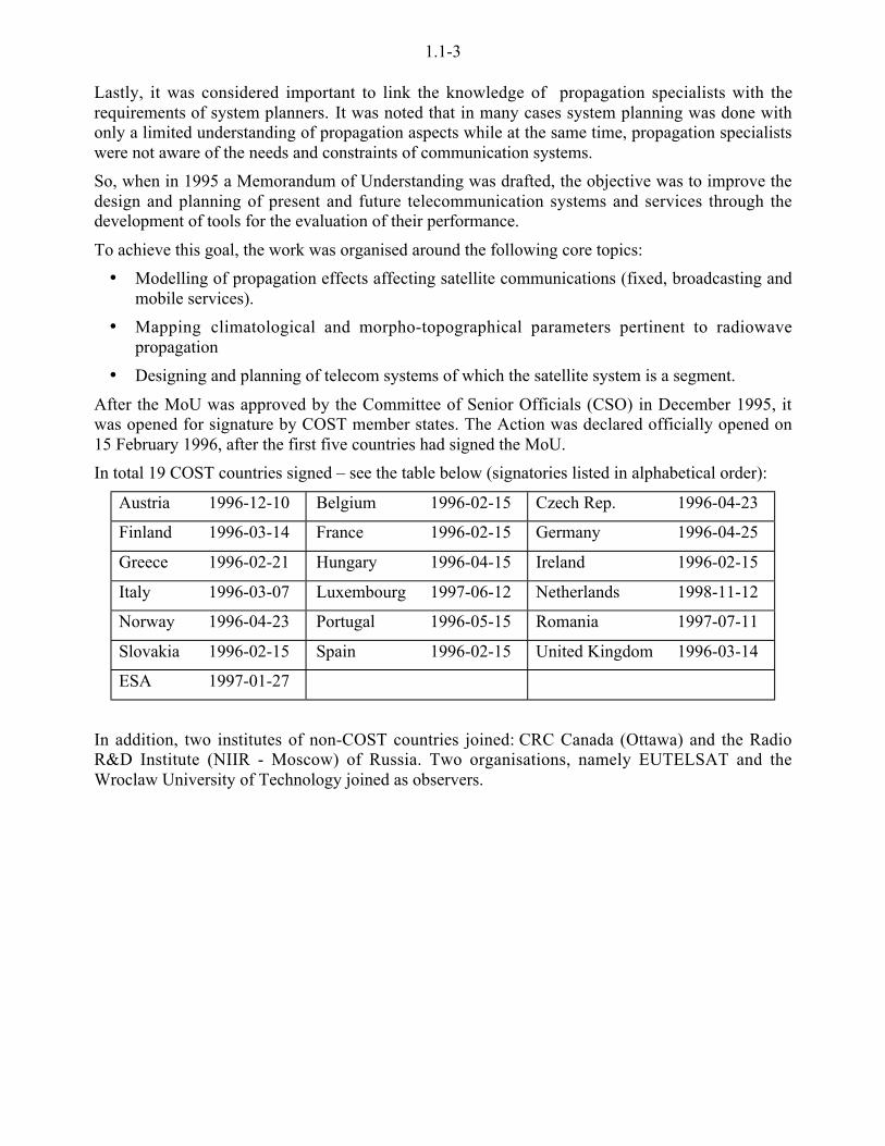
After the MoU was approved by the Committee of Senior Officials (CSO) in December 1995, itwas opened for signature by COST member states. The Action was declared officially opened on15 February 1996, after the first five countries had signed the MoU.

In total 19 COST countries signed – see the table below (signatories listed in alphabetical order):

Austria 1996-12-10 Belgium 1996-02-15 Czech Rep. 1996-04-23

Finland 1996-03-14 France 1996-02-15 Germany 1996-04-25

Greece 1996-02-21 Hungary 1996-04-15 Ireland 1996-02-15

Italy 1996-03-07 Luxembourg 1997-06-12 Netherlands 1998-11-12

Norway 1996-04-23 Portugal 1996-05-15 Romania 1997-07-11

Slovakia 1996-02-15 Spain 1996-02-15 United Kingdom 1996-03-14

ESA 1997-01-27

In addition, two institutes of non-COST countries joined: CRC Canada (Ottawa) and the RadioR&D Institute (NIIR - Moscow) of Russia. Two organisations, namely EUTELSAT and theWroclaw University of Technology joined as observers.

1.1-4

1.1.2.2 Participants

The following organisations have been actively participating in the work of COST 255:

Country Participating Institution

Austria TU Graz INW (Communications & Wave Propagation)

Joanneum Research - IAS Institute of Applied Systems Techn.

Belgium Université Catholique de Louvain (UCL) Microwave Laboratory

KU Leuven

Canada Communications Research Centre (CRC)

Czech Rep. TESTCOM, Telecommunications Experts Dpt.

Czech Technical University, Dept Electromagnetic Fields

Inst. of Atmospheric Physics (IAP)

Finland Helsinki University of Technology, Radio Laboratory

University of Oulu, Telecommunication Lab

France France Telecom - CNET

CERT-ONERA DERMO

Germany Inst. of Mobile & Sat. Comm. Techniques (IMST)

Aachen University of Technology, Communication Networks Dept.

Deutsche Telekom AG, Technologiezentrum Darmstadt

German Aerospace Research DLR, NE-NT-S, Inst. f. Telecoms

Univ. Karlsruhe, Lehrstuhl f. Nachrichtensysteme

Greece National Technical University of Athens, Mobile Communications Lab.

Nat. Observatory of Athens, Institute of Ionospheric & Space Research

Aristotelion University of Thessaloniki, Electrical Eng. Dept

Hungary Technical University of Budapest, Dept. of Microwave Telecomm

Ireland Univ. of Dublin - Trinity College, Dept. of Electronic & Electrical Engg

Italy Università dell’Aquila, Dip. di Ingegneria Elettrica

Politecnico di Milano, CSTS-CNR

CSELT, Mobile Services and Radio Propagation

Fondazione Ugo Bordoni, Radiocommunications Dept

Luxembourg UF Data Analysis

Société Européenne des Satellites (SES/ASTRA)

Netherlands Eindhoven University of Technology

Norway Telenor , Research and Development

Poland Wroclaw University of Technology (Observer)

1.1-5

Portugal Inst. Sup. Tecnico de Lisboa, Dep. Engenharia Electronica e de Comp.

Universidade de Aveiro, Instituto de Telecomunicacoes

Romania Technical University of Cluj-Napoca, Faculty of Electronics & Telecoms

Russia Radio R&D Institute (NIIR)

Slovakia Slovak Technical University, Faculty of Electrical Engineering

Spain USC Vigo, E.T.S.I. Telecomunication

Universidad Politecnica de Madrid (UPM), ETSI Telecomunication.

United Kingdom ERA Technology Ltd., Electronic & Software Engineering Div.

CCLRC-Rutherford Appleton Lab., Radio Communications Research

University of Surrey, Centre for Communication Systems Research

Coventry University, School of Engineering

University of Portsmouth, Dept. of E&E Engineering

University of Glamorgan, Dept. of Electronics & Information Technology

University of York, Dept of Electronics

University of Bath, Dept of Electronic and Electrical Engineering

Radiocommunications Agency

ESA ESTEC, Electromagnetics Division

EUTELSAT Systems Engineering Division (Observer)

1.1.2.3 Management Committee

COUNTRY MC MEMBER(s)

Austria Mr. Erwin Kubista, Joanneum Research - IAS

Belgium Prof. Andre Vander Vorst, Universite Catholique de Louvain

Prof. Danielle Vanhoenacker, Universite Catholique de Louvain

Czech Rep. Dr. Ondrej Fiser, Inst. of Atmospheric Physics

Dr. Vaclav Kvicera, TESTCOM

Finland Prof. Erkki Salonen, University of Oulu

Dr. Jouni Tervonen, Helsinki University of Technology

France Mr. Laurent Castanet, ONERA-CERT

Dr. Joel G. Lemorton, ONERA-CERT

Germany Mr. Joerg Habetha, Aachen University, Comnets

Dr. Gerd Ortgies, Deutsche Telekom AG

Greece Prof. Philip Constantinou, National Technical University of Athens

Prof. Stamatis S. Kouris, Aristotelion University of Thessaloniki

Hungary Prof. Istvan Frigyes, Technical University of Budapest

1.1-6

Ireland Dr. Peter J. Cullen, University of Dublin, Trinity College

Italy Dr. Francesco Barbaliscia, Fondazione Ugo Bordoni

Prof. Aldo Paraboni, Politecnico di Milano

Luxembourg Mr. John Raabo Larsen, Societe Europeenne des Satellites (SES/ASTRA)

Mr. Marcel Pettinger, Societe Europeenne des Satellites , (SES/ASTRA)

Netherlands Mr. Max Van de Kamp, Eindhoven University of Technology

Norway Mr. A. Nordbotten, Telenor Research

Dr. Terje Tjelta, Telenor

Portugal Prof. Francisco Cercas, Instituto Superior Tecnico de Lisboa

Prof. Armando C. D. Rocha, Universidade de Aveiro

Romania Dr. Tudor Palade, Technical University of Cluj-Napoca

Slovakia No active member. (Prof. Chytil, deceased, Slovak Univ.of Technology)

Spain Prof. Leandro de Haro Ariet, Universidad Politecnica de Madrid

Dr. Fernando Perez Fontan, E.T.S.I. Telecomunication, U. Vigo

United Kingdom Dr. Misha Filip, University of Portsmouth

Dr. John W.F. Goddard, CCLRC-Rutherford Appleton Laboratory

ESA Mr. J.P.V. Poiares Baptista, ESA/ESTEC

Mr. Bertram Arbesser-Rastburg, ESA/ESTEC

1.1.2.4 Working method

The Action was officially kicked off at the first Management Committee meeting in May 1996. Itwas then decided, to hold an average of two meetings per year, in which each meeting would be acombination of management committee meeting and technical meeting. All material to be presentedat a meeting would be available to all participants well ahead of the meeting. The documents wouldbe downloadable in PDF format on a password-protected WEB site. No paper copies were mailed tothe participants, with the exception of the official minutes of the meeting. This method was usedvery successfully – more than 150 technical papers were produced within 3 years – forming thebasis of this Final Report.

The work was, from the beginning, divided among four working groups, with the following titlesand chairmen:

WG1A - 'Fixed Propagation Modelling': Aldo Paraboni

WG1B - 'Mobile Propagation': Fernando Perez-Fontan

WG2 - 'Climatic Parameters and Mapping': Pedro Baptista

WG3 - 'Systems and Simulation Issues': Paul Thompson, later Marcel Pettinger

The Working Group chairmen organised working sessions as part of each bi-annual MC meeting.Usually two days out of three were devoted to Working Groups meeting in parallel sessions. At theearly meetings this enabled each group to concentrate fully on its own area of work. Technicalcontributions were formally presented and discussed, and recommendations made for further workto be completed by the next meeting. However it became clear that the parallel sessions made it

1.1-7

realise test cases. Peter Watson was assigned the task of overall co-ordinator of the two ProjectGroups;

PG-A - 'Fixed Link Test Cases': Misha Filip

PG-B - 'Test Cases with a Mobile Link': Simon Saunders

Plenary sessions were arranged to hear of the progress made in the other groups, but the limitedtime available made these rather short and ineffective. The minutes of each meeting were as full aspossible, and sent to each participant in paper form, but it was still difficult to gain an overview ofthe complete project before the Final Meeting. At this meeting a draft version of the Final Reportwas on the table, thanks to enormous effort on behalf of the chapter editors and the secretariat. Thiswould not have been possible without electronic mail and the use of the ESTEC FTP server. TheCOST 255 web page is located on the ESTEC server: http://www.estec.esa.nl/xewww/cost255/

It should be mentioned, that a major contribution to the smooth and effective operation of thisCOST Action was the continuous effort of the Action Secretary and Grant Holder, Sue Upton. Sheprepared all the necessary correspondence and annual reports for the COST Secretariat, preparedinformation on meetings and workshops and ensured that the financial aspects of the Action weremanaged in line with the overall rules of COST.

.

Meetings of the Management Committee

MEETING DATE LOCATION HOST ORGANISATION

1st Preparatory Mtg 1995 Dec 12 Brussels EC

2nd Preparatory Mtg 1996 Feb 14/15 Brussels EC

1st MC Meeting 1996 May 21/22 Brussels EC

2nd MC Meeting 1996 Nov 25/26 Athens National Technical Univ. of Athens

3rd MC Meeting 1997 May 12/14 Trest/Prague Institute of Atmospheric Physics

4th MC Meeting 1997 Oct 27/29 Brussels EC

5th MC Meeting 1998 May 27/29 Vigo University of Vigo

6th MC Mtg &Workshop

1998 Oct 28/30 Noordwijk ESA-ESTEC

7th MC Mtg &Workshop

1999 May 18/21 Toulouse CERT-ONERA and SUPAERO

8th MC Mtg &Workshop

1999 Oct 25/27 Bech, Lux. SES-ASTRA

Management Committee Meetings were attended by an average of 50 delegates.

About 100 delegates attended the Workshops. The Workshop held in Toulouse was organisedjointly with COST Actions 252 and 253.

Short-term scientific missions

Eleven Short Term Scientific Missions (STSM) have been funded in the framework of COSTActions 255. The purpose of these missions was twofold:

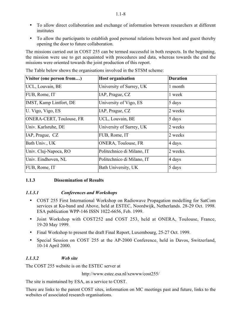
1.1-8

• To allow direct collaboration and exchange of information between researchers at differentinstitutes

• To allow the participants to establish good personal relations between host and guest therebyopening the door to future collaboration.

The missions carried out in COST 255 can be termed successful in both respects. In the beginning,the mission were use to get acquainted with procedures and data, whereas towards the end themissions were oriented towards the joint production of this report.

The Table below shows the organisations involved in the STSM scheme:

Visitor (one person from…) Host organisation Duration

UCL, Louvain, BE University of Surrey, UK 1 month

FUB, Rome, IT IAP, Prague, CZ 1 week

IMST, Kamp Lintfort, DE University of Vigo, ES 5 days

U. Vigo, Vigo, ES IAP, Prague, CZ 2 weeks

ONERA-CERT, Toulouse, FR UCL, Louvain, BE 5 days

Univ. Karlsruhe, DE University of Surrey, UK 2 weeks

IAP, Prague, CZ FUB, Rome, IT 2 weeks

Bath Univ., UK ONERA, Toulouse, FR 4 days.

Univ. Cluj-Napoca, RO Politechnico di Milano, IT 2 weeks.

Univ. Eindhoven, NL Politechnico di Milano, IT 4 days

FUB, Rome, IT Bath University, UK 5 days

1.1.3 Dissemination of Results

1.1.3.1 Conferences and Workshops

• COST 255 First International Workshop on Radiowave Propagation modelling for SatComservices at Ku-band and Above, held at ESTEC, Noordwijk, Netherlands. 28-29 Oct. 1998.ESA publication WPP-146 ISSN 1022-6656, Feb. 1999.

• Joint Workshop with COST252 and COST 253, held at ONERA, Toulouse, France,19-20 May 1999.

• Final Workshop to present the draft Final Report, Luxembourg, 25-27 Oct. 1999.

• Special Session on COST 255 at the AP-2000 Conference, held in Davos, Switzerland,10-14 April 2000.

1.1.3.2 Web site

The COST 255 website is on the ESTEC server at

http://www.estec.esa.nl/xewww/cost255/

The site is maintained by ESA, as a service to COST.

There are links to the parent COST sites, information on MC meetings past and future, links to thewebsites of associated research organisations.

1.1-9

Of major importance is the password protected private area, where bona fide COST members havebeen able to access all the technical documents, reports on Short Term Scientific Missions andnames and addresses of members. As far as possible all papers presented at meetings have beenavailable on the web in advance, which has contributed greatly to the overall success of the project.

1.1.3.3 Transfer of results

The primary vehicle for the transfer of results is this Final Report, see Section 1.1.3.4

The new global maps of meteorological parameters are available on the ESTEC FTP server andthose of water vapour, the 0º C isotherm and topography have been submitted to the ITU-R.

The work carried out under WG2 regarding the precipitation maps for propagation models has beenadopted by the ITU-R to replace the recommendation ITU-R P837 (characteristics of precipitationfor propagation modelling). Also adopted by the ITU is the map of cloud columnar water content(in Rec. P-840).

Early in the project an active attempt was made to contact operators and manufacturers by sendingout a questionnaire on future satellite systems to 200 organisations, but it elicited very littleresponse (8%).

There has been active participation in COST255 from EUTELSAT and from SES (ASTRA), whohave been very helpful in identifying future satellite systems. As active members they have also hadthe opportunity to influence the direction of the research and benefit directly from the results.

1.1.3.4 The Final Report

The key result of the work of COST Action 255 is this Final Report. The Final Report has beendivided in 7 Parts, coordinated by Part editors. In the following, the Parts (2 to 7) are brieflyintroduced and the responsible Part Editors are mentioned:

Part 2: Fixed propagation models (Part Editor: Antonio Martellucci)

Summarizes the results of the WG1A on propagation modeling for fixed satellite systems, includingmodel description and testing.

Part 3: Climatic Parameters (Part Editors: J.P.V. Poiares Baptista and T. Tjelta)

Based on the results of WG2, it contains a description of the climatic parameters relevant to satellitepropagation modelling and illustrates the available databases to be used as input to propagationmodels.

Part 4: Terrain and Clutter Effects, Mobile Modelling (Part Editor: F. Perez-Fontan)

This part illustrates current models, techniques and databases for the propagation in satellite-mobilesystems as analysed in the activities of WG1B.

Part 5: Systems and simulation Issues (Part Editor: M. Pettinger)

This part contains an overview of trends in satellite communication systems and the impact ofpropagation modelling. It also presents techniques for fade mitigation needed for the design of newsatellite communication systems. The material represents the results of the work of WG3.

1.1-10

Part 6: Test Cases Involving Fixed Satellite Links: Part Editor M. Filip

Part 7: Test Cases Involving Mobile Links: Part Editor S. Saunders

Those two parts summarize the results of the test case analysis performed by Projects Groups A andB. Using the results and the indications of WG1A, 1B, 2 and 3, the propagation prediction methodsand data have been applied to currently envisaged satellite communications systems. These testcases demonstrate the possibilities, limitations and future needs of propagation models for satellitecommunication systems.

This paper copy will be complemented by a CD-ROM containing propagation models, databasesand documentation.

The completion of the final version of this Report was made possible by the efforts of the followingindividuals:

• The Part editors listed above and the Chapter editors listed on the title page of every chapterwho had been instrumental in creating a coherent report from many individual contributions.

• Peter Gallois who kindly accepted to be Report Editor after the Final Workshop in Bech. Heperformed a thorough review leading to a substantial improvement of the consistency,presentation and language. Pedro Baptista and Sue Upton who, besides correcting andrefining the text, communicated with the editors of the different parts on the necessarymodifications.

• Prof. W. Riedler and Prof. M. Tomlinson, who had been appointed reviewers of the Action,carefully evaluated the Final Report in March 2001. Their suggestions have contributed to anumber of clarifications and improvements.

• Bob Harris of the ESA Publications Division, who spent many long hours getting all chapterand section headings, equation numbers and figure captions right. Richard Magri, whohelped in fixing automatic numberings and references.

• Antonio Martellucci, who has performed the final editing and review of this report.

1.1.4 Concluding remarks

Successes of COST Action 255 have been:

• Excellent co-operation between countries

• Good use of previously measured propagation data

• Two successful workshops

• Validation of new propagation models

• Establishment of communication between propagation experts and operators

• Encouragement of young scientists through the Short Term Scientific Mission opportunities

• Use of the world wide web as a means of disseminating results

It is felt that COST 255 has made a useful contribution towards improved planning of spectrumefficient telecommunication systems.

Bertram Arbesser-Rastburg,Chairman

PART 2 Fixed Propagation Modelling

2.1-1

CHAPTER 2.1Propagation Effects due to

Atmospheric Gases and Clouds

Editor: Antonio Martellucci1

Authors: Marina Boumis2, Ermanno Fionda3, Ondrej Fiser4, Antonio Martellucci1,Frank S. Marzano5, Peter Watson6, Charles Wrench7

1 European Space Agency, ESA-ESTEC, Keplerlaan 1, PB 299, NL-2200 AG Noordwijk, The Netherlands

Tel: +31-71-565-5603, Fax: +31-71-565-4999, e-mail: Antonio.Martellucci@esa.int2 Fondazione Ugo Bordoni, Radiocommunications Dept., Viale Europa 190, I-00144 Rome, Italy

Tel: +39-6-5480-2119, Fax: +39-6-5480-4401, e-mail: mboumis@fub.it3 Fondazione Ugo Bordoni, Radiocommunications Dept., Viale Europa 190, I-00144 Rome, Italy

Tel: +39-6-5480-2118, Fax: +39-6-5480-4401, e-mail: efionda@fub.it4 Institute of Atmospheric Physics of the Czech Academy, Bocni street II/1401, 141 31 Praha 4, Czech Republic

Tel.: +420-2-769702ext.108, Fax.: +420-2-72763745 , e-mail: ondrej@ufa.cas.cz5 Dip. di Ingegneria Elettrica, Universita' dell'Aquila, Monteluco di Roio, I-67040 L'Aquila, Italy

Tel: +39-862-434412, Fax: +39-862-434414, E-mail: franko@ing.univaq.it36 Electronic and Electrical Engineering, University of Bath, Claverton Down,, BATH BA2 7AY, U.K.

Tel: +44-1225 826330, Fax: +44-1225 826412, e-mail: p.a.watson@bath.ac.uk7 CCLRC Rutherford Appleton Labs, Chilton, Didcot, Oxfordshire OX11 0QX, United Kingdom

2.1-2

2.1 Propagation Effects due to Atmospheric Gases and Clouds

In this chapter the models of the main propagation effects due to oxygen, water vapour andatmospheric clouds, are described. The discussion is mainly focused on gaseous and cloudattenuation but models for the atmospheric sky noise and the propagation path delay are also shown.The chapter is completed by the comparison of some of the presented models with experimentaldata. The annex describes a database of clear air propagation parameters derived from a world-widedatabase of radiosonde meteorological measurements.

2.1.1 Gaseous attenuation

The attenuation introduced by atmospheric gases can be described using either an accurate physicalmodel, such as Liebe’s model, or approximate or probabilistic models such as the ITU-R orSalonen’s models.

Liebe’s model performs accurate calculations of air refractivity, for frequencies from 1 to 1000GHz, but it is computationally demanding and requires vertical profiles of meteorologicalparameters, whose accuracy has to be carefully checked. Therefore, Liebe’s model is mainly usedeither as a reference for comparison with the other models or to derive propagation parameters forother models, such as mass absorption coefficients or attenuation equivalent heights.

The ITU-R1 and Salonen’s models predict gaseous attenuation, at Ku band and above, using asinput climatic parameters that are currently also available in the radio-climatological maps of ITU-R (see Chapter 3.1).

In addition to the above models, [Konefal et al., 2000] proposed another model for prediction ofmonthly water vapour attenuation, that makes use of Salonen’s vapour attenuation model and isbased on a prediction model of monthly statistics of ground water vapour density described inChapter 3.2.

2.1.1.1 Liebe’s Model of air refractivity and specific attenuation

The radio refractive index n of a medium is defined as the ratio of the speed of light in vacuum tothe speed in the medium itself. As n is very close to unity in the atmosphere, the radio refractivityN, the difference of n from unity in parts per million, is commonly used:

( )N n= !10 16(ppm) 2.1-1

where:

n n jn= " ! "" = # = refractive index

# # #= " ! ""j = complex permittivity of the medium.

The radio refractivity is a complex variable, locally function of meteorological parameters and canbe expressed as:

( )N N N fo= + (ppm) 2.1-2

where:

f = frequency in GHz

1 A h i f bli i f hi h ITU R d [ITU R P 676 4 1999] d l f d

2.1-3

No = non-dispersive term

( ) ( ) ( )N f N f jN f= " + "" = dispersive term of radio refractivity

N’(f) = dispersive phase shifting term

N”(f) = frequency dependent absorption term

The refractive index of the atmosphere due to atmospheric gases can be accurately determined usingthe Millimetre-Wave Propagation Model (MPM), developed by H. J. Liebe [Liebe, 1981, 1985,1989, Liebe et al., 1993]. The input parameters of the MPM model are: pressure, temperature andrelative humidity, measured along an atmospheric vertical profile. In this paragraph the latest of theLiebe’s models, MPM93, is described [Liebe et al., 1993].

The frequency independent term of the radio refractivity can be expressed as the sum of three terms:

N N N N0 1 2 3= + + (ppm) 2.1-3

where:

N pd1 0 2588= $ $. % = non-dispersive contribution of oxygen

( )N e2 4163 0 239= $ + $ $. .% % = non-dispersive contribution of water vapour

N3 = N0w = non-dispersive term due to liquid water or ice particles.

pd = pressure of dry air (hPa)

% = 300/(T+273.15) reciprocal temperature (K-1)

T = temperature (°C)

( )eRH

= $ $ ! $100

2 408 1011 22 6445. exp .% % = water vapour pressure (hPa)

p= pd + e = total air pressure (hPa)

RH = relative humidity (%)

&v Te=

216 51. = water vapour density (g/m3).

An example of the vertical profile of the air refractivity, derived in Milano from localmeteorological measurements is given in Figure 2.1-1.

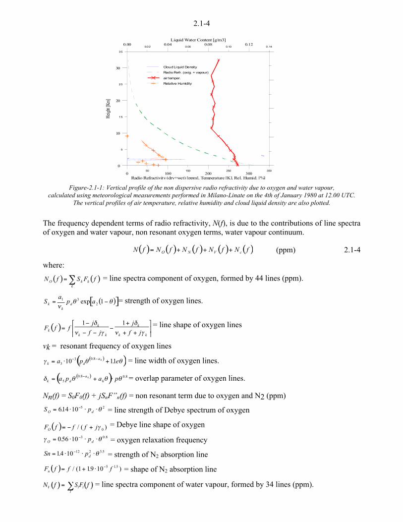
2.1-4

Figure-2.1-1: Vertical profile of the non dispersive radio refractivity due to oxygen and water vapour,calculated using meteorological measurements performed in Milano-Linate on the 4th of January 1980 at 12.00 UTC.

The vertical profiles of air temperature, relative humidity and cloud liquid density are also plotted.

The frequency dependent terms of radio refractivity, N(f), is due to the contributions of line spectraof oxygen and water vapour, non resonant oxygen terms, water vapour continuum.

( ) ( ) ( ) ( ) ( )N f N f N f N f N fO N V c= + + + (ppm) 2.1-4

where:

( ) ( )N f S F fO k kk

= ' = line spectra component of oxygen, formed by 44 lines (ppm).

( )[ ]Sa

p akk

d= !1 32 1

(% %exp = strength of oxygen lines.

( )F f fj

f j

j

f jkk

k k

k

k k

=!

! !!

+

+ +

)

*+

,

-.

1 1/( 0

/( 0

= line shape of oxygen lines

vk = resonant frequency of oxygen lines

( )( )0 % %k daa p e= $ +! !

33 0 810 114. . = line width of oxygen lines.

( )( )/ % % %k daa p a p= + $!

50 8

60 84. . = overlap parameter of oxygen lines.

Nn(f) = S0F0(f) + jSnF”n(f) = non resonant term due to oxygen and N2 (ppm)

S pO d= $ $ $!614 10 5 2. % = line strength of Debye spectrum of oxygen

( )F f f f jO = ! +/ ( )0 0 = Debye line shape of oxygen

0 %O dp= $ $ $!0 56 10 3 0. .8 = oxygen relaxation frequency

Sn pd= $ $ $!14 10 12 2 3 5. .% = strength of N2 absorption line

( )F f f fn = + $ !/ ( . ).1 19 10 5 1 5 = shape of N2 absorption line

( ) ( )N f S F fV l ll

= ' = line spectra component of water vapour, formed by 34 lines (ppm).

50 150 250 3500 100 200 300

Radio Refractivity (dry+wet) [ppm], Temperature [K], Rel. Humid. [%]

0.02 0.06 0.10 0.140.00 0.04 0.08 0.12

Liquid Water Content [g/m3]

Cloud Liquid Density

Radio Refr. (oxig. + vapour)

air temper.

Relative Humidity

5

15

25

35

0

10

20

30

Heig

ht [K

m]

2.1-5

( )[ ]%%(

!= 1exp 25.31 be

bS

ll = strength of water vapour lines.

( )F f ff j f jl

l l l l

=! !

!+ +

)

*+

,

-.

1 1( 0 ( 0

= line shape of water vapour lines

l = resonant frequency of water vapour lines

( )564

33 10 b

db

l pebb %%0 +$= ! = line width of water vapour lines.

Nc(f) = water vapour continuum term (ppm), pseudo-line located at 1780 GHz.

The specific attenuation, 0a(z,f) at height z and frequency f, can be derived from the frequencydependent absorption term N”(f):

( ) ( )0 a z f f N f, .= $ $ ""0 1820 (dB/km) 2.1-5

The specific path delay, d(z,f) at height z and frequency f, can be derived from the sum of thenon-dispersive term, N0 and the dispersive phase shifting term, N’(f):

( ) ( )[ ]fNNfzd "+$= 03356.3, (ps/km) 2.1-6

Liebe’s Model: Total attenuation due to oxygen and water vapour

The total path attenuation due to gases, at frequency f and along a slant path at elevation %, can bederived, assuming that the atmosphere is longitudinally homogeneous, as:

( )( )[ ]1

2

3=

h

ag dz

zsinz

A0

(dB) 2.1-7

where:

( ) ( )0 a z f f N f, .= $ $ ""0 1820 = specific attenuation of gases at height z and frequency f,see equation 2.1-5 (dB/km)

( ) ( ) ( ) ( )( ) ( ) .

-

,+*

)$+

$$+=3

znzrhnhr

z4cos

arccos

r = Earth’s radius = 6 370 km

n(z) = air refractive index see equation 2.1-1

h = station altitude

4 = elevation angle (degree). 4 5 10°. For elevation angles lower than 10° the ray bending has to beconsidered.

Liebe’s model makes it possible to model accurately the gaseous attenuation up to 1000 GHz. InFigure 2.1-2 the frequency spectrum of zenith gaseous attenuation in Milano is given,, calculatedusing mean monthly vertical profiles of meteorological parameters [Barbaliscia et al., 1994] and[Barbaliscia et al., 1995].

2.1-6

0.1

1

10

100

0 50 100 150 200 250 300 350

Atte

nuat

ion

[dB

]

Frequency [GHz]

Milano, Mean Monthly Profiles

January, Stratus at 500 m, Thickness 1 kmJanuary

July

Figure 2.1-2: Frequency spectrum of the zenith gaseous attenuation in Milano calculated using the mean monthlyprofiles (January/July). The zenith attenuation due to gases and stratus cloud is also plotted.

The total attenuation due to atmospheric gases, Ag(f), can be expressed as the sum of totalattenuation due to oxygen and water vapour, AO(f), AV(f):

( ) ( ) ( )A f A f A fg O V= + (dB) 2.1-8

where:

( ) ( ) ( )A fsin

z f dzO O=2

11

0%0 , ; ( ) ( ) ( )A f

sinz f dzV V=

2

11

0%0 ,

( ) ( ) ( )[ ]0 O O nz f f N f N f, .= $ $ "" + ""01820 = specific attenuation due to oxygen at frequency f and height z

(dB/km)

( )""N fO = imaginary part of refractivity due to line spectra component of oxygen (ppm)

( )""N fn = imaginary part of refractivity due to non resonant term due to oxygen and N2 (ppm).

( ) ( ) ( )[ ]0V V cz f f N f N f, .= $ $ "" + ""01820 = specific attenuation due to vapour at frequency f and height z

(dB/km)

( )""N fV = imaginary part of refractivity due to line spectra component of vapour (ppm)

( )""N fC = imaginary part of refractivity due to vapour continuum term (ppm).

In Figure 2.1-3 the cumulative distribution function of total attenuation (along the path to theITALSAT satellite) and calculated values (using the MPM93 and radiosonde data) are given. Thecloud attenuation, calculated using the model of [Salonen et al., 1990] for cloud detection and theRayleigh model of liquid water specific attenuation (see Section 2.1.2-1) are also given. The figuredemonstrates the effect of atmospheric gases with respect to the cloud attenuation, near the oxygenabsorption peak.

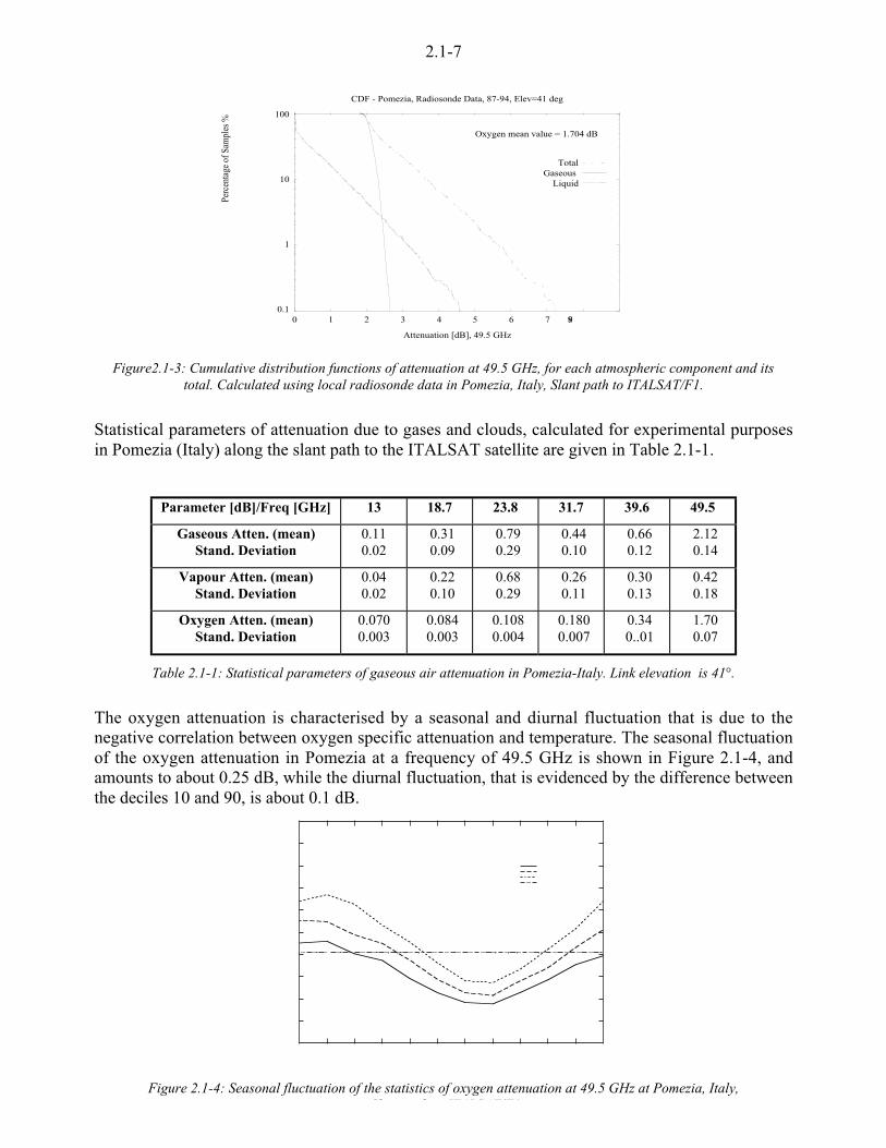
2.1-7

0.1

1

10

100

0 1 2 3 4 5 6 7 89

Perc

enta

ge o

f Sam

ples

%

Attenuation [dB], 49.5 GHz

CDF - Pomezia, Radiosonde Data, 87-94, Elev=41 deg

Oxygen mean value = 1.704 dB

TotalGaseous

Liquid

Figure2.1-3: Cumulative distribution functions of attenuation at 49.5 GHz, for each atmospheric component and itstotal. Calculated using local radiosonde data in Pomezia, Italy, Slant path to ITALSAT/F1.

Statistical parameters of attenuation due to gases and clouds, calculated for experimental purposesin Pomezia (Italy) along the slant path to the ITALSAT satellite are given in Table 2.1-1.

Parameter [dB]/Freq [GHz] 13 18.7 23.8 31.7 39.6 49.5

Gaseous Atten. (mean)Stand. Deviation

0.110.02

0.310.09

0.790.29

0.440.10

0.660.12

2.120.14

Vapour Atten. (mean)Stand. Deviation

0.040.02

0.220.10

0.680.29

0.260.11

0.300.13

0.420.18

Oxygen Atten. (mean)Stand. Deviation

0.0700.003

0.0840.003

0.1080.004

0.1800.007

0.340..01

1.700.07

Table 2.1-1: Statistical parameters of gaseous air attenuation in Pomezia-Italy. Link elevation is 41°.

The oxygen attenuation is characterised by a seasonal and diurnal fluctuation that is due to thenegative correlation between oxygen specific attenuation and temperature. The seasonal fluctuationof the oxygen attenuation in Pomezia at a frequency of 49.5 GHz is shown in Figure 2.1-4, andamounts to about 0.25 dB, while the diurnal fluctuation, that is evidenced by the difference betweenthe deciles 10 and 90, is about 0.1 dB.

Figure 2.1-4: Seasonal fluctuation of the statistics of oxygen attenuation at 49.5 GHz at Pomezia, Italy,Sl h ITALSAT/F1

2.1-8

Similarly the water vapour attenuation is characterised by seasonal differences, in addition to dailyfluctuations, due to the increase of the total water vapour content of the atmosphere during thesummer. In Figure 2.1-5 the seasonal fluctuation of the water vapour attenuation at 23.8 GHz, inPomezia, is shown. The seasonal fluctuation amounts to about 1 dB, while the diurnal fluctuation isabout 0.4 dB.

0

0.5

1

1.5

2

Jan Feb Mar Apr May Jun Jul Aug Sep Oct Nov Dec

Water Vapour Attenua

Month

Decile 10Decile 50Decile 90

Mean value

Figure 2.1-5: Seasonal fluctuation of the statistics of oxygen attenuation at 49.5 GHz, a, and water vapour attenuationat 23.8 GHz, b, at Pomezia, Italy, Slant path to ITALSAT/F1

Other statistical parameters of the gaseous attenuation in the Ka and V frequency bands, calculatedusing radiosonde meteorological measurements performed in various locations around the world,can be found in the database described in Section 2.1-8.

Liebe’s Model: Mass absorption coefficient of Water Vapour

In moderate humidity conditions, the specific attenuation due to water vapour, 0V, is approximatelyproportional to the water vapour density &v.

( )0 &V V Vz f a z f z( , ) , ( )= $ (dB/km) 2.1-9

where:

aV(z,f) = water vapour mass absorption coefficient at height z and frequency f (dB/mm)

&V(z) = water vapour density at height z (g /m3)

z = height (km).

Hence the total zenith attenuation due to water vapour AV calculated according to Liebe’s model inequation 2.1-8, can be also estimated by means of the following relationship:

( ) ( )A f a f VV V= $ (dB) 2.1-10

where:

( ) ( ) ( )a fV

a z f z dzV V V=2

11

0, & = instantaneous value, averaged along the vertical, of water vapour

mass absorption coefficient (dB/mm)

( )V z dzV=2

1 &0

= integrated or total water vapour content (mm). 1 kg/m2 corresponds to 1 mm of

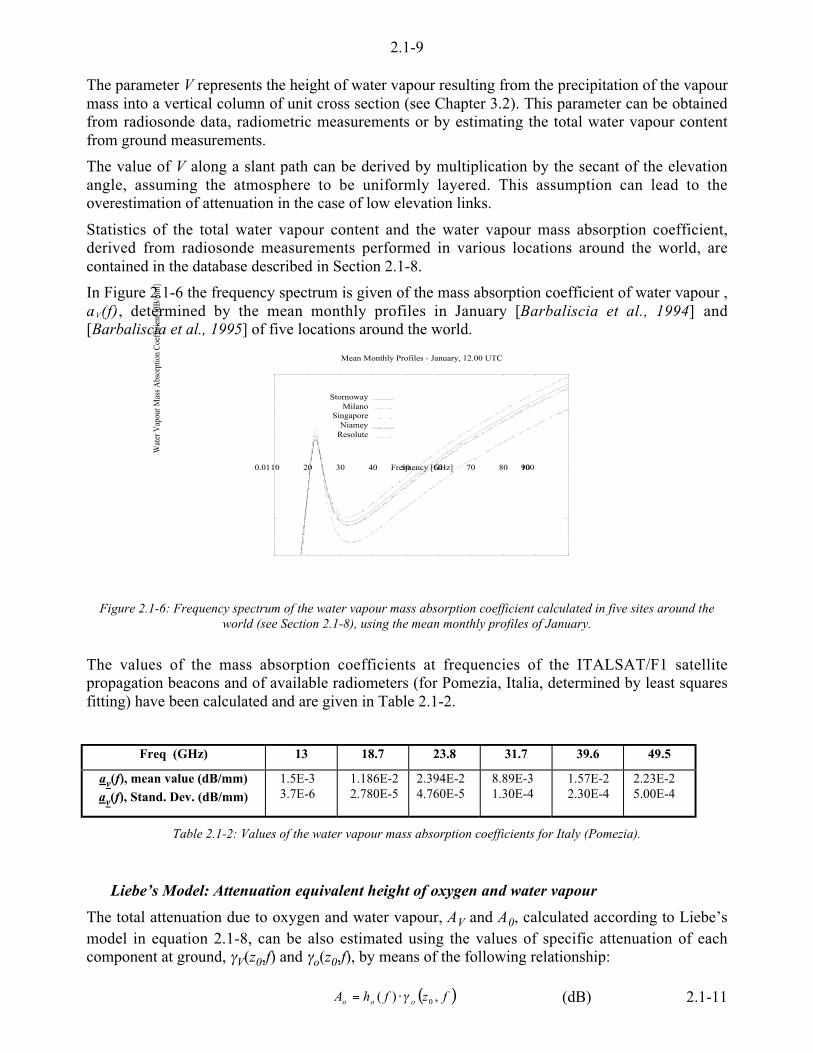
2.1-9

The parameter V represents the height of water vapour resulting from the precipitation of the vapourmass into a vertical column of unit cross section (see Chapter 3.2). This parameter can be obtainedfrom radiosonde data, radiometric measurements or by estimating the total water vapour contentfrom ground measurements.

The value of V along a slant path can be derived by multiplication by the secant of the elevationangle, assuming the atmosphere to be uniformly layered. This assumption can lead to theoverestimation of attenuation in the case of low elevation links.

Statistics of the total water vapour content and the water vapour mass absorption coefficient,derived from radiosonde measurements performed in various locations around the world, arecontained in the database described in Section 2.1-8.

In Figure 2.1-6 the frequency spectrum is given of the mass absorption coefficient of water vapour ,aV(f), determined by the mean monthly profiles in January [Barbaliscia et al., 1994] and[Barbaliscia et al., 1995] of five locations around the world.

0.0110 20 30 40 50 60 70 80 90100

Wat

er V

apou

r Mas

s Abs

orpt

ion

Coe

ffic

ient

[dB

/mm

]

Frequency [GHz]

Mean Monthly Profiles - January, 12.00 UTC

StornowayMilano

SingaporeNiamey

Resolute

Figure 2.1-6: Frequency spectrum of the water vapour mass absorption coefficient calculated in five sites around theworld (see Section 2.1-8), using the mean monthly profiles of January.

The values of the mass absorption coefficients at frequencies of the ITALSAT/F1 satellitepropagation beacons and of available radiometers (for Pomezia, Italia, determined by least squaresfitting) have been calculated and are given in Table 2.1-2.

Freq (GHz) 13 18.7 23.8 31.7 39.6 49.5

av(f), mean value (dB/mm)av(f), Stand. Dev. (dB/mm)

1.5E-33.7E-6

1.186E-22.780E-5

2.394E-24.760E-5

8.89E-31.30E-4

1.57E-22.30E-4

2.23E-25.00E-4

Table 2.1-2: Values of the water vapour mass absorption coefficients for Italy (Pomezia).

Liebe’s Model: Attenuation equivalent height of oxygen and water vapour

The total attenuation due to oxygen and water vapour, AV and A0, calculated according to Liebe’smodel in equation 2.1-8, can be also estimated using the values of specific attenuation of eachcomponent at ground, 0V(z0,f) and 0o(z0,f), by means of the following relationship:

( )fzfhA ooo ,)( 00$= (dB) 2.1-11

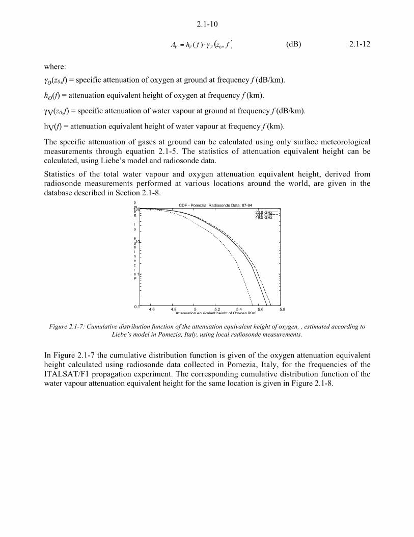
2.1-10

( )fzfhA VVV ,)( 00$= (dB) 2.1-12

where:

0o(z0,f) = specific attenuation of oxygen at ground at frequency f (dB/km).

ho(f) = attenuation equivalent height of oxygen at frequency f (km).

0V(z0,f) = specific attenuation of water vapour at ground at frequency f (dB/km).

hV(f) = attenuation equivalent height of water vapour at frequency f (km).

The specific attenuation of gases at ground can be calculated using only surface meteorologicalmeasurements through equation 2.1-5. The statistics of attenuation equivalent height can becalculated, using Liebe’s model and radiosonde data.

Statistics of the total water vapour and oxygen attenuation equivalent height, derived fromradiosonde measurements performed at various locations around the world, are given in thedatabase described in Section 2.1-8.

0.1

1

10

100

4.6 4.8 5 5.2 5.4 5.6 5.8

Percentage of Samp

Attenuation equivalent height of Oxygen [Km]

CDF - Pomezia, Radiosonde Data, 87-94

23.8 GHz39.6 GHz49.5 GHz

Figure 2.1-7: Cumulative distribution function of the attenuation equivalent height of oxygen, , estimated according toLiebe’s model in Pomezia, Italy, using local radiosonde measurements.

In Figure 2.1-7 the cumulative distribution function is given of the oxygen attenuation equivalentheight calculated using radiosonde data collected in Pomezia, Italy, for the frequencies of theITALSAT/F1 propagation experiment. The corresponding cumulative distribution function of thewater vapour attenuation equivalent height for the same location is given in Figure 2.1-8.

2.1-11

Figure 2.1-8: Cumulative distribution function of the attenuation equivalent height of and water vapour, estimatedaccording to Liebe’s model in Pomezia, Italy, using local radiosonde measurements.

2.1.1.2 Salonen’s model of oxygen attenuation

A prediction method for the attenuation due to dry air on a slant path for frequencies below theoxygen resonant frequency near 60 GHz has been developed by Salonen [Salonen et al., 1990,1994] using radiosonde observations in five different climatological areas in Europe (Jokioinen,Finland; Stuttgart, Germany; Valentia, Ireland; Madrid, Spain; Athens, Greece). Liebe’s method forthe specific attenuation of dry air was used in the reference calculations of zenith attenuation usingthe radiosonde data.

Because the diurnal temperature variations are higher at ground level than on the effectivepropagation path, the weighted mean temperature tm was used in the correlation studies. The best fitwas reached with tm=0.55t+0.45t-12, where t is the temperature at ground level during theradiosonde measurements and t-12 is the temperature 12 hours earlier. In this method, the equivalentheight hoL has been defined as the ratio of zenith attenuation to the reference specific attenuation 0oL

(pref, tref, f) calculated by Liebe’s method.

The following formula for the effective height of dry air for frequencies f650 GHz, has beendeveloped through correlation studies:

( )( )

( )h

ft

f

R t

gp

oL m= ! +7

89

:

;< !

)

*+

,

-. $ +

!+

+ 789

:;<

)

*++

,

-..

1 0 00491300

15 4 9520

60

272 2

1000 1013

2

2 2. ..

ln (km) 2.1-13

where:

f = frequency, [GHz]

tm = (0.55t+0.45t-12 )= weighted mean ground temperature, [C].

t , t-12 = ground temperature at current time and 12 hours earlier, [C].

p = the pressure at ground level, [hPa].

R = 287.05 J kg-1K-1 = the dry air gas constant.

g =9.80665 [m/s2] = acceleration due to Earth’s gravity.

The attenuation due to dry air for the elevation angles %>10° can be calculated using the equivalentheight hoL:

0.1

1

10

100

1 1.5 2 2.5 3 3.5 4 4.5 5

Percentage of Samp

Attenuation equivalent height of Vapour [Km]

CDF - Pomezia, Radiosonde Data, 87-94

23.8 GHz31.7 GHz49.5 GHz

2.1-12

( ) ( )A

h f p t f p to

o m=

$L oL ref ref, , , ,

sin

0

%(dB) 2.1-14

where:

0oL = reference specific attenuation of dry air calculated with Liebe’s model atthe reference temperature (tref = 15 C) and pressure (pref = 1013 hPa).

For elevation angles below 10°, the earth’s curvature should be taken into account (see Section2.1.1-6).

A comparison between Salonen's model of oxygen attenuation and the MPM93 prediction, carriedout by means of radiosonde measurements in Pomezia, at a frequency of 31.7 GHz is given inFigure 2.1-9.

Salonen's model underestimates the oxygen attenuation by less than 0.02 dB.

0.1

1

10

100

0.14 0.15 0.16 0.17 0.18 0.19 0.2 0.21 0.22

Perc

enta

ge o

f Sa

mpl

es [

%]

Oxygen Total Attenuation [dB], 31.7 GHz

Pomezia, Elev=41 deg, No rain data, 1987

Radiosonde + HUTRadiosonde + MPM

Figure 2.1-9: Comparison between the model of [Salonen and Uppala, 1991] for oxygen attenuation and MPM93,at 31.7 GHz, in Pomezia for the slant path to the ITALSAT satellite.

2.1.1.3 Salonen’s model of water vapour attenuation

This model is based on the result that the zenith attenuation of water vapour is related to theintegrated water vapour amount, V [kg/m2], using Liebe’s water vapour absorption [Salonen et al.,1990, 1994].

Therefore the dependence of the zenith attenuation on V at the reference frequency fref = 20.6 GHzand then the frequency scaling factor (a ratio of the specific attenuation coefficients at the referenceconditions for the equivalent propagation path) can be defined.

The reference meteorological parameters for the model are defined in Table 2.1-3:

pref Reference pressure [hPa] 780

&v, ref Reference water vapour density [g/m3] V(P)/4

tref Reference temperature [C] ( ) 322.0ln14 refv, +$$ &

V(P) integrated water vapour thresholdexceeded for P% of the time

derived from meteorological measurements

2.1-13

The slant path water vapour attenuation using Liebe’s model can be calculated using:

( ) ( ) ( )( )refrefv,refrefL

refrefv,refLw ,,,

,,,

sin0173.0

,,tpf

tpfPVPfA

&0

&0

%% $= 2.1-15

where

f = frequency [GHz]

fref = 20.6 [GHz]

% = elevation angle

P = percentage of time

The formula is valid for elevation angles %>10°; for lower elevations, the Earth’s curvature shouldbe taken into account. 0L is the specific attenuation calculated by Liebe’s Model.

0.1

1

10

100

0 0.2 0.4 0.6 0.8 1 1.2 1.4 1.6

Perc

enta

ge o

f Sa

mpl

es [

%]

Water Vapour Total Attenuation [dB], 23.8 GHz

Pomezia, Elev=41 deg, No rain data, 1987-1994

Radiosonde + HUTRadiosonde + MPM

Figure 2.1-10: Comparison between the model of [Salonen and Uppala, 1991] for water vapour attenuation andMPM93, at 23.8 GHz, in Pomezia for the slant path to the ITALSAT satellite.

Water vapour attenuation calculated by this procedure agrees very well with the correspondingspecific attenuation methods applied to radiosonde observations under different climatic conditionsin Europe. The temperature does not play an important role in the calculation of water vapourattenuation and the zenith attenuation can be calculated very accurately, if the integrated amount ofwater vapour is available.

A comparison between Salonen's Model of water vapour attenuation and the MPM93 prediction,carried out by means of radiosonde measurements in Pomezia, at 23.8 GHz is given inFigure 2.1-10. At this frequency Salonen's model shows excellent agreement with Liebe's model.

2.1-14

2.1.1.4 ITU-R model of oxygen attenuation2

ITU-R recommends a procedure to calculate attenuation by atmospheric oxygen [Gibbins 1986],[ITU-R, 1998]. The specific attenuation due to dry air at ground level (pressure equal to 1013 hPa),and at a temperature of 15 °C can be approximated by the following equations:

( )3222

52252210

44.257

5.7351.0

27.7 !$$$..-

,

++*

)

$$+!+

$$+= tp

tptpo rrf

rrfrrf0 (dB/km) 2.1-16

for f 6 57 GHz and by:

( ) ( ) ( ) ( ) ( ) ( ) ( ) ( )6318

6057635766.157

186360 5.82

otpoo

ffffrr

ff000 $

!$!+!$!$$!$

!$!= (dB/km) 2.1-17

for 57 GHz 6 f 6 63 GHz.

where:

f = frequency, (GHz).

p = total air pressure (hPa)

1013prp =

T = temperature (oC)

rt = 288/(T+273) = reciprocal temperature (K-1)

The algorithm given by equations 2.1-16 and 2.1-17 applies to a pressure range of 1013 ±50 hPaand is estimated to have an accuracy of approximately ±15% over the temperature range from–20 °C to 40 °C.

As an approximation, the zenith path attenuation, from sea level, may be obtained by multiplyingthe specific attenuation given by equations 2.1-16 and 2.1-17 by the equivalent heights for dry airgiven, respectively by:

( ) GHz57km6 <= fforho 2.1-18

( )( ) GHz35063km

17.118

406

2<<

+!+= ffor

fho 2.1-19

For a ground temperature different from 15 ºC, the equivalent height of oxygen can be corrected by0.1% (clear weather) or 1 % (rain) per ºC.

The total oxygen zenith attenuation, according to the ITU-R model, is then:

ooo hA 0= [dB] 2.1-20

2 At the time of publication of this report, the ITU-R recommends [ITU-R, P.676-4, 1999] a model of oxygenattenuation that is different from the one used during the COST 255 project [ITU-R, P.676-3, 1998].

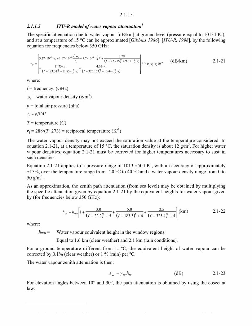
2.1-15

2.1.1.5 ITU-R model of water vapour attenuation3

The specific attenuation due to water vapour [dB/km] at ground level (pressure equal to 1013 hPa),and at a temperature of 15 °C can be approximated [Gibbins 1986], [ITU-R, 1998], by the followingequation for frequencies below 350 GHz:

( )

( ) ( )

42

2222

224

732

10

44.10153.325

01.4

85.1131.183

73.11

81.9235.2279.3

107.71067.11027.3!

!!!

$$$

.

.

.

.

.

-

,

+++++

*

)

$$+!

$+

$$+!

$+

$$+!+$$+$+$$

= ptv

tp

t

tp

t

tpp

vtt

W rrf

rrf

r

rrf

r

rrff

rr

r

&

&

0(dB/km) 2.1-21

where:

f = frequency, (GHz).

v& = water vapour density (g/m3).

p = total air pressure (hPa)

1013prp =

T = temperature (C)

rt = 288/(T+273) = reciprocal temperature (K-1)

The water vapour density may not exceed the saturation value at the temperature considered. Inequation 2.1-21, at a temperature of 15 °C, the saturation density is about 12 g/m3. For higher watervapour densities, equation 2.1-21 must be corrected for higher temperatures necessary to sustainsuch densities.

Equation 2.1-21 applies to a pressure range of 1013 ±50 hPa, with an accuracy of approximately±15%, over the temperature range from –20 °C to 40 °C and a water vapour density range from 0 to50 g/m3.

As an approximation, the zenith path attenuation (from sea level) may be obtained by multiplyingthe specific attenuation given by equation 2.1-21 by the equivalent heights for water vapour givenby (for frequencies below 350 GHz):

( ) ( ) ( ) .-

,+*

)

+!+

+!+

+!+=

44.325

5.2

63.183

0.5

52.22

0.31

222W0Wfff

hh (km) 2.1-22

where:

hW0 = Water vapour equivalent height in the window regions.

Equal to 1.6 km (clear weather) and 2.1 km (rain conditions).

For a ground temperature different from 15 ºC, the equivalent height of water vapour can becorrected by 0.1% (clear weather) or 1 % (rain) per ºC.

The water vapour zenith attenuation is then:

WWW hA 0= (dB) 2.1-23

For elevation angles between 10° and 90°, the path attenuation is obtained by using the cosecantlaw:

3 A h i f bli i f hi h ITU R d [ITU R P 676 4 1999] d l f

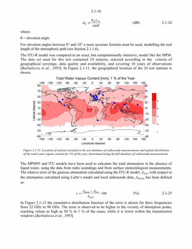
2.1-16

%0

sinh

A WWW = (dB) 2.1-24

where:

% = elevation angle.

For elevation angles between 0° and 10° a more accurate formula must be used, modelling the reallength of the atmospheric path (see Section 2.1.1.6).

The ITU-R model was compared to an exact, but computationally intensive, model like the MPM.The data set used for this test contained 24 stations, selected according to the criteria ofgeographical coverage, data quality and availability, and covering 10 years of observations[Barbaliscia et al., 1995]. In Figure 2.1-11, the geographical location of the 24 test stations isshown.

-180 -150 -120 -90 -60 -30 0 30 60 90 120 150 180

Longitude [degree]

-180 -150 -120 -90 -60 -30 0 30 60 90 120 150 180

-90

-70

-50

-30

-10

10

30

50

70

90

Latit

ude

[deg

ree]

-90

-70

-50

-30

-10

10

30

50

70

90

0

20

40

60

80

Total Water Vapour Content [mm], 1 % of the Year

Figure 2.1-11: Location of stations included in the test database of radiosonde measurements and spatial distributionof the total water vapour content for 1% of the year, determined using the full database of radiosonde measurements.

The MPM93 and ITU models have been used to calculate the total attenuation in the absence ofliquid water, using the data from radio soundings and from surface meteorological measurements.The relative error of the gaseous attenuation calculated using the ITU-R model, AITU, with respect tothe attenuation calculated using Liebe’s model and local radiosonde data, AMPM, has been definedas:

100$!

=MPM

ITUMPM

A

AA# (%) 2.1-25

In Figure 2.1-12 the cumulative distribution function of the error is shown for three frequenciesfrom 22 GHz to 90 GHz. The error is observed to be higher in the vicinity of absorption peaks,reaching values as high as 50 % in 1 % of the cases, while it is lower within the transmissionwindows [Barbaliscia et al., 1995].

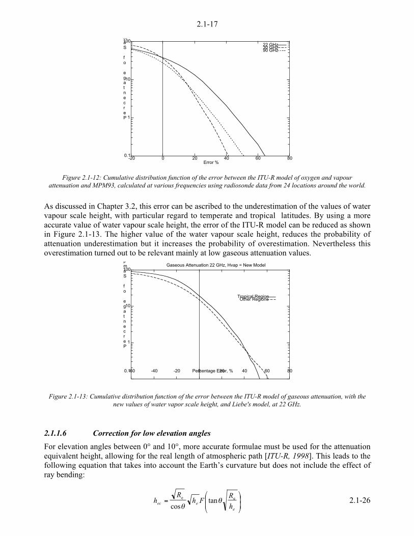
2.1-17

0.1

1

10

100

-20 0 20 40 60 80

Percentage of Sam

Error %

22 GHz30 GHz90 GHz

Figure 2.1-12: Cumulative distribution function of the error between the ITU-R model of oxygen and vapourattenuation and MPM93, calculated at various frequencies using radiosonde data from 24 locations around the world.

As discussed in Chapter 3.2, this error can be ascribed to the underestimation of the values of watervapour scale height, with particular regard to temperate and tropical latitudes. By using a moreaccurate value of water vapour scale height, the error of the ITU-R model can be reduced as shownin Figure 2.1-13. The higher value of the water vapour scale height, reduces the probability ofattenuation underestimation but it increases the probability of overestimation. Nevertheless thisoverestimation turned out to be relevant mainly at low gaseous attenuation values.

0.1

1

10

100

-60 -40 -20 0 20 40 60 80

Percentage of Samp

Percentage Error, %

Gaseous Attenuation 22 GHz, Hvap = New Model

Tropical RegionOther Regions

Figure 2.1-13: Cumulative distribution function of the error between the ITU-R model of gaseous attenuation, with thenew values of water vapor scale height, and Liebe's model, at 22 GHz.

2.1.1.6 Correction for low elevation angles

For elevation angles between 0° and 10°, more accurate formulae must be used for the attenuationequivalent height, allowing for the real length of atmospheric path [ITU-R, 1998]. This leads to thefollowing equation that takes into account the Earth’s curvature but does not include the effect ofray bending:

<<;

:998

7=

eeec h

RFh

Rh ee tan

cos%

%2.1-26

2.1-18

where:

hec = attenuation equivalent height of oxygen or water vapour, corrected for lowelevation angles.

% = elevation angle.

Re = effective Earth radius including refraction (Recommendation ITU-R 834) (km)(a value of 8500 km is generally acceptable).

he = attenuation equivalent height of oxygen (see equations 2.1-11, 2.1-13, 2.1-18 and 2.1-19)or water vapour (see equations 2.1-12 and 2.1-22).

The function F is defined as:

( )F xx x

=+ +

1

0 661 0 339 5512. . .2.1-27

2.1.2 Cloud Attenuation

The attenuation due to suspended water droplets contained in atmospheric clouds can be determinedwith a great accuracy, using the Rayleigh model of electromagnetic wave scattering. This physicalapproach requires the assessment of the cloud vertical profile, that can be derived from radiosondemeasurements (see Chapter 3.2). Using this approach, the attenuation estimation depends mainly onthe accuracy of radiosonde measurements. Therefore, if reliable radiosonde data are available, theresults of the Rayleigh model can be used as a reference for testing of the other models or to derivelocal propagation parameters, such as the mass absorption coefficients of clouds.

On the other hand the availability of global meteorological databases, that contain the statistics ofcloud parameters, permits to predict the statistics of cloud attenuation in the K and V frequencybands in a simpler way with respect to the Rayleigh model, under some general assumptions and/orapproximations. The Salonen-Uppala and Dissanayake-Allnutt-Haidara models of cloud attenuationare based on this latter approach.

Another model, which makes use of the Salonen-Uppala cloud attenuation model, has beenproposed by [Konefal et al., 1999] to predict monthly distribution of cloud attenuation. This modelemploys the ITU-R meteorological database of atmospheric profiles to calculate the monthly cloudliquid water, as described in Chapter 3.2.

Moreover the cloud attenuation model, proposed by [Wrench et al., 1999], based on extensiveanalysis of available measurements of cloud characteristics, (synoptic observations, radiosonde andmeteorological satellites) has been used to produce worldwide maps of attenuation.

2.1.2.1 Rayleigh model for cloud radio refractivity

The radio refractivity of a suspended non-precipitating cloud, composed of liquid water or iceparticles, can be calculated using the general equation [Van de Hulst, 1957] that describes the effectof a dispersion of spherical particles on to the electromagnetic field propagating through it. Thisequation can be solved and the cloud is assumed to be equivalent to a slab of dielectric material.Therefore the following equations hold:

( ) ( ) ( ){ }

( ) ( ) ( ){ }1

12

2

$$=""

$$="

036

036

,,Re,2

10,,

,,Im,2

10,,

drTfrSzrnk

zTfN

drTfrSzrnk

zTfN

W

W

=

=

[ppm] 2.1-28

2.1-19

where:

( ) ( ) ( )zTfNjzTfNzTfN WWW ,,,,,, ""$+"= = cloud radio refractivity (ppm). See equation 2.1-1.

( )zTfNW ,," = real part of cloud radio refractivity (ppm).

( )zTfNW ,,"" = Imaginary part of cloud radio refractivity (ppm)

f = frequency (GHz).

T = liquid water or ice temperature. It can change along the vertical profile.

z = height (Km).

S(r,f,T) = forward scattering amplitude of the particle.

> = c/f = wavelength (m)

k = 2=/> = wavenumber (m-1)

c = 0.2998 (m/ps) = speed of light in the vacuum

r = droplet radius (mm)

n(r,z) = droplet radius distribution per unit volume (m3 mm-1), at height z.It is related to the total content of liquid water or ice for unit volume, &w(z).

( ) ( )12

$=0

36 ,1034

drzrnrzW =&& = total content of liquid water or ice for unit volume at height z (g/m3)

& = specific weight of the material, g/cm3 (& = 1 for liquid water, & = 0.916 for ice)

The specific attenuation and delay of a cloud, 0w and dw, can be derived using the followingequations, (see also the corresponding equations 2.1-5 and 2.1-6 for gases). The relationship withthe height, z, results from the temperature vertical profile of liquid or solid water, T(z), and from thevertical profile of the liquid or ice density [Liebe, 1989]:

( ) ( )zTfNffz WW ,,1820.0, ""$$=0 [dB/Km] 2.1-29

( ) ( )zTfNfzd WW ,,3356.3, "$= [ps/Km] 2.1-30

As discussed in [Barbaliscia et al, 1995], the Rayleigh approximation can be used to calculatecloud attenuation for frequencies lower than 300 GHz. The radio refractivity due to cloud dropletscan be simplified as [Liebe, 1989]:

( ) ( )( )

( )

( ) ( )( )

( )&

&##

&&

##

zTfTf

zTfN

zTfTf

zTfN

WW

WW

?@A

BCD

+!

E""

?@A

BCD

+!

E"

2,1,

Re5.1,,

2,1,

Im5.1,,

[ppm] 2.1-31

where:

&w(z) = total content of liquid water or ice for unit volume (g/m3) at height z.

& = specific weight of the material, g/cm3 (& = 1 for liquid water, & = 0.916 for ice)

( ) ( ) ( )TfjTfTf ir ,,, ### != = complex permittivity of liquid water or ice.

( ) ( ) ( )TfTTfr ,, 0 ### "+= = real part of permittivity of water or ice.

#0(T) = component of #r independent of frequency.

2.1-20

#i(f,T)= imaginary part of permittivity of water or ice.

T = liquid water or ice temperature. It can change along the vertical profile.

z = height (km).

In addition, using the Rayleigh approximation, the frequency independent term of radio refractivitydue to clouds can be demonstrated, as in equation 2.1-2 for gases.

( )( )

( )&

&#

zT

zTN WW <<

;

:998

7

+!=

23

15.1,0

0 (ppm) 2.1-32

The non dispersive path delay due to cloud liquid or ice can be calculated using equations 2.1-30

and 2.1-32.

The permittivity of water can be calculated using several models. According to the double-Debyemodel [Liebe, 1989] the water refractivity is:

( ) ( )

( )( )( )

( )( )( )2

212

10

2221

210

11

11

s

s

p

p

sp

ff

ff

ff

ff

ffff

+

!+

+

!=""

++

!+

+

!="

#####

#####

#

2.1-33

where:

#0=77.66+103.3(rt+1)

#1 =5.48

#2 =3.51

rt = 300/(T+273.15) = reciprocal temperature (K-1)

( ) ( )2129414.14209.20 !+!!= ttp rrf (GHz)

( )11500590 !!= ts rf (GHz)

An example of calculation of cloud liquid attenuation, for the frequencies of the ITALSAT/F1propagation experiment, is given in Figure 2.1-14. The liquid water density profile has beenestimated from local radiosonde measurements, using the model of [Salonen et al., 1990] for clouddetection.

2.1-21

0.1

1

10

100

0 1 2 3 4 5

Percentage of Samp

Cloud Attenuation [dB]

CDF - Pomezia- Radiosonde Data, 1987-94, Elev = 41 deg

13 GHz18.723.831.739.649.5

Figure 2.1-14: Cumulative distribution function of the cloud attenuation for the frequencies of the ITALSAT/F1propagation experiment, calculated in Pomezia, Italy, using the Rayleigh model, local radiosonde measurements and

Salonen’s model for estimation of cloud liquid water density

Rayleigh model: Mass absorption coefficient of Liquid Water

The total attenuation due to cloud liquid, AL, can be expressed as:

LaA LL $= (dB) 2.1-34

where:

( ) ( ) ( )a fL

a z f z dzL L W=2

11

0, & = instantaneous value, averaged along the vertical, of liquid water vapour

mass absorption coefficient (dB/mm).

aL(z,f) = liquid water mass absorption coefficient at frequency f and height z (dB/mm)

&w(z) = total content of liquid water or ice for unit volume (g/m3) at height z.

( )L z dzW=2

1 &0

= integrated or total liquid water content (mm).

Statistics of the total liquid water content and of the mass absorption coefficient of liquid water,derived from radiosonde measurements performed at various locations around the world, arecontained in the database described in Section 2.1.8.

The values of the mass absorption coefficients at the frequencies of the ITALSAT/F1 satellitepropagation beacons and of available radiometers, for Pomezia, Italy, determined using leastsquares fitting, have been calculated and are given in Table 2.1-4. Similar results are available forother experimental sites.

Liquid Water Mass Abs. Coeff/Freq (GHz)

13 18.7 23.8 31.7 39.6 49.5

Mean (dB/mm)Stand. Dev. (dB/mm)

0.1526.5E-5

0.472.66E-4

0.485.600E-4

0.8161.350E-6

1.842.66E-3

2.654.40E-3

Table 2.1-4: Values of the liquid water mass absorption coefficients for Pomezia (Italy).

2.1-22

2.1.2.2 Salonen and Uppala Model for cloud attenuation statistics

The [Salonen and Uppala, 1991] method can be used for calculation of the attenuation due toclouds at a given frequency f and elevation angle everywhere on the globe.

The specific attenuation 0w of clouds depends on frequency f, total liquid water content L andtemperature T. The temperature dependence of cloud attenuation can be taken into account bydefining the reduced liquid water content, wred, so that the following holds:

( ) ( )TLGHzfCTwGHzf WredW ,,430,,43 ==== 00 2.1-35

Because the temperature dependence of 0w is almost constant over the frequency range from 10 to60 GHz, the calculated statistics are also valid in this frequency range. Then, wred is integrated as afunction of height, resulting in the integrated reduced liquid water content Wred (kg/m2).

Global statistics for the integrated reduced liquid water content Wred (kg/m2) have been calculatedusing global data from the ECMWF numerical analyses (1.5° spatial resolution, based on two yearsof data).

The formula for the slant path attenuation due to cloud liquid, AL, can be written as:

( ) ( ) ( )( )%sin1

$$= PWfgPA redL 2.1-36

where:

( ) ( )21819.0

F# +""$

=f

fg = cloud attenuation frequency dependent constant.

f = frequency (GHz)

P = probability %

( ) ##F """+= 2

#’ = real of liquid water permittivity, see equation 2.1-33, (T=0 C).

#” = imaginary part of liquid water permittivity, see equation 2.1-33, (T=0 C).

% = slant path elevation angle.

Therefore, equation 2.1-36 can be used with the maps of Wred for the worldwide evaluation of cloudattenuation for frequencies below 60 GHz.

When no meteorological information is available, Rec. ITU-R PN.840-recommends to estimatecloud attenuation using Wred = 0.5 kg/m2 in equation 2.1-36, corresponding to a liquid water contentof 0.5 g/m3 and a cloud thickness of 1 km.

2.1-23

2.1.2.3 Dissanayake, Allnutt and Haidara model for cloud attenuation statistics

The model [Dissanayake et al., 1997] was derived using average cloud properties of four cloudtypes together with the assumption that the statistical distribution of cloud attenuation follows a log-normal probability law. The characteristics of the selected cloud types are given in Table 2.1-5.

Cloud type Code Vertical extent, Hc, [km] Horizontal extent, Lc, [km] Water cont, &&&&w, [g/m3]

Cumulonimbus

Cumulus

Nimbostratus

Stratus

Cb

Cu

Ns

St

3.0

2.0

0.8

0.6

4.0

3.0

10.0

10.0

1.0

0.6

1.0

0.4

Table 2.1-5: Average properties of the four cloud types used in the cloud attenuation model.

The specific attenuation of each cloud type is calculated using the following equation:

wW &##

>&=

0 <;

:98

7+!

!<<;

:998

7=

21

Im100

64343.0 2.1-37

where

&w = total content of liquid water or ice for unit volume (g/m3). Derived from Table2.1-5.

> = c/f = wavelength (m)

& = specific weight of the material, g/cm3 (& = 1 for liquid water)

# = complex permittivity of liquid water. See equation 2.1-33

The path attenuation for each of the cloud types is calculated assuming that the cloud shape is avertical cylinder having the horizontal and vertical dimension (Hc and Lc), shown in Table 2.1-5.The total path attenuation due to cloud liquid, ALi, is given by:

( ) ( ) ( )( ) ( ) ( )G%%0

G%%0

tan;cos

tan;sen

arcLA

arcHA

geiWLi

ciWLi

<$=

5$=2.1-38

where

cici LH=G

% = slant path elevation angle.

( )[ ]gigi

cigicigei

LL

LLLL

2exp138.078.01 !!!+

!+= = horizontal projection of the effective path length.

( )%tancigi HL = = horizontal projection of the path length through an infinite cloud layer.

i = index of cloud type in Table 2.1-5.

The total path attenuation is corrected by an adjustment factor equal to 25/48 to account for the factthat the cloud cover amounts in the cloud world atlas apply to the complete sky and the cloudattenuation is calculated along a given direction. The percentage of cloud cover from themeteorological database is needed as input for each of the cloud types in Table 2.1-5. The fourcloud types are ranked in order of attenuation and provide four points on the conditional cloud

2.1-24

( ) <<;

:998

7 !=>

L

LL

AAPAAP

H2

lnlnerfc

20 2.1-39

where

P = the probability of cloud attenuation Ac not exceeding A.

P0 = the probability of cloud attenuation being present.

erfc = the complementary error function.

LA = the mean value of AL, to be derived by best fit log-normal relationship.

Hs = the standard deviation of AL, to be derived by best fit log-normal relationship.

The total cloud cover provides the conditional probability for the cloud attenuation distribution.

Cloud attenuation measurements made in Darmstadt at 20 and 30 GHz are reported by[Ortgies et al., 1990]. Figure 2.1-15 shows the comparison of the model against the measured data.The measurements have been made with radiometers at an elevation angle of 28°. Themeasurements pertain only to non-rainy conditions, and the cloud contribution to the totalattenuation has been extracted, allowing an easy comparison with the model predictions. It is seenthat at both frequencies reasonably good agreement exists between the model and themeasurements.

Figure 2.1-15: Measured and Predicted Cloud Attenuation at Darmstadt, Germany; a) 20GHz, b) 30 GHz

2.1.3 Frequency scaling of gas and cloud attenuation

Liebe’s model can be used to accurately calculate the instantaneous frequency scaling of clear airattenuation, separating the effects of gas and clouds.

Figures 2.1-16 and 2.1-17 show the scatter-plots of theoretical values of clear air attenuationcomputed from one year of Milano radiosonde data (1995) for various pairs of the ITALSAT/F1and radiometric frequencies, in Ka Band and from Ka to V Band. It can be deduced that frequencyscaling is very promising for frequencies which are far from the water vapour resonant frequency(22.3 GHz). One can find relations between clear air attenuation at different frequencies, whichhave been derived through linear regression, while the coefficient of determination shows thesuitability of concrete frequency scaling.

2.1-25

Figure 2.1-16: Instantaneous frequency scaling of gasand cloud attenuation at 23 and 31 GHz

Figure 2.1-17: Instantaneous frequency scaling of gasand cloud attenuation at 31 and 49 GHz

In Figure 2.1-18 the frequency scaling ratio is shown of gas and cloud attenuation at 18.7 and49.GHz, calculated using equiprobability values of attenuation at the two frequencies. It results thatfor probability values higher than 40 %, the effect of water vapour and oxygen is dominant andresults in values of frequency scaling ratio higher than 6. For percentages lower than 10 % the totalfrequency scaling ratio is mainly affected by clouds.

4

5

6

7

8

9

10

0.1110100

49.5/18.7 Frequency

Probability, %

Pomezia, Radiosonde Data, 87-94, Elev=41 deg

Total AttenuationGaseous Attenuation

Cloud Attenuation

Figure 2.1-18: Statistics of the equiprobable frequency scaling of attenuation at 18.7 and 49.5 GHz,due to gas, clouds and total. Pomezia, Italy, Slant path to ITALSAT/F1.

2.1.4 Atmospheric Noise Temperature

The antenna of a radiocommunication system collects the power spontaneously emitted by theatmosphere. This latter effect has to be included when considering the system noise figure. Theatmospheric noise temperature can be calculated by means of the radiative transfer equation (RTE).

Different approaches have to be used to solve the radiative transfer equation, in order to separate thecase of a non-scattering atmosphere (i.e. an atmosphere with only gaseous absorption or light tomoderate clouds) from the case of a scattering atmosphere (i.e. an atmosphere with heavy clouds orrainfall).

In both cases the vertical profiles and the spatial description of meteorological parameters ared d i t t th l ith

2.1-26

2.1.4.1 Atmospheric Noise Temperature in absence of scattering

The power flux density spontaneously emitted by the atmosphere and collected by an antennapointed towards the space is defined as the atmospheric brightness.

This parameter, B(z,%,f), can be derived from the radiative transfer equation, assuming a pureabsorbing medium in thermodynamic equilibrium:

( ) ( ) ( )( )

( )( ) ( )[ ] ( )

( )zd

fzzfzTFfz

fzzfzBfzB

z

zpla

c

".-

,+*

) "!""+

+.-

,+*

)!=

1 %I

0%

%I

%

sin,,

exp,,sin

1

sin,,

exp,,,

max

maxmax

<;

:98

7srHzm

W2

2.1-40

where:

z = height of the receiving antenna, [m]

% = elevation angle (degree), % 5 10°.For elevation angles lower than 10° the ray bending has to beconsidered.

f = frequency (Hz)

( )( ) .

-

,+*

)

!=

1exp12

, 2

3

kThfchf

fTFpl = Planck's function, .-

,+*

)srHzm

W2

, (sr is a steradian)

( )fFfzB pl ,16.270),( max != = cosmic background contribution, .-

,+*

)srHzm

W2

( ) ( )dzfzfzzz

z

a1""

"

=""" ,,, 0I = optical depth between z' and z", at frequency f (neper)

( )fza ,0 = specific attenuation at height z and frequency f (neper/km), see equation 2.1-5.

T(z) = temperature of the absorbing medium at height z (K)

h = 6.63 10-34 (Js) = Planck's constant

c = 2.998 108 (m/s) = light speed

k = 1.38 10-23 (J/K) = Boltzmann's constant

The brightness B(z,%,f) can be expressed in terms of the equivalent brightness temperature,Tb(z,%,f) (J), which is the physical temperature of a blackbody having the same brightness. The skynoise temperature observed at the ground along a slant path with an inclination %, is obtained bysolving the equation:

( ) ),,0(, fBfTF bpl %= 2.1-41

The total atmospheric attenuation, At, can be derived by the atmospheric brightness temperature,Tsky, using the following equation:

I$= 343.4TA (dB) 2.1-42

where:

( ) ( )[ ]bmrcmr TTTT !!= lnI = Optical depth of the atmosphere [nep]

2.1-27

Tmr = The mean radiating temperature calculated using equation 2.1-41with Tsky = Tmr and B = Bmr.

( ) ( ) ( )[ ] ( ) ( )( ) ( ) ( )( )[ ]%I%I0%

sin,exp1sin,exp,sin

1max

max

zzzdzzfzTFzBz

z

plamr !!""!""= 1

= Mean radiating brightness.

Tc = Brightness temperature of cosmic background, [K].It is obtained by solving the equation ( ) ( )fzBfTF cpl ,, max= .In Ka band a value of 2.73 K can be used.

Statistics of the brightness temperature in the K and V bands, calculated using radiosondemeasurements performed at various locations around the world, are contained in the databasedescribed in Section 2.1.8.

In Figure 2.1-19 the spectrum of the sky noise temperature up to 300 GHz is given. These valueshave been evaluated using the MPM93 model and the mean monthly profiles of five locations, inJanuary. The regional variations of the sky noise temperature, due to fluctuations of temperatureand of the water vapour content, are clearly visible in the transmission bands [Barbaliscia et al.,1995].

0

50

100

150

200

250

300

0 50 100 150 200 250

Bri

ghtn

ess

Tem

pera

ture

[K

]

Frequency [GHz]

Mean Monthly Profiles, January 12.00 UTC

StornowayMilano

SingaporeNiamey

Resolute

Figure 2.1-19: Zenith brightness temperature vs frequency at five locations.Calculated by the MPM93 and mean monthly profiles in January

2.1.4.2 Atmospheric Noise Temperature in presence of scattering

In the model described by [Marzano et al., 1999], a solution of the three-dimensional radiativetransfer equation for a horizontally finite and vertically inhomogeneous precipitating cloud, iscalculated. This approach can be used both to calculate the values of sky brightness temperature inthe presence of a precipitating cloud and to calculate atmospheric attenuation, given the rainfall anda defined geometrical configuration of the link.

In the case of media with non-zero albedo, the Radiative Transfer Equation can be written withrespect to the optical thickness distance coordinate [Brussaard., 1985], [Marzano, et al. 1999] asfollows:

2.1-28

( ) ( ) ( )fJfTd

fdTB

B ,,,,,,,,,

IKµIKµI

IKµ+!= 2.1-43

where:

( )fT B ,,, IKµ = Atmospheric brightness temperature [K] at optical depth I along the direction (µ,K)at frequency f .

( ) ( )[ ] ( ) ( ) ( ) '',,','),,,,','(4

1,,,2

0

1

1KµIKµIKµKµ

=IIKµ

=ddfTfp

fwTfwfJ B1 1

+

!+!=

= pseudo-source function

( )( )fk

fkfp

s

d=IKµKµ 4),,,,','( = = Volumetric scattering phase function.

kd(f) = differential scattering coefficient [Np/km sr] at frequency f. Calculated by integrating thedifferential cross section over the particle size distribution (and, possibly, over its shape andorientation parameters).

( )%µ cos= with % the zenithal angle and K the azimuthal angle.

( ) ( )dzfkfd e=I : differential zenith optical depth [Neper] at frequency f.

ke(f) = extinction coefficient [Np/km] at frequency f.

ks(f) = scattering coefficient [Np/km] at frequency f.

( )( )fkfk

fwe

s=)( = single-scattering albedo

T(I) = Physical temperature of the medium.[K].

For spherical particles, the Mie theory can be applied to derive ke, ks and kd.

Following the theoretical framework of [Brussaard, 1985], the scattering phase function has beensupposed to be unitary, that is the multiple scattering contribution has been assumed to be isotropic.Therefore the source function, J(µ,K,I,f), can be described by means of recursive relationships.

The solution of the radiative transfer equation for an antenna located at ground (i.e., for I = 0)pointing towards a scattering medium along the direction specified by (µ,K) is:

( ) [ ] ( )( ) oooo

eTefTeTdefJfT cmrcBIIIII

I4µII4µI4µ !!!"! +!==+"== 1 1,0,,,',,,0,,0

2.1-44

where:

Io = optical depth of the raining atmosphere along the pointing direction.

Tc = cosmic background temperature in the microwave range (equal 2.73 K).

( )[ ] ( )

o

o

o

o

eeTfT

e

defJfT cB

mr I

I

I

II

I4µII4µI4µ

!

!

!

"!

!!=

=!

"L=

11

,0,,1

,',,,0,, 0

= Mean radiating temperature.

Note that Tmr is not equal to the physical temperature for a scattering medium such as rainfall andmay depend on the observation geometry.

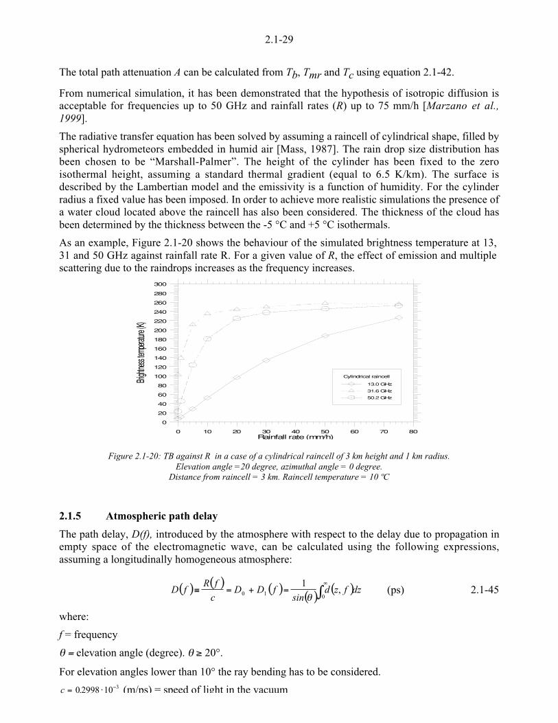
2.1-29

The total path attenuation A can be calculated from Tb, Tmr and Tc using equation 2.1-42.

From numerical simulation, it has been demonstrated that the hypothesis of isotropic diffusion isacceptable for frequencies up to 50 GHz and rainfall rates (R) up to 75 mm/h [Marzano et al.,1999].

The radiative transfer equation has been solved by assuming a raincell of cylindrical shape, filled byspherical hydrometeors embedded in humid air [Mass, 1987]. The rain drop size distribution hasbeen chosen to be “Marshall-Palmer”. The height of the cylinder has been fixed to the zeroisothermal height, assuming a standard thermal gradient (equal to 6.5 K/km). The surface isdescribed by the Lambertian model and the emissivity is a function of humidity. For the cylinderradius a fixed value has been imposed. In order to achieve more realistic simulations the presence ofa water cloud located above the raincell has also been considered. The thickness of the cloud hasbeen determined by the thickness between the -5 °C and +5 °C isothermals.

As an example, Figure 2.1-20 shows the behaviour of the simulated brightness temperature at 13,31 and 50 GHz against rainfall rate R. For a given value of R, the effect of emission and multiplescattering due to the raindrops increases as the frequency increases.

0 10 20 30 40 50 60 70 80Rainfall rate (mm/h)

0

20

40

60

80

100

120

140

160

180

200

220

240

260

280

300

Bright

ness te

mpera

ture (K

)

Cylindrical raincell

13.0 GHz

31.6 GHz

50.2 GHz

Figure 2.1-20: TB against R in a case of a cylindrical raincell of 3 km height and 1 km radius.Elevation angle =20 degree, azimuthal angle = 0 degree.

Distance from raincell = 3 km. Raincell temperature = 10 ºC

2.1.5 Atmospheric path delay

The path delay, D(f), introduced by the atmosphere with respect to the delay due to propagation inempty space of the electromagnetic wave, can be calculated using the following expressions,assuming a longitudinally homogeneous atmosphere:

( ) ( ) ( )( )

( )12

=+=L010 ,

1dzfzd

sinfDD

cfR

fD%

(ps) 2.1-45

where:

f = frequency

% = elevation angle (degree). % 5 20°.

For elevation angles lower than 10° the ray bending has to be considered.

c = $ !0 2998 10 3. (m/ps) = speed of light in the vacuum

2.1-30

R(f) = R0 + Rd(f) = excess path length due to the atmosphere (m)

R0 = Rdry+ Rwet = non dispersive excess path length [m]

Rdry = non dispersive excess path length due to oxygen [m], defined as dry term.

Rwet = non dispersive excess path length, due to water vapour [m] , defined as wet term. Thepresence of clouds can introduce an additional contribution that is very small and is usuallyneglected.

Rd(f) = dispersive excess path length at frequency f (m).

D0 = non-dispersive atmospheric path delay (ps)

D1(f) = dispersive atmospheric path delay (ps)

( )fzd , = specific delay at height z and frequency f (ps/km), see equation 2.1-6.

Statistics of the excess path length parameters, R0 and Rd(f) in the Ka and V frequency bands, havebeen calculated using radiosonde measurements performed at various locations around the worldand are contained in the database described in Section 2.1-8.

The non-dispersive excess path length, R0, can be also estimated from local meteorologicalmeasurements using the [Thayer, 1974] model or using the following equation:

TV

pR 79.100227.00 +M (m) 2.1-46

where:

p = ground air pressure (hPa)

V = integrated or total water vapour content (kg/m2 or mm).

T = ground temperature (K)

2.1.6 Comparison of models with experimental data

2.1.6.1 Total gaseous attenuation and radiometric measurements

A comparison has been made between the MPM93 model of the total gaseous attenuation andradiometric measurements carried out in Spino D'Adda, Milano, by means of a three channelradiometer pointed to the ITALSAT satellite and operating at 22.2, 31.65 and 50.2 GHz. Themeasurements cover the period from August 1993 to June 1994 [Bosisio, 1994].

2.1-31

0.1

1

10

100

0 1 2 3 4 5

Prob

abili

ty [

%]

Attenuation [dB]

Milano, path to ITALSAT, Clear Air Attenuation CDF

22.2 GHz, Radiometer22.2 GHz, Radiosonde

31.65 GHz, Radiometer31.65 GHz, Radiosonde

52.2 GHz, Radiometer52.2 GHz, Radiosonde

Figure2.1-21: Calculated and measured Cumulative distribution function of clear sky attenuation atSpino D'Adda (ITALSAT).

The results of the comparison are given in Figure 2.1-21 and a good agreement between modelcalculation and measurements can be observed [Barbaliscia et al., 1995].

0

0.5

1

1.5

2

2.5

3

3.5

4

4.5

5

0.1 1 10 100

Atte

nuat

ion

[dB

]

Percentage of Year

Martlesham (UK), 30 GHz, Slant Path to OLYMPUS

OLYMPUS meas.Radios. Data, GAS+CLOUD

Radios. Data, GAS

Figure 2.1-22: Comparison of total attenuation at 30 GHz, measured by the OLYMPUS satellite, with the totalattenuation due to clouds and gases.

In Figure 2.1-22 Liebe’s model is also compared with the experimental results of the OLYMPUSpropagation measurements performed at Martlesham Heath, Ipswich, United Kingdom by BritishTelecom Laboratories [Howel et al., 1992].

The OLYMPUS measurements are contained in the DBOPEX experimental database. Theradiosonde measurements carried out in Martlesham (see Annex), have been used as input toLiebe’s model. In order to extend the range of validity of statistics of calculated parameters, theradiosonde data collected in presence of rain have also been used. The link elevation was 28degrees.

The measurements started on November 1 1989 and were completed in February 2 1991. The resultfor 29.66 GHz is given in Figure 2.1-22. The model takes into account also the effect of clouds(estimated according to Salonen's model - see Part 3) and the Rayleigh model (see Chapter 1.2).The model and measurements are in agreement down to 1% of the year. At lower percentages oftime the effect of rain becomes relevant [Barbaliscia et al., 1996].

In Figure 2.1-23 the comparison is shown between radiometric measurements, performed inPomezia, Italy, of total atmospheric attenuation during selected cloud events and the results ofLiebe’s Model, using as input local radiosonde observations.

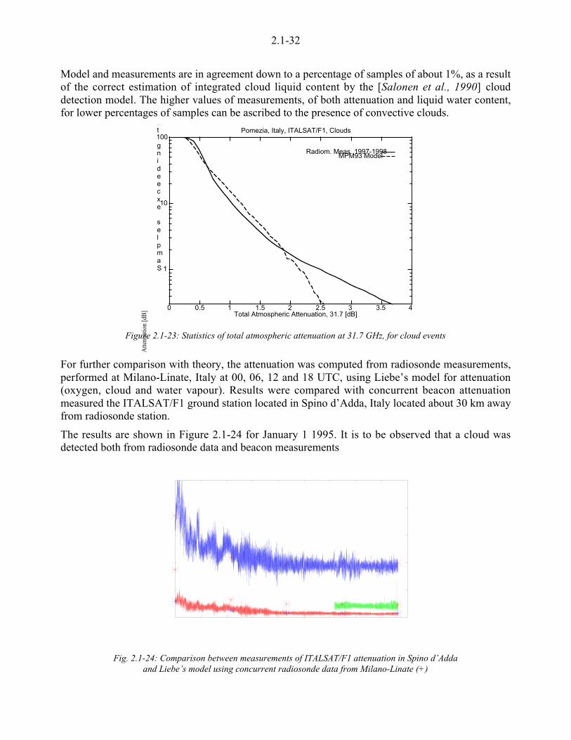
2.1-32

Model and measurements are in agreement down to a percentage of samples of about 1%, as a resultof the correct estimation of integrated cloud liquid content by the [Salonen et al., 1990] clouddetection model. The higher values of measurements, of both attenuation and liquid water content,for lower percentages of samples can be ascribed to the presence of convective clouds.

1

10

100

0 0.5 1 1.5 2 2.5 3 3.5 4

Samples exceeding th

Total Atmospheric Attenuation, 31.7 [dB]

Pomezia, Italy, ITALSAT/F1, Clouds

Radiom. Meas. 1997-1998MPM93 Model

Figure 2.1-23: Statistics of total atmospheric attenuation at 31.7 GHz, for cloud events

For further comparison with theory, the attenuation was computed from radiosonde measurements,performed at Milano-Linate, Italy at 00, 06, 12 and 18 UTC, using Liebe’s model for attenuation(oxygen, cloud and water vapour). Results were compared with concurrent beacon attenuationmeasured the ITALSAT/F1 ground station located in Spino d’Adda, Italy located about 30 km awayfrom radiosonde station.

The results are shown in Figure 2.1-24 for January 1 1995. It is to be observed that a cloud wasdetected both from radiosonde data and beacon measurements

Atte

nuat

ion

[dB

]

Fig. 2.1-24: Comparison between measurements of ITALSAT/F1 attenuation in Spino d’Addaand Liebe’s model using concurrent radiosonde data from Milano-Linate (+)

2.1-33

2.1.6.2 Sky noise temperature and radiometric measurements

Making use of the above radiometric measurements carried out at Spino d’Adda, Italy, by thePolitecnico di Milano [Bosisio, 1994], a comparison was also made between the MPM93 model ofthe sky noise temperature and radiometric measurements carried out in Milano.

An example is given in Figure 2.1-25, for 50.2 GHz, near the oxygen absorption peak, in theabsence of clouds and rain. Fair agreement can be observed between the model assessment ofgaseous effects, and measurements [Barbaliscia et al., 1995].

105

110

115

120

125

130

135

140

145

0 10 20 30 40 50 60 70

Tsk

y 50

.2 G

Hz,

[K

]

Total water vapour content along the path [mm]

Milano, Path to ITALSAT, Radiometric Measurements

Experimental Data 8/93 - 6/94Radiosonde data, D10Radiosonde data, D50Radiosonde data, D90

Figure 2.1-25: Comparison between the values of sky noise temperature1) measured by means of a radiometer and 2) calculated using the MPM93 model and radiosonde data.

The effects of clouds and gases on the atmospheric noise temperature, in Ka Band, can be derivedfrom the comparison between model and radiometric measurements in Pomezia, Italy, shown inFigure 2.1-26, for selected cloud events.

The agreement between model and measurements in the absence of clouds, observed in the lowerpart of the figure, confirms the accuracy of Liebe’s Model for atmospheric gases. The differencebetween the model and measurements, for sky noise temperatures at 31.7 GHz higher than 100K,can be ascribed to the underestimation of Salonen’s model of integrated liquid water content forconvective clouds

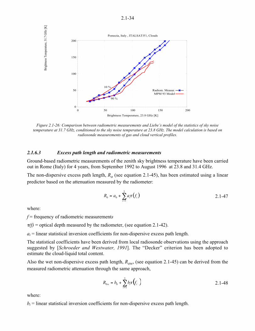
2.1-34

0

50

100

150

200

0 50 100 150 200

Brig

htne

ss T

empe

ratu

re, 3

1.7

GH

z [K

]

Brightness Temperature, 23.8 GHz [K]

Pomezia, Italy , ITALSAT/F1, Clouds

10 %

90 %

Radiom. Measur.MPM 93 Model

Figure 2.1-26: Comparison between radiometric measurements and Liebe’s model of the statistics of sky noisetemperature at 31.7 GHz, conditioned to the sky noise temperature at 23.8 GHz. The model calculation is based on

radiosonde measurements of gas and cloud vertical profiles.

2.1.6.3 Excess path length and radiometric measurements

Ground-based radiometric measurements of the zenith sky brightness temperature have been carriedout in Rome (Italy) for 4 years, from September 1992 to August 1996 at 23.8 and 31.4 GHz.

The non-dispersive excess path length, Ro (see equation 2.1-45), has been estimated using a linearpredictor based on the attenuation measured by the radiometer:

( )'=

+=2

100

iii faaR I 2.1-47

where:

f = frequency of radiometric measurements

I(f) = optical depth measured by the radiometer, (see equation 2.1-42).

ai = linear statistical inversion coefficients for non-dispersive excess path length.

The statistical coefficients have been derived from local radiosonde observations using the approachsuggested by [Schroeder and Westwater, 1991]. The “Decker” criterion has been adopted toestimate the cloud-liquid total content.

Also the wet non-dispersive excess path length, Row, (see equation 2.1-45) can be derived from themeasured radiometric attenuation through the same approach,

( )'=

+=2

100

iiiw fbbR I 2.1-48

where:

bi = linear statistical inversion coefficients for non-dispersive excess path length.

2.1-35

The radiosonde observation data base has been used also to calculate the theoretical values of Roand Row [Schroeder and Westwater, 1991], [Thayer, 1974]. Figure 2.1-27 shows the cumulativedistribution functions (CDF) of the non-dispersive excess path length estimated by radiometric datausing equation 2.1-47 and by the models. Liebe’s model (MPM93), has been used with a differentset of radiosonde observations performed in Pomezia in 1987and 1989 and from 1990 to 1994.Radiometric 1993-1996 CDF and radiosonde CDF show a good agreement, the maximumdiscrepancy being less than 1 cm, for values of less than 10% of the time, for the Thayer model.Liebe’s model predicts values lower than the measured values but this can be ascribed to theutilisation of a different database of radiosonde observations.

Excess Path Lenght [cm]

Perc

enta

ge o

f Sa

mpl

es, [

%]

230 240 250 2601

10

100

Rome

1993-1996

Thayer model

MPM'93

Figure 2.1-27: Yearly cumulative distribution functions of the measured total excess path length, with the valuespredicted using the Thayer and Liebe (MPM93) models.

Figure 2.1-28 shows the CDF of the wet term of the non-dispersive excess path length derived fromradiometric measurements and the results of the Elgered model obtained from Radiosondeobservations [Elgered, 1993]. The good agreement between the radiometrically wet excess pathlength and the Elgered model statistics is worth noting .

0 20Wet path-length, [cm]

1

10

100

Perc

enta

ge o

f sam

ples

[%]

Rome

radiometric estimation

Elgered model (1993-1996)

Figure 2.1-28: Cumulative distribution functions of the measured wet excess path length and predicted by the Elgeredmodel.

2.1-36

2.1.7 References

[Barbaliscia et al., 1994]Barbaliscia F., Boumis M., Martellucci A., Baptista J.P.V. 1994,”Modelling the atmosphericattenuation by means of meteorological parameters”, Alta Frequenza, Vol. 6, Num. 6, pp 101-105.

[Barbaliscia et al., 1995]Barbaliscia F., Boumis M., Martellucci A.,”Study of scaling of propagation effects from microwaveto optical frequencies”, ESA/ESTEC Contract 10195/92/NL/GS, 1995.

[Barbaliscia et al., 1996]Barbaliscia F., Boumis F., A. Martellucci, ”Statistical evaluation of atmospheric attenuation forVSAT systems using accurate physical models and large meteorological databases”, Proceedings ofthe Second Ka Band Utilization Conference, Firenze, Italy, 24-26 September 1996.

[Bosisio, 1994]Bosisio A.V., PhD Thesis, Polytechnic of Milano, Dept. of Electronics, 1994.

[Brussaard., 1985]Brussaard G., "Radiometry: a useful prediction tool ?", ESA Report SP-1071, 1985.

[Dissanayake et al., 1997]Dissanayake, A., Allnutt, J., Haidara, F., ”A prediction model that combines rain attenuation andother propagation that combines rain attenuation and other propagation impairments along earth-satellite paths”, IEEE Transactions on Antennas and Propagation, Vol. 45, No. 10, pp. 1546-1558,1997.

[Elgered, 1993]Elgered G., “Troposheric radio-path delay from ground-based microwave radiometry”, Chapter 5 ofthe “Atmospheric Remote Sensing by Microwave Radiometry”, Edited by M. Janssen, John Wiley& Sons, 1993.

[Gibbins, 1986]Gibbins C. J.,“Improved algorithms for the determination of specific attenuation at sea level by dryair and water vapour in the range 1-350 GHz”, Radio Science, 21(6), pp.945-954

[Hall, 1986]Hall, M.P.M., “Effects of the troposphere on radio communication”, IEE Electromagnetic Series 8,Peter Peregrinus Ltd, 1986.

[Howel et al., 1992]Howel R.G., Harris J. W. and Mehler M., “Satellite Copolar Measurements at BT Laboratories”, BTTechnol. Journal, Vol. 10, N. 4, pp 34-50, October 1992.

[ITU-R, 1998]ITU-R, Recommendation P.676-3, ”Attenuation by atmospheric gases”, 1998

[ITU-R, 1999]ITU-R, Recommendation P.676-4, ”Attenuation by atmospheric gases”, 1999

[Konefal et al., 2000]Konefal, T., Watson P.A., Shikla, A.K. and Akram, A., “”Prediction of Monthly and AnnualAvailabilities on 10-50 GHz Satellite to Earth and Aircraft to Aircraft links”, Proc. IEE –Microwaves, Antennas and Propagation, 147, pp 122-1277, April 2000

[Liebe, 1981]Liebe H. J.,“Modelling attenuation and phase of radio waves in air at frequencies below1000 GHz” Radio Science 16(6) pp 1183 1199 1981

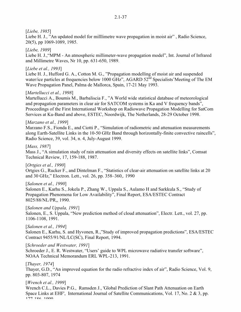
2.1-37

[Liebe, 1985]Liebe H. J., ”An updated model for milllimetre wave propagation in moist air” , Radio Science,20(5), pp 1069-1089, 1985.

[Liebe, 1989]Liebe H. J.,“MPM - An atmospheric millimeter-wave propagation model”, Int. Journal of Infraredand Millimetre Waves, Nr 10, pp. 631-650, 1989.

[Liebe et al., 1993]Liebe H. J., Hufford G. A., Cotton M. G., ”Propagation modelling of moist air and suspendedwater/ice particles at frequencies below 1000 GHz”, AGARD 52nd Specialists’Meeting of The EMWave Propagation Panel, Palma de Mallorca, Spain, 17-21 May 1993.

[Martellucci et al., 1998]Martellucci A., Boumis M., Barbaliscia F., ”A World wide statistical database of meteorologicaland propagation parameters in clear air for SATCOM systems in Ka and V frequency bands”,Proceedings of the First International Workshop on Radiowave Propagation Modelling for SatComServices at Ku-Band and above, ESTEC, Noordwijk, The Netherlands, 28-29 October 1998.

[Marzano et al., 1999]Marzano F.S., Fionda E., and Ciotti P., “Simulation of radiometric and attenuation measurementsalong Earth-Satellite Links in the 10-50 GHz Band through horizontally-finite convective raincells”,Radio Science, 39, vol. 34, n. 4, July-August 1999.

[Mass, 1987]Mass J., “A simulation study of rain attenuation and diversity effects on satellite links”, ComsatTechnical Review, 17, 159-188, 1987.

[Ortgies et al., 1990]Ortgies G., Rucker F., and Dintelman F., “Statistics of clear-air attenuation on satellite links at 20and 30 GHz,” Electron. Lett., vol. 26, pp. 358–360,. 1990

[Salonen et al., 1990]Salonen E., Karhu S., Jokela P., Zhang W., Uppala S., Aulamo H and Sarkkula S., “Study ofPropagation Phenomena for Low Availability”, Final Report, ESA/ESTEC Contract8025/88/NL/PR,, 1990.

[Salonen and Uppala, 1991]Salonen, E., S. Uppala, “New prediction method of cloud attenuation”, Electr. Lett., vol. 27, pp.1106-1108, 1991.

[Salonen et al., 1994]Salonen E., Karhu, S. and Hyvonen, R.,”Study of improved propagation predictions”, ESA/ESTECContract 9455/91/NL/LC(SC), Final Report, 1994.

[Schroeder and Westwater, 1991]Schroeder J., E. R. Westwater, “Users’ guide to WPL microwave radiative transfer software”,NOAA Technical Memorandum ERL WPL-213, 1991.

[Thayer, 1974]Thayer, G.D., “An improved equation for the radio refractive index of air”, Radio Science, Vol. 9,pp. 803-807, 1974

[Wrench et al., 1999]Wrench C.L., Davies P.G., Ramsden J., 'Global Prediction of Slant Path Attenuation on EarthSpace Links at EHF', International Journal of Satellite Communications, Vol. 17, No. 2 & 3, pp.177 186 1999

2.1-38

[Van de Hulst, 1957]Van de Hulst C. “Light scattering by small particles”, New York: Wiley, 1957.

2.1-39

2.1.8 Annex to Chapter 2.1: Gas and clouds propagation data available on CD-ROM

The propagation effects due to atmospheric gases and clouds, discussed in Chapter 2.1, have beenstudied in depth and a world-wide database of meteorological, propagation and statisticalparameters has been generated.

Starting from the FUB/ESA meteorological database DST.MET, that contains radiosondemeasurements of atmospheric vertical profile performed at 350 stations around the world[Martellucci et al., 1998], the propagation parameters indicated in Table 2.1-A1 have beencalculated using Liebe’s (see Section 2.1.1.1) and the ITU-R models of gaseous attenuation (seeSections 2.1.1.4 and 2.1.1.5), the Rayleigh model for cloud attenuation (see Section 2.1.2.1) andassuming zenith-viewing paths and non rainy conditions.

The results have been stored in the propagation database, PROP.HUT. The cloud liquid waterdensity has been estimated using the Salonen Model [Salonen 1990].

The same propagation parameters have been calculated making use of the mean monthly profiles ofthe atmospheric parameters, stored in the meteorological database DST.STD [Martellucci et al.,1998], not including the cloud liquid water content. The results are contained in the propagationdatabase named PROP.STD.

Propagation Parameters Frequencydependent

LiebeModel

ITU-R

Model4

SalonenModel

Gaseous Attenuation (Oxygen + Water Vapour) [dB] ! ! !

Total Attenuation (Oxygen + Water Vapour + Liquid Water) [dB] ! ! !

Dispersive Atmosph. path Delay (Oxyg.+Vapour+Liq. Water) [ps] ! ! !

Non dispersive Atmospheric Path Delay [ps] !

Brightness Temperature without cosmic background [K] ! ! !

Brightness Temperature with cosmic background (Tc = 3 K) [K] ! ! !

Mean Radiating Temperature [K] ! ! !

Oxygen Specific Attenuation at ground[dB/km] ! ! !

Water Vapour Specific Attenuation at ground [dB/km] ! ! !

Oxygen Attenuation Equivalent Height [km] ! ! !

Water Vapour Attenuation Equivalent Height [km] ! ! !

Water Vapour Mass Absorption Coefficient [dB/mm] ! !

Liquid Water Mass Absorption Coefficient [dB/mm] ! ! !

Table 2.1-A1: Parameters calculated from meteorological databases and propagation models, for the frequencies:18.7, 19.77, 21.3, 22.2, 23.8, 30, 31.7, 37.5, 40, 45, 49.5, 74, 90 and 110.8 GHz.

(The Salonen model is used to estimate the cloud liquid water density)

An extensive statistical analysis has been carried out of the results contained in the propagationdatabase PROP.HUT and a corresponding statistical database STAT.HUT has been generated. In

4 At the time of publication of this report, the ITU-R recommends [ITU-R, 1999] a model of oxygen and water vapourspecific attenuation that is different from the one used during the COST 255 project [ITU R 1998]

2.1-40

Table 2.1-A2 the parameters used for statistical analysis are given. An example of statisticalparameters, calculated for Milano-Linate, is given in Table 2.1-A3 and in Figure 2.1-A1.

Parameter Unit Freq. depend.

Total water vapor content mm

Total liquid water content mm

Total ice content mm

Water vapor ground density g/m3

Ground pressure kPa

Ground temperature C

Non dispersive excess path length m

Gaseous attenuation dB !

Total attenuation dB !

Brightness temperature K !

Dispersive excess path length mm !

Water vapour mass absorption coefficient dB/mm !

Liquid water mass absorption coefficient dB/mm !

Table 2.1-A2: Parameters used for statistical analysis frequencies:18.7, 19.77, 21.3, 22.2, 23.8, 30, 31.7, 37.5, 40, 45, 49.5, 74, 90 and 110.8 GHz

110

100

1 1.5 2 2.5 3 3.5 4 4.5 5Perc

enta

ge o

f the

Yea

r

Exceeded Attenuation [dB], 49.5 GHz

16080/MILANO/LINATE,IY/Lat=45.26 [deg], Lon=9.17 [deg], asl=107 [m]

Total AttenuationGaseous Attenuation

Figure 2.1-A1: Cumulative distribution function of gaseous and total attenuation, zenith values,in Milano at 49.5 GHz

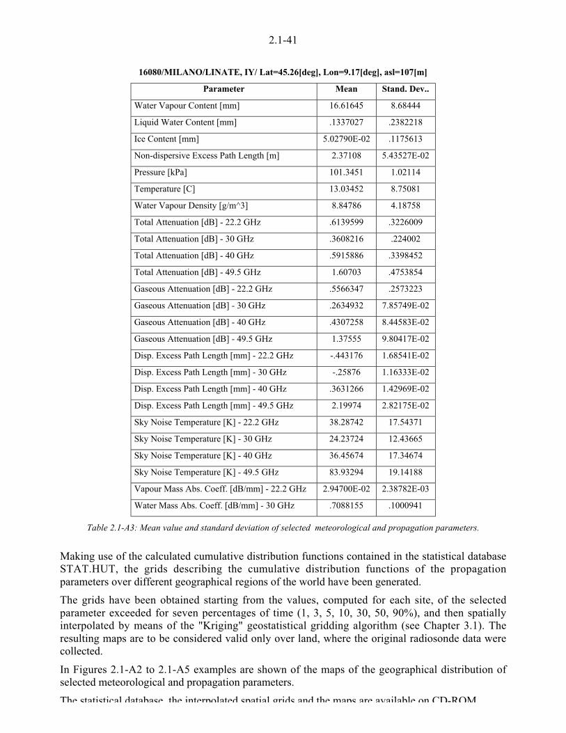
2.1-41

16080/MILANO/LINATE, IY/ Lat=45.26[deg], Lon=9.17[deg], asl=107[m]

Parameter Mean Stand. Dev..

Water Vapour Content [mm] 16.61645 8.68444

Liquid Water Content [mm] .1337027 .2382218

Ice Content [mm] 5.02790E-02 .1175613

Non-dispersive Excess Path Length [m] 2.37108 5.43527E-02

Pressure [kPa] 101.3451 1.02114

Temperature [C] 13.03452 8.75081

Water Vapour Density [g/m^3] 8.84786 4.18758

Total Attenuation [dB] - 22.2 GHz .6139599 .3226009

Total Attenuation [dB] - 30 GHz .3608216 .224002

Total Attenuation [dB] - 40 GHz .5915886 .3398452

Total Attenuation [dB] - 49.5 GHz 1.60703 .4753854

Gaseous Attenuation [dB] - 22.2 GHz .5566347 .2573223

Gaseous Attenuation [dB] - 30 GHz .2634932 7.85749E-02

Gaseous Attenuation [dB] - 40 GHz .4307258 8.44583E-02

Gaseous Attenuation [dB] - 49.5 GHz 1.37555 9.80417E-02

Disp. Excess Path Length [mm] - 22.2 GHz -.443176 1.68541E-02

Disp. Excess Path Length [mm] - 30 GHz -.25876 1.16333E-02

Disp. Excess Path Length [mm] - 40 GHz .3631266 1.42969E-02

Disp. Excess Path Length [mm] - 49.5 GHz 2.19974 2.82175E-02

Sky Noise Temperature [K] - 22.2 GHz 38.28742 17.54371

Sky Noise Temperature [K] - 30 GHz 24.23724 12.43665

Sky Noise Temperature [K] - 40 GHz 36.45674 17.34674

Sky Noise Temperature [K] - 49.5 GHz 83.93294 19.14188

Vapour Mass Abs. Coeff. [dB/mm] - 22.2 GHz 2.94700E-02 2.38782E-03

Water Mass Abs. Coeff. [dB/mm] - 30 GHz .7088155 .1000941

Table 2.1-A3: Mean value and standard deviation of selected meteorological and propagation parameters.

Making use of the calculated cumulative distribution functions contained in the statistical databaseSTAT.HUT, the grids describing the cumulative distribution functions of the propagationparameters over different geographical regions of the world have been generated.

The grids have been obtained starting from the values, computed for each site, of the selectedparameter exceeded for seven percentages of time (1, 3, 5, 10, 30, 50, 90%), and then spatiallyinterpolated by means of the "Kriging" geostatistical gridding algorithm (see Chapter 3.1). Theresulting maps are to be considered valid only over land, where the original radiosonde data werecollected.

In Figures 2.1-A2 to 2.1-A5 examples are shown of the maps of the geographical distribution ofselected meteorological and propagation parameters.

The statistical database the interpolated spatial grids and the maps are available on CD-ROM

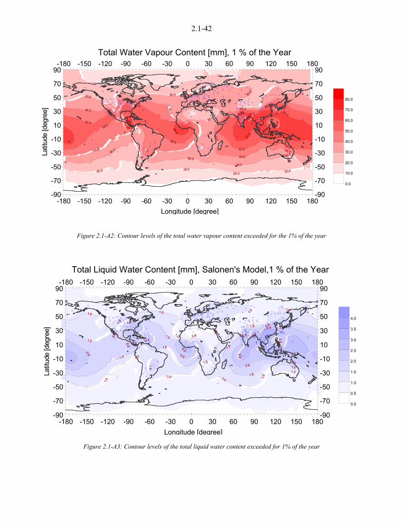
2.1-42

Figure 2.1-A2: Contour levels of the total water vapour content exceeded for the 1% of the year

-180 -150 -120 -90 -60 -30 0 30 60 90 120 150 180

Longitude [degree]

-180 -150 -120 -90 -60 -30 0 30 60 90 120 150 180

-90

-70

-50

-30

-10

10

30

50

70

90

Latit

ude

[deg

ree]

-90

-70

-50

-30

-10

10

30

50

70

90

0.0

0.5

1.0

1.5

2.0

2.5

3.0

3.5

4.0

Total Liquid Water Content [mm], Salonen's Model,1 % of the Year

Figure 2.1-A3: Contour levels of the total liquid water content exceeded for 1% of the year

-180 -150 -120 -90 -60 -30 0 30 60 90 120 150 180

Longitude [degree]

-180 -150 -120 -90 -60 -30 0 30 60 90 120 150 180

-90

-70

-50

-30

-10

10

30

50

70

90

Latit

ude

[deg

ree]

-90

-70

-50

-30

-10

10

30

50

70

90

0.0

10.0

20.0

30.0

40.0

50.0

60.0

70.0

80.0

Total Water Vapour Content [mm], 1 % of the Year

2.1-43

Figure 2.1-A4: World-wide contour levels of the zenith non rainy atmospheric attenuation [dB] exceeded for 1% of the year at 22 GHz

-180 -150 -120 -90 -60 -30 0 30 60 90 120 150 180

Longitude [degree]

-180 -150 -120 -90 -60 -30 0 30 60 90 120 150 180

-90

-70

-50

-30

-10

10

30

50

70

90

Latit

ude

[deg

ree]

-90

-70

-50

-30

-10

10

30

50

70

90

0.0

1.0

2.0

3.0

4.0

5.0

6.0

7.0

8.0

49.5 GHz, Total Attenuation, [dB],1 % of year

Figure 2.1-A5: World-wide contour levels of the zenith non rainy atmospheric attenuation [dB] exceeded for 1% of the year at 49.5 GHz

2.2-1

CHAPTER 2.2Rain Attenuation

Editor: Ondrej Fiser1

Authors: Ioan Chisalita2, Michele D’Amico3, Boris Gremont4, Martin Hajny5,Frank S. Marzano6, Tudor Palade7 , Carlo Riva8

1 Institute of Atmospheric Physics of the Czech Academy, Bocni street II/1401, 141 31 Praha 4, Czech Republic

Tel: +420-2-769702 ext.108, Fax.: +420-2-72763745, e-mail: ondrej@ufa.cas.cz2 Techn. Univ. of Cluj-Napoca, 15C.Daicoviciu Str/POB 1124, Ro-3400 Cluj, Romania

Tel: +40 64 191689; Fax. +40 64 194831/ 195590, e-mail: chisalita@utcluj.ro3 Politecnico di Milano/CSTS, Piazza Leonardo da Vinci 32, I-20133 Milano, Italy

Tel: +39-2-2399-3613, Fax: +39-2-2399-3413, e-mail: damico@elet.polimi.it4 University of Portsmouth, Microwave and Signal Processing Lab, Anglesea Rd, Portsmouth PO1 3DJ, U.K.

Tel: +44-1705-842543, Fax: +44-1705-842792, e-mail: gremont@ee.port.ac.uk5 Inst. of Atmospheric Physics, Czech Academy, Bocni street II/1401, 141 31 Praha 4, Czech Republic

Tel: +420-2-769702ext.175, Fax.: +420-2-72763745, e-mail: hajny@ufa.cas.cz6 Dipartimento di Ingegneria Elettrica, Università dell'Aquila, (Italy) Monteluco di Roi, 67040 L’Aquila;

Tel: +39.0862.434412; Fax. +39.0862.434414; e-mail: marzano@ing.univaq.it7 Technical University of Cluj-Napoca, 15C Daicoviciu Str/POB 1124, Ro-3400 Cluj, Romania

Tel. +40 64 191689; Fax. +40 64 194831/ 195590, e-mail: palade@utcluj.ro8 Politecnico di Milano/CSTS Piazza Leonardo da Vinci 32 I-20133 Milano Italy

2.2-2

2.2 Rain Attenuation

2.2.1 Models of Rain Attenuation Statistics

Attenuation due to rain is an important propagation effect which must be considered in the design ofsatellite telecommunication systems. The attenuation by rain depends on the temperature, sizedistribution, terminal velocity and shape of the raindrops.

The rain attenuation can be measured quite accurately by means of satellite beacon signals andradiometers. However, since propagation experiments are carried out only in a few places in theworld and for a limited number of frequencies and link geometry, their results cannot be directlyapplied to all sites. For this reason, several attenuation models based on physical facts and usingavailable meteorological data, have been developed to provide adequate inputs for system margincalculations in all regions of the world.

In particular, the prediction of rain induced attenuation starting from the cumulative distribution ofrainfall intensity has been the subject of a major effort carried out by many researchers: severalmethods have been developed and tested against available data to relate the site climatic parametersto the signal attenuation statistics. The following rain prediction models, which are among the bestperforming, are briefly described in this chapter:

1. Assis-Einloft Improved 9. ITU-R 618-5

2. Australian 10. ITU-R 618-6

3. Brazil 11. Karasawa

4. Bryant 12. Leitao-Watson

5. Crane Global 13. Matricciani

6. Crane two components 14. Misme-Waldteufel

7. EXCELL 15. SAM

8. Garcia 16. Svjatogor

In Table 2.2-1 the input parameters necessary for rain attenuation prediction models are listed anddescribed.

2.2.1.1 Improved Assis-Einloft model

The original Assis-Einloft model was developed for terrestrial links [Assis and Einloft, 1977] andwas extended for satellite links using the ITU-R rain height, hR, considering the satellite linkelevation [Fiser, 1986]. The improvement of the accuracy published in [Costa, 1983] is realisedthrough equation 2.2-8.

The step by step procedure for calculating the attenuation distribution can be described in thefollowing manner:

Step 1: For e*5° compute the slant-path length, Ls, below the rain height from:

( )esin

ss

HhL R <= [km] 2.2-1

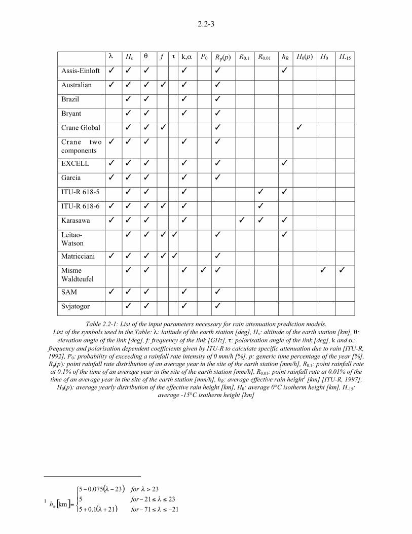
2.2-3

h Hs e f o k,_ P0 Rp(p) R0.1 R0.01 hR H0(p) H0 H-15

Assis-Einloft ! ! ! ! ! !

Australian ! ! ! ! ! !

Brazil ! ! ! !

Bryant ! ! ! !

Crane Global ! ! ! ! !

Crane twocomponents

! ! ! ! !

EXCELL ! ! ! ! ! !

Garcia ! ! ! ! !

ITU-R 618-5 ! ! ! ! !

ITU-R 618-6 ! ! ! ! ! !

Karasawa ! ! ! ! ! ! !

Leitao-Watson

! ! ! ! ! !

Matricciani ! ! ! ! ! !

MismeWaldteufel

! ! ! ! ! ! !

SAM ! ! ! ! !

Svjatogor ! ! ! !

Table 2.2-1: List of the input parameters necessary for rain attenuation prediction models.List of the symbols used in the Table: h: latitude of the earth station [deg], Hs: altitude of the earth station [km], e:

elevation angle of the link [deg], f: frequency of the link [GHz], o: polarisation angle of the link [deg], k and _:frequency and polarisation dependent coefficients given by ITU-R to calculate specific attenuation due to rain [ITU-R,1992], P0: probability of exceeding a rainfall rate intensity of 0 mm/h [%], p: generic time percentage of the year [%],Rp(p): point rainfall rate distribution of an average year in the site of the earth station [mm/h], R0.1: point rainfall rateat 0.1% of the time of an average year in the site of the earth station [mm/h], R0.01: point rainfall rate at 0.01% of thetime of an average year in the site of the earth station [mm/h], hR: average effective rain height1 [km] [ITU-R, 1997],

H0(p): average yearly distribution of the effective rain height [km], H0: average 0°C isotherm height [km], H-15:average -15°C isotherm height [km]

1 [ ]

( )

( )«

««©

¨

<))<++

))<

><<

=2171211.05

23215

2323075.05

kmR hh

h

hh

for

for

for

h

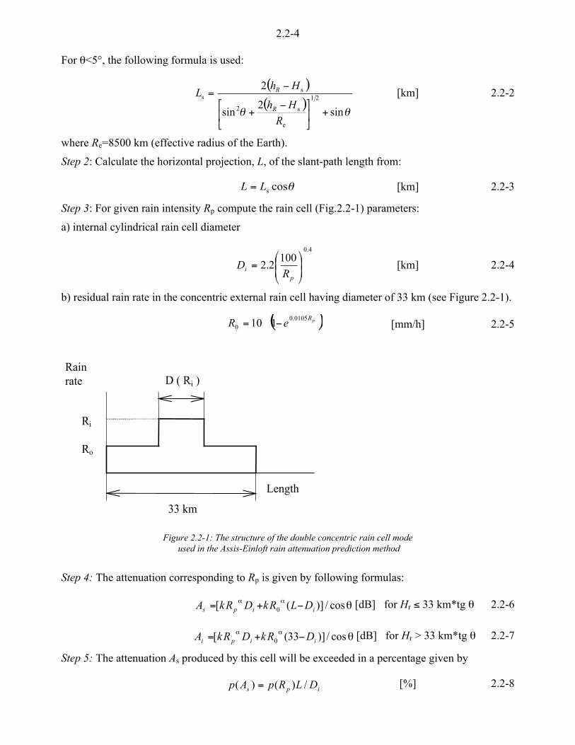
2.2-4

For e<5°, the following formula is used:

( )( )

ee sin2

sin

221

e

s2

ss

+µ�

�³�

� <+

<=

R

Hh

HhL

R

R [km] 2.2-2

where Re=8500 km (effective radius of the Earth).

Step 2: Calculate the horizontal projection, L, of the slant-path length from:

ecossLL = [km] 2.2-3

Step 3: For given rain intensity Rp compute the rain cell (Fig.2.2-1) parameters:

a) internal cylindrical rain cell diameter

4.0

1002.2 ´

´¦

¥²²¤

£=

pi R

D [km] 2.2-4

b) residual rain rate in the concentric external rain cell having diameter of 33 km (see Figure 2.2-1).

( )pReR 0105.00 110 <= [mm/h] 2.2-5

Rain rate

Ri

Ro

33 km

D ( Ri )

Length

Figure 2.2-1: The structure of the double concentric rain cell mode used in the Assis-Einloft rain attenuation prediction method

Step 4: The attenuation corresponding to Rp is given by following formulas:

e<+= __ cos/)]([ 0 iips DLRkDRkA [dB] for Hr ) 33 km*tg e 2.2-6

e<+= __ cos/)]33([ 0 iipi DRkDRkA [dB] for Hr > 33 km*tg e 2.2-7

Step 5: The attenuation As produced by this cell will be exceeded in a percentage given by

ips DLRpAp /)()( = [%] 2.2-8

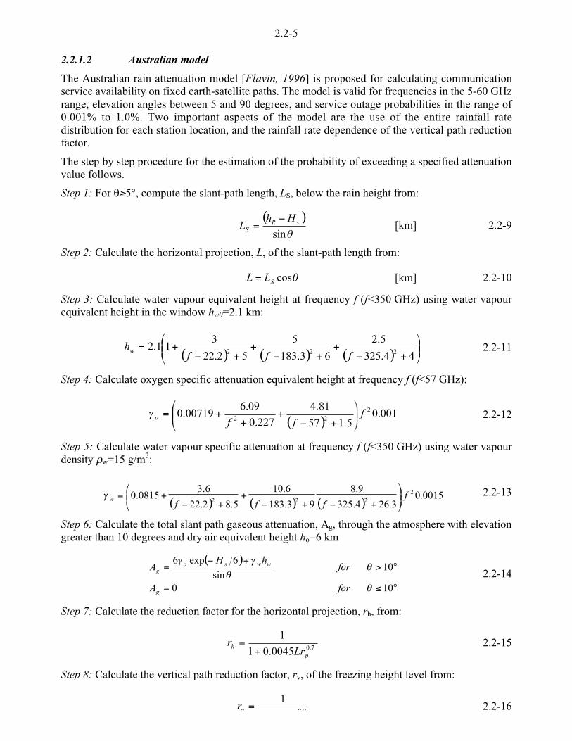
2.2-5

2.2.1.2 Australian model

The Australian rain attenuation model [Flavin, 1996] is proposed for calculating communicationservice availability on fixed earth-satellite paths. The model is valid for frequencies in the 5-60 GHzrange, elevation angles between 5 and 90 degrees, and service outage probabilities in the range of0.001% to 1.0%. Two important aspects of the model are the use of the entire rainfall ratedistribution for each station location, and the rainfall rate dependence of the vertical path reductionfactor.

The step by step procedure for the estimation of the probability of exceeding a specified attenuationvalue follows.

Step 1: For e*5°, compute the slant-path length, LS, below the rain height from:

( )esin

sRS

HhL

<= [km] 2.2-9

Step 2: Calculate the horizontal projection, L, of the slant-path length from:

ecosSLL = [km] 2.2-10

Step 3: Calculate water vapour equivalent height at frequency f (f<350 GHz) using water vapourequivalent height in the window hw0=2.1 km:

( ) ( ) ( ) ´́¦

¥²²¤

£

+<+

+<+

+<+=

44.325

5.2

63.183

5

52.22

311.2

222 fffhw 2.2-11

Step 4: Calculate oxygen specific attenuation equivalent height at frequency f (f<57 GHz):

( )001.0

5.157

81.4

227.0

09.600719.0 2

22f

ffo ´́¦

¥²²¤

£

+<+

++=a 2.2-12

Step 5: Calculate water vapour specific attenuation at frequency f (f<350 GHz) using water vapourdensity lw=15 g/m3:

( ) ( ) ( )0015.0

3.264.325

9.8

93.183

6.10

5.82.22

6.30815.0 2

222f

fffw ´

´¦

¥²²¤

£

+<+<+

+<+=a 2.2-13

Step 6: Calculate the total slant path gaseous attenuation, Ag, through the atmosphere with elevationgreater than 10 degrees and dry air equivalent height ho=6 km

( )

°)=

°>+<

=

100

10sin

6exp6

e

ee

aa

forA

forhH

A

g

wwsog 2.2-14

Step 7: Calculate the reduction factor for the horizontal projection, rh, from:

7.00045.01

1

ph Lr

r+

= 2.2-15

Step 8: Calculate the vertical path reduction factor, rv, of the freezing height level from:

70

1vr = 2.2-16

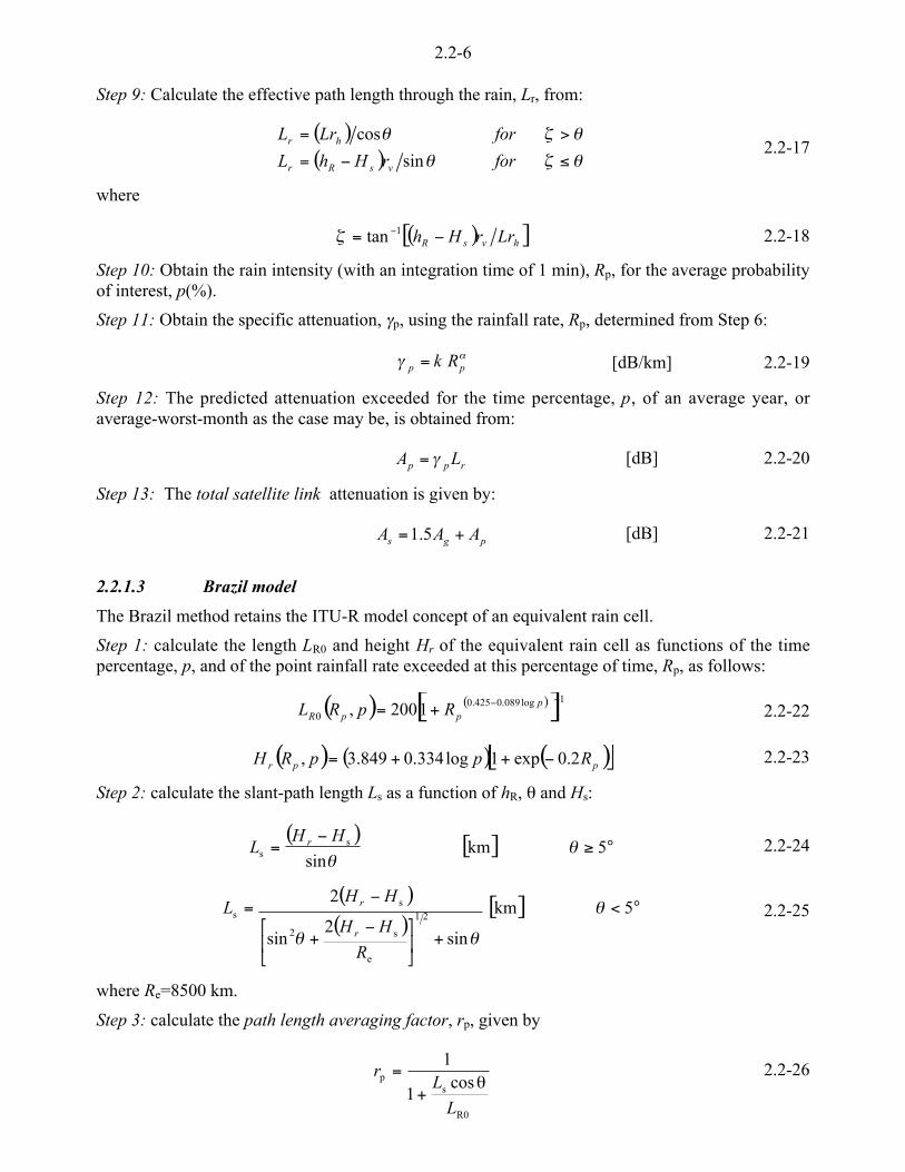
2.2-6

Step 9: Calculate the effective path length through the rain, Lr, from:

( )( ) ece

ece

)<=

>=

forrHhL

forLrL

vsRr

hr

sin

cos2.2-17

where

( )[ ]hvsR LrrHh <= <1tanc 2.2-18

Step 10: Obtain the rain intensity (with an integration time of 1 min), Rp, for the average probabilityof interest, p(%).

Step 11: Obtain the specific attenuation, ap, using the rainfall rate, Rp, determined from Step 6:

_a pp Rk= [dB/km] 2.2-19

Step 12: The predicted attenuation exceeded for the time percentage, p, of an average year, oraverage-worst-month as the case may be, is obtained from:

rpp LA a= [dB] 2.2-20

Step 13: The total satellite link attenuation is given by:

pgs AAA += 5.1 [dB] 2.2-21

2.2.1.3 Brazil model

The Brazil method retains the ITU-R model concept of an equivalent rain cell.

Step 1: calculate the length LR0 and height Hr of the equivalent rain cell as functions of the timepercentage, p, and of the point rainfall rate exceeded at this percentage of time, Rp, as follows:

( ) ( )[ ]1log089.0425.00 1200,

<<+= pppR RpRL 2.2-22

( ) ( ) ( )[ ]ppr RppRH 2.0exp1log334.0849.3, <++= 2.2-23

Step 2: calculate the slant-path length Ls as a function of hR, e and Hs:

( ) [ ] °*<

= 5kmsin

ss e

e

HHL r 2.2-24

( )( )

[ ] °<

+µ�

�³�

� <+

<= 5km

sin2

sin

221

e

s2

ss e

eeR

HH

HHL

r

r2.2-25

where Re=8500 km.

Step 3: calculate the path length averaging factor, rp, given by

R0

sp cos

1

1

L

Lr

e+

= 2.2-26

2.2-7

Step 4: calculate the attenuation As, exceeded at a time percentage p:

effps LA u= a [dB] 2.2-27

with

_a pp Rk u= [dB/km] 2.2-28

pseff rLL u= [km] 2.2-29

2.2.1.4 Bryant model

The Bryant method uses the concept of effective rain cell and variable rain height to calculate thedistribution of rain attenuation [Bryant et al., 1999].

Step 1: calculate the PR parameter:

D

LPR

/+=

21 2.2-30

where D is the rain cell diameter given by 12540 <u= pRD

and the horizontal projection L is given by etanrHL = .

Step 2: calculate the rain height Hr:

65.10005.05.4 pr RH += [km] 2.2-31

Step 3: the attenuation along the slant path is then given by

DL

LkDA s

pnms +=

ja57.1 [km] 2.2-32

where:

Ls is the slant-path length,

ap is the specific attenuation [dB/km],

( )DDm /= 2 ,

nk is the number of cells and

( )pn Rk 007.0exp= 2.2-33

( )

ǻ

«©

¨

°>ee

°)ee=j

55tan1.1

55sinexp2

1

2.2-34

2.2.1.5 Crane Global model

The Crane Global model was developed using geophysical observations of the statistics of pointrain rate, of the horizontal structure of rainfall, and of the vertical temperature structure of theatmosphere.

2.2-8

The step-by-step application of the model is:

Step 1: Determine the global model rain climate region for the propagation path using the mapsgiven in [Crane, 1980]. The rain rate distribution P(R) for each region is listed in [Crane, 1980].

Step 2: Establish surface horizontal projected path length L:

( )( )10

10tan0

<=

°*<=

es

ee

e

s

RL

HpHL2.2-35

where:

( )( )( ) ( )( ) ( ) ( ) µ

�

�³�

�´¦¥²

¤£ e+<<+<+e+u

+e

=s sin2sincos

arcsin 2200

22

0esssees

e

RHHpHHpHRRHRpH

2.2-36

Re is the effective Earth’s radius (8500 km) and

H0(p) is obtained by interpolation (linearly in H0 and logarithmically in p) in Figure 14 of [Crane,1980] for the time percentage, p, of interest.

If L>22.5 km, use both L0=22.5 km and a new point rate vRp for the modified time percentage, p´:

µ�

�³�

�=v

L

Lpp 0 2.2-37

for subsequent calculations.

Step 3: Determine _0 and `0 for the frequency of interest from Table III or Figures 18 and 19 of[Crane, 1980].

Step 4: Calculate the surface projected attenuation value A from Rp and L (or vRp and L0):

( )

( )

( ) ( ) ( )°==<=

<µ�

�³�

� <=

))µ�

�³�

�+<

<=

900,

1,

1,

0

0

0

00000

0

p000p

0p0p

0000

p0p

e_

`_

```_

`

``

``````

LRLHLRA

lLu

eRLRA

LLlc

eb

c

eb

u

eRLRA

du

Dcdcdu

2.2-38

where:

[ ]

p

p

017-p

ln6.08.3

ln03.0026.0

3.2

ln

Rl

Rc

Rb

dbe

ucd

<=

<=

=

=

2.2-39

Step 5: Adjust for height along a slant path:

( )L

LALA s=s

2.2-40

2.2-9

where:

( ) ( ) ( )( ) °<es++<+++=

°*ee=

10cos2

10cos

022

0 LRLRLRLRL

LL

eeees

s2.2-41

where s is given by Equation 2.2-36.

2.2.1.6 Crane Two-Component model

The Crane Two-Component model for the prediction of attenuation due to rain separately addressesthe contributions of rain showers, referred to as cells, and the larger regions of lighter rain intensitysurrounding the showers, referred to as debris. The Two-Component model handles the cells andthe debris independently. All storms contain cells and debris, but propagation paths through the raindo not always intersect a single isolated cell; the Two-Component model assumes either a singlecell or only debris or both along a path. The model is designed for the calculation of the probabilitythat a specified attenuation is exceeded. One of the two components of the rain process, a cell ordebris, may produce the attenuation value. The probability associated with each component iscalculated, and the two values are summed independently to provide the desired probabilityestimate.

The step by step procedure for the estimation of the probability of exceeding a specified attenuationvalue follows.

Step 1: Determine the global model rain climate region for the propagation path using the mapsgiven in [Crane, 1980] and [Crane, 1982]. The parameters for each region, Pc, Rc, PD, RD and SD,are listed in [Crane, 1982]. Since the Crane maps were not available to us in electronic format wehave used, for test purposes, the ITU-R rain zone and equivalent parameters for the rain ratedistribution in each zone. Possibly the method can perform better with parameters of Crane rainzones.

Step 2: Establish the maximum projected path length for cells, Lc, and debris, LD.

For cells:

( ) [ ]( )

( )[ ][ ] °)e

<+e+e

<=

°>ee<=

10km85002tantan

2

10kmtan

21

c2

cc

cc

s

s

s

HH

HHL

HHL

2.2-42

where:

( )[ ]°<<= 452sin7.11.3c hH [km] 2.2-43

For debris:

( ) [ ]( )

( )[ ][ ] °)

<++

<=

°><=

10km85002tantan

2

10kmtan

21

D2

DD

DD

eee

ee

s

s

s

HH

HHL

HHL

2.2-44

where:

( )[ ]°= 452sin9182 hH [km] 2 2 45

2.2-10

Step 3: Determine the reduced attenuation value for the calculation of probability:

A A= coss e 2.2-46

where As is the path attenuation of interest.

Step 4: Calculate the initial cell rain rate estimate for A [dB]:

( )p_

d

<

´́¦

¥²²¤

£=

1

i

7.0

k

AR [mm/h] 2.2-47

where d=1.87 and i=0.04.

Step 5: Calculate the cell horizontal extent:

pd -ic RW = [km] 2.2-48

If Wc>Lc, then Wc=Lc.

Step 6: Calculate the adjustment for debris associated with a cell:

( )( )cc

cc

1

7.01

WL

WLC

<+

<+= 2.2-49

Step 7: If a slant path, reduce the cell width if the implied cell thickness is too large:

jn -ic RT = [km] 2.2-50

where the thickness parameters c=1.6 and j=0.24, and:

[ ] 21

c2

cT

85002tantan

2

T

TW

++=

ee[km] 2.2-51

If Wc>WT, then Wc=WT.

Step 8: Get the final cell rain rate estimate, Rf:

( ) _1cf kWCAR = [mm/hr] 2.2-52

Step 9: Calculate the probability of intersecting a cell on the propagation path:

( ) ( )cfcccf exp1 RRWLPP <+= 2.2-53

Step 10: Calculate the initial debris rain rate estimate for A [dB]:

( )b_<

´́¦

¥²²¤

£

1=

1

a k

AR [mm/hr] 2.2-54

where 1=29.7 and b=0.34 are the debris parameters.

Step 11: Calculate the debris horizontal extent:

b-aD RW 1= [km] 2.2-55

If WD>LD, then WD=LD.

2.2-11

Step 12: If a slant path, reduce the debris width if the implied cell thickness is too large. For Ra>1,

( ) ( )[ ]®­¬

ª©¨

+

<+<=

a

a

R

RHHHHT

ln1

ln6.11 sDsDD [km] 2.2-56

[ ] 21

D2

DL

85002tantan

2

T

TW

++=

ee[km] 2.2-57

If WD>WL, then WD=WL.

Step 13: Get the final debris rain rate, Rz:

( ) _1Dz kWAR = [mm/hr] 2.2-58

Step 14: Calculate the probability of intersecting debris on the propagation path:

( ) ( )´´¦

¥²²¤

£+=

D

DaDDDg

2

lnerfc

2

11

S

RRWLPP 2.2-59

where erfc is the complementary error function.

Step 15: Sum the cell and debris probability values to determine the probability of exceeding theattenuation A:

( )P a A P P> = +f g 2.2-60

Step 16: If the attenuation value corresponding to a specified probability value is desired,interpolation will be required between the probability value versus attenuation calculations.

2.2.1.7 EXCELL model

The basic assumption of the EXCELL model is the description of the precipitation environment bymeans of a population hereinafter referred to as “synthetic isolated cells” with exponential profile ofthe rain inside and rotational symmetry [Capsoni et al., 1987a] derived by studies of radar rainmaps.

If we consider exponential cells, the rain rate R at a distance l from the cell centre is given by:

( )R RM= <exp l l02.2-61

where RM is the peak rain intensity and l0 is the “cell radius”, i.e. the distance at which the rain ratedecreases by a factor 1/e.

The model is characterised by the cell identifiers, RM and l0, and by the spatial density of thepopulation N(RM, l0). Since it has been observed that, for a given RM value, cell dimensions, l0, areexponentially distributed, the number of cells per square kilometre and per unit range of ln(RM) andl l0 0 can be written as:

( ) ( ) ( )N R N RM Mln , ln expl l l0 0 0 0= < 2.2-62

where l0 is the conditional average radius, given by:

( ) ( )[ ]l0

10 0 2617 6 6 5= + >

< <.

.R R RM M M

2.2-63

2.2-12

and the spatial density, N0(ln RM), is derived by the local cumulative distribution function of thepoint rain intensity (fitted by an analytical expression) by means of the formula:

( ) [ ] ( )N R P RM M0 021 4ln = < /l

'''2.2-64

where P(RM)vvv is the third order derivative of the point rate intensity cumulative distribution P(R)with respect to ln(R), evaluated at R=RM. Actually to derive the cumulative distribution, which isusually given for fixed probabilities, it is necessary to fit it by a proper function.

If we assume that the random process describing a given propagation impairment is generated bythe pure translation movement of the above described rain cells in the region where the radio systemis located, the statistical behaviour of the parameter of interest can then be studied by assuming thateach structure occupies all the possible positions in the plane. It then becomes possible to determineall the positions of the system relative to the cell in which a prefixed value of the parameter understudy is exceeded. The ensemble of these points constitutes a surface which will be referred to asthe “kernel” of the considered parameter [Capsoni et al., 1987b] and its area is proportional to theprobability that the fixed parameter value is exceeded.

For instance, referring to the cell model of equation 2.2-61, the area of the circle where the pointrain intensity exceeds a prefixed value R is the kernel of the parameter “point rain intensity”. Itsvalue is given by:

( )S R RM0 02 2= /l ln 2.2-65

To calculate the kernel of rain attenuation, it is convenient to introduce the concept of “equivalentrain intensity” RE, defined as:

( ) ( )dxyxRL

yxRLx

LxE ,1

,2

20+

<

__ = 2.2-66

With reference to Figure 2.2-2, x and y are the co-ordinates of the medium point of the link and Lis the path length. The kernel of equivalent rain is then given by [Capsoni et al., 1987b]:

LMMS +/= 21 2.2-67

where:

( )( )M R RM E= <ln minl l0 0 and

l0 min is the minimum radius of a cell with equivalent rain RE.

Once we have evaluated the equivalent rain intensity, the cell attenuation is easily obtained by theexpression:

sEc LKRA _= 2.2-68

where:

L is the slant path length given by:

ee sincos Rs hLL == 2.2-69

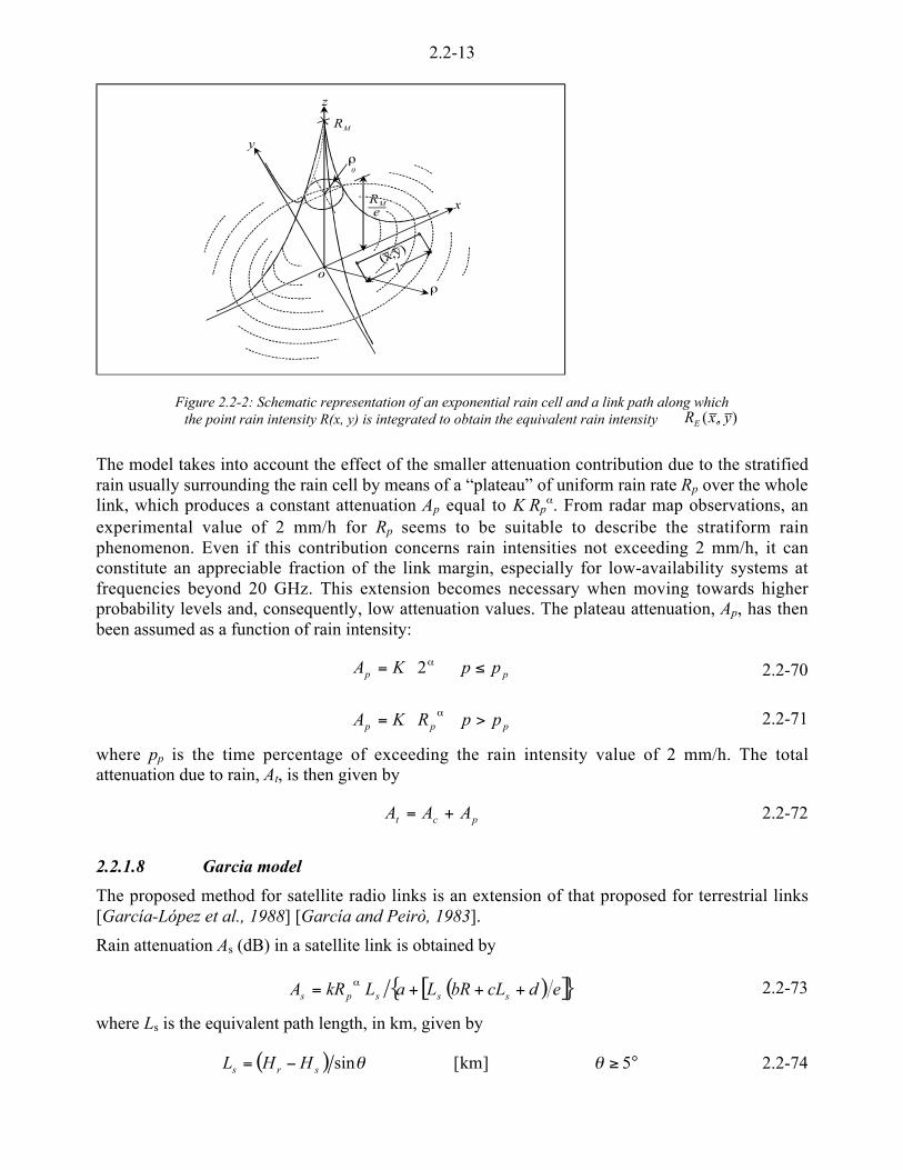
2.2-13

RM

x

y

z

o

RM

e

l0

l

(x,y)

l

Figure 2.2-2: Schematic representation of an exponential rain cell and a link path along whichthe point rain intensity R(x, y) is integrated to obtain the equivalent rain intensity .

The model takes into account the effect of the smaller attenuation contribution due to the stratifiedrain usually surrounding the rain cell by means of a “plateau” of uniform rain rate Rp over the wholelink, which produces a constant attenuation Ap equal to K Rp

_. From radar map observations, anexperimental value of 2 mm/h for Rp seems to be suitable to describe the stratiform rainphenomenon. Even if this contribution concerns rain intensities not exceeding 2 mm/h, it canconstitute an appreciable fraction of the link margin, especially for low-availability systems atfrequencies beyond 20 GHz. This extension becomes necessary when moving towards higherprobability levels and, consequently, low attenuation values. The plateau attenuation, Ap, has thenbeen assumed as a function of rain intensity:

pp ppKA )= _2 2.2-70

ppp ppRKA >= _ 2.2-71

where pp is the time percentage of exceeding the rain intensity value of 2 mm/h. The totalattenuation due to rain, At, is then given by

A A At c p= + 2.2-72

2.2.1.8 Garcia model

The proposed method for satellite radio links is an extension of that proposed for terrestrial links[García-López et al., 1988] [García and Peirò, 1983].

Rain attenuation As (dB) in a satellite link is obtained by

( )[ ]{ }edcLbRLaLkRA sssps +++= _ 2.2-73

where Ls is the equivalent path length, in km, given by

( ) °*<= 5]km[sin eesrs HHL 2.2-74

),( yxRE

2.2-14

with

[ ]( ) [ ]ǻ

«©¨

°*°<<

°<<=

36km36075.04

360km4

hh

hrH 2.2-75

The coefficients a, b, c, and d are constants depending, in general, on the geographical area and canbe determined easily by regression techniques based on simultaneous rain attenuation and rainintensity. Coefficient e is only a scaling factor. Taking e=104, the “worldwide” coefficients are:a=0.7, b=18.35, c=-16.51, d= 500.

2.2.1.9 ITU-R Rec. 618-5 model

ITU-R formerly recommended a procedure to estimate the long-term statistics of the slant-path rainattenuation at a given location for frequencies up to 30 GHz.

The step by step procedure for calculating the attenuation distribution is given hereinafter.

Step 1: For e*5° compute the slant-path length, Ls, below the rain height from:

( ) [ ]kmsin

ss e

HhL R <

= 2.2-76

For e<5°, the following formula is used:

( )( )

[ ]km

sin2

sin

221

e

s2

ss

ee +µ�

�³�

� <+

<=

R

Hh

HhL

R

R 2.2-77

where Re=8500 km.

Step 2: Calculate the horizontal projection, L, of the slant-path length from:

[ ]kmcoss eLL = 2.2-78

Step 3: Obtain the rain intensity, R0.01, exceeded for 0.01% of an average year (with an integrationtime of 1 min).

Step 4: Calculate the reduction factor, r0.01, for 0.01% of the time for R0.01)100 mm/h:

001.0 1

1

LLr

+= 2.2-79

where L0=35 exp(-0.015 R0.01).

For R0.01>100 mm/h, use the value 100 mm/h in place of R0.01.

Step 5: Obtain the specific attenuation, a0.01:

( )_a 01.00.01 Rk= [dB/km] 2.2-80

Step 6: The predicted attenuation exceeded for 0.01% of an average year is obtained from:

01.0S0.0101.0 rLA a= [dB] 2.2-81

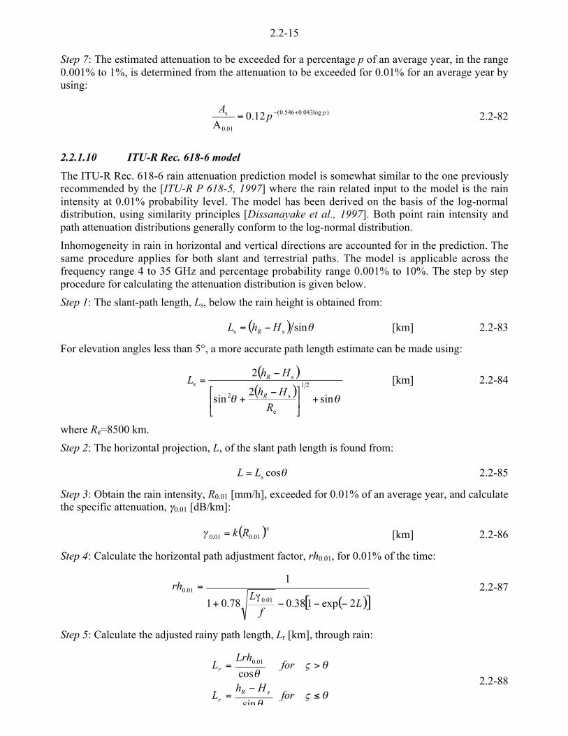
2.2-15

Step 7: The estimated attenuation to be exceeded for a percentage p of an average year, in the range0.001% to 1%, is determined from the attenuation to be exceeded for 0.01% for an average year byusing:

)log043.0546.0(

0.01

s 12.0A

ppA +<= 2.2-82

2.2.1.10 ITU-R Rec. 618-6 model

The ITU-R Rec. 618-6 rain attenuation prediction model is somewhat similar to the one previouslyrecommended by the [ITU-R P 618-5, 1997] where the rain related input to the model is the rainintensity at 0.01% probability level. The model has been derived on the basis of the log-normaldistribution, using similarity principles [Dissanayake et al., 1997]. Both point rain intensity andpath attenuation distributions generally conform to the log-normal distribution.

Inhomogeneity in rain in horizontal and vertical directions are accounted for in the prediction. Thesame procedure applies for both slant and terrestrial paths. The model is applicable across thefrequency range 4 to 35 GHz and percentage probability range 0.001% to 10%. The step by stepprocedure for calculating the attenuation distribution is given below.

Step 1: The slant-path length, Ls, below the rain height is obtained from:

( ) esinss HhL R <= [km] 2.2-83

For elevation angles less than 5°, a more accurate path length estimate can be made using:

( )( )

ee sin2

sin

221

e

s2

ss

+µ�

�³�

� <+

<=

R

Hh

HhL

R

R [km] 2.2-84

where Re=8500 km.

Step 2: The horizontal projection, L, of the slant path length is found from:

ecossLL = 2.2-85

Step 3: Obtain the rain intensity, R0.01 [mm/h], exceeded for 0.01% of an average year, and calculatethe specific attenuation, a0.01 [dB/km]:

( )_a 01.001.0 Rk= [km] 2.2-86

Step 4: Calculate the horizontal path adjustment factor, rh0.01, for 0.01% of the time:

( )[ ]Lf

Lrh

2exp138.078.01

1

01.0

0.01

<<<a

+

= 2.2-87

Step 5: Calculate the adjusted rainy path length, Lr [km], through rain:

ene

ene

)<

=

>=

forHh

L

forLrh

L

sRr

r

sin

cos01.0

2.2-88

2.2-16

where ´́¦

¥²²¤

£ <=

01.0

sarctanLrh

HhRn .

Step 6: Calculate the vertical reduction factor, rv0.01, for 0.01% of the time:

[ ]( )µµ�

�

³³�

�<

a<e+

=r+e< 45.0131sin1

1

2

01.0r1

0.01

f

Le

rv 2.2-89

where:

°*h=r

°<hh<=r

360

3636

for

for2.2-90

Step 7: The effective path length through rain, Le [km], is given by:

01.0re rvLL = [km] 2.2-91

Step 8: The attenuation exceeded for 0.01% of an average year may then be obtained from:

e01.001.0 LA a= [dB] 2.2-92

Step 9: The attenuation to be exceeded for the other percentages of an average year, in the range0.001% to 10.0%, may be estimated from the attenuation to be exceeded for 0.01% for an averageyear by using:

( )[ ]pzApp

AA<e<<+<

´¦

¥²¤

£=1sinln045.0ln033.0655.0

01.0s

01.0

01.02.2-93

where p is the percentage probability of interest and

z for p*1% is equal to zero and for p<1% is given by:

( )( ) °<h°<ee<+<h<=

°<h°*e<h<=

°*h=

3625sin25.48.136005.0

362536005.0

360

andforz

andforz

forz

2.2-94

2.2.1.11 Karasawa model

The step by step procedure for calculating the attenuation distribution is given below.

Step 1: Calculate the effective rain height, Hr, as follows:

[ ] ( )ª©¨

<hhu+

*hhu=

36.02803

3636-0.075-4kmr for

forH 2.2-95

Step 2: Calculate the vertical reduction factor, rv:

Rrv hHr = 2.2-96

Step 3: Compute the slant-path length, Ls [km], from:

2.2-17

( )

( )( )

°<e

e+<

+e

<=

°*ee

<=

5

sin2

sin

2

5sin

e

sRv2

sRvs

sRvs

R

Hhr

HhrL

HhrL

2.2-97

Step 4: Calculate the horizontal projection, L [km], of the slant path length from:

e= cossLL 2.2-98

Step 5: Calculate the horizontal reduction factor, rh,0.01, from:

0h,0.01 1

1

LLr

+= 2.2-99

where:

( ) [ ][ ]

L R R

L R R

0 0 01 0 01

0 0 01 0 01

35 0 015 80

94 80

= < )

= >

exp . . .

. .

mm h

mm h2.2-100

Step 6: Obtain the specific attenuation, a0.01, from:

_=a 01.00.01 kR 2.2-101

Step 7: The predicted attenuation exceeded for 0.01% of an average year is obtained from:

h,0.01s0.0101.0 rLA a= [dB] 2.2-102

Step 8: The predicted attenuation exceeded for 0.1% of an average year is obtained from:

( )[ ] 01.001.01.01.0 23.038.0 ARRA += [dB] 2.2-103

Step 9: Calculate the rain attenuation, As, as a function of time percentage, p:

( )

( ) 01.0001.02log1074.1

101.010

101.3

01.0s

s

))+<=

))=+

+

ppsAA

pAsm

pqsm

2.2-104

where:

( )

( )1.001.010

01.0101.010

10

32

log30.1

log03.3log03.4

log1

0657.0144.0847.033.2

AAs

AAm

px

xxxxq

=

<=

+=

<<<=

2.2-105

2.2.1.12 Leitao-Watson showery model

The Leitao-Watson showery model is based entirely on the structure of storms as observed on adual-polarisation radar and interpreted using scattering theory.

Essential steps in the development of the model are as follows:

2.2-18

1. characterisation of the statistical properties of rain-fall and path attenuation on horizontalpaths, leading to determination of the rainfall rate reduction factor CR and an attenuationconversion factor CA for showery rain;

2. evolution of relationships between attenuation on horizontal and slant paths for showeryrain, including the effects of elevation dependence, melting band and variation in rainheight;

3 . climatic characteristics of rainfall types and freezing heights including the seasonaldependence of rain intensity and rain height

4. determination of the freezing height during rainfall.

The rain attenuation models for widespread rain and convective rain are based on the same set ofequations; only the models parameters are dependent on the rain type. The model parameters areonly given for several fixed frequencies between 10 and 30 GHz.

According to the Leitao Watson showery model, the rain attenuation A [dB] along the horizontalprojection L [km] of the slant path Ls [km] is calculated from the equation:

( ) LRLRCA uu= ,A 2.2-106

where:

R is the point rainfall rate [mm/h] and

CA [(dB/km)/(mm/h)] is a point-to-path conversion factor obtained from the radar measurementsand defined by the equation:

( )( )

( )0

1

, 0R

A =

a

=0

xR

dxxL

LRC

L

2.2-107

where:

aR(x) [dB/km] is the specific attenuation due to rain on the horizontal path.

CA depends on the link parameters and rain data (the temperature of raindrops is assumed to be10°C) and may be calculated using the following equation:

( )

««

ª

««

©

¨

*´¦

¥²¤

£

<´¦

¥²¤

£

=

<

<

hmm2020

hmm2020

,

1

1

A

RRa

RRa

LRC

yy

xx

2.2-108

The model parameters a, x and y are calculated for the required polarisation from the followingequations [Nowland et al., 1977]:

( )a a a a a= + + <h v h v cos cos2 2 2e o 2.2-109

( ) ( )x a x a x a x a x a= + + <h h v v h h v v cos cos2 2 2e o 2.2-110

( ) ( )y a y a y a y a y a= + + <h h v v h h v v cos cos2 2 2e o 2.2-111

2.2-19

The factors ah,v, xh,v and yh,v are given by the empirical equations:

L

sa

0.01+1vh,

vh, = 2.2-112

( ) vh,10vh,vh, 1log uLtx ++= 2.2-113

( ) vh,10vh,vh, 1log wLvy ++= 2.2-114

In the above expressions h and v refer to the horizontal and vertical polarisation, respectively. Theconstants sh,v, th,v, uh,v and wh,v are dependent on the frequency and rain type. For convective rain inthe U.K., they are given in [COST 205, 1985a]. If necessary, frequency interpolation for ah,v, xh,v

and yh,v between fv and fw may be performed through the following expressions, where f is thedesired frequency:

( )log log loglog log

log loglog, , , ,a a a

f f

f fah v h v h v h v= vv < v

< v

vv < v+ v 2.2-115

( )x x xf f

f fxh v h v h v h v, , , ,

log log

log log= vv < v

< v

vv < v+ v 2.2-116

( )y y yf f

f fyh v h v h v h v, , , ,

log log

log log= vv < v

< v

vv < v+ v 2.2-117

The rain attenuation As [dB] on the slant path is obtained, if the rain specific attenuation is assumedconstant in the vertical direction:

( ) sAs

s , LRLRCL

LAA uu== 2.2-118

The lengths L and Ls may be calculated from the formulae in ITU-R Recommendation 618-5 [ITU-R, 1997]:

( )( )

««««

ª

««««

©

¨

°<e

e+<

+e

<

°*ee

<

=

5

sin2

sin

2

5sin

e

s2

s

s

s

R

HH

HH

HH

L

r

r

r

2.2-119

e= cossLL 2.2-120

where:

Re is the effective radius of Earth (8500 km).

Care has to be used, when the Leitao-Watson model is applied for elevation angles less than about10°, because the longest horizontal path length L considered in the development of the model is 12km.

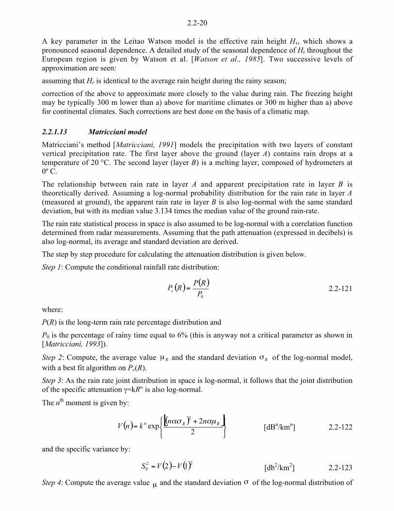
2.2-20

A key parameter in the Leitao Watson model is the effective rain height H r, which shows apronounced seasonal dependence. A detailed study of the seasonal dependence of Hr throughout theEuropean region is given by Watson et al. [Watson et al., 1985]. Two successive levels ofapproximation are seen:

assuming that Hr is identical to the average rain height during the rainy season;

correction of the above to approximate more closely to the value during rain. The freezing heightmay be typically 300 m lower than a) above for maritime climates or 300 m higher than a) abovefor continental climates. Such corrections are best done on the basis of a climatic map.

2.2.1.13 Matricciani model

Matricciani’s method [Matricciani, 1991] models the precipitation with two layers of constantvertical precipitation rate. The first layer above the ground (layer A) contains rain drops at atemperature of 20 °C. The second layer (layer B) is a melting layer, composed of hydrometers at0º C.

The relationship between rain rate in layer A and apparent precipitation rate in layer B istheoretically derived. Assuming a log-normal probability distribution for the rain rate in layer A(measured at ground), the apparent rain rate in layer B is also log-normal with the same standarddeviation, but with its median value 3.134 times the median value of the ground rain-rate.

The rain rate statistical process in space is also assumed to be log-normal with a correlation functiondetermined from radar measurements. Assuming that the path attenuation (expressed in decibels) isalso log-normal, its average and standard deviation are derived.

The step by step procedure for calculating the attenuation distribution is given below.

Step 1: Compute the conditional rainfall rate distribution:

( ) ( )0P

RPRPc = 2.2-121

where:

P(R) is the long-term rain rate percentage distribution and

P0 is the percentage of rainy time equal to 6% (this is anyway not a critical parameter as shown in[Matricciani, 1993]).

Step 2: Compute, the average value Rµ and the standard deviation Rm of the log-normal model,with a best fit algorithm on Pc(R).

Step 3: As the rain rate joint distribution in space is log-normal, it follows that the joint distributionof the specific attenuation a=kR_ is also log-normal.

The nth moment is given by:

( ) ( )[ ]®­¬

ª©¨ +

=2

2exp

2RRn nn

knV_µ_m

[dBn/kmn] 2.2-122

and the specific variance by:

( ) ( )220 12 VVS <= [db2/km2] 2.2-123

Step 4: Compute the average value µ and the standard deviation m of the log-normal distribution of

2.2-21

( ) ´́¦

¥²²¤

£+=m

m<=µ 1ln

2ln

2

22

2

M

SM 2.2-124

where:

( ) ( )( )ABBAA LLVLVM <+= 11 [dB] 2.2-125

BBABABAA ISISSISS 2000

20

2 2 ++= [dB2] 2.2-126

where the moments ( )1,baV and 2,0 BAS are calculated using the appropriate µ , k and _ of the two

layers (particles of layer A and B at, respectively, 20°C and 0°C). The rain paths LA,B are given by:

( ) [ ]( ) [ ]kmsin

kmsin

e

e

sBB

sAA

HHL

HHL

<=

<=2.2-127

[ ]

( )ª©¨

°*<<

°<=

<=

2323075.05

235

km4.0

hh

hB

BA

H

HH

2.2-128

The terms IA, IB and IAB represent the integration of the normalised covariance c(x) that is a functionof the distance x along the path:

( )

( )

( )0 0

0 0

0 0

<=

<=

<=

B B

A

B

A

B

A

A B

L L

L

AB

L

L

L

L

B

L L

A

dxdyyxcI

dxdyyxcI

dxdyyxcI

0

0 0

2.2-129

( ) ( ){ }[ ]( ){ } ( ){ }[ ]

( ) ( )

( ) ( )°e=e`

=

<+<

<+<=

e`<

m_m_

__m

32coscos46.0

11

111212

22

1

212

xexb

ee

exbxc

RR

R

2.2-130

Step 5: Compute the probability of attenuation A [dB]:

( ) ( ) [ ]( )0'

m

µ<

</

=µ�

�³�

�m

µ<=

A

dyyPA

QPAPln

200 2exp

2

ln2.2-131

where Q(x) is the Gaussian integral function.

2.2.1.14 Misme Waldteufel model

The well known Misme-Waldteufel model [Misme and Waldteufel, 1980] was modified by Fiser[Fiser, 1984, 1986], in order to simplify the half-infinity integral computation. It computes the

b bilit th t th i ll th i i tt ti A Th i t i i ll i th

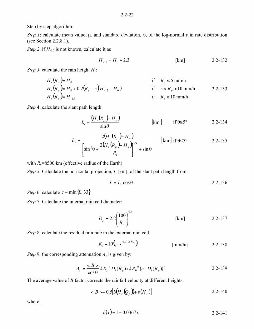
2.2-22

Step by step algorithm:

Step 1: calculate mean value, µ, and standard deviation, m, of the log-normal rain rate distribution(see Section 2.2.8.1).

Step 2: if H-15 is not known, calculate it as

3.2015 +=< HH [km] 2.2-132

Step 3: calculate the rain height Hr:

( )( ) ( )( )( ) mm/h10if

mm/h105if52.0

mm/h5if

15

0150

0

*=

<<<<+=

)=

<

<

ppr

pppr

ppr

RHRH

RHHRHRH

RHRH

2.2-133

Step 4: calculate the slant path length:

( )( )[ ]km

sins

s e

HRHL pr <

= if e*5° 2.2-134

( )( )( )( )

[ ]km

sin2

sin

221

e

s2

ss

e+µ�

�³�

� <+e

<=

R

HRH

HRHL

pr

prif e<5° 2.2-135

with Re=8500 km (effective radius of the Earth)

Step 5: Calculate the horizontal projection, L [km], of the slant path length from:

e= cossLL 2.2-136

Step 6: calculate { }33,min Lc =

Step 7: Calculate the internal rain cell diameter:

4.0

1002.2 ´

´¦

¥²²¤

£=

pp R

D [km] 2.2-137

Step 8: calculate the residual rain rate in the external rain cell

( )pReR 0105.00 110 <= [mm/hr] 2.2-138

Step 9: the corresponding attenuation As is given by:

}])({)([cos 0 pipips RDcRkRDRk

BA <+

e

><= __ 2.2-139

The average value of B factor corrects the rainfall velocity at different heights:

( )( ) ( )[ ]sjr HbQHbB +>=< 5.0 2.2-140

where:

( ) xxb 0367.01<= 2.2-141

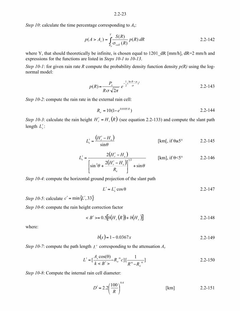
2.2-23

Step 10: calculate the time percentage corresponding to As:

dRRpR

RSAAp

Y

R cells

p

)()(

)()( 0 m=> 2.2-142

where Y, that should theoretically be infinite, is chosen equal to 1201_dR [mm/h], dR=2 mm/h andexpressions for the functions are listed in Steps 10-1 to 10-13.

Step 10-1: for given rain rate R compute the probability density function density p(R) using the log-normal model:

2)ln

(2

1

2)( m

µ

/m

<<

=R

o eR

PRp 2.2-143

Step 10-2: compute the rain rate in the external rain cell:

)1(10 0105.0 Ro eR <= 2.2-144

Step 10-3: calculate the rain height ( )RHH rr =v (see equation 2.2-133) and compute the slant path

length sLv :

( )esin

ss

HHL r <v=v [km[, if e*5° 2.2-145

( )( )

ee sin2

sin

221

e

s2

ss

+µ�

�³�

� <v+

<v=v

R

HH

HHL

r

r [km], if e<5° 2.2-146

Step 10-4: compute the horizontal ground projection of the slant path

ev=v cossLL 2.2-147

Step 10-5: calculate { }33,min Lc v=v

Step 10-6: compute the rain height correction factor

( )( ) ( )[ ]sr HbRHbB +>=v< 5.0 2.2-148

where:

( ) xxb 0367.01<= 2.2-149

Step 10-7: compute the path length Lv corresponding to the attenuation As

]1

[])cos(

[__

_

<<

>v<

e=v

o

os

RRcR

Bk

AL 2.2-150

Step 10-8: Compute the internal rain cell diameter:

4.0100

2.2 ´¦

¥²¤

£=vR

D [km] 2.2-151

2.2-24

Step 10-9: If Lv<0 compute:

><

e=v

_oo

s

BRk

AL

cos2.2-152

where:

( )( ) ( )[ ]sr HbRHbB +>=< 00 5.0 2.2-153

( ) xxb 0367.01<= 2.2-154

and assign a new value to the parameter D=33 km

Step 10-10: Evaluate:

ǻ

«©¨

<

*<=

LD

LDLDM

0

22

2.2-155

Step 10-11: Evaluate:

««ª

««©

¨

)/

>=

02

0

Lartcg

LL

Marctg

P 2.2-156

Step 10-12: Evaluate the plane S (the rain cell can be placed there)

)**(*5.0*)( 2 MLDPMLLS g <+<= 2.2-157

Step 10-13: Evaluate the plane of the rain cell

4

2Dcell

/m = 2.2-158

We neglected the rain attenuation dependence on the temperature. In original model b(x) contains atemperature dependence factor [OPEX, 1994].

2.2.1.15 SAM model

The Simple Attenuation Model developed by [Stutzman and Dishman,1984] is based on an effectiverain rate profile that is exponential in shape.

The spatial rainfall distribution along the slant path is given by:

( ) [ ]( ) ( )[ ] [ ]hmm10cos10lnexp

hmm10

000

00

>eK<=

)=

RlRRlR

RRlR2.2-159

for l)Ls,

where:

R0 [mm/h] is the point rainfall intensity,

e is the slant path elevation angle,

2.2-25

l [km] is the spatial co-ordinate along the slant path and the slant path length,

Ls, is given by:

( ) e<= sinss HHL r 2.2-160

The effective rain height, hR [km], is given by:

[ ]( ) [ ]hmm1010log

hmm10

000

00

*+=

)=

RRHH

RHH

r

r 2.2-161

where:

H0 [km] is the 0° isotherm height.

The seasonal average of H0 is obtained by the following equation [Crane, 1978]:

°*hhu<=

°)h=

301.08.7

308.4

0

0

H

H2.2-162

The total attenuation due to a point rainfall rate R0 is found by using the effective rain profile ofEquation 2.2-159 in the path integral:

( ) ( )[ ]0 a=s

0

0

L

s dllRRA 2.2-163

where a[R(l)] is the specific attenuation due to rain:

( )[ ]_a lRk= [dB/km] 2.2-164

Evaluation of the integral (equation 2.2-163) yields the final expressions:

( )

( ) ( )[ ]( )

hmm10cos10ln

cos10lnexp1

hmm10

00

s000

0s00

*K

K<<=

)=

RR

LRkRRA

RLkRRA

s

s

e_

e__

_

2.2-165

The value of K equal to 1/14 was found to be optimised with an expanded database for which bothattenuation and rain rate data were available.

2.2.1.16 Svjatogor model

The Svjatogor model [Svjatogor, 1985] defines its effective rain height Hr depending on the rainintensity:

pp

r RR

H 0015.0)5.13.0(log

7.2

10

++

= [km] 2.2-166

The path length reduction factor is formulated in the following expression:

6.068.0 ])tan(

[0045.0;e

<== rp

Yrs

HRYek 2.2-167

2.2-26

Finally, the rain attenuation As is given by:

rssps kLRkA _= [dB] 2.2-168

where:

( )esin

ss

HHL r <= [km], if e * 5° 2.2-169

( )( )

ee sin2

sin

221

e

s2

ss

+µ�

�³�

� <+

<=

R

HH

HHL

r

r [km], if e < 5° 2.2-170

and Re=8500 km (effective radius of the Earth)

The probability of exceeding this attenuation equals that of the rain rate: )()( ps RpAp = .

2.2.2 Modelling of Frequency Scaling

Knowledge of the relationship between attenuation values at different frequencies is needed for theevaluation of system performance based on measurements at other frequencies. The most usefulparameter to scale attenuation is the frequency scaling ratio, rfs, i.e. the ratio between attenuationvalues (expressed in dB), A1 and A2, at different frequencies:

1

2

A

Arfs = 2.2-171

Two different frequency scaling factors can be considered:

a) The long-term frequency scaling that describes the relationship between attenuation values atdifferent frequencies for the same probability level. It allows the calculation of thecumulative distribution function of attenuation at frequencies different from those used forthe measurements.

b) The short-term frequency scaling (or instantaneous frequency scaling (IFS)), that relatessimultaneous attenuation values at different frequencies.

A useful tool to examine the relationship between instantaneous attenuation at different frequenciesis the scatter-plot between (simultaneous or equiprobable) values of rfs and A (attenuation) or,obviously, directly between A1 and A2.

Attenuation is, in principle, the combination of contributions from different causes: rain, gaseousabsorption by oxygen or water vapour, clouds and scintillation. These contributions depend onfrequency in different ways. This is the main cause of inaccuracy for long-term frequency scalingpredictions. On the other hand, the short-term frequency scaling fluctuations are essentially due tothe natural variability of the various phenomena. A statistical approach is then required forfrequency scaling modelling whose complexity depends on the influence of the different effects.The frequency scaling technique is most satisfactory when one cause predominates, otherwise thefrequency scaling technique can become less interesting when compared with directmeteorologically-derived predictions.

On the other hand, the frequency independence of the attenuating path makes the frequency scalingratio more stable.

2.2-27

2.2.2.1 Long-Term Frequency Scaling

Rain (or, rarely, total) attenuation statistics at one frequency can be extrapolated from another(usually lower) frequency using a long term or equiprobability frequency scaling factor, [COST205, 1985b] [OPEX, 1994]. Long-term frequency scaling has been applied in the past to extrapolaterain attenuation mainly from Ku to Ka band. In Ku band the non-rain contributions to attenuation aregenerally negligible and the frequency scaling technique works particularly well (possibly byamending a little the Ka attenuation, to account for non-rain attenuation).

Many prediction methods for long-term frequency scaling, mainly related to rain, have been devisedin the past. The most widely used methods are the following:

1. CCIR [Drufuca, 1974] [Boithias and Battesti, 1981], recommended by the CCIR (now ITU-R);

2. Fixed Effective Rain [COST 205, 1985a], which assumes the ratio caused by an effectiverain intensity of 66 mm/h along the whole path;

3. Variable Effective Rain [COST 205, 1985a], which assumes the ratio caused by an effectiverain intensity increasing with increasing attenuation;

4. [ITU-R, 1997], presently recommended by the ITU-R.

The application of these models gives errors which are significantly lower than by predictingattenuation statistics from rain data only (12 - 15% against 30 - 40%). This applies however forpercentages of time below about 1%.

All methods are based on a formula of the type:

)(

)(

1

2

2

1

fg

fg

A

Arfs == 2.2-172

where f1 and f2 are the two frequency values and the function g(f) is defined according to themethod.

CCIR method

For the CCIR method, g(f) is defined by the equation:

( ) 72.144.37

72.1

1031f

f

ffg 5

u+=

<2.2-173

Fixed Effective Rain Model

For the Fixed Effective Rain model, g(f) is defined by the equation:

( ) ( ) ( )polfRpolfkfg ,, _= 2.2-174

where:

pol stands for polarisation,

k and _ are the well known constants that relate rain intensity to specific attenuation due to rain[ITU-R, 1992] and

R is the effective rainrate, assumed to be 66 mm/h.

2.2-28

Variable Effective Rain Model

The Variable effective rain model uses the same equation as the fixed one but with a different(variable) effective rain R:

39.0

1

139.0

1

39.01 78.578.5 ´́

¦

¥²²¤

£5´́

¦

¥²²¤

£=

k

A

k

AR

d 2.2-175

with:

( ) ( )( )[ ] 1,,39.01 121 5_<_<=d <polfpolf 2.2-176

ITU-R Model

In the case of the ITU-R model, we have:

( )( )

( )121 ,,1

1

2

1

2

1

2

AH

fg

fg

A

Aqq<

µ�

�³�

�

q

q== 2.2-177

where:

( )24

2

101 f

ff

<+=q 2.2-178

and

( ) 55.011

5.0

1

231012.1 AH q´́¦

¥²²¤

£

q

qu= < 2.2-179

Example of Long-term Frequency Scaling Models versus ITALSAT Measurements

Even though not completely appropriate, the measured long term frequency scaling ratio ofITALSAT total attenuation (including the effects of gas, clouds, turbulence and rain) was comparedwith that predicted by the models described in the previous paragraphs (devised when only rain-attenuation experimental data were available).

The results of this comparison are shown in Figures 2.2-3 to 2.2-5 that give long term statistics(asterisks) and frequency scaling ratios for the three frequencies available from the ITALSATexperiment, along with the model predictions. As far as the 50 GHz frequency is concerned, Figures2.2-4 and 2.2-5 show that the ITU-R model performs satisfactorily up to 50 GHz and below 1%probability. The error seems to be within 15% for attenuations exceeding 2.5 dB at 20 GHz or 7 dBat 40 GHz, which corresponds to about 1% of the time for both cases. Greater discrepancies forhigher probabilities must be attributed to non-rain effects that have different scaling.

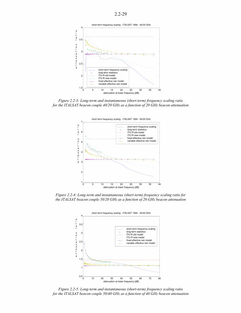
2.2-29

Figure 2.2-3: Long-term and instantaneous (short-term) frequency scaling ratiofor the ITALSAT beacon couple 40/20 GHz as a function of 20 GHz beacon attenuation

Figure 2.2-4: Long-term and instantaneous (short-term) frequency scaling ratio forthe ITALSAT beacon couple 50/20 GHz as a function of 20 GHz beacon attenuation

Figure 2.2-5: Long-term and instantaneous (short-term) frequency scaling ratiofor the ITALSAT beacon couple 50/40 GHz as a function of 40 GHz beacon attenuation

0 5 10 15 20 25 30 35 401.5

2

2.5

3

3.5

4short term frequency scaling - ITALSAT 1994 - 40/20 GHz

attenuation at lower frequency [dB]

attenuation ratio

short term frequency scalinglong-term statisticsITU-R old modelITU-R new modelfixed effective rain modelvariable effective rain model

0 5 10 15 20 25 30 35 401

2

3

4

5

6

7short term frequency scaling - ITALSAT 1994 - 50/20 GHz

attenuation at lower frequency [dB]

attenuation ratio

short term frequency scalinglong-term statisticsITU-R old modelITU-R new modelfixed effective rain modelvariable effective rain model

0 10 20 30 40 50 60 70 800.5

1

1.5

2

2.5

3

3.5

4short term frequency scaling - ITALSAT 1994 - 50/40 GHz

attenuation at lower frequency [dB]

attenuation ratio

short term frequency scalinglong-term statisticsITU-R old modelITU-R new modelfixed effective rain modelvariable effective rain model

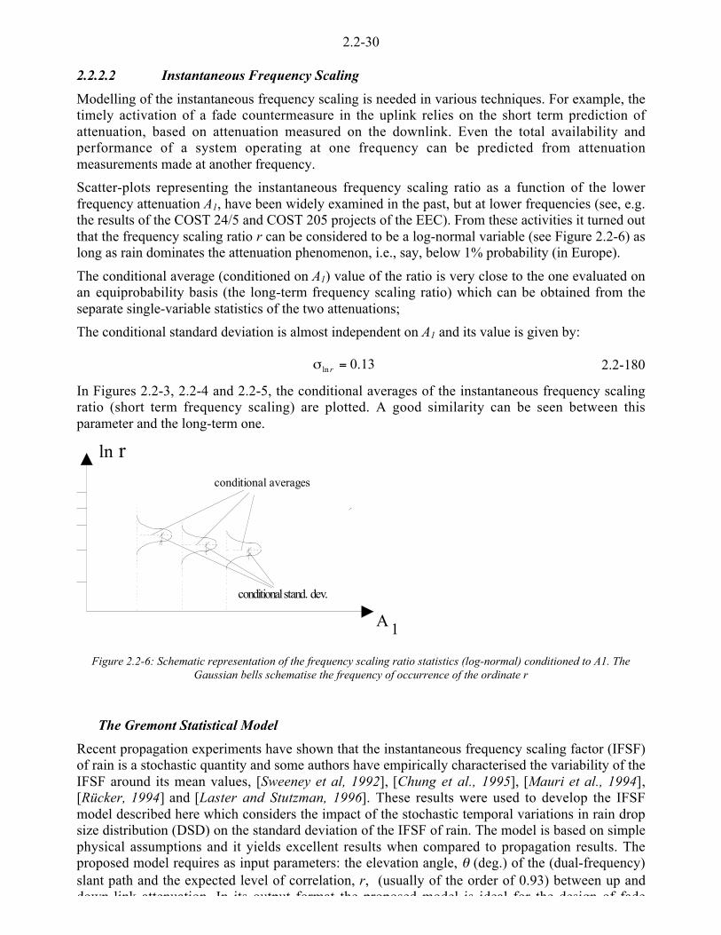
2.2-30

2.2.2.2 Instantaneous Frequency Scaling

Modelling of the instantaneous frequency scaling is needed in various techniques. For example, thetimely activation of a fade countermeasure in the uplink relies on the short term prediction ofattenuation, based on attenuation measured on the downlink. Even the total availability andperformance of a system operating at one frequency can be predicted from attenuationmeasurements made at another frequency.

Scatter-plots representing the instantaneous frequency scaling ratio as a function of the lowerfrequency attenuation A1, have been widely examined in the past, but at lower frequencies (see, e.g.the results of the COST 24/5 and COST 205 projects of the EEC). From these activities it turned outthat the frequency scaling ratio r can be considered to be a log-normal variable (see Figure 2.2-6) aslong as rain dominates the attenuation phenomenon, i.e., say, below 1% probability (in Europe).

The conditional average (conditioned on A1) value of the ratio is very close to the one evaluated onan equiprobability basis (the long-term frequency scaling ratio) which can be obtained from theseparate single-variable statistics of the two attenuations;

The conditional standard deviation is almost independent on A1 and its value is given by:

13.0ln =m r 2.2-180

In Figures 2.2-3, 2.2-4 and 2.2-5, the conditional averages of the instantaneous frequency scalingratio (short term frequency scaling) are plotted. A good similarity can be seen between thisparameter and the long-term one.

A 1

ln rconditional averages

conditional stand. dev.

Figure 2.2-6: Schematic representation of the frequency scaling ratio statistics (log-normal) conditioned to A1. TheGaussian bells schematise the frequency of occurrence of the ordinate r

The Gremont Statistical Model

Recent propagation experiments have shown that the instantaneous frequency scaling factor (IFSF)of rain is a stochastic quantity and some authors have empirically characterised the variability of theIFSF around its mean values, [Sweeney et al, 1992], [Chung et al., 1995], [Mauri et al., 1994],[Rücker, 1994] and [Laster and Stutzman, 1996]. These results were used to develop the IFSFmodel described here which considers the impact of the stochastic temporal variations in rain dropsize distribution (DSD) on the standard deviation of the IFSF of rain. The model is based on simplephysical assumptions and it yields excellent results when compared to propagation results. Theproposed model requires as input parameters: the elevation angle, e (deg.) of the (dual-frequency)slant path and the expected level of correlation, r, (usually of the order of 0.93) between up anddown link attenuation In its output format the proposed model is ideal for the design of fade

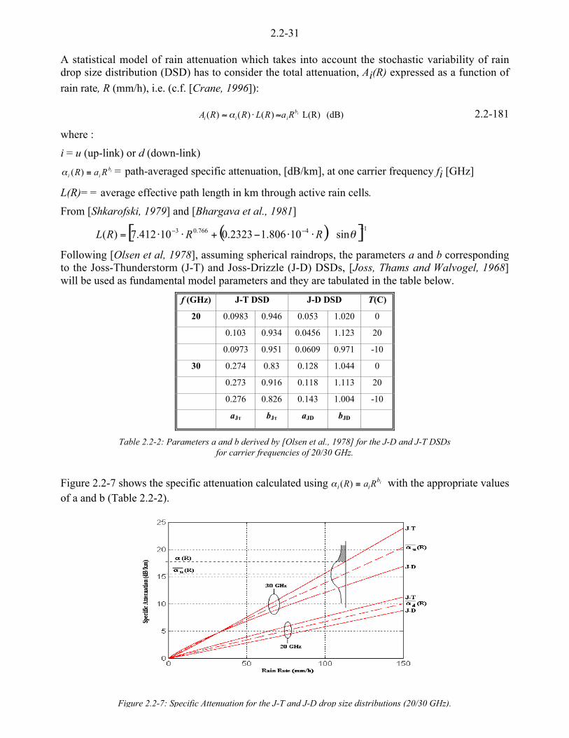
2.2-31

A statistical model of rain attenuation which takes into account the stochastic variability of raindrop size distribution (DSD) has to consider the total attenuation, Ai(R) expressed as a function of

rain rate, R (mm/h), i.e. (c.f. [Crane, 1996]):

(dB) L(R) )()()( ibiii RaRLRRA 5u5 _ 2.2-181

where :

i = u (up-link) or d (down-link)ib

ii RaR >)(_ = path-averaged specific attenuation, [dB/km], at one carrier frequency fi [GHz]

L(R)= = average effective path length in km through active rain cells.

From [Shkarofski, 1979] and [Bhargava et al., 1981]

( )[ ]14766.03 sin10806.12323.010412.7)(<<< uu<+uu= eRRRL

Following [Olsen et al, 1978], assuming spherical raindrops, the parameters a and b correspondingto the Joss-Thunderstorm (J-T) and Joss-Drizzle (J-D) DSDs, [Joss, Thams and Walvogel, 1968]will be used as fundamental model parameters and they are tabulated in the table below.

f (GHz) J-T DSD J-D DSD T(C)

20 0.0983 0.946 0.053 1.020 0

0.103 0.934 0.0456 1.123 20

0.0973 0.951 0.0609 0.971 -10

30 0.274 0.83 0.128 1.044 0

0.273 0.916 0.118 1.113 20

0.276 0.826 0.143 1.004 -10

aJT bJT aJD bJD

Table 2.2-2: Parameters a and b derived by [Olsen et al., 1978] for the J-D and J-T DSDsfor carrier frequencies of 20/30 GHz.

Figure 2.2-7 shows the specific attenuation calculated using ibii RaR >)(_ with the appropriate values

of a and b (Table 2.2-2).

Figure 2.2-7: Specific Attenuation for the J-T and J-D drop size distributions (20/30 GHz).

2.2-32

( ) 2

2

32

2

2D

U

D

DUD

D

Ur _

m

_

mmlm

__

m +<´́¦

¥²²¤

£5

The instantaneous frequency scaling ratio of rain attenuation, rfs, is given by:

)()()(/)()( RRRARARr dudufs __== 2.2-182

It is assumed that the mean values of instantaneous frequency scaling ratio of rain attenuation, fsr , is

given by the former CCIR model for long term frequency scaling (see equation 2.2-173).

Rücker [Rücker, 1994] carried out an detailed analysis of rain attenuation at 20/30 GHz based ondata collected during the Olympus experiment over a period of 2 years and 8 months. His resultsshowed that the conditional cumulative distribution function of the instantaneous frequency scalingratio of rain is well approximated as Gaussian for the percentiles lying between 5% and 95% andbase attenuation between 3.5 and 9.5 dB. Therefore the stochastic model for the rfs it is assumed tobe :

µµ�

�

³³�

� <<=

)(2

)(

)(2

1)|(

2

2

R

rrExp

RRrf

r

fsfs

r

fs mm/2.2-183

The variance of instantaneous frequency scaling ratio of rain attenuation, )(2 Rrm , depends on the

variability of the specific attenuation ibii RaR >)(_ conditioned on the rain rate, that can be ascribed

to random changes in the rain drop size distribution between the J-T and J-D distributions (seeFigure 2.2-8). Those fluctuations of the rain drop size distribution for a given rainrate, are reflectedin the random variation of parameters of a and b.

It is shown in [Gremont and Filip, 1998] that mk(R) can be estimated from the mean and variance of

the specific attenuation at two carrier frequencies.

This gives (the dependency on R is omitted for clarity):

2.2-184

where:

l = the expected correlation factor between up and down-link rain attenuation time series.A value of between 0.9 and 0.99 is suggested by empirical data.

)200/%(

)()()(

1 PQ

RRR ii

i <

<=

__m

iJTbi

JTi RaR =)(_

( )iJD

iJT bi

JDbi

JTi RaRaR += 5.0)(_ = mean specific attenuation conditioned on rain rate. It corresponds to thedashed lines in Figure 2.2-9

i = u (up-link) or d (down-link)

P% = scaling parameter. A value of 97.8% is suggested by [Gremont and Filip, 1998]

()uQ = standard error function.

The parameter P%, measures the long-term variability in rain types on a particular slant path(between drizzle and thunderstorm) and it indicates the percentage of the rain events that liebetween the J-T and J-D curves shown in Figure 2.2-7.

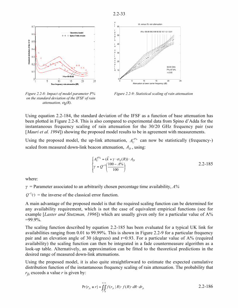
2.2-33

0 5 10 15 20 250

10

20

30

40

50

60UL versus DL rain attenuation

Attenuation at lower carrier frequency (dB)

Attenuation at higher fre

A%= 99.99 99.9 99 90 50 10 1 0.1 0.01

30/20 GHz P%=97.8% r=0.93

Figure 2.2-8: Impact of model parameter P% Figure 2.2-9: Statistical scaling of rain attenuation on the standard deviation of the IFSF of rain attenuation, mk(R).

Using equation 2.2-184, the standard deviation of the IFSF as a function of base attenuation hasbeen plotted in Figure 2.2-8. This is also compared to experimental data from Spino d’Adda for theinstantaneous frequency scaling of rain attenuation for the 30/20 GHz frequency pair (see[Mauri et al. 1994]) showing the proposed model results to be in agreement with measurements.

Using the proposed model, the up-link attenuation, %AUA can now be statistically (frequency-)

scaled from measured down-link beacon attenuation, DA , using:

ǻ

«©

¨

´¦

¥²¤

£ <=

uu+=

<

100

%100))((

1

%

AQ

ARkA DkA

U

a

ma2.2-185

where:

a = Parameter associated to an arbitrarily chosen percentage time availability, A%

)(1 u<Q = the inverse of the classical error function.

A main advantage of the proposed model is that the required scaling function can be determined forany availability requirement, which is not the case of equivalent empirical functions (see forexample [Laster and Stutzman, 1996]) which are usually given only for a particular value of A%=99.9%.

The scaling function described by equation 2.2-185 has been evaluated for a typical UK link foravailabilities ranging from 0.01 to 99.99%. This is shown in Figure 2.2-9 for a particular frequencypair and an elevation angle of 30 (degrees) and r=0.93. For a particular value of A% (requiredavailability) the scaling function can then be integrated in a fade countermeasure algorithm as alook-up table. Alternatively, an approximation can be fitted to the theoretical predictions in thedesired range of measured down-link attenuations.

Using the proposed model, it is also quite straightforward to estimate the expected cumulativedistribution function of the instantaneous frequency scaling of rain attenuation. The probability thatrfs exceeds a value r is given by:

0 0' '

uuu=*r

fsfsfs drdRRfRrfrr0

)()|(}Pr{ 2.2-186

2.2-34

where )|( Rkf is given in equation 2.2-183 and it is well known that rain rate is reasonably wellmodelled as lognormal i.e.

( )µµ�

�

³³�

� <<=

2

2

2

)ln(

2

1)(

R

R

R

mRExp

RRf

mm/2.2-187

The two parameters mR and mR can easily be evaluated from empirical CDFs or the rain maps

provided for example by the ITU-R model.

The model has been tested using the measurements performed by [Laster and Stutzman, 1996 withthe Olympus satellite. Equation 2.2-186 has been evaluated using the empirical parameters mr=5.64and mr=7.57 suggested by [Laster and Stutzman, 1996].

The model results are shown in Figure 2.2-10 and indicate a very good agreement withmeasurements.

0 0.1 0.2 0.3 0.4 0.5 0.6 0.7 0.8 0.9 10

0.5

1

1.5

2

2.5

3

3.5

4

4.5

5

Probability that IFSF exceeds ordinate

IFSF

CDF of the IFSF (VPI results)

model VPI results

Figure 2.2-10: Probability that the instantaneous frequency scaling ratio of rain attenuation (IFSF) exceeds the ordinate

2.2.3 Fade Duration

The statistical behaviour of fade duration is of great importance to design future TLC systemsbeyond 10 GHz. In fact the availability of ISDN connections, for example, is specified in terms ofcumulative exceedance time composed by intervals longer than 10 s [ITU-T, 1996] forsynchronisation reasons. The design of these connections therefore requires knowledge of fadeduration statistics down to the lowest values considered so far in propagation experiments (of theorder of 1 s in most cases). Also the design of advanced systems using a shared resource on board toassist earth terminals undergoing severe fading conditions [Acampora, 1979], [Carassa, 1984],[Chakraborty and Davarian, 1991] requires knowledge of the time the resource is likely to beengaged. Moreover site diversity systems to avoid the problem of too frequent switching betweenthe terminals must account for the fade duration statistics. Finally the design of up-link powercontrol systems may require knowledge of the dynamic variation of the down link signal amplitude(including fade duration statistics) to optimise the up-link power control.

From the point of view of medium modelling, investigation of fade durations can also help indistinguishing rain-induced fades from fading induced by other mechanisms (multiple scattering,atmospheric turbulence etc.). This aspect also has a direct impact on the design of future systems, asthe distinction between various fade phenomena is important for attenuation prediction models.

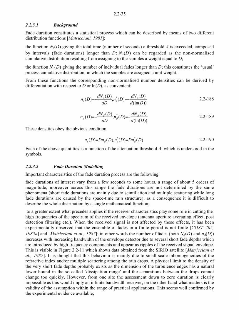
2.2-35

2.2.3.1 Background

Fade duration constitutes a statistical process which can be described by means of two differentdistribution functions [Matricciani, 1981]:

the function Ns(D) giving the total time (number of seconds) a threshold A is exceeded, composedby intervals (fade durations) longer than D ; Ns(D) can be regarded as the non-normalisedcumulative distribution resulting from assigning to the samples a weight equal to D;

the function Nd(D) giving the number of individual fades longer than D; this constitutes the ‘usual’process cumulative distribution, in which the samples are assigned a unit weight.

From these functions the corresponding non-normalised number densities can be derived bydifferentiation with respect to D or ln(D), as convenient:

))(ln(

)()(,

)()( *

Dd

DdNDn

dD

DdNDn s

ss

s <=<= 2.2-188

))(ln(

)()(,

)()( *

Dd

DdNDn

dD

DdNDn d

dd

d <=<= 2.2-189

These densities obey the obvious condition:

)()(,)()( ** DnDDnDnDDn dsds == 2.2-190

Each of the above quantities is a function of the attenuation threshold A, which is understood in thesymbols.

2.2.3.2 Fade Duration Modelling

Important characteristics of the fade duration process are the following:

fade durations of interest vary from a few seconds to some hours, a range of about 5 orders ofmagnitude; moreover across this range the fade durations are not determined by the samephenomena (short fade durations are mainly due to scintillation and multiple scattering while longfade durations are caused by the space-time rain structure); as a consequence it is difficult todescribe the whole distribution by a single mathematical function;

to a greater extent what precedes applies if the receiver characteristics play some role in cutting thehigh frequencies of the spectrum of the received envelope (antenna aperture averaging effect, postdetection filtering etc.). When the received signal is not affected by these effects, it has beenexperimentally observed that the ensemble of fades in a finite period is not finite [COST 205,1985a] and [Matricciani et al., 1987]: in other words the number of fades (both Nd(D) and nd(D))increases with increasing bandwidth of the envelope detector due to several short fade depths whichare introduced by high frequency components and appear as ripples of the received signal envelope.This is visible in Figure 2.2-11 which shows data obtained from the SIRIO satellite [Matricciani etal., 1987]. It is thought that this behaviour is mainly due to small scale inhomogeneities of therefractive index and/or multiple scattering among the rain drops. A physical limit to the density ofthe very short fade depths probably exists as the dimension of the turbulence edges has a naturallower bound in the so called ‘dissipation range’ and the separations between the drops cannotchange too quickly. However, from one site the assessment down to zero duration is clearlyimpossible as this would imply an infinite bandwidth receiver; on the other hand what matters is thevalidity of the assumption within the range of practical applications. This seems well confirmed bythe experimental evidence available;

2.2-36

the behaviour of Nd(D), nd(D) implies that concepts like ‘average duration’ or ‘percentile durations’have little meaning because they depend critically on the receiving system characteristics; therefore,their use should be avoided;

Ns(D) must tend instead to a finite limit Ntot >>>> Ns(0), the total exceedance time (obviously finite),which can be separately estimated by means of one of the many attenuation prediction methodsavailable today [Capsoni et al., 1987a, b]. The quantity:

tot

s

N

DNADF

)(),( > 2.2-191

can be regarded as the fraction of the exceedance time composed by fade duration longer than D;

statistical samples corresponding to very long fade durations can occasionally be missing from datacollected in too limited observation periods: on the other hand, looking at data relative to someyears of total experimentation made around the world, it would be hard to determine whether this isa genuine effect or an effect of the limited sample size; once again, as in the case of very short fadedurations, we must remember that any statement made about the behaviour of physical variablesoutside the range where it has been experimentally observed, is inherently hazardous; in any casethe problem of scarce samples in the range of the long fade duration can be alleviated when a largedata base is available on which to base a model.

Figure 2.2-11: Cumulative distributions of fade durations: ___ Gera Lario, 1978-1981; - - - Spino d'Adda, 1979-1982; . - . Fucino, 1978-1981

In the open literature only a few models have been presented. The idea developed in the frame ofCOST205 [COST 205, 1985a] of different distributions for short and long duration has beenreviewed in the frame of OPEX [OPEX, 1994] and formalised in a new model [Paraboni and Riva,1994]. This model (which appears to be that best fitting the available data) complies with all theabove requirements: it assumes a log-normal distribution for fade duration exceeding about oneminute (‘slow phenomena’) and a power-law distribution for shorter fade durations ('fastphenomena') [COST 205, 1985a]. This double assumption requires harmonising the variousfunctions describing the process with respect to both the global normalisation and the continuity

1E+0 1E+1 1E+2 1E+3 1E+4Duration [s]

1E+0

1E+1

1E+2

1E+3

1E+4

1E+5

Num

ber o

f fad

es lo

nger

than

abs

ciss

a

2.2-37

Slow phenomena: log-normal model

The duration of fades, mainly induced by space-time variations of the rain structure, which exceed aminimum duration Dt (referred to in the following as the transition duration), is modelled with alog-normal function:

ttots DDDD

QNDN *´́¦

¥²²¤

£d= ,)(

0

2.2-192

where

Q(z) is the gauss-integral function:

0'

m

<

/>

/)ln(

2

1 2

2

1)(

z

xdxezQ 2.2-193

with m and D0 being canonical parameters.

Considering d as a conditioning probability (the fraction of the time for which log-normalityapplies), D0 can be regarded as a conditional median and m as a conditional standard deviation.

Taking into account (equation 2.2-188) and (equation 2.2-189) and the condition(equation 2.2-190):

´́¦

¥²²¤

£d=

21

)(DD

QD

NDN tot

d 2.2-194

where the parameters D1 and D2 are given by:

´́¦

¥²²¤

£ m<=

2exp

2

01 DD 2.2-195

( )202 exp m<=DD 2.2-196

Notice that all the densities defined by (equation 2.2-188) and (equation 2.2-189) assume the formof the well known gaussian function in ln(D) with common standard deviation m but with differentaverages and coefficients.

Fast phenomena: power law model

The duration of fades mainly induced by atmospheric turbulence [Tatarski, 1967], multiplescattering among raindrops [Capsoni and Paraboni, 1978] or variations of the local raindrop sizedistribution [Sweeney and Bostian, 1992] etc, are modelled with function of the type:

tt

ttotd DD

D

D

D

DQ

D

NDN <´́

¦

¥²²¤

£´́¦

¥²²¤

£d=

a<

,)(21

2.2-197

(a being a positive constant) written so as to show the continuity with (equation 2.2-194) across Dt.By differentiating (equation 2.2-197), applying (equation 2.2-190) and integrating again from D toinfinity, we obtain:

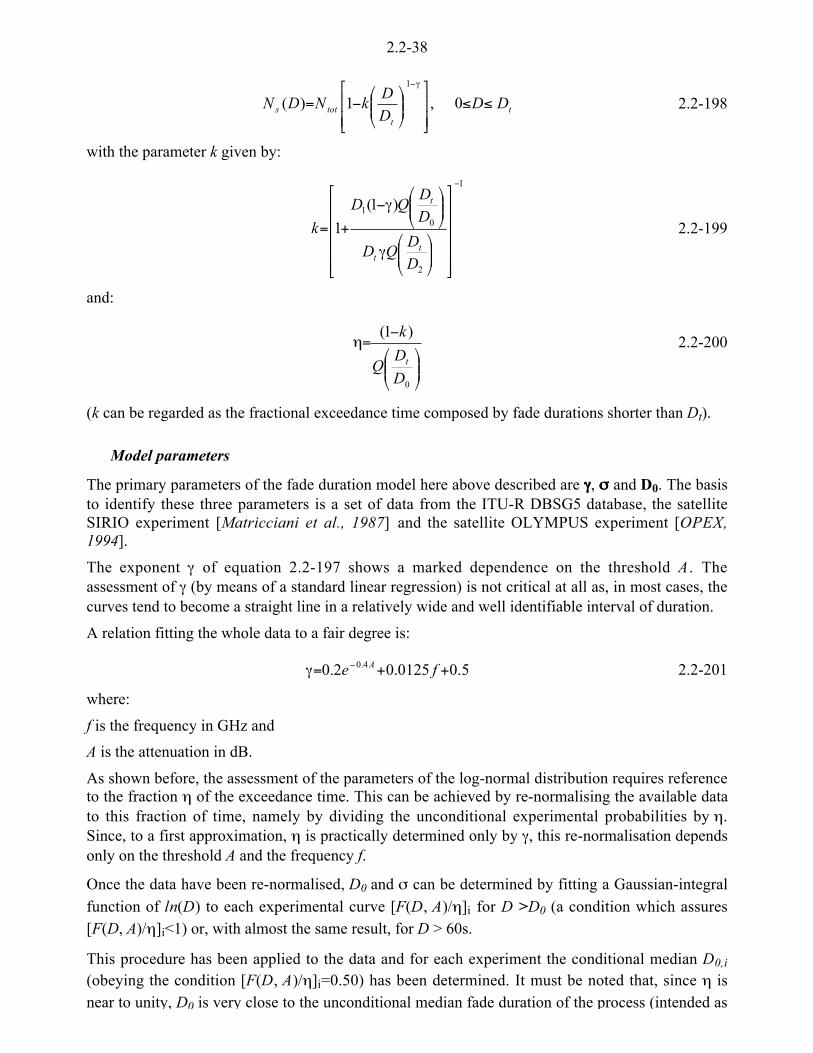
2.2-38

tt

tots DDDD

kNDN ))µµ�

�

³³�

�´́¦

¥²²¤

£<=

a<

0,1)(1

2.2-198

with the parameter k given by:

1

2

01 )1(

1

<

µµµµµ

�

�

³³³³³

�

�

´́¦

¥²²¤

£a

´́¦

¥²²¤

£a<

+=

DD

QD

DD

QD

kt

t

t

2.2-199

and:

´́¦

¥²²¤

£

<=d

0

)1(

D

DQ

k

t

2.2-200

(k can be regarded as the fractional exceedance time composed by fade durations shorter than Dt).

Model parameters

The primary parameters of the fade duration model here above described are aaaa, mmmm and D0. The basisto identify these three parameters is a set of data from the ITU-R DBSG5 database, the satelliteSIRIO experiment [Matricciani et al., 1987] and the satellite OLYMPUS experiment [OPEX,1994].

The exponent a of equation 2.2-197 shows a marked dependence on the threshold A . Theassessment of a (by means of a standard linear regression) is not critical at all as, in most cases, thecurves tend to become a straight line in a relatively wide and well identifiable interval of duration.

A relation fitting the whole data to a fair degree is:

5.00125.02.0 4.0 ++=a < fe A 2.2-201

where:

f is the frequency in GHz and

A is the attenuation in dB.

As shown before, the assessment of the parameters of the log-normal distribution requires referenceto the fraction d of the exceedance time. This can be achieved by re-normalising the available datato this fraction of time, namely by dividing the unconditional experimental probabilities by d.Since, to a first approximation, d is practically determined only by a, this re-normalisation dependsonly on the threshold A and the frequency f.

Once the data have been re-normalised, D0 and m can be determined by fitting a Gaussian-integralfunction of ln(D) to each experimental curve [F(D, A)/d]i for D >D0 (a condition which assures[F(D, A)/d]i<1) or, with almost the same result, for D > 60s.

This procedure has been applied to the data and for each experiment the conditional median D0,i

(obeying the condition [F(D, A)/d]i=0.50) has been determined. It must be noted that, since d isnear to unity, D0 is very close to the unconditional median fade duration of the process (intended as

2.2-39

Distinguishing a clear dependence of D0,i from the attenuation level beyond about 2 dB has beenfound difficult. A marked dependence of D0,i on the elevation q of the link was observed; therelation:

degreesins,in,3050 04.0

0 qq= < DD 2.2-202

seems appropriate to express this dependence even if a large spread exists around this value in thedata. It must be considered that D also possibly depends on many other parameters like generalclimatology, the type of prevailing rain (stratified, convective or orografic) or the link orientationwith respect to the prevailing winds.

Finally, a constant value of 1.5 has been estimated for the m parameter.

During the COST255 activity, an improvement of this model was also available to the authors asthe result of the research study carried out during the COST255 activity in the frame of an Intelsatcontract. The improvement of the Paraboni and Riva model consisted only in the followingmodification of the relationships giving the parameters a, D0 and m (obtained from the analysis ofITALSAT data collected at Spino d’Adda):

003.065.0055.0 <=a Af 2.2-203

[ ]s80 39.04.14.00

<<q= AfD 2.2-204

027.005.085.1 <<=m Af 2.2-205

where:

f is the frequency in GHz,

A the threshold in dB and

q the elevation angle in degrees.

2.2.4 Attenuation due to the Melting Layer

The melting layer is a region of the atmosphere just below the 0°C isotherm level, where ice andsnow hydrometeors turn into water drops. Stratiform precipitation phenomena usually start with iceclouds, constituted by ice crystals. The ice crystals can aggregate during their fall, to form large,low density structures like snowflakes; or, they can grow due to collisions with supercooled waterdrops, leading in this case to much higher density particles (hailstones). In general, just above themelting layer, a mixture of ice structures with different size and densities will be present [Stewart etal, 1984], [Willis and Heyms, 1989]. The melting process usually starts around the 0°C isothermheight; a few hundred metres below the 0°C isotherm the melting process is complete and onlyraindrops are present. There is current interest in the melting layer since the signals radiated fromthe ever-growing number of spaceborne communication and remote sensing systems can experiencevarious impairments (extra attenuation, scattering and depolarisation) when passing through it.

2.2.4.1 The Melting Layer

The first step towards modelling of the melting layer is the identification of realistic compositionand shapes for the melting particles. From the numerous observations carried out in the past years[Stewart et al., 1984], [Willis and Heyms, 1989] a very heterogeneous situation emerges,characterised by the presence of particles of very different shape, mixed in different proportions indifferent events.

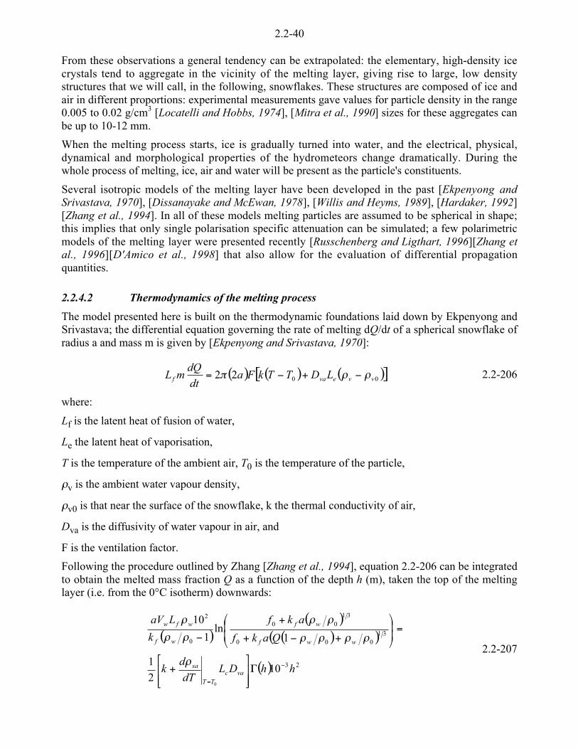
2.2-40

From these observations a general tendency can be extrapolated: the elementary, high-density icecrystals tend to aggregate in the vicinity of the melting layer, giving rise to large, low densitystructures that we will call, in the following, snowflakes. These structures are composed of ice andair in different proportions: experimental measurements gave values for particle density in the range0.005 to 0.02 g/cm3 [Locatelli and Hobbs, 1974], [Mitra et al., 1990] sizes for these aggregates canbe up to 10-12 mm.

When the melting process starts, ice is gradually turned into water, and the electrical, physical,dynamical and morphological properties of the hydrometeors change dramatically. During thewhole process of melting, ice, air and water will be present as the particle's constituents.

Several isotropic models of the melting layer have been developed in the past [Ekpenyong andSrivastava, 1970], [Dissanayake and McEwan, 1978], [Willis and Heyms, 1989], [Hardaker, 1992][Zhang et al., 1994]. In all of these models melting particles are assumed to be spherical in shape;this implies that only single polarisation specific attenuation can be simulated; a few polarimetricmodels of the melting layer were presented recently [Russchenberg and Ligthart, 1996][Zhang etal., 1996][D'Amico et al., 1998] that also allow for the evaluation of differential propagationquantities.

2.2.4.2 Thermodynamics of the melting process

The model presented here is built on the thermodynamic foundations laid down by Ekpenyong andSrivastava; the differential equation governing the rate of melting dQ/dt of a spherical snowflake ofradius a and mass m is given by [Ekpenyong and Srivastava, 1970]:

( ) ( ) ( )[ ]0022 vvevaf LDTTkFadtdQ

mL ll/ <+<= 2.2-206

where:

Lf is the latent heat of fusion of water,

Le the latent heat of vaporisation,

T is the temperature of the ambient air, T0 is the temperature of the particle,

lv is the ambient water vapour density,

lv0 is that near the surface of the snowflake, k the thermal conductivity of air,

Dva is the diffusivity of water vapour in air, and

F is the ventilation factor.

Following the procedure outlined by Zhang [Zhang et al., 1994], equation 2.2-206 can be integratedto obtain the melted mass fraction Q as a function of the depth h (m), taken the top of the meltinglayer (i.e. from the 0°C isotherm) downwards:

( )( )

( )( )

( ) 23

31000

3100

0

2

1021

1ln

1

10

0

hhDLdT

dk

Qakf

akf

k

LaV

vacTT

sa

wwf

wf

wf

wfw

<

=

Kµµ�

�

³³�

�+

=´´

¦

¥

²²

¤

£

+<+

+

<

l

llll

ll

ll

l

2.2-207

2.2-41

where:

00

1

TT

v

TT

sa

dTd

UdTd

==

=ll

2.2-208

where:

U is the relative humidity of the air,

a(cm) is the (melted) drop radius,

l0 (g/cm3) is the “equivalent" initial density of the melting particle,

lw (g/cm3) is the water density,

f0 5 0.685 and

kf 5 89.5 1/cm.

The last five parameters are derived from [Pruppacher and Rasmussen, 1979].

K(h) is the saturated adiabatic lapse rate, or temperature gradient, in the melting layer; it can beconstant or dependent on height; if constant, it is usually assumed to be equal to 6.5 C/km. Theexpression for Vw is given in equation 2.2-211. For our purposes we can assume that (dlsa/dT )|T=T0

5 0.332. We have also assumed with [Klaassen, 1988] Lf =335 J/g, Le=2500 J/g, k=0.024 J/(m s K),

Dva = 0.225u10-4 m2/s and lw = 1 g/cm3.

It is convenient to relate the melted volume fraction f to the melted mass fraction Q through theequation:

( )[ ]ww qQf

llll

0

0

111

<<<= 2.2-209

For the determination of the drop population it is necessary to know the fall velocity of the particlesduring all the melting process. If it is assumed that all the particles fall at terminal velocity, thentheir Reynolds numbers are constant as the particle melts [Hardaker, 1992]; we can then relate thefall speed V (m/ s) of a melting particle to the fall velocity Vw of a raindrop:

( )1

2

ms<

´́¦

¥²²¤

£=

aa

VV w 2.2-210

where:

a(cm) is the radius of the melted raindrop and

a2 (cm) is the radius of the melting particle.

A very accurate expression of the terminal fall velocity of a raindrop, as a function of its radius, isgiven by [Gunn and Kinzer, 1949].

( ) ( )1ms12exp3.1065.9 <<<= aVw2.2-211

2.2.4.3 Modelling the particle population in the melting layer

Knowledge of the particle size distribution (DSD) is essential for the evaluation of the scatteringproperties of the medium. In the rain region the natural form of the drop size distribution can be

2.2-42

( ) ( ) ( )130 cmmexp <<R<= DDNDN µ 2.2-212

where D is the particle's diameter (cm).

The three parameters µ, N0 and R define the DSD. The exponent µ can have positive as well asnegative values; when µ = 0 we find the well-known Marshall and Palmer DSD. The analysis ofexperimental observations has shown that, in general, N0 and µ are correlated [Ulbrich, 1983][Russchenberg, 1993].

Once the parameters of the gamma drop size distribution (in the rain region) are known, it ispossible to estimate the drop size distribution in the melting region. In the melting layer, in fact, theparticle size distribution may change because of three main processes: a) variation in fall velocity;b) condensation of water vapour on the melting particles; c) aggregation and break-up.

In a first approximation we can neglect the two last phenomena; as a consequence of thishypothesis, we can apply the conservation of the mass for each single drop. In a stationary situationthere is an equal inflow and outflow of particles in a certain air volume that can be expressed as:

( ) ( ) ( ) ( ) constDVDNDVDN ww == 2.2-213

where:

N(D) and V(D) are the number density and the drop fall velocity in the melting layer respectively,and

Nw(D) and Vw(D) are the same quantities in the rain region.

So, the drop size distribution in the melting zone is obtained from that in the rain region through theequation

( ) ( ) ( )( )DV

DVDNDN ww= 2.2-214

As said, the shape of the melting hydrometeors can be extremely complex; as often happens when amodel has to be developed, we have to simplify the reality, and assume a shape that can beanalytically treatable. The simplest shape of all, the sphere, gives very satisfactory results if we areinterested in non-polarimetric quantities [Meneghini and Kumagai, 1994], like specific attenuation_; for this reason this will be the shape assumed for this work.

2.2.4.4 The electromagnetic model of the melting layer

Melting particles are characterised by a quite complex microstructure; this poses a serious problemabout which model is the most accurate for the evaluation of their electromagnetic properties.Dissanayake and McEwan [Dissanayake and McEwan, 1978] assumed a solid ice core surrounded,as soon as the melting process starts, by a water shell; Hardaker [Hardaker, 1992] extendedDissanayake's model replacing, among other things, the solid ice core with an ice-air mixture in theproportions ‘20% air - 80% ice’. Recent research [Bohren and Battan, 1982], [Klaassen, 1988],[Zhang et al., 1994], [Russchenberg and Ligthart, 1996], however, tends to prefer the uniformmixture as a more accurate model of the particles that are more frequently present in the meltinglayer; the layered model seems to be appropriate mainly to some hailstones and ice pellets. For thisreason, in this work we will adopt the “uniform mixture” model.

The microstructure of the mixing has to be addressed now; the effect of topology on the scatteringproperties of mixed-phase (water/ice) hydrometeors is, in fact, known to be quite dramatic[Chylek et al., 1991]; in the most general case, the so-called dynamic effective mediumappro imation [St d d P 1978] m st be sed

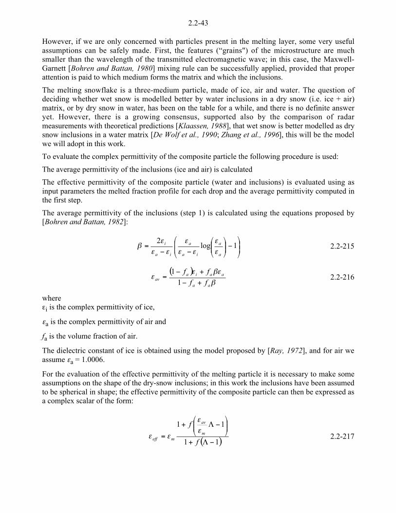
2.2-43

However, if we are only concerned with particles present in the melting layer, some very usefulassumptions can be safely made. First, the features (“grains") of the microstructure are muchsmaller than the wavelength of the transmitted electromagnetic wave; in this case, the Maxwell-Garnett [Bohren and Battan, 1980] mixing rule can be successfully applied, provided that properattention is paid to which medium forms the matrix and which the inclusions.

The melting snowflake is a three-medium particle, made of ice, air and water. The question ofdeciding whether wet snow is modelled better by water inclusions in a dry snow (i.e. ice + air)matrix, or by dry snow in water, has been on the table for a while, and there is no definite answeryet. However, there is a growing consensus, supported also by the comparison of radarmeasurements with theoretical predictions [Klaassen, 1988], that wet snow is better modelled as drysnow inclusions in a water matrix [De Wolf et al., 1990; Zhang et al., 1996], this will be the modelwe will adopt in this work.

To evaluate the complex permittivity of the composite particle the following procedure is used:

The average permittivity of the inclusions (ice and air) is calculated

The effective permittivity of the composite particle (water and inclusions) is evaluated using asinput parameters the melted fraction profile for each drop and the average permittivity computed inthe first step.

The average permittivity of the inclusions (step 1) is calculated using the equations proposed by[Bohren and Battan, 1982]:

´´¦

¥²²¤

£<´́

¦

¥²²¤

£

<<= 1log

2

a

a

ia

a

ia

i

¡¡

¡¡¡

¡¡¡

` 2.2-215

( )``¡¡

¡aa

aaiaav ff

ff

+<

+<=

1

12.2-216

where¡i is the complex permittivity of ice,

¡a is the complex permittivity of air and

fa is the volume fraction of air.

The dielectric constant of ice is obtained using the model proposed by [Ray, 1972], and for air weassume ¡a = 1.0006.

For the evaluation of the effective permittivity of the melting particle it is necessary to make someassumptions on the shape of the dry-snow inclusions; in this work the inclusions have been assumedto be spherical in shape; the effective permittivity of the composite particle can then be expressed asa complex scalar of the form:

( )11

11

<R+

´́¦

¥²²¤

£<R+

=f

fm

av

meff

¡¡

¡¡ 2.2-217

2.2-44

where:

´́¦

¥²²¤

£<+

=R

11

1

3

1

m

av

m

¡¡

¡ 2.2-218

In the previous equation, f is the total volume fraction of all N inclusions, ¡m is the permittivity ofthe matrix (water) and ¡av is the permittivity of the inclusions.

The vertical profiles of the melted volume fractions for each drop size, that were obtained with themeteorological model, are used as inputs to equation 2.2-217 as well as the complex permittivity ofthe inclusions previously computed. This procedure generates the vertical profiles of the effectivepermittivity of the melting hydrometeors.

Once the permittivity is known, the scattering properties of the melting spheres can easily beevaluated by appliying the Mie algorithm [Van De Hulst, 1957]; the specific attenuation _ can beeventually calculated by integrating over the drop size distribution:

( ) ( )0 ¼= dDDNSh_ 2.2-219

where:

h is the wavelength and

¼(S) is the imaginary part of the scattering amplitude in the forward direction.

As an example, Figure 2.2-12 shows the vertical profiles of specific attenuation _ (dB/km)calculated at 18.7 GHz, for R=10 mm/h in the rain region; the 0°C isotherm is supposed to belocated at a height of 2500 metres. Curves (right to left) correspond to values of the initial particledensity l0 equal to 0.1 (solid), 0.2 (dashed), 0.4 (dotted) and 0.9 (dash-and-dotted), in g/cm3. Ascan be observed from the figure, the values of attenuation that the signal experiences in the meltinglayer can be significantly higher than those in the rain region underneath. Figure 2.2-13 shows thesame curves, evaluated at 39.6 GHz.

0 1 2 3 4 5 6 71000

1500

2000

2500

Specific Attenuation, dB/km

Hei

ght,

m

Figure 2.2-12: Vertical profiles (model) of specific attenuation (dB/km) at 18.7 GHz, for R=10 mm/h; curves

(right to left) correspond to ql values of 0.1 (solid), 0.2 (dashed), 0.4 (dotted) and 0.9 (dash-and-dotted) g/cm.

2.2-45

0 2 4 6 8 10 12 141000

1500

2000

2500

Specific Attenuation, dB/km

Hei

ght,

m

Figure 2.2-13: As Figure 2.2-12, but for 39.6 GHz.

2.2.5 Assessment of K-____ Parameters in the K and V Frequency Bands

In this paragraph the assessment of K and _ coefficients for rain specific attenuation is presented,based on a novel methods for drop scattering and for the approximation of the relationship betweenrain intensity and attenuation.

The scattering of the electromagnetic wave by rain drops has been calculated using the Multiple-MultiPole (MMP) method [Hafner, and Bolmholt, 1993]. The theoretical background of thecalculation is described in [Hajn_ et al., 1998].

The scattering function has been obtained for the rain drop shape model of [Pruppacher and Pitte,1971]. The [Manabe et al., 1987] model for water refractive index model has been used with awater temperature ranging from 0 ºC to 25 ºC with a step of 5 ºC. For calculation of rain specificattenuation, the drop size distribution described by [Marshall and Palmer, 1948] was used. Theintegration was done over a diameter scale ranging from 0.5 to 8.0 mm with the step being 0.5mm.

The frequencies used for calculation have been selected from those generally used in beacon andradiometric measurements performed in the OLYMPUS and ITALSAT propagation experiments:12.5, 13, 18.65, 19.77, 21.3, 23, 29.65, 31.7, 37.5, 39.592, 47.5 and 49.497 GHz

The total attenuation can be calculated using:

0 uuuu= dDRDnDfk

RA vhvh ),()(Im210686.8)( ,3

,/ 2.2-220

where:

vhA , = specific rain attenuation for vertical and horizontal polarisation [dB/km]

R = rain intensity [mm/h]

k = propagation constant [m-1]

)(, Df vh= forward scattering function [m]

D = effective raindrop diameter [mm]

),( RDn = Distribution of raindrop size [m-3mm-1]

The values of the rain specific attenuation calculated using the MMP technique, for various waterh i Fi 2 2 14 Th ff f i l l

2.2-46

In Figure 2.2-15 the comparison is shown between values of attenuation obtained using the MMPscattering calculationand the values obtained using the ITU-R Ka parameters. The ITU-R valuesappears to be lower than those predicted by the MMP, at 23.8 and 31.7 GHz. At 13 GHz thesituation is reversed.

Attenuation - 13GHz - HP

0

2

4

6

8

10

0 30 60 90 120 150R[mm/h]

A[dB

/km]

0°C5°C10°C15°C20°C25°C

Attenuation - 23.8GHz - HP

0

5

1 0

1 5

2 0

2 5

0 3 0 6 0 9 0 120 150

R[mm/h]

A[dB

/km]

0°C5°C10°C15°C20°C25°C

Attenuation - 31.7GHz - HP

0

5

10

15

20

25

30

35

0 30 60 90 120 150

R[mm/h]

A[dB

/km]

0°C

5°C

10°C

15°C

20°C

25°C

Figure 2.2-14: Specific rain attenuation at 13.0, 23.8 and 31.7 GHz calculated for horizontal polarisationusing MMP method for different water temperatures.

2.2-47

Rain specific Attenuation 13.0MMP calculations and ITU-R

0

1

2

3

4

5

6

7

8

0 1 0 2 0 3 0 4 0 5 0 6 0 7 0 8 0 9 0 100 110 120

R[mm/h

A[d

B/k

m]

HP-MMP

VP-MMP

HP-ITUVP-ITU

a

Rain specific Attenuation 23.8MMP calculations and ITU-R

02468

1 01 21 41 61 82 0

0 1 0 2 0 3 0 4 0 5 0 6 0 7 0 8 0 9 0 100 110 120

R[mm/h

A[d

B/k

m]

HP-MMP

VP-MMPHP-ITU

VP-ITU

b

Rain specific Attenuation 31.7MMP calculations and ITU-R

0

5

1 0

1 5

2 0

2 5

3 0

0 1 0 2 0 3 0 4 0 5 0 6 0 7 0 8 0 9 0 100 110 120

R[mm/h

A[d

B/k

m]

HP-MMP

VP-MMP

HP-ITU

VP-ITU

c

Figure 2.2-15: Comparison between ITU-R and MMP Specific rain attenuation at 13.0, 23.8 and 31.7 GHz forhorizontal and vertical polarisation. Water temperature is 0 ºC.

The approximation of specific rain attenuation was calculated using the input rain intensities from1mm/h to 100mm/h with step 1mm/h. In documents ITU-R [ITU-R, 1992] there is an

2.2-48

approximation was described in detail in [Olsen et al., 1978]. The improved power lawapproximation (equation 2.2-222) has better agreement with accurate values than the first, but thethird parameter ` is required [Baptista, 1998]. The polynomial approximation (equation 2.2-223)also has a good agreement with accurate values of specific rain attenuation.

hRKRA hh_u=)( vRKRA vv

_u=)( , cRKRA cc_u=)( 2.2-221

( )( )Rhh

hhRKRA ln)( u+u= `_ , ( )( )Rvv

vvRKRA ln)( u+u= `_ , ( )( )Rcc

ccRKRA ln)( u+u= `_ 2.2-222

cvhcvhcvhcvh xRxRxRA 0,0,01,1,12

2,2,2,, )( ++= 2.2-223

where:

)(,, RA cvh = specific rain attenuation for horizontal, vertical and circular polarisation [dB/Km]

cvhK ,, , cvh ,,_ = parameters of power low approximation for horizontal, vertical and circular

polarisation

cvhK ,, , cvh ,,_ , cvh ,,` = parameters of power low approximation [Baptista, 1998] horizontal, vertical and

circular polarisation

cvhx ,,2,

cvhx ,,1,

cvhx ,,0= parameters of polynomial second order approximation horizontal, vertical and

circular polarisation.

For description of approximation errors parameter RMSE (root mean square error) is used as well asa maximum difference 6max :

-=

=n

iiV

nRMSE

1

212.2-224

( ) ( )iappriexacti RARAV <= 2.2-445

( ) ( )( )iappriexacti RARAV <==6 MAX)(MAXmax , 2.2-226

where:

iR = 1, 2, .. , 100 mm/h

( )iexact RA , ( )iappr RA = Exact (equation 2.2-220) and approximate values (equations 2.2-221, 2.2-222 or

2.2-224) of specific rain attenuation [dB/km]

RMSE = root mean square error [dB/km]

iV = Difference between the exact and approximate value of attenuation [dB/km]

6max = Maximum difference between exact and approximate value of attenuation [dB/km]

Equation (2.2-221) is the "classical" one regarding two parameters only. It is possible to interpolatethem with respect to the frequency. Equation 2.2-222 seems to be much better; the average value ofRMSE (0.017 dB in the case of water temperature 0°C and 0.011 dB in the case of 15°C) is lowerthan the RMSE value of the power law (equation 2.2-221) approximation (0.284 dB compared with0.287 dB). The same can be deduced when comparing the maximum differences between exact andapproximate values of specific rain attenuation in the rain intensity range 1 -100 mm/h. Thepolynomial approximation is a compromise between the approximations in equations 2-2-221 and2.2-222.

2.2-49

Approximation: Equation 2.2-221 Equation 2.2-222 Equation 2.2-223f[GHz] pol. K ____ K ____ `̀̀̀ x2 x1 x0

h 0.02362 1.16339 0.02234 1.20856 -0.00771 -0.08951 0.04304 7.40E-05

12.5 v 0.02324 1.11401 0.02110 1.19228 -0.01336 -0.06007 0.03649 2.50E-05c 0.02328 1.14284 0.02176 1.19770 -0.00937 -0.07504 0.03977 5.30E-05

h 0.02602 1.15890 0.02450 1.20782 -0.00835 -0.09502 0.04675 7.60E-05

13 v 0.02566 1.10832 0.02314 1.19205 -0.01429 -0.06241 0.03955 2.40E-05c 0.02568 1.13763 0.02386 1.19750 -0.01022 -0.07916 0.04318 5.30E-05

h 0.06251 1.11604 0.05579 1.20823 -0.01574 -0.16532 0.09921 6.50E-05

18.65 v 0.06115 1.06363 0.05301 1.17943 -0.01977 -0.08652 0.08132 -9.00E-06c 0.06183 1.09125 0.05430 1.19649 -0.01797 -0.12917 0.09067 2.10E-05

h 0.07219 1.10721 0.06357 1.21031 -0.01760 -0.17766 0.11174 5.10E-05

19.77 v 0.07020 1.05675 0.06042 1.17845 -0.02078 -0.09060 0.09135 -2.20E-05c 0.07128 1.08279 0.06185 1.19792 -0.01965 -0.13769 0.10201 5.00E-06

h 0.08696 1.09453 0.07514 1.21302 -0.02023 -0.19086 0.12971 2.40E-05

21.3 v 0.08384 1.04738 0.07137 1.17796 -0.02229 -0.09463 0.10595 -4.30E-05c 0.08564 1.07100 0.07305 1.19994 -0.02201 -0.14641 0.11834 -2.30E-05

h 0.11519 1.07242 0.09657 1.21539 -0.02441 -0.19945 0.16055 -3.80E-05

23.8 v 0.10963 1.03148 0.09152 1.17789 -0.02499 -0.09455 0.13174 -9.00E-05c 0.11292 1.05102 0.09375 1.20186 -0.02575 -0.15010 0.14664 -8.20E-05

h 0.20187 1.01753 0.16025 1.20474 -0.03196 -0.13531 0.23426 -2.48E-04

29.65 v 0.18873 0.99015 0.15087 1.17171 -0.03099 -0.03933 0.19754 -2.55E-04c 0.19634 1.00198 0.15516 1.19284 -0.03258 -0.08730 0.21607 -2.72E-04

h 0.23876 0.99843 0.18718 1.19575 -0.03368 -0.08306 0.25899 -3.34E-04

31.7 v 0.22277 0.97483 0.17599 1.16595 -0.03262 0.00299 0.22093 -3.27E-04c 0.23192 0.98477 0.18119 1.18491 -0.03416 -0.03898 0.24000 -3.50E-04

h 0.35816 0.94765 0.27537 1.16078 -0.03638 0.13533 0.32258 -5.83E-04

37.5 v 0.33465 0.93195 0.25886 1.14014 -0.03554 0.18649 0.28379 -5.46E-04c 0.34764 0.93829 0.26677 1.15296 -0.03664 0.16376 0.30293 -5.79E-04

h 0.40543 0.93091 0.31092 1.14611 -0.03674 0.23367 0.34285 -6.70E-04

39.592 v 0.37957 0.91722 0.29259 1.12823 -0.03602 0.27225 0.30451 -6.26E-04c 0.39370 0.92273 0.30144 1.13923 -0.03696 0.25606 0.32336 -6.61E-04

h 1.05831 0.45709 0.63447 0.87191 -0.07081 1.77895 0.13939 -8.40E-04

47.5 v 0.94266 0.52666 0.65217 0.82534 -0.05099 1.69522 0.15986 -8.19E-04c 0.99365 0.49450 0.64454 0.84543 -0.05990 1.73446 0.15005 -8.32E-04

h 0.64305 0.86377 0.49630 1.07379 -0.03585 0.76764 0.41915 -1.03E-03

49.49 v 0.60942 0.85573 0.47116 1.06436 -0.03561 0.75927 0.38509 -9.71E-04c 0.62707 0.85909 0.48356 1.06979 -0.03597 0.76635 0.40172 -1.01E-03

Table 2.2-3: Parameters of specific rain attenuation approximations for horizontal, vertical and circular polarisation.The rain drop size distribution is the Marshal-Palmer model. Canting angle and elevation angle are 0 [deg].

Water temperature is 0 C. The parameters were derived from rain intensities ranging from 1 to 100 mm/h,with a step of 1 mm/h.

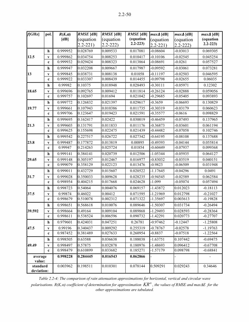
2.2-50

f[GHz] pol. R(K,____)[dB]

RMSE [dB](equation2.2-221)

RMSE [dB](equation2.2-222)

RMSE [dB](equation2.2-223)

max6666 [dB](equation2.2-221)

max6666 [dB](equation2.2-222)

max6666 [dB](equation2.2-223)

h 0.999952 0.028769 0.009533 0.017081 -0.08604 -0.03013 0.069305

12.5 v 0.999862 0.034754 0.008253 0.010417 -0.10106 -0.02545 0.045254c 0.999932 0.029424 0.008323 0.013864 -0.08691 -0.0261 0.057527

h 0.999947 0.032208 0.009667 0.017987 -0.09592 -0.03061 0.073281

13 v 0.999845 0.038731 0.008138 0.01058 -0.11197 -0.02503 0.046595c 0.999922 0.033307 0.008439 0.014455 -0.09798 -0.02655 0.06035

h 0.99982 0.10375 0.018948 0.028493 -0.30111 -0.05971 0.12302

18.65 v 0.999696 0.092765 0.009412 0.011814 -0.26124 -0.02888 0.059056c 0.999757 0.102697 0.01694 0.021042 -0.29685 -0.05405 0.093893

h 0.999772 0.126832 0.021397 0.029617 -0.3659 -0.06693 0.130829

19.77 v 0.999661 0.107943 0.010386 0.011735 -0.30319 -0.03179 0.060623c 0.999706 0.123647 0.019423 0.021591 -0.35577 -0.0616 0.098829

h 0.999695 0.162417 0.02422 0.030019 -0.46459 -0.07493 0.137965

21.3 v 0.999603 0.131791 0.011833 0.011176 -0.36873 -0.03601 0.061194c 0.999625 0.155698 0.022475 0.021439 -0.44482 -0.07058 0.102746

h 0.999542 0.227517 0.026722 0.027342 -0.64195 -0.08108 0.137688

23.8 v 0.999487 0.177872 0.013819 0.00895 -0.49393 -0.04144 0.055814c 0.99947 0.214263 0.025724 0.01854 -0.60449 -0.07937 0.099368

h 0.999141 0.384141 0.020739 0.012506 -1.05344 -0.05935 0.064127

29.65 v 0.999148 0.305197 0.012467 0.016977 -0.83032 -0.03519 0.040151c 0.999079 0.358129 0.022123 0.013476 -0.9823 -0.06509 0.031948

h 0.999011 0.432729 0.015607 0.020522 -1.17645 -0.04296 0.0491

31.7 v 0.999028 0.350033 0.009628 0.028235 -0.94545 -0.02589 0.062584c 0.998954 0.404215 0.017668 0.024628 -1.099 -0.05074 0.057494

h 0.998723 0.54064 0.004076 0.069157 -1.43872 0.012023 -0.18113

37.5 v 0.99874 0.46022 0.00412 0.071595 -1.21969 0.012798 -0.21027c 0.998679 0.510078 0.002312 0.071322 -1.35697 0.003613 -0.19828

h 0.998651 0.568618 0.010076 0.089646 -1.50307 0.031734 -0.26494

39.592 v 0.998664 0.49164 0.009104 0.089868 -1.29493 0.028593 -0.28364c 0.998611 0.538524 0.006596 0.090732 -1.42291 0.020773 -0.27707

h 0.979601 0.424031 0.047251 0.26781 -0.97462 -0.12447 -1.25808

47.5 v 0.99196 0.340437 0.009292 0.255319 -0.78767 -0.02578 -1.19763c 0.987452 0.381489 0.027633 0.260954 -0.8837 -0.07518 -1.22564

h 0.998505 0.63588 0.036638 0.188038 -1.63751 0.107442 -0.69475

49.49 v 0.998497 0.57875 0.032878 0.180976 -1.48693 0.096412 -0.67708c 0.998479 0.610899 0.033682 0.185271 -1.57179 0.098798 -0.68841

averagevalue:

0.998228 0.284445 0.016543 0.062866 - - -

standarddeviation:

0.003962 0.198511 0.010301 0.078144 0.509291 0.029243 0.34646

Table 2.2-4: The comparison of rain attenuation approximations for horizontal, vertical and circular wave

polarisations. R(K,_) coefficient of determination for approximation _KR , the values of RMSE and max6E for theother approximations are tabulated.

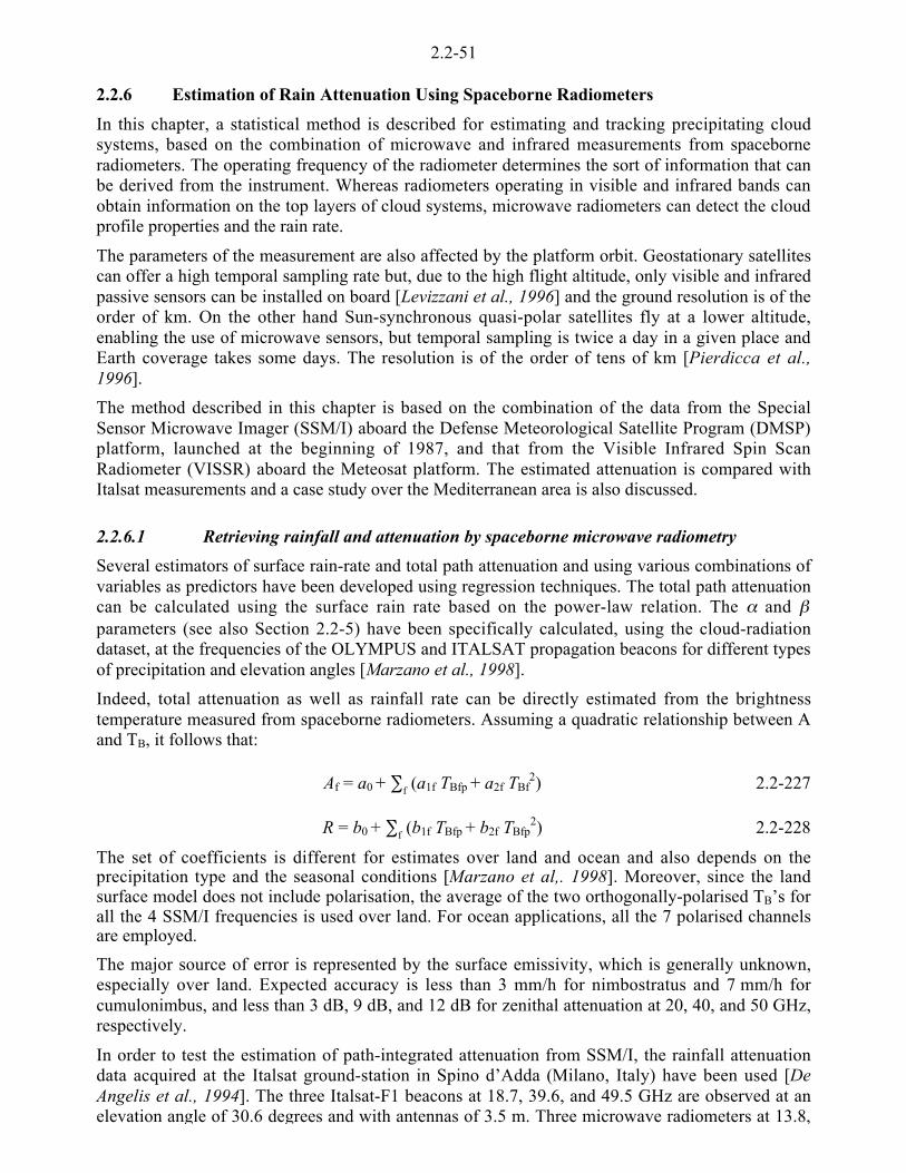
2.2-51

2.2.6 Estimation of Rain Attenuation Using Spaceborne Radiometers

In this chapter, a statistical method is described for estimating and tracking precipitating cloudsystems, based on the combination of microwave and infrared measurements from spaceborneradiometers. The operating frequency of the radiometer determines the sort of information that canbe derived from the instrument. Whereas radiometers operating in visible and infrared bands canobtain information on the top layers of cloud systems, microwave radiometers can detect the cloudprofile properties and the rain rate.

The parameters of the measurement are also affected by the platform orbit. Geostationary satellitescan offer a high temporal sampling rate but, due to the high flight altitude, only visible and infraredpassive sensors can be installed on board [Levizzani et al., 1996] and the ground resolution is of theorder of km. On the other hand Sun-synchronous quasi-polar satellites fly at a lower altitude,enabling the use of microwave sensors, but temporal sampling is twice a day in a given place andEarth coverage takes some days. The resolution is of the order of tens of km [Pierdicca et al.,1996].

The method described in this chapter is based on the combination of the data from the SpecialSensor Microwave Imager (SSM/I) aboard the Defense Meteorological Satellite Program (DMSP)platform, launched at the beginning of 1987, and that from the Visible Infrared Spin ScanRadiometer (VISSR) aboard the Meteosat platform. The estimated attenuation is compared withItalsat measurements and a case study over the Mediterranean area is also discussed.

2.2.6.1 Retrieving rainfall and attenuation by spaceborne microwave radiometry

Several estimators of surface rain-rate and total path attenuation and using various combinations ofvariables as predictors have been developed using regression techniques. The total path attenuationcan be calculated using the surface rain rate based on the power-law relation. The _ and `parameters (see also Section 2.2-5) have been specifically calculated, using the cloud-radiationdataset, at the frequencies of the OLYMPUS and ITALSAT propagation beacons for different typesof precipitation and elevation angles [Marzano et al., 1998].

Indeed, total attenuation as well as rainfall rate can be directly estimated from the brightnesstemperature measured from spaceborne radiometers. Assuming a quadratic relationship between Aand TB, it follows that:

Af = a0 + -f (a1f TBfp + a2f TBf2) 2.2-227

R = b0 + -f (b1f TBfp + b2f TBfp2) 2.2-228

The set of coefficients is different for estimates over land and ocean and also depends on theprecipitation type and the seasonal conditions [Marzano et al,. 1998]. Moreover, since the landsurface model does not include polarisation, the average of the two orthogonally-polarised TB’s forall the 4 SSM/I frequencies is used over land. For ocean applications, all the 7 polarised channelsare employed.

The major source of error is represented by the surface emissivity, which is generally unknown,especially over land. Expected accuracy is less than 3 mm/h for nimbostratus and 7 mm/h forcumulonimbus, and less than 3 dB, 9 dB, and 12 dB for zenithal attenuation at 20, 40, and 50 GHz,respectively.

In order to test the estimation of path-integrated attenuation from SSM/I, the rainfall attenuationdata acquired at the Italsat ground-station in Spino d’Adda (Milano, Italy) have been used [DeAngelis et al., 1994]. The three Italsat-F1 beacons at 18.7, 39.6, and 49.5 GHz are observed at anelevation angle of 30.6 degrees and with antennas of 3.5 m. Three microwave radiometers at 13.8,

2.2-52

balloon station some tens of kilometres away, operated by the Italian Air-Force. The availableSSM/I-F13 overpasses over Milano during precipitation in 1994 have been processed, together withthe Italsat attenuation measurement time-series with a 1 minute sampling and 1 hour temporalwindow around RAOB launchings and SSM/I overpasses.

The results are comparable when using different prediction models. The overall error bias is 0.9,2.7, and 1.1 dB, and the root mean square (rms) error is 1.9, 8.3, and 6.4 dB at 20, 40, and 50 GHz,respectively.

Combining geo-stationary infrared and Sun-synchronous microwave data

In order to combine geostationary infrared temperatures to SSM/I-derived rain rates, there are atpresent three operational SSM/I's (F11, F13, F14). The SSM/I satellite radiometers measure themicrowave emission from the Earth at four frequencies, i.e., 19.35, 22.235, 37.0 and 85.5 GHz[Hollinger et al., 1989]. The SSM/I orbit is circular, near-polar, and Sun-synchronous with analtitude of 860 km, an inclination angle of 98.8° and a swath-width of 1400 km. The spatialresolution of the images depends upon the frequency; specifically, the 3-dB footprint sizes (along-track by cross-track) are 69 x 43 km, 50 x 40 km, 37 x 29 km, and 15 x 13 km for the 19, 22, 37,and 85 GHz channels, respectively.

The Meteosat orbit is geostationary. The VISSR aboard the Meteosat platforms is a multispectralradiometer with three bands: 0.4-1.1 µm (VIS, near-IR), 5.7-7.1 µm (middle-IR, water vapourband), and 10.5-12.5 µm (thermal IR) [Levizzani, et al. 1996]. The ground resolution at nadir isabout 2.4 km for visible and 5.0 km for infrared. The data acquisition is performed every 30minutes and the approximate useful limits for quantitative studies are between 55° N/S latitude.

The combination technique is based on a probability-matched relationship that is derived betweenthe histograms of the IR temperatures (TIR) and the SSM/I-derived rainrates, see [Atlas et al., 1990],[Crosson et al., 1996]. Since the useful field of view of a geostationary satellite extends 50-60degrees on any side of satellite sub-point, any useful statistical technique must include the presenceof many distinct rain systems with different characteristics, each in their own state of evolution.This is accomplished by subdividing the overall region of interest (in this example, central andsouthern Europe) into smaller sub-regions of 5 degrees, and performing probability matching for thecoincident SSM/I and Meteosat-7 data that fall within each sub-region. Using inverse distanceweighting of nearby sub-regions, discontinuities are eliminated when composing the rain rate andattenuation images from these sub-regions.

2.2.6.2 Analysis of a case study

A series of heavy rainstorms that occurred in central and southern Europe, during the beginning ofOctober 1998, was selected for the assessment of the proposed technique.

Figure 2.2-16 shows the Meteosat-7 infrared imagery over Southern Europe at 0600 UTC onOctober, 6. Figure 2.2-17 shows the corresponding SSM/I image, acquired at 0540 UTC by thevertically-polarised 85-GHz channel. The low 85-GHz TB values are mainly related to precipitationsystems, therefore the areas covered by rain cells appear to be much smaller than the regionscovered by clouds(evidenced by values of TIR less than –5 °C). The low pressure was located at thattime along the western Alps, and the cyclone pattern can be seen from the IR image.

Figure 2.2-118 shows the surface rain, accumulated at 2130 UTC during the previous 24 hours.Finally, Figure 2.2-19 show the estimates of the 20-GHz zenithal attenuation.

The temporal evolution of the path attenuation is tracked in accordance with the meteorologicalevolution, denoting values up to 10 dB (which corresponds to 20 dB for a 30°-elevation link) withinthe convective cells The corresponding images (not shown) at 40 and 50 GHz show zenithal

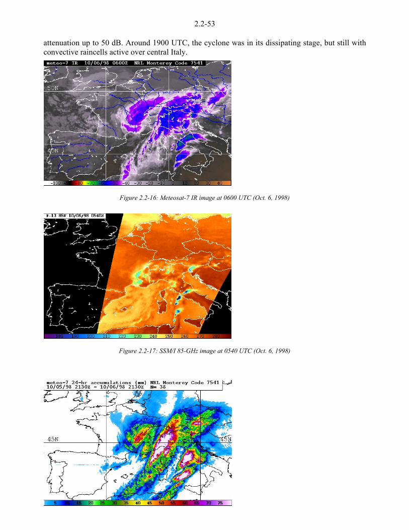
2.2-53

attenuation up to 50 dB. Around 1900 UTC, the cyclone was in its dissipating stage, but still withconvective raincells active over central Italy.

Figure 2.2-16: Meteosat-7 IR image at 0600 UTC (Oct. 6, 1998)

Figure 2.2-17: SSM/I 85-GHz image at 0540 UTC (Oct. 6, 1998)

2.2-54

Figure 2.2-19: 20-GHz attenuation map at 0600 UTC (Oct. 6, 1998)

2.2-55

2.2.7 References

[Acampora, 1979]Acampora A.S., “A shared resource TDMA approach to increase the rain margin of 12-14 GHzsatellite systems”, Bell System Technical Journal, Vol. 58, pp. 2097-2111, 1979

[Assis and Einloft, 1977]Assis, M.S., Einloft, C.M., “A Simple Method for Estimating Rain Attenuation Distributions.”Proc. URSI, La Baule, p.301, 1977

[Atlas et al., 1990]Atlas D., Rosenfeld D, Wolff D.B., “Climatologically tuned reflectivity-rainrate relations and linksto area-time integrals”, J. Appl. Meteor, vol. 3, pp. 1120-1135, 1990

[Baptista, 1998]Baptista, J., P., private communication, 1st International Workshop on Radiowave PropagationModelling for SatCom Services at Ku-band and above, ESTEC, Noordwijk, 1998.

[Bhargava et al., 1981]Bhargava V.K., Haccoun D., Matyas R., Nuspl P.P., “Digital communications by satellite:Modulation, Multiple Access and Coding", Wiley-Interscience, John Wiley and Sons, 1981

[Bohren and Battan, 1980]Bohren C.F., and Battan L.J., “Radar Backscattering by Inhomogeneous Precipitation Particles.Journal of Atmospheric Sciences”, 37, pp.1821-1827, 1980.

[Bohren and Battan, 1982]Bohren C.F., and Battan L.J., “Radar Backscattering of Microwaves by Spongy Ice Spheres”,Journal of Atmospheric Sciences, 39, pp. 2623-2628, 1982.

[Boithias and Battesti, 1981]Boithias L. and L. Battesti, “Au sujet de la dépendence en fréquence de l’affaiblissement dû à lapluie”, Annales des Télécommunications, Vol. 36, N. 7-8, pp. 483, 1981.

[Bryant et al., 1999]Bryant G.F., Adimula I., Riva C., and G. Brussaard, “Rain Attenuation Statistics from Rain CellDiameters and Heights”, submitted to International Journal of Satellite Communications, 1999.

[Capsoni and Paraboni, 1978]Capsoni C. and A. Paraboni, “Properties of the forward- scattered incoherent radiation throughintense precipitation”, IEEE Transactions on Antennas and Propagation, Vol. 26, No. 6, pp. 804-809, 1978

[Capsoni et al., 1987a]Capsoni C., F. Fedi, C. Magistroni, A. Pawlina and A. Paraboni, “Data and theory for a new modelof the horizontal structure of rain cells for propagation applications”, Radio Science, Vol. 22, No. 3,pp. 395-404, 1987

[Capsoni et al., 1987b]Capsoni, C., F. Fedi and A. Paraboni, “A comprehensive meteorologically oriented methodologyfor the prediction of wave propagation parameters in telecommunication applications beyond 10GHz”, Radio Science, Vol. 22, No. 3, pp. 387-393, 1987

[Carassa, 1984]Carassa F., “Adaptive methods of counteract rain attenuation effects in the 20/30 GHz band”, SpaceCommunication and Broadcasting, Vol. 2, pp. 253-269, 1984

2.2-56

[Chakraborty and Davarian, 1991]Chakraborty J. and F. Davarian, “The ACTS propagation Program”, Nasa PropagationExperimenters Meeting and Acts Propagation Studies Workshop, NAPEX XV, London, Ontario,Canada, 1991

[Chung et al., 1995]Chung T.K.P., Gallois A.P., Gremont B.C., “Frequency Scaling of Rain attenuation: Results fromOlympus Satellite", Proc. ICAP'95, pp. 2-179, 1995

[Chylek et al., 1991]Chylek P., Pinnick R.G., and Srivastava V., “Effect of Topology of Water-Ice Mixture on RadarBackscattering by Hailstones”, Journal of Applied Meteorology, 30, pp.954-959, 1991.

[COST 205, 1985a]COST 205, Report EUR9923EN, Luxembourg, 1985

[COST 205, 1985b]Fedi F. (ed), “Project COST 205: Frequency and Polarisation Scaling of Rain Attenuation”, AltaFrequenza, vol LVI, No. 3, May-June, 1985

[Costa, 1983]Costa E.,“An analytical and numerical comparison between two rain attenuation prediction methodfor Earth-satellite paths,“Proc. URSI Comm. F, Louvain-la-Neuve, pp. 213, 1983

[Crane, 1978]Crane R.K., “A global model for rain attenuation prediction”, EASCON Rec., pp. 391-395, 1978

[Crane, 1980]Crane R.K. “Prediction of attenuation by rain”, IEEE Transaction on Communications, COM-28,pp. 1717-1733, 1980

[Crane, 1982]Crane R.K., “A two-component rain model for the prediction of attenuation statistics”, RadioScience, Vol. 17, No. 6, pp. 1371-1387, 1982

[Crane, 1996]Crane R.K., “Electromagnetic wave propagation therough rain", John Wiley & Sons, 1996

[Crosson et al., 1996]Crosson W.L., Duchon C.E., Raghavan R., Goodman S.J. “Assessment of rainfall estimates using astandard Z-R relationship and the probability matching method applied to composite radar data incentral Florida”, J. Appl. Meteor., vol. 35, pp. 1203-1219, 1996

[D'Amico et al., 1998]D'Amico M., Holt A. R. and Capsoni C., “An Anisotropic Model of the Melting Layer”. RadioScience, 33(3), 1998.

[De Angelis et al., 1994]De Angelis G, Paraboni A., Riva C., Zaccarini F., Dellagiacoma G., Ordano L., Polonio R, MauriM. and Pawlina A. “Attenuation and scintillation statistics with Italsat and Italsat satellites in Italy”,Alta Frequenza, vol. 6, pp. 66-69, 1994

[De Wolf et al., 1990]De Wolf D.A., Russchenberg H.W., Ligthart L.P., “Effective Permittivity of and Scattering fromWet Snow and ice Droplets at Weather Radar Wavelengths”. IEEE Transactions on Antennas andPropagation, 38(9), pp.1317-1325, 1990.

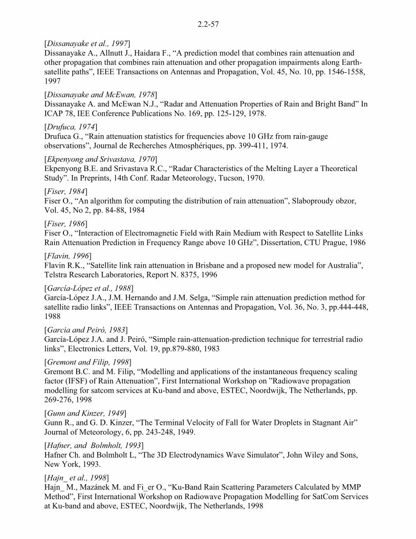
2.2-57

[Dissanayake et al., 1997]Dissanayake A., Allnutt J., Haidara F., “A prediction model that combines rain attenuation andother propagation that combines rain attenuation and other propagation impairments along Earth-satellite paths”, IEEE Transactions on Antennas and Propagation, Vol. 45, No. 10, pp. 1546-1558,1997

[Dissanayake and McEwan, 1978]Dissanayake A. and McEwan N.J., “Radar and Attenuation Properties of Rain and Bright Band” InICAP 78, IEE Conference Publications No. 169, pp. 125-129, 1978.

[Drufuca, 1974]Drufuca G., “Rain attenuation statistics for frequencies above 10 GHz from rain-gaugeobservations”, Journal de Recherches Atmosphériques, pp. 399-411, 1974.

[Ekpenyong and Srivastava, 1970]Ekpenyong B.E. and Srivastava R.C., “Radar Characteristics of the Melting Layer a TheoreticalStudy”. In Preprints, 14th Conf. Radar Meteorology, Tucson, 1970.

[Fiser, 1984]Fiser O., “An algorithm for computing the distribution of rain attenuation”, Slaboproudy obzor,Vol. 45, No 2, pp. 84-88, 1984

[Fiser, 1986]Fiser O., “Interaction of Electromagnetic Field with Rain Medium with Respect to Satellite LinksRain Attenuation Prediction in Frequency Range above 10 GHz”, Dissertation, CTU Prague, 1986

[Flavin, 1996]Flavin R.K., “Satellite link rain attenuation in Brisbane and a proposed new model for Australia”,Telstra Research Laboratories, Report N. 8375, 1996

[García-López et al., 1988]García-López J.A., J.M. Hernando and J.M. Selga, “Simple rain attenuation prediction method forsatellite radio links”, IEEE Transactions on Antennas and Propagation, Vol. 36, No. 3, pp.444-448,1988

[Garcia and Peirò, 1983]García-López J.A. and J. Peiró, “Simple rain-attenuation-prediction technique for terrestrial radiolinks”, Electronics Letters, Vol. 19, pp.879-880, 1983

[Gremont and Filip, 1998]Gremont B.C. and M. Filip, “Modelling and applications of the instantaneous frequency scalingfactor (IFSF) of Rain Attenuation”, First International Workshop on ”Radiowave propagationmodelling for satcom services at Ku-band and above, ESTEC, Noordwijk, The Netherlands, pp.269-276, 1998

[Gunn and Kinzer, 1949]Gunn R., and G. D. Kinzer, “The Terminal Velocity of Fall for Water Droplets in Stagnant Air”Journal of Meteorology, 6, pp. 243-248, 1949.

[Hafner, and Bolmholt, 1993]Hafner Ch. and Bolmholt L, “The 3D Electrodynamics Wave Simulator”, John Wiley and Sons,New York, 1993.

[Hajn_ et al., 1998]Hajn_ M., Mazánek M. and Fi_er O., “Ku-Band Rain Scattering Parameters Calculated by MMPMethod”, First International Workshop on Radiowave Propagation Modelling for SatCom Servicesat Ku-band and above, ESTEC, Noordwijk, The Netherlands, 1998

2.2-58

[Hardaker, 1992]Hardaker P.J., “A Study of the Melting Layer in Single Polarisation Radar Echoes with Applicationto Operational Weather Radar” PhD thesis, University of Essex, Department of Mathematics, 1992.

[Hollinger et al., 1989]Hollinger J.P., Pierce J.L. and Poe G.A. “SSM/I instrument evaluation”, IEEE Trans. Geosci. andRem. Sens., vol. 28: pp. 781-790, 1989.

[ITU-R, 1992]ITU-R, “Specific attenuation model for rain for use in prediction methods”, Propagation in Non-Ionised Media, Recommendation 838, Geneva, 1992

[ITU-R, 1997]ITU-R, “Propagation data and prediction methods required for the design of Earth-spacetelecommunication systems”, Propagation in Non-Ionised Media, Recommendation 618-5, Geneva,1997

[ITU-T, 1996]ITU-T, “Error performance of an international digital connection operating at a bit rate below theprimary rate and forming part of an integrated services digital network”, Recommendation G.821,1996

[Joss, Thams and Walvogel, 1968]Joss J., Thams J.C., Walvogel A., “The variation of rain drop-size distributions at Locarno”, Proc.Int .Conf. Cloud Physics, pp. 369-373, 1968

[Klaassen, 1988]Klaassen W., “Radar Observations and Simulation on the Melting Layer of Precipitation” Journal ofthe Atmospheric Sciences, 45:3741-3753, 1988.

[Laster and Stutzman, 1996]Laster J.D., Stutzman W.L., “Frequency scaling of rain attenuation for satellite communicationslinks”, IEEE Trans. Ant. Prop., Vol. AP-43, No 11, pp. 1207-1215, 1996

[Levizzani et al., 1996]Levizzani V., Porcù F., Marzano F.S., Mugnai A., Smith E.A. and Prodi F., "Investigating a SSM/Imicrowave algorithm to calibrate METEOSAT infrared instantaneous rainrate estimates", Meteor.Applications, 3, 5-17, 1996

[Locatelli and Hobbs, 1974]Locatelli I.D., and P.V. Hobbs, “Fall Speeds and Masses of Solid Precipitation Particles” Journal ofGeophysical Research, 79, pp.2185-2197, 1974.

[Manabe et al., 1987]Manabe T., H.J. Liebe, G.A. Hufford, “Complex permittivity of water between 0 and 30 THz, 12th

International Conference on infrared and millimetre waves”, Conference digest, pp.229-230, LakeBuena Vista, Florida, 1987

[Marshall and Palmer, 1948]Marshall J.and Palmer W., “The distribution of raindrops with size”, Journal Meteorology, No.5,pp. 165-166, 1948.

[Marzano et al., 1998]Marzano F.S., J. Turk, P. Ciotti, S. Di Michele, and N. Pierdicca, “Combined use of spacebornepolar-orbiting microwave and geostationary infrared radiometers for estimating rainfall attenuationalong earth-satellite links”, Proc. of the First Intern. Workshop on Radiowave PropagationModelling for SatCom Services at Ku-band and above, pp. 1-10, Noordwijk (NL), 28-29 October,1998.

2.2-59

[Matricciani, 1981]Matricciani E., “Duration of rain-induced fades of signal from SIRIO at 11.6 GHz”, ElectronicsLetters, Vol. 17, N. 1, pp. 29-30, 1981

[Matricciani et al., 1987]Matricciani E., M. Mauri and A. Paraboni, “Dynamic characteristics of rain attenuation: durationand rate of change”, Alta Frequenza, Vol. LVI, N. 1-2, pp. 33-45, 1987

[Matricciani, 1991]Matricciani E., “Rain attenuation predicted with two-layer rain model”, European Transactions onTelecommunication, Vol. 2, No. 6, pp. 715-727, Nov.-Dec. 1991.

[Matricciani, 1993]Matricciani E., “Prediction of Rain Attenuation in Slant Paths in Equatorial Areas: Application ofthe Two Layer Rain Model”, Electronics Letters, Vol. 29, pp. 72-73, 1993

[Mauri et al., 1994]Mauri M., Paraboni A., Riva C., “Instantaneous frequency scaling”, OPEX 2nd workshop of theOlympus experimenters, Vol. 6: Proceedings, ESA WPP-083, Noordwijk, 1994

[Meneghini and Kumagai, 1994]Meneghini R., and H. Kumagai, “Characteristics of the Vertical Profiles of Dual-Frequency, Dual-Polarisation Radar Data in Stratiform Rain” Journal of Atmospheric and Oceanic Technology,11:701-711, 1994.

[Misme and Waldteufel, 1980]Misme P. and Waldteufel P., “A model for attenuation by precipitation on a microwave earth-spacelink.” Ra. Sci., Vol.15, p.655, 1980

[Mitra et al., 1990]Mitra S.K., O. Vohl, M. Ahr, and H.R. Pruppacher, “A Wind Tunnel and Theoretical Study of theMelting Behaviour of Atmospheric Ice Particles” VI: Experiment and Theory for Snow Flakes.Journal of the Atmospheric Sciences, 47(5), pp. 584-591, 1990.

[Nowland et al., 1977]Nowland W.L., Olsen R.L., Shkarofsky I.P., “Theoretical relationship between rain depolarisationand attenuation”, Electronics Letters, Vol. 13, No. 22, pp. 676-678, 1977

[Olsen et al, 1978]Olsen L.R., Rogers D.V., Hodge D.B., “The aRb Relation in the Calculation of Rain Attenuation”,IEEE Trans. Ant. Prop., Vol. AP-26, No.2, pp. 318-329, 1978.

[OPEX, 1994]OPEX, “ESA, OPEX 2nd workshop of the Olympus experimenters”, Vol. 1: Reference book onattenuation measurement and prediction, ESA WPP-083, Noordwijk, 1994

[Paraboni and Riva, 1994]Paraboni A. and C. Riva, “A new method for the prediction of fade duration statistics in satellitelinks beyond 10 GHz”, International Journal of Satellite Communications, Vol. 12, pp. 387-394,1994

[Pierdicca et al., 1996]Pierdicca N., Marzano F.S., D'Auria G., Basili P., Ciotti P. and Mugnai A. “Precipitation retrievalfrom spaceborne microwave radiometers using maximum a posteriori probability estimation”, IEEETrans. Geosci. and Rem. Sens., vol. 34, pp. 831-846, 1996

[Pruppacher and Rasmussen, 1979]Pruppacher H.R., and R. Rasmussen, “A Wind Tunnel Investigation of the Rate of Evaporation ofL W D F lli T i l V l i i Ai ” J l f h A h i S i 36

2.2-60

[Pruppacher and Pitte, 1971]Pruppacher H.R.and Pitter R.L., “A Semi-Empirical Determination of the Shape of Cloud and RainDrops”, Journal of the Atmospheric Sciences, Vol. 28, pp. 86-94, 1971.

[Ray, 1972]Ray P.S, “Broadband Complex Refractive Indices of Ice and Water”, Applied ‘Optics, 11(8),pp.1836-1844, 1972.

[Rücker, 1994]Rücker F., “The impact of the variation of instantaneous frequency scaling factor on up-link powercontrol”, AEÜ, Vol. 48, No 2, pp. 119-121, 1994

[Russchenberg, 1993]Russchenberg H.W.J., “Doppler Polarimetric Radar Measurements of the Gamma Drop SizeDistribution of Rain”, Journal of Applied Meteorology, 32(12), pp.1815-1825, 1993.

[Russchenberg and Ligthart, 1996]Russchenberg H.W.J. and L.P. Ligthart, “Backscattering by and Propagation through the MeltingLayer of Precipitation: a New Polarimetric Model” IEEE Transactions on Geoscience and RemoteSensing, 34(1), pp. 3-14, 1996.

[Shkarofski, 1979]Shkarofski I.P., “Dependence of rain attenuation and cross-polarisation on drop-size distribution”,IEEE Trans. Ant. Prop., Vol. AP-27, No 4, pp. 538-542, 1979

[Stewart et al., 1984]Stewart R.E., J.D. Marwitz, J.C. Pace and R.E. Carbone, “Characteristics Through the MeltingLayer of Stratiform Clouds” Journal of the Atmospheric Sciences, 41, pp.3227-3237, 1984.

[Stroud and Pan, 1978]Stroud D. and F.D. Pan, “Self-consistent Approach to Electromagnetic Wave Propagation inComposite Media: Application to Model Granular Metals” Physics Review, B17, pp.1602-1610,1978.

[Stutzman and Dishman,1984]Stutzman W.L., Dishman W.K., “A simple model for the estimation of rain-induced attenuationalong earth-space paths at millimeter wavelengths”, Radio Science, Vol. 19, p. 946, 1984

[Svjatogor, 1985]Svjatogor L., “Prostranstvennaia korelacia vypadenjija dozdjej vdol zemnoj poverchnostji (inRussian), Symposium expertov stran uchastnic programmy INTERKOSMOS (Interkosmossymposium, theme 5 of the established telecommunication working group, Dresden, GDR, 1985

[Sweeney and Bostian, 1992]Sweeney D.G. and C.W. Bostian, “The dynamics of rain-induced fades”, IEEE Transactions onAntennas and Propagation, Vol. 40, No. 3, pp. 275-278, 1992

[Sweeney et al, 1992]Sweeney D.G., Pratt T., Bostian C.W., “Hysteresis effect in instantaneous frequency scaling of rainattenuation on 20 GHz and 30 GHz satellite links”, Electronics Letters, pp. 76-78, Vol. 28, No 1,January, 1992

[Tatarski, 1967]Tatarski V.I., “Wave propagation in a turbulent medium”, Dover Publications, New York, 1967

[Ulbrich, 1983]Ulbrich C.W., “Natural Variations in the Analytical Form of the Raindrop Size Distribution”Journal of Climate and Applied Meteorology, 22(10), pp.1764-1775, 1983.

2.2-61

[Van De Hulst, 1957]Van De Hulst H.C.,“Light Scattering by Small Particles”, John Wiley & Sons Inc., 1957

[Watson et al., 1985]Watson P.A., Leitao M.J., Turney O., Sengupta N., “Development of a climatic map of rainfallattenuation for Europe”, Postgraduate School of Electrical & Electronic Engineering, University ofBradford, Report No. 372 (final report for ESA/ESTEC contract No. 5192/82/NL/GM), 1985

[Willis and Heyms, 1989]Willis P.T. and A.J. Heyms, “Structure of the Melting Layer in Mesoscale Convective SystemStratiform Precipitation” Journal of the Atmospheric Sciences, 46, pp. 2008-2025, 1989.

[Zhang et al., 1994]Zhang W., S.I. Karhu and E. Salonen., “Prediction of Radiowave Attenuations Due to a MeltingLayer of Precipitation” IEEE Transactions on Antennas and Propagation, 42(4), pp. 492-499, 1994.

[Zhang et al., 1996]Zhang W., J. Tervonen and E. Salonen, “Backward and Forward Scattering by the Melting LayerComposed of Spheroidal Hydrometeors at 5-100 GHz” IEEE Transactions on Antennas andPropagation, 44(9), pp. 1208-1219, 1996.

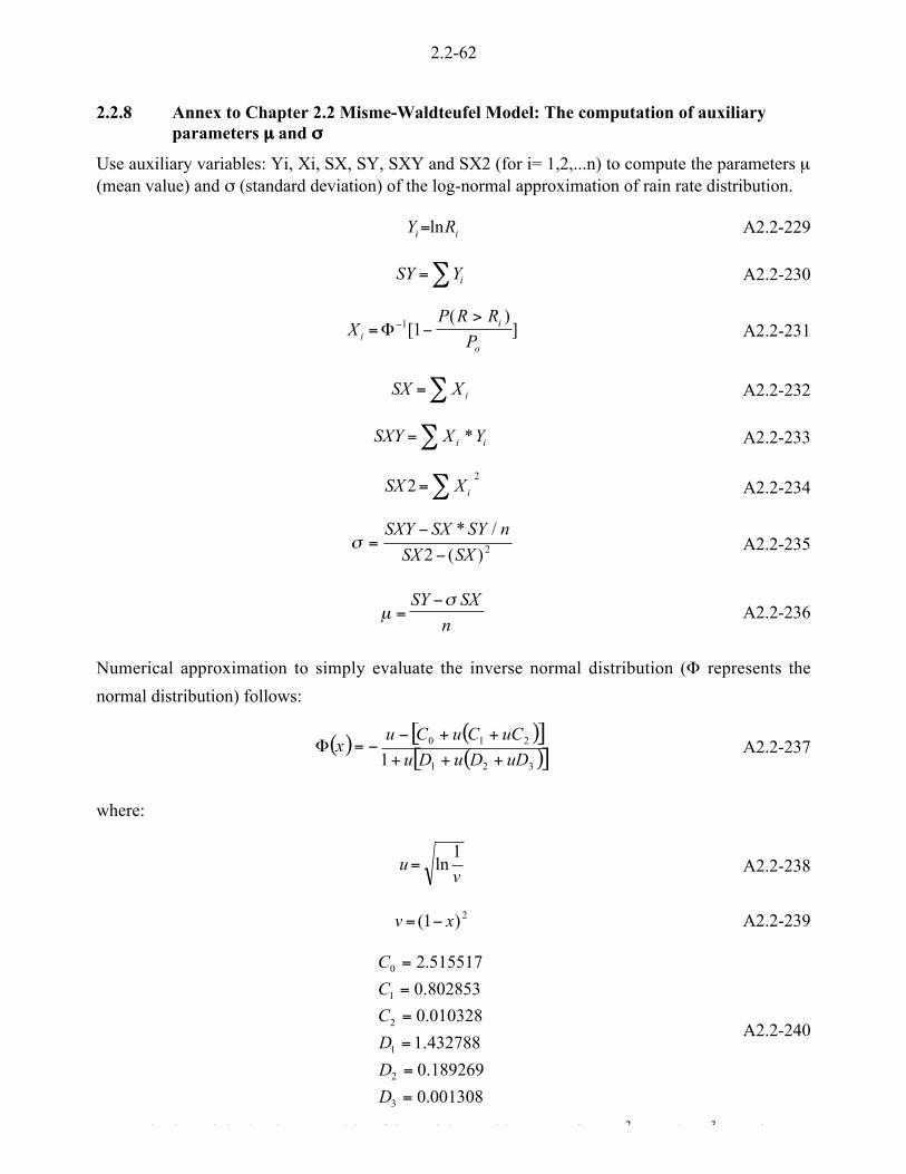
2.2-62

2.2.8 Annex to Chapter 2.2 Misme-Waldteufel Model: The computation of auxiliaryparameters µµµµ and mmmm

Use auxiliary variables: Yi, Xi, SX, SY, SXY and SX2 (for i= 1,2,...n) to compute the parameters µ(mean value) and m (standard deviation) of the log-normal approximation of rain rate distribution.

ii RY ln= A2.2-229

SY Yi=- A2.2-230

XP R R

Pii

o

= <><\ 1 1[

( )] A2.2-231

SX X i=- A2.2-232

SXY X Yi i=- * A2.2-233

SX Xi22

=- A2.2-234

m =<

<

SXY SX SY n

SX SX

* /

( )2 2 A2.2-235

µm

=<SY SX

nA2.2-236

Numerical approximation to simply evaluate the inverse normal distribution (\ represents the

normal distribution) follows:

( ) ( )[ ]( )[ ]321

210

1 uDDuDu

uCCuCux

+++

++<<=\ A2.2-237

where:

uv

= ln1

A2.2-238

v x= <( )1 2 A2.2-239

001308.0

189269.0

432788.1

010328.0

802853.0

515517.2

3

2

1

2

1

0

=

=

=

=

=

=

D

D

D

C

C

C

A2.2-240

R k h i i l Mi W ld f l d l id 2 f 10 2 % d 10 3 % i

2.3-1

CHAPTER 2.3Scintillation/Dynamics of the signal

Editor: Danielle Vanhoenacker1

Authors: Marie Edith Gimonet2, Max M.J.L. van de Kamp3, Frank S. Marzano4,Carlo Riva5, Errki Salonen6

1 Universite Catholique de Louvain, Place du Levant 3, B-1348 Louvain-la-Neuve, Belgium

Tel: +32-10-47-2304, Fax: +32-10-47-8705, e-mail: hoenacke@emic.ucl.ac.be2 ONERA-CERT DEMR, 2 Avenue Edouard Belin, BP4025, F-31055 Toulouse , CEDEX 4 France

Tel: +33-562-25-2720 Fax: +33-562-25-2577 e-mail: Marie-Edith.Gimonet@onecert.fr3 Eindhoven University of Technology, P.O. Box 513, 5600 MB Eindhoven, The Netherlands

Tel.: +31 40 247 2326, Fax.: +31 40 245 5197, e-mail: m.m.j.l.v.d.kamp@ele.tue.nl4 Dip. di Ingegneria Elettrica, Universita' dell'Aquila, Monteluco di Roio, I-67040 L'Aquila, Italy

Tel: +39-862-434412, Fax: +39-862-434414, e-mail: franko@ing.univaq.it35 Dipartimento di Elettronica e Informazione, Politecnico di Milano, P.zza L. Da Vinci 32, 20133 Milano, Italy.

Tel.: +39-02-23993586, Fax.: +39-02-23993413, e-mail: riva@elet.polimi.it6 University of Oulu Telecommunication Lab., P.O.Box 444, FIN-90571 Oulu, Finland

Tel: +358 40 524 2406, Fax: +358-8-553 2845, e-mail: Erkki.Salonen@ee.oulu.fi

2.3-2

2.3 Scintillation/Dynamics of the Signal

Tropospheric scintillation is caused by small-scale refractive index inhomogeneities induced bytropospheric turbulence along the propagation path. It results in rapid fluctuations of received signalamplitude and phase which affect Earth-space links above 10 GHz. On satellite links, the significantscintillation effects are mainly attributed to strong turbulence in clouds and are more severe insummer around noon. Tropospheric scintillation intensity is proved to increase with increasingcarrier frequency and with decreasing elevation angle and antenna size. Scintillation fades can havea major impact on the performances of low margin communication systems, for which the long-term availability is sometimes predominantly governed by scintillation effects rather than by rain. Inaddition, the dynamics of scintillation may interfere with tracking systems or fade mitigationtechniques. Scintillation is generally associated with the presence of clouds, especially cumulus andcumulonimbus clouds.

The parameters used for the characterisation of scintillation are the following:

• the amplitude deviation y in dB

• the variance m2 and the standard deviation m of the log-amplitude

• the predicted variance mp2 and standard deviation mp

2.3.1 Prediction models for long term standard deviation

All the classical models for scintillation are based on the assumption that the short-term probabilitydensity function (pdf) of the log-amplitude is Gaussian. The models are statistical models thatallow to calculate either a probability density function or a cumulative distribution function (cdf) ofthe log-amplitude of the fluctuation or the variance (or standard deviation) of the log-amplitude.

2.3.1.1 Karasawa and ITU-R models

[Karasawa et al., 1988] and [ITU-R, 1999] present similar prediction models for the calculation ofthe standard deviation of signal fluctuation due to scintillation. Both these models use the wet partof ground refractivity Nwet, a function of relative humidity and temperature, averaged at least overone month, as input parameter.

In the Karasawa model, the predicted standard deviation is given by

¡mm 6.29.0 sin/)( erefp DGf=2.3-1

where

f = frequency [GHz]

¡ = link elevation angle

wetref N43 10186.11042.3 << ×+×=m

( )2

)273/(7.19

273

22790

+=

+

T

eUN

TT

wet = Air refractivity due to water vapour (wet) at ground level.

U = Relative Humidity at ground level [%].

T = Temperature at ground level [C].

These meteorological input parameters should be averaged over a period of the order of a month.

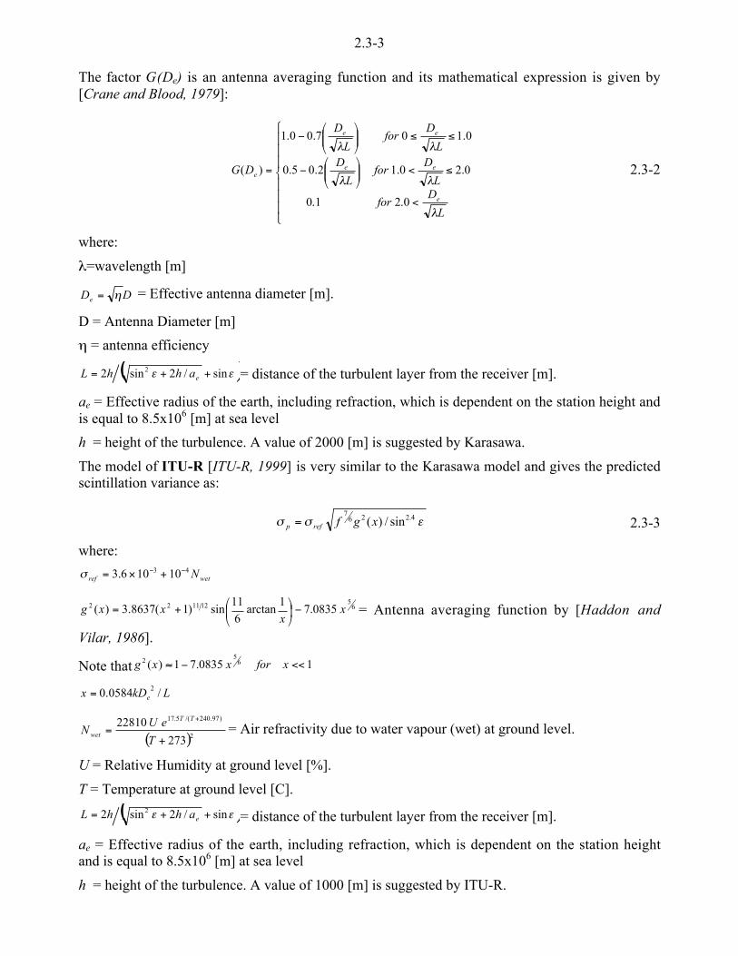
2.3-3

The factor G(De) is an antenna averaging function and its mathematical expression is given by[Crane and Blood, 1979]:

«««

ª

«««

©

¨

<

)<´́¦

¥²²¤

£<

))´́¦

¥²²¤

£<

=

L

Dfor

L

Dfor

L

DL

Dfor

L

D

DG

e

ee

ee

e

h

hh

hh

0.21.0

0.20.12.05.0

0.107.00.1

)( 2.3-2

where:

h=wavelength [m]

DDe d= = Effective antenna diameter [m].

D = Antenna Diameter [m]

d = antenna efficiency

( )¡¡ sin/2sin2 2 ++= eahhL = distance of the turbulent layer from the receiver [m].

ae = Effective radius of the earth, including refraction, which is dependent on the station height andis equal to 8.5x106 [m] at sea level

h = height of the turbulence. A value of 2000 [m] is suggested by Karasawa.

The model of ITU-R [ITU-R, 1999] is very similar to the Karasawa model and gives the predictedscintillation variance as:

¡mm 4.2267

sin/)(xgfrefp = 2.3-3

where:

wetref N43 10106.3 << +×=m

65121122 0835.7

1arctan

6

11sin)1(8637.3)( x

xxxg <´

¦

¥²¤

£+= = Antenna averaging function by [Haddon and

Vilar, 1986].

Note that 10835.71)( 652 <<<5 xforxxg

LkDx e /0584.0 2=

( )2

)97.240/(5.17

273

22810

+=

+

T

eUN

TT

wet = Air refractivity due to water vapour (wet) at ground level.

U = Relative Humidity at ground level [%].

T = Temperature at ground level [C].

( )¡¡ sin/2sin2 2 ++= eahhL = distance of the turbulent layer from the receiver [m].

ae = Effective radius of the earth, including refraction, which is dependent on the station heightand is equal to 8.5x106 [m] at sea level

h = height of the turbulence. A value of 1000 [m] is suggested by ITU-R.

2.3-4

All the parameters are averaged values over a period of at least one month. These models are notable to predict short term standard deviations

The model of Karasawa has been validated by comparison with measurements for elevation anglesbetween 4° and 30°, frequencies in the range 7.3 to 14.2 GHz and antenna diameters from 3 to36.6m. The average Nwet varied from 20 to 130 ppm. The ITU-R model is based on measurementswith elevation angles in the range from 4 to 32˚, for frequencies between 7 and 14 GHz and forantenna diameters between 3 and 36 m.

An improvement of the ITU-R model, including the sky noise temperature has been proposed by[Belloul et al.,1998].

2.3.1.2 Otung model

The model of [Otung, 1996] is very similar to the ITU-R one. The difference is in the fact that theITU-R model uses an empirical dependence on the elevation angle and the Otung model makes useof a factor obtained from simplified theoretical expressions. The predicted scintillation variancebecomes:

¡mm 61126

7sin/)(xgfrefp = 2.3-4

This recent model has been validated with one-year measurements in the United Kingdom, usingthe Olympus 20 GHz beacon, with an elevation angle of 28.7˚ and an antenna of 1.2 m diameter[Otung & Evans, 1995].

2.3.1.3 Ortgies models

These two recent models of [Ortgies, 1993] have been derived from the Olympus experiment dataand give the monthly mean value of ln(m2), indicated as m, as a function of the monthly mean of ameteorological parameter which is either the ground temperature, T, or the air refractivity, Nwet :

5.120865.0

45.130462.0

<=

<=

Tm

Nm

n

wetn 2.3-5

where:

T = temperature (˚ C)

wetN = Air refractivity due to water vapour (wet) at ground level

( )2ln m=m

( )( ) ´

´¦

¥²²¤

£+=

ae

n fDgmm

2

4.2sinln

¡

( )eDg 2 = Antenna averaging factor.

a=1.21. As determined from the measurements.

The standard deviation of ln(m2) appears to be independent of the meteorological data and is found,from the experimental data, to be equal to 1.01.

The model has been derived from 30 months of Olympus measurements in Germany, at 12, 20 and30 GHz and is assumed to be valid for elevation angles ranging from 6.5° to 30°.

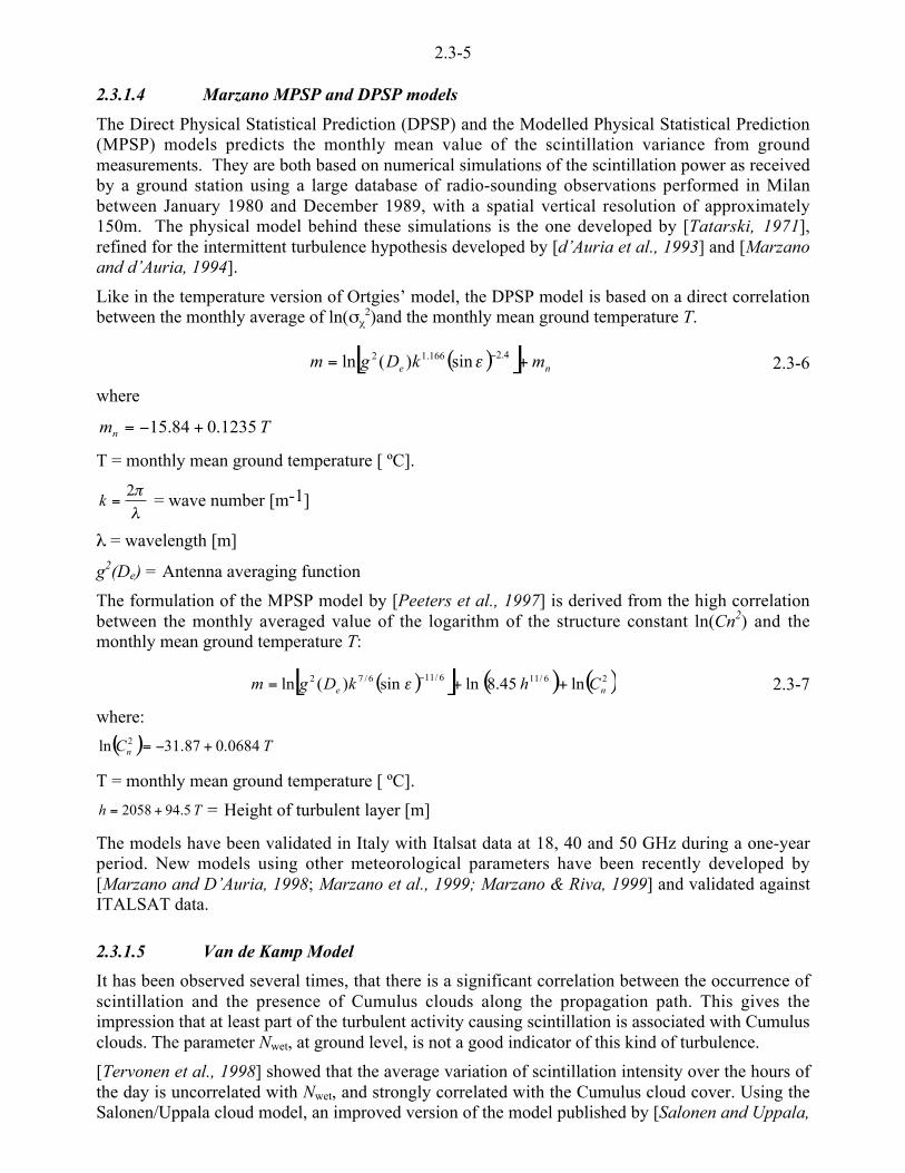
2.3-5

2.3.1.4 Marzano MPSP and DPSP models

The Direct Physical Statistical Prediction (DPSP) and the Modelled Physical Statistical Prediction(MPSP) models predicts the monthly mean value of the scintillation variance from groundmeasurements. They are both based on numerical simulations of the scintillation power as receivedby a ground station using a large database of radio-sounding observations performed in Milanbetween January 1980 and December 1989, with a spatial vertical resolution of approximately150m. The physical model behind these simulations is the one developed by [Tatarski, 1971],refined for the intermittent turbulence hypothesis developed by [d’Auria et al., 1993] and [Marzanoand d’Auria, 1994].

Like in the temperature version of Ortgies’ model, the DPSP model is based on a direct correlationbetween the monthly average of ln(mr

2)and the monthly mean ground temperature T.

( )[ ] ne mkDgm += < 4.2166.12 sin)(ln ¡ 2.3-6

where

Tmn 1235.084.15 +<=

T = monthly mean ground temperature [ ºC].

h/2

=k = wave number [m-1]

h = wavelength [m]

g2(De) = Antenna averaging function

The formulation of the MPSP model by [Peeters et al., 1997] is derived from the high correlationbetween the monthly averaged value of the logarithm of the structure constant ln(Cn2) and themonthly mean ground temperature T:

( )[ ] ( ) ( )26/116/116/72 ln45.8lnsin)(ln ne ChkDgm ++= <¡ 2.3-7

where:

( ) TCn 0684.087.31ln 2 +<=

T = monthly mean ground temperature [ ºC].

Th 5.942058 += = Height of turbulent layer [m]

The models have been validated in Italy with Italsat data at 18, 40 and 50 GHz during a one-yearperiod. New models using other meteorological parameters have been recently developed by[Marzano and D’Auria, 1998; Marzano et al., 1999; Marzano & Riva, 1999] and validated againstITALSAT data.

2.3.1.5 Van de Kamp Model

It has been observed several times, that there is a significant correlation between the occurrence ofscintillation and the presence of Cumulus clouds along the propagation path. This gives theimpression that at least part of the turbulent activity causing scintillation is associated with Cumulusclouds. The parameter Nwet, at ground level, is not a good indicator of this kind of turbulence.

[Tervonen et al., 1998] showed that the average variation of scintillation intensity over the hours ofthe day is uncorrelated with Nwet, and strongly correlated with the Cumulus cloud cover. Using theSalonen/Uppala cloud model, an improved version of the model published by [Salonen and Uppala,

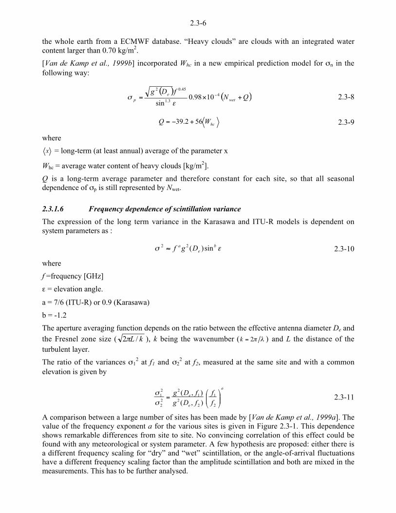
2.3-6

the whole earth from a ECMWF database. “Heavy clouds” are clouds with an integrated watercontent larger than 0.70 kg/m2.

[Van de Kamp et al., 1999b] incorporated Whc in a new empirical prediction model for mn in thefollowing way:

( )( )QN

fDgwet

ep +×= <4

3.1

45.02

1098.0sin ¡

m 2.3-8

hcWQ 562.39 +<= 2.3-9

where

x = long-term (at least annual) average of the parameter x

Whc = average water content of heavy clouds [kg/m2].

Q is a long-term average parameter and therefore constant for each site, so that all seasonaldependence of mp is still represented by Nwet.

2.3.1.6 Frequency dependence of scintillation variance

The expression of the long term variance in the Karasawa and ITU-R models is dependent onsystem parameters as :

¡m be

a Dgf sin)(22 5 2.3-10

where

f =frequency [GHz]

¡ = elevation angle.

a = 7/6 (ITU-R) or 0.9 (Karasawa)

b = -1.2

The aperture averaging function depends on the ratio between the effective antenna diameter De andthe Fresnel zone size ( kL /2/ ), k being the wavenumber ( h/2=k ) and L the distance of theturbulent layer.

The ratio of the variances m12 at f1 and m2

2 at f2, measured at the same site and with a commonelevation is given by

a

e

e

ff

fDgfDg

´́¦

¥²²¤

£=

2

1

22

12

22

21

),(),(

mm

2.3-11

A comparison between a large number of sites has been made by [Van de Kamp et al., 1999a]. Thevalue of the frequency exponent a for the various sites is given in Figure 2.3-1. This dependenceshows remarkable differences from site to site. No convincing correlation of this effect could befound with any meteorological or system parameter. A few hypothesis are proposed: either there isa different frequency scaling for “dry” and “wet” scintillation, or the angle-of-arrival fluctuationshave a different frequency scaling factor than the amplitude scintillation and both are mixed in themeasurements. This has to be further analysed.

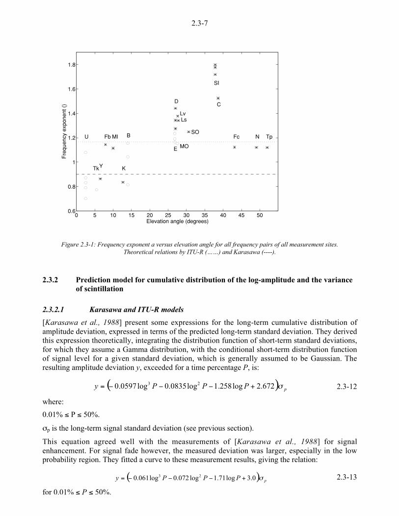
2.3-7

0 5 10 15 20 25 30 35 40 45 500.6

0.8

1

1.2

1.4

1.6

1.8

Elevation angle (degrees)

Freq

uenc

y ex

pone

nt ()

U

TkY

MI

K

B

E

D

MO

LsLv

SO

SI

C

Fb Fc N Tp

Figure 2.3-1: Frequency exponent a versus elevation angle for all frequency pairs of all measurement sites.Theoretical relations by ITU-R (……) and Karasawa (----).

2.3.2 Prediction model for cumulative distribution of the log-amplitude and the varianceof scintillation

2.3.2.1 Karasawa and ITU-R models

[Karasawa et al., 1988] present some expressions for the long-term cumulative distribution ofamplitude deviation, expressed in terms of the predicted long-term standard deviation. They derivedthis expression theoretically, integrating the distribution function of short-term standard deviations,for which they assume a Gamma distribution, with the conditional short-term distribution functionof signal level for a given standard deviation, which is generally assumed to be Gaussian. Theresulting amplitude deviation y, exceeded for a time percentage P, is:

( ) pPPPy m672.2log258.1log0835.0log0597.0 23 +<<<= 2.3-12

where:

0.01% ) P ) 50%.

mp is the long-term signal standard deviation (see previous section).

This equation agreed well with the measurements of [Karasawa et al., 1988] for signalenhancement. For signal fade however, the measured deviation was larger, especially in the lowprobability region. They fitted a curve to these measurement results, giving the relation:

( ) pPPPy m0.3log71.1log072.0log061.0 23 +<<<= 2.3-13

for 0.01% ) P ) 50%.

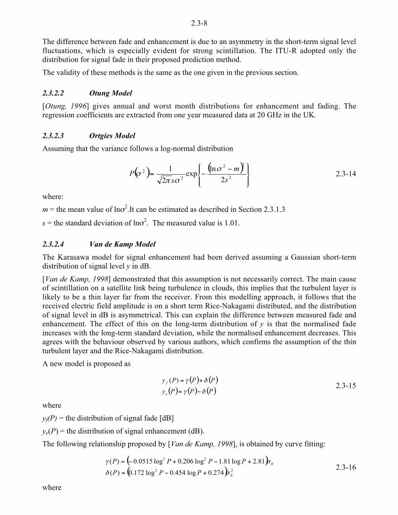
2.3-8

The difference between fade and enhancement is due to an asymmetry in the short-term signal levelfluctuations, which is especially evident for strong scintillation. The ITU-R adopted only thedistribution for signal fade in their proposed prediction method.

The validity of these methods is the same as the one given in the previous section.

2.3.2.2 Otung Model

[Otung, 1996] gives annual and worst month distributions for enhancement and fading. Theregression coefficients are extracted from one year measured data at 20 GHz in the UK.

2.3.2.3 Ortgies Model

Assuming that the variance follows a log-normal distribution

( ) ( )«®

«­¬

ǻ

«©¨ <<=

2

22

2

2

2

lnexp

2

1

s

m

sP

m

m/m 2.3-14

where:

m = the mean value of lnm2.It can be estimated as described in Section 2.3.1.3

s = the standard deviation of lnm2. The measured value is 1.01.

2.3.2.4 Van de Kamp Model

The Karasawa model for signal enhancement had been derived assuming a Gaussian short-termdistribution of signal level y in dB.

[Van de Kamp, 1998] demonstrated that this assumption is not necessarily correct. The main causeof scintillation on a satellite link being turbulence in clouds, this implies that the turbulent layer islikely to be a thin layer far from the receiver. From this modelling approach, it follows that thereceived electric field amplitude is on a short term Rice-Nakagami distributed, and the distributionof signal level in dB is asymmetrical. This can explain the difference between measured fade andenhancement. The effect of this on the long-term distribution of y is that the normalised fadeincreases with the long-term standard deviation, while the normalised enhancement decreases. Thisagrees with the behaviour observed by various authors, which confirms the assumption of the thinturbulent layer and the Rice-Nakagami distribution.

A new model is proposed as

( ) ( )( ) ( ) ( )PPPy

PPPy

e

f

ba

ba

<=

+=)(2.3-15

where

yf(P) = the distribution of signal fade [dB]

ye(P) = the distribution of signal enhancement (dB).

The following relationship proposed by [Van de Kamp, 1998], is obtained by curve fitting:

( )( ) 22

23

274.0log454.0log172.0)(

81.2log81.1log206.0log0515.0)(

lt

lt

PPP

PPPP

mb

ma

+<=

+<+<=2.3-16

where

2.3-9

These equations form a new model for the long-term distribution of signal level. The advantages ofthis model with respect to Karasawa’s model are that the asymmetry of the long-term distribution isnow theoretically predicted, and this asymmetry increases with the scintillation intensity, consistentwith measurement results.

2.3.2.5 UCL method

Radiosonde data are a valuable source of information for characterising tropospheric turbulence anda statistical method has been proposed to derive long-term scintillation statistics. The method isdescribed by [Vasseur et al., 1996] and [Vasseur et al., 1998]. It consists of two main steps.

In the first step, the statistical characteristics of the refractive index structure parameter verticalprofile are extracted from radiosonde ascent data collected over a long time period. For thispurpose, a statistical model is used to estimate turbulence parameters from meteorologicalsoundings.

In the second step, long-term statistics of slant-path scintillation are derived from the inferredtropospheric turbulence feature, using a rigorous statistical approach and the theory of propagationthrough a turbulent medium. In addition to radiosonde data, the only parameters required forscintillation prediction are the frequency, elevation angle (the method is valid at elevations higherthan about 5 to 10°) and antenna diameter.

The proposed method does not suffer from the limitations of the current empirical scintillationprediction models. It does not include any particular propagation measurement but is only based onradiosonde data and theoretical considerations. The method is applied to one year radiosonde datacollected in Belgium and the prediction results compare very well with the scintillationmeasurements carried out using an Olympus ground station located near to the meteorologicalstation.

2.3-10

2.3.3 References

[Belloul et al.,1998]Belloul B., S. Saunders, B. Evans, “Prediction of Scintillation Intensity from Sky-noiseTemperature in Earth-Satellite Links”, Electr. Lett., vol. 34, n°10, pp. 1023-1024, 1998.

[Crane and Blood, 1979]Crane R.K. and D.W. Blood, “Handbook for the estimation of microwave propagation effects”,NASA Contract NAS5-25341, NASA GSFC Greenbelt, MA, Technical Report No°1, Doc. 7376-TR1, June 1979.

[d’Auria et al., 1993]d’Auria G., F.S. Marzano, U. Merlo, “Model for Estimating the Refractive Index StructureConstant in Clear-Air Intermittent Turbulence”, Applied Optics, vol. 32, pp. 2674-2680, 1993.

[Haddon and Vilar, 1986]Haddon J., E. Vilar, “Scattering Induced Microwave Scintillation from Clear Air and Rain on Earth-Space Paths and the Influence of the Antenna Aperture”, IEEE Trans. Ant. Prop., vol. 34, No° 5,pp. 646-657, 1986.

[ITU-R, 1999]ITU-R, Rec. PN. 618-6 “Propagation Data and Prediction Methods Required for Earth-SpaceTelecommunication Systems ”, 1999.

[Karasawa et al., 1988]Karasawa Y., M. Yamada, J.E. Allnutt, “A New Predicition Method for Tropospheric Scintillationon Earth-Space Paths”, IEEE Trans. Ant. Prop., vol 36, No°11, pp. 1608-1614, 1988.

[Marzano and d’Auria, 1994]Marzano F.S., G. d’Auria, “Estimation of Intermittent Scintillation on Microwave Links fromMeteorological Data”, Alta Frequenza, vol. 6, pp. 94-97, 1994.

[Marzano and d’Auria, 1998]Marzano F.S., G. d’Auria, “Model-based prediction of amplitude scintillation variance due to clear-air turbulence for Earth-satellite microwave links”, IEEE Trans. Ant. Prop., vol. 46, pp. 1506-1518.1998.

[Marzano et al., 1999]Marzano F. S., C. Riva, A. Banich, F. Clivio, “Assessment of model-based scintillation varianceprediction on long-term basis using ITALSAT satellite measurements”, Int. J. Sat. Com., vol. 17,Issue 1, pp. 17-36, 1999.

[Marzano & Riva, 1999]Marzano F.S. and C. Riva, "Evidence of long-term correlation between clear-air scintillation andattenuation in microwave and millimeter-wave satellite links", IEEE Trans. Ant. Prop., vol. 47, pp.1749-1757, 1999.

[Ortgies, 1993]Ortgies G., “Prediction of Slant-Path Amplitude Scintillations from Meteorological Parameters”,Proc. 1993 Int. Symp. Radio Propagation, Beijing, pp. 218-221, 1993.

[Otung, 1996]Otung I. E., Prediction of Tropospheric Amplitude Scintillation on a Satellite Link”, IEEE Trans.Ant. Prop., vol. 44, n°12, pp. 1600-1608, 1996.

[Otung & Evans, 1995]Otung I.E., B.G. Evans, “Short Term Distribution of Amplitude Scintillation on a Satellite Link”,El t L tt l 31 N °16 1328 1329 1995

2.3-11

[Peeters et al., 1997]Peeters G., F.S. Marzano, G. d’Auria, C. Riva, D. Vanhoenacker-Janvier, “Evaluation of StatisticalModels for Clear-Air Scintillation Using Olympus Satellite Measurements”, Int. J. Sat. Com., vol.15, pp. 73-88, 1997.

[Salonen et al., 1994]Salonen E., S. Karhu, S. Uppala and R. Hyvönen, “Study of improved propagation predictions”,Final Report for ESA/Estec Contract 9455/91/NL/LC(SC), Helsinki University of Technology andFinnish Meteorological Institute, pp. 83-87, 1994.

[Salonen and Uppala, 1991]Salonen E. and S. Uppala, “New prediction method of cloud attenuation”, Electr. Lett., vol. 27, pp.1106-1108, 1991.

[Tatarski, 1971]Tatarski V.I., “The effects of the turbulent atmosphere on Wave Propagation”, Israel Program forScientific Translations, Jerusalem, 1971.

[Tervonen et al., 1998]Tervonen J. K, M.M.J.L. van de Kamp and E. T. Salonen, “Prediction Model for the DiurnalBehavior of the Tropospheric Scintillation Variance”, IEEE Trans. Ant. Prop., vol. 46, pp. 1372-1378, 1998.

[Van de Kamp, 1998]Van de Kamp M.M.J.L., “Asymmetrical signal level distribution due to tropospheric scintillation”,Electr. Lett, vol. 34, pp. 1145-1146, 1998.

[Van de Kamp et al., 1999a]Van de Kamp M.M.J.L., C. Riva, J. Tervonen, E. Salonen, “Frequency Dependence of AmplitudeScintillation”, IEEE Trans. Ant. Prop., vol. 47, No°1, pp. 77-85, 1999.

[Van de Kamp et al., 1999b]Van de Kamp M.M.J.L., J.K. Tervonen, E.T. Salonen, and J.P.V. Poiares Baptista, “ImprovedModels for Long-Term Prediction of Tropospheric Scintillation on Slant Paths”, IEEE Trans. Ant.Prop., vol. 47, n°2, pp. 249-260, 1999.

[Vasseur et al., 1996]Vasseur H., O. Ravard, D. Vanhoenacker-Janvier, “Prediction of slant-path scintillation fromradiosonde measurements”, Proc. Climpara’96, pp. 12-13, Oslo, June 1996.

[Vasseur et al., 1998]Vasseur H., D. Vanhoenacker, “Characterisation of tropospheric turbulent layers from theradiosonde data”, Electr. Lett., vol. 34, No°4, pp. 318-319, 1998.

2.4-1

CHAPTER 2.4Rain and Ice Depolarisation

Editor: Antonio Martellucci1

Authors: Max van de Kamp2, Antonio Martellucci1, Aldo Paraboni3

1 European Space Agency, Estec, Keplerlaan 1, Postbus 299, 2200 AG Noordwijk, The Netherlands

Tel: +31 71 565 5603, Fax: +31 71 565 4999, e-mail: Antonio.Martellucci@esa.int

2 Eindhoven University of Technology, Postbus 513, 5600 MB Eindhoven, The Netherlands

Tel.: +31 40 247 2326, Fax.: +31 40 245 5197, e-mail: m.m.j.l.v.d.kamp@ele.tue.nl

3 Politecnico di Milano, CSTS, Pza Leonardo da Vinci 32, 20133 Milano, Italy

Tel. +39 2 23993586, Fax +39 2 3993413, e-mail: aparaboni@elet.polimi.it

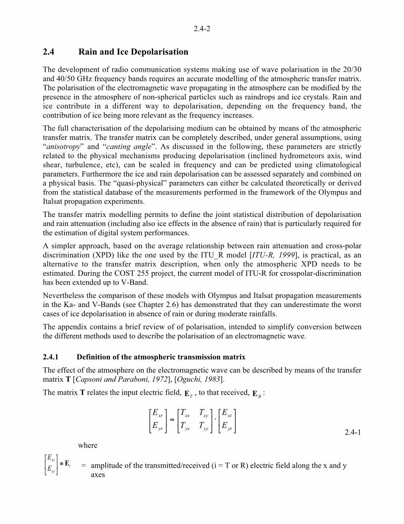
2.4-2

iyi

xi

E

EE>µ

�

�³�

�

2.4 Rain and Ice Depolarisation

The development of radio communication systems making use of wave polarisation in the 20/30and 40/50 GHz frequency bands requires an accurate modelling of the atmospheric transfer matrix.The polarisation of the electromagnetic wave propagating in the atmosphere can be modified by thepresence in the atmosphere of non-spherical particles such as raindrops and ice crystals. Rain andice contribute in a different way to depolarisation, depending on the frequency band, thecontribution of ice being more relevant as the frequency increases.

The full characterisation of the depolarising medium can be obtained by means of the atmospherictransfer matrix. The transfer matrix can be completely described, under general assumptions, using“anisotropy” and “canting angle”. As discussed in the following, these parameters are strictlyrelated to the physical mechanisms producing depolarisation (inclined hydrometeors axis, windshear, turbulence, etc), can be scaled in frequency and can be predicted using climatologicalparameters. Furthermore the ice and rain depolarisation can be assessed separately and combined ona physical basis. The “quasi-physical” parameters can either be calculated theoretically or derivedfrom the statistical database of the measurements performed in the framework of the Olympus andItalsat propagation experiments.

The transfer matrix modelling permits to define the joint statistical distribution of depolarisationand rain attenuation (including also ice effects in the absence of rain) that is particularly required forthe estimation of digital system performances.

A simpler approach, based on the average relationship between rain attenuation and cross-polardiscrimination (XPD) like the one used by the ITU_R model [ITU-R, 1999], is practical, as analternative to the transfer matrix description, when only the atmospheric XPD needs to beestimated. During the COST 255 project, the current model of ITU-R for crosspolar-discriminationhas been extended up to V-Band.

Nevertheless the comparison of these models with Olympus and Italsat propagation measurementsin the Ka- and V-Bands (see Chapter 2.6) has demonstrated that they can underestimate the worstcases of ice depolarisation in absence of rain or during moderate rainfalls.

The appendix contains a brief review of of polarisation, intended to simplify conversion betweenthe different methods used to describe the polarisation of an electromagnetic wave.

2.4.1 Definition of the atmospheric transmission matrix

The effect of the atmosphere on the electromagnetic wave can be described by means of the transfermatrix T [Capsoni and Paraboni, 1972], [Oguchi, 1983].

The matrix T relates the input electric field, ET, to that received, ER

:

µ�

�³�

�uµ

�

�³�

�=µ

�

�³�

�

yt

xt

yyyx

xyxx

yr

xr

E

E

TT

TT

E

E

2.4-1

where

= amplitude of the transmitted/received (i = T or R) electric field along the x and y axes

2.4-3

Tij = copolar component received on the channel employing polarisation i, when an electric field

with an amplitude equal to one is transmitted on the channel employing polarisation j.( i and j = x or y).

When two generic orthogonal polarisations, E// and E�, are transmitted, the transfer matrix, T, can betransformed into the matrix M, by using:

( ) ( )( ) ( )

( ) ( )( ) ( )µ�

�³�

�

<uuµ

�

�³�

�

<= ++<

<

__

__

__

__bbb

b

cossin

sincos

cossin

sincosjjj

j

eee

eTM 2.4-2

where:( ) ( )[ ]yx b__ jeEE sincos0// +=

_, b = Parameters that describes the transmitted polarisation. (See Section 1 of the appendix).

A particular case of M occurs when circular polarisation is employed. The transfer matrix, C,expressed using the right, r, and left-hand, l, circular polarisation, Er and El is:

µ�

�³�

�uµ

�

�³�

�=µ

�

�³�

�

lt

rt

lllr

rlrr

lr

rr

E

E

CC

CC

E

E2.4-3

where:

µ�

�³�

�>

lllr

rlrr

CC

CCC = Atmospheric transfer matrix using right and left hand circular polarisation

][ )()(? xyyxyyxxrr TTjTTC <++= ; [ ])()(? xyyxyyxxll TTjTTC <<+=

[ ])()(? xyyxyyxxrl TTjTTC ++<= ; [ ])()(? xyyxyyxxlr TTjTTC +<<=

The copolar term of the transfer matrix, Tii, describes the fading of polarisation i, Ai, in dB:

( )( )yyy

xxx

TA

TA

log20

log20

<=

<= ;

( )( )llcl

rrcr

CA

CA

log20

log20

<=

<=2.4-4

The crosspolar discrimination, XPDij, is the ratio between the copolar component received on thechannel employing polarisation j, Tjj, and the crosspolar component received on the channel usingpolarisation i, Tij, when only polarisation j is transmitted:

yxxxyx

xyyyxy

TTXPD

TTXPD

log20

log20

=

= ;

lrrrlr

rlllrl

CCXPD

CCXPD

log20

log20

=

=2.4-5

where :

ijjjij TT l= = complex depolarisation ratio

The crosspolar isolation, XPIij, is defined as the ratio between the copolar part of the signal on thechannel using polarisation i Tii and the crosspolar component of the signal received on the same

µ�

�³�

�>

yyyx

xyxx

TT

TTT = atmospheric transfer matrix using x and y polarisations

2.4-4

yxyyyx

xyxxxy

TTXPI

TTXPI

log20

log20

=

= ;

yxyyyx

xyxxxy

TTXPI

TTXPI

log20

log20

=

=2.4-6

The transfer matrix T can be normalised to one of its elements, e.g. Txx

. Therefore only a maximum

of three complex parameters is actually needed to describe the transfer channel.

The two eigenvectors of the transfer matrix T, defined as the characteristic polarisations,represent the two polarisations that propagate in the atmosphere without undergoing depolarisation[Capsoni and Paraboni, 1972; Oguchi, 1983].

If the characteristic polarisations are linear, then they are orthogonal vectors and the planesidentified by the linear polarisation vectors and the propagation direction are defined as principalplanes of the transfer channel.

In the general case, the eigenvalues of the transfer matrix T are related to the propagation constantsof the characteristic polarisations and are given by:

( ) ( ) ( )

( ) ( ) ( )µ��

³�� +<<+=<=K

µ��

³�� +<++=<=K

yxxyxxyyxxyyIIII

yxxyxxyyxxyyII

TTTTTT

TTTTTT

42

1exp

421

exp

2

2

a

a2.4-7

where:

aI , a

II = propagation constants of the eigenvectors I e II, defined as characteristic polarisations.

I = Polarisation characterised by the lower attenuation or the lower phase shift.

II = Polarisation characterised by the higher attenuation or the higher phase shift.

The anisotropy of the medium, 6, is defined as the difference between the propagation constants ofthe characteristic polarisations:

III aa <=6 2.4-8

where:

Re(6) = Differential Attenuation of the atmosphere for the characteristic polarisations, [nep]

Im(6) = Differential phase shift of the atmosphere for the characteristic polarisations, [rad]

In the general case, the eigenvectors of characteristic polarisations, EI and E

II, of the transfer matrix

T are elliptical polarisations and are given by:

( ) ( )´´

¦

¥

²²

¤

£

<

+<+<=

xy

yxxyxxyyxxyyI

T

TTTTTT

2

42

E

;

( ) ( ) ´

´

¦

¥

²²

¤

£

+<+<=

yxxyxxyyxxyy

xy

II TTTTTT

T

4

22E 2.4-9

where:

0=u III EE

The two characteristic polarisations can be described by means of the complex canting angle ofeigenvector II, \ (see Section 6 of the appendix), that is given by the following relationship:

( )( ) ( )

xy

yxxyxxyyxxyy

T

TTTTTT

2

4tan

2 +<+<=\ 2.4-10

2.4-5

where:

( )\Re = Canting angle of the ellipse with respect x axes. ( ) 2Re2 // +)\<<

( )[ ]\Imtanh = Axial ratio of the ellipse.

The occurrence of principal planes in the atmospheric medium is revealed by thecondition, { } 0Im =\ . In this particular case the characteristic polarisations, EI and EII, are twoorthogonal linear polarisations, canted at an angle Re{\} with respect to the y and x axes.

2.4.2 Model of the transfer matrix

A model of the propagation of a polarised electromagnetic plane wave through a spatial distributionof non-spherical particles, can be derived under the following general assumptions:

1) The amplitude of the field scattered by the particles can be calculated using the Fresnelapproximation.

2) The contribution to the transmitted field by scattering from directions different from thepropagation direction of the plane wave can be ignored. (i.e. only the forward scattering byparticles contributes to the transmitted field).

3) The shape of atmospheric particles (rain drops and ice crystals) has an axis of symmetry.

4) The distribution of particles is longitudinally homogeneous.

Using these assumptions the differential equation that describes the electromagnetic wavepropagation can be solved, by means of the technique based on eigenvectors and eigenvalues[Capsoni et al., 1981]. It turns out that the number of complex parameters, needed to describe thetransfer matrix T, reduces from three to two. The medium transfer matrix, using linear polarisationsx and y, is given by:

( ) ( )( ) ( ) µ

�

�³�

�´́¦

¥²²¤

£

\<\

\\u´

¦

¥²¤

£ 6<´́¦

¥²²¤

£u´

¦

¥²¤

£ 6u´́¦

¥²²¤

£ +<=

2cos2sin

2sin2cos

2sinh

10

01

2cosh

2expT yxl

aa 2.4-11

where :

ax, ay = propagation constants of x and y polarisations

III aa <=6 = anisotropy of the medium.

aI , a

II = propagation constants of characteristic polarisations I and II.

IR j\+\=\ = complex canting angle of polarisation II

l = length of dispersion of particles.

Therefore the transfer matrix can be completely described by means of the anisotropy of themedium, 6, and the complex canting angle, \.

The crosspolar discrimination of linear polarisation can be calculated using the complexdepolarisation ratios (see equation 2.4-5):

( )

( )\´¥

²£ 6+

\´¦

¥²¤

£ 6<=

2costanh1

22

tanh sen

xyl ; ( )

( )\´¥

²£ 6

\´¦

¥²¤

£ 6<=

2costanh1

22

tanh sen

yxl 2.4-12

2.4-6

The medium transfer matrix C, when right or left handed circular polarisation are transmitted, isgiven by:

( )( ) µ

�

�³�

�´́¦

¥²²¤

£

\<

\+u´

¦

¥²¤

£ 6<´́¦

¥²²¤

£u´

¦

¥²¤

£ 6u´́¦

¥²²¤

£ +<=

02exp

2exp0

2sinh

10

01

2cosh

2expC

j

jl yx aa

2.4-13

Similarly the complex depolarisation ratios of circular polarisation are:

( )\´¦

¥²¤

£ 6<= 2exp2

tanh jrll ; ( )\<´¦

¥²¤

£ 6<= 2exp2

tanh jlrl 2.4-14

The propagation parameters needed for the evaluation of the atmospheric transmission matrix canbe calculated using the scattering matrix of all the particles:

( )

( )-

-

+=

+=

qe/

a

qe/

a

,,,2

,,,2

2

2

afSk

jk

afSk

jk

yyy

xxx

2.4-15

( ) ( ) ( ) ( )

( ) ( )( ) ( )µ

µ�

�

³³�

�

+<

<<=\

<<+<=6

--

--

q

q

qq/

jSS

jSSj

jSSjSSk

2exp

2expln

4

2exp2exp2

12

12

121222.4-16

where:

the sum is performed over all the particles contained in the distribution

f = frequency [Hz]

a = parameter that describes the dimension of the particle(e.g. equivolumetric radius).

e, q = angles that describe the spatial orientation of the symmetry axis of each particle,with respect to the propagation direction, on longitudinal plane (e, /e )<0 )and transverse plane (q, 22 /q/ +)<< )

k = 2//h = wave-number [rad/m]

S1, S2 = copolar elements of the scattering matrix when polarisation 1 or 2 are

transmitted.

Polarisations 1 or 2 are respectively parallel and orthogonal to the symmetry axis of the particle.

( ) ( )( )( ) ( )( )

( )( )=

«®

«­

¬

<==

<<+=

<++=

22sin

22cos2

22cos2

12

1221

1221

SSSS

SSSSS

SSSSS

yxxy

yy

xx

q

q

q Elements of the particle scattering matrix (x or y polarn).

For a general description of models to calculate the scattering matrix see [Poiares Baptista, 1994].

From the previous equations it can be derived that the characteristic polarisations are linear and themedium is characterised by the existence of principal planes of polarisation (i.e. Im(\)=0) whenone of the following conditions holds:

1) The scattering matrix of the particles can be calculated using the Rayleigh approximation forspheroidal particles.

2.4-7

2) The statistical distribution of the orientations of the particle symmetry axis is asymmetric function.

This general model can be further developed to describe the following particular cases:

2.4.2.1 Fully aligned particles

When all the particles are aligned, with their symmetry axes oriented along the direction describedby the longitudinal canting angle ek and the transverse canting angle qk, the total anisotropy and thecomplex canting angle of the medium are given by the following relationships:

( ) ( ) ( )[ ]0 <=6 daafSafSanlk 002002 ,,,,,,

2qeqe

/ 2.4-17

( ) 0Re q=\ ; ( ) 0Im =\ 2.4-18

where:

( )an = distribution of drop size.

l = length of dispersion of particles.

Therefore the characteristic polarisations are linear and canted at an angle q0 with respect to the x

and y axes.

2.4.2.2 Particles with Gaussian distribution of orientations

When the longitudinal canting angle e and the transverse canting angle q are statisticallyindependent and are distributed according to a normal model, the total anisotropy and the complexcanting angle of the medium are given by the following relationships:

( ) ( ) ( )[ ]0 <=6 daafSafSank

Lr 0010022

,,,,,,2

qeqe/

2.4-19

( ) 0Re q=\ ; ( ) 0Im =\ 2.4-20

where:

( )[ ] ( )22 2exp2exp121

qe mm <<+=r = reduction factor of the anisotropy due to misalignment of particles

eo , qo = mean values of longitudinal and transverse canting angle.

qe mm , = standard deviations of longitudinal and transverse canting angle.

Therefore the medium is still characterised by linear characteristic polarisations and equation 2.4-17can be used by taking into account the reduction factor r.

2.4.2.3 Medium composed of two different types of particle

It is assumed that in the atmosphere there are two different distributions of particles in cascade, e.g.rain and ice. Each family is characterised by anisotropy, 6

1 and 6

2, and the characteristic

polarisations are linear, canted at angles q1 and q

2 with respect to the x and y axes [Martellucci et

al., 1993; Martelluci & Paraboni, 1994; Dintelmann, 1994].

The overall transmission matrix T is the product of the two transmission matrices ZZZZ1 and ZZZZ2 The

2.4-8

( ) 22tanh 6�6 and that .212121 xxxxyxxyxxxx TTTTTT �+

Using these approximations the overall transfer matrix of the atmosphere, using circularpolarisation, is given by :

µ�

�³�

�=

1

1

lr

rl

C

CC 2.4-21

where:

[ ] [ ])2(exp2

)2(exp2 22

211

1 q_q_ +<+<= jd

jd

Crl

[ ] [ ])2(exp2

)2(exp2 22

211

1 q_q_ <<<<= jd

jd

Clr

( )iii jd _exp=6 = anisotropy of the first or second (i=1 or 2) family of particles.

di = amplitude of anisotropy of family i

_i = phase of anisotropy of family i.

q1, q

2 = canting angle of the linear characteristic polarisation of the first and

the second families of particles.

The overall anisotropy of the medium, 6, can be obtained by inversion of equation 2.4-13:

lrrlCCKKK 2321 >++=6 2.4-22

where:

)2exp( 1211 _jdK =

)2exp( 2222 _jdK =

( )[ ] ( )[ ]2121213 2cosexp2 qq__ <u+u= jddK

It is to be noted that by means of anisotropy the difference between the canting angles of the twopopulations, (q1 - q2), also affects the depolarisation. When the two populations are aligned or are

geometrically orthogonal, the overall anisotropy becomes:

( )( )ª

©¨

±=<6<6

=<6+6=6

2for;

0for;

2121

2121

/qq

qq2.4-23

Therefore the combination of the depolarisation effects of rain and ice must take into account theirrelative geometrical orientation, in order to assess if the overall depolarisation is increased orreduced with respect to the separate depolarisations. This is particularly relevant duringthunderstorms and at V-Band where the ice depolarisation is higher than at K-Band.

Measurements of Anisotropy and Canting Angle

The model of the atmospheric transfer matrix described in this chapter makes possible the completeassessment of atmospheric depolarisation if the anisotropy and the canting angle are known. Theexperimental assessment of those parameters has been performed using the dual polarisationpropagation beacons of the Olympus and Italsat satellites, at 29,7 and 49.5 GHz respectively[Dintelmann, 1994; Aresu et al. 1994; Martellucci et al., 2000]. Those measurements can be used tocreate a new statistical database to be included in the ITU R database of propagation experiments

2.4-9

The data measured by the Olympus station located in Spino D'Adda, near Milano, are presented asan example of anisotropy and canting angle on slant paths [Aresu et al., 1995]. The elevation to thesatellite was 31 degrees and the polarisation tilt angle was 25 degrees.

The presence of ice at low attenuation values has been shown statistically by the Imaginary part ofthe overall anisotropy, 6.

In Figure 2.4-1a the statistics are given of the real part of rain anisotropy, conditioned onattenuation. This parameter appears to be linearly related to the rain attenuation. The differencebetween the theoretical (discussed in Section 2.4.2.4) and the experimental values of the real part ofrain anisotropy, suggest a reduction factor of about 0.6, that is in agreement with previousmeasurements on terrestrial path [Aresu et al., 1993].

The anisotropy of ice, conditioned on attenuation, is given in Figure 2.4-1b. The theoreticalmaximum value of ice anisotropy derived from local radiosonde meteorological measurements isalso plotted (see Section 2.4.2.4) [Paraboni et al., 1997]. The model value of ice cloud anisotropy isin agreement with the mean value of measurements for attenuation values lower than 20 dB. Athigher attenuations the ice anisotropy can be relevant and exhibits a correlation with the intensity ofrainfall.

0

1

2

3

4

5

6

7

0 5 10 15 20 25 30 35

Re{Anisotropy} [dB

Attenuation [dB]

Spino D'Adda, OLYMPUS, 20 GHz

Measurements, D90-D10Measurements, Mean

Model, Marshall-Palmer Distr.

a)

05101520253035

0 5 10 15 20 25 30 35Im{Anisotropy} [de

Attenuation [dB]

Spino D'Adda, OLYMPUS, 20 GHz

Measurements, D90,D10Measurements, meanModel, radiosonde data

b)

Figure 2.4-1: Deciles of real part of rain anisotropy (a) and imaginary part of ice anisotropy (b)d d d dd h l ll b

2.4-10

Italsat measurements of the atmospheric transfer matrix at 49.5 GHz, performed by [Martellucci etal., 2000] confirmed the Olympus results. In addition it was found that ice anisotropy at 49.5 GHzcan be described by a log-normal model. The average of ice anisotropy value increases with rainfallintensity, and the standard deviation oscillates around a constant value for attenuation valuesranging from 0 to 10 dB at 49.5 GHz, then it decreases for higher attenuation values.

The statistics of canting angle, with respect to local horizontal, of the raindrops and ice crystals,conditioned on attenuation values, are given in Figure 2.4-2.

As far as the rain population is concerned, there is a tendency for rain drops to stabilise duringthunderstorms within a range of about 20 degrees around the horizontal, confirming similar resultsobtained on a terrestrial link [Aresu et al., 1993].

On the contrary the measurements show that ice crystals can change orientation duringthunderstorms, due to electrostatic discharges and aerodynamic effects, leading to fluctuations ofmore than 50°.

-90

-75

-60

-45

-30

-15

0

15

30

45

60

75

90

0 5 10 15 20 25 30 35

Rain Canting Angle

Attenuation [dB]

Spino D'Adda, OLYMPUS, 20 GHz

Measurements, D90, D10mean

a)

-90-75-60-45-30-1501530

45

60

75

90

0 5 10 15 20 25 30 35Ice Canting Angle

Attenuation [dB]

Spino D'Adda, OLYMPUS, 20 GHz

Measurements, D60-D40Measurements, mean

b)

Figure2.4-2: Deciles of canting angle of rain (a) and ice (b) conditioned on attenuationmeasured in Spino D'Adda, using the Olympus Satellite beacon at 19.77 GHz.

2.4-11

2.4.2.4 Theoretical calculation of depolarisation due to rain and ice

The atmospheric particles that can contribute to microwave depolarisation along a slant path areraindrops, melting particles (formed by a mixture of air, water and ice) and ice crystals. Accordingto the model illustrated in the previous chapter, the depolarisation due to atmospheric particles canbe estimated theoretically, by using the appropriate microphysical parameters and models of theatmospheric particles.

As far as the melting layer is concerned, it can be expected that its thickness is lower than thecharacteristic size of both the ice layer and the rain cell. Therefore the depolarisation of the meltinglayer can be neglected, as a first approximation, when comparing the rain and ice anisotropy.

In following paragraphs, examples of modelling and calculations of the crosspolar discriminationdue to rain and ice clouds in the Ka and V-Bands will be illustrated. The simultaneous occurrenceof rain and ice depolarisation is also discussed and a statistical model is presented for estimating thetotal ice content based on the rain rate at the ground.

The parameters used for those assessments have been derived from analysis of the Olympus andItalsat propagation experiments.

Rain depolarisation

The following parameters and models have been selected for rain depolarisation:

• Water temperature = 0 ˚C.

• Shape of drops = oblate spheroid.

• Orientation of particle symmetry axis = parallel to the vertical direction.

• Model of rain drop size distribution = Marshall-Palmer, exponential.

• Drops are aligned , with a canting angle ranging from 5° to 45°.

• Rain cell length = 1 km.

• The water refractive index has been calculated according to [Ray, 1972].

• The scattering matrix of drops is calculated using the Oguchi’s Point MatchingTechnique [Oguchi, 1983].

The model parameters have been verified using results from terrestrial measurements, where no iceor snow is measured, and satellite measurements, separating rain and ice [Aresu et al., 1993; Aresuet al., 1994 and Aresu et al., 1995]. The statistics of canting angle, anisotropy and rain reductionfactor have been determined from those measurements.

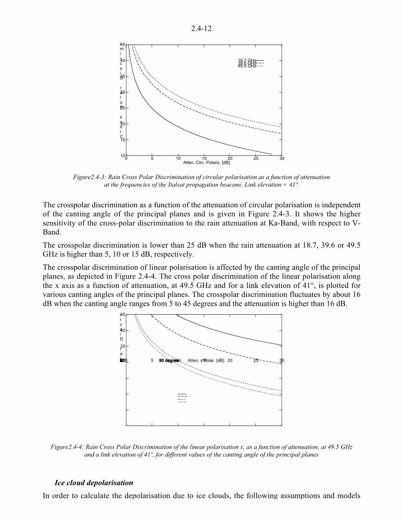
2.4-12

10

15

20

25

30

35

40

45

0 5 10 15 20 25 30

Cross Polar Discrimi

Atten. Circ. Polariz. [dB]

18.7 GHz39.6 GHz49.5 GHz

Figure2.4-3: Rain Cross Polar Discrimination of circular polarisation as a function of attenuationat the frequencies of the Italsat propagation beacons. Link elevation = 41º.

The crosspolar discrimination as a function of the attenuation of circular polarisation is independentof the canting angle of the principal planes and is given in Figure 2.4-3. It shows the highersensitivity of the cross-polar discrimination to the rain attenuation at Ka-Band, with respect to V-Band.

The crosspolar discrimination is lower than 25 dB when the rain attenuation at 18.7, 39.6 or 49.5GHz is higher than 5, 10 or 15 dB, respectively.

The crosspolar discrimination of linear polarisation is affected by the canting angle of the principalplanes, as depicted in Figure 2.4-4. The cross polar discrimination of the linear polarisation alongthe x axis as a function of attenuation, at 49.5 GHz and for a link elevation of 41°, is plotted forvarious canting angles of the principal planes. The crosspolar discrimination fluctuates by about 16dB when the canting angle ranges from 5 to 45 degrees and the attenuation is higher than 16 dB.

1015202530

35

40

45

0 5 10 15 20 25 30Cross Polar Discri

Atten. x Polar. [dB]5 degree10 degree30 degree45 degree

Figure2.4-4: Rain Cross Polar Discrimination of the linear polarisation x, as a function of attenuation, at 49.5 GHzand a link elevation of 41º, for different values of the canting angle of the principal planes

Ice cloud depolarisation

In order to calculate the depolarisation due to ice clouds, the following assumptions and models

2.4-13

• Ice temperature = -15 ºC.

• Shape of ice needles = prolate spheroid.

• Model of ice distribution size = Gamma function, Cirrostratus cloud.

• Ice density is assumed to be constant in the vertical direction.

• Scattering functions of ice crystals is calculated using the Rayleigh model.

• The ice refractive index has been calculated according to [Ray, 1972].

It can be assumed that the ice needles are maintained aligned on to the horizontal plane byaerodynamic and electrostatic effects, and can rotate freely in this plane.

When the ice crystals are completely aligned, the anisotropy depends on the rotation angle of thecrystals and is higher when the rotation angle is equal to 90° and the apparent canting angle is equalto 0°. The apparent canting angle of the ice cloud is given by the projection of the symmetry axeson the plane orthogonal to the direction of propagation:

( ) ( ) ( )[ ]eaaq sincotarctan2 u<= 2.4-24

where:

a = Horizontal rotation angle of the symmetry axis of the needle with respect to the propagation direction.

` = elevation angle

When the ice crystals are randomly aligned in to the horizontal plane, the anisotropy is non-zerowhile the apparent canting angle is equal to zero.

Using this simple model, the ice anisotropy results depend on the total ice content, I:

( ) ( ) 22max CBIIi +6=6 2.4-25

where :

( ) ( )12max

1ccIj <

<=6

h/¡ = maximum of ice anisotropy when all the needles are aligned and

a = 90 [degrees] (the needle is transversal to the propagation direction).

I = total ice content, mm

( ) ( )[ ]a` <= 902sinsinB

( )[ ] ( ) ( )[ ] 1902coscos5.0902cos 2 <<<<= a`aC

<> = ensemble average of the parameter.

( ) 11 11

1

ac

<<=

¡;

( ) 22 11

1a

c<<

=¡

; ( ) µµ

�

�

³³

�

�

´´

¦

¥

²²

¤

£

<<

<+

<<

<=

1

1ln

12

1

12 2

2

221mm

mm

mm

m

ma ;

12 21 aa <=

2nj ir =<= ¡¡¡ = complex permittivity

1>= bam

a,b = major and minor semiaxis of the particle

The values of parameters B and C are given in the following table for some particular cases.

2.4-14

Crystals Orientation <aaaa> deg B C

Random Orientation 0 0 ( )`2cos5.0

All Aligned a0 ( ) ( )02a` sinsin ( ) ( ) ( )`aa 20

20

2 sencossen <

All Aligned 0 0 ( )`2sen<

All Aligned 90 0 1

Table 2.4-1: Values of B and C parameters for calculation of ice anisotropy.

The crosspolar discrimination of circular polarisation, for various frequencies, is plotted inFigure 2.4-5 as a function of the total ice content of the cloud [Paraboni et al., 1997]. Theconcurrent attenuation is almost equal to zero.

This shows that the ice crosspolar discrimination can drop below 30 dB, at 18.7, 39.6 and 49.5 GHzfor a total ice content of 0.25, 0.15 and 0.1 mm, for a cloud thickness of 500 m. It is to be noted thatice depolarisation increases with frequency.

15

20

25

30

35

40

45

0.05 0.1 0.15 0.2 0.25 0.3 0.35 0.4 0.45 0.5

XPD of Circul. Po

Ice Total Content [mm]

18.7 GHz39.6 GHz49.5 GHz

Figure2.4-5: Crosspolar discrimination (XPD) for circular polarisation at Ka and V-Band, versus total ice content.The ice needles are aligned. Rotation angle, a = 90 º. Link elevation =41º

The value of total ice content in the absence of rain can be estimated using radiosondemeasurements of the vertical profile of meteorological parameters. Statistics of the total ice content,derived from radiosonde measurements performed at various locations around the world, are givenin the database described in Chapter 2.1. For example, according to this database, the value of totalice content exceeded in Europe for 1 % of the time, ranges from 0.5 to 1.2 mm.

The ice crystals can exhibit higher and faster rotational variations than raindrops, due toaerodynamic and electrostatic effects and this influences the dynamic behaviour of icedepolarisation.

The effect of the rotation of ice crystals on circular and linear polarisations is described inFigure 2.4-6. The considerable reduction of crosspolar discrimination resulting from smallfluctuations in the ice crystal orientation can be evaluated, in particular for linear polarisation.

Therefore it is to be expected that ice depolarisation can be characterised by faster fluctuations thanduring rain depolarisation.

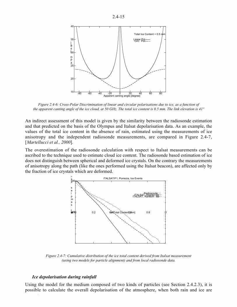
2.4-15

15

20

25

30

35

40

-80 -60 -40 -20 0 20 40 60 80

XPD [dB]

Apparent canting angle [degree]

Total Ice Content = 0.5 mm

Linear Pol.Circ. Pol.

Figure 2.4-6: Cross-Polar Discrimination of linear and circular polarisations due to ice, as a function ofthe apparent canting angle of the ice cloud, at 50 GHz. The total ice content is 0.5 mm. The link elevation is 41º

An indirect assessment of this model is given by the similarity between the radiosonde estimationand that predicted on the basis of the Olympus and Italsat depolarisation data. As an example, thevalues of the total ice content in the absence of rain, estimated using the measurements of iceanisotropy and the independent radiosonde measurements, are compared in Figure 2.4-7,[Martellucci et al., 2000].

The overestimation of the radiosonde calculation with respect to Italsat measurements can beascribed to the technique used to estimate cloud ice content. The radiosonde based estimation of icedoes not distinguish between spherical and deformed ice crystals. On the contrary the measurementsof anisotropy along the path (like the ones performed using the Italsat beacon), are affected only bythe fraction of ice crystals which are deformed.

110

100

0 0.2 0.4 0.6 0.8 1Number of samples exc

Ice Total Content [mm]

ITALSAT/F1, Pomezia, Ice Events

RadiosondeITALSAT, Aligned Ice

ITALSAT, Random Ice

Figure 2.4-7: Cumulative distribution of the ice total content derived from Italsat measurement(using two models for particle alignment) and from local radiosonde data.

Ice depolarisation during rainfall

Using the model for the medium composed of two kinds of particles (see Section 2.4.2.3), it ispossible to calculate the overall depolarisation of the atmosphere, when both rain and ice are

t

2.4-16

As discussed in the previous chapter, rain and ice anisotropy are related to the rain attenuation andto the ice content respectively. A statistical analysis of anisotropy measurements performed withOlympus and Italsat has shown that ice anisotropy appears to be related to rain intensity, with adifferent relationship according to the rainfall type (stratiform or convective). This observationsuggests the existence of a statistical relationship, between the rain rate at the ground and thecontent of ice crystals at the top of the raincell, that could be used to derive ice depolarisationduring rainfall, from statistics of the rain attenuation.

To this end, the measurements of the atmospheric transfer matrix performed, from April to July1993 with an Olympus station located in Torino, Italy, have been used by [Paraboni et al., 1998] todetermine the joint statistics of the rain rate and the total ice content.

The relationship between rain rate and ice content was characterised by two different types ofbehaviour, according to the rainfall type. During stratiform rainfall the ice total content is related tothe rain rate, but its values are similar to those observed in ice clouds. On the other hand the icetotal content turned out to be higher during convective rainfall and it exhibited large fluctuations.

The ice total content, along the zenith is given by:

iii bRaI += * 2.4-26

where:

i=20,50 or 80, indicates the values exceeded by 20%, 50% and 80% of the samples (deciles)

For rain rates, R < 30 mm/hr:

ai = 0.0067, 0.0032, 0.0016;

bi = 0.07, 0.04, 0.02

For rain rates, R > 40 mm/hr:

ai = 0;

bi = 0.7, 0.4, 0.2

This model has been assumed to be valid over the European region and has been used to calculatethe values of the total ice content in the Netherlands, using as input the cumulative distributionfunction of rain rate measured at Eindhoven [Poiares Baptista & Davies, 1994]. The data have beencompared with estimation of the ice total content based on radiosonde measurements performed inDe Bilt, The Netherlands. A fair agreement has been observed between the predicted statistics ofthe total ice content and the statistics of local radiosonde data (see Figure 2.4-8).

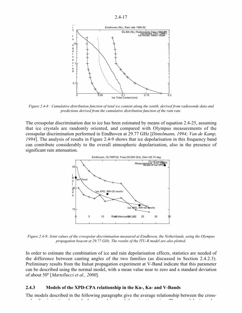
2.4-17

0.1

1

10

0 0.05 0.1 0.15 0.2

Percentage of Tim

Ice Total Content [cm]

Eindhoven (NL), Rain rate 1990-92

De Bilt (NL) Radiosonde Data 1980-89Ice Model, D20, D80

Ice Model, Mean value

Figure 2.4-8 : Cumulative distribution function of total ice content along the zenith, derived from radiosonde data andpredictions derived from the cumulative distribution function of the rain rate.

The crosspolar discrimination due to ice has been estimated by means of equation 2.4-25, assumingthat ice crystals are randomly oriented, and compared with Olympus measurements of thecrosspolar discrimination performed in Eindhoven at 29.77 GHz [Dintelmann, 1994; Van de Kamp,1994]. The analysis of results in Figure 2.4-9 shows that ice depolarisation in this frequency bandcan contribute considerably to the overall atmospheric depolarisation, also in the presence ofsignificant rain attenuation.

15

30

45

0 5 10 15 20 25 30 35

XPD [dB]

Rain Attenuation [dB]

Eindhoven, OLYMPUS, Freq=29.656 GHz, Elev=26.74 deg

Ice Cloud

Ice XPD, RR=30 mm/hr

Ice XPD, RR=40 mm/hr

ITU-R modelMeasurements, D10..D90

Model of Ice XPD

Figure 2.4-9: Joint values of the crosspolar discrimination measured at Eindhoven, the Netherlands, using the Olympuspropagation beacon at 29.77 GHz. The results of the ITU-R model are also plotted.

In order to estimate the combination of ice and rain depolarisation effects, statistics are needed ofthe difference between canting angles of the two families (as discussed in Section 2.4.2.3).Preliminary results from the Italsat propagation experiment at V-Band indicate that this parametercan be described using the normal model, with a mean value near to zero and a standard deviationof about 50º [Martellucci et al., 2000].

2.4.3 Models of the XPD-CPA relationship in the Ku-, Ka- and V-Bands

The models described in the following paragraphs give the average relationship between the cross-l di i i ti d t b th i d i d th i tt ti Th d l ( l

2.4-18

crosspolar discrimination. On the other hand these models tend to underestimate the crosspolardiscrimination at 30 GHz and in the 40/50 GHz frequency band at low levels of attenuation.

Furthermore, combined statistics of depolarisation and attenuation are necessary to assess themargins of both parameters required for a certain system outage probability [Mauri et al., 1987;Vasseur et al., 1996]. Therefore these models are mainly to be used for estimating the CDF of thecrosspolar discrimination, using the CDF of rain attenuation as input.

A description is also given of current models of the XPD-CPA relationship for rain and a newmodel is proposed, based on the assessment of each model against experimental results.

2.4.3.1 The ITU-R Model for Ka-Band and its extension to V-Band

This model permits the evaluation of the cumulative distribution function of crosspolardiscrimination by means of an equiprobability relationship between the attenuation and the XPD.Such a relationship can be also assumed as the average relationship between the two parameters[ITU-R, 1999].

The following parameters are needed:

Ap = the rain attenuation exceeded for the percentage of time p, dB.

o = tilt angle of the polarisation with respect to the local horizontal [degrees].(o =45° for circular polarisation)

f = frequency, GHz. The model can be used in the range 8 ) f ) 35 GHz

` = link elevation in degrees. The model can be used in the range ` ) 60°.

For the percentage of time p the crosspolar discrimination, due to rain, is lower than the valueXPD1,p:

( ) m`o CCCAVUXPD pp +<<<= log,1 2.4-27

where:

( )fU log30= = frequency dependent term.

ª©¨

))

))u=

GHz3520;6.22

GHz208;8.12 19.0

f

ffV = Attenuation dependent term [Fukuchi et al., 1984].

( )( )[ ]oo 4cos1484.01log10 +u<u=C = Polarisation dependent term.

( )`` log40 u=C = link elevation dependent term.

20052.0 pC mm = = parameter related to the fluctuation of the raindrops canting angle

during the events and from event to event. mp = 0°, 5°, 10°

when p = 1%, 0.1 %, 0.01 %.

It is assumed that due to the effect of ice particles the crosspolar discrimination is lower thanXPD

2,p, for the percentage of time p:

( )[ ]pXPDXPD pp log1.03.05.0,1,2 +uu= 2.4-28

The ice correction parameter has been empirically determined.

The crosspolar discrimination due to rain and ice is lower than the value XPD for the percentage

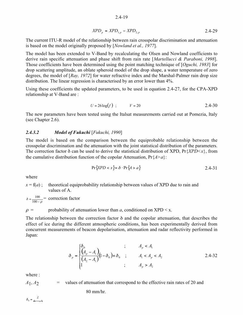
2.4-19

( )_b =

12

0

ppp XPDXPDXPD ,2,1 <= 2.4-29

The current ITU-R model of the relationship between rain crosspolar discrimination and attenuationis based on the model originally proposed by [Nowland et al., 1977].

The model has been extended to V-Band by recalculating the Olsen and Nowland coefficients toderive rain specific attenuation and phase shift from rain rate [Martellucci & Paraboni, 1998].Those coefficients have been determined using the point matching technique of [Oguchi, 1983] fordrop scattering amplitude, an oblate spheroid model of the drop shape, a water temperature of zerodegrees, the model of [Ray, 1972] for water refractive index and the Marshal-Palmer rain drop sizedistribution. The linear regression is characterised by an error lower than 4%.

Using these coefficients the updated parameters, to be used in equation 2.4-27, for the CPA-XPDrelationship at V-Band are :

( ) 20;log26 == VfU 2.4-30

The new parameters have been tested using the Italsat measurements carried out at Pomezia, Italy(see Chapter 2.6).

2.4.3.2 Model of Fukuchi [Fukuchi, 1990]

The model is based on the comparison between the equiprobable relationship between thecrosspolar discrimination and the attenuation with the joint statistical distribution of the parameters.The correction factor b can be used to derive the statistical distribution of XPD, Pr{XPD<x}, fromthe cumulative distribution function of the copolar Attenuation, Pr{A>a}:

{ } { }aAxXPD >u=< PrPr b 2.4-31

where

x = f(a) ; theoretical equiprobability relationship between values of XPD due to rain and values of A.

lb

<=

100

100 = correction factor

l = probability of attenuation lower than a, conditioned on XPD < x.

The relationship between the correction factor b and the copolar attenuation, that describes theeffect of ice during the different atmospheric conditions, has been experimentally derived fromconcurrent measurements of beacon depolarisation, attenuation and radar reflectivity performed inJapan:

( )( )

( )

««ª

««©

¨

>

<<+<<

<<

=

2

210012

1

10

;1

;1

;

AA

AAAAA

AAAA

p

pp

p

p bb

b

b 2.4-32

where :

A1, A2 = values of attenuation that correspond to the effective rain rates of 20 and

80 mm/hr.

2.4-20

rainfall events._ = stratus rain ratio. The ratio between the number of stratus rainfall events

and the total number of rain events. _<1(a value of 0.8 was suggested by Fukuchi).

The percentage of time during which the crosspolar discrimination due to rain and ice is lower thanXPD

p, Perc{XPD< XPD

p}, is calculated by multiplying the percentage of time, p, during which the

Crosspolar Discrimination due to rain ice is lower than XPDp, calculated according to the ITU/R

model (see equation 2.4-27, and the extension up to V-Band in equation 2.4-30), for thecorresponding ice correction factor b

p, derived using the cumulative distribution function of

attenuation Ap:

{ } pXPDXPD pp u=< bPerc 2.4-33

The model has been checked against measurements performed in Japan with ETS-II and the BSEpropagation experiments, with a good accuracy at 11.5 GHz (linear and circular polarisation) and afixed underestimation of about 6 dB at 34 GHz. This underestimation has been ascribed to the lackof accuracy of the attenuation statistical distribution. The model has also been checked using theITU/R database of XPD distribution, that contains data measured at frequencies from 11 to 35 GHz,and the prediction error was ±10% for the majority of experiments contained in the database.

2.4.3.3 Dissanayake, Haworth, Watson analytical model [Dissanayake et al., 1980]

The model is valid in the range 9-30 GHz and determines the relationship between rain crosspolardiscrimination and attenuation by means of small amplitude and phase approximations of the raintransmission matrix.

( ) mo` CCCAVUXPD p v+v<<v<v= log,12.4-34

where :

( ) ( )fxfxfU yy log9.2132.508.888.84 <+<=v = frequency dependent term (x = 0.759, y = 0.08).

20=vV = attenuation dependent term.

( )[ ]`` coslog40 u=C = link elevation dependent term.

( )[ ]oo 2sinlog20=vC = polarisation dependent term.

237.17 mm =C = parameter related to the distribution of the raindrop canting angle.

m = r.m.s raindrop canting angle [rad].

The depolarisation due to ice is determined, modelling the ice needles as prolate spheroids that liein the horizontal plane and applying Rayleigh scattering. The complex depolarisation ratio of linearand circular polarisation can be simplified assuming a small argument approximation and randomorientation of the needles.

( )o`2sin

2cos

22 ´

¦

¥²¤

£65 I

lX

( ) ( )o`/2cos

2cos

222 ´

¦

¥²¤

£6<5 I

lXArg 2.4-35

2.4-21

( )o`2exp

2cos

22 j

iX I

c ´¦

¥²¤

£65

where:

( )lkkI 21 <=6 = anisotropy of ice crystals, [rad].

ii Vukh/3

= = propagation constants of the polarisation parallel (i=1) and perpendicular

(i=2) to the symmetry axis of the particle.

l = path length, m

V = total volume of ice/m3. The total ice content is V*l.

h = wavelength, m.

ui = anisotropy coefficients for Rayleigh scattering.

For ice needles u1 = 0.7228 - i0.00285, u2 = 0.3468 - i0.00066.

As discussed earlier, the effect of the melting layer is ignored, because it is assumed to be anisotropic medium, and the combined effect of rain and ice particles on the complex depolarisationratio is determined by discarding the products of cross-polar terms. The overall depolarisation isobtained by adding the complex depolarisation ratio.

( ) ( )( )

( )

( ) ( )iceXrainXX

iceXrainT

rainTrainXX

ccc

lll

+5

+511

22

2.4-36

where:

T11

(rain), T22

(rain) = Copolar terms of the rain transmission matrix

2.4.3.4 Other models of the XPD-CPA relationship due to rain

In the literature other models can be found that describe the average relationship between copolarattenuation and the crosspolar discrimination due to rain.

Chu Model [Chu, 1982]

( ) 5.11log20,1 +<+<<<= xpp CCCCAUXPD m`o2.4-37

where :

( )fU log20= = frequency dependent term.

( ) ( )[ ]{ }20024.0exp4cos15.0log10  o mo <<uu=C = Polarisation dependent term.

m  = standard deviation of raindrops during a thunderstorm, (m  = 3 degrees)

( )[ ]`` coslog40 u=C = link elevation dependent term.

( ) ( ) px AC uuu= o` 2coscos075.0 2 = difference between horizontal and vertical polarisation.

20052.0 pC mm = = parameter related to the fluctuation of the raindrop canting angle

during the events and from event to event.

2.4-22

Stutzman and Runyon model [Stuzman and Runyon, 1984]

( ) ( )rCCCAUXPD pp log5.9log19,1 <++<<<= m`o 2.4-38

where :

( )fU log3.17= = frequency dependent term.

( ) ( )[ ]{ }20024.0exp4cos15.0log10  o mo <<uu=C = polarisation dependent term.

m 

= standard deviation of raindrops during a thunderstorm, (m  = 3 degrees)

( )[ ]`` coslog42 u=C = link elevation dependent term.

20052.0 pC mm = = parameter related to the fluctuation of the raindrop canting angle

during the events and from event to event.

r = fraction of non-spherical raindrops (see equation 2.4-19)

Nowland, Sharofsky and Olsen (NOS) model [Nowland et al., 1977]

( ) ( ) ( )LVCCCAVUXPD pp log201.4log,1 <+++<<<= m`o2.4-39

where :

( )fU log26= = frequency dependent term.

ª©¨

))

))=

GHz3515;23

GHz158;20

f

fV = attenuation dependent term (as ITU-R).

( )oo 2sinlog20 u=C = polarisation dependent term.

( )[ ]`` coslog40 u=C = link elevation dependent term.

20052.0 pC mm = = parameter related to the fluctuation of the raindrop canting angle

during the events and from event to event.

L = path length through rain (an empirical relationship has beensuggested by the authors).

Van de Kamp Model [Van de Kamp, 1999]

The parameters of this model have been determined by comparing a general XPD-CPA relationshipwith a large group of measurements performed at 29 different locations. The frequencies of themeasurements vary from 11 to 50 GHz, and the elevation angles from 3º to 50º. The polarisationangles vary from 0º to 180º, including also measurements at circular polarisation. The dependencyof each parameter has been assessed separately by selecting each time a group of measurementswhich are equal in all but one parameter.

The general equation that has been tested, using the measurements, is:

( ) ( ) ( ) SCCDCAVfCXPD xpp +<+<<<= mo `logloglog,12.4-40

where:

the model parameters are C V D and S

2.4-23

( ) UfC =u log = frequency dependent term.

o = polarisation tilt angle [degree]

oC = polarisation dependent term.

` = link elevation [degree]

( )[ ] `` CD =coslog = link elevation dependent term.

( ) ( ) px AC uuu= o` 2coscos075.0 2 = difference between horizontal and vertical polarisation

[Chu, 1982].20052.0 pC mm = = parameter related to the fluctuation of the raindrop canting angle.

S = constant value.

From the separate assessment of each equation with experimental values, we have:

C V D S

20 (11.6 to 29.7 GHz) 16.3 41 8

Table2.4-2: Parameters of the Van de Kamp model of rain XPD-CPA

For the experiments at frequencies from 28.5 to 49.5 GHz it was found that the correlation ismaximised for C equal to 25, in good agreement with the theoretical assessment performed inSection 2.4.3.1 (C=26).

In Figure 2.4-10, the model of equation 2.4-40 and all measurements used to perform modelassessment are plotted, normalised according to the following equation:

( )xnorm CCCUXPDXPD <<<<= `o2.4-41

Figure 2.4-10: General test of the model: normalised XPD versus CPA, for 45 experiments;and a curve fitted to the results (thick dashed line).

2.4.4 The effect of depolarisation on radio communication systems

In order to estimate the effect of atmospheric depolarisation on radio communication systems, adistinction must be made between full co-channel frequency reuse and frequency-interleaved reuse

0 5 10 15 20 25 30-30

-25

-20

-15

-10

-5

0

5

10

15

20

CPA (dB)

norm

alis

ed X

PD

(dB

)

45 experiments

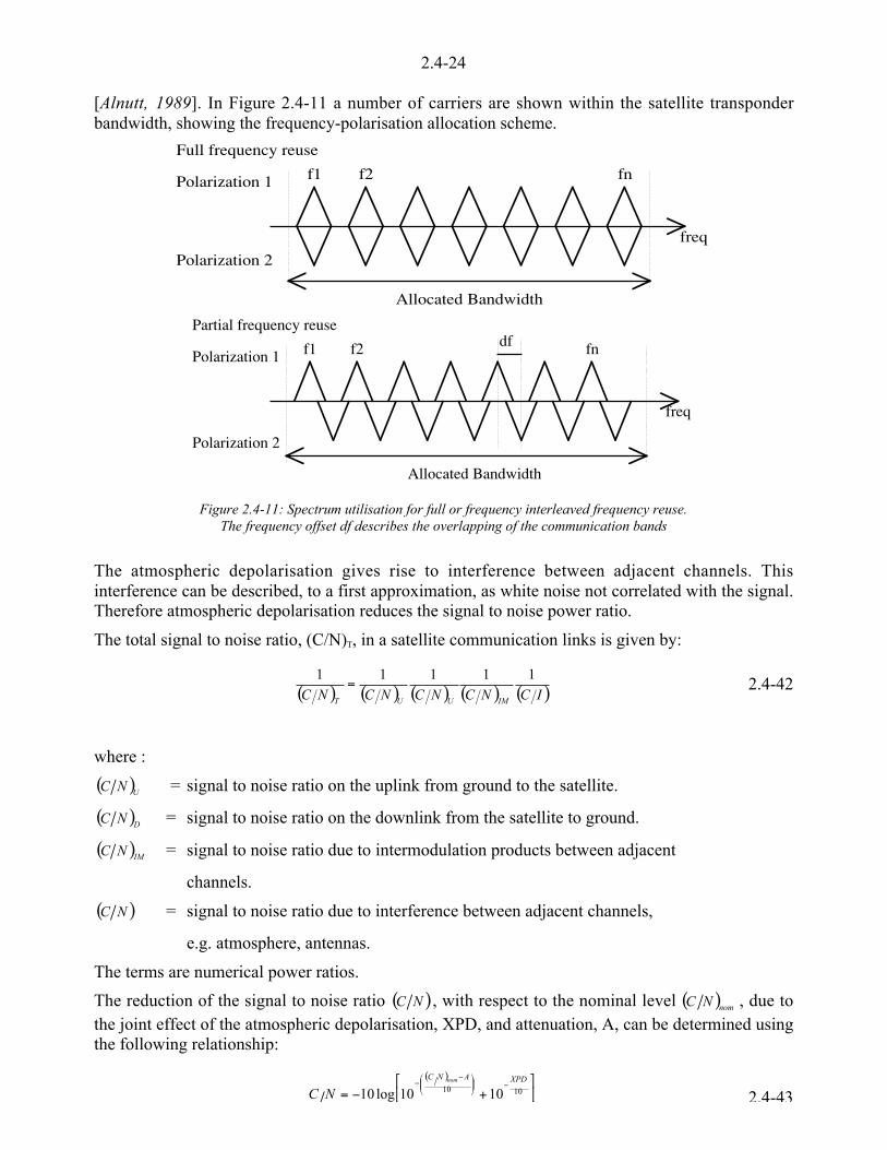
2.4-24

[Alnutt, 1989]. In Figure 2.4-11 a number of carriers are shown within the satellite transponderbandwidth, showing the frequency-polarisation allocation scheme.

Polarization 1

Polarization 2

f1 f2 fn

freq

Allocated Bandwidth

Full frequency reuse

Polarization 1

Polarization 2

f1 f2 fn

freq

Allocated Bandwidth

Partial frequency reusedf

Figure 2.4-11: Spectrum utilisation for full or frequency interleaved frequency reuse.The frequency offset df describes the overlapping of the communication bands

The atmospheric depolarisation gives rise to interference between adjacent channels. Thisinterference can be described, to a first approximation, as white noise not correlated with the signal.Therefore atmospheric depolarisation reduces the signal to noise power ratio.

The total signal to noise ratio, (C/N)T, in a satellite communication links is given by:

( ) ( ) ( ) ( ) ( )ICNCNCNCNC IMUUT

11111= 2.4-42

where :

( )UNC = signal to noise ratio on the uplink from ground to the satellite.

( )DNC = signal to noise ratio on the downlink from the satellite to ground.

( )IMNC = signal to noise ratio due to intermodulation products between adjacent

channels.

( )NC = signal to noise ratio due to interference between adjacent channels,

e.g. atmosphere, antennas.

The terms are numerical power ratios.

The reduction of the signal to noise ratio ( )NC , with respect to the nominal level ( )nomNC , due tothe joint effect of the atmospheric depolarisation, XPD, and attenuation, A, can be determined usingthe following relationship:

( )

µµ�

³³�

+<=<´́

¦

¥²²¤

£ <<

1010 1010log10XPDANC nom

NC 2.4-43

2.4-25

These relationships and the type of modulation employed by the radiocommunication system,define a bi-dimensional set of attenuation, A, and cross-polar discrimination values, XPD, that giverise to a bit error rate (BER) that is still below the desired threshold, e.g. 10

-6. This set of values, D,

is formed by the joint values of A and XPD that satisfy the following relationship:

( ) ( )BERTXPDAf >, 2.4-44

where :

( )XPDAf , = function of A, attenuation, and XPD, crosspolar discrimination.

( )BERT = threshold value which depends on the required Bit Error Rate (BER) and onthe system characteristics

The behaviour of attenuation and cross polar discrimination can be described by their jointprobability function ( )p A XPD, , where ( )p A XPD dAdXPD, is the probability that attenuation and

crosspolar discrimination are contained in the following ranges: A a A dA) < + ;XPD d XPD dXPD) < + .

Therefore the probability that the communication system is characterised by a BER lower than therequired threshold, in the presence of atmospheric attenuation and crosspolar discrimination, isgiven by the following relationship:

( ) ( )dAdXPDXPDApBERD

,Pr 00= 2.4-45

In order to estimate the performance of a frequency reuse communication system, the jointprobability density function ( )p A XPD, for the link site, frequency, adopted polarisation and

geometry is needed [Mauri et al., 1987].

2.4-26

2.4.5 References

[Alnutt, 1989]Alnutt J., “Satellite-to-ground Radiowave Propagation”, IEE Electromagnetic Waves Series, 29,1989

[Amaya, 1995]Amaya-Byrne C., “Depolarisation due to troposphere and its impact on satellite-to-earthcommunications”, PhD Thesis, Université Catholique de Louvain-la-Neuve, Belgium, June 1995.

[Aresu et al. 1995]Aresu A., A. Martellucci, A. Paraboni, R. Polonio, "Theoretical and experimental channelcharacterisation of spatial links at 20 and 50 GHz", Proceedings of 7th International Union of RadioScience Commission F Open Symposium "Wave Propagation and remote sensing", Ahmedabad,India, 20-24 November 1995, pp. 303-306.

[Aresu et al. 1994]Aresu A., E. Damosso, A. Martellucci, L. Ordano, A. Paraboni, "Depolarisation of electromagneticwaves due to rain and ice: theory and experimental results", Alta Frequenza, Vol. 6, N. 6,November-December 1994, pp 70-75

[Aresu et al. 1993]Aresu A., Martellucci A. and Paraboni A., "Experimental assessment of rain anisotropy and cantingangle in horizontal path at 30 GHz", IEEE Trans. on Antennas and Propagation, Vol. 41, No. 9, pp.1331-1335, September 1993

[Capsoni & Paraboni, 1972]Capsoni C.and Paraboni A., “Depolarisation of an EM Wave traveling through a stratified aerosolof non spherical scatterers”, AGARD EPP Tech. Meeting, Gausdal Norway, Sept. 1972.

[Capsoni et al., 1981Capsoni C., Paraboni A., Fedi F., Maggiori D.,“A model oriented approach to measure rain inducedcrosspolarisation”, Annal. de Telecommunicat., Vol. 36, n. 1-2, Jan-Feb. 1981.

[Chu, 1982]Chu, T. S., “A semi-empirical formula for microwave depolarisation versus rain attenuation onearth-space paths”, IEEE Trans. Commun., COM-30(12), 2550-2554, 1982.

[Dintelmann, 1994]Dintelmann F. (Editor), “Reference Book on Depolarisation”, OPEX- ESA WPP-083, 1994.

[Dissanayake et al., 1980]Dissanayake A. W., Haworth D. P. and Watson P. A, “Analytical models for cross-polarisation onearth space radio paths for frequency range 9-30 GHz” H., Ann. Telecommunic., 35, n° 11-12,1980, pp 398-404.

[Fukuchi, 1990]Fukuchi H., “Prediction of depolarisation distribution on earth-space paths”, IEE Proceedings, Vol.137, Pt. II, n. 6, December 1990.

[Fukuchi et al., 1984]Fukuchi H J Awaka and T Oguchi “Improved theoretical formula for the relationship between

2.4-27

[ITU-R, 1999]ITU-R, P 618-6, “Propagation data and prediction methods required for the design of Earth-spacetelecommunication systems”, 1999,

[Martellucci et al., 1993]Martellucci A., Mauri M. and Paraboni A., “The physical basis of depolarisation”, Proceedings ofOlympus Utilisation Conference, (Sevilla, Spain), 20-22 April 1993, pp. 573-581.

[Martellucci & Paraboni, 1994]Martellucci A. and Paraboni A., "Modelling of Depolarisation due to Hydrometeors: Utilisation ofmultipolarisation radiowave beacon for estimation of quasi-phyisical parameters", Proc. of PIERS94, ESA, Noordwijk,The Netherlands, July 11-15 1994.

[Martellucci & Paraboni, 1998]Martellucci A. and A. Paraboni, “Test and Development of Models of Atmospheric CrosspolarDiscrimination for Satellite Communication Systems at Ka- and V-Band”, Proceed. of the firstinternational Workshop on Radiowave Propag. Model. for SatCom Serv. at Ku-band and above,Estec, Noordwijk, The Netherlands, 28-29 October 1998

[Martellucci et al., 2000]Martellucci A., Paraboni A. and Filipponi M. “Measurements and modeling of rain and icedepolarisation on spatial links in the Ka- and V-Bands”, invited paper, AP2000 MillenniumConference on Antennas and Propagation, Davos, Switzerland, 9-14 April 2000.

[Mauri et al., 1987]Mauri M., A. Paraboni and D. Tarducci, “Depolarisation Measurements and their use in thedetermination of dual polarisation links performance”, Alta Frequenza, Vol. LVI, No. 1-2, Jan.-Apr.1987

[Nowland et al., 1977]Nowland W.L., Olsen R. L., Shkarofsky, “Theoretical relationship between rain depolarisation andattenuation”, Electronics Letters, Vol. 13, No. 22, pp 676-678, 27 October 1977

[Oguchi, 1983]Oguchi T., “Electromagnetic wave propagation and scattering in rain and other hydrometeors”,Proc. IEEE, Vol. 71, No. 9, pp. 1029-1078, September 1983.

[Paraboni et al. 1997]Paraboni A., A. Martellucci and R. Polonio, “A probabilistic model of rain and ice depolarisationbased on the experimental estimation of the atmospheric ice content”, Proc SBMO/IEEEInternational Microwave and Optoelectronics Conference, Natal, Brazil, 11-14 August 1997, pp707-712

[Paraboni et al., 1998]Paraboni A., A. Martellucci, R. Polonio, “Statistical Modelling of Depolarisation due to Rain andIce During Thunderstorms Based on the Italsat and Olympus Measurements”, Proc. 8th URSICommission F Triennial Open Symposium, , Aveiro, Portugal, 22-25 September 1998, pp. 288-291.

[Poiares Baptista & Davies, 1994]Poiares Baptista, J.P.V. and Davies P. G. (Editors), “OPEX: Reference Book on Attenuationmeasurements and prediction”, ESA WPP-83, November 1994.

2.4-28

[Poiares Baptista, 1994]Poiares Baptista J.P.V. (Editor), “Reference Book on Radar”, OPEX- ESA WPP-083, November1994.

[Ray, 1972 ]Ray P. S., “Broad Band Complex refractive index of ice and water”, Applied Optics, Vol. 11, No. 8,1972.

[Stuzman and Runyon, 1984]Stutzman, W. L., and D. L. Runyon, “The relationship of rain- induced cross-polarisationdiscrimination to attenuation for 10 to 30 GHz earth-space radio links”, IEEE Trans. AntennasPropagat., AP-32(7), 705-710, 1984.

[Van de Kamp, 1999]Van de Kamp M. (1999), “Depolarisation due to rain: the XPD-CPA relation”, Int. J. Sat. Com.,Vol. 9, Issue 3, pp. 285-301, 2001.

[Vasseur et al., 1996]Vasseur, H., I. Adams, C. Amaya, and D. Vanhoenacker (1994), “Comparison of Yearly Statisticswith CCIR Prediction Methods”, Proceedings of 21st Meeting of Olympus PropagationExperimenters, OPEX XXI, Louvain-la-Neuve, Belgium, May 1994, 80-89.

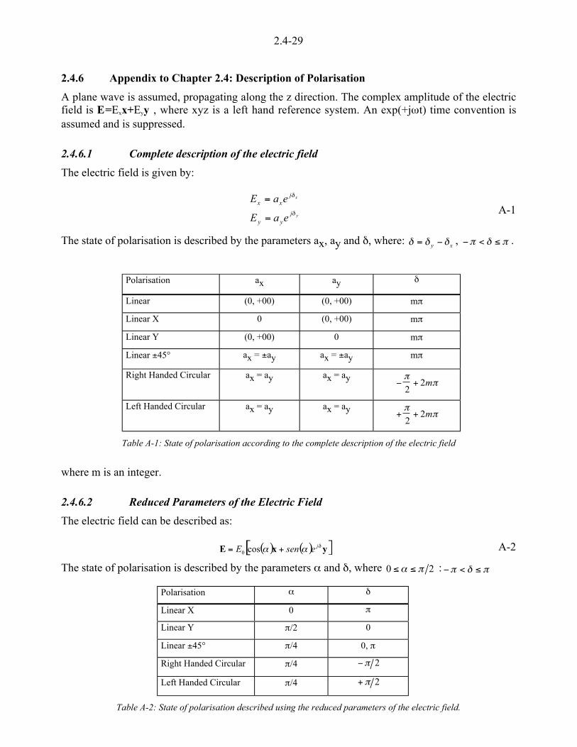
2.4-29

2.4.6 Appendix to Chapter 2.4: Description of Polarisation

A plane wave is assumed, propagating along the z direction. The complex amplitude of the electricfield is E=Exx+Eyy , where xyz is a left hand reference system. An exp(+jtt) time convention isassumed and is suppressed.

2.4.6.1 Complete description of the electric field

The electric field is given by:

y

x

jyy

jxx

eaE

eaEb

b

=

=A-1

The state of polarisation is described by the parameters ax, ay and b, where: b b b= <y x , < < )/ b / .

Table A-1: State of polarisation according to the complete description of the electric field

where m is an integer.

2.4.6.2 Reduced Parameters of the Electric Field

The electric field can be described as:

( ) ( )[ ]yxE b__ jesenE += cos0A-2

The state of polarisation is described by the parameters _ and b, where 0 2) )_ / :< < )/ b /

Table A-2: State of polarisation described using the reduced parameters of the electric field.

Polarisation ax ay b

Linear (0, +00) (0, +00) m/

Linear X 0 (0, +00) m/

Linear Y (0, +00) 0 m/

Linear ±45° ax = ±ay ax = ±ay m/

Right Handed Circular ax = ay ax = ay < +/

/2

2m

Left Handed Circular ax = ay ax = ay + +/

/2

2m

Polarisation _ b

Linear X 0 /

Linear Y //2 0

Linear ±45° //4 0, /

Right Handed Circular //4 </ 2

Left Handed Circular //4 + / 2

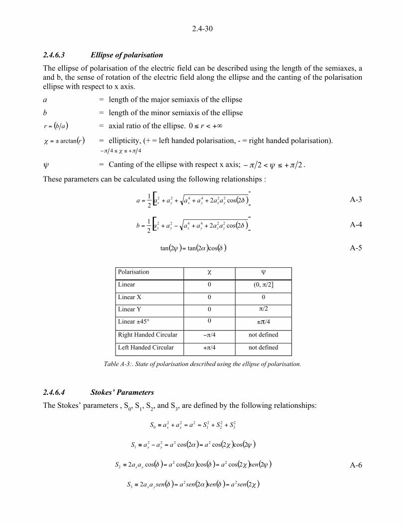
2.4-30

2.4.6.3 Ellipse of polarisation

The ellipse of polarisation of the electric field can be described using the length of the semiaxes, aand b, the sense of rotation of the electric field along the ellipse and the canting of the polarisationellipse with respect to x axis.

a = length of the major semiaxis of the ellipse

b = length of the minor semiaxis of the ellipse

( )abr = = axial ratio of the ellipse. 0 ) < +'r

( )rarctan±=r = ellipticity, (+ = left handed polarisation, - = right handed polarisation). 44 /r/ +))<

s = Canting of the ellipse with respect x axis; < < ) +/ s /2 2 .

These parameters can be calculated using the following relationships :

( )[ ]b2cos221 224422

yxyxyx aaaaaaa ++++= A-3

( )[ ]b2cos221 224422

yxyxyx aaaaaab ++<+= A-4

( ) ( ) ( )b_s cos2tan2tan = A-5

Table A-3:. State of polarisation described using the ellipse of polarisation.

2.4.6.4 Stokes’ Parameters

The Stokes’ parameters , S0, S

1, S

2, and S

3, are defined by the following relationships:

23

22

21

2220 SSSaaaS yx ++==+>

( ) ( ) ( )sr_ 2cos2cos2cos 22221 aaaaS yx ==<>

( ) ( ) ( ) ( ) ( )srb_b 22coscos2coscos2 222 senaaaaS yx ==> A-6

( ) ( ) ( ) ( )rb_b 222 223 senasensenasenaaS yx ==>

Polarisation r s

Linear 0 (0, //2]

Linear X 0 0

Linear Y 0 //2

Linear ±45° 0 ±//4

Right Handed Circular <//4 not defined

Left Handed Circular +//4 not defined

2.4-31

The vector S = (S1, S2, S3) can be used to describe the polarisation. The extremes of this vector arelocated on a sphere, that is called the Poincaré sphere, whose radius is equal to S

0. Orthogonal

polarisations are described by opposite Stokes’ vectors, making the identification simple.

Table A-4: State of polarisation described using the Stokes’ parameters.

2.4.6.5 Complex Polarisation Factor

The complex polarisation ratio, p, is the ratio between the component of the electrical field:

( ) b_ j

x

y eE

Ep tan== A-7

This complex parameter represents the stereographic projection of a point on the Poincaré sphere onthe plane orthogonal to axis S1, with Re(p) parallel to S2 and Im(p) parallel to S3.

Table A-5: State of polarisation described using the complex polarisation factor.

2.4.6.6 Complex canting angle of the polarisation ellipse

The complex canting angle of the polarisation is given by the following relationship:

( ) p=\tan A-8

This parameter is related to the parameters of the polarisation ellipse by the following relationships:

( ) s=\Re = canting angle of the ellipse with respect x axis. ( ) 2Re2 // +)\<<

( )[ ]\=> Imtanhbar = axial ratio of the ellipse. +'<) r0

Polarisation S

Linear (S1 , S2, 0)

Linear X (S0 , 0, 0)

Linear Y (-S0 , 0, 0)

Linear ±45° (0 , ±S0, 0)

Right Handed Circular (0 , 0, -S0)

Left Handed Circular (0 , 0, S0)

Polarisation Re(p) Im(p)

Linear [0,+ ') 0

Linear X 0 0

Linear Y ' 0

Linear ±45° ±1 0

Right Handed Circular 0 -1

Left Handed Circular 0 +1

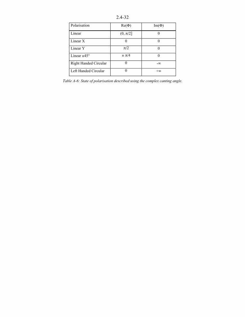
2.4-32

Table A-6: State of polarisation described using the complex canting angle.

Polarisation Re(\) Im(\)

Linear (0, //2] 0

Linear X 0 0

Linear Y //2 0

Linear ±45° ± //4 0

Right Handed Circular 0 -'

Left Handed Circular 0 +'

2.5-1

CHAPTER 2.5Combination of Different Attenuation Effects

Editor: Erkki Salonen1

Authors: Marina Boumis2, Laurent Castanet3, Hahtokari K. 4, Antonio Martellucci5, Carlo Riva6

Peter Watson7, Charles Wrench8

1 University of Oulu Telecommunication Lab. P.O.Box 444 FIN-90571 Oulu Finland

Tel: +358 40 524 2406 Fax: +358-8-553 2845 E-m: Erkki.Salonen@ee.oulu.fi

2 Fondazione Ugo Bordoni,Radiocommunications Dept., Viale Europa 190, I-00144 Rome, Italy

Tel: +39-6-5480-2118, Fax: +39-6-5480-4401, e-mail: mboumis@fub.it

3 ONERA-CERT DEMR, 2 Avenue Edouard Belin, BP4025, F-31055 Toulouse, Cedex 4 France

Tel: +33-562-25-2729, Fax: +33-562-25-2577, E-m: laurent.castanet@onecert.fr

4 University of Oulu Telecommunication Lab. P.O.Box 444, FIN-90571 Oulu, Finland

Tel: +358 40 524 2406, Fax: +358-8-553 2845

5 European Space Agency, ESA-ESTEC, Keplerlaan 1, PB 299, NL-2200 AG Noordwijk, The Netherlands

Tel: +31-71-565-5603, Fax: +31-71-565-4999, e-mail: Antonio.Martellucci@esa.int

6 Dipartimento di Elettronica e Informazione, Politecnico di Milano, P.zza L. Da Vinci 32, 20133 Milano, Italy.

Tel.: +39-02-23993586, Fax.: +39-02-23993413, e-mail: riva@elet.polimi.it

7 Electronic and Electrical Engineer., University of Bath, Claverton Down, Bath BA2 7AY, United Kingdom

Tel: +44-1225 826330, Fax: +44-1225 826412, e-mail: p.a.watson@bath.ac.uk

8 CCLRC Rutherford Appleton Labs Chilton Didcot Oxfordshire OX11 0QX United Kingdom

2.5-2

2.5 Combination of Different Attenuation Effects

2.5.1 Introduction

Since the telecommunication scenario is characterised by allowed outage percentages of the orderof 1% (low availability systems) and small earth terminals, rain is no more the dominatingattenuation phenomenon and the effects of the melting layer, clouds, water vapour and oxygen mustbe taken into account as well. When the statistical distributions of the different attenuationphenomena are calculated separately, the problem is how these attenuation phenomena can becombined to get the total attenuation distribution.

In this chapter, mathematical and statistical tools for combining different phenomena are presented,together with the assumptions required for different methods.

Correlation studies of different attenuation phenomena, that are essential to find reasonable rules orassumptions for combining methods, have been performed using different databases and arepresented in Section 2.5.3.

In Sections 2.5.4 to 2.5.8, most interesting published methods for calculating the total fadedistribution, as well as methods developed during the COST 255 project, are described andevaluated from the physical point of view. Also the applicability of each method for globalprediction is considered.

2.5.2 Statistical tools for combination of phenomena

Various possibilities for statistical combination are briefly reviewed in this section. They can beconsidered as building blocks for different methods of calculating total attenuation distributions.The required assumptions for these mathematical tools are also presented.

2.5.2.1 Equiprobability summing

Equiprobability summing means adding attenuation levels for equal probabilities, i.e., totalattenuation from the two attenuation distributions A1(P) and A2(P) is simply:

( ) ( ) ( ) P APAPAtot 21 += 2.5-1

This method assumes that the different effects are fully correlated. In practice, two (or more)attenuation phenomena are not fully correlated and therefore equiprobability summing givespessimistic values for low outage times. Thus, the equiprobability summing may be used for theworst case approximation.

2.5.2.2 Convolution method

Considering that two fade phenomena are not correlated, their statistical distributions can becombined in an independent way. The cumulative distribution P(At) of the total attenuation At isthen described by the convolution:

dAAAPApAP t

A

t

t

)()()( 21 <= 0'<

2.5-2

where: p1(A) is the probability density distribution of fade phenomenon 1

P2(A) is the cumulative distribution due to fade phenomenon 2.

2.5-3

This method can be applied numerically so that the both distributions are divided into n equallyspaced probability interval 6p about pi (pi-6p/2, pi+6p/2). All combinations of the fade A1,i and fadeA2,j are first summed as Aij= A1,i + A2,j, and then the sums Aij are ranked in order of size to obtainthe cumulative total fade distribution.

2.5.2.3 Disjoint summing

Considering that two phenomena are disjoint, their statistical attenuation distributions can becombined by adding the probabilities for given attenuation levels. A typical case is whenattenuation effects are calculated separately for rain and non-rain conditions. Then, we get

( ) ( ) ( ) a A P a A P a AP rainnon-rain t >+>=> 2.5-3

where:

At = total attenuation

The probabilities for the rain and non-rain components are calculated over the total (rainy and non-rainy) time.

Disjoint summing is recommended if it is possible to calculate disjoint distributions. Unfortunately,the required meteorological input parameters are not usually available separately, i.e. for rainy time,non-rainy cloudy time and clear-sky time.

2.5.2.4 Disjoint summing of monthly distributions

One way to decrease the error due to combination is first to calculate monthly distributions of totalattenuation using some approximation and then to calculate the annual distribution using disjointsumming from monthly distributions. This method is used in the combining method of [Feldhake,1997] and using the monthly prediction model of [Konefal et al., 1999]. One problem with thismethod is that it is difficult to find reliable worldwide input data on a monthly basis.

2.5.2.5 Root-sum-square addition

One possible method for combining two attenuation distributions is to use the following formula:

( ) ( ) ( )222

1 PAPAPAtot += 2.5-4

It is easy to see that this equation gives smaller values for total attenuation than the equiprobability

summing if equation 2.5-1 is written as:

( ) ( ) ( )[ ] )()(2)()( 212

22

12

21 PAPAPAPAPAPAPAtot ++=+= 2.5-5

Therefore it is clear that equation 2.5-4 generally underestimates the combined attenuation. Forexample, the average combined attenuation is smaller than the sum of the averages of thecomponents. One feature of equation 2.5-4 is that the effect of the smaller component decreaseswhen the bigger component increases, for example, in the case A1 =A2=1 dB the result is 1.41 dBbut if A1 =1 dB and A2=10 dB the result is 10.1 dB. Due to these numerical properties, this methodis not generally useful for combination purposes.

2.5.2.6 Coherent summing

If all attenuation phenomena can be calculated for a given time tI, then total attenuation can be

2.5-4

( ) -=

=n

jijitot tAtA

1

)( 2.5-6

When the total attenuation values are calculated for a given period, the distribution for that periodcan easily be produced. However, it is difficult to find a single time series source for all thenecessary radio-meteorological input data and anyway the amount of these data would be enormousfor global predictions. Therefore, this method can be used only as a reference method to test othercombination methods for such cases, when different phenomena can be calculated from thecommon time series data set.

2.5.3 Studies of dependencies of different attenuation phenomena

In this section, dependencies of different phenomena are discussed and some results based on thecalculations using data from ECMWF numerical analyses and radiosonde measurements arepresented.

The dependencies for the following cases are considered:

• oxygen attenuation vs. water vapour attenuation

• cloud attenuation vs. gas attenuation

• total attenuation due to gases and clouds both in rainy and non-rainy conditions

• effects of scintillation fading on total fading.

2.5.3.1 Water vapour and oxygen attenuation

The vertical profiles from the ECMWF numerical analyses have been used in correlation studiesbetween oxygen and water vapour attenuation. The zenith attenuation values at 50 GHz for bothoxygen and water vapour have been calculated using the method of [Liebe, 1989]. At 50 GHz theoxygen attenuation is already significant and the attenuation variations due to oxygen and watervapour may be of the same order, particularly in high latitudes.

The results are presented in scattergrams for six locations in different climates. Figure 2.5-1 showsthat the oxygen attenuation is almost constant at tropical sites, because the temperature and pressurevariations are very small. In the most northerly site (latitude 67.5° N), the attenuation variations ofoxygen and water vapour are of the same order, because the amount of water vapour dependsstrongly on temperature while the oxygen attenuation depends inversely on the temperature.

The zenith oxygen attenuation estimated by the ITU-R method [ITU-R, 1997a] is higher (1.57 dB at15 ºC) than the values calculated from the vertical profiles at tropical sites. This over-estimation canbe ascribed to the temperature correction factor of the ITU-R model, (see Chapter 2.1). The effectof ground temperature can be considered using the method of [Salonen, 1991].

Because the other attenuation phenomena (fading due to clouds, rain and tropospheric scintillation)are more severe in the summer period, the oxygen attenuation correlates inversely with otherattenuation phenomena. If annual mean oxygen attenuation is used, it causes a slight overestimationfor the predicted total attenuation in particular at such sites where temperature changes betweensummer and winter are large.

2.5.3.2 Attenuation due to clouds and gases

The correlation between cloud and water vapour attenuation has been studied using the time seriesof the vertical profiles from the ECMWF numerical analysis. The attenuation has been calculatedusing the [Salonen and Uppala, 1991] model for cloud attenuation and model of [Liebe, 1989] for

2.5-5

Figure 2.5-1: Oxygen attenuation vs. vapour attenuation at 50 GHz at different sites.

The scattergrams in Figures 2.5-2 and 2.5-3 show the dependencies of calculated water vapourattenuation and cloud attenuation at 40 GHz at 12 locations with different climates. They show clearcorrelation between water vapour and cloud attenuation at all sites, but the correlation is highest attropical sites and lowest at mid-latitude sites. Similar results have been obtained at frequenciesbetween 20 and 50 GHz.

Therefore, it may be assumed that a good combining method for water vapour and cloud attenuationcan be found if a weighted sum of the equiprobability method and the convolution method is used.It can be written in the form:

)()1()()( ,, PAqPAqPA convgceqgcgc u<+u= 2.5-7

where:

q = weight (0<q<1)

Agc,eq , Agc,conv = gas and cloud attenuation values combined using the equiprobabilitysumming and the convolution method, respectively.

Using the time series data from the ECMWF numerical analysis, the distribution from the coherentsumming can be calculated and used as a reference distribution.

The optimum weight values q for different sites at frequencies of 20, 40 and 50 GHz were found byfitting equation 2.5-7 with the distributions from the coherent summing results. The highest valuesare at tropical sites, which may be caused by the fact that the temperature variations are very smalland then high water vapour density means also high relative humidity, which is a condition forcloud forming.

2.5-6

Figure 2.5-2: Calculated water vapour attenuation vs. cloud attenuation for six northern and mid-latitude sites.

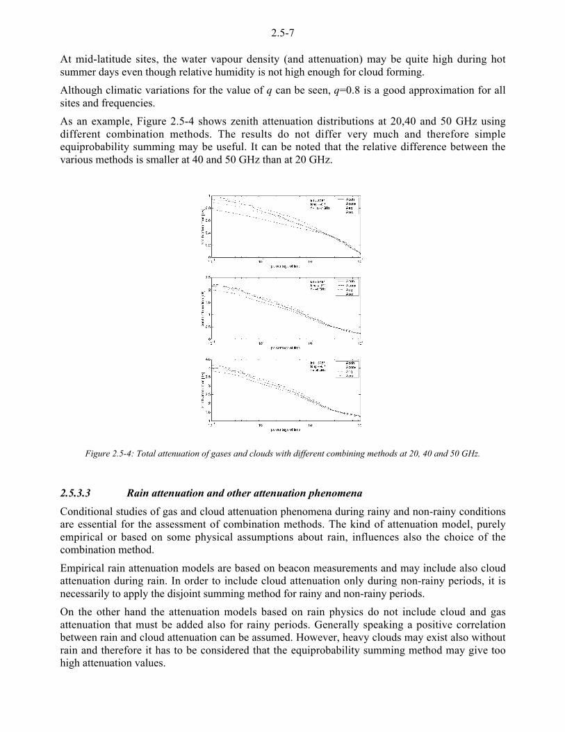
2.5-7

At mid-latitude sites, the water vapour density (and attenuation) may be quite high during hotsummer days even though relative humidity is not high enough for cloud forming.

Although climatic variations for the value of q can be seen, q=0.8 is a good approximation for allsites and frequencies.

As an example, Figure 2.5-4 shows zenith attenuation distributions at 20,40 and 50 GHz usingdifferent combination methods. The results do not differ very much and therefore simpleequiprobability summing may be useful. It can be noted that the relative difference between thevarious methods is smaller at 40 and 50 GHz than at 20 GHz.

Figure 2.5-4: Total attenuation of gases and clouds with different combining methods at 20, 40 and 50 GHz.

2.5.3.3 Rain attenuation and other attenuation phenomena

Conditional studies of gas and cloud attenuation phenomena during rainy and non-rainy conditionsare essential for the assessment of combination methods. The kind of attenuation model, purelyempirical or based on some physical assumptions about rain, influences also the choice of thecombination method.

Empirical rain attenuation models are based on beacon measurements and may include also cloudattenuation during rain. In order to include cloud attenuation only during non-rainy periods, it isnecessarily to apply the disjoint summing method for rainy and non-rainy periods.

On the other hand the attenuation models based on rain physics do not include cloud and gasattenuation that must be added also for rainy periods. Generally speaking a positive correlationbetween rain and cloud attenuation can be assumed. However, heavy clouds may exist also withoutrain and therefore it has to be considered that the equiprobability summing method may give toohigh attenuation values.

2.5-8

Comparisons using radiosonde data and synoptic observations

The measurement of profiles of meteorological parameters by means of radiosondes can be used toassess the different condition of the atmosphere in the absence of rain and during precipitation.

To this end, a small data set of available radiosonde data, containing measurements performed bothduring rain and in the absence of precipitation has been used (see Chapter 3.2). The presence ofprecipitation is derived from meteorological synoptic data, measured at the time of the radiosondelaunch. The sites have been selected according to data quality and quantity. The cloud water contentvalues have been estimated from radiosonde data using the model proposed by [Salonen et al.,1990]. Table 2.5-1 lists the sites that have been examined, extracted from the database ofradiosonde measurements described in Chapter 2.1

Station Name Country Latitude Longitude A.s.l. Years Launch/day

STORNOWAY UK 58.13 -6.59 14 10 2

HEMSBY-IN-NORFOLK UK 52.41 1.41 13 10 2

DE-BILT NL 52.06 5.11 2 10 2

LYON/SATOLAS FR 45.44 5.05 240 10 2

Table 2.5-1: List of sites examined

Due to the large sample period, the data measured during rainy periods have been checked in orderto avoid any bias resulting from scarcity or concentration of data in one season of the year.

The radiosonde data set has been used to calculate zenith attenuation due to oxygen, water vapourand clouds at 40 and 50 GHz, using the model of [Liebe et al., 1993] (see also Chapter 2.1). Foreach site, the statistics of total vapour and liquid content as well as oxygen, vapour, cloud, gaseousand total attenuation have been derived. The difference between the cumulative distributionfunction derived from the full set of radiosonde measurements (rain and non-rain) and that derivedfrom the radiosonde data collected in the absence of rain, can be described by:

( ) ( ) ( )( )pX

pXpXp

F

FNRNR

<=6 2.5-8

where:

XF(p) = value of the parameter X (e.g. attenuation) exceeded by p% of measurements,

calculated using the full set of radiosonde measurements (rain and non-rain).

XNR(p) = value of the parameter X (e.g. attenuation) exceeded by p% of measurements,

calculated using only the radiosonde data collected in absence of rain.

The results for the examined sites show that, in general, the use of meteorological data collected inthe absence of rain can lead to an underestimation of total attenuation with respect to the valuesobtained using radiosonde measurements collected both in rain and in non-rain conditions. This isdue to higher values of both the total water vapour and liquid content in presence of rain.

In Figure 2.5-5 values are shown of 6NR in Stornoway for the gaseous, cloud, total (gas+cloud)attenuation at 40 GHz (a) and 50 GHz (b) and for the total water vapour and cloud liquid content(c).

The difference in total attenuation is about 10-20% at 40 GHz and 7-13 % at 50 GHz and thedifferences of cloud attenuation statistics predominate over gaseous attenuation.

2.5-9

-40

-35

-30

-25

-20

-15

-10

-5

0

0.1 1 10

Difference between Ful

Percentage of samples %

Stornoway, UK, Radiosonde Data, 1980-89, MPM93, 40 GHz

Total Attenuation (Gas+Cloud)Cloud Attenuation Gas Attenuation

-40

-35

-30

-25

-20

-15

-10

-5

0

0.1 1 10

Difference between Ful

Percentage of Samples %

Stornoway, UK, Radiosonde Data, 1980-89, MPM93, 50 GHz

Total Attenuation (Gas+Cloud)Cloud AttenuationGas. Attenuation

a) b)

-40

-35

-30

-25

-20

-15

-10

-5

0

0.1 1 10

Difference between Fu

Percentage of samples %

Stornoway, UK, Radiosonde Data, 1980-89

Total Vapour ContentTotal Liquid Content

c)

Figure 2.5-5 Difference 6NR for the attenuation of different atmospheric components at

40 GHz (a), 50 GHz (b) and of total vapour and cloud liquid content (c).

This effect can be ascribed mainly to the presence of higher values of liquid water in the set ofmeasurements carried out during rain, as shown in Figure 2.5-5c. However the atmospheric contentof water vapour is also higher during precipitation.

Comparisons using data from the ECMWF weather forecast system

The gas and cloud attenuation values can also be calculated from the vertical profiles of theECMWF numerical analyses. For separating rainy and non-rainy periods, the predicted rainfallsfrom the ECMWF weather forecast system have been used. The estimate for rainy periods was thatthe total forecast 6-h rain amount was greater than a given threshold both before and after the timeof vertical profile. The proper threshold was found so that the rain probability is in close agreementwith the measured rainfall rate. The gas and cloud attenuation distributions for different locationswere calculated for rainy and non-rainy periods as well as for the whole measurement period. Alsoin this case the results show that, as expected, gas and cloud attenuation values are usually higherduring rainy periods than during non-rainy periods.

In particular for tropical locations these differences are rather large, although the highest gas andcloud attenuation values in rainy and non-rainy conditions are very similar.

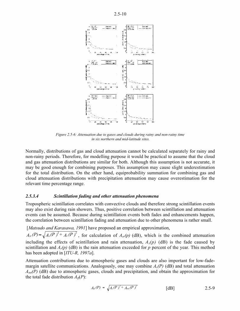
2.5-10

Figure 2.5-6: Attenuation due to gases and clouds during rainy and non-rainy time in six northern and mid-latitude sites.

Normally, distributions of gas and cloud attenuation cannot be calculated separately for rainy andnon-rainy periods. Therefore, for modelling purpose it would be practical to assume that the cloudand gas attenuation distributions are similar for both. Although this assumption is not accurate, itmay be good enough for combining purposes. This assumption may cause slight underestimationfor the total distribution. On the other hand, equiprobability summation for combining gas andcloud attenuation distributions with precipitation attenuation may cause overestimation for therelevant time percentage range.

2.5.3.4 Scintillation fading and other attenuation phenomena

Tropospheric scintillation correlates with convective clouds and therefore strong scintillation eventsmay also exist during rain showers. Thus, positive correlation between scintillation and attenuationevents can be assumed. Because during scintillation events both fades and enhancements happen,the correlation between scintillation fading and attenuation due to other phenomena is rather small.

[Matsudo and Karasawa, 1991] have proposed an empirical approximation,

)(PA + )(PA (P)A rssr225 , for calculation of Asr(p) (dB), which is the combined attenuation

including the effects of scintillation and rain attenuation, As(p) (dB) is the fade caused byscintillation and Ar(p) (dB) is the rain attenuation exceeded for p percent of the year. This methodhas been adopted in [ITU-R, 1997a].

Attenuation contributions due to atmospheric gases and clouds are also important for low-fade-margin satellite communications. Analogously, one may combine As(P) (dB) and total attenuationAtot(P) (dB) due to atmospheric gases, clouds and precipitation, and obtain the approximation forthe total fade distribution Atf(P):

)(PA + )(PA (P)A2

tot2

stf = [dB] 2.5-9

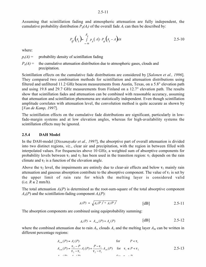
2.5-11

Assuming that scintillation fading and atmospheric attenuation are fully independent, thecumulative probability distribution Ptf(At) of the overall fade At can then be described by:

( ) ( ) ( ) dAAt

Aa

Pt

A

As

pt

Atf

P <u0'<

= 2.5-10

where:

ps(A) = probability density of scintillation fading

Pa(A) = the cumulative attenuation distribution due to atmospheric gases, clouds andprecipitation.

Scintillation effects on the cumulative fade distributions are considered by [Salonen et al., 1996].They compared two combination methods for scintillation and attenuation distributions usingfiltered and unfiltered 11.2 GHz beacon measurements from Austin, Texas, on a 5.8° elevation pathand using 19.8 and 29.7 GHz measurements from Finland on a 12.7° elevation path. The resultsshow that scintillation fades and attenuation can be combined with reasonable accuracy, assumingthat attenuation and scintillation phenomena are statistically independent. Even though scintillationamplitude correlates with attenuation level, the convolution method is quite accurate as shown by[Van de Kamp, 1997].

The scintillation effects on the cumulative fade distributions are significant, particularly in low-fade-margin systems and at low elevation angles, whereas for high-availability systems thescintillation effects may be ignored.

2.5.4 DAH Model

In the DAH-model [Dissanayake et al., 1997], the absorptive part of overall attenuation is dividedinto two distinct regions, viz., clear air and precipitation, with the region in between filled withinterpolated values. For frequencies above 10 GHz, a weighted sum of absorptive components forprobability levels between o1 and o2 has been used in the transition region: o1 depends on the rainclimate and o2 is a function of the elevation angle.

Above the o2 level, the impairments are entirely due to clear-air effects and below o1 mainly rainattenuation and gaseous absorption contribute to the absorptive component. The value of o1 is set bythe upper limit of rain rate for which the melting layer is considered valid(i.e. R ) 2 mm/h).

The total attenuation At(P) is determined as the root-sum-square of the total absorptive componentAa(P) and the scintillation-fading component As(P):

)(PA + )(PA (P)A2

s2

at = [dB] 2.5-11

The absorption components are combined using equiprobability summing:

PAPA (P)A grcma )()( += [dB] 2.5-12

where the combined attenuation due to rain Ar, clouds Ac and the melting layer Am can be written indifferent percentage regions:

PPAPA

PPAP

PAP

PA

PPAPA

cmrrcm

rrcm

)

<)<

<+

<

<=

<=

2112

1

12

2

1

for)()(

for)()()(

for)()(

o

oooo

o

oo

o

o

2.5-13

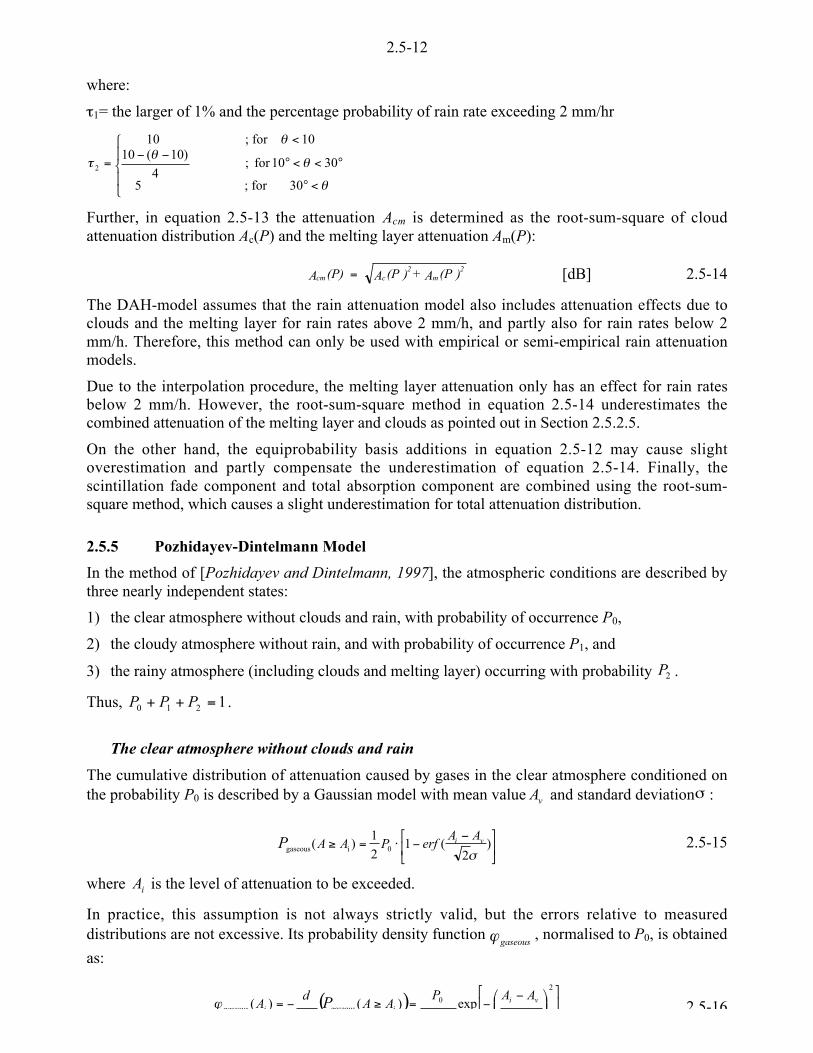
2.5-12

where:

o1= the larger of 1% and the percentage probability of rain rate exceeding 2 mm/hr

ǻ

«©

¨

<°

°<<°<<

<

=

e

ee

e

o

30for ;5

3010for ;4

)10(1010for;10

2

Further, in equation 2.5-13 the attenuation Acm is determined as the root-sum-square of cloudattenuation distribution Ac(P) and the melting layer attenuation Am(P):

)(PA + )(PA (P)A2

m2

ccm = [dB] 2.5-14

The DAH-model assumes that the rain attenuation model also includes attenuation effects due toclouds and the melting layer for rain rates above 2 mm/h, and partly also for rain rates below 2mm/h. Therefore, this method can only be used with empirical or semi-empirical rain attenuationmodels.

Due to the interpolation procedure, the melting layer attenuation only has an effect for rain ratesbelow 2 mm/h. However, the root-sum-square method in equation 2.5-14 underestimates thecombined attenuation of the melting layer and clouds as pointed out in Section 2.5.2.5.

On the other hand, the equiprobability basis additions in equation 2.5-12 may cause slightoverestimation and partly compensate the underestimation of equation 2.5-14. Finally, thescintillation fade component and total absorption component are combined using the root-sum-square method, which causes a slight underestimation for total attenuation distribution.

2.5.5 Pozhidayev-Dintelmann Model

In the method of [Pozhidayev and Dintelmann, 1997], the atmospheric conditions are described bythree nearly independent states:

1) the clear atmosphere without clouds and rain, with probability of occurrence P0,

2) the cloudy atmosphere without rain, and with probability of occurrence P1, and

3) the rainy atmosphere (including clouds and melting layer) occurring with probability 2P .

Thus, 1210 =++ PPP .

The clear atmosphere without clouds and rain

The cumulative distribution of attenuation caused by gases in the clear atmosphere conditioned onthe probability P0 is described by a Gaussian model with mean value vA and standard deviationm :

µ�

�³�

� <<u=* )

2(1

2

1)( 0igaseous

mvi AA

erfPAAP 2.5-15

where iA is the level of attenuation to be exceeded.

In practice, this assumption is not always strictly valid, but the errors relative to measureddistributions are not excessive. Its probability density function

gaseous  , normalised to P0, is obtained

as:

( ) µ�

³�

´́¥

²²£ <

<=*<=2

0igaseous exp)()(  vi

igaseous

AAPAA

d

dA P 2 5-16

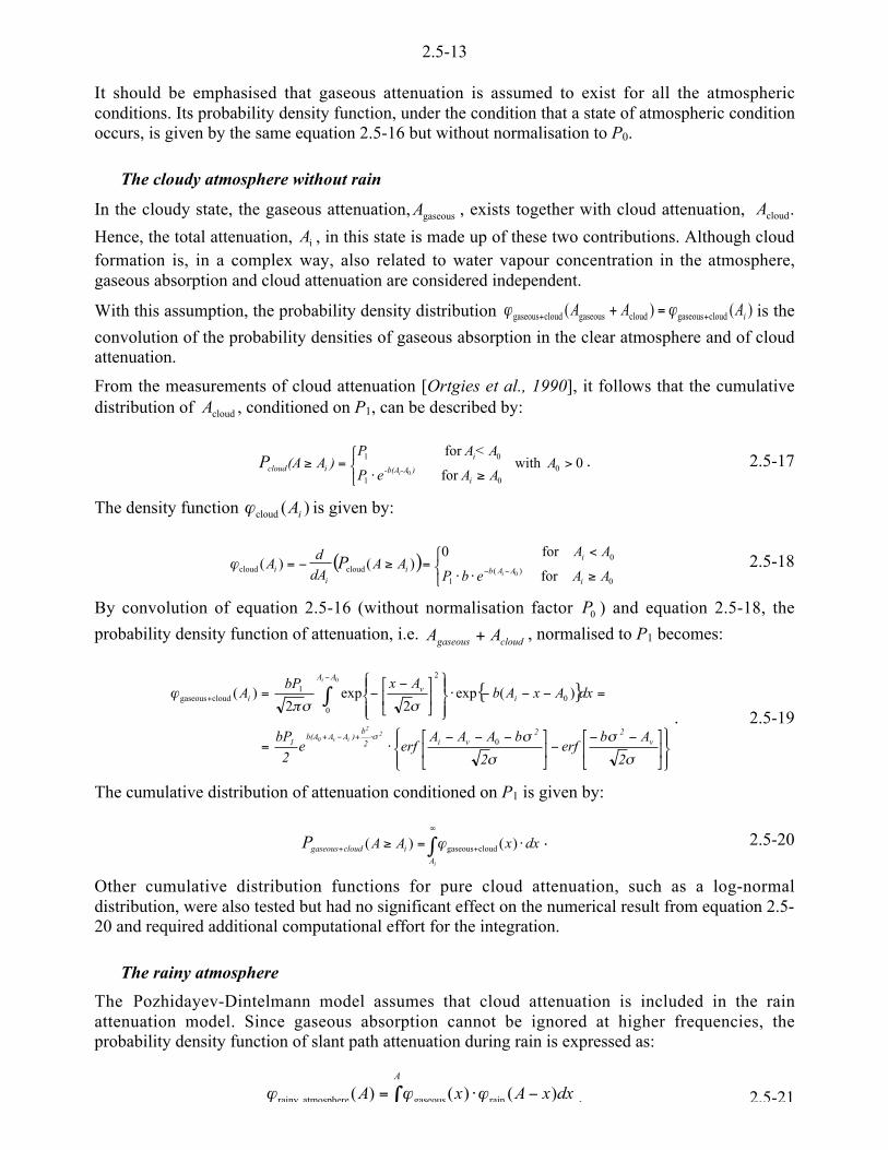
2.5-13

It should be emphasised that gaseous attenuation is assumed to exist for all the atmosphericconditions. Its probability density function, under the condition that a state of atmospheric conditionoccurs, is given by the same equation 2.5-16 but without normalisation to P0.

The cloudy atmosphere without rain

In the cloudy state, the gaseous attenuation, gaseousA , exists together with cloud attenuation, cloudA .

Hence, the total attenuation, iA , in this state is made up of these two contributions. Although cloudformation is, in a complex way, also related to water vapour concentration in the atmosphere,gaseous absorption and cloud attenuation are considered independent.

With this assumption, the probability density distribution )()( cloudgaseouscloudgaseouscloudgaseous iAAA ++ =+    is the

convolution of the probability densities of gaseous absorption in the clear atmosphere and of cloudattenuation.

From the measurements of cloud attenuation [Ortgies et al., 1990], it follows that the cumulativedistribution of cloudA , conditioned on P1, can be described by:

0withfor

for0

01

01

0>

ª©¨

*u=* A

A A eP

< A A P)A(A

i)-A-b(A

iicloud

iP . 2.5-17

The density function )(cloud iA  is given by:

( )ª©¨

*uu

<=*<=

<<0

)(1

0cloudcloud

for

for 0)()(

0 AAebP

AAAA

dAd

Ai

AAb

ii

ii

iP  2.5-18

By convolution of equation 2.5-16 (without normalisation factor 0P ) and equation 2.5-18, the

probability density function of attenuation, i.e. cloudgaseous AA + , normalised to P1 becomes:

{ }

«®

«­¬

ǻ

«©¨

µ�

�³�

� <<<µ

�

�³�

� <<<u=

=<<<u«®

«­¬

ǻ

«©¨

µ�

�³�

� <<=

u+<+

<

+ 0

m

m

m

m

mm/ 

m

2

Aberf

2

bAAAerfe

2

bP

dxAxAbAxbP

A

v22

vi2

b)AAb(A

1

AA

iv

i

22

iv0

i

0

0

0

2

1cloudgaseous

0

)(exp2

exp2

)(

. 2.5-19

The cumulative distribution of attenuation conditioned on P1 is given by:

dxxAAiA

icloudgaseousP u=* 0'

++ )()( cloudgaseous  . 2.5-20

Other cumulative distribution functions for pure cloud attenuation, such as a log-normaldistribution, were also tested but had no significant effect on the numerical result from equation 2.5-20 and required additional computational effort for the integration.

The rainy atmosphere

The Pozhidayev-Dintelmann model assumes that cloud attenuation is included in the rainattenuation model. Since gaseous absorption cannot be ignored at higher frequencies, theprobability density function of slant path attenuation during rain is expressed as:

dxxAxAA

)()()( raingaseousatmosphererainy <u= 0     , 2.5-21

2.5-14

The density distribution  gaseous( )x modelled by equation 2.5-20 is used without normalisation to

P0. A lognormal model [Fedi, 1980] for rain attenuation has been selected:

2

2

2

)(ln

2rain

2)( r

A

r

eA

PA m

µ

m/ 

<<

= 2.5-22

where:

µ = average of ln(A)

rm = standard deviation of ln(A)

If the frequency is sufficiently far away from the water vapour absorption band then the gaseous( )x can be simplified using a step function:

else 0

AxAfor 2

P(x) vv

0

gaseous

ǻ

«©

¨+<)<

=mm

m  2.5-23

This is justified by the fact that rain attenuation is normally much greater than gaseous absorption.Therefore the following probability density function is obtained for a rainy atmosphere:

{ }

{ }

for )()( 4

P

for 1)( 4

-for 0

)(

212

12

atmosphererainy

««««

ª

««««

©

¨

+*<µ�

�³�

�

+<<<+µ�

�³�

�

)

=

AAzerfzerf

AAAzerfP

AA

A

v

vv

v

m

mmm

m

  2.5-24

where:

r

vAAz

m

µm

2

)ln(1

<+<=

r

vAAz

m

µm

2

)ln(2

<<<= .

The condition m  <)= vatmosphererainy AAfor 0)(A is required for mathematical reasons in order to

describe the complete density distribution.

The cumulative distribution of attenuation in the rainy atmosphere conditioned to P2 is:

dx)()( atmosphererainy atmosphererainy 0'

=*iAi xAAP   . 2.5-25

The total cumulative distribution of atmospheric attenuation is obtained by summing theprobabilities for the nearly independent phenomena, i.e.

)()()()( atmosphererainy cloudgaseousgaseoustota iiiil AAAAAAAA PPPP *+*+*=* +. 2.5-26

The model assumes that cloud and gas attenuation phenomena are independent, which is not inagreement with the results of sections of this report. On the other hand, that assumption is inagreement with the radiometer results from Germany [Ortgies et al., 1990]. Scintillation fading isnot considered, which causes underestimation particularly for low elevation angles.

One interesting feature of the method is that the total attenuation can be presented in analytical form

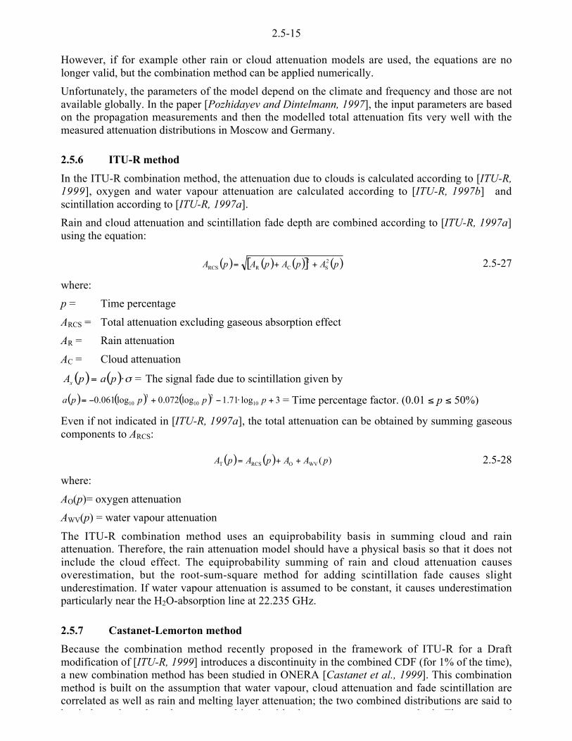
2.5-15

However, if for example other rain or cloud attenuation models are used, the equations are nolonger valid, but the combination method can be applied numerically.

Unfortunately, the parameters of the model depend on the climate and frequency and those are notavailable globally. In the paper [Pozhidayev and Dintelmann, 1997], the input parameters are basedon the propagation measurements and then the modelled total attenuation fits very well with themeasured attenuation distributions in Moscow and Germany.

2.5.6 ITU-R method

In the ITU-R combination method, the attenuation due to clouds is calculated according to [ITU-R,1999], oxygen and water vapour attenuation are calculated according to [ITU-R, 1997b] andscintillation according to [ITU-R, 1997a].

Rain and cloud attenuation and scintillation fade depth are combined according to [ITU-R, 1997a]using the equation:

( ) ( ) ( )[ ] ( )pApApApA 2S

2CRRCS ++= 2.5-27

where:

p = Time percentage

ARCS = Total attenuation excluding gaseous absorption effect

AR = Rain attenuation

AC = Cloud attenuation

( ) ( ) mu= papAs = The signal fade due to scintillation given by

( ) ( ) ( ) 3log71.1log072.0log061.0 102

103

10 +u<+<= ppppa = Time percentage factor. (0.01 ) p ) 50%)

Even if not indicated in [ITU-R, 1997a], the total attenuation can be obtained by summing gaseouscomponents to ARCS:

( ) ( ) )(WVORCST pAApApA ++= 2.5-28

where:

AO(p)= oxygen attenuation

AWV(p) = water vapour attenuation

The ITU-R combination method uses an equiprobability basis in summing cloud and rainattenuation. Therefore, the rain attenuation model should have a physical basis so that it does notinclude the cloud effect. The equiprobability summing of rain and cloud attenuation causesoverestimation, but the root-sum-square method for adding scintillation fade causes slightunderestimation. If water vapour attenuation is assumed to be constant, it causes underestimationparticularly near the H2O-absorption line at 22.235 GHz.

2.5.7 Castanet-Lemorton method

Because the combination method recently proposed in the framework of ITU-R for a Draftmodification of [ITU-R, 1999] introduces a discontinuity in the combined CDF (for 1% of the time),a new combination method has been studied in ONERA [Castanet et al., 1999]. This combinationmethod is built on the assumption that water vapour, cloud attenuation and fade scintillation arecorrelated as well as rain and melting layer attenuation; the two combined distributions are said tob i d d b h bi d i h h h d Th d

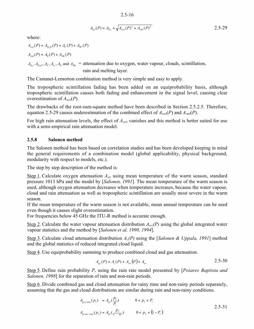
2.5-16

22 )()()(2

PAPAAPA rmlwetOtot ++= 2.5-29

where:

)()()()(2

PAPAPAPA SCCOHwet ++=

)()()( PAPAPA MLRrml +=

MLRscCOHO AAAAAA and,,,,22

= attenuation due to oxygen, water vapour, clouds, scintillation,

rain and melting layer.

The Castanet-Lemorton combination method is very simple and easy to apply.

The tropospheric scintillation fading has been added on an equiprobability basis, althoughtropospheric scintillation causes both fading and enhancement in the signal level, causing clearoverestimation of Awet(P).

The drawbacks of the root-sum-square method have been described in Section 2.5.2.5. Therefore,equation 2.5-29 causes underestimation of the combined effect of Awet(P) and Arml(P).

For high rain attenuation levels, the effect of Awet vanishes and this method is better suited for usewith a semi-empirical rain attenuation model.

2.5.8 Salonen method

The Salonen method has been based on correlation studies and has been developed keeping in mindthe general requirements of a combination model (global applicability, physical background,modularity with respect to models, etc.).

The step by step description of the method is:

Step 1. Calculate oxygen attenuation Aox using mean temperature of the warm season, standardpressure 1013 hPa and the model by [Salonen, 1991]. The mean temperature of the warm season isused, although oxygen attenuation decreases when temperature increases, because the water vapour,cloud and rain attenuation as well as tropospheric scintillation are usually most severe in the warmseason.If the mean temperature of the warm season is not available, mean annual temperature can be usedeven though it causes slight overestimation.For frequencies below 45 GHz the ITU-R method is accurate enough.

Step 2. Calculate the water vapour attenuation distribution Awv(P) using the global integrated watervapour statistics and the method by [Salonen et al, 1990, 1994].

Step 3. Calculate cloud attenuation distribution Ac(P) using the [Salonen & Uppala, 1991] methodand the global statistics of reduced integrated cloud liquid.

Step 4. Use equiprobability summing to produce combined cloud and gas attenuation.

( ) oxwvcgc APAPAPA ++= )()( 2.5-30

Step 5. Define rain probability Pr using the rain rate model presented by [Poiares Baptista andSalonen, 1998] for the separation of rain and non-rain periods.

Step 6. Divide combined gas and cloud attenuation for rainy time and non-rainy periods separately,assuming that the gas and cloud distributions are similar during rain and non-rainy conditions.

( )rgcrainnogc

rr

gcainyrgc

PpP

pApA

PpP

pApA

<<<=

<<=

< 10)1

()(

0)()(

22

2

11

1

2.5-31

2.5-17

The results in Section 2.5.3.3 show that water vapour and cloud attenuation values are usuallyhigher during rainy periods than non-rainy periods. Therefore, some underestimation is caused forrainy-period distribution by the assumption that cloud and water vapour attenuation distributions aresimilar for rainy and non-rainy periods. On the other hand, the equiprobability summing inequations 2.5-30 and 2.5-32 may cause a small overestimation.Step 7. Select the model for precipitation attenuation and calculate the rain attenuation distribution,calculating the required rainfall rate from the rain rate model.

Step 8. Combine the rain attenuation distribution and the combined gas and cloud attenuationdistribution for rainy periods, using the equiprobability method.

)()()( ´ PAPAPA rrainygcrainytot += 2.5-32

Step 9. Invert the cumulative distributions to obtain probability as a function of attenuation level forrainy and non-rainy periods. Use then disjoint summing for combining the calculated attenuationdistributions during rainy and non-rainy periods.

( ) ( ) ( )totrainytottotrainnogctot AAPAAPAP >+>= <2.5-33

Step 10. Calculate the scintillation fading distribution using the [ITU-R, 1997a] method and convertit to the probability density distribution ps(A) of scintillation.

Step 11. Combine total attenuation and scintillation fading using convolution to obtain the total fadedistribution Ptf(At):

( ) ( ) ( ) dAAt

Aa

Pt

A

As

pt

Atf

P <u0'<

= 2.5-34

This method is proposed because [Salonen et al, 1996] shows that it is a better method thanmodified equiprobability summing. However, the scintillation fading may not be very important at40 and 50 GHz with elevation angles above 20 degrees and then the less accurate [ITU-R, 1997a]method can also be used.

The proposed procedure can be applied with the physical rain attenuation models, which do notinclude cloud attenuation.

The method can be used for global prediction of total attenuation distributions in order to getsatellite communications coverage areas at specified availability levels. The required globalmeteorological statistics derived from the data from ECMWF weather forecast systems areavailable on the CD attached to this report.

2.5-18

2.5.9 References

[Castanet et al., 1999]Castanet L., J. Lemorton, T. Konefal, A.K. Shukla, P.A. Watson, C.L.Wrench: “Comparison ofvarious methods for combining propagation effects and predicting loss in low-availability systemsin the 20 GHz to 50 GHz frequency range”, International Journal of Satellite Communications,Vol 19, no. 3, pp 317-334, May-June 2001.

[Dissanayake et al., 1997]Dissanayake A., J. Allnutt, and F. Haidara: “A prediction model that combines rain attenuation andother propagation impairments along earth-satellite paths”, IEEE Transactions on Antennas andPropagation, Vol. 45, no.10, pp. 1546-1558, 1997.

[Fedi, 1980]Fedi F.: “Rain attenuation on Earth-satellite links: A prediction method based on point rainfallintensity statistics”, Proc. URSI Comm. F Open Symposium, Lennoxville, pp. 4.12.1-4.12.6, 1980

[Feldhake, 1997]Feldhake G., “Estimating the attenuation due to combined atmospheric effects on modern earth-space paths”, IEEE Antennas and Propagation Magazine, Vol. 39, No. 4, 1997.

[ITU-R, 1997a]ITU-R Recommendation P 618-5, “Propagation data prediction methods required for the design ofEarth-space telecommunication systems”, 1997.

[ITU-R, 1997b]ITU-R Recommendation P 676-3, Attenuation by atmospheric gases, Propagation in Non-IonisedMedia, Geneva, 1997.

[ITU-R, 1999]ITU-R Recommendation 840-2 Attenuation due to clouds and fog, Propagation in Non-IonisedMedia, Geneva, 1999

[Van de Kamp, 1997]Van de Kamp M.M.J.L.: “Relations between the scintillation, attenuation and total fadedistributions”, COST 255 document CP21A04, Nov. 1996.

[Konefal et al., 1999]Konefal T., Watson P.A. Shukla A.K. , Akram A.: “Prediction of monthly and annual availabilitieson 10 - 50 GHz satellite to Earth links and aircraft to aircraft links”, Proc. IEE, MicrowavesAntennas and Propagation, Vol 147, No 2, pp 122-127, April 2000.

[Liebe, 1989]Liebe H.J.: “MPM - An atmospheric millimeter-wave propagation model”, International Journal ofInfrared and Millimeter Waves, Vol. 10, pp. 631-650, 1989.

2.5-19

[Liebe et al., 1989]H.J. Liebe, T. Manabe and G.A. Hufford, ‘Millimetre-wave attenuation and delay rates due tofog/cloud conditions’, Trans. IEEE Ant. & Prop., 37, pp 1617-1623, 1989.

[Liebe et al., 1993]Liebe H. J., Hufford G. A., Cotton M. G., ”Propagation modelling of moist air and suspendedwater/ice particles at frequencies below 1000 GHz”, AGARD 52nd Specialists’Meeting of The EMWave Propagation Panel, Palma De Maiorca, Spain, 17-21 May 1993.

[Matsudo and Karasawa, 1991]Matsudo T. and Karasawa Y., "Characteristics and prediction methods for the occurrence rate ofSES in available time affected by tropospheric scintillation," Electronics and Communications inJapan, vol. 74, no. 8, pp. 89-100, 1991.

[Ortgies et al., 1990]Ortgies, G., Rücker, F. and Dintelmann, F.: “Statistics of clear-air attenuation on satellite links at 20and 30 GHz”, Electronics Letters, Vol. 26, No. 6, 358-360, 1990

[Poiares Baptista and Salonen, 1998]Poiares Baptista J. P. V., Salonen E. T.: “Review of rainfall rate modelling and mapping”,Proceedings of URSI Open Symposium, CLIMPARA'98, Ottawa 27-29 June 1998, pp. 35-44.

[Pozhidayev and Dintelmann, 1997]Pozidayev V. and Dintelmann F.: “Evaluation of total radiowave attenuation statistics for slant pathlinks from phenomenon-based attenuation distributions”, European Transactions onTelecommunications, Vol. 8, No. 3, pp. 259-263, 1997.

[Salonen, 1991]Salonen E.: “Prediction method for oxygen attenuation on slant propagation path for10-57 GHz”, Antennas and Prop. Society Symp., 1991 Digest Vol. 3, London, Canada, pp. 1804-1807, June 1991.

[Salonen and Uppala, 1991]Salonen E. and S. Uppala: “New prediction method of cloud attenuation”, Electronics Letters, vol.27, no. 12, pp. 1106-1108, June 1991

[Salonen et al., 1990]Salonen E., S. Karhu, P. Jokela, W. Zhang, S. Uppala, H. Aulamo, S. Sarkkula: “Study ofpropagation phenomena for low availabilities”, Final Report for the European Space Agency underESTEC contract 8025/88/NL/PR. November 1990, 316 p.

[Salonen et al., 1994]Salonen E., Karhu S., Uppala S., Hyvönen R.: Study of improved propagation predictions, Finalreport ESTEC contract 9455/91/NL/LC(SC), pp. 380, 1994.

[Salonen et al., 1996]Salonen E. T., Tervonen J. K., Vogel W. J.: “Scintillation effects on total fade distributions forearth-satellite links”, IEEE Transactions on Antennas and Propagation, Vol. 44, No. 1, pp. 23-27,

2.6-1

CHAPTER 2.6Testing of Prediction Models

Editor: Carlo Riva1

Authors: Ioan Chisalita2, Ondrej Fiser3, Edit Gimonet4, Joel Lemorton5,Antonio Martellucci6, Tudor Palade7, Erkki Salonen8, Max van de Kamp9

1 Dipartimento di Elettronica e Informazione, Politecnico di Milano, P.zza L. Da Vinci 32, 20133 Milano, Italy.

Tel: +39-02-23993586, Fax: +39-02-23993413, e-mail: riva@elet.polimi.it2 Technical University of Cluj-Napoca, 15 C. Daicoviciu Str, POB 1124, RO-3400 Cluj-Napoca, Romania

Tel: +40-64-191689, Fax: +40-64-192055, e-mail: chisalita@el.el.obs.utcluj.ro3 Inst. of Atmospheric Physics, Bocni II/1401, CZ-141 31 Praha 4, Czech Republic

Tel: +420-2-769702x108, Fax: +420-2-763745, e-mail: ondrej@ufa.cas.cz4 ONERA-CERT DEMR 2 Avenue Edouard Belin, BP4025, F-31055 Toulouse, CEDEX 4 France

Tel: +33-562-25-2720, Fax: +33-562-25-2577, e-mail: Marie-Edith.Gimonet@onecert.fr5 ONERA-CERT DEMR, 2 Avenue Edouard Belin, BP4025, F-31055 Toulouse, CEDEX 4 France

Tel: +33-562-25-2720, Fax: +33-562-25-2577, e-mail: lemorton@onecert.fr6 European Space Agency, ESA-ESTEC, Kepleerlan 1, PB 299, NL-2200 AG Noordwijk, The Netherlands

Tel: +31-71-565-5603, Fax: +31-71-565-4999, e-mail: Antonio.Martellucci@esa.int7 Technical University of Cluj-Napoca, 15 C. Daicoviciu Str, POB 1124, RO-3400 Cluj-Napoca ,Romania

Tel: +40-64-191689, Fax: +40-64-192055, e-mail: Tudor.Palade@com.utcluj.ro8 University of Oulu, Telecommunication Lab. P.O.Box 444, FIN-90571 Oulu, Finland

Tel: +358 40 524 2406, Fax: +358-8-553 2845, e-mail: Erkki.Salonen@ee.oulu.fi9 Eindhoven University of Technology, TTE-ECR, P O Box 513, 5600 MB Eindhoven, The Netherlands

T l +31 40 247 2326 F +31 40 245 5197 il j l d k @ l t l

2.6-2

2.6 Testing of Prediction Models

The achievement of high availability targets in advanced satellite link design requires a deepknowledge of the radio channel behaviour. This implies accurate studies to assess the majorimpairments affecting signal propagation through the atmosphere and their statistical properties. Infact, at millimetre wave frequencies, several physical phenomena such as precipitation, clouds,atmospheric gases and tropospheric scintillation can severely degrade communication systemperformance.

The effects due to different atmospheric causes can be measured quite accurately by means ofsatellite beacon signals. However, since propagation experiments are carried out in only a fewplaces all over the world and for a limited number of frequencies and link configurations, theirresults cannot be directly applied to all design objectives. For this reason, several models have beendeveloped which are able to predict the effects due to various causes, like rain, gas, clouds andturbulence, to provide adequate inputs for system margin calculation in all regions of the world.

During the OLYMPUS and ITALSAT lifetimes, many beacon measurements have been carried out,at frequencies ranging from 12 to 50 GHz, at many sites in Europe, using both co- and cross-polarised channels. Radiometric and meteorological measurements have also been taken at the sametime. The utilisation of these measurements, which was initiated in the framework of the OPEX andCEPIT projects, is one of the principal objectives of the COST 255 programme.

Implementation and testing of prediction models is one of the most significant among theseactivities. The bulk of the measurements cited above, with the possible addition of new datacollected from ITALSATand other satellites such as DFS-KOPERNIKUS or Tvsat, constitute theideal basis for the testing activity, together with the advice that experts on new telecommunicationsystems may give (particular types of tests or testing criteria).

Tests on prediction models published in the open literature or developed in the frame of COST 255have been carried out using the existing data from ITU-R (DBSG5), OPEX (DBOPEX) and CEPIT(DBCEPIT) data banks over the following propagation parameters:

• Yearly and worst month rain attenuation exceedance probability

• Yearly total attenuation (clouds, rain and scintillation effects) exceedance probability

• Site diversity gain

• Fade duration

• Scintillation standard deviation or variance

• Yearly XPD exceedance probability

Data in addition to those available in the ITU-R DBSG5 database are described in the Annex andincluded on the COST255 CD-ROM.

2.6.1 Yearly rain attenuation exceedance probability

Attenuation due to rain is an important propagation impairment to be considered in the design ofsatellite telecommunication systems. The actual attenuation due to rain depends on the temperature,size distribution, terminal velocity and shape of the raindrops. Since rain varies noticeably in spaceand time, only knowledge of the rain drop characteristics at each point on the paths would allow theaccurate calculation of the total attenuation.

The prediction of rain-induced attenuation starting from the cumulative distribution of rainfallintensity has been the subject of a major effort, carried out by many researchers. Several methodshave been developed to achieve this objective starting from the site climatic parameters and tested

2.6-3

hand, in the coming years, a large number of new satellite systems will operate at frequencies above20 GHz, so that an urgent question arises whether the “old” prediction methods are still of use at thenew frequencies and with what performance.

After years of measurement campaigns carried out at different sites in the world, it is now possibleboth to improve the prediction algorithms and to perform very reliable tests at frequencies above 20GHz, using long term statistical distributions of point rainfall intensity as input.

2.6.1.1 Rain attenuation prediction models

A common feature of the prediction methods available today is that they use the cumulativedistribution of point rainfall intensity P(R) as input and give, as output, the cumulative distributionof predicted attenuation P(Ap). Even though many methods can be found in the literature, only 15 ofthe best, which do not require input data other than P(R) and link characteristics, were considered:

1. Assis Eiloft Improved [Costa, 1983]

2. Brazil [CCIR, 1992]

3. Bryant [Bryant et al., 2001]

4. Crane Global [Crane, 1980]

5. Crane Two-Component [Crane, 1985]

6. DAH [Dissanayake et al., 1997]

7. EXCELL [Capsoni et al., 1987]

8. Australian [Flavin, 1996]

9. Garcia [Garcia et al., 1988]

10. ITU-R Rec. 618-5 [ITU-R, 1997b]

11. Japan [CCIR, 1993]

12. Leitao Watson Showery [COST205, 1985]

13. Matricciani [Matricciani, 1991]

14. SAM [Stutzman and Dishman, 1984]

15. Svjatogor [Svjatogor, 1985]

For the complete description of the models refer to Section 2.2.2.1.

2.6.1.2 Experimental data used for the test

A test of the prediction models was carried out using the large set of experimental data collected inthe annual rain attenuation statistics section of the earth-space path ITU-R (DBSG5), OPEX(DBOPEX) and CEPIT (DBCEPIT) databases. The cumulative distributions of rain rate andmeasured attenuation are available as functions of the “standard” probabilities for which the raineffect is predominant over the other atmospheric attenuation effects (gas and scintillation): 0.001,0.002, 0.003, 0.005, 0.01, 0.02, 0.03, 0.05, 0.1%.

However, it would not have been appropriate to use for testing the data as they appear in thedatabases, since very often the experimenters did not indicate how they calculated the reference0 dB level to obtain atmospheric attenuation. Hence, when not indicated, the attenuation value at1% of the time has been used to separate ad hoc experiments measuring extra attenuation (cloudsand rain) from those measuring total attenuation (gas, clouds, scintillation and rain).

2.6-4

The three databases (ITU-R, OPEX and CEPIT) provided a total of 104 beacon experiments, withrain concurrent measurements. Their duration is generally greater than 300 days. The frequenciesrange from about 6 to about 35 GHz, giving a good testing data set for studying the frequencydependence of the methods. The database is available, in DBSG5 export format, on the COST255CD-ROM.

2.6.1.3 Test activity: results

As figure of merit of the considered prediction methods, in agreement with the last ITU-RRecommendation [ITU-R, 1997a], the test variable defined by the following equation has beenchosen:

( )( )( )

( )

( )( )( )

¡

¡

PA P

A P

A Pfor A

PA P

A Pfor A

p

m

mm

p

mm

=£

¤²

¥

¦´ ×

£¤²

¥¦́

)

=£

¤²

¥

¦´ >

10010

10

100 10

0 2

ln

ln

.

dB

dB

2.6-1

where Ap(P) and Am(P) are respectively the predicted and measured rain attenuation for a givenprobability, P. The parameter ¡ is essentially independent of attenuation [ITU-R, 1997a] andconsequently preferable when pooling estimates of attenuation at different probability levels.

The testing of rain attenuation prediction models has been carried out, comparing predictions fromthe 15 selected models and measurements from the database of 104 experiments described in theprevious section. The link data necessary as input parameters of the models have been obtainedfrom the database. The test has been carried out using, as input for rain prediction models, both themeasured and the predicted (using Baptista-Salonen maps [Poiares Baptista and Salonen, 1998])cumulative distribution of rain intensity. In the first case, when the measured rain data are notpresent in the database, the corresponding experiments have been excluded from the test.

For each method and each probability the following four quantities, which were obtained byaveraging the errors over the whole set of experiments (the duration of the generic experiment “i” isT(i)), are shown:

• ensemble mean error: ( )( ) ( )

( )-

- u¡=¡

i

i

iT

iTPiP

,

• ensemble root mean square: ( )( ) ( )

( )-

- u¡=¡

i

i

iT

iTPiP

,2

2

• ensemble standard deviation: ( ) ( ) ( ) 22 PPP ¡<¡=m

• total weight of the data (expressed in years) contributing to the given outage probability.

The complete tables of errors for each outage probability are shown in Annex to Chapter 2.6.

The errors averaged over the probability range 0.001-0.1% were also calculated:

( ) ( )

( )-

- u¡=¡ P

tot PT

PTP

2.6-1

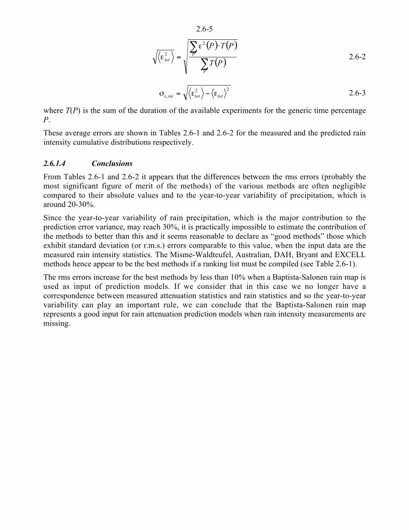
2.6-5

( ) ( )

( )-

- u¡=¡

P

Ptot PT

PTP2

2 2.6-2

22, tottottot ¡<¡=m¡ 2.6-3

where T(P) is the sum of the duration of the available experiments for the generic time percentageP.

These average errors are shown in Tables 2.6-1 and 2.6-2 for the measured and the predicted rainintensity cumulative distributions respectively.

2.6.1.4 Conclusions

From Tables 2.6-1 and 2.6-2 it appears that the differences between the rms errors (probably themost significant figure of merit of the methods) of the various methods are often negligiblecompared to their absolute values and to the year-to-year variability of precipitation, which isaround 20-30%.

Since the year-to-year variability of rain precipitation, which is the major contribution to theprediction error variance, may reach 30%, it is practically impossible to estimate the contribution ofthe methods to better than this and it seems reasonable to declare as “good methods” those whichexhibit standard deviation (or r.m.s.) errors comparable to this value, when the input data are themeasured rain intensity statistics. The Misme-Waldteufel, Australian, DAH, Bryant and EXCELLmethods hence appear to be the best methods if a ranking list must be compiled (see Table 2.6-1).

The rms errors increase for the best methods by less than 10% when a Baptista-Salonen rain map isused as input of prediction models. If we consider that in this case we no longer have acorrespondence between measured attenuation statistics and rain statistics and so the year-to-yearvariability can play an important rule, we can conclude that the Baptista-Salonen rain maprepresents a good input for rain attenuation prediction models when rain intensity measurements aremissing.

2.6-6

Averaged errors summaryMethod

tot¡ 2tot¡ tot,¡m

WeightYears

Misme-Waldteufel -0.8 27.5 27.5 68.3Australian -7.9 27.7 26.5 76.4

ITU-R Rec. 618-6 -10.1 28.0 26.1 79.8Bryant -5.0 28.5 28.1 76.3

EXCELL -1.7 29.0 28.9 81.1ITU-R Rec. 618-5 -9.1 31.6 30.3 79.8

Brazil -13.3 31.7 28.8 76.4Matricciani 3.6 32.3 32.1 79.7Svjatogor -11.3 32.6 30.5 76.4

Japan -12.7 32.7 30.2 70.2Assis Einloft -9.6 33.1 31.7 63.5Crane Global 8.3 33.9 32.9 75.6Leitao Watson

(Showery) -22.1 34.5 26.5 48.9

SAM -9.0 35.1 33.9 76.4Garcia -21.7 35.8 28.5 76.4

Crane Two Components -1.8 40.4 40.3 77.8

Table 2.6-1: Results of rain attenuation test using the measured rain intensity statistics as input of prediction models(Costbeacexc.sel.rainconc.exp - Measured rain data - Probability range: 0.001-0.1%

Averaged on 104 experiments - Total time: 106.3 years).

Averaged errors summaryMethod

tot¡ 2tot¡ tot,¡m

WeightYears

Misme-Waldteufel -4.2 35.0 34.7 73.1ITU-R Rec. 618-6 -7.9 35.9 35.0 81.1

Matricciani -1.9 36.0 35.9 80.1ITU-R Rec. 618-5 -6.5 36.4 35.9 81.1

Australian -6.9 36.8 36.2 81.1Japan -12.1 37.9 35.9 81.1Bryant -3.5 37.9 37.7 81.1

EXCELL 0.5 38.4 38.4 81.1Assis Eiloft -8.5 38.4 37.4 81.1

Brazil -12.1 39.4 37.5 81.1Leitao Watson

(Showery)-18.7 40.0 35.3 52.0

Crane Two Components -1.8 40.4 40.3 77.8SAM -7.2 40.5 39.8 81.1Garcia -19.7 41.4 36.5 81.1

Svjatogor -10.0 41.7 40.5 81.1Crane Global 9.3 42.4 41.4 80.3

Table 2.6-2 Results of rain attenuation test using rain intensity statistics from Baptista-Salonen map as input ofprediction models (Costbeacexc.sel.rainconc.exp - Baptista-Salonen rain map - Probability range: 0.001-0.1% -

Averaged on: 104 experiments - Total time: 106.3 years).

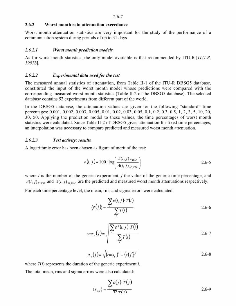
2.6-7

2.6.2 Worst month rain attenuation exceedance

Worst month attenuation statistics are very important for the study of the performance of acommunication system during periods of up to 31 days.

2.6.2.1 Worst month prediction models

As for worst month statistics, the only model available is that recommended by ITU-R [ITU-R,1997b].

2.6.2.2 Experimental data used for the test

The measured annual statistics of attenuation, from Table II-1 of the ITU-R DBSG5 database,constituted the input of the worst month model whose predictions were compared with thecorresponding measured worst month statistics (Table II-2 of the DBSG5 database). The selecteddatabase contains 52 experiments from different part of the world.

In the DBSG5 database, the attenuation values are given for the following “standard” timepercentages: 0.001, 0.002, 0.003, 0.005, 0.01, 0.02, 0.03, 0.05, 0.1, 0.2, 0.3, 0.5, 1, 2, 3, 5, 10, 20,30, 50. Applying the prediction model to these values, the time percentages of worst monthstatistics were calculated. Since Table II-2 of DBSG5 gives attenuation for fixed time percentages,an interpolation was necessary to compare predicted and measured worst month attenuation.

2.6.2.3 Test activity: results

A logarithmic error has been chosen as figure of merit of the test:

( ) ´´¦

¥²²¤

£u=

WMM

WMP

jiA

jiAji

,

,

),(

),(log100,¡ 2.6-5

where i is the number of the generic experiment, j the value of the generic time percentage, and

WMPjiA ,),( and WMMjiA ,),( are the predicted and measured worst month attenuations respectively.

For each time percentage level, the mean, rms and sigma errors were calculated:

( )( ) ( )

( )-

- u=

i

i

iT

iTjij

,¡¡ 2.6-6

( )( ) ( )

( )-

- u=

i

i

iT

iTjijrms

,2¡

¡ 2.6-7

( ) ( ) ( ) 22 jrmsj ¡<=m ¡¡2.6-8

where T(i) represents the duration of the generic experiment i.

The total mean, rms and sigma errors were also calculated:

( ) ( )

( )-

- u

= jtot jT

jTj¡

¡ 2.6-9

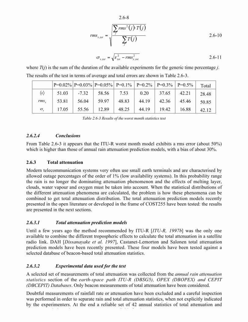
2.6-8

( ) ( )

( )-

- u

=

j

jtot jT

jTjrms

rms

2

,¡ 2.6-10

2,

2, tottottot rms¡¡ ¡m <= 2.6-11

where T(j) is the sum of the duration of the available experiments for the generic time percentage j.

The results of the test in terms of average and total errors are shown in Table 2.6-3.

P=0.02% P=0.03% P=0.05% P=0.1% P=0.2% P=0.3% P=0.5% Total¡ 51.03 -7.32 58.56 7.53 0.20 37.65 42.21 28.48

¡rms 53.81 56.04 59.97 48.83 44.19 42.36 45.46 50.85

¡m 17.05 55.56 12.89 48.25 44.19 19.42 16.88 42.12

Table 2.6-3 Results of the worst month statistics test

2.6.2.4 Conclusions

From Table 2.6-3 it appears that the ITU-R worst month model exhibits a rms error (about 50%)which is higher than those of annual rain attenuation prediction models, with a bias of about 30%.

2.6.3 Total attenuation

Modern telecommunication systems very often use small earth terminals and are characterised byallowed outage percentages of the order of 1% (low availability systems). In this probability rangethe rain is no longer the dominating attenuation phenomenon and the effects of melting layer,clouds, water vapour and oxygen must be taken into account. When the statistical distributions ofthe different attenuation phenomena are calculated, the problem is how these phenomena can becombined to get total attenuation distribution. The total attenuation prediction models recentlypresented in the open literature or developed in the frame of COST255 have been tested: the resultsare presented in the next sections.

2.6.3.1 Total attenuation prediction models

Until a few years ago the method recommended by ITU-R [ITU-R, 1997b] was the only oneavailable to combine the different tropospheric effects to calculate the total attenuation in a satelliteradio link. DAH [Dissanayake et al. 1997], Castanet-Lemorton and Salonen total attenuationprediction models have been recently presented. These four models have been tested against aselected database of beacon-based total attenuation statistics.

2.6.3.2 Experimental data used for the test

A selected set of measurements of total attenuation was collected from the annual rain attenuationstatistics section of the earth-space path ITU-R (DBSG5), OPEX (DBOPEX) and CEPIT(DBCEPIT) Databases. Only beacon measurements of total attenuation have been considered.

Doubtful measurements of rainfall rate or attenuation have been excluded and a careful inspectionwas performed in order to separate rain and total attenuation statistics, when not explicitly indicatedby the experimenters. At the end a reliable set of 42 annual statistics of total attenuation and

i i i il bl f h

2.6-9

Unfortunately the location of the experiments was predominantly in Europe (only a fewexperiments in USA).

The cumulative distributions of rain rate and measured attenuation are available as a function of the“standard” probabilities: 0.01, 0.02, 0.03, 0.05, 0.1, 0.2, 0.3, 0.5, 1, 2, 3, 5 and 10 %.

2.6.3.3 Test activity: results

Since Castanet-Lemorton and Salonen are methods more to combine the tropospheric effects than topredict total attenuation, in some cases, best models for the various effects had to be chosen.

In the case of the Castanet-Lemorton method, DAH rain attenuation prediction model has been usedas suggested by the authors. As for gas, clouds and scintillation attenuation ITU-RRecommendations 676-3, 840-2 and 618-5 have been used.

In the Salonen combination method, the rain intensity cumulative distribution was separated intowidespread and convective components; a physical model (EXCELL) was then used to calculaterain attenuation.

In the case of the ITU-R model, Recommendation 618-5 has been used for rain attenuation. In fact,with Recommendation 618-6 theITU-R and DAH modes are almost the same.

The following meteorological input parameters, required by the models, were derived usingECMWF maps:

• percentage of rainy time (for the Salonen method);

• average widespread rain height (0°C isotherm height averaged during large scale rainfall rateperiods) and convective rain height (-5°C isotherm height averaged during convective rainfallrate periods) (for the Salonen method);

• average ground temperature (for all methods);

• columnar water vapour and corresponding water vapour density (for all methods);

• reduced columnar cloud liquid water (for the Castanet-Lemorton, ITU-R and Salonen methods);

• median value of wet term of refractive index, Nwet (for all methods);

As the figure of merit of the total attenuation prediction methods, the test variable reported inequation 2.6-1 was used, where the predicted and measured attenuation is total attenuation insteadof rain attenuation. The mean, rms and standard deviation errors were calculated according toequations 2.6-2, 2.6-3 and 2.6-4 in the probability range 0.01-10%.

Two tests have been run using rainfall rate measurements and Baptista-Salonen rain maps as inputfor rain attenuation prediction models. The results are summarised in Tables 2.6-4 and 2.6-5,respectively.

Averaged errors summary WeightMethodmean Rms std Years

CastanetLemorton

5.3 21.2 20.5 36.6

DAH 10.6 24.6 22.3 35.5ITU-R Rec. 618-5 16.0 28.6 23.6 36.6

Salonen 1.6 22.2 22.1 36.0

Table 2.6-4 Results of total attenuation test carried out using the measured cumulative distributions of rain intensityand the set of 42 total attenuation beacon statistics

2.6-10

Averaged errors summary WeightMethodmean rms std Years

CastanetLemorton

-4.9 26.1 25.6 36.6

DAH 0.3 28.2 28.2 35.5ITU-R Rec. 618-5 2.8 29.7 29.6 36.6

Salonen -7.5 27.7 26.7 36.2

Table 2.6-5 Results of total attenuation test carried out using the Baptista-Salonen rain mapsand the set of 42 total attenuation beacon statistics

2.6.3.4 Conclusions

Since the available reference data are concentrated on Europe, the conclusions of the test are validonly for temperate and continental climates.

From Tables 2.6-4 and 2.6-5, it appears that the differences between the combination methodstested are rather small.

The Castanet-Lemorton and Salonen methods are slightly better than DAH and ITU-R.

Using the rain rate model instead of measured rain rate, the rms-values typically increase by a fewper cent, as expected. In fact, the rain maps used as input for the rain prediction models are notconcurrent with the measured total attenuation statistics that can change from one year to another.

2.6.4 Site diversity gain models

Site diversity is a promising technique to overcome severe attenuation on earth-spacecommunications links. This is based on the experimental evidence that intense rain events arelimited in extent so that the substitution of one station by two or more stations separated by a fewkilometres may reduce the outage probability of the communication system.

2.6.4.1 Site diversity gain prediction models

Some models for the performance prediction of site diversity systems are present in the literature:they can be classified into empirical and physical models. The former normally use an analyticalrelationship whose parameters have been obtained throughout a best-fit procedure on manyexperimental results; the latter start from a model of the rain structure and evaluate its influence onthe link(s) under test.

In the COST255 activity, the following models have been considered:

1. Allnutt and Rogers [Allnutt and Rogers, 1982]

2. EXCELL [Bosisio and Riva, 1998]

3. Goldhirsh [Goldhirsh, 1982]

4. Hodge [Hodge, 1982]

5. ITU-R [ITU-R, 1997b]

6. Mass [Mass, 1987]

7. Matricciani [Matricciani, 1994]

2.6-11

2.6.4.2 Database used for the test

To test the diversity prediction models we have used the large set of data experiments collected inthe site diversity statistics section of the earth-space path ITU-R Study Group 5 database, in whichfurther data reported in the literature have been merged. The single site and joint cumulativedistributions of attenuation were available for the “standard” probabilities: 0.001, 0.002, 0.003,0.005, 0.01, 0.02, 0.03, 0.05, 0.1, 0.2, 0.3, 0.5 and 1%. As the methods also require local rainfallrate statistics, which are not present in all experiments, we have decided to use probabilitydistributions estimated from the corresponding ITU-R rain zones.

The total number of considered experiments is 90; among which 10 are beacon, 33 radar and 47radiometer measurements. While the direct measurements (beacon and radiometer) normally referto one site diversity system, the indirect measurements (radar) explore several possibleconfigurations (with different link elevations and or station distances). Moreover they consider thesame link in every possible position in the radar maps; for their statistical confidence, we haveassigned to all radar experiments a conventional duration of one year.

Frequency ranges from 11 up to 30 GHz. To verify the frequency dependence of the models wehave subdivided the database into two frequency band classes: the first for frequencies less than 15GHz and the second for frequencies greater than 15 GHz. Distances between the two diversitystations range up to 213 km, even if only below 30 km experiments can be considered uniformlydistributed. The site distance dependence has been assessed by subdividing the range into thefollowing classes: below 5 km (typical range for a city link), between 5 and 15 km, 15 and 30 kmand above 30 km. The experiments were carried out in different ITU-R rain zones; a satisfactorystatistical confidence (more than about ten experiments) was obtained for the E, F, K and M zones.

The database is available in DBSG5 export format on the COST255 CD-ROM.

2.6.4.3 Test activity: results

We have chosen as a figure of merit of the methods the error in estimating the “relative diversitygain” g, i.e. the ratio between the gain G and the corresponding single link attenuation of the mainstation, As (the average attenuation of the two links was not always available for the whole range ofprobability):

g G As= 2.6-12

The parameter g is essentially independent of attenuation and consequently preferable when poolingestimates of gain at different attenuation levels. The percentage error ¡ is defined as

( ) ( ) ( )[ ]¡ P g P g Pest mea= <100 2.6-13

where gest(P) and gmea(P) are predicted and measured relative gains for a given probability.

The results are presented in terms of ensemble averages and rms of ¡ weighted with the duration ofthe experiment.

Table 2.6-6 shows the performance of the considered methods relative to the beacon, radiometerand radar data sets, and to the complete data set. Among the empirical methods, Hodge performs byfar the best, with very stable results for the different data sets, if we take into account the limitednumber of beacon experiments. The performance of the physical models Mass and Matricciani arecomparable, even though Matricciani shows a more stable behaviour and reduced mean error.

Table 2.6-7 is relative to the baseline distance classes. The Matricciani and Hodge models yieldcomparable statistical errors in the whole range of site separation distance. EXCELL is the bestperforming model in its applicability range for site separations not exceeding 15 km The Allnutt

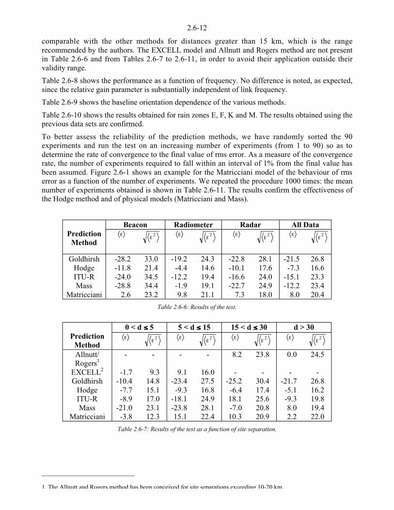
2.6-12

comparable with the other methods for distances greater than 15 km, which is the rangerecommended by the authors. The EXCELL model and Allnutt and Rogers method are not presentin Table 2.6-6 and from Tables 2.6-7 to 2.6-11, in order to avoid their application outside theirvalidity range.

Table 2.6-8 shows the performance as a function of frequency. No difference is noted, as expected,since the relative gain parameter is substantially independent of link frequency.

Table 2.6-9 shows the baseline orientation dependence of the various methods.

Table 2.6-10 shows the results obtained for rain zones E, F, K and M. The results obtained using theprevious data sets are confirmed.

To better assess the reliability of the prediction methods, we have randomly sorted the 90experiments and run the test on an increasing number of experiments (from 1 to 90) so as todetermine the rate of convergence to the final value of rms error. As a measure of the convergencerate, the number of experiments required to fall within an interval of 1% from the final value hasbeen assumed. Figure 2.6-1 shows an example for the Matricciani model of the behaviour of rmserror as a function of the number of experiments. We repeated the procedure 1000 times: the meannumber of experiments obtained is shown in Table 2.6-11. The results confirm the effectiveness ofthe Hodge method and of physical models (Matricciani and Mass).

Beacon Radiometer Radar All DataPrediction

Method¡ ¡ 2 ¡ ¡ 2 ¡ ¡ 2 ¡ ¡ 2

Goldhirsh -28.2 33.0 -19.2 24.3 -22.8 28.1 -21.5 26.8Hodge -11.8 21.4 -4.4 14.6 -10.1 17.6 -7.3 16.6ITU-R -24.0 34.5 -12.2 19.4 -16.6 24.0 -15.1 23.3Mass -28.8 34.4 -1.9 19.1 -22.7 24.9 -12.2 23.4

Matricciani 2.6 23.2 9.8 21.1 7.3 18.0 8.0 20.4

Table 2.6-6: Results of the test.

0 < d )))) 5 5 < d )))) 15 15 < d )))) 30 d > 30Prediction

Method¡ ¡ 2 ¡ ¡ 2 ¡ ¡ 2 ¡ ¡ 2

Allnutt/Rogers1

- - - - 8.2 23.8 0.0 24.5

EXCELL2 -1.7 9.3 9.1 16.0 - - - -Goldhirsh -10.4 14.8 -23.4 27.5 -25.2 30.4 -21.7 26.8

Hodge -7.7 15.1 -9.3 16.8 -6.4 17.4 -5.1 16.2ITU-R -8.9 17.0 -18.1 24.9 18.1 25.6 -9.3 19.8Mass -21.0 23.1 -23.8 28.1 -7.0 20.8 8.0 19.4

Matricciani -3.8 12.3 15.1 22.4 10.3 20.9 2.2 22.0

Table 2.6-7: Results of the test as a function of site separation.

1. The Allnutt and Rogers method has been conceived for site separations exceeding 10-20 km.

2.6-13

10 )))) f )))) 15 15 < f )))) 30PredictionMethod ¡ ¡ 2 ¡ ¡ 2

Goldhirsh -21.6 27.3 -21.2 25.8Hodge -7.6 17.4 -6.4 14.8ITU-R -13.8 22.5 -18.1 25.0Mass -12.5 22.8 -11.6 24.8

Matricciani 8.1 21.3 7.9 18.2

Table 2.6-8: Results of the test as a function of transmission frequency.

Baseline angle = 0° Baseline angle = 90°Prediction

Method¡ ¡ 2 ¡ ¡ 2

Goldhirsh -21.7 25.4 -19.8 27.7Hodge -6.8 12.8 -10.1 20.4ITU-R -12.3 17.8 -18.8 27.4Mass -21.1 24.7 -13.1 22.1

Matricciani 9.7 15.9 6.3 20.7

Table 2.6-9: Results of the test as a function of baseline angle.

Rain zone E Rain zone F Rain zone K Rain zone MPrediction

Method¡ ¡2 ¡ ¡2 ¡ ¡2 ¡ ¡2

Goldhirsh -21.2 25.8 -8.2 11.5 -22.4 27.6 -16.0 20.1Hodge -10.7 14.7 -4.0 9.7 -5.7 17.5 1.4 11.6ITU-R -8.9 14.4 -5.7 9.7 -16.7 24.6 -9.9 17.2Mass -11.1 20.2 -14.2 15.6 -12.4 25.1 3.0 14.8

Matricciani 12.5 21.9 10.3 19.1 11.3 20.2 3.1 13.0

Table 2.6-10: Results of the test as a function of rain zone.

0 10 20 30 40 50 60 70 80 90number of experiments

14

16

18

20

22

24

26

3<¡

2 >

Figure 2.6-1: Rms error of the Matricciani method versus number of experiments (solid line), for one single iteration;the dotted lines represent the chosen tolerance interval

2.6-14

MethodMean number of

experimentsMatricciani 47

Hodge 51Mass 53

Goldhirsh 60ITU-R 66

Table 2.6-11: Results of the test of convergence rate: mean number of experiments requiredso that rms falls within an interval of 1% from the final value.

2.6.4.4 Conclusion

Seven site diversity models (Allnutt and Rogers, EXCELL, Goldhirsh, Hodge, ITU-R, Mass andMatricciani) have been tested against a large set of data from 90 experiments of direct (beacons andradiometers) and indirect (radars) measurements collected in the ITU-R DBSG5 data base and inthe literature. We have compared the predicted (gest) and measured (gmea) relative gain for equalprobabilities, defining the percent difference of the two quantities, ¡=100 (gest-gmea), as a figure ofmerit of the prediction.

Among the empirical methods, Hodge shows the best performance with the complete data set,nearly always underestimating the mean relative gain with an rms below 20%; this is in part due tothe fact that more than a third of the database was used to fit the model's parameters. Anyway, sinceits performance change is negligible when looking at a data subset, this means that all the mainsystem parameters are considered and well weighted in the model. Moreover the model presents agood convergence rate.

The EXCELL model considers only one single cell acting on the link and represents the rainstructure well in the case of system configurations with site separation not exceeding, perhaps,15 km; in this range EXCELL is the best performing method with a reduced mean error (less than10%) and rms value less than 20%.

The Allnutt and Rogers method gives satisfactory results - if we consider its simplicity - in thedistance range above 15 km, where the authors suggest to use it.

The not completely satisfactory results of the ITU-R method may depend on the fact that theestimated parameter is the improvement factor; the diversity gain values are then deduced byinterpolation, which limits the probability range of applicability and could introduce systematicerrors.

Among the physical models, Matricciani gives a mean error of less than 15% and an rmsconsiderably less than 25% independent of the data subset considered. A remarkable feature of thismethod is its fast convergence rate.

The Mass method performs better for baseline distance values above 15 km where thepredominantly stratiform rain structure is well approximated by a constant rain rate cell. Baselineorientation does not affect the method’s performance, due to the isotropic properties of rain cells.

The aim of producing a list of the best prediction models can be fulfilled only in a qualitative way.The various methods have been developed taking into account different initial conditions andalgorithms and yet the performance differences are almost negligible. Having said this, the Hodge,EXCELL and Matricciani models offer the best accuracy and reliability.

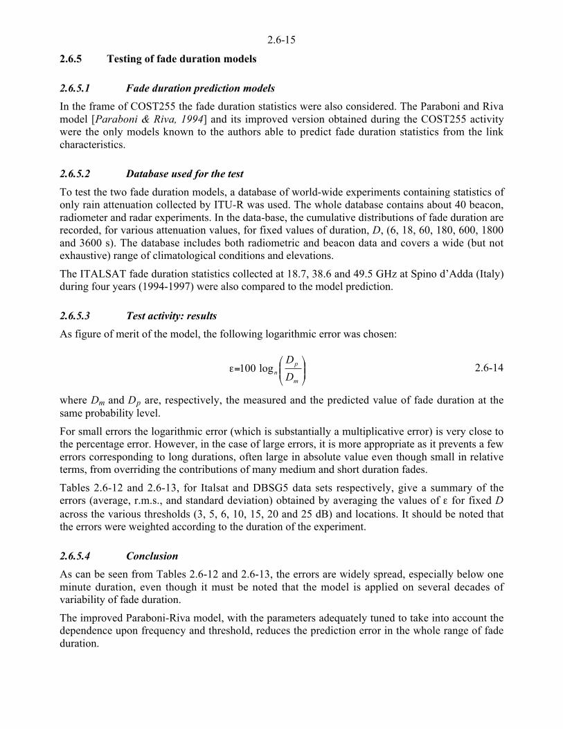
2.6-15

2.6.5 Testing of fade duration models

2.6.5.1 Fade duration prediction models

In the frame of COST255 the fade duration statistics were also considered. The Paraboni and Rivamodel [Paraboni & Riva, 1994] and its improved version obtained during the COST255 activitywere the only models known to the authors able to predict fade duration statistics from the linkcharacteristics.

2.6.5.2 Database used for the test

To test the two fade duration models, a database of world-wide experiments containing statistics ofonly rain attenuation collected by ITU-R was used. The whole database contains about 40 beacon,radiometer and radar experiments. In the data-base, the cumulative distributions of fade duration arerecorded, for various attenuation values, for fixed values of duration, D, (6, 18, 60, 180, 600, 1800and 3600 s). The database includes both radiometric and beacon data and covers a wide (but notexhaustive) range of climatological conditions and elevations.

The ITALSAT fade duration statistics collected at 18.7, 38.6 and 49.5 GHz at Spino d’Adda (Italy)during four years (1994-1997) were also compared to the model prediction.

2.6.5.3 Test activity: results

As figure of merit of the model, the following logarithmic error was chosen:

´́¦

¥²²¤

£=¡

m

pn D

Dlog100 2.6-14

where Dm and Dp are, respectively, the measured and the predicted value of fade duration at thesame probability level.

For small errors the logarithmic error (which is substantially a multiplicative error) is very close tothe percentage error. However, in the case of large errors, it is more appropriate as it prevents a fewerrors corresponding to long durations, often large in absolute value even though small in relativeterms, from overriding the contributions of many medium and short duration fades.

Tables 2.6-12 and 2.6-13, for Italsat and DBSG5 data sets respectively, give a summary of theerrors (average, r.m.s., and standard deviation) obtained by averaging the values of ¡ for fixed Dacross the various thresholds (3, 5, 6, 10, 15, 20 and 25 dB) and locations. It should be noted thatthe errors were weighted according to the duration of the experiment.

2.6.5.4 Conclusion

As can be seen from Tables 2.6-12 and 2.6-13, the errors are widely spread, especially below oneminute duration, even though it must be noted that the model is applied on several decades ofvariability of fade duration.

The improved Paraboni-Riva model, with the parameters adequately tuned to take into account thedependence upon frequency and threshold, reduces the prediction error in the whole range of fadeduration.

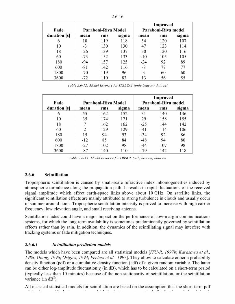
2.6-16

Paraboni-Riva ModelImproved

Paraboni-Riva modelFadeduration [s] mean rms sigma mean rms sigma

6 10 119 118 54 120 10710 -3 130 130 47 123 11418 -26 139 137 30 120 11660 -73 152 133 -10 105 105180 -94 157 125 -24 92 89600 -81 142 116 -8 77 77

1800 -70 119 96 3 60 603600 -72 110 83 13 56 55

Table 2.6-12: Model Errors ¡ for ITALSAT (only beacon) data set

Paraboni-Riva ModelImproved

Paraboni-Riva modelFadeduration [s] mean rms sigma mean rms sigma

6 55 162 152 31 140 13610 35 174 171 29 158 15518 7 162 162 -25 144 14260 2 129 129 -41 114 106180 15 94 93 -34 92 86600 -12 85 84 -48 94 80

1800 -27 102 98 -44 107 983600 -87 140 110 -79 142 118

Table 2.6-13: Model Errors ¡ for DBSG5 (only beacon) data set

2.6.6 Scintillation

Tropospheric scintillation is caused by small-scale refractive index inhomogeneities induced byatmospheric turbulence along the propagation path. It results in rapid fluctuations of the receivedsignal amplitude which affect earth-space links above about 10 GHz. On satellite links, thesignificant scintillation effects are mainly attributed to strong turbulence in clouds and usually occurin summer around noon. Tropospheric scintillation intensity is proved to increase with high carrierfrequency, low elevation angle, and small receiving antenna.

Scintillation fades could have a major impact on the performance of low-margin communicationssystems, for which the long-term availability is sometimes predominantly governed by scintillationeffects rather than by rain. In addition, the dynamics of the scintillating signal may interfere withtracking systems or fade mitigation techniques.

2.6.6.1 Scintillation prediction models

The models which have been compared are all statistical models [ITU-R, 1997b; Karasawa et al.,1988; Otung, 1996; Ortgies, 1993; Peeters et al., 1997]. They allow to calculate either a probabilitydensity function (pdf) or a cumulative density function (cdf) of a given random variable. The lattercan be either log-amplitude fluctuation r (in dB), which has to be calculated on a short-term period(typically less than 10 minutes) because of the non-stationarity of scintillation, or the scintillationvariance (in dB2).

All classical statistical models for scintillation are based on the assumption that the short-term pdfof the log amplitude is gaussian which leads to a symmetrical distribution of signal level

2.6-17

various sites, especially during strong scintillation periods. That is why we have introduced the newmodel proposed by Van de Kamp in this test activity; indeed this one is based on an alternativetheoretical formulation for the signal fluctuations which leads directly to asymmetry of thedistribution of signal fluctuations.

Concerning the long term pdf of scintillation variance, two different models can be found: either agamma distribution (ITU-R, Karasawa, Otung models, van de Kamp model) or a log-normaldistribution (both versions of Ortgies model, DPSP and MPSP models).

It must be noted that in this test, the latest version of the Van de Kamp model [van de Kamp et al.,1998] has not been used.

2.6.6.2 Experimental data used for the test

In our test activity, the scintillation data used originate from three different data sets:

• the DBSG5 data base, the latest version of which has been extracted from the COST255 Website;

• scintillation data which are related to measurements in Spino d’Adda (Italy) using theITALSAT satellite 39.6 and 49.5 GHz beacons;

• scintillation data which among others include some OLYMPUS measurements[OPEX, 1994];

• other measurements gathered from the literature.

As far as the DBSG5 database is concerned, the comparison can deal with scintillation standarddeviation and for some of the experiments present in the database with cdf of scintillation fading,both on a monthly basis.

For data related to the ITALSAT measurements in Spino d’Adda and to the OLYMPUS data, it ispossible to compare scintillation standard deviations, cdf of scintillation fading and enhancement,also on a monthly basis.

2.6.6.3 Test activity: results

The comparison between measurements and predictions is achieved either using a graphicalrepresentation of the predicted values or distributions along with the corresponding experimentaldata or through the calculation of the relative error (in %) between the model and the measuredvalues. Figure 2.6-2 illustrates the global scatter of points obtained for all models on the DBSG5database, in terms of standard deviation. Of course, it is not easy to draw conclusions from this typeof figure. But it seems that the models always tend to underestimate the scintillation intensity (ascompared to measurements). As is already known, for low elevations the scintillation intensity ishigher than for medium elevation paths. Figure 2.6-3 shows the resulting scintillation fadedistribution only for one experiment (Austin, 11 GHz). Some models overestimate the scintillationfades, but some underestimate them. Figure 2.6-4 shows the resulting scintillation fade distributiononly for one month of 40 GHz ITALSAT data in Spino d’Adda. The Ortgies-T model agrees verywell.

2.6-18

Figure 2.6-2: Comparison of various models (standard deviation) for different sites (DBSG5 database)

Figure 2.6-3 Comparison of various models (scintillation fades) for Austin

2.6-19

Figure 2.6-4 Italsat 40 GHz data at Spino d’Adda: scintillation fade for January

Table 2.6-14 shows the results of the test through the calculation of the relative error (in %)between the model and the measured values. For each model, the errors associated with eachexperiment have been summed up, and analysed statistically in order to get the global mean error,the standard deviation and the root mean square error of the prediction.

Table 2.6-14a presents the results with the DBSG5 database. There is no obvious general trend fromthe first comparison. Nevertheless the ITU-R and Karasawa models seem to give quite a good fit tothe measurements. As far as other models are concerned, occasionally they can give a predictionvery close to the experimental data but the predicted value can also be very far from the measuredone. It is not obvious to deduce their respective specific validity domains from the comparisons wehave made so far.

Table 2.6-14b shows results with INTELSAT data from Okinawa and some OLYMPUS data fromEindhoven. The ITU-R and Karasawa models do not give good agreement, whereas the Van deKamp and Ortgies-T models are not so bad.

Table 2.6-14c concerns the results from OLYMPUS data in Eindhoven. The ITU-R and Karasawamodels do not give good agreement. The Van de Kamp and Ortgies-T models are quite good (whichseems sensible because they have mainly been developed using OLYMPUS data). The DPSP andMPSP models are not so bad for this set of data.

Generally speaking, in the EHF band, the predictions are not so far from the measurements althoughthe models are used outside their validity domains. Particularly the Ortgies-T and Van de Kampmodels seem to agree quite well with the experimental data. The same trend has already beenobserved [Vasseur & Douchin, 1997] on our CELESTE data at 35 GHz at low elevation angle (5°)where all predictions overestimate values of scintillation fading and the Ortgies-T model seemed tobe the closest to the experimental data in such propagation conditions.

We can state that:

• ITU-R and Karasawa performs well on DBSG5 database

• Ortgies-T and Van de Kamp models seem promising, especially for high frequency links

• DPSP and MPSP always give moderate agreement with experimental data

2.6-20

a) Data base DBSG5

Num Itur Karasawa Dpsp Mpsp Ortgies-Nw Ortgies-T Otung M.Van deKamp

Moy 2.900 1.743 -21.767 -47.835 -24.339 -46.989 -43.577 -37.253|Moy| 14.805 12.310 29.510 49.037 38.981 47.003 43.577 37.959std 17.802 17.366 26.960 23.840 34.571 12.587 15.044 24.872rms 18.036 17.454 34.650 53.447 42.280 48.645 46.101 44.792

b) Okinowa and Eindhoven Data

Num Itur Karasawa Dpsp Mpsp Ortgies-Nw Ortgies-T Otung M.Van deKamp

Moy 114.467 112.348 23.427 3.225 42.273 -5.991 61.356 3.402|Moy| 115.189 113.730 27.605 26.055 48.816 21.344 79.350 14.010std 71.309 74.920 27.076 31.299 39.223 26.220 63.714 17.859rms 134.862 135.037 35.804 31.465 57.667 26.896 88.454 18.180

c) Eindhoven Data (three frequencies) - f1=12.5GHz, f2=19.77 GHz, f3=29.66 GHz

Num Itur Karasawa Dpsp Mpsp Ortgies-Nw Ortgies-T Otung M.Van deKamp

Moy 110.393 109.402 24.399 13.352 30.782 6.086 70.353 7.980|Moy| 110.393 109.402 24.692 15.929 30.782 9.267 70.353 9.305std 76.804 78.653 25.329 20.714 28.281 12.566 50.302 12.404rms 134.482 134.741 35.169 24.644 41.802 13.962 86.486 14.749

Table 2.6-14: Test results

2.6.7 Testing of XPD-CPA Models at Ka and V Bands

The models of atmospheric depolarisation, discussed in Chapter 2.4, are based either on theatmospheric transmission matrix, that permits a full description of polarisation effects, or on theequiprobability relationship between rain attenuation and the cross-polar discrimination.

The [ITU-R, 1997b], [Fukuchi, 1990] and the DHW [Dissanayake et. al, 1980] models for theestimation of the cumulative distribution function of the Crosspolar Discrimination at a givenpercentage of the year, have been checked using the measurements of the ITALSAT andOLYMPUS propagation beacons [Martellucci & Paraboni, 1998]. For the analysis of the DHWmodel, only the equations applicable to the rain depolarization have been used.

The statistics from the OLYMPUS propagation experiment (see [Dintelmann, 1994]) contained inthe DBOPEX database, Table II-5a (Slant Path Annual XPD statistics), have been compared withmodels.

The structure of the DBOPEX is almost identical to the ITU-R propagation database of StudyGroup V, the DBSGV database. The OLYMPUS measurements have been performed by EindhovenTechnical University (EUT), the Netherlands, [Hogers et. al. 1991], [Van de Kamp, 1994a; 1994b;1995; 1999] and by the Université Catholique de Louvain (UCL) in Louvain-la-Neuve and inLessive, Belgium [Dintelmann 1994].

The ITALSAT measurements have been the performed by Fondazione Ugo Bordoni from 1994 to1995 in Pomezia, near Rome, Italy, and the examined data cover the period from 1994 to 1995[Martellucci et al. 1997]. The measurements cover the whole period, but due to system maintenancethe ground system did not perform measurements during summer, resulting in the loss of summer

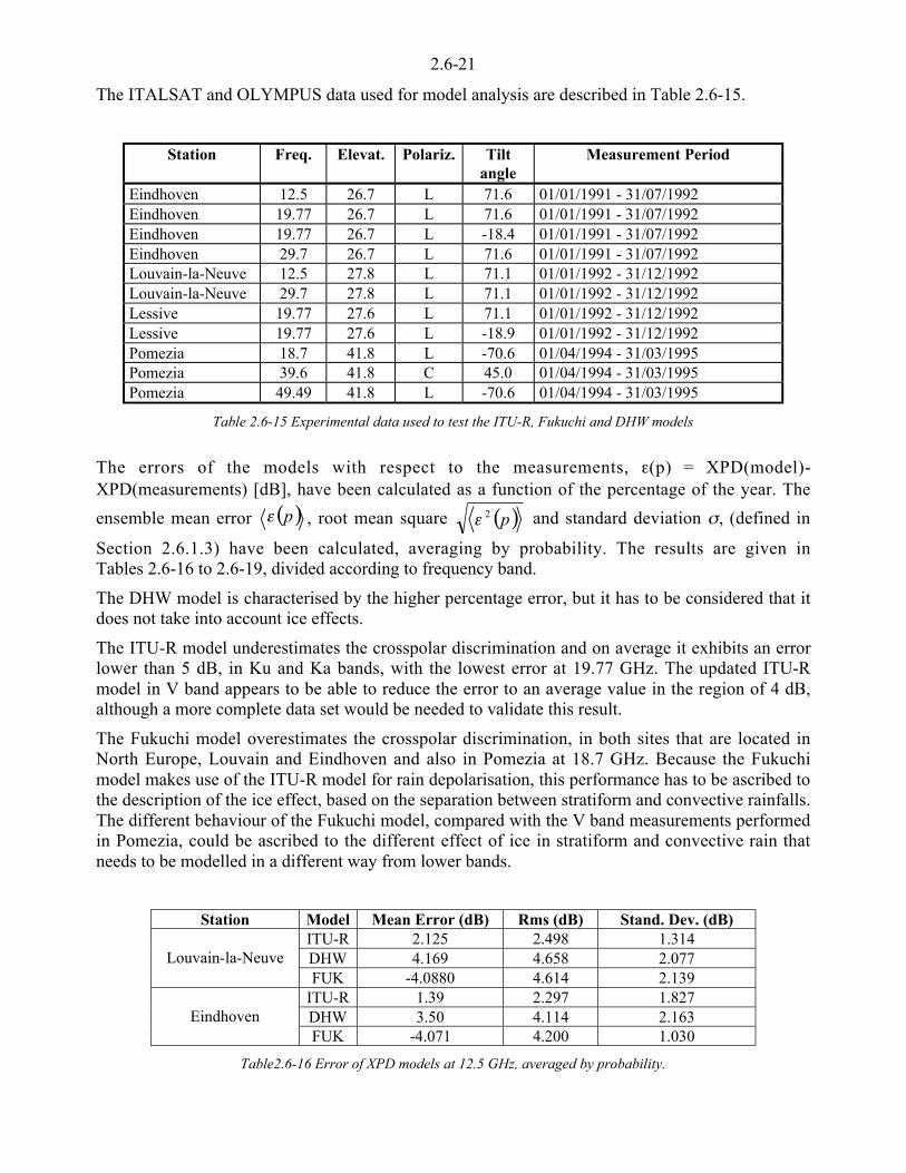
2.6-21

The ITALSAT and OLYMPUS data used for model analysis are described in Table 2.6-15.

Station Freq. Elevat. Polariz. Tiltangle

Measurement Period

Eindhoven 12.5 26.7 L 71.6 01/01/1991 - 31/07/1992Eindhoven 19.77 26.7 L 71.6 01/01/1991 - 31/07/1992Eindhoven 19.77 26.7 L -18.4 01/01/1991 - 31/07/1992Eindhoven 29.7 26.7 L 71.6 01/01/1991 - 31/07/1992Louvain-la-Neuve 12.5 27.8 L 71.1 01/01/1992 - 31/12/1992Louvain-la-Neuve 29.7 27.8 L 71.1 01/01/1992 - 31/12/1992Lessive 19.77 27.6 L 71.1 01/01/1992 - 31/12/1992Lessive 19.77 27.6 L -18.9 01/01/1992 - 31/12/1992Pomezia 18.7 41.8 L -70.6 01/04/1994 - 31/03/1995Pomezia 39.6 41.8 C 45.0 01/04/1994 - 31/03/1995Pomezia 49.49 41.8 L -70.6 01/04/1994 - 31/03/1995

Table 2.6-15 Experimental data used to test the ITU-R, Fukuchi and DHW models

The errors of the models with respect to the measurements, ¡(p) = XPD(model)-XPD(measurements) [dB], have been calculated as a function of the percentage of the year. The

ensemble mean error ( )p¡ , root mean square ( )p2¡ and standard deviation m, (defined in

Section 2.6.1.3) have been calculated, averaging by probability. The results are given inTables 2.6-16 to 2.6-19, divided according to frequency band.

The DHW model is characterised by the higher percentage error, but it has to be considered that itdoes not take into account ice effects.

The ITU-R model underestimates the crosspolar discrimination and on average it exhibits an errorlower than 5 dB, in Ku and Ka bands, with the lowest error at 19.77 GHz. The updated ITU-Rmodel in V band appears to be able to reduce the error to an average value in the region of 4 dB,although a more complete data set would be needed to validate this result.

The Fukuchi model overestimates the crosspolar discrimination, in both sites that are located inNorth Europe, Louvain and Eindhoven and also in Pomezia at 18.7 GHz. Because the Fukuchimodel makes use of the ITU-R model for rain depolarisation, this performance has to be ascribed tothe description of the ice effect, based on the separation between stratiform and convective rainfalls.The different behaviour of the Fukuchi model, compared with the V band measurements performedin Pomezia, could be ascribed to the different effect of ice in stratiform and convective rain thatneeds to be modelled in a different way from lower bands.

Station Model Mean Error (dB) Rms (dB) Stand. Dev. (dB)ITU-R 2.125 2.498 1.314DHW 4.169 4.658 2.077Louvain-la-NeuveFUK -4.0880 4.614 2.139

ITU-R 1.39 2.297 1.827DHW 3.50 4.114 2.163EindhovenFUK -4.071 4.200 1.030

Table2.6-16 Error of XPD models at 12.5 GHz, averaged by probability.

2.6-22

Station Model Mean Error (dB) Rms (dB) Stand. Dev. (dB)Pomezia ITU-R -1.270 1.832 1.320

18.68 GHz DHW 1.097 1.291 .6806Tilt Angle –70.55 FUK -6.527 6.600 .9766

Lessive ITU-R .7126 1.650 1.48819.77 GHz DHW 3.207 3.715 1.875

Tilt Angle –18.9 FUK -6.426 6.706 1.918Lessive ITU-R .9402 1.723 1.444

19.77 GHz DHW 3.382 3.881 1.904Tilt Angle 71.1 FUK -5.729 6.012 1.821

Eindhoven ITU-R 1.040 1.651 1.28319.77 GHz DHW 4.044 4.263 1.351

Tilt Angle –18.4 FUK -6.443 6.539 1.115Eindhoven ITU-R -2.004 2.180 .859319.77 GHz DHW .6516 1.067 .8449

Tilt Angle 71.60 FUK -10.26 10.33 1.219

Table 2.6-17 Error of XPD models at 18.68 and 19.77 GHz, averaged by probability.

Station Model Mean Error (dB) Rms (dB) Stand. Dev. (dB)Louvain-la-Neuve ITU-R 6.023 6.717 2.973

Tilt Angle 71.1 DHW 8.431 8.694 2.124FUK .2161 4.450 4.445

Eindhoven ITU-R 2.878 3.148 1.274Tilt Angle 71.60 DHW 5.428 5.575 1.271

FUK -3.784 3.993 1.275

Table 2.6-18 Error of XPD models at 29.66 GHz, averaged by probability.

Station Model Mean Error (dB) Rms (dB) Stand. Dev. (dB)Pomezia ITU-R .1180 1.478 1.47439.6 GHz FUK 1.694 2.486 1.820Pomezia ITU-R 3.900 5.010 3.14549.5 GHz FUK 6.086 6.690 2.777

Table 2.6-19 Error of XPD models in V Band, averaged by probability.

The effect of ice at higher frequencies can be understood, from a physical point of view, byexamining the relationship between the overall crosspolar discrimination and the rain attenuation,predicted by the models and measured, that is given for 12.5, 29.7 and 49.5 GHz in Figure2.6-5. Inthis way the effective applicability of the equiprobability relationship can also be verified.

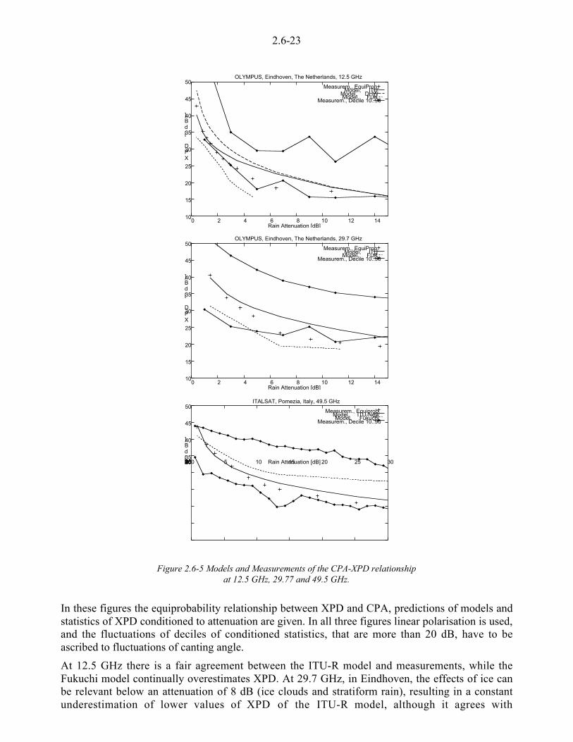
2.6-23

10

15

20

25

30

35

40

45

50

0 2 4 6 8 10 12 14

XPD [dB]

Rain Attenuation [dB]

OLYMPUS, Eindhoven, The Netherlands, 12.5 GHz

Measurem., EquiProb. Model, ITU

Model, DHWModel, FUK

Measurem., Decile 10..90

10

15

20

25

30

35

40

45

50

0 2 4 6 8 10 12 14

XPD [dB]

Rain Attenuation [dB]

OLYMPUS, Eindhoven, The Netherlands, 29.7 GHz

Measurem., EquiProb. Model, ITU

Model, FUKMeasurem., Decile 10..90

101520253035

40

45

50

0 5 10 15 20 25 30XPD [dB]

Rain Attenuation [dB]

ITALSAT, Pomezia, Italy, 49.5 GHz

Measurem., Equiprob.Model, ITU-NewModel, Fukuchi

Measurem., Decile 10..90

Figure 2.6-5 Models and Measurements of the CPA-XPD relationshipat 12.5 GHz, 29.77 and 49.5 GHz.

In these figures the equiprobability relationship between XPD and CPA, predictions of models andstatistics of XPD conditioned to attenuation are given. In all three figures linear polarisation is used,and the fluctuations of deciles of conditioned statistics, that are more than 20 dB, have to beascribed to fluctuations of canting angle.

At 12.5 GHz there is a fair agreement between the ITU-R model and measurements, while theFukuchi model continually overestimates XPD. At 29.7 GHz, in Eindhoven, the effects of ice canbe relevant below an attenuation of 8 dB (ice clouds and stratiform rain), resulting in a constantunderestimation of lower values of XPD of the ITU-R model, although it agrees with

2.6-24

equiprobability statistics. In this case the Fukuchi model predicts the maximum value of overalldepolarisation.

At 49.5 GHz although they agree, neither the equiprobability value nor the updated ITU-R andFukuchi models, predict actual values of XPD, up to an attenuation of 20 dB. The data and themodels are in agreement only in presence of rain thunderstorms, when rain depolarisation isprevalent over the ice depolarisation.

2.6-25

2.6.8 References

[Allnutt and Rogers, 1982]Allnutt, J.E. and D.V. Rogers, “Novel method for predicting site diversity gain on satellite-to-ground radio paths”, Electronics Letters, Vol. 18, No. 5, pp. 233-235, 1982.

[Bosisio & Riva, 1998]Bosisio, A.V. and C. Riva, “A novel method for the statistical prediction of rain attenuation in sitediversity systems: theory and comparative testing against experimental data”, International Journalof Satellite Communications, Vol. 16, pp. 47-52, 1998,

[Bryant et al., 2001]Bryant G.H., I. Adimula, C. Riva and G. Brussaard, “Rain Attenuation Statistics from Rain CellDiameters and Heights”, Int. J. Satellite Comm., Vol 19, 3, pp 263-283, 2001.

[Capsoni et al., 1987]Capsoni C., F. Fedi and A. Paraboni, “A comprehensive meteorologically oriented methodology forthe prediction of wave propagation parameters in telecommunication applications beyond 10 GHz”,Radio Science, Vol. 22, No. 3, pp. 387-393, 1987.

[CCIR, 1992]CCIR, M.S. Pontes and Linear.A.R. Silva Mello, “Progress on the investigation of a slant-pathattenuation prediction method based on the complete point rainfall rate probability distribution”,PG3 Document 92/7, 1992.

[CCIR, 1993]CCIR, Japan, “Proposal of a rain attenuation method”, PG3 Document 93/6, rev. 2, 1993.

[COST205, 1985]Ed. F. Fedi, “Prediction of rain attenuation statistics from point rainfall intensity data”,Alta Frequenza, Vol. LIV, No. 3, pp. 140-156, 1985.

[Costa, 1983]Costa, E., “An analytical and numerical comparison between two rain attenuation predictionmethod for earth-satellite paths”, Proc. URSI Comm. F, Louvain-la-Neuve, pp. 213, 1983.

[Crane, 1980]Crane, R.K., “Prediction of attenuation by rain”, IEEE Transaction on Communications, Vol. 28,pp. 1717-1733, 1980.

[Crane, 1985]Crane, R.K., “Comparative evaluation of several rain attenuation prediction models”, RadioScience, Vol. 20, No. 4, pp. 843-863, 1985.

[Dintelmann, 1994]Dintelmann, F. (Editor), “Reference Book on Depolarisation”, OPEX- ESA WPP-083, 1994.

2.6-26

[Dissanayake et. al, 1980]Dissanayake, A.W., D.P. Haworth and P.A. Watson, “Analytical models for cross-polarization onearth space radio paths for frequency range 9-30 GHz”, Ann. Telecommunic., Vol. 35, No. 11-12,pp 398-404, 1980.

[Dissanayake et al., 1997]Dissanayake, A., J. Allnutt and F. Haidara, “A prediction model that combines rain attenuation andother propagation impairments along earth-satellite paths”, IEEE Transactions on Antennas andPropagation, Vol. 45, No. 10, pp. 1546-1558, 1997.

[Flavin, 1996]Flavin, R.K., “Satellite link rain attenuation in Brisbane and a proposed new model for Australia”,Telstra Research Laboratories, Report N. 8375, 1996.

[Fukuchi, 1990]Fukuchi, H., “Prediction of depolarisation distribution on earth-space paths”, IEE Proceedings, Vol.137, Pt. II, n. 6, December 1990, 1990.

[Garcia et al., 1988]García-López, J.A., J.M. Hernando and J.M. Selga, “Simple rain attenuation prediction method forsatellite radio links”, IEEE Transactions on Antennas and Propagation, Vol. 36, No. 3, pp. 444-448,1988.

[Goldhirsh, 1982]Goldhirsh, J., “Space diversity performance prediction for earth-satellite paths using radarmodelling techniques”, Radio Science, Vol. 17, No. 6, pp. 1400-1410, 1982.

[Hodge, 1982]Hodge, D.B., “An improved model for diversity gain on earth-space propagation paths”, RadioScience, Vol. 17, No. 6, pp. 1393-1399, 1982.

[Hogers et. al. 1991]Hogers, R., M. Herben and G. Brussaard, “Depolarisation analysis of the 12.5 and 30 GHz Olympusbeacon signals”, Proc. 1st OPEX Workshop, ESTEC, Noordwijk, The Netherlands, pp. 2.4.1-2.4.12, 1991.

[ITU-R, 1997a]ITU-R, “Acquisition, presentation and analysis of data in studies of tropospheric propagation”,Propagation in Non-Ionized Media, Rec. 311-8, 1997.

[ITU-R, 1997b]ITU-R, “Propagation data and prediction methods required for the design of Earth-spacetelecommunication systems”, Propagation in Non-Ionized Media, Rec. 618-5, 1997.

[Karasawa et al., 1988]Karasawa, Y., K. Yasukawa and M. Yamada, “Tropospheric scintillation in the 14/11-GHz bandson earth-space paths with low elevation angles”, IEEE Transactions on Antennas and Propagation,Vol. 36, pp. 563-569, 1988.

2.6-27

[Martellucci & Paraboni, 1998]Martellucci, A. and A. Paraboni, “Test and Development of Models of Atmospheric CrosspolarDiscrimination for Satellite Communication Systems at Ka and V band”, Proceed. of the firstinternational Workshop on Radiowave Propagation Modelling for SatCom Services at Ku-band andabove, ESTEC, Noordwijk, The Netherlands, 1998.

[Martellucci et al. 1997]Martellucci, A., F. Barbaliscia and A. Aresu, “Measurements of attenuation and Cross-PolarDiscriminination performed using the ITALSAT propgation beacons at 18.7, 40 and 50 GHz”,Proceed. Of 3rd Ka-Band Utiliz. Conf., Sorrento, Italy, pp. 113-119, 1997.

[Mass, 1987]Mass, J., “A simulation study of rain attenuation and diversity effects on satellite links”, ComsatTechnical Review, Vol. 17, No. 1, pp. 159-186, 1987.

[Matricciani, 1991]Matricciani, E., “Rain attenuation predicted with two-layer rain model”, European Transactions onTelecommunication, Vol. 2, No. 6, pp. 715-727, 1991.

[Matricciani, 1994]Matricciani, E., “Prediction of site diversity performance in satellite communications systemsaffected by rain attenuation: extension of the two layer rain model”, European Transactions onTelecommunications, Vol. 5, No. 3, pp. 27-36, 1994.

[OPEX, 1994]OPEX Editors:Poiares Baptista, J.P.V.,and P.G. Davies, “Reference Book on AttenuationMeasurement and Prediction”, 2nd Workshop of the OLYMPUS Propagation Experimenters(OPEX), Doc. ESA-ESTEC-WPP-083 volume 1, Noordwijk, The Netherlands, 1994.

[Ortgies, 1993]Ortgies, G., “Prediction of slant-path amplitude scintillations from meteorological parameters”,Proc. Int. Symp. on Radio Propagation, Beijing, pp. 218-221, 1993.

[Otung, 1996]Otung, I.E., “Prediction of Tropospheric Amplitude Scintillation on a Satellite Link”, IEEETransactions on Antennas and Propagation, Vol. 44, No. 12, pp. 1600-1608, 1996.

[Paraboni & Riva, 1994]Paraboni, A. and C. Riva, “A new method for the prediction of fade duration statistics in satellitelinks beyond 10 GHz”, International Journal of Satellite Communication, Vol. 12, pp. 387-394,1994.

[Peeters et al., 1997]Peeters, G., F.S. Marzano, G. D’Auria, C. Riva and D. Vanhoenacker-Janvier, “Evaluation ofstatistical models for clear-air scintillation prediction using Olympus satellite measurements”,International Journal of Satellite Communications, Vol. 15, pp. 73-88, 1997.

2.6-28

[Poiares Baptista and Salonen, 1998]Poiares Baptista, J.P.V. and E.T. Salonen, “Review of Rainfall rate modelling and mapping”,CLIMPARA’98, Ottawa (Canada), 1998.

[Stutzman and Dishman, 1984]Stutzman, W.L. and W.K. Dishman, “A simple model for the estimation of rain-induced attenuationalong earth-space paths at millimeter wavelengths”, Radio Science, Vol. 19, pp. 946, 1984.

[Svjatogor, 1985]Svjatogor, L., “Prostranstvennaia korelacia vypadenjija dozdjej vdol zemnoj poverchnostji” (inRussian), Symposium expertov stran uchastnic programmy INTERKOSMOS (Interkosmossymposium), theme 5 of the established telecommunication working group , Dresden,GDR, 1985.

[Van de Kamp, 1994a]Van de Kamp, M.M.J.L., E.J.M. Smits, M.H.A.J. Herben and G. Brussaard, “ExperimentalVerification of Existing Rain Depolarisation Models”, Archiv für Elektronik undÜbertragungstechnik, Vol. 48, No. 3, pp. 173-176., 1994

[Van de Kamp, 1994b]Van de Kamp, M.M.J.L., “Dual-Channel Crosspolarisation Analysis”, Final Report of ESA/ESTECContract 10290/93/NL/GS, Eindhoven University of Technology, 1994.

[Van de Kamp, 1995]Van de Kamp, M.M.J.L., “On the Derivation of Rain Anisotropy from Olympus BeaconMeasurements”, 9th International Conference on Antennas and Propagation, IEE Conf. Publ. 407,Vol. 2, pp. 18-22, 1995.

[Van de Kamp, 1999]Van de Kamp, M.M.J.L., private communication, 1999.

[van de Kamp et al., 1998]Van de Kamp, M.M.J.L., J.K. Tervonen, E.T. Salonen and J.P.V. Poiares-Baptista, “Improvedmodel for log-term prediction of Tropospheric Scintillation on slant paths”, COST 255 Workshop,Noordwijk, 1998.

[Vasseur & Douchin, 1997]Vasseur, H. and N. Douchin, “Experimental Analysis of Tropospheric Scintillation on a Low-Elevation Path”, Proc. ICAP'97, 1997.

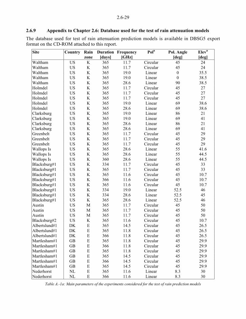
2.6-29

2.6.9 Appendix to Chapter 2.6: Database used for the test of rain attenuation models

The database used for test of rain attenuation prediction models is available in DBSG5 exportformat on the CD-ROM attached to this report.

Site Country Rainzone

Duration[days]

Frequency[GHz]

Poln Pol. Angle[deg]

Elevn

[deg]Waltham US K 365 11.7 Circular 45 24Waltham US K 365 11.7 Circular 45 24Waltham US K 365 19.0 Linear 0 35.5Waltham US K 365 19.0 Linear 0 38.5Waltham US K 365 28.6 Linear 90 38.5Holmdel US K 365 11.7 Circular 45 27Holmdel US K 365 11.7 Circular 45 27Holmdel US K 365 11.7 Circular 45 27Holmdel US K 365 19.0 Linear 69 38.6Holmdel US K 365 28.6 Linear 69 38.6Clarksburg US K 365 19.0 Linear 86 21Clarksburg US K 365 19.0 Linear 69 41Clarksburg US K 365 28.6 Linear 86 21Clarksburg US K 365 28.6 Linear 69 41Greenbelt US K 365 11.7 Circular 45 29Greenbelt US K 365 11.7 Circular 45 29Greenbelt US K 365 11.7 Circular 45 29Wallops Is US K 365 28.6 Linear 55 41.6Wallops Is US K 365 28.6 Linear 55 44.5Wallops Is US K 360 28.6 Linear 55 44.5Blacksburg#1 US K 334 11.7 Circular 45 33Blacksburg#1 US K 365 11.7 Circular 45 33Blacksburg#1 US K 365 11.6 Circular 45 10.7Blacksburg#1 US K 366 11.6 Circular 45 10.7Blacksburg#1 US K 365 11.6 Circular 45 10.7Blacksburg#1 US K 334 19.0 Linear 52.5 46Blacksburg#1 US K 334 28.6 Linear 52.5 45Blacksburg#1 US K 365 28.6 Linear 52.5 46Austin US M 365 11.7 Circular 45 50Austin US M 365 11.7 Circular 45 50Austin US M 365 11.7 Circular 45 50Blacksburg#2 US K 365 11.6 Circular 45 10.7Albertslund#1 DK E 365 14.5 Circular 45 26.5Albertslund#1 DK E 365 11.8 Circular 45 26.5Albertslund#1 DK E 366 11.8 Circular 45 26.5Martlesham#1 GB E 365 11.8 Circular 45 29.9Martlesham#1 GB E 366 11.8 Circular 45 29.9Martlesham#1 GB E 365 11.8 Circular 45 29.9Martlesham#1 GB E 365 14.5 Circular 45 29.9Martlesham#1 GB E 366 14.5 Circular 45 29.9Martlesham#1 GB E 365 14.5 Circular 45 29.9Nederhorst NL E 365 11.6 Linear 8.3 30Nederhorst NL E 366 11.6 Linear 8.3 30

Table A.-1a: Main parameters of the experiments considered for the test of rain prediction models

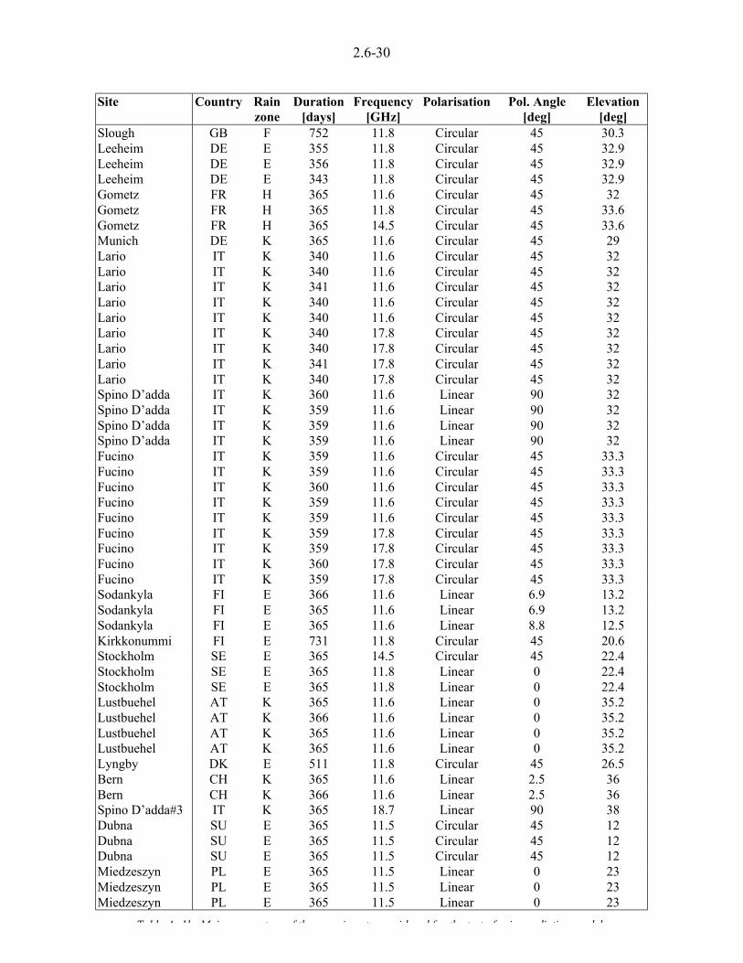
2.6-30

Site Country Rainzone

Duration[days]

Frequency[GHz]

Polarisation Pol. Angle[deg]

Elevation[deg]

Slough GB F 752 11.8 Circular 45 30.3Leeheim DE E 355 11.8 Circular 45 32.9Leeheim DE E 356 11.8 Circular 45 32.9Leeheim DE E 343 11.8 Circular 45 32.9Gometz FR H 365 11.6 Circular 45 32Gometz FR H 365 11.8 Circular 45 33.6Gometz FR H 365 14.5 Circular 45 33.6Munich DE K 365 11.6 Circular 45 29Lario IT K 340 11.6 Circular 45 32Lario IT K 340 11.6 Circular 45 32Lario IT K 341 11.6 Circular 45 32Lario IT K 340 11.6 Circular 45 32Lario IT K 340 11.6 Circular 45 32Lario IT K 340 17.8 Circular 45 32Lario IT K 340 17.8 Circular 45 32Lario IT K 341 17.8 Circular 45 32Lario IT K 340 17.8 Circular 45 32Spino D’adda IT K 360 11.6 Linear 90 32Spino D’adda IT K 359 11.6 Linear 90 32Spino D’adda IT K 359 11.6 Linear 90 32Spino D’adda IT K 359 11.6 Linear 90 32Fucino IT K 359 11.6 Circular 45 33.3Fucino IT K 359 11.6 Circular 45 33.3Fucino IT K 360 11.6 Circular 45 33.3Fucino IT K 359 11.6 Circular 45 33.3Fucino IT K 359 11.6 Circular 45 33.3Fucino IT K 359 17.8 Circular 45 33.3Fucino IT K 359 17.8 Circular 45 33.3Fucino IT K 360 17.8 Circular 45 33.3Fucino IT K 359 17.8 Circular 45 33.3Sodankyla FI E 366 11.6 Linear 6.9 13.2Sodankyla FI E 365 11.6 Linear 6.9 13.2Sodankyla FI E 365 11.6 Linear 8.8 12.5Kirkkonummi FI E 731 11.8 Circular 45 20.6Stockholm SE E 365 14.5 Circular 45 22.4Stockholm SE E 365 11.8 Linear 0 22.4Stockholm SE E 365 11.8 Linear 0 22.4Lustbuehel AT K 365 11.6 Linear 0 35.2Lustbuehel AT K 366 11.6 Linear 0 35.2Lustbuehel AT K 365 11.6 Linear 0 35.2Lustbuehel AT K 365 11.6 Linear 0 35.2Lyngby DK E 511 11.8 Circular 45 26.5Bern CH K 365 11.6 Linear 2.5 36Bern CH K 366 11.6 Linear 2.5 36Spino D’adda#3 IT K 365 18.7 Linear 90 38Dubna SU E 365 11.5 Circular 45 12Dubna SU E 365 11.5 Circular 45 12Dubna SU E 365 11.5 Circular 45 12Miedzeszyn PL E 365 11.5 Linear 0 23Miedzeszyn PL E 365 11.5 Linear 0 23Miedzeszyn PL E 365 11.5 Linear 0 23

T bl A 1b M i t f th i t id d f th t t f i di ti d l

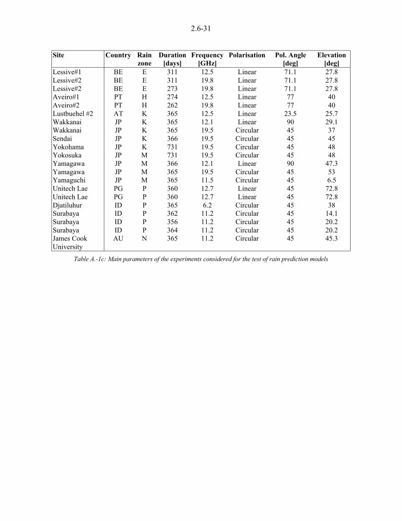
2.6-31

Site Country Rainzone

Duration[days]

Frequency[GHz]

Polarisation Pol. Angle[deg]

Elevation[deg]

Lessive#1 BE E 311 12.5 Linear 71.1 27.8Lessive#2 BE E 311 19.8 Linear 71.1 27.8Lessive#2 BE E 273 19.8 Linear 71.1 27.8Aveiro#1 PT H 274 12.5 Linear 77 40Aveiro#2 PT H 262 19.8 Linear 77 40Lustbuehel #2 AT K 365 12.5 Linear 23.5 25.7Wakkanai JP K 365 12.1 Linear 90 29.1Wakkanai JP K 365 19.5 Circular 45 37Sendai JP K 366 19.5 Circular 45 45Yokohama JP K 731 19.5 Circular 45 48Yokosuka JP M 731 19.5 Circular 45 48Yamagawa JP M 366 12.1 Linear 90 47.3Yamagawa JP M 365 19.5 Circular 45 53Yamaguchi JP M 365 11.5 Circular 45 6.5Unitech Lae PG P 360 12.7 Linear 45 72.8Unitech Lae PG P 360 12.7 Linear 45 72.8Djatiluhur ID P 365 6.2 Circular 45 38Surabaya ID P 362 11.2 Circular 45 14.1Surabaya ID P 356 11.2 Circular 45 20.2Surabaya ID P 364 11.2 Circular 45 20.2James CookUniversity

AU N 365 11.2 Circular 45 45.3

Table A.-1c: Main parameters of the experiments considered for the test of rain prediction models

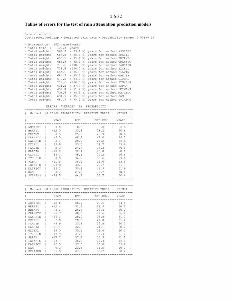
2.6-32

Tables of errors for the test of rain attenuation prediction models

Rain attenuationCostbeacexc.sel.exp - Measured rain data - Probability range: 0.001-0.1%

* Averaged on: 102 experiments* Total time : 103.3 years* Total weight: 568.3 ( 79.1 %) years for method ASSISEI* Total weight: 684.5 ( 95.3 %) years for method BRAZIL* Total weight: 683.5 ( 95.1 %) years for method BRYANT* Total weight: 688.9 ( 95.9 %) years for method CRANETC* Total weight: 718.6 (100.0 %) years for method DAHRAIN* Total weight: 718.6 (100.0 %) years for method EXCELL* Total weight: 684.5 ( 95.3 %) years for method FLAVIN* Total weight: 684.5 ( 95.3 %) years for method GARCIA* Total weight: 677.5 ( 94.3 %) years for method GLOBAL* Total weight: 718.6 (100.0 %) years for method ITU-618* Total weight: 631.5 ( 87.9 %) years for method JAPAN* Total weight: 439.8 ( 61.2 %) years for method LEIWA-S* Total weight: 706.6 ( 98.3 %) years for method MATRICC* Total weight: 684.5 ( 95.3 %) years for method SAM* Total weight: 684.5 ( 95.3 %) years for method SVIATOG

__________ ERRORS AVERAGED BY PROBABILITY ____________============================================================| Method |0.0010% PROBABILITY RELATIVE ERROR | WEIGHT |------------------------------------------------------------| | MEAN RMS STD.DEV. | YEARS |------------------------------------------------------------| ASSISEI | 0.0 0.0 0.0 | 0.0 || BRAZIL | -12.0 30.6 28.2 | 50.6 || BRYANT | 0.5 25.9 25.9 | 50.6 || CRANETC | -5.0 48.3 48.0 | 46.7 || DAHRAIN | -2.1 25.2 25.2 | 53.6 || EXCELL | 10.8 33.5 31.7 | 53.6 || FLAVIN | 2.3 24.5 24.3 | 50.6 || GARCIA | -18.8 32.1 26.0 | 50.6 || GLOBAL | 38.1 45.1 24.2 | 46.6 || ITU-618 | -8.9 34.8 33.6 | 53.6 || JAPAN | -11.5 35.5 33.6 | 43.6 || LEIWA-S | -20.8 33.9 26.7 | 36.7 || MATRICC | 26.1 50.2 42.9 | 51.6 || SAM | 8.2 27.9 26.7 | 50.6 || SVIATOG | -24.5 44.9 37.7 | 50.6 |------------------------------------------------------------

============================================================| Method |0.0020% PROBABILITY RELATIVE ERROR | WEIGHT |------------------------------------------------------------| | MEAN RMS STD.DEV. | YEARS |------------------------------------------------------------| ASSISEI | -12.6 26.7 23.6 | 34.4 || BRAZIL | -12.4 31.8 29.3 | 60.2 || BRYANT | -3.1 26.5 26.4 | 60.2 || CRANETC | -6.7 48.0 47.6 | 56.2 || DAHRAIN | -10.1 28.7 26.8 | 61.2 || EXCELL | 2.8 28.0 27.8 | 61.2 || FLAVIN | -3.9 23.1 22.8 | 60.2 || GARCIA | -21.1 32.0 24.1 | 60.2 || GLOBAL | 28.0 35.3 21.4 | 60.2 || ITU-618 | -17.9 37.0 32.4 | 61.2 || JAPAN | -17.7 37.7 33.3 | 51.1 || LEIWA-S | -23.7 36.2 27.4 | 46.3 || MATRICC | 12.0 37.0 35.0 | 59.2 || SAM | 0.2 23.5 23.5 | 60.2 || SVIATOG | -26.9 47.9 39.7 | 60.2 |------------------------------------------------------------

2.6-33============================================================| Method |0.0030% PROBABILITY RELATIVE ERROR | WEIGHT |------------------------------------------------------------| | MEAN RMS STD.DEV. | YEARS |------------------------------------------------------------| ASSISEI | -12.2 25.7 22.7 | 50.1 || BRAZIL | -13.8 31.8 28.7 | 63.2 || BRYANT | -5.4 27.2 26.7 | 63.2 || CRANETC | -5.9 49.2 48.9 | 64.2 || DAHRAIN | -13.1 29.0 25.8 | 65.2 || EXCELL | -0.1 26.4 26.4 | 65.2 || FLAVIN | -7.1 23.3 22.2 | 63.2 || GARCIA | -22.6 32.5 23.4 | 63.2 || GLOBAL | 22.1 30.3 20.8 | 63.2 || ITU-618 | -19.2 35.7 30.1 | 65.2 || JAPAN | -17.6 35.7 31.1 | 55.1 || LEIWA-S | -24.2 36.4 27.2 | 47.3 || MATRICC | 6.4 31.6 30.9 | 63.2 || SAM | -4.2 23.9 23.5 | 63.2 || SVIATOG | -28.5 47.8 38.3 | 63.2 |------------------------------------------------------------

============================================================| Method |0.0050% PROBABILITY RELATIVE ERROR | WEIGHT |------------------------------------------------------------| | MEAN RMS STD.DEV. | YEARS |------------------------------------------------------------| ASSISEI | -8.3 24.0 22.5 | 63.9 || BRAZIL | -13.0 28.6 25.5 | 69.9 || BRYANT | -4.3 24.4 24.0 | 69.9 || CRANETC | -2.0 42.7 42.7 | 67.0 || DAHRAIN | -12.3 25.5 22.3 | 70.9 || EXCELL | 0.1 22.8 22.8 | 70.9 || FLAVIN | -7.9 21.2 19.7 | 69.9 || GARCIA | -21.1 29.6 20.8 | 69.9 || GLOBAL | 18.1 26.3 19.1 | 69.9 || ITU-618 | -16.1 31.3 26.9 | 70.9 || JAPAN | -13.9 30.1 26.7 | 60.8 || LEIWA-S | -21.5 32.6 24.5 | 51.1 || MATRICC | 5.7 29.8 29.2 | 69.9 || SAM | -5.2 25.3 24.8 | 69.9 || SVIATOG | -28.2 44.3 34.2 | 69.9 |------------------------------------------------------------

============================================================| Method |0.0100% PROBABILITY RELATIVE ERROR | WEIGHT |------------------------------------------------------------| | MEAN RMS STD.DEV. | YEARS |------------------------------------------------------------| ASSISEI | -11.2 29.9 27.7 | 78.6 || BRAZIL | -13.8 29.3 25.8 | 85.6 || BRYANT | -5.9 26.7 26.1 | 85.6 || CRANETC | -3.4 41.3 41.1 | 82.7 || DAHRAIN | -13.9 29.4 25.9 | 85.6 || EXCELL | -2.9 25.4 25.2 | 85.6 || FLAVIN | -9.6 25.2 23.4 | 85.6 || GARCIA | -21.9 33.3 25.1 | 85.6 || GLOBAL | 11.0 26.6 24.3 | 85.6 || ITU-618 | -13.3 29.8 26.7 | 85.6 || JAPAN | -14.3 30.4 26.8 | 75.6 || LEIWA-S | -21.7 32.9 24.8 | 55.9 || MATRICC | 0.5 27.5 27.5 | 84.6 || SAM | -8.2 31.6 30.6 | 85.6 || SVIATOG | -27.3 42.9 33.1 | 85.6 |------------------------------------------------------------

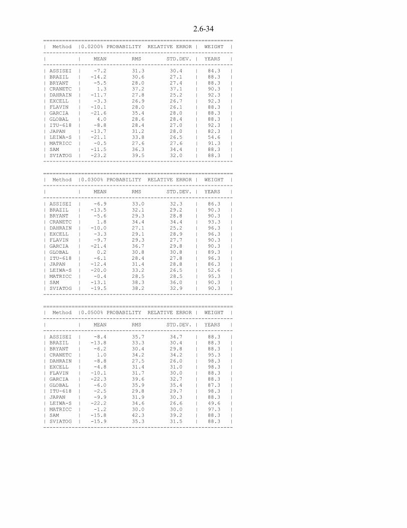
2.6-34============================================================| Method |0.0200% PROBABILITY RELATIVE ERROR | WEIGHT |------------------------------------------------------------| | MEAN RMS STD.DEV. | YEARS |------------------------------------------------------------| ASSISEI | -7.2 31.3 30.4 | 84.3 || BRAZIL | -14.2 30.6 27.1 | 88.3 || BRYANT | -5.5 28.0 27.4 | 88.3 || CRANETC | 1.3 37.2 37.1 | 90.3 || DAHRAIN | -11.7 27.8 25.2 | 92.3 || EXCELL | -3.3 26.9 26.7 | 92.3 || FLAVIN | -10.1 28.0 26.1 | 88.3 || GARCIA | -21.6 35.4 28.0 | 88.3 || GLOBAL | 4.0 28.6 28.4 | 88.3 || ITU-618 | -8.8 28.4 27.0 | 92.3 || JAPAN | -13.7 31.2 28.0 | 82.3 || LEIWA-S | -21.1 33.8 26.5 | 54.6 || MATRICC | -0.5 27.6 27.6 | 91.3 || SAM | -11.5 36.3 34.4 | 88.3 || SVIATOG | -23.2 39.5 32.0 | 88.3 |------------------------------------------------------------

============================================================| Method |0.0300% PROBABILITY RELATIVE ERROR | WEIGHT |------------------------------------------------------------| | MEAN RMS STD.DEV. | YEARS |------------------------------------------------------------| ASSISEI | -6.9 33.0 32.3 | 86.3 || BRAZIL | -13.5 32.1 29.2 | 90.3 || BRYANT | -5.6 29.3 28.8 | 90.3 || CRANETC | 1.8 34.4 34.4 | 93.3 || DAHRAIN | -10.0 27.1 25.2 | 96.3 || EXCELL | -3.3 29.1 28.9 | 96.3 || FLAVIN | -9.7 29.3 27.7 | 90.3 || GARCIA | -21.4 36.7 29.8 | 90.3 || GLOBAL | 0.2 30.8 30.8 | 89.3 || ITU-618 | -6.1 28.4 27.8 | 96.3 || JAPAN | -12.4 31.4 28.8 | 86.3 || LEIWA-S | -20.0 33.2 26.5 | 52.6 || MATRICC | -0.4 28.5 28.5 | 95.3 || SAM | -13.1 38.3 36.0 | 90.3 || SVIATOG | -19.5 38.2 32.9 | 90.3 |------------------------------------------------------------

============================================================| Method |0.0500% PROBABILITY RELATIVE ERROR | WEIGHT |------------------------------------------------------------| | MEAN RMS STD.DEV. | YEARS |------------------------------------------------------------| ASSISEI | -8.4 35.7 34.7 | 88.3 || BRAZIL | -13.8 33.3 30.4 | 88.3 || BRYANT | -6.2 30.4 29.8 | 88.3 || CRANETC | 1.0 34.2 34.2 | 95.3 || DAHRAIN | -8.8 27.5 26.0 | 98.3 || EXCELL | -4.8 31.4 31.0 | 98.3 || FLAVIN | -10.1 31.7 30.0 | 88.3 || GARCIA | -22.3 39.6 32.7 | 88.3 || GLOBAL | -6.0 35.9 35.4 | 87.3 || ITU-618 | -2.5 29.8 29.7 | 98.3 || JAPAN | -9.9 31.9 30.3 | 88.3 || LEIWA-S | -22.2 34.6 26.6 | 49.6 || MATRICC | -1.2 30.0 30.0 | 97.3 || SAM | -15.8 42.3 39.2 | 88.3 || SVIATOG | -15.9 35.3 31.5 | 88.3 |------------------------------------------------------------

2.6-35============================================================| Method |0.1000% PROBABILITY RELATIVE ERROR | WEIGHT |------------------------------------------------------------| | MEAN RMS STD.DEV. | YEARS |------------------------------------------------------------| ASSISEI | -13.5 45.8 43.8 | 82.4 || BRAZIL | -12.2 36.0 33.8 | 88.3 || BRYANT | -7.2 34.6 33.9 | 87.3 || CRANETC | 1.3 36.5 36.5 | 93.3 || DAHRAIN | -7.6 30.2 29.2 | 95.3 || EXCELL | -7.0 35.7 35.0 | 95.3 || FLAVIN | -9.5 35.1 33.8 | 88.3 || GARCIA | -23.8 44.3 37.4 | 88.3 || GLOBAL | -15.0 44.7 42.1 | 87.3 || ITU-618 | 2.2 32.8 32.7 | 95.3 || JAPAN | -7.5 33.5 32.6 | 88.3 || LEIWA-S | -23.5 37.0 28.5 | 45.6 || MATRICC | -2.5 34.4 34.3 | 94.3 || SAM | -19.5 47.5 43.3 | 88.3 || SVIATOG | -9.3 34.5 33.2 | 88.3 |------------------------------------------------------------

------------------------------------------------------------

_______________ AVERAGED ERRORS SUMMARY ________________

************************************************************| Method | AVERAGED ERRORS SUMMARY | WEIGHT |------------------------------------------------------------| | MEAN RMS STD.DEV. | YEARS |------------------------------------------------------------| ASSISEI | -9.7 33.2 31.8 | 63.1 || BRAZIL | -13.3 31.8 28.9 | 76.1 || BRYANT | -5.1 28.6 28.1 | 75.9 || CRANETC | -1.3 40.5 40.4 | 76.5 || DAHRAIN | -10.1 28.0 26.1 | 79.8 || EXCELL | -1.7 29.2 29.1 | 79.8 || FLAVIN | -7.9 27.7 26.6 | 76.1 || GARCIA | -21.8 35.9 28.5 | 76.1 || GLOBAL | 8.3 33.9 32.9 | 75.3 || ITU-618 | -9.1 31.6 30.3 | 79.8 || JAPAN | -12.7 32.7 30.2 | 70.2 || LEIWA-S | -22.1 34.5 26.5 | 48.9 || MATRICC | 3.5 32.5 32.3 | 78.5 || SAM | -9.1 35.1 33.9 | 76.1 || SVIATOG | -21.9 41.2 34.9 | 76.1 |************************************************************

___________ RMS ERROR TEST SCORE ____________

**************************************************| Place | Method | RMS ERROR | Distance |--------------------------------------------------| 1 | FLAVIN | 27.7 | + 0.0 || 2 | DAHRAIN | 28.0 | + 0.2 || 3 | BRYANT | 28.6 | + 0.6 || 4 | EXCELL | 29.2 | + 0.6 || 5 | ITU-618 | 31.6 | + 2.5 || 6 | BRAZIL | 31.8 | + 0.1 || 7 | MATRICC | 32.5 | + 0.7 || 8 | JAPAN | 32.7 | + 0.2 || 9 | ASSISEI | 33.2 | + 0.5 || 10 | GLOBAL | 33.9 | + 0.7 || 11 | LEIWA-S | 34.5 | + 0.5 || 12 | SAM | 35.1 | + 0.6 || 13 | GARCIA | 35.9 | + 0.8 || 14 | CRANETC | 40.5 | + 4.6 || 15 | SVIATOG | 41.2 | + 0.8 |--------------------------------------------------

Table A-2: Results of rain attenuation test using the measured rain intensity statistics as input of prediction models.

2.6-36Rain attenuationCostbeacexc.sel.exp - Baptista-Salonen rain map - Probability range: 0.001-0.1%

* Averaged on: 115 experiments* Total time : 117.2 years* Total weight: 830.0 (100.0 %) years for method ASSISEI* Total weight: 830.0 (100.0 %) years for method BRAZIL* Total weight: 830.0 (100.0 %) years for method BRYANT* Total weight: 798.9 ( 96.3 %) years for method CRANETC* Total weight: 830.0 (100.0 %) years for method DAHRAIN* Total weight: 830.0 (100.0 %) years for method EXCELL* Total weight: 830.0 (100.0 %) years for method FLAVIN* Total weight: 830.0 (100.0 %) years for method GARCIA* Total weight: 823.0 ( 99.2 %) years for method GLOBAL* Total weight: 830.0 (100.0 %) years for method ITU-618* Total weight: 830.0 (100.0 %) years for method JAPAN* Total weight: 527.8 ( 63.6 %) years for method LEIWA-S* Total weight: 821.0 ( 98.9 %) years for method MATRICC* Total weight: 830.0 (100.0 %) years for method SAM* Total weight: 830.0 (100.0 %) years for method SVIATOG

___________ AVERAGED ERRORS BY PROBABILITY ____________============================================================| Method |0.0010% PROBABILITY RELATIVE ERROR | WEIGHT |------------------------------------------------------------| | MEAN RMS STD.DEV. | YEARS |------------------------------------------------------------| ASSISEI | 2.6 33.7 33.6 | 59.8 || BRAZIL | 2.6 36.0 35.9 | 59.8 || BRYANT | 11.5 36.2 34.4 | 59.8 || CRANETC | -4.2 48.4 48.2 | 52.9 || DAHRAIN | 4.1 32.7 32.4 | 59.8 || EXCELL | 26.5 41.4 31.7 | 59.8 || FLAVIN | 15.9 35.2 31.4 | 59.8 || GARCIA | -6.6 35.3 34.7 | 59.8 || GLOBAL | 51.6 60.6 31.9 | 55.8 || ITU-618 | -0.1 33.3 33.3 | 59.8 || JAPAN | -4.7 33.7 33.4 | 59.8 || LEIWA-S | -4.5 31.9 31.6 | 44.0 || MATRICC | 20.1 39.1 33.5 | 58.8 || SAM | 23.6 39.0 31.0 | 59.8 || SVIATOG | -12.8 46.2 44.4 | 59.8 |------------------------------------------------------------

============================================================| Method |0.0020% PROBABILITY RELATIVE ERROR | WEIGHT |------------------------------------------------------------| | MEAN RMS STD.DEV. | YEARS |------------------------------------------------------------| ASSISEI | -1.9 34.0 33.9 | 71.0 || BRAZIL | -0.5 37.0 37.0 | 71.0 || BRYANT | 5.5 36.6 36.2 | 71.0 || CRANETC | -6.7 46.9 46.4 | 66.0 || DAHRAIN | -3.2 35.3 35.1 | 71.0 || EXCELL | 15.4 37.5 34.2 | 71.0 || FLAVIN | 6.9 34.1 33.4 | 71.0 || GARCIA | -10.6 36.5 34.9 | 71.0 || GLOBAL | 38.4 50.1 32.2 | 71.0 || ITU-618 | -9.2 36.7 35.5 | 71.0 || JAPAN | -9.9 36.8 35.5 | 71.0 || LEIWA-S | -10.1 35.7 34.3 | 53.2 || MATRICC | 7.5 35.0 34.2 | 70.0 || SAM | 12.2 34.9 32.7 | 71.0 || SVIATOG | -17.3 49.1 46.0 | 71.0 |------------------------------------------------------------

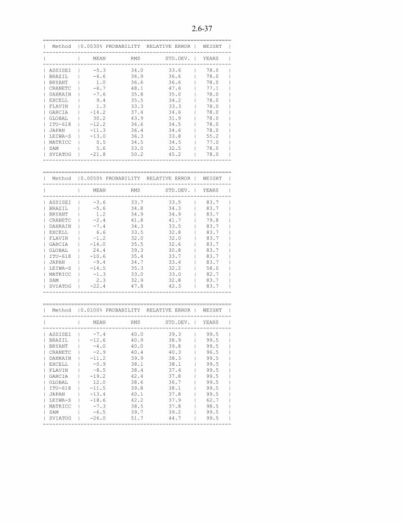
2.6-37============================================================| Method |0.0030% PROBABILITY RELATIVE ERROR | WEIGHT |------------------------------------------------------------| | MEAN RMS STD.DEV. | YEARS |------------------------------------------------------------| ASSISEI | -5.3 34.0 33.6 | 78.0 || BRAZIL | -4.6 36.9 36.6 | 78.0 || BRYANT | 1.0 36.6 36.6 | 78.0 || CRANETC | -6.7 48.1 47.6 | 77.1 || DAHRAIN | -7.6 35.8 35.0 | 78.0 || EXCELL | 9.4 35.5 34.2 | 78.0 || FLAVIN | 1.3 33.3 33.3 | 78.0 || GARCIA | -14.2 37.4 34.6 | 78.0 || GLOBAL | 30.2 43.9 31.9 | 78.0 || ITU-618 | -12.2 36.6 34.5 | 78.0 || JAPAN | -11.3 36.4 34.6 | 78.0 || LEIWA-S | -13.0 36.3 33.8 | 55.2 || MATRICC | 0.5 34.5 34.5 | 77.0 || SAM | 5.6 33.0 32.5 | 78.0 || SVIATOG | -21.8 50.2 45.2 | 78.0 |------------------------------------------------------------

============================================================| Method |0.0050% PROBABILITY RELATIVE ERROR | WEIGHT |------------------------------------------------------------| | MEAN RMS STD.DEV. | YEARS |------------------------------------------------------------| ASSISEI | -3.6 33.7 33.5 | 83.7 || BRAZIL | -5.6 34.8 34.3 | 83.7 || BRYANT | 1.2 34.9 34.9 | 83.7 || CRANETC | -2.4 41.8 41.7 | 79.8 || DAHRAIN | -7.4 34.3 33.5 | 83.7 || EXCELL | 6.6 33.5 32.8 | 83.7 || FLAVIN | -1.2 32.0 32.0 | 83.7 || GARCIA | -14.0 35.5 32.6 | 83.7 || GLOBAL | 24.4 39.3 30.8 | 83.7 || ITU-618 | -10.6 35.4 33.7 | 83.7 || JAPAN | -9.4 34.7 33.4 | 83.7 || LEIWA-S | -14.5 35.3 32.2 | 58.0 || MATRICC | -1.3 33.0 33.0 | 82.7 || SAM | 2.3 32.9 32.8 | 83.7 || SVIATOG | -22.4 47.8 42.3 | 83.7 |------------------------------------------------------------

============================================================| Method |0.0100% PROBABILITY RELATIVE ERROR | WEIGHT |------------------------------------------------------------| | MEAN RMS STD.DEV. | YEARS |------------------------------------------------------------| ASSISEI | -7.4 40.0 39.3 | 99.5 || BRAZIL | -12.6 40.9 38.9 | 99.5 || BRYANT | -4.0 40.0 39.8 | 99.5 || CRANETC | -2.9 40.4 40.3 | 96.5 || DAHRAIN | -11.2 39.9 38.3 | 99.5 || EXCELL | -0.9 38.1 38.1 | 99.5 || FLAVIN | -8.5 38.4 37.4 | 99.5 || GARCIA | -19.2 42.4 37.8 | 99.5 || GLOBAL | 12.0 38.6 36.7 | 99.5 || ITU-618 | -11.5 39.8 38.1 | 99.5 || JAPAN | -13.4 40.1 37.8 | 99.5 || LEIWA-S | -18.6 42.2 37.9 | 62.7 || MATRICC | -7.3 38.5 37.8 | 98.5 || SAM | -6.5 39.7 39.2 | 99.5 || SVIATOG | -26.0 51.7 44.7 | 99.5 |------------------------------------------------------------

2.6-38============================================================| Method |0.0200% PROBABILITY RELATIVE ERROR | WEIGHT |------------------------------------------------------------| | MEAN RMS STD.DEV. | YEARS |------------------------------------------------------------| ASSISEI | -9.0 40.2 39.2 | 106.2 || BRAZIL | -15.0 41.1 38.3 | 106.2 || BRYANT | -4.4 39.1 38.8 | 106.2 || CRANETC | 1.2 36.5 36.5 | 104.2 || DAHRAIN | -9.7 37.8 36.5 | 106.2 || EXCELL | -3.3 38.4 38.3 | 106.2 || FLAVIN | -11.1 38.5 36.9 | 106.2 || GARCIA | -20.8 42.9 37.6 | 106.2 || GLOBAL | 3.0 37.0 36.8 | 106.2 || ITU-618 | -7.7 37.6 36.9 | 106.2 || JAPAN | -14.4 39.9 37.2 | 106.2 || LEIWA-S | -18.1 40.9 36.7 | 65.4 || MATRICC | -6.4 36.8 36.2 | 105.2 || SAM | -12.3 41.3 39.4 | 106.2 || SVIATOG | -22.2 48.4 43.0 | 106.2 |------------------------------------------------------------

============================================================| Method |0.0300% PROBABILITY RELATIVE ERROR | WEIGHT |------------------------------------------------------------| | MEAN RMS STD.DEV. | YEARS |------------------------------------------------------------| ASSISEI | -11.7 39.1 37.3 | 110.2 || BRAZIL | -16.7 40.1 36.5 | 110.2 || BRYANT | -6.1 38.0 37.5 | 110.2 || CRANETC | 1.6 34.1 34.1 | 107.2 || DAHRAIN | -9.2 35.0 33.8 | 110.2 || EXCELL | -5.1 37.6 37.2 | 110.2 || FLAVIN | -13.0 37.2 34.9 | 110.2 || GARCIA | -22.6 42.2 35.6 | 110.2 || GLOBAL | -2.7 35.2 35.1 | 109.2 || ITU-618 | -6.1 35.3 34.8 | 110.2 || JAPAN | -14.4 38.1 35.3 | 110.2 || LEIWA-S | -18.4 39.3 34.7 | 65.4 || MATRICC | -6.4 34.9 34.3 | 109.2 || SAM | -16.4 41.2 37.7 | 110.2 || SVIATOG | -19.9 45.7 41.1 | 110.2 |------------------------------------------------------------

============================================================| Method |0.0500% PROBABILITY RELATIVE ERROR | WEIGHT |------------------------------------------------------------| | MEAN RMS STD.DEV. | YEARS |------------------------------------------------------------| ASSISEI | -13.6 39.0 36.5 | 112.2 || BRAZIL | -17.0 39.0 35.1 | 112.2 || BRYANT | -6.9 36.5 35.9 | 112.2 || CRANETC | 1.0 34.2 34.2 | 109.2 || DAHRAIN | -8.5 33.3 32.2 | 112.2 || EXCELL | -6.7 37.4 36.8 | 112.2 || FLAVIN | -14.0 36.6 33.8 | 112.2 || GARCIA | -24.3 42.4 34.8 | 112.2 || GLOBAL | -9.8 36.6 35.2 | 111.2 || ITU-618 | -2.9 34.1 34.0 | 112.2 || JAPAN | -12.8 36.6 34.3 | 112.2 || LEIWA-S | -20.5 39.6 33.9 | 65.4 || MATRICC | -4.9 33.8 33.4 | 111.2 || SAM | -19.9 42.0 37.0 | 112.2 || SVIATOG | -15.4 41.8 38.9 | 112.2 |------------------------------------------------------------

2.6-39============================================================| Method |0.1000% PROBABILITY RELATIVE ERROR | WEIGHT |------------------------------------------------------------| | MEAN RMS STD.DEV. | YEARS |------------------------------------------------------------| ASSISEI | -18.1 40.5 36.3 | 109.2 || BRAZIL | -18.0 40.9 36.7 | 109.2 || BRYANT | -11.3 38.6 36.9 | 109.2 || CRANETC | 2.1 37.7 37.6 | 105.8 || DAHRAIN | -9.7 34.3 32.9 | 109.2 || EXCELL | -11.1 40.3 38.8 | 109.2 || FLAVIN | -16.0 38.7 35.2 | 109.2 || GARCIA | -28.9 46.1 35.9 | 109.2 || GLOBAL | -21.2 43.4 37.9 | 108.2 || ITU-618 | -1.0 35.0 35.0 | 109.2 || JAPAN | -13.0 37.6 35.3 | 109.2 || LEIWA-S | -21.9 42.8 36.8 | 58.5 || MATRICC | -5.4 35.7 35.3 | 108.2 || SAM | -25.7 46.2 38.3 | 109.2 || SVIATOG | -11.3 41.3 39.7 | 109.2 |------------------------------------------------------------

------------------------------------------------------------

_______________ AVERAGED ERRORS SUMMARY ________________

************************************************************| Method | AVERAGED ERRORS SUMMARY | WEIGHT |------------------------------------------------------------| | MEAN RMS STD.DEV. | YEARS |------------------------------------------------------------| ASSISEI | -8.7 37.8 36.8 | 92.2 || BRAZIL | -11.2 39.0 37.3 | 92.2 || BRYANT | -2.8 37.6 37.5 | 92.2 || CRANETC | -1.3 40.1 40.1 | 88.8 || DAHRAIN | -7.7 35.6 34.7 | 92.2 || EXCELL | 1.2 37.8 37.8 | 92.2 || FLAVIN | -6.4 36.4 35.8 | 92.2 || GARCIA | -19.2 40.9 36.1 | 92.2 || GLOBAL | 9.5 41.9 40.8 | 91.4 || ITU-618 | -6.7 36.1 35.5 | 92.2 || JAPAN | -12.0 37.4 35.5 | 92.2 || LEIWA-S | -16.0 38.7 35.2 | 58.6 || MATRICC | -1.9 35.7 35.6 | 91.2 || SAM | -7.1 39.7 39.1 | 92.2 || SVIATOG | -18.9 46.8 42.8 | 92.2 |************************************************************

___________ RMS ERROR TEST SCORE ____________

**************************************************| Place | Method | RMS ERROR | Distance |--------------------------------------------------| 1 | DAHRAIN | 35.6 | + 0.0 || 2 | MATRICC | 35.7 | + 0.1 || 3 | ITU-618 | 36.1 | + 0.4 || 4 | FLAVIN | 36.4 | + 0.3 || 5 | JAPAN | 37.4 | + 1.0 || 6 | BRYANT | 37.6 | + 0.2 || 7 | ASSISEI | 37.8 | + 0.2 || 8 | EXCELL | 37.8 | + 0.0 || 9 | LEIWA-S | 38.7 | + 0.9 || 10 | BRAZIL | 39.0 | + 0.3 || 11 | SAM | 39.7 | + 0.8 || 12 | CRANETC | 40.1 | + 0.4 || 13 | GARCIA | 40.9 | + 0.8 || 14 | GLOBAL | 41.9 | + 1.0 || 15 | SVIATOG | 46.8 | + 4.9 |--------------------------------------------------

Table 2.6-22 Results of rain attenuation test using rain intensity statisticsfrom Baptista-Salonen map as input of prediction models.

PART 3 Climatic Parameters and Mapping

3.1-1

CHAPTER 3.1Clear air (Refractivity part)

Editor: Terje Tjelta1

Authors: Ana Benarroch2, Laurent Blanchard3, Marina Boumis4, Sofus L. Lystad5,Kevin Marsh6, Jose M. Riera2, Daniela Rezacova7, Ben Segal8,Zbynek Sokol7, Terje Tjelta1, Ole Einar Tveito5

1 Telenor R&D, P.O. Box 83, N-2007 Kjeller, Norway

Tel: +47 638487, Fax: +4763819810, e-mail: terje.tjelta@telenor.com2 Universidad Politecnica de Madrid, ETSIT, Ciudad Universitaria, E-28040 Madrid, Spain

Tel: +34 1 3367218, Fax:.: +34 1 3377350, e-mail: ana@grc.ssr.upm.es3 France Telecom, CNET/DMR/URR, 6 Av des Usines, F-90000 Belfort, France

Tel: +33 3 84544249, Fax: +33 3384544396, e-mail: laurent.blamchard@cnet.francetelecom.fr4 Fondazione ‘Ugo Bordoni’, Viale Europa, 19000144 Roma, Italy

Tel: +39 6 54802119, Fax: +39 6 54804401, e-mail: mboumis@fub.it5 Norwegian meteorological institute, P.O. Box 43, Blindern, N-0313 Oslo, Norway

Tel: +47 22963000, Fax: +47 22963050, e-mail: sofus.lystad@dnmi.no6 CCLRC Rutherford Appleton Laboratory, RCRU, Chilton, Didcot, Oxfordshire OX11 0QX, United Kingdom

Tel: +44 1235 446521, Fax: +44 1235 446140, e-mail: k.marsh@rl.ac.uk7 Inst. of Atmos. Physics, Academy of Sciences of the Czech Republic, Bocnì II, 141 31 Praha 4, Czech Republic

Tel: +42 02 769702, Fax: +42 02 763745, e-mailrez@info.cas.cz

3.1-2

Tel: +1 613 998 2468, Fax: +1 613 998 4077, e-mail: ben.segal@crc.ca

3.1 Clear air (Refractivity part)

The clear-air research results reported here were commenced under a previous COST action [COST235, 1996]. A great deal of progress has been made since then and this should help to provide amore solid foundation upon which to establish dependable propagation models. The followingpages include results and analyses of new refractivity measurements from different geographicregions as well as new global maps of various meteorological parameters. Data are presented forconditions both on and near the surface of the Earth. Wherever appropriate, attempts have also beenmade to include discussion of the difficulties and limitations in the measurement, analysis andpresentation of the relevant parameters, as well as outlining some of the newer approaches to thestudy of atmospheric refractivity.

3.1.1 Characteristics of refractivity of the upper air

The behaviour of a radio wave propagating in the atmosphere is largely determined by the variationin the radio refractive index along the path(s) traversed between the transmitter and receiver.Among the earliest manifestations of anomalous clear-air propagation were over-the-horizontransmissions that took place primarily in a hot and humid environment. The cause of theseanomalous signals was attributed to the existence of strong atmospheric “ducts” – strongly negativegradients of refractive index as a function of height. On shorter paths, or on low-angle Earth-spacelinks, multipath propagation, which may give rise to periodic signal fading and enhancement, islikewise the result, either directly or indirectly, of variations in the refractive index of the medium.

The refractive index, n, of the atmosphere differs only slightly from unity, so that it is customary todefine refractivity, N, as the amount by which the refractive index is greater than one, expressed inparts per million, i.e., [ITU-R, 1999c],

)0.1(106 <= nN 3.1-1

At radio frequencies, the refractivity may be derived from the expression

´¦

¥²¤

£ +=T

eP

TN 4810

6.773.1-2

where:

P = Atmospheric pressure (hPa)

e = Water vapour pressure (hPa)

T = Absolute temperature (K).

The contribution to the total refractivity due to dry atmospheric gases alone is:

TP

N dry 6.77= 3.1-3

The contribution to the total refractivity due to water vapour is:

2510733.3

Te

N wet ×= 3.1-4

A related useful parameter for refractivity studies is the modified refractivity (M), which is simplyderived from N at a height h (m) above the ground (or relative to sea level) by:

3.1-3

3.1.1.1 Refractive index of the atmosphere

Although the refractive index of the atmosphere varies in both space and time, it is instructive toconsider its basic characteristics. Figure 3.1-1 displays the lowest 30 km of an idealised standardatmosphere and is recommended for general reference purposes where detailed local information isnot available or necessary [ITU-R, 1999e]. The model temperature is seen to decrease at a linearrate until approximately 10 km altitude (tropopause); the pressure, meanwhile, decreases rapidly ata nearly exponential rate. As a result, the “dry” refractivity term also diminishes rapidly (Figure 3.1-2).

Figure 3.1-1: standard reference atmosphere:temperature and pressure profiles

Figure 3.1-2: “Dry” refractivity computed for thestandard reference atmosphere model

Under stable conditions, the refractivity gradient in the lower atmosphere results in a verticaldeviation along the direction of propagation which may be significant for low-angle Earth-spacelinks [ITU-R, 1999d]. Stable conditions, however, do not produce the volatile multipath fading andenhancement observed both on terrestrial and on low-angle Earth-space links. In this regard thepresence of water vapour is central. This is a result of the fact that the “wet” refractivitycontribution is usually a significant one. In addition, the wet term is usually more volatile as afunction of time. Because the water vapour is most prominent at lower elevations in thetroposphere, clear-air anomalous propagation arises mainly out of conditions that prevail close tothe surface.

Figure 3.1-3 shows the worst-month water vapour pressure for Europe, based on 4 years ofobservations at 1571 locations and averaged on a 1.5° grid. Even on this smoothed presentation, thevapour pressure is seen to vary from below 6 hPa to above 22 hPa. The vapour pressure is seen toincrease strongly with increasing ambient temperature. Along with this increase in vapour pressurethere are increases in the wet component of refractivity and in the overall variability of totalrefractivity and hence the likelihood of increased anomalous propagation.

3.1-4

Figure 3.1-3 Surface water vapour pressure [hPa] for the “worst month” in Europe

The average seasonal behaviour of observed refractivity at the surface is presented in Figure 3.1-4for a maritime temperate location [Segal and Barrington, 1977]. The average wet and drycomponents are displayed independently, with error bars indicating the standard deviation for each.While the wet term component is smaller than the dry term, it nonetheless represents a verysignificant fraction of the latter during late summer months. In addition, the variability of the wetterm is considerably greater than that for the dry term during the same period.

Figure 3.1-4: Average values of ‘wet’ and ‘dry’ components of surface refractivity for a typical maritime temperatelocation. Vertical bars indicate the standard deviations for observations during the calendar months indicated

3.1.1.2 Worldwide refractivity studies

In a pioneering work, [Bean et al., 1966] analysed sample radiosonde observations recorded at 99locations around the world and summarised the results in a set of seasonal maps of percentage oftime that the average refractivity lapse rate over the lowest 100 m exceeds-100 N/km. These maps were accepted into the ITU-R documentation and incorporated intoanomalous propagation models for both terrestrial and Earth-space links [ITU-R, 1999a,b]. [Bean etl 1966] l d h l i di di ib i h l 100 f 22 f h

3.1-5

the lowest 100 metre gradients for an additional 87 sites in the Northern Hemisphere. These wereaugmented by [Samson, 1976] with data for a further 65 sites worldwide. Additionally, moreexhaustive statistical analyses were conducted for individual countries [e.g., Segal and Barrington,1977], and a massive global analysis of radiosonde data was conducted by [Ortenburger andLawson, 1985] who tabulated various refractivity gradient statistics. Despite the existence of theseenhanced data sets, the lack of suitable maps and characteristic parameters has retarded progress onmore physically based propagation models.

3.1.1.3 Measurements of Refractivity

Atmospheric refractivity may be determined in a number of ways, either directly (using arefractometer), or indirectly using measurements of temperature and humidity made by otherinstruments (such as radiosondes). Recent improvements in technology have also permitted the useof lidar (light detection and ranging) measurement systems. Pulses of radiation are fired from alaser, and the radiation backscattered by atmospheric gases and particles is measured. The Ramanlidar technique can measure water vapour and temperature profiles in this way, and is thereforesuited to sensing radio refractivity. However, while this method can yield high measurementaccuracy, the expense of equipment prohibits its widespread use.

Radiosondes are far less expensive than refractometers and, due to the large number of radiosondestations worldwide, are able to provide very good global coverage, and are the most widely usedinstrument for upper air measurements. These devices are attached to hydrogen or helium filledballoons and launched from a ground station. They contain sensors to measure temperature,pressure and humidity, along with an oscillator to encode the output from these sensors into anaudio tone, and a RF transmitter to send this information back to a ground station. Received tonesare converted to pre-calibrated standard units and logged as the balloon ascends, thus providing avertical profile of the measurements.

[Bean et al., 1966] first performed the mapping of climatological parameters derived fromradiosondes to examine their effects on radio propagation. This study involved data fromradiosonde stations over a period of 5 years (with data from only 4 months of each year beingincluded). Through the use of a more extensive dataset, improvements in the radiosondeinstruments themselves and much greater computing power, it has now become possible to studythe behaviour of the atmospheric refractivity profile in far more detail than previously possible.

Measurements by surface stations

Current propagation models tacitly assume the occurrence of tropospheric duct(s) to be critical tothe production of clear-air fading on both terrestrial and Earth-space links [ITU-R, 1999a,b] andemploy observations taken by radiosondes in order to derive the necessary statistics. The standardradiosonde was not developed, nor was its network of stations implemented, with radio propagationresearch as a significant objective. Despite many improvements in radiosonde instrumentation,there remain a number of inherent problems in applying such statistics, e.g.,

• profile inaccuracy due to limited sampling as a consequence of the rapid transit of the sondewhich traverses the lowest 100 m in approximately 20 seconds,

• interpolation between ‘mandatory’ pressure levels at many (most?) sites rather than use of fixedgeophysical heights,

• universally synchronised sampling, two or four times daily, at different local times dependingon the longitude of the site but in no way related to times of propagation disturbances,

• relatively large spacing between locations in most parts of the globe,

• t i ti di th i iti l diti f t t d h idit i t

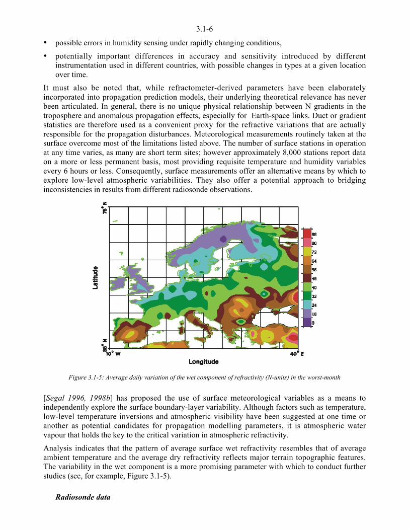
3.1-6

• possible errors in humidity sensing under rapidly changing conditions,

• potentially important differences in accuracy and sensitivity introduced by differentinstrumentation used in different countries, with possible changes in types at a given locationover time.

It must also be noted that, while refractometer-derived parameters have been elaboratelyincorporated into propagation prediction models, their underlying theoretical relevance has neverbeen articulated. In general, there is no unique physical relationship between N gradients in thetroposphere and anomalous propagation effects, especially for Earth-space links. Duct or gradientstatistics are therefore used as a convenient proxy for the refractive variations that are actuallyresponsible for the propagation disturbances. Meteorological measurements routinely taken at thesurface overcome most of the limitations listed above. The number of surface stations in operationat any time varies, as many are short term sites; however approximately 8,000 stations report dataon a more or less permanent basis, most providing requisite temperature and humidity variablesevery 6 hours or less. Consequently, surface measurements offer an alternative means by which toexplore low-level atmospheric variabilities. They also offer a potential approach to bridginginconsistencies in results from different radiosonde observations.

Figure 3.1-5: Average daily variation of the wet component of refractivity (N-units) in the worst-month

[Segal 1996, 1998b] has proposed the use of surface meteorological variables as a means toindependently explore the surface boundary-layer variability. Although factors such as temperature,low-level temperature inversions and atmospheric visibility have been suggested at one time oranother as potential candidates for propagation modelling parameters, it is atmospheric watervapour that holds the key to the critical variation in atmospheric refractivity.

Analysis indicates that the pattern of average surface wet refractivity resembles that of averageambient temperature and the average dry refractivity reflects major terrain topographic features.The variability in the wet component is a more promising parameter with which to conduct furtherstudies (see, for example, Figure 3.1-5).

Radiosonde data

3.1-7

Direct sensing of pressure, temperature and water vapour pressure profiles is routinely carried outby means of radiosonde balloon ascents. Radiosonde observations (RAOBs) are currently made atover 1000 stations around the world on a twice-daily basis, nominally at 0000 and 1200 UT.

Following the introduction of improved radiosonde equipment, certain stations are now recordingdata at a higher vertical resolution. This allows identification of quite narrow layers of anomalouspropagation. Although this high-resolution data is, as yet, not widely archived due to its largevolume, data have been obtained during COST 255 for a number of locations in Norway and theUK.

While there are several tens of thousands of stations reporting regular surface level meteorologicalmeasurements, the availability of upper air data is somewhat more limited, partly due to the expenseand complexity of upper air sensing techniques. Surface measurement and data logging is a largelyautomated process using relatively inexpensive instrumentation, however upper air measurementsgenerally require human assistance and more expensive technology.

Radiosondes do have a number of limitations, which should be borne in mind when analysing thedata [Craig and Hayton, 1995]. The vertical resolution of most of the archived data is relativelypoor, and is often greater than 100 m. The sondes are also advected by the mean winds, and so donot yield a vertical “snapshot” of the atmosphere. There are also time lags in the response of theinstruments to changes in the measured parameters, which can act to obscure small-scale features.However, the extensive database available offers the chance to perform global studies and toexamine the large-scale characteristics of the refractivity structure in considerable detail.

Low resolution radiosonde data (LORES)

Data from these ascents are archived by the World Meteorological Organization (WMO) and theseare a valuable source of data, providing global coverage over a long time span. The format of atypical radiosonde ascent after extraction from the WMO archive format is shown in Table (to aheight of about 3 km).

Level Pressure

(hPa)

Geopotentialheight

(m)

Temperature

(ºC)

Dew pointdepression

(ºC)

Winddirection

(deg)

Windspeed(kt)

Qualitymarks

1 1003.0 99999.0 2.8 2.1 999.0 999.0 V2 1000.0 38.0 3.2 3.1 999.0 999.0 AA3 935.0 99999.0 .2 2.5 999.0 999.0 A4 921.0 99999.0 1.4 2.9 999.0 999.0 A5 857.0 99999.0 -1.3 2.8 999.0 999.0 A6 850.0 1343.0 -1.7 3.1 165.0 36.0 AA A7 829.0 99999.0 -2.3 4.2 999.0 999.0 A8 811.0 99999.0 -1.9 6.0 999.0 999.0 A9 765.0 99999.0 -4.9 7.0 999.0 999.0 A10 700.0 2870.0 -10.1 6.0 160.0 48.0 AA A11 594.0 99999.0 -19.1 3.5 999.0 999.0 A

Table 3.1-1: Example of radiosonde ascent data extracted from NCAR dataset

There are two levels at which data is reported. At standard pressure levels which are agreed by theWMO (1000, 850, 700, 500, … hPa) all parameters are given. Only the 1000 hPa and 850 hPalevels are normally relevant to terrestrial radio links, the lower pressure levels being too high inaltitude. At significant levels (heights which show features such as change of slope in the verticalprofiles of temperature or dew point) only pressure, temperature and dew point are given, the othercolumns being filled with 9s to represent missing data. There may be several significant levelsbelow a height of 1000 m. An examination of Table 3.1-1 shows that:

• Pressure values are rounded to 1 hPa. This gives an effective height resolution of

3.1-8

• Height is given as geopotential height rather than true height, which is required for this study.However, the difference between the two quantities at altitudes relevant here is less than 1%,

• Temperature is rounded to 0.1°C,

• Dew point depression is rounded to 0.1°C. This can be used to directly obtain water vapourpressure for use in equation 3.1-2.,

• Wind direction and speed are not relevant in this study, and

• Quality marks, added by the National Center for Atmospheric Research, USA (NCAR), showthe results of consistency checks applied to the data.

The Radio Communications Research Unit (RCRU) archive of world radiosonde data initiallycovered the period 1/1/83 to 31/12/92. This dataset has been used in several studies during COST255. This was recently extended to cover an additional 10 years, and now extends from 1/1/77 to31/12/96. These data were obtained from NCAR.

These reporting levels are extracted from the ‘raw’ high resolution data directly measured by theradiosonde as it ascends (with typically 10 m height resolution in modern systems) via a complexreduction process that may involve smoothing and interpolation. Indeed, until relatively recently,significant levels were usually manually extracted from the raw data, and even though modernradiosonde systems automate this process there is no universally agreed procedure for definingsignificant levels. The standard/significant level data are referred to as low-resolution (LORES)data. A main aim of this study was to examine the effects of this data reduction process on theusefulness of WMO data for refractivity studies.

High resolution radiosonde data (HIRES)

For modern radiosondes, the height resolution of the ‘raw’ data from which the standard andsignificant levels are extracted is high. The Vaisala sondes, currently used by many countriesincluding the UK, send back data every 2 seconds, giving a height resolution of about 10 m.Although usually discarded after generation of the low-resolution data, these data (referred to hereas HIRES) are increasingly being archived in digital form. An example of these data is given inTable 3.1-2.

Data from several UK stations and one Norwegian station have been obtained in HIRES form. Thedata files are in a similar, but not identical, format to the low-resolution data, and contain 14primary or derived parameters at each 2-second reporting level, the first level generally being lessthan 20 m above the ground. Only the pressure, temperature and dew point parameters are utilisedfor refractivity studies.

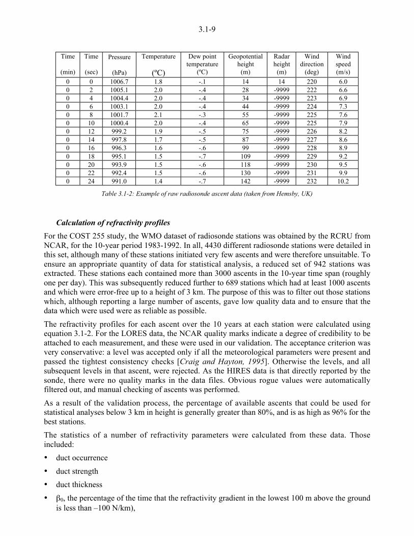
3.1-9

Time

(min)

Time

(sec)

Pressure

(hPa)

Temperature

(ºC)

Dew pointtemperature

(ºC)

Geopotentialheight

(m)

Radarheight

(m)

Winddirection

(deg)

Windspeed(m/s)

0 0 1006.7 1.8 -.1 14 14 220 6.00 2 1005.1 2.0 -.4 28 -9999 222 6.60 4 1004.4 2.0 -.4 34 -9999 223 6.90 6 1003.1 2.0 -.4 44 -9999 224 7.30 8 1001.7 2.1 -.3 55 -9999 225 7.60 10 1000.4 2.0 -.4 65 -9999 225 7.90 12 999.2 1.9 -.5 75 -9999 226 8.20 14 997.8 1.7 -.5 87 -9999 227 8.60 16 996.3 1.6 -.6 99 -9999 228 8.90 18 995.1 1.5 -.7 109 -9999 229 9.20 20 993.9 1.5 -.6 118 -9999 230 9.50 22 992.4 1.5 -.6 130 -9999 231 9.90 24 991.0 1.4 -.7 142 -9999 232 10.2

Table 3.1-2: Example of raw radiosonde ascent data (taken from Hemsby, UK)

Calculation of refractivity profiles

For the COST 255 study, the WMO dataset of radiosonde stations was obtained by the RCRU fromNCAR, for the 10-year period 1983-1992. In all, 4430 different radiosonde stations were detailed inthis set, although many of these stations initiated very few ascents and were therefore unsuitable. Toensure an appropriate quantity of data for statistical analysis, a reduced set of 942 stations wasextracted. These stations each contained more than 3000 ascents in the 10-year time span (roughlyone per day). This was subsequently reduced further to 689 stations which had at least 1000 ascentsand which were error-free up to a height of 3 km. The purpose of this was to filter out those stationswhich, although reporting a large number of ascents, gave low quality data and to ensure that thedata which were used were as reliable as possible.

The refractivity profiles for each ascent over the 10 years at each station were calculated usingequation 3.1-2. For the LORES data, the NCAR quality marks indicate a degree of credibility to beattached to each measurement, and these were used in our validation. The acceptance criterion wasvery conservative: a level was accepted only if all the meteorological parameters were present andpassed the tightest consistency checks [Craig and Hayton, 1995]. Otherwise the levels, and allsubsequent levels in that ascent, were rejected. As the HIRES data is that directly reported by thesonde, there were no quality marks in the data files. Obvious rogue values were automaticallyfiltered out, and manual checking of ascents was performed.

As a result of the validation process, the percentage of available ascents that could be used forstatistical analyses below 3 km in height is generally greater than 80%, and is as high as 96% for thebest stations.

The statistics of a number of refractivity parameters were calculated from these data. Thoseincluded:

• duct occurrence

• duct strength

• duct thickness

• `0, the percentage of the time that the refractivity gradient in the lowest 100 m above the groundis less than –100 N/km),

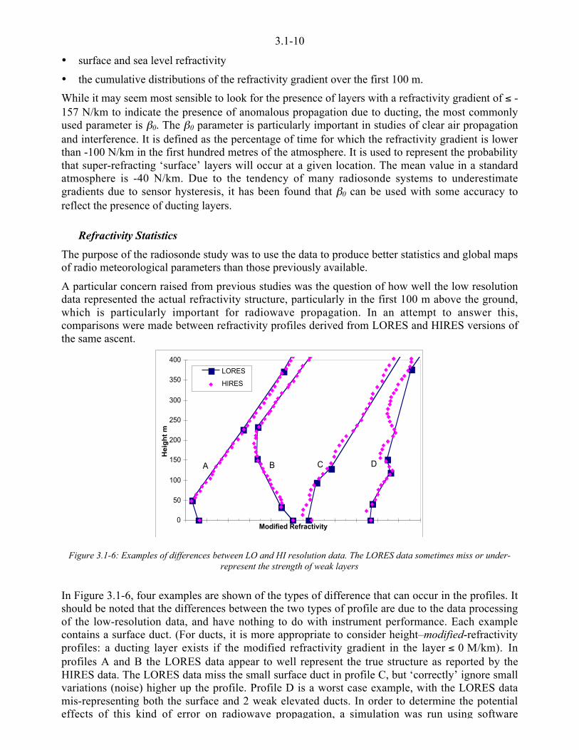
3.1-10

• surface and sea level refractivity

• the cumulative distributions of the refractivity gradient over the first 100 m.

While it may seem most sensible to look for the presence of layers with a refractivity gradient of ) -157 N/km to indicate the presence of anomalous propagation due to ducting, the most commonlyused parameter is `0. The `0 parameter is particularly important in studies of clear air propagationand interference. It is defined as the percentage of time for which the refractivity gradient is lowerthan -100 N/km in the first hundred metres of the atmosphere. It is used to represent the probabilitythat super-refracting ‘surface’ layers will occur at a given location. The mean value in a standardatmosphere is -40 N/km. Due to the tendency of many radiosonde systems to underestimategradients due to sensor hysteresis, it has been found that `0 can be used with some accuracy toreflect the presence of ducting layers.

Refractivity Statistics

The purpose of the radiosonde study was to use the data to produce better statistics and global mapsof radio meteorological parameters than those previously available.

A particular concern raised from previous studies was the question of how well the low resolutiondata represented the actual refractivity structure, particularly in the first 100 m above the ground,which is particularly important for radiowave propagation. In an attempt to answer this,comparisons were made between refractivity profiles derived from LORES and HIRES versions ofthe same ascent.

0

50

100

150

200

250

300

350

400

Modified Refractivity

He

igh

t m

LORES

HIRES

A B C D

Figure 3.1-6: Examples of differences between LO and HI resolution data. The LORES data sometimes miss or under-represent the strength of weak layers

In Figure 3.1-6, four examples are shown of the types of difference that can occur in the profiles. Itshould be noted that the differences between the two types of profile are due to the data processingof the low-resolution data, and have nothing to do with instrument performance. Each examplecontains a surface duct. (For ducts, it is more appropriate to consider height–modified-refractivityprofiles: a ducting layer exists if the modified refractivity gradient in the layer ) 0 M/km). Inprofiles A and B the LORES data appear to well represent the true structure as reported by theHIRES data. The LORES data miss the small surface duct in profile C, but ‘correctly’ ignore smallvariations (noise) higher up the profile. Profile D is a worst case example, with the LORES datamis-representing both the surface and 2 weak elevated ducts. In order to determine the potentialeffects of this kind of error on radiowave propagation, a simulation was run using software

3.1-11

implementing a parabolic equation modelling (PEM) technique on this profile. A full description ofthe PEM software and method is given in [Levy and Craig, 1996].

Figures 3.1-7 and 3.1-8 here show a vertical slice through the atmosphere, with a transmitter (at thelower left side of the plot, 10 m above ground) seen on land (80 m above sea) near a cliff andbroadcasting over the sea. Using the HIRES data (Figure 3.1-7) we see that as the transmitter isalmost at the height of the first elevated ducting layer, trapping occurs because the angle ofincidence is sufficiently low. Relative signal strengths exceeding +20 dB are seen up to 200 kmaway.

Figure 3.1-7: PEM simulation using the HIRES profiles D fromFigure 3.1-6.

Using the LORES profile (Figure 3.1-8) some trapping still occurs, but as the duct strength is under-represented by the LORES data, the ducting effect seen is much reduced.

Figure 3.1-8: As for Figure 3.1-7, but using the LORES profile for the same ascent.Strong coupling from the transmitter (10 m above ground, 90 m above sea) into the duct can be seen.

As the duct strength is under represented here the coupling is not as extensive

An examination of the ` 0 parameter derived from the two data sets for two UK stations, revealedh bl d d l i d d (Fi 3 1 9) Th hl d i i il

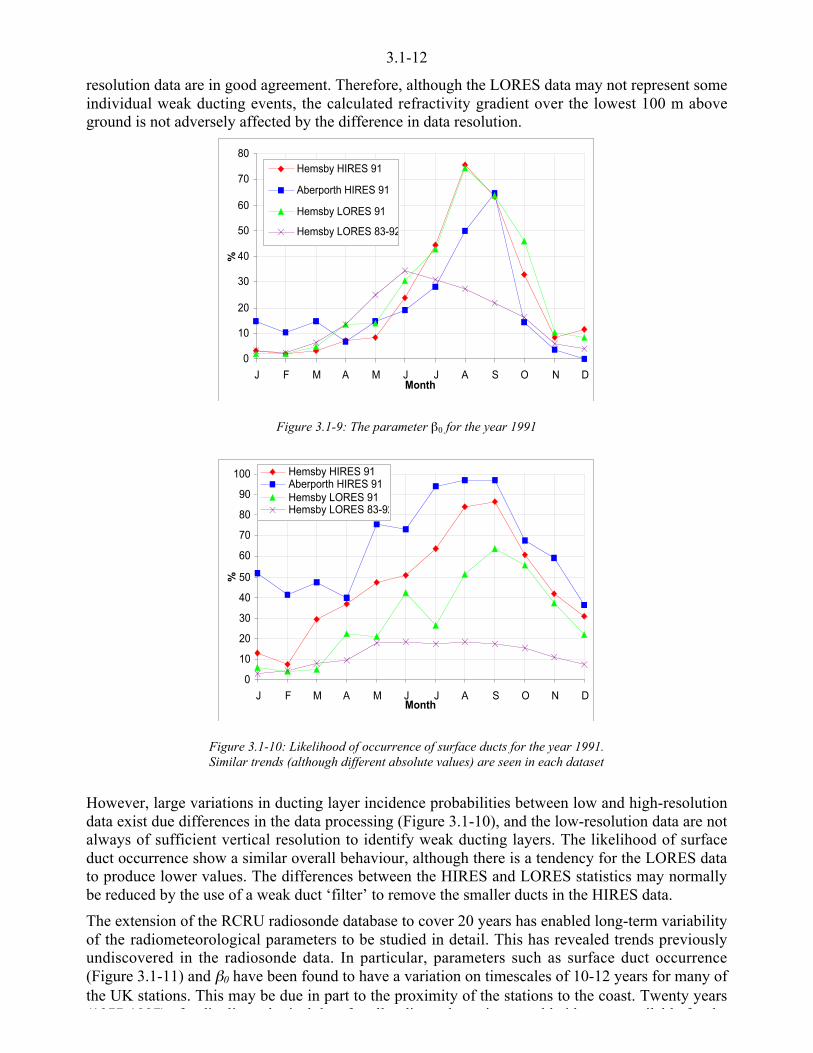
3.1-12

resolution data are in good agreement. Therefore, although the LORES data may not represent someindividual weak ducting events, the calculated refractivity gradient over the lowest 100 m aboveground is not adversely affected by the difference in data resolution.

0

10

20

30

40

50

60

70

80

J F M A M J J A S O N DMonth

%

Hemsby HIRES 91

Aberporth HIRES 91

Hemsby LORES 91

Hemsby LORES 83-92

Figure 3.1-9: The parameter `0 for the year 1991

0

10

20

30

40

50

60

70

80

90

100

J F M A M J J A S O N DMonth

%

Hemsby HIRES 91Aberporth HIRES 91Hemsby LORES 91Hemsby LORES 83-92

Figure 3.1-10: Likelihood of occurrence of surface ducts for the year 1991.Similar trends (although different absolute values) are seen in each dataset

However, large variations in ducting layer incidence probabilities between low and high-resolutiondata exist due differences in the data processing (Figure 3.1-10), and the low-resolution data are notalways of sufficient vertical resolution to identify weak ducting layers. The likelihood of surfaceduct occurrence show a similar overall behaviour, although there is a tendency for the LORES datato produce lower values. The differences between the HIRES and LORES statistics may normallybe reduced by the use of a weak duct ‘filter’ to remove the smaller ducts in the HIRES data.

The extension of the RCRU radiosonde database to cover 20 years has enabled long-term variabilityof the radiometeorological parameters to be studied in detail. This has revealed trends previouslyundiscovered in the radiosonde data. In particular, parameters such as surface duct occurrence(Figure 3.1-11) and `0 have been found to have a variation on timescales of 10-12 years for many ofthe UK stations. This may be due in part to the proximity of the stations to the coast. Twenty years(1977 1997) f di li l i l d f ll di d i ld id il bl f h

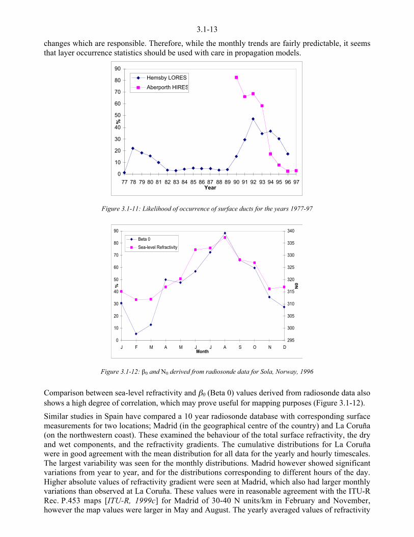
3.1-13

changes which are responsible. Therefore, while the monthly trends are fairly predictable, it seemsthat layer occurrence statistics should be used with care in propagation models.

0

10

20

30

40

50

60

70

80

90

77 78 79 80 81 82 83 84 85 86 87 88 89 90 91 92 93 94 95 96 97Year

%

Hemsby LORES

Aberporth HIRES

Figure 3.1-11: Likelihood of occurrence of surface ducts for the years 1977-97

0

10

20

30

40

50

60

70

80

90

J F M A M J J A S O N DMonth

%

295

300

305

310

315

320

325

330

335

340

N0

Beta 0

Sea-level Refractivity

Figure 3.1-12: `0 and N0 derived from radiosonde data for Sola, Norway, 1996

Comparison between sea-level refractivity and `0 (Beta 0) values derived from radiosonde data alsoshows a high degree of correlation, which may prove useful for mapping purposes (Figure 3.1-12).

Similar studies in Spain have compared a 10 year radiosonde database with corresponding surfacemeasurements for two locations; Madrid (in the geographical centre of the country) and La Coruña(on the northwestern coast). These examined the behaviour of the total surface refractivity, the dryand wet components, and the refractivity gradients. The cumulative distributions for La Coruñawere in good agreement with the mean distribution for all data for the yearly and hourly timescales.The largest variability was seen for the monthly distributions. Madrid however showed significantvariations from year to year, and for the distributions corresponding to different hours of the day.Higher absolute values of refractivity gradient were seen at Madrid, which also had larger monthlyvariations than observed at La Coruña. These values were in reasonable agreement with the ITU-RRec. P.453 maps [ITU-R, 1999c] for Madrid of 30-40 N units/km in February and November,however the map values were larger in May and August. The yearly averaged values of refractivity

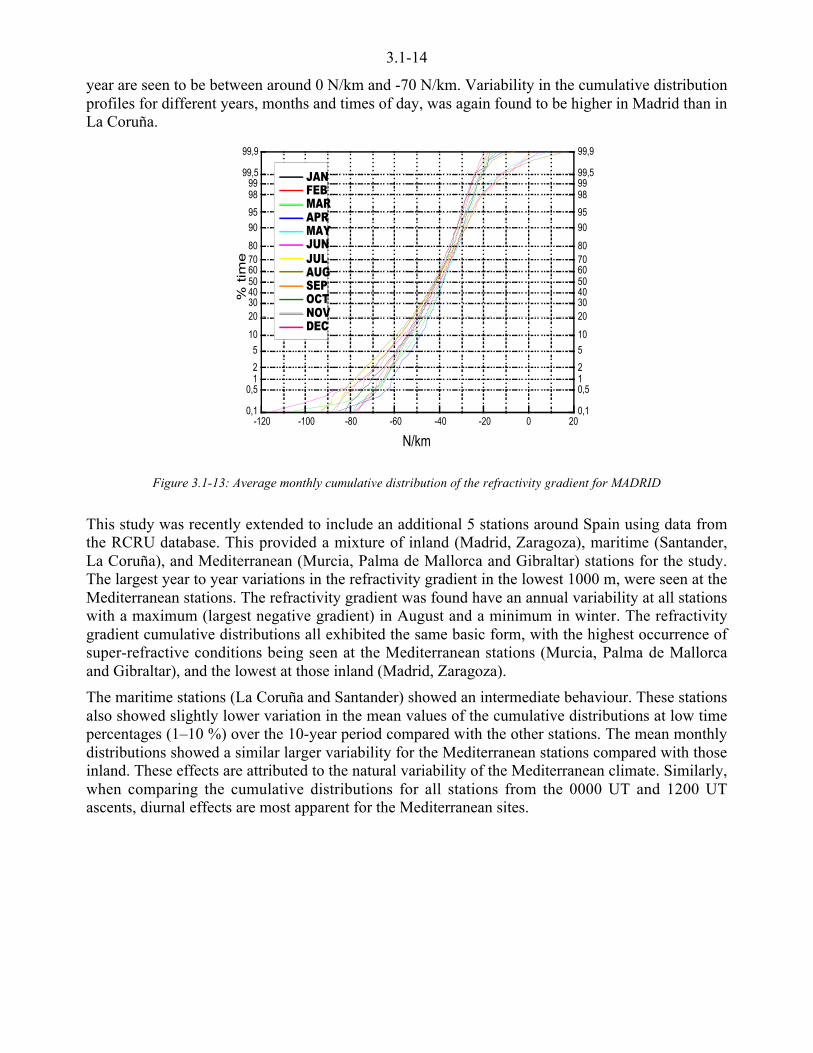
3.1-14

year are seen to be between around 0 N/km and -70 N/km. Variability in the cumulative distributionprofiles for different years, months and times of day, was again found to be higher in Madrid than inLa Coruña.

0,1

0,512

5

10

20304050607080

90

95

9899

99,5

99,9

-120 -100 -80 -60 -40 -20 0 200,1

0,512

5

10

20304050607080

90

95

989999,5

99,9

JAN FEB MAR APR MAY JUN JUL AUG SEP OCT NOV DEC

N/km

% tim

e

Figure 3.1-13: Average monthly cumulative distribution of the refractivity gradient for MADRID

This study was recently extended to include an additional 5 stations around Spain using data fromthe RCRU database. This provided a mixture of inland (Madrid, Zaragoza), maritime (Santander,La Coruña), and Mediterranean (Murcia, Palma de Mallorca and Gibraltar) stations for the study.The largest year to year variations in the refractivity gradient in the lowest 1000 m, were seen at theMediterranean stations. The refractivity gradient was found have an annual variability at all stationswith a maximum (largest negative gradient) in August and a minimum in winter. The refractivitygradient cumulative distributions all exhibited the same basic form, with the highest occurrence ofsuper-refractive conditions being seen at the Mediterranean stations (Murcia, Palma de Mallorcaand Gibraltar), and the lowest at those inland (Madrid, Zaragoza).

The maritime stations (La Coruña and Santander) showed an intermediate behaviour. These stationsalso showed slightly lower variation in the mean values of the cumulative distributions at low timepercentages (1–10 %) over the 10-year period compared with the other stations. The mean monthlydistributions showed a similar larger variability for the Mediterranean stations compared with thoseinland. These effects are attributed to the natural variability of the Mediterranean climate. Similarly,when comparing the cumulative distributions for all stations from the 0000 UT and 1200 UTascents, diurnal effects are most apparent for the Mediterranean sites.

3.1-15

0,1

0,512

5

10

20304050607080

90

95

9899

99,5

99,9

-180 -160 -140 -120 -100 -80 -60 -40 -20 00,1

0,512

5

10

20304050607080

90

95

989999,5

99,9

JAN FEB MAR APR MAY JUN JUL AUG SEP OCT NOV DEC

N/km

% t

ime

Figure3.1-14: Average monthly cumulative distribution of the refractivity gradient for LA CORUÑA

Measurements in towers

Tower-based meteorological instruments have long been employed as a means of assessing theconditions giving rise to clear-air anomalous propagation. [Ikegami, 1959] used fixed wet and drytemperature sensors at 12 levels on a 300 m tower to deduce refractivity gradients and correlated theobservations with co-incident signal strength measurements over horizontal and oblique terrestrialpaths. [Ikegami, et al., 1968] used similar instruments on an 80 m tower as well as radiosondesoundings to relate refractivity profiles with variations in angles-of-arrival over an oblique path.

Although multipath fading is observed on Earth-space links for elevation angles below about 5degrees [ITU-R, 1999b], the phenomenon is more commonly encountered on terrestrial links. Forstrong atmospheric multipath to occur on a non-inclined path, there must be extremely largepositive (Figure 3.1-15) or negative (Figure 3.1-16) refractivity gradients above and below thenominal propagation trajectory.

For atmospheric multipath to occur on an Earth-space path, the refractivity must vary horizontallyas well as vertically. Insights into the relevant propagation mechanisms as well as the problems indeveloping suitable propagation models are thus better approached from the simpler terrestrialgeometry.

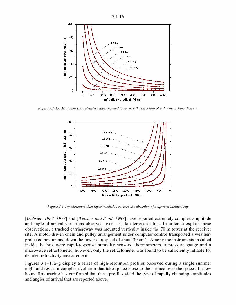
3.1-16

Figure 3.1-15: Minimum sub-refractive layer needed to reverse the direction of a downward-incident ray

Figure 3.1-16: Minimum duct layer needed to reverse the direction of a upward-incident ray

[Webster, 1982, 1997] and [Webster and Scott, 1987] have reported extremely complex amplitudeand angle-of-arrival variations observed over a 51 km terrestrial link. In order to explain theseobservations, a tracked carriageway was mounted vertically inside the 70 m tower at the receiversite. A motor-driven chain and pulley arrangement under computer control transported a weather-protected box up and down the tower at a speed of about 30 cm/s. Among the instruments installedinside the box were rapid-response humidity sensors, thermometers, a pressure gauge and amicrowave refractometer; however, only the refractometer was found to be sufficiently reliable fordetailed refractivity measurement.

Figures 3.1–17a–g display a series of high-resolution profiles observed during a single summernight and reveal a complex evolution that takes place close to the surface over the space of a fewhours. Ray tracing has confirmed that these profiles yield the type of rapidly changing amplitudesand angles of arrival that are reported above.

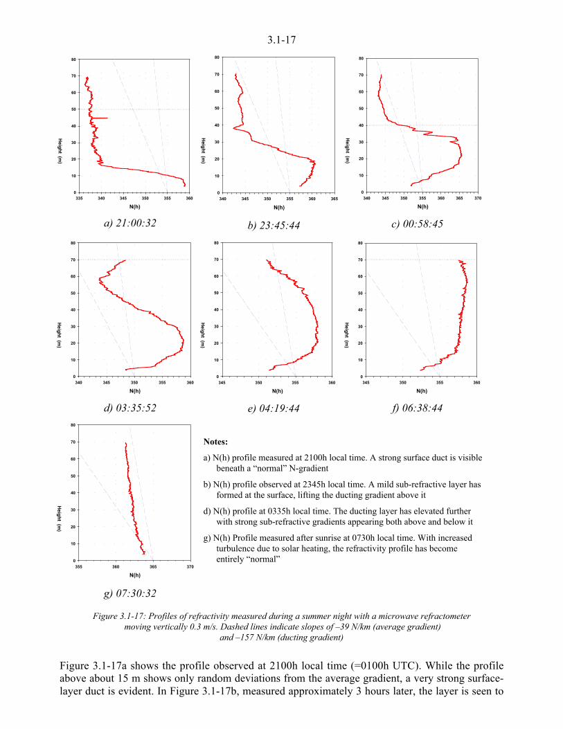
3.1-17

N(h)

335 340 345 350 355 360

Heig

ht (m

)

0

10

20

30

40

50

60

70

80

a) 21:00:32

N(h)

340 345 350 355 360 365

Heig

ht (m

)

0

10

20

30

40

50

60

70

80

b) 23:45:44

N(h)

340 345 350 355 360 365 370

Heig

ht (m

)

0

10

20

30

40

50

60

70

80

c) 00:58:45

N(h)

340 345 350 355 360

Heig

ht (m

)

0

10

20

30

40

50

60

70

80

d) 03:35:52

N(h)

345 350 355 360

Heig

ht (m

)

0

10

20

30

40

50

60

70

80

e) 04:19:44

N(h)

345 350 355 360

Heig

ht (m

)

0

10

20

30

40

50

60

70

80

f) 06:38:44

N(h)

355 360 365 370

Heig

ht (m

)

0

10

20

30

40

50

60

70

80

g) 07:30:32

Notes:

a) N(h) profile measured at 2100h local time. A strong surface duct is visiblebeneath a “normal” N-gradient

b) N(h) profile observed at 2345h local time. A mild sub-refractive layer hasformed at the surface, lifting the ducting gradient above it

d) N(h) profile at 0335h local time. The ducting layer has elevated furtherwith strong sub-refractive gradients appearing both above and below it

g) N(h) Profile measured after sunrise at 0730h local time. With increasedturbulence due to solar heating, the refractivity profile has becomeentirely “normal”

Figure 3.1-17: Profiles of refractivity measured during a summer night with a microwave refractometer moving vertically 0.3 m/s. Dashed lines indicate slopes of –39 N/km (average gradient)

and –157 N/km (ducting gradient)

Figure 3.1-17a shows the profile observed at 2100h local time (=0100h UTC). While the profileabove about 15 m shows only random deviations from the average gradient, a very strong surface-layer duct is evident. In Figure 3.1-17b, measured approximately 3 hours later, the layer is seen to

3.1-18

in Figure 3.1-17d, recorded some 7 hours after the initial profile was taken. The profile now formsan elevated duct extending between 15 m and 55 m with strong sub-refractive layers both above andbelow the negative gradient. As dawn arrives, the gradients expand and weaken until, by 0730hlocal time (=1230 UTC), the profile (Figure 3.1-17g) appears to be entirely “normal”. It isimportant to note that, in this instance, routine meteorological radiosonde launches would havefailed to record the existence of any ducts.

An alternative method of studying the refractive index profile near the ground is to use aninstrumented tower with temperature and humidity sensors positioned at various heights. Thesemeasurements can then be used to derive the refractivity values at these heights. A network of suchtowers was used in France between 1983 and 1989 to study the refractivity gradient statistics in thefirst 100 m. The instruments used for the measurements were wet and dry bulb psychrometers, oneplaced just above the ground and the second at the top of the tower. The difference in heightbetween the sensors was between 58 and 98 m for the eleven masts used in the study. These wereconnected to a barometer and a data processing and recording system. One advantage of this type ofstudy was that the measurements are made continuously throughout the day, rather than the single“snapshot” of the atmosphere provided by radiosondes as they ascend. It therefore enabled thehourly variations of the refractivity gradient to be monitored. These were generally found tobecome larger (more negative) during the day, and smaller at night.

The cumulative distributions of the refractivity gradient were calculated and used to examine theoccurrence of super-refractive conditions. Larger gradients (more negative) were seen in summerrather than winter. Larger refractivity lapse rates were observed in summer than in winter alongwith a decrease in super-refractive conditions in winter. The `0 parameter indicted a maximumvalue in summer exceeding 40 % and in winter minimum of less than 5%.

Comparison with radiosonde data

The refractivity statistics from psychrometer towers in France during the ARGOS experiment,between 1983 and 1989, were compared to statistics derived from the RCRU database ofradiosonde measurements (1983-1992). The radiosonde ground stations were situated at variouslocations as shown in Figure 3.1-18. The comparison between the two data sets concentrated onthose sites where the two were closely located; Nancy and Lyon. Unfortunately, the psychrometerdata from Nancy were considered to be unreliable, hence the direct comparison between thepsychrometers and the radiosonde measurements was restricted to data from the Lyon station.

The RCRU radiosonde database for France was analysed to yield 40,000 useful ascents for the 10year period, 5899 of which were from the Lyon station. Refractivity parameters were thencalculated for each station following the method described in detail in [Craig and Hayton, 1995].

3.1-19

Figure 3.1-18: Location of radiosonde (red) and psychrometer (green) stations in France.Note that observations were made using both instruments at sites in Nancy and Lyon

The cumulative distributions of refractivity gradient are shown in Figure 3.1-19 for all radiosondelocations in France. The distributions are fairly consistent with one another except for Ajaccio,which shows a greatly enhanced probability of superrefractive, and duct gradients. This is believedto be a consequence of its coastal location in the Mediterranean.

0

20

40

60

80

100

120

-200

-180

-160

-140

-120

-100

-80

-60

-40

-20 0

20

40

60

80

100

N/km

% o

f ti

me

Brest

Trappes

Nancy

Lyon

Bordeaux

Nimes

Ajaccio

Figure 3.1-19: Cumulative distributions of refractivity gradient for all availableFrench radiosonde locations (1983-1992)

The annual variation of `0 is shown in Figure 3.1-20 for all available French stations. They allshowed a clear annual cycle, with a maximum in July/August and a minimum in December/January.

3.1-20

0

10

20

30

40

50

60

Janu

ary

Febr

uary

Mar

chApr

ilMay

June

July

Augus

t

Septembe

r

Octob

er

Novem

ber

Decem

ber

Month

% o

f ti

me

Brest

Trappes

Nancy

Lyon

Bordeaux

Nimes

Ajaccio

Figure 3.1-20: Seasonal variation of `0 for all available French radiosonde locations (1983-1992)

The radiosonde data for Lyon were also analysed in terms of time of release (0Z or 12Z) over theentire 10 year period (over 5000 radiosonde ascents) to see if there were any significant differencesbetween the two (Figure 3.1-21). No marked differences were present, although any short termvariability may well be smoothed out due to the large amount of data analysed. The derivedrefractivity statistics were therefore calculated from all available ascents from the Lyon station, inorder to give the best possible representation of the refractivity conditions.

0

20

40

60

80

100

120

-200

-180

-160

-140

-120

-100 -8

0-6

0-4

0-2

0 0 20 40 60 80 100

N/km

% o

f T

ime

0Z

12Z

0Z&12Z

Figure 3.1-21: Cumulative distributions derived from radiosonde ascents at different times

The radiosonde refractivity data for Lyon were analysed to derive the monthly mean cumulativedistributions of the refractivity gradient. The curves for each month are presented in Figure 3.1-22.These show that there is a clear variation in the occurrence of large negative refractivity gradientsover the course of the year. In December, the values at -100 N/km are around 4 %, while at theirmaximum in June they have increased by a factor of 5 to 20 %. This annual variation is also presentfor gradients larger (more negative) than -180 N/km, while the distributions tend to converge forgradients smaller (more positive) than -40 N/km.

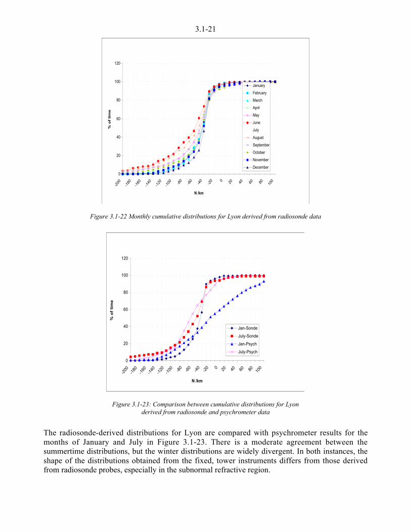
3.1-21

0

20

40

60

80

100

120

-200

-180

-160

-140

-120

-100 -8

0-60

-40

-20 0 20 40 60 80 10

0

N /km

% o

f ti

me

January

February

March

April

May

June

July

August

September

October

November

December

Figure 3.1-22 Monthly cumulative distributions for Lyon derived from radiosonde data

0

20

40

60

80

100

120

-200

-180

-160

-140

-120

-100 -8

0-6

0-4

0-2

0 0 20 40 60 80 100

N /km

% o

f ti

me

Jan-Sonde

July-Sonde

Jan-Psych

July-Psych

Figure 3.1-23: Comparison between cumulative distributions for Lyonderived from radiosonde and psychrometer data

The radiosonde-derived distributions for Lyon are compared with psychrometer results for themonths of January and July in Figure 3.1-23. There is a moderate agreement between thesummertime distributions, but the winter distributions are widely divergent. In both instances, theshape of the distributions obtained from the fixed, tower instruments differs from those derivedfrom radiosonde probes, especially in the subnormal refractive region.

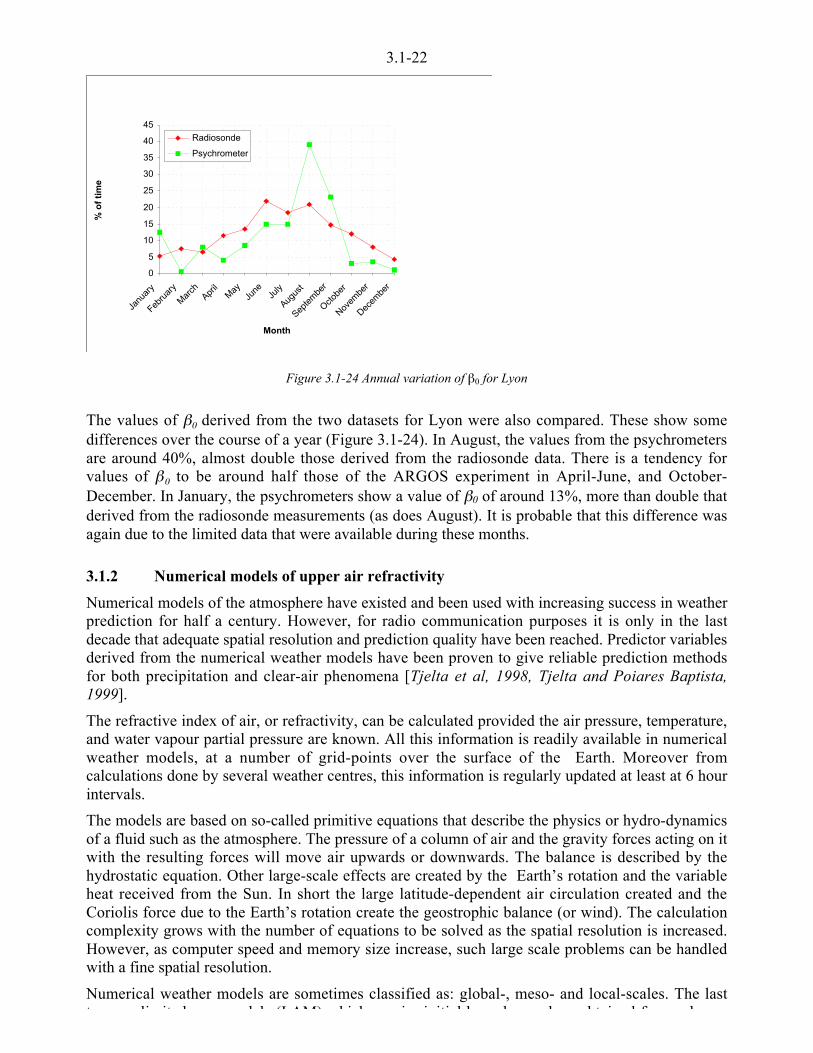
3.1-22

0

5

10

15

20

25

30

35

40

45

Janu

ary

Febru

ary

Mar

chApr

ilM

ayJu

neJu

ly

Augus

t

Septe

mbe

r

Octobe

r

Novem

ber

Decem

ber

Month

% o

f ti

me

Radiosonde

Psychrometer

Figure 3.1-24 Annual variation of `0 for Lyon

The values of `0 derived from the two datasets for Lyon were also compared. These show somedifferences over the course of a year (Figure 3.1-24). In August, the values from the psychrometersare around 40%, almost double those derived from the radiosonde data. There is a tendency forvalues of `0 to be around half those of the ARGOS experiment in April-June, and October-December. In January, the psychrometers show a value of `0 of around 13%, more than double thatderived from the radiosonde measurements (as does August). It is probable that this difference wasagain due to the limited data that were available during these months.

3.1.2 Numerical models of upper air refractivity

Numerical models of the atmosphere have existed and been used with increasing success in weatherprediction for half a century. However, for radio communication purposes it is only in the lastdecade that adequate spatial resolution and prediction quality have been reached. Predictor variablesderived from the numerical weather models have been proven to give reliable prediction methodsfor both precipitation and clear-air phenomena [Tjelta et al, 1998, Tjelta and Poiares Baptista,1999].

The refractive index of air, or refractivity, can be calculated provided the air pressure, temperature,and water vapour partial pressure are known. All this information is readily available in numericalweather models, at a number of grid-points over the surface of the Earth. Moreover fromcalculations done by several weather centres, this information is regularly updated at least at 6 hourintervals.

The models are based on so-called primitive equations that describe the physics or hydro-dynamicsof a fluid such as the atmosphere. The pressure of a column of air and the gravity forces acting on itwith the resulting forces will move air upwards or downwards. The balance is described by thehydrostatic equation. Other large-scale effects are created by the Earth’s rotation and the variableheat received from the Sun. In short the large latitude-dependent air circulation created and theCoriolis force due to the Earth’s rotation create the geostrophic balance (or wind). The calculationcomplexity grows with the number of equations to be solved as the spatial resolution is increased.However, as computer speed and memory size increase, such large scale problems can be handledwith a fine spatial resolution.

Numerical weather models are sometimes classified as: global-, meso- and local-scales. The lastt li it d d l (LAM) hi h i i iti l b d l bt i d f l

3.1-23

Model Horizontal resolution Vertical levels

Global 60-100 km 30-60

Regional 30-50 km 30-60

Local 5-10 km 30-60

Table 3.1-3: Numerical weather model resolution

In Section 3.1.6.5 several maps of clear-air parameters, described in Section 3.1.4.4, are produced,based on refractivity derived a from 2-year numerical weather data set derived from 1 October 1992to 1 October 1994 [v.d. Kamp et al, 1997]. This particular data set has a spatial resolution of1.5° x 1.5°, which is about 165 km at the equator but the east-west resolution becomes increasinglyfine at higher latitudes. The vertical resolution had 23 levels, but was based on a numerical modelwith 32 levels. The most relevant effects for clear-air parameters are due to the lowest level, nearthe surface of the Earth and to the first level at about 65 m above the terrain.

3.1.3 Vertical refractivity profiles derived by using a 3-D objective analysis technique

A technique is presented for the calculation of the dN/dz values in the lower atmosphere layersusing as input values dense ground synoptic observations of meteorological quantities, based on theapplication of the 3-D Objective Analysis technique [Sokol and Stekl, 1994].

3.1.3.1 Input Data

The meteorological data used for the calculations of dN/dz include the atmospheric vertical profilesof pressure (hPa), temperature (°C), and relative humidity (%) from the radiosonde station Prague-Libus (Czech Republic), and the ground data (SYNOP reports) from meteorological stations locatedaround Prague. The observation period is 1994-1996. The radiosonde data refer to two observationsa day at the standard synoptic times 0000 and 1200 UTC. The SYNOP reports from threeobservations a day (0000, 1200 and 1800 UTC) were considered.

3.1.3.2 The method of 3-D Objective Analysis

The 3-D Objective Analysis (OA) method treats ground variables measured at different stationelevations. In this sense the data are considered to be in a three-dimensional space and the field ofvertical gradient is a by-product of the interpolation procedure. The OA method is based on thecombination of two interpolation (extrapolation) techniques: polynomial approximation using theleast-squares method and the Successive Correction Method (SCM). To determine the verticalgradient of a scalar variable over a regular grid the analysis is based on the following:

• calculation of vertical gradients (the coefficient at z co-ordinate) performed by means of a three-dimensional first-order polynomial approximation that uses the least squares method.

• horizontal interpolation of vertical gradients to the grid points performed by using the SCM.

The objective analysis was carried out in stereographic projection with a horizontal step of 32 kmon the territory of the Czech Republic. The resultant grid values of dN/dz were interpolated to thePrague-Libus location.

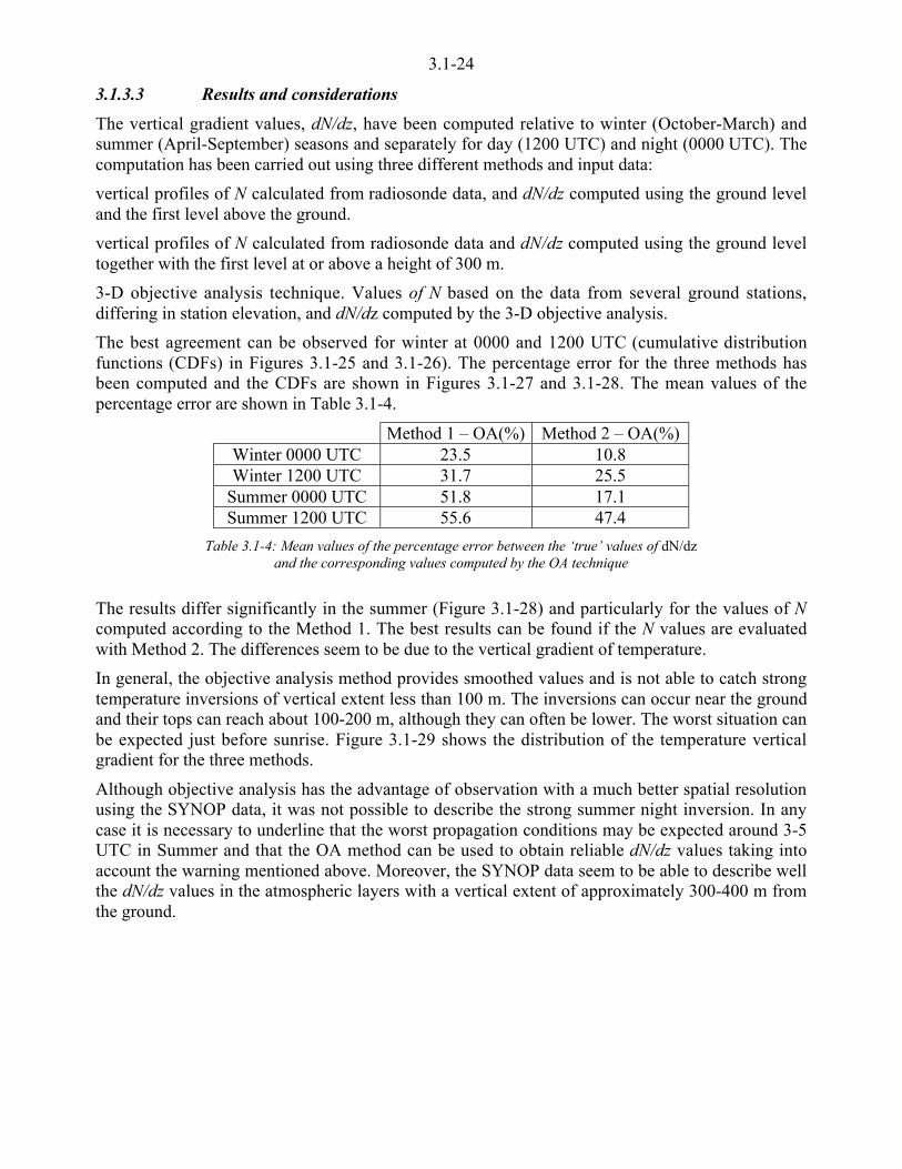
3.1-24

3.1.3.3 Results and considerations

The vertical gradient values, dN/dz, have been computed relative to winter (October-March) andsummer (April-September) seasons and separately for day (1200 UTC) and night (0000 UTC). Thecomputation has been carried out using three different methods and input data:

vertical profiles of N calculated from radiosonde data, and dN/dz computed using the ground leveland the first level above the ground.

vertical profiles of N calculated from radiosonde data and dN/dz computed using the ground leveltogether with the first level at or above a height of 300 m.

3-D objective analysis technique. Values of N based on the data from several ground stations,differing in station elevation, and dN/dz computed by the 3-D objective analysis.

The best agreement can be observed for winter at 0000 and 1200 UTC (cumulative distributionfunctions (CDFs) in Figures 3.1-25 and 3.1-26). The percentage error for the three methods hasbeen computed and the CDFs are shown in Figures 3.1-27 and 3.1-28. The mean values of thepercentage error are shown in Table 3.1-4.

Method 1 – OA(%) Method 2 – OA(%)Winter 0000 UTC 23.5 10.8Winter 1200 UTC 31.7 25.5

Summer 0000 UTC 51.8 17.1Summer 1200 UTC 55.6 47.4

Table 3.1-4: Mean values of the percentage error between the ‘true’ values of dN/dzand the corresponding values computed by the OA technique

The results differ significantly in the summer (Figure 3.1-28) and particularly for the values of Ncomputed according to the Method 1. The best results can be found if the N values are evaluatedwith Method 2. The differences seem to be due to the vertical gradient of temperature.

In general, the objective analysis method provides smoothed values and is not able to catch strongtemperature inversions of vertical extent less than 100 m. The inversions can occur near the groundand their tops can reach about 100-200 m, although they can often be lower. The worst situation canbe expected just before sunrise. Figure 3.1-29 shows the distribution of the temperature verticalgradient for the three methods.

Although objective analysis has the advantage of observation with a much better spatial resolutionusing the SYNOP data, it was not possible to describe the strong summer night inversion. In anycase it is necessary to underline that the worst propagation conditions may be expected around 3-5UTC in Summer and that the OA method can be used to obtain reliable dN/dz values taking intoaccount the warning mentioned above. Moreover, the SYNOP data seem to be able to describe wellthe dN/dz values in the atmospheric layers with a vertical extent of approximately 300-400 m fromthe ground.

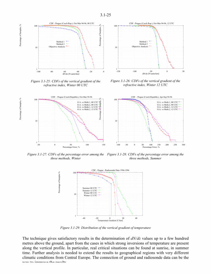
3.1-25

1

10

100

-100 -80 -60 -40 -20 0

Perc

enta

ge o

f Sa

mpl

es, %

dN/dz [N-units/km]

CDF - Prague (Czech Rep.), Oct-Mar 94-96, 00 UTC

Method 1Method 2

Objective Analysis

Figure 3.1-25: CDFs of the vertical gradient of therefractive index, Winter 00 UTC

1

10

100

-150 -100 -50 0 50

Perc

enta

ge o

f Sa

mpl

es, %

dN/dz [N-units/km]

CDF - Prague (Czech Rep.), Oct-Mar 94-96, 12 UTC

Method 1Method 2

Objective Analysis

Figure 3.1-26: CDFs of the vertical gradient of therefractive index, Winter 12 UTC

1

10

100

-50 0 50 100 150

Perc

enta

ge o

f Sa

mpl

es, %

Percentage Error, %

CDF - Prague (Czech Republic), Oct-Mar 94-96

O.A. vs Meth.1, 00 UTCO.A. vs Meth.2, 00 UTCO.A. vs Meth.1, 12 UTCO.A. vs Meth.2, 12 UTC

Figure 3.1-27: CDFs of the percentage error among thethree methods, Winter

1

10

100

-100 -50 0 50 100 150 200 250 300

Perc

enta

ge o

f Sa

mpl

es, %

Percentage Error, %

CDF - Prague (Czech Republic), Apr-Sep 94-96

O.A. vs Meth.1, 00 UTCO.A. vs Meth.2, 00 UTCO.A. vs Meth.1, 12 UTCO.A. vs Meth.2, 12 UTC

Figure 3.1-28: CDFs of the percentage error among thethree methods, Summer

1

10

100

-40 -20 0 20 40

Perc

enta

ge o

f Sa

mpl

es %

Temperature Gradient [C/km]

CDF - Prague - Radiosonde Data 1994-1996

Summer 00 UTCSummer 12 UTC

Winter 00 UTCWinter 12 UTC

Figure 3.1-29: Distribution of the vertical gradient of temperature

The technique gives satisfactory results in the determination of dN/dz values up to a few hundredmetres above the ground, apart from the cases in which strong inversions of temperature are presentalong the vertical profile. In particular, real critical situations can be found at sunrise, in summertime. Further analysis is needed to extend the results to geographical regions with very differentclimatic conditions from Central Europe. The connection of ground and radiosonde data can be theway to improve the results

3.1-26

3.1.4 Clear air parameters

A radio wave propagation prediction method taking into account effects that vary with time, has toinclude clear-air phenomena. Some clear-air parameters are already in use in prediction methods forradio systems design [ITU-R, 1999a,b]. This section describes the actual parameters as well as somenew ones that might become of interest. The variables are all derived from the refractive index n, ormore precisely refractivity N (see equation 3.1-2) or modified refractivity M (see equation 3.1-5).

The parameters of interest are:

• Ns – the refractivity at ground level

• No – the value of Ns scaled to sea level

• Nwet – the wet component of refractivity

• 6Nt – the change in total refractivity at the surface of the Earth

• Nw,m – the maximum wet term of refractivity at the surface of the Earth

• 6Nw,a – the average change of wet term of refractivity at the surface of the Earth

• dN/dz – the distribution of refractivity gradient in general with three special cases:

< ` o – the percentage of the time that the refractivity gradient in the lowest 100 m above theground is less than -100 N/km

< PL – a (pseudo-)worst month value of ` 0

< 6N – the difference between the values of refractivity at the ground and 1 km

• Sp – Surface duct occurrence in percent of an average year

• St – Average yearly median of surface duct thickness in m,

• Ss – Average yearly median of surface duct strength in M-units,

• Ep – Elevated duct occurrence in percent of an average year,

• Et – Average yearly median of elevated duct thickness in m

• Es – Average yearly median of elevated duct strength in M-units

• Eb – Average yearly median of elevated duct base height in m.

Three different sources of data are used for deriving the parameters: radiosonde observations,surface measurements, and data from numerical modelling of the atmosphere. Some parameters canbe derived from all three sources.

3.1.4.1 Refractivity gradients

The refractivity gradient variable `0 is defined for the lowest 100 m of the atmosphere as theoccurrence of dN/dz values equal or less than -100 N-units/km with dz = 100 m.

Neither radiosondes nor the numerical atmosphere models give N values exactly at 100 m, but thevalues at ground are available. To obtain the values at 100 m, linear interpolation has been used forradiosondes.

For the numerical model only, the first altitude was employed giving a separation of about 65 m.

This report includes three versions of the parameter: worst month and annual median, `0,w and `0,a,respectively, from recent radiosonde data, and `0ww the worst season at worst hour of the day fromnumerical atmosphere models.

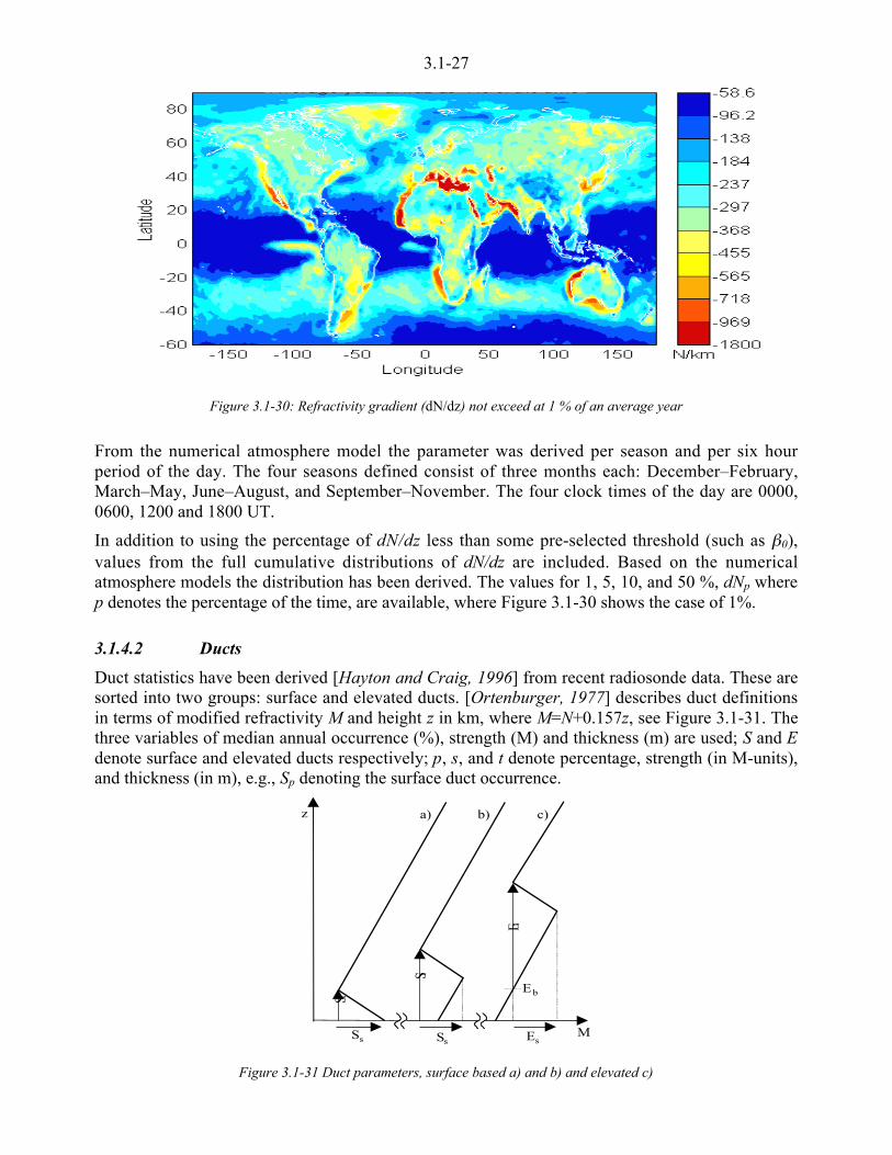
3.1-27

Figure 3.1-30: Refractivity gradient (dN/dz) not exceed at 1 % of an average year

From the numerical atmosphere model the parameter was derived per season and per six hourperiod of the day. The four seasons defined consist of three months each: December–February,March–May, June–August, and September–November. The four clock times of the day are 0000,0600, 1200 and 1800 UT.

In addition to using the percentage of dN/dz less than some pre-selected threshold (such as `0),values from the full cumulative distributions of dN/dz are included. Based on the numericalatmosphere models the distribution has been derived. The values for 1, 5, 10, and 50 %, dNp wherep denotes the percentage of the time, are available, where Figure 3.1-30 shows the case of 1%.

3.1.4.2 Ducts

Duct statistics have been derived [Hayton and Craig, 1996] from recent radiosonde data. These aresorted into two groups: surface and elevated ducts. [Ortenburger, 1977] describes duct definitionsin terms of modified refractivity M and height z in km, where M=N+0.157z, see Figure 3.1-31. Thethree variables of median annual occurrence (%), strength (M) and thickness (m) are used; S and Edenote surface and elevated ducts respectively; p, s, and t denote percentage, strength (in M-units),and thickness (in m), e.g., Sp denoting the surface duct occurrence.

M

z

S t

S t

E t

Ss Ss Es

a) b) c)

Eb

Figure 3.1-31 Duct parameters, surface based a) and b) and elevated c)

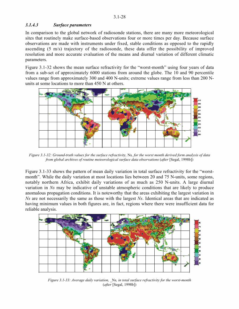
3.1-28

3.1.4.3 Surface parameters

In comparison to the global network of radiosonde stations, there are many more meteorologicalsites that routinely make surface-based observations four or more times per day. Because surfaceobservations are made with instruments under fixed, stable conditions as opposed to the rapidlyascending (5 m/s) trajectory of the radiosonde, these data offer the possibility of improvedresolution and more accurate evaluation of the means and diurnal variation of different climaticparameters.

Figure 3.1-32 shows the mean surface refractivity for the “worst-month” using four years of datafrom a sub-set of approximately 6000 stations from around the globe. The 10 and 90 percentilevalues range from approximately 300 and 400 N-units; extreme values range from less than 200 N-units at some locations to more than 450 N at others.

Figure 3.1-32: Ground-truth values for the surface refractivity, Ns, for the worst month derived form analysis of datafrom global archives of routine meteorological surface data observations (after [Segal, 1998b])

Figure 3.1-33 shows the pattern of mean daily variation in total surface refractivity for the “worst-month”. While the daily variation at most locations lies between 20 and 75 N-units, some regions,notably northern Africa, exhibit daily variations of as much as 250 N-units. A large diurnalvariation in Ns may be indicative of unstable atmospheric conditions that are likely to produceanomalous propagation conditions. It is noteworthy that the areas exhibiting the largest variation inNs are not necessarily the same as those with the largest Ns. Identical areas that are indicated ashaving minimum values in both figures are, in fact, regions where there were insufficient data forreliable analysis.

Figure 3.1-33: Average daily variation, _Ns, in total surface refractivity for the worst-month(after [Segal, 1998b])

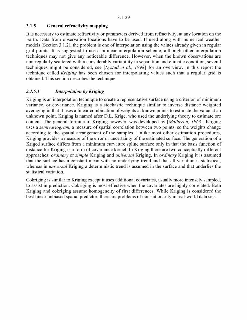
3.1-29

3.1.5 General refractivity mapping

It is necessary to estimate refractivity or parameters derived from refractivity, at any location on theEarth. Data from observation locations have to be used. If used along with numerical weathermodels (Section 3.1.2), the problem is one of interpolation using the values already given in regulargrid points. It is suggested to use a bilinear interpolation scheme, although other interpolationtechniques may not give any noticeable difference. However, when the known observations arenon-regularly scattered with a considerably variability in separation and climatic condition, severaltechniques might be considered, see [Lystad et al., 1998] for an overview. In this report thetechnique called Kriging has been chosen for interpolating values such that a regular grid isobtained. This section describes the technique.

3.1.5.1 Interpolation by Kriging

Kriging is an interpolation technique to create a representative surface using a criterion of minimumvariance, or covariance. Kriging is a stochastic technique similar to inverse distance weightedaveraging in that it uses a linear combination of weights at known points to estimate the value at anunknown point. Kriging is named after D.L. Krige, who used the underlying theory to estimate orecontent. The general formula of Kriging however, was developed by [Matheron, 1963]. Kriginguses a semivariogram, a measure of spatial correlation between two points, so the weights changeaccording to the spatial arrangement of the samples. Unlike most other estimation procedures,Kriging provides a measure of the error or uncertainty of the estimated surface. The generation of aKriged surface differs from a minimum curvature spline surface only in that the basis function ofdistance for Kriging is a form of covariance kernel. In Kriging there are two conceptually differentapproaches: ordinary or simple Kriging and universal Kriging. In ordinary Kriging it is assumedthat the surface has a constant mean with no underlying trend and that all variation is statistical,whereas in universal Kriging a deterministic trend is assumed in the surface and that underlies thestatistical variation.

Cokriging is similar to Kriging except it uses additional covariates, usually more intensely sampled,to assist in prediction. Cokriging is most effective when the covariates are highly correlated. BothKriging and cokriging assume homogeneity of first differences. While Kriging is considered thebest linear unbiased spatial predictor, there are problems of nonstationarity in real-world data sets.

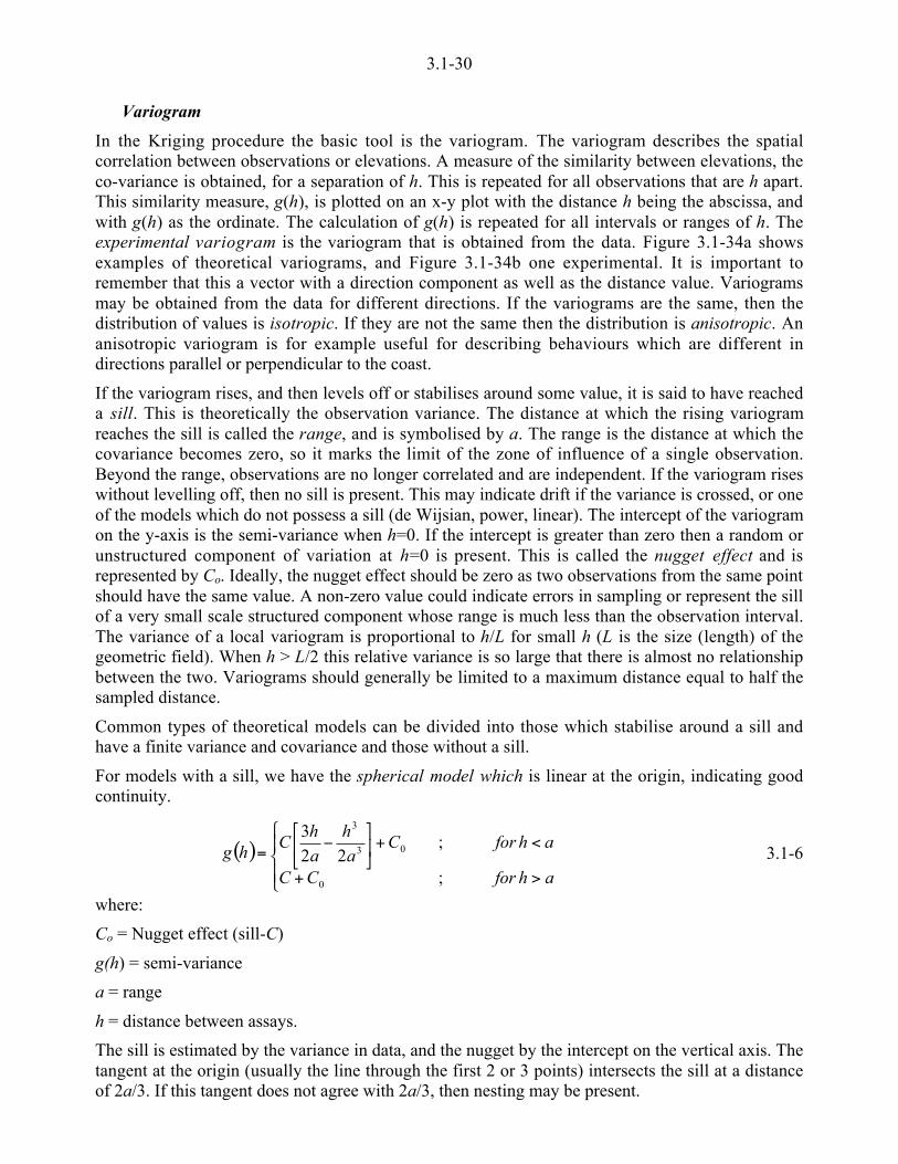
3.1-30

Variogram

In the Kriging procedure the basic tool is the variogram. The variogram describes the spatialcorrelation between observations or elevations. A measure of the similarity between elevations, theco-variance is obtained, for a separation of h. This is repeated for all observations that are h apart.This similarity measure, g(h), is plotted on an x-y plot with the distance h being the abscissa, andwith g(h) as the ordinate. The calculation of g(h) is repeated for all intervals or ranges of h. Theexperimental variogram is the variogram that is obtained from the data. Figure 3.1-34a showsexamples of theoretical variograms, and Figure 3.1-34b one experimental. It is important toremember that this a vector with a direction component as well as the distance value. Variogramsmay be obtained from the data for different directions. If the variograms are the same, then thedistribution of values is isotropic. If they are not the same then the distribution is anisotropic. Ananisotropic variogram is for example useful for describing behaviours which are different indirections parallel or perpendicular to the coast.

If the variogram rises, and then levels off or stabilises around some value, it is said to have reacheda sill. This is theoretically the observation variance. The distance at which the rising variogramreaches the sill is called the range, and is symbolised by a. The range is the distance at which thecovariance becomes zero, so it marks the limit of the zone of influence of a single observation.Beyond the range, observations are no longer correlated and are independent. If the variogram riseswithout levelling off, then no sill is present. This may indicate drift if the variance is crossed, or oneof the models which do not possess a sill (de Wijsian, power, linear). The intercept of the variogramon the y-axis is the semi-variance when h=0. If the intercept is greater than zero then a random orunstructured component of variation at h=0 is present. This is called the nugget effect and isrepresented by Co. Ideally, the nugget effect should be zero as two observations from the same pointshould have the same value. A non-zero value could indicate errors in sampling or represent the sillof a very small scale structured component whose range is much less than the observation interval.The variance of a local variogram is proportional to h/L for small h (L is the size (length) of thegeometric field). When h > L/2 this relative variance is so large that there is almost no relationshipbetween the two. Variograms should generally be limited to a maximum distance equal to half thesampled distance.

Common types of theoretical models can be divided into those which stabilise around a sill andhave a finite variance and covariance and those without a sill.

For models with a sill, we have the spherical model which is linear at the origin, indicating goodcontinuity.

( )ǻ

«©

¨

>+

<+µ�

�³�

�<

=

ahforCC

ahforCa

hah

Chg

;

;22

3

0

03

3

3.1-6

where:

Co = Nugget effect (sill-C)

g(h) = semi-variance

a = range

h = distance between assays.

The sill is estimated by the variance in data, and the nugget by the intercept on the vertical axis. Thetangent at the origin (usually the line through the first 2 or 3 points) intersects the sill at a distanceof 2a/3. If this tangent does not agree with 2a/3, then nesting may be present.

3.1-31

0 5 10 15 20 25 300

0.2

0.4

0.6

0.8

1

Distance

Co-

vari

ance

Gaussian

Exponential

SphericalSill

Nugget Range

a)

0

50

100

150

200

250

0 10 20 30 40 50 60 70 80 90

`0 Semi-variogram

Degrees

b)

Figure 3.1-34: a) Types of theoretical variograms b) Derived from radiosonde data

The exponential model is also linear at the origin, but reaches the sill asymptotically, well beyondthe value of the true range.

g(h) = C [ 1 - exp(-h/a)] + Co 3.1-7

As it is characterised by a gradual approach to the sill, the true range a is one third the value of thepractical range a'. The practical range is the distance at which g(h) approximates the sill. The truerange may also be obtained by the intersection of the tangent at the origin with the sill.

The Gaussian model is parabolic at the origin (indicating perfect continuity) and reaching the sillasymptotically.

g(h) = C [1 - exp(-h2/a2)] + Co 3.1-8

The true range equals 1/33 the value of the practical range. A hole effect shows oscillations ofdecreasing amplitude around the sill. It reflects periodicity in the data and is generally found nestedwith other models.

Of models without a sill we have de Wij's model. It rises to the sill asymptotically, but thevariogram becomes linear when the distance is scaled logarithmically.

g(h) = A ln(h) + B 3.1-9

where A is the slope (equal to 3 times the absolute coefficient of dispersion) and B is related to thedistance between observations and can be used to determine if anisotropy is present. This model isthe theoretical limit of a nested succession of spherical models whose range increasesgeometrically.

The power models are a group of models with the general equation:

g(h) = hn + Co 3.1-10

where: 0 < n < 2

The models show a range of behaviour at the origin as n varies. It should be noted that for smalldistances a linear model (n = 1) can be fitted to any model as there tends to be linear behaviour atand near the origin.

3.1-32

A nested model is one in which two or more theoretical models are combined. Variances arepositive and additive. The total variance is always the sum of all component variances.

The parameters `0 and St are shown in Figures 3.1–35 and 3.1-36, respectively. A sphericalvariogram was used for both with a range of 4000 km and sill of 14 % and 10 m respectively, andno nugget.

Mathematical formulation

Let Z be the parameter to be interpolated at locations x, and let Z0 be observations of the parametergiven at locations xi, such that xi=xni, The values of Z0(xi) may have errors.

Z0(xi) = Z(xi) + ¡0(xi) 3.1-11

where:

the error ¡0(x i) is assumed to be normally distributed with zero mean and variance m20i.

Z consists of a global part M and some arbitrary variation, i.e., Z(x) = M(x) + ¡(x) and from this thedifferent models for Kriging emerge.

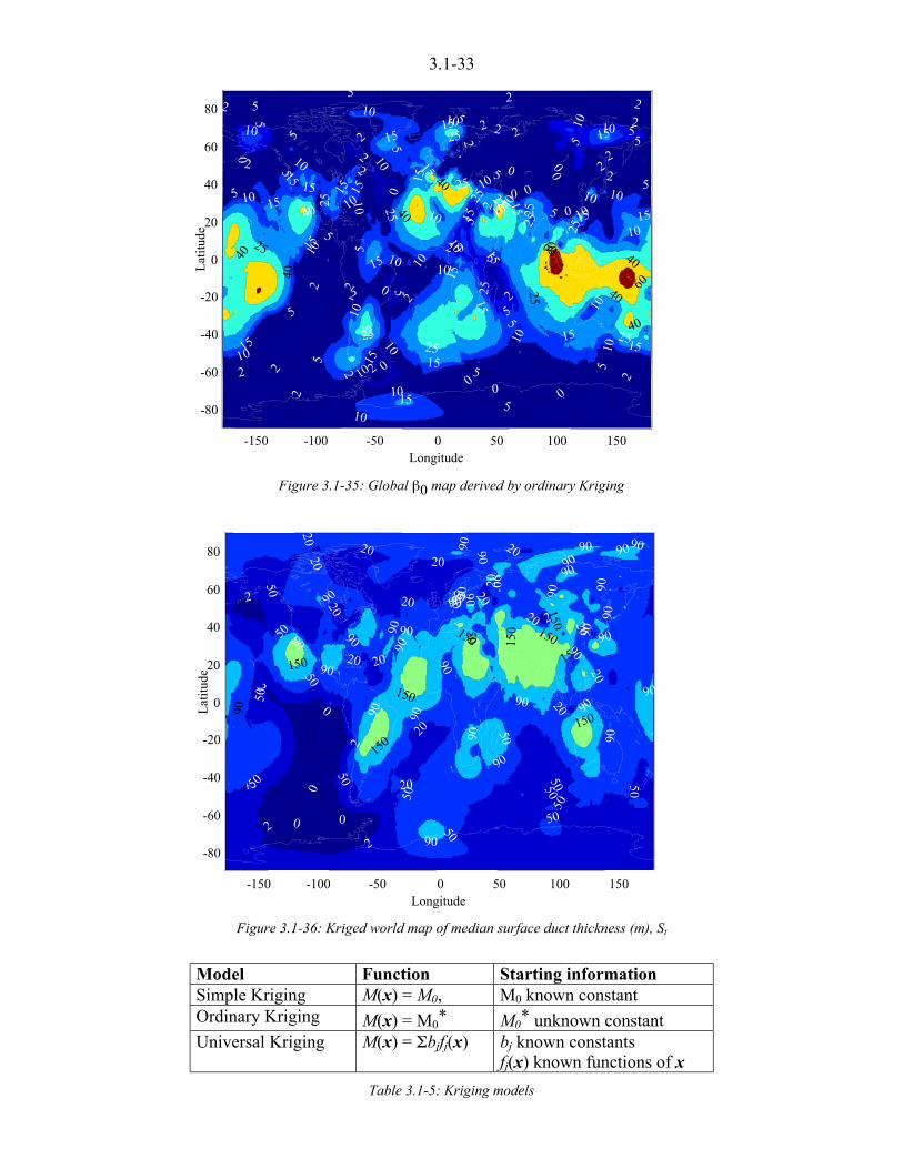
3.1-33

Figure 3.1-35: Global `0 map derived by ordinary Kriging

Figure 3.1-36: Kriged world map of median surface duct thickness (m), St

Model Function Starting informationSimple Kriging M(x) = M0, M0 known constantOrdinary Kriging M(x) = M0

* M0* unknown constant

Universal Kriging M(x) = Ybjfj(x) bj known constantsfj(x) known functions of x

Table 3.1-5: Kriging models

-150 -100 -50 0 50 100 150

-80

-60

-40

-20

0

20

40

60

80

15

5

5

0

22

2 22

2

2

2

22

2

2

2

5

5

55

5

5

5

5

55

5

5

5

5

5

10

1010

1010

10

10

1010

10

1010

1515

15

15

15

15

15

15 1510

10

10

10

10

15

15

15 25

25

25 25

15

15

15

25

40

40 40

10

10

25

2525

2

25

5

5

5

55

5

10

10

15

25

00 0

40

25

25

2 2

5

22

25

2

15

40

2

0

10

40

2

0

40

25

6015

10

60

15

0

15

10

10

10

15

40

10

0

25

40

25

2 15

2

15

00

15

10

00

2

2

2

40 10

10

15

5

2

10

0

5

0

2

Lat

itude

Longitude

-150 -100 -50 0 50 100 150

-80

-60

-40

-20

0

20

40

60

8090

90

2

50

50

50

50

50

50

50

50

50

50

50

50

50

90

90

90

9090

90

90 90

22

2

22

2020

2020

0 0

0

0

150

150 150

90

90

90

90

20

9090

9090

150

150

90

150

90

90

90

20

2

90

150

90

90

20150

90

50

5090

90

90

90

150

20

90

20

20

90

50

90

20

20

90

20

20

90

20

90 90

20

20

Lat

itude

Longitude

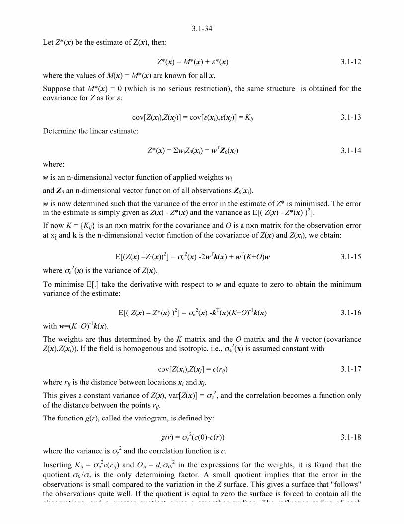
3.1-34

Let Z*(x) be the estimate of Z(x), then:

Z*(x) = M*(x) + ¡*(x) 3.1-12

where the values of M(x) = M*(x) are known for all x.

Suppose that M*(x) = 0 (which is no serious restriction), the same structure is obtained for thecovariance for Z as for ¡:

cov[Z(xi),Z(xj)] = cov[¡(xi),¡(xj)] = Kij 3.1-13

Determine the linear estimate:

Z*(x) = YwiZ0(xi) = wTZ0(xi) 3.1-14

where:

w is an n-dimensional vector function of applied weights wi

and Z0 an n-dimensional vector function of all observations Z0(xi).

w is now determined such that the variance of the error in the estimate of Z* is minimised. The errorin the estimate is simply given as Z(x) - Z*(x) and the variance as E[( Z(x) - Z*(x) )2].

If now K = {Kij} is an n×n matrix for the covariance and O is a n×n matrix for the observation errorat xi and k is the n-dimensional vector function of the covariance of Z(x) and Z(xi), we obtain:

E[(Z(x) –Zu(x))2] = me2(x) -2wTk(x) + wT(K+O)w 3.1-15

where me2(x) is the variance of Z(x).

To minimise E[.] take the derivative with respect to w and equate to zero to obtain the minimumvariance of the estimate:

E[( Z(x) – Z*(x) )2] = me2(x) -kT(x)(K+O)-1k(x) 3.1-16

with w=(K+O)-1k(x).

The weights are thus determined by the K matrix and the O matrix and the k vector (covarianceZ(x),Z(xi)). If the field is homogenous and isotropic, i.e., me

2(x) is assumed constant with

cov[Z(xi),Z(xj] = c(rij) 3.1-17

where rij is the distance between locations xi and xj.

This gives a constant variance of Z(x), var[Z(x)] = me2, and the correlation becomes a function only

of the distance between the points rij.

The function g(r), called the variogram, is defined by:

g(r) = me2(c(0)-c(r)) 3.1-18

where the variance is me2 and the correlation function is c.

Inserting Kij = me2c(rij) and Oij = dijm0i

2 in the expressions for the weights, it is found that thequotient m0i/me is the only determining factor. A small quotient implies that the error in theobservations is small compared to the variation in the Z surface. This gives a surface that "follows"the observations quite well. If the quotient is equal to zero the surface is forced to contain all theobservations and a greater quotient gives a smoother surface The influence radius of each

3.1-35

The minimum variance of the estimate is independent of the observed values, and can be calculatedwhen the configuration of the observations is given and the statistical parameters are specified.Inversion of the K+O matrices is also necessary to compute the weights w. The advantage of thisquantity is that it indicates the uncertainty of the computed values. In areas far away from theobservation locations it is equal to me

2(x) or the variance of Z, and at the observation locations it isequal to m0i

2(x), or the variance of the error in the observations. The variance of the estimate dividedby the variance of Z give a more objective measure for the uncertainty, and can be used to decidewhich areas have observations dense enough to give an interpolation that has any meaning.

3.1.5.2 Interpolation by triangulation

A triangulated global map of the `0 parameter is shown in Figure 3.1-37.

Figure 3.1-37:. Global `0 map derived from a triangulation of the 10-year global radiosonde database.The geometric origins of the procedure are clearly visible in the derived surface

3.1.5.3 Trend analysis

Trends in `0 with variations of geophysical parameters are sought in order to reduce, or eveneliminate, the need for the maps and to replace them with functions of the parameters.

`0 Sp Ss St Ep Es Et SpSs*EpEs

|latitude| 0.53 0.44 0.56 0.44 0.54 0.65 0.70 0.63longitude 0.20 0.34 0.14 0.09 0.35 0.09 0.02 0.33

station height 0.11 0.13 0.13 0.11 0.25 0.01 0.09 0.13distance from coast 0.27 0.30 0.09 0.01 0.46 0.10 0.17 0.36

Table 3.1-6: Initial correlation coefficients

`0 Sp Ss St Ep Es Et SpSs*EpEs

|latitude| 0.00 0.00 0.00 0.00 0.00 0.00 0.00 0.00longitude 0.27 0.41 0.21 0.07 0.46 0.18 0.04 0.48

station height 0.22 0.21 0.06 0.05 0.38 0.12 0.26 0.29distance from coast 0.27 0.30 0.06 0.03 0.51 0.07 0.17 0.40

Table 3.1-7: Residual correlation’s (after removing latitude trend)

From the global map in Figure 3.1–35, it is apparent that there is a correlation between `0 andlatitude, with higher values in the equatorial regions and lower values toward the poles. Table 3.1-6

3.1-36

height and distance from the coast) and outputs (`0, probability of occurrence (%), strength, andthickness of surface and elevated ducts, and a new combined parameter.

It can be seen that |latitude| gives the best correlations, with coefficients of between 0.44 and 0.70for the ducting parameters shown. To be able to see any residual trends more easily, this latitudetrend was then removed from the values, and the residual correlations examined (Table 3.1-7). Theeffects here are generally less marked, and may be related to local mesoscale variations in climaterather than globally quantifiable parameters.

3.1.5.4 Neural modelling

As an alternative to performing multiple residual analyses to parameterise `0 and others, neuralnetworks [Beale and Jackson, 1990] have also been used to predict ducting. Back-propagationneural nets are particularly suited to predicting output values (e.g. `0) when given noisy input data(latitude, longitude, etc.) where no relationship is previously known. A neural net was trained onknown data from a subset of 254 of the radiosonde stations from the 689 available for the 10 yeardataset. Absolute value of latitude, longitude, and station height were given as inputs, and `0 as anoutput.

The equation

log `0 = -0.015 |lat| + 1.67 3.1-19

derived from this approach has been tested in the ITU-R microwave interference predictionprocedure [ITU-R, 1999f] and gives improved results compared to the current, more complex,equations.

It is then possible to use the neural network to produce maps of `0 and other statistics. By doingthis, we can see the influence of all the input parameters on the predicted output, rather than just thetrend with latitude as above. Figure 3.1-38 shows a global map of network predicted `0 values,where the predicted effects of longitude and station height, as well as latitude, can be seen (note inthis monochrome reproduction that values below sea level are not shown, to aid clarity). Furtherverification of predicted values is required however, to ensure sensible operation of the neuralnetwork.

Figure 3.1-38: Global `0 map as predicted by a neural network

3.1-37

3.1.5.5 Atlas

A number of the variables described are given in a numerical atlas (CD-ROM), issued in parallelwith this Final Report. The data formats are described as well. Every parameter is usually availablein a 1.5°x1.5° resolution.

3.1.6 Application examples

In the [ITU-R, 1999a] global prediction method for the multipath fading and enhancementdistribution, variable pL is used. This variable is the highest `0 taken from one the four maps(February, May, August and November) in [ITU-R, 1999c]. Initial analysis [COST 235, 1996] andmore recently [Tjelta et al., 1998], showed that the variables derived from the global radiosondedata [Craig and Hayton, 1995], should be used in revised prediction methods. These are: therecalculated `0, the refractive gradient at a chosen percentage of the worst season, or annual medianduct characteristics (e.g. thickness).

The prediction method in [ITU-R, 1999f] made use of `0 and the refractivity gradient, 6N, in thefirst kilometre above ground to estimate the interference caused by clear-air phenomena. In the lastversion (P.452-9), the `0 variable has been given by a simple linear model of latitude rather thantaken from the map. The refractivity at the surface, Ns, along with climate classification is used inprediction of troposcatter. The revised new values [Hayton and Craig, 1996, Segal, 1998a] canpossibly be used, but it would be necessary to refine the methods using the new variables. [Olsenand Tjelta 1997] describe how LOS data can be used to derive longitudinal and latitudinaldependent correction factors for the climate variables.

Observed fading on extremely low-elevation satellite links suggested similar mechanisms as seenon terrestrial (horizontal) links. However, the lack of data made it difficult to derive a predictionmethod. By combining the information derived from LOS links [Olsen, 1995] made use of pL topredict the low-elevation fading distribution. The prediction method for low-elevation clear-airfading distribution is adopted in [ITU-R, 1999b]. The wet term of the refractivity, Nw, is used inprediction of scintillation on satellite links. Updated maps of the climate variables along withrefined methods would presumably improve prediction accuracy.

3.1-38

3.1.7 References

[Beale and Jackson, 1990]Beale, R. and T. Jackson, “Neural Computing: an introduction,” Adam Hilger Publishing, UK,1990.

[Bean et al., 1966]Bean, B.R., B.A. Cahoon, C.A. Samson and G.D. Thayer, 1966, "A world atlas of radiorefractivity," Monograph 1, U.S. Department of Commerce, Washington, USA.

[COST 235, 1996]COST Project 235, 1996, "Radiowave propagation effects on next-generation fixed-servicesterrestrial telecommunication systems", Final Report, Office for official publications of theEuropean Community, Luxembourg.

[Craig and Hayton, 1995]Craig, K.H. and T.G. Hayton, Climatic mapping of refractivity parameters from radiosonde data, inNATO/AGARD Conf. Proc. CP-567, North Atlantic Treaty Organization, Paris, France, pp. 43.1-12,1995.

[Hayton and Craig, 1996]Hayton, T.G. and K.H. Craig, “Mapping of radiosonde-derived clear air climatic parameters”, URSIClimpara 96 conference, Oslo, 1996.

[Ikegami, 1959]Ikegami, F., “Influence of an atmospheric duct on microwave fading”, IRE Trans. Ant. Prop., AP-7(3), pp. 252-257, 1959.

[Ikegami, et al., 1968]Ikegami, F., T. Akiyama, S. Aoyagi, and H. Yoshida, “Variations of radio refraction in the loweratmosphere”, IEEE Trans. Ant. Prop., AP-16 (2), pp. 194-200, 1968.

[ITU-R, 1999a]ITU-R, “Propagation data and prediction methods for the design of terrestrial line-of-sightsystems”, Rec. P.530-8, International Telecommunication Union, Geneva, 1999.

[ITU-R, 1999b]ITU-R, “Propagation data and prediction methods for the design of Earth-space telecommunicationsystems”, Rec. P.618-6, International Telecommunication Union, Geneva, 1999.

[ITU-R, 1999c]ITU-R, “The radio refractive index: its formula and refractivity data", Rec. P.453-7, InternationalTelecommunication Union, Geneva, 1999.

[ITU-R, 1999d]ITU-R, “Effects of tropospheric refraction on radiowave propagation”, Rec. P.834-3, InternationalTelecommunication Union, Geneva, 1999.

[ITU-R, 1999e]ITU-R, "Reference standard atmospheres," Rec. P.835-3, International Telecommunication Union,Geneva, 1999.

[ITU-R, 1999f]ITU-R, “Prediction procedure for the evaluation of microwave interference between stations on thesurface of the Earth at frequencies above about 0.7 GHz,” Rec. P 452-8, InternationalTelecommunication Union, Geneva, 1999.

3.1-39

[v.d. Kamp et al, 1997]Kamp, M. van de, J. Tervonen, E. Salonen, and K. Kalliola, "Study of low elevation anglescintillation modelling," Final Report, ESTEC Contract No. 10827/94/NL/NB(SC), 1997.

[Levy and Craig, 1996]Levy, M.F., and K.H. Craig, "TERPEM propagation package for operational forecasting withEEMS," Battlespace Atmospherics Conference (BAC ’96), San Diego, 1996.

[Lystad et al., 1998]Lystad, S., T.G. Hayton, A.K. Marsh, and T. Tjelta, "Interpolation of clear-air parameters observedat non-regular observation locations," Proceedings URSI Comm. F Symposium, Climpara’98,Ottawa, Canada, pp. 15-26, 1998.

[Matheron, 1963]Matheron, G., “Principles of geostatistics,” Economic Geology, 58, pp.1246-1266, 1963.

[Olsen, 1995]Olsen, R.L., "Summary of worldwide procedures for the prediction of clear-air fading distributionson very-low-angle satellite links," in Proc. of the Seventh URSI Comm. F Int. Triennial Open Symp.on 'Wave Propagation and Remote Sensing', Ahmedabad, India,pp. 115-118, 1995.

[Olsen and Tjelta 1997]Olsen, R.L. and T. Tjelta, “Application of global geo-climatic information from multi-path fadingon terrestrial L-O-S links to other clear-air propagation effects,” in Proc. of ISRP’97, Qingdao,China, pp. 39-46, 1997.

[Ortenburger, 1977]Ortenburger, L.N., "Radiosonde Data Analysis II," GTE/Sylvania Incorporated, 1977.

[Ortenburger and Lawson, 1985]Ortenburger, L.N., and S.B. Lawson, “Radiosonde Data Analysis,” GTE Government SystemsCorp., Mountain View, USA, 1985.

[Samson, 1975]Samson, C.A., “Refractivity gradients in the Northern hemisphere,” Report OT-75-59,US Dept. of Commerce, 1975.

[Samson, 1976]Samson, C.A., “Refractivity and rainfall data for radio systems engineering,” Report OT-76-105,US Dept. of Commerce, 1976.

[Segal, 1996]Segal, B., “Surface-based meteorological parameters for use in global modelling of clear-airmicrowave fading characteristics,” Proceedings URSI Comm. F Symposium, Climpara’96, Oslo,Norway, pp. 10-11, 1996.

[Segal, 1998a]Segal, B., “Multipath propagation mechanisms deduced from tower-based meteorologicalmeasurements,” Proceedings of First international workshop on radiowave propagation modellingfor SatCom services at Ku-band and above, ESTEC, Noordwijk, 1998.

[Segal, 1998b]Segal, B., “Mapping of surface meteorological variables,” Proceedings URSI Comm. FSymposium, Climpara’98, Ottawa, Canada, pp. 9-14, 1998.

[Segal and Barrington, 1977]Segal, B., and R.A. Barrington, 1977, “Tropospheric refractivity atlas for Canada,”C i i R h C R CRC 1315

3.1-40

[Sokol and Stekl, 1994]Sokol, Z. and J. Stekl, "3-D mesoscale Objective Analysis of selected elements from SYNOP andSYRED reports," Meteorol. Z., 1994, N.F.3, H.4, pp. 242-246, 1994.

[Tjelta and Poiares Baptista, 1999]Tjelta, T. and Poiares Baptista, J.P.V., ”Climatic parameters in propagation prediction”, in Reviewof Radio Science, URSI, Oxford University Press, New York, pp. 459-469, 1999.

[Tjelta et al, 1998]Tjelta, T., T.G. Hayton, B. Segal, and E. Salonen, “Correlation of observed multipath occurrencewith climatic parameters derived from radiosondes, surface stations, and numerical atmospheremodels,” In Proc. of URSI Comm. F Symp. CLIMPARA’98, Ottawa, Canada, pp. 85-92, 1998.

[Webster, 1982]Webster, A.R., “Raypath parameters in tropospheric multipath propagation”, IEEE Trans. Ant.Prop., AP-30 (4), pp. 796-800, 1982.

[Webster, 1997]Webster, A.R., “Extended observations of fading on a terrestrial microwave link”, Radio Science,32 (1), pp. 231-238, 1997.

[Webster and Scott, 1987]Webster, A.R., A.M. Scott, “Angles-of-arrival and tropospheric multipath microwave propagation”,IEEE Trans. Ant. Prop., AP-35 (1), pp. 94-99, 1987.

3.2-1

CHAPTER 3.2Precipitation, Clouds

and Other RelatedNon-Refractive Parameters

Editor: J.P.V. Poiares Baptista1

Authors: A. Benarroch2, M. Boumis3, L. Castanet4, J.C. Coma2, O. Fiser5, T. Konefal6,V. Kvicera7, A. Martellucci8, D. Rezacova9, E.T. Salonen10, P.A. Watson11,

1 European Space Agency, ESA-ESTEC, Kepleerlan 1, PB 299, NL-2200 AG Noordwijk, The NetherlandsTel.: +31-71-5654319, Fax.: +31-71-5654999, e-mail: pedro@xe.estec.esa.nl

2 Universidad Politecnica de Madrid, ETSIT, Ciudad Universitaria, E-28040 Madrid, SpainTel: +34-1 3367218, Fax: +34-1-3377350, e-mail: ana@grc.ssr.upm.es

3 Fondazione Ugo Bordoni,Radiocommunications Dept., Viale Europa 190, I-00144 Rome, ItalyTel: +39-6-5480-2119, Fax: +39-6-5480-4401, e-mail: mboumis@fub.it

4 ONERA-CERT DEMR, 2 Avenue Edouard Belin, BP4025, F-31055 Toulouse, CEDEX 4, FranceTel: +33-562-25-2729, Fax: +33-562-25-2577, e-mail: laurent.castanet@onecert.fr

5 Institute of Atmospheric Physics of the Czech Academy, Bocni street II/1401, 141 31 Praha 4, Czech RepublicTel.: +420-2-769702ext.108, Fax: +420-2-72763745, e-mail: ondrej@ufa.cas.cz

6 University of York, Dept of Electronics, Heslington, York YO10 5DD, United KingdomTel: +44-1904-432383, Fax: +44-1904-433224, e-mail: tk@ohm.york.ac.uk

7 TESTCOM, Telecommunications Transmission Dpt., Hvozdanska 3, CZ-14801 Praha 4, Czech RepublicTel: +420-2-799-2225, Fax: +420-2-793-4588, e-mail: kvicera@testcom.cz

8 European Space Agency, ESA-ESTEC, Kepleerlan 1, PB 299, NL-2200 AG Noordwijk, The NetherlandsTel: +31-71-565-5603, Fax: +31-71-565-4999, e-mail: Antonio.Martellucci@esa.int

9 Institute of Atmospheric Physics of the Czech Academy, Bocni street II/1401, 141 31 Praha 4, Czech RepublicTel: +420-2-769702, Fax: +420-2-763745, e-mail: rez@ufa.cas.cz

10 University of Oulu Telecommunication Lab. P.O.Box 444 FIN-90571 Oulu FinlandTel: +358 40 524 2406, Fax: +358-8-553 2845 e-mail: Erkki.Salonen@ee.oulu.fi

11 Electronic and Electrical Engineer, University of Bath, Claverton Down,, BATH BA2 7AY, United Kingdom

3.2-2

3.2 Precipitation, Clouds and Other Related Non-Refractive Parameters

This chapter describes models and databases of the climatogical parameters relevant for theestimation of propagation parameters, with particular regard to atmospheric attenuation. Theparameters represent the input to the propagation models described in Part 2.

The chapter has been divided into three main sections.

In the first section the analysis of data collected in specific sites is presented and it comprises both aworld-wide database of meteorological parameters, such as the vertical profile water vapourdensity, and an extensive analysis of long-term rainfall rates statistics in Spain and in the Czechrepublic, that describes accurately both the climatic and temporal variability of rainfalls.

In the second section current models and data for global mapping of rainfall rate are illustrated byshowing the exploitation of the global meteorological databases that have been made available byweather forecast agencies and climate studies.

In the last section of this chapter some models are illustrated for the assessment of monthly statisticsof parameters such as the water vapour density, the cloud liquid content and the rainfall rate.

3.2.1 Single Site Characterisation

3.2.1.1 The FUB/ESA propagation oriented meteorological database

Meteorological data regarding both upper air and surface meteorological measurements wereacquired by Fondazione Ugo Bordoni (FUB) from NCAR (Boulder, USA), under an ESA/ESTECresearch Contract [Barbaliscia et al., 1944; 1995, Boumis, 1994].

The meteorological information is contained in an extensive Data Base, named FERAS (FUB andESA RAdiosonde and Surface), covering all the regions of the world (about 1600 sites) for 10 years(1980 - 1989). The upper air soundings are limited to the standard synoptic times 0.00 and 12.00Universal Time Coordinate (UTC), and include the data of pressure [hPa], temperature [ºC] andrelative humidity [%], describing the atmospheric vertical profiles.

They were classified as "rainy" or "not rainy", according to the meteorological conditions at thelaunch time as specified by the information contained in the concurrent surface data. "Rainy" and"not rainy" soundings were identified and separated.

The corresponding ground observations, referred to the standard synoptic times, are measured everythree hours starting from 0.00 UTC, for a total of 8 observations a day.

In particular, the ground observations are relative to: pressure [hPa]; wind direction [deg]; windspeed [knots]; air temperature [ºC]; dewpoint depression [ºC]; horizontal visibility; present weather;past weather; cloud coverage and cloud type.

In order to furnish very reliable and proper data for propagation studies, a subset of 354 locationswas selected from the FERAS data base and stored in two new databases named DST.MET (upperair data) and DST.SRF (surface data). The basic criteria applied for the selection of the locationswere the following:

• geographical and climatological coverage;

• availability of radiosonde launches;

• availability of concurrent surface data;

• reliability of data for processing purposes.

Th d lid i f d b f d bl i d b d b h h

3.2-3

consistency of the measurements. The checks were carried out on all measured data, both for theupper air and for the surface observations. It is important to underline that the data validation isneeded to solve some basic difficulties of dealing with the meteorological parameters measuredwith the radiosonde.

In particular:

1. the radiosondes are usually launched up to only four times a day at the standard synoptictimes and since the recorded data have to be incorporated in the World Weather Watch, theyare launched at the same UTC, consequently particular attention must be paid to thecomparison between data measured at different stations.

2. the radiosonde measurements are not always reliable and particular care must be taken in thechecking of the erroneous data.

3. the measuring devices can be different depending on the period and the station, leading todifferences of the experimental accuracy.

After the submission of the data to the preprocessing and validation procedures, 15% of data werelost even for the best quality stations (Europe and USA) and as much as 50% in the worst cases.

The information contained in the first level of the radiosonde profile was considered representativeof the actual meteorological ground conditions. When the first level of the radiosonde profile wasfound to contain unreliable information, the ground measurements were replaced by thecorresponding surface data.

Moreover, additional parameters of importance for propagation studies were computed and added tothe meteorological upper air data, in particular the profiles of water vapour density [g/m3], liquidwater density [g/m3], ice density [g/m3] and the profile of the air refractivity frequency independentterm [ppm].

The liquid water density was calculated making use of the estimation algorithm developed by[Salonen et al., 1990]. This is described later.

The non-dispersive term of air refractivity was computed according to [ITU-R, 2000a]:

251073.36.77

T

eTP

N uu+u= [ppm] 3.2-1

where:

P = atmospheric pressure [hPa]

T = absolute temperature [K]

e = water vapour pressure [hPa]

Examples of DST.MET and DST.SRF contents are given in Tables 3.2-1 and 3.2-2.

In addition, for a simpler climatic characterisation of the locations and for a faster evaluation of thepropagation parameters, for each location the mean monthly profiles of pressure, temperature andrelative humidity were computed as well and stored in a dataset named DST.STD, maintaining theseparation between observations at 00.00 and 12.00 UTC. The vertical resolution of the meanprofiles is 500 m up to the maximum height of 16 km from the ground.

These standard mean monthly profiles have been adopted by ITU-R as reference standardatmospheres [ITU-R, 1999].

3.2-4

yymmddhh Nlevels89 1 712 45

Press [hPa] Height[km]

Temp [K] Rel. Hum [0-1] Liq. g/m3] Ice [g/m3] N0 [ppm]

1006.000 0.17 280.16 0.960E+00 0.000E+00 0.000E+00 0.324E+031003.000 0.19 279.96 0.960E+00 0.000E+00 0.000E+00 0.323E+031000.000 0.22 279.76 0.959E+00 0.128E-05 0.000E+00 0.322E+03

985.000 0.34 279.02 0.964E+00 0.124E-01 0.000E+00 0.317E+03970.000 0.46 278.28 0.969E+00 0.222E-01 0.000E+00 0.312E+03955.000 0.59 277.52 0.973E+00 0.335E-01 0.000E+00 0.306E+03940.000 0.72 276.75 0.978E+00 0.454E-01 0.000E+00 0.301E+03925.000 0.85 275.96 0.983E+00 0.577E-01 0.000E+00 0.296E+03910.000 0.98 275.17 0.988E+00 0.701E-01 0.000E+00 0.291E+03895.000 1.11 274.36 0.993E+00 0.827E-01 0.000E+00 0.286E+03884.333 1.21 274.76 0.995E+00 0.960E-01 0.000E+00 0.283E+03873.667 1.31 275.16 0.998E+00 0.110E+00 0.000E+00 0.281E+03863.000 1.40 275.56 0.100E+01 0.120E+00 0.000E+00 0.279E+03858.696 1.45 275.76 0.950E+00 0.127E+00 0.000E+00 0.276E+03854.414 1.49 275.96 0.900E+00 0.133E+00 0.000E+00 0.273E+03850.000 1.53 276.16 0.848E+00 0.137E+00 0.000E+00 0.270E+03849.000 1.54 276.16 0.842E+00 0.333E-01 0.000E+00 0.270E+03829.000 1.74 274.88 0.609E+00 0.000E+00 0.000E+00 0.255E+03809.000 1.93 273.56 0.370E+00 0.000E+00 0.000E+00 0.241E+03794.500 2.08 274.06 0.548E+00 0.000E+00 0.000E+00 0.243E+03780.000 2.22 274.56 0.730E+00 0.000E+00 0.000E+00 0.245E+03762.000 2.41 275.36 0.695E+00 0.000E+00 0.000E+00 0.239E+03734.500 2.71 274.38 0.623E+00 0.000E+00 0.000E+00 0.228E+03707.000 3.01 273.36 0.549E+00 0.000E+00 0.000E+00 0.218E+03700.000 3.10 272.86 0.547E+00 0.000E+00 0.000E+00 0.215E+03678.000 3.35 271.48 0.486E+00 0.000E+00 0.000E+00 0.207E+03656.000 3.61 270.06 0.423E+00 0.000E+00 0.000E+00 0.199E+03626.500 3.97 268.01 0.454E+00 0.000E+00 0.000E+00 0.191E+03597.000 4.35 265.86 0.486E+00 0.109E-05 0.865E-06 0.183E+03587.000 4.48 264.26 0.739E+00 0.184E+00 0.191E+00 0.185E+03573.000 4.67 261.66 0.790E+00 0.140E+00 0.211E+00 0.181E+03556.000 4.90 260.66 0.843E+00 0.372E-01 0.652E-01 0.176E+03524.000 5.35 259.06 0.465E+00 0.000E+00 0.000E+00 0.162E+03500.000 5.71 256.06 0.545E+00 0.000E+00 0.000E+00 0.157E+03448.000 6.52 249.26 0.695E+00 0.000E+00 0.000E+00 0.143E+03418.000 7.02 244.86 0.622E+00 0.000E+00 0.000E+00 0.135E+03400.000 7.34 242.66 0.557E+00 0.000E+00 0.000E+00 0.130E+03333.000 8.62 233.26 0.377E+00 0.000E+00 0.000E+00 0.111E+03309.000 9.12 228.46 0.000E+00 0.000E+00 0.000E+00 0.105E+03250.000 10.51 218.66 0.000E+00 0.000E+00 0.000E+00 0.887E+02200.000 11.90 208.26 0.000E+00 0.000E+00 0.000E+00 0.745E+02150.000 13.67 213.06 0.000E+00 0.000E+00 0.000E+00 0.546E+02125.000 14.81 211.66 0.000E+00 0.000E+00 0.000E+00 0.458E+02117.000 15.22 214.66 0.000E+00 0.000E+00 0.000E+00 0.423E+02100.000 16.20 213.46 0.000E+00 0.000E+00 0.000E+00 0.364E+02

Table 3.2-1: Data base DST.MET: atmospheric vertical profiles of pressure, height, temperature, relative humidity,liquid water density, ice density and radio refractivity (non dispersive term). The header record of each profile

indicates the year (yy=1981), month (mm=2), day of the month (dd=10), the launch time (hh=12)and the total numbers of profile levels (nlevels).

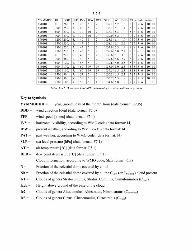
3.2-5

YYMMDD HH DDD FFF IVV IPW IWL SLP AT DPD Cloud Information890101 0 260. 3. 20 5 2 1039.1 6.2 1.6 8 8 5 6 10 10890101 300 250. 3. 40 5 2 1038.7 6.1 1.4 8 8 5 6 10 10890101 600 230. 2. 30 10 2 1038.3 5.3 .7 8 8 5 6 10 10890101 900 230. 2. 30 10 2 1039.0 5.2 .7 7 7 5 6 10 10890101 1200 210. 5. 40 5 2 1038.8 6.1 1.9 7 7 5 6 10 10890101 1500 250. 6. 45 5 2 1038.1 6.1 2.6 7 7 5 6 10 10890101 1800 220. 2. 45 5 2 1037.9 5.3 1.9 8 8 5 6 10 10890101 2100 220. 2. 45 5 2 1038.6 5.0 2.2 8 5 6 10 10 10890102 0 220. 5. 45 5 2 1038.6 5.1 3.5 8 8 5 6 10 10890102 300 360. 0. 40 5 2 1037.6 4.6 2.7 8 8 5 6 10 10890102 600 120. 2. 56 5 2 1037.6 5.0 2.5 8 8 5 6 10 10890102 900 170. 2. 60 99 99 1038.0 5.0 2.5 8 8 5 6 10 10890102 1200 110. 5. 60 99 99 1037.5 6.5 2.3 8 8 5 6 10 10890102 1500 90. 7. 57 5 2 1036.3 6.5 2.3 7 7 5 5 10 10890102 1800 90. 8. 50 5 2 1035.7 6.5 1.8 8 8 5 5 10 10890102 2100 100. 9. 50 5 1 1034.6 6.0 1.9 2 2 5 6 0 0

Table 3.2-2: Data base DST.SRF: meteorological observations at ground.

Key to Symbols

YYMMDDHH = year, ,month, day of the month, hour (data format: 3I2,I5)

DDD = wind direction [deg] (data format: F5.0)

FFF = wind speed [knots] (data format: F5.0)

IVV = horizontal visibility, according to WMO code (data format: I4)

IPW = present weather, according to WMO code, (data format: I4)

IW1 = past weather, according to WMO code, (data format: I4)

SLP = sea level pressure [hPa] (data format: F7.1)

AT = air temperature [°C] (data format: F5.1)

DPD = dew point depressure [°C] (data format: F5.1)

Cloud Information, according to WMO code, (data format: 6I3)

N = Fraction of the celestial dome covered by cloud

Nh = Fraction of the celestial dome covered by all the CLow (or CMedium) cloud present

Ic1 = Clouds of genera Stratocumulus, Stratus, Cumulus, Cumulonimbus (CLow)

Izcb = Height above ground of the base of the cloud

Ic2 = Clouds of genera Altocumulus, Altostratus, Nimbostratus (CMedium)

Ic3 = Clouds of genera Cirrus, Cirrocumulus, Cirrostratus (CHigh)

3.2-6

Columnar water vapour, cloud liquid water and ice content from radiosonde data

In the following detailed information about the calculation of columnar water vapour, cloud liquidwater and ice content is discussed.

The calculations have been performed assuming zenith-viewing paths.

Columnar water vapour content (WVC)

The mass of water vapour in a vertical column of unit cross sectional area from the surface toaltitude z is called "the columnar vapour", sometimes called "precipitable water" as defined by[Rogers and 1989; Mc Ilveen, 1991].

Consider a vertical column of moist air, with air density l [kg m-3] and specific humidity q [gkg-1]The mass m of of water vapour in a slice of depth (z2 - z1) and unit horizontal area is given by:

( )12 zzqm <= l [g] 3.2-2

This equation, according to the hydrostatic equation, ( ) ( )1212 zzgPP <=< l , can be rewritten as:

( )12 PPg

qm <= [g] 3.2-3

where:

g is the gravity acceleration [ms-2]

p1 and p2 [hPa] are the air pressure at the base and top of the slice respectively.

The water vapour density, lv, in the layer is:

( )( )( )12

12

12 zz

PP

g

q

zz

mv <

<=

<=l [g m-3] 3.2-4

If this vapour were to be precipitated into a raingauge at the foot of the column, it would yield alayer of water with a depth h:

w

mh

l= [mm] or [kg m-2] 3.2-5

where

lw [kg m-3] is the density of the precipitated water.

It follows that:

( )w

PP

g

qh

l12 <= [mm] or [kg m-2] 3.2-6

The term in square brackets can be readily calculated for any slice of an upper air sounding inwhich humidity is reported, and the columnar water vapour content, WVC, is calculated by addingthe contributions from all atmospheric layers containing water vapour.

An example of the cumulative distribution functions of WVC for two locations with differentclimate is shown in Figure 3.2-1. This parameter is also characterised by a seasonal and diurnalvariation, as shown in Figure 3.2-2.

3.2-7

1

10

100

0 5 10 15 20 25 30 35

Perc

enta

ge o

f th

e Y

ear

Exceeded Columnar Water Vapour Content [mm]

STORNOWAY, UK Lat=58.13 deg, Lon=-7 deg, Asl=14 m

Radiosonde Data 1980-1989

1

10

100

0 10 20 30 40 50 60 70

Perc

enta

ge o

f th

e Y

ear

Exceeded Columnar Water Vapour Content [mm]

SINGAPORE, SR Lat=1.22 deg, Lon=103.59 deg, Asl=14 m

Radiosonde Data 1980-1989

Figure 3.2-1: Cumulative Distribution Function of the Columnar Water Vapour Content [mm], radiosonde data from DST:MET, two different locations

Figure 3.2-2: Seasonal and diurnal variation of Columnar Water Vapour content, measured by radiosonde

Calculation of the water vapour content by means of the vapour scale height

It is also possible to estimate the total water vapour content, V, making use of the water vapourdensity at ground, lV(z0), and assuming that the water vapour density along the vertical isdistributed exponentially with a vapour scale height, hV. The water vapour scale height can bedetermined by means of exponential least square fitting of the vertical profile of water vapourdensity, as measured by the radiosonde.

According to this model the total water vapour content can be estimated using the followingequation:

( )0zhV VV lu= [mm] 3.2-7

where:

lV(z0) = water vapour density at ground [kg/m3].

0

5

10

15

20

25

30

35

40

45

50

Jan Feb Mar Apr May Jun Jul Aug Sep Oct Nov Dec

Wat

er V

apou

r C

onte

nt [

mm

]

Month

Pomezia, Italy, Radiosonde Data, 1987-1994

Decile 10Decile 50Decile 90

Mean value

3.2-8

In order to assess the water vapour scale height in various climates, a reduced database has beencreated of radiosonde measurements containing 24 sites, selected according to data quality andavailability. The stations contained in this test database are listed in Table 3.2-3 and sortedaccording to the latitude belt. The radiosonde data have been collected in absence of rain. Thelatitude belts are :

PB = Polar-Boreal Belt. Absolute latitude values contained in range: 60..90 (deg).

T = Temperate Belt. Absolute latitude values contained in range: 40..60 (deg).

ST = Subtropical Belt. Absolute latitude values contained in range: 25..40 (deg).

TR = Tropical Belt Absolute latitude values contained in range: 0..25 (deg).

The water vapour scale height has been determined, using exponential least squares fitting, for eachradiosonde launch. In order to assess the validity of the exponential model the correlationcoefficient of the least squares fitting, that ranges from 0 to 1 and indicates better agreement whennearest to 1, can be used. The data corresponding to values lower than 0.2, that were only a smallfraction of the total number of samples and in general denote conditions of thermal inversions of theatmosphere, have been removed from the database.

The correlation coefficient of the fitting of the exponential model had an average value of about0.89 with a standard deviation of 0.114, confirming the applicability of the model. The statistics ofthe correlation coefficient, conditioned to the total water vapour content, given in Figure 3.2-3,demonstrate that the exponential model shows a better agreement with actual profiles in thepresence of higher values of the vapour content, and hence of higher attenuation values.

The values of the mean and of the r.m.s. of the water vapour scale height of the exponential model,for each station of the test database, are given in Table 3.2-3. The stations located in the polar-boreal, temperate and subtropical belts exhibit similar statistical parameters, with a average valuesthat range from 1.7 up to 2 km, with the exception of Denver and Cape Town that are to beconsidered as particular cases and will excluded by the following analysis. In general the stationslocated in tropical belt are characterised by an average value of more than 2.4 km, apart fromLihue-on-Kauai that will not be included in the following.

This statistical difference between the climatic belts is clearly evident also in the cumulativedistribution function of the water vapour scale height, given in Figure 3.2-4, that indicates aregional difference, between the different geographical region, of about 500 m over a large range ofprobability levels. As a preliminary result of this analysis of the water vapour scale height thevalues contained in Table 3.2-4 can in general be used.

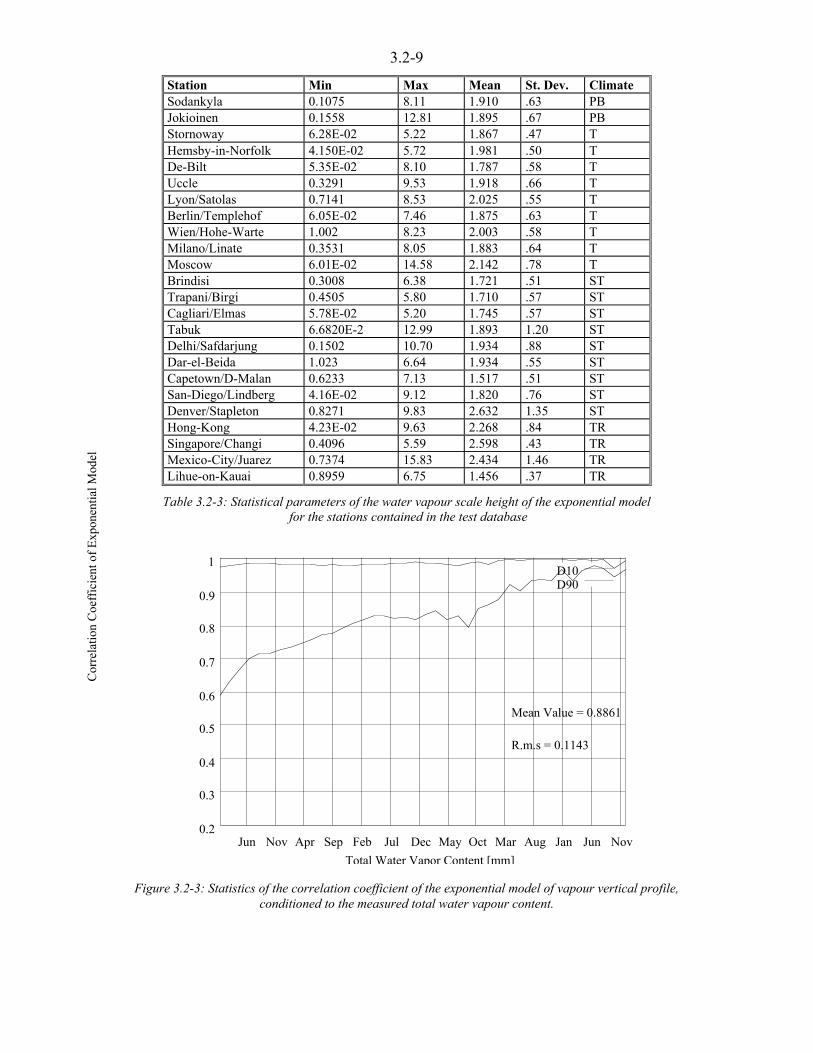
3.2-9

Station Min Max Mean St. Dev. ClimateSodankyla 0.1075 8.11 1.910 .63 PBJokioinen 0.1558 12.81 1.895 .67 PBStornoway 6.28E-02 5.22 1.867 .47 THemsby-in-Norfolk 4.150E-02 5.72 1.981 .50 TDe-Bilt 5.35E-02 8.10 1.787 .58 TUccle 0.3291 9.53 1.918 .66 TLyon/Satolas 0.7141 8.53 2.025 .55 TBerlin/Templehof 6.05E-02 7.46 1.875 .63 TWien/Hohe-Warte 1.002 8.23 2.003 .58 TMilano/Linate 0.3531 8.05 1.883 .64 TMoscow 6.01E-02 14.58 2.142 .78 TBrindisi 0.3008 6.38 1.721 .51 STTrapani/Birgi 0.4505 5.80 1.710 .57 STCagliari/Elmas 5.78E-02 5.20 1.745 .57 STTabuk 6.6820E-2 12.99 1.893 1.20 STDelhi/Safdarjung 0.1502 10.70 1.934 .88 STDar-el-Beida 1.023 6.64 1.934 .55 STCapetown/D-Malan 0.6233 7.13 1.517 .51 STSan-Diego/Lindberg 4.16E-02 9.12 1.820 .76 STDenver/Stapleton 0.8271 9.83 2.632 1.35 STHong-Kong 4.23E-02 9.63 2.268 .84 TRSingapore/Changi 0.4096 5.59 2.598 .43 TRMexico-City/Juarez 0.7374 15.83 2.434 1.46 TRLihue-on-Kauai 0.8959 6.75 1.456 .37 TR

Table 3.2-3: Statistical parameters of the water vapour scale height of the exponential model for the stations contained in the test database

0.2

0.3

0.4

0.5

0.6

0.7

0.8

0.9

1

Jun Nov Apr Sep Feb Jul Dec May Oct Mar Aug Jan Jun Nov

Cor

rela

tion

Coe

ffic

ient

of

Exp

onen

tial M

odel

Total Water Vapor Content [mm]

Mean Value = 0.8861

R.m.s = 0.1143

D10D90

Figure 3.2-3: Statistics of the correlation coefficient of the exponential model of vapour vertical profile,conditioned to the measured total water vapour content.

3.2-10

Climate Water Vapour Scale Height[km]

Polar-Boreal 1.9Temperate 1.9Sub Tropical 1.9Tropical 2.4

Table 3.2-4: Average values of the water vapour scale height for different climates

1

10

100

0 1 2 3 4 5 6

Perc

enta

ge o

f Sa

mpl

es

Water Vapour Scale Height [km], Exponential Model

Tropical BeltPol+Temp+SubTr

Figure 3.2-4: Cumulative distribution function of the vapour scale height,calculated using the test database and classified according to the climate.

Columnar Liquid and Solid Water Content (LWC and IWC): Salonen Model

The calculation of the columnar liquid water content of clouds from radiosonde measurements isbased on the model proposed by [Salonen et al., 1990].

The cloud detection is performed using the "critical humidity" function defined as follows:

( ) ( ) ( )[ ]5.0111 <+<<= m`m_mPUc 3.2-8

where:

m = p/p0 = ratio between the atmospheric pressure at the considered level and the pressureat the ground

_ = 1.0

3=`

Within the cloud layer the water density w of any slice of the upper air sounding is a function of theair temperature, t [ºC], and of the layer height, h [m]:

( ) ( ) ´́¦

¥²²¤

£ <uu=

r

b

h

hhctwhtw exp, 0

[g m-3] 3.2-9

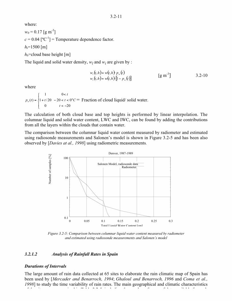
3.2-11

where:

w0 = 0.17 [g m-3]

c = 0.04 [ºC-1] = Temperature dependence factor.

hr=1500 [m]

hb=cloud base height [m]

The liquid and solid water density, wl and wi are given by :

( ) ( ) ( )( ) ( ) ( )[ ]tphtwhtw

tphtwhtw

wi

wl

<u=

u=

1,,

,, [g m-3] 3.2-10

where

20

020

0

0

20/1

1

)(

<<

°<<<

<

ǻ

«©

¨

+=

t

Ct

t

ttpw = Fraction of cloud liquid/ solid water.

The calculation of both cloud base and top heights is performed by linear interpolation. Thecolumnar liquid and solid water content, LWC and IWC, can be found by adding the contributionsfrom all the layers within the clouds that contain water.

The comparison between the columnar liquid water content measured by radiometer and estimatedusing radiosonde measurements and Salonen’s model is shown in Figure 3.2-5 and has been alsoobserved by [Davies at al., 1998] using radiometric measurements.

0.1

1

10

100

0 0.05 0.1 0.15 0.2 0.25 0.3

Num

ber

of s

ampl

es [

%]

Total Liquid Water Content [cm]

Denver, 1987-1989

Salonen Model, radiosonde dataRadiometer

Figure 3.2-5: Comparison between columnar liquid water content measured by radiometerand estimated using radiosonde measurements and Salonen’s model

3.2.1.2 Analysis of Rainfall Rates in Spain

Durations of Intervals

The large amount of rain data collected at 65 sites to elaborate the rain climatic map of Spain hasbeen used by [Mercader and Benarroch, 1994; Ghaloul and Benarroch, 1996 and Coma et al.,1998] to study the time variability of rain rates. The main geographical and climatic characteristics

f th it i d i T bl 3 2 5 i l di th b f f d t il bl f h

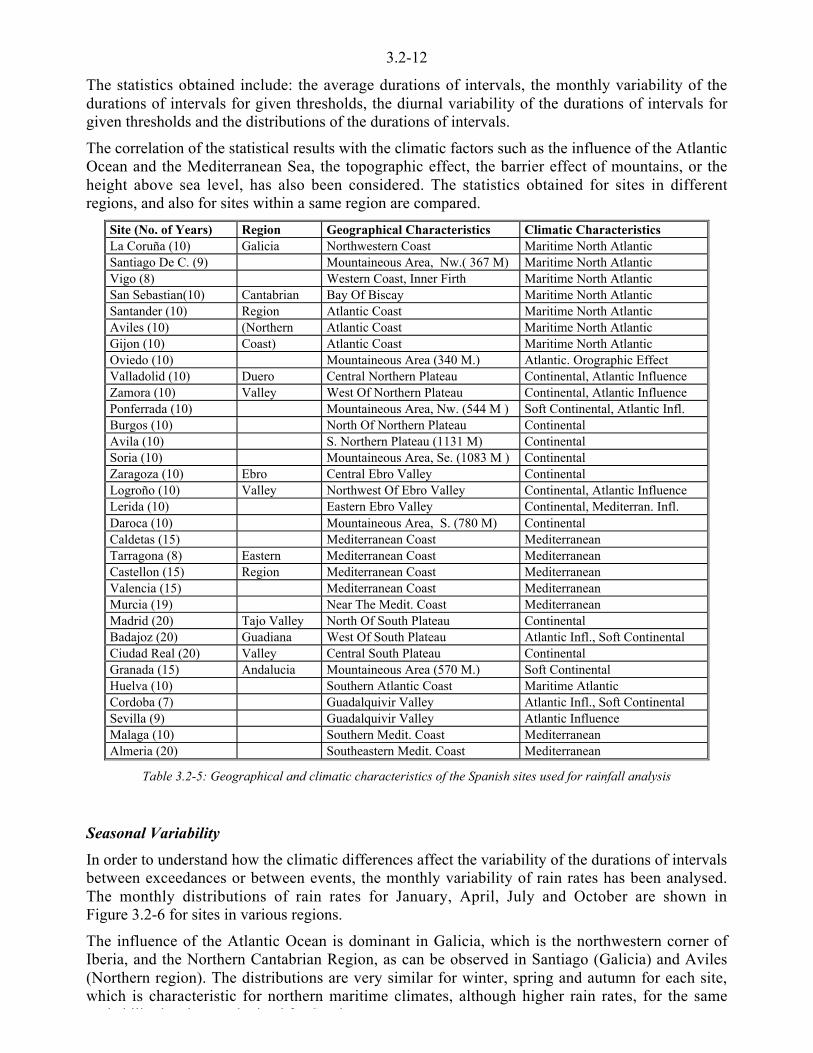
3.2-12

The statistics obtained include: the average durations of intervals, the monthly variability of thedurations of intervals for given thresholds, the diurnal variability of the durations of intervals forgiven thresholds and the distributions of the durations of intervals.

The correlation of the statistical results with the climatic factors such as the influence of the AtlanticOcean and the Mediterranean Sea, the topographic effect, the barrier effect of mountains, or theheight above sea level, has also been considered. The statistics obtained for sites in differentregions, and also for sites within a same region are compared.

Site (No. of Years) Region Geographical Characteristics Climatic CharacteristicsLa Coruña (10) Galicia Northwestern Coast Maritime North AtlanticSantiago De C. (9) Mountaineous Area, Nw.( 367 M) Maritime North AtlanticVigo (8) Western Coast, Inner Firth Maritime North AtlanticSan Sebastian(10) Cantabrian Bay Of Biscay Maritime North AtlanticSantander (10) Region Atlantic Coast Maritime North AtlanticAviles (10) (Northern Atlantic Coast Maritime North AtlanticGijon (10) Coast) Atlantic Coast Maritime North AtlanticOviedo (10) Mountaineous Area (340 M.) Atlantic. Orographic EffectValladolid (10) Duero Central Northern Plateau Continental, Atlantic InfluenceZamora (10) Valley West Of Northern Plateau Continental, Atlantic InfluencePonferrada (10) Mountaineous Area, Nw. (544 M ) Soft Continental, Atlantic Infl.Burgos (10) North Of Northern Plateau ContinentalAvila (10) S. Northern Plateau (1131 M) ContinentalSoria (10) Mountaineous Area, Se. (1083 M ) ContinentalZaragoza (10) Ebro Central Ebro Valley ContinentalLogroño (10) Valley Northwest Of Ebro Valley Continental, Atlantic InfluenceLerida (10) Eastern Ebro Valley Continental, Mediterran. Infl.Daroca (10) Mountaineous Area, S. (780 M) ContinentalCaldetas (15) Mediterranean Coast MediterraneanTarragona (8) Eastern Mediterranean Coast MediterraneanCastellon (15) Region Mediterranean Coast MediterraneanValencia (15) Mediterranean Coast MediterraneanMurcia (19) Near The Medit. Coast MediterraneanMadrid (20) Tajo Valley North Of South Plateau ContinentalBadajoz (20) Guadiana West Of South Plateau Atlantic Infl., Soft ContinentalCiudad Real (20) Valley Central South Plateau ContinentalGranada (15) Andalucia Mountaineous Area (570 M.) Soft ContinentalHuelva (10) Southern Atlantic Coast Maritime AtlanticCordoba (7) Guadalquivir Valley Atlantic Infl., Soft ContinentalSevilla (9) Guadalquivir Valley Atlantic InfluenceMalaga (10) Southern Medit. Coast MediterraneanAlmeria (20) Southeastern Medit. Coast Mediterranean

Table 3.2-5: Geographical and climatic characteristics of the Spanish sites used for rainfall analysis

Seasonal Variability

In order to understand how the climatic differences affect the variability of the durations of intervalsbetween exceedances or between events, the monthly variability of rain rates has been analysed.The monthly distributions of rain rates for January, April, July and October are shown inFigure 3.2-6 for sites in various regions.

The influence of the Atlantic Ocean is dominant in Galicia, which is the northwestern corner ofIberia, and the Northern Cantabrian Region, as can be observed in Santiago (Galicia) and Aviles(Northern region). The distributions are very similar for winter, spring and autumn for each site,which is characteristic for northern maritime climates, although higher rain rates, for the same

b bili l l b i d f S i

3.2-13

The Northern and Southern Plateaux have continental climate due to their height above sea level, tothe isolating mountain ranges and the distance from the coasts, although most of the rain in theseregions is caused by Atlantic fronts. The monthly distributions of rain rate are given for Burgos(Northern Plateau) and Ciudad Real (Southern Plateau). Higher rain rates from Atlantic systems areexpected in Burgos in spring, while in winter intensities are lower. Ciudad Real is at a largerdistance from the Atlantic Ocean, showing lower rain rates, very similar for autumn and spring, andeven lower in winter and summer.

The regions along the Mediterranean Coast are more or less isolated from the influence of theAtlantic Ocean due to the mountain ranges in the interior and along this coast. The MediterraneanSea influence is dominant in these regions, where rainfall frequently has convective characteristics,in particular during late summer and autumn. In consequence, a large seasonal variability isobserved in Castellon, with higher intensities for October, for almost all probability levels. It mustalso be noticed, comparing all the locations in Figure 3.2-6, that the highest rain rates during thistime of the year are observed in this region.

The climate in the Ebro Valley, encircled by mountain ranges, has continental characteristics, withrainfall caused both by Atlantic fronts and convective Mediterranean events, depending on the siteand on the season of the year. The rain rate seasonal variability for Zaragoza, in the centre of theValley, is similar to that of Ciudad Real; however, Lerida, in the eastern part of the Ebro Valleyshows a Mediterranean seasonal variability, with higher rain intensities in autumn.

The Climate of Western Andalucia is also affected by the Atlantic Ocean. Huelva is located in aregion of maritime climate, but rain rate characteristics are different to those of the north andnorthwest, with a larger seasonal variability. The highest rain intensities occur during the autumn,when Atlantic rain systems reach that region, while the rest of the year these systems move alongmore northerly latitudes.

Some sites in other regions show peculiar results due to topographic effects, such as Granada whichshows results similar to Ciudad Real, very different to other sites in Andalucia; or Avila, with somedifferent results to those obtained for other sites in the Northern Plateau. Also, the sites along theEastern Coast, from Almeria to Catalonia, although of Mediterranean climate, show some differentresults; in particular, rain rates for sites in the southern part are lower than for sites in the northernpart as discussed by [Mercader and Benarroch, 1994].

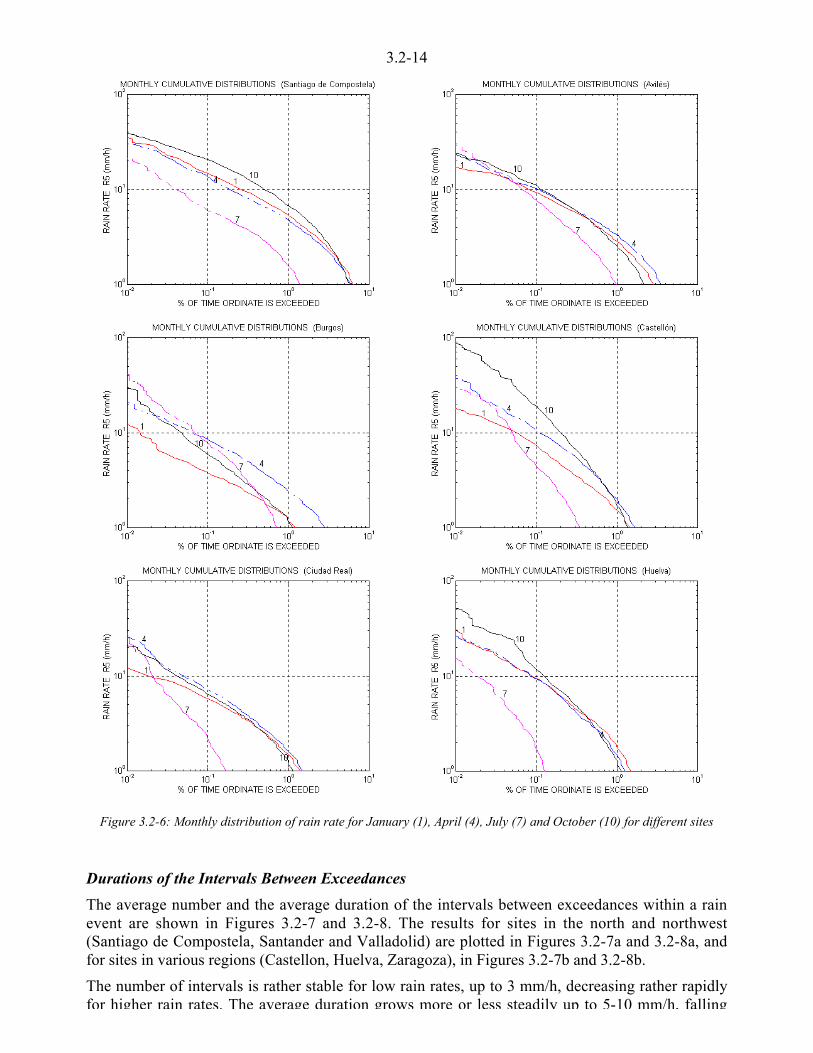
3.2-14

Figure 3.2-6: Monthly distribution of rain rate for January (1), April (4), July (7) and October (10) for different sites

Durations of the Intervals Between Exceedances

The average number and the average duration of the intervals between exceedances within a rainevent are shown in Figures 3.2-7 and 3.2-8. The results for sites in the north and northwest(Santiago de Compostela, Santander and Valladolid) are plotted in Figures 3.2-7a and 3.2-8a, andfor sites in various regions (Castellon, Huelva, Zaragoza), in Figures 3.2-7b and 3.2-8b.

The number of intervals is rather stable for low rain rates, up to 3 mm/h, decreasing rather rapidlyfor higher rain rates. The average duration grows more or less steadily up to 5-10 mm/h, falling

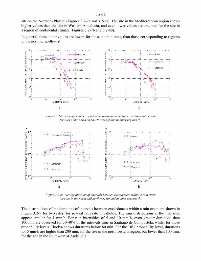
3.2-15

site on the Northern Plateau (Figures 3.2-7a and 3.2-8a). The site in the Mediterranean region showshigher values than the site in Western Andalucia, and even lower values are obtained for the site ina region of continental climate (Figures 3.2-7b and 3.2-8b).

In general, these latter values are lower, for the same rain rates, than those corresponding to regionsin the north or northwest.

a b

Figure 3.2-7: Average number of intervals between exceedances within a rain eventfor sites in the north and northwest (a) and in other regions (b)

a b

Figure 3.2-8: Average duration of intervals between exceedances within a rain eventfor sites in the north and northwest (a) and in other regions (b)

The distributions of the durations of intervals between exceedances within a rain event are shown inFigure 3.2-9 for two sites, for several rain rate thresholds. The rain distributions at the two sitesappear similar for 1 mm/h. For rain intensities of 5 and 10 mm/h, even greater durations than100 min are observed for 30-40% of the intervals time in Santiago de Compostela, while, for thoseprobability levels, Huelva shows durations below 80 min. For the 10% probability level, durationsfor 5 mm/h are higher than 200 min. for the site in the northwestern region, but lower than 100 min.for the site in the southwest of Andalucia.

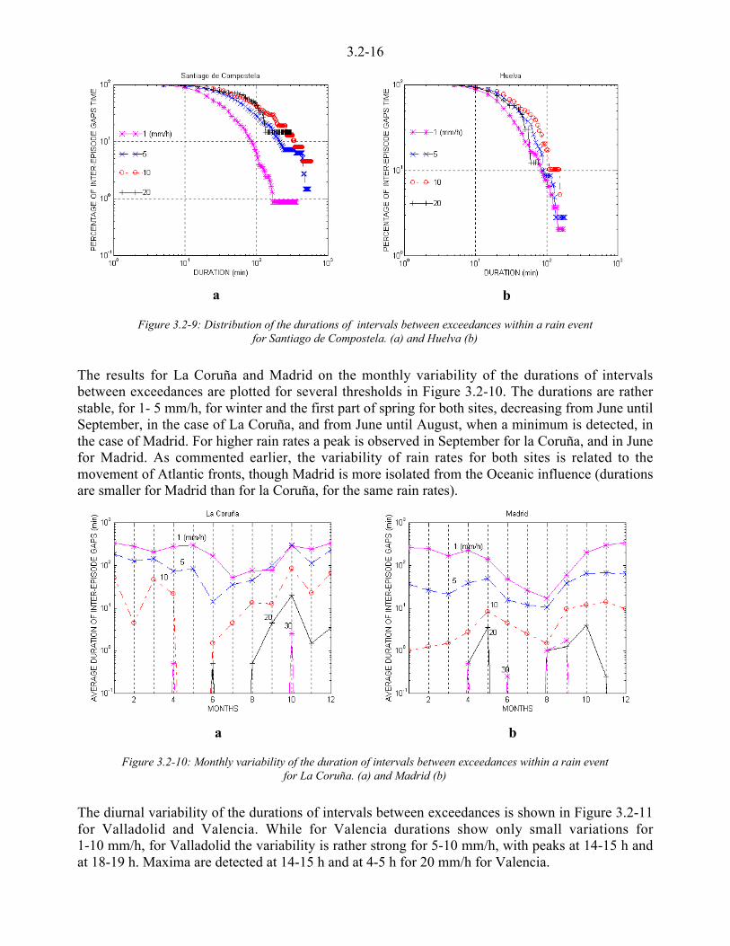
3.2-16

a b

Figure 3.2-9: Distribution of the durations of intervals between exceedances within a rain eventfor Santiago de Compostela. (a) and Huelva (b)

The results for La Coruña and Madrid on the monthly variability of the durations of intervalsbetween exceedances are plotted for several thresholds in Figure 3.2-10. The durations are ratherstable, for 1- 5 mm/h, for winter and the first part of spring for both sites, decreasing from June untilSeptember, in the case of La Coruña, and from June until August, when a minimum is detected, inthe case of Madrid. For higher rain rates a peak is observed in September for la Coruña, and in Junefor Madrid. As commented earlier, the variability of rain rates for both sites is related to themovement of Atlantic fronts, though Madrid is more isolated from the Oceanic influence (durationsare smaller for Madrid than for la Coruña, for the same rain rates).

a b

Figure 3.2-10: Monthly variability of the duration of intervals between exceedances within a rain eventfor La Coruña. (a) and Madrid (b)

The diurnal variability of the durations of intervals between exceedances is shown in Figure 3.2-11for Valladolid and Valencia. While for Valencia durations show only small variations for1-10 mm/h, for Valladolid the variability is rather strong for 5-10 mm/h, with peaks at 14-15 h andat 18-19 h. Maxima are detected at 14-15 h and at 4-5 h for 20 mm/h for Valencia.

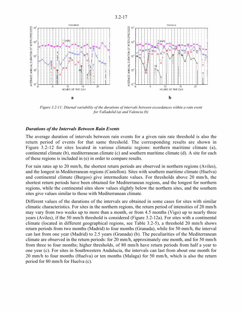
3.2-17

a b

Figure 3.2-11: Diurnal variability of the durations of intervals between exceedances within a rain eventfor Valladolid (a) and Valencia (b)

Durations of the Intervals Between Rain Events

The average duration of intervals between rain events for a given rain rate threshold is also thereturn period of events for that same threshold. The corresponding results are shown inFigure 3.2-12 for sites located in various climatic regions: northern maritime climate (a),continental climate (b), mediterranean climate (c) and southern maritime climate (d). A site for eachof these regions is included in (e) in order to compare results.

For rain rates up to 20 mm/h, the shortest return periods are observed in northern regions (Aviles),and the longest in Mediterranean regions (Castellon). Sites with southern maritime climate (Huelva)and continental climate (Burgos) give intermediate values. For thresholds above 20 mm/h, theshortest return periods have been obtained for Mediterranean regions, and the longest for northernregions, while the continental sites show values slightly below the northern sites, and the southernsites give values similar to those with Mediterranean climate.

Different values of the durations of the intervals are obtained in some cases for sites with similarclimatic characteristics. For sites in the northern regions, the return period of intensities of 20 mm/hmay vary from two weeks up to more than a month, or from 4.5 months (Vigo) up to nearly threeyears (Aviles), if the 50 mm/h threshold is considered (Figure 3.2-12a). For sites with a continentalclimate (located in different geographical regions, see Table 3.2-5), a threshold 20 mm/h showsreturn periods from two months (Madrid) to four months (Granada), while for 50 mm/h, the intervalcan last from one year (Madrid) to 2.5 years (Granada) (b). The peculiarities of the Mediterraneanclimate are observed in the return periods: for 20 mm/h, approximately one month, and for 50 mm/hfrom three to four months; higher thresholds, of 80 mm/h have return periods from half a year toone year (c). For sites in Southwestern Andalucia, the intervals can last from about one month for20 mm/h to four months (Huelva) or ten months (Malaga) for 50 mm/h, which is also the returnperiod for 80 mm/h for Huelva (c).

3.2-18

a) Northern maritime climate b) Continental climate

c) Mediterranean climate d) Southerm maritime climate

e) a site from figures a, b,c and d

Figure 3.2-12: Average duration of intervals between rain events for several sites for different climates.

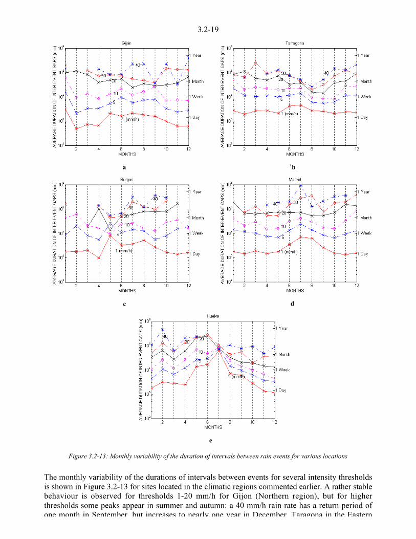
3.2-19

a `b

c d

e

Figure 3.2-13: Monthly variability of the duration of intervals between rain events for various locations

The monthly variability of the durations of intervals between events for several intensity thresholdsis shown in Figure 3.2-13 for sites located in the climatic regions commented earlier. A rather stablebehaviour is observed for thresholds 1-20 mm/h for Gijon (Northern region), but for higherthresholds some peaks appear in summer and autumn: a 40 mm/h rain rate has a return period ofone month in September, but increases to nearly one year in December. Taragona in the Eastern

3.2-20

above 20 mm/h. The shortest intervals for 30-40 mm/h are expected in August (below one month),and the longest in spring and autumn (five to eight months). The variability for two sites withcontinental climate, Burgos and Madrid, located in different geographical regions is plotted in (c)and (d). Events of low intensity occurring in winter and autumn have smaller return periods thanduring the rest of the year. For high rain rates, the shortest intervals correspond to spring andAugust (about one month for Burgos and three months for Madrid).

The strongest variability for all thresholds is observed in Huelva (e), which corresponds to South-western Andalucia. Any event occurring in July has a return period of 1-2 months, while shorterreturn periods are expected for low thresholds (1-10 mm/h) during any other month. The shortestintervals for rain rates of 40 mm/h are detected from August to December and also in March (one totwo months).

Stability of rainfall rate distributions

In order to analyse the long term stability of rainfall rate cumulative distributions, several sites havebeen selected taking into account the number of years of data available. A more detailed analysis oftime variability was presented during the COST 255 project.

The stability of precipitation statistics has been analysed by means of the parameter Dn proposed by

[Baptista et. al., 1986] and defined as :

-=

=n

iin e

nD

1

21 [g m-3] 3.2-11

where

( ) ( )( )

100u<

=PR

PRPRe

LT

LTnn [%]

( )PRLT = rain rate exceeded for P% of the time according to the long-term cumulativedistribution derived from N years of measurements. [mm/hr]

( )PRn = rain rate exceeded for P% of the time according to the cumulative distributionderived from n years of measurements (n < N ). [mm/hr]

In this analysis it has been assumed that a rain distribution calculated for n years is a validapproximation of the long term distribution (obtained for the total number of years available N>n) ifDn is smaller than 3%.

The results shown in Figures 3.2-14 and 3.2-15 correspond to sites with 20 years of data (n=1, 3, 5,8, 10, 12, 14, 16, 18). All these sites are located either on the Southern Plateau or along theSoutheastern Coast, with climatic peculiarities whose effects are detected in the stability results.

3.2-21

a) (n=1,3,5,8,10,12,14,16, 18) 20 years of data

b) (n=1,3,5,8,10,12,14,16, 18) 20 years of data c) (n=1,3,5,8,10,12,14,16, 18) 20 years of data

d) (n=1,3,5,8,10,12,14,16, 18) 20 years of data e) (n=1,3,5,8,10,12,14,16, 18) 20 years of data

Figure 3.2-14: Dependence of Dn on the percentage of time for n years

Badajoz (a) shows higher stability than the other sites. The distribution for 14 years is adequate forBadajoz for the interval 0.004-0.4%, and for all the intervals if 16 years or more are employed.

For Ciudad Real (b) at least 16 years are needed for the 0.05-0.8% interval, and 18 years or over forthe entire interval considered, while Caceres (c) shows poorer results, requiring at least 18 years ofdata.

For Madrid and Toledo (d and e), most of the higher probabilities (over 0.05%) can be consideredif at least 12 years of data are employed. A minimum of 16 years are required to obtain stableresults, for the total range of probabilities for Madrid, and for probabilities above 0.005 for Toledo.

Poorer stability results are obtained for the sites along the Mediterranean southeastern coast see

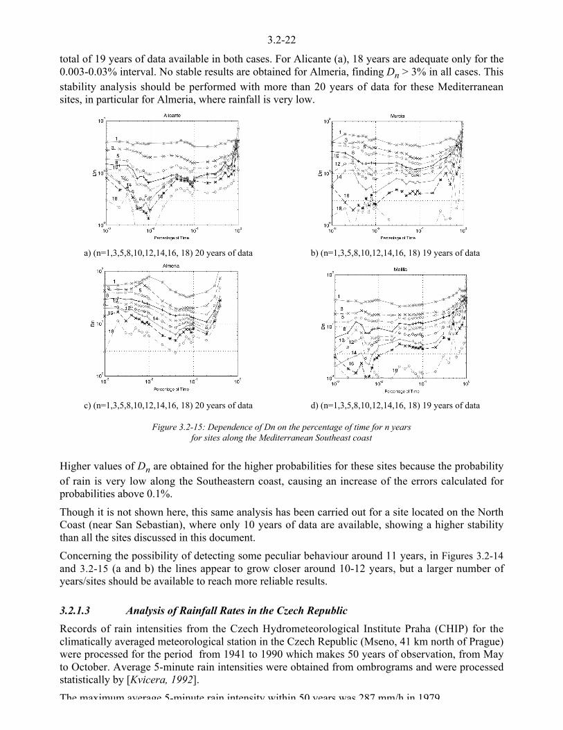
3.2-22

total of 19 years of data available in both cases. For Alicante (a), 18 years are adequate only for the0.003-0.03% interval. No stable results are obtained for Almeria, finding Dn > 3% in all cases. Thisstability analysis should be performed with more than 20 years of data for these Mediterraneansites, in particular for Almeria, where rainfall is very low.

a) (n=1,3,5,8,10,12,14,16, 18) 20 years of data b) (n=1,3,5,8,10,12,14,16, 18) 19 years of data

c) (n=1,3,5,8,10,12,14,16, 18) 20 years of data d) (n=1,3,5,8,10,12,14,16, 18) 19 years of data

Figure 3.2-15: Dependence of Dn on the percentage of time for n yearsfor sites along the Mediterranean Southeast coast

Higher values of Dn are obtained for the higher probabilities for these sites because the probabilityof rain is very low along the Southeastern coast, causing an increase of the errors calculated forprobabilities above 0.1%.

Though it is not shown here, this same analysis has been carried out for a site located on the NorthCoast (near San Sebastian), where only 10 years of data are available, showing a higher stabilitythan all the sites discussed in this document.

Concerning the possibility of detecting some peculiar behaviour around 11 years, in Figures 3.2-14and 3.2-15 (a and b) the lines appear to grow closer around 10-12 years, but a larger number ofyears/sites should be available to reach more reliable results.

3.2.1.3 Analysis of Rainfall Rates in the Czech Republic

Records of rain intensities from the Czech Hydrometeorological Institute Praha (CHIP) for theclimatically averaged meteorological station in the Czech Republic (Mseno, 41 km north of Prague)were processed for the period from 1941 to 1990 which makes 50 years of observation, from Mayto October. Average 5-minute rain intensities were obtained from ombrograms and were processedstatistically by [Kvicera, 1992].

The maximum average 5-minute rain intensity within 50 years was 287 mm/h in 1979

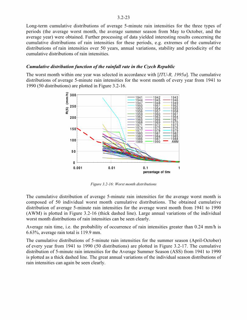
3.2-23

Long-term cumulative distributions of average 5-minute rain intensities for the three types ofperiods (the average worst month, the average summer season from May to October, and theaverage year) were obtained. Further processing of data yielded interesting results concerning thecumulative distributions of rain intensities for these periods, e.g. extremes of the cumulativedistributions of rain intensities over 50 years, annual variations, stability and periodicity of thecumulative distributions of rain intensities.

Cumulative distribution function of the rainfall rate in the Czech Republic

The worst month within one year was selected in accordance with [ITU-R, 1995a]. The cumulativedistributions of average 5-minute rain intensities for the worst month of every year from 1941 to1990 (50 distributions) are plotted in Figure 3.2-16.

0

5 0

1 0 0

1 5 0

2 0 0

2 5 0

3 0 0

0.001 0.01 0.1 1percentage of time

R(5

) (m

m/h

)

1941 1942 19431944 1945 19461947 1948 19491950 1951 19521953 1954 19551956 1957 19581959 1960 19611962 1963 19641965 1966 19671968 1969 19701971 1972 19731974 1975 19761977 1978 19791980 1981 19821983 1984 19851986 1987 19881989 1990 AWM

Figure 3.2-16: Worst month distributions

The cumulative distribution of average 5-minute rain intensities for the average worst month iscomposed of 50 individual worst month cumulative distributions. The obtained cumulativedistribution of average 5-minute rain intensities for the average worst month from 1941 to 1990(AWM) is plotted in Figure 3.2-16 (thick dashed line). Large annual variations of the individualworst month distributions of rain intensities can be seen clearly.

Average rain time, i.e. the probability of occurrence of rain intensities greater than 0.24 mm/h is6.63%, average rain total is 119.9 mm.

The cumulative distributions of 5-minute rain intensities for the summer season (April-October)of every year from 1941 to 1990 (50 distributions) are plotted in Figure 3.2-17. The cumulativedistribution of 5-minute rain intensities for the Average Summer Season (ASS) from 1941 to 1990is plotted as a thick dashed line. The great annual variations of the individual season distributions ofrain intensities can again be seen clearly.

3.2-24

0

5 0

1 0 0

1 5 0

2 0 0

2 5 0

3 0 0

0.001 0.01 0.1 1

percentage of time

R(5

) (m

m/h

)

1941 1942 19431944 1945 19461947 1948 19491950 1951 19521953 1954 19551956 1957 19581959 1960 19611962 1963 19641965 1966 19671968 1969 19701971 1972 19731974 1975 19761977 1978 19791980 1981 19821983 1984 19851986 1987 19881989 1990 ASS

Figure 3.2-17: Summer season distributions

As siphon raingauge measurements usually start on about 15 May and finish on about 15 October inthe Czech Republic due to cold weather, we were confined to choose the worst month from withinthe calendar period June-September. Cumulative distribution of rain intensities for the average yearis composed of distributions for summer and winter seasons. Distribution for cold seasons couldonly be estimated. In cold seasons, rain intensities are about one third of those in the summer (inaccordance with CHIP). This fact and the knowledge of rain total for an average meteorologicalstation (610 mm) were used for the calculation of the rain intensity cumulative distribution for theaverage year from 1941 to 1990.

The cumulative distributions of 5-minute rain intensities for individual whole years are not defined.The cumulative distribution of 5-minute rain intensities for an average year within the period 1941-1990 have been derived from the measured cumulative distribution of 5-minute rain intensities forthe average summer season and from calculated cumulative distribution for the winter season.

The cumulative distributions of 5-minute rain intensities for individual years (re-calculated fromsummer season to a whole year basis) from 1941 to 1990 (50 distributions) are plotted inFigure 3.2-18 (because the yearly statistics are based only on summer measurements, the influenceof the cold weather is not taken into account). The cumulative distribution of 5-minute rainintensities for the average year (without the influence of the cold seasons) from 1941 to 1990 (AY)is plotted as a thick dashed line.

The average rain time is 4.48%, average rain total is 610 mm.

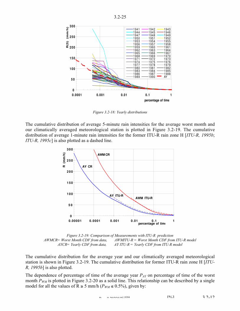
3.2-25

0

5 0

1 0 0

1 5 0

2 0 0

2 5 0

3 0 0

0.0001 0.001 0.01 0.1 1

percentage of time

R(5

) (m

m/h

)

1941 1942 19431944 1945 19461947 1948 19491950 1951 19521953 1954 19551956 1957 19581959 1960 19611962 1963 19641965 1966 19671968 1969 19701971 1972 19731974 1975 19761977 1978 19791980 1981 19821983 1984 19851986 1987 19881989 1990 AY

Figure 3.2-18: Yearly distributions

The cumulative distribution of average 5-minute rain intensities for the average worst month andour climatically averaged meteorological station is plotted in Figure 3.2-19. The cumulativedistribution of average 1-minute rain intensities for the former ITU-R rain zone H [ITU-R, 1995b;ITU-R, 1995c] is also plotted as a dashed line.

0

5 0

1 0 0

1 5 0

2 0 0

2 5 0

3 0 0

0.00001 0.0001 0.001 0.01 0.1 1percentage of time

R (

mm

/h)

AWM CR

AY CR

AWM ITU-RAY ITU-R

Figure 3.2-19: Comparison of Measurements with ITU-R predictionAWMCR= Worst Month CDF from data, AWMITU-R = Worst Month CDF from ITU-R model

AYCR= Yearly CDF from data, AY ITU-R = Yearly CDF from ITU-R model

The cumulative distribution for the average year and our climatically averaged meteorologicalstation is shown in Figure 3.2-19. The cumulative distribution for former ITU-R rain zone H [ITU-R, 1995b] is also plotted.

The dependence of percentage of time of the average year PAY on percentage of time of the worstmonth PWM is plotted in Figure 3.2-20 as a solid line. This relationship can be described by a singlemodel for all the values of R * 5 mm/h (PWM ) 0.5%), given by:

18384.1282380 PP [%] 3 2-12

3.2-26

0.000001

0.00001

0.0001

0.001

0.01

0.1

1

0.0001 0.001 0.01 0.1 1

Pwm (%)

Pay

(%

)

measuredapproxITU-R

Figure 3.2-20: Dependence of PAY on PWM . Measured values, ITU-R model and single model

A better approximation can be obtained by using different models for low and high intensityrainfalls.

For low rain rates, in the range 5 ) R(5) ) 57 [mm/h] (0.018 % ) PWM ) 0.5 %), the followingmodel has been derived:

29758.139611.0 WMAY PP = [%] 3.2-13

For high intensity rainfalls, in the range 57 < R(5) ) 287 mm/h (0.00011% ) PWM ) 0.018%) themodel was found to be:

10522.117911.0 WMAY PP = [%] 3.2-14

These relationships are plotted in Figure 3.2-21 as dashed lines. The model proposed by [ITU-R,1995b] is plotted in both of the figures as a dotted line.

0.000001

0.00001

0.0001

0.001

0.01

0.1

1

0.0001 0.001 0.01 0.1 1

Pwm (%)

Pay

(%

)

measuredapprox 1approx 2ITU-R

Figure 3.2-21: Dependence of PAY on PWM .

Measured values, ITU-R model and models for low and high rain rates

3.2-27

Table 3.2-6 gives the fitting parameters of all the models.

Model Rain rate range Correl. Coeff. r.m.s. % Error [%]Single Model R > 5 mm/hr 0.9985 0.0038 ± 38Low rain rate 5 ) R(5) ) 57 0.9995 0.0028 ± 13High Rain Rate 57 < R(5) ) 287 0.9991 0.00005 ± 19

Table 3.2-6: Fitting parameters of the models for the relationship between PAY and PWM

Analysis of Extreme values

The boundaries for monthly distributions, e.g. for distributions for the worst month over fifty years(WM) and for the best month over fifty years (BM) together with the distribution for the averageworst month (AWM) are shown in Figure 3.2-22.

0

5 0

1 0 0

1 5 0

2 0 0

2 5 0

3 0 0

0.0001 0.001 0.01 0.1 1

percentage of time

R(5

) (

mm

/h) AWM over 5O years

WM over 50 yearsBM over 50 years

Figure 3.2-22: Boundaries for monthly distributions

The boundaries for yearly distributions, e.g. for distributions for the worst year over fifty years(WY) and for the best year over fifty years (BY) together with the distribution for the average year(AY) are shown in Figure 3.2-23.

0

5 0

1 0 0

1 5 0

2 0 0

2 5 0

3 0 0

0.00001 0.0001 0.001 0.01 0.1 1

percentage of time

R(5

) (m

m/h

)

AY over 50 years

WY over 50 years

BY over 50 years

Figure 3.2-23: Boundaries for yearly distributions

3.2-28

The driest (rainy) year is defined as the year with the minimum (maximum) total amount of rain. Inaccordance with the CHIP, the driest year over the whole period 1941-1990 was 1959, with a totalof 384 mm of rain and the most rainy year was 1981 with a total of 980 mm.

The driest period May-October was in 1994 with a total amount of rain of 176 mm and the mostrainy period was in 1981 with rain total of 629 mm. The cumulative distributions of 5-minute rainintensities are shown in Figure 3.2-24 for the worst months in these years and in Figure 3.2-25 forthe yearly average.

The cumulative distributions for individual years (seasons) were calculated from the period May-October and were converted to one year bases. The differences between distributions for a dry and awet year or period does not appear to be relevant.

0

1 0

2 0

3 0

4 0

5 0

6 0

7 0

8 0

9 0

0.001 0.01 0.1 1

percentage of time

R(5

) (m

m/h

)

WM 1981 (most wet year, season

WM 1959 (most dry year)

WM 1947 (most dry season)

Figure 3.2-24: Distributions for the worst months in the driest and the most rainy years and seasons.

0

1 0

2 0

3 0

4 0

5 0

6 0

7 0

8 0

9 0

0.001 0.01 0.1 1

percentage of time

R(5

) (m

m/h

)

1981 (most wet year, season)

1959 (most dry year)

1947 (most dry season)

Figure 3.2-25: Yearly cumulative distribution function in the driest and the most rainy years and seasons.

3.2-29

Variations of rainfall rate statistics for the worst month, the summer season and the year

In order to characterise the annual variations of the worst month statistics the following parametershave been used:

( ) ( ) ( )( ) ( ) ( )imiavgmim

iavgmimim

PRPRPQ

PRPRPQ

min,,min,

,max,max,

/

/

=

=[%] 3.2-15

where

( )im PR max, = the maximum rain intensity for the worst month at Pi

( )iavgm PR , = the rain intensity for the average worst month at Pi

( )im PR min, = the minimum rain intensity at Pi

iP = percentage of time of the worst month.

The values of Qm,max and Qm,min, derived from the worst month distribution (see Figure 3.2-16) areshown below, as a function of the percentages of time (month).

0

0.5

1

1.5

2

2.5

3

3.5

4

4.5

0.001 0.01 0.1 1percentage of time

Qm Qm,i,max

Qm,i,min

Figure 3.2-26 Annual variations of the worst month distributions

Similarly the following parameters for the summer season (April-October) variations can bedefined:

( ) ( ) ( )( ) ( ) ( )isiavgsis

iavgsisis

PRPRPQ

PRPRPQ

min,,min,

,max,max,

/

/

=

=[%] 3.2-16

where

( )is PR max, = the maximum rain intensity for the summer season at Pi

( )iavgs PR , = the rain intensity for the average summer season at Pi

( )is PR min, = the minimum rain intensity for the summer season at Pi

iP = percentage of time of summer season

The values of Qs,max and Qs,min for the chosen percentages of time derived from summer seasonstatistics (see Fig re 3 2 17) are sho n in Fig re 3 2 27

3.2-30

0

0.5

1

1.5

2

2.5

3

3.5

4

4.5

0.001 0.01 0.1 1percentage of time

Qs Qs,i,max

Qs,i,min

Figure 3.2-27: Annual variations of the summer season distributions

The variations between different years can be characterised by using:

( ) ( ) ( )( ) ( ) ( )iyiavgyiy

iavgyiyiy

PRPRPQ

PRPRPQ

min,,min,

,max,max,

/

/

=

=[%] 3.2-17

where

( )iy PR max, = the maximum rain intensity for the year at Pi

( )iavgy PR , = the rain intensity for the average year season at Pi

( )iy PR min, = the minimum rain intensity for the year at Pi

iP = percentage of time of the year

The values Qy max and Qy,min , derived from the yearly cumulative distributions functions of rain rate(see Figure 2.2-18) are shown in the next figure as a function of the (time) percentage of the year.

0.00 .51 .01 .52 .02 .53 .03 .54 .04 .55 .05 .56 .0

0.0001 0.001 0.01 0.1 1

percentage of time

Qy Qy,i,max

Qy,i,min

Figure 3.2-28: Annual variations of the years distributions

The annual variations for all the distributions (worst month, summer season and year average)decreases from 3.5 to 1.5 for percentages of time ranging from 0.001 to 0.1.

3.2-31

Year to Year variation of the rainfall rate distributions

The temporal variations of the cumulative distributions for the worst months have been derivedfrom data illustrated in Figures 3.2-16 to 3.2-18 (worst month, summer and year distributions) for0.01% and 0.1% and these are plotted in Figure 3.2-29

0

5 0

1 0 0

1 5 0

2 0 0

2 5 0

1940 1950 1960 1970 1980 1990year

R(5

) (m

m/h

)

0.01%

0.1%

a)

0

5 0

1 0 0

1 5 0

2 0 0

2 5 0

1940 1950 1960 1970 1980 1990year

R(5

) (m

m/h

)

0.01%0.1%

b)

0

5 0

1 0 0

1 5 0

2 0 0

2 5 0

1940 1950 1960 1970 1980 1990year

R(5

) (m

m/h

)

0.001%0.01%0.1%

c)

Figure 3.2-29: Year to year variations of the cumulative distribution of a) the worst months, b) the summer season and c) year distributions for different percentages of time.

In the following table the long-term average values of rainfall are given:

Distribution R(0.001 %) mm/hr R(0.01 %) [mm/hr] R(0.1 %) [mm/hr]Worst Month - 70. 18.5Summer Season - 42. 10.Year 70. 26. 6.

Table 3.2-7: Average values of rainfall rates at various percentages of time for different distributions

Stability of the worst month, summer and year distributions

The stability of the rainfall rate statistics has been estimated using the parameter Dn proposed by

[Baptista et al., 1986] (see also Equation 3.2-11). The values of en have been calculated by using amoving window containing n consecutive years within the N year total, so that Dn was calculatedfor N values of en if n = 1, N - 1 values if n = 2, etc. In this case N= 50, and the values of n= 1,2, 3, ... 50 years were taken into account.

3.2-32

Plots of Dn against the percentage of time of month (percentage of probability for month) that agiven rain intensity threshold is exceeded are shown in Figure 3.2-30 for the worst monthdistribution.

0.1

1

1 0

1 0 0

0.0001 0.001 0.01 0.1 1Percentage of time

Dn

(%

)

n=1 n=2n=3 n=4n=5 n=6n=7 n=8n=9 n=10n=11 n=12n=13 n=14n=15 n=16n=17 n=18n=19 n=20n=21 n=22n=23 n=24n=25 n=26n=27 n=28n=29 n=30n=31 n=32n=33 n=34n=35 n=36n=37 n=38n=39 n=40n=41 n=42n=43 n=44n=45 n=46n=47 n=48n=49

Figure 3.2-30: Stability parameter Dn as a function of the percentage of time for the worst month distributions

If a stability value lower than 3% is required, it can be obtained for percentages of time greater than0.1, 0.01 and 0.001 by using 23, 45 and 49 years of rainfall data respectively. If only five years areavailable, then the stability factor is lower than 20, 25 and 40 % for percentages of time greater than0.1, 0.01 and 0.001 respectively.

Plots of Dn against percentage of time of summer season month (percentage of probability forsummer season) that a given rain intensity threshold is exceeded are shown in Figure 3.2-31.

In this case the stability threshold of 3% is reached for percentages of time greater than 0.1, 0.01and 0.001 by using 15, 20 and 36 years of rainfall data respectively. When only 5 years areavailable, then the stability factor is lower than 7, 15 and 33 % for percentages of time greater than0.1, 0.01 and 0.001 respectively.

0.1

1

1 0

1 0 0

0.00001 0.0001 0.001 0.01 0.1 1Percentage of time

Dn

(%

)

n=1 n=2n=3 n=4n=5 n=6n=7 n=8n=9 n=10n=11 n=12n=13 n=14n=15 n=16n=17 n=18n=19 n=20n=21 n=22n=23 n=24n=25 n=26n=27 n=28n=29 n=30n=31 n=32n=33 n=34n=35 n=36n=37 n=38n=39 n=40n=41 n=42n=43 n=44n=45 n=46n=47 n=48n=49

Figure 3.2-31: Stability parameter Dn as a function of the percentage of time for summer season distributions

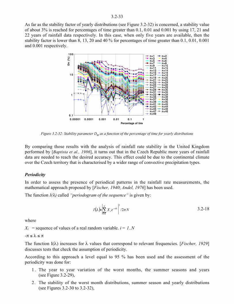
3.2-33

As far as the stability factor of yearly distributions (see Figure 3.2-32) is concerned, a stability valueof about 3% is reached for percentages of time greater than 0.1, 0.01 and 0.001 by using 17, 21 and22 years of rainfall data respectively. In this case, when only five years are available, then thestability factor is lower than 8, 13, 20 and 40 % for percentages of time greater than 0.1, 0.01, 0.001and 0.001 respectively.

0.1

1

1 0

1 0 0

0.00001 0.0001 0.001 0.01 0.1 1Percentage of time

Dn

(%

) n=1 n=2n=3 n=4n=5 n=6n=7 n=8n=9 n=10n=11 n=12n=13 n=14n=15 n=16n=17 n=18n=19 n=20n=21 n=22n=23 n=24n=25 n=26n=27 n=28n=29 n=30n=31 n=32n=33 n=34n=35 n=36n=37 n=38n=39 n=40n=41 n=42n=43 n=44n=45 n=46n=47 n=48n=49

Figure 3.2-32: Stability parameter Dn as a function of the percentage of time for yearly distributions

By comparing those results with the analysis of rainfall rate stability in the United Kingdomperformed by [Baptista et al., 1986], it turns out that in the Czech Republic more years of rainfalldata are needed to reach the desired accuracy. This effect could be due to the continental climateover the Czech territory that is characterised by a wider range of convective precipitation types.

Periodicity

In order to assess the presence of periodical patterns in the rainfall rate measurements, themathematical approach proposed by [Fischer, 1940; Andel, 1976] has been used.

The function I(h) called “periodogram of the sequence“ is given by:

( ) NeXI itN

tt /h h 2/

2

1

<

=-= 3.2-18

where

Xi = sequence of values of a real random variable. i = 1..N

-/ ) h ) /

The function I(h) increases for h values that correspond to relevant frequencies. [Fischer, 1929]discusses tests that check the assumption of periodicity.

According to this approach a level equal to 95 % has been used and the assessment of theperiodicity was done for:

1 . The year to year variation of the worst months, the summer seasons and years(see Figure 3.2-29),

2. The stability of the worst month distributions, summer season and yearly distributions(see Figures 3.2-30 to 3.2-32),

3.2-34

4. The maximum rain intensities for individual years.

In all cases the periodicity hypothesis was statistically not confirmed.

3.2.2 Global Characterisation – Mapping of Precipitation

Rain attenuation is the most important atmospheric effect in terms of its impact on satellitecommunications systems above 10 GHz. Short integration-time rainfall rate is the most essentialinput parameter in the prediction models for rain attenuation. However, short integration-timemeasurements of rainfall rate are not common and are not available with a global coverage. Evenlong integration-time (i.e. monthly totals) measurements with a global coverage and with a uniformquality control have only recently started to become available through the Global PrecipitationClimatology Project (GPCP) of the World Climate Research Programme (WCRP), see[Rudolf, 1996].

This type of data is fundamental not only for purposes of planning and design of satellitecommunications but mostly important for the management of water resources and to assess theimpact of climate change.

Also in this frame, the European Centre for Medium-Range Weather Forecasting [ECWMF, 1997]re-analysed all previous archived data to create a meaningful climatological data set to cover15 years (from 1979 to 1993) of precipitation and upper air data. An extension of this project tocover a period of 40 years is under discussion.

Also worth mentioning is the Tropical Rain Measurement Mission (TRMM). ThisAmerican-Japanese Earth observation mission described by [Okamoto et al., 1998], was launched inNovember 1997, and measured and mapped precipitation in the tropics.

3.2.2.1 Approaches

Three different general approaches have been used to globally characterise the cumulativedistributions of precipitation for telecom applications.

1. The globe is divided into climatologically significant rain zones using general climatologicalinformation and precipitation measurements. Each of the precipitation climate zones is thencharacterised by a cumulative rainfall rate distribution. Good examples of this approach arethe models proposed by [Crane, 1982, 1985, 1996, 1998, 1990], for Global Rain-RateClimate and the [ITU-R, 1992] rain climate zones.

2. The cumulative distribution of precipitation is derived for as many sites as possible in theregion of interest and then interpolated, using fixed annual exceedence probabilities, forthose points or regions where there is no data. A good example of this approach is the oneused by [Watson et al , 1987] that mapped the precipitation exceeded in Europe for 0.1%and 0.01% of the year.

3. This approach uses precipitation data that are available all over the globe and uses them toderive the cumulative distribution of precipitation for short integration-time. Examples ofthis approach are [Salonen and Baptista, 1997; Rice and Holmberg, 1973 and Dutton et al.,1974].

The first approach has been widely used up to 2000 by the ITU-R [ITU-R, 1992]. The advantage ofthis approach is that even in the absence of high spatial resolution point precipitation information,maps can be drawn using general climatological information (e.g. given by [Haurwitz and Austin,1944; Koeppen, 1923 and Landsberg, 1974] to characterise each of the regions of the globe.

This is also the reason why the climate regions proposed by the ITU-R [ITU-R, 1992] still preserveshapes that are very similar to those in [Koeppen 1923] that were drawn with the scant information

3.2-35

The disadvantage of the approach is mainly two-fold,

1. the maps have discontinuities due to the borders of the climate regions making them lessuseful when designing and optimising spacecraft systems (e.g. antennas) that cover wideregions

2. they are difficult to update in a automatic way because the definition of the borders of theclimate region includes information from many different sources, requiring humanintervention. Even with these drawbacks, this approach has given very good results thathave withstood the test of time.

The second approach, used by [Watson et al., 1987], has been excellent in providing high qualityestimates of rain intensity and was used to update the ITU-R rain zones in Europe. The drawback ofthis approach is that it requires a relatively high density of short integration-time point precipitationmeasurements or measurements from which these can be derived ([Watson et al., 1987] used datafrom more than 400 sites). The topography is also not explicitly taken into account, also thereforerequiring a high spatial resolution for the measurement data.

This approach cannot be easily used on global data due to the low spatial resolution of pointmeasurements on a global scale and the errors that would arise from the spatial interpolation ofprecipitation rates for fixed annual probability levels. It will not be discussed further here.

The third approach is only possible if two conditions are satisfied:

1. High quality, long integration-time (a few hours) and high spatial resolution precipitationdata (on the order of a grid point per 100 km) are available;

2. Models that allow the derivation of short integration-time precipitation data from longintegration-time data.

While the second condition seems satisfied, see [Salonen and Baptista, 1997; Dutton et al., 1974and Salonen et al., 1994] the first condition can be satisfied only recently with the availability of themonthly precipitation totals from GPCP [Rudolf, 1996] and the 6-hourly forecast precipitation fieldsfrom [ECWMF, 1997].

This third approach will be used and developed here using the [Rice and Holmberg, 1973 andDutton et al., 1974] model and the [Salonen and Baptista, 1997] method as well as the GPCP andthe ECMWF global data. Comparisons between the results obtained with this approach with thosefrom another approach will also be presented and discussed.

3.2.2.2 Global precipitation data sources

Data from the precipitation forecasts of ECMWF

Data from the numerical analysis of ECMWF have been successfully used in the propagationstudies for low-fade-margin systems by [Salonen et al., 1994]. The use of ECMWF data has theadvantage that spatially continuous rainfall maps can be derived for the whole globe.

ECMWF has carried out global numerical weather forecasts since 1979. The forecast modelphysics, simulating the thermodynamic processes in the atmosphere, produces rainfall within eachtime step. Forecast precipitation amounts integrated over six-hour periods are stored for thesynoptic times. The topography also has an impact on the forecasted fields and is treated explicitlyin the model physics.

The data used here are for the period from 1979 to 1993 (15 years) and all data archived at theECMWF were re-analysed to produce a consistent set of forecasts using the same assimilationprocedures and model physics. This exercise was deemed necessary since the forecast model has

3.2-36

The spatial resolution of the data is a grid point every 1.5° of latitude and longitude. Precipitation isdivided into three components: 1) large scale (widespread or stratiform) precipitation, 2) convectivescale (shower-type) precipitation and 3) snowfall. The total amount of data (binary format) is3.3 Gbyte.

[Salonen and Baptista, 1997] also used a smaller ECMWF dataset (from October 1992 toSeptember 1994) but with a spatial resolution of 0.75° inº latitude and longitude.

Global Precipitation Climate Project (GPCP) data

Long-term precipitation statistics are available over land areas (islands and atolls included) from theGlobal Precipitation Climate Project (GPCP) of GEWEX. The GPCP data set includes monthlyprecipitation amounts over land areas in grid-points with a spatial resolution of 2.5°. The GPCPdata is based on rainfall measurements from about more than 30000 raingauge stations world-wide[Rudolf, 1996]. The minimum time resolution available from these data, for the moment, is onemonth and there is no distinction between rain and snowfall. The data include both types ofprecipitation.

Future development in GPCC (Global Precipitation Climate Centre) may decrease the timeresolution to around a week and to separate snowfalls from rain.

For operational reasons, the number of measurement sites decreases through the years i.e. there aremore sites contributing to the monthly totals in 1986 than in 1995.

An extended GPCP dataset includes estimates of monthly amounts over the oceans. These werederived using space remote sensing data from geostationary VIS-IR sensors (i.e. Meteosat, GMSand GOES) and Sun-synchronous multi-frequency microwave radiometers (SSM/I). This extendeddataset was not used here. The authors preferred to use only the rain gauge based data.

The mean annual precipitation amounts from 1986 to 1995 have been used here. Because the annualprecipitation data from the GPCP are based closely on rainfall measurements, the GPCP data maybe more accurate than the ECMWF data, however there are still several areas of the world wheredata are scarce or non-existent. For these, spatial interpolation techniques that take into account alsothe topography were used by the GPCP. The total amount of data from GPCP is 19 Mbyte in ASCIIformat.

Use of ECMWF and GPCP data

From the ECMWF data the following parameters were derived globally to apply the Rice-Holmbergmodel and the Salonen-Baptista method:

• Annual rainfall amount Mre (mm), (snowfalls excluded)

• Probability of rainy 6h periods Pre6 (%) in the year

• Mean ratio of convective rain amount above different thresholds (3, 4, 6, 10, 15 and 25 mm in6h) to all rain, `

• Mean annual rainfall amount of convective-type rains Mce

• Mean annual rainfall amount of stratiform-type rains Mse

• Probability of rainy 6h periods Pce6 (%), where more convective than stratiform rain wasforecast

• Probability of rainy 6h periods Pse6 (%), where more (or equal amount) stratiform rain thanconvective rain was forecast

• Mean annual ratio of snowfalls to all precipitation q

3.2-37

• Mean annual number of rainy days

The GPCP data set does not contain enough information to be used on its own however the monthlyrain amounts could be more accurate than those forecast by the ECMWF.

For a joint use of the ECMWF and GPCP data it has been assumed that in principle the monthlytotals from GPCP are more accurate. For this reason the GPCP precipitation amounts are treatedusing the ECMWF’s derived qs to exclude the snowfall. On the same basis the probability of6-hourly rainy periods derived from the ECMWF data is re-normalised to reflect the GPCP monthlyamounts (at the moment no distinction is made between rain and snowfall).

Because dry snowfall does not cause significant attenuation in microwave or millimetre waveranges, the snowfall must be excluded from the GPCP input data. The annual rainfall amount Mrg inthe GPCP data is calculated by removing snowfall from the precipitation data Mpg with the ratio qs

in the ECMWF data:

pgsrg MqM )1( <= 3.2-19

The GPCP data were used to correct the probability of rainy 6-hourly periods Pre6 in the ECMWFderived data. The corrected probability Prg6 (%) of rainy 6h periods is:

µµµ

�

�

³³³

�

�

´¦

¥²¤

£<<u=

re

rg

M

M

rerg

PP

10011100 6

6 3.2-20

Comparison ECMWF and GPCP data

The ECMWF rainfall forecasts from two years period, previously used by [Salonen and Baptista,1997], were compared with the GPCP data for the same period. The differences of precipitationamounts are usually rather small except on the south west coast of Sumatra and on the western coastof Central America. Both of those areas are near the equator and there are high mountains near thecoast, where the ECMWF forecast model version used for the period of 1992/10 - 1994/9 does notwork very well. This is believed to be due to “ringing” effects of the spherical expansion used in theECMWF forecasts [Beajaars, 1999]. The new ECMWF re-analysis data (15 years) does not havethis problem and the agreement between the ECMWF data and GPCP data is rather good also inthose difficult areas. The portion of stratiform rains is also clearly higher in the 15 years re-analyseddata than in the data from the earlier and shorter ECMWF data set.

3.2.2.3 Rain Rate climatological models

There are several rain-rate climatological models for short integration-time statistics ofprecipitation. In this study we are especially interested, as previously mentioned, in two of them.The reason for interest is because they allow us to derive the statistics of rain-rate from longintegration-time data.

Other rain-rate climatological models deserve mention, even if at this stage they cannot be used forthe same purposes as the Rice-Holmberg and the Salonen-Baptista methods. Among possiblechoices there are the Excell model [Capsoni et al. 1987], Crane’s two component model[Crane, 1982] and possibly the models of [Flavin, 1992 and Segal, 1979] could be used for thesame purpose with some manipulations..

Rice-Holmberg rainfall rate model

The rainfall rate model by [Rice and Holmberg, 1973] enables the calculation of annual cumulative

3.2-38

statistics into attenuation statistics, an integration time of one minute is chosen, as recommended bythe ITU-R. The Rice-Holmberg rainfall rate model contains three basic parameters:

• the average annual rainfall, Mr in mm

• the ratio of thunderstorm rain to total rain, `

• the annual average number of days with rainfall *0.25 mm, D

The ratio of thunderstorm rain to total rain ` is not readily available from meteorological databases.Thus, [Dutton et al., 1974] have presented a calculation method for ` from three parameters, whichare available from long-term meteorological observations: 1) maximum monthly rainfall amount in30 years, 2) average number of thunderstorm days in a year and 3) average number of rainy days ina year. This method was successfully used in the propagation studies for low fade margin systemsin the European region by [Dutton et al., 1974].

The data from ECMWF rainfall forecasts provides a possibility to estimate the input parameters ofthe Rice-Holmberg model. The estimates for ` have been calculated directly as a ratio of convectiverain to all rain with different thresholds of convective rains (3, 4, 6, 10, 15 and 25 mm in 6 hours).The best results were obtained with the threshold of 6mm/6h, when the two-year data set was usedby [Salonen and Baptista, 1997]. However, in addition to the results here, other comparisons by[Goldhirsch and Katz, 1979] show that the Rice-Holmberg method tends to overestimate rainfallrates for time percentages below 0.01%.

Figure 3.2-33 shows the results for the Rice-Holmberg model with the earlier shorter ECMWF dataset of 2 years. As can be seen the modelled rainfall rates are much worse than those obtained byusing the rain zones proposed by [ITU-R, 1992].

Figure 3.2-33: RMS and mean errors for predicted rainfall rates: ITU-R rain zones (x), Rice-Holmberg model withECMWF-data (9) and ECMWF+GPCP data (z). The ECMWF data used in this case covers only 2 years

Salonen-Baptista model

Because it was found that the Rice-Holmberg rainfall rate model is not accurate enough for highavailability systems, new rainfall rate model development was started. First, an attempt was made tofind proper functions, which describe rainfall rate distributions well, in both tropical andmid-latitude climates. It was found, that the probability, that the rainfall rate r is exceeded, can bedescribed well with the function:

)1(

)1(

0)( cr

brra

ePrP +

+u<

u= 3.2-21

Th d l i i l f i l l b d h i

3.2-39

data-sets from a two year period were used either alone or with the GPCP-data. The parameters ofmany different functions were optimised by minimising the following error-parameter:

µµ

�

�

´´¦

¥²²¤

£ <+

³³�

�

´´¦

¥²²¤

£

+

<-==

2

,

,,

2

,1,1 ,,

,,,,

mm/h2 ir

irip

njni jim

jimjipi M

MM

r

rrT

p

s

3.2-22

where

rp,i,j and rm,i,j are the predicted and measured rainfall rates for site i and probability level j.

Ti = length of experiment of site i in years.

The value of 2 mm/h is added to the denominator of the first term to decrease the effects of the largerelative errors of low rainfall rate measurements. The purpose of the second term is to make surethat the annual rainfall amount integrated from the predicted distributions Mp,i is near to the inputparameter Mr,i.

The rainfall rate data for the optimisation is based mainly on the ITU-R DBSG5 database, fromwhich the overlapping data were first removed. A few exceptional measurements were removedbecause the total rain amount estimated from measured rainfall rates was very different from long-term annual rain amount from other data sources for the same site. On the other hand, the databasewas completed with several new measurement results particularly from the tropics [Crane, 1990;Lekkla et al., 1995; Rodda and Williamson, 1997 and Juy et al., 1990].

Together, rainfall rate data from more than 71 sites in different climates corresponding to 144experiment-years were used in the optimisation, meaning more than 700 terms in the sum ofEquation 3.2-22.

The first model that was developed used latitude as a parameter and was published by [Salonen andBaptista, 1997]. The second model, has been discussed during COST 255 activities and is based onseparate parts for convective type and large-scale rains and it has no latitude dependence, but it ismore complicated. These two models were validated against rainfall rate data from the same sites.The mean RMS-error between predicted and measured rainfall rates for a time percentage rangefrom 0.001 to 1% was about 28%, when ECMWF and GPCP-data were used jointly and about 32%,when only the global ECMWF-data were used. These values refer only to the 2 year ECMWF dataset. The RMS error between ITU-R rain zones and the measured rainfall rates used is about 38%.

The parameter estimation for the rain rate models using the longer ECMWF re-analysis data(15 years) showed that the rather complicated model developed using the 2 year ECMWF data setcan be simplified with no significant impairments on the accuracy.

The meteorological parameters needed for this simplified model are:

• Annual rainfall amount of convective-type rains Mc (mm)

• Annual rainfall amount of stratiform-type rains Ms (mm)

• Probability of rainy 6 h periods Pr6 (%)

The function in Equation 3.2-21 is used for the annual probability P(r), that rainfall rate r (mm/h) isexceeded. The probability of rain is approximated by:

´´

¦

¥

²²

¤

£<=

<6

0117.0

60 1 r

s

P

M

r ePP 3.2-23

and other parameters:

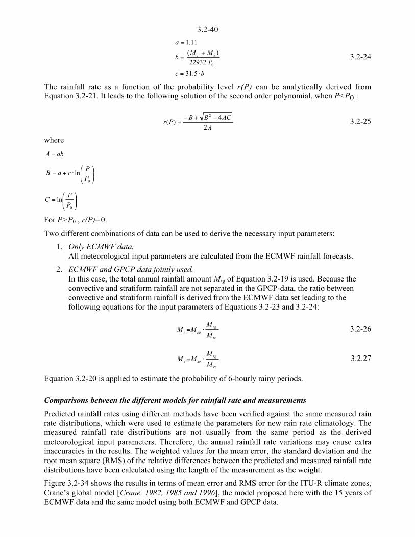
3.2-40

bc

P

MMb

a

sc

u=

+=

=

5.31

22932

)(

11.1

0

3.2-24

The rainfall rate as a function of the probability level r(P) can be analytically derived fromEquation 3.2-21. It leads to the following solution of the second order polynomial, when P<P0 :

A

ACBBPr

2

4)(

2 <+<= 3.2-25

where

abA =

´́¦

¥²²¤

£u+=

0

lnP

PcaB

´́¦

¥²²¤

£=

0

lnP

PC

For P>P0 , r(P)=0.

Two different combinations of data can be used to derive the necessary input parameters:

1. Only ECMWF data.All meteorological input parameters are calculated from the ECMWF rainfall forecasts.

2. ECMWF and GPCP data jointly used.In this case, the total annual rainfall amount Mrg of Equation 3.2-19 is used. Because theconvective and stratiform rainfall are not separated in the GPCP-data, the ratio betweenconvective and stratiform rainfall is derived from the ECMWF data set leading to thefollowing equations for the input parameters of Equations 3.2-23 and 3.2-24:

re

rgcec M

MMM u= 3.2-26

re

rgses M

MMM u= 3.2.27

Equation 3.2-20 is applied to estimate the probability of 6-hourly rainy periods.

Comparisons between the different models for rainfall rate and measurements

Predicted rainfall rates using different methods have been verified against the same measured rainrate distributions, which were used to estimate the parameters for new rain rate climatology. Themeasured rainfall rate distributions are not usually from the same period as the derivedmeteorological input parameters. Therefore, the annual rainfall rate variations may cause extrainaccuracies in the results. The weighted values for the mean error, the standard deviation and theroot mean square (RMS) of the relative differences between the predicted and measured rainfall ratedistributions have been calculated using the length of the measurement as the weight.

Figure 3.2-34 shows the results in terms of mean error and RMS error for the ITU-R climate zones,Crane’s global model [Crane, 1982, 1985 and 1996], the model proposed here with the 15 years ofECMWF data and the same model using both ECMWF and GPCP data.

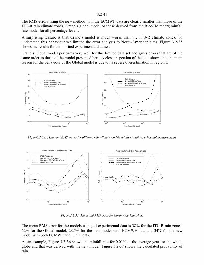
3.2-41

The RMS-errors using the new method with the ECMWF data are clearly smaller than those of theITU-R rain climate zones, Crane’s global model or those derived from the Rice-Holmberg rainfallrate model for all percentage levels.

A surprising feature is that Crane’s model is much worse than the ITU-R climate zones. Tounderstand this behaviour we limited the error analysis to North-American sites. Figure 3.2-35shows the results for this limited experimental data set.

Crane’s Global model performs very well for this limited data set and gives errors that are of thesame order as those of the model presented here. A close inspection of the data shows that the mainreason for the behaviour of the Global model is due to its severe overestimation in region H.

10-3

10-2

10-1

100

-20

-10

0

10

20

30

40

50

60

Annual probability (perc.)

Model results for all sites

ITU-R Rainzones New Model-ECMWF data New Model-ECMWG+GPCP dataCrane Rainzones

10-3

10-2

10-1

10

20

30

40

50

60

70

80

Annual probability (perc.)

Model results for all sites

ITU-R RainzonesNew Model-ECMWF dataNew Model-ECMWG+GPCP dataCrane Rainzones

Figure3.2-34: Mean and RMS errors for different rain climate models relative to all experimental measurements

10-3

10-2

10-1

100

-40

-30

-20

-10

0

10

20

Annual probability (perc.)

Model results for all North-American sites

ITU-R Rainzones New Model-ECMWF data New Model-ECMWG+GPCP dataCrane Rainzones

10-3

10-2

10-1

100

10

15

20

25

30

35

40

45

50

55

60

Annual probability (perc.)

Model results for all North-American sites

ITU-R Rainzones New Model-ECMWF data New Model-ECMWG+GPCP dataCrane Rainzones

Figure3.2-35: Mean and RMS error for North-American sites.

The mean RMS error for the models using all experimental data is 38% for the ITU-R rain zones,62% for the Global model, 28.5% for the new model with ECMWF data and 34% for the newmodel with both ECMWF and GPCP data.

As an example, Figure 3.2-36 shows the rainfall rate for 0.01% of the average year for the wholeglobe and that was derived with the new model. Figure 3.2-37 shows the calculated probability ofrain.

3.2-42

Conclusions

Here, a new rainfall rate model is presented. This model requires input parameters that were derivedfrom the 15 years of ECMWF re-analysis data. The predicted rainfall rates from the new model,Rice-Holmberg, ITU-R rain climates and Crane’s Global Rain-Rate Climate model are comparedagainst available rainfall rate measurements. The comparisons show that the model is more accuratethan the other methods. This exercise proves also that high quality numerical weather forecast datacan be used with very good results in the field of wave propagation. This is especially interestingsince at the moment, precipitation is not assimilated into these models. Developments to assimilateprecipitation data in the ECMWF may render this type of data even more attractive.

The new model presented here has been adopted by the ITU-R [ITU-R, 2000b]. Further studies formodelling monthly and/or worst month statistics as well as estimation of annual and seasonalvariations are also planned. The availability of upper air and precipitation data from the planned re-analysis exercise covering a period of 40 years is expected to improve the quality of theprecipitation climatology as well as allow more stable statistics at the level of the monthlyvariability.

Other work also in the frame of CLIMPARA (URSI) has demonstrated the quality of numericalweather forecast data for clear-air and cloud propagation effects that affect telecommunications. Inthis area access to global atmospheric vertical profiles is essential.

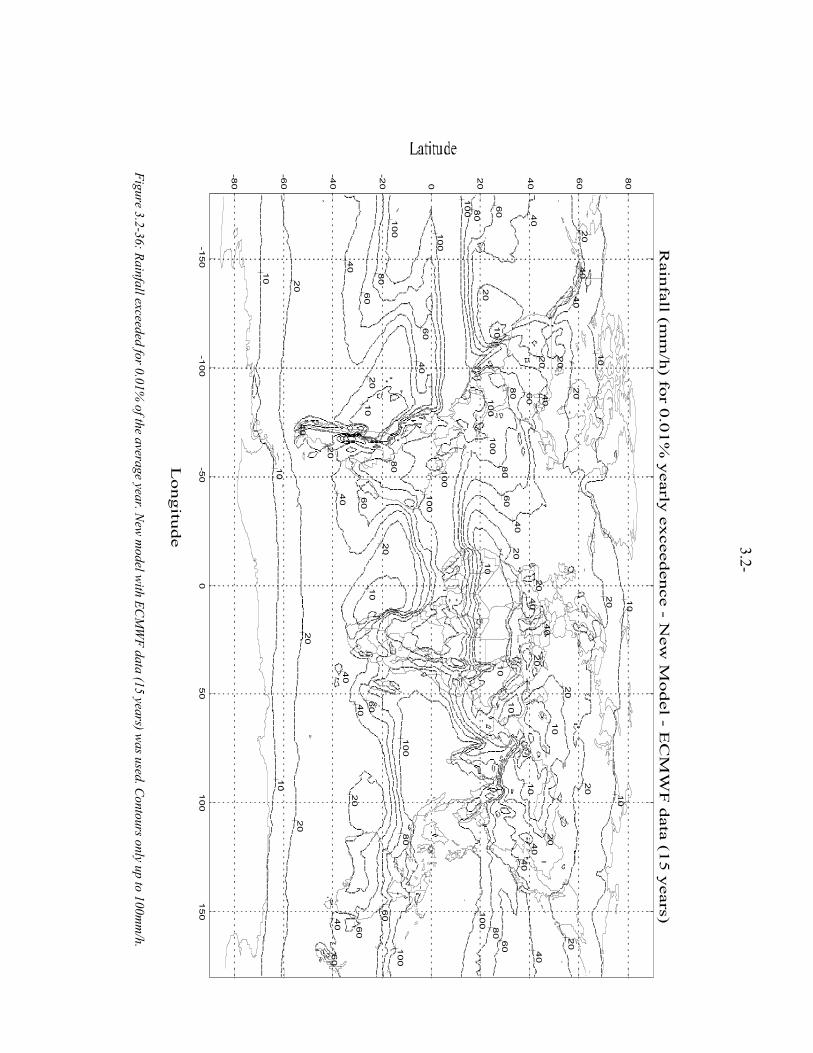
3.2-

Figure 3.2-36: R

ainfall exceeded for 0.01% of the average year. N

ew m

odel with E

CM

WF

data (15 years) was used. C

ontours only up to 100mm

/h.

-150

-100

-50

050

100

150

-80

-60

-40

-20 0

20

40

60

80

20

10

20

20

10

10

40

60

80

100 100

60

40

20

10

40 60

100

80

10

20

20

40

40

20

10

10

10

20

20

20

20

40

6080

100

20

10

20

20

40

60

80

80

60

40

20

10

10

20

20

10

40

60

80

100

10

20

40

20

20

40

40

100

100

100

80

6040

40

60

60

100

60

100

40

10

40

40

Rain

fall (m

m/h

) for 0

.01%

yearly

exceedence - N

ew

Model - E

CM

WF

data

(15 y

ears)

Longitu

de

3.2-

Figure 3.2-37:P

robability of rain. Same m

odel as Figure 4

-150

-100

-50

050

100

150

-80

-60

-40

-20 0

20

40

60

80

5

10

5

10

10

10

5

5 10

10

55

5

10

5

55

5

5

10 10

15

5

5

5

10

10

10

10

15

5

10

15

10

5

5

5

10

510

10

10

5

10

5

10

515

15

5

510

5

5

1010

Pro

bab

ility o

f Rain

(%) - N

ew

Mo

del - E

CM

WF

data

(15

years)

Lo

ng

itud

e

3.2-45

3.2.3 Models of Monthly Distributions

3.2.3.1 Monthly distribution of the water vapour

The model proposed by [Konefal et al., 2000] predicts monthly exceedance probabilities of watervapor density at the ground in order to derive monthly distribution of the attenuation due to watervapour in rainy conditions.

The model uses as input the annual statistical databases from radiosonde ascents [Davies et al.,1998] weighted to give monthly values. Annual exceedance statistics for the total water vapourcontent, V [kgm-2], are given at grid points separated by 1.5º in latitude and longitude. At each gridpoint an annual exceedance probability can be associated with V through an equation of the formV p a b p( ) ln= < where a and b are local regression coefficients. The surface value of water vapourdensityl s [gm-3] is given in [Salonen, et al., 1994] as l s sp V p h( ) ( ) /= where hs is the scale

height (assumed to be 2.93 km in rain conditions).

The annual exceedance probability of l s is thus given by ( )ssP `l_l <= exp)( where

( )baexp=_ and bhs=` . The model assumes the exponential distribution also for monthly

exceedance probabilities P em s mm s( )l _ ` l= < where_ m and ` m are the monthly parameters. By

considering a time series of l s at a particular location, it is readily verified that annual and monthlyexceedance probabilities of any particular value of l s are related by:

P Pannual mm

==-

1

12 1

12

3.2-28

Those assumptions lead to the equations:

` `m = 3.2-29

_ _==-

1

12 1

12

mm

3.2-30

We note that _ lm m sP= >( )0 and it assumed that this probability is proportional to lm , the mean

value of l s during month m.

The lm parameter can be found from the temperature and surface humidity grids using the

following equation developed by [Hall, 1979].

lmm

mm

mtU

t

t=

+×

+

�

�³

�

�µ

216 5

273611

19 7

273

.

( ). exp

. [gm-3] 3.2-31

Here tm is the mean surface temperature (ºC) and Um is the mean surface relative humidity

( 0 1) )Um ). Note that Equation 3.2-31 is approximate since it is not generally true that

f x y f x y( , ) ( , )= , where x denotes the mean value of x.

Therefore it can be assumed _ lm mk= v and we can use Equation 3.2-30 to obtain:

3.2-46

_ _l

lm

m

mm

=¨©ª

¬­®=

-1

12 1

123.2-32

l s is thus associated with a monthly exceedance probability p where

l`

_`

_l

ls m

sm

s s s

m

mm

s

p pbh

bh

pah

bh

bh

p( ) ln ln ln ln ln ln= < = < = +

¨

©««

ª««

¬

­««

®««

<

=-

1 11

12 1

12 3.2-33

Monthly surface exceedances of water vapour specific attenuation can then be found by applyingEquation 3.2-33 to the [ITU-R, 1998] water vapour attenuation model and performing numericalintegration along the radio path with an exponential atmosphere. The link path is divided into Nsections, and the height hq above the Earth’s surface for each section located at rq is determined

(q=0 to N-1). For each point Q on the Earth’s surface directly below rq the nearest four grid points

are found. Local linear regression is used to determine the annual coefficients ai and bi in the

expression V p a b pi i i( ) ln= < from the annual water vapour data grids, for each of the four grid

points (i=1 to 4). Equation 3.2-33 can then be written as:

pbbapVphm

mmss ln12

1ln)()(

12

1

<´¦

¥²¤

£+== -

=

lll 3.2-34

which suggests a monthly correction factor to ai of:

´¦

¥²¤

£=6 -

=

12

112

1ln

m

im

imi

mi ba ll 3.2-35

The value of lmi can be calculated from Equation 3.2-31, which relies on direct data from our

surface humidity and temperature grids.

Weighting factors wi are deduced for each coefficient, based on the proximity of the point Q to

each grid point. The surface value of V pq ( ) at the point Q is interpolated according to

V p a b pq q q( ) ln= < where:

-

-

=

=

6+=

4

1

4

1

)(

ii

i

miii

q

w

aawa ; b

w b

wq

i ii

ii

= =

=

-

-1

4

1

4 3.2-36

This defines a monthly surface exceedance probability for the water vapour contentl sq q sp V p h( ) ( ) /= . The surface specific attenuation of water vapoura wsq p( ) must be multiplied by

a correction factor Ctq to account for the fact that the value of l sq p( ) may not be physically

achievable at the temperature of 15 ºC taken from Equation 3.2-35. A saturation temperature iscomputed for l sq p( ) , given by t psatq sq= 14 0 22ln( . ( ))l ºC. If Ctsatq °)15 , then the correction

factor is Ctq = 1.

3.2-47

Ct

tqsatq= <

<£¤²

¥¦´1

0 6 15

100

. ( )3.2-37

In this way it is corrected for the higher temperatures necessary to sustain the higher values of l sq

(i.e. greater than about 13.3 [gm-3]). The value of attenuation coefficient, which is exceeded withprobability p at the point rq on the link path, is then given by:

a awq q wsq tq q wh p p C h h( , ) ( ) exp( / )= < 3.2-38

where

hw = 2.1 km = Equivalent height of water vapour in rain conditions multiplied by a frequencydependent factor (see [ITU-R, 1998] and Chapter 2.1).

A conservative estimate of the total water vapour attenuation for the link path is found by addingattenuations for equal exceedances for each of the N sections of the link path.

Hence, given rainy conditions, the water vapour attenuation statistics are given by:

-<

=

<=

1

0

12),()(N

qqwq

Rwvap N

phpArr

a dB 3.2-39

where r r2 1< is the distance between the two end points of the link path in km.

3.2.3.2 Monthly distribution of cloud liquid content

This model predicts monthly exceedance probabilities of reduced cloud water content in order toderive monthly distributions of cloud attenuation [Konefal et al., 2000].

The exceedance probability of redW , (kg/m3) integrated reduced liquid water content defined by the

[Salonnen and Uppala, 1991 ] cloud attenuation model, can be written in the formredW

red eWP `_ <=)( where _ and ` are local regression coefficients.

In the [Salonnen and Uppala, 1991] cloud model, there is assumed to be no liquid water present inthe cloud at temperatures below –20 ºC (see also Equation3.2-10). Thus the cloud band may beconsidered to lie within a shell lying between the 0 ºC and –20 ºC isotherms and its thickness, hc, isassumed to be about 4 km.

Mean monthly profiles (with height) of pressure, temperature and relative humidity have been madeavailable by [Barbaliscia et al., 1994] for 350 global stations (see Section 3.2.1.1 and[ITU-R, 1999]). Using linear interpolation of the respective profiles, the (mean monthly) cloud baseheight, detected using the critical humidity, i.e. the humidity value that can result in liquid watercondensation according to the Salonen model for cloud detection, and the corresponding humidityat this height could be found. These two data values were mapped on to 1.5o global grids, whichwere then used as weighting factors to predict monthly cumulative distributions of exceedances ofintegrated water vapour content (V) and integrated reduced liquid water content (Wred), from annualdistributions of these quantities.

The annual cumulative statistics of V and Wred have been produced by [Baptista and Salonen, 1998]in the form of 1.5o grids for 8 exceedance probabilities.)

The same form for monthly exceedance of Wred as for annual exceedance of ls (see previous

paragraph) , is assumed, i.e. P W em red mWm red( ) = <_ ` where _ m and ` m are monthly rather than

l t

3.2-48

By using the same mathematical form as in the previous chapter (see Equations 3.2-28 to 3.2-30)the parameters _ m m red mP W P Cloud= > =( ) ( )0 (the probability of cloud being present for the

month) and `m = ` can be derived.

It is assumed that the probability of the presence of cloud is proportional to the mean monthlysurface humidity and to the mean monthly height h-20m of the –20 ºC isotherm. The latter isassumed to be approximately 4 km above the freezing height described by [Watson et al., 1987].Therefore mmm hkU 20<=_ , where the humidity Um is interpolated from a 0 ºC isotherm grid, and k

is a proportionality constant. From Equation 3.2-30 we have for Wred :

-=

<

=12

120

12

mmmhU

k_ 3.2-40

so that

®­¬

ª©¨

==

-=

<

<< 12

120

2020

12

1

mmm

mmmmm

hU

hUhkU __ 3.2-41

(_ is known from annual statistics).

The cloud attenuation statistics along a slant path are developed in the following manner. The paththrough the cloud is divided into N sections, defining section vectors rq where q varies from 0 to

N-1. For each value of q we project back to the Earth’s surface to a point Q. The nearest four data(grid) points to Q are found and local linear regression is used on the database (grid) of annualupper air data values to find the annual regression coefficients ci and ei in the expression

W p c e predi

i i( ) ln= < for each of the four grid points (i=1 to 4). Note that ci and ei are related to

_ i and ` i by iie `1= and ( ) iiic `_ln= where _ i and ` i are annual coefficients. A monthly

correction factor to ci is introduced given by:

««®

««­

¬

««ª

««©

¨

=6

-=

<

<12

120

20

121

ln1

m

im

im

im

im

i

mi

hU

hUc

`3.2-42

based on Equation 3.2-41. The humidities Umi are direct entries in the 0 ºC isotherm humidity grids.

Weighting factors wi are deduced for each coefficient, based on the proximity of the point Q to

each grid point. The value of W predq ( ) at the point rq on the link path is then interpolated as

W p c e predq

q q( ) ln= < where:

cw c c

wq

i i im

i

ii

=+

=

=

-

-

( )61

4

1

4 ; ew e

wq

i ii

ii

= =

=

-

-1

4

1

4 3.2-43

The total cloud attenuation along the slant path, Acl, is found by combining all the contributionsalong the path, giving:

( )1N f r

3.2-49

where:

rc is the total path through cloud expressed in km.

g(f) = cloud attenuation frequency dependant constant (see Chapter 2.1)

3.2.3.3 Monthly Distributions of the Rainfall Rate

The basic form of the model equation, proposed by [Tattelman and Scharr, 1983] for prediction ofthe monthly rainfall rate distribution is:

),( TLfDICTBAR ppppp +++= 3.2-45

where

pR is the estimated 1-min. rain intensity (mm/min) for exceedance level p,

T is the monthly mean temperature (oF),

I is the precipitation index (monthly mean precipitation in mm divided by the monthly meannumber of days with precipitation)

),( TLf is a latitude-temperature term.

pA is a constant for exceedance level p pB ,

pC and pD are multiple regression coefficients for

exceedance level p. The coefficients pA ,

pB , pC and

pD correspond to a rainy day being defined

by a minimum of 0.25mm of precipitation.

The term ),( TLf is defined by:

ǻ

«©

¨

°><

°)<<

°)

=

)40()5.2340(

)405.23()5.23(

)5.23(0

),(

LT

LTL

L

TLf 3.2-46

Monthly precipitation, temperature and number of rainy days

The basic data for the grids were acquired from the Potsdam Institute for Climate Impact Research(PIK), and were originally compiled by [Cramer, 1998]. The grids in original form are global landbased grids with 0.5º resolution in latitude and longitude. For COST 255 activities it was desired toconvert the grids into global grids with 1.5º resolution in latitude and longitude, extrapolating thedata into regions over the ocean where few or no data are available.

A method was devised to smooth the original data and at the same time provide extrapolated dataover the oceans. The original PIK data were first reduced to a 1.5º land based grid, providing 6960global data points of which 838 are in the European region. The smoothed (interpolated) datum atan output grid point kr on the globe is found from the equation

-

-

=

== 6960

1

6960

1

)()(

nnk

nnnk

k

w

DwD

rr 3.2-47

where

)( nD r is the datum at each of the land based grid points nr .

3.2-50_

e ´́¦

¥²²¤

£

+=

nknkw

11 = weighting factor.

nke = angle [deg] between nr and kr .Each of these vectors has its origin at the centre of the Earth.

Various values were tried for _ . If 2<_ a lot of local detail is lost from the original PIK data(i.e. the contours are widely spaced). If 4>_ there is a lot of local detail but the contours are foundto crowd together in regions of open ocean. A value of 3=_ was finally chosen as a compromisebetween local detail being present in the contours, a degree of smoothing of the data, and contoursbeing reasonably sensibly interpolated in the ocean regions. This method of smoothing andextrapolation was found to be more than two orders of magnitude faster than the standard krigingroutines provided with IDL. The method also has the advantage that contours are properlyinterpolated on to a sphere rather than a plane, so that contours at longitudes of ± 180º join upsmoothly, and there are no contours intersecting the lines of latitude at ± 90º.

Preparation of rain intensity grids

Having produced global grids for temperature, precipitation and number of rainy days, Europeansub-grids were used in the rain rate prediction method described by Equation 3.2-45. Two rain rateexceedance levels were considered, namely 0.01% and 0.1%. Where rain provides the dominantmechanism for attenuation, these levels should prove useful in predicting the fade marginsnecessary to sustain monthly system availabilities of 99.99% and 99.9% respectively. The 1-minrain intensity grids, in units of mm/hr, have been analysed in for exceedance levels of 0.01% and0.1%.

The following points relating to the [Tattelman and Scharr, 1983] model should be noted:.

1. The Tattelman and Scharr method is not valid when T<0 ºC (32 ºF).The mean monthly temperature in many parts of Europe is less than 0 ºC during the wintermonths. In such cases, the temperature has been increased to 0 ºC in Equation 3.2-45. Thisshould provide a conservative overestimate of the rain rate.

2. The Tattelman and Scharr method is not valid when the rain rate is not a consistentlydecreasing function of exceedance probability p.In cases where the rain rate increases with p in the original model, the temperature has beenraised to 6 ºC in an attempt to produce a consistently decreasing function, whilst providing aconservative overestimate of rain rate. If after raising the temperature to 6 ºC the rain rate isstill inconsistent, a value of 0 has been entered into the rain rate grids.

3. The Tattelman and Scharr method is not valid when the precipitation index I<2 mm per dayor the number of rainy days is less than 1.In such cases a value of 0 has been entered into the rain rate grids.This mainly affects predicted rain rates in North Africa.

In view of the fact that experimental monthly rain rate data are not generally available, the datahave been integrated up to produce annual predictions for 77 European locations. (To this end themonthly exceedance levels for a given rain rate must be averaged to find the annual exceedancelevel for that rain rate).

Annual experimental rain rate data at 0.01% and 0.1% exceedance levels are available at theselocations, which include stations in Belgium, the Czech Republic, Denmark, Finland, Germany,the Netherlands, Norway, Spain, Sweden, Switzerland and the UK. Although errors in Spain of over100% were observed in the rain rate at the 0.1% exceedance level, the overall rms error at 0.1% was33.0%, whilst the rms error at 0.01% was 30.5%.

3.2-51

Excluding stations in Norway, Finland, Switzerland and Spain (leaving 46 stations), the rms errorwas found to be 15.3% for the 0.1% level and 24.0% for the 0.01% level.

The work described in this chapter has been supported by the Radio Science and PropagationGroup, DERA, Malvern, U.K. under contract number CSM/584/UA.

3.2-52

3.2 References

[Andel, 1976]Andel J., “Statistical Analysis of Time Series (Statisticka analyza casovych rad),“ SNTL 1976

[Baptista et al., 1986]Poiares Baptista J. P. V., Z. W. Zhang and N. J. McEwan, “Stability of Rain-rate CumulativeDistributions,“ Electronics Letters, Vol. 22, No. 7, pp. 350-352, March 1986

[Baptista and Salonen,, 1998]Poiares Baptista, J.P.V. and Salonen, E., "Review of rainfall rate modelling and mapping" ,Proceedings of URSI Climpara’98 Commission F Open Symposium on “Climatic Parameters inRadiowave Propagation Prediction”, Ottawa, Canada, April 1998, pp35-44

[Barbaliscia et al, 1994]Barbaliscia F., M. Boumis, A. Martellucci, J.P.V. Poiares Baptista "Modelling of the atmosphericattenuation by means of meteorological parameters", Alta Frequenza, Vol. 6, N. 6, November-December 1994, pp 101-105.

[Barbaliscia et al, 1995]Barbaliscia F., Boumis M., Martellucci A., 1995,”Study of scaling of propagation effects frommicrowave to optical frequencies”, ESA/ESTEC Contract 10195/92/NL/GS.

[Beajaars, 1999]Beajaars, A., private communication, ECMWF, 1999.

[Boumis, 1994]Boumis M., "The use of meteorological databases for the evaluation of atmospheric propagationparameters", Alta Frequenza, Vol. 6, N. 6, Novembre-Dicembre 1994, pp 106-108.

[Capsoni et al. 1987]Capsoni, C., F. Fedi, C. Magistroni, A. Paraboni, A. Pawlina, “Data and theory for a new model ofthe horizontal structure of rain cells for propagation applications”, Radio Science, Vol. 22, N.3,395-404, 1987.

[Coma et al., 1998]Coma Juan C., F. Ghaloul and A. Benarroch, “Statistics of Rain Rate Variability for SpanishRegions: The Durations of Exceedances”, Proc. of CLIMPARA’98, pp. 62-65, Ottawa, Canada,April 1998.

[Cramer, 1998]Cramer W., The CLIMATE database version 2.1, Potsdam Institute for Climate Impact Research,Personal Comm., 1998.

[Crane, 1982]Crane, R.K, “A two-component rain model for the prediction of attenuation statistics”,Radio Science, Vol. 17, N.6, 1371-1387, 1982

[Crane,1985]Crane, R.K., “Comparative evaluation of several rain attenuation prediction models”,Radio Science, Vol.20, N. 3, 843-863, 1985

[Crane, 1990]Crane R. K., “Modelling attenuation by rain in tropical regions”, Int. J. Sat. Com., Vol. 8,pp. 197-210, 1990.

[Crane, 1996]Crane R.K., Electromagnetic wave propagation through rain, John Wiley & Sons, Inc., 1996.

3.2-53

[Crane, 1998]Crane, R.K., “A local model for the prediction of attenuation caused by rain”, Climpara’98, Ottawa,1998

[Davies at al., 1998]Davies O.T., R.G. Howell, P.A. Watson, "Measurements and modelling of cloud attenuation atmillimetre wavelengths", Electronics Letters 10th Dec 1998, Vol. 34, No. 25, pp 2433-2434.

[Dutton et al., 1974]Dutton E.J., Dougherty H.T., Martin R.F., “Prediction of European rainfall and link performancecoefficients at 8 to 30 GHz”, NTIS, U.S. Department of Commerce, Rep. AD/A-000804, 1974.

[ECWMF, 1997]ECMWF, ECMWF Re-Analysis Project (ERA), 1997

[Fischer, 1940]Fischer R. A., “ On the similarity of the distributions found for the test of significance in harmonicanalysis and in Steven´s problem in geometrical probability,“ Annals of Eugenics, 10, pp. 14-17,1940

[Fischer, 1929]Fischer R. A., “Tests of significance in harmonic Analysis,“ Proc. Roy. Soc., A 125, p. 54, 1929

[Flavin, 1992]Flavin, R.K., “Rain-attenuation considerations for satellite paths in Australia”, AustralianTelecommunication Research, Vol. 16, N.2, 11-24, 1992.

[Ghaloul and Benarroch, 1996]Ghaloul F. and A. Benarroch, “Durations of the Intervals Between Rain Events for South Spain”,Proc. of CLIMPARA’96, pp. 38-39, Oslo, Norway, June 1996

[Goldhirsch and Katz, 1979]Goldhirsch J and Katz I, “Useful experimental results from earth-satellite rain attenuationmodelling, IEEE Trans. Ant. Prop., AP-27, 413-415, 1979.

[Hall, 1979]Hall, M.P.M., "Effects of the troposphere on radio communication", IEE Electromagnetic Series 8,Peter Peregrinus Ltd, 1979.

[Haurwitz and Austin, 1944]Haurwitz, B. and J.M. Austin, Climatology, McGraw-Hill, New York, 1944.

[ITU-R, 1992]ITU-R Rec. 837-1, Characteristics of precipitation for propagation modelling, ITU, Geneva, 1992.

[ITU-R, 1995a]ITU-R Recommendations, 1994 PN Series Volume, Rec. ITU-R PN. 581-2, ITU 1995

[ITU-R, 1995b]ITU-R Recommendations, 1994 PN Series Volume, Rec. ITU-R PN. 837-1, ITU 1995

[ITU-R, 1995c]ITU-R Recommendations, 1994 PN Series Volume, Rec. 841, ITU 1995

[ITU-R, 1998]ITU-R Rec. P.676-2, "Attenuation by atmospheric gases", Geneva, 1998

[ITU-R, 1999]ITU-R, Recommendation P.835-3, ”Reference standard atmospheres”, 1999

3.2-54

[ITU-R, 2000a]ITU-R, Recommendation P.453-8, ”The Radio refractive index: its formula and refractivity data”,2000

[ITU-R, 2000b]ITU-R Recommendations, P.837-2,"Characteristics of precipitiation for propagation modelling",2000

[Juy et al., 1990]Juy M, Maurel R, Rooryck M, Nugroho I A and Hariman T, 1990,”Measurements of 11 GHzattenuation using the INTELSAT V beacon in Indonesia”, Int. J. of Sat. Comm., 8, 251-256

[Lekkla et al., 1995]

Lekkla R, Lim S L, Wachja J, McCormick K S, “Rain attenuation measurements in South-EastAsia”, Proc. of the 7th URSI Comm. Open Symp., Ahmedabad, India, 241-244, 1995.

[Koeppen, 1923]Koeppen, W., Die Klimate der Erde, Walter de Gruyter, Berlin & Leipzig, 1923.

[Konefal et al., 2000]Konefal T., Watson P.A., Shukla A. K., Akrem A., 1999, ‘Prediction of Monthly and annualavailabilities on 10-50 GHz satellite-Earth and aircraft-to-aircraft links’, IEE Proc.-Microw,Antennas and Propag., Vol. 147, No. 2, April 2000

[Kvicera, 1992]Kvicera V., “Investigation of radio wave propagation for radio-relay paths and internationalcollaboration (Vyzkum sireni elektromagnetickych vln pro radioreleove spoje a mezinarodnispoluprace),“ Report of TESTCOM, Task 1 33 122, November 1992

[Landsberg, 1974]Landsberg, H., Volumes in the World Survey of Climatology, Elsevier North-Holland, New York,1974.

[Mc Ilveen, 1991]Mc Ilveen R., "Fundamentals of Weather and Climate", Chapman & Hall, 1991.

[Mercader and Benarroch, 1994]Mercader L. and A. Benarroch, “Rain Rate Distributions in Spain Related to its ClimaticCharacteristics”, Proc. of CLIMPARA’94, pp. 11.1.1-11.1.4, Moscow, Russia, 1994

[Okamoto et al., 1998]Okamoto, K., T. Iguchi, T. Kozu, H. Kumagai, J. Awaka and R. Meneghini, “Early results from theprecipitation radar on the tropical rainfall measuring mission”, Climpara’98, Ottawa, 1998

[Rogers and Yau, 1989]Rogers R. and M. K. Yau, "A Short Course in Cloud Physics", Pergamon Press, 1989.

[Rudolf, 1996]Rudolf B, 1996, “Methods and new results of estimating the global precipitation”,Abstracts of XXVth GA of URSI, 302.

[Salonen et al., 1990]Salonen E., Karhu S., Jokela P., Zhang W., Uppala S., Aulamo H., Sarkkula S., “Study ofpropagation phenomena for low availabilities”, ESA/ESTEC Contract 8025/88/NL/PR,Final Report, 1990

[Salonen and Uppala, 1991]Salonen, E. and S. Uppala, 1991, “New prediction method of cloud attenuation”, Electr. Lett.,

l 27 1106 1108

3.2-55

[Salonen et al., 1994]Salonen E, Karhu S, Uppala S, Hyvönen R, 1994, “Study of improved propagation predictions”,Final Report for ESA/ESTEC Contract 9455/91/NL/LC(SC).

[Salonen and Baptista, 1997]Salonen E T and J.P.V. Poiares Baptista, “A new global rainfall rate model”, Tenth Int. Conf. onAntennas and Propagation, IEE Conf. Publ. 436, Vol. 2, pp. 2.182-2.185, 1997.

[Rice and Holmberg, 1973]Rice P.L. andHolmberg N.R., “Cumulative time statistics of surface-point rainfall rates”, IEEETrans. Comm., COM-21, 1131-1136, 1973.

[Rodda and Williamson, 1997]Rodda M J and Williamson A G, 1997, “Results of a two year radiometric measurement programmein New Zealand”, Electronics Letters, Vol. 33, No. 4, 326-328

[Segal, 1979]Segal, B., “High-intensity rainfall statistics for Canada”, CRC report N. 1329-E, Ottawa, 1979.

[Watson et al , 1987]Watson, P.A., M.J. Leitao, V. Sathiaseelan, M. Gunes, J.P.V. Poiares Baptista, B.A. Potter, N.Sengupta, O.Turney and G. Brussaard, “Prediction of attenuation on satellite-Earth links in theEuropean region”, IEE Proc. Vol. 134, Pt.F, N.6, 583-596, 1987.

[Tattelman and Scharr, 1983]Tattelman, P. and Scharr, K.G., A model for estimating one minute rainfall rates, Journal ofClimate and Applied Meteorology, Vol. 22, September 1983, pp1575-1580.

PART 4 Terrain and Clutter Effects.

Mobile Modelling

4.1-1

CHAPTER 4.1Overview of Mobile Modelling Propagation

Author: F.Pérez-Fontán1

1Dept of Communications Technologies University of Vigo Campus universitario 36200 Vigo Spain

4.1-2

4.1 Overview of Mobile Modelling Propagation

4.1.1 Introduction

This Part of the COST 255 Final Report deals with the modelling of Terrain and Clutter Effects,primarily shadowing and multipath, which affect mobile communication systems operating in urbanareas or tree shadowed environments. In the study of mobile system performance and in systemplanning, terrain and clutter effects have to be added to tropospheric effects. The studies performedare very much related to systems currently under-deployment as well as to satellite systems of thirdand future generations. The results of Working Group 1B (Mobile Modelling) should be of help inthe evaluation of system concepts which are still in their development stages at the time of thiswriting.

At the present time only a few truly mobile satellite systems are operational, examples of suchsystems are the Euteltracs/Onmitracs, the Inmarsat M and C or the AMSC systems. These systemsare basically oriented towards the transmission of low rate data. Other, not-totally mobile systems(briefcase terminals) are available for voice applications. Typically (except for theEuteltracs/Onmitracs case) L-Band is used by these systems.

Currently, systems that may be considered to be second generation are beginning their operationaland commercial life, although with great difficulties. Examples of these systems are Iridium,Globalstar and ICO. These are all global systems, aiming to provide coverage of most parts of theplanet and based on constellations of numerous satellites either in LEO or MEO orbits, converselyto what is the case in first (or zero-th) generation mobile satellite systems which are based on GEOsatellites and aim at a regional market (except for Inmarsat). The bands used are L and S and,simplified, interworking functions with terrestrial networks, e.g. GSM, have already been definedfor dual-mode terminals.

Currently, efforts are being carried out in different international bodies towards the definition offuture third (3G) generation mobile systems (S-UMTS, IMT-2000 air interface R3, etc.).Frequencies in the S-band have already been allocated to these 3G personal communication systemsat different World Radio Conferences, WRCs. In addition to 3G systems, a need for higherbandwidth services has already led to a lot of work on 3G+ or 4G systems intended to operate innew, high-capacity bands such as Ka.

3G systems already implement the personal communications concept which is partly realised bymore complete interworking functions between the terrestrial segment (macrocells and microcells)and the satellite segment (megacells) and accomplished through the use of multi-mode terminals.

Appropriate knowledge of propagation channel conditions for mobile/personal terminals underdifferent scenarios and for different satellite constellations, is required for the definition of suchnew 3G and 3G+ systems. This has been the major objective of Euro-COST activities dealing withmobile satellite communications.

4.1.2 Modelling requirements and different approaches

From this brief overview of current and future systems several clear needs are observed. The first isrelated to the bands currently allocated for use in new satellite systems. It is clear that S-Band willcontinue to be an area of interest, since different WRCs (World Radio Conferences) have allocatedportions of this band to 3G systems. Similarly, Ka-Band is of great interest for its application tobroadband services.

Another aspect exerting a decisive influence on the modelling of the channel (actually being anintrinsic part of it) is the use of LEO or MEO satellites. How satellite movement and user terminal

4.1-3

A closely related issue to that of the orbits used is the possibility of simultaneous multi-satelliteconnections for improved availability. The utilisation of LEO or MEO satellites implies the use ofconstellations comprising a number of satellites. At a given position on Earth it may be possible forthe personal terminal to “see” several satellites at the same time (provided there is no blockage byman-made or natural features in the vicinity of the personal terminal). This fact may be used to theadvantage of system operation, especially in very cluttered environments where deep shadowingeffects would give rise to unacceptable system outages unless some satellite diversity were providedby the system - in the form of, for example, hard or soft hand-offs. This raises the issue of thecorrelation between shadowing effects for different instantaneous satellite constellation states.

If “site-specific” models are used in propagation studies, correlation effects are readily present inthe results obtained. However, if empirical or statistical models are used, correlation informationmust be forced into the modelling of simultaneously received signals from several satellites by agiven personal terminal on a given environment (dense urban, light urban, suburban, ...) andconsidering a given instantaneous constellation configuration.

The existence of brief negative correlation events is good news from the availability point of view.

Again, of course, typical mobile satellite channel aspects keep attracting the attention ofpropagation engineers. In this respect the modelling of both shadowing and multipath effects stillneeds a lot of attention.

As the bandwidths used increase, the influence of time dispersion, due to multipath, on TDMA andCDMA systems is also of great importance and a suitable characterisation of these effects is needed.

Other topics that have received some attention are those related to mobility modelling of thepersonal communication terminal and how this is introduced into the propagation models togetherwith satellite trajectories, for a realistic assessment of availability and performance.

Additional aspects to be accounted for by propagation engineers are antenna effects: how theirpatterns affect C/N statistics and consequently performance. Also the influence of the head of theuser on the actual antenna pattern has received interest. Eventually, especially for the higherfrequencies, directive antennas must be considered and aspects like tracking errors become part ofthe channel itself.

Finally, the current trend in satellite mobile propagation modelling is the development of generativemodels whose outputs are actually time series: signal variations with time, series of time-varyingtapped-delay lines, time-varying channel frequency transfer functions, etc. This approach facilitatesthe smooth and easy usage of propagation results by system engineers trying to assess theperformance of new communication systems.

The evaluation of second order statistics like distributions of fade duration with respect to a givensignal level is a major driver in this modelling trend (generative models).

4.1.3 Outcome of COST 255 mobile activities

In this section the main outcome of COST 255 from the mobile propagation modelling point ofview is presented. Apart from the usefulness of work currently under way in different projects(European Union’s ACTS, ESA, Inmarsat, ...) and its future use in the development of new systems,or contributions made or to be made to international bodies like ITU-R (Rec. P.618), ETSI, etc.

Part 4 is concerned with mobile propagation modelling. Actually, the word “mobile” is not the mostsuitable one. Part 4 actually deals with “terrain and clutter effects”. On top of those, atmosphericeffects especially at the higher frequencies, Ku-Band and above have to be added.

Part 4 of this Final Report is broken down into the following Chapters:

) I t d ti (thi h t )

4.1-4

b) Data and databases;

c) Statistical modelling;

d) Physical-statistical modelling;

e) Correlation modelling;

f) Deterministic modelling and acceleration techniques for ray-path searching in urban andsuburban environments;

g) Antenna effects: gain, polarisation and noise temperature.

In Chapter 4.2 a compilation is made of data such as electromagnetic constants of materials,normalised radar cross sections of different terrain types, and penetration losses of different walltypes. In addition, the important topic of terrain database, land usage database and urban databaseformats is included in this chapter. In Chapter 4.3 conventional and more advanced widebandgenerative statistical models are covered. Also parameters determined experimentally for thesemodels for different environments, frequency bands and elevation angles are provided. A furtherstep (Chapter 4.4) towards improved modelling of the satellite mobile channels is the use of aphysical model to describe the electromagnetic properties of the channel: diffraction, reflection, etc.The statistical part comes from the introduction of statistical observations of the environment itself,e.g. building height distributions. Chapter 4.5 analyses the correlation of shadowing effects formulti-satellite scenarios. The Mobile Propagation Modelling Working Group (WG1B) has not limititself to conventional approaches (statistical or ray-tracing based) and has gone further and morerigorous methods have been analysed from the electromagnetic point of view, such as the use of“integral equation” methods. Such approaches may not be used immediately but as computationpower increases, more thorough models will eventually be used. In addition to this, a review ismade of the basic propagation mechanisms and different electromagnetic formulations. Also inChapter 4.6 “site specific” models are dealt with. They use as inputs comprehensive representationsof the environment such as urban databases, and ray-tracing and UTD techniques are employed toanalyse the channel behaviour. Finally, Chapter 4.7 analyses antenna related effects, namely, gain,polarisation and noise temperature.

Unfortunately, the number of participating members of the mobile working group has not allowedthe coverage of important topics of decisive importance in the characterisation of relevantoperational scenarios. The urban environment is very well covered but, from the deterministicmodelling point of view, rural environment effects like vegetation absorption have not beencovered. In this case, reference has to be made to other COST work (e.g. COST 235).

4.1.4 Conclusions

In this chapter the main activities carried out in the field of Mobile Satellite Propagation Modellingwithin COST 255 are presented. The studies carried out have been put in the perspective of the new3G and 3G+ systems currently in their conception stages.

4.2-1

CHAPTER 4.2 Data and Databases

for Land Mobile Satellite Propagation

Editor: Martin Döttling1

Authors: Martin Döttling1, Norbert Geng2, Werner Wiesbeck2

1 Siemens AG, System Engineering / UMTS Development, Haidenauplatz 1, D-81667 Muenchen, Germany Tel. +49-89-722-58703, Fax: +49-89-722-27089, E-Mail: Martin.Doettling@mch.siemens.de 2 Universität Karlsruhe, IHE, Kaiserstraße 12, D-76128 Karlsruhe, Germany, Tel.: +49-721-608-6257, Fax.: +49-721-691865, e-mail: Werner.Wiesbeck@etec.uni-karlsruhe.de

4.2-2

4.2 Data and Databases for land mobile satellite propagation

The land mobile satellite (LMS) propagation channel is predominantly influenced by the surroundings of the mobile terminal (MT), e.g. by shadowing or multipath. Hence, the description of the operational scenario is of major importance for any kind of channel model.

Empirical channel models simply use a qualitative description of the mobile user's surroundings with coarse and often not well-defined classification of the environment. In contrast, all models, which rely on a physical background, need a more elaborate representation of the environment. Physical-statistical models derive channel statistics by means of a statistical description of the environment. Therefore satellite elevation or building height distributions are typically required. Physical-deterministic models require detailed data of relevant terrain features (like topography, land use, or building data) and electromagnetic parameters (e.g., permittivity, roughness parameters) to predict wideband and narrowband channel parameters.

The prediction performance of all channel model types is closely linked to the accuracy of the databases, which serve as model inputs. This chapter considers topographical, land use and building data, which describe the terrestrial part of the propagation scenario. In addition, electromagnetic and statistical parameters of natural and man-made land use elements, as well as parameters for empirical propagation models for penetration losses and scattering are summarised. Statistical parameters for empirical channel models (such as channel state probabilities, distribution functions for fast and long-term fading, etc.) are excluded, since they are model-specific and do not describe the environment as such. The focus is on format, resolution, availability and relevance of the data. Parameter variability and the main parameter dependencies are also considered.

4.2.1 Description of the Propagation Scenario

This section gives an overview of the data required to specify the terrestrial part of the propagation scenario. Data formats, processing and resolution issues are addressed.

4.2.1.1 Data Content The description of the terrestrial environment uses the following data types: topography, land use, building data and mobile path. Depending on the application, only a subset of these data sets can be used, since other data may be irrelevant.

Topographical data contain information about the local terrain height above sea level. A classification of the terrain usage is provided by land use data. These data provide macroscopic information about the land use (e.g., built-up land, agriculture, forest, and water). Single (but important) terrain features, like roadside buildings, roadside trees, power lines, utility poles, streets and street borders are not included in these databases. These objects must be included statistically (see Section 4.2.1.3 ).

Classifications of natural and man-made areas are widely used in agriculture, geography, environmental policy and remote sensing. For wave propagation modelling the classification must distinguish classes with relevant changes in electromagnetic material properties. Therefore specific classification schemes have been proposed [Ulaby and Dobson, 1989; Döttling et al., 1998; ITU-R, 1998b; Döttling, Wiesbeck, 1999].

While land use data are sufficient for rural applications, a precise knowledge of building geometry is required in urban areas. This may also include information about trees, parks, rivers and lakes in towns.

To assess the impact of user mobility on the LMS communication channel, the mobile path also has to be specified. Therefore available GPS measurement data, user-specified mobile trajectories or random walk generators are used. The spatial or temporal sampling rate must resolve the channel

4.2-3

coherence time and ensure that all relevant changes in the environment of the mobile terminal are included.

In satellite communications, system planning is required rather than local coverage planning. Consequently, topographical, land use, building and mobile data can be generated synthetically [Schorcht et al., 1996], since only typical landscapes are required to obtain representative channel data.

4.2.1.2 Deterministic Data

Raster Data Deterministic databases are provided in either raster or vector format. In the first case, a matrix of data values is given and a relationship between the row and column indices and the distance from the origin is established. It is convenient to use (or convert the given data to) matrices with equidistant data values in a Cartesian co-ordinate system with orthogonal basis vectors. Thus the co-ordinates &�x i, j� � of each matrix point can be calculated according to:

��&�x i, j� � &�x 0� i � rx � ˆ e x � j � ry � ˆ e y 4.2-1

where:

��&�x 0 = co-ordinates of the origin

i , j = column and row indices (integer)

rx , ry = grid resolution along the x- and y-axes

ˆ e x , ˆ e y = unit vectors along the co-ordinate axes, respectively.

For each pair of i and j, a value f (i, j) is given in the database.

In many applications data values are required for points, which do not coincide with a grid point of the database, i.e., the matrix indices are real-valued. Since the channel model's performance is sensitive to resolution and accuracy of the input data, it is crucial to extract maximum information from the database.

For continuous data (like topographical height) a bilinear interpolation scheme may be used:

f (x, y) bc � f (i� , j� ) � bd � f (i� , j�) � ad � f (i � , j �) � ac � f (i� , j� )

bc � bd � ad � ac 4.2-2

which uses the surrounding four data values y(ir , jr ) of the database.

The parameters a, b, c and d are given by:

a (y � j �) and b ( j� � y)

c (i� � x) and d (x � i�) 4.2-3

where x and y are the real-valued indices of the point under test.

Figure 4.2-1 shows an example and the definition of the geometrical parameters.

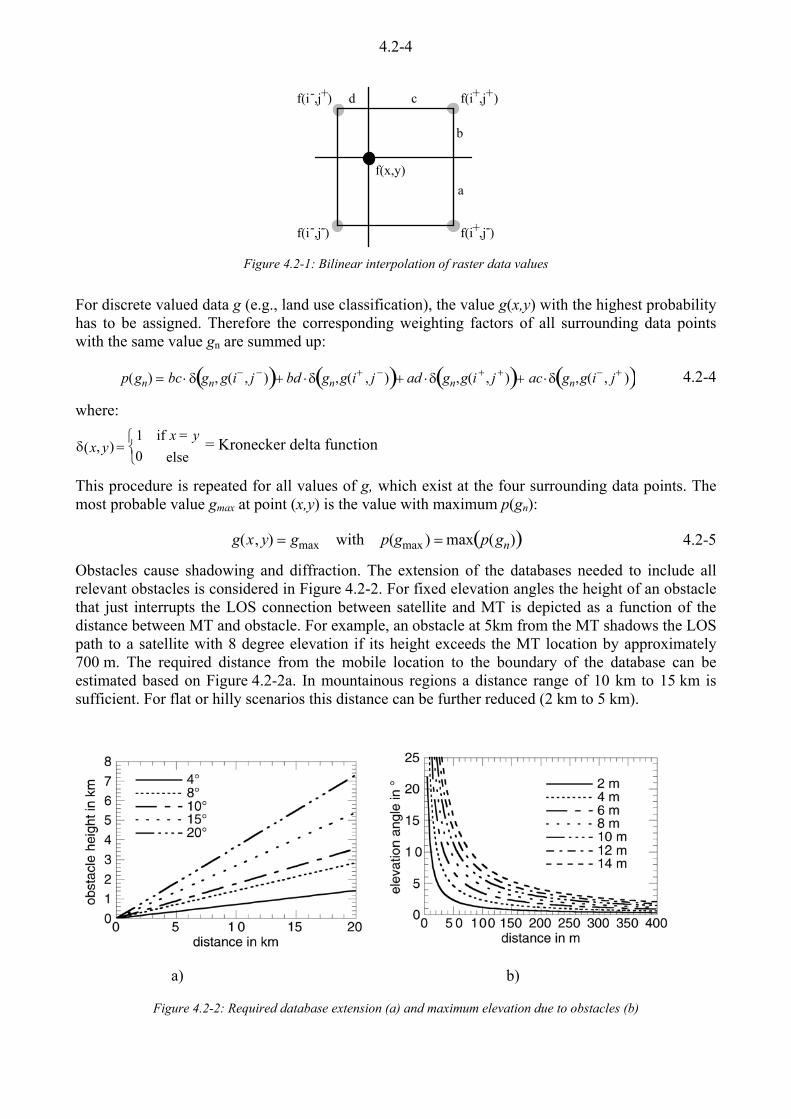
4.2-4

Figure 4.2-1: Bilinear interpolation of raster data values

For discrete valued data g (e.g., land use classification), the value g(x,y) with the highest probability has to be assigned. Therefore the corresponding weighting factors of all surrounding data points with the same value gn are summed up:

p(gn) bc � G gn, g(i� , j �)� �� bd �G gn,g(i� , j �)� �� ad �G gn,g(i � , j �)� �� ac �G gn,g(i� , j� )� � 4.2-4

where:

G(x�y�� 1 if x y� else­�®�¯�

= Kronecker delta function

This procedure is repeated for all values of g, which exist at the four surrounding data points. The most probable value gmax at point (x,y) is the value with maximum p(gn):

g(x, y) gmax with p(gmax ) max p(gn)� � 4.2-5

Obstacles cause shadowing and diffraction. The extension of the databases needed to include all relevant obstacles is considered in Figure 4.2-2. For fixed elevation angles the height of an obstacle that just interrupts the LOS connection between satellite and MT is depicted as a function of the distance between MT and obstacle. For example, an obstacle at 5km from the MT shadows the LOS path to a satellite with 8 degree elevation if its height exceeds the MT location by approximately 700 m. The required distance from the mobile location to the boundary of the database can be estimated based on Figure 4.2-2a. In mountainous regions a distance range of 10 km to 15 km is sufficient. For flat or hilly scenarios this distance can be further reduced (2 km to 5 km).

a) b)

Figure 4.2-2: Required database extension (a) and maximum elevation due to obstacles (b)

a

b

cd

f(i-,j-) f(i+,j-)

f(i+,j+)f(i-,j+)

f(x,y)

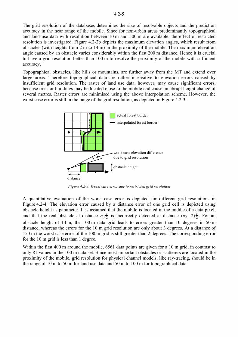
4.2-5

The grid resolution of the databases determines the size of resolvable objects and the prediction accuracy in the near range of the mobile. Since for non-urban areas predominantly topographical and land use data with resolution between 10 m and 500 m are available, the effect of restricted resolution is investigated. Figure 4.2-2b depicts the maximum elevation angles, which result from obstacles (with heights from 2 m to 14 m) in the proximity of the mobile. The maximum elevation angle caused by an obstacle varies considerably within the first 200 m distance. Hence it is crucial to have a grid resolution better than 100 m to resolve the proximity of the mobile with sufficient accuracy.

Topographical obstacles, like hills or mountains, are further away from the MT and extend over large areas. Therefore topographical data are rather insensitive to elevation errors caused by insufficient grid resolution. The raster of land use data, however, may cause significant errors, because trees or buildings may be located close to the mobile and cause an abrupt height change of several metres. Raster errors are minimised using the above interpolation scheme. However, the worst case error is still in the range of the grid resolution, as depicted in Figure 4.2-3.

Figure 4.2-3: Worst case error due to restricted grid resolution

A quantitative evaluation of the worst case error is depicted for different grid resolutions in Figure 4.2-4. The elevation error caused by a distance error of one grid cell is depicted using obstacle height as parameter. It is assumed that the mobile is located in the middle of a data pixel, and that the real obstacle at distance n0

r2 is incorrectly detected at distance (n0 � 2) r

2 . For an obstacle height of 14 m, the 100 m data grid leads to errors greater than 10 degrees in 50 m distance, whereas the errors for the 10 m grid resolution are only about 3 degrees. At a distance of 150 m the worst case error of the 100 m grid is still greater than 2 degrees. The corresponding error for the 10 m grid is less than 1 degree.

Within the first 400 m around the mobile, 6561 data points are given for a 10 m grid, in contrast to only 81 values in the 100 m data set. Since most important obstacles or scatterers are located in the proximity of the mobile, grid resolution for physical channel models, like ray-tracing, should be in the range of 10 m to 50 m for land use data and 50 m to 100 m for topographical data.

worst case elevation differencedue to grid resolution

obstacle height

distance

actual forest border

interpolated forest border

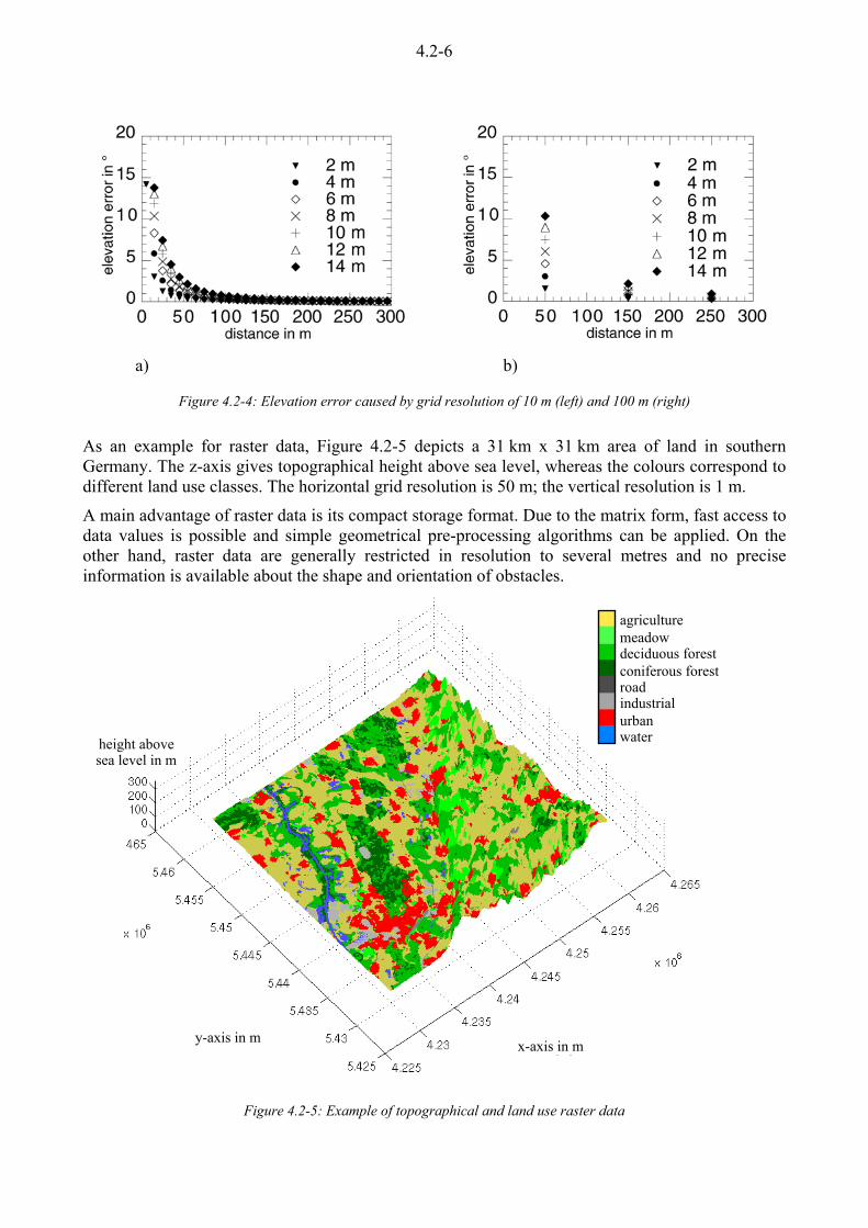
4.2-6

a) b)

Figure 4.2-4: Elevation error caused by grid resolution of 10 m (left) and 100 m (right)

As an example for raster data, Figure 4.2-5 depicts a 31 km x 31 km area of land in southern Germany. The z-axis gives topographical height above sea level, whereas the colours correspond to different land use classes. The horizontal grid resolution is 50 m; the vertical resolution is 1 m.

A main advantage of raster data is its compact storage format. Due to the matrix form, fast access to data values is possible and simple geometrical pre-processing algorithms can be applied. On the other hand, raster data are generally restricted in resolution to several metres and no precise information is available about the shape and orientation of obstacles.

height above sea level [m]

road

water

agriculturemeadowdeciduous forestconiferous forest

industrialurban

height above sea level in m

y-axis in m x-axis in m

Figure 4.2-5: Example of topographical and land use raster data

4.2-7

Vector Data Vector data represent the objects as polygons. 2.5D vector data use the 2D-co-ordinates of the objects' ground plan and assign a constant height above ground to the whole object (e.g., building). This implies that the vertical facets must be perpendicular to the ground plane. In general, these data do not include information about the shape of the roof. In 3D vector data an object is specified by explicitly giving the 3D-co-ordinates of all corners. Therefore each facet is represented by a separate polygon. This format makes it possible to include roof data efficiently. In addition, elevated structures like bridges and balconies can be modelled. Figures 4.2-6 and 4.2-7 respectively show examples of 2.5D and 3D vector data for urban areas.

The same object can be specified in many ways, which has led to a vast number of specific vector data formats used in propagation modelling. Recently, standardisation processes have been started [DERA, 1998] which are based on the CAD format DXF, mainly due to its status as an industrial standard, but also due to the relative ease of interpretation and the availability of powerful visualisation tools.

To allow the use of efficient data processing algorithms all polygons must be closed (i.e., the first and last point of a facet are identical). Inner and outer areas can be distinguished either by means of a test point within the facet or orientation of the borderlines. Further attributes are assigned to each facet, such as type of object, material and electromagnetic parameters. Object types can be a classification of land use, buildings, vegetation layers, and river or water outlines. Basic geometrical processing algorithms for vector data include the calculation of facing walls, intersection and visibility tests, as well as point location procedures (cf. Chapter 4.7).

height aboveground in m

y-axis in m

x-axis in m

Figure 4.2-6: 2.5D urban vector data

The main advantages of vector data are high accuracy (in the range of decimetres to 1 m) and resolution (centimetres or decimetres), as well as exact orientation information for each facet. However, the vector data format is less well optimised for storage. Moreover, consistency problems like overlapping or nested polygons, multiple digitisation of the same object, self-intersection or non-planar facets need to be addressed. In general, the geometrical processing (path finding) is more complex than with raster data, resulting in higher computational effort.

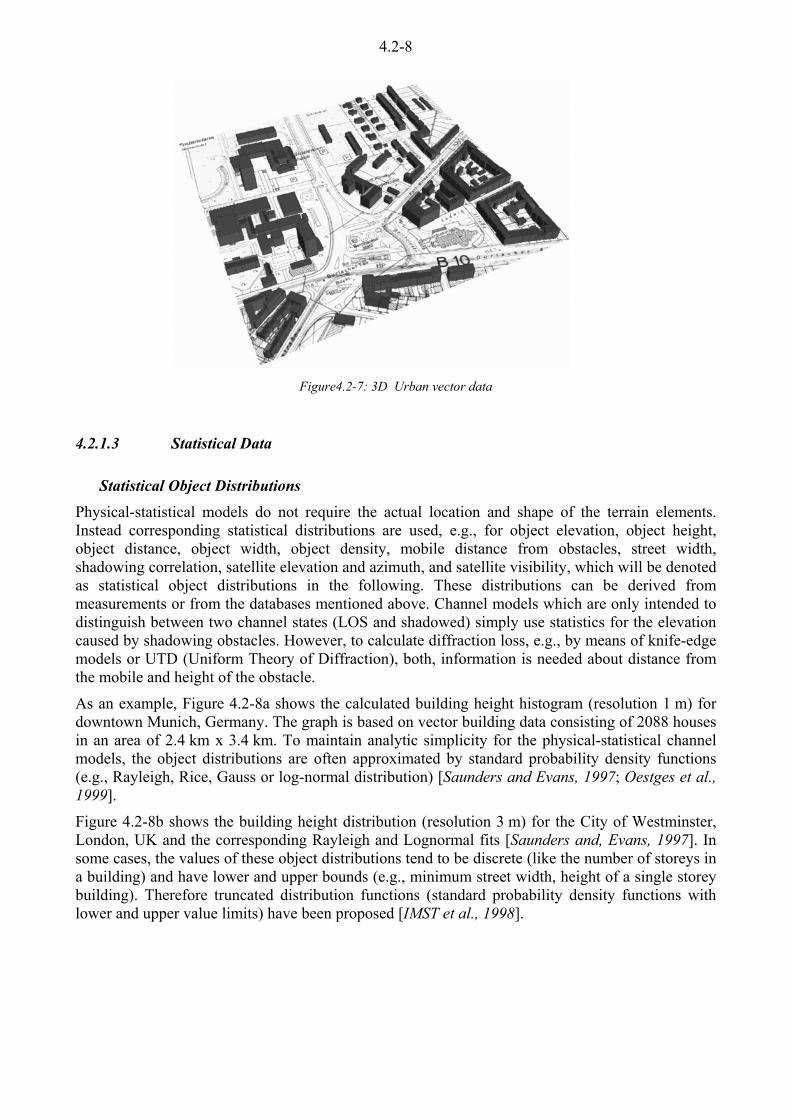
4.2-8

Figure4.2-7: 3D Urban vector data

4.2.1.3 Statistical Data

Statistical Object Distributions Physical-statistical models do not require the actual location and shape of the terrain elements. Instead corresponding statistical distributions are used, e.g., for object elevation, object height, object distance, object width, object density, mobile distance from obstacles, street width, shadowing correlation, satellite elevation and azimuth, and satellite visibility, which will be denoted as statistical object distributions in the following. These distributions can be derived from measurements or from the databases mentioned above. Channel models which are only intended to distinguish between two channel states (LOS and shadowed) simply use statistics for the elevation caused by shadowing obstacles. However, to calculate diffraction loss, e.g., by means of knife-edge models or UTD (Uniform Theory of Diffraction), both, information is needed about distance from the mobile and height of the obstacle.

As an example, Figure 4.2-8a shows the calculated building height histogram (resolution 1 m) for downtown Munich, Germany. The graph is based on vector building data consisting of 2088 houses in an area of 2.4 km x 3.4 km. To maintain analytic simplicity for the physical-statistical channel models, the object distributions are often approximated by standard probability density functions (e.g., Rayleigh, Rice, Gauss or log-normal distribution) [Saunders and Evans, 1997; Oestges et al., 1999].

Figure 4.2-8b shows the building height distribution (resolution 3 m) for the City of Westminster, London, UK and the corresponding Rayleigh and Lognormal fits [Saunders and, Evans, 1997]. In some cases, the values of these object distributions tend to be discrete (like the number of storeys in a building) and have lower and upper bounds (e.g., minimum street width, height of a single storey building). Therefore truncated distribution functions (standard probability density functions with lower and upper value limits) have been proposed [IMST et al., 1998].

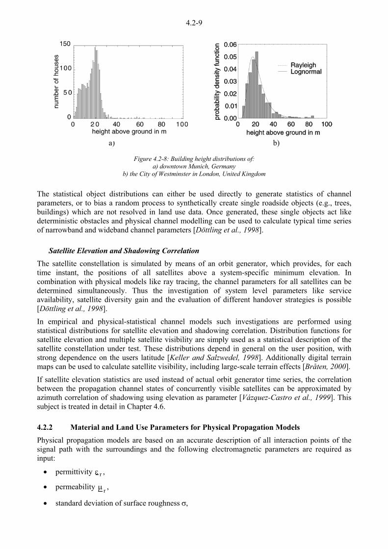
4.2-9

a) b)

Figure 4.2-8: Building height distributions of: a) downtown Munich, Germany

b) the City of Westminster in London, United Kingdom

The statistical object distributions can either be used directly to generate statistics of channel parameters, or to bias a random process to synthetically create single roadside objects (e.g., trees, buildings) which are not resolved in land use data. Once generated, these single objects act like deterministic obstacles and physical channel modelling can be used to calculate typical time series of narrowband and wideband channel parameters [Döttling et al., 1998].

Satellite Elevation and Shadowing Correlation The satellite constellation is simulated by means of an orbit generator, which provides, for each time instant, the positions of all satellites above a system-specific minimum elevation. In combination with physical models like ray tracing, the channel parameters for all satellites can be determined simultaneously. Thus the investigation of system level parameters like service availability, satellite diversity gain and the evaluation of different handover strategies is possible [Döttling et al., 1998].

In empirical and physical-statistical channel models such investigations are performed using statistical distributions for satellite elevation and shadowing correlation. Distribution functions for satellite elevation and multiple satellite visibility are simply used as a statistical description of the satellite constellation under test. These distributions depend in general on the user position, with strong dependence on the users latitude [Keller and Salzwedel, 1998]. Additionally digital terrain maps can be used to calculate satellite visibility, including large-scale terrain effects [Bråten, 2000].

If satellite elevation statistics are used instead of actual orbit generator time series, the correlation between the propagation channel states of concurrently visible satellites can be approximated by azimuth correlation of shadowing using elevation as parameter [Vázquez-Castro et al., 1999]. This subject is treated in detail in Chapter 4.6.

4.2.2 Material and Land Use Parameters for Physical Propagation Models

Physical propagation models are based on an accurate description of all interaction points of the signal path with the surroundings and the following electromagnetic parameters are required as input:

x� permittivity H r ,

x� permeability P r ,

x� standard deviation of surface roughness V�

4.2-10

x� correlation length L,

x� specific attenuation parameters K��Q and J�

x� mean layer height hv

Table 4.2-1 summarises the most important propagation phenomena and the required parameters. A definition of the parameters will be given in the following. Typical mean parameter values for different materials and land use classes have been compiled from the literature and are given in [IMST et al., 1998] and [Döttling, 1998]. Tabulations of material parameters for dielectric matter can be found in [Hippel, 1995].

Model Hro Hrf fr N Pr V� L K Q J hv

LOS x reflection x x x x x diffraction x x x x x surface scattering x x x x x x x volume scattering x x x x x x x x transmission loss x x x x

Table 4.2-1: Required electromagnetic parameters

4.2.2.1 Permittivity Reflection, diffraction and rough surface scattering calculations use the complex permittivity H r of the material, defined by:

H r Hrc � jHr cc � j N2SfHo

, 4.2-6

where:

Hr c = Real part of the permittivity

Hr cc= Dielectric losses

N = Conductivity.

Due to the wide frequency range to be covered, from L-Band to EHF-Band, the dominant influence of dispersion and water content on permittivity is further considered. For water, the Debye formula [Ulaby et al., 1981] models the frequency dependence of the permittivity using a static and a high frequency value (Hro and Hrf , respectively) of the dielectric constant and the relaxation frequency fr :

H r f� � Hrf �Hro � Hrf1 � j f

fr

� j N2SfHo

. 4.2-7

The relaxation frequency fr is a function of temperature, with values approximately to 9 and 17 GHz for temperatures of 0 and 20 qC [Ulaby et al., 1981], leading to a high variability of the permittivity at Ka-Band. As an example, Figure 4.2-9 shows the frequency dependence of the real and imaginary part of the permittivity for pure (p) and sea (s) water [Ulaby et al., 1981].

Equation 4.2-7 describes the relaxation phenomenon of water. Most natural materials can be considered as a homogeneous mixture of a background material and water. Thus the above formula can be used with effective values of Hro and Hrf [Mätzler, 1994], which depend on the water content. Hro values range from 5 (very dry terrain) to 40 (very wet terrain), whereas Hrf is always

4.2-11

a) b)

Figure 4.2-9: Frequency dependence of the permittivity for water

about 5 [Geng and Wiesbeck, 1998]. Since information on water content is difficult to obtain, and due to the fact that the water content of man-made and natural structures shows distinct spatial and temporal variations, only mean values for Hro and Hrf are available. The values for different land use classes are derived from measurement data in [COST 712, 1999].

Figure 4.2-9a shows the frequency dependence of reflection from medium wet terrain (Hro = 20) for circular co-polarisation (cp) and cross-polarisation (xp). The difference in reflection coefficient between L-Band and EHF-Band is below 2 dB for most of the elevation angles. Co- and cross-polarisation reach equal level around the Brewster angle, for higher elevations cross-polarisation dominates.

The dependency on water content is more distinct, as depicted in Figure 4.2-9b. For 1.5 and 40 GHz the reflection coefficients are given for dry terrain with Hro = 5 and for wet terrain Hro = 40. Increasing water content increases the cross-polarisation and decreases the co-polarised reflection. Land use classes or materials, that do not show the typical relaxation behaviour (e.g., due to negligible water content), can be modelled by

Hro Hrf . 4.2-8

a) b)

Figure 4.2-10: Dependence of reflection coefficient on frequency for medium wet farmland

4.2-12

4.2.2.2 Permeability A complex permeability is defined, similar to Equation 4.2-7. However, since natural and man-made structures d noto in general have magnetic properties, one may use:

Pr c�P�r � j c�c�P�r | 1 4.2-9

4.2.2.3 Surface Roughness Parameters For rough surface scattering a statistical description of the ground surface is necessary. It is based on the standard deviation V and correlation length L of surface height [Ruck et al., 1970; Ulaby et al., 1981]. Additionally, an appropriate height correlation function has to be identified to use the Small Perturbation Method [Ulaby et al, 1981], one of the Kirchhoff Models [Ruck et al., 1970], or the Integral Equation approach derived in [Fung, 1994].

The standard deviation V of a statistically rough surface is defined as:

V z(x,y) � z(x, y)� �2 4.2-10

where

z(x, y) = Mean height in an area of Lx �Ly [Geng and Wiesbeck, 1998]:

z(x, y) 1

LxLyz(x,y)dxdy

�Ly2

�Ly2

³�Lx

2

�Lx2

³ 4.2-11

Typical values of V are in the range of a few centimetres for natural surfaces and in the millimetre range for man-made surfaces [Borgeaud et al., 1995; Oh et al., 1992; Mattia et al., 1997; Borgeaud & Bellini, 1998]. The normalised autocorrelation function U of the height fluctuations 'z is defined by

U 'x,'y� �

'z(x, y)'z(x � 'x, y � 'y)dxdy�Ly

2

�Ly2

³�Lx

2

�Lx2

³

'z(x, y)2 dxdy�L y

2

�L y2

³�Lx

2

�Lx2

³

4.2-12

with

'z z(x, y) � z(x, y)

The correlation length L is defined as the distance where the value of U reduces for the first time to 1/e:

U 'xL,'yL� � 1e

o L 'xL2 � 'yL

2 . 4.2-13

For natural terrain L is in the range of decimetres [Borgeaud et al., 1995; Oh et al., 1992; Mattia et al., 1997; Borgeaud & Bellini, 1998]].

Electromagnetically smooth surfaces have to be distinguished from rough surfaces, because reflection models can calculate wave interaction with the former, whereas scattering models have to

4.2-13

be applied for the latter. The appropriate smoothness condition is known as the Fraunhofer criterion:

V �O

32 cosT i 4.2-14

where

Ti = Incident angle of the signal with respect to the surface normal.

Equation 4.2-14 shows that roughness in electromagnetic terms is dependent on the wavelength and the incidence angle. For example a rough surface with V = 2 cm will result in specular reflection for elevations lower than 18 degrees at L-Band, whereas at 20 GHz this angle is already in the range of 1 degree. With increasing elevation and frequency, surfaces appear "rougher" in an electromagnetic sense. Thus increasing roughness or increasing frequency leads to a transition from specular reflection to diffuse scattering.

4.2.2.4 Mean Layer Height If raster data are used, topographical data contain only the terrain height above sea level. Therefore a mean layer height above ground has to be identified for areas with high vegetation (forests, bushes, etc.) or built-up areas [Döttling, 1998]. The total height (including the land use layer) is especially important for determining LOS conditions, penetration length inside the medium, etc.

4.2.3 Parameters for Empirical Propagation Models

A thorough physical calculation of wave propagation effects is sometimes omitted due to the complexity of the propagation phenomenon. Empirical propagation models are used instead, the parameters of which are derived using measurement data matching rather than physical insight into the propagation process. All such models involve one or more arbitrary constants, which are generally functions of several physical parameters, such as surface type or frequency. In the following, empirical propagation models for forward scattering in foliage, for building penetration and for rough surface scattering, are considered, with emphasis on the required parameters and validity range.

4.2.3.1 Attenuation in Vegetation Volume scattering theory has to be applied to calculate bistatic scattering from dense vegetation (e.g. forests). Due to computational complexity and missing ground truth parameters, today's wave propagation tools rarely use physical volume scattering models (e.g., the Radiative Transfer Theory [Ishimaru, 1978; Fung, 1994; Didascalou et al., 1999]). For forward scattering the empirical Modified Exponential Decay Model is frequently used:

Dp

dB K �

f1MHz§�©�¨� ·�

¹�¸�Q

�d

1m§�©�¨� ·�

¹�¸�J

. 4.2-15

In this model the empirical parameters K��Q and J have to be determined.

In [ITU-R, 1986] the following parameters are given:

K 0.187, X 0.284, J 0.588 0 m � d � 400m 4.2-16

According to [ITU-R, 1986] the exponential decay model is valid from 200 MHz to 95 GHz and for penetration lengths d less than 400 m. The COST 235 action distinguishes between leafless and leafy cases. Based on measurements in the frequency range from 11.2 to 37.5 GHz the following parameters are determined [COST 235, 1996]:

4.2-14

K 26.6, X �0.2, J 0.5 leafless caseK 15.6, X �0.009, J 0.26 in leaf case 4.2-17

A comparative study of these models with Ka-Band measurements is given in [D'Amato et al., 1997]. Further empirical constants have been obtained for UHF and L-Band in [Barts and Stutzman, 1992]:

K 0.45, X 0.284, J 0.0 0m � d �14 mK 1.33, X 0.284, J �0.412 14 m � d � 400m 4.2-18

Another way of modelling vegetation losses is proposed by Tamir [Tamir, 1977]. This approach assumes lateral wave propagation along the forest - air interface. The vegetation is considered as a homogeneous dielectric slab with an effective value for the permittivity. Although commonly used up to L-Band, the original work mentions an upper validity limit of 200 MHz. For all these approaches, the thickness of vegetation layers hv is necessary to calculate the path length d in the absorbing layer.

4.2.3.2 Building Penetration Building walls consist of material mixtures, multiple layers and rough surfaces. Modern windows are also complex materials, often including special coatings. Therefore analytical calculation of radio transmission is very complicated, also due to missing information on exact material parameters. Consequently, measurements of transmission loss are widely used in wireless communication systems planning. The following section summarises relevant measurements of building penetration.

Different definitions are used in literature for the term "building penetration loss", for example:

a) the difference between the signal level before the wall and immediately behind the wall [ITU-R, 1998a],

b) the difference between the median signal level at 1.5 m above the ground and the signal level immediately inside the building at some reference level on the floor of interest [ITU-R, 1998a].

Definition (1) considers the loss introduced by one specific wall at a specific incidence angle, whereas definition (2) – originating from measurements for terrestrial wireless systems – includes different physical effects (slant range, incidence angle, transmission loss, number of walls, etc.). Thus definition (2) is dependent on the specific scenario under consideration, but gives rough overall estimates of signal quality at typical indoor locations. For definition (2) median values between 10 dB and 18 dB with a standard deviation of about 7.5 dB or 8 dB are reported in the literature [ITU-R, 1998a; 1998c]. An overall decrease of 1.9 dB per floor with increasing height is reported. Signal loss within the building also increases when the distance to the exterior wall increases. Measurements indicate inverse distance power law exponents between 2 and 4 [ITU-R, 1998a]. A summary of published penetration loss measurements for different frequencies and materials is given in Table 4.2-2 [COST 231, 1999; De Backer et al., 1996; Tanis and Pilato, 1993].

The frequency dependence of building penetration is investigated in [Zhang and Hwang, 1994]. The penetration loss is measured according to definition (1) for different wall types in the frequency range from 1.5 GHz to 18 GHz (see Figure 4.2-11).

While the penetration loss increases steadily with frequency for the (reinforced) concrete walls, the plasterboard wall measurement shows a minimum at 7 GHz. Considering the low link margins of LMS systems, reliable indoor coverage (apart from high-penetration paging) seems to be almost impossible without dedicated signal repeating systems.

4.2-15

Type of wall Frequency in GHz

penetration loss in dB

thick (25cm) concrete, large windows 1.7 4 - 12 thick concrete, no windows 1.7 10 - 18 thin (10cm) concrete 1.7 3 - 7 brick wall (25cm), small windows 1.7 3 – 5 steel wall (1cm), large reinforced windows 1.7 9 – 11 glass wall 1.7 1 - 3 reinforced glass 1.7 7 - 9 brick wall with thin concrete layer, one three-plate glass window, open window

1.8 0 – 12

brick wall with thin concrete layer, one three-plate glass window, closed window

1.8 11 – 16

office complex 1.9 10 mall 1.9 11 hotel 1.9 11 bi-level mall 1.9 8 plain glass 60 5/cm marble 60 5/cm natural slate 60 50/cm solid brick 60 4/cm asbestos cement 60 25/cm dry plastered brick 60 1.5/cm – 3/cm dry plaster 60 0.8/cm – 2/cm humid plaster 60 8/cm fibre board 60 6/cm – 8/cm synthetic carpet 60 1/cm plywood 60 6/cm cardboard 60 4.5/cm paper 60 7/cm plaster 3 0.44/cm natural slate 60 50/cm

Table 4.2-2: Penetration loss for different materials

Figure 4.2-11: Frequency dependence of penetration loss

A comprehensive study of the satellite-to-indoor propagation channel can be found in [Bodnár et al., 1999]. The elevation and azimuth dependence of penetration loss into a 7-storey concrete office building is investigated, based on helicopter measurements at L- and S-Band. Building penetration losss with respect to a reference measurement at the building roof, ranges from 19 to 25dB on the first floor, from 13 to 18 dB on the 4th floor and from 16 to 19 dB at the 7th floor. For the lower floors high elevation angles yield a maximum of attenuation, whereas a minimum is observed for

4.2-16

higher floors. Particularly the azimuth dependence (but also the elevation dependence) is very sensitive to the satellite and mobile position, as well as to the building structure [Bodnár et al., 1999].

Since handheld terminals may also be operated inside a car, the transmission loss through car windscreens is of particular interest for LMS system planning. At 1.9 GHz penetration losses between 8 and 10 dB are reported [ITU-R, 1998a]. The frequency dependence of radio transmission through car windows is investigated in [Zwick et al., 1997]. Measurements are performed between 4 GHz and 20 GHz using different incidence angles. A typical car front screen with two layers of glass and an intermediate PVC layer is used. The penetration loss is between 4 and 7 dB at S-Band and between 8 and 13 dB at K-Band. The results depend on incidence angle and polarisation. Moreover, multiple reflections within the windscreen lead to a distinct frequency dependence of the penetration loss, with a minimum of 1 to 2 dB at 11 GHz [Zwick et al., 1997].

4.2.3.3 Empirical Scattering Models Experimental results show that the scattering from tree canopies often have a cosine-behaviour versus incidence angle if the contribution from underlying soil can be neglected [Ulaby and Dobson, 1989]. A common approach to approximate the radar cross section (RCS) per unit area J�is the bistatic formulation of Lambert's law:

J (-i,-s ) K1 �cos(-i )cos(- s ) 4.2-19

where:

-i , -s = incidence and the scattered angle with respect to the surface normal.

Similar concepts are recently successfully used to model the LMS radio channel in non-urban areas [Péréz-Fontán et al, 1995]. Good results are reported in the literature for X-band and higher frequencies [Ulaby and Dobson, 1989], while rather poor agreement with measurements is obtained at lower frequencies [Ruck et al., 1970]. As an extension of equation 4.2-19 the generalised Lambert scattering formula yields

J (-i,-s ) K2 � cos(-i )cos(- s)> @n 4.2-20

where n needs not be an integer.

Though not explainable analytically, this model shows good performance for angles somewhat away from normal incidence [Ruck et al., 1970]. Another model, denoted as the Lommel-Seeliger model, concurs with visual observations of the Moon at optical frequencies, and was also proposed for modelling of rough surface scattering from terrain. The corresponding formula is given by

J (-i,-s ) K3 �2 � cos(-i )cos(-s )cos(-i ) � cos(-s )

4.2-21

where :

Ki , n = frequency dependent empirical constants to be determined for each land use class.

Those empirical models do not consider polarisation, nor do they predict azimuth variations in the scattering pattern. Since this is only the case for totally diffuse scattering, these models are restricted to surfaces with roughness considerably larger than wavelength.

To assess the performance of these models in LMS propagation modelling, a parameter fitting based on the RCS database in [Ulaby and Dobson, 1989] is performed. Due to the lack of bistatic RCS measurement data, equations 4.2-19 to 4.2-21 are reduced to the monostatic case (-i = -s) and the empirical constants are extracted by curve fitting procedures.

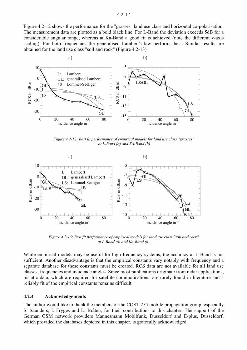
4.2-17

Figure 4.2-12 shows the performance for the "grasses" land use class and horizontal co-polarisation. The measurement data are plotted as a bold black line. For L-Band the deviation exceeds 5dB for a considerable angular range, whereas at Ka-Band a good fit is achieved (note the different y-axis scaling). For both frequencies the generalised Lambert's law performs best. Similar results are obtained for the land use class "soil and rock" (Figure 4.2-13).

a) b)

Figure 4.2-12: Best fit performance of empirical models for land use class "grasses" at L-Band (a) and Ka-Band (b)

a) b)

Figure 4.2-13: Best fit performance of empirical models for land use class "soil and rock" at L-Band (a) and Ka-Band (b)

While empirical models may be useful for high frequency systems, the accuracy at L-Band is not sufficient. Another disadvantage is that the empirical constants vary notably with frequency and a separate database for these constants must be created. RCS data are not available for all land use classes, frequencies and incidence angles. Since most publications originate from radar applications, bistatic data, which are required for satellite communications, are rarely found in literature and a reliably fit of the empirical constants remains difficult.

4.2.4 Acknowledgements

The author would like to thank the members of the COST 255 mobile propagation group, especially S. Saunders, I. Fryges and L. Bråten, for their contributions to this chapter. The support of the German GSM network providers Mannesmann Mobilfunk, Düsseldorf and E-plus, Düsseldorf, which provided the databases depicted in this chapter, is gratefully acknowledged.

4.2-18

4.2.5 References

[De Backer et al., 1996] De Backer, B.; Borjeson, H.; Olyslager, F.; De Zutter, D., "The Study of Wave-propagation through a Windowed Wall at 1.8 GHz," Proc. IEEE Vehicul. Technol. Conf. VTC '96, pp. 165-169 vol.1, 1996.

[Barts and Stutzman, 1992] Barts, R.M. and Stutzman, W.L., "Modeling and Simulation of Mobile Satellite Propagation," IEEE Trans. Antennas Propagat., vol. 40, no. 4, pp. 375-382, 1992.

[Bodnár et al., 1999] Bodnár Z., Herczku Z., Bérces J., Papp I., Som F. and Frigyes I., " A Detailed Experimental Study of the LEO Satellite to Indoor Channel Characteristics," Int. Journal Wireless Information Systems, vol. 6, no. 2, pp. 79-91, 2000.

[Borgeaud & Bellini, 1998] Borgeaud, M. and Bellini, A., "A Database for Electromagnetic Scattering Studies of Bare Soil Surfaces," Proc. International Geosci. Remote Sensing Symposium IGARSS'98, Seattle, Washington, USA, pp. 1197-1199, 1998.

[Borgeaud et al., 1995] Borgeaud, M., Attema, E., Salgado-Gispert, G., Bellini, A. and Noll, J., "Analysis of bare soil surface roughness parameters with ERS-1 SAR data," Symposium on the extraction of bio- and geophysical parameters from SAR data for land applications, Toulouse, France, pp. 307-316, 1995.

[Bråten, 2000] Bråten, L., " Satellite Visibility in Northern Europe Based on Digital Maps," Int. J. Sat. Comm., Vol 18, No 1, Jan/Feb 2000, pp 47-62.

[COST 231, 1999] COST 231, Digital mobile radio towards future generation systems, Final Report, European Commission, Brussels, Belgium, 1999.

[COST 235, 1996] COST 235, Radiowave propagation effects on next-generation fixed services terrestrial telecommunications systems, Final Report, European Commission, Brussels, Belgium, 1996.

[COST 712, 1999] Mätzler C. (ed.), "Radiative transfer models for microwave radiometry", COST Action 712 "Application of microwave radiometry to atmospheric research and monitoring", Meteorology, Final Report of Project 1, European Commission, Directorate General for Research, EUR 19543, ISBN 92-828-9842-3, 2000.

[D'Amato et al., 1997] D'Amato, L., Borghino, L., Buonomo, S., "Analysis of Mobile-Satellite Propagation Measurements at 18.7 GHz: Vegetation Effects," Proc. IEE Tenth Intern. Conf. Antennas Propagat. ICAP'97, Edinburgh, United Kingdom, pp. 2.9-2.14, 1997.

[DERA, 1998] ----- "Technical Working Party on Mobile and Terrestrial Propagation Proposed Format for 3-D Geographical Datasets (Ver. 2.0)," Technical Report, University of Bristol, RAL, 1998.

[Didascalou et al., 1999] Didascalou, D., Younis, M., Wiesbeck, W., "Millimeter-Wave Scattering and Attenuation in Limited Vegetation Structures," Proc. International Geosci. Remote Sensing Symposium IGARSS'99, Hamburg, Germany, pp. 1835-1838, 1999.

4.2-19

[Döttling et al., 1998] Döttling, M., Jahn, A., Kunisch, J., Buonomo, S., "A Versatile Channel Simulator for Land Mobile Satellite Applications," Proc. IEEE Vehicu. Technol. Conf. VTC'98, Ottawa, Ontario, Canada, pp. 213-217, 1998.

[Döttling, Wiesbeck, 1999] Döttling, M., Wiesbeck, W., "A Hierarchical Electromagnetic Land Use Parameter Data Base for Wave Propagation Modeling," IEEE Geosci. Remote Sensing Newsletter, Issue #109, pp. 6-10, 1999.

[Fung, 1994] Fung, A.K., Microwave Scattering and Emission Models and Their Applications, Artech House, Inc., Norwood, MA, USA, ISBN 0-89006-523-3, 1994.

[Geng and Wiesbeck, 1998] Geng, N., Wiesbeck, W., Planungsmethoden für die Mobilkommunikation: Funknetzplanung unter realen physikalischen Ausbreitungsbedingungen, in German, Springer, Berlin, Heidelberg, Germany, ISBN 3-540-64778-3, 1998.

[Hippel, 1995] Hippel, A., 1995, Dielectric Materials and Applications, Artech House, Boston, USA.

[IMST et al., 1998] IMST, DLR, IHE, "Land Mobile Satellite Propagation Model for Non-Urban Areas," Final Report, ESA-Contract Nr. 12044/96/NL/NB(SC), 1998.

[Ishimaru, 1978] Ishimaru, A., Wave Propagation and Scattering in Random Media, Academic Press, New York, 1978.

[ITU-R, 1986] ITU-Report 236-6, "Influence of Terrain Irregularities and Vegetation on Tropospheric Propagation," Vol. V: "Propagation in non-ionised media", CCIR XVth Plenary Assembly, Dubrovnik, 1986.

[ITU-R, 1998a] ITU-Recommendation M.1034-1, "Requirements for the Radio Interface(s) for International Mobile Telecommunications-2000 (IMT-2000)", International Telecommunication Union, Geneva, Switzerland, 1998.

[ITU-R, 1998b] ITU-Recommendation P.1058-1, "Digital Topographic Databases For Propagation Studies", International Telecommunication Union, Geneva, Switzerland, 1998.

[ITU-R, 1998c] ITU-Recommendation M.1225, "Guidelines for Evaluation of Radio Transmission Technologies for IMT-2000", International Telecommunication Union, Geneva, Switzerland, 1998.

[Keller and Salzwedel, 1998] Keller, H. and Salzwedel, H., "Comparision of the Probability of Visibility of New Planned Mobile Satellite Systems (M-Star, Celestri, SkyBridge)," Proc. IEEE Vehicular Technology Conference VTC ‘98, Ottawa, Canada, pp. 81-85, 1998.

[Mattia et al., 1997] Mattia, F. et al., "The Effect of Surface Roughness on Multifrequency Polarimetric SAR Data", IEEE Transactions on Geosci. Remote Sensing, vol. 35, no. 4, pp. 954-966, 1997.

[Mätzler, 1994] Mätzler C., “Microwave (1-100 GHz) Dielectric model of leaves”, IEEE Trans. Geosci. Rem. Sens., Vol 32, No 5, pp 947-949, 1994.

4.2-20

[Oestges et al., 1999] Oestges, C., Saunders, S.R., Vanhoenacker-Janvier, D., "Physical-statistical modelling of the land mobile satellite channel based on ray-tracing," IEE Proc. Microw. Antenn. Propagat., vol. 146, no. 1, pp. 45-49, 1999.

[Oh et al., 1992] Oh, Y., Sarabandi, K., Ulaby, F.T., "An Empirical Model and an Inversion Technique for Radar Scattering from Bare Soil Surface," IEEE Transactions on Geosci. Remote Sensing, vol. 30, no. 2, pp. 370-381, 1992.

[Péréz-Fontán et al, 1995] Pérez-Fontán, F., Baptista, J.P.V., Castro, A.V., "Simple numerical propagation model for non-urban mobile applications," Electronic Letters, vol. 31, no. 25, pp. 2212-2213, 1995.

[Ruck et al., 1970] Ruck, G.T., Barrick, D.E., Stuart, W.D., Krichbaum, C.K., Radar Cross Section Handbook, Plenum Press, NY, USA, ISBN 306-30343-4, 1970.

[Saunders and Evans, 1997] Saunders, S.R., Evans, B.G., "A Physical-Statistical Model for Land Mobile Satellite Propagation in Built-up Areas," IEE Tenth Intern. Conf. on Antennas Propaga. ICAP'97, Edinburgh, United Kingdom, pp. 2.44-2.47, 1997.

[Schorcht et al., 1996] Schorcht, G., Freund, U., Salzwedel, H., Keller, H., "Modeling of Terrains for Simulation of Integrated Mobile Terrestrial and Satellite Communication Systems," Proc. IEEE Vehicul. Technol. Conf. VTC ‘96, Atlanta, Georgia, USA, pp. 1288-1292, 1996.

[Tamir, 1977] Tamir, T. "Radio Wave Propagation Along Mixed Paths in Forest Environments," IEEE Trans. Antennas Propagat., vol. AP-25, no. 4, pp. 471-477, 1977,.

[Tanis and Pilato, 1993] Tanis, W.J., Pilato, G.J., "Building Penetration Characteristics of 880MHz and 1922MHz Radio Waves," Proc. IEEE Vehicul. Technol. Conf. VTC '93, pp. 206-209, 1993.

[Ulaby and Dobson, 1989] Ulaby, F.T., Dobson, M.C., Handbook of Radar Scattering Statistics for Terrain, Artech House, MA, USA, ISBN 0-89006-336-2, 1989.

[Ulaby et al., 1981] Ulaby, F.T., Moore, R.K., Fung, A.K., Microwave Remote Sensing Active and Passive, Addison-Wesley Publishing Company, MA, USA, ISBN 0-201-10759-7, 1981.

[Vázquez-Castro et al., 1999] Vázquez-Castro, M.A. et al., "Shadowing Correlation for Mobile Satellite Diversity," Proc. COST Joint International Workshop COST252, COST253, COST255, Toulouse, France, 1999. pp. 37-48.

[Zhang and Hwang, 1994] Zhang, Y.P., Hwang, Y., "Measurements of the Characteristics of Indoor Penetration Loss," Proc. IEEE Vehicul. Technol. Conf. VTC '94, pp. 1741-1744, 1994.

[Zwick et al., 1997] Zwick, T., Schmitt, K., Wiesbeck, W., "Radio Communication through Car Windows," Automobiltechnische Zeitschrift ATZ, vol. 99, no. 4, pp. 220-226, 1994.

4.3-1

CHAPTER 4.3Statistical modellingof the LMS channel

Editor: F.Perez-Fontan1

Authors: F.Perez-Fontan1, M.A.V.Castro2, S.Buonomo3, J. Kunisch4, J.Pamp5, E.Zollinger6

E.Kubista7, J.P.V.P.Baptista8, B.Arbesser-Rastburg9,L. E. Bråten10, N. Kawai11, Y. Louahdi11 and T. Tjelta12

1 E.T.S.I.Telecomunication, U. de VIGO, Campus Universitario, E-36280 Vigo, SpainTel: +34-629-877-896 Fax: +34-986-812-116 E-mail: fpfontan@tsc.uvigo.es

2 Dpt. Tecnologias de las Comunicaciones, Universidad Carlos III, Butarque 15, 28911-Leganés, Madrid, SpainTel: +34916249173 Fax: +34916249430 Email: maryan@tsc.uc3m.es

8 ESA/ESTEC, XEP, Keplerlaan 1, P.O. Box 299, NL-2200 AG Noordwijk, NetherlandsTel: +31-71-565-5328 Fax: +31-71-565-4999 E-mail: napoli@xe.estec.esa.nl

4 Inst.of Mobile & Sat.Comm. Tech. (IMST), Carl-Friedrich Gauss Str. 2a, D-47475 Kamp-Lintfort, Germany Tel: +49-2842-981454 Fax: +49-2842-981499 E-mail: kunisch@imst.de5 Inst.of Mobile & Sat.Comm. Tech (IMST), Carl-Friedrich Gauss Str. 2a, D-47475 Kamp-Lintfort, Germany Tel: +49-2842-981450 Fax: +49-2842-981499 E-mail: pamp@imst.de6 Inst.of Mobile & Sat.Comm. Tech (IMST), Carl-Friedrich Gauss Str. 2a, D-47475 Kamp-Lintfort, Germany

Tel: +49-2842-981452 Fax: +49-2842-981499 E-mail: zollinger@imst.de7 Joanneum Research - IAS, Institute of Applied Systems Techn. Inffeldgasse 12, A-8010 Graz, Austria Tel: +43-316-876-2510 Fax: +43-316-876-2502 E-mail: erwin.kubista@joanneum.ac.at8 ESA/ESTEC, TOS-EEP, Keplerlaan 1, P.O. Box 299, NL-2200 AG Noordwijk, Netherlands

Tel: +31-71-565-4319 Fax: +31-71-565-4999 E-mail: pedro@xe.estec.esa.nl9 ESA/ESTEC, TOS-EEP, Keplerlaan 1, PO Box 299, NL-2200 AG Noordwijk, Netherlands

Tel: +31-71-565-4541 Fax: +31-71-565-4999 E-mail: bertram@xe.estec.esa.nl10 Telenor, R & D, Satellite & Radio Systems, Instituttveien 23, PB 83, N-2007 Kjeller, Norway

Tel: +47-6-384-48715 Fax: +47-6-381-9810 E-mail: Lars.Braten@fou.telenor.no11 INMARSAT, 99 City Rd, EC1, London. United Kingdom,

Tel +44-20-7728 1000, Fax +44-20-7728 104412 Telenor, R&D, Instituttveien 23, PB 83, N-2007 Kjeller, Norway

4.3-2

4.3 Data and Databases for Land Mobile Satellite Propagation

In this chapter the basic principles are presented for the design and implementation of statisticalmodels for the LMS (land mobile satellite) channel at various frequency bands. Statistical modelsmay be valid for different services including communications, broadcast, navigation, etc.Simulators implementing statistical models must be suitable for the study of new systems, includingthose using LEO and other non-GEO orbits.

For current LMS engineering, applications models solely providing cumulative distributions, CDFs,are not enough. New statistical models must be suited for interfacing system studies including linklevel simulations and network level simulations. This is the reason why a new generation ofstatistical LMS propagation models capable of producing “time-series” (generative models) hasappeared.

Another feature that is very distinctive of the LMS channel when compared to the terrestrial mobilechannel is that a single distribution no longer describes its behaviour: very marked statisticaldifferences are observed for line-of-sight (LOS) links and shadowed links. This explains whymodels try to classify propagation events according to the degree of shadowing and model themindependently (good and bad states).

In this chapter two different approaches to the statistical modelling of the LMS channel arepresented: a three-state approach [Fontan et al., 97] and a two-state approach [Bråten et al., 97].

4.3.1 Three-State Approach

Land mobile satellite (LMS) terminals tend to operate within cluttered areas where shadowingeffects may dominate (e.g. urban, tree-shadowed areas, etc.). System engineers, operators andplanners require reliable and comprehensive information related to the propagation effects that suchsystems face. This chapter addresses the statistical modelling of shadowing and multipath effects inLMS applications for a wide range of environments (from open to dense urban areas), elevationangles (5º- 90º) at L-, S- or Ka-Bands for a range or environments from open to very cluttered(urban or tree shadowed).

A basic feature of the model described in this section is that it is able to generate time-series of anychannel parameter whose study is required: signal envelope, phase, instantaneous power delayprofiles, Doppler spectra, etc. As a second step, conventional statistics, e.g. CDFs, are computedafterwards from the generated series.

To illustrate some of the features found in the LMS channel, two examples of measured time-seriesare presented. Figure 4.3-1 [Smith et al., 92] shows the signal amplitude variations received undernarrow-band conditions and Figure 4.3-2 [Parks et al., 97] shows a measured series of power delayprofiles (PDP) (wide-band reception).

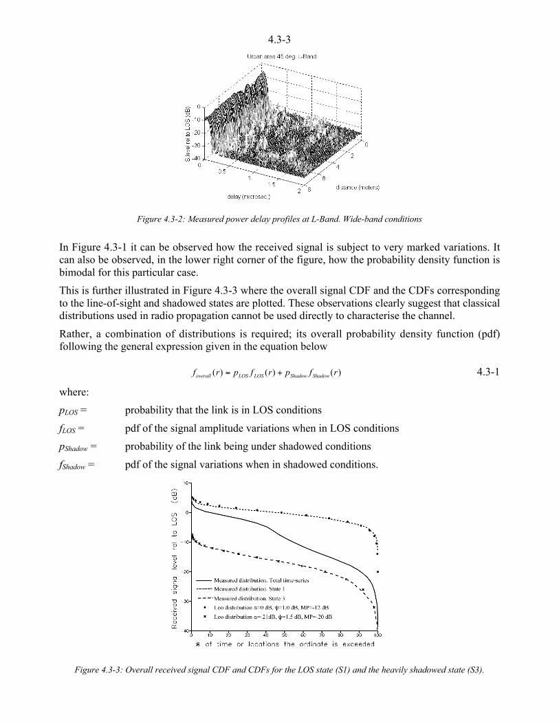
4.3-3

Figure 4.3-2: Measured power delay profiles at L-Band. Wide-band conditions

In Figure 4.3-1 it can be observed how the received signal is subject to very marked variations. Itcan also be observed, in the lower right corner of the figure, how the probability density function isbimodal for this particular case.

This is further illustrated in Figure 4.3-3 where the overall signal CDF and the CDFs correspondingto the line-of-sight and shadowed states are plotted. These observations clearly suggest that classicaldistributions used in radio propagation cannot be used directly to characterise the channel.

Rather, a combination of distributions is required; its overall probability density function (pdf)following the general expression given in the equation below

)()()( rfprfprf ShadowShadowLOSLOSoverall += 4.3-1

where:

pLOS = probability that the link is in LOS conditions

fLOS = pdf of the signal amplitude variations when in LOS conditions

pShadow = probability of the link being under shadowed conditions

fShadow = pdf of the signal variations when in shadowed conditions.

Figure 4.3-3: Overall received signal CDF and CDFs for the LOS state (S1) and the heavily shadowed state (S3).

h i h i lid f h d f li k b d i hi h d d li k i d

4.3-4

duration of different shadowing events or angle of arrival or time or arrival of multipath echoes, andtheir influence on link and system performance, an approach capable of producing time-series isindicated. In this case a Markov chain model has been selected to accomplish the goals previouslystated.

Figure 4.3-2 shows that the channel not only causes signal amplitude variations but also gives riseto time dispersion in the received signal that, depending on the transmitted signal bandwidth, willgive rise to distortion effects like frequency selectivity or inter-symbol interference (ISI). These andother features of the LMS channel have to be appropriately accounted for in a suitable propagationmodel.

The LMS channel may present significant differences depending on the elevation angle and theenvironment where the mobile terminal is located. If Geostationary orbit (GEO) satellites are used,relatively low elevation angles are found, especially for the northern latitudes. Other orbits such aslow or medium Earth orbits (LEO, MEO, ...) or highly elliptical orbits (HEO) provide higherelevation angles for satellite-to-mobile transmissions, thus making it possible to overcome, in part,the shadowing effects caused by man-made and/or natural features in the vicinity of the mobile.

4.3.1.1 Model Basics

The different elements making up the received signal traversing the LMS channel are the directsignal and the multipath component. The time and location variability and the time dispersionintroduced have to be accurately characterised. An important feature to be included in newer LMSmodels is the possibility to account for both mobile and satellite movement along their respectivetrajectories.

The model sought is of the statistical type, this means that assumptions have to be made in whichgiven statistical distributions are used to describe the different physical phenomena affecting thedirect signal and the multipath component. In this respect, a first order Markov model [Lutz, 91;Vucetic and Du, 92; Fontan et al, 97] is used to describe the slow variations of the direct signalbasically due to shadowing/blockage effects. The overall signal variations due to shadowing andmultipath effects are assumed to follow a [Loo, 85] distribution, different for each shadowingcondition (Markov state).

Up to this point the model is of the narrow-band type since it does not account for time dispersioneffects. These effects are introduced by using a negative exponential distribution to represent theexcess delays of the different echoes [Jahn et al., 96].

Different operational situations have been identified, depending on the type of satellite and mobileuser, that may require slightly different implementations:

• case 1.- stationary satellite & stationary mobile;

• case 2.- stationary satellite & moving mobile;

• case 3.- moving satellite & stationary mobile;

• case 4.- moving satellite & moving mobile.

When shadowing effects for links from two different satellites to the same mobile are significantlycorrelated, for example if the satellites are seen by the mobile terminal with closely spaced angles,this circumstance has to be accounted for. [Lutz, 96] has described a method of producing correlatedMarkov chains. Chapter 4.4 addresses shadowing correlation issues in detail.

The statistical model described here assumes ideal transmission conditions, i.e., no band-limitingeffects due to transmit and receive filters are included. This means that the different paths aretreated as ideal delta functions affected by attenuation, phase shift and delay, which are time-

i i di t d i

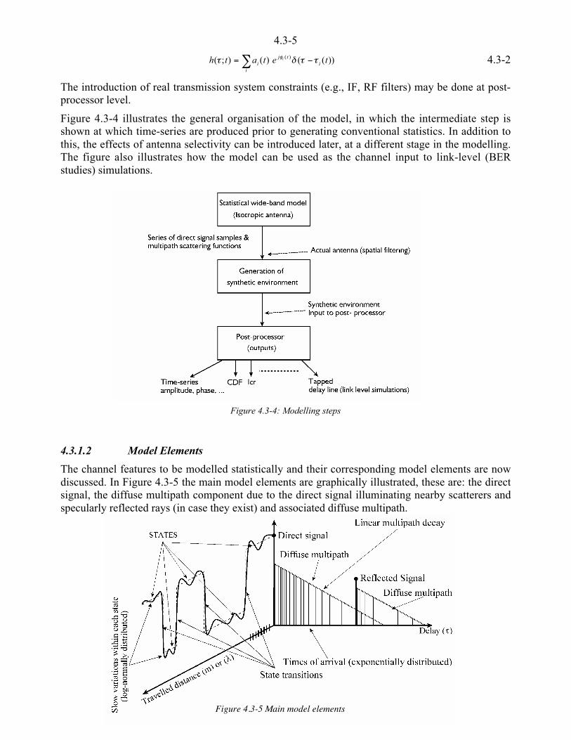
4.3-5

- <=i

itj

i tetath i ))(()();( )( oobo q 4.3-2

The introduction of real transmission system constraints (e.g., IF, RF filters) may be done at post-processor level.

Figure 4.3-4 illustrates the general organisation of the model, in which the intermediate step isshown at which time-series are produced prior to generating conventional statistics. In addition tothis, the effects of antenna selectivity can be introduced later, at a different stage in the modelling.The figure also illustrates how the model can be used as the channel input to link-level (BERstudies) simulations.

Figure 4.3-4: Modelling steps

4.3.1.2 Model Elements

The channel features to be modelled statistically and their corresponding model elements are nowdiscussed. In Figure 4.3-5 the main model elements are graphically illustrated, these are: the directsignal, the diffuse multipath component due to the direct signal illuminating nearby scatterers andspecularly reflected rays (in case they exist) and associated diffuse multipath.

Figure 4.3-5 Main model elements

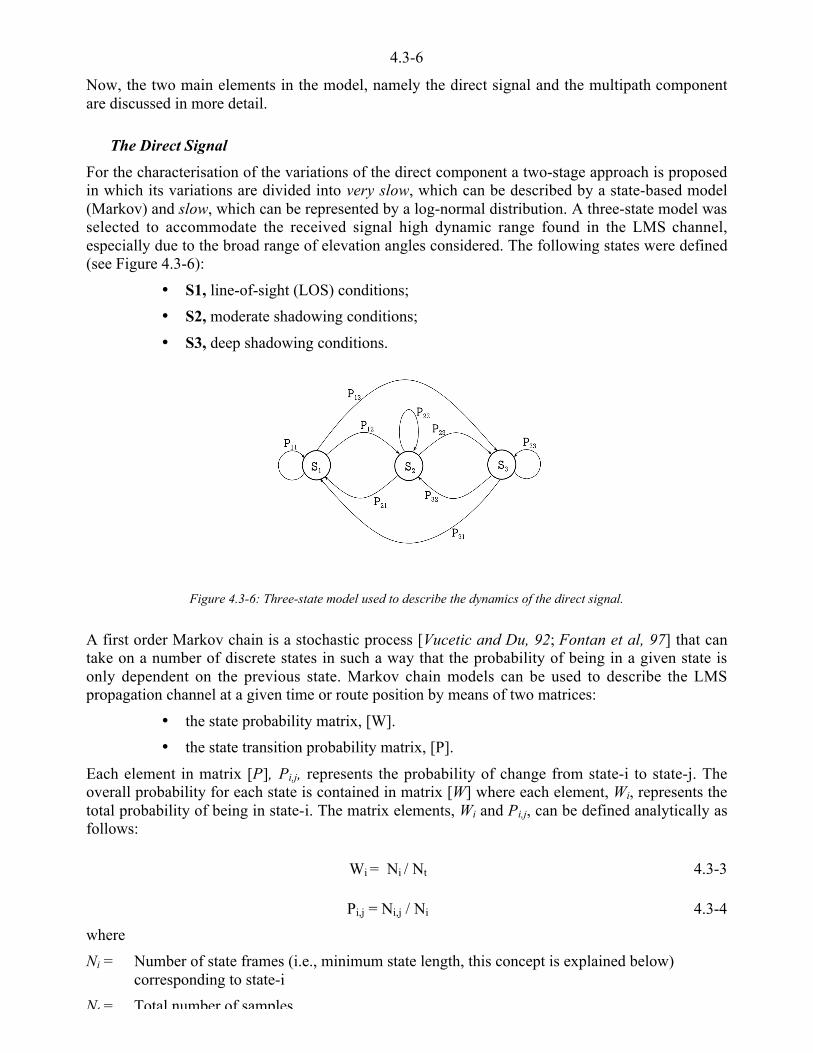
4.3-6

Now, the two main elements in the model, namely the direct signal and the multipath componentare discussed in more detail.

The Direct Signal

For the characterisation of the variations of the direct component a two-stage approach is proposedin which its variations are divided into very slow, which can be described by a state-based model(Markov) and slow, which can be represented by a log-normal distribution. A three-state model wasselected to accommodate the received signal high dynamic range found in the LMS channel,especially due to the broad range of elevation angles considered. The following states were defined(see Figure 4.3-6):

• S1, line-of-sight (LOS) conditions;

• S2, moderate shadowing conditions;

• S3, deep shadowing conditions.

Figure 4.3-6: Three-state model used to describe the dynamics of the direct signal.

A first order Markov chain is a stochastic process [Vucetic and Du, 92; Fontan et al, 97] that cantake on a number of discrete states in such a way that the probability of being in a given state isonly dependent on the previous state. Markov chain models can be used to describe the LMSpropagation channel at a given time or route position by means of two matrices:

• the state probability matrix, [W].

• the state transition probability matrix, [P].

Each element in matrix [P], Pi,j, represents the probability of change from state-i to state-j. Theoverall probability for each state is contained in matrix [W] where each element, Wi, represents thetotal probability of being in state-i. The matrix elements, Wi and Pi,j, can be defined analytically asfollows:

Wi = Ni / Nt 4.3-3

Pi,j = Ni,j / Ni 4.3-4

where

Ni = Number of state frames (i.e., minimum state length, this concept is explained below)corresponding to state-i

Nt = Total number of samples

4.3-7

Ni = Number of state frames corresponding to state-i.

For the computation of matrices [W] and [P] a sufficiently large number of states and transitions isrequired in the experimental data set used.

Three properties of Markov chains will be highlighted here:

• the sum of all elements in every [P] row must be equal to one;

• the sum of all elements in matrix [W] must be equal to one;

• the asymptotic behaviour (convergence property) of the Markov chain is defined bythe equation

[ ][ ] [ ]WPW = 4.3-5

The number of states in the model (three for each environment) was selected by trading offcomplexity and received signal dynamic range for every environment and elevation angle. It hasbeen taken into account also that the model has to describe very different situations ranging fromvery cluttered areas at low elevations to open areas at very high elevation angles.

Typically, each state will last a few metres along the travelled route. In [Fontan et al, 98] aminimum state length or state frame with a length, LFrame of 3 to 5 m was observed in the analysis ofa large experimental dataset [Smith et al, 92] obtained at S-Band. The definition of a frame orminimum state length affects the generation of direct signal variation series: a new state will bedrawn randomly every time the mobile travels a distance of LFrame metres. The triggering of theMarkov engine (or engines if different elevations are considered) involved in the modelling of thevariations of the received signal as the mobile and/or the satellite move is discussed later in thischapter.

The model makes the simplifying assumption of the existence of three basic rates of change (veryslow, slow and fast) in the received signal, corresponding to the different behaviours of itscomponents. States represent different gross shadowing conditions, e.g., if the mobile goes frombeing behind a tree (or a building) to being in the clear line-of-sight of the transmitter. Thesesituations correspond to different states. The marked signal variations due to state changes areconsidered as the very slow variations of the direct signal (and consequently of the overall signal).

As for the slow variations, they represent small-scale changes in the shadowing attenuationproduced as the mobile travels in the shadow of the same obstacle. For example, shadowingvariations behind a group of trees due to different leaf and branch densities or shadowing variationsbehind a single building or group of buildings.

In the line-of-sight (LOS) state slow variations may be due to different reasons: for example, non-uniform receive antenna patterns and/or changes in mobile orientation with respect to the satellite.

An element in the modelling of the slow variations for which sufficient reported data are lacking isthe auto-correlation or correlation distance, LCorr, (see Figure 4.3-7). This parameter describes howfast the log-normally distributed variations are. LCorr values in the order of 1-3 m have beenobserved [Fontan et al., 98].

The auto-correlation properties of the very slow variations are implicitly present in the Markovmodel and in the state frame concept.

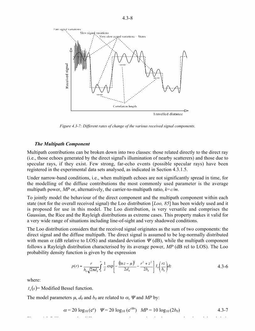
4.3-8

Figure 4.3-7: Different rates of change of the various received signal components.

The Multipath Component

Multipath contributions can be broken down into two classes: those related directly to the direct ray(i.e., those echoes generated by the direct signal's illumination of nearby scatterers) and those due tospecular rays, if they exist. Few strong, far-echo events (possible specular rays) have beenregistered in the experimental data sets analysed, as indicated in Section 4.3.1.5.

Under narrow-band conditions, i.e., when multipath echoes are not significantly spread in time, forthe modelling of the diffuse contributions the most commonly used parameter is the averagemultipath power, MP or, alternatively, the carrier-to-multipath ratio, k=c/m.

To jointly model the behaviour of the direct component and the multipath component within eachstate (not for the overall received signal) the Loo distribution [Loo, 85] has been widely used and itis proposed for use in this model. The Loo distribution, is very versatile and comprises theGaussian, the Rice and the Rayleigh distributions as extreme cases. This property makes it valid fora very wide range of situations including line-of-sight and very shadowed conditions.

The Loo distribution considers that the received signal originates as the sum of two components: thedirect signal and the diffuse multipath. The direct signal is assumed to be log-normally distributedwith mean _ (dB relative to LOS) and standard deviation ^ (dB), while the multipath componentfollows a Rayleigh distribution characterised by its average power, MP (dB rel to LOS). The Looprobability density function is given by the expression

( )dz

brz

Ib

zrd

zzdb

rrp ´́

¦

¥²²¤

£µ�

�³�

� +<

<<= 0

'

00

0 0

22

0

2

0022

lnexp

1

2)(

µ

/4.3-6

where:

( )xI 0 = Modified Bessel function.

The model parameters µ, d0 and b0 are related to _, ^ and MP by:

_ = 20 log10 (eµ) ^ = 20 log10 (e3do) MP = 10 log10 (2b0) 4.3-7

Fi 4 3 7 ill h diff i i i h b d d l d h i

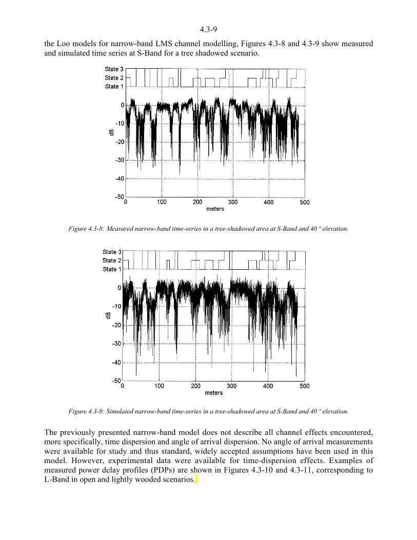
4.3-9

the Loo models for narrow-band LMS channel modelling, Figures 4.3-8 and 4.3-9 show measuredand simulated time series at S-Band for a tree shadowed scenario.

Figure 4.3-8: Measured narrow-band time-series in a tree-shadowed area at S-Band and 40 º elevation.

Figure 4.3-9: Simulated narrow-band time-series in a tree-shadowed area at S-Band and 40 º elevation.

The previously presented narrow-band model does not describe all channel effects encountered,more specifically, time dispersion and angle of arrival dispersion. No angle of arrival measurementswere available for study and thus standard, widely accepted assumptions have been used in thismodel. However, experimental data were available for time-dispersion effects. Examples ofmeasured power delay profiles (PDPs) are shown in Figures 4.3-10 and 4.3-11, corresponding toL-Band in open and lightly wooded scenarios.

4.3-10

0 0.5 1 1.5 2-35

-30

-25

-20

-15

-10

-5

0

Delay (us)

Figure 4.3-10: Measured and model fitted averaged power delay profilefor an open area for 80 º elevation at L-Band [Parks et al, 97].

0 0.5 1 1.5 2-35

-30

-25

-20

-15

-10

-5

0

Delay (us)

Surrey, L-Band, LIGHTLY WOODED. Elev. 45º.

Figure 4.3-11: Measured averaged power delay profile with far echoesfor a lightly wooded scenario and 45 º elevation at L-Band [Parks et al, 97].

So far, multipath has been introduced in terms of its average power, MP, and this approach is validwhen time-dispersion is not significant. However, to include wide-band effects, the time spreadingcaused by the channel must be included in the modelling. That is, it must be acknowledged thatechoes arrive at the receiver with different excess delays with respect to the direct signal (shadowedor not). An overview of the model is graphically illustrated in Figures 4.3-5 and 4.3-12.

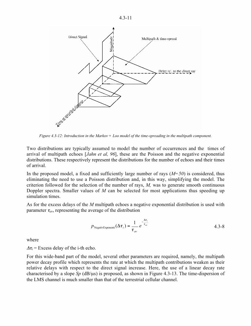
4.3-11

Figure 4.3-12: Introduction in the Markov + Loo model of the time-spreading in the multipath component.

Two distributions are typically assumed to model the number of occurrences and the times ofarrival of multipath echoes [Jahn et al, 96], these are the Poisson and the negative exponentialdistributions. These respectively represent the distributions for the number of echoes and their timesof arrival.

In the proposed model, a fixed and sufficiently large number of rays (M=50) is considered, thuseliminating the need to use a Poisson distribution and, in this way, simplifying the model. Thecriterion followed for the selection of the number of rays, M, was to generate smooth continuousDoppler spectra. Smaller values of M can be selected for most applications thus speeding upsimulation times.

As for the excess delays of the M multipath echoes a negative exponential distribution is used withparameter oav, representing the average of the distribution

av

i

epav

io

o

oo

6<

=61

)(onentiNegativExp 4.3-8

where

6oi = Excess delay of the i-th echo.

For this wide-band part of the model, several other parameters are required, namely, the multipathpower decay profile which represents the rate at which the multipath contributions weaken as theirrelative delays with respect to the direct signal increase. Here, the use of a linear decay ratecharacterised by a slope Sp (dB/µs) is proposed, as shown in Figure 4.3-13. The time-dispersion ofthe LMS channel is much smaller than that of the terrestrial cellular channel.

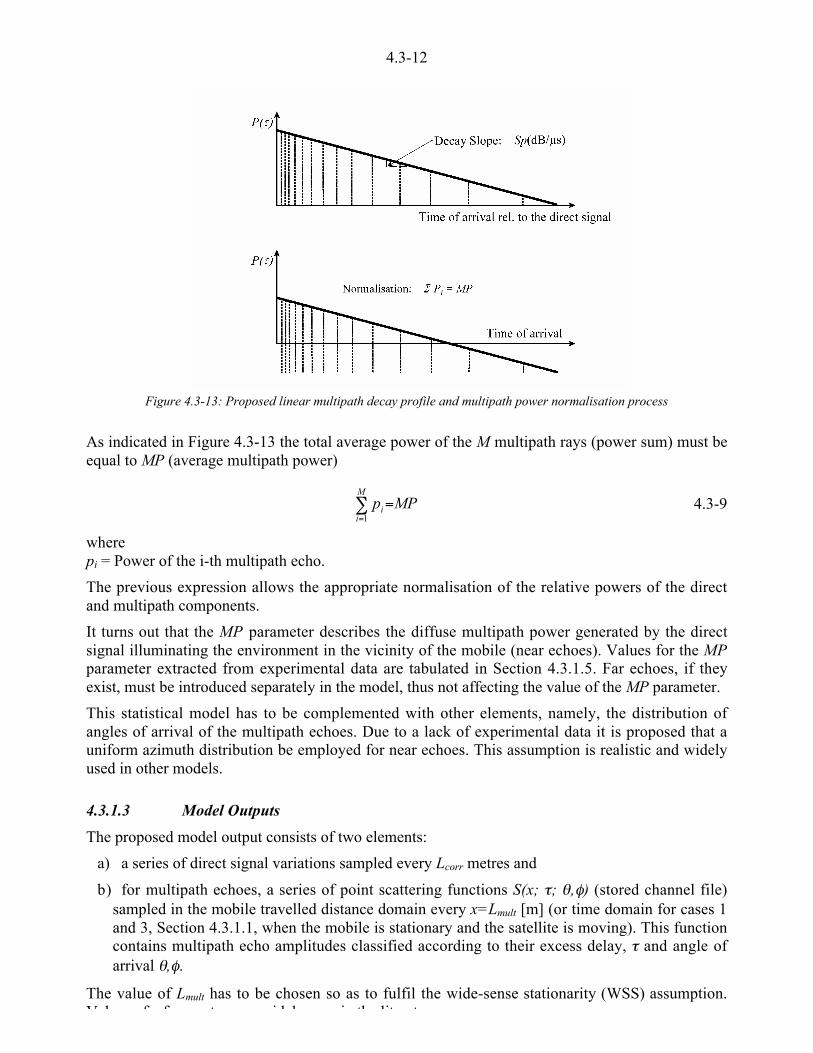
4.3-12

Figure 4.3-13: Proposed linear multipath decay profile and multipath power normalisation process

As indicated in Figure 4.3-13 the total average power of the M multipath rays (power sum) must beequal to MP (average multipath power)

-=

=M

ii MPp

14.3-9

wherepi = Power of the i-th multipath echo.

The previous expression allows the appropriate normalisation of the relative powers of the directand multipath components.

It turns out that the MP parameter describes the diffuse multipath power generated by the directsignal illuminating the environment in the vicinity of the mobile (near echoes). Values for the MPparameter extracted from experimental data are tabulated in Section 4.3.1.5. Far echoes, if theyexist, must be introduced separately in the model, thus not affecting the value of the MP parameter.

This statistical model has to be complemented with other elements, namely, the distribution ofangles of arrival of the multipath echoes. Due to a lack of experimental data it is proposed that auniform azimuth distribution be employed for near echoes. This assumption is realistic and widelyused in other models.

4.3.1.3 Model Outputs

The proposed model output consists of two elements:

a) a series of direct signal variations sampled every Lcorr metres and

b) for multipath echoes, a series of point scattering functions S(x; o; e,q) (stored channel file)sampled in the mobile travelled distance domain every x=Lmult [m] (or time domain for cases 1and 3, Section 4.3.1.1, when the mobile is stationary and the satellite is moving). This functioncontains multipath echo amplitudes classified according to their excess delay, o and angle ofarrival e,q.

The value of Lmult has to be chosen so as to fulfil the wide-sense stationarity (WSS) assumption.Val es of a fe metres are idel seen in the literat re

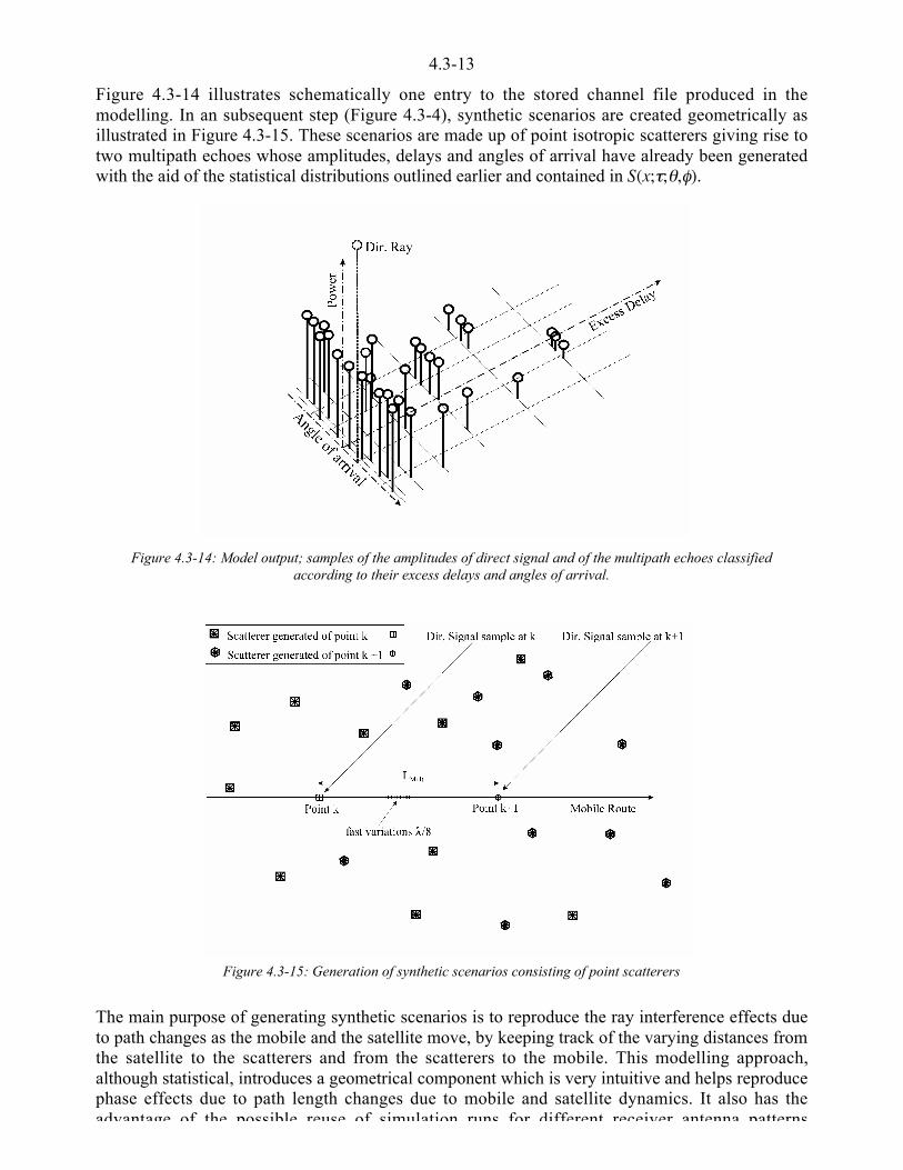
4.3-13

Figure 4.3-14 illustrates schematically one entry to the stored channel file produced in themodelling. In an subsequent step (Figure 4.3-4), synthetic scenarios are created geometrically asillustrated in Figure 4.3-15. These scenarios are made up of point isotropic scatterers giving rise totwo multipath echoes whose amplitudes, delays and angles of arrival have already been generatedwith the aid of the statistical distributions outlined earlier and contained in S(x;o;e,q).

Figure 4.3-14: Model output; samples of the amplitudes of direct signal and of the multipath echoes classifiedaccording to their excess delays and angles of arrival.

Figure 4.3-15: Generation of synthetic scenarios consisting of point scatterers

The main purpose of generating synthetic scenarios is to reproduce the ray interference effects dueto path changes as the mobile and the satellite move, by keeping track of the varying distances fromthe satellite to the scatterers and from the scatterers to the mobile. This modelling approach,although statistical, introduces a geometrical component which is very intuitive and helps reproducephase effects due to path length changes due to mobile and satellite dynamics. It also has theadvantage of the possible reuse of simulation runs for different receiver antenna patterns

4.3-14

To clarify the use of the synthetic scenario approach two post-processing examples are presented,namely, the procedures for the generation of narrow-band received signal time-series and thegeneration of Doppler shift time-series.

Generation Of Narrow-Band Time-Series

To show how the model outputs (direct signal series and series of multipath point scatteringfunctions, S(x;o;e,q), and their corresponding synthetic scenarios) may be processed to producemeaningful information, the generation process of narrow-band received amplitude series isexplained with the aid of Figures 4.3-15 and 4.3-16 for Case 2 (stationary satellite & movingmobile).

Figure 4.3-16: Combination of rays to generate complex-envelope time-series.

In the figures, for two points along the mobile route (k and k+1) point scatterer synthetic scenarioshave been created, corresponding to two neighbouring scattering functions, S(x=k,o,e,q) andS(x=k+1,o,e,q). In Figure 4.3-16 two scatterers are shown, i and j, generated for route points k andk+1. Scatterers i and j correspond to scattering functions Sk and Sk+1 respectively.

For the generation of the narrow-band received amplitude series, the coherent sum of all raysarriving at every sampling point (typically a separation of h/8-h/10 is sufficient) is computed thusproducing a complex (amplitude and phase) time-series of the received signal.

In order to maintain continuity in the generated received signal series (amplitude and phase), twoneighbouring scattering functions (Sk and Sk+1) are used when performing the coherent sum of rays.A linear weighting algorithm is employed to provide a smooth transition of generated receivedamplitudes and phases.

At the same time, samples of the direct signal produced Lcorr m apart have to go through a rateconversion process to yield a sample every h/8-h/10 meters, the same as in the multipath case. Also,the direct signal phase is kept track of by computing and updating the satellite-to-mobile distance.

Figure 4.3-17 illustrates the satellite-to-mobile geometry and the reference co-ordinate system.

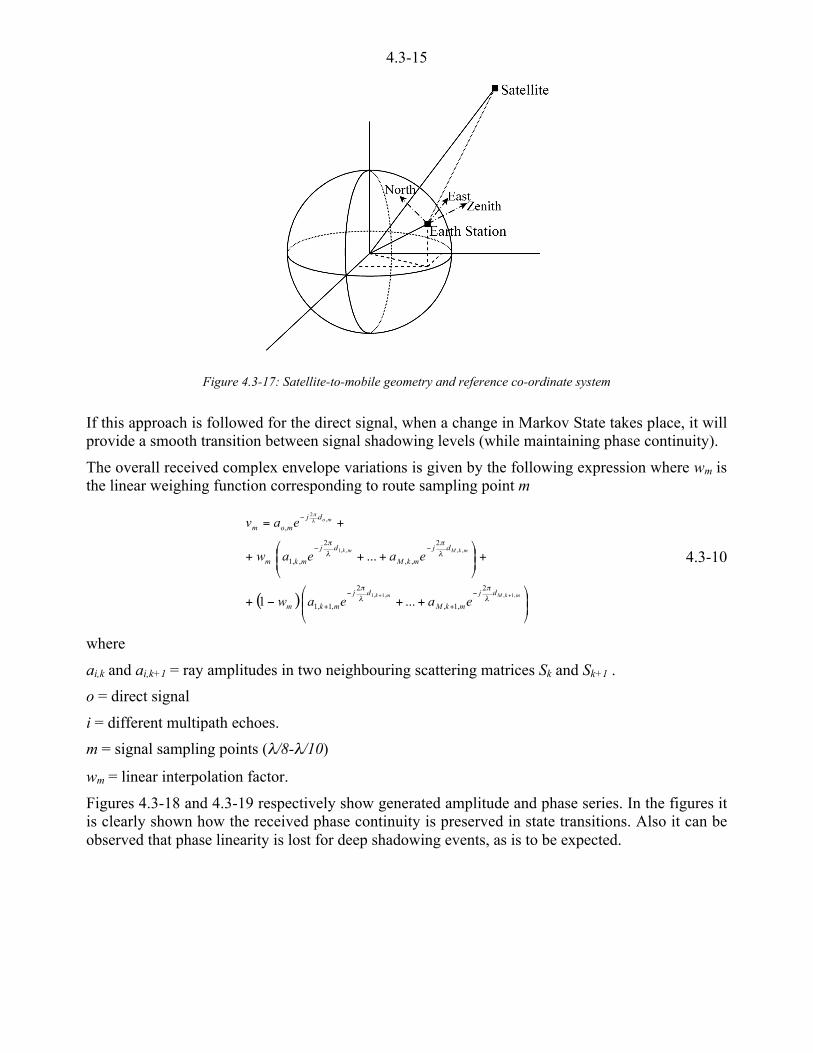
4.3-15

Figure 4.3-17: Satellite-to-mobile geometry and reference co-ordinate system

If this approach is followed for the direct signal, when a change in Markov State takes place, it willprovide a smooth transition between signal shadowing levels (while maintaining phase continuity).

The overall received complex envelope variations is given by the following expression where wm isthe linear weighing function corresponding to route sampling point m

( ) ´´¦

¥²²¤

£++<+

+´´¦

¥²²¤

£+++

+=

++ <

+

<

+

<<

<

mkMmk

mkMmk

mo

dj

mkM

dj

mkm

dj

mkM

dj

mkm

djmom

eaeaw

eaeaw

eav

,1,,1,1

,,,,1

,2

2

,1,

2

,1,1

2

,,

2

,,1

,

...1

...

h/

h/

h

/

h

/

h/

4.3-10

where

ai,k and ai,k+1 = ray amplitudes in two neighbouring scattering matrices Sk and Sk+1 .

o = direct signal

i = different multipath echoes.

m = signal sampling points (h/8-h/10)

wm = linear interpolation factor.

Figures 4.3-18 and 4.3-19 respectively show generated amplitude and phase series. In the figures itis clearly shown how the received phase continuity is preserved in state transitions. Also it can beobserved that phase linearity is lost for deep shadowing events, as is to be expected.

4.3-16

Figure 4.3-18: Example of generated signal amplitude series.

Figure 4.3-19: Example of generated phase series corresponding to the same simulation as Figure 4.3-18

Doppler Spectra

Each received signal contribution (direct ray and multipath echoes) is subject to Doppler shifts. InFigure 4.3-20 an illustration of this process is presented. The direct signal shift may be calculatedby keeping track of the path increments for each route sampling point (h/8-h/10).

Similarly, for the diffuse scatterers, the situation may be modelled by taking into consideration thatthe total phase of each contribution can be split into:

• a phase change due to the movement of the satellite (or path change from thesatellite to the scatterer);

• a phase change due to the movement of the mobile terminal (or path change fromthe scatterer to the mobile)

This condition can be described by:

)()()( ttt MobScatScatSatTot << += qqq 4.3-11

A reasonable simplification may be to consider that the total instantaneous Doppler spectrum ismade up of two independent elements: the mobile movement contributions, Doppler spread, thatcan be several hundred Hz wide, and those due to the satellite movement, Doppler shift, that can beseveral tens of Hz.

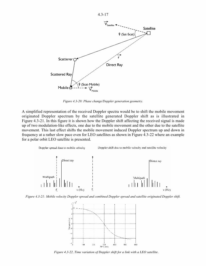
4.3-17

Figure 4.3-20: Phase change/Doppler generation geometry.

A simplified representation of the received Doppler spectra would be to shift the mobile movementoriginated Doppler spectrum by the satellite generated Doppler shift as is illustrated inFigure 4.3-21. In this figure it is shown how the Doppler shift affecting the received signal is madeup of two modulation-like effects, one due to the mobile movement and the other due to the satellitemovement. This last effect shifts the mobile movement induced Doppler spectrum up and down infrequency at a rather slow pace even for LEO satellites as shown in Figure 4.3-22 where an examplefor a polar orbit LEO satellite is presented.

Figure 4.3-21: Mobile velocity Doppler spread and combined Doppler spread and satellite originated Doppler shift.

Figure 4.3-22. Time variation of Doppler shift for a link with a LEO satellite.

4.3-18

4.3.1.4 Model Implementation Issues

In previous sections the basic model elements have been described, now the adequate sequencing ofall these elements to produce the required results is presented. As indicated earlier, the approachfollowed is to generate time-series of the different elements in the received signal: direct ray andmultipath and to combine them suitably at the receiver, taking into consideration their distributionsand their relative rates of change, i.e., slow and fast variations. From the generated time-series, apost-processor is required to produce the relevant received signal statistics for both narrow-bandand wide-band situations.

In a study of a network consisting of a constellation of several satellites, the model must be run asmany times as there are satellites in the constellation under study. The behaviours of the receivedsignals from the different satellites are considered to be independent (Figure 4.3-23). Only when thedegree of correlation is high enough (for small angle separations between two satellites) is thecombined production of correlated time-series required. This special case will occur with a smallprobability. It is proposed that the two-state [Lutz, 96] methodology can be extended in a simplifiedway to the three-state case to account for shadowing correlated cases.

Figure 4.3-23: Availability analysis for multi-satellite systems with uncorrelated shadowing.

The implementation of the described model in a practical channel simulator, with respect toterrestrial channel simulators, has the added problem that not only is the mobile capable of changingits position with time but also the satellites are likely to move at high speeds. There is even the casein which it is only the satellite that moves while the mobile is stationary. The special case in whichboth the satellite and the mobile are stationary must also be contemplated.

This is the reason why, in the model, special attention must be paid to a pre-processing task inwhich positions along the mobile route and the satellite trajectory as well as instants when a statechange event may occur are identified. Event, in this context, means the possibility that a change inshadowing conditions occurs.

Different triggering events must be considered for the different phenomena accounted for in thismodel. Below, the implications related to each of the model elements are analysed.

The direct signal is assumed to be subject to very slow variations with distance along the travelledroute. These variations are modelled by means of a Markov chain model. In the initial narrow-bandmodel [Fontan et al, 97] a minimum state length called Frame was considered. Thus, for everyLFrame metres along the mobile route a random number has to be selected to trigger the Markovchain engine. This is valid for the case where the satellite is stationary and the mobile is moving.However, the situation in which it is the satellite that moves while the mobile is stationary must alsobe considered. For such situations additional triggering events must be considered (Figure 4.3-24).

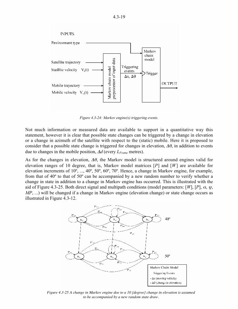
4.3-19

Figure 4.3-24: Markov engine(s) triggering events.

Not much information or measured data are available to support in a quantitative way thisstatement, however it is clear that possible state changes can be triggered by a change in elevationor a change in azimuth of the satellite with respect to the (static) mobile. Here it is proposed toconsider that a possible state change is triggered for changes in elevation, 6e, in addition to eventsdue to changes in the mobile position, 6d (every LFrame metres).

As for the changes in elevation, 6e, the Markov model is structured around engines valid forelevation ranges of 10 degree, that is, Markov model matrices [P] and [W ] are available forelevation increments of 10º, ..., 40º, 50º, 60º, 70º. Hence, a change in Markov engine, for example,from that of 40º to that of 50º can be accompanied by a new random number to verify whether achange in state in addition to a change in Markov engine has occurred. This is illustrated with theaid of Figure 4.3-25. Both direct signal and multipath conditions (model parameters: [W], [P], _, s,MP, ...) will be changed if a change in Markov engine (elevation change) or state change occurs asillustrated in Figure 4.3-12.

Figure 4.3-25 A change in Markov engine doe to a 10 [degree] change in elevation is assumedto be accompanied by a new random state draw.

Reference Location(Platform)

Band(frequency)

SoundingTechnique

Environments Elevations[degree]

Orientation[degree]

AntennamBeamwidth [deg.]

AntennaPosition

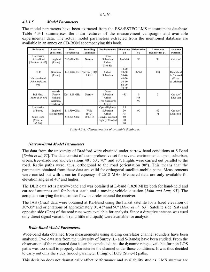
4.3-20

4.3.1.5 Model Parameters

The model parameters have been extracted from the ESA/ESTEC LMS measurement database.Table 4.3-1 summarises the main features of the measurement campaigns and availableexperimental data. The actual model parameters extracted from the mentioned database areavailable in an annex on CD-ROM accompanying this book.

Reference Location(Platform)

Band(frequency)

SoundingTechnique

Environments Elevations(º)

Orientation(º)

AntennamBeamwidth [º.]

AntennaPosition

Universityof Bradford

[Smith et al, 92]England(Plane)

S-2.618 GHz NarrowOpen

SuburbanUrban

Tree-Sh.

0-60-80 90 90 Car roof

DLR

Narrow-Band[Jahn and Lutz,

95]

Germany(Plane)

L-1.820 GHz Narrow (I+Q)8 kHz

UrbanSuburban

10-2020-3030-4040-5050-6060-7070-80

0-360 170 Hand-held& Car roof

(Fixed& driving)

IAS Graz[Murr et al, 95]

AustriaFranceHolland

Germany(ITALSAT)

Ka-18.68 GHz NarrowOpen

SuburbanUrban

Tree-ShadowedMixed

~35 04590

3 Car roofESA van

Universityof Surrey

Wide-Band[Evans et

al, 96]

England(Helicopter)

L-1.550 GHz

S-2.325 GHz

Wide(I+Q)

20 MHz

Open/HighwaySuburban

UrbanHeavily WoodedLightly Wooded

153045607080

90 4271

Car roofDual-freq.

Table 4.3-1: Characteristics of available databases.

Narrow-Band Model Parameters

The data from the university of Bradford were obtained under narrow-band conditions at S-Band[Smith et al, 92]. The data consist of a comprehensive set for several environments: open, suburban,urban, tree-shadowed and elevations 40º, 60º, 70ºº and 80º. Flights were carried out parallel to theroad. Radio paths were, thus, orthogonal to the road (orientation 90º). This means that theparameters obtained from these data are valid for orthogonal satellite-mobile paths. Measurementswere carried out with a carrier frequency of 2618 MHz. Measured data are only available forelevation angles of 40º and higher.

The DLR data set is narrow-band and was obtained at L-band (1820 MHz) both for hand-held andcar-roof antennas and for both a static and a moving vehicle situation [Jahn and Lutz, 95]. Theaeroplane carrying the transmitter flew in circles around the receiver.

The IAS (Graz) data were obtained at Ka-Band using the Italsat satellite for a fixed elevation of30º-35º and orientations of approximately 0º, 45º and 90º [Murr et al., 95]. Satellite side (Sat) andopposite side (Opp) of the road runs were available for analysis. Since a directive antenna was usedonly direct signal variations (and little multipath) were available for analysis.

Wide-Band Model Parameters

Wide-band data obtained from measurements using sliding correlator channel sounders have beenanalysed. Two data sets from the university of Surrey (L- and S-Bands) have been studied. From theobservation of the measured data it can be concluded that the dynamic range available for non-LOSpaths was too small to properly characterise the channel under those conditions. It was thus decidedto carry out only the study (model parameter fitting) of LOS (State-1) paths.

This decision does not dramatically affect performance and availability studies LMS systems are

4.3-21

given threshold (i.e., when in states 2 and 3) system outage will occur regardless of channel timedispersion.

As for LOS (state-1), potential situations of unavailability will occur only when the channel timedispersion is large, since the received signal will, in this case, be above the receive threshold. Thisis actually what was studied in the wide-band characterisation carried out.

The parameter fitting procedure is illustrated in Figure 4.3-26. In order to compare measured withsimulated power delay profiles (PDPs) the internal processes within the channel sounder had to besimulated. Ideal instantaneous channel impulse responses (made up of delta functions) were passedthrough a filter simulating the behaviour and characteristics of the channel sounder used. Beforebeing fitted, measured PDPs were averaged together with neighbouring ones to remove multipathcancellation and enhancement effects (averaged power delay profiles, APDPs). A similar processwas carried out for the simulated instantaneous PDPs. An example of model fitted APDP is shownin Figure 4.3-10.

Figure 4.3-26: Simulation of the channel sounder

Three categories of LOS power delay profiles were considered in this study:

• Type 1.A, representing those APDPs with no features other than in the first delay bin

• Type 1.B, representing those APDPs with additional features in delay bins 2, 3, 4,(i.e., with time dispersion).

• Type 2, i.e., those APDPs where long delays were observed (far echoes).

In the study of these three categories the following approach was followed:

• Type 1.A Profiles:No wide-band model fitting was possible. The channel in this case may be considered to benarrow-band with respect to the channel sounder. Model parameters obtained in narrow-bandmeasurement campaigns can be used.

• Type 1.B profiles:wide-band model fittings were performed and wide-band parameters extracted.Also the occurrence probabilities of profiles 1.A and 1.B have been recorded.

• Type 2 profiles:These occurred very seldom. In the case of type 2 profiles (with far echoes) their occurrencesand relative levels have been recorded.

The proposed PDP classification in types 1.A and 1.B (type 2 may be in a first approachdisregarded given its very low occurrence probability) suggests the extension of the narrow-bandthree-state Markov model to a wide-band model. In this model, only for the LOS state, the Markovengine bounces back and forth from the non-dispersive to the dispersive states as illustrated in

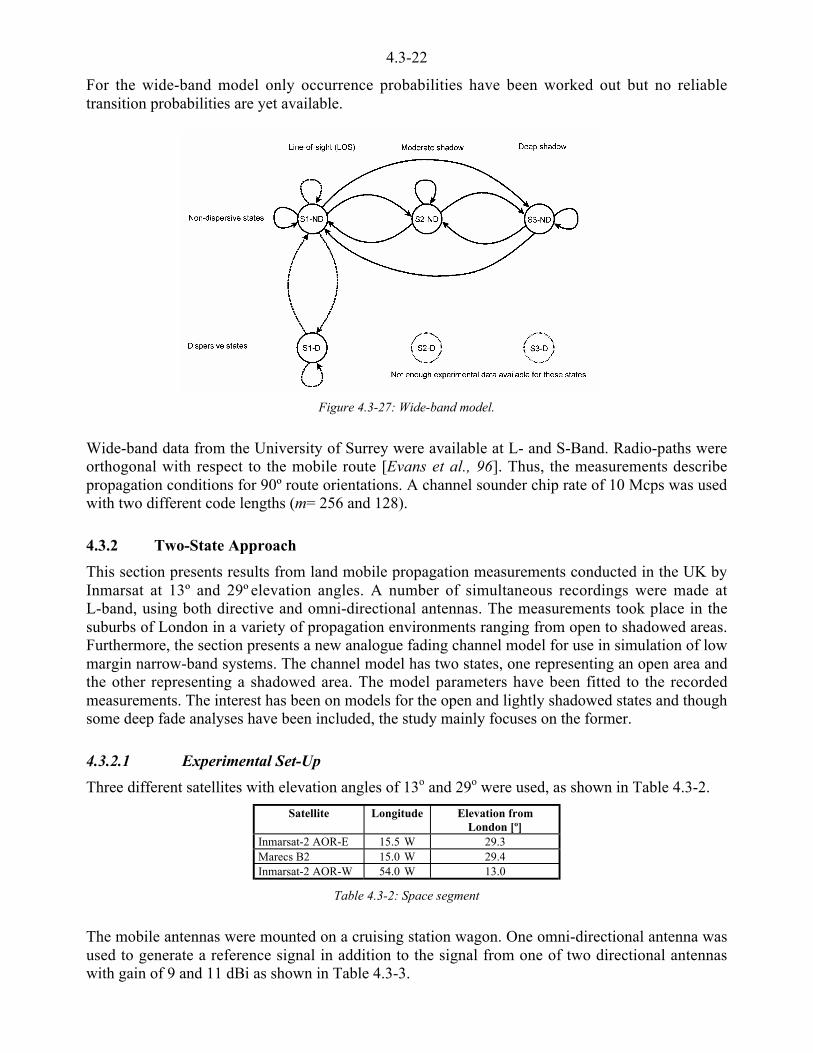
4.3-22

For the wide-band model only occurrence probabilities have been worked out but no reliabletransition probabilities are yet available.

Figure 4.3-27: Wide-band model.

Wide-band data from the University of Surrey were available at L- and S-Band. Radio-paths wereorthogonal with respect to the mobile route [Evans et al., 96]. Thus, the measurements describepropagation conditions for 90º route orientations. A channel sounder chip rate of 10 Mcps was usedwith two different code lengths (m= 256 and 128).

4.3.2 Two-State Approach

This section presents results from land mobile propagation measurements conducted in the UK byInmarsat at 13º and 29º elevation angles. A number of simultaneous recordings were made atL-band, using both directive and omni-directional antennas. The measurements took place in thesuburbs of London in a variety of propagation environments ranging from open to shadowed areas.Furthermore, the section presents a new analogue fading channel model for use in simulation of lowmargin narrow-band systems. The channel model has two states, one representing an open area andthe other representing a shadowed area. The model parameters have been fitted to the recordedmeasurements. The interest has been on models for the open and lightly shadowed states and thoughsome deep fade analyses have been included, the study mainly focuses on the former.

4.3.2.1 Experimental Set-Up

Three different satellites with elevation angles of 13o and 29o were used, as shown in Table 4.3-2.

Satellite Longitude Elevation fromLondon [º]

Inmarsat-2 AOR-E 15.5 W 29.3Marecs B2 15.0 W 29.4Inmarsat-2 AOR-W 54.0 W 13.0

Table 4.3-2: Space segment

The mobile antennas were mounted on a cruising station wagon. One omni-directional antenna wasused to generate a reference signal in addition to the signal from one of two directional antennaswith gain of 9 and 11 dBi as shown in Table 4.3-3.

4.3-23

The received carriers were down converted to base-band, and complex samples together withantenna pointing direction, car heading and speed were recorded. The dynamic range in themeasurements is about 20 dB. The analogue tape recordings were digitised and transferred to aworkstation for statistical analysis.

NoType

Omni/Directional

Peakgain (dBi)

Diameter andHeight (cm)

3 dB beam-widthaz. and el. [º]

1 Directive (D) 9 20, 17.5 70, 402 Directive (D) 11 32, 5 36, 523 Omni (O) 2 - 360, 180

Table 4.3-3: Antenna characteristics

4.3.2.2 Routes Descriptions

Four test routes were chosen, representing propagation conditions ranging from line-of-sight toshadowing and blocking. The different environments cover lightly and heavily wooded areas andboth rural and urban areas as shown in Table 4.3-4.

Testroute

Environment Classification Location

R1Highway, mixture

of open andlightly wooded

Highway Guilford

R2 Heavily woodedroad

Heavily wooded Guilford,Woodford

R3

Suburban roadwith mixture of

open areas,lightly wooded and

2-story houses

Suburban Woodford

R4 Tall buildings Urban Old Street

Table 4.3-4: Test runs

The roads ranged from motorways, single lane roads, underpasses and roundabouts or a circularroute where all possible orientations to the satellite were obtained. The measurements took placeduring the winter months.

4.3.2.3 Statistical Analysis

A statistical analysis has been made of the recorded propagation data, including envelope as well asfade and non-fade duration distributions. The recorded data, sampled at 1000 samples per second,was first low-pass filtered. The cut-off frequency was chosen as 50 Hz in all runs as a compromisebetween noise and spurious rejection and preserving the Doppler spreading. The power in an initialstate, where the vehicle was standing still and no obstacles occurred, was normalised to one beforethe data were sorted into a shadow area and a open area state with a threshold of 3 and 5 dB for thedirectional and omnidirectional antennas respectively. The envelope threshold values were chosenbased on visual inspection of the results of the state-sorting algorithm. When sorting the time seriesinto the shadow and the open states using an envelope threshold, a minimum open state duration of2 m was introduced, to avoid changes in state due to fast signal fluctuations introduced by multipathscattering. The measurements were sorted and grouped according to propagation environment andantenna type before performing the statistical analysis. The two directive antennas, 1 and 2, weregrouped together to obtain better confidence. Each run was carefully inspected and those withrepeated equipment failure were not used. Furthermore, the time series with directive antennamispointing exceeding 5 degrees were not used. The duration statistics were, due to insufficient

4.3-24

speed information for some runs, calculated on the basis of the average vehicle speed in the runs(40 km/h). The two states used in this section are described in further detail below.

Open state model

The open state is represented by the sum of a Rice model of the constant line-of-sight signal with aRayleigh model of the distributed diffuse component, resulting from a number of reflected anddiffracted components.

The envelope probability density function (PDF) of the total fading distortion may be written as[Proakis, 95]:

( ) ( ) ´¦

¥²¤

£= +<20

22

222

mmm rs

Ier

rp sr 4.3-12

where:

12

+=

KK

s = direct component

( )12

12

+=

Km = diffuse component

K = Rice factor.

( )xI 0 = Modified Bessel function.

Figure 4.3-28: Average CDFs at 29º elevation. Measured (solid), Theoretical (dashed),Directive ant. (*), Omnidirectional antenna (o)

The average fade depths shown in Figure 4.3-28 are the average of all the measured environmentsat 29º. The open state received power cumulative density functions (CDFs) are the lower family ofcurves (shallow fades). The low pass filtered signal (see next section),giving the slowly varyingdirect component, is shown in the upper family of curves. Parameters for the average in addition toeach test route are shown in Table 4.3-5.

Shadow state model

The shadow state representing shadowing or blockage is modelled as a linear combination of a

0 5 10 15 2010-1

100

101

102

4.3-25

diffuse component with variancem r2 . The extraction of the slowly varying direct component from

the total fade signal was done by a Chebyshev type II low-pass filter with cut-off frequency of 5 Hz(free of pass-band ripple). The diffuse component was computed by subtracting the directcomponent from the total signal.

The envelope of the direct signal is assumed to have a lognormal probability density function[Vucetic and Du, 92]:

( )( )

21

21

2

ln

1 2

1 m

µ

/m

<<

=r

er

rp 4.3-13

with parameters µ1 and m1.

The mean value of the direct signal's envelope is

2

21

1m

µµ

+= es 4.3-14

and the variance is:

)1(21

21122 <= + mmµm ees 4.3-15

The fade depths in suburban areas for 13º and 29º elevation are shown in Figure 4.3-29. The openstate received power CDFs are the lower family of curves (shallow fades). The slowly varyingdirect component is shown in the upper family of curves.

Figure 4.3-29: Fade depths at 13 and 29º (dashed and solid) elevation for R3.Directive and Omni antenna (* and o).

Large area model

A multi-state model switching randomly between the states is often called a Markov process, withcorresponding state probabilities and state-transition probabilities. Here, a two-state model is givenusing an alternating process; i.e. a state always changes to the other state.

Unlike a Markov process, the model shown in Figure 4.3-30 is driven by an environment signalconsisting of the open and shadow state duration statistics obtained from measured propagation

0 5 10 15 2010-1

100

101

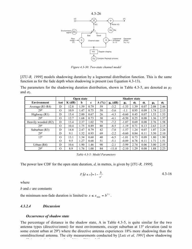
4.3-26

H(f)

x(t) y(t)

a(t) Noise n(t)

NoEnvironmentsignal

Ricemodel

(C)

Lognormalenvelope(µ, m)

Gaussianphase(µe, me)

Doppler shaping

Complex Rayleigh process

Bad Good

Channel state

Figure 4.3-30: Two-state channel model

[ITU-R, 1999] models shadowing duration by a lognormal distribution function. This is the samefunction as for the fade depth when shadowing is present (see Equation 4.3-13).

The parameters for the shadowing duration distribution, shown in Table 4.3-5, are denoted as µ2

and m2.

Open state Shadow stateEnvironment Ant K (dB) b c A (%) µµµµs (dB) µµµµ1 mmmm1 mmmmr µµµµ2 mmmm2

Average (R1-R4) D 12.8 1.59 0.79 59 -3.2 -1.33 1.39 0.07 2.08 2.4629º O 10.9 1.47 0.75 58 -5.6 -1.1 0.95 0.09 1.74 2.13

Highway (R1) D 15.4 2.00 0.67 26 -4.3 -0.60 0.45 0.07 1.53 1.5329º O 12.7 1.68 0.73 30 -4.1 -0.50 0.25 0.08 1.36 1.57

Heavily wooded (R2) D 13.4 2.37 1.02 79 -7.2 -1.07 0.69 0.08 2.76 1.5829º O 10.4 1.75 0.89 80 -8.5 -1.19 0.71 0.13 2.63 2.15

Suburban (R3)29º

DD

14.89.1

2.471.32

0.790.93

4269

-7.0-2.2

-1.57-0.60

1.240.84

0.070.11

1.073.50

2.242.10

13º OO

13.19.5

1.341.27

0.600.68

4051

-6.5-5.1

-1.01-0.89

0.730.78

0.090.11

1.801.71

1.901.51

Urban (R4) D 10.6 1.90 1.46 90 -2.1 -3.99 2.74 0.06 3.00 2.5529º O 8.9 1.76 1.00 84 -11.0 -2.10 1.29 0.08 1.88 2.23

Table 4.3-5: Model Parameters

The power law CDF for the open state duration, d, in metres, is given by [ITU-R, 1999].

( ) cx xb

xdP <=) 1 4.3-16

where

b and c are constants

the minimum non-fade duration is limited to x x b c) =min/1 .

4.3.2.4 Discussion

Occurrence of shadow state

The percentage of distance in the shadow state, A in Table 4.3-5, is quite similar for the twoantenna types (directive/omni) for most environments, except suburban at 13º elevation (and tosome extent urban at 29º) where the directive antenna experiences 18% more shadowing than theomnidirectional antenna. The city measurements conducted by [Lutz et al, 1991] show shadowing

ffi i A i h f 58% 72% 34o

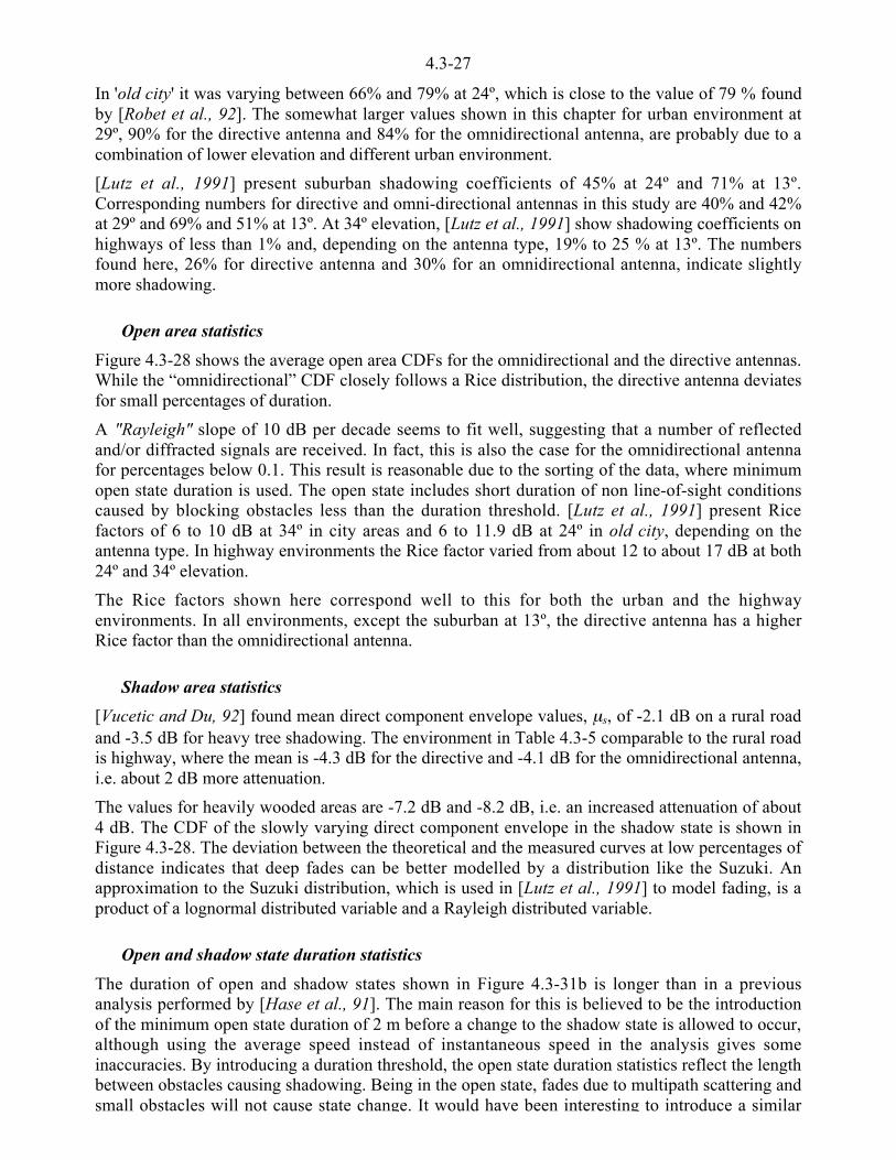
4.3-27

In 'old city' it was varying between 66% and 79% at 24º, which is close to the value of 79 % foundby [Robet et al., 92]. The somewhat larger values shown in this chapter for urban environment at29º, 90% for the directive antenna and 84% for the omnidirectional antenna, are probably due to acombination of lower elevation and different urban environment.

[Lutz et al., 1991] present suburban shadowing coefficients of 45% at 24º and 71% at 13º.Corresponding numbers for directive and omni-directional antennas in this study are 40% and 42%at 29º and 69% and 51% at 13º. At 34º elevation, [Lutz et al., 1991] show shadowing coefficients onhighways of less than 1% and, depending on the antenna type, 19% to 25 % at 13º. The numbersfound here, 26% for directive antenna and 30% for an omnidirectional antenna, indicate slightlymore shadowing.

Open area statistics

Figure 4.3-28 shows the average open area CDFs for the omnidirectional and the directive antennas.While the “omnidirectional” CDF closely follows a Rice distribution, the directive antenna deviatesfor small percentages of duration.

A "Rayleigh" slope of 10 dB per decade seems to fit well, suggesting that a number of reflectedand/or diffracted signals are received. In fact, this is also the case for the omnidirectional antennafor percentages below 0.1. This result is reasonable due to the sorting of the data, where minimumopen state duration is used. The open state includes short duration of non line-of-sight conditionscaused by blocking obstacles less than the duration threshold. [Lutz et al., 1991] present Ricefactors of 6 to 10 dB at 34º in city areas and 6 to 11.9 dB at 24º in old city, depending on theantenna type. In highway environments the Rice factor varied from about 12 to about 17 dB at both24º and 34º elevation.

The Rice factors shown here correspond well to this for both the urban and the highwayenvironments. In all environments, except the suburban at 13º, the directive antenna has a higherRice factor than the omnidirectional antenna.

Shadow area statistics

[Vucetic and Du, 92] found mean direct component envelope values, µs, of -2.1 dB on a rural roadand -3.5 dB for heavy tree shadowing. The environment in Table 4.3-5 comparable to the rural roadis highway, where the mean is -4.3 dB for the directive and -4.1 dB for the omnidirectional antenna,i.e. about 2 dB more attenuation.

The values for heavily wooded areas are -7.2 dB and -8.2 dB, i.e. an increased attenuation of about4 dB. The CDF of the slowly varying direct component envelope in the shadow state is shown inFigure 4.3-28. The deviation between the theoretical and the measured curves at low percentages ofdistance indicates that deep fades can be better modelled by a distribution like the Suzuki. Anapproximation to the Suzuki distribution, which is used in [Lutz et al., 1991] to model fading, is aproduct of a lognormal distributed variable and a Rayleigh distributed variable.

Open and shadow state duration statistics

The duration of open and shadow states shown in Figure 4.3-31b is longer than in a previousanalysis performed by [Hase et al., 91]. The main reason for this is believed to be the introductionof the minimum open state duration of 2 m before a change to the shadow state is allowed to occur,although using the average speed instead of instantaneous speed in the analysis gives someinaccuracies. By introducing a duration threshold, the open state duration statistics reflect the lengthbetween obstacles causing shadowing. Being in the open state, fades due to multipath scattering andsmall obstacles will not cause state change. It would have been interesting to introduce a similar

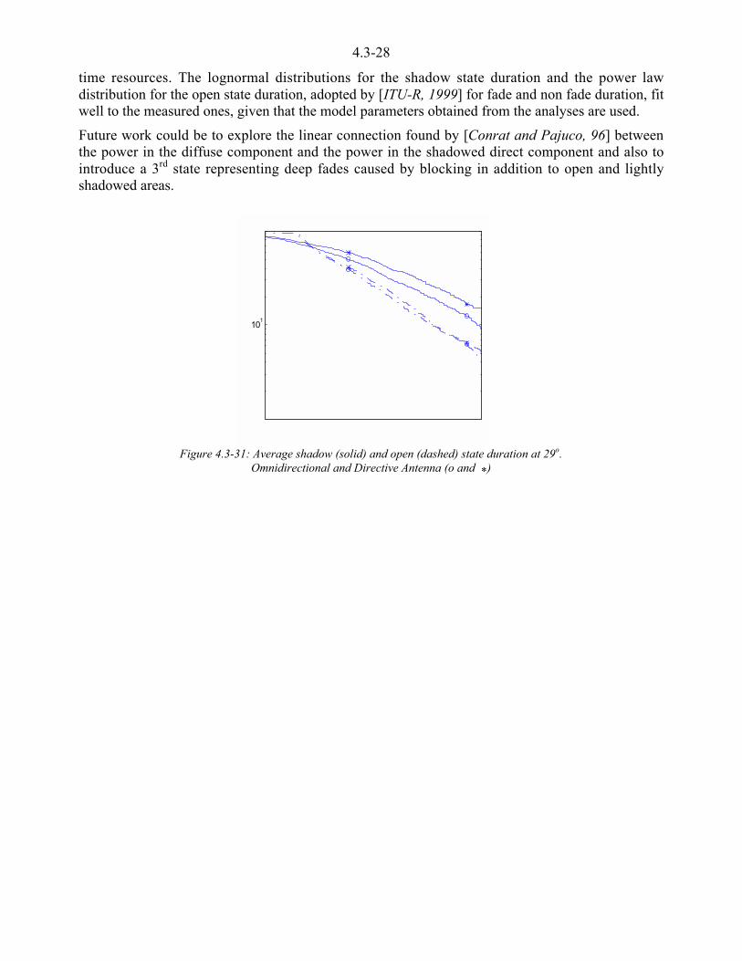
4.3-28

time resources. The lognormal distributions for the shadow state duration and the power lawdistribution for the open state duration, adopted by [ITU-R, 1999] for fade and non fade duration, fitwell to the measured ones, given that the model parameters obtained from the analyses are used.

Future work could be to explore the linear connection found by [Conrat and Pajuco, 96] betweenthe power in the diffuse component and the power in the shadowed direct component and also tointroduce a 3rd state representing deep fades caused by blocking in addition to open and lightlyshadowed areas.

Figure 4.3-31: Average shadow (solid) and open (dashed) state duration at 29o.Omnidirectional and Directive Antenna (o and *)

101

4.3-29

4.3.3 References

[Bråten et al., 1997]Bråten L.E., Kawai N., Louahdi Y and Tjelta T., "Modelling of land mobile satellite channels basedon measurements at 13o and 29o elevation angle" 10th International Conference on Antennas andPropagation, ICAP’97, pp 2.54-2.58, 1997

[Conrat and Pajuco, 1996]Conrat J.M. and Pajuco P., "Fading and shadowing analysis of mobile satellite propagation channelat 1.5 and 2.2 GHz using a helicopter", In Proc. ACTS Mobile Telecommunications summit,Granada, Vol. 2, pp 624-630, 1996

[Evans et al., 1996]Evans B.G., Butt G., Willis M.J., and Parks M.A.N., “Land mobile satellite wideband measurementexperiment at L- and S-Bands, University of Surrey”, ESA ESTEC Contract 10528/93/NL/MB(SC),Final Report, 1996

[Fontan et al., 1997]Fontan F.P., Pereda J., Sedes M.J., Castro M.A.V., Buonomo S. and Baptista P., “Complexenvelope three-state Markov chain simulator for the LMS channel”. Int. J. Sat. Comm., Jan 1997,pp 1-15, 1997

[Fontan et al, 1998]Fontan F.P., Castro M.A.V., Buonomo S., Baptista P. and Arbesser-Rastburg B., "S-Band LMSpropagation channel behaviour for different environments, degrees of shadowing and elevationangles", IEEE Trans. Broadcasting, Vol-44, No. 1, March 98, pp 40-76, 1998.

[Hase et al., 1991]Hase Y., et al., "Fade-durations derived from land-mobile-satellite measurements in Australia",IEEE Trans. Comm., Vol. 39, pp 664-668, 1991

[ITU-R, 1999]ITU-R, Recommendation P.681-4, “Propagation Data Required for the Design of Earth-Space LandMobile Telecommunication Systems”, 1999.

[Jahn and Lutz, 1995]Jahn A. and Lutz E., “Propagation Data and channel model for LMS systems”. Final report,ESA Purchase Order 141742. DLR, 1995.

[Jahn et al., 1996]Jahn A., Bischl H. and Heis G., "Channel characterisation of spread spectrum satellitecommunications". IEEE 4th Int. Symp. Spread Spectrum Techniques and Applications(ISSSTA’96), 1996

[Loo, 1985]Loo C., “A statistical model for land mobile satellite link”. IEEE Trans Vehicular Technology,VT-35, pp 122-127, 1985

[Lutz et al.,1991]Lutz E., D. Cygan, M. Dippold, F. Dolainsky & W. Papke, "The land mobile satellitecommunication channel-recording, statistics, and channel model", IEEE Trans. Vehic. Techn.,VT-30, pp 375-386, 1991

[Lutz, 1996]Lutz E., “A Markov model for correlated land mobile satellite channels” Int. J. Sat. Comm.,Vol. 13, pp 333-339, 1996

4.3-30

[Murr et al., 1995]Murr F., Kastner-Puschl S., Bolzano B., and Kubista E., “Land Mobile Satellite narrowbandpropagation measurement campaign at Ka-Band”, ESTEC Contract 9949/92/NL, Final Report,1995

[Parks et al., 1997]Parks M.A.N., Saunders S.R. and Evans B.G., Wide-band characterisation and modelling of themobile satellite propagation channel at L and S-Bands”, ICAP'97, 1997.

[Proakis, 1995]Proakis J. G., "Digital communications", Third edition, McGraw-Hill, New York, 1995

[Robet et al., 1992]Robet P.P., et al, "Land mobile satellite communication channel model for simultaneoustransmisson from a land mobile terminal via two satellites", Int. J. Sat. Comm., Vol. 10, pp.139-154., 1992

[Smith et al., 1992]Smith, H., Barton S.K., Gardiner J.G. and Sforza M., “Characterisation of the Land Mobile-Satellite(LMS) Channel at L and S bands: narrowband measurements”, ESA AOPs 104433/114473,Bradford, 1992.

[Vucetic and Du, 1992]Vucetic B. and Du J., "Channel modelling and simulation in satellite mobile communicationsystems", IEEE J. Sel. Areas in Comm., Vol. 10, pp 1209-1217, 1992

4.4-1

CHAPTER 4.4 Physical Statistical Modelling

of the LMS channel

Editor: Simon Saunders1

Authors: Simon Saunders1, Costas Tzaras1, Claude Oestges2, D. Vanhoenacker2 1 University of Surrey, Centre for Communication Systems Research, Guildford, GU2 5XH, UK Tel: +44-1483-259806, Fax: +44-1483-259504, e-mail: S.Saunders@ee.surrey.ac.uk 2 Université Catholique de Louvain, Microwave Laboratory, Place du Levant 3, B-1348, Louvain-la-Neuve, Belgium, Tel.: +32-10-478105, Fax.: +32-10-478705, e-mail: Oestges@emic.ucl.ac.be

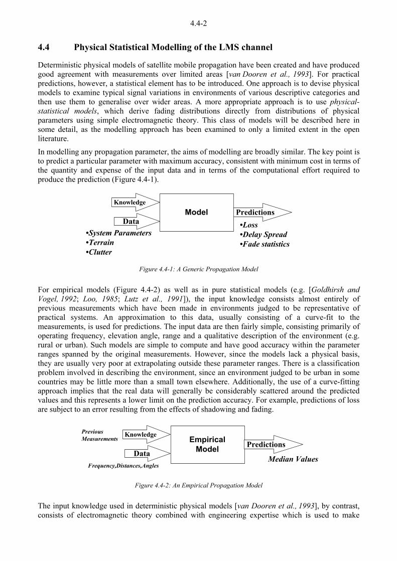
4.4-2

4.4 Physical Statistical Modelling of the LMS channel

Deterministic physical models of satellite mobile propagation have been created and have produced good agreement with measurements over limited areas [van Dooren et al., 1993]. For practical predictions, however, a statistical element has to be introduced. One approach is to devise physical models to examine typical signal variations in environments of various descriptive categories and then use them to generalise over wider areas. A more appropriate approach is to use physical-statistical models, which derive fading distributions directly from distributions of physical parameters using simple electromagnetic theory. This class of models will be described here in some detail, as the modelling approach has been examined to only a limited extent in the open literature.

In modelling any propagation parameter, the aims of modelling are broadly similar. The key point is to predict a particular parameter with maximum accuracy, consistent with minimum cost in terms of the quantity and expense of the input data and in terms of the computational effort required to produce the prediction (Figure 4.4-1).

ModelData

Predictions

•System Parameters•Terrain•Clutter

•Loss•Delay Spread•Fade statistics

Knowledge

Figure 4.4-1: A Generic Propagation Model

For empirical models (Figure 4.4-2) as well as in pure statistical models (e.g. [Goldhirsh and Vogel, 1992; Loo, 1985; Lutz et al., 1991]), the input knowledge consists almost entirely of previous measurements which have been made in environments judged to be representative of practical systems. An approximation to this data, usually consisting of a curve-fit to the measurements, is used for predictions. The input data are then fairly simple, consisting primarily of operating frequency, elevation angle, range and a qualitative description of the environment (e.g. rural or urban). Such models are simple to compute and have good accuracy within the parameter ranges spanned by the original measurements. However, since the models lack a physical basis, they are usually very poor at extrapolating outside these parameter ranges. There is a classification problem involved in describing the environment, since an environment judged to be urban in some countries may be little more than a small town elsewhere. Additionally, the use of a curve-fitting approach implies that the real data will generally be considerably scattered around the predicted values and this represents a lower limit on the prediction accuracy. For example, predictions of loss are subject to an error resulting from the effects of shadowing and fading.

Frequency,Distances,Angles

EmpiricalModelData

PredictionsKnowledgePrevious

Measurements

Median Values

Figure 4.4-2: An Empirical Propagation Model

The input knowledge used in deterministic physical models [van Dooren et al., 1993], by contrast, consists of electromagnetic theory combined with engineering expertise which is used to make

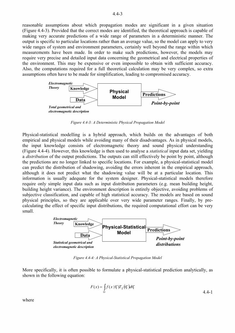
4.4-3

reasonable assumptions about which propagation modes are significant in a given situation (Figure 4.4-3). Provided that the correct modes are identified, the theoretical approach is capable of making very accurate predictions of a wide range of parameters in a deterministic manner. The output is specific to particular locations rather than an average value, so the model can apply to very wide ranges of system and environment parameters, certainly well beyond the range within which measurements have been made. In order to make such predictions, however, the models may require very precise and detailed input data concerning the geometrical and electrical properties of the environment. This may be expensive or even impossible to obtain with sufficient accuracy. Also, the computations required for a full theoretical calculation may be very complex, so extra assumptions often have to be made for simplification, leading to compromised accuracy.

Total geometrical and electromagnetic description

PhysicalModelData

PredictionsKnowledge

ElectromagneticTheory

Point-by-point

Figure 4.4-3: A Deterministic Physical Propagation Model

Physical-statistical modelling is a hybrid approach, which builds on the advantages of both empirical and physical models while avoiding many of their disadvantages. As in physical models, the input knowledge consists of electromagnetic theory and sound physical understanding (Figure 4.4-4). However, this knowledge is then used to analyse a statistical input data set, yielding a distribution of the output predictions. The outputs can still effectively be point by point, although the predictions are no longer linked to specific locations. For example, a physical-statistical model can predict the distribution of shadowing, avoiding the errors inherent in the empirical approach, although it does not predict what the shadowing value will be at a particular location. This information is usually adequate for the system designer. Physical-statistical models therefore require only simple input data such as input distribution parameters (e.g. mean building height, building height variance). The environment description is entirely objective, avoiding problems of subjective classification, and capable of high statistical accuracy. The models are based on sound physical principles, so they are applicable over very wide parameter ranges. Finally, by pre-calculating the effect of specific input distributions, the required computational effort can be very small.

Statistical geometrical and electromagnetic description

Physical-StatisticalModelData

PredictionsKnowledge

ElectromagneticTheory

Point-by-point distributions

Figure 4.4-4: A Physical-Statistical Propagation Model

More specifically, it is often possible to formulate a physical-statistical prediction analytically, as shown in the following equation:

� � KKK dTxfxF N³

:

)|()( 4.4-1

where

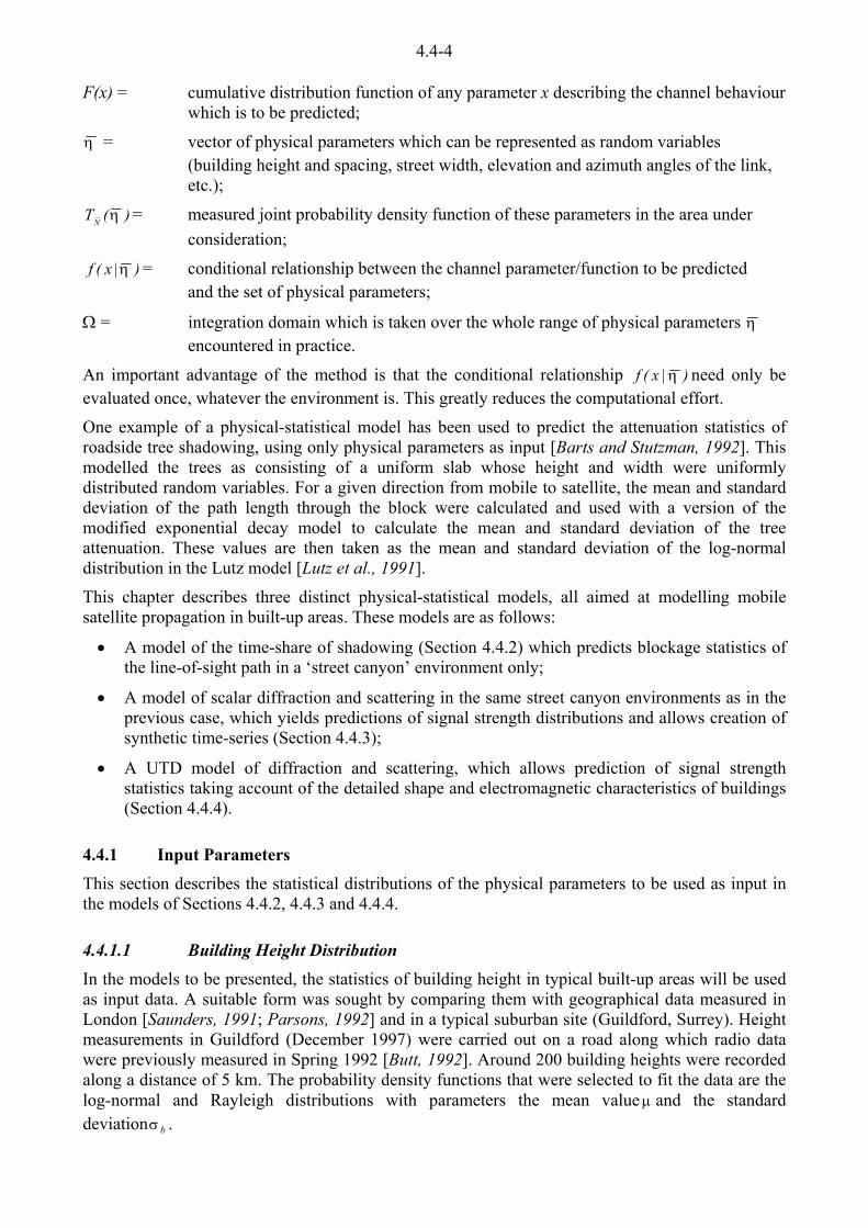
4.4-4

F(x) = cumulative distribution function of any parameter x describing the channel behaviour which is to be predicted;

K = vector of physical parameters which can be represented as random variables (building height and spacing, street width, elevation and azimuth angles of the link, etc.);

)(TN K = measured joint probability density function of these parameters in the area under consideration;

)|x(f K = conditional relationship between the channel parameter/function to be predicted and the set of physical parameters;

: = integration domain which is taken over the whole range of physical parameters K encountered in practice.

An important advantage of the method is that the conditional relationship )|x(f K need only be evaluated once, whatever the environment is. This greatly reduces the computational effort.

One example of a physical-statistical model has been used to predict the attenuation statistics of roadside tree shadowing, using only physical parameters as input [Barts and Stutzman, 1992]. This modelled the trees as consisting of a uniform slab whose height and width were uniformly distributed random variables. For a given direction from mobile to satellite, the mean and standard deviation of the path length through the block were calculated and used with a version of the modified exponential decay model to calculate the mean and standard deviation of the tree attenuation. These values are then taken as the mean and standard deviation of the log-normal distribution in the Lutz model [Lutz et al., 1991].

This chapter describes three distinct physical-statistical models, all aimed at modelling mobile satellite propagation in built-up areas. These models are as follows:

x� A model of the time-share of shadowing (Section 4.4.2) which predicts blockage statistics of the line-of-sight path in a ‘street canyon’ environment only;

x� A model of scalar diffraction and scattering in the same street canyon environments as in the previous case, which yields predictions of signal strength distributions and allows creation of synthetic time-series (Section 4.4.3);

x� A UTD model of diffraction and scattering, which allows prediction of signal strength statistics taking account of the detailed shape and electromagnetic characteristics of buildings (Section 4.4.4).

4.4.1 Input Parameters

This section describes the statistical distributions of the physical parameters to be used as input in the models of Sections 4.4.2, 4.4.3 and 4.4.4.

4.4.1.1 Building Height Distribution In the models to be presented, the statistics of building height in typical built-up areas will be used as input data. A suitable form was sought by comparing them with geographical data measured in London [Saunders, 1991; Parsons, 1992] and in a typical suburban site (Guildford, Surrey). Height measurements in Guildford (December 1997) were carried out on a road along which radio data were previously measured in Spring 1992 [Butt, 1992]. Around 200 building heights were recorded along a distance of 5 km. The probability density functions that were selected to fit the data are the log-normal and Rayleigh distributions with parameters the mean value P and the standard deviation bV .

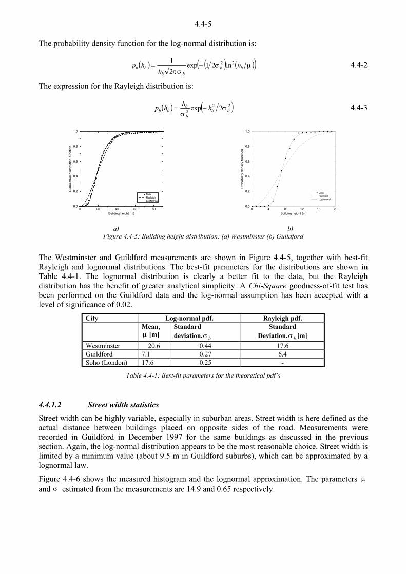
4.4-5

The probability density function for the log-normal distribution is:

� � � � � �� �PVVS

bbbb

bb hh

hp 22 ln21exp21

� 4.4-2

The expression for the Rayleigh distribution is:

� � � �222 2exp bbb

bbb hhhp V

V� 4.4-3

0 20 40 60 80Building height (m)

0.0

0.2

0.4

0.6

0.8

1.0

Cum

ulat

ive

dist

ribut

ion

func

tion

DataRayleighLogNormal

0 4 8 12 16 20

Building height (m)

0.0

0.2

0.4

0.6

0.8

1.0

Prob

abilit

y de

nsity

func

tion

DataRayleighLogNormal

a) b) Figure 4.4-5: Building height distribution: (a) Westminster (b) Guildford

The Westminster and Guildford measurements are shown in Figure 4.4-5, together with best-fit Rayleigh and lognormal distributions. The best-fit parameters for the distributions are shown in Table 4.4-1. The lognormal distribution is clearly a better fit to the data, but the Rayleigh distribution has the benefit of greater analytical simplicity. A Chi-Square goodness-of-fit test has been performed on the Guildford data and the log-normal assumption has been accepted with a level of significance of 0.02.

City Log-normal pdf. Rayleigh pdf. Mean,

P [m] Standard deviation, bV

Standard Deviation, bV [m]

Westminster 20.6 0.44 17.6 Guildford 7.1 0.27 6.4 Soho (London) 17.6 0.25 -

Table 4.4-1: Best-fit parameters for the theoretical pdf’s

4.4.1.2 Street width statistics Street width can be highly variable, especially in suburban areas. Street width is here defined as the actual distance between buildings placed on opposite sides of the road. Measurements were recorded in Guildford in December 1997 for the same buildings as discussed in the previous section. Again, the log-normal distribution appears to be the most reasonable choice. Street width is limited by a minimum value (about 9.5 m in Guildford suburbs), which can be approximated by a lognormal law.

Figure 4.4-6 shows the measured histogram and the lognormal approximation. The parameters P and V estimated from the measurements are 14.9 and 0.65 respectively.

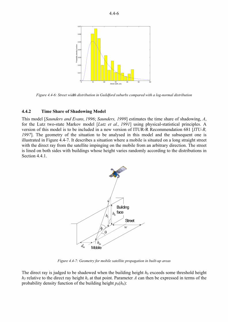
4.4-6

0 10 20 30 40 50 600

0.01

0.02

0.03

0.04

0.05

0.06

0.07

Street width, [m]

Prob

abilit

y de

nsity

func

tion

Figure 4.4-6: Street width distribution in Guildford suburbs compared with a log-normal distribution

4.4.2 Time Share of Shadowing Model

This model [Saunders and Evans, 1996; Saunders, 1999] estimates the time share of shadowing, A, for the Lutz two-state Markov model [Lutz et al., 1991] using physical-statistical principles. A version of this model is to be included in a new version of ITUR-R Recommendation 681 [ITU-R, 1997]. The geometry of the situation to be analysed in this model and the subsequent one is illustrated in Figure 4.4-7. It describes a situation where a mobile is situated on a long straight street with the direct ray from the satellite impinging on the mobile from an arbitrary direction. The street is lined on both sides with buildings whose height varies randomly according to the distributions in Section 4.4.1.

hbhr

w

dm

IT

Buildingface

Street

Mobilehm

Figure 4.4-7: Geometry for mobile satellite propagation in built-up areas

The direct ray is judged to be shadowed when the building height hb exceeds some threshold height hT relative to the direct ray height hs at that point. Parameter A can then be expressed in terms of the probability density function of the building height pb(hb):

4.4-7

� � bbh

bTb dhhphhAT

³f

! )Pr( 4.4-4

Assuming that the building heights follow the Rayleigh distribution (Equation 4.4-3) this yields:

¸̧¹

·¨̈©

§� ¸̧

¹

·¨̈©

§� ³

f

2

2

2

2

2 2exp

2exp

b

Tb

b

b

h b

b hdhhhAT

VVV 4.4-5

The simplest definition of hT is obtained by considering shadowing to occur exactly when the direct ray is geometrically blocked by the building face (a more sophisticated approach [Saunders and Evans, 1996] accounts for the size of the first Fresnel zone at that point). Simple trigonometry applied to this yields the following expression for hT:

� � 0for 0for

sintan

sintan

d��d�

°¯

°®

­

��

�

TSST

TI

TI

mm

mm

rT dwh

dhhh 4.4-6

Figure 4.4-8 compares this model with measurements of A versus elevation angle in city and suburban environments at L-band, taken from [Parks et al., 1993; Lutz et al., 1991; Jahn et al.,

1996]. The model parameters are bV = 15, w = 35, dm = w/2, hm = 1.5 and� .90$ T

Figure 4.4-8: Theoretical and empirical results for time share of shadowing

4.4.3 Time Series Model

Although the approach in the previous paragraph allowed one of the parameters in the Lutz model to be predicted using physical-statistical methods, the rest of the parameters still have to be determined empirically. The [Lutz et al., 1991] model assumes that the lognormal distribution is valid for predicting the shadowing distribution. This distribution comes as a result of a large number of individual effects acting together on the signal [Saunders, 1999]. In the case being treated here, however, only a single building is involved, so the lognormal approximation is questionable. The model described in this section avoids this assumption and directly predicts the statistics of

0 10 20 30 40 50 60 70 80 90Elevation Angle (deg)

0.0

0.1

0.2

0.3

0.4

0.5

0.6

0.7

0.8

0.9

1.0

Shad

owin

g fa

ctor

, A

IEEE Lutz paperCCSR CampaignDLR CampaignPhysical-Statistical Model

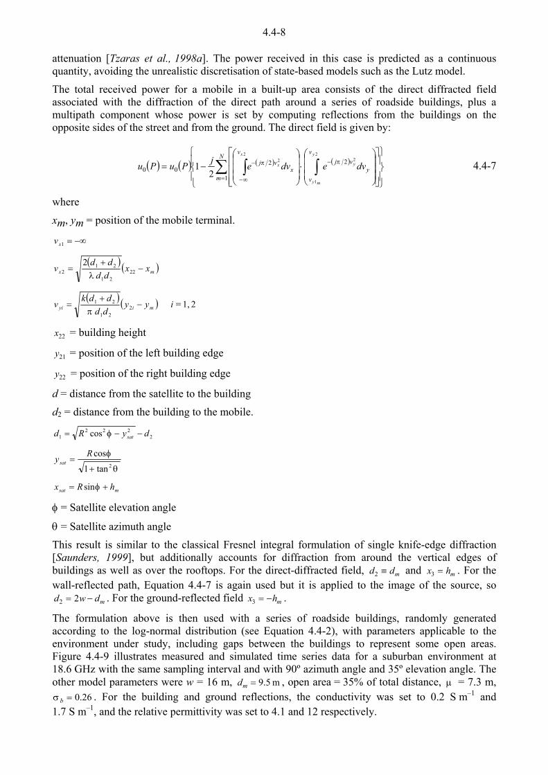
4.4-8

attenuation [Tzaras et al., 1998a]. The power received in this case is predicted as a continuous quantity, avoiding the unrealistic discretisation of state-based models such as the Lutz model.

The total received power for a mobile in a built-up area consists of the direct diffracted field associated with the diffraction of the direct path around a series of roadside buildings, plus a multipath component whose power is set by computing reflections from the buildings on the opposite sides of the street and from the ground. The direct field is given by:

� � � � � � � �

°¿

°¾

½

°¯

°®

­

»»»

¼

º

«««

¬

ª

¸¸¸

¹

·

¨¨¨

©

§�¸¸¸

¹

·

¨¨¨

©

§� ¦ ³³

�

f�

�N

m

v

vy

vjv

xvj

y

my

y

x

x dvedvejPuPu1

2200

2

1

22

2

21 SS 4.4-7

where

xm, ym = position of the mobile terminal.

�f 1xv

� � � �mx xxddddv �

� 22

21

212

2O

� � � � 2 1,= 221

21 iyyddddkv miyi �

�

S

22x = building height

21y = position of the left building edge

22y = position of the right building edge

d = distance from the satellite to the building

d2 = distance from the building to the mobile.

2222

1 cos dyRd sat �� I

T

I2tan1

cos

�

Rysat

msat hRx � Isin

I = Satellite elevation angle�

T = Satellite azimuth angle

This result is similar to the classical Fresnel integral formulation of single knife-edge diffraction [Saunders, 1999], but additionally accounts for diffraction from around the vertical edges of buildings as well as over the rooftops. For the direct-diffracted field, mdd {2 and mhx 3 . For the wall-reflected path, Equation 4.4-7 is again used but it is applied to the image of the source, so

mdwd � 22 . For the ground-reflected field mhx � 3 .

The formulation above is then used with a series of roadside buildings, randomly generated according to the log-normal distribution (see Equation 4.4-2), with parameters applicable to the environment under study, including gaps between the buildings to represent some open areas. Figure 4.4-9 illustrates measured and simulated time series data for a suburban environment at 18.6 GHz with the same sampling interval and with 90º azimuth angle and 35º elevation angle. The other model parameters were w = 16 m, m 5.9 md , open area = 35% of total distance, P = 7.3 m,

26.0 bV . For the building and ground reflections, the conductivity was set to 0.2 S m–1 and 1.7 S m–1, and the relative permittivity was set to 4.1 and 12 respectively.

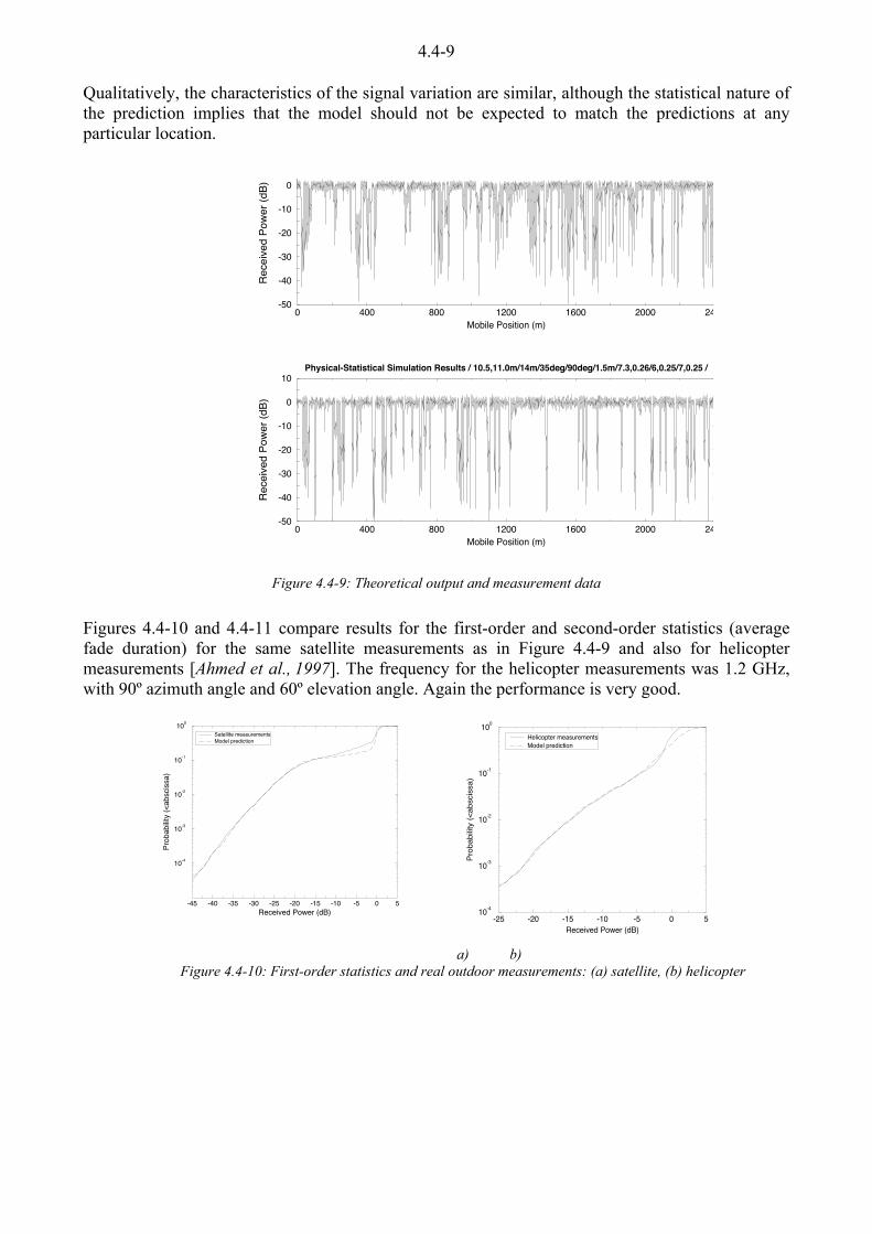
4.4-9

Qualitatively, the characteristics of the signal variation are similar, although the statistical nature of the prediction implies that the model should not be expected to match the predictions at any particular location.

0 400 800 1200 1600 2000 240Mobile Position (m)

-50

-40

-30

-20

-10

0

10

Rec

eive

d Po

wer

(dB)

Physical-Statistical Simulation Results / 10.5,11.0m/14m/35deg/90deg/1.5m/7.3,0.26/6,0.25/7,0.25 /

0 400 800 1200 1600 2000 240Mobile Position (m)

-50

-40

-30

-20

-10

0

Rec

eive

d Po

wer

(dB)

Figure 4.4-9: Theoretical output and measurement data

Figures 4.4-10 and 4.4-11 compare results for the first-order and second-order statistics (average fade duration) for the same satellite measurements as in Figure 4.4-9 and also for helicopter measurements [Ahmed et al., 1997]. The frequency for the helicopter measurements was 1.2 GHz, with 90º azimuth angle and 60º elevation angle. Again the performance is very good.

a) b) Figure 4.4-10: First-order statistics and real outdoor measurements: (a) satellite, (b) helicopter

-45 -40 -35 -30 -25 -20 -15 -10 -5 0 5Received Power (dB)

10-4

10-3

10-2

10-1

100

Prob

abilit

y (<

absc

issa

)

Satellite measurementsModel prediction

-25 -20 -15 -10 -5 0 5Received Power (dB)

10-4

10-3

10-2

10-1

100

Prob

abilit

y (<

absc

issa

)

Helicopter measurementsModel prediction

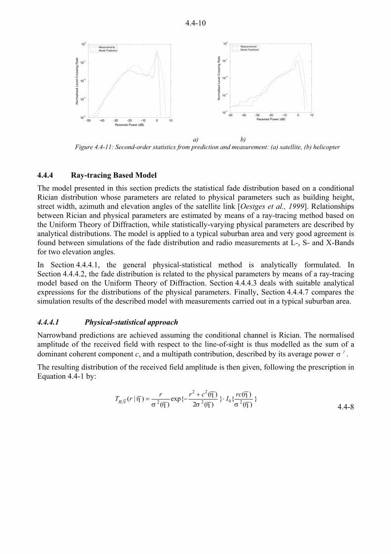
4.4-10

-50 -40 -30 -20 -10 0 10Received Power (dB)

10-4

10-3

10-2

10-1

100

Nor

mal

ised

Lev

el C

ross

ing

Rat

e

MeasurementsModel Prediction

-50 -40 -30 -20 -10 0 10

Received Power (dB)

10-4

10-3

10-2

10-1

100

Nor

mal

ised

Lev

el C

ross

ing

Rat

e

MeasurementsModel Prediction

a) b) Figure 4.4-11: Second-order statistics from prediction and measurement: (a) satellite, (b) helicopter

4.4.4 Ray-tracing Based Model

The model presented in this section predicts the statistical fade distribution based on a conditional Rician distribution whose parameters are related to physical parameters such as building height, street width, azimuth and elevation angles of the satellite link [Oestges et al., 1999]. Relationships between Rician and physical parameters are estimated by means of a ray-tracing method based on the Uniform Theory of Diffraction, while statistically-varying physical parameters are described by analytical distributions. The model is applied to a typical suburban area and very good agreement is found between simulations of the fade distribution and radio measurements at L-, S- and X-Bands for two elevation angles. In Section 4.4.4.1, the general physical-statistical method is analytically formulated. In Section 4.4.4.2, the fade distribution is related to the physical parameters by means of a ray-tracing model based on the Uniform Theory of Diffraction. Section 4.4.4.3 deals with suitable analytical expressions for the distributions of the physical parameters. Finally, Section 4.4.4.7 compares the simulation results of the described model with measurements carried out in a typical suburban area.

4.4.4.1 Physical-statistical approach Narrowband predictions are achieved assuming the conditional channel is Rician. The normalised amplitude of the received field with respect to the line-of-sight is thus modelled as the sum of a dominant coherent component c, and a multipath contribution, described by its average power 2V .

The resulting distribution of the received field amplitude is then given, following the prescription in Equation 4.4-1 by:

}

)()({}

)(2)(exp{

)()|( 202

22

2| KVK

KVK

KVK

rcIcrrrT NR ��

� 4.4-8

4.4-11

The conditional relationships between the physical parameters K and the Rician parameters c and 2V are estimated by means of a ray-tracing technique applied in a canonical configuration, shown

in Figure 4.4-12. In this configuration, the number of buildings is restricted, in order to limit the computation time.

Figure 4.4-12: Canonical scenario in built-up areas

The physical parameters, represented in Figure 4.4-12 are:

x� the building height bh ;

x� the location of the mobile in the street md ;

x� The height of the mobile terminal hm;

x� the street width w;

x� the azimuth angle I relative to the street axis (taken over [0, ʌ/2]);

x� the elevation angle - .

This set of parameters is of course non-exhaustive, but the parameters listed above are considered to be the most relevant ones.

The ray-tracing method is based on the “Uniform Theory of Diffraction” (UTD) and takes into account first order reflection and diffraction mechanisms. The number of buildings in the canonical situation is very small, focusing the study on the influence of the nearest buildings only. This is justified by the following observations. In urban areas, streets are not very long, while in suburbs, they are not straight, which reduces canyon effects and allows restriction to the local environment. Moreover, restricting the number of buildings eliminates artificial enhancing of far reflected or diffracted components, which are actually strongly attenuated on their way to the receiver, due to roughness effects or multiple diffraction and absorption by obstacles. Finally, limiting the number of buildings reduces computation times.

The incident satellite signal is assumed to be a plane wave, with a circular polarisation. The ray-tracer evaluates the fields received by the mobile terminal through various mechanisms, as detailed

I

dm

w

hb

hbA

B

B

-

A

hm

4.4-12

in [Oestges et al., 1998]. The direct field exists in line-of-sight conditions; the fields reflected at the first order from ground and wall surfaces as well as the fields diffracted by single building wedges are also accounted for. Each field component is weighted by the linearly-polarised receiving antenna far-field pattern.

Reflection and diffraction mechanisms depend on surface characteristics. Typical values of conductivity and relative electrical permittivity of ground and brick walls are listed in Table 4.4-2 for several frequency bands [van Dooren, 1994].

Frequency [GHz]

Relative permittivity

Conductivity [S/m]

ground brick ground brick 1.3 (L band) 15 4.3 0.04 0.002 2.4 (S band) 15 4.3 0.40 0.040 10 (X band) 12 4.1 1.70 0.200

Table 4.4-2: Electrical properties of ground and brick

The reflected component is evaluated using Snell's law of reflection, assuming smooth planar surfaces. Only the first order reflected field is calculated, since several simulations have shown that double reflection is insignificant for most practical cases. With regard to single wedge diffraction, the Uniform Theory of Diffraction [Kouyoumjian and Pathak, 1974] and its heuristic extensions [Luebbers, 1984] are applied to locate Keller's diffraction point and calculate the diffracted field. Double diffraction is also implemented, but as far as the canonical scenario is concerned, it is found to be negligible [Oestges et al., 1998].

Any urban or suburban area can be described by the combination of road sections of two kinds, along which fading is not identically distributed: a distinction has therefore to be made between open area sections and built-up sections. The global fade distribution can then be represented by:

� � � � � �aTpaTpaTbAAA ���� )1(

0 4.4-9

where

p = Percentage of open area

0AT = fade probability density function in open areas

bAT = fade probability density function in built-up areas.

The percentage p is to be estimated by inspection of the area.

4.4.4.2 Built-up areas It is assumed that the complex field amplitude is given for any scenario by the sum of a coherent main component plus a random contribution arising from multipath. The amplitude, normalised with respect to the direct component in the line-of-sight is thus modelled as:

rcAb � 4.4-10

where

bA = field amplitude in built-up areas c = dominant component mainly affected by shadowing r = complex quantity with zero mean and independent quadrature components (multipath random contribution).

The field amplitude in built-up areas, bA , therefore follows a Rician distribution, defined by:

4.4-13

� � ¸

¹·

¨©§

¸¸¹

·¨¨©

§ �� 202

22

2 2exp

VVVcaIcaaaT bbb

bAb

4.4-11

where 2V = power of the multipath contribution r.

I0(x) = Modified Bessel Function.

Among the physical parameters, only the elevation angle of the satellite link is given a constant value, as it is strongly related to the particular satellite system and is easily predicted deterministically. The azimuth angle depends on the location of the street axis relative to the satellite while building height and street width are clearly not constant.

Given a fixed elevation angle, Rician parameters c and 2V must be estimated for every combination of building height, street width and azimuth angle, in order to obtain a distribution conditional on these parameters.

This conditional probability density function is then given by:

� � ) I,,whaT bbWHA bb

}),,(),,({}

),,(2),,(exp{

),,( 202

22

2 IVI

IVI

IV whwhcaI

whwhca

wha

b

bb

b

bb

b

b ��

� 4.4-12

Assuming that building height and street width are statistically independent and that distributions of physical parameters, � �bH hT

b, � �wTW , � �I)T , are known for the area, the first order distribution of

fades is given as follows: If we note the fade level A = 1/R, the fade distribution can easily be related to the Rician distribution of the amplitude. Using Equation 4.4-1, the fade distribution is given by:

-I-I

-IS S

dddwdddhTTwTdThT

wdhaT

aT

mbWmDbH

mb

w

WDHA

A

mb

mb

)()()()()(

),,,,|(

)(2/

0

2/

0 0 0 0 |

4)

f f

)4

�����

�

³ ³ ³ ³ ³ 4.4-13

where

)|a1(T

a1)|a(T |R2|A KK 11

The above equation shows that the influence of each physical parameter can be isolated, which is another advantage of the physical-statistical method.

This integral can easily be numerically computed as each distribution can be analytically defined. The description of the conditional distribution is given in Section 4.4.1, while the statistics of the physical parameters are defined in Section 4.4.4.5.

Since the Level Crossing Rate depends on second-order statistics, its prediction cannot easily be formulated analytically. Equation 4.4-1 is then applied using time-series simulations based on a random building generator whose input is precisely the measured distribution of the physical parameters )(TN K .

The simulation of time-series is carried out using a ray-tracing tool. The diffracted field is here calculated using a UTD-based edge equivalent current method, since this method has been proved to give realistic results for simulating time series.

Time series also allow estimation of the average fade duration at any level of attenuation.

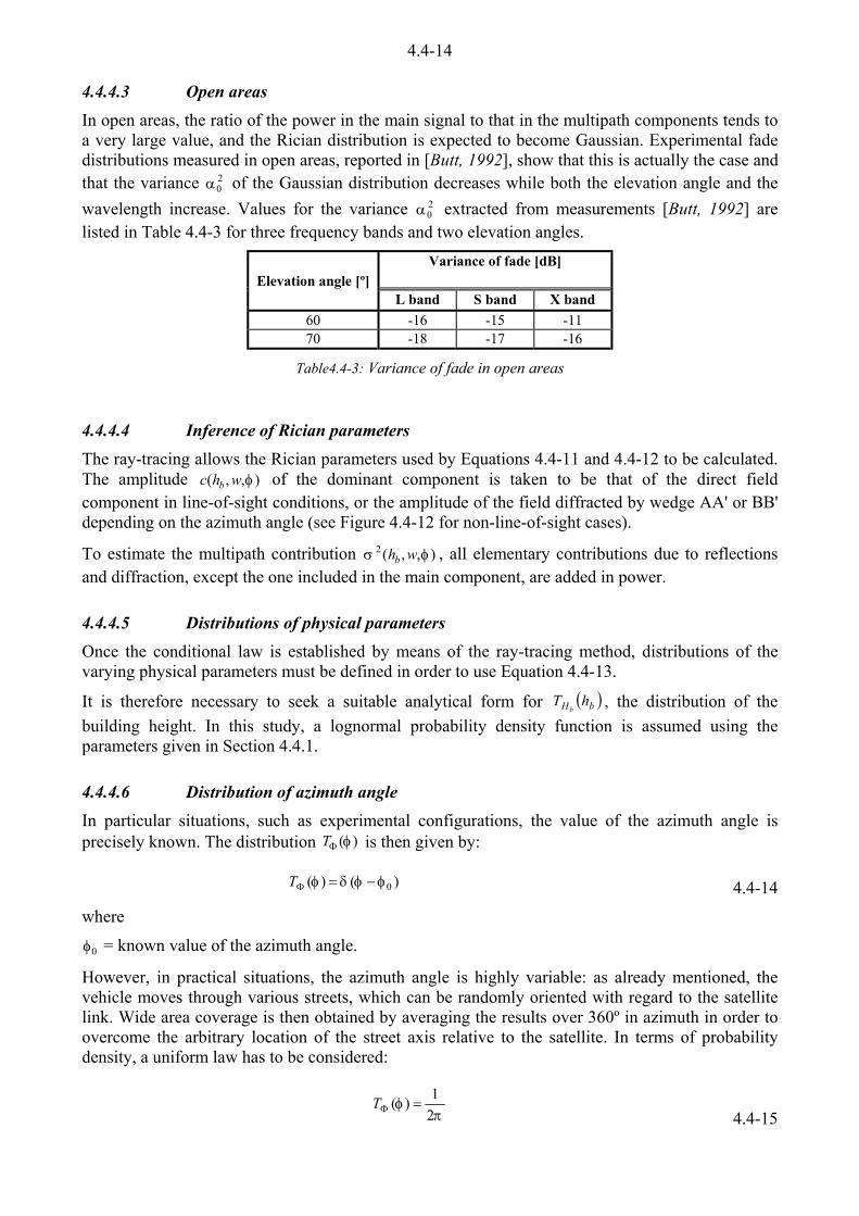
4.4-14

4.4.4.3 Open areas In open areas, the ratio of the power in the main signal to that in the multipath components tends to a very large value, and the Rician distribution is expected to become Gaussian. Experimental fade distributions measured in open areas, reported in [Butt, 1992], show that this is actually the case and that the variance 2

0D of the Gaussian distribution decreases while both the elevation angle and the wavelength increase. Values for the variance 2

0D extracted from measurements [Butt, 1992] are listed in Table 4.4-3 for three frequency bands and two elevation angles.

Variance of fade [dB] Elevation angle [º]

L band S band X band 60 -16 -15 -11 70 -18 -17 -16

Table4.4-3: Variance of fade in open areas

4.4.4.4 Inference of Rician parameters The ray-tracing allows the Rician parameters used by Equations 4.4-11 and 4.4-12 to be calculated. The amplitude ),,( Iwhc b of the dominant component is taken to be that of the direct field component in line-of-sight conditions, or the amplitude of the field diffracted by wedge AA' or BB' depending on the azimuth angle (see Figure 4.4-12 for non-line-of-sight cases).

To estimate the multipath contribution ),,(2 IV whb , all elementary contributions due to reflections and diffraction, except the one included in the main component, are added in power.

4.4.4.5 Distributions of physical parameters Once the conditional law is established by means of the ray-tracing method, distributions of the varying physical parameters must be defined in order to use Equation 4.4-13.

It is therefore necessary to seek a suitable analytical form for � �bH hTb

, the distribution of the building height. In this study, a lognormal probability density function is assumed using the parameters given in Section 4.4.1.

4.4.4.6 Distribution of azimuth angle In particular situations, such as experimental configurations, the value of the azimuth angle is precisely known. The distribution )(I)T is then given by:

)()( 0IIGI � )T 4.4-14

where

0I = known value of the azimuth angle.

However, in practical situations, the azimuth angle is highly variable: as already mentioned, the vehicle moves through various streets, which can be randomly oriented with regard to the satellite link. Wide area coverage is then obtained by averaging the results over 360º in azimuth in order to overcome the arbitrary location of the street axis relative to the satellite. In terms of probability density, a uniform law has to be considered:

SI

21)( )T

4.4-15

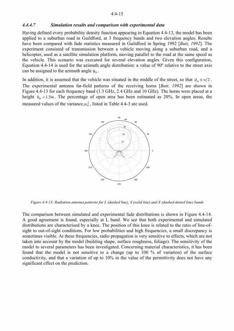
4.4-15

4.4.4.7 Simulation results and comparison with experimental data Having defined every probability density function appearing in Equation 4.4-13, the model has been applied to a suburban road in Guildford, at 3 frequency bands and two elevation angles. Results have been compared with fade statistics measured in Guildford in Spring 1992 [Butt, 1992]. The experiment consisted of transmission between a vehicle moving along a suburban road, and a helicopter, used as a satellite simulation platform, moving parallel to the road at the same speed as the vehicle. This scenario was executed for several elevation angles. Given this configuration, Equation 4.4-14 is used for the azimuth angle distribution: a value of 90º relative to the street axis can be assigned to the azimuth angle 0I .

In addition, it is assumed that the vehicle was situated in the middle of the street, so that 2wdm # . The experimental antenna far-field patterns of the receiving horns [Butt, 1992] are shown in Figure 4.4-13 for each frequency band (1.3 GHz, 2.4 GHz and 10 GHz). The horns were placed at a height mhm 5.1 . The percentage of open area has been estimated as 20%. In open areas, the measured values of the variance, 2

0D , listed in Table 4.4-3 are used.

10

20

30

40

30

210

60

240

90

270

120

300

150

330

180 0

Figure 4.4-13: Radiation antenna patterns for L (dashed line), S (solid line) and X (dashed-dotted line) bands

The comparison between simulated and experimental fade distributions is shown in Figure 4.4-14. A good agreement is found, especially at L band. We see that both experimental and simulated distributions are characterised by a knee. The position of this knee is related to the ratio of line-of-sight to out-of-sight conditions. For low probabilities and high frequencies, a small discrepancy is sometimes visible. At these frequencies, radio propagation is very sensitive to effects, which are not taken into account by the model (building shape, surface roughness, foliage). The sensitivity of the model to several parameters has been investigated. Concerning material characteristics, it has been found that the model is not sensitive to a change (up to 100 % of variation) of the surface conductivity, and that a variation of up to 10% in the value of the permittivity does not have any significant effect on the prediction.

4.4-16

0 10 20

10−2

10−1

100

Fade level, [dB]

Cum

ulat

ive

prob

abilit

y

S band

0 10 2010−2

10−1

100

Fade level, [dB]

Cum

ulat

ive

prob

abilit

y

X band

0 10 20

10−2

10−1

100

Fade level, [dB]

Cum

ulat

ive

prob

abilit

y

L band

Figure 4.4-14: Measured fade statistics at L (1.3 GHz) , S (2.4 GHz) and X (10 GHz) bands for two elevation angles (60º: dashed-dotted lines - 70º: dashed lines) and simulation results

Results provided by the model have also been compared to fade distribution and LCR measurements recorded at L-band in Athens City centre [Kanatas and Constantinou, 1998]. These data were collected at various elevation angles by means of a helicopter, used as satellite platform, flying parallel to the mobile terminal. The street width was around 12 metres and the building height varied between 15 and 21 metres. This physical information is used to infer a rough approximation of )(TN K . Building height is modelled by the lognormal distribution with parameters )3.0,m15(),( VP . Other parameters are given constant values: w = 12m; 2wd m ; I = S/2; - depending on the experiment.

−10 0 10 20 30 40 5010−3

10−2

10−1

100

Fade depth, [dB]

Fade

CPD

Elevation angle = 60 deg.

0 20 40 60−40

−30

−20

−10

0

10

Distance, [m]

Rec

eive

d po

wer

, [dB

]

−50 −40 −30 −20 −10 0 1010−3

10−2

10−1

100

Signal level relative to LOS, [dB]

LCR

, [w

avel

engt

hs−1

]

Figure 4.4-15: Comparison between the model (solid lines) and measured data (dashed lines): - cumulative fade distribution - simulated path loss (measurements are not represented) - normalised level-crossing rate

Figures 4.4-15 and 4.4-16 illustrate the comparison for elevation angles of 60º and 80º. A good agreement is found, while the simulated path loss provided by time series looks realistic if compared to measured path losses presented in [Kanatas and Constantinou, 1998]. It can be noticed that the LCR at 60º presents two peaks, which means that the channel is equivalent to a two-state

4.4-17

Markov process. The advantage is here that the physical-statistical modelling approach is really derived from the environment and contains no empirical assumption.

−20 −10 0 1010−3

10−2

10−1

100

Signal level relative to LOS, [dB]

LCR

, [w

avel

engt

hs−1

]

0 20 40 60−5

0

5

Distance, [m]

Rec

eive

d po

wer

, [dB

]

−10 0 10 20 30

10−2

10−1

100

Fade depth, [dB]

Fade

CPD

Elevation angle = 80 deg.

Figure 4.4-16: Comparison between the model (solid lines) and measured data (dashed lines) : - cumulative fade distribution - simulated path loss (measurements are not represented) - normalised level-crossing rate

4.4.5 Conclusion

In this chapter, three new physical-statistical models have been presented of the land mobile satellite channel in built-up areas. This mixed approach allows mobile-satellite propagation predictions to be assigned parameters which are statistically related to the physical environment.

The physical-statistical modelling approach combines advantages of both deterministic and statistical models : the physical-statistical nature of the approach allows predictions to be obtained from an objective environment description with a modest computational effort.

4.4.6 Acknowledgements

The work described in Section 4.4.4 was carried out while C. Oestges was a visiting Ph. D. student at CCSR, University of Surrey. He is pleased to acknowledge the support of grants from the FNRS (Belgian National Research Fund) and from the Commission of the European Communities in the framework of COST Action 255.

4.4-18

4.4.7 References

[Ahmed et al., 1997] B. Ahmed, S. Buonomo, I.E. Otung, M.H. Aziz, S.R. Saunders and B.G. Evans, “Simulation of 20 GHz narrowband mobile propagation data using N-state Markov channel modelling Approach”, In Proc. 10th Int. Conf. Antennas and Propagation, Edinburgh, 2.48–2.53, 14–17 April 1997.

[Barts and Stutzman, 1992] R.M. Barts and W.L. Stutzman, Modelling and measurement of mobile satellite propagation, IEEE Trans. Ant. Prop., 40 (4), 375–82, 1992.

[Butt, 1992] Butt, G., “Narrowband characterisation of high elevation angle land mobile satellite channel.” PhD Dissertation, University of Surrey, 1992

[van Dooren et al., 1993] G.A.J. van Dooren, M.H.A.J. Herben, G. Brussard, M. Sforza and J.P.V. Poiares Baptista, “Electromagnetic field strength prediction in an urban environment: a useful tool for the planning of LMSS”, In Proc. International Mobile Satellite Conference, 343–48, 1993.

[van Dooren, 1994] Van Dooren, G.A.J., “A deterministic approach to the modelling of electromagnetic wave propagation in urban environments”, PhD Dissertation, Technische Universiteit Eindhoven, 1994

[Goldhirsh and Vogel, 1992] J. Goldhirsh and W.J. Vogel, “Propagation effects for land mobile satellite systems: overview of experimental and modelling results”, NASA Reference Publication 1274, Feb. 1992.

[ITU-R, 1997] International Telecommunication Union, ITU-R Recommendation P.681-3: Propagation data required for the design of earth-space land mobile telecommunication systems, Geneva, 1997.

[Jahn et al., 1996] A. Jahn, H. Bischl and G. Heiss, “Channel characterization for spread-spectrum satellite-communications”, In Proc. IEEE Fourth International Symposium on Spread Spectrum Techniques and Applications, 1221–26, 1996.

[Kanatas and Constantinou, 1998] Kanatas, A.G., Constantinou, P., “City center high-elevation angle propagation measurements at L-band for land mobile satellite systems”, IEEE Trans. Veh. Technol., 47, (3), pp 1002-1011, 1998

[Kouyoumjian and Pathak, 1974] Kouyoumjian, R.G., and Pathak, P.H.: “A uniform geometrical theory of diffraction for an edge in a perfectly conducting surface”, Proc. IEEE, 62, (11), pp. 1448-1461, 1974

[Loo, 1985] C. Loo, “A statistical model for a land mobile satellite link”, IEEE Trans. Veh. Tech., 34 (3), 122–27, 1985.

[Luebbers, 1984] Luebbers, R.J., “Finite conductivity uniform GTD versus knife edge diffraction in prediction of propagation path loss”, IEEE Trans. Antennas Propagat., 32, (1), pp. 70-76, 1984

[Lutz et al., 1991] E. Lutz, D. Cygan, M. Dippold, F. Dolainsky and W. Papke, “The land mobile satellite communication channel-recording, statistics and channel model”, IEEE Trans. Veh. Tech., 40 (2), 375–5, 1991.

4.4-19

[Oestges et al., 1998] Oestges, C., Vasseur, H. and Vanhoenacker, D., “Impact of edge diffraction on the performance of land mobile satellite systems in urban areas”, Proc. 28th European Microwave Conference, EuMC'98, October 1998, Amsterdam, The Netherlands

[Oestges et al., 1999] C. Oestges, S. R. Saunders and D. Vanhoenacker-Janvier, “Physical-statistical modelling of the land mobile satellite channel based on ray-tracing”, IEE Proc. Microwaves, Ant. Prop., 146 (1), 45–49, 1999.

[Parks et al., 1993] M.A.N. Parks, B.G. Evans and G. Butt, “High elevation angle propagation results applied to a statistical model and an enhanced empirical model”, Electronics Letters, 29 (19), 1723–25, 1993.

[Parsons, 1992] Parsons, D., “The mobile radio propagation channel”, (Pentech Press, London, 1992)

[Saunders, 1991] Saunders, S.R., “Diffraction modelling of mobile radio wave propagation in built-up areas”, PhD Dissertation, Brunel University, 1991

[Saunders and Evans, 1996] S.R. Saunders and B.G. Evans, A physical model of shadowing probability for land mobile satellite propagation, Electronics Letters, 32 (17), 1548–89, 1996.

[Saunders, 1999] S.R. Saunders, Antennas and Propagation for Wireless Communication Systems, Wiley, Chichester, ISBN 0471-98609-7, 1999.

[Tzaras et al., 1998] C. Tzaras, B.G. Evans and S.R. Saunders, “A physical-statistical analysis of the land mobile satellite channel”, Electronics Letters, 34 (13), 1355–57, 1998.

4.5-1

CHAPTER 4.5Shadowing Correlation

for Multi-Satellite Diversity

Editor: M.Vazquez-Castro1

Authors: M.Vazquez-Castro1, C. Tzaras2, S. Saunders2, F. Perez-Fontan3

1 Dpt. Tecnologías de las Comunicaciones, Universidad Carlos III, Butarque 15, 28911-Leganés, Madrid, SpainPhone: +34 916249 173, Fax: +34 91 6249430 Email: maryan@tsc.uc3m.es

2 Mobile Communications Research Group, Centre for Communications Systems Research,University of Surrey, Guilford, England GU2 5XH.Phone: +44 1483 259806, Fax: +44 1483 259504, Email: S.Saunders@ee.surrey.ac.uk

3 Dpt. Tecnologías de las Comunicaciones, Universidad de Vigo, Campus Universitario, s/n, 36200-Vigo, SpainPh 34 629 877896 F 34 986 812116 E il f f @ i

4.5-2

4.5 Shadowing Correlation for Multi-Satellite Diversity

Land mobile satellite (LMS) system models together with numerous propagation measurementscarried out using aircraft or other platforms to simulate the mobile-to-satellite link geometryindicate that signal shadowing is the dominant feature influencing LMS system availability andperformance. While multipath fading can be overcome for a given fade margin by using differenttransmission techniques, blockage effects can hardly be mitigated resulting in high bit error ratesand in temporary unavailability. Given the power limitation, especially in the up-link, the solutionto reduce such shadowing effects is path or satellite diversity.

Although most available LMS propagation models can reproduce with fairly good accuracy thevarious channel effects (fading, time dispersion, Doppler, ...) and be used in the evaluation ofdifferent channel coding, modulation or equalisation techniques, only deterministic models can bedirectly used to simultaneously analyse satellite-mobile links, and thus, evaluate the benefits ofsatellite diversity. Basically, shadowing is due to blockage and diffraction effects, especially inurban areas, although other mechanisms like absorption losses through vegetation are also a majorplayer in a number of environments. When using models based on a physical approach, detailedurban layout information can be supplied by means of urban data bases when these are used asexplained in Chapters 4.2 and 4.6. Another approach that makes use of synthetic environments isthe use of physical statistical models, as described in Chapter 4.4. In this case, the inputenvironment is generated from statistical distributions describing building heights and general urbanlayout.

In both cases, deterministic and physical-statistical models, diversity effects can be directly assessedby extending the single link study to a multi-link study performed for the input scenario. This is notthe case in other modelling approaches such as purely statistical (Chapter 4.3) or empirical models.The output of a purely statistical or empirical model is an independent realisation. Therefore thegeneration of correlated realisations could be difficult. Nevertheless the analysis of correlation instatistical or empirical models is interesting, due to their simplicity.

In effect, when assessing a particular multisatellite scenario, i.e. a number of satellites are above theminimum elevation above the horizon, the blockage affecting the links depends exclusively on thephysical characteristics of the environment: buildings heights, distance between the receiver and thelandscape features, etc. Therefore since the available satellite links are correlated to each other sucha correlation must be “forced” into statistical models to accurately reproduce the effects ofcorrelated shadowing effects, as indicated in Chapter 4.4.

It should be noted that three different aspects must be addressed: firstly, quantification of thecorrelation by means of the correlation coefficient; secondly, the appropriate methodology to forcethis correlation information into the channel model and thirdly, the assessment of the diversity gain,which is the actual objective.

It is also worth pointing out that determination of the diversity performance must take into accountnot only the propagation phenomena but also the combining schema to be used at the receiver.

The work presented in this chapter is mainly focused on the quantification of the correlationcoefficient in urban environments and related tasks such as environment parameterisation.

The summary presented in the following section will set the scene before the work carried outwithin COST 255 is presented and discussed.

4.5.1 Overview of Other Satellite Diversity Studies

In this section a brief summary is presented of a number of relevant studies on satellite diversity.

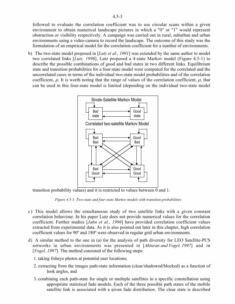
4.5-3

followed to evaluate the correlation coefficient was to use circular scans within a givenenvironment to obtain numerical landscape pictures in which a "0" or "1" would representobstruction or visibility respectively. A campaign was carried out in rural, suburban and urbanenvironments using a video-camera to record the landscape. The outcome of this study was theformulation of an empirical model for the correlation coefficient for a number of environments.

b) The two-state model proposed in [Lutz et al., 1991] was extended by the same author to modeltwo correlated links [Lutz, 1996]. Lutz proposed a 4-state Markov model (Figure 4.5-1) todescribe the possible combinations of good and bad states in two different links. Equilibriumstate and transition probabilities for a four-state model were computed for the correlated and theuncorrelated cases in terms of the individual two-state model probabilities and of the correlationcoefficient, l. It is worth noting that the range of values of the correlation coefficient, l, thatcan be used in this four-state model is limited (depending on the individual two-state model

transition probability values) and it is restricted to values between 0 and 1.

Figure 4.5-1: Two-state and four-state Markov models with transition probabilities

c) This model allows the simultaneous study of two satellite links with a given constantcorrelation behaviour. In his paper Lutz does not provide numerical values for the correlationcoefficient. Further studies [Jahn et al., 1996] have provided correlation coefficient valuesextracted from experimental data. As it is also pointed out later in this chapter, high correlationcoefficient values for 90º and 180º were observed in regular grid urban environments.

d) A similar method to the one in (a) for the analysis of path diversity for LEO Satellite-PCSnetworks in urban environments was presented in [Akturan and Vogel, 1997] and in[Vogel, 1997]. The method consisted of the following steps:

1. taking fisheye photos at potential user locations;

2. extracting from the images path-state information (clear/shadowed/blocked) as a function oflook angles, and

3. combining each path-state for single or multiple satellites in a specific constellation usingappropriate statistical fade models. Each of the three possible path states of the mobilesatellite link is associated with a given fade distribution. The clear state is described

Badstate

Goodstate

Single-Satellite Markov Model

Correlated two-satellite Markov Model

BadBad

GoodBad

GoodGood

BadGood

4.5-4

using a Rice distribution, the shadowed and the blocked states are modelled using theLoo model.

The derived urban three-state model was:

)()()()()()(),( rfBrfSrfCrf LooLooRicer ____ ++= 4.5-1

where _ is the elevation angle.The Rice and Loo distribution parameters were extracted from measurements. The values (%)of C, S and B were estimated from fisheye pictures [Akturan and Vogel, 1996].

e) Another approach to the study of satellite diversity can be found in [Karasawa et al, 1997]. Inthis study, a switching diversity scheme was studied. The clear state is described by a Ricedistribution, the shadowed state is modelled by means of the Loo distribution and the blockedstate is modelled with a Rayleigh distribution. A three-state Markov model is assumed toaccount for the large dynamic range of the received signal. The use of uncorrelated Markovmodels, one per satellite link was proposed (Figure 4.5-2) and it is assumed that stateoccurrences for one satellite link are not correlated with those of other satellite links. Results ofthis study showed a significant improvement in service availability thanks to the diversityeffect.

Figure 4.5-2: Evaluation of satellite diversity gain

f) In [Meenan et al, 1998], the availability of the ICO and Globalstar systems was analysedusing the correlated four-state model developed by Lutz. From fisheye pictures taken inGuilford, Southampton, London and Los Angeles, blockage and correlation statistics wereextracted. In this study it was observed that for azimuth separations smaller than 30º, satellitechannels tend to be correlated.

4.5.2 COST 255: New approaches for correlation quantification

As pointed out in the introduction to this chapter, physical models do not require explicitinformation related to the correlation among the different satellite links since it is implicitly presentin the geometry of models. For statistical models, however, correlation information has to be known

4.5-5

Two different approaches to shadowing correlation characterisation and quantification are discussedhere. One is based on the use of a physical-statistical model and the other on a purely deterministicmodel. The first conclusion to be drawn is that physical channel models (site-specific models) areused to extract the correlation information which must be forced into models lacking a specificenvironment description.

These two approaches produce similar results, as will be shown. The studies carried out withinCOST 255 to quantify the correlation coefficient for different types of environments are based onsimulations using synthetic scenarios. The synthetic environments used in these studies are easilydescribed by a set of parameters related to the degree of urbanisation, that permit a straightforwardextrapolation of the obtained results. Very similar results have been achieved to those obtainedusing measurements, as in [Jahn et al., 1996].

The apparent advantage of the two proposed approaches over the use of measurements and othertechniques (e.g. fish eye photos) is that they can be run on a computer at a much lower cost.Simulations are limited to the urban scenario given its importance and ease of simulation.

In the two cases, either an explicit mathematical expression or tabulated data as a function of thesimple and easy to observe urbanisation parameters are sought.

The two approaches studied within COST 255 are the following:

In [Tzaras et al, 1998a, 1998b] a physical-statistical propagation model was used providing explicitexpressions relating the average correlation coefficient, l , for a given environment characterised bythe height distribution of buildings on both sides of the road.

In [Fontan et al, 1998] the average azimuth correlation sector,B (6q, 6e, eref) is defined, with 6qand 6e being azimuth and elevation separation between pairs of satellites and eref the referenceelevation. This parameter indicates the average angular separation required for two satellites tobecome uncorrelated for a given environment. A deterministic model employing simple ray-tracing(LOS/non-LOS) techniques applied to synthetic environments was used to compute theB parameter(Figure 4.5-3).

Figure 4.5-3: Definition of the average azimuth correlation sector parameter,B (6q, 6e, eref).

Each approach starts off with the same definition of the stochastic process under study (seeFigure 4.5-4) although each follows a different mathematical procedure, leading to similar results asshown below.

A discrete stochastic process Si[n] for satellite-i is defined as follows:

[ ]ª©¨

= conditions shadowed if 0

conditionssight -of-line if 1nSi

4.5-6

The line-of-sight and shadowed states are defined by the existence/non-existence of the direct ray.The stochastic process is considered to be in the shadowed state, with value 0, when the direct ray isblocked and 1 when there is direct visibility to the satellite.

Random variables result from the collection of a number of received signal values (converted toones or zeroes) simultaneously observed at a given time. These values correspond to the receivedsignal for a sufficiently large number of directions (azimuths and elevations) around the receiver(circular scans) located within the test environment.

The objective is, thus, to find the correlation as a function of the azimuth increment, 6q, amongdifferent circular scans corresponding to satellites at the same (6e=0º) or different (6e&0º)elevations.

Figure 4.5-4: Shadowing stochastic process. Diagram showing the two approaches followed

4.5.2.1 Physical-Statistical Approach

By calculating the correlation coefficient between two random variables (normalised second-orderjoint moment):

( )( )[ ]( )[ ] ( )[ ]2

22

2

21

2211

21

21 ),(

SSESSE

SSSSESSCOV

<<

<<==

mml 4.5-2

Fixed user location

Integration over a

height distributionMobile user

Integration over

a street route

eeee1

eeee2

0

00

0 0 1

11

Azimuth angle uniformly

distributed on [0,2W]

Stochastic

process, Si(t)

Azimuths, q

Elevations, e

time

( ei, q1)

( ei, q2)

( ei, qn)

.

.

.

Random variables

Si(to) =S

Satellite i

4.5-7

where the expectation (averaging process) is taken over all possible satellite-to-mobile azimuthsassuming an uniform distribution in the interval [0,2/] and a given distribution for the buildingheights.

The option is only feasible if simplifying assumptions are made about the geometry of the urbanenvironment. The approach followed in [Tzaras et al, 1998a, 1998b] is based on a physical-statistical model [Saunders & Evans, 1997] described in Chapter 4.4 where, basically, physicalpropagation models, including diffraction, are performed on synthetic environments (made up ofplane screens representing buildings) with heights following distributions obtained by directobservation of the urban environment. The physical-statistical model used proposes a canonicalgeometry for the environment traversed by a mobile receiver, typically a street canyon (see Figures4.5-4 and 4.5-5), composed of buildings on both sides of the street.

e

q

Satellite

w

dm hm

BuildingFace

Street

Mobile

hbhr

Figure 4.5-5: Mobile-Satellite canonical street geometry.

The result is an analytic formula that depends only on the azimuth angle separation between the twosatellites. The mathematical procedure [Tzaras et al, 1998a, 1998b] used is described in detail inAppendix 4.5.6.

4.5.2.2 Semi-deterministic Approach

A second alternative is to obtain different realisations (azimuth scan series) of the random processby means of a simple ray-tracing algorithm performed on synthetic environments in the form ofbuilding data bases created according to controlled parameters/distributions.

In [Fontán et al, 1998] and [Vázquez, 1998] this methodology is described. For simplicity, only theblockage of the direct ray is computed and only street canyons are considered. In this case, spatialaveraging is performed, i.e., the averaging is performed over different circular scans for a largenumber of evenly spaced points along the test street. This approach is exactly the same averagingprocess described in the physical-statistical approach but in this case the ray tracing performs thecomputation of the link state on a given street canyon (see Figure 4.5-4).

This second approach can also be expressed mathematically by means of Equation 4.5-3:

( )( )( ) ( )2

22

2

11

2211

21

21 ),(

SSSS

SSSSSSCOV

<<

<<==

mml 4.5-3

Both methods were compared and found to yield exact agreement within the same environment thusverifying the validity of the physical-statistical approach. Figure 4.5-6 shows an example where lwas computed with both methods for a given environment, as a function of the azimuth offset 6q,

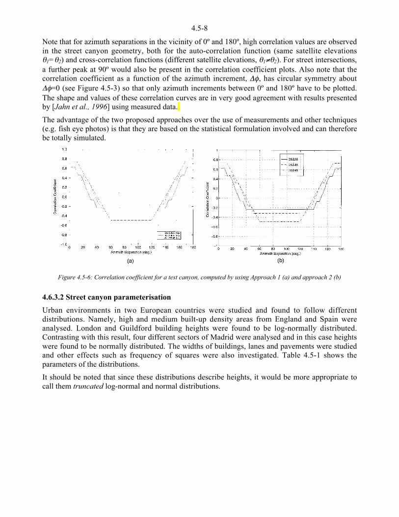
4.5-8

Note that for azimuth separations in the vicinity of 0º and 180º, high correlation values are observedin the street canyon geometry, both for the auto-correlation function (same satellite elevationse1=e2) and cross-correlation functions (different satellite elevations, e1&e2). For street intersections,a further peak at 90º would also be present in the correlation coefficient plots. Also note that thecorrelation coefficient as a function of the azimuth increment, 6q, has circular symmetry about6q=0 (see Figure 4.5-3) so that only azimuth increments between 0º and 180º have to be plotted.The shape and values of these correlation curves are in very good agreement with results presentedby [Jahn et al., 1996] using measured data.

The advantage of the two proposed approaches over the use of measurements and other techniques(e.g. fish eye photos) is that they are based on the statistical formulation involved and can thereforebe totally simulated.

Figure 4.5-6: Correlation coefficient for a test canyon, computed by using Approach 1 (a) and approach 2 (b)

4.6.3.2 Street canyon parameterisation

Urban environments in two European countries were studied and found to follow differentdistributions. Namely, high and medium built-up density areas from England and Spain wereanalysed. London and Guildford building heights were found to be log-normally distributed.Contrasting with this result, four different sectors of Madrid were analysed and in this case heightswere found to be normally distributed. The widths of buildings, lanes and pavements were studiedand other effects such as frequency of squares were also investigated. Table 4.5-1 shows theparameters of the distributions.

It should be noted that since these distributions describe heights, it would be more appropriate tocall them truncated log-normal and normal distributions.

4.5-9

Country Location General Description Distribution

London Densely built-up district, high buildingsLog-normal

µ = 17.6 m, m = 0.31 mEngland

Guildford Medium-size English townLog-normal

µ = 7.2 m, m = 0.26 m

Madrid (La Castellana) Business area, very high buildingsNormal

µ = 21.4 m, m = 8.9 m

Madrid (Chamberí) Residential area, old buildings with few storesNormal

µ = 12.5 m, m = 3.7 m

Madrid (center) Historical and shopping center of MadridNormal

µ = 10, m = 2 mSpain

Madrid (El Viso) Residential area, new individual houses

h < 9 m 5 % h = 9 m 70 % h = 12 m 20 % h > 12 m 5 %

Table 4.5-1: Height Distributions

4.5.3 Simulations

For the simulations, the semi-deterministic model was used to produce statistics of variability of thecorrelation with mobile.

The results obtained for simulations using the second approach are summarised from Tables 4.5-2to 4.5-5 only for the log-normal distributed heights.

Tables 4.5-2 and 4.5-3 show the average azimuth correlation sector values, B (6q,6e,eref), obtainedfrom simulations using the second approach. For satellite-to-mobile links having angle separationsgreater than B , loss of correlation is to be expected and so there will be the possibility of achievingsome diversity gain. The dependence of the correlation parameter with mean street height and widthis apparent from the tables. It can be observed that, for satellites at the same elevation, loss ofcorrelation is reached around 6q = 30º. It can also be observed how correlation is lost for twosatellite links with elevation offsets greater than 20º.

LN(7.2,0.3) LN(17.6,0.3)eeeeref

(º)Ws=10 Ws=15 Ws=20 Ws=10 Ws=15 Ws=20

20 20 24 30 6 10 1430 30 30 22 10 15 2040 30 30 LOS 20 22 2550 LOS LOS LOS 24 30 LOS

Table 4.5-2: B in the vicinity of 6q=0º for 6e=0º and different street widths, Ws(m).

LN(7.2,0.3) LN(17.6,0.3)e (º) Ws=10 Ws=15 Ws=20 Ws=10 Ws=15 Ws=2020 .8/20 0.7/25 0.5/30 0.7/5 0.7/7 0.8/1030 .6/30 0.5/20 - 0.7/10 0.7/15 0.8/540 .5/20 - - 0.8/18 0.8/20 0.8/22

Table 4.5-3: Maxl/ B in the vicinity of 6q=180º for 6e=0º and different street widths, Ws(m)

. – means that the values of l were below the threshold considered, in this case, lth = 0.3.

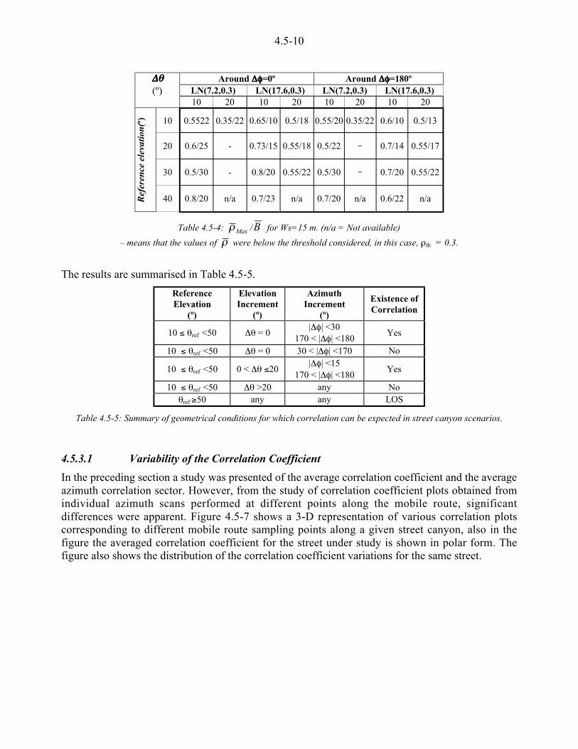
4.5-10

Around 6666qqqq=0º Around 6666qqqq=180ºLN(7.2,0.3) LN(17.6,0.3) LN(7.2,0.3) LN(17.6,0.3)

6666eeee(º)

10 20 10 20 10 20 10 20

10 0.5522 0.35/22 0.65/10 0.5/18 0.55/20 0.35/22 0.6/10 0.5/13

20 0.6/25 - 0.73/15 0.55/18 0.5/22 - 0.7/14 0.55/17

30 0.5/30 - 0.8/20 0.55/22 0.5/30 - 0.7/20 0.55/22

Ref

eren

ce e

leva

tion(

º)

40 0.8/20 n/a 0.7/23 n/a 0.7/20 n/a 0.6/22 n/a

Table 4.5-4: Maxl /B for Ws=15 m. (n/a = Not available)

– means that the values of l were below the threshold considered, in this case, lth = 0.3.

The results are summarised in Table 4.5-5.

ReferenceElevation

(º)

ElevationIncrement

(º)

AzimuthIncrement

(º)

Existence ofCorrelation

10 ) eref <50 6e = 0|6q| <30

170 < |6q| <180Yes

10 ) eref <50 6e = 0 30 < |6q| <170 No

10 ) eref <50 0 < 6e )20|6q| <15

170 < |6q| <180Yes

10 ) eref <50 6e >20 any Noeref *50 any any LOS

Table 4.5-5: Summary of geometrical conditions for which correlation can be expected in street canyon scenarios.

4.5.3.1 Variability of the Correlation Coefficient

In the preceding section a study was presented of the average correlation coefficient and the averageazimuth correlation sector. However, from the study of correlation coefficient plots obtained fromindividual azimuth scans performed at different points along the mobile route, significantdifferences were apparent. Figure 4.5-7 shows a 3-D representation of various correlation plotscorresponding to different mobile route sampling points along a given street canyon, also in thefigure the averaged correlation coefficient for the street under study is shown in polar form. Thefigure also shows the distribution of the correlation coefficient variations for the same street.

4.5-11

Figure 4.5-7: Single route point and route averaged correlation coefficient plots in a street canyon.

In order to further illustrate the correlation coefficient variability, Figures 4.5-7 and 4.5-8 showhistograms computed for various azimuth increments, 6q. This is further illustrated in a schematicform in Figure 4.5-9.

From Figures 4.5-7 and 4.5-8 it is clear that, for simulation purposes, the average correlationcoefficient is not representative of the conditions experienced by two closely spaced mobile-to-satellite links. The use of correlation coefficients in statistical models of the Markov type has to bedone with care, taking into account the variability of the correlation coefficient.

Also from Figure 4.5-8, a very promising feature can be observed in the correlation coefficient plotswhich is the fact that negative values of this parameter occur with significant probabilities.

4.5-12

Figure 4.5-8: Histograms of l for different values of 6q for the case illustrated in Figure 4.5-7.

It is also clear from the observation of these figures that the issue of shadowing correlationcharacterisation is in no way closed and that new in depth studies are still required.

Figure 4.5-9: Schematic representation of the variability of l around its average value probability density function and cumulative distribution function.

4.5.4 Conclusions

This chapter has addressed shadowing effects and their correlation for links with a given angularseparation. First, a review of the most relevant studies dealing with these issues has been made afterwhich the studies carried out within COST 255 have been presented. Two different approaches havebeen followed leading to similar conclusions, one using a physical-statistical model while the otheris based on a purely deterministic approach.

The obtained results can be used in the assessment of different proposed constellations for thirdgeneration personal communications systems. Another application would be to use the results as

4.5-13

It has been shown that correlation coefficients tend to vary about their mean value presenting, for asignificant number of cases, small or even negative values. The characterisation of correlationcoefficient variability and other related issues requires further studies to be carried out in theframework of ensuing COST actions.

4.5-14

4.5.5 References

[Akturan and Vogel, 1996]Akturan R., Vogel W., “Photogrammetric Mobile Satellite Service Prediction”, Electronic Letters,Vol. 31, No. 3, pp. 165-166, 1996.

[Akturan and Vogel, 1997]Akturan R., Vogel W., “Path Diversity for LEO-Satellite-PCS in the Urban Environment”, IEEE onAnt. and Prop., vol. 45, no. 7, July (1997).

[Fontán et al., 1998]Fontan F.P., Vazquez M.A., Buonomo S., Kubista E., Paraboni A., Arbesser B. and Baptista, P.,,“A Methodology for the Characterisation of Environmental Effects on Global navigation SatelliteSystem (GNSS) Propagation”, I.J. of Satellite Communications, Vol 16, pp. 1-22 1998.

[Jahn et al, 1996]Jahn A., Bischl H., Hei` G., “Channel Charaterisation for Spread Spectrum SatelliteCommunications”, Proc IEEE 4th Symposium on Spread Spectrum Techniques and Appl., ISSSTA1996.

[Karasawa et al, 1997]Karasawa Y., Kimura K., Minamisono K., “A Propagation Channel Model for Personal Mobile-Satellite Services”, IEEE Transactions on Veh. Tech, VT-46, No. 4, 1997.

[Lutz et al, 1991]Lutz E., Cygan D., Dippold M., Dolainsky F., Papke W., “The Land Mobile Satellite Channel-recording, statistics and channel model” IEEE Transactions of Veh. Tech., VT-40, pp. 375-386,1991.

[Lutz, 1996]Lutz E., “A Markov Model for correlated land mobile satellite channels”, I.J. of SatelliteCommunications, Vol. 14, pp. 333-339, 1996.

[Meenan et al, 1998]Meenan C., Parks M., Tafazolli R., Evans B.G., “Availability of 1st Generation Satellite PersonalCommunications network Service in Urban Environments”, IEEE VTC’98 pp. 1471-1475, 1998.

[Robet et al, 1992]Robet P.P., Evans B.G. and Ekman A., “Land Mobile Satellite Communications Channel Model forsimultaneous transmission from a Land mobile terminal via two separate satellites”, I.J. of SatelliteCommunications, Vol. 10, pp. 139-154, 1992.

[Saunders & Evans, 1997]Saunders S.R. & B.G. Evans, “A Physical Statistical Model for Land Mobile Satellite Propagationin Built-up Areas”, 10th International Conference on Antennas and Propagation, ICAP’97, pp. 2.44-2.47, 1997.

[Tzaras et al, 1998a]Tzaras C., Evans B.G. and Saunders R.S., "A Physical-Statistical Analysis of the Land MobileSatellite Channel", IEE Electronics Letters, Vol. 34, No. 13, pp. 1355-1357, 1998.

[Tzaras et al, 1998b]Tzaras C., Saunders S.R., Evans B.G., “A Physical-Statistical Propagation model for diversity inmobile Satellite PCN”, IEEE VTC’98, 1998.

[Vázquez, 1998]Vazquez, M.A., “Land Mobile Satellite Channel Modelling by means of Statistical andD t i i ti th d ” Ph D Th i U i it f Vi S i (i S i h) 1998

4.5-15

[Vogel, 1997]Vogel W.J., “Satellite Diversity for Personal Satellite Communications – Modelling andMeasurements”, 10th Int. Conf. on Ant. and Prop., ICAP’97, pp. 1269-1272, 1997.

4.5-16

4.5.6 Appendix to Chapter 4.5: Correlation Modelling Using a Physical StatisticalApproach

The parameters of the physical-statistical model are defined as shown in Figure 4.5-4 and inTable A.4.5-1 (see also Chapter 4.4).

q Elevation angle of the satellite from the mobile

e Azimuth angle of the satellite from the mobile relative to the axis ofthe street

wStreet width (m)

dm Perpendicular distance of the mobile from the building face (m)

hm The height of the phase centre of the mobile antenna above localground level (m)

hb The height of the building immediately below the direct ray relative tolocal ground level (m)

hr The height of the direct ray above the building face relative to localground level (m)

dr The distance along the direct ray from the mobile to the point on theray immediately above the building (m).

Table A.4.5-1: Physical-statistical model parameters.

Simple trigonometry yields the following relationships

( )««ª

««©

¨

)<<

<

)<+=

0- h

0 h

m

m

e/e

q

/ee

q

sin

tandwsin

tand

hm

m

r

A.4.5-1

Under the assumptions made in the model the mean value for the shadowed state is given by

( ) ( ) ( )00 <==//

e/

eee2

0

2

0 2

1sbrisssii dhhudpSS

A.4.5-2

where )( siS e denotes the shadowing state for satellite-i, with azimuth angle se . Where, ui is the unit

step function

ª©¨ *<

=<otherwise0

01)( br

bri

hhhhu A.4.5-3

The value 1 corresponds to the line-of-sight state and the value 0 to the non-line-of-sight state. Forsimplicity, the following notation will be used

( )´́¦

¥²²¤

£

<

<>´́

¦

¥²²¤

£

<> <<

mb

imi

mb

imi hh

tandwsin

hh

tandsina

qq 11 b A.4.5-4

The terms inside the integral (see Equation A.4.5-2) are equal to unity when, for /e )< s0 ,

( )mb

imsbr hh

tandsinhh

<)�*

qe A.4.5-5

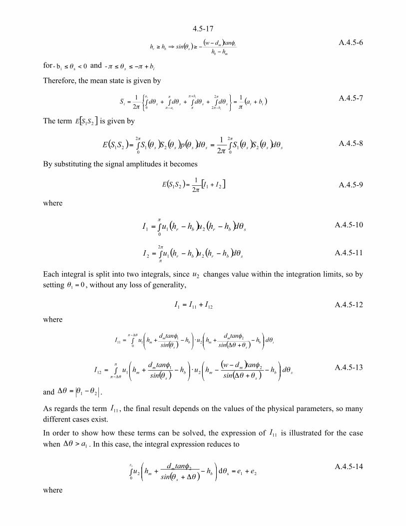
4.5-17

( ) ( )mb

imsbr hh

tandwsinhh

<

<<*�*

qe A.4.5-6

for 0b- si <)e and is b+<)) /e/-

Therefore, the mean state is given by

( )iib

s

b

sa

s

a

si baddddSi

i

i

i

+=®­¬

ª©¨

0+0+0+0=<

+

< /eeee

/

/

/

/

/

/

/

1

2

1 2

20

A.4.5-7

The term [ ]21SSE is given by

( ) ( ) ( ) ( ) ( ) ( )0=0=//

eee/

eeee2

021

2

02121 2

1sssssss dSSdpSSSSE A.4.5-8

By substituting the signal amplitudes it becomes

( ) [ ]2121 2

1IISSE +=

/A.4.5-9

where

( ) ( ) sbrbr dhhuhhuI e/

0 <<=0

211A.4.5-10

( ) ( ) sbrbr dhhuhhuI e/

/0 <<=

2

212 A.4.5-11

Each integral is split into two integrals, since 2u changes value within the integration limits, so bysetting 01 =e , without any loss of generality,

12111 III += A.4.5-12

where

( ) ( ) sbs

mmb

s

mm dh

sin

tandhuh

sin

tandhuI e

ee

q

e

qe/

0 ´́¦

¥²²¤

£<

+6+u´́

¦

¥²²¤

£<+=

6<

0

22

1111

( )( )

( ) sbs

mmb

s

mm dh

sin

tandwhuh

sin

tandhuI e

ee

q

e

q/

e/0 ´́

¦

¥²²¤

£<

+6

<<u´́

¦

¥²²¤

£<+=

6<

22

1112

A.4.5-13

and 21 eee <=6 .

As regards the term 11I , the final result depends on the values of the physical parameters, so manydifferent cases exist.

In order to show how these terms can be solved, the expression of 11I is illustrated for the casewhen 1a>6e . In this case, the integral expression reduces to

( ) 210

s2

2

1

d eehsin

tandhu

z

bs

mm +=0 ´́

¦

¥²²¤

£<

6++ e

ee

q A.4.5-14

where

4.5-18

ǻ

«©

¨

6<

)6+

6+<<66<

=

e

e

eee

2

211

122

1

a 0

az

a

z

za

e A.4.5-15

and

ª©¨

6<<

6*<+<6+=

e/

e//e

21

2212 a

a z

z

ae A.4.5-16

and the term 2e is evaluated only when 21 az <>6+ /e . The term 1z represents the minimum of

1a and e/ 6< . Similar expressions exist for the other cases resulting in a complicated solution.

Following the same approach for 2I ,

22212 III += A.4.5-17

where

( )( )

( )( ) sb

s

mmb

s

mm dh

sin

tandwhuh

sin

tandwhuI e

ee

q

e

qe/

/06<

´́¦

¥²²¤

£<

+6

<<u´́

¦

¥²²¤

£<

<<=

22

21

121

( )( ) ( ) sb

s

mmb

s

mm dh

sin

tandhuh

sin

tandwhuI e

ee

q

e

q/

e/06<

´́¦

¥²²¤

£<

+6+u´́

¦

¥²²¤

£<

<<=

2

2

22

1122 A.4.5-18

Again, the final result for 2I depends on the values for the physical parameters.

A common conclusion is that the final value of [ ]21SSE and hence, l , depends only on thedifference of the azimuth angles of the two satellites and not their absolute values. The standarddeviations are determined by

[ ] [ ]ii SESE 22i <=m A.4.5-19

4-6-1

CHAPTER 4.6Deterministic Modelling and Acceleration

Techniques for Ray-Path Searchingin Urban and Suburban Environments

Editor: Arno Formella1

Authors: Arno Formella1, Fernando Aguado Agelet2, José María Hernando Rábanos3,Conor Brennan4, and Peter Cullen4

1 HTW des Saarlandes, Goebenstraße 40, D-66117 Saarbrücken, Germany.tel: +49 681 831 8858, e-mail: formella@mobile-connect.de, http://www.mobile-connect.de

2 E.T.S.I. Telecomunicaciones. Universidad de Vigo. E-33200 Vigo, Spaintel: +34 986 812122, fax: +34 986 812116, e-mail: faguado@tsc.uvigo.es

3 E.T.S.I. de Telecomunicación. Universidad Politécnica de Madrid. E-28040 Madrid, Spaintel: +34 91 3367346, e-mail: hernando@grc.ssr.upm.es

4 Dept. of Electrical Engineering, Trinity College Dublintel : +35 387 2575739 fax : +35 387 2575739 e-mail: pcullen@tcd ie

4-6-2

4 . 6 Deterministic Modelling and Acceleration Techniques forRay-Path Searching in Urban and Suburban Environments

Maxwell's equations, coupled with the relevant boundary conditions, make it possible to modelelectromagnetic phenomena with high precision. Analytical solutions to Maxwell's equations yieldvaluable insights into electromagnetic phenomena when applied to simple canonical problems andthis insight has been used to great effect in the past in all manner of applications. However, theadvent of the digital computer in the latter half of this century has enabled the engineeringcommunity to numerically tackle problems of a far more general nature, and has resulted in theability to analyse real-life scenarios containing a much higher level of complexity. In the first partof this chapter a brief review of the major issues in the area of computational electromagnetics isgiven.

Within COST 255 especial emphasis has been set on one of the electromagnetic techniquesanalysed in the initial part of this chapter, namely, GTD/UTD techniques. These are tightly relatedto ray-tracing algorithms. The feasibility of using these electromagnetic techniques in real,complex, scenarios such as urban areas is only possible through the use of highly efficient and fastray-tracing algorithms. Extensive work has been carried out in this field and is described in detailthroughout this chapter.

4.6.1 Deterministic modelling of propagation phenomena

The three main formulations that we shall discuss are

• integral equation formulations;

• differential equation formulations;

• asymptotic techniques.

These formulations are deterministic in the sense that they postulate the propagation problem usingMaxwell's equations and allow for direct inclusion of the physical properties of the propagationenvironment, this is in contrast to empirical methods. Of course, in practice, the distinction betweenthe deterministic formulations is not as clear-cut as suggested above. Hybrid formulations abound,each with their own niche applications. In essence the latest progress can be thought of as alessening of the amount of abstraction necessary to analyse propagation problems. A key point toremember however is that while the amount of abstraction has been lessened it has not beeneliminated. Simplifications still have to be introduced to facilitate reasonable modelling.

4.6.1.1 Integral equation

The first deterministic formulation that we shall consider is that of the integral equation. Integralequations are primarily suitable for the description of wave propagation in the vicinity ofinhomogeneities (scatterers) which are embedded in some infinite homogeneous medium. Theguiding motivation of the integral equation formulation is to replace the physical problem with aphysically equivalent problem which produces the same fields but is more amenable to analysis.Two types of integral equation (a "volume integral equation" and "surface integral equation") arepossible.

The simplest analytic solution to the above integral equations is the physical optics solution and themost common numerical procedure is the method of moments. In recent years intense research hasprompted many improvements These include the following methods: the impedance matrixlocalisation method [Canning, 1990a], the natural basis [Moroney and Cullen, 1995], theasymptotic phase method [Aberegg and Peterson, 1995] and the high frequency panel method

4-6-3

iterative solutions. The fast multipole method (FMM) [Rokhlin, 1990] and its derivatives [Lu andChew, 1995; Brennan and Cullen, 1998a, 1998b; Wagner and Chew, 1994; Song and Chew, 1995]offer efficient and robust solutions to a wide class of problems. The fast far-field method (FAFFA)[Lu and Chew, 1995] a simplification of the FMM, has been further specialised to the tabulatedinteraction method (TIM) to facilitate the analysis of large scale UHF propagation problems[Brennan and Cullen, 1998a, 1998b] in realistic computing times.

4.6.1.2 Differential equations

As the name suggests the differential equation formulation of the scattering problem tackles theunderlying equations in their differential form, solving for the unknown electric and magnetic fieldquantities directly on a grid that discretises the entire computational domain of interest. Thedifferential formulation's ability to treat quite heterogeneous scatterers and propagation mediumanomalies in a unified and computationally straightforward manner makes it an attractive one whenconsidering propagation in quite complicated environments. Two differential-equation basedformulations can be pointed out:

• the finite element method [Bayliss and Turkel, 1980; Canning, 1990b]

• the finite difference method [Berenger, 1994; Lindman, 1975; Mur, 1981; Levy, 1990;Janaswamy, 1997]

4.6.1.3 Asymptotic methods

Geometrical optics (GO) is an approximate high frequency method which postulates the existenceof direct, reflected and refracted rays. The field at a point is the superposition of the fieldsassociated with each ray passing through that point. To explain the phenomenon of diffraction thegeometrical theory of diffraction (GTD/UTD) [Keller, 1962; Kouyoumjian and Pathak, 1974] waspostulated. As the wavelength h approaches zero this high frequency solution becomes increasinglyaccurate and we expect GTD to be a good model. However, at lower frequencies its usage is moresuspect.

In studies of UHF propagation over irregular terrain, attempts to include the effects of surfaceroughness and imperfect reflection via a modified reflection coefficient were proposed in[Luebbers, 1984]. Problems arise when diffraction points lie in the transition region of previousdiffraction points. When this occurs the ray is no longer a so-called ray field and conventional UTDfails. A recent innovation tackling this problem is the incorporation of higher order diffracted fields.For instance the inclusion of slope diffraction can improve UTD's capability to describe propagationover a series of knife-edges as shown in [Andersen, 1994]. Slope diffraction adds to the standardUTD diffracted field a contribution due to the slope of the incident field. The diffraction of thisslope field is described by a diffraction coefficient, which is based on the angular derivative of thediffraction coefficient. In [Holm, 1996] a heuristic generalisation is developed of Furutsu'sexpression for double knife diffraction to generate expressions for higher order diffractioncoefficient. Another high frequency asymptotic method worth mentioning is the physical theory ofdiffraction (PTD) [Ufimtsev, 1957].

4.6.2 Review of ray-tracing techniques

Software tools using ray-tracing and UTD techniques may take considerable computation time forthe analysis of the propagation conditions in a given environment, even for a short mobile terminalroute. Efficient acceleration techniques are required to make such analysis tools practical for thedesign of modern radio communication systems. To reduce computation time, ray-tracing should beapplied only in those areas where ray-paths are likely to exist. This is achieved by using visibility

h l ith i t f i t l t i [F ll d Gill 1995] I thi

4-6-4

The simulation methods for wave propagation based on geometric optics and the uniform theory ofdiffraction can be classified into two categories: the earlier ones using the ray-launching approachand the more recent ones using ray-path search.

4.6.2.1 Ray-launching

The ray-launching approach (sometimes called “shooting and bouncing rays method” or “pincushion method”) uses a forward ray-tracing algorithm, which simulates the propagation of thewaves from the source into the space [Rappaport et al., 1993; Schaubach and Davis, 1996;Schaubach et al., 1992; Seidel and Rappaport, 1992; Seidel and Rappaport, 1994]. For each regionor location of interest the “information” carried by the rays crossing the region or passing nearbythe location is superimposed to obtain the overall effect. Due to the sampling nature of such analgorithm the prediction for areas farther away from the source becomes more and more imprecise.Phase information cannot be calculated accurately. For more complex environments or satellitescenarios a ray-launching approach becomes impractical, both due to its computational complexitytracing a sufficiently large number of rays and its difficulties to find the ray-paths, which passsufficiently close to diffractive edges and receiving locations. An advantage of the ray-launchingapproach is the fact that there are no restrictions imposed on the environment, any shape of objectmay be present. The ray-tracing techniques described in this chapter could be improved by usingray-tube or ray-cone techniques..

4.6.2.2 Ray-path search

Using imaging techniques for reflections and rotations for diffractions (see Section 4.6.4), ray-pathsfulfilling Fermat's principle are easy to calculate for an ordered list of objects such as faces andedges. A brute force ray-path search algorithm [Athanasiadou et al., 1995; Lawton and McGeehan,1994; Tan and Tan, 1996] to find all ray-paths between a transmitting point Tx and a receiving pointRx in an polygonal environment would generate successively an ordered list of up to m objects outof the e edges and f faces of the environment, calculate the ray-paths containing up to minteractions, and finally verify whether the paths are obstructed by any face in the environment. Anaive implementation of the ray-path testing can be implemented by a linear search. The runningtime would be proportional to fmmfemfe u+u<uuu )!1())!(!/()!( , or in other words, prohibitively largefor many practical cases. Hence, acceleration methods have to be employed to reduce the number oflists of objects possibly involved in the ray path search and to speed-up the ray-path testing. Besidesthe approach proposed by [Aguado et al., 1996a; Aguado et al., 1996b; Aguado et al., 1997a;Aguado et al., 1997b] and some heuristical algorithms, e.g., [Cichon et al., 1994; Cichon et al.,1995; Cichon et al., 1996], two general methods have been published.

An efficient method, which is restricted to finding 2D ray-paths (see Section 4.6.5.3 for adefinition) is introduced in [Fortune et al., 1995]. They use a Delaunay-triangulation of the groundplane containing the projections of the building blocks to compute approximations of the visiblearea (see Section 4.6.5.1), which significantly reduces the search space for the ray-paths. Thetriangulation also serves as an efficient guide-line for the ray-tracing part. An extension to 3D hasnot yet been reported. It is an open question whether a three-dimensional Delaunay-triangulation iscompetitive to the polar sweep approach enhanced with an adaptive space sub-division, as describedin this chapter.

Another method introducing a so-called angular z-buffer (AZB) is described in [Catedra, et al.,1997; Catedra, et al., 1998; Catedra and Pérez-Arriaga, 1999]. They use a regular angular sub-division (so-called anxels) to reduce the search space for interactions and simultaneously acceleratethe ray-tracing kernel. Previously calculated buffer contents (so-called AZB matrices) are stored forfuture use. They use a quadratic time, exhaustive search pre-processing step to calculate all images

f ll d hi h t i t th l ith f ti l t fi di t t i t ti

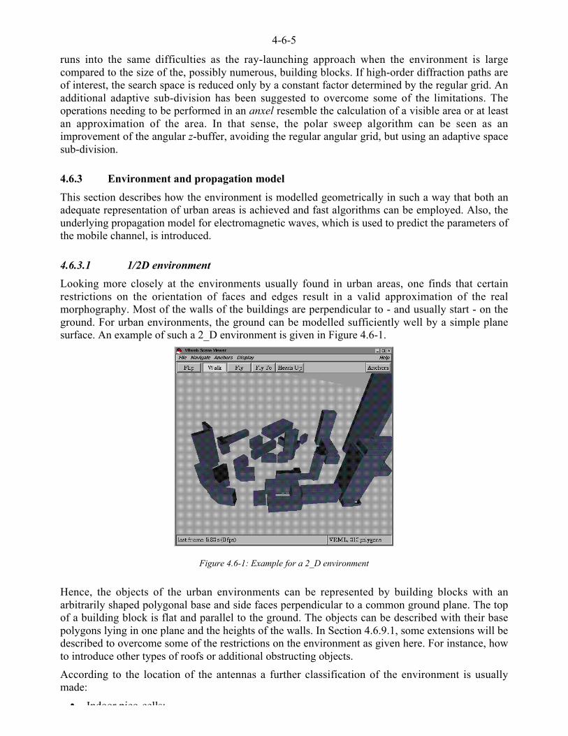
4-6-5

runs into the same difficulties as the ray-launching approach when the environment is largecompared to the size of the, possibly numerous, building blocks. If high-order diffraction paths areof interest, the search space is reduced only by a constant factor determined by the regular grid. Anadditional adaptive sub-division has been suggested to overcome some of the limitations. Theoperations needing to be performed in an anxel resemble the calculation of a visible area or at leastan approximation of the area. In that sense, the polar sweep algorithm can be seen as animprovement of the angular z-buffer, avoiding the regular angular grid, but using an adaptive spacesub-division.

4.6.3 Environment and propagation model

This section describes how the environment is modelled geometrically in such a way that both anadequate representation of urban areas is achieved and fast algorithms can be employed. Also, theunderlying propagation model for electromagnetic waves, which is used to predict the parameters ofthe mobile channel, is introduced.

4.6.3.1 1/2D environment

Looking more closely at the environments usually found in urban areas, one finds that certainrestrictions on the orientation of faces and edges result in a valid approximation of the realmorphography. Most of the walls of the buildings are perpendicular to - and usually start - on theground. For urban environments, the ground can be modelled sufficiently well by a simple planesurface. An example of such a 2_D environment is given in Figure 4.6-1.

Figure 4.6-1: Example for a 2_D environment

Hence, the objects of the urban environments can be represented by building blocks with anarbitrarily shaped polygonal base and side faces perpendicular to a common ground plane. The topof a building block is flat and parallel to the ground. The objects can be described with their basepolygons lying in one plane and the heights of the walls. In Section 4.6.9.1, some extensions will bedescribed to overcome some of the restrictions on the environment as given here. For instance, howto introduce other types of roofs or additional obstructing objects.

According to the location of the antennas a further classification of the environment is usuallymade:

• Indoor pico cells:

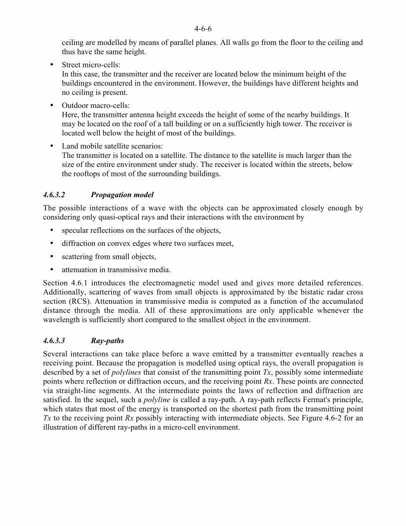
4-6-6

ceiling are modelled by means of parallel planes. All walls go from the floor to the ceiling andthus have the same height.

• Street micro-cells:In this case, the transmitter and the receiver are located below the minimum height of thebuildings encountered in the environment. However, the buildings have different heights andno ceiling is present.

• Outdoor macro-cells:Here, the transmitter antenna height exceeds the height of some of the nearby buildings. Itmay be located on the roof of a tall building or on a sufficiently high tower. The receiver islocated well below the height of most of the buildings.

• Land mobile satellite scenarios:The transmitter is located on a satellite. The distance to the satellite is much larger than thesize of the entire environment under study. The receiver is located within the streets, belowthe rooftops of most of the surrounding buildings.

4.6.3.2 Propagation model

The possible interactions of a wave with the objects can be approximated closely enough byconsidering only quasi-optical rays and their interactions with the environment by

• specular reflections on the surfaces of the objects,

• diffraction on convex edges where two surfaces meet,

• scattering from small objects,

• attenuation in transmissive media.

Section 4.6.1 introduces the electromagnetic model used and gives more detailed references.Additionally, scattering of waves from small objects is approximated by the bistatic radar crosssection (RCS). Attenuation in transmissive media is computed as a function of the accumulateddistance through the media. All of these approximations are only applicable whenever thewavelength is sufficiently short compared to the smallest object in the environment.

4.6.3.3 Ray-paths

Several interactions can take place before a wave emitted by a transmitter eventually reaches areceiving point. Because the propagation is modelled using optical rays, the overall propagation isdescribed by a set of polylines that consist of the transmitting point Tx, possibly some intermediatepoints where reflection or diffraction occurs, and the receiving point Rx. These points are connectedvia straight-line segments. At the intermediate points the laws of reflection and diffraction aresatisfied. In the sequel, such a polyline is called a ray-path. A ray-path reflects Fermat's principle,which states that most of the energy is transported on the shortest path from the transmitting pointTx to the receiving point Rx possibly interacting with intermediate objects. See Figure 4.6-2 for anillustration of different ray-paths in a micro-cell environment.

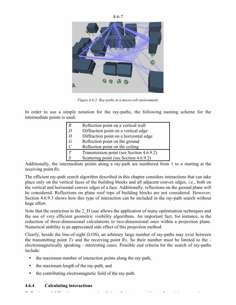
4-6-7

Figure 4.6-2: Ray-paths in a micro-cell environment.

In order to use a simple notation for the ray-paths, the following naming scheme for theintermediate points is used:

R Reflection point on a vertical wallD Diffraction point on a vertical edgeH Diffraction point on a horizontal edgeG Reflection point on the groundC Reflection point on the ceilingT Transmission point (see Section 4.6.9.2)S Scattering point (see Section 4.6.9.2)

Additionally, the intermediate points along a ray-path are numbered from 1 to n starting at thereceiving point Rx.

The efficient ray-path search algorithm described in this chapter considers interactions that can takeplace only on the vertical faces of the building blocks and all adjacent convex edges, i.e., both onthe vertical and horizontal convex edges of a face. Additionally, reflections on the ground plane willbe considered. Reflections on plane roof tops of building blocks are not considered. However,Section 4.6.9.3 shows how this type of interaction can be included in the ray-path search withouthuge effort.

Note that the restriction to the 2_D case allows the application of many optimisation techniques andthe use of very efficient geometric visibility algorithms. An important fact, for instance, is thereduction of three-dimensional calculations to two-dimensional ones within a projection plane.Numerical stability is an appreciated side effect of this projection method.

Clearly, beside the line-of-sight (LOS), an arbitrary large number of ray-paths may exist betweenthe transmitting point Tx and the receiving point Rx. So their number must be limited to the -electromagnetically speaking - interesting cases. Possible end criteria for the search of ray-pathsinclude:

• the maximum number of interaction points along the ray-path,

• the maximum length of the ray-path, and

• the contributing electromagnetic field of the ray-path.

4.6.4 Calculating interactions

R fl ti d diff ti t i l ti h t itti d i i ti

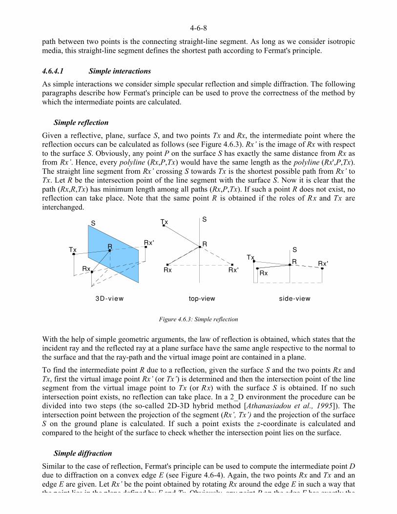
4-6-8

path between two points is the connecting straight-line segment. As long as we consider isotropicmedia, this straight-line segment defines the shortest path according to Fermat's principle.

4.6.4.1 Simple interactions

As simple interactions we consider simple specular reflection and simple diffraction. The followingparagraphs describe how Fermat's principle can be used to prove the correctness of the method bywhich the intermediate points are calculated.

Simple reflection

Given a reflective, plane, surface S, and two points Tx and Rx, the intermediate point where thereflection occurs can be calculated as follows (see Figure 4.6.3). Rx’ is the image of Rx with respectto the surface S. Obviously, any point P on the surface S has exactly the same distance from Rx asfrom Rx’. Hence, every polyline (Rx,P,Tx) would have the same length as the polyline (Rx',P,Tx).The straight line segment from Rx’ crossing S towards Tx is the shortest possible path from Rx’ toTx. Let R be the intersection point of the line segment with the surface S. Now it is clear that thepath (Rx,R,Tx) has minimum length among all paths (Rx,P,Tx). If such a point R does not exist, noreflection can take place. Note that the same point R is obtained if the roles of Rx and Tx areinterchanged.

3D-view top-view

Rx'R

S

Rx

Tx

Rx'

R

STx

Rx

Rx'R

S

Tx

Rx

side-view

Figure 4.6.3: Simple reflection

With the help of simple geometric arguments, the law of reflection is obtained, which states that theincident ray and the reflected ray at a plane surface have the same angle respective to the normal tothe surface and that the ray-path and the virtual image point are contained in a plane.

To find the intermediate point R due to a reflection, given the surface S and the two points Rx andTx, first the virtual image point Rx’ (or Tx’) is determined and then the intersection point of the linesegment from the virtual image point to Tx (or Rx) with the surface S is obtained. If no suchintersection point exists, no reflection can take place. In a 2_D environment the procedure can bedivided into two steps (the so-called 2D-3D hybrid method [Athanasiadou et al., 1995]). Theintersection point between the projection of the segment (Rx’, Tx’) and the projection of the surfaceS on the ground plane is calculated. If such a point exists the z-coordinate is calculated andcompared to the height of the surface to check whether the intersection point lies on the surface.

Simple diffraction

Similar to the case of reflection, Fermat's principle can be used to compute the intermediate point Ddue to diffraction on a convex edge E (see Figure 4.6-4). Again, the two points Rx and Tx and anedge E are given. Let Rx’ be the point obtained by rotating Rx around the edge E in such a way thatthe point lies in the plane defined by E and Tx Obviously any point P on the edge E has exactly the

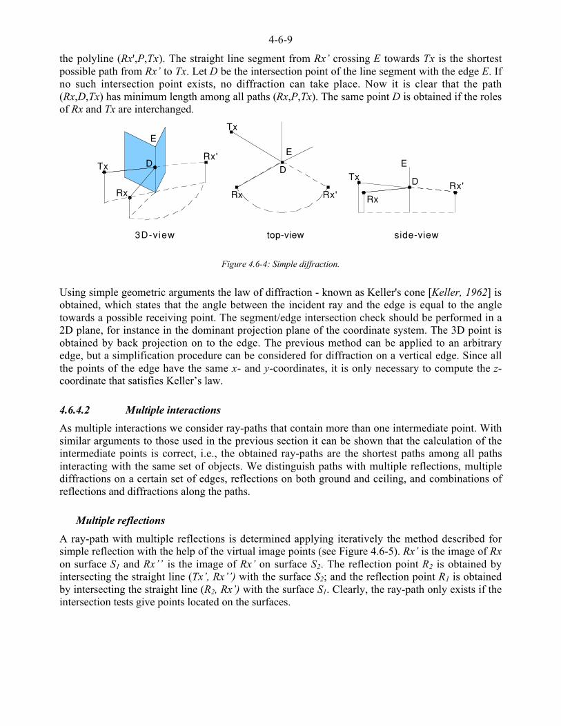
4-6-9

the polyline (Rx',P,Tx). The straight line segment from Rx’ crossing E towards Tx is the shortestpossible path from Rx’ to Tx. Let D be the intersection point of the line segment with the edge E. Ifno such intersection point exists, no diffraction can take place. Now it is clear that the path(Rx,D,Tx) has minimum length among all paths (Rx,P,Tx). The same point D is obtained if the rolesof Rx and Tx are interchanged.

3D-view top-view

Rx'Rx

Tx

Rx'

Tx

Rx

Rx'Tx

Rx

side-view

DD

D

EE

E

Figure 4.6-4: Simple diffraction.

Using simple geometric arguments the law of diffraction - known as Keller's cone [Keller, 1962] isobtained, which states that the angle between the incident ray and the edge is equal to the angletowards a possible receiving point. The segment/edge intersection check should be performed in a2D plane, for instance in the dominant projection plane of the coordinate system. The 3D point isobtained by back projection on to the edge. The previous method can be applied to an arbitraryedge, but a simplification procedure can be considered for diffraction on a vertical edge. Since allthe points of the edge have the same x- and y-coordinates, it is only necessary to compute the z-coordinate that satisfies Keller’s law.

4.6.4.2 Multiple interactions

As multiple interactions we consider ray-paths that contain more than one intermediate point. Withsimilar arguments to those used in the previous section it can be shown that the calculation of theintermediate points is correct, i.e., the obtained ray-paths are the shortest paths among all pathsinteracting with the same set of objects. We distinguish paths with multiple reflections, multiplediffractions on a certain set of edges, reflections on both ground and ceiling, and combinations ofreflections and diffractions along the paths.

Multiple reflections

A ray-path with multiple reflections is determined applying iteratively the method described forsimple reflection with the help of the virtual image points (see Figure 4.6-5). Rx’ is the image of Rxon surface S1 and Rx’’ is the image of Rx’ on surface S2. The reflection point R2 is obtained byintersecting the straight line (Tx’, Rx’’) with the surface S2; and the reflection point R1 is obtainedby intersecting the straight line (R2, Rx’) with the surface S1. Clearly, the ray-path only exists if theintersection tests give points located on the surfaces.

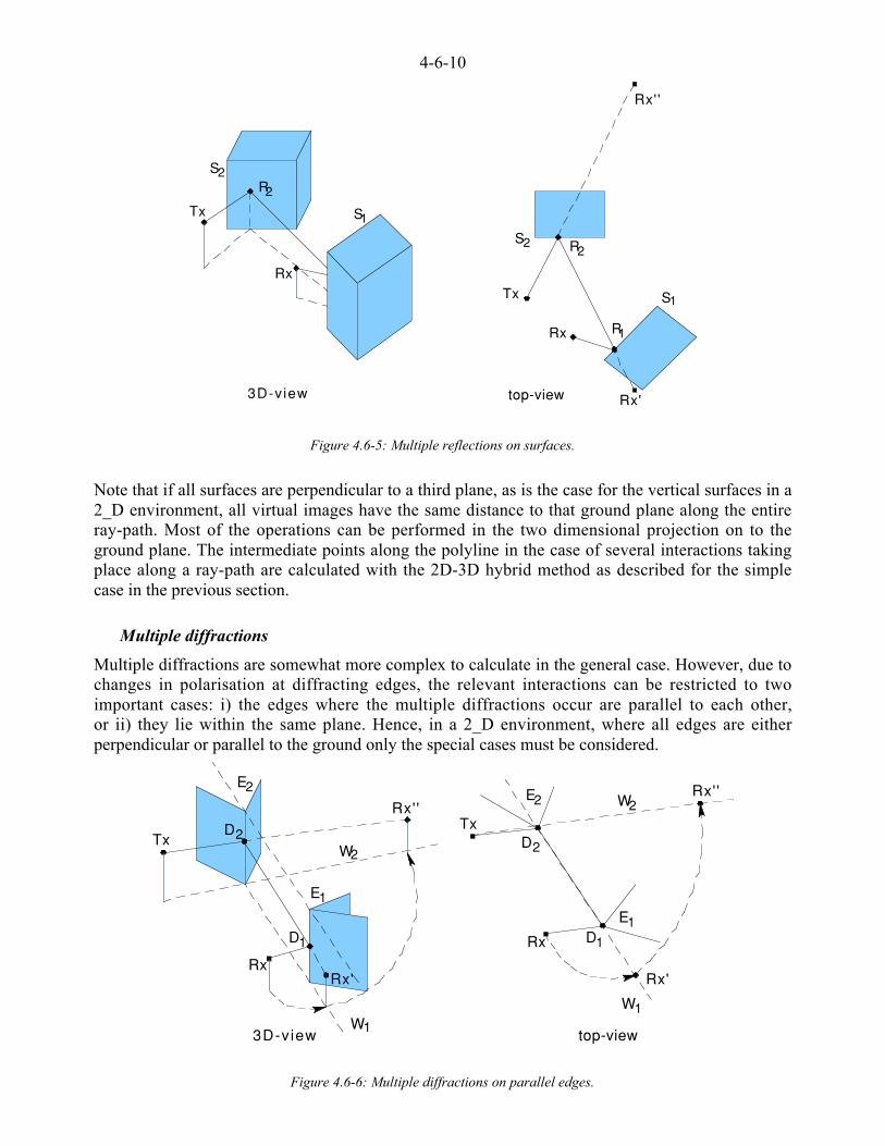
4-6-10

R2

R2

S2

S1

R1

S2

S1

Rx'

Rx''

Tx

Rx

Rx

Tx

top-view 3D-view

Figure 4.6-5: Multiple reflections on surfaces.

Note that if all surfaces are perpendicular to a third plane, as is the case for the vertical surfaces in a2_D environment, all virtual images have the same distance to that ground plane along the entireray-path. Most of the operations can be performed in the two dimensional projection on to theground plane. The intermediate points along the polyline in the case of several interactions takingplace along a ray-path are calculated with the 2D-3D hybrid method as described for the simplecase in the previous section.

Multiple diffractions

Multiple diffractions are somewhat more complex to calculate in the general case. However, due tochanges in polarisation at diffracting edges, the relevant interactions can be restricted to twoimportant cases: i) the edges where the multiple diffractions occur are parallel to each other,or ii) they lie within the same plane. Hence, in a 2_D environment, where all edges are eitherperpendicular or parallel to the ground only the special cases must be considered.

E2

E1

W2

D2

W1

E1

D2

W1

D1

E2 W2

D1

Rx''

Tx

Rx'

Rx''

Rx'

Tx

top-view 3D-view

RxRx

Figure 4.6-6: Multiple diffractions on parallel edges.

4-6-11

The approach using rotations to find the diffraction point D (as described in the previous section)can also be employed to find higher-order diffraction paths. Figure 4.6-6 shows an example for thecase of a double-diffracted ray-path through two parallel edges. First, the plane W1 is constructed,which is uniquely determined by the four end points of the edges E1 and E2. Next, the receivingpoint Rx is rotated around the edge E1 until it lies in plane W1. This point is called Rx’. Then, thetransmitting point Tx, the edge E2, and Rx’ are processed in the same way as outlined for singlediffraction: a plane W2 is determined by Tx and the edge E2 and Rx’ is rotated around edge E2 untilit lies in plane W2. This point is called Rx’’. Obviously, Tx, the edge E2, and Rx’’ lie in a planargeometry. The diffraction point D2 on the edge E2 is the intersection of the line from Tx to Rx’’ withthe edge. The diffraction point D1 is the intersection of the line from D1 to Rx’ with the edge E1. Ofcourse, it is necessary to verify that D1 lies on the edge E1, and D2 on the edge E2. Finally, thedouble diffraction path is (Rx,D1,D2,Tx), provided the two intermediate points exist. The same resultwould have been obtained by rotating both points Tx and Rx around the appropriate edge until theylie in plane W2 and calculating both diffraction points in that plane. Interchanging the roles of E1

and E2 in the discussion, we obtain the second possible diffraction path, which - for simplification -has not been included in the figure. The previous method can be applied to arbitrary orientedparallel edges. However, the simplification procedure, in which most of the calculations areperformed on the ground plane, as presented in the previous , can be applied literally to the multiplevertical diffraction case. If ray-paths with more than two parallel edges are to be calculated, alledges, and the source points, respectively, are transformed by successive rotations into a singleplane such that the distances and the order of the edges and the points along the ray-path are thesame. Note that there may exist up to n! different ray-paths interacting with n parallel edges.

D2 D1

E1E2

D1

E1

D2

E2

Tx

Tx''

Tx'

Rx''

Rx

Rx'

3D-view

RxRx''

Rx'

Tx''Tx

Tx'

top-view

Figure 4.6-7: Multiple diffractions on edges contained in one plane.

Although it might seem at first sight that the geometry of non-parallel edge is different, thecalculation method remains exactly the same. If the edges E1 and E2 are lying in the same plane W(see Figure 4.6-7), the diffraction points D1 and D2 are calculated by rotating Tx and, respectively,Rx around the edges until they lie in the plane W as well. The resulting intersection points of theedges with the line segment from Tx to Rx determine the diffraction points on the edges, if thesepoints exist at all. A special case occurs with edges belonging to the same polygonal surface.Clearly, these edges lie within the same plane and the diffraction points can be obtained as statedabove. Because a different propagation model should be applied to creeping waves, thosediffraction points should be marked differently. This type of diffraction will be called adjacentdiffraction in the sequel. To find all pairs of such adjacent diffractions on a rooftop of a buildingeach pair of edges of the limiting polygon must be considered.

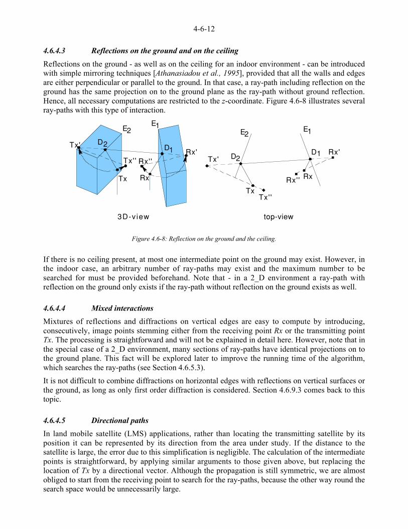
4-6-12

4.6.4.3 Reflections on the ground and on the ceiling

Reflections on the ground - as well as on the ceiling for an indoor environment - can be introducedwith simple mirroring techniques [Athanasiadou et al., 1995], provided that all the walls and edgesare either perpendicular or parallel to the ground. In that case, a ray-path including reflection on theground has the same projection on to the ground plane as the ray-path without ground reflection.Hence, all necessary computations are restricted to the z-coordinate. Figure 4.6-8 illustrates severalray-paths with this type of interaction.

D2 D1

E1E2

D1

E1

D2

E2

Tx

Tx''

Tx'

Rx''

Rx

Rx'

3D-view

RxRx''

Rx'

Tx''Tx

Tx'

top-view

Figure 4.6-8: Reflection on the ground and the ceiling.

If there is no ceiling present, at most one intermediate point on the ground may exist. However, inthe indoor case, an arbitrary number of ray-paths may exist and the maximum number to besearched for must be provided beforehand. Note that - in a 2_D environment a ray-path withreflection on the ground only exists if the ray-path without reflection on the ground exists as well.

4.6.4.4 Mixed interactions

Mixtures of reflections and diffractions on vertical edges are easy to compute by introducing,consecutively, image points stemming either from the receiving point Rx or the transmitting pointTx. The processing is straightforward and will not be explained in detail here. However, note that inthe special case of a 2_D environment, many sections of ray-paths have identical projections on tothe ground plane. This fact will be explored later to improve the running time of the algorithm,which searches the ray-paths (see Section 4.6.5.3).

It is not difficult to combine diffractions on horizontal edges with reflections on vertical surfaces orthe ground, as long as only first order diffraction is considered. Section 4.6.9.3 comes back to thistopic.

4.6.4.5 Directional paths

In land mobile satellite (LMS) applications, rather than locating the transmitting satellite by itsposition it can be represented by its direction from the area under study. If the distance to thesatellite is large, the error due to this simplification is negligible. The calculation of the intermediatepoints is straightforward, by applying similar arguments to those given above, but replacing thelocation of Tx by a directional vector. Although the propagation is still symmetric, we are almostobliged to start from the receiving point to search for the ray-paths, because the other way round thesearch space would be unnecessarily large.

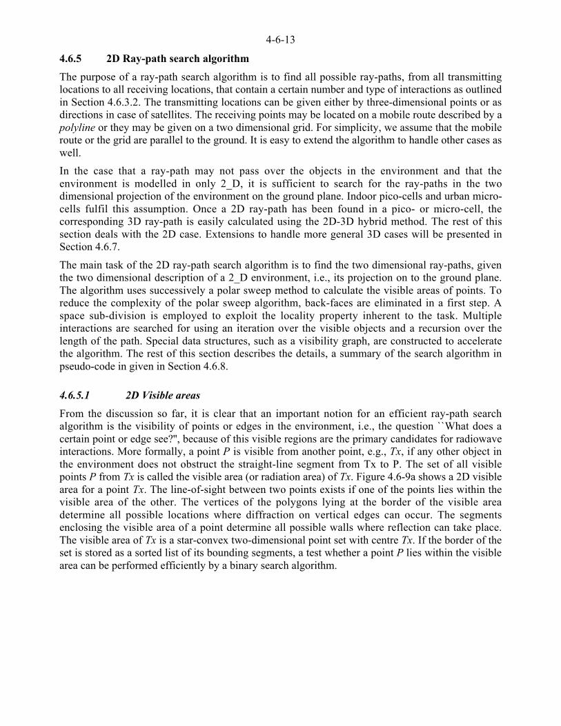
4-6-13

4.6.5 2D Ray-path search algorithm

The purpose of a ray-path search algorithm is to find all possible ray-paths, from all transmittinglocations to all receiving locations, that contain a certain number and type of interactions as outlinedin Section 4.6.3.2. The transmitting locations can be given either by three-dimensional points or asdirections in case of satellites. The receiving points may be located on a mobile route described by apolyline or they may be given on a two dimensional grid. For simplicity, we assume that the mobileroute or the grid are parallel to the ground. It is easy to extend the algorithm to handle other cases aswell.

In the case that a ray-path may not pass over the objects in the environment and that theenvironment is modelled in only 2_D, it is sufficient to search for the ray-paths in the twodimensional projection of the environment on the ground plane. Indoor pico-cells and urban micro-cells fulfil this assumption. Once a 2D ray-path has been found in a pico- or micro-cell, thecorresponding 3D ray-path is easily calculated using the 2D-3D hybrid method. The rest of thissection deals with the 2D case. Extensions to handle more general 3D cases will be presented inSection 4.6.7.

The main task of the 2D ray-path search algorithm is to find the two dimensional ray-paths, giventhe two dimensional description of a 2_D environment, i.e., its projection on to the ground plane.The algorithm uses successively a polar sweep method to calculate the visible areas of points. Toreduce the complexity of the polar sweep algorithm, back-faces are eliminated in a first step. Aspace sub-division is employed to exploit the locality property inherent to the task. Multipleinteractions are searched for using an iteration over the visible objects and a recursion over thelength of the path. Special data structures, such as a visibility graph, are constructed to acceleratethe algorithm. The rest of this section describes the details, a summary of the search algorithm inpseudo-code in given in Section 4.6.8.

4.6.5.1 2D Visible areas

From the discussion so far, it is clear that an important notion for an efficient ray-path searchalgorithm is the visibility of points or edges in the environment, i.e., the question ``What does acertain point or edge see?'', because of this visible regions are the primary candidates for radiowaveinteractions. More formally, a point P is visible from another point, e.g., Tx, if any other object inthe environment does not obstruct the straight-line segment from Tx to P. The set of all visiblepoints P from Tx is called the visible area (or radiation area) of Tx. Figure 4.6-9a shows a 2D visiblearea for a point Tx. The line-of-sight between two points exists if one of the points lies within thevisible area of the other. The vertices of the polygons lying at the border of the visible areadetermine all possible locations where diffraction on vertical edges can occur. The segmentsenclosing the visible area of a point determine all possible walls where reflection can take place.The visible area of Tx is a star-convex two-dimensional point set with centre Tx. If the border of theset is stored as a sorted list of its bounding segments, a test whether a point P lies within the visiblearea can be performed efficiently by a binary search algorithm.

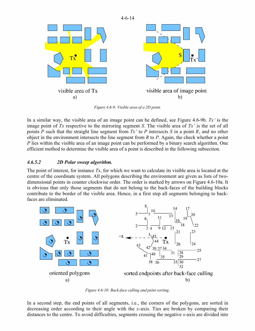
4-6-14

a) b)

Figure 4.6-9: Visible area of a 2D point.

In a similar way, the visible area of an image point can be defined, see Figure 4.6-9b. Tx’ is theimage point of Tx respective to the mirroring segment S. The visible area of Tx’ is the set of allpoints P such that the straight line segment from Tx’ to P intersects S in a point R, and no otherobject in the environment intersects the line segment from R to P. Again, the check whether a pointP lies within the visible area of an image point can be performed by a binary search algorithm. Oneefficient method to determine the visible area of a point is described in the following subsection.

4.6.5.2 2D Polar sweep algorithm.

The point of interest, for instance Tx, for which we want to calculate its visible area is located at thecentre of the coordinate system. All polygons describing the environment are given as lists of two-dimensional points in counter clockwise order. The order is marked by arrows on Figure 4.6-10a. Itis obvious that only those segments that do not belong to the back-faces of the building blockscontribute to the border of the visible area. Hence, in a first step all segments belonging to back-faces are eliminated.

a) b)

Figure 4.6-10: Back-face culling and point sorting.

In a second step, the end points of all segments, i.e., the corners of the polygons, are sorted indecreasing order according to their angle with the x-axis. Ties are broken by comparing theirdistances to the centre. To avoid difficulties, segments crossing the negative x-axis are divided into

4-6-15

Actually, the two steps, namely back-face culling and sorting, can be performed efficiently in asingle run: a segment is a back-face if the order of its end points respective to the angle differs fromthe order of the points in the definition of the polygon. Figure 4.6-10b shows the remainingsegments with their points numbered according to the sorting order.

The third step implements the polar sweep. Consider a ray starting at the centre Tx with direction ofthe negative x-axis and sweeping around the centre in clockwise direction (see Figure 4.6-11a).Theray is called the sweep line. Certain positions (A and B) of the sweep line are added in the figure bydotted lines. The border of the visible area is composed of segments or parts of segments which areclose to the centre. While rotating the sweep line, a segment changes from being visible tobecoming invisible only when the sweep line crosses an end point of a segment. The same is truefor the reverse case.

1

1 3

1 4

1 6

Tx- x 0

A Bsweep

direction

1 21 1

1 5

a) b) c)Figure 4.6-11: a) Polar sweep algorithm and b), c)Polar sweep regions within an angle.

The sweep algorithm iterates over the sorted list of end points and maintains a data structure thatcontains the list of segments which are currently intersected by the sweep line. Each time a left endpoint of a segment is found the corresponding segment is inserted into the data structure. If thesegment is closer than any other segment currently held, this segment determines the visible border.Otherwise the segment being recently visible remains visible. Each time a right end point of asegment is found the corresponding segment is deleted from the data structure. The segment closestto the centre becomes visible at the current angle. For instance, just before the sweep line reachesposition A in Figure 4.6-11a a segment with right end point 13 is visible. At the stopping position A(point 12) the segment with end points 12 and 15 becomes visible and the previously visiblesegment becomes invisible. The next stopping point is 13. There, the segment in the back iseliminated from the data structure, because its right end point has been reached. The visibility doesnot change. The next stopping point is 14. As it is a left end point of a segment, this segment isinserted into the data structure, but the visibility does not change, because the segment lies in thebackground. The next stopping point is 15, position B in the figure. Now, the right end point ofsegment (12,15) has been reached and the segment is deleted from the data structure. Clearly, thesegment in the background becomes visible, i.e., the data structure must deliver the segment closestto the centre currently cut by the sweep line. The point where the visibility starts is marked in thefigure.

Hence, the data structure requires the efficient implementation of the operations insert, delete andfind-minimum on a linearly orderable set. A possible choice is a priority queue where insertion anddeletion take a time proportional to log(q) where q is the current size of the queue. Finding theclosest segment can be done in constant time. The running time of the complete polar sweepalgorithm is proportional to nlog(n) where n is the number of points describing the polygons. Thememory requirements vary linearly with the number of points.

The polar sweep algorithm does not necessarily need to be performed in a full circle around thepoint of interest [Aguado et al., 1996b]. For instance, if the visible area of a diffractive edge has tobe calculated the polar sweep in confined by the two adjacent walls of the edge Similarly the

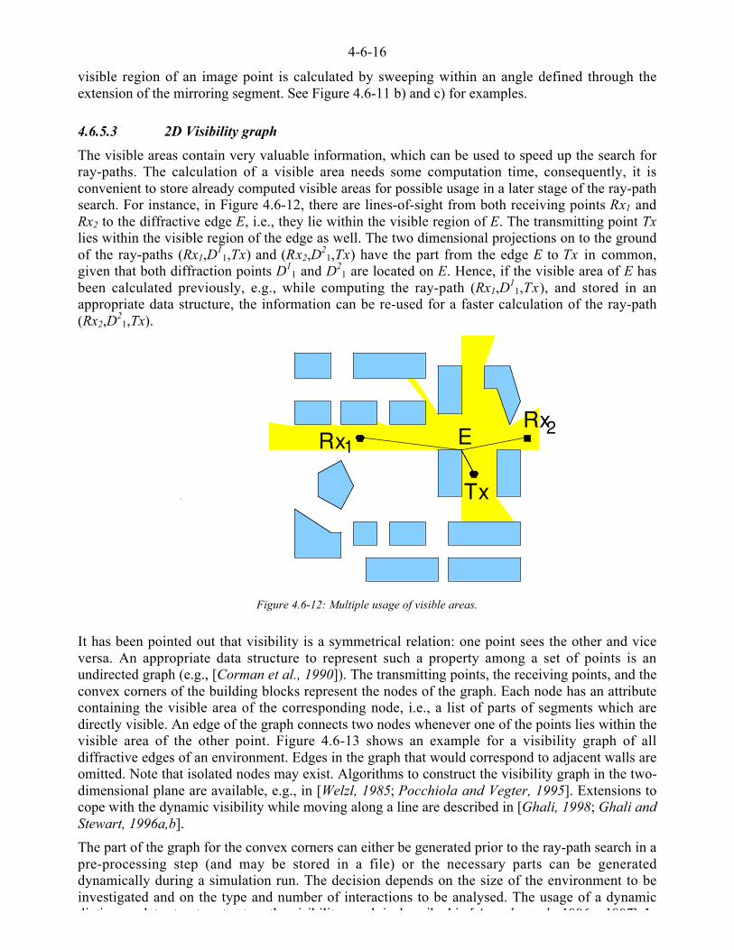
4-6-16

visible region of an image point is calculated by sweeping within an angle defined through theextension of the mirroring segment. See Figure 4.6-11 b) and c) for examples.

4.6.5.3 2D Visibility graph

The visible areas contain very valuable information, which can be used to speed up the search forray-paths. The calculation of a visible area needs some computation time, consequently, it isconvenient to store already computed visible areas for possible usage in a later stage of the ray-pathsearch. For instance, in Figure 4.6-12, there are lines-of-sight from both receiving points Rx1 andRx2 to the diffractive edge E, i.e., they lie within the visible region of E. The transmitting point Txlies within the visible region of the edge as well. The two dimensional projections on to the groundof the ray-paths (Rx1,D

11,Tx) and (Rx2,D

21,Tx) have the part from the edge E to Tx in common,

given that both diffraction points D11 and D2

1 are located on E. Hence, if the visible area of E hasbeen calculated previously, e.g., while computing the ray-path (Rx1,D

11,Tx), and stored in an

appropriate data structure, the information can be re-used for a faster calculation of the ray-path(Rx2,D

21,Tx).

Tx

Rx1Rx2E

Figure 4.6-12: Multiple usage of visible areas.

It has been pointed out that visibility is a symmetrical relation: one point sees the other and viceversa. An appropriate data structure to represent such a property among a set of points is anundirected graph (e.g., [Corman et al., 1990]). The transmitting points, the receiving points, and theconvex corners of the building blocks represent the nodes of the graph. Each node has an attributecontaining the visible area of the corresponding node, i.e., a list of parts of segments which aredirectly visible. An edge of the graph connects two nodes whenever one of the points lies within thevisible area of the other point. Figure 4.6-13 shows an example for a visibility graph of alldiffractive edges of an environment. Edges in the graph that would correspond to adjacent walls areomitted. Note that isolated nodes may exist. Algorithms to construct the visibility graph in the two-dimensional plane are available, e.g., in [Welzl, 1985; Pocchiola and Vegter, 1995]. Extensions tocope with the dynamic visibility while moving along a line are described in [Ghali, 1998; Ghali andStewart, 1996a,b].

The part of the graph for the convex corners can either be generated prior to the ray-path search in apre-processing step (and may be stored in a file) or the necessary parts can be generateddynamically during a simulation run. The decision depends on the size of the environment to beinvestigated and on the type and number of interactions to be analysed. The usage of a dynamicdi ti d t t t t t th i ibilit h i d ib d i [A d t l 1996 1997] I

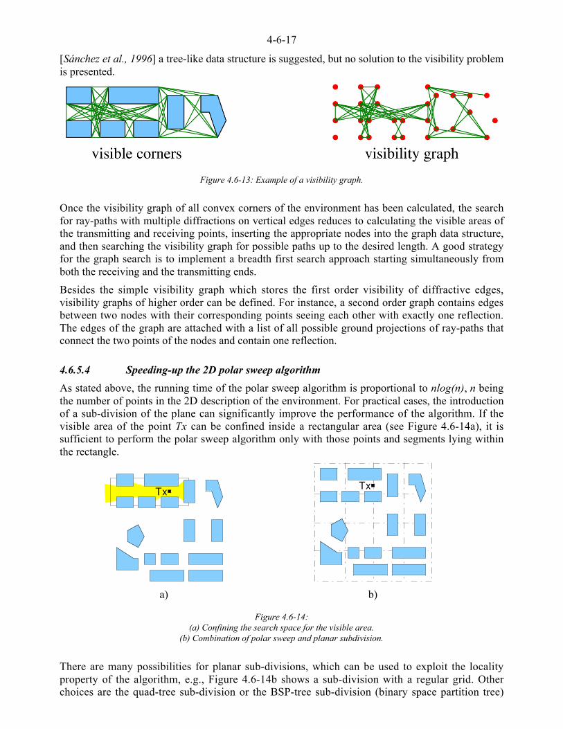
4-6-17

[Sánchez et al., 1996] a tree-like data structure is suggested, but no solution to the visibility problemis presented.

Figure 4.6-13: Example of a visibility graph.

Once the visibility graph of all convex corners of the environment has been calculated, the searchfor ray-paths with multiple diffractions on vertical edges reduces to calculating the visible areas ofthe transmitting and receiving points, inserting the appropriate nodes into the graph data structure,and then searching the visibility graph for possible paths up to the desired length. A good strategyfor the graph search is to implement a breadth first search approach starting simultaneously fromboth the receiving and the transmitting ends.

Besides the simple visibility graph which stores the first order visibility of diffractive edges,visibility graphs of higher order can be defined. For instance, a second order graph contains edgesbetween two nodes with their corresponding points seeing each other with exactly one reflection.The edges of the graph are attached with a list of all possible ground projections of ray-paths thatconnect the two points of the nodes and contain one reflection.

4.6.5.4 Speeding-up the 2D polar sweep algorithm

As stated above, the running time of the polar sweep algorithm is proportional to nlog(n), n beingthe number of points in the 2D description of the environment. For practical cases, the introductionof a sub-division of the plane can significantly improve the performance of the algorithm. If thevisible area of the point Tx can be confined inside a rectangular area (see Figure 4.6-14a), it issufficient to perform the polar sweep algorithm only with those points and segments lying withinthe rectangle.

Tx Tx

a) b)

Figure 4.6-14:(a) Confining the search space for the visible area.

(b) Combination of polar sweep and planar subdivision.

There are many possibilities for planar sub-divisions, which can be used to exploit the localityproperty of the algorithm, e.g., Figure 4.6-14b shows a sub-division with a regular grid. Otherchoices are the quad-tree sub-division or the BSP-tree sub-division (binary space partition tree)

4-6-18

which contain almost a constant number of segments per region. If the visible area of a point is notcontained entirely in the region in which the point is located, neighbouring regions are visited untilthe visible area is computed completely.

Clearly, there is a trade-off between the computation time to perform a polar sweep in a region ofthe sub-division and the number of regions that must be visited. In the case of a quad-tree sub-division, the running time decreases to a magnitude of the order of l.(clog(c)+log(n)),where c is the(constant) number of segments in a rectangle, and l is the number of rectangles that must be visited.The term log(n) is due to operations that must be performed in the data structure of a quad-tree. Thememory requirements increase more than linearly with the number of segments, because a segmentmay intersect more than one rectangle. However, in most practical cases, segments are small and,usually, do not stretch over many rectangles of the quad-tree. Hence, the memory requirementsgenerally are a quasi-linear function of the number of segments.

4.6.6 Ray-tracing algorithm

The 2D version of a ray-path search algorithm, which is based on calculating visible areas andlocating points in star-convex point sets does not need traditional ray-tracing. However, going to 3Dand introducing other types of objects in the environment, will need an efficient ray-tracingalgorithm.

Traditional ray-tracing algorithms perform the following task: given a description of a threedimensional environment that contains certain types of basic objects (such as polygons, spheres,cylinders etc.), the ray-tracing algorithm finds the first intersection point of a ray starting at somepoint in space and pointing into some direction with any of the objects. If no such point exists, anappropriate value is returned. Usually, in the field of computer graphics, ray-tracing algorithms arenot restricted to any special kind of environment, i.e., the basic objects can be arranged arbitrarily inspace.

The implementation of efficient ray-tracing kernels is not the purpose of this chapter, hence, it willnot be discussed in more detail here. In the following, it will be assumed that a sufficiently fastsubroutine is available that returns, for a given ray or ray segment, the closest intersection pointwith any obstructive object in the environment [Foley et al., 1990; Glassner, 1989].

Obviously, such an algorithm can be used to verify whether a given point is located within thevisible area of another point by simply tracing the ray defined through the straight-line segmentbetween the two points. This might be slower than a simple binary search as suggested above.However, any ray-tracing kernel can be extended to find transparent objects and to report thedistance travelled by the ray through the transmissive media. Such objects might not have beenconsidered during the computation of the visible areas, because they do not contribute asobstructive or reflective objects. However, the transparent objects possibly add a certain amount ofattenuation to the electromagnetic field along the ray-paths.

4.6.7 3D Ray-path search algorithm

The main disadvantage of the 2D ray-path search algorithm presented in Section 4.6.5 is that it doesnot find any ray-paths which pass over the objects located in the environment. For indoor andmicro-cell environments, the 2D algorithm with the 2D-3D hybrid method finds all relevant ray-paths, because the ray-paths passing over objects do not exist. For macro-cell or satelliteenvironments, however, the 2D polar sweep algorithm is severely limited in its usage for asufficiently accurate prediction of the radio channel. To solve these shortcomings, the 2D algorithmis extended to a 3D polar sweep algorithm. Nevertheless, the environments to which the algorithmis applied stay as 2_D models. The notion of visible areas and the data structure of a visibility graphare taken over in a very similar manner The details are presented in the following description

4-6-19

4.6.7.1 Visible areas

The definition of the visible area of a point Q in 3D is the same as in the 2D case: a point P isvisible from another point Q, if the straight line segment from Q to P is not obstructed by any otherobject in the environment. However, in 3D, the visible area of Q is confined by the parts of thewalls, which are seen directly by the point. In the following, such visible parts of a wall are calledfacets.

The visible area of a point Q is a star-convex three-dimensional point set with centre Q. The seteither extends to infinity - e.g., towards the sky - or it is enclosed by the facets seen from Q and theground plane. The checking of whether a point P lies within the visible area of Q is more complexto implement, because no simple binary search can be used. The border of the star-convex set canbe projected into a plane and the checking reduces to a point location test combined with a distancetest. However, the checking can also be performed with the help of a ray-tracing routine, checkingthe existence of an intersection point of the ray segment (Q,P) with the environment.

If a ray-tracing kernel is used, the visible area in 3D is not used to speed-up the calculation of line-of-sight ray-paths. Rather, the visible area - more precisely, the border of the visible area - is used todetermine all edges which are candidates for vertical or horizontal diffraction and all walls (facets)where reflection occurs.

The definition of the visible area of an image point is similar to the definition given for the 2D case.Note that a given wall may be divided into many facets. However, due to the restriction to 2_Denvironments, two of them belonging to the same wall are never stacked on top of each other.

An important property of visible areas of points in 2_D environments having the same x- and y-coordinates is the fact that the visible area of the point with larger z-coordinate is a superset of thevisible area of the point with smaller z-coordinate. This statement reflects the common observationthat climbing up a tower increases the visibility compared to the position close to the ground. Theproperty is used later on during the generation of the 3D visibility graph.

4.6.7.2 3D Polar sweep algorithm

The 3D polar sweep algorithm computes the visible area of a 3D point in a 2_D environment. Thebasic principle is much the same as that used in the 2D case. However, instead of sweeping a ray inclockwise polar direction in the ground plane, a half-plane perpendicular to the ground is now sweptaround the point of interest. Figure 4.6-15 illustrates the situation.

Rx

Rx

3D-view side-view

visible facet

sweep plane

Figure 4.6-15: Sweep plane for the 3D polar sweep algorithm

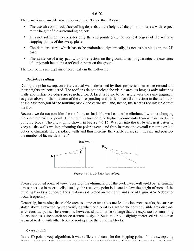
4-6-20

There are four main differences between the 2D and the 3D case:

• The usefulness of back-face culling depends on the height of the point of interest with respectto the height of the surrounding objects.

• It is not sufficient to consider only the end points (i.e., the vertical edges) of the walls asstopping points of the sweep plane.

• The data structure, which has to be maintained dynamically, is not as simple as in the 2Dcase.

• The existence of a ray-path without reflection on the ground does not guarantee the existenceof a ray-path including a reflection point on the ground.

The four points are explained thoroughly in the following.

Back-face culling

During the polar sweep, only the vertical walls described by their projections on to the ground andtheir heights are considered. The rooftops do not enclose the visible area, as long as only mirroringwalls and diffractive edges are searched for. A facet is found to be visible with the same argumentas given above: if the direction of the corresponding wall differs from the direction in the definitionof the base polygon of the building block, the entire wall and, hence, the facet is not invisible fromthe front.

Because we do not consider the rooftops, an invisible wall cannot be eliminated without changingthe visible area of a point if the point is located at a higher z-coordinate than a front wall of abuilding block. The situation is shown in Figure 4.6-16. We run into the trade-off: is it better tokeep all the walls while performing the polar sweep, and thus increase the overall run time or is itbetter to eliminate the back-face walls and thus increase the visible areas, i.e., the size and possiblythe number of facets identified?

Rx

Rx

backwall

Figure 4.6-16: 3D back-face culling.

From a practical point of view, possibly, the elimination of the back-faces will yield better runningtimes, because in macro-cells, usually, the receiving point is located below the height of most of thebuilding blocks and, hence, the situation as depicted on the right hand side of Figure 4.6-16 does notoccur frequently.

Generally, increasing the visible area to some extent does not lead to incorrect results, because asstated above a ray-tracing step verifying whether a point lies within the correct visible area discardserroneous ray-paths. The extension, however, should not be so large that the expansion of mirroringfacets increases the search space tremendously. In Section 4.6.9.1 slightly increased visible areasare used to deal with other types of rooftops for the building blocks.

Cross-points

In the 2D polar sweep algorithm, it was sufficient to consider the stopping points for the sweep onlyat the end points of the segments This is no longer true for the 3D case (see Figure 4 6 17) A wall

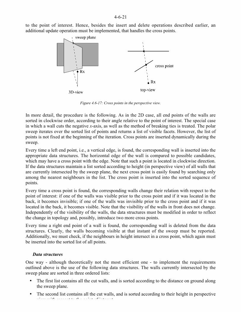
4-6-21

to the point of interest. Hence, besides the insert and delete operations described earlier, anadditional update operation must be implemented, that handles the cross points.

Figure 4.6-17: Cross points in the perspective view.

In more detail, the procedure is the following. As in the 2D case, all end points of the walls aresorted in clockwise order, according to their angle relative to the point of interest. The special casein which a wall cuts the negative x-axis, as well as the method of breaking ties is treated. The polarsweep iterates over the sorted list of points and returns a list of visible facets. However, the list ofpoints is not fixed at the beginning of the iteration. Cross points are inserted dynamically during thesweep.

Every time a left end point, i.e., a vertical edge, is found, the corresponding wall is inserted into theappropriate data structures. The horizontal edge of the wall is compared to possible candidates,which may have a cross point with the edge. Note that such a point is located in clockwise direction.If the data structures maintain a list sorted according to height (in perspective view) of all walls thatare currently intersected by the sweep plane, the next cross point is easily found by searching onlyamong the nearest neighbours in the list. The cross point is inserted into the sorted sequence ofpoints.

Every time a cross point is found, the corresponding walls change their relation with respect to thepoint of interest: if one of the walls was visible prior to the cross point and if it was located in theback, it becomes invisible; if one of the walls was invisible prior to the cross point and if it waslocated in the back, it becomes visible. Note that the visibility of the walls in front does not change.Independently of the visibility of the walls, the data structures must be modified in order to reflectthe change in topology and, possibly, introduce two more cross points.

Every time a right end point of a wall is found, the corresponding wall is deleted from the datastructures. Clearly, the walls becoming visible at that instant of the sweep must be reported.Additionally, we must check, if the neighbours in height intersect in a cross point, which again mustbe inserted into the sorted list of all points.

Data structures

One way - although theoretically not the most efficient one - to implement the requirementsoutlined above is the use of the following data structures. The walls currently intersected by thesweep plane are sorted in three ordered lists:

• The first list contains all the cut walls, and is sorted according to the distance on ground alongthe sweep plane.

• The second list contains all the cut walls, and is sorted according to their height in perspectiveview with respect to the point of interest

4-6-22

• The third list contains only those walls which are currently visible, and is sorted according tothe height in perspective view as well.

Whenever an insert, delete, or update operation takes place, the lists are updated by binary searchoperations or by linear search operations starting at the location where the corresponding wall isplaced in the lists or at the beginning of the lists. More precisely:

• The first list is only changed through insert and delete operations, because the order on theground does not change at a cross point. Such an operation takes a time proportional to log(n)where n is the length of the list.

• The second list is changed through insert and delete operations as well. The running time isalso proportional to log(n). Additionally, the update operation at a cross point can beperformed in constant time per point. The neighbours to check for further cross points arefound in this list in constant time.

• The third list is more involved in each operation:

• A new wall to be inserted may cover currently visible walls. Because the list is sortedaccording to height, we can step linearly through the list and report all facets that no longerremain visible, until the place is found to insert the new wall provided that this is visible at all.Note that the visible facets of walls located behind the new wall have to be reported anyway,thus, a linear operation is not very harmful.

• A wall to be deleted may expose several other walls to visibility. One method to find them isto step linearly through the first list (which is sorted according to the distance on the ground)starting at the position of the wall to be deleted. The search ends when the next wall is foundwhich was previously visible.

• An update operation can be performed in constant time.

Two remarks should be added: The notion of height in the discussion above always means height inthe perspective view relative to the point of interest. In order to have a simple ending criterion whilesearching the lists, it is convenient to add a virtual wall that is always visible at the end of each list,e.g., this virtual wall may be located at infinity and have infinite height.

Reflection on the ground

In the 2D version of the algorithm an existing ray-path always guaranteed the existence of anappropriate ray-path including an additional ground reflection as well. As shown in Figure 4.6-18this is no longer the case in the 3D application. There, the line-of-sight exists, however, a buildingblocks the ground reflection. Nevertheless, both ray-paths have the same projection on the groundplane, hence, a simple test using the ray-tracing kernel detects the correct ray-paths including aground reflection.

TxRxTx Rx

3D-view side-view

Figure 4.6-18: Reflection on the ground.

4-6-23

Running time and memory requirements

The worst case running time of the 3D polar sweep algorithm is proportional to n2log(n), where n isthe number of vertical edges in the environment, because we can construct an environment such thatfor a certain point of interest about n2 cross points exist. As a consequence - theoretically speaking -the operations on the lists containing the walls currently cut by the sweep plane, which areperformed in linear time, do not increase the worst case behaviour of the algorithm (remember thatthe operations on the lists required for cross points are done in constant time). However, in most ofthe practical cases the running time will be proportional to (n+f).log(n), where f is the number offacets being computed during the sweep. This is because usually the number of cross points peredge is limited by a small number. In real environments, the three lists of the walls remain small, somore sophisticated data structures avoiding the linear parts of the operations may not pay off. Butthis remains to be verified by experiments.

4.6.7.3 Visibility graph

The first order visibility graph for the 3D case is similar to the visibility graph presented in thedescription of the 2D case (see Section 4.6.5.3). The nodes in the graph represent the vertical edgesof the environment. A node is attributed by the visible area of the topmost point of the edge, whichis a superset of all the visible areas of the points located below on the same edge. Two nodes areconnected by an edge in the graph whenever the corresponding points of the nodes see each other.

The difference with respect to the 2D case lies in the fact that the search for diffractive ray-paths inthe graph must be followed by a check whether the ray-path defined by the vertical edges is indeednot obstructed by any other object in the environment. The test is necessary because a diffractionpoint below the topmost point of an edge has a smaller visible area. In a similar way, higher ordervisibility graphs can be constructed.

4.6.7.4 Speeding-up the 3D polar sweep algorithm

A planar sub-division has been introduced in the 2D polar sweep algorithm to exploit the localityusually present in urban areas (see Section 4.6.5.4). The same mechanism enhanced with heightinformation is applicable in the 3D case (see Figure 4.6-19a). Whenever the visible area of a pointis enclosed within a region of the sub-division, the computation can be stopped.

Tx

virtual walls

visitedregion

skippedregion

visitedregion

in i t ia lregion

a) b)

Figure 4.6-19:(a) Regular sub-division with additional height information. (b) Skipping regions in a sub-division

How can this information be obtained? In the description of the data structures of the polar sweep

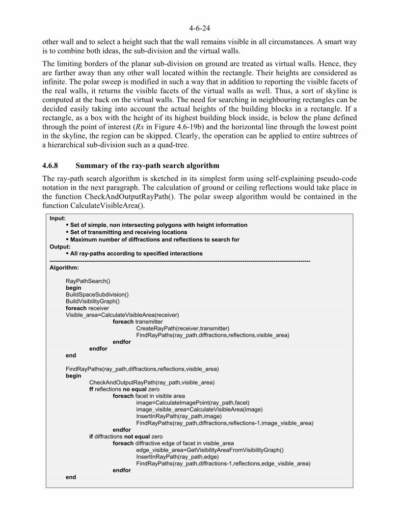
4-6-24

other wall and to select a height such that the wall remains visible in all circumstances. A smart wayis to combine both ideas, the sub-division and the virtual walls.

The limiting borders of the planar sub-division on ground are treated as virtual walls. Hence, theyare farther away than any other wall located within the rectangle. Their heights are considered asinfinite. The polar sweep is modified in such a way that in addition to reporting the visible facets ofthe real walls, it returns the visible facets of the virtual walls as well. Thus, a sort of skyline iscomputed at the back on the virtual walls. The need for searching in neighbouring rectangles can bedecided easily taking into account the actual heights of the building blocks in a rectangle. If arectangle, as a box with the height of its highest building block inside, is below the plane definedthrough the point of interest (Rx in Figure 4.6-19b) and the horizontal line through the lowest pointin the skyline, the region can be skipped. Clearly, the operation can be applied to entire subtrees ofa hierarchical sub-division such as a quad-tree.

4.6.8 Summary of the ray-path search algorithm

The ray-path search algorithm is sketched in its simplest form using self-explaining pseudo-codenotation in the next paragraph. The calculation of ground or ceiling reflections would take place inthe function CheckAndOutputRayPath(). The polar sweep algorithm would be contained in thefunction CalculateVisibleArea().

Input:•••• Set of simple, non intersecting polygons with height information•••• Set of transmitting and receiving locations•••• Maximum number of diffractions and reflections to search for

Output:•••• All ray-paths according to specified interactions

---------------------------------------------------------------------------------------------------------------------------------------Algorithm:

RayPathSearch()beginBuildSpaceSubdivision()BuildVisibilityGraph()foreach receiverVisible_area=CalculateVisibleArea(receiver)

foreach transmitterCreateRayPath(receiver,transmitter)FindRayPaths(ray_path,diffractions,reflections,visible_area)

endforendfor

end

FindRayPaths(ray_path,diffractions,reflections,visible_area)begin

CheckAndOutputRayPath(ray_path,visible_area)ff reflections no equal zero

foreach facet in visible areaimage=CalculateImagePoint(ray_path,facet)image_visible_area=CalculateVisibleArea(image)InsertInRayPath(ray_path,image)FindRayPaths(ray_path,diffractions,reflections-1,image_visible_area)

endforif diffractions not equal zero

foreach diffractive edge of facet in visible_areaedge_visible_area=GetVisibilityAreaFromVisibilityGraph()InsertInRayPath(ray_path,edge)FindRayPaths(ray_path,diffractions-1,reflections,edge_visible_area)

endforend

4-6-25

It is very important to implement the polar sweep algorithm used to calculate the visible areas insuch a way that the data structures maintained during the iteration always reflect a consistenttopological view of the environment. Errors due to rounding of floating point numbers may lead tosign changes in certain crucial operations (e.g., point location respective to a plane). Due to thediscrete representation of numbers in a computer, care must be taken to implement robustsubroutines, for instance, while trying to find the intersection point of two straight lines. The tiebreaking decisions, during the sorting processes, must be selected in such a way that even the casethat many points have the same polar angle is handled correctly. It is a challenge to implement bothfast and robust algorithms. The reader is advised to seriously think about this problem prior tostarting implementation of the algorithms presented in this chapter [Burnikel et al., 1994; Mehlhornand Näher, 1995]. There is a great amount of literature available, which deals with the robustness ofgeometric algorithms.

4.6.9 Extension of the environment and further interactions

The algorithms presented so far - in the 2D as well as in the 3D version - can handle only pure 2_Denvironments. However, there are potential extensions available, which make the polar sweepalgorithm suitable for more complex environments.

Note that adding more objects in the environment at most decreases the visibility, i.e., the visibleareas computed by a polar sweep are always valid as a search space for ray-paths. If only additionalobstructive objects that do not fulfil the restrictions of the 2_D definition are added, the ray-tracingkernel can just handle them, so those invalid paths are discarded. An example of such an object is anon-planar ground modelled by a height-field or a set of triangles. However, for efficiency reasonsor in order to find more interacting features, it might be interesting to use some types of objects tofurther confine the visible areas as well.

4.6.9.1 Complex building blocks

Roof types

Many houses commonly found in urban or suburban environments are covered with sloping roofs.With the help of a simple trick, approximations of the visible areas enclosed by these houses can beintroduced. Figure 4.6-20a depicts the scenario. An additional virtual wall defining the ridge of thehouse is passed to the polar sweep algorithm. Consequently, the visible areas are slightly too large,but the verification of the ray-paths through ray-tracing routine discards impossible ray-paths.

RxRx

3D-view top view

v i r tuawal l

a) b)Figure 4.6-20: (a) Introducing tilted roofs. (b) Introducing cylinders and poles.

Because the gables are not modelled, reflections at these surfaces cannot be accounted for.However, raising the side walls until they reach the ridge and treating them both as transmissive andobstructive, allows these details to be handled whenever required. In a very similar way, roofs with

4-6-26

Cylinders and poles

Other commonly structures sometimes found in urban areas are cylindrical objects and poles.Although more complex to handle in order to compute interactions for the propagation ofelectromagnetic waves, it is straightforward to handle them in the computation of the visible areasas long as their axes are perpendicular to the ground plane. Figure 4.6-20b) illustrates the method.

The cylinder, or the pole, is replaced during the sweep by a wall that is perpendicular both to theground and to the line-of-sight between the centre of the cylinder and the point of interest, e.g., Rx.The width of the wall is determined by the chord between the two points obtained by the tangentstouching the cylinder and passing through Rx. The height of the wall is taken as the height of thecylinder.

4.6.9.2 Scattering and attenuating objects

Scatterers

Scattering objects receive certain amount of energy from the transmitting source and re-transmit afraction of this energy in the direction of the receiving point. Hence, from the transmitter's point ofview, they play the role of a receiver and from the receiver's point of view, they play the role of atransmitter. Consequently, they can be handled as additional receiving and transmitting pointshaving some special properties. However, in most practical cases, only first order interactions willbe of interest. So the ray-tracing kernel can handle the search for line-of-sight ray-paths betweenscatterer and transmitting and receiving points. One should be aware that such scattering objectsmight add a huge number of additional ray-paths. The deterministic simulation approach might notbe the method of choice in the case that many scattering objects have to be modelled.

Attenuators

As already mentioned in Section 4.6.4.4, transmissions without refraction can be handled easilywhenever the ray-tracing kernel is able to report the location or, at least, the length of the pathtravelled by the ray through the transmissive media. An object which is both reflective andtransmissive can be handled in a straightforward way as well.

4.6.9.3 Additional interactions

Diffraction on horizontal edges

In the description of the ray-path search algorithm, we have not given details about the calculationof first order horizontal diffraction. The visible areas obtained as a result of the polar sweepalgorithm provide a list of all visible facets. If such a facet has as topmost edge a horizontal edge ofa building block - or at least a part of such an edge, this edge is used to calculate a ray-pathincluding horizontal diffraction, applying the method described in Section 4.6.4.1. The ray-pathsearch should take into account that a horizontal edge of a building block may contribute to severalfacets but only to one ray-path interacting with this edge (see Figure 4.6-21). Ray-paths withadditional reflections on the ground are easily computed using the image points of the receiver orthe transmitter, respectively. In practical cases, only the ray-paths where the reflection on theground is the last interaction before reaching the receiving location are of interest. Because ahorizontal edge always belongs to the polygon of the roof of a building block, ray-paths includingadjacent horizontal diffraction can be found by iterating over the edges of the polygon. Similarlyadjacent diffractions combining a vertical and a horizontal diffraction can be searched for.

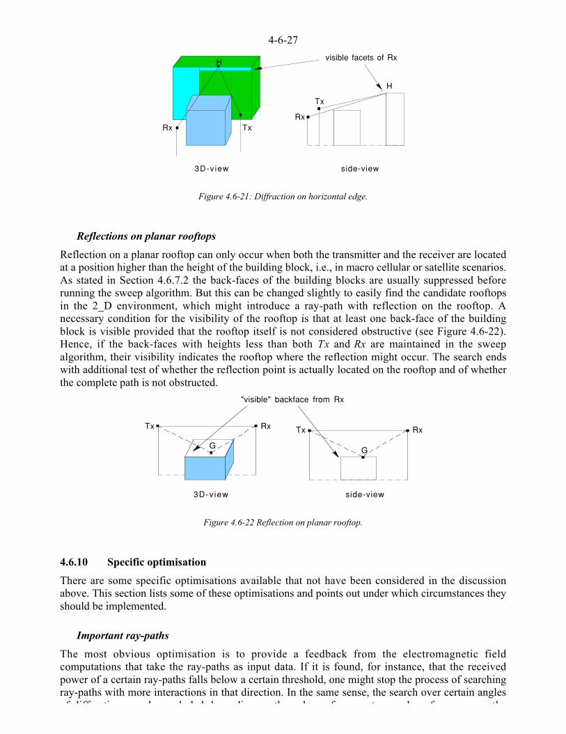
4-6-27

Rx

3D-view side-view

Rx

visible facets of Rx

Tx

H

Tx

H

Figure 4.6-21: Diffraction on horizontal edge.

Reflections on planar rooftops

Reflection on a planar rooftop can only occur when both the transmitter and the receiver are locatedat a position higher than the height of the building block, i.e., in macro cellular or satellite scenarios.As stated in Section 4.6.7.2 the back-faces of the building blocks are usually suppressed beforerunning the sweep algorithm. But this can be changed slightly to easily find the candidate rooftopsin the 2_D environment, which might introduce a ray-path with reflection on the rooftop. Anecessary condition for the visibility of the rooftop is that at least one back-face of the buildingblock is visible provided that the rooftop itself is not considered obstructive (see Figure 4.6-22).Hence, if the back-faces with heights less than both Tx and Rx are maintained in the sweepalgorithm, their visibility indicates the rooftop where the reflection might occur. The search endswith additional test of whether the reflection point is actually located on the rooftop and of whetherthe complete path is not obstructed.

TxRxTx Rx

3D-view side-view

G G

"visible" backface from Rx

Figure 4.6-22 Reflection on planar rooftop.

4.6.10 Specific optimisation

There are some specific optimisations available that not have been considered in the discussionabove. This section lists some of these optimisations and points out under which circumstances theyshould be implemented.

Important ray-paths

The most obvious optimisation is to provide a feedback from the electromagnetic fieldcomputations that take the ray-paths as input data. If it is found, for instance, that the receivedpower of a certain ray-paths falls below a certain threshold, one might stop the process of searchingray-paths with more interactions in that direction. In the same sense, the search over certain anglesof diffraction ma be e cl ded depending on the al es of parameters s ch as freq enc or the

4-6-28

Specialising the visibility graph

It is sufficient to calculate the visible area for a vertical edge at the height equal to the maximum ofthe heights of both Rx and Tx. However, for an interactive application of the program, it is better topre-calculate the visibility graph considering the topmost points or to update the visibility graphdynamically.

Special optimisation in the case of satellites

In the case of studies of satellite constellations, the following observation gives rise to certain typesof optimisations: given that the distance to a satellite is usually very large compared to thedimensions of the environment, the satellite can be modelled through its direction, e.g., withazimuth and elevation angles. Satellites with the same elevation angle generate equal diffractionpoints on vertical edges.

Hence, in the search for ray-paths from the receiving location towards the satellites, those satelliteshaving the same elevation angle share the sub-ray-paths until the last point of vertical diffraction.On the other hand, if a ray-path towards a certain satellite is discarded as being obstructed, allsatellite positions with the same azimuthal angle but lower elevation angle are obstructed as well.

Antenna patterns

Because the polar sweep algorithm already takes into account angular aspects of visibility, it is veryeasy to include antenna radiation patterns as well. The visible areas of the transmitting (or thereceiving) point can be limited to the appropriate main radiation lobe. Actual data from measuredantennas can provide information to what extent the polar sweep should be performed. Moreover,certain statistics on the arrival time of different signals correlated to the arriving angle can begathered easily.

First order diffuse reflection

Because the 3D polar sweep algorithm calculates all visible facets exactly, it is possible toincorporate first order diffuse reflections models into the radio channel predictions.

Continuous receiver locations

Perhaps one of the most promising optimisations is the introduction of continuous sets for thespecification of receiver locations. Up to now, it was assumed that all receiver positions have beenobtained through a sampling process that might depend on the frequency of the electromagneticwave. The algorithm has the possibility to circumvent this discrete model of the receiving locations.The definition of the visibility graph has to be modified in such a way that its nodes do notrepresent single points but entire point sets such as segments or areas. The development of theappropriate data structures and details of the algorithm are the topic of on-going work of one of theauthors.

4.6.11 Example of software package

RadioTracer [Aguado et al., 1999] is a software package that implements a site-specific propagationtool valid for a wide range of scenarios ranging from indoor pico-cells and street micro-cells toconventional macro-cells and satellite cells (Land Mobile Satellite (LMS) scenarios). In this respect,the tool has being used for the characterisation of the LMS propagation environment for the GlobalSatellite Navigation System GNSS-2 under European Space Agency contract No. 12223/96/NL/JSC[Aguado et al., 1999]. In the project availability studies have been carried out for such systems

i lti l t llit t ll ti d f t ti bit Th th h

4-6-29

implemented to deal with the practical cases. The electromagnetic part of RadioTracer implements acomputationally improved version of the GTD/UTD approach taken from [McNamara et al., 1990].

4.6.12 Conclusions

This chapter has described an efficient ray-path search algorithm, which can be used for the analysisof the propagation conditions of electromagnetic waves applying geometrical optics and thegeometric theory of diffraction in its uniform theory of diffraction version. The scenarios wererestricted to 2_D environments. However, certain extensions were presented to overcome some ofthe limitations. The method is applicable for indoor pico-cell, micro-cell, macro-cell and satellitescenarios. The core idea of the algorithm is to first compute visible areas before using a ray-tracingkernel for a final check. The algorithm to compute the visible areas was based on the sweep planeparadigm from computational geometry. Sophisticated data structures - such as graphs, dictionaries,and space sub-divisions - were introduced to further reduce the computation time by dynamicallystoring intermediate results for a later fast lookup.

4-6-30

4.6.13 References

[Aberegg and Peterson, 1995]Aberegg K. and Peterson A., "Integral Equation Asymptotic Phase method to two dimensionalscattering" IEEE Trans. Ant. Prop. Vol.43 No.5 pp 534-537, 1995.

[Aguado et al., 1996a]Aguado Agelet F., Pérez Fontán F. and Formella A. “Fast Ray Tracing for Microcellular and IndoorEnvironments”. In Proc. of the 7th Biennial IEEE Conf. on Electromagnetic Field Computation(IEEE CEFC'96), PA-2, March 1996.

[Aguado et al., 1996b]Aguado Agelet F., Pérez Fontán F. and Formella A. “UTD Electromagnetic Simulation forMicrocell and Indoor Environments based on 2 1/2 D Ray Tracing.” In Proc. of PIERS 1996,Progress In Electromagnetics Research Symposium, 599 pp, University of Innsbruck, Austria, July1996.

[Aguado et al., 1997a]Aguado Agelet F., Pérez Fontán F. and Formella A. “Fast Ray Tracing for Microcellular and IndoorEnvironments”. IEEE Transactions on Magnetics, 33(2):1484-1487, March 1997.

[Aguado et al., 1997b]Aguado Agelet F., Pérez Fontán F., and Formella A. “Indoor and Outdoor Channel Simulator basedon Ray Tracing”. Proc. of the IEEE Vehicular Technology Conf.'97, Phoenix, pp 2065-2069, May,1997.

[Aguado et al., 1999]Aguado Agelet F., Formella A., and Pérez Fontán, F. “Radio-tracer: A Tool for DeterministicSimulation of Wave Propagation”. In B. Arbesser-Rastburg, editor, Proc. of the COST255 1thInternational Workshop on Radiowave Propagation Modelling for SatCom Services at Ku-band andabove, European Space Agency Publications Division, WPP-146, pp 135-138, February 1999.

[Alpert et al., 1993]Alpert B., Beylkin G., Coifman R. and Rokhlin V., "Wavelet-like bases for the fast solution ofsecond kind integral equations', SIAM J. Sci. Comput. Vol. 14 No. 1, pp 159-184, 1993.

[Andersen, 1994]Andersen J.B., "Transition zone diffraction by multiple edges", IEE Proc.-Microw. AntennasPropag., Vol.141, No.5, pp 382-384, 1994.

[Athanasiadou et al., 1995]Athanasiadou G.E., Nix A.R. and McGeehan J.P. “A Ray Tracing Algorithm for Microcellular andIndoor Propagation Modelling”. In Antennas and Propagation, no. 407, pp 231-235, IEEConference Publication, April 1995.

[Bayliss and Turkel, 1980]Bayliss A. and Turkel E., "Radiation boundary conditions for wave-like equations" Comm. PureAppl. Math. Vol. 33 pp 707-725, 1980.

[Berenger, 1994]Berenger J.P., "A perfectly matched layer for the absorption of electromagnetic waves", J. Comp.Phys. Vol. 114, pp 185-200, 1994.

[Brennan and Cullen, 1998a]Brennan C. and Cullen P., "Tabulated Interaction Method for UHF terrain propagation problems",IEEE Trans. Ant. Prop. Vol.46 No.5 pp 738-739, 1998.

4-6-31

[Brennan and Cullen, 1998b]Brennan C. and Cullen P., "Application of the Fast Far-Field Approximation to the computation ofUHF path loss over irregular terrain", IEEE Trans. Ant. Prop. Vol.46 No.6, 1998.

[Burnikel et al., 1994]Burnikel C., Mehlhorn K., and Schirra S. “How to Compute the Voronoi Diagram of LineSegments: Theoretical and Experimental Result”. In Proc. of the ESA'94, vol. 855 of LNCS,pp 227-239, Springer-Verlag Berlin, 1994.

[Canning, 1990a]Canning F.X., "The Impedance Matrix Localisation (IML) Method for Moment MethodCalculations". IEEE Trans. Ant. and Prop. Magazine, pp 18-30, October 1990.

[Canning, 1990b]Canning F.X., "On the application of some radiation boundary conditions", IEEE Trans. Ant.Prop.Vol.38, pp 740-745, May 1990.

[Catedra, et al., 1997]Cátedra M.F., Pérez-Arriaga J., González A., Saez de Adana F., and Gutiérrez O. “Fast ComputerTool for the Analysis of Propagation in Urban Cells”. In Proc. of Wireless Communications Conf.,pp 240-245, August 1997.

[Catedra, et al., 1998]Cátedra M.F., Pérez-Arriaga J., Saez de Adana F., and Gutiérrez O. “Efficient Ray-TracingTechniques for 3D Analysis of Propagation in Mobile Communications. Application to Picocell andMicrocell Scenarios”. IEEE Antennas and Propagation Magazine, 40(2):15-28, April 1998.

[Catedra and Pérez-Arriaga, 1999]Cátedra M.F. and Pérez-Arriaga J. “Cell Planning for Wireless Communications”. Artech House,London, ISBN 0-89006-601-9, 1999.

[Cichon and Wiesbeck, 1994]Cichon D.J. and Wiesbeck W. “Indoor and Outdoor Propagation Modelling in Pico Cells”. InPIMRC'94, pp 491-495, 1994.

[Cichon and Wiesbeck, 1995]Cichon D.J. and Wiesbeck W. “Comprehensive Ray Optical Propagation Models for Indoor andOutdoor Environments: Theory and Applications”. In Proc. of COMMSPHERE'95, pp 201-208,Israel, January 1995.

[Cichon et al., 1996]Cichon D.J., Becker T.C., and Dottling M.. “Ray Optical Prediction of Outdoor and IndoorCoverage in Macro and Micro Cells”. In Proc. of IEEE Vehicular Technology Conf., Atlanta, USA,April 1996.

[Corman et al., 1990]Corman T.H., Leiserson C.E., and Rivest R.L. “Introduction to Algorithms”. MIT-Press/McGraw-Hill, 1990.

[Foley et al., 1990]Foley J.D., van Dam A., Feiner S.K., and Hughes J.F. “Computer Graphics: Principles andPractices (2nd Edition)”. Addison Wesley, 1990.

[Formella and Gill, 1995]Formella A. and Gill C. “Ray Tracing: A Quantitative Analysis and a New Practical Algorithm”.The Visual Computer, 11(9):465-476, December 1995.

4-6-32

[Fortune et al., 1995]Fortune S., Gay D., Kernighan B., Landron O., Valenzuela R., and Wright M.. “WISE Design ofIndoor Wireless System: Practical Computation and Optimization”. IEEE Computational Scienceand Engineering, pp 58-68, 1995.

[Ghali, 1998]Ghali. S. “Computation and maintenance of visibility and shadows in the plane”. In Václav Skala,editor, Proc. of 6th International Conf. in Central Europe on Computer graphics and Visualization.University of West Bohemia, ISBN 80-7082-360-7, pp 117-124, February 1998.

[Ghali and Stewart, 1996aGhali S. and Stewart A.J. “Incremental Update of the Visibility Map as Seen by a MovingViewpoint in Two Dimensions”. In Proc. of Eurographics Workshop on Computer Animation andSimulation, pp 1-11, 1996.

[Ghali and Stewart, 1996b]Ghali S. and Stewart A.J. “Maintenance of the Set if Segments Visible from a Moving Viewpoint inTwo Dimensions”. In Proc. 12th Annual ACM Symposium on Computational Geometry, pp V3-V4,ACM Press, 1996.

[Glassner, 1989]Glassner A.S., editor. “An Introduction to Ray Tracing”. Academic Press, 1989.

[Holm, 1996]Holm P.D., "UTD-Diffraction Coefficients for Higher Order Wedge Diffracted Fields", IEEETrans. Ant. Prop. Vol.44 No.6, pp 879-888, 1996.

[Janaswamy, 1997]Janaswamy R., "Propagation Predictions Over Rural Terrain by the Split Step Parabolic Method",COST259 TD(97)45 Lisbon, Portugal, 24-26 September 1997.

[James, 1990]James R.M., "A Contribution to Scattering Calculation for Small Wavelengths - The HighFrequency Panel Method" IEEE Trans. Ant. Prop. Vol.38 No. 10, pp 1625-1630, 1990.

[Keller, 1962]Keller J.B., "Geometric Theory of Diffraction", Jnl. Opt. Soc. Am. Vol.52, pp 116-130, 1962.

[Kouyoumjian and Pathak, 1974]Kouyoumjian R.G. and Pathak P.H., "A uniform geometrical theory of diffraction for an edge in aperfectly conducting surface", Proc. IEEE, Vol.62, no.11, pp 1448-1461, November 1974.

[Lawton and McGeehan, 1994]Lawton M.C. and McGeehan J.P. “The Application of a Deterministic Ray Launching Algorithmfor the Prediction of Radio Channel Characteristics in Small-Cell Environments”, IEEE Trans.Vehicular Technology, 43(4):955-969, 1994.

[Levy, 1990]Levy M.F., "Parabolic Equation Modelling of Propagation over Irregular Terrain", Elec. LettersVol.26 No.15 pp 1153-1155, 1990.

[Lindman, 1975]Lindman E.L., "Free-space boundary conditions for the time dependent wave equation", Jnl. Comp.Phys. Vol. 18. pp 67-78, 1975.

[Lu and Chew, 1995]Lu C.C. and Chew W.C., 1995, "Fast Far Field Approximation for Calculating the RCS of LargeObjects" Micro. Opt. Tech. Lett. Vol. 8, No. 5, pp 238-241, 1975.

4-6-33

[Luebbers, 1984]Luebbers R.J., "Finite Conductivity Uniform GTD versus Knife Edge Diffraction in Prediction ofPropagation Path Loss", IEEE Trans. Ant. Prop. Vol.32 No.1, 1984.

[McNamara et al., 1990]McNamara D.A., Pistorius C.W.I., and Malherbe J.A.G. “Introduction to the Uniform GeometricalTheory of Diffraction”. Artech House, Boston, 1990.

[Mehlhorn and Näher, 1995]Mehlhorn K. and Näher St. “LEDA, A Platform for Combinatorial and Geometric Computing”.Communications of the ACM, 38(1):96-106, 1995.

[Moroney and Cullen, 1995]Moroney D. and Cullen P. J., "A Fast Integral Equation Approach to UHF Coverage Estimation inMobile and Personal Communications" pp 343-350, edited E. del Re. Elsevier Press, 1995.

[Mur, 1981]Mur G., "Absorbing Boundary Conditions for the finite difference approximation of the timedomain electromagnetic field equations", IEEE Trans. Electromagnet. Compat. Vol. EMC-23,pp377-382, Nov. 1981

[Pocchiola and Vegter, 1995]Pocchiola M. and Vegter G. “Computing the Visibility Graph via Pseudo-triangulation”.In Proc. of the ACM Symposium on Computational Geometry, pp 248-257, ACM Press, June 1995.

[Rappaport et al., 1993]Rappaport T.S., Seidel S.Y., and Schaubach K.R. “Site-Specific Propagation for PCS SystemDesign Wireless Personal Communications”. pp 281-315, Kluwer Academic Publishers, Boston,1993.

[Rokhlin, 1990]Rokhlin V., "Rapid Solution of integral equations of scattering theory in two dimensions", Jnl.Comp. Phys. Vol.36,No.2,pp 414-439, 1990.

[Samet., 1989]Samet H.. “The Design and Analysis of Spatial Data Structures”. Addison-Wesley, Reading,Massachusetts, 1989.

[Sánchez et al., 1996]Sánchez M.G., de Haro L., Pino A.G., and Calvo M.. “Exhaustive Ray Tracing Algorithm forMicrocellular Propagation Prediction Models”. IEE Electronics Letters, 32(7):624-625, 1996.

[Schaubach and Davis, 1996]Schaubach K.R. and Davis N.J. “Microcellular Radio-Channel Propagation Prediction”.IEEE Antennas and Propagation Mag., 36(4):25-34, August 1996.

[Schaubach et al., 1992]Schaubach K.R, Davis N.J., and Rappaport T.S. “A Ray Tracing Method for Predicting Path Lossand Delay Spread in Microcellular Environments”.In IEEE Vehicular Technology Conf., pp 932-935, 1992.

[Seidel and Rappaport, 1992]Seidel S.Y. and Rappaport T.S. “A Ray-Tracing Technique to Predict Path Loss and Delay SpreadInside Buildings”. In Proc. of IEEE GLOBECOM, pp 649-653, December 1992.

[Seidel and Rappaport, 1994]Seidel S.Y. and Rappaport T.S. “Site-Specific Propagation Prediction for Wireless in BuildingPersonal Communication System Design.”IEEE Trans. on Vehicular Technology, 43(4):879-891,N b 1994

4-6-34

[Song and Chew, 1995]Song J. M. and Chew W. C., "Multilevel fast multipole algorithm for solving combined fieldintegral equations of electromagnetic scattering" Micro. Opt. Tech. Lett. Vol. 10, No. 1, pp 14-19,1995.

[Tan and Tan, 1996]Tan S.Y. and Tan H.S. “A Microcellular Communications Propagation Model Based on theUniform Theory of Diffraction and Multiple Image Theory”. IEEE Trans. Antennas andPropagation, 44(10):1317-1326, October 1996.

[Ufimtsev, 1957]Ufimtsev P.Y., "Approximate Computation of the diffraction of plane electromagnetic waves atcertain metal bodies", Sov. Tech. Phys. pp 1708-1718, 1957.

[Wagner and Chew, 1994]Wagner R. and Chew W.C., "A Ray-Propagation Fast Multipole Method", Micro. Opt. Tech. Lett.Vol. 7 No. 10, pp 435-438, 1994.

[Welzl, 1985]Welzl E. “Constructing the Visibility Graph for n Line Segments in O(n2) Time”.Information Processing Letters, 20, 167-171, 1985.

4.7-1

CHAPTER 4.7Antenna effects in

Land Mobile Satellite Systems

Editor: István Frigyes1

Authors: István Frigyes1, Leandro de Haro2, Simon Saunders3, Andreas-Albertos Agius

1 Technical University of Budapest, Goldmann György tér 3, H-1111 Budapest, Hungary

Tel: +36-1-463-3689, Fax: +36-1-463-3289, e-mail: t-frigyes@nov.mht.bme.hu2 Universidad Politecnica de Madrid, ETSI Telecomunication, Ciudad Universitaria E-28040 Madrid, Spain

Tel: +34-91-549-5700-386, Fax: +34-91-543-2002, e-mail: leandro@gr.ssr.upm.es3 University of Surrey, Centre for Communication Systems Research, Guildford GU2 5XH, United Kingdom

Tel: +44 1483 259806 Fax: +44 1483 259504 e mail: S Saunders@ee surrey ac uk

4.7-2

4.7 Antenna effects in Land Mobile Satellite Systems

In this chapter the propagation effects on antenna parameters are discussed, with particular regard tomultipath. These effects are quite different from the case of direct line-of-sight links. The effectiveantenna gain when the field is diffuse, due to scattering objects along the link, the impact of theantenna pattern on the radio channel and the noise collected by a mobile terminal are discussed inthe following.

LEO satellite links are analysed, but the results are also valid for other types of satelliteconstellations. Downlink propagation is assumed in most cases, but the results are equally valid inthe up-link case.

It is to be noted that some innovative aspects of antennas in mobile satellite links (in particularsmart antennas) are not discussed in this chapter. A more detailed analysis of antenna aspects hasbeen performed in the COST Action 260 "Smart Antennas: Computer aided design & technology".

4.7.1 Antenna gain in handheld terminals

As received field at the handheld terminal can be diffuse, both antenna gain and spatial correlationcharacteristics are radically different from those of free-space antennas of the same design.

The field becomes diffuse if the line of sight between the onboard antenna and the antenna of theground terminal is heavily shadowed, or even if there is a line of sight but scatterers of variousshapes and sizes influence the wave propagation. (e.g. for satellite to indoor links). Similar effectscan occur in the case of an outdoor ground terminal antenna shadowed by foliage or buildings.

The assessment of antenna parameters with respect to the link quality is more important for higher-microwave frequencies than for lower bands. Whereas antennas for lower frequencies have alimited gain (due to size constraints) and employ linear vertical polarisation, at frequencies aboveKu-Band antennas of considerable gain and with circular polarisation may be considered forsatellite systems.

In this paragraph a theoretical analysis is given, based on the methods of wave propagation inrandom media by [Ishimaru, 1997]. Measurements are also presented.

In a satellite to land mobile terminal link (e.g. satellite-to-urban streets, satellite-to-indoor, etc.)heavy shadowing can occur between transmitter and receiver and the electromagnetic wave isstrongly attenuated and affected by random scattering. In this chapter the “shadowed line-of-sight”(S-LOS) concept will be used. In S-LOS situations objects causing shadowing will (virtually) beregarded as scatterers, causing both scattering and absorption [Ishimaru, 1997].

S-LOS scenarios are characterised by high absorption and large low density scatterers. First ordermultiple scattering can be used and the wave incident to the scatterers and the scattered wave (and,in principle, also the direct wave) are attenuated by the absorption and the scattering by otherobjects.

High gain transmit and receive antennas are assumed and the configuration shown in Figure 4.7-1 isanalysed. In this case two of the rays are assumed to arrive within the main beam of the receiveantenna while the third one is well outside it.

4.7-3

Figure 4.7-1: Scattering configuration

The volume V surrounding the receive antenna, designated by the dotted line, contains randomscattering objects (the small circles) with a scattering amplitude f(oe, ie; r) and scattering crosssection:

( ) ( ) ( )rrr ast mmm += . 4.7-1

where o and i are the vectors in the directions of the observation and the incident wave directions,respectively, and subscript e stands for unit vectors; the t, s and a subscripts mean the total,scattering and absorption cross-sections respectively and r is the radius vector of the scatterer’slocation.

A plane wave of unit amplitude incident on a scatterer from the direction of i causes the scatteredwave in the direction of o:

( ) ( )R

jkR;,fEs

exprio= 4.7-2

with R the distance of the receiving antenna from the scattering object. This equation is valid in thefar field region of the scatterer and neglecting the effect of other objects.

4.7.1.1 Average received power

The received field can be decomposed into a coherent and a non-coherent component. As illustratedby [Ishimaru, 1997] the power of the coherent field is that of the direct wave and the power of thenon-coherent field is due to the scattered field. In S-LOS situations there is no need to make adistinction between components because the direct ray is completely missing. The power densityincident on a scatterer contained in the elementary volume dV of the total volume V is:

( ) atet e�R

PiGS <= 2

1

14

4.7-3

where Gt is the transmit antenna gain function in direction ie, Pt is the transmit power, R1 thedistance between the transmitter and the scatterer and e-a is the loss due to the scatterers overdistance, with:

( ) ( )0=1

0

R

t dsssa ml 4.7-4

where l(s) is the density of scattering objects at a distance s from the transmitter.

The power density at the receiver antenna due to scattering in volume dV is expressed as:

( ) bdV.eSR

ñfS <= 12

2

2

ri;o,4.7-5

V

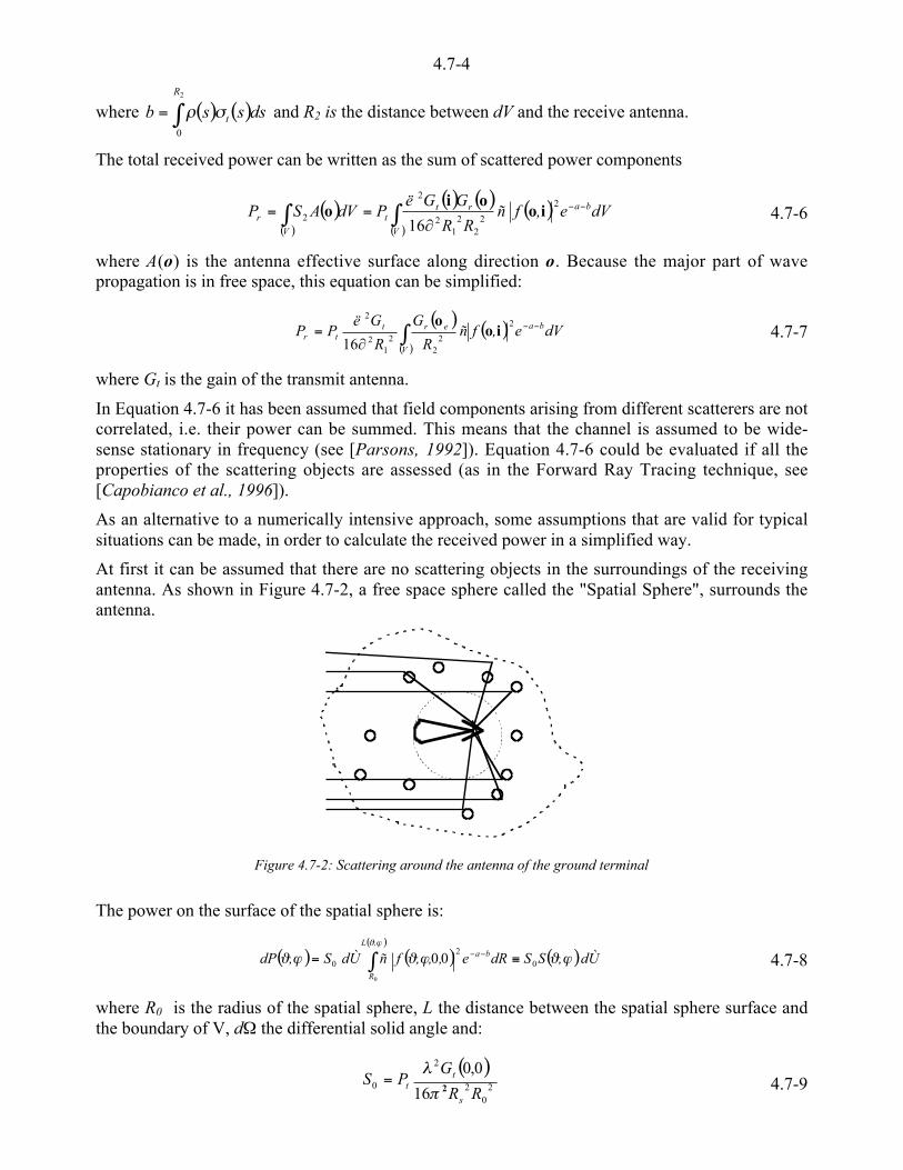
4.7-4

where ( ) ( )b s s dst

R

= 0 l m0

2

and R2 is the distance between dV and the receive antenna.

The total received power can be written as the sum of scattered power components

( )( )

( ) ( ) ( )( )

dVe,fñRR�

GGëPdVASP ba

V

rt

t

V

r<<00 ==

2

22

21

2

2

216

iooi

o 4.7-6

where A(o) is the antenna effective surface along direction o. Because the major part of wavepropagation is in free space, this equation can be simplified:

( ) ( )( )

dVe,fñR

G

R�

GëPP ba

V

ert

tr<<0=

2

22

21

2

2

16io

o4.7-7

where Gt is the gain of the transmit antenna.

In Equation 4.7-6 it has been assumed that field components arising from different scatterers are notcorrelated, i.e. their power can be summed. This means that the channel is assumed to be wide-sense stationary in frequency (see [Parsons, 1992]). Equation 4.7-6 could be evaluated if all theproperties of the scattering objects are assessed (as in the Forward Ray Tracing technique, see[Capobianco et al., 1996]).

As an alternative to a numerically intensive approach, some assumptions that are valid for typicalsituations can be made, in order to calculate the received power in a simplified way.

At first it can be assumed that there are no scattering objects in the surroundings of the receivingantenna. As shown in Figure 4.7-2, a free space sphere called the "Spatial Sphere", surrounds theantenna.

Figure 4.7-2: Scattering around the antenna of the ground terminal

The power on the surface of the spatial sphere is:

( ) ( )( )

( )dÙ,SSdRe,,,fñ dÙS,dP,L

R

ba  � � � �

0

2

0

0

00 >= 0 << 4.7-8

where R0 is the radius of the spatial sphere, L the distance between the spatial sphere surface andthe boundary of V, d1 the differential solid angle and:

( )2

02

2

016

0,0

RR

GPS

s

tt 2/

h= 4.7-9

4.7-5

It has been assumed that the direct ray arrives from the direction of the x axis (0,0) and the (�, )denotes the angle of observation.

According to Equation 4.7-8 the total received power is:

( ) ( ) � � � �/

/

/

dSGSP rr 0 0<

=2/

2/

2

0

0 d cos,, 4.7-10

with S(�, ) given in Equation 4.7-8. This equation shows that the ground terminal antenna gain inS-LOS links is considerably reduced with respect to free space propagation.

Equation 4.7-8 is valid if the spatial sphere is in the far field of the antenna. The far fieldassumption is valid in this case if h/2

0 aRR * , where Ra is the radius of the smallest sphere thatincludes the antenna, and the beam-width is approximated by LB /88,0 h� 5 (rad), where L is the

length of the aperture. Therefore the condition 20 /8,0 BR �h* must be satisfied. Assuming that in

reasonable cases 30 cm of free space can be assumed around the antenna the condition offB /1*� holds (e.g. at 12 GHz �B* 0.29 rad, that corresponds to L ) 9 cm). The head of the

communicating person was regarded as a part of the antenna.

For example, we can use the following model for field distribution (used in terrestrial mobile links):

( ) ( )/

�b �21

, =S 4.7-11

(i.e. azimuth omnidirectional distribution and zero elevation).

The antenna gain function can be expressed as:

( ) ( ) ( ) � � hGg,Gr = 4.7-12

where ( ) ( )0 02

2

2

0

cos/4�/

-��

�

ddhg�G=  �� � .

The resulting received power is:

( )0<

=2/

2/

0 d cos/2/

/

���gSPr 4.7-13

It is independent of azimuth characteristic, and the apparent gain is equal to that of anomnidirectional antenna in the azimuth.

Similarly, if the field is uniformly distributed in space, i.e. ( )S �   /, /= 1 4 , according to

Equation 4.7-10 the antenna apparent gain is unity.

In a further case the received power can be uniformly distributed over a solid angle 1.. Then theapparent gain can be approximated by:

{ }1= /4,min /GGap 4.7-14

Because the assumption of a uniform distribution along some solid angle of the fields is valid inmost of the cases under investigation, the use of a very directive antenna does not result in anincrease of the apparent gain.

The assessment of the correlation of the received fields of two spatially displaced antennas, that isl t i th ibl li ti f di it b f d b f th fi t d

4.7-6

( ) { }*.E 21 VVdB = 4.7-15

where V1 and V2 are the voltages on the load resistance of the antennas. V1 is proportional to theelectric field at r and V2 to that of r+d. E{x} is the expected value of the variable x, and * is thecomplex conjugate. It is assumed that the antennas are pointed to the same direction.

d

1

2

z

xy

d

1

2

z

xy

a) b)

Figure 4.7-3: Two-antenna arrangements for correlation - Identical (a) and different pointing (b)

The following approximations can be used:

( ) ( ) ( )( ) ( ) ( ) scatterer;,xRfxRf,xRf

,G,G,G

RRR

RRR

eeee �55

55

5

5<

21

2211

221

21

11

coscos

 � � �

 �

4.7-16

It is assumed that the satellite is on the x axis, i.e. ie= xe.

Then using Equations 4.7-15, 4.7-8 and 4.7-10:

( ) ( ) ( )B d S G S e djkd= 0004

�   �  /

�  , , cos cos 1 4.7-17

Note that B(d) is given by a Fourier-transform of the function G(�, )S(�, ).

The correlation could be evaluated numerically if G(�, ) and S(�, ) are known, but a simplifiedanalysis can be performed using the following assumptions:

S(�, ) is uniformly distributed over the solid angle 1, i.e. S(�, )=4//1, (�, )D1;

G(�, ) is constant over a narrow beam of solid angle 1B and zero outside this;

The beams are directed toward �0, with  0 coinciding with the centre of 1.

Assuming that the antenna pointing direction is contained in the (x, y) plane, the correlation is:

( )

( )

0 0

0 0+

<

+

<

+

<

+

<

<

= 2

2

2

2

2

2

2

2

sincoscos

0 0

0

0

0

0

0

0

0

0000

cos

cos4

/

/

/

/

/

/

/

/

.jkdjkd

B

B

B

B

B

B

B

B

dd

ddee

Ù�

SdB ��

��

  

  

��

��

  

  

   � 

� �

� �

4.7-18

If  0=//2 (antenna pointing perpendicular to the plane (y,z)):

4.7-7

( ) 1<1

=� BB

B

kd

kdSdB  

 

 /;

2/

2/sin40 4.7-19

In this case the correlation will be decreased if the distance between the antennas is increased, alsoif the antenna beam-width is increased (i.e. the antenna gain is lowered).

If  0 = 0 (i.e. the antennas are pointed in the direction parallel to axis y) then the correlationbecomes independent of the distance, d between antennas:

( )1

=/4

0SdBpar 4.7-20

If the directions of antenna pointing are different, in particular in the case of non-overlapping beams(see Figure 4.3-7b) the situation is completely different:

( ) ( ) ( ){ }( )

0 <<1= �

l � � � �,

22211102211 ,*,E,,,,L

R

ba

ö

dReVVdSddB 4.7-21

Where (�1, 1) and V2(�2, 2) indicate the pointing directions of the two antennas.

The expectation value in the previous equation is equal to zero assuming that the direct(unscattered) wave is strongly attenuated, the antenna beams do not overlap and considering that theelectromagnetic waves due to different scatterers are uncorrelated. Therefore the correlation value isalso zero.

The following conclusions can be drawn:

The received power is independent of antenna gain.

On the other hand the spatial correlation can be significantly affected by the gain ofantennas. Correlation is low if the antennas are pointed to different directions (anglediversity). An high correlation can be achieved, even if the antennas are far from each other,by using narrow beam antennas pointed in the same direction.

4.7.2 Polarisation effects

Effects of antenna polarisation are discussed in this paragraph making use of the Stokes parameters[Born and Wolf, 1964] (see also Chapter 2.5). The electric field of a plane wave propagating alongthe z direction can be represented using by the vector QT = (Q0, Q1, Q2, Q3)):

2203

222

1

sin2

cos2

yxyx

yxyx

EEä ; QEEQ

äEE; QEEQ

+==

=<=4.7-22

where, T means the transpose of the vector, Ex and Ey are the electromagnetic wave componentsalong directions x and y , b is the phase difference between the two components and

23

22

21

20 QQQQ ++= represents the intensity of the wave.

In the case of a partially polarised wave:

{ } { }{ } { }22

03

222

1

sin2

cos2

yxyx

yxyx

EE ; QäEEQ

äEE; QEEQ

EEEE

+==

=<=4.7-23

where 23

22

21

20 QQQQ ++* .

Th d f l i ti b h t i d b

4.7-8

GQ Q Q

Qp =+ +1

22

23

2

02

4.7-24

If the polarisation is completely random, Q1 = Q2 = Q3 = 0.

The effect of scattering on polarisation is described by a 4×4 Stokes-scattering-matrix mmmm:

is QóQ u= 4.7-25

where subscript i means the incident and s the scattered wave, see [Ishimaru, 1997].

The electromagnetic field obtained by the sum of two uncorrelated waves is characterised by thesum of the individual Stokes-vectors [Chandrashekar, 1960]. Therefore the state of polarisation ofthe received field on the spatial sphere (see Equation 4.7-8) is given by:

( )( )

dRdÙS,d i

,L

R

QóQ 0 u= �

 �0

0 4.7-26

where dQ represents the state of polarisation of the scattered wave, m the scattering matrix of thescatterer located at (R,�, ).Assuming that the antenna is an ideal polarisation filter and that theantenna polarisation is q, the antenna Stokes scattering matrix is (see Appendix A4.7.1):

Tqqó u=2

14.7-27

with q0=1.

The polarisation state of the output wave of this filter is equal to that of the filter, i.e. its Stokesvector is parallel to q. When the polarisation of the input wave is orthogonal to that of the filter thenthe amplitude of the output wave is zero. The received intensity is:

inT

outQ Qq u=21

0 4.7-28

The polarisation mismatch loss is:

0

0

in

outP Q

QL = 4.7-29

If the received wave is randomly polarised, the average polarisation loss becomes 3 dB.

The general expression of the loss due to polarisation mismatch between a polarised received fieldand the receive antenna is

( )rar a 2sin2sin2cos2cos2cos121

/1 ±+=pL 4.7-30

where   is the angle between the major axis of the polarisation ellipse of the input wave and thex axis, tan(a) is the axial ratio of the received field, and the sign in the last term is positive if thesenses of rotation of field and antenna are identical and negative if they are opposite. When theaxial ratios of the received filed and the antenna are identical and the two senses of rotation are thesame, then:

a2sin/11 2** pL 4.7-31

4.7-9

012cos2 ** pLa 4.7-32

In the case of non-ideal polarisation filters it can be shown that if the crosspolar isolation of apolarisation filter is Ip, then the Stokes scattering matrix of the antenna is:

´´¦

¥²²¤

£u+u= ��

T

p

T

Iqqqq

1

2

1m 4.7-33

where q� is the polarisation orthogonal to that of the antenna.

4.7.2.1 Distribution of the polarisation loss

To calculate the distribution of the polarisation mismatch loss it has been assumed that thepolarisation state of the received field is randomly distributed. Therefore the probability distributionof the state of polarisation on the Poincaré sphere is uniform:

( ) 4

122

�øã,p = 4.7-34

where tan(a), 22 �/ã ) , is the axial ratio of the polarisation ellipse and s, �ø 220 )) , is the

canting angle of the ellipse.

Due to the spherical symmetry, the polarisation mismatch loss distribution will be the same,whatever the polarisation vector of the receiver antenna is. So an antenna with a circularpolarisation has been assumed, ( )1001 ,,,T =q and:

( )a2sin121

/1 +=pL 4.7-35

Therefore the reciprocal loss, 1/Lp , is uniformly distributed over (0,1):

( ) ( )1,0 ;1/1 D= ttppL 4.7-36

In the case of a non-ideal polarisation filter, with a crosspolar isolation Ip, 1/Lp is uniformlydistributed between 1/Ip and 1.

When the received polarisation is linear with a random distribution of its orientation, thedistribution of the state of polarisation on the Poincaré sphere is:

( ) ( )ãä�

ã,p 221

22 =  4.7-37

When ( )0011 ,,,T =q , then the polarisation mismatch loss is ( ) 2cos121

1 +=p/L

Therefore the distribution of the polarisation mismatch loss becomes:

( )( )

( )101

111 ,;t

tt�tp

p/L D<

= 4.7-38

Details of the calculation are given in Appendix A4.7.2.

4.7-10

4.7.2.2 Error probability with (and without) polarisation diversity in a diffuse fadingchannel

The error probability, conditioned on the fading loss , Lf, and on the polarisation mismatch loss, Lp ,is a function of the symbol energy to noise power spectral density, E/N0:

( ) ´´¦

¥²²¤

£= ,...

L,

L;

NE

f,LLPpf

pfE

11

0

4.7-39

The total probability of error can then be determined assuming that the probability distribution of1/Lf is known and using the two cases of distribution of 1/Lp, discussed in the previous chapter.

As an example of the effect of random polarisation on error probability, a uniform distribution ofthe received state of polarisation, Rayleigh fading, additive white Gaussian noise and binary PSKmodulation are assumed.

The Rayleigh-fading term is used only as a designation. The actual signal energy is the sum ofsquares of four independent Gaussian random variables, (i.e. the real and imaginary parts of the -say - x and y components of the field) and is characterised by a Chi-square distribution with fourdegrees of freedom.

The expression for error probability for the case of matched polarisation is [Chandrashekar, 1960]:

2

3

16

3

1132

4

1

ZZ

Z

Z

ZPE 5´

´

¦

¥

²²

¤

£´¦

¥²¤

£+

++

<= 4.7-40

where the Z is the average bit energy to noise spectral density, and the approximation is valid forhigh Z.

Thus for random polarisation, assuming that the average power is equally distributed betweenorthogonal polarisations:

/ZZ/Z/Zdt

Zt/

Zt/dt

Zt/

Zt/PE

21

1

2

3

21

1

4

121

4

3

2

1

21

2

21

232

4

1 1

0

1

0

3

++

+++<=´

´

¦

¥

²²

¤

£´¦

¥²¤

£+

++

<= 0 0 4.7-41

For high values of Z:

ZPE 2/15 4.7-42

Similarly in the case of Rayleigh-fading and polarisation matching PE 51/4Z.

In the case of polarisation diversity there are two co-located antennas, with orthogonalpolarisations. The signal from the antenna with the higher output power is selected.

When polarisation diversity is employed then the reciprocal loss, 1/Lp, is uniformly distributed overthe range (0.5 - 1):

24

1

21

1

11

1

2

3

214

1

112

121

2

111

2

3

2

1

Z/Z/ZZ/Z/Z/Z/Z

EP 5´́

¦

¥²²¤

£

+<

++

+<

++´

¦

¥²¤

£+<+<= 4.7-43

The error probabilities are given in Figure 4.7-4.

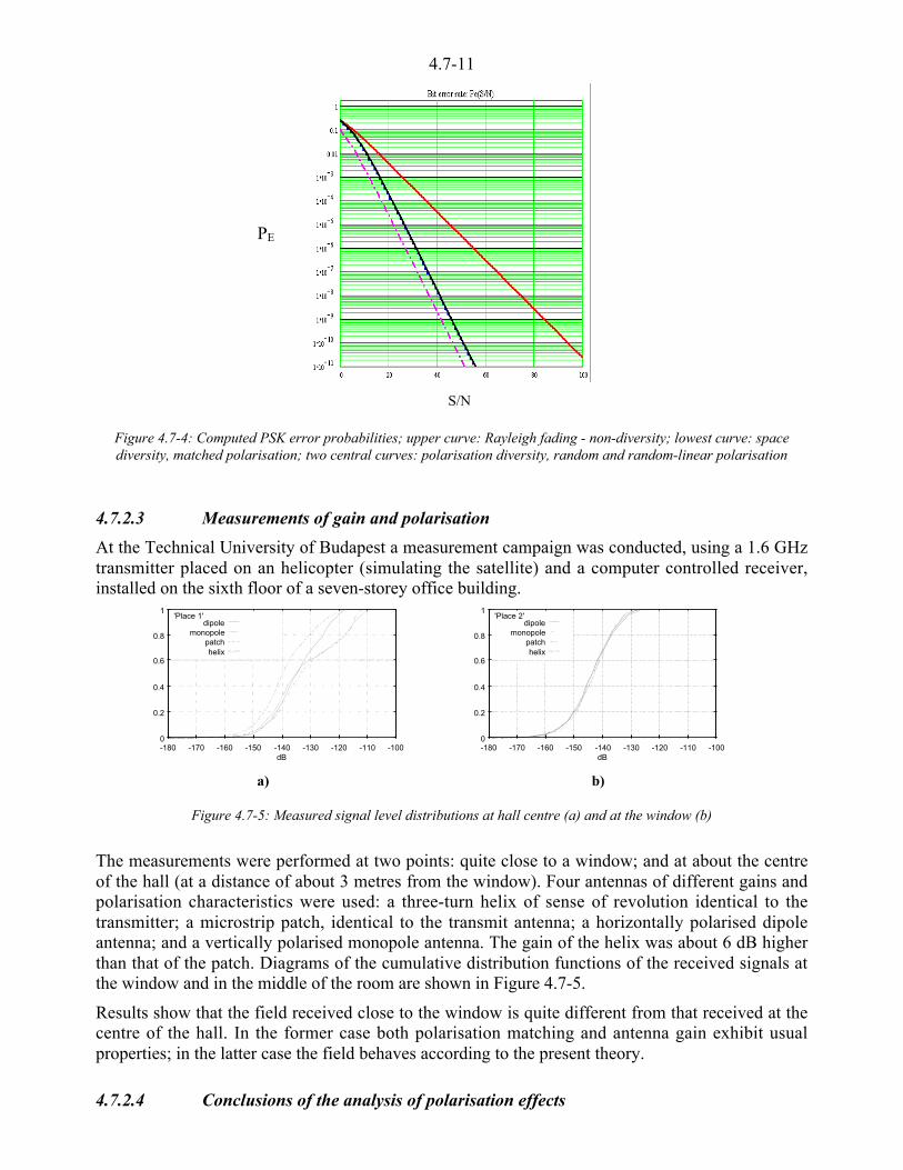
4.7-11

Figure 4.7-4: Computed PSK error probabilities; upper curve: Rayleigh fading - non-diversity; lowest curve: spacediversity, matched polarisation; two central curves: polarisation diversity, random and random-linear polarisation

4.7.2.3 Measurements of gain and polarisation

At the Technical University of Budapest a measurement campaign was conducted, using a 1.6 GHztransmitter placed on an helicopter (simulating the satellite) and a computer controlled receiver,installed on the sixth floor of a seven-storey office building.

0

0.2

0.4

0.6

0.8

1

-180 -170 -160 -150 -140 -130 -120 -110 -100dB

dipolemonopole

patchhelix

'Place 1'

0

0.2

0.4

0.6

0.8

1

-180 -170 -160 -150 -140 -130 -120 -110 -100dB

dipolemonopole

patchhelix

'Place 2'

a) b)

Figure 4.7-5: Measured signal level distributions at hall centre (a) and at the window (b)

The measurements were performed at two points: quite close to a window; and at about the centreof the hall (at a distance of about 3 metres from the window). Four antennas of different gains andpolarisation characteristics were used: a three-turn helix of sense of revolution identical to thetransmitter; a microstrip patch, identical to the transmit antenna; a horizontally polarised dipoleantenna; and a vertically polarised monopole antenna. The gain of the helix was about 6 dB higherthan that of the patch. Diagrams of the cumulative distribution functions of the received signals atthe window and in the middle of the room are shown in Figure 4.7-5.

Results show that the field received close to the window is quite different from that received at thecentre of the hall. In the former case both polarisation matching and antenna gain exhibit usualproperties; in the latter case the field behaves according to the present theory.

4.7.2.4 Conclusions of the analysis of polarisation effects

PE

S/N

4.7-12

Scattering can give rise to a received field that is randomly polarised. In this case theaverage mismatch loss is 3 dB, independent of the antenna polarisation.

In the case of random polarisation the polarisation mismatch loss is uniformly distributed.and the distribution of loss is computed for randomly directed linear polarisation.

The error probability can increase in the presence of random polarisation.

In the case of a received field that randomly polarised the polarisation diversity is aneffective technique to decrease the probability of error.

Measurements were in agreement with the theory.

4.7.3 Effect of antenna pattern on the radio channel

In this paragraph the effects of antenna pattern on propagation channel characteristics areinvestigated. The radio channel can be described by including the transmitter antenna, thepropagation channel and the receiver antenna [Steele, 1992]. The relationship is investigatedbetween the antenna pattern and the statistics of the received signal, with particular regard toDoppler spread and delay spread. The antenna patterns have an important impact on systemperformance, since a reduction of both the fading rate and the delayed echo power can be expectedwhen using a directional antenna.

The complex envelope of the signal at the output of the satellite mobile channel is:

( ) ( ) ( ) ( ) ( )[ ] ( ) ( )[ ] ( ) ( )[ ]tititriririic ,ö,öjtètôfjiri

iriritririrr .eetôtuta,ö.G,öGtz �q�q/�� ++<<=- 2

4.7-44

where Gr(eri, ri) and Gt(eri, ri) are the directive gains of receiver and transmitter antennas,qr(eri, ri) and qt(eri, ri) are the directive phases, u

r(t) is the complex envelope of the signal at the

input of the radio channel, ai(t), ei(t) and oi(t) are the amplitude, phase and delay effects of thepropagation channel and fc is the frequency of the carrier. This equation can be rewritten as:

( ) ( ) ( )-'

<=0

, ooo dtuthtz rr 4.7-45

where

( ) ( ) ( ) ( )[ ]{ }( )-

=

+<=oo

�o/ot

iicii

i

ttfjtawth 2exp, and ( ) ( ) ( ) ( )[ ]{ }- ++=i

tititririrtititririri jGGw q�qq�qq�q� ,,exp,,

Therefore the radiation patterns of the antennas can be taken into account by a suitable modificationof the propagation channel time-varying impulse responses.

4.7.3.1 Scattering functions

The scattering function used when simulating the propagation channel is [Steele, 1992]:

( )2

1

1,

´́¦

¥²²¤

£<

=

m

S

ii

io 4.7-46

where im is the maximum Doppler frequency and mii ) . This result can be derived theoretically

assuming that the model of field distribution described by Equation 4.7-11 is valid. In the case ofLEO satellite to mobile communications due to the fact that nearly all the scattering objects are

4.7-13

near the land mobile terminal, the contribution of the satellite motion to the total Doppler spreadcan be neglected [Frigies et al., 1999].

Under the hypothesis of uniform azimuthal distribution it has been shown by [Jakes, 1994] and[Gans, 1972] that the scattering function is:

( )( ) ( ) ( ) ( )[ ] ( ) ( ) ( ) ( )[ ]

2

22

1

,,,

´́¦

¥²²¤

£<

<<<<+=

mm

gpgp eeGpeeGpS

ii

i

___o____o_io 4.7-47

where ´́¦

¥²²¤

£=

mii

_ arccos , im is the maximum Doppler frequency, p(_,o) represents the power arriving

with angle _ and delay o and ( ) ( )[ ] pgp Lee 12 =__ accounts for the polarisation coupling.

If it is assumed that the vertically polarised components of the incident waves are uniformlydistributed with respect to azimuth angle _, the previous equation can be rewritten as:

( ) ( ) ( ) ( ) ( )2

1

,,,

´́¦

¥²²¤

£<

<<+=

mm

GpGpS

ii

i

_o__o_io 4.7-48

Table 4.7-41 gives the scattering functions for various types of antennas.

Antenna Gain Scattering function

vertically polarisedomni-directional

G(_) = A( )

2

1

2,

´́¦

¥²²¤

£<

=

mm

AS

ii

i

io

Vertical monopole G(_)=3/2( )

2

1

3,

´́¦

¥²²¤

£<

=

mm

S

ii

i

io

Vertical loop in aplane perpendicularto vehicle motion

G(_)=(3/2).sin2(_)( )

2

2

1

3

, ´́¦

¥²²¤

£<

´́¦

¥²²¤

£

=mm

mSii

i

ii

io

vertical loop in theplane of vehicle

motion

G(_))=(3/2)*cos2(_)) ( )2

2

1

3

,

´́¦

¥²²¤

£<

´́¦

¥²²¤

£

=

mm

mS

ii

i

ii

io

Table 4.7-1: Scattering functions of various types of antenna calculated under the assumptions of Equation 4.7-48.

4.7.3.2 Spatial distribution of scatters.

The assumption of uniform distribution of received power in the horizontal plane used in theprevious paragraph, could be invalid in some cases. [Lee, 1973] demonstrates that assuming thishypothesis would result in errors when characterising radio channels that include directionalreceiver antennas. On the other hand practical measurement of p(_,o) is difficult [Steele, 1992].

4.7-14

Considering that the scattering function contains information about the spatial distribution ofscatterers then the angular distribution of received power, p(_,o), can be derived fromEquation 4.7-48 if the directional pattern of the receiving antenna is known.

If the receiving antenna radiation pattern is symmetric about _= 0º, Equation 4.7-48 can berewritten as:

( ) ( ) ( )2

1

,2,

´́¦

¥²²¤

£<

=

mm

GpS

ii

i

_o_io 4.7-49

and the angular distribution of received power, p(_,o) is:

( )( )

( )2

1,2

1, ´́

¦

¥²²¤

£<=

mmS

Gp

ii

iio_

o_ 4.7-50

In the case of an omnidirectional antenna p(_,o) becomes:

( ) ( )2

1,21

, ´́¦

¥²²¤

£<=

mmSp

ii

iioo_ 4.7-51

The spatial distribution of the power incident calculated in this way can be used for the assessmentof the Scattering Function for the same environment and different antenna patterns.

The Power Delay Profile can obtained by integration of the Scattering Function

( ) ( )0'

'<

= iioo dSP , 4.7-52

4.7.4 Assessment of antenna noise temperature for handheld terminals

In this paragraph the ratio (G/T) between the antenna gain and the antenna noise temperature isanalysed. This is one of the factors that determines the link performance and is affected by variousparameters such as the antenna pattern, the spatial distribution of noise generating obstacles aroundthe handheld terminal and the interaction of the handheld with the user.

Techniques to counteract fading and interference on satellite links are difficult to implement inmobile terminals. Therefore the terminal G/T(e,q) parameter can be severely degradaded due to theincrease of the received noise from the environment and it is necessary to assess the G/T in differentsituations in order to select the most suitable antenna pattern to establish a high qualitycommunication. Moreover this is the only parameter that can be optimised after the satellite islaunched.

By means of this analysis the antenna radiation pattern can be optimised, subject to certainconstraints (e.g. size, construction etc), to satisfy the requirements for the radiation pattern.

The G/T is expressed in dB as:

)log(10),(),( AdBdB TGTG

u<=  e e 4.7-53

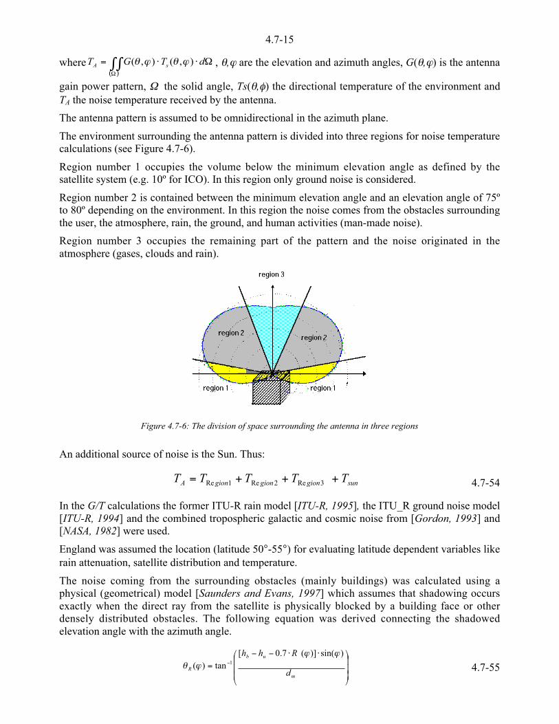
4.7-15

where( )0 01

1uu= dTGT sA ),(),(  e e , e,  are the elevation and azimuth angles, G(e, ) is the antenna

gain power pattern, 1 the solid angle, Ts(e,q) the directional temperature of the environment andTA the noise temperature received by the antenna.

The antenna pattern is assumed to be omnidirectional in the azimuth plane.

The environment surrounding the antenna pattern is divided into three regions for noise temperaturecalculations (see Figure 4.7-6).

Region number 1 occupies the volume below the minimum elevation angle as defined by thesatellite system (e.g. 10º for ICO). In this region only ground noise is considered.

Region number 2 is contained between the minimum elevation angle and an elevation angle of 75ºto 80º depending on the environment. In this region the noise comes from the obstacles surroundingthe user, the atmosphere, rain, the ground, and human activities (man-made noise).

Region number 3 occupies the remaining part of the pattern and the noise originated in theatmosphere (gases, clouds and rain).

Figure 4.7-6: The division of space surrounding the antenna in three regions

An additional source of noise is the Sun. Thus:

sungiongiongionA TTTTT +++= 3Re2Re1Re 4.7-54

In the G/T calculations the former ITU-R rain model [ITU-R, 1995], the ITU_R ground noise model[ITU-R, 1994] and the combined tropospheric galactic and cosmic noise from [Gordon, 1993] and[NASA, 1982] were used.

England was assumed the location (latitude 50°-55°) for evaluating latitude dependent variables likerain attenuation, satellite distribution and temperature.

The noise coming from the surrounding obstacles (mainly buildings) was calculated using aphysical (geometrical) model [Saunders and Evans, 1997] which assumes that shadowing occursexactly when the direct ray from the satellite is physically blocked by a building face or otherdensely distributed obstacles. The following equation was derived connecting the shadowedelevation angle with the azimuth angle.

´´´

¦

¥

²²²

¤

£ uu<<= <

m

ub

R d

Rhh )sin()](7.0[tan)( 1

   e 4.7-55

4.7-16

where ))(cos()sin(

)( e 

h 

u

u= md

R is the first Fresnel zone radius, dm the distance from the reference

obstacle face, hb is the building height and hu the user height.

In the noise temperature calculation a uniform maximum height was assumed, for calculationsimplicity, for all the buildings, but a more statistical or realistic distribution can also be used.

Region 1 is dominated by ground noise. In the case of flat terrain (minimum elevation angle notcompletely covered with obstacles) a contribution from rain and clear sky can also be added.

13211Re etcggggion TTTTT +++= 4.7-56

 ee/

e

ddT

PTi

ingi uu

1u= 0 0

I

2

0

)( 4.7-57

««ª

««©

¨

<=

5<<=

)<=

<)=

=

4

3

2

1

10ºfor K 10)4(

)10º( elev.angle.min0ºfor K 50)3(

º010º-for K 150)2(

º10for K 290)1(

e

e

e

e

i

i

i

i

Ti 4.7-58

 eeee

e/

ddTAT

PTme

sh

raincsnetc uu

1

+uu= 0 0

I

2

0

1

)()()()( 4.7-59

where i=1,2,3 and corresponds to one of the three first ground noise sub-regions, me is theminimum elevation angle (rad), sh is the non-shadowed angle below me (rad), Tetcj is the noisetemperature coming from the non dominating sources (K), Train(e ) and A(e ) are the rain noisetemperature and the rain attenuation respectively and Tcs(e ) is the clear sky noise temperature.

Region 2 is characterised by the presence of buildings. The part of the pattern illuminated by thebuildings receives their noise temperature (average air temperature for different latitudes) and thepart illuminated by the sky receives the clear sky noise temperature. Ground noise and man-madenoise are also present

2_2_2_1_12Re etccssidebsidecssidebsidegion TTTTTT ++++= 4.7-60

0 0 uu1

u=I

/  e

 e 0

)(

0

_

_

)(kR

ddT

PT buildnbsidek 4.7-61

0 0 uu1

uu=

I

/

 e

 eee

 0 )(

_

_

)()()(

hecs

ncssidek

kR

ddAT

PT 4.7-62

0 0 uuu1

+u=

I

/

 ee 2

0

_42 sin)(

hemademan

netc

me

ddTT

PT 4.7-63

where he is the highest elevation angle of Region 2 (ranging from 75º to 80º) and depends on themaximum elevation angle shadowed by the obstacle, Tbuild is the building temperature equal to themean temperature of the examined latitude, Tsidek(e) is the noise coming from the building face infront of and behind the user (side1, side2). (When the user stands in the middle of the street thenoise coming from each side is the same for buildings of the same height), Tsidek_b,Tsidek_cs arerespectively the noise from side k from the buildings and the sky e ( ) is calculated from

4.7-17

Finally in Region 3 the contribution is mainly due to the sky:

0 0I1

++u=

//

eeee

2

0

24

3Re

)()()()(

he

raincsngion

TTATPT 4.7-64

The last contribution to noise is due to the Sun at daytime and the Moon at night. The noisetemperature of the Moon can be neglected and the noise temperature of the Sun is:

)()5.0

(105.13

5 ee

ATdB

sun uuu= 4.7-65

where e3dB is the 3dB beamwidth of the receiving antenna, 1.5 105 K is the temperature of the Sun,0.5º the Sun’s angular diameter.

The evaluation of G/T has been done using three radiation patterns taken presented by [Agius et al.,1996a,b]. These patterns were selected because they represent three distinct but practical cases (seeFigure 4.7-7).

Pattern 0 is an isotropic pattern of gain 0 dBi. Pattern 1 has its maximum gain at 30º above thehorizon and has a small dip at its zenith. Pattern 2 has its maximum at zenith (almost hemisphericalpattern) and it is has the highest maximum gain of the four and finally Pattern 3 has its maximum at25º above the horizon, has a very distinctive dip at the zenith and the greatest backlobe of the three.

-4

-3

-2

0

1

2

3

4

-90

-60

-30 0

30 60 90 120

150

180

210

240

270

elevation angle [deg]

[dB

i]

pattern 0

pattern 2

patte

rn 3

pattern 1

Figure 4.7-7: The Gain patterns used in the G/T evaluation

Four different environments were initially used for evaluation. In Figure 4.7-8 the variation of theshadowed elevation angle is shown.

-10

0

10

20

30

40

50

60

70

80

-90 -60 -30 0 30 60 90 120 150 180 210 240 270

azimuth [deg]

elev

atio

n [d

eg]

heavy urban(A) urban (B) rural road (C) flat terrain (D)

(A)

(B)

(C)

(D)

(A)

(B)

(C)

(D)

Figure 4.7-8: Theoretical Blockage environments

Environment A describes a heavy urban situation with a street width of 18 m (5 cars 2 pavements

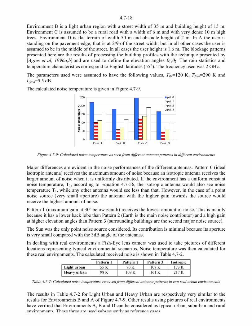
4.7-18

Environment B is a light urban region with a street width of 35 m and building height of 15 m.Environment C is assumed to be a rural road with a width of 6 m and with very dense 10 m hightrees. Environment D is flat terrain of width 50 m and obstacle height of 2 m. In A the user isstanding on the pavement edge, that is at 2/9 of the street width, but in all other cases the user isassumed to be in the middle of the street. In all cases the user height is 1.6 m. The blockage patternspresented here are the results of processing the building profiles with the technique presented by[Agius et al, 1996a,b] and are used to define the elevation angles e1,e2. The rain statistics andtemperature characteristics correspond to English latitudes (55°). The frequency used was 2 GHz.

The parameters used were assumed to have the following values, TRx=120 K, Tfeed=290 K andLfeed=5.5 dB.

The calculated noise temperature is given in Figure 4.7-9.

0

50

100

150

200

250

Envir. A Envir. B Envir. C Envir. D

No

iseT

emp

erat

ure

[K

]

pat. 0

pat. 1

pat. 2

pat. 3

Figure 4.7-9: Calculated noise temperature as seen from different antenna patterns in different environments

Major differences are evident in the noise performances of the different antennas. Pattern 0 (idealisotropic antenna) receives the maximum amount of noise because an isotropic antenna receives thelarger amount of noise when it is uniformly distributed. If the environment has a uniform constantnoise temperature, T1, according to Equation 4.7-56, the isotropic antenna would also see noisetemperature T1, while any other antenna would see less than that. However, in the case of a pointnoise source (very small aperture) the antenna with the higher gain towards the source wouldreceive the highest amount of noise.

Pattern 1 (maximum gain at 30º below zenith) receives the lowest amount of noise. This is mainlybecause it has a lower back lobe than Pattern 2 (Earth is the main noise contributor) and a high gainat higher elevation angles than Pattern 3 (surrounding buildings are the second major noise source).

The Sun was the only point noise source considered. Its contribution is minimal because its apertureis very small compared with the 3dB angle of the antennas.

In dealing with real environments a Fish-Eye lens camera was used to take pictures of differentlocations representing typical environmental scenarios. Noise temperature was then calculated forthese real environments. The calculated received noise is shown in Table 4.7-2.

Pattern 1 Pattern 2 Pattern 3 IsotropicLight urban 55 K 70 K 108 K 173 KHeavy urban 98 K 109 K 161 K 217 K

Table 4.7-2: Calculated noise temperature received from different antenna patterns in two real urban environments

The results in Table 4.7-2 for Light Urban and Heavy Urban are respectively very similar to theresults for Environments B and A of Figure 4.7-9. Other results using pictures of real environmentshave verified that Environments A, B and D can be considered as typical urban, suburban and ruralenvironments. These three are used subsequently as reference cases.

4.7-19

Noise measurements were also made. Measurement shows a good agreement with results inTable 4.7-2.

The calculated values of the G/T pattern could be used directly within a downlink budget to predictthe link performance for each satellite elevation angle. To this end the statistics of the satelliteelevation can be used to calculate the Effective Statistical G/T, GTeff:

eee/

dPGTGT SSeff uu= 0 )()(2

0

4.7-66

where GT(e) is the calculated G/T pattern, PSS(e) is the percentage of time that a satellite stays at aparticular elevation angle for different latitudes, assuming a uniform distribution of satellites inazimuth with respect to the environment.

The G Teff depends on all relevant parameters, including the satellite system, the user, thepropagation environment and the antenna itself. The same approach can be used to calculate theGTeff for the first (highest) and the second (next highest) satellites by using the relevant distributionof elevation angle PSS(e).

4.7-20

4.7.5 References

[Agius et al., 1996a]Agius A.A., M. Mahmoud, R. Tafazolli and B.G. Evans, “Quadrifilar helical Antenna (QHA) -Characteristics of a proposed wire antenna for a SPCN handheld terminal”, International Workshopon Mobile Communications, Thessaloniki, Greece, 19-21 September 1996

[Agius et al., 1996b]Agius A.A., M. Mahmoud, R. Tafazolli and B.G. Evans,“Quadrifilar Helical Antenna for HandheldTerminal in Satellite Personal Communication Networks (SPCN)” 5th ICSSMCN, IEE ConferencePublication No. 424, pp.76-79, London,13-15 May 1996

[Born and Wolf, 1964]Born M and E.Wolf, Principles of optics, Macmillan, New York, 1964.

[Capobianco et al., 1996]Capobianco F., J. Constantin, I. Frigyes, S: Jones: Modelling of the microcell channel - preliminaryresults, IEE Conf. on Wave Propagation, London, UK, 17 Oct. 1996

[Chandrashekar, 1960]Chandrashekar S., Radiative transfer, London etc., Oxford Univ. Press, 1960

[Frigyes et al., 1999]Frigyes I., B. Molnar, R. Vallet, Z. Herczku, Z. Bodnar, “Doppler spread characteristics of LEOsatellite to mobile channels”, Int, J. Sat. Comm., Vol 19, No 3, May-June 2001, pp 251-262.

[Gans, 1972]Gans, M. J, “A Power-Spectral Theory of Propagation in the Mobile-Radio Enviroment”, IEEETrans. on VT, vol. VT-21. Feb, 1972.

[Gordon, 1993]G.D. Gordon and W.L.Morgan, Principles of Communications Satellites, New York, 1993

[ITU-R, 1994]ITU-R, Recommendation 372-6, ”Radio Noise”, Propagation in Non-Ionized Media, Geneva, 1994

[ITU-R, 1995]ITU-R, Recommendation 618-4, “Propagation data and prediction methods required for the designof Earth-space telecommunication systems”, Propagation in Non-Ionized Media, Geneva, 1995

[Ishimaru, 1997]Ishimaru A., Wave propagation and scattering in random media, IEEE press, 1997

[Jakes, 1994]Jakes W.C., Microwave Mobile Communications, IEEE Press, 1994.

[Lee, 1973]Lee, W. C. Y, “Finding the Aproximate Angular Probability Density Function of Wave Arrival byUsing a Directional Antenna”, IEEE Trans. on AP, vol. AP-21. May, 1973.

[Parsons, 1992]Parsons D., Mobile Radio Propagation Channel, Pentech Press London, ISBN: 0-7273-1316-9,1996.[Saunders and Evans, 1997]Saunders S.R., Evans B.G., “A Physical-Statistical Model for Land Mobile Satellite Propagation inBuilt-up Areas”, ICAP ‘97, Heriot-Watt University, Edinburgh, UK, 14-18 April, 1997.

[Steele, 1992]Steele R Mobile Radio Communications Pentech Press London 1992

4.7-21

4.7.6 Appendix 1 to Chapter 4.7: Stokes Matrix of a polarisation filter

The output wave of the ideal polarisation filter must be in polarisation state q - whatever thepolarisation state Q of the input wave is. This is only possible if mmmm is expressed in dyadic form:

Tiu= qó A4.7.1-1

therefore

qQqóQ cT =u= i A4.7.1-2

Where c can determined considering that if Q=q then the output wave is unaltered, while if Q=q�,0=u �

Tqq then the output is zero:

q21=i A4.7.1-3

4.7-22

4.7.7 Appendix 2 to Chapter 4.7: Loss distribution with random polarisation

Under the assumption of Equation 4.7 34 and assuming ( )1001 ,,,T =q , the cumulative distributionfunction of the reciprocal polarisation mismatch loss is:

{ } ( ) ( ) ( )ãdããd�

t/L�ã

�/

p 2sin12

1222sin

4

11Pr

2

0

2

2

+==< 00<

  A4.7.2-1

But according to Equation 4.7-35 this is equal to 1/Lp, i.e. the distribution is uniform.

On the other hand using Equation 4.7-37 marginal distribution of 2  is uniform; and the appropriatetransformation has to be made on that random variable. Standard techniques lead toEquation 4.7-38.

PART 5 Systems and Simulation Issues

5.1-1

CHAPTER 5.1Service Requirements and Performance

Criteria

Editor: Marcel Pettinger1

Authors: Marcel Pettinger1, Peter Watson2, Simon Saunders3, Misha Filip4

1 SES-Astra, L-6815 Château de Betzdorf, Luxembourg

Tel.: +352-710-725-268, Fax: +352-710-725-9305, e-mail: Marcel_Pettinger@ses-astra.com2 University of Bath

Tel.: +44-1225-826330, Fax.: +44-1225-826412 , e-mail: P.A.Watson@bath.ac.uk3 University of Surrey, Centre for Communication Systems Research

Tel.: +44-1483-259-806 , Fax.: +44-1483-259-504 , e-mail: S.Saunders@ee.surrey.ac.uk4 University of Portsmouth Dept of E&E Engineering Anlgesea Road Portsmouth PO1 3DJ UK

5.1-2

5.1 Service Requirements and Performance Criteria

This chapter describes the service oriented application of propagation models for predicting theimpact of the atmosphere on the Earth-space link.

Service or system requirements and relevant criteria for a specified performance are defined andlink budgets established. Practical ways to overcome propagation impairments by using fademitigation techniques are also included. All these factors are then put together and various test casesare solved using the previously described models.

5.1.1 Generic Service Classifications

In the era of integrated service provision, no matter what the delivery medium of the service, it hasbecome common practice to refer to a set of generic service categories. Those categories can beused to define and distinguish user services, whether or not these are delivered over satellite orcable, or in the context of fixed or mobile systems.

The importance of such a “top-down” approach to user service classification is well illustrated bythe convergence of broadcast and VSAT type systems in their capability of addressing a similarsubset of these services.

The classification of user services given in Table 5.1-1 was developed in the context of RACEProject 1006 in the context of broadband services.

5.1.2 System Requirements

This chapter describes a number of systems with different applications and specific sets ofcharacteristics, and their requirements in terms of quality and availability.

5.1.2.1 VSATs

Very Small Aperture Terminals (VSATs) are designed for data transmission and distribution over awide geographical area amongst a large number of locations. Typical examples are stock exchangeinformation and transactions, bookmaker odds making and race data, supermarket price and stockinformation, company internal correspondence etc.

VSATs cannot support satellite links with large capacities, but they are cheap and easy to install andthus within the financial capabilities of small companies. They can be used to rapidly set up smallcapacity satellite links in a flexible way. Capacities are normally of the order of a few tens of kbit/s,but can reach up to few hundred kbit/s.

A VSAT network, usually involves a central hub station with an antenna of larger diameter(typically 4 to 11 m) and a more powerful amplifier. The hub usually houses a central hostcomputer, which can act as a data switching centre. The architecture of the network naturallybecomes star shaped, [Maral, 1995]. The links from the hub to the VSAT are called outbound links.The links from the VSAT to the hub are called inbound links. Both inbound and outbound linksconsist of two partss, uplink and downlink. It is not unusual that inbound and outbound linksoperate at different transmission speeds, i.e. in asymmetrical mode.

5.1-3

BASIC SERVICE QUALITYCLASS

TYPICAL USER SERVICES

GENERICSERVICE CLASS

INFO. CLASS

AUDIO STANDARDor

HI FI

Telephony

Audioconference

VIDEO SUBSTANDARDor

STANDARDor

EXTENDEDor

HDTV

Video-telephony

Videotelephone conference

Surveillance

Educational Service

DIALOGUESERVICES

DATA (DATA) - Data processingComputer aided design & manufacturingReal-time controlTelemetryInteractive games/amusement libraryHome bankingComputer assisted teachingTeleworking (or Home Office)Alarm Systems

AUDIO STANDARDor

HI FIVoice Messaging

VIDEO STANDARDor

EXTENDEDor

HDTV

Business video mail (e.g. advertising spots)

Personal video mail (e.g. short own madefilms)

DATA (DATA) - Computer program downloadingFile transferCAD/CAMElectronic funds transferTeleworking (or Home Office)

TEXT TeletexIMAGE Telefax

MESSAGINGSERVICES

DATA(DOCUMENT)

MIXED MODESTANDARD

orHI QUALITY

Business electronic mail

Electronic newspapers & magazinesAdvertising mailTeleworking (or Home Office)

Table 5.1-1: Summary service classification (continued on next page)

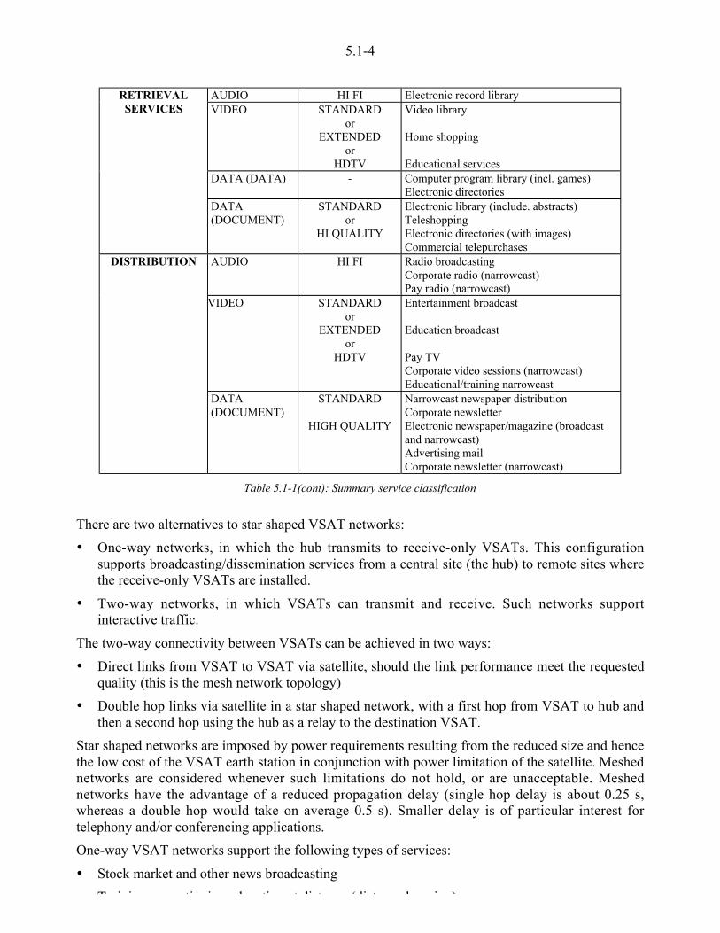
5.1-4

AUDIO HI FI Electronic record libraryVIDEO STANDARD

orEXTENDED

orHDTV

Video library

Home shopping

Educational servicesDATA (DATA) - Computer program library (incl. games)

Electronic directories

RETRIEVALSERVICES

DATA(DOCUMENT)

STANDARDor

HI QUALITY

Electronic library (include. abstracts)TeleshoppingElectronic directories (with images)Commercial telepurchases

AUDIO HI FI Radio broadcastingCorporate radio (narrowcast)Pay radio (narrowcast)

VIDEO STANDARDor

EXTENDEDor

HDTV

Entertainment broadcast

Education broadcast

Pay TVCorporate video sessions (narrowcast)Educational/training narrowcast

DISTRIBUTION

DATA(DOCUMENT)

STANDARD

HIGH QUALITY

Narrowcast newspaper distributionCorporate newsletterElectronic newspaper/magazine (broadcastand narrowcast)Advertising mailCorporate newsletter (narrowcast)

Table 5.1-1(cont): Summary service classification

There are two alternatives to star shaped VSAT networks:

• One-way networks, in which the hub transmits to receive-only VSATs. This configurationsupports broadcasting/dissemination services from a central site (the hub) to remote sites wherethe receive-only VSATs are installed.

• Two-way networks, in which VSATs can transmit and receive. Such networks supportinteractive traffic.

The two-way connectivity between VSATs can be achieved in two ways:

• Direct links from VSAT to VSAT via satellite, should the link performance meet the requestedquality (this is the mesh network topology)

• Double hop links via satellite in a star shaped network, with a first hop from VSAT to hub andthen a second hop using the hub as a relay to the destination VSAT.

Star shaped networks are imposed by power requirements resulting from the reduced size and hencethe low cost of the VSAT earth station in conjunction with power limitation of the satellite. Meshednetworks are considered whenever such limitations do not hold, or are unacceptable. Meshednetworks have the advantage of a reduced propagation delay (single hop delay is about 0.25 s,whereas a double hop would take on average 0.5 s). Smaller delay is of particular interest fortelephony and/or conferencing applications.

One-way VSAT networks support the following types of services:

• Stock market and other news broadcasting

• T i i ti i d ti t di t (di t l i )

5.1-5

• Updates of market related data, news and catalogue prices

• Distribution of video or TV programmes

• Distribution of music in stores and public areas

• Relaying of advertising to electronic signs in retail stores

Two-way networks support:

• Interactive computer transactions

• Low rate video conferencing; satellite news gathering (SNG)

• Database enquiries, E-mail

• Bank transactions, automatic teller machines

• Reservation systems; sales monitoring and stock control

• Distributed remote process control and telemetry; medical data transfer

• Voice communications

• Emergency services

Most of the two-way services deal with interactive data traffic, where the user terminals are mostoften personal computers. The most notable exceptions are voice communications and SNG.

Depending on the service the traffic flow between the hub and the VSATs may have differentcharacteristics and requirements:

Data transfer or broadcasting which belongs to the category of one-way services, typically displaysfile transfers of 1 to 100 MBytes of data. This kind of service is not delay sensitive, but requires ahigh integrity of the data which are transferred.

Interactive data is a two-way service corresponding to several transactions per minute and perterminal of single packets 50 to 250 Bytes long on both inbound and outbound links. The requiredresponse times are typically a few seconds.

Enquiry/response is a two-way service corresponding to several transactions per minute andterminal. Inbound packets (typically 30 to 100 Bytes) are shorter than outbound packets (typically500 to 2000 Bytes). The required response time is typically a few seconds.

Supervisory control and data acquisition (SCADA) is a two-way service corresponding to onetransaction per second or minute per terminal. Inbound packets (typically 100 Bytes) are longerthan outbound packets (typically 10 Bytes). The required response time ranges from a few secondsto a few minutes. What is most important is the high data security level, and the low powerconsumption of the terminal.

Each communication service demands certain features of its delivery system in terms of:

• connectivity

• connection delay

• transmission delay

• link quality

• transmission capacity

The degree of connectivity determines whether the service is private, semi-private or public.Connection delay depends on the service. For example, a voice connection could be allowed alonger call set up delay than say a datagram service. Excessive transmission delay can affect a real-

5.1-6

quality may not be so critical for a real time service with a high redundancy alphabet (speech) but ismore critical for a funds transfer service. Transmission capacity is a function of the sourceinformation encoding process and the efficiency in being able to decode at the sink. Transmissioncapacity requirements are also dependent on the cost of the transmission media.

Response time is defined as the time elapsed between emission of speech and reception of the othertalker’s response in case of voice telephony communications, or time elapsed between transmissionof an enquiry message initiated on a transmitting computer and the appearance of the first characterof the response message on the receiving computer screen.

Response time for data transfer builds up from several components:

• queuing time at the transmitting side as a result of possible delay for capacity reservation beforetransmission occurs;

• time for transmission of the emitted message which depends on the length of the message andthe transmission bit rate;

• propagation time which occurs on the forward and return links;

• processing time of the enquiry message at the receiver, and time necessary for generating andtransmitting the response;

• protocol induced delay, as a result of error recovery and flow control between the transmittingand receiving sides.

The VSAT network is only responsible for the routing delay which includes propagation delay andprocessing delay as a result of protocol handshake between VSATs and hub front end processor, butexcludes the processing delay of the data terminal equipment.

A VSAT network user is only concerned by the baseband link quality, which is stipulated either insignal power to noise power ratio, S/N, for analogue signals, or in Bit Error Rate (BER) for digitalsignals.

For analogue television, a typical S/N objective is 50 dB. This ensures recovery of a signal with aquality suitable for subsequent terrestrial broadcasting or cable distribution. For digitaltransmission, a typical BER objective is 10-7. This objective guarantees an acceptable quality forvoice or video communications. For data communications, the bit error rate is not a significantparameter, as the transmission can be made error-free due to the retransmission protocols that areusually implemented between end-to-end terminals. However, the bit error rate influences thenumber of required retransmissions, hence influences the delay.

In general terms, availability is defined as the ratio of the time a unit is functioning , to the totaltime of usage. Network link availability is the percentage of time the service is delivered at a givensite with the requested quality (BER less than specified value; response time within specifiedlimits). Network availability builds upon equipment reliability, propagation impairments, and Suntransit outage.

More precisely, network availability can be expressed as Anet = ATxAsatAlinkARx where ATx is thetransmitting earth station availability, Asat the space segment availability, Alink the link availability,and ARx the receiving station availability. Table 5.1-2 gives some typical equipment availabilityfigures.

Remote VSAT Space Segment Link Hub NetworkEquipmentAvailability [%] 99.9 99.95 99.9 99.999 99.7

Table 5.1-2: Typical figures for availability, [Maral, 1995]

An availability of 99 7 % corresponds to a cumulative down time of 26 hours per year However it

5.1-7

Should the service interruption be caused by equipment failure, an appropriate maintenanceprocedure should be implemented to restore the service within the requested time. This isparticularly crucial for the hub station, as its outage affects the whole star network. Shouldpropagation impairments be responsible for the service interruption, then site diversity can beconsidered. Finally, back-up terrestrial connection may be a means to achieve service continuity.

5.1.2.2 DVB-based Multimedia System at the Ku-Band

In the following, a system description and performance quality are given for a DVB (Digital VideoBroadcasting) based system operating at Ku-band to provide PC-based Internet and databroadcasting services via satellite.

The traffic for multimedia applications on the Internet is mainly asymmetric: almost all browsingtraffic involves much more data moving from the server to the end-user than in the oppositedirection, especially for video or audio applications. This system is thus asymmetric and takesadvantage of TV broadcasting techniques for the forward link; the return link may use a telephoneline/modem.

There are two components to this system; the uplink site, where the base station operates as a DVBbroadcaster and as a satellite gateway operator and the downlink site, where the end-users PCsreceive the Internet and data broadcaster services.

The base station consists of a DVB uplink and a satellite router/server, which are directlyinterconnected with a DVB gateway. It performs basic server tasks and delivers IP datagramsencapsulated in an MPEG-2 data structure. The DVB uplink performs all necessary multiplexing,coding and modulation tasks for transmitting data over a direct broadcast satellite, at a data rate upto 40 Mbit/s.

The user equipment consists of a small satellite dish (whose size depends on the location of thedownlink site, for instance 60 cm over western Europe) and a DVB PC-board for processing theincoming satellite data. A standard World Wide Web (WWW) browser with any necessary plug-insis used for interaction with the system.

The DVB PC board performs demodulation, decoding and demultiplexing, reconstructs IPdatagrams from the cells and routes internally to the appropriate applications. The end-user stationscan access the base station in a number of ways, for instance a telephone line/modem.

Satellite Internet access can support the following applications:

• High-speed Internet access: data are requested via the return link and retrieved over the satellitelink at, for example, 2 Mbit/s

• On-demand services: transmission of the request on the return link and data are retrieved overthe satellite link

• Data broadcasting: data are filtered by the multicast or broadcast services from the local harddisk and no return link is therefore required

• Intranet/Extranet: data are requested via the return link and retrieved over the satellite link, ordata are pushed to the end-user PC.

Since the system uses DVB, it ensures “Quasi Error Free” (QEF) operation with approximately oneuncorrected error event per transmission hour; the corresponding BER ranges between 10–10 and10–11 at the input of the MPEG-2 multiplexer. The nominal availability of the system is 99.7% ofthe year.

5.1-8

5.1.2.3 Multimedia GSO/NGSO Configurations

In addition to the VSAT system and the DVB Multimedia requirement presented before, a few othertypes of multimedia consumer networks are considered here. These kinds of systems will benefitfrom propagation prediction methods which take the specific choice of frequencies and operationalparameters into consideration. The technical background for the systems in question is similar tothat for VSATs, but one major difference could be that these small multimedia earth stations for theconsumer are planned to be sold like GSM hand-held terminals, not needing an individualtransmission licence.

This is a star-type network with both incoming and outgoing traffic. In the outgoing direction (fromthe hub to the consumer), the normal Ku-band Direct-To-Home bands are used: 12.75-13.25 GHz,13.75-14.50 GHz, and 17.30-18.10 GHz for the uplink and 10.70-12.75 GHz for the downlink.

In the return direction, from the consumer to the hub, a 80 or 120 MHz channel at Ka-band is usedwith 29.50-30.00 GHz for the uplink and 18.30-18.80 GHz for the downlink to the hub.

The services envisaged for the system include:

• General data gathering for e.g. enterprises with many branch offices, affiliates, businessassociations or employees working at home, including store & forward and transfer of trafficinto terrestrial infrastructure

• Feederlink for data content, including real time (High-Speed Internet and IP Multicast) and non-real time (file transfer) applications

• Live interactions (e.g. requests, votes, still images and low quality video, video conferences) forremote learning/training applications.

The forward path of the digital system is based on MPEG transmissions, using relevant ETSI, DVBand DAVIC standards, and also the return path uses digital standards, so that Internet Protocol andAsynchronous Transfer Mode (ATM) can be used on the network. The range of applications thatneed to be supported require a flexible standard, ensuring QEF transmission (equivalent to a biterror rate on the satellite link not exceeding 10-10, while the link is considered available).

The hub station will use an antenna with a diameter of 6 to 9 m, possibly with site diversity. Theconsumer Satellite Interactive Terminal (SIT) consists of an Outdoor Unit (ODU) with an antennadiameter of 0.6-1.2 m. The SIT also contains an Indoor Unit (IDU), functioning like a modem,attached to a User Device, which can be a PC or a TV set.

Maximum transmission power at around 29.7 GHz will be 0.5 W for the small 60 cm antenna, and2 W with the 1.2 m antenna. The polarisation is linear, with polarisation re-use in a total of 8 uplinkbeams covering Western and Central Europe on the first satellite (ASTRA-1H). A ‘receive beforetransmit’ procedure will be inherent in the SIT. The maximum user data rate will be 144 kbit/s to2 Mbit/s.

The BER on the satellite link should not exceed 10-10 for it to be considered available. The designguideline for the return link availability is better than 99.5 % of an average year.

5.1.2.4 Future Geostationary Ka/Ka-Band Consumer Systems

While the system described above is already being built, future systems operating exclusively at20/30 GHz are under consideration by many operators. The most likely bands for GSO Ka-bandconsumer systems are 27.5–28.6 GHz and 29.1–30.0 GHz for the Uplink and 18.3–18.8 GHz,19.3-20.2 GHz and 21.4–22.0 GHz for the downlink.

In these bands, one-way star-type networks from hub to consumer are likely to appear, but also two-way systems. These may either be via the hub in both directions, but could also be for direct

5.1-9

It is most likely that due to propagation factors, these Ka-band networks will not be based on highreliability, and therefore reliable propagation predictions valid for time percentages around 99.0 to99.9 % of a year would serve this purpose.

5.1.2.5 Particular Considerations for Non-Geostationary Systems

Non-Geostationary (NGSO) networks are now being planned with consumer terminals in the range10.7–30.0 GHz. Users will not only be mobile, but more typically with antennas mounted on or nearhouses. A constant link with a satellite in a NGSO constellation is maintained by the antenna, whichfollows the moving satellite and typically every few minutes switches to another satellite. Thisraises a particular question on fade dynamics in NGSO systems, when disregarding the mobile use.The fade dynamics in such NGSO systems will not be determined by the movement of the rain cellrelative to the Earth, but rather by the beam movement across the rain cell, when following asatellite. A model for fade duration/interval or fade slope under these circumstances would be ofparticular interest.

Also the normal use of elevation angles near 90° will be new in Europe, and it may necessitatemodifications to the existing ITU-R propagation model, which is based on static conditions andelevation angles in Europe typically below 40°.

5.1.3 Performance Objectives and Evaluation

For radio-relay system planners it is of vital importance to have outage prediction methods at handin order to optimise each hop, technically and economically, according to a requested transmissionquality. According to ITU-T, each direction of a path can be in one of two states, available time orunavailable time. Error and availability performance objectives are specified and measured foravailable time. A bi-directional path is in the unavailable state if either or both directions are in theunavailable state.

Error performance objectives of an international digital connection operating at a bit rate belowthe primary rate 2.048 (1.544) Mbit/s and forming part of an ISDN, are given in ITU-T Rec.G.821.

The error performance objectives in this recommendation are stated for each direction of aN x 64 kbit/s connection (1 ) N < 32 (24)) independent of the transmission medium. Prior to theapproval of ITU-T Rec. G.826, real digital radio-relay links forming part of the high-, medium- andlocal grade portion within an ISDN were designed by applying the error performance objectives forconnections at a bit rate below the primary rate, directly at the system bit rate. Translation ruleshave been used to normalise error performance measurements obtained at the system bit rate to the64 kbit/s level.

The following error performance events are defined:

• Errored Second (ES): a one second period in which one or more bits are in error

• Severely Errored Second (SES): a one-second period which has a bit-error ratio> 10–3.

The following error performance parameters are defined:

• Errored Second Ratio (ESR): the ratio of ES to total seconds in available time during a fixedmeasurement interval

• Severely Errored Second Ratio (SESR): the ratio of SES to total seconds in available timeduring a fixed measurement interval.

Error performance parameters and objectives for international, constant bit-rate digital paths at orabove the primary rate 2.048 (1.544) Mbit/s, are given in Rec. G.826. The recommendation is

5.1-10

reference path (HRP). It applies as well for PDH, SDH and ATM-network. It is also independent ofthe transmission medium. One big difference between G.821 and G.826 is that in G.826 theparameters are based on errored blocks and not on errored bits. A block is a set of consecutive bitsassociated with the path.

The parameters defined in G.826 are based on the following events:

• Errored Block (EB): a block in which one or more bits are in error

• Errored Second (ES): a one second period with one or more errored blocks

• Severely Errored Second (SES): a one-second period, which contains 30 % errored blocks or atleast one defect. SES is a subset of ES

• Background Block Error (BBE): an errored block not occurring as part of an SES.

The following error performance parameters are defined:

• Errored Second Ratio (ESR): the ratio of ES to total seconds in available time during a fixedmeasurement interval

• Severely Errored Second Ratio (SESR): the ratio of SES to total seconds in available timeduring a fixed measurement interval

• Background Block Error Ratio (BBER): the ratio of BBE to total blocks in available time duringa fixed measurement interval. The count of total blocks excludes all blocks during SESs.

The path fails to meet the error performance requirements if any of the objectives is not met.

The end-to-end objectives are divided into one national portion and one international portion. Forterrestrial systems, the national portion is subdivided into three basic sections: Long haul-, Shorthaul- and Access network sections. The Long haul section shall make use of the distance basedallocation and part of the fixed block allocation. The Short haul section shall make use only of thefixed block allocation contribution. The Access section shall make use only of the fixed blockallocation contribution.

Availability parameters and objectives for path elements of international constant bit-rate digitalpaths at or above the primary rate are given in ITU-T Rec. G.827. The recommendation isapplicable to digital paths based on PDH, SDH and some other cell-based (ATM) transportnetworks.

Performance objectives are given for two availability performance parameters, availability ratio andmean time between digital path outage:

• Availability ratio (AR): the ratio of time that a path element is in the available state to total timeduring an observation period. The converse of AR, the unavailability ratio, UR, is defined asUR = 1 - AR

• Mean time between digital path outages (Mo): the average duration of any continuous intervalduring which the digital path portion is available.

In the fixed-satellite service availability objectives are given in ITU-R Rec. S.579 for a satelliteHRDP used for telephony and using pulse-code modulation (PCM) or as part of an ISDNhypothetical reference connection. This Recommendation specifies unavailability due to bothequipment and propagation. Unavailability due to equipment should be not more than 0.2 % of ayear. Unavailability due to propagation should be not more than 0.2 % of any month, whichcorresponds to 0.04 % of any year with a conversion factor of 5.

Prior to the approval of ITU-T Rec. G.826 and ITU-R Recommendations. F.1189 and F.1092, realdigital radio-relay links forming part of an ISDN were designed by applying the error performanceobjectives of G 821 and related ITU R Recs directly at the system bit rate As a consequence

5.1-11

system bit rate to 64 kbit/s level and all outage predictions were made for a BER equal to 10-3

which defines a SES event in G.821.

5.1.4 Quality and Availability in Mobile Satellite Systems

Operators of mobile satellite systems need to calculate power link budget margins to guarantee acertain degree of coverage. In these systems power is a valuable resource, and the link marginshould be as small as possible while still obtaining the required availability. Practical experienceindicates that the traditional method of calculating the link margins directly from the channelcumulative density functions is a too pessimistic approach, the link budgets contain unnecessarypower margins. Another problem often encountered results from applying availability and qualitytime requirements as defined for terrestrial cable systems, to mobile satellite systems, as addressedin ITU-R Question 112/8.

The traditional method of calculating fade margins has been to use the channel fade depth at a givenpercentage of distance or time. There are other approaches where the benchmark is the systemperformance, e.g. in our case the bit error rate, and not solely the channel fluctuations due tomultipath.

The average bit error rate method to calculate the necessary fade margin results in decreased fademargin compared to the traditional method. The key point is to note the different parameters used,that is purely fade statistics or average bit error rate. An additional quality parameter, which couldbe applied, is the instantaneous bit error rate. This approach turns out to be exactly the same as thetraditional method of fade margin calculations based purely on the channel statistics when theavailability required is A=100%. The two approaches can be merged into a combined methodtaking into account both average and instantaneous bit error probability when the system isavailable.

The instantaneous bit error rate shall typically exceed 10-3 during less than I % of the time (forinstance I = 99%) during the time when the average bit error rate requirement is fulfilled. Thepercentage I depends on the application’s sensitivity to error bursts and could be a quality of serviceparameter negotiated at connection set-up between the application and the network.

Calculating the needed fade margin to satisfy the instantaneous bit error probability leads to anincreased fade margin compared to the average method in some cases.

The combined method utilises the short term or instantaneous availability method given that we arein a period of long term availability in a combined approach to satisfy both requirements. It is anadditional requirement, which increases the quality with respect to the instantaneous bit error rateduring the time A in which the long term bit error rate requirement is met.

The overall fade margin MC is the larger of the two margins MA and MC; the margin MA is relatedto the average bit error probability within the availability region A.

Both the average method and the combined approach result in smaller fade margins than thetraditional method based on channel power statistics. Although the actual system availability andquality decrease with decreasing fade margin, the target availability and quality is still met withreduced power margin.

The combined approach, targeting both the average and the instantaneous bit error probability in theavailable region, separates the terms availability and quality. The method gives fade margins in therange mobile satellite operators employ, which are based on experimental results. The methodresults in lower calculated fade margins than compared to the traditional approach where channelcumulative distribution functions are used.

Further work could include using the packet or frame error rate instead of the bit error rate as in[V 1994] Th ff f f f di hi h b i i d b i l i i h f

5.1-12

of interest that could be considered. Establishment of a method between time based availability andquality criteria and statistical approaches could be further elaborated.

5.1.5 Systems Architectures and Communications Technologies

5.1.5.1 Systems Convergence

In the past we have been used to having individual communications services provided by physicallydiscrete networks. We are currently moving to integrated service provision over physical networksthat are transparent to the user. The user services supported on such networks are then perhaps bestclassified in a general way (see Table 5.1-1).

Examples of this convergence are to be found in our test cases. We note in particular the use ofdirect broadcast links with a return path and, although the traffic on such systems is highlyasymmetric, there is an obvious convergence with conventional VSAT systems. Also to be noted isthe use of LEO systems for multimedia services to both fixed and mobile terminals.

5.1.5.2 Frequency Bands

Relevant frequency bands for current and next generation satellite systems are listed in Table 5.1-3.It is to be noted that most of these are allocated for shared use with terrestrial systems. Also to benoted is the imminent use of the 47/48 GHz bands by High Altitude Platforms (HAPs), which areclassified by the ITU as being terrestrial systems.

5.1.5.3 Orbits, Radio Paths and Terminals

There are several kinds of satellite links and orbits. These and their combinations affect thepropagation characteristics of radio paths and dictate the capabilities of earth station terminals. Inthe broadest sense, Earth terminal to satellite links can be classified as fixed (point-to-point, point-to-multipoint, broadcast) or mobile (hand held or vehicular based terminals, including personalcommunications). Links between satellites (intersatellite links) facilitate complex but efficient waysof deploying large communication network systems.

The geostationary earth orbit (GEO) is in the equatorial plane at an altitude of 36,000 km with aperiod of one sidereal day (23 h 56 m 4.09 s). GEO satellites appear to be almost stationary fromthe ground (subject to small perturbation) and the ground antennas pointing to these satellites mayneed only limited or no tracking capability. The radio paths between ground terminals and a satelliteare at a fixed angle (elevation and azimuth).

A GEO satellite cannot “see” the Earth above 81.3º latitude. A geosynchronous orbit has a period,which is a multiple of the Earth’s rotation period, but it is not necessarily circular and it may beinclined. Therefore, GEO is a special case of a geosynchronous orbit. Molniya and Tundra orbitsare critically inclined (inclination angle of 63.4º) elliptical orbits (HIEO) to cause the satellite’ssubsatellite ground trace to dwell at apogee at the same place each day. Such orbits whosesubsatellite paths trace a repetitive loop allow several satellites to be phased to offer quasi-stationary satellite service at high latitudes.

The orbits for which the highest altitude (apogee) is at or greater than GEO are sometimes referredto as high Earth orbits (HEO). Low earth orbits (LEO) typically range from a few hundredkilometres to about 1000 km and medium Earth orbits (MEO) are at intermediate altitudes. Anynon-geostationary orbit will normally result in a variable angle radio path, regardless of whether theearth station terminal is fixed or mobile. This imposes an antenna tracking requirement upon theterminal.

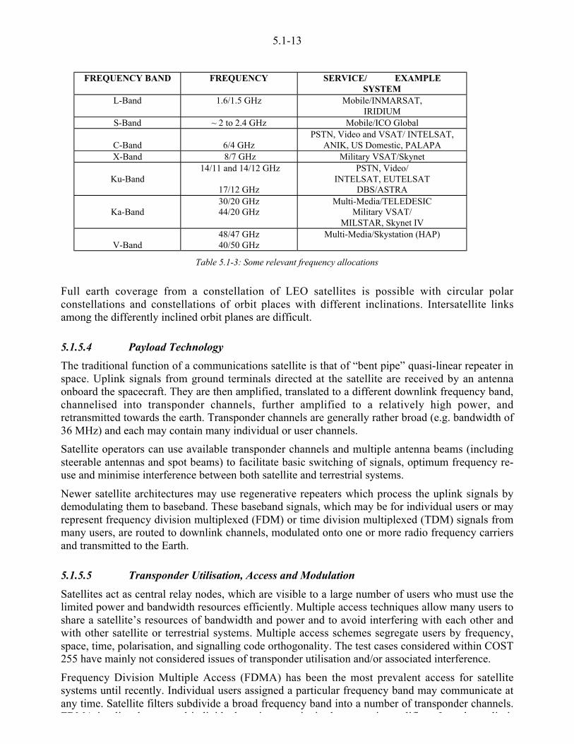
5.1-13

FREQUENCY BAND FREQUENCY SERVICE/ EXAMPLESYSTEM

L-Band 1.6/1.5 GHz Mobile/INMARSAT,IRIDIUM

S-Band ~ 2 to 2.4 GHz Mobile/ICO Global

C-Band 6/4 GHzPSTN, Video and VSAT/ INTELSAT,

ANIK, US Domestic, PALAPAX-Band 8/7 GHz Military VSAT/Skynet

Ku-Band 14/11 and 14/12 GHz

17/12 GHz

PSTN, Video/INTELSAT, EUTELSAT

DBS/ASTRA

Ka-Band30/20 GHz44/20 GHz

Multi-Media/TELEDESICMilitary VSAT/

MILSTAR, Skynet IV

V-Band48/47 GHz40/50 GHz

Multi-Media/Skystation (HAP)

Table 5.1-3: Some relevant frequency allocations

Full earth coverage from a constellation of LEO satellites is possible with circular polarconstellations and constellations of orbit places with different inclinations. Intersatellite linksamong the differently inclined orbit planes are difficult.

5.1.5.4 Payload Technology

The traditional function of a communications satellite is that of “bent pipe” quasi-linear repeater inspace. Uplink signals from ground terminals directed at the satellite are received by an antennaonboard the spacecraft. They are then amplified, translated to a different downlink frequency band,channelised into transponder channels, further amplified to a relatively high power, andretransmitted towards the earth. Transponder channels are generally rather broad (e.g. bandwidth of36 MHz) and each may contain many individual or user channels.

Satellite operators can use available transponder channels and multiple antenna beams (includingsteerable antennas and spot beams) to facilitate basic switching of signals, optimum frequency re-use and minimise interference between both satellite and terrestrial systems.

Newer satellite architectures may use regenerative repeaters which process the uplink signals bydemodulating them to baseband. These baseband signals, which may be for individual users or mayrepresent frequency division multiplexed (FDM) or time division multiplexed (TDM) signals frommany users, are routed to downlink channels, modulated onto one or more radio frequency carriersand transmitted to the Earth.

5.1.5.5 Transponder Utilisation, Access and Modulation

Satellites act as central relay nodes, which are visible to a large number of users who must use thelimited power and bandwidth resources efficiently. Multiple access techniques allow many users toshare a satellite’s resources of bandwidth and power and to avoid interfering with each other andwith other satellite or terrestrial systems. Multiple access schemes segregate users by frequency,space, time, polarisation, and signalling code orthogonality. The test cases considered within COST255 have mainly not considered issues of transponder utilisation and/or associated interference.

Frequency Division Multiple Access (FDMA) has been the most prevalent access for satellitesystems until recently. Individual users assigned a particular frequency band may communicate atany time. Satellite filters subdivide a broad frequency band into a number of transponder channels.FDMA i li h l i di id l i i i h i lifi I d li i

5.1-14

operated in a backed off condition which results in the reduction (output back off) of the outputpower of the individual carriers. For amplifiers with many carriers, the intermodulation productshave a noise-like spectrum and the noise power ratio is a good measure of multicarrier performance.

Time Division Multiple Access (TDMA) users share a common (wide) frequency band and are eachassigned a unique (short) time slot for their digital transmission. At any instant there is only onecarrier in the transmit amplifier, requiring little or no backoff from saturation. A drawback is thesystem complexity required to synchronise widely dispersed users in order to avoid intersymbolinterference caused by more than one user signal appearing in a given time slot. The totaltransmission rate in a TDMA satellite channel must be essentially the sum of the users’ rates,including overhead bits, such as for framing, synchronisation and clock recovery, and sourcecoding.

Code Division Multiple Access (CDMA) modulates each carrier with a unique pseudo randomcode, usually by means of either a direct sequence or frequency hopping spread spectrummodulation. As the CDMA users occupy the same frequency band at the same time, the aggregatesignal in the satellite amplifier is noise-like. Individual signals are extracted at the receiver bycorrelation processes. CDMA tolerates noise-like interference but does not tolerate large deviationsfrom average loading conditions. One or more very strong carriers could violate the noise-likeinterference condition and generate strong intermodulation signals.

User access is via assignments of a frequency, time slot, or code. Fixed assigned channels allow auser unlimited access. However, this may result in poor utilisation efficiency for the satelliteresources and may imply higher user costs (analogous to a leased terrestrial line). Other assignmentschemes include demand assigned multiple access (DAMA) and random access (e.g. for the Alohaconcept). DAMA systems require the user to first send a channel request over a common controlchannel. The network controller (at another earth station) seeks an empty channel and instructs thesending and receiving units to tune to it (either in frequency or time slot). A link is maintained forthe call duration and then released to the system for other users to request. Random access iseconomical for lightly used burst traffic such as data. It relies on random time of arrival of datapackets and protocols are in place for repeat requests in the event of collisions.

In practice, combinations of multiplexing and access techniques may be used. A broad band may bechannelised or frequency division multiplexed (FDM) and FDMA may be used in each subband,e.g. FDM/FDMA. Other combinations are also used.

Efficient source encoding algorithms, coupled with forward error correction channel coding havebrought about the dominance of digital modulation methods such as M-ary PSK and QAM invirtually all contemporary satellite communications services. Quality of a digital link can bespecified, controlled and guaranteed on an end-to-end basis.

5.1.5.6 Rationale for Test Cases

Test cases were chosen in accordance with the following broad objectives:

• to illustrate how the propagation factors can be applied in system design

• to apply the latest propagation data both to the performance prediction of existing systems (forexample existing VSAT and DBS systems) and to future systems

• to cover the range of frequencies for which the COST 255 project has contributed substantialrelevant propagation data and models

• to cover a representative range of systems applications especially including multimediatechniques.

The systems architectures taken for the test cases were either those of existing systems (for example

5.1-15

leap in technology. It was not seen as the role of the test cases to study novel system architectures orto apply a detailed analysis to unproven technologies. Advanced technologies have thus beenavoided and though it was recognised that on-board processing (including regeneration) would leadto significant system performance improvements, especially for Ka and V band systems, bent-pipetransponders have been taken in all test cases.

As a minimum it was expected that detailed link budgets and coverage evaluations would beundertaken for each test case. For the fixed link applications, reference stations were identified inthe coverage regions for which time-series data were available for evaluating fade mitigationtechniques through simulations. These reference stations were also those used for calculatingdetailed link budgets.

It was taken to be essential to cover both fixed and mobile systems and to examine the types oforbits currently being used, including LEO examples in addition to GEO systems. The test casesfinally chosen are listed in Table 5.1-4.

TestCase

Fixed orMobile

Orbit System Description

1 Fixed GEO Ku-Band VSAT System2 Fixed GEO Ka-Band VSAT Videoconference System3 Fixed GEO V-Band Asymmetric Multimedia System4 Fixed LEO Ka-Band Iridium Feeder Link5 Mobile LEO L-Band Low-Bit Rate System6 Mobile LEO Ka-Band Multimedia System

Table 5.1-4:Test case studies

5.1-16

5.1.6 References

[Maral, 1995]Maral, G., VSAT Networks; John Wiley & Sons Ltd; ISBN 0-471-95302-4, 1995.

[Vojcic, 1994]Vojcic B. R., L.B. Milstein, R. Picholtz, "Outage Probability for the Uplink of a DS-CDMA SystemOperating Over a LEO Mobile Satellite Channel", Proc. PIMRC'94, pp. 574-578, 1994.

5.1.7 Bibliography

U Casiraghi, S Dionis and P Nava; ”Assessments of the impact of CCITT G.826 recommendationon radio relay system design and radio link deployments”. ECRR 93, IEE Conference PublicationNo. 386, 1993, pp. 15-20, 1993.

Danielsson, Bernt; ”Using old bit error measurements to evaluate error performance andavailabilityaccording to G.826 parameters”. Telia Research Rep. 6/0363 FCPA 106 3053”, 1996.

Davarian F., "Fade margin calculation for channels impaired by Ricean fading," IEEE Transactionson vehicular technology, 34, 41-44, 1985.

Dorf, R.C. (Editor-in-Chief); Electrical Engineering Handbook; IEEE Press/CRC Press,ISBN 0-8493-0185-8, 1993

Evans, B.G., (Editor); Satellite Communication Systems; IEE/Peter Peregrinus Ltd.;ISBN 0-86341-106-1; 1987.

Gagliardi R. M., Satellite Communications, Second edition, Van Nostrand Reinhold, New York,ISBN 0-442-22745-0, 1991.

ITU-R Question 112/8, "Performance objectives for mobile-satellite services forming part ofISDN."

Proakis J. G., Digital communications, Third edition, McGraw-Hill, New York.ISBN 0-07-051726-6, 1995.

M Shafi and P Smith, ”The impact of G.826”. IEEE Communication Magazine, pp. 56-62,September 1993.

5.2-1

CHAPTER 5.2Propagation Impairments and Impact on

System Design

Editor: Michael Schnell1

Authors: Michael Schnell1, Uwe-Carsten Fiebig2, Enric Vilar3 , Carlos Catalan4

1 German Aerospace Center, Site Oberpfaffenhofen, Institute for Communications Technology,P.O. Box 1116, D-82230 Wessling, GermanyTel.: +49-(0)8153-282858, Fax.: +49-8153-281442, e-mail: Michael.Schnell@dlr.de

2 German Aerospace Center, Site Oberpfaffenhofen, Institute for Communications Technology,P.O. Box 1116, D-82230 Wessling, Germany

Tel.: +49-(0)8153-282835, Fax.: +49-8153-281442, e-mail: Uwe.Fiebig@dlr.de3 University of Portsmouth, Department of Electrical and Electronical Engineering,

Anglesea Building, Anglesea Road, Portsmouth PO1 3DJ, United Kingdom

Tel.: +44-(0)23-92842539, Fax.: +44-(0)23-92842792, e-mail: ev@ee.port.ac.uk4 University of Portsmouth, Department of Electrical and Electronical Engineering,

Anglesea Building Anglesea Road Portsmouth PO1 3DJ United Kingdom

5.2-2

5.2 Propagation Impairments and Impact on System Design

In this chapter, both the propagation effects and the system design are considered by investigatingthe impact of propagation impairments on the design of future satellite systems. Based oninvestigations of propagation effects, evaluation concepts are developed which are suitable forproper system design. Thus, a means is produced to map propagation effects into systemparameters, such as the required link margin or the required dynamic range for fade mitigationtechniques.

The evaluation concepts developed in this chapter are valid for and applicable to all kinds ofservices – fixed, portable, and mobile. The evaluation results, however, focus on fixed and portableservices, since the propagation measurements have been performed using the 40 GHz beacon of thegeostationary satellite ITALSAT and a non-mobile – fixed or portable – station on the ground.

5.2.1 Propagation Impairments

The propagation effects are investigated using beacon measurements. Therefore, the combinedeffects of gaseous, cloud, rain and ice attenuation are considered and the evaluation of themeasurement results focuses on the net effect on the communication link. Moreover, thepropagation phase noise is investigated. Especially, the impact of propagation phase on the systemdesign for portable terminals is considered. Other propagation effects, such as scintillation or rainand ice depolarisation are not taken into account.

5.2.2 Impact of Atmospheric Attenuation on System Design

The design of SATCOM systems has to satisfy several requirements. Among others the linkavailability is an important issue, which strongly influences the required fade margin. Appropriatefigures for the fade margin can be derived from the cumulative distribution of attenuation that givesthe percentage of time for which a certain attenuation level is exceeded. Various versions of thesedistributions exist, reflecting seasonal and diurnal variations. It depends on the requirements of thesupported service, which of these versions has to be taken into account. To illustrate this issue,consider three imaginary services denoted A, B, and C , all of them requiring the same linkavailability. We assume that the required link availability for service A has to be satisfied onaverage over the whole year, whereas services B and C require the link availability to be guaranteedfor every month and for the evening hours, respectively. Obviously, the different requirements ofthese services yield different fade margins, since signal attenuation is subjected to both seasonal anddiurnal variations. As a result, service C requires the largest link margin, whereas considerablysmaller link margins suffice to satisfy the link availability requirements for services A and B, withthe smallest link margin for service A.

In addition to link availability other parameters may be of interest in applications such as TV andaudio broadcasting. A link availability of 99.9 % only indicates that a loss of service occurs onaverage during 8:45 hours a year. However, this figure does not reveal for how long and how oftenthe service is expected to be interrupted: the link could be interrupted a thousand times a year forabout 30 seconds or about 50 times a year for 10 consecutive minutes. A service provider offeringpayTV may see a big difference between these two situations. Rather than in link availability aservice provider may be interested in outage probability [Fiebig and Schnell, 1997, 1998] which isthe probability that a specific attenuation level is exceeded for more than o consecutive minutesduring a specific time interval which corresponds with the length of a film or sporting event. Thus,fade margin design can also be carried out with respect to a tolerable outage probability.

Link availability and probability of outage can be guaranteed by appropriate fade margins which,however might become unrealistically large In order to decrease the fade margin which is

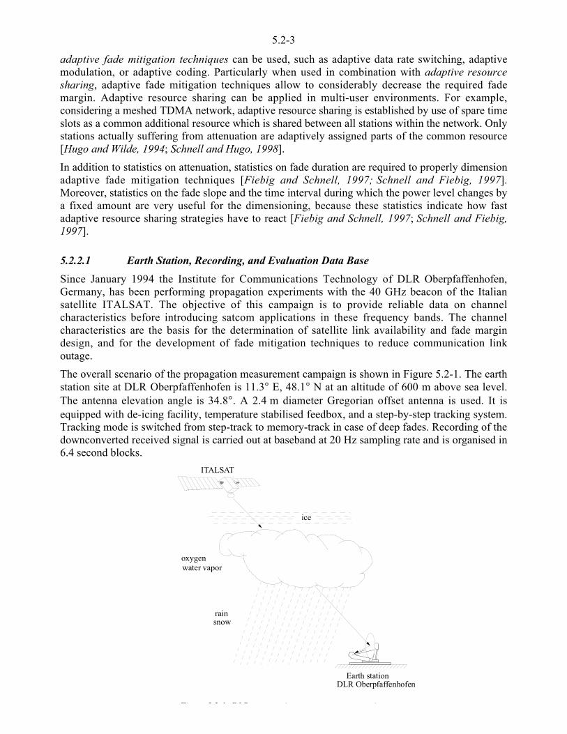
5.2-3

adaptive fade mitigation techniques can be used, such as adaptive data rate switching, adaptivemodulation, or adaptive coding. Particularly when used in combination with adaptive resourcesharing, adaptive fade mitigation techniques allow to considerably decrease the required fademargin. Adaptive resource sharing can be applied in multi-user environments. For example,considering a meshed TDMA network, adaptive resource sharing is established by use of spare timeslots as a common additional resource which is shared between all stations within the network. Onlystations actually suffering from attenuation are adaptively assigned parts of the common resource[Hugo and Wilde, 1994; Schnell and Hugo, 1998].

In addition to statistics on attenuation, statistics on fade duration are required to properly dimensionadaptive fade mitigation techniques [Fiebig and Schnell, 1997; Schnell and Fiebig, 1997].Moreover, statistics on the fade slope and the time interval during which the power level changes bya fixed amount are very useful for the dimensioning, because these statistics indicate how fastadaptive resource sharing strategies have to react [Fiebig and Schnell, 1997; Schnell and Fiebig,1997].

5.2.2.1 Earth Station, Recording, and Evaluation Data Base

Since January 1994 the Institute for Communications Technology of DLR Oberpfaffenhofen,Germany, has been performing propagation experiments with the 40 GHz beacon of the Italiansatellite ITALSAT. The objective of this campaign is to provide reliable data on channelcharacteristics before introducing satcom applications in these frequency bands. The channelcharacteristics are the basis for the determination of satellite link availability and fade margindesign, and for the development of fade mitigation techniques to reduce communication linkoutage.

The overall scenario of the propagation measurement campaign is shown in Figure 5.2-1. The earthstation site at DLR Oberpfaffenhofen is 11.3° E, 48.1° N at an altitude of 600 m above sea level.The antenna elevation angle is 34.8°. A 2.4 m diameter Gregorian offset antenna is used. It isequipped with de-icing facility, temperature stabilised feedbox, and a step-by-step tracking system.Tracking mode is switched from step-track to memory-track in case of deep fades. Recording of thedownconverted received signal is carried out at baseband at 20 Hz sampling rate and is organised in6.4 second blocks.

water vapor

ITALSAT

oxygen

rainsnow

Earth station

ice

DLR Oberpfaffenhofen

Fi 5 2 1 DLR i i

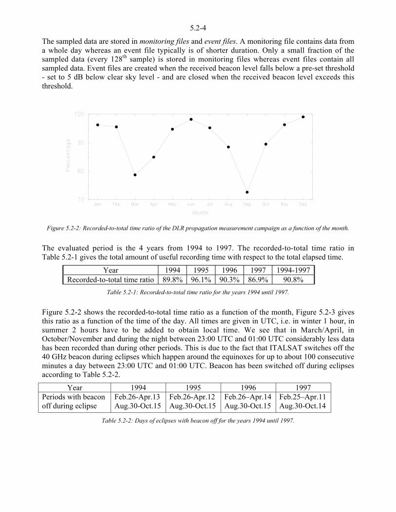
5.2-4

The sampled data are stored in monitoring files and event files. A monitoring file contains data froma whole day whereas an event file typically is of shorter duration. Only a small fraction of thesampled data (every 128th sample) is stored in monitoring files whereas event files contain allsampled data. Event files are created when the received beacon level falls below a pre-set threshold- set to 5 dB below clear sky level - and are closed when the received beacon level exceeds thisthreshold.

Figure 5.2-2: Recorded-to-total time ratio of the DLR propagation measurement campaign as a function of the month.

The evaluated period is the 4 years from 1994 to 1997. The recorded-to-total time ratio inTable 5.2-1 gives the total amount of useful recording time with respect to the total elapsed time.

Year 1994 1995 1996 1997 1994-1997Recorded-to-total time ratio 89.8% 96.1% 90.3% 86.9% 90.8%

Table 5.2-1: Recorded-to-total time ratio for the years 1994 until 1997.

Figure 5.2-2 shows the recorded-to-total time ratio as a function of the month, Figure 5.2-3 givesthis ratio as a function of the time of the day. All times are given in UTC, i.e. in winter 1 hour, insummer 2 hours have to be added to obtain local time. We see that in March/April, inOctober/November and during the night between 23:00 UTC and 01:00 UTC considerably less datahas been recorded than during other periods. This is due to the fact that ITALSAT switches off the40 GHz beacon during eclipses which happen around the equinoxes for up to about 100 consecutiveminutes a day between 23:00 UTC and 01:00 UTC. Beacon has been switched off during eclipsesaccording to Table 5.2-2.

Year 1994 1995 1996 1997Periods with beaconoff during eclipse

Feb.26-Apr.13Aug.30-Oct.15

Feb.26-Apr.12Aug.30-Oct.15

Feb.26–Apr.14Aug.30-Oct.15

Feb.25–Apr.11Aug.30-Oct.14

Table 5.2-2: Days of eclipses with beacon off for the years 1994 until 1997.

5.2-5

Figure 5.2-3: Recorded-to-total time ratio of the DLR propagation measurement campaignas a function of the time of the day (in hours in UTC).

5.2.2.2 Cumulative Distribution of Attenuation

Statistical Evaluation

Figure 5.2-4 gives the cumulative distribution of attenuation for each of the 12 months January toDecember, where the data base for each monthly statistic is the respective 4 months of the period1994 to 1997. Furthermore, the cumulative distribution of attenuation is shown for the whole period1994 to 1997.

Figure 5.2-4: Seasonal variations of the cumulative distribution of attenuation:(a) the 6 months January to June;

(b) the 6 months July to December as obtained in the 4 year period 1994 to 1997.

5.2-6

Figure 5.2-5: Diurnal variations of the cumulative distribution of attenuation; all times given in UTC:(a) 4 year period 1994to 1997; (b) July 1994, July 1995, July 1996, July 1997.

Figure 5.2-6: Variation of the cumulative distribution of attenuation from year to year.(a) for the years 1994 to 1997; (b) for the month July in the years 1994 to 1997.

It can be seen that attenuation strongly depends on the season and that June, July, and Augustprovide the largest amount of attenuation. Figure 5.2-5 shows the diurnal variations of thecumulative distribution of attenuation. We see that the largest amount of attenuation is expected inthe evening hours; this effect is most dramatic in the summer, especially in July. Note that the timeis given in UTC, i.e. 1 hour has to be added to obtain local time in the winter, but 2 hours have to beadded to obtain local time in the summer.

From Figure 5.2-6 we see that the cumulative distribution of attenuation may differ considerablyfrom year to year. Thus, the fade margins which are obtained from the figures above are valid for anaverage year, but do not necessarily fit with the characteristics of a specific year. Weatherconditions are subject to many variations. There are wet and dry years causing more, respectivelyless attenuation of the received signal than expected on average. Weather conditions in Germanycan change significantly from year to year, especially in summer periods which provide most of thethunderstorms (and mostly these thunderstorms are responsible for deep fades). We see that July1995 experienced severe attenuation, in contrast to July 1996 where less than average attenuationwas observed. Also in the winter, attenuation may change from year to year. This is due to the factthat precipitation in the winter can be all month long, in the form of dry snow, causing only littleattenuation, but also in the form of rain in warmer years causing a large amount of attenuation.Figure 5.2-7a reveals this fact, showing the differences between the various curves obtained forJanuary Not only seasonal but also diurnal statistics are subject to variations see Figure 5 2-7b In

5.2-7

1995 attenuation between 18:00 UTC and 20:00 UTC was considerably larger than in the otherthree years under observation.

Figure 5.2-7: Variation of the cumulative distribution of attenuation from year to year:(a) for the month January in the years 1994 to 1997;

(b) for the period 18:00 UTC to 20:00 UTC in the years 1994 to 1997.

Impact on System Design

From the figures shown above it is obvious that fade margin design depends not only on therequired availability but also very much on season and time of the day. Figures 5.2-8 and 5.2-9 givethe fade margin in dB which must be implemented to guarantee various levels of availability from95% to 99.99%. Table 5.2-3 gives the required fade margin in dB to guarantee the various levels ofavailability during the four year period from 1994 to 1997.

Availability 95% 99% 99.5% 99.9% 99.95% 99.99%Fade margin in dB (00:00 – 24:00 UTC) 2.7 5.3 7.5 15.9 23.1 39.0Fade margin in dB (06:00 – 16:00 UTC) 2.6 4.9 6.6 13.3 18.5 25.4Fade margin in dB (18:00 – 20:00 UTC) 2.9 6.2 9.1 22.8 29.7 41.1

Table 5.2-3: Required fade margin in dB to guarantee the various levels of availabilityduring the 4 year period 1994 to 1997.

Figure 5.2-8: Required fade margin for various levels of availability as a function of the month;

5.2-8

Figure 5.2-9: Required fade margin for various levels of availability as a function of the hour of the day;data basis is the period 1994 to 1997.

We see that systems are likely to be designed in a totally different manner depending on when aservice is offered. There is a large difference in fade margin, depending on whether a service has tofulfil the availability requirement on average over a whole year or for a particular month or at aparticular time of the day. A relatively small fade margin is required when availability has to beguaranteed during the winter months. However, a large fade margin up to 20 or 30 dB and more hasto be implemented when a high degree of availability is required during the summer months. Fademargin becomes even higher when the service operates solely in the summer and in the eveninghours.

5.2.2.3 Fade Duration

Statistical Evaluation

Fade duration is defined as the time duration during which attenuation is always larger than acertain threshold value. The average number of fades expected per month depends on the fadeduration and the threshold value. In Figures 5.2-10 and 5.2-11 the average number of fades isplotted as a function of the threshold value; parameter is the fade duration. We see from thesefigures that the average number of fades per month has a tendency to decrease with increasingthreshold: The larger the threshold, the fewer fades are observed.

Figure 5 2 10: Average number of fades per month as a function of the threshold value (attenuation) in dB

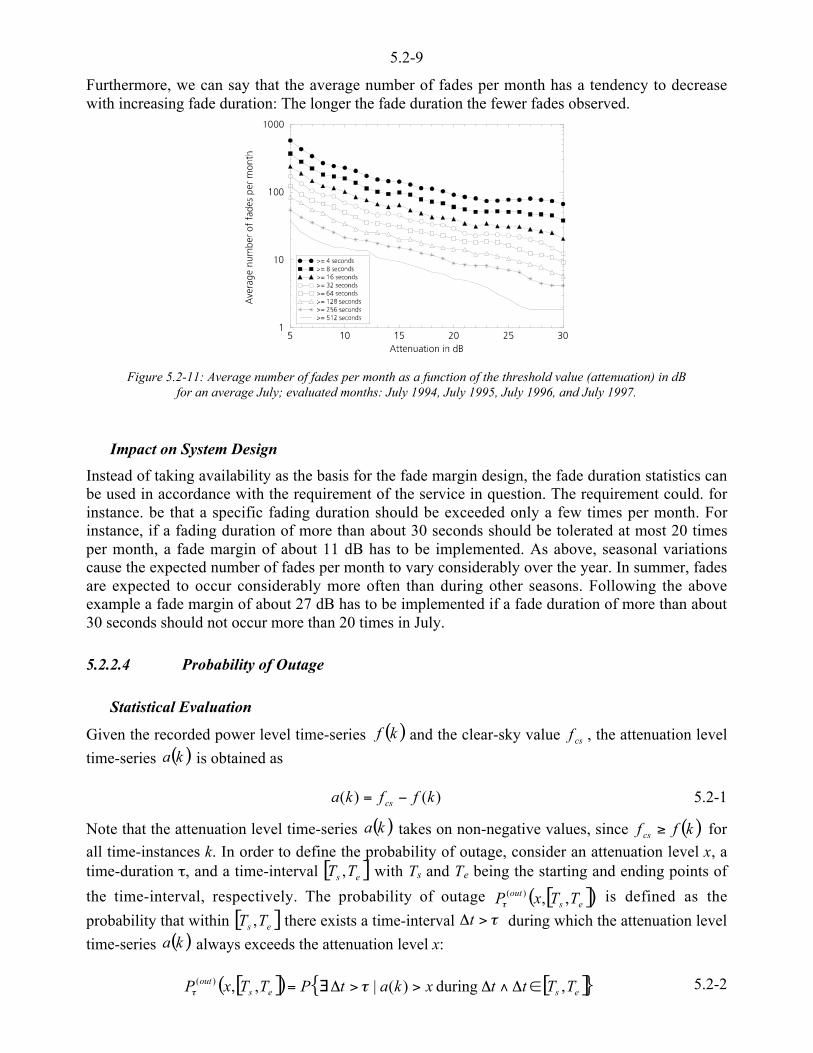
5.2-9

Furthermore, we can say that the average number of fades per month has a tendency to decreasewith increasing fade duration: The longer the fade duration the fewer fades observed.

Figure 5.2-11: Average number of fades per month as a function of the threshold value (attenuation) in dBfor an average July; evaluated months: July 1994, July 1995, July 1996, and July 1997.

Impact on System Design

Instead of taking availability as the basis for the fade margin design, the fade duration statistics canbe used in accordance with the requirement of the service in question. The requirement could. forinstance. be that a specific fading duration should be exceeded only a few times per month. Forinstance, if a fading duration of more than about 30 seconds should be tolerated at most 20 timesper month, a fade margin of about 11 dB has to be implemented. As above, seasonal variationscause the expected number of fades per month to vary considerably over the year. In summer, fadesare expected to occur considerably more often than during other seasons. Following the aboveexample a fade margin of about 27 dB has to be implemented if a fade duration of more than about30 seconds should not occur more than 20 times in July.

5.2.2.4 Probability of Outage

Statistical Evaluation

Given the recorded power level time-series ( )kf and the clear-sky value csf , the attenuation level

time-series ( )ka is obtained as

)()( kffka cs <= 5.2-1

Note that the attenuation level time-series ( )ka takes on non-negative values, since ( )kff cs * for

all time-instances k. In order to define the probability of outage, consider an attenuation level x, atime-duration o, and a time-interval [ ]es TT , with Ts and Te being the starting and ending points of

the time-interval, respectively. The probability of outage [ ]( )esout TTxP ,,)(

o is defined as the

probability that within [ ]es TT , there exists a time-interval o>6t during which the attenuation level

time-series ( )ka always exceeds the attenuation level x:

[ ]( ) [ ]{ }esesout TTttxkatPTTxP , during )(| ,,)( D6�6>>6�= oo

5.2-2

5.2-10

Considering the probability of outage in more detail, the meaning of the parameters o, x, and [ ]es TT ,

becomes evident:

Link margin:The parameter x determines the attenuation level which is critical for the satellite link. Ifattenuation exceeds this level x, the satellite link is interrupted. Thus, the parameter x can beviewed as the link margin which is foreseen for the satellite link and is a system designparameter.

Diurnal variations:The time-interval [ ]es TT , can be used to reflect diurnal variations by choosing appropriate

values for Ts and Te. Moreover, the duration of that interval can be adjusted. In this section,time-intervals of duration two hours are considered. This is a typical value for the duration ofa film or sporting event.

Providers' point of view:The parameter o is the time-duration of an outage the users may be willing to tolerate during[ ]es TT , , i.e. during a 2-hour time-interval, e.g. a film or sporting event. This aspect is

especially interesting for providers since the probability of outage can be determined as afunction of o and, therefore, as a function of the users' requirements.

Impact on System Design

Figure 5.2-12 gives the probability of outage as a function of x for the time interval [18, 20] UTCfor both the summer months June, July, and August, and for an average year. The time is in UTC,i.e. 2 hours has to be added in the summer yielding local time 8 p.m. to 10 p.m. This is the favouritetime for films and sporting events which typically last 2 hours. It can be seen that the probability ofoutage decreases with increasing o and increasing attenuation.

1 5 10 1 5 10Length of outage in minutesAll year summer

Fade margin in dB 4.8 5.5 7.2 7.8 9.8 15.0

Table 5.2-4: Required fade margin in dB to guarantee that probability of outage is below 5%.Data basis is the 4 year period 1994 tol 1997.

If a service provider guarantees that the outage probability is on average lower than 5% between8 p.m. and 10 p.m.(local time), and if outage is defined as a continuous interruption of thecommunications link of more than 5 minutes, then a fade margin of 9.8 dB has to be implemented.Table 5.2-4 gives the fade margins for various scenarios.

5.2-11

Figure5.2-12: Probability of outage as a function of x for the time interval [18, 20] UTC;summer months June, July, and August, and all year statistics; data basis is the 4 year period 1994 to 1997.

5.2.2.5 Fade Slope and 3dB Time Duration

In order to derive statistics on fade slopes we focus on fade events. They are recorded in event filesand contain the relevant data to answer the questions: What fade slopes have to be expected? Whatare the maximum fade slopes observed? Before analysing the event files the recorded signal is lowpass filtered in order to remove fluctuations that are caused by scintillation. Low pass filtering isrealised by a weighted moving average. The time window for averaging is set to 10=avT sec, thus,

spanning 201=avN recorded values. The discrete weighting function ( )khav is chosen to be a

squared cosine halfwave

( )ǻ

«©

¨<<´́

¦

¥²²¤

£ uu=

otherwise 0

100100 cos2 k-T

Tkkh

av

a

av

/5.2-3

where Ta is the sampling period which is 20 Hz. The 3dB cut off frequency of the low pass filter is0.1 Hz, removing almost all scintillation. After low pass filtering the time window is shifted by 20samples instead of one, in order to perform a downsampling to 1=dsT sec. Thus, the filtered power

level time-series denoted ( )nf is obtained. The derivative ( )nf v of ( )nf is then determined by

( )dsT

nfnfnf

)1()()(

<<=v 5.2-4

The fade slope is defined as the absolute value ( )nf v of the derivative at the time-instant n and

gives the power level changes based on 1sec intervals.

The cumulative distribution of fade slopes is given in Figure 5.2-13, which is based onmeasurements carried out during June, July, and August 1996. A total of 127 fading events wererecorded on 43 different days, comprising 59.4 hours which is referred to as fade event time.Figure 5.2-13 distinguishes between negative and positive slopes. As can be seen, fade slopes up to3.2 dB/sec are observed. However, steep fade slopes of more than 2.0 dB/sec are very rare and weremeasured during a single fading event. In 99.99 % of the fading event time the fade slopes for bothnegative and positive slopes are less than 1.9 dB/sec. Figure 5.2-13 indicates that negative andpositive slopes are equally likely. This is a surprising result, since it has been observed that

5.2-12

time interval of duration 1 sec. The observation that “attenuation increases faster than it decreases”can be shown when considering time intervals of longer duration. It is the 3dB time durationintroduced below which reveals the differences between positive and negative slopes.

Figure 5.2-13: Cumulative distribution of positive and negative fade slopes as observedduring deep fades in the months June, July, and August 1996.

The 3 dB time duration 3dBT is defined as the time interval during which the power level changes by

3 dB and is determined in the following manner: For every time-instant n of the low pass filteredfading event with power level ( )nf , the next possible time-instant m>n with power level ( )mf is

determined which satisfies the relation ( ) ( ) 3>< mfnf dB for a negative slope and( ) ( ) 3<< mfnf dB for a positive slope. A value of 3 dB is chosen for the power level change,

taking into account typical switching thresholds for satellite systems which apply advanced fademitigation techniques [Hugo and Wilde, 1994; Schnell and Hugo, 1998]. However, these fademitigation techniques also operate with other thresholds and so values of 4.5 dB and 6 dB are alsoconsidered. The respective time durations are denoted 4.5dBT and 6dBT .

The probability density functions of 3dBT , 4.5dBT , and 6dBT obtained during the fading event time in

June, July, and August 1996 are given in Figure 5.2-14 for both negative and positive slopes. Ascan be seen, the probability density functions for values smaller than 20 seconds are about twice aslarge for negative slopes as for positive slopes indicating that “attenuation increases faster than itdecreases” on average. This is consistent with the observation that heavy rain fall usually sets inmore abruptly than it stops. Another result from Figure 5.2-14 is that a considerable number ofpower level changes of 3dB occur within a few seconds.

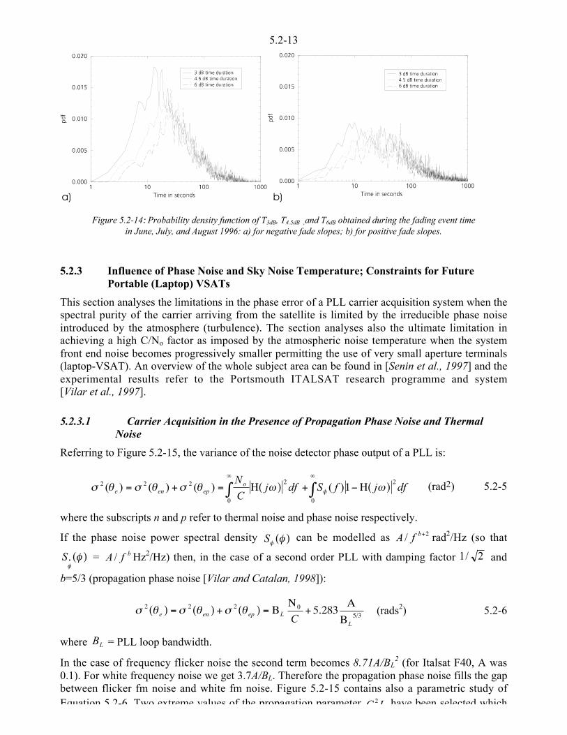
5.2-13

Figure 5.2-14: Probability density function of T3dB, T4.5dB ,and T6dB obtained during the fading event timein June, July, and August 1996: a) for negative fade slopes; b) for positive fade slopes.

5.2.3 Influence of Phase Noise and Sky Noise Temperature; Constraints for FuturePortable (Laptop) VSATs

This section analyses the limitations in the phase error of a PLL carrier acquisition system when thespectral purity of the carrier arriving from the satellite is limited by the irreducible phase noiseintroduced by the atmosphere (turbulence). The section analyses also the ultimate limitation inachieving a high C/No factor as imposed by the atmospheric noise temperature when the systemfront end noise becomes progressively smaller permitting the use of very small aperture terminals(laptop-VSAT). An overview of the whole subject area can be found in [Senin et al., 1997] and theexperimental results refer to the Portsmouth ITALSAT research programme and system[Vilar et al., 1997].

5.2.3.1 Carrier Acquisition in the Presence of Propagation Phase Noise and ThermalNoise

Referring to Figure 5.2-15, the variance of the noise detector phase output of a PLL is:

dfjfSdfjC

Noepene

2'

0

2'

0

)(N<1+)(N=+= 00 ttememem q )()()()( 222 (rad2) 5.2-5

where the subscripts n and p refer to thermal noise and phase noise respectively.

If the phase noise power spectral density )(qqS can be modelled as 2/ +bfA rad2/Hz (so that

)(• qq

S = bfA / Hz2/Hz) then, in the case of a second order PLL with damping factor 2/1 and

b=5/3 (propagation phase noise [Vilar and Catalan, 1998]):

5/30222

J

I5.283+

TJ=)(+)(=)(

L

Lepene Cememem (rads2) 5.2-6

where LB = PLL loop bandwidth.

In the case of frequency flicker noise the second term becomes 8.71A/BL2 (for Italsat F40, A was

0.1). For white frequency noise we get 3.7A/BL. Therefore the propagation phase noise fills the gapbetween flicker fm noise and white fm noise. Figure 5.2-15 contains also a parametric study ofEquation 5 2-6 Two extreme values of the propagation parameter LC 2 have been selected which

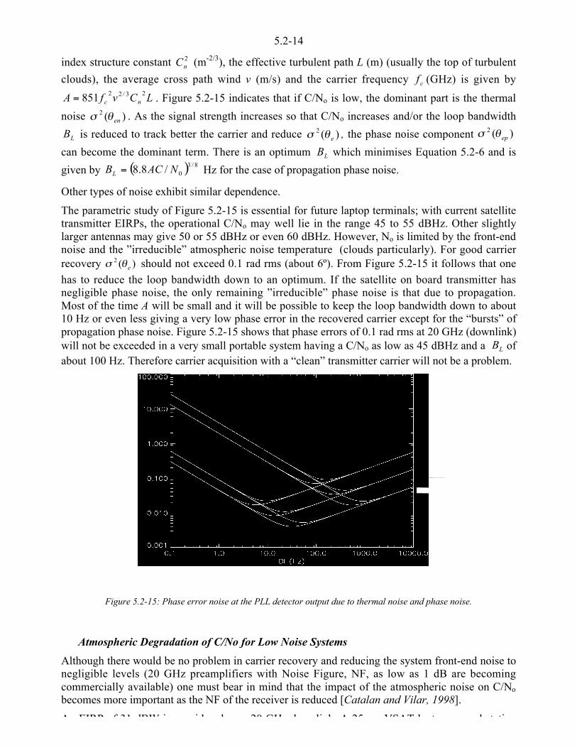
5.2-14

index structure constant 2nC (m-2/3), the effective turbulent path L (m) (usually the top of turbulent

clouds), the average cross path wind v (m/s) and the carrier frequency cf (GHz) is given by

LCvfA nc23/22851= . Figure 5.2-15 indicates that if C/No is low, the dominant part is the thermal

noise )(2enem . As the signal strength increases so that C/No increases and/or the loop bandwidth

LB is reduced to track better the carrier and reduce )(2eem , the phase noise component )(2

epem

can become the dominant term. There is an optimum LB which minimises Equation 5.2-6 and is

given by ( ) 8/30/8.8 NACBL = Hz for the case of propagation phase noise.

Other types of noise exhibit similar dependence.

The parametric study of Figure 5.2-15 is essential for future laptop terminals; with current satellitetransmitter EIRPs, the operational C/No may well lie in the range 45 to 55 dBHz. Other slightlylarger antennas may give 50 or 55 dBHz or even 60 dBHz. However, No is limited by the front-endnoise and the ”irreducible” atmospheric noise temperature (clouds particularly). For good carrierrecovery )(2

eem should not exceed 0.1 rad rms (about 6º). From Figure 5.2-15 it follows that one

has to reduce the loop bandwidth down to an optimum. If the satellite on board transmitter hasnegligible phase noise, the only remaining ”irreducible” phase noise is that due to propagation.Most of the time A will be small and it will be possible to keep the loop bandwidth down to about10 Hz or even less giving a very low phase error in the recovered carrier except for the “bursts” ofpropagation phase noise. Figure 5.2-15 shows that phase errors of 0.1 rad rms at 20 GHz (downlink)will not be exceeded in a very small portable system having a C/No as low as 45 dBHz and a LB ofabout 100 Hz. Therefore carrier acquisition with a “clean” transmitter carrier will not be a problem.

40 GHz

20 GHz

Cn

2L=3.42x10-11

C/No = 45 dBHz

C/No = 65 dBHz

C/No = 55 dBHz

Cn

2L=6.6x10-8

mmmm((((eeeee))))

(rads)

VCOFilter F(s)

Recoveredcarrier

eeeei

eeeee ====eeee

i <<<<eeee

o

H(s)=eeee

o((((s))))

eeeei((((s))))

1/s

eeeeo

Figure 5.2-15: Phase error noise at the PLL detector output due to thermal noise and phase noise.

Atmospheric Degradation of C/No for Low Noise Systems

Although there would be no problem in carrier recovery and reducing the system front-end noise tonegligible levels (20 GHz preamplifiers with Noise Figure, NF, as low as 1 dB are becomingcommercially available) one must bear in mind that the impact of the atmospheric noise on C/No

becomes more important as the NF of the receiver is reduced [Catalan and Vilar, 1998].

An EIRP of 31 dBW is considered on a 20 GH do nlink A 25 cm VSAT laptop gro nd station

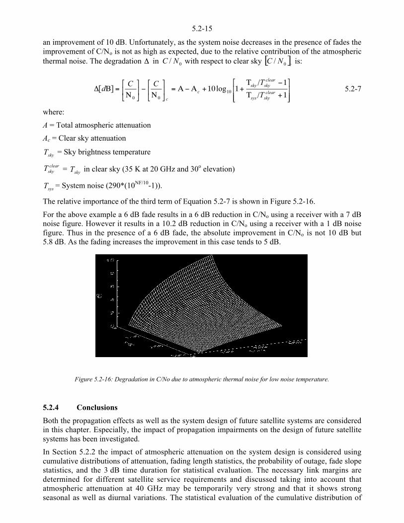
5.2-15

an improvement of 10 dB. Unfortunately, as the system noise decreases in the presence of fades theimprovement of C/No is not as high as expected, due to the relative contribution of the atmosphericthermal noise. The degradation 6 in 0/ NC with respect to clear sky [ ]cNC 0/ is:

µµ�

�

³³�

�

1+/Z

1</Z+110+I<I=µ

�

�³�

�

T<µ

�

�³�

�

T=]J[6 10

00clear

skysys

clearskysky

c

cT

TCCd log 5.2-7

where:

A = Total atmospheric attenuation

Ac = Clear sky attenuation

skyT = Sky brightness temperature

clearskyT = skyT in clear sky (35 K at 20 GHz and 30o elevation)

sysT = System noise (290*(10NF/10-1)).

The relative importance of the third term of Equation 5.2-7 is shown in Figure 5.2-16.

For the above example a 6 dB fade results in a 6 dB reduction in C/No using a receiver with a 7 dBnoise figure. However it results in a 10.2 dB reduction in C/No using a receiver with a 1 dB noisefigure. Thus in the presence of a 6 dB fade, the absolute improvement in C/No is not 10 dB but5.8 dB. As the fading increases the improvement in this case tends to 5 dB.

Figure 5.2-16: Degradation in C/No due to atmospheric thermal noise for low noise temperature.

5.2.4 Conclusions

Both the propagation effects as well as the system design of future satellite systems are consideredin this chapter. Especially, the impact of propagation impairments on the design of future satellitesystems has been investigated.

In Section 5.2.2 the impact of atmospheric attenuation on the system design is considered usingcumulative distributions of attenuation, fading length statistics, the probability of outage, fade slopestatistics, and the 3 dB time duration for statistical evaluation. The necessary link margins aredetermined for different satellite service requirements and discussed taking into account thatatmospheric attenuation at 40 GHz may be temporarily very strong and that it shows strongseasonal as well as diurnal variations. The statistical evaluation of the cumulative distribution of

5.2-16

very much on season and time of the day. Summer months require a considerably larger link marginthan winter months when the same availability has to be guaranteed. Furthermore, evening hoursrequire a larger link margin than other times of the day. If service requirements other thanavailability have to be satisfied, the fade duration statistics and the probability of outage arevaluable link margin design data. The link margin for the requirement that a specific fading durationshould be exceeded only a few times per month can be evaluated using fading duration statistics.The probability of outage is used to determine the link margin necessary to guarantee that anintolerably long outage is unlikely to occur during a certain period, e.g. during a film or sportingevent. If high availability or low probability of outage is required, especially for a certain season ortime of the day, extremely large link margins, which might be 30 dB or more, have to beimplemented. Since large link margins are too expensive to implement, fade mitigation techniquestogether with a sophisticated adaptive resource sharing strategy should be applied for future satellitesystems operating in the higher frequency range. To properly design fade mitigation techniques,fade slope statistics and 3 dB time duration are proposed. Both evaluation statistics can be used todetermine the required dynamic behaviour of fade mitigation techniques.

In Section 5.2.3 the influence of phase noise and sky noise temperature on future portable (laptop)VSATs is investigated. In particular it is shown that by augmenting the spectral purity of thesatellite on-board transmitter one can decrease the loop bandwidth of the carrier acquisition system(PLL). However, there is a limitation imposed by the irreducible propagation phase noise, whichhas been quantified in Section 5.2.3. Moreover, it is shown that atmospheric noise limits theimprovement achievable by increasing the noise performance of the microwave front end of theVSAT receiver. Therefore, the relative improvement in C/No brought about by substantiallyreducing the receiver noise figure results in a variability (sensitivity) 0NC6 greater than the

variability in attenuation. As a result, if the receiver noise figure is reduced substantially, the C/N0

improves but can fluctuate more than the atmospheric attenuation.

5.2-17

5.2.5 References

[Catalan and Vilar, 1998]Catalan, C.; Vilar, E.: "Transformation of Beacon AttenuationStatistics in C/No Statistics", FirstInternational Workshop on Radiowave Propagation Modelling for SatCom Services at Ka band andAbove, ESA WPP-146, pp. 283-287, ESTEC, Noordwijk, The Netherlands, 28-29 October 1998.

[Fiebig and Schnell, 1997]Fiebig, U.-C.; Schnell, M.: “40 GHz Measurement Campaign - Evaluation with Respect to SystemDesign and Fade Countermeasures”, Proceedings of 4th European Conference on SatelliteCommunications, ECSC-4, Rome, Italy, pp. 199-204, November 1997.

[Fiebig and Schnell, 1998]Fiebig, U.-C.; Schnell, M.: “Impact of Rain Attenuation on Satellite Broadcasting Systems at Ka-band”, Proceedings of First Int. Workshop on Radiowave Propagation Modelling for SatComServices at Ku-band and above, Noordwijk, The Netherlands, October 1998

[Hugo and Wilde, 1994]Hugo, D. von; Wilde, A.: “An Adaptive Resource Sharing Strategy for TDMA”, InternationalJournal of Satellite Communications, Vol. 12 (1994), No. 3, pp. 249-256, March 1994.

[Schnell and Fiebig, 1997]Schnell, M.; Fiebig, U.-C.: “Fade Slope Statistics of 40 GHz Beacon Signals”, Electronics Letters,Vol. 33., No. 21, pp. 1819-1821, October 1997.

[Schnell and Hugo, 1998]Schnell, M.; Hugo, D. von: “Fade Countermeasures and Adaptive Resource Sharing for anExperimental TDMA Satellite Communications System Operating at Ka-Band”, European Trans.on Telecommunications (ETT), Vol. 9, No. 6, pp. 561-568, Nov./Dec. 1998.

[Senin et al., 1997]Senin, S.; Catalan, C.; Vilar, E.: “Influence of Sky Noise Temperature and Propagation Phase Noiseon VSAT Design at Millimetre-Wave Frequencies”, Third Ka Band Utilization Conference,Sorrento, Italy, pp. 401-406, September 1997.

[Vilar et al., 1997]Vilar, E., J. Waight, S. Senin, C. Catalan, J. Vilar, A. Cazolama, J. Romeu, S. Morell, J. Woodroffe:“A Comprehensive/Selective mm-wave Satellite Downlink Experiment on Fade Dynamics”, 10th

IEE International Conference on Antennas and Propagation, pp. 2.98-2.101, April 1997.

[Vilar and Catalan, 1998]Vilar, E.; Catalan, C.: "Propagation Phase Noise. Impact on Future VSAT System Design", FirstInternational Workshop on Radiowave Propagation Modelling for SatCom Services at Ka band andAbove, ESA WPP-146, pp. 235-242, ESTEC, Noordwijk, The Netherlands, 28-29 Oct. 1998.

5.3-1

CHAPTER 5.3Impairment Mitigation

and Performance Restoration

Editor: Laurent Castanet1

Authors: Michel Bousquet2, Laurent Castanet1, Misha Filip3, Paul Gallois4, Boris Gremont5,Leandro de Haro6, Joël Lemorton7, Aldo Paraboni8, Michael Schnell9

1 ONERA CERT, 2 avenue Edouard Belin, BP 4025, F-31055 Toulouse CEDEX 4, France

Tel.: +33-5-6225-2729, Fax.: +33-5-6225-2577, e-mail: laurent.castanet@onecert.fr2 Supaero, 10 avenue Edouard Belin, BP 4025, F-31055 Toulouse CEDEX 4, France

Tel.: +33-5-6217-8086, Fax.: +33-5-6217-8380, e-mail: michel.bousquet@supaero.fr3 University of Portsmouth, Anglesea Bldg, Anglesea Rd, Portsmouth, PO1 3DJ, United Kingdom

Tel.: +44-23-9284-2310, Fax.: +44-23-9284-2561, e-mail: misha.filip@port.ac.uk4 Coventry University, Priory Str, Coventry, CV1 5FB, United Kingdom

Tel.: +44-12-0383-8854, Fax.: +44-12-0383-8949, e-mail: a.p.gallois@coventry.ac.uk5 University of Portsmouth, Anglesea Bldg, Anglesea Rd, Portsmouth, PO1 3DJ, United Kingdom

Tel.: +44-23-9284-2543, Fax.: +44-23-9284-2792, e-mail: boris.gremont@ee.port.ac.uk6 Universidad Politecnica de Madrid, Ciudad Universitaria, E-28040 Madrid, Spain

Tel.: +34-91-549-5700, Fax.: +34-91-543-2002, e-mail: leandro@gr.ssr.upm.es7 ONERA CERT, 2 avenue Edouard Belin, BP 4025, F-31055 Toulouse CEDEX 4, France

Tel.: +33-5-6225-2720, Fax.: +33-5-6225-2577, e-mail: joel.lemorton@onecert.fr8 Politecnico di Milano, Pza Leonardo da Vinci 32, I-20133 Milano, Italy

Tel.: +39-02-2399-3586, Fax.: +39-02-2399-3413, e-mail: paraboni@elet.polimi.it9 DLR Oberpfaffenhofen PF 1116 D 82230 Wessling Germany

5.3-2

5.3 Impairment Mitigation and Performance Restoration

Satellite communications present some significant advantages over terrestrial networks, such asflexibility and reconfigurability of the network, the possibility to establish point-to-multipoint links(broadcasting, mobiles…). Therefore communication satellites need to be integrated with terrestrialnetworks, and should provide high data rates. To carry such high data rates, higher frequenciesshould be considered, such as Ka-band (20 GHz - 30 GHz), V-band (40 GHz - 50 GHz) or EHF-band (20 GHz - 45 GHz). These offer large bandwidths that are not available at L to Ku band. Forsome years, innovative satellite systems have been proposed, either in Ka or V band for civilapplications (Cyberstar, Euroskyway, Skybridge 2, Skystation, Teledesic, West…) or in EHF bandfor military applications (ST3SII, GFSatCom, Skynet, Milstar).

One of the problems raised by these new frequency bands is how to quantify precisely the influenceof the atmosphere on the propagation of electromagnetic waves. Due to technology limitations,system margin can no longer be considered as the sole means to compensate propagationdisturbances at any percentage of time.

Some preliminary studies have demonstrated that the feasibility of such links seems to beguaranteed. However, it is now necessary on the one hand to determine which level of serviceavailability will be supplied to the user, and on the other hand to investigate the behaviour of theseanticipated systems when subject to the severe fading conditions encountered at frequencies above20 GHz.

As it is not cost efficient to design a large power margin, link signal fading must be compensated byother means in order to increase system availability. These alternatives, which overcome fadingwithout the use of large fixed margins, are known as Fade Mitigation Techniques (FMT) or FadeCounter-Measures (FCM).1

With such techniques, it will, for instance, be possible to design VSAT systems with a fixed margincorresponding to the worst case of fading occurring in clear-sky conditions; the implementation ofFMT allowing to counteract, in real time, cloud attenuation, some fraction of rain attenuation,scintillation, and depolarisation events.

The objective of this chapter is to give an overview on the application of FMT. It is organised intwo main sections: firstly a state-of-the-art report of FMT, and secondly a synthesis of thedevelopments carried out in this field in the framework of COST 255 Working Group 3.

Moreover, the propagation issues of the operational implementation of FMT, and especially theproblem of detection, control and prediction, are laid down. Three detection schemes: open-loop,closed-loop and hybrid-loop are investigated and compared, and recommendations are given ontheir suitability in relation to the frequency band.

5.3.1 FMT: state-of-the-art report

This review has been done without considering specific system architecture and multiple accessschemes and only gives a description of FMT. Fade detection and prediction, which are relatedtopics to be considered to implement FMT techniques, are beyond the scope of this chapter.

1 in the following, these techniques will be referred as Fade MitigationTechniques (FMT) rather than the term FadeCountermeasures usually used in the literature, but which has a typical radar signification. Indeed, a countermeasure isan active technique aimed to cause interference to an opposing system. If the intention is to use the radar language,FMT h ld h b i il d h b i h ff f h i

5.3-3

5.3.1.1 Presentation of FMT

Various methods exist to mitigate propagation effects and the choice of the most relevant onesshould take into account operating frequency bands, the performance objectives of the system andthe geometry of the network (system architecture, multiple access schemes…) [Willis and Evans,1988; Tartara, 1989; Allnutt and Rogers, 1993; Gallois, 1993; Acosta, 1997].

It is possible to divide FMT into three categories: Power Control, Signal Processing and DiversityFMT.

Power Control and Signal Processing FMT are characterised by the sharing of unused (excess)system resources, whereas diversity FMT implies adopting a re-routing strategy. Sharing unusedresources aims to compensate fading occurring on a particular link in order to maintain or toimprove the link performance (C/No), whereas diversity techniques maintain link performance bychanging the frequency band or the link geometry.

It is possible to distinguish three types of Power Control FMT: Up-Link Power Control where theoutput power of a transmitting Earth station is matched to up-link or down-link (in case of non-regenerative transponder) impairments, Down-Link Power Control where the on-board repeateroutput power (before the antenna) is adjusted and On-Board Beam Shaping which consists ofchanging on-board antenna radiation patterns. Down-Link Power Control and On-Board BeamShaping (for transmitting antenna) can be considered as Satellite EIRP Control techniques.

As far as Signal Processing FMT is concerned, two classes of methods can be identified which leadto a modification of the sharing of the satellite resources by acting on the information data rate or onthe bandwidth. The objective of the first class is to introduce extra coding in order to compensateadditional attenuation on the link by maintaining the nominal BER or to change modulationschemes to implement more robust modulations requiring less symbol energy. A second class oftechniques aims to reduce the information data rate at constant transmission data rate, which alsoleads to maintaining the BER.

Finally, Diversity FMT results in setting up a new link: Frequency Diversity permits, amongdifferent payloads on a satellite system, to choose the payload whose frequency band is the leastaffected by the meteorological situation, whereas geometrical (Site or Satellite) Diversity avoids anatmospheric perturbation which is going to produce a fade. Site diversity consists in transmitting theinformation through a second link less affected by propagation conditions and afterward to re-routethe information to the first destination by another path (for instance by a terrestrial network).Satellite diversity can be carried out within a satellite constellation, in order to choose the satellitethat offers the link with the highest service quality.

5.3.1.2 Description of the main fade mitigation methods

As already stated in the previous paragraph, FMT can be divided into 3 classes:

• Power Control FMT: transmit power level matched to propagation impairments,

• Signal Processing FMT: fade compensated by making use of a more efficient communicationscheme,

• Diversity FMT: fade avoided by the use of another, less disturbed, link.

Power Control techniques

In the case of transparent bent pipes, the goal of Power Control is not only to adapt transmittedpower to counteract uplink fading, but in a more general way, to adapt power in order to optimisethe overall C/No.

5.3-4

Power Control can be carried out at two locations: first on the ground segment where the outputpower of a transmitting Earth station is adapted to up-link and this is named Up-Link Power Control(ULPC); secondly, on-board the satellite, which leads either to the concept of Down-Link PowerControl (DLPC) which acts on the satellite transmitter power in front of the transmit antenna or tothe concept of On-Board Beam Shaping (OBBS) which aim is to adjust antenna patterns as afunction of propagation conditions and as a function of the traffic.

Up-Link Power Control (ULPC)

The aim of power control is to adapt the carrier power level to the propagationconditions. To demonstrate the interest in ULPC, it is necessary to distinguish the casesof transparent and regenerative repeaters.

Transparent repeater

In the case of a transparent repeater, the adaptation of the carrier power level by thetransmitting Earth station acts on both uplink and downlink budgets [Hörle, 1988]. Asfar as the uplink is concerned, ULPC adjusts the transmitted power of the Earth stationeither to transmit the minimum required power in clear sky conditions or to compensatepropagation impairments to maintain the uplink budget. Then, the Earth stations whichdoes not suffer from propagation impairments are able to operate without rain margin.When an ULPC technique is implemented, it is not necessary to consider link powermargins (to compensate for rain attenuation) in the design of the system, whichtranslates into a higher system capacity.

The influence of ULPC on the downlink budget can be considered in two ways: firstlyin avoiding reductions of satellite EIRP caused by the decreased uplink power level thatwould occur in the absence of ULPC, secondly in compensating downlink propagationimpairments, if the repeater dynamic range between the operating point and thesaturation level (maximum power) is sufficient [Egami, 1982], i. e. if the satellite poweramplifier is not operated at full power.

In addition, in a multicarrier environment, [Dodel and Riedl, 1991] have demonstratedthat the optimal satellite capacity is obtained if all carriers are attenuated in the sameway on the uplink; the worst case corresponds to the situation in which only a fewcarriers are faded and suffer from a non-linear capture effect. Therefore, in amulticarrier environment, adaptation of Earth station EIRP to propagation conditionsallows to keep a constant power level of all the carriers at the input of the repeater, thenavoiding excessive intermodulation.

In conclusion, ULPC can be seen on the one hand as a way to keep a constant level ofall the carriers at the input of the repeater, and on the other hand as a way to maintainthe overall link budget of the links in order to optimise the satellite capacity.

Regenerative repeater

With a regenerative repeater carriers are demodulated onboard the satellite, whichmakes the baseband signals available for specific processing prior to the modulation ofthe downlink carriers. On-Board Processing (OBP) can be used to optimise the overalllink budget of the system. In principle, this technique allows to match the waveform(data rate, coding rate, modulation scheme) to the propagation conditions.

However, in the case of low margin systems or for systems operating at or above Ka-Band, a static margin sufficient to prevent outages due to propagation conditions (evenstratiform rains) especially on the uplink is not realistic. This is particularly the case atKa-band or EHF-band where there is a strong relative difference between up and down

5.3-5

frequencies, and for which a strong protection against uplink fading is important. So theinterest of ULPC is reinforced.

Furthermore, it is necessary to pay attention to the sensitivity of on-board demodulationto signal dynamic range at the input of the repeater. As FDMA is a typical choice on theuplink, if OBP is sensitive to strong variations between carriers, therefore, even for highmargin systems, it is recommended to use ULPC in order to avoid capture effects ofcarriers faded by severe propagation conditions. In this case, the monitoring of allcarrier levels has to be carried out on-board the spacecraft, before the spacecraftindicates to the appropriated Earth station the necessary adjustments of up-link transmitpower [Acosta, 1997].

Therefore, in the case of a regenerative repeater, for low margin systems and systemsoperating at or above Ka-band, use of ULPC is helpful in order to prevent systemcapacity degradations due to propagation conditions.

In conclusion, Up-Link Power Control makes use only of transmitted Earth stationpower; without constraints on the sharing of the system resource and without a need forspecific delay before mitigation. This argument makes this technique a very flexibleone.

Down-Link Power Control (DLPC)

DLPC [Acosta, 1997; Karasawa and Maekawa, 1997] aims to allocate a relatively smallamount of extra-power on-board (due to limitations in TWTA output power), in order tocompensate a possible degradation in term of down-link C/No due to propagationconditions in a particular region. In this case, all Earth stations in the same beamcoverage benefit from the improvement of EIRP.

This technique applies only if the transponders are designed in such a way that verylittle adjacent channel interference and intermodulation noise are produced by theincreased transmitted power. Furthermore, it is necessary to verify on the one hand thatthe ground power flux density specification is not exceeded (to cope with radio-regulation and to avoid interference problems), and on the other hand that no serviceoutage occurs during changes in power level.

An estimate of the benefit obtainable by the DLPC can be obtained by comparing thetwo curves giving the outage as a function of the system power margin when this isallocated in a uniform or optimised way. From these two curves two parameters can beobtained, the adaptivity gain and the adaptivity improvement, whose meaning is similarto the one defined in the case of space diversity: the dBs spared to have the same outagein the first case, or the ratio of the lost users for the same margin, in the second.

On-Board Beam shaping (OBBS)

This technique is based on active antenna flexibility, which permits the adaptation ofspot beams to propagation conditions [Poiares-Baptista and Paraboni, 1995]. If themeteorological situation in a particular area can potentially cause fading by degradingthe link quality of the Earth stations located in this zone, it is possible, with activeantennas, to adjust the satellite antenna gain by reducing the size of the spot beampointing to this region. In fact, the objective is to radiate extra-power, and tocompensate rain attenuation only on spot beams where rain is likely to occur.

To apply this FMT, it is not necessary to analyse in real time the fade dynamic as forother FMT but to realise short-term weather predictions (Nowcasting) to determine the

5.3-6

principle of Nowcasting could be to use satellite imagery in order to analyse theevolution of the meteorological situation (cloud type and cloud motion identification,rain height and rain intensity determination…) to carry out very short-range forecastingof the propagation conditions [Hartigan and Gallois, 1993].

Two kinds of antennas have been considered in a study conducted by ESA [Poiares-Baptista and Paraboni, 1995]: a multi-feed antenna fitted with a beam-forming networkwith variable power dividers and a Cassegrain antenna with a single feed and twoshaped reflectors with small subreflector capable of being re-shaped in orbit. Theconclusion of this study is that the first solution is both more flexible and allows higheradaptive gain.

Recent simulations made by assuming a cluster composed of 8 spots fed by the sameamplifier (total power constant but different powers relocatable among the spots) havedemonstrated that adaptivity advantages of the order of 3 to 5 can be reached, byexploiting the variability of the weather conditions across the whole of Europe, for asystem margin of 1.5 and 3 dB.

In fact, this technique appears to be interesting but it could be too expensive (in terms ofdevelopment costs) for the first generation of Ka band payloads, mainly due to threekinds of problem:

• the difficulty to accommodate a relatively large antenna within the launcher fairing,

• the use of large active antennas for telecommunications purposes, due to limitationsin the development of on-board technology, and the feasibility of re-shaping spotbeams without penalising the global coverage; even though, for instance, the currentantenna technology allows to obtain European coverage with a cluster of 32 feeds,

• the elaboration of meteorological Nowcasting, which is a very promising techniquefor short range propagation predictions in the frame of high frequency satellitetelecommunications. However, the nowcasting accuracy is improving rapidly, bothconcerning the ECMWF (European Centre for Medium-range Weather Forecasting)and Meteosat. Moreover, the fact that no spatial detail below 100 km is necessaryhelps, indicating that a space-time accuracy is not really a stringent requirement.

The advantage of this method is that it gives similar results to ULPC or DLPC, withoutincreasing transmit power. Furthermore it allows a better design of satellite coverage,taking account of propagation conditions but also the distribution of users in thecoverage area (e.g. for mobile systems).

Signal processing techniques or Adaptive Signal Processing (ASP)

These techniques have been named Adaptive Resource Sharing because the available resources onthe satellite depend on the number of users requesting a part of these resources at the same time.Actually, it would be better to use the term Adaptive Signal Processing (ASP) to distinguish themfrom power control FMT that can also be considered as Adaptive Resource Sharing techniques.Three kinds of adaptive methods can be distinguished: Adaptive Coding, Adaptive Modulation andData Rate Reduction.

Adaptive Coding (AC)

When a link is experiencing fading, the introduction of coding allows to add redundantbits to the information bits, in order to detect and to correct errors (FEC…) caused by

5.3-7

bit. Adaptive coding consists in implementing a variable coding rate in order to matchimpairments due to propagation conditions.

Various possibilities exist to vary coding rates; for instance the use of separateoptimised codes for each data rate [Schnell and Von Hugo, 1998], the use of"punctured" codes [Willis and Evans, 1988], or of convolutional codes. A gain oftypically 2-10 dB can be achieved, depending on the coding rate [Willis and Evans,1988].

The fading satellite telecommunications channel does not produce independent errorsbut blocks of errors. Therefore most Forward Error Correcting codes are designed toimprove system performances by correcting errors which are supposed to beindependent, they are not very efficient in counteracting fading. The performance of themitigation technique can be improved by using block codes (such as Reed-Solomoncodes) which are more robust to bursts of errors, and with interleaving, which scramblesthe coded data in such a way that, after descrambling, errors can be consideredindependent [Proakis, 1995]. Interleaving is efficient only for very short fades andespecially for scintillation. Higher performances can be obtained by the concatenationof a convolutional code (Viterbi algorithm) with a block code (such as a Reed-Solomoncode), the convolutional code being efficient at correcting random errors, whereas theblock code is a good solution to correct error bursts.

The limitations of this FMT are linked to the additional bandwidth requirements forFDMA and larger bursts in the same frame for TDMA (due to implementation ofredundancy bytes). Adaptive coding can therefore be used when the application permitsreduced throughput when multiple links are experiencing fading simultaneously. Inaddition, transmission delays are proportionally larger for low data rate increase [Allnuttand Rogers, 1993], because of processing and interleaving, which makes this FMT lessreactive and flexible than for instance power control techniques.

Adaptive Modulation (AM)

Higher system capacity for a specified bandwidth can be achieved by using modulationschemes with high spectral efficiency such as coded modulation or combined amplitudeand phase modulation. Indeed, digital transmission with M-level digital modulationsmakes it possible to transmit more bits per second and yet not increase the bandwidthproportionally [Filip and Vilar, 1990; Maral and Bousquet, 1998].

As with Adaptive Coding, the aim of the Adaptive Modulation technique is to decreasethe required bit energy per noise energy ratio (Eb/No) corresponding to a given BER, byreducing the spectral efficiency as the C/N decreases. The reduction of the spectralefficiency can be obtained by introducing lower level modulation schemes. Forinstance, if very efficient modulations such as 16-PSK, 64-PSK or 256-QAM can beused in clear-sky conditions, in bad propagation conditions, Adaptive Modulation FMTmakes use of more robust modulations such as QPSK or BPSK [Filip and Vilar, 1990;Gallois, 1993].

This technique requires a high Eb/N0: for instance, implementing a 16-PSK modulationscheme requires an Eb/N0 of 24 dB to obtain a BER of 10-6. Such a link budget will bedifficult to establish, especially at Ka or V band.

Another way of reducing the required Eb/N0 is to introduce coding into the modulation.This method allows to exchange spectral efficiency for power when the link experiencesfading due to bad propagation conditions. New modulation schemes such as TrellisC d d M d l i (TCM) h ld i d l h Ad i M d l i FMT

5.3-8

Such a system based on adaptive pragmatic trellis coded modulation has been proposedrecently [Gremont et al., 1999a]. The proposed FMT system can be seen as ageneralised one since it encompasses adaptive coding and adaptive modulation assubsets. It is in effect a multiple FMT system relying on adaptive signal processingtechniques and is suitable for services which can accept a variable user data rate (i.e. thesatellite bandwidth occupancy is fixed on a channel basis). The supported modulationsare convolutionally encoded BPSK/QPSK with code rates 1/2, 2/3, rate 2/3 pragmatic8PSK and rate 3/4 pragmatic 16PSK as well as uncoded B/Q/8/16PSK. The authorsshowed that such a multiple FMT modem could very significantly outperform systemsrelying on single FMTs such as adaptive coding or adaptive (uncoded) modulation.

Data Rate Reduction (DRR)

Differently from ULPC, which aims at restoring the Carrier-to-Noise Ratio (C/No)through an increase of the Earth Station transmitted power, Adaptive Coding (AC),Adaptive Modulation (AM) and Data Rate Reduction (DRR) all allow reduction of therequired C/No while maintaining the link performance in terms of BER. Whereas ACand AM allow the required energy-per-information bit (Eb/No) to be reduced, DRR aimsto decrease the information data rate, at constant BER.

As already mentioned, making use of extra coding schemes or higher modulation levelsimplies longer bursts in the same frame for TDMA or larger bandwidth for FDMA,which penalises other users. Indeed, with these FMTs, a constant information data rateinvolves a higher transmitted data rate and requires the use of a larger part of thesatellite resource. However, resource sharing can be improved by reducing the data rate,which translates into a further reduction of the required power. Indeed, it is possible tooperate with constant resource by keeping the same transmitted data rate thanks to adecrease in information data rate. In this case, user data rates can be matched topropagation conditions: nominal data rates are used under clear sky conditions (nodegradation of the service quality with respect to the system margin), whereasreductions of data rates are introduced according to fading levels.

A possible technique using this principle to counteract propagation fading has beendesigned in the framework of the OLYMPUS project. This FMT, based on the principleof Fade Spreading, has been tested within the DICE videoconference experiment[Kerschat et al., 1993]. This FMT consists of reducing the codec rate from 2.048 Mbit/s(nominal data rate) to 1024, 512 and 256 kbit/s when fading increases, which results inpossible gains of 3, 6 and 9 dB. More precisely, the variable source data rate iscombined with a pseudo-random data sequence at the fixed “clear sky” data rate. Whenfading appears, the source data rate is decreased while the PR sequence rate is keptconstant, leading to a spreading of the data: the higher the spreading factor, the higherthe processing gain.

The interest of the Fade Spreading method is to operate at constant satellite resourceallocation per user (bandwidth, burst length) through constant transmitted data rate. Thelimitation of the method results in the possible compensation gain, a direct function ofthe range between nominal and smallest admissible information data rate for the user.Therefore, this FMT can be applied only for specific services which can tolerate asignificant reduction of the information rate such as video transmission or datatransmission (through an increase of transfer duration), but seems to be difficult to usewith voice transmission for instance. Moreover, extra delay appears due to the necessarydialog between transmitter and receiver, as well as to the data rate reduction of the videosignal

5.3-9

Diversity techniques

The objective of these techniques is to adopt a network re-routing strategy in order to avoidimpairments due to an atmospheric perturbation. Three types of diversity techniques can bedesigned: site, orbit and frequency diversity.

Site Diversity (SD)

Site Diversity can only be used for FSS (Fixed Satellite Services). This FMT has beenused essentially in Ku-band, where the propagation conditions that could overcome themargin occur only during, relatively rare, strong events (convective precipitation,storms).

Heavy precipitation or a storm are very localised events, with a central convective cellof about 1 km diameter and surrounded by a wider area (several kilometres diameter)with exponentially decreasing rain rate. The principle of SD is to use the fact that twofades experienced by two Earth stations separated by a distance higher than the size of aconvective rain cell (at least 10 km), are statistically independent [Poiares-Baptista andDavies, 1994]. The Earth station statistically affected by a weaker event is used and theinformation is routed to the original destination through a terrestrial network.

Typical diversity gains achievable with this method are between 10 dB and 30 dB atKa-band according to the distance between Earth stations (from 5 km) [ITU-R, 1994].The OPEX campaign has shown that the use of more than two stations does not improvethe diversity gain. This method is particularly efficient (high diversity gain) when thepercentage of time considered is low (high availability systems). Indeed, very low timepercentages correspond to very strong and local events, like convective rains andstorms. However, this technique requires the existence of terrestrial links between Earthstations. So actually, site diversity is suited to control stations and major gateways, butseems to be too expensive for low-cost VSATs or USATs without using publicterrestrial networks.

Satellite diversity (SatD)

In relation to the current developments of new Ka-band satellite constellation systems,Satellite diversity (SatD) is one solution to prevent degradation of the service quality.SatD can be regarded in two different ways: on one hand, when designing the system,by optimising the size of the constellation (that is the number of satellites) in order toprevent communications at low elevation angles, and on the other in allowing Earthstations to choose between various satellites, the one which allows to establish the mostfavourable link with respect to the propagation conditions [Capsoni and Matricciani,1985].

Some experiments have been carried out in the past, with SIRIO and OTS [Capsoni etal., 1990] and with OLYMPUS and ITALSAT [Matricciani and Mauri, 1995]spacecrafts. These campaigns have demonstrated the possible use of SatD as a FMT forfuture high-frequency satellite telecommunications systems. The SIRIO-OTS 12 GHzexperiment has pointed out that the diversity gain (either statistical or instantaneous) ishigher for low-elevation links than for higher elevation links [Capsoni et al., 1990].These results have been obtained for the working frequency of 12 GHz and are expectedto be improved in Ka-band.

As far as the OLYMPUS-ITALSAT SatD experiment is concerned, two kinds ofconclusion have been drawn [Matricciani and Mauri, 1995]. For low attenuation( if l d i i i ) S D i i i if h l d i i

5.3-10

ensure inhomogeneities in the meteorological cell). For high attenuation (convectiveclouds or precipitation), two situations may occur: either both attenuations are notcorrelated and therefore the diversity gain is high, or both attenuations are correlatedand the efficiency of this technique is lower. In general, this SatD experiment hasdemonstrated that for this particular geometrical configuration (small angular separationbetween spacecraft placed on the GSO), the normalised gain, expressed in percent, is ofthe order of magnitude of the angular separation between satellites, expressed indegrees; this was 30 % in the case of the OLYMPUS-ITALSAT experiment.Furthermore, this result is reliable only for high percentages of time (>0.5%), becauseof the short duration of this experiment. Additional campaigns should allow togeneralise these results.

For telecommunications systems based on a satellite constellation, SatD seems to be avaluable alternative or complement to site diversity. Although the maximum achievablediversity gain is higher in Site Diversity than in Satellite diversity (because in SD it ispossible to have Earth stations far enough apart to experience non-correlated fade eventswhich seems to be more difficult with SatD), SatD does not require terrestrialconnections. However, from the operational point of view, using this FMT impliesshifting the antenna pointing from one satellite to an other, which could lead to aninterruption of service. This interruption can be brief if either ephemerides of bothspacecraft have been introduced in the Earth station tracking software or if activeantennas are used for the ground segment. A dual beam antenna could also beconsidered.

Frequency Diversity (FD)

Frequency Diversity is a technique which requires that payloads using two differentfrequency bands are available onboard [Carassa and Tartara, 1988]. When a fadeoccurs, the routing strategy adopts links using the lowest frequency band payload.

Currently, some new high frequency band systems should use on the one hand Ka orEHF bands and on the other hand X or Ku bands. For this kind of system, twofrequency diversity techniques can be implemented, either cross-shaping or double-hop.

• Cross-shaping frequency diversity: the up-link and down-link frequency bands are not the same,and a switch onboard allows the transfer. To use it as a FMT to counteract propagationconditions requires that one or both users be equipped with two terminals (one in eachfrequency band).

• Double-hop frequency diversity: in order to counteract propagation conditions, the informationhas to be sent through a third user that is able to send the message to the original destination inthe other frequency band.

This FD technique is relatively expensive, because it involves having one user with apair of terminals, the first for the lower band and the second for the higher band.Furthermore, the sharing of the satellite resource is not optimised. In practice, thistechnique should be reserved for very specific communications.

Other FMTs

Other techniques, such as carrier reallocation [Pujante and De Haro, 1998], have been studied inthe framework of COST 255, with the aim of improving the carrier to intermodulation ratio, alimiting impairment factor for a satellite link in multicarrier operation. With this technique, it ispossible to avoid any modification of the transmission plan, that is the power and the centref f ll i i h d f h i d i

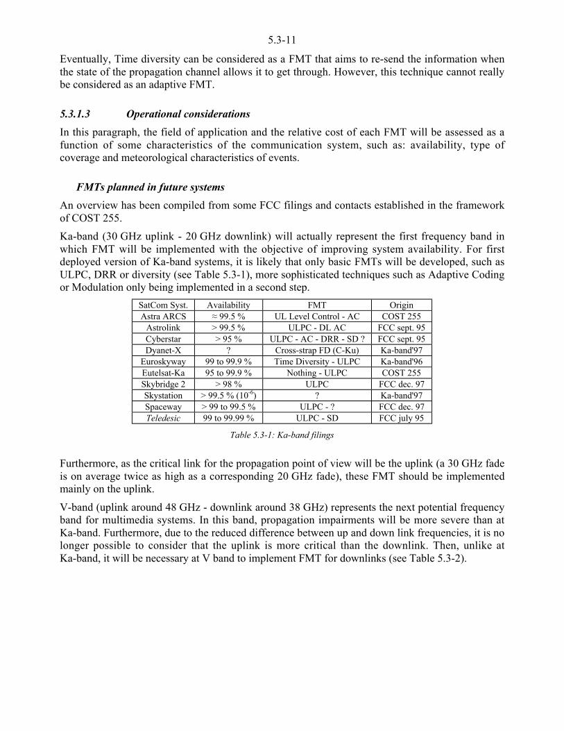
5.3-11

Eventually, Time diversity can be considered as a FMT that aims to re-send the information whenthe state of the propagation channel allows it to get through. However, this technique cannot reallybe considered as an adaptive FMT.

5.3.1.3 Operational considerations

In this paragraph, the field of application and the relative cost of each FMT will be assessed as afunction of some characteristics of the communication system, such as: availability, type ofcoverage and meteorological characteristics of events.

FMTs planned in future systems

An overview has been compiled from some FCC filings and contacts established in the frameworkof COST 255.

Ka-band (30 GHz uplink - 20 GHz downlink) will actually represent the first frequency band inwhich FMT will be implemented with the objective of improving system availability. For firstdeployed version of Ka-band systems, it is likely that only basic FMTs will be developed, such asULPC, DRR or diversity (see Table 5.3-1), more sophisticated techniques such as Adaptive Codingor Modulation only being implemented in a second step.

SatCom Syst. Availability FMT OriginAstra ARCS § 99.5 % UL Level Control - AC COST 255

Astrolink > 99.5 % ULPC - DL AC FCC sept. 95Cyberstar > 95 % ULPC - AC - DRR - SD ? FCC sept. 95Dyanet-X ? Cross-strap FD (C-Ku) Ka-band'97

Euroskyway 99 to 99.9 % Time Diversity - ULPC Ka-band'96Eutelsat-Ka 95 to 99.9 % Nothing - ULPC COST 255Skybridge 2 > 98 % ULPC FCC dec. 97Skystation > 99.5 % (10-6) ? Ka-band'97Spaceway > 99 to 99.5 % ULPC - ? FCC dec. 97Teledesic 99 to 99.99 % ULPC - SD FCC july 95

Table 5.3-1: Ka-band filings

Furthermore, as the critical link for the propagation point of view will be the uplink (a 30 GHz fadeis on average twice as high as a corresponding 20 GHz fade), these FMT should be implementedmainly on the uplink.

V-band (uplink around 48 GHz - downlink around 38 GHz) represents the next potential frequencyband for multimedia systems. In this band, propagation impairments will be more severe than atKa-band. Furthermore, due to the reduced difference between up and down link frequencies, it is nolonger possible to consider that the uplink is more critical than the downlink. Then, unlike atKa-band, it will be necessary at V band to implement FMT for downlinks (see Table 5.3-2).

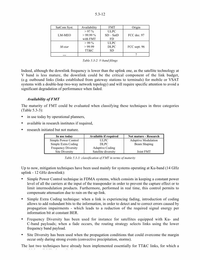
5.3-12

SatCom Syst. Availability FMT Origin

LM-MEO> 97 %

> 99.99 %with FMT

ULPCSD – SatD

FDFCC dec. 97

M-star> 99 %> 99.99TT&C

ULPCDLPC

SDFCC sept. 96

… ?

Table 5.3-2: V-band filings

Indeed, although the downlink frequency is lower than the uplink one, as the satellite technology atV band is less mature, the downlink could be the critical component of the link budget,(e.g. outbound links (links established from gateway stations to terminals) for mobile or VSATsystems with a double-hop two-way network topology) and will require specific attention to avoid asignificant degradation of performance when faded.

Availability of FMT

The maturity of FMT could be evaluated when classifying these techniques in three categories(Table 5.3-3):

• in use today by operational planners,

• available in research institutes if required,

• research initiated but not mature.

In use today Available if required Not mature - ResearchSimple Power ControlSimple Extra CodingFrequency Diversity

Site Diversity

ULPCDLPC

Adaptive CodingSatellite diversity

Adaptive ModulationBeam Shaping

Joint FMT

Table 5.3-3: classification of FMT in terms of maturity

Up to now, mitigation techniques have been used mainly for systems operating at Ku-band (14 GHzuplink - 12 GHz downlink):

• Simple Power Control technique in FDMA systems, which consists in keeping a constant powerlevel of all the carriers at the input of the transponder in order to prevent the capture effect or tolimit intermodulation products. Furthermore, performed in real time, this control permits tocompensate attenuation due to rain on the up-link.

• Simple Extra Coding technique: when a link is experiencing fading, introduction of codingallows to add redundant bits to the information, in order to detect and to correct errors caused bypropagation impairments - which leads to a reduction of the required signal energy perinformation bit at constant BER.

• Frequency Diversity has been used for instance for satellites equipped with Ku- andC-band payloads; when a fade occurs, the routing strategy selects links using the lowerfrequency band payload.

• Site Diversity has been used when the propagation conditions that could overcome the marginoccur only during strong events (convective precipitation, storms).

The last two techniques have already been implemented essentially for TT&C links, for which ahi h il bili i i d

5.3-13

Some other techniques are ready to be used, such as Up-Link Power Control and Down-Link PowerControl, Adaptive Coding and Data Rate Reduction, as well as Satellite Diversity for constellations.No significant difficulty is expected in the implementation of these techniques.

Three FMTs can rather be classified in the research domain:

• Adaptive modulation: the principle of this method is well known, but the problem lies in thepractical implementation of modems and in the power available at the receiving level.

• On-Board Beam Shaping: this technique requires sophisticated active antennas and relatedprocessing to be placed on-board the satellite.

• Joint FMT, i. e. a combination of several single FMTs possibly represents the most promisingsolution.

Availability range objectives

Three types of FMT have been identified above: Power Control techniques (ULPC, DLPC andOBBS), Adaptive Signal Processing techniques (AC, AM and DRR) and diversity techniques (FD,SD and SatD). Due to their principles and to the consequences in terms of network resource sharing,each of these methods is adapted to a specific part of the availability range objectives of a satcomsystem.

Up-Link Power Control makes use only of transmitted Earth station power; therefore it can beimplemented for any percentage of time, which makes this technique a very flexible one. Thelimitations of ULPC are the Earth station power range and the repeater gain margin for transparentrepeaters, which means in practice that very strong fades cannot be compensated entirely with thistechnique. However the range of power control should be sufficient to counteract effects of cloudsor weak precipitation (high percentages of time).

Regarding Down-link Power Control and On-Board Beam Shaping, the size of spot beams(e3dB < 0.5°) in Ka and EHF bands will, in practice, allow to counteract events spread over an areaof some hundreds of kilometres. The most efficient use of these techniques will be obtained if theaperture of spot beams does not greatly exceed the rain cell size. Consequently, DLPC and OBBScan be efficiently applied to large meteorological stratiform structures corresponding to high timepercentages.

The advantage of Adaptive Signal Processing FMT is to be able to maintain the transmission datarate of the service, which makes also this technique a very flexible one. However, this kind of FMTis only interesting if the extra capacity does not represent a large part of the total satellite resourcewhich would affect the overall performance of the system. For instance, without taking into accountstatistical fluctuations, if only 5 % of the links experience fading at any time, then the amount ofcommon resource needed is only 5 % of the total required, if all Earth stations operate with a fixedmargin [Willis and Evans, 1988]. Consequently, Adaptive Coding or Modulation techniques canonly be really efficient if only a few Earth stations experience fading at the same time. Therefore,these techniques are best suited to local or to rare impairments (such as heavy clouds and strongprecipitation) where the probability of simultaneous fading on many links is very low (decorrelatedevents). When fades are highly correlated, ASP is less effective [Jones and Watson, 1993].

The Frequency Diversity technique is relatively expensive, should be restricted to very specificcommunications and should be used to prevent a saturation of the system. From this assumption, itcan be stated that Frequency Diversity can be applied to any percentages of time.

Geometrical Diversity techniques are more efficient if the atmosphere is not homogeneous, in orderto be able to find another path not affected by a strong impairment (high diversity gain). Thissituation is more likely to be encountered when the percentage of time considered is very low

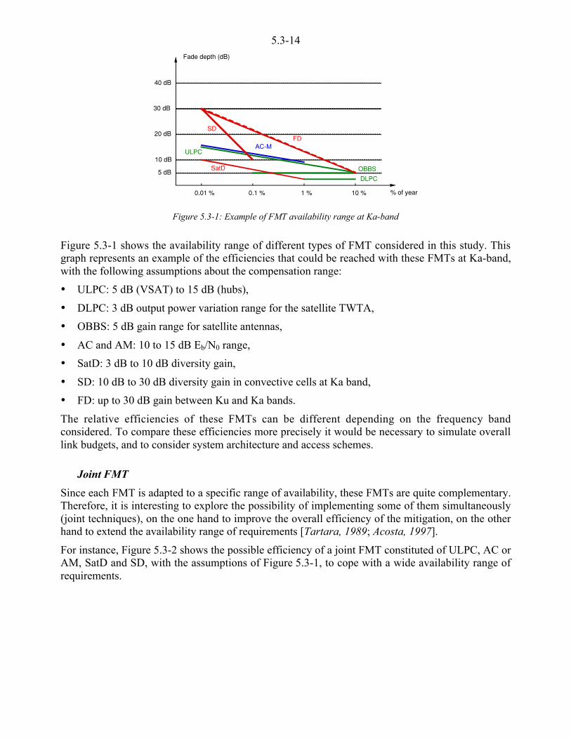
5.3-14

5 dB

10 dB

30 dB

40 dB

0.01 % 0.1 % 1 % 10 % % of year

Fade depth (dB)

20 dBFD

SD

SatD

AC-MULPC

DLPCOBBS

Figure 5.3-1: Example of FMT availability range at Ka-band

Figure 5.3-1 shows the availability range of different types of FMT considered in this study. Thisgraph represents an example of the efficiencies that could be reached with these FMTs at Ka-band,with the following assumptions about the compensation range:

• ULPC: 5 dB (VSAT) to 15 dB (hubs),

• DLPC: 3 dB output power variation range for the satellite TWTA,

• OBBS: 5 dB gain range for satellite antennas,

• AC and AM: 10 to 15 dB Eb/N0 range,

• SatD: 3 dB to 10 dB diversity gain,

• SD: 10 dB to 30 dB diversity gain in convective cells at Ka band,

• FD: up to 30 dB gain between Ku and Ka bands.

The relative efficiencies of these FMTs can be different depending on the frequency bandconsidered. To compare these efficiencies more precisely it would be necessary to simulate overalllink budgets, and to consider system architecture and access schemes.

Joint FMT

Since each FMT is adapted to a specific range of availability, these FMTs are quite complementary.Therefore, it is interesting to explore the possibility of implementing some of them simultaneously(joint techniques), on the one hand to improve the overall efficiency of the mitigation, on the otherhand to extend the availability range of requirements [Tartara, 1989; Acosta, 1997].

For instance, Figure 5.3-2 shows the possible efficiency of a joint FMT constituted of ULPC, AC orAM, SatD and SD, with the assumptions of Figure 5.3-1, to cope with a wide availability range ofrequirements.

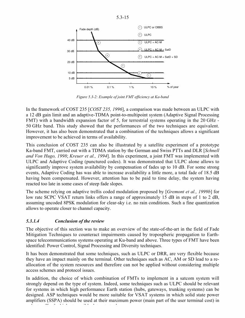
5.3-15

5 dB

10 dB

30 dB

40 dB

0.01 % 0.1 % 1 % 10 % % of year

Fade depth (dB)

20 dB

12

3

4

5

1

2

3

4

5

ULPC or OBBS

ULPC

ULPC + AC-M

ULPC + AC-M + SatD

ULPC + AC-M + SatD + SD

Figure 5.3-2: Example of joint FMT efficiency at Ka-band

In the framework of COST 235 [COST 235, 1996], a comparison was made between an ULPC witha 12 dB gain limit and an adaptive-TDMA point-to-multipoint system (Adaptive Signal ProcessingFMT) with a bandwidth expansion factor of 5, for terrestrial systems operating in the 20 GHz -50 GHz band. This study showed that the performances of the two techniques are equivalent.However, it has also been demonstrated that a combination of the techniques allows a significantimprovement to be achieved in terms of availability.

This conclusion of COST 235 can also be illustrated by a satellite experiment of a prototypeKa-band FMT, carried out with a TDMA station by the German and Swiss PTTs and DLR [Schnelland Von Hugo, 1998; Kreuer et al., 1994]. In this experiment, a joint FMT was implemented withULPC and Adaptive Coding (punctured codes). It was demonstrated that ULPC alone allows tosignificantly improve system availability by compensation of fades up to 10 dB. For some strongevents, Adaptive Coding has was able to increase availability a little more, a total fade of 18.5 dBhaving been compensated. However, attention has to be paid to time delay, the system havingreacted too late in some cases of steep fade slopes.

The scheme relying on adaptive trellis coded modulation proposed by [Gremont et al., 1999b] forlow rate SCPC VSAT return links offers a range of approximately 15 dB in steps of 1 to 2 dB,assuming uncoded 8PSK modulation for clear-sky i.e. no rain conditions. Such a fine quantizationallows to operate closer to channel capacity.

5.3.1.4 Conclusion of the review

The objective of this section was to make an overview of the state-of-the-art in the field of FadeMitigation Techniques to counteract impairments caused by tropospheric propagation to Earth-space telecommunications systems operating at Ku-band and above. Three types of FMT have beenidentified: Power Control, Signal Processing and Diversity techniques.

It has been demonstrated that some techniques, such as ULPC or DRR, are very flexible becausethey have an impact mainly on the terminal. Other techniques such as AC, AM or SD lead to a re-allocation of the system resources and therefore can not be applied without considering multipleaccess schemes and protocol issues.

In addition, the choice of which combination of FMTs to implement in a satcom system willstrongly depend on the type of system. Indeed, some techniques such as ULPC should be relevantfor systems in which high performance Earth station (hubs, gateways, trunking systems) can bedesigned. ASP techniques would be more suitable for VSAT systems in which solid state poweramplifiers (SSPA) should be used at their maximum power (main part of the user terminal cost) in

d t ff th hi h t ibl d t t t th

5.3-16

This work points out two important aspects for new systems operating from Ku to V band:

• On the one hand, it appears that each FMT is adapted to a specific range of availability. Thenthese fade mitigation methods are quite complementary and can be implemented simultaneously(joint techniques) to extend the availability range of requirements. Following some conclusionsof the COST 235 project and [Vasseur et al., 1998], this state-of-the-art report shows that Kaand EHF band satellite telecommunications systems with high service availability aretechnically possible only if a combination of different FMTs (Joint FMT) is implemented.

• On the other hand, such methods implemented individually can compensate only relativelysmall propagation impairments. It will be possible to improve the performance of the mitigationto a large extent, by carrying out a combination of different kinds of FMT when there is a needto transmit high priority information [Vasseur et al., 1998].

In Chapters 6.1 to 6.4, some FMTs are used in COST 255 test case analyses. These are listed in thefollowing table:

FMT actually simulated FMT forecast or possibleTest case 1 ULPC + AM ACTest case 2 ULPC + DRR AC - AM - DLPCTest case 3 - ARS - TD - SDTest case 4 ULPC + DLPC SD – Sat D

Table 5.3-4: FMT used in test case analyses

5.3.2 COST 255 developments

5.3.2.1 Simulation and performance evaluation of FMT Systems

At Ka or V band, the main limitations are due to the signal variations caused by clouds, rainattenuation, thermal noise and tropospheric scintillations. In order to build and test communicationsystems using FMTs, it is necessary to consider the modelling of the Ka-band faded satellitechannel. Essentially this requires an extension of the link power budget analysis which canencompass the main statistical and dynamical characteristics of the atmospheric processes involvedas well as system parameters.

Short-term analysis, relying on event-based simulation is useful for evaluating the real-timebehaviour of an overall communication system in the presence of dynamic atmospheric fading.With such an approach, the focus is placed on optimising real-time algorithms (e.g. fade detection,prediction, data link layer ARQ protocols) so that satellite links can be serviced in a transparent andefficient manner. This can be done using propagation beacon data if available. An alternative is tosynthesise time-series using DSP and use these generated signals [Gremont and Filip, 1998].

The ultimate objective is to design systems that can perform satisfactorily on a long-term basis. It isthus important to obtain estimates of the likely performance probably on a worst-month or yearlybasis. This can be achieved either by running an event-based simulation over the required timespan, or, in some simple cases using mathematical solutions. For example [Gremont and Filip,1999] evaluated the expected CNR statistics for inbound and outbound channels of a duplexsatellite link with ULPC with a 5 dB range. Once the CNR statistics are known it is quitestraightforward to estimate the BER/throughput of practical communication systems.

FMT Techniques: Carrier Reallocation

Among satellite communications interference sources, intermodulation noise is the limitingimpairment factor for a satellite link in multicarrier operation. The higher the operating point (lower

5.3-17

point, C/Iintermodulation<C/N and << C/I on the uplink). So, in rain fade conditions, the improvementof the C/Iintermodulation ratio of the affected carrier is a useful technique to improve the quality ofservice.

The proposed approach [Pujante and De Haro, 1998] is to apply the simulated annealingoptimisation technique on a dynamic basis to those carriers affected by rain fade in a multicarriersatellite transponder. The advantage of this proposal is that it avoids any modification of thetransmission plan, that is, the power and the centre frequency of all carriers remain unchanged,except for the faded carrier, which is reallocated to a frequency where the best C/Iintermodulation ratiocan be found. This technique can be implemented either on a single station, or by means of a NMS(Network Management Station) on a VSAT network.

As a first advantage, the optimised configuration for the transmission plan is more robust in case ofa rain fade, than a classical transmission plan approach with correlative frequency assignment.

As this optimisation technique can be reiterated over any configuration, after the modification ofany of the carrier blocks in the transponder, it can be used to redistribute the intermodulation noiseof any carrier block in the transponder under rain fade conditions. Thereby all carriers contribute tothe protection of the faded carrier, but without modification of the transmission plan of the carriersthat keep operating under nominal conditions, and only the faded carried should re-optimise itscentral frequency.

In the studies developed, this improvement is as high as 4.4 dB with respect to the classicaltransmission plan approach, and 0.7 dB with respect to the previously optimised configuration. Indigital transmission this margin is enough to bring the signal back above the demodulator threshold.

The implementation of this technique is feasible on a station by station basis (point-to-point links)or on a NMS station attended-VSAT network basis. The best operational advantage arises from thefact that there is no need to modify the transmission plan for the carriers that are not affected by rainfading.

5.3.2.2 Problem of impairment detection

Up to now, the use of Fade Mitigation Techniques has been discussed from the system point ofview. In implementing an FMT, a real problem is to detect and predict, in real time, the dynamicbehaviour of a propagation impairment. It is then necessary to discuss the methods for detecting andquantifying a possible fade, and the method of distributing the information to the equipment that isgoing to implement the compensation (transmitting Earth station, satellite, control station…).

Possible configurations

From the operational point-of-view, the first action to perform consists of evaluating when anoutage of the system due to propagation conditions is going to happen. More precisely, it impliesbeing able to detect a propagation event and to quantify it in order to estimate whether or not thesystem margin is going to be exceeded. Therefore, as it is necessary to measure the depth of anevent, this measurement must be done on the particular link which suffers it, the ground segment(either the transmitting or the receiving Earth station) being the most suitable to carry out thisfunction, for technical (identification of the station suffering the fade) and cost reasons.

From this assumption, three kinds of detection concepts can be designed for an Earth station[Egami, 1982; Hörle, 1988; Cacopardi et al., 1993; Dissanayake, 1997]: open-loop, closed-loopand hybrid-loop.

5.3-18

Open loop principle

The open-loop detection concept relies on the estimation, by the Earth station, of theuplink impairment, from a measurement of the propagation conditions. Thismeasurement can be carried out in four different ways:

• temperature, pressure, humidity and rain intensity measurements realised with a meteorologicalstation (with a rain-gauge),

• sky brightness temperatures measured with a multifrequency radiometer,

• attenuation measurements realised from a satellite beacon operating at uplink frequency,

• attenuation measurements realised from a satellite beacon operating at downlink frequency.

Meteorological and radiometrical detection concepts seem difficult to implement forsystems with low cost constraints on the ground segment. Regarding rain-gaugemeasurements, the accuracy that could be reached is not very good, because it does notallow to know the distribution of the rain intensity along the whole path, but only at therain-gauge location.

Accordingly, an analysis performed for the ACTS campaign (USA) [Dissanayake,1997] has shown that a sufficient accuracy can only be obtained with beaconmeasurements. Of course the best accuracy can be obtained with satellite beaconsoperating at both uplink and downlink frequencies (in this case, there is no frequencyscaling to perform). The World Administrative Radio Conference held in 1992allocated a frequency band for uplink frequency beacons at Ka-Band.

However, it seems that the implementation of an uplink frequency beacon receiver inthe Earth stations (especially VSATs) will be considered too expensive for new satellitesystems operating at Ka or EHF bands, whereas it is not the case for a downlinkfrequency beacon (already in the channel receiver frequency band).

CONTROL STATION OR VSAT

Beacon measurement " Aup (C)

Frequency scaling

U or V-SAT : if low-cost constraints � no beaconreceiver

A : CNR from C

" Adown(A)

Given Aup(C) " Aup(A)

Freq. scaling

A

C

Figure 5.3-3: Basic open-loop principle

In practice, the open-loop detection scheme will be based on the measurement of adownlink beacon (in general the satellite TT&R beacon) preferably in the downlinkfrequency band (see Figure 5.3-3). Once the downlink attenuated signal has beenmeasured, the use of instantaneous frequency scaling algorithms between uplink anddownlink frequencies allows to estimate the uplink fade in real-time (for the downlink,the impairment is directly measured by the Earth station). Differently from bothfollowing concepts the open loop method presents the advantage of not implying the

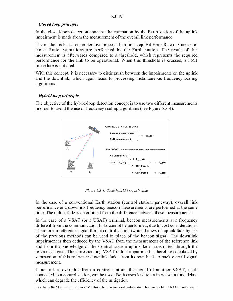
5.3-19

Closed loop principle

In the closed-loop detection concept, the estimation by the Earth station of the uplinkimpairment is made from the measurement of the overall link performance.

The method is based on an iterative process. In a first step, Bit Error Rate or Carrier-to-Noise Ratio estimations are performed by the Earth station. The result of thismeasurement is afterwards compared to a threshold, which represents the requiredperformance for the link to be operational. When this threshold is crossed, a FMTprocedure is initiated.

With this concept, it is necessary to distinguish between the impairments on the uplinkand the downlink, which again leads to processing instantaneous frequency scalingalgorithms.

Hybrid loop principle

The objective of the hybrid-loop detection concept is to use two different measurementsin order to avoid the use of frequency scaling algorithms (see Figure 5.3-4).

CONTROL STATION or VSAT

Beacon measurement " Aup (C)

CNR measurement

U or V-SAT : if low-cost constraints � no beacon receiver

A : CNR from C

" Adown(A)

Given Aup (C) " Aup(A)

A : CNR from A

or

A : CNR from B " Aup(B)

A

C B

Figure 5.3-4: Basic hybrid-loop principle

In the case of a conventional Earth station (control station, gateway), overall linkperformance and downlink frequency beacon measurements are performed at the sametime. The uplink fade is determined from the difference between these measurements.

In the case of a VSAT (or a USAT) terminal, beacon measurements at a frequencydifferent from the communication links cannot be performed, due to cost considerations.Therefore, a reference signal from a control station (which knows its uplink fade by useof the previous method) can be used in place of the beacon signal. The downlinkimpairment is then deduced by the VSAT from the measurement of the reference linkand from the knowledge of the Control station uplink fade transmitted through thereference signal. The corresponding VSAT uplink impairment is therefore calculated bysubtraction of this reference downlink fade, from its own back to back overall signalmeasurement.

If no link is available from a control station, the signal of another VSAT, itselfconnected to a control station, can be used. Both cases lead to an increase in time delay,which can degrade the efficiency of the mitigation.

[Filip 1996] describes an OSI data link protocol whereby the imbedded FMT (adaptive

5.3-20

main advantage of such an approach is that fade detection and the requiredcommunication of FMT specific information between transmitter and receiver areinherently provided by an appropriate extension of the standard OSI Layer 2 protocol.In such a case, there is no need to discriminate between up and down link fades, whichmay improve upon the overall accuracy since there is no need for instantaneousfrequency scaling. This technique bases its decision and actions on the actual quality ofthe received data. It can thus be considered as objective since it does not rely on someopen loop parameters of the physical channel.

Comparative evaluation

The objective of this paragraph is to compare the relative performances of these three detectionconcepts. Therefore, some steps that are involved in each scheme, such as scintillation filtering ordetermination of clear sky attenuation (see Chapter 2.1), will not be developed here.

Open-loop detection scheme

The relative efficiency of the open-loop detection scheme depends on the accuracy ofboth beacon measurements and frequency scaling.

Beacon measurements are affected by instrumental drifts such as: instabilities of theEarth station radio-frequency chain, variations of the satellite EIRP (transmitted power,pointing accuracy, platform instabilities), and thermal noise. With a good calibrationdevice, a relative accuracy of ±1 dB can be obtained [Castanet et al., 1997], whichshould be adequate for FMT [Willis and Evans, 1988].

As far as frequency scaling is concerned, several factors have to be processed,corresponding respectively to gas, cloud and rain attenuations, and also to scintillationand depolarisation [Sweeney et al., 1992; Rucker, 1994; Salonen et al. 1994; ITU-R,1994; Mauri et al. 1996]. Experiments realized in the framework of the ACTScampaign (USA) have demonstrated that an accuracy better than ±2.5 dB can beobtained in processing only rain attenuation and clear sky scintillation fixed frequencyscaling ratios [Dissanayake, 1996]. At Ku band (INTELSAT VI experiment), anaccuracy better than ±1.5 dB has been obtained by same authors [Dissanayake et al.,1993].

At Ka band, the indirect estimation of the down link attenuation has to be scaledaccording to the ratio of the frequencies, by a factor of approximately (f2/f1)

1.72.Consideration must be given to the uncertainty of the instantaneous ratio between thetwo attenuations (particularly important for 20/30 GHz), which can be rather dispersed,especially in the case when rain is not the only cause of fading.

The ratio between rain attenuations has been studied during [COST 205, 1985]; it wasfound that for outage probabilities lower than say 0.1% (rain effect prevailing), thisratio, r, can be considered a log-normal variate whose standard deviation rlnm is 0.13and whose median is given by the almost constant ratio between the equiprobableattenuation values (approximately r50% = (f2/f1)

1.72; <ln r � 1.72. ln (f2/f1).

This has been confirmed by OLYMPUS [Poiares-Baptista and Davies, 1994] andITALSAT measurements.

Closed-loop detection scheme

The relative efficiency of the closed-loop detection scheme depends on both overall linkf d f li

5.3-21

It is interesting to consider the type of measurement to realise. Two kinds ofmeasurements are theoretically possible: Carrier-to-Noise Ratio or Bit Error Ratemeasurements performed by the Earth station. In the case of BER estimations, it isnecessary to have a sufficient number of errors to obtain an accurate BER and thereforeto be able to conclude about the fade level. Consequently, extra time delays, whichincrease with decreasing data rate, have to be taken into account before theimplementation of the mitigation. The following points must be considered:

• While propagation conditions are in the range of the system margin, BER will be too small(typically about 10-7 - 10-9) to allow accurate BER measurements in real-time. In this case,Carrier-to-Noise Ratio seems more suitable for fade detection.

• When propagation conditions are leading to the crossing of the system margin, BER isincreasing extremely quickly. In this case, there will not be enough time to adjust the mitigation.Full capacity will then likely be used.

Therefore, even if Carrier-to-Noise Ratio does not allow to carry out measurements withhigh accuracy, it seems to be more suitable for propagation impairment detection.However, when concatenated codes are implemented, reliable BER measurements canbe made at the output of the inner decoder.

Secondly, reliable propagation measurements are difficult to achieve from the signaltransmitted by the satellite repeater. Instrumental drifts include, as in the beacon case:contribution of thermal noise, instabilities of the Earth station radio-frequency chain,variations of the satellite EIRP due to pointing errors of the satellite receiving antennaand especially the instantaneous repeater gain which is not known with a good accuracy(5 3 dB uncertainty). Moreover, the dynamic range of the measurement (with respect tothe beacon one) is lower, because the measurement includes both uplink and downlinkattenuations.

In addition it is necessary to discriminate up and downlink contributions to propagationimpairments, which implies the use of instantaneous frequency scaling algorithms as inthe open-loop scheme. Another approach has been proposed [Willis and Evans, 1988]:to monitor many carriers from different Earth stations. As only a small proportion of thecarriers is likely to be attenuated at the same time, the knowledge of the number offaded carriers makes it possible to deduce whether the propagation impairment affectingthe useful carrier is on the up or the downlink (a relatively homogeneous attenuation ofall carriers suggesting a downlink impairment).

In conclusion, measurements of overall link performances are not really accurate withrespect to beacon measurements. Such measurements have been carried out in the past,in particular with the OTS satellite and were abandoned for this reason.

Hybrid detection scheme

A hybrid detection scheme is characterised by the best performances in term ofaccuracy, since it uses beacon measurements without using frequency scalingalgorithms.

In fact, the limitation of this concept is firstly linked to the delay involved in carryingout the measurement before the introduction of the mitigation. This extra-delay, whichrepresents half a hop (station to satellite) in the case of a control station, increases to ahop and a half in the case of a VSAT. For a geostationary satellite, this extra time delayranges from 125 ms for a control station to 375 ms for a VSAT terminal.

Secondly as two signals have to be processed the processing delay is double In fact it

5.3-22

time necessary to filter scintillation in real time is about 10 s, as the mean fade slopeduring an event is about 0.2 dB/s at Ka-band (0.1 dB/s at Ku-band), the total extra-delayintroduced can cause an error of ±2 dB at Ka-band (±1 dB at Ku-band) [Poiares-Baptista and Davies, 1994; Ortgies, 1996].

Comparative analysis

The comparison between the detection concepts defined above is made mainly betweenopen-loop and hybrid-loop schemes.

The interest of a basic closed-loop scheme is to avoid the implementation of a specificbeacon receiver that would increase the cost of VSAT terminals. However, thisdetection concept is not very attractive, since it keeps the drawback of open-loop(frequency scaling) without the advantages (simplicity, accuracy of measurements). Infact, the feasibility of FMT based on this control scheme seems to be doubtful.

The advantages of the open-loop detection scheme are a good accuracy and a gooddynamic range for the beacon measurements. This concept is quite simple and low-cost.In addition, differently from both of the following concepts, the open-loop methodofferss the advantage of not implying an extra allocation of system resources. Theeffectiveness is actually only conditioned by the knowledge of the instantaneousfrequency scaling ratio which varies in a significant way during convective events.However, experiments carried out in the USA [Dissanayake et al., 1993; Dissanayake,1997] have demonstrated that accuracies of ±1.5 dB at Ku-band and ±2.5 dB at Ka-bandcan be achieved with fixed frequency scaling ratios.

As far as the hybrid-loop detection scheme is concerned, the accuracy of the methoditself is better than in closed-loop because it is not necessary to use frequency scaling.The improved accuracy is balanced by a more complex system architecture andtherefore by an increase in cost. In addition, this concept is characterised by extra timedelay, which induces a new error contribution, which can be of the same order as open-loop accuracy for small low-cost terminals.

The different error contributions for a system operating at Ka-band are summarised inTable 5.3-5, these contributions being summed in a quadratic way:

Error contribution Open-loop Closed-loop Hybrid-loopMeasurement accuracy ± 1 dB ± 3 dB ± 1 dBFrequency scaling ± 2.5 dB ± 2.5 dB /Processing time delay ± 2 dB ± 2 dB ± 2 dBExtra time delay / / ± 2 dBTotal error budget ± 3.4 dB ± 4.4 dB < ± 3 dB

Table 5.3-5: Example of error budget at Ka-band

It appears that the interest of open-loop or hybrid-loop schemes depends on the systemarchitecture and on the frequency band. Indeed, according to the relative differencebetween uplink and downlink frequencies, the accuracy of frequency scaling algorithmsmay or may not be acceptable.

Table 5.3-6 gives the results of the technical analysis in relation to frequency band(without considerations of cost), the analysis being essentially conditioned by frequencyscaling accuracy.

5.3-23

Frequency Bands Ku FSS Ku BSS Ka V EHFuplink frequency 14 GHz 18 GHz 31 GHz < 50 GHz 44 GHzdownlink frequency 12 GHz 12 GHz 21 GHz > 40 GHz 21 GHz6F / Fdown 17 % 50 % 48 % < 25 % 110 %

appropriated mode open loop open loop orhybrid loop

open loop orhybrid loop

open loop hybrid loop

Table 5.3-6: Suitability according to frequency band

For instance, at Ku-band the accuracy of frequency scaling is quite good, therefore itdoes not seem useful to implement a hybrid-loop detection scheme which is morecomplicated and expensive than an open-loop scheme. On the contrary, at EHF band,uplink and downlink frequencies are relatively far apart, which leads to the preferencefor the hybrid-loop concept.

5.3.2.3 Predictive control

All the detection concepts defined in previous paragraphs can be considered as a posterioritechniques, since the system is able to react only after detection of an event. Therefore, extra timedelay is introduced when processing detection of an event and estimation of the mitigation to becarried out, which implies a delay in the activation of the FMT.

This extra time delay leads to other error contributions that could be reduced through theimplementation of real-time predictions at the terminal level. Actually, two kinds of prediction canbe realised in real time: instantaneous frequency scaling ratio and channel behaviour predictions.

Instantaneous frequency scaling ratio

As already mentioned, the frequency scaling ratio can exhibit a strong variation during an event,specially for convective rain. This behaviour is characterised by a hysteresis effect [Sweeney et al.,1992], mainly caused by dynamic variations of drop size distribution, effective path length throughthe precipitation and antenna effects [Dintelmann et al., 1993].

Results from [Rucker, 1994] obtained during the OPEX campaign have shown that errors due to theuse of a fixed frequency scaling ratio can reach up to ±4 dB [Ortgies, 1993]. An improvement canbe made to the method, either by the introduction of a variable frequency scaling ratio [ITU-R,1994], or by the modelling of the inhomogeneity of the medium from differential attenuation andphase measurements [Ortgies, 1993].

[Gremont and Filip, 1998] proposed an open-loop statistical model for the instantaneous frequencyscaling of rain attenuation. This model considers the impact of random variations in rain drop sizedistribution on the scaling factor. The model is further developed for inclusion in fade predictionschemes required in FMTs.

Instantaneous frequency scaling procedures recommended in [ITU-R, 1994] only take into accountrain attenuation. In reality, other effects, such as gaseous, cloud and melting layer attenuation aswell as scintillation (in both clear sky and clouds) and depolarisation (due to rain and ice), must beconsidered. Some procedures have been proposed to calculate frequency scaling ratios due to gasand clouds [Salonen et al., 1994], scintillation [Ortgies and Rucker, 1992] and depolarisation[Mauri et al., 1996].

It may also prove important to consider the impact of the variability of the scaling factor ofscintillation variance. To date the ITU-R only proposes a fixed value for this scaling factor.However there is experimental evidence that the ratio is highly random Such models can naturally

5.3-24

be included in advanced detection schemes relying on a variable detection margin [Gremont et al.,1999b].

Short term prediction of the channel behaviour

Such methods aim to estimate the channel behaviour in real-time, so that the system can react at themoment where the event is occuring, rather than afterwards. In other words, it aims to determineattenuation at time t + 6t, from the attenuation at time t. To reach this objective, real-timepredictions of fade slope have to be carried out [Gallois, 1993; Willis and Evans, 1988].

In the frame of the OPEX campaign [Poiares-Baptista and Davies, 1994], the feasibility of short-term prediction of the propagation channel behaviour, and the interest of introducing fade slope datawere demonstrated. An autocorrelation analysis was carried out on a 30 GHz OLYMPUS event, andshowed that attenuation correlation time was more than 100 seconds, whereas that for scintillationwas less than 2 seconds, for the same event. In addition, it was demonstrated that the introduction offade slope data could improve the prediction, although the improvement was not relevant for thisparticular event. In Chapter 6.2, a practical application is given of the use of the fade slopeinformation to predict in real time the behaviour of the propagation channel for a Ka-bandvideoconference VSAT system [Vasseur et al., 1998].

An advanced short-term predictor using a self-tuning minimum-variance algorithm has been appliedsuccessfully to Olympus Ka band data. This was then used for the estimation of the performance ofadaptive coding and adaptive symbol rate FMTs [Gremont et al., 1996, 1997]. The self-tuningpredictor has been characterised on a long-term basis and a statistical model has been developed toestimate the impact of fade detection/prediction on the overall performance of practical FMTsystems. The self-tuning predictor has also been compared to more classical schemes such as theslope-based predictor and the self-tuning predictor was found superior [Gremont, 1997]. Due to itsself-tuning property the predictor will track naturally the changes in fade dynamics due to the non-stationarity of the rain process. Finally, since it is based on a minimum variance criterion, it can alsobe used to separate rain/cloud attenuation from amplitude scintillations in a quasi optimum way.This is particularly useful if instantaneous frequency scaling of each fading component is needed.

Management of FCM resources can also be made using Neural Networks. [Mayligin et al., 1996]describe a generic FMT controller which relies on an artificial neural network. Here the fadeprediction and the countermeasure decision are merged into a single subsystem which can drive theembedded FMT directly. A first stage estimates mean attenuation and scintillation standarddeviation. Decision thresholds are then implemented and give as an output the required FMT settingfor the detected/predicted propagation conditions.

5.3.3 Conclusion

This chapter has presented the work carried out and the results obtained in the framework of the"System and simulation issue" Working Group of COST 255.

In the first part, an overview has been presented of the state-of-the-art in the field of FMT tocounteract impairments caused by tropospheric propagation to Ka-band and EHF Earth-spacetelecommunications systems . Three types of FMT have been identified: Power Control, SignalProcessing and Diversity techniques.

It has been demonstrated that some techniques, such as ULPC or DRR, are very flexible becausethey mainly have an impact only on the terminal. Other techniques, such as AC, AM or SD, lead toa re-allocation of the system resources and therefore cannot be applied without considering multipleaccess schemes and protocol issues.

In addition, the choice of a combination of FMTs to implement in a satcom system will depend

5.3-25

systems in which high performance Earth stations (hubs, gateways, trunking systems) are involved.ASP techniques would be more suitable for VSAT systems in which SSPAs should be used at theirmaximum power (main part of the user terminal cost) in order to offer the highest possible data rateto the user.

This work points out two important aspects for new systems operating from Ku to V bands:

• On the one hand, it appears that each FMT is adapted to a specific range of availability. Thismeans that these fade mitigation methods are quite complementary and can be implementedsimultaneously (combined techniques) to extend the availability range of requirements.Following some conclusions of the COST 235 project and [Vasseur et al., 1998], this reportshows that Ka and EHF band satellite telecommunications systems with high service availabilityare technically possible only if a combination of different s (Mixed FMTs) is implemented.

• On the other hand, each method implemented individually can compensate only relatively smallpropagation impairments. It will be possible to selectively improve the performance of themitigation to a large extent, by carrying out a combination of different kinds of FMT when thereis a need to transmit a high priority type of information [Vasseur et al., 1998].

In a second section, developments carried out in the framework of COST 255 in the field of FMThave been synthesised.

However, FMT cannot be applied without a knowledge of real-time propagation conditions fromfade detection. Accurate instantaneous estimation of fade dynamics (fade and interfade duration,fade slope, fade depth…) is required, with only a short time delay before the introduction of thecompensation.

5.3-26

5.3.4 References

[Acosta, 1997]Acosta R.J., "Rain fade compensation alternatives for Ka-band communication satellites", 3rd Ka-band Utilization Conference, Sorrento, Italy, 15-18 Sept. 1997.

[Allnutt and Rogers, 1993]Allnutt J.E., Rogers D.V., "Recent developments in propagation counter-measures for VSATservices", ICAP'93, Heriot-Watt University, UK, 30 March - 2 April 1993.

[Cacopardi et al., 1993]Cacopardi S., Martinino F., Reali G., "Power control techniques performances evaluation in theSCPC/DAMA access scheme", European Conference on Satellite Communications, Manchester,UK, 2-4 November 1993.

[Capsoni et al., 1990]Capsoni C., Matricciani E., Mauri M., "Sirio-Ots 12-GHz orbital diversity experiment at Fucino",IEEE Trans. on Ant. and Prop., Vol. 38, n°6, pp. 777-782, June 1990.

[Capsoni and Matricciani, 1985]Capsoni C., Matricciani E., "Orbital and site diversity systems in rain environment: radar-derivedresults", IEEE Trans. on Ant. and Prop., Vol. 33, n°5, pp. 517-522, May 1985.

[Carassa and Tartara, 1988]Carassa F., Tartara G., "Frequency diversity and its applications", Int. Journ. of Sat. Com., Vol. 6,pp. 313-322, June 1988.

[Castanet et al., 1997]Castanet L., Lemorton J., Roy P., Dufourg A., Marsault T., Destruhaut F., Grely S., Le Boulc'h D.,"EXPRESS: EXperimentation of PRopagation in the Ehf-band from the satellite STENTOR",ICAP'97, Edinburgh, 14-17 April 1997.

[COST 205, 1985]COST Project 205a, "Prediction of Rain Attenuation Statistics from Point Rainfall Intensity Data",Report EUR 9923 EN, 1985.

[COST 235, 1996]COST Project 235, "Radiowave propagation effects on next generation fixed-services terrestrialtelecommunications systems", Final report, n° EUR 16992 EN, Chapter 3, pp. 159-168, 1996.

[Dintelmann et al., 1993]Dintelmann F., Ortgies G., Rucker F., Jakoby R., "Results from 12-30 GHz German propagationexperiments carried out with radiometers and the OLYMPUS satellite", Proc. of the IEEE, Vol. 81n°6, June 1993.

[Dissanayake et al., 1993]Dissanayake A.W., Lin K.T., Zaks C., Allnutt J.E., "Results of an experiment to demonstrate theeffectiveness of open-loop up-link power control for Ku-band satellite links", ICAP'93, Edinburgh,UK, 30 March - 2 April 1993.

[Dissanayake, 1997]Dissanayake A.W., "Application of open-loop uplink power control in Ka-band satellite links",Proc. of the IEEE, Vol. 85, n°6, June 1997.

[Dissanayake, 1996]Dissanayake A.W., "Fade mitigation techniques at Ka-band", NAPEX XX, Fairbanks, Alaska,USA, June 4-6 1996.

5.3-27

[Dodel and Riedl, 1991]Dodel H., Riedl C., "Can ULPC double satellite capacity ?", 2nd Euro. Conf. on Sat. Com., Liège,Belgium, 22-24 Oct. 1991.

[Egami, 1982]Egami S., "Individual closed-loop satellite access power control system using overall satellite linkquality level", IEEE Trans. Com., Vol. 30, n°7, July 1982.

[Filip, 1996]Filip M., "OSI Layer 2 Protocol for a fade countermeasure system",COST 255 CP23001, November1996.

[Filip and Vilar, 1990]Filip M., Vilar E., "Implementation of adptive modulation as a fade countermeasure", Int. Jour. ofSat. Com., Vol. 8, pp. 33-41, June 1990.

[Gallois, 1993]Gallois A.P., "Fade countermeasure techniques for satellite communication links", Int. Symp. onComms Theory and Applications, July 1993.

[Gremont, 1997]Gremont, B.C. "Fade Countermeasure modelling for Ka band digital satellite links", PhD thesis,Coventry University, 1997.

[Gremont et al., 1996]Gremont B.C., Gallois A.P., Bate S., "Efficient fade compensation for Ka band VSAT systems",Proc, 2nd Int. Ka band Utilization Conf. And workshop on SCGII, Florence, Italy, pp 439-443,1996.

[Gremont et al., 1997]Gremont B.C., Gallois A.P., Bate S., "Predictive fade countermeasures for Ka band satellitesystems", IEE Conf. On Ant. And Prop., Edinburgh (UK), IEE, Vol. No 2, pp 164-168, 1997.

[Gremont and Filip, 1998]Gremont B.C, Filip M., "Modelling the instantaneous frequency scaling of rain attenuation andapplications", 1st int. Workshop on radiowave propagation modelling for SatCom services at Kaband and above, ESTEC, Noordwijk, The Netherlands, 28-29 Oct. 1998, pp 269-276.

[Gremont and Filip, 1999]Gremont B.C, M. Filip, "Simulation Test Case 1: Ku band System performance Long termanalysis", COST CP73021, March 1999.

[Gremont et al., 1999a]Gremont B.C, Filip M., Vilar E., "Simulation of a high frequency satellite link with a fadecountermeasure", IEE Conf. On Ant. And Prop., York (UK), March-April 1999, IEE Conf. Publ.No 461, pp 164-168, 1999.

[Gremont et al., 1999b]Gremont B.C., Gallois A.P., Filip M., Bate S., "Comparative analysis and performance of twopredictive fade detection schemes for Ka band countermeasures", IEEE J. on selected areas inComms, Special issue on direct-to-user satellite systems at Ka band and beyond, Vol. 17 No 2,February 1999, pp 180-182, 1999.

[Hartigan and Gallois, 1993]Hartigan P.F.- Gallois A.P., "The use of satellite imagery for forecasting rain attenuation", 8thICAP, Edinburgh, UK, March - April 1993.

[Hörle, 1988]H l J "U li k l f lli E h i f d f 20/30 GH

5.3-28

[ITU-R, 1994]ITU-R, "Propagation data and prediction methods required for Earth-Space telecommunicationssystems", CCIR Rec., Propagation in non-ionised media, RPN serie, Rec. 618-3, Geneva, 1994.

[Jones and Watson, 1993]Jones S.M.R., Watson P.A., "Attenuation and countermeasures in millimeter-wave point-to-multipoint networks", Radio Science, Vol. 28, n°6, pp. 1057-1069, Nov. - Dec. 1993.

[Karasawa and Maekawa, 1997]Karasawa Y., Maekawa Y., "Ka-band Earth-space propagation research in Japan", Proc. IEEE,Vol. 85, n°6, June 1997.

[Kerschat et al., 1993]Kerschat K., Koudelka O., Riedler W., Tomlinson M., Hughes C.D., Hörle J., "A variable spread-spectrum fade countermeasure system for the DICE video conference system", Proc. Olympus Util.Conference, Seville, Apr. 1993.

[Kreuer et al., 1994]Kreuer D., Radaermacher A., Martin S., Frach T., "A prototype adaptive fade countermeasuresystem for TDMA operation at Ka-band", PIMRC'94, The Hague, The Netherlands, Sept. 1994.

[Mayligin et al., 1996]Malygin A., Filip M., Vilar E.: "Development of a digital modem for adaptive countermeasureVSAT system at Ka-band", Second Ka-band Utilization Conference, Firenze, Italy, Sept. 1996.

[Maral and Bousquet, 1998]Maral G., Bousquet M., "Satellite Communications Systems", 2nd ed., John Wiley & Sons, 1998.

[Matricciani and Mauri, 1995]Matricciani E., Mauri M., "Italsat-Olympus 20-GHz orbital diversity experiment at Spino d'Adda",IEEE Trans. on Ant. and Prop., Vol. 43, n°1, pp. 105-108, Jan. 1995.

[Mauri et al. 1996]Mauri M., Paraboni A., Pawlina-Bonati A., Polonio R., Riva C., "The main results of the ITALSATpropagation experiment at 18.7, 39.6 and 49.5 GHz", 2nd Ka-band Utilization Conference,Florence, Italy, 24-26 Sept. 1996.

[Poiares-Baptista and Davies, 1994]Poiares-Baptista P. and Davies P. (Editors), " OPEX, Reference Book on Attenuation Measurementand Prediction", 2nd Workshop of the OLYMPUS Propagation Experimenters (OPEX), Doc. ESA-ESTEC-WPP-083, vol. 1, Noordwijk, The Netherlands, Nov. 1994.

[Poiares-Baptista and Paraboni, 1995]Poiares Baptista P., Paraboni A., "Active compensation techniques for spacecraft antennas", ESApublication, "Preparing for the future", vol. 5, n°1, March 1995.

[Ortgies and Rucker, 1992]Ortgies G., Rucker F.: "Frequency scaling of slant-path amplitude scintillations", URSI OpenSymp. on Wave Propagation and Remote Sensing, Ravenscar, UK, June 1992.

[Ortgies, 1993]Ortgies G., "Dynamics of satellite slant-path attenuation: consequences for up-link power control",XXIVth General Assembly of the International Union of Radio Sciences, Kyoto, 1993.

[Ortgies, 1996]Ortgies G., "Analysis of Ka-band attenuation effects measured with radiometers and beacons of theITALSAT satellite", 2nd Ka-band Utilization Conference, Florence, Italy, 24-26 Sept. 1996.

5.3-29

[Proakis, 1995]Proakis J.G., "Digital Communications", Mc Graw-Hill Int. Ed., Electrical Engineering Series,Third Edition, 1995.

[Pujante and De Haro, 1998]Pujante A., De Haro L., "Satellite communications C/Iintermodulation improvement in rain fadeconditions by means of simulated annealing iptimization as a mitigation technique", COST 255document, CP53009, May 1998.

[Rucker, 1994]Rucker F.: "The impact of the variation of instantaneous attenuation frequency scaling factors onUp-Link Power Control", AEÜ, Vol. 48, n° 2, 1994.

[Salonen et al. 1992]Salonen E., Karhu S., Jokela P., Zhang W., Uppala S., Aulamo H., Sarkkula S., and Poiares BaptistaP., "Modelling and calculation of atmospheric attenuation for low-fade-margin satellitecommunications", ESA Journal, Vol. 16, n° 3, pp. 299-317, 1992.

[Salonen et al. 1994]Salonen E., Karhu S., Uppala S., Hyvönen R., "Study of improved propagation predictions",ESTEC report 9455/91/NL/LC(SC), December 1994.

[Schnell and Von Hugo, 1998]Schnell M., Von Hugo D., "Fade countermeasures and adaptive resource sharing for anexperimental TDMA satellite communications system operating at Ka-band",TelecommunicationTransmission, Vol. 9, nº 6, December 1998.

[Sweeney et al., 1992]Sweeney D.G., Pratt T., Bostian C.W., "Hysteresis effects in instantaneous frequency scaling ofattenuation on 20 and 30 GHz satellite links", Electronics Letters, Vol. 28, n°1, 2 Jan. 1992.

[Tartara, 1989]Tartara G., "Fade countermeasures in millimetre-wave satellite communications: a survey ofmethods and problems", Proc. Olympus Util. Conference, Vienna, Austria, April 1989.

[Vasseur et al., 1998]Vasseur H., Czarnecki M., Castanet L., Bousquet M., "Performance simulation of a Ka-band VSATvideoconferencing system", First International Workshop on "Radiowave propagation modelling forsatcom services at Ku-band and above", Noordwijk, The Netherlands, October 1998.

[Willis and Evans, 1988]Willis M.J., Evans B.G., "Fade countermeasures at Ka-band for OLYMPUS", Int. J. Sat. Com.,Vol. 6, pp. 301-311, June 1988.

5.3-30

5.3.5 List of acronyms

AC Adaptive Coding

AFS Attenuation due to Free Space

AGC Automatic Gain Control

AM Adaptive Modulation

AP Attenuation due to tropospheric Propagation

ARS Adaptive Resource Sharing

ASP Adaptive Signal Processing

B receiver noise Bandwidth

BSS Broadcasting Satellite Service

C/N Carrier-to-Noise Ratio

CS Cross Shaping

DH Double Hop

DL Down-Link

DLPC Down-Link Power Control

DRR Data Rate Reduction

EIRP Equivalent Isotropic Radiated Power

ES Earth Station

FD Frequency Diversity

FMT Fade Mitigation Technique

FS Fade Spreading

FSS Fixed Satellite Service

G/T figure of merit

IBO Input Back-Off

k Boltzmann's constant

MSS Mobile Satellite Service

OBBS On-Board Beam Shaping

OBEC On-Board EIRP Control

OBO Output Back-Off

OBP On-Board Processing

PC Power Control

SatD Satellite diversity

SD Site Diversity

SEC Simple Extra Coding

SL SateLlite

5.3-31

SSPA Solid state power amplifier

TCM Trellis Coded Modulation

TT&R Telemetry, Telecommand and Ranging

TWTA Travelling Wave Tube Amplifier

UL Up-Link

ULPC Up-Link Power Control

USAT Ultra Small Aperture Terminal

VSAT Very Small Aperture Terminal

PART 6 Test Cases InvolvingFixed Satellite Links

6.1-1

CHAPTER 6.1Ku-Band VSAT Asymmetrical Data

Communication System

Editor: Dr Misha Filip1

Authors: Dr Misha Filip, Dr Boris Grémont2, Mr Peng Zong3, Dr Carlo Riva4

1 University of Portsmouth, Dept. of E&E Engineering, Anlgesea Road, Portsmouth, PO1 3DJ, UK

Tel.: +44-23-9284-2310, Fax.: +44-23-9284-2561, e-mail: misha.filip@port.ac.uk2 University of Portsmouth, Dept. of E&E Engineering, Anlgesea Road, Portsmouth, PO1 3DJ, UK

Tel.: +44-23-9284-2543, Fax.: +44-23-9284-2561, e-mail: boris.gremont@port.ac.uk3 University of Portsmouth, Dept. of E&E Engineering, Anlgesea Road, Portsmouth, PO1 3DJ, UK

Tel.: +44-23-9284-2545, Fax.: +44-23-9284-2792, e-mail: pzong@ee.port.ac.uk4 Politecnico di Milano, CSTS, Dip. Di Elettronica, Piazza Leonardo da Vinci 32, 20133 Milano, Italy

6.1-2

6.1 Ku-Band VSAT Asymmetrical Data Communication System

6.1.1 Overview

This chapter is concerned with an asymmetrical very small aperture terminal (VSAT) datamessaging network operating in Europe at Ku band. The case is broadly based on a commercialnetwork and was considered by Working Group 3 of the COST Action 255 to be a relevant steppingstone to considerations of new types of services at higher frequencies.

Following the system description and specification, the link budgets are developed for a singletwo-way satellite link, between a hub and a VSAT. Statistical propagation models are then appliedto the links, as well as the recorded time series of a propagation measurement campaign in a MonteCarlo simulation of the OSI Layer 2 protocol performance.

The performance of the links is discussed in the concluding part of the chapter.

6.1.1.1 System Description

VSATs in Europe use 14.0-14.25 GHz uplinks and 12.5-12.75 GHz downlinks. These frequenciesare dedicated to fixed satellite services so VSATs can be type-approved instead of being testedindividually. The satellite is EUTELSAT II F4. Both linear polarisations are used to give about450 MHz bandwidth in an occupied band of 250 MHz. Transponder coverage is all of Europe plusthe Azores, Greenland, Finland, Moscow and Jordan (see Figure 6.1-1).

The hub has a 7.2 m diameter antenna and uses 350 W or 600 W TWTAs, though each 512 kbit/soutbound signal contributes only about 1 W into the feed. Such a large hub allows to keep theinbound downlink noise at a low level. Increasing its antenna size would only give rise to marginalimprovements. The VSATs are 1.2 m, with RF power of 1 W or 2 W depending on their position inthe uplink beam, and whether the data rate is 64 or 128 kbit/s.

Modulation is QPSK to save bandwidth, FEC is half–rate with sequential decoding on both inboundand outbound paths. On the inbound path, sequential FEC is used in burst mode (TDMA), lockingand recovering sync. within 16 bit. The system frame length is 45 ms, defined at the hub andbroadcast on the TDM outbound path, and used by each receiver to synchronize its TDMA frame.

With a few specific exceptions, asymmetrical data messaging VSAT links use packet service. Dataconnections, whether X25, SDLC, Ethernet TCP/IP, Token Ring/SNA, or bit transparent, are madeover the satellite link outbound and inbound channels in packets of up to 246 Bytes. There is a linkcontrol protocol which monitors the CRC segment of each packet and requests a retransmission inthe event of packet loss. The system works on positive acknowledgements (ACK), so if an ACK isnot received within a few seconds, the packet is transmitted again.

Packet loss on the satellite link causes an interruption to data flow which is restored when thereplacement packet is received. Interruption of data is manageable by most protocols through theirflow control procedures, and results in a variation of the transit delay, which normally variesanyway by about 0.2 sec around the typical round trip delay of 0.8 sec (Aloha) or 1.4 sec(Transaction reservation).

6.1-3

46 dBW

45 dBW42 dBW

40 dBW

Figure 6.1-1 Eutelsat II F4 coverage

In this environment, it is easy to see that this network takes bit errors in its stride. A BER of 10–6

approximates to a PER of around 10–4, but under occasional stress conditions performance can bean order of magnitude or more worse than this. It is important to ensure that clear sky (95%)conditions have minimal transmission errors, so that there is reasonable customer tolerance to theoccasional slow period. It can be noted that very few complaints are received even for rain fadeevents, which would be seen as a long or very long response time.

Quality Performance Objectives

Bit error rate (BER) of 10–6, Packet error rate (PER) of 10–4, round trip delay 0.8 ± 0.2 s (Aloha)or1.4 ± 0.2 s (Transaction reservation).

Availability Objectives

Clear sky availability 95%, rain event outages not longer than 3 minutes.

6.1.1.2 Performance Evaluation and Simulation

Due to limited resources available for the development and considerations of test cases, only linklevel performance of the test case could be achieved in the time frame allowed. A hypothetical hubat a location in the UK and a VSAT at a location in Italy were defined. A full duplex (forward andreturn) link was considered. The propagation models for both locations were identified and acomprehensive set of the VSAT location attenuation time series recordings selected.

Availability of suitable propagation models for both locations enabled a detailed statisticalevaluation of the inbound and outbound links to take place, whereas the availability of time seriesfor the VSAT location, coupled with the detailed HDLC protocol model available, constrained thetime series simulations to an analysis of the inbound link only.

6.1.2 System Specification and Link Power Budgets

6.1-4

location in Portsmouth, UK, via the Eutelsat II F4 satellite to the VSAT at Spino d’Adda, Italy. Theinbound from the VSAT to the hub complemented the full duplex link.

The general approach to specifying the key system parameters was to bring them up as required forthe purposes of link power budget calculations. The link power budget calculations were based onideal propagation conditions (’clear sky’) and did not take into account any propagation phenomenaother than propagation through free space. This was done on purpose. Although a Ku band systemcan well be designed by simply considering the excess atmospheric attenuation for a given targetavailability criterion, the philosophy for the design of new satellite services should be based oncareful consideration of the propagation effects at both earth station sites. The link power budgetthus becomes a dynamic equation which, at best, reduces itself to the clear sky case. Considerationof the joint propagation statistics should lead to a more optimum final link design.

6.1.2.1 General Information

Sub-satellite point longitude, ls 7° E

Satellite orbit radius, rs 42242 km

Earth radius, re 6370 km

Hub latitude, Le(H), and longitude, le(H) Latitude 50.78° N ; Longitude 1.09° W

´¦¥²

¤£ <<+=

e(H)l

sl

e(H)L

er

sr2

er2

sr

HR coscos2 38576 km, distance from the hub to

satellite

)cos(cos21

)))cos(ossin(acos(cacos

e(H)lsle(H)L

srer

2

srer

e(H)lsle(H)L

H

<<+

<=

´¦¥²

¤£´

¦¥²

¤£

¡ 31.36°; elevation angle of the hub-to-satellite path

VSAT latitude, Le(V), and longitude, le(V) Latitude 45.5° N ; Longitude 9.5° E

´¦¥²

¤£ <<+=

e(V)l

sl

e(V)L

er

sr2

er2

sr

VR coscos2

38054 km, distance from the VSAT tosatellite

)cos(cos21

)))cos(ossin(acos(cacos

e(V)lsle(V)L

srer

2

srer

e(V)lsle(V)L

V

<<+

<=

´¦¥²

¤£´

¦¥²

¤£

¡ 37.65°; elevation angle of the VSAT-to-satellite path

Speed of light, c 300,000 km/s or 3*108 m/s

Boltzmann’s constant, 10log10 k -228.6 dBK-1

/ 3.14...

TWT power 13 dBW

Satellite figure of merit (G/T)s 4.5 dB/K

EIRP Downlink, EIRPs 46 dBW

Transponder bandwidth 36 MHz

Antenna max transmitting gain, Gt 33dBi

Antenna max receiving gain, Gr 34dBi

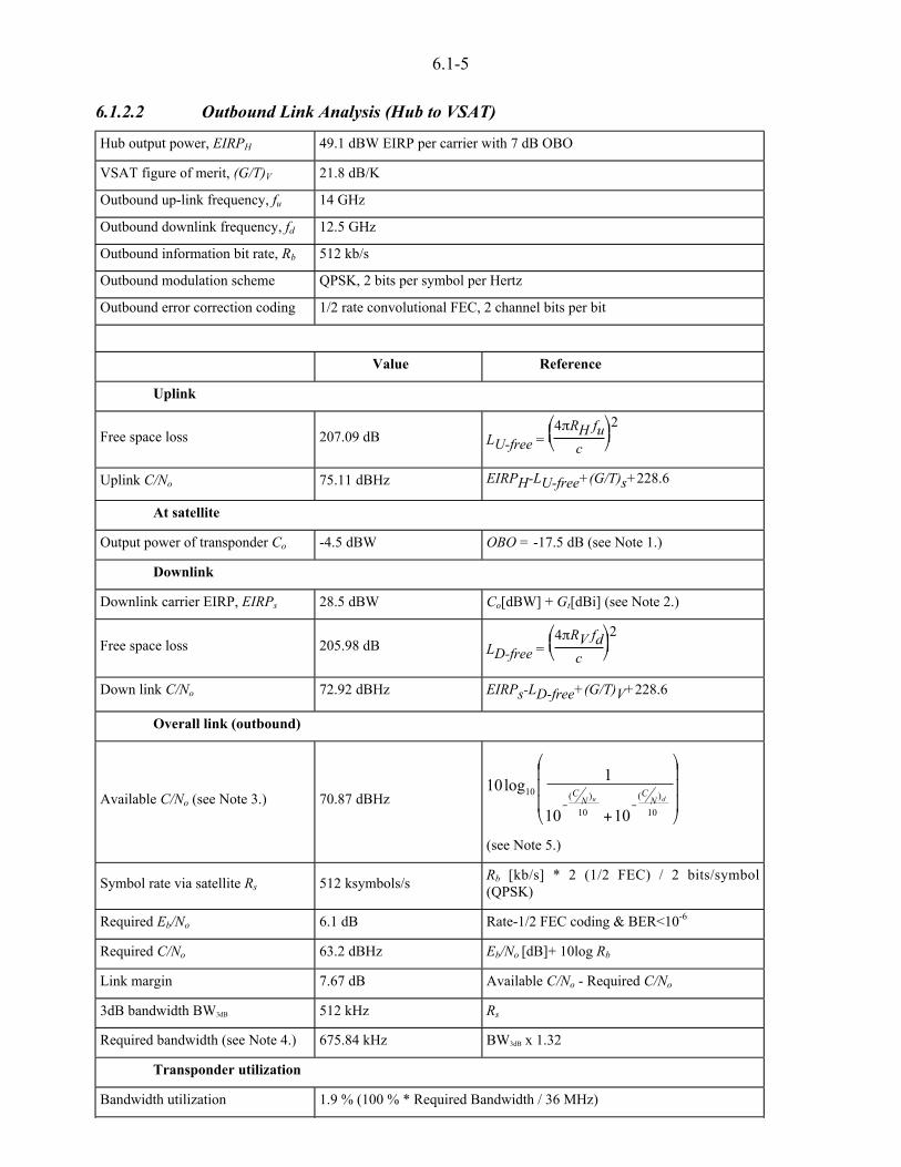
6.1-5

6.1.2.2 Outbound Link Analysis (Hub to VSAT)

Hub output power, EIRPH 49.1 dBW EIRP per carrier with 7 dB OBO

VSAT figure of merit, (G/T)V 21.8 dB/K

Outbound up-link frequency, fu 14 GHz

Outbound downlink frequency, fd 12.5 GHz

Outbound information bit rate, Rb 512 kb/s

Outbound modulation scheme QPSK, 2 bits per symbol per Hertz

Outbound error correction coding 1/2 rate convolutional FEC, 2 channel bits per bit

Value Reference

Uplink

Free space loss 207.09 dB LU-free = ¤²£

¦́¥4/RH fu

c

2

Uplink C/No 75.11 dBHz EIRPH-LU-free+(G/T)s+228.6

At satellite

Output power of transponder Co -4.5 dBW OBO = -17.5 dB (see Note 1.)

Downlink

Downlink carrier EIRP, EIRPs 28.5 dBW Co[dBW] + Gt[dBi] (see Note 2.)

Free space loss 205.98 dB LD-free = ¤²£

¦́¥4/RV fd

c

2

Down link C/No 72.92 dBHz EIRPs-LD-free+(G/T)V+228.6

Overall link (outbound)

Available C/No (see Note 3.) 70.87 dBHz ´´´

¦

¥

²²²

¤

£

+<<

10

)(

10

)(10

1010

1log10

du NC

NC

(see Note 5.)

Symbol rate via satellite Rs 512 ksymbols/sRb [kb/s] * 2 (1/2 FEC) / 2 bits/symbol(QPSK)

Required Eb/No 6.1 dB Rate-1/2 FEC coding & BER<10-6

Required C/No 63.2 dBHz Eb/No [dB]+ 10log Rb

Link margin 7.67 dB Available C/No - Required C/No

3dB bandwidth BW3dB 512 kHz Rs

Required bandwidth (see Note 4.) 675.84 kHz BW3dB x 1.32

Transponder utilization

Bandwidth utilization 1.9 % (100 % * Required Bandwidth / 36 MHz)

6.1-6

6.1.2.3 Inbound Link Analysis (VSAT to Hub)

VSAT HPA output power 1 W

VSAT transmit antenna gainGVt = 10log10ª«

©«̈

®«­«¬

d¤²£

¦́¥/Dfu

c

2 = 42.84 dBi

VSAT maximum EIRP, EIRPV 42.84 dBW

Hub figure of merit, (G/T)H 34.5 dB/K

Inbound up-link frequency, fu 14.25 GHz

Inbound downlink frequency, fd 12.75 GHz

Inbound information bit rate, Rb 64 kb/s

Inbound modulation scheme QPSK, 2 bits per symbol per Hertz

Inbound error correction coding 1/2 rate convolutional FEC, 2 channel bits per bit

Value Reference

Uplink

Free space loss 207.13dB LU-free = ¤²£

¦́¥4/RV fu

c

2

Uplink C/No 68.81 dBHz EIRPV-LU-free+(G/T)s+228.6

At satellite

Output power of transponder Co -14 dBW OBO = -27 dB (see Note 1.)

Downlink

Downlink carrier EIRP, EIRPs 19 dBW Co [dBW] + Gt [dBi] (see Note 2.)

Free space loss 206.28 dB LD-free =¤²£

¦́¥4/RH fd

c

2

Down link C/No 75.82 dBHz EIRPs-LD-free+(G/T)H+228.6

Overall link (inbound)

Available C/No (see Note 3.) 68.02 dBHz( ) ( )

´´´´

¦

¥

²²²²

¤

£

+<<

1010

10

1010

1log10

du NC

NC

(see Note 5.)

Symbol rate via satellite Rs 64 ksymbols/sRb [kb/s] * 2 (1/2 FEC) / 2 bits/symbol(QPSK)

Required Eb/No 6.1 dB 1/2FEC coding & BER<10-6

Required C/No 54.16 dBHz Eb/No [dB]+ 10log Rb

Link margin 13.86 dB Available C/No - Required C/No

3dB bandwidth BW3dB 64 kHz Rs

Required bandwidth (see Note 4.) 84.48 kHz BW3dB x 1.32

Transponder utilization

Bandwidth utilization 0.0236 % (100 % * Required Bandwidth / 36 MHz)

6.1-7

6.1.2.4 Notes on Link Budget Calculations

1. Based on the assumption of the balance of power and bandwidth resource sharing, if the signaloccupies p% of the transponder bandwidth, it should not have more than p% of the total power. Arounded OBO decibel value is specified which, when expressed as a percentage of the total poweravailable does not exceed p% of the total power.

2. Assuming that all Antenna losses are 0, Lpol = Lfeed = Lpoint = 0 dB.

3. If the various other interference/noise powers had been added (apart from the additive whiteGaussian noise), the result would have been worse by some 2 dB for the outbound link and by 5 dBfor the inbound link.

4. Based on a 40% roll–off filter: Required Bandwidth = 1.32 x BW3dB

5. The links are considered in isolation, i.e. no interference calculations have been taken intoaccount. Private communication with Olivetti-Hughes and Eutelsat representatives indicated thatthe dominant interference effect would be from an adjacent satellite on down-links.Worst casereduction of the available CNR would be around 7 dB in both directions, had those effects beenconsidered.

6.1.3 Long Term Link Performance Statistics

This section is concerned with the evaluation of the long term statistics of the performance of theconsidered inbound and outbound links. The approach adopted for evaluation of the statistics isbriefly explained and followed by the results of the numerical analysis. Conclusions are finallypresented in which the link appears not to suffer from the atmospheric effects in the consideredscenario and may well be over–designed.

6.1.3.1 Evaluation Approach

The starting point for the evaluation is the clear sky link power budget. In order to carry out theanalysis properly, four probability cumulative distribution functions are required, for the hublocation at the outbound up–link frequency and the inbound down–link frequency and for the VSATlocation at the outbound down–link frequency and the inbound up–link frequency. In this particularcase, the propagation fading processes are considered to be statistically independent. Thisassumption is justified by the spatial separation of the two sites and can be viewed as a lower boundon possible propagation effects. However, should the separation not be as great, some correlationbetween the processes would have to be considered. The worst case would be a back to back linkwhen there would be perfect correlation between the fading processes on the up and the down link,thus resulting in an upper bound on the effects.

Overall CNR drop

For the outbound link, the up–link C/N0 is 75.1 dBHz which is affected by Hub up–link attenuation.Down–link C/N0 is 72.9 dBHz which is affected by VSAT down–link attenuation. The clear skyavailable C/N0 is 70.9 dBHz.

On the inbound link, the up–link C/N0 is 68.8 dBHz which is affected by VSAT up–linkattenuation. Down–link C/N0 is 75.8 dBHz which is affected by hub down–link attenuation. Clearsky available C/N0 is 68.0 dBHz.

The respective drops of the inbound and outbound CNR may be expressed as transformationfunctions of relevant attenuation variables on a link. Thus,

6.1-8

ª©¨

=

=AA

AA

)(T

)(T

o

iVS

dSH

uo

HSd

SVui

y,yz

y,yz6.1-1

where z is the CNR drop, subscripts i and o denote inbound and outbound links, respectively andsubscripts u and d denote up– and down–link carrier frequencies. V, S and H denote VSAT, satelliteand Hub station respectively and, for example, VzS is the link from VSAT to satellite. Thetransformation functions Ti, To also take into account that the total attenuation only generates extra

thermal noise on satellite down–links.

Although the inbound and outbound links are different (up–link power control is present on theoutbound link), the two links can be analyzed in a similar manner. That analysis can be performedin each case by considering the CNR drop function:

)T( du y,yz = 6.1-2

Statistical Modelling of Attenuation

The statistical analysis of the links requires numerical integration of the transformed input(attenuation) statistics. Probability density functions are required and yet, the usual way ofmodelling the attenuation is by means of a cumulative distribution function, tabulated in a modestnumber of points. Three such distributions were provided by Working Group 1, the [ITU-R, 1999],the EXCELL [Capsoni et al., 1987] and the [ITU-R, 1997] models (also described in Chapter 2.2).

A computationally efficient way of evaluating the long term statistics of a CNR drop is toapproximate the attenuation statistics with lognormal distribution functions. Based on the statisticalmodels for the two locations, the best lognormal models fitting the data were identified byfollowing the procedure defined by [Filip and Vilar, 1990].

Models m mmmm Fit Quality

Average 14 -4.7713 1.67685 Good

Average 12 -5.0246 1.67446 Good

Table 6.1-1 Parameters of lognormal distributions fitted to Hub location statistical models

The values of the lognormal distribution parameters, as well as the quality of fit, are given inTables 6.1-1 and 6.1-2. In the tables “Average 14” and “Average 12” refer to 14 and 12 GHz bands,respectively. The averaging process refers to the cumulative distribution function obtained byaveraging, on an equi-probability basis, the predictions made by the three models.

Models m mmmm Fit Quality

Average 14 -3.84899 1.64333 Good

Average 12 -4.0685 1.63909 Good

Table 6.1-2 Parameters of lognormal distributions fitted to VSAT location statistical models

As the hub and the VSAT locations (Portsmouth and Spino d’Adda, respectively) are widelyseparated, it has been assumed that the attenuations of signals at these two locations are statisticallyindependent i e the joint cdf of attenuation is given by:

6.1-9

{ } { } { }du yProbyProbProb *u*= dudu yyyy , 6.1-3

sif ideal up–link power control (ULPC) with a range of B dBW is employed, it can be shown thatthe joint cdf becomes:

{ } { } { }du yProbByProbProb *u+*= dudu yyyy , 6.1-4

Calculation of CNR drop statistics

Once the joint pdf of up–link and down–link attenuation (Equation 6.1-3 or 6.1-4) is known and thetransformation function (Equation 6.1-2) of the drop in CNR is developed, the long term statisticsof the CNR drop can be computed.

The probability { }zProb )z given that ( )du,yyT=z can be evaluated as:

( ) duy yyzd

ddf ,yu00I

=) zProb 6.1-5

where f is the probability distribution function and I is the the area for which z)z which is alsodelimited by a discrete contour ( ))()( kCk uzd yy = .

Calculation of BER statistics

Once the statistics of the CNR drop is known, it is straight forward to estimate the cdf of the biterror rate. Namely we have:

( ) ( )reqCNRProbBERProb )=* CNRBER 6.1-6

where zBWCNR <<= 10log100CNR and ( )BER1g<=reqCNR . )g(CNRBER = is the BER v. CNR

curve of the particular modulation/coding mode used for transmission over the link. Using all these,(6.1-6) can be rewritten as:

( ) ( )( )BERBWzBER 110 glog10 <<<*=* 0CNRProbBERProb 6.1-7

6.1.3.2 Results

The computation of the cumulative distribution functions of the drop in CNR for the inbound andoutbound links of the Ku band VSAT system was based on the lognormal distribution fitted topropagation models. This was done because there was little difference in the end results whendifferent actual models were used.

Matlab code was written that represented a ’dynamic’ link power budget of the inbound and theoutbound links, including details such as the transponder transfer characteristics and an increase inthe system noise temperature on the down–link. Furthermore, the effects of the up–link powercontrol available on the outbound link were also considered.

The Inbound Link

Figure 6.1-2 shows the contour plot of the drop in the overall carrier to noise spectral density ratiofor the inbound link. Each contour delimits a region of integration for evaluation of the overall CNRdrop cumulative distribution function.

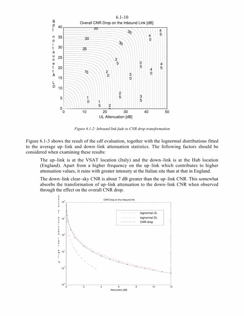
6.1-10

Figure 6.1-2: Inbound link fade to CNR drop transformation

Figure 6.1-3 shows the result of the cdf evaluation, together with the lognormal distributions fittedto the average up–link and down–link attenuation statistics. The following factors should beconsidered when examining these results:

The up–link is at the VSAT location (Italy) and the down–link is at the Hub location(England). Apart from a higher frequency on the up–link which contributes to higherattenuation values, it rains with greater intensity at the Italian site than at that in England.

The down–link clear–sky CNR is about 7 dB greater than the up–link CNR. This somewhatabsorbs the transformation of up–link attenuation to the down–link CNR when observedthrough the effect on the overall CNR drop.

0 2 4 6 8 10 1210

-3

10-2

10-1

100

101

102

Attenuation [dB]

% time that abscissa is exceed

CNR Drop on the Inbound link

lognormal UL

lognormal DLCNR drop

0 10 20 30 40 500

5

10

15

20

25

30

35

4045

25

3040

10

15

15

20

20

25

25

40

35

45

30

30

3535

35

UL Attenuation [dB]

Overall CNR Drop on the Inbound Link [dB]

DL Attenuation [dB

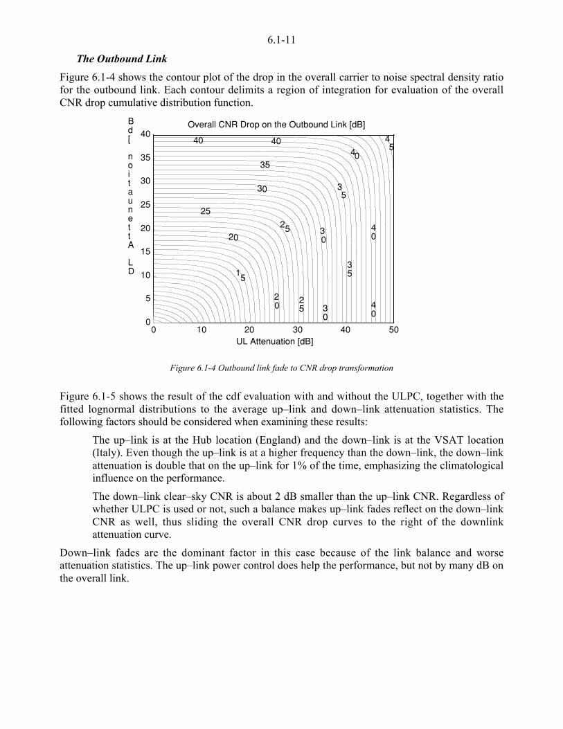
6.1-11

The Outbound Link

Figure 6.1-4 shows the contour plot of the drop in the overall carrier to noise spectral density ratiofor the outbound link. Each contour delimits a region of integration for evaluation of the overallCNR drop cumulative distribution function.

Figure 6.1-4 Outbound link fade to CNR drop transformation

Figure 6.1-5 shows the result of the cdf evaluation with and without the ULPC, together with thefitted lognormal distributions to the average up–link and down–link attenuation statistics. Thefollowing factors should be considered when examining these results:

The up–link is at the Hub location (England) and the down–link is at the VSAT location(Italy). Even though the up–link is at a higher frequency than the down–link, the down–linkattenuation is double that on the up–link for 1% of the time, emphasizing the climatologicalinfluence on the performance.

The down–link clear–sky CNR is about 2 dB smaller than the up–link CNR. Regardless ofwhether ULPC is used or not, such a balance makes up–link fades reflect on the down–linkCNR as well, thus sliding the overall CNR drop curves to the right of the downlinkattenuation curve.

Down–link fades are the dominant factor in this case because of the link balance and worseattenuation statistics. The up–link power control does help the performance, but not by many dB onthe overall link.

0 10 20 30 40 500

5

10

15

20

25

30

35

40 45

30

30

40

15

20

20

2525

25

30

40

4035

35

35

40 40

UL Attenuation [dB]

Overall CNR Drop on the Outbound Link [dB]

DL Attenuation [dB

6.1-12

Figure 6.1-5 Cumulative distribution of the outbound CNR drop

BER Statistics

The built–in margins in both inbound and outbound link power budgets of this system areconsiderable. The outbound link overall margin is 7.7 dB and that of the inbound link is 13.9 dB.For a higher frequency band these values may not be sufficient but at the Ku band they do seem tobe substantial.

The inbound link margin would be breached for much less than 0.01% of the time. The BERavailability then is virtually guaranteed. The outbound link margin would be breached for less than0.1% of the time, which is still well within the 95% ’clear–sky’ availability. The ULPC affects theperformance for percentages of the time greater than 0.1%.

Attempts to numerically evaluate and tabulate the BER cumulative distribution functions resulted innumerically unstable results which are, for that very reason, not presented in this section. This wasprimarily due to the fact that very low values for BER were being achieved, jeopardizing thenumerical accuracy of the routines.

6.1.3.3 Discussion

The particular configuration of the test case made it possible to somewhat simplify thecomputations. First, the two attenuation processes on each link could justifiably be considered to beindependent. This simplifies the evaluation of the joint probability density function of theattenuation. Second, due to the frequency band in question, a number of atmospheric effects couldbe disregarded. For example, although the numerical model can cater for the distribution ofamplitude scintillations, as a minor contributor they were not considered in this case. The up–linkpower control on the outbound link was considered to be ideal which further reduces the simulationcomplexity.

On the other side, a fairly detailed dynamic link power budget model was used to map the contoursof the overall CNR drop on the two links. This was coupled with the approximation of the realsatellite transponder non–linear transfer characteristic. The numerical evaluation of the statistics

ff i l f d i Fi h i f h i d d li k

0 1 2 3 4 5 6 7 8 910

-3

10-2

10-1

100

101

102

Attenuation [dB]

% time that abscissa is exceed

CNR Drop on the Outbound link

lognormal DLlognormal ULCNR drop (No ULPC)CNR drop (5 dB ULPC)

6.1-13

domain over which the integration of the joint pdf of link attenuation was then performed as thesecond stage.

6.1.4 Time Series Simulations

This section is concerned with the simulation of ’real time’ performance of the inbound link of thetest case in terms of OSI Layer 2 error free frame throughput and delay.

The attenuation time series recorded at the VSAT location are fed into the model where they affectthe up–link of the simulated inbound link and the down–link of the outbound link which, in theconfigured simulation model, is used only for acknowledgments. Results of some of the 34 possible24 hour simulations are shown and discussed.

6.1.4.1 Simulation Approach

The objectives of the simulations were somewhat governed by the features of the existing tools atthe University of Portsmouth while at the same time attempts were made to configure the simulatoras close to the test case as possible. An alternative simulator could have been constructed but thatwas considered to be beyond the scope of the resources available.

The performance criteria relevant for the time series simulation are reduced to the requirement thatthere should be no link outage longer than three minutes, thus keeping any current data link sessionsopen. The total number of errored frames received during the course of simulations is also noted.

6.1.4.2 Simulation Model

The simulator, implemented in Alta BONeS Designer, models the scenario presented inFigure 6.1-6. A VSAT located at a site in Milan (Spino d’Adda) sends data frames of 1000 bit at afull rate of 64 frames per second (data rate 64 kb/s) via the Eutelsat satellite to a hub located inEngland. As the physical layer of the inbound employs rate 1/2 convolutional coding with QPSKmodulation, each data link frame of 1000 user bit was transmitted as a physical frame of 2000 bit.

The time series that were made available by the Politecnico di Milano through WG1 were ASCIIfiles (one file for each day) formatted in three columns, with the attenuation in dB at 18.7, 39.6 and49.5 GHz. The attenuation was measured every second and so there were 86400 samples per day.There were 34 rainy day events provided. Whole days were saved so that a window could be chosenwhen required.

The inbound up–link is attenuated by a fading time series recorded at the site. As the beaconmeasurements were taken at 18.7 GHz frequency, the recorded dB attenuation levels had to bescaled down to 14.25 GHz frequency of the inbound up–link. A widely used frequency scalingformula was applied which gave the scaling factor of 0.625. There was no scaling factor applied forthe clear sky (i.e. scintillation) periods that would cater for the different apertures of the beaconmeasurement station (3 m dish) and the hypothetical VSAT (1.2 m).

6.1-14

VSAT Hub

inbound link

Figure 6.1-6 Communication and fading scenario for simulation

The attenuated up–link carrier to noise spectral density ratio, together with the unfaded down–linkcarrier to noise spectral density ratio dynamically determined the overall available CNR and thusthe instantaneous bit error rate, in accordance with the BER curve of a practical Viterbi codec andQPSK modem.

The instantaneous BER was used to determine by statistical trial whether a received frame waserrored or not. If no errors were detected, the successful (error free) frame count was incremented.If a frame had errors, the selective repeat ARQ initiated the retransmissions. Therefore, if there wasonly one bit error (after Viterbi decoding) during the whole 24 hour simulation period, then therewas one frame that had to be retransmitted and thus the link could not have provided the 100% errorfree performance.

Every time a new frame was released into the HDLC protocol, it had a time stamp associated withit. When a frame was received error free, the interval between the frame being generated and thecurrent time was calculated. If this interval was longer than three minutes, it meant that an effectiveoutage had happened and that the performance objectives were not met.

At the end of the simulation, the total number of error free frames received was reported, togetherwith the report on any error free transmission outages longer than three minutes.

6.1.4.3 Simulation Results

The simulator is quite a detailed model of the HDLC protocol, originally developed for a differentlevel of analysis, and as such is rather computationally intensive. One simulation of a 24–hourperiod took around eight hours on a low–end workstation.

Each day’s worth of data is stored in a file with the name of the form CPYYMMDD.dat where YY isthe year (e.g. 94), MM is the calendar month and DD is the day in a month. Simulation runs andrespective results are thus referenced by the attenuation time series data file name.

Table 6.1-3 summarizes the results of playing back some of the available time series data sets. Themajority of simulations reported identical results, i.e. that there were no problems caused by thepropagation fading. The number of outages indicates the total number of frames that had suffered adelay longer than three minutes. Had such a frame existed, it would be logical to expect that a datacommunication session that generated the affected frame would have been broken and that it wouldhave to be re–established. The model would not be able to evaluate the user perception of such an

it id ti d ith th l f th d t li k l f f f

6.1-15

The “error free frames not received” column gives the total number of frames that were created atthe VSAT end but that were not received correctly. The ARQ protocol ensured that any such framewas retransmitted and eventually correctly received. It was not possible to track whether oneparticular frame was resent more than once. The rightmost column gives the percentage frames in awhole 24 hour period that were not received correctly.

Data FileName

Number ofOutages

Error freeframes notreceived

% erroredframes in24 hours

CP940418 0 82 0.00%

CP940619 0 82 0.00%

CP940626 0 3854 0.07%

CP940706 0 82 0.00%

CP940823 0 82 0.00%

CP940824 0 83 0.00%

CP940825 0 157 0.00%

CP940924 0 25784 0.47%

CP960425 0 82 0.00%

CP960728 0 82 0.00%

CP961002 0 2604 0.05%

CP970828 0 82 0.00%

Table 6.1-3 Simulation results

A detailed tracking of frame delays was implemented but was limited to testing the outage criteriononly, for reasons of memory usage during simulations.

The inbound link has a substantial link power budget margin. Depending on exact BERcharacteristic used for the 1/2 rate encoded QPSK, this is between 11 and 13 dB, well above theaverage expected Ku band atmospheric attenuation even for fade availabilities of the order of99.9%. It was quite obvious, even without use of a simulator of any kind that the link would simplybehave well in presence of atmospheric impairments. This is proven in the summary of simulationresults in Table 6.1-3.

Virtually all data played back presented no real problems for the error free throughput of the link. Inonly three out of the total of 34 simulations was there any noticeable number of errored frames. Theclosest that the link came to suffering from the rain attenuation was on the time series of24 September 1994. However, even on that ’day’, there were no outages (frame delays longer than3 minutes) recorded.

6.1.4.4 Discussion

As far as the performance of the simulated link is concerned, the only conclusion that can be drawnfrom the analysis presented in this section is the same as the conclusions of the long term statisticalanalysis in the previous section, or those that can be drawn from simply observing the link power

6.1-16

in periods in which there were quite heavy precipitation intervals, the link had not dropped toomany Layer 2 frames. What was really surprising was that not a single frame suffered from a transitdelay longer than three minutes, the condition that would cause the link layer session(s) to bebroken. It must be concluded that the session breaking in this system happens for reasons other thansimple propagation fading, i.e. other network problems and/or equipment malfunctions. As a meansof verifying the simulator, the threshold for detecting delay problems was reduced to 60 seconds.There was a significant number of frames delayed by more than a minute during periods of heavyrain.

There could be several reasons for this to have happened. First, the system is based on a commercialVSAT network and satellite operators tend to take a conservative approach to atmosphericattenuation. Second, the link considered is taken in complete isolation from other links of the samenetwork and even other service providers on the same transponder. There could be significant, butby no means dominant, interference effects degrading the clear sky link budgets. Third, the networkprovider would most probably offer the same VSAT hardware to all its potential customers andthere may be locations in the network coverage zone that would not have performed as well as thisparticular link.

6.1.5 Conclusions and Additional Considerations

The long term statistical results obtained are consistent with earlier analyses and with theconfigurations of the links. There are a number of conclusions that can be drawn. First, fornumerically efficient algorithms which yield reliable results, the propagation models should ideallybe provided as analytical (joint) probability density functions. Second, the process for evaluation ofa single network node (i.e. one VSAT) seems quite complex. Analysis of the whole network in suchdetail would require quite a large effort. From a system point of view, it was evident from the linkpower budgets that there are substantial margins built into them. This was simply confirmed by boththe long term analysis and the time series simulations presented here. The reason for such anapparent overdesign of the links lies in the fact that the link was considered in isolation and thatinterference issues were not considered (see Note 5 in Section 6.1.2-4)

The overall conclusions thus far are actually quite consistent with the situation regarding VSATservices for lower frequency bands. The link budget employs a simple, ’spreadsheet’, approach, theextent of the atmospheric impairments is catered for by a nominal fixed link budget margin andthere are few problems with the whole set-up.

It was considered to be of some interest to evaluate a few ’what–if?’ scenarios. How much smaller(in terms of EIRP) could the VSAT be to just meet the 95% availability objective is one example.Along the lines of the Monte Carlo simulations undertaken for this test case, it was interesting toassess the throughput benefits of an adaptive physical layer implementation, should one be possiblewithin a system like that considered here.

The VSAT was considered to be able to support an adaptive physical layer with three PSKmodulation schemes (BPSK, QPSK and 8–PSK), each rate-1/2 convolutionally encoded and Viterbidecoded. The HDLC model was enabled to choose the best physical layer configuration in realtime. The worst possible time series file (24 September 1994) was used in a window of just overfour hours of real time encompassing the deepest fade available. The data link layer was presentedwith the user data rate of 96 kbit/s in a continuous stream of 1000 bit long frames. The inbound linklayer 2 protocol at the hub received 1,386,412 error free frames during the simulation. When thesame time series was fed through the fixed QPSK rate-1/2 encoded system (i.e. the test casescenario), the number of error free frames received at the hub in the period was only 940,581. Insummary, by allowing the data link layer to speed up to 8–PSK during good propagation conditions,47% more error free traffic found its way to the hub. The fact that the adaptive system had the morerob st BPSK a ailable as ell meant that d ring the deepest fade some error free frames

6.1-17

Starting from the premise that the VSAT is overdesigned for the purpose, a parametric study of theVSAT’s antenna diameter and its output power was carried out next. A simple relationship in thelink budgets exists such that the VSAT antenna size affects both the inbound and the outbound linkoverall CNR, whereas its output power only affects the inbound link. This is evident fromFigure 6.1-7. Every time a parameter is varied, the overall statistics change as well.

The outbound link clearly sets the limit to which the VSAT antenna may safely be reduced in size.Once an acceptable outbound CNR is achieved, the VSAT output power may be reduced to thepoint where the inbound link yields an acceptable CNR. If one is looking for a good balancebetween the inbound and the outbound link, an intersection of two parametric curves may provide aclue for such a set-up. Based on clear sky CNR alone, this case would suggest an antenna of about1.1 m and output power of 0.25 W. Other combinations would also be possible.

Figure 6.1-7 Parametric study of VSAT specification parameters

Whether a combination of parameters actually satisfies the long term performance objectives can,however, only be established by considerations of the BER cumulative distribution functions of thetwo links, shown in Figure 6.1-8. The balance of the statistical properties of the propagation effectshas a significant influence on this kind of analysis. For example, from clear sky CNRconsiderations, it would appear that for an antenna size of 1 m, the outbound link would overtakethe inbound link in terms of quality, albeit by a fraction of a dB. However, if one sets a statisticalperformance criterion for the links to be a BER of better than 10-6 for 99% of the time (the originalcriterion was for 95% of the time), a different result emerges. The outbound link would satisfy thecriterion with the VSAT antenna of 1 m in diameter. When the inbound link is considered for suchan antenna size and for varying output power, it turns out that the inbound link exceeds theperformance criterion even for the output power of 0.15W, lower than the clear sky analysis wouldsuggest.

0.4 0.6 0.8 1 1.2 1.4 1.6 1.80

2

4

6

8

10

12

14

16

18

20

1 W

VSAT Antenna Diameter [m]

Overall Clear-Sky CNR [dB]

0.5 W

0.25 W

outbound

inbound

VSAT Power

6.1-18

Figure 6.1-8 Parametric study of the long–term BER performance of the links

The underlying conclusion is that, for each link in a network, there may be an optimisation routeavailable. However, this cannot be done in a fully optimum way by considering only the statistics ofindividual sites. Consideration of the joint probability distribution function of atmosphericattenuation is required instead. Furthermore, it also became evident that, for Ku band at least,atmospheric impairments are marginal compared with the interference issues.

6.1.6 Acknowledgements

The production of the working documents associated with this test case during the course of COSTAction 255 and, consequently, this chapter would not have been possible without the discussionswith and advice from Mr Dave McGovern of Olivetti-Hughes Network Systems (UK), and DrEmmanuel Lance of EUTELSAT (France). Their help is hereby gratefully acknowledged.

The support of the Overseas Research Scholarship (ORS) scheme of the UK’s Committee of ViceChancellors and Principals (CVCP), University of Portsmouth and the Engineering and PhysicalScience Research Council (EPSRC, grant No. GR/L37342) is also gratefully acknowledged.

10-10

10-9

10-8

10-7

10-6

10-5

10-4

10-3

10-1

100

101 Outbound Link

BER

% time that abscissa is exceed

1.5 m

1.2 m

1.0 m

0.8 m

ULPC 5dB no ULPC

VSAT Antenna

10-10

10-9

10-8

10-7

10-6

10-5

10-4

10-3

10-3

10-2

10-1

100

101 Inbound Link (1 m Antenna)

BER

% time that abscissa is exceed

0.5 W

1 W

0.25 W

0.15 W

6.1-19

6.1.7 References

[Capsoni et al., 1987]Capsoni C., F. Fedi, C. Magistroni, A. Pawlina and A. Paraboni, “Data and theory for a new modelof the horizontal structure of rain cells for propagation applications”, Radio Science, Vol. 22, No. 3,pp. 395-404, 1987

[Filip and Vilar, 1990]Filip, M. and Vilar, E.; "Optimum Utilization of the Channel Capacity of a Satellite Link in thePresence of Amplitude Scintillations and Rain Attenuation", IEEE Transactions onCommunications, Vol 38. No. 11, pp 1958 - 1965, November 1990.

[ITU-R, 1997]ITU-R ”Propagation data and prediction methods required for the design of Earth-spacetelecommunication systems”, Propagation in Non-Ionized Media, Recommendation 618-5, Geneva,1997,

[ITU-R, 1999]ITU-R, ”Propagation data and prediction methods required for the design of Earth-spacetelecommunication systems”, Propagation in Non-Ionized Media, Recommendation 618-6, Geneva,1999

6.2-1

CHAPTER 6.2Ka-Band Videoconference VSAT system

Editors: Laurent Castanet1, David Mertens2

Authors: Bruno Audoire3, Michel Bousquet4, Laurent Castanet1, Mariusz Czarnecki5,David Mertens2, Andrew Page6, André Vander Vorst7, Hugues Vasseur8

1 ONERA CERT, 2 avenue Edouard Belin, BP 4025, F-31055 Toulouse CEDEX 4, France

Tel.: +33-5-6225-2729, Fax.: +33-5-6225-2577, e-mail: laurent.castanet@onecert.fr2 Université catholique de Louvain, Bat. Maxwell, Pl. du Levant 3, B-1348 Louvain-la-Neuve, Belgium

Tel.: +32-1047-2315, Fax.: +32-1047-8705, e-mail: mertens@emic.ucl.ac.be3 ONERA CERT, 2 avenue Edouard Belin, BP 4025, F-31055 Toulouse CEDEX 4, France

Tel.: +33-5-6225-2729, Fax.: +33-5-6225-2276, e-mail: bruno.audoire@onecert.fr4 Supaéro, 10 avenue Edouard Belin, BP 4025, F-31055 Toulouse CEDEX 4, France

Tel.: +33-5-6217-8086, Fax.: +33-5-6217-8380, e-mail: michel.bousquet@supaero.fr5 Technical University of Lodz, Stefanowskiego 18/22, 90-537 Lodz, Poland

Tel.: +48-4-2631-2636, Fax.: +48-4-2636-2238, e-mail: mbczarny@ck-sg.p.lodz.pl6 University of Bath, Claverton Down, Bath BA2 7AY, United Kingdom

Tel.: +44-12-2582-6061, Fax.: +44-12-2582-6061, e-mail: eepap@bath.ac.uk7 Université catholique de Louvain, Bat. Maxwell, Pl. du Levant 3, B-1348 Louvain-la-Neuve, Belgium

Tel.: +32-1047-2305, Fax.: +32-1047-8705, e-mail: vandervorst@emic.ucl.ac.be8 Université catholique de Louvain Bat Maxwell Pl du Levant 3 B-1348 Louvain-la-Neuve Belgium

6.2-2

6.2 Ka-Band Videoconference VSAT system

Due to the congestion of the radioelectric spectrum and in order to offer broader transmissionchannels for multimedia applications, satellite communication systems are evolving toward higherfrequency bands. An increasing number of new services are being promoted for Ka-band(20/30 GHz) satellite systems, involving very small aperture terminals (VSAT). At the Ka-band,propagation impairments strongly limit the quality and availability of satellite communications.Adaptive impairment mitigation techniques have to be used in order to improve link performance.

The design and planning of future Ka-band services require accurate estimates of the impact ofpropagation degradations (gaseous absorption, rain and cloud attenuation, scintillation, impairmentdynamics) on system performances. In this paper, simulations based on actual propagation data arecarried out in order to evaluate the performance reduction of a typical Ka-band application causedby the combined tropospheric effects.

For this purpose, a realistic Ka-band VSAT videoconferencing satellite system has been conceived.The link budget has been calculated between two sites for which propagation data are available andsimulations of the quality of service have been performed. The simulation results give acomprehensive insight into the reduction of link quality and service availability due to propagationimpairments. They make it possible to evaluate the efficiency of fade mitigation techniques inrestoring quality and improving availability.

6.2.1 System definition

The Ka-band system considered is a representative VSAT network in a mesh configuration forvideoconferencing application. The system consists of ten geostationary satellites providing aworld-wide coverage. It uses the 29.0 - 30.0 GHz frequency band for its uplink and 19.2 GHz -20.2 GHz frequency band for itsdownlink. Each satellite supplies 64 Ka-band spot beams with125 MHz bandwidth.

The system allows symmetrical digital video communications with USAT (Ultra Small Aperture(personal) Terminals) and VSAT (professional terminals) at data rates from 256 kbit/s to 2 Mbit/s,using the ITU-T H.261 digital video compression format. The traffic is routed through regenerativerepeaters, with an on-board baseband switch processor. The system employs QPSK modulation andrate-1/2 convolutional encoding/soft decision Viterbi decoding FEC. The access schemes areFDMA for uplinks and TDM for downlinks.

Two different fade mitigation techniques (FMT) are envisaged to improve the service availability:open-loop uplink power control (ULPC) and adaptive reduction of the data rate based on a variablespread spectrum technique. A high-quality videoconferencing service is intended, with a maximumacceptable BER of 10-8.

6.2.1.1 System requirements

Geographical considerations

1.1 Tx ES location (long., lat., alt.): Louvain 4.62° E - 50.67° N - 160 m

1.2 Rx ES location (long., lat., alt.): Lessive 5.25° E - 50.22° N - 162 m

1.3 Satellite orbital location 19° W in the GSO

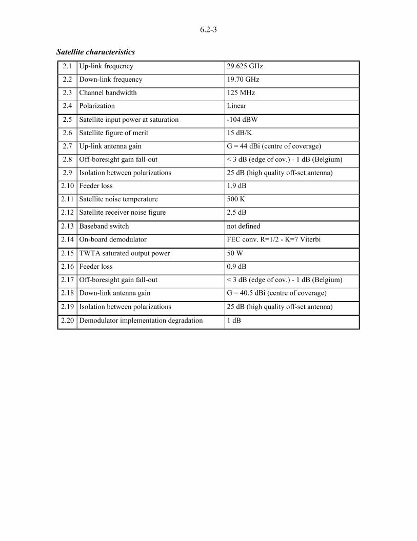
6.2-3

Satellite characteristics

2.1 Up-link frequency 29.625 GHz

2.2 Down-link frequency 19.70 GHz

2.3 Channel bandwidth 125 MHz

2.4 Polarization Linear

2.5 Satellite input power at saturation -104 dBW

2.6 Satellite figure of merit 15 dB/K

2.7 Up-link antenna gain G = 44 dBi (centre of coverage)

2.8 Off-boresight gain fall-out < 3 dB (edge of cov.) - 1 dB (Belgium)

2.9 Isolation between polarizations 25 dB (high quality off-set antenna)

2.10 Feeder loss 1.9 dB

2.11 Satellite noise temperature 500 K

2.12 Satellite receiver noise figure 2.5 dB

2.13 Baseband switch not defined

2.14 On-board demodulator FEC conv. R=1/2 - K=7 Viterbi

2.15 TWTA saturated output power 50 W

2.16 Feeder loss 0.9 dB

2.17 Off-boresight gain fall-out < 3 dB (edge of cov.) - 1 dB (Belgium)

2.18 Down-link antenna gain G = 40.5 dBi (centre of coverage)

2.19 Isolation between polarizations 25 dB (high quality off-set antenna)

2.20 Demodulator implementation degradation 1 dB

6.2-4

USAT characteristics

3.1 USAT nominal data rate 2 Mbit/s

3.2 USAT minimum data rate 256 kbit/s

3.3 Modulation scheme QPSK

3.4 Channel coding FEC conv. R=1/2 - K=7 Viterbi

3.5 Up-link multiple access method FDMA

3.6 Down-link multiple access method TDM

3.7 USAT antenna size 60 cm

3.8 USAT antenna efficiency 0.6

3.9 Antenna depointing angle < 0.2°

3.10 Isolation between polarizations 20 dB (low cost off-set antenna)

3.11 USAT HPA minimum output power 1.5 W

3.12 USAT HPA maximum output power 3 W

3.13 USAT antenna noise temperature 130 K

3.14 USAT feeder loss 0.2 dB

3.15 USAT LNA noise figure 3.5 dB (low cost terminal)

3.16 Demodulator implementation degradation 2 dB

Fade Mitigation Techniques

4.1 Up-Link Power Control Open-loop scheme

4.2 Data Rate Reduction [Kerschat et al., 1993] Open-loop scheme

6.2.1.2 Link budget set up

The document focuses on a link between two USATs, which are personal terminals characterised byantenna diameters of 60 cm and low transmitted power. A typical 2 Mbit/s USAT link is consideredbetween Louvain-la-Neuve and Lessive (both in Belgium) through the 19°W spacecraft. Theselocations are chosen because of the availability of propagation data at 12.5 and 30 GHz in Louvain-la-Neuve, and at 12.5 and 20 GHz in Lessive, measured during the Olympus experiment. TheseKa-band links present an elevation of 27.6 º for Louvain-la-Neuve and 27.8 º for Lessive, which arerepresentative of a typical mean elevation European link with a geostationary satellite.

Link budgets in clear sky conditions with the nominal USAT transmitted power (1.5 W) are givenin Tables 6.2-1 and 6.2-3.

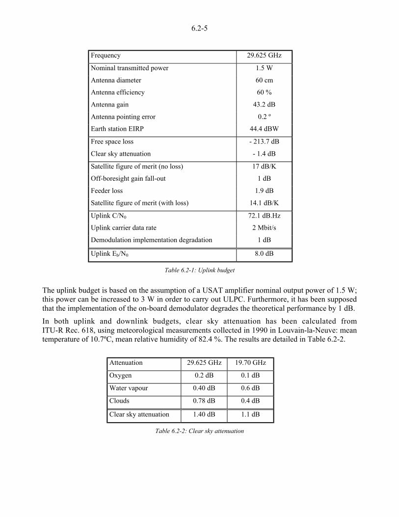
6.2-5

Frequency 29.625 GHz

Nominal transmitted power 1.5 W

Antenna diameter 60 cm

Antenna efficiency 60 %

Antenna gain 43.2 dB

Antenna pointing error 0.2 º

Earth station EIRP 44.4 dBW

Free space loss - 213.7 dB

Clear sky attenuation - 1.4 dB

Satellite figure of merit (no loss) 17 dB/K

Off-boresight gain fall-out 1 dB

Feeder loss 1.9 dB

Satellite figure of merit (with loss) 14.1 dB/K

Uplink C/N0 72.1 dB.Hz

Uplink carrier data rate 2 Mbit/s

Demodulation implementation degradation 1 dB

Uplink Eb/N0 8.0 dB

Table 6.2-1: Uplink budget

The uplink budget is based on the assumption of a USAT amplifier nominal output power of 1.5 W;this power can be increased to 3 W in order to carry out ULPC. Furthermore, it has been supposedthat the implementation of the on-board demodulator degrades the theoretical performance by 1 dB.

In both uplink and downlink budgets, clear sky attenuation has been calculated fromITU-R Rec. 618, using meteorological measurements collected in 1990 in Louvain-la-Neuve: meantemperature of 10.7ºC, mean relative humidity of 82.4 %. The results are detailed in Table 6.2-2.

Attenuation 29.625 GHz 19.70 GHz

Oxygen 0.2 dB 0.1 dB

Water vapour 0.40 dB 0.6 dB

Clouds 0.78 dB 0.4 dB

Clear sky attenuation 1.40 dB 1.1 dB

Table 6.2-2: Clear sky attenuation

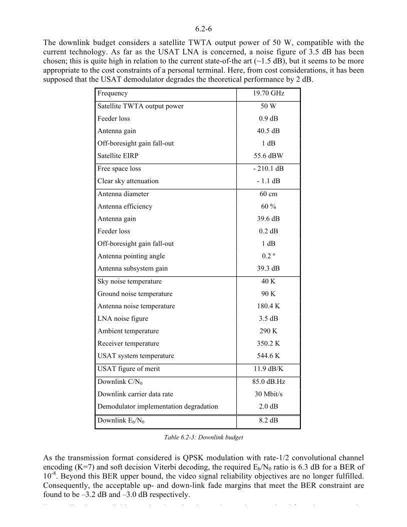
6.2-6

The downlink budget considers a satellite TWTA output power of 50 W, compatible with thecurrent technology. As far as the USAT LNA is concerned, a noise figure of 3.5 dB has beenchosen; this is quite high in relation to the current state-of-the art (~1.5 dB), but it seems to be moreappropriate to the cost constraints of a personal terminal. Here, from cost considerations, it has beensupposed that the USAT demodulator degrades the theoretical performance by 2 dB.

Frequency 19.70 GHz

Satellite TWTA output power 50 W

Feeder loss 0.9 dB

Antenna gain 40.5 dB

Off-boresight gain fall-out 1 dB

Satellite EIRP 55.6 dBW

Free space loss - 210.1 dB

Clear sky attenuation - 1.1 dB

Antenna diameter 60 cm

Antenna efficiency 60 %

Antenna gain 39.6 dB

Feeder loss 0.2 dB

Off-boresight gain fall-out 1 dB

Antenna pointing angle 0.2 º

Antenna subsystem gain 39.3 dB

Sky noise temperature 40 K

Ground noise temperature 90 K

Antenna noise temperature 180.4 K

LNA noise figure 3.5 dB

Ambient temperature 290 K

Receiver temperature 350.2 K

USAT system temperature 544.6 K

USAT figure of merit 11.9 dB/K

Downlink C/N0 85.0 dB.Hz

Downlink carrier data rate 30 Mbit/s

Demodulator implementation degradation 2.0 dB

Downlink Eb/N0 8.2 dB

Table 6.2-3: Downlink budget

As the transmission format considered is QPSK modulation with rate-1/2 convolutional channelencoding (K=7) and soft decision Viterbi decoding, the required Eb/N0 ratio is 6.3 dB for a BER of10-8. Beyond this BER upper bound, the video signal reliability objectives are no longer fulfilled.Consequently, the acceptable up- and down-link fade margins that meet the BER constraint arefound to be –3.2 dB and –3.0 dB respectively.

E ll h il bl i h h h i b i l f h i

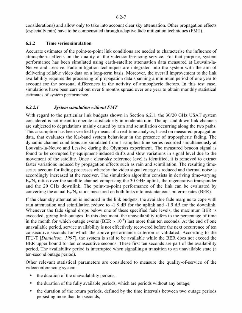
6.2-7

considerations) and allow only to take into account clear sky attenuation. Other propagation effects(especially rain) have to be compensated through adaptive fade mitigation techniques (FMT).

6.2.2 Time series simulation

Accurate estimates of the point-to-point link conditions are needed to characterise the influence ofatmospheric effects on the quality of the videoconferencing service. For that purpose, systemperformance has been simulated using earth-satellite attenuation data measured at Louvain-la-Neuve and Lessive. Fade mitigation techniques are integrated into the system with the aim ofdelivering reliable video data on a long-term basis. Moreover, the overall improvement to the linkavailability requires the processing of propagation data spanning a minimum period of one year toaccount for the seasonal differences in the activity of atmospheric factors. In this test case,simulations have been carried out over 6 months spread over one year to obtain monthly statisticalestimates of system performance.

6.2.2.1 System simulation without FMT

With regard to the particular link budgets shown in Section 6.2.1, the 30/20 GHz USAT systemconsidered is not meant to operate satisfactorily in moderate rain. The up- and down-link channelsare subjected to degradations mainly caused by rain and scintillation occurring along the two paths.This assumption has been verified by means of a real-time analysis, based on measured propagationdata, that evaluates the Ka-band system behaviour in the presence of tropospheric fading. Thedynamic channel conditions are simulated from 1 sample/s time-series recorded simultaneously atLouvain-la-Neuve and Lessive during the Olympus experiment. The measured beacon signal isfound to be corrupted by equipment-induced drifts and slow variations in signal level due to themovement of the satellite. Once a clear-sky reference level is identified, it is removed to extractfaster variations induced by propagation effects such as rain and scintillation. The resulting time-series account for fading processes whereby the video signal energy is reduced and thermal noise isaccordingly increased at the receiver. The simulation algorithm consists in deriving time-varyingEb/No ratios over the satellite channel comprising the 30 GHz uplink, the regenerative transponderand the 20 GHz downlink. The point-to-point performance of the link can be evaluated byconverting the actual Eb/No ratios measured on both links into instantaneous bit error rates (BER).

If the clear sky attenuation is included in the link budgets, the available fade margins to cope withrain attenuation and scintillation reduce to -1.8 dB for the uplink and -1.9 dB for the downlink.Whenever the fade signal drops below one of these specified fade levels, the maximum BER isexceeded, giving link outages. In this document, the unavailability refers to the percentage of timein the month for which outage events (BER > 10-8) last more than ten seconds. At the end of oneunavailable period, service availability is not effectively recovered before the next occurrence of tenconsecutive seconds for which the above performance criterion is validated. According to theITU-T [Danielson, 1997], the system is said to be available while the BER does not exceed theBER upper bound for ten consecutive seconds. These first ten seconds are part of the availabilityperiod. The availability period is interrupted when signalling a transition to an unavailable state (aten-second outage period).

Other relevant statistical parameters are considered to measure the quality-of-service of thevideoconferencing system:

• the duration of the unavailability periods,

• the duration of the fully available periods, which are periods without any outage,

• the duration of the return periods, defined by the time intervals between two outage periodspersisting more than ten seconds,

6.2-8

The performance analysis of the USAT-to-USAT link has been conducted using 6 complete monthsof 30/20 GHz data, assuming the transmitter operated in 3 different continuous modes:

• with the nominal power of 1.5 W and a nominal data rate of 2.048 Mbit/s,

• with the maximum power of 3.0 W and nominal data rate,

• with the nominal power and an effective data rate reduced to 256 kbit/s.

The first mode determines the system performance when no fade mitigation technique isimplemented. In the second mode, the effects of up-link fades ranging from 4.8 dB to 0 dB areideally compensated for. In the last mode, the 256 kbit/s digital video signal is combined with aspreading sequence whose chip rate is equal to the nominal data rate. The achieved processing gainGR provides additional fade margins (+ 9 dB) on both up- and down-links.

Performance results for the cases described are used later for assessing the actual improvement ofoverall link availability when resorting to adaptive fade mitigation techniques (power control andvariable data rate).

Month

Mode

Availability

ITU-T

%

Unavail

%

Mean duration

Avail. Unavail Return

hour min hour

January 1992 1.5 W

3 W

GR=8, 1.5 W

99.792

99.996

100.000

0.194

0.004

0.000

5.54

15.04

20.63

1.47

0.38

-

8.19

20.63

23.29

March 1992 1.5 W

3 W

GR=8, 1.5 W

97.953

99.677

99.982

1.873

0.298

0.017

1.19

4.04

17.28

1.82

1.24

0.94

1.49

5.36

19.10

May 1992 1.5 W

3 W

GR=8, 1.5 W

98.051

99.139

99.870

1.818

0.808

0.123

1.54

3.02

13.04

3.04

2.86

2.35

2.46

4.71

13.53

July 1990 1.5 W

3 W

GR=8, 1.5 W

98.058

99.359

99.944

1.766

0.586

0.056

1.31

2.43

15.58

2.70

2.74

2.67

2.25

5.80

17.92

October 1990 1.5 W

3 W

GR=8, 1.5 W

97.190

99.520

99.967

2.706

0.450

0.033

2.58

4.64

19.28

5.67

1.78

2.06

2.96

5.14

19.28

November 1990 1.5 W

3 W

GR=8, 1.5 W

98.039

99.634

99.979

1.822

0.333

0.020

1.31

3.12

14.05

2.56

1.19

0.68

2.09

4.73

16.39

Table 6.2-4: simulation results without fade compensation

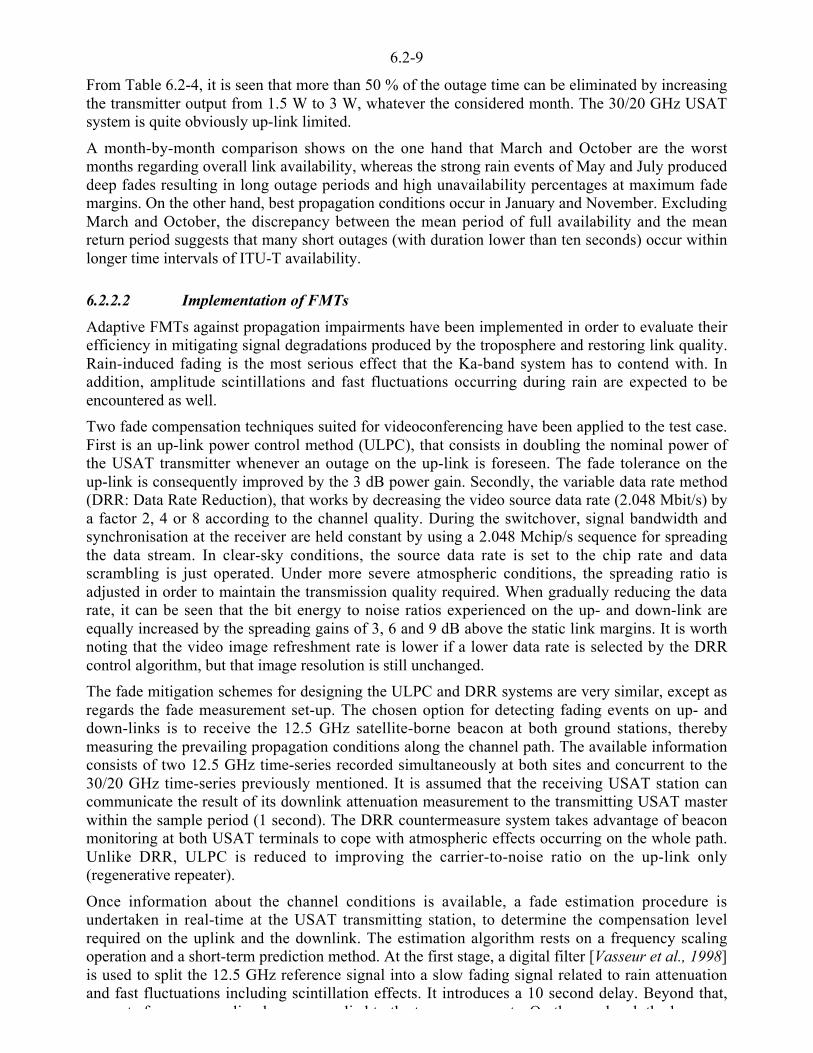
6.2-9

From Table 6.2-4, it is seen that more than 50 % of the outage time can be eliminated by increasingthe transmitter output from 1.5 W to 3 W, whatever the considered month. The 30/20 GHz USATsystem is quite obviously up-link limited.

A month-by-month comparison shows on the one hand that March and October are the worstmonths regarding overall link availability, whereas the strong rain events of May and July produceddeep fades resulting in long outage periods and high unavailability percentages at maximum fademargins. On the other hand, best propagation conditions occur in January and November. ExcludingMarch and October, the discrepancy between the mean period of full availability and the meanreturn period suggests that many short outages (with duration lower than ten seconds) occur withinlonger time intervals of ITU-T availability.

6.2.2.2 Implementation of FMTs

Adaptive FMTs against propagation impairments have been implemented in order to evaluate theirefficiency in mitigating signal degradations produced by the troposphere and restoring link quality.Rain-induced fading is the most serious effect that the Ka-band system has to contend with. Inaddition, amplitude scintillations and fast fluctuations occurring during rain are expected to beencountered as well.

Two fade compensation techniques suited for videoconferencing have been applied to the test case.First is an up-link power control method (ULPC), that consists in doubling the nominal power ofthe USAT transmitter whenever an outage on the up-link is foreseen. The fade tolerance on theup-link is consequently improved by the 3 dB power gain. Secondly, the variable data rate method(DRR: Data Rate Reduction), that works by decreasing the video source data rate (2.048 Mbit/s) bya factor 2, 4 or 8 according to the channel quality. During the switchover, signal bandwidth andsynchronisation at the receiver are held constant by using a 2.048 Mchip/s sequence for spreadingthe data stream. In clear-sky conditions, the source data rate is set to the chip rate and datascrambling is just operated. Under more severe atmospheric conditions, the spreading ratio isadjusted in order to maintain the transmission quality required. When gradually reducing the datarate, it can be seen that the bit energy to noise ratios experienced on the up- and down-link areequally increased by the spreading gains of 3, 6 and 9 dB above the static link margins. It is worthnoting that the video image refreshment rate is lower if a lower data rate is selected by the DRRcontrol algorithm, but that image resolution is still unchanged.

The fade mitigation schemes for designing the ULPC and DRR systems are very similar, except asregards the fade measurement set-up. The chosen option for detecting fading events on up- anddown-links is to receive the 12.5 GHz satellite-borne beacon at both ground stations, therebymeasuring the prevailing propagation conditions along the channel path. The available informationconsists of two 12.5 GHz time-series recorded simultaneously at both sites and concurrent to the30/20 GHz time-series previously mentioned. It is assumed that the receiving USAT station cancommunicate the result of its downlink attenuation measurement to the transmitting USAT masterwithin the sample period (1 second). The DRR countermeasure system takes advantage of beaconmonitoring at both USAT terminals to cope with atmospheric effects occurring on the whole path.Unlike DRR, ULPC is reduced to improving the carrier-to-noise ratio on the up-link only(regenerative repeater).

Once information about the channel conditions is available, a fade estimation procedure isundertaken in real-time at the USAT transmitting station, to determine the compensation levelrequired on the uplink and the downlink. The estimation algorithm rests on a frequency scalingoperation and a short-term prediction method. At the first stage, a digital filter [Vasseur et al., 1998]is used to split the 12.5 GHz reference signal into a slow fading signal related to rain attenuationand fast fluctuations including scintillation effects. It introduces a 10 second delay. Beyond that,separate freq enc scaling la s are applied to the t o components On the one hand the lo pass

6.2-10

scaling factor according to the methods of [ITU-R, 1997a] or Laster and Stutzman [Laster andStutzman, 1995] applicable for rain attenuation. On the other hand, the scintillation variance iscalculated and translated to higher frequency in order to obtain a short-term stochasticcharacterisation of the scintillation process expected on the up- or down-link. The scintillationamplitude value is loaded into a FIFO shift register containing the last 21 samples upon whichstandard deviation is calculated. At each sampling time, the register output returns a measure offluctuation intensity validated within a time-scale of about 20 seconds. The reduced set of elementsconsidered makes it possible to account for fast fluctuations, which may exhibit strong amplitudevariations during rain periods. The scaling law for scintillation has the form:

),()(

)(),(

12/7

bbb

fx

x

f

ff tS

g

gtS rr ´́

¦

¥²²¤

£= 6.2-1

where ),( bftS r denotes the time-varying scintillation intensity (dB) experienced at base frequency

with the actual 1.8 m antenna that received Olympus beacon signals. The antenna averaging ratiocalculated at both sites is found to be close to 1 and has been discarded for the simulation purposes.On the basis of the scaling equation above, the actual scintillation amplitudes at the higherfrequency are statistically compensated by allocating a dynamic margin identified by the amplitudelevel not exceeded for some prescribed percentage of time. If the percentile threshold is set to97.5 %, the associated scintillation margin at time t is given by ),(96.1 ftS r with:

975.0)exp(1

2

296.1

22�<0

'<

dxS

x

S

S

rr

r

/6.2-2

Rain fade prediction on a short-term basis is next introduced, using only fade slope [Vasseur et al.,1998] to compensate for filter delay and to get a one-second early estimate of the rain attenuationlevel, hereafter denoted )(ˆ 1+trA . If scintillation amplitude mitigation is specially required, thescintillation offset mentioned above is added to the predicted rain fade.

Hence, the predictor is:

),()(ˆ)1(ˆ 96.11 fSf ddtStAtA r <<++=+ r 6.2-3

assuming that the scintillation intensity at the next second is fairly approximated by the scaledscintillation process intensity a time 1++ Sf dd seconds before, where fd and Sd respectively stand

for the delays introduced by the filtering process and the moving variance.

According to the predictor value, the countermeasure control system is requested to adjust outputpower (ULPC) at the next second whenever a prescribed attenuation threshold is crossed [Vasseuret al., 1998]. In the DRR case, three attenuation thresholds are defined for switching from onespreading state to another (four data rate levels).

When fading occurs, a primary concern is to initiate the appropriate countermeasure in good time.The control algorithm implemented makes use of a detection margin [ITU-R, 1994] as a means ofanticipating the fading process. The detection margin scheme is needed for two reasons. Firstly,constant fade slope has been assumed for extrapolating the delayed version of rain attenuation to thepredicted level 1+fd seconds later. Within this period and the set-up time of an actual fade

countermeasure system, tropospheric attenuation signal is prone to random variations, resulting inlikely detection outages in the absence of protection against fades which increase more rapidly thanexpected. Use of a sufficient detection margin enables the control system to be initiated promptlyenough to minimise the detection outage probability in the month. Secondly, the fixed detection

6.2-11

before for avoiding brief outages caused by fast fluctuations. Another aspect in the matter ofdetection outages is that median expressions for the instantaneous frequency scaling factor havebeen used instead of percentile laws obtained from long-term empirical models for a highoccurrence level of fade ratio. Therefore, it must be pointed out that departures of the effective ratioabove the median level produce outages whenever the scaling error exceeds the detection marginallocated. Such outages are part of the category of detection outages, as they result from failures ofthe control system to cope with the stochastic nature of the satellite atmospheric channel. As afunction of precipitation, the time-varying scaling behaviour of rain attenuation is a severelimitation on the resource control accuracy of the open-loop mitigation scheme. Due to thesignificant gap between the 30 GHz uplink signal band and the beacon frequency, the 30/12.5 GHzfade ratio dispersion is rather important, making the up-link control system operation speciallysensitive to the detection margin value associated with a given scaling model.

When more favourable transmissions conditions are recovered, fade countermeasures are graduallydisabled and the nominal operating mode is restored. An additional hysteresis margin is required[Vasseur et al., 1998] to prevent repeated mode switching if the predictor fluctuates around thedecision threshold for switching on.

6.2.2.3 System simulation with FMT

System simulation with ULPC

In Section 6.2.2.1, simulation results of the videoconferencing system operating with fixed powerand spreading ratio parameters have been presented. It has been suggested that significantimprovements of the USAT-to-USAT link performance could be achieved by resorting to adaptivefade mitigation techniques such as ULPC and DRR. The present objective is to evaluate theeffectiveness of the actual open-loop power control algorithm to offer the quality-of-serviceexpected.

The considered ULPC system is designed to operate either in the nominal power mode (1.5 W) or inthe increased power mode (3 W). The decision thresholds for changing output power are fdependenton the detection and hysteresis margins. Using ULPC as a countermeasure, the detection d andhysteresis h parameters leading to the best system performances have been identified on a monthlybasis. A wide range of possible margins has been investigated: d = 0.0, 0.1, 0.2, … , 1.2 dB andh = 0.3, 0.4, …, 0.9 dB with 5.1)+hd dB.

Performance of the power control system may be evaluated according to various criteria, dependingon the application. With regard to videoconferencing, the optimisation of control margins isperformed by taking into account output parameters that are the most representative of the quality-of-service to be delivered. These are, in order of their importance with respect to the user’ssatisfaction: the availability, the average switching rate in the month, the mean duration ofunavailable periods and return periods, and the percentage of time for which the maximum powermode is on. Other calculated quantities may have some interest to FMT designers for measuring thefraction of outage time due to imperfect fade compensation:

• the percentage of time accumulated by detection outage events lasting less than ten seconds,

• the percentage of time accumulated by long-lasting detection outage events (with durationo * 10 s) ; these are part of unavailable time and can affect total availability.

The influence of frequency scaling methods on system performance has been evaluated using eitherthe ITU-R model for rain attenuation or the empirical method proposed by Laster and Stuztman[Laster and Stutzmann, 1995] from Virginia Tech Olympus measurements (‘VIR’). In addition, thescaling procedure for amplitude scintillation can be applied to mitigate scintillation effects on

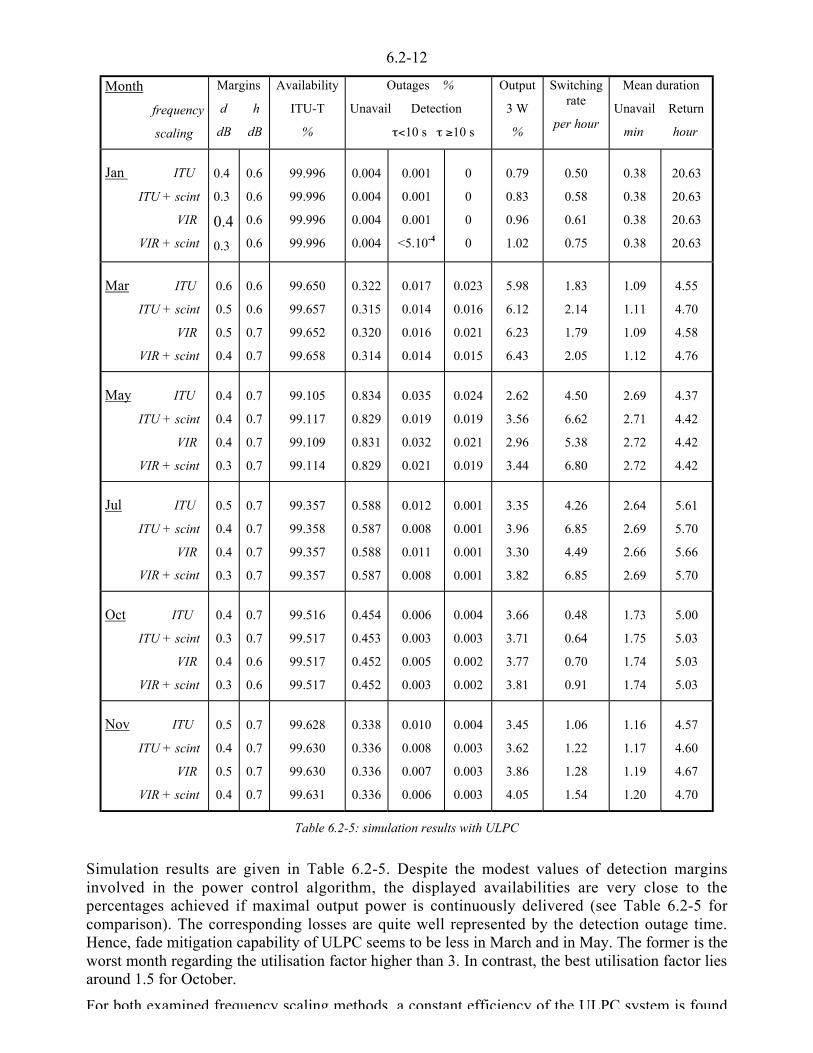
6.2-12

Month

frequency

scaling

Margins

d h

dB dB

Availability

ITU-T

%

Outages %

Unavail Detection

o<10 s o *10 s

Output

3 W

%

Switchingrate

per hour

Mean duration

Unavail Return

min hour

Jan ITU

ITU + scint

VIR

VIR + scint

0.4

0.3

0.4

0.3

0.6

0.6

0.6

0.6

99.996

99.996

99.996

99.996

0.004

0.004

0.004

0.004

0.001

0.001

0.001

<5.10-4

0

0

0

0

0.79

0.83

0.96

1.02

0.50

0.58

0.61

0.75

0.38

0.38

0.38

0.38

20.63

20.63

20.63

20.63

Mar ITU

ITU + scint

VIR

VIR + scint

0.6

0.5

0.5

0.4

0.6

0.6

0.7

0.7

99.650

99.657

99.652

99.658

0.322

0.315

0.320

0.314

0.017

0.014

0.016

0.014

0.023

0.016

0.021

0.015

5.98

6.12

6.23

6.43

1.83

2.14

1.79

2.05

1.09

1.11

1.09

1.12

4.55

4.70

4.58

4.76

May ITU

ITU + scint

VIR

VIR + scint

0.4

0.4

0.4

0.3

0.7

0.7

0.7

0.7

99.105

99.117

99.109

99.114

0.834

0.829

0.831

0.829

0.035

0.019

0.032

0.021

0.024

0.019

0.021

0.019

2.62

3.56

2.96

3.44

4.50

6.62

5.38

6.80

2.69

2.71

2.72

2.72

4.37

4.42

4.42

4.42

Jul ITU

ITU + scint

VIR

VIR + scint

0.5

0.4

0.4

0.3

0.7

0.7

0.7

0.7

99.357

99.358

99.357

99.357

0.588

0.587

0.588

0.587

0.012

0.008

0.011

0.008

0.001

0.001

0.001

0.001

3.35

3.96

3.30

3.82

4.26

6.85

4.49

6.85

2.64

2.69

2.66

2.69

5.61

5.70

5.66

5.70

Oct ITU

ITU + scint

VIR

VIR + scint

0.4

0.3

0.4

0.3

0.7

0.7

0.6

0.6

99.516

99.517

99.517

99.517

0.454

0.453

0.452

0.452

0.006

0.003

0.005

0.003

0.004

0.003

0.002

0.002

3.66

3.71

3.77

3.81

0.48

0.64

0.70

0.91

1.73

1.75

1.74

1.74

5.00

5.03

5.03

5.03

Nov ITU

ITU + scint

VIR

VIR + scint

0.5

0.4

0.5

0.4

0.7

0.7

0.7

0.7

99.628

99.630

99.630

99.631

0.338

0.336

0.336

0.336

0.010

0.008

0.007

0.006

0.004

0.003

0.003

0.003

3.45

3.62

3.86

4.05

1.06

1.22

1.28

1.54

1.16

1.17

1.19

1.20

4.57

4.60

4.67

4.70

Table 6.2-5: simulation results with ULPC

Simulation results are given in Table 6.2-5. Despite the modest values of detection marginsinvolved in the power control algorithm, the displayed availabilities are very close to thepercentages achieved if maximal output power is continuously delivered (see Table 6.2-5 forcomparison). The corresponding losses are quite well represented by the detection outage time.Hence, fade mitigation capability of ULPC seems to be less in March and in May. The former is theworst month regarding the utilisation factor higher than 3. In contrast, the best utilisation factor liesaround 1.5 for October.

For both examined frequency scaling methods, a constant efficiency of the ULPC system is found

6.2-13

slight improvements of availability by mitigating short- as well as long-lasting detection outages. Itresults in a significant increase of the mean switching rate. The highest rates are reached in May andJuly.

System simulation with DRR

The considered DRR case featuring four countermeasure states is attractive as an alternative toULPC. No extra resource is needed to compensate for rain fades up to 10 dB occurring along eachsatellite-to-USAT link. Two open-loop detection schemes have been considered for testing thevariable data rate technique on the videoconferencing test case. In the first case, the data ratecontroller is beacon-assisted on the up-link only. In the second, link quality is estimated on both theup- and the down-links and spreading gain is adjusted in real-time according to the most severe fademeasurement.

Next to the output parameters previously defined, the concept of throughput must be introduced toaccount for the information bit rate reduction being operated. This is the ratio of the total number ofbits effectively transmitted during the availability period, to the maximum number of bitstransmitted in one complete month at the constant 2.048 Mbit/s data rate.

Table 6.2-6 displays performance results obtained from a trade-off between availability on the onehand and throughput and mean switching rate on the other.

Best absolute availability performances are clearly achieved with beacon monitoring activated onboth links. As a by-product, the return period is extended at the cost of a reasonable degradation ofthroughput. Furthermore, it is found that detection outage time does not increase significantly, (Julyapart), even though double scaling/prediction procedures are involved in estimating both up- anddown-link fades. The additional detection outage time indicates how well the controller is able tocounteract downlink fades when using identical detection margins on both links. This suggests thatdownlink fading can be managed by the countermeasure algorithm with a lower detection marginthan that required on the up-link. Finally, slight reductions of detection outage percentage arenoticed in March, May and November. This effect reveals that up-link outages uncompensated byup-link data rate control may be mitigated by DRR with up- and down-link monitoring when fadeevents occur simultaneously on the up-link and the down-link.

Simulation results show that performance parameters are sensitive to the frequency scaling methodemployed by the data rate management algorithm. Whatever the month considered, the DRRefficiency is found to be superior when frequency scaling is based on the Laster and Stutzmanempirical method instead of the ITU-R model. As previously stressed in discussing the ULPC case,the scintillation amplitude mitigation technique is once again invoked to reduce the total detectionoutage time, including outage periods of duration longer than ten seconds. Nevertheless, a smallincrease of switching rate is to be deplored, suggesting that more false alarms are likely to occur.From one month to another, mean switching rate is the most variable statistical parameterconsidered. It peaks in May and July or during deep fade periods.

6.2-14

Monthfrequency

scaling

Marginsd hdB dB

AvailabilityITU-T

%

Outages %Unavail Detection o<10 s o *10 s

Through-put%

Switchingrate

/ hour

Mean durationUnavail Return

min hour

Jan up-link ITU + scint

VIRup- & down-link ITU + scint

VIR

0.30.4

0.30.4

0.50.6

0.50.6

99.99699.997

99.999100.000

0.0040.003

0.0010

0.0010.001

0.0010.001

0.0010

0.0010

99.6199.51

99.5899.42

0.690.64

0.830.75

0.380.53

0.23-

21.6321.88

21.8823.29

Mar up-link ITU + scint

VIR VIR + scintup- & down-link ITU + scint

VIR VIR + scint

0.50.50.4

0.50.50.4

0.70.70.7

0.70.70.7

99.79699.79799.807

99.93199.93899.947

0.1790.1780.169

0.0600.0520.046

0.0260.0270.024

0.0250.0260.023

0.0400.0340.026

0.0380.0310.025

96.3696.5996.50

95.9596.1596.02

2.362.252.58

2.772.693.16

0.760.760.79

0.540.520.52

5.455.495.84

9.309.8010.67

May up-link ITU + scint VIR

VIR + scintup- & down-link ITU + scint VIR

VIR + scint

0.50.50.4

0.50.50.4

0.70.70.7

0.70.70.7

99.43199.42799.452

99.80599.82199.832

0.5350.5390.517

0.1800.1650.155

0.0340.0440.033

0.0350.0420.030

0.0520.0370.030

0.0520.0380.029

97.2697.6297.35

97.0297.4697.04

8.857.329.12

10.468.6611.22

1.791.761.94

1.141.211.39

4.524.444.95

7.308.029.13

Jul up-link ITU + scint

VIR VIR + scintup- & down-link ITU + scint

VIR VIR + scint

0.40.40.3

0.50.40.3

0.70.70.7

0.70.70.7

99.51299.52899.533

99.85099.85199.862

0.4450.4300.425

0.1410.1400.128

0.0180.0210.016

0.0260.0340.028

0.0570.0400.039

0.0830.0830.072

97.5097.8297.57

96.8097.7597.39

7.014.657.07

10.846.129.40

1.671.671.66

0.930.990.91

4.895.035.07

7.467.797.79

Oct up-link ITU + scint

VIR VIR + scintup- & down-link ITU + scint

VIR VIR + scint

0.60.50.4

0.60.50.4

0.50.70.7

0.50.70.7

99.81099.84299.845

99.89899.92999.934

0.1660.1390.135

0.0900.0630.058

0.0220.0170.014

0.0220.0160.014

0.0540.0270.024

0.0540.0270.024

97.4897.5997.55

97.3297.4297.35

1.831.041.32

2.161.261.62

0.820.840.84

0.690.670.67

6.107.047.17

8.3210.1710.61

Nov up-link ITU + scint

VIR VIR + scintup- & down-link ITU + scint

VIR VIR + scint

0.60.50.4

0.60.50.4

0.60.70.7

0.60.70.7

99.79999.82099.825

99.93499.95699.961

0.1730.1550.151

0.0580.0400.035

0.0270.0260.023

0.0280.0260.023

0.0340.0190.014

0.0330.0170.013

97.4697.7997.69

97.2097.5797.42

2.141.621.90

2.642.082.43

0.660.700.76

0.410.390.44

4.985.686.14

7.739.5610.92

Table 6.2-6: simulation results with DRR

6.2-15

6.2.2.4 Event-based analysis

In this paragraph, simulation results are presented for one specific event occurring on the uplink, inorder to illustrate the instantaneous behaviour of the fade compensation system. The eventintroduced in the simulation was measured in Louvain-la-Neuve (10 July) at 12.5 GHz and 30 GHz(see Figure 6.2-1) ; it is a typical convective rain event which reached a depth of 12 dB.

0 500 1000 1500 2000 2500 3000 3500 4000!12

!10

!8

!6

!4

!2

0OLYMPUS measurements at Louvain!la!Neuve (UCL)

Time (s)

In!

exce

ss a

ttenu

atio

n tim

e se

ries

(dB

)

LLN ! 29.625 GHzLLN ! 12.5 GHz

Figure 6.2-1: Rain event firstly introduced in the simulation

The instantaneous behaviour of the control system, submitted to the above event, is illustrated inFigure 6.2-2: without FMT, with ULPC only, DRR only and finally with both ULPC and DRRcombined (see [Vasseur et al., 1998] and [Castanet and Vasseur, 1998]).

0 500 1000 1500 2000 2500 3000 3500 4000!6

!4

!2

0

2

4

6

8

10

12

14

16Uplink budget ! No Fade Mitigation Technique

Time (s)

Eb/

N0

(dB

)

Transmitted power (W)Spreading gain (dB)Eb/N0 without FMT (dB)Outage threshold

0 500 1000 1500 2000 2500 3000 3500 4000!6

!4

!2

0

2

4

6

8

10

12

14

16Uplink budget ! 0.5 dB detection margin ! 0.0 dB hysteresis

Time (s)

Eb/

N0

(dB

)

Transmitted power (W)Spreading gain (dB)Eb/N0 with FMT (dB)Outage threshold (dB)

2500 2550 2600 2650 2700 2750 2800!4

!2

0

2

4

6

8

10

12

14Uplink budget ! 1.0 dB detection margin ! 0.7 dB hysteresis

Time (s)

Eb/

N0

(dB

)

Transmitted power (W)Spreading gain (dB)Eb/N0 with FMTOutage threshold (dB)

2500 2550 2600 2650 2700 2750 2800!2

0

2

4

6

8

10

12

14

16Uplink budget ! 1.0 dB detection margin ! 0.7 dB hysteresis

Time (s)

Eb/

N0

(dB

)

Transmitted power (W)Spreading gain (dB)Eb/N0 with FMT (dB)Outage threshold (dB)

Figure 6 2-2: Uplink performance with and without FMT

6.2-16

More precisely, Figure 6.2-2 presents the variation of the uplink Eb/N0 around the attenuation peak.Due to the limited margin available, ULPC is activated most of the time and compensates most ofthe fading except for the highest attenuation part. When the attenuation signal peaks, the variabledata rate action complements the mitigation. Thanks to the combined FMT, the uplink Eb/N0 isalways above the minimum required ratio (6.3 dB) and the link remains available.

6.2.2.5 Conclusion for the time series analysis

On the basis of six complete months of propagation data, simulation results of the Ka-bandvideoconference USAT system were presented and discussed in terms of performance parametersmeasuring the quality-of-service. The investigation demonstrated that fade mitigation techniquesimplemented as open-loop systems are expected to be fairly effective in contending rain-impairmentand scintillation amplitudes. If the frequency scaling model and the control parameters are properlyselected, link availability may considerably be improved up to 99 %, 99.4 % and 99.8 % in anyconsidered month using respectively, up-link power control, up-link data-rate control and data ratecontrol with up- and down-link monitoring.

6.2.3 Link performance prediction

In this subsection, the ability of current propagation prediction models to estimate the systemquality of service is evaluated. Procedures based on propagation models that yield reasonablepredictions of system availability, outage duration and return period are proposed. The accuracy ofthese procedures is evaluated by comparing simulated performances with predictions.

6.2.3.1 Conventional approach

In the conventional approaches, cumulative distributions of impairments are predicted withstatistical models on a yearly basis. This kind of methodology allows either the estimation of thefade level the system is likely to face (a function of the time percentage) and therefore of the fademargin, or the calculation of the time percentage occurrence of outages corresponding to a givenattenuation.

Louvain - OLYMPUS - Lessive prediction

In the following, prediction models recommended by ITU-R are used to estimate propagationeffects at Ka-band, i. e. oxygen and water vapour [ITU-R, 1998], cloud [ITU-R,1997b] and rain[ITU-R, 1999] attenuations, as well as scintillation depth [ITU-R, 1999] from Climpara’98 maps[Baptista and Salonen, 1998].

Results shown in Figure 6.2-3 confirm the assumptions made in Section 6.2.1. The clear skyattenuation (oxygen, water vapour and cloud) is 1.1 dB at 19.70 GHz and 1.4 dB at 29.625 GHz for1 % of the time and 1.3 dB and 1.7 dB (at the same frequencies) for 0.1 % of time.

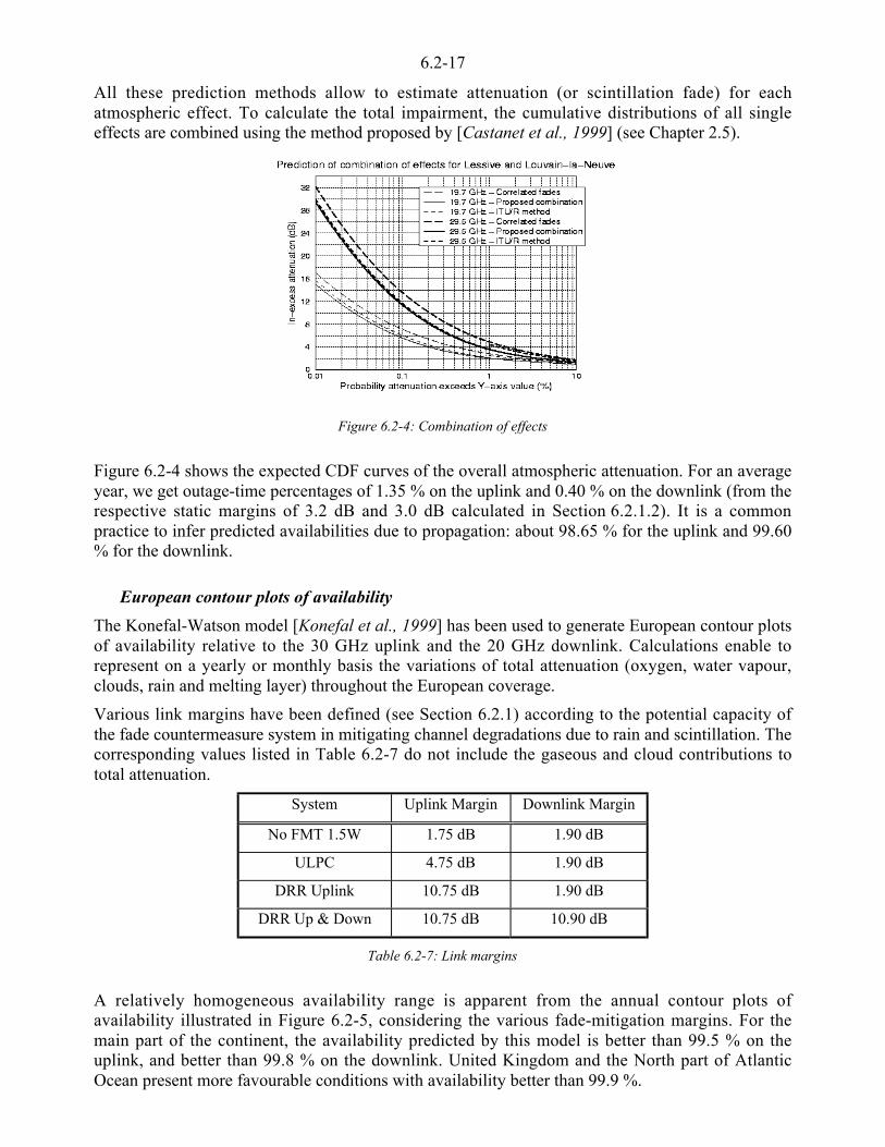
6.2-17

All these prediction methods allow to estimate attenuation (or scintillation fade) for eachatmospheric effect. To calculate the total impairment, the cumulative distributions of all singleeffects are combined using the method proposed by [Castanet et al., 1999] (see Chapter 2.5).

Figure 6.2-4: Combination of effects

Figure 6.2-4 shows the expected CDF curves of the overall atmospheric attenuation. For an averageyear, we get outage-time percentages of 1.35 % on the uplink and 0.40 % on the downlink (from therespective static margins of 3.2 dB and 3.0 dB calculated in Section 6.2.1.2). It is a commonpractice to infer predicted availabilities due to propagation: about 98.65 % for the uplink and 99.60% for the downlink.

European contour plots of availability

The Konefal-Watson model [Konefal et al., 1999] has been used to generate European contour plotsof availability relative to the 30 GHz uplink and the 20 GHz downlink. Calculations enable torepresent on a yearly or monthly basis the variations of total attenuation (oxygen, water vapour,clouds, rain and melting layer) throughout the European coverage.

Various link margins have been defined (see Section 6.2.1) according to the potential capacity ofthe fade countermeasure system in mitigating channel degradations due to rain and scintillation. Thecorresponding values listed in Table 6.2-7 do not include the gaseous and cloud contributions tototal attenuation.

System Uplink Margin Downlink Margin

No FMT 1.5W 1.75 dB 1.90 dB

ULPC 4.75 dB 1.90 dB

DRR Uplink 10.75 dB 1.90 dB

DRR Up & Down 10.75 dB 10.90 dB

Table 6.2-7: Link margins

A relatively homogeneous availability range is apparent from the annual contour plots ofavailability illustrated in Figure 6.2-5, considering the various fade-mitigation margins. For themain part of the continent, the availability predicted by this model is better than 99.5 % on theuplink, and better than 99.8 % on the downlink. United Kingdom and the North part of AtlanticOcean present more favourable conditions with availability better than 99.9 %.

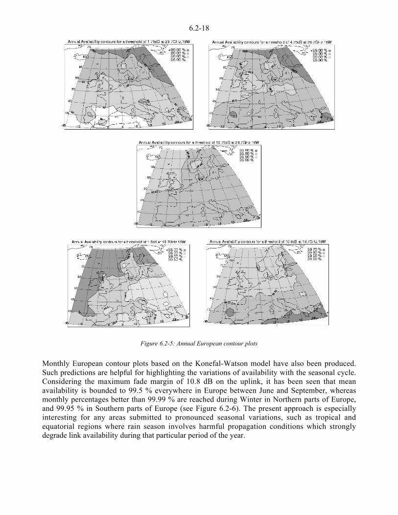
6.2-18

Figure 6.2-5: Annual European contour plots

Monthly European contour plots based on the Konefal-Watson model have also been produced.Such predictions are helpful for highlighting the variations of availability with the seasonal cycle.Considering the maximum fade margin of 10.8 dB on the uplink, it has been seen that meanavailability is bounded to 99.5 % everywhere in Europe between June and September, whereasmonthly percentages better than 99.99 % are reached during Winter in Northern parts of Europe,and 99.95 % in Southern parts of Europe (see Figure 6.2-6). The present approach is especiallyinteresting for any areas submitted to pronounced seasonal variations, such as tropical andequatorial regions where rain season involves harmful propagation conditions which stronglydegrade link availability during that particular period of the year.

6.2-19

Figure 6.2-6: Monthly European contour plots

6.2.3.2 Prediction of service availability

If up- and down-link fades do not occur simultaneously, system availability is predicted as

Availability = 100 (1 - Pr{Aup * Mup} - Pr{Adown * Mdown})(%) 6.2-4

where Pr{A * a} is the probability that tropospheric attenuation A exceeds a level a,

Mup, Mdown are the up- and down-link margins respectively.

It must be noted that

(i) Equation 6.2-1 states that every second for which attenuation does not exceed the link margin isconsidered as available. However, the simulated system is required to work properly for more thanten consecutive seconds in order to conform to the system availability criterion as specified byITU T As long as only outage events lasting less than ten seconds are encountered the required

6.2-20

the next occurrence of any ten-second-outage period. It has been found that time-series simulationproduces very similar availability percentages whether the ITU-T ten-second criterion is adopted ornot. The absolute in excess ITU-T percentage is less than 0.03 % for any of the 6 monthsconsidered.

(ii) Unlike the prediction procedure, fade periods detected concurrently on the uplink and on thedownlink are part of the monthly outage time evaluated by time-series simulation. For any givenmonth, the resulting availability performance is logically slightly higher than, or equal to, theexpected percentage calculated by using Equation 6.2-4 as the definition of system availability.

(iii) Simulations account for the imperfections of the countermeasure technique in contending withthe actual fading process, while prediction models, relying on definition (i) to calculate availability,assume that the fade mitigation technique performs ideally. The related deficiency in terms ofservice availability is adequately represented by the detection outage percentage, tabulated in theprevious section.

Whenever any adaptive fade compensation is to be operated, the corrective effects mentioned in (ii)and (iii) act in opposite ways on the overall availability time. In this study case, on the average, theprediction methods should slightly overestimate system availability with respect to time-seriessimulation.

Three propagation models have been considered to estimate link availability: the [ITU-R, 1997b]prediction model for rain attenuation, the [ITU-R, 1999] prediction model for rain attenuation[Dissanayake et al., 1997] and the [ITU-R 1999] prediction model for scintillation fade. Forcombining attenuation and scintillation, we use the simple method proposed by [ITU-R, 1997b]

MonthTemperature

(°C)Humidity(% - g/m3)

Amount ofrain (mm)

Numberof days

R0.01

(mm/h)

July 90 16.1°C 75 % - 10.25 g/m3 34.6 mm 7 d 39.84 mm/h

October 90 12.6°C 87 % - 9.60 g/m3 86.0 mm 9 d 40.59 mm/h

November 90 5.8°C 94 % - 6.71 g/m3 77.1 mm 16 d 12.46 mm/h

January 92 2.1°C 97 % - 5.41 g/m3 24.9 mm 6 d 1.28 mm/h

March 92 7.7°C 92 % - 7.44 g/m3 87.4 mm 14 d 20.54 mm/h

May 92 13.6°C 85 % - 9.98 g/m3 55.0 mm 6 d 42.39 mm/h

Average(Climpara)

9.15°C (LLN)9.45°C (LSV)

84.7 % - 7.52 g/m3

H LLN = 7.66 g/m3- - 28.08 mm/h (LLN)

28.25 mm/h (LSV)

Table 6.2-8 : Meteorological data recorded at Louvain-la-Neuve

The propagation models need surface meteorological data: rainfall rate exceeded for 0.01% of thetime (R0.01) for the rain attenuation models and mean temperature and humidity for the scintillationmodel. On one hand, monthly cumulative amounts of rain and monthly number of rainy daysmeasurements, carried out in Louvain-la-Neuve during the OPEX campaign (Table 6.2-8), havebeen used to predict R001 with theTattelman & Sharr model [Tattelman and Scharr, 1983] (with arain detection threshold of 1 mm).

On the other hand, monthly values of R0.01 have been inferred from concurrent measurement ofattenuation exceeded for 0.01% of the time at two different frequencies (12.5/20 or 12.5/30 GHz),using the ITU-R model. In Table 6.2-9, the average value of R0.01 is taken from the ITU-R rainclimatic zone maps (zone E for Belgium).

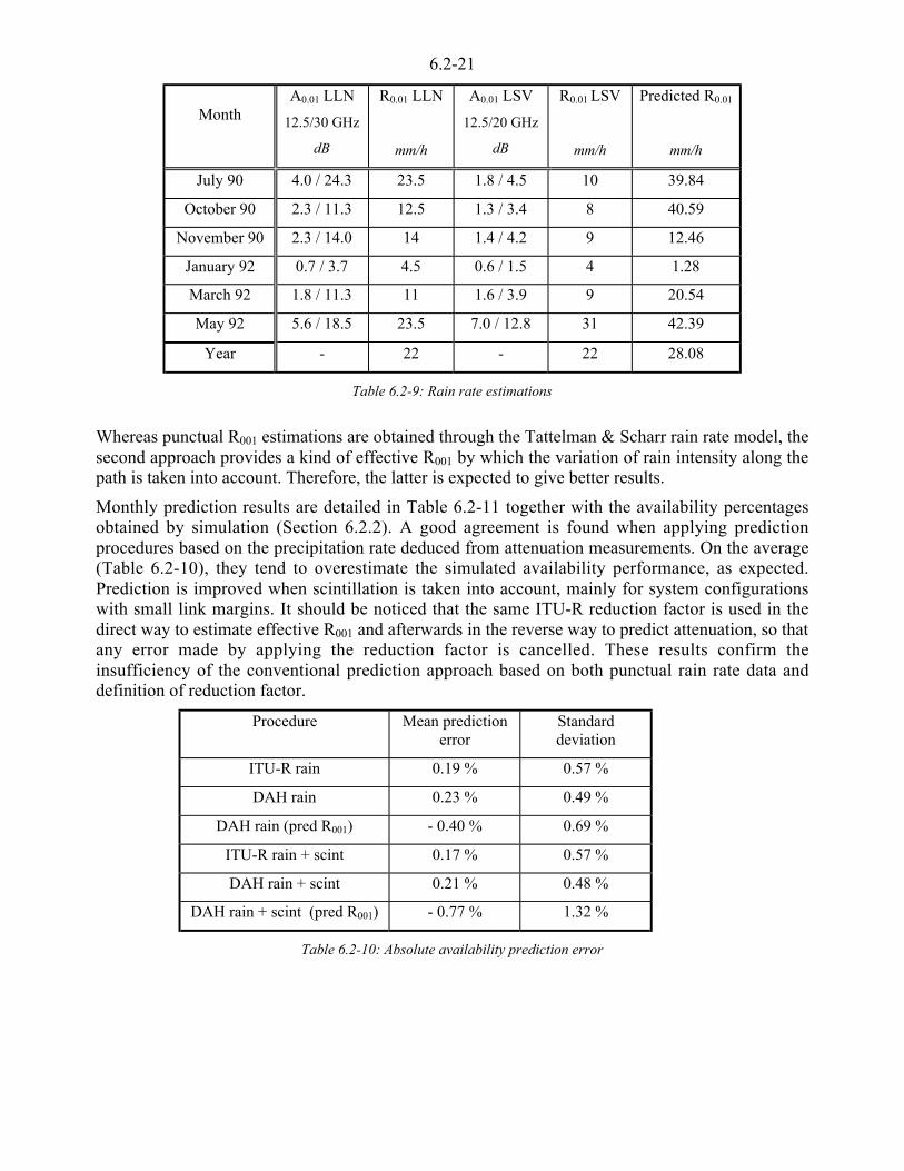
6.2-21

MonthA0.01 LLN

12.5/30 GHz

dB

R0.01 LLN

mm/h

A0.01 LSV

12.5/20 GHz

dB

R0.01 LSV

mm/h

Predicted R0.01

mm/h

July 90 4.0 / 24.3 23.5 1.8 / 4.5 10 39.84

October 90 2.3 / 11.3 12.5 1.3 / 3.4 8 40.59

November 90 2.3 / 14.0 14 1.4 / 4.2 9 12.46

January 92 0.7 / 3.7 4.5 0.6 / 1.5 4 1.28

March 92 1.8 / 11.3 11 1.6 / 3.9 9 20.54

May 92 5.6 / 18.5 23.5 7.0 / 12.8 31 42.39

Year - 22 - 22 28.08

Table 6.2-9: Rain rate estimations

Whereas punctual R001 estimations are obtained through the Tattelman & Scharr rain rate model, thesecond approach provides a kind of effective R001 by which the variation of rain intensity along thepath is taken into account. Therefore, the latter is expected to give better results.

Monthly prediction results are detailed in Table 6.2-11 together with the availability percentagesobtained by simulation (Section 6.2.2). A good agreement is found when applying predictionprocedures based on the precipitation rate deduced from attenuation measurements. On the average(Table 6.2-10), they tend to overestimate the simulated availability performance, as expected.Prediction is improved when scintillation is taken into account, mainly for system configurationswith small link margins. It should be noticed that the same ITU-R reduction factor is used in thedirect way to estimate effective R001 and afterwards in the reverse way to predict attenuation, so thatany error made by applying the reduction factor is cancelled. These results confirm theinsufficiency of the conventional prediction approach based on both punctual rain rate data anddefinition of reduction factor.

Procedure Mean predictionerror

Standarddeviation

ITU-R rain 0.19 % 0.57 %

DAH rain 0.23 % 0.49 %

DAH rain (pred R001) - 0.40 % 0.69 %

ITU-R rain + scint 0.17 % 0.57 %

DAH rain + scint 0.21 % 0.48 %

DAH rain + scint (pred R001) - 0.77 % 1.32 %

Table 6.2-10: Absolute availability prediction error

6.2-22

System Month

Measuredavailability

%

Prediction

ITU rain

%

PredictionDAH rain

%

Pred. R001

DAH rain

%

PredictionITU rain

+ scint

%

PredictionDAH rain

+ scint

%

Pred. R001

DAH rain

+ scint

%

No FMT

1.5 W

Jan

Mar

May

Jul

Oct

Nov

Avrg

Year

99.792

97.953

98.051

98.058

97.190

98.039

98.181

-

99.906

99.392

97.004

97.807

99.260

99.083

98.742

97.655

99.840

99.298

97.779

98.251

99.202

99.064

98.906

98.125

99.986

98.25

95.74

96.03

95.95

99.10

97.51

97.39

99.894

99.348

96.878

97.703

99.196

99.035

98.676

97.566

99.827

99.259

97.686

98.170

99.148

99.025

98.853

98.058

99.983

96.40

93.46

93.93

93.65

99.06

96.08

95.37

ULPC

Jan

Mar

May

Jul

Oct

Nov

Avrg

Year

99.996

99.658

99.117

99.358

99.517

99.629

99.546

-

99.985

99.867

98.784

99.587

99.861

99.820

99.651

99.252

99.960

99.790

99.066

99.538

99.785

99.740

99.647

99.312

99.998

99.36

98.33

98.45

98.42

99.69

99.04

99.01

99.984

99.859

98.744

99.571

99.850

99.812

99.637

99.228

99.958

99.782

99.037

99.523

99.775

99.732

99.635

99.294

99.997

99.34

98.29

98.42

98.38

99.68

99.02

98.99

DRR

uplink

Jan

Mar

May

Jul

Oct

Nov

Avrg

Year

99.997

99.807

99.452

99.533

99.845

99.825

99.743

-

99.992

99.927

99.057

99.860

99.940

99.919

99.783

99.494

99.979

99.883

99.335

99.807

99.897

99.872

99.796

99.559

99.999

99.59

98.91

98.99

98.96

99.80

99.38

99.36

99.991

99.921

99.021

99.848

99.932

99.913

99.771

99.473

99.977

99.876

99.310

99.796

99.889

99.866

99.786

99.544

99.998

99.57

98.87

98.96

98.93

99.79

99.35

99.34

DRR

uplink

&downlink

Jan

Mar

May

Jul

Oct

Nov

Avrg

Year

100.000

99.947

99.832

99.862

99.934

99.961

99.923

-

99.999

99.990

99.919

99.941

99.987

99.982

99.970

99.940

99.997

99.977

99.900

99.921

99.972

99.965

99.955

99.918

5 100

99.92

99.77

99.79

99.79

99.97

99.87

99.88

99.999

99.990

99.919

99.940

99.986

99.982

99.969

99.940

99.997

99.977

99.900

99.921

99.972

99.965

99.955

99.918

5 100

99.92

99.77

99.79

99.79

99.97

99.87

99.88

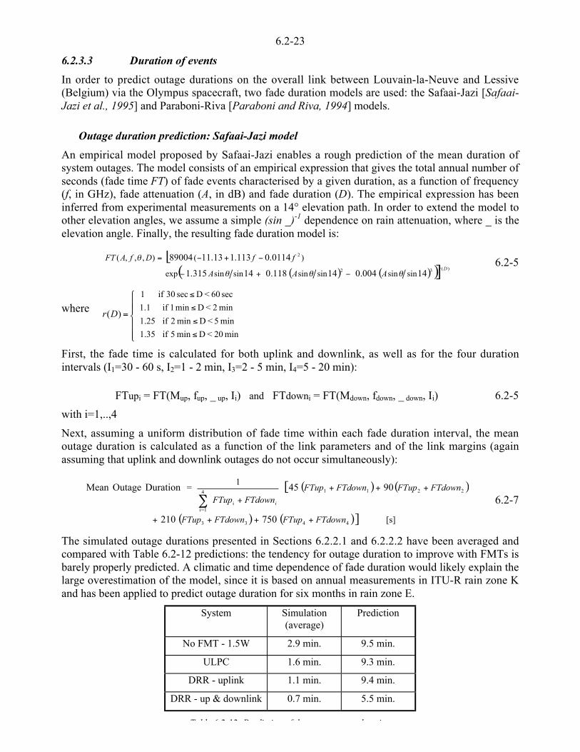
6.2-23

6.2.3.3 Duration of events

In order to predict outage durations on the overall link between Louvain-la-Neuve and Lessive(Belgium) via the Olympus spacecraft, two fade duration models are used: the Safaai-Jazi [Safaai-Jazi et al., 1995] and Paraboni-Riva [Paraboni and Riva, 1994] models.

Outage duration prediction: Safaai-Jazi model

An empirical model proposed by Safaai-Jazi enables a rough prediction of the mean duration ofsystem outages. The model consists of an empirical expression that gives the total annual number ofseconds (fade time FT) of fade events characterised by a given duration, as a function of frequency(f, in GHz), fade attenuation (A, in dB) and fade duration (D). The empirical expression has beeninferred from experimental measurements on a 14° elevation path. In order to extend the model toother elevation angles, we assume a simple (sin _)-1 dependence on rain attenuation, where _ is theelevation angle. Finally, the resulting fade duration model is:

[( ) ( )( )] )(32

2

14004.014118.014315.1

0114.0113.113.1189004

sinsinsinsinsinsinexp

)(),,,(Dr

AAA

ffDfAFT

eee

e

<+<

<+<= 6.2-5

where

««ª

««©

¨

=

)

)

)

)

min 20 < D min 5 if 1.35

min 5 < Dmin 2 if 1.25

min 2 < D min 1 if 1.1

sec 60 < D sec 30 if 1

)(Dr

First, the fade time is calculated for both uplink and downlink, as well as for the four durationintervals (I1=30 - 60 s, I2=1 - 2 min, I3=2 - 5 min, I4=5 - 20 min):

FTupi = FT(Mup, fup, _ up, Ii) and FTdowni = FT(Mdown, fdown, _ down, Ii) 6.2-5

with i=1,..,4

Next, assuming a uniform distribution of fade time within each fade duration interval, the meanoutage duration is calculated as a function of the link parameters and of the link margins (againassuming that uplink and downlink outages do not occur simultaneously):

( ) ( )[

( ) ( )] [s]

1=

4433

22114

1=ii

750210

9045 DurationOutage Mean

FTdownFTupFTdownFTup

FTdownFTupFTdownFTupFTdownFTup i

++++

++++- 6.2-7

The simulated outage durations presented in Sections 6.2.2.1 and 6.2.2.2 have been averaged andcompared with Table 6.2-12 predictions: the tendency for outage duration to improve with FMTs isbarely properly predicted. A climatic and time dependence of fade duration would likely explain thelarge overestimation of the model, since it is based on annual measurements in ITU-R rain zone Kand has been applied to predict outage duration for six months in rain zone E.

System Simulation(average)

Prediction

No FMT - 1.5W 2.9 min. 9.5 min.

ULPC 1.6 min. 9.3 min.

DRR - uplink 1.1 min. 9.4 min.

DRR - up & downlink 0.7 min. 5.5 min.

T bl 6 2 12 P di ti f th t d ti

6.2-24

Outage duration prediction: Paraboni-Riva model

The Paraboni-Riva model is extremely valuable for generating cumulative distributions of fadeduration for any fixed attenuation level. The model outputs are either the number of fade durations(Nd(D)) longer than a given duration (D) for one exceeded attenuation level, or the fraction of time(F(D) = Ns(D)/Ntot) made up fades exceeding that attenuation threshold and lasting more than agiven duration. The model is described in Chapter 2.2.

a - Overall link extrapolation

In order to assess the fade duration distribution of the overall link, a specific analysis has to becarried out using the fade duration statistics Fup(D), Fdown(D) provided by the Paraboni-Riva modelfor individual up- and down-links. With the assumption that no correlation exists between up- anddown-link fade events, the total duration of outage events longer than D can be expressed by:

µµ�

�

³³�

�´´¦

¥²²¤

£<´

´¦

¥²²¤

£<<=<==

expexpexp_expexp 1.11.)1.(.

T

N

T

NTPTPTN

downs

ups

outagenooutages 6.2-8

where Texp is the time duration of the experiment (1 month, 1 year, …). It follows that,

expT

NNNNN

downs

upsdown

supss <+= Ù

downs

ups

downs

ups

s

N

T

N

TNN

N

expexp

11

+

<=+

6.2-9

The second term represents less than 0,5% of the ratio in the worst case (see Table 6.2-13). As aconsequence, it may be assumed that fade events on the two links do not occur simultaneously, with

downs

upss NNN += .

Attenuation thresholdCumulative outage time

for one year Ntot

1.75 dB 651506 s

4.75 dB 141062 s

10.75 dB 32254 s

1.90 dB 171042 s

10.90 dB 6627 s

Table 6.2-13: Calculation of Ntot with DAH model

Hence, considering the overall link, the fraction of time constituted by outage durations longer thansome specific duration can be written as:

downdown

upupdown

totuptot

downdowntot

upuptot

downtot

uptot

downs

ups

overalltot

s FFNN

FNFN

NN

NN

N

N..

..__ +=

+

+=

+

+=µ

�

� 6.2-10

b - Comparison prediction / simulation

To determine the expected outage time constituted by fade events lasting more than any prescribedduration over the 6-month period, the fade duration distribution Ns(D) has been expressed instead ofF(D) = Ns(D)/Ntot, using the DAH prediction model for rain attenuation to estimate the total outagetime Ntot (from predicted R001 in Table 6.2-8).

6.2-25

Figure 6.2-7: Cumulative Fade Durations over 6 months – overall link

The comparative plots of Figure 6.2-7 suggest that the poor estimation of Ntot would be one of thereasons leading to the large overestimation of Ns(D), for any fade duration value or attenuationthreshold. The logarithmic prediction error has been tabulated here for each pair of fade mitigationmargins. The error is seen to be less for low margin configurations.

6 s 18 s 60 s 180 s 600 s 1800 s

1.75/1.9 dB 365.5 271.9 174.6 100.8 47.3 47.6

4.75/1.9 dB 496.9 397.4 294.4 221.8 163.2 240.8

10.75/1.9 dB 504.2 406.8 305.3 224.7 170.2 220

10.75/10.9 dB 549.6 443.9 336.7 252.5 296.7 -

Table 6.2-14: logarithmic error of the model [Paraboni and Riva, 1994]

Prediction of return period duration

The empirical model considered for predicting the mean outage duration may also be used forestimating the mean duration of return period. The proposed procedure is described hereafter.

The annual availability time (AT, in s) is calculated by:

( )-=

+<=4

1

3600*24*365i

ii FTdownFTupAT 6.2-11

The mean number of outages (NO) is obtained by dividing, for each duration interval, the fade timeby the mean outage duration:

6.2-26

( ) ( ) ( )

( )750

210904544

332211

FTdownFTup

FTdownFTupFTdownFTupFTdownFTupNO

++

++

++

++

=6.2-12

The mean duration of return period may therefore be predicted as AT/NO (in seconds).

Table 6.2-15 displays the results of return period duration prediction, together with the simulatedresults. Again, the prediction is quite inaccurate, but it at least gives an idea of the order ofmagnitude as well as of the general tendency. The prediction procedure seems to be inadequate forhigh link margins, as the number of outages (NO) becomes very small and may be less than 1.

System Simulation(average)

Prediction

No FMT-1.5W 3.2 hour. 0.8 hour

ULPC 7.5 hour 2.5 hour

DRR - Uplink 8.5 hour. 3.1 hour

DRR - Up & Downlink 12.1 hour. -

Table 6.2-15: Prediction of mean return-period duration.

6.2.3.4 Conclusion for the prediction analysis

Different procedures based on current propagation models have been examined for predictingquality-of-service performance. Their efficiency has been assessed by comparing their results withtime-series simulation results.

This comparison has shown that blind predictions realized with conventional statistical models(either rain attenuation models or models combining rain attenuation and scintillation) are relativelyinaccurate, even though monthly rain intensity data are used to improve the prediction. However,service availability is predicted reasonably well when effective rain rate is inferred from attenuationmeasurements. This conclusion reinforces the interest of using time series analysis to estimatesystem QoS.

As far as fade duration predictions are concerned, only rough estimates of the outage duration andreturn period are obtained, using available empirical and statistical models. These prediction modelssystematically overestimate the simulated results and do not give really satisfactory results. It isacknowledged that the Paraboni-Riva model is relatively user-friendly and flexible since it allowslink characteristics to be used as inputs but a climatic dependency of some of its intermediateparameters remains to be investigated.

6.2.4 Conclusion

Simulations of system performance using actual propagation data offer an efficient means foraccurately estimating the global quality of service of future Ka-band systems. They make it possibleto assess the impact of various atmospheric effects impairing propagation, mainly rain attenuationand scintillation, on various system parameters measuring the QoS to be delivered.

For the generic VSAT videoconferencing system considered, system performances have beensimulated over six complete months spread over the year so as to get an insight into the seasonalvariability of QoS due to changes in the activity of atmospheric factors. A statistical and event-based analysis of performance results has made it possible to optimise fade mitigation techniquesappropriate to the application In addition the influence of fade dynamics on the FMT efficiency

6.2-27

In a second part, different procedures based on current propagation models for predicting the mostrelevant parameters in the matter of quality-of-service have been examined. Their efficiency hasbeen assessed by comparing their results with time-series simulation results. Whereas theconventional prediction methods are not really satisfactory when using monthly surfacemeteorological measurements, service availability has been fairly well predicted by usingattenuation statistics derived from time-series. From the system designer’s point of view,propagation data at the required frequency will be rarely available, so conventional statisticalmodels should be used most of the time. As it has been demonstrated that time series analysisproduces good estimations of system parameters, time-series synthetic models will be required inthe future.

6.2-28

6.2.5 References

[Castanet and Vasseur, 1998]Castanet L., Vasseur H.: "Link budget and first performance simulations of a Ka-bandvideoconferencing VSAT system", COST 255, STSM report, September 1998.

[Castanet et al., 1999]Castanet L., Lemorton J., Konefal T., Shukla A.K., Watson P.A., Wrench C.L.: "Comparison ofvarious methods for combining propagation effects and predicting loss in low-availability systemsin the 20 GHz to 50 GHz frequency range", Int. Jour. of Sat. Com., Special issue on Propagation,(to be published).

[Danielson, 1997]Danielson B.: "Performance and availability criteria for digital radio-relay and satellite systems",COST 255, CP 30002, May 1997.

[Dissanayake et al., 1997]Dissanayake A., Allnutt J., Haidara F.: "A prediction model that combines rain attenuation andother propagation impairments along earth-satellite paths", IEEE Trans. Antennas Propagat., vol.45, n°10, pp. 1546-1558, October 1997.

[ITU-R, 1994]ITU-R Rec. S. 1061, ‘Utilization of fade countermeasures strategies and techniques in the fixed-satellite service’, ITU, Geneva, 1994.

[ITU-R, 1997a]ITU-R Rec. PN. 618-5, ‘Propagation data and prediction methods required for the design of earth-space telecommunication systems’, Geneva, January 1997.

[ITU-R, 1997b]ITU-R Rec P.840-2, “Attenuation due to clouds and fog”, 1997

[ITU-R, 1998]ITU-R Rec P.676-3, “Attenuation by atmospheric gases”, 1998

[ITU-R, 1999]ITU-R Rec. P.618-6, ‘Propagation data and prediction methods required for the design of Earth-space telecommunication systems’, 1999.

[Kerschat et al., 1993]Kerschat K. - Koudelka O. - Riedler W. - Tomlinson M. - Hughes C.D. - Hörle J.: "A variablespread-spectrum fade countermeasure system for the DICE video conference system", Proc.Olympus Util. Conference, Seville, April 93.

[Konefal et al., 1999]Konefal T., Watson P.A., Shukla A.K., Akram A.: "Prediction of monthly and annual availabilitieson 10-50 GHz satellite-Earth links", COST 255, CP71A05, May 1999.

[Laster and Stutzman, 1995]Laster J.D., Stutzman W.L.: "Frequency scaling of rain attenuation for satellite communicationlinks", IEEE Trans Ant. Prop., vol. 43, n°11, pp. 1207-1216, Nov. 1995.

[Paraboni and Riva, 1994]Paraboni A., Riva C.:"A new method for the prediction of fade duration statistics in satellite linksabove 10 GHz", Int. Journal of Satellite Communications, vol. 12, 387-394, 1994.

[Baptista & Salonen, 1998]Poiares-Baptista J.P.V., Salonen E.T.: "Review of rainfall rate modelling and mapping",

6.2-29

[Safaai-Jazi et al., 1995]Safaai-Jazi A., Ajaz H., Stutzman W.L.: "Empirical models for rain fade time on Ku- and Ka-bandsatellite links", IEEE Trans. Ant. Prop., vol. 43, n°12, pp. 1411-1415, Dec. 1995.

[Tattelman and Scharr, 1983]Tattelman P., Scharr K.G.: "A model for estimating one minute rainfall rates", Journal of Climateand Applied Meteorology, Vol. 22, September 1983.

[Vasseur et al., 1998]Vasseur H., Czarnecki M., Castanet L., Bousquet M.: "Performance Simulation of Ka-band VSATVideoconferencing System", COST 255, First International Workshop on Radiowave PropagationModelling for SatCom Services at Ku-band and Above, ESTEC, Noordwijk, The Netherlands,October 1998, pp. 227-234.

6.3-1

CHAPTER 6.3V-Band VSAT Asymmetrical Data

Communication System

Editor: Prof. P.A. Watson1

Authors: Prof. P.A. Watson, Mr A. Page2, Dr. A. Martellucci3

1 University of Bath, Dept. of E&E Engineering, Claverton Down, Bath, BA2 7AY, UKTel.: +44-1225-826-6330, Fax.: +44-1225-826-6305, e-mail: P.A.Watson@bath.ac.uk

2 University of Bath, Dept. of E&E Engineering, Claverton Down, Bath, BA2 7AY, UKTel.: +44-1225-826-6061, Fax.: +44-1225-826-6305, e-mail: A.Page@bath.ac.uk

3 European Space Agency, ESA-ESTEC, Kepleerlan 1, PB 299, NL-2200 AG Noordwijk, The NetherlandsTel: +31-71-565-5603 Fax: +31-71-565-4999 e-mail: Antonio Martellucci@esa int

6.3-2

6.3 V-Band VSAT Asymmetrical Data Communication System

This system study explores the area of convergence between V-Sat systems and direct broadcastsystems. At the highest degree of traffic asymmetry, the system may be regarded as a directbroadcast link with a low-data rate return channel for such applications as pay-per-view TV,impulse buying from TV commercials and audience polling or participation.

As a further step, the system may be extended to support a range of Internet based applications,ranging from a limited system with a hub based server for specific applications linked to directbroadcast TV services (home shopping for example) to full world-wide-web access. In both casesthe system will exploit the developing situation which offers extensive, low cost memory, at bothhub and user stations.

As the growth of internet traffic is currently exponential and as the cable network operators arethemselves having difficulty in anticipating the nature of future growth, it would be unwise for us tospeculate too deeply on traffic models (the use of home based servers for example will havesignificant impact on traffic patterns). In this case study we merely recognise the fact that WWWaccess will be commonplace in the home and that there is an opportunity for IP based applicationsto be associated with direct broadcasting.

6.3.1 Architecture

This study is directed towards the use of a traditional bent-pipe transponder. The availablebandwidth per transponder is considered to be 72 MHz, re-useable in spot beams and bypolarisation re-use. For outbound channels we consider 16 carriers with 6 Mbit/s used in TDMA.For the return channel we consider up to 125 carriers of 512 kbit/s accessed by MF-TDMA. Otherreturn path carriers/capacity (15 channels) will be used for order wire requests. All carriers areseparated by a guard band of one channel width, avoiding interference due to intermodulation ofcarriers when using a non-linear transponder amplifier.

6.3.2 Number of Users

6.3.2.1 Low-bit rate return path

For a broadcast return channel system, the number of simultaneous users is limited by the capacityof the return channel. More subscribers could be on-line, though not transmitting. This systemsupports at least 100,000 users per spot beam, using a total return channel data capacity of64 Mbit/s. The actual number of active users depends on traffic and tariffing.

6.3.2.2 IP–type applications

Internet browser applications are characterised by the asymmetric ratio of the received data, to thesize of the request. This ratio is highly flexible and will increase with the use of audio and video inweb page design. Total outbound system capacity (96 Mbit/s) is shared by the number of users.Reducing the number of users increases the maximum bandwidth available for each user. Assumingthat all users are web browsing and an average web page size of 20 kbit/s 12 kbytes per page plusallowance for future growth in page sizes), the system can support approximately 5000simultaneous users.

6.3-3

6.3.3 Link and Service Availabilities

The bands at 40/50 GHz offer significant spectrum for exploitation by such services, but atrelatively low link availabilities. Typical values range from 99.5 to 99.8% at 40 GHz and 98.0 to99.5% at 50 GHz, for the coverage considered in this case study and with a 10 dB fade margin (seeFigure 6.3-1). Two important factors in system design are thus evident:

memory must be exploited in the hub and V-Sat stations to give the user a good serviceavailability despite the relatively poor link availability, and

it is critical that the user stations have enough link margin to accommodate the lossesencountered from clouds and atmospheric gases and that adaptive techniques (resource sharingwith adaptive coding, space and time diversity, application specific protocols) and outbounduplink power control are used as mitigation techniques during rainfall.

6.3.4 System Description

The system provides packet transmission from a hub to VSAT terminals, through a bent-pipesatellite. The V-band frequencies allocated by the ITU for fixed satellite services at V-band havebeen used (37.5-40.5 GHz downlink & 47.2-50.2 GHz uplink). The data rates are flexible,depending on the volume of packets received.

6.3.4.1 Outbound Link

On the outbound link (hub to VSAT) TDMA is used at a burst rate compatible with MPEG-2(6 Mbit/s). Variable length packets from higher layer applications (video, audio, data) areencapsulated in a MPEG transport stream packet (188 bytes). Individual terminals identify userdata from the destination address header in the broadcast stream.

6.3.4.2 Inbound Link

The in-bound link uses ATM packets (48 bytes data + 5 bytes header) to access the internet andcommunicate directly with the hub. ATM provides a guaranteed QoS and short packet sizes(16 kbit/s). Each frame (512 kbit/s) contains 32 ATM cells and each user can request up to 4 cells(64 kbit/s = IP cell) per frame, depending on channel traffic. Both MF-TDMA and CDMA havebeen considered for multiple access. MF-TDMA offers efficient allocation of return path capacityin a variety of user applications and is especially suited to adaptive resource sharing in anenvironment where individual links may suffer occasional deep fades. In MF-TDMA users cancombine non-overlapping time and frequency slots to form a frame.

Contention techniques are avoided for return path access. When large numbers of users are queued,waiting to send, these are dealt with by polling (e.g. pay-per-view) and selective polling (audienceparticipation). Home shopping is dealt with as an IP application, making use of hub and VSATcache memory.

6.3.4.3 Modulation and Coding

The outbound and inbound links use the DVB-S standard defining modulation and coding (ETS 300421). This ensures compatibility between equipment manufacturers and global performancerequirements. Each time slot contains a single transmission packet (MPEG-2 or ATM), protectedwith a concatenated FEC scheme (16 byte Reed-Solomon outer code & rate-1/2, K=7 convolutional

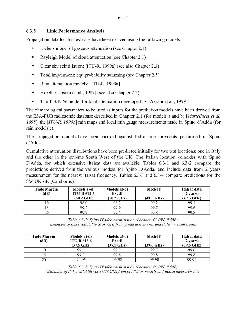
6.3-4

6.3.5 Link Performance Analysis

Propagation data for this test case have been derived using the following models:

• Liebe’s model of gaseous attenuation (see Chapter 2.1)

• Rayleigh Model of cloud attenuation (see Chapter 2.1)

• Clear sky scintillation: [ITU-R, 1999a] (see also Chapter 2.3)

• Total impairment: equiprobability summing (see Chapter 2.5)

• Rain attenuation models: [ITU-R, 1999a]

• Excell [Capsoni et. al., 1987] (see also Chapter 2.2)

• The T-S/K-W model for total attenuation developed by [Akram et al., 1999]

The climatological parameters to be used as inputs for the prediction models have been derived fromthe ESA-FUB radiosonde database described in Chapter 2.1 (for models a and b) [Martellucci et al,1998], the [ITU-R, 1999b] rain maps and local rain gauge measurements made in Spino d’Adda (forrain models e).

The propagation models have been checked against Italsat measurements performed in Spinod’Adda.

Cumulative attenuation distributions have been predicted initially for two test locations: one in Italyand the other in the extreme South West of the UK. The Italian location coincides with SpinoD'Adda, for which extensive Italsat data are available. Tables 6.3-1 and 6.3-2 compare thepredictions derived from the various models for Spino D'Adda, and include data from 2 yearsmeasurement for the nearest Italsat frequency. Tables 6.3-3 and 6.3-4 compare predictions for theSW UK site (Camborne).

Fade Margin(dB)

Models a)-d)ITU-R 618-6(50.2 GHz)

Models a)-d)Excell

(50.2 GHz)

Model f)

(49.5 GHz)

Italsat data(2 years)

(49.5 GHz)10 98.0 98.2 99.2 99.115 99.2 99.0 99.7 99.620 99.7 99.5 99.8 99.8

Table 6.3-1: Spino D'Adda earth station (Location 45.40N, 9.50E).Estimates of link availability at 50 GHz from prediction models and Italsat measurements

Fade Margin(dB)

Models a)-d)ITU-R 618-6(37.5 GHz)

Models a)-d)Excell

(37.5 GHz)

Model f)

(39.6 GHz)

Italsat data(2 years)

(39.6 GHz)10 99.6 99.2 99.7 99.615 99.9 99.8 99.8 99.820 99.95 99.92 99.90 99.90

Table 6.3-2: Spino D'Adda earth station (Location 45.40N, 9.50E).Estimates of link availability at 37/39 GHz from prediction models and Italsat measurements

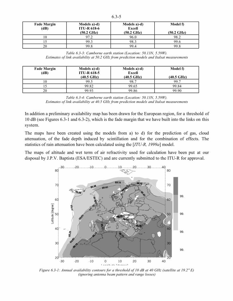
6.3-5

Fade Margin(dB)

Models a)-d)ITU-R 618-6(50.2 GHz)

Models a)-d)Excell

(50.2 GHz)

Model f)

(50.2 GHz)10 97.2 96.0 98.215 99.3 98.3 99.620 99.8 99.4 99.8

Table 6.3-3: Camborne earth station (Location: 50.13N, 5.59W).Estimates of link availability at 50.2 GHz from prediction models and Italsat measurements

Fade Margin(dB)

Models a)-d)ITU-R 618-5 (40.5 GHz)

Models a)-d)Excell

(40.5 GHz)

Model f)

(40.5 GHz)10 99.5 98.7 99.715 99.82 99.65 99.8420 99.93 99.86 99.90

Table 6.3-4: Camborne earth station (Location: 50.13N, 5.59W).Estimates of link availability at 40.5 GHz from prediction models and Italsat measurements

In addition a preliminary availability map has been drawn for the European region, for a threshold of10 dB (see Figures 6.3-1 and 6.3-2), which is the fade margin that we have built into the links on thissystem.

The maps have been created using the models from a) to d) for the prediction of gas, cloudattenuation, of the fade depth induced by scintillation and for the combination of effects. Thestatistics of rain attenuation have been calculated using the [ITU-R, 1999a] model.

The maps of altitude and wet term of air refractivity used for calculation have been put at ourdisposal by J.P.V. Baptista (ESA/ESTEC) and are currently submitted to the ITU-R for approval.

Figure 6.3-1: Annual availability contours for a threshold of 10 dB at 40 GHz (satellite at 19.2° E)(ignoring antenna beam pattern and range losses)

-30 -20 -10 0 10 20 30 40Longitude [degree]

-30 -20 -10 0 10 20 30 40

20

30

40

50

60

70

80

Latit

ude

[deg

ree]

20

30

40

50

60

70

80

99.

99.

99.

99.

6.3-6

-30 -20 -10 0 10 20 30 40Longitude [degree]

-30 -20 -10 0 10 20 30 40

20

30

40

50

60

70

80La

titud

e [d

egre

e]

20

30

40

50

60

70

80

94.0

95.0

97.0

99.0

99.5

99.7

Figure 6.3-2: Annual availability contours for a threshold of 10 dB at 50 GHz (satellite at 19.2° E)(ignoring antenna beam pattern and range losses)

6.3.6 Outbound Link Analysis (Hub to VSAT)

Bit rate 6 Mbit/s

Modulation scheme QPSKFEC Concatenated Reed-Solomon (204,188)Coding Convolutional, K = 7, rate = 1/2

Multiple access scheme TDMA

UplinkFrequency 47.2 GHzHub power 20 dBW (100 W @ 5dB OBO)Antenna diameter 3 mAntenna efficiency 75 %Antenna transmitter gain 62.2 dBi

EIRP 82.2 dBW

Free-space path loss 217.7 dB

At SatelliteAntenna diameter 0.54 mAntenna efficiency 80 %Antenna receiver gain 47.6 dBiReceiver noise temperature 30.92 dB/K Uplink C/NO 109.4 dBHz

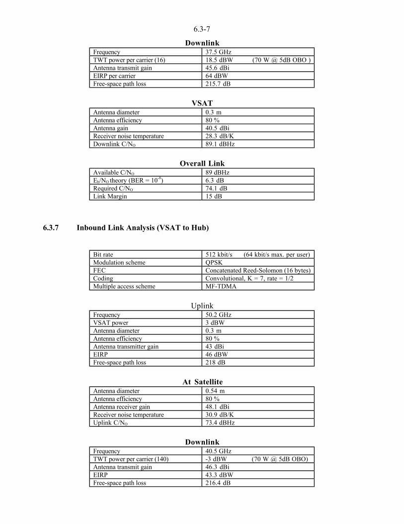
6.3-7

DownlinkFrequency 37.5 GHzTWT power per carrier (16) 18.5 dBW (70 W @ 5dB OBO )Antenna transmit gain 45.6 dBiEIRP per carrier 64 dBWFree-space path loss 215.7 dB

VSATAntenna diameter 0.3 mAntenna efficiency 80 %Antenna gain 40.5 dBiReceiver noise temperature 28.3 dB/K Downlink C/NO 89.1 dBHz

Overall LinkAvailable C/NO 89 dBHzEb/NO theory (BER = 10-8) 6.3 dBRequired C/NO 74.1 dBLink Margin 15 dB

6.3.7 Inbound Link Analysis (VSAT to Hub)

Bit rate 512 kbit/s (64 kbit/s max. per user)Modulation scheme QPSKFEC Concatenated Reed-Solomon (16 bytes)Coding Convolutional, K = 7, rate = 1/2Multiple access scheme MF-TDMA

UplinkFrequency 50.2 GHzVSAT power 3 dBWAntenna diameter 0.3 mAntenna efficiency 80 %Antenna transmitter gain 43 dBiEIRP 46 dBWFree-space path loss 218 dB

At SatelliteAntenna diameter 0.54 mAntenna efficiency 80 %Antenna receiver gain 48.1 dBiReceiver noise temperature 30.9 dB/K Uplink C/NO 73.4 dBHz

DownlinkFrequency 40.5 GHzTWT power per carrier (140) -3 dBW (70 W @ 5dB OBO)Antenna transmit gain 46.3 dBiEIRP 43.3 dBWFree-space path loss 216.4 dB

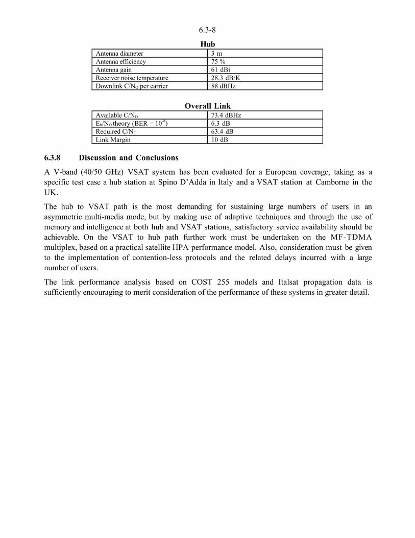
6.3-8

HubAntenna diameter 3 mAntenna efficiency 75 %Antenna gain 61 dBiReceiver noise temperature 28.3 dB/K Downlink C/NO per carrier 88 dBHz

Overall LinkAvailable C/NO 73.4 dBHzEb/NO theory (BER = 10-8) 6.3 dBRequired C/NO 63.4 dBLink Margin 10 dB

6.3.8 Discussion and Conclusions

A V-band (40/50 GHz) VSAT system has been evaluated for a European coverage, taking as aspecific test case a hub station at Spino D’Adda in Italy and a VSAT station at Camborne in theUK.

The hub to VSAT path is the most demanding for sustaining large numbers of users in anasymmetric multi-media mode, but by making use of adaptive techniques and through the use ofmemory and intelligence at both hub and VSAT stations, satisfactory service availability should beachievable. On the VSAT to hub path further work must be undertaken on the MF-TDMAmultiplex, based on a practical satellite HPA performance model. Also, consideration must be givento the implementation of contention-less protocols and the related delays incurred with a largenumber of users.

The link performance analysis based on COST 255 models and Italsat propagation data issufficiently encouraging to merit consideration of the performance of these systems in greater detail.

6.3-9

6.3.9 References

[Akram et al., 1999]Akram A., Shukla A., Konefal T. and Watson P.A., "Midas: A monthly link budget and decision aidtool for frequencies between 10 and 50 GHz", , IEE ICAP, York, April 1999, pp 152-155, 1999

[Capsoni et. al., 1987]Capsoni C., F. Fedi, C. Magistroni, A. Pawlina and A. Paraboni, “Data and theory for a new modelof the horizontal structure of rain cells for propagation applications”, Radio Science, Vol. 22, No. 3,pp. 395-404, 1987

[ITU-R, 1999a]ITU-R, Rec. PN. 618-6 “Propagation Data and Prediction Methods Required for Earth-SpaceTelecommunication Systems”, 1999.

[ITU-R, 1999b]ITU-R, Rec. PN. 837-2, “Characteristics of precipitation for propagation modelling”, 1999.

[Martellucci et al, 1998]Martellucci A., Boumis M., Barbaliscia F., ”A World wide statistical database of meteorological andpropagation parameters in clear air for SATCOM systems in Ka and V frequency bands”,Proc. 1st Intern. Workshop Radiow. Propag. Modelling for SatCom Services at Ku-Band and above,ESTEC, Noordwijk, The Netherlands, 28-29 October 1998.

6.4-1

CHAPTER 6.4Ka-band IRIDIUM Feeder Link

Editor: Jörg Habetha1

Authors: Laurent Castanet2, Edith Gimonet3, Jörg Habetha1, Carlo Riva4

1 Philips Research Laboratories, 'Digital Comm. and Networking', Weisshausstr. 2, D-52066 Aachen, GermanyTel.: +49-241-6003-560, Fax: +49-241-6003-519, e-mail: joerg.habetha@philips.com

2 ONERA CERT, 2 avenue Edouard Belin, BP 4025, F-31055 Toulouse CEDEX 4, France

Tel.: +33-5-6225-2729, Fax.: +33-5-6225-2577, e-mail: laurent.castanet@onecert.fr3 ONERA CERT, 2 avenue Edouard Belin, BP 4025, F-31055 Toulouse CEDEX 4, France

Tel.: +33-5-6225-2727, Fax.: +33-5-6225-2577, e-mail: edith.gimonet@onecert.fr4 Politecnico di Milano, Pza Leonardo da Vinci 32, I-20133 Milano, Italy

Tel.: +39-02-2399-3659, Fax.: +39-02-2399-3413, e-mail: riva@elet.polimi.it

6.4-2

6.4 Ka-band IRIDIUM Feeder Link

In this chapter the best statistical models identified in Part 2 are applied to a Low Earth OrbitSatellite (LEO) System to calculate impairment statistics. The propagation effects studied in theanalysis comprise oxygen, water vapour, cloud and rain attenuation as well as scintillation. The testcase only deals with the Feeder Link of the system and can therefore be classified as a fixed testcase. The mobile user link is studied in Chapter 7.2 with a different approach.

6.4.1 System Description

6.4.1.1 Overview

For this study the IRIDIUM Mobile Satellite System has been chosen as test system. The systemhas been chosen as an example of a LEO system that introduces additional complexity into thepropagation analysis due to varying elevation angles of the satellites.

The orbital height of the LEO satellites varies between 200 km and the van Allen belt at 1500 kmabove the Earth’s surface. The satellites are non-geostationary and their coverage area thereforechanges as the satellite rotates around the Earth. To permanently cover a fixed point on the Earth’ssurface a sufficiently large number of satellites has to be launched. Each time a satellite passes outof sight of the user, communication has to be taken over by another satellite. LEO/MEO systemsconsequently imply a relatively complicated system design and control. Other disadvantages ofLEO and MEO systems are small coverage areas per satellite compared to GEO satellites and shortconnection times to a given satellite with changing elevation angles. Nevertheless LEO and MEOsystems offer important advantages over GEO systems:

• low required transmission power due to the low orbit altitude,

• higher spectral efficiency,

• higher average elevation angles - the satellite next to the user can be chosen,

• high system reliability because of high redundancy,

• coverage of zones at high latitudes including the polar regions,

• low propagation delay.

The low power level necessary for transmission is probably the most important feature of LEOsystems, because it allows the use of small antennas and hand-held user terminals as is the case withthe IRIDIUM system. Due to the scarce frequency resources spectral efficiency is also a veryimportant topic. Cell diameters become smaller, the lower the orbital height of a satellite is. Smallcell diameter allow better frequency reuse and results in higher system capacity.

The IRIDIUM system was the first operational LEO Satellite Communication System (November1998). The system uses a constellation of 66 satellites at an altitude of 780 km as illustrated inFigure 6.4-1. The IRIDIUM system was originally designed to consist of 77 satellites, but thisnumber was later reduced to only 66 satellites. For this test case the 66 satellite constellation hasbeen chosen. The 66 satellites are equally distributed on 6 orbital planes each containing 11satellites. The planes are inclined by 86° with respect to the equatorial plane. The system isdesigned to guarantee a minimal elevation angle of 8° above the horizon with at least one satellitevisible to the user at any time. Each satellite generates a cluster of 48 cells on the Earth’s surface,formed by phased array L-band antennas. Variable antenna gains and automatic power control areused to compensate for the different path losses from innermost to outermost cells and varyingtransmission conditions. Frequency reuse within a satellite footprint follows a 12 cell cluster pattern(cf Figure 6 4 2)

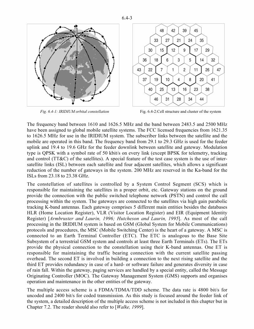
6.4-3

Fig. 6.4-1: IRIDIUM orbital constellation Fig. 6.4-2:Cell structure and cluster of the system

The frequency band between 1610 and 1626.5 MHz and the band between 2483.5 and 2500 MHzhave been assigned to global mobile satellite systems. The FCC licensed frequencies from 1621.35to 1626.5 MHz for use in the IRIDIUM system. The subscriber links between the satellite and themobile are operated in this band. The frequency band from 29.1 to 29.3 GHz is used for the feederuplink and 19.4 to 19.6 GHz for the feeder downlink between satellite and gateway. Modulationtype is QPSK with a symbol rate of 50 kbit/s on every link (except BPSK for telemetry, trackingand control (TT&C) of the satellites). A special feature of the test case system is the use of inter-satellite links (ISL) between each satellite and four adjacent satellites, which allows a significantreduction of the number of gateways in the system. 200 MHz are reserved in the Ka-band for theISLs from 23.18 to 23.38 GHz.

The constellation of satellites is controlled by a System Control Segment (SCS) which isresponsible for maintaining the satellites in a proper orbit, etc. Gateway stations on the groundprovide the connection with the public switched telephone network (PSTN) and control the callprocessing within the system. The gateways are connected to the satellites via high gain parabolictracking K-band antennas. Each gateway comprises 5 different main entities besides the databasesHLR (Home Location Register), VLR (Visitor Location Register) and EIR (Equipment IdentityRegister) [Armbruster and Laurin, 1996; Hutcheson and Laurin, 1995]. As most of the callprocessing in the IRIDIUM system is based on GSM (Global System for Mobile Communications)protocols and procedures, the MSC (Mobile Switching Center) is the heart of a gateway. A MSC isconnected to an Earth Terminal Controller (ETC). The ETC is analogous to the Base SiteSubsystem of a terrestrial GSM system and controls at least three Earth Terminals (ETs). The ETsprovide the physical connection to the constellation using their K-band antennas. One ET isresponsible for maintaining the traffic bearing connection with the current satellite passingoverhead. The second ET is involved in building a connection to the next rising satellite and thethird ET provides redundancy in case of a hard- or software failure and generates diversity in caseof rain fall. Within the gateway, paging services are handled by a special entity, called the MessageOriginating Controller (MOC). The Gateway Management System (GMS) supports and organisesoperation and maintenance in the other entities of the gateway.

The multiple access scheme is a FDMA/TDMA/TDD scheme. The data rate is 4800 bit/s foruncoded and 2400 bit/s for coded transmission. As this study is focused around the feeder link ofthe system, a detailed description of the multiple access scheme is not included in this chapter but inChapter 7.2. The reader should also refer to [Walke, 1999].

7 4743 22

37

40

46 31 28 34 44

23 38161325

19 10 4 8 20 41

261121

36 18 6 3 5 14 32

2917121530

33 27 21 24 35

45394248

9

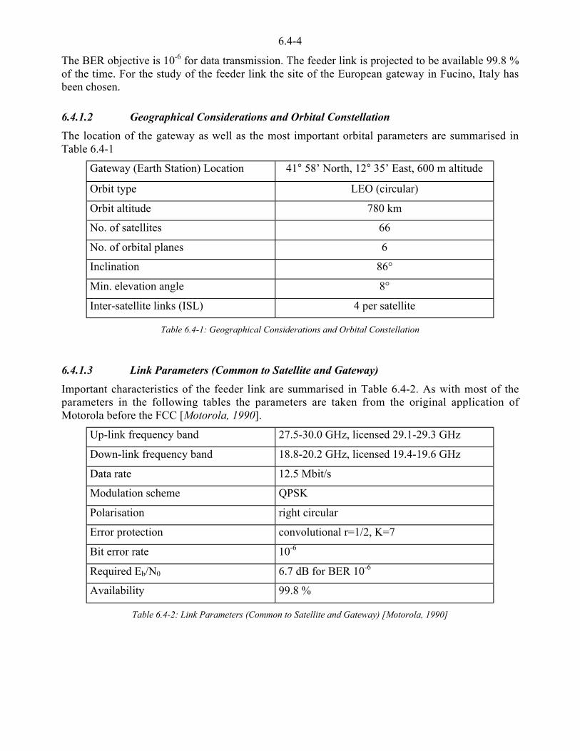
6.4-4

The BER objective is 10-6 for data transmission. The feeder link is projected to be available 99.8 %of the time. For the study of the feeder link the site of the European gateway in Fucino, Italy hasbeen chosen.

6.4.1.2 Geographical Considerations and Orbital Constellation

The location of the gateway as well as the most important orbital parameters are summarised inTable 6.4-1

Gateway (Earth Station) Location 41° 58’ North, 12° 35’ East, 600 m altitude

Orbit type LEO (circular)

Orbit altitude 780 km

No. of satellites 66

No. of orbital planes 6

Inclination 86°

Min. elevation angle 8°

Inter-satellite links (ISL) 4 per satellite

Table 6.4-1: Geographical Considerations and Orbital Constellation

6.4.1.3 Link Parameters (Common to Satellite and Gateway)

Important characteristics of the feeder link are summarised in Table 6.4-2. As with most of theparameters in the following tables the parameters are taken from the original application ofMotorola before the FCC [Motorola, 1990].

Up-link frequency band 27.5-30.0 GHz, licensed 29.1-29.3 GHz

Down-link frequency band 18.8-20.2 GHz, licensed 19.4-19.6 GHz

Data rate 12.5 Mbit/s

Modulation scheme QPSK

Polarisation right circular

Error protection convolutional r=1/2, K=7

Bit error rate 10-6

Required Eb/N0 6.7 dB for BER 10-6

Availability 99.8 %

Table 6.4-2: Link Parameters (Common to Satellite and Gateway) [Motorola, 1990]

6.4-5

6.4.1.4 Satellite

Satellite parameters relevant to the feeder link are included in Table 6.4-3.

Antenna type Planar phased array

Emitter output power 0.6-13.6 dBW (depending on atm. cond.)

Emitter net antenna gain 18.0 dB

Emitter losses 3.5 dB

Emitter EIRP 15.1-28.1 dBW (depending on atm. cond.)

Receiver net antenna gain 21.5 dB

Receiver antenna noise temperature 290.0 K

Receiver losses 4.0 dB

Receiver noise figure 3.0 dB

Receiver noise bandwidth 69.4 dBHz

Receiver G/T -10.1 dB/K

Table 6.4-3: Satellite parameters of the feeder link [Motorola, 1990]

6.4.1.5 Gateway

Gateway parameters regarding the feeder link are contained in Table 6.4-4.

Antenna type Parabolic

Antenna diameter 3.5 m

3 dB beamwidth 0.36° at 20 GHz, 0.24° at 30 GHz

Pointing angle range 5°-90° elevation

Emitter output power (-2.1)-24.0 dBW (depending on atm. cond.)

Emitter net antenna gain 57.1 dB

Emitter losses 3.5 dB

Emitter EIRP 51.6-77.6 dBW(±3dB) (depending on atm. cond.)

Receiver net antenna gain 53.7 dB

Receiver antenna noise temperature 30.0 K

Receiver losses 4.0 dB

Receiver noise figure 3.0 dB

Receiver noise bandwidth 69.4 dBHz

Receiver G/T 22.9 dB/K

Table 6.4-4: Gateway parameters of the feeder link [Motorola, 1990]

6.4-6

6.4.2 Link budgets

Table 6.4-5 shows link budgets of the feeder link as reported in [Motorola, 1990].

DOWNLINK UPLINK

Clear Rain Clear Rain

CENTER FREQ (GHz) 20.0 20.0 29.8 29.8

XMTR: HPA Output Power(dBW)

0.6 13.6 -2.1 24.0

Peak Ant Gain (dBi) 20.0 20.0 57.6 57.6

Off-Peak Loss (dB) 2.0 2.0 0.5 0.5

Net Antenna Gain (dB) 18.0 18.0 57.1 57.1

XMIT Circuit Losses (dB) 3.5 3.5 3.5 3.5

EIRP (dBWi) 15.1 28.1 51.6 77.6

Path Loss (dB) 185.7 185.7 189.1 189.1

Polarisation Loss (dB) 0.5 0.5 0.5 0.5

Atmos Loss (dB) 3.3 3.3 3.3 3.3

Rain Loss (dB) 0.0 13.0 0.0 26.0

TOT PROPAG. LOSS (dB) 189.5 202.5 192.9 218.9

RCVR: Ant Peak Gain (dBi) 54.2 54.2 23.5 23.5

Blockage/Off-Pk Loss (dB) 0.5 0.5 2.0 2.0

NET ANT GAIN (dB) 53.7 53.7 21.5 21.5

NOM RCV'D POWER (dBW) -120.7 -120.7 -119.9 -119.9

Net Ant Noise Temp (K) 30.0 30.0 290.0 290.0

Diplxr/FLT/Lim Losses (dB) 4.0 4.0 4.0 4.0

LNA Noise Fig (dB) 3.0 3.0 3.0 3.0

SYS NOISE TEMP, Ts (K) 1193.4 1193.4 1453.4 1453.4

G/Ts (dBi/K) 22.9 22.9 -10.1 -10.1

Boltzmann's (dBW/HzK) -228.6 -228.6 -228.6 -228.6

RCV'D C/N0 (dB) 77.1 77.1 77.1 77.1

Required Eb/N0 (dB) 5.7 5.7 5.7 5.7

RCVR Noise BW (dBHz) 69.4 69.4 69.4 69.4

Modem Impl Loss (dB) 2.0 2.0 2.0 2.0

REQUIRED C/N0 (dBHz) 77.1 77.1 77.1 77.1

LINK MARGIN (dB) 0.0 0.0 0.0 0.0

FLUX DENS (dBW/m2, 4 kHz) -155.1 -155.1 -118.6 -118.6

Table 6.4-5: Satellite-Gateway Link Budget - Downlink and Uplink [Motorola, 1990]

6.4-7

6.4.3 Approach to the study

6.4.3.1 Elevation and time percentage dependency of impairment

Conventional propagation studies were mostly carried out to generate the cumulative distributionfunction of attenuation (CDF) on a link between an earth station and a geostationary satellite, whichis characterised by a fixed elevation. Here, the considered system consists of a LEO constellation,which leads to a varying elevation angle that has to be taken into account when establishing theCDF. This can be done with the introduction of the elevation probability density function (PDF) ofthe link.

A procedure to calculate long-term statistics of impairments has been detailed in the new ITU-Rdraft Rec. P 618-6 [ITU-R, 1994]. This procedure recommends to calculate the conditional CDF ofimpairment for a single satellite in the following way:

determine the PDF of elevation angle of one satellite from a given earth station,

calculate the CDF of impairment corresponding to each elevation angle increment,

for each elevation angle calculate the time percentage that each impairment is exceeded (product ofthe probability that this elevation occurs and the percentage of time this impairment is exceeded),

for each impairment level, sum all percentage values (calculated in step 3).

This method is used in the present section to calculate the conditional cumulative distribution ofimpairment for the IRIDIUM feeder link.

6.4.3.2 Generation of elevation time series and statistics

As outlined in the previous section the PDF of elevation angle statistics is needed to generaterealistic impairment statistics. For this purpose the SaCoS (Satellite Communication Simulator)developed at the Chair of Communication Networks (ComNets) at Aachen University ofTechnology has been used. The simulator is able to evaluate the performance of protocols formallyspecified in SDL (Specification and Description Language). In this study only the constellationspecific part of the simulator has been needed. By simulating the orbital movement of the 66satellites of the IRIDIUM system, elevation angle statistics as seen from the Fucino gateway stationhave been generated. Different satellite selection strategies are implemented in the simulator. In thiscase it has been assumed that it is always the satellite with the highest elevation that is connected tothe gateway. The resulting PDF is illustrated in Figure 6.4-3.

0

0.005

0.01

0.015

0.02

0.025

0.03

0.035

0.04

0.045

0.05

0 10 20 30 40 50 60 70 80 90

Pro

babi

lity

Den

sity

Fun

ctio

n

Elevation Angle

Elevation Angle Statistics

elevation_stats

6.4-8

6.4.4 Propagation influence on air interface performance

The objective of this section is to determine the influence of propagation effects on the availabilityof the system. The method followed in this study consists firstly in selecting appropriatepropagation models, either to be able to take into account the given variation of elevation (throughits probability density function) or to ensure a relatively good accuracy of the prediction. In asecond step, cumulative distributions are established of separate impairments as well as of the totalimpairment.

6.4.4.1 Selection of propagation models

Simulations are realised using conventional prediction models which allow to evaluate the mainpropagation effects at Ka-band. These effects can be separated into two groups. The first containsclear sky effects: oxygen, water vapour and cloud attenuation as well as scintillation. The other israin attenuation. The influence of depolarisation will not be studied in the following.

Selecting the most appropriate propagation model to estimate the influence of propagation effectson the IRIDIUM feeder link is achieved through a comparison with measurements carried outduring the SIRIO experiment between 1978 and 1981 in Fucino.

The SIRIO results considered here were produced from excess attenuation measurements of a17.8 GHz beacon signal, realised with an earth station (antenna diameter of 17 m) located in Fucino[COST 205, 1985]. The large diameter of this earth station allows scintillation effects to be ignored,so rain attenuation prediction models can be tested in isolation.

Four years of data are available (see Figure 6.4-4). Among these four years, three CDFs exhibit asimilar behaviour (1978, 1979 and 1981) whereas the 1980 CDF is different. However, this effect isencountered only for time percentages lower than 0.005 %, which concerns rare strong events, anddoes not correspond to a possible availability target of the IRIDIUM feeder link at Ka band (due tothe limited margin available from the current state of the technology).

Fig. 6.4-4: Comparison prediction / measurements

CDF of measured rain attenuation are then compared to results obtained with both the DAH model(now, ITU-R recommendation P 618-6) and the EXCELL model [Capsoni et al., 1987], in whichthe CDF of rain rate is established with the Climpara model [Poiares-Baptista and Salonen, 1998].Although the measured CDF does not exceed time percentages higher than 0.04 % of the time, itcan be inferred from Figure 6.4-4 that the accuracy of both prediction models is relatively good.From this comparison, both predicted CDFs exhibit a good behaviour, so the model used for rain

6.4-9

6.4.4.2 Statistical simulation results

Simulation of CDF of impairments for the IRIDIUM feeder link are carried out with the bestconventional statistical models tested by COST 255 WG1 (see chapter 2.6).

For each propagation effect at Ka-band, the corresponding prediction model is given hereafter (forthe model description see also Chapters 2.1 to 2.6):

Oxygen attenuation: Salonen model [Salonen et al., 1992],

Water vapour attenuation: Salonen model [Salonen et al., 1992],

Cloud attenuation: ITU-R Recommendation P 840-2,

Clear sky scintillation: Van de Kamp model [Van de Kamp et al., 1999],

Rain attenuation: ITU-R draft Recommendation P 618-6 [ITU-R, 1994]

Total impairment: The Castanet-Lemoron method [Castanet et al., 2001]

Each calculation is performed using radiometeorological parameters (temperature, integrated watervapour content, integrated liquid water content, integrated liquid water content of heavy clouds, rainrate for 0.01 % of an average year) obtained for Fucino from Climpara maps [Poiares-Baptista andSalonen, 1998].

Simulations were carried out for all possible elevation angles to derive the conditional CDF ofimpairments with the procedure described above. In addition, conditional CDFs are compared withCDFs obtained for the corresponding minimum, maximum and mean fixed elevation angles(cf. Figure 6.4-5).

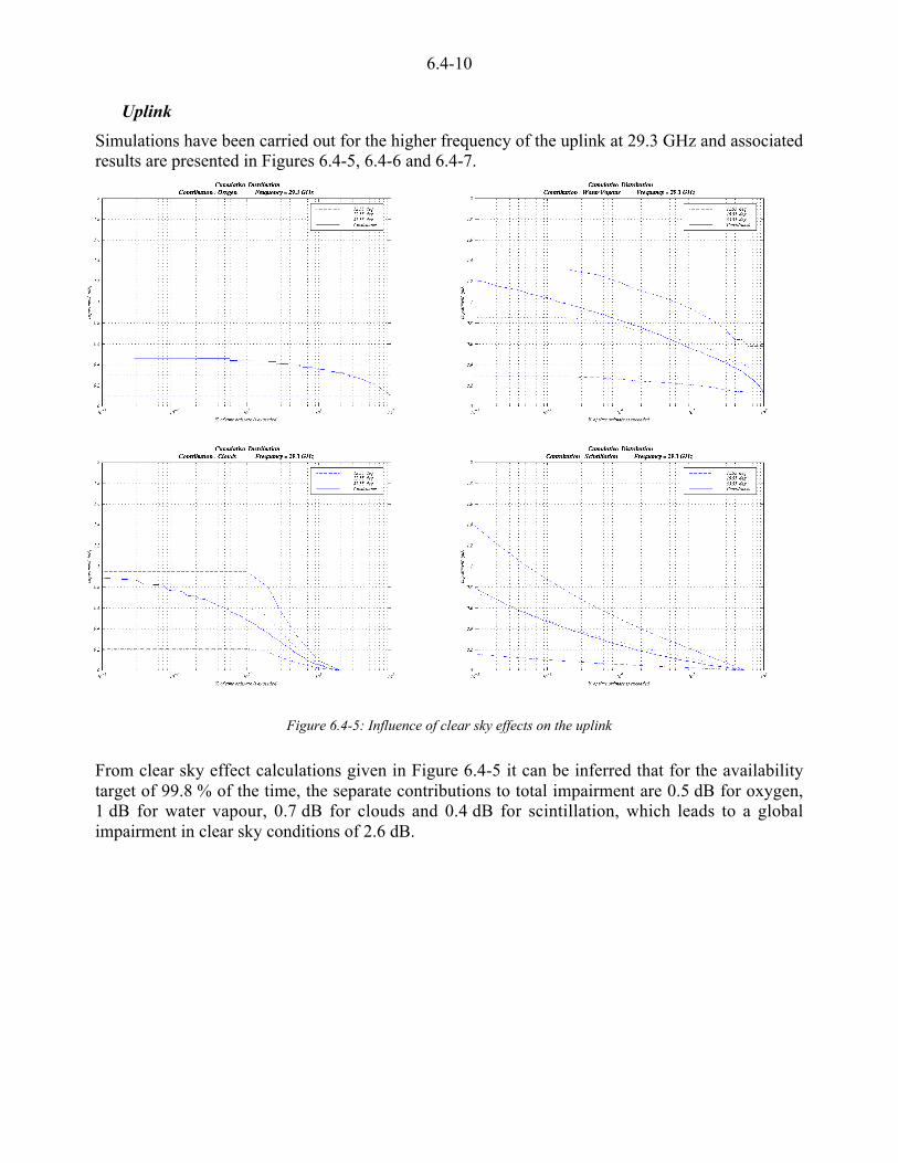
6.4-10

Uplink

Simulations have been carried out for the higher frequency of the uplink at 29.3 GHz and associatedresults are presented in Figures 6.4-5, 6.4-6 and 6.4-7.

Figure 6.4-5: Influence of clear sky effects on the uplink

From clear sky effect calculations given in Figure 6.4-5 it can be inferred that for the availabilitytarget of 99.8 % of the time, the separate contributions to total impairment are 0.5 dB for oxygen,1 dB for water vapour, 0.7 dB for clouds and 0.4 dB for scintillation, which leads to a globalimpairment in clear sky conditions of 2.6 dB.

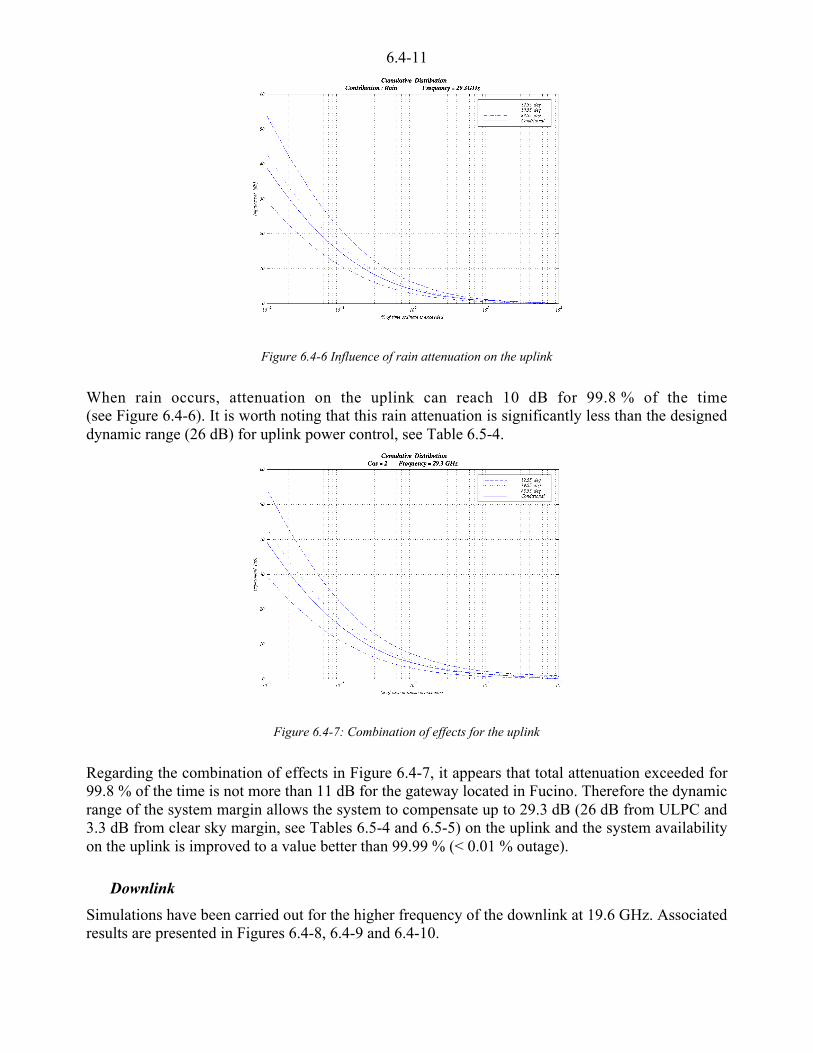
6.4-11

Figure 6.4-6 Influence of rain attenuation on the uplink

When rain occurs, attenuation on the uplink can reach 10 dB for 99.8 % of the time(see Figure 6.4-6). It is worth noting that this rain attenuation is significantly less than the designeddynamic range (26 dB) for uplink power control, see Table 6.5-4.

Figure 6.4-7: Combination of effects for the uplink

Regarding the combination of effects in Figure 6.4-7, it appears that total attenuation exceeded for99.8 % of the time is not more than 11 dB for the gateway located in Fucino. Therefore the dynamicrange of the system margin allows the system to compensate up to 29.3 dB (26 dB from ULPC and3.3 dB from clear sky margin, see Tables 6.5-4 and 6.5-5) on the uplink and the system availabilityon the uplink is improved to a value better than 99.99 % (< 0.01 % outage).

Downlink

Simulations have been carried out for the higher frequency of the downlink at 19.6 GHz. Associatedresults are presented in Figures 6.4-8, 6.4-9 and 6.4-10.

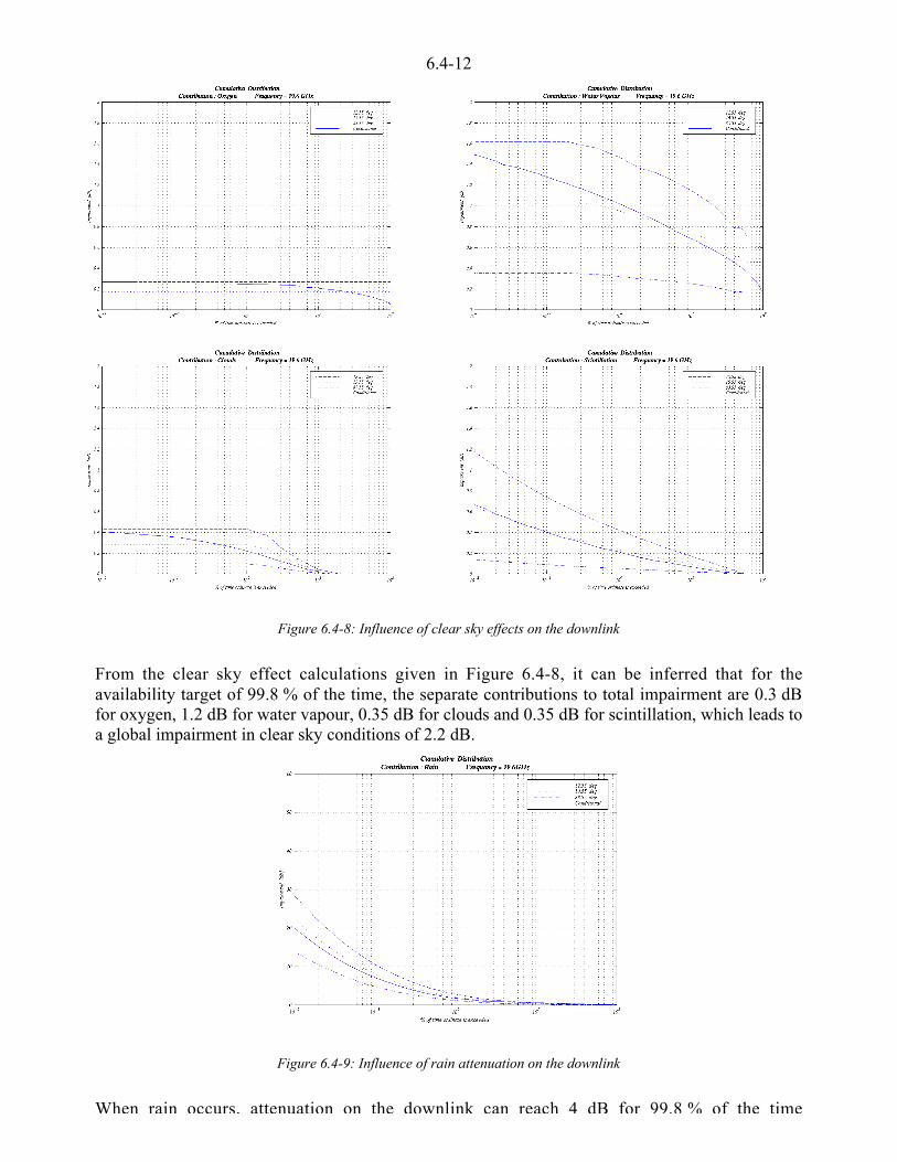
6.4-12

Figure 6.4-8: Influence of clear sky effects on the downlink

From the clear sky effect calculations given in Figure 6.4-8, it can be inferred that for theavailability target of 99.8 % of the time, the separate contributions to total impairment are 0.3 dBfor oxygen, 1.2 dB for water vapour, 0.35 dB for clouds and 0.35 dB for scintillation, which leads toa global impairment in clear sky conditions of 2.2 dB.

Figure 6.4-9: Influence of rain attenuation on the downlink

When rain occurs, attenuation on the downlink can reach 4 dB for 99.8 % of the time

6.4-13

dynamic range due to the ability to increase satellite EIRP in rain conditions (from 15.1 dBW to28.1 dBW), see Table 6.4-3.

Figure 6.4-10: Combination of effects for the downlink

Regarding the combination of effects in Figure 6.4-10, it appears that total attenuation exceeded for99.8 % of the time is not higher than 5 dB for the Earth station located in Fucino. Therefore thedynamic range of EIRP adjustment added to the clear sky margin allows the system to compensateup to 16.3 dB (13 dB for DLPC and 3.3 dB for clear sky margin) on the downlink and the systemavailability on the downlink could be improved to a value better than 99.98 % (< 0.02 % outage).

6.4.5 Conclusion

Availability due to propagation conditions has been evaluated for the feeder link using the bestconventional models tested by COST 255 WG1a and checked (for rain attenuation) with SIRIO18 GHz beacon data collected in Fucino.

Conditional CDF of total impairments have been established for both up and down links. It has beeninferred from this analysis that the IRIDIUM feeder link should comply with the availability targetof 99.8 % for both links, taking into account a clear sky static margin of 3.3 dB (for each link) and adynamic margin due to the use of Fade Mitigation Techniques (26 dB for Up Link Power Controland 13 dB for Down Link Power Control). More precisely, assuming a perfect FMT control loopbehaviour, the whole margins implemented in the system should allow to reach availability valuesbetter than 99.99 % for the uplink and better than 99.98 % for the downlink.

Eventually, it appears that the IRIDIUM feeder link simulated in this analysis is rather over-designed for an availability target of 99.8 % and for a gateway located in Fucino. But it has to betaken into account that other gateways around the globe may be situated in regions with lessfavourable climatic conditions. Besides, the practical availability supplied by the system, for actualcommunications established between users and using both the IRIDIUM constellation and theterrestrial network, will be essentially conditioned by the performance of the link established withthe mobile (due mainly to shadowing).

6.4.6 Acknowledgements

The authors would like to thank Prof. Dr. B. Walke, the head of the Institute of CommunicationNetworks at Aachen University of Technology, where the work of Jörg Habetha has been carriedout.

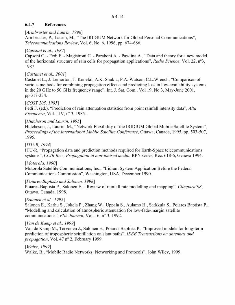
6.4-14

6.4.7 References

[Armbruster and Laurin, 1996]Armbruster, P., Laurin, M., “The IRIDIUM Network for Global Personal Communications”,Telecommunications Review, Vol. 6, No. 6, 1996, pp. 674-686.

[Capsoni et al., 1987]Capsoni C. - Fedi F. - Magistroni C. - Paraboni A. - Pawlina A., “Data and theory for a new modelof the horizontal structure of rain cells for propagation applications”, Radio Science, Vol. 22, nº3,1987

[Castanet et al., 2001]Castanet L., J. Lemorton, T. Konefal, A.K. Shukla, P.A. Watson, C.L.Wrench, “Comparison ofvarious methods for combining propagation effects and predicting loss in low-availability systemsin the 20 GHz to 50 GHz frequency range”, Int. J. Sat. Com., Vol 19, No 3, May-June 2001,pp 317-334.

[COST 205, 1985]Fedi F. (ed.), “Prediction of rain attenuation statistics from point rainfall intensity data”, AltaFrequenza, Vol. LIV, nº 3, 1985.

[Hutcheson and Laurin, 1995]Hutcheson, J., Laurin, M., “Network Flexibility of the IRIDIUM Global Mobile Satellite System”,Proceedings of the International Mobile Satellite Conference, Ottawa, Canada, 1995, pp. 503-507,1995.

[ITU-R, 1994]ITU-R, “Propagation data and prediction methods required for Earth-Space telecommunicationssystems”, CCIR Rec., Propagation in non-ionised media, RPN series, Rec. 618-6, Geneva 1994.

[Motorola, 1990]Motorola Satellite Communications, Inc., “Iridium System Application Before the FederalCommunications Commission”, Washington, USA, December 1990.

[Poiares-Baptista and Salonen, 1998]Poiares-Baptista P., Salonen E., “Review of rainfall rate modelling and mapping”, Climpara’98,Ottawa, Canada, 1998.

[Salonen et al., 1992]Salonen E., Karhu S., Jokela P., Zhang W., Uppala S., Aulamo H., Sarkkula S., Poiares Baptista P.,“Modelling and calculation of atmospheric attenuation for low-fade-margin satellitecommunications”, ESA Journal, Vol. 16, n° 3, 1992.

[Van de Kamp et al., 1999]Van de Kamp M., Tervonen J., Salonen E., Poiares Baptista P., “Improved models for long-termprediction of tropospheric scintillation on slant paths”, IEEE Transactions on antennas andpropagation, Vol. 47 nº 2, February 1999.

[Walke, 1999]Walke, B., “Mobile Radio Networks: Networking and Protocols”, John Wiley, 1999.

PART 7 Test Cases Involving Mobile Links

7.1-1

CHAPTER 7.1Simulation Approach

Editor: Simon R. Saunders1

Authors: Martin Döttling2, Claude Oestges3

1 Centre for Communication Systems Research, University of Surrey, Guildford, Surrey, GU2 5XH, UKTel.: +44-1483-259806, Fax.: +44-1483-259504, e-mail: S.Saunders@ee.surrey.ac.uk

2 Siemens AG, System Engineering / UMTS Development, ICM MP TI 6,Haidenauplatz 1, D-81667 Muenchen, GermanyTel. +49-89-722-58703, Fax: +49-89-722-27089, E-Mail: Martin.Doettling@mch.siemens.de

3 Université catholique de Louvain (UCL), Microwave Laboratory (EMIC),Place du Levant 3, B-1348 Louvain-la-Neuve, BelgiumTel.: +32-10-478105, Fax.: +32-10-478705, e-mail: Oestges@emic.ucl.ac.be

7.1-2

7.1 Simulation Approach

The work described in part was initiated with the following objectives:

• To demonstrate that the mobile propagation models described in Section 4 can be applied toreal system performance simulations. This helps to verify the usefulness of the individualmodels and demonstrates the general method of application to potential users of these models.

• To show that simulation approaches other than the conventional brute-force Monte-Carlomethods commonly followed can yield advantages in terms of allowing estimation of systemand link performance with relatively little computational effort.

The general approach followed in the simulations is described in chapters 7.1-1, 7.1-2 and 7.1-3.The approach is then followed for two particular test cases:

• a narrowband LEO 66 TDMA system (see Chapter 7.2);

• a wideband S-IMT-2000 system based on the Deligo constellation and a CDMA airinterface(see Chapter 7.3).

In each of the test cases, results from a selection of the Part 4 models are presented.

7.1.1 Approach

A two-level simulation approach is followed, split into:

• Link-Level simulation to determine the dependence of raw and coded BER on satellite,environment and user parameters, via an analytical expression for the relationship betweeninstantaneous signal-to-interference-plus-noise ratio (SINR) and raw BER (see Figure 7.1-1).

Channel Model

Satellite

Environment

User

SINR to BER mapping

DeInterleave

FEC correction/detection capabilities

Eb/No Time seriesor CDF

Pe Statistics ofRaw BER

Statistics ofcoded BER/FER

Figure 7.1-1: Link level simulation

7.1-3

• The results from the link level simulation are then implemented as look-up tables within theSystem-Level simulation, which is used with a constellation parameter generator andappropriate criteria for availability to determine overall system availability results (see Figure7.1-2).

Generation of Time Series

Link Modelling

Availability Evaluation

Satellites

Environment

Statistics of coded BER

Link Availability Statistics

Figure 7.1-2: System level simulation

The key reason for this split approach is to adopt the simplest method that will yield meaningfuloutputs. Conventional Monte-Carlo bit-by-bit simulation is avoided as being too time-consuming.

Note that this simulation approach (and probably any other method capable of yielding the samelevel of information) requires channel models capable of generating representative time series. Thuspurely statistical models that are only capable of predicting cumulative attenuation statistics, such asthose recommended by [ITU-R, 681-6, 1999], are inappropriate.

This is particularly the case when considering coded modulation schemes or time-dependentalgorithms such as power control.

7.1.2 Link Simulation

Simulations are mandatory for predicting the performance of land mobile satellite (LMS)communication systems. For system availability calculations a versatile two-level simulationapproach is used, which separates link-level and system-level simulation. The former aims atderiving statistics of coded bit error rate (BER) from propagation models, whereas the latter usesthe results of the link-level simulation to calculate the service availability statistics for dedicatedoperational scenarios.

The goal of this contribution is to approximate the function of channel coding without usingexpensive and time-consuming commercial system simulation packages. This allows a freedistribution among the COST 255 members and forms an open, simple and well-defined interfacefor different propagation models. Moreover, the system simulations within COST 255 are not

7.1-4

intended as in-depth studies of dedicated systems, but to highlight and illustrate the application ofstate-of-the-art LMS propagation modelling.

Basically two different strategies exist for the calculation of coded BER from propagation data:simulation and analytical approaches. Simulation software generates random bit errors andimplements the receiver function to correct these errors and retrieve the information. Variouscommercial and academic software packages exist. In general, a considerable computational effortis necessary and the application and interfacing with different propagation models is notstraightforward. Therefore the COST 255 link-level simulation uses analytical formulas, whichrequire only limited computer resources and allow the use of both, narrowband and widebandchannel models.

After a brief review of analytical bounds on coded BER for convolutional codes, the COST 255link-level simulation approach is outlined.

7.1.2.1 Analytical Bounds on coded BER

For convolutional codes with known transfer function a tight upper bound on the BER for softdecision Viterbi decoding is derived in [Proakis, 1995]:

BER tk

R dEN

tc dd d

b

free

, erfc10

12

( ) < u u u u ( )£

¤²

¥

¦´

=

'

-` 7.1-1

where `d is a factor obtained from the derivative of the code transfer function, the so-called codeweight distribution [Proakis, 1995]. dfree is the free distance of the code, R = k/n is the code rate andEb/N0 the information bit energy per spectral noise density.

For large Eb/N0 values the asymptotic performance is given by

BER tk

R dEN

tcd

freebfree

, erfc202

( ) < u u u ( )£

¤²

¥

¦´

`7.1-2

If the code transfer function is not known the convolutional channel coding theorem may be used[Viterbi and Omura, 1979], [Proakis, 1995] which yields the ensemble average error rate of aconvolutional code on a discrete memoryless channel:

BER t R R tc

k kKR t R

k R t R R,

( )/

( ( ) )/( )3 2 0

2 1 2

1 2

0

0( ) <

<( ) u<[ ]

� )<

< < 7.1-3

where K is the constraint length and R0 is the cut-off rate defined by [Viterbi and Omura, 1979],[Proakis, 1995]:

R t eR

EN

tb

0 21 1 0( ) = < +£

¤²²

¥

¦´´

< u ( )log 7.1-4

Unfortunately, equations 7.1-2 and 7.1-3 do not hold for small values of Eb/N0. In this case equation7.1-1 has to be used.

Figure 7.1-3a shows a comparison of these bounds for a R = 3/4, K = 7 convolutional code, as usedby Iridium and in the LEO66 test case of COST 255. The first ten terms of the code weight

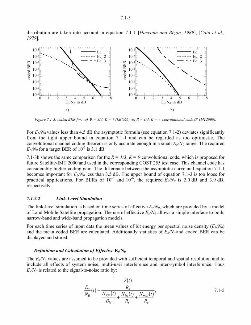
7.1-5

distribution are taken into account in equation 7.1-1 [Haccoun and Bégin, 1989], [Cain et al.,1979].

10-8

10-7

10-6

10-5

10-4

10-3

10-2

10-1

0 1 2 3 4 5 6 7 8

Eq. 1Eq. 2Eq. 3

code

d B

ER

Eb/N0 in dB

10-8

10-7

10-6

10-5

10-4

10-3

10-2

10-1

0 1 2 3 4 5 6 7 8

Eq. 1Eq. 2Eq. 3

code

d B

ER

Eb/N0 in dB

a) b)

Figure 7.1-3: coded BER for: a) R = 3/4, K = 7 (LEO66) ;b) R = 1/3, K = 9 convolutional code (S-IMT2000).

For Eb/N0 values less than 4.5 dB the asymptotic formula (see equation 7.1-2) deviates significantlyfrom the tight upper bound in equation 7.1-1 and can be regarded as too optimistic. Theconvolutional channel coding theorem is only accurate enough in a small Eb/N0 range. The requiredEb/N0 for a target BER of 10-2 is 3.1 dB.

7.1-3b shows the same comparison for the R = 1/3, K = 9 convolutional code, which is proposed forfuture Satellite-IMT 2000 and used in the corresponding COST 255 test case. This channel code hasconsiderably higher coding gain. The difference between the asymptotic curve and equation 7.1-1becomes important for Eb/N0 less than 3.5 dB. The upper bound of equation 7.1-3 is too loose forpractical applications. For BERs of 10-3 and 10-6, the required Eb/N0 is 2.0 dB and 3.9 dB,respectively.

7.1.2.2 Link-Level Simulation

The link-level simulation is based on time series of effective Es/N0, which are provided by a modelof Land Mobile Satellite propagation. The use of effective Es/N0 allows a simple interface to both,narrow-band and wide-band propagation models.

For each time series of input data the mean values of bit energy per spectral noise density (Eb/N0)and the mean coded BER are calculated. Additionally statistics of Eb/N0 and coded BER can bedisplayed and stored.

Definition and Calculation of Effective Es/N0

The Es/N0 values are assumed to be provided with sufficient temporal and spatial resolution and toinclude all effects of system noise, multi-user interference and inter-symbol interference. ThusEs/N0 is related to the signal-to-noise ratio by:

EN

t

S tR

N tB

N tR

N tR

s s

sys

N

isi

s

mai

c

0( ) =

( )

( )+

( )+

( ), 7.1-5

7.1-6

where S(t) is the received signal power, Nsys(t) the system noise, BN the noise bandwidth, Nisi(t) theequivalent noise due to inter-symbol interference, Nmai(t) the multiple access interference, Rs thechannel symbol rate and Rc the chip rate for CDMA systems.

This generic definition allows to investigate time division multiple access (TDMA), frequencydivision multiple access (FDMA) and code division multiple access (CDMA) systems as well ascombinations of these access schemes. While for TDMA/FDMA system noise will limit Es/N0, Nmai

is dominant in CDMA systems. For TDMA/FDMA schemes one might additionally set Rc = Rs anduse Nmai to represent co- and neighbouring channel interference.

Simple and narrowband models may assume constant values for the noise contributions in equation7.1-5. However, this definition is open enough to enable the use of more advanced models, that usetime-variant noise due to multiple access interference and inter-symbol interference, e.g. [Döttlinget al. , 1999].

The calculation of the signal and noise terms in equation 7.1-5 from wideband data is based on thecomplex polarimetric transmission matrix Ti(t), which is provided by the channel model for eachsatellite and every time step t. Additionally, the delay time oi(t) and direction of arrival (�i,si) aregiven for all N(t) relevant rays at time t.

After weighting each ray with the antenna pattern CR of the mobile terminal the complextransmission factor Ai(t) is obtained [Döttling et al. , 1999]:

A t C T ti RT

i i i( ) = ( ) u ( )� s, 7.1-6

where the superscript T denotes the transpose operation.

The superposition of all contributions yields the power delay profile, which is equivalent to thesatellite's time-variant channel impulse response

h t A t t tch i ii

N to b o o, ( ),

( )

( ) = ( ) u <( )=-

1

. 7.1-7

The received signal in the n-th symbol period Ts can be expressed as

y t a h n l t

a h t a h n l t

R l totl

n tot l totll n

o , ,

, , ,

( ) = <[ ]( )

= ( ) + <[ ]( )=<'

'

=<'&

'

-

-

Ts

0 Ts 7.1-8

where the first term represents the contribution of the wanted symbol an and the second term theinfluence of all other symbols [Miller et al., 1993], [Proakis, 1995].

The total impulse response htot is given by:

h t h h ttot sys cho o o, ,( ) = ( )� ( ) . 7.1-9

The system impulse response hsys of LMS systems is often of the raised-cosine filter type. Byevaluation of equations 7.1-7, 7.1-8 and 7.1-9 the wanted signal power yields:

S t P G P A t h t tT T R i sys ii

N t( ) ( ),

( )

= £¤

¥¦

( ) u <( )-h

o0

14

2 2

/7.1-10

7.1-7

and the corresponding inter-symbol interference power is

N t P G P

A t h n l t t

isi T T R

i sys ii

N t

ll n

( )

( ), .( )

= £¤

¥¦

u

( ) u <[ ] <( )==<'

&

'

--

h

o

02

2

4/

Ts1

7.1-11

Although Nisi is most often negligible for today's systems, it may influence future widebandsystems. For CDMA systems multiple access interference is the limiting factor for Es/N0.

For the downlink the MAI is a function of the received power Ps = Ss + Nisi,s from each visiblesatellite s and the number of equivalent channels Ceq per satellite:

N t P t Cmai ss s

S t

eq( )( )

= ( )=- u

0

. 7.1-12

Ps is calculated by the propagation model for all S(t) visible satellites. For synchronous orthogonalCDMA s0 = 2 (i.e. no MAI from the serving satellite), or else s0 = 1. Ceq depends on the number ofco-channel beams, beam overlap, channel utilisation, voice activity and antenna discrimination.Comprehensive derivations of Ceq can be found in [De Gaudenzi and Giannettti, 1998] and[Monsen, 1995].

In the uplink, the channel states of the interferers are not known and reasonable assumptions have tobe made for the mean value of Nmai.

Calculation of Effective Eb/N0 and coded BER

The corresponding Eb/N0 is calculated according to the modulation index M and the code rateR = k/n:

EN

tR M

EN

tb s

0 2 0

1( ) =u

u ( )log

. 7.1-13

As a point of reference, the raw bit error rate BERr for BPSK and QPSK can be calculated by

[Proakis, 1995]:

BER tEN

trb( ) = u ( )

£

¤²

¥

¦´

12 0

erfc . 7.1-14

In the COST 255 link-level software, the coded BER is calculated using equations 7.1-1 and 7.1-13.For each channel time series a corresponding time series of Eb/N0 and coded BER are generated, aswell as the corresponding probability density functions and the cumulative distribution functions[Döttling and Saunders, 1999]. Additionally, the mean value of Eb/N0 and the mean coded BER arecalculated.

7.1-8

7.1.3 System-Level Simulation

This section details the system-level simulation method in the context of Land Mobile Satellitesystems, as discussed in Section 7.1-1.

The inputs of the link-level simulation software are :

• a time-series of Eb/N0 values;

• a system parameter file;

• several simulation parameters.

The availability/coverage estimation is based on a new point of view, which differentiates temporalavailability and spatial coverage.

7.1.4.1 Time series simulation and evaluation of performance

Assuming that the elevation angle is kept constant, time series of fade levels have to be generatedon the basis of a propagation model. The fade time series are then easily converted into effectiveEb/N0 time series. Introducing the resulting Eb/N0 time series into the link model, statistics of BERare obtained for the environment. We note )|x(T |X �O , the statistical distribution of any of these

parameters (X = coded BER or effective Eb/N0), conditioned to the elevation angle. The time seriesthat are generated have to include all effects that induce a variation of the mobile channel, namelythe area surrounding the terminal as well as the azimuth angle, which continuously change overtime.

The azimuth angle relative to the street axis depends on both the random location of the receiver(random distribution) and the time-varying satellite position (smooth variation). In order tosimplify, it is assumed here that the azimuth angle is only associated with the mobile position.Therefore its variation should be taken into account within the propagation modelling.

Performance is usually expressed in terms of a specified BER which is not exceeded for a givenpercentage of time. For example, the LEO 66 performance for voice transmission given in the nextsection is defined by a BER of 10-2 with a global availability of 95 %.

In this study, a distinction is made between temporal availability (denoted as ‘availability’) andspatial coverage. The ultimate goal is to define the performance for a given area, such as a large cityand its suburbs, by a performance criterion which is not exceeded during o % of the time and overa % of the potentially usable area, e.g. non built-up areas. The performance criterion is for examplethe average raw or coded BER/FER, etc.

When the elevation angle is kept constant ( 0�� = ), the conditional distribution of X (e.g. coded

BER, effective Eb/N0) is equivalent to a distribution over the area for this particular value of � .The probability density function of X is indeed calculated on the basis of time series. These aregoverned by the characteristics of the area and of the terminal movements that feed the propagationmodel. On the other hand, the varying elevation angle is related to the satellite movement(depending on the system), and thus to ‘time’.

From the previous considerations, the conditional distribution )|x(T 0|X ��O = can be seen as a

spatial distribution (i.e. over the area) at a fixed time given by 0� .

Since the criterion X is usually a monotonic function of the elevation angle, knowing)|x(T 0|X ��O = makes it possible to obtain a spatial distribution achieved during a certain

cumulated percentage of time o. The latter is given by:

7.1-9

ǻ

«©

¨

=>=

>=

02

0

0|XX

0

d)(T][p

)|x(T)(T/

�O

O

����o

��o

7.1-15

where )(TX o stands for the distribution over the area of performance parameter X, for a percentageof time o.

The statistical distribution of elevation angle � can be easily calculated from orbit generators forany latitude on the globe. For example, the distribution of the elevation angle for the LEO66 systemcan be well approximated by a log-normal distribution. If an analytical distribution cannot be found,the probability density function of elevation angle has to be numerically defined.

A system-level simulation program has been developed to implement the formalism outlined above.Its inputs are:

• Time series of Eb/N0, for a range of elevation angles;

• Vector of elevation angle corresponding to the time series;

• Satellite system to be simulated;

• Latitude (the user can here choose between two latitudes: London and Rome, Italy);

• Parameter X to be represented (X = coded BER or Eb/N0).

The program produces several curves of area distribution of X, )(TX o , each being related to acertain time percentage o.

7.1-10

7.1.4 References

[Cain et al., 1979]Cain, J.B., Clark, G.C., Geist, J.M., "Punctured convolutional codes of Rate (n-1)/n and SimplifiedMaximum Likelihood Decoding", IEEE Trans. on Information Theory, vol. IT-25, no. 1, pp. 97-100, 1979.[De Gaudenzi and Giannettti, 1998]

De Gaudenzi, R., Giannetti, F., "DS-CDMA Satellite Diversity Reception for Personal SatelliteCommunication: Satellite-to-Mobile Link Performance Analysis", IEEE Trans. on VehicularTechnology, vol. 47, no. 2, pp. 658-672, 1998.[Döttling et al. , 1999]

Döttling, M., Zwick, T., Wiesbeck, W., "Investigation of Satellite Diversity and HandoverStrategies in Land Mobile Satellite Systems based on a Ray Tracing Propagation Model," Proc. Int.Mobile Satellite Conference. IMSC'99, Ottawa, Canada, 1999, pp. 128-133, 1999.[Döttling and Saunders, 1999]

Döttling, M., Saunders, S., "Bit Error Rate Calculation for Satellite Communication Systems", Proc.COST Joint International Workshop COST 252, COST 253, COST 255, Toulouse, France,. pp. 51-55, 1999.[Haccoun and Bégin, 1989]

Haccoun, D., Bégin, G., "High-Rate Punctured Convolutional Codes for Viterbi and SequentialDecoding", IEEE Trans. on Communications, vol. 37, no. 11, pp. 1113-1125, 1989.[ITU-R, 681-6, 1999]

International Telecommunication Union,"ITU-R Recommendation P.681-6: Propagation datarequired for the design of earth-space land mobile telecommunication systems", Geneva, 1999.[Miller et al., 1993]

Miller, M.J., Vucetic, B., Berry, L., "Satellite Communications – Mobile and Fixed Services",Kluwer Academic Publishers, 1993.[Monsen, 1995]

Monsen, P.,"Multiple-Access Capacity in Mobile User Satellite Systems," IEEE Journal onSelected Areas in Communications, vol. 13, no. 2, 1995, pp. 222-231, 1995.[Proakis, 1995]Proakis, J.G., "Digital Communications", Third Edition, McGraw-Hill, Inc., New York, 1995.[Viterbi and Omura, 1979]

Viterbi, A.J., Omura, J.K., "Principles of Digital Communications and Coding", McGraw-Hill, Inc.,New York, 1979.

7.2-1

CHAPTER 7.2LEO 66 Mobile Link

Editors: Jörg Habetha1, Simon Saunders2

Authors: Martin Döttling3, Jörg Habetha1, Claude Oestges4, Fernando Pérez-Fontán5, MaryanÁngeles Vázquez-Castro6, Werner Wiesbeck7

1 Philips Research Laboratories, 'Digital Comm. and Networking', Weisshausstr. 2, D-52066 Aachen, GermanyTel.: +49-241-6003-560, Fax: +49-241-6003-519, e-mail: joerg.habetha@philips.com

2 Centre for Communication Systems Research, University of Surrey, Guildford, Surrey, GU2 5XH, UKTel.: +44-1483-259806, Fax.: +44-1483-259504, e-mail: S.Saunders@ee.surrey.ac.uk

3 Siemens AG, System Engineering / UMTS Development, ICM MP TI 6,Haidenauplatz 1, D-81667 Muenchen, GermanyTel.: +49-89-722-58703, Fax: +49-89-722-27089, E-Mail: Martin.Doettling@mch.siemens.de

4 Université catholique de Louvain (UCL), Microwave Laboratory (EMIC),Place du Levant 3, B-1348 Louvain-la-Neuve, BelgiumTel.: +32-10-478105, Fax.: +32-10-478705, e-mail: Oestges@emic.ucl.ac.be

5 Universidad de Vigo, Escuela Superior de Ingenieros de Telecomunicaciones,Departamento de Tecnologías de las Comunicaciones, Campus Universitario, 36200 - Vigo, SpainTel.: +34-986-812137, Fax.: +34-986-812121, e-mail: fpfontan@tsc.uc3m.es

6 Universidad Carlos III de Madrid, Escuela Politécnica Superior,Departamento de Tecnologías de las Comunicaciones,Avda. de la Universidad, 30, 28911-Leganés, Madrid, Spain

Tel.: +34-91-6249173, Fax.: +34-91-6249430, e-mail: maryan@tsc.uc3m.es7 Universität Karlsruhe, Institut für Höchstfrequenztechnik und Elektronik,

Kaiserstr. 12, D-76128 Karlsruhe, Germany,Tel.: +49-721-608-6257, Fax.: +49-721-691865, e-mail: Werner.Wiesbeck@etec.uni-karlsruhe.de

7.2-2

7.2 LEO 66 Mobile Link

The simulation approach outlined in Chapter 7.1 will now be applied to a first test case system. Thisis a Low Earth Orbit (LEO) satellite system using a constellation of 66 satellites at an altitude of780 km. For the determination of the most important parameters of the system, data available fromthe IRIDIUM satellite system have been used.

The IRIDIUM system has already been introduced in Chapter 6.4, in which its feeder link has beenstudied. In this chapter we will deal with the mobile link between the user and a satellite. Eventhough the system has already been described we will briefly mention the main characteristics ofthe system once again. After a short description of the system, the most important systemparameters as well as the link budgets for the mobile user link will be presented in form of tables.Most of the data are taken from the original FCC application of Motorola Inc. [Motorola, 1990].

The 66 satellites of the test case system are equally distributed on 6 orbital planes, each containing11 satellites. The planes are inclined at 86° with respect to the equatorial plane. The system isdesigned to guarantee a minimal elevation angle of 8° above the horizon with at least one satellitevisible to the user at any time. Each satellite generates a cluster of 48 cells on the Earth’s surface,formed by phased array L-band antennas. Variable antenna gains and automatic power control areused to compensate for the different path losses from innermost to outermost cells and varyingtransmission conditions. Frequency reuse within a satellite footprint follows a 12 cell clusterpattern.

The constellation of satellites is controlled by a System Control Segment (SCS) which is, amongother things, responsible for maintaining the satellites in a proper orbit. Gateway stations on theground provide the connection with the public switched telephone network (PSTN) and control thecall processing within the system. The gateways are connected to the satellites via high gainparabolic tracking K-band antennas. Each gateway comprises 5 different main entities besides thedatabases HLR (Home Location Register), VLR (Visitor Location Register) and EIR (EquipmentIdentity Register) ([Armbruster and Laurin, 1996] and [Hutcheson and Laurin, 1995]). As most ofthe call processing in the IRIDIUM system is based on GSM (Global System for MobileCommunications) protocols and procedures, the MSC (Mobile Switching Center) is the heart of agateway. A MSC is connected to an Earth Terminal Controller (ETC). The ETC is analogous to theBase Site Subsystem of a terrestrial GSM system and controls at least three Earth Terminals (ETs).The ETs provide the physical connection to the constellation using their K-band antennas. One ETis responsible for maintaining the traffic-bearing connection with the current satellite passingoverhead. The second ET is involved in building a connection to the next rising satellite and thethird ET provides redundancy in case of a hardware or software failure and eventually raindiversity. Within the gateway, paging services are handled by a special entity, called the MessageOriginating Controller (MOC). The Gateway Management System (GMS) supports and organisesoperation and maintenance in the other entities of the gateway.

Mobile users communicate with the constellation via hand-held mobile voice terminals (handhelds)or pagers called Message Termination Controllers (MTD). The antenna of a subscriber unit is aQuadrifilar Helix L-band antenna.

Iridium subscriber links between the satellite and the mobile operate in the frequency range from1610 to 1626.5 MHz, but the FCC has only licensed operation from 1621.35 to 1626.5 MHz in theUSA. Modulation type is QPSK with a symbol rate of 50 kbit/s on the mobile user link.

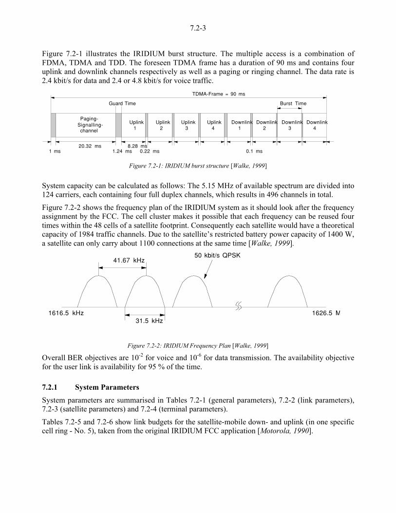
7.2-3

Figure 7.2-1 illustrates the IRIDIUM burst structure. The multiple access is a combination ofFDMA, TDMA and TDD. The foreseen TDMA frame has a duration of 90 ms and contains fouruplink and downlink channels respectively as well as a paging or ringing channel. The data rate is2.4 kbit/s for data and 2.4 or 4.8 kbit/s for voice traffic.

Figure 7.2-1: IRIDIUM burst structure [Walke, 1999]

System capacity can be calculated as follows: The 5.15 MHz of available spectrum are divided into124 carriers, each containing four full duplex channels, which results in 496 channels in total.

Figure 7.2-2 shows the frequency plan of the IRIDIUM system as it should look after the frequencyassignment by the FCC. The cell cluster makes it possible that each frequency can be reused fourtimes within the 48 cells of a satellite footprint. Consequently each satellite would have a theoreticalcapacity of 1984 traffic channels. Due to the satellite’s restricted battery power capacity of 1400 W,a satellite can only carry about 1100 connections at the same time [Walke, 1999].

1626.5 M

50 kbit/s QPSK41.67 kHz

31.5 kHz1616.5 kHz

Figure 7.2-2: IRIDIUM Frequency Plan [Walke, 1999]

Overall BER objectives are 10-2 for voice and 10-6 for data transmission. The availability objectivefor the user link is availability for 95 % of the time.

7.2.1 System Parameters

System parameters are summarised in Tables 7.2-1 (general parameters), 7.2-2 (link parameters),7.2-3 (satellite parameters) and 7.2-4 (terminal parameters).

Tables 7.2-5 and 7.2-6 show link budgets for the satellite-mobile down- and uplink (in one specificcell ring - No. 5), taken from the original IRIDIUM FCC application [Motorola, 1990].

Signalling-channel

Paging-Uplink

41Uplink

2Uplink

3Uplink Downlink

1Downlink

2Downlink

3 4Downlink

Burst Time

TDMA-Frame = 90 ms

20.32 ms 8.28 ms0.22 ms1.24 ms1 ms 0.1 ms

Guard Time

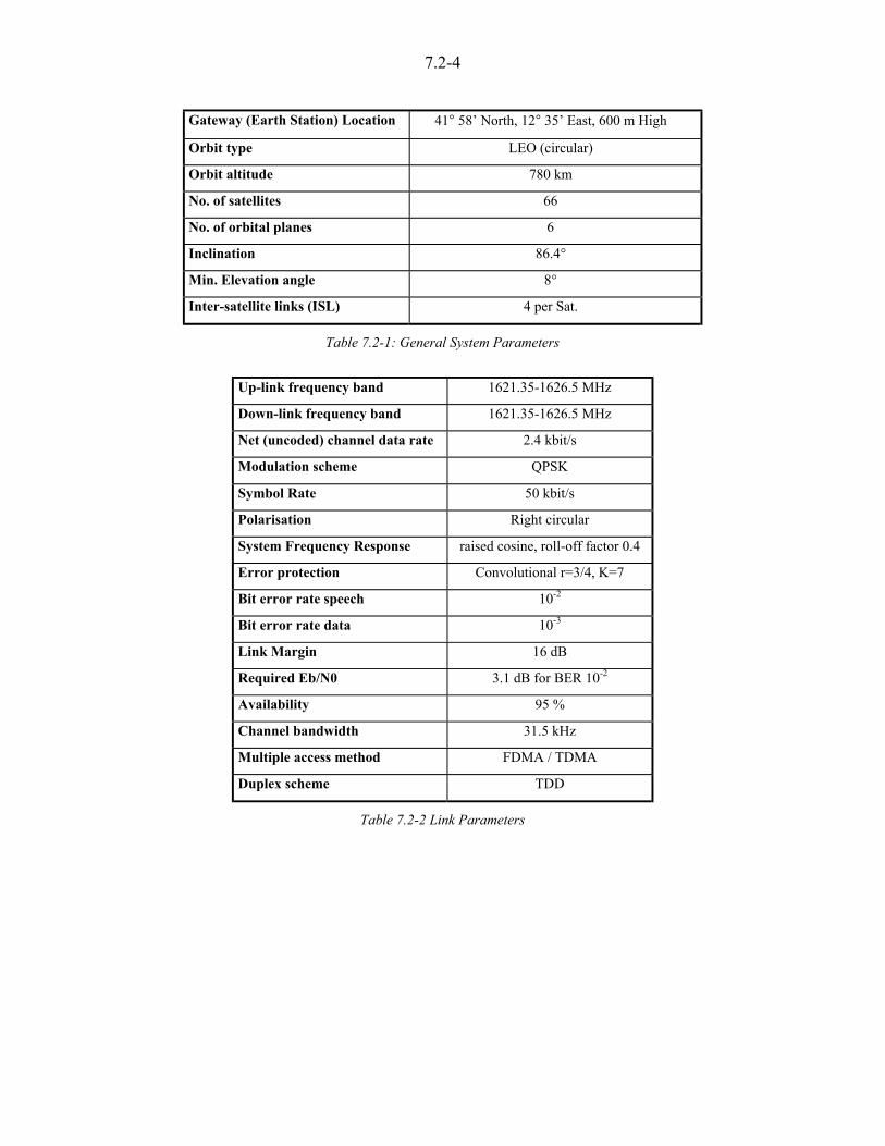
7.2-4

Gateway (Earth Station) Location 41° 58’ North, 12° 35’ East, 600 m High

Orbit type LEO (circular)

Orbit altitude 780 km

No. of satellites 66

No. of orbital planes 6

Inclination 86.4°

Min. Elevation angle 8°

Inter-satellite links (ISL) 4 per Sat.

Table 7.2-1: General System Parameters

Up-link frequency band 1621.35-1626.5 MHz

Down-link frequency band 1621.35-1626.5 MHz

Net (uncoded) channel data rate 2.4 kbit/s

Modulation scheme QPSK

Symbol Rate 50 kbit/s

Polarisation Right circular

System Frequency Response raised cosine, roll-off factor 0.4

Error protection Convolutional r=3/4, K=7

Bit error rate speech 10-2

Bit error rate data 10-3

Link Margin 16 dB

Required Eb/N0 3.1 dB for BER 10-2

Availability 95 %

Channel bandwidth 31.5 kHz

Multiple access method FDMA / TDMA

Duplex scheme TDD

Table 7.2-2 Link Parameters

7.2-5

Antenna type Planar phased array

Emitter burst power 1.5-11.8 dBW (depending on cell position)

Emitter net antenna gain 8.2-22.3 dBi (depending on cell position)

Emitter feeder loss 1.3 dB

Emitter EIRP 12.3-31.7 dBW (depending on cell position)

Receiver net antenna gain 8.2-22.3 dBi (depending on cell position)

Receiver antenna noise temperature 290.0 K

Receiver feeder loss 1.8 dB

Receiver noise figure 1.0 dB

Receiver noise bandwidth 126.0 kHz

Receiver G/T (-19.2)-(-5.1) dBi/K (depending on cell position)

No. of cells per satellite 48

Frequency reuse 12 cell cluster

No. of channels per satellite 1100 a 2.4 kbit/s (power limited)

Satellite transmission mode Regenerative / Switching

Table 7.2-3: Satellite Parameters

Antenna type Quadrifilar Helix

Emitter burst power 1.6-8.5 dBW (depending on cell position)

Emitter net antenna gain 1.0-3.0 dBi (depending on cell position)

Emitter feeder loss 0.7 dB

Emitter EIRP 1.9-10.3 dBW (depending on cell position)

Receiver net antenna gain 1.0-3.0 dBi (depending on cell position)

Receiver antenna noise temperature 150.0 K

Receiver feeder loss 1.0 dB

Receiver noise figure 0.8 dB

Receiver noise bandwidth 280.0 kHz

Receiver G/T (-23.8)-(-21.7) dBi/K (depending on cell position)

Table 7.2-4: Terminal Parameters

7.2-6

With Shadowing No ShadowingAzimuth Angle (deg) 30.0 30.0Ground Range (km) 1377.9 1377.9Nadir Angle (deg) 56.3 56.3Grazing Angle (deg) 21.4 21.4Slant Range (km) 1643.3 1643.3HPA Burst Power (W) 7.2 2.3dBW 8.6 3.7XMTR Peak Ant Gain (dBi) 23.0 23.0Edge Loss (dB) 1.5 1.5Scan Loss (dB) 3.0 3.0Taper Loss (dB) 1.0 1.0Net XMTR ANT GAIN (dBi) 17.5 17.5XMTR Feed / Ckt Loss (dB) 1.3 1.3EIRP (dBWi) 24.8 19.9Path Loss (dB) 160.9 160.9Polarisation Loss (dB) 0.5 0.5Atmos Absorption Loss (dB) 0.3 0.3Mean Vegetation Loss (dB) 8.2 0.0TOT PROPAG. LOSS (dB) 169.9 161.7RCVR Ant Net Gain (dBi) 1.2 1.2RCV'D SIG LEVEL, C (dBW) -143.9 -140.7RCVR Antenna N-Temp (K) 150.0 150.0RCVR Feed/Ckt Loss (dB) 1.0 1.0LNA Noise Figure (dB) 0.8 0.8RCV SYS NOISE TEMP, Ts (K) 298.9 298.9G/Ts (dBi/K) -23.6 -23.6RCVR Noise BW, B (kHz) 280.0 280.0Sensitivity = kTsB (dBW) -149.4 -149.4RCV'D C/N (dB) 5.4 8.7C/I (dB) 18.0 18.0RCV'D C/(N+I) (dB) 5.2 8.2RCV'D C/(N0+I0) (dB) 59.7 62.7Required Eb/N0 (dB) 3.2 3.2Modem Impl Loss (dB) 2.0 2.0REQUIRED C/(N+I) (dB) 5.2 5.2LINK MARGIN (dB) 0.0 3.0FLUX DENS (dBW/sq-m, 4 kHz) -127.5 -132.5

Table 7.2-5: Satellite-Mobile Link Budget - Downlink [Motorola, 1990]

7.2-7

With Shadowing No Shadowing

Azimuth Angle (deg) 30.0 30.0

Ground Range (km) 1377.9 1377.9

Nadir Angle (deg) 56.3 56.3

Grazing Angle (deg) 21.4 21.4

Slant Range (km) 1643.3 1643.3

HPA Burst Power (W) 6.9 2.2

DBW 8.4 3.5

NET XMTR ANT GAIN (dBi) 1.2 1.2

XMTR Feed / Ckt Loss (dB) 0.7 0.7

EIRP (dBWi) 8.9 4.0

Path Loss (dB) 160.9 160.9

Polarisation Loss (dB) 0.5 0.5

Atmos Absorption Loss (dB) 0.3 0.3

Mean Vegetation Loss (dB) 8.2 0.0

TOT PROPAG. LOSS (dB) 169.9 161.7

RCVR Peak Ant Gain (dBi) 23.0 23.0

Edge Loss (dB) 1.5 1.5

Scan Loss (dB) 3.0 3.0

Taper Loss (dB) 1.0 1.0

NET RCVR ANT GAIN (dBi) 17.5 17.5

RCV'D SIG LEVEL, C (dBW) -143.6 -140.2

RCVR Antenna N-Temp (K) 290.0 290.0

RCVR Feed/Ckt Loss (dB) 1.8 1.8

LNA Noise Figure (dB) 1.0 1.0

RCV SYS NOISE TEMP, Ts (K) 552.6 552.6

G/Ts (dBi/K) -9.9 -9.9

RCVR Noise BW, B (kHz) 126.0 126.0

Sensitivity = kTsB (dBW) -150.2 -150.2

RCV'D C/N (dB) 6.6 9.9

C/I (dB) 18.0 18.0

RCV'D C/(N+I) (dB) 6.3 9.3

RCV'D C/(N0+I0) (dB) 57.3 60.3

Required Eb/N0 (dB) 4.3 4.3

Modem Impl Loss (dB) 2.0 2.0

REQUIRED C/(N+I) (dB) 6.3 6.3

LINK MARGIN (dB) -0.6 3.0

FLUX DENS (dBW/sq-m, 4 kHz) -142.5 -144.9

Table 7.2-6: Mobile-Satellite Link Budget - Uplink [Motorola, 1990]

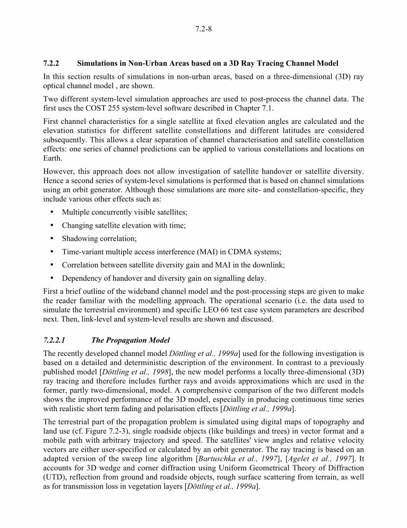
7.2-8

7.2.2 Simulations in Non-Urban Areas based on a 3D Ray Tracing Channel Model

In this section results of simulations in non-urban areas, based on a three-dimensional (3D) rayoptical channel model , are shown.

Two different system-level simulation approaches are used to post-process the channel data. Thefirst uses the COST 255 system-level software described in Chapter 7.1.

First channel characteristics for a single satellite at fixed elevation angles are calculated and theelevation statistics for different satellite constellations and different latitudes are consideredsubsequently. This allows a clear separation of channel characterisation and satellite constellationeffects: one series of channel predictions can be applied to various constellations and locations onEarth.

However, this approach does not allow investigation of satellite handover or satellite diversity.Hence a second series of system-level simulations is performed that is based on channel simulationsusing an orbit generator. Although those simulations are more site- and constellation-specific, theyinclude various other effects such as:

• Multiple concurrently visible satellites;

• Changing satellite elevation with time;

• Shadowing correlation;

• Time-variant multiple access interference (MAI) in CDMA systems;

• Correlation between satellite diversity gain and MAI in the downlink;

• Dependency of handover and diversity gain on signalling delay.

First a brief outline of the wideband channel model and the post-processing steps are given to makethe reader familiar with the modelling approach. The operational scenario (i.e. the data used tosimulate the terrestrial environment) and specific LEO 66 test case system parameters are describednext. Then, link-level and system-level results are shown and discussed.

7.2.2.1 The Propagation Model

The recently developed channel model Döttling et al., 1999a] used for the following investigation isbased on a detailed and deterministic description of the environment. In contrast to a previouslypublished model [Döttling et al., 1998], the new model performs a locally three-dimensional (3D)ray tracing and therefore includes further rays and avoids approximations which are used in theformer, partly two-dimensional, model. A comprehensive comparison of the two different modelsshows the improved performance of the 3D model, especially in producing continuous time serieswith realistic short term fading and polarisation effects [Döttling et al., 1999a].

The terrestrial part of the propagation problem is simulated using digital maps of topography andland use (cf. Figure 7.2-3), single roadside objects (like buildings and trees) in vector format and amobile path with arbitrary trajectory and speed. The satellites' view angles and relative velocityvectors are either user-specified or calculated by an orbit generator. The ray tracing is based on anadapted version of the sweep line algorithm [Bartuschka et al., 1997], [Agelet et al., 1997]. Itaccounts for 3D wedge and corner diffraction using Uniform Geometrical Theory of Diffraction(UTD), reflection from ground and roadside objects, rough surface scattering from terrain, as wellas for transmission loss in vegetation layers [Döttling et al., 1999a].

7.2-9

For each satellite and every time step t the complex polarimetric transmission matrix Ti(t), delaytime oi(t) and direction of arrival (�i,si) are calculated for all N(t) relevant rays. After weightingeach ray with the antenna pattern CR of the mobile terminal (MT) the complex transmission factorAi(t) is obtained. The superposition of all contributions yields the power delay profile, which isequivalent to the satellite's time-variant channel impulse response:

h t A t t tch i ii

N to b o o, ( ),

( )

( ) = ( ) u <( )=-

1

7.2-1

7.2.2.2 Signalling Delay

For LMS systems propagation time has to be considered. Especially the efficiency of system controlcommands is impaired by the signalling delay, which can be approximated by [Döttling et al.,1999b]:

6t t n t h t ts st st gw mt pr( ) = u ( )( ) +, ,¡ ¡ , 7.2-2

where nst is the number of signal trips between gateway and MT required to complete the signalling,tst the corresponding propagation time and tpr an additional delay due to signal processing in thecontrol instances. The impact of the slant range on tst is calculated based on orbit height h and thesatellite elevations as seen from the gateway (¡gw) and from the mobile terminal (¡mt).

7.2.2.3 Power Control (PC)

The system's power control is simulated by a user-defined number of power control steps, thecorresponding thresholds and power correction steps. Additionally, the target signal-to-noise ratio(SNR), the dynamic range, as well as the power control update rate are specified by the user. Thepower-controlled received power Ps(t) is calculated by:

P t t t P ts s s nom( ) = <( ) u ( )a 6 , , 7.2-3

where a is the power control factor and Ps,nom the received power for nominal transmitted power[Döttling et al., 1999b].

7.2.2.4 Handover Modelling

This study considers also the feasibility and benefit of satellite handover (HO) based on SNRmeasurements, since this type of handover requires the highest signalling effort and loads thesystem resources notably. To mitigate shadowing, a fast handover scheme is necessary. It is basedon a constant monitoring of the SNR values of all satellites. If the SNR of the active satellite fallsbelow a certain margin 6SNRHO with respect to the best satellite, a HO is initiated. To preventsystem congestion with signalling, a maximum HO rate can be specified. Based on theseparameters, a time series of bit energy to spectral noise density (Eb/N0) is calculated, which includesthe effect of handover and signalling delay 6ts. The performance of the handover scheme isevaluated by comparing the corresponding cumulative distribution function (CDF) of Eb/N0. Furtherdetails can be found in [Döttling et al., 1999b].

7.2.2.5 Satellite Diversity Modelling

Another way to increase system availability is satellite diversity. The SNR values of all satellites arel i d F b h lli di i i i h i lli i

7.2-10

established and power-controlled. The actual number of satellites in the active set is determined by6SNRadd and 6SNRdrop. If the SNR level of an inactive satellite is less than 6SNRadd below the bestsatellite, a request for adding this satellite to the active set is issued. In a similar way, a request fordropping a satellite from the active set is transmitted if its SNR value is more than 6SNRdrop belowthe best satellite. Both actions occur with signalling delay.

The superposition of the active satellites' signals is performed in the combiner. In this context onlymaximum ratio combining and two-branch diversity are considered. A comparison betweendifferent combining schemes and two- and three-branch diversity is given in [Döttling et al.,1999b], [Döttling et al., 1999c].

In diversity systems the trade-off between diversity gain and system loading due to the L(t)channels per connection has to be considered. The PDF and CDF of Eb/N0 after combining allowsevaluation of the diversity gain, while the cost in terms of system capacity is determined by themean number of active channels.

7.2.2.6 Polarisation Diversity Modelling

Measurement campaigns [Agius et al., 1999] and simulations [Döttling et al., 1999c] have recentlyemphasised the potential of polarisation diversity at the mobile terminal in certain propagationconditions. This diversity technique does not affect system capacity adversely, since only one trafficchannel is required. In this investigation polarisation diversity with maximum ratio combining isconsidered. Throughout the simulations right hand circular polarisation (RHCP) is used at thetransmitter. The primary receiver antenna is co-polarised. The second MT antenna is assumed tohave an identical antenna pattern and to be matched to the left hand circular polarisation (LHCP).

7.2.2.7 The Operational Scenario

The simulations are based on topographical and land use data of a 20km x 20km area in the RhineValley near Karlsruhe, Germany. The z-axis in Figure 7.2-3) shows topographical height, the landuse classes are shown in different greys. The landscape shows a typical non-urban mixture of terrainand land use elements. The mobile trajectory is depicted as a white arrow. The grid resolution is50 m.

Roadside trees and buildings are generated stochastically, with varying statistics for density, heightand location according to the land use class of the mobile position [IMST, DLR, IHE, 1998]. By thisway a synthetically and automatically generated fisheye image comparable to those in [Akturan andVogel, 1997] can be obtained. To illustrate this input data, Figure 7.2-3 depicts a snapshot of theLEO 66 simulations, showing the maximum elevation caused by topography and land use, as wellas the silhouettes of roadside trees and buildings as seen from the mobile antenna. The abscissagives the azimuth angle normalised to the momentary heading of the MT and the ordinate is theelevation angle.

7.2-11

20km

20km

heightin m

urbanindustrialstreetwatermobile path

open/agriculturemeadowdeciduous forestconiferous forestdense urban

300100

Figure 7.2-3: Topography, land use and mobile path in the Rhine Valley near Karlsruhe, Germany.

Table 7.2-7 shows simulation parameters that are common to all simulations. The simulations basedon satellite elevation statistics use 1000 points and 17 elevation angles from 5° to 85°.

parameter simulations using satelliteelevation statistics

simulations using an orbitgenerator

signal dynamic range 30dB

transmitted polarisation RHCP

sampling time 10ms 90ms

simulation time – 10min

mobile speed 1m/s, 15m/s, 30m/s 30m/s

total path length 10m, 150m, 300m 18 000 m

Channel impulse responses per simulations

204 000 24 797

Table 7.2-7: General Simulation Parameters

For each elevation angle, 12 different azimuth angles are simulated to perform sufficient averagingover azimuth, yielding a total number of over 200 000 channel impulse responses. The samplinginterval is 10 ms to resolve the channel coherence time and to include all relevant changes in thepropagation environment.

Characteristics of paths used for simulations based on satellite elevation statistics are summarised inTable 7.2-8. Path 1 simulates a pedestrian user walking at 1m/s.

Mobile Speed [m/s] Total Path Length [m]

Path 1 1 10

Path 2 15 150

Path 3 30 300

Table 7.2-8: Characteristics of paths used for simulations using satellite elevation statistics

7.2-12

The orbit generator simulations use 6655 simulation points. The number of visible satellites is time-and constellation-dependent. For the LEO 66 test case 24 797 channel impulse responses arecalculated.

The sampling time is 90 ms, since these investigations are intended to include the effect of the time-varying satellite positions and to average over a larger area of mobile locations.

7.2.2.8 System simulation Parameters

The baseline simulations use isotropic MT antennas and no power control. Additional simulationsare performed to investigate the impact of the MT antenna pattern, the efficiency of power control(PC), satellite handover, as well as satellite and polarisation diversity. The main system parametersrelevant for simulations are listed in Table 7.2-9.

parameter LEO 66 simulations

signalling delay nst = 2

power control 3-bit closed-loop power control

±10dB dynamic range90ms update interval

target Eb/N0 of 19.1dB

satellite handover 16dB hysteresis150ms processing time90ms update interval

satellite diversity 2-branch maximum ratio combining6dB hysteresis

90ms update interval

polarisation diversity maximum ratio combining

Table 7.2-9: Main LE0 66 Simulation Parameters

7.2.2.9 Simulations using Satellite Elevation Statistics

In this section results are presented, that use the channel model outlined above in combination withthe COST 255 system- and link-level software. Three different mobile paths are simulated, (seeTable 7.2-8).

The MT antenna pattern is assumed to be either isotropic or a that of a typical low-directivityhandheld antenna. The latter antenna pattern suppresses predominantly ground-reflected signals, thediscrimination of elevation angles greater than 5° is always below 3 dB. The LEO 66 satelliteelevation statistics are taken from Chapter 7.1.3.

Mainly four different types of graphs are shown:

• the samples of Eb/N0, to show the results of the channel model,

• the cumulative distribution function (CDF) of Eb/N0 for different elevation angles,

• the complementary cumulative distribution function (CCDF) of coded BER for differentelevation angles (link-level simulation results),

• the average coded BER versus percentage of area and time using the LEO 66 satelliteelevation distributions for latitudes of Rome and London (system-level simulations results).

7.2-13

The channel model results for satellites at 25°, 45° and 65° elevation are depicted in Figures 7.2-4and 7.2-5 path 1 (v = 1m/s) and path 3 (v = 30m/s), respectively. A thousand samples correspond toeach of the twelve different azimuth angles, which are separated by 30°. It is obvious that the shad-owing probability as well as the short term fading depth decreases with increasing elevation angle.

-10

-505

1015

202530

0 1000 2000 3000 4000 5000 6000 7000 8000 9000 10000 11000 12000

25°45°65°

Eb/N

0 i

n dB

sample no.

Figure 7.2-4: Eb/N0 samples for 25°, 45° and 65° elevation, path 1, 1000 samples correspond to one azimuth angle

-10

-505

1015

202530

0 1000 2000 3000 4000 5000 6000 7000 8000 9000 10000 11000 12000

25°45°65°

Eb/N

0 in

dB

sample no.

Figure 7.2-5: Eb/N0 samples for 25°, 45° and 65° elevation, path 3

The corresponding Eb/N0 statistics are shown in Figures 7.2-6a) and 7.2-9a).

Figures 7.2-6b) and 7.2-9b) show how the distributions of Eb/N0 translate into distributions of codedBER. The legends for these and subsequent plots are given in Figure 7.2-7.

Table 7.2-10 summarises the probabilities that the target BER of 10-2 is exceeded at elevationangles of 5°, 25°, 45° and 65° for the different simulations.

7.2-14

0

0.2

0.4

0.6

0.8

1

-10 -5 0 5 10 15 20 25 30

prob

abili

ty (

Eb/N

0 <

abs

ciss

a)

Eb/N0 in dB

0.0

0.1

0.2

0.3

0.4

0.5

0.6

0.7

10-6 10-5 10-4 10-3 10-2 10-1

prob

abili

ty (

BE

R >

abs

ciss

a)

BER

a) b)

Figure 7.2-6: CDF of Eb/N0 (a) and CCDF of BER (b) for path 1, isotropic antenna

5°10°15°20°25°30°35°40°45°

50°55°60°65°70°75°80°85°

100%99.98%97.63%87.13%69.90%51.58%35.97%24.18%

15.90%10.33%6.67%4.29%2.77%1.79%1.16%0.76%

a) b)

Figure 7.2-7: Legends for subsequent plots: a) elevation angle in CDFs of Eb/N0 and CCDFs of BERb) Time percentages for system-level simulation results at the latitude of Rome

Elevation angle Path 1 Path 2 Path 3 Path 1antenna

Path 1PC

5° 48.2% 48.2% 35.9% 55.5% 28.2%

25° 36.2% 20.0% 21.3% 37.0% 16.1%

45° 17.8% 12.4% 14.6% 18.2% 6.0%

65° 1.2% 1.2% 4.3% 1.5% 2.8%

Table 7.2-10: Probability of BER>10-2 for different simulation paths and elevation angles

System-level results are given in Figures 7.2-8 and 7.2-9b. Figure 7.2-8 shows the impact ofdifferent latitudes on system performance for path 1. In Figure 7.2-8a the satellite elevationdistributions for the latitudes of London and Rome are used.

At the target BER and 100% time percentage, the difference in percentage of area between bothplots is only 0.3% (97.3% for Rome and 97.6 % for London).

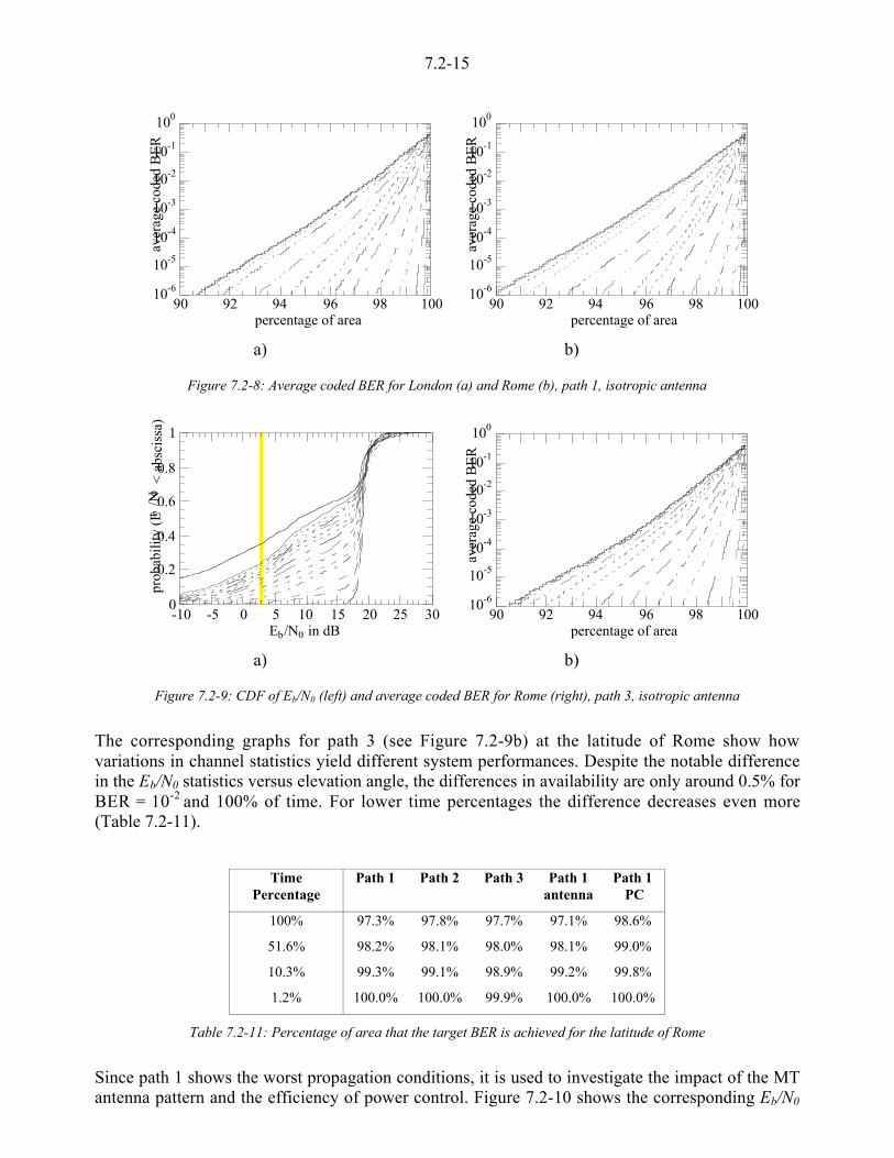
7.2-15

10-6

10-5

10-4

10-3

10-2

10-1

100

90 92 94 96 98 100

aver

age

code

d B

ER

percentage of area

10-6

10-5

10-4

10-3

10-2

10-1

100

90 92 94 96 98 100

aver

age

code

d B

ER

percentage of area

a) b)

Figure 7.2-8: Average coded BER for London (a) and Rome (b), path 1, isotropic antenna

0

0.2

0.4

0.6

0.8

1

-10 -5 0 5 10 15 20 25 30

prob

abili

ty (

Eb/N

0 <

abs

ciss

a)

Eb/N0 in dB

10-6

10-5

10-4

10-3

10-2

10-1

100

90 92 94 96 98 100

aver

age

code

d B

ER

percentage of area

a) b)

Figure 7.2-9: CDF of Eb/N0 (left) and average coded BER for Rome (right), path 3, isotropic antenna

The corresponding graphs for path 3 (see Figure 7.2-9b) at the latitude of Rome show howvariations in channel statistics yield different system performances. Despite the notable differencein the Eb/N0 statistics versus elevation angle, the differences in availability are only around 0.5% forBER = 10-2

and 100% of time. For lower time percentages the difference decreases even more(Table 7.2-11).

TimePercentage

Path 1 Path 2 Path 3 Path 1antenna

Path 1 PC

100% 97.3% 97.8% 97.7% 97.1% 98.6%

51.6% 98.2% 98.1% 98.0% 98.1% 99.0%

10.3% 99.3% 99.1% 98.9% 99.2% 99.8%

1.2% 100.0% 100.0% 99.9% 100.0% 100.0%

Table 7.2-11: Percentage of area that the target BER is achieved for the latitude of Rome

Since path 1 shows the worst propagation conditions, it is used to investigate the impact of the MTantenna pattern and the efficiency of power control. Figure 7.2-10 shows the corresponding Eb/N0

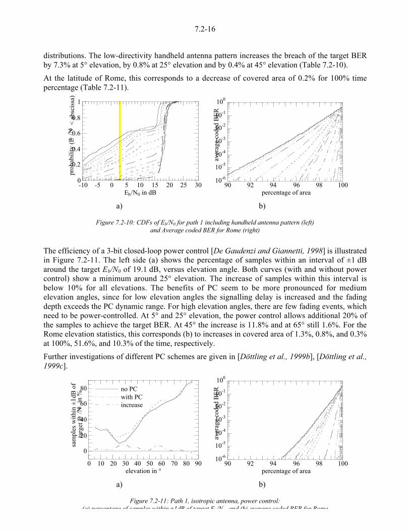
7.2-16

distributions. The low-directivity handheld antenna pattern increases the breach of the target BERby 7.3% at 5° elevation, by 0.8% at 25° elevation and by 0.4% at 45° elevation (Table 7.2-10).

At the latitude of Rome, this corresponds to a decrease of covered area of 0.2% for 100% timepercentage (Table 7.2-11).

0

0.2

0.4

0.6

0.8

1

-10 -5 0 5 10 15 20 25 30

prob

abili

ty (

Eb/N

0 <

abs

ciss

a)

Eb/N0 in dB

10-6

10-5

10-4

10-3

10-2

10-1

100

90 92 94 96 98 100

aver

age

code

d B

ER

percentage of area

a) b)

Figure 7.2-10: CDFs of Eb/N0 for path 1 including handheld antenna pattern (left)and Average coded BER for Rome (right)

The efficiency of a 3-bit closed-loop power control [De Gaudenzi and Giannetti, 1998] is illustratedin Figure 7.2-11. The left side (a) shows the percentage of samples within an interval of ±1 dBaround the target Eb/N0 of 19.1 dB, versus elevation angle. Both curves (with and without powercontrol) show a minimum around 25° elevation. The increase of samples within this interval isbelow 10% for all elevations. The benefits of PC seem to be more pronounced for mediumelevation angles, since for low elevation angles the signalling delay is increased and the fadingdepth exceeds the PC dynamic range. For high elevation angles, there are few fading events, whichneed to be power-controlled. At 5° and 25° elevation, the power control allows additional 20% ofthe samples to achieve the target BER. At 45° the increase is 11.8% and at 65° still 1.6%. For theRome elevation statistics, this corresponds (b) to increases in covered area of 1.3%, 0.8%, and 0.3%at 100%, 51.6%, and 10.3% of the time, respectively.

Further investigations of different PC schemes are given in [Döttling et al., 1999b], [Döttling et al.,1999c].

0

20

40

60

80

0 10 20 30 40 50 60 70 80 90

no PCwith PCincrease

sam

ples

with

in ±

1dB

of

targ

et E

b/N

0 in

%

elevation in °

10-6

10-5

10-4

10-3

10-2

10-1

100

90 92 94 96 98 100

aver

age

code

d B

ER

percentage of area

a) b)

Figure 7.2-11: Path 1, isotropic antenna, power control:(a) percentage of samples within ±1dB of target Eb/N0 and (b) average coded BER for Rome

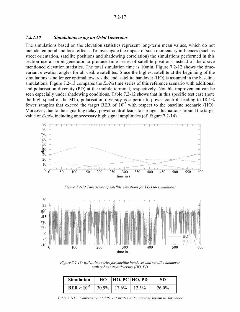
7.2-17

7.2.2.10 Simulations using an Orbit Generator

The simulations based on the elevation statistics represent long-term mean values, which do notinclude temporal and local effects. To investigate the impact of such momentary influences (such asstreet orientation, satellite positions and shadowing correlation) the simulations performed in thissection use an orbit generator to produce time series of satellite positions instead of the abovementioned elevation statistics. The total simulation time is 10min. Figure 7.2-12 shows the time-variant elevation angles for all visible satellites. Since the highest satellite at the beginning of thesimulations is no longer optimal towards the end, satellite handover (HO) is assumed in the baselinesimulations. Figure 7.2-13 compares the Eb/N0 time series of this reference scenario with additionaland polarisation diversity (PD) at the mobile terminal, respectively. Notable improvement can beseen especially under shadowing conditions. Table 7.2-12 shows that in this specific test case (notethe high speed of the MT), polarisation diversity is superior to power control, leading to 18.4%fewer samples that exceed the target BER of 10-2 with respect to the baseline scenario (HO).Moreover, due to the signalling delay, power control leads to stronger fluctuations around the targetvalue of Eb/N0, including unnecessary high signal amplitudes (cf. Figure 7.2-14).

0102030405060708090

0 50 100 150 200 250 300 350 400 450 500 550 600

elev

atio

n in

°

time in s

Figure 7.2-12 Time series of satellite elevations for LEO 66 simulations

-10

-505

1015

202530

0 100 200 300 400 500 600

HOHO, PD

Eb/N

0 in

dB

time in s

Figure 7.2-13: Eb/N0 time series for satellite handover and satellite handoverwith polarisation diversity (HO, PD

Simulation HO HO, PC HO, PD SD

BER > 10-2 30.9% 17.6% 12.5% 26.0%

Table 7.2-12: Comparison of different strategies to increase system performance

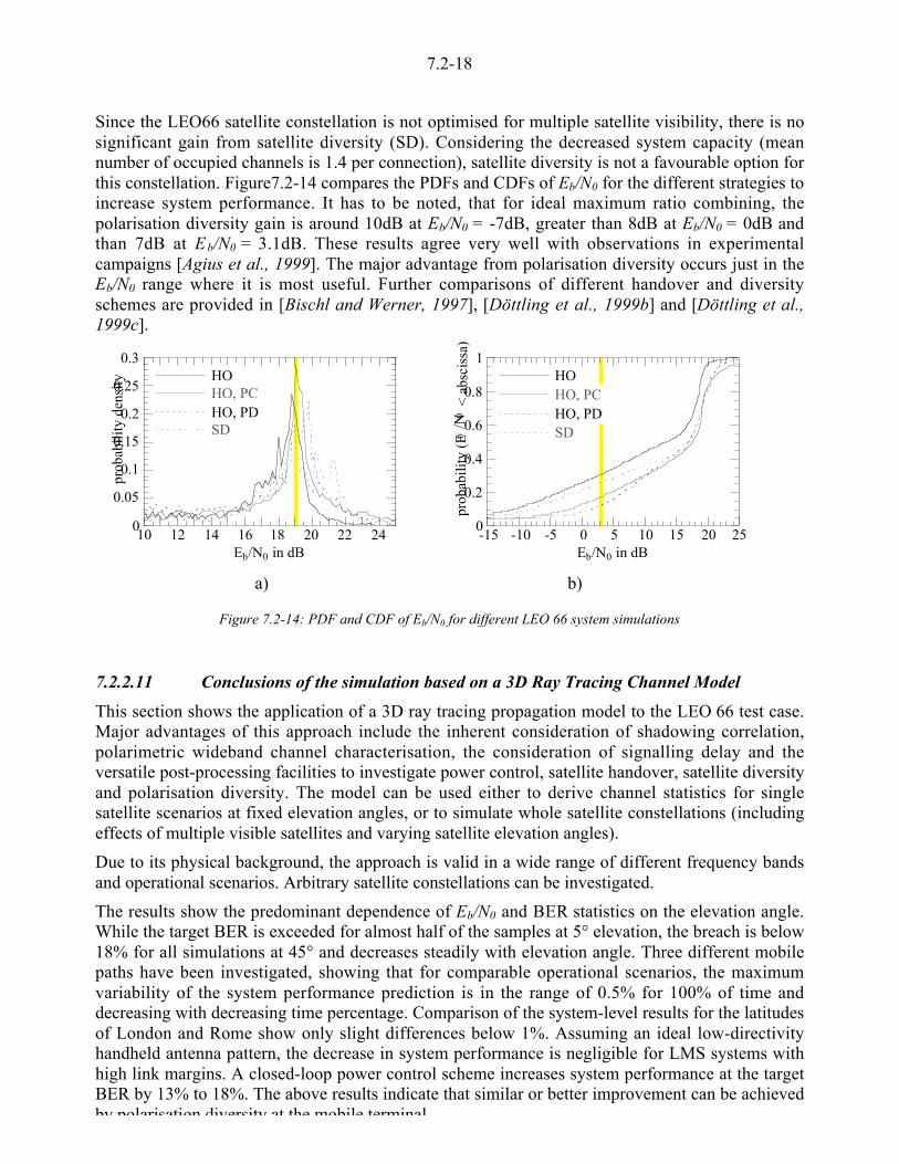
7.2-18

Since the LEO66 satellite constellation is not optimised for multiple satellite visibility, there is nosignificant gain from satellite diversity (SD). Considering the decreased system capacity (meannumber of occupied channels is 1.4 per connection), satellite diversity is not a favourable option forthis constellation. Figure7.2-14 compares the PDFs and CDFs of Eb/N0 for the different strategies toincrease system performance. It has to be noted, that for ideal maximum ratio combining, thepolarisation diversity gain is around 10dB at Eb/N0 = -7dB, greater than 8dB at Eb/N0 = 0dB andthan 7dB at Eb/N0 = 3.1dB. These results agree very well with observations in experimentalcampaigns [Agius et al., 1999]. The major advantage from polarisation diversity occurs just in theEb/N0 range where it is most useful. Further comparisons of different handover and diversityschemes are provided in [Bischl and Werner, 1997], [Döttling et al., 1999b] and [Döttling et al.,1999c].

0

0.05

0.1

0.15

0.2

0.25

0.3

10 12 14 16 18 20 22 24

HOHO, PCHO, PDSD

prob

abili

ty d

ensi

ty

Eb/N0 in dB

0

0.2

0.4

0.6

0.8

1

-15 -10 -5 0 5 10 15 20 25

HOHO, PCHO, PDSD

prob

abili

ty (

Eb/N

0 <

abs

ciss

a)

Eb/N0 in dB

a) b)

Figure 7.2-14: PDF and CDF of Eb/N0 for different LEO 66 system simulations

7.2.2.11 Conclusions of the simulation based on a 3D Ray Tracing Channel Model

This section shows the application of a 3D ray tracing propagation model to the LEO 66 test case.Major advantages of this approach include the inherent consideration of shadowing correlation,polarimetric wideband channel characterisation, the consideration of signalling delay and theversatile post-processing facilities to investigate power control, satellite handover, satellite diversityand polarisation diversity. The model can be used either to derive channel statistics for singlesatellite scenarios at fixed elevation angles, or to simulate whole satellite constellations (includingeffects of multiple visible satellites and varying satellite elevation angles).

Due to its physical background, the approach is valid in a wide range of different frequency bandsand operational scenarios. Arbitrary satellite constellations can be investigated.

The results show the predominant dependence of Eb/N0 and BER statistics on the elevation angle.While the target BER is exceeded for almost half of the samples at 5° elevation, the breach is below18% for all simulations at 45° and decreases steadily with elevation angle. Three different mobilepaths have been investigated, showing that for comparable operational scenarios, the maximumvariability of the system performance prediction is in the range of 0.5% for 100% of time anddecreasing with decreasing time percentage. Comparison of the system-level results for the latitudesof London and Rome show only slight differences below 1%. Assuming an ideal low-directivityhandheld antenna pattern, the decrease in system performance is negligible for LMS systems withhigh link margins. A closed-loop power control scheme increases system performance at the targetBER by 13% to 18%. The above results indicate that similar or better improvement can be achievedby polarisation diversity at the mobile terminal

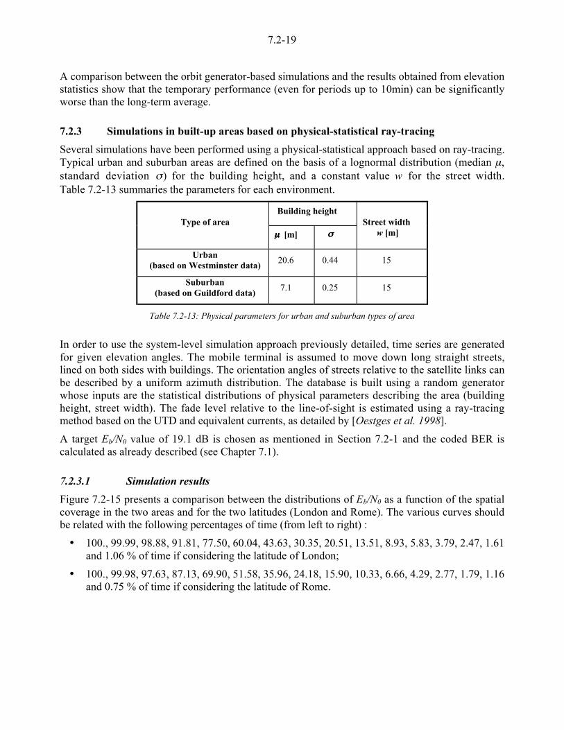
7.2-19

A comparison between the orbit generator-based simulations and the results obtained from elevationstatistics show that the temporary performance (even for periods up to 10min) can be significantlyworse than the long-term average.

7.2.3 Simulations in built-up areas based on physical-statistical ray-tracing

Several simulations have been performed using a physical-statistical approach based on ray-tracing.Typical urban and suburban areas are defined on the basis of a lognormal distribution (median µ,standard deviation m) for the building height, and a constant value w for the street width.Table 7.2-13 summaries the parameters for each environment.

Building heightType of area

µµµµ [m] mmmmStreet width

w [m]

Urban(based on Westminster data)

20.6 0.44 15

Suburban(based on Guildford data)

7.1 0.25 15

Table 7.2-13: Physical parameters for urban and suburban types of area

In order to use the system-level simulation approach previously detailed, time series are generatedfor given elevation angles. The mobile terminal is assumed to move down long straight streets,lined on both sides with buildings. The orientation angles of streets relative to the satellite links canbe described by a uniform azimuth distribution. The database is built using a random generatorwhose inputs are the statistical distributions of physical parameters describing the area (buildingheight, street width). The fade level relative to the line-of-sight is estimated using a ray-tracingmethod based on the UTD and equivalent currents, as detailed by [Oestges et al. 1998].

A target Eb/N0 value of 19.1 dB is chosen as mentioned in Section 7.2-1 and the coded BER iscalculated as already described (see Chapter 7.1).

7.2.3.1 Simulation results

Figure 7.2-15 presents a comparison between the distributions of Eb/N0 as a function of the spatialcoverage in the two areas and for the two latitudes (London and Rome). The various curves shouldbe related with the following percentages of time (from left to right) :

• 100., 99.99, 98.88, 91.81, 77.50, 60.04, 43.63, 30.35, 20.51, 13.51, 8.93, 5.83, 3.79, 2.47, 1.61and 1.06 % of time if considering the latitude of London;

• 100., 99.98, 97.63, 87.13, 69.90, 51.58, 35.96, 24.18, 15.90, 10.33, 6.66, 4.29, 2.77, 1.79, 1.16and 0.75 % of time if considering the latitude of Rome.

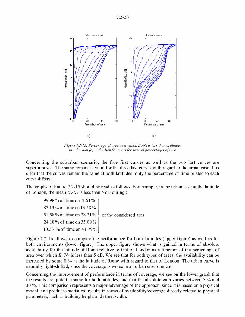
7.2-20

a) b)

Figure 7.2-15: Percentage of area over which Eb/N0 is less than ordinate,in suburban (a) and urban (b) areas for several percentages of time

Concerning the suburban scenario, the five first curves as well as the two last curves aresuperimposed. The same remark is valid for the three last curves with regard to the urban case. It isclear that the curves remain the same at both latitudes; only the percentage of time related to eachcurve differs.

The graphs of Figure 7.2-15 should be read as follows. For example, in the urban case at the latitudeof London, the mean Eb/N0 is less than 5 dB during :

«««

®

«««

­

¬

% 41.79on timeof % 10.33

% 35.00on timeof % 24.18

% 28.21on timeof % 51.58

% 13.58on timeof % 87.13

% 2.61on timeof % 99.98

of the considered area.

Figure 7.2-16 allows to compare the performance for both latitudes (upper figure) as well as forboth environments (lower figure). The upper figure shows what is gained in terms of absoluteavailability for the latitude of Rome relative to that of London as a function of the percentage ofarea over which Eb/N0 is less than 5 dB. We see that for both types of areas, the availability can beincreased by some 8 % at the latitude of Rome with regard to that of London. The urban curve isnaturally right-shifted, since the coverage is worse in an urban environment.

Concerning the improvement of performance in terms of coverage, we see on the lower graph thatthe results are quite the same for both latitudes, and that the absolute gain varies between 5 % and30 %. This comparison represents a major advantage of the approach, since it is based on a physicalmodel, and produces statistical results in terms of availability/coverage directly related to physicalparameters, such as building height and street width.

7.2-21

Figure 7.2-16: Comparison - between availabilities for both latitudes as a function of coverage (upper graph) andbetween coverages for both areas as a function of availability (lower graph)

The time series of fade also lead to the prediction of coded BER, as previously detailed.Figure 7.2-17 presents the coverage for a number of availabilities. The coverage is defined by thepercentage of area over which the coded BER is less than a certain value. The various availabilitiesdepend on the latitude, the percentages of time related to each curve remaining the same as thosefound for Eb/N0 curves.

a) b)

Figure 7.2-17: Percentage of area over which the coded BER is less than ordinate, in suburban (a) and urban (b) areasfor the latitudes of London and Rome and for several percentages of time

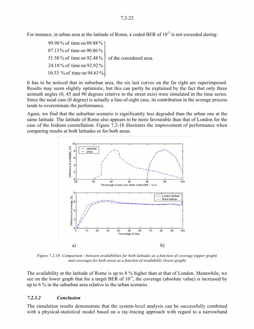
7.2-22

For instance, in urban area at the latitude of Rome, a coded BER of 10-3 is not exceeded during:

«««

®

«««

­

¬

% 94.63on timeof % 10.33

% 92.92on timeof % 24.18

% 92.48on timeof % 51.58

% 90.86on timeof % 87.13

% 89.88on timeof % 99.98

of the considered area.

It has to be noticed that in suburban area, the six last curves on the far right are superimposed.Results may seem slightly optimistic, but this can partly be explained by the fact that only threeazimuth angles (0, 45 and 90 degrees relative to the street axis) were simulated in the time series.Since the axial case (0 degree) is actually a line-of-sight case, its contribution in the average processtends to overestimate the performance.

Again, we find that the suburban scenario is significantly less degraded than the urban one at thesame latitude. The latitude of Rome also appears to be more favourable than that of London for thecase of the Iridium constellation. Figure 7.2-18 illustrates the improvement of performance whencomparing results at both latitudes or for both areas.

a) b)

Figure 7.2-18: Comparison - between availabilities for both latitudes as a function of coverage (upper graph)and coverages for both areas as a function of availability (lower graph)

The availability at the latitude of Rome is up to 8 % higher than at that of London. Meanwhile, wesee on the lower graph that for a target BER of 10-3, the coverage (absolute value) is increased byup to 6 % in the suburban area relative to the urban scenario.

7.2.3.2 Conclusion

The simulation results demonstrate that the system-level analysis can be successfully combinedwith a physical-statistical model based on a ray-tracing approach with regard to a narrowband

7.2-23

mobile satellite system. Since the combined method quite directly links the statistical properties ofthe physical area with the system performance it is very advantageous.

7.2.4 Simulations in Urban and Suburban Areas based on a Wideband Markov Channel(WMC) propagation model

The main focus of this section is on a detailed study of some key features related to the link-levelperformance evaluation of the LEO 66 Land Mobile Satellite system.

The key characteristics of the performance evaluation to be investigated are those which can beevaluated directly from time series of channel amplitude generated with a channel model. Systemlevel simulations results are also presented.

For performance physical-level evaluation of 3rd generation networks a single simulator approachwould be preferred but the complexity of such a simulator - including everything from transmittedwaveforms to multi-cell network and world coverage - is far too high. Therefore separate link andsystem level simulators are needed, even though it is not clear what kind of format is required forthe link level simulation outputs from the point of view of the system level simulator. In thissection, the interface to connect link and system level simulations is also addressed.

A wideband Markov channel propagation model has been used for generation of channel timeseries. The model is adequately described in Chapter 4.3 and a brief outline is given subsequently.

Simulations have been carried out for urban and suburban areas. The operational scenario isdescribed next. To streamline the reading, the foregoing nomenclature to specify differentparameters and simulations results are in agreement with similar topics described in other sections.

Only the uplink is investigated here as it is considered to be the most critical. For instance, powermeasurement is more complex since for the forward link, power is measured continuously on apilot.

It is worth clarifying that simulations described in this section are always static simulations in thesense that dynamic aspects of the system producing randomness in system parameters are not takeninto account. This means for example that simulations investigating the power control algorithm,which is a radio resource management algorithm consider a static Eb/No target. Consequently,dynamic aspects such as net capacity variability due to handover and diversity, increase of other cellinterference or compensation of fast fading, lie beyond the scope of this section.

Specific parameters considered for this simulation are listed in Table 7.2-14.

Parameter LEO 66 simulations

Elevations 15º - 45º

45º - 65º

65º - 85º

Power control 3-bit closed-loop power control

update times (Tpc):

from 10ms (Tpc = Tf) to 200 ms (Tpc = 20 Tf)

20 dB dynamic range

target Eb/N0 of 19.1 dB

Table 7.2-14: Specific LE0 66 Parameters Used for Simulations based on WMC model

7.2-24

7.2.4.1 The Propagation Model

The Wideband statistical model [Fontán et al., 1997] and [Fontán et al. 1998], used for thefollowing investigation is based on the 3-state Markov Model described in Chapter 4.3.

A basic feature of the model is that it is able to generate time-series of any channel parameter whosestudy is required: signal envelope, phase, instantaneous power delay profiles, Doppler spectra, etc.As a second step, conventional statistics, e.g. Cumulative Distribution Functions, are computedafterwards from the generated series.

The model makes the simplifying assumption of the existence of three basic rates of change (veryslow, slow and fast) in the received signal, corresponding to the different behaviours of itscomponents. As for the slow variations, they represent small-scale changes in the shadowingattenuation produced as the mobile travels in the shadow of the same obstacle or shadowingvariations behind a single building or group of buildings. In the line-of-sight (LOS) state slowvariations may be due to different reasons: for example, non-uniform receiving antenna patternsand/or changes in mobile orientation with respect to the satellite. Correlation distance, describinghow fast the log-normally-distributed variations are, is also considered in the model. Statesrepresent different gross shadowing conditions. Signal variations due to state changes areconsidered as the very slow variations of the direct signal (and consequently of the overall signal).Multipath contributions give rise to very fast variations which can be broken down into two classes:those related directly to the direct ray (that is, those echoes generated by the direct signal'sillumination of nearby scatterers) and those due to specular rays, if they exist. A few strong, farecho events (possible specular rays) have been registered in the experimental data sets [Smith andBarton, 1992] and [Jahn and Lutz, 1995].

Narrow-Band parameters are:

• State probability matrices: absolute state probability matrix [W] and state transition matrix[P].

• Loo distribution parameters for the different states: Si(_i, qi, MP). The Loo distribution isused to characterise both the direct signal (Log-Normal distribution: (_i, qi) and multipath(MP) for each state, environment and elevation.

• Correlation length of direct signal variations. In order to generate realistic signal series, longterm variation is introduced.

• State frame length or minimum state length.

Wide-Band parameters are:

• Average decay slope, S (dB, µs)

• Total multipath power, MP (dB relative to LOS)

• Distribution of times of arrival of echoes. Negative exponential distribution is assumed.

• Directions of arrival of multipath echoes. An uniform azimuth angle is assumed.

7.2.4.2 Power Control: Theoretical aspects

Power control is particularly important in a multiple access satellite system where users’propagation loss can vary over tens of decibels due to different distances and, to a lesser extent, toshadowing effects.

7.2-25

Power control mechanisms include both open and closed loop power control for the uplink andrelatively slow power control for the downlink.

Open Loop Power Control

The open loop power control adjusts the initial access channel transmission power and compensatesvariations in the path loss. The automatic gain control (AGC), gives a rough estimate of thepropagation loss of the forward link power received by the mobile unit. The mobile station controlsits transmit power according this estimate.

Closed Loop Power Control

Open loop cannot compensate the independence of the Rayleigh fading in the uplink and downlinkand therefore a closed loop power control is implemented for both the forward and the return link.This loop is driven in order to set the measured SIR (over an adequate period of time) to a targetvalue [Viterbi, 1998].

Power control commands are transmitted uncoded causing a high error ratio on the order of 5%[Öjanpera and Prasad, 1998]. However, since the loop is of delta modulation type (i.e. power isadjusted continuously up or down) this can be tolerable.

The dynamic range for the closed loop power control is on the order of 20 dB.

Downlink Slow Closed Loop Power Control

The target value is itself adaptively modified by means of slower outer control loop based on frameerror ratio (FER) measurements. Transmitted power in the downlink is periodically reduced, themobile unit measures the FER and when a predefined limit is exceeded, additional power isrequested.

The size of power control step defines the change introduced in the transmission power. A simpleup/down adjustment or several power adjustment levels are possible. Typical step sizes are between0.5 and 2 dB. It is worth noting that power control adjustment is relative to the previous powersetting, since absolute power setting would require expensive circuitry [Fukusawa and Sato, 1996].

7.2.4.3 Power Control: Simulations

Since no assumptions are made on the system features related to power control (PC) of the satellitecomponent of LEO 66, simulations were carried out for several Tpc (update rate), namely, Tpc = Tf,5 Tf, 10 Tf, 15 Tf and 20 Tf.

Simulations following a Montecarlo approach are able to simulate PC control algorithms at bit leveland makes FER and SIR measurements feasible. However, the purpose here is to use onlyinformation generated with the channel model, meaning that the criterion to be used throughout thesimulations is based on path loss.

Channel amplitude time series were generated with the previously mentioned 3-state Markovmodel, properly normalised to yield received signal or Eb/N0. Power correction steps of ± 0.75,± 1.10 and ± 1.9 dB were used as in [De Gaudenzi and Giannetti, 1998].

The time resolution has been set to 10 ms, which is coincident with the frame length. Coherencetimes of the channel for mobile speeds of 1 m/s, 15 m/s and 30 m/s are 80 ms, 5 ms and 2.5 msrespectively, meaning that time variability for 15 m/s and 30 m/s is undersampled. However it is notexpected that PC commands are activated at such a high rate.

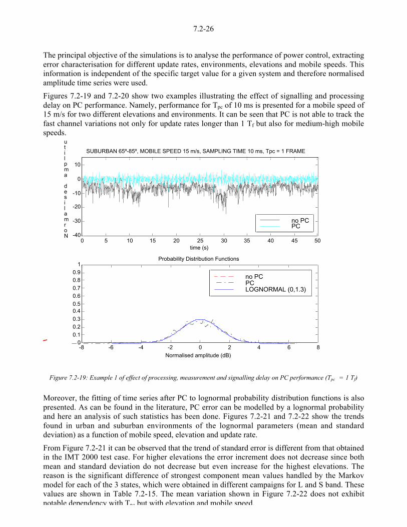
7.2-26

The principal objective of the simulations is to analyse the performance of power control, extractingerror characterisation for different update rates, environments, elevations and mobile speeds. Thisinformation is independent of the specific target value for a given system and therefore normalisedamplitude time series were used.

Figures 7.2-19 and 7.2-20 show two examples illustrating the effect of signalling and processingdelay on PC performance. Namely, performance for Tpc of 10 ms is presented for a mobile speed of15 m/s for two different elevations and environments. It can be seen that PC is not able to track thefast channel variations not only for update rates longer than 1 Tf but also for medium-high mobilespeeds.

0 5 10 15 20 25 30 35 40 45 50-40

-30

-20

-10

0

10

SUBURBAN 65º-85º, MOBILE SPEED 15 m/s, SAMPLING TIME 10 ms, Tpc = 1 FRAME

time (s)

Normalised amplitu

no PCPC

-8 -6 -4 -2 0 2 4 6 80

0.1

0.2

0.3

0.40.5

0.6

0.7

0.8

0.9

1Probability Distribution Functions

Normalised amplitude (dB)

no PCPCLOGNORMAL (0,1.3)

Figure 7.2-19: Example 1 of effect of processing, measurement and signalling delay on PC performance (Tpc = 1 Tf)

Moreover, the fitting of time series after PC to lognormal probability distribution functions is alsopresented. As can be found in the literature, PC error can be modelled by a lognormal probabilityand here an analysis of such statistics has been done. Figures 7.2-21 and 7.2-22 show the trendsfound in urban and suburban environments of the lognormal parameters (mean and standarddeviation) as a function of mobile speed, elevation and update rate.

From Figure 7.2-21 it can be observed that the trend of standard error is different from that obtainedin the IMT 2000 test case. For higher elevations the error increment does not decrease since bothmean and standard deviation do not decrease but even increase for the highest elevations. Thereason is the significant difference of strongest component mean values handled by the Markovmodel for each of the 3 states, which were obtained in different campaigns for L and S band. Thesevalues are shown in Table 7.2-15. The mean variation shown in Figure 7.2-22 does not exhibitnotable dependency with Tpc but with elevation and mobile speed.

7.2-27

0 5 10 15 20 25 30 35 40 45 50-40

-30

-20

-10

0

10

URBAN 15º-45º, MOBILE SPEED 15 m/s, SAMPLING TIME 10 ms, Tpc = 1 FRAME

time (s)

Normalised amplitu

no PCPC

-8 -6 -4 -2 0 2 4 6 80

0.1

0.2

0.3

0.40.5

0.6

0.7

0.8

0.9

1Probability Distribution Functions

Normalised amplitude (dB)

no PCPCLOGNORMAL (0,0.8)

Figure 7.2-20: Example 2 of effect of processing, measurement and signalling delay on PC performance (Tpc = 1 Tf)

15º - 45º 45º - 65º 65º - 85º

State1 State 2 State 3 State1 State 2 State 3 State1 State 2 State 3

Sub. -1.0 -3.7 -15.0 -0.3 -2.0 -3.8 -0.4 -2.5 -4.2S

Band Urb. -0.3 -8.0 -24.0 -0.35 -6.3 -15.2 -0.25 -6.6 -11

Sub. 0.0 -6.3 -9.0 -0.5 -6.5 -14.0 -0.2 -6.0 -11.5L

Band Urb. 0.6 -15.3 -30.0 0.2 -4.2 -6.5 -0.5 -4.3 -6.6

Table 7.2-15: Mean value of the strongest component for each state, environment and elevation

In conclusion, it is very difficult for a PC algorithm to track fast fading at high mobile speeds due tomeasurement delay, signalling delay, etc. A possible mitigation of this is the use of coding andinterleaving (time diversity) which are more effective at fast mobile speeds but there is an “adverse”region around 30 m/s where neither power control nor the coding and interleaving are effective.Then, requirements for power control parameters should be set according to these mobile speeds. Itwould be optimum to have variable power control rate according to the mobile speed.

7.2-28

0 5 10 15 200

0.5

1

1.5

2

2.5

3

3.5

Tpc (in number of frames, frame = 10 ms)

LogNormal standard deviation Elevations : 15º - 45º

0 5 10 15 200

0.5

1

1.5

2

2.5

3

3.5

Tpc (in number of frames, frame = 10 ms)

LogNormal standard deviation Elevations : 45º - 65º

0 5 10 15 200

0.5

1

1.5

2

2.5

3

3.5

Tpc (in number of frames, frame = 10 ms)

LogNormal standard deviation Elevations : 65º - 85º

0 5 10 15 200

0.5

1

1.5

2

2.5

3

3.5

Tpc (in number of frames, frame = 10 ms)

LogNormal standard deviation Elevations : 15º - 45º

0 5 10 15 200

0.5

1

1.5

2

2.5

3

3.5

Tpc (in number of frames, frame = 10 ms)

LogNormal standard deviation Elevations : 45º - 65º

0 5 10 15 200

0.5

1

1.5

2

2.5

3

3.5

Tpc (in number of frames, frame = 10 ms)

LogNormal standard deviation Elevations : 65º - 85º

Figure 7.2-21: Effects of elevation, mobile speed and PC update time on PC error measured in terms of the lognormalstandard deviation variability. Suburban (top) and urban (down), (o) 1 m/s, (*) 15 m/s, (+) 30 m/s

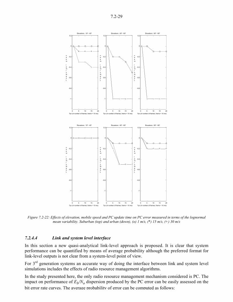
7.2-29

0 5 10 15 20

-1

-0.8

-0.6

-0.4

-0.2

0

0.2

Tpc (in number of frames, frame = 10 ms)

LogNormal mean

Elevations : 15º - 45º

0 5 10 15 20

-1

-0.8

-0.6

-0.4

-0.2

0

0.2

Tpc (in number of frames, frame = 10 ms)

LogNormal mean

Elevations : 45º - 65º

0 5 10 15 20

-1

-0.8

-0.6

-0.4

-0.2

0

0.2

Tpc (in number of frames, frame = 10 ms)

LogNormal mean

Elevations : 65º - 85º

0 5 10 15 20

-1

-0.8

-0.6

-0.4

-0.2

0

0.2

Tpc (in number of frames, frame = 10 ms)

LogNormal mean

Elevations : 15º - 45º

0 5 10 15 20

-1

-0.8

-0.6

-0.4

-0.2

0

0.2

Tpc (in number of frames, frame = 10 ms)

LogNormal mean

Elevations : 45º - 65º

0 5 10 15 20

-1

-0.8

-0.6

-0.4

-0.2

0

0.2

Tpc (in number of frames, frame = 10 ms)

LogNormal mean

Elevations : 65º - 85º

Figure 7.2-22: Effects of elevation, mobile speed and PC update time on PC error measured in terms of the lognormalmean variability. Suburban (top) and urban (down), (o) 1 m/s, (*) 15 m/s, (+) 30 m/s

7.2.4.4 Link and system level interface

In this section a new quasi-analytical link-level approach is proposed. It is clear that systemperformance can be quantified by means of average probability although the preferred format forlink-level outputs is not clear from a system-level point of view.

For 3rd generation systems an accurate way of doing the interface between link and system levelsimulations includes the effects of radio resource management algorithms.

In the study presented here, the only radio resource management mechanism considered is PC. Theimpact on performance of Eb/No dispersion produced by the PC error can be easily assessed on thebit error rate curves. The average probability of error can be computed as follows:

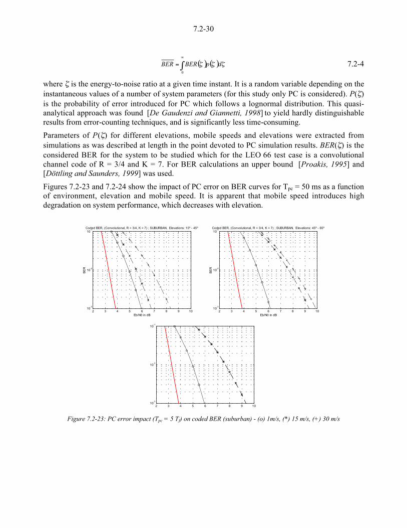
7.2-30

( ) ( ) ccc dpBERBER 0'

=0

7.2-4

where c is the energy-to-noise ratio at a given time instant. It is a random variable depending on theinstantaneous values of a number of system parameters (for this study only PC is considered). P(c)is the probability of error introduced for PC which follows a lognormal distribution. This quasi-analytical approach was found [De Gaudenzi and Giannetti, 1998] to yield hardly distinguishableresults from error-counting techniques, and is significantly less time-consuming.

Parameters of P(c) for different elevations, mobile speeds and elevations were extracted fromsimulations as was described at length in the point devoted to PC simulation results. BER(c) is theconsidered BER for the system to be studied which for the LEO 66 test case is a convolutionalchannel code of R = 3/4 and K = 7. For BER calculations an upper bound [Proakis, 1995] and[Döttling and Saunders, 1999] was used.

Figures 7.2-23 and 7.2-24 show the impact of PC error on BER curves for Tpc = 50 ms as a functionof environment, elevation and mobile speed. It is apparent that mobile speed introduces highdegradation on system performance, which decreases with elevation.

Figure 7.2-23: PC error impact (Tpc = 5 Tf) on coded BER (suburban) - (o) 1m/s, (*) 15 m/s, (+) 30 m/s

2 3 4 5 6 7 8 9 1010-3

10-2

10-1Coded BER, (Convolutional, R = 3/4, K = 7) ; SUBURBAN, Elevations: 15º - 45º

Eb/N0 in dB

BER

2 3 4 5 6 7 8 9 1010-3

10-2

10-1Coded BER, (Convolutional, R = 3/4, K = 7) ; SUBURBAN, Elevations: 45º - 65º

Eb/N0 in dB

BER

2 3 4 5 6 7 8 9 1010-3

10-2

10-1

7.2-31

Figure 7.2-24: PC error impact (Tpc = 5 Tf) on coded BER (urban). - (o) 1m/s, (*) 15 m/s, (+) 30 m/s

7.2.4.5 System Level Simulations

In order to calculate spatial coverage and temporal availability [Oestges, 1999], time series obtainedin the simulations described throughout the previous sections have been used as inputs to theCOST 255 link and system level software described in Chapter 7.1.

The ultimate objective of this study is to obtain the system performance and availability for thescenarios analysed so far, including different latitudes (Rome and London), environments (urbanand suburban) and mobile speeds. For doing that, simulations carried out assuming constantelevation angles are averaged with probability density functions of elevations. In this case, aconstellation consisting of 66 satellites in 6 orbital planes was considered.

Spatial coverage obtained for 99% of time is presented in Table 7.2-16. It can be observed thatspatial coverage for average coded BER of 10-3 never lies bellow 95%. Mobile speed does not seemto introduce significant loss of coverage.

ROME LONDON

A1 A2 B1 B2 A1 A2 B1 B2

1 m/s 99.1 96.6 98.5 96.0 99.0 96.0 97.5 94.5

15 m/s 98.5 96.5 98.0 95.0 99.0 96.0 96.0 93.0

30 m/s 98.5 96.0 98.0 95.0 99.0 96.0 96.0 93.0

Table 7.2-16: Spatial Coverage for 99% of the timeA1: suburban environment, average coded BER > 10-3; A2: suburban environment, average coded BER > 10-6

B1: urban environment, average coded BER > 10-3; B2: urban environment, average coded BER > 10-6

2 3 4 5 6 7 8 9 1010-3

10-2

10-1Coded BER, (Convolutional, R = 3/4, K = 7) ; URBAN, Elevations: 15º - 45º

Eb/N0 in dB

BER

2 3 4 5 6 7 8 9 1010-3

10-2

10-1Coded BER, (Convolutional, R = 3/4, K = 7) ; URBAN, Elevations: 45º - 65º

Eb/N0 in dB

BER

2 3 4 5 6 7 8 9 1010-3

10-2

10-1

7.2-32

7.2.5 Acknowledgements

The authors would like to thank Dr. A. Jahn and H. Ernst, DLR, Germany for providing the orbitgenerator and the module to generate roadside obstacles described in Section 7.2.2, and Prof. Dr. B.Walke, the head of the Institute of Communication Networks at Aachen University of Technology,where the work of Jörg Habetha has been carried out.

7.2-33

7.2.6 References

[Agelet et al., 1997]Agelet, F., Perez-Fontán, F., Formella, A., “Fast Ray Tracing For Microcellular and IndoorEnvironments”, IEEE Trans. on Magnetics, vol. 33, no. 2, pp. 1484-1487, 1997.

[Agius et al., 1999]Agius, A.A., Leach, S.M., Saunders, S.R., “Measurement of the Polarisation State of Satellite toMobile Signals in Scattering Environments”, Proc. Int. Mobile Satellite Conf. IMSC'99, Ottawa,Canada, pp.134-138, 1999.

[Akturan and Vogel, 1997]Akturan, R. and Vogel, W.J., “Path Diversity for LEO Satellite-PCS in the Urban Environment”,IEEE Trans. Vehicul. Technol., vol. 45, no. 7, pp. 1107-1116, 1997.

[Armbruster and Laurin, 1996]Armbruster, P., Laurin, M., “The IRIDIUM Network for Global Personal Communications”,Telecommunications Review, Vol. 6, No. 6, 1996, pp. 674-686, 1996.

[Bartuschka et al., 1997]Bartuschka, U., Mehlhorn, K., Näher, S., “A Robust and Efficient Implementation of a Sweep LineAlgorithm for the Straight Line Segment Intersection Problem”, Proc. Workshop on AlgorithmEngineering WAE, Venice, Italy, pp. 124-136., 1997

[Bischl and Werner, 1997]Bischl, H. and Werner, M., “Channel Adaptive Satellite Diversity for Non-Geostationary MobileSatellite Systems”, Proc. Fifth Int. Mobile Satellite Conf. IMSC97, pp. 25-31, 1997.

[De Gaudenzi and Giannetti, 1998]De Gaudenzi, R., Giannetti, F., “DS-CDMA Satellite Diversity Reception for Personal SatelliteCommunication: Satellite-to-Mobile Link Performance Analysis”, IEEE Trans. Vehicul. Technol.,vol. 47, no. 2, pp.658-672, 1998.

[Döttling et al., 1998]Döttling, M., Jahn, A., Kunisch, J., Buonomo, S., “A Versatile Channel Simulator for Land MobileSatellite Applications”, Proc. IEEE Vehicul. Technol. Conf. VTC'98, Ottawa, Canada, pp. 213-217,1998.

[Döttling et al., 1999a]Döttling, M., Zwick, T., Wiesbeck, W., "Ray Tracing Techniques and their Applications in LandMobile Satellite Propagation," Proc. European Wireless '99, München, Germany, 1999, pp. 107-111, 1999.

[Döttling et al., 1999b]Döttling, M., Zwick, T., Wiesbeck, W., “Investigation of Satellite Diversity and HandoverStrategies in Land Mobile Satellite Systems based on a Ray Tracing Propagation Model”, Proc. Int.Mobile Satellite Conf. IMSC'99, Ottawa, Canada, pp. 128-133, 1999.

[Döttling et al., 1999c]Döttling, M., Didascalou, D., Wiesbeck, W., “Wideband Channel Modeling and DiversityTechniques for Satellite-UMTS”, Proc. IEEE Vehicul. Technol. Conf. VTC'99 Fall, Amsterdam,The Netherlands, 1999, pp. 2770-2774, 1999.

7.2-34

[Döttling and Saunders, 1999]Döttling M., Saunders, S.“Bit Error Rate Calculation for Satellite Communications Systems”,COST 255 Radiowave Propagation Modelling for New SatCom Services at Ku-Band and above,Toulouse, May 1999.

[Fontán, et al. 1997]Fontán F.P., Pereda J., Sedes M.J., Castro M.A.V., Buonomo S., Baptista P., “Complex envelopethree-state Markov chain simulator for the LMS channel”, International Journal of SatelliteCommunications, January 1997, pp 1-15, 1997.

[Fontán et al. 1998]Fontán F.P., Castro M.A.V, Buonomo S., Baptista P., Arbesser-Rastburg B., “S-Band LMSpropagation channel behaviour for different environments, degrees of shadowing and elevationangles”, IEEE Transactions Broadcasting, Vol. 44, No. 1, March 1998, pp 40-76, 1998.

[Fukusawa and Sato, 1996]Fukusawa A., Sato T., Takizawa Y., Kato T., Kawabe M., Fisher R. E., “Wideband CDMA Systemfor Personal Radio Communications”, IEEE Communications Magazine, October 1996, pp. 116-123, 1996.

[Hutcheson and Laurin, 1995]Hutcheson, J., Laurin, M., “Network Flexibility of the IRIDIUM Global Mobile Satellite System”,Proceedings of the International Mobile Satellite Conference, Ottawa, Canada, 1995, pp. 503-507,1995.

[IMST, DLR, IHE, 1998]IMST, DLR, IHE, “Land Mobile Satellite Propagation Model for Non-Urban Areas”, Final Report,European Space Agency (ESA) Contract No. AO/1-3101/96/NL/NB, Document Reference4300/7290/6/2, 1998.

[Jahn and Lutz, 1995]Jahn A. and Lutz E., “Propagation Data and channel model for LMS systems”, Final report. ESAPurchase Order 141742. DLR, 1995.

[Motorola, 1990]Motorola Satellite Communications, Inc., “Iridium System Application Before the FederalCommunications Commission”, Washington, USA, December 1990.

[Oestges et al. 1998]Oestges, C., Vasseur, H., Vanhoenacker, D., “Impact of edge diffraction on the performance of landmobile satellite systems in urban areas”, Proc. European Microwave Conference EuMC'98, October1998, Amsterdam, The Netherlands, pp. 357-361.

[Oestges, 1999]Oestges C., 1999, “System-level Simulation for Land Mobile Satellite Services”, COST 255Radiowave Propagation Modelling for New SatCom Services at Ku-Band and above, Toulouse,May 1999.

[Öjanpera and Prasad, 1998]Öjanpera, T., Prasad, R., “Wideband CDMA for third Generation Mobile Communications”, ArtechHouse, 1998.

[Proakis, 1995]Proakis, J. G., “Digital Communications”, McGraw-Hill, 3rd edition, New York, 1995.

7.2-35

[Smith and Barton, 1992]Smith, H., Barton S.K., Gardiner J.G., Sforza M., “Characterisation of the Land Mobile-Satellite(LMS) Channel at L and S bands: narrowband measurements”, ESA AOPs 104433/114473,Bradford, 1992.

[Viterbi, 1998]Viterbi, A. J., “CDMA principles of Spread Spectrum”, Addison-Wesley Wireless CommunicationsSeries, 1998

[Walke, 1999]Walke, B., “Mobile Radio Networks: Networking and Protocols”, John Wiley, 1999.

7.3-1

CHAPTER 7.3Satellite IMT-2000 Mobile Link

Editor: Simon Saunders1

Authors: Francisco Cercas2, Martin Döttling3, Claude Oestges4,Fernando Pérez-Fontán5, Simon Saunders1, M. Ángeles Vázquez-Castro6 and WernerWiesbeck7

1 Centre for Communication Systems Research, University of Surrey, Guildford, Surrey, GU2 5XH, UKTel.: +44-1483-259806, Fax.: +44-1483-259504, e-mail: S.Saunders@ee.surrey.ac.uk

2 Instituto Superior Tecnico de Lisboa, Dep. Engenharia Electronica e de Comp,Avenida Roviso Pais, 1096 Lisboa CODEX, Portugal,Tel: +351-1-841-8485, Fax: +351-1-841-7164, e-mail: Francisco.Cercas@lx.it.pt

3 Siemens AG, System Engineering / UMTS Development, ICM MP TI 6,Haidenauplatz 1, D-81667 Muenchen, GermanyTel.: +49-89-722-58703, Fax: +49-89-722-27089, e-mail: Martin.Doettling@mch.siemens.de

4 Université catholique de Louvain (UCL), Microwave Laboratory (EMIC),Place du Levant 3, B-1348 Louvain-la-Neuve, BelgiumTel.: +32-10-478105, Fax.: +32-10-478705, e-mail: Oestges@emic.ucl.ac.be

5 Universidad de Vigo, Escuela Superior de Ingenieros de Telecomunicaciones,Departamento de Tecnologías de las Comunicaciones, Campus Universitario, 36200 - Vigo, SpainTel.: +34-986-812137, Fax.: +34-986-812121, e-mail: fpfontan@tsc.uc3m.es

6 Universidad Carlos III de Madrid, Escuela Politécnica Superior,Departamento de Tecnologías de las Comunicaciones,Avda. de la Universidad, 30, 28911-Leganés, Madrid, Spain

Tel.: +34-91-6249173, Fax.: +34-91-6249430, e-mail: maryan@tsc.uc3m.es7 Universität Karlsruhe, Institut für Höchstfrequenztechnik und Elektronik,

Kaiserstr. 12, D-76128 Karlsruhe, Germany,Tel : +49 721 608 6257 Fax : +49 721 691865 e mail: Werner Wiesbeck@etec uni karlsruhe de

7.3-2

7.3 Satellite IMT-2000 Mobile Link

S-IMT 2000 is a wideband CDMA system based on the specifications in [Dahlmann et al., 1998]and [Caire et al., 1999].

This system was proposed by the European Space Agency as a candidate for S-IMT-2000,providing bearer data rates up to 64 kbit/s.

7.3.1 Orbital Constellation

The original ESA proposal did not specify any particular satellite constellation. For the purposes ofthe test case, the DELIGO satellite constellation [Meenan et al., 1995] with 64 satellites in eightorbital planes at 1626 km altitude is used, since it provides high probabilities for multiple satellitevisibility and allows investigation of satellite diversity. Two particular locations were chosen forsimulation, namely London and Rome, with elevation statistics as specified in Figure 7.3-1.

0 10 20 30 40 50 60 70 80 900

0.5

1

1.5

2

2.5

3

3.5

4

4.5

Elevation angle, [deg.]

Pro

babi

lity

dens

ity fu

nctio

n

LondonRome

Figure 7.3-1: Elevation Statistics for the Deligo constellation in London and Rome

7.3.2 Link Parameters (Common to Satellite and Mobile Terminal)

A static link margin of 6 dB is assumed. The satellite EIRP is assumed to compensate ideally forfree space propagation loss, i.e. the line-of-sight signal level corresponds to the target Eb/N0 (bitenergy to spectral noise density) of 8 dB. The baseline simulations use an isotropic mobile terminal(MT) antenna and a 2-bit closed-loop power control. To infer power control efficiency underdifferent conditions, simulations without power control are also shown. Additional simulations areperformed to investigate satellite handover, satellite diversity and polarisation diversity. The mainS-IMT 2000 simulation parameters are listed in Table 7.3-1.

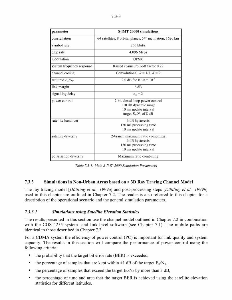
7.3-3

parameter S-IMT 20000 simulations

constellation 64 satellites, 8 orbital planes, 54° inclination, 1626 km

symbol rate 256 kbit/s

chip rate 4.096 Mcps

modulation QPSK

system frequency response Raised cosine, roll-off factor 0.22

channel coding Convolutional, R = 1/3, K = 9

required Eb/N0 2.0 dB for BER = 10-3

link margin 6 dB

signalling delay nst = 2

power control 2-bit closed-loop power control±10 dB dynamic range10 ms update intervaltarget Eb/N0 of 8 dB

satellite handover 6 dB hysteresis150 ms processing time10 ms update interval

satellite diversity 2-branch maximum ratio combining6 dB hysteresis

150 ms processing time10 ms update interval

polarisation diversity Maximum ratio combining

Table 7.3-1: Main S-IMT-2000 Simulation Parameters

7.3.3 Simulations in Non-Urban Areas based on a 3D Ray Tracing Channel Model

The ray tracing model [Döttling et al., 1999a] and post-processing steps [Döttling et al., 1999b]used in this chapter are outlined in Chapter 7.2. The reader is also referred to this chapter for adescription of the operational scenario and the general simulation parameters.

7.3.3.1 Simulations using Satellite Elevation Statistics

The results presented in this section use the channel model outlined in Chapter 7.2 in combinationwith the COST 255 system- and link-level software (see Chapter 7.1). The mobile paths areidentical to those described in Chapter 7.2.

For a CDMA system the efficiency of power control (PC) is important for link quality and systemcapacity. The results in this section will compare the performance of power control using thefollowing criteria:

• the probability that the target bit error rate (BER) is exceeded,

• the percentage of samples that are kept within ±1 dB of the target Eb/N0,

• the percentage of samples that exceed the target Eb/N0 by more than 3 dB,

• the percentage of time and area that the target BER is achieved using the satellite elevationstatistics for different latitudes.

7.3-4

The channel simulations are performed at 17 different elevation angles from 5° to 85° using twelvedifferent azimuth angles at each elevation angle to provide sufficient averaging over azimuth.Figures 7.3-2 and 7.3-3 show the power-controlled time series for 25°, 45° and 65° elevation forpath 1 (v = 1 m/s) and path 3 (v = 30 m/s), respectively. A thousand samples correspond to eachazimuth angle.

It is obvious from these plots that the power control efficiency decreases with increasing user speed.The PC is no longer able to track the fast channel variations and leads to strong fluctuations aroundthe target value. The signal variations are more pronounced for low elevation angles, wheremultipath effects reach their maximum.

-20

-15-10

-5

05

101520

0 1000 2000 3000 4000 5000 6000 7000 8000 9000 10000 11000 12000

25°45°65°

Eb/N

0 i

n dB

sample no.

Figure 7.3-2: Eb/N0 samples for 25°, 45° and 65° elevation, path 1, power control

-20

-15-10

-5

05

101520

0 1000 2000 3000 4000 5000 6000 7000 8000 9000 10000 11000 12000

25°45°65°

Eb/N

0 i

n dB

sample no.

Figure 7.3-3: Eb/N0 samples for 25°, 45° and 65° elevation, path 3, power control

The cumulative distribution functions (CDF) of Eb/N0 for path 1, without and with power control,are depicted in Figure 7.3-4. The corresponding legends are given in Figure 7.3-5. Table 7.3-2shows the corresponding BER statistics. For path 1, the power control increases the number ofsamples with BER < 10-3 by 15.6% at 5° elevation, by 21.7% at 25° elevation, by 11.4% at 45°elevation and by 6.2% at 65° elevation.

7.3-5

0

0.2

0.4

0.6

0.8

1

-20 -15 -10 -5 0 5 10 15 20

prob

abili

ty (

Eb/N

0 <

abs

ciss

a)

Eb/N0 in dB

0

0.2

0.4

0.6

0.8

1

-20 -15 -10 -5 0 5 10 15 20

prob

abili

ty (

Eb/N

0 <

abs

ciss

a)

Eb/N0 in dB

a) b)

Figure 7.3-4: CDF of Eb/N0 )for, path 1, without (a) and with power control (b)

5°10°15°20°25°30°35°40°45°

50°55°60°65°70°75°80°85°

100%96.97%89.63%

76.57%58.29%

44.07%

31.54%21.23%13.44%

7.73%3.61%

Figure 7.3-5: Legends for subsequent plots: left: elevation angle in CDFs of Eb/N0 and CCDFs of BER, right: time percentages for system-level simulation results at the latitude of Rome

Elevation angle[degree]

Path 1 Path 1PC

Path 2 Path 2PC

Path 3 Path 3PC

5 63.7% 48.1% 67.9% 52.0% 57.6% 41.5%

25 58.8% 37.1% 43.9% 26.8% 46.5% 29.2%

45 29.9% 18.5% 33.4% 16.4% 35.6% 20.6%

65 8.7% 2.5% 6.4% 2.5% 19.0% 7.9%

Table7.3-2: Probability of BER>10-3 for different simulation paths and elevation angles

The channel simulations show maximum short term fading depths around 25º elevation, which leadto a minimum percentage of samples within an interval of ±1 dB around the target Eb/N0 at thisangle (see Figure 7.3-6). The capability of the power control to keep the Eb/N0 within this intervaldecreases with increasing mobile speed. Figure 7.3-6b) shows that the power control leads to anincreased number of samples, which exceed the target Eb/N0 by 3 dB and thus introduceunnecessary power consumption and interference. This effect aggravates with increasing userspeed. At a MT speed of 30 m/s, PC leads to an increase of samples with Eb/N0 > 11 dB greater than13% for the elevation angles between 10° and 35°. In general, the low elevation angles are mostaffected by this effect.

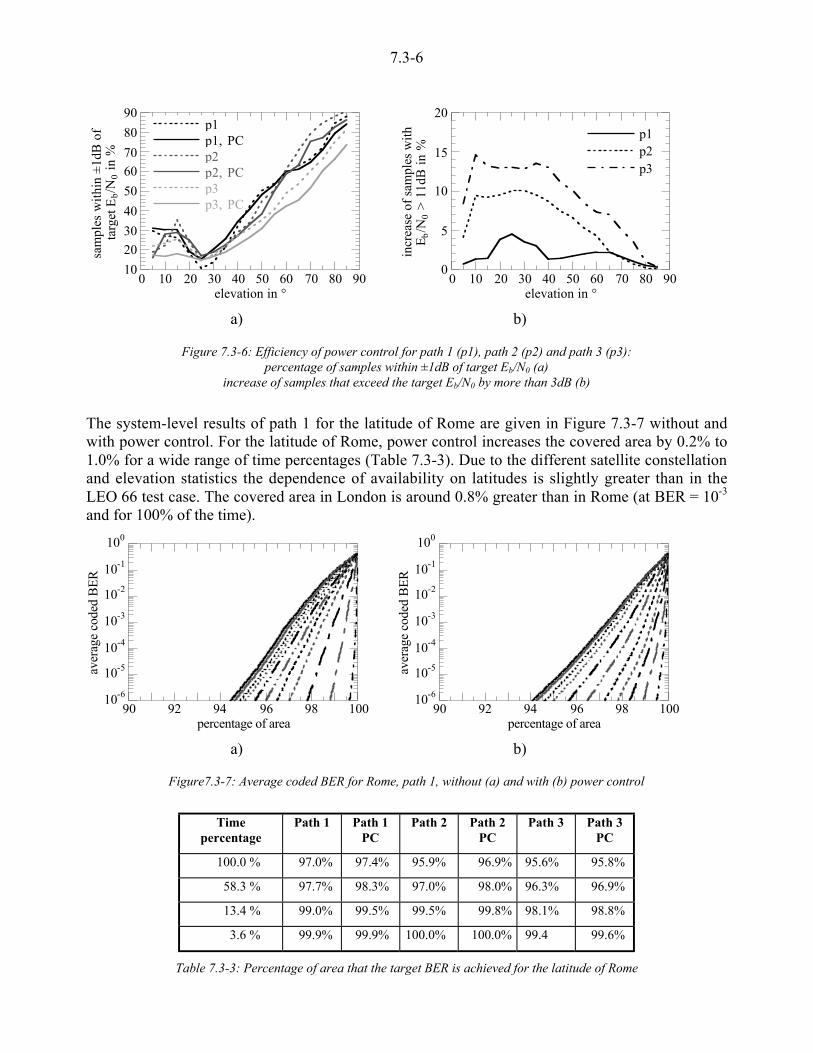
7.3-6

10

20

30

40

50

6070

80

90

0 10 20 30 40 50 60 70 80 90

p1p1, PCp2p2, PCp3p3, PC

sam

ples

with

in ±

1dB

of

targ

et E

b/N

0 i

n %

elevation in °

0

5

10

15

20

0 10 20 30 40 50 60 70 80 90

p1p2p3

incr

ease

of

sam

ples

with

Eb/N

0 >

11d

B i

n %

elevation in °

a) b)

Figure 7.3-6: Efficiency of power control for path 1 (p1), path 2 (p2) and path 3 (p3):percentage of samples within ±1dB of target Eb/N0 (a)

increase of samples that exceed the target Eb/N0 by more than 3dB (b)

The system-level results of path 1 for the latitude of Rome are given in Figure 7.3-7 without andwith power control. For the latitude of Rome, power control increases the covered area by 0.2% to1.0% for a wide range of time percentages (Table 7.3-3). Due to the different satellite constellationand elevation statistics the dependence of availability on latitudes is slightly greater than in theLEO 66 test case. The covered area in London is around 0.8% greater than in Rome (at BER = 10-3

and for 100% of the time).

10-6

10-5

10-4

10-3

10-2

10-1

100

90 92 94 96 98 100

aver

age

code

d B

ER

percentage of area

10-6

10-5

10-4

10-3

10-2

10-1

100

90 92 94 96 98 100

aver

age

code

d B

ER

percentage of area

a) b)

Figure7.3-7: Average coded BER for Rome, path 1, without (a) and with (b) power control

Timepercentage

Path 1 Path 1PC

Path 2 Path 2PC

Path 3 Path 3PC

100.0 % 97.0% 97.4% 95.9% 96.9% 95.6% 95.8%

58.3 % 97.7% 98.3% 97.0% 98.0% 96.3% 96.9%

13.4 % 99.0% 99.5% 99.5% 99.8% 98.1% 98.8%

3.6 % 99.9% 99.9% 100.0% 100.0% 99.4 99.6%

Table 7.3-3: Percentage of area that the target BER is achieved for the latitude of Rome

7.3-7

Figure 7.3-8 shows the CDF of Eb/N0 and system-level results for path 3. A comparison of theresults for different user paths highlights the important influence of the local terrain effects onsystem performance (cf. Figures 7.3-4a) and 7.3-7b).

Table 7.3-3 summarises the main results for the latitude of Rome and BER = 10-3.

0

0.2

0.4

0.6

0.8

1

-20 -15 -10 -5 0 5 10 15 20

prob

abili

ty (

Eb/N

0 <

abs

ciss

a)

Eb/N0 in dB

10-6

10-5

10-4

10-3

10-2

10-1

100

90 92 94 96 98 100

aver

age

code

d B

ER

percentage of area

a) b)

Figure 7.3-8: CDF of Eb/N0 (left) and average coded BER for Rome (right), path 3, power control

7.3.3.2 Simulations using an Orbit Generator

The simulations in this section use time series of satellite positions provided by an orbit generatorinstead of elevation statistics. Figure 7.3-9 shows the elevation angles for the 600 s simulation time.The S-IMT 2000 satellite constellation provides high probability of multiple satellite visibility athigh elevation angles. Thus the investigation of satellite diversity is especially interesting. Thebaseline scenario uses the power control scheme outlined above.

0102030405060708090

0 50 100 150 200 250 300 350 400 450 500 550 600

elev

atio

n in

°

time in s

Figure 7.3-9: Time series of satellite elevations for S-IMT 2000 simulations

The simulations distinguish between up- and downlink, since in CDMA systems multiple accessinterference (MAI) is assumed to be the limiting factor on Eb/N0. For the uplink reasonableassumptions for the noise due to MAI have been made, since the channel states of the interferingusers are not known. The number of equivalent channels (see also Chapter 7.1) for the uplink hasbeen chosen to yield the target Eb/N0 for line-of-sight conditions without power control. Thus theMAI noise power is constant:

( ) constCPtN toteqLOS

upimai == 7 3-1

7.3-8

For the downlink, however, the ray tracer provides the channel impulse responses for all visiblesatellites simultaneously. The number of equivalent channels per satellite is adjusted in a way that,for each satellite, line-of-sight conditions would correspond to the target Eb/N0. No MAI from theserving satellite i is considered, since orthogonal and synchronous CDMA is assumed. This leads toa time-variant MAI noise power:

( )( )

( ) Seq

tS

iss

Sd

imai CtPtN -&=

=1

, . 7.3-2

Thus the correlation between downlink MAI and satellite diversity gain can be modelled.

Uplink

Figure 7.3-10 depicts a comparison of the channel time series using power control (PC), PC with 2-branch satellite diversity (SD) and maximum ratio combining, as well as a combination of PC, SDand polarisation diversity (PD) at the mobile terminal. The simulations show considerably satellitediversity gain. In combination with polarisation diversity additional improvements are seenespecially between t = 100 s and t = 150 s. The CDF of Eb/N0 in Figure 7.3-11 shows a satellitediversity gain of 8.8 dB at Eb/N0 = 2 dB. Even at a high handover rate of 0.3 Hz, satellite handoverwould provide less gain (6.5 dB). Polarisation diversity provides 5.7 dB gain and a combination ofboth diversity schemes results in 10.1 dB gain (see Figure 7.3-11b). The mean number of requiredchannels for satellite diversity is 1.44 for 6 dB hysteresis to add and drop satellites to/from thediversity connection. The use of satellite diversity decreases the probability to exceed the targetBER by 31.5% (from 43.2% to 11.7%). The combination of satellite and polarisation diversitywould allow reaching the target value in 96.9% (Table 7.3-4).

-20

-15-10-5

05

101520

0 100 200 300 400 500 600

PCPC, SDPC, SD, PD

Eb/N

0 in

dB

time in s

Figure 7.3-10: Eb/N0 time series comparing power control (PC), PC in combination with satellite diversity (SD) and thecombination of PC, SD with polarisation diversity (PD), uplink

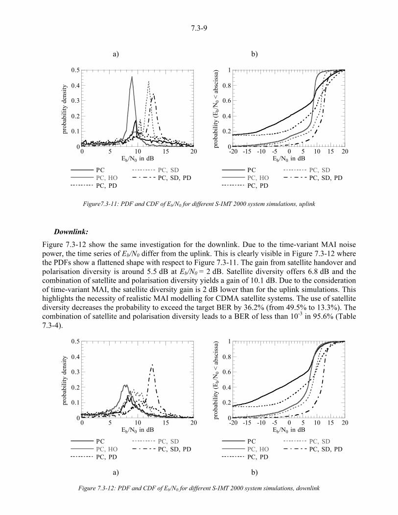
7.3-9

a) b)

0

0.1

0.2

0.3

0.4

0.5

0 5 10 15 20

PCPC, HOPC, PD

PC, SDPC, SD, PD

prob

abili

ty d

ensi

ty

Eb/N0 in dB

0

0.2

0.4

0.6

0.8

1

-20 -15 -10 -5 0 5 10 15 20

PCPC, HOPC, PD

PC, SDPC, SD, PD

prob

abili

ty (

Eb/N

0 <

abs

ciss

a)

Eb/N0 in dB

Figure7.3-11: PDF and CDF of Eb/N0 for different S-IMT 2000 system simulations, uplink

Downlink:

Figure 7.3-12 show the same investigation for the downlink. Due to the time-variant MAI noisepower, the time series of Eb/N0 differ from the uplink. This is clearly visible in Figure 7.3-12 wherethe PDFs show a flattened shape with respect to Figure 7.3-11. The gain from satellite handover andpolarisation diversity is around 5.5 dB at Eb/N0 = 2 dB. Satellite diversity offers 6.8 dB and thecombination of satellite and polarisation diversity yields a gain of 10.1 dB. Due to the considerationof time-variant MAI, the satellite diversity gain is 2 dB lower than for the uplink simulations. Thishighlights the necessity of realistic MAI modelling for CDMA satellite systems. The use of satellitediversity decreases the probability to exceed the target BER by 36.2% (from 49.5% to 13.3%). Thecombination of satellite and polarisation diversity leads to a BER of less than 10-3 in 95.6% (Table7.3-4).

0

0.1

0.2

0.3

0.4

0.5

0 5 10 15 20

PCPC, HOPC, PD

PC, SDPC, SD, PD

prob

abili

ty d

ensi

ty

Eb/N0 in dB

0

0.2

0.4

0.6

0.8

1

-20 -15 -10 -5 0 5 10 15 20

PCPC, HOPC, PD

PC, SDPC, SD, PD

prob

abili

ty (

Eb/N

0 <

abs

ciss

a)

Eb/N0 in dB

a) b)

Figure 7.3-12: PDF and CDF of Eb/N0 for different S-IMT 2000 system simulations, downlink

7.3-10

uplink Downlink

Simulation gain atEb/N0 = 2dB

gain atEb/N0 = 8dB

probabilityBER > 10-3

gain atEb/N0 = 2dB

Gain atEb/N0 = 8dB

probabilityBER > 10-3

PC – – 43.2% – – 49.5%

PC, HO 6.5dB 0.8dB 15.6% 5.3dB 0.3dB 17.1%

PC, PD 5.7dB 2.3dB 25.6% 5.7dB 2.5dB 31.3%

PC, SD 8.8dB 3.6dB 11.7% 6.8dB 2.0dB 13.3%

PC, SD, PD 10.1dB 4.6dB 3.1% 10.1dB 4.8dB 4.4%

Table7.3-4: Comparison of different strategies to increase system performance

7.3.3.3 Conclusions of the simulation based on a 3D Ray Tracing Channel Model

A comparison of the results obtained in this section (cf. Tables 7.3-2 and 7.3-3) shows that theCDMA system using 6 dB static link margin, power control and a R = 1/3, K = 9 convolutional codeperforms similarly to the TDMA/FDMA system using 16 dB link margin and a R = 3/4, K = 7convolutional code (see Chapter 7.2). However, the S-IMT2000 system performance decreases withincreasing MT speed due to the degraded performance of the S-IMT 2000 power control scheme.

Table 7.3-5 compares the covered area for 100% of time.

Simulation Path 1 Path 2 Path 3

System LEO 66 S-IMT 2000 LEO 66 S-IMT 2000 LEO 66 S-IMT 2000

Percentage of area 97.3% 97.4% 97.8% 96.9% 97.1% 95.8%

Table 7.3-5: Comparison of system-level results of the LEO 66 (see chapter 7.2)and S-IMT 2000 test case for 100% of time

The impact of elevation angle and MT speed on power control efficiency has been investigated. Theresults show that the largest short term fading depths are experienced at medium low elevationangles, causing considerable problems for the power control to track the signal variations. Theseproblems become worse with increasing MT velocity for all elevation angles. For high speedapplications, the delayed power control reaction causes unnecessary high signal amplitudes (incases where the channel has already re-entered line-of-sight conditions while the power control stillremains active), which generates unwanted interference power.

The simulations based on an orbit generator allow the investigation of the performance of differentsystem designs for S-IMT 2000. For both, uplink and downlink, satellite diversity keeps the breachof the target BER below 14%. The satellite diversity gain (with respect to the baseline scenariousing power control) is in the range of 7 dB to 9 dB at the target Eb/N0 value. Other simulationsshow lower gain [Döttling et al., 1999c]. Thus it is anticipated that the satellite diversity gain issensitive to the operational scenario, the satellite constellation and the probability or Eb/N0 value atwhich it is calculated. For example, at Eb/N0 = 8 dB the satellite diversity gain is only between 2 dBand 4 dB.

Polarisation diversity provides considerable gain (5 dB to 6 dB at Eb/N0 = 2 dB), which is in goodagreement with measurements [Agius et al., 1999]. The combination of satellite and polarisationdiversity at the MT yields around 10 dB diversity gain and coverage for more than 95% of the time.A comprehensive comparison of the different strategies to increase system performance is given inT bl 7 3 4

7.3-11

7.3.4 Simulations in built-up areas based on a physical-statistical ray-tracing

In this paragraph the physical-statistical approach based on ray-tracing is used to carry outsimulations (see also Chapter 7.2.3). Typical urban and suburban areas are defined on the basis of alognormal distribution (median µ, standard deviation m) for the building height, and a constantvalue w for the street width (see Table 7.2.3.1-1). A more detailed description of the model can befound in Chapter 7.2.

A target Eb/N0 value of 8 dB has been selected (see Table 7.3-1). However, since S-IMT2000 is awideband CDMA system, simulations have to take into account the multiple access interference(MAI) as well as the power control that is applied to the received signal. The intersymbolinterference is neglected because its effect seems to be insignificant compared to MAI. Themethods described in Chapter 7.2 are applied to integrate MAI. On the other hand, an open-looppower control is implemented, with a maximal correction of 10 dB and an update time of 100 ms(see Table 7.3-1).

7.3.4.1 Simulation results for a pedestrian speed

The distribution of coded BER as a function of the spatial coverage are shown in Figure 7.3-13 inboth urban and suburban areas and for the two latitudes (London and Rome). A pedestrian speed of1 ms-1 is first assumed.

The various curves on the figure are associated with the following percentages of time (from left toright) :

• 100.00, 100.00, 96.79, 89.35, 78.52, 68.25, 57.83, 46.04, 31.95, 16.50 and 7.64 % of timewhile considering the latitude of London;

• 100.00, 96.97, 89.63, 75.57, 58.29, 44.07, 31.54, 21.23, 13.44, 7.72 and 3.61 % of time atthe latitude of Rome.

For instance, in an urban environment at the latitude of Rome, the mean coded BER is less than 10-3

during :

«««

®

«««

­

¬

% 99.37on timeof % 7.72

% 97.35on timeof % 21.23

% 97.24on timeof % 44.07

% 96.53on timeof % 75.57

% 96.31on timeof % 96.97

of the considered area.

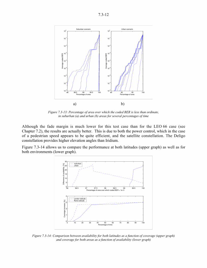
7.3-12

98 98.5 99 99.5 10010

!8

10!7

10!6

10!5

10!4

10!3

10!2

10!1

100

Percentage of area

Ave

rage

cod

ed B

ER

Suburban scenario

85 90 95 10010

!8

10!7

10!6

10!5

10!4

10!3

10!2

10!1

100

Percentage of area

Ave

rage

cod

ed B

ER

Urban scenario

a) b)

Figure 7.3-13: Percentage of area over which the coded BER is less than ordinate,in suburban (a) and urban (b) areas for several percentages of time

Although the fade margin is much lower for this test case than for the LEO 66 case (seeChapter 7.2), the results are actually better. This is due to both the power control, which in the caseof a pedestrian speed appears to be quite efficient, and the satellite constellation. The Deligoconstellation provides higher elevation angles than Iridium.

Figure 7.3-14 allows us to compare the performance at both latitudes (upper graph) as well as forboth environments (lower graph).

96 96.5 97 97.5 98 98.5 99 99.5 1000

5

10

15

20

25

30

Percentage of area over which coded BER < 1e!3

Diff

eren

ce o

f ava

ilabi

lity,

[%] suburban

urban

0 10 20 30 40 50 60 70 80 90 1000

1

2

3

4

Percentage of time

Cov

erag

e in

crea

se, [

%] London latitude

Rome latitude

Figure 7.3-14: Comparison between availability for both latitudes as a function of coverage (upper graph)and coverage for both areas as a function of availability (lower graph)

7.3-13

It can be seen that there is a gain of time availability between the two simulated latitudes of about25 %. This is much greater than the value obtained for the LEO 66 test case (see Chapter 7.2). Inthe lower graph, the coverage is increased by only 3% when comparing suburban to urban areas.

Finally, Figure 7.3-15 highlights the effect of power control on the performance. For all simulatedscenarios, the gain in performance is plotted against the availability when comparing the coveragebetween those results that take power control into account and those that do not. In suburban areas,the gain of 1% is quite constant. Meanwhile, the gain in urban areas decreases for high percentagesof time, which could be explained by the deeper fades encountered at low elevation angles in urbanareas.

0 10 20 30 40 50 60 70 80 90 1000

0.2

0.4

0.6

0.8

1

1.2

1.4

1.6

Percentage of time

Diff

eren

ce o

f cov

erag

e, [%

]

suburban ! London latitudesuburban ! Rome latitude urban ! London latitude urban ! Rome latitude

Figure 7.3-15: Effect of power control in all simulated cases : performance gain (coverage increase)

7.3.4.2 Simulation results for high-speed scenarios

A high-speed scenario (15 ms-1) is also investigated, all other parameters remaining the same asbefore. Figure 7.3-16 depicts the degradation of area performance as a function of the percentage oftime. It is actually quite limited (0.5 to 1.5%), despite significant signalling delays in the powercontrol process. It has however been noticed that these results are very sensitive to the powercontrol parameters (update rate, correction step).

Considering a mobile speed of 30 ms-1, it can be seen in Figure 7.3-17 that the degradation is againquite small (1 to 1.8 %).

7.3-14

0 10 20 30 40 50 60 70 80 90 1000

0.2

0.4

0.6

0.8

1

1.2

1.4

1.6

1.8

Percentage of time

Diff

eren

ce o

f cov

erag

e, [%

]

suburban ! London latitudesuburban ! Rome latitude urban ! London latitude urban ! Rome latitude

Figure 7.3-16: Degradation of performance for a high-speed (15 ms-1) scenario relative to a pedestrian case

0 10 20 30 40 50 60 70 80 90 1000

0.2

0.4

0.6

0.8

1

1.2

1.4

1.6

1.8

Percentage of time

Diff

eren

ce o

f cov

erag

e, [%

]

suburban ! London latitudesuburban ! Rome latitude urban ! London latitude urban ! Rome latitude

Figure 7.3-17: Degradation of performance for a high-speed (30 ms-1) scenario relative to a pedestrian case

7.3.5 Simulations in Urban and Suburban Areas based on a Wideband Markov Channel(WMC) propagation model

The main focus of this section lies on a detailed study of some key features related to the link-levelperformance evaluation of a Satellite test-environment based on a Wideband Direct-Sequence CodeDivision Multiple Access (W-DS-CDMA) system. The key characteristics of the performanceevaluation to be made are those which can be evaluated directly from time series of channelamplitude generated with a channel model.

The general discussion on approach based on the Wideband Markov Channel propagation modeland Power Control is given in Chapter 7.2.

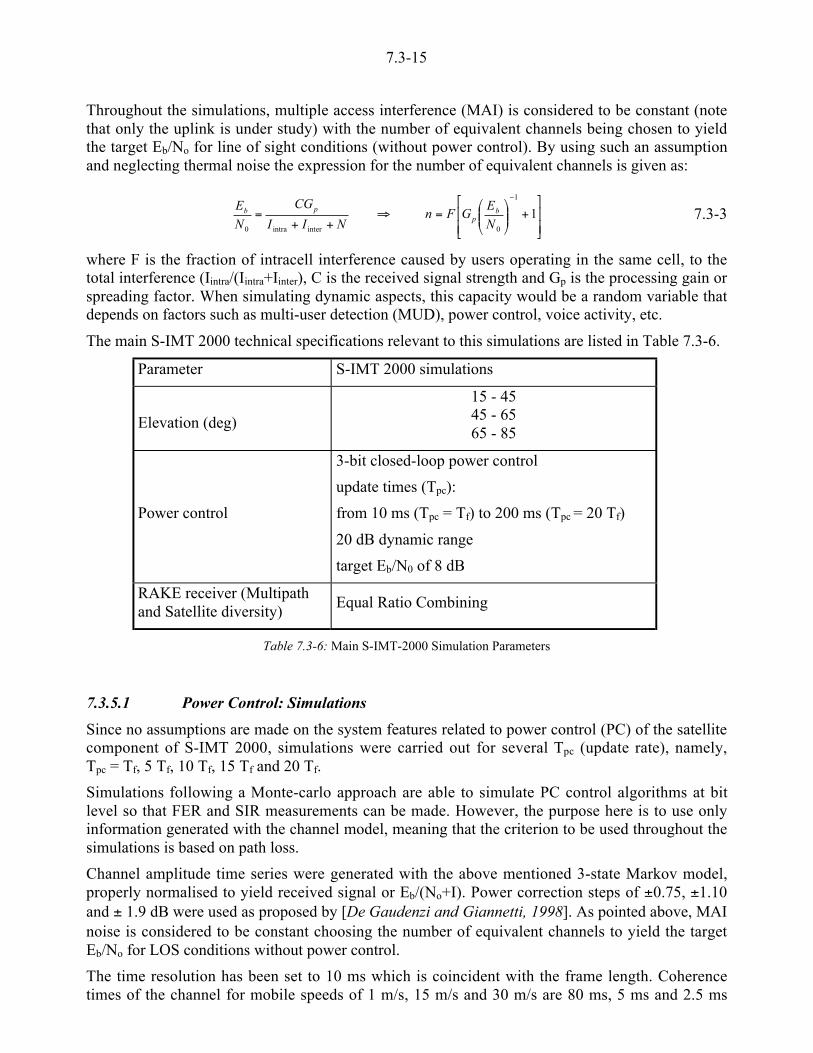
7.3-15

Throughout the simulations, multiple access interference (MAI) is considered to be constant (notethat only the uplink is under study) with the number of equivalent channels being chosen to yieldthe target Eb/No for line of sight conditions (without power control). By using such an assumptionand neglecting thermal noise the expression for the number of equivalent channels is given as:

µµ�

�

³³�

�+´́

¦

¥²²¤

£=�

++=

<

11

0interintra0 N

EGFn

NII

CG

N

E bp

pb 7.3-3

where F is the fraction of intracell interference caused by users operating in the same cell, to thetotal interference (Iintra/(Iintra+Iinter), C is the received signal strength and Gp is the processing gain orspreading factor. When simulating dynamic aspects, this capacity would be a random variable thatdepends on factors such as multi-user detection (MUD), power control, voice activity, etc.

The main S-IMT 2000 technical specifications relevant to this simulations are listed in Table 7.3-6.

Parameter S-IMT 2000 simulations

Elevation (deg)

15 - 4545 - 6565 - 85

Power control

3-bit closed-loop power control

update times (Tpc):

from 10 ms (Tpc = Tf) to 200 ms (Tpc = 20 Tf)

20 dB dynamic range

target Eb/N0 of 8 dB

RAKE receiver (Multipathand Satellite diversity)

Equal Ratio Combining

Table 7.3-6: Main S-IMT-2000 Simulation Parameters

7.3.5.1 Power Control: Simulations

Since no assumptions are made on the system features related to power control (PC) of the satellitecomponent of S-IMT 2000, simulations were carried out for several Tpc (update rate), namely,Tpc = Tf, 5 Tf, 10 Tf, 15 Tf and 20 Tf.

Simulations following a Monte-carlo approach are able to simulate PC control algorithms at bitlevel so that FER and SIR measurements can be made. However, the purpose here is to use onlyinformation generated with the channel model, meaning that the criterion to be used throughout thesimulations is based on path loss.

Channel amplitude time series were generated with the above mentioned 3-state Markov model,properly normalised to yield received signal or Eb/(No+I). Power correction steps of ±0.75, ±1.10and ± 1.9 dB were used as proposed by [De Gaudenzi and Giannetti, 1998]. As pointed above, MAInoise is considered to be constant choosing the number of equivalent channels to yield the targetEb/No for LOS conditions without power control.

The time resolution has been set to 10 ms which is coincident with the frame length. Coherencetimes of the channel for mobile speeds of 1 m/s, 15 m/s and 30 m/s are 80 ms, 5 ms and 2.5 ms

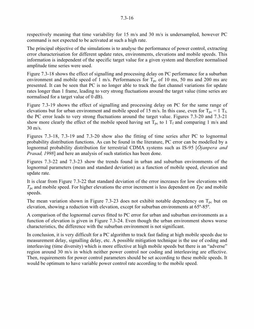
7.3-16

respectively meaning that time variability for 15 m/s and 30 m/s is undersampled, however PCcommand is not expected to be activated at such a high rate.

The principal objective of the simulations is to analyse the performance of power control, extractingerror characterisation for different update rates, environments, elevations and mobile speeds. Thisinformation is independent of the specific target value for a given system and therefore normalisedamplitude time series were used.

Figure 7.3-18 shows the effect of signalling and processing delay on PC performance for a suburbanenvironment and mobile speed of 1 m/s. Performances for Tpc of 10 ms, 50 ms and 200 ms arepresented. It can be seen that PC is no longer able to track the fast channel variations for updaterates longer than 1 frame, leading to very strong fluctuations around the target value (time series arenormalised for a target value of 0 dB).

Figure 7.3-19 shows the effect of signalling and processing delay on PC for the same range ofelevations but for urban environment and mobile speed of 15 m/s. In this case, even for Tpc = 1 Tf,the PC error leads to very strong fluctuations around the target value. Figures 7.3-20 and 7.3-21show more clearly the effect of the mobile speed having set Tpc to 1 Tf and comparing 1 m/s and30 m/s.

Figures 7.3-18, 7.3-19 and 7.3-20 show also the fitting of time series after PC to lognormalprobability distribution functions. As can be found in the literature, PC error can be modelled by alognormal probability distribution for terrestrial CDMA systems such as IS-95 [Öjanpera andPrasad, 1998] and here an analysis of such statistics has been done.

Figures 7.3-22 and 7.3-23 show the trends found in urban and suburban environments of thelognormal parameters (mean and standard deviation) as a function of mobile speed, elevation andupdate rate.

It is clear from Figure 7.3-22 that standard deviation of the error increases for low elevations withTpc and mobile speed. For higher elevations the error increment is less dependent on Tpc and mobilespeeds.

The mean variation shown in Figure 7.3-23 does not exhibit notable dependency on Tpc but onelevation, showing a reduction with elevation, except for suburban environments at 65º-85º.

A comparison of the lognormal curves fitted to PC error for urban and suburban environments as afunction of elevation is given in Figure 7.3-24. Even though the urban environment shows worsecharacteristics, the difference with the suburban environment is not significant.

In conclusion, it is very difficult for a PC algorithm to track fast fading at high mobile speeds due tomeasurement delay, signalling delay, etc. A possible mitigation technique is the use of coding andinterleaving (time diversity) which is more effective at high mobile speeds but there is an “adverse”region around 30 m/s in which neither power control nor coding and interleaving are effective.Then, requirements for power control parameters should be set according to these mobile speeds. Itwould be optimum to have variable power control rate according to the mobile speed.

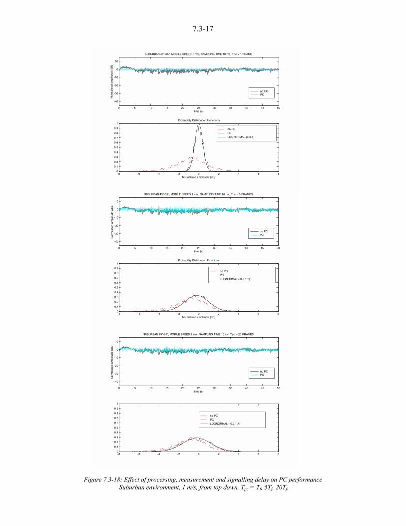
7.3-17

Figure 7.3-18: Effect of processing, measurement and signalling delay on PC performance Suburban environment, 1 m/s, from top down, Tpc = Tf, 5Tf, 20Tf.

no PCPC

0 5 10 15 20 25 30 35 40 45 50

-40

-30

-20

-10

0

10

SUBURBAN 45º-65º, MOBILE SPEED 1 m/s, SAMPLING TIME 10 ms, Tpc = 1 FRAME

time (s)No

rmal

ised

ampl

itude

(dB)

no PC PC LOGNORMAL (0,0.4)

-8 -6 -4 -2 0 2 4 6 80

0.10.20.30.40.50.60.70.80.9

1

Normalised amplitude (dB)

Probability Distribution Functions

no PCPC

0 5 10 15 20 25 30 35 40 45 50

-40

-30

-20

-10

0

10

SUBURBAN 45º-65º, MOBILE SPEED 1 m/s, SAMPLING TIME 10 ms, Tpc = 5 FRAMES

time (s)

Norm

alise

d am

plitu

de (d

B)

no PC PC LOGNORMAL (-0.2,1.2)

-8 -6 -4 -2 0 2 4 6 80

0.10.20.30.40.50.60.70.80.9

1

Normalised amplitude (dB)

Probability Distribution Functions

no PCPC

0 5 10 15 20 25 30 35 40 45 50

-40

-30

-20

-10

0

10

SUBURBAN 45º-65º, MOBILE SPEED 1 m/s, SAMPLING TIME 10 ms, Tpc = 20 FRAMES

time (s)

Norm

alise

d am

plitu

de (d

B)

no PC PC LOGNORMAL (-0.2,1.4)

-8 -6 -4 -2 0 2 4 6 80

0.10.20.30.40.50.60.70.80.9

1

7.3-18

Figure 7.3-19: Effect of processing, measurement and signalling delay on PC performance.Urban environment, 15 m/s, from top down, Tpc = Tf, 5Tf,20Tf.

no PCPC

0 5 10 15 20 25 30 35 40 45 50

-40

-30

-20

-10

0

10

URBAN 45º-65º, MOBILE SPEED 15 m/s, SAMPLING TIME 10 ms, Tpc = 1 FRAME

time (s)No

rmal

ised

ampl

itude

(dB)

no PC PC LOGNORMAL (0,1.5)

-8 -6 -4 -2 0 2 4 6 80

0.10.20.30.40.50.60.70.80.9

1

Normalised amplitude (dB)

Probability Distribution Functions

no PCPC

no PC PC LOGNORMAL (-0.4,2.2)

0 5 10 15 20 25 30 35 40 45 50

-40

-30

-20

-10

0

10

URBAN 45º-65º, MOBILE SPEED 15 m/s, SAMPLING TIME 10 ms, Tpc = 5 FRAMES

time (s)

Norm

alise

d am

plitu

de (d

B)

-8 -6 -4 -2 0 2 4 6 80

0.10.20.30.40.50.60.70.80.9

1

Normalised amplitude (dB)

Probability Distribution Functions

no PCPC

0 5 10 15 20 25 30 35 40 45 50

-40

-30

-20

-10

0

10

URBAN 45º-65º, MOBILE SPEED 15 m/s, SAMPLING TIME 10 ms, Tpc = 20 FRAMES

time (s)

Norm

alise

d am

plitu

de (d

B)

no PC PC LOGNORMAL (-0.4,3)

-8 -6 -4 -2 0 2 4 6 80

0.10.20.30.40.50.60.70.80.9

1

7.3-19

0 5 10 15 20 25 30 35 40 45 50-15

-10

-5

0

5

10

15

SUBURBAN 15º-45º, MOBILE SPEED 1 m/s, SAMPLING TIME 10 ms, Tpc = 1 FRAMES

time (s)

Normalised amplitud

no PCPC

-8 -6 -4 -2 0 2 4 6 80

0.1

0.2

0.3

0.4

0.5

0.6

0.7

0.8

0.9

1Probability Distribution Functions

Normalised amplitude (dB)

no PCPCLOGNORMAL (0,0.6)

Figure 7.3-20: Suburban environment, 1 m/s.

0 5 10 15 20 25 30 35 40 45 50-15

-10

-5

0

5

10

15SUBURBAN 15º-45º, MOBILE SPEED 30 m/s, SAMPLING TIME 10 ms, Tpc = 1 FRAMES

time (s)

Normalised amplitud

no PCPC

-8 -6 -4 -2 0 2 4 6 80

0.1

0.2

0.3

0.4

0.5

0.6

0.7

0.8

0.9

1Probability Distribution Functions

Normalised amplitude (dB)

no PCPCLOGNORMAL (0,1.9)

Figure 7.3-21: Urban environment, 15 m/s

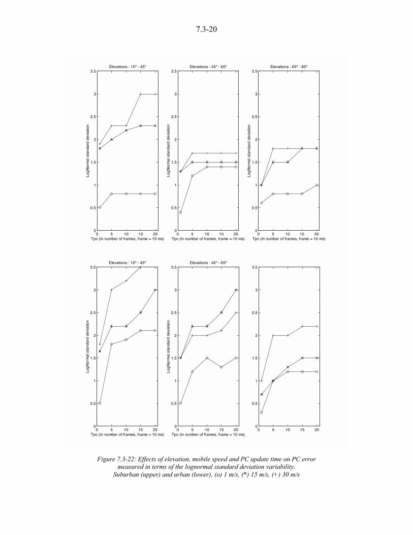
7.3-20

Figure 7.3-22: Effects of elevation, mobile speed and PC update time on PC errormeasured in terms of the lognormal standard deviation variability.

Suburban (upper) and urban (lower), (o) 1 m/s, (*) 15 m/s, (+) 30 m/s

0 5 10 15 200

0.5

1

1.5

2

2.5

3

3.5

Tpc (in number of frames, frame = 10 ms)

LogN

orm

al s

tand

ard

devia

tion

Elevations : 15º - 45º

0 5 10 15 200

0.5

1

1.5

2

2.5

3

3.5

Tpc (in number of frames, frame = 10 ms)

LogN

orm

al s

tand

ard

devia

tion

Elevations : 45º - 65º

0 5 10 15 200

0.5

1

1.5

2

2.5

3

3.5

Tpc (in number of frames, frame = 10 ms)

LogN

orm

al s

tand

ard

devia

tion

Elevations : 65º - 85º

0 5 10 15 200

0.5

1

1.5

2

2.5

3

3.5

Tpc (in number of frames, frame = 10 ms)

LogN

orm

al s

tand

ard

devia

tion

Elevations : 15º - 45º

0 5 10 15 200

0.5

1

1.5

2

2.5

3

3.5

Tpc (in number of frames, frame = 10 ms)

LogN

orm

al s

tand

ard

devia

tion

Elevations : 45º - 65º

0 5 10 15 200

0.5

1

1.5

2

2.5

3

3.5

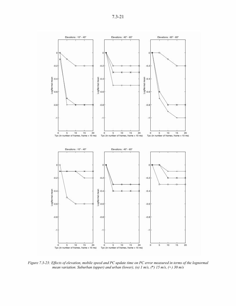
7.3-21

Figure 7.3-23: Effects of elevation, mobile speed and PC update time on PC error measured in terms of the lognormalmean variation. Suburban (upper) and urban (lower), (o) 1 m/s, (*) 15 m/s, (+) 30 m/s

0 5 10 15 20

-1

-0.8

-0.6

-0.4

-0.2

0

Tpc (in number of frames, frame = 10 ms)

LogN

orm

al m

ean

Elevations : 15º - 45º

0 5 10 15 20

-1

-0.8

-0.6

-0.4

-0.2

0

Tpc (in number of frames, frame = 10 ms)

LogN

orm

al m

ean

Elevations : 45º - 65º

0 5 10 15 20

-1

-0.8

-0.6

-0.4

-0.2

0

Tpc (in number of frames, frame = 10 ms)

LogN

orm

al m

ean

Elevations : 65º - 85º

0 5 10 15 20

-1

-0.8

-0.6

-0.4

-0.2

0

Tpc (in number of frames, frame = 10 ms)

LogN

orm

al m

ean

Elevations : 15º - 45º

0 5 10 15 20

-1

-0.8

-0.6

-0.4

-0.2

0

Tpc (in number of frames, frame = 10 ms)

LogN

orm

al m

ean

Elevations : 45º - 65º

0 5 10 15 20

-1

-0.8

-0.6

-0.4

-0.2

0

7.3-22

-10 -8 -6 -4 -2 0 2 4 6 8 100

0.05

0.1

0.15

0.2

0.25

0.3SUBURBAN, 30 m/s, Tpc = 20 frames (200 ms)

Normalised amplitude (dB)

-10 -8 -6 -4 -2 0 2 4 6 8 100

0.05

0.1

0.15

0.2

0.25

0.3URBAN, 30 m/s, Tpc = 20 frames (200 ms)

Normalised amplitude (dB)

15º-45º, LN(-0.3,3.7)45º-65º, LN(-0.2,2.5)65º-85º, LN(-0.1,2.2)

15º-45º, LN(-0.8,3)45º-65º, LN(-0.5,1.7)65º-85º, LN(-1,1.8)

Figure 7.3-24: Effects of elevation, and environment on PC performance.

7.3.5.2 Rake Receiver: Theoretical aspects

A Rake receiver consists of correlators, each receiving resolvable multipath signals (arriving morethan one chip apart from each other). Theoretically, the Rake receiver has a receiver finger for eachmultipath component. After despreading by correlators, the signals are weighted and combined.Maximal ratio, equal gain and selection diversity are the principal combining techniques. In themaximal ratio technique, the received signals are weighted according to their received SIR, while inequal gain combining, no weighting is performed. Selection diversity consists of selecting the signalwith the highest SNR.

It is important to take into account small and large-scale changes. Due to the mobile movement, thedelays and attenuation factors affecting the multipath will change (large-scale changes) with thelocal environment and therefore Rake fingers have to be reallocated. Small-scale changes producechanges of less than one chip. Time delays of each multipath signal are tracked by a code-trackingloop.

A Rake receiver can be used not only for multipath diversity, where multipath is resolved andcoherently added, but also for macro-diversity or satellite diversity where different transmissionsfrom several sources are handled by one receiver unit.

7.3.5.3 Rake Receiver: Simulations

In this case, simulations have been carried out for two different scenarios: multipath diversity andmacro or satellite diversity.

7.3-23

Multipath Diversity

Even though a LMS channel is not likely to produce multipath contributions, the 1/4096 MHz(0.2 µs), measurement campaigns carried out by ESA [Smith and Barton, 1992] and [Jahn and Lutz,1995] have shown that they exist at least for around 12% of the time.

Simulated Rake is not an ideal Rake since unresolvable multipath was taken into account. Thesimulated scheme is given in Figure 7.3-25. Equal gain combining was used.

#Nf

#1

Tc

Tc

PN code

Waveform matched filter

PN code

Waveform matched filter

Tc

PN code

Waveform matched filter

PN code

Waveform matched filter

EQUAL RATIO COMBINING

Figure 7.3-25: Simulated CDMA demodulator (non ideal Rake receiver) for multipath diversity.

Table 7.3-7 shows the multipath diversity gains obtained for different urban scenarios with a Rakereceiver of 2 fingers. From these results it is clear that the multipath diversity gain is not relevantfor fade depths above –10 dB. The reason is that all the contributions arriving at the receiver presentcorrelated fading and shadowing and therefore the energy gathered from different fingers iscorrelated. Simulations with 3 and 4 fingers gave rise to similar results.

1 m/s 15 m/s 30 m/sFade Depth[dB] 15º-45º 45º-65º 65º-85º 15º-45º 45º-65º 65º-85º 15º-45º 45º-65º 65º-85º

< -10 8 3 1.0 4 2 1.0 2.0 1 0.5

> -10 2 1 0.5 2 1 0.2 0.5 1 0.0

Table 7.3-7: Multipath diversity gains for Urban environment

Figure 7.3-26 shows an example of cumulative distribution for an urban environment and a mobilespeed of 15 m/s, as a function of elevation.

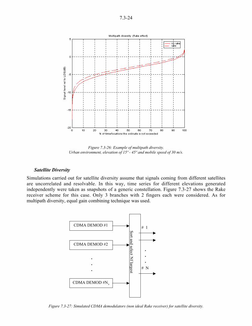
7.3-24

Figure 7.3-26: Example of multipath diversity.Urban environment, elevation of 15º - 45º and mobile speed of 30 m/s.

Satellite Diversity

Simulations carried out for satellite diversity assume that signals coming from different satellitesare uncorrelated and resolvable. In this way, time series for different elevations generatedindependently were taken as snapshots of a generic constellation. Figure 7.3-27 shows the Rakereceiver scheme for this case. Only 3 branches with 2 fingers each were considered. As formultipath diversity, equal gain combining technique was used.

# N

# 1CDMA DEMOD #1

CDMA DEMOD #2

CDMA DEMOD #Ns

.

.

.

Sort and selectN

flargest

.

.

.

Figure 7.3-27: Simulated CDMA demodulators (non ideal Rake receiver) for satellite diversity.

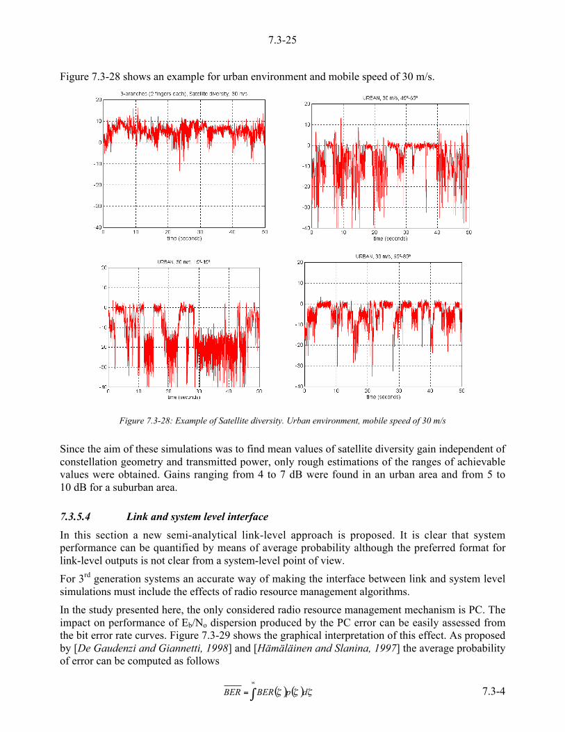
7.3-25

Figure 7.3-28 shows an example for urban environment and mobile speed of 30 m/s.

Figure 7.3-28: Example of Satellite diversity. Urban environment, mobile speed of 30 m/s

Since the aim of these simulations was to find mean values of satellite diversity gain independent ofconstellation geometry and transmitted power, only rough estimations of the ranges of achievablevalues were obtained. Gains ranging from 4 to 7 dB were found in an urban area and from 5 to10 dB for a suburban area.

7.3.5.4 Link and system level interface

In this section a new semi-analytical link-level approach is proposed. It is clear that systemperformance can be quantified by means of average probability although the preferred format forlink-level outputs is not clear from a system-level point of view.

For 3rd generation systems an accurate way of making the interface between link and system levelsimulations must include the effects of radio resource management algorithms.

In the study presented here, the only considered radio resource management mechanism is PC. Theimpact on performance of Eb/No dispersion produced by the PC error can be easily assessed fromthe bit error rate curves. Figure 7.3-29 shows the graphical interpretation of this effect. As proposedby [De Gaudenzi and Giannetti, 1998] and [Hämäläinen and Slanina, 1997] the average probabilityof error can be computed as follows

( ) ( ) ccc dpBERBER 0'

= 7.3-4

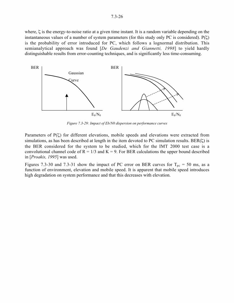
7.3-26

where, c is the energy-to-noise ratio at a given time instant. It is a random variable depending on theinstantaneous values of a number of system parameters (for this study only PC is considered). P(c)is the probability of error introduced for PC, which follows a lognormal distribution. Thissemianalytical approach was found [De Gaudenzi and Giannetti, 1998] to yield hardlydistinguishable results from error-counting techniques, and is significantly less time-consuming.

Figure 7.3-29: Impact of Eb/N0 dispersion on performance curves

Parameters of P(c) for different elevations, mobile speeds and elevations were extracted fromsimulations, as has been described at length in the item devoted to PC simulation results. BER(c) isthe BER considered for the system to be studied, which for the IMT 2000 test case is aconvolutional channel code of R = 1/3 and K = 9. For BER calculations the upper bound describedin [Proakis, 1995] was used.

Figures 7.3-30 and 7.3-31 show the impact of PC error on BER curves for Tpc = 50 ms, as afunction of environment, elevation and mobile speed. It is apparent that mobile speed introduceshigh degradation on system performance and that this decreases with elevation.

Gaussian

Curve

BER

Eb/N0

BER

Eb/N0

7.3-27

Figure 7.3-30: PC error impact (Tpc = 5 Tf) on coded BER (suburban) (o) 1m/s, (*) 15 m/s, (+) 30 m/s

Figure 7.3-31: PC error impact (Tpc = 5 Tf) on coded BER (urban) (o) 1m/s, (*) 15 m/s, (+) 30 m/s

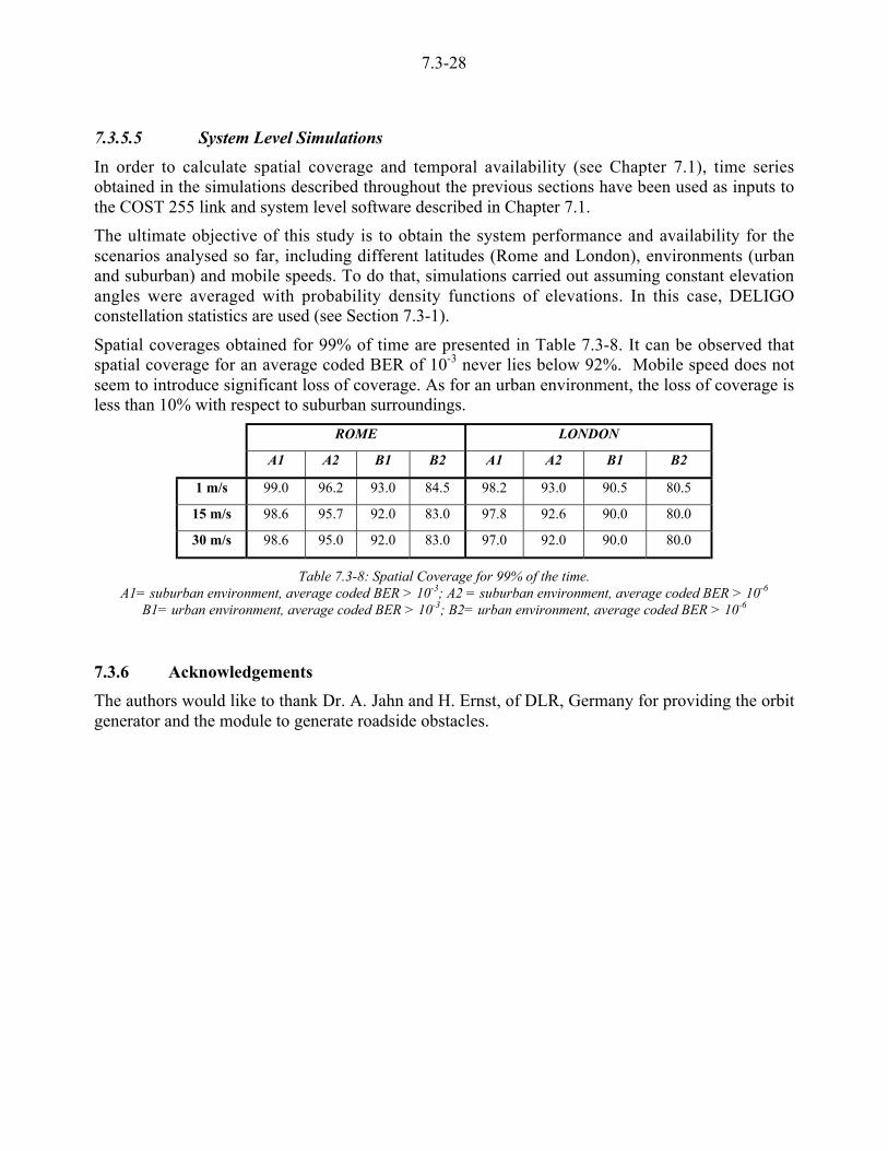
7.3-28

7.3.5.5 System Level Simulations

In order to calculate spatial coverage and temporal availability (see Chapter 7.1), time seriesobtained in the simulations described throughout the previous sections have been used as inputs tothe COST 255 link and system level software described in Chapter 7.1.

The ultimate objective of this study is to obtain the system performance and availability for thescenarios analysed so far, including different latitudes (Rome and London), environments (urbanand suburban) and mobile speeds. To do that, simulations carried out assuming constant elevationangles were averaged with probability density functions of elevations. In this case, DELIGOconstellation statistics are used (see Section 7.3-1).

Spatial coverages obtained for 99% of time are presented in Table 7.3-8. It can be observed thatspatial coverage for an average coded BER of 10-3 never lies below 92%. Mobile speed does notseem to introduce significant loss of coverage. As for an urban environment, the loss of coverage isless than 10% with respect to suburban surroundings.

ROME LONDON

A1 A2 B1 B2 A1 A2 B1 B2

1 m/s 99.0 96.2 93.0 84.5 98.2 93.0 90.5 80.5

15 m/s 98.6 95.7 92.0 83.0 97.8 92.6 90.0 80.0

30 m/s 98.6 95.0 92.0 83.0 97.0 92.0 90.0 80.0

Table 7.3-8: Spatial Coverage for 99% of the time.A1= suburban environment, average coded BER > 10-3; A2 = suburban environment, average coded BER > 10-6

B1= urban environment, average coded BER > 10-3; B2= urban environment, average coded BER > 10-6

7.3.6 Acknowledgements

The authors would like to thank Dr. A. Jahn and H. Ernst, of DLR, Germany for providing the orbitgenerator and the module to generate roadside obstacles.

7.3-29

7.3.7 References

[Agius et al., 1999]Agius, A.A., Leach, S.M., Saunders, S.R., "Measurement of the Polarisation State of Satellite toMobile Signals in Scattering Environments," Proc. Int. Mobile Satellite Conf. IMSC'99, Ottawa,Canada, pp. 134-138, 1999.

[Caire et al., 1999]Caire, G. et al., "Development and Validation of Wideband-CDMA IMT-2000 Physical Layer ForSatellite Applications," Proc. Int. Mobile Satellite Conf. IMSC'99, Ottawa, Canada, pp. 213-219,1999.

[Dahlmann, E. et al., 1998]Dahlmann, E. et al., "WCDMA – The Radio Interface for Future Mobile MultimediaCommunications," IEEE Trans. Vehicul. Technol., vol. 47, no. 4, pp. 1105-1118, 1998.

[Döttling et al., 1999a]Döttling, M., Zwick, T., Wiesbeck, W."Ray Tracing Techniques and their Applications in LandMobile Satellite Propagation," Proc. European Wireless Conf. 99, Munich, Germany, pp. 107-111,1999, .

[Döttling et al., 1999b]Döttling, M., Zwick, T., Wiesbeck, W., "Investigation of Satellite Diversity and HandoverStrategies in Land Mobile Satellite Systems based on a Ray Tracing Propagation Model," Proc. Int.Mobile Satellite Conf. IMSC'99, Ottawa, Canada, pp. 128-133, 1999.

[Döttling et al., 1999c]Döttling, M., Didascalou, D., Wiesbeck, W., "Wideband Channel Modeling and DiversityTechniques for Satellite-UMTS," Proc. IEEE Vehicul. Technol. Conf. VTC'99 Fall, Amsterdam,The Netherlands, pp. 2770-2774, 1999.

[Fontán and Pereda, 1997]Fontán F.P., Pereda J., Sedes M.J., Castro M.A.V., Buonomo S., Baptista P. “Complex envelopethree-state Markov chain simulator for the LMS channel” International Journal of SatelliteCommunications, pp 1-15, January 1997

[Fontán and Castro, 1998]Fontán F.P., Castro M.A.V, Buonomo S., Baptista P., Arbesser-Rastburg B. "S-Band LMSpropagation channel behaviour for different environments, degrees of shadowing and elevationangles" IEEE Transactions Broadcasting, Vol. 44, No. 1, pp 40-76, March 1998

[Fukusawa and Sato, 1996]Fukusawa A., Sato T., Takizawa Y., Kato T., Kawabe M., Fisher R. E. "Wideband CDMA Systemfor Personal Radio Communications" IEEE Communications Magazine, pp. 116-123, October 1996

[De Gaudenzi and Giannetti, 1998]De Gaudenzi, R., Giannetti F. "DS-CDMA Satellite Diversity Reception for Personal SatelliteCommunication: Satellite-to-Mobile Link Performance Analysis" IEEE Transactions on VehicularTechnology, Vol. 47, No. 2, pp. 658-672, May 1998

[Hämäläinen and Slanina, 1997]Hämäläinen S., Slanina P., Hartman M., Lappeteläinen, Holma H., Salonaho O. "A novel interfacebetween link and system level simulations" ACTS'97, pp 599-604

7.3-30

[Jahn and Lutz, 1995]Jahn A. and Lutz E.,1995 “Propagation Data and channel model for LMS systems”. Final report.ESA Purchase Order 141742. DLR, 1995

[Meenan et al., 1995]Meenan C, Sammut A, Tafazolli R, Evans BG. "Deligo: Repetitive Ground Track 100% Dual-Diversity LEO Satellite Constellation for S-PCN", IEE Electronics Letters, Vol. 31, Part 17, August1995, pp. 1407-1408

[Oestges, 1999]Oestges C., "System-level Simulation for Land Mobile Satellite Services" COST 255 RadiowavePropagation Modelling for New SatCom Services at Ku-Band and above, Toulouse, May 1999.

[Öjanpera and Prasad, 1998]Öjanpera, T., Prasad, R. Wideband CDMA for third Generation Mobile Communications ArtechHouse, 1998

[Proakis, 1995]Proakis, J. G. Digital Communications, McGraw-Hill, 3rd edition, New York, 1995

[Smith and Barton, 1992]Smith, H., Barton S.K., Gardiner J.G., Sforza M.“Characterisation of the Land Mobile-Satellite(LMS) Channel at L and S bands: narrowband measurements” ESA AOPs 104433/114473,Bradford, 1992.

[Viterbi, 1998]Viterbi, A. J. CDMA principles of Spread Spectrum, Addison-Wesley Wireless CommunicationsSeries, 1998