An intercomparison between low-frequency variability indices
Atmos. Chem. Phys., 15, 2269–2293, 2015
www.atmos-chem-phys.net/15/2269/2015/
doi:10.5194/acp-15-2269-2015
© Author(s) 2015. CC Attribution 3.0 License.
Copernicus stratospheric ozone service, 2009–2012: validation,
system intercomparison and roles of input data sets
K. Lefever1, R. van der A2, F. Baier3, Y. Christophe1, Q. Errera1, H. Eskes2, J. Flemming4, A. Inness4, L. Jones4,
J.-C. Lambert1, B. Langerock1, M. G. Schultz5, O. Stein5, A. Wagner6, and S. Chabrillat1
1Belgian Institute for Space Aeronomy, BIRA-IASB, Ringlaan 3, 1080 Brussels, Belgium2Royal Dutch Meteorological Institute, KNMI, P.O. Box 201, 3730 AE De Bilt, the Netherlands3German Aerospace Center, DLR, Muenchner Str. 20, 82234 Wessling, Germany4European Centre for Medium-range Weather Forecasts, ECMWF, Shinfield Park, Reading RG2 9AX, UK5Research Center Jülich, FZJ, Institute for Energy and Climate Research, IEK-8: Troposphere,
Wilhelm-Johnen-Straße, 52428 Jülich, Germany6Deutscher Wetterdienst, DWD, Meteorologisches Observatorium Hohenpeissenberg, Albin-Schwaiger-Weg 10,
82383 Hohenpeissenberg, Germany
Correspondence to: S. Chabrillat ([email protected])
Received: 31 March 2014 – Published in Atmos. Chem. Phys. Discuss.: 15 May 2014
Revised: 15 December 2014 – Accepted: 29 January 2015 – Published: 3 March 2015
Abstract. This paper evaluates and discusses the quality of
the stratospheric ozone analyses delivered in near real time
by the MACC (Monitoring Atmospheric Composition and
Climate) project during the 3-year period between Septem-
ber 2009 and September 2012. Ozone analyses produced
by four different chemical data assimilation (CDA) systems
are examined and compared: the Integrated Forecast Sys-
tem coupled to the Model for OZone And Related chemi-
cal Tracers (IFS-MOZART); the Belgian Assimilation Sys-
tem for Chemical ObsErvations (BASCOE); the Synoptic
Analysis of Chemical Constituents by Advanced Data As-
similation (SACADA); and the Data Assimilation Model
based on Transport Model version 3 (TM3DAM). The as-
similated satellite ozone retrievals differed for each system;
SACADA and TM3DAM assimilated only total ozone obser-
vations, BASCOE assimilated profiles for ozone and some
related species, while IFS-MOZART assimilated both types
of ozone observations.
All analyses deliver total column values that agree well
with ground-based observations (biases < 5 %) and have
a realistic seasonal cycle, except for BASCOE analyses,
which underestimate total ozone in the tropics all year long
by 7 to 10 %, and SACADA analyses, which overestimate to-
tal ozone in polar night regions by up to 30 %. The validation
of the vertical distribution is based on independent obser-
vations from ozonesondes and the ACE-FTS (Atmospheric
Chemistry Experiment – Fourier Transform Spectrometer)
satellite instrument. It cannot be performed with TM3DAM,
which is designed only to deliver analyses of total ozone
columns. Vertically alternating positive and negative biases
are found in the IFS-MOZART analyses as well as an over-
estimation of 30 to 60 % in the polar lower stratosphere dur-
ing polar ozone depletion events. SACADA underestimates
lower stratospheric ozone by up to 50 % during these events
above the South Pole and overestimates it by approximately
the same amount in the tropics. The three-dimensional (3-D)
analyses delivered by BASCOE are found to have the best
quality among the three systems resolving the vertical di-
mension, with biases not exceeding 10 % all year long, at
all stratospheric levels and in all latitude bands, except in the
tropical lowermost stratosphere.
The northern spring 2011 period is studied in more detail
to evaluate the ability of the analyses to represent the excep-
tional ozone depletion event, which happened above the Arc-
tic in March 2011. Offline sensitivity tests are performed dur-
ing this month and indicate that the differences between the
forward models or the assimilation algorithms are much less
important than the characteristics of the assimilated data sets.
They also show that IFS-MOZART is able to deliver realistic
analyses of ozone both in the troposphere and in the strato-
Published by Copernicus Publications on behalf of the European Geosciences Union.

2270 K. Lefever et al.: Copernicus stratospheric ozone service, 2009–2012
sphere, but this requires the assimilation of observations from
nadir-looking instruments as well as the assimilation of pro-
files, which are well resolved vertically and extend into the
lowermost stratosphere.
1 Introduction
The presence of a high-altitude ozone layer in the atmo-
sphere, which protects the Earth system against the harm-
ful ultraviolet (UV) light from the Sun, was first deter-
mined in the 1920s from observations of the solar UV spec-
trum. Systematic measurements of stratospheric ozone using
ozonesondes started in the late 1950s (Solomon et al., 2005).
At that time, the development of satellites just started, the
first one (Sputnik) being launched in 1957.
Systematic satellite measurements of ozone started in the
late 1970’s with the series of Total Ozone Mapping Spec-
trometer (TOMS) and Solar Backscatter Ultraviolet Instru-
ment (SBUV) instruments. The discovery of the Antarctic
ozone hole in 1985 (Farman et al., 1985) led to the develop-
ment of improved satellite instruments to observe the com-
position and dynamics of the stratosphere. These instruments
played a key role in the discovery of the physical processes
responsible for the ozone hole (e.g. Solomon, 1999).
Data assimilation determines a best possible state for a
system using observations and short range forecasts. This
process was first developed to enable numerical weather pre-
diction (NWP; e.g. Lorenc, 1986). In view of the planned in-
crease in the number and variety of sounders monitoring the
ozone layer, the last years of the 1980s saw the appearance of
a new application for data assimilation: chemical data assimi-
lation (CDA), or more properly, constituent data assimilation
(Rood et al., 1989; Lahoz and Errera, 2010).
Satellite observations of stratospheric composition are re-
trieved with varying spatial and temporal resolutions, which
depend on the instrument design, the retrieval strategy and
the circumstances of its operational use. Data assimilation
systems can process these data sets (Lahoz and Errera,
2010) to deliver, at regular time intervals, analyses which
are meshed on a two-dimensional grid (total column) or on a
three-dimensional (3-D) grid (vertically resolved field). The
spatial and temporal gradients in these analyses are expected
to reflect dynamical and chemical processes rather than the
details of the observing system. This feature is exploited in
several studies of the photochemistry of the middle atmo-
sphere, especially in the polar regions (see Robichaud et al.,
2010; Lahoz et al., 2011; Sagi et al., 2014).
Thanks to their gridded and instantaneous description
of the atmospheric composition, chemical analyses enable
short-range to middle-range forecasts (Flemming et al.,
2011) and are much easier to use and to interpret than
satellite observations. The resulting “snapshot” maps show
stratospheric composition at a specific time and are rou-
tinely used to monitor the evolution of the ozone layer, e.g.
above the Antarctic (Antarctic ozone bulletins distributed
by WMO/GAW: http://www.wmo.int/pages/prog/arep/gaw/
ozone/index.html).
For 10 years, the development of these monitoring and
forecasting abilities has been the primary goal of a series
of European projects. The European Union project MACC-
II (Monitoring Atmospheric Composition and Climate – In-
terim Implementation) was the third in a series of projects
funded since 2005 to build up the atmospheric service com-
ponent of the Global Monitoring for Environment and Secu-
rity (GMES)/Copernicus European programme (Peuch et al.,
2014). In this paper, the term “MACC” refers to both the
MACC and MACC-II projects. The final goal of MACC is
to cover all aspects of atmospheric dynamics and chemistry
with one global data assimilation system (DAS) based on an
operational numerical weather prediction (NWP) system.
Two coupled systems were created in MACC: IFS-TM5
and IFS-MOZART (Flemming et al., 2009; Stein et al.,
2013). These coupled dynamics-chemistry DAS are run
at the European Centre for Medium-Range Weather Fore-
casts (ECMWF) in near-real-time (NRT) for monitoring
present and near-future atmospheric conditions up to 5 days
ahead, through analyses and forecasts of carbon monoxide
(CO), formaldehyde (HCHO), nitrogen oxides (NOx, i.e.
NO+NO2), sulfur dioxide (SO2) and ozone (O3). They were
both designed to deliver in one run a complete and self-
consistent picture of atmospheric chemistry and dynamics
and both solve explicitly a complete set of photochemical
reactions relevant to tropospheric chemistry. The description
of photochemistry in IFS-MOZART also includes the halo-
gen species, the reactions of interest in the stratosphere, and a
parameterisation of the heterogeneous reactions responsible
for ozone depletion in the polar lower stratosphere.
For European-scale analyses relevant to air quality ap-
plications, MACC successfully organised an ensemble of
limited-area CDA systems (Gauss et al., 2013). A similar
approach was adopted to deliver global analyses of strato-
spheric and total column ozone through the MACC strato-
spheric ozone service (http://www.copernicus-stratosphere.
eu). Besides IFS-MOZART, this service uses three indepen-
dent CDA systems in order to identify model weaknesses and
aid in the improvement of the main system. These three sys-
tems are BASCOE (Errera et al., 2008; Viscardy et al., 2010),
SACADA (Elbern et al., 2010) and TM3DAM (Eskes et al.,
2003; van der A et al., 2010). These three systems first de-
livered monitoring services for the programme PROMOTE
(PROtocol MOniToring for the GMES Service Element At-
mosphere – http://www.gse-promote.org), which was funded
by the European Space Agency from 2004 until 2009. They
are run at the centres where they were designed, use offline
analyses of atmospheric dynamics, and have more relaxed
operational constraints than the NRT runs of IFS-MOZART
and IFS-TM5 at ECMWF.
Atmos. Chem. Phys., 15, 2269–2293, 2015 www.atmos-chem-phys.net/15/2269/2015/

K. Lefever et al.: Copernicus stratospheric ozone service, 2009–2012 2271
The TM3DAM system is specifically designed to gener-
ate a long-term ozone column data set: the ozone Multi-
Sensor Reanalysis (MSR), which documents the day-to-day
variability and allows trend studies trends in total ozone
over more than 30 years. Contrarily to IFS-MOZART, BAS-
COE and SACADA are developed specifically to study and
monitor stratospheric chemistry. Their adjoint models in-
clude photochemistry, allowing these 4D-Var systems to de-
liver multi-variate analyses that should provide a more self-
consistent chemical analysis of the stratosphere than possi-
ble with IFS-MOZART. Until now BASCOE and SACADA
have assimilated only one instrument at a time and BASCOE
processed only vertical profiles from limb-scanning instru-
ments. In view of its advanced modelling of transport and
background error covariances, it was decided to assimilate
with SACADA only total ozone columns. This sub-optimal
configuration was meant to test the quality of 3-D ozone anal-
yses by an advanced 4D-Var system in the absence of limb
profilers.
In this paper we compare the ozone analyses delivered in
NRT by these four systems over the 3-year period September
2009–September 2012, using as reference several data sets
of independent observations: ground-based instruments; bal-
loon soundings; and a solar occultation satellite instrument.
We also explore the roles of the input data sets in the out-
come of this exhaustive validation. Our study is similar to the
intercomparison of ozone analyses realised in the Assimila-
tion of Envisat Data (ASSET) project (Geer et al., 2006; La-
hoz et al., 2007), with some major differences: here the DAS
were configured primarily to satisfy operational constraints
and deliver NRT products (and in the case of IFS-MOZART
to deliver several tropospheric products in addition to strato-
spheric ozone); we assimilated a large variety of data sets
while ASSET used only observations from Envisat (Environ-
mental Satellite); and the investigated period is much longer
(3 years instead of 5 months).
The next section describes the different analyses in the
MACC stratospheric ozone service and the reference obser-
vations used for their validation. Section 3 contains the eval-
uation of the total ozone columns based on Brewer–Dobson
observations, while the vertical distribution of ozone is as-
sessed in Sects. 4 and 5, through comparison with ozoneson-
des and ACE-FTS satellite data, respectively. In Sect. 6,
we assess the performance of the MACC analyses during
an event of exceptional nature: the Arctic ozone hole, 2011
(Manney et al., 2011). We additionally investigate the influ-
ence of the assimilated data set on the performance of the
analyses for 1 month covered by this event: March 2011. The
final section provides a summary and conclusions.
2 Data
The MACC stratospheric ozone service currently consists of
four independent systems, running routinely on a daily ba-
sis, with a maximum delay of 4 days between data acqui-
sition and delivery of the analyses: IFS-MOZART (1 day);
BASCOE (4 days); SACADA (2 days); and TM3DAM (2
days). This section gives a detailed description of the analy-
ses: the observations that were assimilated; the underlying
atmospheric composition models; the applied data assimi-
lation algorithms; and the way the different DAS deal with
background error statistics. Table 1 summarises the satel-
lite retrievals of ozone that were actively assimilated by the
four DAS of the MACC stratospheric ozone service, while
an overview of the system specifications can be found in Ta-
ble 2. This section additionally includes a description of the
data sets used in the validation of the four analyses.
2.1 Assimilated observations
2.1.1 Aura satellite: OMI total columns and MLS
profiles
Aura is NASA’s (National Aeronautics and Space Admin-
istration) third large Earth Observing System (EOS) mis-
sion, flying in a sunsynchronous nearly polar orbit since 9
August 2004, aiming at the provision of trace gas observa-
tions for climate and air pollution studies (Schoeberl et al.,
2006). Due to its nearly polar orbit, Aura is able to pro-
vide a nearly global latitude coverage. It has four instruments
onboard, amongst which the Ozone Monitoring Instrument
(OMI, Levelt et al., 2006) and the Microwave Limb Sounder
(MLS, Waters et al., 2006), which provide complementary
information.
The OMI instrument is a nadir-viewing imaging spec-
trometer, measuring the solar radiation backscattered by the
Earth’s atmosphere and surface in the ultraviolet to visible
(UV–Vis) wavelength range, providing total ozone columns
with a horizontal resolution of 13 km× 24 km at nadir. This
data set is delivered in near real-time and was validated using
Brewer and Dobson spectrophotometer ground-based obser-
vations (Balis et al., 2007). While OMI also provides nadir
ozone profiles, these have not been assimilated.
The MLS instrument is a limb-viewing microwave ra-
diometer, providing some 3500 daily vertical profile mea-
surements of several atmospheric parameters, such as ozone
(O3), nitric acid (HNO3), water vapour (H2O), hydrochlo-
ric acid (HCl), hypochlorous acid (HOCl), and nitrous ox-
ide (N2O) from about 8 to 80 km (0.02 hPa to 215 hPa) with
a vertical resolution of about 3 km in the stratosphere and
a horizontal resolution of 200–300 km (Waters et al., 2006).
As a microwave remote sensing sounder, MLS also provides
observations during the polar night, which has a positive im-
pact on ozone analyses during the onset of the ozone hole.
Ozone data retrieved from MLS are delivered in near real-
time by NASA/JPL (Jet Propulsion Laboratory), with a la-
tency of only 2 to 4 h, whereas a scientific data set, contain-
ing additionally non-ozone species, is delivered with a delay
of 4 days. The former data set is used for the assimilation of
www.atmos-chem-phys.net/15/2269/2015/ Atmos. Chem. Phys., 15, 2269–2293, 2015

2272 K. Lefever et al.: Copernicus stratospheric ozone service, 2009–2012
Table 1. Satellite retrievals of ozone that were actively assimilated by the four models of the MACC stratospheric ozone service. The
Aura MLS data used by IFS-MOZART and BASCOE are not the same: IFS-MOZART used the MLS NRT retrievals of ozone only, while
BASCOE used the standard scientific, offline retrievals including five other species. PC stands for partial columns, TC for total columns and
PROF for profiles. When two references are provided, the first refers to the satellite sensor, the second one to the retrieval algorithm.
Analysis Satellite Sensor Provider Version Assim. data Period Reference
IFS-MOZART NOAA- SBUV/2 NOAA V8.0 PC 1 Sep 2009– Bhartia et al. (2013)
17/18/19 (see text) 30 Sep 2012
Aura OMI NASA/JPL V003 TC 1 Sep 2009– Levelt et al. (2006)
30 Sep 2012
Envisat SCIAMACHY KNMI TOSOMI v2.0 TC 1 Sep 2009– Eskes et al. (2005)
7 Apr 2012
Aura MLS NASA/JPL V2.2, NRT PROF, 1 Sep 2009– Waters et al. (2006)
< 68 hPa 30 Sep 2012 Livesey et al. (2006)
BASCOE Aura MLS NASA/JPL V2.2, SCI PROF 1 Jul 2009– Waters et al. (2006)
30 Sep 2012 Livesey et al. (2013a)
SACADA V2.0 Envisat SCIAMACHY DLR, on behalf SGP-5.01 TC 5 Mar 2010– von Bargen et al. (2007)
of ESA 27 Oct 2011
SACADA V2.4 MetOp-A GOME-2 EUMETSAT GDP 4.1 TC 28 Oct 2011– Loyola et al. (2011)
30 Sep 2012 van Roozendael et al. (2006)
TM3DAM Envisat SCIAMACHY KNMI TOSOMI v2.0 TC 16 Mar 2010– Eskes et al. (2005)
31 Mar 2012
MetOp-A GOME-2 DLR GDP 4.x TC 1 Apr 2012– Loyola et al. (2011)
30 Sep 2012 van Roozendael et al. (2006)
ozone by IFS-MOZART (see Sect. 2.2.1), whereas the latter
is used by BASCOE (see Sect. 2.2.2) for the assimilation of
O3, HNO3, H2O, HCl, and N2O (v2.2). The useful range of
both data sets differs: NRT ozone profiles were only recom-
mended for scientific use at pressure levels 0.2–68 hPa, while
the offline MLS data set could be used for the entire pressure
range 0.02–215 hPa.
Froidevaux et al. (2008) estimated from comparisons with
other instruments that the MLS v2 ozone profiles have an
uncertainty of the order of 5 % in the stratosphere, with
values closer to 10 % at the lowest stratospheric altitudes.
These lower stratospheric biases mostly disappear with the
improved MLS v3.4 data (Livesey et al., 2013b), which have
a useful range of 261 to 0.1 hPa. Sensitivity tests were per-
formed with IFS-MOZART, BASCOE and SACADA using
the offline MLS v3 data set (see section 6.2). The accuracy
and precision of these retrievals (Livesey et al., 2013b) are
very similar to those reported for MLS v2 (Livesey et al.,
2013a) so the uncertainties of MLS v3 are expected to be at
least as small as those reported for MLS v2.
2.1.2 Envisat satellite: SCIAMACHY total columns
The SCIAMACHY instrument (SCanning Imaging Ab-
sorption spectroMeter for Atmospheric CHartographY) is
a UV–Vis–NIR (near-infrared) imaging spectrometer on-
board ESA’s Environmental Satellite (Envisat) launched on
1 March 2002. SCIAMACHY observed earthshine radiance
in limb and nadir viewing geometry and solar and lunar
light transmitted through the atmosphere in occultation view-
ing geometry. While spectrometers such as MLS are able
to provide ozone profiles over the poles throughout the
year, UV–Vis instruments such as SCIAMACHY are lim-
ited to periods with sufficient solar radiation. On the other
hand, they can attain much higher spatial resolution. SCIA-
MACHY total columns have a horizontal resolution of typi-
cally 32 km× 60 km and were extensively validated against
ground-based measurements (Eskes et al., 2005).
After having operated 5 years beyond the planned mis-
sion lifetime of 5 years, all communication with the Envisat
satellite was lost on 8 April 2012. IFS-MOZART assimi-
lated SCIAMACHY total ozone columns until the last date (7
April 2012). To have a clean monthly mean, it was decided to
reprocess TM3DAM for the first days of April using GOME-
2 from 1 April 2012 onwards. Due to a better global cover-
age within 1 day for GOME-2 (SCIAMACHY attains global
coverage in 6 days), leading to an improved performance,
the official MACC NRT product for SACADA had al-
ready switched from SACADA-SCIAMACHY to SACADA-
GOME2 on 28 October 2011.
2.1.3 MetOp-A satellite: GOME-2 total columns
The GOME-2 (Global Ozone Monitoring Experiment-2) in-
strument carried onboard EUMETSAT’s (European Organi-
sation for the Exploitation of Meteorological Satellites) Me-
teorological Operational Satellite MetOp-A (launched in Oc-
tober 2006) continues the long-term monitoring of atmo-
spheric trace gases by ESA’s (European Space Agency)
ERS-2 (European Remote sensing Satellite-2) GOME. It is
Atmos. Chem. Phys., 15, 2269–2293, 2015 www.atmos-chem-phys.net/15/2269/2015/

K. Lefever et al.: Copernicus stratospheric ozone service, 2009–2012 2273
a nadir-viewing UV–Vis scanning spectrometer, which is
able to achieve global coverage within 1 day (Munro et al.,
2006). Total columns are provided with a horizontal reso-
lution of 80 km× 40 km. GOME-2 total ozone columns are
available about 2 h after sensing and were validated against
ground-based measurements by Loyola et al. (2011). Ozone
profiles are also retrieved from this instrument but this study
used only the total columns.
2.1.4 NOAA satellite: SBUV-2 partial columns
SBUV/2 is a series of seven remote sensors on NOAA
weather satellites (McPeters et al., 2013), of which three
were assimilated by IFS-MOZART during the period inves-
tigated here (September 2009 to September 2012): NOAA-
17 and NOAA-18 during the whole period; NOAA-19 after
2011-06-22. Bhartia et al. (2013) describe the two latest ver-
sions of the SBUV/2 retrievals: v8 which was available dur-
ing the period investigated here, and v8.6 which was released
more recently. While SBUV v8.6 includes the averaging ker-
nels (AK) for each retrieved profile, these were not available
in the v8 BUFR data used operationally at ECMWF. Hence
we used the same procedure as first described for ERA-40
(Dethof and Hólm, 2004): in order to decrease unwanted ver-
tical correlations between errors at different levels, the thir-
teen layers of the original SBUV v8 retrievals were combined
at ECMWF over six thick layers (0.1–1 hPa, 1–1.6 hPa, 1.6–
4.1 hPa, 4.1–6.4 hPa, 6.4–16 hPa, 16 hPa–surface). Among
the resulting partial ozone columns, the last one contributes
most to the total columns.
2.2 Description and setup of the data assimilation
systems
2.2.1 IFS-MOZART
Within the GEMS project, the Integrated Forecast System
(IFS), operated by ECMWF, was extended to be able to sim-
ulate and assimilate the abundance of greenhouse gases (En-
gelen et al., 2009), aerosols (Morcrette et al., 2009; Benedetti
et al., 2009), as well as tropospheric and stratospheric reac-
tive gases (Flemming et al., 2009; Inness et al., 2009; Stein
et al., 2012) from satellite retrieval products. Satellite ob-
servations for the following reactive gases can be assimi-
lated: O3; nitrogen dioxide (NO2); carbon monoxide (CO);
formaldehyde (HCHO); and sulfur dioxide (SO2); but only
the former three were assimilated in the operational analy-
sis discussed in this paper. The assimilation window of IFS-
MOZART is 12 h.
The version of IFS-MOZART used here was described in
detail by Stein et al. (2013). To provide concentrations and
chemical tendencies of the reactive gases, the IFS was cou-
pled to a chemistry transport model (CTM) using the cou-
pling software OASIS4 (Ocean Atmosphere Sea Ice Soil:
Redler et al., 2010). The IFS computes only the transport of
the aforementioned reactive gases, while the coupled CTM
provides the chemical tendencies due to chemical conver-
sion, deposition and emission.
The CTM selected to deliver analyses of stratospheric
ozone for the MACC global monitoring and forecast system
is MOZART-3 (Kinnison et al., 2007; Stein et al., 2012) be-
cause it simulates both tropospheric and stratospheric chem-
istry, including the catalytic destruction of ozone in the lower
polar stratosphere. Inness et al. (2009) give a detailed de-
scription of the applied procedure for the assimilation of at-
mospheric constituents in IFS-MOZART.
During the period studied here, the IFS was run at
T159L60, where T159 denotes an expansion to wave num-
ber 159 in the spherical-harmonic representation used by the
model (corresponding to approximately 125 km horizontal
resolution at the equator), and L60 denotes a vertical grid
comprising 60 hybrid-pressure levels extending from 0.1 hPa
down to the surface. This run uses IFS version (“cycle”)
36R1. The CTM component, MOZART-3, used the same
60 vertical levels and a regular longitude–latitude grid with
1.875◦× 1.875◦ horizontal resolution. Its chemical scheme
includes 115 species interacting through 325 reactions (Stein
et al., 2013).
The following satellite O3 data were simultaneously as-
similated (see Table 1): partial columns by NOAA SBUV-2;
total columns by Aura OMI and Envisat SCIAMACHY; and
profiles by Aura MLS down to 68 hPa. Note that all ozone
data assimilated in IFS-MOZART are NRT products. Hence
the MLS data set used here (v2.2) is the product delivered 2
to 4 h after measurement, in contrast to the data assimilated
by BASCOE (see Sect. 2.2.2).
The IFS-MOZART version described here was run daily
(experiment f93i) from 1 September 2009 to 30 September
2012, which determined the period considered in this paper.
2.2.2 BASCOE
BASCOE (Errera et al., 2008) is a 4D-Var system developed
at the Belgian Institute for Space Aeronomy, BIRA-IASB.
Based on a stratospheric CTM, BASCOE assimilates satellite
retrievals of O3, H2O, HNO3, HCl, HOCl, and N2O, gathered
by MLS. The assimilation window is 24 h, while BASCOE
produces output every 3 h. The CTM includes 57 species that
interact using 143 gas-phase reactions, 48 photolysis reac-
tions and 9 heterogeneous reactions.
Heterogeneous reactions on the surface of polar strato-
spheric cloud (PSC) particles are explicitly taken into ac-
count. The BASCOE version used here adopts a simple cold-
point temperature parameterisation to represent the surface
area available for these reactions: type Ia (Nitric Acid Trihy-
drate) PSCs are set to appear at temperatures between 186
and 194 K with a surface area density of 10−7 cm2 cm−3. At
grid points colder than 186K they are replaced by type II
PSCs (i.e. water ice particles) with a surface area density of
10−6 cm2 cm−3.
www.atmos-chem-phys.net/15/2269/2015/ Atmos. Chem. Phys., 15, 2269–2293, 2015

2274 K. Lefever et al.: Copernicus stratospheric ozone service, 2009–2012
When the BASCOE forward CTM is run with no con-
straining observations, the stratospheric ozone fields become
less realistic after a few weeks or months, depending on the
region. These results are similar to those found with IFS-
MOZART by Flemming et al. (2011). In the case of the
BASCOE CTM, this is due to the absence of tropospheric
processes and surface emissions, which prevents proper ex-
changes with the troposphere; and to the parameterisation of
PSC surface area density, which lacks any memory of the
coldness experienced by polar air masses. This last issue
was discussed by Lindenmaier et al. (2011) using the cou-
pled model GEM-BACH that inherited its photochemistry
and PSC parameterisation from BASCOE.
For the MACC stratospheric ozone service, the BASCOE
DAS is driven by the ECMWF operational 6-hourly analyses
(winds, temperature and surface pressure). BASCOE is run
at a horizontal resolution of 3.75◦ longitude by 2.5◦ latitude
and uses a vertical hybrid-pressure grid comprising 37 levels,
most of them lying in the stratosphere. As the driving mete-
orological analyses, this vertical grid extends from 0.01 hPa
down to the surface. BASCOE does not include any tropo-
spheric processes and is therefore not expected to produce
a realistic chemical composition below the tropopause, re-
sulting in larger systematic error biases for the total columns
and in the lower stratosphere.
Both BASCOE and IFS-MOZART analyses assimilate
Aura MLS data, but while IFS-MOZART uses the NRT re-
trievals v2.2 of ozone only, BASCOE uses the standard sci-
entific, offline retrievals (level-2) v2.2 including five other
species, which are available with a delay of typically 4 days.
BASCOE was configured to filter out ozone observations be-
low 150 hPa.
2.2.3 SACADA
Within the project SACADA, a 4D-Var scheme has been
developed by the Rhenish Institute for Environmental Re-
search at the University of Cologne and partners (Elbern
et al., 2010) aiming at the assimilation of atmospheric En-
visat data using state-of-the-art numerical methods. This
system has been implemented for operational use at the
Deutsches Zentrum für Luft- und Raumfahrt, DLR, who de-
liver routinely daily (12 h UT) trace gas analyses based on
Envisat SCIAMACHY ozone columns since March 2010.
In parallel, another SACADA service assimilates MetOp-
A GOME-2 total column data since January 2008. In re-
search mode, SACADA has been successfully applied to
other satellite- and ground-based observations (Elbern et al.,
2010; Schwinger and Elbern, 2010; Baier et al., 2013).
The SACADA system uses an icosahedral grid (i.e. 20
equilateral triangles) on sigma-pressure levels with an ap-
proximate resolution of 250 km. The vertical grid consists
of 32 model levels extending from 7 to 66 km altitude (440
to 0.1 hPa). The tropospheric ozone column is prescribed
from the TOMS V8 climatology. Like IFS-MOZART and
BASCOE, SACADA applies a comprehensive stratospheric
chemistry scheme (see Table 2). The NRT service addition-
ally provides information on the following unconstrained
species: HNO3, H2O, and HCl. Unlike the other CDA sys-
tems used in MACC, SACADA is not driven directly by
winds and temperature from the IFS NWP system; it takes
these input fields from the meteorological forecast system
GME (Majewski et al., 2001), run at DLR. GME is started
from ECMWF analyses data daily at 00:00 UTC and pro-
vides its own 24 h forecasts. The SACADA 4D-Var as-
similation uses an assimilation window of 24 h. Note that
SACADA products are delivered on a standard latitude–
longitude grid with 3.75◦ by 2.5◦ resolution from 147 to
0.3 hPa altitude.
Here we investigate two independent SACADA NRT
products for two consecutive time intervals (see Table 1).
NRT delivery started on 4 March 2010 with SACADA
2.0 assimilating SCIAMACHY observations of total ozone
columns (version 5). After 28 October 2011, SACADA was
upgraded to version 2.4 and switched to the GOME-2 instru-
ment (retrieval version GDP 4.1), which has a better daily
data coverage than SCIAMACHY.
2.2.4 TM3DAM
The TM3DAM data assimilation system is based on the
TM3/TM5 tracer transport model and is driven by oper-
ational 6-hourly meteorological fields from ECMWF. The
main purpose of TM3DAM is the generation of 30–45 year
reanalyses of total ozone based on all available satellite data
sets (van der A et al., 2010), but in MACC it has also been
operated to provide real time analyses and forecasts. TM3
contains parameterised schemes for the description of strato-
spheric gas-phase and heterogeneous ozone chemistry.
The assimilation scheme in TM3DAM is based on a sim-
plified Kalman-filter approach, with a time and space de-
pendent error covariance, but with fixed correlations (Eskes
et al., 2003), which considerably reduces the computational
cost. The TM3DAM assimilation code has been updated as
described in van der A et al. (2010). The system is run at
a global horizontal resolution of 3◦ longitude by 2◦ latitude.
It applies a vertical hybrid-pressure grid, consisting of 44 lev-
els extending from 0 hPa to the surface (1013 hPa). From the
upper troposphere upwards, the layers coincide with the 60-
layer vertical grid used at ECMWF.
TM3DAM assimilates near real-time level-2 total ozone
column data from Envisat/SCIAMACHY until the end of
March 2012 and switched to MetOp-A/GOME-2 after all
communication with the Envisat satellite was lost on 8 April
2012. NRT production of daily analyses (valid at 21 h UT)
in the framework of MACC started on 16 March 2010.
Only total columns are available. Besides the daily analy-
ses, TM3DAM also generates daily forecasts for up to 9
days ahead. The Observation-minus-Forecast (OmF) statis-
tics show that the bias of the system compared to the indi-
Atmos. Chem. Phys., 15, 2269–2293, 2015 www.atmos-chem-phys.net/15/2269/2015/

K. Lefever et al.: Copernicus stratospheric ozone service, 2009–2012 2275
vidual satellite measurements is typically less than 1 % for
a forecast period of 1 day.
2.3 Comparison of ozone background errors
The specification of the background error covariance matrix
(e.g. Kalnay, 2002) is one of the most difficult parts of an
assimilation system: since assimilation errors are never ob-
served directly, they can only be estimated in a statistical
sense. Each of the considered analyses has a different way of
dealing with background error statistics. In IFS-MOZART,
the background error covariance matrix is given in a wavelet
formulation (Fisher, 2006), allowing both spatial and spec-
tral variations of the horizontal and vertical background error
covariances (Inness et al., 2013). For ozone, the background
error correlations were derived from an ensemble of forecast
differences, using a method proposed by Fisher and Anders-
son (2001). The background error standard deviation profiles
and the horizontal and vertical correlations can be found in
Fig. 1 of Inness et al. (2009).
BASCOE analyses use a diagonal background error cor-
relation matrix B with a fixed error usually between 20 to
50 % of the background field, 30 % in this version. The diag-
onal setup of B implies that spatial correlations are neglected.
Spatial correlations help to spread the information from the
data into the model. As mentioned by Errera et al. (2008),
they can be neglected in a first approximation if the spatial
coverage of the assimilated observations and their vertical
resolution are comparable to the DAS resolution. This is the
case here, where a maximum of 3 days of MLS observations
are necessary to constrain all BASCOE grid points. Note that
spatial correlation on the B-matrix has been implemented re-
cently in BASCOE (Errera and Ménard, 2012), following the
method by Hollingsworth and Lönnberg (1986).
The SACADA 4D-Var assimilation uses a flow dependent
paramaterisation of the background error covariance matrix
with a diffusion approach (Weaver and Courtier, 2001). The
basic idea is to formulate covariances by Gaussians and ap-
proximate these Gaussians by integration of the diffusion op-
erator over a specified time. Horizontal and vertical back-
ground error correlation lengths are fixed to 600 km and
3 km, respectively. The background standard deviation is set
to 50 % of the background field, which is quite low and al-
lows the observations to have a strong impact on results.
In the parameterised Kalman filter approach of TM3DAM,
the forecast error covariance matrix is written as a product of
a time independent (i.e. fixed) correlation matrix and a time
dependent diagonal variance (Eskes et al., 2003). All aspects
of the covariance matrix, including the time dependent er-
ror growth and correlation length, are carefully tuned on the
basis of OmF (Observation minus Forecast) statistics. In the
total ozone product, a realistic time dependent error bar is
provided for each location and time.
Figure 1. Location of all stations used in this paper. O3 sondes
are indicated as filled black circles. The ones selected for a more
detailed discussion have been marked in red: Ny-Ålesund (79◦ N,
12◦ E) in the Arctic, Nairobi (1.27◦ S, 36.8◦ E) in the tropics, and
Neumayer (70.65◦ S, 8.25◦W) in the Antarctic. The three sites se-
lected for the total ozone column (TOC) discussion are indicated by
the red squares.
2.4 Reference ozone data
2.4.1 Brewer–Dobson observations
To assess the condition of the ozone layer, one frequently
uses the total column of ozone. Roughly 150 ground sta-
tions perform total ozone measurements on a regular ba-
sis. Data are submitted into the World Ozone and UV Data
Center (WOUDC), operated by Environment Canada (http:
//www.woudc.org), as part of the Global Atmosphere Watch
(GAW) programme of the World Meteorological Organiza-
tion (WMO). The observations are predominantly taken with
Dobson and Brewer UV spectrophotometers at about 60 and
70 stations respectively, but WOUDC also includes observa-
tions from UV–Vis DOAS spectrometers.
Even though Dobson and Brewer instruments are based
on the same general measurement principle, previous stud-
ies have identified a seasonal bias of a few percent between
their midlatitude total ozone column measurements, Brewer
measurements being in slightly better agreement with satel-
lite data than Dobson measurements. In the northern hemi-
sphere, Dobson instruments exhibit a +1 % bias compared
to Brewer instruments and the bias exhibits a seasonal cycle
which is not the case for Brewer instruments (Scarnato et al.,
2009; Lerot et al., 2013). Similar conclusions hold for the
southern hemisphere. Since the Brewer network has not such
a good coverage in the southern hemisphere, however, we use
the Dobson instruments as a reference in the Antarctic, keep-
ing in mind this +1 % bias compared to Brewer instruments
(i.e. we did not correct the Dobsons for this bias, but instead
used the original data).
In order to assess the quality of the total ozone columns
(TOCs) delivered by the four systems, we selected three sta-
tions from the WOUDC database for which the time cover-
www.atmos-chem-phys.net/15/2269/2015/ Atmos. Chem. Phys., 15, 2269–2293, 2015

2276 K. Lefever et al.: Copernicus stratospheric ozone service, 2009–2012
Table 2. Specification of the characteristics of the four assimilation systems: IFS-MOZART; BASCOE; SACADA; and TM3DAM. The
horizontal and vertical resolution have been abbreviated to Hor. and Vert. resol. respectively. Freq. stands for frequency, and Assim. for
assimilation.
IFS-MOZART BASCOE SACADA TM3DAM
Hor. resol. 1.875◦× 1.875◦ 3.75◦× 2.5◦ 250 km 3◦× 2◦
Vert. resol. 60 layers up to 0.1 hPa 37 layers up to 0.1 hPa 32 layers between 44 layers between
7 and 66 km 0 and 1013 hPa
Output freq. 6-hourly 3-hourly daily, at 12 h UT daily, at 21 h UT
Meteo input operational hourly operational 6-hourly 24 h GME forecast operational 6-hourly
meteo fields from IFS meteo analyses from IFS initialised by IFS analyses meteo analyses from IFS
Advection MOZART: flux form flux form semi-Lagrangian flux-based second-order
scheme semi-Lagrangian semi-Lagrangian and upstream method moments scheme
(Lin and Rood, 1996) (Lin and Rood, 1996) (Prather, 1986)
IFS: semi-Lagrangian
Chemical JPL-06 JPL-06 JPL-06 Cariolle parameterisation
mechanism (Sander et al., 2006) (Sander et al., 2006) (Sander et al., 2006) + cold tracer (2 species)
with some modifications Aerosols and PSCs Aerosols and PSCs (Cariolle and Teyssèdre, 2007)
as described in (Damski et al., 2007)
Stein et al. (2013)
115 species 57 species 48 species
325 reactions 200 reactions 177 reactions
Assim. method 4D-Var 4D-Var 4D-Var Kalman filter approach
Assim. window 12 h 24 h 24 h 24 h
age for this 3-year period was sufficiently large (red squares
in Fig. 1): a high northern latitude station, Alert (82.49◦ N,
62.42◦W, data gathered by the Meteorological Service of
Canada); a tropical station, Chengkung (23.1◦ N, 121.365◦ E,
data gathered by the Central Weather Bureau of Taiwan);
and a southern latitude station, Syowa (69◦ S, 39.58◦ E, data
gathered by the Japan Meteorological Agency). As indicated
above, we used the observations gathered by the Brewer in-
struments at Alert and Chengkung, and those gathered by the
Dobson spectrophotometer for Syowa. For Alert, we used
the data for both Brewer instruments 019 (MKII) and 029
(MKV). The Brewer instrument (#061) at Chengkung is of
type MKIV. Brewer data at µ> 3 were filtered out, where
µ is the increase in the ozone optical path length due to the
obliquity of the sun’s rays (Brewer, 1973). The Dobson in-
strument (#119) at Syowa was replaced on 1 February 2011
by a new Beck model (#122).
2.4.2 DOAS observations
Conventional techniques for measuring ozone in the UV,
such as Dobson spectrometers, are inapplicable for so-
lar zenith angles (SZA) larger than about 80◦. Zenith-sky
ultraviolet–visible (UV–Vis) spectroscopy allows measure-
ments of the atmospheric absorption of scattered sunlight
at the zenith sky. This is the only type of ground-based in-
struments able to measure continuously and at all latitudes
outside of areas in polar night. The retrieval is based on dif-
ferential optical absorption spectroscopy (DOAS). This tech-
nique was validated by Van Roozendael et al. (1998) through
comparisons with Dobson measurements and was recently
improved by Hendrick et al. (2011).
The SAOZ (Système d’Analyse par Observation
Zenithale, Pommereau and Goutail (1988)) instruments
belong to this family and have a standardised design, which
allows observations of NO2 and O3 total columns twice
a day during twilight (sunrise and sunset). As a general
result, the SAOZ O3 measurements are between 2–8 %
higher than the Dobson ones, with a scatter of about 5 % in
midlatitudes and increasing at higher latitudes.
For the “Arctic ozone hole 2011” case study in this pa-
per (see Sect. 6), the total ozone columns by the four anal-
yses were compared with data received by three UV–Vis
zenith-sky instruments at Arctic locations, which are part
of the Network for the Detection of Atmospheric Compo-
sition Change (NDACC, http://www.ndacc.org): Scoresby
Sund (Greenland, 70.49◦ N, 21.98◦W); Zhigansk (Russia,
66.8◦ N, 123.4◦ E); and Harestua (Norway, 60◦ N, 11◦ E).
The instruments at Zhigansk and Scoresby Sund have the
SAOZ design and are owned by LATMOS/CNRS (Labora-
toire Atmosphères, Milieux, Observations Spatiales/Centre
National de Recherche Scientifique), while the instrument at
Harestua has an improved design and is operated by BIRA-
IASB (van Roozendael et al., 1995).
Atmos. Chem. Phys., 15, 2269–2293, 2015 www.atmos-chem-phys.net/15/2269/2015/

K. Lefever et al.: Copernicus stratospheric ozone service, 2009–2012 2277
2.4.3 Ozonesonde profiles
Balloon-borne ozonesondes measure the vertical distribu-
tion of ozone concentrations up to an altitude of about
35 km. The observed ozonesonde profiles are archived by
NDACC, WOUDC, and the Southern Hemisphere ADdi-
tional OZonesondes network (SHADOZ, http://croc.gsfc.
nasa.gov/shadoz/). The majority of soundings (85 %) are per-
formed with electrochemical concentration cell (ECC) son-
des, while the remaining part consists of Brewer-Mast, In-
dian and Japanese Carbon-Iodine sondes. Optimally treated,
ECC sondes yield profiles with random errors of 3–5 % and
overall uncertainties of about 5 % in the stratosphere (Smit
et al., 2007; Deshler et al., 2008; Stübi et al., 2008; Hassler
et al., 2014). Other sonde types have somewhat larger ran-
dom errors of 5–10 % (Kerr et al., 1994; Smit et al., 1996).
We use ozone observations gathered by balloon sondes at
38 locations, taken from the above-mentioned databases for
the period September 2009 to September 2012: 12 in the Arc-
tic; 19 in the tropics; and 7 in the Antarctic (see Fig. 1). For
each latitude band, we picked out one station which is repre-
sentative for the general behaviour in this latitude band and
for which the time coverage for this 3-year period was suffi-
ciently large, for a more detailed discussion: the Arctic sta-
tion at Ny-Ålesund (79◦ N, 12◦ E); the equatorial station at
Nairobi (1.27◦ S; 36.8◦ E); and the Antarctic station at Neu-
mayer (70.65◦ S, 8.25◦W) (red dots in Fig. 1). Data are pro-
vided by the Alfred-Wegener Institute in Potsdam, Germany
(for Ny-Ålesund and Neumayer) and by MeteoSwiss in Pay-
erne, Switzerland (for Nairobi).
2.4.4 ACE-FTS satellite data
ACE-FTS is one of the two instruments on the Canadian
satellite mission SCISAT-1 (first Science Satellite), ACE
(Bernath et al., 2005). It is a high spectral resolution Fourier
transform spectrometer operating with a Michelson interfer-
ometer. Vertical profiles of atmospheric parameters such as
temperature, pressure and volume mixing ratios of trace con-
stituents are retrieved from the occultation spectra, as de-
scribed in Boone et al. (2005), with a vertical resolution
of maximum 3–4 km. Level 2 ozone retrievals (version 3.0)
are used as an independent reference data set to validate the
ozone profiles of the MACC stratospheric ozone system.
It must be noted that the low spatio-temporal sampling of
ACE-FTS (due to the solar occultation technique) does not
deliver profiles in all latitude bands for each month. There
are also two periods during the year where there are no mea-
surements for a duration of almost 3 weeks due to the fact
that the spacecraft is in constant sunlight: June and December
(Hughes and Bernath, 2012). There are four periods per year,
lasting about 1 month (northern hemisphere: April, June, Au-
gust, December; southern hemisphere: February, June, Oc-
tober, December) with no occultation poleward of 60◦ (see
Fig. 4 of Hughes and Bernath (2012)). At very high β angles
(i.e. the angle between the orbital plane of the satellite and
the Earth–Sun direction> 57◦), it is common practice to skip
more than half of the available measurement opportunities to
avoid exceeding onboard storage capacities and overlapping
command sequences. Therefore, the amount of observations
in the tropics is significantly lower than in the polar regions.
The previous version of these retrievals (version 2.2) was
extensively validated against 11 other satellite instruments,
ozonesondes and several types of ground-based instruments
(Dupuy et al., 2009). This version reports more ozone than
most correlative measurements from the upper troposphere
to the lower mesosphere. Dupuy et al. (2009) found a “slight
positive bias with mean relative differences of about 5 % be-
tween 15 and 45 km. Tests with a preliminary version of
the next generation ACE-FTS retrievals (version 3.0) have
shown that the slight positive stratospheric bias has been re-
moved.” Adams et al. (2012) additionally present an inter-
comparison of ACE ozone profiles (both versions 2.2 and
3.0) against ground-based observations at Eureka, confirm-
ing that the new ACE-FTS v3.0 and the validated v2.2 par-
tial ozone columns are nearly identical, with mean relative
difference of 0.0± 0.2 % for v2.2. minus v3.0.
Standard deviations for levels where there are fewer
than 20 observations are omitted for reasons of non-
representativeness.
3 Validation of total ozone columns
We intercompare for the first time analyses based on data
from different satellites and of different types: partial/total
ozone columns, profile observations or a combination of
both. For an optimal interpretation of the validation re-
sults, it is important to keep in mind that SACADA and
TM3DAM exclusively assimilated total ozone columns, but
while TM3DAM delivers only total ozone columns as out-
put product, SACADA also provides ozone profiles. BAS-
COE exclusively assimilated vertical profiles of ozone (be-
sides other species) and IFS-MOZART used a combination
of total columns, partial columns and vertical profiles from
various instruments.
In this section, we discuss the results obtained for the val-
idation of the total ozone columns against Brewer observa-
tions at Alert (Arctic) and Chengkung (tropics), and against
Dobson observations at Syowa (Antarctic). The TOC data
sets from the four systems were interpolated to the latitude
and longitude of these stations. The resulting time series are
shown in Fig. 2, side by side with the corresponding observed
ground-based data.
3.1 Alert (Arctic)
The seasonal O3 cycle at Alert is very similar each year.
The only deviations from usual behaviour of the total ozone
columns occur, e.g. in November 2009, when an air mass
www.atmos-chem-phys.net/15/2269/2015/ Atmos. Chem. Phys., 15, 2269–2293, 2015

2278 K. Lefever et al.: Copernicus stratospheric ozone service, 2009–2012
Syowa (69S, 39.58E)
Ozo
ne (
vmr)
1Jan2010 1Jan2011 1Jan2012100
200
300
400
Chengkung (23.1N, 121.365E)
O3 T
C (
DU
)
200
240
280
320
Alert (82.49N, 62.42W)
O3 T
C (
DU
)
250
350
450
550
IFS-MOZART
BASCOE
SACADA
TM3DAM
Figure 2. Comparison between the TOC time series (5-day moving average) of the four analyses of the MACC stratospheric ozone service
(IFS-MOZART in red, BASCOE in blue, SACADA in green, and TM3DAM in cyan) interpolated to a high northern latitude station (Alert,
82.49◦ N, 62.42◦W), a tropical station (Chengkung, 23.1◦ N, 121.365◦ E) and a southern latitude station (Syowa, 69◦ S, 39.58◦ E), for the
period from September 2009 to September 2012. Black symbols are 5-day moving averages of Brewer (for Alert and Chengkung) and
Dobson (for Syowa) observations from the WOUDC network. In order to indicate the observational uncertainty, the height of each symbol
is set to 4 % of the observed value.
with exceptionally high ozone passed over Alert, and in
February–March 2011, when 30 % of the total ozone column
above Alert was destroyed by the end of March. The latter
event will be studied in detail in Sect. 6 as a separate case
study.
All four analyses match each other and the observed total
ozone columns very closely. Peak-to-peak difference in TOC
are of the order of 250 Dobson Units (DU), with maximum
values reached during boreal winter and spring as a result of
poleward and downward transport of ozone-rich air by the
large-scale Brewer–Dobson circulation (Brewer, 1949; Dob-
son, 1956; Weber et al., 2011).
The only significant differences among the analyses occur
during the O3 maximum in northern spring (where mutual
differences of maximum 50 DU, about 10 %, are observed)
and during the Arctic ozone hole season, where SACADA
delivers TOC values which are about 75 DU (20 %) above the
other analyses. Unfortunately, this coincides exactly with the
periods where reliable ground-based observations are miss-
ing due to the lack of sunlight.
3.2 Chengkung (tropics)
The ozone columns in the tropics are lower (between 240 and
330 DU) due to the large-scale ascent of tropospheric low-
ozone air and the higher incidence of solar radiation. Ozone
maxima are reached in April each year, after which ozone is
decreasing slowly until the beginning of November and more
rapidly afterwards. The lowest values are seen in December,
January, and February (DJF), when the upwelling part of the
Brewer–Dobson circulation is strongest. Ozone is recover-
ing very rapidly from January to April. This seasonality is
in general well reproduced by all analyses. The ozone recov-
ery is slower in the analyses than in the observations and the
observed ozone maxima are never reached.
IFS-MOZART, SACADA, and TM3DAM mutually dif-
fer by 2 % at most, and underestimate the Brewer observa-
tions by no more than 5 %. BASCOE systematically under-
estimates total ozone by 20 DU throughout the year (about
7–10 %). As discussed below (Sect. 4.4.2), this is due to the
underestimation of ozone in the lower stratosphere.
Atmos. Chem. Phys., 15, 2269–2293, 2015 www.atmos-chem-phys.net/15/2269/2015/
K. Lefever et al.: Copernicus stratospheric ozone service, 2009–2012 2279
3.3 Syowa (Antarctic)
At the Antarctic station Syowa, the local spring-time ozone
hole is evident, with values below 200 DU during the months
September, October, and November (SON). The total ozone
columns are reduced by up to 50 %, from approximately
300 DU during austral summer and autumn down to 150 DU
during the austral spring season.
The seasonal cycle of total ozone is very well reproduced
by the IFS-MOZART, BASCOE and TM3DAM analyses
with results very close to each other (biases < 2 %). After
the loss of Envisat in April 2012, the differences between
IFS-MOZART and TM3DAM become slightly larger. Before
this incident, both IFS-MOZART and TM3DAM assimilated
SCIAMACHY data, but afterwards, TM3DAM switched to
GOME-2, while IFS-MOZART continued to assimilate ob-
servations from SBUV/2, OMI, and MLS.
SACADA exhibits strong positive biases from observa-
tions during austral winters, right before the onset of the
ozone hole (up to 30 % in 2012). Closer inspection of
SACADA analyses shows that these larger differences coin-
cide with missing SCIAMACHY and GOME-2 observations
during polar night when solar zenith angles are close to or in
excess of 90◦. While this coverage effect should especially
influence systems that assimilate data from UV instruments
only, the TM3DAM system is found less vulnerable to data
gaps than SACADA, as it performs very well under the same
circumstances.
3.4 Discussion of SACADA total column results
All analyses show a realistic seasonal cycle in all three lati-
tude bands and total ozone column values, which are gener-
ally in very good agreement with independent observations,
with the exception of SACADA during polar night. Differ-
ences between IFS-MOZART, BASCOE, and TM3DAM are
usually within 5 %. Only a few exceptions were identified,
i.e. larger mutual differences (up to 10 %) are found at high
altitudes during polar night, and for BASCOE in the tropics,
where the system underestimates total ozone by 7–10 %.
In contrast to these three analyses, SACADA total ozone
results deviate strongly from observations during certain
episodes. There is a general tendency in SACADA re-
sults for positively biased ozone columns during the winter
months at high latitudes compared to Alert and Syowa sta-
tion data in the northern and southern hemispheres, respec-
tively. Backscatter UV instruments provide no information
for zenith angles above 90◦. As recommended for SCIA-
MACHY data version 3 (Lerot et al., 2007), only observa-
tions with zenith angles up to 75◦ were used. Thus, no SCIA-
MACHY data were assimilated until May 2011 at the lati-
tudes of Alert station (82.49◦ N). Accordingly, at Syowa sta-
tion (69◦ S), SCIAMACHY data were not processed from the
end of March until the end of September.
From 28 October 2011 onwards, GOME-2 observations
were assimilated by SACADA up to zenith angles of 90◦. In
this case, the instrument is blind from mid September 2011
to April 2012 at Alert, and from mid April to mid Septem-
ber at Syowa. These time periods correlate generally well
with the positive bias anomalies in ozone columns found in
SACADA results. The area of impact of a total column ob-
servation on assimilation results is limited by the background
correlation matrix, which uses a horizontal correlation radius
of 600 km. Latitudes not covered by observations can there-
fore only be influenced via tracer transport and chemistry. In
summary, we conclude that these large biases reflect a gen-
eral tendency of the SACADA model to overestimate total
ozone in polar night regions. Since its assimilation setup was
limited to UV–Vis observations, these could not constrain the
erroneous model results at high latitudes.
4 Validation of the vertical distribution of
stratospheric ozone against ozonesondes
In this section, we discuss the results obtained for the val-
idation of the ozone profiles against ozonesonde observa-
tions at Ny-Ålesund (Arctic), Nairobi (tropics), and Neu-
mayer (Antarctic).
In order to compare the ozone fields from the three sys-
tems with the observed ozonesonde data, the analyses were
first linearly interpolated to the geographical location of
the launch sites. Even though sondes may drift long dis-
tances during their ascent, especially within the polar vor-
tex, this often significant horizontal movement was disre-
garded, as tracking information is not always available. As
a next step, the two analysis profiles preceding and follow-
ing the measurement closest in time were linearly interpo-
lated to the time of observation. Since the ozonesonde pro-
files have a much higher vertical resolution than the anal-
yses, the ozonesonde data have been vertically re-gridded
to the coarser pressure grid of the DAS, degrading the ob-
servations to the lower resolution of the DAS through a
mass-conserving algorithm (Langerock et al., 2014). Fig-
ure 3 shows time series of the monthly mean ozone bias pro-
files with respect to the ozonesondes at the selected sites for
each of the three MACC systems.
4.1 Arctic – Ny-Ålesund
The seasonal cycle at Ny-Ålesund is very well reproduced
by the three analyses. Biases at Ny-Ålesund are generally
smaller than 20 % for all MACC analyses throughout the
stratosphere (Fig. 3). The time series of the ozone pro-
files shows alternating behaviour in the vertical for IFS-
MOZART, persistent over the entire 3-year period, with pos-
itive biases in the lower (below 70 hPa) and upper (above
20 hPa) stratosphere and no or only slightly negative bi-
ases (mostly 5–10 %) in the middle stratosphere. The per-
www.atmos-chem-phys.net/15/2269/2015/ Atmos. Chem. Phys., 15, 2269–2293, 2015

2280 K. Lefever et al.: Copernicus stratospheric ozone service, 2009–2012
Ny-Å
lesun
dN
airob
iN
eum
aye
r
IFS-MOZART BASCOE SACADA
Rela
tive d
iffere
nce
(%
)
>50
40
20
30
10
5
-5
-10
-20
-30
-40
-50
Rela
tive d
iffere
nce (
%)
>50
40
20
30
10
5
-5
-10
-20
-30
-40
-50
Rela
tive d
iffere
nce
(%
)
>50
40
20
30
10
5
-5
-10
-20
-30
-40
-50
Figure 3. Time series of monthly mean ozone biases (analysis minus observations) with respect to ozonesondes at Ny-Ålesund (top panel,
78.92◦ N, 11.93◦ E), Nairobi (middle panel, 1.27◦ S, 36.8◦ E) and Neumayer (bottom panel, 70.68◦ S, 8.26◦W) for the period September
2009 to September 2012 in %. Left: IFS-MOZART, middle: BASCOE, right: SACADA.
formance of BASCOE is stable throughout the stratosphere
and for the entire 3-year period, with biases mostly less than
5 %. Largest biases over the whole period for IFS-MOZART
(−20 to −30 % between 50 and 70 hPa) and for SACADA
(> 50% between 35 and 65 hPa) are found for March 2011.
While the ozone hole simulated by IFS-MOZART is too
deep, SACADA simulates an Arctic ozone hole, which is
not deep enough. This special event will be discussed in de-
tail in Sect. 6. Until March 2011, SACADA mainly overes-
timates ozone over the entire altitude range, while middle
stratospheric ozone is mostly underestimated afterwards.
4.2 Tropics – Nairobi
The O3 bias profile time series (Fig. 3) now displays a chang-
ing performance in the vertical for all three analyses. Lower
stratospheric ozone is underestimated by more than 40 % by
both IFS-MOZART and BASCOE (below 80 hPa and be-
low 100 hPa, respectively) throughout the year. For BAS-
COE, this is followed by a small pressure range just above
(between 75 and 90 hPa), where ozone values are overesti-
mated by more than 50 %. The results for the remaining mid-
dle to upper part of the stratosphere are almost identical to
the observed ozondesonde values at Nairobi, although with
a tendency to overestimate O3 by IFS-MOZART (< 20%).
SACADA, on the other hand, overestimates ozone below
40 hPa with more than 50 %, while its performance is usu-
ally very good above. Between July 2011 and May 2012,
however, SACADA underestimates O3 with up to 20 %, and
even 30 % from September to December 2011, in the pres-
sure range between 10 and 30 hPa.
This is reflected in the time series at 50 hPa: all analyses
overestimate O3. Whereas IFS-MOZART and BASCOE pro-
duce very similar results at 50 hPa (IFS-MOZART slightly
Atmos. Chem. Phys., 15, 2269–2293, 2015 www.atmos-chem-phys.net/15/2269/2015/

K. Lefever et al.: Copernicus stratospheric ozone service, 2009–2012 2281
Antarctic (90°S-60°S) Tropics (30°S-30°N) Arctic (60°N-90°N)
pre
ssure
(hP
a)
partial pressure (mPa)partial pressure (mPa) partial pressure (mPa)
-40 -20 0 20 40relative difference (%)
-40 -20 0 20 40relative difference (%)
-40 -20 0 20 40relative difference (%)
pre
ssure
(hP
a)
Biases |(A-O)/O| s( (A-O)/O )
Mean profilesSep2009-Sep2012
Figure 4. Top row: mean ozone profiles (top rows) as partial pressures in mPa from IFS-MOZART (red), BASCOE (blue), SACADA (green)
and ozonesondes (black). Bottom row: mean and (solid lines) and standard deviations (dashed lines) of the relative differences, in %, of these
analyses against the ozonesondes. over the period from September 2009 to September 2012.
above BASCOE) with biases of about 15 % compared to the
ozonesonde data at Nairobi, and even up to 30 % in the pe-
riod August–November 2010, SACADA shows ozone values
which are at least 35 % higher than the other two analyses,
while the seasonality is well reproduced. The discontinuity
in the SACADA products from 6 to 7 September 2010, is
due to resumption of the assimilation after a period where
SACADA ran freely (July–September 2010) due to a data
gap in the assimilated SCIAMACHY. As mentioned before
for the total ozone columns, the SACADA analysis tends
to drift in the absence of UV observations to assimilate.
Once resumed, the assimilation reduces the mismatch with
the other two analyses from 60 % down to only 10 %.
4.3 Antarctic – Neumayer
The O3 bias profile time series show that the biases are
smallest and most stable for BASCOE (usually less than
10 %). IFS-MOZART on the other hand has an annually re-
current pattern, overestimating O3 with more than 50 % be-
tween roughly 70 and 150 hPa each Antarctic ozone hole
season, from September to December, while underestimat-
ing ozone between 30 and 60 hPa in September. This indi-
cates that IFS-MOZART has problems with a correct sim-
ulation of the ozone depletion. This is a known problem of
the underlying MOZART CTM in the MACC configuration,
which cannot be completely fixed by the data assimilation
(Flemming et al., 2011; Inness et al., 2013), especially be-
cause the assimilated profile only gives information down to
68 hPa. MOZART performs better with WACCM meteorol-
ogy (Kinnison et al., 2007), which indicates that the chemical
parameterisations are sensitive to the meteorological fields
that are used to drive transport in the models. SACADA has
problems to correctly simulate the ozone concentration in the
lower stratosphere (below 80 hPa) . While the ozone hole
depth of 2010 is underestimated (positive bias), the corre-
sponding ozone depletion in 2011 and 2012 is overestimated
by more than 50 %. This is related to the premature onset and
end of the ozone depletion as predicted by the model, which
is reflected also in the ozone values at 50 hPa. Apart from
this, the observed ozone values at Neumayer at 50 hPa are in
general well reproduced by the three analyses of the MACC
system. IFS-MOZART and BASCOE do not differ much in
their analyses.
4.4 Discussion
4.4.1 SACADA results
In our evaluation, SACADA is the only chemical data as-
similation system with full chemistry that assimilates total
column ozone only. Ozone columns are assimilated by con-
straining the system’s ozone column first guess at the satellite
footprint. We find that, as in the case of SACADA, the lack of
information constraining the shape of the ozone profile leads
primarily to an overestimation of ozone in the lower strato-
sphere as can be seen, e.g. in Fig. 3 in comparison to the
www.atmos-chem-phys.net/15/2269/2015/ Atmos. Chem. Phys., 15, 2269–2293, 2015
2282 K. Lefever et al.: Copernicus stratospheric ozone service, 2009–2012
station at Nairobi (1.27◦ S). The excess ozone in the lower
stratosphere leads to an underestimation at higher altitudes
above 30 hPa (see also Fig. 4). The standard deviations be-
tween the MACC systems and the ozonesondes are largest
for SACADA. We conclude that total column assimilation
does not sufficiently constrain the system’s ozone profile.
4.4.2 IFS-MOZART and BASCOE results
Biases are mostly smaller than 10 % for IFS-MOZART and
BASCOE in the middle to upper stratosphere. IFS-MOZART
has problems with a correct representation of the vertical dis-
tribution of ozone. Often, over- and underestimations are al-
ternating in the vertical. Biases are highest in austral spring
during the Antarctic ozone hole season. Also during March
2011, when the first documented significant ozone hole in
the Arctic occurred (Manney et al., 2011), somewhat larger
differences are found. While IFS-MOZART and BASCOE
deliver quite similar results, BASCOE profiles have a more
stable behaviour at all altitudes and during the Arctic and
Antarctic ozone hole seasons. Largest biases occur, for both
systems, in the lower stratosphere in the tropics.
This can be partially explained by the strong gradients in
ozone near the tropopause, which is located at higher alti-
tudes in the tropics than at the poles. These sharp ozone gra-
dients in the upper troposphere–lower stratosphere (UTLS)
are very difficult to represent in three-dimensional models
and likely require a very fine vertical resolution (Considine
et al., 2008). Furthermore relative differences are amplified
in this region due to its low ozone abundance.
For BASCOE, two more elements play a role in the poorer
performance in the lower tropical stratosphere: the low ver-
tical resolution and aliasing errors in the horizontal wind
fields, which are larger close to the UTLS and which lead
to noise in the horizontal distribution of chemical tracers.
This bug has been corrected in an upgraded version, which
has been running operationally since the beginning of 2013.
The vertical grid of the system is improved, from 37 levels
to 91 levels, with a much finer resolution in the UTLS re-
gion. Comparison between both versions shows that O3 val-
ues become smaller around 80 hPa and larger at lower heights
(which would thus correct the currently large biases in these
regions).
The larger biases for IFS-MOZART in the lower strato-
sphere globally (i.e. not only at the tropics, but also at the
poles, especially in the Antarctic) also result from the fact
that the useful range of the NRT MLS v2.2 data was re-
stricted to levels above 68 hPa, which means that it included
no profile information below that pressure level, in contrast
to BASCOE, which assimilated the offline MLS v2.2 data
set down to 150 hPa. Tests with the improved NRT MLS
v3.4 data (Livesey et al., 2013b), which can be used down to
261hPa, show that many of those biases in the lower strato-
sphere disappear (see Sect. 6.2).
To illustrate that the selected stations at each latitude band
are representative for the results at all stations and that the
same conclusions hold in general, we additionally show the
mean ozone profiles and ozone bias profiles for the MACC
analyses compared to all considered ozonesonde measure-
ments in each latitude band (see Fig. 1), averaged over the
entire 3-year period from September 2009 to September 2012
(Fig. 4). On average, all analyses agree with the sondes
mostly to within ±10 % above 70 hPa. Larger biases are ob-
served for IFS-MOZART in the upper stratosphere (above
10 hPa) at the poles and in the lower stratosphere with over-
all biases reaching 30 % in the Antarctic and −40 % at the
equator, and for BASCOE below 150 hPa.
Standard deviations between the MACC systems and the
ozonesondes are smallest for BASCOE, and only slightly
higher for IFS-MOZART, usually between 10 and 20 %, ex-
cept for the region below 70 hPa in the tropics. The standard
deviations for IFS-MOZART are higher in the area between
60 and 100 hPa in the tropics, and between 100 and 200 hPa
in the Antarctic.
4.4.3 Influence of the temporal and horizontal
resolution
SACADA data are sampled only once a day (at 12 h UT),
IFS-MOZART 6-hourly, and BASCOE data 3-hourly. This
may affect their performances when compared to ozoneson-
des. To exclude the effect of temporal resolution, we have
degraded the temporal resolution of both IFS-MOZART and
BASCOE to the temporal resolution of SACADA.
Relative differences between the fine and the coarse tem-
poral resolution data sets are usually less then 2 %, but can be
as high as 10 % for some months, and at some altitudes with-
out any clear pattern. The effect on the standard deviation of
the differences when using the 24 h resolution data set for all
three analyses is not significant except in the lower tropical
stratosphere (figures not shown).
On the other hand, a lower horizontal resolution may also
lead to larger standard deviations. BASCOE and SACADA
have, however, the same horizontal resolution (3.75◦ by
2.5◦), which is coarser than for IFS-MOZART (1.875◦ by
1.875◦). This illustrates that the differences in standard de-
viations between the MACC systems are not exclusively de-
pendent of the temporal nor the horizontal resolution.
5 Validation of the vertical distribution of
stratospheric ozone against ACE-FTS
In addition to the ground-based and ozonesonde data, the
MACC ozone analyses have been compared to independent
ACE-FTS satellite observations. The comparison between
the measurements by ACE-FTS and the analysis output is
performed in the following manner. The analyses, first re-
gridded to a common 1◦× 1◦ grid, are collocated with the
Atmos. Chem. Phys., 15, 2269–2293, 2015 www.atmos-chem-phys.net/15/2269/2015/

K. Lefever et al.: Copernicus stratospheric ozone service, 2009–2012 2283
Jan2010 Jan2011 Jan20120
5
10
15
20
IFS−MOZARTBASCOESACADA
Monthly mean stddev between AN and ACE−FTS for 90S−90N
[%]
Figure 5. Comparison of the global (i.e. from 90◦ S to 90◦ N)
monthly mean standard deviation between IFS-MOZART (red),
BASCOE (blue), and SACADA (green) with ACE-FTS (analysis
minus observations) in %, for the [200,5]hPa pressure bin, for the
period September 2009 to September 2012. Standard deviations for
levels with less than 20 observations are omitted. Note that standard
deviations are not weighted by the cosine of the latitude.
ACE-FTS data in space (horizontally and vertically) and
time through linear interpolation. Since SACADA results are
only provided every 24 h, we assume a constant composi-
tion throughout the day. Monthly mean biases of the spatial-
temporal collocated data are calculated for five latitude bins,
using 25 pressure bins based on the standard Upper Atmo-
sphere Research Satellite (UARS) fixed pressure grid (i.e. six
pressure levels per decade, which corresponds approximately
to 2.5 km). These monthly mean biases and their associated
standard deviations can be displayed as time series (Figs. 5
and 6) or as vertical profiles (Fig. 7).
In view of the problems to constrain the SACADA three-
dimensional ozone field using only total column assimila-
tion, we will still show the SACADA results in the figures
but we will not include these analyses in the discussion.
5.1 Partial ozone columns
The time series of the standard deviations in Fig. 5 gives
a global view of how well the analyses are performing against
the satellite data. The standard deviations are averaged over
the entire globe (90◦ S–90◦ N) and over the entire strato-
spheric area of interest (200–5 hPa). As shown earlier, when
compared with ground-based and ozonesonde observations,
the results by IFS-MOZART and BASCOE are very simi-
lar. Standard deviations are on average around 6–7 % This
is only slightly larger than the relative mean difference be-
tween ACE-FTS and coincident MLS profiles, reported by
Dupuy et al. (2009, Table 7) as +4.7 %. The largest standard
deviations are found around March and August each year.
Binning into a stratospheric pressure layer (100–5 hPa
for the tropics, and 200–5 hPa for all other latitude bands)
shows small overall mean biases for both systems. Individ-
ual monthly mean biases for IFS-MOZART and BASCOE
10 hPa50 hPa100 hPa
Figure 6. Comparison of the monthly mean relative ozone bi-
ases between IFS-MOZART (red), BASCOE (blue), and SACADA
(green) and ACE-FTS (analysis minus observations) in %, at 100
(dashed), 50 (full) and 10 hPa (dotted) for the period September
2009 to September 2012 for the Arctic (top) and the Antarctic (bot-
tom).
always remain below 5 %, which shows that these analyses
have an overall stable behaviour (figure not shown).
5.2 Ozone at predefined pressure levels
Even though partial columns indicate a stable behaviour for
both IFS-MOZART and BASCOE, interpolation at specific
pressure levels (10, 50, and 100 hPa) reveals alternating pos-
itive and negative biases in the vertical for IFS-MOZART,
both in the Arctic and in the Antarctic, especially during
ozone hole events (Fig. 6), which was also seen earlier in
the comparison with O3 sondes (Fig. 3). These vertical os-
cillations in bias compensate to deliver correct (assimilated)
partial or total columns (see Sect. 3).
In the Arctic, biases are, for all analyses, largest in March
2011. Biases remain low for BASCOE (< 10 %), but attain
values up to 20 % for IFS-MOZART. One obvious expla-
nation is the occurrence of extreme conditions in the Arctic
during this period (Manney et al., 2011). This event will be
discussed in Sect. 6.
www.atmos-chem-phys.net/15/2269/2015/ Atmos. Chem. Phys., 15, 2269–2293, 2015

2284 K. Lefever et al.: Copernicus stratospheric ozone service, 2009–2012
Seasonal mean bias versus ACE-FTS: Antarctic (90°S-60°S), Sept-Oct-Nov Arctic (90°N-60°N), Dec-Jan-Feb5
10
20
50
100
200
Pre
ssu
re (
hP
a)
-40 -30 -20 -10 0 10 20 30 40relative difference (%)
-30 -20 -10 0 10 20 30relative difference (%)
2009-20102010-20112011-2012
Figure 7. Seasonally averaged relative ozone bias profiles of IFS-MOZART (red), BASCOE (blue), and SACADA (green) vs. ACE-FTS
(analysis minus observations) in % for the Antarctic spring (left: months September, October, and November) and for the Arctic winter (right:
months December, January, and February) in 2009–2010 (full lines), 2010–2011 (dashed lines) and 2011–2012 (dotted lines).
The same conclusions can be drawn for the Antarctic dur-
ing the yearly ozone hole conditions. Biases for BASCOE
still remain within 10 %, but are more pronounced for IFS-
MOZART than in the Arctic, especially in the lower strato-
sphere (100 hPa), where relative differences up to almost
50 % in 2011 and even 60 % in 2010 are found in September,
even now that Aura MLS data are available for assimilation.
5.3 Seasonal mean ozone profiles
Figure 7 shows seasonally averaged relative ozone biases
for austral spring and boreal winter, for the three consecu-
tive years in the studied period. BASCOE has a stable per-
formance compared to ACE-FTS data throughout the strato-
sphere, very similar each year, but slightly underestimating
ozone with an average of 5 % in the Arctic. While the bi-
ases vary between −10 and 0 % in austral spring 2010, the
variability is larger (biases between −15 and +5 %) in aus-
tral spring 2011. The seasonal mean biases of IFS-MOZART
again illustrate the oscillating behaviour of the profiles, both
in the Arctic and Antarctic. Antarctic biases appear to be
three times as large as those in the Arctic, and largest for
the first year.
6 Arctic ozone hole event 2011
6.1 Case study
Besides the overall performance of the different analyses, we
want to evaluate the ability of the MACC system to capture
special events, such as the yearly recurrent Antarctic ozone
holes, or the exceptional Arctic ozone hole in northern win-
ter/spring 2011 (Manney et al., 2011). Long-lasting excep-
tionally cold conditions prevailing over the Arctic, together
with man-made ozone-depleting compounds lingering in the
atmosphere, caused the destruction of almost 40 % of strato-
spheric ozone by the end of March (Manney et al., 2011).
In this section, we address the performance of the MACC
system during this particular event. Throughout the previous
discussions, we have already shown that biases with respect
to observations are largest at the peak of the ozone hole (i.e.
March 2011), illustrating that most systems have difficulties
to correctly simulate such an unexpected event.
Figure 8 shows the evolution of the ozone depletion, as
simulated by IFS-MOZART and BASCOE in the North Pole
vortex at 485 K potential temperature (∼ 20 km, ∼ 50 hPa)
during the month of March 2011. The vortex is determined
by the potential vorticity (PV). Two contours of scaled’ PV
(sPV) delimit the outer and inner vortex edges, respectively
using an sPV of 1.4 10−4 (as in Manney et al., 2011) and
1.7 10−4 s−1. In view of the fact that SACADA did not as-
similate SCIAMACHY data at high northern latitudes before
May 2011 (see earlier), we have omitted the discussion of
SACADA results in this particular case study.
Manney et al. (2011) showed that, in February–March
2011, the barrier to transport at the Arctic vortex edge was
the strongest in either hemisphere for the last ∼ 30 years.
This barrier isolates the cold air in the vortex, preventing it
from mixing with air in the midlatitudes, causing a build-up
of ozone, brought by long-range transport outside the vor-
tex. Inside the vortex, the air masses were cold enough to al-
low PSC particles to condense. Heterogeneous reactions took
place at the surface of these particles, converting chlorine
reservoir molecules HCl and ClONO2 into chemically active
Atmos. Chem. Phys., 15, 2269–2293, 2015 www.atmos-chem-phys.net/15/2269/2015/

K. Lefever et al.: Copernicus stratospheric ozone service, 2009–2012 2285
volu
me m
ixin
g r
atio (
ppm
v)
4
3.5
3
2.5
2
1.5
1
0.5
volu
me m
ixin
g r
atio
(ppm
v)
4
3.5
3
2.5
2
1.5
1
0.5
1 March 2011 13 March 2011 26 March 2011
IFS
-MO
ZA
RT
BA
SC
OE
Figure 8. Evolution of ozone volume mixing ratios at 485 K (∼ 20 km,∼ 50 hPa) during March 2011 (left: 1 March, middle: 13 March, right:
26 March). Red/blue colours indicate respectively high/low ozone values. In white, the inner and outer polar vortex edges are indicated,
calculated with an sPV of, respectively, > 1.7e−4 s−1 and > 1.4e−4 s−1. Top: IFS-MOZART, bottom: BASCOE. The location of three
SAOZ stations used for the detailed total ozone column evaluation are indicated by black crosses: Zhigansk (Russia, 66.8◦ N, 123.4◦ E);
Harestua (Norway, 60◦ N, 11◦ E); Scoresby Sund (Greenland, 70.49◦ N, 21.98◦W); as well as the location of the O3 sonde at Ny-Ålesund
(Spitsbergen, 78.933◦ N, 11.883◦ E).
ClO and Cl2. Hence catalytic destruction of ozone could start
as soon as sunlight came back to illuminate these air masses.
From late February/early March 2011 onwards, reduced
levels of ozone were observed inside the vortex and the
ozone hole started to develop. The largest chemical loss was
recorded on 26 March. At that time, a stretched vortex was
covering Scandinavia and northwest Russia.
As seen in Fig. 8, IFS-MOZART and BASCOE pro-
vide very similar results, BASCOE values being slightly
higher and slightly noisier than the IFS-MOZART ones. The
slightly higher noise has been corrected in a later version of
BASCOE (see Sect. 2.2.2).
In Fig. 9 we compare the IFS-MOZART, BASCOE, and
TM3DAM analyses with data received by three UV–Vis
SAOZ/DOAS instruments at Arctic locations, which are
part of the NDACC: Zhigansk (Russia, 66.8◦ N, 123.4◦ E);
Harestua (Norway, 60◦ N, 11◦ E, DOAS); and Scoresby Sund
(Greenland, 70.49◦ N, 21.98◦W) (see Sect. 2.4.2). From
Fig. 8, we see that on 1, 13, and 26 March, respectively only
Zhigansk, only Scoresby Sund, and only Harestua are located
inside the wintertime polar vortex. The total column observa-
tions (Fig. 9) are well reproduced by the three analyses, with
a tendency to a slight overestimation.
Comparison with ozone soundings at Ny-Ålesund (Spits-
bergen), which is always located within the polar vortex,
shows that both IFS-MOZART and BASCOE could cor-
rectly reproduce the ozone hole conditions with relative bi-
ases mostly less than 10 % in the stratosphere (Fig. 10). IFS-
MOZART has, however, problems with a correct simulation
of the vertical profile, when the ozone depletion is strongest
(in March 2011) and alternating positive and negative biases
up to 30 % can be seen.
6.2 Influence of the assimilated data on the
performance of the analyses
On 26 March 2011, Aura MLS stopped sending data and
resumed normal operations on 19 April 2011. BASCOE
ran freely (unconstrained CTM mode) during this time, and
started again to assimilate MLS as soon as observations came
www.atmos-chem-phys.net/15/2269/2015/ Atmos. Chem. Phys., 15, 2269–2293, 2015
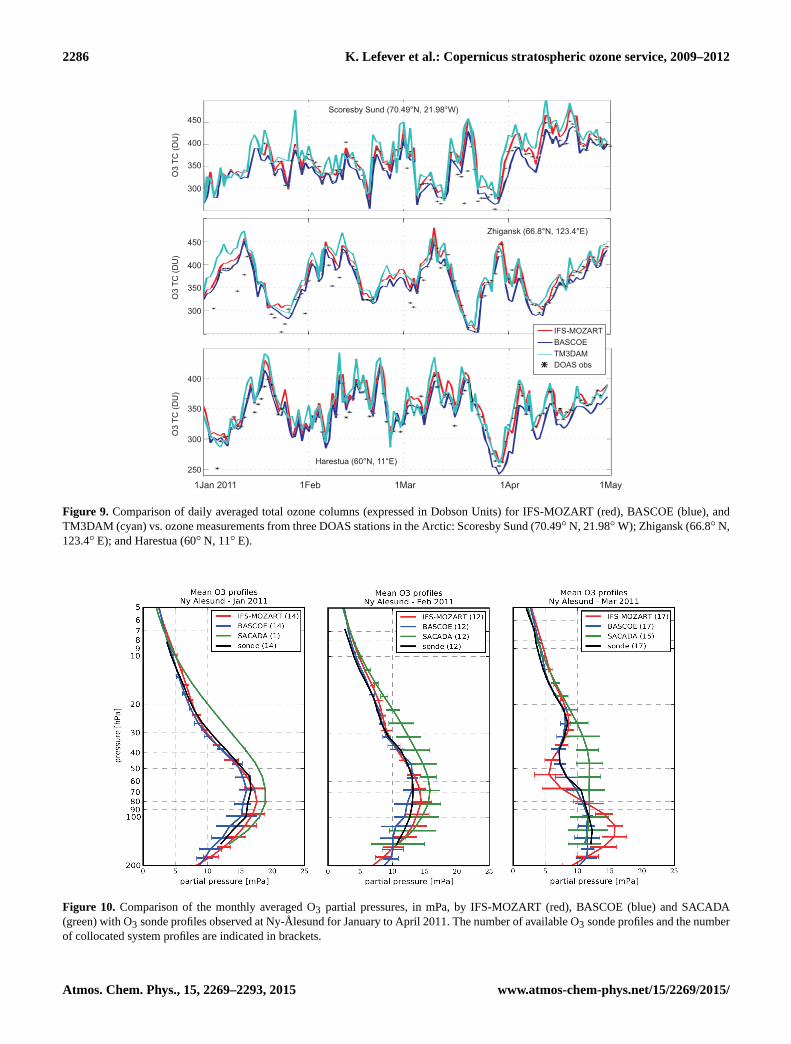
2286 K. Lefever et al.: Copernicus stratospheric ozone service, 2009–2012
Zhigansk (66.8°N, 123.4°E)
IFS-MOZART
BASCOE
TM3DAM
DOAS obs+x
O3 T
C (
DU
)
300
350
450
400
O3 T
C (
DU
)
300
350
400
250Harestua (60°N, 11°E)
O3 T
C (
DU
)
300
350
450
400
Scoresby Sund (70.49°N, 21.98°W)
1Jan 2011 1Feb 1Mar 1Apr 1May
Figure 9. Comparison of daily averaged total ozone columns (expressed in Dobson Units) for IFS-MOZART (red), BASCOE (blue), and
TM3DAM (cyan) vs. ozone measurements from three DOAS stations in the Arctic: Scoresby Sund (70.49◦ N, 21.98◦W); Zhigansk (66.8◦ N,
123.4◦ E); and Harestua (60◦ N, 11◦ E).
Figure 10. Comparison of the monthly averaged O3 partial pressures, in mPa, by IFS-MOZART (red), BASCOE (blue) and SACADA
(green) with O3 sonde profiles observed at Ny-Ålesund for January to April 2011. The number of available O3 sonde profiles and the number
of collocated system profiles are indicated in brackets.
Atmos. Chem. Phys., 15, 2269–2293, 2015 www.atmos-chem-phys.net/15/2269/2015/

K. Lefever et al.: Copernicus stratospheric ozone service, 2009–2012 2287
mean bias (A-O)/O and stddev versus ACE-FTS in Arctic vortex (sPV>1.7e-4) for 20110302-20110325
1200
1000
800
600
400
Th
eta
(K
)
-30 30relative difference (%)
-20 -10 0 10 20 -30 30relative difference (%)
-20 -10 0 10 20
IFS-MOZART NRT
BASCOE
SACADA NRT
IFS-MOZART OFL
BASCOE
SACADA OFL
Figure 11. Mean bias and standard deviations, in %, of the differences between the NRT analyses (left) and the offline experiments (right)
of IFS-MOZART, BASCOE, and SACADA, on the one hand, and ACE-FTS observations, on the other hand, within the North Pole vortex
(vortex edge calculated with an sPV of > 1.7e−4 s−1) for March 2011. The ozone hole level used in Fig. 8 (θ ∼=485 K) is indicated as the
black horizontal line.
Mean bias (A-O)/O (%) versus ozonesondes, March 2011
-60 -40 -20 0 20 40 60relative difference (%)
Antarctic (90°S-60°S) Tropics (30°S-30°N) Arctic (60°N-90°N)
-60 -40 -20 0 20 40 60relative difference (%)
-60 -40 -20 0 20 40 60relative difference (%)
pre
ssure
(hP
a)
Figure 12. Mean biases, in %, of three ozone analyses by IFS-MOZART using O3 sonde profiles as reference, for March 2011. Results are
shown for the Antarctic (left), tropics (centre) and Arctic (right) latitude bands using the IFS-MOZART NRT analyses (red lines), the offline
experiment assimilating only MLS v3 (blue lines) and another offline experiment assimilating MLS v3 and the UV–Vis observations (green
lines). See text for details.
back. IFS-MOZART assimilated only UV–Vis observations
from 26 March 2011 until 10 May 2011, when the assim-
ilation of Aura MLS was switched back on. Unfortunately,
ACE-FTS did not collect any measurements in the Arctic
during April 2011 (see Sect. 2.4.4).
These uncontrolled modifications of the observing system
led us to explore in a more systematic manner the impact of
the assimilated observations on the quality of the analyses.
We chose a 1-month period with the Arctic ozone depletion
already well underway while MLS and ACE-FTS were still
scanning the area, i.e. the month of March 2011. We first de-
fined three new experiments with IFS-MOZART, BASCOE
and SACADA assimilating the same data set: Aura MLS
version 3.3 offline ozone, keeping all observations down to
215 hPa. BASCOE was not allowed to assimilate any other
species than ozone. To allow a short spin-up period of about
1 week, the three systems were started on 25 February from
the BASCOE analysis delivered in NRT for that date.
Figure 11 (left) shows the mean bias and standard devi-
ations of the differences between the NRT (i.e. the origi-
nal) analyses and ACE-FTS observations, keeping only the
(∼ 200) ACE profiles within the North Pole vortex, with
the vortex edge calculated with an sPV of > 1.7e−4 s−1.
At the level where ozone depletion is at its maximum (θ ≈
485 K), we see that the depletion is much too severe in IFS-
MOZART NRT analyses and completely absent in SACADA
NRT analyses. Figure 11 (right) shows the results of the three
www.atmos-chem-phys.net/15/2269/2015/ Atmos. Chem. Phys., 15, 2269–2293, 2015

2288 K. Lefever et al.: Copernicus stratospheric ozone service, 2009–2012
new offline experiments assimilating the same data set; now
all analyses perform very similarly.
To identify the exact cause of the large improvement in
IFS-MOZART analyses, we ran a last sensitivity test with
IFS-MOZART assimilating the usual set of UV–Vis data
(OMI and SCIAMACHY total columns; SBUV/2 partial
columns) in addition to the offline MLS v3 data set. As can be
seen in Fig. 12, the bad performance of IFS-MOZART NRT
was not due to the assimilation of UV–Vis data but rather to
the assimilation of the MLS v2 NRT data. If the MLS v3 and
UV–Vis observations are assimilated together (green curves),
the quality of the ozone analyses delivered by IFS-MOZART
improves: tropospheric ozone is improved over the previous
sensitivity test assimilating only MLS v3 (blue curves), and
the simultaneous assimilation of UV–Vis observations does
not degrade the analysis of stratospheric ozone.
The worse performance of IFS-MOZART NRT is prob-
ably not due to the earlier version of the MLS data set ei-
ther, because our sensitivity test with BASCOE (Fig. 11, blue
lines) shows that the analyses of MLS v2.2 SCI (left) per-
formed nearly as well as the analyses of MLS v3 (right) de-
spite the use of an earlier version of BASCOE. Hence the
better performance of BASCOE NRT is primarily due to
its assimilation of MLS v2.2 SCI down to 150 hPa, while
IFS-MOZART had to assimilate MLS v2.2 NRT, which was
not valid (and filtered out) below 68 hPa. This subtle differ-
ence in configuration is due to an operational constraint: IFS-
MOZART had to be run closer to real-time and could not wait
3 extra days for the distribution of MLS v2.2 SCI.
It is now possible to interpret the slight differences be-
tween the performances of the three systems assimilating the
same MLS data set (Fig. 11, right). The biases and standard
deviations are smallest for IFS-MOZART, probably thanks to
its higher horizontal resolution. The standard deviations for
SACADA are slightly larger than the ones for IFS-MOZART
and BASCOE, which is due to its lower time sampling (24 h
output frequency instead of 6 h for the two other). Finally,
the BASCOE experiment delivers smaller biases and stan-
dard deviations than the original NRT analysis. This may be
due to two different causes: the assimilation of MLS offline
v3.3 instead of MLS offline v2.2, and/or an improvement in
the pre-processing of the ECMWF wind fields that drive the
transport in BASCOE. The BASCOE version used in NRT
suffered from aliasing errors in the input wind fields, lead-
ing to some erroneous noise in the horizontal distribution of
chemical tracers (Fig. 8).
7 Conclusions
Four ozone data assimilation systems (DAS) have been run
continuously and simultaneously since September 2009. We
have validated and compared the resulting analyses over a
period of 3 years, i.e. until September 2012. These DAS have
very different designs (offline or online dynamics; grid setup;
specification of background error covariances) and were set
up very differently with respect to the assimilated data sets.
In this paper we seized this opportunity, first to provide an
intercomparison and validation of the resulting analyses, and
second to investigate the causes of their very different biases.
This study shows what can be achieved in near real time
(NRT) with state-of-the-art DAS for stratospheric ozone and
provides guidance to the users of the resulting analyses.
Among the three sets of vertically resolved NRT analyses
of stratospheric ozone, those delivered by BASCOE had the
best overall quality. This is due primarily to the focus of
BASCOE on stratospheric observations retrieved from limb
sounders, and to more relaxed operational constraints allow-
ing it to wait for the delivery of the best input data set avail-
able.
TM3DAM is based on a sequential Kalman Filter algo-
rithm and does not model stratospheric chemistry explicitly.
It aims only to provide total columns of ozone by making
optimal use of the ozone column measurements from UV–
Vis satellite sounders, with very small biases between the
analyses/forecasts and satellite data sets. It was shown that
TM3DAM is a good reference to test the ability of the three
other systems to produce accurate ozone column amounts.
The low quality of the analyses delivered in NRT by
SACADA is a good indication of the drawbacks to expect
from current CDA systems when they are configured to as-
similate total ozone columns only. This should be considered
as a worst-case scenario in a future situation where no limb
sounder would be available and no proper effort would be in-
vested to assimilate the vertical profiles retrieved from nadir-
looking instruments.
Finally, while IFS-MOZART did not deliver the best NRT
analyses in this intercomparison, it still has the potential to
deliver the best analyses (Figs. 11 and 12). Official reviews
of international monitoring capacities (e.g. WMO, 2011), ex-
pect an imminent lack of ozone-profiling capabilities at high
vertical resolution. Contrarily to the BASCOE version used
here, IFS-MOZART should be able to adapt to this situation
thanks to its demonstrated ability to assimilate several instru-
ments simultaneously.
From a system design point of view, the sensitivity tests
performed in Sect. 6.2 deliver important conclusions:
– All systems used in MACC require profile data to pro-
vide a good vertical distribution of stratospheric ozone.
– These profile data must include the lower stratosphere.
– IFS-MOZART is able to assimilate limb profiles and
nadir products successfully. The profiles constrain well
the stratosphere, allowing the partial and total columns
(from UV–Vis instruments) to constrain well the tropo-
sphere.
– When they assimilate the same data set with good
quality and large observational density, BASCOE, IFS-
Atmos. Chem. Phys., 15, 2269–2293, 2015 www.atmos-chem-phys.net/15/2269/2015/

K. Lefever et al.: Copernicus stratospheric ozone service, 2009–2012 2289
MOZART and SACADA deliver very similar perfor-
mance despite their very different designs. The quality
of modern ozone analyses depends primarily on the as-
similated data. This conclusion has large implications
for the planning of future satellite missions.
The newer SBUV/2 v8.6 profiles are distributed over 21
layers and each profile is distributed with its matrix of aver-
aging kernels. Kramarova et al. (2013) illustrated the impor-
tance of using this information properly. While it is planned
to implement SBUV/2 averaging kernels in the MACC NRT
system at ECMWF, the sensitivity test in Sect. 6.2 shows that
this improvement was not necessary to assimilate success-
fully SBUV/2 v8 after a vertical re-gridding over six thick
layers.
This study demonstrates the large benefit obtained from
the assimilation of a single limb-scanning instrument with
a high density of observations (Aura MLS). Therefore we
can only share the serious concern about the lack of ozone-
profiling capabilities at high vertical resolution in the short
term, as expressed already in WMO (2011).
Acknowledgements. This work was carried out in the framework
of the MACC and MACC II projects. Both projects were funded
under the European Community’s Seventh Research Framework
Programme for research and technological development including
demonstration activities. MACC ran from 1 June 2009 to 31 De-
cember 2011. MACC II ran from 1 November 2011 to 31 July 2014
and was funded under grant agreement CP-CSA 283576. The au-
thors thank the MACC GRG and VAL teams for constructive dis-
cussions.
We thank the O3M SAF project of the EUMETSAT for provid-
ing the GOME-2 ozone product used in this paper. We acknowledge
the EVIVA (Envisat Value Adding for Continuous Monitoring of
Atmospheric Trace Gases and Aerosols) project funded by the Ger-
man Aerospace Center for processing and providing SCIAMACHY
data on behalf of ESA. We also thank NOAA and NASA for grant-
ing access to the other satellite ozone products assimilated in the
MACC systems, as well as the Canadian Space Agency and sci-
ence teams for providing validation observations by ACE-FTS, an
instrument on the Canadian satellite SCISAT-1.
For the use of ground-based Brewer–Dobson, SAOZ/DOAS, and
ozonesonde data, we thank both the individual contributors and the
projects and databases from which they were obtained: the World
Ozone and Ultraviolet Radiation Data Centre (WOUDC, http://
www.woudc.org); the Network for the Detection of Atmospheric
Composition Change (NDACC, http://www.ndsc.ncep.noaa.gov/
data/); and the Southern Hemisphere ADditional OZonesondes net-
work (SHADOZ, http://croc.gsfc.nasa.gov/shadoz/). We thank in
particular the agencies which provided the data that were shown
explicitly as a reference in this paper, i.e. the Meteorological Ser-
vice of Canada, the Central Weather Bureau of Taiwan, the Japan
Meteorological Agency, the Belgian Institute for Space Aeronomy,
the National Centre of Scientific Research of France, the Central
Aeronomy Observatory of Russia, the Danish Meteorological Insti-
tute, the Alfred-Wegener Institute of Potsdam, and MeteoSwiss of
Switzerland.
The comparisons against ozonesondes have been obtained by
means of validation tools developed in the NORS project (Demon-
stration Network Of ground-based Remote Sensing observations in
support of the Copernicus Atmospheric Service, which was funded
by the European Community’s Seventh Research Framework
Programme under grant agreement 284421.
Edited by: W. Lahoz
References
Adams, C., Strong, K., Batchelor, R. L., Bernath, P. F., Brohede,
S., Boone, C., Degenstein, D., Daffer, W. H., Drummond, J. R.,
Fogal, P. F., Farahani, E., Fayt, C., Fraser, A., Goutail, F., Hen-
drick, F., Kolonjari, F., Lindenmaier, R., Manney, G., McElroy,
C. T., McLinden, C. A., Mendonca, J., Park, J.-H., Pavlovic, B.,
Pazmino, A., Roth, C., Savastiouk, V., Walker, K. A., Weaver, D.,
and Zhao, X.: Validation of ACE and OSIRIS ozone and NO2
measurements using ground-based instruments at 80◦ N, Atmos.
Meas. Tech., 5, 927–953, doi:10.5194/amt-5-927-2012, 2012.
Baier, F., Erbertseder, T., Elbern, H., and Schwinger, J.: Impact
of different ozone sounding networks on a 4D-Var stratospheric
data assimilation system, Q. J. Roy. Meteorol. Soc., 139, 2055–
2067, doi:10.1002/qj.2086, 2013.
Balis, D., Kroon, M., Koukouli, M. E., Brinksma, E. J., Labow,
G., Veefkind, J. P., and McPeters, R. D.: Validation of
Ozone Monitoring Instrument total ozone column measure-
ments using Brewer and Dobson spectrophotometer ground-
based observations, J. Geophys. Res.-Atmos., 112, D24S46,
doi:10.1029/2007JD008796, 2007.
Benedetti, A., Morcrette, J.-J., Boucher, O., Dethof, A., Engelen,
R. J., Fisher, M., Flentje, H., Huneeus, N., Jones, L., Kaiser,
J. W., Kinne, S., Mangold, A., Razinger, M., Simmons, A. J.,
and Suttie, M.: Aerosol analysis and forecast in the European
Centre for Medium-Range Weather Forecasts Integrated Fore-
cast System: 2. Data assimilation, J. Geophys. Res.-Atmos., 114,
D13205, doi:10.1029/2008JD011115, 2009.
Bernath, P. F., McElroy, C. T., Abrams, M. C., Boone, C. D., But-
ler, M., Camy-Peyret, C., Carleer, M., Clerbaux, C., Coheur, P.-
F., Colin, R., DeCola, P., De Mazière, M., Drummond, J. R.,
Dufour, D., Evans, W. F. J., Fast, H., Fussen, D., Gilbert, K.,
Jennings, D. E., Llewellyn, E. J., Lowe, R. P., Mahieu, E., Mc-
Connell, J. C., McHugh, M., McLeod, S. D., Michaud, R., Mid-
winter, C., Nassar, R., Nichitiu, F., Nowlan, C., Rinsland, C. P.,
Rochon, Y. J., Rowlands, N., Semeniuk, K., Simon, P., Skel-
ton, R., Sloan, J. J., Soucy, M.-A., Strong, K., Tremblay, P.,
Turnbull, D., Walker, K. A., Walkty, I., Wardle, D. A., Wehrle,
V., Zander, R., and Zou, J.: Atmospheric Chemistry Experiment
(ACE): Mission overview, Geophys. Res. Lett., 32, L15S01,
doi:10.1029/2005GL022386, 2005.
Bhartia, P. K., McPeters, R. D., Flynn, L. E., Taylor, S., Kramarova,
N. A., Frith, S., Fisher, B., and DeLand, M.: Solar Backscatter
UV (SBUV) total ozone and profile algorithm, Atmos. Meas.
Tech., 6, 2533–2548, doi:10.5194/amt-6-2533-2013, 2013.
Boone, C. D., Nassar, R., Walker, K. A., Rochon, Y., McLeod, S. D.,
Rinsland, C. P., and Bernath, P. F.: Retrievals for the atmospheric
chemistry experiment Fourier-transform spectrometer, Appl. Op-
tics IP, 44, 7218–7231, doi:10.1364/AO.44.007218, 2005.
www.atmos-chem-phys.net/15/2269/2015/ Atmos. Chem. Phys., 15, 2269–2293, 2015
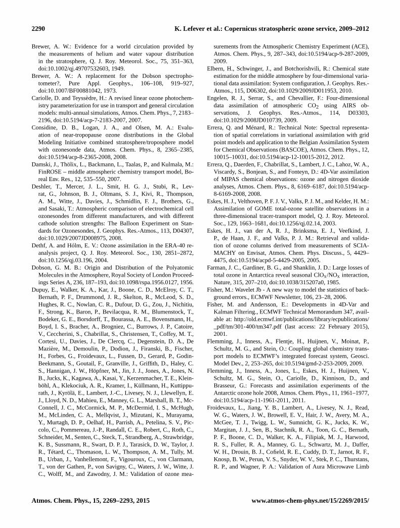
2290 K. Lefever et al.: Copernicus stratospheric ozone service, 2009–2012
Brewer, A. W.: Evidence for a world circulation provided by
the measurements of helium and water vapour distribution
in the stratosphere, Q. J. Roy. Meteorol. Soc., 75, 351–363,
doi:10.1002/qj.49707532603, 1949.
Brewer, A. W.: A replacement for the Dobson spectropho-
tometer?, Pure Appl. Geophys., 106–108, 919–927,
doi:10.1007/BF00881042, 1973.
Cariolle, D. and Teyssèdre, H.: A revised linear ozone photochem-
istry parameterization for use in transport and general circulation
models: multi-annual simulations, Atmos. Chem. Phys., 7, 2183–
2196, doi:10.5194/acp-7-2183-2007, 2007.
Considine, D. B., Logan, J. A., and Olsen, M. A.: Evalu-
ation of near-tropopause ozone distributions in the Global
Modeling Initiative combined stratosphere/troposphere model
with ozonesonde data, Atmos. Chem. Phys., 8, 2365–2385,
doi:10.5194/acp-8-2365-2008, 2008.
Damski, J., Thölix, L., Backmann, L., Taalas, P., and Kulmala, M.:
FinROSE – middle atmospheric chemistry transport model, Bo-
real Env. Res., 12, 535–550, 2007.
Deshler, T., Mercer, J. L., Smit, H. G. J., Stubi, R., Lev-
rat, G., Johnson, B. J., Oltmans, S. J., Kivi, R., Thompson,
A. M., Witte, J., Davies, J., Schmidlin, F. J., Brothers, G.,
and Sasaki, T.: Atmospheric comparison of electrochemical cell
ozonesondes from different manufacturers, and with different
cathode solution strengths: The Balloon Experiment on Stan-
dards for Ozonesondes, J. Geophys. Res.-Atmos., 113, D04307,
doi:10.1029/2007JD008975, 2008.
Dethf, A. and Hólm, E. V.: Ozone assimilation in the ERA-40 re-
analysis project, Q. J. Roy. Meteorol. Soc., 130, 2851–2872,
doi:10.1256/qj.03.196, 2004.
Dobson, G. M. B.: Origin and Distribution of the Polyatomic
Molecules in the Atmosphere, Royal Society of London Proceed-
ings Series A, 236, 187–193, doi:10.1098/rspa.1956.0127, 1956.
Dupuy, E., Walker, K. A., Kar, J., Boone, C. D., McElroy, C. T.,
Bernath, P. F., Drummond, J. R., Skelton, R., McLeod, S. D.,
Hughes, R. C., Nowlan, C. R., Dufour, D. G., Zou, J., Nichitiu,
F., Strong, K., Baron, P., Bevilacqua, R. M., Blumenstock, T.,
Bodeker, G. E., Borsdorff, T., Bourassa, A. E., Bovensmann, H.,
Boyd, I. S., Bracher, A., Brogniez, C., Burrows, J. P., Catoire,
V., Ceccherini, S., Chabrillat, S., Christensen, T., Coffey, M. T.,
Cortesi, U., Davies, J., De Clercq, C., Degenstein, D. A., De
Mazière, M., Demoulin, P., Dodion, J., Firanski, B., Fischer,
H., Forbes, G., Froidevaux, L., Fussen, D., Gerard, P., Godin-
Beekmann, S., Goutail, F., Granville, J., Griffith, D., Haley, C.
S., Hannigan, J. W., Höpfner, M., Jin, J. J., Jones, A., Jones, N.
B., Jucks, K., Kagawa, A., Kasai, Y., Kerzenmacher, T. E., Klein-
böhl, A., Klekociuk, A. R., Kramer, I., Küllmann, H., Kuttippu-
rath, J., Kyrölä, E., Lambert, J.-C., Livesey, N. J., Llewellyn, E.
J., Lloyd, N. D., Mahieu, E., Manney, G. L., Marshall, B. T., Mc-
Connell, J. C., McCormick, M. P., McDermid, I. S., McHugh,
M., McLinden, C. A., Mellqvist, J., Mizutani, K., Murayama,
Y., Murtagh, D. P., Oelhaf, H., Parrish, A., Petelina, S. V., Pic-
colo, C., Pommereau, J.-P., Randall, C. E., Robert, C., Roth, C.,
Schneider, M., Senten, C., Steck, T., Strandberg, A., Strawbridge,
K. B., Sussmann, R., Swart, D. P. J., Tarasick, D. W., Taylor, J.
R., Tétard, C., Thomason, L. W., Thompson, A. M., Tully, M.
B., Urban, J., Vanhellemont, F., Vigouroux, C., von Clarmann,
T., von der Gathen, P., von Savigny, C., Waters, J. W., Witte, J.
C., Wolff, M., and Zawodny, J. M.: Validation of ozone mea-
surements from the Atmospheric Chemistry Experiment (ACE),
Atmos. Chem. Phys., 9, 287–343, doi:10.5194/acp-9-287-2009,
2009.
Elbern, H., Schwinger, J., and Botchorishvili, R.: Chemical state
estimation for the middle atmosphere by four-dimensional varia-
tional data assimilation: System configuration, J. Geophys. Res.-
Atmos., 115, D06302, doi:10.1029/2009JD011953, 2010.
Engelen, R. J., Serrar, S., and Chevallier, F.: Four-dimensional
data assimilation of atmospheric CO2 using AIRS ob-
servations, J. Geophys. Res.-Atmos., 114, D03303,
doi:10.1029/2008JD010739, 2009.
Errera, Q. and Ménard, R.: Technical Note: Spectral representa-
tion of spatial correlations in variational assimilation with grid
point models and application to the Belgian Assimilation System
for Chemical Observations (BASCOE), Atmos. Chem. Phys., 12,
10015–10031, doi:10.5194/acp-12-10015-2012, 2012.
Errera, Q., Daerden, F., Chabrillat, S., Lambert, J. C., Lahoz, W. A.,
Viscardy, S., Bonjean, S., and Fonteyn, D.: 4D-Var assimilation
of MIPAS chemical observations: ozone and nitrogen dioxide
analyses, Atmos. Chem. Phys., 8, 6169–6187, doi:10.5194/acp-
8-6169-2008, 2008.
Eskes, H. J., Velthoven, P. F. J. V., Valks, P. J. M., and Kelder, H. M.:
Assimilation of GOME total-ozone satellite observations in a
three-dimensional tracer-transport model, Q. J. Roy. Meteorol.
Soc., 129, 1663–1681, doi:10.1256/qj.02.14, 2003.
Eskes, H. J., van der A, R. J., Brinksma, E. J., Veefkind, J.
P., de Haan, J. F., and Valks, P. J. M.: Retrieval and valida-
tion of ozone columns derived from measurements of SCIA-
MACHY on Envisat, Atmos. Chem. Phys. Discuss., 5, 4429–
4475, doi:10.5194/acpd-5-4429-2005, 2005.
Farman, J. C., Gardiner, B. G., and Shanklin, J. D.: Large losses of
total ozone in Antarctica reveal seasonal ClOx/NOx interaction,
Nature, 315, 207–210, doi:10.1038/315207a0, 1985.
Fisher, M.: Wavelet Jb - A new way to model the statistics of back-
ground errors., ECMWF Newsletter, 106, 23–28, 2006.
Fisher, M. and Andersson, E.: Developments in 4D-Var and
Kalman Filtering., ECMWF Technical Memorandum 347, avail-
able at: http://old.ecmwf.int/publications/library/ecpublications/
_pdf/tm/301-400/tm347.pdf (last access: 22 February 2015),
2001.
Flemming, J., Inness, A., Flentje, H., Huijnen, V., Moinat, P.,
Schultz, M. G., and Stein, O.: Coupling global chemistry trans-
port models to ECMWF’s integrated forecast system, Geosci.
Model Dev., 2, 253–265, doi:10.5194/gmd-2-253-2009, 2009.
Flemming, J., Inness, A., Jones, L., Eskes, H. J., Huijnen, V.,
Schultz, M. G., Stein, O., Cariolle, D., Kinnison, D., and
Brasseur, G.: Forecasts and assimilation experiments of the
Antarctic ozone hole 2008, Atmos. Chem. Phys., 11, 1961–1977,
doi:10.5194/acp-11-1961-2011, 2011.
Froidevaux, L., Jiang, Y. B., Lambert, A., Livesey, N. J., Read,
W. G., Waters, J. W., Browell, E. V., Hair, J. W., Avery, M. A.,
McGee, T. J., Twigg, L. W., Sumnicht, G. K., Jucks, K. W.,
Margitan, J. J., Sen, B., Stachnik, R. A., Toon, G. C., Bernath,
P. F., Boone, C. D., Walker, K. A., Filipiak, M. J., Harwood,
R. S., Fuller, R. A., Manney, G. L., Schwartz, M. J., Daffer,
W. H., Drouin, B. J., Cofield, R. E., Cuddy, D. T., Jarnot, R. F.,
Knosp, B. W., Perun, V. S., Snyder, W. V., Stek, P. C., Thurstans,
R. P., and Wagner, P. A.: Validation of Aura Microwave Limb
Atmos. Chem. Phys., 15, 2269–2293, 2015 www.atmos-chem-phys.net/15/2269/2015/
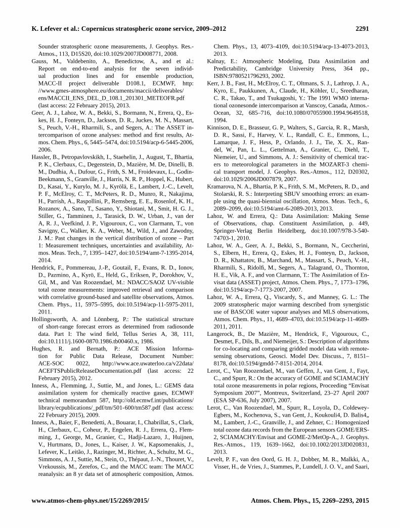
K. Lefever et al.: Copernicus stratospheric ozone service, 2009–2012 2291
Sounder stratospheric ozone measurements, J. Geophys. Res.-
Atmos., 113, D15S20, doi:10.1029/2007JD008771, 2008.
Gauss, M., Valdebenito, A., Benedictow, A., and et al.:
Report on end-to-end analysis for the seven individ-
ual production lines and for ensemble production,
MACC-II project deliverable D108.1, ECMWF, http:
//www.gmes-atmosphere.eu/documents/maccii/deliverables/
ens/MACCII_ENS_DEL_D_108.1_201301_METEOFR.pdf
(last access: 22 February 2015), 2013.
Geer, A. J., Lahoz, W. A., Bekki, S., Bormann, N., Errera, Q., Es-
kes, H. J., Fonteyn, D., Jackson, D. R., Juckes, M. N., Massart,
S., Peuch, V.-H., Rharmili, S., and Segers, A.: The ASSET in-
tercomparison of ozone analyses: method and first results, At-
mos. Chem. Phys., 6, 5445–5474, doi:10.5194/acp-6-5445-2006,
2006.
Hassler, B., Petropavlovskikh, I., Staehelin, J., August, T., Bhartia,
P. K., Clerbaux, C., Degenstein, D., Mazière, M. De, Dinelli, B.
M., Dudhia, A., Dufour, G., Frith, S. M., Froidevaux, L., Godin-
Beekmann, S., Granville, J., Harris, N. R. P., Hoppel, K., Hubert,
D., Kasai, Y., Kurylo, M. J., Kyrölä, E., Lambert, J.-C., Levelt,
P. F., McElroy, C. T., McPeters, R. D., Munro, R., Nakajima,
H., Parrish, A., Raspollini, P., Remsberg, E. E., Rosenlof, K. H.,
Rozanov, A., Sano, T., Sasano, Y., Shiotani, M., Smit, H. G. J.,
Stiller, G., Tamminen, J., Tarasick, D. W., Urban, J., van der
A, R. J., Veefkind, J. P., Vigouroux, C., von Clarmann, T., von
Savigny, C., Walker, K. A., Weber, M., Wild, J., and Zawodny,
J. M.: Past changes in the vertical distribution of ozone – Part
1: Measurement techniques, uncertainties and availability, At-
mos. Meas. Tech., 7, 1395–1427, doi:10.5194/amt-7-1395-2014,
2014.
Hendrick, F., Pommereau, J.-P., Goutail, F., Evans, R. D., Ionov,
D., Pazmino, A., Kyrö, E., Held, G., Eriksen, P., Dorokhov, V.,
Gil, M., and Van Roozendael, M.: NDACC/SAOZ UV-visible
total ozone measurements: improved retrieval and comparison
with correlative ground-based and satellite observations, Atmos.
Chem. Phys., 11, 5975–5995, doi:10.5194/acp-11-5975-2011,
2011.
Hollingsworth, A. and Lönnberg, P.: The statistical structure
of short-range forecast errors as determined from radiosonde
data. Part I: The wind field, Tellus Series A, 38, 111,
doi:10.1111/j.1600-0870.1986.tb00460.x, 1986.
Hughes, R. and Bernath, P.: ACE Mission Informa-
tion for Public Data Release, Document Number:
ACE-SOC 0022, http://www.ace.uwaterloo.ca/v22data/
ACEFTSPublicReleaseDocumentation.pdf (last access: 22
February 2015), 2012.
Inness, A., Flemming, J., Suttie, M., and Jones, L.: GEMS data
assimilation system for chemically reactive gases, ECMWF
technical memorandum 587, http://old.ecmwf.int/publications/
library/ecpublications/_pdf/tm/501-600/tm587.pdf (last access:
22 February 2015), 2009.
Inness, A., Baier, F., Benedetti, A., Bouarar, I., Chabrillat, S., Clark,
H., Clerbaux, C., Coheur, P., Engelen, R. J., Errera, Q., Flem-
ming, J., George, M., Granier, C., Hadji-Lazaro, J., Huijnen,
V., Hurtmans, D., Jones, L., Kaiser, J. W., Kapsomenakis, J.,
Lefever, K., Leitão, J., Razinger, M., Richter, A., Schultz, M. G.,
Simmons, A. J., Suttie, M., Stein, O., Thépaut, J.-N., Thouret, V.,
Vrekoussis, M., Zerefos, C., and the MACC team: The MACC
reanalysis: an 8 yr data set of atmospheric composition, Atmos.
Chem. Phys., 13, 4073–4109, doi:10.5194/acp-13-4073-2013,
2013.
Kalnay, E.: Atmospheric Modeling, Data Assimilation and
Predictability, Cambridge University Press, 364 pp.,
ISBN:9780521796293, 2002.
Kerr, J. B., Fast, H., McElroy, C. T., Oltmans, S. J., Lathrop, J. A.,
Kyro, E., Paukkunen, A., Claude, H., Köhler, U., Sreedharan,
C. R., Takao, T., and Tsukagoshi, Y.: The 1991 WMO interna-
tional ozonesonde intercomparison at Vanscoy, Canada, Atmos.-
Ocean, 32, 685–716, doi:10.1080/07055900.1994.9649518,
1994.
Kinnison, D. E., Brasseur, G. P., Walters, S., Garcia, R. R., Marsh,
D. R., Sassi, F., Harvey, V. L., Randall, C. E., Emmons, L.,
Lamarque, J. F., Hess, P., Orlando, J. J., Tie, X. X., Ran-
del, W., Pan, L. L., Gettelman, A., Granier, C., Diehl, T.,
Niemeier, U., and Simmons, A. J.: Sensitivity of chemical trac-
ers to meteorological parameters in the MOZART-3 chemi-
cal transport model, J. Geophys. Res.-Atmos., 112, D20302,
doi:10.1029/2006JD007879, 2007.
Kramarova, N. A., Bhartia, P. K., Frith, S. M., McPeters, R. D., and
Stolarski, R. S.: Interpreting SBUV smoothing errors: an exam-
ple using the quasi-biennial oscillation, Atmos. Meas. Tech., 6,
2089–2099, doi:10.5194/amt-6-2089-2013, 2013.
Lahoz, W. and Errera, Q.: Data Assimilation: Making Sense
of Observations, chap. Constituent Assimilation, p. 449,
Springer-Verlag Berlin Heidelberg, doi:10.1007/978-3-540-
74703-1, 2010.
Lahoz, W. A., Geer, A. J., Bekki, S., Bormann, N., Ceccherini,
S., Elbern, H., Errera, Q., Eskes, H. J., Fonteyn, D., Jackson,
D. R., Khattatov, B., Marchand, M., Massart, S., Peuch, V.-H.,
Rharmili, S., Ridolfi, M., Segers, A., Talagrand, O., Thornton,
H. E., Vik, A. F., and von Clarmann, T.: The Assimilation of En-
visat data (ASSET) project, Atmos. Chem. Phys., 7, 1773–1796,
doi:10.5194/acp-7-1773-2007, 2007.
Lahoz, W. A., Errera, Q., Viscardy, S., and Manney, G. L.: The
2009 stratospheric major warming described from synergistic
use of BASCOE water vapour analyses and MLS observations,
Atmos. Chem. Phys., 11, 4689–4703, doi:10.5194/acp-11-4689-
2011, 2011.
Langerock, B., De Mazière, M., Hendrick, F., Vigouroux, C.,
Desmet, F., Dils, B., and Niemeijer, S.: Description of algorithms
for co-locating and comparing gridded model data with remote-
sensing observations, Geosci. Model Dev. Discuss., 7, 8151–
8178, doi:10.5194/gmdd-7-8151-2014, 2014.
Lerot, C., Van Roozendael, M., van Geffen, J., van Gent, J., Fayt,
C., and Spurr, R.: On the accuracy of GOME and SCIAMACHY
total ozone measurements in polar regions, Proceeding “Envisat
Symposium 2007”, Montreux, Switzerland, 23–27 April 2007
(ESA SP-636, July 2007), 2007.
Lerot, C., Van Roozendael, M., Spurr, R., Loyola, D., Coldewey-
Egbers, M., Kochenova, S., van Gent, J., Koukouli4, D. Balis4„
M., Lambert, J.-C., Granville, J., and Zehner, C.: Homogenized
total ozone data records from the European sensors GOME/ERS-
2, SCIAMACHY/Envisat and GOME-2/MetOp-A., J. Geophys.
Res.-Atmos., 119, 1639–1662, doi:10.1002/2013JD020831,
2013.
Levelt, P. F., van den Oord, G. H. J., Dobber, M. R., Malkki, A.,
Visser, H., de Vries, J., Stammes, P., Lundell, J. O. V., and Saari,
www.atmos-chem-phys.net/15/2269/2015/ Atmos. Chem. Phys., 15, 2269–2293, 2015

2292 K. Lefever et al.: Copernicus stratospheric ozone service, 2009–2012
H.: The Ozone Monitoring Instrument, IEEE T. Geosci. Remote,
44, 1093–1101, doi:10.1109/TGRS.2006.872333, 2006.
Lin, S. J. and Rood, R. B.: A fast flux form semi-Lagrangian trans-
port scheme on the sphere, Mon. Weather Rev., 124, 2046–2070,
1996.
Lindenmaier, R., Strong, K., Batchelor, R. L., Bernath, P. F.,
Chabrillat, S., Chipperfield, M. P., Daffer, W. H., Drummond,
J. R., Feng, W., Jonsson, A. I., Kolonjari, F., Manney, G. L.,
McLinden, C., Ménard, R., and Walker, K. A.: A study of the
Arctic NOy budget above Eureka, Canada, J. Geophys. Res.-
Atmos., 116, D23302, doi:10.1029/2011JD016207, 2011.
Livesey, N. J., van Snyder, W., Read, W. G., and Wagner,
P. A.: Retrieval Algorithms for the EOS Microwave Limb
Sounder (MLS), IEEE T. Geosci. Remote, 44, 1144–1155,
doi:10.1109/TGRS.2006.872327, 2006.
Livesey, N. J., Read, W., Lambert, A., Cofield, R., Cuddy, D.,
Froidevaux, L., Fuller, R., Jarnot, R., Jiang, J., Jiang, Y., Knosp,
B., Kovalenko, L., Pickett, H., Pumphrey, H., Santee, M.,
Schwartz, M., Stek, P., Wagner, P., Waters, J., and Wu, D.: Earth
Observing System (EOS) Aura Microwave Limb Sounder (MLS)
Version 2.2 and 2.3 Level 2 data quality and description docu-
ment, Tech. rep., Jet Propulsion Laboratory, http://mls.jpl.nasa.
gov/data/v2_data_quality_document.pdf (last access: 22 Febru-
ary 2015), 2013a.
Livesey, N. J., Read, W. G., Froidevaux, L., Lambert, A., Manney,
G. L., Pumphrey, H. C., Santee, M. L., Schwartz, M. J., Wang,
S., Cofield, R. E., Cuddy, D. T., Fuller, R. A., Jarnot, R. F., Jiang,
J. H., Knosp, B. W., Stek, P. C., Wagner, P. A., and Wu, D. L.:
Earth Observing System (EOS) Aura Microwave Limb Sounder
(MLS) Version 3.3 and 3.4 Level 2 data quality and description
document, Tech. rep., Jet Propulsion Laboratory, http://mls.jpl.
nasa.gov/data/v3-3_data_quality_document.pdf (last access: 22
February 2015), 2013b.
Lorenc, A. C.: Analysis methods for numerical weather
prediction, Q. J. Roy. Meteorol. Soc., 112, 1177–1194,
doi:10.1002/qj.49711247414, 1986.
Loyola, D. G., Koukouli, M. E., Valks, P., Balis, D. S., Hao, N., van
Roozendael, M., Spurr, R. J. D., Zimmer, W., Kiemle, S., Lerot,
C., and Lambert, J.-C.: The GOME-2 total column ozone prod-
uct: Retrieval algorithm and ground-based validation, J. Geo-
phys. Res.-Atmos., 116, D07302, doi:10.1029/2010JD014675,
2011.
Majewski, D., Liermann, D., Prohl, P., Ritter, B., Buchhold, M.,
Hanisch, T., Paul, G., Wergen, W., and Baumgardner, J.: The
operational global icosahedral-hexagonal gridpoint model GME:
Description and high resolution tests, Mon. Weather Rev., 130,
319–338, doi:10.1029/1998GL900152, 2001.
Manney, G. L., Santee, M. L., Rex, M., Livesey, N. J., Pitts, M. C.,
Veefkind, P., Nash, E. R., Wohltmann, I., Lehmann, R., Froide-
vaux, L., Poole, L. R., Schoeberl, M. R., Haffner, D. P., Davies,
J., Dorokhov, V., Gernandt, H., Johnson, B., Kivi, R., Kyrö, E.,
Larsen, N., Levelt, P. F., Makshtas, A., McElroy, C. T., Nakajima,
H., Parrondo, M. C., Tarasick, D. W., von der Gathen, P., Walker,
K. A., and Zinoviev, N. S.: Unprecedented Arctic ozone loss in
2011, Nature, 478, 469–475, doi:10.1038/nature10556, 2011.
McPeters, R. D., Bhartia, P. K., Haffner, D., Labow, G. J.,
and Flynn, L.: The version 8.6 SBUV ozone data record:
An overview, J. Geophys. Res.-Atmos., 118, 8032–8039,
doi:10.1002/jgrd.50597, 2013.
Morcrette, J.-J., Boucher, O., Jones, L., Salmond, D., Bechtold, P.,
Beljaars, A., Benedetti, A., Bonet, A., Kaiser, J. W., Razinger,
M., Schulz, M., Serrar, S., Simmons, A. J., Sofiev, M., Suttie, M.,
Tompkins, A. M., and Untch, A.: Aerosol analysis and forecast
in the European Centre for Medium-Range Weather Forecasts In-
tegrated Forecast System: Forward modeling, J. Geophys. Res.-
Atmos., 114, D06206, doi:10.1029/2008JD011235, 2009.
Munro, R., Anderson, C., and Callies, J. e. a.: GOME-2 on
MetOp, in: Atmospheric Science Conference, vol. 628 of ESA
Special Publication, http://earth.esa.int/workshops/atmos2006/
participants/35/paper_Munro_Day5_GOME-2_on_MetOp_
Paper.pdf (last access: 22 February 2015), 2006.
Peuch, V.-H., Engelen, R., Simmons, A., Lahoz, W., Laj, P., and
Galmarini, S. (Eds.): Monitoring atmospheric composition and
climate, research in support of the Copernicus/GMES atmo-
spheric service, Special Issue, Atmos. Chem. Phys., http://www.
atmos-chem-phys.net/special_issue310.html, 2014.
Pommereau, J. P. and Goutail, F.: O3 and NO2 ground-based
measurements by visible spectrometry during Arctic win-
ter and spring 1988, Geophys. Res. Lett., 15, 891–894,
doi:10.1029/GL015i008p00891, 1988.
Prather, M. J.: Numerical advection by conservation of
second-order moments, J. Geophy. Res., 91, 6671–6681,
doi:10.1029/JD091iD06p06671, 1986.
Redler, R., Valcke, S., and Ritzdorf, H.: OASIS4 – a coupling soft-
ware for next generation earth system modelling, Geosci. Model
Dev., 3, 87–104, doi:10.5194/gmd-3-87-2010, 2010.
Robichaud, A., Ménard, R., Chabrillat, S., de Grandpré, J., Rochon,
Y. J., Yang, Y., and Charette, C.: Impact of energetic particle
precipitation on stratospheric polar constituents: an assessment
using monitoring and assimilation of operational MIPAS data,
Atmos. Chem. Phys., 10, 1739–1757, doi:10.5194/acp-10-1739-
2010, 2010.
Rood, R. B., Allen, D. J., Baker, W. E., Lamich, D. J., and
Kaye, J. A.: The Use of Assimilated Stratospheric Data in
Constituent Transport Calculations, J. Atmos. Sci., 46, 687–702,
doi:10.1175/1520-0469(1989)046<0687:TUOASD>2.0.CO;2,
1989.
Sagi, K., Murtagh, D., Urban, J., Sagawa, H., and Kasai, Y.: The
use of SMILES data to study ozone loss in the Arctic win-
ter 2009/2010 and comparison with Odin/SMR data using as-
similation techniques, Atmos. Chem. Phys., 14, 12855–12869,
doi:10.5194/acp-14-12855-2014, 2014.
Sander, S. P., Golden, D. M., and Kurylo, M. J., e. a.: Chemical Ki-
netics and Photochemical Data for Use in Atmospheric Studies,
Evaluation Number 15, JPL Publication 02-25, Jet Propulsion
Laboratory, Pasadena, CA, USA, http://jpldataeval.jpl.nasa.gov/
pdf/JPL_15_AllInOne.pdf (last access: 22 February 2015), 2006.
Scarnato, B., Staehelin, J., Peter, T., GröBner, J., and Stübi, R.:
Temperature and slant path effects in Dobson and Brewer to-
tal ozone measurements, J. Geophys. Res.-Atmos., 114, D24303,
doi:10.1029/2009JD012349, 2009.
Schoeberl, M. R., Douglass, A. R., Hilsenrath, E., Bhartia, P. K.,
Beer, R., Waters, J. W., Gunson, M. R., Froidevaux, L., Gille,
J. C., Barnett, J. J., Levelt, P. F., and de Cola, P.: Overview of
the EOS Aura Mission, IEEE T. Geosci.Remote, 44, 1066–1074,
doi:10.1109/TGRS.2005.861950, 2006.
Schwinger, J. and Elbern, H.: Chemical state estimation for
the middle atmosphere by four-dimensional variational data
Atmos. Chem. Phys., 15, 2269–2293, 2015 www.atmos-chem-phys.net/15/2269/2015/

K. Lefever et al.: Copernicus stratospheric ozone service, 2009–2012 2293
assimilation: a posteriori validation of error statistics in
observation space, J. Geophys. Res.-Atmos., 115, D18307,
doi:10.1029/2009JD013115, 2010.
Smit, H. G. J., Sträter, W., Helten, M., Kley, D., Ciupa, D., Claude,
H., Köhler, U., Hoegger, B., Levrat, G., Johnson, B., Oltmans,
S. J., Kerr, J. B., Tarasick, D. W., Davies, J., Shitamichi, M.,
Srivastav, S. K., and Vialle, C.: JOSIE: The 1996 WMO in-
ternational intercomparison of ozonesondes under quasi-flight
conditions in the environmental chamber at Jülich, in Atmo-
spheric Ozone, Proceedings of the Quadrennial O3 Symposium,
l’Aquila, Italy, 971–974, 1996.
Smit, H. G. J., Straeter, W., Johnson, B. J., Oltmans, S. J., Davies,
J., Tarasick, D. W., Hoegger, B., Stubi, R., Schmidlin, F. J.,
Northam, T., Thompson, A. M., Witte, J. C., Boyd, I., and Posny,
F.: Assessment of the performance of ECC-ozonesondes under
quasi-flight conditions in the environmental simulation cham-
ber: Insights from the Juelich Ozone Sonde Intercomparison
Experiment (JOSIE), J. Geophys. Res.-Atmos., 112, D19306,
doi:10.1029/2006JD007308, 2007.
Solomon, S.: Stratospheric ozone depletion: a review of concepts
and history, Rev. Geophys., 37, 275–316, 1999.
Solomon, S., Portmann, R. W., Sasaki, T., Hofmann, D. J., and
Thompson, D. W. J.: Four decades of ozonesonde measure-
ments over Antarctica, J. Geophys. Res.-Atmos., 110, D21311,
doi:10.1029/2005JD005917, 2005.
Stein, O., Flemming, J., Inness, A., Kaiser, J., and Schultz,
M.: Global reactive gases forecasts and reanalysis in
the MACC project, J. Integr. Environ. Sci., 9, 57–70,
doi:10.1080/1943815X.2012.696545, 2012.
Stein, O., Huijnen, V., and Flemming, J.: Model descrip-
tion of the IFS-MOZART and IFS-TM5 coupled sys-
tems, MACC-II project deliverable D55.4, ECMWF, http:
//www.gmes-atmosphere.eu/documents/maccii/deliverables/grg/
MACCII_GRG_DEL_D_55.4_IFS-MOZART_and_TM5.pdf
(last access: 22 February 2015), 2013.
Stübi, R., Levrat, G., Hoegger, B., Viatte, P., Staehelin, J., and
Schmidlin, F. J.: In-flight comparison of Brewer-Mast and elec-
trochemical concentration cell ozonesondes, J. Geophys. Res.-
Atmos., 113, D13302, doi:10.1029/2007JD009091, 2008.
van der A, R. J., Allaart, M. A. F., and Eskes, H. J.: Multi sensor re-
analysis of total ozone, Atmos. Chem. Phys., 10, 11277–11294,
doi:10.5194/acp-10-11277-2010, 2010.
van Roozendael, M., Hermans, C., Kabbadj, Y., Lambert, J.-C.,
Vandaele, A.-C., Simon, P. C., Carleer, M., Guilmot, J.-M.,
and Colin, R. : Ground-based measurements of stratospheric
OCIO, NO2 and O3 at Harestua, Norway (60◦N, 10◦E) during
SESAME, European rocket and balloon programmes and related
research, 370, 305, 1995.
Van Roozendael, M., Peeters, P., Roscoe, H. K., De Backer, H.,
Jones, A. E., Bartlett, L., Vaughan, G., Goutail, F., Pommereau,
J.-P., Kyro, E., Wahlstrom, C., Braathen„ G., and Simon, P. C.:
Validation of Ground-Based Visible Measurements of Total
Ozone by Comparison with Dobson and Brewer Spectropho-
tometers, J. Atmos. Chem., 29, 55–83, 1998.
van Roozendael, M., Loyola, D., Spurr, R., Balis, D., Lambert,
J.-C., Livschitz, Y., Valks, P., Ruppert, T., Kenter, P., Fayt, C.,
and Zehner, C.: Ten years of GOME/ERS-2 total ozone data
- The new GOME data processor (GDP) version 4: 1. Al-
gorithm description, J. Geophys. Res.-Atmos., 111, D14311,
doi:10.1029/2005JD006375, 2006.
Viscardy, S., Errera, Q., Christophe, Y., Chabrillat, S., and Lambert,
J.-C.: Evaluation of ozone analyses from UARS MLS assimila-
tion by BASCOE between 1992 and 1997, JSTARS 3, 190–202,
2010.
von Bargen, A., Schröder, T., Kretschel, K., Hess, M., Lerot, C.,
Van Roozendael, M., Vountas, M., Kokhanovsky, A., Lotz, W.,
and H., B.: Operational SCIAMACHY Level 1B-2 Off-line pro-
cessor: total vertical columns for O3 and NO2 and cloud prod-
ucts., Proceeding Envisat Symposium 2007, Montreux, Switzer-
land, 23–27 April 2007 (ESA SP-636, July 2007), 2007.
Waters, J. W., Froidevaux, L., Harwood, R. S., Jarnot, R. F., Pick-
ett, H. M., Read, W. G., Siegel, P. H., Cofield, R. E., Filipiak,
M. J., Flower, D. A., Holden, J. R., Lau, G. K., Livesey, N. J.,
Manney, G. L., Pumphrey, H. C., Santee, M. L., Wu, D. L.,
Cuddy, D. T., Lay, R. R., Loo, M. S., Perun, V. S., Schwartz,
M. J., Stek, P. C., Thurstans, R. P., Boyles, M. A., Chandra,
K. M., Chavez, M. C., Chen, G.-S., Chudasama, B. V., Dodge,
R., Fuller, R. A., Girard, M. A., Jiang, J. H., Jiang, Y., Knosp,
B. W., Labelle, R. C., Lam, J. C., Lee, A. K., Miller, D., Oswald,
J. E., Patel, N. C., Pukala, D. M., Quintero, O., Scaff, D. M.,
Vansnyder, W., Tope, M. C., Wagner, P. A., and Walch, M. J.: The
Earth Observing System Microwave Limb Sounder (EOS MLS)
on the Aura Satellite, IEEE T. Geosci. Remote, 44, 1075–1092,
doi:10.1109/TGRS.2006.873771, 2006.
Weaver, A. and Courtier, P.: Correlation modelling on the sphere
using a generalized diffusion equation, Q. J. Roy. Meteorol. Soc.,
127, 1815–1846, 2001.
Weber, M., Dikty, S., Burrows, J. P., Garny, H., Dameris, M., Ku-
bin, A., Abalichin, J., and Langematz, U.: The Brewer-Dobson
circulation and total ozone from seasonal to decadal time scales,
Atmos. Chem. Phys., 11, 11221–11235, doi:10.5194/acp-11-
11221-2011, 2011.
WMO: WMO/UNEP Report of the 8th ORM (Ozone Research
Managers) Meeting of the Parties to the Vienna Convention for
the Protection of the Ozone Layer (Geneva, Switzerland, 2–4
May 2011), http://ozone.unep.org/new_site/en/Treaties/treaties_
decisions-hb.php?dec_id=1003 (last access: 22 February 2015),
2011.
www.atmos-chem-phys.net/15/2269/2015/ Atmos. Chem. Phys., 15, 2269–2293, 2015
Copyright © 2022 FDOKUMEN