Coordination in cobweb experiments with(out) elicited beliefs

This version: April 2004

Angela Sutana*, Marc Willingerb

Abstract. We address empirically the rational expectations hypothesis implication of perfect coordination in beliefs in simple environments. Early experiments on the "guessing game" (Nagel, 1995) suggested that subjects' beliefs are poorly coordinated. In contrast, in a market environment where subjects choose output levels, our results show that decisions are strongly correlated, although not necessarily on the equilibrium price level. Our experimental design relies on a linear cobweb model for which the equilibrium can be obtained through eductive reasoning, i.e. iterated elimination of dominated strategies (Guesnerie (1992)). We manipulate two treatment variables : the "speed" of convergence and belief elicitation. We compare sessions with and without belief elicitation to test whether explicit belief elicitation favours the type of (eductive) reasonin underlying the convergence process towards equilibrium. Our data does not support the hypothesis that belief elicitation favours the coordination of subjects’ decisions. However, in all sessions, even for those where divergence was predicted, we observe strong coordination on a price level that is slightly above the rational expectation equilibrium price.

Keywords: beliefs elicitation, coordination, price forecasts, cobweb model, eductive learning

JEL Classification: C72, C92, D84

a BETA-Theme, Université Louis Pasteur, Strasbourg b LAMETA, Université Montpellier 1, Montpellier * corresponding author: BETA-Theme, bureau 154, PEGE, 61, avenue de la Forêt Noire, 67000 Strasbourg, France, tél. 03.90.24.20.92, fax. 03.90.24.20.71 sutan@cournot.u-strasbg.fr

1.Introduction

According to the rational expectations hypothesis, the assumption of rational behaviour can be

extended to the formation of beliefs (Muth, 1961). On average, agents make correct forecasts

because it is in their own best interest to act in this way. In equilibrium, all agents hold

exactly the same expectations, i.e. expectations are perfectly coordinated beliefs. This

hypothesis relies on two fundamental principles : Bayesian rationality and common

knowledge of rationality. The implication is that agents are induced to take actions whose

aggregated outcome matches exactly their expectations.

While the underlying reasoning sustaining this type of equilibrium is well known, it remains

an empirical issue to know whether agents are able to coordinate their beliefs and take actions

that exactly confirm their beliefs. For example, does learning through repeated market

interactions orient belief formation in the direction of a common expectation ? Do

coordination failures lead to an updating of the process of belief formation which favours

coordination ?

In this paper we present preliminary results of experiments whose objective is to investigate

belief formation and learning in a dynamic market. These experiments were led in the

simplest dynamic market model, the cobweb model. The cobweb model predicts price

adjustments in a market of a non-storable good. Output decisions must be made one period

before the production is sold on the market. Therefore, upon making their production plan,

producers must anticipate the price at which their output will be sold. Ex post, the selling

price is determined according to the demand schedule and the aggregated output.

The Rational Expectation (RE) hypothesis assumes that agents form their beliefs by relying

on all available information. Furthermore, they know perfectly the market equilibrium

equations. Two different justifications of the RE hypothesis are generally put forward : we

call them hereafter adaptive and eductive justification respectively. The adaptative

justification relies on the repeated interaction among agents and on the induced learning

possibilities : in feedback learning a myopic best-reply guides the agents’ behaviour towards

the rational expectation outcome. The eductive justification relies on an individual mental

process : reasoning about the logic of the situation ("forecasting the forecasts of others",

2

Binmore, 1987), leads rational agents to eliminate dominated outcomes. This paper is

primarily motivated by investigating the predictions of the eductive justification. In the linear

cobweb model (Guesnerie, 1992) eductive reasoning leads, through the iterated elimination of

dominated strategies (the "tâtonnement" of the cobweb in notional time), to the convergence

(divergence) towards the equilibrium price.

Price adjustment in the linear cobweb model through eductive learning

To be more precise, let us describe the price adjustment process in the linear cobweb model.

Let the marginal cost of each producer be given by MC(q) = q/c+d. Thus the total cost

function is given by the quadratic form C(q) = q²/2c+dq. We assume that there is a finite

number n of identical producers on the market. Furthermore we assume that producers are

"small" with respect to the size of the market. Aggregate supply is thus given by S(p) = C(p-

d), with C = nc. Assume that aggregate demand is a linear function D(p) = A – Bp if A- Bp >

0, and 0 if not, with A, B > 0. The Rational Expectation Equilibrium (REE) is reached when

the price p is equal to the marginal cost.

At the beginning of each period producers choose their output level and at the end of the

period all units produced must be sold at the prevailing market price. The equilibrium price

can be reached through eductive reasoning if the condition B > C is met, i.e. the slope of the

demand function is greater (in absolute value) than the slope of the supply function. The price

adjustment process towards the equilibrium price p* underlying eductive reasoning is

illustrated in figure 1. Let us describe the eductive learning process for this specification of

the cobweb model.

(i) Step 1 : At notional time t = 0, each producer knows that the maximum possible

market price is po=A/B. For larger prices, the aggregate demand is null. Therefore

aggregate supply cannot exceed qo in order to be sold at a strictly positive price.

This leads to the "elimination" of any aggregate output level larger than qo.

(ii) Step 2 : at the maximum aggregate output level qo, since all production is sold on

the market, it is common knowledge that the minimum selling price is equal to p1.

3

If the selling price is at least equal to p1 aggregate supply is at least q1. Therefore

any aggregate output level below q1 can be eliminated1 .

(iii) Step 3 : If total output were equal to q1, it would be common knowledge that it

would be sold at price p2. But at that price level producers would like to supply an

aggregate output level not larger than q2. Therefore any output level above q2 can

be eliminated2.

(iv) Step 4 : output levels below q3 are eliminated

………….

p2

q1

q2 q3

p1

q0

p0 p*

A

D,S

p

Figure 1: Convergence in the cobweb model when the slope of the

demand function is larger than the slope of the supply function (B>C)

The process of iterative elimination of aggregate output levels narrows down the set of

possible output levels until the equilibrium price p* is reached3. At price p* only one output

1

01 pBC

BCdAp −

+=

2

+−

+= 0

2

2 1 pBC

BC

BCdAp

3 o

nn

nn

n pBC

BCdA

BC

BC

BCdAp

−×

++

+

−−

×+

= )1(1

)1(1, =nn

p∞→

limCB

CdA++ = p*( when B>C)

4

level is possible, and since all producers are identical, they all produce the same fraction of

total output.

A direct test of the eductive reasoning hypothesis seems out of reach, since the underlying

iterative elimination process is conducted in notional time. Our aim is therefore less ambitious

since we only try to test the predictions of the eductive reasoning hypothesis on the basis of a

simple cobweb market experiment. In particular, we are interested in the prediction that

agents are able to coordinate their beliefs on a common price expectation. Experimental

observations in the "guessing game" (Nagel,1995), whose beliefs structure is isomorphic to

the cobweb model, seem to show that experimental subjects are able to coordinate only partly

on a common expectation. Furthermore, the "depth" of eductive reasoning seems to seldom

exceed degree 2.

Beliefs elicitation

In the "guessing game", a subject's task is to guess a number implying that his expectation

coincides with his decision. Expectations are therefore observable in guessing games. In

contrast, in cobweb market experiments subjects have to make output decisions, based on

their beliefs about the market price. In the standard experiment, the subject's price

expectations are therefore not observable. To make an inference about the unobserved

expectation requires an assumption relating beliefs to output decisions. Furthermore, it is not

obvious whether the subject's mental process leading to their output decision is based on a

price expectation.

In order to understand how they take into account their beliefs and how these beliefs evolve

with experience, we elicited subject's beliefs in the experiment. Belief elicitation has several

advantages : it allows us to test whether output decisions are correlated with beliefs, we can

study how beliefs are updated with previous market experience, and finally we can investigate

our main question whether subjects are able to coordinate on a common price expectation. On

the other hand, elicitation focuses the subject's attention on a particular process of reasoning

for taking their output decision, which may favour coordination of beliefs. Our hypothesis is

therefore that belief elicitation facilitates coordination on a common expectation. In order to

test this assumption, we compare sessions with belief elicitation to sessions without.

5

Speed of convergence

Our second treatment variable is the speed of convergence. In the linear cobweb model, the

eductive reasoning hypothesis implies an infinite number of steps. If the demand and supply

schedules are step functions, the equilibrium is necessarily reached in a finite number of steps.

Although the eductive reasoning is the same whatever the number of steps, we hypothesize

that coordination on a common expectation will be easier the smaller the number of steps. We

therefore compare treatments with a small number of steps ("fast convergence") to treatments

with a large number of steps ("slow convergence"). Furthermore, we also consider the case of

divergence, i.e. treatments for which convergence is impossible according to eductive

reasoning, because the slope of the supply curve is larger than the slope of the demand curve.

Earlier experiments on cobweb markets have been carried out by Holt & Villamil (1986),

Hommes (2000) and Hommes and Sonnemans (2002). The last two papers are based on a

design where subjects are asked to predict next period's aggregate price in a dynamic

commodity market model with feedback from individual expectations and with no

information about underlying market equilibrium equations. In the stable treatment prices

remain close to the RE steady state, while in the unstable treatments prices exhibit large

fluctuations around the RE steady state. The mean of realized prices is close to the RE state,

but there remains excess volatility. Closely related to our approach are the experiment carried

out by Wellford (1989) and Hens and Vogt (2001), for which selling prices are determined by

subjects’ output choices like in our design. They observe circulation around the equilibrium

and the price is slightly above the equilibrium price.

The remainder of the paper is organized as follows : Section 2 describes the model

calibration, the experimental design and summarizes the hypotheses that are tested. As

emphasised before, we are interested in theory predictions, so, section 3 presents the results

about subjects' performance which is measured by the realized profit level and section 4

analyses price dynamics across groups and compares the different treatments with respect to

the speed of convergence. Section 5 discusses the hypotheses support provided by the data

and concludes.

6

2. Model calibration and experimental procedures

Number of steps of convergence

The experiments were conducted at the LEES laboratory between July 2002 and July 2003, on

the basis of a computer network. The supply and demand schedules were defined in discrete

(integer) units, so that each producer had to choose an integer valued output level. With this

setting aggregate supply and demand curves are step functions. The implication is that

eductive reasoning leads to the equilibrium point in a finite number of iterations instead of the

infinite number of reasoning steps as presented in the introduction of the paper. Furthermore,

we can manipulate the number of steps by changing the shape of the supply or the demand

curve.

The intuition is that with a smaller number of reasoning steps subjects can find the

equilibrium more easily. A similar design was used by Ho & al. (1998) in the guessing game

to investigate the assumption that equilibrium beliefs will be easier to attain for a small

number of iterated dominance steps. They found that finite-step games get closer to the

equilibrium than infinite-step games. Recall that iterated elimination of dominated strategies

leads to the equilibrium in the linear cobweb model only if he condition B > C is met.

We consider two treatments under such a condition. B, the slope of the demand function is

held fixed, and we vary C, the slope of the supply curve. As the value of C increases and

comes close to B, the number of iteration increases. For a large difference B – C, the number

of iterations is small, for small differences the number of iteration will be large. We therefore

consider a small value for C and a large value. Since for a small value of C the number of

iterated dominance reasoning steps is also small we hypothesize that subjects will have less

difficulty to coordinate on the equilibrium belief. By repeating the market many times, our

conjecture is therefore that if ever the realized price convergences towards the equilibrium

price over time, the process will be faster for low C than for large C.

Since B is fixed in our experimental design, the treatment with low C (large difference B – C)

will be called fast convergence condition and the treatment with large C (small difference B –

C) will be called slow convergence condition. We also investigate an additional treatment for

7

which B – C < 0. Theoretically, under this condition the equilibrium is never reached, since

eductive reasoning leads to divergence. We call this treatment the divergence condition.

Beliefs elicitation

Our second treatment variable is belief elicitation. In order to prompt the type of reasoning

underlying iterated dominance solvability, we asked subjects in some sessions to state their

beliefs about the prevailing market price explicitly. This was implemented by using a

payment scheme which rewarded the accuracy of the prediction with respect to the realized

market price. Our hypothesis is that in sessions with belief elicitation, learning would be

faster and more oriented towards the the equilibrium price. Furthermore, in sessions with

belief elicitation we are able to investigate the consistency of subject's output decision with

respect to their price expectation.

Table 1 summarizes our experimental design which is based on a 2×3 factorial design. The

cells indicate the number of independent observations collected in each condition. One

observation corresponds to a group of 5 subjects who interact over 40 periods.

Convergence condition

Fast

Convergence

Slow

Convergence

Divergence

Yes 6 6 6

Belief

Elicitation

No 3 3 3

Table 1 : Summary of the experimental design (number of independent markets)

Market design

Subjects received written instructions containing detailed information about the aggregate

demand function and their individual marginal cost function. The demand function is

decreasing with price and the marginal cost function increasing with price. The demand and

cost functions are presented to subjects as tables. The levels of individual output are grouped

8

into intervals of homogeneous size in each treatment. The size of these intervals differed

according to the convergence condition (1 for the fast condition, 8 in slow condition and 20

for the divergent condition). Therefore the number of steps is not equal across conditions4.

The last interval of individual output was an open interval. To each interval corresponded a

different level of marginal cost, in multiples of 5. The range varied according to the

convergence condition in order that the equilibrium price and quantity remained constant

across treatments5. Table 2 summarizes the parameter values that were chosen for the

different treatments.

fast slow divergent

A 900 900 900

B 9 9 9

c 1/10 8/5 21/5

C 5/10 8 21

d -660 15 300/7

Table 2: Parameters of the experimental treatments

Subjects knew that the sum of the individual productions determined total output, and that the

output had to be sold within the period, so that the selling price was determined according to

the demand schedule. It was common knowledge to the subjects of each session that the

individual marginal cost functions were identical and that all subjects received the same

instructions. In other words the subjects knew that all subjects in a market had the same

information, the same characteristics and were required to make the same type of decisions

simultaneously.

The aggregate demand function is defined on { 0,1,…900 }. This function is identical for all

the treatments, as indicated in table 2. The upper limit of this interval determines the capacity

of the market or the total output (for a higher quantity the selling price is zero). All possible

choices for the total output are divided into 21 homogeneous intervals of amplitude 45 units.

Each interval of total output determines a selling price. This implies that there are 21 possible

4 14 output intervals for the fast condition, 21 for the slow condition and 16 for the divergence condition. 5 The range of marginal cost was 10 to 140 for the fast condition, 20 to 120 for the slow condition and 45 to 120 for the divergent condition.

9

prices on the market, in multiples of 5. The maximum price is obtained for a zero demand and

it is equal to 100. The subjects had a table for the demand function, which specified, for each

interval of total output, a price within the set {0, …, 100} corresponding to aggregate output

levels in the set {0, …, 900}.

Profit functions

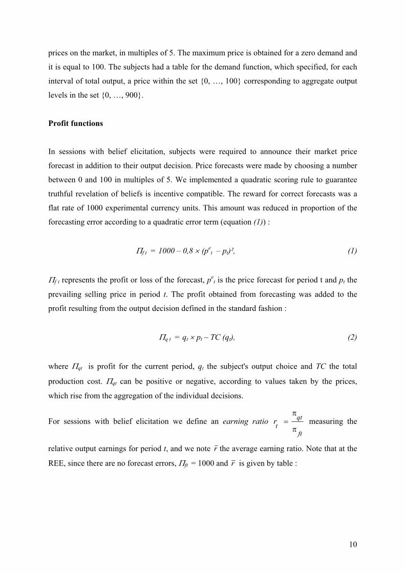
In sessions with belief elicitation, subjects were required to announce their market price

forecast in addition to their output decision. Price forecasts were made by choosing a number

between 0 and 100 in multiples of 5. We implemented a quadratic scoring rule to guarantee

truthful revelation of beliefs is incentive compatible. The reward for correct forecasts was a

flat rate of 1000 experimental currency units. This amount was reduced in proportion of the

forecasting error according to a quadratic error term (equation (1)) :

Πf t = 1000 – 0,8 × (pet – pt)², (1)

Πf t represents the profit or loss of the forecast, pe

t is the price forecast for period t and pt the

prevailing selling price in period t. The profit obtained from forecasting was added to the

profit resulting from the output decision defined in the standard fashion :

Πq t = qt × pt – TC (qt), (2)

where Πqt is profit for the current period, qt the subject's output choice and TC the total

production cost. Πqt can be positive or negative, according to values taken by the prices,

which rise from the aggregation of the individual decisions.

For sessions with belief elicitation we define an earning ratio ft

qttr π

π= measuring the

relative output earnings for period t, and we note r the average earning ratio. Note that at the

REE, since there are no forecast errors, Πft = 1000 and r is given by table :

10

fast convergence slow convergence divergence

r 3.4 1.4 0.4

Table 3 : Predicted value of the earning ratio according to treatment.

The elicitation of price forecasts should favour the coordination and the convergence in the

cobweb model, especially because price forecast are rewarded according to the quadratic

scoring rule. This should lead subjects to coordinate their beliefs and move therefore faster to

the equilibrium price.

Each session involved 5 subjects interacting during 40 periods in a cobweb market as

described previously. Communication between subjects was not allowed. At the beginning of

the experiment subjects received a fixed endowment of currency units, called capital. After

each period earnings were added to the initial capital and losses were subtracted. The initial

capital was constant across treatments. At the end of each period, subjects were informed

about the prevailing selling price, their production cost, their profit or loss and the remaining

capital. In treatments with belief elicitation they were also informed about their forecast

earnings. Furthermore, subjects could see at any time their past data by clicking a history

button. Each session begun with two trial periods in order to familiarize subjects with the

graphic interface. The subjects' understanding of the instructions and procedures was checked

by a short computerized questionnaire submitted before the beginning of the experiment.

During the experiment, the subjects could make written comments on a sheet. Subjects

involved in this experiment had never participated before in a similar experiment. A total of

135 subjects participated. They earned between 6 and 30 euros for an average time of 90

minutes per session6.

6 The participants in the sessions were students, randomly selected from a large subject pool of 1500 volunteers. The pool includes students from all disciplines from the universities of Strasbourg and is refreshed every year; the experimental history of each subject his recorded, together with individual data.

11

Hypotheses

Following our previous discussion we summarize the hypotheses to be tested as 4 short

statements :

H1) subjects decision are based on an eductive-type of reasoning independently of belief

elicitation

H2) subjects learn in both types of treatments (with and without belief-elicitation)

H3) subjects are able to coordinate their beliefs for both types of treatments depending on the

speed of convergence

H4) belief elicitation improves learning and coordination, and favours eductive learning,

leading to higher output earnings

In the result sections we shall focus on H4 which is our main hypothesis. However, we cannot

investigate H4 independently, and therefore we address also hypotheses H1-3.

3. Comparison of profit levels

We first look for differences in output earnings induced by belief elicitation. Since we expect

belief elicitation to facilitate coordination of beliefs, we also expected subjects to converge

faster to the equilibrium price when the output profit is large with respect to the forecasting

profit. We hypothesize that larger values of r will lead to larger levels output profits.

Table 4 summarizes our observations in terms of average output profit ( qπ ) and standard

deviations (σ) for the first 20 periods (1-20) and for the last 20 periods (21-40). Averaging

over the two sub-periods allows us to detect a rough effect of learning and to verify H2. As we

see from table 4 our rough indicators already show the effect of learning with repetition. The

average profit from the production activity increases with repetition, both for the fast and slow

treatments with belief elicitation7. In contrast, this is not the case for the divergent treatment

with elicitation groups. In order to test this conclusion for without data, as we only have 3

7 this is supported by a Wilcoxon rank sum test ( p<0,03)

12

independent measures in each type of treatment, we provide further analysis in the next

paragraph.

fast slow divergent

with without with without with without

qπ 2685 3171 1433 1589 224 950

Periods

1 to 20 σ 5388 786 2116 1284 6079 385

qπ 3439 3634 1662 1763 813 765

Periods

21 to 40 σ 632 345 385 325 720 302

Table 4: Average earnings and standard deviation according to treatments and

periods

Learning

In order to test H2 for without data, and to strengthen our previous non-parametric results for

H2 for with groups, we set up a more refined analysis of learning by taking into account the 40

periods. In order to do so, for all groups, all treatments and all periods, we introduce the time

variable in a regression on past realized prices, to predict the average output profit of a group,

as follows :

Πq t = β1 pt-1 + β2 t + εt, t={1,…40} (3)

In order to accept H2 the coefficient of the time variable ( β2) should be significant and

positive, i.e. the average output profit increases with repetition due to learning. Table 5

summarizes for our 27 groups, and all treatments, the significance level for the t-test. When a

negative sign is found for the t-test, the coefficient β2 of the time variable is also negative.

For almost all the fast and slow groups, the time variable is significant and exhibits positive

coefficients, which is true for only one divergent group. This implies that learning is observed

only in convergent groups, a fact that only partly supports H2.

13

fast slow divergent

with without with without with without

gr1 2,86 7,55 3,59 2,64 -1,21 -1,47

gr2 5,35 3,83 3,96 2,26 0,27 0,15

gr3 4,42 6,31 2,08 1,66 2,16 -1,18

gr4 4,74 1,44 0,64

gr5 0,76 2,10 1,12

group

gr6 3,12

1,80

-1,38

Table 5: Significance levels (t-test) and sign (+/-) for time variable

Table 4 exhibited several interesting features which are almost common to all treatments.

First, the average output profit increases between sub-periods in all treatments except for the

treatments divergent, where most of the coefficients are negative or not significant. Since the

average profit increases, subjects become more and more “efficient”, a fact that is compatible

with our learning hypothesis (H2), if we consider that the leaning increases efficiency.

Second, we observe that the variability of profits decreases sharply from the first sub-period

to the second. In other words, individual differences decrease with repetition which suggests

that subjects’ choices become closer to each other in the second half of the experiment than in

the first half. This observation supports our coordination hypothesis (H3). The β2 values in

table 5 for the divergent cases support our hypothesis H1. The application of eductive

reasoning to the divergent treatment implies that subjects become less and less efficient. As β2

values for the divergent case are negative, this implies that, with time, subjects in those

treatments do not improve their profits, which could be consistent with an evolution trough an

eductive type of reasoning. Our observations are compatible with the earlier results of

Hommes and alii (2002).

Table 4 presents several others interesting features. Comparing sessions with belief elicitation

to sessions without, we observe that the average output profit is always larger in sessions

without and the variability is smaller. These observations which are in contradiction with

hypothesis 4 (H4) are very surprising, since belief elicitation was supposed to favour

coordination among subjects and increase their output profit. Does it mean that without belief

14

elicitation, subjects are actually better forecasters ? It could be the case that belief elicitation

adds an element of complexity or confusion for the subjects. Instead of facilitating their

production decision, this additional prediction task could have increased the difficulty because

they do not necessarily connect their production decision with their forecast.

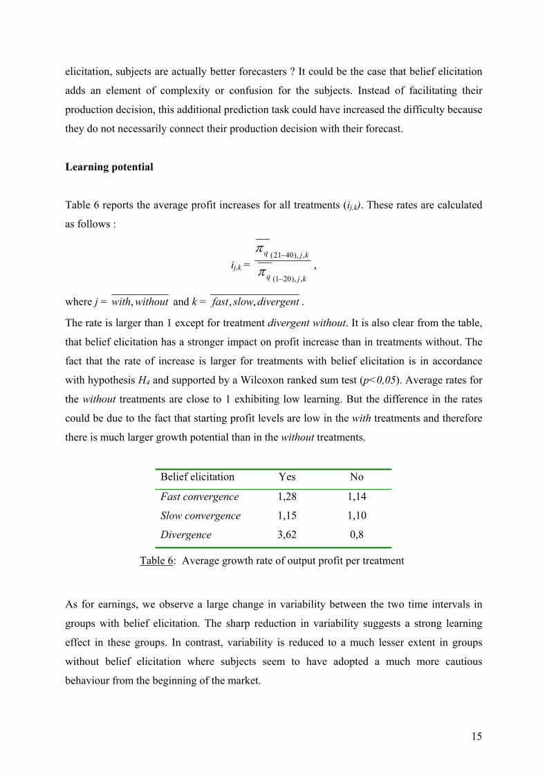
Learning potential

Table 6 reports the average profit increases for all treatments (ij,k). These rates are calculated

as follows :

ij,k = kjq

kjq

,),201(

,),4021(

−

−

π

π,

where j = withoutwith, and k = divergentslowfast ,, .

The rate is larger than 1 except for treatment divergent without. It is also clear from the table,

that belief elicitation has a stronger impact on profit increase than in treatments without. The

fact that the rate of increase is larger for treatments with belief elicitation is in accordance

with hypothesis H4 and supported by a Wilcoxon ranked sum test (p<0,05). Average rates for

the without treatments are close to 1 exhibiting low learning. But the difference in the rates

could be due to the fact that starting profit levels are low in the with treatments and therefore

there is much larger growth potential than in the without treatments.

Belief elicitation Yes No

Fast convergence 1,28 1,14

Slow convergence 1,15 1,10

Divergence 3,62 0,8

Table 6: Average growth rate of output profit per treatment

As for earnings, we observe a large change in variability between the two time intervals in

groups with belief elicitation. The sharp reduction in variability suggests a strong learning

effect in these groups. In contrast, variability is reduced to a much lesser extent in groups

without belief elicitation where subjects seem to have adopted a much more cautious

behaviour from the beginning of the market.

15

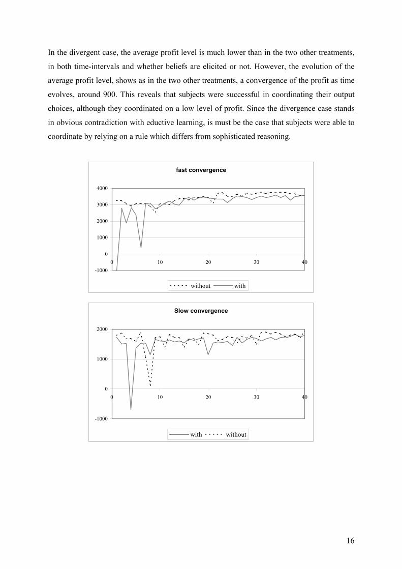
In the divergent case, the average profit level is much lower than in the two other treatments,

in both time-intervals and whether beliefs are elicited or not. However, the evolution of the

average profit level, shows as in the two other treatments, a convergence of the profit as time

evolves, around 900. This reveals that subjects were successful in coordinating their output

choices, although they coordinated on a low level of profit. Since the divergence case stands

in obvious contradiction with eductive learning, is must be the case that subjects were able to

coordinate by relying on a rule which differs from sophisticated reasoning.

fast convergence

-1000

0

1000

2000

3000

4000

0 10 20 30 40

without with

Slow convergence

-1000

0

1000

2000

0 10 20 30 40

with without

16

Divergence

-1000

0

1000

2000

0 10 20 30 40

with without

Figure 2 : Evolution of average profits.

4. Price evolution

The fact that total output is sold at the market demand price, the REE implies that, with our

assumptions and choice of parameters, the price is the same in all treatments : 60 currency

units per unit of output.

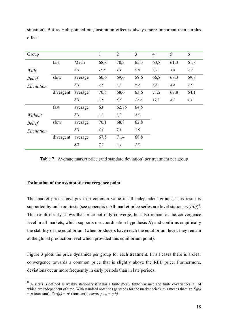
Table 7 presents the average market price and the standard deviations calculated for each

group, and each treatment.

According to table 7 there are few differences in average realized prices between groups and

across treatments. Average prices do not differ much between groups with elicitation and

groups without elicitation. However, since market prices could only take values in multiples

of 5, in most cases the average market price is only 1 or 2 steps away from the REE

equilibrium. Notice however that all average prices are above the REE price which is equal to

60. Therefore there is a tendency for subjects to choose output levels below the equilibrium

level. This implies that prices will converge to the REE state from above, which confirms an

institution effect - our design is close to PO markets, where average price are at or above the

Nash range (Holt, 1993), but not surplus analyses (Smith, 1962) : in DA markets, if producers

surplus exceeds consumers surplus, which is the case in our convergent theoretical design,

price tends to converge to the competitive level from below and from above if the reverse

17

situation). But as Holt pointed out, institution effect is always more important than surplus

effect.

Group 1 2 3 4 5 6

Mean 68,8 70,3 65,3 63,8 61,3 61,8 fast SD 15,8 4,4 5,8 3,7 3,8 2,9

average 60,6 69,6 59,6 66,8 68,3 69,8 slow SD 2,5 3,3 9,2 6,8 4,4 2,5

average 70,5 68,6 63,6 71,2 67,8 64,1

With

Belief

Elicitation divergent

SD 3,8 6,6 12,2 19,7 4,1 4,1

average 63 62,75 64,5 fast SD 3,3 3,2 2,5

average 70,1 68,8 62,8 slow SD 4,4 7,1 3,6

average 67,5 71,4 68,8

Without

Belief

Elicitation divergent

SD 7,5 6,4 5,8

Table 7 : Average market price (and standard deviation) per treatment per group

Estimation of the asymptotic convergence point

The market price converges to a common value in all independent groups. This result is

supported by unit root tests (see appendix). All market price series are level stationary(I(0))8.

This result clearly shows that price not only converge, but also remain at the convergence

level in all markets, which supports our coordination hypothesis H3 and confirms empirically

the stability of the equilibrium (when producers have reach the equilibrium level, they remain

at the global production level which provided this equilibrium point).

Figure 3 plots the price dynamics per group for each treatment. In all cases there is a clear

convergence towards a common price that is slightly above the REE price. Furthermore,

deviations occur more frequently in early periods than in late periods.

8 A series is defined as weakly stationary if it has a finite mean, finite variance and finite covariances, all of which are independent of time. With standard notations (p stands for the market price), this means that: ∀t, E(pt) = µ (constant), Var(pt) = σ² (constant), cov(pt, pt+h) = γ(h)

18

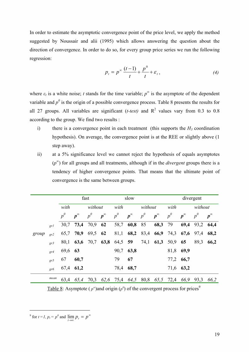
In order to estimate the asymptotic convergence point of the price level, we apply the method

suggested by Noussair and alii (1995) which allows answering the question about the

direction of convergence. In order to do so, for every group price series we run the following

regression:

tt tp

ttpp ε++−

= ∞0)1(

, (4)

where εt is a white noise; t stands for the time variable; p∞ is the asymptote of the dependent

variable and p0 is the origin of a possible convergence process. Table 8 presents the results for

all 27 groups. All variables are significant (t-test) and R2 values vary from 0.3 to 0.8

according to the group. We find two results :

i) there is a convergence point in each treatment (this supports the H3 coordination

hypothesis). On average, the convergence point is at the REE or slightly above (1

step away).

ii) at a 5% significance level we cannot reject the hypothesis of equals asymptotes

(p∞) for all groups and all treatments, although if in the divergent groups there is a

tendency of higher convergence points. That means that the ultimate point of

convergence is the same between groups.

fast slow divergent

with without with without with without

p0 p∞ p0 p∞ p0 p∞ p0 p∞ p0 p∞ p0 p∞

gr1 30,7 73,4 70,9 62 58,7 60,8 85 68,3 79 69,4 93,2 64,4

gr2 65,7 70,9 69,5 62 81,1 68,2 83,4 66,9 74,3 67,6 97,4 68,2

gr3 80,1 63,6 70,7 63,8 64,5 59 74,1 61,3 50,9 65 89,3 66,2

gr4 69,6 63 90,7 63,8 81,8 69,9

gr5 67 60,7 79 67 77,2 66,7

group

gr6 67,4 61,2

78,4 68,7

71,6 63,2

mean 63,4 65,4 70,3 62,6 75,4 64,5 80,8 65,5 72,4 66,9 93,3 66,2

Table 8: Asymptote ( p∞)and origin (p0) of the convergent process for prices9

9 for t =1, pt = p0 and ∞

∞→= pptt

lim

19

The next graphs consolidate our previous results. As shown in Table 7 (the standard deviation

values), the evolution of market prices in the "without" treatments (right side) is smoother

than in analogous "with" treatments (left side).

Fast with elicitation

0 20 40 60 80

100

0 5 10 15 20 25 30 35 40

gr 1gr 2gr 3gr 4gr 5gr 6REE

Slow with elicitation

0 20 40 60 80

100

0 10 20 30 40

gr 1gr 2gr 3gr 4gr 5gr 6REE

Divergence with elicitation

0 20 40 60 80

100

0 5 10 15 20 25 30 35 40

gr 1gr 2gr 3gr 4gr 5gr 6REE

Fast without elicitation

0

20

40

60

80

100

0 5 10 15 20 25 30 35 40

gr1gr2gr3REE

Slow without elicitation

0

20

40

60

80

100

0 10 20 30 40

gr1gr2gr3REE

Divergence without elicitation

0

20

40

60

80

100

0 10 20 30 40

gr1gr2gr3REE

Figure 3 : Market price evolution per treatment

20

The period of convergence

While prices convergence to a common value, convergence might happen more or less early

according to groups or treatments. We therefore analyse the period of convergence group by

group. We define the convergence period (noted h) as the time period at which the market

price enters into a "restricted price interval" and remains in it until the last period. We call this

interval the interval of convergence and the corresponding period the convergence period.

Convergence is thus characterized by two attributes: its type (strong, moderate or weak) and

its speed (fast or slow). According to the amplitude of the convergence interval, we shall

speak about strong convergence (in a narrow interval) and weak convergence (in a broad

interval).

We construct convergence intervals as follows. Let ph be the market price in period h for

some group, and let the values a, b, c, d ∈ {0,..100}, with a<b< c< d, be an ordered

sequence of possible price units in the experiment, i.e. multiples of 5. Starting from period h,

if we observe that the price remains in an interval of two consecutive price units (for example

[c, d], an amplitude 5 interval) until period 40, we shall speak about strong convergence, and

we identify h as the convergence period. The convergence period is the observable

counterpart of the speed of convergence. With faster convergence, the convergence period

will be further away from the end period. If convergence happens in a larger interval (for

example [ b, d ], an amplitude 10 interval) we shall speak about weak convergence. We look

for weak convergence (thus on 3 prices on a whole of 21).

Since all the groups, even within the same treatment, do not converge at the same period, we

compare the relative periods of convergence and try to see whether we can observe

outstanding differences in speed of convergence.

Table 9 presents the speed of convergence for all treatments and all groups. Treatments with

belief elicitation do not seem to converge faster than their counterpart without belief

elicitation. Furthermore, treatments for which convergence is "fast" do not converge faster

than treatments for which convergence should be slow.10 Although further investigation is

required, these preliminary findings clearly contradict the predictions of the eductive

reasoning hypothesis H1 for the divergent groups.

10 Mann-Whitney test (p>0,05)

21

fast 2 5 7 9 17 18

slow 1 2 5 11 20 23

with

divergence 2 9 10 21 23 30

fast 4 5 9

slow 5 18 32

without

divergence 6 18 25

Table 9: Convergence periods for market price

Predictability of prices

To get a further insight, we investigated the characteristics of the market price series. Do these

series incorporate a trend or structure which could help subjects to forecast the price for the

next period and to correlate their production decisions with that forecast in order to perform

better? To answer that question we analyse for each group and each treatment the

autocorrelation structure of market prices. The results are extremely suggestive. With few

exceptions, for the treatments with elicitation, there is no price pattern easily exploitable by

the subjects. When regressions are conducted with the 10 firsts lags, very few lags are

significant and we cannot observe a regular lag structure.

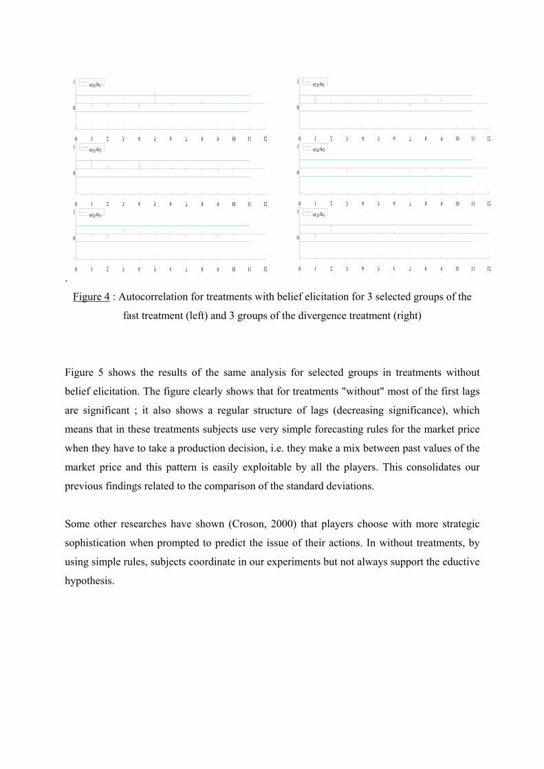
In figure 4 we report the results for 6 selected groups which were involved in treatments with

belief elicitation. The first 3 groups are of fast type and the 3 last of the divergent type.11(see

appendix for all treatments).

11 The lines in the plots are the two standard error Barlett bands at 2,5% significance level

22

0 1 2 3 4 5 6 7 8 9 10 11 12

0

1ACF-gr1

0 1 2 3 4 5 6 7 8 9 10 11 12

0

1ACF-gr2

0 1 2 3 4 5 6 7 8 9 10 11 12

0

1ACF-gr3

.

0 1 2 3 4 5 6 7 8 9 10 11 12

0

1ACF-gr1

0 1 2 3 4 5 6 7 8 9 10 11 12

0

1ACF-gr2

0 1 2 3 4 5 6 7 8 9 10 11 12

0

1ACF-gr3

Figure 4 : Autocorrelation for treatments with belief elicitation for 3 selected groups of the

fast treatment (left) and 3 groups of the divergence treatment (right)

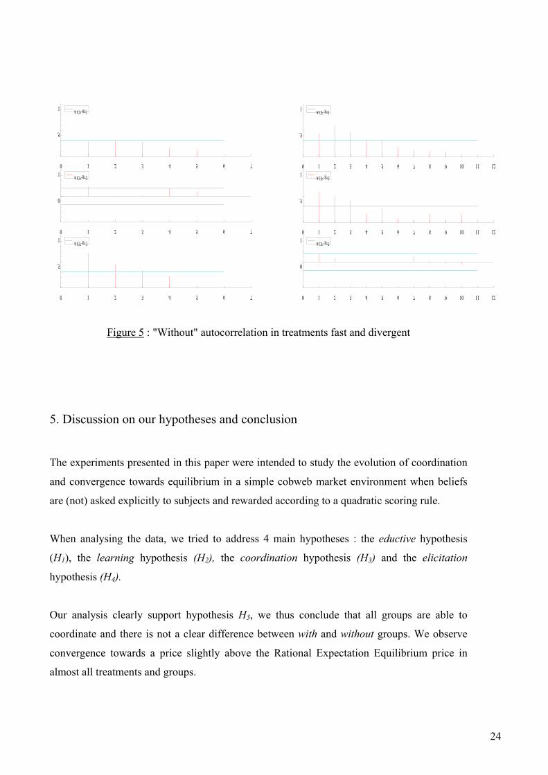
Figure 5 shows the results of the same analysis for selected groups in treatments without

belief elicitation. The figure clearly shows that for treatments "without" most of the first lags

are significant ; it also shows a regular structure of lags (decreasing significance), which

means that in these treatments subjects use very simple forecasting rules for the market price

when they have to take a production decision, i.e. they make a mix between past values of the

market price and this pattern is easily exploitable by all the players. This consolidates our

previous findings related to the comparison of the standard deviations.

Some other researches have shown (Croson, 2000) that players choose with more strategic

sophistication when prompted to predict the issue of their actions. In without treatments, by

using simple rules, subjects coordinate in our experiments but not always support the eductive

hypothesis.

0 1 2 3 4 5 6 7

.5

1ACF-gr1

0 1 2 3 4 5 6 7

0

1ACF-gr2

0 1 2 3 4 5 6 7

.5

1ACF-gr3

0 1 2 3 4 5 6 7 8 9 10 11 12

.5

1ACF-gr1

0 1 2 3 4 5 6 7 8 9 10 11 12

.5

1ACF-gr2

0 1 2 3 4 5 6 7 8 9 10 11 12

0

1ACF-gr3

Figure 5 : "Without" autocorrelation in treatments fast and divergent

5. Discussion on our hypotheses and conclusion

The experiments presented in this paper were intended to study the evolution of coordination

and convergence towards equilibrium in a simple cobweb market environment when beliefs

are (not) asked explicitly to subjects and rewarded according to a quadratic scoring rule.

When analysing the data, we tried to address 4 main hypotheses : the eductive hypothesis

(H1), the learning hypothesis (H2), the coordination hypothesis (H3) and the elicitation

hypothesis (H4).

Our analysis clearly support hypothesis H3, we thus conclude that all groups are able to

coordinate and there is not a clear difference between with and without groups. We observe

convergence towards a price slightly above the Rational Expectation Equilibrium price in

almost all treatments and groups.

24

Belief elicitation does not seem to improve the convergence process, but on the contrary to

add more noise in early periods of the market. However, belief elicitation seems to improve

subject's learning ability. Thus the evidence on hypothesis H2 is more mitigate : all groups are

able to learn, except for the divergent ones, and with groups have an important learning

potential.

Our results seem to contradict the assumption from the hypothesis H1 according to which

subject's behaviour might be described by iterated elimination of dominated strategies

(eductive reasoning). Experimental subjects in with treatments clearly adopt sophisticated

rules when forecasting prices, and these rules could be assimilated to eductive reasoning. In

contrast, experimental subjects in without treatments seem to adopt simple rules, such as

expecting the next period price by looking at past realized prices. Because most subjects adopt

such simple rules, belief coordination becomes very efficient, and fast convergence to a

narrow price interval is observed in many groups and treatments. Divergent groups seem

clearly to avoid the eductive reasoning which could lead them to chaos and reach coordination

by other learning rules.

As for our main hypothesis H4, the support provided for the other hypotheses does not allow

us to clearly reject the assumption of equivalence of treatments with and without.

Experimental subjects in treatments with have a better learning potential, but a lower initial

efficiency point. They are able to use sophisticated learning rules, but reach coordination in

the same asymptotic conditions as the without subjects.

25

Appendix 1. Unit root tests for market price series The ADF test consists in running a regression of the first difference of the series against the series lagged once, lagged difference terms, and optionally, a constant and a time trend.

∆X t=α+γX t-1+β1∆X t-1+…+βh∆X t-h+u t Test stands for (γ-1) = 0. A large negative t-statistic rejects the hypothesis of a unit root and suggests that the series is stationary. Fast without Critical values: 5%=-2.942 1%=-3.617; Constant included t-adf beta Y_1 \sigma lag t-DY_lag t-prob F-prob AIC Gr1 -2.5529 0.46975 2.9022 2 -1.2184 0.2317 2.2327 Gr1 -2.9754* 0.40100 2.9228 1 -1.9088 0.0648 0.2317 2.2227 Gr1 -4.9860** 0.16939 3.0312 0 0.0902 2.2704 Gr2 -3.5254* 0.20160 2.7610 2 -0.68336 0.4992 2.1330 Gr2 -4.4145** 0.12787 2.7393 1 1.0348 0.3081 0.4992 2.0930 Gr2 -4.6297** 0.24279 2.7421 0 0.4755 2.0700 Gr3 -3.1124* 0.59153 1.6123 2 -1.0282 0.3113 1.0571 Gr3 -3.4222* 0.56164 1.6136 1 -0.29239 0.7718 0.3113 1.0346 Gr3 -3.7456** 0.55000 1.5924 0 0.5702 0.98301 Fast with Critical values: 5%=-2.942 1%=-3.617; Constant included t-adf beta Y_1 \sigma lag t-DY_lag t-prob F-prob AIC gr1 -4.8610** -0.23968 3.3765 2 0.41048 0.6841 2.5355 gr1 -5.7676** -0.17846 3.3349 1 1.6917 0.0999 0.6841 2.4865 gr1 -5.9477** 0.043284 3.4225 0 0.2423 2.5133 gr2 -3.2944* -0.040427 3.7081 2 -1.4258 0.1633 2.7228 gr2 -5.3822** -0.32794 3.7640 1 1.0161 0.3167 0.1633 2.7286 gr2 -6.9145** -0.14156 3.7658 0 0.2276 2.7044 gr3 -2.8079 0.28628 2.4659 2 -0.58294 0.5639 1.9069 gr3 -3.8379** 0.20263 2.4419 1 -0.18700 0.8528 0.5639 1.8631 gr3 -5.4367** 0.17647 2.4080 0 0.8303 1.8101 gr4 -4.0061** -0.24625 11.251 2 0.56830 0.5737 4.9427 gr4 -4.7412** -0.13503 11.138 1 0.012885 0.9898 0.5737 4.8983 gr4 -6.9202** -0.13281 10.978 0 0.8515 4.8443 gr5 -3.0288* 0.31029 4.4114 2 0.35846 0.7223 3.0702 gr5 -3.3116* 0.35009 4.3545 1 0.064511 0.9489 0.7223 3.0200 gr5 -4.0705** 0.35740 4.2921 0 0.9360 2.9661 gr6 -3.1603* 0.022369 4.2686 2 -1.2414 0.2232 3.0044 gr6 -5.0003** -0.21751 4.3024 1 0.37789 0.7079 0.2232 2.9960 gr6 -7.9347** -0.14386 4.2494 0 0.4394 2.9461 Slow with Critical values: 5%=-2.942 1%=-3.617; Constant included t-adf beta Y_1 \sigma lag t-DY_lag t-prob F-prob AIC Gr1 -3.8257** 0.39332 4.7002 2 -0.85606 0.3981 3.1970 Gr1 -4.0579** 0.36921 4.6817 1 -0.89605 0.3765 0.3981 3.1649 Gr1 -4.8189** 0.31407 4.6685 0 0.4735 3.1342 Gr2 -4.8838** -0.24435 3.9430 2 0.44815 0.6570 2.8457 Gr2 -5.3776** -0.18986 3.8964 1 0.87259 0.3890 0.6570 2.7977 Gr2 -6.5483** -0.058548 3.8831 0 0.6278 2.7658 Gr3 -5.8756** -0.49457 3.6615 2 2.9663 0.0056 2.6976 Gr3 -4.6449** -0.023904 4.0598 1 0.59227 0.5576 0.0056 2.8799 Gr3 -5.8740** 0.065539 4.0220 0 0.0171 2.8361 Gr4 -1.4301 0.70496 2.2273 2 -0.013230 0.9895 1.7034 Gr4 -1.6408 0.70370 2.1943 1 -2.9615 0.0055 0.9895 1.6493 Gr4 -3.9985** 0.37288 2.4256 0 0.0227 1.8247 Gr5 -3.6080* 0.35609 2.5089 2 0.16175 0.8725 1.9415 Gr5 -3.7326** 0.36310 2.4727 1 -0.15135 0.8806 0.8725 1.8882 Gr5 -4.4234** 0.35049 2.4380 0 0.9761 1.8349 Gr6 -5.0619** -0.47885 9.0277 2 1.9300 0.0622 4.5024

26

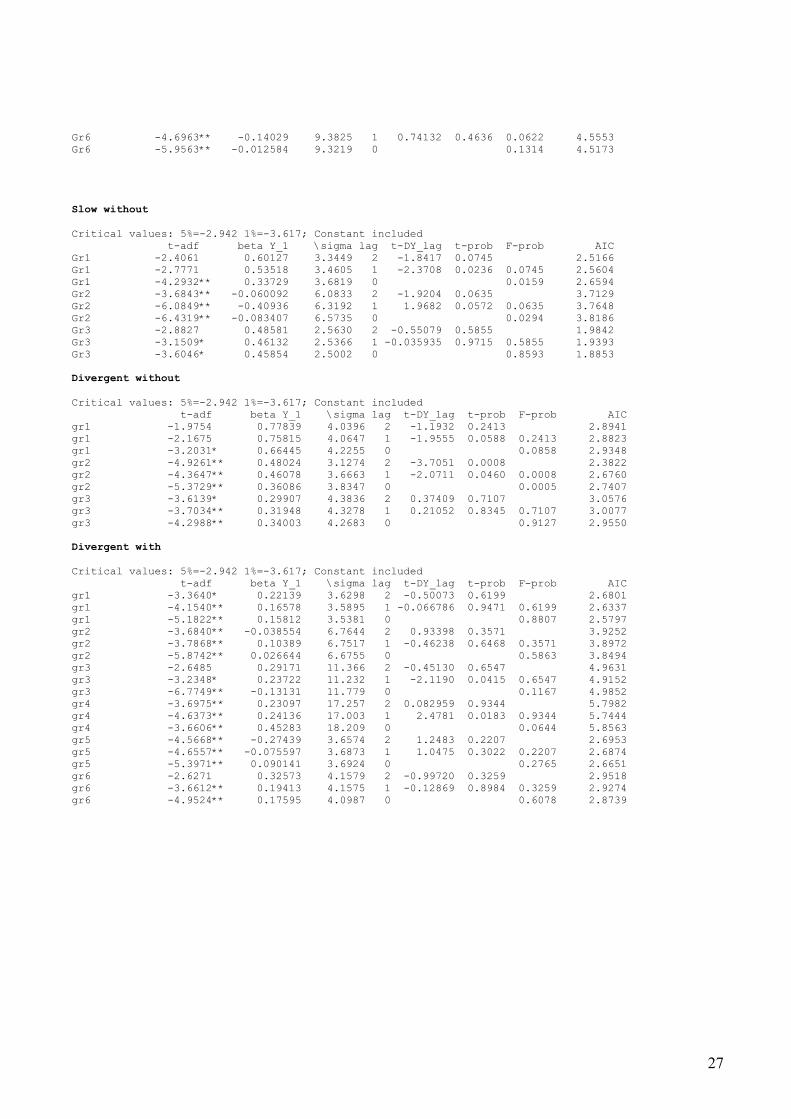
Gr6 -4.6963** -0.14029 9.3825 1 0.74132 0.4636 0.0622 4.5553 Gr6 -5.9563** -0.012584 9.3219 0 0.1314 4.5173 Slow without Critical values: 5%=-2.942 1%=-3.617; Constant included t-adf beta Y_1 \sigma lag t-DY_lag t-prob F-prob AIC Gr1 -2.4061 0.60127 3.3449 2 -1.8417 0.0745 2.5166 Gr1 -2.7771 0.53518 3.4605 1 -2.3708 0.0236 0.0745 2.5604 Gr1 -4.2932** 0.33729 3.6819 0 0.0159 2.6594 Gr2 -3.6843** -0.060092 6.0833 2 -1.9204 0.0635 3.7129 Gr2 -6.0849** -0.40936 6.3192 1 1.9682 0.0572 0.0635 3.7648 Gr2 -6.4319** -0.083407 6.5735 0 0.0294 3.8186 Gr3 -2.8827 0.48581 2.5630 2 -0.55079 0.5855 1.9842 Gr3 -3.1509* 0.46132 2.5366 1 -0.035935 0.9715 0.5855 1.9393 Gr3 -3.6046* 0.45854 2.5002 0 0.8593 1.8853 Divergent without Critical values: 5%=-2.942 1%=-3.617; Constant included t-adf beta Y_1 \sigma lag t-DY_lag t-prob F-prob AIC gr1 -1.9754 0.77839 4.0396 2 -1.1932 0.2413 2.8941 gr1 -2.1675 0.75815 4.0647 1 -1.9555 0.0588 0.2413 2.8823 gr1 -3.2031* 0.66445 4.2255 0 0.0858 2.9348 gr2 -4.9261** 0.48024 3.1274 2 -3.7051 0.0008 2.3822 gr2 -4.3647** 0.46078 3.6663 1 -2.0711 0.0460 0.0008 2.6760 gr2 -5.3729** 0.36086 3.8347 0 0.0005 2.7407 gr3 -3.6139* 0.29907 4.3836 2 0.37409 0.7107 3.0576 gr3 -3.7034** 0.31948 4.3278 1 0.21052 0.8345 0.7107 3.0077 gr3 -4.2988** 0.34003 4.2683 0 0.9127 2.9550 Divergent with Critical values: 5%=-2.942 1%=-3.617; Constant included t-adf beta Y_1 \sigma lag t-DY_lag t-prob F-prob AIC gr1 -3.3640* 0.22139 3.6298 2 -0.50073 0.6199 2.6801 gr1 -4.1540** 0.16578 3.5895 1 -0.066786 0.9471 0.6199 2.6337 gr1 -5.1822** 0.15812 3.5381 0 0.8807 2.5797 gr2 -3.6840** -0.038554 6.7644 2 0.93398 0.3571 3.9252 gr2 -3.7868** 0.10389 6.7517 1 -0.46238 0.6468 0.3571 3.8972 gr2 -5.8742** 0.026644 6.6755 0 0.5863 3.8494 gr3 -2.6485 0.29171 11.366 2 -0.45130 0.6547 4.9631 gr3 -3.2348* 0.23722 11.232 1 -2.1190 0.0415 0.6547 4.9152 gr3 -6.7749** -0.13131 11.779 0 0.1167 4.9852 gr4 -3.6975** 0.23097 17.257 2 0.082959 0.9344 5.7982 gr4 -4.6373** 0.24136 17.003 1 2.4781 0.0183 0.9344 5.7444 gr4 -3.6606** 0.45283 18.209 0 0.0644 5.8563 gr5 -4.5668** -0.27439 3.6574 2 1.2483 0.2207 2.6953 gr5 -4.6557** -0.075597 3.6873 1 1.0475 0.3022 0.2207 2.6874 gr5 -5.3971** 0.090141 3.6924 0 0.2765 2.6651 gr6 -2.6271 0.32573 4.1579 2 -0.99720 0.3259 2.9518 gr6 -3.6612** 0.19413 4.1575 1 -0.12869 0.8984 0.3259 2.9274 gr6 -4.9524** 0.17595 4.0987 0 0.6078 2.8739

27

Appendix 2. Autocorrelations plots Autocorrelations plots for fast with groups :

0 5 10

0

1ACF-gr1

0 5 10

0

1ACF-gr2

0 5 10

0

1ACF-gr3

0 5 10

0

1ACF-gr4

0 5 10

0

1ACF-gr5

0 5 10

0

1ACF-gr6

Autocorrelations plots for slow with groups :

0 5 10

0

1ACF-gr1

0 5 10

0

1ACF-gr2

0 5 10

0

1ACF-gr3

0 5 10

0

1ACF-gr4

0 5 10

.5

1ACF-gr5

0 5 10

0

1ACF-gr6

28

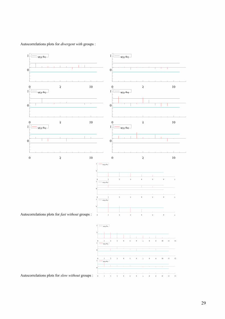
Autocorrelations plots for divergent with groups :

0 5 10

0

1ACF-gr1

0 5 10

0

1ACF-gr2

0 5 10

0

1ACF-gr3

0 5 10

0

1ACF-gr4

0 5 10

0

1ACF-gr5

0 5 10

0

1ACF-gr6

Autocorrelations plots for fast without groups :

0 1 2 3 4 5 6 7

.5

1ACF-gr1

0 1 2 3 4 5 6 7

0

1ACF-gr2

0 1 2 3 4 5 6 7

.5

1ACF-gr3

Autocorrelations plots for slow without groups :

0 1 2 3 4 5 6 7 8 9 10 11 12

.5

1ACF-gr1

0 1 2 3 4 5 6 7 8 9 10 11 12

0

1ACF-gr2

0 1 2 3 4 5 6 7 8 9 10 11 12

0

1ACF-gr3

29

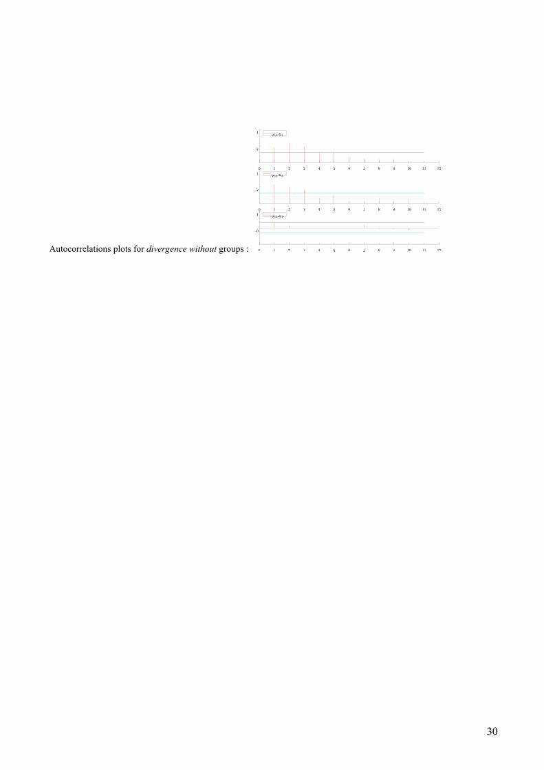
Autocorrelations plots for divergence without groups :

0 1 2 3 4 5 6 7 8 9 10 11 12

.5

1ACF-gr1

0 1 2 3 4 5 6 7 8 9 10 11 12

.5

1ACF-gr2

0 1 2 3 4 5 6 7 8 9 10 11 12

0

1ACF-gr3

30

Acknowledgements

We thank Roger Guesnerie, for the discussions on the specification of the experiments and for

his help for the experiments. We also thank Bodo Vogt and Thorsten Hens, for interesting

suggestions for our experiments, Jan Tuinstra and Cars Hommes for very helpful discussions ;

Christian Schade, our discussant in ESA Meeting in Erfurt 2003, for his comments on an

earlier version. We particularly thank Kene Boun My, which programmed our experiments

and supervised the sessions.

31

References

Binmore, K. (1987), "Modelling rational players: Part 1", Economics and Philosophy, 3,

17-214.

Bray, M. M., Savin, N. E. (1986), "Rational expectations equilibria, learning and model

specification", Econometrica, 54, 1129-1160.

Guesnerie, R. (1992), "An exploration of the eductive justifications of the rational

expectations hypothesis", American Economic Review, 82, 1254-1278.

Ho, Camerer & Weigelt. (1992), "Iterated dominance and iterated best-response in

experimental “p-beauty contests”", American Economic Review, 88, 4, 947-967.

Hommes, C. H. , Sonnemans, J., van de Velden, H. (2000), "Expectation formation in an

experimental cobweb economy", in Interaction and Market Structure, Essays on

Heterogeneity in Economics, Berlin/Heidelberg (eds D. Delli Gatti, M. Gallegati and A.

Kirman), Lecture Notes in Economics and Mathematical Systems, 884, 253-266, Spinger

Verlag.

Hommes, C. H., Sonnemans, J., Tuinstra, J., van de Velden, H. (2002), "Coordination of

expectations in asset pricing experiments", CeNDEF Working Paper Series, 02-07,

Universiteit van Amsterdam.

Ho, T.-H., Camerer C., Weigelt K., (1998), "Iterated dominance and iterated best-response in

experimental 'p-beauty contest'", A laboratory experiment with a single person cobweb", The

American Economic Review, 88, 4, 947-969.

Holt, C. A, Villamil, A.P. (1986), "A laboratory experiment with a single person cobweb",

Atlantic Economic Journal, 14, 51-54.

32

Davis, D., Holt, C. (1993), "Experimental Economics", Princeton University Press, Princeton,

New Jersey .

Muth, J. F. (1961), "Rational expectations and the theory of price movements",

Econometrica, 29, 315-335.

Nagel, R. (1995), "Unraveling in Guessing Games: An Experimental Study", American

Economic Review 85(5), 1313-1326.

Sutan, A., Willinger, M. (2003), "Price forecasts and coordination by the beliefs: an

experimental approach", in Integrare europeana in contextul globarizarii economice, vol. I,

Editions AGIR, 2003, pp.43-76.

Van Huyck, J., Battalio, R., Beil, R. (1990), "Tacit coordination games, strategic uncertainty,

and coordination failure", American Economic Review, 80,234-248.

Wellford, C.P. (1989), "A laboratory analysis of price dynamics and expectations in the

cobweb model", Discussion Paper, 89-15, Department of Economics, University of Arizona.

33