1

Control of Pore Radius Regulation for Electroporation-based Drug Delivery

Xiaopeng Zhao, Mingjun Zhang, and Ruoting Yang Mechanical, Aerospace and Biomedical Engineering Department

University of Tennessee Knoxville, TN 37996-2030

Abbreviated Title: Control of Pore Radius for Electroporation

Corresponding author: Xiaopeng Zhao Mechanical, Aerospace and Biomedical Engineering Department University of Tennessee Knoxville, TN 37996-2030 Email: xzhao9@utk.edu. Phone: (865) 974-7682 Fax : (865) 974-7663

2

Abstract—Electroporation uses electric pulses to create transient, nonselective pores in a

cell’s membrane, allowing drugs to be delivered into the targeted cells. To ensure proper

uptake of drug molecules, it is essential to control the radii of the pores and the time

duration, for which the pores remain open. Electroporation is intrinsically a nonlinear

dynamic process. A careful analysis of the electroporation dynamics reveals that, under

variation of the magnitude of the input voltage, the equilibrium pore radius undergoes a

pair of saddle node bifurcations. As a result, there exists a range of pore radii that is

physically unstable and thus cannot be maintained in conventional experiments. The

bifurcations and the associated unstable regime impose restrictions on the operation of

electroporation, limiting the sizes of deliverable drug particles. To overcome these

problems, we design a novel control strategy to stabilize the originally unstable solutions.

In contrast to the conventional control algorithms based on local stability analysis, the

present control is globally stable. Numerical examples show that the control eliminates

the original bifurcations and allows one to achieve a wide range of pore radii. The

robustness and effectiveness of the control strategy would potentially enhance the

application of electroporation.

PACS Codes: 87.50.cj, 02.30.Oz, 05.45.-a Key words: Electroporation, Control, Bifurcation

3

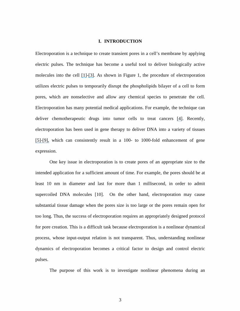
I. INTRODUCTION

Electroporation is a technique to create transient pores in a cell’s membrane by applying

electric pulses. The technique has become a useful tool to deliver biologically active

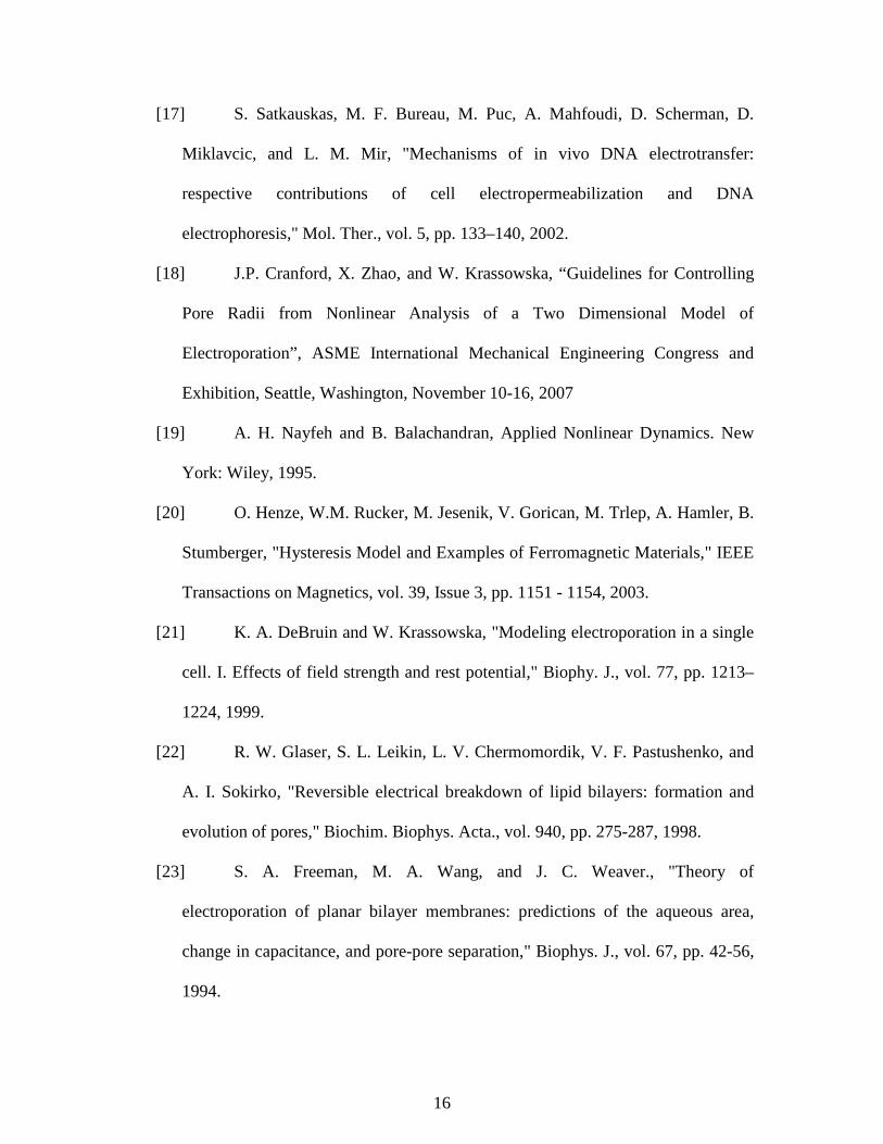
molecules into the cell [1]-[3]. As shown in Figure 1, the procedure of electroporation

utilizes electric pulses to temporarily disrupt the phospholipids bilayer of a cell to form

pores, which are nonselective and allow any chemical species to penetrate the cell.

Electroporation has many potential medical applications. For example, the technique can

deliver chemotherapeutic drugs into tumor cells to treat cancers [4]. Recently,

electroporation has been used in gene therapy to deliver DNA into a variety of tissues

[5]-[9], which can consistently result in a 100- to 1000-fold enhancement of gene

expression.

One key issue in electroporation is to create pores of an appropriate size to the

intended application for a sufficient amount of time. For example, the pores should be at

least 10 nm in diameter and last for more than 1 millisecond, in order to admit

supercoiled DNA molecules [10]. On the other hand, electroporation may cause

substantial tissue damage when the pores size is too large or the pores remain open for

too long. Thus, the success of electroporation requires an appropriately designed protocol

for pore creation. This is a difficult task because electroporation is a nonlinear dynamical

process, whose input-output relation is not transparent. Thus, understanding nonlinear

dynamics of electroporation becomes a critical factor to design and control electric

pulses.

The purpose of this work is to investigate nonlinear phenomena during an

4

electroporation process and to explore possible control mechanisms to improve the

effectiveness of the process. Using bifurcation analysis, we investigate the relation

between input voltage and the size of the created pores. The result demonstrates that a

range of pore sizes is not achievable in experiments. Moreover, the bifurcation leads to a

hysteresis phenomenon. These nonlinear phenomena bring a substantial challenge to

design electric pulses, and thereby, limit the operation of electroporation.

Currently, the strength and duration of the electric field in electroporation are

mainly determined by trial-and-error. Moreover, the common pulses used in experiments

are open-loop controlls, which suffer bifurcations and hysteresis. Recently, Ma and

Zhang [11] proposed a feedback-linearization based nonlinear controller to regulate a

target transmembrane potential. In this paper, we propose a new control algorithm to

improve the two-phase protocol in regulating the pore size. A detailed analysis

demonstrates the robustness and the efficacy of the algorithm. In addition, the control

strategy is globally stable and allows one to achieve a wide range of pore radii.

This artcile is organized as follows. Section II introduces mathematical

description of the physical processes of electroporation. A simplified mathematical model

is presented based on a commonly adopted protocol. Then, Section III explores nonlinear

dynamics of the model and demonstrates how bifurcations limite the operation of

electroporation. A feedback control algorithm is introduced in Sectoin IV to eliminate the

bifurcations and to improve the efficiency of electroporation. Finally, Section V presents

conclusions and discussions.

II. PROBLEM DESCRIPTION

Mathematical models have been developed to describe an electroporation process [12]-

5

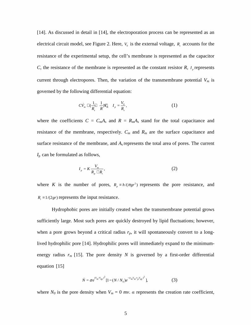
[14]. As discussed in detail in [14], the electroporation process can be represented as an

electrical circuit model, see Figure 2. Here, 0V is the external voltage, sR accounts for the

resistance of the experimental setup, the cell’s membrane is represented as the capacitor

C, the resistance of the membrane is represented as the constant resistor R, pI represents

current through electropores. Then, the variation of the transmembrane potential Vm is

governed by the following differential equation:

01 1( ) = ,m m p

s s

VCV V I

R R R+ + +ɺ (1)

where the coefficients C = CmAs and R = RmAs stand for the total capacitance and

resistance of the membrane, respectively. Cm and Rm are the surface capacitance and

surface resistance of the membrane, and As represents the total area of pores. The current

Ip can be formulated as follows,

= ,mp

p i

VI K

R R+ (2)

where K is the number of pores, 2/( )pR h grπ= represents the pore resistance, and

1/(2 )iR gr= represents the input resistance.

Hydrophobic pores are initially created when the transmembrane potential grows

sufficiently large. Most such pores are quickly destroyed by lipid fluctuations; however,

when a pore grows beyond a critical radius rp, it will spontaneously convert to a long-

lived hydrophilic pore [14]. Hydrophilic pores will immediately expand to the minimum-

energy radius rm [15]. The pore density N is governed by a first-order differential

equation [15]

2 2( / ) ( / )

0= [1 ( / ) ],V V r V r Vm ep m m p epN e N N eα

−−ɺ (3)

where N0 is the pore density when Vm = 0 mv. α represents the creation rate coefficient,

6

and Vep stands for the characteristic voltage of electroporation.

The bilayer energy can be described in four components as follows,

4

2 2*max= 2 ,eff m

rr r F V r

rβ πγ πσ Ω + − −

(4)

In the above equation, the bilayer energy Ω contains four contributions: steric repulsion

energy ( )4

* /r rβ , edge energy 2 rπγ , membrane tension 2eff rπσ , and transmembrane

potential 2max mF V r . Here, β is the steric repulsion energy with minimum hydrophilic pore

radius *r , and γ is the edge energy, and s stands for the combined area of the pores. The

membrane tension is given by

02

(2 )( ) = 2 ,

(1 / )

′ −′ −−eff s

s

AA A

σ σσ σ (5)

where As = Kπr2 represents the total area of pores, while A stands for the total area of

membrane. σ' is the interfacial energy per unit area of the hydrocarbon-water interface,

and σ0 denotes the surface tension of the intact membrane wit 0sA = . The coefficient Fmax

is the maximum electric force.

Pores that initially have radii rm will change their radii to minimize the bilayer

energy W. As a result, the average pore radius can be expressed as

42*

max5= = [ 4 2 2 ],

∂Ω− − − + − −∂

ɺ eff mB a B a

rD Dr r F V

k T r k T rβ πγ π σ (6)

where D is the diffusion coefficient of the pore radius, kB is the Boltzmann constant, and

Ta is the absolute temperature. The model parameters are summarized in the Table 1.

Sukharev et al. [16] proposed a two-pulse protocol, which consists of two electric

pulses separated by a relaxation interval, see illustration in Figure 3. The first pulse is a

large voltage for a short duration, which quickly creates a number of pores. During the

7

relaxation interval, all pores shrink to a minimum size. Then, a long yet weak pulse is

applied to maintain the growth of the pores to facilitate electrophoretic movement of drug

molecules. Experiments proved that the two-pulse protocol is more efficient in uptake of

drug particles than a single pulse [17].

Besides its efficacy in drug delivery, the two-pulse protocol also allows

significant simplifications to the model of electroporation [18]. Specifically, since all

pores are created in the first phase and they all shrink to the minimum size during the

relaxation interval, the following conditions hold for pores in the second phase: (i) the

number of pores is constant and (ii) all pores have the same size. As a result, the model

(1,5,6) is reduced to the following form:

01 1 1,m

m ps s

dV VV I

dt C R R R

= − + −

(7)

42*

max54 2 2 .eff m

B a

rdr Dr F V

dt k T rβ πγ π σ

= − − + − −

(8)

In the following, we will analyze the nonlinear dynamics of electroporation using this

model.

III. BIFURCATION AND HYSTERESIS

Dynamics of the model (7) - (8) can be understood from a phase-plane analysis based on

nullclines. On a V-nullcline (or r-nullcline), the rate of change of Vm (or r) is zero, that is,

dVm/dt=0 (or dr/dt =0). Thus, the intersections of a V-nullcline and an r-nullcline

correspond to equilibria of the system. Figure 4 shows the V-nullclines for V0 = 0.2, 1.0,

2.2, and 4.0 V and the r-nullcline. For purpose of illustration, we choose the number of

pores K=2500 in this paper although the results for other values of K will be similar.

8

It can be seen from (7) and (8), a V-nullcline is a function of V0 whereas an r-

nullcline is independent of V0. Moreover, one can show that when V0 increases

(decreases), the V-nullcline shifts up (down). One can show that dr/dt<0 in the region

below the N-shaped r-nullcline whereas dr/dt>0 when it is above the r-nullcline.

Correspondingly, dVm/dt>0 in the region below the V-nullcline and dVm/dt<0 in the

region above the V-nullcline. As seen in Figure 4, for a very small V0 (e.g. V0=0.2 V), the

V- and r-nullclines intersect at the leftmost branch of the r-nullcline, corresponding to a

small pore radius in equilibrium. When V0 increases, the equilibrium value of r increases.

For example, when V0 = 1.0 V, the V- and r-nullclines intersect at a point in the middle

branch of the r-nullcline. When V0 is further increased, the nullclines may have multiple

intersections. For example, when. V0=2.2 V, there are two intersections at the middle

branch and one at the right branch. Finally, when V0 is sufficiently large (e.g. V0=4.0 V),

there is one intersection at the right branch of the r-nullcline. Figure 4 indicates that the

number of equilibriums varies as V0 changes, a phenomenon known as bifurcation [19].

When a constant V0 is applied, Vm and r reach their equilibriums values after a

few microseconds. The equilibriums of Vm and r depend on V0 in a nonlinear fashion. In

particular, there exists a range of V0 characterized by the coexistence of multiple

solutions. Diagrams in Figure 5 are known as bifurcation diagrams, which show that

there coexist three solution branches for 01.82 2.83V V V≤ ≤ (the dashed curves). Here, the

top and bottom branches are stable whereas the middle branch is unstable. The critical

point where a stable and an unstable solution branches meet corresponds to a saddle-node

bifurcation [19].

The existence of saddle-node bifurcations leads to hysteresis, which is a path-

9

dependent phenomenon and occurs in magnetic and ferromagnetic materials [20]. The

output of a hysteresis system depends not only on the input but also on the input history.

To demonstrate, let us assume that one starts from a small value of V0 that corresponds to

the leftmost point on Figure 5. Then when the value of V0 is quasi-statically increased,

the response of Vm (r) follows the upper (lower) solid curve shown in the top (bottom)

panel of Figure 5 until V0 reaches the intersection between the upper (lower) solid curve

and the middle dashed curve. When the value of V0 is further increased, the solution of

Vm (r) jumps to and stays on lower (upper) solid curve shown in the top (bottom) panel.

Correspondingly, if one starts from a large value of V0 and slowly decreases V0, the

solution of Vm (r) will experience the opposite jump from the lower (upper) branch to the

upper (lower) branch. The above process suggests that, during “loading” and “unloading”

processes, the response of the system follows two different paths, i.e. hysteresis. To

illustrate the hysteresis of electroporation, we use a stimulus of 0 2.5 sin( )V t= + to simulate

a quasi-static loading and unloading process; see Figure 6. Here, after a short transient,

the system’s response falls on a hysteresis loop, which consists of a loading (increasing in

V0) branch, an unloading branch, and quick transitions between the two branches. The

hysteresis phenomenon results from the existence of saddle-node bifurcations. Indeed, the

loading and unloading branches in the hysteresis loops correspond to the two equilibrium

branches in the bifurcation diagrams (cf. Figures 5 and 6). And jumps between the

loading and unloading branches are due to the bifurcation points. The corresponding time

histories of V0, Vm, and r are shown in Figure 7.

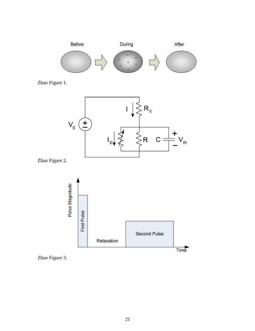
The existence of multiple stable solutions in the range 01.82 2.83V V V≤ ≤ indicates

that different initial conditions may lead to different equilibrium solutions. It is

10

interesting to ask which solution can be achieved from a certain initial condition. To

answer this question, we plot the stable manifold of the unstable saddle node

corresponding to 0 2.5V V= , see the red dotted curve in Figure 8. This manifold divides the

(r, Vm) state space into two regions. It can be concluded that any point on the left of the

manifold will lead to the stable equilibrium at 10r ≈ nm and any point on the right will

lead to the stable equilibrium at 29r ≈ nm.

IV. CONTROLLER DESIGN

Electroporation has been used to deliver drugs and other biological molecules into cells

[4]-[9]. When electroporation is used for drug delivery, different drugs would need

different pore sizes. While smaller pores are sufficient for delivering many types of

anticancer drugs, large pores are needed to deliver DNA. Thus, functionality of

electroporation greatly depends on its ability in creating pores of different sizes. However,

as shown in Figure 5, a pore size in the range between 15 µm and 25 µm is unstable.

Thus, it is not possible to achieve pores in this range using the conventional open-loop

input. To overcome this problem and to eliminate the hysteresis phenomenon described

earlier, we design a control mechanism by choosing V0 as follows:

( )0 control

1 1,

= + + + −

s m s p p m

s

V R V R I K V VR R

(9)

where Kp is a control gain. This controlled input renders Equation (7) as

( )control

1.= −m

p ms

dVK V V

dt CR (10)

We now design two different control strategies: 1.) voltage targeted control; and

2.) radius targeted control. The first control strategy is easy to achieve. Because when a

11

constant Vtarget is chosen such that Vcontrol=Vtarget, the dynamics of Vm becomes

independent of r. Then, it is trivial to show that this control mechanism is stable as long

as the gain Kp is chosen to be positive. Under this control, the equation of r becomes a

“slave equation” in that the dynamics of r is determined by Vm but r has no influence to

Vm. Therefore, although this strategy can eliminate the bistability and hysteresis problems

[11], it is not possible to know the resulted value of r in advance. Thus, the control has

limited applications.

The second control strategy, although much more involved, is more desired in

practical applications. To achieve this control goal, we select the control input to be

control null target( ),= + −rV V K r r (11)

where Vnull is implicitly defined as the nullcline function of r, Kr is a control gain, and

r target represent the desired pore size. With this control, one can easily show that (r target,

Vnull(r target)) is a fixed point of the controlled system (8, 10). To analyze the stability of the

control, we compute the Jacobian matrix as follows

null

,1 1

∂ ∂ ∂ ∂ = ∂ − − ∂

m

p p rs s

f f

r VJ

VK K K r

CR CR r

(12)

where 4

2*max5

4 2 2 .

= − − + − −

eff mB a

rDf r F V

k T rβ πγ π σ To have stable solutions, both eigenvalues

of the Jacobian matrix must have negative real parts [19]. One shall then choose the

proper values of gains Kp and Kr to satisfy this condition.

However, this criterion of the gains based on eigenvalues can only guarantee local

stability. As such, the system may still have other stable solutions and an arbitrarily given

initial condition may not converge to the desired target value. To resolve this issue, we

12

design a globally stable control algorithm based on the nullclines to achieve any desired

pore size with arbitrarily given initial conditions. From Eqn. (8), one can show that

dr/dt<0 in the region below the N-shaped r-nullcline whereas dr/dt>0 when it is above

the r-nullcline. Thus, a simple yet effective control strategy is to place V0 above the r-

nullcline (pores will grow) when r < r target and below the r-nullcline (pores will shrink)

when r > r target. We can then choose the control gains according to this criterion based on

the nullcline.

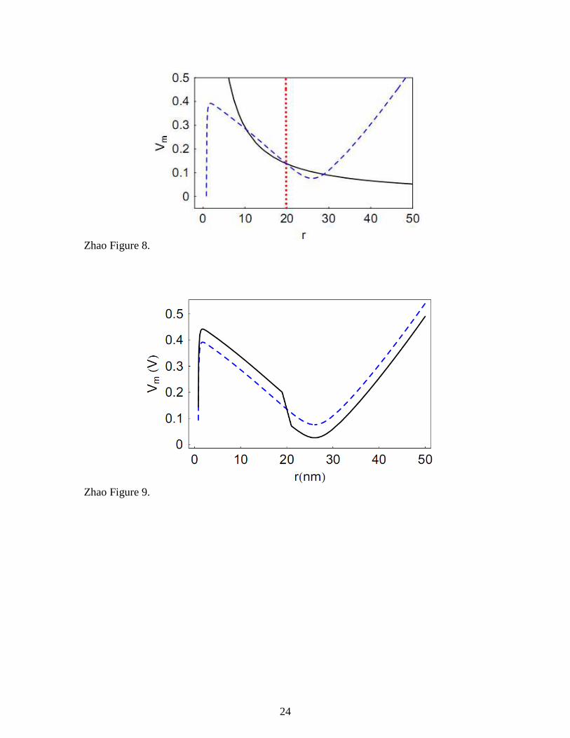
One problem remains if the control gains are set to be constants. Because the

control input Vcontrol is linearly proportional to r target – r, it may become exceedingly large

when r is too far away from r target and thus causes damage to the tissue. To ensure a

realistic control effort and avoid potential harms, one can saturate the magnitude of

Vcontrol when |r target-r| is over a certain limit. For example, we let Vcontrol=Vnull+Kr*1 nm

wehn r<r target- 1 nm and Vtarget=Vnull -Kr*1 nm when r>r target-1 nm. The concept of the

control algorithm is illustrated in Figure 9 using Kr=0.05 V/nm and r target=20 nm. Here,

the control algorithm leaves the r-nullcline unchanged but alters the V-nullcline to the

shape of the black solid curve (cf. Figure 4 and Figure 9).

To demonstrate the effectiveness of the control algorithm, we plot the control

result for r target = 20 nm, as shown in Figure 10. Recall from Figure 5 that this specific

pore radius is not achievable under a conventional constant-magnitude pulse. However, it

is easily achieved with the proposed control. Figure 10 shows the successful control

response, where simulations are based on Kp = 1 µs−1 and Kr = 0.05 V/nm. We test the

robustness of the control algorithm by choosing various values of r target and the control is

always able to stably achieve the desired pore size.

13

V. CONCLUSIONS

We have investigated nonlinear dynamics of electroporation under a commonly adopted

two-pulse protocol. Results based on phase portrait and bifurcation analysis demonstrate

limitations in the conventional constant-voltage input. Specifically, under variation of the

magnitude of the applied voltage, the equilibrium pore radius undergoes a pair of saddle

node bifurcations, which are connected through an unstable branch of solution

corresponding to a range of pore radii that cannot be maintained in conventional

experiments. These undesirable nonlinear characters restrict the operation of

electroporation, limiting the sizes of deliverable drug particles. Moreover, bifurcations

may also induce hysteresis phenomena under quasistatic loading and unloading inputs.

To overcome these shortcomings, we have explored both voltage- and radius-targeted

control mechanisms. Since the conventional control mechanisms based on local stability

analysis are not able to guarantee global stabilities, we have designed a novel control

strategy based on phase space analysis. The designed algorithm eliminates the original

bifurcations and allows one to achieve any desired pore radius starting from arbitrary

initial conditions. Since the control algorithm is globally stable, it ensures robust

operation of electroporation. This control strategy would potentially enhance the

effectiveness of electroporation, making it a more attractive technique for drug delivery

and other bio-molecular applications.

ACKNOWLEDGEMENT

X. Z. would like to thank the financial support of the NSF under grant No. CMMI-

0845753.

14

REFERENCES

[1] I. G. Abiror, V. B. Arakelyan, L. V. Chernomordik, Y. A. Chizmadzhev, V. F.

Pastushenko, and M. R. Tarasevich, "246 - Electric breakdown of bilayer lipid

membranes I. The main experimental facts and their qualitative discussion,"

Bioelectrochemistry and Bioenergetics, vol. 6, pp. 37-52, 1979.

[2] L. M. Mir, S. Orlowski, J. Belehradek, J., and C. Paoletti, "Electrochemotherapy

potentiation of antitumour effect of bleomycin by local electric pulses," Eur. J.

Cancer, vol. 27, pp. 68-72, 1991.

[3] J. C. Weaver, "Electroporation: a general phenomenon for manipulating cells and

tissues," J. Cell. Biochem., vol. 51, pp. 426-435, 1993.

[4] S. B. Dev, D. P. Rabussay, G. Widera, and G. A. Hofmann, "Medical applications

of electroporation," Plasma Science, IEEE Transactions on, vol. 28, pp. 206-223,

2000.

[5] H. Aihara and J. Miyazaki, "Gene transfer into muscle by electroporation in

vivo," Nat Biotech, vol. 16, pp. 867-870, 1998.

[6] W. Tao and M. Zhang, Physical methods for gene therapy, Micro- and Nano-

manipulations: Fundamentals with Biomedical Applications: Artech publishing

house, 2008.

[7] P. Bigey, M. F. Bureau, and D. Scherman, " In vivo plasmid DNA

electrotransfer," Curr Opin Biotechnol, vol. 13, pp. 443-447, 2002.

[8] J. Gehl, "Electroporation: theory and methods, perspectives for drug delivery,

gene therapy and research," Acta physiologica Scandinavica, vol. 177, pp. 437-

447, 2003.

15

[9] J. McMahon and D. Wells, "Electroporation for gene transfer to skeletal muscles:

current status," BioDrugs, vol. 18, pp. 155-165, 2004.

[10] V. V. Rybenkov, A. V. Vologodskii, and N. R. Cozzarelli, “The effect of

ionic conditions on the conformations of supercoiled DNA,” Sedimentation

analysis, J. Mol. Biol., vol. 267, pp. 299–311, 1997.

[11] O. Ma and M. Zhang, "Dynamics Modeling and Control of

Electroporation-Mediated Gene Delivery," IEEE Transactions On Automation

Science and Engineering, 2008.

[12] R. P. Joshi and K. H. Schoenbach, "Electroporation dynamics in biological

cells subjected to ultrafast electrical pulses: A numerical simulation study,"

Physical Review E, vol. 62, p. 1025, 2000.

[13] W. Krassowska and P. D. Filev, "Modeling Electroporation in a Single

Cell," Biophys. J., vol. 92, pp. 404-417, January 15, 2007.

[14] K. C. Smith, J. C. Neu, and W. Krassowska, "Model of Creation and

Evolution of Stable Electropores for DNA Delivery," Biophys. J., vol. 86, pp.

2813-2826, 2004.

[15] J. C. Neu and W. Krassowska, "Asymptotic model of electroporation,"

Physical Review E, vol. 59, p. 3471, 1999.

[16] S. I. Sukharev, V. A. Klenchin, S. M. Serov, L. V. Chernomordik, and

Chizmadzhev YuA, "Electroporation and electrophoretic DNA transfer into cells.

The effect of DNA interaction with electropores," Biophys. J., vol. 63, pp. 1320-

1327, 1992.

16

[17] S. Satkauskas, M. F. Bureau, M. Puc, A. Mahfoudi, D. Scherman, D.

Miklavcic, and L. M. Mir, "Mechanisms of in vivo DNA electrotransfer:

respective contributions of cell electropermeabilization and DNA

electrophoresis," Mol. Ther., vol. 5, pp. 133–140, 2002.

[18] J.P. Cranford, X. Zhao, and W. Krassowska, “Guidelines for Controlling

Pore Radii from Nonlinear Analysis of a Two Dimensional Model of

Electroporation”, ASME International Mechanical Engineering Congress and

Exhibition, Seattle, Washington, November 10-16, 2007

[19] A. H. Nayfeh and B. Balachandran, Applied Nonlinear Dynamics. New

York: Wiley, 1995.

[20] O. Henze, W.M. Rucker, M. Jesenik, V. Gorican, M. Trlep, A. Hamler, B.

Stumberger, "Hysteresis Model and Examples of Ferromagnetic Materials," IEEE

Transactions on Magnetics, vol. 39, Issue 3, pp. 1151 - 1154, 2003.

[21] K. A. DeBruin and W. Krassowska, "Modeling electroporation in a single

cell. I. Effects of field strength and rest potential," Biophy. J., vol. 77, pp. 1213–

1224, 1999.

[22] R. W. Glaser, S. L. Leikin, L. V. Chermomordik, V. F. Pastushenko, and

A. I. Sokirko, "Reversible electrical breakdown of lipid bilayers: formation and

evolution of pores," Biochim. Biophys. Acta., vol. 940, pp. 275-287, 1998.

[23] S. A. Freeman, M. A. Wang, and J. C. Weaver., "Theory of

electroporation of planar bilayer membranes: predictions of the aqueous area,

change in capacitance, and pore-pore separation," Biophys. J., vol. 67, pp. 42-56,

1994.

17

[24] J. Israelachvili, Intermolecular and Surface Forces, 2nd ed. London, UK:

Academic Press, 1992.

[25] S. Weidmann, "Electrical constants of trabecular muscle from mammalian

heart," J. Physiol., vol. 210, pp. 1041–1054, 1970.

18

TABLE I PARAMETERS OF THE ELECTROPORATION MODEL

Symbol Value Description

α 1 × 109 m-2s-1 Creation rate coefficient [21]

Vep 0.258 V Characteristic voltage [21]

N0 1.5 × 109 m-2 Equilibrium pore density [21]

r* 0.51 × 10-9 m Min. radius of hydrophilic pores [22]

rm 0.8 × 10-9 m Min. energy radius [22]

D 5 ×1014 m2s –1 Diffusion coefficient for pore radius[23]

Ta 310 K Absolute temperature

β 1.4 ×10-19 J Steric repulsion energy [15]

KB 1.38×10-23 m2kgs-2K-1 Boltzmann constant

γ 1.8 ×10-11 Jm-1 Edge energy [23]

σ0 1 ×10-2 Jm-2 Bilayer tension without pores [23]

σ' 2 ×10-2 Jm-2 Hydrocarbon water interface tension[24]

A 1.26 ×10-9 m2 Total area of membrane [14]

Fmax 7 ×10-10 NV-2 Max. electric force for Vm = 1 V [15]

Cm 9.5 ×10-3 Fm-2 Membrane surface capacitance [21]

Rm 0.523 Ω Membrane surface resistance [21]

Rs 105 Ω Series resistance [18]

h 5 × 10-9 m Membrane thickness [15]

g 2 Sm-1 Conductivity of the solution [25]

19

Figure 1. Schematic illustration of an electroporation process: a strong electric pulse

temporarily disrupts the membrane of a cell to form pores, which allow any chemical

species to penetrate the cell.

Figure 2. Circuit representation of the electroporation process.

Figure 1. Illustration of the two-phase protocol. The first phase uses a strong and short

pulse to create pores. A relaxation time follows the first phase to allow pores to recover.

The second phase uses a low-magnitude pulse to expand the pores.

Figure 4. Phase plane analysis showing V-nullclines (solid, from top to bottom)

corresponding to V0 = 0.2 V, 1.0 V, 2.2 V, and 4.0 V, respectively and r-nullcline

(dashed).

Figure 5. Bifurcation diagrams showing equilibrium Vm vs. V0 (top) and equilibrium r vs.

V0 (bottom). Solid curves correspond to stable solutions whereas dashed curves

correspond to unstable solutions.

Figure 6. Hysteresis loops of Vm and r under a slowly varying pulse.

Figure 7. Response of Vm (blue dotted) and r (black dashed) to a slowly varying

sinusoidal pulse (red solid) showing hysteresis.

20

Figure 8. When V0 = 2.5 V, the V-nullcline (solid, black) and the r-nullcline (dashed,

blue) intersect to produce three equilibria. The left and right intersections are stable

equilibria whereas the middle intersection is an unstable saddle node. The red dotted

curve represents the stable manifold of the saddle node.

Figure 9. Relation between Vtarget and Vnull (i.e. the r-nullcline) when r target = 20 nm and Kr

= 0.05 V/nm

Figure 10. Controlled input V0 (top) and the response in Vm (middle) and r (bottom) under

control.

21

Zhao Figure 1.

Zhao Figure 2.

Zhao Figure 3.

22

Zhao Figure 4.

Zhao Figure 5.

23

Zhao Figure 6.

Zhao Figure 7.

24

Zhao Figure 8.

Zhao Figure 9.

25

Zhao Figure 10.