Game theory model for European government bonds market stabilization: a saving-State proposal
Upload
khangminh22Category
view
0download
0
ST. PETERSBURG UNIVERSITYGraduate School of Management
Faculty of Applied Mathematics & Control ProcessesTHE INTERNATIONAL SOCIETY OF DYNAMIC GAMES
(Russian Chapter)
CONTRIBUTIONS TO GAME THEORY
AND MANAGEMENT
Volume IV
The Fourth International ConferenceGame Theory and Management
June 28-30, 2010, St. Petersburg, Russia
Collected papersEdited by Leon A. Petrosyan and Nikolay A. Zenkevich
Graduate School of ManagementSt. Petersburg University
St. Petersburg2011

УДК 518.9, 517.9, 681.3.07
Contributions to game theory and management. Vol. IV. Collected paperspresented on the Fourth International Conference Game Theory and Management /Editors Leon A. Petrosyan, Nikolay A. Zenkevich. – SPb.: Graduate School of Man-agement SPbU, 2011. – 514 p.
The collection contains papers accepted for the Fourth International Confer-ence Game Theory and Management (June 28–30, 2010, St. Petersburg University,St. Petersburg, Russia). The presented papers belong to the field of game theoryand its applications to management.
The volume may be recommended for researches and post-graduate students ofmanagement, economic and applied mathematics departments.
c© Copyright of the authors, 2011c© Graduate School of Management, SPbU, 2011
ISBN 978-5-9924-0069-4
Успехи теории игр и менеджмента. Вып. 4. Сб. статей четвертой меж-дународной конференции по теории игр и менеджменту / Под ред. Л.А. Пет-росяна, Н.А. Зенкевича. – СПб.: Высшая школа менеджмента СПбГУ, 2011. –514 с.
Сборник статей содержит работы участников четвертой международнойконференции «Теория игр и менеджмент» (28–30 июня 2010 года, Высшая шко-ла менеджмента, Санкт-Петербургский государственный университет,Санкт-Петербург, Россия). Представленные статьи относятся к теории игр иее приложениям в менеджменте.
Издание представляет интерес для научных работников, аспирантов и сту-дентов старших курсов университетов, специализирующихся по менеджменту,экономике и прикладной математике.
c© Коллектив авторов, 2011c© Высшая школа менеджмента СПбГУ, 2011
Contents
Preface . . . . . . . . . . . . . . . . . . . . . . . . . . . . . . . . . . . . . . . . . . . . . . . . . . . . . . . . . . . . . 6
Graph Searching Games with a Radius of Capture . . . . . . . . . . . . . . . . . . 8Tatiana V. Abramovskaya, Nikolai N. Petrov
Non-Cooperative Games with Chained Confirmed Proposals . . . . . . . . 19G. Attanasi, A. Garcıa-Gallego, N. Georgantzıs, A. Montesano
The Π-strategy: Analogies and Applications . . . . . . . . . . . . . . . . . . . . . . . 33A. A. Azamov, B. T. Samatov
About Some Non-Stationary Problems of Group Pursuitwith the Simple Matrix . . . . . . . . . . . . . . . . . . . . . . . . . . . . . . . . . . . . . . . . . . . . . 47
Alexander Bannikov, Nikolay Petrov
Mathematical Model of Diffusion in Social Networks . . . . . . . . . . . . . . . 63Olga Bogdanova, Elena Parilina
Product Diversity in a Vertical Distribution Channelunder Monopolistic Competition . . . . . . . . . . . . . . . . . . . . . . . . . . . . . . . . . . . . 71
Igor Bykadorov, Sergey Kokovin, Evgeny Zhelobodko
Strong Strategic Support of Cooperative Solutionsin Differential Games . . . . . . . . . . . . . . . . . . . . . . . . . . . . . . . . . . . . . . . . . . . . . . . 105
Sergey Chistyakov, Leon Petrosyan
Strategic Bargaining and Full Efficiency . . . . . . . . . . . . . . . . . . . . . . . . . . . . 112Xianhua Dai, Hong Li†, Xing Tong
Socially Acceptable Values for Cooperative TU Games . . . . . . . . . . . . . 117Theo Driessen, Tadeusz Radzik
Auctioning Big Facilities under Financial Constraints . . . . . . . . . . . . . . . 132Marıa Angeles de Frutos, Marıa Paz Espinosa
Numerical Study of a Linear Differential Gamewith Two Pursuers and One Evader . . . . . . . . . . . . . . . . . . . . . . . . . . . . . . . . 154
Sergey S. Ganebny, Sergey S. Kumkov, Stephane Le Menec, Valerii S. Patsko
The Dynamic Procedure of Information Flow Network . . . . . . . . . . . . . 172Hongwei GAO, Zuoyi LIU, Yeming DAI
Game Theory Approach for Supply Chains Optimization . . . . . . . . . . . 188Mansur G. Gasratov, Victor V. Zakharov
Stochastic Coalitional Games with Constant Matrixof Transition Probabilties . . . . . . . . . . . . . . . . . . . . . . . . . . . . . . . . . . . . . . . . . . . 199
Xeniya Grigorieva

4
Cash Flow Optimization in ATM Network Model . . . . . . . . . . . . . . . . . . 213
Elena Gubar, Maria Zubareva, Julia Merzljakova
Stable Families of Coalitions for Network ResourceAllocation Problems . . . . . . . . . . . . . . . . . . . . . . . . . . . . . . . . . . . . . . . . . . . . . . . . 223
Vladimir Gurvich, Sergei Schreider
Signaling Managerial Objectives to Elicit Volunteer Effort . . . . . . . . . . 231
Gert Huybrechts, Jurgen Willems, Marc Jegers, Jemima Bidee, Tim Van-tilborgh, Roland Pepermans
Two Solution Concepts for TU Gameswith Cycle-Free Directed Cooperation Structures . . . . . . . . . . . . . . . . . . . 241
Anna Khmelnitskaya, Dolf Talman
Tax Auditing Models with the Application of Theory of Search . . . . . 266
Suriya Sh. Kumacheva
Bargaining Powers, a Surface of Weights, and Implementationof the Nash Bargaining Solution . . . . . . . . . . . . . . . . . . . . . . . . . . . . . . . . . . . . 274
Vladimir D. Matveenko
On Games with Constant Nash Sum . . . . . . . . . . . . . . . . . . . . . . . . . . . . . . . . 294
Pierre von Mouche
Claim Problems with Coalition Demands . . . . . . . . . . . . . . . . . . . . . . . . . . . 311
Natalia I. Naumova
Games with Differently Directed Interestsand Their Application to the Environmental Management . . . . . . . . . 327
Guennady A.Ougolnitsky
Memento Ludi: Information Retrievalfrom a Game-Theoretic Perspective . . . . . . . . . . . . . . . . . . . . . . . . . . . . . . . . 339
George Parfionov, Roman Zapatrin
The Fixed Point Method Versus the KKM Method . . . . . . . . . . . . . . . . . 347
Sehie Park
Proportionality in NTU Games:on a Proportional Excess Invariant Solution . . . . . . . . . . . . . . . . . . . . . . . . 361
Sergei L. Pechersky
On a Multistage Link Formation Game . . . . . . . . . . . . . . . . . . . . . . . . . . . . . 368
Leon Petrosyan, Artem Sedakov
Best Response Digraphs for Two Location Games on Graphs . . . . . . . 378
Erich Prisner
Uncertainty Aversion and Equilibrium in Extensive Games . . . . . . . . . 389
Jorn Rothe

5
Nash Equilibrium in Games with Ordered Outcomes . . . . . . . . . . . . . . . 407Victor V. Rozen
Cooperative Optimality Conceptsfor Games with Preference Relations . . . . . . . . . . . . . . . . . . . . . . . . . . . . . . . 421
Tatiana F. Savina
A Fuzzy Cooperative Game Model for ConfigurationManagement of Open Supply Networks . . . . . . . . . . . . . . . . . . . . . . . . . . . . . 433
Leonid B. Sheremetov, Alexander V. Smirnov
Modeling of Environmental Projects under Conditionof a Random Time Horizon . . . . . . . . . . . . . . . . . . . . . . . . . . . . . . . . . . . . . . . . . 447
Ekaterina Shevkoplyas, Sergey Kostyunin
A Data Transmission Game in OFDM Wireless NetworksTaking into Account Power Unit Cost . . . . . . . . . . . . . . . . . . . . . . . . . . . . . . 460
Anton Toritsyn, Rimma Salakhieva, Andrey Garnaev
Strict Proportional Power and Fair Voting Rules in Committees . . . . 473Frantisek Turnovec
Subgame Consistent Solution for Random-HorizonCooperative Dynamic Games . . . . . . . . . . . . . . . . . . . . . . . . . . . . . . . . . . . . . . 489
David W.K. Yeung, Leon A. Petrosyan
Efficient CS-Values Based on Consensus and Shapley Values . . . . . . . . 502Alexandra B. Zinchenko, Polina P. Provotorova and George V. Mironenko

Preface
This edited volume contains a selection of papers that are an outgrowth ofthe Fourth International Conference on Game Theory and Management with afew additional contributed papers. These papers present an outlook of the currentdevelopment of the theory of games and its applications to management and variousdomains, in particular, energy, the environment and economics.
The International Conference on Game Theory and Management, a three dayconference, was held in St. Petersburg, Russia in June 28-30, 2010. It was the initia-tive of St. Petersburg University carried out by the Graduate School of ManagementSPbU and the Department of Applied Mathematics Control Processes SPbU in col-laboration with The International Society of Dynamic Games (Russian Chapter).More than 100 participants from 25 countries had an opportunity to hear state-of-the-art presentations on a wide range of game-theoretic models, both theory andmanagement applications.
Plenary lectures covered different areas of games and management applica-tions. They had been delivered by Professor Alain Haurie, University of Geneva(Switzerland); Professor Arkady Kryazhimskiy International Institute for AppliedSystems Analysis (Austria) and Steklov Mathematical Institute RAS (Russia; Pro-fessor Herve Moulin, Rice University (USA) and Professor Ralph Tyrrell Rockafellar,University of Washington (USA).
The importance of strategic behavior in the human and social world is increas-ingly recognized in theory and practice. As a result, game theory has emerged as afundamental instrument in pure and applied research. The discipline of game theorystudies decision making in an interactive environment. It draws on mathematics,statistics, operations research, engineering, biology, economics, political science andother subjects. In canonical form, a game obtains when an individual pursues anobjective(s) in a situation in which other individuals concurrently pursue other(possibly conflicting, possibly overlapping) objectives and in the same time the ob-jectives cannot be reached by individual actions of one decision maker. The problemis then to determine each individual’s optimal decision, how these decisions inter-act to produce equilibria, and the properties of such outcomes. The foundations ofgame theory were laid more than sixty years ago by von Neumann and Morgenstern(1944).
Theoretical research and applications in games are proceeding apace, in areasranging from aircraft and missile control to inventory management, market devel-opment, natural resources extraction, competition policy, negotiation techniques,macroeconomic and environmental planning, capital accumulation and investment.
In all these areas, game theory is perhaps the most sophisticated and fertileparadigm applied mathematics can offer to study and analyze decision making underreal world conditions. The papers presented at this Fourth International Conferenceon Game Theory and Management certainly reflect both the maturity and thevitality of modern day game theory and management science in general, and of

7
dynamic games, in particular. The maturity can be seen from the sophistication ofthe theorems, proofs, methods and numerical algorithms contained in the most ofthe papers in these contributions. The vitality is manifested by the range of newideas, new applications, the growing number of young researchers and the expandingworld wide coverage of research centers and institutes from whence the contributionsoriginated.
The contributions demonstrate that GTM2010 offers an interactive program onwide range of latest developments in game theory and management. It includesrecent advances in topics with high future potential and exiting developments inclassical fields.
We thank Anna Tur from the Faculty of Applied Mathematics (SPbU) for dis-playing extreme patience and typesetting the manuscript.
Editors, Leon A. Petrosyan and Nikolay A. Zenkevich
Graph Searching Games with a Radius of Capture �
Tatiana V. Abramovskaya and Nikolai N. Petrov
St.Petersburg State University,Faculty of Mathematics and Mechanics,
Universitetsky prospekt, 28, 198504, Peterhof, St. Petersburg, Russia.E-mail: [email protected]
Abstract. The problem of guaranteed search on graphs, the so–called ε–search problem, is considered. The properties of the Golovach function whichis the ε–search number as the function of the radius of capture ε are studied.In the present work, we show that the jumps of the Golovach function fortrees may have an arbitrarily large height. We describe some classes of treeswith the non–degenerate Golovach function, and construct the minimal treewith a non–unit jump.
Keywords: guaranteed search, team of pursuers, evader, ε–capture, searchnumbers, Golovach function, unit jumps.
1. Introduction
Here, we deal with a problem of guaranteed search on graphs ”with a radius ofcapture”. As was mentioned by Parsons (1976) — one of the pioneers of the theoryof the guaranteed search — the main features of the guaranteed search in generalcan be studied from the article (Breisch, 1967) by speleologist Richard Breisch.Breisch considered the following problem. A person is lost in a cave, which is intotal darkness, and wandering aimlessly. We are looking for an efficient way forrescue party to search the lost person: what is the minimum number of searchersrequired to explore a cave so that it is impossible to miss finding the victim if he isin the cave. The article of Breisch doesn’t contain strict statements of this problembut provides a lot of examples.
Now, let the cave be represented by the finite connected graph G so that therooms are described by vertices and the passages — by edges. We may assume that Gis embedded in IR3 so that its vertices are points in IR3 and its edges are representedby closed line segments which intersect only at vertices of G. The searchers mustproceed according to a predetermined plan which will find the lost man even if hewas that sort of victim who knows the searcher’s every move, is arbitrarily fast andinvisible for rescuers, and tries to avoid meeting doing his best (in such assumptionit is more correct to call the lost man as evader and the searchers as pursuers). Afamily Π = {x1, . . . , xn} of continuous functions is called a search plan (program).A search plan Π is called winning if for every continuous function there exist i ∈ 1, nand t ∈ [0, T ] such that xi(t) = y(t) holds. The search number of the graph G isthe minimum cardinality of all winning search plans for G.
In this way the problem was posed by Parsons (1976). Later but independentlyand in slightly different terms the similar problem of guaranteed search was posed
� This work was supported by the Federal Targeted Program ”Scientific and EducationalHuman Resources for Innovation-Driven Russia” under grant No.2010-1.1-111-128-033
Graph Searching Games with a Radius of Capture 9
by the second author of the present work (Petrov, 1982). As was proven by Golovachboth problems are equivalent to a certain discrete one (Golovach, 1989).
Later many other ”search numbers” appear in different variations of the de-scribed problem depending on the possible behavior of the players and other con-straints. So that it becomes necessary to distinguish corresponding search numbersfrom each other. Thus search number which is considered in the Parsons-Petrovproblem is called the edge–search number.
There are different connections and applications of the guaranteed graph search-ing. Search numbers are closely connected with some parameters of linear layouts(cut–width, topological bandwidth), which play significant role in extra-large-scaleintegrated circuits (ELSI). There are notable relations between the graph searchingproblems and the theory of graph minors by Robertson and Seymour. Also searchnumbers appear in pebble games, which model the rational computer memory us-age. There are connections between the graph searching problem and different topicsof Information Security, Biology, Linguistics, Robotics and chess composition (see(Fomin and Thilikos, 2008) for more details).
2. The search problem with a radius of capture and the Golovachfunction
The problem of guaranteed search on graphs with a radius of capture was posed byGolovach (1990).
Let a topological graph G be embedded in three dimensional Euclidean spaceso as it was described in Introduction. From this time only finite connected graphswithout loops and multiple edges are considered. And for further simplicity, we shallassume that the edges of the graph are polygonal lines with finite number of linesegments. By ρ we denote the inner metric of the graph, i.e. ρ(x, y) is the shortestpath (in the Euclidean norm) with ends in x and y and contained entirely in G.
A team of pursuers P = (P1, . . . , Pk) and an evader E are bounded within thegraph and possess the simple motions:
(Pi) : xi = ui, ‖ui‖ ≤ 1, i ∈ 1, k,(E) : y = u0,
where the ‖ . . . ‖ is the Euclidean norm and admissible controls are piecewise con-stant functions defined on arbitrary closed ”time” segments. The trajectories of theplayers are piecewise affine vector–functions with values in G. The team of pursuerstries to catch the invisible evader. It is supposed that the evader is caught by thepursuer if they are on distance less than or equal to a given non–negative numberε which is a radius of capture.
The ε–search number, denoted by sG(ε), is the minimum number of pursuerswhich can catch the evader with the radius of capture equal to ε. The problem isto find the ε–search number for each topological graph and given radius of captureε. The given problem is also called the ε–search problem or the Golovach problem.
The function assigning the ε–search number to each ε ≥ 0 is called the Golovachfunction. Let us notice the Golovach function is piecewise constant non-increasingright continuous function.
The rest of this article deals with the problem mentioned above for the case oftrees.

10 Tatiana V. Abramovskaya, Nikolai N. Petrov
2.1. Some properties of the Golovach function for trees
Let us remind that the program of the team of pursuers is the collection Π ofthe trajectories {x1(t), . . . , xk(t), t ∈ [0, T ]}. The program is winning if for everytrajectory y of the evader defined on [0, T ] there are t ∈ [0, T ] and i ∈ 1, k such thatρ(xi(t), y(t)) ≤ ε.
The minimum number of pursuers required for zero–radius capture on G isdenoted by s(G).
Given a positive integer k ≤ s(G), let εG(k) denote the minimum capture radiusfor which k pursuers surely catch the evader on G (it exists in virtue of the rightcontinuity of the Golovach function).
If v is the vertex of tree T , a branch of T at v is a maximal subtree B of Tsubject to the condition that v be of degree 1 in B.
We say that a pursuer P is ε–close to (ε–far from) a point a of the tree at somemoment t if ρ(a, x(t)) ≤ ε (respectively, ρ(a, x(t)) > ε).
The next two lemmas and the theorem were proved in (Abramovskaya andPetrov, 2010).
Lemma 1. For any subtree T ′ of an arbitrary tree T , εT ′(k) ≤ εT (k).
Lemma 2. Let B1, B2 and B3 are distinct branches of T at a. Suppose that foreach branch Bi with i = 1, 2, 3 the following condition holds: for any program ofa team P winning in the ε–capture problem on Bi, there exists a moment of timeat which all of the pursuers are ε–far from a. Then, team P cannot successfullycomplete the ε–search on T .
For any ε > 0, let T (ε) denote the set of all trees T in which a distance betweenarbitrary vertices of degree at least 3 is not equal to 2ε.
Theorem 1. Suppose that T ∈ T (ε) and k pursuers catch an evader with captureradius ε on T . Then, the group of k + 1 pursuers can surely perform the δ–captureon T for some δ < ε.
According to the hypothesis of Theorem 1, the Golovach function for a tree Thas unit jump (or is continuous) at ε subject to the condition that T ∈ T (ε). (Notethat this condition is sufficient but is not necessary.) Thus if for each ε at which theGolovach function for tree T may have a jump it is known that T ∈ T (ε), one canconclude that the Golovach function for T has only unit jumps. Then the followingassertion holds: let a team P can catch the evader on T with a capture radius ε > 0,then the team with more number of pursuers than in P can catch the evader on Twith the capture radius less than ε.
Let us consider the following problem. Suppose that a number k of the pursuersis fixed. The problem is for each topological graph G to find the minimum radiusof capture ε ≥ 0 so that the team of k pursuers can catch the evader on G withcapture radius ε.
For the case of trees and one pursuer this problem was solved in (Abramovskaya,2010). Let T be a tree. Let Z = (a1, . . . , an) is a chain of maximal length in T ,subtrees A1, . . . , Am are branches of T at the vertices of Z subject to the conditionthat each Ai, i = 1, . . . ,m, contains only one vertex of Z. By li, i = 1, . . . ,m, wedenote the maximal length of a chain in Ai that starts at the vertex of Z.

Graph Searching Games with a Radius of Capture 11
Lemma 3. The following equality holds:
εT (1) =1
2mini∈1,m
li.
This assertion has a simple corollary.
Corollary 1. Let T be a tree, if s(T ) > 1, then εT (2) < εT (1).
Further, we study the problem of the existence of non–unit jumps of the Golovachfunction for trees. It was proved in (Golovach et al., 2000) that non–unit jumpsappear in the case of the complete graphs for which the jump may have an arbitrarilylarge height. The case of trees seems greatly simpler but has the same degeneration(the existence of the non–unit jumps) of the Golovach function.
2.2. The main results
In the rest of the present article we denote by T the tree which contains one edgeof length 3 and two edges of length 1, and one vertex of degree 3.
The tree T0 is constructed using three copies of tree T . For each such copy thependant vertex which is incident to the edge of length 3 identified with a certainvertex c0 (see Fig.1, the digits indicate edge lengths).
T
3
1
T1
T2
T0
1
3
c0
3
1
1
c1
1
1
1
3
c2
Fig. 1.
If a tree Tn−1, n ≥ 1, has been defined, let Tn be constructed as follows. Let’sconsider three disjoint copies of tree Tn−1 and a new vertex cn. Let’s connect thevertex cn with the vertex of each branch which is respective with cn−1 by edges oflength 1.
Theorem 2. For each n ≥ 0 and 0 ≤ ε < 0.5 the equality sTn(ε) = n + 3 holds.
Proof. Let’s consider an arbitrary 0 ≤ ε < 0.5 and prove the statement by induction.Let n = 0, three pursuers capture the evader on T0 by means of the following
program with zero radius of capture. P1 is standing in vertex c0 during the wholeprogram. Other two pursuers are searching on the branches of T0 at c0. Further, eachbranch of T0 at c0 coincides with T and requires at least 2 ε–far from c0 pursuers to

12 Tatiana V. Abramovskaya, Nikolai N. Petrov
succeed in ε–capture. Thus, two pursuers can’t catch the evader on T0 with captureradius ε.
The winning program on T1 for the team of four pursuers with zero radius ofcapture is as follows. P1 occupies c1 and stays there in what follows. Sequentiallyfor each branch of T1 at c1, pursuers P2, P3, P4 slide along the edge incident to c1into a vertex c′ respective with c0 in T0. While P2 stays at vertex c′, pursuers P3
and P4 are searching on the remained branches at c′. Further, three pursuers can’tcatch the evader on T1 with capture radius ε in virtue of Lemma 2, because eachbranch of T1 at c1 requires at least 3 ε–far from c1 pursuers to succeed in ε–capture.
Let n− 1 > 1, suppose that the team of n + 2 pursuers can catch the evader onTn−1 with zero radius of capture, and a certain winning program of n + 2 pursuerson Tn−1 allows that a single pursuer is motionless in the vertex cn−1 during thewhole program. Furthermore, suppose that the team of n+ 1 pursuers has failed inpointwise capturing on T .
Let’s proceed by induction from n − 1 to n. The winning program of n + 3pursuers on Tn is as follows. Pursuer P1 occupies vertex cn and stays there in whatfollows. Sequentially for each branch of Tn at cn, pursuers P2, . . . , Pn+3 slide alongthe edge incident to cn to the other endpoint of the edge, say, c′, and then, whileP2 stays at vertex c′, pursuers P3, . . . , Pn+3 are searching on the remained branchesat c′.
To finish the proof it is sufficient to show that the team of n + 2 pursuers areunable to catch the evader on Tn with capture radius ε. Indeed, by the inductionhypothesis it is necessary to put at least n + 2 pursuers on tree Tn−1 to catch theevader with capture radius ε. According to the construction of Tn, the three copiesof Tn−1 connect to vertex cn by the unit length edge. As 2ε is less than 1, theε–catching on each branch of Tn at cn requires n + 2 pursuers ε–far from cn, andLemma 2 takes effect. ��
Theorem 3. Let n ≥ 1, the Golovach function for tree Tn has the jump of height⌈n2
⌉+ 1.
Proof. First we prove that n + 2 −⌈n2
⌉pursuers can catch the evader on Tn with
capture radius 0.5. We consider separately the cases of odd and even n.Let us consider an arbitrary path in Tn from cn to the vertex incident to the edge
of length 3. Let us denote the vertices of this path so that the vertex incident tocn is denoted by cn−1, the vertex incident to ci is denoted by ci−1, i = 1, . . . , n− 1(see Fig.2).
Let n = 2l + 1, thus we deal with the team of l + 2 pursuers. Initially allpursuers are located in cn. Then sequentially for each branch of Tn at cn and foreach path from cn to the vertex incident to the edge of length 3, the pursuers moveas follows. We will explain the common behavior of the pursuers by the example ofpath (cn, cn−1, . . . , c0). First P1 slides from cn to the midpoint of edge (cn, cn−1).Then P2 slides from cn to the midpoint of edge (cn−2, cn−3), e.t.c. Pl+1 slides fromcn to the midpoint of edge (c1, c0). Thus pursuers P1, . . . , Pl+1 control the wholepath since they possess the capture radius 0.5. The branches at c0 which contain theedges of length 3 coincide with the tree T . So the single pursuer Pl+2 can check thisbranches with capture radius 0.5. Then Pl+1 slides via vertex c1 to the midpoint ofthe another edge incident to c1 and adjacent to the edge of length 3. Thus, a newpath from cn is under control of pursuers P1, . . . , Pl+1, and so on.
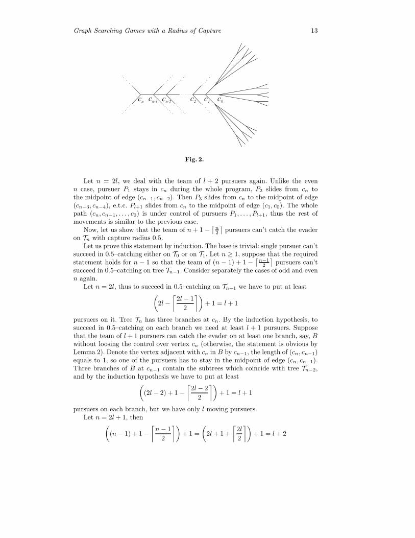
Graph Searching Games with a Radius of Capture 13
c0
c1
cn
cn-1 c
n-2c
2
Fig. 2.
Let n = 2l, we deal with the team of l + 2 pursuers again. Unlike the evenn case, pursuer P1 stays in cn during the whole program, P2 slides from cn tothe midpoint of edge (cn−1, cn−2). Then P3 slides from cn to the midpoint of edge(cn−3, cn−4), e.t.c. Pl+1 slides from cn to the midpoint of edge (c1, c0). The wholepath (cn, cn−1, . . . , c0) is under control of pursuers P1, . . . , Pl+1, thus the rest ofmovements is similar to the previous case.
Now, let us show that the team of n + 1 −⌈n2
⌉pursuers can’t catch the evader
on Tn with capture radius 0.5.Let us prove this statement by induction. The base is trivial: single pursuer can’t
succeed in 0.5–catching either on T0 or on T1. Let n ≥ 1, suppose that the requiredstatement holds for n − 1 so that the team of (n − 1) + 1 −
⌈n−12
⌉pursuers can’t
succeed in 0.5–catching on tree Tn−1. Consider separately the cases of odd and evenn again.
Let n = 2l, thus to succeed in 0.5–catching on Tn−1 we have to put at least(2l−
⌈2l− 1
2
⌉)+ 1 = l + 1
pursuers on it. Tree Tn has three branches at cn. By the induction hypothesis, tosucceed in 0.5–catching on each branch we need at least l + 1 pursuers. Supposethat the team of l + 1 pursuers can catch the evader on at least one branch, say, Bwithout loosing the control over vertex cn (otherwise, the statement is obvious byLemma 2). Denote the vertex adjacent with cn in B by cn−1, the length of (cn, cn−1)equals to 1, so one of the pursuers has to stay in the midpoint of edge (cn, cn−1).Three branches of B at cn−1 contain the subtrees which coincide with tree Tn−2,and by the induction hypothesis we have to put at least(
(2l− 2) + 1−⌈
2l− 2
2
⌉)+ 1 = l + 1
pursuers on each branch, but we have only l moving pursuers.Let n = 2l + 1, then(
(n− 1) + 1−⌈n− 1
2
⌉)+ 1 =
(2l + 1 +
⌈2l
2
⌉)+ 1 = l + 2
14 Tatiana V. Abramovskaya, Nikolai N. Petrov
pursuers are required to succeed in 0.5-catching on Tn−1, but
n + 1−⌈n
2
⌉= l + 1,
and the statement has been proven by Lemma 1.Thus, in virtue of Theorem 2,
εTn(k)
⎧⎪⎨⎪⎩= 0, k = n + 3,
= 0.5, k = n + 2−⌈n2
⌉, . . . , n + 2,
> 0.5, k ≤ n + 1−⌈n2
⌉that was to be proved. ��
3. The minimal trees with the degenerate Golovach function
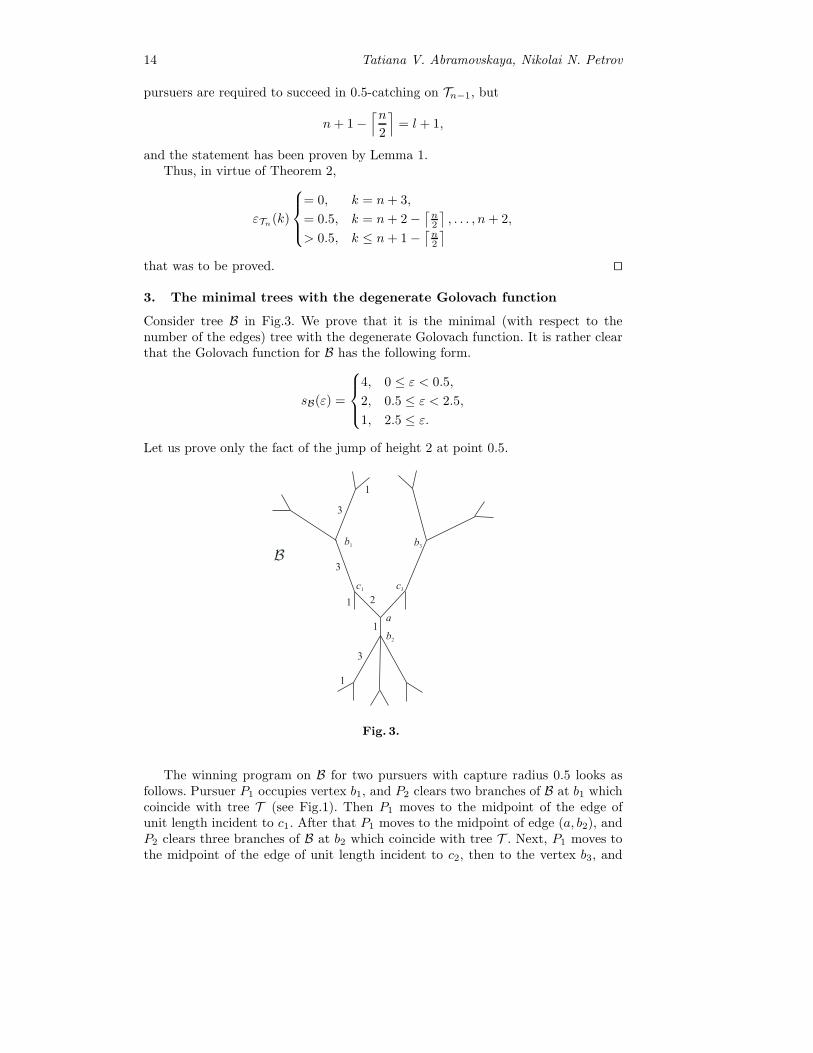
Consider tree B in Fig.3. We prove that it is the minimal (with respect to thenumber of the edges) tree with the degenerate Golovach function. It is rather clearthat the Golovach function for B has the following form.
sB(ε) =
⎧⎪⎨⎪⎩4, 0 ≤ ε < 0.5,
2, 0.5 ≤ ε < 2.5,
1, 2.5 ≤ ε.
Let us prove only the fact of the jump of height 2 at point 0.5.
Fig. 3.
The winning program on B for two pursuers with capture radius 0.5 looks asfollows. Pursuer P1 occupies vertex b1, and P2 clears two branches of B at b1 whichcoincide with tree T (see Fig.1). Then P1 moves to the midpoint of the edge ofunit length incident to c1. After that P1 moves to the midpoint of edge (a, b2), andP2 clears three branches of B at b2 which coincide with tree T . Next, P1 moves tothe midpoint of the edge of unit length incident to c2, then to the vertex b3, and
Graph Searching Games with a Radius of Capture 15
P2 clears the branches at b3 which match up with tree T . After that, the searchprocedure ends.
Suppose 0 < ε′ < 0.5, then three pursuers can’t catch the evader on B withcapture radius ε. Indeed, in virtue of Theorem 2, the three pursuers are necessaryto succeed in capturing on T0 with capture radius ε′.
Consider a tree T , a ∈ T , and δ > 0, let Nδ(a) = {x ∈ T |ρ(a, x) ≤ 2δ} — a setof all 2δ–close to a points of T .
Then trees K1 and K3 (which contain vertices b1 and b3 respectively) obtainedby the closure of set B\N0.5(a) have form T0. Further, the subtree K2 obtained byremoval edge (a, b2) of the branch of B at a which contains vertex b2 has form T0,too. It is clear now that we have to put at least three ε′–far from a pursuers on eachsubtree Ki, i ∈ 1, n to success in ε′–catching on Ki. According to the hypothesis ofLemma 2, three pursuers can’n catch the evader on B with capture radius less than0.5.
We have shown that the Golovach function for tree B has a jump of height 2.Actually, the Golovach function for trees with lower number of edges have no non–unit jumps. First we give several definitions and proposition, and then will provethis statement.
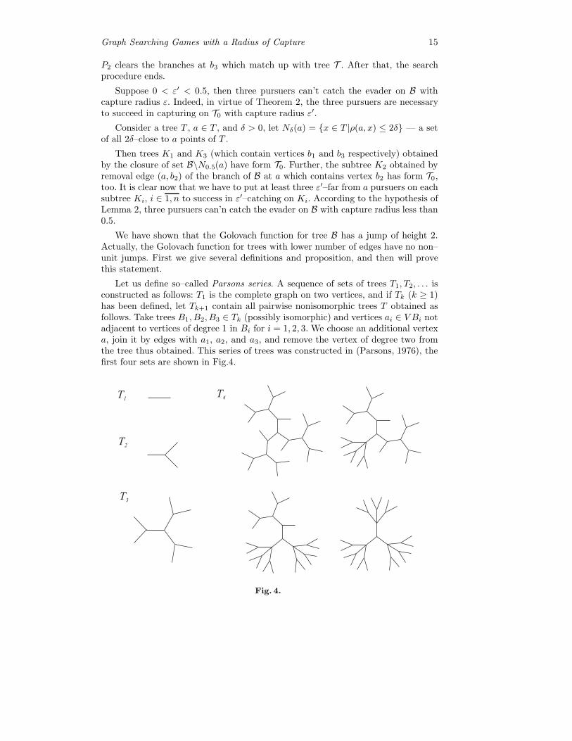
Let us define so–called Parsons series. A sequence of sets of trees T1, T2, . . . isconstructed as follows: T1 is the complete graph on two vertices, and if Tk (k ≥ 1)has been defined, let Tk+1 contain all pairwise nonisomorphic trees T obtained asfollows. Take trees B1, B2, B3 ∈ Tk (possibly isomorphic) and vertices ai ∈ V Bi notadjacent to vertices of degree 1 in Bi for i = 1, 2, 3. We choose an additional vertexa, join it by edges with a1, a2, and a3, and remove the vertex of degree two fromthe tree thus obtained. This series of trees was constructed in (Parsons, 1976), thefirst four sets are shown in Fig.4.
Fig. 4.

16 Tatiana V. Abramovskaya, Nikolai N. Petrov
The contraction of an edge (a, b) in a graph G is the procedure for obtaininga new graph G′ from graph G. Vertices a and b and edge (a, b) are removed, anadditional vertex c is inserted so that the edges incident to c in graph G′ eachcorrespond to an edge incident to either a or b except edge (a, b).
We say that a graph H is contained in a graph G if G has a subgraph G′ suchthat either this subgraph is isomorphic to H or a graph isomorphic to H can beobtained from G′ by contracting some of its edges. A tree T is called a minimal treewith search number k if s(T ) = k and s(T ′) < k for any tree T ′ not isomorphic toT and contained in T .
As was proven in (Golovach, 1992) the Parsons series represent the minimal treeswith the given search number.
Proposition 1. For a tree T , s(T ) = k if and only if there exists a T ′ ∈ Tkcontained in T and any T ′′ ∈ Tk+1 is not contained in T .
We are ready to prove the main result of this section.
Theorem 4. If a tree T has at most 27 edges, then the Golovach function for Thas only unit jumps.
Proof. If s(T ) = 1, then the Golovach function for tree T is constant. If s(T ) = 2,then, by definition, εT (1) > 0, whereas εT (2) = 0. It follows that the Golovachfunction has one unit jump. If s(T ) = 3, then εT (3) = 0, εT (2) > εT (3), andεT (1) > 0. By Corollary 1, εT (2) < εT (1). Thus, 0 = εT (3) < εT (2) < εT (1).
There is the only tree, say, T 14 from the set T4 with 27 edges, thus if s(T ) = 4
then T is isomorphic to T 14 . As above, the following inequalities are obvious:
εT (4) = 0, εT (4) < εT (3), εT (2) < εT (1), εT (1) > 0.
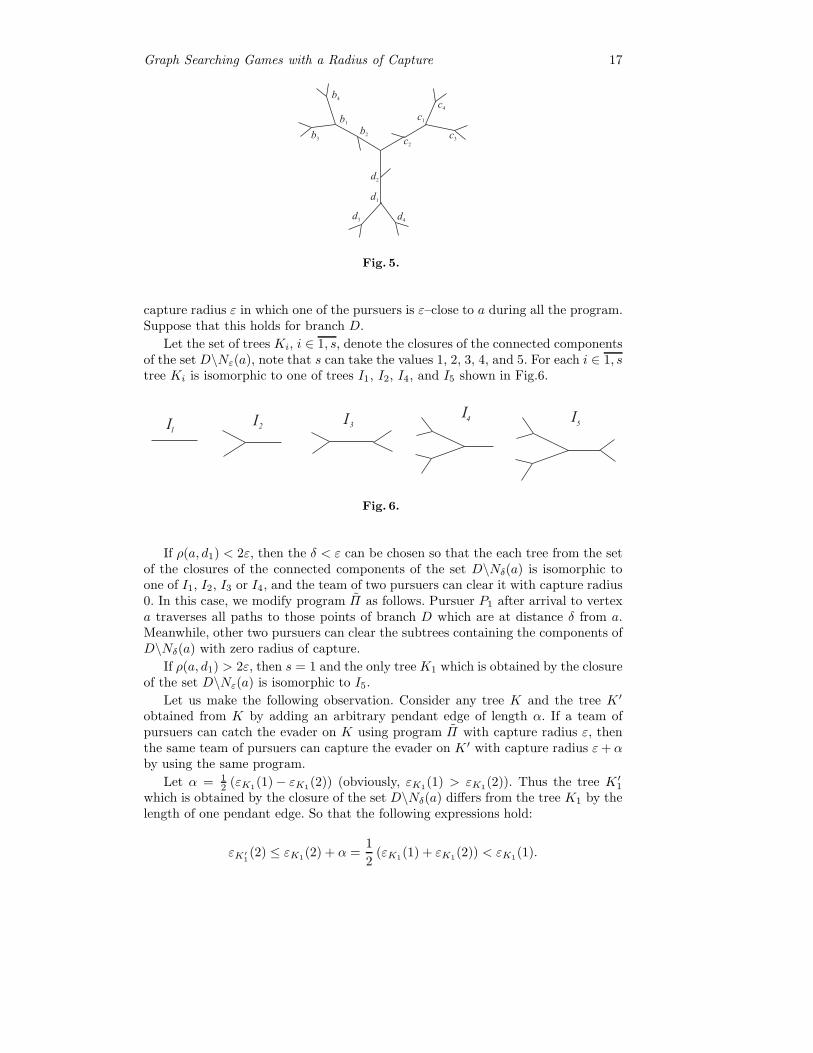
Now we have to check the jump at the point εT (2) is unit.We denote the vertices of tree T as in Fig.5. Let B, C, and D denote the branches
of T at a and containing the vertices b1, c1, and d1, respectively. By Lemma 1, theinequality
εT (2) ≥ max {εB(2), εC(2), εD(2)} (1)
holds. Letε := max {εB(2), εC(2), εD(2)} .
Suppose that the inequality (1) is strict, then we can instantly construct the winningprogram for the team of tree pursuers with capture radius ε: one pursuer occupiesvertex a, and other two pursuers check branches B, C, and D.
Suppose that the inequality (1) is an equality. If the numbers εB(2), εC(2), εD(2)are different, say, εB(2) ≥ εC(2) > εD(2), then we can again specify a program Πon T for three pursuers with capture radius εD(2). This program looks as follows.Pursuer P1 occupies vertex b1, and other two pursuers check the branches at b1 andcontaining b3 and b4 (two pursuers can clear them with zero capture radius). ThenP1 slides to vertex b2, and P2 clears the pendant edge incident to b2. After that, P1
moves to a, and other two pursuers clear tree D. Then P1 moves to c2, P2 clearsthe pendant edge incident to c2, P1 moves to c1, and other two pursuers clear thebranches at c1 which containing c3 and c4. After this step, the program ends.
Consider the case εT (2) = εB(2) = εC(2) = εD(2) = ε. By Lemma 2, for atleast one of branches B, C, D there exists a winning program for two pursuers with
Graph Searching Games with a Radius of Capture 17
c1
c2
c3
c4
b1
b2b
3
b4
d1
d4
d3
d2
Fig. 5.
capture radius ε in which one of the pursuers is ε–close to a during all the program.Suppose that this holds for branch D.
Let the set of trees Ki, i ∈ 1, s, denote the closures of the connected componentsof the set D\Nε(a), note that s can take the values 1, 2, 3, 4, and 5. For each i ∈ 1, stree Ki is isomorphic to one of trees I1, I2, I4, and I5 shown in Fig.6.
I1
2 34I I
I I5
Fig. 6.
If ρ(a, d1) < 2ε, then the δ < ε can be chosen so that the each tree from the setof the closures of the connected components of the set D\Nδ(a) is isomorphic toone of I1, I2, I3 or I4, and the team of two pursuers can clear it with capture radius0. In this case, we modify program Π as follows. Pursuer P1 after arrival to vertexa traverses all paths to those points of branch D which are at distance δ from a.Meanwhile, other two pursuers can clear the subtrees containing the components ofD\Nδ(a) with zero radius of capture.
If ρ(a, d1) > 2ε, then s = 1 and the only tree K1 which is obtained by the closureof the set D\Nε(a) is isomorphic to I5.
Let us make the following observation. Consider any tree K and the tree K ′
obtained from K by adding an arbitrary pendant edge of length α. If a team ofpursuers can catch the evader on K using program Π with capture radius ε, thenthe same team of pursuers can capture the evader on K ′ with capture radius ε + αby using the same program.
Let α = 12 (εK1(1)− εK1(2)) (obviously, εK1(1) > εK1(2)). Thus the tree K ′
1
which is obtained by the closure of the set D\Nδ(a) differs from the tree K1 by thelength of one pendant edge. So that the following expressions hold:
εK′1(2) ≤ εK1(2) + α =
1
2(εK1(1) + εK1(2)) < εK1(1).

18 Tatiana V. Abramovskaya, Nikolai N. Petrov
As was mentioned, there exists a winning program for the team of two pursuers withcapture radius ε on D such that one of the pursuers is ε–close to a during the wholeprogram, which means that εK1(1) ≤ ε. Let us modify program Π again. PursuerP1 after arrival to vertex a moves toward vertex d1 for a distance δ = ε− 1
2α. Othertwo pursuers are able to clear tree K ′
1 with capture radius εK′1(2) < ε. The rest of
the program repeats Π .If ρ(a, d1) = 2ε, then s = 2, let δ = ε
2 . In this case pursuer P1 after arrival to thevertex a passes distant δ toward the vertex d1. Pursuers P2 and P3 act as follows: P2
occupies d3 and P3 clears the pendant edges incident to d3; then P2 and P3 occupyd4, P3 goes to vertex d1, passes distance δ from d1 along the edge (a, d1), returns tod1, clears the pendant edge incident to d1, and returns to d4; next, P2 and P3 moveto d5, and at the final step, P3 clears the pendant edge incident to d5. Program Πthus modified is winning for three pursuers on T with capture radius δ.
If s(T ) ≥ 5, then T contains a tree from T5, while the minimum number of edgesfor a tree from the set T5 is 81. ��
References
Abramovskaya, T. V. (2010). Nontrivial discontinuities of the Golovach functions for trees.Vestnik St. Petersburg Univ. Math., 43(3), 123-130.
Abramovskaya, T. V. and N. N. Petrov (2010). On some problems of guaranteed search ongraphs. Vestnik St. Petersburg Univ. Math., 43(2), 68-73.
Breisch, R. (1967). An intuitive approach to speleotopology. Southwestern Cavers, VI, 72-78.
Golovach, P. A. (1989). Equivalence of two formalizations of a search problem on a graph.Vestnik Leningrad Univ. Math., 22(1), 13-19.
Golovach, P. A. (1990). An extremal search problem on graphs. Vestnik Leningrad Univ.Math., 23(3), 19-25.
Golovach, P. A. (1992). Minimal trees of a given search number. Cybernetics and SystemsAnalysis, 28(4), 509–513.
Golovach, P. A., N. N. Petrov and F. V. Fomin (2000). Search in graphs. Proc. Steklov Inst.Math., 1, S90-S103.
Fomin, F. V. and D. M. Thilikos (2008). An annotated bibliography on guaranteed graphsearching. Theoret. Comp. Science, 399(3), 236-245.
Parsons, T. D. (1976). Pursuit–evasion in a graph. In: Theory and Applications of Graphs(Alavi, Y. and D. R. Lick, eds), Vol. 642, pp. 426-441. Springer: Berlin.
Petrov, N. N. (1982) A problem of pursuit in the absence of information on the pursued.Differ. Uravn., 18(8), 1345–1352 (in Russian).
Non-Cooperative Games with Chained Confirmed Proposals�
G. Attanasi1, A. Garcıa-Gallego2, N. Georgantzıs3 and A. Montesano4
1 LERNA, Toulouse School of Economics2 GLOBE, U. of Granada & LEE, U. Jaume I of Castellon
3 GLOBE, U. of Granada & LEE, U. Jaume I of Castellon & BELIS, U. of Istambul4 Bocconi University, Milan (Italy)
Abstract. We propose a bargaining process with alternating proposals asa way of solving non-cooperative games, giving rise to Pareto efficient agree-ments which will, in general, differ from the Nash equilibrium of the originalgames.
Keywords: Bargaining; Confirmed Proposals; Confirmed Agreement.
JEL classification: C72; C73; C78.
1. Introduction
Since the seminal contributions by Nash (1950, 1953), bargaining models play acentral role in the analysis of situations in which economic agents try to reach anagreement on the split of a certain asset. A plethora of approaches has resulted in avariety of bargaining mechanisms1 keeping fixed the objective of splitting the pie. Ina parallel and mostly independent effort, non-cooperative game theory undertookthe task of determining the actions of individual agents in interactive strategicsituations. While the efficiency of outcomes has been a central issue in both gametheoretic paradigms2, the role of bargaining as a determinant of individual actionsin non-cooperative games has not been systematically explored.
In this paper, we illustrate the consequences of applying alternating proposalprotocols as a way of solving non-cooperative games. From a technical point of view,the basic difference between our framework and that of bargaining over the split of apie is that, in ours, two agents bargain about which strategy profile they will play in anon-cooperative game. Apart from the obvious departure from Rubinstein’s (1982)model in that the set of possible agreements is finite,3 in our setup a confirmedagreement between bargaining agents concerns the pair of strategies that will beactually played in the original non-cooperative game. This fact increases by one thedegrees of freedom and, thus, the dimension of the outcome space, allowing the use
� G. Attanasi gratefully acknowledges financial support by the Chair “Georges Meyer”in Mathematical Economics at Jean-Jacques Laffont Foundation (TSE) and theFrench National Research Agency (ANR) through the project on “Fair Environmen-tal Policies”. N. Georgantzıs and A. Garcıa-Gallego acknowledge financial supportby Bancaixa (P1 1B2007-14) and the Spanish Ministry of Science and Innovation(SEJ2008/04636/ECON). N. Georgantzıs gratefully acknowledges financial support bythe Junta de Andalucıa (P07-SEJ-03155) and hospitality at LEM of University Paris II.
1 While an exhaustive list of the relevant references is beyond the scope of this paper, itis worth mentioning Harsanyi (1956, 1962), Sutton (1986) and Binmore (1987).
2 Relevant references are Harsanyi (1961), Friedman (1971), Smale (1980), and Cubittand Sugden (1994).
3 For a formal treatment of this issue, see the insightful analysis by Muthoo (1991).

20 G. Attanasi, A. Garcıa-Gallego, N. Georgantzıs, A. Montesano
of bargaining with alternating proposals as a method of solving non-cooperativegames.
Assume that two players bargain over the strategy profile to play, given thateach player knows the opponent’s set of possible strategies. Then, there is a non-cooperative game whose execution leads to the two players’ final payoffs and asupergame whose actions in each bargaining period are proposals of strategies forthe original non-cooperative game. Games with confirmed proposals are interac-tive strategic situations in which a player, in order to give official acceptance of acontract, must confirm his/her proposed strategy combined with the strategy cho-sen by his/her opponent.4 Here we focus on non-cooperative games with completeinformation and finite strategy spaces. The bargaining supergame built on themis an infinite horizon game with perfect information. We show that the equilib-rium outcome of the supergame can be unique even though each player’s strategyspace in the supergame and its number of stages are infinite. We call equilibriumconfirmed agreement the corresponding equilibrium contract between players in thesupergame, leading to a strategy profile to be played in the original non-cooperativegame.
2. The Bargaining Supergame
Throughout the paper, we consider only two-players non-cooperative games; thetwo players alternate proposals in the bargaining supergame. The supergame endswhen a player confirms the proposal he/she made the previous stage in which he/shewas active. In modelling the supergame, we focus on a specific family of gameswith confirmed proposals, those with chained proposals. That is, in the case of noconfirmation by one player, the non confirmed strategy profile is taken as the newstarting point for the subsequent negotiation. Except for the selection of the firstmover at the beginning of the supergame, the rules of the game are symmetric.
Let us denote by Sh the finite strategy space for player h (with h = i, j) in theoriginal non-cooperative game. The (super-)game with confirmed proposals is builtsuch that the set of possible proposals of player h in the supergame coincides withthe set of his/her strategies Sh in the original game. The set of possible agreementsof the game with confirmed proposals coincides with the set of outcomes of theoriginal game, i.e. the product set S i × Sj contains all possible agreements of thegame with confirmed proposals built on the original game.
Denote by sth the strategy proposed by player h in stage t of the supergame, witht = 1, 2, ...,+∞. Suppose that player i (“she”) starts the supergame with player j(“he”).
The sequence of alternating proposals is as follows:Stage 1. Player i proposes a certain strategy s1i ∈ Si to player j. Player i would
actually play s1i if (and only if) she would confirm this strategy after the counter-proposal of player j.
Stage 2. Player j proposes strategy s2j ∈ Sj to player i. This strategy would
actually be played if (and only if) either i will confirm her previous strategy s1i orj will confirm his proposal s2j after the counterproposal of player i.
4 The original non-cooperative game can be a game with perfect or imperfect informa-tion and/or with complete or incomplete information. When information is incomplete,players can exploit the bargaining process to extract information on their opponent’stype through their proposals.
Non-Cooperative Games with Chained Confirmed Proposals 21
Stage 3. Player i chooses whether or not to confirm her previous strategy s1i . Ifshe confirms s1i , i.e. s3i = s1i , then the bargaining process ends, through the sequence(s1i , s
2j , s
1i ), with the confirmed agreement (s1i , s
2j) and the two players receive the
payoffs corresponding to the strategy profile (s1i , s2j) in the original game. If she
does not confirm, i.e. she proposes a new strategy s3i = s1i , the bargaining processcontinues with s2j being player j’s proposal and s3i being player i’s counterproposalto j’s proposal.
Stage 4. Player j chooses whether or not to confirm his previous strategy s2j . If
he confirms s2j , i.e. s4j = s2j , then the bargaining process ends, through the sequence
(s2j , s3i , s
2j), with the confirmed agreement (s2j , s
3i ) and the two players receive the
payoffs corresponding to the strategy profile (s3i , s2j) in the original game. If he
does not confirm, i.e. he proposes a new strategy s4j = s2j , the bargaining process
continues with s3i being player i’s proposal and s4j being player j’s counterproposalto i’s proposal.
And so on and so forth.If no strategy profile is ever confirmed by either player, then the outcome is
the disagreement event Ω. Define with f(st−2h , st−1
−h ) the outcome of the game with
confirmed proposals in case the agreement (st−2h , st−1
−h ) would be confirmed in staget, with t = 3, ...,+∞. We assume that each player h’s preference relation �h satisfiesthe following conditions:5
(a) Disagreement is not better than any agreement :Ω �h f(st−2
h ,st−1−h ) for all (st−2
h , st−1−h ) ∈ Sh × S−h and for all t = 3, ...,+∞.
(b) Patience, i.e. the time of the agreement is irrelevant: if st−2h = st
′−2h and st−1
−h =
st′−1−h , then f(st−2
h , st−1−h )∼hf(st
′−2h , st
′−1−h ) for all t = t′, with t, t′ = 3, ...,+∞.
(c) Stationarity, i.e. the preference between two agreements does not depend on
time: if st−2h = st
′−2h , st−1
−h = st′−1−h , st−2
h = st′−2h and st−1
−h = st′−1−h , then
f(st−2h , st−1
−h ) �h f(st−2h , st−1
−h ) if and only if f(st′−2h , st
′−1−h ) �h f(st
′−2h , st
′−1−h ),
for all t = t′, with t, t′ = 3, ...,+∞.
We refer to the extensive (super-)game with perfect information thus defined asthe game with chained confirmed proposals (henceforth GCCP).
In the next section, we analyze the GCCP version of some well-known inter-active strategic situations, extensively studied both in the theoretical and in theexperimental literature. First, we analyze two examples in which the original gameis a 2x2 static game. Then, by maintaining the assumption of two players only, weconcentrate on three cases where the original game is a two-stage dynamic gamewith perfect information.
In each of the GCCP discussed in the paper, we basically look for the set of sub-game perfect equilibrium outcomes (equilibrium confirmed agreements). Now, thebackward induction solution procedure is well-defined for all generic finite gameswith perfect information. Games with confirmed proposals are games with perfectinformation if the non-cooperative game on which they rely is with perfect infor-mation (as in the cases we analyze here). However, they are by construction neitherfinite nor generic, given that different terminal histories can yield the same payoff
5 Conditions (a) and (c) characterize also Rubinstein (1982), while in Rubinstein’s modeltime is valuable and a discount factor is introduced accordingly.

22 G. Attanasi, A. Garcıa-Gallego, N. Georgantzıs, A. Montesano
vector. In fact, the same agreement can be obtained through different combinationsof proposals and counterproposals. Nonetheless, the backward induction procedurecan be easily applied to some non-generic games of perfect information, specificallyto those with no-relevant ties.6 Games with confirmed proposals do belong to thiscategory, if the non-cooperative game on which they rely is static and with no rel-evant ties (as in the two examples in section 3.1). If the original game is dynamic(as in the three examples in section 3.2), the fact that it has no relevant ties isnot enough: given that the payoff function of the game with confirmed proposals isdefined over the strategic form of this game, at least one player 7 each time wherehe/she active, he/she will have at his/her disposal (at least) two proposals (corre-sponding to payoff-equivalent strategies in the original game) leading to (at least)two payoff-equivalent confirmed agreements.
In all the games with confirmed proposals analyzed in the paper, we obtain theequilibrium outcome(s) through iterated weak dominance, that in generic gamesof perfect information yields the backward induction outcome. In section 3.1 weanalyze the GCCP version of the Prisoner’s Dilemma and of the Battle of Sexes.In section 3.2 we focus on the Trust Game, the Entry Game and the UltimatumGame. Here we show that iterated weak dominance yields the backward inductionoutcome also for the GCCP built on these specific dynamic games with no relevantties.
3. Confirmed Agreements in Standard Two-Player Games
3.1. Bargaining over Static Games
Consider the GCCP version of the Prisoner ’s Dilemma (PD). The original gameis a standard static PD, and the bargaining supergame built on it is an infinitehorizon game with perfect and complete information. The sets of players’ feasibleproposals in the GCCP coincide with their sets of actions in the original game: Si =Sj = {Cooperate,Defect}, henceforth {C,D} . Figure 1, with a > c > d > z showsthe simultaneous-move original game and all possible agreements of the bargainingsupergame with chained confirmed proposals built on it.
Fig. 1. Payoff matrix of the PD game
6 A game with perfect information has no relevant ties if, for every pair of distinct terminalhistories, the player who is decisive for one vs the other (i.e. the player who is activeat the last common predecessor of the two terminal histories) is not indifferent betweenthem.
7 This applies to all players having the possibility to observe their opponent’s action inthe constituent game. Only a first mover who is active once does not belong to thiscategory.
Non-Cooperative Games with Chained Confirmed Proposals 23
The original game has the profile (D,D) as equilibrium in dominant actions.The same equilibrium outcome would be found in the standard two-stage game(without bargaining and without confirmation), where one of the two players movesfirst and the other observes his/her “proposal” before choosing his/her own.
Let us now calculate the subgame perfect equilibrium outcome of the GCCPversion of the PD game.
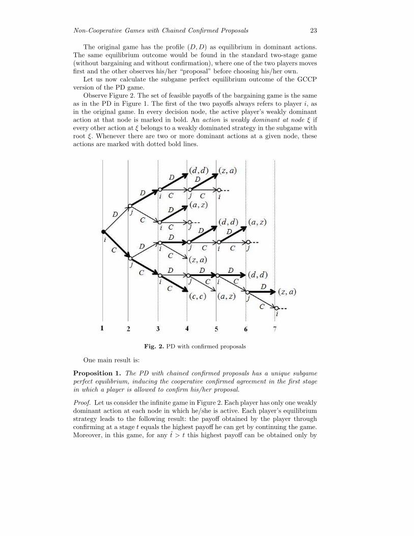
Observe Figure 2. The set of feasible payoffs of the bargaining game is the sameas in the PD in Figure 1. The first of the two payoffs always refers to player i, asin the original game. In every decision node, the active player’s weakly dominantaction at that node is marked in bold. An action is weakly dominant at node ξ ifevery other action at ξ belongs to a weakly dominated strategy in the subgame withroot ξ. Whenever there are two or more dominant actions at a given node, theseactions are marked with dotted bold lines.
Fig. 2. PD with confirmed proposals
One main result is:
Proposition 1. The PD with chained confirmed proposals has a unique subgameperfect equilibrium, inducing the cooperative confirmed agreement in the first stagein which a player is allowed to confirm his/her proposal.
Proof. Let us consider the infinite game in Figure 2. Each player has only one weaklydominant action at each node in which he/she is active. Each player’s equilibriumstrategy leads to the following result: the payoff obtained by the player throughconfirming at a stage t equals the highest payoff he can get by continuing the game.Moreover, in this game, for any t > t this highest payoff can be obtained only by

24 G. Attanasi, A. Garcıa-Gallego, N. Georgantzıs, A. Montesano
confirming the same agreement confirmed at t. The subgame perfect equilibriumis found through iterated weakly dominance in three steps. Observe that in Figure2 (first 7 stages of the game) there are four decision nodes where a player canconfirm the agreement yielding him/her a, his/her highest payoff possible. At staget=4, after the non-terminal history (D,D,C), player j can get a by choosing D,hence confirming his most preferred agreement. If, instead of confirming, playerj chooses to continue the game, he can get, in any subgame in the continuationgame, at most a payoff of a, by confirming the same agreement he could alreadyconfirm at stage t=4. Therefore, for player j confirming (D,C) at stage t=4 weaklydominates continuing the game. The same holds for player i at stage t=3, afterhistory (D,C), and at stage t=5 after history (C,D,D,C); and for player j at staget=6 after history (C,C,D,D,C). Therefore, at the first step the action prescribingnot to confirm the favourable asymmetric agreement is eliminated at each node inwhich it is available. Given that, in order to prevent the opponent from confirminghis/her favorable asymmetric agreement, the agreement (D,D) should be confirmedwhenever possible. Therefore, it is weakly dominant to propose D in each stage twhen at least one of the two players has proposed D in at least a t < t and topropose C otherwise. By eliminating all other actions at the second step, we areleft with the two terminal histories (C,C,C) and (D,D,D). At the third step, theaction D in t=1 is eliminated. ��
Thus, in the unique subgame perfect equilibrium of the game, player i starts byproposing strategy C to player j, who counter-proposes strategy C. Then, player iconfirms her strategy C, such that the original game strategy profile (C,C) is the(unique) confirmed agreement. This is reached already in stage t = 3, after the firstinteraction among players takes place.
Consider now the GCCP version of the Battle of Sexes (BS). The set of players’feasible proposals, which coincides with the set of players’ actions in the originalgame, is Si = Sj = {Opera, Football}, henceforth {O,F} . Figure 3 shows theone-shot original game and, also, all possible agreements of the GCCP built on it.Parameters are such that a > b > max {c1, c2, c3, c4}.
Fig. 3. Payoff matrix of the BS game
The original game has two Nash equilibria in pure strategies: (O,O) and (F, F ).In the standard two-stage dynamic version of the game, the player moving first8
has an advantage. Consider now the BS with confirmed proposals for the case inwhich player i is the first mover (Figure 4). Observe that, surprisingly, there isa first-mover disadvantage: the unique equilibrium confirmed agreement coincideswith the Nash equilibrium of the original game which is preferred by player j.
8 In fact, this is equivalent to a commitment.

Non-Cooperative Games with Chained Confirmed Proposals 25
Fig. 4. BS with confirmed proposals
Proposition 2. The BS with chained confirmed proposals has a unique equilibriumconfirmed agreement, involving players’ coordination on the constituent game equi-librium favourable to the second mover.
Proof. The game ends with the confirmation of the strategy profile (F , F ), whateveris player i’s initial proposal. In each of the two subgame perfect equilibria in purestrategies, j replies to i’s first proposal by indicating the opposite proposal (F if Oand O if F ). By doing that, j obliges player i to propose the same action alreadyproposed by him (otherwise, i would confirm her initial action and would get c1 < bor c3 < b). If this action is F , then j confirms F and gets his highest payoff possible.If instead this action is O, then j proposes F and i finds convenient to propose F,since, otherwise, she would get c1 < b; then j confirms F and gets his highest payoffpossible. Therefore, in the first stage player i is indifferent between her two possibleproposals. ��
Thus, in the BS with chained confirmed proposals the second mover is able toconfirm the coordinating equilibrium outcome of the original game more favorableto him.
3.2. Bargaining over Dynamic Games
Let us now focus on the case where the bargaining supergame concerns a dynamicoriginal game. Here the confirmed proposals structure is built on the strategic formof the original game. Therefore, a player’s set of possible proposals in the GCCPcorresponds to his/her set of strategies in the original game.
Let us begin by considering as original game the Trust Game (TG). In theoriginal game, player i (the truster) chooses whether to Trust (T ) or to Not trust(N) player j (the trustee). In case i trusts j, total profits are higher. In that case, jwould decide whether to Grab (G) or to Share (S) the higher profits. The strategicform of the game in Figure 5, where x :=“x if T ”, with x = G,S, and ci > di >

26 G. Attanasi, A. Garcıa-Gallego, N. Georgantzıs, A. Montesano
z ≥ 0, a > cj > dj > 0, a + z = ci + cj , represents all possible agreements of theGCCP built on this dynamic game.9
Fig. 5. Payoff matrix of the TG
In the unique subgame perfect equilibrium of the original game, i does not trustj, while the latter would choose to grab if i had trusted him in the first place.
Given players’ role asymmetries in the original game, the resulting GCCP in-volves two possible versions: one in which the truster in the original game (i) is thefirst mover of the bargaining sequence, and one in which the trustee in the originalgame (j) is the first mover of the bargaining sequence. In the latter case, j beginsthe GCCP by announcing his intention to grab or to share the higher total profitsin case i would trust him. The two versions of the TG with chained confirmed pro-posals are represented in Figure 6.a and 6.b respectively. Recall that the first of thetwo payoffs always refers to player i, as in the original game.
Fig. 6. TG with confirmed proposals, with i (Figure 6.a) or j (Figure 6.b) as first mover
For the two GCCP in Figure 6, the following result holds.
9 Notice that, in order for j to confirm an agreement, he has to re-propose the samestrategy in two subsequent stages in which he is active. According to this rule, forexample (S,N,G) is not a terminal history of the GCCP, even though both strategyprofiles (N,S) and (N,G) induce the same terminal history in the original game.
Non-Cooperative Games with Chained Confirmed Proposals 27
Proposition 3. The TG with chained confirmed proposals has a unique equilibriumconfirmed agreement, the cooperative one. This agreement is immediately confirmedby the first mover in the GCCP.
Proof. We impose that when a player is active at a decision node, he/she plays aweakly dominant action at that node. Because of that, in both GCCP in Figure6, at each stage t each player would: (1) confirm his/her most preferred agreementif he/she is given the possibility in that stage; (2) confirm agreements other thanhis/her most preferred if: (2.1) in some stage t > t (with t < ∞) of the equilib-rium continuation path, his/her opponent would confirm an agreement not betterfor him/her than the one he/she could confirm in t; (2.2) by not confirming in t,neither (1) nor (2.1) applies to any stage t+k, with k = 1, ...,+∞, and the bestagreement he/she could confirm when he/she is active in the continuation subgameis payoff-equivalent to the one he/she could confirm in stage t. When the first moveris player i, in stage 3 she would confirm (T, S) because of (1). She would confirmalso (N,G) because of (2.1), and (N,S) because of (2.2). Instead, she would notconfirm (T,G), given that none of the above mentioned cases applies. Hence, shewould propose N after history (T,G). In stage 4, after (T,G,N), player j is in-different between confirming the agreement (N,G) and proposing S. In both casesthe payoffs are (di, dj), since, if he proposes S, in the subsequent stage, player iwould confirm (N,S) because of (2.2) (as we have previously seen after history(N,S)). Thus, the subgame perfect equilibrium path is (T, S, T ), with i confirmingthe agreement (T, S) in stage 3. When the first mover is player j, in equilibrium heconfirms the same agreement in stage 3. This follows from the fact that in stage 3 hewould confirm the agreement (T,G) because of (1), (T, S) because of (2.1) and heis indifferent between confirming or not the agreements (N,G) and (N,S) becauseof (2.2) (as we have already seen when the first mover is the player i, after history(T,G,N)). ��
Notice that, as in the example of the BS, in both versions of the TG withchained confirmed proposals, the second mover reciprocates in stage 2 the first-mover’s proposal: he/she cooperates if the first-mover’s proposal is cooperative (Sif T and T if S, respectively) and does not cooperate otherwise (G if N and N ifG, respectively).
Consider now as original game the dynamic Entry Game (EG). In the originalgame i (the potential entrant) chooses whether to Enter (E) or to Stay Out (S) ofthe market, with j (the incumbent) deciding whether to Accommodate (A) or Fight(F ) if the entrant decides to enter. The strategic form of the game in Figure 7, wherex :=“x if E”, with x = A,F , and a > d > 0 > z, represents all possible agreementsof the bargaining GCCP built on this dynamic game. In the unique subgame perfectequilibrium of the original game, i’s entry takes place, with j accommodating it.
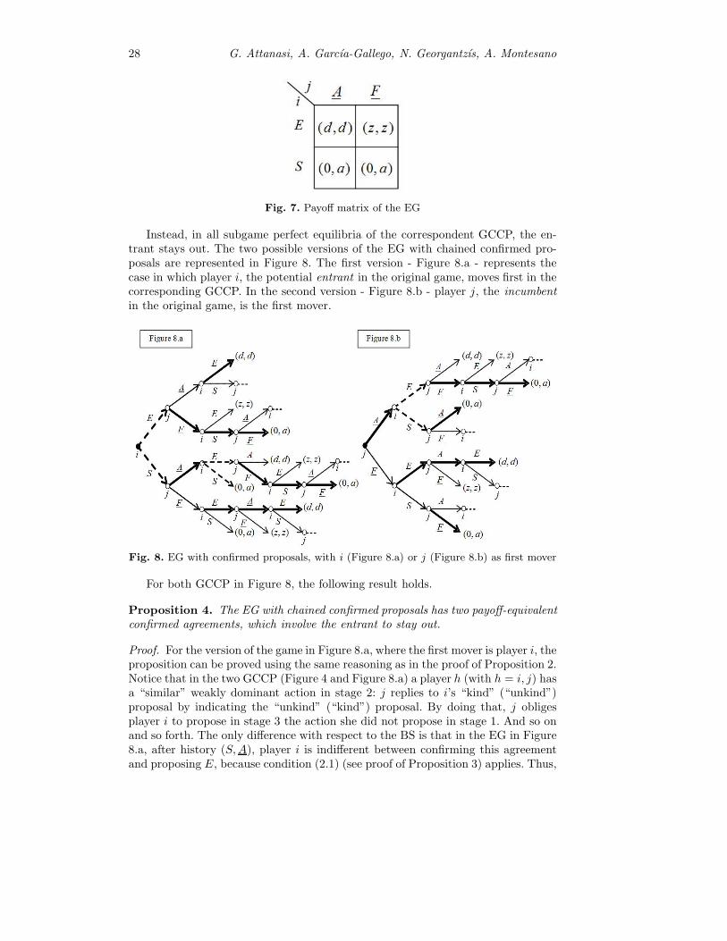
28 G. Attanasi, A. Garcıa-Gallego, N. Georgantzıs, A. Montesano
Fig. 7. Payoff matrix of the EG
Instead, in all subgame perfect equilibria of the correspondent GCCP, the en-trant stays out. The two possible versions of the EG with chained confirmed pro-posals are represented in Figure 8. The first version - Figure 8.a - represents thecase in which player i, the potential entrant in the original game, moves first in thecorresponding GCCP. In the second version - Figure 8.b - player j, the incumbentin the original game, is the first mover.
Fig. 8. EG with confirmed proposals, with i (Figure 8.a) or j (Figure 8.b) as first mover
For both GCCP in Figure 8, the following result holds.
Proposition 4. The EG with chained confirmed proposals has two payoff-equivalentconfirmed agreements, which involve the entrant to stay out.
Proof. For the version of the game in Figure 8.a, where the first mover is player i, theproposition can be proved using the same reasoning as in the proof of Proposition 2.Notice that in the two GCCP (Figure 4 and Figure 8.a) a player h (with h = i, j) hasa “similar” weakly dominant action in stage 2: j replies to i’s “kind” (“unkind”)proposal by indicating the “unkind” (“kind”) proposal. By doing that, j obligesplayer i to propose in stage 3 the action she did not propose in stage 1. And so onand so forth. The only difference with respect to the BS is that in the EG in Figure8.a, after history (S,A), player i is indifferent between confirming this agreementand proposing E, because condition (2.1) (see proof of Proposition 3) applies. Thus,
Non-Cooperative Games with Chained Confirmed Proposals 29
besides the agreement (S, F ), also (S,A) is an equilibrium agreement, equivalent inpayoff to (S, F ). More precisely, if player i starts the bargaining process, there arethree equilibrium terminal histories: (E,F , S, F ), (S,A,E, F , S, F ) and (S,A, S).When the first mover is player j (Figure 8.b), there are two equilibrium terminalhistories: (A,E, F , S, F ) and (A,S,A). This follows from the fact that: each playeralways confirms agreements leading to his/her highest payoff possible, i.e. (d, d) forplayer i and (0, a) for player j; players’ optimal behavior after history (S,A,E) inFigure 8.b is the same as after history (A,E) in Figure 8.a; after history (A), playeri is indifferent between E and S because condition (2.1) (see proof of Proposition3) applies. ��
Therefore, in both GCCP in Figure 8, there is an equilibrium confirmed agree-ment in which the incumbent threatens to fight, (S, F ), and an additional one inwhich he would accommodate in case his opponent would enter, (S,A). In bothagreements the potential entrant accepts to stay out. If player i is the first mover(Figure 8.a), in equilibrium she will either immediately confirms the agreement(S,A) or she will no longer be able to confirm any agreement at all: only player jwould confirm from stage 4 onwards. If player i is not the first mover (Figure 8.b),in equilibrium she will never be able to confirm any agreement: only player j canconfirm (in stage 3 or 5). Notice that, in the GCCP version of the EG, the followingproperties hold:
(i) only two agreements can be confirmed in equilibrium;(ii) the two equilibrium confirmed agreements are payoff-equivalent;
(iii) both of them are Pareto efficient;(iv) none of them is a subgame perfect equilibrium of the original game;(v) in one of the two equilibrium agreements player i’s strategy is not even a best
reply strategy in the original game;(vi) the second mover in the original game (j) is able to benefit from the confirmed
proposals structure, getting his highest payoff possible;(vii) in the equilibrium path, player i is indifferent between her two possible proposals
in the first stage in which she is active;(viii) properties (i)–(vii) hold independently of whether the player is assigned the role
of first mover in the GCCP.
We show below that the same features emerge when analyzing the (super-)gamewith confirmed proposals version of a totally different strategic interaction setting:the Ultimatum Game (UG). In the original game, i (proposer) can offer a fair (F )or unfair (U) division to j (respondent); the latter, after having received i’s offer,may either accept (A) or reject (R). In the (super-)game with confirmed proposalsversion of the original game, the set of i’s possible proposals coincides with heractions in the original game, while the set of j’s possible proposals coincides withhis strategies in the original game, i.e. Sj = {AA,AR,RA,RR}, with xy :=“x if Fand y if U”, with x, y = A,R.
The strategic form of the UG in Figure 9 (with a > f > b > 0) represents allpossible agreements of the GCCP built on this dynamic game.10
10 Recall that confirmation is achieved through re-proposal of the same strategy, thusa history like (AR, F,AA) is not terminal for the GCCP, even though both strategyprofiles (F,AR) and (F,AA) induce the same terminal history in the original game.

30 G. Attanasi, A. Garcıa-Gallego, N. Georgantzıs, A. Montesano
Fig. 9. Payoff matrix of the UG
In the unique subgame perfect equilibrium of the original game, unfair divisiontakes place, with j accepting both i’s offers.
Figure 10 shows the two possible versions of the UG with chained confirmedproposals. Figures 10.a refers to the case in which the proposer in the original gamemoves first in the supergame. Figure 10.b shows the version with the responder inthe original game being the first mover in the supergame.
Fig. 10. UG with confirmed proposals, with i (Figure 10.a) or j (Figure 10.b) as firstmover
For both GCCP in Figure 10, the following result holds.
Proposition 5. The UG with chained confirmed proposals has an infinite numberof subgame perfect equilibria, all leading to two payoff-equivalent confirmed agree-ments, which involve the egalitarian outcome.
Proof. The proof is similar for the two versions of the GCCP. Consider the firstversion of the game, where i is the first mover (Figure 10.a). By imposing that eachplayer chooses a weakly dominant action at each node where he/she is active, playeri is never able to confirm her most preferred agreement (U,AA) or (U,RA). In fact,if she proposed an unfair offer, j would reply with a proposal not incorporating

Non-Cooperative Games with Chained Confirmed Proposals 31
the acceptance of U (AR or RR), otherwise i would confirm U in the subsequentstage. Therefore, in every subgame after i has proposed U , j would never proposeAA or RA. Then, both after each history of the type (..., stj , U,AR) with stj = ARand after each (..., stj , U,RR) with stj = RR , i would propose F , otherwise shewould confirm j’s rejection of her unfair offer, hence getting 0. Then, after each(..., stj , U,AR, F ) with stj = AR, j would propose AR, thus confirming his mostpreferred agreement (F,AR); after each (..., stj , U,RR, F ) with stj = RR, j wouldnever propose RR, because that would lead to confirm an agreement involvingthe rejection of i’s fair offer, hence getting 0. Moreover, player j is always able toavoid confirming the agreements (U,RR) and (U,AR). In fact, after each history(..., RR,U), he would propose the strategy AR, thus avoiding to confirm the zero-payoff agreement (U,RR) or to give player i the possibility to confirm (U,AA) or(U,RA) in the subsequent stage; after each history (..., AR,U), he would proposeRR, thus avoiding to confirm the zero-payoff agreement (U,AR), or to give player ithe possibility to confirm (U,AA) or (U,RA) in the subsequent stage. This explainswhy whenever an agreement is confirmed by j in a stage t > 3, this agreement is(F,AR) and each terminal history is of the type (..., U,AR, F,AR). All previousconsiderations about player j’s weakly dominant proposals in stage t conditionalon i’s possible proposals in stage t − 1 explain why player i could never obtainthe confirmation of an agreement which would impose player j to accept an unfairoffer. Therefore, whenever in a stage t > 3 she has to choose between confirmingan agreement (F,Ax), with x = A,R and entering a subgame leading to a terminalsub-history of the type (U,AR,F,AR), she is indifferent according to condition (2.2)(see proof of Proposition 3): both choices allow player i to get her second highestpayoff possible and player j to get his highest payoff possible. Moreover, given thati would always propose F in each decision node where she could confirm (U,RR),then, after every sequence of proposals (F, stj , U,RR) with stj = AA,AR,RA, someequilibrium loops could emerge, thus leading to an infinite number of equilibriumterminal histories, all ending with player j’s confirmation of the agreement (F,AR),or with player i’s confirmation of the agreement (F,Ax), with x = A,R. The onlycase in which player j can confirm, in equilibrium, an agreement different from(F,AR) is in stage 3 of the GCP (Figure 10.b), where he confirms the payoff-equivalent agreement (F,AA). ��
Therefore, in every subgame perfect equilibrium of the UG with chained con-firmed proposals, i offers a fair division to j, and j accepts. In each GCCP inFigure 10 we indicated the unique equilibrium terminal history leading to confirmthe agreement (F,AA) in stage 3, and two among the infinite possible equilibriumterminal histories leading to confirm the agreement (F,AR) in a stage t > 3. Bothkind of agreements lead to a fair division.
Quite surprisingly, the equilibrium agreements of the chained confirmed propos-als version of the UG satisfy the same features (i)–(viii) characterizing the equilibriain the EG with chained confirmed proposals. In this regard, note also the strongsimilarity between the subgame perfect equilibrium paths of TG with chained con-firmed proposals in Figure 6.a and those of the PD with chained confirmed proposalsin Figure 2. The same holds for the EG with chained confirmed proposals in Figure8.a and the BS with chained confirmed proposals in Figure 4. Finally, for the threeGCCP in Figure 4 (BS), 8.a (EG) and 10.a (UG) it is common that a first-mover
32 G. Attanasi, A. Garcıa-Gallego, N. Georgantzıs, A. Montesano
disadvantage exists, while instead the relative original games are all characterizedby a first-mover advantage.
All these results suggest that the bargaining mechanism proposed in this paperas a supergame works in the same way for original games with different strategicstructures.
4. Conclusions
Throughout the paper, we have defined games with confirmed proposals as a wayof representing bargaining over the strategies of a non-cooperative game. We haveshown the effect of this mechanism on players’ ability to coordinate on Pareto ef-ficient outcomes even in cases in which they are not equilibrium outcomes of theoriginal non-cooperative game. Our focus was on a confirmed proposal mechanismwith a chain, requiring that in the bargaining supergame each non-confirmed strat-egy profile becomes the starting point for the next negotiation round. One coulddiscuss the implications of breaking this chain on the main features of the confirmedproposal mechanism. We leave this for future research.
References
Binmore, K. (1987). Perfect equilibria in bargaining models. In: Economics of Bargaining(Binmore, K. and P. Dasgupta, eds), Cambridge University Press, Cambridge.
Cubitt, R. and R. Sugden (1994). Rationally justifiable play and the theory of non-cooperative games. Economic Journal, 104, 798-803.
Friedman, J. W. (1971). A non-cooperative equilibrium for supergames. Review of EconomicStudies, 38, 1-12.
Harsanyi, J. (1956). Approaches to the bargaining problem before and after the theory ofgames: A critical discussion of Zeuthen’s, Hicks’, and Nash’s theories. Econometrica,24, 144-157.
Harsanyi, J. (1961). On the rationality postulates underlying the theory of cooperativegames. Journal of Conflict Resolution, 5, 179-196.
Harsanyi, J. (1962). Bargaining in ignorance of the opponent’s utility function. Journal ofConflict Resolution, 6, 29-38.
Muthoo, A. (1991). A note on bargaining over a finite number of feasible agreements.Economic Theory, 1, 290-292.
Nash, J. (1950). The bargaining problem. Econometrica, 18, 155-162.Nash, J. (1953). Two-person cooperative games. Econometrica, 21, 128-140.Rubinstein, A. (1982). Perfect equilibrium in a bargaining model. Econometrica, 50, 97-
109.Smale, S. (1980). The Prisoner’s Dilemma and Dynamical Systems Associated to Non-
cooperative Games. Econometrica, 48, 1617-1634.Sutton, J. (1986). Non-cooperative bargaining theory: An introduction. Review of Economic
Studies, 53, 709-724.

The Π-strategy: Analogiesand Applications
A.A. Azamov1 and B.T. Samatov2
1 Institute of Mathematics and Informational Technologiesof Academy of Sciences of UzbekistanE-mail: [email protected]
2 Namangan State University, UzbekistanE-mail: [email protected]
Abstract. The notion of the strategy of parallel pursuit (brieflyΠ-strategy)was introduced and used to solve the quality problem in ”the game with asurvival zone” by L.A.Petrosyan. Further it was found other applications ofΠ-strategy. In the present work Π-strategy will be constructed in the caseswhen 1) a control function of Pursuer should be chosen from the space L2
and that for Evader should be chosen from L∞; 2) control functions bothof players should be chosen from the space L2; 3) a control function of Pur-suer should be chosen from intersection of spaces L2 and L∞ while that forEvader should belong to L∞.
Keywords: differential game, Pursuer, Evader, strategy, parallel pursuit,domain of attainability, survival zone
AMS classification numbers: 91A23, 49N70
1. Formulation of the problem
Consider the differential game when Pursuer P and Evader E having radius vectorsx and y correspondingly move in the space Rn. If their velocity vectors are u and vthen the game will be described by the equations:
x = u, x(0) = x0,y = v, y(0) = y0,
(1)
where x, y, u, v ∈ Rn, n > 1, x0 and y0 are initial points of x and y correspondingly.The family of all measurable functions u(·) : R+ → Rn (controls of P ) satisfying
the following condition∞∫0
|u(t)|2dt ≤ ρ2, ρ ≥ 0, (2)
is denoted by Uρ, Uρ ⊂ L2[0,∞). The family of all measurable functions u(·) :R+ → Rn satisfying the next condition
|u(t)| ≤ α almost everywhere (a.e.) t ≥ 0, (3)
is denoted by Uα, Uα ⊂ L∞[0,∞). Further the family of all measurable functionssatisfying both of conditions (2) and (3) will be denoted Uρ
α.Analogously the family of all measurable functions v(·) : R+ → Rn satisfying
∞∫0
|v(t)|2dt ≤ σ2, σ ≥ 0, (4)

34 A. A. Azamov, B. T. Samatov
is denoted by V σ, V σ ⊂ L2[0,∞) and satisfying the following condition
|v(t)| ≤ α a. e. t ≥ 0 (5)
is denoted by Vβ , Vβ ⊂ L∞[0,∞). Besides the family of all measurable functionssatisfying both of conditions (4) and (5) also will be denoted V σ
β .In the theory of Differential Games an inequality of the forms (2) and (4) is
usually called an integral constraint for control function (we will briefly say I-constraint). Analogously an inequality of the forms (3) and (5) is called a geometricconstraint (briefly G-constraint).
The condition consisting of both inequalities (2)-(3) (or (4)-(5)) will be called acomplex constraint (briefly C-constraint).
If U (correspondingly V ) is one the introduced classes then there would be9 possibilities of pairs (U, V ) each of them generates the appropriate variant ofsimple motioned pursuit-evasion game. For brevity we will indicate this addingcorresponding abbreviations to the word ”game” as a prefix. For example the pair(Uα, Vβ) defines G-game, (Uρ, Vβ) does IG-game and e. c.
We are going to study mainly the game with phase constraints for Evader beinggiven by a subset L of Rn which is called ”a Survival Zone” (for Evader naturally).(Notice that in the case L = ∅ we have a simple pursuit-evasion game.)
Each pair (x0, u(·)) consisting of an initial position x0 and a control functionu(·) ∈ U (correspondingly (y0, v(·)), v(·) ∈ V ) generates the path by the formula
x(t) = x0 +
t∫0
u(s)ds, (y(t) = y0 +
t∫0
v(s)ds).
Further we will assume initial positions x0 and y0 are given such that x0 = y0and y0 ∈ L.
In the game ’with the Survival Zone L’ Pursuer P aims to catch Evader E, i.e.to realize the equality x(t) = y(t) for some t > 0, while E stays in the zone Rn \L.The aim of E is to reach the zone L before being caught by Pursuer or to keep therelation x(t) = y(t) for all t, t ≥ 0. Notice that L doesn’t anyway restrict motion ofP .
The Differential Game with ’a Survival Zone’ was suggested by R. Isaacs in(Isaacs, 1965) for G-game. He solved it when L was a half-plane and formulated theProblem 5.9.1 about the case when L is a disk. The game solved by L.A.Petrosyanfor an arbitrary convex survival zone introducing the strategy of parallel pursuit(briefly Π-strategy; the prefix Π can be interpreted as meaning the word ’parallel’and the initial letter of the family name of its author as well). About further studies,see (Azamov, 1986) - (Azamov and Samatov, 2000), (Petrosyan, 1977) - (Petrosyanand Dutkevich, 1969), (Satimov, 2003)- (Samatov, 2008).
Well known that control functions for P are not sufficient to solve a pursuitproblem as they depend only on time-parameter t, t ≥ 0 so the suitable types ofcontrols should be strategies. There are different ways of defining such a notion. Forus it is enough the following conception.
Definition 1. The map u : V → U is called the strategy for P if the followingproperties are held:
1o (admissibility). For every v(·) ∈ V the inclusion u(·) = u[v(·)] ∈ U is true.

The Π-strategy: Analogies and Applications 35
2o (volterranianity). For every v1(·), v2(·) ∈ V and t, t ≥ 0, the equality v1(s) =v2(s) a.e. on [0, t] implies u1(s) = u2(s) a.e. on [0, t] with ui(·) = u[vi(·)], i = 1, 2.
Definition 2. A strategy u(v) is called winning for P on the interval [0, T ] in thesimple game if for every v(·) ∈ V there exists a moment t∗ ∈ [0, T ] that is to reachthe equality x(t∗) = y(t∗).
Definition 3. A strategy u(v) for the player P is called winning on the interval[0, T ] in the game with ”the survival zone” L if for every v(·) ∈ V there exists somemoment t∗ ∈ [0, T ] that
1) x(t∗) = y(t∗);
2) y(t) ∈ L while t ∈ [0, t∗].
Definition 4. A control function v∗(·) ∈ V for the player E is called winning inthe game with ”the survival zone” L if for every u(·) ∈ U : 1) there exists somemoment t, t > 0, that y(t) ∈ L and x(t) = y(t) while t ∈ [0, t]; or 2)x(t) = y(t) forall t ≥ 0.
2. The ΠG-strategy
2.1. Definition of the ΠG-strategy
The main aim of the present paper is to construct analogies of Π-strategy forIG−, I− and CG-games. In this section the definition and some properties of Π-strategy settled by L.A.Petrosyan will be given for fullness of the exposition usinganalytical approach (see (Petrosyan, 1977)).
The G-game is a problem on simple pursuit with geometric constraints |u| ≤ αand |v| ≤ β for the control functions of the players P and E respectively .
Let z = x − y. In order to define the ΠG-strategy consider a state vector ζ =(x, y) such that x = y and suppose E holds the constant control v, v ∈ Sβ whereSβ = {v : |v| ≤ β} is a ball. If P also applies the constant vector u, |u| = α, helpingP to meet E at some moment T, T > 0, then Tu = Tv − z or
u = v − λξ (6)
where λ = |z|/T and ξ = z/|z|. From (6) the following equation for λ will beobtained: λ2− 2〈ξ, v〉λ−α2 + v2 = 0, where < v, ξ > is the scalar production of thevectors v and ξ in Rn. It has the positive root λG(z, v) = 〈ξ, v〉+
√DG(z, v) if and
only if
DG(z, v) := 〈ξ, v〉2 + α2 − |v|2 ≥ 0. (7)
Substituting this value into (6) adduces to the formula
u = v − λG(z, v)ξ =: uG(z, v). (8)
Definition 5. The function uG(z, v) defined on the region (7) is called the strategyof parallel pursuit in the G-game or briefly the ΠG-strategy.
36 A. A. Azamov, B. T. Samatov
Let the initial state ζ0 be fixed, z0 = x0− y0 and E applies the arbitrary controlv(·) ∈ Vβ while P runs the ΠG-strategy. Then the dynamics of the vector z will bedescribed by the Cauchy problem:
z = x− y = −λG(z, v(t))ξ, z(0) = z0. (9)
Obviously, the conditions of the existence theorem of Caratheodory (Alekseevet al., 1979) for the problem (9) are valid therefore that has the unique solution.Denote it z(t, z0, v(·)) or simply z(t) and call a trajectory.
The following statement explains the term ”parallel pursuit” for the ΠG-strategy(Petrosyan, 1965, 1977).
Theorem 1. For every z0, z0 = 0, and v(·) ∈ Vβ the formula z(t) = ΛG(t)z0 is
true where ΛG(t) = 1− 1|z0|
t∫0
λG(z0, v(s))ds.
Corollary.
uG(z(t), v(t)) = uG(z0, v(t)), t ≥ 0. (10)
Indeed, uG(z, v) is homogeneous on the variable z.
Henceforth ΛG(·) will be called the approach function in the G-game whileλG(z, v) can be interpreted as the speed of approach.
Theorem 2. In the G-game ΠG-strategy is wining for P on the interval [0, TG],where TG = |z0|/(α− β).
2.2. ΠG-strategy and Apollonian sphere
The first essential application of ΠG-strategy was brought out to the game with sur-vival zone (Petrosyan, 1965, 1977) basing on an interesting link between ΠG−strategyand Apollonian sphere.
To expose this link let us consider the region
AG(x, y) =
{w : |w − x| ≥ α
β|w − y|
};
what’s boundary is just Apollonian sphere. Bringing its equation to the form |w −cG| = RG one easily can find the center cG(x, y) and the radius of Apollonian sphere(Azamov, 1986): cG(x, y) = (α2y − β2x)/(α2 − β2), RG(x, y) = αβ|z|/|α2 − β2|.
It’s easy to proof using (10) the following property
Theorem 3. AG(x(t), y(t)) = x(t) + ΛG(t)[AG(x0, y0) − x0] for t ∈ [0, t∗], wheret∗ = min{t : z(t) = 0}.
Theorem 4 (monotonicity of Apollonian Sphere (Petrosyan, 1965, 1977)).If 0 ≤ t1 ≤ t2 then AG(x(t1), y(t1)) ⊃ AG(x(t2), y(t2)).
Below in the section 6 the direct analytical proof of these assertions will be repre-sented for more general situation.
The Π-strategy: Analogies and Applications 37
2.3. G-game with ”a Survival Zone”
It has been noted above that Isaacs’ game with ”line of survival” was solved byL.A.Petrosyan using the method of approximating measurable controls by piecewiseconstant.
Theorem 5 (L.A.Petrosyan’s theorem). If α > β and L⋂AG(x0, y0) = ∅
then the ΠG-strategy is winning in G-game with the Survival zone L.
P r o o f follows from Theorem 3.
C o m m e n t. The condition of Theorem 4 is necessary the player P towin. This is obvious for the condition α > β. If L
⋂AG(x0, y0) = ∅, for example the
intersection contains a point w, then E is able reaches w by the constant controlv = β(w − y0)/|w − y0| and wins the game.
3. ΠIG-strategy
Now let us consider IG-game where controls of P should satisfy integral constraintswhile controls of E do geometric constraints. Our aim is to transfer constructionsof L.A.Petrosyan to IG-game.
3.1. Definition of ΠIG-strategy
First of all we are to notice in IG-game as distinct from the G-game the currentphase state ζ should also include besides geometrical positions x, y (or reducedphase parameter z = x− y if this is enough) the current resource ρ of the player Pdefining by the formula
ρ(t) = ρ2 −t∫
0
|u(s)|2ds.
Therefore in IG-game a state vector must be the triple ζ = (x, y, ρ). Choosingthe vector u and the number T from the conditions: Tu = Tv − z, T |u|2 = ρ onegets the following quadratic equation for the variable λ = |z|/T :
λ2 − 2λ(μ/2 + 〈ξ, v〉) + |v|2 = 0, (11)
where μ = ρ/|z|, ξ = z/|z|.Further in this section we will suppose μ ≥ 4β. This implies the discriminant
D(z, ρ, v) := (μ/2 + 〈ξ, v〉)2 − |v|2 is nonnegative and the equation (11) has thepositive root λIG(z, ρ, v) = μ/2 + 〈ξ, v〉+
√D(z, ρ, v).
Though the obtained formula for λIG is some bulky it takes part in the following
Definition 6. The function uIG(z, ρ, v) := v − λIG(z, ρ, v)ξ defined in the regionμ ≥ 4β is called the ΠIG-strategy in the IG-game for the player P.
Let us suppose that a perty in IG-game starts from a initial state ζ0 = (x0, y0, ρ2)
and P applies ΠIG-strategy while E may choose any control function v(·) ∈ Vβ .These data naturally generate the augmented trajectory x(t), y(t), ρ(t) describingthe party in IG-game. Now put z(t) = x(t)− y(t). Then the path (z(t), ρ(t)) will befound as the solution of Cauchy problem{
dz/dt = −λIG(z, ρ, v(t))z/|z|, z(0) = z0,
dρ/dt = −λIG(z, ρ, v(t))ρ/|z|, ρ(0) = ρ2,(12)
which is valid while μ ≥ 4β and z = 0.

38 A. A. Azamov, B. T. Samatov
Theorem 6. If D(z(t), ρ(t), v(t)) ≥ 0 a.e. on some interval [0, t∗), t∗ > 0, then
a) μ(t) = μ0, where μ0 = ρ2/|z0|;b) uIG(z(t), ρ(t), v(t), ) = uIG(z0, ρ
2, v(t));
c) |uIG(z0, ρ2, v(t))|2 = μ0λIG(z0, ρ
2, v(t)).
P r o o f is immediately followed from the equation (12).
This statement allows to redefine ΠIG-strategy in more simply way putting
uIG(v) = v − λIG(z0, ρ2, v)ξ0.
3.2. IG-game without phase constraints
Let an initial position and control v(·) ∈ Vβ of E be given and P run ΠIG-strategy.Then one has the generated trajectory z(t) and can define the approach function inIG-game by the following way
ΛIG(t) = 1− 1
|z0|
t∫0
λIG(z0, ρ2, v(s))ds.
Denote TIG = |z0|/(μ0
2 − β +
√μ20
4 − μ0β).
The following statements expresses an analogy of the properties of ΠG-strategyfor IG-game.
Theorem 7. If 4β ≤ μ0 then for every v(·) ∈ Vβ the following properties are true
a) z(t) = ΛIG(t)z0; ρ(t) = ΛIG(t)ρ2;
b) there is t∗ ∈ [0, TIG] such that ΛIG(t∗) = 0 and ΛIG(t) > 0 while t < t∗.
Theorem 8. If 4β ≤ μ0 then in the simple motion IG-game the ΠIG-strategy iswinning on [0, TIG].
P r o o f of these theorems in more general situation will be given in the section 5.
3.3. Pascal’s snail and Cartesian’s oval
As in G-game in order to solve IG-game with a survival zone following L.A.Petrosyanwe will try to find the set of all points where P is able to reach earlier than Esupposing they start their motions from some current positions x, y respectively.
Let E moves holding a constant vector v and P aims to catch it by a constantcontrol u as well spending over his resource ρ. Let w be a point where P meetsE. The set of all such points will be described by the following relations: |w −x| = T |u|, |w − y| = T |v|, T |u|2 = ρ. Excluding T and |u| one gets the surface|v||w − x|2 = ρ|w − y| that bounders the searching region
AIG(x, y, ρ) ={w : |w − x|2 ≥ (ρ/β)|w − y|
}For n = 2 the boundary of the region AIG will be Cartesian oval (if 4β < μ) or
the inner loop of Pascal’s snail (if 4β = μ). It is interesting to remember here thatsuch curves appeared in G-game with a survival zone considered under terminalcondition of l-capture (Petrosyan and Dutkevich, 1969).

The Π-strategy: Analogies and Applications 39
3.4. IG-game with ”a Survival Zone”
Now let P hold the ΠIG-strategy while E can apply any control v(·) ∈ Vβ . Naturallyan initial position is being considered.
Theorem 9. The following properties take a place:A. AIG(x(t), y(t), ρ(t)) = x(t) + ΛIG(t)[AIG(x0, y0, ρ
2)− x0].B. If 0 ≤ t1 ≤ t2 then AIG(x(t1), y(t1), ρ(t1)) ⊃ AIG(x(t2), y(t2), ρ(t2)).
The statement will be also proven below in the section 5. It implies
Theorem 10 (Petrosyanian type theorem). If 4β ≤ μ0 andL⋂AIG(x0, y0, ρ
2) = ∅ then ΠIG-strategy is winning in IG-game with ”the SurvivalZone” L (for E).
C o m m e n t. The condition of the last theorem is necessary, too, because onecan easily notes that if a) 4β ≤ μ0 and L
⋂AIG(x0, y0, ρ
2) = ∅ or b) 4β > μ0
then the Player E would win the game holding simply some constant control v∗,|v∗| = β.
4. ΠI-strategy
4.1. Definition of ΠI-strategy
Now we consider I-game where admissible controls of both players should satisfyintegral constraints as u(·) ∈ Uρ, v(·) ∈ V σ (see (Ushakov, 1972)). Since consider-ations principally repeat those provided for G- and IG-games here they will exposesomewhat shorter. In I-game a state vector should be a quadruple ζ = (x, y, ρ, σ)including current values of the rest of resources of the players P and E respectively,i.e.
ρ(t) = ρ2 −t∫
0
|u(s)|2ds, σ(t) = σ2 −t∫
0
|v(s)|2ds.
Arguments, like above, lead to the following system to build the Π-strategy forthe I-Game: Tu = Tv−z ρ−T |u|2 = σ−T |v|2, T > 0 or u = v−λξ, |u|2−|v|2 =λδ where λ = |z|/T, δ = (ρ− σ)/|z|. Hence
λ = δ + 2〈ξ, v〉. (13)
Obviously, the formula (13) has sense when δ + 2〈ξ, v〉 > 0. If δ+ 2〈ξ, v〉 ≤ 0 weput λ = 0. Unifying two cases gives the next formula
λI(z, δ, v) := max{0, δ + 2〈ξ, v〉}.
Definition 7. The function uI(z, δ, v) := v − λI(z, δ, v)ξ is called ΠI-strategy inthe I-game.
Let the initial state ζ = (x0, y0, ρ2, σ2) be given and z0 = x0 − y0. Suppose
P applies ΠI -strategy while E may choose any control function v(·) ∈ V σ. Thesedata naturally generate the augmented trajectory x(t), y(t), ρ(t), σ(t) describingthe party in I-game.
40 A. A. Azamov, B. T. Samatov
Now put z(t) = x(t) − y(t) and δ(t) = θ(t)/|z(t)|, where θ(t) = ρ(t) −σ(t), θ(0) = θ0 = ρ2 − σ2. Notice δ0 = δ(0) = θ0/|z0|. Then the path (z(t), θ(t))will be defined as the solution of Cauchy problem{
dz/dt = −λI(z, δ, v(t))z/|z|, z(0) = z0,
dθ/dt = −λI(z, δ, v(t))θ/|z|, θ(0) = θ0.(14)
The problem (14) has the unique solution while z = 0.
Theorem 11. If δ(t) > 0 a.e. on some interval [0, t∗), t∗ > 0, then
a) δ(t) = δ0;
b) uI(z(t), δ(t), v(t)) = uI(z0, δ0, v(t));
c) |uI(z0, δ0, v(t))|2 = |v(t)|2 + λI(z0, δ0, v(t))δ0.
Proof is easily follows from the equation (14)
Thanks to the property b) the function
uI(v) = uI(z0, δ0, v) = v − λI(z0, δ0, v)ξ0
can be used as ΠI -strategy instead of uI(z, δ, v).
4.2. I-game
Here the following function
ΛI(t) = 1− 1
|z0|
t∫0
λI(z0, δ0, v(s))ds
services as the measure of approach of P to E.
Theorem 12. z(t) = ΛI(t)z0, θ(t) = ΛI(t)θ0.
Theorem 13. If ρ > σ then ΠI-strategy is winning in the interval [0, TI ] whereTI = |z0|2/(ρ− σ)2.
Proof. Applying the inequality of Cauchy to the scalar production in (13) givesthe estimation ΛI(t) ≤ 1 −max{0, δ0t − 2σ
√t}/|z0|. That’s why there exists t∗,(
2σδ0
)2< t∗ ≤ TI such ΛI(t
∗) = 0.
Further we are to verify admissibility of the corresponding realization of ΠI -strategy when E runs his admissible control v(·) ∈ V σ. Thus
t∗∫0
|uI(v(s))|2ds =
t∗∫0
|v(s)|2ds + δ0
t∗∫0
λI(v(s))ds ≤ σ2 + δ0|z0| = ρ2,
where t∗ = min{t : ΛI(t) = 0} Q.E.D.

The Π-strategy: Analogies and Applications 41
4.3. I-game with a ”Survival Zone”
Let the current state ζ = (x, y, ρ, σ), x = y, be considered and E be supposedmoving by a constant velocity v. Consider the situation when P tries to catch Ealso by a constant control u unless the players spend their resource fully. If w isthe point where P meets E and T is the time of occurrence of such event then|w − x| = T |u|, |w − y| = T |v|, T |u|2 = ρ, T |v|2 = σ.
In the case ρ > σ the exclusion of T, |u| and |v| from the relations just writtengives the equation of the Apollonian sphere |w − cI | = RI where cI = y − σξ0/δ0and RI =
√ρ σ/δ0.
Denote
AI(ζ) =
{{w : |w − cI | ≤ RI} if ρ > σ,
{w : 〈2w − x− y, z〉 ≤ 0} if ρ = σ.
And now consider the party in the I-game when P holds ΠI -strategy while Eapplies some his admissible control v(·) ∈ Vβ accounting some initial position isfixed.
Theorem 14. AI(ζ(t1)) ⊃ AI(ζ(t2)) for 0 ≤ t1 ≤ t2.
The Proof is elementary and differs in the cases ρ > σ and ρ = σ but requires longcalculations that’s why will be omitted here.
Theorem 15 (Petrosyanian type theorem). If ρ ≥ σ and L∩AI(ζ0) = ∅ thenthe ΠI-strategy is winning for P in the I-Game with ”the Survival Zone L.”
C o m m e n t. If either a) ρ ≥ σ and L ∩ AI(ζ0) = ∅ or b) ρ < σ thenthere exists a control function v∗(t) ∈ V σ being considered as a particular sort ofstrategies of E is winning for E in the I-Game with ”the Survival Zone L”.
5. ΠCG-strategy
Further it will be considered the game (1) under the following conditions
u(·) ∈ Uρα, v(·) ∈ Vβ (15)
called complex-geometric constraints. As we have come to an agreement the game(1), (15) will be called CG-game and studied from the view of the theory of L.S.Petrosyan.
Let p = (α, β, μ) ∈ P, where
P = {p ∈ R3+ : f(β, μ) ≤ α, μ ≥ 4β, α > 0, μ > 0},
f(β, μ) =μ
2−√
μ2
4− μβ, μ =
ρ2
|z0|, z0 = x0 − y0 = 0.
Then for all v, |v| ≤ β, the following functions are defined correctlyλG(v) =< ξ0, v > +
√< ξ0, v >2 +α2 − |v|2, ξ0 = z0
|z0| ,
λIG(v) = μ2 + < ξ0, v > +
√(μ2+ < ξ0, v >)2 − |v|2,
λCG(v) = min {λG(v), λIG(v)} , (see sections 2.1 and 3.1).

42 A. A. Azamov, B. T. Samatov
Definition 8. The function
uCG(v) = v − λCG(v)ξ0 (16)
is called the strategy of parallel pursuit in CG-game (briefly, ΠCG-strategy) .
The following theorem reinforces theorems 2 and 8.
Theorem 16. If p ∈ P then the ΠCG-strategy is winning for P on [0, TCG] whereTCG = max {TG, TIG}.
Proof. An initial position takes part in the condition p ∈ P. Suppose that theplayer P runs ΠCG-strategy while E may apply ani his admissible control v(·) ∈ Vβ .They generate appropriate paths P : x(t) and E : y(t). Putting z(t) = x(t) − y(t)the definition of the ΠCG-strategy (see (16)) implies
z(t) = ΛCG(t)z0, (17)
where ΛCG(t) = 1− 1|z0|
t∫0
λCG(v(s))ds. The formula (17) explains the term ”parallel
pursuit” for the ΠCG-strategy. One can write the inequality
ΛCG(t) ≤ 1− 1
|z0|min
v(·)∈Vβ
t∫0
λCG(v(s))ds
on the right side of that it is sitting the problem of minimizing called an elementarycontrol problem (Alekseev et al., 1979, p.360). Solving it, one gets the followingestimation
ΛCG(t) ≤ 1− t
|z0|min|v|≤β
λCG(v).
Because of the condition p ∈ P it is obvious
min|v|≤β
λCG(v) = min
{α− β,
μ
2− β +
√μ2
4− μβ
}.
Henceforth ΛCG(t) ≤ 1−t/TCG. As ΛCG(t) is continuous in [0, TCG] and ΛCG(0) = 1there exists t∗ ∈ [0, TCG] such that ΛCG(t∗) = 0 or x(t∗) = y(t∗). Let t∗ be theminimal value of such t∗. Notice u = 0 for t ≥ t∗.
Now we are to prove admissibility of ΠCG-strategy on [0, t∗]. For that notice
|uCG(v)|2 =
{|v − λG(v)ξ0|2 if λG(v) ≤ λIG(v),|v − λIG(v)ξ0|2 if λIG(v) < λG(v),
(18)
die to the definition of ΠCG-strategy. Revealing squares in (18) and due to thedefinitions of λG(v) and λIG(v) one can rewrite (18) in the next form
|uCG(v)|2 =
{α2 if λG(v) ≤ λIG(v),
μλIG(v) if λIG(v) < λG(v).(19)
But here the inequality λIG(v) < λG(v) implies the estimation μλIG(v) < α2. Thus,|uCG(v)|2 ≤ α2, i.e. uCG(v(·)) ∈ Uα.

The Π-strategy: Analogies and Applications 43
We should also show that uCG(v(·)) ∈ Uρ on [0, t∗]. For that let us divide theinterval [0, t∗] into two parts by following way
E≤ = {s : λG(v(s)) ≤ λIG(v(s))}, E> = {s : λG(v(s)) > λIG(v(s))}.
It is clear that this sets are measurable. We have
t∗∫0
|uCG(v(s))|2ds =
∫E≤
α2ds + μ
∫E>
λIG(v(s))ds.
Taking into account α2 ≤ μλG(v(s)) for s ∈ E≤ and p ∈ P we get
t∗∫0
|uCG(v(s))|2ds ≤ μ
t∗∫0
min{λG(v(s)), λIG(v(s))}ds =
= ρ2 (1− ΛCG(t∗)) = ρ2
Q.E.D.
6. CG-game
We continue to suppose that the conditions of Theorem 1 take place and considerthe situation when the player E moves from a position y with a constant velocity v,|v| ≤ β while P holding ΠCG-strategy from a position x having some current qualityof his resource ρ. Let w be a point where P would meet E. The set ACG(x, y, ρ) ofall such points can be described by the following manner
a) if λG(v) ≤ λIG(v) then ACG(x, y, ρ) = AG(x, y);
b) if λIG(v) ≤ λG(v) then ACG(x, y, ρ) = AIG(x, y, ρ).
We denote A∗CG(x, y, ρ) the union of sets AG(x, y) and AIG(x, y, ρ).
Now consider the party when P applies ΠCG-strategy (16)and some controlv(·) ∈ Vβ , on the interval [0, t∗] is chosen by E till the time-moment t∗ = min{t :ΛCG(t) = 0}
Let x(t), y(t) are the current positions of the players and ρ(t) is the currentresource of the pursuer P defining as
ρ(t) = ρ2 −t∫
0
|uCG(v(s))|2ds, ρ(0) = ρ2, t ≥ 0. (20)
We are going to study the dynamics of the attainable domains
ACG(t) = x(t) + ΛCG(t)(ACG(0)− x0), A∗CG(t) = AG(t) ∪ AIG(t),
whereAG(t) = AG(x(t), y(t)), AIG(t) = AIG(x(t), y(t), ρ(t)),
AG(0) = AG(x0, y0), AIG(0) = AIG(x0, y0, ρ2),
ACG(0) = AG(0) ∪ AIG(0), ACG(0) = A∗CG(0).

44 A. A. Azamov, B. T. Samatov
Theorem 17. A∗CG(t) ⊂ ACG(t) while t ∈ [0, t∗].
Proof. Obviously
A∗CG(t)− x(t) = (AG(t)− x(t)) ∪ (AIG(t)− x(t)).
Using formulas (17), (20) and the inequality ρ(t) ≥ ρ2ΛCG(t) we have
AG(t)− x(t) = {w : |w| ≥ (α/β)|w + ΛCG(t)z0|} = ΛCG(t)(AG(0)− x0),
AIG(t)− x(t) = {w : |w|2 ≥ (ρ(t)/β)|w + ΛCG(t)z0|} ⊂
⊂ {w : |w|2 ≥ (ρ2ΛCG(t)/β)|w + ΛCG(t)z0|} = ΛCG(t)(AIG(0)− x0),
those imply the desired result. Q.E.D.
Theorem 18. The set-valued function coACG(t) is monotonically nondecreasingon the interval [0, t∗] in the sense of order by inclusion. (coA denotes the convexhull of the set A.)
Proof. Using the condition |v| ≤ β and relations (18)-(19) we obtain
|v − λG(v)ξ0| ≥ α|v|/β if λG(v) ≤ λIG(v)
and
|v − λIG(v)ξ0| ≥√μλIG(v)|v|/β if λG(v) > λIG(v).
In its turn this assertions are equivalent to the following ones
|z0|v + λG(v)y0 ∈ λG(v)AG(0) if λG(v) ≤ λIG(v)
and
|z0|v + λIG(v)y0 ∈ λIG(v)AIG(0) if λG(v) > λIG(v).
Hence |z0|v+λCG(v)y0 ∈ λCG(v)ACG(0). Now using the support function C(A, p) =supw∈A
< w, p > (Blagodatskiy, 1979) it easy to see
< |z0|v, p > −λCG(v)C(ACG(0)− y0, p) ≤ 0
for all p, |p| = 1. Hence
< v − λCG(v)ξ0, p > − 1
|z0|λCG(v)C(ACG(0)− x0, p) =
d
dtC(ACG(t), p) ≤ 0
Q.E.D.
Theorem 19 follows the main result of the paper concerning to CG-game with aSurvival Zone, being denoted L as before.
Theorem 19 (Petrosyanian type theorem). If p ∈ P and coACG(0) ∩ L = ∅then a strategy uCG(v) for the player P is winning on the interval [0, TCG] in thegame with ”the survival zone” L.
The Π-strategy: Analogies and Applications 45
C o m m e n t. Here the property of necessity of the condition ’p ∈ P and coACG(0)∩L = ∅’ is true as well. Moreover as in the case p ∈ P and ACG(0) ∩ L = ∅ and soin the case p ∈ E = R3
+ \P the player E is able to solve the evasion problem usingsome constant control v∗, |v∗| = β.
The conclusion. It has been considered the pursuit-evasion game with differ-ent constraints for both Pursuer and Evader described by the simplest differentialequation (1) only. The circumstance allowed us to construct winning strategies ex-plicitly and to solve nontrivial problem of pursuit when a Survival Zone for Evaderis present. Even for the simplest dynamics (1) there are problems staying open.For example we don’t know how to solve pursuit problem for GC-,CI-,IC-,GI- andC-games with a Survival Zone.
Finally the authors thank prof. L.A.Petrosyan and prof N.A.Zenkevich for at-tention and support.
References
Alekseev, V. M., Tikhomirov, V. M. and S. V. Fomin (1979). Optimal Control (in Russian).Nauka, Moscow, 432 p.
Azamov, A. A. (1986). About the quality problem for the games of simple pursuit with therestriction (in Russian). Serdika. Bulgarian math. spisanie, 12, p. 38–43.
Azamov, A. A. and B. T. Samatov (2000). Π-strategy. Tashkent: UzNU, 36 p.Blagodatskiy, V. I. (1979). Differential Inclusions Theory - I (in Russian). Moscow: MSU,
89 p.Chikrii, A. A. (1997). Conflict-controlled processes. Boston-London-Dordrecht: Kluwer
Academ. Publ., 424 p.Friedman, A. (1971). Differential Games. New York: Wiley, 350 p.Grigorenco, N. L. (1990). Diff. games pursuit with some objects (in Russian). Moscow,
MSU, 198 p.Hajek, O. (1975). Pursuit Games. New York: AkademPress, 12, 266 p.Isaacs, R. (1965). Differential Games, J. Wiley, New York-London-Sydney, 384 p.Ibragimov, G. I. (2004). Collective pursuit with integral constrains on the controls of play-
ers. Siberian Advances in Mathematics, 14(2), 13–26.Krasovskiy, N. N. (1985). Control of a Dynamical System (in Russian). Nauka, Moscow,
520 p.Petrosyan, L. A. (1965). About some of the family differential games at a survival in the
space Rn (in Russian). Dokl.Akad.Nauk SSSR, 161(1), 52–54.Petrosyan, L. A. (1977). The Differential Games of pursuit(in Russian). Leningrad, LSU,
224 p.Petrosyan, L. A. and B. B. Rikhsiev (1991). Pursuit on the plane (in Russian). Nauka,
Moscow, 96 p.Petrosyan, L. A. and V. V. Mazalov (1996). Game Theory and Applications I, II, New
York: Nova Sci. Publ., 211 p., 219 p.Petrosyan, L. A. (1967). Pursuit Games with ”a Survival Zone” (in Russian). Vestnic
Leningard State Univ., 13, 76–85.Petrosyan, L. A. and V. G. Dutkevich (1969). Games with ”a Survival Zone”, Occation
l-catch (in Russian). Vestnic LLeningard State Univ., No.13, v.3, 31–38.Pontryagin, L. S. Linear Differential Pursuit Games , Math. Sb. [Math. USSR-Sb], 112(3),
307-330.Pshenichnyi, B. N. (1976). The simple pursuit with some objects. Cybernetics, 3, 145–146.Rikhsiev, B. B. (1989). The differential games with simple motions (in Russian). Tashkent:
Fan, 232 p.
46 A. A. Azamov, B. T. Samatov
Ushakov, V. N. (1972). Extremal strategies in Theory Differential Games with integral con-straints. Journal of Applied Mathematics and Mechanics, 36(1), 15–22.
Satimov, N. Yu. (2003). Methods of solving of pursuit problem in differential games (inRussian). Tashkent: NUUz, 245 p.
Samatov, B. T. (1986). The construction of the Π-strategy for the game on simple pur-suit with integral constraints(in Russian).The boudary value problems for non-classicalmathematical-physical eguations. Tashkent: Fan, p. 402-412.
Samatov, B. T. (1990). The some problems Linear Differential Games with integral con-straints(in Russian). The pertaining to kandidat dissertation, Tashkent, 127 p.
Samatov, B. T. (2008). The Differential Game with ”A Survival Zone” with DifferentClasses of Admissiable Control Functions. Game Theory and Applications. NovaScience Publ, 13, 143–150.
About Some Non-Stationary Problems of Group Pursuitwith the Simple Matrix�
Alexander Bannikov and Nikolay Petrov
Udmurt State University,Faculty of Mathematics,
Universitetskay st. 1, Izhevsk, 426034, RussiaE-mail: [email protected], [email protected]
Abstract. We consider two linear non-stationary problems of evasion of oneevader from group of pursuers provided that players possess equal dynamicpossibilities and the evader does not leave limits of some set. It is provedthat if the number of pursuers is less than dimension of space the evaderevades from a meeting on an interval [t0,+∞).
Keywords: differential pursuit-evasion games.
1. Introduction
The important direction of the modern theory of differential games is linked withworking out of solution methods of pursuit - evasion game problems with severalplayers. Deriving both necessary and sufficient conditions of solvability of problemsof evasion and pursuit under the initial data and game parameters thus is of interest.In the given research two non-stationary linear differential games with a simplematrix are considered.
2. The Non-stationary Problem with Simple Motion
In the space IRk(k ≥ 2) a differential game of n + 1 persons: n pursuers P1, . . . , Pnand a single evader E, is considered.
The motion law of each pursuer Pi has the form
xi = b(t)ui, ‖ui‖ ≤ 1. (1)
The motion law of the evader has the form
y = b(t)v, ‖v‖ ≤ 1. (2)
At t = t0 initial positions of pursuers x01, . . . , x
0n and initial position of evader
y0, are set and x0i = y0, i = 1, . . . , n.
Here b : [t0,∞)→ IR1 — measurable function.It is supposed that evader E in the course of game does not leave convex
set D (D ⊂ IRk) with a nonempty interior.At b(t) ≡ 1 and with the lack of phase restrictions the problem was considered
in Petrosyan L. A., 1966, Pshenichnii B. N., 1976, at b(t) ≡ 1 with phase restrictionsthe problem was considered in Ivanov R. P., 1978, Petrov N. N., 1984,
� This work was supported by the Presidium of the Russian Academy of Sciences underthe program ”the Mathematical control theory”.

48 Alexander Bannikov, Nikolay Petrov
Kovshov A. M., 2009, Satimov N. Yu. and Kuchkarov A. Sh., 2001. The non-statio-nary case under a condition n ≥ k was considered inBannikov A. S. and Petrov N. N., 2010.
Let σ be some partition t0 < t1 < · · · < ts < . . . of interval [t0,∞), not havingfinite condensation points.
Definition 1. The piecewise–program strategy V of the evader E which is definedon [0,∞) that correspond to a partition σ is the family of mappings {cl}∞l=0 whichare putting in correspondence to magnitudes
(tl, x1(tl), . . . , xn(tl), y(tl))
measurable function v = vl(t) which is defined for t ∈ [tl, tl+1) and such that||vl(t)|| ≤ 1, y(t) ∈ D, t ∈ [tl, tl+1).
Let’s designate the given game through Γ.
Definition 2. We say that in game Γ an evasion from a meeting occurs if a parti-tion σ of interval [t0,+∞) exists without having finite condensation points, strat-egy V of the evader E corresponding to partition σ, such that for any trajectoriesx1(t), . . . , xn(t) of pursuers P1, . . . , Pn takes place
xi(t) = y(t), t ≥ t0, i = 1, . . . , n,
where y(t) is the trajectory of the evader E realized in the present state of affairs.
Theorem 1. If y0 ∈ IntD, b is the function bounded on any compact set then theevasion from meeting is happening in the game Γ .
Proof. Because y0 ∈ IntD, Dr(q) — full-sphere with the radius r with the centerin the point q exists and y0 ∈ IntDr(q) ⊂ D.
Let ε — distance from y0 to boundary Dr(q), Il = [t0 + l − 1, t0 + l], bl > 0 issuch that |b(t)| ≤ bl for all t ∈ Il,
Ωj(τ) ={t > τ :
t∫τ
|b(s)|ds =ε
j + 1
}.
Note that if t ∈ Ω(τ) τ, t ∈ Il for some l, then
ε
j + 1=
t∫τ
|b(s)|ds ≤ bl(t− τ).
Therefore
t− τ ≥ ε
bl(j + 1). (3)
Let us define partition σl of the segment for all segments Il and the number ml
in the this way. Let us consider the segment I1. Let τ10 = t0, j = 1, 2 . . . ,
τ1j =
{inf{t > τ1j−1, t ∈ Ωj(τ
1j−1)}, if τ1j < t0 + 1 and Ωj(τ
1j−1) = ∅,
t0 + 1, otherwise.
About Some Non-Stationary Problems of Group Pursuit with the Simple Matrix 49
Then we assume that m1 = min{j : τ1j = t0 + 1}, σ1 = {τ10 , . . . , τ1m1}.
Let us consider the segment I2. Let τ20 = t0 + 1. For all j = 1, 2 . . . ,
τ2j = inf{t > τ2j−1, t ∈ Ωj+m1 (τ2j−1)},
ifτ2j < t0 + 2 Ωj+m1 (τ2j−1) = ∅
and τ2j = t0 + 2, if appropriate conditions aren’t fulfilled.Then we assume that
m2 = m1 + min{j : τ2j = t0 + 2}, σ2 = {τ20 , . . . , τ2m2−m1}.
We assume that partition σl−1 of the segment Il−1 and the number ml−1 aredefined. Let us consider the segment Il. Let τ l0 = t0 + l − 1. For all j = 1, 2 . . . ,
τ lj = inf{t > τ2j−1, t ∈ Ωj+ml−1(τ lj−1)},
ifτ lj < t0 + l and Ωj+ml−1
(τ lj−1) = ∅
and τ lj = t0 + l, if appropriate conditions aren’t fulfilled.Then we assume that
ml = ml−1 + min{j : τ lj = t0 + l}, σl = {τ l0, . . . , τ2ml−ml−1}.
Note that in view of (3) the numbers ml exist for all l. As the partition σ of theinterval [t0,∞), we take such partition that contraction σ on all segment Il matcheswith σl. Let σ = {τ0 = t0 < τ1 < · · · < τr < . . . }. We define strategy V of theevader in follows. v(t) = vj sign b(t), t ∈ [τj , τj+1), where vj is defined from thefollowing conditions
(vj , xi(τj)− y(τj)) = 0, i = 1, . . . , n, (vj , y(τj)− q) ≤ 0, ‖vj‖ = 1.
As n < k system has the solution.Let us show that V is the evasion strategy. Let us consider the segment [τj , τj+1].
Then from systems (1), (2) we have
y(t) = y(τj) +
t∫τj
|b(s)|ds · vj ,
xi(t) = xi(τj) +
t∫τj
b(s)ui(s)ds.
Therefore
‖xi(t)− y(t)‖ = ‖xi(τj)− y(τj)−Mj(t)vj + Mj(t)ui(t)‖ ≥≥ ‖xi(τj)− y(τj)−Mj(t)vj‖ −Mj(t) =
=√‖ai(τj)‖2 − 2Mj(t)(ai(τj), vj) + M2
j (t)−Mj(t) =
=√‖ai(τj)‖2 + M2
j (t)−Mj(t), (4)

50 Alexander Bannikov, Nikolay Petrov
where ai(τj) = xi(τj)− y(τj), Mj(t) =t∫τj
|b(s)|ds,
ui(t) =
⎧⎪⎨⎪⎩1
Mj(t)
t∫τj
b(s)ui(s)ds, if Mj(t) = 0
0, if Mj(t) = 0
,
and ‖ui(t)‖ ≤ 1 for all t ∈ [τj , τj+1]. From (4) it follows that if xi(τj) = y(τj) thenxi(t) = y(t) for all t ∈ [τj , τj+1]. It means that if caption didn’t occur at the momentτj then it wouldn’t on the segment [τj , τj+1].
As x0i = y0 for all i then y(t) = xi(t) for all i, t ≥ t0.
Let us prove now that y(t) ∈ D for all t ≥ t0. Let us consider the segment[τ0, τ1]. Then
‖y(t)− q‖ = ‖y0 + M1(t)v1 − q‖ =
=√‖y0 − q‖2 + 2(y0 − q, v1)M1(t) + M2
1 (t) ≤√
(r − ε)2 + M21 (t).
As M1(t) ≤ ε2 for all t ∈ [τ0, τ1] then
‖y(t)− q‖ ≤√
(r − ε)2 +(ε
2
)2≤ r − ε
2.
Thus, y(t) ∈ D for all t ∈ [τ0, τ1].Let us assume that inequality ‖y(t) − q‖ ≤ r − ε
j+1 is proved for all t ∈[τj−1, τj ], j ≤ l − 1. Let us prove that for all t ∈ [τl−1, τl] inequality ‖y(t) − q‖ ≤r − ε
l+1 holds true.
‖y(t)− q‖ = ‖y(tl−1) + Ml(t)vl − q‖ =
=√‖y(tl−1)− q‖2 + 2(y(tl−1)− q, vl)Ml(t) + M2
l (t) ≤
≤√
(r − ε
l)2 + M2
l (t).
As Ml(t) ≤ εl+1 for all t ∈ [τl−1, τl] then
‖y(t)− q‖ ≤√
(r − ε
l)2 +
( ε
l + 1
)2≤ r − ε
l + 1.
So we prove that V is the evasion strategy. ��
3. Linear non-stationary problem of evasion in a cone
In the space IRk(k ≥ 2), a differential game of n+ 1 persons: n pursuers P1, . . . , Pnand a single evader E, is considered.
The motion law of each pursuer Pi has the form
xi = a(t)xi + ui, ‖ui‖ ≤ 1. (5)
The motion law of the evader E has the form
y = a(t)y + v, ‖v‖ ≤ 1. (6)

About Some Non-Stationary Problems of Group Pursuit with the Simple Matrix 51
At t = t0 we have the initial positions of the pursuers x01, . . . , x
0n and the initial
position of the evader y0 and x0i = y0, i = 1, . . . , n.
Here a : [t0,∞)→ IR1 is a measurable function.It is supposed that the evader E in the course of the game does not leave convex
coneD = {y : y ∈ IRk, (pj , y) ≤ 0, j = 1, . . . r},
where p1, . . . pr are the unit vectors IRk such that IntD = ∅.The evader uses piecewise-program strategies.At a(t) ≡ a, a < 0 and lack of phase restrictions the problem was considered
in Pshenichnii B. N. and Rappoport I. S., 1979, at a(t) ≡ a, a < 0, n ≥ k with phaserestrictions the problem was considered in Petrov N. N., 1988; at a(t) ≡ a, a <0, n < k with phase restrictions the problem was considered in Petrov N. N., 1998,and at a(t) ≡ a, a > 0, n < k with phase restrictions the problem was consideredin Shuravina I. N., 2009.
Theorem 2. Let y0 ∈ IntD, a is a bounded function on any compact and n < k.Then the evasion from meeting occurs in the game Γ .
Proof. Let’s consider segment Il, tl = t0 + l. In systems (5), (6) let’s make a changeof variables
xi = e
t∫tl
a(s)ds
wli, y = e
t∫tl
a(s)ds
zl.
We will receive systems
wli = e−
t∫tl
a(s)ds
ui, zl = e−
t∫tl
a(s)ds
v. (7)
Let’s notice that xi(τ) = y(τ) at some i, τ ∈ Il if and only if wli(τ) = zl(τ).Besides y(t) ∈ D if and only if zl(t) ∈ D. Let further
bl(t) = e−
t∫tl
a(s)ds
,Kl = e−tl−1∫tl
a(s)ds
,
Dr(q) – a full-sphere with radius r with the center in a point q y0 ⊂ Dr(q) ⊂ D,ε – distance from y0 to boundary Dr(q), q1 = K1q, r1 = K1r, ε1 = K1ε, ql =Klql−1, rl = Klrl−1, l ≥ 2. Let’s notice that bl(t) > 0 for all t ∈ Il.
For the segment I1 on ε1 and function b1 we will define number m1 and partitionσ1 under the scheme of the previous section. For the segment I2 on ε2 = K2ε1
m1+2 andfunction b2 we will define number m2 and partition σ2 and so on. For segment Ilon εl = Klεl−1
ml−1+2 and function bl we will define ml and partition σl. As a partition
σ of interval [t0,∞) we take such partition, which contraction on any segment Ilcoincides with σl.
Let τj , τj+1 ∈ σl. We set strategy V of evader E on [τj , τj+1] supposing v(t) = vlj ,
where vlj is defined from following system
(vlj , zl(τj)− wli(τj)) = 0, i = 1, . . . , n, (vlj , ql − zl(τj)) ≥ 0, ‖vlj‖ = 1.
As n < k then vlj is always exists. Let’s show that strategy V guarantees evasionfrom meeting.
52 Alexander Bannikov, Nikolay Petrov
1. Let’s show that zl(t) = wli(t) for all i, t ∈ Il. Let τj , τj+1 ∈ σl. From sys-tems (7) we have
zl(t) = zl(τj) +
t∫τj
bl(s)ds · vlj ,
wli(t) = wli(τj) +
t∫τj
bl(s)ui(s)ds.
Therefore for all t ∈ [τj , τj+1)
‖zl(t)− wli(t)‖ ≥ ‖zl(τj) + M lj(t)v
lj − wli(τj)‖ −M l
j(t) =
=√
(ali(τj))2 + 2M l
j(t)(vlj , a
li(τj)) + (M l
j(t))2 −M l
j(t) =
=√
(ali(τj))2 − (M l
j(t))2 −M l
j(t) > 0 if ali(τj) = 0.
Here
M lj(t) =
t∫τj
bl(s)ds, ali(τj) = zl(τj)− wli(τj).
Therefore if capture didn’t occur at τj then it wouldn’t occur on segment [τj , τj+1].As z0 − w0
i = 0 for all i then we prove that zl(t) = wli(t) for all i, l, t ∈ Il.
2. Let’s introduce that for all natural l, t ∈ Il following inequalities hold
‖zl(t)− ql‖ ≤ rl −εl
j + 1, t ∈ [τj , τj+1], (τj , τj+1 ∈ σl). (8)
Let’s consider the segment I1 = [t0, t1] and partition σ1 of this segment.
‖z1(t0)− q1‖ = ‖K1y0 −K1q‖ = K1(r − ε) = r1 − ε1.
Let t ∈ [τ10 , τ11 ]. Then
‖z1(t)− q1‖ = ‖z1(t0) + M10 (t)v11 − q1‖ =√
‖z1(t0)− q1‖2 + 2M10 (t)(z1(t0)− q1, v11) + (M1
0 (t))2 ≤
≤√
(r1 − ε1)2 +(ε
2
)2≤ r1 −
ε12,
because M10 (t) ≤ ε1
2 for all t ∈ [τ10 , τ11 ] owing to a choice τ11 . The further proof of an
inequality (8) for I1 is similar to the proof of a corresponding inequality from theprevious section.
Let us assume that equality (8) is proved for all Il, l ≤ s. Let us prove aninequality for Is+1. Owing to the supposition inequalities holds true
‖zs(ts)− qs‖ ≤ rs −εs
ms + 2.

About Some Non-Stationary Problems of Group Pursuit with the Simple Matrix 53
Then
‖zs+1(ts)− qs+1‖ = ‖Ks+1(y(ts)− qs)‖ =
= Ks+1‖zs(ts)− qs‖ ≤ Ks+1(rs −εs
ms + 2) = rs+1 − εs+1.
Therefore the proof of the inequality (8) for Is+1 is similar to the proof (8) for I1.Therefore we have
zl(t) ⊂ Drl(ql) ⊂ D
for all t ∈ Il and for l. Therefore we have y(t) ∈ D for all t ≥ t0. Thus specifiedstrategy V is the evasion strategy. The theorem is proved. ��
Theorem 3. Let y0 ∈ IntD,
0 /∈ {z01 , . . . , z0n, p1, . . . , pr}.
Then evasion from meeting occurs in the game Γ .
The proof of this theorem is similar to the proof of the stationary casePetrov N. N., 1988.
4. Evasion problem from group inertial pursuits
In the space IRk(k ≥ 2) a differential game of n + 1 persons: n pursuers P1, . . . , Pnand a single evader E, is considered.
The motion law of each pursuer Pi has the form
xi(t) = a(t)ui(t), ui ∈ U.
The motion law of the evader E is
y(t) = a(t)v(t), v ∈ U,
and at t = t0 initial positions of pursuers xi(t0) = x0i , xi(t0) = x0
i and initialposition of evader
y(t0) = y0, y(t0) = y0, x0i = y0, i = 1, . . . , n,
are set.Here xi, y, ui, v ∈ IRk, U ⊂ IRk — convex compact, 0 ∈ IntU ; a(t) — bounded
measurable function integrated on any compact subset of axis t, a(t) = 0 almosteverywhere on interval [t0,+∞). Measurable functions ui(t), v(t) accept values att ≥ t0 from set U.
Let’s designate the given game through Γ = Γ (n, z(t0)), where
z(t) = (z1(t), z1(t), . . . , zn(t), zn(t)), zi(t) = xi(t)− y(t), i = 1, . . . , n.
At a(t) ≡ 1 resolvability sufficient conditions of the local evasion problem havebeen got by Prokopovich P. V., Chikrii A. A., 1989.
Sufficient conditions of resolvability of the local evasion problem for a stationarycontrol example of Pontryagin have been got byChikrii A. A.,Prokopovich, P. V., 1994.
In this section, using ideas of Chikrii and Prokopovich, the conditions of resol-vability of the local evasion problem have been got in a non-stationary case.
54 Alexander Bannikov, Nikolay Petrov
Definition 3. Positional counter-strategy V of evader E is the measurable mapping
[t0,+∞)× IR2nk × Un → U.
Then at set controls ui(t) of pursuers Pi, i = 1, . . . , n strategy V defines controlv(t) = V (t, z(t), u1(t), . . . , un(t)), which will measurable function.
Definition 4. We say that in differential game Γ from initial position z(t0) localevasion problem is solvable, if for all measurable functions
ui(t), t ≥ t0, ui ∈ U, i = 1, . . . , n,
strategy V of evader E exists such that zi(t) = 0 for all t ≥ t0, i = 1, . . . , n.
We consider that controls of pursuers are formed on the basis information aboutposition z(t) of differential game.
Theorem 4. If the condition 0 /∈ co{z01 , . . . , z0n} is satisfied then in game Γ localevasion problem from initial position z(t0) is solvable.
Proof. Let 0 /∈ co{z01 , . . . , z0n}. Based on the convex sets separation theorem unitvector p and number ε > 0 exist such that
maxi=1,...,n
(z0i , p) ≤ −2ε. (9)
Let us designate
η(t) = mini=1,...,n
‖zi(t)‖, (10)
δ = min{1, ε,√η(t0)}. (11)
1. Let max1,...,n
(z0i , p) ≤ 0. Let us suppose
v(t) = vp(t) =
{vp, a(t) > 0,v−p, a(t) < 0,
(12)
where vp, v−p ∈ U are vectors such that (vp, p) = C(U, p), (v−p,−p) = C(U,−p).Then for all i = 1, . . . , n we have
(zi(t), p) =
= (z0i , p) + (t− t0)(z0i , p) +
t∫t0
(t− s)a(s)(ui(s)− vp(t), p) ds ≤ −2ε(t− t0) < 0
at t > t0. The local evasion problem from initial position z(t0) is solvable.2. Let us assume that (z01 , p) > 0 and (z0i , p) ≤ 0 for all i ∈ {2, . . . , n}. Let us
describe evasion maneuver which guarantees the solvability of evasion problem for
the such initial position z(t0). Let K = min{1, 1|U|c}, τ1 = K δ
4 , δ1 = K δ2
4 < η(t0).
Let’s supposev(t) = vp(t), t ∈ [t0,+∞)\[t1, t1 + δ1),

About Some Non-Stationary Problems of Group Pursuit with the Simple Matrix 55
where t1 is either first moment, when for the first time equalities are fulfilled‖z1(t1)‖ = δ1 and (z1(t1), p) > 0, or +∞, and if t1 < +∞, then on interval [t1, t1 +τ1), we choose control v(t) in special way.
This way chosen control of evader E the pursuer Pi, i ∈ {2, . . . , n} does notinfluence a game course. Really, at any controls ui(t), i = 1, . . . , n, we have
(zi(t), p) = (zi(t0), p) +
t∫t0
a(s)((ui(s), p)− (v(s), p)
)≤
≤ −2δ + 2c|U |τ1 < −δ, t ≥ t0. (13)
Therefore
(zi(t), p) = (zi(t0), p) +
t∫t0
(zi(s), p) ds < (zi(t0), p) ≤ 0, t ≥ t0, i = 1. (14)
So we have at t ≥ t0 ‖zi(t)‖ = 0, i = 1.Let us notice that at t = t1 ‖z1(t1)‖ = δ1, therefore at any controls u1(t) and
v(t) on segment [t1, t1 + τ1]
(z1(t1 + τ1), p) = (z1(t1), p) +
t1+τ1∫t1
(z1(s), p) ds < δ1 − δτ1 = 0. (15)
Therefore, at t = t1 + τ1 position z(t1 + τ1) of differential game corresponds toprevious case 1:
(zi(t1 + τ1), p) < −δ,(zi(t1 + τ1), p) < 0, i = 1, . . . , n.
Thus,if on any controls u1(s) we can specify control v(s), s ∈ [t1, t1 + τ1), such that‖z1(t)‖ = 0 at t ∈ [t1, t1+τ1], then the solvability of local evasion problem for initialposition z(t0) in the case 2 will be proved.
Let us assume that
(z1(t1), z1(t1)) = −‖z1(t1)‖‖z1(t1)‖. (16)
Vectors z1(t1) and z1(t1) are linearly dependent, therefore unit vector ψ exists suchthat
(ψ, z1(t1)) = (ψ, z1(t1)) = 0. (17)
Let ε1 ∈ (0, τ1) is some number such that at arbitrary control u1(s), v(s), s ∈[t1, t1 + ε1], inequality (z1(s), p) > 0 is fulfilled. On the segment [t1, t1 + ε1] wechoose control v(s) so that
(ψ, v(s)) =
{C(U,ψ), (ψ, u1(s)) ≤ 0,
−C(U,−ψ), (ψ, u1(s)) > 0.(18)
Let us show that the number γ1 ∈ (0, ε1) exits such that
(z1(t1 + γ1), z1(t1 + γ1)) = −‖z1(t1 + γ1)‖‖z1(t1 + γ1)‖. (19)
56 Alexander Bannikov, Nikolay Petrov
At t ≥ t1 let us consider the functions
f1(t) = (ψ, z1(t)) =
t∫t1
(t− s)a(s)(ψ, u1(s)− v(s)) ds,
f2(t) = (ψ, z1(t)) =
t∫t1
a(s)(ψ, u1(s)− v(s)) ds.
(20)
The functions f1(t), f2(t), t1 ≤ t ≤ t1 + ε1, satisfy to the set of equations
f1(t) = f2(t),
f2(t) = a(t)(ψ, u1(t)− v(t)),(21)
and f1(t1) = f2(t2) = 0.As 0 ∈ IntU then C(U, q) > 0 for all q = 0. Therefore |a(t)(ψ, u1(t)− v(t))| > 0
almost everywhere on [t1, t1 +ε1] and f2(t) ≡ 0 on any segment [α, β] ⊂ [t1, t1 +ε1],t1 < α < β. Therefore the set G = {t ∈ (t1, t1 + ε1)|f2(t) = 0}is the nonempty openset. Therefore G =
⋃j
(αj , βj), when {(αj , βj)} is no more than countable system of
not intersected intervals.Let (αj0 , βj0) is the some interval of this system. Then we have
f2(αj0) = f2(βj0) = 0, f2(t) = 0, t ∈ (αj0 , βj0).
If f1(αj0 ) = 0 then the relation (15) is fulfilled at t1 + γ1 = αj0 . If f1(αj0) = 0 then
f1(t) = f2(t) = 0, t ∈ (αj0 , βj0).
Therefore f1(t)f2(t) > 0 on (αj0 , βj0). So at t1 + γ1 = τ, when τ is some arbi-trarily chosen number from an interval (αj0 , βj0), the relation (15) takes place.
Thus, control v(s) at s ∈ [t1, t1 + ε1] is defined according to a rule (14). Thenwe have
‖z1(t)‖ = 0, t ∈ [t1, t1 + ε1],
and at some moment t = t1 + γ1 the relation (15) will be fulfilled.If
(z1(t1), z1(t1) = −‖z1(t1)‖‖z1(t1)‖, (22)
then we suppose γ1 = 0. Let’s notice that (z1(t1 + γ1), p) > 0 and (z1(t1 + γ1), p) <−δ, therefore from the inequality (15) linear independence of the vectors z1(t1 +γ1)and z1(t1 + γ1) follows. Further for all s ∈ [t1 + γ1, t1 + τ1) we will suppose v(s) =u1(s). Then we have
z1(t) = z1(t1 + γ1) + (t− t1 − γ1)z1(t1 + γ1) (23)
at t1 + γ1 ≤ t ≤ t1 + τ1, therefore ‖z1(t)‖ = 0 at t ∈ [t1 + γ1, t1 + τ1].Thus on any measurable function u1(s) ∈ U it is possible to construct such
measurable function
v(s) = V (s, z(s), u1(s), . . . , un(s)), v(s) ∈ U, s ∈ [t1, t1 + τ1),

About Some Non-Stationary Problems of Group Pursuit with the Simple Matrix 57
that ‖z1(t)‖ = 0 at t ∈ [t1, t1+τ1]. The solvability of local evasion problem is provedin the case 2.
3. Let (z0i , p) > 0 for all i ∈ I ′ = {1, . . . , s}, s ≤ n, and (z0i , p) ≤ 0 for i ∈{1, . . . , n}\I ′. We define such numbers τj , δj, j = 1, . . . , N1, N1 ≤ s, that
τj > τj+1, δj > δj+1, j = 1, . . . , N1 − 1,
and if at t′ > t0 for some i ∈ {1, . . . , s} equality ‖zi(t′)‖ = δj hold and (zi(t′), p) >
then (zi(t′ + τj), p) < 0 for any controls ui(s), v(s) defined on [t′, t′ + τj ].
Time moment ti > t0 when equality η(t) = δi the first time is carried out andnumber � ∈ {1, . . . , s}, exists such that ‖z(ti)‖ = δi, (z(ti), p) > 0, we name the i-th meeting moment. Without reducing a generality, we suppose that at t = ti wehave ‖zi(ti)‖ = δi and (zi(ti), p) > 0. it means that pursuers are numbered in thatorder in what their meeting with the evader happens.
Let us suppose
v(t) = vp(t), t ∈ [t0,+∞)\T, T =⋃
i=1,...,N1
[ti, ti + τi), (24)
At t = t0 we construct sequences {τ i1}∞i=1, {δi1}∞i=1 in follows:
τ i1 = Kδ
2i+1, δi1 = δτ i1 = K
δ2
2i+1. (25)
Numbers τi, i = 1, . . . , N1, will be defined so that τi ≤ τ i1, i = 1, . . . , N1, therefore
∑i=1,...,N1
τi < ξ1 = Kδ
2≤ δ
2|U |c .
Then for any control ui(s), i = 1, . . . , n, defined on [t0, t] and v(s) defined on[t0, t] ∩ T we have inequalities
(zi(t), p) = (z0i , p) +
∫[t0,t]∩T
a(s)(ui(s)− v(s), p) ds+
+
∫[t0,t]\T
a(s)(ui(s)− vp(t), p) ds ≤ −2δ + 2|U |cμ(T ) <
< −2δ + 2|U |cξ1 ≤ −δ, t ∈ [t0,+∞), i = 1, . . . , n. (26)
Therefore (zi(t′ + τ), p) = (zi(t
′), p) +t′+τ∫t′
(zi(s), p) ds < (zi(t′), p), t′ ≥ t0, τ > 0.
And it means that approaching with the pursuer Pi, i ∈ {1, . . . , n}\I ′ will not occur.Without limiting a generality, we consider further that N1 = n, i.e. approachingoccurs with each pursuer.
Note that, if at the time instant t = t′ for some i ∈ {1, . . . , n} we have therelations
‖zi(t′)‖ = δi1, (zi(t′), p) > 0,
58 Alexander Bannikov, Nikolay Petrov
then for any controls ui(s), v(s) defined on segment [t′, t′ + τ i1] we have
(zi(t′ + τ ii ), p) = (zi(t
′), p) +
t′+τ i1∫t′
(zi(s), p) ds < δi1 − δτ i1 = 0. (27)
Let τ1 = τ11 , δ1 = δ11 . Then t1 > t0. Let us define the evasion maneuver recur-rently. Let us have at the time instant t = ti we have the relations ‖zi(ti)‖ = δi,(zi(ti), p) > 0, with defined number τi and monotonically decreasing sequences ofpositive numbers {τ i }∞=i, {δi}∞=i.
Let us suppose (zi(ti), zi(ti)) = −‖zi(ti)‖‖zi(ti)‖. The number εi ∈ (0, τi) existsso that at arbitrary u(s), � = 1, . . . , n, v(s), s ∈ [ti, ti + εi], we have inequalities
minτ∈[0,εi]
‖z(ti + τ)‖ > δi+1i , (zi(s), p) > 0. (28)
The vectors zi(ti), zi(ti) are linear dependent, therefore there is an unit vectorψi that
(ψi, zi(ti)) = (ψi, zi(ti)) = 0.
We choose control v(s) on segment [ti, ti + εi] so that
(ψi, v(s)) =
{C(U,ψi), (ψi, ui(s)) ≤ 0,
−C(U,−ψi), (ψi, ui(s)) > 0.(29)
Then we have γi ∈ (0, εi) so that
(zi(ti + γi), zi(ti + γi)) = −‖zi(ti + γi)‖‖zi(ti + γi)‖.
From (28) and inequality (zi(ti + γi), p) < −δ we have linear independence ofvectors zi(ti+γi) and zi(ti+γi). If (zi(ti), zi(ti)) = −‖zi(ti)‖‖zi(ti)‖ then we assumethat γi = 0.
According to the reasonings in the case 2, the evader control v(s) on interval [ti+γi, ti + τi) it is necessary to consider ui(s) as equal.However if i < n then on [ti +γi, ti + τi) approaching with pursuers Pi, i + 1, . . . , n, might occur. Therefore
v(s) = ui(s), s ∈ [ti + γi, ti + τi)\⋃
j=i+1,...,n
[tj , tj + τj),
if i < n andv(s) = un(s), [tn + γn, tn + τn).
Let i < n and t ∈ [ti + γi, ti + τi), � = i + 1, . . . , n. The evader will approachwith pursuers Pi+1, . . . , Pn so close and bypass them for such a short period oftime, that on the trajectory zi(t) on segment [ti + γi, ti + τi] at any controls ui(s),s ∈ [ti + γi, ti + τi] next relations holds true:
(zi(ti + τ), zi(ti + τ)) = −‖zi(ti + τ)‖‖zi(ti + τ)‖, τ ∈ [γi, τi], (30)
mint∈[ti+γi,ti+τi]
‖zi(t)‖ ≥ αi, (31)
αi > δi+1. (32)

About Some Non-Stationary Problems of Group Pursuit with the Simple Matrix 59
From (32) we have, that approach of evader with each pursuer can occur nomore than once.
Let Hi(ti+γi+τ), τ ∈ IR1, be the line which is passing through points zi(ti+γi)+τ zi(ti+γi) and zi(ti+γi). On the basis of linear independence of vectors zi(ti+γi)and zi(ti + γi) we have at any τ vectors zi(ti + γi) + τ zi(ti + γi) and zi(ti + γi)linearly are independent. Therefore at any τ we have
f(τ) = minx∈Hi(ti+γi+τ)
‖x‖ > 0. (33)
(f(τ) =
‖((1 − τ)‖b‖2 − (a, b)
)(a + (τ − 1)b
)+ ‖a + b‖2b‖
‖a + b‖2 ,
a = zi(ti + γi), b = zi(ti + γi))
What is more the function f(τ) is continuous.Let us define the number at the timeinstant t = ti + γi
βi = minτ∈[0,τi−γi]
f(τ). (34)
If v(s) = ui(s) at s ∈ [ti + γi, ti + τi] then the corresponding trajectory is
z◦i t = zi(ti + γi) + (t− ti − γi)zi(ti + γi)
andz◦i (t) = zi(ti + γi), t ∈ [ti + γi, ti + τi].
It is clear that at any t ∈ [ti + γi, ti + τi]
‖z◦i (t)‖ ≥ βi, ‖z◦i (t)‖ ≥ βi. (35)
Let us assume that on segment [ti + γi, ti + γi) we have the final system ofintervals [tr, tr + τr), r = 1, . . . , �, � ≥ 1, such that
μ(⋃
r=1,...,l
[tr, tr + τr)) < ξi+1, (36)
ξi+1 = min
{√τ2i +
βi2|U |c − τi,K
βi4
}. (37)
Let us show if
v(s) = ui(s), s ∈ [ti + γi, ti + τi)\⋃
r=1,...,
[tr, tr + τr),
control v(s) is defined on the set⋃
r=1,...,
[tr, tr + τr) and control ui(s) is defined on
segment [ti + γi, ti + τi] are chosen arbitrarily, so corresponding trajectory zli(t),t ∈ [ti + γi, ti + τi], such that
‖zi (t)− z◦i (t)‖ < βi2, (38)
‖zi (t)− z◦i (t)‖ ≤ βi2, (39)
60 Alexander Bannikov, Nikolay Petrov
Let � = 1. It is clear that
z1i (t1) = z◦i (t1), ‖z1i (t1 + τ1)− z◦i (t1 + τ1)‖ ≤ |U |c(τ1)2
and at t1 + τ1 < t ≤ ti + τi
‖z1i (t)− z◦i (t)‖ ≤ |U |c((τ1)2 + 2τ1(τi − τ1)) < |U |c((τ1)2 + 2τ1τi).
Therefore at any t ∈ [ti + γi, ti + τi]
‖z1i (t)− z◦i (t)‖ < |U |c((τ1)2 + 2τ1τi) < |U |c(ξ2i+1 + 2ξi+1τi).
Analogically, for � ∈ IN, t ∈ [ti + γi, ti + τi] we have
‖zi (t)− z◦i (t)‖ < |U |c(ξ2i+1 + 2ξi+1τi) ≤βi2
(40)
owing to relations (36), (37).Thus the inequality (38) is proved. The inequality (39) implies from the definition
of the number ξi+1.Let us show for any τ ∈ [γi, τi]
(zi (ti + τ), zi (ti + τ)) = −‖zi (ti + τ)‖‖zi (ti + τ)‖. (41)
Let us assume the opposite, there are
τ0 ∈ [γi, τi], q ∈ IR1, q > 0,
such that zi (ti + τ0) = −qzi (ti + τ0). Owing to inequalities (38), (39) we have
minti+γi,ti+τi
‖zi (t)‖ ≥βi2, (42)
z◦i (ti + τ0) ∈ zi (ti + τ0) +βi2S, z◦i (ti + τ0) ∈ zi (ti + τ0) +
βi2S, (43)
i.e. vectors z◦i (ti + τ0), z◦i (ti + τ0) can be shown as
z◦i (ti + τ0) = zi (ti + τ0) + x, z◦i (ti + τ0) = zi (ti + τ0) + y,
where x, y ∈ βi2 S, S ⊂ IRn full-sphere with the radius 1 and with center in the
origin. LetΣ = {α = (α1, α2) ∈ IR2|α1 + α2 = 1}.
According to (34),
minα∈Σ‖α1(zi (ti + τ0) + x) + α2(zi (ti + τ0) + y)‖ ≥ βi.
On the other side for α∗1 = 1
1+q , α∗2 = q
1+q
‖α∗1(zi (ti + τ0) + x) + α∗
2(zi (ti + τ0) + y)‖ =
= ‖α∗1x + α∗
2y‖ ≤βi2.
About Some Non-Stationary Problems of Group Pursuit with the Simple Matrix 61
Therefore the inequality (41) holds true for any τ ∈ [γi, τi].Let us define sequence {τ i+1}∞=i+1 at the instant moment t = ti + γi on ξi+1 in
follows:
τ i+1i+1 = min{τ i+1
i ,ξi+1
2}, τ i+ki+1 =
τ i+1i+1
2k−1, k ≥ 2.
It is clear thatn−i∑k=1
τ i+ki+1 < ξi+1.
We construct new sequence on the basis of the previous sequence
{δi+ki+1}∞k=1, δi+ki+1 = δτ i+ki+1 .
Let δi+1 = δi+1i+1 , τi+1 = τ i+1
i+1 . Then we have δi+1 ≤ τ i+1i+1 ≤
βi8 . In respect
that (42) we have inequalities (31), (32).Thus we choose the control v(s) which is defined at s ∈ [ti, ti + γi] from rela-
tions (24) and
v(s) = ui(s), s ∈ [ti + γi, ti + τi)\⋃
p=i+1,...,n
[tp, tp + τp),
if i < n,v(s) = un(s), s ∈ [tn + γn, tn + τn).
Then we have ‖zi(t)‖ = 0 at t ∈ [ti, ti + τi] and (zi(t), p) < 0 at t ≥ ti + τi,i = 1, . . . , n.
Note that the approaching of evader with pursuers can occur not later than
t0 +
maxi=1,...,n
(z0i , p)
δ.
The theorem is proved. ��
References
Petrosyan, L. A. (1966). Pursuit games with many players. Izvestiya AN Arm. SSR, 5,331–340.
Pshenichnii, B. N. (1976). Simple pursuit by several pursuits. Kibernetika, 3, 145–146.Ivanov, R. P. (1978). Simple pursuit on a compact. DAN SSSR, 6, 1318–1321.Petrov, N. N. (1984). Simple pursuit with phase constraints. Dep. in VINITI, 1684-84.Kovshov, A. M. (2009). Strategy of parallel approach in the simple pursuit game on the
sphere. Geodesic approach. Matematicheskaya teoriya igr i eyo prilozheniya 4, 41–62.Satimov N. Yu. and Kuchkarov A. Sh. (2001). Evasion frome several pursuits on surface.
Uzbekskii matematicheskii jurnal,1, 51–55.Bannikov, A. S. and Petrov, N. N. (2010). To non-stationary group pursuit problem. Trudy
Inst. Math. Mech. UrO RAN, 1, 40–51.Pshenichnii, B. N. and Rappoport, I. S. (1979). About one group pursuit problem. Kiber-
netika, 6, 145–146.Petrov, N. N. (1988). About one group pursuit problem with phase constraints. Prikladnaya
Matematika i mechanika, 6, 1060–1063.Petrov, N. N. (1998). One evasion problem from several pursuits. Izvestiya RAN. Teoriya
i sistemy upravleniya, 6, 41–43.

62 Alexander Bannikov, Nikolay Petrov
Shuravina, I. N. (2009). About one evasion problem in a cone. Vestnik Udmurtskogo uni-versiteta. Matematika. Mechanika. Komputernye nauki, 2, 13–16.
Prokopovich, P. V., Chikrii, A. A., (1989). One Differential Game of Escape. Dokl. Akad.Nauk Ukrainy, l, 71–74
Chikrii, A. A., Prokopovich, P. V., (1994). The problem of evasion from a group for inertialobjects of a single type. Differential Equations, 6, 998–1003

Mathematical Model of Diffusion in Social Networks
Olga Bogdanova1 and Elena Parilina2
St.Petersburg State University,Faculty of Applied Mathematics and Control Processes
1E-mail: [email protected]: [email protected]
Abstract. Network of interacting agents whose actions are influenced bythe actions of their neighbors according to the simple diffusion rule is con-sidered. The paper examines some special types of the diffusion function forwhich the conditions of the network equilibrium are derived. Network equi-librium supposes that the network dynamics is in the stationary state, i.e.relative density of active agents is not changed. The numerical experimentfor social network ”vkontakte.ru” was made. Some statistical hypothesesabout the type of connectivity distribution were checked.
Keywords: social networks, diffusion function, diffusion mechanism.
1. Introduction
Social network is a social structure characterized by the set of individuals and theset of relationships among these individuals through which social influence operates.Many social phenomena can be simulated with the help of social networks. For ex-ample, it could be diffusion of epidemics, innovations or products at the market.At present social networks uniting people either in real or virtual communicationare widespread. Most people are users of the Internet as well as special social In-ternet projects such as www.facebook.com, www.vkontakte.ru (popular in Russia),www.livejournal.com, etc. Social networks attract great attention of market ana-lysts whose main task is to find new effective strategies to have a market for goodsand services. It is social networks that let spread information quickly from one net-work user to another, i.e. if a network user possesses some product or service, thosenetwork users who communicate with him can also have the same things with ahigh probability.
In Gubanov et al., 2009 the main idea is the dynamics of agents’ opinions takesplace in the social network. Authors model this dynamics by Markov chain. Alsothey represent the game-theoretical models of informational confrontation in socialnetworks.
The present work is based on the paper Lopez-Pintado, 2008. The dynamicmodel of social network represented in this work is supposed to know the diffusionmechanism namely the effective spreading rate of the product and the diffusionfunction. Stochastic dynamics of the social network can be determined as a con-tinuous Markov chain but analytical results are too complicated to be represented.That is why we can use an approximation (with large population) of the dynamicsdescribed in Benaim and Weibull, 2003. So we apply the mean-field dynamics tomodel the diffusion dynamics in social networks.
64 Olga Bogdanova, Elena Parilina
2. Mathematical Model
The matematical model of the social network is graph Γ = 〈N,L〉, where N ={1, 2, . . . , n} is the set of agents and L ⊆ N ×N is the set of links between agents.We assume that network Γ is undirected and doesn’t contain reflexive links, i.e. if(i, j) ∈ L then (j, i) ∈ L for any i, j ∈ L, and (i, i) /∈ L for any i ∈ L.
Let Ni = {j ∈ N : (i, j) ∈ L} be the set of individuals with whom agent i islinked. And ki = |Ni| is the number of neighbors of agent i which is also calledagent’s connectivity.
One of the main parameters of the network is its connectivity distribution.
Definition 1 (Lopez-Pintado, 2008). The connectivity distribution P (k) dis-plays for each k ≥ 1 the fraction of agents with connectivity k in the population:
∞∑k=1
P (k) = 1. (1)
We assume that all agents have at least one neighbor, i.e. P (0) = 0.The following types of networks have great importance:
– Homogeneous networks, where all agents have the same connectivity:
P (k) = 1 (2)
for some k ≥ 1;– Exponential networks, where the connectivity distribution is an exponential
function:
P (k) ∼ e−k; (3)
– Scale-free networks, where the connectivity distribution is a power function:
P (k) ∼ k−γ , (4)
where 2 ≤ γ ≤ 3.
The majority of complex social networks, such as the Internet, is characterizedby scale-free connectivity distributions.
Consider the dynamic model of diffusion of a new product on the market.At time t the state of the system is described by n–dimensional vector st =(s1t, . . . , sit, . . . , snt) ∈ Sn = {0, 1}n, consisting of zeroes and ones, where sit = 0if i is a susceptible agent at time t and sit = 1 if i is an active agent at time t. Asusceptible agent doesn’t have the product but is capable of obtaining it if exposedto someone who does. An active agent already has the product and can influenceneighbors in favor of adopting it.
Let an agent i be susceptible at time t. This agent becomes active at a rateF (ν, ki, ai), which depends on the spreading rate of the product ν ≥ 0, the connec-tivity ki and the number of active neighbors ai =
∑j∈Ni
sj .
Assume that the rate F (ν, ki, ai) can be represented as follows:
F (ν, ki, ai) = νf(ki, ai), (5)
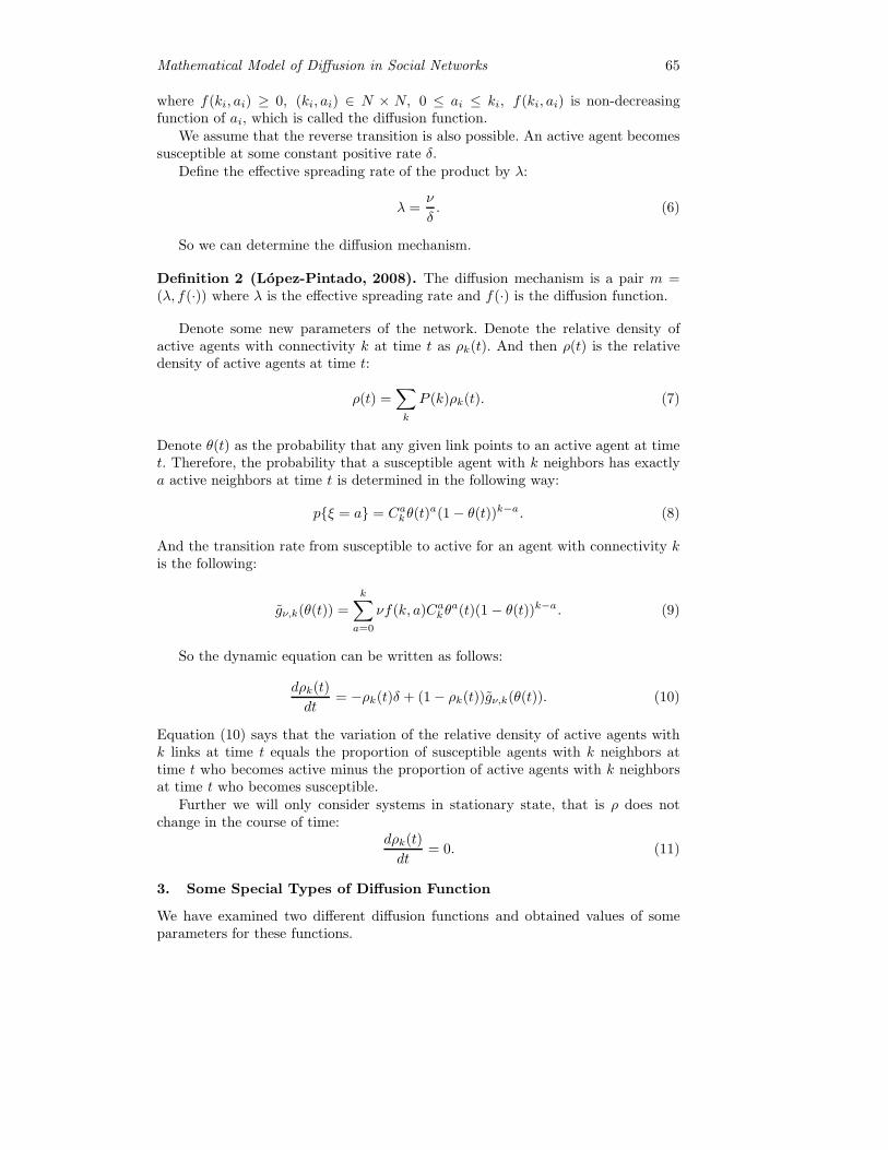
Mathematical Model of Diffusion in Social Networks 65
where f(ki, ai) ≥ 0, (ki, ai) ∈ N × N, 0 ≤ ai ≤ ki, f(ki, ai) is non-decreasingfunction of ai, which is called the diffusion function.
We assume that the reverse transition is also possible. An active agent becomessusceptible at some constant positive rate δ.
Define the effective spreading rate of the product by λ:
λ =ν
δ. (6)
So we can determine the diffusion mechanism.
Definition 2 (Lopez-Pintado, 2008). The diffusion mechanism is a pair m =(λ, f(·)) where λ is the effective spreading rate and f(·) is the diffusion function.
Denote some new parameters of the network. Denote the relative density ofactive agents with connectivity k at time t as ρk(t). And then ρ(t) is the relativedensity of active agents at time t:
ρ(t) =∑k
P (k)ρk(t). (7)
Denote θ(t) as the probability that any given link points to an active agent at timet. Therefore, the probability that a susceptible agent with k neighbors has exactlya active neighbors at time t is determined in the following way:
p{ξ = a} = Cakθ(t)a(1− θ(t))k−a. (8)
And the transition rate from susceptible to active for an agent with connectivity kis the following:
gν,k(θ(t)) =k∑a=0
νf(k, a)Cakθa(t)(1 − θ(t))k−a. (9)
So the dynamic equation can be written as follows:
dρk(t)
dt= −ρk(t)δ + (1− ρk(t))gν,k(θ(t)). (10)
Equation (10) says that the variation of the relative density of active agents withk links at time t equals the proportion of susceptible agents with k neighbors attime t who becomes active minus the proportion of active agents with k neighborsat time t who becomes susceptible.
Further we will only consider systems in stationary state, that is ρ does notchange in the course of time:
dρk(t)
dt= 0. (11)
3. Some Special Types of Diffusion Function
We have examined two different diffusion functions and obtained values of someparameters for these functions.
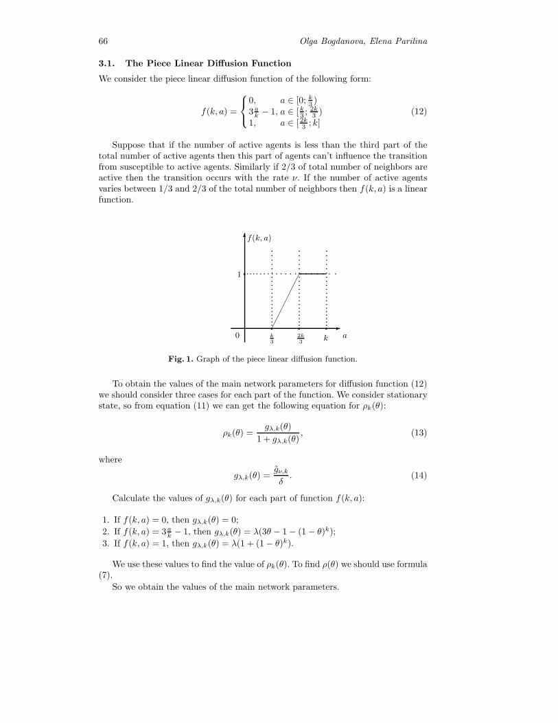
66 Olga Bogdanova, Elena Parilina
3.1. The Piece Linear Diffusion Function
We consider the piece linear diffusion function of the following form:
f(k, a) =
⎧⎨⎩0, a ∈ [0; k3 )3ak − 1, a ∈ [k3 ; 2k
3 )1, a ∈ [ 2k3 ; k]
(12)
Suppose that if the number of active agents is less than the third part of thetotal number of active agents then this part of agents can’t influence the transitionfrom susceptible to active agents. Similarly if 2/3 of total number of neighbors areactive then the transition occurs with the rate ν. If the number of active agentsvaries between 1/3 and 2/3 of the total number of neighbors then f(k, a) is a linearfunction.
�
�
������
a
f(k, a)
0 k3
2k3
k
� � �
�1
Fig. 1. Graph of the piece linear diffusion function.
To obtain the values of the main network parameters for diffusion function (12)we should consider three cases for each part of the function. We consider stationarystate, so from equation (11) we can get the following equation for ρk(θ):
ρk(θ) =gλ,k(θ)
1 + gλ,k(θ), (13)
where
gλ,k(θ) =gν,kδ
. (14)
Calculate the values of gλ,k(θ) for each part of function f(k, a):
1. If f(k, a) = 0, then gλ,k(θ) = 0;
2. If f(k, a) = 3ak − 1, then gλ,k(θ) = λ(3θ − 1− (1− θ)k);
3. If f(k, a) = 1, then gλ,k(θ) = λ(1 + (1− θ)k).
We use these values to find the value of ρk(θ). To find ρ(θ) we should use formula(7).
So we obtain the values of the main network parameters.
Mathematical Model of Diffusion in Social Networks 67
Proposition 1. The relative density of active agents with connectivity k in thenetwork with diffusion function (12) at the stationary state is
ρk(θ) =
⎧⎪⎨⎪⎩0, a ∈ [0; k3 )λ(3θ−1−(1−θ)k)
1+λ(3θ−1−(1−θ)k) , a ∈ [k3 ; 2k3 )
λ(1+(1−θ)k)1+λ(1+(1−θ)k) , a ∈ [ 2k3 ; k]
; (15)
and the relative density of active agents at the stationary state in this network is
ρ =
⎧⎪⎨⎪⎩0, a ∈ [0; k3 )∑k P (k)ρk =
∑k P (k) λ(3θ−1−(1−θ)k)
1+λ(3θ−1−(1−θ)k) , a ∈ [k3 ; 2k3 )∑
k P (k)ρk =∑k P (k) λ(1+(1−θ)k)
1+λ(1+(1−θ)k) , a ∈ [ 2k3 ; k]
. (16)
3.2. Diffusion Function with Exponential Part
Consider the diffusion function with exponential central part of the following form:
f(k, a) =
⎧⎪⎨⎪⎩0, a ∈ [0; k3 )
1
e23 −e
13eak − 1
e13 −1
, a ∈ [k3 ; 2k3 )
1, a ∈ [ 2k3 ; k]
(17)
This diffusion function is constructed similarly to the previous one. But if thenumber of active agents varies between 1/3 and 2/3 of the total number of agentsthen f(k, a) is an exponential function.
�
�
a
f(k, a)
0 k3
2k3
k
� � �
�1
Fig. 2. Graph of diffusion function (17) with exponential central part.
For this function we obtain the values of the main network parameters.
Proposition 2. The relative density of active agents with connectivity k in thenetwork with diffusion function (17) at the stationary state is as follows:
ρk(θ) =
⎧⎪⎨⎪⎩0, a ∈ [0; k3 )x
1+x , a ∈ [k3 ; 2k3 )
λ(1+(1−θ)k)1+λ(1+(1−θ)k) , a ∈ [ 2k3 ; k]
, (18)
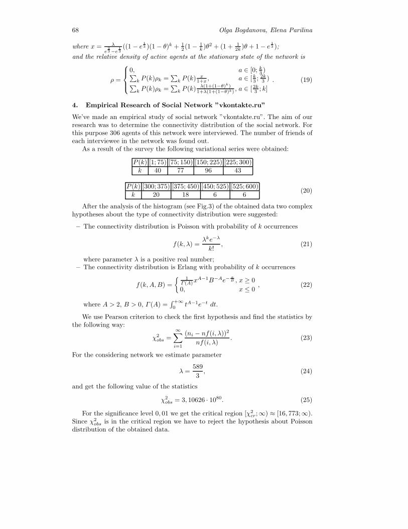
68 Olga Bogdanova, Elena Parilina
where x = λ
e23 −e
13
((1 − e13 )(1− θ)k + 1
2 (1− 1k )θ2 + (1 + 1
2k )θ + 1− e13 );
and the relative density of active agents at the stationary state of the network is
ρ =
⎧⎪⎨⎪⎩0, a ∈ [0; k3 )∑
k P (k)ρk =∑
k P (k) x1+x , a ∈ [k3 ; 2k
3 )∑k P (k)ρk =
∑k P (k) λ(1+(1−θ)k)
1+λ(1+(1−θ)k) , a ∈ [ 2k3 ; k]
. (19)
4. Empirical Research of Social Network ”vkontakte.ru”
We’ve made an empirical study of social network ”vkontakte.ru”. The aim of ourresearch was to determine the connectivity distribution of the social network. Forthis purpose 306 agents of this network were interviewed. The number of friends ofeach interviewee in the network was found out.
As a result of the survey the following variational series were obtained:
P (k) [1; 75) [75; 150) [150; 225) [225; 300)k 40 77 96 43
P (k) [300; 375) [375; 450) [450; 525) [525; 600)k 20 18 6 6
(20)
After the analysis of the histogram (see Fig.3) of the obtained data two complexhypotheses about the type of connectivity distribution were suggested:
– The connectivity distribution is Poisson with probability of k occurrences
f(k, λ) =λke−λ
k!, (21)
where parameter λ is a positive real number;– The connectivity distribution is Erlang with probability of k occurrences
f(k,A,B) =
{ 1Γ (A)x
A−1B−Ae−xB , x ≥ 0
0, x ≤ 0, (22)
where A > 2, B > 0, Γ (A) =∫ +∞0
tA−1e−t dt.
We use Pearson criterion to check the first hypothesis and find the statistics bythe following way:
χ2obs =
∞∑i=1
(ni − nf(i, λ))2
nf(i, λ). (23)
For the considering network we estimate parameter
λ =589
3, (24)
and get the following value of the statistics
χ2obs = 3, 10626 · 1080. (25)
For the significance level 0, 01 we get the critical region [χ2cr;∞) ≈ [16, 773;∞).
Since χ2obs is in the critical region we have to reject the hypothesis about Poisson
distribution of the obtained data.
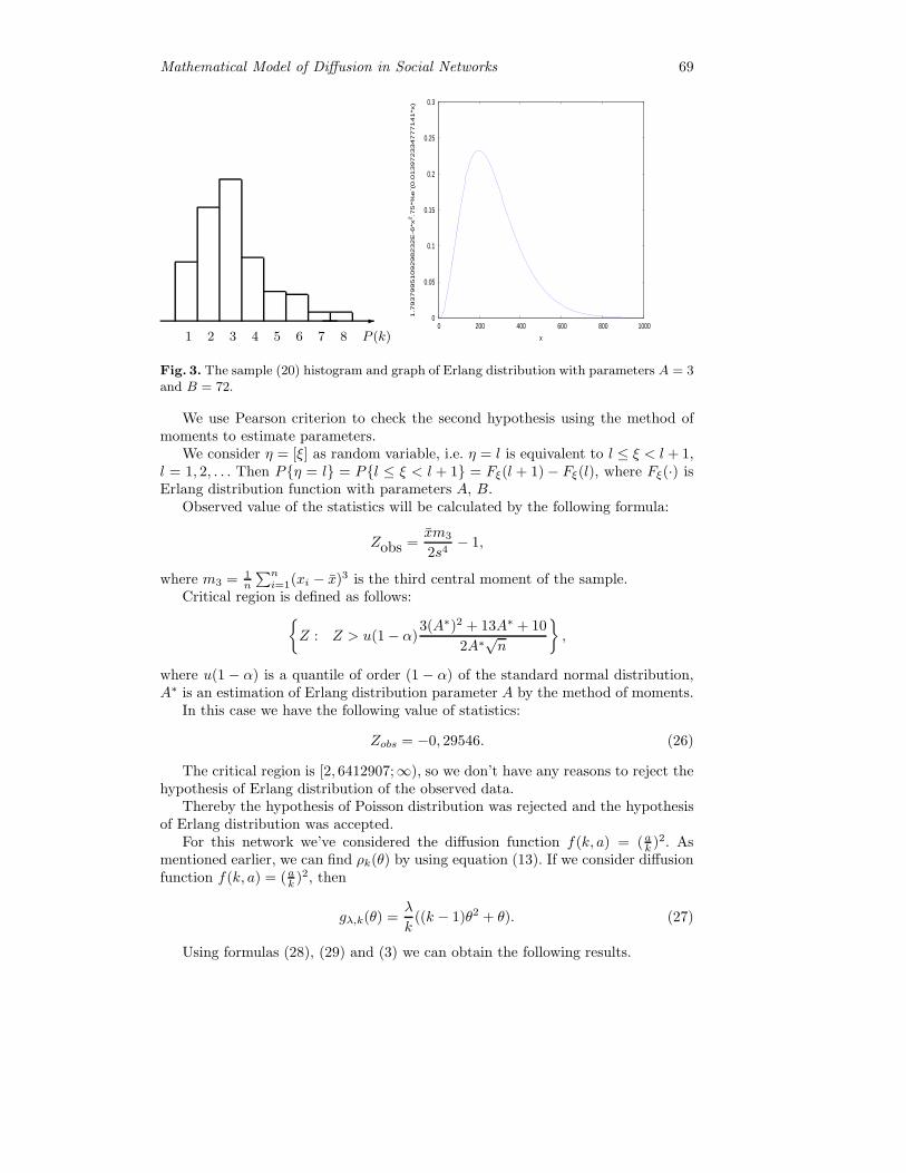
Mathematical Model of Diffusion in Social Networks 69
�1 2 3 4 5 6 7 8 P (k)
0
0.05
0.1
0.15
0.2
0.25
0.3
0 200 400 600 800 1000
1.7
93
79
95
10
92
98
23
2E
-6*x
2.7
5*%
e- (
0.0
13
97
23
34
77
71
41
*x)
x
Fig. 3. The sample (20) histogram and graph of Erlang distribution with parameters A = 3and B = 72.
We use Pearson criterion to check the second hypothesis using the method ofmoments to estimate parameters.
We consider η = [ξ] as random variable, i.e. η = l is equivalent to l ≤ ξ < l + 1,l = 1, 2, . . . Then P{η = l} = P{l ≤ ξ < l + 1} = Fξ(l + 1)− Fξ(l), where Fξ(·) isErlang distribution function with parameters A, B.
Observed value of the statistics will be calculated by the following formula:
Zobs =xm3
2s4− 1,
where m3 = 1n
∑ni=1(xi − x)3 is the third central moment of the sample.
Critical region is defined as follows:{Z : Z > u(1− α)
3(A∗)2 + 13A∗ + 10
2A∗√n
},
where u(1 − α) is a quantile of order (1 − α) of the standard normal distribution,A∗ is an estimation of Erlang distribution parameter A by the method of moments.
In this case we have the following value of statistics:
Zobs = −0, 29546. (26)
The critical region is [2, 6412907;∞), so we don’t have any reasons to reject thehypothesis of Erlang distribution of the observed data.
Thereby the hypothesis of Poisson distribution was rejected and the hypothesisof Erlang distribution was accepted.
For this network we’ve considered the diffusion function f(k, a) = (ak )2. Asmentioned earlier, we can find ρk(θ) by using equation (13). If we consider diffusionfunction f(k, a) = (ak )2, then
gλ,k(θ) =λ
k((k − 1)θ2 + θ). (27)
Using formulas (28), (29) and (3) we can obtain the following results.
70 Olga Bogdanova, Elena Parilina
Proposition 3. The relative density of active agents with connectivity k for thedata (20) obtained from the network ”vkontakte.ru” with diffusion function f(k, a) =(ak )2 at the stationary state is the following:
ρk(θ) =λk ((k − 1)θ2 + θ)
1 + λk ((k − 1)θ2 + θ)
, (28)
and the relative density of active agents at the stationary state of the same networkis
ρ(θ) =∑k
P (k)λk ((k − 1)θ2 + θ)
1 + λk ((k − 1)θ2 + θ)
. (29)
5. Conclusion
There are some open questions in our work. To determine the diffusion mechanismwe have to know the effective spreading rate λ. It is suggested that this parameteris known to the researcher. But how will you determine this parameter? If you wantto examine some social network you should make series of the empirical experimentsto get more faithful type of connectivity distribution.
References
Gubanov, D. A., Novikov, D. A. and Chkhartishvili, A. G. (2009). Models of influence insocial networks. Large-scale Syst. Manag., 27, 205–281 (in Russian).
Benaim, M. and J. Weibull (2003). Deterministic approximation of stochastic evolution ingames. Econometrica, 71, 873–903.
Dodds, P. S. and Watts, D. J. (2004). Universal behavior in a generalized model of conta-gion. Phys. Rev. Lett., 92, 2187011-2187014.
Lopez-Pintado, D. (2008) Diffusion in complex social networks. Gam. and Econ. Beh., 62,573–590.
Jackson, M. (2008). Social and Economic Networks. Princeton University Press: Princeton,NJ.
Pastor-Sattoras, R. and A. Vespignani (2001). Epidemic spreading in scale-free networks.Phys. Rev. Lett., 86, 3200–3203.

Product Diversity in a Vertical Distribution Channelunder Monopolistic Competition �
Igor Bykadorov1, Sergey Kokovin2 and Evgeny Zhelobodko3
1 Sobolev Institute of Mathematics, Siberian Branch of the Russian Academy of SciencesAcad. Koptyug avenue 4, Novosibirsk, 630090, Russiaand Novosibirsk State University, Novosibirsk, Russia
E-mail: [email protected] Sobolev Institute of Mathematics, Siberian Branch of the Russian Academy of Sciences
Acad. Koptyug avenue 4, Novosibirsk, 630090, Russiaand Novosibirsk State University, Novosibirsk, Russia
E-mail: [email protected] Novosibirsk State University
Pirogova str. 2, Novosibirsk, 630090, RussiaE-mail: [email protected]
Abstract. In Russia the chain-stores gained a considerable market power.In the paper we combine a Dixit-Stiglitz industry with a monopolistic re-tailer. The questions addressed are: Does the retailer always deteriorate wel-fare, prices and variety of goods? Which market structure is worse: Nash orStackelberg behavior? What should be the public policy in this area?
Keywords: monopolistic competition, Dixit-Stiglitz model, retailer, Nashequilibrium, Stackelberg equilibrium, social welfare, Pigouvian taxation.
1. Introduction
In 2000-s, Russia and other developing markets of FSU have shown dramatic growthof chain-stores and similar retailing firms. Inspired by Wal-Mart and other successfulgiants abroad, Russian food traders like Perekrestok and Pyaterochka has gainedconsiderable shares of the market and noticeable market power, both in Moscow andin province. This shift in the market organization was suspected by newspapers fornegative welfare effects, accompanied by upward pressure on prices and inflation.Public interest to this question is highlighted by anti-chain-stores bill currentlypassed in Russian Parliament (Duma).
Leaving aside the empirical side of this question, this project focuses on con-structing and analyzing the adequate model of vertical market interaction, suit-able for Russian retailing markets of food, clothes and durables. We step asidefrom the traditional models of monopolistic or oligopolistic vertical interaction orfranchising (see, e.g. review in (Tirole, 1990)), and stick instead to more modernmonopolistic-competition representation of an industry in the Dixit-Stiglitz spirit(Dixit and Stiglitz, 1977), but combined with vertical interaction. This combinationis rather new, being pioneered by Chen (Chen, 2004) and Hamilton and Richards(Hamilton and Richards, 2007), as described below in the literature review.
� The work on this paper was supported by an individual grant R08-1071 from the Eco-nomics Education and Research Consortium, Inc. (EERC), with funds provided by theEurasia Foundation (with funding from the US Agency for International Development),The World Bank Institution, the Global Development Network and the Government ofSweden.
72 Igor Bykadorov, Sergey Kokovin
Our departure from the former two papers is that it is the retailer who is ex-ercising the monopsony power after market concentration, while the productionis organized as monopolistic-competition industry with free entry. This hypothesisseems rather realistic, at least for developing markets. Indeed, there are numer-ous evidences in economic newspapers (see (Nikitina, 2006), (Sagdiev et al., 2006),(Slovak Republic, 2007), (FAS, 2007) cited in our literature review) that each ofseveral big retailers has much stronger bargaining power than quite numerous man-ufacturers and importers of consumer goods like sausages, shirts, etc. (even such biginternational companies as Coca-Cola are not strong enough to enforce their termsof trade to Russian retailers).
To reflect such relations, our stylized model of market concentration considers amonopsonistic and monopolistic retailer (as a proxy of an oligopsonistic/oligopolisticretailer). This monopolistic intermediary deals with a continuum [0, N ] of Dixit-Stiglitz manufacturers on one side of two-sided market and a representative con-sumer on another. Each manufacturer has a fixed cost and a variable cost, he pro-duces a single variety of the “commodity” and sets the price for this variety. Themost natural timing of the model is the retailer’s leadership, i.e., the retailer startswith announcing her markup policy correctly anticipating the subsequent manufac-turers’ responses, and simultaneously chooses the scope of varieties/firms to buyfrom. At the next stage the manufacturers come up with their prices and then themarket clears the quantities. Both sides take into account the demand profile gen-erated by a consumer’s quasi-linear utility function. Another situation is when theretailer can also impose entrance fee on producers or/and consumers.
One or another monopolistic organization of the industry is compared to the pre-concentration situation where multiple shops operate. For simplicity, each varietyis assumed to be sold through one shop. There can be three kinds of situations,ordered by increasing market power of the producers.
(1) The myopic (Nash) behavior of both manufacturers and retailer(s) who areunable to predict and influence the market. Which model is closer to reality, wetried to find out from empirical market papers (see literature review below), butdid not come to a definite conclusion. So, both pre-concentration versions remaindiscussed.
(2) Leadership of manufacturers, who choose their wholesale prices correctlyanticipating the best-response retailer’s markup added later on.1
(3) Vertical integration from the side of producer, who owns the shop selling itsvariety or, equivalently, dictates the terms of trade and uses entrance fee or othertools to appropriate whole profit.2
The questions addressed in our paper are: Does the emergence of the monopson-istic retailer enhance or deteriorate welfare, and how much? Which retailer behavioris worse: usual monopoly or price discrimination with entrance fees? What shouldbe the guidelines for public regulation (if any) in this area?
1 Such interaction is somewhat similar to the concept of “common agency” consideredin contract theory (see e.g. (Bernheim and Whinston, 1986)), but our leaders are indifferent position because each manufacturer is dealing with one or more small shops,knowing their costs. Instead of common agent (hypermarket) for all producers whichshould be assumed in “common agency” approach.
2 This situation seems less realistic than other two, but used to compare with verticalintegration from retailer’s side.
Product Diversity in a Vertical Distribution Channel 73
In general the question is cumbersome, but definite results of this kind wereobtained for the case of quasi-linear quadratic utility like in Ottaviano, Tabuchiand Thisse (Ottaviano et al., 2002), that means linear demands. For this model (incontrast with common wisdoms of politicians) it turns out under rather realisticassumptions that:
(i) Market concentration always enhances social welfare through softening the“double marginalization effect”, this enhancement can work through lower pricesand bigger consumption, or through adjusting the inefficiently low or inefficientlyhigh number of varieties.
(ii) Under market concentration, further enforcement of the monopolist’s marketpower by allowing for price discrimination (entrance fees) further enhances socialwelfare. Even the first-best (Pareto) optimum is guaranteed if the monopolist isable to use entrance fees on both sides: for producers and consumers. The lattersituation turns out equivalent in welfare and (socially optimal) consumptions to theintegrated monopoly, which means that one firm owns both production and retailingof the whole industry.
(iii) The governmental regulation of a simple monopolistic intermediary throughcapping the markup – enhances welfare. However, such regulation is not needed forprice discriminating monopolist (even under entrance fees on manufacturing sideonly). If the government uses Pigouvian stimulation, then not taxes but subsidiesto the monopsonistic retailer enhance welfare.
Additionally, in comparisons of various situations we tell what happens to prices,quantities and diversity under changing market organization.
To explain surprisingly positive influence of certain steps in increasing the re-tailer’s market power, we can mention two general ideas. First, more market powersoftens the effects of double marginalization. Second, when the industry involvesmonopolistic competition, some sort of monopolistic behavior is present anyway.Therefore, the retailer’s market power do not aggravate welfare losses of this kind,but instead internalize the externalities on the supply side. When the main decision-maker in the industry is powerful enough, she internalize them better, sometimesas good as the social planner would.
In the sections that follow we first describe more extensively the literature andmotivation for our approach, then introduce the model and finally describe theresults.
2. Literature Review
There is a broad literature on vertical interaction between a producer and a retailer,see reviews in (Perry, 1989) and (Rey, 2003); they study various economic conse-quences of such interaction. The early classical paper of Spengler (Spengler, 1950)explored the simplest case of Stackelberg game between two monopolists, one abovethe other, that entails “double marginalization.” In essence, the second monopolistadds her own markup to the monopolistic price of the first one and further de-teriorates social welfare, see (Tirole, 1990). A broad range of papers relaxed theSpengler’s assumptions of homogeneous commodity, single producer and single re-tailer, which is natural and realistic. The difference among them lies mainly in var-ious models of the oligopolists interaction. First of all, there is a strand of spatialHotelling-type models (Hotelling, 1929) and another class of “representative con-sumer” models like Dixit-Stiglitz one (Dixit and Stiglitz, 1977). Among the spatial

74 Igor Bykadorov, Sergey Kokovin
models, Salop (Salop, 2006) started with the circular city model with one producerand several retailers distributing themselves around this city to meet the demandof the continuous population. The main result is that under reasonable assump-tions all consumers are served and the inefficiency found by Spengler disappears.Therefore there is no welfare motive for integration between the producer and theretailers. In contrast, Dixit (Dixit, 1983) modified this model to include produc-tion activity of “retailers” who used also other production factors. Then there isa welfare reason for integration, because it reducers the inefficiently-big numberof retailers-producers and increases welfare. Further these ideas were developed in(Mathewson and Winter, 1983).
Another approach explores the idea of representative consumer in Dixit-Stiglitzmanner. In particular, Perry and Groff (Perry and Groff, 1989) use constant-elasticity-of-substitution (CES) utility function of the consumer, defined on manydiscrete varieties, each produced by a single retailer. The main result is that suchcompetition brings both distorted prices and distorted number of retailers, and in-terestingly, integration of two stages of production turns out welfare-deterioratingbecause the decrease in the varieties outweighs the decreasing prices. Here, like inDixit’s circular city, the retailers are the low-level producers also, modifying thecommodity, otherwise a consumer buying from all retailers would look strange. An-other step in this direction is Chen (Chen, 2004) where a multi-product monopolisticproducer at the first stage chooses the number of varieties produced and thereforethe number of retailers, because one-to-one correspondence remains. Afterwardshe performs a bargaining procedure with each of them, and finally the marketsclear taking into account the substitutability among the varieties. The number ofdifferentiated goods turns out smaller than the constrained social optimum; the re-tailer’s countervailing power lowers consumer prices but exacerbates the distortionin product diversity.
Finally, Hamilton and Richards (Hamilton and Richards, 2007) synthesizeHotelling-type and Dixit-Stiglitz-type models, i.e., the spatial-market and thedifferentiated-goods approaches in modeling the oligopoly competition among multi-product firms – “supermarkets,” who face a competitive manufacturers. Two kindsof diversities are involved. There is a potentially large number of spatially-diversifiedsupermarkets to choose from, but a consumer enjoys also a product-variety fromthe product line designed in a (single) supermarket chosen. It is found that increasein product differentiation on the manufacturers’ side need not increase the equi-librium length of the product lines when retailers are specializing. Besides, underboth no-entry and free-entry oligopoly conditions for retailers, product variety isundersupplied; several other effects are also found and the impact of excise taxationstudied.
In contrast, in our setting, as we have mentioned, the monopolist is the retailer,but these are the producers who are organized as a Dixit-Stiglitz industry. To mo-tivate such unusual approach, we can note that such or similar situation is rathertypical for today Russian market. At least, there are many observations that mod-ern supermarkets and hypermarkets have dominant bargaining power in relationswith more numerous producers. For example, in (Nikitina, 2006) we read:
“... chain-stores ... capture the substantial part of profit of the small suppliers...These chains force suppliers to participate in various promotional actions, no matterwhether such advertising or discounts are useful for suppliers or not... Overwhelming

Product Diversity in a Vertical Distribution Channel 75
majority of the retailers require payments from suppliers, not only “payment forthe shelf,” but also so-called retro-bonus, i.e. “sale percentage.” According to theagreements between suppliers and retailers, the latter receive 5 % on average ...Another “trap” for a supplier is the obligation to guarantee some sales volume.If the quantity sold turns out lower for some reasons, the supplier has to pay thedifference between the planned and the actual sales... As a result, the total markupappropriated by a retailer can be from 30 to 50 % of the cost.”
Similarly, in (Sagdiev et al., 2006) we can read:
“Retailers require from suppliers dozens thousands dollars only to start sellingtheir goods... As the suppliers confess, the price of the “entrance ticket” dependson the producer’s reputation and his spending for advertising. A retailer can makea discount when the manufacturer agrees to spend a lot on promotion of his com-modities . . . The entrance ticket is not the only payment by a supplier wishing toenter a chain-store network. The total share going to the retailers can be about 35%of the consumer price.”3
Another important citation can be found, e.g. in the website of the FederalAntimonopoly Service of Russian Federation (FAS, 2007): ”Transformation of retailtrade sector into big trade networks (retailers) allowed the latter, despite theirseemingly small market share, dictate the rules of the game and determine thenetwork entry conditions for suppliers and producers.”
Such market power of the retailer in Russia is not surprising. The deficit of trad-ing facilities is artificially aggravated by considerable corruption in trading land andin licensing trade in cities. As mentioned in McKinsey Global Institute survey ofRussian retailing (Kaloshkina et al., 2009), during 2002-07 the sales of such bigchain-stores as Eldorado, X5, Magnit, Metro Group, Auchan were growing by ap-proximately 50% annually. However, the share of the market in the hands of allchain-stores still remains smaller than 50% in 2010.
This situation is not unique only for Russia. It is also, for instance, in some coun-tries of East Europe, as shows the following citation from the site of AntimonopolyOffice of Slovak Republic (Slovak Republic, 2007): “In view of the existing struc-ture of the individual local markets, high barriers to entry (considerable direct andforced investments, sunk costs related to the required advertising and marketingsupport when entering the market, administrative barriers to entry, time neces-sary for entry into the market, and so forth), saturation of the individual relevantmarkets, and the nonexistence of potential competitors, if the concentration werecarried out, the undertaking Tesco plc would establish or strengthen its dominantposition. Consequently, the undertaking Tesco plc. would not be subject to substan-tial competition and, given its economic strength, it could act independently withrespect to its suppliers, consumers, and competitors.”
Besides, the Slovak case is not unique, see, e.g. (Lira et al., 2008) for the case ofChile.
3 The same article note that “...in international practice, a bonus payed for the entranceinto the trading network is known, ... but in less scale... In Germany only small supplierspay for starting to distribute goods through the supermarkets... In Great Britain thescheme ”money for distribution” is not common, but retailer and supplier can promotethe goods together...”

76 Igor Bykadorov, Sergey Kokovin
3. Model
We consider a monopolistic competition model modified to include the two-levelinteraction “manufacturer – retailer – consumer.”
3.1. Demand
On consumers’ side, there is a representative consumer, endowed with L units oflabor supplied to the market inelastically, and labor is the only production factor.There are two types of goods in the economy. The first “commodity” consist of manyvarieties, for instance, milk of different brands. The second one is the numerairerepresenting other (perfectly competitive) goods. The income effect is neglected. Ageneral-type quasi-linear utility function of any consumer reflects preferences overtwo kinds of goods:
U(q, N,A) = V (q, N) + A.
Here N is the length of the product line, reflecting the scope (the interval) ofvarieties; q(i) ≥ 0 is “quantity” or the consumption of i-th variety chosen by anyagent (consumer) and q = (q(i))i∈[0,N ] is the infinite-dimensional vector or functionq(·) : [0, N ] → R describing the whole profile of varieties, all profiles keepingbold notation hereafter. Variable A ≥ 0 is the consumption of the numeraire good.However, we use this general function V only to formulate the concepts of equilibria.Throughout we study a tractable special case, namely, the quadratic class of utilityfunction formulated below. It was introduced by G.I.P. Ottaviano, T. Tabuchi andJ.-F. Thisse (Ottaviano et al., 2002) (see also (Combes et al., 2008)) and becamequite popular for modeling monopolistic competition:
U(q, N,A) = α
∫ N
0
q(i)di − β − γ
2
∫ N
0
[q(i)]2di− γ
2
[∫ N
0
q(i)di
]2+ A.
Here α, β and γ are some positive parameters, satisfying β > γ > 0, to have U quasi-concave. This condition ensures also that our consumer prefers larger diversity. Incontrast, under β = γ, only the total quantity of consumption Q = qN but not thediversity per se influences utility. Two quadratic terms here ensure strict concavityin two dimensions, i.e., definite consumer’s choice among varieties and between thetwo sectors.
The main feature achieved by this three-term construction is that this utilitygenerates the system of linear demands for each variety and linear demand for thewhole differentiated sector.
To formulate the budget constraint, p(i) denotes the price of variety i for theconsumer (which equals the wholesale price p(i) when there is no retailer), w ≡ 1is the wage rate in the economy, PA is the price of the numeraire, also becoming 1at the equilibrium.
Then the utility-maximization problem of the representative consumer takes theform
U(q,N,A) = V (q,N) + A→ max(q,A)∫ N
0
p(i)q(i)di + PAA ≤ wL +
∫ N
0
πM(i)di + πR,
where πM(i) is the profit of i-th manufacturer, while πR is the profit of retailer.

Product Diversity in a Vertical Distribution Channel 77
The budget constraint has a natural interpretation. Its right-hand side is GrossDomestic Product (GDP) of the economy with respect to income, while the left-hand side represents expenditures.
As to the solution to the consumer’s problem, in the case when the incomeis sufficiently large, it does not influence the demand, due to quasi-linear utility,standardly.4
Therefore, for any price-profile p : [0, N ] �→ R+ , the individual demand-profilefunction q∗ for all varieties is defined as follows (any “profile” is a function w.r.t.varieties’ names i ∈ [0, N ] and bold letters p, q denote such profiles, in contrastwith certain points p(i), q(i) of the profiles)
q∗(N,p) = arg maxq
[V (q,N)−
∫ N
0
p(i)q(i)di
]. (1)
Solving FOC of this problem in another direction for each price-profile, in Section4.1 we derive the inverse demand function p(i, q(i), N,p−i) of any variety i for ourquadratic utility. This function p describes how i-th consumer’s price depends uponi-th quantity q(i) and upon exogenous parameters: number N of competitors andthe price profile p−i including all prices but for i. This inverse-demand function istaken into account by producers, to be described now.
3.2. Supply
On the supply side there can be several different situations, modeled differently.Anyway manufacturers sell the goods only indirectly, through some retailer, buteither they can interact myopically (Nash equilibrium) or one or another side ofvertical relations may be the leader.
In all situations we denote by p(i) wholesale price and by r(i) the retailer’smarkup or price margin (we use these terms interchangeably). Therefore the ulti-mate i-th retailing price amounts to the sum p(i) = p(i)+r(i). Each manufacturer’scost function takes the following form: C(q) = cq+F. So, i-th manufacturer’s profit-maximization problem takes the form
πM(i) = p(i)q(i,p + r)− C(q(i,p + r)) → maxp(i)
,
where p is the wholesale price-profile for all producers and p + r are the retail(consumer) prices; therefore, r is the retail markup profile. In the long run, freeentry reduces profits to zero but at this stage profit maximizing determines priceand quantity.
Now let us turn to the monopsonistic retailer (emerging after market concen-tration) or many retailers (existing before market concentration). Their numbermakes difference only when the retailer is big enough to control the market. Inmulti-retailer situation, we assume that one retailer may sell one variety or several,but each variety is sold through one retailer. As soon as markup optimization pereach variety is similar, it is sufficient to describe the behavior of the “gross retailer”
4 In the opposite case when the income is small, there can be a boundary solution whenwhole consumer’s income is spent only for the diversified commodity. We, traditionally,ignore this case but for specifying some restrictions on parameters ensuring absence ofincome effect.
78 Igor Bykadorov, Sergey Kokovin
representing the whole population of them. Gross retailer’s cost function is similarto that of the manufacturers:
CR(q) =
∫ N
0
p(i)q(i)di +
∫ N
0
cRq(i)di +
∫ N
0
FRdi .
Here the first integral shows the expenditures to buy from the manufacturers, whilethe second and the third item show the retail costs: cR is the number of labor unitsrequired from retailer to sell a unit of any differentiated good, FR is the retailer’sfixed cost (also measured in labor) required to start selling any differentiated good.Then the retailer’s profit-maximization problem is
πR =
∫ N
0
[r(i)− cR]q(i,p + r)di −∫ N
0
FRdi → maxr
,
where r(i) = pR(i)− p(i) is the markup of the i-th goods variety.We consider the following types of timing, or, rather, types of leader-follower
relationship between the manufacturers and the retailer, ordered by decreasing re-tailer’s bargaining power:
– Leading retailer, i.e., monopolistic competition with strategic behavior of re-tailer5:• at first the retailer chooses markups and the scope of product varieties,
correctly anticipating the subsequent response of manufacturers;• then each manufacturer chooses, to enter the market or not and the whole-
sale price;– Nash equilibrium, when manufacturers and retailer choose p and r simultane-
ously and myopically6.– Leading manufacturer, i.e., monopolistic competition with strategic behavior of
manufacturers7:• at first all manufacturers simultaneously choose, to enter the market or not,
and the wholesale prices (the number of firms is determined by the zero-profit condition), correctly anticipating the individually adjusted markupfunction;• then the retailer chooses the markup for each commodity (each manufac-
turer);
5 Note that, in addition to the retailer presence, another distinction here from the standardmonopolistic competition is that the equilibrium number of firms is chosen by theretailer, not by the free entry condition. This assumption is rather plausible, as shownby the following saying (Sokolov, 2006) of an owner of a retail supermarket about theirpolicy concerning the diversity: “... for dried crusts ... we deal with a limited numberof suppliers, since increasing the number of brands in such commodity groups does notlead to the increase in total sales... ”
6 The Nash variant of interaction seems less realistic than two leadership cases of interac-tion with more far-sighted behavior. But Nash interaction can be interesting as startingpoint to compare and estimate everybody’s gains and losses from the strategic behavior.
7 Though not as realistic as the previous concept, wise producers still can be a plausi-ble approximation of reality. As we have mentioned in Introduction, this concept is,essentially, the solution concept in Common Agency models (the principals are manu-facturers while the agent is retailer). The only distinction is the absence of informationasymmetry among the participants.

Product Diversity in a Vertical Distribution Channel 79
– “No-retailer” equilibrium, when manufacturers enforce the terms of trade quitestrongly, or each retailer of a variety just belongs to the manufacturer of relatedvariety.
We formally express these four concepts in (most natural) symmetric case asfollows.
Definitions. 1) Symmetric Nash-equilibrium is a quadruple (pNash, rNash, qNash,NNash) ∈ R4
+, such that related price profile p = p(i) ≡ pNash solves each manu-facturer’s problem under external parameters NNash,p−i ≡ pNash, markup rNash
maximizes the manufacturer profit under pNash, NNash, while q(i) ≡ qNash solvesthe consumer’s problem under NNash,p ≡ pNash and NNash satisfies the zero-profitcondition.
2) Symmetric RL-equilibrium is a quadruple (pRL, rRL, qRL, NRL) ∈ R4+, such
that related price function ρ(i, r,p−i, NRL) describes the optimal response of each
manufacturer to external markup r and parameters NRL,p−i ≡ pRL, markup rRL
and NRL maximize the retailer’s profit under this function ρ, pRL = ρ(i, rRL, pRL,NRL), while q(i) ≡ qRL solves the consumer’s problem under NRL,p ≡ pRL.
3) Symmetric ML-equilibrium is a quadruple (pML, rML, qML, NML) ∈ R4+, such
that related markup function μ(i, p(i),p−i, NML) describes the optimal response of
the retailer to i-th price p(i) and parameters NML,p−i ≡ pML, price pML maximizethe manufacturer profit under this function μ, rML = μ(i, pML, pML, NML), whileq(i) ≡ qML solves the consumer’s problem under NML,p ≡ pML and NML satisfiesthe zero-profit condition.
4) NR-equilibrium. Each manufacturer owns the shop, bears joint fixed andvariable costs of production and trade, C(q) = (c + cR)q + F +FR, and maximizesthe profit function
πNR(i) = p(i, q(i), N,p−i)q(i)− C(q(i)) → maxq(i)
.
To compare the social outcomes of these concepts of equilibria, we formulate thewelfare function analogous to the previous one, but for modified retailing cost:
W = V (q,N)−∫ N
0
(c + cR)q(i)di −∫ N
0
(F + FR)di.
The symmetric solution qMaxW , NMaxW to this optimization program is calledsocially-optimal quantity and socially-optimal diversity.
Besides, we formulate the consumer surplus as
CS = V (q,N)−∫ N
0
(p(i) + r(i))q(i)di.
Thus we have introduced the model and now start analyzing it.
4. Market Concentration
In this section we approach the question: Does market concentration enhance ordeteriorate welfare? We consider two models of pre-concentration market: Nashbehavior or strategic behavior of producers, leaving to the reader the choice ofmore realistic one and discussing other relevant models in the end of section. Bothare compared to stylized model of extreme concentration: one retailer owns all shopsand behaves as a leader, and to social optimum. Thus, we study:
80 Igor Bykadorov, Sergey Kokovin
– “no retailer” equilibrium (NR);– strategic behavior of manufacturers-leaders (ML);– Nash equilibrium (Nash);– strategic behavior of retailer-leader (RL);– socially-optimal quantity and socially-optimal length of the product line (MaxW ).
4.1. Equilibria Characterization
Demand. Under this utility function, the consumer’s problem can be written asfollowing:
α
∫ N
0
q(i)di − β − γ
2
∫ N
0
[q(i)]2di − γ
2
[∫ N
0
q(i)di
]2+ A→ max
q,A
∫ N
0
pR(i)q(i)di + A ≤ L +
∫ N
0
πM(i)di + πR .
Here we analyse only the case when the consumer’s income is sufficiently large anddoes not influence the consumption of the diversified products.
By standard technique (using the first order conditions, cf. (Ottaviano et al., 2002))we can express the equilibrium retail price through the parameters as
p(i) + r(i) = α− (β − γ)q(i)− γ
∫ N
0
q(j)dj , i ∈ [0, N ]. (2)
Moreover, solving FOC in the opposite direction, we can obtain the linear demandfunction for any variety i ∈ [0, N ]:
q(i) = a− (b + gN)[p(i) + r(i)] + gP, (3)
where coefficients are
a =α
β + (N − 1)γ, b =
1
β + (N − 1)γ, g =
γ
(β − γ)[β + (N − 1)γ](4)
and price index
P =
∫ N
0
[p(j) + r(j)]dj
expresses the aggregate pricing behavior of all firms, negligibly influenced by firmi. In symmetric equilibrium p, q, r both above integrals can be simplified as∫ N
0
q(j)dj = Nq, P = N(p + r).
Method of finding (Nash), (ML) equilibria and (MaxW ). Using the de-mands system obtained, we calculate all kinds of market outcomes defined: (Nash),(ML) and socially-optimal (MaxW ), and then (RL). All these are found in closedform in Result 2 below, proceeding as follows.
Solution MaxW is found directly from FOC. The method of calculating Nash isalso rather usual: system of FOC for all participants is combined with the zero-profitcondition, resulting in unique solution. For finding equilibrium ML, we first derive
Product Diversity in a Vertical Distribution Channel 81
the markup function ri(p(i), P,N) which is the best-response of the retailer (a smallshop) to any price p(i) (P,N given). Then we optimize prices of the manufacturershaving this markup function, and adding the zero-profit condition get the uniqueequilibrium.
Method of finding (RL) equilibrium. More complicated is calculating equi-librium RL. Here, having in mind demands q(i, r(i), N, P ) and optimal price poli-cies p∗(i, r(i), N, P ) as functions of markup r(i) and diversity N , the retailer jointlychooses profile r = (r(i))i∈N and N as the solution to her program in the form
πR =∫ N0
[r(i) − cR]q(i,p∗(r,N) + r)di−∫ N0
FRdi → maxr,N ,
πM(p∗(i, r(i), N, P ), r(i),N) ≥ 0 .
If we, reasonably, assume only symmetric variables p, q, r (bar accent denoting sym-metrization, in particular p∗(r,N) = p∗(i, r, N,Np) ∀i) this retailer’s problem issimplified as
πR = N [r − cR]q(p∗(r,N)+r)−NFR → maxr,N ,
πM(p∗(r,N),r, N) ≥ 0 .
Remark that in symmetric RL case one has the following expressions q and p asfunctions of r and N :
q = q(r,N) =(b + gN)[a− b(c + r)]
2b + gN(5)
p = p(r,N) =a + (b + gN)c− br
2b + gN(6)
Strictly speaking, now we have stepped aside from the monopolistic competitionmodel, since N need not be necessarily determined by the free entry or zero-profitcondition. More specifically, there can be two types of solution, or regimes thatwe call artificially restricted market or un-restricted market. The first case meansnon-negative-profit constraint occurring non-binding, i.e., optimization of the un-constrained function πR resulting in positive manufacturers’ profit πM > 0. Inthis case the retailer really ignores “free entry” condition imposing instead her ownrestriction on entry (so, we also ignore free entry within calculations). Otherwiseretailer first use “free entry” condition to calculate N(r) as a function of r, thenmaximize her profit with respect to r. As we have found by direct calculations, theartificially restricted solution happens if and only if some crucial constant exceedsone:
F =FR2F≥ 1.
Thus, postponing its further economic discussion, we can formulate now
Result 1 It is profitable for the retailer-leader to artificially restrict the entry, whenher fixed cost exceeds doubled manufacturer’s fixed cost.
This constant F denoting relation of retailing fixed costs over manufacturingfixed cost plays hereafter an important role. To concisely formulate the characteri-zation of all our solutions, we introduce the following auxiliary notations (some of
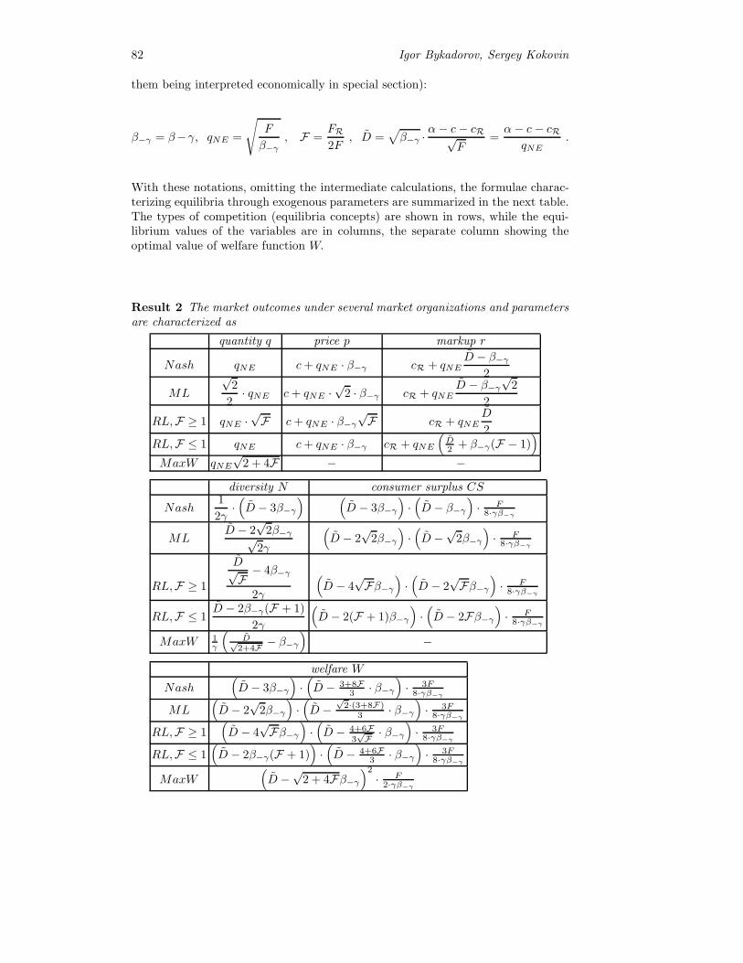
82 Igor Bykadorov, Sergey Kokovin
them being interpreted economically in special section):
β−γ = β−γ, qNE =
√F
β−γ, F =
FR2F
, D =√β−γ ·
α− c− cR√F
=α− c− cR
qNE.
With these notations, omitting the intermediate calculations, the formulae charac-terizing equilibria through exogenous parameters are summarized in the next table.The types of competition (equilibria concepts) are shown in rows, while the equi-librium values of the variables are in columns, the separate column showing theoptimal value of welfare function W.
Result 2 The market outcomes under several market organizations and parametersare characterized as
quantity q price p markup r
Nash qNE c + qNE · β−γ cR + qNED − β−γ
2
ML
√2
2· qNE c + qNE ·
√2 · β−γ cR + qNE
D − β−γ√
2
2
RL,F ≥ 1 qNE ·√F c + qNE · β−γ
√F cR + qNE
D
2RL,F ≤ 1 qNE c + qNE · β−γ cR + qNE
(D2 + β−γ(F − 1)
)MaxW qNE
√2 + 4F − −
diversity N consumer surplus CS
Nash1
2γ·(D − 3β−γ
) (D − 3β−γ
)·(D − β−γ
)· F8·γβ−γ
MLD − 2
√2β−γ√
2γ
(D − 2
√2β−γ
)·(D −
√2β−γ
)· F8·γβ−γ
RL,F ≥ 1
D√F− 4β−γ
2γ
(D − 4
√Fβ−γ
)·(D − 2
√Fβ−γ
)· F8·γβ−γ
RL,F ≤ 1D − 2β−γ(F + 1)
2γ
(D − 2(F + 1)β−γ
)·(D − 2Fβ−γ
)· F8·γβ−γ
MaxW 1γ
(D√
2+4F − β−γ)
−
welfare W
Nash(D − 3β−γ
)·(D − 3+8F
3 · β−γ)· 3F8·γβ−γ
ML(D − 2
√2β−γ
)·(D −
√2·(3+8F)
3 · β−γ
)· 3F8·γβ−γ
RL,F ≥ 1(D − 4
√Fβ−γ
)·(D − 4+6F
3√F · β−γ
)· 3F8·γβ−γ
RL,F ≤ 1(D − 2β−γ(F + 1)
)·(D − 4+6F
3 · β−γ)· 3F8·γβ−γ
MaxW(D −
√2 + 4Fβ−γ
)2· F2·γβ−γ
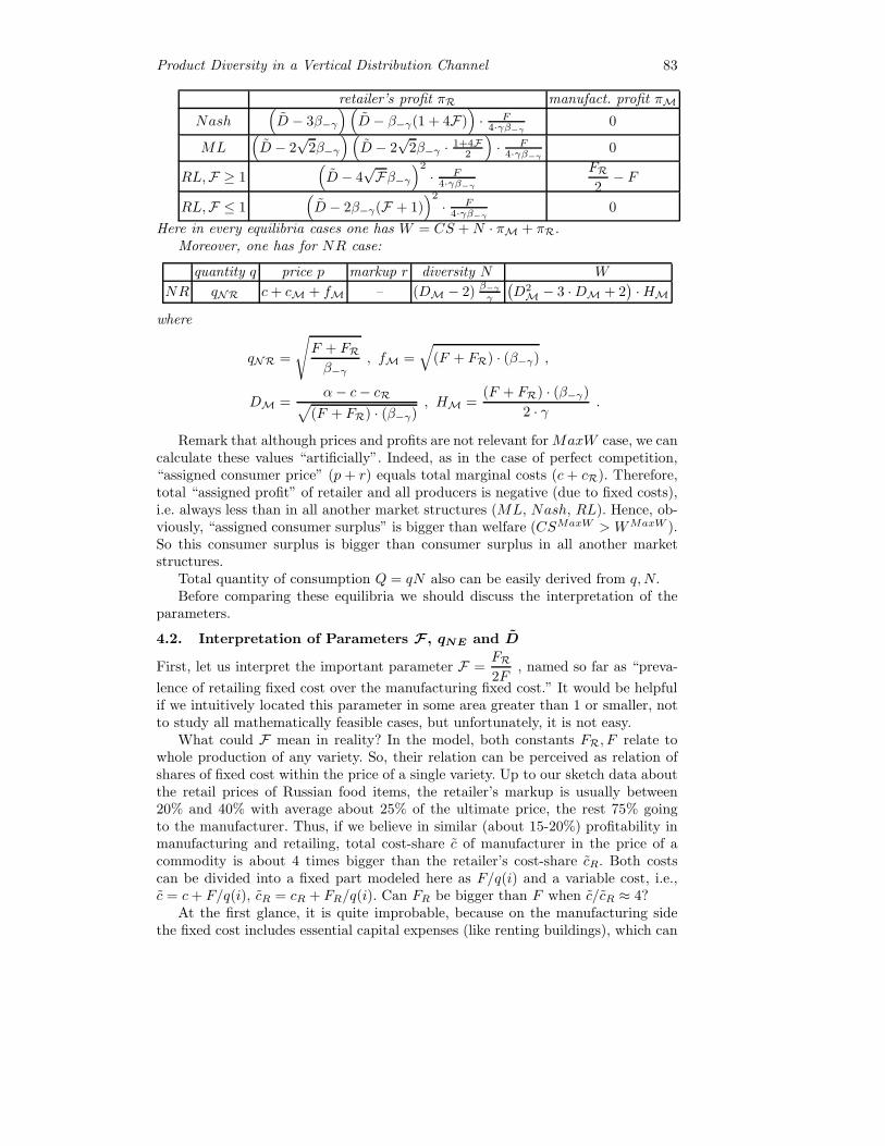
Product Diversity in a Vertical Distribution Channel 83
retailer’s profit πR manufact. profit πM
Nash(D − 3β−γ
)(D − β−γ(1 + 4F)
)· F4·γβ−γ
0
ML(D − 2
√2β−γ
)(D − 2
√2β−γ · 1+4F
2
)· F4·γβ−γ
0
RL,F ≥ 1(D − 4
√Fβ−γ
)2· F4·γβ−γ
FR2− F
RL,F ≤ 1(D − 2β−γ(F + 1)
)2· F4·γβ−γ
0
Here in every equilibria cases one has W = CS + N · πM + πR.Moreover, one has for NR case:
quantity q price p markup r diversity N W
NR qNR c + cM + fM – (DM − 2)β−γγ
(D2
M − 3 ·DM + 2)·HM
where
qNR =
√F + FRβ−γ
, fM =√
(F + FR) · (β−γ) ,
DM =α− c− cR√
(F + FR) · (β−γ), HM =
(F + FR) · (β−γ)
2 · γ .
Remark that although prices and profits are not relevant for MaxW case, we cancalculate these values “artificially”. Indeed, as in the case of perfect competition,“assigned consumer price” (p + r) equals total marginal costs (c + cR). Therefore,total “assigned profit” of retailer and all producers is negative (due to fixed costs),i.e. always less than in all another market structures (ML, Nash, RL). Hence, ob-viously, “assigned consumer surplus” is bigger than welfare (CSMaxW > WMaxW ).So this consumer surplus is bigger than consumer surplus in all another marketstructures.
Total quantity of consumption Q = qN also can be easily derived from q,N.Before comparing these equilibria we should discuss the interpretation of the
parameters.
4.2. Interpretation of Parameters F , qNE and D
First, let us interpret the important parameter F =FR2F
, named so far as “preva-
lence of retailing fixed cost over the manufacturing fixed cost.” It would be helpfulif we intuitively located this parameter in some area greater than 1 or smaller, notto study all mathematically feasible cases, but unfortunately, it is not easy.
What could F mean in reality? In the model, both constants FR, F relate towhole production of any variety. So, their relation can be perceived as relation ofshares of fixed cost within the price of a single variety. Up to our sketch data aboutthe retail prices of Russian food items, the retailer’s markup is usually between20% and 40% with average about 25% of the ultimate price, the rest 75% goingto the manufacturer. Thus, if we believe in similar (about 15-20%) profitability inmanufacturing and retailing, total cost-share c of manufacturer in the price of acommodity is about 4 times bigger than the retailer’s cost-share cR. Both costscan be divided into a fixed part modeled here as F/q(i) and a variable cost, i.e.,c = c + F/q(i), cR = cR + FR/q(i). Can FR be bigger than F when c/cR ≈ 4?
At the first glance, it is quite improbable, because on the manufacturing sidethe fixed cost includes essential capital expenses (like renting buildings), which can

84 Igor Bykadorov, Sergey Kokovin
be about 1/2 of total cost. However, in the long run capital becomes a variable cost.Then the “fixed cost,” more or less independent of the production volume, amountsmainly to advertising and intellectual capital of a company: analytics and mainspecialists with their accumulated knowledge. This cost can be below 10% of totalcost. It is unclear, is such share similar or much bigger in retailing. Here “fixedcost,” spent on each variety, more or less independently of the retailing volume,amounts to maintaining the shell devoted to this variety, costs of bargaining with themanufacturer, of book-keeping this item, and certain advertising efforts of the shop.Naturally, selling a bigger diversity is more costly, under the same volume of sells.We would say, that if it is more costly almost proportionally to N , then the shareof fixed cost FR/q(i) in retailer’s cost cR is close to 1. Elaborating this idea further,we can note that our fixed-plus-linear cost model F + cq is only a linearization ofsome real cost functions C(q) and CR(q). To make a good approximation, we neednot ask a manufacturer about her capital stock and advertising expenses. Instead,we should ask about her current production q and total cost (the point (q, C(q)) oflinearization) and about the derivative C
′(q) = c: “How costly it could be to increase
production for 10-15% or how much you can economize from a decrease.” Then our“fixed cost” parameter F could be calculated as F = C(q)− qC
′(q). The same for
retailer. In this view, concavity or convexity of real cost functions can make F, FRbigger or smaller, positive or negative, with small respect to expenses like advertisingcost. Summarizing this discussion, we understand what kind of real data would behelpful to calibrate our stylized model and reduce the area of search for realisticeffects. But we are unable to calibrate it now even approximately, so, all values ofF are analyzed below. It turns out that this relation between manufacturing andretailing fixed cost essentially change the character of behavior in the industry.
Having explained this, another parameter qNE =√F/β−γ is explained as the
quantity of individual variety emerging at Nash equilibrium (Nash serves as a refer-ence point for other equilibria). We observe that quantity qNE depends only on themanufacturer’s fixed cost and consumer’s variety-loving, being independent of theretailer’s parameters. Observe that the bigger is the entry barrier of fixed cost, thelarger market space is captured by a single producer, that looks reasonable. Besides,the stronger is variety-loving β−γ , the smaller is each manufacturer’s share of themarket at the Nash equilibrium, that also looks reasonable. The table shows thatsimilar reactions to these parameters F, β−γ are demonstrated also by equilibriatypes ML and RL, only the individual quantity itself can be bigger or smaller thanat Nash.
We observe also that wholesale prices at various regimes of competition includeproduction cost and some additional term proportional to the individual quantity,which depends positively upon the fixed cost. Analogously is expressed the retailer’smarkup.
Different is the formula for the diversity N , which positively (and linearly) cor-relates with parameter D, named so especially to highlight this correlation.
D =√β−γ
α− c− cR√F
=α− c− cR
qNE
In the numerator there is the “interval for feasible prices” in this industry, i.e.,the chocking price α (upper limit on the willingness to pay) minus the marginalcost of production and retailing c + cR. If this magnitude is zero, the industrycannot survive. The greater it is, the bigger is the pie of potential wealth that
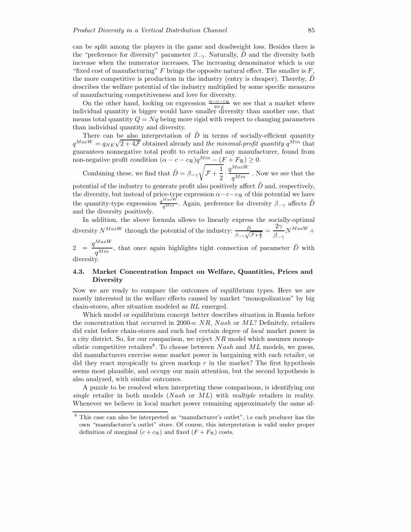
Product Diversity in a Vertical Distribution Channel 85
can be split among the players in the game and deadweight loss. Besides there isthe “preference for diversity” parameter β−γ . Naturally, D and the diversity bothincrease when the numerator increases. The increasing denominator which is our“fixed cost of manufacturing” F brings the opposite natural effect. The smaller is F ,the more competitive is production in the industry (entry is cheaper). Thereby, Ddescribes the welfare potential of the industry multiplied by some specific measuresof manufacturing competitiveness and love for diversity.
On the other hand, looking on expression α−c−cRqNE
we see that a market whereindividual quantity is bigger would have smaller diversity than another one, thatmeans total quantity Q = Nq being more rigid with respect to changing parametersthan individual quantity and diversity.
There can be also interpretation of D in terms of socially-efficient quantityqMaxW = qNE
√2 + 4F obtained already and the minimal-profit quantity qMin that
guarantees nonnegative total profit to retailer and any manufacturer, found fromnon-negative profit condition (α− c− cR)qMin − (F + FR) ≥ 0.
Combining these, we find that D = β−γ
√F +
1
2· qMaxW
qMin. Now we see that the
potential of the industry to generate profit also positively affect D and, respectively,the diversity, but instead of price-type expression α−c−cR of this potential we have
the quantity-type expression qMaxW
qMin . Again, preference for diversity β−γ affects Dand the diversity positively.
In addition, the above formula allows to linearly express the socially-optimal
diversity NMaxW through the potential of the industry: D
β−γ√
F+ 12
=2γ
β−γNMaxW +
2 =qMaxW
qMin, that once again highlights tight connection of parameter D with
diversity.
4.3. Market Concentration Impact on Welfare, Quantities, Prices andDiversity
Now we are ready to compare the outcomes of equilibrium types. Here we aremostly interested in the welfare effects caused by market “monopolization” by bigchain-stores, after situation modeled as RL emerged.
Which model or equilibrium concept better describes situation in Russia beforethe concentration that occurred in 2000-s: NR, Nash or ML? Definitely, retailersdid exist before chain-stores and each had certain degree of local market power ina city district. So, for our comparison, we reject NR model which assumes monop-olistic competitive retailers8. To choose between Nash and ML models, we guess,did manufacturers exercise some market power in bargaining with each retailer, ordid they react myopically to given markup r in the market? The first hypothesisseems most plausible, and occupy our main attention, but the second hypothesis isalso analyzed, with similar outcomes.
A puzzle to be resolved when interpreting these comparisons, is identifying oursingle retailer in both models (Nash or ML) with multiple retailers in reality.Whenever we believe in local market power remaining approximately the same af-
8 This case can also be interpreted as “manufacturer’s outlet”, i.e each producer has theown “manufacturer’s outlet” store. Of course, this interpretation is valid under properdefinition of marginal (c+ cR) and fixed (F + FR) costs.

86 Igor Bykadorov, Sergey Kokovin
ter retailing property concentration, the main change could be in costs. Probably,in Russia the costs of selling did not change too dramatically because of ownershipconcentration itself (leaving aside other causes). Of course, chain-stores economizedsomewhat on unified book-keeping, unified marketing specialists and, notably, onunified logistics. Still, we prefer to ignore this change and do model the sellingcost function FR + cqR as remaining the same during concentration, for two rea-sons. First, we want to analytically separate the market-concentration effect fromeconomies of scale in retailing. Second, since the welfare effect of concentration isfound being positive, our conclusion should be only enforced if we take into accountthese economies of scale also.
Effects of Switching from ML to RL. In addition to these precautions, we alsoshould combine inequalities NML ≥ 0, NRL ≥ 0 with equilibria characterization andget the following conditions on combinations of parameters F and D/β−γ ensuringnon-empty market:
D/β−γ ≥ 4 ·√F if F ≥ 1,
D/β−γ ≥ max{2 ·√
2, 2 · (F + 1)} if F < 1.(7)
Now, under these restrictions, we can formulate the main results on the marketconcentration modeled as switching from ML to RL regimes.
Welfare, Consumer Surplus, Retailer surplus. Algebraic manipulationswith the equilibria formulae obtained yield the unambiguous welfare conclusion:9
Restricted market: F= FR2F > 1 ⇒ WML < WRL
Unrestricted market: F= FR2F ≤ 1⇒ WML ≤WRL
Result 3 Generally there are positive social welfare gains from market concentra-tion, similar in restricted and non-restricted markets.
To comment on this result, the welfare increase may seem quite counter-intuitivefrom the first glance. Normally one expects social losses from market concentration,and exactly such anti-trust reasons stay behind recent proposal by Russian Dumaof the new law restricting chain-stores. Why any gains may occur instead of lossesexpected?
To answer, we first give general reasons, and then look carefully on quantity anddiversity changes during the concentration. Generally, it is a textbook result in IOthat a two-tier monopoly causes higher deadweight loss than a simple monopoly. So,when a two-tier monopoly becomes vertically integrated through ownership concen-tration, it can be quite beneficial for society. In our setting something similar occursunder horizontal concentration, only the changes in the diversity complicate the pic-ture. Indeed, when a leader-manufacturer monopolistically optimizes her price andhas in mind the optimal response of the (locally) monopolistic retailer, this situationis rather similar to the two-tier monopoly. In contrast, when the monopsonistic (andmonopolistic also) retailer exercise essential market power over the manufacturers,it is somewhat similar to vertical concentration, bringing the decision-making intoessentially one hands. In this general view, the welfare gains are not too surprising.
As to consumer surplus CS, the situation is not so simple. The complete solutionis given below.
9 Equality WML = WRL in case F ≤ 1 occurs as a degenerate case, only under specific
parameters Dβ−γ
= 2√
2 and F =√
2 − 1.
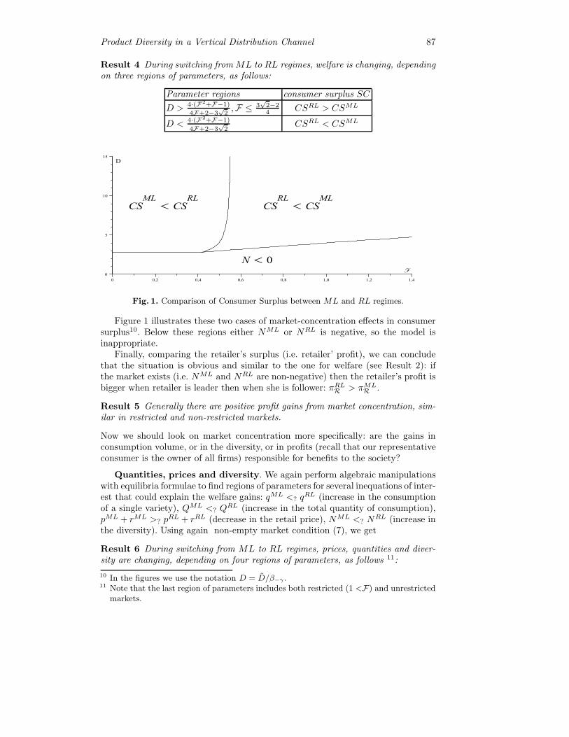
Product Diversity in a Vertical Distribution Channel 87
Result 4 During switching from ML to RL regimes, welfare is changing, dependingon three regions of parameters, as follows:
Parameter regions consumer surplus SC
D > 4·(F2+F−1)
4F+2−3√2,F ≤ 3
√2−24 CSRL > CSML
D < 4·(F2+F−1)
4F+2−3√2
CSRL < CSML
CSML! CS
RLCS
RL! CS
ML
N! 0
D
F
0 0,2 0,4 0,6 0,8 1,0 1,2 1,40
5
10
15
Fig. 1. Comparison of Consumer Surplus between ML and RL regimes.
Figure 1 illustrates these two cases of market-concentration effects in consumersurplus10. Below these regions either NML or NRL is negative, so the model isinappropriate.
Finally, comparing the retailer’s surplus (i.e. retailer’ profit), we can concludethat the situation is obvious and similar to the one for welfare (see Result 2): ifthe market exists (i.e. NML and NRL are non-negative) then the retailer’s profit isbigger when retailer is leader then when she is follower: πRLR > πML
R .
Result 5 Generally there are positive profit gains from market concentration, sim-ilar in restricted and non-restricted markets.
Now we should look on market concentration more specifically: are the gains inconsumption volume, or in the diversity, or in profits (recall that our representativeconsumer is the owner of all firms) responsible for benefits to the society?
Quantities, prices and diversity. We again perform algebraic manipulationswith equilibria formulae to find regions of parameters for several inequations of inter-est that could explain the welfare gains: qML <? q
RL (increase in the consumptionof a single variety), QML <? QRL (increase in the total quantity of consumption),pML + rML >? p
RL + rRL (decrease in the retail price), NML <? NRL (increase in
the diversity). Using again non-empty market condition (7), we get
Result 6 During switching from ML to RL regimes, prices, quantities and diver-sity are changing, depending on four regions of parameters, as follows 11:
10 In the figures we use the notation D = D/β−γ .11 Note that the last region of parameters includes both restricted (1 <F) and unrestricted
markets.
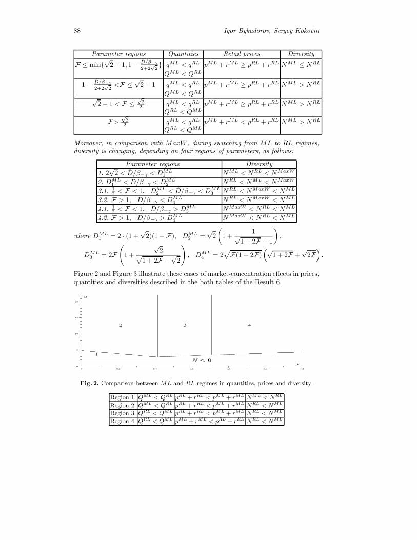
88 Igor Bykadorov, Sergey Kokovin
Parameter regions Quantities Retail prices Diversity
F ≤ min{√
2− 1, 1− D/β−γ2+2
√2} qML < qRL pML + rML ≥ pRL + rRL NML ≤ NRL
QML < QRL
1− D/β−γ2+2
√2<F ≤
√2− 1 qML < qRL pML + rML ≥ pRL + rRL NML > NRL
QML < QRL
√2− 1 < F ≤
√22 qML < qRL pML + rML ≥ pRL + rRL NML > NRL
QRL < QML
F>√22 qML < qRL pML + rML < pRL + rRL NML > NRL
QRL < QML
Moreover, in comparison with MaxW , during switching from ML to RL regimes,diversity is changing, depending on four regions of parameters, as follows:
Parameter regions Diversity
1. 2√
2 < D/β−γ < DML1 NML < NRL < NMaxW
2. DML1 < D/β−γ < DML
2 NRL < NML < NMaxW
3.1. 12 < F < 1, DML
2 < D/β−γ < DML3 NRL < NMaxW < NML
3.2. F > 1, D/β−γ < DML4 NRL < NMaxW < NML
4.1. 12 < F < 1, D/β−γ > DML
3 NMaxW < NRL < NML
4.2. F > 1, D/β−γ > DML4 NMaxW < NRL < NML
where DML1 = 2 · (1 +
√2)(1−F), DML
2 =√
2
(1 +
1√1 + 2F − 1
),
DML3 = 2F
(1 +
√2√
1 + 2F −√
2
), DML
4 = 2√F(1 + 2F)
(√1 + 2F +
√2F).
Figure 2 and Figure 3 illustrate these cases of market-concentration effects in prices,quantities and diversities described in the both tables of the Result 6.
1
2 3 4
N! 0
D
F
0 0,2 0,4 0,6 0,8 1,0 1,2
0
5
10
15
20
Fig. 2. Comparison between ML and RL regimes in quantities, prices and diversity:
Region 1: QML < QRL pRL + rRL < pML + rML NML < NRL
Region 2: QML < QRL pRL + rRL < pML + rML NRL < NML
Region 3: QRL < QML pRL + rRL < pML + rML NRL < NML
Region 4: QRL < QML pML + rML < pRL + rRL NRL < NML
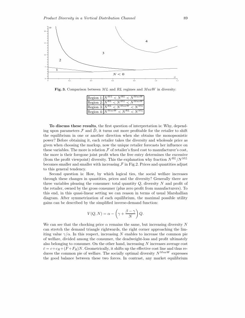
Product Diversity in a Vertical Distribution Channel 89
1
2
3
4
N! 0
D
F
0 0,2 0,4 0,6 0,8 1,0 1,2
0
5
10
15
20
Fig. 3. Comparison between ML and RL regimes and MaxW in diversity:
Region 1: NML < NRL < NMaxW
Region 2: NRL < NML < NMaxW
Region 3: NRL < NMaxW < NML
Region 4: NMaxW < NRL < NML
To discuss these results, the first question of interpretation is: Why, depend-ing upon parameters F and D, it turns out more profitable for the retailer to shiftthe equilibrium in one or another direction when she obtains the monopsonisticpower? Before obtaining it, each retailer takes the diversity and wholesale price asgiven when choosing the markup, now the unique retailer forecasts her influence onthese variables. The more is relation F of retailer’s fixed cost to manufacturer’s cost,the more is their foregone joint profit when the free entry determines the excessive(from the profit viewpoint) diversity. This the explanation why fraction NRL/NML
becomes smaller and smaller with increasing F in Fig.2. Prices and quantities adjustto this general tendency.
Second question is: How, by which logical ties, the social welfare increasesthrough these changes in quantities, prices and the diversity? Generally there arethree variables pleasing the consumer: total quantity Q, diversity N and profit ofthe retailer, owned by the gross consumer (plus zero profit from manufacturers). Tothis end, in this quasi-linear setting we can reason in terms of usual Marshalliandiagram. After symmetrization of each equilibrium, the maximal possible utilitygains can be described by the simplified inverse-demand function:
V (Q,N) = α−(γ +
β − γ
N
)Q.
We can see that the chocking price α remains the same, but increasing diversity Ncan stretch the demand triangle rightwards, the right corner approaching the lim-iting value γ/α. In this respect, increasing N enables to increase the common pieof welfare, divided among the consumer, the deadweight-loss and profit ultimatelyalso belonging to consumer. On the other hand, increasing N increases average costc = c+cR+(F +FR)N . Geometrically, it shifts up the effective cost line and thus re-duces the common pie of welfare. The socially optimal diversity NMaxW expressesthe good balance between these two forces. In contrast, any market equilibrium
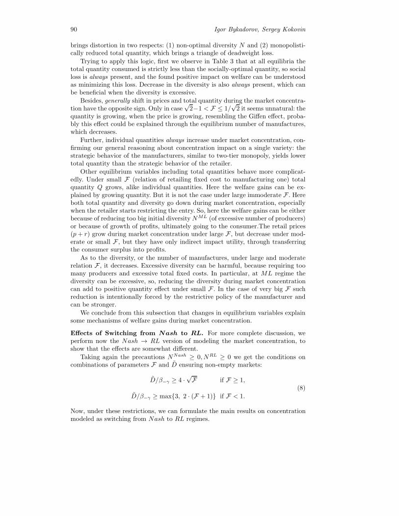
90 Igor Bykadorov, Sergey Kokovin
brings distortion in two respects: (1) non-optimal diversity N and (2) monopolisti-cally reduced total quantity, which brings a triangle of deadweight loss.
Trying to apply this logic, first we observe in Table 3 that at all equilibria thetotal quantity consumed is strictly less than the socially-optimal quantity, so socialloss is always present, and the found positive impact on welfare can be understoodas minimizing this loss. Decrease in the diversity is also always present, which canbe beneficial when the diversity is excessive.
Besides, generally shift in prices and total quantity during the market concentra-tion have the opposite sign. Only in case
√2−1 < F ≤ 1/
√2 it seems unnatural: the
quantity is growing, when the price is growing, resembling the Giffen effect, proba-bly this effect could be explained through the equilibrium number of manufactures,which decreases.
Further, individual quantities always increase under market concentration, con-firming our general reasoning about concentration impact on a single variety: thestrategic behavior of the manufacturers, similar to two-tier monopoly, yields lowertotal quantity than the strategic behavior of the retailer.
Other equilibrium variables including total quantities behave more complicat-edly. Under small F (relation of retailing fixed cost to manufacturing one) totalquantity Q grows, alike individual quantities. Here the welfare gains can be ex-plained by growing quantity. But it is not the case under large immoderate F . Hereboth total quantity and diversity go down during market concentration, especiallywhen the retailer starts restricting the entry. So, here the welfare gains can be eitherbecause of reducing too big initial diversity NML (of excessive number of producers)or because of growth of profits, ultimately going to the consumer.The retail prices(p + r) grow during market concentration under large F , but decrease under mod-erate or small F , but they have only indirect impact utility, through transferringthe consumer surplus into profits.
As to the diversity, or the number of manufactures, under large and moderaterelation F , it decreases. Excessive diversity can be harmful, because requiring toomany producers and excessive total fixed costs. In particular, at ML regime thediversity can be excessive, so, reducing the diversity during market concentrationcan add to positive quantity effect under small F . In the case of very big F suchreduction is intentionally forced by the restrictive policy of the manufacturer andcan be stronger.
We conclude from this subsection that changes in equilibrium variables explainsome mechanisms of welfare gains during market concentration.
Effects of Switching from Nash to RL. For more complete discussion, weperform now the Nash → RL version of modeling the market concentration, toshow that the effects are somewhat different.
Taking again the precautions NNash ≥ 0, NRL ≥ 0 we get the conditions oncombinations of parameters F and D ensuring non-empty markets:
D/β−γ ≥ 4 ·√F if F ≥ 1,
D/β−γ ≥ max{3, 2 · (F + 1)} if F < 1.
(8)
Now, under these restrictions, we can formulate the main results on concentrationmodeled as switching from Nash to RL regimes.
Product Diversity in a Vertical Distribution Channel 91
Welfare. Algebraic manipulations with the equilibria formulae obtained yield,using again non-empty market condition (8), the unambiguous welfare conclusion:
Result 7 During switching from Nash to RL regimes, welfare is changing, depend-ing on three regions of parameters, as follows:
Parameter regions WelfareF < 1
2 WNash < WRL(9·√F
2 + 1√F−3−2·F
)·D/β−γ>
74 ,F > 1
2 WNash > WRL(9·√F
2 + 1√F−3−2·F
)·D/β−γ<
74 WNash < WRL
For the consumer surplus CS, the situation is more simple12:
Parameter regions consumer surplus SC
1. Small: F <1
2CSNash < CSRL
2. Large: F >1
2CSRL < CSNash
Figure 4 illustrates these cases of market-concentration effects in welfare andconsumer surplus.
WNash!W
RLWRL!W
NashWNash!W
RL
CSNash! CS
RLCS
RL! CS
NashCS
RL! CS
Nash
N! 0
D
F
0 0,5 1,0 1,5 2,0 2,50
5
10
15
20
25
Fig. 4. Comparison between Nash and RL regimes in welfare and consumer surplus.
We see that welfare increases during switching from Nash regime to RL regimeonly under big or small relative fixed cost F , but decreases under moderate one;while consumer surplus increases during the switching only under small relativefixed cost F . As an interpretation of the Figure 4, remark that, since in the middleregion WN∫〈 > WRL, Nash outcome here is more “competitive” than outcomeunder the leadership of retailer.
Quantities, prices and diversity. We again perform algebraic manipulationswith equilibria formulae to find regions of parameters for several inequations ofinterest: qNash <? q
RL (increase in the consumption of a single variety), QNash <?
QRL (increase in the total quantity of consumption), pNash + rNash <? pRL + rRL
(increase in the retail price), NNash <? NRL (increase in the diversity).
Using again non-empty market condition (8), we get
12 Cf. the case of switching from ML to RL, see the Table in Result 2 and Figure 1.
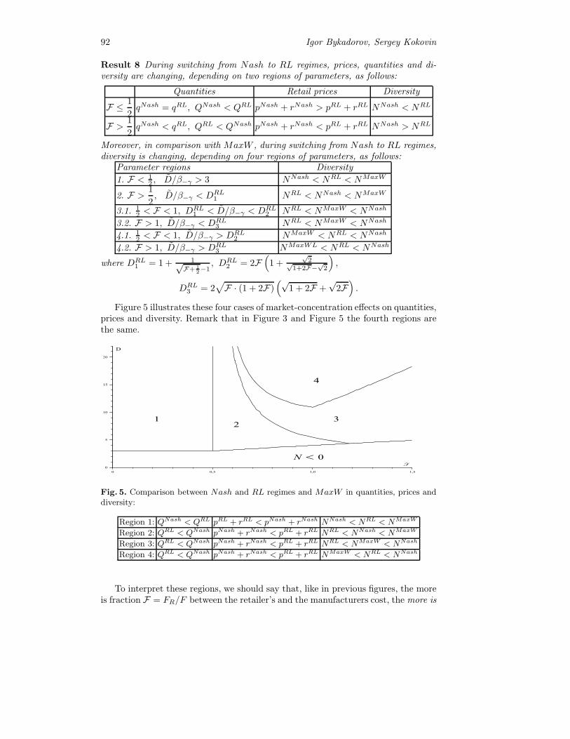
92 Igor Bykadorov, Sergey Kokovin
Result 8 During switching from Nash to RL regimes, prices, quantities and di-versity are changing, depending on two regions of parameters, as follows:
Quantities Retail prices Diversity
F ≤ 1
2qNash = qRL, QNash < QRL pNash + rNash > pRL + rRL NNash < NRL
F >1
2qNash < qRL, QRL < QNash pNash + rNash < pRL + rRL NNash > NRL
Moreover, in comparison with MaxW , during switching from Nash to RL regimes,diversity is changing, depending on four regions of parameters, as follows:
Parameter regions Diversity
1. F < 12 , D/β−γ > 3 NNash < NRL < NMaxW
2. F >1
2, D/β−γ < DRL
1 NRL < NNash < NMaxW
3.1. 12 < F < 1, DRL
1 < D/β−γ < DRL2 NRL < NMaxW < NNash
3.2. F > 1, D/β−γ < DRL3 NRL < NMaxW < NNash
4.1. 12 < F < 1, D/β−γ > DRL
2 NMaxW < NRL < NNash
4.2. F > 1, D/β−γ > DRL3 NMaxWL < NRL < NNash
where DRL1 = 1 + 1√
F+ 12−1
, DRL2 = 2F
(1 +
√2√
1+2F−√2
),
DRL3 = 2
√F · (1 + 2F)
(√1 + 2F +
√2F).
Figure 5 illustrates these four cases of market-concentration effects on quantities,prices and diversity. Remark that in Figure 3 and Figure 5 the fourth regions arethe same.
12
3
4
N! 0
D
F
0 0,5 1,0 1,5
0
5
10
15
20
Fig. 5. Comparison between Nash and RL regimes and MaxW in quantities, prices anddiversity:
Region 1: QNash < QRL pRL + rRL < pNash + rNash NNash < NRL < NMaxW
Region 2: QRL < QNash pNash + rNash < pRL + rRL NRL < NNash < NMaxW
Region 3: QRL < QNash pNash + rNash < pRL + rRL NRL < NMaxW < NNash
Region 4: QRL < QNash pNash + rNash < pRL + rRL NMaxW < NRL < NNash
To interpret these regions, we should say that, like in previous figures, the moreis fraction F = FR/F between the retailer’s and the manufacturers cost, the more is

Product Diversity in a Vertical Distribution Channel 93
the need to diminish the excessive variety, determined by the free entry without therespect for the retailer’s losses from the excessive diversity (free entry pays respectonly to F ). When switching to RL regime, the retailer becomes capable to influencethis excess (from her viewpoint) diversity directly or indirectly.
We did not compare No-retailer equilibrium with RL-equilibrium because wedo not suppose NR case realistic enough. Never substantial share of the retailingmarket was covered by the shops belonging to producers. Instead we use this modelas theoretical reference point: vertical integration of the industry performed fromabove, from the producer’s side. It is compared in the next section to vertical inte-gration from below, from the retailer’s side.
Generally, in this section we have seen that a conclusion about welfare benefitsof market concentration, switching from one or another previous industry organiza-tion may depends upon demand functions and technologies, but welfare gains frommarket concentration is quite plausible. Therefore, in spite of noticeable public com-plaints about the retailer’s bargaining power (mentioned in Intro), this power andleadership in relations with manufacturers can occur socially desirable. In this casean economist should not advice a governmental intervention against chain-storesand similar practices, recently suggested by Duma. Section 6 devoted to regulationadds arguments in the same direction.
Possible extensions of the setting. We conclude this section devoted tomarket concentration effects by the question: Which is the most realistic model ofpre-concentration retailing? Instead of two alternative models that we could useseveral other versions. First, we could study a market with direct selling by man-ufacturers without any retailing shops, but it seems less realistic (as suggested bydiscussants in our presentations). Second, the case when manufacturers have biggermarket power than retailing sector, seems irrelevant to pre-concentration regimein Russia and similar countries, because several manufacturers jointly controllingcommon retailer seems unrealistic.
It means that manufacturers behave simultaneously but strategically towardsthe retailing sector and consumers, percept as their common agent in principal-agent relations, and considering externalities onto each other. It seems not a goodmodel for our question. Indeed, before market concentration, typical manufacturerof consumer goods in Russia sold to several shops shared with several other suppliers.For big manufacturers the markup was the result of individual bargaining with ashop (like in ML equilibrium), for small ones it was a market constant (like in Nashequilibrium). Anyway, a common-agency story seems irrelevant. Instead, a moresophisticated and realistic description of concentration would like to undertake twodetailizations of the model.
(1) We can consider big and small manufacturers or/and retailers, describingconcentration as appearance of more and more big chain-stores among the compet-itive fringe of small shops.
(2) In addition, spatial structure of the market should be described somehowto explain why in reality the same varieties are sold for much smaller prices inchain-stores outside the city center than in small shops in the center.
However, both extensions wait for another paper.
94 Igor Bykadorov, Sergey Kokovin
5. Entrance Fees
Now we describe an extension of our setting motivated as follows. In Intro we havementioned that trade relations between the manufacturers and the retailers ofteninvolves more complex terms than just a markup. Rather typically, to start andmaintain selling anything through a chain-store, a manufacturer is forced to pay anentrance fee to the retailer, annually or monthly. Denoting this per-period fee asFE we can look on it as an addition to the manufacturer’s fixed cost, that becomesnow F = F + FE . This amount is subtracted from the retailers fixed cost thatbecomes FR = FR − FE . This fee FE is as a new pricing tool optimized by theretailer simultaneously with optimizing the markup and the diversity. The regimestudied is when the retailer is leading the game.
We want to know: What happens to price and variety because of the two-parttariff practice? Is this practice really harmful for society, as manufacturers andmany journalists and politicians suggest in the cited papers (Nikitina, 2006) and(Sagdiev et al., 2006), or not? We are going to show positive gains of the entrancefee. So, the government and legislature should not do what they do now, prohibitingthe fee.13
Equilibrium with entrance fee. To support our hypothesis, we modify theretailer’s optimization program and the equilibrium formulae for the case ”RL”.The profit function of i-th manufacturer becomes
πM(i) = [p(i)− c]q(i)− (F + FE)
and the profit of the retailer is now
πR =
∫ N
0
[r(i) − cR]q(i)di−∫ N
0
(FR − FE)di.
Since the retailer is the leader, in symmetric equilibria we have the same expres-sions as before (see (5)-(6)) for the wholesale price p and quantity q of each varietyas functions of markup r and diversity N :
q = q(r,N) =(b + gN)[a− b(c + r)]
2b + gN, p = p(r,N) =
a + (b + gN)c− br
2b + gN.
Therefore, the new profit-maximization problem of the retailer is
πR = N [(r − cR)q(r,N)− FR + FE ] → maxr,N,FE ,
πM = [p(r,N)− c]q(r,N)− (F + FE) ≥ 0 .
Since
∂πR∂FE
= N > 0, (9)
the objective function should attain a boundary maximum, so restriction on non-negative profit πM is active in the equilibria, i.e. free entry condition πM = 0 holds.
13 Notably, Russian parliament has just adopted a bill (”Law on trade...”) that prohibitsthe entrance fees in retailing, because they are supposed harmful for competition andwelfare.

Product Diversity in a Vertical Distribution Channel 95
Hence
FE = −F + [p(r,N)− c]q(r,N) = −F +q2(r,N)
b + gN. (10)
Substituting this into πR we obtain the unconstrained optimization problem
πR = N [q2(r,N)
b + gN+ (r − cR)q(r,N)− (FR + F )] → max
r,N.
Its solution is
NE =
D√1 + 2F
− 2β−γ
2γ, rE = cR + qNE
(D
2− β−γ
√1 + 2F
).
Surprisingly, for each diversity the optimal entrance fee equals exactly to thefixed selling cost FE = FR. The quantity is qE = qNE
√1 + 2F and the wholesale
price is pE = c + qNEβ−γ√
1 + 2F .Finally, we calculate profit, social welfare and consumer surplus under two-part
tariff:
πER =(D − 2
√1 + 2F · β−γ
)2· F
4γβ−γ, CSE =
F
8γβ−γ·(D − 2
√1 + 2F · β−γ
)D,
WE = πER + CSE =3F
8γβ−γ·(D − 2
√1 + 2F · β−γ
)·(D − 4
3·√
1 + 2F · β−γ
).
Comparing all the above formulae with the ones in Result 2 (see page 11), it is easyto derive the following consequences of introducing the two-part tariff.
Result 9 When the leader-retailer introduces the entrance fee,
– pE > pRL, i.e. entrance fee always pushes up the wholesale price, thuscompensating the fee to manufacturers,
– rE < rRL, i.e. entrance fee decreases the markup, and, surprisingly,
– pE + rE < pRL+ rRL, i.e. entrance fee always pushes down the retail price!– qE > qRL, i.e. the entrance fee always increases quantity of each variety,– QE > QRL, i.e. the entrance fee increases total quantity of the industry,– WE > WRL, CSE > CSRL, πER > πRLR , i.e. entrance fee always increases
social welfare and consumer surplus.
As to the diversity N, under the fee NE can be less or more than NRL, dependingon two regions of parameters D and F as follows:
Parameter regions DiversityDβ−γ
> DRL
NE < NRL
DRL
> Dβ−γ
> DRL NE > NRL
where bounds of these regions are the following continuous functions of F :
DRL =
{4√F , F ≥ 1;
2(F + 1), F ≤ 1;DRL
=
{(1 +
√1F + 2
)·√
1 + 2F · 2F1+F , F ≥ 1;(
1 +√
1 + 2F)·√
1 + 2F , F ≤ 1.

96 Igor Bykadorov, Sergey Kokovin
NE! N
RLNRL! N
E
N! 0
D
F
0 1 2 30
1
2
3
4
5
6
7
8
9
Fig. 6. Comparison between RL and Entrance fee regimes in diversity.
Figure 6 explains the comparison in diversity: when NE < NRL and whenNE > NRL. One can see that when the retailer’s fixed cost is sufficiently biggerthan manufacturer’s one and the slack between the chocking price and costs is small,the entrance fee increases the diversity.
Why the optimal entrance (shelf) fee becomes equal to the retailer’s fixed costs?To understand the result obtained, let us note that an increase in entrance fee(in first approximation) leads to the growth of retailer’s profit (it is easy to see,for instance, from (9)). On the other hand, when entrance fee increases, the fixedcosts of producers also increase. These additional costs must be covered by higher
wholesale price or/and by bigger per-firm output. Therefore, generally∂N
∂FE< 0,
i.e, the number of varieties (i.e. the number of firms in the industry) decreases14.This tendency hampers the increase in the retailer’s profit. The interaction of thesetwo forces determines the equilibrium entrance fee. For the linear functional form ofdemand, it turns out that resulting entrance fee equals to the retailer’s fixed costs.Probably (in our opinion), for other functional forms the optimal entrance fee maybe bigger or less than the retailer’s fixed costs, depending on the value of theseopposite forces.
Another way to understand this effect is the comparison of entrance fee practicewith the vertical integration of the industry. We use such comparison below toexplain why the entrance fee increases social welfare and even the consumer surplus(in contrast to what Russian legislature thinks about it).
This increase becomes not so surprising, if we recall that generally in manymarket situations it is not the monopolism per se responsible for the welfare losses,but the inability of the monopolist to use the efficient tools of pricing like perfectprice discrimination, etc. In particular, the entrance fee works here exactly like intypical situations where two-part tariff compensates the fixed cost and increasesthe efficiency of the market through making prices closer to costs. Here the markupworks like a price for manufacturers to get the service of retailer. Thus, the welfareincrease under entrance fee has the common nature with a two-part tariff.
14 If we substitute in (10) the expression (see (5)) q = q(r,N) = (b+gN)[a−b(c+r)]2b+gN
, then
FE + F =(α−c−r)2·β−γ(2β−γ+γN)2
. So, ∂N∂FE
< 0.

Product Diversity in a Vertical Distribution Channel 97
More light on increasing welfare is shaded by the following argument. Supposethat starting from situation with entrance fees the next step in retailer’s enforcementis undertaken: vertical integration of the industry. It means that the monopolisticretailer becomes the owner of the whole industry with its manufacturing and re-tailing. She chooses the retail price and the number of varieties (the product line),bearing all manufacturing and retailing costs. Does this integration change the mar-ket outcome and her profit? The surprising answer is “no”.
To show this, we maximize the owner’s profit π = ((pR− c− cR)q(pR, N)−F −FR)N with respect to the length N of the product line and the retail price pR equalto previous p + r. Here, as previously, the demand for a variety i is qi(pR, N) =
a− (b+gN)piR+g∫ N0
pjRdj where a, b, g are dependent on N as in (4). Taking intoaccount that the solution should be symmetric, we replace pi and pj by pR and get
q(pR, N) =α− pR
β + γ(−1 + N)(11)
Maximizing profit and simplifying the result we get the market outcome(qMon, pMon
R , NMon) of such integrated monopoly:
qMon =
√F + FRβ−γ
= qE , pMonR =
α + c + cR2
= pE + rE ,
NMon =β−γ2γ
(−2 +
α− c− cR√(F + FR)β−γ
)= NE,
which turns out exactly the same as under retailer leadership with entrance fee.Naturally, profit and welfare also coincide. Thus, we have proved that combinationof two pricing tools: entrance fee plus markup is equivalent to integratedmonopoly. With their help the retailer fully controls the industry, to the benefitof consumers, neutralizing the shortcomings of two-tier monopoly and resolving thenegative externalities among manufacturers.
The next improvement in the same direction, aiming to get first-best Paretoefficiency would be exercising the entrance fee FC for consumers (using two-parttariff instead of linear pricing). To show this, use (5)-(6) under symmetry assumptionand maximize such price-discriminating monopolist’s profit
πDMon = ((pDM − c− cR)q(pDM , N)− F − FR)N + FC → maxpDM ,N,FC
FC ≤ [α− β−γ2
q(pDM , N)− γ
2Nq(pDM , N)− pDM ]Nq(pDM , N).
Here the right-hand side describes the potential consumer surplus from using thediversified industry. This CS is completely captured by the monopolist through theconsumer’s entrance fee (nothing remains actually), but it returns to consumer inthe form of monopolist’s profit and spent on other goods. It can be observed fromthe above program that the monopolist just maximizes the consumer’s welfare, andthe outcome will be price equal to marginal cost, efficient quantity, see Result 2,and efficient diversity NMaxW :
pDMonR = c + cR, qDMon =
√2 · F + FR
β−γ,

98 Igor Bykadorov, Sergey Kokovin
FC =α− c− cR
2γ·(α− c− cR −
√2 · (F + FR)β−γ
),
NDMon =β−γ2γ·(−2 +
α− c− cR√(F + FR)β−γ
√2
),
πDMonR = WDMon =
(D −
√2(1 + 2F)(β − γ)
)2· F + FR
2 · γβ−γ.
Comparing with previous results, observe that qDMon = qMaxW > qMon = qE ,NDMon = NMaxW > NMon = NE , WDMon = WMaxW > WMon; therefore al-lowing for more powerful and sophisticated monopolist increases both consumptionand diversity, thereby increasing welfare (as sophistication typically does in IO).
Our conjecture is that this market outcome can be obtained indirectly, namelya retailer-leader can use both entrance fees (FE for manufacturers and FC for con-sumers) instead of integrating the industry to arrive at the same first-best outcomeas we have just found for integrated monopoly. Then, usage of discount cards payedby consumers in some shops (entrance fees) can be welfare improving.
Finally, let us compare Entrance fee equilibrium with NR equilibrium. It turnsout that qNR = qE , NNR = 2·NE, i.e., under NR regime, the quantity equalsto the quantity in the situation with Entrance fee, while the diversity istwo times more then the diversity in the situation with Entrance fee.
So, we find the correspondence between NR and Entrance fee regimes. There-fore, it seems interesting to compare consumer surplus and welfare for these regimes.One has
CSE =F
8γβ−γ·(D − 2
√1 + 2F · β−γ
)D,
WE =3F
8γβ−γ·(D − 2
√1 + 2F · β−γ
)·(D − 4
3·√
1 + 2F · β−γ
),
CSNR = WNR =3F
8γβ−γ·(D − 2
√1 + 2F · β−γ
)·(
4
3· D − 4
3·√
1 + 2F · β−γ
).
Hence
CSNR − CSE =3F
8γβ−γ·(D − 2
√1 + 2F · β−γ
)·(D − 2
3·√
1 + 2F · β−γ
)> 0,
WNR −WE =F
8γβ−γ·(D − 2
√1 + 2F · β−γ
)· D > 0,
i.e., under NR regime, welfare and consumer surplus are bigger then thecorrespondence ones under Entrance fee regime.
For the government, the ideas of this section suggest refraining from any regu-lation, when profits are transferred to consumers and redistribution needs does notforce the regulation. The next section expands these ideas.

Product Diversity in a Vertical Distribution Channel 99
6. Governmental Regulation of Retailing
Based on the above analysis, this section considers the outcomes of several possiblemeasures that the state may wish to use, under one or another market situation.Namely, when the retailer’s leadership after market concentration arise, it maytempt the state (the government or legislature) to restrict the market size of eachfirm, or/and the markup or/and restrict entrance fee when it is used (exactly likethe Russian legislature did).
Section 4.3 about concentration showed that restriction of concentration by thestate can be detrimental, at least under our assumptions.
As we have seen in the previous section, prohibition of entrance fee for manu-facturers is detrimental for welfare. Now we study alternative measures.
6.1. Government Intervention through Capping Markup
Consider the specific situation when the government starts regulating the markupof the retailer-leader who does not use any entrance fees. So, regulated markup rmaximizes welfare, being chosen by the government who correctly anticipates thesubsequent choices of retailer, producers and consumers. The retailer-leader choosesonly variety N within the constraint of non-negative producers’ profits, which istypically binding.
To solve the equilibrium by backward induction, we have seen in (5)–(6) thatthe output and wholesale price of a firm in the long-run is always
q = q(r,N) =(b + gN)[a− b(c + r)]
2b + gN, p = p(r,N) =
a + (b + gN)c− br
2b + gN.
Having this in mind, the retailer solves the problem
πR = N [(r − cR)q(r,N)− FR] → maxN
,
πM = [p(r,N)− c]q(r,N)− F ≥ 0
(12)
obtaining her best response N = N(r) to the markup regulated by the government.Anticipating this N(r), the government solves the welfare maximization problem
W = W (r) → maxr
.
We restrict our study only to the important case when the parameters of the modelmake “the non-negative manufacturer’s profit” condition πM ≥ 0 active, i.e. theretailer becomes a dummy in the game whereas free entry determines N(r) 15. Then,it is easy to see that under direct intervention of the government into pricing,quantity qd, wholesale price pd, markup rd, diversity Nd and social welfare W d
become
qd = qNE =
√F
β−γ, pd = c + qNE · β−γ , rd = cR + qNE · D ·
FF + 1
,
15 The class of parameters generating the opposite type of equilibrium (restricted entry)is not so easy to analyse. Besides, the regulating measures hardly can be confined tocapping markup in this case, so a richer model is needed.

100 Igor Bykadorov, Sergey Kokovin
Nd =
D
1 + F − 2β−γ
γ, πdR =
(D − 2β−γ · (1 + F)
)2· F
(1 + F)2· F
γβ−γ,
CSd =(D − 2β−γ · (1 + F)
)·(D − β−γ · (1 + F)
)· 1
2 · (1 + F)2· F
γβ−γ,
W d =(D − 2β−γ · (1 + F)
)·(D − 1 + 4F
1 + 2F · β−γ · (1 + F)
)· 1 + 2F
2 · (1 + F)2· F
γβ−γ.
Comparing this outcome with the previous results we get the following comparisonof the direct intervention of the government with the “RL” (free entry!) case 16.
Result 10 One has
– qd = qRL, i.e direct intervention of the government does not change thequantity of each variety
– pd = pRL, i.e direct intervention of the government does not change thewholesale price
– rd < rRL, i.e direct intervention of the government decreases the markup– Nd > NRL, i.e direct intervention of the government increases the diversity– W d > WRL, i.e direct intervention of the government increases the social
welfare
Now, using the above formulae, we can compare diversities Nd NRL with the socialoptimal diversity NMaxW . A natural conjecture is that socially efficient diversityis the largest among NRL, Nd, NMaxW . Surprisingly, it is not true in general. Thetable below shows that all three cases NRL < Nd < NMaxW , NRL < NMaxW <Nd, NMaxW < NRL < Nd are possible:
Parameter regions Diversity
1. 2(1 + F) < Dβ−γ
< DMaxW , F ≤ 1 NRL < Nd < NMaxW
2.1. DMaxW < Dβ−γ , F < 0.5 NRL < NMaxW < Nd
2.2. DMaxW < Dβ−γ , F > 0.5, D
β−γ < DMaxW
NRL < NMaxW < Nd
3. DMaxW
< Dβ−γ
, 0.5 < F ≤ 1 NMaxW < NRL < Nd
where
DMaxW = −4−√
2 + 4F +14F + 6 + (4F + 2)3/2
−F2 + 2F + 1,
DMaxW
= 3 +√
2 + 4F +3 +√
4F + 2
2F − 1.
Moreover (see Figure 7), region 1 where NRL < Nd < NMaxW is rather small,while the other two zones are large.
Thus, we conclude that direct intervention of the government may lead to“over-production of diversity” and in the case when the diversity is alreadytoo large, the intervention aggravates “over-production of diversity”.
Further, we can ask: Does the government enhance social welfare when it pro-hibits entrance fee (previously existing), and simultaneously restricts markup fromabove? Some ideas for the answer we can find in the table below16 Let us recall that we consider here only free entry case, hence F < 1.

Product Diversity in a Vertical Distribution Channel 101
1
2
3
N! 0
D
F
0,1 0,2 0,3 0,4 0,5 0,6 0,7 0,8 0,9 1,00
5
10
15
20
Fig. 7. Comparison between RL, Capping markup and MaxW regimes in diversity:
Region 1: NRL < Nd < NMaxW
Region 2: NRL < NMaxW < Nd
Region 3: NMaxW < NRL < Nd
Parameter regions WelfareDβ−γ
> DEd WE < W d
2(1 + F) < Dβ−γ
< DEd, F ≤ 1 WE > W d
where DEd = −8Fd1+√d21+d2
, d1 = 5√1+2F2 + 5
1+F − 8 < 0, d2 = 8F(F−1)(3F+1)(1+F)2 ≤
0 ∀ F ∈ [0; 1].Comparing such intervention with entrance fee situation, we see on Figure 8 that
capping markup is better for welfare than entrance fee where D = (α−c−cR)√
β−γF
is big and F = FR2F small, but the opposite is true in another region. So, when
retailer’s fixed cost are sufficiently bigger than manufacturer’s one and the slackbetween the chocking price and costs is small, the government should not intervenein this fashion.
WE!W
dWd!W
E
N! 0
D
F
0 0,2 0,4 0,6 0,8 1,00
2
4
6
8
10
Fig. 8. Comparison between Entrance fee and Capping markup regimes in welfare.
102 Igor Bykadorov, Sergey Kokovin
6.2. Pigouvian Regulation: to Tax or to Subside the Retailer?
Suppose that the government stimulates the market in Pigouvian way. The retailerpays the tax τ per every unit of goods sold. Then the retailer’s profit takes the form∫ N
0
[r(i) − (cR + τ)]q(i)di −∫ N
0
FRdi.
The collected taxes are redistributed among the consumers in a lump-sum manner.In the case of negative τ it means a Pigouvian subsidy, funded from a lump-sum
taxes on consumers in amount NF = τ∫ N0
q(i)di.The welfare function WRL(q(τ), N(τ)) has the previous form, only equilibrium
variables q(τ), N(τ) become the functions of tax τ . They, and welfare, can be foundfrom the previous formulae. Knowing these equilibrium expressions, the governmentcan maximize the welfare function with respect to τ , and find the taxation policythat maximizes the social welfare. We did not solve this problem here (though itis possible), finding instead only the sign: Should the government start taxing orsubsidizing the retailer for a small amount? In other words, the question is: Whenit is beneficial for the government to tax the retailer (τ > 0), or to subside her(τ < 0)?
Result 11 Under the strategic behavior of the retailer, it is beneficial for the gov-ernment to subside her, i.e. τ∗ < 0.
This fact seems unnatural in anti-trust logics: the state should subsidize a mo-nopolist/monopsonist. However, such effects are rather typical in IO literature andthe proofs are simple. We just have ensured that our more complicated situationwith varieties keeps the same effect.
7. Conclusion
We study the model where the monopolistic-competition industry is selling manyvarieties through the monopsonistic retailer. The emergence of such retailer witha two-sided market power is compared to initial situation, when the manufactur-ers were selling through many retailers having a local selling market power but nobuying power. Thereby we model the welfare and marketing effects of the mar-ket concentration after the emergence of big chain-stores in Russia and other CIScountries.
In the special case of quadratic valuations (linear demands) it turns out thatgenerally the concentration enhances social welfare. This effect, unexpected for non-economists, actually is not too surprising, because it reminds the switch from a two-tier monopoly to a simple monopoly. The welfare increase here, however, can go notonly through the growth of the total quantity, but in some cases through growingtotal profits and, notably, through decreasing excessive diversity. The retailer isshown to be generally interested in restricting the diversity, but it is not harmfulitself.
In the case of the governmental regulation of the monopsonistic retailer throughPigouvian taxes, it turns out that subsidies instead of taxes are needed, that alsoreminds similar effect known for a simple monopoly/monopsony.
The anti-chain-stores bill recently suggested by Russian Parliament (Duma)shows the public interest in this type of questions.

Product Diversity in a Vertical Distribution Channel 103
Acknowlegments. We are grateful to EERC experts, especially to Prof. RichardEricson, Prof. Russell Pittman, Prof Shlomo Weber, Prof. Michael Alexeev, Prof.Oleksandr Shepotylo and Prof. Gary Krueger for the attention to the research anduseful suggestions.
References
Bernheim, B. D. and Whinston, M. D. (1986). Common agency. Econometrica, 54, 923–942.
Chen, Z. (2004). Monopoly and Production Diversity: The role of retailer CountervailingPower. - November 8, 2004, 25 p. - Discussion Paper of Carleton University.
Combes, P. -P. T. Mayer and J. -F. Thisse (2008). Economic Geography. The Integrationof Regions and Nations. Princeton University Press.
Dixit, A. K. (1983). Vertical integration in a monopolistically competitive industry. Inter-national Journal of Industrial Organization, 1, 63–78.
Dixit, A. K. and J. E. Stiglitz (1977). Monopolistic competition and optimum product di-versity. American Economic Review, 67, 297–308.
FAS (2007) FAS Russia’s activities on developing competition in retail (October 2007).Site of the Federal Antimonopoly Service of Russian Federation (is available inhttp://www.fas.gov.ru/english/decisions/15841.shtml )
Hamilton, S. F. and T. J. Richards (2007). Comparative Statics for Supermarket Oligopolywith Applications to Sales Taxes and Slotting Allowances. May 31 2007, 22 p. – SelectedPaper prepared for presentation at the American Agricultural Economics AssociationAnnual Meeting, Portland, OR, July 29 - August 1, 2007.
Hotelling, H. (1929). Stability in competition. The Economic Journal, 37, 41–57.Kaloshkina, M., V. Klintsov, S. Shelukhin, I. Shvakman and A. Sukharevsky (2009).
Lean Russia: The productivity of retail. McKinsey Global Institute (is available inhttp://www.mckinsey.com/mgi/publications/lean russia/)
Lira, L., M. Ugarte and R. Vergara (2008). Prices and Market Structure: An EmpiricalAnalysis of the Supermarket Industry in Chile. Pontificia Universidad Catolica de Chile.Discussion Paper, No. 346, Noviembre 2008, 29 p.
Mathewson, G. F. and R. A. Winter (1983). Vertical integration by contractual restraintsin spatial markets. Journal of Business, 56, 497–517.
Nikitina E. (2006). Arifmetika sborov po vnutrennim prais-listam “na vkhod”v magaziny krupnejshikh stolichnykh ritejlerov - “Auchana”, “Patersona”,“Sed’mogo kontinenta” i dr. SmartMoney, 07.08.2006 (in Russian) (is availablein http://compromat.ru/main/mix/retail1.htm)
Ottaviano, G. I. P., T. Tabuchi and J. -F. Thisse (2002). Agglomeration and trade revised.International Economic Review, 43, 409–436.
Perry, M. K. (1989). Vertical integration. In: Handbook of Industrial Organization, Chap.4. Elsevier Science Publishers B.V.: North-Holland, Amsterdam et al.
Perry, M. K. and R. H. Groff (1985). Resale price maintenance and forward integrationinto a monopolistically competitive industry. Quarterly Journal of Economics, 100,1293–1311.
Slovak Republic (2007). Slovak Republic: Prohibition of the concentration between the un-dertakings Tesco and Carrefour. Site of the Antimonopoly Office of Slovak Republic (isavailable in http://www.antimon.gov.sk/451/2607/ prohibition-of-the-concentration-between-the-undertakings-tesco-and-carrefour.axd)
Rey, P. (2003). The Economics of Vertical Restraints. In: Handbook of Industrial Organi-zation (Armstrong, M. and R. Porter, eds.), Vol. III. (preprint version).
Sagdiev, R., P. Pintusov, P. Milyaev and K. Koryukin (2006). Vkhod v magazin - platnyj.Takie pravila dejstvuyut pochti dlya vsekh tovarov. Vedomosti, 27.04.2006 (in Russian)(is available in http://compromat.ru/main/mix/retail.htm )

104 Igor Bykadorov, Sergey Kokovin
Salop, S. (1979). Monopolistic competition with outside goods. Bell Journal of Economics,10, 141–156.
Sokolov, S. (2006). “Sibirskij bereg” bol’she ne zhaluetsya na “Holi-day Classics”. Kommersant, 16.06.2006 (in Russian) (is available inhttp://www.sostav.ru/news/2006/06/16/14/ )
Spengler, J. J. (1950). Vertical integration and antitrust policy. Journal of Political Econ-omy, 53, 347–352.
Tirole, J. (1990). The Theory of Industrial Organization, 4th Edition, The MIT Press:Cambridge, Massachusetts.

Strong Strategic Support of Cooperative Solutionsin Differential Games
Sergey Chistyakov and Leon Petrosyan
St. Petersburg University,Faculty of Applied Mathematics and Control Processes,
35 Universitetsky prospekt, St. Petersburg, 198504, RussiaE-mail: [email protected]
Abstract. The problem of strategically provided cooperation in n-personsdifferential games with integral payoffs is considered. Based on initial dif-ferential game the new associated differential game (CD-game) is designed.In addition to the initial game it models the players actions connected withtransition from the strategic form of the game to cooperative with in ad-vance chosen principle of optimality. The model provides possibility of re-fusal from cooperation at any time instant t for each player. As cooperativeprinciple of optimality the core operator is considered. It is supposed thatcomponents of an imputation form the core along any admissible trajec-tory are absolutely continuous functions of time. In the bases of CD-gameconstruction lies the so-called imputation distribution procedure describedearlier in (Petrosjan and Zenkevich, 2009). The theorem established by au-thors says that if at each instant of time along the conditionally optimal(cooperative) trajectory the future payments to each coalition of players ac-cording to the imputation distribution procedure exceed the maximal guar-anteed value which this coalition can achieve in CD-game, then there exist astrong Nash equilibrium in the class of recursive strategies first introducedin (Chistyakov, 1999). The proof of this theorem uses results and methodspublished in (Chistyakov, 1999, Chentsov, 1976).
Keywords: strong Nash equilibrium, time-consistency, core, cooperativetrajectory.
1. Introduction
Similar to (Petrosjan and Zenkevich, 2009) in this paper the problem of strategicallysupport of the cooperation in differential m-person game with prescribed durationT and independent motions is considered.
dx(i)
dt= f (i)(t, x(i), u(i)), i ∈ I = [1;m], (1)
x(i) ∈ Rn(i), u(i) ∈ P (i) ∈ CompRk(i)
x(i)(t0) = x(i)0 , i ∈ I. (2)
The payoffs of players i ∈ I = [1 : m] have integral form
H(i)t0,x0
(u(·)) =
∫ T
t0
h(i)(t, x(t, t0, x0, u(·)))dt. (3)

106 Sergey Chistyakov, Leon Petrosyan
Here u(·) = (u(1)(·), . . . , u(m)(·)) is a given m-vector of open loop controls,
x(t, t0, x0, u(·)) =
(x(1)(t, t0, x0, u
(1)(·)), . . . , x(m)(t, t0, x0, u(m)(·))
),
where x(i)(·) = x(·, t0, x(i)0 , u(i)(·)) is the solution of the Cauchy problem for i-th
subsystem of (1) with corresponding initial conditions (2) and admissible open loopcontrol u(i)(·) of player i.
Admissible open loop controls of players i ∈ I are Lebesgue measurable openloop controls
u(i)(·) : t �→ u(i)(t) ∈ Rk(i)
such thatu(i)(t) ∈ P (i) for all t ∈ [t0, T ].
It is supposed that each of the functions
f (i) : R×Rk(i) × P (i) → Rk(i), i ∈ I
are continuous, locally Lipschitz with respect to x(i) and satisfies the followingcondition: ∃λ(i) > 0 such, that
||f (i)(t, x(i), u(i))|| ≤ λ (i)(1 + ||x(i)||) ∀x(i) ∈ Rk(i), ∀u(i) ∈ P (i).
Each of the functions
h(i) : R×Rk(i) × P (i) → R, i ∈ I
are also continuous.It is supposed that at each time instant t ∈ [t0, T ] the players have infor-
mation about the trajectory (solution) x(i)(τ) = x(τ, t0, x0, u(i)(·)) of the system
(1), (2) on the time interval [t0, t] and use recursive strategies (Chistyakov, 1977,Chistyakov, 1999).
2. Recursive strategies
Recursive strategies were first introduced in (Chistyakov, 1977) for justification ofdynamic programming approach in zero sum differential games, known as methodof open loop iterations in non regular differential games with non smooth valuefunction. The ε-optimal strategies constructed with the use of this method areuniversal in the sense that they remain ε-optimal in any subgame of the previouslydefined differential game (for every ε > 0). Exploiting this property it becamepossible to prove the existence of ε-equilibrium (Nash equilibrium) in non zero sumdifferential games (for every ε > 0) using the so called ”punishment strategies”(Chistyakov, 1981).
The basic idea is that when one of the players deviates from the conditionallyoptimal trajectory other players after some small time delay start to play againstthe deviating player. As result the deviating player is not able to get much morethan he could get using the conditionally optimal trajectory. The punishment of thedeviating player at each time instant using one and the same strategy is possiblebecause of the universal character of ε-optimal strategies in zero sum differentialgames.

Strong Strategic Support of Cooperative Solutions in Differential Games 107
In this paper the same approach is used to testify the stability of cooperativeagreements in the game Γ (t0, x0) and as in mentioned case the principal argumentis the universal character of ε-optimal recursive strategies in specially defined zerosum games ΓS(t0, x0), S ⊂ I associated with the non-zero sum game Γ (t0, x0).
The recursive strategies lie somewhere in-between piecewise open loop strategies(Petrosjan, 1993) and ε-strategies introduced by B. N. Pshenichny (Pschenichny,1973). The difference from piecewise open loop strategies consists in the fact that likein the case of ε-strategies of B. N. Pshenichny the moments of correction of open loopcontrols are not prescribed from the beginning of the game but are defined duringthe game process. In the same time they differ from ε-strategies of B. N. Pshenichnyby the fact that the formation of open loop controls happens in finite number ofsteps.
Recursive strategies U(n)i of player i with maximal number of control corrections
n is a procedure for the admissible open loop formation by player i in the gameΓ (t0, x0), (t0, x0) ∈ D.
At the beginning of the game Γ (t0, x0) player i using the recursive strategy U(n)i
defines the first correction instant t(i)1 ∈ (t0, T ] and his admissible open loop control
u(i) = u(i)(t) on the time interval [t0, t(i)1 ]. Then if t
(i)1 < T having the information
about state of the game at time instant t(i)1 he chooses the next moment of correction
t(i)2 and his admissible open loop control u(i) = u(i)(t) on the time interval (t
(i)1 , t
(i)2 ]
and so on. Then whether on k-th step (k ≤ n − 1) the admissible control will beformed on the time interval [t∗, T ] or on the step n player i will end up with the
process by choosing at time instant t(i)n−1 his admissible control on the remaining
time interval (t(i)n−1, T ].
3. Associated zero sum games and corresponding solutions
For each given state (t∗, x∗) ∈ D and non void coalition S ⊂ I consider zero sumdifferential game ΓS(t∗, x∗) between coalition S and I\S with the same dynamics asin Γ (t∗, x∗) and payoff of the coalition S equal to the sum of payoffs of the playersi ∈ S in the game Γ (t∗, x∗):∑
i∈SH
(i)t∗x∗(u(S)(·), u(I\S)(·)) =
∑i∈S
H(i)t∗x∗(u(·)) =
∑i∈S
∫ T
t0
h(i)(t, x(t), u(t))dt
hereu(S)(·) = {u(i)(·)}i∈S ,
u(I\S)(·) = {u(j)(·)}j∈I\S ,
u(·) = (u(S)(·), u(I\S)(·)) = (u(1)(·), . . . , u(m)(·)).The game ΓS(t∗, x∗), S ⊂ I, (t∗, x∗) ∈ D, as Γ (t∗, x∗), (t∗, x∗) ∈ D we consider inthe class of recursive strategies. Under the above formulated conditions each of thegames ΓS(t∗, x∗), S ⊂ I, (t∗, x∗) ∈ D has a value
valΓS(t∗, x∗).
If S = I the game ΓS(t∗, x∗) became an one player optimization problem. Wesuppose that in this game there exist an optimal open loop solution. The corre-sponding trajectory — solution of (1), (2) on the time interval [t0, T ] we denote
108 Sergey Chistyakov, Leon Petrosyan
by
x0(·) = (x(1)0 (·), . . . , x(m)
0 (·))and call ”conditionally optimal cooperative trajectory”. This trajectory may not benecessary unique. Thus on the set D the mapping
v(·) : D → R2I
is defined with coordinate functions
vS(·) : D → R, S ⊂ I,
vS(t∗, x∗) = valΓS(t∗, x∗).
This mapping correspond to each state (t∗, x∗) ∈ D a characteristic function v(t∗, x∗) :2I → R of non zero-sum game Γ (t∗, x∗) and thus m-person classical cooperativegame (I, v(t∗, x∗)).
Let E(t∗, x∗) be the set of all imputations in the game (I, v(t∗, x∗)). Multivaluemapping
M : (t∗, x∗) �→M(t∗, x∗) ⊂ E(t∗, x∗) ⊂ Rm,
M(t∗, x∗) = Λ ∀(t∗, x∗) ∈ D,
is called ”optimality principle” (defined over the family of games Γ (t∗, x∗),(t∗, x∗) ∈ D) and the set M(t∗, x∗) ”cooperative solution of the game Γ (t∗, x∗)corresponding to this principle”.
As it follows from (Fridman, 1971) under the above imposed conditions thefollowing Lemma holds.
Lemma 1. The functions vS(·) : D → R,S ∈ I, are locally Lipschitz.
Since the solution of the Cauchy problem (1), (2) in the sense of Caratheodoryis absolutely continuous, from Lemma 1 it follows.
Theorem 1. For every solution of the Cauchy problem (1), (2) in the sense ofCaratheodory
x(·) = (x(1)(·), . . . , x(m)(·)),corresponding to the m-system of open loop controls
u(·) = (u(1)(·), . . . , u(m)(·))
(x(i)(·) = x(·, t0, x(i)0 , u(i)(·)), i ∈ I),
the functionsϕS : [t0, T ]→ R, S ⊂ I, ϕS(t) = vS(t, x(t))
are absolutely continuous functions on the time interval [t0, T ].
Suppose that M(t∗, x∗) is the core of the game Γ (t∗, x∗), and let the imputation
ξ(t∗, x∗) = {ξ1(t∗, x∗), . . . , ξm(t∗, x∗)} ∈M(t∗, x∗).
Then for each coalition S ⊂ I we have∑i∈S
ξi(t∗, x∗) ≥ vS(t∗, x∗).

Strong Strategic Support of Cooperative Solutions in Differential Games 109
4. Realization of cooperative solutions.
The realization of the solution of the game Γ (t0, x0) we shall connect with the known”imputation distribution procedure” (IDP) (Petrosjan and Danilov, 1979, Petrosjan,1995).
Under IDP of the imputation ξ(t0, x0) from the core M(t0, x0) of the gameΓ (t0, x0) along conditionally optimal trajectory x0(·) we understand such function
β(t) = (β1(t), . . . , βm(t)), t ∈ [t0, T ], (4)
that
ξ(t0, x0) =
∫ T
t0
β(t)dt (5)
and ∫ T
t
β(t)dt ∈ E(t, x0(t)) ∀t ∈ [t0, T ] (6)
where E(t, x0(t)) is the set of imputations in the game (I, v(t, x0(t))).The IDP β(t), t ∈ [t0, T ] of the solution M(t0, x0) of the game Γ (t0, x0) is
called dynamically stable (time-consistent) along the conditionally optimal trajec-tory x0(·) if ∫ T
t
β(t)dt ∈M(t, x0(t)) ∀t ∈ [t0, T ] (7)
The solution M(t0, x0) of the game Γ (t0, x0) is dynamically stable (time-consis-tent) if along at least one conditionally optimal trajectory the dynamically stableIDP exist.
Suppose that M(t, x0(t)) = ∅, t ∈ [t0, T ] (M(t, x0(t)) is the core in the subgameΓ (t, x0(t)) with initial conditions on conditionally optimal cooperative trajectorywith duration T − t), and ξ(t, x0(t)) ∈ M(t, x0(t)) can be selected as absolutelycontinuous function of t. Then the following theorem holds.
Theorem 2. For any conditionally optimal trajectory x0(·) the following IDP ofthe solution ξ(t0, x0) ∈M(t0, x0) of the game Γ (t0, x0)
β(t) = − d
dtξ(t, x0(t)), t ∈ [t0, T ], (8)
is the dynamically stable IDP along this trajectory. Therefore the solution ξ(t0, x0) ∈M(t0, x0) of the game Γ (t0, x0) is dynamically stable.
5. About the strategically support of the imputation ξ(t0, x0) from thecore M(t0, x0).
If in the game the cooperative agreement is reached and each player gets his payoffaccording to the IDP (8), then it is natural to suppose that those who violate thisagreement are to be punished. The effectiveness of the punishment (sanctions) comesto question of the existence of strong Nash Equilibrium in the following differentialgame Γ ξ(t0, x0) which differs from Γ (t0, x0) only by payoffs of players.
The payoff of player i in Γ ξ(t0, x0) is equal to
H(ξ, i)t0,x0
(u(·)) = −∫ t(u(·))
t0
d
dtξi(t, x0(t))dt +
∫ T
t(u(·))h(i)(t, x(t, t0, x0, u(·)))dt

110 Sergey Chistyakov, Leon Petrosyan
where t(u(·)) is the last time instant t ∈ [t0, T ] for which
x0(τ) = x(τ, t0, x, u(·)) ∀τ ∈ [t0, t].
In this paper we use the following definition of strong Nash equilibrium.
Definition 1. Let γ = 〈I, {Xi}i∈I , {Ki}i∈I〉 be the m-person game in normal form,here I = [1 : m] is the set of players, Xi the set of strategies of player i and
Ki : X = X1 ×X2 × · · · ×Xm → R
the payoff function of player i. We shall say that in the game γ there exists a strongNash equilibrium if
∀ε > 0 ∃xε = (xε1, xε2, . . . , x
εm) ∈ X
such that
∀S ⊂ I, ∀xS ∈ XS =∏i∈S
Xi
∑i∈S
Ki(xs, xεI\S)− ε ≤
∑i∈S
Ki(xε),
where
xεI\S = {xεj}j∈I\S (xεI\S ∈ XI\S).
Let C(t∗, x∗) be the core of the game (I, v(t∗, x∗)).
Theorem 3. In the game Γ ξ(t0, x0) there exist a strong Nash equilibrium withoutcomes (payoffs) of players in this equilibrium equal to
ξ(t0, x0) = {ξ1(t0, x0), . . . , ξm(t0, x0)} ∈M(t0, x0).
The idea of the proof is following. Since ξ(t0, x0) belongs to the core M(t0, x0)of the game Γ (t0, x0) we have∑
i∈Sξi(t, x0(t)) ≥ vS(t, x0(t)) ∀S ⊂ I ∀t ∈ [t0, T ] (9)
This means that at each time instant t ∈ [t0, T ] moving along conditionallyoptimal trajectory x0(·) no coalition can guarantee himself the payoff [t, T ] morethan according to IDP (8), i.e. more than
∑i∈S
∫ T
t
β(τ)dτ = −∑i∈S
∫ T
t
d
dtξ(τ, x0(τ))dτ =
∑i∈S
ξi(t, x0(t)),
in the same time on the time interval [t0, t] according to the IDP she already gotthe payoff equal to
∑i∈S
∫ t
t0
βi(τ)dτ = −∑i∈S
∫ t
t0
d
dtξi(τ, x0(τ))dτ =
∑i∈S
ξi(t0, x0)−∑i∈S
ξi(t, x0(t))

Strong Strategic Support of Cooperative Solutions in Differential Games 111
Consequently no coalition can guarantee in the game Γ ξ(t0, x0) the payoff morethan ∑
i∈Sξi(t0, x0).
According to the cooperative solution x0(·) but moving always in the game Γ ξ(t0, x0)along conditionally optimal trajectory each coalition will get his payoff accordingto the imputation ξ(t0, x0) from the core M(t0, x0). Thus no coalition can benefitfrom the deviation from the conditionally optimal trajectory which in this case isnatural to call ”strongly equilibrium trajectory”.
References
Petrosjan, L. A., Zenkevich, N. A. (2009). Principles of stable cooperation. The mathemat-ical games theory and its applications, 1, 1, 102–117 (in Russian).
Chistyakov, S. V. (1977). To the solution of game problem of pursuit. Prikl. Math. i Mech.,41, 5, 825–832, (in Russian).
Chistyakov, S. V. (1999). Operatory znacheniya antagonisticheskikx igr (Value Operatorsin Two-Person Zero-Sum Differential Games). St. Petersburg: St. Petersburg Univ.Press.
Chentsov, A. G. (1976). On a game problem of convering at a given instant time. Math.USSR Sbornic, 28, 3, 353–376.
Chistyakov, S. V. (1981). O beskoalizionnikx differenzial’nikx igrakx (On Coalition-FreeDifferential Games). Dokl. Akad. Nauk, 259(5), 1052–1055; English transl. in SovietMath. Dokl. 24, 1981, no. 1, pp. 166–169.
Petrosjan, L. A. (1993). Differential Games of Pursuit. World Scientific, Singapore.Pschenichny, B. N. (1973). E-strategies in differential games. Topics in Differential Games.
New York, London, Amsterdam, pp. 45–56Fridman, A. (1971). Differential Games. John Wiley and Sons, New York, NY.Petrosjan, L. A., Danilov, N. N. (1979). Stability of Solutions in nonzero-sum Differential
Games with Integral Payoffs. Viestnik Leningrad University, N1, pp. 52–59.Petrosjan, L. A. (1995). The Shapley Value for Differential Games. Annals of the Inter-
national Society of Dynamic Games, Vol.3, Geert Jan Olsder Editor, Birkhauser, pp.409–417.

Strategic Bargaining and Full Efficiency
Xianhua Dai, Hong Li†, Xing Tong
Wuhan Institute of Technology, 430205, P. R. China†E-mail: [email protected]
Abstract. In strategic bargaining, Bolton (1991) assumes that the deciderfeels envy or inequality aversion, Rabin (1997) characterized how fairnessaffects bargaining efficiency and distribution of bargaining outcomes, butleaves tolerance open. It is a difficult topic to incorporate tolerance to fairbargaining structure, and discuss bargaining outcomes. In this paper, weconsider decider withholding cooperation from proposer even if the pro-poser mistreated the decider, and explore the proposer’s force and the de-cider’s deciding power. For self-interested and tolerably fair motivated pref-erences, we present some results predictable in classical game theoretic per-spective. When full efficiency is obtained as the maximum payoffs possibleare reached when parties make the type of small sacrifices people make allthe time to cooperate with one another, we can characterize full efficiency.Since our bargaining structure incorporates tolerance, our results extends(Bolton, 1991, Rabin, 1997).
Keywords:Strategic Bargaining, Fairness, Tolerance, Full Efficiency
JEL classification: A12, A13, B49, C70, D63
1. Introduction
In abstract proposer-decider game, the proposer makes a take-it-or-leave-it offer tothe decider on how they should split some money. The decider then chooses whetherto accept or reject that split considering his tolerance. If she accepts, the two getthe proposed allocation. If she rejects, each get nothing. Well, sometimes she willaccept the offer even if the proposer treats her unfairly. Division of surplus will bemore even than in classical game theory assuming self-interested players.
In complete information, it is expected that the actual outcome will accord withclassical game-theoretic prediction in one respect. Hence, it will be efficient. If theproposer is fully aware of what the decider’s threshold is, she will always make anoffer sharing the entire surplus that the decider will accept.
Some proposers may be motivated by fairness, but some proposers would betempted to make ungenerous offer, some deciders may tolerate to accept, whilesome may not. As a consequence, inefficient outcomes arise possibly. The ineffi-ciency here may be surprising in a traditional economic perspective, since it iscomplete and perfect information with no transactions costs, and people may tol-erate to cooperate with those who treat them unfairly. This phenomena has beenobserved, for example, by Akerlof (1982), (1984), Akerlof and Yellen (1990) in laboreconomics, Rudolph (2006) in financial economics, and Bolton (1991), Rabin (1997)in theoretical analysis.
In strategic bargaining, Bolton (1991) assumes that the decider feels envy orinequality aversion, Rabin (1997) characterized how fairness affects bargaining effi-ciency and distribution of bargaining outcomes. In this stage, as we know, tolerance

Strategic Bargaining and Full Efficiency 113
is not incorporated to bargaining structure. It is a bit more difficult to incorporatetolerance to fair bargaining structure, and discuss bargaining outcomes.
In this paper, we consider decider withholding cooperation from proposer evenif the proposer mistreated the decider, formalizes a simple class of bargaining struc-ture incorporating tolerance into fair bargaining structure, and explore the pro-poser’s force and the decider’s deciding power. For self-interested and tolerablyfair motivated preferences, we present some results predictable in classical gametheoretic perspective. When full efficiency is obtained as the maximum payoffspossible are reached when parties make the type of small sacrifices people makeall the time to cooperate with one another, we can characterize full efficiency.Since our bargaining structure incorporates tolerance, our results extends ones from(Bolton, 1991, Rabin, 1997).
The remaining is organized as follows: In Section 2, we present the class ofbargaining structures and characterize the preferences we will consider in this paper;in Section 3, we formalize full efficiency; Section 4 is for some concluding remarks.
2. Proposer-Decider Games
In two-person bargaining games, one party (the proposer) makes an offer on howto split some money, and a second party (the decider) determines by her responsewhether and how it is divided. In this section, we define a class of Proposer-DeciderGames with following structure, but different from (Rabin, 1997) in that the decidermay withhold cooperation from the proposer even if mistreated.
Definition 1. A game splitting a pie of size 1 is an extended proposer-decider game(EPDG henceforth) if
The proposer can propose any (1 − x, x) such that x ∈ [Y, 1], for an exogenousparameter Y ∈ [0, 1];
After observing x, the decider chooses some γ ∈ [0, 1];The proposer and the decider respectively get monetary outcomes g1(1 − x, γ)
and g2(1−x, γ) with g1(1−x, 0) = 1−x+x∗ and g2(x, 0) = x−x∗ for all x, wherefor x < Y , x∗ > 0 dependent on Y − x; for x > Y , g1 and g2 are non-increasing inγ, i.e. for all γ > γ′, g1(x, γ) < g1(x, γ′), g2(x, γ) < g2(x, γ′).
In the EPDG, the proposer is allowed to offer the decider an amount less thanY . The decider can choose either to accept the proposer’s offer or to take someaccording to exogenously given rules. Here different from the PDG, γ = 0 doesnot still mean accepting all, and γ = 1 does not still mean accepting nothing. To acertain degree the value Y is to determine the decider’s bargaining power consideringthe decider’s withholding degree. We define the deciding power so that the decidercan always guarantee herself at least proportion ρ of the pie, in convenience toclarify the role of Y .
Definition 2. A decider has deciding power ρ in a EPDG whereρ = supx−x∗(Y−x)≥Y {k | for every offer x, there exists a γ for the decider suchthat g2(x, γ) ≥ k}.
In any EPDG, assuming pure self-interest classical game-theoretic prediction isfor the proposer to propose (1− Y, Y ), and the decider to accept such an offer.Proposition 1. If both the proposer and the decider were purely self-interested,the unique subgame-perfect Nash equilibrium (SPNE henceforth) would always be

114 Xianhua Dai, Hong Li, Xing Tong
that the proposer proposes (1−Y, Y ), and the decider accepts this offer, i.e., choosesγ such that (g1(Y, γ), g2(Y, γ)) = (1− Y, Y ).
Proof. Trivial.
From the lemma above, ρ can be taken as a measure of bargaining power forthe decider. Though completely determining the outcome for pure self interest, ρdoes not completely determine the outcome for the alternative preferences, sincethe proposer can force a particular outcome. For example, the decider has no say atall in the dictator game (Camerer and Thaler, 1995). Therefore we give a measureof force for the proposer below.
Definition 3. A proposer has force π in a EPDG where π = supγ∈[0,1]{k | thereexists x for the proposer such that g1(x, γ) ≥ k for all γ}.
π is a measure of how much the proposer can grab without the decider’s co-operation, ρ is a measure of how much the decider is guaranteed possibly withoutthe proposer’s cooperation, and in all EPDGs, ρ + π ≥ 1. When ρ + π > 1, thedecider withhold cooperation from the proposer even if he is treated unfairly. Whenρ + π ≡ 1, the subgame-perfect equilibrium outcome is (ρ, π) when the two playersare each trying to maximize their money outcome. When ρ+π < 1, the part 1−ρ−πneeds the consent of both parties before its allocation. Starkness below is taken asa measurement of the decider’s ability to harm the proposer of a EPDG.
Definition 4. Let r(x) ≡ supγ{g1(1 − x, γ)|g1(1 − x, γ) < 1 − x + x∗(Y − x)}. Ifg1(1− x, γ) = 1− x+ x∗(Y − x) for all γ, then r(x) = 0. Starkness σ in a EPDG is
defined as σ = minx−x∗(Y−x)≥Y1−x+x∗(Y−x)−r(x)
1−x+x∗(Y−x) .
The measure r(x) is the largest amount which the decider can give to the pro-poser who has just offered x to her without fully accepting the offer, from whichwe can derive a measure σ of the minimum the proposer can be punished (if he ispunished at all) if he just offers x.
The EPDG above specifies payoffs in terms of money outcomes. Economicalanalysis specifies outcomes in terms of players’ utilities, here we take the proposer’sutility U1(g1, g2, x, Y ) ≡ g1. We allow the decider to lower the proposer’s payoffwhenever the proposer has proposed an unfair split. The decider’s payoff can dependon all the relevant variables and parameter on their monetary payoffs g1 and g2, theoffer x, the minimum allowable offer Y , and withholding function x∗ with respectto Y − x.
Definition 5. The decider’s preferences U2(g1, g2, x, Y, x0) are self-interest and tol-erably fairness motivated (SITFM preferences henceforth) if there exists a functionE(Y ) such that:
(1) U2 is continuous in all variables;(2) U2 is increasing in g2;(3) U2 is increasing in x0;(4) When x− x∗(E(Y )− x) ≥ E(Y ), U2 does not depend on g1;(5) When x−x∗(E(Y )−x) < E(Y ), U2 is decreasing in g1 for all g1 > 1−E(Y );(6) For all x, Y and x∗, the set of indifference curves has slope dg2
dg1> 0;
(7) There exists K > 0 such that, for all x, Y, x∗, g1, and g2, these indifferencecurves have slope dg2
dg1≤ K;
Strategic Bargaining and Full Efficiency 115
(8) For all Y and ε > 0, there exists L(Y, ε) > 0 such that for all x− x∗(E(Y )−x) < E(Y ) − ε and for all g1 ≥ 1 − x, the slope of these indifference curves dg2
dg1≥
L(Y, ε).
SITFM preferences are similar to SIFM preferences in (Rabin, 1997) in condi-tions (1-3) and (6-8), but condition (5-6) depends on x∗(E(Y )−x), important herefor a proposer’s force and decider’s deciding power, which is distinguished from(Rabin, 1997).
3. Full Efficiency
Given a class of EPDGs and SITM preferences, we present some general results thatwe can predict, and characterize full efficiency.
It is always feasible for the proposer to offer (1 − x, x) = (1 −max[E(Y ), Y ] +x∗(Y −E(Y )),max[E(Y ), Y ]− x∗(Y −E(Y ))) and the decider accepts, hence, anyequilibrium in a EPDG must give at least 1−E(Y )+x∗(Y −E(Y )) to the Proposer.Proposition 2. For all EPDGs, and all SITFM preferences, the proposer’s equi-librium payoff must be at least 1− E(Y ) + x∗(Y − E(Y )).
Proof. Given the assumptions, the proposer can get 1−E(Y )+x∗(Y −E(Y )) himselfby offering (1 − E(Y ) + x∗(Y − E(Y )), E(Y ) − x∗(Y − E(Y ))), which lowers hispayoff.
For any SITFM preferences and any allocation that gives the proposer at leasta payoff of 1−E(Y ) +x∗(Y −E(Y )), there exists a EPDG for which this allocationis the equilibrium.Proposition 3. Given any Y and any SITFM preferences, for every z1 ∈ (min[1−E(Y ) + x∗(Y − E(Y )), 1 − Y + x∗(Y − E(Y ))], 1 − Y + x∗(Y − E(Y ))) and everyz2 ∈ [Y − x∗(Y −E(Y )), 1− z1], there exists a EPDG with ρ = Y − x∗(Y −E(Y ))such that (z1, z2) is the unique equilibrium of EPDG.
Proof. It can be adapted from the proof of Proposer 1 in (Rabin, 1997).
From the proposition above, for any allocation where the proposer gets morethan 1 − E(Y ) + x∗(Y − E(Y )), there exists a bargaining structure yielding thatoutcome in the unique equilibrium, also any combination of offer by the proposerand degree of rejection by the decider is possible if the proposer gets more than1− E(Y ) + x∗(Y − E(Y )).
Since parties may sacrifice a little to cooperate with one another, we define fullefficiency below as the maximum payoffs possible.
Definition 6. An equilibrium (z1, z2) is full efficient in a EPDG if it yields payoffsg1(z1, γ
∗) + g2(z2, γ∗) ≡ maxγ∈[0,1]{g1(z1, γ) + g2(z2, γ)}.
Proposition 4. For all SITFM preferences, and all Y , the outcome in every EPDGwith starkness σ > E(Y )− x∗(Y − E(Y )) will be fully efficient.
Proof. Since the proposer can guarantee himself 1−E(Y )+x∗(Y −E(Y )) by offering(1−E(Y ) +x∗(Y −E(Y )), E(Y )−x∗(Y −E(Y ))), and any rejected offer will yieldhim g1 < 1− Y − σ < (1−E(Y ) + x∗(Y −E(Y )), he will never make an offer thatwill be rejected, hence the proposition follows.
116 Xianhua Dai, Hong Li, Xing Tong
4. Concluding Remarks
In this paper, incorporating tolerance to fair bargaining structure, we consider de-cider withholding cooperation from proposer even if the proposer mistreated thedecider, and explore the proposer’s force and the decider’s deciding power. For self-interested and tolerably fair motivated preferences, we present some results pre-dictable in classical game theoretic perspective. When full efficiency is obtained asthe maximum payoffs possible are reached when parties make the type of small sac-rifices people make all the time to cooperate with one another, we can characterizefull efficiency.
Since our bargaining structure incorporates tolerance, our results extends (Bolton,1991, Rabin, 1997), since Bolton (1991) assumes that the decider feels envy or in-equality aversion, Rabin (1997) characterized how fairness affects bargaining effi-ciency and distribution of bargaining outcomes, but they all leaves tolerance asideof bargaining structure.
Two problems, as we know, are still open. In bargaining structures of morethan two stages, full efficiency need be considered carefully since it is complicatedto allow preferences to depend on the other player’s behavior. In addition, fullefficiency may be more complicated when the exact preferences of the decider arenot common knowledge, since inefficiency can arise from complete information.
5. Acknowledgement
We had the pleasure to thank Akerlof G. for addressing our attention on (Akerlofand Yellen, 1990). X. Dai was supported financially by Wuhan Institute of Tech-nology, the Humanities and Social Science Research Foundation, Hubei ProvincialDepartment of Education, P. R. China (Grant No: 2009y068), and the ScientificResearch Foundation for the Returned Overseas Chinese Scholars, State EducationMinistry ([2010]609).
References
Akerlof, G. A. (1982). Labor Contracts as Partial Gift Exchange. Quarterly Journal ofEconomics, 97, 543–569.
Akerlof, G. A. (1984). Gift Exchange and Efficiency-Wage Theory: Four Views. AmericanEconomic Review, 74(2), 79–83.
Akerlof, G. A. and J. L. Yellen (1990). The Fair Wage-Effort Hypothesis and Unemploy-ment. Quarterly Journal of Economics, 105(2), 255–283.
Bolton, G. E. (1991). A Comparative Model of Bargaining: Theory and Evidence. TheAmerican Economic Review, 81(5), 1096–1136.
Camerer, C. and R. Thaler (1995). Anomalies: Ultimatums, Dictators and Manners. Jout-nal of Economic Perspectives, 9(2), 209–219.
Rabin, Matthew (1997). Bargaining Structure, Fairness, and Efficiency, mimeo.Rudolph, Kai (2006). Bargaining Power Effects in Financial Contracting, Lecture Notes in
Economics and Mathematical Systems 577 Springer Publish.

Socially Acceptable Values for Cooperative TU Games
Theo Driessen1 and Tadeusz Radzik2
1 Faculty of Electric Engineering, Computer Science, and Mathematics,Department of Applied Mathematics, University of Twente,
P.O. Box 217, 7500 AE Enschede, The Netherlands,E-mail: [email protected]
2 Institute of Mathematics, Wroclaw University of Technology,50-370 Wroclaw, Wybrzeze Wyspianskiego 27, Poland,
E-mail: [email protected]
Abstract. In the framework of the solution theory for cooperative trans-ferable utility games, a value is called socially acceptable with reference toa certain basis of games if, for each relevant game, the payoff to any pro-ductive player covers the payoff to any non-productive player. Firstly, it isshown that two properties called desirability and monotonicity are sufficientto guarantee social acceptability of type I . Secondly, the main goal is toinvestigate and characterize the subclass of efficient, linear, and symmetricvalues that are socially acceptable for any of three types (with clear affinitiesto simple unanimity games).
Keywords: cooperative game, unanimity game, socially acceptable value,Shapley value, solidarity value, egalitarian value
Mathematics Subject Classification 2000: 91A12
1. Introduction and notions
Formally, a transferable utility game (or cooperative game or coalitional game withside payments) is a pair 〈N, v〉, where N is a finite set of at least two players andv : 2N → R is a characteristic function satisfying v(∅) = 0. An element of N(notation: i ∈ N) and a nonempty subset S of N (notation: S ⊆ N or S ∈ 2N withS = ∅) is called a player and coalition respectively, and the real number v(S) iscalled the worth of coalition S. A TU game 〈N, v〉 is called monotonic if v(S) ≤ v(T )for all S, T ⊆ N with S ⊆ T . The size (cardinality) of coalition S is denoted by |S|or, if no ambiguity is possible, by s. Particularly, n denotes the size of the player setN . Let GN denote the linear space consisting of all games with fixed player set N .Given two games 〈N, v〉, 〈N,w〉, and two scalars β, δ ∈ R, their linear combination〈N, β · v + δ · w〉 is defined by (β · v + δ · w)(S) = β · v(S) + δ · w(S) for all S ⊆ N .
The solution part of cooperative game theory deals with the allocation problemof how to divide, for any game 〈N, v〉, the worth v(N) of the grand coalition Namong the players. The traditional one-point solution concepts associate, with everygame, a single allocation called the value of the game. Formally, a value on GN isa function ψ that assigns a single payoff vector ψ(N, v) = (ψi(N, v))i∈N ∈ RN toevery TU game 〈N, v〉. The so-called value ψi(N, v) of player i in the TU game〈N, v〉 represents an assessment by i of his gains for participating in the game. Forinstance, the egalitarian value ψEG allocates the same payoff to every player in that
ψEGi (N, v) = v(N)n for all games 〈N, v〉 and all i ∈ N . Throughout the paper we
restrict ourselves to the class of efficient, linear, and symmetric values.

118 Theo Driessen, Tadeusz Radzik
Definition 1. A value ψ on GN is said to possess
(i) efficiency, if∑i∈N
ψi(N, v) = v(N) for all games 〈N, v〉;
(ii) linearity, if ψ(N, β · v + δ · w) = β · ψ(N, v) + δ · ψ(N,w) for all games 〈N, v〉,〈N,w〉, and all scalars β, δ ∈ R;
(iii) symmetry, if ψπ(i)(N, πv) = ψi(N, v) for all games 〈N, v〉, all i ∈ N , and everypermutation π on N . Here the game 〈N, πv〉 is defined by (πv)(πS) := v(S) forall S ⊆ N .
Our main goal is to develop the notion of social acceptability on the class of effi-cient, linear, and symmetric values. Undoubtedly, the Shapley value (Shapley, 1953)is the most appealing value of this class, whereas the solidarity value introducedin (Nowak and Radzik, 1994) has clear affinities to the Shapley value. In fact,these clear affinities have been stressed in Calvo’s approach (Calvo, 2008) to non-transferable utility (NTU) games (inclusive of TU games) by introducing the so-called “random marginal NTU value” and “random removal NTU value” as theNTU counterparts of the Shapley TU value and the solidarity TU value, respec-tively, in the sense that pairwise coincidence of values happens to occur on the classof TU games. Surprisingly, it turns out that the solidarity value and the varioussocial acceptability notions are well-matched. In order to review similar axiomati-zations of both the Shapley value and the solidarity value, we recall three essentialproperties of values for TU games.
Definition 2. A value ψ on GN possesses
(i) substitution property, if ψi(N, v) = ψj(N, v) for all games 〈N, v〉, all pairs i, j ∈N , such that players i and j are substitutes in the game 〈N, v〉, i.e., v(S∪{i}) =v(S ∪ {j}) for all S ⊆ N\{i, j};
(ii) null player property, if ψi(N, v) = 0 for all games 〈N, v〉, all i ∈ N , such thatplayer i is a null player in the game 〈N, v〉, i.e., v(S ∪ {i}) = v(S) for allS ⊆ N\{i};
(iii) A-null player property, if ψi(N, v) = 0 for all games 〈N, v〉, all i ∈ N , such that
player i is a A-null player in the game 〈N, v〉, i.e.,∑k∈S
[v(S) − v(S\{k})
]= 0
for all S ⊆ N with i ∈ S.
It is well-known that the symmetry property implies the substitution property.(Shapley, 1953) and (Nowak and Radzik, 1994) proved that there exists a uniquevalue on GN satisfying the following four properties: efficiency, linearity, symme-try, and either null player property or A-null player property. In fact, the ex-plicit formulas for the Shapley value ψSh(N, v) = (ψShi (N, v))i∈N and the solidar-ity value ψSol(N, v) = (ψSoli (N, v))i∈N are as follows (Shapley, 1953; Roth, 1988;Driessen, 1988; Nowak and Radzik, 1994): for all i ∈ N
ψShi (N, v) =∑
S⊆N\{i}
1
n ·(n−1s
) · [v(S ∪ {i})− v(S)
], (1)

Socially Acceptable Values for Cooperative TU Games 119
or equivalently,
ψShi (N, v) =∑T⊆N,T�i
1
n ·(n−1t−1
) · [v(T )− v(T \{i})];
ψSoli (N, v) =∑T⊆N,T�i
1
n ·(n−1t−1
) · 1
t·∑k∈T
[v(T )− v(T \{k})
]. (2)
According to the so-called “Equivalence Theorem” concerning the class of effi-cient, linear, and symmetric values, the following equivalent interpretations will beexploited throughout the remainder of this paper (cf. (Driessen and Radzik, 2002),(Driessen and Radzik, 2003), (Ruiz et al., 1998)).
Theorem 1. The next four statements for a value ψ on GN are equivalent.
(i) ψ verifies efficiency, linearity, and symmetry;(ii) There exists a unique collection of constants {ρk}nk=1 with ρn = 1 such that,
for every n-person game 〈N, v〉 with at least two players, the value payoff vector(ψi(N, v))i∈N is of the following form (cf. (Ruiz et al., 1998), Lemma 9, page117): for all i ∈ N
ψi(N, v) =∑S⊆N,S�i
ρss· v(S)−
∑S⊆N,S ��i
ρsn− s
· v(S); (3)
(iii) There exists a unique collection of constants B = {bk}nk=1 with bn = 1 suchthat, for every n-person game 〈N, v〉 with at least two players, the value payoffvector (ψi(N, v))i∈N is of the following form (cf. (Driessen and Radzik, 2002),(Driessen and Radzik, 2003)): for all i ∈ N
ψi(N, v) =∑
S⊆N\{i}
1
n ·(n−1s
) · [bs+1 · v(S ∪ {i})− bs · v(S)
]; (4)
(iv) There exists a unique collection of constants B = {bk}nk=1 with bn = 1 suchthat ψ(N, v) = ψSh(N,Bv) for every n-person game 〈N, v〉 with at least twoplayers. Here the n-person game 〈N,Bv〉, called B-scaled game, is defined by(Bv)(S) = bs · v(S) for all S ⊆ N , S = ∅.
By straightforward computations, the reader may verify that the expression onthe right hand of (3) agrees with the one on the right hand of (4) by choosingbk =
(nk
)· ρk for all k = 1, 2, . . . , n. Clearly, the expression on the right hand
of (4) reduces to the Shapley value payoff (1) of player i in the n-person game〈N, v〉 itself (denoted by ψ = ψSh) whenever bk = 1 for all k = 1, 2, . . . , n, that is
ρk =(nk
)−1= k!·(n−k)!
n! .
Remark 1. Let ψ be an efficient, linear, and symmetric value on GN of the form(4) with reference to the collection of constants B = {bk}nk=1 with bn = 1. Fix twoplayers i ∈ N , j ∈ N , i = j. Without going into details, by distinguishing between
120 Theo Driessen, Tadeusz Radzik
coalitions containing none, one or both players, straightforward calculations yieldthe next relationship about the difference between the value payoffs of both players:
ψj(N, v) − ψi(N, v) =∑
S⊆N\{i,j}
γ(n− 1, s)
n· bs+1 ·
[v(S ∪ {j})− v(S ∪ {i})
](5)
where γ(n− 1, s) = s!·(n−2−s)!(n−1)! for all s = 0, 1, 2, . . . , n− 2.
Generally speaking, in view of (1), the right hand of (4) equals the Shapleyvalue payoff Shi(N,Bv) of player i in the B-scaled game 〈N,Bv〉. In summary, theEquivalence Theorem 1 states that a value ψ is efficient, linear, and symmetric ifand only if the ψ-value of a game coincides with the Shapley value of the B-scaledgame (denoted by ψ(N, v) = ψSh(N,Bv)). We call ψ the per-capita Shapley valuewhenever bs = 1
s for all s = 1, 2, . . . , n − 1. It appears that the solidarity valueψSol(N, v) of the form (2) arises whenever bs = 1
s+1 for all s = 1, 2, . . . , n− 1, that
is ρs = s!·(n−s)!n!·(s+1) . As a last, but appealing example, ψ is called a discount Shapley
value if there exists a discount factor 0 < δ ≤ 1 such that the value payoff ψ(N, v)is of the form (4) with reference to the collection of constants bs = δn−s for alls = 1, 2, . . . , n, that is the larger the coalition size, the larger the discount factorδn−s of the worth v(S) of any coalition S.
Remark 2. For future purposes, we list a number of combinatorial (in)equalities.
n−1∑k=t
(kt
)· 1k = t−1 ·
(n−1t
)for all t = 1, 2, . . . , n− 1. (6)
n−1∑k=t
(kt
)· nk2·(k+1) ≤ t−1 ·
(n−1t
)for all t = 1, 2, . . . , n− 1. (7)
n−1∑k=t
(kt
)· nk·(n−k)·(n−k+1) ≥ t−1 ·
(n−1t
)for all t = 1, 2, . . . , n− 1. (8)
The proofs of both (6) and (7) proceed by induction on n and are left to thereader. In fact, (8) applied to t = 1 reduces to an equality since it concerns atelescoping sum. For all t ≥ 2, the expression on the left hand of (8) applied tok = n− 1 already covers the single term on the right hand.
2. Socially Acceptable Values of Three Types
Any linear value ψ on GN is fully determined by the value payoffs of games thatform a basis of GN . It is well-known that the collection of simple unanimity gamesU = {〈N, uT 〉 | T ⊆ N, T = ∅} forms a (2n − 1)-dimensional basis of GN . Here the{0, 1}-unanimity game 〈N, uT 〉 is defined by uT (S) = 1 if T ⊆ S, and uT (S) = 0otherwise. In order to simplify forthcoming mathematical expressions, we prefer todeal with the adapted collection of non-simple unanimity games 〈N, utT 〉, T ⊆ N ,T = ∅, given by utT (S) = t if T ⊆ S, and utT (S) = 0 otherwise. Throughoutthis paper we aim to investigate the value payoffs for productive players of T incomparison with non-productive players of N\T .

Socially Acceptable Values for Cooperative TU Games 121
Definition 3. A value ψ on GN is called socially acceptable of type I if the collectionof value payoffs (ψk(N, utT ))k∈N of any adapted unanimity game 〈N, utT 〉 are suchthat, for all T ⊆ N , T = ∅, every productive player of T receives at least as muchas every non-productive player of N\T , that is
ψi(N, utT ) ≥ ψj(N, utT ) ≥ 0 for all i ∈ T , and all j ∈ N\T . (9)
Remark 3. Since non-productive players j ∈ N\T are null players in the adaptedunanimity game 〈N, utT 〉, their Shapley value payoff ψShj (N, utT ) = 0, whereas pro-ductive players i ∈ T are treated as substitutes who allocate the worth uT (N) = tequally in that ψShi (N, utT ) = 1. Without going into details, it is possible to derivefrom (2) that the solidarity value payoffs for these adapted unanimity games arebounded such that for all T ⊆ N , T = ∅,
0 < ψSolj (N, utT ) < tn if j ∈ N\T and t
n < ψSoli (N, utT ) < 1 if i ∈ T .
In words, the egalitarian value, the Shapley value and the solidarity value are so-cially acceptable of type I in that these three linear values favour, in a weak or strictsense, the productive players to the non-productive players of any (adapted) una-nimity game. We remark that non-linear values like the nucleolus (Schmeidler, 1969)and the τ -value (Tijs, 1981) are also socially acceptable in that, for simple unanim-ity games, both of them coincide with the Shapley value. As already mentioned, werestrict ourselves to the class of efficient, linear, and symmetric values.
Definition 4. Let the collection W = {〈N,wT 〉 | T ⊆ N, T = ∅} of coalition-
size dependent unanimity games be defined by wT (S) = st ·(st
)−1if T ⊆ S, and
wT (S) = 0 otherwise.A value ψ on GN is called socially acceptable of type II if the collection of valuepayoffs (ψk(N,wT ))k∈N of any coalition-size dependent unanimity game 〈N,wT 〉are such that, for all T ⊆ N , T = ∅, every productive player of T receives at leastas much as every non-productive player of N\T , that is
ψi(N,wT ) ≥ ψj(N,wT ) ≥ 0 for all i ∈ T , and all j ∈ N\T . (10)
Remark 4. The (2n−1)-dimensional collectionW of coalition-size dependent una-nimity games forms a basis of GN since, for any TU game 〈N, v〉, its game rep-resentation is given by v =
∑T⊆N αvT · wT , where αvT = v(T ) if |T | = 1 and
αvT = v(T ) −∑k∈T
v(T\{k})|T |−1 if |T | ≥ 2. Notice that wT (T ) = 1 and further,
wT (N) < 1 if and only if 1 < t < n.In this setting, a player i is called a scale dummy in the game 〈N, v〉 if, for all S ⊆ Nwith |S| ≥ 2 containing i, it holds
∑k∈S v(S\{k}) = (|S| − 1) · v(S). Particularly,
any player j ∈ N\T is a scale dummy in the coalition-size dependent unanimitygame 〈N,wT 〉.
Definition 5. Let the collection Z = {〈N, ztT 〉 | T � N} of complementary una-nimity games be defined by ztT (S) = t if S∩T = ∅, S = ∅, and zT (S) = 0 otherwise.Note that ztT (N) = 0 whenever T = ∅. In case T = ∅, then z0∅(S) = 1 for all S ⊆ N ,S = ∅, and all players are substitutes in the unitary game 〈N, z0∅〉.A value ψ on GN is called socially acceptable of type III if the collection of valuepayoffs (ψk(N, ztT ))k∈N of any complementary unanimity game 〈N, ztT 〉 are such
122 Theo Driessen, Tadeusz Radzik
that, for all T � N , T = ∅, every player of T (considered as an enemy) receives atmost as much as every player of N\T (considered as a friend), of which the payoffis bounded above by the ratio of the number of enemies to the number of players,that is
ψi(N, ztT ) ≤ ψj(N, ztT ) ≤ t
nfor all i ∈ T , and all j ∈ N\T . (11)
This paper is organized as follows. In Sections 3. and 4. we investigate and char-acterize the class of efficient, linear, and symmetric values that verify the socialacceptability. In Section 3. it is shown that two additional properties called desir-ability and monotonicity are sufficient to guarantee social acceptability of type Ibecause of unitary conditions 0 ≤ bk ≤ 1 for all k = 1, 2, . . . , n − 1. In Section 4.the main goal is, given an efficient, linear, and symmetric value ψ, to determine theexact conditions for social acceptability of each of three types, in terms of columnsums of suitably chosen n × n lower triangular matrices Aψ, Bψ, and Cψ respec-tively. Section 5. contains some concluding remarks. Throughout this paper we dealwith efficient, linear, and symmetric values in such a way that the value represen-tation (4) with reference to the collection of constants B = {bk}nk=1 is the mostappropriate tool.
3. A Sufficient Property for Social Acceptability of Values
To start with, we list the following two properties of values that turn out to besufficient for social acceptability of type I.
Definition 6. Let ψ be a value on GN .
(i) ψ satisfies desirability if ψj(N, v) ≤ ψi(N, v) whenever player j is less desirablethan player i in the game 〈N, v〉, that is v(S ∪ {j}) ≤ v(S ∪ {i}) for all S ⊆N\{i, j}.
(ii) ψ satisfies monotonicity if ψi(N, v) ≥ 0 for all i ∈ N and every monotonic game〈N, v〉.
Theorem 2. If a value ψ on GN verifies both desirability and monotonicity, thenψ is socially acceptable of type I.
Proof. Suppose a value ψ on GN verifies both desirability and monotonicity. LetT ⊆ N , T = ∅, i ∈ T , j ∈ N\T . Since utT (S ∪ {j}) = 0 ≤ utT (S ∪ {i}) forall S ⊆ N\{i, j}, we obtain that player j is less desirable than player i in theadapted unanimity game 〈N, utT 〉. ¿From the desirability property of ψ, we deriveψj(N, utT ) ≤ ψi(N, utT ). Because the adapted unanimity game 〈N, utT 〉 is monotonic,it follows from the monotonicity property of ψ that ψk(N, utT ) ≥ 0 for all k ∈ N .So, ψ is socially acceptable of type I. ��
Neither the coalition-size dependent unanimity games 〈N,wT 〉 nor the comple-mentary unanimity games 〈N, ztT 〉 are monotonic games, so the latter proof doesnot apply in their context. Next we show that the two properties of desirability andmonotonicity are equivalent to [0, 1] boundedness for the underlying collection ofconstants associated with any efficient, linear, and symmetric value.
Theorem 3. Let ψ be an efficient, linear, and symmetric value on GN of the form(4) with reference to a collection of constants B = {bk}nk=1 with bn = 1.
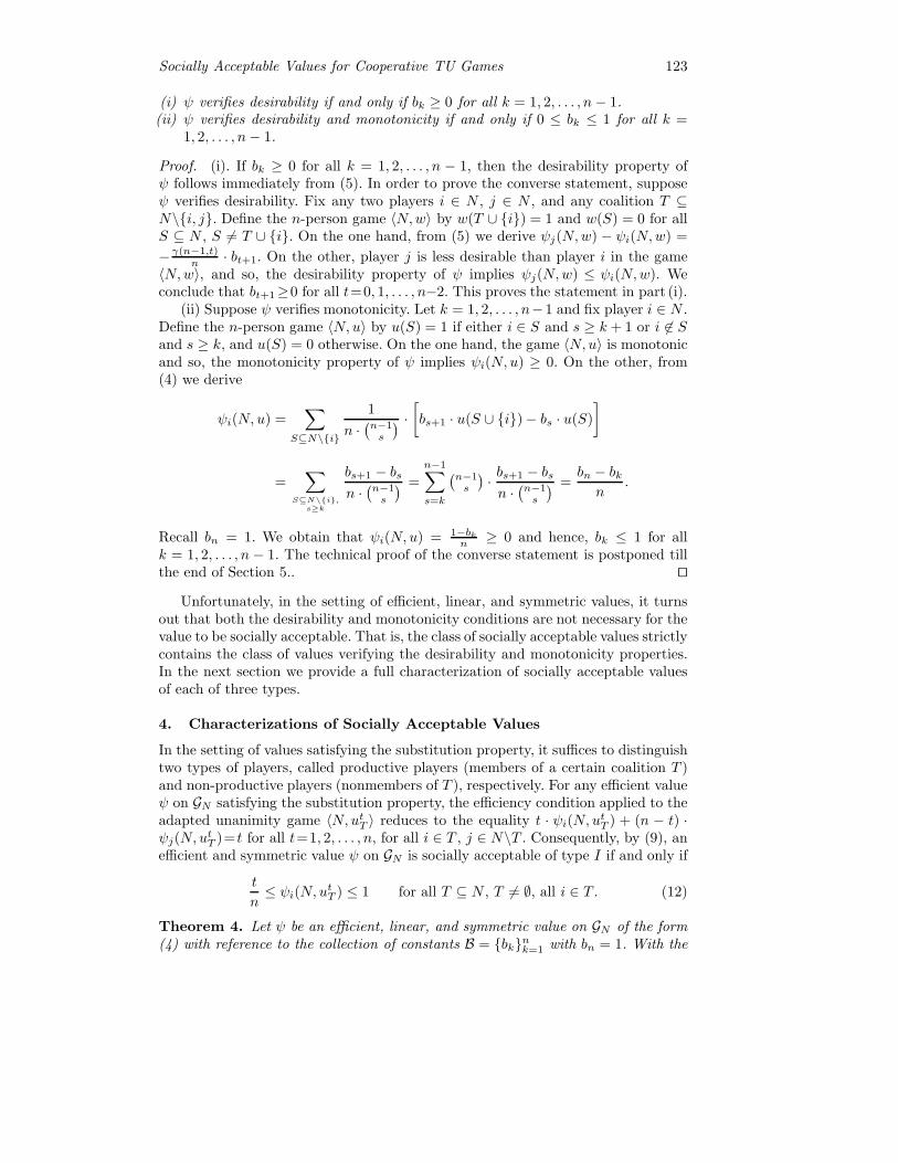
Socially Acceptable Values for Cooperative TU Games 123
(i) ψ verifies desirability if and only if bk ≥ 0 for all k = 1, 2, . . . , n− 1.(ii) ψ verifies desirability and monotonicity if and only if 0 ≤ bk ≤ 1 for all k =
1, 2, . . . , n− 1.
Proof. (i). If bk ≥ 0 for all k = 1, 2, . . . , n − 1, then the desirability property ofψ follows immediately from (5). In order to prove the converse statement, supposeψ verifies desirability. Fix any two players i ∈ N , j ∈ N , and any coalition T ⊆N\{i, j}. Define the n-person game 〈N,w〉 by w(T ∪ {i}) = 1 and w(S) = 0 for allS ⊆ N , S = T ∪ {i}. On the one hand, from (5) we derive ψj(N,w) − ψi(N,w) =
− γ(n−1,t)n · bt+1. On the other, player j is less desirable than player i in the game
〈N,w〉, and so, the desirability property of ψ implies ψj(N,w) ≤ ψi(N,w). Weconclude that bt+1≥0 for all t=0, 1, . . . , n−2. This proves the statement in part (i).
(ii) Suppose ψ verifies monotonicity. Let k = 1, 2, . . . , n−1 and fix player i ∈ N .Define the n-person game 〈N, u〉 by u(S) = 1 if either i ∈ S and s ≥ k + 1 or i ∈ Sand s ≥ k, and u(S) = 0 otherwise. On the one hand, the game 〈N, u〉 is monotonicand so, the monotonicity property of ψ implies ψi(N, u) ≥ 0. On the other, from(4) we derive
ψi(N, u) =∑
S⊆N\{i}
1
n ·(n−1s
) · [bs+1 · u(S ∪ {i})− bs · u(S)
]
=∑
S⊆N\{i},s≥k
bs+1 − bs
n ·(n−1s
) =
n−1∑s=k
(n−1s
)· bs+1 − bs
n ·(n−1s
) =bn − bk
n.
Recall bn = 1. We obtain that ψi(N, u) = 1−bkn ≥ 0 and hence, bk ≤ 1 for all
k = 1, 2, . . . , n− 1. The technical proof of the converse statement is postponed tillthe end of Section 5.. ��
Unfortunately, in the setting of efficient, linear, and symmetric values, it turnsout that both the desirability and monotonicity conditions are not necessary for thevalue to be socially acceptable. That is, the class of socially acceptable values strictlycontains the class of values verifying the desirability and monotonicity properties.In the next section we provide a full characterization of socially acceptable valuesof each of three types.
4. Characterizations of Socially Acceptable Values
In the setting of values satisfying the substitution property, it suffices to distinguishtwo types of players, called productive players (members of a certain coalition T )and non-productive players (nonmembers of T ), respectively. For any efficient valueψ on GN satisfying the substitution property, the efficiency condition applied to theadapted unanimity game 〈N, utT 〉 reduces to the equality t · ψi(N, utT ) + (n − t) ·ψj(N, utT )= t for all t=1, 2, . . . , n, for all i ∈ T , j ∈ N\T . Consequently, by (9), anefficient and symmetric value ψ on GN is socially acceptable of type I if and only if
t
n≤ ψi(N, utT ) ≤ 1 for all T ⊆ N , T = ∅, all i ∈ T . (12)
Theorem 4. Let ψ be an efficient, linear, and symmetric value on GN of the form(4) with reference to the collection of constants B = {bk}nk=1 with bn = 1. With the
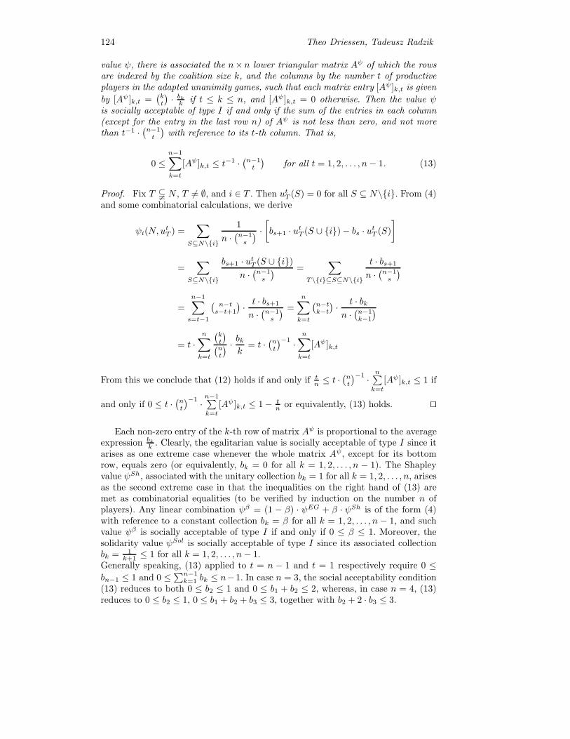
124 Theo Driessen, Tadeusz Radzik
value ψ, there is associated the n×n lower triangular matrix Aψ of which the rowsare indexed by the coalition size k, and the columns by the number t of productiveplayers in the adapted unanimity games, such that each matrix entry [Aψ ]k,t is given
by [Aψ ]k,t =(kt
)· bkk if t ≤ k ≤ n, and [Aψ]k,t = 0 otherwise. Then the value ψ
is socially acceptable of type I if and only if the sum of the entries in each column(except for the entry in the last row n) of Aψ is not less than zero, and not morethan t−1 ·
(n−1t
)with reference to its t-th column. That is,
0 ≤n−1∑k=t
[Aψ]k,t ≤ t−1 ·(n−1t
)for all t = 1, 2, . . . , n− 1. (13)
Proof. Fix T � N , T = ∅, and i ∈ T . Then utT (S) = 0 for all S ⊆ N\{i}. From (4)and some combinatorial calculations, we derive
ψi(N, utT ) =∑
S⊆N\{i}
1
n ·(n−1s
) · [bs+1 · utT (S ∪ {i})− bs · utT (S)
]
=∑
S⊆N\{i}
bs+1 · utT (S ∪ {i})n ·(n−1s
) =∑
T\{i}⊆S⊆N\{i}
t · bs+1
n ·(n−1s
)=
n−1∑s=t−1
(n−ts−t+1
)· t · bs+1
n ·(n−1s
) =
n∑k=t
(n−tk−t)· t · bkn ·(n−1k−1
)= t ·
n∑k=t
(kt
)(nt
) · bkk
= t ·(nt
)−1 ·n∑k=t
[Aψ]k,t
From this we conclude that (12) holds if and only if tn ≤ t ·
(nt
)−1 ·n∑k=t
[Aψ]k,t ≤ 1 if
and only if 0 ≤ t ·(nt
)−1 ·n−1∑k=t
[Aψ ]k,t ≤ 1− tn or equivalently, (13) holds. ��
Each non-zero entry of the k-th row of matrix Aψ is proportional to the averageexpression bk
k . Clearly, the egalitarian value is socially acceptable of type I since itarises as one extreme case whenever the whole matrix Aψ, except for its bottomrow, equals zero (or equivalently, bk = 0 for all k = 1, 2, . . . , n − 1). The Shapleyvalue ψSh, associated with the unitary collection bk = 1 for all k = 1, 2, . . . , n, arisesas the second extreme case in that the inequalities on the right hand of (13) aremet as combinatorial equalities (to be verified by induction on the number n ofplayers). Any linear combination ψβ = (1 − β) · ψEG + β · ψSh is of the form (4)with reference to a constant collection bk = β for all k = 1, 2, . . . , n − 1, and suchvalue ψβ is socially acceptable of type I if and only if 0 ≤ β ≤ 1. Moreover, thesolidarity value ψSol is socially acceptable of type I since its associated collectionbk = 1
k+1 ≤ 1 for all k = 1, 2, . . . , n− 1.Generally speaking, (13) applied to t = n − 1 and t = 1 respectively require 0 ≤bn−1 ≤ 1 and 0 ≤
∑n−1k=1 bk ≤ n−1. In case n = 3, the social acceptability condition
(13) reduces to both 0 ≤ b2 ≤ 1 and 0 ≤ b1 + b2 ≤ 2, whereas, in case n = 4, (13)reduces to 0 ≤ b2 ≤ 1, 0 ≤ b1 + b2 + b3 ≤ 3, together with b2 + 2 · b3 ≤ 3.

Socially Acceptable Values for Cooperative TU Games 125
Further, observe that a n×n lower triangular matrix A = [A]k,t induces an efficient,linear, and symmetric value on GN of the form (4) with reference to a collection of
constants {bk}nk=1 with bn = 1 provided that, for all 1 ≤ k ≤ n− 1,(kt
)−1 · [A]k,t isthe same for all 1 ≤ t ≤ k.
In the context of values satisfying the substitution property, the efficiency con-dition applied to the coalition-size dependent unanimity game 〈N,wT 〉 reduces to
the equality t · ψi(N,wT ) + (n − t) · ψj(N,wT ) = nt ·(nt
)−1for all t = 1, 2, . . . , n,
for all i ∈ T , j ∈ N\T . Thus, by (10), an efficient and symmetric value ψ on GN issocially acceptable of type II if and only if
1t ·(nt
)−1 ≤ ψi(N,wT ) ≤ nt2 ·(nt
)−1for all T ⊆ N , T = ∅, all i ∈ T . (14)
Theorem 5. Let ψ be an efficient, linear, and symmetric value on GN of the form(4) with reference to the collection of constants B = {bk}nk=1 with bn = 1. With thevalue ψ, there is associated the n×n lower triangular matrix Bψ of which the rowsare indexed by the coalition size k, and the columns by the number t of productiveplayers in the coalition-size dependent unanimity games, such that each matrix entry[Bψ]k,t is given by [Bψ]k,t = bk if t ≤ k ≤ n, and [Bψ ]k,t = 0 otherwise. Then thevalue ψ is socially acceptable of type II if and only if the sum of the entries in eachcolumn (except for the entry in the last row n) of Bψ is not less than zero, and notmore than n−t
t with reference to its t-th column. That is,
0 ≤n−1∑k=t
[Bψ ]k,t ≤n− t
tfor all t = 1, 2, . . . , n− 1. (15)
Proof. The same proof technique applies as before by modifying the choice of thebasis of GN . Fix T � N , T = ∅, and i ∈ T . Then wT (S) = 0 for all S ⊆ N\{i}. Inthe current framework, from (4) and some combinatorial calculations, we derive
ψi(N,wT ) =∑
S⊆N\{i}
bs+1·wT (S∪{i})n·(n−1
s )=
∑T\{i}⊆S⊆N\{i}
s+1t ·
(s+1t
)−1 · bs+1
n·(n−1s )
=
n−1∑s=t−1
(n−ts−t+1
)· s+1
t ·(s+1t
)−1 · bs+1
n·(n−1s )
=
n∑k=t
(n−tk−t)· kt ·
(kt
)−1 · bkn·(n−1
k−1)
= t−1 ·(nt
)−1 ·n∑k=t
bk = t−1 ·(nt
)−1 ·n∑k=t
[Bψ ]k,t
From this we conclude that (14) holds if and only if t−1 ·(nt
)−1 ≤ t−1 ·(nt
)−1 ·n∑k=t
[Bψ]k,t ≤ nt2 ·(nt
)−1if and only if 1 ≤
n∑k=t
[Bψ]k,t ≤ nt or equivalently, (15) holds.
��
Clearly, the egalitarian value is socially acceptable of type II, whereas the Shap-ley value, associated with the unitary collection, fails to be of type II. The extremecase in that the inequalities of (15) are met as combinatorial equalities happens forthe collection of constants bk = n
k·(k+1) for all k = 1, 2, . . . , n−1, because of its tele-
scoping sum. Consequently, the solidarity value ψSol is socially acceptable of type II

126 Theo Driessen, Tadeusz Radzik
since its associated collection bk = 1k+1 ≤
nk·(k+1) for all k = 1, 2, . . . , n− 1. Due to
the development of the theory about social acceptability of type II, we end up withthe introduction of an appealing value on GN transforming an n-person game 〈N, v〉into its per-capita game 〈N, vpc〉, applying the solidarity value and finally, repairingefficiency in a multiplicative fashion. In formula, ψ(N, v) = n·ψSol(N, vpc) where the
characteristic function of the per-capita game 〈N, vpc〉 is defined by vpc(S) = v(S)|S|
for all S ⊆ N , S = ∅.
In the framework of values satisfying the substitution property, the efficiencycondition applied to the complementary unanimity game 〈N, ztT 〉 reduces to theequality t · ψi(N, ztT ) + (n − t) · ψj(N, ztT ) = 0 for all t = 1, 2, . . . , n − 1, for alli ∈ T , j ∈ N\T . Thus, by (11), an efficient and symmetric value ψ on GN is sociallyacceptable of type III if and only if
tn − 1 ≤ ψi(N, ztT ) ≤ 0 for all T � N , T = ∅, all i ∈ T . (16)
Theorem 6. Let ψ be an efficient, linear, and symmetric value on GN of the form(4) with reference to the collection of constants B = {bk}nk=1 with bn = 1. With thevalue ψ, there is associated the n× n lower triangular matrix Cψ of which the rowsare indexed by the coalition size k, and the columns by the number t of productiveplayers in the complementary unanimity games, such that each matrix entry [Cψ]k,tis given by [Cψ]k,t =
(kt
)· bn−k
k if t ≤ k ≤ n − 1, and [Cψ ]k,t = 0 otherwise. Thenthe value ψ is socially acceptable of type III if and only if the sum of the entriesin each column (except for the entry in the last row n) of Cψ is not less than zero,and not more than t−1 ·
(n−1t
)with reference to its t-th column. That is,
0 ≤n−1∑k=t
[Cψ ]k,t ≤ t−1 ·(n−1t
)for all t = 1, 2, . . . , n− 1. (17)
Proof. The same proof technique applies as before by modifying the choice of thebasis of GN . Fix T � N , T = ∅, and i ∈ T . Then ztT (S ∪{i}) = 0 for all S ⊆ N\{i}.In the current framework, from (4) and some combinatorial calculations, we derive
ψi(N, ztT ) =∑
S⊆N\{i},S �=∅
−bs·ztT (S)
n·(n−1s )
= −∑
∅�=S⊆N\{i},S∩T=∅
t·bsn·(n−1
s )= −
∑S⊆N\T,S �=∅
t·bsn·(n−1
s )
= −n−t∑s=1
(n−ts
)· t·bsn·(n−1
s )= −
n−t∑s=1
(n−st )
(nt)· t·bsn−s
= −t ·n−1∑k=t
(kt)(nt)
bn−kk = −t ·
(nt
)−1 ·n−1∑k=t
[Cψ]k,t
From this we conclude that (16) holds if and only if tn−1 ≤ −t·
(nt
)−1 ·n−1∑k=t
[Cψ]k,t ≤ 0
if and only if 0 ≤n−1∑k=t
[Cψ ]k,t ≤ t−1 ·(n−1t
)or equivalently, (17) holds. ��
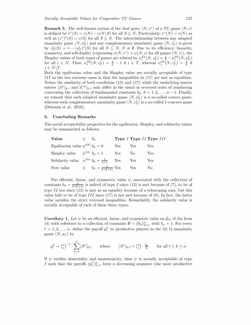
Socially Acceptable Values for Cooperative TU Games 127
Remark 5. The well-known notion of the dual game 〈N, v∗〉 of a TU game 〈N, v〉is defined by v∗(S) = v(N)− v(N\S) for all S ⊆ N . Particularly, v∗(N) = v(N) aswell as (v∗)∗(S) = v(S) for all S ⊆ N . The interrelationship between any adaptedunanimity game 〈N, utT 〉 and any complementary unanimity game 〈N, ztT 〉 is givenby ztT (S) = t − (utT )∗(S) for all S ⊆ N , S = ∅. Due to its efficiency, linearity,symmetry, and self-duality (expressing ψ(N, v∗) = ψ(N, v) for all games 〈N, v〉), theShapley values of both types of games are related by ψShi (N, ztT ) = t
n −ψShi (N, utT )for all i ∈ N . Thus, ψShi (N, ztT ) = t
n − 1 if i ∈ T , whereas ψShj (N, ztT ) = tn if
j ∈ N\T .Both the egalitarian value and the Shapley value are socially acceptable of typeIII as the two extreme cases in that the inequalities in (17) are met as equalities.Notice the similarity of both conditions (13) and (17), while the underlying matrixentries [Aψ]k,t and [Cψ]k,t only differ in the usual or reversed order of numberingconcerning the collection of fundamental constants bk, k = 1, 2, . . . , n − 1. Finally,we remark that each adapted unanimity game 〈N, utT 〉 is a so-called convex game,whereas each complementary unanimity game 〈N, ztT 〉 is a so-called 1-concave game(Driessen et al., 2010).
5. Concluding Remarks
The social acceptability properties for the egalitarian, Shapley, and solidarity valuesmay be summarized as follows.
Value ψ bk Type I Type II Type III
Egalitarian value ψEG bk = 0 Yes Yes Yes
Shapley value ψSh bk = 1 Yes No Yes
Solidarity value ψSol bk = 1k+1 Yes Yes Yes
New value ψ bk = nk·(k+1) Yes Yes No
The efficient, linear, and symmetric value ψ, associated with the collection ofconstants bk = n
k·(k+1) is indeed of type I since (13) is met because of (7), to be of
type II too since (15) is met as an equality because of a telescoping sum, but thisvalue fails to be of type III since (17) is not met because of (8). In fact, the lattervalue satisfies the strict reversed inequalities. Remarkably, the solidarity value issocially acceptable of each of these three types.
Corollary 1. Let ψ be an efficient, linear, and symmetric value on GN of the form(4) with reference to a collection of constants B = {bk}nk=1 with bn = 1. For every
t = 1, 2, . . . , n, define the payoff pψt to productive players in the {0, 1}-unanimitygame 〈N, uT 〉 by
pψt =(nt
)−1 ·n∑k=t
[Aψ]k,t where [Aψ ]k,t =(kt
)· bkk for all t ≤ k ≤ n
If ψ verifies desirability and monotonicity, then ψ is socially acceptable of typeI such that the payoffs (pψt )nt=1 form a decreasing sequence (the more productive
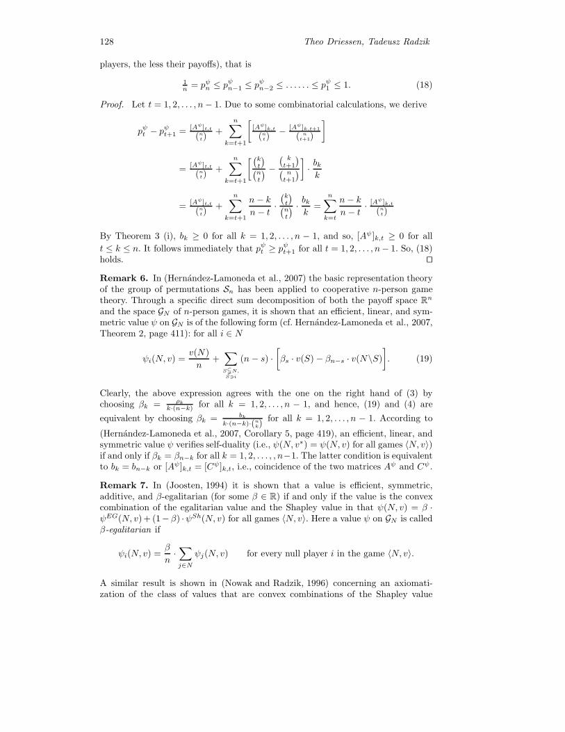
128 Theo Driessen, Tadeusz Radzik
players, the less their payoffs), that is
1n = pψn ≤ pψn−1 ≤ pψn−2 ≤ . . . . . . ≤ pψ1 ≤ 1. (18)
Proof. Let t = 1, 2, . . . , n− 1. Due to some combinatorial calculations, we derive
pψt − pψt+1 =[Aψ]t,t
(nt)+
n∑k=t+1
[[Aψ]k,t
(nt)− [Aψ]k,t+1
( nt+1)
]
=[Aψ]t,t
(nt)+
n∑k=t+1
[(kt
)(nt
) − ( kt+1
)(nt+1
)] · bkk
=[Aψ]t,t
(nt)+
n∑k=t+1
n− k
n− t·(kt
)(nt
) · bkk
=
n∑k=t
n− k
n− t· [A
ψ]k,t
(nt)
By Theorem 3 (i), bk ≥ 0 for all k = 1, 2, . . . , n − 1, and so, [Aψ ]k,t ≥ 0 for all
t ≤ k ≤ n. It follows immediately that pψt ≥ pψt+1 for all t = 1, 2, . . . , n− 1. So, (18)holds. ��
Remark 6. In (Hernandez-Lamoneda et al., 2007) the basic representation theoryof the group of permutations Sn has been applied to cooperative n-person gametheory. Through a specific direct sum decomposition of both the payoff space Rn
and the space GN of n-person games, it is shown that an efficient, linear, and sym-metric value ψ on GN is of the following form (cf. Hernandez-Lamoneda et al., 2007,Theorem 2, page 411): for all i ∈ N
ψi(N, v) =v(N)
n+∑S�N,S�i
(n− s) ·[βs · v(S)− βn−s · v(N\S)
]. (19)
Clearly, the above expression agrees with the one on the right hand of (3) bychoosing βk = ρk
k·(n−k) for all k = 1, 2, . . . , n − 1, and hence, (19) and (4) are
equivalent by choosing βk = bkk·(n−k)·(nk)
for all k = 1, 2, . . . , n − 1. According to
(Hernandez-Lamoneda et al., 2007, Corollary 5, page 419), an efficient, linear, andsymmetric value ψ verifies self-duality (i.e., ψ(N, v∗) = ψ(N, v) for all games 〈N, v〉)if and only if βk = βn−k for all k = 1, 2, . . . , , n−1. The latter condition is equivalentto bk = bn−k or [Aψ]k,t = [Cψ]k,t, i.e., coincidence of the two matrices Aψ and Cψ .
Remark 7. In (Joosten, 1994) it is shown that a value is efficient, symmetric,additive, and β-egalitarian (for some β ∈ R) if and only if the value is the convexcombination of the egalitarian value and the Shapley value in that ψ(N, v) = β ·ψEG(N, v) + (1− β) ·ψSh(N, v) for all games 〈N, v〉. Here a value ψ on GN is calledβ-egalitarian if
ψi(N, v) =β
n·∑j∈N
ψj(N, v) for every null player i in the game 〈N, v〉.
A similar result is shown in (Nowak and Radzik, 1996) concerning an axiomati-zation of the class of values that are convex combinations of the Shapley value
Socially Acceptable Values for Cooperative TU Games 129
and the solidarity value. Clearly, each value of this class is socially acceptable. In(Dragan et al., 1996) collinearity between the Shapley value and various types ofegalitarian values has been treated for a class of zero-normalized games called pro-portional average worth games.
Remark 8. We conclude this paper with the proof of the “if” part of Theorem3(ii). Let ψ be an efficient, linear, and symmetric value on GN of the form (4) withreference to a collection of constants B = {bs}ns=1 with bn = 1 and 0 ≤ bs ≤ 1 forall s = 1, 2, . . . , n− 1 as well. By Theorem 3(i), ψ verifies desirability. It remains toprove that ψ verifies monotonicity too. Let 〈N, v〉 be a monotonic n-person game
and i ∈ N . We show ψi(N, v) ≥ 0. Write b0 = 0 and as usual, γ(n, s) = s!·(n−1−s)!n!
for all s = 0, 1, . . . , n− 1. At this stage, we put forward our claim that the player’spayoff satisfies, for all k = 0, 1, . . . , n− 2,
ψi(N, v) ≥ fk(ψ, v, {i}) + gk+1(ψ, v, {i}) where for all � = 0, 1, . . . , n− 1,(20)
f(ψ, v, {i}) =∑
S⊆N\{i},s≤�
γ(n, s) · [bs+1 − bs] · v(S ∪ {i}) (21)
g(ψ, v, {i}) = γ(n, �) · [bn − b] ·∑
S⊆N\{i},s=�
v(S ∪ {i}) (22)
The proof of the claim (20) proceeds by backwards induction on k, k = 0, 1, . . . , n−2.For k = n − 2, the claim follows immediately from the representation (4) for ψ byobserving that bn = 1 and bs · v(S) ≤ bs · v(S ∪ {i}) for all S ⊆ N\{i} due to themonotonicity of the game 〈N, v〉 together with bs ≥ 0 for all s = 0, 1, . . . , n− 1.Suppose that the claim holds for some k, k ∈ {1, 2, . . . , n− 2}. We verify the claimfor k − 1. For that purpose, note that s · v(S ∪ {i}) ≥
∑j∈S v((S ∪ {i})\{j}) for
all S ⊆ N\{i} by the monotonicity of the game 〈N, v〉. By summing up over allcoalitions of size k + 1, not containing player i, we obtain∑S⊆N\{i},s=k+1
v(S∪{i}) ≥ 1
k + 1
∑S⊆N\{i},s=k+1
∑j∈S
v((S∪{i})\{j}) =n− 1− k
k + 1
∑T⊆N\{i},
t=k
v(T∪{i}).
where the last equality is due to the combinatorial argument that any T ⊆ N\{i}of size k arises from n − k − 1 coalitions S of the form T ∪ {j}, where j ∈ N\T ,j = i. ¿From the latter inequality, together with (22) and bk+1 ≤ 1 = bn, we derivethe following:
gk+1(ψ, v, {i}) = γ(n, k + 1) · [bn − bk+1] ·∑
S⊆N\{i},s=k+1
v(S ∪ {i})
≥ γ(n, k + 1) · [bn − bk+1] · n− 1− k
k + 1
∑T⊆N\{i},
t=k
v(T ∪ {i})
= γ(n, k) · [bn − bk+1]∑
S⊆N\{i},s=k
v(S ∪ {i})
where the latter equality holds because of γ(n, k + 1) · n−1−kk+1 = γ(n, k). ¿From the
latter inequality, together with the induction hypothesis (20), (21), (22) respectively,

130 Theo Driessen, Tadeusz Radzik
it follows that
ψi(N, v) ≥ fk(ψ, v, {i}) + gk+1(ψ, v, {i})
= fk−1(ψ, v, {i}) + γ(n, k) · [bk+1 − bk] ·∑
S⊆N\{i},s=k
v(S ∪ {i}) + gk+1(ψ, v, {i})
≥ fk−1(ψ, v, {i}) + γ(n, k) · [bn − bk] ·∑
S⊆N\{i},s=k
v(S ∪ {i})
= fk−1(ψ, v, {i}) + gk(ψ, v, {i})
This completes the backwards inductive proof of the claim (20). For k = 0 the claimyields
ψi(N, v) ≥ f0(ψ, v, {i}) + g1(ψ, v, {i})
= γ(n, 0) · [b1 − b0] · v({i}) + γ(n, 1) · [bn − b1] ·∑
j∈N\{i}v({i, j})
=b1n· v({i}) +
1− b1n · (n− 1)
·∑
j∈N\{i}v({i, j}).
Note that v(S) ≥ 0 for all S ⊆ N by monotonicity of 〈N, v〉. Together with 0 ≤ b1 ≤1, the latter inequality yields ψi(N, v) ≥ 0. This completes the proof of Theorem3(ii). ��
References
Calvo, E. (2008). Random marginal and random removal values. International Journal ofGame Theory, 37, 533–563.
Dragan, I., Driessen, T. S. H. and Y. Funaki (1996). Collinearity between the Shapley valueand the egalitarian division rules for cooperative games. OR Spektrum, 18, 97–105.
Driessen, T. S. H. (1988). Cooperative Games, Solutions, and Applications. Kluwer Aca-demic Publishers, Dordrecht, The Netherlands.
Driessen, T. S. H. and T. Radzik (2002). Extensions of Hart and Mas-Colell’s consistencyto efficient, linear, and symmetric values for TU-games. In: ICM2002GTA proceedingsvolume of International Congress of Mathematicians, Game Theory and ApplicationsSatellite Conference (Gao, H., Petrosjan, L.A., Shao, F. Jianpei Xu J., Yeung, D.W.,Zakharov, V.V., Zenkevich, N.A., Zhang, S., and Zhang, T., eds), pp. 129–146. QingdaoPublishing House, Qingdao,China,.
Driessen, T. S. H. and T. Radzik (2003). Extensions of Hart and Mas-Colell’s consistencyto efficient, linear, and symmetric values for TU-games. In: ICM Millennium Lectureson Games. Volume dedicated to the International Congress of Mathematicians, GameTheory and Applications Satellite Conference, August 14-17, 2002, Qingdao, China(Petrosyan, L.A. and Yeung, D.W.K., eds). pp. 147–166. Springer-Verlag, Heidelberg,Germany.
Driessen, T. S. H., Khmelnitskaya, A. B. and J. Sales (2010). 1-Concave basis for TU gamesand the library game. TOP, doi:10.1007/s11750-010-0157-5. Published online on 1stSeptember 2010.
Hernandez-Lamoneda, L., Juarez, R. and F. Sanchez-Sanchez (2007). Dissection of solu-tions in cooperative game theory using representation techniques. International Journalof Game Theory, 35, 395–426.

Socially Acceptable Values for Cooperative TU Games 131
Joosten, R., Peters, H. J. M. and F. Thuijsman (1994). Socially acceptable values for trans-ferable utility games. Report M94-03, Department of Mathematics, University of Maas-tricht, The Netherlands.
Nowak, A. S. and T. Radzik (1994). A solidarity value for n-person transferable utilitygames. International Journal of Game Theory, 23, 43–48.
Nowak, A. S. and T. Radzik (1996). On convex combinations of two values. ApplicationesMathematicae, 24, 47–56.
Roth, A. E. (editor) (1988). The Shapley value: Essays in honor of Lloyd S. Shapley. Cam-bridge University Press, Cambridge, U.S.A.
Ruiz, L. M., Valenciano, F. and J. M. Zarzuelo (1998). The family of least square valuesfor transferable utility games. Games and Economic Behavior, 24, 109–130.
Shapley, L. S., (1953). A value for n-person games. Annals of Mathematics Study, 28,307–317 (Princeton University Press). Also in (Roth, 1988), pp. 31–40.
Schmeidler, D. (1969). The nucleolus of a characteristic function game. SIAM Journal ofApplied Mathematics, 17, 1163–1170.
Tijs, S. H. (1981). Bounds for the core and the τ -value. In: Game Theory and Mathemat-ical Economics (Moeschlin, O. and Pallaschke, D., eds), pp. 123–132. North-HollandPublishing Company, Amsterdam.

Auctioning Big Facilities under Financial Constraints�
Marıa Angeles de Frutos1 and Marıa Paz Espinosa2
1 Universidad Carlos III de MadridDepartamento de Economıa
C./ Madrid, 126, 28903 Getafe, Madrid, SpainE-mail: [email protected] Universidad del Paıs Vasco
Departamento de Fundamentos del Analisis Economico IIFacultad Ciencias Economicas y Empresariales
Avda. Lehendakari Aguirre 83, 48015 Bilbao, SpainE-mail: [email protected]
Abstract. This paper analyzes auctions for big facilities or contracts wherebidders face financial constraints that may force them to resell part of theproperty of the good (or subcontract part of a project) at a resale mar-ket. We show that the interaction between resale and financial constraintschanges previous results on auctions with financial constraints and those inauctions with resale. The reason is the link between the resale price and theauction price introduced by the presence of financial constraints. Such linkinduces a potential loser to modify the auction price in order to fine-tune thewinner’s resale offer, which may require forcing the winner to be financiallyconstrained.
Keywords: auctions, big facilities, resale, financial constraints, subcontract-ing
Introduction
The allocation of a big contract or facility usually involves a small number of qual-ified buyers who assign a large value to the good and face financial constraints.One specific example is the allocation problem of the European Spallation Sourcethat had to be allocated to a single country or location but whose property can beshared after the initial allocation, to alleviate the winner’s financial constraints.1
Similarly, operating licences (e.g., in the telecommunications sector) are awardedto one firm, and (some or all of) the actual services can be subcontracted.2 Partialresale or horizontal subcontracting is also a common assumption in two-stage con-tract games (Kamien et al., 1989; Spiegel, 1993; Chen et al., 2004; and Meland andStraume, 2007).
� We acknowledge comments and suggestions from participants at the M-SWET 2009 andGTM 2010. We gratefully acknowledge financial aid from MICINN (SEJ2007/04339/001and ECO2009-09120) and Gobierno Vasco, DEUI (IT-313-07).
1 On September 10, 2008, the European Strategy Forum on Research Infrastructures(ESFRI) published its report on the three candidates to host the European SpallationSource (ESS): Lund in Sweden, Bilbao in Spain, and Debrecen in Hungary. A decisionwas reached in May 2009 in favour of Lund. In June 2009, Spain and Sweden agreed tocollaborate in order to build the European Spallation Source; a facility for manufacturingsome accelerator components will be built in Bilbao.
2 There is horizontal subcontracting or horizontal outsourcing whenever parts of the finalproduction of a good are subcontracted to rival firms.

Auctioning Big Facilities under Financial Constraints 133
Previous work on auctions with resale relies mostly on the potential inefficienciesof the auction allocation mechanism to provide the basis for resale. An inefficientallocation may result from noisy signals at the time of the auction, as in Haile (2000,2001, 2003), from asymmetries between bidders when the auction is conducted asfirst price, as in Gupta and Lebrun (1998) or Hafalir and Krishna (2008), or fromthe presence of speculators who value the object only by its resale price, as inGarratt and Troger (2006). In contrast, in our model the auction is a second priceauction and there are no pure speculators, all participants value the good, and theresale market is justified by the presence of financial constraints which may forcethe winner of the auction to sell part of the property of the good. That is, if bidderswere wealthy enough the resale market would be inactive and it is the presenceof financial constraints which makes participants aware that there will be partialresale.
The main purpose of the paper is to check the robustness of previous resultsof auctions with resale and auctions where bidders face financial constraints. Thisis particularly important when auctioning big facilities or contracts. Our resultsare driven by the link between auction price and resale price, which induces apotential loser to increase the auction price in order to fine-tune the winner’s resaleoffer, which may require forcing the winner to be financially constrained. We firstcompare the outcomes of the auction with resale and financial constraints, to thosewithout resale or without financial constraints, and find that the loser’s incentivesto modify the resale price may preclude a truth telling behavior and also biddingthe minimum between valuation and wealth as part of the equilibrium. We also findthat the presence of financial constraints may eliminate the speculative equilibria ala Garrat and Troger in auctions with resale.
The paper is organized as follows. Section 1 presents the model. In Section 2 wesolve the resale stage. Section 3 presents the bidding stage under private informationand the main results of the paper. Section 4 concludes.
1. The model
A government wants to auction the location of a facility, or to assign a big projectto one of two potential risk-neutral buyers, buyer A and buyer B. The worth of theauctioned good may be large compared to the buyers’ wealth, so that default mayoccur. Each buyer i has a budget or wealth wi. As in Zheng (2001), a buyer wealthrepresents both her liquidity constraint and her liability. Thus, wA and wB will setthe maximum amount by which buyers can be penalized if they default. We assumethat wA and wB are known.
Buyer i has use value vi when i is the solo owner of the good.3 If i obtains afraction z of the property of the good then her use value will be zvi. Use values vAand vB are private information. Each vi has distribution Fi with associated densityfi and supports [vi, vi] for vi, with vA ≥ vB and vi−vi = 1. We will denote by hi(vi)
the hazard rate of Fi, i.e. hi(x) = fi(x)1−Fi(x) and we will assume that it is increasing.
The hazard rate represents the instantaneous probability that the valuation of buyeri is vi given that it is not smaller than vi. Monotonicity of the hazard rate implies
3 Due to the possibility of resale, and following Haile (2003), we will distinguish betweenbuyers’ use value of the object which is exogenously determined and buyers’ valuation -the value players attach to winning the auction- which will be endogenously determined.
134 Marıa Angeles de Frutos, Marıa Paz Espinosa
that the virtual use valuations (ψi(vi) = vi− 1−Fifi
, i = A,B) are strictly increasing,
and it is equivalent to assume log-concavity of the reliability function.4 We furtherassume vAhA(vA) > 1 which is the necessary condition for no buyer A exclusionthrough a positive reserve price being profitable for the seller.
We will define buyers ex-ante financial situation by the relationship betweentheir use values and their wealth. We will say that buyer i is ex-ante financiallyconstrained if vi > wi, and that i is ex-ante unconstrained otherwise.
An important assumption of the model is the inability of the initial seller toprohibit resale. Because of this, buyers participate de facto in a two-stage sellinggame; in the first stage, they compete for the object at the auction, and in thesecond stage the auction winner can make a take-it-or-leave-it offer to the auctionloser for the entire or for part of the property of the object. Player i can alwaysguarantee himself wi, by not participating in the selling game.
At the first stage, the good is sold through a second-price auction and assignedto a single buyer. Bids are denoted b = (bA, bB). We will denote by p the price tobe paid by the winner, i; this payment will take place at the end of the game. Theloser does not pay anything to the auctioneer. We will denote by UWj
i the utility ofplayer i, i = A,B, when the auction winner is j, j = A,B. At the end of this firststage the auction price is announced publicly.
At the second stage, the winner of the first stage auction, i, must decide whetherto keep the object or to resell it, and if so, at what price and which fraction. Wewill assume that the winner has all the bargaining power.5 Thus, resale takes placevia monopoly pricing - the winner of the auction makes an offer to the loser afterupdating her prior beliefs based on her winning and on the information revealed bythe auction price. A resale offer by bidder i, Oi, is a pair [ri, zi] which comprises aresale price ri and a fraction of the good zi. Keeping the object is dominated byreselling it if the auction winner does not have wealth enough to cover the auctionprice, i.e., if wi < p.6 We will denote the option of keeping the object by the offerOi = [0, 0]. If the winner is unable to pay p after resale, she defaults and loses allher wealth. We will denote defaulting by an empty offer, i.e., by Oi = ∅. Note thatif p > wA + wB then Oi = ∅ no matter the identity of the auction winner. Theauction loser must decide whether to accept or reject the resale offer. It can beeasily verified that the auction loser j will accept to buy zi at a price ri if and onlyif the following two conditions simultaneously hold: 1) ri ≤ vj and 2) rizi ≤ wj .
We search for the Perfect Bayesian Equilibria of the selling game (PBE, forshort). A strategy for a player must hence specify a first round bid, a second roundoffer if the player is the auction winner, and a second round acceptance decision if theplayer is the auction loser. Furthermore, posterior beliefs are determined by Bayesrule whenever possible and the resale offer is optimal given the posterior beliefs andthe first round bids. Regarding the off-equilibrium beliefs, we will assume that the
4 See Bagnoli and Bergstrom (2005) for the class of distributions satisfying this property.5 Similar assumption is adopted in Zheng (2002) to characterize the optimal auction with
resale, and can also be found in Hafalir and Krishna (2008). In contrast, Pagnozzi (2007)assumes that bidders bargain in the resale market, so that the outcome is given by theNash bargaining solution.
6 An alternative interpretation is that the winning bidder can sell equity to finance aportion of his bid as in Rhodes-Kropf and Viswanathan (2005). But here the equityprovider is the losing bidder and not the equity market.
Auctioning Big Facilities under Financial Constraints 135
posteriors will coincide with the priors whenever the first stage bid is outside therange of equilibrium bids.7 Finally, we will only consider rationalizable equilibria orequilibria which survive the elimination of (weakly) dominated strategies.
2. The resale stage
The optimal offers at the resale stage will depend on the winner’s use value, on thefirst round price, on bidders’ wealth and on the information revealed at the firststage. Since bidders’ posteriors depend on the first round bids, different informa-tion structures can exist at the second stage. At one extreme, after the auction andbefore the resale stage, the loser’s use value becomes common knowledge (perfectlyrevealing first round bids or separating equilibrium); at the other extreme, the pos-terior and the prior on the loser’s use value coincide (perfect pooling equilibrium).The resale offers in a first-stage fully separating equilibrium coincide with those de-scribed in previous section as there will be perfect information at the resale stage.We concentrate here on the case of incomplete information at the resale stage.
To solve the resale stage, we assume that bidding strategies are non-decreasing,so that the behavior of the winner at the resale stage must take into account whatshe learns from the auction price.
Lemma 1. If the auction loser, bidder j, followed a non-decreasing bidding strat-egy at the first stage such that p = bj (vj) for all vj ∈
[vLj , v
Hj
]and p = bj (vj)
for vj /∈[vLj , v
Hj
], the winner, bidder i, has updated beliefs given by Fj (x) =
Pr(vj ≤ x| vj ∈ [vLj , v
Hj ]), where
Fj (x) =
⎧⎪⎨⎪⎩Fj(x)−Fj(vLj )
Fj(vHj )−Fj(vLj )if x ∈ [vLj , v
Hj )
1 if x ≥ vHj0 if x < vLj
with p = bj(vLj)
= bj(vHj), and vj ≤ vLj < vHj ≤ vj.
If vLj = vj and vHj = vj, then the updated distribution coincides with the prior dis-
tribution, i.e., Fj (x) = Fj (x). Conversely, if vLj = vHj then the updated distributionis a point distribution.
At the resale stage, the auction winner will set the resale offer that maximizes herexpected payoff given her posterior beliefs about the loser’s use value. The objectivefunction for player i is hence:
maxzi,ri
{[wi − p + rizi + vi (1− zi)]
(1− Fj (ri)
)+ Ki(p)Fj (ri)
}where
Ki(p) =
{0 if p > wi
vi + wi − p if p ≤ wi
Ki(p) stands for the utility when buyer i keeps the object because the resale offeris rejected. It coincides with the utility in an auction without resale and it hence
7 We will do so whenever these off-equilibrium beliefs satisfy Cho and Kreps IntuitiveCriterion.
136 Marıa Angeles de Frutos, Marıa Paz Espinosa
takes on the positive value vi +wi− p when there is no risk of default (p ≤ wi) and0 when there is risk of default.
The key difference between the strong buyer and the weak buyer behavior atthe resale stage lies in the shares they put up for sale. Whereas buyer A resells
the minimum fraction needed to cover the auction price, i.e., zA = min(p−wArA
, 0)
,
buyer B may resell the entire object if wA ≥ vLA. Resale offers will hence depend onthe identity of the winner.
2.1. Resale offers by the strong buyer
If the winner is player A, she will not resell if p ≤ wA as vA > vB . Thus, ifp ≤ wA then OA = [0, 0]. At the other extreme, A will always default, OA = ∅, ifp > min(wB , v
HB ) + wA.
For intermediate prices, p ∈ (wA,min(wB , vHB ) + wA], player A resells the mini-
mum fraction needed to cover the first round price, i.e., zA ∈ (0, 1] : zArA = p−wA.Note that the loss from increasing zA out-weights its gain as vA ≥ vB ≥ vHB > rA,so that zArA = p− wA follows. Thus, buyer A will set rA ∈
[vLB , v
HB
)to maximize
her expected utility given by
maxrA
{(vA
(1−
(p− wArA
))+ rAzA + wA − p
)(1− FB (rA)
)+ 0FB (rA)
}where FB (rA) is the probability that A’s offer be rejected. Since the objectivefunction is concave, the unconstrained optimal resale price must solve the firstorder condition, which after some simplifications, can be written as
rA
(rA
p− wA− 1
)=
1
hB(rA)(1)
where hB(rA) = fB(rA)
1−FB(rA). Let r∗A(p) be implicitly defined by
r∗Ap−wA = 1
r∗AhB(r∗A)+1.
Since 1
r∗AhB(r∗A)+ 1 is decreasing in rA for any regular cdf, a necessary condition for
the unconstrained maximum to satisfy r∗A ≥ vLB is that(vLB)
2fB(vLB)
1+vLB fB(vLB)≤ p− wA.
Denoting MB(vLB) =1+vLB fB(vLB)(vLB)
2fB(vLB)
, buyer A’s optimal resale offers when p−wA ≤
min(wB , vHB ) are hence:
O∗A(p− wA) =
⎧⎪⎪⎨⎪⎪⎩[0, 0] if p− wA ≤ 0[vLB, p−wA
vLB
]if 0 < p− wA ≤ 1
MB(vLB)[r∗A, (p−wA)
r∗A
]if 1MB(vLB)
< p− wA ≤ min(wB , vHB )
Discussion above is summarized in the next lemma.
Lemma 2. At the resale stage, player A will set OA = O∗A(p − wA) if p − wA ≤
min(wB , vHB ), and she will default, OA = ∅, if p− wA > min(wB , v
HB ).
If the first stage bids are weakly non-decreasing, so that FB is a truncation ofFB , then O∗
A(p − wA) is non-decreasing in p, and r∗A(p) is increasing in p. PlayerB’s behavior at the first stage auction will take this into account if he were to setp.

Auctioning Big Facilities under Financial Constraints 137
2.2. Resale offers by the weak buyer
Assume now that winner is player B and that p < min(wA, vHA ) + wB so that he is
not forced to default.Denoting by (roB , z
oB) the optimal pair, some basic properties of the optimal offer
are first derived.
Lemma 3. An optimal offer (roB, zoB) must satisfy the following properties: (i) vHA ≥
roB ≥ vLA and roBzoB ≤ wA; (ii) If roBz
oB < wA, then zoB = 1; (iii) If zoB < 1, then
roBzoB = wA, and (iv) If wA < vLA, then zoB < 1.
Buyer B can either sell the entire object (zB = 1) or only a part of it (zB < 1).When zB = 1, rB must solve
maxrB
{[wB − p + rB ]
(1− FA (rB)
)+ KB(p)FA (rB)
}In an interior solution, the optimal resale price when zB = 1, denoted r∗B(p), isimplicitly defined by:
rB − (p + KB(p)− wB) =1
hA (rB). (2)
This equation yields the optimal price when the solution satisfies (a) r∗B ≥ vLA (seeLemma 3 (i)), which requires the LHS to be larger than the RHS when evaluated atthe minimum possible price vLA and (b) r∗B ≤ wA (from zB = 1 and Lemma 3 (i)),which requires the LHS to be larger than the RHS when evaluated at wA. Note alsothat, from Lemma 3 (iv), zB = 1 may only be optimal when wA ≥ vLA. Trivially, ifwA > vHA then the condition r∗B ≤ wA will never bind as r∗B ≤ vHA holds by Lemma3 (i). Finally, there can also exist corner solutions with resale offers
[vLA, 1
]if (a)
fails, and [wA, 1] if (b) fails.
When selling only part of the object, zB < 1, then rBzB = wA (Lemma 3 (iii))and rB must solve
maxrB
{[wB − p + wA + vB
(1− wA
rB
)](1− FA (rB)
)+ KB(p)FA (rB)
}In an interior solution, when zB < 1 the optimal resale price r∗∗B (p) is implicitlydefined by:
rBvBwA
[rB(wA − (p + KB(p)− wB) + vB)− vBwA] =1
hA (rB)(3)
and z∗∗B = wAr∗∗B
. The equation for r∗∗B yields the optimal price when the solution
satisfies r∗∗B ≥ max{vLA, wA} (from Lemma 3 (i)) r∗∗B ≥ vLA, and from Lemma 3(iii) r∗∗B ≥ wA is necessary for r∗∗B zB = wA and zB < 1 to hold simultaneously).When wA < vLA, the condition r∗∗B ≥ vLA requires that the LHS of equation abovebe larger than its RHS when evaluated at vLA, whereas when wA ≥ vLA the relevantcondition is r∗∗B ≥ wA, which requires that the LHS of equation above be largerthan its RHS when evaluated at wA. We may also have corner solutions with resale
offers[vLA, wA
vLA
]and [wA, 1] when the aforementioned conditions fail (r∗∗B < vLA and
r∗∗B < wA, respectively).
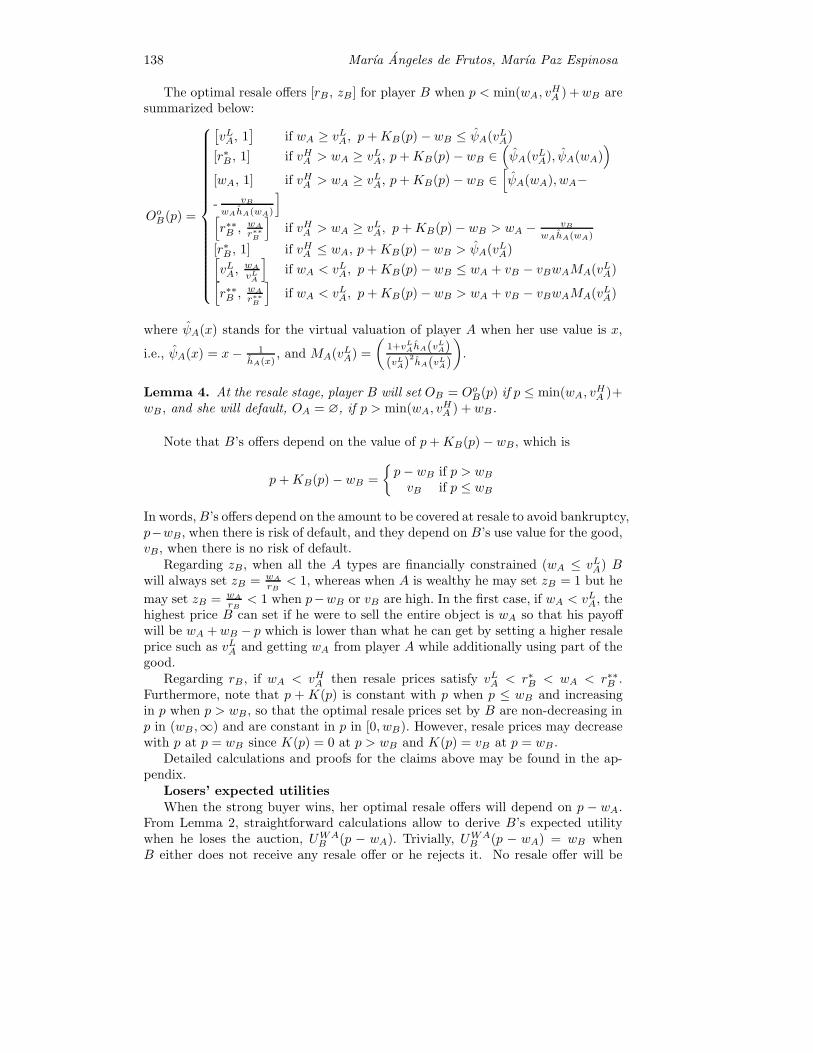
138 Marıa Angeles de Frutos, Marıa Paz Espinosa
The optimal resale offers [rB , zB] for player B when p < min(wA, vHA ) +wB are
summarized below:
OoB(p) =
⎧⎪⎪⎪⎪⎪⎪⎪⎪⎪⎪⎪⎪⎪⎪⎪⎪⎨⎪⎪⎪⎪⎪⎪⎪⎪⎪⎪⎪⎪⎪⎪⎪⎪⎩
[vLA, 1
]if wA ≥ vLA, p + KB(p)− wB ≤ ψA(vLA)
[r∗B , 1] if vHA > wA ≥ vLA, p + KB(p)− wB ∈(ψA(vLA), ψA(wA)
)[wA, 1] if vHA > wA ≥ vLA, p + KB(p)− wB ∈
[ψA(wA), wA−
- vBwAhA(wA)
][r∗∗B , wA
r∗∗B
]if vHA > wA ≥ vLA, p + KB(p)− wB > wA − vB
wAhA(wA)
[r∗B , 1] if vHA ≤ wA, p + KB(p)− wB > ψA(vLA)[vLA, wA
vLA
]if wA < vLA, p + KB(p)− wB ≤ wA + vB − vBwAMA(vLA)[
r∗∗B , wAr∗∗B
]if wA < vLA, p + KB(p)− wB > wA + vB − vBwAMA(vLA)
where ψA(x) stands for the virtual valuation of player A when her use value is x,
i.e., ψA(x) = x− 1hA(x)
, and MA(vLA) =
(1+vLAhA(vLA)(vLA)
2hA(vLA)
).
Lemma 4. At the resale stage, player B will set OB = OoB(p) if p ≤ min(wA, vHA )+
wB , and she will default, OA = ∅, if p > min(wA, vHA ) + wB.
Note that B’s offers depend on the value of p + KB(p)− wB, which is
p + KB(p)− wB =
{p− wB if p > wBvB if p ≤ wB
In words, B’s offers depend on the amount to be covered at resale to avoid bankruptcy,p−wB, when there is risk of default, and they depend on B’s use value for the good,vB, when there is no risk of default.
Regarding zB, when all the A types are financially constrained (wA ≤ vLA) Bwill always set zB = wA
rB< 1, whereas when A is wealthy he may set zB = 1 but he
may set zB = wArB
< 1 when p−wB or vB are high. In the first case, if wA < vLA, thehighest price B can set if he were to sell the entire object is wA so that his payoffwill be wA + wB − p which is lower than what he can get by setting a higher resaleprice such as vLA and getting wA from player A while additionally using part of thegood.
Regarding rB, if wA < vHA then resale prices satisfy vLA < r∗B < wA < r∗∗B .Furthermore, note that p + K(p) is constant with p when p ≤ wB and increasingin p when p > wB, so that the optimal resale prices set by B are non-decreasing inp in (wB ,∞) and are constant in p in [0, wB). However, resale prices may decreasewith p at p = wB since K(p) = 0 at p > wB and K(p) = vB at p = wB .
Detailed calculations and proofs for the claims above may be found in the ap-pendix.
Losers’ expected utilitiesWhen the strong buyer wins, her optimal resale offers will depend on p − wA.
From Lemma 2, straightforward calculations allow to derive B’s expected utilitywhen he loses the auction, UWA
B (p − wA). Trivially, UWAB (p − wA) = wB when
B either does not receive any resale offer or he rejects it. No resale offer will be
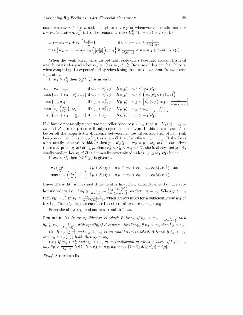
Auctioning Big Facilities under Financial Constraints 139
made whenever A has wealth enough to cover p or whenever A defaults becausep− wA > min(wB , v
HB )). For the remaining cases UWA
B (p− wA) is given by
wB + wA − p + vB
(p−wAvLB
)if 0 < p− wA ≤ 1
MB(vLB)
max{wB + wA − p + vB
(p−wAr∗A(p)
), wB
}if 1
MB(vLB)< p− wA ≤ min(wB , v
HB ).
When the weak buyer wins, his optimal resale offers take into account his rivalwealth, particularly whether wA ≥ vLA or wA < vLA. Because of this, in what follows,when computing A’s expected utility when losing the auction we treat the two casesseparately.
If wA ≥ vLA then UWBA (p) is given by
wA + vA − vLA if wA < vHA , p + KB(p)− wB ≤ ψA(vLA)
max {wA + vA − r∗B , wA} if wA < vHA , p + KB(p)− wB ∈(ψA(vLA), ψA(wA)
)max {vA, wA} if wA < vHA , p + KB(p)− wB ∈
[ψA(wA), wA − vB
wAhA(wA)
]max
{vA
(wAr∗∗B
), wA
}if wA < vHA , p + KB(p)− wB > wA − vB
wAhA(wA)
max {wA + vA − r∗B , wA} if wA ≥ vHA , p + KB(p)− wB > ψA(vLA)
If A faces a financially unconstrained seller because p < wB then p+KB(p)−wB =vB and B’s resale prices will only depend on his type. If this is the case, A isbetter off the larger is the difference between her use values and that of her rival,being maximal if vB ≤ ψA(vLA) as she will then be offered rB = vLA. If she facesa financially constrained bidder then p + KB(p) − wB = p − wB and A can affectthe resale price by affecting p. Since vLA < r∗B < wA < r∗∗B , she is always better off,
conditional on losing, if B is financially constrained unless vB ≤ ψA(vLA) holds.If wA < vLA then UWB
A (p) is given by
vA
(wAvLA
)if p + KB(p)− wB ≤ wA + vB − wAvBMA(vLA), and
max{vA
(wAr∗∗B
), wA
}if p + KB(p)− wB > wA + vB − wAvBMA(vLA).
Buyer A’s utility is maximal if her rival is financially unconstrained but has very
low use values, i.e., if vB ≤ 1MA(vLA)
=(vLA)2
hA(vLA)1+vLAhA(vLA)
, as then r∗∗B = vLA. When p > wB
then r∗∗B = vLA iff vB ≤ wA+wB−pwAMA(vLA)−1
, which always holds for a sufficiently low wA or
if p is sufficiently large as compared to the total resources, wA + wB.
From the above expressions, next result follows.
Lemma 5. (i) In an equilibrium in which B loses: if bA > wA + 1
MB(vLB)then
bB ≥ wA+ 1MB(vLB)
, with equality if F concave. Similarly, if bA > wA then bB > wA.
(ii) If wA ≥ vLA and wB < vA, in an equilibrium in which A loses: if bB > wBand vB > ψA(vLA) hold, then bA > wB.
(iii) If wA < vLA and wB < vA, in an equilibrium in which A loses: if bB > wBand vB > 1
MA(vLA)hold, then bA ∈ (wB , wB + wA
(1− vBMA(vLA)
)+ vB].
Proof. See Appendix.

140 Marıa Angeles de Frutos, Marıa Paz Espinosa
Results in Lemma 5 stem from the loser’s preference for facing a financiallyconstrained winner. Buyer B will not receive a resale offer unless A is financiallyconstrained, which explains part (i). Similarly, if the loser is buyer A, to induce thebest possible resale offer she will make her rival financially constrained (parts (ii)and (iii)). Because of this, whenever A is always ex-ante financially constrained astrategy profile in which A bids no more than her wealth can only be part of a PBEif it results in A losing.
The importance of bidders’ use-values asymmetries is also highlighted in Lemma5. If A loses but her rival has very low use-values as compared to hers, then shewill always be offered rB = vLA. When this is the case, a loser buyer A will makeno attempt to manipulate the auction price (other than avoiding default). Theconditions for rB = vLA are
vB ≤ ψA(vLA) if wA ≥ vLA, and vB ≤1
MA(vLA)if wA < vLA.
If asymmetries are less severe (as would be the case for example with vB = vA)then those inequalities will not hold for, at least, vLA = vA.
3. Results
The possibility of default due to the presence of financial constraints creates alink between the resale price and the auction price. This link can affect equilibriumbehavior at the auction stage, an issue we explore next. We have seen in the previoussection that the presence of financial constraints may induce a potential loser toincrease the auction price in order to fine-tune the winner’s resale offer. Similarly,the presence of a resale market affects the possibility of default as the auction winnercan get extra resources from reselling.
To disentangle the impact of resale from that of financial constrains, in whatfollows we first explore if the equilibria when there is resale among unconstrainedbuyers remain equilibria under financial constraints. We then analyze whether theequilibria in no-resale auctions with financial constraints remain equilibria whenthere is resale. Finally, we explore the equilibria emerging from the interplay betweenresale and financial constraints.
3.1. The resale equilibria
Garrat and Troger (2006) have shown that in second-price and English auctions re-sale creates a role for a speculator -a bidder with zero use value for the good on sale.Because of this, in a second price auction with resale the truth-telling equilibriumcoexists with a continuum of inefficient equilibria in which the speculator wins theauction and makes positive profits. In our set-up no buyer is a pure-speculator astheir use values are strictly positive. Nevertheless if vB is sufficiently low, buyer Bcould be considered as a speculator.
We first show that financial constraints preclude the existence of a truth-tellingequilibria.
Proposition 1. Truth-telling at the bidding stage is part of a PBE of the auctionwith resale if and only if wA ≥ vA.
Proof. See Appendix.

Auctioning Big Facilities under Financial Constraints 141
Proposition above shows that when there are potential financial constraints,truth-telling fails to be an equilibrium. Moreover, as soon as there exist “poten-tial” financial constraints, a separating perfect revealing equilibrium fails to be anequilibrium. The reason is that whenever the strong buyer can be made financiallyconstrained the weak one takes advantage of it by raising the price at least up towA + ε. Thus, a strategy by bidder A such as bA = vA > wA can only be part ofan equilibrium if bB > wA. Recall from Lemma 5 that If b = (bA, bB) is such thatbA(vA) > wA and bA(vA) ≥ bB(vB) for some pair (vA, vB), then p > wA for b to bepart of a PBE equilibrium.
We study next if a profitable “speculative-like” equilibrium a la Garrat andTroger can exist when the strong buyer is financially constrained. Garrat and Troger(2006) show that the following strategies constitute an equilibrium of a second-priceauction with resale among two buyers: a non-speculator buyer i with use values inthe range [0, 1] bids 0 if vi < θ∗ and bids her use value (bθ
∗i (vi) = vi) if vi ≥ θ∗, and
a speculator with zero use value bids θ∗. They show that there is an equilibrium inthis family for each θ∗ ∈ [0, 1]. Thus, there is a continuum of inefficient speculativeθ∗-equilibria.
Considering the weak buyer as a speculator, and considering the strategy profilein which buyer A bids vA if vi < θ∗ and bids her use value (bθ
∗i (vi) = vi) if vi ≥ θ∗,
and buyer B bids θ∗ no matter his type (this candidate to equilibrium will bereferred to as the speculative θ∗-equilibrium, as displayed below)
bA : vA−−−−−−−−︸ ︷︷ ︸vA
θ∗−−−−−−−−︸ ︷︷ ︸vA
vA
bB : vB −−−−−−−−−−−−−−−−︸ ︷︷ ︸θ∗
vB
We next show that a “speculative-like” θ∗-equilibrium can only exist if θ∗ = vAand wB > vA. For any other θ∗ ∈ (vA, vA), a speculative θ∗-equilibrium (in whichbuyer A bids vA if vi < θ∗ and bids vi if vi ≥ θ∗, and buyer B bids θ∗) fails to existdue to the combination of budget constraints and the fact that vA ≥ vB > 0.
Proposition 2. (i) A speculative θ∗-equilibrium, θ∗ < vA, does not exist for anywA < vA.
(ii) The speculative vA-equilibrium with bids (vA, vA) is part of a PBE in whichthe low valuation bidder wins (and makes positive profits if vB > ψA(vA))8 if wB ≥vA > wA ≥ vA, while it is not otherwise.
Proof. See Appendix.
Note that financial constraints destroy any speculative θ∗-equilibrium other thanθ∗ = vA (Proposition 2 part (i)). To see this, note that if θ∗ < vA then in aspeculative θ∗-equilibrium some types of buyer A are bidding her value while beingleft financially unconstrained as vA < p = θ∗ < wA so that buyer B is betteroff deviating to force his rival to be financially constrained. When wA < vA aspeculative θ∗-equilibrium ( θ∗ < vA) fails to exist as A types above θ∗ win the
8 Trivially, it is an equilibrium for buyer B to bid sufficiently high, say vA, and for buyerA to bid vA, provided that at the resale stage B sets rB = vA which will be the case ifvB ≤ ψA(vA). At such an equilibrium B breaks even.

142 Marıa Angeles de Frutos, Marıa Paz Espinosa
auction but face the risk of default and are hence better off by deviating to lose andthen buying at the resale market.
For θ∗ = vA at the speculative vA-equilibrium buyer B always wins and ifwB ≥ vA holds, then he cannot be made financially constrained. His only possibledeviation is to lose which is unprofitable if wA ≥ vA. In contrast, if wB < vAand vB > ψA(vA) the strategy profile (vA, vA) cannot be part of an equilibrium,given that, conditional on losing, buyer A is always better off forcing his rival to beconstrained.
Note that if vB is sufficiently low so that B could be considered a speculator,when he wins he prefers to resell the entire good. At p = vA, he makes a loss fromany fraction he gets to consume as p > vB. Because of this, whenever he offersa resale price larger than the auction price, his offer is unaccepted with positiveprobability, and he will be forced to consume the good. For some types of buyerB to find it profitable to set rB > vA it must be the case that vB > ψA(vA)holds ( which will be the case if vB = vA). In Garrat and Troger’s θ∗-equilibriump = vB = 0 so that the disutility from a price higher than the use value does notarise. Furthermore, vB > ψA(vA) does always hold in their set-up as vA = vB = 0and ψA(0) = − 1
hA(0) < 0.
In sum, financial constraints destroy all the resale equilibria unless one of thebuyers be wealthy enough so that wi ≥ vA holds for some i. When it is the strongbuyer, then truth-telling is the unique resale equilibria that survives the introductionof financial constraints. When it is the weak one then the speculative θ∗-equilibriumwith θ∗ = vA is the only surviving equilibrium.
3.2. The financial constraints equilibria
In a static one-round SPA with budget constraints it is a dominant strategy to bidmin(wi, vi) (see Che and Gale, 1998). The reason is that if the second highest bidis above the winner’s budget, he will renege, will not get the object and will paythe fine, resulting in a negative surplus. With the possibility of resale this argumentbreaks down if the winner can resell the good and, by doing so, can get more thanthe auction price. This is the case here as long as the potential buyer at the resalemarket does not follow dominated strategies.
Arguably, truth-telling is not an equilibrium in the auction with resale as it isnot an equilibrium either in an auction without resale among financially constrainedbidders. Recall that the equilibrium bids in undominated strategies of the auctionwithout resale requires each buyer to bid bi = min {vi, wi} (in what follows werefer to this as the no-resale equilibrium). Acknowledging this fact, we explore nextthe conditions needed for the equilibrium in the auction without resale to be anequilibrium under resale.
The possible realizations of bidders’ wealths with their corresponding biddingstrategies in the no-resale equilibrium are displayed in table below.
wealths vB ≤ wB < vA wB ≥ vAvB ≤ wA < vA (wA,min {wB, vB}) (wA, vB)vA ≤ wA (min {wA, vA} ,min {wB , vB}) (min {wA, vA} , vB)
The no-resale equilibrium is not an equilibrium under resale in the first row, i.e.,if wA < vA, because any loser bidder B with vB < wA is better off deviating so asto win and then reselling part of the good. Note that whenever buyer A wins, since

Auctioning Big Facilities under Financial Constraints 143
wA > min {vB , wB} for A to win, she will make no resale offer so that B’s utilitywill be wB . By deviating to wA + ε, B wins and by setting [rB, zB] = [vA,
wAvA
] he
gets a larger expected utility since he recovers the price wA and is able to consumea fraction of the good.
If wA ≥ vA (second row) then at the no-resale equilibrium buyer B follows aweakly dominated strategy as he is bidding below his lowest possible endogenousvaluation vA. His endogenous valuations takes into account the overall surplus fromwinning and reselling the object. Since wA ≥ vA buyer B can always get vA fromthe resale market so that bB = vA weakly dominates bB = min {wB , vB}. If eitherwinning or losing with the two of them they yield the same profits. But if winningwith bB = vA while losing with min {wB , vB} then the former yields larger expectedprofits as p < vA ≤ rB so that
UWBB (bA, vA) > wB = UWA
B (bA,min {wB , vB}) .
Next proposition summarizes this discussion.
Proposition 3. (i) If wA < vA then bidding bi = min {wi, vi} i = A,B at the firststage is never part of a PBE.
(ii) If wA ≥ vA then bidding bi = min {wi, vi} i = A,B at the first stage cannever be part of a PBE in which bidders do not employ weakly dominated strategies.
3.3. Resale and Financial constraints
We have seen that buyers’ attempts to make their rivals financially constrained giverise to profitable deviations which may destroy the equilibria under resale. Similarly,we have seen that the existence of a resale market can generate buyers’ valuationsabove the use values making some strategies weakly dominated.
Since buyers will anticipate their rivals’ incentives to make them financiallyconstrained, they can incorporate these incentives in their bidding. Similarly, bidsmust account for the prospects at the post-auction resale, which, in turn, dependon wealth. We next characterize equilibrium bids depending of the strong buyerwealth.
High budget buyer A: wA ≥ vA
We consider that player A has a relatively high budget, wA ≥ vA , while main-taining the assumption that she is at least potentially financially constrained sothat wA ≤ vA.
By weak dominance arguments, any bB < vA is now weakly dominated.Consider the family of cut-off strategies bλ
∗A (vA), parameterized by λ∗ with λ∗ ∈
[vA, vA), consisting of strategies for which any bidder A with a use value below λ∗
bids her value, while any bidder with use value above λ∗ bids wA, i.e.,
bλ∗A (vA) =
{vA if vA ≤ λ∗
wA if vA > λ∗
bA : vA−−−−−−−−︸ ︷︷ ︸vA
λ∗−−−−−−−−︸ ︷︷ ︸wA
vA.
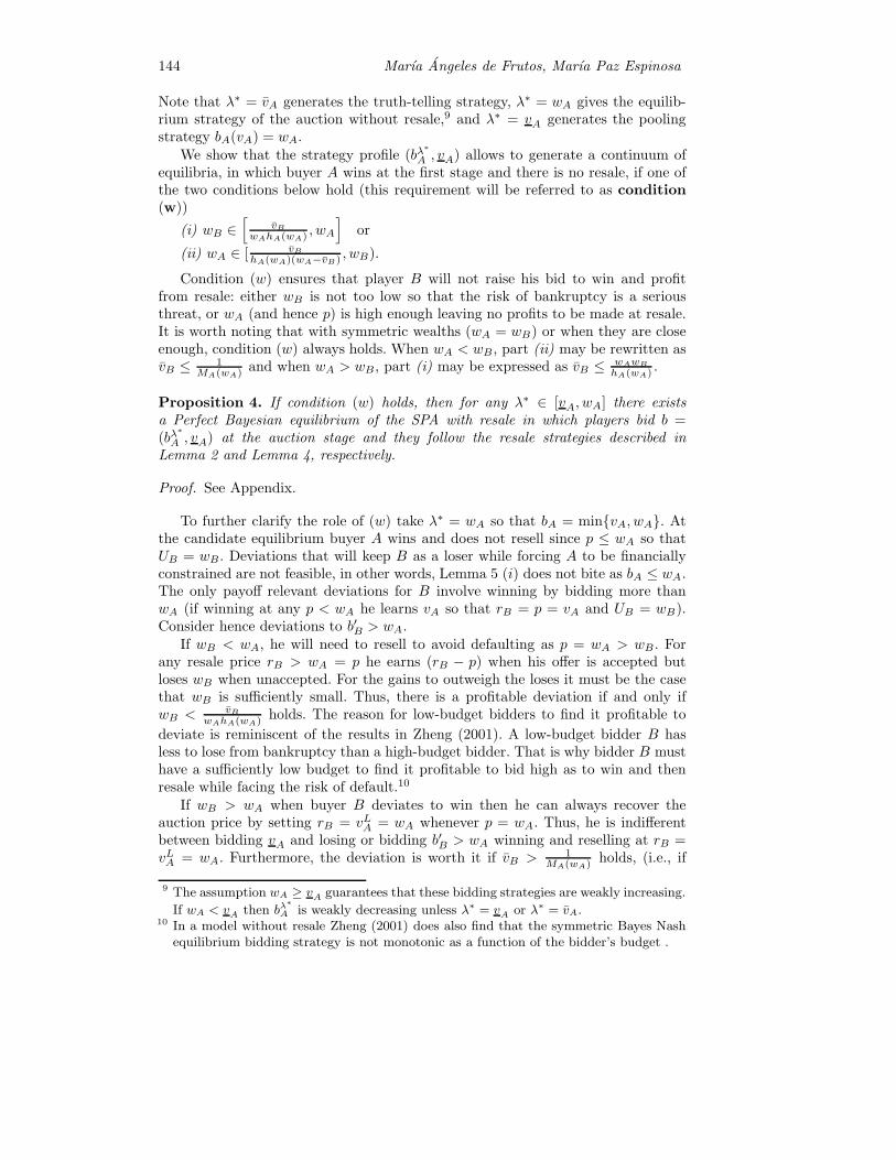
144 Marıa Angeles de Frutos, Marıa Paz Espinosa
Note that λ∗ = vA generates the truth-telling strategy, λ∗ = wA gives the equilib-rium strategy of the auction without resale,9 and λ∗ = vA generates the poolingstrategy bA(vA) = wA.
We show that the strategy profile (bλ∗A , vA) allows to generate a continuum of
equilibria, in which buyer A wins at the first stage and there is no resale, if one ofthe two conditions below hold (this requirement will be referred to as condition(w))
(i) wB ∈[
vBwAhA(wA) , wA
]or
(ii) wA ∈ [ vBhA(wA)(wA−vB) , wB).
Condition (w) ensures that player B will not raise his bid to win and profitfrom resale: either wB is not too low so that the risk of bankruptcy is a seriousthreat, or wA (and hence p) is high enough leaving no profits to be made at resale.It is worth noting that with symmetric wealths (wA = wB) or when they are closeenough, condition (w) always holds. When wA < wB, part (ii) may be rewritten asvB ≤ 1
MA(wA) and when wA > wB, part (i) may be expressed as vB ≤ wAwBhA(wA) .
Proposition 4. If condition (w) holds, then for any λ∗ ∈ [vA, wA] there existsa Perfect Bayesian equilibrium of the SPA with resale in which players bid b =(bλ
∗A , vA) at the auction stage and they follow the resale strategies described in
Lemma 2 and Lemma 4, respectively.
Proof. See Appendix.
To further clarify the role of (w) take λ∗ = wA so that bA = min{vA, wA}. Atthe candidate equilibrium buyer A wins and does not resell since p ≤ wA so thatUB = wB. Deviations that will keep B as a loser while forcing A to be financiallyconstrained are not feasible, in other words, Lemma 5 (i) does not bite as bA ≤ wA.The only payoff relevant deviations for B involve winning by bidding more thanwA (if winning at any p < wA he learns vA so that rB = p = vA and UB = wB).Consider hence deviations to b′B > wA.
If wB < wA, he will need to resell to avoid defaulting as p = wA > wB. Forany resale price rB > wA = p he earns (rB − p) when his offer is accepted butloses wB when unaccepted. For the gains to outweigh the loses it must be the casethat wB is sufficiently small. Thus, there is a profitable deviation if and only ifwB < vB
wAhA(wA) holds. The reason for low-budget bidders to find it profitable to
deviate is reminiscent of the results in Zheng (2001). A low-budget bidder B hasless to lose from bankruptcy than a high-budget bidder. That is why bidder B musthave a sufficiently low budget to find it profitable to bid high as to win and thenresale while facing the risk of default.10
If wB > wA when buyer B deviates to win then he can always recover theauction price by setting rB = vLA = wA whenever p = wA. Thus, he is indifferentbetween bidding vA and losing or bidding b′B > wA winning and reselling at rB =vLA = wA. Furthermore, the deviation is worth it if vB > 1
MA(wA) holds, (i.e., if
9 The assumption wA ≥ vA guarantees that these bidding strategies are weakly increasing.
If wA < vA then bλ∗
A is weakly decreasing unless λ∗ = vA or λ∗ = vA.10 In a model without resale Zheng (2001) does also find that the symmetric Bayes Nash
equilibrium bidding strategy is not monotonic as a function of the bidder’s budget .
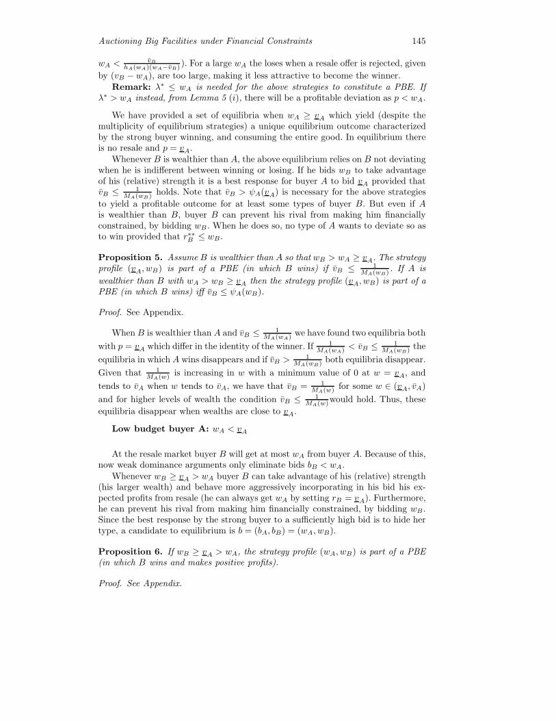
Auctioning Big Facilities under Financial Constraints 145
wA < vBhA(wA)(wA−vB) ). For a large wA the loses when a resale offer is rejected, given
by (vB − wA), are too large, making it less attractive to become the winner.
Remark: λ∗ ≤ wA is needed for the above strategies to constitute a PBE. Ifλ∗ > wA instead, from Lemma 5 (i), there will be a profitable deviation as p < wA.
We have provided a set of equilibria when wA ≥ vA which yield (despite themultiplicity of equilibrium strategies) a unique equilibrium outcome characterizedby the strong buyer winning, and consuming the entire good. In equilibrium thereis no resale and p = vA.
Whenever B is wealthier than A, the above equilibrium relies on B not deviatingwhen he is indifferent between winning or losing. If he bids wB to take advantageof his (relative) strength it is a best response for buyer A to bid vA provided thatvB ≤ 1
MA(wB) holds. Note that vB > ψA(vA) is necessary for the above strategies
to yield a profitable outcome for at least some types of buyer B. But even if Ais wealthier than B, buyer B can prevent his rival from making him financiallyconstrained, by bidding wB . When he does so, no type of A wants to deviate so asto win provided that r∗∗B ≤ wB .
Proposition 5. Assume B is wealthier than A so that wB > wA ≥ vA. The strategyprofile (vA, wB) is part of a PBE (in which B wins) if vB ≤ 1
MA(wB) . If A is
wealthier than B with wA > wB ≥ vA then the strategy profile (vA, wB) is part of aPBE (in which B wins) iff vB ≤ ψA(wB).
Proof. See Appendix.
When B is wealthier than A and vB ≤ 1MA(wA) we have found two equilibria both
with p = vA which differ in the identity of the winner. If 1MA(wA) < vB ≤ 1
MA(wB) the
equilibria in which A wins disappears and if vB > 1MA(wB) both equilibria disappear.
Given that 1MA(w) is increasing in w with a minimum value of 0 at w = vA, and
tends to vA when w tends to vA, we have that vB = 1MA(w) for some w ∈ (vA, vA)
and for higher levels of wealth the condition vB ≤ 1MA(w)would hold. Thus, these
equilibria disappear when wealths are close to vA.
Low budget buyer A: wA < vA
At the resale market buyer B will get at most wA from buyer A. Because of this,now weak dominance arguments only eliminate bids bB < wA.
Whenever wB ≥ vA > wA buyer B can take advantage of his (relative) strength(his larger wealth) and behave more aggressively incorporating in his bid his ex-pected profits from resale (he can always get wA by setting rB = vA). Furthermore,he can prevent his rival from making him financially constrained, by bidding wB .Since the best response by the strong buyer to a sufficiently high bid is to hide hertype, a candidate to equilibrium is b = (bA, bB) = (wA, wB).
Proposition 6. If wB ≥ vA > wA, the strategy profile (wA, wB) is part of a PBE(in which B wins and makes positive profits).
Proof. See Appendix.
146 Marıa Angeles de Frutos, Marıa Paz Espinosa
4. Conclusion
This paper has analyzed the effect of two important features related to auctions forbig facilities or contracts: partial resale and binding budget constraints. In theseauctions bidders usually face severe financial constraints that may force them toresell part of the property of the good (or subcontract part of the project) at aresale market. We show that the interaction between resale and financial constraintschanges previous results on auctions with financial constraints and those in auctionswith resale. The reason is the link between the resale price and the auction priceintroduced by the presence of financial constraints. Such link induces a potentialloser to increase the auction price in order to fine-tune the winner’s resale offer. Wealso characterize equilibria of the auction with resale and financial constraints thatdo not involve speculative behavior by the low use value player and yield efficientoutcomes.
References
Bagnoli, M. and T. Bergstrom (2005). Log-concave probability and its applications. Eco-nomic Theory, 26(2), 445–469.
Che, Y.-K. and I. Gale (1998). Standard auctions with financially constrained bidders.Review of Economic Studies, 65(1), 1–21.
Chen, Y., J. Ishikawa and Z. Yu (2004). Trade liberalization and strategic outsourcing.Journal of International Economics, 63(2), 419–436.
Garratt, R. and Th. Troger (2006). Speculation in standard auctions with resale. Econo-metrica, 74(3), 753–769.
Gupta, M. and B. Lebrun (1999). First price auctions with resale. Economics Letters,64(2), 181–185.
Hafalir, I. E. and V. Krishna (2008). Asymmetric auctions with resale. American EconomicReview, 98(1), 87–112.
Haile, Ph. A. (2000). Partial pooling at the reserve price in auctions with resale opportu-nities. Games and Economic Behavior, 33(2), 231–248.
Haile, Ph. A. (2001). Auctions with resale markets: An application to U.S. Forest Servicetimber sales. American Economic Review, 91(3), 399–427.
Haile, Ph. A. (2003). Auctions with private uncertainty and resale opportunities. Journalof Economic Theory, 108(1), 72–110.
Kamien, M. I., L. Li and D. Samet (1989). Bertrand competition with subcontracting.RAND Journal of Economics, 20(4), 553–567.
Meland, F. and O. Straume (2007). Outsourcing in contests. Public Choice, 131(3), 315–331.
Pagnozzi, M. (2007). Bidding to lose? Auctions with resale. RAND Journal of Economics,38(4), 1090–1112.
Rhodes-Kropf, M. and S. Viswanathan (2005). Financing auction bids. RAND Journal ofEconomics, 36(4), 789–815.
Spiegel, Y. (1993). Horizontal subcontracting. RAND Journal of Economics, 24(4), 570–590.
Zheng, Ch. (2001). High bids and broke winners. Journal of Economic Theory, 100(1),129–171.
Zheng, Ch. (2002). Optimal auction with resale. Econometrica, 70, 2197–2224.

Auctioning Big Facilities under Financial Constraints 147
5. Appendix
Proof of lemma 3 (i) Since buyer A will never pay more than her use value,vHA ≥ roB, and since any type will pay at least vLA then roB ≥ vLA. Finally, buyer Atotal payment cannot exceed her wealth, roBz
oB ≤ wA.
(ii) If roBzoB < wA it is possible for B to increase his utility by increasing zoB
and keeping roB constant, so that roBzoB < wA still holds. Since his utility increases
(roB ≥ vLA ≥ vB and the probability of acceptance does not change) it must be thecase that zoB = 1 if roBz
oB < wA. The same arguments show (iii).
(iv) Assume not, zoB = 1. Then roB = roBzoB ≤ wA < vLA, which contradicts (i).�
Proof of Lemma 4 We derive the optimal resale offers by player B.
Case 1. p ≤ wB.
If wA ≥ vLA bidder B can set zB = 1 and rB ∈[vLA,min(wA, v
HA ))
to maximizeher expected utility,
maxrB{wB − p + rB Pr (rB ≤ vA/p) + vB Pr (rB ≥ vA/p)} .
Solving the maximization problem above, B’s optimal resale price r∗B is the solutionto equation below:
rB − vB =1
hA (rB)(4)
which has a unique solution as the standard hazard rate condition holds. Since theLHS of (4) is strictly increasing while the RHS is strictly decreasing a necessarycondition for r∗B to be interior is that vLA − vB < 1
hA(vLA). Finally, the solution to
equation above fails to be lower than wA if wA − vB > 1
hA(wA). The constrained
maximum in then r∗B = wA.
Alternatively, B can set zB be such that zBrB = wA, so that rB ∈[vLA, v
HA
]if
wA < vLA and rB ∈[wA, v
HA
]if wA ≥ vLA will solve
maxrB
{wB − p +
(wA + vB
(1− wA
rB
))(1− FA (rB)
)+ vBFA (rB)
}= max
rB
{wB − p + vB + wA
(1− vB
rB
)(1− FA (rB)
)}The optimal resale price r∗B is the solution to:
rBvB
(rB − vB) =1
hA (rB)(5)
For the same arguments as before, the optimal (unconstrained) resale price is vLA if(vLA − vB
) vLAvB
> 1
hA(vLA). It will be larger than wA if wA
vB(wA − vB) < 1
hA(wA).
By comparing the two offers it follows that [rB = r∗B, zB < 1] dominates[rB = wA, zB = 1] if wA < vLA as UB (rB = r∗B , zB < 1) ≥ UB
(rB = vLA, zB < 1
)by
the optimality of r∗B, and the fact thatUB(rB = vLA, zB < 1
)> UB (rB = wA, zB = 1). The optimal resale offers by B
148 Marıa Angeles de Frutos, Marıa Paz Espinosa
when wA ≤ vLA are hence
O∗B(p) =
⎧⎪⎨⎪⎩[rB = vLA, zB = wA
vLA
]if vB <
(vLA)2hA(vLA)
1+vLAhA(vLA)[rB = r∗B , zB = wA
r∗B
]if vB ≥ (vLA)
2hA(vLA)
1+vLAhA(vLA)
If wA ≥ vLA since r∗B > r∗B (the LHS of (4) is steeper than the correspond-ing one in (5) while they are both equal to zero at rB = vB), the resale offer[rB = r∗B < wA, zB = 1] dominates the offer [rB = r∗B, zB < 1]. But if r∗B > wA (i.e.
if wAhA (wA) < vB(wA−vB) ) then [rB = r∗B > wA, zB < 1] dominates
[rB = r∗B = wA, zB = 1] as with both B gets the same resources, namely wA, whereaswith the former he gets to consume part of the good in return for the risk of gettingmore often his offer rejected. Because of this wA cannot be too large. In sum, theoptimal resale offers if B is unconstrained are[
rB = vLA, zB = 1]
if vB ≤ ψA(vLA)
[rB = r∗∗B , zB = 1] if vB ∈[ψA(vLA), ψA(wA)
][rB = wA, zB = 1] if vB ∈
[ψA(wA), wA − vB
wAhA(wA)
][rB = r∗∗B > wA, zB < 1] if vB ≥ wA − vB
wAhA(wA)·
Case 2. p ∈(wB , min(wA, v
HA ) + wB
].
Bidder B will maximize:
maxrB ,zB
{(wB − p + rBzB + vB(1 − zB))
(1− FA(rB)
)}As in case 1, whenever wA ≥ vLA bidder B may sell the entire object,11 zB = 1,
for a resale price rB ∈[vLA, v
HA
)which maximizes his expected utility,
maxrB
{(wB − p + rB)
(1− FA(rB)
)}The optimal resale price r∗∗B is the solution to equation below
rB − (p− wB) =1
hA (rB)(6)
The optimal resale offers by B when wA > vLA and zB = 1 are as follows⎧⎪⎨⎪⎩[rB = vLA, zB = 1
]if p− wB ≤ ψA(vLA)
[rB = r∗∗B (p), zB = 1] if p− wB ∈[ψA(vLA), ψA(wA)
][rB = wA, zB = 1] if p− wB ≥ ψA(wA)·
11 Assume that the optimal (r∗B, z∗B) is such that z∗B < 1.Then, if r∗Bz
∗B < wA it is possible
to increase utility by increasing z∗B and keeping r∗B constant, since r∗B > vB and the prob-ability of acceptance does not change. If r∗Bz
∗B = wA, increasing zB requires decreasing
rB and this changes the objective function with the sign of [−(1−F )+ zBrB
(1−zB)f ′(rB)].
Auctioning Big Facilities under Financial Constraints 149
Alternatively, buyer B can set zBrB = wA and rB ∈[vLA, v
HA
)to maximize(
wB − p + wA + vB
(1− wA
rB
))(1− FA (rB)
)+ 0
The optimal resale price r∗∗B (p) is now the solution to equation below:
rBvB
(rB (wA + wB − p + vB)− wAvB) =wA
hA (rB), (7)
where r∗∗B (p) > wA for wA > vLA iff p−wB > wA − vBwAhA(wA)
, whereas for wA < vLAit always holds that r∗∗B (p) > wA.
If wA ≤ vLA then the optimal resale offers are⎧⎨⎩[rB = vLA, zB = wA
vLA
]if
vLAvB
(vLA (wA + wB − p + vB)− wAvB
)> wA
hA(vLA)[rB = r∗∗B (p), zB = wA
r∗∗B
]if
vLAwA
(vLA (wA + wB − p + vB)− wAvB
)≤ vB
hA(vLA)
whereas when wA > vLA they are as follows[rB = vLA, zB = 1
]if p− wB ≤ ψA(vLA)
[rB = r∗∗B , zB = 1] if p− wB ∈[ψA(vLA), ψA(wA)
][rB = wA, zB = 1] if p− wB ∈
[ψA(wA), wA − vB
wAhA(wA)
][rB = r∗∗B > wA, zB < 1] if p− wB ≥ wA − vB
wAhA(wA).
Combining the different cases, OoB follows.�Proof of Lemma 5 (i) Let us write for short p − wA as y. Since for any y ≤(vLB)
2fB(vLB)
1+vLB fB(vLB)= 1
MB(vB)the expected utility by loser B is strictly increasing in y as
UWAB (y) = wB + (vB − vLB)
y
vLB,
it trivially follows that y = 1
MB(vB)yields larger expected utility to buyer B than
any lower y. Thus, if b = (bA, bB) is such that bA(vA) > wA and bA(vA) ≥ bB(vB)for some pair (vA, vB), then p > wA for b to be part of a PBE equilibrium, as B isalways better off if A is financially constrained. Note that if A wins and has wealthenough to cover the auction price she will not resell, so that UWA
B (vA, vB) = wB .In contrast, if B deviates to bidding b′B = wA + ε he will get an expected utilitylarger than wB , as player A still wins but he must now resell zA = ε
r∗A. As buyer
A’s posterior will coincide with her prior, her optimal resale offer employs fB = fBand vLB = vB. By making ε arbitrarily small so that ε ≤ 1
MB(vB)holds, it follows
that r∗A = vB, and UWAB (vA, wA + ε) > wB .
We next show that for larger values of y bounded above by min(wBvHB ) there
exists vB > rA such that∂UWA
B (y)∂y > 0 if vB > vB whereas
∂UWAB (y)∂y < 0 otherwise,
where
UWAB (y) = max
{wB + (vB − r∗A(y))
y
r∗A(y), wB
}so that for any vB ≥ rA

150 Marıa Angeles de Frutos, Marıa Paz Espinosa
it follows that∂UWA
B (y)
∂y=
vB (r∗A − yr′∗A )− (r∗A)2
(r∗A)2 . (8)
Total differentiation of rA
(rAy − 1
)= 1
hB(rA)gives
drAdy
=r2A
(hB(rA)
)2y
[(2rA − y)
(hB(rA)
)2+ yh′
B(rA)
] > 0
where the sign of the denominator equals the sign of −∂2UA(rA)∂r2A
and is hence positive
by the concavity of UA. Plugging its value into (r∗A − yr′∗A ) and simplifying we get
vBr∗A
(1− yr′∗A
r∗A
)− (r∗A)
2= r∗A
(vB
(1− yr′∗A
r∗A
)− r∗A
)so that the sign of (8) is given
by the sign of vB
(1− yr′∗A
r∗A
)− r∗A, with
vB
(1− yr′∗A
r∗A
)−r∗A =
((hB(r∗A)
)2(r∗A − y) + yh′
B(r∗A)
)[vB − r∗A]− r∗A
(hB(r∗A)
)2(hB(r∗A)
)2(2r∗A − y) + yh′
B(r∗A)
Since vB ≥ rA must hold for buyer B to accept rA, it follows that∂UWA
B (y)∂y < 0
for vB = rA, whereas∂UWA
B (y)∂y could be positive for vB sufficiently above r∗A. Since
vB − r∗A < vB − vB = 1 we have that
vB
(1− yr′∗A
r∗A
)− r∗A <
y
[h′B(r∗A)−
(hB(r∗A)
)2](hB(r∗A)
)2(2r∗A − y) + yh′
B(r∗A)
=
y[
f ′B(r∗A)
1−FB(r∗A)
](hB(r∗A)
)2(2r∗A − y) + yh′
B(r∗A)
< 0
where the equality follows from the fact that h′B(r∗A) =
(hB(r∗A)
)2+
f ′B(r∗A)
1−FB(r∗A), and
the last inequality from the concavity of F .(ii). Assume by contradiction that there exists an equilibrium in which A loses by
bidding bA < wB while bB > wB and vB > ψA(vLA) hold. Since vLA < r∗B < wA < r∗∗Bthen A expected utility is bounded above by wA + vA − r∗B. Since by deviating tobA = wB + ε < bB her expected utility is wA + vA − vLA > wA + vA − r∗B, we havefound a profitable deviation contradicting equilibrium behavior.
(iii). Assume by contradiction that there exists an equilibrium in which A losesby bidding bA < wB while bB > wB and vB > 1
MA(vLA)hold. At such an equilibrium
her expected utility equals wA+(vA−r∗∗B )wAr∗∗Bwhich is smaller than wA+(vA−vLA)wA
vLAthe utility he would get if bA = wB + ε < bB. The same arguments apply forbA > wB + wA
(1− vBMA(vLA)
)+ vB which shows our claim.�

Auctioning Big Facilities under Financial Constraints 151
Proof of Proposition 1 The if part was first shown in Haile (1999). For the onlyif part assume first that wA ∈ [vA, vA). By following the truth-telling equilibriumstrategies player B loses and sets the auction price at p = vB ≤ vA. Player A winsand as she has wealth enough to cover the auction price she does not resell, so thatUWAB (vA, vB) = wB . In contrast, if B deviates to bidding b′B = wA+ε he will get an
expected utility larger than wB . If vA ≥ wA+ ε then the result follows from Lemma5 (i). If vA < wA + ε buyer B wins and can infer vA from the auction price. Hewill optimally resell the entire object at a price vA so that UWB
B (vA, wA + ε) = wB .Summing up over all the possible types of bidder A it follows that b′B = wA + εconstitutes a profitable deviation so that (vA, vB) do not constitute equilibriumbids. Assume next that wA < vA. By deviating to wA + ε player B remains aloser (as with vB) and gets larger expected profit as he will get to use part of thegood that he will acquire at the resale market. Since for any wA < vA there is aprofitable deviation, the statement follows. Finally, note that at wA = vA we haveUWBB (vA, wA + ε) = UWA
B (vA, vB) = wB so that the deviation does not yield largerprofits.�
Proof of Proposition 2 (i) At any θ∗-equilibrium (θ∗ < vA) buyer B wins iffacing types vA < θ∗ and loses otherwise.
Assume first wA ∈ [θ∗, vA) so that buyer B gets utility wB if he loses as typesvA ≥ θ∗ will not resell. In contrast, if deviating to bid b′B = wA + ε he will geta larger expected utility. Profits from types vA < θ∗ will coincide with the twostrategies. If he remains a loser with b′B because vA ≥ wA + ε then he now makeslarger profits (the result follows from Lemma 5 (i)). If vA < wA + ε buyer B winswith the deviation, he infers vA from the auction price. He will optimally resell theentire object at a price vA so that UWB
B (vA, wA+ε) = wB if p = vA > vA. Summingup over all the possible types of bidder A it follows that b′B = wA + ε constitutes aprofitable deviation.
Assume next wA ∈ [vA, θ∗) so that types vA ≥ θ∗ are financially constrained
when winning. We first note that vA > wA+ 1
MB(vB)for some vA ∈ (θ∗, vA) suffices
for B to find profitable to deviate to bid wA+ 1
MB(vB)(recall Lemma 5 (i)). Even if
vA < wA + 1
MB(vB)holds then high use-values types prefer to get the entire object
at the resale market rather than winning and being forced to resell as p > wA.Let us finally consider the case wA < vA. A buyer A with type vA > θ∗ wins
and will have to resell so that her utility is bounded above by(
1− p−wArA
)vA where
p = θ∗ so that UWAA ≤
(1− θ∗−wA
vB
)vA as rA < vB.
If deviating to lose, by bidding vA so as to pool with types vA ≤ θ∗ she getsUWBA = wA
rBvA, where we are using the fact that rB < θ∗ so that wA
rBvA > wA
θ∗ vA >wA. The deviation is profitable as
wAθ∗−(vB − θ∗ + wA
vB
)=
(vB − θ∗)wA + θ∗ (θ∗ − vB)
θ∗vB
=(θ∗ − wA) (θ∗ − vB)
θ∗vB> 0.
(ii) For θ∗ = vA at the speculative vA-equilibrium buyer B always wins and aswB > vA holds, he cannot be made financially constrained. Because of this, buyer A

152 Marıa Angeles de Frutos, Marıa Paz Espinosa
is trivially best-responding. As for buyer B, if vB > ψA(vA) he will profitably resell,i.e., p = vA = vLA < rB. His only possible deviation is to lose which is unprofitableif wA ≥ vA as then buyer A will not resell.
We next show that if wB < vA and vB > ψA(vA) holds then the strategyprofile (vA, vA) cannot be part of an equilibrium. Conditional on losing, buyer Ais always better-off forcing his rival to be constrained and to set the best offerfrom her viewpoint, i.e., zB = 1 and rB = vLA. Buyer A can do so if by biddingbA = wB + vA − 1
hA(vA) . But then p > rB and B is better off deviating to lose.
Finally If wA < vA, buyer B will partially resell getting wA at the resale marketand consuming part of the good. Let vB be such that vB = 1
MA(vA) (vB = vB if
vB ≤ 1MA(vA) ). For any vB ≤ vB we have r∗∗B (vB) = vA so that UWB
B (p = vA) =
wB − vA + vB + wA
(1− vB
vA
)< wB as vB
vA(vA − wA) < vA − wA. Buyer B with
use value below vB is hence better-off deviating to lose. Since r∗∗B (vB) is increasingin vB for types sufficiently close to vB such that r∗∗B (vB) > vA it remains true thatbuyer B prefers to deviate so that (vA, vA) is not an equilibrium as claimed. �
Proof of Proposition 4 At the purported strategies bidder A wins the auc-tion, keeps the entire good and pays p = vA so that UWA
B (bλ∗A , bB) = wB and
UWAA (bλ
∗A , bB) = vA + wA − vA. Consider first deviations by player A. The only
payoff-relevant deviations require losing the auction and buying the entire goodat the resale market at a cheaper price which is unfeasible as r∗B ≥ vA = p. Ithence follows that A will not deviate. Consider now player B. If he deviates toany b′B < wA he will win the auction if vA ≤ λ∗, will pay the use value of itsrival and will resell at a price equal to that use value so that his expected utilitywill be equal to that under bB, namely wB . If he deviates to any b′B > wA, hewill win to any buyer A. Now if p < wA then his expected payoff will be wB asr∗B = p = vA. If p = wA he will infer that vLA = λ∗. The deviation will be prof-itable if and only if B finds optimal reselling part of the good at rB > wA (i.e., if
rB = r∗∗B ). For wB > p = wA since FA (x) = FA(x)−FA(λ∗)1−FA(λ∗) , the deviation is unprof-
itable iff rB = r∗∗B , or, iff (wA − vB) wAvB ≥1
hA(wA) (see the computations of B resale
offers).12 Since the LHS is decreasing in vB then (wA − vB) wAvB≥ 1
hA(wA) must hold
for (bλ∗A , bB) to be part of a PBE, i.e., vB ≤ 1
MA(wA)
For vB < wB < p = wA deviation is unprofitable iff r∗∗B ∈ [λ∗, wA] and z∗∗B = 1which is the case if wA
vBwB ≥ 1
hA(wA) as shown in Lemma 4. Consequently, since
wB > vB and wAhA (wA) ≥ 1, the deviation is not profitable in this case either.�
Proof of Proposition 5 At the purported equilibrium profile (vA, wB), buyer Bwins and pays p = vA. At the resale stage he will follow the resale offers in Lemma4 for FB(vA) = FB(vA). The only types that can (potentially) profitably deviateare types of buyer A with vA > wB.
12 If FA is a truncation of F then FA (x) =FA(x)−FA(vLA)
1−FA(vLA)
so that
1
hA(wA)=
1 − FA (wA)
fA (wA)=
1 − FA (wA)
fA (wA)=
1
hA(wA)
Auctioning Big Facilities under Financial Constraints 153
If they deviate to win they will while wB > wA they will have to resell part of
the good so that UWAA <
(1− wB−wA
r∗A
)vA. Since
(1− wB−wA
r∗A
)vA < vA− r∗B +wA
provided that r∗B < wA +(wB−wAr∗A
)vA then vB < ψA(wA) guarantees that the
deviation is unprofitable as r∗B ≤ wA. Similarly, if she only consumes part of thegood but r∗∗B ≤ wB player A will not deviate as
UWBA (vA, wB)− UWA
A (bA, wB) = vAwAr∗∗B− vA
(r∗A − (wB − wA)
r∗A
)= vA
[r∗A (wA − r∗∗B ) + (wB − wA) r∗∗B
r∗∗B r∗A
]> vA
[r∗A (wA − r∗∗B ) + (wB − wA) r∗A
r∗∗B r∗A
]= vA
[(wB − r∗∗B )
r∗∗B
]≥ 0,
where the first inequality follows from r∗A < vB < vA < r∗∗B and the second one
from r∗∗B ≤ wB . Note that r∗∗B ≤ wB requires wBvB
> wBhA(wB)+1hA(wB)wB
(see equation (5)
in the appendix). It hence follows that vB <w2BhA(wB)
wBhA(wB)+1 = 1MA(wB) suffices for the
deviation by the strong buyer to be unprofitable.If wA > wB, the expected utilities are given by
UWBA (vA, wB) =
{wA if vA < r∗BvA − r∗B + wA if vA ≥ r∗B
and
UWBB (vA, wB) > wB as r∗B > vLA = vA.
If B deviates the only payoff relevant deviation is to bid as to lose but thenUWAB = wB as A will not resale. Since UWB
B (vA, wB) > wB the deviation is un-profitable.
Focus next on buyer A. If her use value is below wB she is better-off losing thanwinning so she will not deviate. If her use value is above wB she will deviate if andonly if r∗B > wB so that vB ≤ ψA(wB) is a necessary and sufficient condition forthe above strategies to be an equilibrium whenever wB < wA. �Proof of Proposition 6 At the purported equilibrium profile buyer B wins andmust pay p = wA. At the resale stage B will follow the resale offers in Lemma 4 forFB(vA) = FB(vA). B only payoff relevant deviation is to lose but then his expectedutility will be wB as A will not resell. The only other deviation to check is that oftypes vA > wB . Since if deviating to win, she will have to resell, the deviation isunprofitable. More precisely, at the candidate equilibrium UWB
A = max{wAr∗∗B vA, wA}.If deviating to win, she will have to resell so that her utility is bounded above by
UWAA ≤
(1− p− wA
r∗A
)vA.
Since(
1− wB−wAr∗A
)vA ≤
(1− wB−wA
vB
)vA ≤ wA
r∗∗BvA the result follows as r∗∗B > wA
implies
wAr∗∗B−(
1− wB − wAvB
)=
(vB − r∗∗B )wA + r∗∗B (wB − vB)
r∗∗B vB
>(vB − vA)wA + wA (wB − vB)
r∗∗B vB=
(wB − vA)wAr∗∗B vB
> 0.�

Numerical Study of a Linear Differential Gamewith Two Pursuers and One Evader�
Sergey S. Ganebny1, Sergey S. Kumkov1, Stephane Le Menec2 andValerii S. Patsko1
1 Institute of Mathematics and Mechanics,S.Kovalevskaya str., 16, Ekaterinburg, 620990, Russia,
E-mail: [email protected] EADS/MBDA France,
1 avenue Reaumur, 92358 Le Plessis-Robinson Cedex, France,E-mail: [email protected]
Abstract. A linear pursuit-evasion differential game with two pursuers andone evader is considered. The pursuers try to minimize the final miss (anideal situation is to get exact capture), the evader counteracts them. Twocase are investigated. In the first case, each one pursuer is dynamicallystronger than the evader, in the second one, they are weaker. Results ofnumerical study of value function level sets (Lebesgue sets) for these casesare given. A method for constructing optimal feedback controls is suggestedon the basis of switching lines. Results of numerical simulation are shown.
Keywords: pursuit-evasion differential game, linear dynamics, value func-tion, optimal feedback control.
1. Introduction and Problem Formulation
1. In the paper, a model differential game with two pursuers and one evader isstudied. Three inertial objects moves in the straight line. The dynamics descriptionsfor pursuers P1 and P2 are
zP1 = aP1 , zP2 = aP2 ,
aP1 = (u1 − aP1)/lP1 , aP2 = (u2 − aP2)/lP2 ,
|u1| ≤ μ1, |u2| ≤ μ2,
aP1(t0) = 0, aP2(t0) = 0.
(1)
Here, zP1 and zP2 are the geometric coordinates of the pursuers, aP1 and aP2 aretheir accelerations generated by the controls u1 and u2. The time constants lP1 andlP2 define how fast the controls affect the systems.
The dynamics of the evader E is similar:
zE = aE , aE = (v − aE)/lE ,
|v| ≤ ν, aE(t0) = 0.(2)
Let us fix some instants T1 and T2. At the instant T1, the miss of the first pursuerwith the respect to the evader is computed, and at the instant T2, the miss of the
� This work was supported by the Russian Foundation for Fundamental Researches undergrants No.09-01-00436, 10-01-96006, and by the Program “Mathematical control theory”of the Presidium of RAS.
Numerical Study of a Linear Differential Game 155
second one is computed:
rP1,E(T1) = |zE(T1)− zP1,E(T1)|, rP2,E(T2) = |zE(T2)− zP2,E(T2)|. (3)
Assume that the pursuers act in coordination. This means that we can join theminto one player P (which will be called the first player). This player governs thevector control u = (u1, u2). The evader is counted as the second player. The resultmiss is the following value:
ϕ = min{rP1,E(T1), rP2,E(T2)}. (4)
At any instant t, all players know exact values of all state coordinates zP1 ,zP1 , aP1 , zP2 , zP2 , aP2 , zE , zE, aE. The first player choosing its feedback controlminimizes the miss ϕ, the second one maximizes it.
Relations (1)–(4) define a standard antagonistic differential game. One needs toconstruct the value function of this game and optimal strategies of the players.
2. Nowadays, there are a lot of publications dealing with differential gameswhere one group of objects pursues another group; see, for example, the followingworks (in some order): (Stipanovic et al., 2009), (Blagodatskih and Petrov, 2009),(Chikrii, 1997), (Levchenkov and Pashkov, 1990), (Abramyantz and Maslov, 2004),(Pshenichnii, 1976), (Grigorenko, 1991), (Breakwell, 1976). The problem under con-sideration has two pursuers and one evader. So, from the point of view of numberof objects, it is the simplest one. On the other hand, strict mathematical stud-ies of problems “group-on-group” usually include quite strong assumptions for thedynamics of objects, dimension of the state vector and conditions of termination.Conversely, this paper considers the problem without any assumptions of this type.Solution of the problem can be interesting for the group differential games.
3. Now, let us describe a practical problem, whose reasonable simplification givesmodel game (1)–(4). Suppose that two pursuing objects attacks the evading one oncollision courses. They can be rockets or aircrafts in the horizontal plane. A nominalmotion of the first pursuer is chosen such that at the instant T1 the exact captureoccurs. In the same way, a nominal motion of the second pursuer is chosen (thecapture is at the instant T2). But indeed, the real positions of the objects differ fromthe nominal ones. Moreover, the evader using its control can change its trajectoryin comparison with the nominal one (but not principally, without sharp turns).Correcting coordinated efforts of the pursuers are computed during the process bythe feedback method to minimize the result miss, which is the minimum of absolutevalues of deviations at the instants T1 and T2 from the first and second pursuers,respectively, to the evader.
The passage from the original non-linear dynamics to a dynamics, which islinearized with the respect to the nominal motions, gives (Shima and Shinar, 2002),(Shinar and Shima, 2002) the problem under considerations.
4. The paper includes results of numerical study of game (1)–(4) for two marginalcases: 1) both pursuers P1 and P2 are dynamically stronger than the evader E; 2)both pursuers are dynamically weaker. Results for intermediate situations will bepublished in another work.
Difficulty of the solution is stipulated by the fact that the payoff function ϕis not convex (even for the case T1 = T2). In the paper (Le Menec, 2011), a case
156 Sergey S. Ganebny, Sergey S. Kumkov, Stephane Le Menec, Valerii S. Patsko
of “stronger” pursuers is considered and analytically methods are applied to theproblem of solvability set construction in the game with zero result miss. For T1 =T2, an exact solution is obtained; if T1 = T2, then some upper approximation forthe set is given. In general case, the exact analytical solution cannot be got, in theauthors opinion.
The numerical study is based on algorithms and programs for solving lineardifferential games worked out in the Institute of Mathematics and Mechanics (UralBranch of Russian Academy of Sciences, Ekaterinburg, Russia). The central proce-dure is the backward constructing level sets (Lebesgue sets) of the value function.Optimal strategies of the players are constructed by some processing of the levelsets.
2. Passage to Two-Dimensional Differential Game
At first, let us pass to relative geometric coordinates y1 = zE−zP1 , y2 = zE−zP2 indynamics (1), (2) and payoff function (4). After this, we have the following notations:
y1 = aE − aP1 y2 = aE − aP2
aP1 = (u1 − aP1)/lP1 aP2 = (u2 − aP2)/lP2
aE = (v − aE)/lP1 |u2| ≤ μ2
|u1| ≤ μ1, |v| ≤ ν ϕ = min{|y1(T1)|, |y2(T2)|}.
(5)
State variables of system (5) are y1, y1, aP1 , y2, y2, aP2 , aE ; u1 and u2 are controlsof the first player; v is the control of the second one. The payoff function ϕ dependson the coordinate y1 at the instant T1 and on the coordinate y2 at the instant T2.From general point of view (existence of the value function, positional type of theoptimal strategies), differential game (5) is a particular case of a differential gamewith a positional functional (Krasovskii and Krasovskii).
A standard approach, which is set forth in (Krasovskii and Subbotin, 1974) and(Krasovskii and Subbotin, 1988) for study linear differential games with fixed ter-minal instant and payoff function depending on some state coordinates at the ter-minal instant is to pass to new state coordinates. They can be treated as valuesof the target coordinates forecasted to the terminal instant under zero controls. Inour situation, we have two instants T1 and T2, but coordinates computed at theseinstants are independent; namely, at the instant T1, we should take into accounty1(T1) only, and at the instant T2, we use the value y2(T2). This fact allows us touse the mentioned approach when solving differential game (5). With that, we passto new state coordinates x1 and x2, where x1(t) is the value of y1 forecasted to theinstant T1, and x2(t) is the value of y2 forecasted to the instant T2.
The forecasted values are computed by formula
xi = yi + yiτi + aPi l2Pih(τi/lPi) + aEl
2Eh(τi/lE), i = 1, 2. (6)
Here, xi, yi, and yi depends on t; τi = Ti−t; h(α) = e−α+α+1. Emphasize that thevalues τ1 and τ2 are connected to each other by the relation τ1−τ2 = const = T1−T2.One has xi(Ti) = yi(Ti).
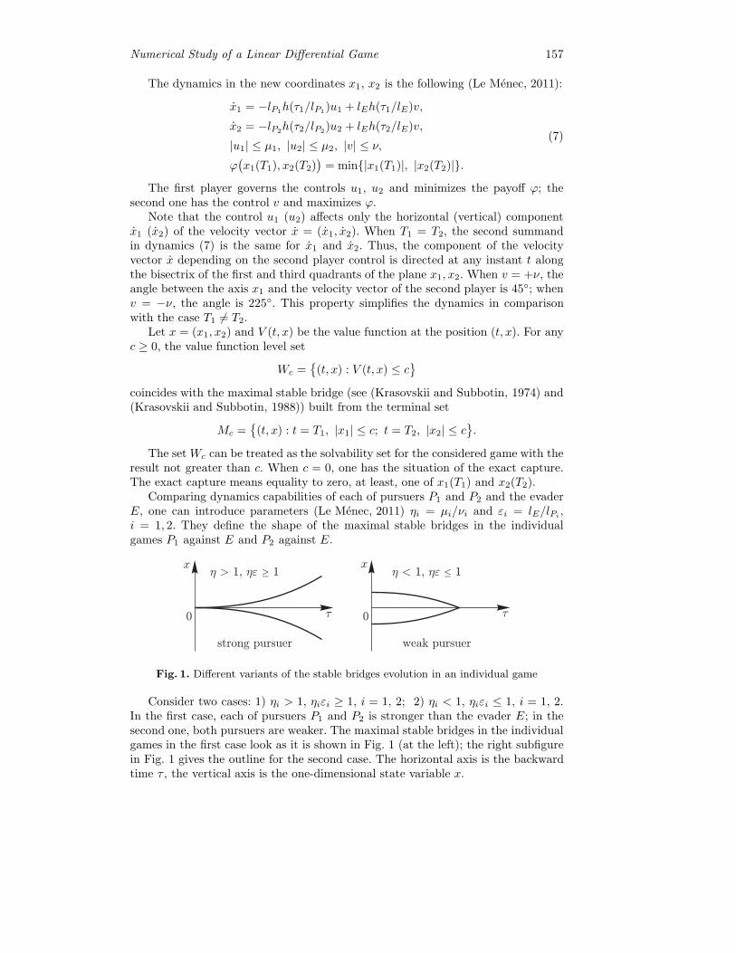
Numerical Study of a Linear Differential Game 157
The dynamics in the new coordinates x1, x2 is the following (Le Menec, 2011):
x1 = −lP1h(τ1/lP1)u1 + lEh(τ1/lE)v,
x2 = −lP2h(τ2/lP2)u2 + lEh(τ2/lE)v,
|u1| ≤ μ1, |u2| ≤ μ2, |v| ≤ ν,
ϕ(x1(T1), x2(T2)
)= min{|x1(T1)|, |x2(T2)|}.
(7)
The first player governs the controls u1, u2 and minimizes the payoff ϕ; thesecond one has the control v and maximizes ϕ.
Note that the control u1 (u2) affects only the horizontal (vertical) componentx1 (x2) of the velocity vector x = (x1, x2). When T1 = T2, the second summandin dynamics (7) is the same for x1 and x2. Thus, the component of the velocityvector x depending on the second player control is directed at any instant t alongthe bisectrix of the first and third quadrants of the plane x1, x2. When v = +ν, theangle between the axis x1 and the velocity vector of the second player is 45◦; whenv = −ν, the angle is 225◦. This property simplifies the dynamics in comparisonwith the case T1 = T2.
Let x = (x1, x2) and V (t, x) be the value function at the position (t, x). For anyc ≥ 0, the value function level set
Wc ={
(t, x) : V (t, x) ≤ c}
coincides with the maximal stable bridge (see (Krasovskii and Subbotin, 1974) and(Krasovskii and Subbotin, 1988)) built from the terminal set
Mc ={
(t, x) : t = T1, |x1| ≤ c; t = T2, |x2| ≤ c}.
The set Wc can be treated as the solvability set for the considered game with theresult not greater than c. When c = 0, one has the situation of the exact capture.The exact capture means equality to zero, at least, one of x1(T1) and x2(T2).
Comparing dynamics capabilities of each of pursuers P1 and P2 and the evaderE, one can introduce parameters (Le Menec, 2011) ηi = μi/νi and εi = lE/lPi ,i = 1, 2. They define the shape of the maximal stable bridges in the individualgames P1 against E and P2 against E.
Fig. 1. Different variants of the stable bridges evolution in an individual game
Consider two cases: 1) ηi > 1, ηiεi ≥ 1, i = 1, 2; 2) ηi < 1, ηiεi ≤ 1, i = 1, 2.In the first case, each of pursuers P1 and P2 is stronger than the evader E; in thesecond one, both pursuers are weaker. The maximal stable bridges in the individualgames in the first case look as it is shown in Fig. 1 (at the left); the right subfigurein Fig. 1 gives the outline for the second case. The horizontal axis is the backwardtime τ , the vertical axis is the one-dimensional state variable x.

158 Sergey S. Ganebny, Sergey S. Kumkov, Stephane Le Menec, Valerii S. Patsko
3. Level Sets of the Value Function
As it was mentioned above, a level set Wc of the value function is the maximalstable bridge for dynamics (7) built in the space t, x from the target set Mc. A timesection (t-section) Wc(t) of the bridge Wc at the instant t is a set in the plane oftwo-dimensional variable x.
To be definite, let T1 ≥ T2. Then, for any t ∈ (T2, T1], the set Wc(t) is a verticalstripe around the axis x2. Its width along the axis x1 equals the width of the bridgein the individual game P1–E at the instant τ = T1− t of the backward time. At theinstant t = T1, half-width of Wc(T1) is equal to c.
Denote by Wc(T2 + 0) the right limit of the set Wc(t) as t→ T2 + 0. Then, theset Wc(T2) is cross-like, obtained by union of the vertical stripe Wc(T2 + 0) and ahorizontal one around the axis x1 with the width equal 2c along the axis x2.
When t ≤ T2, the backward construction of the sets Wc(t) is made starting fromthe set Wc(T2).
The algorithm, which is suggested by the authors for constructing the appro-ximating sets Wc(t), uses a time grid in the interval [0, T1]: tN = T1, tN−1, . . . ,
tS = T1, tS−1, tS−2, . . . . For any instant tk from the taken grid, the set Wc(tk)
is built on the basis of the previous set Wc(tk+1) and a dynamics obtained from(7) by fixing its value at the instant tk+1. So, dynamics (7), which varies in theinterval (ti, ti+1], is changed by a dynamics with simple motions (Isaacs, 1965). The
set Wc(tk) is treated as a collection of all positions at the instant tk, where from
the first player guarantees guiding the system to the set Wc(tk+1) under “frozen”dynamics (7) and discrimination of the second player, that is, when the secondplayer announces its constant control v, |v| ≤ ν, in the interval [ti, ti+1].
Due to symmetry of dynamics (7) and the sets Wc(T1), Wc(T2) with the respectto the origin, one gets that for any t ≤ T1 the t-section Wc(t) is symmetric also.
3.1. Maximal Stable Bridges for the Case of Strong Pursuers
Simultaneous dynamic advantage of P1 and P2 with the respect to E implies thatfor any c, Wc(t) ⊂ Wc(t) if t < t. This means that the bridge Wc expands in thebackward time. The latter allows to make independent constructions in all fourquadrants. And due to the central symmetry, it is sufficient to make the construc-tions in the I and II quadrants only.
Let us give results of constructing t-sections Wc(t) for the following values ofgame parameters:
μ1 = 2, μ2 = 3, ν = 1,
lP1 = 1/2, lP2 = 1/0.857, lE = 1.
Equal terminal instants. Let T1 = T2 = 6. Fig. 2 shows results of constructingthe set W0 (that is, with c = 0). In the figure, one can see several time sections W0(t)of this set. The bridge has a quite simple structure. At the initial instant τ = 0 ofthe backward time (when t = 6), its section coincides with the target set M0, whichis the union of two coordinate axes. Further, at the instants t = 4, 2, 0, the crossthickens, and two triangles are added to it. The widths of the vertical and horizontalparts of the cross correspond to sizes of the maximal stable bridges in the individualgames with the first and second pursuers. These triangles are located in the II andIV quadrants (where the signs of x1 and x2 are different, in other words, when the
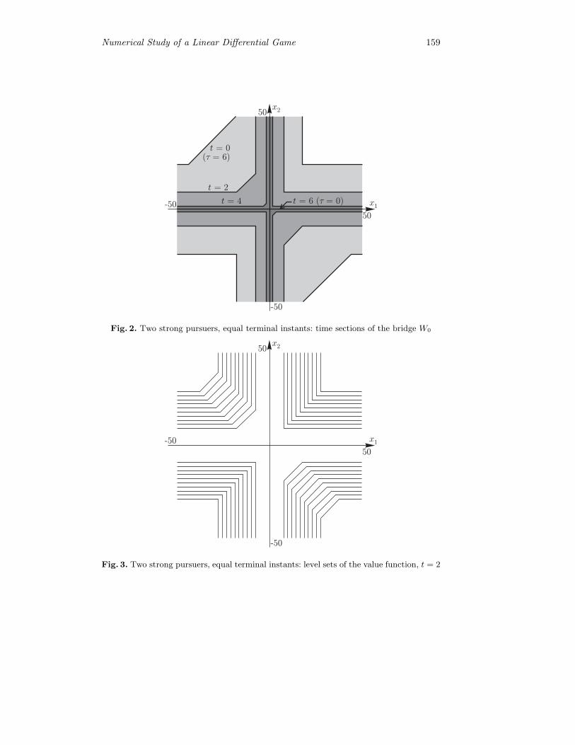
Numerical Study of a Linear Differential Game 159
Fig. 2. Two strong pursuers, equal terminal instants: time sections of the bridge W0
Fig. 3. Two strong pursuers, equal terminal instants: level sets of the value function, t = 2
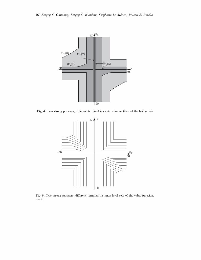
160 Sergey S. Ganebny, Sergey S. Kumkov, Stephane Le Menec, Valerii S. Patsko
Fig. 4. Two strong pursuers, different terminal instants: time sections of the bridge W0
Fig. 5. Two strong pursuers, different terminal instants: level sets of the value function,t = 2

Numerical Study of a Linear Differential Game 161
evader is between the pursuers) give the zone where the capture is possible onlyunder collective actions of both pursuers.
Time sections Wc(t) of other bridges Wc, c > 0, have a shape similar to W0(t).In Fig. 3, one can see the sections Wc(t) at t = 2 (τ = 4) for a collection {Wc}corresponding to some series of values of the parameter c. For other instants t, thestructure of the sections Wc(t) is similar.
Different terminal instants. Let T1 = 7, T2 = 5. Results of construction of theset W0 are given in Fig. 4. When t < 5, time sections W0(t) grow both horizontallyand vertically; two additional triangles appear, but now they are curvilinear.
Total structure of the sections Wc(t) at t = 2 is shown in Fig. 5.
3.2. Maximal Stable Bridges for the Case of Weak Pursuers
Now, we consider a variant of the game when both pursuers are weaker than theevader. Let us take the parameters
μ1 = 0.9, μ2 = 0.8, ν = 1, lP1 = lP2 = 1/0.7, lE = 1.
Let us show results for the case of different terminal instants only: T1 = 7,T2 = 5.
Since in this variant the evader is more maneuverable than the pursuers, theycannot guarantee the exact capture.
Fix some level of the miss, namely,∣∣x1(T1)
∣∣ ≤ 2.0,∣∣x2(T2)
∣∣ ≤ 2.0. Time sectionsW2.0(t) of the corresponding maximal stable bridge are shown in Fig. 6. The upper-left subfigure corresponds to the instant when the first player stops to pursue. Theupper-right subfigure shows the picture for the instant, when the second pursuerfinishes its pursuit. At this instant, the horizontal strip is added, which is a bitwider than the vertical one contracted during the passed period of the backwardtime. Then, the bridges contracts both in horizontal and vertical directions, and twoadditional curvilinear triangles appear (see middle-left subfigure). The middle-rightsubfigure gives the view of the section when the vertical strip collapses, and thelower-left subfigure shows the configuration just after the collapse of the horizontalstrip. At this instant, the section loses connectivity and disjoins into two partssymmetrical with respect to the origin. Further, these parts continue to contract(as it can be seen in the lower-right subfigure) and finally disappear.
Time sections{Wc(t)
}are given in Fig. 7 at the instant t = 0 (τ1 = 7, τ2 = 5).
4. Optimal Feedback Control
Using knowledge of the value function provided by its level sets Wc, we can constructoptimal strategies of the first and second players. Let us do it dividing the planex1, x2 for every instant t to some cells. Inside each cell, the optimal control takessome extremal values.
Rewrite system (7) as
x = D1(t)u1 + D2(t)u2 + E (t)v,
|u1| ≤ μ1, |u2| ≤ μ2, |v| ≤ ν.
Here, x = (x1, x2); vectors D1(t), D2(t), and E (t) look like
D1(t) =(−lP1h((T1 − t)/lP1), 0
), D2(t) =
(0, −lP2h((T2 − t)/lP2)
),
E (t) =(lEh((T1 − t)/lE), lEh((T2 − t)/lE)
).

162 Sergey S. Ganebny, Sergey S. Kumkov, Stephane Le Menec, Valerii S. Patsko
Fig. 6. Two weak pursuers, different termination instants: time sections of the maximalstable bridge W2,0

Numerical Study of a Linear Differential Game 163
Fig. 7. Two weak pursuers, different terminal instants: level sets of the value function,t = 0
We see that the vector D1(t) (D2(t)) is directed along the horizontal (vertical) axis;when T1 = T2, the angle between the axis x1 and the vector E (t) equals 45◦; whenT1 = T2, the angle changes in time.
4.1. Switching Lines in the Case of Strong Pursuers
Feedback control of the first player. Analyzing the change of the value functionalong a horizontal line in the plane x1, x2 for a fixed instant t, one can concludethat the minimum of the function is reached in the segment of intersection of thisline and the set W0(t). With that, the function is monotonic at both sides of thesegment. For points at the right (at the left) from the segment, the control u1 = μ1
(u1 = −μ1) directs the vector D1(t)u1 to the minimum.
Splitting the plane into horizontal lines and extracting for each line the segmentof minimum of the value function, one can gather these segments into a set in theplane and draw a switching line through this set, which separates the plane into twoparts at the instant t. At the right from this switching line, we choose the controlu1 = μ1, and at the left the control is u1 = −μ1. On the switching line, the controlu1 can be arbitrary obeying the constraint |u1| ≤ μ1. The easiest way is to take thevertical axis x2 as the switching line.
In the same way, using the vector D2(t), we can conclude that the horizontalaxis x1 can be taken as the switching line for the control u2.
Thus,
u∗i (t, x) =
⎧⎪⎨⎪⎩μ, if xi > 0,
−μ, if xi < 0,
any ui ∈ [−μ, μ] if xi = 0.
(8)
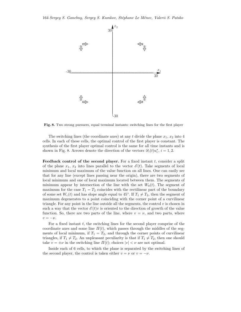
164 Sergey S. Ganebny, Sergey S. Kumkov, Stephane Le Menec, Valerii S. Patsko
Fig. 8. Two strong pursuers, equal terminal instants: switching lines for the first player
The switching lines (the coordinate axes) at any t divide the plane x1, x2 into 4cells. In each of these cells, the optimal control of the first player is constant. Thesynthesis of the first player optimal control is the same for all time instants and isshown in Fig. 8. Arrows denote the direction of the vectors Di(t)u
∗i , i = 1, 2.
Feedback control of the second player. For a fixed instant t, consider a splitof the plane x1, x2 into lines parallel to the vector E (t). Take segments of localminimum and local maximum of the value function on all lines. One can easily seethat for any line (except lines passing near the origin), there are two segments oflocal minimum and one of local maximum located between them. The segments ofminimum appear by intersection of the line with the set W0(t). The segment ofmaximum for the case T1 = T2 coincides with the rectilinear part of the boundaryof some set Wc(t) and has slope angle equal to 45◦. If T1 = T2, then the segment ofmaximum degenerates to a point coinciding with the corner point of a curvilineartriangle. For any point in the line outside all the segments, the control v is chosen insuch a way that the vector E (t)v is oriented to the direction of growth of the valuefunction. So, there are two parts of the line, where v = ν, and two parts, wherev = −ν.
For a fixed instant t, the switching lines for the second player comprise of thecoordinate axes and some line Π(t), which passes through the middles of the seg-ments of local minimum, if T1 = T2, and through the corner points of curvilineartriangles, if T1 = T2. An unpleasant peculiarity is that if T1 = T2, then one shouldtake v = ±ν in the switching line Π(t); choices |v| < ν are not optimal.
Inside each of 6 cells, to which the plane is separated by the switching lines ofthe second player, the control is taken either v = ν or v = −ν.

Numerical Study of a Linear Differential Game 165
Fig. 9. Two strong pursuers, equal terminal instants: switching lines for the second player,t = 0
The second player optimal synthesis for the case T1 = 7, T2 = 5 is shown inFig. 9 for t = 0. Arrows denote direction of the vectors E (t)v∗.
4.2. Switching Lines in the Case of Weak Pursuers
In the case of pursuers weaker than the evader, the structure of the sets Wc is morecomplex in some neighborhood of the origin. This leads to more complicated shapeof the switching lines both for the first and second players.
Switching lines of the first player are given in Fig. 10 at the instant t = 0 (τ1 = 7,τ2 = 5). The dashed line is the switching line for the component u1; the dotted oneis for the component u2. The switching lines are obtained as a result of the analysisof the function x→ V (t, x) in horizontal (for u1 in accordance with the direction ofthe vector D1(t)) and vertical (for u2 in accordance with the direction of the vectorD2(t)) lines. If in the considered horizontal (vertical) line the minimum of the valuefunction is attained in a segment, then the middle of such a segment is taken as apoint for the switching line. Arrows show the directions of the vectors D1(t)u∗
1 andD2(t)u∗
2 in 4 cells.In Fig. 11 switching lines and the directions of the vectors E (t)v∗ are shown
for t = 0. In this picture, we have 4 cells with constant values of the second playercontrol.
4.3. Generating Feedback Controls. Discrete Scheme of Control
Switching lines are built as a result of processing the boundary of the sets Wc(t).With that, some grid of instants tk, where the t-sections Wcj (tk) of the maximalstable bridges Wcj are constructed by the backward procedure. The values cj arealso taken in some grid. For any instant tk, approximating switching lines are storedas polygonal lines in the memory of a computer.

166 Sergey S. Ganebny, Sergey S. Kumkov, Stephane Le Menec, Valerii S. Patsko
Fig. 10. Two weak pursuers, equal terminal instants: switching lines for the first player,t = 0
Fig. 11. Two weak pursuers, equal terminal instants: switching lines for the second player,t = 0

Numerical Study of a Linear Differential Game 167
Having a position x(tk) at the instant tk, it is possible to compute the controlsu∗1
(tk, x(tk)
)and u∗
2
(tk, x(tk)
)analyzing location of the point x(tk) with the respect
to the switching lines for u1 and u2. The vectors D1(tk) and D2(tk) are used forthis. In the case of strong pursuers, the axis x2 is the switching line for the controlu1, and the axis x1 is the switching line for the control u2. The values of u∗
1 andu∗2 are defined by formula (8). In the case of weak pursuers, the switching line is
unique for each component ui of the control too. Drawing a ray from the point x(tk)with the directing vector Di(tk), one can decide whether it crosses a switching linecorresponding to the index i. If it does not, then u∗
i
(tk, x(tk)
)= −μi; if it crosses,
then u∗i
(tk, x(tk)
)= μi.
The first player control chosen at the instant tk is kept until the instant tk+1.At the position
(tk+1, x(tk+1)
), a new control value is chosen, etc. So, the feedback
control generated by the switching lines is applied in a discrete control scheme(Krasovskii and Subbotin, 1974, Krasovskii and Subbotin, 1988).
To construct v∗(tk, x(tk)
)we use the vector E (tk). Compute how many times
(even or odd) a ray with the beginning at the point x(tk) and the directing vectorE (tk) crosses the second player switching lines. If the number of crosses is even(absence of crosses means that the number equals zero and is even), then we takev∗(tk, x(tk)
)= +ν; otherwise, v∗
(tk, x(tk)
)= −ν. The chosen control is kept until
the next instant tk+1. In the position(tk+1, x(tk+1)
), a new control is built, etc.
This synthesis for the first (second) player is suboptimal. Analysis of its close-ness to an optimal one needs an additional study. Namely, it is necessary to showthat under a coordinated choice of diameters Δt and Δc of grids in t and c, thefeedback control of the first (second) player built on the basis of switching linesguarantees the limit of result as Δt → 0 and Δc → 0, which is not greater (notless) than V (t0, x0) for any initial position (t0, x0). Such a study for linear differ-ential games with convex t-sections Wc(t) of maximal stable bridges is made in theworks (Botkin and Patsko, 1982, Zarkh, 1990, Patsko, 2006). In the problem underconsideration the sections Wc(t) are not convex, and this fact preconditions thedifficulty of this problem.
5. Simulation Results
Let the pursuers P1, P2, and the evader E move in the plane. At the initial instantt0 = 0, velocities of all objects are parallel (Fig. 12) and sufficiently greater thanthe possible changes of the lateral velocity components. The instant of longitudinalcoincidence of objects P1 and E is T1; the instant of coincidence of the objects P2
and E is T2. The dynamics of lateral motion is described by relations (1), (2); theresulting miss is given by formula (4).
Fig. 12. Schematic initial positions of the pursuers and evader
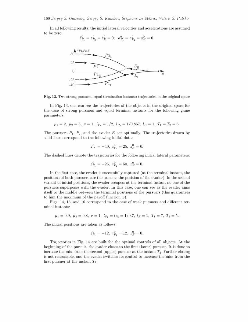
168 Sergey S. Ganebny, Sergey S. Kumkov, Stephane Le Menec, Valerii S. Patsko
In all following results, the initial lateral velocities and accelerations are assumedto be zero:
z0P1= z0P2
= z0E = 0; a0P1= a0P2
= a0E = 0.
Fig. 13. Two strong pursuers, equal termination instants: trajectories in the original space
In Fig. 13, one can see the trajectories of the objects in the original space forthe case of strong pursuers and equal terminal instants for the following gameparameters:
μ1 = 2, μ2 = 3, ν = 1, lP1 = 1/2, lP2 = 1/0.857, lE = 1, T1 = T2 = 6.
The pursuers P1, P2, and the evader E act optimally. The trajectories drawn bysolid lines correspond to the following initial data:
z0P1= −40, z0P2
= 25, z0E = 0.
The dashed lines denote the trajectories for the following initial lateral parameters:
z0P1= −25, z0P2
= 50, z0E = 0.
In the first case, the evader is successfully captured (at the terminal instant, thepositions of both pursuers are the same as the position of the evader). In the secondvariant of initial positions, the evader escapes: at the terminal instant no one of thepursuers superposes with the evader. In this case, one can see as the evader aimsitself to the middle between the terminal positions of the pursuers (this guaranteesto him the maximum of the payoff function ϕ).
Figs. 14, 15, and 16 correspond to the case of weak pursuers and different ter-minal instants:
μ1 = 0.9, μ2 = 0.8, ν = 1, lP1 = lP2 = 1/0.7, lE = 1, T1 = 7, T2 = 5.
The initial positions are taken as follows:
z0P1= −12, z0P2
= 12, z0E = 0.
Trajectories in Fig. 14 are built for the optimal controls of all objects. At thebeginning of the pursuit, the evader closes to the first (lower) pursuer. It is done toincrease the miss from the second (upper) pursuer at the instant T2. Further closingis not reasonable, and the evader switches its control to increase the miss from thefirst pursuer at the instant T1.

Numerical Study of a Linear Differential Game 169
Fig. 15 gives the trajectories, when the pursuers use their optimal feedbackcontrols generated by switching lines, but the evader applies a constant controlv ≡ ν escaping from P1 and ignoring P2. In Fig. 16, the situation is given, whenthe evader, vice versa, keeps control v ≡ −ν escaping from P2 and ignoring P1. Inboth these situations, the payoff is less than in the case when the second player usesoptimal control. When a constant control v = +ν is applied, the miss to the secondpursuer at the instant T2 is less; when the second player keeps v = −ν, the miss tothe first pursuer at the instant T1 decreases.
Fig. 14. Two weak pursuers, different termination instants: trajectories of the objects inthe original space, optimal control of the second player
Fig. 15. Two weak pursuers, different termination instants: trajectories of the objects inthe original space, constant control of the second player v = +ν
Fig. 16. Two weak pursuers, different termination instants: trajectories of the objects inthe original space, constant control of the second player v = −ν

170 Sergey S. Ganebny, Sergey S. Kumkov, Stephane Le Menec, Valerii S. Patsko
6. Conclusion
A problem of pursuit-evasion with two pursuing objects and one evading objectis considered as a two-dimensional antagonistic differential game. Difficulty of nu-merical solution of this problem is conditioned by the fact that the t-sections ofthe value function level sets are not convex. For two qualitatively different types ofparameters (“strong” pursuers, “weak” pursuers), an analysis of the value functionlevel sets is worked out in the paper. On the basis of this analysis, optimal strategiesof players are built.
References
Abramyantz, T. G. and E. P. Maslov (2004). A differential game of pursuit of a grouptarget. Izv. Akad. Nauk Teor. Sist. Upr, 5, 16–22 (in Russian).
Blagodatskih, A. I. and N. N. Petrov (2009). Conflict Interaction Controlled ObjectsGroups. Izhevsk: Udmurt State University (in Russian).
Botkin, N. D. and V. S. Patsko (1983). Universal strategy in a differential game with fixedterminal time. Problems of COntrl and Inform. Theory, 11, 419–432.
Chikrii, A. A. (1997). Conflict-Controlled Processes. Mathematics and its Applications,Vol. 405. Dordrecht: Kluwer Academic Publishers Group.
Grigorenko, N. L. (1991). The problem of pursuit by several objects. In: Differentialgames — developments in modelling and computation (Espoo, 1990), Lecture Notesin Control and Inform. Sci., Vol. 156, pp. 71–80. Berlin: Springer.
Hagedorn, P. and J. V. Breakwell (1976). A differential game with two pursuers and oneevader. Journal of Optimization Theory and Applications 18(2), 15–29.
Isaacs, R. (1965). Differential Games. New York: Wiley & Sons.
Krasovskii, N. N. and A. N. Krasovskii (1993). A differential game for the minimax of apositional functional. In: Adv. Nonlin. Dynamics. and Control: A report from Russia.pp. 41–73. Berlin: Birkhauser.
Krasovskii, N. N. and A. I. Subbotin (1974). em Positional Differential Games. Moscow:Nauka (in Russian).
Krasovskii, N. N. and A. I. Subbotin (1988). Game-Theoretical Control Problems. NewYork: Springer-Verlag.
Levchenkov, A. Y. and A. G. Pashkov (1990). Differential game of optimal approach oftwo inertial pursuers to a noninertial evader. Journal of Optimization Theory andApplications, 65, 501–518.
Le Menec, S. (2011). Linear differential game with two pursuers and one evader. In: Annalsof the International Society of Dynamic Games, Vol. 11: Advances in Dynamic Games.Theory, Applications, and Numerical Methods for Differential and Stochastic Games.M. Breton, K. Szajowski (eds.), pp. 209–226. Boston: Birkhauser.
Patsko, V. (2006). Switching surfaces in linear differential games. Journal of MathematicalSciences, 139(5), 6909–6953.
Pschenichnyi, B.N. (1976). Simple pursuit by several objects. Kibernetika, 3, 145–146(in Russian).
Shima, T. and J. Shinar (2002). Time varying linear pursuit-evasion game models withbounded controls. Journal of Guidance, Control and Dynamics, 25(3), 425–432.
Shinar, J. and T. Shima (2002) Non-orthodox guidance law development approach for theinterception of maneuvering anti-surface missiles. Journal of Guidance, Control, andDynamics. 25(4), 658–666.
Numerical Study of a Linear Differential Game 171
Stipanovic, D. M., A. A. Melikyan, and N. Hovakimyan (2009). Some sufficient conditionsfor multi-player pursuit-evasion games with continuous and discrete observations. In:Annals of the International Society of Dynamic Games (P. Bernhard, V. Gaitsgory, O.Pourtallier, eds.), Vol. 11: Advances in Dynamic Games and Applications, pp. 133–145.Berlin: Springer.
Zarkh, M. A. (1990). Unversal strategy of the second player in a linear differential game.Prikl. Math. Mekh. 54(3), 395–400 (in Russian).
The Dynamic Procedure of Information Flow Network�
Hongwei GAO1, Zuoyi LIU2 and Yeming DAI3
1 Qingdao University,College of Mathematics,
308 Ningxia Road, Qingdao, P.R.CHINA, 266071E-mail: [email protected]
2 Department of Management Sciences, National Natural Science Foundation ofChina(NSFC), 83 Shuangqing Road, Haidian District, Beijing, P.R.CHINA, 100085
E-mail: [email protected] Qingdao University,College of Mathematics,
308 Ningxia Road, Qingdao, P.R.CHINA, 266071E-mail: [email protected]
Abstract. The characterization of the architecture of information flow equi-librium networks and the dynamics of network formation are studied underthe premise of local information flow. The main result of this article is thatit gives the dynamic formation random procedure in the local informationflow network. The research shows that core-periphery structure is the mostrepresentative equilibrium network in the case of the local information flowwithout information decay whatever the cost of information is homogeneousor heterogeneous and it obtains the theory of equilibrium network architec-ture on two kinds of typical core-periphery architecture networks. If profitsand link costs are homogeneous under the premise of local information flowand with the presence of decay beside empty network complete network istypical equilibrium network when the cost of linking is small enough andthey are tried to prove theoretically.
Keywords: local information flow, information decay, random dynamic pro-cedure, core-periphery architecture, equilibrium network.
1. Introduction
The main actors of information flow network are players. The difference betweeninformation flow network and regular network is that the equilibrium network ofinformation flow network not only depends on its topological structure and playershave the need and competence of acquiring information personally and getting in-formation from others in the given network structure. In 2010 Goyal S suggestedthat the dynamic formation procedure of information flow network is one of themost worthy of concern question in his latest article (Galeotti and Goyal, 2010).
� This work was supported by National Natural Science Foundation of China under grantsNo.70871064, 70971070, and 71003057, the International (Regional) Joint Research Pro-gram of China under grant No.71011120107, Natural Science Foundation of ShandongProvince, China under grant No.ZR2010GQ001, the Innovation Project of GraduateEducation in Shandong Province, China under grant No.SDYC08045, Research Projectof Social Science Plan in Shandong Province, China under grant No.09DJGZ07, Re-search planning Project of Humanities and Social Science for Colleges and Universitiesof Shandong Province under grant No.J09WH12, Research Project of Teaching of Qing-dao University under grants No.JY0943 and JY0982.
The Dynamic Procedure of Information Flow Network 173
([original text] In actual practice individuals decide on information acquisition andlinks with others over time, and it is important to understand these dynamics). Sim-ilar to “Two-way” flow network model in common sense (Bala and Goyal, 2000), animportant assumption is that “unilateral formation connection and bilateral infor-mation exchange”, that is to say, a link is formed once some player pays for it andit allows both players to access the information personally acquired by the otherplayer.
2. The local information flow network without decay
Let N = {1, 2, ..., n} with n ≥ 3 be the set of players and let i and j be typicalmembers of this set. Each player chooses a level of personal information acquisitionxi ∈ X = [0,+∞] and a set of links with others to access their information, whichis represented as a (row) vector:
gi = (gi1, ..., gii−1, gii, gii+1, ..., gin)
where gii = 0, ∀i ∈ N and gij ∈ {0, 1}, for each j ∈ N\{i}. We say that player i hasa link with player j if gij = 1, and the cost of linking with one other person is k > 0.Otherwise we have gij = 0. Our paper assumes that the cost of linking with oneother person is homogeneous, and the link between player i and j allow both playersshare information. The set of strategies of player i is denoted by Si = X×Gi. DefineS = S1×...×Sn as the set of strategies of all players. A strategy profile s = (x, g) ∈ Sspecifies the personal information acquired by each player x = (x1, x2, ..., xn), andthe network of relations (connection Matrix) g = (g1, g2, ..., gn)T , where the Tspecifies a transposition.
The network g is a directed graph, where the arrow from i to j specifies gij = 1.Let G be the set of all possible directed graphs on n vertices. Define Ni(g) = {j ∈N : gij = 1} as the set of players with whom i has formed a link. Let ηi(g) =|Ni(g)|. The closure of g is an undirected network denoted by g = cl(g), wheregij = max{gij , gji}. In words, the closure of a directed network involves replacingevery directed edge of by an undirected one. Define Ni(g) = {j ∈ N : gij = 1} asthe set of players directly connected to i. The undirected link between two playersreflects bilateral information exchange between them.
The payoffs to player i under strategy profile s = (x, g) are:
Πi(s) = f(xi +∑
j∈Ni(g)xj)− cixi − ηi(g)k (1)
Where ci > 0 the cost of information. We assume the cost of information thatpersonally acquired is heterogeneous. We will assume that f(y) is twice continuouslydifferentiable, increasing, and strictly concave in y. To focus on interesting cases wewill assume that
f(0) = 0, f ′(0) > c0 = max1≤i≤n
{ci}
andlim
y→+∞f ′(y) = m < c0 = min
1≤i≤n{ci}
Under these assumptions there exists a number yi > 0 such that
yi = arg maxy∈X
[f(y)− ciy]
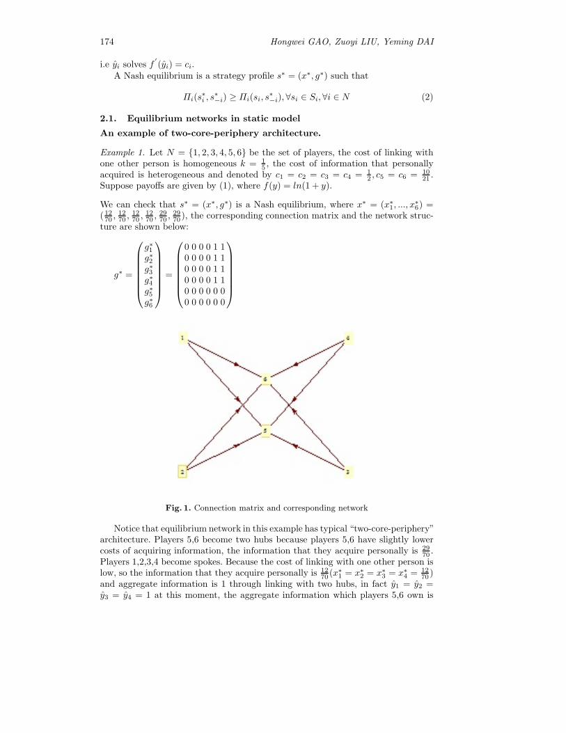
174 Hongwei GAO, Zuoyi LIU, Yeming DAI
i.e yi solves f′(yi) = ci.
A Nash equilibrium is a strategy profile s∗ = (x∗, g∗) such that
Πi(s∗i , s
∗−i) ≥ Πi(si, s
∗−i), ∀si ∈ Si, ∀i ∈ N (2)
2.1. Equilibrium networks in static model
An example of two-core-periphery architecture.
Example 1. Let N = {1, 2, 3, 4, 5, 6} be the set of players, the cost of linking withone other person is homogeneous k = 1
5 , the cost of information that personallyacquired is heterogeneous and denoted by c1 = c2 = c3 = c4 = 1
2 , c5 = c6 = 1021 .
Suppose payoffs are given by (1), where f(y) = ln(1 + y).
We can check that s∗ = (x∗, g∗) is a Nash equilibrium, where x∗ = (x∗1, ..., x
∗6) =
(1270 ,1270 ,
1270 ,
1270 ,
2970 ,
2970 ), the corresponding connection matrix and the network struc-
ture are shown below:
g∗ =
⎛⎜⎜⎜⎜⎜⎜⎝g∗1g∗2g∗3g∗4g∗5g∗6
⎞⎟⎟⎟⎟⎟⎟⎠ =
⎛⎜⎜⎜⎜⎜⎜⎝0 0 0 0 1 10 0 0 0 1 10 0 0 0 1 10 0 0 0 1 10 0 0 0 0 00 0 0 0 0 0
⎞⎟⎟⎟⎟⎟⎟⎠
Fig. 1. Connection matrix and corresponding network
Notice that equilibrium network in this example has typical “two-core-periphery”architecture. Players 5,6 become two hubs because players 5,6 have slightly lowercosts of acquiring information, the information that they acquire personally is 29
70 .Players 1,2,3,4 become spokes. Because the cost of linking with one other person islow, so the information that they acquire personally is 12
70 (x∗1 = x∗
2 = x∗3 = x∗
4 = 1270 )
and aggregate information is 1 through linking with two hubs, in fact y1 = y2 =y3 = y4 = 1 at this moment, the aggregate information which players 5,6 own is
The Dynamic Procedure of Information Flow Network 175
1110 = y5 = y6. Under the equilibrium network, the payoff of spokes is
Πi(s∗) = ln(1 + yi)− cix
∗i − 2k = ln(1 + 1)− 1
2× 6
35− 2× 1
5= 0.2074, i = 1, 2, 3, 4
However, when spokes acquire the optimal aggregate information 1 personally anddon’t link with hubs, the payoff is
Πi(s) = ln(1 + yi)− ci = ln(1 + 1)− 1
2= 0.193, i = 1, 2, 3, 4
Similarly, we can verify Πi(s) < Πi(s∗), ∀s ∈ Si, ∀i ∈ N . So the spokes form links
with two hubs while don’t form links between them and two hubs don’t form linksbetween them is the equilibrium strategy for the players.
In this example, there is no link between two hubs because of k > c5y6 =c6y5(0.2 > 10
21 ×2970 = 0.1973). Spokes choose to form links with hubs because of
k < ciy5 = ciy6(i = 1, 2, 3, 4), i.e.0.2 < 12 ×
2970 = 0.2071.
Network characteristics with “multi-core-periphery” architecture. As wesee in Example 1, the cost heterogeneity of information acquisition is based on twolevels and slight differences. The primary cause lies in the high complexity of thealgorithm of general equilibrium network. In fact, slight cost difference can helpus distinguish which players attain information actively and which players becomespokes.
To simplify symbolic system, we mark y1 and y as the optimal value of infor-mation, which are obtained by players who have information cost advantage andhaven’t advantage. We use c = c−ε < c to express the slight advantage of attaininginformation cost, where ε > 0 is a small number.
In the network g with core-periphery architecture, we will assume that Nc(g)be the set of hubs, where |Nc(g)| = m, then N\Nc(g) be the set of spokes, and wehave |N\Nc(g)| = mq, where q ∈ N+, namely n = (q+ 1)m. The homogeneous costof linking with one other person is k which satisfy f(y)− cy < f(my1)−mk.
Lemma 1. In the equilibrium networks with core-periphery architecture, if for eachl ∈ N , we have xl > 0, then xi+yi = y1, for each i ∈ Nc(g). Moreover, xp+yp = y,for each p ∈ N\Nc(g).
The proof of this lemma is similar to the lemma 1 in [1].
Definition 1. The local information flow network is called core-empty-periphery,if for any pair of player i, i
′ ∈ Nc(g), we have gii′ = 0, and for each player p ∈N\Nc(g), we have gp1 = gp2 = ... = gpm = 1.
Definition 2. The local information flow network is called core-completely-periphery,if for any pair of player i, i
′ ∈ Nc(g), we have gii′ = 1, and for each playerp ∈ N\Nc(g), we have gp1 = gp2 = ... = gpm = 1.
Theorem 1. The local information flow network is a equilibrium network with“core-empty-periphery” architecture, if1) The personal information acquired by each player i is:
xi = y(mq
m2q − 1)− (
1
m2q − 1)y1, ∀i ∈ Nc(g)
176 Hongwei GAO, Zuoyi LIU, Yeming DAI
2) The personal information acquired by each player p is:
xp =my1 − y
m2q − 1, ∀p ∈ N\Nc(g)
3) cxp < k < cxi, k > cxi,ck > m
y−xp , where i ∈ Nc(g), p ∈ N\Nc(g).
In fact, the first inequality in term 3) assures that any spokes are not beingconnected and spokes are favorable to link with hubs; the second inequality assuresthat any hubs are not being connected; the third inequality assures that spokes linkwith hubs if they acquire partial information actively. Meeting with informationlevel of terms 1) and 2) can guarantee hubs own the aggregate information y1 inthe network, while the aggregate information owned by spokes is y. As shown inExample 1.
Theorem 2. The local information flow network is a equilibrium network with“core-completely-periphery” architecture, if1)The personal information acquired by each player i is:
q
mq − 1y − 1
m2q −my1, ∀i ∈ Nc(g)
2)The personal information acquired by each player p is:
xp =y1 − y
mq − 1, ∀p ∈ N\Nc(g)
3)cxp < k < cxi < cxi,ck > m
y−xp , where i ∈ Nc(g), p ∈ N\Nc(g).
Similar to Theorem 1, the first inequality in term 3) assures that spokes don’tform links between them while hubs are favorable to form links with each otherand spokes are favorable to form links with hubs; the second inequality assuresthat spokes link with hubs if they acquire partial information actively. Meetingwith information level of terms 1) and 2) can guarantee hubs own the aggregateinformation y1 in the network, while the aggregate information owned by spokes isy.
We can see from the above situation, after fixing the amount of hubs, the infor-mation acquisition of spokes is degressive. So if q → +∞then xp → 0. Relatively,the information acquisition of hubs is increasing.
The result also reflects contents of “The law of the few”, that is a lot of informa-tion will be grasped in a few hubs, while most of other players, that is, the spokeswill choose to link with hubs to get information, but themselves will choose little“personal information acquisition”, or even entirely depends on the connection toget information, making their “personal information acquisition” to zero.
An example of multi-core-periphery architecture.
Example 2. Let N = {1, 2, 3, 4, 5, 6, 7, 8, 9} be the set of players, the cost of linkingwith one other person is homogeneous, we denote by k = 0.15, the cost of infor-mation that personally acquired is heterogeneous and denote by c1 = c2 = c3 =c4 = c5 = c6 = 1
2 , c7 = c8 = c9 = 1021 . Suppose payoffs are given by (1), where
f(y) = ln(1 + y). The initial matrix is a zero Matrix, and the initial informationvector is (0, 0, 0, 0, 0, 0, 1130 ,
1130 ,
1130 ).

The Dynamic Procedure of Information Flow Network 177
We can check that s∗ = (x∗, g∗) is a Nash equilibrium, where x∗ = (0, 0, 0, 0, 0,0, 1130 ,
1130 ,
1130 ).
g∗ =
⎛⎜⎜⎜⎜⎜⎜⎜⎜⎜⎜⎜⎜⎝
g∗1g∗2g∗3g∗4g∗5g∗6g∗7g∗8g∗9
⎞⎟⎟⎟⎟⎟⎟⎟⎟⎟⎟⎟⎟⎠=
⎛⎜⎜⎜⎜⎜⎜⎜⎜⎜⎜⎜⎜⎝
0 0 0 0 0 0 0 1 10 0 0 0 0 0 0 1 10 0 0 0 0 0 0 1 10 0 0 0 0 0 0 1 10 0 0 0 0 0 0 1 10 0 0 0 0 0 0 1 10 0 0 0 0 0 0 0 10 0 0 0 0 0 0 0 00 0 0 0 0 0 0 0 0
⎞⎟⎟⎟⎟⎟⎟⎟⎟⎟⎟⎟⎟⎠
Fig. 2. Connection matrix and three-core-completely-periphery structure of equilibriumnetwork
2.2. Dynamic procedure and algorithm
The algorithm that we study in this paper is built on the dynamic procedure (Gao,et al, 2010, Gao and Petrosyan, 2009, Hojman and Szeidl, 2008). Considered thatthe algorithmic which even for some player build his best strategy will have n varies,it is no doubt that it is very complicated.
Dynamic procedure: Given the set of players, at each stage, agents who arechosen at random play their best response, they adjust their links in response tothe network structure and the personal information acquired by oneself in previousperiod and then compose the network structure and the personal information.(it iscalled the player’s non-coordinated behavior)
Algorithm: At stage t, first select a subset R of the set of players N at random.For every selected player i ∈ R, we calculate his optimal personal information andthe best link set by comparing all of his possible links, namely the player’s bestresponse strategy. Each player who is selected at random chooses a pure strategy
178 Hongwei GAO, Zuoyi LIU, Yeming DAI
best response to the strategy of all other agents in the previous period and for theplayer who isn’t selected he maintains the strategy chosen in the previous period.Compose all strategies, and then dynamic procedure comes to stage t + 1.
The algorithm of dynamic procedure. Based on above dynamic procedure theadvantage of the algorithm is that the optimization question has only one variable.The network reaches a stable state when no one chooses to change his links andpersonal information during dynamic procedure, and then we can get equilibriumstrategy profile s∗ = (x∗, g∗) and relative information equilibrium network.
Given an initial stage t0, an initial information vector xt0 = (xt01 , ..., xt0n ), initiallink matrix [αt0ij ] ∈ {0, 1}N×N , where αt0ii = 0, i ∈ N and αt0ij ∈ {0, 1}, ∀j ∈ N\{i}.Homogeneous link costs k ≥ 0 and heterogeneity profits ci ≥ 0 are given.
At stage t, let information vector be xt = (xt1, ..., xtn), link matrix [αtij ] =
(αt1, ..., αtn)T ∈ {0, 1}N×N , where αti is the row i of the link matrix [αtij ].
Select randomly the set of players R = (i1, ..., ir) ⊆ N . For every ik ∈ R, therow ik of link matrix has 2n−1 possibilities if we fix the rest n− 1 rows. For everypossibility, first calculate αtikj = max{αtikj , α
tjik} ∈ {0, 1}, it is easy to see αtikik = 0.
Consider that
max θtik = f(xtik +∑j∈N
αtikjxtj)− cikx
tik −
∑j∈N
αtikjk (3)
s.t.
xtik ≥ 0
Notice that∑
j∈N αtikjxtj and
∑j∈N αtikjk in objective function are constant for
given stage t and all probably value of line ik in link matrix [αtij ]. So the variablein (3) only is xtik .
Suppose that the optimal value is reached at xtik . For all the possibilities in rowik we calculate relative optimal value xtik and θtik . At last by comparing above 2n−1
optimal value θtik , we can find max θtik , and then output relative optimal value xtikand αtik .
Based on the algorithm we compose above results, let
[αt+1ij ] = (αt1, ..., α
ti1 , ..., α
tir , ..., α
tn)T
be link matrix at stage t + 1, and information vector
xt+1 = (xt+11 , ..., xt+1
n ) = (xt1, ..., xti1 , ..., x
tir , ..., x
tn)T
The dynamic procedure comes into stage t+1. Select the set of players at randomagain and the network formation procedure is repeated.
The dynamic procedure is end until no one chooses to change his links and per-sonal information. Notice that some examples show that the dynamic proceduremay be a circulation, when we need special terminator program. At last we getthe information flow equilibrium network and equilibrium strategy profile will com-prise the link matrix of the equilibrium network and the optimal personal acquiredinformation vector.
Program: Compute programming language is maple.

The Dynamic Procedure of Information Flow Network 179
Examples of dynamic procedure. Corresponding to Theorem 2 we give twoexamples and model the dynamic procedure using the program.
Example 3. Given the set of players N = {1, 2, 3, 4, 5, 6}, homogeneous link costsk = 0.04 and personal information heterogeneity profits c1 = c2 = c3 = c4 =110 , c5 = c6 = 1
11 . Payoff function is given by (1), where f(y) = ln(1 + y). Initial linkmatrix and initial information vector are 0.
It is different to reach final stage for each implementation of the dynamic processprogram and convergence to the equilibrium state because the non-coordinatedbehavior of the players caused by the randomness of process of forming dynamicnetwork. Therefore there is not practical significance for number of stages to achievea equilibrium state.
We only had one interception of several typical stages in some run results inFigure 3, and let K be the number of stages needed to achieve a equilibrium state.
The network structure and dynamics of information vectors in example 3:1) At initial stage select the set of players R = {2, 3, 4, 5, 6} at random, because
of the initial matrix is zero, they all choose to acquire their optimal aggregateinformation and don’t form any link. And then it will come into an empty networkby the first round of iteration. But the information level vector is x1 = (x1
1, ..., x16) =
(0, 9, 9, 9, 10, 10).2) Owing to the selected set of players is R = {3, 5, 6} at stage 1, we can infer
that it is the best response for player 3 to form links with player 2,4,5,6 and he don’tacquire information personally, the payoff Π3(.) = ln[1+(9+9+10+10)]−4×0.04≈3.5036 is larger than the payoff in any other situations. Because player 5,6 have thesame acquired advantage, it is the best response for player 5,6 to form links with2,3,4,6 and he don’t acquire information. The dynamic procedure comes into stage2.
3) When the dynamic procedure comes into stage t1 it is two-core-peripheryarchitecture. The information level vector of players is xt1 = (0, 9, 0, 0, 0, 0). Selectset of the players R = {1, 4, 5, 6} randomly. Although here the two-core-peripheryarchitecture is the same as the eventual equilibrium structure formally. (player 2,4are temporal core), obviously, for player 5,6 their aggregate information don’t reachtheir optimal value y5 = y6 = 10, so here the network isn’t equilibrium networkand not stable. For player 5,6 they will delete their link with player 4 and maintaintheir link with player 2 and acquire information 1 by themselves, the payoff Πi(.) =ln[1 + (9 + 1)]− 1
11 × 1− 0.04 ≈ 2.2669, i = 5, 6 is lager than any other situations,so it is the best response for them on this stage. Because player 4 don’t acquire anyinformation personally, player 1,5,6 will delete their link with 4 and player 1,4 canacquire their optimal aggregate information 9 by maintaining their link with 2.
4) When the dynamic procedure comes into stage t2, it is three-core-completely-periphery architecture. The information level of players is xt2 = (0, 3, 1, 0, 5, 1).Selected set of the players R = N . So here for player 1,4 it is their best response tomaintain their link with player 2,3,5,6, player 2,3 will maintain their link and reducetheir information 1 by themselves and for player 5,6 they maintain their strategyin pre-period. Notice that here the network is four-core-completely-periphery archi-tecture, it is not stable.
5) When the dynamic procedure comes into stage K − 1, the information levelof players is xK−1 = (0, 0, 0, 0, 8, 2). Selected set of the players R = {1} randomly.For player 1 it is his best response to delete his link with player 3 and maintain
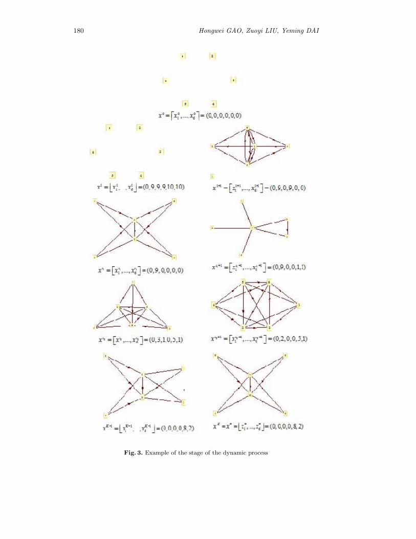
180 Hongwei GAO, Zuoyi LIU, Yeming DAI
Fig. 3. Example of the stage of the dynamic process
The Dynamic Procedure of Information Flow Network 181
his link with 5,6 while he acquires no information. So “two-core-periphery” equilib-rium network is formed, the hub is composed of two players with information costadvantage acquired actively. The dynamic procedure is over.
2.3. Conclusion
Core-periphery structure is the most representative equilibrium network in the caseof the local information flow without information loss. In fact, under the premise ofplayers have two levels of information each person who has a comparative advantageof the cost of acquiring information would become the hub possibly. The statisticalresults show that it is the easiest to form “single-core-periphery” structure; butthe “multi-core-periphery” structure which contains all players who has the sameadvantage on the cost as the hubs (maximum) has the smallest probability; thosewhich between these two kinds become harder and harder with the increasing ofthe players’ number in the core.
We believe that there are several reasons why the dynamics are important. Onereason is that a dynamic model allows us to study the process by which individualagents learn about the network and adjust their links in response to their learning.Relatedly, dynamic may help select among different equilibria of the static game.
There is very important prospect to study the characterization of the architec-ture of information flow equilibrium networks and the dynamics of network forma-tion under the premise of local information flow and without the presence of decay.In addition, consider that some of the players may coordinate and prepare to max-imize the common interests of members by some local cooperation; the model andalgorithm in this essay can be transformed to an incomplete information cooperativegame model. This article assumes that the players have the need and competence ofacquiring information personally and getting information from others in the givennetwork structure, in fact, this can also be diversified.
3. The local information flow equilibrium network with homogeneouscosts and information decay
3.1. The characteristic of equilibrium network architecture
Lemma 2. In the local information flow equilibrium network with decay g, we havexi + yi ≥ y, for all i ∈ N , and if xi > 0, then xi + yi = y. Here yi =
∑j∈Ni(g) δxj ,
that is to say yi represents the information that player i acquires from his neighbors.
Proof. Suppose not, then there must exist some player i such that xi + yi < yin equilibrium network g. Under the assumptions that f(y) is twice continuouslydifferentiable, increasing, and strictly concave in y, we know f ′(xi+yi) > c, so playeri can strictly increase his payoffs by increasing personal information acquisition, acontradiction with equilibrium. So we know xi + yi ≤ y, ∀i ∈ N . Next suppose thatxi > 0 and xi + yi > y. Under our assumptions on f(.) and c, if xi + yi > y thenf ′(xi+yi) < c, and then player i can strictly increase his payoffs by lowering personalinformation acquisition, which contradicts equilibrium. Therefore, if xi > 0, thenxi + yi = y.
Theorem 3. In the local information flow equilibrium network with decay, if k >cδy, the empty network is unique equilibrium. every player acquires information ypersonally and no one forms links.

182 Hongwei GAO, Zuoyi LIU, Yeming DAI
Proof. 1) Suppose that the strategy profile s = (x, g) corresponds to an emptynetwork. If player i forms m1 links with other m1 players and personally acquiresinformation x′
i, here the strategy profile is s|s′i. Lemma 2 implies that the aggregateinformation of player i should be y, and then his payoff is
Πi(s|s′i) = f(y)− c(y − δm1y)−m1k
however, in the empty networks, his payoff is
Πi(s) = f(y)− cy
Since k > cδy, we haveΠi(s) > Πi(s|s′i)
2) Suppose player i forms m2 links with other m2 players initiatively based onthe empty network, and x′′
i = 0, the strategy profile is s|s′′i , payoff is
Πi(s|s′′i ) = f(δm2y)−m2k
. Here δm2y ≥ y, then δm2 ≥ 1. Therefore
Πi(s|s′′i ) = f(δm2y)−m2k < f(δm2y)− cm2δy ≤ f(y)− cy = Πi(s)
Due to k > cδy, the first inequality is strict obviously, since f(y) is twice contin-uously differentiable, increasing, and strictly concave in y, the second is hold. Thenthe empty network is equilibrium network.
Finally, we will show that the empty network is unique equilibrium. As we allknow, every player’s personal information acquisition are no more than y, if someplayer i want to form a link with other player (say j), player i can obtain δxj fromj, and satisfied cδxj > k, this would contradict with k > cδy(because y > xj).
Lemma 3. If complete network is the local information flow equilibrium networkwith decay, the personal information acquisition of each player is equal and x =
y1+(n−1)δ .
Proof. For every player he acquires information personal xi ≥ 0. If there are m(1 ≤m < n) players who personally acquires information 0, we let x1 = x2 = ... = xm =0, according to Lemma 2, we conclude following inequalities:{ ∑
i∈N\{1,...,m} δxi ≥ y
xj +∑
i∈N\{j} δxi = y, j = m + 1, ..., n
We can obtain xm+1 = ... = xn = y1+(n−m−1)δ from the second inequality, hence,
δ ≥ 1 a contradiction. Hence, in complete network, we have xi > 0, ∀i ∈ N . AsLemma 2, we have
xi +∑
j∈N\{i}δxj = y, i = 1, ..., n
therefore
x1 = x2 = ... = xn = x =y
1 + (n− 1)δ
The Dynamic Procedure of Information Flow Network 183
Theorem 4. In the local information flow equilibrium network with decay, if k <cδx = cδy
1+(n−1)δ , complete network is the unique equilibrium.
Proof. Firstly prove that if the personal information acquisition of each player isequal and x = y
1+(n−1)δ in complete network, complete network is equilibrium
structure. Let s∗ = (s∗1, ..., s∗n) be the strategy profile in complete network, where
s∗i = (g∗i , x). If player i have m(0 ≤ m ≤ n− 1) links which he formed with others,since every player can obtain information from other n− 1 players, they would notform links with others.
Secondly, we show that it is not the best response for player i of deleting linksor changing his personal information level.
Now consider the case m = 0, player i can change their personal informationacquisition to be x′, we can write strategy profile s∗|s′i, hence
Πi(s∗|s′i) = f(y − x + x′)− cx′ < f(y)− cx = Πi(s
∗)
so changing strategies are not the best response for player i.Consider the case m = 1, if player i deletes links and acquires information
(1 + δ)x personally, hence
Πi(s∗|s′i) = f(y)− c(1 + δ)x
Since k < cδx
Πi(s∗|s′i) = f(y)− c(1 + δ)x < f(y)− cx− k = Πi(s
∗)
so changing strategies are not the best response for player i.Similarly, we can show that the best response for player i is to maintain current
strategy and completeness of network when m = 2, ..., n− 1 and k < cδx.Following we show that if k < cδx = cδy
1+(n−1)δ , each player acquires information
x = y1+(n−1)δ personally, complete network is the unique equilibrium.
Lemma 3 implies that if complete network is equilibrium structure, the personalinformation acquisition of each player is equal and x = y
1+(n−1)δ .
Two steps: the first step is to prove the connected but not completely networkis not equilibrium, the second step is to prove not connected network is not equi-librium.Step 1.
Suppose not. Then suppose the connected but not completely network is equi-librium. (These connected but not completely network is seen as the sub-networkwhich is formed by deleting several links at random based on a complete network.Actually, the network must not be equilibrium where the number of links betweentwo players are more than 1.)(the link number is n − 1 (Bala and Goyal, 2000) inthe minimal connected network).
We delete any link in complete network, gij = 0 or gji = 0, let g1 be the network.Suppose g1 is equilibrium. Since Lemma 2, every player’s aggregate informationshould be more than or equal to y. Since gij = 0, we have k > cδxi and k > cδxj .Players who are in N\{i, j} have links with each other, let N1 = {i, j}, N2 =N\{i, j}, I(s) = {p|xp > 0, p ∈ N}. For q ∈ N2 ∩ I(s), we have
xq +∑
p∈(N2∩I(s))\{q}δxp +
∑t∈N1
δxt = y

184 Hongwei GAO, Zuoyi LIU, Yeming DAI
If xi = xj = 0, and i, j ∈ N1, so that
xi +∑
p∈N2∩I(s)δxp = 0 +
∑p∈N2∩I(s)
δxp < y
xj +∑
p∈N2∩I(s)δxp = 0 +
∑p∈N2∩I(s)
δxp < y
a contradiction with equilibrium.If xi = 0, xj > 0, and i ∈ N1, hence
xi +∑
p∈N2∩I(s)δxp = 0 +
∑p∈N2∩I(s)
δxp < y
Then player i can strictly increase his payoffs by increasing personal informationacquisition. It contradicts with equilibrium.
The case of xj = 0, xi > 0 is similarly to the above.Hence, we can conclude that personal information acquisition of i and j more
than 0. Otherwise, for l ∈ N2\I(s), we have
xl +∑
p∈N2∩I(s)δxp +
∑t∈N1
δxt
= 0 +∑
p∈N2∩I(s)δxp +
∑t∈N1
δxt
=∑
p∈(N2∩I(s))\{q}δxp + δxq +
∑t∈N1
δxt
< xq +∑
p∈(N2∩I(s))\{q}δxp +
∑t∈N1
δxt = y
That is to say, the aggregate information of l is less than y, contradiction. Hence,for any i ∈ N , every player’s personal information acquisition is xi > 0. Accordingto Lemma 2, the following inequalities are hold{
xt +∑p∈N2
δxp = y, ∀t ∈ N1
xq +∑
p∈N2\{q} δxp +∑t∈N1
δxt = y, ∀q ∈ N2
So we have every player personal information acquisition in N1 equal to xi =xj = x′, and personal information acquisition in N2 equal to xq = x′′, ∀q ∈ N2, sothat {
x′ = (1−δ)y1+δ−2nδ2+4δ2
x′′ = (1−2δ)y1+δ−2nδ2+4δ2
For any n ≥ 3, any network is not equilibrium network.Similarly, we can show that except complete network, connected network is not
the equilibrium network.Step 2.
Firstly, suppose there is an isolated player in equilibrium network at least, theset of these players is N0. The personal information acquisition is y in N0. Due to
The Dynamic Procedure of Information Flow Network 185
k < cδx < cδy, there must exist some player in N \N0 who will strictly increase hispayoffs by lowering his personal information acquisition and switching to link withplayers in N0, contradiction with equilibrium.
Secondly, suppose C1(g) and C2(g) are two part of the network g, and everypart has more than one player.
From Step 1, we know that the two parts are complete.Suppose |C1(g)| = n1 > 1, |C2(g)| = n2 > 1, and assume n1 ≤ n2. Lemma 2 and
Lemma 3 claimed that the information is equal in C1(g) and C2(g), respectively:
xn1 =y
1 + (n1 − 1)δ, xn2 =
y
1 + (n2 − 1)δ
Then xn1 ≥ xn2 > x. We can concluded that k < cδx < cδxn2 ≤ cδxn1 , theplayers in C2(g) will link with the players in C1(g) initiatively. A contradictioncompletes the proof.
Similarly, we can show that non-connected network which contains multipleparts is not the equilibrium.
Theorem 5. In the local information flow network equilibrium structure with de-cay, if cδx < k < cδy, x = y
1+(n−1)δ , no equilibrium structure exist.
All of the examples show the results of Theorem 5 are correct, but the strictproof is not yet complete.
3.2. Examples of Equilibrium Network
Example 4. Let N = {1, 2, 3, 4, 5, 6} be the set of players, the homogeneous cost oflinking with one other person is denoted by k, the homogeneous cost of informationthat players acquire is denoted by c, the index of local information decay is denotedby δ and 0 < δ < 1, where payoffs are given by (1), f(y) = ln(1 + y).
As shown in Fig.4, δ is x-coordinate, k is y-coordinate, where n = 6, c = 13 , y = 2,
the curve equation is k = 2δ3+15δ , and the linear equation is k = 2
3δ. If k < 2δ3+15δ ,
complete network (Fig.5) is the unique equilibrium, write C; if k > 23δ, empty
network is the unique equilibrium, write A; if 2δ3+15δ < k < 2
3δ, there exists noequilibrium, write B.

186 Hongwei GAO, Zuoyi LIU, Yeming DAI
Fig. 4. Distribution of equilibrium network
Fig. 5. Completely network
The Dynamic Procedure of Information Flow Network 187
References
Galeotti, A. and Goyal, S. (2010). The Law of the Few. American Economic Review,100(4), 1468–1492.
Bala, V. and Goyal, S. (2000). A Noncooperative Model of Network Formation. Economet-rica. 68, 1181–1229.
Gao, H. W., Yang, H. J. and Wang, G. X. et al. (2010). The existence theorem of absoluteequilibrium about games on connected graph with state payoff vector. Science ChinaMath, 53(6), 1483–1490.
Gao, H. W. and Petrosyan, L. A. (2009). Dynamics Cooperative Games. Science Press:Beijing.
Hojman, D. and Szeidl, A. (2008). Core and periphery in networks. Journal of EconomicTheory, 139, 295–309.

Game Theory Approach for Supply Chains Optimization
Mansur G. Gasratov1 and Victor V. Zakharov2
1 St.Petersburg State University,Faculty of Applied Mathematics and Control Processes,
Universitetskaya pl. 35, St.Petersburg, Petergoph, 198504, [email protected]
2 St.Petersburg State University,Faculty of Applied Mathematics and Control Processes,
Universitetskaya pl. 35, St.Petersburg, Petergoph, 198504, [email protected]
Abstract. In this paper game theoretic mathematical models of inventorysystems are treated. We consider a market, where several distributors areacting. Each distributor has warehouse for storage goods before supply tocustomers. Assume that demand for their goods has deterministic natureand depends on total supply or on prices of distributors. So we will con-sider quantitative and price competition among distributors. Distributorsare considered as players in non-cooperative game. First we treat quanti-tative competition in context of model of Cournot. Then to consider pricecompetition we use modified model of Bertrand. For modeling of control ofinventory system we use the relaxation method of inventory regulation withadmission of deficiency.
Keywords: Nash equilibrium, optimal, internal strategy, external strategy,demand, distributor.
1. Basic Model for Inventory Policy with Backordering
Let’s consider a single-product inventory control system of stocks with a defi-ciency assumption. We will use relaxation method of regulation of stocks to min-imize long-run inventory costs (Grigoriev M.N., Dolgov A.P., Uvarov S.A., 2006),(Hedly J., Uaitin T., 1969). Assume the demand for items of product is known anduniform during a period of planning. The dynamic of inventory system is illustratedin Figure 1.
The following parameters are used to establish a mathematical model for thisproblem
K – fixed cost per order.c – unit cost of procurement an item of product.h – cost per holding item in inventory during the period of planning.g – cost of being short one item during the entire period of planning.a – demand per inventory circle.y – order quantity.S – maximal inventory level.D – demand for the period of planning.Variables y and S are controlled variables in the problem and may be assumed
as strategies.The usual objective of an inventory policy is to minimize cost of inventory sys-
tem. To meet a given constant demand for the period of planning distributor has to
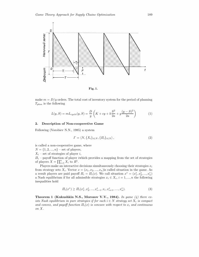
Game Theory Approach for Supply Chains Optimization 189
Fig. 1.
make m = D/y orders. The total cost of inventory system for the period of planningTplan is the following
L(y, S) = mLcycle(y, S) =D
y
(K + cy + h
S2
2a+ g
(y − S)2
2a
)(1)
2. Description of Non-cooperetive Game
Following (Vorobiev N.N., 1985) a system
Γ = 〈N, {Xi}i∈N , {Πi}i∈N〉 , (2)
is called a non-cooperative game, where
N = {1, 2, ..., n} – set of players,
Xi – set of strategies of player i,
Πi – payoff function of player iwhich provides a mapping from the set of strategiesof players X =
∏ni=1 Xi to R1.
Players make an interactive decisions simultaneously choosing their strategies xifrom strategy sets Xi. Vector x = (x1, x2, ..., xn)is called situation in the game. Asa result players are paid payoff Πi = Πi(x). We call situation x∗ = (x∗
1, x∗2, ..., x
∗n)
a Nash equilibrium if for all admissible strategies xi ∈ Xi, i = 1, ..., n the followinginequalities hold
Πi(x∗) ≥ Πi(x
∗1, x
∗2, ..., x
∗i−1, xi, x
∗i+1, ...., x
∗n). (3)
Theorem 1 (Kukushkin N.S., Morozov V.V., 1984). In game (4) there ex-ists Nash equilibrium in pure strategies if for each i ∈ N strategy set Xi is compactand convex, and payoff function Πi(x) is concave with respect to xi and continuouson X.
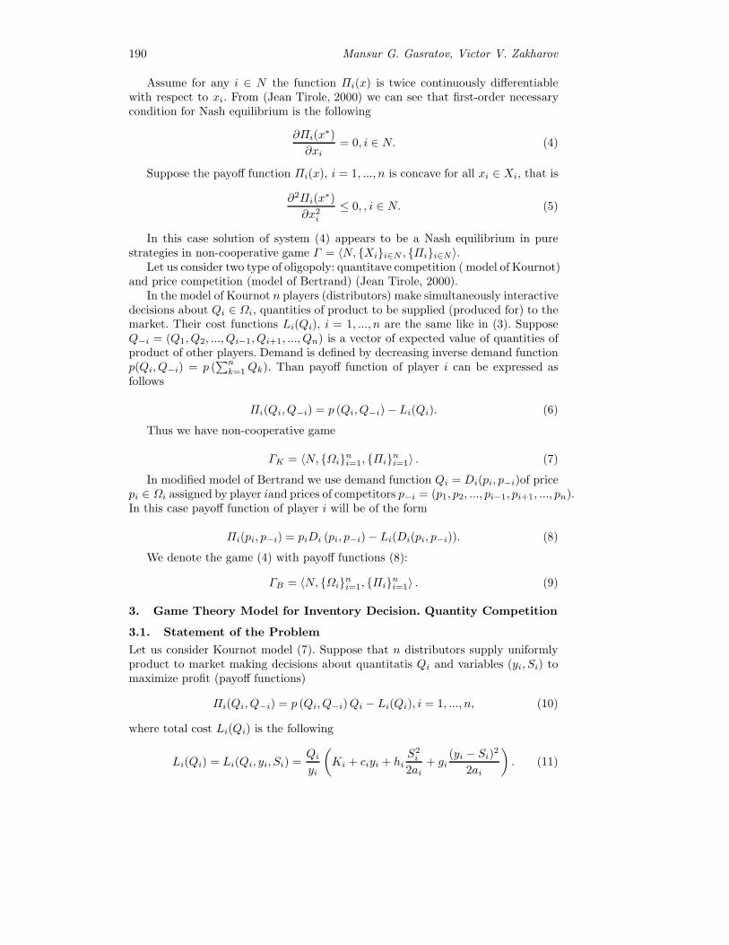
190 Mansur G. Gasratov, Victor V. Zakharov
Assume for any i ∈ N the function Πi(x) is twice continuously differentiablewith respect to xi. From (Jean Tirole, 2000) we can see that first-order necessarycondition for Nash equilibrium is the following
∂Πi(x∗)
∂xi= 0, i ∈ N. (4)
Suppose the payoff function Πi(x), i = 1, ..., n is concave for all xi ∈ Xi, that is
∂2Πi(x∗)
∂x2i
≤ 0, , i ∈ N. (5)
In this case solution of system (4) appears to be a Nash equilibrium in purestrategies in non-cooperative game Γ = 〈N, {Xi}i∈N , {Πi}i∈N〉.
Let us consider two type of oligopoly: quantitave competition ( model of Kournot)and price competition (model of Bertrand) (Jean Tirole, 2000).
In the model of Kournot n players (distributors) make simultaneously interactivedecisions about Qi ∈ Ωi, quantities of product to be supplied (produced for) to themarket. Their cost functions Li(Qi), i = 1, ..., n are the same like in (3). SupposeQ−i = (Q1, Q2, ..., Qi−1, Qi+1, ..., Qn) is a vector of expected value of quantities ofproduct of other players. Demand is defined by decreasing inverse demand functionp(Qi, Q−i) = p (
∑nk=1 Qk). Than payoff function of player i can be expressed as
follows
Πi(Qi, Q−i) = p (Qi, Q−i)− Li(Qi). (6)
Thus we have non-cooperative game
ΓK = 〈N, {Ωi}ni=1, {Πi}ni=1〉 . (7)
In modified model of Bertrand we use demand function Qi = Di(pi, p−i)of pricepi ∈ Ωi assigned by player iand prices of competitors p−i = (p1, p2, ..., pi−1, pi+1, ..., pn).In this case payoff function of player i will be of the form
Πi(pi, p−i) = piDi (pi, p−i)− Li(Di(pi, p−i)). (8)
We denote the game (4) with payoff functions (8):
ΓB = 〈N, {Ωi}ni=1, {Πi}ni=1〉 . (9)
3. Game Theory Model for Inventory Decision. Quantity Competition
3.1. Statement of the Problem
Let us consider Kournot model (7). Suppose that n distributors supply uniformlyproduct to market making decisions about quantitatis Qi and variables (yi, Si) tomaximize profit (payoff functions)
Πi(Qi, Q−i) = p (Qi, Q−i)Qi − Li(Qi), i = 1, ..., n, (10)
where total cost Li(Qi) is the following
Li(Qi) = Li(Qi, yi, Si) =Qi
yi
(Ki + ciyi + hi
S2i
2ai+ gi
(yi − Si)2
2ai
). (11)

Game Theory Approach for Supply Chains Optimization 191
Notice that demand per inventory circle ai(·)may be constant or considered asa function of price per item of product. Let ai(p) = ai(p(Qi, Q−i)) = bi(Qi, Q−i),i = 1, ..., n. In this case cost function (11) will be in the form
Li(Qi, Q−i, yi, Si) =Qi
yi
(Ki + ciyi + hi
S2i
2bi(Qi, Q−i)+ gi
(yi − Si)2
2bi(Qi, Q−i)
). (12)
Substituting (12) to expression (11) we get
Πi(Qi, Q−i) = Πi(Qi, Q−i, yi, Si) =
= p(Qi, Q−i)Qi −Qi
yi(Ki + ciyi + hi
S2i
2bi(Qi, Q−i)+ gi
(yi − Si)2
2bi(Qi, Q−i)). (13)
Function (13) for each i, i = 1, ..., n is continuously differentiable on yi and Siand concave with respect to vector of variables (yi, Si) on the set [0,∞) × [0,∞)when admissible vector (Qi, Q−i)is fixed. Notice also that according to (13) profitof a distributor i is influenced by supply strategy of all competitors and variables(yi, Si) as well.
Definition 1. We will call pair (yi, Si) internal strategy and quantity Qi externalstrategy of player i.
Denote strategy sets of player i, i = 1, ..., n by : Ω(1)i =
{Qi
∣∣ Qi ∈ [a(1)i , b
(1)i ] ⊂
[0,∞)}
; Ω(2)i =
{yi∣∣ yi ∈ [a
(2)i , b
(2)i ] ⊂ (0,∞)
}; Ω
(3)i =
{Si∣∣ Si ∈ [a
(3)i , b
(3)i ] ⊂
[0,∞)}
. Let a(j)i � b
(j)i for all i = 1, ..., N j = 1, 2, 3.
3.2. Internal optimization problem
Considering vector of external strategies (Qi, Q−i) ∈ Ω(1) = Ω(1)1 ×Ω
(1)2 ×...×Ω
(1)N ⊂
Rn+ as given player i chooses internal strategy (yi, Si) ∈ Ω(2)i × Ω
(3)i to miximize
payoff function
Πi(Qi, Q−i, yi, Si)→(yi,Si) max, yi ∈ Ω(2)i , Si ∈ Ω
(3)i . (14)
Solving problem (14) for each i = 1, ..., n we get
y∗i = y∗i (Qi, Q−i) =
√2Ki(gi + hi)
higibi(Qi, Q−i), (15)
S∗i = S∗
i (Qi, Q−i) =
√2Kigi
hi(gi + hi)bi(Qi, Q−i). (16)
3.3. Existence of Nash equilibrium in pure strategies
Substituting optimal internal strategy of player i (y∗i ,S∗i ), i = 1, ..., n defined by (15)
and (16) we get the following expression for payoff functions
Πi(Qi, Q−i, y∗i (Qi, Q−i), S
∗i (Qi, Q−i)) = Φi(Qi, Q−i) =
= Qip(Qi, Q−i)−
√2Kigihihi + gi
· Qi√bi(Qi, Q−i)
−Qici. (17)

192 Mansur G. Gasratov, Victor V. Zakharov
These functions are only influenced by strategies (Qi, Q−i). Thus we have now non-cooperative n-person game of type (7) (model of Kournot)
ΓK = 〈N, {Ωi}ni=1, {Φi}ni=1〉 . (18)
The following theorem takes place
Theorem 2. Suppose the following conditions hold for i = 1, ..., n:
1) reverse demand function p(Qi, Q−i) is twice differentiable, decreasing and
concave with respect to Qi ∈ Ω(1)i for any fixed Q−i ∈ Ω(1)/Ω
(1)i ;
2) function Qi√bi(Qi,Q−i)
is continuous on Ω(1), convex with respect to Qi ∈ Ω(1)i
for any fixed Q−i ∈ Ω(1)/Ω(1)i or the following inequality holds (if bi(Qi, Q−i) –
twice differentiable)
3Qi
(∂bi(Qi,Q−i)
∂Qi
)2
≥ 4bi(Qi,Q−i)∂bi(Qi,Q−i)
∂Qi+ 2Qibi(Qi,Q−i)
∂2bi(Qi,Q−i)
∂Q2i
3) there exists∼Qi∈ (a
(1)i , b
(1)i )such that
p(Qi, Q−i) <
√2Kigihigi + hi
·bi(Qi, Q−i)− 1/2Qi
∂bi(Qi,Q−i)∂Si
b3/2i (Qi, Q−i)
+ ci (19)
for Qi ≥∼Qi
.
Then in game (18) there exists Nash equilibrium in pure strategies (Q∗1, Q
∗2, . . . , Q
∗N),
and Q∗i ∈ [a
(1)i ,
∼Qi), i = 1, ..., n.
The proof of this theorem is based on the first-order (4) and second-order (5)conditions. According to the proof of the theorem Nash equilibrium is a solution ofthe following system
∂Πi(Qi, Q−i)
∂Qi= 0, i = 1, ..., n
or the same
∂p(Qi, Q−i)
∂QiQi + p(Qi, Q−i)−
√2Kigihigi + hi
b(Qi, Q−i)− 1/2Qi∂bi(Qi,Q−i)
∂Qi
b3/2i (Qi, Q−i)
− ci = 0,
(20)
i = 1, ..., n.
Substituting solution of this system to (15) and (16) to calculate optimal internalstrategies (y∗i , S
∗i ) where y∗i = y∗i (Q∗
1, Q∗2, . . . , Q
∗n), S∗
i = S∗i (Q∗
1, Q∗2, . . . , Qn), we
will finally get optimal distributor’s strategies U∗i = (Q∗
i , y∗i , S
∗i ), i = 1, ...., n, which
maximize profit and support Nash equilibrium in the game.

Game Theory Approach for Supply Chains Optimization 193
4. Game Theory Model for Inventory Decision. Price Competition
4.1. Statement of the problem
To formalize game theory model of price competition we consider model of Bertranddescribed in chapter 2. According to (8) profit of distributor i = 1, ..., nis expressedas follows
Πi(pi, p−i) = Di(pi, p−i)pi − Li(Di(pi, p−i)), (21)
where Li(Di(pi, p−i)) is the cost function of inventory system. From (3) we get thefollowing expression for the cost function
Li(Di(pi, p−i)) = Li(pi, p−i, yi, Si) =
=Di(pi, p−i)
yi
(Ki + ciyi + hi
S2i
2ai+ gi
(yi − Si)2
2ai
). (22)
In a similar manner as in chapter 3 we consider demand function per inventory circleai(·) of the form ai = bi(pi, p−i), i = 1, ..., n. Thus function (22) can be rewrittenin the form
Li(Di(pi, p−i)) =Di(pi, p−i)
yi
(Ki + ciyi + hi
S2i
2bi(pi, p−i)+ gi
(yi − Si)2
2bi(pi, p−i)
). (23)
Substituting (23) in (21) we get profit function as follows
Πi(pi, p−i) = Πi(pi, p−i, yi, Si) =
= Di(pi, p−i)pi −Di(pi, p−i)
yi
(Ki + ciyi + hi
S2i
2bi(pi, p−i)+ gi
(yi − Si)2
2bi(pi, p−i)
). (24)
Analogously to chapter 3 we call (yi, Si) internal strategy, pi – external strategyof distributor i, i = 1, ..., n.Strategy sets of player i, i = 1, ..., n are as follows
Ω(1)i =
{pi∣∣ pi ∈ [a
(1)i , b
(1)i ] ⊂ [0,∞)
}; Ω
(2)i =
{yi∣∣ yi ∈ [a
(2)i , b
(2)i ] ⊂ (0,∞)
};
Ω(3)i =
{Si∣∣ Si ∈ [a
(3)i , b
(3)i ] ⊂ [0,∞)
}. Thus we have two level optimization prob-
lem for each distributor. It is also can be presented as combination of internal andexternal problems.
4.2. Internal optimization problem
In internal optimization problem player i chooses internal strategy (yi, Si) ∈ Ω(2)i ×
Ω(3)i with fixed given prices of all players (pi, p−i) ∈ Ω(1) = Ω
(1)1 ×Ω
(1)2 × ...×Ω
(1)n
to maximize profit function
Πi(pi, p−i, yi, Si)→(yi,Si) max, yi ∈ Ω(2)i , Si ∈ Ω
(3)i . (25)
Note that profit function (24) for each i is continuously differentiable with re-spect to yi and Si taken separately and also is convex with respect to (yi, Si) on
the set [0,∞)× [0,∞) (in particular on Ω(2)i ×Ω
(3)i ) when vector of prices (pi, p−i)
is fixed.Solving problem (25) we get the following internal strategies of players
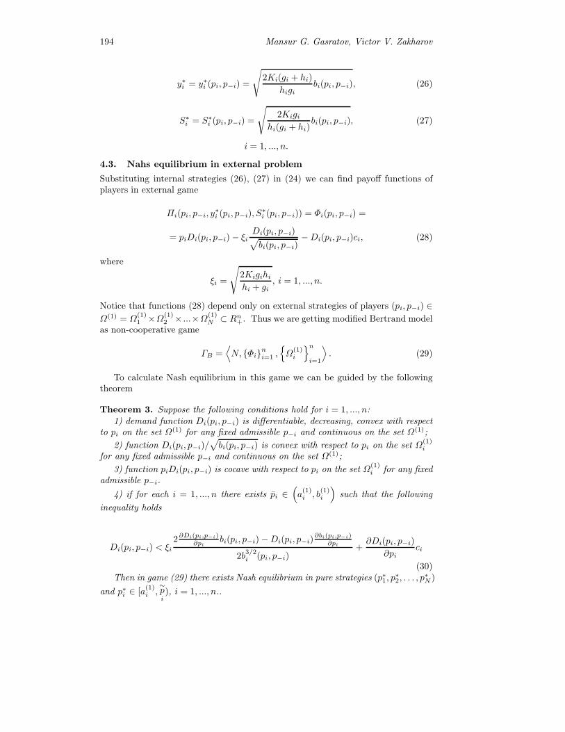
194 Mansur G. Gasratov, Victor V. Zakharov
y∗i = y∗i (pi, p−i) =
√2Ki(gi + hi)
higibi(pi, p−i), (26)
S∗i = S∗
i (pi, p−i) =
√2Kigi
hi(gi + hi)bi(pi, p−i), (27)
i = 1, ..., n.
4.3. Nahs equilibrium in external problem
Substituting internal strategies (26), (27) in (24) we can find payoff functions ofplayers in external game
Πi(pi, p−i, y∗i (pi, p−i), S
∗i (pi, p−i)) = Φi(pi, p−i) =
= piDi(pi, p−i)− ξiDi(pi, p−i)√bi(pi, p−i)
−Di(pi, p−i)ci, (28)
where
ξi =
√2Kigihihi + gi
, i = 1, ..., n.
Notice that functions (28) depend only on external strategies of players (pi, p−i) ∈Ω(1) = Ω
(1)1 ×Ω
(1)2 × ...×Ω
(1)N ⊂ Rn+. Thus we are getting modified Bertrand model
as non-cooperative game
ΓB =⟨N, {Φi}ni=1 ,
{Ω
(1)i
}ni=1
⟩. (29)
To calculate Nash equilibrium in this game we can be guided by the followingtheorem
Theorem 3. Suppose the following conditions hold for i = 1, ..., n:1) demand function Di(pi, p−i) is differentiable, decreasing, convex with respect
to pi on the set Ω(1) for any fixed admissible p−i and continuous on the set Ω(1);
2) function Di(pi, p−i)/√bi(pi, p−i) is convex with respect to pi on the set Ω
(1)i
for any fixed admissible p−i and continuous on the set Ω(1);
3) function piDi(pi, p−i) is cocave with respect to pi on the set Ω(1)i for any fixed
admissible p−i.
4) if for each i = 1, ..., n there exists pi ∈(a(1)i , b
(1)i
)such that the following
inequality holds
Di(pi, p−i) < ξi2∂Di(pi,p−i)∂pi
bi(pi, p−i)−Di(pi, p−i)∂bi(pi,p−i)
∂pi
2b3/2i (pi, p−i)
+∂Di(pi, p−i)
∂pici
(30)Then in game (29) there exists Nash equilibrium in pure strategies (p∗1, p
∗2, . . . , p
∗N )
and p∗i ∈ [a(1)i ,
∼pi), i = 1, ..., n..

Game Theory Approach for Supply Chains Optimization 195
As in Theorem 2 the proof of Theorem 3 is based on the first-order (4) andsecond-order (5) conditions.
Nash equilibrium (p∗1, p∗2, . . . , p
∗N) can be found as a solution of the following
system∂Di(pi, p−i)
∂pibi(pi, p−i) + Di(pi, p−i) =
= ξi2∂Di(pi,p−i)∂pi
bi(pi, p−i)−Di(pi, p−i)∂bi(pi,p−i)
∂pi
2b3/2i (pi, p−i)
+∂Di(pi, p−i)
∂pici, i = 1, ..., n.
(31)
In the case when period of planning is constant, that is Ti = Di(pi,p−i)bi(pi,p−i)
=const ,
we haveDi(pi, p−i)√bi(pi, p−i)
=Di(pi, p−i)√Di(pi, p−i)/Ti
=√TiDi(pi, p−i),
and profit function (28) will be in the form
Φi(pi, p−i) = piDi(pi, p−i)− ρi√Di(pi, p−i)−Di(pi, p−i)ci, (32)
where
ρi =
√2TiKigihihi + gi
, i = 1, ..., n.
Then Nash equilibrium (p∗1, p∗2, . . . , p
∗n) could be defined as a solution of the
system
∂Di(pi, p−i)
∂pibi(pi, p−i)+Di(pi, p−i) = ρi
∂Di(pi, p−i)
2∂pi
1√Di(pi, p−i)
+∂Di(pi, p−i)
∂pici,
(33)
i = 1, ..., n
if there exists pi ∈(a(1)i , b
(1)i
), i = 1, ..., n such that
Di(pi, p−i) < ρi∂Di(pi, p−i)
2∂pi
1√Di(pi, p−i)
+∂Di(pi, p−i)
∂pici
for pi > pi. Moreover p∗i ∈ [a(1)i , pi), ∀ i.
Internal strategies of players as optimal reaction to equilibrium external strate-gies (p∗1, p
∗2, . . . , p
∗n) by the formulas
y∗i = y∗i (p∗i , p∗−i) =
√2Ki(gi + hi)bi(p∗i , p
∗−i)
higi, (34)
S∗i = S∗
i (p∗i , p∗−i) =
√2Kigibi(p∗i , p
∗−i)
hi(gi + hi), (35)
i = 1, ..., n.

196 Mansur G. Gasratov, Victor V. Zakharov
5. Example of inventory system in case of price competition
Suppose that demand function Di(pi, p−i) and demand per inventory circle functionbi(pi, p−i) for each distributor i has the same properties of depending on externalstrategies. Analogously to (Jean Tirole, 2000) we introduce these functions as fol-lows
Di(pi, p−i) = dipβi11 pβi22 . . . p
βi,i−1
i−1 pβi,i+1
i+1 . . . pβinn
p1+αii
, (36)
bi(pi, p−i) = eipβi11 pβi22 . . . p
βi,i−1
i−1 pβi,i+1
i+1 . . . pβnn
p1+αii
, (37)
where di and ei – a positive constants , αi > βij > 0 ∀ j = i, i = 1, ..., n.Elasticity of distributor’s demand function Di(pi, p−i)with respect to his price
is negative εii = −1 − αi < 0, i = 1, ..., n, and with respect to competitors pricesare positive and the following inequalities hold εij = βij > 0.∀ j = i, i = 1, ..., n
So demand is uniform during the period of planning and a circle as well wenotice that period of planning is equal to Di(pi, p−i)/bi(pi, p−i) = di/ei.
Let us consider internal and external problems in this case.Internal problem. We can rewrite formulas for yi and Si in the form
y∗i (pi, p−i) =
√√√√2Ki(gi + hi)eipβi11 pβi22 . . . p
βi,i−1
i−1 pβi,i+1
i+1 . . . pβnn
higip1+αii
,
S∗i (pi, p−i) =
√√√√2Kigieipβi11 pβi22 . . . p
βi,i−1
i−1 pβi,i+1
i+1 . . . pβnn
hi(gi + hi)p1+αii
.
Denote γi(p−i) = pβi11 pβi22 . . . pβi,i−1
i−1 pβi,i+1
i+1 . . . pβnn . Than we get for i = 1, ..., n
y∗i (pi, p−i) =
√2Ki(gi + hi)eiγi(p−i)
higip1+αii
, (38)
S∗i (pi, p−i) =
√2Kigieiγi(p−i)
hi(gi + hi)p1+αii
. (39)
External problem. We substitute internal strategies (38), (39) in (32). Dueto (36) and (37) we get
Φi(pi, p−i) =diγi(p−i)
pαii− di
p(1+αi)/2i
√2Kigihiγi(p−i)
ei(gi + hi)− diciγi(p−i)
p1+αii
. (40)
Thus we state model of Bertrand for our case as non-cooperative game
Γ 1K =
⟨N, {Ω(1)
i }ni=1, {Φi}ni=1
⟩, (41)
where Ω(1)i – the set of external strategies of player i, Ω
(1)i = {pi|a(1)i ≤ pi ≤ b
(1)i },
i = 1, ..., n.One can notice that for our case the following corollary takes place

Game Theory Approach for Supply Chains Optimization 197
Corollary 1. For any αi > 0, i = 1, ..., n in game Γ 1K (41) there exists unique Nash
equilibrium in pure strategies. If 0 < αi < 1, i = 1, ..., n, then payoff functions onequilibrium strategies has positive values.
Solving of the problem . It is easy to see that second-order condition for
function (40) is fulfilled ∂2Φi(pi,p−i)∂p2i
≤ 0 and from the first order condition (4) we
get the following system
∂Φi(pi, p−i)
∂pi= −αidiγi(p−i)
p1+αii
+di(1 + αi)
2
√2Kigihiγi(p−i)
ei(gi + hi)
1
p(3+αi)/2i
+
+(1 + αi)diγi(p−i)ci
p2+αii
= 0, i = 1, ..., n. (42)
It can also be written in the form
−αipi +1 + αi
2
√2Kigihi
ei(gi + hi)γi(p−i)p(1+αi)/2i + (1 + αi)ci = 0, i = 1, ..., n. (43)
Denoting
ξi =1 + αi
2
√2Kigihi
ei(gi + hi), (44)
we get system
ξip1+αi
2i =
√pβi11 pβi22 . . . p
βi−1,1
i−1 pβi+1,1
i+1 . . . pβinn (αipi − (1 + αi)ci) , i = 1, ..., n.
This system can be only solved by numerical methods.Let us consider game of two players i.e. n = 2. For this case we will have the
following system to find Nash equilibrium
ξ1pα1+1
21 −
√pβ12
2 (α1p1 − (α1 + 1)c1) = 0,
ξ2pα2+1
22 −
√pβ21
1 (α2p2 − (α2 + 1)c2) = 0.(45)
Let parameters of the model are as followsK1 = 400 USD, c1 = 10 USD, h1 = 10 USD/h, d1 = 100000, e1 = 10000, g1 = 5USD/h, α1 = 1/2, β12 = 1/4, K2 = 400 USD, c2 = 8 USD, h2 = 8 USD/h,d2 = 100000, e2 = 10000, g2 = 6 USD/h, α2 = 1/2, β21 = 1/4.
System (45) will be of the form
0, 3872983344p341 − p
182
(12p1 − 15
)= 0,
0, 3927922024p342 − p
181
(12p2 − 12
)= 0.
With the solution p∗1 = 37, 68643585 USD and p∗2 = 30, 47300925 USD. These pricesare values of external strategies in Nash equilibrium. Profit of distributors for thissituation are Φ1 (p∗1, p
∗2) = 26744, 43112 and Φ2 (p∗1, p
∗2) = 22422, 48488.
Using (38) and (39) we also calculate internal strategies y∗1 , S∗1 ? y∗2 , S∗
2 : y∗1 ≈156, S∗
1 ≈ 52 and y∗2 ≈ 185, S∗2 ≈ 79.

198 Mansur G. Gasratov, Victor V. Zakharov
6. Conclusion
In this paper we have discussed two models of control of inventory systems in caseof quantitative and price competition.
For each model necessary and sufficient conditions for existence of Nash equilib-rium in pure strategies are proposed. Methods for finding Nash equilibrium in purestrategies are discussed.
Using these methods it is possible to get analytical expressions for internal andexternal strategies in deterministic models. When it is not the case we can findsolutions numerically.
References
Grigiriev, M. N., Dolgov, A. P., Uvarov, S. A. (2006). Logistics: Study Letter. M.: Gardariki,363 p.
Hedly, J., Uaitin, T. (1969). The analysis of control systems of stocks/Translation fromEnglish. M.: Nauka, 512 p.
Vorobiev, N. N. (1985). The Game Theory for The economist-kibernetik. M.: Nauka, 272p.
Kukushkin, N. S., Morozov, V. V. (1984). The nonantagonistic Game Theory. M.: MoscowState University, 103 p.
Jean Tirole (2000). The markets and the market power: The organization and industrytheory/ Translation from English by J.M. Donc, M.D. Facsirova, under edition A.S.Galperina and N.A. Zenkevich. SPb: Institute ”Economic school”, In2000. In 2 Vol-umes. V.1. 328 p. V.2. 240 p.
Stochastic Coalitional Games with Constant Matrixof Transition Probabilties
Xeniya Grigorieva
St.Petersburg State University,Faculty of Applied Mathematics and Control Processes,
University pr. 35, St.Petersburg, 198504, RussiaE-mail: [email protected]
WWW home page: http://www.apmath.spbu.ru/ru/staff/grigorieva/
Abstract. The stochastic game Γ under consideration is repetition of thesame stage game G which is played on each stage with different coali-tional partitions. The transition probabilities over the coalitional structuresof stage game depends on the initial stage game G in game Γ . The pay-offs in stage games (which is a simultaneous game with a given coalitionalstructure) are computed as components of the generalized PMS-vector (see(Grigorieva and Mamkina, 2009), (Petrosjan and Mamkina, 2006)). The to-tal payoff of each player in game Γ is equal to the mathematical expectationof payoffs in different stage games G (mathematical expectation of the com-ponents of PMS-vector). The concept of solution for such class of stochasticgame is proposed and the existence of this solution is proved. The theoryis illustrated by 3-person 3-stage stochastic game with changing coalitionalstructure.
Keywords: stochastic games, coalitional partition, Nash equilibrium, Shap-ley value, PMS-vector.
1. Introduction.
In the papers (Grigorieva, 2010) a class of multistage stochastic games with dif-ferent coalitional partitions where the transition probability from some coalitionalgame to another depends from coalitional partition in the initial game and from then-tuple of strategies which realizes in initial game is examined. A new mathemat-ical method for solving stochastic coalitional games, based on constructing Nashequilibrium (NE) in a stochastic game similarly scheme of constructing of abso-lute NE in a multistage game with perfect information ((Zenkevich et al., 2009),(Petrosjan et al., 1998)), and based on calculation of the generalized PMS-value in-troduced in (Grigorieva and Mamkina, 2009), (Petrosjan and Mamkina, 2006), forthe first time, is proposed along with the proof of the solution existence. In thispaper transition probability from some coalitional game to another depends onlyfrom coalitional partition in the initial game. So the matrix transition probabilitieswhich is constant during of whole multistage game is form.
The theory is illustrated by 3-person 3-stage stochastic game with changingcoalitional structure.
Remind that coalitional game is a game where players are united in fixed coali-tions in order to obtain the maximum possible payoff, and stochastic game is amultistage game with random transitions from state to state, which is played byone or more players.
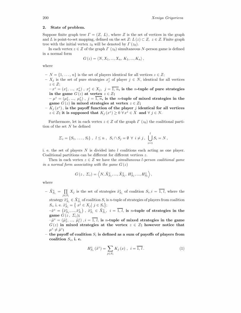
200 Xeniya Grigorieva
2. State of problem.
Suppose finite graph tree Γ = (Z, L) , where Z is the set of vertices in the graphand L is point-to-set mapping, defined on the set Z: L (z) ⊂ Z, z ∈ Z. Finite graphtree with the initial vertex z0 will be denoted by Γ (z0).
In each vertex z ∈ Z of the graph Γ (z0) simultaneous N -person game is definedin a normal form
G (z) = 〈N,X1, ..., Xn, K1, ...,Kn〉 ,
where
– N = {1, . . . , n} is the set of players identical for all vertices z ∈ Z;– Xj is the set of pure strategies xzj of player j ∈ N , identical for all vertices
z ∈ Z;– xz = (xz1, ..., xzn) , xzj ∈ Xj , j = 1, n, is the n-tuple of pure strategiesin the game G (z) at vertex z ∈ Z;– μz = (μz1, ..., μzn) , j = 1, n, is the n-tuple of mixed strategies in thegame G (z) in mixed strategies at vertex z ∈ Z;
– Kj (xz) , is the payoff function of the player j identical for all verticesz ∈ Z; it is supposed that Kj (xz) ≥ 0 ∀xz ∈ X and ∀ j ∈ N.
Furthermore, let in each vertex z ∈ Z of the graph Γ (z0) the coalitional parti-tion of the set N be defined
Σz = {S1, . . . , Sl} , l ≤ n , Si ∩ Sj = ∅ ∀ i = j ,
l⋃i=1
Si = N ,
i. e. the set of players N is divided into l coalitions each acting as one player.Coalitional partitions can be different for different vertices z.
Then in each vertex z ∈ Z we have the simultaneous l-person coalitional gamein a normal form associating with the game G (z)
G (z , Σz) =⟨N, Xz
S1, ..., Xz
Sl , HzS1, ..., Hz
Sl
⟩,
where
– XzSi
=∏j∈Si
Xj is the set of strategies xzSi of coalition Si, i = 1, l, where the
strategy xzSi ∈ XzSi
of coalition Si is n-tuple of strategies of players from coalition
Si, i. e. xzSi ={xj ∈ Xj
∣∣ j ∈ Si}
;
–xz =(xzS1
, ..., xzSl), xzSi ∈ Xz
Si, i = 1, l, is n-tuple of strategies in the
game G (z , Σz);–μz = (μz1, ..., μzl ) , i = 1, l, is n-tuple of mixed strategies in the gameG (z) in mixed strategies at the vertex z ∈ Z; however notice thatμz = μz;
– the payoff of coalition Si is defined as a sum of payoffs of players fromcoalition Si, i. e.
HzSi (xz) =
∑j∈Si
Kj (x) , i = 1, l . (1)
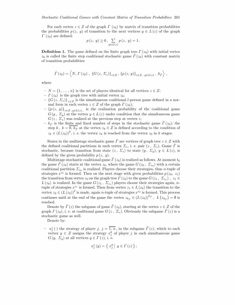
Stochastic Coalitional Games with Constant Matrix of Transition Probabilties 201
For each vertex z ∈ Z of the graph Γ (z0) by matrix of transition probabilitiesthe probabilities p (z, y) of transition to the next vertices y ∈ L (z) of the graphΓ (z0) are defined:
p (z, y) ≥ 0 ,∑
y∈L(z)p (z, y) = 1 .
Definition 1. The game defined on the finite graph tree Γ (z0) with initial vertexz0 is called the finite step coalitional stochastic game Γ (z0) with constant matrixof transition probabilities:
Γ (z0) =⟨N, Γ (z0) , {G (z, Σz)}z∈Z , {p (z, y)}z∈Z , y∈L(z) , kΓ
⟩,
where
– N = {1, . . . , n} is the set of players identical for all vertices z ∈ Z;– Γ (z0) is the graph tree with initial vertex z0;– {G (z, Σz)} z∈Z is the simultaneous coalitional l-person game defined in a nor-
mal form in each vertex z ∈ Z of the graph Γ (z0);– {p (z, y)}z∈Z , y∈L(z) , is the realization probability of the coalitional game
G (y , Σy) at the vertex y ∈ L (z) under condition that the simultaneous gameG (z , Σz) was realized at the previous step at vertex z;
– kΓ is the finite and fixed number of steps in the stochastic game Γ (z0); thestep k , k = 0, kΓ at the vertex zk ∈ Z is defined according to the condition of
zk ∈ (L (z0))k, i. e. the vertex zk is reached from the vertex z0 in k stages.
States in the multistage stochastic game Γ are vertices of graph tree z ∈ Z withthe defined coalitional partitions in each vertex Σz, i. e. pair (z , Σz). Game Γ isstochastic, because transition from state (z , Σz) to state (y , Σy), y ∈ L (z), isdefined by the given probability p (z, y).
Multistage stochastic coalitional game Γ (z0) is realized as follows. At moment t0the game Γ (z0) starts at the vertex z0, where the game G (z0 , Σz0) with a certaincoalitional partition Σz0 is realized. Players choose their strategies, thus n-tuple ofstrategies xz0 is formed. Then on the next stage with given probabilities p (z0, z1)the transition from vertex z0 on the graph tree Γ (z0) to the game G (z1 , Σz1) , z1 ∈L (z0) is realized. In the game G (z1 , Σz1) players choose their strategies again, n-tuple of strategies xz1 is formed. Then from vertex z1 ∈ L (z0) the transition to the
vertex z2 ∈ (L (z0))2
is made, again n-tuple of strategies xz2 is formed. This process
continues until at the end of the game the vertex zkΓ ∈ (L (z0))kΓ , L
(zkΓ)
= ∅ isreached.
Denote by Γ (z) the subgame of game Γ (z0), starting at the vertex z ∈ Z of thegraph Γ (z0), i. e. at coalitional game G (z , Σz). Obviously the subgame Γ (z) is astochastic game as well.
Denote by:
– uzj (·) the strategy of player j, j = 1, n , in the subgame Γ (z), which to eachvertex y ∈ Z assigns the strategy xyj of player j in each simultaneous gameG (y, Σy) at all vertices y ∈ Γ (z), i. e.
uzj (y) ={xyj∣∣ y ∈ Γ (z)
};

202 Xeniya Grigorieva
– uzSi (·) the strategy of coalition Si in the subgame Γ (z), which is a set ofstrategies uzj (·) , j ∈ Si;
– uz (·) = (uz1 (·) , . . . , uzn (·)) =(uzS1
(·) , . . . , uzSn (·))
the n-tuple in the game
Γ (z).
It’s easy to show that the payoff Ezj (uz (·)) of player j, j = 1, n, in any game
Γ (z) is defined as the mathematical expectation of payoffs of player j in all itssubgames, i. e. by the following formula (Zenkevich et al., 2009, p. 158):
Ezj (uz (·)) = Kj (xz) +
∑y∈L(z)
[p (z, y) Ey
j (uy (·))]. (2)
Thus, a coalitional stochastic game Γ (z0) with constant matrix of transitionprobabilities can be written as a game in normal form
Γ (z0) =
=
⟨N, Γ (z0) , {G (z, Σz)}z∈Z , {p (z, y)} z∈Z,
y∈L(z),{Uzj
}j=1,n
,{Ezj
}j=1,n
, kΓ
⟩,
where Uzj is the set of the strategies uzj (·) of the player j, j = 1, n.
The payoff HzSi
(xz) of coalition Si ∈ Σz, i = 1, l , in each coalitional gameG (z , Σz) at the vertex z ∈ Z is defined as the sum of payoffs of players from thecoalition Si, see formula (1):
HzSi (xz) =
∑j∈Si
Kj (xz) .
The payoff HzSi
(uz (·)) , Si ∈ Σz, i = 1, l , in the subgame Γ (z) of the game
Γ (z0) at the vertex z ∈ Z is defined as the sum of payoffs of players from thecoalition Si in the subgame Γ (z) at the vertex z ∈ Z:
HzSi (uz (·)) =
∑j∈Si
Ezj (uz (·)) =
=∑j∈Si
⎧⎨⎩Kj (xz) +∑
y∈L(z)
[p (z, y) Ey
j (uy (·))]⎫⎬⎭ =
=∑j∈Si
Kj (xz) +∑j∈Si
⎧⎨⎩ ∑y∈L(z)
[p (z, y) Ey
j (uy (·))]⎫⎬⎭ =
=∑j∈Si
Kj (xz) +∑
y∈L(z)
⎡⎣p (z, y)∑j∈Si
Eyj (uy (·))
⎤⎦ =
= HzSi (xz) +
∑y∈L(z)
[p (z, y)Hy
Si(uy (·))
]. (3)
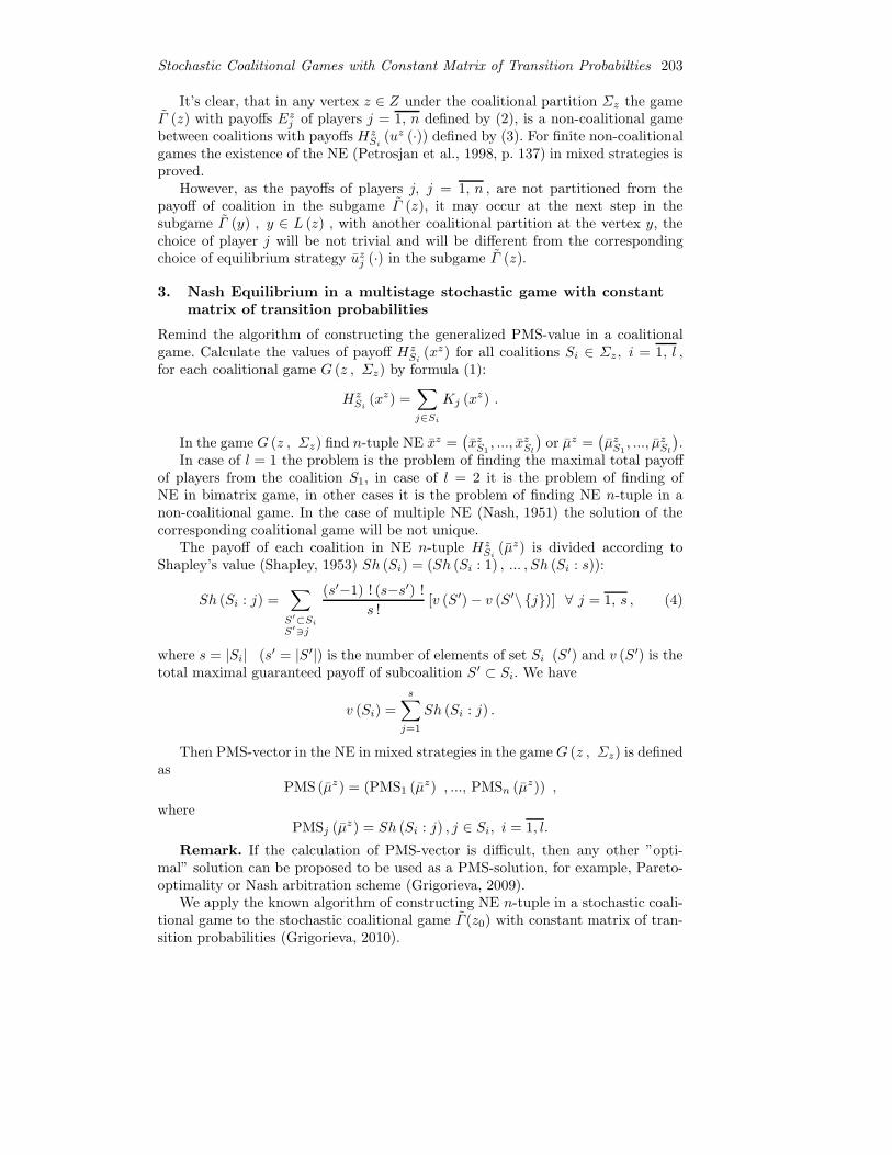
Stochastic Coalitional Games with Constant Matrix of Transition Probabilties 203
It’s clear, that in any vertex z ∈ Z under the coalitional partition Σz the gameΓ (z) with payoffs Ez
j of players j = 1, n defined by (2), is a non-coalitional gamebetween coalitions with payoffs Hz
Si(uz (·)) defined by (3). For finite non-coalitional
games the existence of the NE (Petrosjan et al., 1998, p. 137) in mixed strategies isproved.
However, as the payoffs of players j, j = 1, n , are not partitioned from thepayoff of coalition in the subgame Γ (z), it may occur at the next step in thesubgame Γ (y) , y ∈ L (z) , with another coalitional partition at the vertex y, thechoice of player j will be not trivial and will be different from the correspondingchoice of equilibrium strategy uzj (·) in the subgame Γ (z).
3. Nash Equilibrium in a multistage stochastic game with constantmatrix of transition probabilities
Remind the algorithm of constructing the generalized PMS-value in a coalitionalgame. Calculate the values of payoff Hz
Si(xz) for all coalitions Si ∈ Σz, i = 1, l ,
for each coalitional game G (z , Σz) by formula (1):
HzSi (xz) =
∑j∈Si
Kj (xz) .
In the game G (z , Σz) find n-tuple NE xz =(xzS1
, ..., xzSl)
or μz =(μzS1
, ..., μzSl).
In case of l = 1 the problem is the problem of finding the maximal total payoffof players from the coalition S1, in case of l = 2 it is the problem of finding ofNE in bimatrix game, in other cases it is the problem of finding NE n-tuple in anon-coalitional game. In the case of multiple NE (Nash, 1951) the solution of thecorresponding coalitional game will be not unique.
The payoff of each coalition in NE n-tuple HzSi
(μz) is divided according toShapley’s value (Shapley, 1953) Sh (Si) = (Sh (Si : 1) , ... , Sh (Si : s)):
Sh (Si : j) =∑S′⊂SiS′�j
(s′−1) ! (s−s′) !
s ![v (S′)− v (S′\ {j})] ∀ j = 1, s , (4)
where s = |Si| (s′ = |S′|) is the number of elements of set Si (S′) and v (S′) is thetotal maximal guaranteed payoff of subcoalition S′ ⊂ Si. We have
v (Si) =
s∑j=1
Sh (Si : j) .
Then PMS-vector in the NE in mixed strategies in the game G (z , Σz) is definedas
PMS (μz) = (PMS1 (μz) , ..., PMSn (μz)) ,
wherePMSj (μz) = Sh (Si : j) , j ∈ Si, i = 1, l.
Remark. If the calculation of PMS-vector is difficult, then any other ”opti-mal” solution can be proposed to be used as a PMS-solution, for example, Pareto-optimality or Nash arbitration scheme (Grigorieva, 2009).
We apply the known algorithm of constructing NE n-tuple in a stochastic coali-tional game to the stochastic coalitional game Γ (z0) with constant matrix of tran-sition probabilities (Grigorieva, 2010).

204 Xeniya Grigorieva
4. Examples.
Example 1. Let there be 3 players in the game each having 2 strategies, and letpayoffs of each player be defined, see table 1. Consider all possible combinations ofcoalitional partitions, cooperative and non-coalitional cases.
Table 1.
The strategies The payoffs The payoffs of coalition
I II III I II III (I, II) (II, III) (I, III) (I, II, III)
1 1 1 4 2 1 6 3 5 7
1 1 2 1 2 2 3 4 3 5
1 2 1 3 1 5 4 6 8 9
1 2 2 5 1 3 6 4 8 9
2 1 1 5 3 1 8 4 6 9
2 1 2 1 2 2 3 4 3 5
2 2 1 0 4 3 4 7 3 7
2 2 2 0 4 2 4 6 2 6
1. Solve coalitional game G (Σ1), Σ1 = {S = {I, II} , N\S = {III}}, by calcu-lating PMS-value (Grigorieva and Mamkina, 2009) as follows.
1.1. Find NE in mixed strategies in the bimatrix game:
η = 3/7 1− η = 4/7
00
ξ = 1/31− ξ = 2/3
1 2(1, 1) [6, 1] [3, 2](2, 2) [4, 3] [4, 2](1, 2) [4, 5] [6, 3](2, 1) [8, 1] [3, 2] .
First and second rows are dominated by the last and third ones correspondingly.Find n-tuple of NE in the mixed strategies in the bimatrix game
μ2 =(
3/7 4/7), μ1 =
(0 0 1/3 2/3
),
by using the theorem about complete mixed equilibrium [(Petrosjan et al., 1998),p. 135].
Realization of payoffs of coalitions S and N\S in mixed strategies take placewith follows probabilities:
η1 η2ξ1 0 0ξ2 0 0
ξ3 1/74/21
ξ4 2/78/21
.
Calculate mathematical expectation of payoffs in NE in mixed strategies:
E(μ1, μ2
)=
1
7[4, 5] +
2
7[8, 1] +
4
21[6, 3] +
8
21[3, 2] =
[36
7,
7
3
]=
[5
1
7, 2
1
3
].
1.2. Find guaranteed payoffs v {I} and v {II} of players I and II, see table 2, asfollows. Fix strategy of player III
μ2 =(
3/7 4/7).

Stochastic Coalitional Games with Constant Matrix of Transition Probabilties 205
Then mathematical expectation of payoffs of players of coalition S under fix strategyof coalition N\S looks as:
ES(1, 1)(μ2)
=(37 · 4 + 4
7 · 1 ; 37 · 2 + 4
7 · 2)
=(2 27 ; 2)
;ES(1, 2)
(μ2)
=(37 · 3 + 4
7 · 5 ; 37 · 1 + 4
7 · 1)
=(4 17 ; 1)
;ES(2, 1)
(μ2)
=(37 · 5 + 4
7 · 1; 37 · 3 + 4
7 · 2)
=(2 57 ; 2 3
7
);
ES(2, 2)(μ2)
=(37 · 0 + 4
7 · 0 ; 37 · 4 + 4
7 · 4)
= (0; 4) .
Hence, guaranteed payoffs are calculated as follows:
minH1
(x1 = 1, x2, μ
2)
= min{
2 27 ; 4 1
7
}= 2 2
7 ;minH1
(x1 = 2, x2, μ
2)
= min{
2 57 ; 0}
= 0;
∣∣∣∣ v {I} = max{
2 27 ; 0}
= 2 27 ;
minH2
(x1, x2 = 1, μ2
)= min
{2; 2 3
7
}= 2 ;
minH2
(x1, x2 = 2, μ2
)= min {1; 4} = 1;
∣∣∣∣ v {II} = max {2; 1} = 2.
Thus, guaranted payoffs equals: v {I} = 2 27 , v {II} = 2.
Table 2.
1.3. Divide the payoff E1
(μ1, μ2
)= 5 1
7 according to the Shapley’s value (Shap-ley, 1953):
Sh1 = v {I}+ 12 (v {I, II} − v {II} − v {I}) = 2 2
7 + 12
(5 17 − 2 2
7 − 2)
= 2 57 ;
Sh2 = v {II}+ 12 (v {I, II} − v {II} − v {I}) = 2 3
7 .
Then PMS-vector (Grigorieva and Mamkina, 2009) will be:
PMS1 = 25
7; PMS2 = 2
3
7; PMS3 = 2
1
3.
2. Solve coalitional game G (Σ2), Σ2 = {S = {II, III} , N\S = {I}}, by calcu-lating PMS-vector (Grigorieva and Mamkina, 2009) as follows.
2.1. Find NE in mixed strategies in the bimatrix game:

206 Xeniya Grigorieva
η = 1 1− η = 0
00
ξ = 01− ξ = 1
1 2(1, 1) [3, 4] [4, 5](2, 2) [4, 5] [6, 0](1, 2) [4, 1] [4, 1](2, 1) [6, 3] [7, 0] .
First three rows are dominated by the last, second column is dominated by first.Hence,
μ2 =(
1 0), μ1 =
(0 0 0 1
),
and vector of coalitional payoffs is E(μ1, μ2
)= [6, 3]
2.2. Find guaranteed payoffs v {II} = 2 and v {III} = 2 of players II and III. Fixstrategy of player I
μ2 =(
1 0).
Then:
minH2
(μ2, x2 = 1, x3
)= min {2; 2} = 2 ;
minH2
(μ2, x2 = 2, x3
)= min {1; 1} = 1;
∣∣∣∣ v {II} = max {2; 1} = 2;
minH3
(μ2, x2, x3 = 1
)= min {1; 5} = 1 ;
minH3
(μ2, x2, x3 = 2
)= min {2; 3} = 2;
∣∣∣∣ v {III} = max {1; 2} = 2.
Thus, guaranted payoffs are: v {II} = 2, v {III} = 2.2.3. Divide the payoff E1
(μ1, μ2
)= 6 according to the Shapley’s value (Shapley,
1953):
Sh2 = v {II}+ 12 (v {II, III} − v {II} − v {III}) ;
Sh3 = v {III}+ 12 (v {II, III} − v {II} − v {III}) .
Then PMS-vector ((Grigorieva and Mamkina, 2009), (Petrosjan and Mamkina,2006)):
PMS1 = PMS2 = PMS3 = 3 .
3. Solve coalitional game G (Σ3), Σ3 = {S = {I, III} , N\S = {II}}, by calcu-lating PMS-value (Grigorieva and Mamkina, 2009) as follows.
3.1. Find NE in mixed strategies in the bimatrix game:
η = 5/6 1− η = 1/6
ξ = 1/200
1− ξ = 1/2
1 2(1, 1) [5, 2] [8, 1](2, 2) [3, 2] [2, 4](1, 2) [3, 2] [8, 1](2, 1) [6, 3] [3, 4] .
Second and third rows are dominated by first. Find NE in the mixed strategiesin the bimatrix game
μ2 =(
5/6 1/6), μ1 =
(1/2 0 0 1/2
),
vector of coalitional payoffs is
E(μ1, μ2
)=
5
12[5, 2] +
1
12[8, 1] +
5
12[6, 3] +
1
12[3, 4] =
[66
12,
30
12
]=
[5
1
2, 2
1
2
].

Stochastic Coalitional Games with Constant Matrix of Transition Probabilties 207
3.2. Fix strategy of player II μ2 =(
5/6 1/6)
and find guaranteed payoffs v {I} =
= 1.68 and v {III} = 2 of players I and III, see table 3.
Table 3.
3.3. Divide the payoff E1
(μ1, μ2
)= 5.5 according to the Shapley’s value (Shap-
ley, 1953):
Sh1 = v {I}+ 12 (v {I, III} − v {I} − v {III}) ;
Sh3 = v {III}+ 12 (v {I, III} − v {I} − v {III}) .
Then PMS-vector in mixed strategies (Grigorieva and Mamkina, 2009):
PMS1 = 2.59; PMS2 = 2.5; PMS3 = 2.91 .
4. Solve cooperative game G (Σ4), Σ4 = {N = {I, II, III}}, see table 2. Find themaximum payoff of coalition N and divide it according to Shapley’s value (Shapley,1953):
Sh1 =1
6[v {I, II}+ v {I, III} − v {II} − v {III}]+1
3[v {I, II, III} − v {II, III}+ v {I}] ;
Sh2 =1
6[v {II, I}+ v {II, III} − v {I} − v {III}]+1
3[v {I, II, III} − v {I, III}+ v {II}] ;
Sh3 =1
6[v {III, I}+ v {III, II} − v {I} − v {II}]+1
3[v {I, II, III} − v {I, II}+ v {III}] .
Find guaranteed payoffs:
v{I, II} = max{4, 3} = 4 , v{I, III} = max{3, 2} = 3 , v{II, III} = max{3, 4} = 4 ,
v{I} = max{1, 0} = 1 , v{II} = max{2, 1} = 2 , v{III} = max{1, 2} = 2 .
Then
Sh(2, 1, 1)1 = Sh
(1, 2, 2)1 = Sh
(1, 2, 1)1 =
1
3+
1
6+
1
3[9− 4] +
1
3=
1
3+
1
6+
5
3+
1
3= 2
1
2,
Sh(2, 1, 1)2 = Sh
(1, 2, 2)2 = Sh
(1, 2, 1)2 =
1
2+
1
3+
1
3[9− 3] +
2
3=
1
2+
1
3+
6
3+
2
3= 3
1
2,
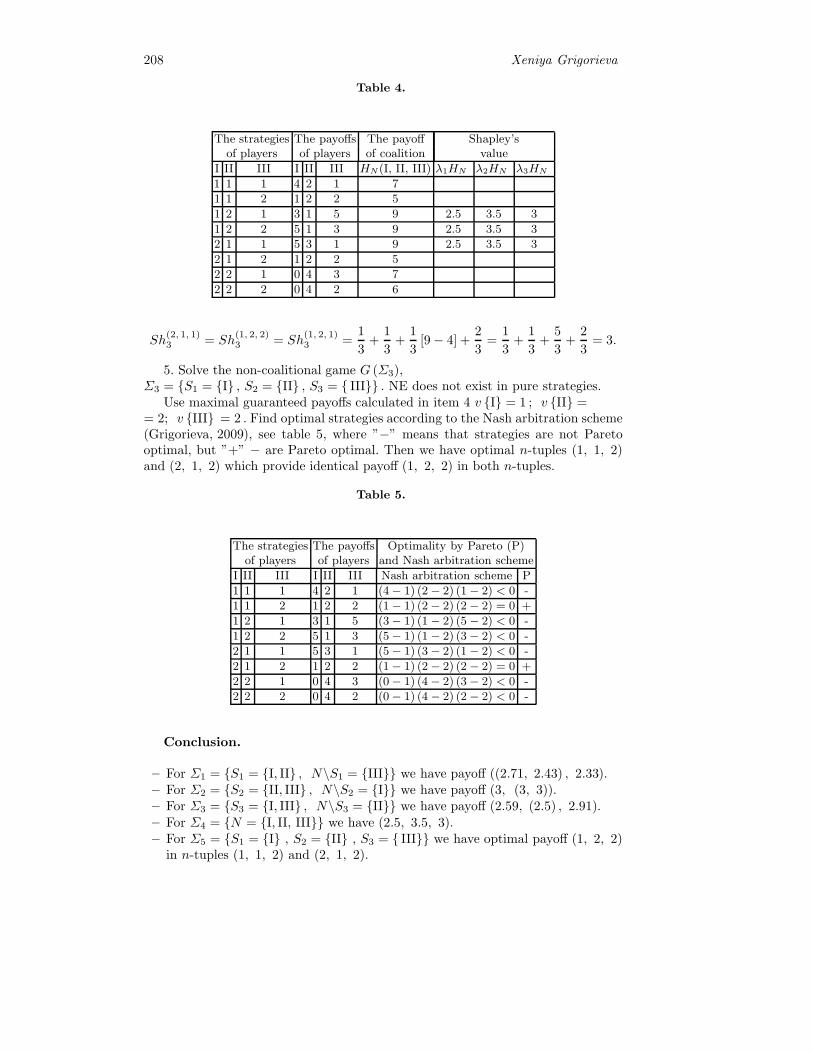
208 Xeniya Grigorieva
Table 4.
The strategies The payoffs The payoff Shapley’sof players of players of coalition value
I II III I II III HN(I, II, III) λ1HN λ2HN λ3HN
1 1 1 4 2 1 7
1 1 2 1 2 2 5
1 2 1 3 1 5 9 2.5 3.5 3
1 2 2 5 1 3 9 2.5 3.5 3
2 1 1 5 3 1 9 2.5 3.5 3
2 1 2 1 2 2 5
2 2 1 0 4 3 7
2 2 2 0 4 2 6
Sh(2, 1, 1)3 = Sh
(1, 2, 2)3 = Sh
(1, 2, 1)3 =
1
3+
1
3+
1
3[9− 4] +
2
3=
1
3+
1
3+
5
3+
2
3= 3.
5. Solve the non-coalitional game G (Σ3),Σ3 = {S1 = {I} , S2 = {II} , S3 = { III}} . NE does not exist in pure strategies.
Use maximal guaranteed payoffs calculated in item 4 v {I} = 1 ; v {II} == 2; v {III} = 2 . Find optimal strategies according to the Nash arbitration scheme(Grigorieva, 2009), see table 5, where ”−” means that strategies are not Paretooptimal, but ”+” − are Pareto optimal. Then we have optimal n-tuples (1, 1, 2)and (2, 1, 2) which provide identical payoff (1, 2, 2) in both n-tuples.
Table 5.
The strategies The payoffs Optimality by Pareto (P)of players of players and Nash arbitration scheme
I II III I II III Nash arbitration scheme P
1 1 1 4 2 1 (4 − 1) (2 − 2) (1 − 2) < 0 -
1 1 2 1 2 2 (1 − 1) (2 − 2) (2 − 2) = 0 +
1 2 1 3 1 5 (3 − 1) (1 − 2) (5 − 2) < 0 -
1 2 2 5 1 3 (5 − 1) (1 − 2) (3 − 2) < 0 -
2 1 1 5 3 1 (5 − 1) (3 − 2) (1 − 2) < 0 -
2 1 2 1 2 2 (1 − 1) (2 − 2) (2 − 2) = 0 +
2 2 1 0 4 3 (0 − 1) (4 − 2) (3 − 2) < 0 -
2 2 2 0 4 2 (0 − 1) (4 − 2) (2 − 2) < 0 -
Conclusion.
– For Σ1 = {S1 = {I, II} , N\S1 = {III}} we have payoff ((2.71, 2.43) , 2.33).– For Σ2 = {S2 = {II, III} , N\S2 = {I}} we have payoff (3, (3, 3)).– For Σ3 = {S3 = {I, III} , N\S3 = {II}} we have payoff (2.59, (2.5) , 2.91).– For Σ4 = {N = {I, II, III}} we have (2.5, 3.5, 3).– For Σ5 = {S1 = {I} , S2 = {II} , S3 = { III}} we have optimal payoff (1, 2, 2)
in n-tuples (1, 1, 2) and (2, 1, 2).
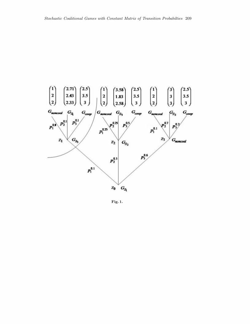
Stochastic Coalitional Games with Constant Matrix of Transition Probabilties 209
Fig. 1.

210 Xeniya Grigorieva
Example 2. Consider the following stochastic game, see picture 1. Transitionprobabilities (p1, p2, p3) from one game to another game are shown on the graphshown in the picture 1.
Transition probabilities are determined by table 6. Table 6 defines the matrix oftransition probabilities as follows. In the left column the games from which is donetransition to the games locating by the first row of the table with probabilities incorresponding rows are located.
Table 6.
The Gnoncoal GS1 GS2 GS3 Gcoop
probabilities
Gnoncoal 0.1 0 0.7 0 0.2
GS1 0.6 0 0.3 0.1 0
GS2 0.25 0 0 0.25 0.5
GS3 0.8 0.1 0 0 0.1
Gcoop 0.1 0.1 0.5 0.1 0.2
Payoffs of players in n-tuple of NE of the following simultaneous games G areequal to (see example 1)
PMSnoncoal = (1, 2, 2) , PMSGS1= (2.71, 2.43, 2.33) , PMSGS2
= (3, 3, 3) ,
PMSGS3= (2.59, 2.5, 2.91) , PMScoop =
(2
1
2, 3
1
2, 3
),
Algorithm for solving the problem.1. Consider two step game Γ (GS3), shown at the very left and upper angle of
the graph in the picture 1:
PMSΓ (GS3)(μ) = PMSGS3
(μ) + p1(GS3 ||Gnoncoal) PMSGnoncoal+
+p2(GS3 ||GS1)PMSGS1+ p3(GS3 ||Gcoop) PMSGcoop =
= PMSGS3(μ) +
⎛⎝1.322.192.13
⎞⎠ =
⎛⎝2.592.52.91
⎞⎠+
⎛⎝1.322.192.13
⎞⎠ =
⎛⎝3.914.695.04
⎞⎠ ,
μ = {σ(1, 1, 1) = 0.42, σ(1, 2, 1) = 0.08, σ(2, 1, 1) = 0.42, σ(2, 2, 1) = 0.08},where σ(x) is realization probability of NE n-tuple x in pure strategies.
2. Similarly solve games Γ (GS2) and Γ (Gnoncoal), see picture 1.
PMSΓ (GS2)(x) = PMSGS2
(x) + p1(GS2 ||Gnoncoal) PMSGnoncoal+
+p2(GS2 ||GS3)PMSGS3+ p3(GS2 ||Gcoop) PMSGcoop =
= PMSGS2(x) + 0.25 ·
⎛⎝122
⎞⎠+ 0.25 ·
⎛⎝2.592.52.91
⎞⎠+ 0.5 ·
⎛⎝2.53.53
⎞⎠ =

Stochastic Coalitional Games with Constant Matrix of Transition Probabilties 211
= PMSGS2(x) +
⎛⎝2.152.882.73
⎞⎠ =
⎛⎝333
⎞⎠+
⎛⎝2.152.882.73
⎞⎠ =
⎛⎝5.155.885.73
⎞⎠ ,
x = (1, 2, 1);
PMSΓ (Gnoncoal)(x) = PMSGnoncoal
(x) + p1(Gnoncoal||Gnoncoal) PMSGnoncoal+
+p2(Gnoncoal||GS2)PMSGS2+ p3(Gnoncoal||Gcoop) PMSGcoop =
= PMSGnoncoal(x) + 0.1 ·
⎛⎝122
⎞⎠+ 0.7 ·
⎛⎝333
⎞⎠+ 0.2 ·
⎛⎝2.53.53
⎞⎠ =
= PMSGnoncoal(x) +
⎛⎝2.73
2.9
⎞⎠ =
⎛⎝122
⎞⎠+
⎛⎝2.73
2.9
⎞⎠ =
⎛⎝3.75
4.9
⎞⎠ ,
x = (1, 1, 2) or x = (2, 1, 2).
3. Now solve the game Γ (Γ (GS3), Γ (GS2), Γ (Gnoncoal)), see picture 1.
PMSΓ (Γ (GS3),Γ (GS2),Γ (Gnoncoal))(μ) = PMSGS1
(μ)+
+p1(GS1 || Γ (Gnoncoal)) PMSΓ (Gnoncoal)+
+p2(GS1 || Γ (GS2))PMSΓ (GS2)+ p3(GS1 || Γ (GS3)) PMSΓ (GS3)
=
= PMSGS1(μ) + 0.6 ·
⎛⎝3.75
4.9
⎞⎠+ 0.3 ·
⎛⎝5.155.885.73
⎞⎠+ 0.1 ·
⎛⎝3.914.695.04
⎞⎠ =
= PMSGS1(μ) +
⎛⎝4.165.235.16
⎞⎠ =
⎛⎝2.712.432.33
⎞⎠+
⎛⎝4.165.235.16
⎞⎠ =
⎛⎝6.877.667.49
⎞⎠ ,
μ = {σ(1, 2, 1) = 0.14, σ(1, 2, 2) = 0.19, σ(2, 1, 1) = 0.29, σ(2, 1, 2) = 0.38}.Since the game Γ (Γ (GS3), Γ (GS2), Γ (Gnoncoal)) is three stage game, then mean
payoff of each player at one step can be calculated by formula:
(6.87, 7.66, 7.49) /3 = (2.29, 2.55, 2.5) .
References
Grigorieva, X. (2010). Solutions for a class of stochastic coalitional games. Contributionsto Game Theory and Management. Collected papers presented on the Third Interna-tional Conference ”Game Theory and Management” (GTM’2009) / Edited by LeonA. Petrosjan, Nikolay A. Zenkevich. - SPb.: Graduate School of Management, SPbSU,144–161.
Grigorieva, X. V. (2010). Optimization for a class of stochastic coalitional games. GameTheory and Application. ., v., SPbSU, pp. 45–60.
Zenkevich, N., Petrosjan, L., Young, D. (2009). Dynamic Games and their applications inmanagement. - SPb.: Graduate School of Management.

212 Xeniya Grigorieva
Petrosjan, L., Zenkevich, N., Semina, E. (1998). The Game Theory. - M.: High School.Grigorieva, X., Mamkina, S. (2009). Solutions of Bimatrix Coalitional Games. Contribu-
tions to game and management. Collected papers printed on the Second InternationalConference ”Game Theory and Management” [GTM’2008]/ Edited by Leon A. Pet-rosjan, Nikolay A. Zenkevich. - SPb.: Graduate School of Management, SpbSU, pp.147–153.
Petrosjan, L., Mamkina, S. (2006). Dynamic Games with Coalitional Structures. Intersec-tional Game Theory Review, 8(2), 295–307.
Nash, J. (1951). Non-cooperative Games. Ann. Mathematics 54, 286–295.Shapley, L. S. (1953). A Value for n-Person Games. In: Contributions to the Theory of
Games( Kuhn, H. W. and A. W. Tucker, eds.), pp. 307–317. Princeton UniversityPress.
Grigorieva, X. V. (2009). Nash bargaining solution for solving the coalitional bimatrixgames. In: Interuniversity thematic collection of works of St. Petersburg State Uni-versity of Civil Engineering (Ed. Dr., prof. B. G. Wager). Vol. 15. Pp. 56–61.
Cash Flow Optimization in ATM Network Model
Elena Gubar, Maria Zubareva, Julia Merzljakova
St.Petersburg State University,Faculty of Applied Mathematics and Control Processes,Universitetskiy pr. 35, St.Petersburg, 198504, Russia
fax:+7 (812) 428 71 59http://[email protected] [email protected]
Abstract. The main purpose of this work is to optimize cash flow in case ofthe encashment process in the ATM network with prediction of ATM refusal.The solution of these problems is based on some modified algorithms for theVehicle Routing Problem and use statistical methods to compile the requestsfrom the ATM network. A numerical example is considered.
Keywords: ATM network, route optimization, Vehicle Routing Problem,cash flow, statistical methods.
1. Introduction
Nowadays ATM network and credit cards are the essential parts of modern lifestyle,consequently one of the most actual problem in the bank’s ATM network is opti-mization of cash flow and organization of uninterrupted work. For the bank it isimportant to prevent the rush demand for cash withdrawals by customers, thatcan be provoked by the delayed loading of ATMs, and reduce the service expenses.Serving the ATMs network is a costly task: it takes employees’ time to supervisethe network and make decisions about cash management and it involves high op-erating costs (financial, transport, etc.). At the present time more and more banksare turning their attention to have greater efficiency in how they manage their cashin ATMs.
Through cash management optimization banks can avoid falling into the trap ofmaintaining too much cash and begin to profit by mobilizing idle cash. Effective cashmanagement and control starts with accurate prediction of ATMs refusal, allowingbanks to forecast cash demand for the network, and find an optimal routes, whichmanage to reduce servicing costs. The increase of transportation and servicing costcan be substantial for banks. Route optimization for the collector teams is allow toreduce bank expenses and to control the encashment process (Simutis et al., 2007).
In this work we consider a problem in which a set of geographically dispersedATMs with known requirements must be served with a fleet of money collector teamsstationed in the depot in such a way as to minimize some distribution objective.This problem is combined with the problem of composition of service requests fromthe ATM network. We assume that the money collector teams are identical withthe equal capacity and must start and finish their routes at the depot. To estimatean average cash amount in each ATM and form the requests for the money collectorteams we use following factors:
214 Elena Gubar, Maria Zubareva, Julia Merzljakova
– ATM location and open hours;
– Irregular number of operations per week;
– Increasing of operation number in holidays and salary days.
Moreover we define the necessity of servicing each ATM and predict the fu-ture requests for the collector teams based on the statistical data and restrictions,which are proposed above. The optimal routes to load ATMs depend on the currentrequests and predictable requests.
The main purpose of this work is to optimize cash flow in case of the encashmentprocess in the ATM network with prediction of ATM refusal. To solve the problemwe base on some modified algorithms for the Vehicle Routing Problem and usestatistical methods to compile the requests from the ATM network. In the paper anumerical simulation for ATM network of one bank of St. Petersburg is considered.
2. Route optimization for collector teams
In this section we consider a problem in which a set of geographically dispersedATMs must be served with a fleet of money collector teams stationed in the bank.This problem will be solved based on the Capacitated Vehicle Routing Problem(CVRP) see (Hall, 2003), which is the problem of designing feasible routes for aset of homogeneous vehicles that make up a vehicle fleet. The routes are formedminimizing total travel costs of all of the routes. Each route begins and ends atthe depot and contains a subset of the stops requiring service. A solution to thisproblem is feasible if the vehicle capacity on each route is not exceeded and allstops are assigned to a route. In the simplest statement of the CVRP there are nolower and upper bounds on the duration of each route. As such, there are no routebalance considerations.
To describe the basic CVRP we suppose, that a complete undirected network(or graph) G = (V,E) is given where V = (0, 1, . . . , n) is the set of vertices and E isthe set of undirected arcs (edges). A non-negative cost cij is associated with everyedge. V ′ = V \ {0} is a set of n vertices, each vertex corresponds to a stop, vertex 0corresponds to the depot. Henceforth, i will be used interchangeably to refer bothto a stop and to its vertex location. Each stop i requires a supply of qi units fromdepot 0. A set of M identical vehicles of capacity Q is located at the depot and isused to service the stops; these M vehicles comprise the homogeneous vehicle fleet.It is required that every vehicle route starts and ends at the depot and that theload carried by each vehicle is no greater than Q.
The route cost corresponds to the distance travelled on the route and is com-puted as the sum of the costs of the edges forming the route.
An optimal solution for the CVRP is a set of M feasible routes, one for eachvehicle, in which all stops are visited, the capacity of each vehicle is not exceededand the sum of the route costs is minimized.
In the case of street routing the stops are located on a street network and thetravel time between stops is computed as the shortest travel time path betweenstops. If the travel time matrix is symmetric, then we have the symmetric or basicCVRP. In the symmetric CVRP it can be assumed that there are no one-way streetsand turn and street crossing difficulties are not considered in setting up the traveltime matrix. In this paper we consider one procedure for solving the symmetricalCVRP, using statistical methods to reduce model dimension.

Cash Flow Optimization in ATM Network Model 215
2.1. Integer programming formulation of the CVRP
Consider the presentation of the CVRP, where V = (0, 1, . . . , n) is the complete setof vertices, subset V ′ = V \ {0} is a set of n vertices without depot, each vertexcorresponds to a stop, vertex 0 corresponds to the depot. Let xij be an integervariable representing the number of vehicles traversing the undirected arc (edge){i, j}, and let r(S) be the number of vehicles needed to satisfy the demand ofATMs in S, cij are costs.
Here we present the formalization of the basic CVRP problem:
min∑i<j
cijxij , (1)
∑i<j
xij +∑i>j
xji = 2, i ∈ V ′, (2)
∑i∈S
∑j∈V \S
xij ≥ 2r(s), S ⊆ V ′, |S| > 1, (3)
∑j∈V ′
x0j = 2M, (4)
xij ∈ {0, 1}, i ∈ V ′, j ∈ V ′, i < j, (5)
x0j ∈ {0, 1, 2}, j ∈ V ′. (6)
Constraints (2) are the degree constraints for each ATM. Constraints (3) arethe capacity constraints which, for any subset S of ATMs, that does not includethe depot, impose that r(S) vehicles enter and leave S, where r(S) is the minimumnumber of vehicles of capacity Q required for servicing the ATMs in S. Constraints(3) are also called generalized subtour elimination constraints. It is NP-hard tocompute r(S), since it corresponds to solve a bin-packing problem where r(S) is theminimum number of bins of capacity Q that are needed for packing the quantities.However, inequalities (3) remain valid if r(S) is replaced by a lower bound to itsvalue, such as [
∑i∈S qi/Q] where [y] denotes the smallest integer not less than y and
qi is required amount of cash for each ATM. Constraint (4) states that M vehiclesmust leave and return to the depot while constraints (5) and (6) are the integralityconstraints. Finally, x0j = 2 corresponds to a route containing only stop j.
This formulation cannot be solved directly by a general purpose integer pro-gramming algorithm because constraints (3) are too numerous to be enumerated apriori. However if the dimension of model will be reduced, this formulation will besolved.
At the present time various approaches to the solution of the CVRP have beenproposed in different papers. In our work we focused on several papers and hand-books. The main sources is (Hall, 2003), which presents several formulations ofVehicle Routing Problem and it’s modification, as well as some ideas and methodsof solution are described. Nowadays Vehicle Routing Problem (VRP) is very ac-tual and many authors concentrate on application of different methods and theirextensions to solve VRP. This paper is based on some previous works, for in-stance, (Ralphs et al., 2003), in their work, suggest a decomposition-based sepa-ration methodology for the capacity constraints. Meanwhile the paper (Lysgaard et
216 Elena Gubar, Maria Zubareva, Julia Merzljakova
al., 2003) describes a branch-and-cut algorithm based on application of variety ofcutting planes.
In current work we offer to reduce dimension of the model and simplify con-straints (3) using statistical analysis on the ATM network.
3. Forecasting of Cash Flows in ATM Network
In current section we consider a problem of cash flow forecasting in the ATM net-work, especially focused on forecasting of cash balance in ATMs and the moment ofATM upload. Moreover we find the moment of each ATM refusal and compile therequests for the bank’s processing center (Vasin, 2005). We analyzed cash flows ofeach ATM, using statistical data, and found that cash withdrawal is heterogeneousprocess which depends on following factors:
– Paydays, weekends, holidays, etc.;– ATM location;– ATM open hours.
Consider the set of geographically dispersed ATMs and a bank, defined in Section2. Here V ′ = V \ {0} is a subset of n ATMs, without bank, as in previous sectionvertex 0 corresponds to the bank. According to the factors mentioned above thewhole set of ATMs V ′ is divided into m subsets Sk ⊆ V ′, Sk ∩ Sl = ∅, k = l,k, l ∈ {1, . . . ,m}. Lets define yit as the amount of cash withdrawal from ATM i atday t.
Consider each subset Sk consisting of nk ATMs separately. Using statistical cashwithdrawal data for each ATM over N days, we describe an average amount of cashwithdrawal per day for subset Sk by following expression:
ykt =1
nk
∑i∈Sk
yit, t = 1, . . . , N, k = 1, . . . ,m. (7)
Thus we obtain cash withdrawal time series for each subset Sk: (yk1, yk2, . . . , ykN ).Estimate trend and periodic component of the time series, for that purpose chooselinear trend and find equation of linear regression (Bure, Evseev, 2004):
trkt = ak + bkt, t = 1, . . . , N, k = 1, . . . ,m, (8)
where the evaluations of unknown parameters ak, bk are calculated with the least-squares procedure.
The periodic component is estimated by the the following formula, removingtrend from the time series:
Pkt =1
zk
zk−1∑j=0
(yk,t+j·Tk − trk,t+j·Tk ), t = 1, . . . , Tk, k = 1, . . . ,m, (9)
where N – number of observations in subset Sk, Tk – period length, zk = NTk
–integer number of periods.
Thereby we define cash withdrawal time series for each subset Sk:
ykt = trkt + Pkt, t = 1, . . . , N, k = 1, . . . ,m. (10)
Cash Flow Optimization in ATM Network Model 217
The cash withdrawal forecast for two weeks is evaluated with the formula (10):
Ykt = trkt + Pkt, t = N + 1, . . . , N + 14, k = 1, . . . ,m. (11)
Proceed the forecasting of cash balance in ATMs network and extend this pro-cedure for all subgroups Sk. Assume Bit is the cash balance in ATM i at day t.If we know the cash balance for exact day, we can make the cash balance fore-cast using cash withdrawal forecast calculated by formula (11), i.e. find Bit whent = N + 1, . . . , N + 14. Now we can detect the moment of each ATM refusal, i.e.when the cash balance approaches zero, and generate requests for the money col-lector teams.
Our purpose is to form the requests for service senter for each day of the fore-casting period. Every request should contain the information about ATMs neededto be serviced and the quantity of cartridges (Diebold). We do not take into accountthe nominal of banknotes.
The algorithm for cash balance forecast was simulated in the MATLAB systemand for each date of the forecasting period we received the requests for ATM ser-vice with numbers of ATMs, their addresses and number of cartridges. Requests aretransmitted to the encashment department and can be used to reduce CVRP di-mension and respectively the number on constraints (3), while constructing optimalencashment routes.
3.1. Numerical simulation
Consider one bank of St. Petersburg with ATM network consisting of 49 items andapply the procedure offered above. Divide subset V ′ into several subsets Sk whichare presented in the Table 1:
Table 1. Subsets of ATM network
Subset Sk Name (location) Quantity of ATMs Open hours
S1 Subway 21 Open dailyS2 Shop 8 Open dailyS3 Shopping Mall 9 Open dailyS4 Educational Organization 2 Mo–FrS5 Enterprise 2 Mo–FrS6 Bank 7 Mo–Fr
Consider each group separately and analyze cash withdrawal time series usingformulas (7)-(9). For example, examine the subset S1, which is the group of ATMssituated at the subway. We construct time series for the period from 10 may 2010to 20 june 2010. The diagram of the average cash withdrawal time series for thesubset S1 is presented in Fig.1. It shows that on Friday and Saturday the amountof cash withdrawal increases rapidly.
We construct equation of linear regression with estimated trend and periodiccomponent: trt = 369, 5t + 167022. We have 42 observations, then the length oftime period T1 = 7 and hence the integer number of periods is z1 = n
T1= 6.
Make the cash withdrawal forecast for two weeks. The diagram of the time seriesestimation and the cash withdrawal forecast for the period from 21 june 2010 to4 july 2010 is presented in Fig.2.

218 Elena Gubar, Maria Zubareva, Julia Merzljakova
Fig. 1. Cash withdrawal time series for the subset S1
Fig. 2. Cash withdrawal time series, time series estimation and forecast for the subset S1
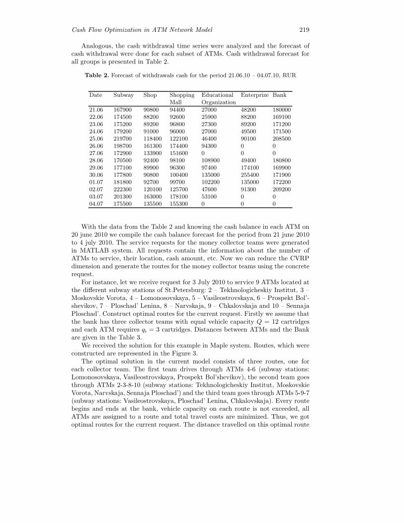
Cash Flow Optimization in ATM Network Model 219
Analogous, the cash withdrawal time series were analyzed and the forecast ofcash withdrawal were done for each subset of ATMs. Cash withdrawal forecast forall groups is presented in Table 2.
Table 2. Forecast of withdrawals cash for the period 21.06.10 – 04.07.10, RUR
Date Subway Shop ShoppingMall
EducationalOrganization
Enterprize Bank
21.06 167900 90800 94400 27000 48200 18000022.06 174500 88200 92600 25900 88200 16910023.06 175200 89200 96800 27300 89200 17120024.06 179200 91000 96000 27000 49500 17150025.06 219700 118400 122100 46400 90100 20850026.06 198700 161300 174400 94300 0 027.06 172900 133900 151600 0 0 028.06 170500 92400 98100 108900 49400 18080029.06 177100 89900 96300 97400 174100 16990030.06 177800 90800 100400 135000 255400 17190001.07 181800 92700 99700 102200 135000 17220002.07 222300 120100 125700 47600 91300 20920003.07 201300 163000 178100 53100 0 004.07 175500 135500 155300 0 0 0
With the data from the Table 2 and knowing the cash balance in each ATM on20 june 2010 we compile the cash balance forecast for the period from 21 june 2010to 4 july 2010. The service requests for the money collector teams were generatedin MATLAB system. All requests contain the information about the number ofATMs to service, their location, cash amount, etc. Now we can reduce the CVRPdimension and generate the routes for the money collector teams using the concreterequest.
For instance, let we receive request for 3 July 2010 to service 9 ATMs located atthe different subway stations of St.Petersburg: 2 – Tekhnologicheskiy Institut, 3 –Moskovskie Vorota, 4 – Lomonosovskaya, 5 – Vasileostrovskaya, 6 – Prospekt Bol’-shevikov, 7 – Ploschad’ Lenina, 8 – Narvskaja, 9 – Chkalovskaja and 10 – SennajaPloschad’. Construct optimal routes for the current request. Firstly we assume thatthe bank has three collector teams with equal vehicle capacity Q = 12 cartridgesand each ATM requires qi = 3 cartridges. Distances between ATMs and the Bankare given in the Table 3.
We received the solution for this example in Maple system. Routes, which wereconstructed are represented in the Figure 3.
The optimal solution in the current model consists of three routes, one foreach collector team. The first team drives through ATMs 4-6 (subway stations:Lomonosovskaya, Vasileostrovskaya, Prospekt Bol’shevikov), the second team goesthrough ATMs 2-3-8-10 (subway stations: Tekhnologicheskiy Institut, MoskovskieVorota, Narvskaja, Sennaja Ploschad’) and the third team goes through ATMs 5-9-7(subway stations: Vasileostrovskaya, Ploschad’ Lenina, Chkalovskaja). Every routebegins and ends at the bank, vehicle capacity on each route is not exceeded, allATMs are assigned to a route and total travel costs are minimized. Thus, we gotoptimal routes for the current request. The distance travelled on this optimal route

220 Elena Gubar, Maria Zubareva, Julia Merzljakova
Table 3. Distances between ATMs and bank, m
Bank ?2 ?3 ?4 ?5 ?6 ?7 ?8 ?9 ?10
Bank 0 3250 6530 9000 5005 10007 6680 7810 7650 3940?2 3250 0 2930 10000 4870 13500 5480 3860 6770 1280?3 6530 2930 0 10120 7940 13070 10610 5410 9180 4050?4 9000 10000 10120 0 13690 6000 11900 14500 15100 10540?5 5005 4870 7940 13690 0 15300 5990 5970 2750 4030?6 10007 13500 13070 6000 15300 0 11100 14560 14600 10480?7 6680 5480 10610 11900 5990 11100 0 9070 4690 6500?8 7810 3860 5410 14500 5970 14560 9070 0 8300 4670?9 7650 6770 9180 15100 2750 14600 4690 8300 0 5010?10 3940 1280 4050 10540 4030 10480 6500 4670 5010 0
corresponds to 64 332 meters, this is a minimal length of all possible routes for themoney collector teams.
Fig. 3. Routes of the money collector teams.
4. Discussions
This paper’s main contribution is in using general results from the theory of CVRPand statistical analysis to simulate the optimal bank strategy for the encashmentprocess and predict the ATM failure in the network.
In discussion section we would like to consider one application of the optimiza-tion procedure for the encashment process, in particular case, in two different situ-
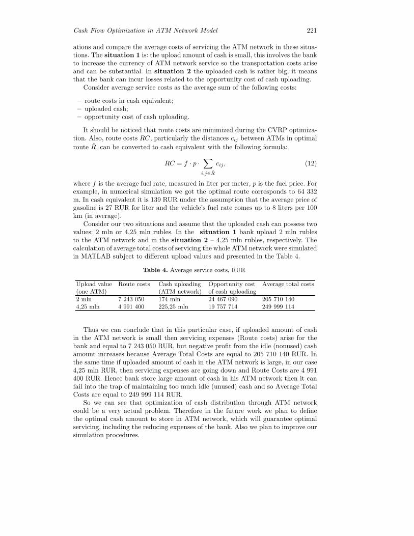
Cash Flow Optimization in ATM Network Model 221
ations and compare the average costs of servicing the ATM network in these situa-tions. The situation 1 is: the upload amount of cash is small, this involves the bankto increase the currency of ATM network service so the transportation costs ariseand can be substantial. In situation 2 the uploaded cash is rather big, it meansthat the bank can incur losses related to the opportunity cost of cash uploading.
Consider average service costs as the average sum of the following costs:
– route costs in cash equivalent;– uploaded cash;– opportunity cost of cash uploading.
It should be noticed that route costs are minimized during the CVRP optimiza-tion. Also, route costs RC, particularly the distances cij between ATMs in optimal
route R, can be converted to cash equivalent with the following formula:
RC = f · p ·∑i,j∈R
cij , (12)
where f is the average fuel rate, measured in liter per meter, p is the fuel price. Forexample, in numerical simulation we got the optimal route corresponds to 64 332m. In cash equivalent it is 139 RUR under the assumption that the average price ofgasoline is 27 RUR for liter and the vehicle’s fuel rate comes up to 8 liters per 100km (in average).
Consider our two situations and assume that the uploaded cash can possess twovalues: 2 mln or 4,25 mln rubles. In the situation 1 bank upload 2 mln rublesto the ATM network and in the situation 2 – 4,25 mln rubles, respectively. Thecalculation of average total costs of servicing the whole ATM network were simulatedin MATLAB subject to different upload values and presented in the Table 4.
Table 4. Average service costs, RUR
Upload value(one ATM)
Route costs Cash uploading(ATM network)
Opportunity costof cash uploading
Average total costs
2 mln 7 243 050 174 mln 24 467 090 205 710 1404,25 mln 4 991 400 225,25 mln 19 757 714 249 999 114
Thus we can conclude that in this particular case, if uploaded amount of cashin the ATM network is small then servicing expenses (Route costs) arise for thebank and equal to 7 243 050 RUR, but negative profit from the idle (nonused) cashamount increases because Average Total Costs are equal to 205 710 140 RUR. Inthe same time if uploaded amount of cash in the ATM network is large, in our case4,25 mln RUR, then servicing expenses are going down and Route Costs are 4 991400 RUR. Hence bank store large amount of cash in his ATM network then it canfail into the trap of maintaining too much idle (unused) cash and so Average TotalCosts are equal to 249 999 114 RUR.
So we can see that optimization of cash distribution through ATM networkcould be a very actual problem. Therefore in the future work we plan to definethe optimal cash amount to store in ATM network, which will guarantee optimalservicing, including the reducing expenses of the bank. Also we plan to improve oursimulation procedures.

222 Elena Gubar, Maria Zubareva, Julia Merzljakova
References
Bure V. M., Evseev E. A. (2004). Basis of econometrics. Saint Petersburg State University.Hall R. W. (2003). Handbook of Transportation Science. Springer.Hurlimann T. (2003). Modelling the CVRP using LPL. Mathematical Programming, pp.
343–359.Lysgaard J., Letchford A., Eglese R. (2003). A New Branch-and-Cut Algorithm for the
Capacitated Vehicle Routing Problem. Aarhus School of Business, Denmark.Ralphs T., Kopman L., Pulleyblank W., Trotter L. (2003). On the Capacitated Vehicle
Routing Problem. Mathematical Programming, pp. 343-359.Simutis R., Dilijonas D., Bastina L., Friman J.,Drobinov P. (2007). Optimization of cash
management for ATM network. Information technology and control, Vol.36, No.1A.Hamdy A. Taha. (2003). Operations Research: an Introduction. University of Arkansas,
Fayetteville: Pearson Education, Inc.Vasin N. S. (2005). The Mathematical-statistical Model for Accounting of Payment Trans-
actions in ATM Networks. Discount and Tax Policy: Planning and DevelopmentProspects: Materials of All-Russian Theoretical and Practical Conference. Orel, pp.215-217.
http://www.diebold.com/ficcdsvdoc/techpubs/Opteva/TP-820820-001/tp-820820-001-1.htm

Stable Families of Coalitions for Network ResourceAllocation Problems
Vladimir Gurvich1,3 and Sergei Schreider2
1 RUTCOR, Rutgers Center for Operations Research, Rutgers University,640 Bartholomew Road, Piscataway, New Jersey, 08854-8003, USA
2 School of Mathematical and Geospatial Sciences, RMIT University, GPO Box 2476,Melbourne Vic 3001, Australia, email: [email protected]
3 International Institute of Earthquake Prediction Theory andMathematical Geophysics, Russian Academy of Sciences, Profsoyuznaya St, 84/32,
Moscow, 117997, Russia
Abstract. A very common question appearing in resource managementis: what is the optimal way of behaviour of the agents and distribution oflimited resources. Is any form of cooperation more preferable strategy thanpure competition? How cooperation can be treated in the game theoreticframework: just as one of a set of Pareto optimal solutions or cooperativegame theory is a more promising approach? This research is based on resultsproving the existence of a non-empty K -core, that is, the set of allocationsacceptable for the family K of all feasible coalitions, for the case when thisfamily is a set of subtrees of a tree.
A wide range of real situations in resource management, which include op-timal water, gas and electricity allocation problems can be modeled usingthis class of games. Thus, the present research is pursuing two goals: 1.optimality and 2. stability.
Firstly, we suggest to players to unify their resources and then we optimizethe total payoff using some standard LP technique. The same unification andoptimization can be done for any coalition of players, not only for the totalone. However, players may object unification of resources. It may happenwhen a feasible coalition can guarantee a better result for every coalition-ist. Here we obtain some stability conditions which ensure that this cannothappen for some family K. Such families were characterized in Boros et al.(1997) as Berge’s normal hypergraphs. Thus, we obtain a solution which isoptimal and stable. From practical point of view, we suggest a distributionof profit that would cause no conflict between players.
’What to suggest?. . . They write and write [. . . ] . It makesmy head reel. Just take everything and share equally. . .’
Michail Bulgakov, The heart of a dog
1. Introduction
1.1. Rationale
Optimal performance of multi-agent economic systems is a pivotal problem of themodern economics. Performance quality of such systems can be described by a setof numerical characteristics reflecting the way these systems operate. These char-acteristics could include profit, cost, gross margin, quantity or number of producedcommodities, and will be referred to henceforth as Objective Functions (OF). The

224 Vladimir Gurvich, Sergei Schreider
primal managerial task is to optimize (maximize or minimize) these OF. Withoutloosing the generality, the maximization formulation will be considered.
There are two possible approaches to selecting the optimal strategy. The firstone (henceforth ‘collective’ approach) is used when an overall system performanceis considered and individual agents’ performances are not the main focus of theresearch. In this case, the most common tool employed for the system optimiza-tion is the non-linear or linear programming, usually integer or mixed. The secondapproach implies optimization considered from each of the agents’ point of view(henceforth referred to as ‘individual’). With this approach, the system optimiza-tion tool is the game theoretic methods. The fist approach (overall optimization) isequivalent to the second approach (game) when all agents form one large coalition.The value of overall maximized OF is not less than the sums of the individual OFsobtained by individual players or coalitions as solutions of a game. It is temptingto suggest that agents form one coalition and then divide the total payoff betweenthem. However, some players (or coalitions of players) might be better off pursuingstrategies different from the strategy formulated for the overall optimization for ‘onelarge coalition’ game. Moreover, players or coalitions of players, which are betteroff playing separately, exist in the general case.
This paper describes quite a wide range of systems for which the non-conflictingdistribution of optimal ‘collective’ OFs between a system’s agents is possible. Thesesystems belong to the class of the so-called network systems and are characterizedby the existence of carriers connecting individual players who are located in nodes.The performance of such systems can be optimized using the network LP methods,containing a set of very specific constraints, related to the capacity of the carriersand the existence of paths between different nodes. A wide range of real economicsystems (water supply networks, electricity and gas supply networks, telecommuni-cations, etc.) can be described as such network systems, which makes the results ofthe reported research highly demanded by managerial practices in these areas. Thefundamental result employed in this paper states that for such systems there existsa non-conflicting redistribution of total income between the players.
1.2. Mathematical formulation
We consider the situation when a group of agents I that has an access to the setof limited resources R has a goal to optimize some objective function. P is the setof products (industries). We ask the following question: what optimal cooperationstrategy, or coalition structure, should be chosen by the agents in order to optimizetheir economic outputs.
The linear case appears when for each player i ∈ I his strategies xi are theshares of his activities in industry (product) p ∈ P . Let
A = ‖arp‖
be a matrix representing the amount of resource r ∈ R needed for producing aunit of product p ∈ P , and
bi = (bi1, bi2, . . . , b
i|R|)
be a vector of resources available for player i.Then we can formulate the production strategy choice for each player as a LP
problem:
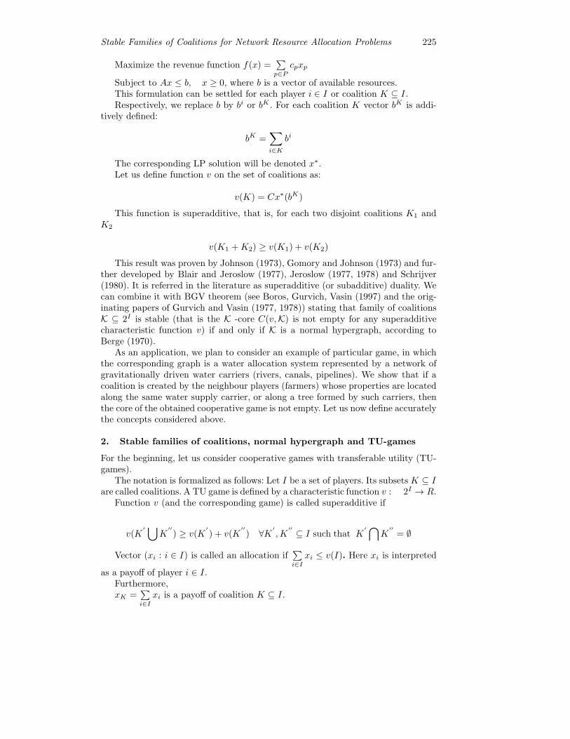
Stable Families of Coalitions for Network Resource Allocation Problems 225
Maximize the revenue function f(x) =∑p∈P
cpxp
Subject to Ax ≤ b, x ≥ 0, where b is a vector of available resources.This formulation can be settled for each player i ∈ I or coalition K ⊆ I.Respectively, we replace b by bi or bK . For each coalition K vector bK is addi-
tively defined:
bK =∑i∈K
bi
The corresponding LP solution will be denoted x∗.Let us define function v on the set of coalitions as:
v(K) = Cx∗(bK)
This function is superadditive, that is, for each two disjoint coalitions K1 andK2
v(K1 + K2) ≥ v(K1) + v(K2)
This result was proven by Johnson (1973), Gomory and Johnson (1973) and fur-ther developed by Blair and Jeroslow (1977), Jeroslow (1977, 1978) and Schrijver(1980). It is referred in the literature as superadditive (or subadditive) duality. Wecan combine it with BGV theorem (see Boros, Gurvich, Vasin (1997) and the orig-inating papers of Gurvich and Vasin (1977, 1978)) stating that family of coalitionsK ⊆ 2I is stable (that is the K -core C(v,K) is not empty for any superadditivecharacteristic function v) if and only if K is a normal hypergraph, according toBerge (1970).
As an application, we plan to consider an example of particular game, in whichthe corresponding graph is a water allocation system represented by a network ofgravitationally driven water carriers (rivers, canals, pipelines). We show that if acoalition is created by the neighbour players (farmers) whose properties are locatedalong the same water supply carrier, or along a tree formed by such carriers, thenthe core of the obtained cooperative game is not empty. Let us now define accuratelythe concepts considered above.
2. Stable families of coalitions, normal hypergraph and TU-games
For the beginning, let us consider cooperative games with transferable utility (TU-games).
The notation is formalized as follows: Let I be a set of players. Its subsets K ⊆ Iare called coalitions. A TU game is defined by a characteristic function v : 2I → R.
Function v (and the corresponding game) is called superadditive if
v(K′ ⋃
K′′) ≥ v(K
′) + v(K
′′) ∀K ′
,K′′ ⊆ I such that K
′⋂K
′′= ∅
Vector (xi : i ∈ I) is called an allocation if∑i∈I
xi ≤ v(I). Here xi is interpreted
as a payoff of player i ∈ I.Furthermore,xK =
∑i∈I
xi is a payoff of coalition K ⊆ I.

226 Vladimir Gurvich, Sergei Schreider
The core C(v) of the obtained superadditive TU game is defined by the systemof linear inequalities
C(v) = {x ∈R|I||xI ≤ v(I) and xK ≥ v(K) ∀K ⊆ I}It can be interpreted as a set of allocations (xi: i ∈ I) acceptable for all coalitions
K ⊆ I.
In other words, the core of a TU-game is empty whenever each allocation isrejected by a coalition. The core is a natural and probably the simplest concept ofsolution in cooperative game theory. Yet it has an important disadvantage: C(v) isfrequently empty, because it must be acceptable for all 2|I| coalitions.
Yet in real life not every coalition has a chance to appear, because some agentsmay not know or not like each other. The following relaxation of the concept iscommon in the literature:
Given a family of coalitions K ⊆ 2I the K–core is defined as a family of alloca-tions acceptable for all coalitions K ∈ K, that is
C(v,K) = {x ∈ R|I|| xI ≤ v(I) and xK ≥ v(K) ∀K ∈ K}Family K ⊆ 2I is called stable if the K–core is not empty for any superadditive
TU-game v : 2I → R.
An important result obtained by Boros et al. (1997), which is referred to as theBGV theorem, claims that family of coalitions K is stable if and only if K is a Bergenormal hypergraph (Berge (1970)). The definitions of terms ‘perfect graph’, ‘normalhypergraph’ and explanation of links between games, coalitions and hypergraphs aregiven in Appendix to Gurvich and Schreider (2010), accessible online.
For the present paper the following example is most important: Let T be a tree,assign a player to every vertex of T . Then an arbitrary family of subtrees of T formsa stable family of coalitions.
This special case of the BGV theorem, considered already in Gurvich and Vasin(1977), is important in applications. As it has been already mentioned above, weconsider the family of LP problems whose resource constraints (right-hand side) bKdepends on a coalition. Hence, the optimal solution v(K) = Cx∗(bK) = Cx∗(K) isa superadditive function of K. Thus the BGV theorem is applicable. Hence, it existsuch a distribution of the total optimal payoff v(I) among the players that will causeno objection from any coalition. Which coalitions are feasible will be discussed inthe Section 4.
3. Network supply systems and games
Water, electricity and gas supply systems fall into the class of the so-called networksystems. The common characteristics of all these allocation systems is that theycan be represented as a set of nodes (for instance, reservoirs, junctions and users)interconnected by a system of carriers with different capacities (wires, channels,pipelines). The last two decades a number of publications appeared when thesetypes of systems were described by linear and non-linear optimization methods. Forwater supply system this approach was employed for instance in Perera et al. (2005).Electricity supply systems and associated electricity market, as well as traffic andtelecommunication systems, were considered in Hu and Ralph (2007) and Ralph(2008). Gas supply system for Europe and placeNorth America were also modelledby similar methods of network LP optimization (Egging et al. (2008) and Gabrielet al. (2005)).
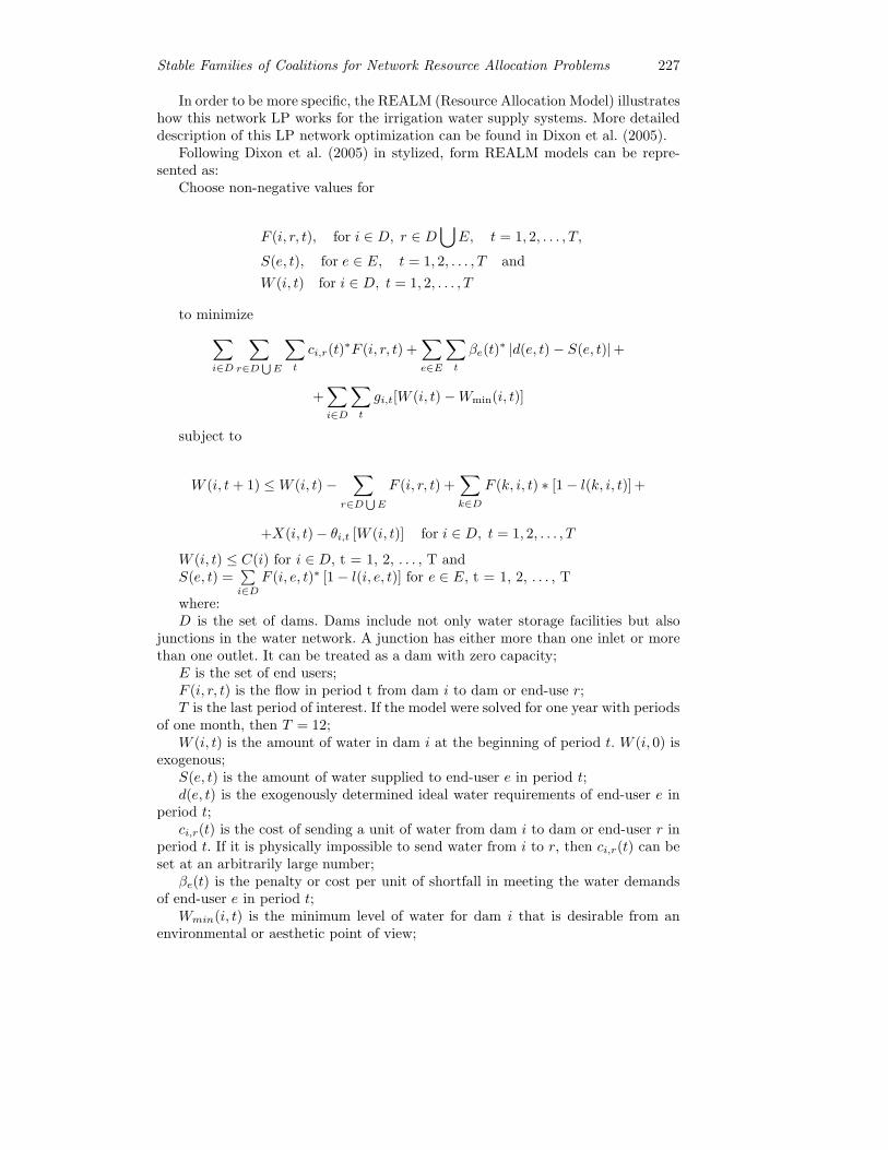
Stable Families of Coalitions for Network Resource Allocation Problems 227
In order to be more specific, the REALM (Resource Allocation Model) illustrateshow this network LP works for the irrigation water supply systems. More detaileddescription of this LP network optimization can be found in Dixon et al. (2005).
Following Dixon et al. (2005) in stylized, form REALM models can be repre-sented as:
Choose non-negative values for
F (i, r, t), for i ∈ D, r ∈ D⋃
E, t = 1, 2, . . . , T,
S(e, t), for e ∈ E, t = 1, 2, . . . , T and
W (i, t) for i ∈ D, t = 1, 2, . . . , T
to minimize∑i∈D
∑r∈D
⋃E
∑t
ci,r(t)∗F (i, r, t) +
∑e∈E
∑t
βe(t)∗ |d(e, t)− S(e, t)|+
+∑i∈D
∑t
gi,t[W (i, t)−Wmin(i, t)]
subject to
W (i, t + 1) ≤W (i, t)−∑
r∈D⋃E
F (i, r, t) +∑k∈D
F (k, i, t) ∗ [1− l(k, i, t)] +
+X(i, t)− θi,t [W (i, t)] for i ∈ D, t = 1, 2, . . . , T
W (i, t) ≤ C(i) for i ∈ D, t = 1, 2, . . . , T andS(e, t) =
∑i∈D
F (i, e, t)∗ [1− l(i, e, t)] for e ∈ E, t = 1, 2, . . . , T
where:D is the set of dams. Dams include not only water storage facilities but also
junctions in the water network. A junction has either more than one inlet or morethan one outlet. It can be treated as a dam with zero capacity;
E is the set of end users;F (i, r, t) is the flow in period t from dam i to dam or end-use r;T is the last period of interest. If the model were solved for one year with periods
of one month, then T = 12;W (i, t) is the amount of water in dam i at the beginning of period t. W (i, 0) is
exogenous;S(e, t) is the amount of water supplied to end-user e in period t;d(e, t) is the exogenously determined ideal water requirements of end-user e in
period t;ci,r(t) is the cost of sending a unit of water from dam i to dam or end-user r in
period t. If it is physically impossible to send water from i to r, then ci,r(t) can beset at an arbitrarily large number;
βe(t) is the penalty or cost per unit of shortfall in meeting the water demandsof end-user e in period t;
Wmin(i, t) is the minimum level of water for dam i that is desirable from anenvironmental or aesthetic point of view;

228 Vladimir Gurvich, Sergei Schreider
gi,t is a penalty function. It takes positive values if W (i, t) – Wmin(i, t) is nega-tive;
l(k, i, t) is losses per unit of flow from dam k to dam or end-user i in period t(exchange losses);
X(i, t), specified exogenously, is the natural inflow to dam i in period t;θi,t is a function giving evaporation from dam i in period t;C(i) is the capacity of dam i. If dam i is a junction then C(i) = 0.Models such as REALM can be used to plan flows in a hydrological area and to
decide how these flows should be varied in response to changes in rainfall [reflectedin X(i, t)], changes in demands [d(e, t)], and changes in a myriad of technical andcost coefficients.
Similar optimization formulations can be used for electricity and gas supplysystems.
4. Superadditive characteristic functions related to linear programming
Here we refer to an important result obtained by Jonson (1973), Gomory and Jonson(1973), Blair and Jeroslow (1977), Jeroslow (1977, 1978) and Schrijver (1980).
Let a LP formulation be given in the following form:Maximize the revenue function f(x) =
∑p∈P
cpxp = Cx
Subject to Ax ≤ b, x ≥ 0where b is a vector of resources and c is a vector of prices.The optimal solution is a vector x∗ = (x∗
i , i ∈ I)For each coalition K, the function bK is defined additively:
bK =∑i∈K
bi
Then function v is defined on the set of coalitions as v(K) = Cx∗(bK), whichis the optimal value of objective function subject to resources bK available for thecoalition K.
Then, it appears that v(K) is a superadditive function, that is,
v(K1 + K2) ≥ v(K1) + v(K2) for any pair of disjoint coalitions, K1
⋂K2 = ∅
5. Stability of optimal solutions
Let us consider a network LP optimization problem for an acyclic graph. Referringto the results mentioned in Section 2 , we can state that a family of coalitions isstable if and only if it is a normal hypergraph. In particular any family subtrees of atree form a stable family of coalitions. Thus, there exists an allocation correspondingto the optimal LP solution, which is stable. It means that there is a distribution ofthe total income among players which is acceptable for all feasible coalitions.
6. Concluding remarks
In nutshell, this paper suggests a new approach to optimization and fair distri-bution of total payoff among players. This method is based on integration of twofundamental results, which are
Stable Families of Coalitions for Network Resource Allocation Problems 229
1. Superadditive duality for LP optimization, and2. The BGV theorem claiming that a family of coalitions K is stable (that is theK–core C(v,K) is not empty for any superadditive characteristic function v) ifand only if K is a normal hypergraph.
Then BGV theorem can be applied for acyclic network systems. The followingtwo assumptions are crucial: 1. acyclicity of corresponding graph and 2. superad-ditivity of the optimal value. It allows us to conclude that some ‘natural’ familiesof coalitions are stable, that is, admit a non-empty core. Therefore, it is possible toconclude that a fair distribution of payoff among the payers is possible. Thus, theexistence of an optimal and stable solution for such class of games is proven.
A few words should be written about possible further continuation of this re-search. Firstly, we plan to illustrate these results by considering the real networksupply system (say, the water allocation system modelled by REALM model) anddemonstrate that for the full set of possible coalitions the game is unstable, that is,the core is empty. Then we will select a set of ‘natural’ coalitions, say, coalitions offarmers whose properties are located on the same water carrier, and demonstratethat such families are stable. The next step of this research is consideration of moresophisticated network supply systems and demonstration what are the optimal andstable solution in this case. The key point is formulation of appropriate managerialadvises about redistribution of optimal income between real players constitutingthese systems. We also plan to consider not only TU but also more general classesof cooperative games such as games with non-transferable utilities, so-called NTU-games, also games in normal form, in effectivity function form, etc.
It should be also mentioned that the ”superadditive duality” holds not only forLP but for integer programming as well. Hence, the same analyses of stability isapplicable for these, more general, models.
Finally, we plan to consider the non-linear case related to the objective functionin form of Cobb-Douglass’ production function:
CB(u1, u2, . . . , u|R|) =∏
i=1,..,n
uγii where ui are production factors and
γ1 + γ2 + ... + γ|P | = 1Schreider, Zeephongsekul and Abbasi (2010) proved that this function is also
superadditive. This result gives us a potential to employ similar approach for thegame on non-cyclic graphs with Cobb-Douglass objective function.
References
Berge, C. (1970). Graphs and Hypergraphs. Dumond, Paris, English translation, North-Holland, Amsterdam, 1973.
Berge, C. (1984). Minimax theorems for normal hypergraphs and balanced hypergraphs - asurvey. Annals of Discrete Mathematics, 21, 3–19.
Blair, C. E. and Jeroslow, R. G. (1977). The value function of a mixed integer program 1,Mathematical programming, 19, 121–138.
Boros, E., Gurvich, V. and Vasin, A. (1997). Stable families of coalitions and normalhypergraphs. Mathematical Social Sciences, 34, 107–123.
Boros, E. and Gurvich, V. (2000). Stable effectivity functions and perfect graphs. Mathe-matical Social Sciences, 39, 175–194.
Dixon, P., Schreider, S. and Wittwer, G. (2005). Combining engineering-based water modelswith a CGE model, Chapter 2 in Quantitative Tools in Microeconomic Policy Analysis,

230 Vladimir Gurvich, Sergei Schreider
Pincus, J. (editor), Publisher: Australian Productivity Commission, Canberra, 2005,pp. 17 – 30.
Egging R., Gabriel, S. A., Holz, F. and Zhuang, J. (2008). A complimentary model for theEuropean natural gas market. Energy policy, 36, 2385–2414.
Gabriel, S. A., Zhuang, J. and Kiet, S. (2005). A large-scale complimentary model of theNorth American natural gas market. Energy economics, 27, 639–665.
Gomory, R. E., Johnson, E. L. (1973). The group problem and subadditive functions. In:Hu, T. C., Robinson, S. M. (eds), Mathematical Programming, Academic Press, NewYork, 157–184.
Gurvich and Vasin (1977). Reconciable sets of coalitions. In: Questions of applied math.Siberian Energetic Institute, CityplaceIrkutsk, 20–30 (in Russian).
Gurvich, V. and Vasin, A. (1978). Reconcilable sets of coalitions for normal form games. In:”Numerical methods in optimization theory(Applied math.)”, Siberian Inst. of Energy,Irkutsk, 27–38 (in Russian).
Gurvich, V. and Schreider, S. (2010). Network supply systems, stable families of coalitionsfor superadditive TU-games and Berge’s normal hypergraphs. RUTCOR preprint, RRR20-2010, November, 2010, Rutgers University, 22 p.
Hu, X. and Ralph, D. (2007). Using EPECs to model bilevel games inrestructured electricitymarkets with locational prices. Operations research, 55(5), 809–827.
Jeroslow, R. G. (1977). Cutting plane theory: Disjunctive methods. Annals of discrete math-ematics, 1, 293–330.
Jeroslow, R. G. (1978). Cutting plane theory: Algebraic methods. Discrete mathematics,23, 121–150.
Jonson, E. L. (1973). Cyclic groups, cutting planes and shortest paths, in MathematicalProgramming, Hu, T.C. and Robinson, S. (eds.) Academic Press, 185–211.
Perera, B. J. C., James, B. and Kularathna, M. D. U. (2005). Computer Software Tool forSustainable Water Allocation and Management - REALM. Journal of EnvironmentalManagement, 77(4), 291–300.
Ralph, D. (2008). Mathematical programs with complementarity constraints in traffic andtelecommunications networks. Royal Society of London, Philosophical Transactions.Mathematical, Physical and Engineering Sciences, 366(1872), 1973–1987.
Schreider, S., Zeephongsekul, P. and Abbasi, B. (2011). Game theoretic approach for fer-tiliser application: propensity to cooperate, how important is it? MODSIM2011 (sub-mitted).
Schrijver, A. (1980). On cutting planes. Annals of Discrete mathematics, 9, 291–296.
Signaling Managerial Objectives to Elicit Volunteer Effort�
Gert Huybrechts1, Jurgen Willems1, Marc Jegers1, Jemima Bidee2,Tim Vantilborgh2 and Roland Pepermans2
1 Vrije Universiteit Brussel,Micro-economics for Profit and Non Profit Sector,
Pleilaan 2, 1050 Brussels, BelgiumE-mail: [email protected]
2 Vrije Universiteit Brussel,Work and Organizational Psychology,Pleilaan 2, 1050 Brussels, Belgium
Abstract. We examine a nonprofit organization (npo) with a manager anda motivated volunteer, assume that the manager has private informationabout the volunteer’s utility function, that the volunteer has no private in-formation on the manager’s utility function, and propose a signaling solutionfor the volunteer’s effort decision. We focus on the general properties of asignal in a npo, specifically taking into account the effects of the volunteer’smotivations on the signal. We find that, due to the diversity of volunteermotivations, the set of signals can be large. We relate this to signals thatcan be used by nonprofit managers in practice and we reinterpret existingpractices as signals.
Keywords: signaling; volunteers; nonprofit organizations; motivation, in-centives
1. Introduction
Volunteers are an important resource for many nonprofit organizations (npos).Therefore, appropriate management of volunteers can help these npos to achievetheir mission. A volunteer (he) is by definition unpaid for his work, but can receivenon-monetary rewards from the output that is produced by his effort (Besley andGhatak, 2003), thus reaching a number of his goals, e.g. values (helping others),understanding (acquiring new skills), career (increasing future job opportunities),enhancement (increasing self-esteem), social (establishing social relationships) andprotective (addressing personal problems) functions (Clary et al., 1996). The volun-teer’s goals are the functions that he wants to satisfy and he can do this by produc-ing output. The volunteer’s valuation of output depends on the manager (she). Forexample, managers can be of different types (competent, incompetent, honest, dis-honest, etc.) which affects output. Managers have private information about theirown type, so there exists a problem of asymmetric information. This problem isaggravated because the volunteer’s reward is non-monetary. Promises about somekinds of non-monetary rewards cannot be legally binding: in these cases the volun-teer cannot sue the npo to pay compensation when the npo reneges on its promises(Suazo et al., 2009).
� The authors would like to thank Bruno Heyndels, Stijn Van Puyvelde and Lore Wellensfor their helpful comments as well as the participants of the Fourth International Confer-ence on Game Theory and Management (St. Petersburg, 2010) where an earlier versionof this paper was presented.

232 Gert Huybrechts, Jurgen Willems, Marc Jegers
In the presence of asymmetric information, the manager can steer the volunteer’sbehavior with incentives. Incentives (such as controlling, monitoring, monetary re-wards, threats, deadlines, etc.) may be used to influence the volunteer’s effort. Ex-amining a wide range of compensation and incentive schemes such as promotions,deferred compensation, and efficiency wages, Prendergast (1999) finds that agents(in a profit context) do respond positively to these schemes in certain cases.
In other cases, when performance measurement is noisy or biased, incentives maybe less useful, and can even be contra-productive, resulting in sabotage (Gibbons,1998). A possible explanation for the negative effects of incentives especially usefulin a nonprofit setting is given by Frey (1997) and Frey and Jegen (2001) who statethat certain incentives can crowd out intrinsic motivation. A literature overview onthe interaction effects between monetary and non-monetary motives is given by Fehrand Falk (2002). There is a need to solve the problem of asymmetric information innpos, but due to the specific role of motivations in the nonprofit sector, incentivesmay not be very useful. Instead we discuss an alternative solution: signaling. A signalis an action that the manager can undertake to give the volunteer information abouthis expected utility. The difference between signaling and incentives is that in thecase of signaling the volunteer feels that his actions are a personal choice while inthe case of control he feels like he is obeying a regulation. Indeed, the volunteer’sintrinsic motivation can be influenced by feelings of autonomy or control. If hefeels he is being controlled, then his intrinsic motivation will decrease (Ryan andDeci, 2000) and he might leave the organization, which is easier for a volunteerthan for a (paid) employee. The literature shows that non-monetary motivation(such as intrinsic motivation) is important for volunteers. When this is the case it isoften better to use non-controlling motivation tools to steer the volunteer’s behavior.Therefore, we feel that it is important to recognize the important role that signalingmay play in volunteer behavior and motivation. Signaling in the unique context ofa npo is the focus of this paper.
We follow Benabou and Tirole (2003) who state that any action can have threeeffects on the manager’s utility: 1) the direct effect of the action on the manager’sutility, for example the cost of the action, 2) the direct effect of the action on theutility of the employee or volunteer, he can like or dislike the action, 3) the indirectsignaling effect, the employee or volunteer learns new information which influencesthe expected utility of his effort.
Several authors have considered different actions that can serve as a signal. Wediscuss briefly the signaling effects of rewards, contracts and trust. A reward canbe a signal of task attractiveness when it gives information about the manager’sestimation of the agent’s intrinsic motivation (Benabou and Tirole, 2003). For ex-ample, a high reward may lead the agent to believe that the task is very risky orunpleasant. Other possible signals are the properties of the contract between agentand principal. Contracts that are based on measured output can be a signal ofthe manager’s ability to distort output (Allen and Gale, 1993). Similarly to Inderst(2001), Spier (1993) states that a contract that insures the principal against possiblenegative outcomes may be a signal that negative outcomes are likely. Kreps (1997)considers the length of an employment contract as a signal, for example when themanager chooses a contract that makes it very costly for her to fire the employee,the employee may interpret this as a signal of job security. Besides rewards or con-tracts, trust can also be a signal. When the principal decides to trust the agent, she

Signaling Managerial Objectives to Elicit Volunteer Effort 233
shows that she believes that most agents are trustworthy. If some agents are con-formists and act like the majority of agents, then these agents may react positivelyto the manager’s decision to trust (Slikwa, 2007). If the agent considers trust as thepreferred action of the type of manager that gives him the highest utility of effort,a principal who trusts can give a signal about her type (Ellingsen and Johannesson,2008).
A common element in these studies is that the principal has private informationabout the state of the world that determines the agent’s utility. The principal’sactions have different costs in different states. We show that an action can be usedas a signal if the action has the lowest cost for the principal in the state that isoptimal from the viewpoint of the agent, given that action. We discussed authorsthat use this property in a model with a specific signal, and show that this propertyalso holds for a general signal. Our model shows that the cost of the signal in theoptimal state must not be strictly lower than in any other state. Even if the costof the action is only weakly lower in the optimal state, then this action may stillbe a signal. We therefore take a broader view than the studies above in the sensethat we do not focus on any particular signal. Instead we focus on the set of actionsthat possess the characteristics necessary to be a signal and we apply this to thespecific environment of a npo with volunteers. The requirements of a signal are: 1)the manager must know which state the volunteer considers to be optimal; 2) theaction must be observed by the volunteer; and 3) the signal must be reliable, thesignal must have weakly lower costs for the manager in the optimal state.
A mission driven organization, like a npo, does not only rely on the competenceof the manager but also on her goals, so the manager has to signal her goals ormission. Volunteers, who commit specific resources to the npo, need to have infor-mation about the manager’s goals. The signals that are sent by the manager to givethis information have a specific nature, as they are signals about intangible andsubjective properties of the manager.
The set of actions that can be a possible signal is large. Many management prac-tices may have signaling effects, though some of these effects may not be known tothe manager. Therefore, we stress the importance for managers to asses their prac-tices so that they can eliminate unwanted signals. Viewing management practicesas a signal allows us to reinterpret their effect on the organization. To illustrate thiswe discuss some potential signals. We first discuss an example of current manage-ment practices (formal control) and offer an alternative explanation for its existence,compared to what is commonly found in the literature. Then we make two sugges-tions of signals that managers of a npo could use in practice (non-mission relatedactivities and volunteering in similar organizations).
According to Frey (1997) using a formal control system in an organization toreduce agency problems between managers and employees may be problematic initself because formal control may undermine the employees’ intrinsic motivationto perform well. Intrinsic motivation may be lower because formal control systemscan have a negative effect on the employee’s feelings of competence or autonomy(Ryan and Deci, 2000). Our paper may offer an alternative explanation. If withoutformal control volunteers exhibit some form of non-productive behavior, it maybe profitable for the npo to increase formal control so that this non-productivebehavior is removed. The absence of formal control can be viewed as a signal.Compassionate and understanding managers may have fewer problems with non-

234 Gert Huybrechts, Jurgen Willems, Marc Jegers
productive behavior than others. These managers may be preferred by a value-driven volunteer who works for a npo for altruistic or humanitarian reasons. Thesemanagers may use this insight to send a signal to the volunteer. Other managers,having a cost disadvantage, may not be able or willing to bear the extra (utility)cost of non-productive behavior. By not increasing formal control, and so bearingthe extra cost of non-productive behavior, the manager may convince a value-drivenvolunteer that she is compassionate and understanding. This, in turn, may increasevolunteer effort if he believes that a compassionate and understanding manager isalso value-driven.
Caers et al. (2009) suggest that the goals of managers and volunteers in a npocan be divided in three categories: individual goals (income, reputation and effort),organizational goals (only help those clients whose profile matches the organization’smission statement) and client goals (help the client no matter what his profile is).If the volunteer is client-driven (he wants to do good for other people), then hemay prefer to work for a manager who finds client goals important. The amountof resources that the organization uses for client goals may be a signal of how wellthe volunteer will be able to help others. There may be an offsetting increase involunteer effort when the manager diverts resources from organizational goals toclient goals.
Managers who share the same goals as the volunteer might also like to do similarvolunteer work in other organizations. A manager who is less caring or altruisticreceives fewer (utility) benefits from volunteering, so she will be less willing tovolunteer. When the volunteer observes that the manager volunteers in other (com-parable) organizations, he may interpret this as a signal that the manager is caringor altruistic. This may induce the volunteer to increase his effort. If the volunteerwants to increase his skills then he may prefer to work for a manager who is alsointerested in acquiring skills through volunteering. Such a manager may indeed pos-sess the skills that the volunteer wants to acquire. If the volunteer wants to increaseor strengthen his social relationships, the manager can show by participating inother organizations that she can be a good link towards other social groups.
This result is not only important for volunteers but is also important for otherstakeholders of the organization who want to interpret the organization’s behavior.Board members need to take into account the signaling behavior of managers whenthey evaluate the manager. Which signals does the manager send? Are these signalsoptimal for the organization? Are there other signals the manager could send? Whatdo these signals tell about the true preferences of the manager? Donors can interpretsignals to know whether their donations will be put to good use. Governments andother funding authorities can use signals to verify whether the organization willkeep its promises or obligations.
In the next section we formally present our model and Section 3 is the conclu-sion. It is not our ambition to develop a complete model of a npo. Therefore, wedeliberately keep our model simple by only considering signaling effects, not morethan two types of managers, one-dimensional motivations, and we ignore dynamics.Whereas a case can be made that a more realistic model can lead to interestingconclusions, we believe that it is better to focus on the basic principles of signalingwithin a npo.

Signaling Managerial Objectives to Elicit Volunteer Effort 235
2. The model
2.1. Introduction
In this section, we develop a model of a nonprofit manager who tries to convincethe volunteer to perform high effort. The volunteer has no knowledge about themanager’s type, there is asymmetric information. We propose that managers cansend signals that give information to the volunteer about their type.
We assume there are two types of managers, the ’identical’ type who shares thesame goals as the volunteer and the ’non-identical’ type who does not share the samegoals. Whether the volunteer is able to satisfy his goals when he is working for thenpo depends on the type of manager. We assume that the manager’s type is the onlydeterminant of the state of the world that is relevant for the volunteer. The volunteeronly prefers high effort when he is working for an identical manager. The managercan try to signal that this is her type. The order of the game between the managerand the volunteer is as follows: nature chooses the type of the manager which isnot revealed to the volunteer. The manager can send a signal to the volunteer toconvince him that her type is the identical type. Given the signal, the volunteerchooses his optimal amount of effort.
If a managerial action has the lowest cost in the state of the world that isoptimal for the volunteer then it can lead to a separating equilibrium. Whether ornot it does depends on the manager’s incentive compatibility constraints. If theseconstraints are satisfied then the identical manager can distinguish herself from thenon-identical manager. This increases the volunteer’s effort she receives. A managerin the optimal state can send a signal so that the volunteer knows with certaintythat the manager is in this state.
In the signaling models we discussed in the introduction, the actions alwayshad the lowest cost in the state optimal for the agent. In reality, this criterionincludes a large amount of possible actions. When judging management practices,one therefore must be careful to examine whether these management practices donot have some kind of signaling function.
First, we describe the manager’s utility function and the differences betweendifferent types of managers. Second, we propose the volunteer’s utility function,and how he obtains information about the manager’s type. Finally, we summarizeour model in three propositions and discuss the results.
2.2. The manager
The manager of a npo wants to convince a volunteer to exert high effort, andtherefore produces a signal. If the volunteer exerts effort (e) then he produces outputy(e). There are two types of managers, the identical manager (i) and the non-identical manager (ni). The set of types t is therefore {i, ni}. Volunteers observe asignal if S > 0. When S = 0 there is no signal. The cost of sending a signal is Ci(S)for the identical manager and Cni(S) for the non-identical manager. We make thefollowing assumptions about the cost functions of signaling:
Assumption 1: Ci(S), Cni(S) are non-negative, continuous and non-decreasingfunctions in S, S ∈ [0,+∞] .
Assumption 2: Ci(S) < Cni(S), ∀S > 0.Assumption 3: Ci(S) ≥ 0 and Cni(S) > 0, ∀S > 0, Ci(0) = Cni(0) = 0.Assumption 4: S0 is the set of signals: Ci(S) = 0. S∗ is the maximum of this
set.
236 Gert Huybrechts, Jurgen Willems, Marc Jegers
Assumption 2 states that the identical manager has a cost advantage. For eachstrictly positive signal, the identical manager has lower signaling costs. Assumption3 says that the signaling costs must be larger than or equal to 0. Assumption 4says that Ci(S) ’leaves’ the horizontal axis at some positive S called S∗, this is thestrongest signal that identical manager can send without cost. S∗ is either zero orgreater than zero. Both cases are compatible with the other assumptions.
The utility function of the manager, given in Equation (1), combines two addi-tively separable elements: the output produced by the effort of the volunteer andthe signaling costs.
UM,t = y(e)− Ct(S) (1)
The manager wants to send a signal because this message may influence thevolunteer’s choice of effort. We will elaborate on this in the next section when wediscuss the volunteer’s utility function. The manager chooses the level of S so thather expected utility is maximized. The term y(e) can be interpreted as the manager’svaluation of the volunteer’s effort.
2.3. The volunteer
The volunteer wants to produce output to satisfy his goals (e.g. values, understand-ing, career, enhancement, social and protective goals (Clary et al., 1996)). Whetheror not he will get the chance to produce such output depends on the type of themanager. If the manager is identical, then the volunteer’s goals will be achievedif he chooses high effort. The volunteer’s utility function (UV ) is increasing in thevolunteer’s valuation of the amount of output produced ((vt(e)) and decreasing inthe amount of effort exerted. We call the cost of effort c(e). We make the follow-ing assumptions (and use ’ to indicate first derivates) about the volunteer’s utilityfunction:
Assumption 5: UV has a unique maximum for each t ∈ {i, ni},Assumption 6: ∀ei : vi(e) > vni(e),Assumption 7: ∀ei : v′i(e) > v′ni(e),Assumption 8: vi(e) and vni(e) are concave and increasing functions in e.Assumption 9: c(e) is increasing in e and is non-concave.The volunteer’s valuation depends on the type of the manager:
UV = vt(e)− c(e) (2)
The volunteer chooses the amount of e that maximizes the expected value ofequation (2). It is easily shown that under our assumptions the optimal effortwhen volunteering for an identical manager is higher than when working for anon-identical manager, an implication compatible with intuition: if el is the vol-unteer’s optimal choice of effort when he works for the non-identical manager thenv′ni(el) = c′(el). According to assumption 7: v′i(el) > c′(el), from which, with As-sumption 5, UV is maximized for a value eh > el. This is also implied by thedefinition of the identical manager, which is the manager for which the volunteerwants to exert high effort.
However, the volunteer is uncertain about the manager’s type. The manager’stype is assumed to be her private information. Both types of managers have anincentive to try to convince the volunteer that they are of the identical type. There-fore, the volunteer’s maximization problem is given in (3):
Signaling Managerial Objectives to Elicit Volunteer Effort 237
maxe
E[UV ] = E[vt(e)|S]− c(e) (3)
If the manager’s type is expected to be i then the volunteer chooses high efforteh. If the manager’s type is expected to be non-identical, then the volunteer chooseslow effort el. For any probability p ∈ [0, 1] that the manager is (perceived to be)identical the volunteer chooses his effort level e ∈ [el, eh]. We call e∗ the effort ofthe volunteer in a pooling equilibrium:
c′(e∗) = pv′i(e∗) + (1− p)v′ni(e
∗) (4)
2.4. Results
We summarize the results of our model in two propositions.
Proposition 1. There is a separating equilibrium at S = S where y(e∗)− y(el) =Cni(S) when y(eh)− y(e∗) > Ci(S) holds.
See Appendix A for the proof.Proposition 1 states that in a separating equilibrium the identical manager sends
a signal that is just costly enough to deter the non-identical manager from sendingthat signal.
Proposition 2. There is a pooling equilibrium at S∗ when y(eh) − y(e∗) < Ci(S)and y(e∗)− y(el) > Cni(S
∗) hold.
The signal in a pooling equilibrium does not have an influence on p and isequal to S0 (see Appendix B for the proof). Proposition 2 states that in a poolingequilibrium the identical manager sends a signal that minimizes her signaling cost.It is just high enough so that the non-identical manager cannot be identified withcertainty as being non-identical.
These results show that if certain incentive compatibility constraints are satis-fied, the identical manager can send a signal that convinces the volunteer that sheis indeed identical. In this case, even if there is asymmetric information and man-agers have an incentive to lie, the volunteer still has reason to believe the manager’ssignal. Signaling allows the volunteer to have greater confidence in an otherwiseuncertain, hard to measure and subjective outcome.
The signal does not have to be a single action, it can also be a bundle of severalactions. We found a separating equilibrium because there are differences in costsbetween identical and non-identical managers. However, we do not require that thesignal is a unique action. The signal can also be a bundle of actions and not everyaction in this bundle needs to have strictly lower costs for the identical manager.Some actions may have weakly lower costs. This enlarges the set of possible signalsthat the manager can choose from and allows her to be creative to find a uniquecombination of actions that can serve as the best signal for her.
3. Conclusion
We started from the assumption that different types of managers have different costfunctions for certain actions (’signals’). If these actions satisfy assumptions 1, 2 and3 then for some incentive compatibility constraints, these actions are signals thatlead to a separating equilibrium. The cost is high enough to deter the non-identical
238 Gert Huybrechts, Jurgen Willems, Marc Jegers
manager from sending it, but not high enough to deter the identical manager. In ourmodel there can be separating equilibrium and a pooling equilibrium. This allows usto shed some light on practices by managers. Are current management practices asignal? In the introduction we have discussed several examples of how managementpractices can be reinterpreted as a signal. Managers can try to convince volunteersto exert high effort in many ways. If incentives are not an option, then maybe signalsare. The manager can signal her values, skills or social capital by doing volunteerwork in another organization, she can signal that she is kind and understandingby allowing some slack behavior by her subordinates by not using formal controlmethods, she can signal that volunteering for the organization may lead to a goodcareer within the organization by spending money on emoluments or she can signalher values by diverting money to client goals.
These examples show that managerial signaling can be diverse in the nonprofitsector. There are many signals conceivable because volunteers have different mo-tives. The volunteer’s interpretation of the signal depends on his underlying moti-vation to volunteer. Therefore, we stress the importance for the manager to knowthe voluntee’s motivation. Once the manager knows the volunteer’s motivation, shemust find the appropriate signal. Thus our model predicts that there is a relation-ship between the signal sent by the manager and the (perceived) motivation of thevolunteer. This prediction can be verified empirically; therefore a possible directionfor future research is to empirically investigate whether volunteers try to overcomeuncertainty by looking for signals and whether managers provide these signals. Theanswer to this question is not only useful for volunteer but for all stakeholders ofthe organization.
Our model started from the assumption that the volunteer was already workingfor the npo. We did not model the volunteer’s decision to join the npo. This questionis also important but needs to be addressed in a different way, the results of whichcan be used to verify the conclusions of the present model. Of course, the model thatwe considered made a number of simplifying assumptions (only signaling effects areimportant, only two types of managers, only one dimension of the volunteer’s andmanager’s motivation). Relaxing these assumptions may lead to furhter interestinginsights.
Appendix
1. Appendix A
If a separating equilibrium is to occur at , then the identical manager must alwayssend a signal and the non-identical never sends . We compare eh with e∗ for theidentical manager and e∗ with el for the non-identical manager. The non-identicalmanager never receives eh, because if that were the case the volunteer would believethat p = 1, which is false. For the same reason, the identical manager never receivesel.
The identical manager always sends when (ICC1):y(eh)− y(e∗) < Ci(S).
The non-identical manager never sends when (ICC2):y(e∗)− y(el) < Cni(S).
The identical manager chooses such that is the smallest value that satisfiesy(e∗)−y(el) < Cni(S). This satisfies ICC2 and minimizes the signaling costs for theidentical manager. If this value for S also satisfies ICC1, then there is a separatingequilibrium.
Signaling Managerial Objectives to Elicit Volunteer Effort 239
2. Appendix B
If, in a pooling equilibrium, S > S∗ both types can increase their utility by choosinga smaller S. If S ≤ S∗, the identical manager is indifferent between all S ≤ S∗, thenon-identical manager can increase her utility by choosing the signal S : Cni(S) = 0meaning S = 0. In this case e cannot be independent of S. No non-identical managerwould ever choose S∗, this would increase the effort at S∗ to the same level asthe separating equilibrium. All identical managers would choose S∗ and the non-identical manager would have to mimic this behavior. This means that the poolingequilibrium exists and is unique when the following ICCs are satisfied:
The identical manager sends S∗ when (ICC3): y(eh)− y(e∗) < Ci(S).The non-identical manager sends S∗ when (ICC4): y(e∗)− y(el) ≥ Cni(S
∗).
References
Allen, F. and D. Gale (1992). Measurement Distortion and Missing contingencies in Op-timal Contracts. Economic theory, 1(1), 1–26.
Benabou, R. and J. Tirole (2003). Intrinsic and Extrinsic Motivation. The Review ofEconomic Studies, 70(3), 616–636.
Besley, T. and M. Ghatak (2005). Competition and Incentives with Motivated Agents.American Economic Review, 95(3), 616–636.
Caers, R., C. Du Bois, S. De Gieter, R. De Cooman and R. Pepermans (2009). A Micro-economic Perspective on Manager Selection in Nonprofit Organizations. EuropeanJournal of Operational Research, 192(1), 173–197.
Clary, E., M. Snyder and M. Stukas (1995). Volunteers’ Motivations: Findings from aNational Survey. Nonprofit and Voluntary Sector Quarterly, 25(4), 486–505.
Ellingsen, T. and M. Johannesson (2008). Pride and Prejudice: The Human Side of Incen-tive Theory. American Economic Review, 98(3), 990–1008.
Falk, A. and M. Kosfeld (2006). The Hidden Costs of Control. American Economic Review,96(5), 1611–1630.
Fehr, E. and A. Falk (2006). Psychological Foundations of Incentives. European EconomicReview, 46(4-5), 687–724.
Frey, B. (1997). Not Just for the Money: An Economic Theory of Personal Motivation.Edward Elgar Publishing: Cheltenham.
Frey, B. and R. Jegen (2001). Motivation Crowding Theory. Journal of Economic Surveys,15(5), 687–724.
Gibbons, R. (1998). Incentives in Organizations. Journal of Economic Surveys, 15(5),687–724.
Inderst, R. (2001). Incentive Schemes as a Signaling Device. Journal of Economic Behaviorand Organization, 44(4), 445–465.
Kreps, D. (1998). Intrinsic Motivation and Extrinsic Incentives. American Economic Re-view, 87(2), 359–364.
Murdock, K. (2002). Intrinsic Motivation and Optimal Incentive Contracts. RAND Journalof Economics, 33(4), 650–671.
Prendergast, C. (1999). The Provision of Incentives in Firms. Journal of Economic Liter-ature, 37(1), 7–63.
Ryan, R. and E. Deci (2000). Self-Determination Theory and the Facilitation of IntrinsicMotivation, Social Development, and Well-Being. American Psychologist, 55(1), 68–78.
Slikwa, D. (2007). Trust as a Signal of a Social Norm and the Hidden Costs of IncentiveSchemes. American Economic Review, 97(3), 999–1012.
Speckbacher, G. (2003). The Economics of Performance Management in Nonprofit Orga-nizations. Nonprofit Management and Leadership, 13(3), 267–281.

240 Gert Huybrechts, Jurgen Willems, Marc Jegers
Spier, K. (1992). Incomplete Contracts and Signalling. The RAND Journal of Economics,23(3), 432–443.
Suazo, M., P. Martinez and R. Sandoval (2009). Creating Psychological and Legal Con-tracts through Human Resource Practices: A Signaling Theory Perspective. ResourceManagement Review , 19(2), 154–166.
Two Solution Concepts for TU Gameswith Cycle-Free Directed Cooperation Structures�
Anna Khmelnitskaya1 and Dolf Talman2
1 SPb Institute for Economics and Mathematics Russian Academy of Sciences,1 Tchaikovsky St., 191187, St.Petersburg, Russia,
E-mail: [email protected] CentER, Department of Econometrics & Operations Research, Tilburg University,
P.O. Box 90153, 5000 LE Tilburg, The Netherlands,E-mail: [email protected].
Abstract. For arbitrary cycle-free directed graph games tree-type valuesare introduced axiomatically and their explicit formula representation isprovided. These values may be considered as natural extensions of the treeand sink values as has been defined correspondingly for rooted and sink for-est graph games. The main property for the tree value is that every playerin the game receives the worth of this player together with his successorsminus what these successors receive. It implies that every coalition of playersconsisting of one of the players with all his successors receives precisely itsworth. Additionally their efficiency and stability are studied. Simple recur-sive algorithms to calculate the values are also provided. The application tothe water distribution problem of a river with multiple sources, a delta andpossibly islands is considered.
Keywords: TU game, cooperation structure, Myerson value, efficiency, dele-tion link property, stability
JEL Classification Number: C71Mathematics Subject Classification 2000: 91A12, 91A43
1. Introduction
In standard cooperative game theory it is assumed that any coalition of playersmay form. However, in many practical situations the collection of coalitions thatcan be formed is restricted by some social, economical, hierarchical, communication,or technical structure. The study of games with transferable utility and limited co-operation introduced by means of communication graphs was initiated by Myerson(Myerson, 1977). In this paper we restrict our consideration to the class of cycle-freedigraph games in which the players are partially ordered and the communicationvia bilateral agreements between players is represented by a directed graph withoutdirected cycles. A cycle-free digraph cooperation structure allows modeling of vari-ous flow situations when several links may merge at a node, while other links splitat a node into several separate ones.
It is assumed that a directed link represents a one-way communication situation.This restricts the set of coalitions that can be formed. In the paper we consider two
� The research was supported by NWO (The Netherlands Organization for Scientific Re-search) grant NL-RF 047.017.017. The research was partially done during Anna Khmel-nitskaya 2008 research stay at the Tilburg Center for Logic and Philosophy of Science(TiLPS, Tilburg University) whose hospitality and support are highly appreciated aswell.

242 Anna Khmelnitskaya, Dolf Talman
different scenarios possible for controlling cooperation in case of directed commu-nication. First it is assumed that players can only control their successors and if inthe underlying graph structure a player is a successor of another player and bothplayers are members of some coalition, then also within this coalition the formerplayer must be a successor of the last player. Another scenario assumes that playerscan only control their predecessors and nobody accepts that one of his predecessorsbecomes his equal partner if a coalition forms.
We introduce tree-types values for cycle-free digraph games axiomatically andprovide their explicit formula representation. On the class of cycle-free digraphgames the (root-)tree value is completely characterized by maximal-tree efficiency(MTE) and successor equivalence (SE), where a value is maximal-tree efficient iffor every root of the graph, being a player without predecessors, it holds that thepayoff for him and his successors is equal to the worth they can get by their own,and a value is successor equivalent if when a link towards a player is deleted thisplayer and all his successors will get the same payoff. It implies that every playerreceives what he contributes when he joins his successors in the graph and that thetotal payoff for any player together with all his successors is equal to the worth theycan get by their own. Similarly, we introduce the sink-tree value which on the classof cycle-free digraph games is completely characterized by maximal-sink efficiency(MSE) and predecessor equivalence (PE). At the sink value every player receiveswhat he contributes when he joins his predecessors in the graph and the total payofffor this player and all his predecessors is equal their worth. It is worth to emphasizethat both values should not be considered as personal payment by one player toanother one (the boss to his subordinate) but as distribution of the total worthaccording to the proposed scheme. We also provide simple recursive computationalmethods for computing these values and study their efficiency and when possibletheir stability. The introduced tree and sink values for arbitrary cycle-free digraphgames may be considered as natural extensions of the tree and sink values definedcorrespondingly for rooted and sink forest digraph games (cf. (Demange, 2004),(Khmelnitskaya, 2010)). Furthermore, we extend the Ambec and Sprumont line-graph river game model of sharing a river (Ambec and Sprumont, 2002) to thecase of a river with multiple sources, a delta and possibly islands by applying theresults obtained to this more general problem of sharing a river among differentagents located at different levels along the river bed restated in terms of a cycle-freedigraph game.
The structure of the paper is as follows. Basic definitions and notation are intro-duced in Sect. 2.. Sect. 3. provides an axiomatic characterization of the tree valuefor a rooted-tree digraph game via component efficiency and subordinate equiva-lence. In Sect. 4. we discuss application to the water distribution problem of a riverwith multiple sources, a delta and possibly islands.
2. Preliminaries
A cooperative game with transferable utility (TU game) is a pair 〈N, v〉, where N ={1, . . . , n} is a finite set of n, n ≥ 2, players and v : 2N → IR is a characteristicfunction, defined on the power set of N , satisfying v(∅) = 0. A subset S ⊆ N is calleda coalition and the associated real number v(S) represents the worth of coalitionS. The set of TU games with fixed player set N we denote GN . For simplicity ofnotation and if no ambiguity appears, we write v instead of 〈N, v〉 when we refer to a

Two Solution Concepts for TU Games 243
TU game. A game v ∈ G is superadditive if v(S ∪T ) ≥ v(S)+v(T ) for all S, T ⊆ N ,such that S ∩ T = ∅, and v ∈ G is convex if v(S ∪ T ) + v(S ∩ T ) ≥ v(S) + v(T ),for all S, T ⊆ N . A value on a subset G of GN is a function ξ : G → IRN thatassigns to every game v ∈ G a vector ξ(v) ∈ IRN ; the number ξi(v) represents thepayoff to player i, i ∈ N , in the game v. In the sequel we use standard notationx(S)=
∑i∈S xi, xS =(xi)i∈S for any x∈IRN and S ⊆ N , |A| for the cardinality of a
given set A, and omit brackets when writing one-player coalitions such as i insteadof {i}, i ∈ N .
A payoff vector x ∈ IRN in a game v ∈ G is efficient if it holds that x(N) = v(N).We also say that a coalition S ⊆ N is efficient in a game v ∈ G with respect to apayoff vector x ∈ IRN if x(S) = v(S).
The core (Gillies, 1953) of a game v ∈ GN is defined as
C(v) = {x ∈ IRN | x(N) = v(N), x(S) ≥ v(S), for all S ⊆ N}.
For a game v ∈ GN , together with the core, we may consider the weak core definedas
C(v) = {x ∈ IRN | x(N) ≤ v(N), x(S) ≥ v(S), for all S � N}.A value ξ on a subset G of GN is stable if for any game v ∈ G it holds that ξ(v) ∈C(v), and a value ξ on G is weakly stable if for any game v ∈ G it holds thatξ(v) ∈ C(v).
The cooperation structure on the player set N is specified by a graph, directedor undirected, on N . An undirected graph on N consists of a set of nodes, being theelements of N , and a collection of unordered pairs of nodes Γ ⊆ Γ c
N = { {i, j} | i, j ∈N, i = j}, where Γ c
N is the complete undirected graph without loops on N and anunordered pair {i, j} ∈ Γ is a link between i, j ∈ N . A directed graph, or digraph,on N is given by a collection of directed links Γ ⊆ Γ c
N = {(i, j) | i, j ∈ N, i = j}. Asubset Γ ′ of a graph Γ on N is a subgraph of Γ . For a subgraph Γ ′ of Γ , S(Γ ′) ⊆ Nis the set of nodes in Γ ′, i.e., S(Γ ′) = {i ∈ N | ∃j ∈ N : {i, j} ∈ Γ ′}, if Γ isundirected, and S(Γ ′) = {i ∈ N | ∃j ∈ N : {(i, j), (j, i)}∩Γ ′ = ∅}, if Γ is a digraph.For a graph Γ on N and a coalition S ⊆ N , the subgraph of Γ on S is the graphΓ |S = {{i, j}∈Γ | i, j∈S}, if Γ is undirected, and Γ |S = {(i, j)∈Γ | i, j∈S}, if Γis directed.
In a graph Γ on N a sequence of different nodes p = (i1, . . . , ir) is a path in Γfrom node i1 to node ir if r ≥ 2 and for h=1, . . . , r−1 it holds that {ih, ih+1}∈Γwhen Γ is undirected and {(ih, ih+1), (ih+1, ih)} ∩ Γ = ∅ when Γ is directed. In adigraph Γ on N a path p = (i1, . . . , ir) is a directed path from node i1 to node irif for all h=1, . . . , r−1 it holds that (ih, ih+1) ∈ Γ . For a digraph Γ on N and anyi, j∈N we denote by P Γ (i, j) the set of all directed paths from i to j in Γ . Any nodei of a (directed) path p we denote as an element of p, i.e., i ∈ p. Moreover, whenfor a directed path p in a digraph Γ we write (i, j) ∈ p, we assume that i and j areconsecutive nodes in p. For any set P of (directed) paths, by S(P ) = {i ∈ p | p ∈ P}we denote the set of nodes determining the paths in P . A directed link (i, j) ∈ Γfor which there exists a directed path p in Γ from i to j such that p = (i, j) isinessential, otherwise (i, j) is an essential link. A directed path p is a proper pathif it contains only essential links.
In a graph Γ on N , undirected or directed, a sequence of nodes (i1, . . . , ir+1) isa cycle if r ≥ 3, (i1, . . . , ir) and (i2, . . . , ir+1) are paths and i1 = ir+1. In a digraphΓ a sequence of nodes (i1, . . . , ir+1) is a directed cycle if r ≥ 2, (i1, . . . , ir) and

244 Anna Khmelnitskaya, Dolf Talman
(i2, . . . , ir+1) are directed paths, and i1 = ir+1. An undirected graph Γ is cycle-freeif it contains no cycles. A digraph Γ on N is cycle-free if it contains no directedcycles, i.e., no node is a successor of itself. A digraph Γ on N is strongly cycle-free ifit is cycle-free and contains no cycles. Remark that in a strongly cycle-free digraphall links are essential.
For a directed link (i, j) ∈ Γ , i is the origin and j is the terminus, i is a superiorof j and j is a subordinate or follower of i. If a directed link (i, j) is essential, thenj is a proper subordinate of i and i is a proper superior of j. All nodes having thesame superior in Γ are called brothers. Besides, for i, j ∈ N , j is a (proper) successorof i and i is a (proper) predecessor of j if there is a directed (proper) path from i toj. For i ∈ N , we denote by PΓ (i) the set of all predecessors of i in Γ , by OΓ (i) theset of all superiors of i in Γ , by O∗
Γ (i) the set of all proper superiors of i, by FΓ (i)the set of all subordinates of i in Γ , by F ∗
Γ (i) the set of all proper subordinates ofi, by SΓ (i) the set of all successors of i in Γ , and by BΓ (i) the set of all brothersof i in Γ . Moreover, for i ∈ N , we define PΓ (i) = PΓ (i) ∪ i, SΓ (i) = SΓ (i) ∪ i, andBΓ (i) = BΓ (i) ∪ i. A coalition S ⊆ N is a full successors set in Γ , if S = SΓ (i)for some i ∈ N , and is a full predecessors set in Γ , if S = PΓ (i) for some i ∈ N .A node i ∈ N having no superior in Γ , i.e., OΓ (i) = ∅, is a root in Γ . A nodei ∈ N having no subordinate in Γ , i.e., FΓ (i) = ∅, is a leaf in Γ . For any S ⊆ Ndenote by RΓ (S) the set of all roots in Γ |S and by LΓ (S) the set of all leaves inΓ |S . For simplicity of notation, for a digraph Γ on N and i ∈ N , by Γ i we denotethe subgraph Γ |SΓ (i) and by Γi the subgraph Γ |PΓ (i). Given a digraph Γ on N andi ∈ N , the in-degree of i is defined as dΓ (i) = |O∗
Γ (i)| and the out-degree of i as
dΓ (i) = |F ∗Γ (i)|, while for any i ∈ N and j ∈ SΓ (i) the in-degree of j with respect to
i is equal to d i(j) = |O∗Γ i(j)| and for any j ∈ PΓ (i) the out-degree of j with respect
to i is equal to di(j) = |F ∗Γi
(j)|. Given a digraph Γ on N , i ∈ N and j ∈ PΓ (i),a node h ∈ S(P Γ (i, j)) such that d i(h) · dj(h) > 1 is called a proper intersectionpoint in S(P Γ (i, j)).
Given a graph Γ on N , two nodes i and j in N are connected if there exists apath from node i to node j. Graph Γ on N is connected if any two nodes in N areconnected. Given a graph Γ on N , a coalition S ⊆ N is connected if the subgraphΓ |S is connected. For a graph Γ on N and coalition S ⊆ N , CΓ (S) is the set of allconnected subcoalitions of S, S/Γ is the set of maximally connected subcoalitionsof S, called the components of S, and (S/Γ )i is the component of S containingplayer i ∈ S.
A directed graph Γ on N is a (rooted) tree if it has precisely one root, denotedr(Γ ), and there is a unique directed path in Γ from this node to any other node inN . In a tree the root plays the role of the source of the stream presented via thisgraph. A directed graph Γ on N is a sink tree if the directed graph composed bythe same set of links as Γ but with the opposite orientation is a rooted tree; in thiscase a root of a tree changes its meaning to an absorbing sink. A directed graph Γ isa (rooted/sink) forest if it is composed by a number of disjoint (rooted/sink) trees.A line-graph is a forest that contains links only between subsequent nodes. Both arooted tree and a sink tree, and in particular a line-graph, are strongly cycle-free.For a directed graph Γ , a subgraph T is a subtree of Γ if T is a tree on S(T ). Asubtree T of a digraph Γ is a full subtree if it contains together with its root r(T )all successors of r(T ), in other words, S(T ) = SΓ (r(T )). A full subtree T of Γ is amaximal subtree if its root is a root of Γ .
Two Solution Concepts for TU Games 245
In what follows it is assumed that the cooperation structure on the player set Nis specified by a cycle-free directed graph, not necessarily being strongly cycle-free.A pair 〈v,Γ 〉 of a game v ∈ GN and a cycle-free directed communication graph Γon N constitutes a game with cycle-free limited cooperation or cycle-free digraphstructure and is also called a directed cycle-free graph game or just a cycle-freedigraph game. The set of all cycle-free digraph games on a fixed player set N isdenoted GΓN . A value on a subset G of GΓN is a function ξ : G → IRN that assigns toevery cycle-free digraph game 〈v,Γ 〉 ∈ G a vector of payoffs ξ(v,Γ ) ∈ IRN . For anygraph game 〈v,Γ 〉 ∈ GΓN , a payoff vector x ∈ IRN is component efficient if for everycomponent C ∈ N/Γ it holds that x(C) = v(C).
3. Main results
In this section we introduce two values for the class of cycle-free digraph games, notbeing necessarily strongly cycle-free.
For a directed link in an arbitrary digraph there are two different interpretationspossible. One interpretation is that a link is directed to indicate which player hasinitiated the communication, but at the same time it represents a fully developedcommunication link. In such a case, following Myerson (Myerson, 1977), it is as-sumed that cooperation is possible among any set of connected players, i.e., thecoalitions in which players are able to cooperate, the productive coalitions, are allthe connected coalitions. In this case the focus is on component efficient values.Another interpretation of a directed link assumes that a directed link representsthe only one-way communication situation. In that case not every connected coali-tion might be productive. In this paper we abide by the second interpretation ofa directed link and consider two different options for creation of the productivecoalitions.
3.1. Tree connectedness
In a cycle-free digraph Γ there is at least one node having no superior. A nodewithout superior, i.e., any root in the graph, can be seen as a topman of the commu-nication structure given by Γ . There are different scenarios possible for controllingcooperation in case of directed communication. First we assume that in any coalitioneach player can be controlled only by his predecessors and that nobody accepts thatone of his subordinates becomes his equal partner if a coalition forms. This entailsthe assumption that the only productive coalitions are the so-called tree connected,or simply t-connected, coalitions, being the connected coalitions S ∈ CΓ (N) thatalso meet the condition that for every root i∈RΓ (S) it holds that i /∈SΓ (j) for anyother root j ∈RΓ (S). It is not difficult to see that the latter condition guaranteesthat every t-connected coalition inherits the subordination of players prescribed byΓ in N . Obviously, every component C ∈ N/Γ is t-connected. Moreover, any fullsuccessors set in Γ is t-connected. A t-connected coalition is full t-connected, if ittogether with its roots contains all successors of these roots. Observe that a fullt-connected coalition is the union of several full successors sets.
In what follows for a cycle-free digraph Γ on N and a coalition S ⊆ N , letCΓt (S) denote the set of all t-connected subsets of S, [S/Γ ]t the set of maximally
t-connected subsets of S, called the t-connected components of S, and [S/Γ ]ti thet-connected component of S containing player i ∈ S.
246 Anna Khmelnitskaya, Dolf Talman
Since the communication is assumed to be one-way, we require for efficiency ofa value that the t-connected coalition consisting of one of the roots of the graphtogether with all his successors realizes its worth. This gives the first property avalue must satisfy, what we call maximal-tree efficiency.
A value ξ on GΓN is maximal-tree efficient (MTE) if for every cycle-free digraphgame 〈v,Γ 〉 ∈ GΓN it holds that∑
j∈SΓ (i)
ξj(v,Γ ) = v(SΓ (i)), for all i ∈ RΓ (N).
MTE generalizes the usual definition of efficiency for a tree. In a digraph withonly one topman, the maximal-tree efficiency just says that the total payoff shouldbe equal to the worth of the grand coalition. Still, MTE is not the productivecomponent efficiency condition. Different from the Myerson case with undirectedcommunication graph (Myerson, 1977) we assume that not every productive com-ponent is able to realize its exact capacity but only those with a tree structure. Forexample if one worker works in two different divisions, the two managers of thesefirms and the worker create a productive coalition. Yet, it is impossible to guaranteethe efficiency of this coalition because there is no communication link between themanagers of the two divisions.
The next property, what we call successor equivalence, says that if a link isdeleted, each successor of the terminus of this link still receives the same payoff.
A value ξ on GΓN is successor equivalent (SE) if for every cycle-free digraph game〈v,Γ 〉 ∈ GΓN it holds that for all (i, j) ∈ Γ
ξk(v,Γ\(i, j)) = ξk(v,Γ ), for all k ∈ SΓ (j).
SE means that the payoff to any member in the full successors set of a playerdoes not change if any of the superiors of that player breaks his link to that player. Itimplies that for each successors set the payoff distribution is completely determinedby the players of this set.
Along with MTE we consider a stronger efficiency property, what we call full-treeefficiency, that requires that every full successors set realizes its worth.
A value ξ on GΓN is full-tree efficient (FTE) if for every cycle-free digraph game〈v,Γ 〉 ∈ GΓN it holds that∑
j∈SΓ (i)
ξj(v,Γ ) = v(SΓ (i)), for all i ∈ N. (1)
Proposition 1. On the class of cycle-free digraph games GΓN MTE and SE togetherimply FTE.
Proof. Let ξ be a value on GΓN that meets MTE and SE, and let a cycle-free digraphgame 〈v,Γ 〉 ∈ GΓN be arbitrarily chosen. For every i ∈ N the subgraph Γ i is amaximal tree in the subgraph Γ\
⋃j∈OΓ (i)
{(j, i)}. Hence, due to MTE,∑j∈SΓ (i)
ξj(v,Γ\⋃
k∈OΓ (i)
{(k, i)}) MTE= v(SΓ (i)).
By successive application of SE,

Two Solution Concepts for TU Games 247
ξj(v,Γ\⋃
k∈OΓ (i)
{(k, i)}) SE= ξj(v,Γ ), for all j ∈ SΓ (i).
Whence, ∑j∈SΓ (i)
ξj(v,Γ ) = v(SΓ (i)), for all i ∈ N,
i.e., the value ξ meets FTE.
It turns out that MTE and SE uniquely define a value on the class of cycle-freedigraph games.
Theorem 1. On the class of cycle-free digraph games GΓN there is a unique valuet that satisfies MTE and SE. For every cycle-free digraph game 〈v,Γ 〉 ∈ GΓN , thevalue t(v,Γ ) satisfies the following conditions:
(i) it obeys the recursive equality
ti(v,Γ ) = v(SΓ (i))−∑
j∈SΓ (i)
tj(v,Γ ), for all i ∈ N ; (2)
(ii) it admits the explicit representation in the form
ti(v,Γ ) = v(SΓ (i))−∑
j∈SΓ (i)
κi(j)v(SΓ (j)), for all i ∈ N, (3)
where for all i ∈ N , j ∈ SΓ (i)
κi(j) =
n−2∑r=0
(−1)rκri (j), (4)
and κri (j) is the number of tuples (i0, . . . , ir+1) such that i0 = i, ir+1 = j, ih ∈SΓ (ih−1), h = 1, . . . , r + 1.
Proof. Due to Proposition 1 the value t on GΓN that satisfies MTE and SE meetsFTE as well, wherefrom the recursive equality (2) follows straightforwardly. Next,we show that the representation in the form (2) is equivalent to the representationin the form (3). According to (2) it holds for the value t that every player receiveswhat this player together with his successors can get on their own, their worth,minus what all his successors will receive by themselves. Since the same propertyholds for these successors as well, it is not difficult to see that (3) follows directlyfrom (2) by successive substitution. Indeed,
ti(v,Γ ) = v(SΓ (i))−∑
j∈SΓ (i)
tj(v,Γ )(2)=
v(SΓ (i))−∑
j∈SΓ (i)
v(SΓ (j))+∑
j∈SΓ (i)
∑k∈SΓ (j)
tk(v,Γ )(2)=
v(SΓ (i))−∑
j∈SΓ (i)
v(SΓ (j)) +∑
j∈SΓ (i)
∑k∈SΓ (j)
v(SΓ (k))−∑
j∈SΓ (i)
∑k∈SΓ (j)
∑h∈SΓ (k)
th(v,Γ )(2)=
. . . = v(SΓ (i))−∑
j∈SΓ (i)
n−2∑r=0
(−1)rκri (j)v(SΓ (j)) = v(SΓ (i))−∑
j∈SΓ (i)
κi(j)v(SΓ (j)).

248 Anna Khmelnitskaya, Dolf Talman
From (3), we obtain immediately that the value t meets SE, because in any di-graph Γ for all (i, j) ∈ Γ and for every k ∈ SΓ (j) the full subtrees Γ k and (Γ\(i, j))kcoincide. This completes the proof, since MTE follows from FTE automatically.
Corollary 1. According to (2) the value t assigns to every player the worth of hisfull successors set minus the total payoff to his successors. Wherefrom we obtaina simple recursive algorithm for computing the value t going upstream from theleaves of the given digraph.
Observe that the computation of the coefficients κi(j), i ∈ N , j ∈ SΓ (i), in theexplicit formula representation (3) requires, in general, the enumeration of quitea lot of possibilities. We show below that in many cases the coefficients κi(j) canbe easily computed and the value t can be presented in a computationally moretransparent and simpler form. Before formulating the next theorem we introducesome additional notation.
For any digraph Γ on N and i ∈ N the set SΓ (i) of all successors of i can bepartitioned into three disjoint subsets F ∗
Γ (i), S1Γ (i), and S2
Γ (i), i.e.,
SΓ (i) = F ∗Γ (i) ∪ S1
Γ (i) ∪ S2Γ (i),
where both sets S1Γ (i) and S2
Γ (i) are composed by successors of i that are notproper subordinates of i. S1
Γ (i) consists of any of them for which all paths from ito that node j can be partitioned into a number of separate groups, might be onlyone group, such that all paths in the same group have at least one common nodedifferent from i and j and paths from different groups do not intersect between iand j, namely,
S1Γ (i) =
{j ∈ SΓ (i)\F ∗
Γ (i) | P Γ (i, j) =
q⋃h=1
P h,P h∩P l = ∅, h = l :
∀h = 1, ..., q, ∃kh ∈ S(P h)\{i, j} :
kh ∈ p, ∀p ∈ P h and ph∩pl = {i, j}, ∀ph ∈ P h, ∀pl ∈ P l, h = l}
andS2Γ (i) = SΓ (i) \
(F ∗Γ (i) ∪ S1
Γ (i)).
Remark that all j ∈ SΓ (i) \ F ∗Γ (i) with d i(j) = 1 belong to S1
Γ (i) since the uniqueproper superior of j belongs to all paths p ∈ P Γ (i, j); in particular, it holds thatj ∈ S1
Γ (i), when there is only one path from i to j, i.e., when |P Γ (i, j)| = 1. Fromhere besides it follows that for all j ∈ S2
Γ (i), d i(j) > 1. For every j ∈ S1Γ (i) we
define the proper in-degree d i(j) of j with respect to i as the number of groups P h,h = 1, ..., q, in the partition of P Γ (i, j).
Next, observe that for a given digraph Γ on N , for any i ∈ N and j ∈ SΓ (i),all nodes forming a tuple (i0, ..., ir+1) in which i0 = i, ir+1 = j, ih ∈ SΓ (ih−1),h = 1, ..., r + 1, belong to the same directed path p ∈ P Γ (i, j). Wherefrom it easilyfollows that for all i∈N and j∈SΓ (i), κi(j) given by (4) in fact is defined via tuplesof nodes from the set of nodes S(P Γ (i, j)) that determine the set of directed pathsP Γ (i, j). Similar to the definition of κi(j) given by (4), for any subset of nodesM ⊆ S(P Γ (i, j)) containing nodes i and j, we may define
κi(M ; j) =
n−2∑r=0
(−1)rκri (M ; j), (5)

Two Solution Concepts for TU Games 249
where κri (M ; j) counts only the tuples (i0, ..., ir+1) for which i0 = i, ir+1 = j,and ih ∈ SΓ (ih−1) ∩M , h = 1, . . . , r + 1. Remark that κi(j) = κi(S(P Γ (i, j)); j).The subset of S(P Γ (i, j)) composed by i, j, all proper subordinates h ∈ F ∗
Γ (i) ∩S(P Γ (i, j)) and all proper intersection points in S(P Γ (i, j)) is called the uppercovering set for P Γ (i, j) and denoted MΓ (i, j). It turns out that on F ∗
Γ (i) and S1Γ (i)
the exact value of κi(j) can be simply computed, while on S2Γ (i) the computation
of κi(j) can be reduced to the enumeration only over the nodes from the uppercovering set for P Γ (i, j). For simplicity of notation we denote κi(MΓ (i, j); j) byκMi (j).
Theorem 2. For every cycle-free digraph game 〈v,Γ 〉 ∈ GΓN the value t given by(3) admits the equivalent representation in the form
ti(v,Γ ) = v(SΓ (i))−∑
j∈F∗Γ (i)
v(SΓ (j)) +
+∑
j∈S1Γ (i)
(d i(j)− 1)v(SΓ (j))−∑
j∈S2Γ (i)
κMi (j)v(SΓ (j)), for all i ∈ N. (6)
If the consideration is restricted to only strongly cycle-free digraph games, thenthe above representation reduces to
ti(v,Γ ) = v(SΓ (i))−∑
j∈FΓ (i)
v(SΓ (j)), for all i ∈ N. (7)
For rooted-forest digraph games defined by rooted forest digraph structures thatare strongly cycle-free, the value given by (7) coincides with the tree value intro-duced first under the name of hierarchical outcome in (Demange, 2004), where it isalso shown that under the mild condition of superadditivity it belongs to the coreof the restricted game defined in (Myerson, 1977). More recently, the tree value forrooted-forest games was used as a basic element in the construction of the aver-age tree solution for cycle-free undirected graph games in (Herings et al., 2008). In(Khmelnitskaya, 2010) it is shown that on the class of rooted-forest digraph gamesthe tree value can be characterized via component efficiency and successor equiv-alence; moreover, it is shown that the class of rooted-forest digraph games is themaximal subclass in the class of strongly cycle-free digraph games where this ax-iomatization holds true. It is worth to recall that by definition for a rooted-treedigraph game every connected component is a tree. Hence, on the class of rooted-forest digraph games every connected component is productive and maximal-treeefficiency coincides with component efficiency.
From now on we refer to the value t given by (3), or equivalently by (6), as to theroot-tree value, or simply the tree value, for cycle-free digraph games. The tree valueassigns to every player the payoff equal to the worth of his full successors set minusthe worths of all full successors sets of his proper subordinates plus or minus theworths of all full successors sets of any other of his successors that are subtractedor added more than once. Moreover, for any player i ∈ N and his successor j ∈ Nthat is not his proper subordinate, the coefficient κi(j) indicates the number ofoverlappings of full successors sets of all proper subordinates of i at node j. In facta player receives what he contributes when he joins his successors when only the fullsuccessors sets, that are the only efficient productive coalitions, are counted. Since

250 Anna Khmelnitskaya, Dolf Talman
a leaf has no successors, a leaf just gets his own worth. Besides, it is worth to noteand not difficult to check that the right sides of both formulas (6) and (7) beingconsidered with respect not to coalitional worths but to players in these coalitionscontain only player i when taking into account all pluses and minuses.
The validity of the first statement of Theorem 2 follows directly from Theorem 1and Lemma 1 below. The second statement follows easily from the first one. Indeed,in any strongly cycle-free digraph Γ all links are essential and d i(j) = 1 for alli ∈ N , j ∈ SΓ (i). Whence it easily follows that F ∗
Γ (i) = FΓ (i), S2Γ (i) = ∅, and
d i(j) = d i(j) = 1 for all j ∈ S1Γ (i).
Lemma 1. For a given digraph Γ on N , the coefficients κi(j), i ∈ N , j ∈ SΓ (i),defined by (4) satisfy the following properties:
(i) if a link (k, l)∈Γ is inessential, then for all i∈N and j ∈SΓ (i), κi(j) definedon Γ is equal to κi(j) defined on Γ\(k, l);
(ii) κi(j) = 1 for all i ∈ N , j ∈ F ∗Γ (i);
(iii) κi(j) = −d i(j) + 1 for all i ∈ N , j ∈ S1Γ (i);
(iv) κi(j)=κMi (j) for all i∈N and j∈SΓ (i).
Proof. (i). It is sufficient to prove the statement only in case when k ∈ SΓ (i) andj ∈ SΓ (l). Let p ∈ P Γ (i, j) be such that p � (k, l). By definition of an inessentiallink there exists p0 ∈ P Γ (k, l) such that p0 = (k, l). It is not difficult to see that thepath p1 = p\(k, l)∪ p0 obtained from the path p by replacing the link (k, l) by thepath p0 belongs to P Γ (i, j), and moreover, all tuples (i0, ..., ir+1) in the definitionof κi(j) that belong to p also belong to p1. Whence it follows straightforwardly thatdeleting an inessential link does not change the value of κi(j).
(ii). If j ∈ F ∗Γ (i), then P Γ (i, j) contains only the path p = (i, j) and the only
tuple (i0, ..., ir+1) is (i, j) with r = 0. Wherefrom it follows that κi(j) = 1.
(iii). Let j ∈ S1Γ (i). First consider the case when d i(j) = 1. Then there exists
k ∈ S(P Γ (i, j)), k = i, j, such that k ∈ p for all p ∈ P Γ (i, j). By definition,κri (j) is equal to the number of tuples (i0, . . . , ir+1) such that i0 = i, ir+1 = j,ih ∈ SΓ (ih−1), h = 1, . . . , r + 1, or equivalently, κri (j) is equal to the number ofthese tuples (i0, . . . , ir+1) that do not contain k plus the number of these tuples(i0, . . . , ir+1) that contain k. Notice that since k ∈ p for all p ∈ P Γ (i, j), for everyr-tuple (i0, . . . , ir+1) that does not contain k there exists a uniquely defined (r+2)-tuple composed by the same nodes plus the node k. From which together withequality (4) it follows that κi(j) = 0.
Let now d i(j) > 1. Then P Γ (i, j) =q⋃
h=1
P h with q = d i(j) and there exist nodes
kh = i, j, h = 1, ..., q such that kh ∈ p for all paths p ∈ P h and all paths ph ∈ P h
and pl ∈ P l, h = l, intersect only at i and j. We may split the computation of κi(j)by the computation via groups of paths P h excluding on each step the tuples thatwere counted at the previous steps, i.e.,
κi(j) = κi(S(P 1); j)+[κi(S(P 2); j)−κi(S(P 1∩P 2; j)]+ . . .
. . . + [κi(S(P q); j)− κi(S(
q⋂h=1
P h); j)].

Two Solution Concepts for TU Games 251
Applying the same argument as in the proof of the case when d i(j) = 1, we obtainthat for all h = 1, . . . , q,
κi(S(P h); j) = 0.
Since the paths from different groups P h do not intersect between i and j, onlytuple (i0, i1) = (i, j) with r = 0 belongs to all p ∈ P Γ (i, j). Therefore, for allh = 2, . . . , q,
κi(S(
h⋂h=1
P h); j) = −1.
Then the validity of (iii) follows immediately from the last three equalities.
(iv). If MΓ (i, j) = S(P Γ (i, j)), consider arbitrary k ∈ S(P Γ (i, j)) \MΓ (i, j).We may split the computation of κi(j) into two parts:
κi(j) = κi(j; k) + κi(S(P Γ (i, j)) \ {k}; j),
where κi(j; k) is computed via tuples (i0, . . . , ir+1) � k and κi(S(P Γ (i, j))\{k}; j) iscomputed via tuples (i0, . . . , ir+1) ⊂ S(P Γ (i, j))\{k}, i.e., tuples (i0, . . . , ir+1) � k.By definition of a covering set, MΓ (i, j) contains predecessors of k, i.e., MΓ (i, j) ∩PΓ (k) = ∅. Moreover, since k /∈ MΓ (i, j), i.e., k is neither a proper subordinateof i nor a proper intersection point in the subgraph Γ |S(P Γ (i,j)), there exists h ∈MΓ (i, j) ∩ PΓ (k) that belongs to all paths p ∈ P Γ (i, j), p � k. Applying the sameargument as above in the proof of the statement (iii), now with respect to h, weobtain that κi(j; k) = 0. Thus κi(j) = κi(S(P Γ (i, j))\{k}; j). Repeating the samereasoning successively with respect to all k′ ∈ S(P Γ (i, j)) \
(MΓ (i, j) ∪ {k}
)we
obtain κi(j)=κi(MΓ (i, j); j)def= κMi (j).
Example 1. The examples of digraphs given in Figure 1 demonstrate the more com-plicated situation with the computation of coefficients κi(j) when j ∈ S2
Γ (i) for somei ∈ N .
1
2 3 4
5 6
7
a)
1
2 3
4 5
6
b)
1
2 3
4 5
6 7
8
c)
Fig. 1.
Figure 1,a: 7 ∈ S2Γ (1), d 1(7) = 2, κ1(7) = 0;
Figure 1,b: 6 ∈ S2Γ (1), d 1(6) = 2, κ1(6) = 1.
Figure 1,c: 8 ∈ S2Γ (1), d 1(8) = 2, κ1(8) = −1.
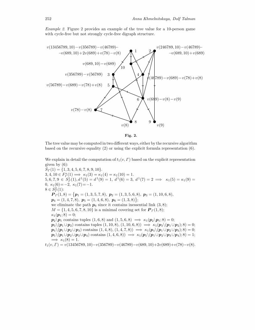
252 Anna Khmelnitskaya, Dolf Talman
Example 2. Figure 2 provides an example of the tree value for a 10-person gamewith cycle-free but not strongly cycle-free digraph structure.
1 2
10
3 4
5
6
7
8 9
v(13456789, 10)−v(356789)−v(46789)−−v(689, 10)+2v(689)+v(78)−v(8)
v(246789, 10)−v(46789)−−v(689, 10)+v(689)
v(356789)−v(56789)v(46789)−v(689)−v(78)+v(8)
v(56789)−v(689)−v(78)+v(8)
v(689)−v(8)−v(9)
v(78)−v(8)
v(8) v(9)
v(689, 10)−v(689)
Fig. 2.
The tree value may be computed in two different ways, either by the recursive algorithmbased on the recursive equality (2) or using the explicit formula representation (6).
We explain in detail the computation of t1(v,Γ ) based on the explicit representationgiven by (6):SΓ (1) = {1, 3, 4, 5, 6, 7, 8, 9, 10}.3, 4, 10 ∈ F ∗
Γ (1) =⇒ κ1(3) = κ1(4) = κ1(10) = 1.5, 6, 7, 9 ∈ S1
Γ (1), d 1(5) = d 1(9) = 1, d 1(6) = 3, d 1(7) = 2 =⇒ κ1(5) = κ1(9) =0, κ1(6)=−2, κ1(7)=−1.8 ∈ S2
Γ (1):P Γ (1, 8) =
{p1 = (1, 3, 5, 7, 8), p2 = (1, 3, 5, 6, 8), p3 = (1, 10, 6, 8),
p4 = (1, 4, 7, 8), p5 = (1, 4, 6, 8), p6 = (1, 3, 8)}
;we eliminate the path p6 since it contains inessential link (3, 8);M = {1, 4, 5, 6, 7, 8, 10} is a minimal covering set for P Γ (1, 8);κ1(p1; 8) = 0;p2\p1 contains tuples (1, 6, 8) and (1, 5, 6, 8) =⇒ κ1(p2\p1; 8) = 0;p3\(p1∪p2) contains tuples (1, 10, 8), (1, 10, 6, 8)) =⇒ κ1(p3\(p1∪p2); 8) = 0;p4\(p1∪p2∪p3) contains (1, 4, 8), (1, 4, 7, 8)) =⇒ κ1(p4\(p1∪p2∪p3); 8) = 0;p5\(p1∪p2∪p3∪p4) contains (1, 4, 6, 8)) =⇒ κ1(p5\(p1∪p2∪p3∪p4); 8) = 1;=⇒ κ1(8) = 1.
t1(v,Γ ) = v(13456789, 10)−v(356789)−v(46789)−v(689, 10)+2v(689)+v(78)−v(8).
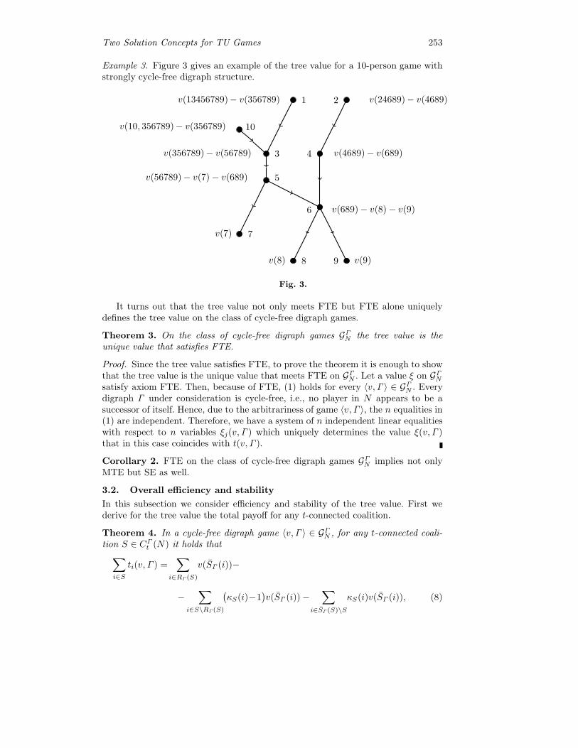
Two Solution Concepts for TU Games 253
Example 3. Figure 3 gives an example of the tree value for a 10-person game withstrongly cycle-free digraph structure.
1 2
10
3 4
5
6
7
8 9
v(13456789)− v(356789) v(24689)− v(4689)
v(10, 356789)− v(356789)
v(356789)− v(56789) v(4689)− v(689)
v(56789)− v(7)− v(689)
v(689)− v(8)− v(9)
v(7)
v(8) v(9)
Fig. 3.
It turns out that the tree value not only meets FTE but FTE alone uniquelydefines the tree value on the class of cycle-free digraph games.
Theorem 3. On the class of cycle-free digraph games GΓN the tree value is theunique value that satisfies FTE.
Proof. Since the tree value satisfies FTE, to prove the theorem it is enough to showthat the tree value is the unique value that meets FTE on GΓN . Let a value ξ on GΓNsatisfy axiom FTE. Then, because of FTE, (1) holds for every 〈v,Γ 〉 ∈ GΓN . Everydigraph Γ under consideration is cycle-free, i.e., no player in N appears to be asuccessor of itself. Hence, due to the arbitrariness of game 〈v,Γ 〉, the n equalities in(1) are independent. Therefore, we have a system of n independent linear equalitieswith respect to n variables ξj(v,Γ ) which uniquely determines the value ξ(v,Γ )that in this case coincides with t(v,Γ ).
Corollary 2. FTE on the class of cycle-free digraph games GΓN implies not onlyMTE but SE as well.
3.2. Overall efficiency and stability
In this subsection we consider efficiency and stability of the tree value. First wederive for the tree value the total payoff for any t-connected coalition.
Theorem 4. In a cycle-free digraph game 〈v,Γ 〉 ∈ GΓN , for any t-connected coali-tion S ∈ CΓ
t (N) it holds that∑i∈S
ti(v,Γ ) =∑
i∈RΓ (S)
v(SΓ (i))−
−∑
i∈S\RΓ (S)
(κS(i)−1
)v(SΓ (i))−
∑i∈SΓ (S)\S
κS(i)v(SΓ (i)), (8)
254 Anna Khmelnitskaya, Dolf Talman
whereSΓ (S) =
⋃i∈RΓ (S)
SΓ (i),
κS(i) =∑
j∈PΓ (i)∩SΓ (S)
κj(i), for all i ∈ SΓ (S),
while κS(i) = 1 when dN (i) = 1, where for any t-connected coalition S ∈ CΓt (N),
for all i ∈ SΓ (S), dS(i) is the in-degree of i in the subgraph Γ |SΓ (S), i.e.,
dS(i) = |OΓ (i) ∩ SΓ (S)|,
in particular, dN (i) = dΓ (i) for all i ∈ N .If the consideration is restricted to only strongly cycle-free digraph games, then
for any t-connected coalition S ∈ CΓt (N) it holds that∑
i∈Sti(v,Γ ) =
∑i∈RΓ (S)
v(SΓ (i))−
−∑
i∈S\RΓ (S)
(dS(i)−1
)v(SΓ (i))−
∑i∈RΓ (SΓ (S)\S)
dS(i)v(SΓ (i)). (9)
Proof. Let 〈v,Γ 〉 ∈ GΓN be a cycle-free digraph game and let S be any t-connectedcoalition S ∈ CΓ
t (N). Then it holds that∑i∈S
ti(v,Γ )(3)=∑i∈S
(v(SΓ (i))−
∑j∈SΓ (i)
κi(j)v(SΓ (j)))
=
=∑
i∈RΓ (S)
v(SΓ (i))−∑
i∈S\RΓ (S)
( ∑j∈SΓ (i)
(κi(j)−1)v(SΓ (i))
)−
∑i∈SΓ (S)\S
( ∑j∈SΓ (i)
κi(j)v(SΓ (i))).
Since for all i, j ∈ S with j ∈ SΓ (i) every path from i to j belongs to S, (8) followsstraightforwardly from the last equality.
Next, if dN (i) = 1, then due to Lemma 1 for all j ∈(PΓ (i) ∩ SΓ (S)
)\FΓ (i),
d j(i) = 0 and therefore κj(i) = 0, and for j ∈ FΓ (i) ∩ SΓ (S), κj(i) = 1.In case Γ is a strongly cycle-free digraph, it holds that∑
i∈Sti(v,Γ )
(7)=∑i∈S
(v(SΓ (i))−
∑j∈FΓ (i)
v(SΓ (j)))
=
=∑
i∈RΓ (S)
v(SΓ (i))−∑
i∈S\RΓ (S)
(dS(i)−1
)v(SΓ (i))−
∑j∈FΓ (i)
i∈S, j /∈S
dS(j)v(SΓ (j)).
To complete the proof of (9) it suffices to notice that, since Γ a strongly cycle-freedigraph, every subordinate j∈FΓ (i) of i∈S that does not belong to S is a root inSΓ (S)\S.
From Theorem 4 it follows that for any cycle-free digraph game 〈v,Γ 〉 ∈ GΓN theoverall efficiency is given by∑
i∈Nti(v,Γ ) =
∑i∈RΓ (N)
v(SΓ (i))−∑
i∈N\RΓ (N)
(κN (i)−1
)v(SΓ (i)), (10)

Two Solution Concepts for TU Games 255
while if the consideration is restricted to only strongly cycle-free digraph games,(10) reduces to∑
i∈Nti(v,Γ ) =
∑i∈RΓ (N)
v(SΓ (i))−∑
i∈N\RΓ (N)
(dΓ (i)−1
)v(SΓ (i)). (11)
To support these expressions we recall the Myerson model in of a game withundirected cooperation structure (Myerson, 1977), in which the component effi-ciency entails the equality ∑
i∈Nξi(v,Γ ) =
∑C∈N/Γ
v(C). (12)
While the right-side expression in (12) is composed by connected components thatare the only efficient productive elements in the Myerson’s model, the building bricksin (10) and (11) are the full successors sets which are the only efficient productivecoalitions under the assumption of tree connectedness. Observe also that for stronglycycle-free rooted-forest digraph games (11) reduces to (12),∑
i∈Nti(v,Γ ) =
∑i∈RΓ (N)
v(SΓ (i)) =∑
C∈N/Γv(C).
For a cycle-free digraph game 〈v,Γ 〉 ∈ GΓN , we define the t-core Ct(v,Γ ) as theset of component efficient payoff vectors that are not dominated by any t-connectedcoalition,
Ct(v,Γ ) = {x ∈ IRN | x(C) = v(C), ∀C ∈ N/Γ ; x(S) ≥ v(S), ∀S ∈ CΓt (N)}, (13)
while the weak t-core Ct(v,Γ ) is the set of weakly component efficient payoff vectorsthat are not dominated by any t-connected coalition,
Ct(v,Γ ) = {x ∈ IRN | x(C) ≤ v(C), ∀C ∈ N/Γ ; x(S) ≥ v(S), ∀S ∈ CΓt (N)}. (14)
Theorem 5. The tree value on the subclass of superadditive rooted-forest digraphgames is t-stable.
Proof. Let 〈v,Γ 〉 ∈ GΓN be a superadditive rooted-forest digraph game arbitrarilychosen. We show that the tree value t(v,Γ ) belongs to the core Ct(v,Γ ). Considerarbitrary C ∈ N/Γ , then C is a tree. Let i ∈ C be a root in Γ , then C = SΓ (i)because of the rooted-forest structure of Γ . Due to the full-tree efficiency of the treevalue, it holds that ∑
j∈SΓ (i)
tj(v,Γ )FTE= v(SΓ (i)),
wherefrom it follows that ∑j∈C
tj(v,Γ ) = v(C).
Let now S ∈ CΓt (N). Because of the rooted-forest structure of Γ , it holds
that dN (i) = 1 for all i ∈ N\RΓ (N). Wherefrom it follows that Γ |S containsexactly one root, say, node i, Γ |S is a subtree, and S ⊆ SΓ (i). Moreover, since Γ is
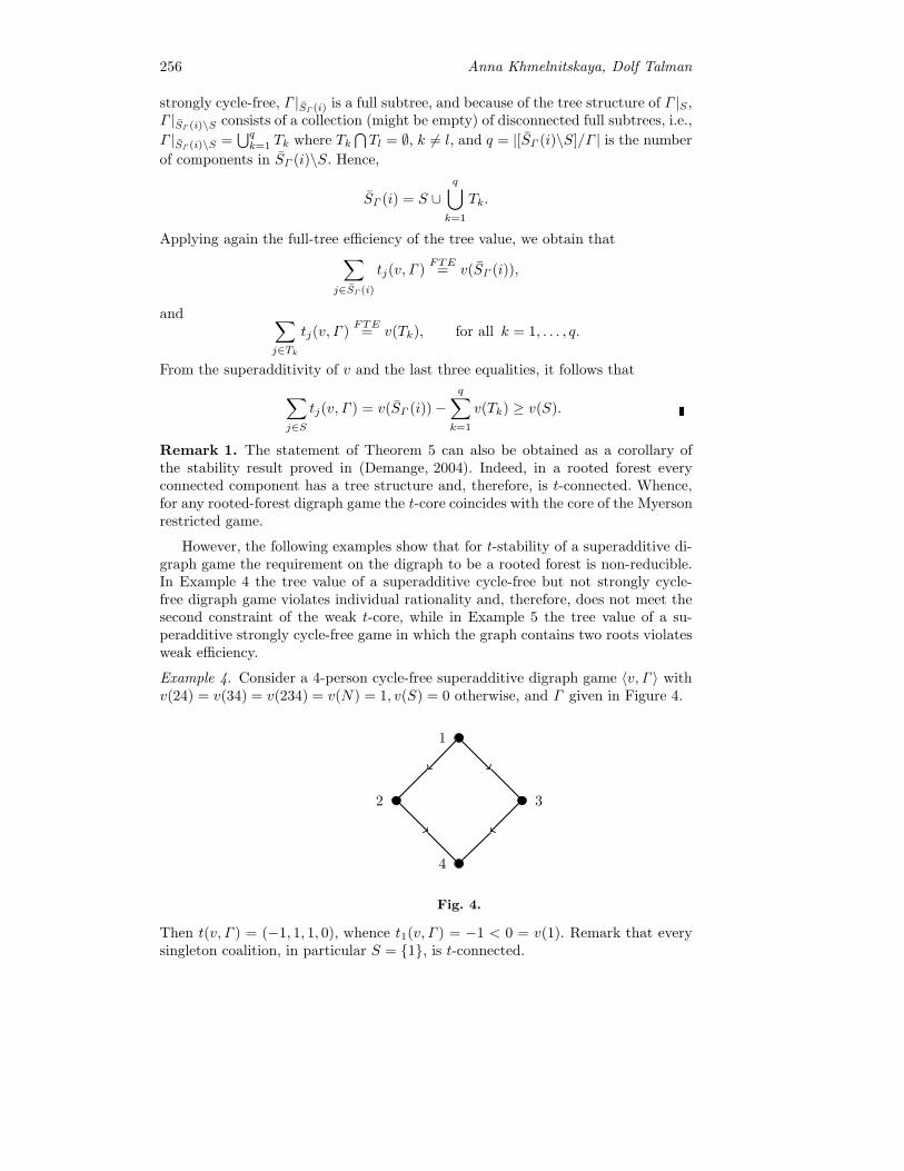
256 Anna Khmelnitskaya, Dolf Talman
strongly cycle-free, Γ |SΓ (i) is a full subtree, and because of the tree structure of Γ |S ,Γ |SΓ (i)\S consists of a collection (might be empty) of disconnected full subtrees, i.e.,
Γ |SΓ (i)\S =⋃qk=1 Tk where Tk
⋂Tl = ∅, k = l, and q = |[SΓ (i)\S]/Γ | is the number
of components in SΓ (i)\S. Hence,
SΓ (i) = S ∪q⋃
k=1
Tk.
Applying again the full-tree efficiency of the tree value, we obtain that∑j∈SΓ (i)
tj(v,Γ )FTE= v(SΓ (i)),
and ∑j∈Tk
tj(v,Γ )FTE= v(Tk), for all k = 1, . . . , q.
From the superadditivity of v and the last three equalities, it follows that∑j∈S
tj(v,Γ ) = v(SΓ (i))−q∑
k=1
v(Tk) ≥ v(S).
Remark 1. The statement of Theorem 5 can also be obtained as a corollary ofthe stability result proved in (Demange, 2004). Indeed, in a rooted forest everyconnected component has a tree structure and, therefore, is t-connected. Whence,for any rooted-forest digraph game the t-core coincides with the core of the Myersonrestricted game.
However, the following examples show that for t-stability of a superadditive di-graph game the requirement on the digraph to be a rooted forest is non-reducible.In Example 4 the tree value of a superadditive cycle-free but not strongly cycle-free digraph game violates individual rationality and, therefore, does not meet thesecond constraint of the weak t-core, while in Example 5 the tree value of a su-peradditive strongly cycle-free game in which the graph contains two roots violatesweak efficiency.
Example 4. Consider a 4-person cycle-free superadditive digraph game 〈v,Γ 〉 withv(24) = v(34) = v(234) = v(N) = 1, v(S) = 0 otherwise, and Γ given in Figure 4.
1
2 3
4
Fig. 4.
Then t(v,Γ ) = (−1, 1, 1, 0), whence t1(v,Γ ) = −1 < 0 = v(1). Remark that everysingleton coalition, in particular S = {1}, is t-connected.

Two Solution Concepts for TU Games 257
Example 5. Consider a 3-person cycle-free superadditive digraph game 〈v,Γ 〉 withv(12) = v(13) = v(N) = 1, v(S) = 0 otherwise, and Γ given in Figure 5.
1 2
3
Fig. 5.
Then t(v,Γ ) = (1, 1, 0), whence t1(v,Γ ) + t2(v,Γ ) + t3(v,Γ ) = 2 > 1 = v(N).
A cycle-free digraph game 〈v,Γ 〉 is t-convex, if for all t-connected coalitionsT,Q ⊂ CΓ
t (N) such that T is a full t-connected set, Q is a full successors set, andT ∪Q ∈ CΓ
t (N), it holds that
v(T ) + v(Q) ≤ v(T ∪Q) + v(T ∩Q). (15)
Theorem 6. The tree value on the subclass of t-convex strongly cycle-free digraphgames is weakly efficient.
Proof. Let 〈v,Γ 〉 ∈ GΓN be any t-convex strongly cycle-free digraph game. Assumethat Γ is connected, otherwise we apply the same argument to any componentC ∈ N/Γ . If there is only one root in Γ , it holds that
∑ni=1 ti(v,Γ ) = v(N) and
the tree value is even efficient. So, suppose that there are q different roots r1, . . . , rqin Γ for some q ≥ 2. Since Γ is connected, the roots in Γ can be ordered in such away that
j−1⋃h=1
SΓ (rh) ∩ SΓ (rj) = ∅, for j = 2, ..., q.
For j = 1, ..., q let Tj =⋃jh=1 SΓ (rh). Then from the strongly cycle-freeness of Γ it
follows that for j = 2, ..., q there exists a unique ij ∈ N such that
Tj−1 ∩ SΓ (rj) = SΓ (ij).
By t-convexity of the digraph game 〈v,Γ 〉 it holds that
v(Tj−1) + v(SΓ (rj)) ≤ v(Tj) + v(SΓ (ij)), for j = 2, ..., q.
Since T1 = SΓ (r1) and Tq = N , then applying the last inequality successively q− 1times we obtain
q∑j=1
v(SΓ (rj)) ≤ v(N) +
q∑j=2
v(SΓ (ij)).
Hence,
v(N)≥q∑j=1
v(SΓ (rj))−q∑j=2
v(SΓ (ij)).

258 Anna Khmelnitskaya, Dolf Talman
Since Γ is strongly cycle-free, for any i ∈ N\RΓ (N), node i has dΓ (i) different rootsas predecessor, which implies that the term v(SΓ (i)) appears precisely dΓ (i) − 1times. Therefore,
v(N) ≥∑
i∈RΓ (N)
v(SΓ (i))−∑
i∈N\RΓ (N)
(dΓ (i)−1
)v(SΓ (i)).
The following example of a convex strongly cycle-free digraph game shows thateven under the assumption of convexity of a given digraph game, which is strongerthan t-convexity, one or more constraints for not being dominated in the definitionof the week t-core might be violated by the tree value, and therefore, the tree valueis not weakly t-stable.
Example 6. Consider a 5-person cycle-free convex digraph game 〈v,Γ 〉 with v(N) =10, v(123) = v(1234) = v(1235) = 3, v(1345) = v(2345) = 2, v(S) = 0 otherwise,and the strongly cycle-free digraph Γ given in Figure 6.
1 2
3
4 5
Fig. 6.
Then t(v,Γ ) = (1, 1, 0, 0, 0), whence, the total payoff of t-connected coalition S ={1, 2, 3} t1(v,Γ ) + t2(v,Γ ) + t3(v,Γ )=2<3=v(123).
From (10) it follows that for a cycle-free (for simplicity connected) digraph game〈v,Γ 〉 ∈ GΓN a necessary and sufficient condition for the weak efficiency of the treevalue is that ∑
i∈RΓ (N)
v(SΓ (i)) ≤ v(N) +∑
i∈N\RΓ (N)
(κN (i)−1
)v(SΓ (i)). (16)
Since N =⋃
i∈RΓ (N)
SΓ (i), the grand coalition equals the union of the successors sets
of all roots in the graph Γ . In case there is only one root in Γ , condition (16) isredundant, because the left side is then equal to v(N). In case there is more thanone root in Γ , the different successors sets of the roots of Γ will intersect each otherand for any i ∈ N\RΓ (N) the number κN (i) − 1 is the number of times that thesuccessors set SΓ (i) of node i equals the intersection of successors sets of the roots ofΓ . Therefore, condition (16) is a kind of convexity condition for the grand coalitionsaying that the sum of the worths of the successors sets of all the roots of the graphshould be less than or equal to the worth of the grand coalition (their union) plusthe total worths of their intersections. In a firm where any full successors set of aroot is a division within the firm and subdivisions that are intersections of several
Two Solution Concepts for TU Games 259
divisions are shared by these divisions, in (16) the left-side minus the sum in theright-side can be economically interpreted as the total worths of the divisions whenthey do not cooperate, while v(N) is the worth of the firm when the divisions docooperate. To have weak efficiency the latter value should be at least equal to theformer value. Remark that v(N) minus the total payoff at the tree value can beinterpreted as the net profit of the firm (or the synergy effect from cooperation)that can be given to its shareholders.
3.3. Sink connectedness
We consider now another scenario of controlling cooperation in case of directedcommunication and assume that in any coalition each player may be controlledonly by his successors and that nobody accepts that his former superior becomeshis equal partner if a coalition forms. This entails the assumption that the onlyproductive coalitions are the so-called sink connected, or simply s-connected, beingthe connected coalitions S ∈ CΓ(N) that meet also the condition that for everyleaf i ∈ LΓ (S) it holds that i /∈ PΓ (j) for another leaf j ∈ LΓ (S). Similar to thecase of tree connectedness, every s-connected coalition inherits the subordinationof players prescribed by Γ in N , every component C ∈ N/Γ is s-connected, andany full predecessors set in Γ is s-connected. We say that an s-connected coalitionis full s-connected, if it together with its leaves contains all predecessors of theseleaves. Observe that a full s-connected coalition is the union of several full prede-cessors sets. For a cycle-free digraph Γ on N and a coalition S ⊆ N , let CΓ
s (S)denote the set of all s-connected subcoalitions of S, [S/Γ ]s the set of maximallys-connected subcoalitions of S, called the s-connected components of S, and [S/Γ ]sithe s-connected component of S containing player i ∈ S.
For efficiency of a value we require that each leaf of the given communicationdigraph together with all his predecessors realizes the total worth they possess.This generates the first property a value must satisfy, what we call maximal-sinkefficiency.
A value ξ on GΓN is maximal-sink efficient (MSE) if for every cycle-free digraphgame 〈v,Γ 〉 ∈ GΓN it holds that∑
j∈PΓ (i)
ξj(v,Γ ) = v(PΓ (i)), for all i ∈ LΓ (N).
The next property, called the predecessor equivalence, says that if a directedlink is broken, each member of the full predecessors set of the origin of this link stillreceives the same payoff.
A value ξ on GΓN is predecessor equivalent (PE) if for every cycle-free digraphgame 〈v,Γ 〉 ∈ GΓN it holds that for all (i, j) ∈ Γ
ξk(v,Γ\(i, j)) = ξk(v,Γ ), for all k ∈ PΓ (i).
Along with MSE we consider a stronger efficiency property, what we call full-sinkefficiency, that requires that every full predecessors set realizes its worth.
A value ξ on GΓN is full-sink efficient (FSE) if for every cycle-free digraph game〈v,Γ 〉 ∈ GΓN it holds that∑
j∈PΓ (i)
ξj(v,Γ ) = v(PΓ (i)), for all i ∈ N.
260 Anna Khmelnitskaya, Dolf Talman
It is easy to see that the assumption of sink connectedness in digraph Γ isequivalent to the assumption of tree connectedness in the digraph Γ composed bythe same set of links as Γ but with the opposite orientation. Moreover, each ofaxioms MSE, FSE and PE with respect to any cycle-free digraph game 〈v,Γ 〉 ∈ GΓNis equivalent to the corresponding MTE, FTE or SE axiom with respect to thedigraph game 〈v, Γ 〉. In case of sink connectedness the last two observations allowto obtain the following results straightforwardly from the results proved above inSubsections 3.1. and 3.2. under the assumption of tree connectedness.
Proposition 2. On the class of cycle-free digraph games GΓN MSE and PE togetherimply FSE.
MSE and PE uniquely define a value on the class of cycle-free digraph games.
Theorem 7. On the class of cycle-free digraph games GΓN there is a unique values that satisfies MSE and PE. For every cycle-free digraph game 〈v,Γ 〉 ∈ GΓN , thevalue s(v,Γ ) satisfies the following conditions:
(i) it obeys the recursive equality
si(v,Γ ) = v(PΓ (i))−∑
j∈PΓ (i)
sj(v,Γ ), for all i ∈ N ; (17)
(ii) it admits the explicit representation in the form
si(v,Γ ) = v(PΓ (i))−∑
j∈PΓ (i)
κi(j)v(PΓ (j)), for all i ∈ N, (18)
where for all i ∈ N , j ∈ PΓ (i),
κi(j) =
n−2∑r=0
(−1)rκri (j), (19)
and κri (j) is the number of tuples (i0, . . . , ir+1) such that i0 = j, ir+1 = i, ih ∈PΓ (ih−1), h = 1, . . . , r + 1.
Before stating the next theorem providing simpler explicit representation of thevalue s we introduce some additional notions and notation. Let
P 1Γ (i) =
{j ∈ PΓ (i)\O∗
Γ (i) | P Γ (j, i) =
q⋃h=1
P h,P h∩P l = ∅, h = l :
∀h = 1, ..., q, ∃kh ∈ S(P h)\{j, i} :
kh ∈ p, ∀p ∈ P h and ph∩pl = {j, i}, ∀ph ∈ P h, ∀pl ∈ P l, h = l}
;
andP 2Γ (i) = PΓ (i) \
(O∗
Γ (i) ∪ P 1Γ (i)
).
Both sets P 1Γ (i) and P 2
Γ (i) are composed by predecessors of i that are not propersuperiors of i. P 1
Γ (i) consists of any such j for which all paths from j to i canbe partitioned into a number of separate groups, might be only one group, suchthat all paths in the same group have at least one common node different from
Two Solution Concepts for TU Games 261
j and i and paths from different groups do not intersect between j and i. Noticethat all j ∈ PΓ (i) \ O∗
Γ (i) with di(j) = 1 belong to P 1Γ (i) since the unique proper
subordinate of j belongs to all paths p ∈ P Γ (j, i); in particular, it holds thatj ∈ P 1
Γ (i), when there is only one path from j to i, i.e., when |P Γ (j, i)| = 1. Fromhere besides it follows that for all j ∈ P 2
Γ (i), di(j) > 1. For every j ∈ P 1Γ (i) we
define the proper out-degree di(j) of j with respect to i as the number of groupsP h, h = 1, ..., q, in the partition of P Γ (j, i). The subset of MΓ (j, i) ⊆ S(P Γ (j, i)),j ∈ PΓ (i), composed by j, i, all proper intersection points in S(P Γ (j, i)) and allproper superiors h ∈ O∗
Γ (i)∩S(P Γ (j, i)) we call the lower covering set for P Γ (j, i).Similarly to the definition of κi(j) given by (19) we define
κMi (j) =n−2∑r=0
(−1)rκr,Mi (j),
where κr,Mi (j) counts only the tuples (i0, ..., ir+1) for which i0 = j, ir+1 = i, andih ∈ PΓ (ih−1) ∩ MΓ (j, i), h = 1, . . . , r + 1.
Theorem 8. For every cycle-free digraph game 〈v,Γ 〉 ∈ GΓN the value s given by(18) admits the equivalent representation in the form
si(v,Γ ) = v(PΓ (i))−∑
j∈O∗Γ (i)
v(PΓ (j)) +
+∑
j∈P 1Γ (i)
(di(j)− 1)v(PΓ (j))−∑
j∈P 2Γ (i)
κMi (j)v(PΓ (j)), for all i ∈ N. (20)
If the consideration is restricted to only strongly cycle-free digraph games, thenthe above representation reduces to
si(v,Γ ) = v(PΓ (i))−∑
j∈OΓ (i)
v(PΓ (j)), for all i ∈ N. (21)
For sink-forest digraph games defined by sink forest digraph structures that arestrongly cycle-free, the value given by (21) coincides with the sink value introducedin (Khmelnitskaya, 2010). By that reason from now on we refer to the value s givenby (18), or equivalently by (20), as to the sink-tree value, or simply the sink value,for cycle-free digraph games.
The sink value assigns to every player the payoff equal to the worth of his fullpredecessors set minus the worths of all full predecessors sets of his proper superiorsplus or minus the worths of all full predecessors sets of any other of his predecessorsthat are subtracted or added more than once. Moreover, for any player i ∈ N andhis predecessor j ∈ N that is not his proper superior, the coefficient κi(j) indicatesthe number of overlappings of full predecessors sets of all proper superiors of i atnode j. In fact a player receives what he contributes when he joins his predecessorswhen only the full predecessors sets, that are the only efficient productive coalitionsunder given assumptions, are counted. Since a root has no predecessors, a root justgets his own worth. Furthermore, it is not difficult to check that the right-sides ofboth formulas (20) and (21) being considered with respect not to coalitional worthsbut to players in these coalitions contain only player i when taking into account allpluses and minuses. Besides, according to (17) the sink value assigns to every player

262 Anna Khmelnitskaya, Dolf Talman
the worth of his full predecessors set minus the total payoff to his predecessors.Wherefrom we obtain a simple recursive algorithm for computing the sink valuegoing downstream from the roots of the given digraph.
Example 7. Figure 7 provides an example of the sink value for a 10-person gamewith cycle-free but not strongly cycle-free digraph structure.
The sink value may be computed in two different ways, either by the recursivealgorithm based on the recursive equality (17), or using the explicit formula repre-sentation (20).
1 2
10
3 4
5
6
7
8 9
v(1) v(2)
v(13)−v(1)v(124)−v(1)−v(2)
v(135)−v(13)
v(123456, 10)−v(135)−v(124)−−v(12, 10)+2v(1)+v(2)
v(123457)−v(135)−−v(124)+v(1)
v(12345678, 10)−v(123457)−−v(123456, 10)+v(135)+v(124)+v(1) v(12343569, 10)−v(123456, 10)
v(12, 10)−v(1)−v(2)
Fig. 7.
The sink value not only meets FSE but FSE alone uniquely defines the sinkvalue on the class of cycle-free digraph games.
Theorem 9. On the class of cycle-free digraph games GΓN the sink value is theunique value that satisfies FSE.
Corollary 3. FSE on the class of cycle-free digraph games GΓN implies not onlyMSE but PE as well.
The next theorem derives the total sink value payoff for any s-connected coali-tion.
Theorem 10. In a cycle-free digraph game 〈v,Γ 〉 ∈ GΓN , for any s-connected coali-tion S ∈ CΓ
s (N) it holds that∑i∈S
si(v,Γ ) =∑
i∈LΓ (S)
v(PΓ (i))−∑
i∈S\LΓ (S)
(κS(i)−1
)v(PΓ (i))−
∑i∈PΓ (S)\S
κS(i)v(PΓ (i)),
wherePΓ (S) =
⋃i∈LΓ (S)
PΓ (i),

Two Solution Concepts for TU Games 263
κS(i) =∑
j∈SΓ (i)∩PΓ (S)
κj(i), for all i ∈ PΓ (S),
while κS(i) = 1 when dN (i) = 1, where for any s-connected coalition S ∈ CΓs (N),
for all i ∈ PΓ (S), dS(i) is the out-degree of i in the subgraph Γ |PΓ (S), i.e.,
dS(i) = |FΓ (i) ∩ PΓ (S)|,
in particular, dN (i) = dΓ (i) for all i ∈ N .
If the consideration is restricted to only strongly cycle-free digraph games, thenfor any s-connected coalition S ∈ CΓ
s (N) it holds that∑i∈S
si(v,Γ )=∑
i∈LΓ (S)
v(PΓ (i))−∑
i∈S\LΓ (S)
(dS(i)−1
)v(PΓ (i))−
∑i∈LΓ (PΓ (S)\S)
dS(i)v(PΓ (i)).
For any cycle-free digraph game 〈v,Γ 〉 ∈ GΓN the overall efficiency is given by∑i∈N
si(v,Γ ) =∑
i∈LΓ (N)
v(PΓ (i))−∑
i∈N\LΓ (N)
(κN (i)−1
)v(PΓ (i)),
while if the consideration is restricted to only strongly cycle-free digraph games, thelast equality reduces to∑
i∈Nsi(v,Γ ) =
∑i∈LΓ (N)
v(PΓ (i))−∑
i∈N\LΓ (N)
(dΓ (i)−1
)v(PΓ (i)).
For a cycle-free digraph game 〈v,Γ 〉 ∈ GΓN , the s-core Cs(v,Γ ) is defined as theset of component efficient payoff vectors that are not dominated by any s-connectedcoalition,
Cs(v,Γ ) = {x ∈ IRN | x(C) = v(C), ∀C ∈ N/Γ ; x(S) ≥ v(S), ∀S ∈ CΓs (N)},
while the weak s-core Cs(v,Γ ) as the set of weakly component efficient payoff vectorsthat are not dominated by any s-connected coalition,
Cs(v,Γ ) = {x ∈ IRN | x(C) ≤ v(C), ∀C ∈ N/Γ ; x(S) ≥ v(S), ∀S ∈ CΓs (N)}.
Theorem 11. The sink value on the subclass of superadditive sink-forest digraphgames is s-stable.
A cycle-free digraph game 〈v,Γ 〉 is s-convex, if for all s-connected coalitionsT,Q ⊂ CΓs (N) such that T is a full s-connected set, Q is a full predecessors set,and T ∪Q ∈ CΓs (N), it holds that
v(T ) + v(Q) ≤ v(T ∪Q) + v(T ∩Q).
Theorem 12. The sink value on the subclass of s-convex strongly cycle-free digraphgames is weakly efficient.
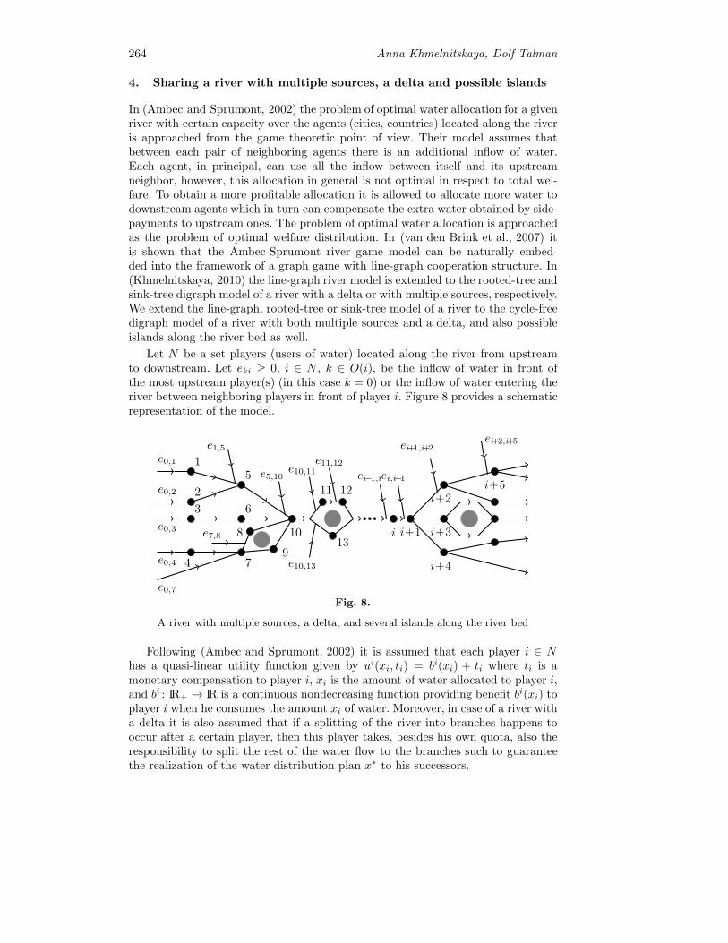
264 Anna Khmelnitskaya, Dolf Talman
4. Sharing a river with multiple sources, a delta and possible islands
In (Ambec and Sprumont, 2002) the problem of optimal water allocation for a givenriver with certain capacity over the agents (cities, countries) located along the riveris approached from the game theoretic point of view. Their model assumes thatbetween each pair of neighboring agents there is an additional inflow of water.Each agent, in principal, can use all the inflow between itself and its upstreamneighbor, however, this allocation in general is not optimal in respect to total wel-fare. To obtain a more profitable allocation it is allowed to allocate more water todownstream agents which in turn can compensate the extra water obtained by side-payments to upstream ones. The problem of optimal water allocation is approachedas the problem of optimal welfare distribution. In (van den Brink et al., 2007) itis shown that the Ambec-Sprumont river game model can be naturally embed-ded into the framework of a graph game with line-graph cooperation structure. In(Khmelnitskaya, 2010) the line-graph river model is extended to the rooted-tree andsink-tree digraph model of a river with a delta or with multiple sources, respectively.We extend the line-graph, rooted-tree or sink-tree model of a river to the cycle-freedigraph model of a river with both multiple sources and a delta, and also possibleislands along the river bed as well.
Let N be a set players (users of water) located along the river from upstreamto downstream. Let eki ≥ 0, i ∈ N , k ∈ O(i), be the inflow of water in front ofthe most upstream player(s) (in this case k = 0) or the inflow of water entering theriver between neighboring players in front of player i. Figure 8 provides a schematicrepresentation of the model.
1
2
3
4
5
6
7
8
9
10
11 12
13i i+1
i+2
i+3
i+4
i+5
e0,1
e0,2
e0,3
e0,4
e1,5
e0,7
e5,10
e7,8
e10,11
e10,13
e11,12ei−1,iei,i+1
ei+1,i+2ei+2,i+5
Fig. 8.
A river with multiple sources, a delta, and several islands along the river bed
Following (Ambec and Sprumont, 2002) it is assumed that each player i ∈ Nhas a quasi-linear utility function given by ui(xi, ti) = bi(xi) + ti where ti is amonetary compensation to player i, xi is the amount of water allocated to player i,and bi : IR+ → IR is a continuous nondecreasing function providing benefit bi(xi) toplayer i when he consumes the amount xi of water. Moreover, in case of a river witha delta it is also assumed that if a splitting of the river into branches happens tooccur after a certain player, then this player takes, besides his own quota, also theresponsibility to split the rest of the water flow to the branches such to guaranteethe realization of the water distribution plan x∗ to his successors.

Two Solution Concepts for TU Games 265
The superadditive river game v ∈ GN introduced under the same assumptionsin (Khmelnitskaya, 2010) for a river with multiple sources or a delta defined as:
for any connected coalition S ⊆ N , v(S) =∑i∈S bi(xSi ), where xS ∈ IRs solves
maxx∈IRs+
∑i∈S
bi(xi) s.t.
⎧⎪⎪⎪⎨⎪⎪⎪⎩∑
j∈PΓ (i)
xj ≤∑
j∈PΓ (i)
∑k∈O(j)
ekj ,
∑j∈PΓ (i)∪BΓ (i)
xj ≤∑
j∈PΓ (i)∪BΓ (i)
∑k∈O(j)
ekj ,∀i ∈ S,
and for any disconnected coalition S ⊂ N , v(S) =∑
T∈CΓ (S)
v(T ),
suits to the case of a river with both multiple sources and a delta, and also possibleislands along the river bed as well. The tree and sink values proposed above can beapplied for the solution of the river game in the general case.
References
Ambec, S. and Y. Sprumont (2002). Sharing a river, Journal of Economic Theory, 107,453–462.
Demange, G. (2004). On group stability in hierarchies and networks, Journal of PoliticalEconomy, 112, 754–778.
Gillies, D. B. (1953). Some Theorems on n-Person Games, Ph.D. thesis, Princeton Uni-versity.
Herings, P. J. J., G. van der Laan, and A. J. J. Talman (2008). The average tree solutionfor cycle-free graph games, Games and Economic Behavior, 62, 77–92.
Khmelnitskaya, A. B. (2010). Values for rooted-tree and sink-tree digraphs games and shar-ing a river, Theory and Decision, 69, 657–669.
Myerson, R. B. (1977). Graphs and cooperation in games, Mathematics of Operations Re-search, 2, 225–229.
van den Brink, R., G. van der Laan, and V. Vasil’ev (2007). Component efficient solutionsin line-graph games with applications, Economic Theory, 33, 349–364.
Tax Auditing Modelswith the Application of Theory of Search
Suriya Sh. Kumacheva
St.Petersburg State University,Faculty of Applied Mathematics and Control Processes,
Bibliotechnaya pl. 2, St.Petersburg, 198504, RussiaE-mail: s [email protected]
Abstract. One of the most important aspects of modeling of taxation —tax control — is studied in the network of game theoretical attitude. Re-alization of systematic tax audits is considered as the interaction of twoplayers – hiding (T – taxpayer) and seeking (A – authority) — in differentstatements of the search game.In the problem statement it is assumed, that tax authority knows due toindirect signs, that some taxpayer T evaded from taxation in the givenperiod (it put down lower than real income in the tax declaration). Alsoit is assumed, that this taxpayer is quite a large company, having manybranches. Company can distribute the hidden income among all or some ofits branches or can hide it in the income of one of its branches. Differentgame cases, which conditions are determined by various possibilities of theevading taxpayer and the tax authority, are considered. In the conditions ofthe games considered, tax authority A solves the problem of maximizationof its income, using mixed strategies, which allow making optimal (in senseof evasion search) tax audits. Taxpayers T aspire to hide their income withthe help of mixed strategies, allowing to reduce a probability of revealing oftheir evasion.
Along with search games, in which tax authority is defined as a search unitor, at best, as several search units, the task of tax audits using the theoryof search of immobile chain with the help of big search system is considered.This model takes into account, that practically tax authority is hierarchicstructure and is solving tasks on different levels (federal, regional, distirctetc.).In this model tax authority solves the task of maximizing the probability ofrevealing of evasion with the help of optimal (in given sense) distribution ofsearch efforts on the given period of time. Company solves the opposite task:to distribute evasion in the way, that minimizes probability of revealing ofevasion.Thus, different possibilities of solving the task of tax evasion search areconsidered.
Keywords: tax control, taxpayers, tax authority, tax evasions, search games,theory of search.
1. Introduction
One of the most important aspects of tax control is revelation of tax evasions. Gath-ering and analysis of indirect information about taxpayers’ income (see, for example,Vasin and Agapova, 1993, Macho-Stadler and Perez-Castrillo, 2002 and others) al-lows to realize systematic tax audits to reveal tax evasions.
Tax Auditing Models with the Application of Theory of Search 267
Another important task of tax authority is to distribute its resources to im-prove the net income, which is realized to the state budget (see, for example,Sanchez and Sobel, 1993).
Tools for solving both of these problems is given by the theory of search, inwhich the probability of revealing of the subject in finite time interval is defined asthe function of the search strategy or search efforts (spent search resources).
At the end of the given tax period each taxpayer declares income and pays taxin compliance with them.
Let’s assume, that tax authority knows due to indirect signs, that some firmevaded from taxation in the given period (it put down lower than real income in thetax declaration). Let’s also assume, that this firm is quite a large company, havingmany branches. The company can distribute the concealed income among all orsome or one of its branches. The tax authority doesn’t know in which.
It should be noted that the solution of mentioned problem can be considered inanother statement:
– the evasion of big company can be distributed among its different business fields,but not among different branches (it is spoken about some total tax payments,including, for example, transport tax, property tax, value-added tax, profit tax,excises etc.);
– a set of taxpayers, acting together in the network of a coalition agreement, canbe considered as evader.
A problem of optimal distribution of resources on tax audit was studied beforeby such authors as Sanchez and Sobel, 1993. Tax authority has hierarchical struc-ture and solves tasks on different levels (federal, regional, distirct etc.). Taking thisfeature into account, use of the described by Hellman, 1985, theory of search ofimmobile chain with the help of a big search system becomes acceptable to the taskof tax audits.
2. The application of theory of search for a big search system to thetask of revelation of tax evasions
Let’s suppose, that the firm conceals income only in one of n branches. Let k bethe number of this branch; the tax authority doesn’t know it. As opposed to thetheory, described by Hellman, 1985, the search of the object (concealed income) isrealized in the discrete space of n branches. Speaking, that the tax authority is abig search system, following Hellman, 1985, let’s assume, that the activity of thesystem’s separate unit can be defined with the help of function λi(t) with the nextcharacteristics:
λi(t) ≥ 0, i = 1, n, t > 0; (1)
n∑i=1
λi(t) = L(t), t > 0; (2)
λi(t)Δt + o(Δt) (3)
– is the probability of revelation of the evasion in the i-th branch in time interval(t, t+Δt) in the condition that in it there is a real evasion, which was not revealeduntil the moment t. λi(t) is called as density or strategy of search.

268 Suriya Sh. Kumacheva
Consider the vector u = (u1, . . . , un), which characterizes a distribution of a taxevasion among branches. Each its component ui is the probability of evasion of thei-th branch.
It should be noted that the distribution u can be improper (see Feller, 1967).
Then the inequalityn∑i=1
ui < 1 is fulfilled. It is due to the information about the tax
evasion (which stimulates the tax authority to audit the taxpayer’s branches) hasan estimation character and can turn out false with some nonnegative probability.(In the paper by Macho-Stadler and Perez-Castrillo, 2002, such information called
as signal). If this information is true, then the conditionn∑i=1
ui = 1 is hold. So, in
the common case (when the tax authority a priori doesn’t know how the signalcorresponds to the reality) let’s suppose that
n∑i=1
ui ≤ 1.
Let k be the number of the branch, where the income concealment was. Let’sdefine {(t1, t2)} as the event consists in that there was no revelation of the evasionin the time interval (t1, t2). Let for fixed k
pi(t) = P{(i = k)|(0, t)}
be the probability of the revealing of the tax evasion in the i-th branch in thecondition that there was the evasion and it was unrevealed until the time t. Fromthe definition of search density obtain:
P{(t, t + Δt)|(i = k)(0, t)} = 1− λi(t)Δt + o(Δt)
– is the probability, that in time interval (t, t + Δt) there is no revelation of theevasion in the branch in which this evasion was in the condition that it was notrevealed until the time t. Then the probability of unrevealing of the evasion of thewhole company in time interval (t, t + Δt):
P{(t, t + Δt)|(0, t)} = 1−Δt
n∑i=1
uiλi(t) + o(Δt).
Let’s denote by P (t) the probability of that the evasion was revealed in timeinterval (0; t): P (t) = 1 − P{(0, t)}. Then, similar to obtained in the book byHellman, 1985, the equality for the probability of revealing of the object in timeT , let’s define the probability of the existing tax evasion of the company in (0;T ),which is a period of limitation for tax crimes:
P (T ) = 1−n∑i=1
ui exp(−∫ T
0
λi(τ)dτ). (4)
The strategy of search λi must be defined such way as it fulfills the conditions(1) – (3) maximizes the probability (4) of the revealing of the evasion in the giventime period (0;T ).

Tax Auditing Models with the Application of Theory of Search 269
Let’s take into consideration a function ϕi(t), which fulfills the conditions
ϕi(T ) =
∫ T
0
λi(τ)dτ ; (5)
ϕi(T ) ≥ 0, i = 1, n; (6)
n∑i=1
ϕi(T ) =
∫ T
0
L(τ)dτ (7)
and call it as the number of search resources, spent on the revelation of the taxevasion in the i-th branch during the time interval (0;T ). Then
P (T ) = 1−n∑i=1
ui exp(−ϕi(T )). (8)
The tax authority’s aim is to distribute the number of search resources ϕi(T ) onthe given tax period (0;T ) in order to fulfill the conditions (5) – (7) and maximizethe probability (8).
The company solves the opposite task: to minimize probability of revealing ofevasion P (T ), i.e. to distribute evasion in the way, that the function probability ofrevealing of evasion get its maximum.
Each proper task requires an individual solution, which depends on a lot ofreasons: a number of branches, involved in the evasion, a geography of branches,resources (time, finances, search units) and the ways helping to realize the auditingetc.
Consider several examples of the search tasks depending on the ways of distribu-tion of the concealed income and the ways of searching it by the tax authority. Thesemodels are based on the search games, studied by Petrosyan and Garnaev, 1992,Petrosyan and Zenkevich, 1987. Let’s consider the tax authority (player A – author-ity) as a searcher and taxpayer (taxpayers) (player T – taxpayers) as a concealer.
The model of search of evasion, which is concentrated in the one branch.The taxpayer T conceals its income in one of its n branches. The tax authorityA also searches in one of them. Both of the players — A and T — have n purestrategies, identifiable with numbers of the branches, chosen for evasion or auditingcorrespondingly. If there is an evasion in the k-th branch and audit is in the i-thbranch, the A’s benefit is equal to
K(i, k) =
{σi, if pk < p∗k0, if pk ≥ p∗k,
where k is the number of the branch, where the evasion was, i is the number of thebranch, where the audit was. The quantity σi (0 < σi ≤ 1, k = 1, n) is interpretedas the probability of revelation of the evasion in the k-th branch.
In the terms of this game the event consists in the revelation of the total evasionof the company, is equal to the revelation of existing evasion in the one (the k-th)branch; uk = 1, that’s why with (8):
σk = 1− e−ϕk(T ), (9)

270 Suriya Sh. Kumacheva
where T can be interpreted as the time interval, given for realization of the audit.As in the terms of this model the audit can be realized only in one branch, it ispossible to suppose that the tax authority will use all of its resources, i. e. total
search effortT∫0
L(τ)dτ . Then (9) will turn out
σk = 1− e−T∫0
L(τ)dτ. (10)
The game considered is the matrix game, and the matrix of the A’s benefits is⎡⎢⎢⎣σ1 0 . . . 00 σ2 . . . 0. . . . . . . . . . . .0 0 . . . σn
⎤⎥⎥⎦ .This game’s value v and optimal mixed strategies are μ∗ = (μ∗
1, . . . , μ∗n) ν∗ =
= (ν∗1 , . . . , ν∗n):
v =1
n∑k=1
1σk
,
μ∗i = ν∗i =
1σin∑k=1
1σk
, i = 1, n.
If σi = σj for i = j, then the choice of the branches, in which there were evasionand audit, are equiprobables for each player. Then the optimal strategies and thegame value get the form
μ∗ = ν∗ = (1
n,
1
n, . . . ,
1
n), v =
1
n.
Then let’s consider the situations in which the company can evade in severalbranches.
The model of search of evasion, which is concentrated in one or twobranches. Let’s suppose, that the company either concealed its income in onebranch or divide it into two parts and distribute on two branches.
The set of T’s pure strategies contains n2 elements and consists of various pares(i, j), where i, j are the numbers of the branches, in which there exist an evasion.
Player A can make an audit in one of n branches. Therefore, he has n purestrategies. Player A’s aim is to maximize the probability of revealing of even one ofthe parts of evasion. In this case the probability of revelation of existing evasion inthe k-th branch during time T is defined similar to the game of search of the oneevasion from (9).
The tax authority’s profit K(k, (i, j)) in the situation (k, (i, j)) is:
K(k, (i, j)) =
⎧⎪⎪⎪⎪⎨⎪⎪⎪⎪⎩0, if i = j, i = k;σi, if i = k, i = j;σj , if j = k, i = j;σi(2− σi), if i = j = k;0, if i = k, j = k.
Tax Auditing Models with the Application of Theory of Search 271
Using the solution of corresponding game (see Petrosyan and Garnaev, 1992),obtain the optimal mixed strategies μ∗ = (μ∗
1, . . . , μ∗n) and ν∗ = {ν∗ij} of the players
A and T correspondingly and the game value v:
μ∗i = ν∗i,i =
1σi(2−σi)n∑l=1
1σl(2−σl)
, if i = 1, n;
ν∗i,j = 0, if i = j;
v =1
n∑l=1
1σl(2−σl)
.
It should be noted that from the statement of T’s strategy it is reasonable forthis player to concentrate total concealed income in one of its branches.
The model with the distribution of the concealed income among mbranches. Assume, that the company T evades in m branches (m ≤ n). It meansthat concealed income is divided into m equal parts and distributed among cor-responding number of T’s branches. The tax authority A can make audits in lbranches at the same time.
Let pi be the probability of revelation of the evasion in the i-th branch when itis audited. First let’s consider an ideal situation, when
pi =
{1, if there is an evasion in this branch;0, if there is no evasion in this branch.
i = 1, n
The number of the taxpayer’s pure strategies is Cmn (various samples withoutreplacement m of n branches to conceal income there), the number of the tax au-thority’s pure strategies is Cln (various samples without replacement l of n branchesto audit them simultaneously).
The player A’s profit is defined as a tax from total income revealed in one orseveral branches (or a number of revealed parts of the income). This player’s aim isto maximize his income. The game matrix has dimension Cmn × Cln.
The solution of this game is found using the results, obtained by Petrosyan andGarnaev, 1992: the player A’s (T’s) optimal mixed strategies μ∗(ν∗) consist in thechoice of one of the Cln(Cmn ) possible pure strategies with probability 1
Cln( 1Cmn
). The
game value is v = mln .
The model with the distribution of equal or different parts of the con-cealed income among m branches. Consider another situation: the taxpayerT divides an income, he wants to conceal, into m different parts. But, distributingthis income among its branches, T can conceal either one or several parts of it ineach branch.
First, let’s suppose that player A can make an audit only in one of T’s branches(this fact can be reasoned by time, financial and official restrictions for the unit oftax authority), but this audit reveals total tax evasion in the branch. In this gameplayers T and A have nm and n pure strategies correspondingly. So, the A’s profitmatrix has dimension n× nm.
Using the results, obtained for the base game by Petrosyan and Garnaev, 1992,define the tax authority’s optimal mixed strategy μ∗ as auditing one of n branches
272 Suriya Sh. Kumacheva
of the company with the probability 1n . The taxpayer’s optimal mixed strategy ν∗
is to choose one of nm possible placements of m parts of the evasion into n brancheswith the probability 1
nm . The game value is equal to mn .
The generalization of considered situation is the case when the tax authority canmake simultaneous audit in l branches, revealing every part of existing evasion inthem. The A’s profit is the tax from total concealed income of the company, revealedas the result of auditing. In this game player T (A) has nm(Cln) pure strategies,therefore, the A’s profit matrix has a dimension Cln × nm.
The tax authority’s optimal mixed strategy μ∗ is to choose one of Cln sampleswithout replacement l of n company’s branches for simultaneous auditing with theprobability 1
Cln. The taxpayer’s optimal mixed strategy ν∗ is to choose one of nm
possible placements of m parts of the evasion into n branches with the probability1nm . The game value is equal to lm
n .
It should be noted that in the case of distribution of the evasion among mbranches the game value is the same as in the last case (when there can be revealedone or several parts of the evasion in audited branch). That is, the possibility toconceal in one branch grater or smaller part of the evasion does not influence onplayer A’s profit.
To approach the models with distribution of concealed income among severalbranches to the practical tax auditing it is necessary to decline an assumption thatthe audit is always effective. That is, the probability of revelation of the tax evasionin the i-th branch during time T , given for the tax audit, can be calculated withuse of (10):
pi(T ) =
{1− e−ϕi(T ), if there is an evasion;0, if there is no evasion,
i = 1, n.
This probability depends on the search efforts, spent in the i-th branch on revelationof the tax evasion, if it exists there.
There are two principally different ways of the searching of tax evasion in oneof l branches — in consecutive order and simultaneous realizing of l audits.
The tax authority doesn’t know in which branches there is concealed income.It makes the estimation of spent resources more difficult and, therefore, it becomesmore difficult to choose the most preferable way of auditing in this sense.
It is also obviously that the consecutive audits have no preferences in comparisonwith parallel auditing in sense of spending time: simultaneous search in l branchestakes as long as an audit of one branch when the consecutive search is realized.
Everything told above lets draw a conclusion that parallel auditing in l branchesis more rational in comparison with consecutive audits.
Total search resources, spent by the tax authority on l simultaneous tax audits,is defined as the amount of search resources in each branch. Then, with (8), theprobability of revelation of the tax evasion when there realized a parallel auditingof l branches in time T is defined as:
P (T ) = 1−j+l−1∑i=j
ui exp(−ϕi(T )). (11)

Tax Auditing Models with the Application of Theory of Search 273
If the company’s evasion is really distributed among l branches, then the vectoru = (u1, . . . , un) is such as
j+l−1∑i=j
ui = 1.
In this case the statement (11) becomes:
P (T ) = 1− exp(−∫ T
0
L(τ)dτ),
where L(T ) is the total cost of simultaneous search of evasion in l branches.
Thus, the application of theory of search to the task of tax auditing is considered.The results, obtained above, allows to solve tasks of tax evasion search and optimaldistribution of tax authority’s resources to improve its net income.
References
Vasin, A. and Agapova, O. (1993). Game Theoretic Model of the Tax Inspection Organiza-tion. International Year-Book of Game Theory and Applications, Novosibitsk: Nauka,1, 83–94.
Macho-Stadler, I. and Perez-Castrillo, J. (2002). Auditing with signals. Economica, 02,1–20.
Sanchez, I. and Sobel, J. (1993). Hierarchical design and enforcement of income tax poli-cies. Journal of Public Economics, 1993, 50, 345-369.
Hellman, O. (1985). Introduction to the theory of optimum search. Optimization and op-eration research. M: Nauka (in Russian).
Feller, V. (1967). Introduction to the theory of probability and its applications. 2. M.: Mir(in Russian).
Petrosyan, L. and Garnaev, A. (1992). The search games. SPb: SPbSU (in Russian).Petrosyan, L. and Zenkevich, N. (1987). The optimum search in the conditions of conflict.
Leningrad: LSU (in Russian).Kumacheva, S. and Petrosyan, L. (2009). A game theoretical model of interaction between
taxpayers and tax authority. St. Petersburg, ”Processes Of Conrtol And Stability: the40-th International Scientific Conference Of Post-graduate And Graduate Students”,634–637 (in Russian).
Bargaining Powers, a Surface of Weights, andImplementation of the Nash Bargaining Solution �
Vladimir D. Matveenko
St. Petersburg Institute for Economics and Mathematics RAS, andNational Research University Higher School of Economics at St. Petersburg
Tchaikovskogo Str., 1, St. Petersburg, 191187, RussiaE-mail: [email protected]
Abstract. In the present paper a new approach to the Nash bargainingsolution (N.b.s.) is proposed. (Shapley, 1969) introduced weights of individ-ual utilities and linked the N.b.s. with utilitarian and egalitarian solutions.This equivalence leaves open a positive question of a possible mechanism ofweights formation. Can the weights be constructed in result of a recurrentprocedure of reconciliation of utilitarian and egalitarian interests? Can a setof feasible bundles of weights be a result of a procedure or a game indepen-dent on a concrete bargaining situation? We answer these questions in thepaper. A two-stage n-person game is considered, where on the first stagethe players on base of their bargaining powers elaborate a set of all possiblebundles of weights Λ = {(λ1, . . . , λn)}. This surface of weights can be usedby an arbitrator for evaluation outcomes in different concrete bargains. Onthe second stage, for a concrete bargain, the arbitrator chooses a vector ofweights and an outcome by use of a maximin criterion. We prove that thistwo-stage game leads to the well-known asymmetric N.b.s.
Keywords: Bargaining powers, Weights of individual utilities, Nash bar-gaining solution, Imlementation, Egalitarian solution, Utilitarian solutionJEL classification C78, D74
1. Introduction
An n-person bargaining problem is defined by a pair (S, d) where S is a convex set inRn (the feasible set) and d ∈ S (the status quo, disagreement point, threat point).Each point in S is interpreted as a bundle of utilities of the players; d is a point ofutilities which can be achieved without cooperation, other points in S are availablein case of cooperation. It is required to choose a ”good”, in one sense or another,outcome x ∈ S.
Instead of x ∈ S it is convenient to consider differences u = x − d. However, itis often assumed that d = 0 , in such case u = x; this assumption is accepted in thepresent paper.
(Nash, 1950) considered the bargaining problem from a normative point of view:he formulated a list of properties (axioms) of a good solution and found a uniquesolution satisfying these axioms. The set of axioms includes Pareto optimality,anonymity (or its weaker version, symmetry), scale invariance and contraction in-dependence (also known as independence of irrelative alternatives). The solution,referred as Nash bargaining solution (hereafter N.b.s.), is the point of maximum
maxx∈S
u1u2 . . . un.
� This work was supported by the Program of Basic Research of the National ResearchUniversity Higher School of Economics.
Bargaining Powers, a Surface of Weights 275
In an asymmetric case, when the players have different bargaining powers, the axiomof symmetry is not true, and the outcome satisfying the remaining three axioms canbe found as a point of maximum
maxx∈S
ub11 ub22 . . . ubnn ,
where bi ≥ 0 are bargaining powers of the players, (Harsanyi and Selten, 1972,Kalai, 1977a).
For reviews of results developing the axiomatic approach to the bargaining prob-lem see (Roth, 1979a), (Thomson and Lendsberg, 1989), (Thomson, 1994),(Serrano, 2008).
Nash himself saw a shortage of the axiomatic approach in a lack of an explicit de-scription of a process of negotiations or of dynamics of formation of the outcome. Aproblem of constructing a non-cooperative strategic game resulting in an outcomesatisfying definite axioms is referred now as Nash program. Contributions to theprogram were provided by (Nash, 1953), (Rubinstein, 1982), (Binmore et al., 1986),(Carlsson, 1991) and many others. Later many authors tried to connect the Nashprogram with the theory of mechanisms. A term implementation appeared, we un-derstand it here as a rather broad approach collecting games and mechanisms sup-porting the N.b.s.
The asymmetric N.b.s. finds applications in very different branches of Eco-nomics such as wage formation (Grout, 1984 and many others), pricing mecha-nisms (Bester, 1993), macroeconomic policy (Alesina, 1987), circulation of ideas(Hellman and Perotti, 2006). A recent paper (Eismont, 2010) is devoted to analysisof the European gas market.
The N.b.s. is closely related with the problem of interpersonal comparison of util-ities and with the use of weights of individual utilities. Historically, the usage of car-dinal utilities of players and sums of individual utilities in Game Theory (in partic-ular in games with transferable utilities) induced a dissatisfaction. (Harsanyi, 1963)and (Shapley, 1969) introduced intrinsically-defined utility weights. Shapley(Shapley, 1969) interpreted them as endogenously determined transfer rates be-tween players’ utilities, i.e. as a kind of prices (analogues of exchange rates, i.e.prices of currencies). Shapley allowed a possibility of a change in weights and con-sidered as solutions both a point of maximum maxx∈S (μ1x1 + . . . + μnxn, ) and apoint of equality λ1x1 = . . . = λnxn (equivalent to finding max
x∈Smini
λixi ). Cor-
respondingly, he spoke about ’efficiency’ weights and ’equity’ weights. These twocriteria correspond two basic concepts of optimality, ”competing” in economic poli-cies. Later (Yaari, 1981) interpreted these criteria as ’utilitarian’ and ’egalitarian’,correspondingly. A review of utilitarian and egalitarian approaches to moral the-ory and, in particular, a discussion of papers (Shapley, 1969) and (Yaari, 1981) isprovided by Binmore (Binmore, 1998, Binmore, 2005).
In relation with the weights of utilities (Shapley, 1969) advanced the followingprinciple: ”(III) An outcome is acceptable as a ”value of the game” only if there existscaling factors for the individual (cardinal) utilities under which the outcome is bothequitable and efficient”. So, of principle for Shapley was the existence of a vector ofweights which could for some outcome serve efficiency and equity simultaneously.For the bargaining problem such solution really exists and it is nothing else but thesymmetric N.b.s. The fact can be formulated in the following way.

276 Vladimir D. Matveenko
Theorem 1. Let the set of feasible utilities, S, be restricted by coordinate planesand by a surface g (x1, . . . , xn) = C , where g is a strictly convex function. Thenthe following two statements are equivalent.
1.For a point x ∈ S there exists such a vector of weights λ1, . . . , λn that x issimultaneously (i) a point of maximum of ’utilitarian’ function λ1x1+. . .+λnxn and(ii) a point where max
xmini
λixi is achieved or, what is the same, where ’egalitarian’
condition λ1x1 = . . . = λnxn takes place.2.Point x ∈ S is a symmetric N.b.s., i.e. the point of maximum of the product
x1 . . . xn.
A proof will be given for a more general Theorem 3 below.In the present paper a new approach to the problem of implementation of the
Nash bargaining solution (N.b.s.) is proposed. The equivalence described in Theo-rem 1 (or in Theorem 3 in an asymmetric case) leaves open a positive question of apossible mechanism of weights formation. Can the weights be formed in result of arecurrent procedure of reconciliation of utilitarian and egalitarian interests? Can aset of feasible bundles of weights be a result of a procedure or a game independenton a concrete bargaining situation?
We consider a two-stage game, where on the first stage the players, on base oftheir bargaining powers, elaborate a set of all admissible bundles of weights Λ ={(λ1, . . . , λn)} which can be used by an arbitrator to assess outcomes in differentconcrete bargains. On the second stage, for a concrete bargain, the arbitrator choosesa vector of weights and an outcome by use of a Rawlsian-type maximin criterion.We prove that this game leads to the asymmetric N.b.s.
We interpret the arbitrator as a society (or a community) in a framework ofwhich the bargains are fulfilled. In fact, in reality very often bargains take placenot in a ”vacuum” but depend on an encirclement and on a choice of moral-ethicalassessments.
We suppose that the society confesses a maximin Rawlsian-type principle ofjustice but attaches weights to individual utilities and is manipulated. The partici-pants, by use of all available means draw up a set Λ of admissible bundles of weights(reputational moral-ethical assessments); bargaining powers of participants becomeapparent in this process. (The bargaining powers depend on an access to politicalpower and to media, on image-makers’ abilities, on previous reputations, etc.) Ineach concrete situation of bargaining the society chooses weights from the set Λ.The assessments (weights) entering the set Λ are not unambiguous, and the societychooses those weights which it finds to be fair in a concrete case. Thus, generally, thesociety is conformist and possesses a whole spectrum of assessments which can beused in case of need. In each concrete bargaining problem there is a correspondenceΛ ↔ ParS between admissible bundles of weights λ ∈ Λ and outcomes x ∈ ParS,where ParS is the Pareto border of S.
In Section 2 we consider a relation between ’efficiency’ weights, ’equity’ weightsand bargaining powers as well as different characterizations of the N.b.s. The con-cepts of weights as moral-ethical assessments and of a two-stage game are introducedin Section 3. In Section 4 the same point of view is applied to two other well-knownbargaining solutions: Kalai-Smorodinsky and egalitarian (Kalai). In Section 5 themoral-ethical assessments are considered as a mechanism working in a concrete bar-gaining situation. In Section 6 a relation between the N.b.s. and the Cobb-Douglasproduction functions is studied. Section 7 concludes.
Bargaining Powers, a Surface of Weights 277
2. The weights of individual utilities and characterizations of theN.b.s.
The question of existence of a ”good” system of weights is a normative one. However,not less interesting is a positive question of what is the system of weights acting ina concrete bargaining situation. In this relation a question arises about a presenceof an iterative process of weights formation similar to a cobweb rule and leading tothe N.b.s.
The set S plays a role similar to the production-possibilities set in the theoryof trade (see, e.g. (Caves et al., 2006)). For the case of 2 players let the set S bebounded by the coordinate axes and a curve g (x1, x2) = C, where g is differentiable.Following (Shapley, 1969) the weights can be considered as coefficients of conversion,i.e. prices. ’Efficient’ prices are being formed similarly to commodity prices in thetrade model: if the economy is interested in achieving a point x then prices λ1, λ2
are established that the marginal rate of substitution is equal to the relative price:
−dx2
dx1(x) =
∂g(x)∂x1
∂g(x)∂x2
=λ1
λ2. (1)
Thus, the relative price is a function of the relative utility:
λ1
λ2= ψ
(x1
x2
). (2)
On the other hand, given current ’efficient’ prices λ1, λ2, the society tries toredistribute the utility fairly. If the utility is transferable, then an outcome x wouldbe chosen to satisfy the system of equations:{
λ1x1 = λ2x2
λ1x1 + λ2x2 = λ1x1 + λ2x2
. (3)
However, as soon as in reality the utility is not transferable, an outcome is chosennot by use of (3) but using the system:{
λ1x1 = λ2x2
g (x1, x2) = C.
Consequently, the new relative utility is connected with the relative price by aninverse relation:
x1
x2=
λ2
λ1
The point (x1, x2) is used on the next iteration to find new ’efficient’ prices
λ1, λ2 such that
λ1
λ2
= ψ
(λ2
λ1
)= ϕ
(λ1
λ2
),
where ϕ (k) = ψ(1k
).
So, an iterative process takes place:(λ1
λ2
)t+1
= ϕ
(λ1
λ2
)t
. (4)
A convergence of this process is of interest.

278 Vladimir D. Matveenko
Theorem 2. A condition of a local stability of the process (4) is inequality |E| > 1,where E is the elasticity of substitution of function g (x1, x2) at point (x1, x2) of thesymmetric N.b.s.
A proof of a more general Theorem 6 is provided below.EXAMPLE. Let set S be constrained by coordinate axes and by curve
δxp1 + (1− δ)xp2 = C, (5)
where 0 < δ < 1, p > 1, C > 0. Then the condition of stability of the cobweb rule(4) is p < 2.
Indeed, (5) can be written as
(δxp1 + (1− p)xp2)1p = C.
The LHS, the well-known CES function, has elasticity of substitution σ = 11−p .
The stability condition |σ| > 1 reduces to p < 2 . So, the stability takes place under1 < p < 2.
The natural generalization of Theorem 3 is the following statement.
Theorem 3. Let S and g satisfy conditions of Theorem 1, and let b1, . . . , bn bepositive bargaining powers. Then the following two statements are equivalent.
1. For a point x there exists such a vector of weights λ1, . . . , λn , that x issimultaneously(i) a point of maximum of ’utilitarian’ function μ1x1 + . . . + μnxn with weights
μi = biλi (i = 1, . . . , n) (6)
and(ii) a point where max
x∈Smini
λixi is achieved or, what is the same, where ’egalitarian’
conditionλ1x1 = . . . = λnxn (7)
takes place.2. Point x is the asymmetric N.b.s. with bargaining powers b1, . . . , bn, i.e. the
point of maximum of functionxb11 . . . xbnn .
Proof. For the problem of maximization of the ’utilitarian’ function a necessary andsufficient condition of optimality is the equation
μiμj
=
∂g∂xi
(x)∂g∂xj
(x)(i, j = 1, . . . , n). (8)
For the problem of maximization of function xb11 . . . xbnn a necessary and sufficientcondition of optimality is the equation
bixjbjxi
=
∂g∂xi
(x)∂g∂xj
(x)(i, j = 1, . . . , n). (9)
Equations (6), (7) and (8) imply (9), i.e. Statement 1 implies Statement 2.

Bargaining Powers, a Surface of Weights 279
Let Statement 2 be true. Then (9) takes place. For point x weights λ1, . . . , λncan be found for which equations (7) are true. Equations (6), (7) and (9) imply (8).Thus, Statement 1 follows from Statement 2.
Binmore (Binmore, 2009) writes that ”A small school of psychologists who work on”modern equity theory” come closest to my own findings. They find experimentalsupport for Aristotle’s ancient contention that ”what is fair is what is proportional”.More precisely, they argue that an outcome is regarded as fair when each person’sgain over the status quo is proportional to that person’s ”social index”. This con-clusion is consistent, for example, with the widespread concern about preservingdifferentials between the wages paid to different trades (such as electricians or car-penters) when there is a general wage increase.”
According to (7), in role of a ’social index’ of player i the value 1λi
reverse toher ’egalitarian’ weight appears.
The relation (6) between ’utilitarian’ weights μi and ’egalitarian’ weights λi canbe interpreted in the following way. The weights λi (i = 1, . . . , n) are constructedin a framework of the ’egalitarian’ criterion and are not suitable for the ’utilitarian’function because they too strongly reflect personalities of the players: players withhigher bargaining powers bi have understated weights λi while for players withlower bargaining powers the weights are overstated. The products μi = biλi contain”correcting” coefficients and provide objective, in some sense, estimates of utilitiesof players for inclusion into the ’utilitarian’ function.
Theorem 4. The asymmetric N.b.s. can be characterized as a point in the Paretoborder, where the pair-wise elasticity of the border is equal to the corresponding ratioof the bargaining powers.
Proof. From (9)∂g∂xi
(x)∂g∂xj
(x)
xixj
=bibj
(i, j = 1, . . . , n).
Geometrically the point of the N.b.s., x, is characterized as follows. Consider a(hyper)plane tangent to surface g(x1, . . . , xn) = C at point x . Let Xi (i = 1, ..., n)be points of intersection of the plane with coordinate axes.
Theorem 5.
x = β1X1 + β2X2 + . . . + βnXn,
where βi = bib1+...+bn
is the relative bargaining power of player i (i = 1, . . . , n),n∑i=1
βi = 1.
Proof. Let μ1x1+ . . .+μnxn = μ1x1+ . . .+μnxn ≡ C be an equation of the tangentplane at point x. The point Xi of intersection of the plane with the i-th coordinateaxis has the i-th coordinate
C
μi=
μ1
μix1 + . . . +
μnμi
xn,
280 Vladimir D. Matveenko
and other coordinates are zero. By Theorem 3, the N.b.s. satisfies equations
xj =bjbi
μiμj
xi (j = 1, . . . , n).
Hence,
C
μi=
b1 + . . . + bnbi
xi.
From here
b1X1 + . . . + bnXn =
(b1
C
μ1, . . . , bn
C
μn
)= (b1 + . . . + bn) x.
Vice versa, an arbitrary point x ∈ S with positive coordinates satisfies equation
x = β1X1 + . . . + βnXn with some coefficients βi > 0,n∑i=1
βi = 1, where Xt is
the point of intersection of the tangent plane at point x with i-th coordinate axis.These coordinates define point x uniquely. According to Theorem 4, point x is theasymmetric N.b.s. with bargaining powers βi > 0 (i = 1, . . . , n) (or any proportionalbargaining powers).
In particular, in case of two players with equal bargaining powers, the N.b.s. xis characterized by the property that the segment of the straight line tangent tocurve g(x1, x2) = C at point x and contained between coordinate axes is dividedin halves by point x. In case of three players with equal bargaining powers, x isthe point of intersection of medians of the triangle formed by intersections of thecoordinate planes with the plane tangent to surface ϕ(x1, x2, x3) = 0 at point x.
Similarly to the previous one, consider an iterative ”cobweb” process of weightsformation. Let μ1, μ2 be ’efficient’ prices under which the society tries to redistributeutilities x1, x2. In case of transferable utility, an outcome (x1, x2) would be chosento satisfy the system of equations{
λ1x1 = λ2x2
μ1x1 + μ2x2 = μ1x1 + μ2x2
, (10)
where λi = μi/bi , and bi is the bargaining power of player i (i = 1, 2). As soon asutility is not in fact transferable, the outcome (x1, x2) has to satisfy the system ofequations {
λ1x1 = λ2x2
g (x1, x2) = C. (11)
Hence, the relative utility is linked with the relative price by equations:
x1
x2=
λ2
λ1=
b1b2
μ2
μ1
On the next iteration the point (x1, x2) is used to define new ’efficient’ prices (μ1, μ2)such that
μ1
μ2=
∂g(x)∂x1
∂g(x)∂x2
= ψ
(x1
x2
)= ψ
(b1b2
μ2
μ1
).

Bargaining Powers, a Surface of Weights 281
So, the following iterative process takes place:(μ1
μ2
)t+1
= ϕ
(μ1
μ2
)t
, (12)
where ϕ(k) = ψ(b1b2
1k
).
Theorem 6. A condition of a local stability of the process (12) is the inequality|E| > 1 , where E is the elasticity of substitution of function g(x1, x2) at point x ofthe asymmetric N.b.s.
Proof. A condition of stability is inequality∣∣∣ϕ′(μ1
μ2
)∣∣∣ < 1 at the steady state. The
weights μ1, μ2 are responded by utilities x1, x2 such that
μ1
b1x1 =
μ2
b2x2.
The following is true:
∣∣∣∣ϕ′(μ1
μ2
)∣∣∣∣ =
∣∣∣∣∣ψ′(x1
x2
)b1b2
(μ2
μ1
)2∣∣∣∣∣ =
∣∣∣∣∣∣∣∣d
(∂g(x)∂x1∂g(x)∂x2
)d| x1x2
(x1
x2
) · x1
x2·∂g(x)∂(x2)
∂g(x)∂x1
∣∣∣∣∣∣∣∣ =
∣∣∣∣ 1
E
∣∣∣∣ ,where E is the elasticity of substitution of function g(x1, x2) at point x. Thus, thestability condition is the inequality |E| > 1.
3. Weights as reputational moral-ethical assessments. Formation ofweights
Many real bargains and negotiations are characterized by two common features.Firstly, it is a presence of a community in role of an arbitrator in a framework ofwhich the bargains are fulfilled. For example, in case of international trade andinternational relations it is a so called ”international community” including gov-ernments of countries, and different international organizations. In case of laborrelations, it is a ”collective” of a firm (or, in the West, a union). In other cases itcan be a local community, a ”scientific community”, an ”artistic community”, andso on.
Secondly, bargains between a fixed set of participants are often not ’one-shot’ butrepresent a routine repeated process, and, along with bargains, a ”public opinion”of the community is being formed. The community acts as an arbitrator realizing acontrol for bargains in such way that unfair, from the point of view of the community,bargains are not possible, at least as routine ones. An outcome of an unfair bargaincan be revised, if not formally, than in result of a conflict. Such conflicts often arise,both in local communities and organizations (conflicts between separate membersof community or between a worker and administration), and on a national level(conflicts between social groups) and in international relations (conflicts betweencountries).
The process of formation of the public opinion goes uninterruptedly, but oftenone does not know what bargains will take place in the future, so the public opinion
282 Vladimir D. Matveenko
is elaborated by parties not in conformity to a concrete bargain but in relationto all admissible situations of bargaining. Moral-ethical assessments formed by useof propaganda emphasize an insufficiency of utilities received by some participantsand an excessiveness of utilities of others. In other words, the essence of the moral-ethical assessments is that they act as decreasing or increasing coefficients (weights)applied to utilities of the participants.
As an example we can compare judgments concerning the annual income ofPresident D. Medvedev on site Compromat.ru of media Gazeta.ru (December 2008)and in Izvestia newspaper (April 2009). The site emphasizes that D. Medvedev has alargest, in comparison with other members of the government, apartment. Izvestia,on the contrary, stresses that D. Medvedev, by the World measure, has one of thelowest wages among state managers of such level.
It is important to emphasize that moral-ethical assessments are usually notunivalent but allow a variance: the public opinion practically always stresses bothpositive and negative features of participants.
Formation of public opinion is performed by means of propaganda and by useof any available tools (e.g. media, Internet, political meetings, creation of gossips).Possibilities of formation of public opinion are limited by an access to media andby professional abilities of ”image-makers” as well as by a presence of adaptive orrational expectations of the audience: it is rather difficult to instill an opinion whichdoes not correspond to expectations.
Concrete weights can differ in different bargains depending on circumstances.Thus, the community deals not with a unique vector of assessments but with acurve (in case of two bargainers) or with a surface of possible assessments. It canbe supposed that the community in its approval or disapproval of an outcome of abargain acts in accordance with a Rawlsian-type maximin principle, paying atten-tion to the most infringed participant and taking into account the whole spectrumof admissible weights of utilities formed in result of propaganda. In result a parityis reached in the model: weighted utilities of the participants coincide.
Curve of weights in case of two participants. Let us consider a two-stagegame. On the first stage the participants form a curve of weights, i.e. a spectrumof all possible assessments of utilities. When the curve of bundles of weights, Λ ={(λ1, λ2)}, is formed it is passed to the arbitrator. On the second stage, for a concretebargain, by use of the system of assessments, Λ, the arbitrator finds the maximin
maxx∈S,λ∈Λ
min{λ1x1, λ2x2}.
What is the same, the problem
maxx∈S,λ∈Λ
{v : v = λ1x1 = λ2x2}
is solved.
Under such mechanism of partition, utility xi gained by player i is negativelyconnected with her own weight λi and is positively connected with λj , j = i. Thatis why on the first stage each participant is interested in diminishing the weightof her own utility and in increasing the weight of the others’ utility. However, innegotiations on the system of weights the player i would agree to a decrease in theother’s weight λj in some part of the curve Λ at the expense of an increase of her

Bargaining Powers, a Surface of Weights 283
own weight λi as soon as her partner similarly temporizes in another part of thecurve Λ.
So far as the system of weights is essential only to within a multiplier, theparticipants may start bargaining from an arbitrary vector of weights.
To what increase in her own weight (under a decrease in the other’s weight)will a player agree? Bargaining powers become apparent here. We suppose that aconstancy of bargaining powers of participants means a constancy of elasticities ofλi with respect to λj . In other words, player j for 1% decrease in the other’s utilitywill agree to an increase in her own utility only to bj/bi per cent, where bi, bj arebargaining powers of the players. The more the relative bargaining power of playeri is, the fewer the increase in her utility is, when the opponent attacks. Thus, thefollowing differential equation is fulfilled:
dλidλj
λjλi
= −bjbi
= const. (13)
By solving this differential equation we receive:
dλ1
λ1b1 = −dλ2
λ2b2,
lnλb11 = − lnλb22 + const,
λb11 λb22 = C.
The curve Λ is defined.Differential game of the weights curve formation. The process of the
formation of Λ can be described more explicitly as a differential game. We assumethat the absolute values of the growth rates of weights, |g1| and |g2| , are constantschosen by the players. Evidently, gi < 0 when player i attacks, and gi > 0 when shedefends. The growth rates gi will be considered as control variables of the players.It is assumed that when player i defends, she solves the following problem:
min gi
s.t. gi ≥ |gj |bjbi.
The meaning of the coefficients in the RHS is following: the opponent’s bargainingpower, bj , sharpens the constraint and leads to increasing the weight λi, while theown bargaining power, bi relaxes the constraint and thus prevents increasing λi.
Thus the differential game is described by a pair of problems:
min g1
s.t. g1 ≥ |g2|b2b1.
andmin g2
s.t. g2 ≥ |g1|b1b2.
A continuum of Nash equilibria exists, each of them satisfying equation
284 Vladimir D. Matveenko
gigj
= −bjbi
which is equivalent to (13).Properties of the curve of weights. Let us see, how does the curve of weights
depend on the relative bargaining power. Let the players start formation of the curveof weights from a point (λ1, λ2). The equation of the curve of weights is:
λb11 λb22 = C = λb11 λb21 .
Hence,
λ1 =
(λ2
λ2
) b2b1
λ1. (14)
When player 2 diminishes her weight (attacks) and player 1 prevents increasing her
weights (defends), under λ2 < λ2, an increase in the relative bargaining power ofplayer 1 would lead, according to (14), to a decrease in her weight. In other words,player 1, defending, reaches the higher success (i.e. the lower weight) the higher herrelative bargaining power is.
Under λ1 < λ1 , if player 1 attacks, to see the role of her relative bargainingpower we have to look at the weight of player 2:
λ2 =
(λ1
λ1
) b1b2
λ2. (15)
With an increase in the relative bargaining power of player 1, the weight of player2 increases, i.e., while attacking, player 1 achieves also a higher (i. e. worse) weightof her opponent.
If b2 → 0, then, according to (14), λ1 → λ1. It means that if player 1 possessesa very high bargaining power then, when player 2 attacks, the weight of player1 increases negligibly. When player 1 attacks, as (15) shows, with an increase in
λ1/λ1, the weight of player 2 increases significantly.Utility of outcome and transformation of scale. Let us consider the case of
two participants. The curve Λ is described as above. Then to any outcome x ∈ ParSa unique vector of weights λ ∈ Λ corresponds such that λ1x1 = λ2x2 . Namely, ifλb11 λb22 = then
λ1 = c1
b1+b2
(x2
x1
) b2b1+b2
, λ2 = c1
b1+b2
(x1
x2
) b1b1+b2
.
The value v(x) = λ1x1 = λ2x2 will be called a value of outcome x. Thus,
v(x) = c1
b1+b2 xb1
b1+b21 x
b2b1+b22 .
Evidently, maxx∈S v(x) is reached at the point x of the asymmetric N.b.s.Let us see, how the value of outcome changes under a change in scales of utilities,
when each possible outcome x = (x1, x2) is transformed into x = (a1x1, a2x2), where
Bargaining Powers, a Surface of Weights 285
a1, a2 are constant. Let λ, λ ∈ Λ be vectors of weights before and after the changein scales:
v(x) = λ1x1 = λ2x2,
v(x) = λ1a1x1 = λ2a2x2.
Consequently,λ1
λ1
=a1λ2
a2λ2
. (16)
On the other hand, λb11 λb22 = λb11 λb22 = c and, therefore,(λ1
λ1
)b1=
(λ2
λ2
)b2. (17)
It follows from (16) and (17) that
λ2 =
(a1a2
) b1b1+b2
λ2.
Hence,
v(x) = ab1
b1+b21 a
b2b1+b22 v(x).
Thus, under a change in scales of utilities with coefficients a1, a2, the value of
outcome is multiplied by ab1
b1+b21 a
b2b1+b22 . It is a fundamental property of the N.b.s.
(x = arg maxx∈s v(x)) to stay invariant under changes in scales of utilities.
Proposition 1. v(x) = maxλ∈Λ
mini=1,2
λixi for any x ∈ S.
Proof. Let λ be a vector of weights satisfying v(x) = λ1x1 = λ2x2 and p ∈ Λ anarbitrary vector of weights, p = λ . Let pi < λi, pj > λj . Then pixi < λixi = λjxjand, hence, min
i=1,2pixi < v(x) = min
i=1,2λixi.
The problem of the arbitrator is to find
maxx∈S
maxλ∈Λ
minλixi.
Theorem 7. For each outcome x = (x1, x2) ∈ S
v(x) = maxλ∈Λ
minλixi = Axb11 xb22 ,
where A = const, and β1, β2 are relative bargaining powers.
See below a proof for the case of n players (Theorem 8).In such way the arbitrator’s problem reduces to finding
maxx∈S
Axb11 xb22 .
The solution is the asymmetric N.b.s.
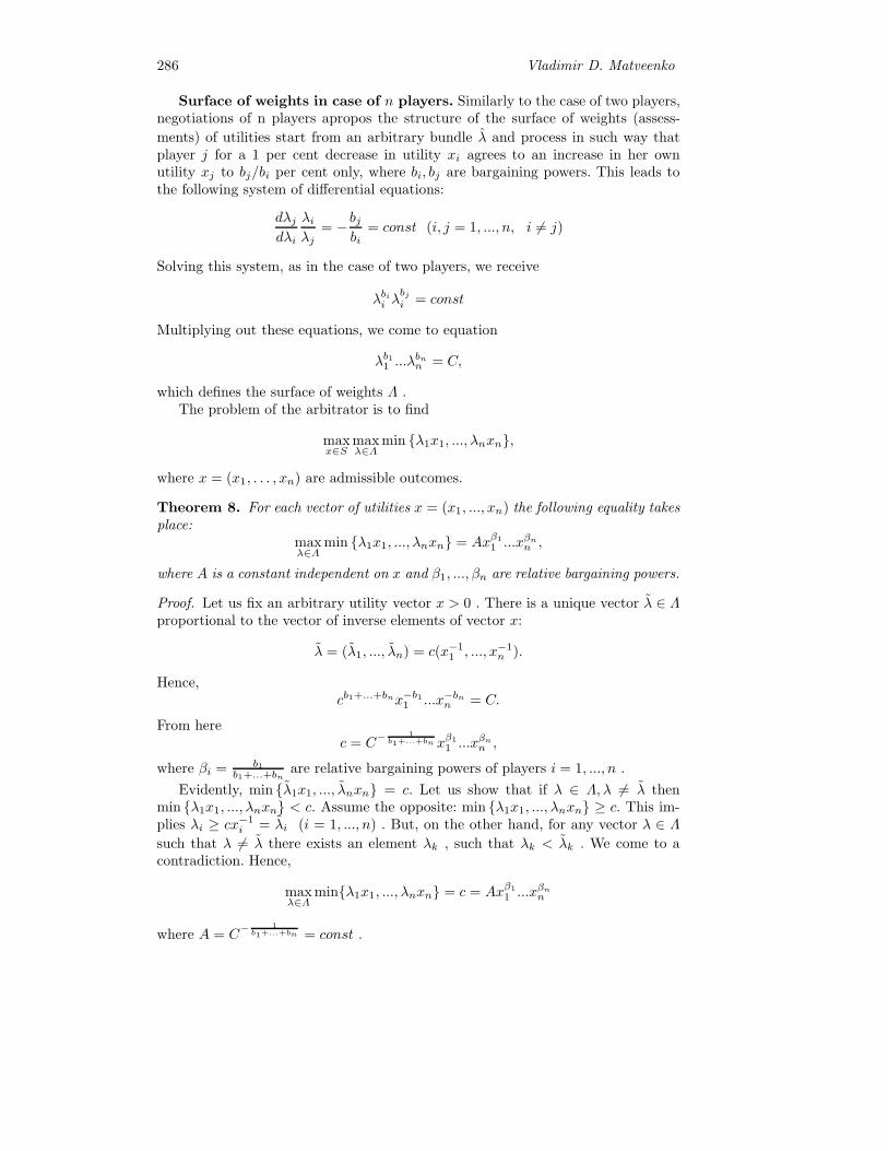
286 Vladimir D. Matveenko
Surface of weights in case of n players. Similarly to the case of two players,negotiations of n players apropos the structure of the surface of weights (assess-
ments) of utilities start from an arbitrary bundle λ and process in such way thatplayer j for a 1 per cent decrease in utility xi agrees to an increase in her ownutility xj to bj/bi per cent only, where bi, bj are bargaining powers. This leads tothe following system of differential equations:
dλjdλi
λiλj
= −bjbi
= const (i, j = 1, ..., n, i = j)
Solving this system, as in the case of two players, we receive
λbii λbji = const
Multiplying out these equations, we come to equation
λb11 ...λbnn = C,
which defines the surface of weights Λ .The problem of the arbitrator is to find
maxx∈S
maxλ∈Λ
min {λ1x1, ..., λnxn},
where x = (x1, . . . , xn) are admissible outcomes.
Theorem 8. For each vector of utilities x = (x1, ..., xn) the following equality takesplace:
maxλ∈Λ
min {λ1x1, ..., λnxn} = Axβ1
1 ...xβnn ,
where A is a constant independent on x and β1, ..., βn are relative bargaining powers.
Proof. Let us fix an arbitrary utility vector x > 0 . There is a unique vector λ ∈ Λproportional to the vector of inverse elements of vector x:
λ = (λ1, ..., λn) = c(x−11 , ..., x−1
n ).
Hence,cb1+...+bnx−b1
1 ...x−bnn = C.
From herec = C
− 1b1+...+bn xβ1
1 ...xβnn ,
where βi = b1b1+...+bn
are relative bargaining powers of players i = 1, ..., n .
Evidently, min {λ1x1, ..., λnxn} = c. Let us show that if λ ∈ Λ, λ = λ thenmin {λ1x1, ..., λnxn} < c. Assume the opposite: min {λ1x1, ..., λnxn} ≥ c. This im-plies λi ≥ cx−1
i = λi (i = 1, ..., n) . But, on the other hand, for any vector λ ∈ Λ
such that λ = λ there exists an element λk , such that λk < λk . We come to acontradiction. Hence,
maxλ∈Λ
min{λ1x1, ..., λnxn} = c = Axβ1
1 ...xβnn
where A = C− 1b1+...+bn = const .

Bargaining Powers, a Surface of Weights 287
In such way the arbitrator’s problem reduces to finding
maxx∈S
Axb11 ...xbnn ,
and we come to the asymmetric N.b.s.The maximin criterion, used here, reminds the Rawlsian criterion of fairness.
However, in our case the society (the arbitrator) looking in each point x for maxi-mum in λ plays in favor of a wealthier player by making worse (i.e. increasing) theweight of a more restrained player.
Similarly to the proof of Theorem 8, it can be proved that
minλ∈Λ
max{λ1x1, ..., λnxn} = c = Axβ1
1 ...xβnn .
It means that a ”Pharisee just” society for which the criterion is
maxx∈S
maxλ∈Λ
min {λ1x1, ..., λnxn}
does not differ in its accepted outcome from a society searching for
maxx∈S
minλ∈Λ
max {λ1x1, ..., λnxn}
and, thus, openly acting in favor of the most wealthy player by improving (i.e.decreasing) her weight.
In such way the model demonstrates that societies with different political mech-anisms may negligibly differ in economic and other objective characteristics of theiractivities.
Now let us show that the same surface of weights Λ provides the N.b.s. as autilitarian solution.
Theorem 9. Solution to the problem
maxx∈S
minλ∈Λ
n∑i=1
μixi, (18)
where μi = biλi (i = 1, ..., n), is
x, λ = (x−11 , ...., x−1
n ),
where x is the asymmetric N.b.s.
Proof. For problem minλ∈Λ
n∑i=1
μixi (with a fixed x) we construct a Lagrangian
L =
n∑i=1
μixi − ν(λb11 ...λbnn − C)
and derive the first order optimality conditions
bixi − νbiλbi−1i
∏k �=i
λbkk = 0 (i = 1, ..., n).
It follows thatxiλi = const (i = 1, ..., n),
and, by use of Theorem 3, the solution of problem (18) is the asymmetric N.b.s.

288 Vladimir D. Matveenko
4. Other bargaining solutions
It is interesting to compare, from the point of view of our two-stage game, theN.b.s. with two other well-known solutions of the bargaining problem: the Kalai-Smorodinsky solution (Kalai and Smorodinsky, 1975) and the Kalai egalitarian so-lution (Kalai, 1977b). In both of them, instead of a surface of weights, a fixed
bundle of weights λ1, ..., λn is used. The arbitrator chooses an outcome by solvingthe problem
maxx∈S
min {λ1x1, ..., λnxn}. (19)
Proposition 2. Problem (19) has a unique solution. This is vector x ∈ ParS
proportional to(
1λ1, ..., 1
λn
).
Proof. The vector x satisfies
λ1x1 = ... = λxn = c.
Let us show that min{λ1x1, ..., λnxn} < c for any x ∈ S, x = x. If the opposite is
true then λixi ≥ c for all i = 1, ..., n. On the other hand, there exists i such thatxi > xi and, hence, c/λi > xi . The contradiction implies that
maxx∈S
min{λ1x1, ..., λnxn} = c,
and solution is reached at the unique point x .
The logic of the Kalai-Smorodinsky solution (Kalai and Smorodinsky, 1975) is that’social indexes’ of players are defined by their maximal possible gains. Then in prob-lem (18) such weights λ1, ..., λn are used that the elements of vector ( 1
λ1, ..., 1
λn) are
proportional (with a common coefficient) to maximal values x1, ..., xn of coordinatesin set S. The solution is a vector x ∈ ParS proportional to x = (x1, ..., xn)
The egalitarian solution (Kalai, 1977b) starts from assumption that all playershave equal ’social indexes’. So, the arbitrator chooses a point solving the problem
maxx∈S
min{x1, ..., xn}.
It follows from Proposition 2 that the solution is a point x∗ with equal elements:
x∗1 = ... = x∗
n.
In case of weighted egalitarian solutions (Roth, 1979b) the surface of weightsalso consists of a single point.
5. Moral-ethical assessments as a mechanism of bargaining
Earlier we supposed that on the first stage of the game the surface (or curve)of weights Λ is constructed, and on the second stage the arbitrator (society) in aconcrete bargaining situation takes a maximin solution. Now let us consider anotherversion of the model: in a concrete bargain participants change weights gradually.Each player tries to diminish the weight of her own utility (or not to allow it toincrease) and to increase the weights of the others’ utilities. The arbitrator controlsthe bargaining process and does not allow the value of outcome, v(x), to diminish.

Bargaining Powers, a Surface of Weights 289
The following scheme can serve as a model. In a two-player game, if for a currentrelative weight, λi/λj , the value of outcome decreases in λi then player i attacksby decreasing her weight, λi , and increasing the other’s weight, λj . The arbitratorallows this as long as the value of outcome, v(x), increases. In these circumstances acounter-attack of player j is impossible because it would lead to a decrease in v(x)what is not allowed by the arbitrator. Player j in this situation can only defendherself using her bargaining power to restrict the decrease in weight λi and theincrease in weight λj . The attack of player i can continue only as long as the valueof outcome, v(x), increases. With continuous time, this process stops as soon as thevalue of outcome v(x) reaches its maximum at point x of the asymmetric N.b.s.
The process can be modeled, for example, by a differential game reducing to thefollowing differential equation which describes a path in the curve Λ as well as acorresponding path in the Pareto frontier of the set S:
λ1
λ1=
⎧⎪⎪⎪⎪⎨⎪⎪⎪⎪⎩−β, if λ1x1 + λ1x1 > 0
(and λ2x2 + λ2x2 < 0
)β, if λ1x1 + λ1x1 < 0
(and λ2x2 + λ2x2 > 0
)0, if λ1x1 + λ1x1 = 0
(and λ2x2 + λ2x2 = 0
).This game leads to a point x described by equations
λ1x1 + λ1x1 = 0, (20)
λ2x2 + λ2x2 = 0.
Hence,dλ1
dλ2
λ2
λ1=
dx1(x)
dx2
x2
x1.
The LHS is equal to −b2/b1. According to Theorem 4, x is the asymmetric N.b.s.A more straightforward proof follows. Let the Pareto frontier of set S be defined
by curve x2 = g(x1). The curve of weights, Λ, is λb11 λb22 = 1. To each vector λ ∈ Λan outcome x ∈ ParS corresponds satisfying equation λ1x1 = λ2x2. It follows that
λ1 =
(g(x1)
x1
) b2b1+b2
.
Transforming, we come to the following form of equation (20):
b2g′(x1)x1 + b1g(x1) = 0. (21)
Equation (21) defines the symmetric N.b.s., as soon as maxx∈S xb11 xb22 is reached
under (21).
6. N.b.s. and Cobb-Douglas production function
One more possible area of application of the N.b.s. is the theory of economic growth.Remind that, according to the neoclassical theory, the Cobb-Douglas productionfunction Y = AKαL1−α (where Y is output, K is capital, and L is labor) reflectsnot only production but also distribution of product: under conditions of perfectcompetition, parameters α and 1−α are not only elasticities of output with respect

290 Vladimir D. Matveenko
to production factors but are also shares of the owners of production factors. Inrecent time a series of research appeared demonstrating a difference in labor andcapital shares in countries of the World (in average, in developing countries thecapital share is higher than in industrial countries) and changes in the factor sharesin time (the capital share increases in all groups of countries). It is possible to usethe N.b.s. concept to explain the differences between countries and the tendency ofchanges in the shares. A constancy of bargaining powers can explain a constancyof factor shares (a validity of the corresponding Kaldor’s stylized fact) in somecountries on a definite stage of their development.
Let us consider a model with two social groups: workers and owners of capital(entrepreneurs) who possess bargaining powers bL and bK , correspondingly, andbargain apropos partition of the national product. The N.b.s. is realized by use ofthe mechanism of propaganda and moral-ethical assessments described above andleads to a distribution of the product in shares bL and bK . To ensure a possibilityof such distribution the social groups choose those production technologies (andfields of specialization of the economy) for which factor elasticities 1 − α = bL
bK+bL
and α = bKbK+bL
are used in the Cobb-Douglas production function. The choice oftechnologies can take place both on stage of R&D and on stage of production (e.g.,workers can violate technologies to receive in result a demanded share of output.This can explain, for example, a tolerance of society to small and big plundering inmanufacturing in the USSR).
The process can be modeled by the two-stage game described above. On thefirst stage two players (entrepreneurs and workers) form a curve Λ = (λK , λL) ofadmissible moral-ethical assessments (weights). On the second stage an arbitrator(society) chooses an admissible pair of weights and divides the product Y amongthe players (Y = YK + YL) to achieve the maximin
maxY,λ
min{λKYK , λLYL}.
The curve of weights formed on the first stage of the game is
λbKK λbLL = C.
For the second stage of the game, Theorem 7 implies the following statement.
Theorem 10. For each outcome (YK , YL) (where YK + YL = const):
maxλ∈Λ
min{λKYK , λLYL} = AYbK
bK+bL
K YbL
bK+bL
L ,
where A = const.
Thus, the arbitrator’s problem reduces to the asymmetric N.b.s. The solution, ascan be easily seen, implies that the players receive shares proportional to theirbargaining powers:
YKYL
=bKbL
.
For such distribution to be possible, the players will choose those technologies (andthose fields of specialization of the economy) under which factor elasticities used ina Cobb-Douglas production function are proportional to the bargaining powers.

Bargaining Powers, a Surface of Weights 291
In relation with globalization, there is a question of stability of a product par-tition between participants of the global production process. The basic argumentof anti-globalists is a reduction in the labor share in advanced countries which isexplained by extension of production in developing countries.
Let us consider a model with three participants: an entrepreneur (a transnationalcompany) acting in two countries and workers (unions) of these two countries. Cap-ital is mobile, in contrast to labor. Will an equilibrium reached inside the countrieson base of ’inner’ bargaining powers of the participants coincide with an equilibriumwhich would arise if the three participants meet in ’global’ negotiations? (In case ofa non-coincidence, one of the social groups would be interested in a revision of the”World order”, and the equilibrium would not be stable). We will find bargainingpowers under which such coincidence takes place.
Let inner bargaining powers of the entrepreneur and the workers be α1, 1 − α1
in country 1 and α2, 1 − α2 in country 2. As a result of a choice of technologiescorresponding to the desired partition of the product, the production functions areA1K
α11 L1−α1
1 and A2Kα22 L1−α2
2 . These functions can also be written as Kα11 L1−α1
1
and Kα22 L1−α2
2 where Li = A1
1−αi Li is the effective labor in country i (i = 1, 2).
The entrepreneur will place the total capital K in a way to equalize the marginalproducts of capital in the countries:
α1Kα1−11 L1−α1
1 = α2Kα2−12 L1−α2
2 .
Denote α, β, γ bargaining powers of participants in a global bargain, α+ β + γ = 1.A coincidence of the equilibria achieved in the inner and in the global bargainsmeans holding equations:
α = α1Y1
Y1 + Y2+ α2
Y2
Y1 + Y2, β = (1− α1)
Y1
Y1 + Y2, γ = (1− α2)
Y2
Y1 + Y2.
Thus, in equilibrium, the workers of country i possess in the global bargain abargaining power equal to their inner bargaining power, 1 − αi with a discountingweight χi = Yi
Y1+Y2equal to the country’s share in the global output. The global
bargaining power of the entrepreneur is equal to the convex combination of herinner bargaining powers αi with the weights χi (i = 1, 2).
Let us consider a case when inner bargaining powers in both countries are thesame: α and 1− α . Then
K α−11 L1−α
1 = K α−12 L1−α
2 .
From here,
K1 =KL1
L1 + L2
,K2 =KL2
L1 + L2
.
Thus, the entrepreneur places the capital proportionally to the effective labor. Inthe global bargaining,
α = α,
β = (1− α)Y1
Y1 + Y2= (1− α)
L1
L1 + L2
,
γ = (1− α)L2
L1 + L2
.

292 Vladimir D. Matveenko
Therefore, for holding the equilibrium, the bargaining power of the entrepreneurin the global bargaining has to be the same as in the inner bargaining, and thebargaining powers of the workers have to be proportional to their effective labor.Each of the two groups of workers has in the global bargaining a bargaining powerless than in the inner bargaining. If the bargaining powers of the two groups ofworkers are summed up, the ”united labor” would have the same bargaining poweras the workers have in inner bargains in each of the countries. In general, this doesnot contradict an intuitive idea of a global bargaining and a partition of the worldgross product.
7. Conclusion
The Nash bargaining solution (N.b.s.) takes a central place in the theory of bargain-ing. Research in this paper differs essentially from known approaches to the N.b.s.which were based, as a rule, either on a choice of axioms of a fair distribution whenparticipants play a purely passive role, or on a choice of a stopping rule in negotia-tions with reference to a concrete bargain. In the present model negotiations relateto a system of weights, Λ. In the negotiations participants exhibit their bargainingpowers. The set Λ can be used not in a single bargain but in a set of bargains ofthe same participants. A special role is plaid by an arbitrator interpreted here as acommunity (society).
A relation between bargaining powers, ’utilitarian’ weights and ’egalitarian weightsis studied. In particular, a cobweb procedure leading to the N.b.s. is considered.
We studied a two-stage game, where on the first stage the players form a setΛ of all possible bundles of weights, and on the second stage, for a concrete bar-gain, the arbitrator finds a maximin solution. We showed that this game leads tothe asymmetric N.b.s. Also it is shown that two other well-known bargaining solu-tions, Kalai-Smorodinsky and egalitarian, can be received as special cases with Λconsisting of a single bundle of weights.
As an example of application of the ideas elaborated in the paper we propose amodel where the asymmetric N.b.s. leads to the Cobb-Douglas production function.
References
Alesina, A. (1987). Macroeconomic policy in a two-party system as a repeated game. Quar-terly Journal of Economics, 102, 651–678.
Aumann, R. J. (1985). An axiomatization of the non-transferable utility value. Economet-rica, 53, 599–612.
Bester, H. (1993). Bargaining versus price competition in markets with quality uncertainty.American Economic Review, 83, 278–288.
Binmore, K. (1998). Egalitarianism versus utilitarianism. Utilitas, 10, 353–367.Binmore, K. (2005). Natural justice. Oxford, Oxford University Press.Binmore, K. (2009). Interpersonal comparison in egalitarian societies. European Journal
of Political Economy. In press, available online.Binmore, K., A. Rubinstein and A. Wolinsky (1986). The Nash bargaining solution in
economic modelling. RAND Journal of Economics, 17, 176–188.Carlsson, H. (1991). A bargaining model where parties make errors. Econometrica, 59,
1487–1496.Caves, R. E., J. A. Frankel and R. W. Jones (2006). World trade and payments: an intro-
duction. 10th ed. New York, Addison and Wesley.Grout, P. A. (1984). Investment and wages in the absence of binding contracts: A Nash
bargaining approach. Econometrica, 52, 449–460.

Bargaining Powers, a Surface of Weights 293
Eismont, O. A. (2010). Analysis of Russian-European gas strategies. In: E. Yasin, ed. X In-ternational Conference on Problems of Development of Economy and Society. Moscow,HSE Publishing House, 185–196. (In Russian)
Harsanyi, J. C. (1963). A simplified bargaining model for the n-person cooperative game.International Economic Review, 4, 194–220.
Harsanyi, J. and R. Selten (1972). A generalized Nash solution for two-person bargaininggames with incomplete information. Management Science, 18, 80–106.
Hellman, T. and P. Perotti (2006). The circulation of ideas: Firms versus markets. CEPRDiscussion Papers 5469.
Kalai, E. (1977a). Nonsymmetric Nash solutions and replications of 2-person bargaining.International Journal of Game Theory, 6, 129-133.
Kalai, E. (1977b). Proportional solutions to bargaining situations: Interpersonal utilitycomparisons. Econometrica, 45, 1623–1630.
Kalai, E. and M. Smorodinsky (1975). Other solution to Nash’s bargaining problem. Econo-metrica, 43, 513–518.
Nash, J. F. (1950). The bargaining problem. Econometrica, 18, 155–162.Nash, J. F. (1953). Two-person cooperative games. Econometrica, 21, 128–140.Roth, A. E. (1979a). Axiomatic models of bargaining. Berlin, Springer Verlag.Roth, A. E. (1979b). Proportional solutions to the bargaining problem. Econometrica, 47,
775–780.Serrano, R. (2008). Bargaining. In: S. Durlauf and L. Blume, eds. New Palgrave Dictionary
of Economics, 2nd ed., v. 1. London, McMillan, 370–380.Shapley, L. S. (1969). Utility comparison and the theory of games. In: G.T. Guilband, ed.
La decision: Agregation et dynamique des orders de preference. Paris, Editions duCNRS, 251–263.
Rubinstein, A. (1982). Perfect equilibrium in a bargaining model. Econometrica, 50, 207–211.
Thomson, W. (1994). Cooperative models of bargaining. In: R.T. Aumann and S. Hart,eds. Handbook of game theory. New York, North-Holland, 1237–1248.
Thomson, W. and T. Lensberg (1989). Axiomatic theory of bargaining with a variablenumber of agents. Cambridge, Cambridge University Press.
Yaari, M. E. (1981). Rawls, Edgeworth, Shapley, Nash: Theories of distributive justice re-examined. Journal of Economic Theory, 24, 1–39.

On Games with Constant Nash Sum
Pierre von Mouche
Wageningen Universiteit,Hollandseweg 1, 6700 EW, Wageningen, The Netherlands
E-mail: [email protected] home page: http://www.pvmouche.de
Abstract. A class of games in strategic form with the following property isidentified: for every n ∈ E, i.e. Nash equilibrium, the (Nash) sum
∑l n
l isconstant. For such a game sufficient conditions for E to be polyhedral andsemi-uniqueness (i.e. #E ≤ 1) are given. The abstract results are illustratedby applying them to a class of games that covers various types of Cournotoligopoly and transboundary pollution games. The way of obtaining theresults is by analysing so-called left and right marginal reductions.
Keywords: Oligopoly, transboundary pollution, Hahn conditions, aggrega-tive game, co-strategy mapping, marginal reduction, non-differentiable pay-off function, structure of set of Nash equilibria, game in strategic form,convex analysis.
1. Introduction
In Szidarovszky and Yakowitz (1982) the following result was proven for the set ofCournot equilibria E of a homogeneous Cournot oligopoly game with N oligopolists:1
Theorem 1. Suppose that each oligopolist has a capacity constraint, the inversedemand function p is concave, decreasing and continuous, and each cost function ci
is convex, increasing and continuous. Then:
I. #E ≥ 1.
II. If each ci is strictly convex or p is strictly decreasing, then:
1. the Nash sum is constant, i.e. there exists Ψ ≥ 0 such that∑N
l=1 nl = Ψ for
all n ∈ E;
2. E is polyhedral.
III. In case p is differentiable, each of the following conditions separately is sufficientfor #E ≤ 1:
1. each ci is strictly convex;
2. p′ < 0. �
1 In this article I understand by a Cournot oligopoly game a game in strategic form withN(≥ 1) players where a player i has strategy set Xi = [0, mi] (capacity constraint mi >0) or Xi = IR+ and payoff function πi(x) = pi(
∑Nl=1 tlx
l)xi − ci(xi). Here ci : Xi → IR
is his cost function and, with Y :=∑N
l=1 tlXl and the tl > 0, pi : Y → IR is his inverse
demand function. With the differentiable case I refer to a Cournot oligopoly game whereall cost functions and inverse demand functions are differentiable. If p1 = · · · = pN =: pand t1 = · · · = tN = 1, then the Cournot oligopoly game is homogeneous.
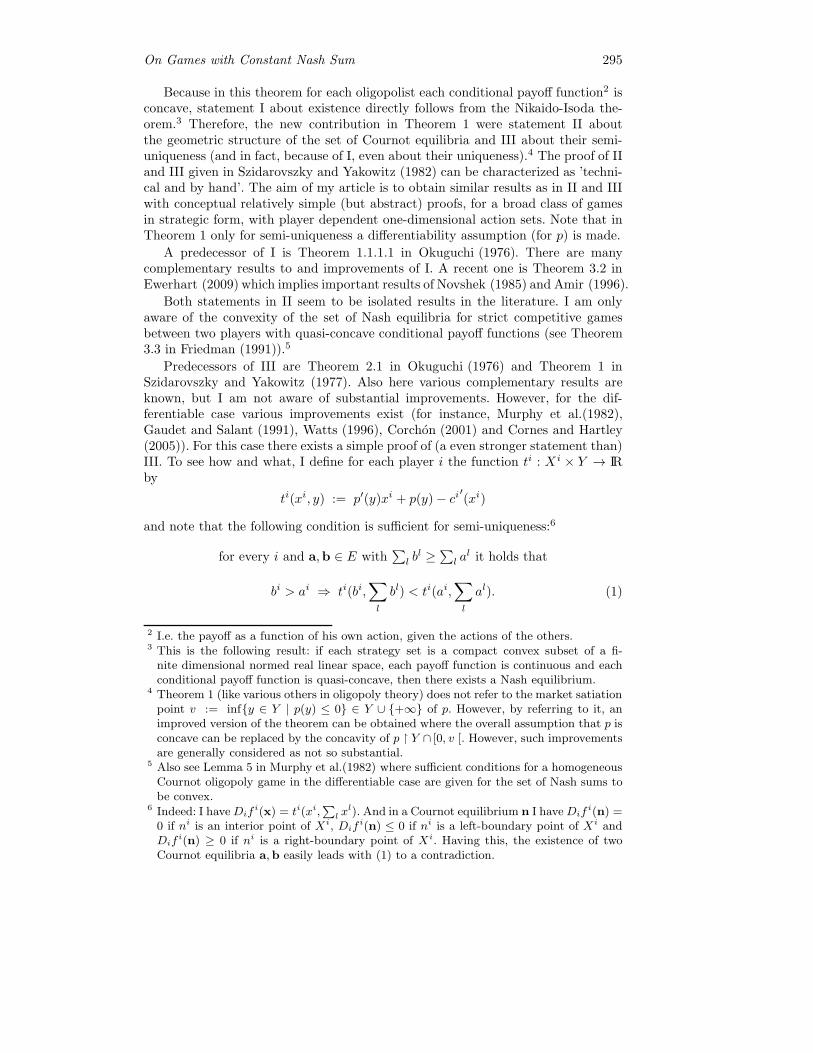
On Games with Constant Nash Sum 295
Because in this theorem for each oligopolist each conditional payoff function2 isconcave, statement I about existence directly follows from the Nikaido-Isoda the-orem.3 Therefore, the new contribution in Theorem 1 were statement II aboutthe geometric structure of the set of Cournot equilibria and III about their semi-uniqueness (and in fact, because of I, even about their uniqueness).4 The proof of IIand III given in Szidarovszky and Yakowitz (1982) can be characterized as ’techni-cal and by hand’. The aim of my article is to obtain similar results as in II and IIIwith conceptual relatively simple (but abstract) proofs, for a broad class of gamesin strategic form, with player dependent one-dimensional action sets. Note that inTheorem 1 only for semi-uniqueness a differentiability assumption (for p) is made.
A predecessor of I is Theorem 1.1.1.1 in Okuguchi (1976). There are manycomplementary results to and improvements of I. A recent one is Theorem 3.2 inEwerhart (2009) which implies important results of Novshek (1985) and Amir (1996).
Both statements in II seem to be isolated results in the literature. I am onlyaware of the convexity of the set of Nash equilibria for strict competitive gamesbetween two players with quasi-concave conditional payoff functions (see Theorem3.3 in Friedman (1991)).5
Predecessors of III are Theorem 2.1 in Okuguchi (1976) and Theorem 1 inSzidarovszky and Yakowitz (1977). Also here various complementary results areknown, but I am not aware of substantial improvements. However, for the dif-ferentiable case various improvements exist (for instance, Murphy et al.(1982),Gaudet and Salant (1991), Watts (1996), Corchon (2001) and Cornes and Hartley(2005)). For this case there exists a simple proof of (a even stronger statement than)III. To see how and what, I define for each player i the function ti : X i × Y → IRby
ti(xi, y) := p′(y)xi + p(y)− ci′(xi)
and note that the following condition is sufficient for semi-uniqueness:6
for every i and a,b ∈ E with∑l bl ≥∑l al it holds that
bi > ai ⇒ ti(bi,∑l
bl) < ti(ai,∑l
al). (1)
2 I.e. the payoff as a function of his own action, given the actions of the others.3 This is the following result: if each strategy set is a compact convex subset of a fi-
nite dimensional normed real linear space, each payoff function is continuous and eachconditional payoff function is quasi-concave, then there exists a Nash equilibrium.
4 Theorem 1 (like various others in oligopoly theory) does not refer to the market satiationpoint v := inf{y ∈ Y | p(y) ≤ 0} ∈ Y ∪ {+∞} of p. However, by referring to it, animproved version of the theorem can be obtained where the overall assumption that p isconcave can be replaced by the concavity of p � Y ∩ [0, v [. However, such improvementsare generally considered as not so substantial.
5 Also see Lemma 5 in Murphy et al.(1982) where sufficient conditions for a homogeneousCournot oligopoly game in the differentiable case are given for the set of Nash sums tobe convex.
6 Indeed: I haveDifi(x) = ti(xi,
∑l x
l). And in a Cournot equilibrium n I have Difi(n) =
0 if ni is an interior point of Xi, Difi(n) ≤ 0 if ni is a left-boundary point of Xi and
Difi(n) ≥ 0 if ni is a right-boundary point of Xi. Having this, the existence of two
Cournot equilibria a,b easily leads with (1) to a contradiction.

296 Pierre von Mouche
Next note that sufficient (but not necessary) for (1) to hold is that ti is strictlydecreasing in its first variable and decreasing in its second.7 Sufficient for this inturn is that p and the ci are twice differentiable and D1t
i = p′(y)−ci′′(xi) < 0 (first
Hahn condition) and D2ti = p′(y) + p′′(y)xi ≤ 0 (second Hahn condition) hold.
I will refer to the above ti as marginal reductions. They first were systematicallyused in Corchon (2001) in the context of uniqueness results for aggregative games.The given proof in footnote 6 is obtained by a slight adaptation of the proof (ofthe semi-uniqueness part) of Proposition 1.3 in Corchon (2001). Note that in (1)in fact only local conditions at Nash equilibria matter: it is not necessary that thedefinition of ti globally makes sense. By studying for the differentiable case8 theglobal properties of the marginal reductions ti by means of the correspondencesbi(y) := {xi ∈ X i | ti(xi, y) = 0} a very strong uniqueness result was obtained.The conditions in this result involve a strong variant of the first Hahn-conditionand, a local condition at Nash equilibria (involving a sum of quotients D2t
i/D1ti).
The games I will deal with encompass various aggregative games with non-differentiable conditional payoff functions. I give with Corollary 1 sufficient (local)conditions for the Nash sum to be constant, and more generally for a functionΦ : X → IRN , to be referred as co-strategy mapping, to be constant on the set ofNash equilibria E. Corollary 2 gives sufficient (local) conditions for #E ≤ 1. Theo-rem 2 provides a class of games with concave conditional payoff functions for whichE is polyhedral. The power of these results is illustrated by applying them to whatI call transboundary Cournot games. In particular such a game allows for a Cournotoligopoly game and for a transboundary pollution game with uniform pollution(see, for instance, Finus (2001) and Folmer and von Mouche (2002)). Transbound-ary pollution games are in some sense dual to Cournot oligopoly games. The mainresult for transboundary Cournot games is Theorem 3; it implies and intrinsicallyimproves Theorem 1.
In order to obtain my results, I use some standard results of convex analysisand refine the ideas in Folmer and von Mouche (2004) and von Mouche (2009). Ingeneral I do not suppose that conditional payoff functions are differentiable. ButI generally make the (weak) assumption that their left and right derivatives exist(in IR := IR ∪ {−∞,+∞}) in Nash equilibria.9 This leads to the concept of rightmarginal reductions T i+ and left marginal reductions T i−. My method consists in amainly local analysis of them; special care is needed to deal in a correct way withboundaries and infinite derivatives.
2. Notations and Co-strategy Mappings
I use the following notations for a subset C of IR:
∂−(C) :=
{{min (C)} if min (C) exists∅ if min (C) does not exist,
∂+(C) :=
{{max (C)} if max (C) exists∅ if max (C) does not exist;
C− := (C \ ∂+(C)) ∪ ∂−(C), C+ := (C \ ∂−(C)) ∪ ∂+(C);
7 Note that then all conditional payoff functions are strictly concave (and therefore exis-tence is guaranteed in case of capacity constraints).
8 Strictly speaking for a situation with a market satiation point v > 0 and p differentiableon [0, v[. In fact there bi : [0, v [� IR.
9 Note that this assumption implicitly even globally holds in Theorem 1 because eachconditional payoff function is concave.

On Games with Constant Nash Sum 297
Int(C) := the topological interior of C.
Now10
∂+(C) ⊆ C+, ∂−(C) ⊆ C−, Int(C) ⊆ C− ⊆ C, Int(C) ⊆ C+ ⊆ C;
C = C− ∪ ∂+(C) = C+ ∪ ∂−(C). (2)
For the whole article I fix a positive integer N , and writing,
N := {1, . . . , N},
I also fix subsetsX i (i ∈ N )
of IR and assume
every X i is a non-degenerate interval.11
I writeX := X1 × · · · ×XN ,
Xı := X1 × · · · ×X i−1 ×X i+1 × · · · ×XN (i ∈ N )
and sometimes identify X with X i ×Xı and then write x ∈ X as x = (xi;xı).A co-strategy function for player i is a function
ϕi : X→ IR
and a co-strategy mapping is a mapping
Φ = (ϕ1, . . . , ϕN ) : X→ IRN .
Given a co-strategy function ϕi, I write
Y i := ϕi(X).
For a subset Z of X, I write
Z(Z) := {i ∈ N | there exist a,b ∈ Z with ai = bi}.
For a subset Z of X, a co-strategy mapping Φ and i ∈ N , the following (weak)Property F iw(Z,Φ) and (strong) Property F is(Z,Φ) will be dealt with:
Property F iw(Z,Φ). For all a,b ∈ Z: Φ(b) Φ(a) ⇒ bi ≤ ai.
Property F is(Z,Φ). For all a,b ∈ Z: Φ(b) ≥ Φ(a) ⇒ bi ≤ ai.
Lemma 1. Let Z be a subset of X and Φ a co-strategy mapping. Each of the fol-lowing conditions separately is sufficient for Φ � Z to be constant:
10 Example: if C = ]−3, 1], then Int(C) = ]−3, 1[, ∂−(C) = ∅, ∂+(C) = {1}, C− = ]−3, 1[and C+ = ]− 3, 1]. And if C = {3}, then Int(C) = ∅ and ∂−(C) = ∂+(C) = C− = C+ ={3}.
11 I.e. a convex subset of IR containing more than one and therefore infinitely many ele-ments.
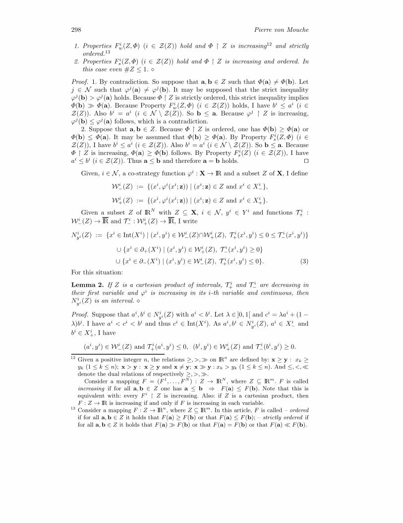
298 Pierre von Mouche
1. Properties F iw(Z,Φ) (i ∈ Z(Z)) hold and Φ � Z is increasing12 and strictlyordered.13
2. Properties F is(Z,Φ) (i ∈ Z(Z)) hold and Φ � Z is increasing and ordered. Inthis case even #Z ≤ 1. �
Proof. 1. By contradiction. So suppose that a,b ∈ Z such that Φ(a) = Φ(b). Letj ∈ N such that ϕj(a) = ϕj(b). It may be supposed that the strict inequalityϕj(b) > ϕj(a) holds. Because Φ � Z is strictly ordered, this strict inequality impliesΦ(b) Φ(a). Because Property F iw(Z,Φ) (i ∈ Z(Z)) holds, I have bi ≤ ai (i ∈Z(Z)). Also bi = ai (i ∈ N \ Z(Z)). So b ≤ a. Because ϕj � Z is increasing,ϕj(b) ≤ ϕj(a) follows, which is a contradiction.
2. Suppose that a,b ∈ Z. Because Φ � Z is ordered, one has Φ(b) ≥ Φ(a) orΦ(b) ≤ Φ(a). It may be assumed that Φ(b) ≥ Φ(a). By Property F is(Z,Φ) (i ∈Z(Z)), I have bi ≤ ai (i ∈ Z(Z)). Also bi = ai (i ∈ N \ Z(Z)). So b ≤ a. BecauseΦ � Z is increasing, Φ(a) ≥ Φ(b) follows. By Property F is(Z) (i ∈ Z(Z)), I haveai ≤ bi (i ∈ Z(Z)). Thus a ≤ b and therefore a = b holds. ��
Given, i ∈ N , a co-strategy function ϕi : X→ IR and a subset Z of X, I define
W i−(Z) := {(xi, ϕi(xi; z)) | (xi; z) ∈ Z and xi ∈ X i
−},
W i+(Z) := {(xi, ϕi(xi; z)) | (xi; z) ∈ Z and xi ∈ X i
+}.
Given a subset Z of IRN with Z ⊆ X, i ∈ N , yi ∈ Y i and functions T i+ :
W i−(Z)→ IR and T i− :W i
+(Z)→ IR, I write
N iyi(Z) := {xi ∈ Int(X i) | (xi, yi) ∈ W i
−(Z)∩W i+(Z), T i+(xi, yi) ≤ 0 ≤ T i−(xi, yi)}
∪ {xi ∈ ∂+(X i) | (xi, yi) ∈ W i+(Z), T i−(xi, yi) ≥ 0}
∪ {xi ∈ ∂−(X i) | (xi, yi) ∈ W i−(Z), T i+(xi, yi) ≤ 0}. (3)
For this situation:
Lemma 2. If Z is a cartesian product of intervals, T i+ and T i− are decreasing intheir first variable and ϕi is increasing in its i-th variable and continuous, thenN iyi(Z) is an interval. �
Proof. Suppose that ai, bi ∈ N iyi(Z) with ai < bi. Let λ ∈ ]0, 1[ and ci = λai + (1−
λ)bi. I have ai < ci < bi and thus ci ∈ Int(X i). As ai, bi ∈ N iyi(Z), ai ∈ X i
− and
bi ∈ X i+, I have
(ai, yi) ∈ W i−(Z) and T i+(ai, yi) ≤ 0, (bi, yi) ∈ W i
+(Z) and T i−(bi, yi) ≥ 0.
12 Given a positive integer n, the relations ≥, >,� on IRn are defined by: x ≥ y : xk ≥yk (1 ≤ k ≤ n); x > y : x ≥ y and x �= y; x � y : xk > yk (1 ≤ k ≤ n). And ≤, <, denote the dual relations of respectively ≥, >,�.
Consider a mapping F = (F 1, . . . , FN ) : Z → IRN , where Z ⊆ IRm. F is calledincreasing if for all a,b ∈ Z one has a ≤ b ⇒ F (a) ≤ F (b). Note that this isequivalent with: every F i � Z is increasing. Also: if Z is a cartesian product, thenF : Z → IR is increasing if and only if F is increasing in each variable.
13 Consider a mapping F : Z → IRn, where Z ⊆ IRm. In this article, F is called – orderedif for all a,b ∈ Z it holds that F (a) ≥ F (b) or that F (a) ≤ F (b); – strictly ordered iffor all a,b ∈ Z it holds that F (a) � F (b) or that F (a) = F (b) or that F (a) F (b).

On Games with Constant Nash Sum 299
Also(ci, yi) ∈ W i
−(Z) ∩W i+(Z).
Indeed: as (ai, yi) ∈ W i−(Z), there exists z ∈ Xı such that (ai; z) ∈ Z and yi =
ϕi(ai; z). As (bi, yi) ∈ W i+(Z), there exists z′ ∈ Xı such that (bi; z′) ∈ Z and
yi = ϕi(bi; z′). As ϕi is increasing in its i-th variable, ϕi(ci; z) ≥ ϕi(ai; z) = yi =ϕi(bi; z′) ≥ ϕi(ci; z′). So ϕi(ci; z) ≥ yi ≥ ϕi(ci; z′). As ϕi is continuous, it followsthat there exists μ ∈ [0, 1] such that for z′′ := μz + (1− μ)z′ I have
yi = ϕi(ci; z′′).
As Z is a cartesian product of intervals, I have (ci; z′′) ∈ Z. It follows that (ci, yi) ∈W i
−(Z) ∩W i+(Z). Because T i+ :W i
−(Z)→ IR and T i− : W i+(Z)→ IR are increasing
in their first variable, I have
T i+(ci, yi) ≤ T i+(ai, yi) ≤ 0 ≤ T i−(bi, yi) ≤ T i−(ci, yi).
Thus ci ∈ N iyi(Z). ��
3. Marginal Reductions
In this section and in the next three I always consider a game in strategic form, withN as the set of players, with X i as strategy set for player i and with f i : X → IRhis payoff function. The set of of Nash equilibria is denoted by
E.
Notation: with (D+i f
i(x) (D−i f
i(x)) I denote the right (left) partial derivativeof f i w.r.t. its i-th variable in x.
Definition 1. Let i ∈ N and Z a subset of X.A two-tuple (T i+, ϕi) with
ϕi : X→ IR a (co-strategy) function and T i+ : W i− → IR a function
where W i− ⊆ X i × Y i such that W i
−(Z) ⊆W i−, is called a right marginal reduction
of f i on Z (with domain W i−) if for every x ∈ Z with xi ∈ X i
−:
– xi ∈ Int(X i) ⇒ f i is right partially differentiable w.r.t. its i-th variable in x;– xi ∈ ∂−(X i) ⇒ the right partial derivative of f i w.r.t. its i-th variable exists in
x as element of IR;– D+
i fi(x) = T i+(xi, ϕi(x)).
A two-tuple (T i−, ϕi, Z), with
ϕi : X→ IR a (co-strategy) function and T i− : W i+ → IR a function
where W i+ ⊆ X i × Y i such that W i
+(Z) ⊆ W i+, is called a left marginal reduction
of f i on Z (with domain W i+) if for every x ∈ Z with xi ∈ X i
+:
– xi ∈ Int(X i) ⇒ f i is left partially differentiable w.r.t. its i-th variable in x;– xi ∈ ∂+(X i) ⇒ the left partial derivative of f i w.r.t. its i-th variable exists in
x as element of IR;
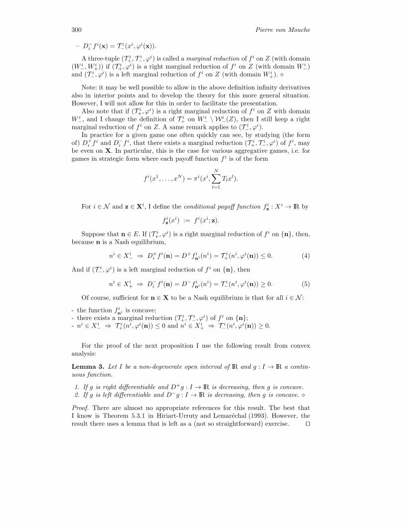
300 Pierre von Mouche
– D−i f
i(x) = T i−(xi, ϕi(x)).
A three-tuple (T i+, T i−, ϕi) is called a marginal reduction of f i on Z (with domain(W i
−,Wi+)) if (T i+, ϕi) is a right marginal reduction of f i on Z (with domain W i
−)and (T i−, ϕi) is a left marginal reduction of f i on Z (with domain W i
+). �
Note: it may be well possible to allow in the above definition infinity derivativesalso in interior points and to develop the theory for this more general situation.However, I will not allow for this in order to facilitate the presentation.
Also note that if (T i+, ϕi) is a right marginal reduction of f i on Z with domainW i
−, and I change the definition of T i+ on W i− \ W i
−(Z), then I still keep a rightmarginal reduction of f i on Z. A same remark applies to (T i−, ϕi).
In practice for a given game one often quickly can see, by studying (the formof) D+
i fi and D−
i fi, that there exists a marginal reduction (T i+, T i−, ϕi) of f i, may
be even on X. In particular, this is the case for various aggregative games, i.e. forgames in strategic form where each payoff function f i is of the form
f i(x1, . . . , xN ) = πi(xi,
N∑l=1
Tlxl).
For i ∈ N and z ∈ Xı, I define the conditional payoff function f iz : X i → IR by
f iz(xi) := f i(xi; z).
Suppose that n ∈ E. If (T i+, ϕi) is a right marginal reduction of f i on {n}, then,because n is a Nash equilibrium,
ni ∈ X i− ⇒ D+
i fi(n) = D+f inı(n
i) = T i+(ni, ϕi(n)) ≤ 0. (4)
And if (T i−, ϕi) is a left marginal reduction of f i on {n}, then
ni ∈ X i+ ⇒ D−
i fi(n) = D−f inı(n
i) = T i−(ni, ϕi(n)) ≥ 0. (5)
Of course, sufficient for n ∈ X to be a Nash equilibrium is that for all i ∈ N :
- the function f inı is concave;- there exists a marginal reduction (T i+, T i−, ϕi) of f i on {n};- ni ∈ X i
− ⇒ T i+(ni, ϕi(n)) ≤ 0 and ni ∈ X i+ ⇒ T i−(ni, ϕi(n)) ≥ 0.
For the proof of the next proposition I use the following result from convexanalysis:
Lemma 3. Let I be a non-degenerate open interval of IR and g : I → IR a contin-uous function.
1. If g is right differentiable and D+g : I → IR is decreasing, then g is concave.2. If g is left differentiable and D−g : I → IR is decreasing, then g is concave. �
Proof. There are almost no appropriate references for this result. The best thatI know is Theorem 5.3.1 in Hiriart-Urruty and Lemarechal (1993). However, theresult there uses a lemma that is left as a (not so straightforward) exercise. ��
On Games with Constant Nash Sum 301
Proposition 1. Let i ∈ N and z ∈ Xı. Suppose that the conditional payoff functionf iz is lower semi-continuous and continuous in each interior point of X i. For f iz tobe concave it is sufficient that ϕi is increasing in its i-th variable and that one ofthe following two properties holds:
I. There exists a right marginal reduction (T i+, ϕi) of f i on Int(X i) × {z} withdomain W i
− such that
a. If (ai, yi) ∈ W i− and bi ∈ Int(X i) with bi > ai, then also (bi, yi) ∈W i
−;
b. T i+ : W i− → IR is decreasing in both variables.
II. There exists a left marginal reduction (T i−, ϕi) of f i on Int(X i) × {z} withdomain W i
+ such that
a. If (ai, yi) ∈ W i+ and bi ∈ Int(X i) with bi > ai, then also (bi, yi) ∈W i
+;
b. T i− : W i+ → IR is decreasing in both variables. �
Proof. I assume that condition I holds; if II holds, the proof is analogous. I willprove that the function g := f iz � Int(X i) is concave; the lower semi-continuity off iz then implies its concavity.
Because (T i+, ϕi) is a right marginal reduction of f i on Int(X i)× {z}, it followsthat for xi ∈ Int(X i), g is right differentiable in xi and D+g(xi) = T i+(xi, ϕi(xi; z)).By Lemma 3, g is concave if D+g is decreasing. So take ai, bi ∈ Int(X i) with ai < bi.As ϕi is increasing in its i-th variable, the inequality ϕi(bi; z) ≥ ϕi(ai; z) holds. Ihave (ai, ϕi(ai; z)) ∈ W i
−(Int(X i)×{z}) ⊆W i−. By a also (bi, ϕi(ai; z)) ∈W i
−. Nowwith b,
D+g(ai) = T i+(ai, ϕi(ai; z)) ≥ T i+(bi, ϕi(ai; z)) ≥ T i+(bi, ϕi(bi; z)) = D+g(bi). ��
4. Constant Nash Sums
For a co-strategy mapping Φ, a subset Z of X and i ∈ N the following fundamentalProperties F iw(Z,Φ) and F is(Z,Φ) will be dealt with:
Property F iw(Z,Φ). There exists a marginal reduction (T i+, T i−, ϕi) of f i on Zsuch that for all a,b ∈ Z with Φ(b) Φ(a): bi > ai ⇒ T i−(bi, ϕi(b)) <T i+(ai, ϕi(a)).
Property F is(Z,Φ). There exists a marginal reduction (T i+, T i−, ϕi) of f i on Zsuch that for all a,b ∈ Z with Φ(b) ≥ Φ(a): bi > ai ⇒ T i−(bi, ϕi(b)) <T i+(ai, ϕi(a)).
Property F iw(Z,Φ) (F is(Z,Φ)) is in terms of properties of left and right marginalreductions and, in case Z ⊆ E sufficient for Property F iw(Z,Φ) (F is(Z,Φ)) to hold:
Proposition 2. Suppose that Z is a subset of E and i ∈ N . Then:
1. F iw(Z,Φ) ⇒ F iw(Z,Φ).2. F is(Z,Φ) ⇒ F is(Z,Φ). �
Proof. 1. By contradiction. So suppose that I have a,b ∈ Z with Φ(b) Φ(a)and bi > ai. By (4) and (5), I have T i−(bi, ϕi(b)) ≥ 0 ≥ T i+(ai, ϕi(a)). Because ofProperty F iw(Z,Φ), also T i−(bi, ϕi(b)) < T i+(ai, ϕi(a)), which is a contradiction.
302 Pierre von Mouche
2. If #Z ≤ 1, then the statement is (logically) trivial true. Now suppose that#Z ≥ 2. I prove by contradiction that Property F is(Z,Φ) holds. So suppose thati ∈ N , a,b ∈ Z with Φ(b) ≥ Φ(a) and bi > ai. Now ai ∈ X i
− and bi ∈ X i+. By
(4) and (5), T i−(bi, ϕi(b)) ≥ 0 ≥ T i+(ai, ϕi(a)). Because of Property F is(Z,Φ), alsoT i−(bi, ϕi(b)) < T i+(ai, ϕi(a)), which is a contradiction. ��
Sufficient for Property F is(Z,Φ) to hold is that there exists a marginal reductionreduction (T i+, T i−, ϕi) of f i on Z with domain (X i × Y i, X i × Y i) such that T i+ =T i− =: T i and T i is strictly decreasing in its first variable and decreasing in itssecond.14
Lemma 1(1) and Proposition 2(1) imply:
Corollary 1. Let Φ be a co-strategy mapping and suppose that Z ⊆ E. Sufficientfor Φ � Z to be constant is that Φ � Z is increasing and strictly ordered and that forevery i ∈ Z(Z) there exists a marginal reduction (T i+, T i−, ϕi) of f i on Z such thatfor all a,b ∈ Z with Φ(b) Φ(a): bi > ai ⇒ T i−(bi, ϕi(b)) < T i+(ai, ϕi(a)). �
Note that if Φ � Z is strictly ordered and non-constant it holds that #Y i ≥2 (i ∈ N ).15
Given a non-empty subset Z of X, I denote in case ϕi � Z is constant, by
Ψ i
its constant value. In case Φ � Z is constant, I denote it by Ψ. And if in this caseϕ1 = · · · = ϕN , then each coefficient of Ψ is the same and Ψ is identified with thiscoefficient and denoted by Ψ ∈ IR.
Lemma 1(2) and Proposition 2(2) imply:
Corollary 2. Let Φ be a co-strategy mapping and suppose that Z ⊆ E. Sufficientfor #Z ≤ 1 is that Φ � Z is increasing and ordered and that for every i ∈ Z(Z)there exists a marginal reduction (T i+, T i−, ϕi) of f i on Z such that for all a,b ∈ Zwith Φ(b) ≥ Φ(a): bi > ai ⇒ T i−(bi, ϕi(b)) < T i+(ai, ϕi(a)). �
5. Polyhedral Structure
Let Φ = (ϕ1, . . . , ϕN ) be a co-strategy mapping and Z a subset of IRN . Supposethat for i ∈ N , (T i+, T i−, ϕi) is a marginal reduction of f i on Z. Then, with N i
yi(Z)
as in (3), I define for y ∈ Y := Y 1 × · · · × Y N
E(y;Z) := (N1y1(Z)× · · · ×NN
yN (Z)) ∩ Φ<−1>(y).
For this situation:
Proposition 3. 1. If n ∈ Z ∩ E, then n ∈ E(Φ(n);Z).
14 A similar result hold for Property F is(Z,Φ).
15 Indeed: because Φ � Z is non-constant, there exist a,b ∈ Z with Φ(a) �= Φ(b). Let j ∈ Nbe such that ϕj(a) �= ϕj(b). Without loss of generality assume ϕj(a) < ϕj(b). BecauseΦ � Z is strictly ordered, Φ(a) Φ(b) follows and therefore ϕi(a) < ϕi(b) (i ∈ N ).Thus #Y i ≥ 2 (i ∈ N ).
On Games with Constant Nash Sum 303
2. Suppose n ∈ X is such that n ∈ E(Φ(n);Z). Then sufficient for n to be a Nashequilibrium is that every f inı is concave. �
Proof. 1. Of course, n ∈ Φ<−1>(Φ(n)). Fix i ∈ N . Because (T i+, T i−, ϕi) is a marginalreduction of f i on {n} and n ∈ E, (4) and (5) give with yi = ϕi(n)
ni ∈ Int(X i) ⇒ [(ni, yi) ∈ W i−(Z) ∩W i
+(Z) ∧ T i+(ni, yi) ≤ 0 ≤ T i−(ni, yi)], (6)
ni ∈ ∂+(X i) ⇒ [(ni, yi) ∈ W i+(Z) ∧ T i−(ni, yi) ≥ 0], (7)
ni ∈ ∂−(X i) ⇒ [(ni, yi) ∈ W i−(Z) ∧ T i+(ni, yi) ≤ 0]. (8)
This implies ni ∈ N iyi(Z) = N i
ϕi(n)(Z).
2. Now ni ∈ N iϕi(n)(Z) (i ∈ N ). This implies for every i, that (6) - (8) hold.
So, because f inı is concave and (T i+, T i−, ϕi) is a marginal reduction of f i on {n}, itfollows that n ∈ E. ��
Proposition 3 (with Z = X) implies:
Corollary 3. Suppose for every i ∈ N that
a. there exists a marginal reduction (T i+, T i−, ϕi) of f i on X;b. for every n ∈ E the conditional payoff f inı is concave.
And further suppose that
c. E = ∅;d. Φ � E is a constant Ψ.
Then E = E(Ψ;X). �
The following theorem deals with a class of games where (according to Proposi-tion 1) each conditional payoff function is concave.
Theorem 2. Let Φ = (ϕ1, . . . , ϕN ) be an affine,16 increasing and strictly orderedco-strategy mapping. Suppose that for each player i the following Properties a–dhold:
a. each conditional payoff function f iz is lower semi-continuous and is continuousin each interior point of X i;
b. there exists a marginal reduction (T i+, T i−, ϕi) of f i on X with domain (X i− ×
Y i−, X
i+ × Y i
+);
c. T i+ : X i− × Y i
− → IR or T i− : X i+ × Y i
+ → IR is decreasing in both variables;d. for all a,b ∈ E with Φ(b) Φ(a):
[i ∈ Z(E), bi > ai] ⇒ T i−(bi, ϕi(b)) < T i+(ai, ϕi(a)).
Then:
1. Φ � E is constant.
16 I.e. there exist a linear mapping A : IRN → IRN and a ∈ IRN such that Φ(x) =A(x) + a (x ∈ X).
304 Pierre von Mouche
2. E is a convex subset of IRN and closed in X. Even: E is the intersection of aninterval17 of IRN and an affine subset of IRN .
3. If each strategy set is closed and each payoff function is continuous, then E ispolyhedral. �
Proof. If #E ≤ 1, then 1–3 hold. Now suppose that #E ≥ 2.1. Having Properties b and d, this follows from Corollary 1 with Z = E.2. The set {x ∈ IRN | A(x) = Ψ − a} is affine and therefore convex and even
polyhedral. Every f inı (i ∈ N ,n ∈ E) is concave. By Corollary 3,
E = (N1Ψ1(X)× · · · ×NN
ΨN (X)) ∩ Φ<−1>(Ψ).
By Lemma 2, N1Ψ1(X)×· · ·×NN
ΨN (X) is a cartesian product of intervals. Note that
Φ<−1>(Ψ) = {x ∈ X | Φ(x) = Ψ} = {x ∈ IRN | A(x) = Ψ− a} ∩X.
ThusE = (N1
Ψ1(X) × · · · ×NNΨN (X)) ∩ {x ∈ IRN | A(x) = Ψ− a},
i.e. E is the intersection of an interval of IRN and an affine subset of IRN andtherefore convex.
3. Now X is closed. As each payoff function f i is continuous, E is a closed subsetof X. Therefore E is a closed subset of IRN that is an intersection of an interval ofIRN and an affine subset of IRN . This implies that E is polyhedral. ��
Property b in Theorem 2 presupposes that W i+(X) ⊆ X i
+ × Y i+ and W i
−(X) ⊆X i
− × Y i−. Sufficient for this to hold is that ϕi is i-regular. This notion is defined as
follows: for all x ∈ X
[xi ∈ X i− ⇒ ϕi(x) ∈ Y i
−] ∧ [xi ∈ X i+ ⇒ ϕi(x) ∈ Y i
+].
Note that each constant co-strategy function is i-regular for all i ∈ N . Anothersufficient condition for a co-strategy function ϕi to be i-regular is that
ϕi is increasing in its i-th variable, #argmax ϕi ≤ 1 and #argmin ϕi ≤ 1.18 (9)
6. Transboundary Cournot Games
The next definition deals with a special class of aggregative games for which theabove abstract results will become more concrete.
Definition 2. A transboundary Cournot game is a game in strategic form whereeach player i has strategy set X i = [0,mi] (capacity constraint) or X i = IR+ andpayoff function
f i(x) = Ai(xi)− (xi)βi
Bi(q(x)),
17 I.e. a cartesian product of N intervals of IR.18 To see this, suppose that xi ∈ Xi
− and ϕi(x) �∈ Y−. By (2), ϕi(x) ∈ ∂+(Y ). BecauseXi is a non-degenerate interval, there exists bi ∈ Xi with bi > xi. Because ϕi isincreasing in its i-th variable, it holds that ϕi(xi;xı) ≤ ϕi(bi;xı). It follows that alsoϕi(bi;xı) ∈ ∂+(Y ). Thus (bi;xı) and (xi;xı) are two maximisers of ϕi, which is acontradiction with (9). The proof of the other statement is similar.

On Games with Constant Nash Sum 305
where βi ∈ {0, 1}, Ai : X i → IR and Bi : Y → IR. Here Y = q(X) with q : X→ IRgiven by
q(x) :=
N∑l=1
Tlxl
with T1, . . . , TN > 0. �
Note that ∂−(Y ) = {0} and ∂+(Y ) = ∅ ⇒ ∂+(Y ) = {∑l Tlm
l}.An example of a transboundary Cournot game is the Cournot oligopoly game
(as defined in footnote 1): take
Ai = −ci, βi = 1, Bi = −pi, Tl = tl.
Of course, often one assumes that pi, ci ≥ 0, that the ci are increasing and that thepi are decreasing. (But this I only will do when I need it.)
Another example is the transboundary pollution game with uniform pollutionas in for instance Finus (2001) and Folmer and von Mouche (2002): take
Ai = P i, βi = 0, Bi = Di, Tl = tl.
So here
f i(x) = P i(xi)−Di(N∑l=1
tlxl).19
Note that in a transboundary Cournot game some players may have a capacityconstraint while others may not have. Also: some players may have a payoff functionof ‘Cournot type’ while others have one of ‘transboundary pollution type’.
Below q will serve as co-strategy function. (9) implies that q is i-regular for everyi ∈ N .
Definition 3. A transboundary Cournot game is quasi-smooth for player i on X ifthe following properties hold.
a. For every xi ∈ X i:
i. if xi ∈ Int(X i), then Ai is left and right differentiable in xi;
ii. if xi = 0, then the right derivative of Ai in 0 exists as element of IR;
iii. if xi ∈ ∂+(X i), then the left derivative of Ai in mi exists as element ofIR ∪ {−∞}.
b. For every y ∈ Y :
i. if y ∈ Int(Y ), then Bi is left and right differentiable in y;
ii. if y = 0, then Bi is right differentiable in 0;
iii. if y ∈ ∂+(Y ), then the left derivative of Bi in∑N
l=1 Tlml exists as element
of IR ∪ {+∞}. �
19 An action of a player in a transboundary pollution game has the real-world interpretationof the emission level of a country, the tl are transport coefficients and the weighted sum∑
l tlxl of emission levels across the countries is interpreted as the deposition level of
emissions.

306 Pierre von Mouche
The special conditions in a(ii,iii) and b(ii,iii) are chosen such that a lot of im-portant cases below can be dealt with.
Given a transboundary Cournot game which is quasi-smooth for player i on X,the function ti+ : X i
− × Y− → IR is well-defined by20
ti+(xi, y) := D+Ai(xi)− Ti(xi)βi
D+Bi(y)− βiBi(y). (10)
and the function ti− : X i+ × Y+ → IR ∪ {−∞} is well-defined by
ti−(xi, y) := D−Ai(xi)− Ti(xi)βi
D−Bi(y)− βiBi(y). (11)
Because q is i-regular it follows that W i−(X) ⊆ X i
− × Y− and W i+(X) ⊆ X i
+ × Y+.Using this, I obtain:
Proposition 4. If a transboundary Cournot game is quasi-smooth for player i onX, then (ti+, t
i−, q) is a marginal reduction of f i on X with domain (X i
−×Y−, Xi+×
Y+). �
I denote the co-strategy mapping (q, . . . , q) by
Q.
For a transboundary Cournot game and i ∈ N , I define the function Ri : Y → IRby
Ri(y) := −yβi
Bi(y).
For a Cournot oligopoly game I refer to Ri(= ypi(y)) as revenue function ofoligopolist i.
Given a transboundary Cournot game and i ∈ N , I consider the following prop-erties:
– CONT(i): Ai and Bi are continuous.– BINC(i): Bi is increasing.– ACONC(i): Ai is concave.– BCONV(i): Bi is convex.– STRIC(i): Ai is strictly concave, or βi = 1 and Bi is strictly increasing.– RCONC(i): Ri is concave.
I note that for player i to have concave conditional payoff functions it is suffi-cient that Properties ACONC(i),BINC(i) and RCONC(i) hold.21 Also I note that[BCONV(i) ∧ BINC(i)] ⇒ RCONC(i) holds.
Lemma 4. Let i ∈ N . Suppose that Properties BINC(i),ACONC(i),BCONV(i)and STRIC(i) hold. Then:
1. The game is quasi-smooth for player i on X.2. Property F iw(X, Q) holds.
20 Indeed: note that the right hand side of (10) is well-defined: undefined operations like∞ −∞ and 0 · ∞ do not occur; fortunately I do not need to define ti+(0,
∑l Tlm
l). Asame remark applies to the definition of ti−.
21 For a proof (in case of a Cournot oligopoly game) see Lemma 1 in Murphy et al.(1982).

On Games with Constant Nash Sum 307
3. Let U ⊆ X. Sufficient for Property F is(U,Q) to hold is that Bi is differentiablein each point of q(U). �
Proof. 1. Ai is concave. Therefore this function is left and right differentiable ineach point of Int(X i) and its right derivative in 0 exists as element of IR ∪ {+∞}.If xi ∈ ∂+(X i), then xi = mi and Ai : [0,mi] → IR is concave. This implies thatthe left derivative of Ai in mi exists as element of IR ∪ {−∞}. Thus Property a inDefinition 3 follows.
Bi is convex. Therefore this function is left and right differentiable in each pointof Int(Y ). As Bi is convex and increasing, Bi is right differentiable in 0. As Bi isconvex, I have if y ∈ ∂+(Y ) that its left derivative in
∑l Tlm
l exists as element ofIR∪{+∞}. Thus Property b in Definition 3 follows. Thus the game is quasi-smoothfor player i on X.
2. By 1 and Proposition 4, (ti+, ti−, q) is a marginal reduction of f i on X with
domain (X i− × Y−, X
i+ × Y+). Suppose that Property F iw(X, Q) would not hold, so
suppose that a,b ∈ X, q(b) > q(a), bi > ai and ti−(bi, q(b)) ≥ ti+(ai, q(a)). By (10)and (11)
D−Ai(bi)− Ti(bi)βi
D−Bi(q(b))− βiBi(q(b))
≥ D+Ai(ai)− Ti(ai)βi
D+Bi(q(a)) − βiBi(q(a)).
I.e.D−Ai(bi)−D+Ai(ai)
≥ ti(
(bi)βi
D−Bi(q(b)) − (ai)βi
D+Bi(q(a)))
+ βi(Bi(q(b)) −Bi(q(a))).
Now I derive a contradiction by determining the signs of the left and right hand sidein the above inequality. Because Ai is concave, ai < bi, the term on the left handside is non-positive. If this function is strictly concave, then this term is negative.Because Bi is convex and increasing and q(b) > q(a), I have
+∞≥ D−Bi(q(b)) ≥ D+Bi(q(a)) ≥ 0. ( )
From this, noting that bi > 0,
(bi)βi
D−Bi(q(b)) ≥ (bi)βi
D+Bi(q(a)) ≥ (ai)βi
D+Bi(q(a)).
Therefore the first term on the right hand side is non-negative. Because Bi is in-creasing, I have Bi(q(b)) ≥ Bi(q(a)). Therefore also the second term there is non-negative. This term is positive if βi = 1 and Bi is strictly increasing. So the righthand side is non-negative and positive if βi = 1 and Bi is strictly increasing. Thusa contradiction follows.
3. By contradiction. So suppose that Bi is differentiable in each point of q(U),a,b ∈ U , q(b) ≥ q(a), bi > ai and ti−(bi, ϕi(b)) ≥ ti+(ai, ϕi(a)). Almost the sameproof as in 2 applies: everywhere replace there D−Bi and D+Bi by DBi. I justnote that ( ) becomes
(DBi)(q(b)) ≥ (DBi)(q(a)) ≥ 0.
Indeed: q(b) ≥ q(a), Bi is convex and increasing and Bi is differentiable. ��

308 Pierre von Mouche
Theorem 3. Consider a transboundary Cournot game.
I. Suppose that each player i has a capacity constraint and that the properties
CONT(i),BINC(i),ACONC(i) and RCONC(i)
hold. Then #E ≥ 1.II. 1. Suppose that for every i ∈ Z(E) the properties
BINC(i),ACONC(i),BCONV(i) and STRIC(i)
hold. Then there exists Ψ ≥ 0 such that∑N
l=1 Tlnl = Ψ for all n ∈ E.
2. Suppose that for every i ∈ N the properties
CONT(i),BINC(i),ACONC(i),BCONV(i)] and STRIC(i)
hold. Then E is polyhedral.III. Suppose that for every i ∈ Z(E) the properties
BINC(i, V ),ACONC(i),BCONV(i) and STRIC(i)
hold.22 Then:1. Bi (i ∈ Z(E)) are differentiable ⇒ #E ≤ 1.2. If E = ∅, then: Bi (i ∈ Z(E)) are differentiable in Ψ ⇒ #E ≤ 1.3. #E ≥ 2 ⇒ there exists i ∈ Z(E) for which Bi is not differentiable in Ψ .4. #E ≥ 2 ⇒ for every i ∈ Z(E) for which Ai is strictly concave, Bi is not
differentiable in Ψ . �
Proof. I. This follows from the Nikaido-Isoda theorem (see footnote 1).II. Applying Lemma 4(1) and Proposition 4 for i ∈ N gives that the game is
quasi-smooth for i on X and that (ti+, ti−, q) is a marginal reduction of f i on X with
domain (X i− × Y−, X
i+ × Y+).
(1). Applying Lemma 4(2) gives that Properties F iw(X, Q) (i ∈ Z(E)) hold.Therefore also Properties F iw(E,Q) (i ∈ Z(E)) hold. This implies that Corollary 1applies with Φ = Q and Z = E. So Q � E is constant. Thus q � E is constant. Ofcourse, if E = ∅ then this constant belongs to [0,+∞ [.
(2). Because the game is quasi-smooth for i on X, it holds that D+Bi(y) ∈IR (y ∈ Y−) and D−Bi(y) ∈ IR ∪ {+∞} (y ∈ Y+). Also noting that Ai is concave, Isee from (10) and (11) that the functions ti+ : X i
− × Y− → IR and ti− : X i+ × Y+ →
IR∪{−∞} are decreasing in their first variable. Because Bi is increasing and convex,it follows that these functions also are decreasing in its second variable. Lemma 4(2)guarantees that Properties F iw(E,Q) (i ∈ N ) hold. Theorem 2(3) applies. Thus Eis polyhedral.
III. Applying Lemma 4(1) and Proposition 4 for i ∈ Z(E) gives that (ti+, ti−, q)
is a marginal reduction of f i on X.(2). I have q(E) = {Ψ}. By Lemma 4(3), Properties F is(E,Q) (i ∈ Z(E)) hold.
Corollary 2 now implies that #E = 1.(1,3). By III(2).(4). By contradiction. So suppose that i ∈ Z(E), Ai is strictly concave and Bi
is differentiable in Ψ . There exist a,b ∈ E with ai = bi. It may be supposed that
22 Thus, by II(1), q � E is a constant Ψ ∈ [0,+∞ [.
On Games with Constant Nash Sum 309
ai < bi. Note that q(a) = q(b) = Ψ . Because ai ∈ X i−, b
i ∈ X i+, (10) and (11) give
ti+(ai, Ψ) ≤ 0 and ti−(bi, Ψ) ≥ 0. Therefore,
D−Ai(bi) ≥ Ti(bi)βi
DBi(Ψ)− βiBi(Ψ), D+Ai(ai) ≤ Ti(ai)βi
DBi(Ψ)− βiBi(Ψ).
Because ai < bi and Ai is strictly concave, D+Ai(ai) > D−Ai(bi) holds. It followsthat
Ti(ai)βi
DBi(Ψ) > Ti(bi)βi
DBi(Ψ),
which is impossible. ��
7. Theorem 1 Revisited
Theorem 3 implies:
Corollary 4. Consider a Cournot oligopoly game where each inverse demand func-tion pi is decreasing.
I. If each oligopolist i has a capacity constraint, pi and ci are continuous, ci isconvex and the revenue function Ri is concave, then #E ≥ 1.
II. 1. Suppose that for each oligopolist i ∈ Z(E): ci is convex, pi is concave, and ci
is strictly convex or pi is strictly decreasing. Then there exists Ψ ∈ [0, +∞ [
such that∑Nl=1 tln
l = Ψ for all n ∈ E.2. Suppose that for each oligopolist i: pi and ci are continuous, ci is convex,
pi is concave, and ci is strictly convex or pi is strictly decreasing. Then Eis polyhedral.
III. Suppose that for each oligopolist i ∈ Z(E): ci is convex, pi is concave, and ci isstrictly convex or pi is strictly decreasing.23 Then:1. pi (i ∈ Z(E)) are differentiable ⇒ #E ≤ 1.2. If E = ∅, then: pi (i ∈ Z(E)) are differentiable in Ψ ⇒ #E ≤ 1.3. #E ≥ 2 ⇒ there exists i ∈ Z(E) for which pi is not differentiable in Ψ .4. #E ≥ 2 ⇒ for every i ∈ Z(E) for which ci is strictly convex, pi is not
differentiable in Ψ . �
Remarks:
1. Of course, II(1), III(1-3) also hold if one replaces there everywhere Z(E) by N .2. Corollary 4 implies Theorem 1 and shows among other things that this theorem
even holds without the overall assumptions that each oligopolist has a capacityconstraint and all cost functions are increasing.
3. As each oligopolist has his own inverse demand function pi, Corollary 4 is alsovalid for a (small) class of oligopolies with product differentiation.
References
Amir, R. (1996). Cournot oligopoly and the theory of supermodular games. Games andEconomic Behavior, 15, 132–148.
Corchon, L. C. (2001). Theories of Imperfectly Competitive Markets, volume 442 of Lec-ture Notes in Economics and Mathematical Systems. Springer-Verlag, Berlin, secondedition.
23 Thus, by II(1), the function∑
l tlxl is on E a constant Ψ ∈ [0, +∞ [.

310 Pierre von Mouche
Cornes, R. and R. Hartley (2005). The geometry of aggregative games. Economic Discus-sion Paper EDP-0514, School of Social Sciences. The University of Manchester.
Ewerhart, C. (2009). Cournot oligoply and concavo-concave demand. Working paper, In-stitue for Empirical Research in Economics. University of Zurich, 9.
Finus, M. (2001). Game Theory and International Environmental Cooperation. EdwardElgar, Cheltenham (UK).
Folmer, H. and P. H. M. von Mouche (2002). The acid rain game: a formal and mathemati-cally rigorous analysis. In P. Dasgupta, B. Kristrom, and K. Lofgren, editors, Festschriftin Honor of Karl-Goran Maler, pages 138–161. Edward Elgar, Cheltenham.
Folmer, H. and P. H. M. von Mouche (2004). On a less known Nash equilibrium uniquenessresult. Journal of Mathematical Sociology, 28, 67–80.
Friedman, J. (1991). Game Theory with Applications to Economics. Oxford UniversityPress, Oxford.
Gaudet, G. and S. W. Salant (1991). Uniqueness of cournot equilibrium: New results fromold methods. The Review of Economic Studies, 58(2), 399–404.
Hiriart-Urruty, J. and C. Lemarechal (1993). Convex Analysis and Minimization Algo-rithms, volume 305 of Grundlehren der mathematischen Wissenschaften. Springer-Verlag, Berlin.
Murphy, F. H., H. D. Sherali, and A. L. Soyster (1982). A mathematical programming ap-proach for determining oligopolistic market equilibrium. Mathematical Programming,24, 92–106.
Novshek, W. (1985). On the existence of Cournot equilibrium. Review of Economic Studies,52(1), 85–98.
Okuguchi, K. (1976). Expectations and Stability in Oligopoly Models. Springer-Verlag,Berlin.
Szidarovszky, F. and S. Yakowitz (1977). A new proof of the existence and uniqueness ofthe Cournot equilibrium. International Economic Review, 18, 787–789.
Szidarovszky, F. and S. Yakowitz (1982). Contributions to Cournot oligopoly theory. Jour-nal of Economic Theory, 28, 51–70.
von Mouche, P. H. M. (2009). Non-differentiability of payoff functions and non-uniquenessof Nash equilibria. World Academy of Science, Engineering and Technology, 53, 731–736.
Watts, A. (1996). On the uniqueness of equilibrium in Cournot oligopoly and other games.Games and Economic Behavior, 13, 269–285.

Claim Problems with Coalition Demands
Natalia I. Naumova
St.Petersburg State University,Faculty of Mathematics and Mechanics
Universitetsky pr. 28, Petrodvorets, St.Petersburg, 198504, RussiaE-mail: [email protected]
Abstract. We consider a generalized claim problem, where each memberof a fixed collection of coalitions of agents A has its claim. Several general-izations of the Proportional method and of the Uniform Losses method forclaim problems are examined.For claim problems, the proportional solution, the proportional nucleolus,and the weighted entropy solution give the same results. For generalizedclaim problem conditions on A that provide the existence of the proportionalsolution and the existence of the weakly proportional solution are obtained.The condition on A for coincidence the weighted entropy solution and theweakly proportional solution is obtained. For such A, we give an axiomaticjustification for a selector of these solutions.For claim problems, the uniform losses solution, the nucleolus, and the leastsquare solution give the same results, but for generalized claim problemsconditions on A concerning existence results and inclusion results are similarto the case of proportional solution.
Keywords:claim problem, cooperative games, proportional solution, weightedentropy, nucleolus, constrained equal losses solution.
1. Introduction
A claim problem is a problem of division a positive amount of resourses among nagents taking into account nonnegative claims of agents. A share of each agent mustbe nonnegative. Claim methods and their axiomatic justifications are described inthe surveys (Moulin, 2002) and (Thomson, 2003).
Here we consider a generalized claim problem. For a fixed collection of coalitionsof agents A, the claims of agents are replaced by the claims of coalitions of agentsfrom this collection. We assume that A covers the set of agents. A solution of thisproblem is a set of vectors of agent’s shares. A method is a map that associates toany problem its solution. We may interpret a generalized claim problem as a TU–cooperative game with limited cooperation possibilities and a method as a value onthe set of such games.
We consider generalizations of the Proportional method for claim problem andthe Uniform Losses method (also called the Constrained Equal Losses method).
For claim problems, the proportional solution, the proportional nucleolus, andthe weighted entropy solution give the same result. Weighted entropy solution forbargaining problems with goal points was introduced first in (Bregman and Ro-manovskij, 1975) and was examined in (Bregman and Naumova, 1984, 2002). Nau-mova (2008a) proposed this solution for cooperative games with unlimited cooper-ation.
In the case of generalized claim problems, for each A, the proportional nucleolusand the weighted entropy solution are always nonempty and define uniquely total
312 Natalia I. Naumova
shares of coalitions in A. The proportional solution is nonempty for all possibleclaims of coalitions in A iff A is a minimal covering of the set of agents.
We define a weakly proportional solution, where the ratios of total shares ofcoalitions to their claims are equal only for disjoint coalitions in A. Necessary andsufficient condition on A that ensures nonemptyness of the weakly proportionalsolution for all possible claims of coalitions in A is obtained.
Since the proportional nucleolus and the weighted entropy solution are general-izations of the proportional solution, we are interested to obtain conditions on Athat ensure the inclusion of these solutions either in the proportional solution or inthe weakly proportional solution.
The proportional nucleolus is contained in the proportional solution for all pos-sible claims of coalitions in A iff A is a partition of the set of agents. The weightedentropy solution is contained in the proportional solution for all possible claims ofcoalitions in A iff A is a partition of the set of agents.
Necessary condition on A for inclusion the proportional nucleolus in the weaklyproportional solution for all possible claims of coalitions in A is obtained. Thiscondition is also necessary for inclusion the weighted entropy solution in the weaklyproportional solution.
Moreover, we obtain necessary and sufficient condition on A for coincidence theweighted entropy solution with the weakly proportional solution. For such A, wegive an axiomatic justification of a selector of these solutions.
In the uniform losses solution of the claim problem, if an agent’s share is positive,then his excess is not less that the excess of any other agent. This property definesthis solution uniquely. The nucleolus and the least square solution on the set ofnonnegative sharings of the total amount give the same result.
The extensions of these methods to generalized claim problems give different re-sults. Conditions on A concerning existence results and inclusion results are similarto the case of proportional solution.
2. Generalizations of the Proportional Solution
A claim problem is a triple (N, t, x), where N is a finite set of agents, t > 0 representsthe amount of resources to be divided by agents, x = {xi}i∈N , xi > 0 for all i, xi isa claim of agent i.
A solution to the claim problem is a vector y = {yi}i∈N such that yi ≥ 0 for alli ∈ N ,
∑i∈N yi = t. A claim method is a map that associates to any claim problem
its solution.
For a fixed collection of nonempty coalitions of agents A ⊂ 2N , we replace thevector x (the set of claims of agents) by {v(T )}T∈A, where v(T ) is a claim of T . Wemay consider a generalized claim problem as a TU–cooperative game with limitedcooperation possibilities.
A generalized claim problem is a family (N,A, t, {v(S)}S∈A) = (N,A, t, v). Weassume that A covers N .
A generalized claim method is a map that associates to any problem (N,A, t, v)a subset of the set {{yi}i∈N : yi ≥ 0,
∑i∈N yi = t}.
Let X ⊂ Rn, f1, . . . , fk be functions defined on X . For z ∈ X , let π be apermutation of {1, . . . , n} such that fπ(i)(z) ≤ fπ(i+1)(z), θ(z) = {fπ(i)(z)}ni=1.

Claim Problems with Coalition Demands 313
Then y ∈ X belongs to the nucleolus with respect to f1, . . . , fk on X iff
θ(y) ≥lex θ(z) for all z ∈ X.
We suppose that v(T ) > 0 for all T ∈ A.
1. A vector y = {yi}i∈N belongs to the proportional solution of (N,A, t, v) iffthere exists α > 0 such that y(T ) = αv(T ) for all T ∈ A, yi ≥ 0 for all i ∈ N ,∑
i∈N yi = t. We denote by P(N,A, t, v) the proportional solution of (N,A, t, v).
2. A vector y = {yi}i∈N belongs to the proportional nucleolus of (N,A, t, v)iff y belongs to the nucleolus w.r.t. {fT }T∈A with fT (z) = z(T )/v(T ) on the set{z = {zi}i∈N : zi ≥ 0,
∑i∈N zi = t}. We denote by N (N,A, t, v) the proportional
nucleolus of (N,A, t, v).
3. A vector y = {yi}i∈N belongs to the weighted entropy solution of (N,A, t, v))iff y minimizes ∑
S∈Az(S)(ln(z(S)/v(S))− 1)
on the set {z = {zi}i∈N : zi ≥ 0,∑
i∈N zi = t}. We denote by H(N,A, t, v) theweighted entropy solution of (N,A, t, v)).
For each A, t > 0, v with v(T ) > 0, the proportional nucleolus and the weightedentropy solution of (N,A, t, v)) are nonempty and define uniquely y(T ) for eachT ∈ A.
Theorem 1. The proportional solution of (N,A, t, v) is nonempty for all t > 0, vwith v(T ) > 0 iff A is a minimal covering of N .
Proof. Let A be a minimal covering of N . Then for each S ∈ A there exists j(S) ∈S \∪Q∈A\{S}Q. Denote J = {j(S) : S ∈ A}. Take y = {yi}i∈N such that yi = 0 forall i ∈ N\J ,
∑i∈N yi = t, and yj(S) are proportional to v(S). Then y ∈ P(N,A, t, v).
Suppose that there exists S ∈ A such that A \ {S} covers N . Take v(S) = t,v(Q) = ε, where 0 < ε < t/|A| for all Q ∈ A \ {S}. Let y ∈ P(N,A, t, v). Thenfor each Q ∈ A \ {S}, y(Q) ≤ ε, hence
∑i∈N yi ≤ |A|ε < t, but this contradicts to∑
i∈N yi = t. ��
A vector y = {yi}i∈N belongs to the weakly proportional solution of (N,A, t, v)iff yi ≥ 0 for all i ∈ N ,
∑i∈N yi = t, y(S)/v(S) = y(Q)/v(Q) for S,Q ∈ A
with S ∩ Q = ∅. We denote by WP(N,A, t, v) the weakly proportional solution of(N,A, t, v).
We describe conditions on A that ensure existence of weakly proportional solu-tions. The following result of the author will be used.
Theorem 2 ( Naumova, 1978, Theorem 2) or (Naumova, 2008b)). Letc > 0, I(c) = {x ∈ R|N | : xi ≥ 0, x(N) = c}, Gr be an undirected graph with theset of nodes A, {"x}x∈I(c) be a family of relations on A, and for each K ∈ A
FK = {x ∈ I(c) : L "x K for all L ∈ A}.
314 Natalia I. Naumova
Let {"x}x∈I(c) satisfy the following 5 conditions.1. "x is acyclic on A.2. If K ∈ A and xi = 0 for all i ∈ K, then x ∈ FK.3. The set FK is closed for each K ∈ A.4. If K "x L, then K and L are adjacent in the graph Gr.5. If a single node is taken out from each component of Gr, then the remainingelements of A do not cover N .
Then there exists x0 ∈ I(c) such that K "x0 L for all K,L ∈ A.
This theorem is a generalization of Peleg’s theorem (Peleg, 1967), where A isthe set of all singletons.
A set of coalitions A generates the undirected graph G = G(A), where A is theset of nodes and K,L ∈ A are adjacent iff K ∩ L = ∅.
Theorem 3. The weakly proportional solution of (N,A, t, v) is nonempty set forall t > 0, v with v(T ) > 0 if and only if A satisfies the following condition:if a single node is taken out from each component of G(A), then the remainingelements of A do not cover N .
Proof. For each imputation x, consider the following relation on A: P "x Q iffP ∩Q = ∅ and x(P )/v(P ) < x(Q)/v(Q). Then x0 ∈ WP(N,A, t, v) iff K "x0 L forall K,L ∈ A. This family of relations and the graph G(A) satisfy all conditions ofTheorem 2, hence WP(N,A, t, v) = ∅ for all t > 0, v.
Now suppose that A does not satisfy the condition of the Theorem. Let m bethe number of components of G(A), S1, . . . , Sm be the nodes taken out from eachcomponent of G(A) such that A \ {S1, . . . , Sm} cover N .
Let us take c > 0, v(Si) = c for all i = 1, . . . ,m, v(Q) = ε for remaining Q ∈ A,where ε|A| < c. Suppose that y ∈ WP(N,A, c, v), then y(Q) ≤ ε for Q = Si, andas such Q cover N , we get y(N) ≤ |A|ε < c = y(N). This contradiction completesthe proof. ��
Example 1. |N | = 4, A consists of no more than 5 two-person coalitions. Then Asatisfies the existence condition of Theorem 3.
Example 2. |N | = 4, A consists of all two-person coalitions. Then A does not satisfythe existence condition of Theorem 3. Indeed, if we take out from A the coalitions{1, 2}, {1, 3}, {2, 3} then the remaining coalitions cover N .
Proposition 1. The proportional nucleolus of (N,A, t, v) is contained in the pro-portional solution of (N,A, t, v) for all t > 0, all v with v(T ) > 0 iff A is a partitionof N .
Claim Problems with Coalition Demands 315
Proof. Let A be a partition of N , then the proportional nucleolus always coincideswith the proportional solution.
Let the proportional nucleolus be always contained in the proportional solution.Suppose that there exist P,Q ∈ A such that P ∩ Q = ∅. We take the following v:v(P ) = 1, v(T ) = ε otherwise, where ε < 1/(4|N |).
Let x ∈ N (N,A, 1, v) then x ∈ P(N,A, 1, v) and x(T ) = εx(P ) for all T ∈A\{P}, hence xi ≤ ε for all i ∈ N \P . As long as A covers N , x(P ) > 3/4. Since xbelongs to the proportional nucleolus and AP = {T ∈ A : T ∩ P = ∅} = ∅, xi = 0for all i ∈ P \ ∪T∈AP T . Then x(S) ≥ x(P )/|P | for some S ∈ AP . Therefore,
x(S) ≥ 3/(4|N |) > ε > εx(P ),
but this contradicts to x(S) = εx(P ). ��
Proposition 2. The weighted entropy solution of (N,A, t, v) is contained in theproportional solution of (N,A, t, v) for all t > 0, all v with v(T ) > 0 iff A is apartition of N .
Proof. Let A be a partition of N , then, as for claim problems, the weighted entropysolution of (N,A, t, v) coincides with the proportional solution.
Let the weighted entropy solution be always contained in the proportional solu-tion. Suppose that A is not a partition of N , then there exist P,Q ∈ A such thatP ∩Q = ∅. We take the following v: v(P ) = 2, v(T ) = ε otherwise, where ε < 1/|N |.
Let x ∈ H(N,A, 1, v). Since x ∈ P(N,A, t, v), x(T ) = εx(P )/2 ≤ ε/2 for allT ∈ A \ {P}, hence xi ≤ ε/2 for all i ∈ N \ P . If xi ≤ ε for all i ∈ P , thenx(N) ≤ ε|N | < 1, hence there exists j0 ∈ P \ ∪T∈A\{P}T such that xj0 > ε.
Let i0 ∈ P ∩Q, y ∈ R|N |, yj0 = xj0 − δ, yi0 = xi0 + δ, otherwise yi = xi. If δ > 0,then y(P ) = x(P ), y(Q) > x(Q), y(T ) ≥ x(T ) for all T ∈ A\{P,Q}, y(N) = x(N).For sufficiently small δ, yi ≥ 0, y(T ) ≤ ε at each T ∈ A \ {P}, hence∑
T∈Ay(T )(ln(y(T )/v(T ))− 1) <
∑T∈A
x(T )(ln(x(T )/v(T ))− 1)
and x ∈ H(N,A, 1, v). ��
Proposition 3. Let the proportional nucleolus of (N,A, t, v) be contained in theweakly proportional solution of (N,A, t, v) for all t > 0, all v with v(T ) > 0. Thenthe case P,Q, S ∈ A, P = Q, P ∩ S = Q ∩ S = ∅, P ∩Q = ∅ is impossible.
Proof. Suppose that there exist P,Q, S ∈ A such that P = Q, P ∩ S = Q ∩ S = ∅,P ∩ Q = ∅. Let us take the following v: v(S) = v(P ) = 1, v(T ) = ε for all T ∈A \ {S, P}, where 0 < ε < 1/|N |. Let x ∈ N (N,A, 1, v).
We prove that x(Q) ≥ x(P )/|P |. Assume the contrary, then x(P ∩ Q) <x(P )/|P |, hence there exists i0 ∈ P \Q with xi0 > x(P )/|P |. Let j ∈ P ∩Q.
Let i0 ∈ T for all T ∈ A \ {P} then we take y ∈ R|N |: yi0 = 0, yj = xj + xi0 ,yi = xi otherwise. Then y(P ) = x(P ), y(Q) > x(Q), y(T ) ≥ x(T ) for all T ∈ A,hence x ∈ N (N,A, 1, v).
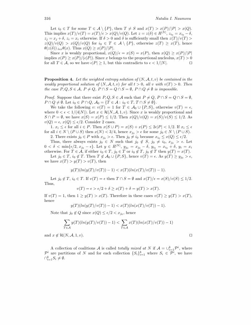
316 Natalia I. Naumova
Let i0 ∈ T for some T ∈ A \ {P}, then T = S and x(T ) > x(P )/|P | > x(Q).This implies x(T )/v(T ) = x(T )/ε > x(Q)/v(Q). Let z = z(δ) ∈ R|N |, zi0 = xi0 − δ,zj = xj + δ, zi = xi otherwise. If δ > 0 and δ is sufficiently small then z(T )/v(T ) >z(Q)/v(Q) > x(Q)/v(Q) for i0 ∈ T ∈ A \ {P}, otherwise z(T ) ≥ x(T ), henceθ(z(δ)) lexθ(x). Thus x(Q) ≥ x(P )/|P |.
Since x is weakly proportional, x(Q)/ε = x(S) = x(P ), then x(Q) ≥ x(P )/|P |implies x(P ) ≥ x(P )/(ε|P |). Since x belongs to the proportional nucleolus, x(T ) > 0for all T ∈ A, so we have ε|P | ≥ 1, but this contradicts to ε < 1/|N |. ��
Proposition 4. Let the weighted entropy solution of (N,A, t, v) be contained in theweakly proportional solution of (N,A, t, v) for all t > 0, all v with v(T ) > 0. Thenthe case P,Q, S ∈ A, P = Q, P ∩ S = Q ∩ S = ∅, P ∩Q = ∅ is impossible.
Proof. Suppose that there exist P,Q, S ∈ A such that P = Q, P ∩ S = Q ∩ S = ∅,P ∩Q = ∅. Let i0 ∈ P ∩Q, A0 = {T ∈ A : i0 ∈ T, T ∩ S = ∅}.
We take the following v: v(T ) = 1 for T ∈ A0 ∪ {P, S}, otherwise v(T ) = ε,where 0 < ε < 1/(4|N |). Let x ∈ H(N,A, 1, v). Since x is weakly proportional andS ∩ P = ∅, we have x(S) = x(P ) ≤ 1/2. Then x(Q)/v(Q) = x(S)/v(S) ≤ 1/2. Asv(Q) = ε, x(Q) ≤ ε/2. Consider 2 cases.
1. xi ≤ ε for all i ∈ P . Then x(S ∪ P ) = x(S) + x(P ) ≤ 2ε|P | < 1/2. If xi ≤ εfor all i ∈ N \ (P ∪ S) then x(N) < 3/4, hence xj0 > ε for some j0 ∈ N \ (P ∪ S).
2. There exists j0 ∈ P with xj0 > ε. Then j0 = i0 because xi0 ≤ x(Q) ≤ ε/2.Thus, there always exists j0 ∈ N such that j0 ∈ S, j0 = i0, xj0 > ε. Let
0 < δ < min{ε/2, xj0 − ε}. Let y ∈ R|N |, yj0 = xj0 − δ, yi0 = xi0 + δ, yi = xiotherwise. For T ∈ A, if either i0 ∈ T , j0 ∈ T or i0 ∈ T , j0 ∈ T then y(T ) = x(T ).
Let j0 ∈ T , i0 ∈ T . Then T ∈ A0 ∪ {P, S}, hence v(T ) = ε. As y(T ) ≥ yj0 > ε,we have x(T ) > y(T ) > v(T ), then
y(T )(ln(y(T )/v(T ))− 1) < x(T )(ln(x(T )/v(T ))− 1).
Let j0 ∈ T , i0 ∈ T . If v(T ) = ε then T ∩ S = ∅ and x(T )/ε = x(S)/v(S) ≤ 1/2.Thus,
v(T ) = ε > ε/2 + δ ≥ x(T ) + δ = y(T ) > x(T ).
If v(T ) = 1, then 1 ≥ y(T ) > x(T ). Therefore in these cases v(T ) ≥ y(T ) > x(T ),hence
y(T )(ln(y(T )/v(T ))− 1) < x(T )(ln(x(T )/v(T ))− 1).
Note that j0 ∈ Q since x(Q) ≤ ε/2 < xj0 , hence∑T∈A
y(T )(ln(y(T )/v(T ))− 1) <∑T∈A
x(T )(ln(x(T )/v(T ))− 1)
and x ∈ H(N,A, 1, v). ��
A collection of coalitions A is called totally mixed at N if A = ∪ki=1P i, whereP i are partitions of N and for each collection {Si}ki=1 where Si ∈ P i, we have∩ki=1Si = ∅.

Claim Problems with Coalition Demands 317
Theorem 4. The weighted entropy solution of (N,A, t, v) coincides with the weaklyproportional solution of (N,A, t, v) for all t > 0, all v with v(T ) > 0 iff A is totallymixed at N .
Proof. Let A be totally mixed at N . Then in view of Theorem 3, the weakly pro-portional solution of (N,A, t, v) is always nonempty. As long as all P i are partitionsof N , x(S) are uniquely defined for all S ∈ A, x ∈ WP(N,A, t, v).
Let y ∈ H(N,A, t, v). Suppose that y ∈ WP(N,A, t, v) then there exists i ∈{1, . . . , k} such that y(S)/v(S) > t(Q)/v(Q) for some S,Q ∈ P i. Since A is totallymixed, there exist sufficiently small δ > 0 and a vector z = z(δ) with zj ≥ 0 suchthat z(Q) = y(Q) + δ, z(S) = y(S)− δ, z(T ) = y(T ) for remaining T ∈ A. Denote
f(δ) =∑T∈A
z(δ)(T )(ln(z(δ)(T )/v(T ))− 1).
Thenf ′(0) = ln(y(Q)/v(Q))− ln(y(S)/v(S)) < 0,
hence for sufficiently small δ > 0,∑T∈A
z(δ)(T )(ln(z(δ)(T )/v(T ))− 1) <∑T∈A
y(T )(ln(y(T )/v(T ))− 1),
but this contradicts y ∈ H(N,A, t, v). Thus H(N,A, t, v) ⊂ WP(N,A, t, v). Sincex(S) are uniquely defined for all x ∈ WP(N,A, t, v), this implies H(N,A, t, v) =WP(N,A, t, v).
Now suppose thatWP(N,A, t, v) = H(N,A, t, v) for all t > 0, all v with v(T ) >
0. By Proposition 4, A =⋃ki=1 Bi, where Bi are subsets of partitions of N . If each Bi
is a partition P i of N then by Theorem 3, for each collection {Si}ki=1 with Si ∈ P i,we have ∩ki=1Si = ∅, so A is totally mixed at N .
Let some Bi be not a partition of N . Then without loss of generality, there existsq < k such that ∪qi=1Bi does not cover N and ∪qi=1Bi ∪Bj covers N for each j > q.Denote N0 =
⋃S∈∪qi=1Bi
S. We consider 2 cases.
Case 1. For each j = q+1, . . . , k, there exists Sj ∈ Bj, such that ∪kj=q+1(Bj \Sj),covers (N \N0).
Take the following v = vε:vε(S) = ε for all S ∈ ∪qj=1Bj,vε(Sj) = 1, j = q + 1, . . . , k,vε(T ) = 1/(2|N |) otherwise.Let xε ∈ H(N,A, 1, vε). Since xε is weakly proportional, xε(T ) ≤ 1/(2|N |) for allT ∈ Bj, T = Sj, j = q + 1, . . . , k, hence xε(N \ N0) ≤ 1/2 and xε(N0) ≥ 1/2.Consider ∑
T∈∪qj=1Bjxε(T )(ln(xε(T )/vε(T ))− 1) =
∑T∈∪qj=1Bj
xε(T )(lnxε(T )− 1)−∑
T∈∪qj=1Bjxε(T )ln(ε).
Note that∑
T∈∪qj=1Bjxε(T ) ≥ x(N0) ≥ 1/2 implies
∑T∈∪qj=1Bj
xε(T )ln(ε)→ −∞ as ε→ 0.

318 Natalia I. Naumova
Moreover, z(T )(lnz(T )− 1) for T ∈ ∪qj=1Bj and z(T )(lnz(T )/vε(T ) − 1) for T ∈∪kj=q+1Bj are bounded below, therefore∑
T∈Axε(T )(ln(xε(T )/v(T ))− 1)→ +∞ as ε→ 0.
Let y ∈ R|N |,∑
i∈N yi = 1, yi > 0 for all i. Define zε ∈ R|N |:zεi = εyi for i ∈ N0,zεi = (1− εy(N0))/y(N \N0)yi for i ∈ N \N0.Let ε→ 0, then∑
T∈∪qj=1Bjzε(T )(ln(zε(T )/vε(T ))− 1) = ε
∑T∈∪qj=1Bj
y(T )(ln(y(T )− 1)→ 0,
∑T∈∪kj=q+1Bj
zε(T )(ln(zε(T )/vε(T ))− 1)→∑
T∈∪kj=q+1Bju(T )(ln(u(T )/vε(T ))− 1),
where u = {uj}j∈N , uj = 0 for j ∈ N0, uj = yj/y(N \N0) for j ∈ N0. Thus,∑T∈A
zε(T )(ln(zε(T )/vε(T ))− 1)→∑
T∈∪kj=q+1Bju(T )(ln(u(T )/vε(T ))− 1) < +∞.
Therefore for sufficiently small ε,∑T∈A
xε(T )(ln(xε(T )/v(T ))− 1) >∑T∈A
zε(T )(ln(zε(T )/vε(T ))− 1),
and this contradicts xε ∈ H(N,A, 1, vε).Case 2. If Sj ∈ Bj is taken out from Bj, j = q + 1, . . . , k, then the remaining
elements of ∪kj=q+1Bj do not cover N \N0.
For each j = q + 1, . . . , k, Sj ∈ Bj, we have Sj ∩ (N \N0) = ∅. Indeed, supposethat Sj0 ⊂ N0 for some j0 > q. Then if we take Sj0 and arbitrary Sj ∈ Bj for j > q,j = j0 out from ∪kj=q+1Bj, the remaining elements of ∪kj=q+1Bj cover N \N0 as if
{N0} ∪ Bj0 covers N .Let
C = {(N \N0) ∩ S : S ∈ ∪kj=q+1Bj, S ∩ P = ∅ for some P ∈ A}.
Then P, S ∈ ∪kj=q+1Bj, P = S, P ∩(N \N0) ∈ C imply P ∩(N \N0) = S∩(N \N0).
Indeed, suppose that P ∩ (N \N0) = S ∩ (N \N0). There exists P 1 ∈ A such thatP ∩P 1 = ∅. If we take S, P 1 and arbitrary Sj ∈ Bj for j > q with P ∈ Bj out from∪kj=q+1Bj, the remaining elements of ∪kj=q+1Bj cover N \ N0 because {N0} ∪ Bj0covers N , where Bj0 � S.
For arbitrary problem (N,A, t, v), where A is under the case 2, consider theproblem (N \ N0, C, t, w), where w(T ) = v(S) for T = S ∩ (N \ N0) ∈ C. As wasproved above, w is well defined. Under the case 2, due to Theorem 3, there existsy ∈ WP(N \N0, C, t, w). Let x ∈ R|N |, xi = 0 for i ∈ N0, xi = yi for i ∈ N \N0,then x ∈ WP(N,A, t, v), x(N0) = 0.
Let v(S) = |S|/|N | for all S ∈ A, xi = 1/|N | for all i ∈ N , then x ∈ H(N,A, 1, v)as if x(S) = v(S) for all S ∈ A, but x(N0) > 0. Thus in case 2 the weighted entropysolution does not coincide with the weakly proportional solution for some problem.
��

Claim Problems with Coalition Demands 319
Corollary 1. The proportional nucleolus of (N,A, t, v), the weighted entropy solu-tion of (N,A, t, v), and the weakly proportional solution of (N,A, t, v) coincide forall t > 0, all v with v(T ) > 0 iff A is totally mixed at N .
3. Axiomatic Justification of a Single–valued Solution
Note that all solutions described above are set valued. In the case of totally mixedset A we propose a selector for these solutions and give an axiomatic justificationto it.
Let A = ∪ki=1P i, where P i are partitions of N , be a totally mixed at N collec-tion of coalitions, t > 0. Then y = {yi}i∈N is the totally proportional solution of(N,A, t, v)) if for each collection {Si}ki=1 with Si ∈ P i,
y(∩ki=1Si) = t
k∏i=1
v(Si)/
k∏i=1
αi,
where αi =∑S∈Pi v(S) and yp = yq for all p, q ∈ ∩ki=1Si.
Example 3. Let N = {1, 2, 3, 4, 5}, A = {{1, 2}, {3, 4, 5}, {1, 3}, {2, 4, 5}}, then thefollowing x ∈ R5 is the totally proportional solution of (N,A, 1, v).
x01 = [v(1, 2)v(1, 3)]/[(v(1, 2) + v(3, 4, 5))(v(1, 3) + v(2, 4, 5))],
x02 = [v(1, 2)v(2, 4, 5)]/[(v(1, 2) + v(3, 4, 5))(v(1, 3) + v(2, 4, 5))],
x03 = [v(3, 4, 5)v(1, 3)]/[(v(1, 2) + v(3, 4, 5))(v(1, 3) + v(2, 4, 4))],
x04 = x0
5 = [v(3, 4, 5)v(2, 4, 5)]/[2(v(1, 2) + v(3, 4, 5))(v(1, 3) + v(2, 4, 5))].
Consider the following properties of methods that generate single-valued solu-tions.
A single-valued method F is anonymous if for each permutation π of N ,F (πN, πA, t, πv) = πF (N,A, t, v).
Players i and j are symmetric with respect to A if for all S ∈ A, either i ∈ Sand j ∈ S or i ∈ S, j ∈ S.
If i and j are symmetric w.r.to A, then the result of glueing i and j at (N,A, t, v)is a game (N[i,j],A[i,j], t, v[i,j]), whereN[i,j] = N \ {i, j} ∪ {i0},Q ∈ A[i,j] iff either Q ∈ A and i ∈ Q or i0 ∈ Q and (Q \ {i0} ∪ {i, j}) ∈ A,v[i,j](Q) = v(Q) for Q ∈ A, or else v[i,j](Q) = v(Q \ {i0} ∪ {i, j}).
F is independent of glueing if for all symmetric w.r.to A i and j, F (N,A, t, v)k =F (N[i,j],A[i,j], t, v[i,j])k for all k ∈ N \ {i, j}.
A single-valued method F is independent of merging if for all S, T ∈ A withS ∩ T = ∅ and (S ∪ T ) ∈ A,
F (N,A, t, v)i = F (N, AS,T , t, vS,T )i ∀ i ∈ (S ∪ T ),
where AS,T = A \ {S, T } ∪ {S ∪ T },vS,T (S ∪ T ) = v(S) + v(T ), otherwise vS,T (Q) = v(Q).
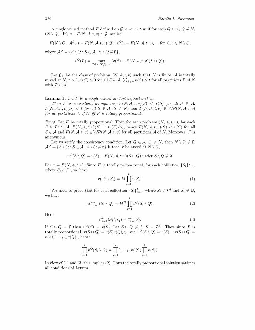
320 Natalia I. Naumova
A single-valued method F defined on G is consistent if for each Q ∈ A, Q = N ,(N \Q, AQ, t− F (N,A, t, v) ∈ G implies
F (N \Q, AQ, t− F (N,A, t, v)(Q), vQ)i = F (N,A, t, v)i for all i ∈ N \Q,
where AQ = {S \Q : S ∈ A, S \Q = ∅},
vQ(T ) = maxS∈A:S\Q=T
(v(S)− F (N,A, t, v)(S ∩Q)).
Let G+ be the class of problems (N,A, t, v) such that N is finite, A is totallymixed at N , t > 0, v(S) > 0 for all S ∈ A,
∑S∈P v(S) > t for all partitions P of N
with P ⊂ A.
Lemma 1. Let F be a single-valued method defined on G+.Then F is consistent, anonymous, F (N,A, t, v)(S) < v(S) for all S ∈ A,
F (N,A, t, v)(S) < t for all S ∈ A, S = N , and F (N,A, t, v) ∈ WP(N,A, t, v)for all partitions A of N iff F is totally proportional.
Proof. Let F be totally proportional. Then for each problem (N,A, t, v), for eachS ∈ P i ⊂ A, F (N,A, t, v)(S) = tv(S)/αi, hence F (N,A, t, v)(S) < v(S) for allS ∈ A and F (N,A, t, v) ∈ WP(N,A, t, v) for all partitions A of N . Moreover, F isanonymous.
Let us verify the consistency condition. Let Q ∈ A, Q = N , then N \ Q = ∅,AQ = {S \Q : S ∈ A, S \Q = ∅} is totally balanced at N \Q,
vQ(S \Q) = v(S)− F (N,A, t, v)(S ∩Q) under S \Q = ∅.
Let x = F (N,A, t, v). Since F is totally proportional, for each collection {Si}ki=1,where Si ∈ P i, we have
x(∩ki=1Si) = M
k∏i=1
v(Si). (1)
We need to prove that for each collection {Si}ki=1, where Si ∈ P i and Si = Q,we have
x(∩ki=1(Si \Q) = MQk∏i=1
vQ(Si \Q). (2)
Here∩ki=1(Si \Q) = ∩ki=1Si. (3)
If S ∩ Q = ∅ then vQ(S) = v(S). Let S ∩ Q = ∅, S ∈ P i0 . Then since F istotally proportional, x(S ∩Q) = v(S)v(Q)μi0 and vQ(S \Q) = v(S)− x(S ∩Q) =v(S)(1 − μi0v(Q)), hence
k∏i=1
vQ(Si \Q) =k∏i=1
(1− μiv(Q))k∏i=1
v(Si).
In view of (1) and (3) this implies (2). Thus the totally proportional solution satisfiesall conditions of Lemma.

Claim Problems with Coalition Demands 321
Now let F satisfy all conditions of Lemma. Let x = F (N,A, t, v), Q ∈ A, Q = N .First we verify that the problem (N \Q, AQ, t− x(Q), vQ) ∈ G+.
Obviously, the collection of coalitions AQ is totally mixed, t − x(Q) > 0, Foreach T ∈ AQ, T = S \ Q for some S ∈ A and such S is unique as if A is totallybalanced, hence vQ(T ) = v(S)− x(S ∩Q) ≥ v(S)− x(S) > 0.
For each partition PQ of N \Q with PQ ⊂ AQ,∑T∈PQ
vQ(T ) > t− x(Q). (4)
Indeed, ∑T∈PQ
vQ(T ) =∑S∈P
vQ(S \Q) (5)
for some partition P of N , P ⊂ A.∑S∈P
vQ(S \Q) =∑S∈P
(v(S)− x(S ∩Q)) =∑S∈P
v(S)− x(N ∩Q) > t− x(Q).
In view of (5) this implies (4). Thus the problem (N \Q, AQ, t−x(Q), vQ) belongsto G+.
Let A = ∪ki=1P i, where P i are partitions of N . We prove by induction on k thatfor each collection {Si}ki=1 with Si ∈ P i,
F (N,A, t, v)(∩ki=1Si) = tk∏i=1
v(Si)/k∏i=1
αi, where αi =∑S∈Pi
v(S). (6)
If k = 1 then (6) is a condition of Lemma. Suppose that (6) is proved for k ≤ m.Let A = ∪mi=0P i, where P i are partitions of N . Let P0 = {S1, . . . , Sr}. Let we takeS2, . . . , Sr out of A. Then due to consistency, we get the game (S1,AS2,...Sr , t −∑r
j=2 x(Sj), vS1), where x = F (N,A, t, v), vS1 = vS2,...Sr , and for each P ij ∈ P i,i ≥ 1,
vS1(S1 ∩ P ij ) = v(P ij )−r∑q=2
x(Sq ∩ P ij ) = v(P ij )− x(P ij ) + x(S1 ∩ P ij ). (7)
By induction assumption, for all P iji , Piqi ∈ P i, i = 1, . . . ,m, we have
x(∩mi=1Piji∩ S1)∏m
i=1 vS1(S1 ∩ P iji)=
x(∩mi=1Piqi ∩ S1)∏m
i=1 vS1(S1 ∩ P iqi ). (8)
Let qi = ji for i = 1, then (8) and (7) imply
x(∩mi=1Piji ∩ S1)[v(P 1
q1 )− x(P 1q1 ) + x(S1 ∩ P 1
q1)] =
x(∩mi=2Piji ∩ S1 ∩ P 1
q1 )[v(P 1j1 )− x(P 1
j1 ) + x(S1 ∩ P 1j1)] (9)
If m = 1 we obtain
x(S1∩P 1j1 )[v(P 1
q1 )−x(P 1q1 )+x(S1∩P 1
q1 )] = x(S1∩P 1q1 )[v(P 1
j1 )−x(P 1j1 )+x(S1∩P 1
j1 )].
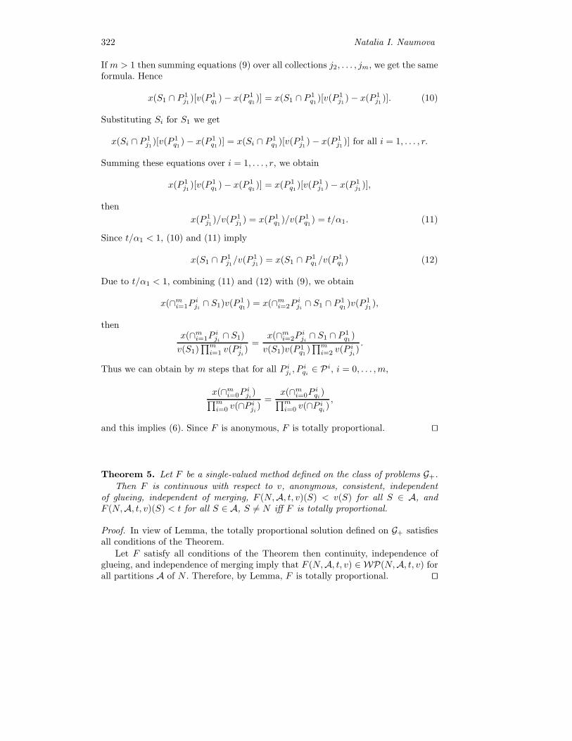
322 Natalia I. Naumova
If m > 1 then summing equations (9) over all collections j2, . . . , jm, we get the sameformula. Hence
x(S1 ∩ P 1j1)[v(P 1
q1 )− x(P 1q1 )] = x(S1 ∩ P 1
q1 )[v(P 1j1 )− x(P 1
j1 )]. (10)
Substituting Si for S1 we get
x(Si ∩ P 1j1)[v(P 1
q1 )− x(P 1q1 )] = x(Si ∩ P 1
q1)[v(P 1j1 )− x(P 1
j1 )] for all i = 1, . . . , r.
Summing these equations over i = 1, . . . , r, we obtain
x(P 1j1 )[v(P 1
q1 )− x(P 1q1 )] = x(P 1
q1 )[v(P 1j1 )− x(P 1
j1 )],
then
x(P 1j1 )/v(P 1
j1 ) = x(P 1q1 )/v(P 1
q1) = t/α1. (11)
Since t/α1 < 1, (10) and (11) imply
x(S1 ∩ P 1j1/v(P 1
j1) = x(S1 ∩ P 1q1/v(P 1
q1) (12)
Due to t/α1 < 1, combining (11) and (12) with (9), we obtain
x(∩mi=1Piji ∩ S1)v(P 1
q1 ) = x(∩mi=2Piji ∩ S1 ∩ P 1
q1)v(P 1j1 ),
thenx(∩mi=1P
iji ∩ S1)
v(S1)∏mi=1 v(P iji )
=x(∩mi=2P
iji ∩ S1 ∩ P 1
q1)
v(S1)v(P 1q1 )∏mi=2 v(P iji)
.
Thus we can obtain by m steps that for all P iji , Piqi ∈ P i, i = 0, . . . ,m,
x(∩mi=0Piji
)∏mi=0 v(∩P iji )
=x(∩mi=0P
iqi)∏m
i=0 v(∩P iqi ),
and this implies (6). Since F is anonymous, F is totally proportional. ��
Theorem 5. Let F be a single-valued method defined on the class of problems G+.
Then F is continuous with respect to v, anonymous, consistent, independentof glueing, independent of merging, F (N,A, t, v)(S) < v(S) for all S ∈ A, andF (N,A, t, v)(S) < t for all S ∈ A, S = N iff F is totally proportional.
Proof. In view of Lemma, the totally proportional solution defined on G+ satisfiesall conditions of the Theorem.
Let F satisfy all conditions of the Theorem then continuity, independence ofglueing, and independence of merging imply that F (N,A, t, v) ∈ WP(N,A, t, v) forall partitions A of N . Therefore, by Lemma, F is totally proportional. ��
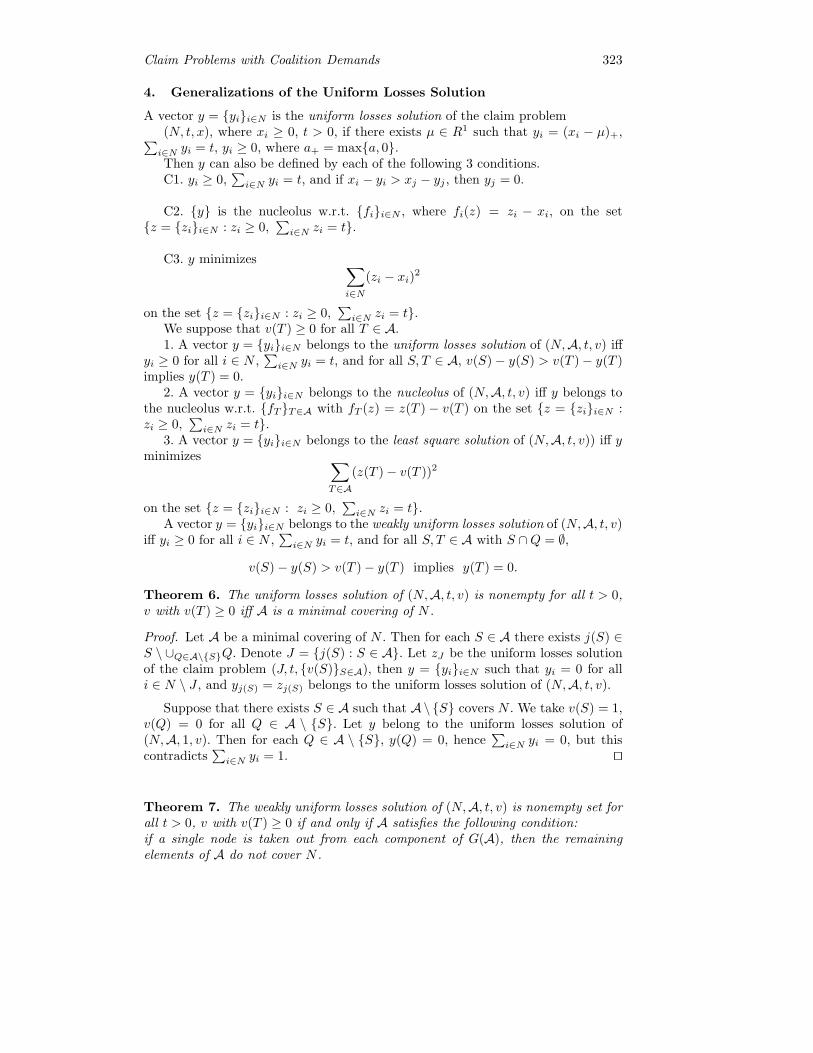
Claim Problems with Coalition Demands 323
4. Generalizations of the Uniform Losses Solution
A vector y = {yi}i∈N is the uniform losses solution of the claim problem(N, t, x), where xi ≥ 0, t > 0, if there exists μ ∈ R1 such that yi = (xi − μ)+,∑i∈N yi = t, yi ≥ 0, where a+ = max{a, 0}.Then y can also be defined by each of the following 3 conditions.C1. yi ≥ 0,
∑i∈N yi = t, and if xi − yi > xj − yj , then yj = 0.
C2. {y} is the nucleolus w.r.t. {fi}i∈N , where fi(z) = zi − xi, on the set{z = {zi}i∈N : zi ≥ 0,
∑i∈N zi = t}.
C3. y minimizes ∑i∈N
(zi − xi)2
on the set {z = {zi}i∈N : zi ≥ 0,∑
i∈N zi = t}.We suppose that v(T ) ≥ 0 for all T ∈ A.1. A vector y = {yi}i∈N belongs to the uniform losses solution of (N,A, t, v) iff
yi ≥ 0 for all i ∈ N ,∑
i∈N yi = t, and for all S, T ∈ A, v(S)− y(S) > v(T )− y(T )implies y(T ) = 0.
2. A vector y = {yi}i∈N belongs to the nucleolus of (N,A, t, v) iff y belongs tothe nucleolus w.r.t. {fT}T∈A with fT (z) = z(T )− v(T ) on the set {z = {zi}i∈N :zi ≥ 0,
∑i∈N zi = t}.
3. A vector y = {yi}i∈N belongs to the least square solution of (N,A, t, v)) iff yminimizes ∑
T∈A(z(T )− v(T ))2
on the set {z = {zi}i∈N : zi ≥ 0,∑i∈N zi = t}.
A vector y = {yi}i∈N belongs to the weakly uniform losses solution of (N,A, t, v)iff yi ≥ 0 for all i ∈ N ,
∑i∈N yi = t, and for all S, T ∈ A with S ∩Q = ∅,
v(S)− y(S) > v(T )− y(T ) implies y(T ) = 0.
Theorem 6. The uniform losses solution of (N,A, t, v) is nonempty for all t > 0,v with v(T ) ≥ 0 iff A is a minimal covering of N .
Proof. Let A be a minimal covering of N . Then for each S ∈ A there exists j(S) ∈S \ ∪Q∈A\{S}Q. Denote J = {j(S) : S ∈ A}. Let zJ be the uniform losses solutionof the claim problem (J, t, {v(S)}S∈A), then y = {yi}i∈N such that yi = 0 for alli ∈ N \ J , and yj(S) = zj(S) belongs to the uniform losses solution of (N,A, t, v).
Suppose that there exists S ∈ A such that A\{S} covers N . We take v(S) = 1,v(Q) = 0 for all Q ∈ A \ {S}. Let y belong to the uniform losses solution of(N,A, 1, v). Then for each Q ∈ A \ {S}, y(Q) = 0, hence
∑i∈N yi = 0, but this
contradicts∑
i∈N yi = 1. ��
Theorem 7. The weakly uniform losses solution of (N,A, t, v) is nonempty set forall t > 0, v with v(T ) ≥ 0 if and only if A satisfies the following condition:if a single node is taken out from each component of G(A), then the remainingelements of A do not cover N .
324 Natalia I. Naumova
The Theorem was proved in (Naumova, 1978). The proof is based on Theorem 2.
Proposition 5. The nucleolus of (N,A, t, v) is contained in the uniform lossessolution of (N,A, t, v) for all t > 0, all v with v(T ) ≥ 0 iff A is a partition of N .
Proof. Let A be a partition of N , then, as for claim problems, the nucleolus alwayscoincides with the uniform losses solution.
Let the nucleolus be always contained in the uniform losses solution. Supposethat A is not a partition of N , then there exist P,Q ∈ A such that P ∩Q = ∅. Wetake the following v: v(P ) = 1, v(T ) = 0 otherwise. Let x belong to the nucleolusof (N,A, 1, v). Since x belongs to the uniform losses solution, x(T ) = 0 for allT ∈ A \ {P}, hence x(P ) = 1. Since x belongs to the nucleolus of (N,A, 1, v) andAP = {T ∈ A : T ∩ P = ∅} = ∅, xi = 0 for all i ∈ P \ ∪T∈AP T . Then there existsj0 ∈ P ∩S for some S ∈ AP such that xj0 > 0. Then x(S) > 0, but this contradictsto x(S) = 0. ��
Proposition 6. The least square solution of (N,A, t, v) is contained in the uniformlosses solution of (N,A, t, v) for all t > 0, all v with v(T ) ≥ 0 iff A is a partitionof N .
Proof. Let A be a partition of N , then, as for claim problems, the least squaresolution always coincides with the uniform losses solution.
Let the least square solution be always contained in the uniform losses solution.Suppose that A is not a partition of N , then there exist P,Q ∈ A such that P ∩Q =∅. We take the following v: v(P ) = 2, v(T ) = ε otherwise, where 0 < ε < 1. Let xbelong to the least square solution of (N,A, 1, v).
Then v(P ) − x(P ) ≥ 1, v(T ) − x(T ) ≤ ε for all T ∈ A \ {P}. Since x belongsto the uniform losses solution, x(T ) = 0 for all T ∈ A \ {P}, hence there existsj0 ∈ P \ ∪T∈A\{P}T such that xj0 > 0.
Let i0 ∈ P ∩Q, y ∈ R|N |, yj0 = xj0 − δ, yi0 = xi0 + δ, yi = xi otherwise. If δ > 0,then y(P ) = x(P ), y(Q) > x(Q), y(T ) ≥ x(T ) for all T ∈ A\{P,Q}, y(N) = x(N).If δ is sufficiently small then yi ≥ 0, y(T ) ≤ ε for all T ∈ A \ {P}, hence∑
T∈A(y(T )− v(T ))2 <
∑T∈A
(x(T )− v(T ))2
and x does not belong to the least square solution of (N,A, 1, v). ��
Proposition 7. Let the nucleolus of (N,A, t, v) be contained in the weakly uniformlosses solution of (N,A, t, v) for all t > 0, all v with v(T ) ≥ 0. Then the caseP,Q, S ∈ A, P = Q, P ∩ S = Q ∩ S = ∅, P ∩Q = ∅ is impossible.
Proof. Suppose that there exist P,Q, S ∈ A such that P = Q, P ∩ S = Q ∩ S = ∅,P ∩ Q = ∅. Let us take the following v: v(S) = v(P ) = 1, v(T ) = 0 for allT ∈ A\{S, P}. Let x belong to the nucleolus of (N,A, 1, v). Then x(Q) = 0 becauseotherwise v(S)− x(S) ≥ 0 > v(Q)− x(Q). If x(P ) = 0 then x(P )− v(P ) = −1 andx does not belong to nucleolus because if z(P ) = z(S) = 1/2 then minT∈A(z(T )−

Claim Problems with Coalition Demands 325
v(T )) ≥ −1/2. Hence x(P ) > 0 and there exists i0 ∈ P \Q such that xi0 > 0. Letj ∈ P ∩Q.
If i0 ∈ T for all T ∈ A \ {P} then we take y ∈ R|N |: yi0 = 0, yj = xj + xi0 ,yi = xi otherwise. Then y(P ) = x(P ), y(Q) > x(Q), y(T ) ≥ x(T ) for all T ∈ A,hence x does not belong to the nucleolus of (N,A, 1, v).
Let i0 ∈ T for some T ∈ A \ {P}, then T = S, v(T ) = 0, and x(T ) − v(T ) >0 = x(Q)− v(Q). Let z = z(δ) ∈ R|N |, zi0 = xi0 − δ, zj = xj + δ, zi = xi otherwise.If δ > 0 and δ is sufficiently small then z(T )− v(T ) > z(Q)− v(Q) > x(Q)− v(Q)for i0 ∈ T ∈ A \ {P}, otherwise z(T ) ≥ x(T ), hence θ(z(δ)) >lex θ(x) and x doesnot belong to the nucleolus of (N,A, 1, v). ��
Proposition 8. Let the least square solution of (N,A, t, v) be contained in theweakly uniform losses solution of (N,A, t, v) for all t > 0, all v with v(T ) ≥ 0.Then the case P,Q, S ∈ A, P = Q, P ∩ S = Q ∩ S = ∅, P ∩Q = ∅ is impossible.
Proof. Suppose that there exist P,Q, S ∈ A such that P = Q, P ∩ S = Q ∩ S = ∅,P ∩Q = ∅. Let i0 ∈ P ∩Q, A0 = {T ∈ A : i0 ∈ T, T ∩ S = ∅}.
We take the following v:v(T ) = 1 for T ∈ A0 ∪ {P, S},otherwise v(T ) = ε, where 0 < ε < 1/(4|N |).
Let x belong to the least square solution of (N,A, 1, v). Since x is weakly uniformlosses, for S ∩ T = ∅ and T = P , either x(T ) = 0 or x(T ) > 0, x(S) < 1, andv(T ) − x(T ) ≥ v(S) − x(S) > 0. As v(T ) = ε, x(T ) < ε. In particular, x(Q) < ε.Consider 2 cases.
1. xi ≤ ε for all i ∈ P . Then x(S ∪ P ) = x(S) + x(P ) ≤ 2ε|P | < 1/2. If xi ≤ εfor all i ∈ N \ (P ∪ S) then x(N) < 3/4, hence xj0 > ε for some j0 ∈ N \ (P ∪ S).
2. There exists j0 ∈ P with xj0 > ε. Then j0 = i0 because xi0 ≤ x(Q) < ε.Thus, there always exists j0 ∈ N such that j0 ∈ S, j0 = i0, xj0 > ε. Let 0 < δ.
Let y = y(δ) ∈ R|N |, yj0 = xj0 − δ, yi0 = xi0 + δ, yi = xi otherwise. For T ∈ A, ifeither i0 ∈ T , j0 ∈ T or i0 ∈ T , j0 ∈ T then y(T ) = x(T ).
Let j0 ∈ T , i0 ∈ T . Then T ∈ A0 ∪ {P, S}, hence v(T ) = ε. Let δ < xj0 − ε.Since y(T ) ≥ yj0 > ε, we have x(T ) > y(T ) > v(T ), then
(y(T )− v(T ))2 < (x(T )− v(T ))2.
Let j0 ∈ T , i0 ∈ T . If v(T ) = ε then T ∩ S = ∅ and x(T ) < ε. Thus, forsufficiently small δ,
v(T ) = ε ≥ x(T ) + δ = y(T ) > x(T ).
If v(T ) = 1, then 1 ≥ y(T ) > x(T ). Therefore in these cases v(T ) ≥ y(T ) > x(T ),hence
(y(T )− v(T ))2 < (x(T )− v(T ))2.
Note that j0 ∈ Q since x(Q) < ε < xj0 , i0 ∈ Q, hence for sufficiently small δ,∑T∈A
(y(T )− v(T ))2 <∑T∈A
(x(T )− v(T ))2
and x does not belong to the least square solution of (N,A, 1, v). ��

326 Natalia I. Naumova
References
Bregman, L. M. and Naumova, N. I. (1984). Arbitration solutions with ideal point generatedby systems of coalitions. Dokl. Akad. Nauk SSSR, 279 (1984), N 1, 16–20, Englishtranslation in Soviet Math. Dokl. vol. 30 (1984), N 3, 583–587.
Bregman, L. M. and Naumova, N. I. (2002). Goal programming solutions generated by utilityfunctions. Lecture Notes in Economic and Math. Systems, 510 (2002), 495–514.
Bregman, L. M. and Romanovskij, J. V. (1975). Allotment and optimization in allocationproblems. Operations Research and Statistical Modeling (editor J.V.Romanovskij),Vyp.3, Izdat. Leningrad.Univ., Leningrad, 137–162. (Russian)
Moulin, H. (2002). Axiomatic cost and surplus sharing. Handbook of Social Choice andWelfare, 1, Chapter 6. Arrow K.J., Sen A.K. and Suzumura K. eds., 289–357.
Naumova, N. I. (1978). M-systems of relations and their application in cooperative games.Vestnik Leningrad. Univ. N 1 (Ser. Math. Mech. Astr. ), 60–66; English transl. inVestnik Leningrad. Univ. Math. 11, 1983, 67–73.
Naumova, N. I. (2008a). Associated consistency based on utility functions of coalitions.Game Theory and Applications, 13. Nova Publishers, New York, 111–121.
Naumova, N. I. (2008b). Generalized kernels and bargaining sets for families of coalitions.In: Contributions to Game Theory and Management. The International ConferenceGame Theory and Management June 28-29 2007, St. Petersburg, Russia. CollectedPapers. Graduate School of Management St.Petersburg State University, 346–360.
Peleg, B. (1967). Equilibrium points for open acyclic relations. Canad. J. Math., 19, 366–369.
Thomson, W. (2003).Axiomatic and game-theoretic analysis of bankruptcy and taxationproblems: a survey. Mathematical Social Sciences, 45, 249–297.

Games with Differently Directed Interestsand Their Application to the Environmental Management
Guennady A.Ougolnitsky
Southern Federal University,8A Milchakov St., 344090 Rostov-on-Don, Russia
E-mail: [email protected]
Abstract. The resolution of numerous ecological problems on different lev-els should be realized on the base of sustainable development concept thatdetermines the conditions to the state of environmental-economic systemsand impacting control actions. Those conditions can’t be realized by them-selves and require special collaborative efforts of different agents using bothcooperation and hierarchical control. To formalize the inevitable trade-offs itis natural to use game theoretic models including the games with differentlydirected interests.
Keywords: differential games, sustainable development, cooperation, dy-namic stability, hierarchical control
JEL classification codes: C70, Q56
1. Introduction
A rapid growth of production and human population, urbanization and activity oftransnational corporations exert an essential influence on the environment and re-sult in many ecological problems on local, regional, and global level. Those problemsare environmental pollution, water and wind erosion, acid rains, global warming,extinction, non-renewable resource exploitation, and so on. A successful solution ofthe problems is possible only within a sustainable development due to which an eco-nomic growth doesn’t violate the ecological equilibrium. Sustainable developmentrequires strong collaborative efforts of states, corporations, social organizations andindividuals. Because of many concerned agents it is evident that sustainable devel-opment is a conflict controlled process which must be described by game theoreticmodels. A special attention has to be given to the classes of differential gamesdescribing hierarchical relations, cooperation and dynamic stability (time consis-tency).A general survey of non-cooperative differential games is given by Basar and Olsder(1995), hierarchical games are considered by Fudenberg and Tirole (1991). Groupoptimal cooperative solutions in differential games are proposed in Dockner andJorgensen (1984), Dockner and Long (1993), Tahvonen (1994), Maler and de Zeeuw(1998), Rubio and Casino (2002). Haurie and Zaccour (1986, 1991), Kaitala andPohjola (1988, 1990, 1995), Kaitala et al (1995), Jorgensen and Zaccour (2001) pre-sented classes of transferable-payoff cooperative games with solutions which satisfygroup optimality and individual rationality. In Leitmann (1974, 1975), Tolwinskyet al (1986), Hamalainen et al (1986), Haurie and Pohjola (1987), Gao et al (1989),Haurie (1991), Haurie et al (1994) are presented solutions satisfying group optimal-ity and individual rationality at the initial time in cooperative games with non-transferable payoffs. In some papers (see Hamalainen et al (1986), Tolwinsky et al
328 Guennady A.Ougolnitsky
(1986)) threats are used to ensure that no players will deviate from the initial co-operative strategies throughout the game horizon. Environmental applications areconsidered in Dockner and Long (1993), Hamalainen et al (1986), Jorgensen andZaccour (2001), Kaitala and Pohjola (1988, 1995), Kaitala et al (1995), Mazalovand Rettieva (2005, 2005, 2006, 2007), Yeung (2009) and others.The problem of dynamic stability in differential games has been intensively ex-plored in the past three decades (Yeung 2009). Haurie (1976) raised the problemof instability when the Nash bargaining solution is extended to differential games.Petrosyan (1977) formalized the notion of dynamic stability in differential games.Kidland and Prescott (1977) introduced the notion of time consistency related toeconomic problems. Petrosyan and Danilov (1979, 1982) proposed an ”imputationdistribution procedure” for cooperative solution. Petrosyan (1991, 1993b) studiedthe dynamic stability of optimality principles in non-zero sum cooperative differ-ential games. Petrosyan (1993a) and Petrosyan and Zenkevich (1996, 2007) havepresented a detailed analysis of dynamic stability in cooperative differential games,in which the method of regularization was used to construct time consistent solu-tions. Yeung and Petrosyan (2001) designed time consistent solutions in differentialgames and characterized the conditions that the allocation-distribution proceduremust satisfy. Petrosyan and Zenkevich (2009) proposed the conditions of sustainablecooperation. Those and other results permit to propose a mathematical formaliza-tion of the concept of sustainable development on the base of a game theoreticmodel (Ougolnitsky 2002).
2. Games with differently directed interests
A general model of game with differently directed interests may be represented asfollows (case n = 2 is considered for simplicity):
u1(x1, x2) = f(x1, x2) + g(x1, x2) + f1(x1, x2)→ maxx1∈X1
;
u2(x1, x2) = f(x1, x2)− g(x1, x2) + f2(x1, x2)→ maxx2∈X2
. (1)
where terms f describe coincident interests, terms g - antagonistic interests, andterms f1 , f2 - independent interests of the players. Specific cases of the model (1)are games with partly coincident interests
u1(x1, x2) = f(x1, x2) + f1(x1, x2)→ maxx1∈X1
;
u2(x1, x2) = f(x1, x2) + f2(x1, x2)→ maxx2∈X2
. (2)
and games with partly antagonistic interests
u1(x1, x2) = g(x1, x2) + f1(x1, x2)→ maxx1∈X1
;
u2(x1, x2) = −g(x1, x2) + f2(x1, x2)→ maxx2∈X2
. (3)

Games with Differently Directed Interests 329
For example, a well-known Germeyer-Vatel model (1974)
u1(x1, x2) = f(a1 − x1, a2 − x2) + f1(x1)→ maxx1∈X1
;
u2(x1, x2) = f(a1 − x1, a2 − x2) + f2(x2)→ maxx2∈X2
. (4)
is a specific case of a game with partly coincident interests (2) for which an existenceof strong equilibrium is proved.There are many natural applications of models (1)-(3) to the management prob-lems. Thus, a model of motivation (impulsion) management
u1(x1, x2) = x1f(x2) + f1(x1, x2)→ max0≤x1≤1
;
u2(x1, x2) = (1− x1)f(x2) + f2(x1, x2)→ max0≤x2≤1
. (5)
belongs to the type (3). In our previous paper (Ougolnitsky 2010) a specific case ofthe model (2) was considered, namely a pricing model of hierarchical control of thesustainable development of the regional construction works complex
uL(p, p0, p) = δpα(p)−Mρ(p, p0)→ max
0 < p0 ≤ p ≤ pmax
uF (p, p0, p) = pα(p) + pξ(p)(1 − α(p))→ max
0 ≤ p ≤ pmax.
Here p is sales price; p0 - normative price of social class residential real estate devel-opment; p - limit price of social class residential real estate development; M >> 1
- penalty constant; ρ(p, p0) = { 0, p ≤ p0,1, p > p0,
; δ - Administration bonus parameter for
social class residential real estate development sales; pmax - ”overlimit” price ofsocial class residential real estate development (there are no sales if p > pmax);α(p) is share of residential real estate development bought by Administration withwarranty; ξ(p) - share of another residential real estate development successfullysold by Developer without help.There are many other examples of game theoretic models of the described type inmanagement, such as models of resource allocation considering private interests,models of organizational monitoring optimization, models of reward systems, cor-ruption models and so on. The games are considered as hierarchical ones.
3. Cooperative differential game of resource allocation with partlycoincident interests on the base of compulsion
A dynamical model of hierarchical control by resource allocation in a tree-like sys-tem may be represented as follows:
330 Guennady A.Ougolnitsky
f0(x(t), u1(•), . . . , un(•)) =∑i∈M
∫ T
t0
gi(x(t), ui(t))dt→ max;
0 ≤ qi(t) ≤ 1; ri(t) ≥ 0, i ∈M ;∑i∈M
ri(t) = 1, t ∈ [t0, T ];
fi(x(t), ui(t)) = gi(x(t), ui(t)) + hi(x(t), ui(t)), i ∈M, t ∈ [t0, T ];
qi(t) ≤ ui(t) ≤ ri(t), i ∈M, t ∈ [t0, T ];
dx
dt= F (x(t), u1(t), . . . , un(t)), x(0) = x0.
The tree-like hierarchical structure consists of n + 1 elements: one element of thehigher level (Leader) designated by index 0 and n elements of the lower level (Fol-lowers). Let’s denote the whole set of elements by N = {0, 1, . . . , n}, and the set ofelements on lower level by M = {1, . . . , n}. The Leader controls the Followers sep-arately by control variables of compulsion qi (administrative impacts) and controlvariables ri of impulsion (resources) (Ougolnitsky 2002). Without lack of generalitywe may consider the total resource equal to one. After receiving the values of qiand ri each Follower i ∈M chooses the control value ui (environmental protectionefforts). The objective of Leader is to maximize the payoff function f0, and theobjective of each Follower is to maximize fi . We suppose that gi represents theecological interests for the whole system, and hi represents private economic inter-ests of the i-th Follower; functions gi are non-negative, continuous, differentiable,monotonically increase on ui , gi(x(t), 0) = 0; functions hi are non-negative, con-tinuous, differentiable, monotonically decrease on ui , hi(x(t), ri(t)) = 0 for eacht ∈ [t0, T ].To define a cooperative differential game with initial state x0 and time horizon[t0, T ] on the base of compulsion it is sufficient to build a characteristic functionv : 2N → R using the definition of compulsion (Ougolnitsky 2002). In this case thevalues of ri are fixed, and the Leader chooses qi , i ∈ M , as open-loop strategiesqi(·) = {qi(t)}, t ∈ [t0, T ]. We have
ν({0};x0, T − t0) =
= max0≤qi(•)≤ri(•),i∈M
minu(t)∈Ri(qi(•),ri(•)),i∈M
∑i∈M
∫ T
t0
gi(x(t), ui(t))dt =
=∑i∈M
∫ T
t0
gi(x(t), ri(t))dt;
Ri(qi(t), ri(t)) = Arg maxqi(•)≤ui(t)≤ri(•)
fi(x(t), ui(t)), i ∈M, t ∈ [t0, T ];
the compulsion mechanism has a form qi(t) = ri(t) ⇒ u∗i (t) = ri(t), i ∈ M , where
u∗i (t) is an optimal reaction of i-th Follower on qi(t), t ∈ [t0, T ]. Respectively,
Games with Differently Directed Interests 331
ν({i};x0, T − t0) =
∫ T
t0
gi(x(t), ri(t))dt +
∫ T
t0
hi(x(t), ri(t))dt =
=
∫ T
t0
gi(x(t), ri(t))dt, i ∈M ;
ν(K;x0, T − t0) =∑i∈K
∫ T
t0
fi(x(t), ri(t))dt =∑i∈K
∫ T
t0
gi(x(t), ri(t))dt,K ⊆M.
So, if Leader has full possibilities of compulsion, he can compel all Followers tofollow the ecological interests only. Farther we get
ν({0} ∪K;x0, T − t0) =
= max0≤qi(•)≤ri(•),i∈M
maxqi(•)≤ui(t)≤ri(•),i∈K
minqi(•)≤ui(t)≤ri(•),i∈M\K
[∑i∈M
∫ T
t0
gi(x(t), ui(t))dt
+∑i∈K
∫ T
t0
gi(x(t), ui(t))dt +∑i∈K
∫ T
t0
hi(x(t), ui(t))dt] =
= max0≤qi(•)≤ri(•),i∈M
maxqi(•)≤ui(t)≤ri(•),i∈K
minqi(•)≤ui(t)≤ri(•),i∈M\K
[∑i∈K
(2
∫ T
t0
gi(x(t), ui(t))dt
+
∫ T
t0
hi(x(t), ui(t))dt) +∑
i∈M\K
∫ T
t0
gi(x(t), ui(t))dt] =
=∑i∈K
∫ T
t0
(2gi(x(t), u∗i (t))dt + hi(x(t), u∗
i (t)))dt +
+∑
i∈M\K
∫ T
t0
gi(x(t), ri(t))dt,
where∑i∈K
∫ T
t0
(2gi(u∗i (t)) + hi(u
∗i (t)))dt =
= max0≤qi(•)≤ri(•),i∈K
maxqi(•)≤ui(•)≤ri(•),i∈K
∑i∈K
∫ T
t0
(2gi(x(t), ui(t)) + hi(x(t), ui(t)))dt,
the mechanism of compulsion is q∗i (•) = {u∗i (•), i ∈ K,ri(•), i ∈M \K.
At last,
ν(N ;x0, T − t0) = max0≤qi(•)≤ri(•),i∈M
maxqi(•)≤ui(t)≤ri(•),i∈M
∑i∈M
∫ T
t0
[2gi(x(t), ui(t)) +
+hi(x(t), ui(t))]dt =∑i∈M
∫ T
t0
[2gi(x(t), u∗i (t))dt + hi(x(t), u∗
i (t))]dt.
So, if the Leader forms a coalition with Followers, he begins to consider their privateinterests, and the point of maximum shifts.
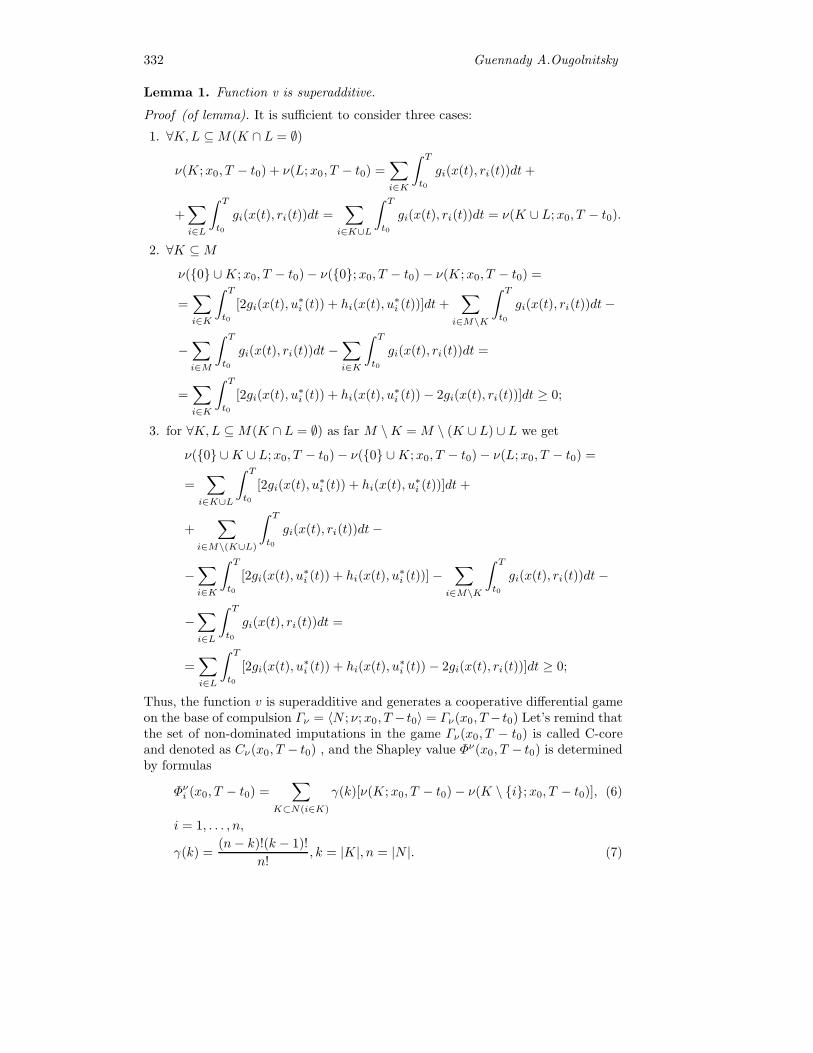
332 Guennady A.Ougolnitsky
Lemma 1. Function v is superadditive.
Proof (of lemma). It is sufficient to consider three cases:
1. ∀K,L ⊆M(K ∩ L = ∅)
ν(K;x0, T − t0) + ν(L;x0, T − t0) =∑i∈K
∫ T
t0
gi(x(t), ri(t))dt +
+∑i∈L
∫ T
t0
gi(x(t), ri(t))dt =∑
i∈K∪L
∫ T
t0
gi(x(t), ri(t))dt = ν(K ∪ L;x0, T − t0).
2. ∀K ⊆M
ν({0} ∪K;x0, T − t0)− ν({0};x0, T − t0)− ν(K;x0, T − t0) =
=∑i∈K
∫ T
t0
[2gi(x(t), u∗i (t)) + hi(x(t), u∗
i (t))]dt +∑
i∈M\K
∫ T
t0
gi(x(t), ri(t))dt−
−∑i∈M
∫ T
t0
gi(x(t), ri(t))dt −∑i∈K
∫ T
t0
gi(x(t), ri(t))dt =
=∑i∈K
∫ T
t0
[2gi(x(t), u∗i (t)) + hi(x(t), u∗
i (t))− 2gi(x(t), ri(t))]dt ≥ 0;
3. for ∀K,L ⊆M(K ∩ L = ∅) as far M \K = M \ (K ∪ L) ∪ L we get
ν({0} ∪K ∪ L;x0, T − t0)− ν({0} ∪K;x0, T − t0)− ν(L;x0, T − t0) =
=∑
i∈K∪L
∫ T
t0
[2gi(x(t), u∗i (t)) + hi(x(t), u∗
i (t))]dt +
+∑
i∈M\(K∪L)
∫ T
t0
gi(x(t), ri(t))dt−
−∑i∈K
∫ T
t0
[2gi(x(t), u∗i (t)) + hi(x(t), u∗
i (t))]−∑
i∈M\K
∫ T
t0
gi(x(t), ri(t))dt −
−∑i∈L
∫ T
t0
gi(x(t), ri(t))dt =
=∑i∈L
∫ T
t0
[2gi(x(t), u∗i (t)) + hi(x(t), u∗
i (t))− 2gi(x(t), ri(t))]dt ≥ 0;
Thus, the function v is superadditive and generates a cooperative differential gameon the base of compulsion Γν = 〈N ; ν;x0, T − t0〉 = Γν(x0, T − t0) Let’s remind thatthe set of non-dominated imputations in the game Γν(x0, T − t0) is called C-coreand denoted as Cν(x0, T − t0) , and the Shapley value Φν(x0, T − t0) is determinedby formulas
Φνi (x0, T − t0) =∑
K⊂N(i∈K)
γ(k)[ν(K;x0, T − t0)− ν(K \ {i};x0, T − t0)], (6)
i = 1, . . . , n,
γ(k) =(n− k)!(k − 1)!
n!, k = |K|, n = |N |. (7)

Games with Differently Directed Interests 333
��
Theorem 1. In the game Γν(x0, T − t0) it is true that Φν(x0, T − t0) ∈ Cν(x0, T −t0).
Proof (of theorem). Let’s calculate the components of Shapley value subject to (6):
Φν0(x0, T − t0) = γ(1)ν({0};x0, T − t0) +
+γ(2)∑
{0}∈K,|K|=2
[ν(K;x0, T − t0)− ν(K \ {0};x0, T − t0)] + · · ·+
+γ(n)∑
{0}∈K,|K|=n[ν(K;x0, T − t0)− ν(K \ {0};x0, T − t0)] +
+γ(n + 1)[ν(N ;x0, T − t0)− ν(M ;x0, T − t0)] =
= γ(1)∑i∈M
∫ T
t0
gi(x(t), ri(t))dt + γ(2)∑
{0}∈K,|K|=2
∫ T
t0
[∑i∈K
(2gi(x(t), u∗i (t)) +
+ hi(x(t), u∗i (t))) +
∑i∈M\K
gi(x(t), ri(t))−∑i∈K
gi(x(t), ri(t))]dt + · · ·+
+γ(n)∑
{0}∈K,|K|=n
∫ T
t0
[∑i∈K
(2gi(x(t), u∗i (t)) + hi(x(t), u∗
i (t))) +
+∑
i∈M\Kgi(x(t), ri(t)) −
∑i∈K
gi(x(t), ri(t))]dt +
+γ(n + 1)[∑i∈M
∫ T
t0
(2gi(x(t), u∗i (t)) + hi(x(t), u∗
i (t)))dt +∑i∈M
∫ T
t0
gi(x(t), ri(t))dt]
= γ(2)∑
{0}∈K,|K|=2
∑i∈K
∫ T
t0
(2gi(x(t), u∗i (t)) + hi(x(t), u∗
i (t)))dt +
+γ(3)∑
{0}∈K,|K|=3
∑i∈K
∫ T
t0
(2gi(x(t), u∗i (t)) + hi(x(t), u∗
i (t)))dt + · · ·+
+γ(n)∑
{0}∈K,|K|=n
∑i∈K
∫ T
t0
(2gi(x(t), u∗i (t)) + hi(x(t), u∗
i (t)))dt +
+γ(n + 1)∑i∈N
∫ T
t0
(2gi(x(t), u∗i (t)) + hi(x(t), u∗
i (t)))dt] =
=
n+1∑s=2
γ(s)∑
{0}∈K,|K|=s
∑i∈K
∫ T
t0
Ai(t)dt,
Ai(t) = 2gi(x(t), u∗i (t)) + hi(x(t), u∗
i (t)).
As each of n players of lower level takes part Cs−1n−1 times in the set of coalitions of
s players than

334 Guennady A.Ougolnitsky
Φν0(x0, T − t0) =
n+1∑s=2
γ(s)Cs−2n−1
∑i∈M
∫ T
t0
Ai(t)dt = 0, 5∑i∈M
∫ T
t0
Ai(t)dt. Thus,
Φν0(x0, T −t0) =∑i∈M
∫ T
t0
(gi(x(t), u∗i (t))+0, 5hi(x(t), u∗
i (t)))dt = 0, 5ν(N ;x0, T −t0)
As far Shapley value is Pareto-optimal we get∑i∈M
Φνi (x0, T − t0) = 0, 5ν(N ;x0, T − t0) = Φν0(x0, T − t0)
and as far all Followers are completely symmetrical we get
Φνi (x0, T − t0) =
∫ T
t0
(gi(x(t), u∗i (t)) + 0, 5hi(x(t), u∗
i (t)))dt, i ∈M.
To complete the proof it is sufficient to verify directly the inequalities of three types:
1.∑i∈K
Φνi (x0, T − t0) +∑j∈L
Φνj (x0, T − t0) ≥ ν(K ∪ L;x0, T − t0);
2. Φν0(x0, T − t0) +∑i∈K
Φνi (x0, T − t0) ≥ ν({0} ∪K;x0, T − t0);
3. Φν0(x0, T − t0) +∑i∈K
Φνi (x0, T − t0) +∑j∈L
Φνj (x0, T − t0) ≥ ν({0} ∪ (K ∪ L)),
K ∩ L = ∅,K, L ⊆M. ��
A cooperative game on the base of impulsion is built similarly. Unfortunately,the optimality principle Φν(x0, T − t0) ∈ Cν(x0, T − t0) is not dynamically stable(time consistent). To provide the dynamic stability a regularization procedure (pay-off distribution procedure) has to be used (Petrosyan and Zenkevich 2007). Define
Φνi (x0, T − t0) =
∫ T
t0
Bi(s)ds,Bi(t) ≥ 0,∑i∈N
Bi(t) = 1, t ∈ [t0, T ].
The quantity Bi(t) =dφνi (x0, T − t0)
dtis the instantaneous payoff to the player i at
the moment t. The vector B(t) = (B0(t), B1(t), . . . , Bn(t)) determines a distributionof the total gain among all players. By the proper choice of B(t) it is possible toensure that at each instant t ∈ [t0, T ] there will be no objections against realizationof the original agreement Φν(x0, T − t0), i.e. the imputation Φν(x0, T − t0) is timeconsistent. It is proved under general conditions that the regularization procedureB(t), t ∈ [t0, T ], leading to the time consistent cooperative solution, exists and isrealizable (Petrosyan and Zenkevich 1996).
4. Conclusion
The resolution of numerous ecological problems on different levels must be imple-mented on the base of sustainable development concept that determines the condi-tions to the state of environmental-economic systems and impacting control actions.Those conditions can’t be realized by themselves and require special collaborative
Games with Differently Directed Interests 335
efforts of different agents using both cooperation and hierarchical control. To for-malize the inevitable trade-offs it is natural to use game theoretic models includingthe games with differently directed interests. Unfortunately, the main optimalityprinciples of hierarchical control (compulsion, impulsion) are not dynamically sta-ble and therefore can’t be recommended as the direct base for collective solutions.The most prospective is the conviction method which is formalized as a transitionfrom hierarchy to cooperation and allows a regularization that provides the dynamicstability. However, in current social conditions other methods of hierarchical controlalso keep their actuality. To provide the dynamic stability of those optimality princi-ples it is necessary to build cooperative differential games on their base. An exampleof the approach is considered in this paper. The following directions of the game the-oretic modeling of the concept of sustainable development are of specific interest:investigation of general game theoretic models of the hierarchical control of sus-tainable development (Ugolnitsky 2002a, 2005; Ougolnitsky 2009); modeling of thehierarchical control of sustainable development of the ecological-economic systems(Ugolnitsky 1999; Ugolnitsky and Usov 2007a, 2009; Ougolnitsky 2002; Ougolnitskyand Usov 2009); modeling of the hierarchical control of sustainable development ofthe systems of another types (Ugolnitsky 2002b); modeling of the multilevel hierar-chical systems of different structure (Ugolnitsky and Usov 2007b, 2010); modelingof the corruption in hierarchical control systems (Rybasov and Ugolnitsky 2004;Denin and Ugolnitsky 2010); development of the information-analytical systems ofdecision support in the hierarchically controlled dynamical systems (Ugolnitsky andUsov 2008).
References
Basar, T. and Olsder, G. J. (1995). Dynamic Noncooperative Game Theory. AcademicPress, L.
Denin, K. I. and Ugolnitsky, G. A. (2010). Game theoretic model of corruption in thesystems of hierarchical control. Izvestiya RAS. Teoria i systemy upravlenia (Journal ofcomputer and system sciences international), 1, 192–198 (in Russian).
Dockner, E. J. and Jorgensen, S. (1984). Cooperative and Non-Cooperative DifferentialGame Solutions to an Investment and Pricing Problem. Journal of the OperationalResearch Society, 35, 731–739.
Dockner, E. J. and Long, N. V. (1993). International Pollution Control: Cooperative versusNon-Cooperative Strategies. Journal of Environmental Economics and Management,24, 13–29.
Fatkhutdinov, R. and Sivkova, L. (1999). Compulsion, impulsion, conviction: a new ap-proach to control methods. Upravlenie personalom (Human resource management), 2,32–40 (in Russian).
French, J. P. R.,Jr., and Raven, B. (1960) The bases of social power. In: Group Dynamics(Cartwright, D. and Zander, A., eds), pp. 607 – 623. Harper and Row, N.Y. French,J.P.R.,Jr., and Raven, B.
Fudenberg, D. and Tirole, J. (1991). Game theory. MIT Press, Mass.Gao, L., Jakubowski, A., Klompstra, M. B. and Olsder, G. J. (1989). Time-Dependent
Cooperation in Game. Springer-Verlag, Berlin.Germeyer, Yu. B., Vatel, I. A. (1974). Games with Hierarchical Vector of Interests. Izvestiya
AN USSR. Technical Cybernetics. Vol.3 (in Russian).Springer-Verlag, Berlin.Haurie, A. (1976). A Note on Nonzero-sum Differential Games with Bargaining Solutions.
Journal of Optimization Theory and Applications, 18, 31–39.Haurie, A. (1991). Piecewise Deterministic and Piecewise Diffusion Differential Games
with Model Uncertainties. Springer-Verlag, Berlin.
336 Guennady A.Ougolnitsky
Haurie, A., Krawczyk, J. B. and Roche, M. (1994). Monitoring Cooperative Equilibria in aStochastic Differential Game. Journal of Optimization Theory and Applications, 81,73–95.
Haurie, A. and Pohjola, M. (1987). Efficient Equilibria in a Differential Game of Capital-ism. Journal of Economic Dynamics and Control, 11, 65–78.
Haurie, A. and Zaccour, G. (1986). A Differential Game Model of Power Exchange betweenInterconnected Utilizers. Proceedings of the 25th IEEE Conference on Decision andControl, Athens, Greece.
Haurie, A. and Zaccour, G. (1991). A Game Programming Approach to Efficient Manage-ment of Interconnected Power Networks. Springer-Verlag, Berlin.
Jorgensen, S. and Zaccour, G. (2001). Time Consistent Side Payments in a Dynamic Gameof Downstream Pollution. Journal of Economic Dynamics and Control, 25, 1973–1987.
Kaitala, V., Maler, K. G. and Tulkens, H. (1995). The Acid Rain Game as a Resource Al-location Process with an Application to the International Cooperation among Finland,Russia, and Estonia. Scandinavian Journal of Economics, 97, 325–343.
Kaitala, V. and Pohjola, M. (1988). Optimal Recovery of a Shared Resource Stock: ADifferential Game with Efficient Memory Equilibria. Natural Resource Modeling, 3,91–118.
Kaitala, V. and Pohjola, M. (1995). Sustainable International Agreements on GreenhouseWarming: A Game Theory Study. Annals of the International Society of DynamicGames, 2, 67–87.
Kaitala, V. and Zaccour, G. (1990). Economic Development and Agreeable Redistributionin Capitalism: Efficient Game Equilibria in a Two-Class Neoclassical Growth Model.International Economic Review, 31(2), 421–438.
Kidland, F. E. and Prescott, E. C. (1977). Rules rather than decisions: the inconsistencyof optimal plans. J. of Polit. Econ., 85, 473–490.
Ledyaev, V. G. (1998). Power: A Conceptual Analysis. Nova Science Publishers, N.Y.Leitmann, G. (1974). Cooperative and Non-Cooperative Many Players Differential Games.
Springer-Verlag, N.Y.Leitmann, G. (1975). Cooperative and Non-Cooperative Differential Games. D.Reide, Am-
stredam.Maler, K. G. and de Zeeuw, A. D. (1998). The Acid Rain Differential Game. Environmental
and Resource Economics, 12, 167–184.Mazalov, V. and Rettieva, A. (2004). A fishery game model with migration: reserved ter-
ritory approach. Game Theory and Applications, 10.Mazalov, V. and Rettieva, A. (2005). Dynamic game methods for reserved territory opti-
mization. Survey in Applied and Industrial Math, 3(12), (in Russian).Mazalov, V. and Rettieva, A. (2006). Nash equilibrium in bioresource management problem.
Mathematical Modeling, 5(18), (in Russian).Mazalov, V. and Rettieva, A. (2007). Cooperative Incentive Equilibrium. In: Collected
papers presented on the International Conference Game Theory and Management(Petrosjan, L.A., Zenkevich, N.A., eds), pp. 316 – 325. SPb.: Graduate School ofManagement SBbU.
Ougolnitsky, G. A. (2002). Game theoretic modeling of the hierarchical control of sustain-able development. In: Game Theory and Applications (Petrosjan, L.A., Mazalov, V.V.,eds), pp. 82 – 91. Nova Science Publishers, N.Y., Vol.8.
Ougolnitsky, G. A. (2009). A Generalized Model of Hierarchically Controlled DynamicalSystem. In: Contributions to game theory and management. ( Petrosjan, L.A., Zenke-vich, N.A., eds), pp. 320 – 333. SPb.: Graduate School of Management SBbU.
Ougolnitsky, G. A. and Usov, A. B. (2009). Problems of the sustainable development ofecological-economic systems. In: Global Climatology and Ecodynamics: AnthropogenicChanges to Planet Earth. ( Cracknell, A.P., Krapivin, V.P., Varotsos, C.A., eds), pp.427 – 444. Springer-Praxis.

Games with Differently Directed Interests 337
Ougolnitsky, G. A. and Usov, A. B. (2010). Three level fan-like systems of control of theecological-economic objects. Problemy upravleniya (Control problems), 1, 26–32 (inRussian).
Petrosyan, L. A. (1977). The stability of solutions in differential games with many players.Vestnik Leningradskogo Universiteta, Ser.1, Iss.4, Vol.19, 46–52 (in Russian).
Petrosyan, L. A. (1991). The Time-Consistency of the Optimality Principles in Non-Zero Sum Differential Games. In: Lecture Notes in Control and Information Sciences(Hamalainen R.P. and Ehtamo H.K., eds), pp. 299 – 311. Springer-Verlag, Berlin,Vol.157.
Petrosyan, L. A. (1993). Strongly Time-Consistent Differential Optimality Principles.Vestnik Saint Petersburg University Mathematics, 26, 40–46 (in Russian).
Petrosyan, L. A. (1993). The Time Consistency in Differential Games with a DiscountFactor. Game Theory and Applications, 1.
Petrosyan, L. A. (1997). Agreeable Solutions in Differential Games. International Jour-nal of Mathematics, Game Theory and AlgebraVestnik Saint Petersburg UniversityMathematics, 7, 165–177.
Petrosyan, L. A. and Danilov, N. N. (1979). Stability of Solutions in Non-Zero Sum Dif-ferential Games with Transferable Payoffs. Vestnik of Leningrad University, 1, 52–59(in Russian).
Petrosyan, L. A. and Danilov, N. N. (1985). Cooperative Differential Games and TheirApplications. Tomsk State University, Tomsk (in Russian).
Petrosyan, L. A. and Zenkevich, N. A. (1996). Game Theory. World Scientific Publ.Co.,Singapore.
Petrosyan, L. A. and Zenkevich, N. A. (2007). Time Consistency of Cooperative Solutions.In: Contributions to game theory and management. Collected papers presented on theInternational Conference Game Theory and Management (Petrosjan, L.A., Zenkevich,N.A., eds), pp. 413 – 440. SPb.: Graduate School of Management SBbU.
Petrosyan, L. A. and Zenkevich, N. A. (2009). Conditions for Sustainable Cooperation. In:Contributions to game theory and management. Vol. II. Collected papers presented onthe International Conference Game Theory and Management (Petrosjan, L.A., Zenke-vich, N.A., eds), pp. 344 – 354. SPb.: Graduate School of Management SBbU.
Pontryagin, L. S., Boltyanskii, V. G., Gamkrelidze, R. V. and Mishchenko, E. F. (1962).The Mathematical Theory of Optimal Processes. Wiley, N.Y.
Rubio, S. J. and Casino, B. (2002). A Note on Cooperative versus Non-Cooperative Strate-gies in International Pollution Control. Resource and Energy Economics, 24, 251–261.
Rybasov, E. A. and Ugolnitsky, G. A. (2004). Mathematical modeling of the hierarchicalcontrol of ecological-economic systems considering corruption. In: Computer modeling.Ecology. Iss.2. (Ugolnitsky, G.A., ed), pp. 44 – 65. Vuzovskaya kniga, Moscow (inRussian).
Sorokin, P. (1957). Social and Cultural Dynamics.A Study of Change in Major Systems ofArt, Truth, Ethics, Law and Social Relationships. Porter Sargent Publisher, Boston.
Tahvonen, O. (1994). Carbon Dioxide Abatement as a Differential Game. European Jour-nal of Political Economy, 10, 685–705.
Tolwinsky, B., Haurie, A. and Leitmann, G. Tahvonen, O. (1970). Cooperative Equilibriain Differential Games. J. of Math. Analysis and Applications, 119, 182–202.
Ugolnitsky, G. A. (1999). Control of Ecological-Economic Systems. Vuzovskaya kniga,Moscow (in Russian).
Ugolnitsky, G. A. (2002). Game theoretic investigation of some methods of hierarchicalcontrol. Izvestiya RAS. Teoria i systemy upravlenia (Journal of computer and systemsciences international), 1, 97–101.
Ugolnitsky, G. A. (2002). Hierarchical control of the sustainable development of social or-ganizations. Obshchestvennye nauki i sovremennost (Social sciences and modernity),3, 133–140 (in Russian).

338 Guennady A.Ougolnitsky
Ugolnitsky, G. A. (2005). Game theoretic principles of optimality of the hierarchical controlof sustainable development. Izvestiya RAS. Teoria i systemy upravlenia (Journal ofcomputer and system sciences international), 4, 72–78 (in Russian).
Ugolnitsky, G. A. and Usov, A. B. (2007). GMathematical formalization of the methodsof hierarchical control of ecological-economic systems. Problemy upravleniya (Controlproblems), 4, 64–69 (in Russian).
Ugolnitsky, G. A. and Usov, A. B. (2007). Hierarchical systems of diamond-shaped struc-ture for river water quality control. Upravlenie bolshimi systemami (Control of bigsystems), 19, 187–203 (in Russian).
Ugolnitsky, G. A. and Usov, A. B. (2008). An information-analytical system of control ofthe ecological-economic objects. Izvestiya RAS. Teoria i systemy upravlenia (Journal ofcomputer and system sciences international), 2, 168–176 (in Russian).
Ugolnitsky, G. A. and Usov, A. B. (2009). Control of the complex ecological-economic sys-tems. Avtomatika i telemechanika (Automation and remote control), 5, 169–179 (inRussian).
United Nations (1987). ”Report of the World Commission on Environment and Develop-ment.” General Assembly Resolution 42/187, 11 December.
Yeung, D. W. K. (2009). Cooperative Game-Theoretic Mechanism Design for Optimal Re-source Use. In: Contributions to game theory and management. Vol. II. Collectedpapers presented on the International Conference Game Theory and Management(Petrosjan, L.A., Zenkevich, N.A., eds), pp. 483 – 513. SPb.: Graduate School ofManagement SBbU.
Yeung, D. W. K. and Petrosyan, L. A. (2001). Proportional Time-Consistent Solution inDifferential Games Saint Petersburg State University.

Memento Ludi: Information Retrievalfrom a Game-Theoretic Perspective�
George Parfionov1 and Roman Zapatrin2
1 Friedmann Laboratory For Theoretical Physics,Department of Mathematics,
SPb EF University, Griboyedova 30–32,191023 St.Petersburg, Russia
2 Department of Information Science,The State Russian Museum, Inzenernaya 4,
191186, St.Petersburg, RussiaE-mail: [email protected]
Abstract. We develop a macro-model of information retrieval process us-ing Game Theory as a mathematical theory of conflicts. We represent theparticipants of the Information Retrieval process as a game of two abstractplayers. The first player is the ‘intellectual crowd’ of users of search engines,the second is a community of information retrieval systems. In order to ap-ply Game Theory, we treat search log data as Nash equilibrium strategiesand solve the inverse problem of finding appropriate payoff functions. Forthat, we suggest a particular model, which we call Alpha model. Withinthis model, we suggest a method, called shifting, which makes it possible topartially control the behavior of massive users.The paper is asddressed to researchers in both game theory (providing a newclass of real life problems) and information retrieval, for whom we presentnew techniques to control the IR environment.
Introduction
The techniques we present are inspired by the success of macro-approach in bothnatural and social science. In thermodynamics, starting from a chaotic motion ofbillions of billions of microparticles, we arrive a simple transparent strongly pre-dictive theory with few macro-variables, such as temperature, pressure, and so on.In models of market behavior the chaotic motion is present as well, but there aretwo definite parties, each consisting of a big number of individuals with commoninterests, whose behavior is not concorded.
From a global perspective, information retrieval looks similar: there are manyindividual seekers of knowledge, on one side, and a number of knowledge providers,on the other: each are both chaotic and non-concorded. There are two definiteparties, whose members have similar interests, and every member of each party tendsto maximally fulfill his own interests. How could a Mathematician help them? Atfirst sight, each party could be suggested to solve a profit maximization problem. Butback in 1928 it was J. von Neumann who realized this approach to be inadequate:you can not maximize the value you do not know (Von Neumann, 1928). In fact, theprofit gained by each agent depends not only on its actions, but also on the activities
� This work was supported by the Russian basic Research Foundation under grant No.07-06-00119.

340 George Parfionov, Roman Zapatrin
of its counterpart, which are not known. Then the game theory was developedreplacing the notion of optimality by that of acceptability. Similarly, the crucialpoint of information retrieval, in contrast to data retrieval, is to get some satisfaction(feeling of relevance) rather than retrieve something exact. The analogy
Data Retrieval −→ matchingInformation Retrieval −→ relevance
� Optimization −→ maximumGame Theory −→ equilibrium
was a starting point for us to explore applications of game theory to the problemsof information retrieval.
The standard problem of game theory is seeking for reasonable (in various senses)strategies. When the rules of the game are given, there is a vast machinery, whichmakes it possible to calculate such strategies. In information retrieval we have twoparties whose interaction is of exactly game nature, but the rules of this game arenot explicitly formulated. However, we may observe the consequence of these rulesas users behavior, that is, we deal with the inverse problem of game theory, studiedby Dragan (Dragan, 1966) for cooperative games. In this paper we expand it to non-cooperative case.It turns out that the solution of the inverse problem is essentiallynon-unique: different rules can produce the same behavior. We suggest a particularclass of models, called Alpha models describing an idealized search system similarto Wolfram Alpha engine.
What can search engine managers benefit of these techniques? Game theorycan work out definite recommendations how to control the interaction between theparties of the information retrieval process. This sounds unrealistic: can one controlmassive chaotic behavior? Thermodynamics shows us that the answer is yes. Wecan not control individual molecules, but in order to alter their collective behaviorwe are able to change macroparameters: the engine of your car reminds it to you.In our case the payoff functions of the Alpha model are just those parameters.
In Section 1. we introduce (only the necessary) basic notion from game theory,in Section 2. we formulate the information retrieval process in terms of game theoryand formulate our method as the inverse problem in game theory. In Section 3. wesuggest its particular solution, which we call Alpha model as it resembles WolframAlpha engine and in Section 4. we suggest a method to control massive users’behavior.
1. Direct problem: classical game theory
Game theory is a mathematical theory studying conflicts and trade-offs. It involvesrational participants who follow formal rules. A game is specified by its players,players’ strategies and players’ payoffs. Begin with a well-known example (a refor-mulated Prisonners’ dilemma (Tucker, 1950)).
There are two players A and B. The player A can choose color: Red or Green ,while B chooses direction: Left or Right . The rules of the game are specified bythe following pair of payoff matrices (Table 1)
The Mathematician can predict the outcome of this game provided the players arerational, namely, wishing to gain more: the rational player A will necessarily chooseRed and B will choose Left .
However, both players know the payoff matrices, so, being rational, why can’tthey agree for A to choose Green and for B to choose Right ? The point is that
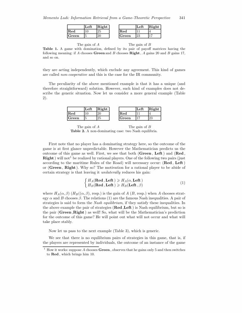
Memento Ludi: Information Retrieval from a Game-Theoretic Perspective 341
Left Right
Red 10 25
Green 5 20
Left Right
Red 11 4
Green 23 17
The gain of A The gain of BTable 1. A game with domination, defined by its pair of payoff matrices having thefollowing meaning: if A chooses Green and B chooses Right , A gains 20 and B gains 17,and so on.
they are acting independently, which exclude any agreement. This kind of gamesare called non-cooperative and this is the case for the IR community.
The peculiarity of the above mentioned example is that it has a unique (andtherefore straightforward) solution. However, such kind of examples does not de-scribe the generic situation. Now let us consider a more general example (Table2).
Left Right
Red 10 20
Green 5 25
Left Right
Red 11 4
Green 17 23
The gain of A The gain of BTable 2. A non-dominating case: two Nash equilibria.
First note that no player has a dominating strategy here, so the outcome of thegame is at first glance unpredictable. However the Mathematician predicts us theoutcome of this game as well. First, we see that both (Green , Left ) and (Red ,Right ) will not1 be realized by rational players. One of the following two pairs (justaccording to the maritime Rules of the Road) will necessary occur: (Red , Left )or (Green , Right ). Why so? The motivation for a rational player to be abide ofcertain strategy is that leaving it unilaterally reduces his gain:{
HA(Red ,Left ) � HA(α,Left )HB(Red ,Left ) � HB(Left , β)
(1)
where HA(α, β) (HB((α, β), resp.) is the gain of A (B, resp.) when A chooses strat-egy α and B chooses β. The relations (1) are the famous Nash inequalities. A pair ofstrategies is said to form the Nash equilibrium, if they satisfy these inequalities. Inthe above example the pair of strategies (Red ,Left ) is Nash equilibrium, but so isthe pair (Green ,Right ) as well! So, what will be the Mathematician’s predictionfor the outcome of this game? He will point out what will not occur and what willtake place stably.
Now let us pass to the next example (Table 3), which is generic.
We see that there is no equilibrium pairs of strategies in this game, that is, ifthe players are represented by individuals, the outcome of an instance of the game
1 How it works: suppose A chooses Green , observes that he gains only 5 and then switchesto Red , which brings him 10.
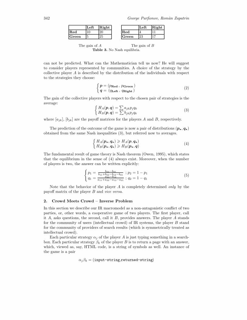
342 George Parfionov, Roman Zapatrin
Left Right
Red 10 20
Green 5 25
Left Right
Red 4 11
Green 23 17
The gain of A The gain of BTable 3. No Nash equilibria.
can not be predicted. What can the Mathematician tell us now? He will suggestto consider players represented by communities. A choice of the strategy by thecollective player A is described by the distribution of the individuals with respectto the strategies they choose: {
p = (pRed , pGreen )q = (qLeft , qRight )
(2)
The gain of the collective players with respect to the chosen pair of strategies is theaverage: {
HA(p, q) =∑
ajkpjqkHB(p, q) =
∑bjkpjqk
(3)
where [ajk], [bjk] are the payoff matrices for the players A and B, respectively.
The prediction of the outcome of the game is now a pair of distributions (p∗, q∗)obtained from the same Nash inequalities (3), but referred now to averages.{
HA(p∗, q∗) � HA(p, q∗)HB(p∗, q∗) � HB(p∗, q)
(4)
The fundamental result of game theory is Nash theorem (Owen, 1995), which statesthat the equilibrium in the sense of (4) always exist. Moreover, when the numberof players is two, the answer can be written explicitly:{
p1 = b22−b21b11+b22−b12−b21 ; p2 = 1− p1
q1 = a22−b12a11+a22−a12−a21 ; q2 = 1− q1
(5)
Note that the behavior of the player A is completely determined only by thepayoff matrix of the player B and vice versa.
2. Crowd Meets Crowd – Inverse Problem
In this section we describe our IR macromodel as a non-antagonistic conflict of twoparties, or, other words, a cooperative game of two players. The first player, callit A, asks questions, the second, call it B, provides answers. The player A standsfor the community of users (intellectual crowd) of IR systems, the player B standfor the community of providers of search results (which is symmetrically treated asintellectual crowd).
Each particular strategy αj of the player A is just typing something in a search-box. Each particular strategy βk of the player B is to return a page with an answer,which, viewed as, say, HTML code, is a string of symbols as well. An instance ofthe game is a pair
αjβk = (input-string,returned-string)

Memento Ludi: Information Retrieval from a Game-Theoretic Perspective 343
which is somehow evaluated by each participant. For example, the payoff valueHA(αjβk) for the player A for the pair
αjβk = (‘accommodation’,’No results found’)
is evidently low. In the meantime we do not dare to ascribe any payoff valueHB(αjβk) of this instance for the player B (we do not know providers’ priori-ties). In more general situations even the evaluations of the player A is not knownas well.
However, numerical payoff values are needed in order to apply game theory: itsbasic concept — of Nash equilibrium — is based on comparison of instances (4).As a matter of fact, the participants of IR process do compare instances, but theydo it qualitatively. But the Mathematician needs numbers! What data should heproceed in order to get them?
Stability and equilibrium. In a sense this week’s World Wide Web is the same as itwas a week ago, whatever be the variety of different queries and answers. What isstable in time is the statistics of instances αjβk: things frequently asked yesterdayrepeat today. The Mathematician tells us that from a game-theoretic perspectivethis stability is not surprising: these are Nash equilibria which are stable, becauseleaving them is unfavorable.
If we had known the payoff functions, we could find the Nash equilibrium. But inour situation we know the equilibrium (statistics of instances) and we have to findthe appropriate payoff functions HA(αjβk), HB(αjβk) in (3). This is the inverseproblem in game theory (Dragan, 1966). The inverse problem has multiple solutions:for given frequencies there are many different payoff matrices yielding the sameequilibrium2. Below, we introduce a specific model, called Alpha model with thesmallest number of free parameters.
3. Alpha model
The raw material for us will be a collection of search strings with appropriatefrequencies and a collection of returned results with appropriate frequencies as well.According to our model, we interpret it as realized equilibrium. Now we are aboutto reconstruct the payoff functions. First, according to the remark made above, weassume that the number of different strategies for both players is the same. If not,we may reach it by appropriate prepocessing of data, identifying some data strings.
Note that, given a pair of strategies (p, q), there are (infinitely) many differentpayoff functions, for which this pair of strategies is equilibrium. Among all suchmodels, we consider the simplest one, closest to data retrieval. For this model, thepayoff matrices are diagonal:
A =
⎛⎜⎜⎝a1 0 . . . 00 a2 . . . 0· · · · · · · · · · · ·0 0 . . . an
⎞⎟⎟⎠ ; B =
⎛⎜⎜⎝b1 0 . . . 00 b2 . . . 0· · · · · · · · · · · ·0 0 . . . bn
⎞⎟⎟⎠ (6)
where a1, . . . , an; b1, . . . , bn are positive numbers.
2 A trivial example of such non-uniqueness is multiplying the payoff matrix by a positivenumber.

344 George Parfionov, Roman Zapatrin
This feature of this model is that the only valuable answer for question αj is βjwith the same index j, other answers βk for k = j are of zero value. This looks likeWolfram Alpha search engine, which provides the only answer to a query, that iswhy we call our model Alpha.
The Nash equilibrium for the game is given by:
pj =b−1j
b−11 + · · ·+ b−1
n
; qk =a−1k
a−11 + · · ·+ a−1
n
(7)
We can check this directly checking Nash inequalities (4). It is sufficient (Owen, 1995)to check it only for pure strategies
≤ (8)
Recall that we have the inverse problem, that is, we know (p, q). Its solution is
aj =a
qj; bk =
b
pk(9)
for any fixed positive numbers a, b. The obtained result shows us that:
– The less frequent is a instance, the higher is its value.
– The value of a question is determined by the frequency of the reply, and viceversa, the value of a reply is determined by the frequency of the question.
The first statement means that within this model frequently asked questions havelow value for the provider B, and, vice versa, rarely delivered answers are of highvalue for the user A.
The magic of Nash theory is captured in the second statement. It means thatthe behavior of player A is completely determined only by the payoff matrix ofplayer B. In other words, the popularity (=frequency) of users’ questions dependson priorities of the answering side rather than on their own priorities.
4. Shifting of users’ behavior
So far, we have suggested a quantitative model of IR process. The aim of this modelis not just to describe, but also to give some means of control to the overall process.There are two parties involved, each having its own interests. Let us consider whatcould the provider B do in order to increase its gain.
At first sight, the strategy q should be changed, but the power of Nash theory isthat the answer is immediate: it does not make sense, any unilateral deviation fromthe equilibrium is unfavorable for B. The player B can not directly, by ordering,control the strategy p of player A, nor its payoff matrix. So, the only thing B cando is to change its own interests : what remains under control of B, is its own payoffmatrix. How it works?
A simple suggestion is to multiply all the elements of B by, say, 1957. Thissuggestion does not affect, as it follows from (7), the strategy of player A: it issimilar to recalculating your wealth from euro to Italian liras: you may feel happy,but your wealth will not grow. So far, we have to accept a normalization condition
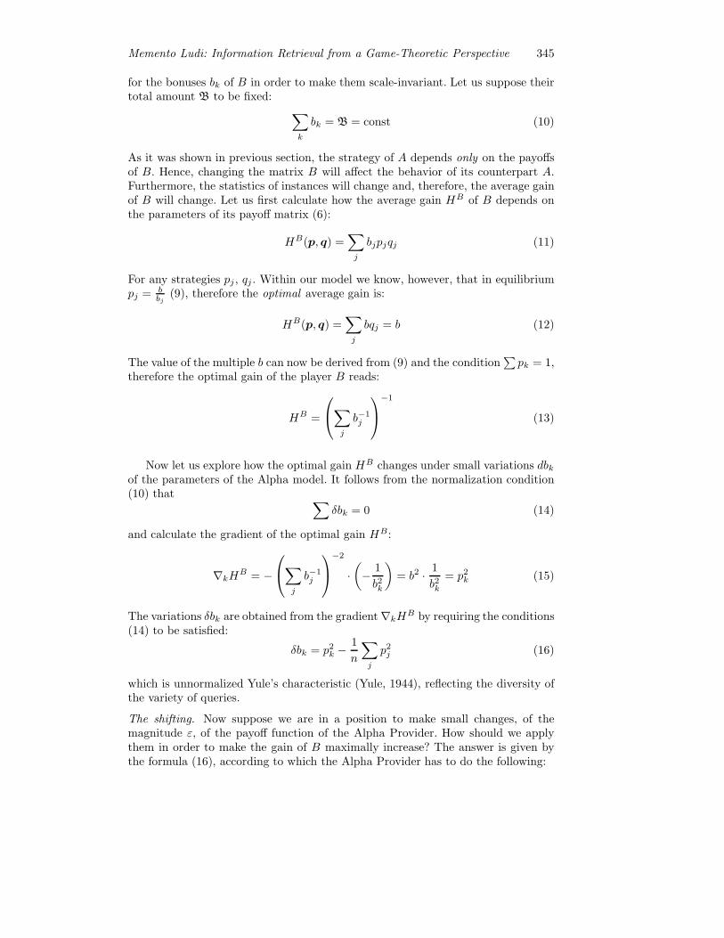
Memento Ludi: Information Retrieval from a Game-Theoretic Perspective 345
for the bonuses bk of B in order to make them scale-invariant. Let us suppose theirtotal amount B to be fixed: ∑
k
bk = B = const (10)
As it was shown in previous section, the strategy of A depends only on the payoffsof B. Hence, changing the matrix B will affect the behavior of its counterpart A.Furthermore, the statistics of instances will change and, therefore, the average gainof B will change. Let us first calculate how the average gain HB of B depends onthe parameters of its payoff matrix (6):
HB(p, q) =∑j
bjpjqj (11)
For any strategies pj , qj . Within our model we know, however, that in equilibriumpj = b
bj(9), therefore the optimal average gain is:
HB(p, q) =∑j
bqj = b (12)
The value of the multiple b can now be derived from (9) and the condition∑
pk = 1,therefore the optimal gain of the player B reads:
HB =
⎛⎝∑j
b−1j
⎞⎠−1
(13)
Now let us explore how the optimal gain HB changes under small variations dbkof the parameters of the Alpha model. It follows from the normalization condition(10) that ∑
δbk = 0 (14)
and calculate the gradient of the optimal gain HB:
∇kHB = −
⎛⎝∑j
b−1j
⎞⎠−2
·(− 1
b2k
)= b2 · 1
b2k= p2k (15)
The variations δbk are obtained from the gradient∇kHB by requiring the conditions(14) to be satisfied:
δbk = p2k −1
n
∑j
p2j (16)
which is unnormalized Yule’s characteristic (Yule, 1944), reflecting the diversity ofthe variety of queries.
The shifting. Now suppose we are in a position to make small changes, of themagnitude ε, of the payoff function of the Alpha Provider. How should we applythem in order to make the gain of B maximally increase? The answer is given bythe formula (16), according to which the Alpha Provider has to do the following:
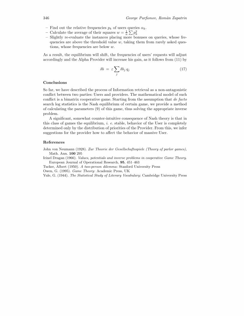
346 George Parfionov, Roman Zapatrin
– Find out the relative frequencies pk of users queries αk.– Calculate the average of their squares w = 1
n
∑p2k
– Slightly re-evaluate the instances placing more bonuses on queries, whose fre-quencies are above the threshold value w, taking them from rarely asked ques-tions, whose frequencies are below w.
As a result, the equilibrium will shift, the frequencies of users’ requests will adjustaccordingly and the Alpha Provider will increase his gain, as it follows from (11) by
δb = ε∑j
δbj qj (17)
Conclusions
So far, we have described the process of Information retrieval as a non-antagonisticconflict between two parties: Users and providers. The mathematical model of suchconflict is a bimatrix cooperative game. Starting from the assumption that de factosearch log statistics is the Nash equilibrium of certain game, we provide a methodof calculating the parameters (9) of this game, thus solving the appropriate inverseproblem.
A significant, somewhat counter-intuitive consequence of Nash theory is that inthis class of games the equilibrium, i. e. stable, behavior of the User is completelydetermined only by the distribution of priorities of the Provider. From this, we infersuggestions for the provider how to affect the behavior of massive User.
References
John von Neumann (1928). Zur Theorie der Gesellschaftsspiele (Theory of parlor games),Math. Ann. 100 295
Irinel Dragan (1966). Values, potentials and inverse problems in cooperative Game Theory.European Journal of Operational Research, 95, 451–463
Tucker, Albert (1950). A two-person dilemma: Stanford University PressOwen, G. (1995). Game Theory : Academic Press, UKYule, G. (1944). The Statistical Study of Literary Vocabulary : Cambridge University Press
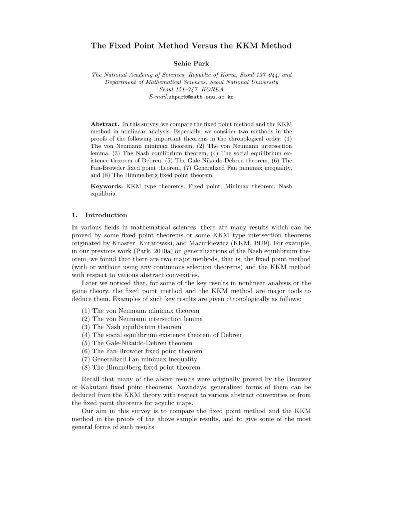
The Fixed Point Method Versus the KKM Method
Sehie Park
The National Academy of Sciences, Republic of Korea, Seoul 137–044; andDepartment of Mathematical Sciences, Seoul National University
Seoul 151–747, KOREAE-mail:[email protected]
Abstract. In this survey, we compare the fixed point method and the KKMmethod in nonlinear analysis. Especially, we consider two methods in theproofs of the following important theorems in the chronological order: (1)The von Neumann minimax theorem, (2) The von Neumann intersectionlemma, (3) The Nash equilibrium theorem, (4) The social equilibrium ex-istence theorem of Debreu, (5) The Gale-Nikaido-Debreu theorem, (6) TheFan-Browder fixed point theorem, (7) Generalized Fan minimax inequality,and (8) The Himmelberg fixed point theorem.
Keywords: KKM type theorems; Fixed point; Minimax theorem; Nashequilibria.
1. Introduction
In various fields in mathematical sciences, there are many results which can beproved by some fixed point theorems or some KKM type intersection theoremsoriginated by Knaster, Kuratowski, and Mazurkiewicz (KKM, 1929). For example,in our previous work (Park, 2010a) on generalizations of the Nash equilibrium the-orem, we found that there are two major methods, that is, the fixed point method(with or without using any continuous selection theorems) and the KKM methodwith respect to various abstract convexities.
Later we noticed that, for some of the key results in nonlinear analysis or thegame theory, the fixed point method and the KKM method are major tools todeduce them. Examples of such key results are given chronologically as follows:
(1) The von Neumann minimax theorem(2) The von Neumann intersection lemma(3) The Nash equilibrium theorem(4) The social equilibrium existence theorem of Debreu(5) The Gale-Nikaido-Debreu theorem(6) The Fan-Browder fixed point theorem(7) Generalized Fan minimax inequality(8) The Himmelberg fixed point theorem
Recall that many of the above results were originally proved by the Brouweror Kakutani fixed point theorems. Nowadays, generalized forms of them can bededuced from the KKM theory with respect to various abstract convexities or fromthe fixed point theorems for acyclic maps.
Our aim in this survey is to compare the fixed point method and the KKMmethod in the proofs of the above sample results, and to give some of the mostgeneral forms of such results.
348 Sehie Park
Recall that such comparison will also work for lots of results other than theabove ones in the KKM theory.
2. Abstract Convex Spaces and the KKM Spaces
Multimaps are also called simply maps. Let 〈D〉 denote the set of all nonemptyfinite subsets of a set D. Recall the following in (Park, 2008a,b,c, 2010b):
Definition 1. An abstract convex space (E,D;Γ ) consists of a topological space E,a nonempty set D, and a multimap Γ : 〈D〉 → 2E with nonempty values ΓA := Γ (A)for A ∈ 〈D〉.
For any D′ ⊂ D, the Γ -convex hull of D′ is denoted and defined by
coΓD′ :=
⋃{ΓA | A ∈ 〈D′〉} ⊂ E.
A subset X of E is called a Γ -convex subset of (E,D;Γ ) relative to D′ if for anyN ∈ 〈D′〉, we have ΓN ⊂ X , that is, coΓD
′ ⊂ X .When D ⊂ E, the space is denoted by (E ⊃ D;Γ ). In such case, a subset X of
E is said to be Γ -convex if coΓ (X ∩D) ⊂ X ; in other words, X is Γ -convex relativeto D′ := X ∩D. In case E = D, let (E;Γ ) := (E,E;Γ ).
Definition 2. Let (E,D;Γ ) be an abstract convex space. If a multimap G : D →2E satisfies
ΓA ⊂ G(A) :=⋃y∈A
G(y) for all A ∈ 〈D〉,
then G is called a KKM map.
Definition 3. The partial KKM principle for an abstract convex space (E,D;Γ )is the statement that, for any closed-valued KKM map G : D → 2E , the family{G(y)}y∈D has the finite intersection property. The KKM principle is the statementthat the same property also holds for any open-valued KKM map.
An abstract convex space is called a KKM space if it satisfies the KKM principle.
Now we have the following diagram for triples (E,D;Γ ):
Simplex =⇒ Convex subset of a t.v.s. =⇒ Lassonde type convex space=⇒ H-space =⇒ G-convex space ⇐⇒ φA-space =⇒ KKM space
=⇒ Space satisfying the partial KKM principle=⇒ Abstract convex space.
We recall the following in (Park, 1999,2001,2008a,b,c):
Definition 4. A generalized convex space or a G-convex space (X,D;Γ ) is an ab-stract convex space such that for each A ∈ 〈D〉 with the cardinality |A| = n + 1,there exists a continuous function φA : Δn → Γ (A) such that J ∈ 〈A〉 impliesφA(ΔJ) ⊂ Γ (J).
Here, Δn is the standard n-simplex with vertices {ei}ni=0, and ΔJ the face of Δn
corresponding to J ∈ 〈A〉; that is, if A = {a0, a1, . . . , an} and J = {ai0 , ai1 , . . . , aik} ⊂A, then ΔJ = co{ei0 , ei1 , . . . , eik}.Definition 5. For an abstract convex space (E ⊃ D;Γ ), a function f : E → Ris said to be quasiconcave [resp., quasiconvex] if {x ∈ E | f(x) > r} [resp., {x ∈E | f(x) < r}] is Γ -convex for each r ∈ R.
For the basic theory on KKM spaces, see Park (2010b) and the references therein.
The Fixed Point Method Versus the KKM Method 349
3. The KKM type theorems
In 1929, Knaster, Kuratowski, and Mazurkiewicz (simply, KKM) obtained the fol-lowing celebrated KKM theorem from the Sperner combinatorial lemma in 1928:
Theorem 1. (KKM, 1929) Let Ai (0 ≤ i ≤ n) be n + 1 closed subsets of an n-simplex p0p1 · · · pn. If the inclusion relation
pi0pi1 · · · pik ⊂ Ai0 ∪ Ai1 ∪ · · · ∪ Aik
holds for all faces pi0pi1 · · · pik (0 ≤ k ≤ n, 0 ≤ i0 < i1 < · · · < ik ≤ n), then⋂ni=0 Ai = ∅.
The first application of this KKM theorem was to give a simple proof of theBrouwer fixed point theorem; see (KKM, 1929) and (Park, 1999). Later, it is knownthat the Brouwer theorem, the Sperner lemma, and the KKM theorem are mutuallyequivalent.
In 1961, Fan extended the KKM theorem as follows:
Lemma 1. (Fan, 1961) Let X be an arbitrary set in a topological vector space Y .To each x ∈ X, let a closed set F (x) in Y be given such that the following twoconditions are satisfied:
(i) The convex hull of a finite subset {x1, · · · , xn} of X is contained in⋃ni=1 F (xi).
(ii) F (x) is compact for at least one x ∈ X.Then
⋂x∈X F (x) = ∅.
From the partial KKM principle for abstract convex spaces, we have a wholeintersection property of the Fan type as follows:
Theorem 2. (Park, 2011b) Let (E,D;Γ ) be an abstract convex space satisfying thepartial KKM principle and a map G : D → 2E satisfy the following:
(1)⋂z∈DG(z) =
⋂z∈D G(z) (G is intersectionally closed-valued);
(2) G is a KKM map (that is, ΓA ⊂ G(A) for all A ∈ 〈D〉); and(3) there exists a nonempty compact subset K of E such that one of the following
holds:(i) E = K;
(ii)⋂{G(z) | z ∈M} ⊂ K for some M ∈ 〈D〉; or
(iii) for each N ∈ 〈D〉, there exists a compact Γ -convex subset LN of E relativeto some D′ ⊂ D such that N ⊂ D′ and
LN ∩⋂z∈D′
G(z) ⊂ K.
Then⋂{G(z) | z ∈ D} = ∅.
When G is closed-valued or transfer closed-valued in (1), we obtain the conclu-sion
K ∩⋂{G(z) | z ∈ D} = ∅.
Theorem 2 subsumes a very large number of particular KKM type theorems inthe literature and has a number of equivalent formulations; see (Park, 2011b).

350 Sehie Park
4. The von Neumann type minimax theorem
In 1928, J. von Neumann obtained the following minimax theorem, which is oneof the fundamental results in the theory of games developed by himself. We adoptKakutani’s formulation in (Kakutani, 1941):
Theorem 3. (von Neumann, 1928) Let f(x, y) be a continuous real-valued functiondefined for x ∈ K and y ∈ L, where K and L are arbitrary bounded closed convexsets in two Euclidean spaces Rm and Rn. If for every x0 ∈ K and for every realnumber α, the set of all y ∈ L such that f(x0, y) ≤ α is convex, and if for everyy0 ∈ L and for every real number β, the set of all x ∈ K such that f(x, y0) ≥ β isconvex, then we have
maxx∈K
miny∈L
f(x, y) = miny∈L
maxx∈K
f(x, y).
In order to give simple proofs of von Neumann’s Lemma in 1937 and the aboveminimax theorem, Kakutani obtained the following generalization of the Brouwerfixed point theorem to multimaps:
Theorem 4. (Kakutani, 1941) If x �→ Φ(x) is an upper semicontinuous point-to-set mapping of an r-dimensional closed simplex S into the family of nonempty closedconvex subset of S, then there exists an x0 ∈ S such that x0 ∈ Φ(x0).
Equivalently,
Corollary 1. (Kakutani, 1941) Theorem 4.2 is also valid even if S is an arbitrarybounded closed convex set in a Euclidean space.
As Kakutani noted, Corollary 1 readily implies von Neumann’s Lemma, andlater Nikaido noted that those two results are directly equivalent.
This was the beginning of the fixed point theory of multimaps having a vitalconnection with the minimax theory in game theory and the equilibrium theory ineconomics.
In 1958, von Neumann’s minimax theorem was extended by Sion to arbitrarytopological vector spaces as follows:
Theorem 5. (Sion, 1958) Let X,Y be a compact convex set in a topological vectorspace. Let f be a real-valued function defined on X × Y . If
(1) for each fixed x ∈ X, f(x, y) is a lower semicontinuous, quasiconvex functionon Y , and
(2) for each fixed y ∈ Y, f(x, y) is an upper semicontinuous, quasiconcave func-tion on X,then we have
miny∈Y
maxx∈X
f(x, y) = maxx∈X
miny∈Y
f(x, y).
Sion’s proof was based on the KKM theorem and this is the first application ofthe theorem after (KKM, 1929).
Recently, by the KKM method, we obtained a very general form of the vonNeumann minimax theorem as follows; see (Park, 2010a).
Let (X ;Γ1) and (Y ;Γ2) be abstract convex spaces. For their product, we candefine ΓX×Y (A) := Γ1(π1(A)) × Γ2(π2(A)) for A ∈ 〈X × Y 〉.

The Fixed Point Method Versus the KKM Method 351
Theorem 6. (Park, 2010a) Let (E;Γ ) := (X × Y ;ΓX×Y ) be the product abstractconvex space, f, s, t, g : X × Y → R be four functions,
μ := infy∈Y
supx∈X
f(x, y) and ν := supx∈X
infy∈Y
g(x, y).
Suppose that(1) f(x, y) ≤ s(x, y) ≤ t(x, y) ≤ g(x, y) for each (x, y) ∈ X × Y ;(2) for each r < μ and y ∈ Y , {x ∈ X | s(x, y) > r} is Γ1-convex; for each r > ν
and x ∈ X, {y ∈ Y | t(x, y) < r} is Γ2-convex;(3) for each r > ν, there exists a finite set {xi}mi=1 ⊂ X such that
Y =
m⋃i=1
Int {y ∈ Y | f(xi, y) > r}; and
(4) for each r < μ, there exists a finite set {yj}nj=1 ⊂ Y such that
X =n⋃j=1
Int {x ∈ X | g(x, yj) < r}.
If (E;Γ ) satisfies the partial KKM principle, then we have
μ = infy∈Y
supx∈X
f(x, y) ≤ supx∈X
infy∈Y
g(x, y) = ν.
5. The von Neumann type intersection theorems
The minimax theorem was later extended by von Neumann in 1937 to the followingintersection lemma. We also adopt Kakutani’s formulation:
Lemma 2. (von Neumann, 1937) Let K and L be two bounded closed convex setsin the Euclidean spaces Rm and Rn respectively, and let us consider their Cartesianproduct K ×L in Rm+n. Let U and V be two closed subsets of K ×L such that forany x0 ∈ K the set Ux0 , of y ∈ L such that (x0, y) ∈ U , is nonempty, closed andconvex and such that for any y0 ∈ L the set Vy0 , of all x ∈ K such that (x, y0) ∈ V ,is nonempty, closed and convex. Under these assumptions, U and V have a commonpoint.
Von Neumann proved this by using a notion of integral in Euclidean spaces andapplied this to the problems of mathematical economics. Kakutani gave a simpleproof by applying his fixed point theorem. Lemma 2 was generalized by Fan, Ma,and others to various Fan type intersection theorems for sets with convex sections.
Let {Xi}i∈I be a family of sets, and let i ∈ I be fixed. Let
X =∏j∈I
Xj and X i =∏
j∈I\{i}Xj .
If xi ∈ X i and j ∈ I \ {i}, let xij denote the jth coordinate of xi. If xi ∈ X i and
xi ∈ Xi, let [xi, xi] ∈ X be defined as follows: Its ith coordinate is xi and, for j = i,its jth coordinate is xij . Therefore, any x ∈ X can be expressed as x = [xi, xi] for
any i ∈ I, where xi denotes the projection of x onto X i.Some of the most general forms of the von Neumann intersection lemma are the
following in the KKM theory:
352 Sehie Park
Theorem 7. (Park, 2010c) Let {(Xi;Γi)}ni=1 be a finite family of compact abstractconvex spaces such that (X ;Γ ) = (
∏ni=1 Xi;Γ ) satisfies the partial KKM principle
and, for each i, let Ai and Bi are subsets of X satisfying
(1) for each xi ∈ X i, ∅ = coΓi Bi(xi) ⊂ Ai(x
i) := {yi ∈ Xi | [xi, yi] ∈ Ai}; and(2) for each yi ∈ Xi, Bi(yi) := {xi ∈ X i | [xi, yi] ∈ Bi} is open in X i.
Then we have⋂ni=1 Ai = ∅.
Theorem 8. (Park, 2001) Let {(Xi;Γi)}i∈I be a family of Hausdorff compact G-convex spaces and, for each i ∈ I, let Ai and Bi are subsets of X =
∏i∈I Xi
satisfying the following:
(1)′ for each xi ∈ X i, ∅ = coΓi Bi(xi) ⊂ Ai(x
i) := {yi ∈ Xi | [xi, yi] ∈ Ai}; and
(2)′ for each yi ∈ Xi, Bi(yi) := {xi ∈ X i | [xi, yi] ∈ Bi} is open in X i.Then we have
⋂i∈I Ai = ∅.
6. The Nash equilibrium theorem
The first remarkable one of generalizations of von Neumann’s minimax theorem wasNash’s theorem (Nash, 1950, 1951) on equilibrium points of non-cooperative games.The following formulation is given by (Fan, 1966):
Theorem 9. (Nash) Let X1, X2, · · · , Xn be n (≥ 2) nonempty compact convex setseach in a real Hausdorff topological vector space. Let f1, f2, · · · , fn be n real-valuedcontinuous functions defined on
∏ni=1 Xi. If for each i = 1, 2, · · · , n and for any
given point (x1, · · · , xi−1, xi+1, · · · , xn) ∈∏j �=iXj, fi(x1, · · · , xi−1, xi, xi+1, · · · , xn)
is a quasi-concave function on Xi, then there exists a point (x1, x2, · · · , xn) ∈∏ni=1 Xi such that
fi(x1, x2, · · · , xn) = maxyi∈Xi
fi(x1, · · · , xi−1, yi, xi+1, · · · , xn) (1 ≤ i ≤ n).
The original form of this theorem in (Nash, 1950, 1951) was for Euclidean spacesand its proofs were based on the Brouwer or Kakutani fixed point theorem.
Moreover, based on a generalization of the Kakutani fixed point theorem dueto Fan (1952) and Glicksberg (1952), certain generalizations of the Nash theoremwere obtained; for example, see (Aliprantis et al., 2006) and (Becker et al., 2006).
The first proof of the Nash theorem by the KKM method was given by Fan(1966). Applying the KKM method or the fixed point method, we obtained someof the most general forms of the Nash theorem as follows:
Theorem 10. (Park, 2010c) Let {(Xi;Γi)}ni=1 be a finite family of compact abstractconvex spaces such that (X ;Γ ) = (
∏ni=1 Xi;Γ ) satisfies the partial KKM principle
and, for each i, let fi, gi : X = X i ×Xi → R be real functions such that(0) fi(x) ≤ gi(x) for each x ∈ X;
(1) for each xi ∈ X i, xi �→ gi[xi, xi] is quasiconcave on Xi;
(2) for each xi ∈ X i, xi �→ fi[xi, xi] is u.s.c. on Xi; and
(3) for each xi ∈ Xi, xi �→ fi[x
i, xi] is l.s.c. on X i.
Then there exists a point x ∈ X such that
gi(x) ≥ maxyi∈Xi
fi[xi, yi] for all i = 1, 2, . . . , n.
The Fixed Point Method Versus the KKM Method 353
Theorem 11. (Park, 2001) Let {(Xi;Γi)}i∈I be a family of Hausdorff compact G-convex spaces and, for each i ∈ I, let fi, gi : X = X i ×Xi → R be real functionssatisfying (0)-(3) in Theorem 10. Then there exists a point x ∈ X such that
gi(x) ≥ maxyi∈Xi
fi[xi, yi] for all i ∈ I.
7. The social equilibrium existence theorem of Debreu
Acyclic versions of the social equilibrium existence theorem of Debreu (1952) areobtained in (Park, 1998, 2011a) as follows:
A polyhedron is a set in Rn homeomorphic to a union of a finite number ofcompact convex sets in Rn. The product of two polyhedra is a polyhedron.
A nonempty topological space is said to be acyclic whenever its reduced homol-ogy groups over a field of coefficients vanish. The product of two acyclic spaces isacyclic by the Kunneth theorem.
The following is due to Eilenberg and Montgomery or, more generally, to Begle(1950):
Lemma 3. (Eilenberg and Montgomery, 1946) Let Z be an acyclic polyhedron andT : Z → 2Z an acyclic map (that is, u.s.c. with acyclic values). Then T has a fixedpoint x ∈ Z; that is, x ∈ T (x).
Recently, we obtained the following new collectively fixed point theorem equiva-lent to Lemma 3:
Theorem 12. (Park, 2011a) Let {Xi}i∈I be any family of acyclic polyhedra, andTi : X → 2Xi an acyclic map for each i ∈ I. Then there exists an x ∈ X such thatxi ∈ Ti(x) for each i ∈ I.
From this, we have the following acyclic version of the social equilibrium existencetheorem of Debreu (1952):
Theorem 13. (Park, 2011a) Let {Xi}i∈I be any family of acyclic polyhedra, Ai :X i → 2Xi closed maps, and fi, gi : Gr(Ai)→ R u.s.c. functions for each i ∈ I suchthat
(1) gi(x) ≤ fi(x) for all x ∈ Gr(Ai);(2) ϕi(x
i) := maxy∈Ai(xi) gi[xi, y] is an l.s.c. function of xi ∈ X i; and
(3) for each i ∈ I and xi ∈ X i, the set
M(xi) := {xi ∈ Ai(xi) | fi[xi, xi] ≥ ϕi(x
i)}
is acyclic.Then there exists an equilibrium point a ∈ Gr(Ai) for all i ∈ I; that is,
ai ∈ Ai(ai) and fi(a) = max
ai∈A(ai)gi[a
i, ai] for all i ∈ I.
Debreu’s theorem is the contractible case in (3) for a finite I.In Park (1998, 2011a), this is applied to deduce acyclic versions of theorems on
saddle points, minimax theorems, and the following Nash equilibrium theorem:

354 Sehie Park
Theorem 14. (Park, 2011a) Let {Xi}i∈I be a family of acyclic polyhedra, X =∏ni=1 Xi, and for each i, fi : X → R a continuous function such that
(0) for each xi ∈ X i and each α ∈ R, the set
{xi ∈ Xi | fi[xi, xi] ≥ α}
is empty or acyclic.Then there exists a point a ∈ X such that
fi(a) = maxyi∈Xi
fi[ai, yi] for all i ∈ I.
In our previous work (Park, 1998), Theorems 12-14 were obtained for a finiteindex set I.
8. The Gale-Nikaido-Debreu theorem
A convex space (in the sense of Lassonde) is a nonempty convex set (in a vectorspace) equipped with any topology that induces the Euclidean topology on theconvex hulls of its finite subsets. Such convex hulls are called polytopes. For details,see (Park, 1999) and references therein.
In 1994, we introduced an admissible class Aκc (X,Y ) of maps T : X → 2Y
between topological spaces X and Y as the one such that, for each T and eachcompact subset K of X , there exists a map Γ ∈ Ac(K,Y ) satisfying Γ (x) ⊂ T (x)for all x ∈ K; where Ac is consisting of finite composites of maps in A, and A is aclass of maps satisfying the following properties:
(i) A contains the class of (single-valued) continuous functions;(ii) each F ∈ Ac is u.s.c. and compact-valued; and(iii) for any polytope P , each F ∈ Ac(P, P ) has a fixed point.Let X be a convex space and Y a Hausdorff space. In 1997, we introduced a
more general “better” admissible class B of multimaps as follows:
F ∈ B(X,Y ) ⇐⇒ F : X → 2Y such that, for any polytope P in X and anycontinuous map f : F (P )→ P , f(F |P ) has a fixed point.
Here, A and B should be denoted by “Fraktur A” and “Fraktur B”, resp.In 1997, we obtained a KKM type theorem related to the better admissible class
B of multimaps. From the theorem, we deduced the following generalization of theso-called Walras excess demand theorem:
Theorem 15. (Park, 1997) Let X be a convex space, Y a Hausdorff space, T ∈B(X,Y ) a compact map, c ∈ R, and φ, ψ : X × Y → R two extended real-valuedfunctions such that
(1) φ(x, y) ≤ ψ(x, y) for each (x, y) ∈ X × Y ;(2) for each x ∈ X, y �→ ψ(x, y) is u.s.c. on Y ;(3) for each y ∈ Y , x �→ φ(x, y) is quasiconvex on X; and(4) φ(x, y) ≥ c for all (x, y) ∈ T (Walras law).
Then there exists a Walras equilibrium; that is, there exists a y0 ∈ Y such that
c ≤ φ(x, y0) for all x ∈ X.
This generalize a result due to Granas and Liu (1986).The following is a different version of Theorem 15:

The Fixed Point Method Versus the KKM Method 355
Theorem 16. (Park, 1997) Let X be a compact convex space, Y a Hausdorff space,and T ∈ Aκc (X,Y ). Let φ : X × Y → R be a continuous function and c ∈ R suchthat
(1) for each y ∈ Y , x �→ φ(x, y) is quasiconvex on X; and(2) φ(x, y) ≥ c for all (x, y) ∈ T (Walras law).
Then there exists a Warlas equilibrium; that is, there exists an (x0, y0) ∈ T suchthat
c ≤ φ(x0, y0) ≤ φ(x, y0) forall x ∈ X.
This extends results due to Granas-Liu (1986), Gwinner (1981), and Zeidler(1986).
From Theorem 16, we deduced the following generalization of the Gale-Nikaido-Debreu theorem:
Theorem 17. (Park, 1997) Let (E,F, 〈 , 〉) be a dual system of Hausdorff topo-logical vector spaces E and F , where the real bilinear form 〈 , 〉 is continuous oncompact subsets of E×F . Let X be a nonempty compact convex subset of E, P theconvex cone
⋃{rX | r ≥ 0}, and P+ = {y ∈ F | 〈p, y〉 ≥ 0, p ∈ P} its positive dual
cone. Then for any map T ∈ Aκc (X,F ) satisfying 〈x, y〉 ≥ 0 for (x, y) ∈ T , thereexists an x ∈ X such that Tx ∩ P+ = ∅.
This generalizes a result of Gwinner (1981). The Gale-Nikaido-Debreu theoremis the case P = {x ∈ Rn | xi ≥ 0, 1 ≤ i ≤ n}, X = {x ∈ P | x1 + · · · + xn = 1},the standard (n − 1)-simplex, and T ∈ K(X,Rn), where K denotes the class ofKakutani maps (that is, u.s.c. maps with closed convex values). For the references,see (Gwinner, 1981).
A nonempty subset X of a t.v.s. E is said to be admissible (in the sense of Klee)provided that, for every compact subset K of X and every neighborhood V of theorigin 0 of E, there exists a continuous map h : K → X such that x− h(x) ∈ V forall x ∈ K and h(K) is contained in a finite dimensional subspace L of E.
It is well-known that every nonempty convex subset of a locally convex t.v.s. isadmissible. Other examples of admissible t.v.s. are �p, Lp(0, 1), Hp for 0 < p < 1,and many others.
In the paper (Park, 2009), from a fixed point theorem for acyclic maps due toPark, we deduced the following generalization of Gwinner’s extension of the Walrastheorem in Gwinner (1981):
Theorem 18. (Park, 2009) Let K and L be compact convex subsets of t.v.s. E andF, resp., such that K is admissible. Let c ∈ R, f : K×L→ R a continuous function,and T : K → 2L a multimap. Suppose
(1) for each y ∈ L, f(·, y) is quasiconvex;(2) T is an acyclic map; and(3) for each x ∈ K and y ∈ T (x), we have f(x, y) ≥ c. (the Walras law)
Then there exists a Walras equilibrium, that is, there exist x ∈ K, y ∈ L such that
y ∈ T (x) and f(x, y) ≥ c for all x ∈ K.
Since every convex subset of a locally convex t.v.s. is admissible, from Theorem18, we immediately have the following:
Corollary 2. Theorem 18 is also valid even if E is a locally convex t.v.s.

356 Sehie Park
For a Kakutani map T instead of an acyclic map, Corollary 2 reduces to (Park,2010d, Theorem 8], where local convexity of F is redundant. To specialize Theorem18 towards the Gale-Nikaido-Debreu theorem, we boil down the function f to abilinear form 〈·, ·〉 for a dual system (E,F, 〈·, ·〉) of t.v.s. E and F .
For a convex cone P of E, the dual cone is defined by
P+ := {y ∈ F | 〈p, y〉 ≥ 0, p ∈ P}.
Theorem 19. (Park, 2010d) Let (E,F, 〈·, ·〉) be a dual system of t.v.s. E and Fsuch that the bilinear form 〈·, ·〉 is continuous on compact subsets of E × F . Let Kand L be compact convex subsets of t.v.s. E and F, resp., such that K is admissible;and P the convex cone
⋃{rK | r ≥ 0}. Let T : K → 2L be an acyclic map such
that 〈x, y〉 ≥ 0 for all x ∈ K and y ∈ T (x). Then there exists x ∈ K such thatT (x) ∩ P+ = ∅.
Corollary 3. (Park, 2010d) Theorem 18 is also valid even if E is a locally convext.v.s. instead of the admissibility of K.
For a Kakutani map T instead of an acyclic map, Corollary 3 reduces to (Gwin-ner, 1981, Corollary to Theorem 8), where local convexity of F is redundant.
With the choice P := {x ∈ Rn | xi ≥ 0; i = 1, 2, . . . , n} and K = L := {x ∈P | x1+x2+· · ·+xn = 1} (the standard simplex), the Gale-Nikaido-Debreu theoremcan be immediately obtained from Corollary 3.
9. The Fan-Browder type fixed point theorem
In 1968, Browder obtained an equivalent form of Fan’s geometric lemma (Fan, 1961).Since then the following is known as the Fan-Browder fixed point theorem:
Theorem 20. (Browder, 1968) Let K be a nonempty compact convex subset of aHausdorff topological vector space. Let T be a map of K into 2K , where for eachx ∈ K,T (x) is a nonempty convex subset of K. Suppose further that for each y inK, T−(y) = {x ∈ K | y ∈ T (x)} is open in K. Then there exists x0 in K such thatx0 ∈ T (x0).
Browder proved this by applying the partition of unity argument [this is whyHausdorffness is assumed] and the Brouwer fixed point theorem.
Later the Hausdorffness in the Fan lemma and Browder’s theorem was knownto be redundant by Lassonde in 1983. Moreover, the Fan lemma and Browder’s the-orem are known to be equivalent to the KKM theorem. Consequently the Browdertheorem can be obtained by a simple KKM proof.
There are several scores of generalizations of Theorem 20. The following aresome of recent ones:
Theorem 21. (Park, 2008c, 2010b) An abstract convex space (X,D;Γ ) is a KKMspace iff for any maps S : D → 2X , T : X → 2X satisfying
(1) S(z) is open [resp., closed ] for each z ∈ D;(2) for each y ∈ X, coΓS
−(y) ⊂ T−(y); and(3) X =
⋃z∈M S(z) for some M ∈ 〈D〉,
T has a fixed point x0 ∈ X; that is x0 ∈ T (x0).
The Fixed Point Method Versus the KKM Method 357
From Theorem 2, we have the following Fan-Browder type fixed fixed pointtheorem:
Theorem 22. Let (X,D;Γ ) be an abstract convex space satisfying the partial KKMprinciple, X is compact, and S : D → 2X , T : X → 2X maps. Suppose that
(1) S is unionly open-valued (that is, Sc is intersectionally closed-valued);(2) for each x ∈ X, M ∈ 〈S−(x)〉 implies ΓM ⊂ T−(x); and(3) X = S(D).
Then T has a fixed point.
10. Generalized Fan minimax inequality
One of the most remarkable equivalent formulations of the KKM theorem is thefollowing minimax inequality established by Ky Fan from his KKM lemma:
Theorem 23. (Fan, 1972) Let X be a compact convex set in a t.v.s. Let f be areal-valued function defined on X ×X such that :
(a) For each fixed x ∈ X, f(x, y) is a lower semicontinuous function of y on X.(b) For each fixed y ∈ X, f(x, y) is a quasiconcave function of x on X.
Then the minimax inequality
miny∈Y
supx∈X
f(x, y) ≤ supx∈X
f(x, x)
holds.
Fan actually assumed the Hausdorffness of the topological vector space in hisKKM lemma and his minimax inequality, but it was known to be redundant later.However, the inequality became a crucial tool in proving many existence problemsin nonlinear analysis, especially, in various variational inequality problems.
The compactness, convexity, lower semicontinuity, and quasiconcavity in theinequality are extended or modified by a large number of authors. For example,the quasicocavity is extended to γ-DQCV by (Zhou and Chen, 1988). Further, (Linand Tian, 1993, Theorem 3) defined γ-DQCV in slightly more general form: LetY be a convex subset of a Hausdorff t.v.s. E and let ∅ = X ⊂ Y . A functionalϕ(x, y) : X × Y → R is said to be γ-diagonally quasi-concave (γ-DQCV) in x if,for any finite subset {x1, . . . , xm} ⊂ X and any xλ ∈ co {x1, . . . , xm}, we havemin1≤j≤m ϕ(xj , xλ) ≤ γ.
Theorem 24. (Lin and Tian, 1993) Let Y be a nonempty convex subset of a Haus-dorff t.v.s. E, let ∅ = X ⊂ Y , and let ϕ : X × Y → R be a functional such that
(i) (x, y) �→ ϕ(x, y) is l.s.c. in y;(ii) (x, y) �→ ϕ(x, y) is γ-DQCV in x;(iii) there exists a nonempty subset C of X such that
⋂x∈C{y ∈ Y | ϕ(x, y) ≤ γ}
is compact and C is contained in a compact convex subset B of Y .Then there exists a point y∗ ∈ Y such that ϕ(x, y∗) ≤ γ for all x ∈ X.
Lin and Tian (1993) proved Theorem 24 by applying the partition of unity argu-ment [this is why Hausdorffness is assumed] and the Brouwer fixed point theorem.Moreover, they showed that Theorem 24 is equivalent to the Fan KKM lemma[where Hausdorffness is redundant].

358 Sehie Park
Comparing these two proofs, the KKM method is simpler than the Fixed Pointmethod assuming the redundant Hausdorffness.
Recently, the C-quasiconcavity due to (Hou, 2009) unifies the diagonal trans-fer quasiconcavity (weaker than quasiconcavity) and the C-concavity (weaker thanconcavity). However, S.-Y. Chang (2010) extended the C-quasiconcavity to 0-pair-concavity and obtained a new Fan type inequality.
From the partial KKM principle we can deduce a very general version of theFan minimax inequality:
Theorem 25. (Park, 2010a,2011b) Let (X,D;Γ ) be an abstract convex space sat-isfying the partial KKM principle, f : D ×X → R, g : X ×X → R extended realfunctions, and γ ∈ R such that
(1) for each z ∈ D, G(z) := {y ∈ X | f(z, y) ≤ γ} is intersectionally closed;(2) for each y ∈ X, coΓ {z ∈ D | f(z, y) > γ} ⊂ {x ∈ X | g(x, y) > γ}; and(3) the compactness condition (3) in Theorem 2 holds.
Then either(i) there exists a x ∈ X such that f(z, x) ≤ γ for all z ∈ D; or(ii) there exists an x0 ∈ X such that g(x0, x0) > γ.
We found that Chang’s Fan type inequality follows from this.
11. The Himmelberg fixed point theorem
In 1972, Himmelberg defined that a subset A of a t.v.s. E is said to be almostconvex if for any neighborhood V ∈ V of the origin 0 in E and for any finite set{w1, . . . , wn} of points of A, there exist z1, . . . , zn ∈ A such that zi−wi ∈ V for alli, and co{z1, . . . , zn} ⊂ A.
Himmelberg derived the following from the Kakutani fixed point theorem:
Theorem 26. (Himmelberg, 1972) Let K be a nonvoid compact subset of a sep-arated locally convex space L and G : K → K be a u.s.c. multifunction such thatG(x) is closed for all x in K and convex for all x in some dense almost convexsubset A of K. Then G has a fixed point.
Theorem 27. (Himmelberg, 1972) Let T be a nonvoid convex subset of a separatedlocally convex space L. Let F : T → T be a u.s.c. multifunction such that F (x) isclosed and convex for all x ∈ T , and F (T ) is contained in some compact subset Cof T . Then F has a fixed point.
We stated their original forms. Usually Theorem 27 is called the Himmelbergfixed point theorem which unifies and generalizes historically well-known theoremsdue to Brouwer, Schauder, Tychonoff, Kakutani, Bohnenblust and Karlin, Fan,Glicksberg, Hukuhara, and others. There have appeared a very large number ofgeneralizations of the theorem even within the category of topological vector spaces,see (Park, 2008). Especially, there are generalizations of Theorems 26 and 27 whichcan be deduced from the KKM theorem and its open version; see also (Park, 2008).
Finally, in this section, we show the open version of the KKM principle can bealso applied to fixed point theorems for KKM spaces.
Definition 6. An abstract convex uniform space (E,D;Γ ;U) is the one with a basisU of a uniform structure of E.

The Fixed Point Method Versus the KKM Method 359
A KKM uniform space (E,D;Γ ;U) is a KKM space with a basis U of a uniformstructure of E.
A KKM uniform space (E ⊃ D;Γ ;U) is called an LΓ -space if D is dense in Eand, for each U ∈ U , the U -neighborhood
U [A] := {x ∈ E | A ∩ U [x] = ∅}
around a given Γ -convex subset A ⊂ E is Γ -convex.
Theorem 28. (Park, 2009) Let (X ⊃ D;Γ ;U) be a Hausdorff LΓ -space and T :X → 2X a compact u.s.c. map with closed Γ -convex values. Then T has a fixedpoint x0 ∈ X.
This is an example of generalizations of the Himmelberg theorem for abstractconvex spaces. For more generalizations, see Park (2008d, 2009).
References
Aliprantis, C. D., D. Glycopantis and D. Puzzello (2006). The joint continuity of the ex-pected payoff functions, J. Math. Econ., 42, 121–130.
Begle, E. G. (1950). A fixed point theorem, Ann. Math., 51, 544–550.Becker, J. G. and D.S. Damianov (2006). On the existence of symmetric mixed strategy
equilibria, Econ. Lett., 90, 84–87.Browder, F. E. (1968). The fixed point theory of multi-valued mappings in topological vector
spaces, Math. Ann., 177, 283–301.Chang, S.-Y. (2010). Inequalities and Nash equilibria, Nonlinear Anal., 73, 2933–2940.Debreu, G. (1952). A social equilibrium existence theorem, Proc. Nat. Acad. Sci. USA
38, 886–893 [= Chap.2, Mathematical Economics: Twenty Papers of Gerald Debreu,Cambridge Univ. Press, 1983].
Eilenberg, S. and D. Montgomery (1946). Fixed point theorems for multivalued transfor-mations, Amer. J. Math., 68, 214–222.
Fan, K. (1952). Fixed-point and minimax theorems in locally convex topological linearspaces, Proc. Nat. Acad. Sci. U.S.A., 38, 121–126.
Fan, K. (1961). A generalization of Tychonoff’s fixed point theorem, Math. Ann., 142,305–310.
Fan, K. (1966). Applications of a theorem concerning sets with convex sections, Math.Ann., 163, 189–203.
Fan, K. (1972). A minimax inequality and applications, Inequalities III (O. Shisha, ed.),103–113, Academic Press, New York.
Glicksberg, I. L. (1952). A further generalization of the Kakutani fixed point theorem, withapplication to Nash equilibrium points, Proc. Amer. Math. Soc., 3, 170–174.
Granas, A. and F.-C. Liu (1986). Coincidences for set-valued maps and minimax inequal-ities, J. Math. Pures et Appl., 65, 119–148.
Gwinner, J. (1981). On fixed points and variational inequalities — A circular tour, Non-linear Anal., 5, 565–583.
Himmelberg, C. J. (1972). Fixed points of compact multifunctions, J. Math. Anal. Appl.,38, 205–207.
Hou, J.-C. (2009). Characterization of the existence of a pure-strategy Nash equilibrium,Appl. Math. Letters, 22, 689–692.
Kakutani, S. (1941). A generalization of Brouwer fixed point theorem, Duke Math. J., 8,457–459.
Knaster, B., C. Kuratowski, S. Mazurkiewicz (1929). Ein Beweis des Fixpunkt-satzes fur n-dimensionale Simplexe, Fund. Math., 14, 132–137.

360 Sehie Park
Lin, Y. J. and G. Tian (1993). Minimax inequalities equivalent to the Fan-Knaster-Kuratowski-Mazurkiewicz theorem, Appl. Math. Optim., 28, 173–179.
Nash, J. F. (1950). Equilibrium points in N-person games, Proc. Nat. Acad. Sci. USA, 36,48–49.
Nash, J. (1951). Non-cooperative games, Ann. Math., 54 (1951), 286–293.Park, S. (1997). A generalized minimax inequality related to admissible multimaps and its
applications, J. Korean Math. Soc., 34, 719–730.Park, S. (1998). Remarks on a social equilibrium existence theorem of G. Debreu, Appl.
Math. Lett., 11, 51–54.Park, S. (1999). Ninety years of the Brouwer fixed point theorem, Vietnam J. Math., 27,
187–222.Park, S. (2001). Generalizations of the Nash equilibrium theorem on generalized convex
spaces, J. Korean Math. Soc., 38, 697–709.Park, S. (2008a). Elements of the KKM theory on abstract convex spaces, J. Korean Math.
Soc., 45, 1–27.Park, S. (2008b). Equilibrium existence theorems in KKM spaces, Nonlinear Anal., 69,
4352–4364.Park, S. (2008c). New foundations of the KKM theory, J. Nonlinear Convex Anal., 9,
331–350.Park, S. (2008d). Generalizations of the Himmelberg fixed point theorem, Fixed Point The-
ory and Its Applications (Proc. ICFPTA-2007), 123–132, Yokohama Publ.Park, S. (2009). Fixed point theory of multimaps in abstract convex uniform spaces, Non-
linear Anal., 71 (2009), 2468–2480.Park, S. (2010a). Generalizations of the Nash equilibrium theorem in the KKM theory,
Fixed Point Theory and Appl., vol. 2010, Article ID 234706, 23pp, doi:10.1155/2010/234706.
Park, S. (2010b). The KKM principle in abstract convex spaces: Equivalent formulationsand applications, Nonlinear Anal., 73, 1028–1042.
Park, S. (2010c). From the KKM principle to the Nash equilibria, Inter. J. Math. & Stat.,6(S10), 77–88.
Park, S. (2010d). Further generalizations of the Gale-Nikaido-Debreu theorem, J. Appl.Math. Comp., 32(1) (2010), 171–176.
Park, S. (2011a). Further extension of a social equilibrium existence theorem of G. Debreu,to appear.
Park, S. (2011b). A genesis of general KKM theorems for abstract convex spaces, to appear.Sion, M. (1958). On general minimax theorems, Pacific J. Math., 8, 171–176.von Neumann, J. (1928). Zur Theorie der Gesellschaftsspiele, Math. Ann., 100, 295–320.von Neumann, J. (1937). Uber ein okonomisches Gleichungssystem und eine Verallge-
meinerung des Brouwerschen Fixpunktsatzes, Ergeb. Math. Kolloq., 8, 73–83.Zeidler, E. (1986). Nonlinear Functional Analysis and its Applications, I. Fixed Point
Theorems, Springer-Verlag, New York.Zhou, J. X. and G. Chen (1988). Diagonal convexity conditions for problems in convex
analysis and quasi-variational inequalities, J. Math. Anal. Appl., 132, 213–225.
Proportionality in NTU Games:on a Proportional Excess Invariant Solution
Sergei L. Pechersky
St.Petersburg Institute for Economics and Mathematics, RAS,and European University at St.Petersburg
Tchaikowski str.1, St.Petersburg, 191187, RussiaE-mail: [email protected]
Abstract. A solution for NTU games which is invariant with respect toproportional excess is defined. It generalizes the corresponding solution forTU games. The existence theorem is proved, and some properties of thesolution are studied.
Keywords: NTU games, proportional excess, bargaining game, propor-tional invariant solution, directional sum of NTU games.
1. Introduction
Our goal in this paper is to generalize to NTU games the proportional excess invari-ant solution (i.e. the solution which is invariant with respect to proportional excess)for positive TU games defined by E.Yanovskaya in (Pechersky and Yanovskaya, 2004)in a following manner.
A solution Ψ on the set of positive TU games GN+ with a set N of play-ers is called invariant with respect to proportional excess, if for any two games(N, v), (N,w) ∈ GN+ and any two payoff vectors x ∈ X(N, v), y ∈ X(N,w)
v(S)
x(S)=
w(S)
y(S)for all S ⊂ N
implyx = Ψ(N, v) ⇐⇒ y = Ψ(N,w). (1)
For example, Ψ defined by
Ψ(N, v) = arg maxx∈X(N,v)
∏S⊂N,S �=N
x(S)w(s)v(S) (2)
for some nonnegative numbers w(s), s ≤ n − 1, s = |S|, n = |N |, where X(N, v) ={x ∈ IRN
++ : x(N) = v(N)}, is a desired solution.We shall call such a solution proportional excess invariant solution, or shortly
proportional invariant solution. Moreover, in the case of TU games this solution issingle-valued, so we call it proportional invariant value.
Clearly, (1) is an analogues of shift covariance for the standard TU excess: letΦ be an arbitrary shift covariant value on GN , and (N, v), (N,w) ∈ GN . Then
v(S)− x(S) = w(S)− y(S) for all S ⊂ N (3)
implyx = Φ(N, v) ⇐⇒ y = Φ(N,w). (4)

362 Sergei L. Pechersky
The paper is organized as follows. In Section 2 we recall some properties of theproportional invariant value for TU games. Section 3 introduces some definitionsand notations concerning the NTU games. In Section 4 we define a proportionalinvariant solution for NTU games and prove the existence theorem. Finally, Section5 studies some properties of the solution defined.
2. Some properties of the proportional invariant value
Firstly we recall some properties of the proportional invariant value for TU gamesstudied by E.Yanovskaya (details and proofs see (Pechersky and Yanovskaya, 2004)).Let G+ be the set of all positive TU games, and GN+ ⊂ G+ be the set of all positiveTU games with a player set N.
Clearly the proportional invariant value is not linear, but we can replace linearityby a weaker property – restricted linearity.
Restricted linearity. A value Ψ for some family of TU games GN is calledrestricted linear, if for all games (N, vk) ∈ GN , k = 1, . . . ,m with the same valueΨ(N, vk) = x it follows that if the game (N,
∑mk=1 αkvk) with
∑mk=1 αk = 1, also
belongs to GN , then it has the same value:
Ψ(N,m∑k=1
αkvk) = x.
The restricted linearity of Ψ means that for every payoff vector x ∈ IRN thisvalue is linear on the subclass of games V x with the value x :
V x = {(N, v) ∈ GN : Ψ(N, v) = x}.
Let us call a subclass G′N ⊂ GN closed under covariant transformations, if for
every game (N, v) ∈ G′ the games (N, av + b) also belong to this class for alla > 0, b ∈ IR.
The following Lemma makes clear the connection between linearity and re-stricted linearity (the proof see (Pechersky and Yanovskaya, 2004)).
Lemma 1. If a value Ψ on a class G′N closed under covariant transformations is
restricted linear and covariant then it is linear.
The following characterization of a proportional invariant value holds (we donot cite here the well-known efficiency and anonimity properties).
Theorem 1. (Yanovskaya). A proportional invariant value Ψ on GN+ satisfiesefficiency, anonimity and restricted linearity axioms if and only if there exist suchnonnegative numbers w(s), s ≤ n− 1, s = |S|, n = |N |, not equal identically to zero,that for every game (N, v) ∈ GN+
Ψ(N, v) = arg maxx∈X(N,v)
∏S⊂N,S �=N
x(S)w(s)v(S), (5)
where X(N, v) = {x ∈ IRN++ : x(N) = v(N)}.

Proportionality in NTU Games: on a Proportional Excess Invariant Solution 363
Let us note that the function in (5) is continuous and concave when w(s)v(S) ≥ 0and the inequality is strict for at least one s = 1, . . . , n− 1. Hence the maximum in(5) is attained in a unique positive point, and the value Ψ is defined correctly.
It is clear that for every game (N, v) ∈ GN+ this value Ψ can be representedequivalently in a following manner:
Ψ(N, v) = arg maxx∈X(N,v)
∑S⊂N
w(s)v(S) ln x(S). (6)
Therefore x = Ψ(N, v) > 0 is a unique solution of the following system:
∑S:S�i
w(s)v(S)
x(S)=∑S:S�j
w(s)v(S)
x(S)for all i, j ∈ N, (7)
and x(N) = v(N).If w(s) = 1 for all s we shall call such proportional invariant value shortly
p.i.-value, and in general case of an arbitrary weights system w – p.i.(w)-value.
3. Some definitions and notations
Now recall some definitions concerning the NTU games.Let N = {1, 2, . . . , n} be a non-empty finite set of players. For a subset S ⊂ N
let IRS denote |S|-dimensional Euclidean space with axes indexed by elements of S.A payoff vector for S is a vector x ∈ IRS . For z ∈ IRN and S ⊂ N , zS will denotethe projection of z on the subspace
IR[S] = {x ∈ IRN : xi = 0 for i /∈ S},
and zS – the restriction of z on IRS .Let x, y ∈ IRN . We will write x ≥ y, if xi ≥ yi for all i ∈ N ; x > y , if xi > yi
for all i ∈ N . DenoteIRN
+ = {x ∈ IRN : x ≥ 0},
IRN++ = {x ∈ IRN : x > 0},
where 0=(0,0,...,0).Let A ⊂ IRN . If x ∈ IRN , then x+A = {x+a : a ∈ A} and λA = {λa : a ∈ A}.
A is comprehensive, if x ∈ A and x ≥ y imply y ∈ A. A is bounded above, ifA ∩ (x + IRN
+ ) is bounded for every x ∈ IRN . The boundary of A is denoted by ∂A.A nontransferable utility game (or shortly NTU game) is a pair (N, V ), where
N is the set of players, and V is the set-valued map that assigns to each coalitionS ⊂ N a set V (S), that satisfies:
(1) V (S) ⊂ IR[S] = {x ⊂ IRN : xi = 0 for i /∈ S};(2) V (S) is closed, non-empty, comprehensive and bounded above.
(Usually V (∅) = ∅.)
Remark 1. Sometimes it is useful to suppose V (S) ⊂ IRS . Obviously, if V (S) ⊂IRS , then V (S) = V (S)× 0N\S ⊂ IR[S]. Conversely, if V (S) ⊂ IR[S], then VS(S) ⊂IRS , where VS(S) denotes the restriction of V (S) on IRS .

364 Sergei L. Pechersky
The following particular cases should be mentioned.TU game. A TU game v can be considered as a NTU game of the following form:
V (S) = {x ∈ IR[S] : x(S) ≤ v(S)},
where x(S) =∑
i∈S xi. The boundary of V (S) is a hyperplane in IR[S] with normaleS , where e = (1, 1, . . . , 1).
Bargaining game. A n-person bargaining game is a pair (q,Q), where q ∈ IRN isthe status quo point, Q ⊂ IRN and N = {1, 2, . . . , n}. When interpreting this pairone can think as follows: if the players act separately the only possible outcome forthe players is q giving utility qi to player i = 1, 2, . . . , n. If all players cooperatethey can potentially agree on an arbitrary outcome x ∈ Q. The corresponding NTUgame can be defined as follows:
V (N) = {x ∈ IRN : there is y ∈ Q such that x ≤ y},
V (S) = {x ∈ IR[S] : xi ≤ qi for every i ∈ S} for S = N.
Let us define the space GN+. A game V ∈ GN+ iff for every S
(a) V (S) is positively generated (i. e. V (S) = (V (S) ∩ IR[S]+ ) − IR
[S]+ , and V+(S) =
V (S) ∩ IR[S]+ is compact), and every ray Lx = {λx : λ ≥ 0}, x = 0 does not
intersect the boundary of V (S) more than once;
(b) 0 is an interior point of the set V ∧(S) = V (S) + IR[N\S].
Recall finally the definition of the proportional excess h for NTU games. Itgeneralizes the TU proportional excess v(S)/x(S) to NTU games (for axiomaticcharacterization of the excess and its properties see (Pechersky, 2007)).
Let V ∈ GN+ be an arbitrary game. For S ⊂ N a set V (S) ⊂ IR[S] will be calleda game subset, if it satisfies (a) and (b). The space consisting of all game subsetssatisfying (a) and (b) will be denoted by GSN+. Define a function hS : GSN+× IRN
+ →IR as follows:
hS(V, x) = 1/γ(V (S), xS), (8)
where γ(W, y) = inf{λ > 0 : y ∈ λW} is the gauge (or Minkowski gauge) function(Rockafellar, 1997).
4. Proportional invariant solution for NTU games: definition andexistence
Now turn to the definition of the proportional invariant solution in the case of NTUgames.
Definition 1. A solution ψ (set-valued in general) on GN+ is called proportionalinvariant (i.e. invariant with respect to proportional excess), if for every two games(N, V ), (N,W ) ∈ GN+ and every x ∈ ∂V+(N), y ∈ ∂W+(N) it follows from
hS(V, x) = hS(W, y) ∀S ⊂ N
thatx ∈ ψ(N, V ) ⇐⇒ y ∈ ψ(N,W ).
Proportionality in NTU Games: on a Proportional Excess Invariant Solution 365
Let us show firstly that the status quo-proportional bargaining solution (sq-proportional solution in what follows) is proportional invariant. SQ -proportionalsolution is defined as follows (see for details (Pechersky, 2009)).
We suppose that every bargaining game (q,Q) satisfies the following properties:
(a) Q ⊂ IRN+ is compact and comprehensive, i. e. x ∈ Q, y ∈ IRN
+ , and x ≥ y implyy ∈ Q;
(b) Q is non-leveled, i. e.
x, y ∈ ∂Q, x ≥ y ⇒ x = y;
(c) q > 0, and there is x ∈ Q such that x > q.
Proposition 1. SQ-proportional solution for bargaining games is invariant withrespect to proportional excess.
Proof. Let (q,Q) and (q1, Q1) be two bargaining games, V and V 1 be correspondingNTU games (note that VS = PqS , where Pz = {y ∈ IRS : y ≤ z} for z ∈ IRS
++). Letx ∈ ∂Q, y ∈ ∂Q1, x = μ(q,Q)q and hS(V, x) = hS(V 1, y) for every S ⊂ N . ClearlyhS(V, x) = 1/μ(q,Q). Then hS(V 1, y) = 1/μ(q,Q) for every S ⊂ N . In particulary1 = μ(q,Q)q11 , ... , yn = μ(q,Q)q1n. Since y ∈ ∂Q1, then μ(q,Q) = μ(q1, Q1), and yis the sq-proportional solution of (q1, Q1).
We base our construction of proportional invariant solution on the correspondingmodification of equations (7), and suppose for simplicity of notations w(s) ≡ 1.
Theorem 2. For every game (N, V ) ∈ GN+ there is x ∈ ∂V+(N), which is asolution of the system∑
S:i∈ShS(V, x) =
∑S:j∈S
hS(V, x) ∀i, j ∈ N. (9)
Therefore there exists a proportional invariant solution on GN+.
Proof. Let us consider an arbitrary game (N, V ) ∈ GN+. Note firstly, that if x is asolution of (9) (even if x does not belong to ∂V+(N)), then λx also is a solution ofthe system for every λ > 0.
Hence, without loss of generality we can suppose that the set ∂V+(N) coincideswith the standard simplex, i. e.
∂V+(N) = T n−1 = {y ∈ IRn+ :∑i
yi = 1}.
For every y ∈ T n−1 and every coalition S = ∅ there is a unique positive number
λ(S)y such that λ
(S)y y ∈ ∂V (S). Note that λ
(S)y depend continuously on y.
Let y ∈ T n−1. Define a positive TU game Vy ∈ GN+ as follows: for every coalitionS = ∅
∂Vy(S) = {z ∈ IRS+ : eS(z − λ(S)
y y) = 0}.(Recall the definition of the NTU games corresponding to TU game in the case ofGN+.) In other words, the part of the boundary of the set Vy(S) belonging to IRS
+
is defined as intersection of a hyperplane in IRS with unit normal passing thorough

366 Sergei L. Pechersky
the point λ(S)y y and the positive orthant IRS
+. Clearly Vy as an element of IR2n
+
continuously depends on y.In this case for the game Vy the p.i.-value Ψ(Vy) is uniquely defined.In accordance with (6) Ψ(Vy) is the unique solution of the maximization problem
for the function
Q(N, Vy) =∑
S⊂N,S �=NVy(S) ln z(S)
on the set X(N, Vy) = {z : z ∈ T n−1}. Note that if zi → 0 for at least one i ∈ N ,then Q(N, Vy)→ −∞.
Since for any z ∈ T n−1 and every coalition S we have z(S) ≤ 1, then all itemsin the sum are nonpositive (since Vy is a positive game). Hence for every y ∈ T n−1
we have
maxz∈Tn−1
∑S⊂N,S �=N
Vy(S) ln z(S) ≥ maxz∈Tn−1
∑S⊂N,S �=N
( maxy∈Tn−1
Vy(S)) ln z(S) ≥
≥ maxz∈Tn−1
∑S⊂N,S �=N
v(S) ln z(S) ≥∑
S⊂N,S �=Nv(S) ln(s/n) = a,
where v(S) = maxy∈Tn−1 Vy(S) > 0, s =| S |.Therefore for every y ∈ T n−1 a solution of the maximization problem of Q(N, Vy)
belongs to a (convex) compact set
Ta = {z ∈ T n−1 :∑
S⊂N,S �=Nv(S) ln z(S) ≥ a} ⊂ T n−1
o ,
where T n−1o denotes the relative interior of the set T n−1.
It is not difficult to note that this solution as a solution of (9) depends continu-ously on y in Ta.
Thus we have constructed a continuous map of the simplex T n−1 into itself, andmore precisely into Ta: y �→ Ψ(Vy). Hence, by Brouwer’s fixed point theorem thereexists such y, that y = Ψ(Vy).
Show now that y defines a solution of V which is invariant with respect to
proportional excess. Indeed, firstly γS(V (S), y) = 1/λ(S)y , but since the proportional
excess coincides in TU case with the TU proportional excess hS(Vy(S), y) =eSλ
(S)y y
eSy,
and hence y solves (9).
Thus we have defined a solution ψ on GN+, which associates with every gameV the set ψ(V ) of the solutions of a system (9). We call this solution also p.i.-solution. Note that in contrast to TU case the solution need not be single-valued.Analogously to TU case the solution corresponding to an arbitrary weights systemw, which clearly exist, we call it p.i.(w)-solution.
5. Some properties of p.i.-solution for NTU games
The following propositions follow immediately from the definition and previoustheorem.
Proposition 2. If V ∈ GN+ corresponds to a TU game, then ψ(V ) = Ψ(v).

Proportionality in NTU Games: on a Proportional Excess Invariant Solution 367
Proposition 3. P.I.-solution ψ possesses efficiency, anonimity and positive homo-geneity properties.
To formulate the property similar to restricted linearity for TU games let usdefine an operation ⊕d on GN+. Let A,B ∈ GSN+. Then for every x ∈ IRS
+ there areexactly two points y ∈ ∂A and z ∈ ∂B such that y = λxx and z = μxx for somepositive numbers λx and μx. Now define a directional sum of the sets A and B asfollows
A⊕d B = comp{⋃x
(λx + μx)x},
where compF denotes the comprehensive hull of a set F . Note that since λtx = λx/t,the union can be taken not over all x ∈ IR+ but over x ∈ T n−1 only.
Let now V,W ∈ GN+. Define the game V ⊕d W , taking for every coalition S
(V ⊕d W )(S) = V (S)⊕d W (S).
Obviously V ⊕d W ∈ GN+. It is clear also that in TU case the directional sumcorresponds to addition of the characteristic functions. Finally, it follows from thedefinition that
hS(V ⊕d W,x) = hS(V, x) + hS(W,x).
Remark 2. It should be noted that the directional sum differs from the inversesum of star-shaped sets, defined by means of addition of gauge functions of thecorresponding sets (cf., for example, (Pechersky and Yanovskaya, 2004)).
We can now formulate the analogue of the restricted linearity property.
Proposition 4. Let V,W ∈ GN+ and x ∈ ψ(V )⋂ψ(W ). Then x ∈ ψ(aV ⊕d (1 −
a)W ) for every 0 < a < 1.
The proof follows immediately from the definitions and properties of the direc-tional sum.
It is clear that these properties hold also for p.i.(w)-solution for every weightssystem w.
References
Pechersky, S. (2007). Proportionality in NTU games: excesses and solutions. // In: Con-tributions to Game Theory and Management. Collected papers presented on the In-ternational Conference Game Theory and Management. St.Petersurg, 394 – 412.
Pechersky, S. (2009). Proportionality in bargaining games: status quo-proportional solutionand consistency // In: Contributions to Game Theory and Management. Collectedpapers presented on the International Conference Game Theory and Management.St.Petersurg, v.II, 334 – 343.
Pechersky, S. and E. Yanovskaya (2004). Cooperative games: solutions and axioms. Euro-pean University at St.Petersburg Press: St.Petersburg. (In Russian)
Rockafellar, R. T. (1997). Convex analysis. Princeton University Press: Princeton, NJ.

On a Multistage Link Formation Game
Leon Petrosyan1 and Artem Sedakov2
St. Petersburg University,Faculty of Applied Mathematics and Control Processes,
35, Universitetskiy pr., Petrodvorets, St. Petersburg, Russia, 198504E-mail: [email protected], [email protected]
Abstract. In the paper we consider a multistage network game with perfectinformation. In each stage of the game a network connecting players is given.In our setting we suppose that each network edge connecting two players hasutility (utility of the first player from the connection with the second player),and players have the right to change the network structure in each stage.We propose a way of finding an optimal players behavior in this type ofmultistage game.
Keywords: network, network games, characteristic function, Shapley value,Nash equilibrium.
1. Introduction
Originally, classical theory of deterministic multistage games was a theory of non-cooperative games in which each participant involved in it was aimed to maximizehis own payoff. As players optimal behavior was proposed a subgame perfect equi-librium. Then, a cooperative way of participants behavior was considered. In thatsetting it was supposed that all participants jointly choose an n-tuple of strategieswhich maximizes total payoff of all players. In that cooperative setting the mainproblem was the allocation of obtained total payoff among the players. The notionof ”imputation” was introduced. Among others, core and Shapley value were con-sidered as optimality principles. A few years ago in (Petrosjan and Mamkina, 2005)and later in (Petrosjan et al., 2006) was proposed a way which used the method-ology of two previous settings. It was supposed that each participant can choose acoalition in which he wants to belong, and then acts in the interest of the chosencoalition.
In this paper we consider another way of players behavior by adding to theexisting theory of multistage games a network component. It is reasonable to addit to the model because in a system of interactions players are connected with eachother. We suppose that during the game process players can reconsider currentsystem of interactions by adding or breaking new connections, since as it is supposedeach connection contains some utility for the player (positive or negative). In thepaper we propose a way of finding players optimal behavior.
Give a short paper overview. In Sec. 2. we define the multistage network game.Particulary, construction of the graph tree of the multistage game and definition ofnetwork structure in each vertex of it are given in Sec. 2.1.. In Sec. 2.2. we definestage payments to each participant in each vertex of the graph tree. The defini-tion of the multistage network game with perfect information and other necessarydefinitions are stated in Sec. 2.3.. Then, in Sec. 3. we propose the algorithm of con-structing players optimal behavior in the multistage network game. And, finally, anumerical example illustrating proposed algorithm is considered in Sec. 4..

On a Multistage Link Formation Game 369
2. The construction of a multistage network game with perfectinformation
Let N = {1, . . . , n} be a set of players. Construct a game tree (a finite graph tree(Kuhn, 1953)) K = (X,F ) with an initial vertex x0. The set X is a set of verticesof the graph K, and F : X �→ X is a point-to-set mapping which to each vertexx ∈ X corresponds a set Fx of vertices directly followed by the vertex x. A vertexx of the graph tree K for which Fx = ∅ is called the terminal vertex.
The set X of vertices of the graph tree K we represent in a common way as aconjunction of n + 1 disjunctive sets: X = P1 ∪ . . . ∪ Pn ∪ Pn+1, where Pi is a setof personal moves of a player i, i ∈ N , and Pn+1 is a set of terminal vertices of thegraph tree K.
Hereinafter, by i(x) we denote a player who makes a decision in a vertex x ofthe graph tree K.
Describe the stepwise evolution of the game.
2.1. The construction of a graph tree of the network game
Initial step. In the initial vertex x0 of the graph tree K a network Gx0 = (N, θ(x0))is defined. Define by gx0 a set of its edges. Let N be the set of network nodes whichcoincides with the set of players (node is identified as a player), and θ(x0) : gx0 �→ Ris a real-valued function which can be interpreted as a utility function.
Step 1. Player i(x0) has exactly n alternatives in the vertex x0:
– not to take any action, and the game process evolves to a vertex y11 ∈ Fx0 ;– break an edge with a player j ∈ N , j = i(x0), if the edge (i(x0), j) ∈ gx0; and
the game process evolves to a vertex y1j ∈ Fx0 ;– propose to the player k, k = i(x0) a new edge (i(x0), k), if such edge (i(x0), k) /∈
gx0 ; and the game process evolves to a vertex y1k ∈ Fx0 .
Each of n vertices y11, {y1j}j , {y1k}k belongs to Fx0 . Subject to player i(x0)choice, the initial network is changed in vertices of the set Fx0 . Thus a set of edgesof the new network has the following form:
gy11 = gx0, if the player i(x0) does not takeany actions;
gy1j = gx0 \ (i(x0), j), if the player i(x0) breaks a connectionwith a player j;
gy1k = gx0 ∪ (i(x0), k), if the player i(x0) propose a new connectionto a player k.
Then for a vertex x1 ∈ Fx0 = {y11, {y1j}j, {y1k}k} a set of edges gx1 is uniquelydefined. If x1 /∈ Pn+1, we consider the second step for each vertex x1 ∈ Fx0 . Thisstep is fully similar to the step 1, so skipping the description of the second step weconsider the step t.
Step t (1 < t ≤ l). Suppose we have constructed the graph tree consisting ofvertices, which can be reached from the initial vertex x0 no more than in t−1 stages.Let {x0, x1, . . . , xt−1} be a path in the constructed graph tree starting from thevertex x0 and leading to the vertex xt−1 in t−1 stages. In all vertices x0, x1, . . . , xt−1
corresponding sets of edges gx0 , gx1 , . . ., gxt−1 are uniquely defined. Define the setgxt .
A player i(xt−1) has exactly n alternatives in the vertex xt−1:
370 Leon Petrosyan, Artem Sedakov
– not to take any action, and the game process evolves to a vertex yt1 ∈ Fxt−1 ;– break an edge with a player j ∈ N , j = i(xt−1), if the edge (i(xt−1), j) ∈ gxt−1 ;
and the game process evolves to a vertex ytj ∈ Fxt−1 ;– propose to the player k, k = i(xt−1) a new edge (i(xt−1), k), if such edge
(i(xt−1), k) /∈ gxt−1 ; and the game process evolves to a vertex ytk ∈ Fxt−1 .
Each of n vertices yt1, {ytj}j, {ytk}k belongs to Fxt−1 . Subject to player i(xt−1)choices, the current network is changed in vertices of the set Fxt−1 . Thus a set ofedges of the new network has the following form:
gyt1 = gxt−1 , if the player i(xt−1) does not takeany actions;
gytj = gxt−1 \ (i(xt−1), j), if the player i(xt−1) breaks a connectionwith a player j;
gytk = gxt−1 ∪ (i(xt−1), k), if the player i(xt−1) propose a new connectionto a player k.
For a vertex xt ∈ Fxt−1 = {yt1, {ytj}j , {ytk}k} a set of edges gxt is uniquelydefined. If xt /∈ Pn+1, we consider the next step for each vertex xt ∈ Fxt−1 , and theconstruction of the graph tree is fully similar to the previous stages. When t = lthe graph tree K is constructed.
2.2. The definition of an individual payment to the player
Definition 1. Let S ⊆ N . A real-valued function v : X × 2N �→ R, defined on acartesian product of the set X and the set of all subsets of the set N , and specifiedas
v(y, S) =∑
(i,j)∈gy : i,j∈Sθij(y), (1)
where y ∈ X , is called the characteristic function. Here θij(y) is the value of theutility function θ(y) in a network game Gy = (N, θ(y)).
Having the set of players N and the function v(y, ·), defined by (1), one canconstruct a game in characteristic function form. In this game a player has only”worths” from the connection with other players. Define a payment to a player inthe network. For this purpose we select an optimality principle from the cooperativegame theory (in our case we select a Shapley value (Shapley, 1953) because of itsuniqueness), and calculate an imputation γ(y) = (γ1(y), . . . , γn(y)) based on thisprinciple. The components of the imputation are calculated as follows:
γk(y) =∑
{S: S⊆N, k∈S}
(n− s)!(s− 1)!
n![v(y, S)− v(y, S \ k)] . (2)
Here s is the cardinal number of a set S, and v(y, S) is the characteristic functiondefined by (1).
Convert the expression in a square brackets in the right side of the equality (2).Using (1) for each y ∈ X and k ∈ N , we get:
v(y, S)− v(y, S \ k) =∑
(i,j)∈gy : i,j∈Sθij(y)−
∑(i,j)∈gy : i,j∈S\k
θij(y) =
=∑
(i,k)∈gy : i∈S\kθik(y) +
∑(k,j)∈gy : j∈S\k
θkj(y). (3)
On a Multistage Link Formation Game 371
Subject to (3) the components of the Shapley value have the form:
γk(y) =∑
{S: S⊆N, k∈S}
(n− s)!(s− 1)!
n!
⎡⎣ ∑(i,k)∈gy : i∈S\k
θik(y)+
+∑
(k,j)∈gy : j∈S\kθkj(y)
⎤⎦ , (4)
where y ∈ X , k ∈ N .
The value∑
(i,k)∈gy : i∈S\k θik(y) +∑
(k,j)∈gy : j∈S\k θkj(y) is a contribution of
player k, if he joints to a coalition S \ k and forms a coalition S. Here the firstsummand
∑(i,k)∈gy : i∈S\k θik(y) is an additional utility of the coalition S \k, which
the player k brings in. The second summand∑
(k,j)∈gy : j∈S\k θkj(y) is an additional
utility of the player k, which he obtains after joining the coalition S \ k.
Suppose in the game a path {x0, . . . , xl} is realized. The total payoff of a playeri ∈ N along this path is defined in the follow way:∑
x∈{x0,...,xl}γi(x), i ∈ N,
where γi(x) is computed by formula (4) in the network game Gx = (N, θ(x)).
2.3. The definition of a multistage network game with perfectinformation
Definition 2. The n person multistage network game with perfect information isa graph tree K with the following properties:
– the set of vertices X is divided into n + 1 disjunctive sets P1, P2, . . . , Pn, Pn+1.Here Pi, i ∈ N is a set of personal moves of a player i, and Pn+1 = {x : Fx = ∅}is a set of terminal vertices;
– in each vertex x ∈ X a network Gx = (N, θ(x)) is uniquely defined, where N isa set of nodes (a set of players), and θ : gx �→ R is a utility function.
Definition 3. A strategy ui(·) of a player i ∈ N is a mapping which to each vertexx ∈ Pi corresponds a vertex y ∈ Fx.
For each n-tuple of strategies (strategy profile) u(·) = (u1(·), . . . , un(·)) in thegame on the graph tree K define a payoff function in the following way. Let astrategy profile u(·) = (u1(·), . . . , un(·)) generate a path {x0, x1, . . . , xl} from theinitial vertex x0 to a terminal one xl. Then the payoff function of a player i has theform:
Hi(u(·)) =∑
x∈{x0,...,xl}γi(x), i ∈ N.
Here γi(x) is a payment to the player i. The payment corresponds to i-th componentof the Shapley value, which is computed for v(x, ·) defined for the network gameGx = (N, θ(x)) in the vertex x (see Sec. 2.2.).
372 Leon Petrosyan, Artem Sedakov
Definition 4. A strategy profile u∗(·) = (u∗1(·), . . . , u∗
i (·), . . . , u∗n(·)) is called a
Nash equilibrium in a multistage network game on a graph tree K with the ini-tial vertex x0 if
Hi(u∗(·)||ui(·)) ≤ Hi(u
∗(·))for each i ∈ N and each admissible ui.
3. The construction of Nash equilibrium in the multistage networkgame
Suppose that the game length is equal to l + 1. To define an optimal behavior ofeach player we use the concept of Nash equilibrium in a finite multistage game withperfect information.
Introduce the Bellman’s function ϕti as a payoff of the player i in a Nash equi-librium (Nash, 1951) in the l − t stage game (suppose ϕl+1
i = 0). Values of theBellman’s function ϕ are defined in a common way using a backward induction(solving the Bellman’s equation with boundary conditions at the terminal vertices)in each vertices of the graph tree K.
In this case the boundary condition has the form:
ϕli(xl) = γi(xl), i ∈ N
for each terminal vertex xl ∈ Pn+1
In an intermediate vertex xt of the graph tree K Bellman’s function satisfies thefollowing functional equation:
ϕti(xt)(xt) = maxy∈Fxt
(γi(xt)(xt) + ϕt+1
i(xt)(y))
=
= γi(xt)(xt) + maxy∈Fxt
(ϕt+1i(xt)
(y))
=
= γi(xt)(xt) + ϕt+1i(xt)
(y). (5)
For a player j = i(xt) the values of Bellman’s function are obtained from thecondition:
ϕtj(xt) = γj(xt) + ϕt+1j (y). (6)
Solving Bellman’s equation we obtain values ϕti, t = 0, . . . , l, i ∈ N . At t = 0the equation has completely solved. An n-dimensional profile (ϕ0
1(x0), . . . , ϕ0n(x0))
we call the value of the multistage network game.Together with the value of the multistage network game we obtain the optimal
players strategies, which constitute the subgame perfect equilibrium: in each vertexx ∈ X of the graph tree K a player i(x) chooses a vertex y ∈ Fx in accordance withthe rule (4). In the equilibrium the path from the initial vertex to a terminal one isrealized. Such path we call the optimal path in the multistage network game.
Theorem 1. An n-tuple of strategies u∗(·) = (u∗1(·), . . . , u∗
1(·)), where for each ver-tex x /∈ Pn+1 a strategy u∗
i (·), i ∈ N is defined as u∗i (·) = y, and y can be found
using (4), constitutes a subgame perfect equilibrium.
Remark Let a vertex y ∈ Fxt maximize the function ϕt+1i(xt)
(y) in (4). Suppose
that a vertex y ∈ Fxt (y = y) is also a maximum point of this function. Obviously,the following equality holds:
ϕt+1i(xt)
(y) = ϕt+1i(xt)
(y),
On a Multistage Link Formation Game 373
which lead us to the same value ϕti(xt)(xt). Therefore, a player who makes a decision
in the vertex xt (a player i(xt)) may choose any vertex y ∈ Fxt which maximize thefunction ϕt+1
i(xt)(y) in (4).
But, generally, in vertices y and y for each player j ∈ N , j = i(xt) the followinginequality is true:
ϕt+1j (y) = ϕt+1
j (y).
This means that the player i(xt) choosing a point from the set
I(xt) = arg maxy∈Fxt
ϕt+1i(xt)
(y) (7)
influences the decision of the following player (because of the difference betweenvalues of the Bellman’s functions of a players followed by i(xt) in points of the setI(xt)). This implies that in general in the multistage network game the optimalpath is not unique.
Nonuniqueness of the optimal trajectory can be avoided by introducing the no-tion of indifferent Nash equilibrium in the multistage game with perfect information(Petrosjan and Mamkina, 2005).
Since in generally |I(xt)| ≥ 1, the player i(xt) is supposed to choose each vertexfrom the set I(xt) with equal probabilities, i. e. pxt(y) = 1/|I(xt)|, for each y ∈ I(xt).Then for an intermediate vertex xt of the graph tree K, ϕti satisfies the followingequation (similar to (4)):
ϕti(xt)(xt) = γi(xt)(xt) +1
|I(xt)|·∑
y∈I(xt)ϕt+1i(xt)
(y). (8)
For the player j = i(xt), a value of ϕ can be calculated as follows:
ϕtj(xt) = γj(xt) +1
|I(xt)|·∑
y∈I(xt)ϕt+1j (y). (9)
Solving Bellman’s equation we obtain values ϕti, t = 0, . . . , l, i ∈ N . At t = 0the equation has completely solved. An n-dimensional profile (ϕ0
1(x0), . . . , ϕ0n(x0))
we also call the value of the multistage network game.Similar to the Theorem 1, the following theorem is true.
Theorem 2. An n-tuple of strategies uIE(·) = (uIE1 (·), . . . , uIEn (·)), where for eachvertex x /∈ Pn+1 a strategy
uIEi (x) = {px(y)}, y ∈ I(x), px(y) =1
|I(x)| , i ∈ N,
constitutes a subgame perfect equilibrium. Here y can be found using (7)–(8).
4. Numerical example
To illustrate the Nash equilibrium constraction algorithm in the network game wegive a numerical example.
Consider a 3-stage network game. Let N = {1, 2, 3} be the set of players. Con-struct a graph tree K with the initial vertex x0.

374 Leon Petrosyan, Artem Sedakov
Fig. 1. Network Gx0
Let in x0 the network shown in the Fig. 1 is given.
The set of edges is gx0 = {(1, 2), (2, 3), (3, 2)}. The utility matrix Θ(x0) has theform:
Θ(x0) =
⎛⎝0 2 00 0 10 1 0
⎞⎠ .
Suppose that in the initial vertex the Pl. 1 makes a move. He has 3 alternatives:(1) not to take any actions (the game process moves to the vertex x1); (2) breakthe connection with Pl. 2 (the game process moves to the vertex x2); (3) propose aconnection to Pl. 3 (the game process moves to the vertex x3). We get:
gx1 = gx0, if Pl. 1 chooses the first alternative in x0;gx2 = gx0 \ (1, 2), if Pl. 1 chooses the second alternative in x0;gx3 = gx0 ∪ (1, 3), if Pl. 1 chooses the third alternative in x0.
Suppose that in x1, x2, x3 utility matrices are:
Θ(x1) =
⎛⎝0 −3 −12 0 25 1 0
⎞⎠ , Θ(x2) = Θ(x3) =
⎛⎝ 0 3 −2−1 0 1
3 1 0
⎞⎠ .
Let x1 and x3 be terminal vertices, and x2 is a personal position of Pl. 2.
In x2 Pl. 2 has 3 alternatives: (1) not to take any actions (the game processmoves to the vertex x4); (2) propose a connection to Pl. 1 (the game process movesto the vertex x5); (3) break the connection with Pl. 3 (the game process moves tothe vertex x6). We get:
gx4 = gx2, if Pl. 2 chooses the first alternative in x2;gx5 = gx2 ∪ (2, 1), if Pl. 2 chooses the second alternative in x2;gx6 = gx2 \ (2, 3), if Pl. 2 chooses the third alternative in x2.
Suppose that in x4, x5, x6 utility matrices are:
Θ(x4) =
⎛⎝0 −3 −12 0 25 1 0
⎞⎠ , Θ(x5) = Θ(x6) =
⎛⎝ 0 −1 −1−1 0 2
2 4 0
⎞⎠ .
Let x4 and x6 be terminal vertices, and x5 is a personal position of Pl. 3.
In x5 Pl. 3 has 3 alternatives: (1) not to take any actions (the game processmoves to the vertex x7); (2) propose a connection to Pl. 1 (the game process moves
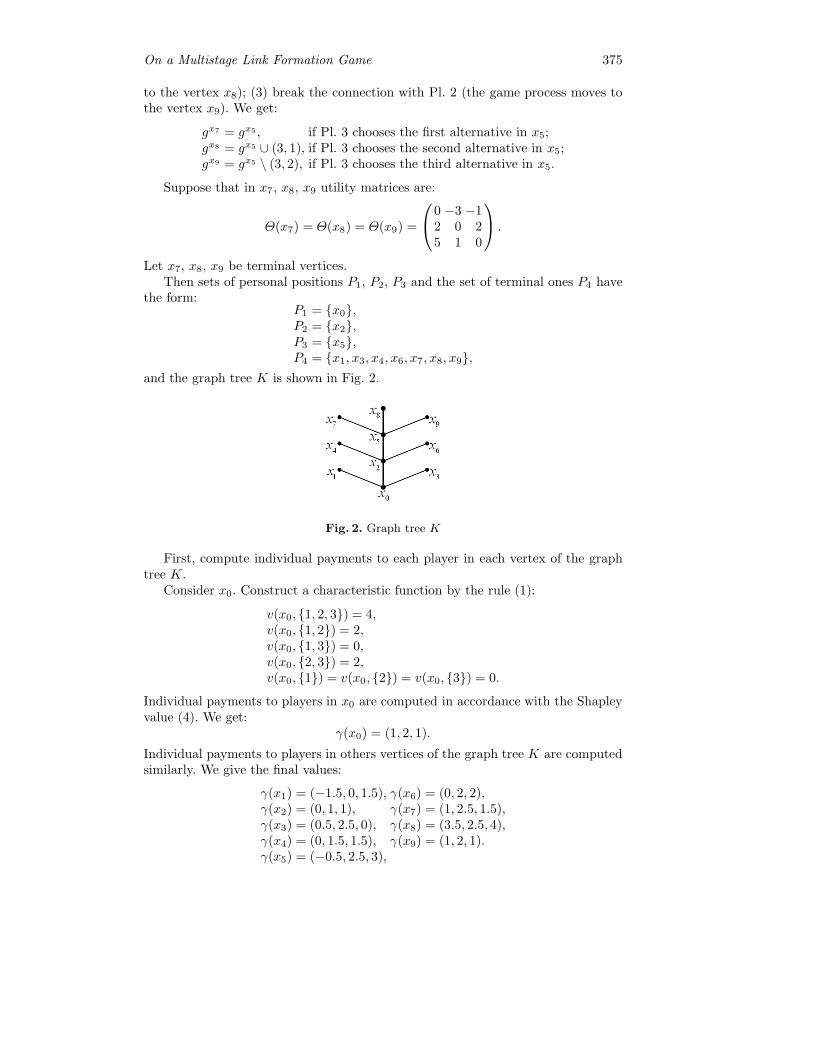
On a Multistage Link Formation Game 375
to the vertex x8); (3) break the connection with Pl. 2 (the game process moves tothe vertex x9). We get:
gx7 = gx5, if Pl. 3 chooses the first alternative in x5;gx8 = gx5 ∪ (3, 1), if Pl. 3 chooses the second alternative in x5;gx9 = gx5 \ (3, 2), if Pl. 3 chooses the third alternative in x5.
Suppose that in x7, x8, x9 utility matrices are:
Θ(x7) = Θ(x8) = Θ(x9) =
⎛⎝0 −3 −12 0 25 1 0
⎞⎠ .
Let x7, x8, x9 be terminal vertices.Then sets of personal positions P1, P2, P3 and the set of terminal ones P4 have
the form:P1 = {x0},P2 = {x2},P3 = {x5},P4 = {x1, x3, x4, x6, x7, x8, x9},
and the graph tree K is shown in Fig. 2.
Fig. 2. Graph tree K
First, compute individual payments to each player in each vertex of the graphtree K.
Consider x0. Construct a characteristic function by the rule (1):
v(x0, {1, 2, 3}) = 4,v(x0, {1, 2}) = 2,v(x0, {1, 3}) = 0,v(x0, {2, 3}) = 2,v(x0, {1}) = v(x0, {2}) = v(x0, {3}) = 0.
Individual payments to players in x0 are computed in accordance with the Shapleyvalue (4). We get:
γ(x0) = (1, 2, 1).
Individual payments to players in others vertices of the graph tree K are computedsimilarly. We give the final values:
γ(x1) = (−1.5, 0, 1.5), γ(x6) = (0, 2, 2),γ(x2) = (0, 1, 1), γ(x7) = (1, 2.5, 1.5),γ(x3) = (0.5, 2.5, 0), γ(x8) = (3.5, 2.5, 4),γ(x4) = (0, 1.5, 1.5), γ(x9) = (1, 2, 1).γ(x5) = (−0.5, 2.5, 3),
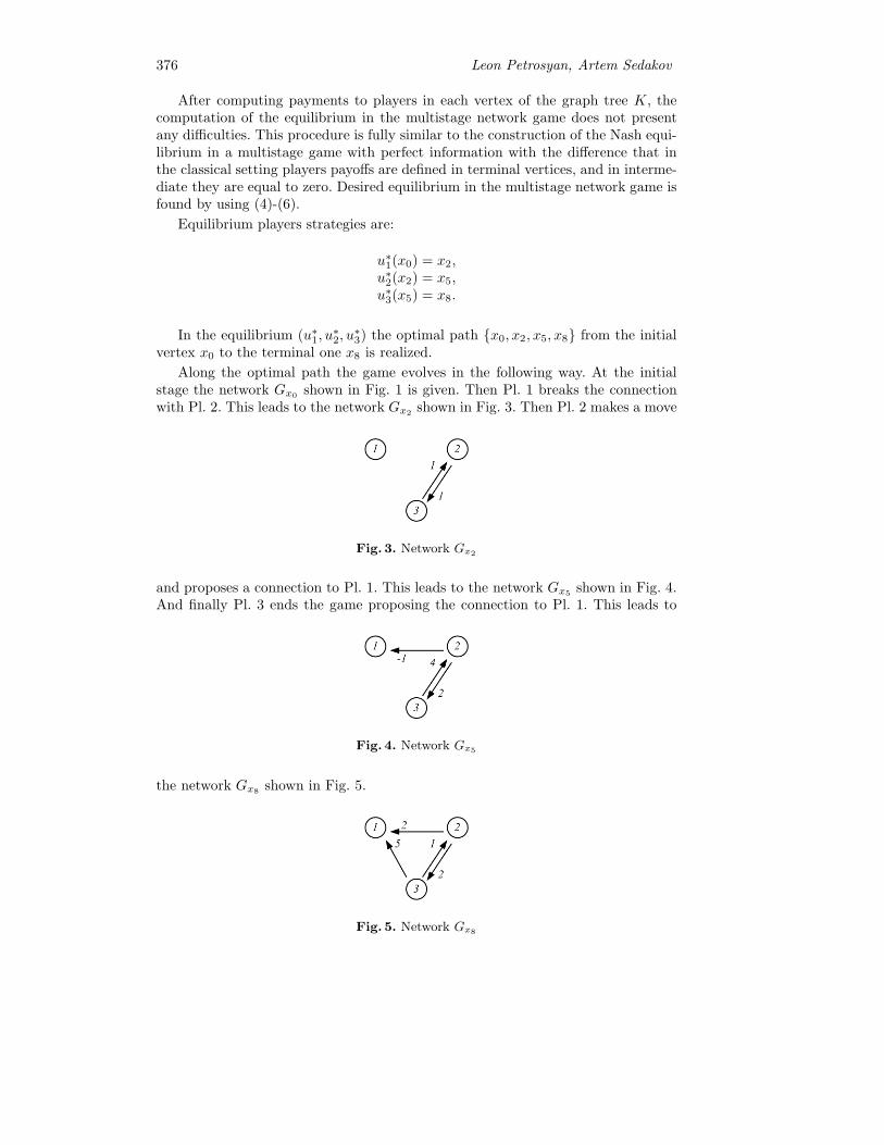
376 Leon Petrosyan, Artem Sedakov
After computing payments to players in each vertex of the graph tree K, thecomputation of the equilibrium in the multistage network game does not presentany difficulties. This procedure is fully similar to the construction of the Nash equi-librium in a multistage game with perfect information with the difference that inthe classical setting players payoffs are defined in terminal vertices, and in interme-diate they are equal to zero. Desired equilibrium in the multistage network game isfound by using (4)-(6).
Equilibrium players strategies are:
u∗1(x0) = x2,
u∗2(x2) = x5,
u∗3(x5) = x8.
In the equilibrium (u∗1, u
∗2, u
∗3) the optimal path {x0, x2, x5, x8} from the initial
vertex x0 to the terminal one x8 is realized.
Along the optimal path the game evolves in the following way. At the initialstage the network Gx0 shown in Fig. 1 is given. Then Pl. 1 breaks the connectionwith Pl. 2. This leads to the network Gx2 shown in Fig. 3. Then Pl. 2 makes a move
Fig. 3. Network Gx2
and proposes a connection to Pl. 1. This leads to the network Gx5 shown in Fig. 4.And finally Pl. 3 ends the game proposing the connection to Pl. 1. This leads to
Fig. 4. Network Gx5
the network Gx8 shown in Fig. 5.
Fig. 5. Network Gx8

On a Multistage Link Formation Game 377
The value of the multistage network game equals to (4, 8, 9) and stage paymentsto players are as follows:
γ(x0) = (1, 2, 1),
γ(x2) = (0, 1, 1),
γ(x5) = (−0.5, 2.5, 3),
γ(x8) = (3.5, 2.5, 4).
References
Bellman, R. (1957). Dynamic Programming. Princeton University Press: Princeton, NJ.Dutta, B., van den Nouweland, A., Tijs, S. (1998). Link formation in cooperative situations.
International Journal of Game Theory, 27, 245–256.Kuhn, H. W. (1953). Extensive Games and Problem Information. Ann. Math Studies, 28,
193–216.Myerson, R. (1977). Graphs and cooperation in games. Mathematics of Operations Re-
search, 2, 225–229.Nash, J. (1951). Non-cooperative Games. Ann. of Math., 54, pp. 286–295.Petrosjan, L. A., Kusyutin, D. V. (2000). Games in extensive form: optimality and stability.
St.Petersburg Univ. Press, St.Petersburg.Petrosjan, L. A., Mamkina, S. I. (2005). Value for the Games with Changing Coalitional
Structure. Games Theory and Applications, 10, 141–152.Petrosyan, L., Sedakov, A. (2009). Multistage networking games with full information.
Upravlenie bolshimi sistemami, 26.1, 121–138 (in russian).Petrosjan, L. A., Sedakov, A. A., Syurin, A. N. (2006). Multistage Games with Coalitional
Structure. Viestnik of St.Petersburg Univ., Sec. 10, Vol. 3, pp. 97-110.Shapley, L. S. (1953). A Value for n-Person Games. Contributions to the Theory of
Games II, Princeton: Princeton University Press, 307–317.

Best Response Digraphs for Two Location Games on Graphs
Erich Prisner1
Franklin College,Via Ponte Tresa 29,
6924 Sorengo-Lugano, Switzerland,E-mail: [email protected]
WWW home page: http://www.eprisner.de
Abstract. We investigate two classes of location games on undirected graphs,where two players simultaneously place one facility each on a vertex. In thefirst class, called ‘Voronoi games’, the payoff for a player is the number ofvertices closer to that player’s facility than to the other one, plus half of thenumber of vertices with equal distance. For the other class, called ‘restaurantlocation games’, the payoff for a player equals 1 plus κ times the numberof private neighbors plus κ/2 times the number of common neighbors, ifboth locations are different, and 1/2 plus κ/2 times the number of commonneighbors provided both locations are identical, for some constant κ. Forboth classes the question of the existence of pure Nash equilibria is investi-gated. Although Voronoi games, which are obviously constant-sum games,do not need to have pure Nash equilibria, Nash equilibria exist if the playgraphs are trees. Restaurant location games have always at least one pureNash equilibrium. We also try to express these Nash equilibria in graph-theoretical terms, and investigate the structure of so-called best responsedigraphs for the games in relation to the structure of the underlying playgraph.
Keywords: simultaneous games, graphs, best response digraph, pure Nashequilibria.
We consider simultaneous 2-player location games played on weighted graphs.The games are defined by two ingredients: There is an underlying undirected graphG = (V,E)—the play graph— which may have positive vertex weights w(x), x ∈ Vand positive edge weights w(xy), xy ∈ E. The second ingredient is a nonincreasingfunction f defined on nonnegative real numbers. Players A and B simultaneouslyselect one vertex, let’s say vertices a and b. Let VA, VB , and V0 denote the sets ofthose vertices that are closer to a than to b, closer to b than to a, or with equaldistance to a and b, respectively. In other words, VA = {x|dG(x, a) < dG(x, b)},VB = {x|dG(x, a) > dG(x, b)}, and V0 = {x|dG(x, a) = dG(x, b)}. Of course thedistance is defined using the edge weights, dG(x, y) is the minimum sum of edgeweights, taken over all paths from x to y. For such choice of moves, the payoffs forplayers A and B are defined by
A(a, b) =∑x∈VA
f(d(x, a))w(x) +1
2
∑x∈V0
f(d(x, a))w(x)
B(a, b) =∑x∈VB
f(d(x, b))w(x) +1
2
∑x∈V0
f(d(x, b))w(x)
The graph could model a physical street network with villages as vertices. Theplayers simultaneously place one facility on some vertex. People may or may not

Best Response Digraphs for Two Location Games on Graphs 379
visit such a facility, depending on the distance they would have to travel, but if theydo, they will always choose the closest one, no matter to which one of the players itbelongs. The numbers f(d) would model the fraction of the population that wouldvisit if the distance to travel would be d. The payoff for each player is the totalnumber of customers visiting his or her facility.
It is possible to modify the games by allowing each player to place k facilities.In this paper we will concentrate on the single-facility case k = 1.
The games are obviously symmetric. They are ususally not zero-sum, except inthe case of f(x) = 1, where all customers always visit one of the locations.
The paper concentrates on two special cases for the function f . The case of aconstant function f(x) = 1 is usually called Voronoi game. We sometimes call itsupermarket location game, since every possible customer has to visit one ofthe locations. The other special case, in a sense on the opposite side, is the casewhere f(2) = 0 and all edge-weights are greater or equal to 1. This case we namerestaurant location game, assuming that customers are not willing to go veryfar for a (possibly fast-food) restaurant. In the Voronoi game case, we will focus onspecial graphs, namely trees and chordal graphs.
For these two special special classes of games, we will discuss the question ofhow the best response digraph looks like for these games, in particular in relationto the underlying undirected play graph. The best response digraph, which will bedefined in the next section, captures the notion of ‘best responses’. We will also seethat every restaurant location game, but not every Voronoi game, has some pureNash equilibria. For Voronoi games, pure Nash equilibria exist under the conditionthat the play graph is a tree.
Location games have been initiated by H. Hotelling (Hotelling, 1929), consider-ing the case of location on a straight line. Later, location games for other geometricalpatterns have been investigated. Location games on graphs have been investigatedby V. Knoblauch in two papers in 1991 and 1995. However, the models she con-sidered differ from ours. In Knoblauch, 1991, location everywhere on the edges isallowed. In Knoblauch, 1995, location is allowed only on some specified vertices ofthe graph, and only functions f of the form f(x) = 1 for x ≤ m, and f(x) = 0otherwise, are considered. In this second model, Knoblauch could show that everysimultaneous 2-person symmetric game is equivalent to such a simultaneous locationgame on a graph.
There is a large literature on Voronoi games played in rectangular or squarespaces, but mostly the games are played sequentially, and each player has several fa-cilities, compare Cheong et al., 2004. Teramoto et al., 2006, discuss multiple-facilityVoronoi games on graphs, but also sequential ones. Durr and Nguyen Kim, 2007,also discuss Voronoi games, but with emphasis on more than two players.
1. Best Response Digraphs
Before discussing these location games, let us introduce the best response digraphs,which will be used later. For Normal Form games, the notion of a best response iscruical for the definition of pure Nash equilibria. In the case of two players, thisnotion could be modeled by a bipartite digraph, or a general digraph in case ofsymmetric games. Recall that a game is symmetric if both players have the samestrategy sets V , and A(x, y) = B(y, x) for every x, y ∈ V , where A(x, y) and B(x, y)

380 Erich Prisner
denote the payoffs of player A or B if player A plays strategy x and player B choosesstrategy y. Then the (condensed) best response digraph of the game has V as vertexset, and an arc from x to y, for x, y ∈ V , if y is among the best responses for oneplayer to move x for the other player.
In this (condensed) best response digraph, pure Nash equilibria appear either aspairs of vertices (x, y) with both (x, y) and (y, x) arcs in the best response digraph—such antidirected arcs are called digons—, or pairs (x, x) with (x, x) an arc in thedigraph—a so-called loop. Thus pure Nash equilibria can be recognized very easilyin the best response digraph.
It is easy to see that every digraph where every vertex has at least one out-goingarc is the best response digraph of some symmetric two-player game. We can evenconstruct such a game where all payoffs are just the numbers 0 or 1. We defineB(x, y) = 1 if (x, y) is an arc in D, and B(x, y) = 0 otherwise. By defining thepayoffs for player A by A(x, y) = B(y, x) we get a symmmetric game with ourdigraph as best response digraph.
2. Constant-sum symmetric games
A two-player game is constant-sum if there is some constant c such that A(x, y) +B(x, y) = c for every strategy x of player A and every strategy y of player B.By concentrating on constant-sum games, the shape of the occuring best responsedigraphs is further restricted.
Theorem 1. A digraph is the best response digraph of a two-player symmetricconstant-sum game if and only if
(1) every vertex has at least one outgoing arc, and(2) For every x = y ∈ V , there is a digon between x and y if and only if there are
loops both at x and y.
Proof. Given a digraph D obeying the two conditions above, we show how to con-struct a zero-sum two-player game with all payoffs equal to -2, -1, 0, 1, 2, whose bestresponse digraph equals D. Since the game is supposed to be zero-sum, it sufficesto define the payoffs A(x, y) for player A.
Let V0 be the set of all loop vertices. We will construct a game where bestresponses to strategies in V0 have a payoff of 0, and best responses to strategies notin V0 have a payoff of 2.
For every x ∈ V , we must define A(x, x) = 0. For the definition of the othervalues A(x, y) we distinguish six cases:
– Case x, y ∈ V0: In this case, according to condition (2) above, both (x, z) and(y, x) are arcs, and we define A(x, y) = A(y, x) = 0.
– The case where exactly one of x, y lies in V0, for instance x ∈ V0, y /∈ V0: Sinceby condition (2) not both (x, y) and (y, x) can be arcs, we get three subcases:• (x, y) is an arc but (y, x) not. We define A(x, y) = A(y, x) = 0.• (y, x) is an arc but (x, y) not. We define A(x, y) = 2 and A(y, x) = −2.• None of (x, y), (y, x) is an arc. Then we define A(x, y) = 1 and A(y, x) = −1.
– Case x, y /∈ V0: Again by condition (2) not both (x, y) and (y, x) can be arcs,so we get two subcases:• One of (x, y), (y, x) is an arc, let’s say (x, y). We define A(x, y) = −2 andA(y, x) = 2.
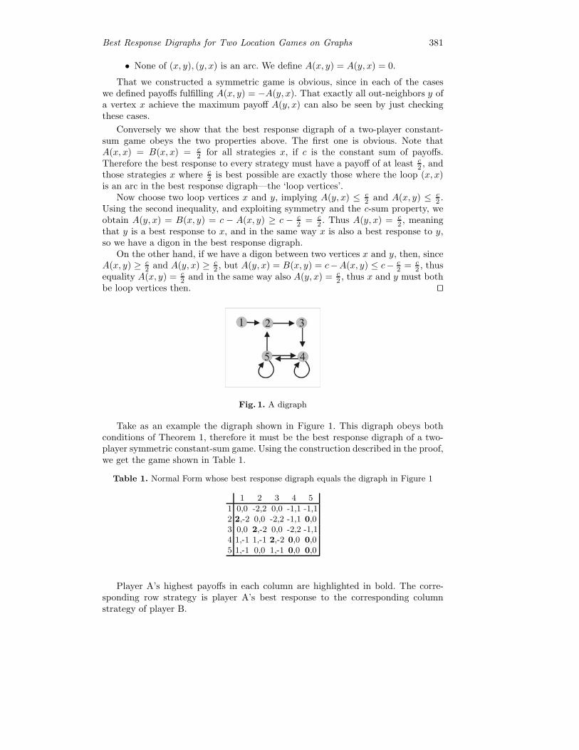
Best Response Digraphs for Two Location Games on Graphs 381
• None of (x, y), (y, x) is an arc. We define A(x, y) = A(y, x) = 0.
That we constructed a symmetric game is obvious, since in each of the caseswe defined payoffs fulfilling A(x, y) = −A(y, x). That exactly all out-neighbors y ofa vertex x achieve the maximum payoff A(y, x) can also be seen by just checkingthese cases.
Conversely we show that the best response digraph of a two-player constant-sum game obeys the two properties above. The first one is obvious. Note thatA(x, x) = B(x, x) = c
2 for all strategies x, if c is the constant sum of payoffs.Therefore the best response to every strategy must have a payoff of at least c
2 , andthose strategies x where c
2 is best possible are exactly those where the loop (x, x)is an arc in the best response digraph—the ‘loop vertices’.
Now choose two loop vertices x and y, implying A(y, x) ≤ c2 and A(x, y) ≤ c
2 .Using the second inequality, and exploiting symmetry and the c-sum property, weobtain A(y, x) = B(x, y) = c − A(x, y) ≥ c − c
2 = c2 . Thus A(y, x) = c
2 , meaningthat y is a best response to x, and in the same way x is also a best response to y,so we have a digon in the best response digraph.
On the other hand, if we have a digon between two vertices x and y, then, sinceA(x, y) ≥ c
2 and A(y, x) ≥ c2 , but A(y, x) = B(x, y) = c−A(x, y) ≤ c− c
2 = c2 , thus
equality A(x, y) = c2 and in the same way also A(y, x) = c
2 , thus x and y must bothbe loop vertices then. ��
Fig. 1. A digraph
Take as an example the digraph shown in Figure 1. This digraph obeys bothconditions of Theorem 1, therefore it must be the best response digraph of a two-player symmetric constant-sum game. Using the construction described in the proof,we get the game shown in Table 1.
Table 1. Normal Form whose best response digraph equals the digraph in Figure 1
1 2 3 4 5
1 0,0 -2,2 0,0 -1,1 -1,12 2,-2 0,0 -2,2 -1,1 0,03 0,0 2,-2 0,0 -2,2 -1,14 1,-1 1,-1 2,-2 0,0 0,05 1,-1 0,0 1,-1 0,0 0,0
Player A’s highest payoffs in each column are highlighted in bold. The corre-sponding row strategy is player A’s best response to the corresponding columnstrategy of player B.

382 Erich Prisner
3. Voronoi Games (Supermarket Location)
Recall that this class of location games is defined by the condition f(x) = 1 for allx ≥ 0. That implies that we get a constant-sum game, since all possible customerswill visit one of the locations. Therefore the sum of the payoffs equals the sum∑
x∈V w(x) of all vertex weights.The best response digraphs of these Voronoi games have to obey the conditions
described in Theorem 1. However, the class of best response digraphs of these gamesis strictly smaller than that, since we have
Proposition 1. The directed cycles C3 and C4 are not best response digraph of anyVoronoi game.
This can be shown by looking on all 3- or 4-vertex graphs. It certainly would beinteresting to find a characterization of best response digraphs of these games.
For Voronoi games played on the continuous square, best responses are not reallydefined, but responses get better and better if the answering move gets closer andcloser to the other move, in the direction of the center of the square. The only pureNash equilibrium is where both players place their facility into the center of thesquare.
If we consider grids Pn×Pm as discrete versions of squares, we get best responsesthat have always distance at most 2 from the original move vertex, and three patternof pure Nash equilibria: If both n and m are odd, the only Nash equilibrum is thepair of both locations in the center. If one of n and m is odd, then a Nash equilibriumis any combination of the two central vertices of the grid. If both n and m are even,then the center consists of four vertices, and any combination of two of them formsa Nash equilibrium. See Figure 2 for an example.
Fig. 2. The best response digraph for the 6 × 6 grid
Thus for variants of the original geometric Voronoi game, we always have Nashequilibria with pairs of vertices in the ‘center’ of the graph, and best response arcsdo not span large distances in the underlying play graph. However, all this can bedifferent for other graphs, as can be seen by a family of examples generalizing anexample given in Durr and Nguyen Kim, 2007: Construct a graph Gr, r ≥ 2, from acycle x0, x1, . . . , x3r−1, by adding three vertices y0, y1, y2 and making y0 adjacent to
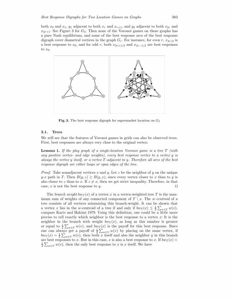
Best Response Digraphs for Two Location Games on Graphs 383
both x0 and x1, y1 adjacent to both xr and xr+1, and y2 adjacent to both x2r andx2r+1. See Figure 3 for G3. Then none of the Voronoi games on these graphs hasa pure Nash equilibrium, and some of the best response arcs of the best responsedigraph cover diametral vertices in the graph Gr. For instance, for even r, x3r/2 isa best response to x0, and for odd r, both x3r+1/2 and x3r−1/2 are best responsesto x0.
Fig. 3. The best response digraph for supermarket location on G3
3.1. Trees
We will see that the features of Voronoi games in grids can also be observed trees.First, best responses are always very close to the original vertex:
Lemma 1. If the play graph of a single-location Voronoi game is a tree T (withany positive vertex- and edge weights), every best response vertex to a vertex y isalways the vertex y itself, or a vertex T -adjacent to y. Therefore all arcs of the bestresponse digraph are either loops or span edges of the tree.
Proof. Take nonadjacent vertices x and y. Let z be the neighbor of y on the uniquey-x path in T . Then B(y, z) ≥ B(y, x), since every vertex closer to x than to y isalso closer to z than to x. If z = x, then we get strict inequality. Therefore, in thatcase, x is not the best response to y. ��
The branch weight bwT (x) of a vertex x in a vertex-weighted tree T is the max-imum sum of weights of any connected component of T \ x. The w-centroid of atree consists of all vertices minimizing this branch-weight. It can be shown thata vertex x lies in the w-centroid of a tree if and only if bwT (x) ≤ 1
2
∑w∈V w(v),
compare Kariv and Hakimi 1979. Using this definition, one could be a little moreprecise to tell exactly which neighbor is the best response to a vertex x: It is theneighbor in the branch with weight bwT (x), as long as this number is greateror equal to 1
2
∑w∈V w(v), and bwT (x) is the payoff for this best response. Since
one can always get a payoff of 12
∑w∈V w(v) by placing on the same vertex, if
bwT (x) = 12
∑w∈V w(v), then both x itself and also the neighbor y in this branch
are best responses to x. But in this case, x is also a best response to x. If bwT (x) <12
∑w∈V w(v), then the only best response to x is x itself. We have
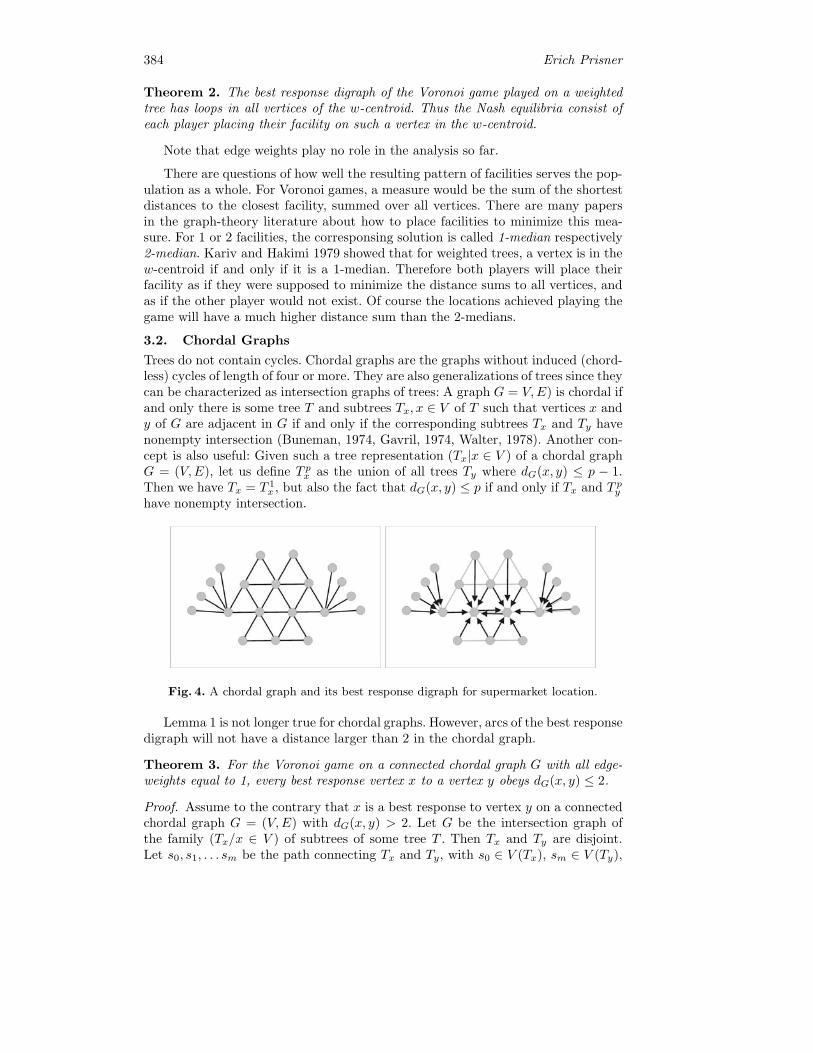
384 Erich Prisner
Theorem 2. The best response digraph of the Voronoi game played on a weightedtree has loops in all vertices of the w-centroid. Thus the Nash equilibria consist ofeach player placing their facility on such a vertex in the w-centroid.
Note that edge weights play no role in the analysis so far.
There are questions of how well the resulting pattern of facilities serves the pop-ulation as a whole. For Voronoi games, a measure would be the sum of the shortestdistances to the closest facility, summed over all vertices. There are many papersin the graph-theory literature about how to place facilities to minimize this mea-sure. For 1 or 2 facilities, the corresponsing solution is called 1-median respectively2-median. Kariv and Hakimi 1979 showed that for weighted trees, a vertex is in thew-centroid if and only if it is a 1-median. Therefore both players will place theirfacility as if they were supposed to minimize the distance sums to all vertices, andas if the other player would not exist. Of course the locations achieved playing thegame will have a much higher distance sum than the 2-medians.
3.2. Chordal Graphs
Trees do not contain cycles. Chordal graphs are the graphs without induced (chord-less) cycles of length of four or more. They are also generalizations of trees since theycan be characterized as intersection graphs of trees: A graph G = V,E) is chordal ifand only there is some tree T and subtrees Tx, x ∈ V of T such that vertices x andy of G are adjacent in G if and only if the corresponding subtrees Tx and Ty havenonempty intersection (Buneman, 1974, Gavril, 1974, Walter, 1978). Another con-cept is also useful: Given such a tree representation (Tx|x ∈ V ) of a chordal graphG = (V,E), let us define T px as the union of all trees Ty where dG(x, y) ≤ p − 1.Then we have Tx = T 1
x , but also the fact that dG(x, y) ≤ p if and only if Tx and T pyhave nonempty intersection.
Fig. 4. A chordal graph and its best response digraph for supermarket location.
Lemma 1 is not longer true for chordal graphs. However, arcs of the best responsedigraph will not have a distance larger than 2 in the chordal graph.
Theorem 3. For the Voronoi game on a connected chordal graph G with all edge-weights equal to 1, every best response vertex x to a vertex y obeys dG(x, y) ≤ 2.
Proof. Assume to the contrary that x is a best response to vertex y on a connectedchordal graph G = (V,E) with dG(x, y) > 2. Let G be the intersection graph ofthe family (Tx/x ∈ V ) of subtrees of some tree T . Then Tx and Ty are disjoint.Let s0, s1, . . . sm be the path connecting Tx and Ty, with s0 ∈ V (Tx), sm ∈ V (Ty),

Best Response Digraphs for Two Location Games on Graphs 385
but all other vertices s1, . . . sm−1 outside of Tx and Ty. Choose that vertex z ∈ Vwhere Tz contains s0 and sk, with k maximum among all such subtrees. By ourassumption dG(x, y) > 2 we know that k < m. We claim that z is a better responseto y, which gives the desired contradiction.
Let Vx denote those vertices closer to x than to y, Vy those vertices closer toy than to x, and V0 those vertices having the same distance. All neighbors of xbelong to Vx, all neighbors of y belong to Vy . Moreover, every vertex v where Txseparates Tv and Ty belongs to Vx, and every vertex v where Ty separates Tv andTx belongs to Vy. These latter vertices, and also all neighbors of y, are closer to zthan to x. Thus, for the vertices considered so far, moving from y to z does notmake a difference.
Now we look at the remaining vertices v. For them, the path between Tv and Tx,as well as the path between Tv and Ty meet the path s0, s1, . . . sm first. Let p be thehighest integer for which T pv is still disjoint to Tx and Tz. Then, if T p+1
v intersectsTy, it also intersects Tz. Thus, all these v are not further away to z than to y.
We have seen that z is as good a response to x than y. Now look at the shortestpath x = x0, x1, . . . , xm = z between x and z. If m is even, xm/2 has the samedistance to x and z, but is closer to x than to y by the choice of z, therefore z is abetter response to x than y. If m is odd, then x(m+1)/2 is closer to z than to x, buthas the same distance to x and y, therefore z is a better response to x than y alsoin this case. ��
We conjecture that actually every Voronoi game on every chordal graph hassome pure Nash equilibria.
4. Restaurant Location Games
We first need a general theorem for games of a special shape:
Theorem 4. Assume a symmetric two-player game has the properties that
1. for every option x there is a value κ(x), and2. for every two options x, y there is a value γ(x, y) = γ(y, x), such that3. if player A chooses option x and player B option y, then A’s payoff equals
A(x, y) = κ(x)− γ(x, y), and B’s payoff equals B(x, y) = κ(y)− γ(x, y).
Then all arcs in every directed cycle of length at least 2 in the (condensed) bestresponse digraph are digons, and in particular the game has at least one Nash equi-librium in pure strategies.
Proof. Let x0, x1, . . . xm, x0 be a directed cycle in the best response digraph of thegame. In case m = 1 we have a loop, and in case m = 2 we just have a digon, solet’s assume that the length m of the directed cycle is greater or equal to 3.
Then x1 is best response to x0, x2 is best response to x1, and so on, and x0 isbest response to xm. We get
B(x0, x1) ≥ B(x0, xm),
A(x2, x1) ≥ A(x0, x1),
B(x2, x3) ≥ B(x2, x1),
A(x4, x3) ≥ A(x2, x3),
· · ·
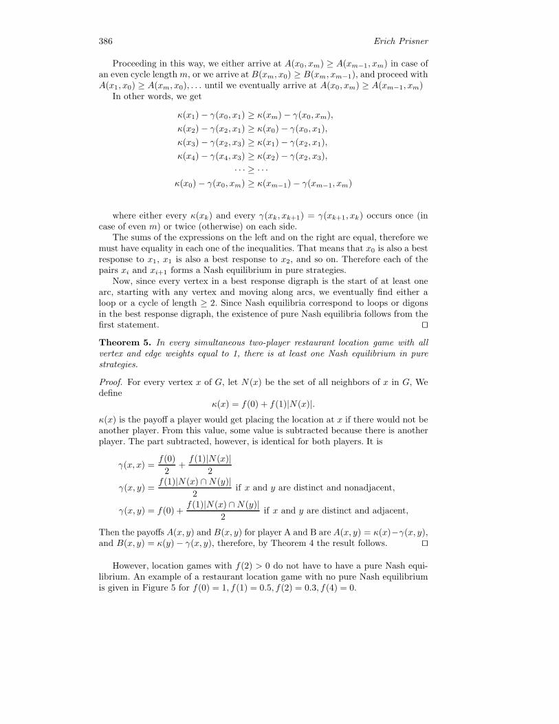
386 Erich Prisner
Proceeding in this way, we either arrive at A(x0, xm) ≥ A(xm−1, xm) in case ofan even cycle length m, or we arrive at B(xm, x0) ≥ B(xm, xm−1), and proceed withA(x1, x0) ≥ A(xm, x0), . . . until we eventually arrive at A(x0, xm) ≥ A(xm−1, xm)
In other words, we get
κ(x1)− γ(x0, x1) ≥ κ(xm)− γ(x0, xm),
κ(x2)− γ(x2, x1) ≥ κ(x0)− γ(x0, x1),
κ(x3)− γ(x2, x3) ≥ κ(x1)− γ(x2, x1),
κ(x4)− γ(x4, x3) ≥ κ(x2)− γ(x2, x3),
· · · ≥ · · ·κ(x0)− γ(x0, xm) ≥ κ(xm−1)− γ(xm−1, xm)
where either every κ(xk) and every γ(xk, xk+1) = γ(xk+1, xk) occurs once (incase of even m) or twice (otherwise) on each side.
The sums of the expressions on the left and on the right are equal, therefore wemust have equality in each one of the inequalities. That means that x0 is also a bestresponse to x1, x1 is also a best response to x2, and so on. Therefore each of thepairs xi and xi+1 forms a Nash equilibrium in pure strategies.
Now, since every vertex in a best response digraph is the start of at least onearc, starting with any vertex and moving along arcs, we eventually find either aloop or a cycle of length ≥ 2. Since Nash equilibria correspond to loops or digonsin the best response digraph, the existence of pure Nash equilibria follows from thefirst statement. ��
Theorem 5. In every simultaneous two-player restaurant location game with allvertex and edge weights equal to 1, there is at least one Nash equilibrium in purestrategies.
Proof. For every vertex x of G, let N(x) be the set of all neighbors of x in G, Wedefine
κ(x) = f(0) + f(1)|N(x)|.κ(x) is the payoff a player would get placing the location at x if there would not beanother player. From this value, some value is subtracted because there is anotherplayer. The part subtracted, however, is identical for both players. It is
γ(x, x) =f(0)
2+
f(1)|N(x)|2
γ(x, y) =f(1)|N(x) ∩N(y)|
2if x and y are distinct and nonadjacent,
γ(x, y) = f(0) +f(1)|N(x) ∩N(y)|
2if x and y are distinct and adjacent,
Then the payoffs A(x, y) and B(x, y) for player A and B are A(x, y) = κ(x)−γ(x, y),and B(x, y) = κ(y)− γ(x, y), therefore, by Theorem 4 the result follows. ��
However, location games with f(2) > 0 do not have to have a pure Nash equi-librium. An example of a restaurant location game with no pure Nash equilibriumis given in Figure 5 for f(0) = 1, f(1) = 0.5, f(2) = 0.3, f(4) = 0.

Best Response Digraphs for Two Location Games on Graphs 387
Fig. 5. On the right is the best response digraph for restaurant location with f(0) =1, f(1) = 0.5, f(2) = 0.3, f(4) = 0 on the graph to the left.
The example in Figure 6 shows that, in our restaurant location games, theNash equilibrium outcomes are not always best-possible for society, or even for amonopoly that would place two restaurants. Different to the Voronoi games, themeasure of quality of such a placement may be the number of people visiting oneof the facility, i.e. the sum of both payoffs. In the example in Figure 6, 1 versus 5,and also 5 versus 6 are the Nash equilibria, giving payoffs of 2 and 2.5. However, ifplayer A builds in 1 and player B in 8, A gets a payoff of 3 and B a payoff of 2. Stillit seems that restaurant location games are closer to the optimum for society thanthe Vornoi (supermarket location) games.
Fig. 6. 1 versus 8 is best for society
Let me close by presenting an example in Figure 7 that shows that if each playerplaces two restaurants, then we do no longer necessarily have pure Nash equilibria.

388 Erich Prisner
Fig. 7. This graph has no pure Nash equilibrium in the restaurant location model withtwo restaurants for each player
References
Hotelling, H. (1929). Stability in competition. Economic Journal, 39, 41–57.Knoblauch, V. (1991). Generalizing Location Games to a Graph. Journal of Industrial
Economics, 34, ....Knoblauch, V. (1995). Geometric versions of finite games: Prisoner’s dilemma, entry de-
terrence and a cyclical majority paradox. International Journal of Game Theory, 24,165–177.
Buneman, P. (1974). A characterization on rigid circuit graphs. Discrete Math., 9, 205–212.Gavril, F. (1974). The intersection graphs of subtrees of a tree are exactly the chordal
graphs. J. Comb. Theory B 16, 46–56.Walter, J. R. (1978). Representations of chordal graphs as subtrees of a tree. J. Graph Th.,
12, 265–267.Cheong, O., S. Har-Peled, N. Linial and J. Matousek (2004). The one-round Voronoi game.
Discrete and Computational Geometry, 31, 125–138.Teramoto, S., E. Demaine and R. Uehara (2006). Voronoi game on graphs and its complex-
ity. Proceedings of the IEEE Symposium on Computational Intelligence and Games(CIG’06), 265–271.
Durr, C. and T. Nguyen Kim (2007). Nash equilibria in Voronoi games on graphs. Pro-ceedings of the 15th Annual European Symposium on Algorithms (ESA’07) 17–28.
Kariv, O. and S.L. Hakimi 1979 (1979). An algorithmic approach to network location prob-lems II: The p-medians. SIAM J. Applied Math., 37, 539-560.
Uncertainty Aversion and Equilibriumin Extensive Games�
Jorn Rothe
London School of Economics,Department of Management,
Managerial Economics and Strategy Group,Houghton Street, London, WC2A 2AE, United Kingdom
E-mail: [email protected] home page: http://www2.lse.ac.uk/management/people/jrothe.aspx
Abstract. This paper formulates a rationality concept for extensive gamesin which deviations from rational play are interpreted as evidence of irra-tionality. Instead of confirming some prior belief about the nature of non-rational play, we assume that such a deviation leads to genuine uncertainty.Assuming complete ignorance about the nature of non-rational play andextreme uncertainty aversion of the rational players, we formulate an equi-librium concept on the basis of Choquet expected utility theory. Equilibriumreasoning is thus only applied on the equilibrium path, maximin reasoningapplies off the equilibrium path. The equilibrium path itself is endogenouslydetermined. In general this leads to strategy profiles differ qualitatively fromsequential equilibria, but still satisfy equilibrium and perfection require-ments. In the centipede game and the finitely repeated prisoners’ dilemmathis approach can also resolve the backward induction paradox.
Keywords: rationality, extensive game, uncertainty aversion, perfect equi-librium, backward induction, maximin, Choquet expected utility theory.
1. Introduction
According to the principle of sequential rationality, a rational player of an extensiveform game regards his opponents as rational even after a deviation from rationalplay. The internal consistency of this principle is subject of much debate (see, e.g.,Aumann (1995, 1996, 1998), Binmore (1996), Reny (1993)).
Attributing non-rational deviations to ‘trembles’ of otherwise perfectly rationalplayers (Selten (1975)) is logically consistent, but raises the second concern withthe principle of sequential rationality, that is its empirical plausibility. Quite inde-pendently of the question whether there exists a rationality concept that implies,or is at least consistent with sequential rationality, the question arises if there isroom for an alternative rationality concept, in which deviations from the solutionconcept are interpreted as evidence of non-rationality. In this paper, we attemptto formulate such a rationality concept on the basis of Choquet expected utilitytheory.
� First version 1999. This paper continues the research presented in Rothe (1996, 2009,2010) and is based on chapter 3 of my PhD thesis submitted to the University of Londonin 1999. I am grateful for financial support from the Deutsche Forschungsgemeinschaft(Graduiertenkolleg Bonn), Deutscher Akademischer Austauschdienst, Economic and So-cial Research Council, the European Doctoral Program and the LSE.

390 Jorn Rothe
In a seminal series of papers, Kreps, Milgrom, Roberts, and Wilson (1982)(henceforth KMRW) developed the methodology for analysing games with possiblynon-rational opponents. In their models, there is some a priori uncertainty about therationality of the opponent. Under subjective expected utility, players act as if theypossess a probability distribution over the ‘type’ of the opponents’ non-rationality.They maximise utility given their beliefs, and in sequential equilibrium their beliefsare consistent with the play of rational opponents. KMRW have shown how evensmall degrees of uncertainty about rationality can have large equilibrium effects.They showed that this can explain both intuitive strategic phenomena, particularlyin industrial organization, and, at least to some degree, experimental evidence.
One problem in this approach, however, is for an outside observer to specifythe probability distribution over the types of the non-rational opponents beforeexperimental or field data are available. A second problem is that analysing thestrategic interaction as a game with incomplete information implies that the otherplayers, whether rational or not, can be modelled as ‘types’, who possess a consistentinfinite hierarchy of beliefs about the strategic interaction. Thus, the players inthis methodology are not really non-rational; rather, they are rational but havepreferences that differ from those that the game attributes to ‘rational’ players.
In this paper, we argue that a consistency argument addresses both of theseproblems. A game-theoretic solution concept that singles out rational strategiesimplicitly defines all other strategies as non-rational. Thus, consistency requiresthat beliefs about non-rational players should not exclude any of these non-rationalstrategies. In other words, if the rationality concept is point-valued, the beliefs aboutnon-rational play should include all deviations, and thus must be set-valued. So inthis sense, the rationality concept itself pins down beliefs about non-rational play,but excludes subjective expected utility theory (henceforth SEU) as the adequatemodel of these beliefs. Thus, SEU is not an appropriate framework for beliefs aboutnon-rationality when rationality is endogenous.
Thus, this paper argues that, after an opponent deviates from rational play,a rational player faces genuine uncertainty. What matters, then, is the rationalplayer’s attitude towards uncertainty. This paper formulates the equilibrium conceptfor the case in which rational players are completely uncertainty averse. It is thiscase that has led to the development of decision theories with set-valued and non-additive beliefs as an explanation of the Ellsberg (1961) paradox. Consequently, webase the equilibrium concept on Choquet expected utility theory (henceforth CEU)developed by Schmeidler (1989).
This paper joins a growing literature that applies CEU to games. The first ofthese were Dow and Werlang (1994) and Klibanoff (1993). Dow and Werlang (1994)consider normal form games in which players are CEU maximisers. Klibanoff (1993)similarly considers normal form games in which players follow maxmin-expectedutility theory (Gilboa and Schmeidler (1989)), which is closely related to CEU. InHendon et al. (1995) players have belief functions, which amounts to a special caseof CEU. Extensions and refinements have been proposed by Eichberger and Kelsey(1994), Lo (1995a), Marinacci (1994) and Ryan (1997). Epstein (1997a) analysedrationalizability in normal form games. These authors consider normal form gamesand do not distinguish between rational and non-rational players. The paper closestto ours is Mukerji (1994), who considers normal form games only but argues thatthe distinction between rational and non-rational players is necessary to reconcile
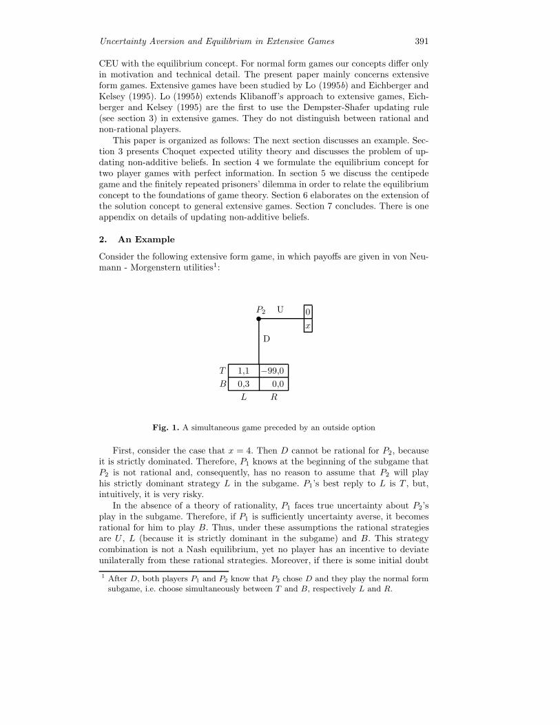
Uncertainty Aversion and Equilibrium in Extensive Games 391
CEU with the equilibrium concept. For normal form games our concepts differ onlyin motivation and technical detail. The present paper mainly concerns extensiveform games. Extensive games have been studied by Lo (1995b) and Eichberger andKelsey (1995). Lo (1995b) extends Klibanoff’s approach to extensive games, Eich-berger and Kelsey (1995) are the first to use the Dempster-Shafer updating rule(see section 3) in extensive games. They do not distinguish between rational andnon-rational players.
This paper is organized as follows: The next section discusses an example. Sec-tion 3 presents Choquet expected utility theory and discusses the problem of up-dating non-additive beliefs. In section 4 we formulate the equilibrium concept fortwo player games with perfect information. In section 5 we discuss the centipedegame and the finitely repeated prisoners’ dilemma in order to relate the equilibriumconcept to the foundations of game theory. Section 6 elaborates on the extension ofthe solution concept to general extensive games. Section 7 concludes. There is oneappendix on details of updating non-additive beliefs.
2. An Example
Consider the following extensive form game, in which payoffs are given in von Neu-mann - Morgenstern utilities1:
P2�
U
D
0
x
T 1,1 −99,0
B 0,3 0,0
L R
Fig. 1. A simultaneous game preceded by an outside option
First, consider the case that x = 4. Then D cannot be rational for P2, becauseit is strictly dominated. Therefore, P1 knows at the beginning of the subgame thatP2 is not rational and, consequently, has no reason to assume that P2 will playhis strictly dominant strategy L in the subgame. P1’s best reply to L is T , but,intuitively, it is very risky.
In the absence of a theory of rationality, P1 faces true uncertainty about P2’splay in the subgame. Therefore, if P1 is sufficiently uncertainty averse, it becomesrational for him to play B. Thus, under these assumptions the rational strategiesare U , L (because it is strictly dominant in the subgame) and B. This strategycombination is not a Nash equilibrium, yet no player has an incentive to deviateunilaterally from these rational strategies. Moreover, if there is some initial doubt
1 After D, both players P1 and P2 know that P2 chose D and they play the normal formsubgame, i.e. choose simultaneously between T and B, respectively L and R.

392 Jorn Rothe
ε > 0 about P2’s rationality2, then D is also not a probability zero event, becausenothing is known about a non-rational player, who might therefore well play D3
All that it takes to reach these conclusion formally is a calculus that allowsnon-additive, or set-valued, beliefs, and that captures P1’s uncertainty as well ashis uncertainty aversion. In addition, in order to conclude that that P2 must benon-rational after D we need an updating rule for non-additive beliefs.
Secondly, consider the case that x = 2. The above criticism of subgame perfectionstill applies: The equilibrium (T, L) in the subgame makes U rational, but once U isdesignated as rational, P1 faces true uncertainty after D and, if uncertainty averse,will rationally deviate to B. So (U,L, T ) is not a rational solution. However, neitheris (D,L,B), because if D is rational then P1 is justified in anticipating strategy L,and should play his best reply T . Now P2 has an incentive to deviate.
So suppose it is rational for P2 to play D with probability p. Suppose furtherthat there is a probability ε > 0 that P2 is not rational at the beginning of thegame. Then P1’s optimal strategy in the subgame will depend on his belief aboutthe rationality of P2, given p and ε. The same updating rule that for x = 4 allowsthe natural conclusion that P2 is rational after D gives the result4 that
v(P2 rational | D) =(1− ε)p
1− (1− ε)(1− p).
Note that v(P2 rational | D) = (1 − ε) pp+ε(1−p) < 1 − ε. Thus, in line with his
uncertainty aversion P1 considers the worst case when he updates his belief ε. Thisworst case is that a non-rational player will play D with probability 1, because thismakes it most likely that his behavior in the subgame is unpredictable, and, againdue to uncertainty aversion, should be evaluated with the worst outcome.
Since a rational P2 will play L, P1 knows that T will give utility 1 with proba-
bility (1−ε)p1−(1−ε)(1−p) . With the complementary probability, P2 is non-rational and the
theory is silent about what this means. Again, P1 faces true uncertainty, and if heis extremely uncertainty averse, he will allocate the complementary probability tothe worst outcome −99. So P1’s expected utility from T is
(1− ε)p
1− (1− ε)(1− p)· 1− 99 · ε
1− (1 − ε)(1− p).
In a mixed strategy equilibrium P1 must be willing to randomize, so we musthave
(1− ε)p− 99ε
1− (1− ε)(1− p)= 0,
2 For simplicity, assume in this example that there is no doubt about the rationality ofP1.
3 If rationality is common knowledge at the beginning of the game, then D is indeed aprobability zero event. In general, we take the view that there is a difference betweenprobability zero events in decision theory and probability zero events in games, wherean event for one player is an act for another. Here, D is an act that might destroy thiscommon knowledge. It is still intuitive that P1 should consider P2 as non-rational. Thisconclusion could be formally reached by taking limits as ε → 0. However, in this paperwe concentrate on the case ε > 0.
4 See the next section and the appendix.
Uncertainty Aversion and Equilibrium in Extensive Games 393
i.e. p = 99 ε1−ε . Note, first, that P1 is willing to mix only if ε < ε = 1
100 , i.e. ifthe initial doubt about rationality is small enough, otherwise T will be too risky.Secondly, as ε goes to zero, p goes to zero, i.e. it is less and less rational for P2 toplay D. Both aspects are quite intuitive.
Further, P2 must be willing to randomize as well, so that we must have 2 =q · 1 + (1− q) · 3, i.e. q = 1
2 , where q is the probability that P1 plays T . Overall, therational strategies for given ε > 0 are given by (p∗ = 99 ε
1−ε , L, q∗ = 1
2 ) if ε < ε and(D,L,B) if ε ≥ ε. Again, no player has an incentive to deviate.
Finally, we can consider the case ε −→ 0. This gives the strategy profile (U,L, q∗ =12 ). Note, however, that if ε = 0 (as opposed to ε↘ 0), P1 has an incentive to deviatefrom q∗ = 1
2 .
3. Choquet Expected Utility and Updating
Under SEU, a player has preferences over acts that map a set of states of nature Sinto a set of consequences Z. Under consistency assumptions about this preferenceordering, the player acts as if he possesses a utility function u over consequences(cardinal, i.e. unique up to affine transformations), and a probability distribution pover states that represents subjective beliefs, and maximises expected utility. Thisaxiomatisation of SEU is due to Savage (1954). Anscombe and Aumann (1963) havesimplified this approach by assuming that acts map states into lotteries (probabilitydistributions) over states.
Ellsberg’s paradox (Ellsberg (1961)) provides evidence, however, that players donot necessarily act as if their beliefs are probability distributions. On the contrary,these experiments provide evidence for the hypothesis that beliefs are non-additive,and that players are uncertainty averse.
CEU also considers a preference relation over acts. Under weaker consistencyassumptions, a player still acts as if he possesses a cardinal utility function u andsubjective beliefs v, and maximises ‘expected utility’. The difference to SEU is thatbeliefs no longer have to be additive. Non-additive beliefs are given by a set functionv that maps events (sets of states) into IR such that
(i) v(∅) = 0,(ii) v(Ω) = 1,(iii) E ⊆ F =⇒ v(E) ≤ v(F ).
CEU was first axiomatised by Schmeidler (1989)5.The expectation of a utility function with respect to non-additive beliefs v is
defined by Choquet (1953). For u ≥ 0 the Choquet integral is given by the extendedRiemann integral ∫
u dv :=
∫ ∞
0
v(u ≥ t)dt,
where v(u ≥ t) is short for v({s ∈ S|u(s) ≥ t}). For arbitrary u = u+ − u−, whereu+ := max{u, 0} and u− := max{−u, 0} denote the positive and the negative part,the Choquet integral is defined as
∫u dv :=
∫u+ dv−
∫u− dv, where v is the dual
of v, i.e. v(E) := 1− v(E) and E is the complement of E.Non-additive beliefs express uncertainty aversion6 if v is supermodular, i.e. v(E∪
E′) + v(E ∩ E′) ≥ v(E) + v(E′). If v is supermodular, then its core Core(v) :=
5 See also Gilboa (1987), Wakker (1989) and Sarin and Wakker (1992).6 Note that we only claim that supermodularity is sufficient for uncertainty aversion, not
that it is also necessary. Necessity is a controversial question (see Epstein (1997b) and

394 Jorn Rothe
{p|p(E) ≥ v(E)} of additive set functions p that eventwise dominate v is non-empty(Shapley, 1971). In that case, we can equivalently think of the players as possessingthe set of additive beliefs Core(v). The Choquet integral of u is then given by∫u dv = minp∈Core(v)
∫u dp (Schmeidler (1986), Schmeidler (1989), Gilboa and
Schmeidler (1989)). .Finally, we have to specify how players update beliefs. There is no universally
agreed upon updating rule for non-additive beliefs. Instead, we take the view thatdifferent updating rules are appropriate for different circumstances. In line with theassumption that players are uncertainty averse, we use the Dempster-Shafer rule(Dempster (1967), Shafer (1976)), which is given by
v(A|B) :=v(A ∪B)− v(B)
1− v(B)
The Dempster-Shafer rule reduces to Bayes’ Rule if the capacity v is additive.Gilboa and Schmeidler (1993) show that the Dempster-Shafer rule corresponds topessimistic updating. The Dempster-Shafer rule is not dynamically consistent, butthere is no dynamically consistent updating rule for non-additive beliefs (see, e.g.,Epstein and Breton (1993) and Eichberger and Kelsey (1996)). Thus the Ellsbergparadox implies that updating must be dynamically inconsistent. The Dempster-Shafer rule preserves supermodularity (Fagin and Halpern (1990)), and is commu-tative (Gilboa and Schmeidler (1993)).
Finally, we note that our approach does not rely on the details of the Dempster-Shafer rule. Any updating rule that takes into account that there are no probabilityzero events when non-rational play is unrestricted is admissible. Which updatingrule will eventually prove to be the correct one is an issue that will have to besettled experimentally, for a first step in this direction see Cohen et al. (1999).
4. Perfect Choquet Equilibria
We use the following notation for extensive form games as defined in Selten (1975)and Kreps and Wilson (1982a): Let Γ be an extensive game, finite and with perfectrecall. Let V be the set of vertices, with decision nodes X and endnodes Z. Let ∅be the origin (empty history). Let ' be the precedence relation, i.e. v ' v′ meansthat there is a path from v to v′. The relation ' is an arborescence, i.e. a partialordering in which different nodes have disjoint successor sets. Let I be the playerset. Let Xi be the decision nodes of player i ∈ I. Let Hi be the set of player i’sinformation sets hi ∈ Hi. Let A(hi) be the set of actions that are available to playeri at his information set hi, similarly let A(xi) be the set of actions that are availableto player i at his decision node xi. Let Ai be the set of actions available to player iat some information set. Let X0 be the set of all nodes at which there is a randommove, and for x0 ∈ X0 let π(x0) be the probability distribution over A(x0).
Let Si be the set of pure strategies si : Hi −→ Ai of player i, si(hi) ∈ A(hi). LetΣi be the set of behavior strategies of player i, i.e. σi(hi) is a probability distributionover A(hi). The sets S and Σ are the sets of pure and behavior strategy profiless ∈ S = ×i∈ISi, σ ∈ Σ = ×i∈IΣi. As usual, s−i and σ−i denote i-incomplete
Ghirardato and Marinacci (1997)). The reason why we associate uncertainty aversionwith supermodularity is that we can then think interchangeably of non-additive andset-valued beliefs.

Uncertainty Aversion and Equilibrium in Extensive Games 395
strategy combinations. Similarly, si,−hi and σi,−hi denote hi-incomplete strategiesof player i, i.e. strategies that do not specify an action at information set hi.
Let ui : Z −→ IR be the von Neumann - Morgenstern utility function of playeri. For s ∈ S, let ui(s) be the expected utility of player i if the pure strategycombination s is played and random moves are drawn according to the distributionsπ(x0). For σ ∈ Σ, let ui(σ) be the expected utility of player i if the behavior strategycombination σ is played. For a decision node x ∈ X , let ui(σ|x) be the conditionalexpected utility of player i, if the game starts at decision node x and the behaviorstrategy combination σ is played.
The definition of a perfect Choquet equilibrium will become quite involved forgeneral extensive games. For this reason, we first restrict attention to two-playergames with perfect information.
Since in extensive games lack of mutual knowledge of rationality arises endoge-nously whenever a player deviates from his rational strategy, we consider a situationin which rationality is in general not mutual knowledge. We aim to define what ra-tional strategies are. We assume that rational players maximise Choquet - expectedutility, i.e. possess a utility function u and maximise utility given their beliefs. Sincethe opponent may be rational or not, their beliefs can be expressed as two capacitiesvR and vR, where vR is the belief about the play of rational opponents and vR thebelief about the play of non-rational opponents. Let εij(xi) be player i’s belief thatplayer j is not rational at decision node xi.
So for given beliefs the rational player chooses his action at decision node xi bymaximising
maxa∈A(xi)
[1− εij(xi)]∫ui(a, σ
∗i,−xi , sj | xi) d vR
+εij(xi)∫ui(a, σ
∗i,−xi , sj | xi) d vR,
where σ∗i,−xi is player i’s plan how to continue playing.
The strategy of a rational opponent has to be determined endogenously. So, inequilibrium beliefs vR gave to coincide with the opponent’s rational strategy σ∗
j . Inparticular, vR is an additive belief and the Choquet integral reduces to the usualintegral, i.e. ∫
ui(a, σ∗i,−xi , sj | xi) d vR =
∫ui(a, σ
∗i,−xi , σ
∗j | xi).
It remains to specify the beliefs vR about play of non-rational opponents. Sincethe solution concept specifies rational strategies only, every deviation has to beconsidered non-rational. Thus vR should not impose any restriction on the play ofa non-rational player, so that the rational player faces non-additive uncertainty.What matters then is the rational players attitude towards uncertainty. We definethe solution concept for the case in which rational players are uncertainty-averse7
Consequently, we assume that vR is the basic capacity that assigns belief
vR(S′j) =
{1, S′
j = Sj0, else
7 The Ellsberg paradox seems to point towards uncertainty aversion, and this has beenthe main motivation for developing CEU. Smithson (1997) reports that uncertaintyaversion is a robust phenomenon in the Ellsberg experiment. However, Smithson (1997)also draws attention to the fact that uncertainty aversion is not a universal empiricalfact.

396 Jorn Rothe
to the event that a non-rational player’s strategy is in the set S′j .
Modelling complete uncertainty as a basic capacity as opposed to a uniformprobability distribution also has the practical advantage that the expected valueof the utility function does not depend on the description of the state space. Forinstance, if a superfluous move, i.e. a copy one of the opponent’s strategies, is addedto the opponent’s strategy set, Choquet expected utility under a basic capacity isthe same, whereas the expected utility under a uniform probability distributionwould, in general, change.
For this capacity, the Choquet integral reduces to8∫ui(a, σ
∗i,−xi , sj | xi) d vR = min
sj∈Sjui(a, σ
∗i,−xi , sj | xi).
Overall, a rational player thus maximises his expected utility, given his beliefsεij , vR and vR. The perfection requirement now means that a player maximises hisutility at each decision node in the game, conditional on that node being reached.Moreover, as the game progresses he updates his beliefs, and since his beliefs aboutnon-rational opponents are non-additive he does so on the basis of the Dempster-Shafer rule. In a perfect Choquet equilibrium, a rational player correctly anticipatesthe play of a rational opponent and has no incentive to deviate. Formally:
Definition 1. Let Γ be a finite extensive two-player game with perfect information.Then σ∗ is a perfect Choquet equilibrium iff (if and only if) for each players i, eachof his decision nodes xi, and each pure action a∗(xi) in the support of σ∗
i (xi)
a∗(xi) ∈ arg maxa∈A(xi)
[1− εij(xi)] ui(a, σ∗i,−xi , σ
∗j | xi)
+εij(xi) [ minsj∈Sj
ui(a, σ∗i,−xi , sj | xi)],
εij(xi) :=εij(x
′i)
1− [1− εij(x′i)][1−
∏x′i≺xj≺xi
σ∗j (xj)]
,
where x′i is player i’s decision node that precedes xi, the product is taken over all
decision nodes of player j that lie between x′i and xi, and σ∗
j (xj) is the probability
that player j takes the action that leads from x′i to xi
9.
Thus, a perfect Choquet equilibrium resolves the infinite regress that arisesin a situation in which rationality is not mutual knowledge: Rationality meansto maximise utility given beliefs; these beliefs take into account that a rationalopponent will do the same, and that the rationality concept does not restrict theplay of a non-rational opponent.
8 Note that in contrast to some of the literature on CEU in games we do not restrictrational players’ beliefs to ‘simple capacities’, i.e. distorted probability distributions.In principle, the players may have arbitrary beliefs about non-rational play. Here, weassume instead that a rational player distinguishes between rational and non-rationalopponents.
9 The updating rule takes into account that the opponent may move more than oncebetween x′
i and xi. See remark (6) in the appendix.
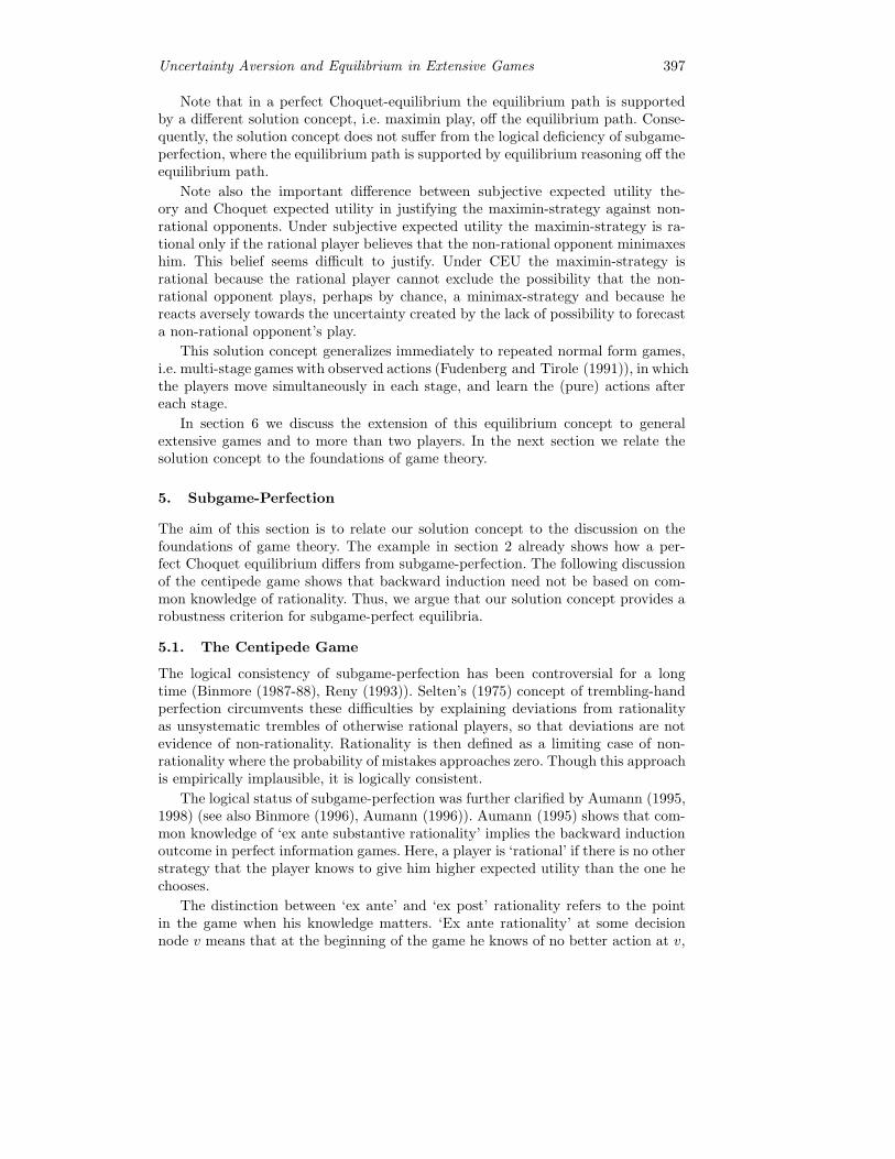
Uncertainty Aversion and Equilibrium in Extensive Games 397
Note that in a perfect Choquet-equilibrium the equilibrium path is supportedby a different solution concept, i.e. maximin play, off the equilibrium path. Conse-quently, the solution concept does not suffer from the logical deficiency of subgame-perfection, where the equilibrium path is supported by equilibrium reasoning off theequilibrium path.
Note also the important difference between subjective expected utility the-ory and Choquet expected utility in justifying the maximin-strategy against non-rational opponents. Under subjective expected utility the maximin-strategy is ra-tional only if the rational player believes that the non-rational opponent minimaxeshim. This belief seems difficult to justify. Under CEU the maximin-strategy isrational because the rational player cannot exclude the possibility that the non-rational opponent plays, perhaps by chance, a minimax-strategy and because hereacts aversely towards the uncertainty created by the lack of possibility to forecasta non-rational opponent’s play.
This solution concept generalizes immediately to repeated normal form games,i.e. multi-stage games with observed actions (Fudenberg and Tirole (1991)), in whichthe players move simultaneously in each stage, and learn the (pure) actions aftereach stage.
In section 6 we discuss the extension of this equilibrium concept to generalextensive games and to more than two players. In the next section we relate thesolution concept to the foundations of game theory.
5. Subgame-Perfection
The aim of this section is to relate our solution concept to the discussion on thefoundations of game theory. The example in section 2 already shows how a per-fect Choquet equilibrium differs from subgame-perfection. The following discussionof the centipede game shows that backward induction need not be based on com-mon knowledge of rationality. Thus, we argue that our solution concept provides arobustness criterion for subgame-perfect equilibria.
5.1. The Centipede Game
The logical consistency of subgame-perfection has been controversial for a longtime (Binmore (1987-88), Reny (1993)). Selten’s (1975) concept of trembling-handperfection circumvents these difficulties by explaining deviations from rationalityas unsystematic trembles of otherwise rational players, so that deviations are notevidence of non-rationality. Rationality is then defined as a limiting case of non-rationality where the probability of mistakes approaches zero. Though this approachis empirically implausible, it is logically consistent.
The logical status of subgame-perfection was further clarified by Aumann (1995,1998) (see also Binmore (1996), Aumann (1996)). Aumann (1995) shows that com-mon knowledge of ‘ex ante substantive rationality’ implies the backward inductionoutcome in perfect information games. Here, a player is ‘rational’ if there is no otherstrategy that the player knows to give him higher expected utility than the one hechooses.
The distinction between ‘ex ante’ and ‘ex post’ rationality refers to the pointin the game when his knowledge matters. ‘Ex ante rationality’ at some decisionnode v means that at the beginning of the game he knows of no better action at v,
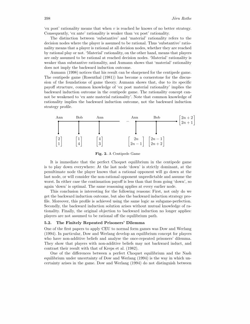
398 Jorn Rothe
‘ex post’ rationality means that when v is reached he knows of no better strategy.Consequently, ‘ex ante’ rationality is weaker than ‘ex post’ rationality.
The distinction between ‘substantive’ and ‘material’ rationality refers to thedecision nodes where the player is assumed to be rational. Thus ‘substantive’ ratio-nality means that a player is rational at all decision nodes, whether they are reachedby rational play or not. ‘Material’ rationality, on the other hand, means that playersare only assumed to be rational at reached decision nodes. ‘Material’ rationality isweaker than substantive rationality, and Aumann shows that ‘material’ rationalitydoes not imply the backward induction outcome.
Aumann (1998) notices that his result can be sharpened for the centipede game.The centipede game (Rosenthal (1981)) has become a cornerstone for the discus-sion of the foundations of game theory. Aumann shows that, due to its specificpayoff structure, common knowledge of ‘ex post material rationality’ implies thebackward induction outcome in the centipede game. The rationality concept can-not be weakened to ‘ex ante material rationality’. Note that common knowledge ofrationality implies the backward induction outcome, not the backward inductionstrategy profile.
� � � � � �
� � � � �
� � �
Ann Bob Ann Ann Bob
[21
] [14
] [43
] [2n
2n− 1
] [2n− 12n + 2
]
[2n + 22n + 1
]
Fig. 2. A Centipede Game
It is immediate that the perfect Choquet equilibrium in the centipede gameis to play down everywhere: At the last node ‘down’ is strictly dominant, at thepenultimate node the player knows that a rational opponent will go down at thelast node, or will consider the non-rational opponent unpredictable and assume theworst. In either case the continuation payoff is less than that from going ‘down’, soagain ‘down’ is optimal. The same reasoning applies at every earlier node.
This conclusion is interesting for the following reasons: First, not only do weget the backward induction outcome, but also the backward induction strategy pro-file. Moreover, this profile is achieved using the same logic as subgame-perfection.Secondly, the backward induction solution arises without mutual knowledge of ra-tionality. Finally, the original objection to backward induction no longer applies:players are not assumed to be rational off the equilibrium path.
5.2. The Finitely Repeated Prisoners’ Dilemma
One of the first papers to apply CEU to normal form games was Dow and Werlang(1994). In particular, Dow and Werlang develop an equilibrium concept for playerswho have non-additive beliefs and analyse the once-repeated prisoners’ dilemma.They show that players with non-additive beliefs may not backward induct, andcontrast their result with that of Kreps et al. (1982).
One of the differences between a perfect Choquet equilibrium and the Nashequilibrium under uncertainty of Dow and Werlang (1994) is the way in which un-certainty arises in the game. Dow and Werlang (1994) do not distinguish between

Uncertainty Aversion and Equilibrium in Extensive Games 399
rational and non-rational players, in their equilibrium concept players are CEUmaximisers who lack, to some degree, logical omniscience. They anticipate thattheir opponents maximise CEU, but do not draw the conclusion about the strategychoice. In other words, theirs is an equilibrium in beliefs. In our model, it is thelack of mutual knowledge of rationality that gives rise to uncertainty. The rationalplayers can anticipate how rational opponents will act, but not how non-rationalopponents will
The main difference, however, that Nash equilibrium under uncertainty is anormal form concept. Thus when players may have non-additive beliefs, cooperationin the first period and defection in the second can be an equilibrium: If the playersbelieve that the opponent cooperates in the second period if, and only if they do soat the first stage, they have an incentive to cooperate early, and for lack of logicalomniscience both players may think so10.
Under complete uncertainty aversion, in a perfect Choquet equilibrium bothplayers defect at all stages: In the second stage defection is strictly dominant, inthe first stage a player can anticipate that a rational opponent will defect in thenext stage, and a non-rational opponent causes uncertainty that is evaluated by itsworst outcome, i.e. defection. So the second stage action is independent of the firststage action, and again defection is strictly dominant in the first stage.
Note that Aumann’s (1995) justification of the backward induction outcomedoes not apply to the repeated prisoners’ dilemma, since it is not a perfect informa-tion game. Thus, the perfect Choquet equilibrium concept sheds some light on therobustness of subgame-perfect equilibria. It is perhaps surprising that backward in-duction is robust in games like the centipede game or the finitely repeated prisoners’dilemma, in which it is most counterintuitive.
However, we can also extend the result of Dow and Werlang (1994) in the fol-lowing way: Instead of assuming that players are completely uncertainty averse,assume that they believe that if the opponent is non-rational, then he will defectin the first period and cooperate in the second period if, and only if, there wascooperation in the first period.
Now, if the probability that the opponent is non-rational is sufficiently high, thenagain it is rational to cooperate in the first period (and to defect in the second pe-riod), because first-period play influences the second-period play of the non-rationalopponents. This result is interesting because it shows that backward induction maybreak down even if the strategies of the rational opponent can be correctly antic-ipated and subgame perfection is required. Yet, a basic shortcoming of this resultis that it rests on this specific belief about non-rational play, that is as difficult tojustify as the ‘crazy type’ of Kreps et al. (1982).
10 In fact this phenomenon is also related to another aspect of the Nash equilibrium underuncertainty in Dow and Werlang (1994), i.e. their definition of support of a non-additivemeasure. The support implicitly defines the knowledge of the players. What the correctsupport notion is for non-additive beliefs is controversial. This issue does not arise in aperfect Choquet equilibrium, in which players know the rational strategies in the usualsense.
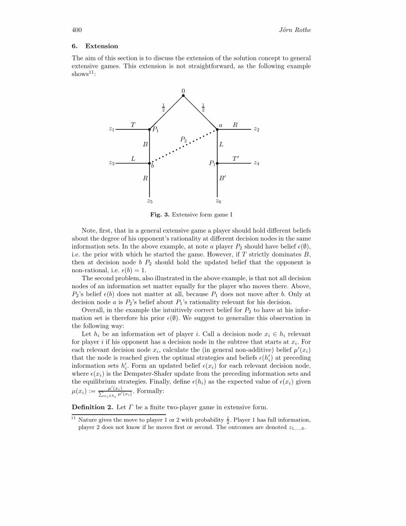
400 Jorn Rothe
6. Extension
The aim of this section is to discuss the extension of the solution concept to generalextensive games. This extension is not straightforward, as the following exampleshows11:
0
12
12
T
B
L
R
R
L
T ′
B′
z1 z2
z3 z4
z5 z6
P1
P1
P2
a
b
��
��
��
��
��
��
��
��
��
��
�
�
�
�
�
��
��
��
������
Fig. 3. Extensive form game I
Note, first, that in a general extensive game a player should hold different beliefsabout the degree of his opponent’s rationality at different decision nodes in the sameinformation sets. In the above example, at note a player P2 should have belief ε(∅),i.e. the prior with which he started the game. However, if T strictly dominates B,then at decision node b P2 should hold the updated belief that the opponent isnon-rational, i.e. ε(b) = 1.
The second problem, also illustrated in the above example, is that not all decisionnodes of an information set matter equally for the player who moves there. Above,P2’s belief ε(b) does not matter at all, because P1 does not move after b. Only atdecision node a is P2’s belief about P1’s rationality relevant for his decision.
Overall, in the example the intuitively correct belief for P2 to have at his infor-mation set is therefore his prior ε(∅). We suggest to generalize this observation inthe following way:
Let hi be an information set of player i. Call a decision node xi ∈ hi relevantfor player i if his opponent has a decision node in the subtree that starts at xi. Foreach relevant decision node xi, calculate the (in general non-additive) belief μ′(xi)that the node is reached given the optimal strategies and beliefs ε(h′
i) at precedinginformation sets h′
i. Form an updated belief ε(xi) for each relevant decision node,where ε(xi) is the Dempster-Shafer update from the preceding information sets andthe equilibrium strategies. Finally, define ε(hi) as the expected value of ε(xi) given
μ(xi) := μ′(xi)∑xi∈hi μ
′(xi) . Formally:
Definition 2. Let Γ be a finite two-player game in extensive form.
11 Nature gives the move to player 1 or 2 with probability 12. Player 1 has full information,
player 2 does not know if he moves first or second. The outcomes are denoted z1,...,6.
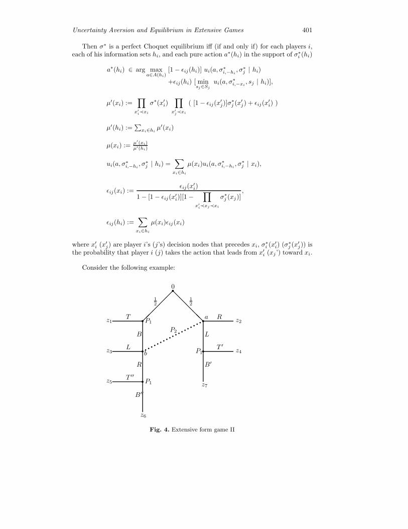
Uncertainty Aversion and Equilibrium in Extensive Games 401
Then σ∗ is a perfect Choquet equilibrium iff (if and only if) for each players i,each of his information sets hi, and each pure action a∗(hi) in the support of σ∗
i (hi)
a∗(hi) ∈ arg maxa∈A(hi)
[1− εij(hi)] ui(a, σ∗i,−hi , σ
∗j | hi)
+εij(hi) [ minsj∈Sj
ui(a, σ∗i,−xi , sj | hi)],
μ′(xi) :=∏x′i≺xi
σ∗(x′i)
∏x′j≺xi
( [1− εij(x′j)]σ
∗j (x′
j) + εij(x′i) )
μ′(hi) :=∑
xi∈hi μ′(xi)
μ(xi) := μ′(xi)μ′(hi)
ui(a, σ∗i,−hi , σ
∗j | hi) =
∑xi∈hi
μ(xi)ui(a, σ∗i,−hi , σ
∗j | xi),
εij(xi) :=εij(x
′i)
1− [1− εij(x′i)][1−
∏x′i≺xj≺xi
σ∗j (xj)]
,
εij(hi) :=∑xi∈hi
μ(xi)εij(xi)
where x′i (x′
j) are player i’s (j’s) decision nodes that precedes xi, σ∗i (x′
i) (σ∗j (x′
j)) isthe probability that player i (j) takes the action that leads from x′
i (xj ’) toward xi.
Consider the following example:
0
12
12
T
B
L
R
R
L
T ′
B′
T ′′
B′′
z1 z2
z3 z4
z6
z7z5
P1
P1
P2
P1
a
b
��������������������
�
�
�
�
�
�
��
���
�����
Fig. 4. Extensive form game II

402 Jorn Rothe
Again, assume that T is strictly dominant, so that ε(b) = 1. Then μ′(a) = 12 and
μ′(b) = 12ε(∅). Note that the calculation of μ′(b) again reflects uncertainty aversion,
because the worst case is that non-rational players would play B, since this wouldgive most weight to the worst outcome as P2 weighs his decision at his informationset.
The extension of the equilibrium concept to more than two players is conceptu-ally straightforward, but computationally demanding. For two opponents Pj and Pkof player i, and beliefs εj and εk about their lack of rationality, the rational playerhas to take all four cases into account: that either of the players is non-rational, thatboth are rational and that neither is. So at decision node xi he should maximise
maxa∈A(xi)
[(1 − εj)(1 − εk)] ui(a, σ∗i,−xi , σ
∗j , σ
∗k)
+[(1− εj)εk] minsk∈Sk
ui(a, σ∗i,−xi , σ
∗j , sk)
+[εj(1− εk)] minsj∈Sj
ui(a, σ∗i,−xi , sj, σ
∗k)
+[εjεk] min(sj ,sk)∈Sj×Sk
ui(a, σ∗i,−xi , sj , sk).
In particular, taking into account that both players may be non-rational meansthat in the worst case their actions may be correlated. Beliefs εj and εk are thenupdated separately on the basis of the Dempster-Shafer rule.
7. Conclusion
The paper has suggested a solution concept that combines equilibrium logic withmaximin play off the equilibrium path. The solution concept is natural if rationalityis not mutual knowledge, no restriction is imposed on deviations from rationality,and if players are uncertainty-averse.
Nevertheless, the solution concept also has some limitations. First, the computa-tional effort of calculating equilibria may be quite high. Secondly, experiments showthat players sometimes systematically deviate from rational play, so that it may bepossible to formulate more restrictive assumptions on non-rational play after all.Note that this would give rise to a difference between a descriptive solution conceptwith such restrictions, and a normative concept like ours where we based the lackof restrictions on the consistency argument that a rationality concept alone doesnot restrict non-rational play.
Thirdly, the assumption that players are completely uncertainty-averse is ex-treme. Yet, at the current stage of the development of Choquet expected utilitytheory there is no ideal alternative12.
Finally, it seems a drastic consequence that strategic interaction comes to acomplete halt after a deviation from rational play. Note, however, that the solu-tion concept applies to one-shot games, and therefore leaves no room for real-worldstrategies to deal with doubts about rationality, e.g. experimentation and com-munication. Note also that trembling-hand perfection makes an equally extremeassumption to ensure logical consistency by postulating that otherwise fully ra-
12 It would be possible to assume that players take a weighted average of the best andthe worst outcome if they are certain to face a non-rational opponent. This is Hurwicz’soptimism-pessimism index (see Arrow and Hurwicz (1972). However, by introducing an-other free parameter the model would lose predictive power.
Uncertainty Aversion and Equilibrium in Extensive Games 403
tional players ‘tremble’, and that deviations therefore provide no evidence againstrationality.
Needless to say, our solution concept provides nothing but a first step that maybe a basis for a more refined analysis.
Acknowlegments. For helpful comments on the first version I would like to thankJurgen Eichberger, Leonardo Felli, Hans Haller, David Kelsey, Marco Mariotti, Su-joy Mukerji, Matthew Ryan and audiences at the Jahrestagung of the Verein furSocialpolitik in Bern (1997), the 1st World Congress of the Game Theory Societyin Bilbao (2000), the 8th World Congress of the Econometric Society in Seattle(2000), and seminar audiences at the universities of Cambridge (2001), Leicester(2005), Newcastle (2006), Moscow (ICEF, 2008) and Bristol (2010). Errors are myresponsibility.
Appendix
Let v be a capacity and consider the events E,F ∈ Σ. The Dempster-Shafer rulespecifies that the posterior capacity of event E is given by (if v(F ) < 1)
v(E|F ) :=v(E ∪ F )− v(F )
1− v(F ).
Let ε be the prior probability that a player is not rational with 0 < ε < 1.Assume that a rational player chooses an action A with probability p. Then theposterior belief about the opponent’s rationality after action A is given by
v(R|A) :=(1− ε)p
1− (1− ε)(1− p).
This is derived as follows:Let R be the event that the player is rational, let R be the event that he is
non-rational.We want to calculate
v(R|A) :=v(R ∪A)− v(A)
1− v(A). (1)
Since a player is either rational or not, we have
v(R|A) + v(R|A) = 1. (2)
Consequently,
(3) v(R|A) = v(R∪A)−v(A)
1−v(A),
(4) v(R|A) = v(R∪A)−v(A)
1−v(A)
implyv(A) = v(R ∪ A) + v(R ∪ A)− 1.
Further,
(5) v(A|R) = v(A∪R)−v(R)
1−v(R), and
(6) v(A|R) = v(A∪R)−v(R)1−v(R) .

404 Jorn Rothe
We know that(7) v(R) = 1− ε,(8) v(R) = ε,(9) v(A|R) = 1− p, and(10) v(A|R) = 0.so that(11) v(A ∪R) = (1− ε)(1− p) + ε, and(12) v(A ∪R) = 1− ε.Thus
v(A) = (1 − ε) + (1− ε)(1 − p) + ε− 1 = (1− ε)(1− p). (13)
Consequently,
v(R|A) :=(1− ε)− (1− ε)(1− p)
1− (1− ε)(1− p)
=(1− ε)p
1− (1− ε)(1− p),
v(R|A) =ε
1− (1− ε)(1− p)
Remarks:(1) The derivation is only valid under lack of mutual knowledge of rationality,i.e. for ε > 0 and ε < 1, otherwise v(A|R) or v(A|R) are not well-defined.
(2) With 0 < ε < 1 there are no probability zero events, since
v(A) = (1− ε)(1− p) < 1.
This holds for any p ∈ [0, 1], including the boundaries.(3) In particular, if ε > 0 then ε′ > 0, independently of p. However, if p = 0, thenε′ = 1. Thus we also need to be able to update the belief ε = 1. Intuitively, ifthe prior belief about the opponent is that he is non-rational and beliefs abouthis behavior are uncertainty averse, then there are no probability zero events,and the posterior belief should also be that the opponent is non-rational.Thiscan be justified directly from the Dempster-Shafer rule (1): From monotonicity,v(R) ≤ v(R∪olA), therefore v(R∪A) = 1. Also, (6) implies v(A|R) = v(A∪R),so again by monotonicity, v(A) ≤ v(A ∪ R) = 0. Since this result also followsif we substitute ε = 1 into (13), we do not have to explicitly track this specialcase.
(4) The reason why ε = 0 has to be excluded is that there is no parallel argumentthat ε = 0 and p = 0 should give ε′ = 1. (3) implies v(A ∪ R) = v(A|R) = 1
and (1) gives ε′ = 1−v(A)
1−v(A), but v(A) < 1.
(5) Note that action A is always interpreted as evidence of non-rationality:v(R|A) = ε 1
1−(1−ε)(1−p) > ε. Thus updating is in line with uncertainty aversion,
which gives rise to non-additive beliefs in the first place. For the player, theworst case is that the non-rational opponent chose action A with probability1, because this makes it more likely, under uncertainty aversion, to receive theworst outcome in the next stage.
(6) Note that if ε′ = ε1−(1−ε)(1−p) and ε′′ = ε′
1−(1−ε′)(1−p′) then ε′′ = ε1−(1−ε)(1−p·p′) .
(7) Finally, note that the argument rests heavily on (2), i.e. the the requirementabout beliefs that an opponent is either rational or non-rational, so that thesebeliefs have to be additive.

Uncertainty Aversion and Equilibrium in Extensive Games 405
References
Anscombe, F. J. and R. J. Aumann (1963). A definition of subjective probability. Annals ofMathematical Statistics, 34, 199–205.
Arrow, K. J. and L. Hurwicz (1972). An optimality criterion for decision-making underignorance. in: Carter & Ford (1972), 1-11.
Aumann, R. J. (1995). Backward induction and common knowledge of rationality. Gamesand Economic Behavior, 8, 6-19.
Aumann, R. J. (1996). Reply to Binmore. Games and Economic Behavior, 17, 138-46.Aumann, R. J. (1998). On the centipede game. Games and Economic Behavior, 23, 97-105.Binmore, K. G. (198788). Modelling rational players I & II. Economics and Phi- losophy
3 & 4, 3:179-214, 4:9-55.Binmore, K. G. (1996). A note on backward induction. Games and Economic Behavior, 17,
135-7.Carter, C. F. and J. L. Ford (Eds.) (1972). Uncertainty and Expectations in Economics.
Basil Blackwell: Oxford.Choquet, G. (1953). Theory of capacities, Annales de l’Institut Fourier (Grenoble), 5,
131–295.Cohen, M., Gilboa, I., Jaffray, J.-Y. and D. Schmeidler (1999). An experimental study of
updating ambiguous beliefs. mimeo.Dempster, A. P. (1967). Upper and lower probabilities induced by a multivalued mapping.
Annals of Mathematical Statistics, 38, 325-39.Dow, J. and S. R. d. C. Werlang (1994). Nash equilibrium under Knightian uncertainty:
Breaking down backward induction. Journal of Economic Theory, 64, 305–324.Eichberger, J. and D. Kelsey (1994). Non-additive beliefs and game theory. Discussion
Paper 9410, Center for Economic Research.Eichberger, J. and D. Kelsey(1995). Signalling games with uncertainty. mimeo.Eichberger, J. and D. Kelsey (1996). Uncertainty aversion and preference for randomisa-
tion. Journal of Economic Theory, 71, 31–43.Ellsberg, D. (1961). Risk, ambiguity and the savage axioms. Quarterly Journal of Eco-
nomics, 75, 643-69.Epstein, L. G. (1997a). Preference, rationalizability and equilibrium. Journal of Economic
Theory, 73, 1–29.Epstein, L. G. (1997b). Uncertainty aversion. mimeo.Epstein, L. G. and M. L. Breton (1993). Dynamically consistent beliefs must be bayesian.
Journal of Economic Theory, 61, 1-22.Fagin, R. and J. Y. Halpern (1990). A new approach to updating beliefs. mimeo.Fudenberg, D. and J. Tirole (1991). Game Theory. MIT Press: Cambridge, MA.Ghirardato, P. and M. Marinacci (1997). Ambiguity made precise: A comparative founda-
tion and some implications. mimeo, University of Toronto.Gilboa, I. (1987). Expected utility with purely subjective non-additive probabilities. Journal
of Mathematical Economics, 16, 65-88.Gilboa, I. and D. Schmeidler (1989). Maxmin expected utility with non-unique prior. Jour-
nal of Mathematical Economics, 18, 141–153.Gilboa, I. and D. Schmeidler (1993). Updating ambiguous beliefs. Journal of Eco- nomic
Theory, 59, 33-49.Hendon, E., Jacobsen, H. J., Sloth, B. and T. Tranaes (1995). Nash equilibrium in lower
probabilities. mimeo.Klibanoff, P. (1993). Uncertainty, decision and normal norm games. mimeo.Kreps, D. M. and R. B. Wilson (1982a). Reputation and imperfect information. Journal of
Economic Theory, 27, 253-79.Kreps, D. M. and R. B. Wilson (1982b). Sequential equilibria. Econometrica 50, 863-894.Kreps, D. M., Milgrom, P., Roberts, J. and R. B. Wilson (1982). Rational cooperation in
the finitely repeated prisoners’ dilemma. Journal of Economic Theory, 27, 245–252.

406 Jorn Rothe
Lo, K. C. (1995a). Nash equilibrium without mutual knowledge of rationality. mimeo, Uni-versity of Toronto.
Lo, K. C. (1995b). Extensive form games with uncertainty averse players. mimeo, Universityof Toronto.
Marinacci, M. (1994). Equilibrium in ambiguous games. mimeo.Milgrom, P. R. and J. Roberts (1982a). Limit pricing and entry under incomplete infor-
mation: An equilibrium analysis. Econometrica, 50, 443-60.Milgrom, P. R. and J. Roberts (1982b). Predation, reputation and entry deterrence. Journal
of Economic Theory, 27, 280-312.Mukerji, S. (1994). A theory of play for games in strategic form when rationality is not
common knowledge. mimeo.Reny, P. J. (1993). Common belief and the theory of games with perfect information. Journal
of Economic Theory, 59, 257-74.Rosenthal, R. W. (1981). Games of perfect information, predatory pricing and the chain
store paradox. Journal of Economic Theory, 25, 92-100.Rothe, J. (1996). Uncertainty aversion and equilibrium. mimeo.Rothe, J. (2009). Uncertainty aversion and equilibrium. In: Contributions to game theory
and management (Petrosjan, L. A. and N. A. Zenkevich, eds), Vol. II, pp. 363–382.Rothe, J. (2010). Uncertainty aversion and equilibrium in normal form games. In: Contri-
butions to game theory and management (Petrosjan, L. A. and N. A. Zenkevich, eds),Vol. III, pp. 342–367.
Ryan, M. (1997). A refinement of Dempster-Shafer equilibrium. mimeo, University of Auck-land.
Sarin, R. and P. P. Wakker (1992). A simple axiomatization of nonadditive expected utility.Econometrica 60, 1255-72.
Savage, L. J. (1954). The Foundations of Statistics. Wiley: New York, NY (2nd edn.: Dover,1972).
Schmeidler, D. (1986). Integral representation without additivity. Proceedings of the Amer-ican Mathematical Society, 97, 255-61.
Schmeidler, D. (1989). Subjective probability and expected utility without additivity. Econo-metrica, 57, 571–587.
Selten, R. (1975). Re-examination of the perfectness concept for equilibrium points in ex-tensive games. International Journal of Game Theory, 4, 25–55.
Shafer, G. (1976). A Mathematical Theory of Evidence. Princeton University Press: Prince-ton, NJ.
Shapley, L. S. (1971). Cores of convex games. International Journal of Game Theory, 1,11–26.
Smithson, M. J. (1997). Human judgment and imprecise probabilities. mimeo, ImpreciseProbability Project.
Wakker, P. P. (1989). Additive Representations of Preferences. Kluwer Academic Publish-ers: Dordrecht.
Nash Equilibrium in Games with Ordered Outcomes
Victor V. Rozen
Saratov State University,Astrakhanskaya St. 83, Saratov, 410012, Russia
E-mail: [email protected]
Abstract. We study Nash equilibrium in games with ordered outcomes.Given game with ordered outcomes, we can construct its mixed extension.For it the preference relations of players are to be extended to the set ofprobability measures. In this work we use the canonical extension of anorder to the set of probability measures.It is shown that a finding of Nash equilibrium points in mixed extension ofa game with ordered outcomes can be reduced to search so called balancedmatrices, which was introduced by the author. The necessary condition forexistence of Nash equilibrium points in mixed extension of a game withordered outcomes is a presence of balanced submatrices for the matrix ofits realization function. We construct a certain method for searching of allbalanced submatrices of given matrix using the concept of extreme balancedmatrix. Necessary and sufficient conditions for Nash equilibrium point inmixed extension of a game with ordered outcomes are given also.
Keywords: Game with ordered outcomes, Nash equilibrium, Mixed exten-sion of a game with ordered outcomes, Balanced matrix, Extreme balancedmatrix, Balanced collection.
1. Introduction
A game G with ordered outcomes is a game in which preferences of players bypartial ordered relations are given (all preliminaries see in Rozen (2010)).
Definition 1. A situation x0 is called Nash equilibrium point in game G if for anyplayer i and its strategy xi the condition
F (x0 ‖ xi)ωi� F (x0) (1)
holds, whereωi� is a preference relation of player i.
We construct a mixed extension of a finite game G with ordered outcomes inthe following way. Mixed strategies of players in game G is defined as usually thatis probability measures on the sets of their pure strategies. A realization functionF of a game G can be extended to a mapping F of mixed situations of game G intothe set A consisting of probability measures on the set outcomes A. Now we need toextend the preference relations of players on A. We define the canonical extensionof order ω ⊆ A2 to the set A by formula
μω
� ν ⇐⇒ (∀f ∈ C(ω)) f(μ) f(ν), (2)
where μ, ν ∈ A, C(ω) is the set of all isotonic functions from A to R under order ωand f(μ) = (f, μ) is the standard scalar product.
408 Victor V. Rozen
Remark 1. In evident form the condition μω
� ν means that μ(B) ν(B) for anysubset B ⊆ A which is majorant stable under order ω (see Rozen (1976)). Recallthat a subset B ⊆ A is called majorant stable one if the conditions a ∈ B and
a′ω
a imply a′ ∈ B.
Corollary 1 (convexity of the canonical extension). Conditions μkω
� νk,where αk > 0 (k = 1, . . . , p),
∑pk=1 αk = 1, imply
p∑k=1
αkμkω
�p∑
k=1
αkνk. (3)
Moreover, if at least one of these conditions is strict then condition (3) is strictalso.
In this article we consider games of two players with ordered outcomes in theform
G = 〈X,Y,A, ω1, ω2, F 〉
where X is a set of strategies of player 1, Y is a set of strategies of player 2, A is aset of outcomes, ωk is an order relation on A which represents preferences of playerk = 1, 2 and F : X × Y → A is a realization function.
According to a general definition a situation(x0, y0
)∈ X×Y is Nash equilibrium
point in game G if for any x ∈ X and y ∈ Y conditions
F(x, y0)
ω1
� F(x0, y0), F(x0, y)
ω2
� F(x0, y0)
hold.
In section 3 it is shown that, for game G, the existence of Nash equilibrium pointsin mixed strategies is connected with so called balanced submatrices its realizationfunction. We study some basic properties of balanced matrices in section 2. Theorem1 shows a simple connection between balanced matrices and well known in gametheory balanced collections. Note that up to now, a concept of balanced collectionwas used for systems of coalitions in cooperative games only (see, for example,Bondareva (1968), Shapley (1965), Peleg (1965)). The main result of our work isTheorem 4 which states a necessary and sufficient conditions for Nash equilibriumpoint in mixed extension of game G with ordered outcomes. To illustrate theseresults we consider some examples.
2. Balanced matrices and balanced collections of subsets
We consider an arbitrary matrix M of size m × n over a set A as a mappingF : I × J → A where I = {1, . . . ,m} , J = {1, . . . , n}. Put M = ‖F (i, j)‖.
We denote by Sm the standard simplex consisting of m–components vectors:
Sm =
{x = (x1, . . . , xm) : xi ≥ 0,
m∑i=1
= 1
}.
Nash Equilibrium in Games with Ordered Outcomes 409
For any x ∈ Sm, y ∈ Sn and a ∈ A put
F(x,y) (a) =∑
F (i, j) = a
(i, j) ∈ I × J
xi · yj . (4)
In particular for any i = 1, . . . ,m and j = 1, . . . , n we have
F(x,j) (a) =∑
F (i,j)=a
xi, F(i,y) (a) =∑
F (i,j)=a
yj . (5)
Remark 2. We identify any index i ∈ I with unit vector ei = (0, . . . , 1, . . . , 0) andalso for any index j ∈ J .
Lemma 1 (linearity property). The function F is linear under all arguments.
Proof (of lemma 1). Verify a linearity under first argument. Put xk ∈ Sm, y ∈Sn, αk ≥ 0 (k = 1, . . . , p),
∑pk=1 αk = 1. We have
F(∑pk=1 αkx
k,y) (a) =∑
F (i, j) = a
(i, j) ∈ I × J
(p∑k=1
αkxki
)yj =
∑F (i, j) = a
(i, j) ∈ I × J
p∑k=1
αkxki yj =
=
p∑k=1
∑F (i, j) = a
(i, j) ∈ I × J
αkxki yj =
p∑k=1
αk∑
F (i, j) = a
(i, j) ∈ I × J
xki yj =
p∑k=1
αkF(xk,y) (a)
which was to be proved. ��
Definition 2. A matrix ‖F (i, j)‖ is called balanced one if there exists such a pairof vectors
(x0, y0
)∈ Sm×Sn with positive components that for any x ∈ Sm, y ∈ Sn
and a ∈ A the equalities
F(x, y0) (a) = F(x0, y0) (a) , F(x0, y) (a) = F(x0, y0) (a) (6)
hold. In this case the pair(x0, y0
)is called a balance pair of vectors.
Note that (4) means the equality of corresponding measures:
F(x, y0) = F(x0, y0), F(x0, y) = F(x0, y0).
Definition 3. A vector x0 ∈ Sm with positive components is called a row balancevector for matrix ‖F (i, j)‖ (i ∈ I, j ∈ J) if for any j1, j2 ∈ J the equality F(x0, j1) =
F(x0, j2) holds. In other words, in this case, the measure F(x0, j) does not dependon j ∈ J . A column balance vector is defined dually that is a vector y0 ∈ Sn withpositive components such that the measure F(i, y0) does not depend on i ∈ I.
Lemma 2. A pair of vectors(x0, y0
)is a balance pair for matrix ‖F (i, j)‖ if and
only if x0 is a row balance vector and y0 is a column balance vector.

410 Victor V. Rozen
Indeed let(x0, y0
)be a balance pair of vectors. Setting in (4) y = j1 and then y =
j2 we have F(x0, j1) = F(x0, y0), F(x0, j2) = F(x0, y0) hence x0 is a row balance vector.Dually, y0 is a column balance vector. Conversely let x0 be a row balance vector andy0 a column balance vector. For arbitrary a ∈ A put p (a) = F(x0, j) (a) (j ∈ J) .
Fix a vector y = (y1, . . . , yn) ∈ Sn. By using a linearity for F (see Lemma 1), weget
F(x0, y) (a) = F(x0,∑j∈J yjej)
(a) =∑j∈J
yjF(x0,j) (a) =
=∑j∈J
yjp (a) = p (a)∑j∈J
yj = p (a) ,
i.e. the measure F(x0,y) does not depend on y ∈ Sn. Then, for any y ∈ Sn we have
F(x0, y) = F(x0, y0) and dually F(x, y0) = F(x0, y0), hence(x0, y0
)is a balance pair of
vectors.
Corollary 2. A balanced matrix is homogeneous (that is, any its row and any col-umn contains a same set of elements).
For the proof it is sufficiently to remark that the set of elements consisting i-throw of matrix ‖F (i, j)‖ coincides with spectrum of the measure F(i, y0) which, inour case, does not depend on i ∈ I.
Recall the concept of balanced collection.
Definition 4. Let E be an arbitrary set and (E1, . . . , Ep) be a covering systemof its subsets. The collection (E1, . . . , Ep) is called balanced one if there exists arepresentative vector for it, i.e. a vector λ = (λ1, . . . , λp) with positive componentssuch that for any e ∈ E the equality∑
Ek�eλk = 1
holds.
Definition 5. Two balanced collections(E1
1 , . . . , E1p
)and
(E2
1 , . . . , E2p
)are said to
be collinearly balanced if for them there exist collinear representative vectors λ1 andλ2 (in notation λ1‖λ2).
Given a matrix F : I × J → A, we define for arbitrary a ∈ A two collections ofcharacteristic subsets (Ua
i )i∈I and(V aj
)j∈J by setting
j ∈ Uai ⇔ F (i, j) = a, i ∈ V a
j ⇔ F (i, j) = a. (7)
Theorem 1. A matrix F : I×J → A is balanced if and only if for any a1, a2 ∈ pr2F
1. Collections (Ua1i )i∈I and (Ua2
i )i∈I are collinearly balanced ones;
2. Collections(V a1j
)j∈J and
(V a2j
)j∈J are collinearly balanced ones.
Lemma 3. A matrix F : I × J → A has a row balanced vector if and only ifa) for any a ∈ pr2F, the collection of its characteristic subsets (Ua
i )i∈I is balancedone;
b) for any a1, a2 ∈ pr2F, collections (Ua1i )i∈I and (Ua2
i )i∈I are collinearly bal-anced ones.

Nash Equilibrium in Games with Ordered Outcomes 411
Proof (of lemma 3). Necessity. Let x = (x1, . . . , xm) be a row balance vector. For
arbitrary a ∈ pr2F put λai = xi/p (a) where p (a) = F(x,j) (a) (the right part ofthis equality does not depend on j ∈ J, see Definition 3). Check that the vectorλa = (λai )i∈I is a representative one for the collection (Ua
i )i∈I . Fix j ∈ J. By using(5), we have∑
Uai �jλai =
∑F (i,j)=a
λai =∑
F (i,j)=a
xip (a)
=1
p (a)
∑F (i,j)=a
xi =1
p (a)p (a) = 1.
Furthermore, for any a1, a2 ∈ pr2F, we get
λa1i : λa2i =xi
p (a1):
xip (a2)
=p (a2)
p (a1)= const under i ∈ I,
i.e. representative vectors λa1 and λa2 are collinear ones.Sufficiency. Let λa = (λai )i∈I be a representative vector for balanced collection
(Uai )i∈I and moreover, for any a1, a2 ∈ pr2F corresponding vectors are collinear,
λa1‖λa2 . Fix a ∈ pr2F and put
xi =λai∑i′∈I λ
ai′, x = (xi)i∈I .
Because representative vectors are collinear, right parts of these equalities do notdepend on element a ∈ A. It is evident that xi > 0 and
∑i∈I xi = 1. By using that
vector λa is a representative one, we have for any j ∈ J
F(x, j) (a) =∑
F (i,j)=a
xi =∑Uai �j
λai∑i′∈I λ
ai′
=
∑Uai �j
λai∑i′∈I λ
ai′
=1∑
i′∈I λai′
= const.
Thus, the measure F(x, j) does not depend on j ∈ J, i.e. x is a row balance vectorfor matrix ‖F (i, j)‖ .
Now, using Lemma 2, we obtain the proof of Theorem 1 from Lemma 3 and itsdual. ��
For matrix M over a set A and a ∈ A we denote by χ (Ma) a matrix withelements ma
ij , where {maij = 1 if F (i, j) = a
maij = 0 if F (i, j) = a.
Theorem 2. Suppose M = ‖F (i, j)‖ is a balanced matrix. Then the followingconditions are equivalent:
1. Matrix M has an unique pair of balance vectors;2. Matrix M is a square one and Det χ (Ma) = 0 for any a ∈ A;3. Matrix M is a square one and Det χ (Ma) = 0 for some a ∈ A.
The proof of Theorem 2 is based on the following lemmas.
Lemma 4. Let E be an arbitrary finite set, |E| = m and (E1, . . . , En) be a balancedcollections of its subsets. Then the collection (E1, . . . , En) has an unique representa-tive vector if and only if the collection of characteristic vectors (χ (E1) , . . . , χ (En))is linearly independent.

412 Victor V. Rozen
Proof (of lemma 4). A vector λ = (λ1, . . . , λn) is a representative one for the col-lection (E1, . . . , En) if and only if it is a positive solution for the following systemof linear equations:
(λ1, . . . , λn) χM = (1, . . . , 1) , (8)
where by χM denoted n × m matrix whose i-th row χ (Ei) is the characteristicfunction of the subset Ei ⊆ E (i = 1, . . . , n) and (1, . . . , 1) is m-component vectorconsisting of 1. Because the collection (E1, . . . , En) is balanced, (8) is a compatiblesystem consisting of m linear equations under λ1, . . . , λn. It is well known that sucha system has an unique solution if and only if r = n where r = rank χM , hence, inthis case, the system of its rows is linearly independent.
Conversely, assume r < n. In this case, the solution of (8) can be represented inthe form λ∗ + L where λ∗ is a partial solution of (8) and L is a general solution ofa corresponding homogeneous system (note that L is a linear space with dimensionn − r). Let λ∗ be a representative vector for collection (E1, . . . , En) . Then all itscomponents are positive. Fix some l∗ ∈ L with l∗ = 0. Then there exists suchpositive ε > 0 that all components of vector λ∗ + εl∗ remain be positive. Hence(λ∗ + εl∗) is some positive solution of (8) with λ∗ + εl∗ = λ∗, then a representativevector for the collection (E1, . . . , En) is not unique. ��
Lemma 5. Let M be a matrix over set A. Then the following conditions are equiv-alent:
1) Matrix M has an unique row balance vector;2) For any a ∈ pr2M, the collection of characteristic vectors (χ (Ua
1 ) , . . . , χ (Uam))
is linearly independent;3) For some a ∈ pr2M, the collection of characteristic vectors (χ (Ua
1 ) , . . . , χ (Uam))
is linearly independent.
Proof (of lemma 5). 1)⇒ 2). Fix a ∈ pr2M. According to Lemma 3 a), the systemof characteristic subsets (Ua
1 , . . . , Uam) forms a balanced collection on the set J .
Let λ = (λ1, . . . , λm) and λ′ = (λ′1, . . . , λ
′m) be two its representative vectors.
Then vectors x = (x1, . . . , xm) and x′ = (x′1, . . . , x
′m) defined by
xi =λi∑i′∈I λi′
, x′i =
λ′i∑
i′∈I λ′i′
are row balance vectors for matrix M (see the proof of Lemma 3). According toassumption 1) we have x = x′, i.e. for any i ∈ I holds the equality
λi∑i′∈I λi′
=λ′i∑
i′∈I λ′i′,
hence λi = kλ′i where k = const. Fix j0 ∈ J. Since λ and λ′ are representative
vectors, we get
1 =∑j0∈Uai
λi =∑j0∈Uai
kλ′i = k
∑j0∈Uai
λ′i = k,
hence k = 1 and λ′ = λ. Thus, the balanced collection (Ua1 , . . . , U
am) has an unique
representative vector and, according with Lemma 4, the collection (χ (Ua1 ) , . . . , χ (Ua
m))is linearly independent.

Nash Equilibrium in Games with Ordered Outcomes 413
It is evident that 2)⇒ 3). Prove 3)⇒ 1). Assume that the collection of charac-teristic vectors (χ (Ua
1 ) , . . . , χ (Uam)) is linearly independent for some a ∈ pr2M. Let
x′ = (x′1, . . . , x
′m) and x′′ = (x′′
1 , . . . , x′′m) be two row balance vectors for matrix M.
Then vectors λ′ and λ′′ defined by λ′i = x′
i/p (a) , λ′′i = x′′
i /p (a) (i ∈ I) are repre-sentative vectors for balanced collection (Ua
1 , . . . , Uam) (see the proof of Lemma 3).
Because the collection (χ (Ua1 ) , . . . , χ (Ua
m)) is linearly independent it follows fromLemma 4 that λ′ = λ′′ hence x′ = x′′ which was to be proved. ��
Let us prove Theorem 2. Assume that matrix M has an unique pair of balancevectors. Then, according with Lemma 2, matrix M has an unique row balancevector. Fix an element a ∈ pr2M and consider the matrix χ (Ma) defined above.Since rows of matrix χ (Ma) are vectors (χ (Ua
1 ) , . . . , χ (Uam)) and according to
Lemma 5, we get that the collection of these vectors is linearly independent, thenm = r where r = rank χ (Ma) . Dually the equality n = r holds, hence we obtainm = n and Det χ (Ma) = 0 which completes the proof of Theorem 2.
Now we consider a problem for finding of all balanced submatrix for given matrix.Given a matrix ‖F (i, j)‖ (i ∈ I, j ∈ J) , fix two subsets I0 ⊆ I, J0 ⊆ J. We denoteby B1
J0a convex polyhedron which consists of all vectors x ∈ Sm satisfying the
condition
(∀j1, j2 ∈ J0) F(x, j1) = F(x, j2). (9)
Dually is defined a convex polyhedron B2I0
which consists of all vectors y ∈ Snsatisfying the condition
(∀i1, i2 ∈ I0) F(i1, y) = F(i2, y). (10)
Definition 6. A submatrix F (I0 × J0) = ‖F (i, j)‖ (i ∈ I0, j ∈ J0) is called anextreme balanced submatrix if it is balanced one and then there exists a balance pairof vectors for it which is an extreme point in the convex polyhedron B1
J0×B2
I0.
For arbitrary polyhedron P , we denote by Ext P the set of extreme point in P. Itis easy to show that Ext
(B1J0×B2
I0
)= Ext
(B1J0
)× Ext
(B2I0
).
Lemma 6. A vector x0 ∈ B1J0
is an extreme point in B1J0
if and only if it is minimalunder spectrum, i.e. for any x ∈ B1
J0the condition
Sp x ⊆ Sp x0 =⇒ x = x0 (11)
holds (we denote by Sp x the spectrum of vector x : Sp x = {i ∈ I : xi = 0}).
Proof (of lemma 6). Let x0 be an extreme point in B1J0. Consider a vector x ∈ B1
J0
satisfying the condition Sp x ⊆ Sp x0. Assume that x = x0. Because∑i∈Sp x
xi =∑
i∈Sp x0
x0i = 1
then between non-zero components of vector x there exists such xi′ that 0 < x0i′ < xi′
hence
0 < ε = mini∈Sp x
x0i
xi< 1. (12)
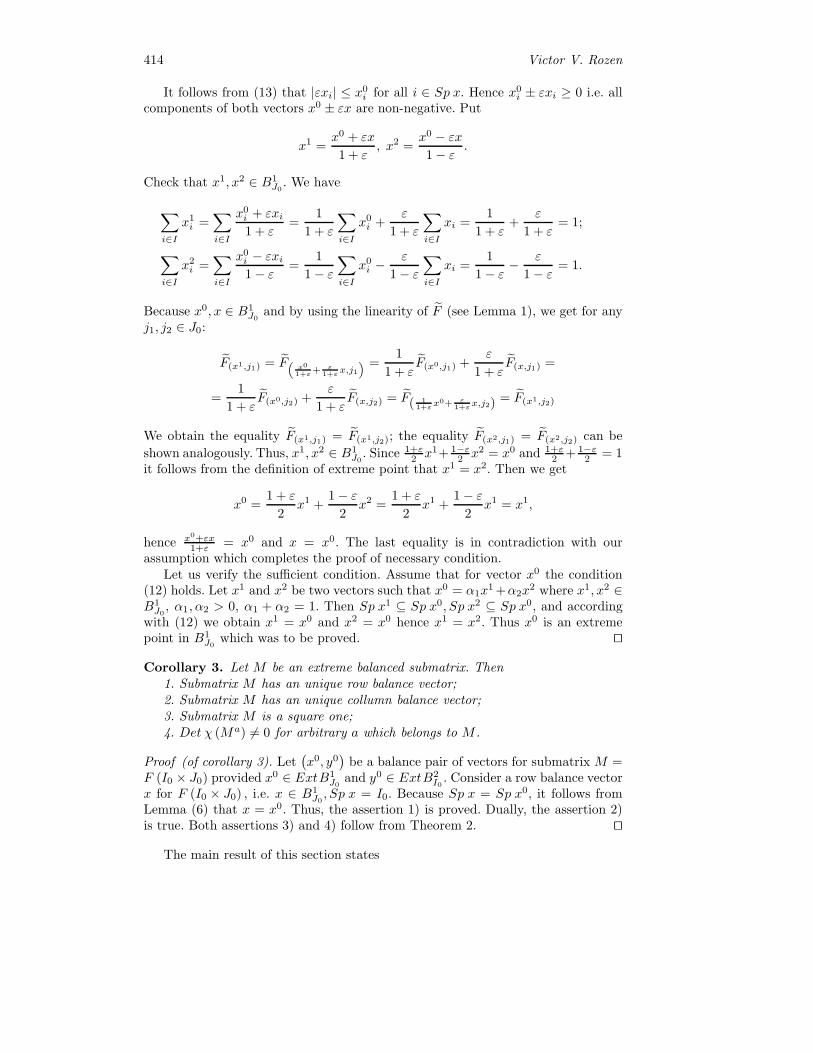
414 Victor V. Rozen
It follows from (13) that |εxi| ≤ x0i for all i ∈ Sp x. Hence x0
i ± εxi ≥ 0 i.e. allcomponents of both vectors x0 ± εx are non-negative. Put
x1 =x0 + εx
1 + ε, x2 =
x0 − εx
1− ε.
Check that x1, x2 ∈ B1J0. We have
∑i∈I
x1i =
∑i∈I
x0i + εxi1 + ε
=1
1 + ε
∑i∈I
x0i +
ε
1 + ε
∑i∈I
xi =1
1 + ε+
ε
1 + ε= 1;
∑i∈I
x2i =
∑i∈I
x0i − εxi1− ε
=1
1− ε
∑i∈I
x0i −
ε
1− ε
∑i∈I
xi =1
1− ε− ε
1− ε= 1.
Because x0, x ∈ B1J0
and by using the linearity of F (see Lemma 1), we get for anyj1, j2 ∈ J0:
F(x1,j1) = F(x0
1+ε+ε
1+εx,j1) =
1
1 + εF(x0,j1) +
ε
1 + εF(x,j1) =
=1
1 + εF(x0,j2) +
ε
1 + εF(x,j2) = F( 1
1+εx0+ ε
1+εx,j2)= F(x1,j2)
We obtain the equality F(x1,j1) = F(x1,j2); the equality F(x2,j1) = F(x2,j2) can be
shown analogously. Thus, x1, x2 ∈ B1J0. Since 1+ε
2 x1+ 1−ε2 x2 = x0 and 1+ε
2 + 1−ε2 = 1
it follows from the definition of extreme point that x1 = x2. Then we get
x0 =1 + ε
2x1 +
1− ε
2x2 =
1 + ε
2x1 +
1− ε
2x1 = x1,
hence x0+εx1+ε = x0 and x = x0. The last equality is in contradiction with our
assumption which completes the proof of necessary condition.Let us verify the sufficient condition. Assume that for vector x0 the condition
(12) holds. Let x1 and x2 be two vectors such that x0 = α1x1 +α2x
2 where x1, x2 ∈B1J0, α1, α2 > 0, α1 + α2 = 1. Then Sp x1 ⊆ Sp x0, Sp x2 ⊆ Sp x0, and according
with (12) we obtain x1 = x0 and x2 = x0 hence x1 = x2. Thus x0 is an extremepoint in B1
J0which was to be proved. ��
Corollary 3. Let M be an extreme balanced submatrix. Then1. Submatrix M has an unique row balance vector;2. Submatrix M has an unique collumn balance vector;3. Submatrix M is a square one;4. Det χ (Ma) = 0 for arbitrary a which belongs to M .
Proof (of corollary 3). Let(x0, y0
)be a balance pair of vectors for submatrix M =
F (I0 × J0) provided x0 ∈ ExtB1J0
and y0 ∈ ExtB2I0. Consider a row balance vector
x for F (I0 × J0) , i.e. x ∈ B1J0, Sp x = I0. Because Sp x = Sp x0, it follows from
Lemma (6) that x = x0. Thus, the assertion 1) is proved. Dually, the assertion 2)is true. Both assertions 3) and 4) follow from Theorem 2. ��
The main result of this section states
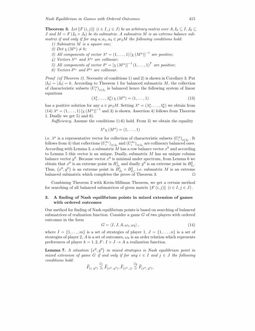
Nash Equilibrium in Games with Ordered Outcomes 415
Theorem 3. Let ‖F (i, j)‖ (i ∈ I, j ∈ J) be an arbitrary matrix over A, I0 ⊆ I, J0 ⊆J and M = F (I0 × J0) be its submatrix. A submatrix M is an extreme balance sub-matrix if and only if for any a, a1, a2 ∈ pr2M the following conditions hold:
1) Submatrix M is a square one;2) Det χ (Ma) = 0;
3) All components of vector λa = (1, . . . , 1) [χ (Ma)]−1 are positive;4) Vectors λa1 and λa2 are collinear;
5) All components of vector δa = [χ (Ma)]−1
(1, . . . , 1)T
are positive;6) Vectors δa1 and δa2 are collinear.
Proof (of Theorem 3). Necessity of conditions 1) and 2) is shown in Corollary 3. Put|I0| = |J0| = k. According to Theorem 1 for balanced submatrix M , the collectionof characteristic subsets (Ua
i )i∈I0 is balanced hence the following system of linearequations
(λa1 , . . . , λak)χ (Ma) = (1, . . . , 1) (13)
has a positive solution for any a ∈ pr2M. Setting λa = (λa1 , . . . , λak) we obtain from
(14) λa = (1, . . . , 1) [χ (Ma)]−1
and 3) is shown. Assertion 4) follows from Theorem1. Dually we get 5) and 6).
Sufficiency. Assume the conditions 1)-6) hold. From 3) we obtain the equality
λaχ (Ma) = (1, . . . , 1)
i.e. λa is a representative vector for collection of characteristic subsets (Uai )i∈I0 . It
follows from 4) that collections (Ua1i )i∈I0 and (Ua2
i )i∈I0 are collineary balanced ones.
According with Lemma 3, a submatrix M has a row balance vector x0 and accordingto Lemma 5 this vector is an unique. Dually, submatrix M has an unique columnbalance vector y0. Because vector x0 is minimal under spectrum, from Lemma 6 weobtain that x0 is an extreme point in B1
J0and dually y0 is an extreme point in B2
I0.
Thus,(x0, y0
)is an extreme point in B1
J0× B2
I0, i.e. submatrix M is an extreme
balanced submatrix which completes the prove of Theorem 3. ��
Combining Theorem 3 with Krein-Millman Theorem, we get a certain methodfor searching of all balanced submatrices of given matrix ‖F (i, j)‖ (i ∈ I, j ∈ J) .
3. A finding of Nash equilibrium points in mixed extension of gameswith ordered outcomes
Our method for finding of Nash equilibrium points is based on searching of balancedsubmatrices of realization function. Consider a game G of two players with orderedoutcomes in the form
G = 〈I, J, A, ω1, ω2〉 , (14)
where I = {1, . . . ,m} is a set of strategies of player 1, J = {1, . . . , n} is a set ofstrategies of player 2, A is a set of outcomes, ωk is an order relation which representspreferences of player k = 1, 2, F : I × J → A a realization function.
Lemma 7. A situation(x0, y0
)in mixed strategies is Nash equilibrium point in
mixed extension of game G if and only if for any i ∈ I and j ∈ J the followingconditions hold:
F(i, y0)
ω1
� F(x0, y0), F(x0, j)
ω2
� F(x0, y0).
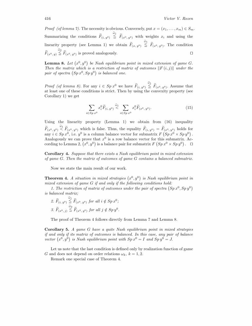
416 Victor V. Rozen
Proof (of lemma 7). The necessity is obvious. Conversely, put x = (x1, . . . , xm) ∈ Sm.
Summarizing the conditions F(i, y0)
ω1
� F(x0, y0) with weights xi and using the
linearity property (see Lemma 1) we obtain F(x, y0)
ω1
� F(x0, y0). The condition
F(x0, y)
ω2
� F(x0, y0) is proved analogously. ��
Lemma 8. Let(x0, y0
)be Nash equilibrium point in mixed extension of game G.
Then the matrix which is a restriction of matrix of outcomes ‖F (i, j)‖ under thepair of spectra
(Sp x0, Sp y0
)is balanced one.
Proof (of lemma 8). For any i ∈ Sp x0 we have F(i, y0)
ω1
� F(x0, y0). Assume thatat least one of these conditions is strict. Then by using the convexity property (seeCorollary 1) we get
∑i∈Sp x0
x0i F(i, y0)
ω1
<∑
i∈Sp x0
x0i F(x0, y0). (15)
Using the linearity property (Lemma 1) we obtain from (16) inequality
F(x0, y0)
ω1
< F(x0, y0) which is false. Thus, the equality F(i, y0) = F(x0, y0) holds for
any i ∈ Sp x0, i.e. y0 is a column balance vector for submatrix F(Sp x0 × Sp y0
).
Analogously we can prove that x0 is a row balance vector for this submatrix. Ac-cording to Lemma 2,
(x0, y0
)is a balance pair for submatrix F
(Sp x0 × Sp y0
). ��
Corollary 4. Suppose that there exists a Nash equilibrium point in mixed extensionof game G. Then the matrix of outcomes of game G contains a balanced submatrix.
Now we state the main result of our work.
Theorem 4. A situation in mixed strategies(x0, y0
)is Nash equilibrium point in
mixed extension of game G if and only if the following conditions hold:
1. The restriction of matrix of outcomes under the pair of spectra(Sp x0, Sp y0
)is balanced matrix;
2. F(i, y0)
ω1
� F(x0, y0) for all i /∈ Sp x0;
3. F(x0, j)
ω2
� F(x0, y0) for all j /∈ Sp y0.
The proof of Theorem 4 follows directly from Lemma 7 and Lemma 8.
Corollary 5. A game G have a quite Nash equilibrium point in mixed strategiesif and only if its matrix of outcomes is balanced. In this case, any pair of balancevector
(x0, y0
)is Nash equilibrium point with Sp x0 = I and Sp y0 = J.
Let us note that the last condition is defined only by realization function of gameG and does not depend on order relations ωk, k = 1, 2.
Remark one special case of Theorem 4.

Nash Equilibrium in Games with Ordered Outcomes 417
Corollary 6. Suppose I0 ⊆ I, J0 ⊆ J are two subsets and corresponding submatrixF (I0 × J0) is balanced. Assume for any i′ /∈ I0, j
′ /∈ J0 there exist i0 ∈ I0, j0 ∈ J0such that for all i ∈ I0 and j ∈ J0 hold the conditions:
F (i′, j)ω1
� F(i0, j
),
F (i, j′)ω2
� F(i, j0
) (16)
hold. Then any balance pair for submatrix(x0, y0
), complemented by zero compo-
nents for i ∈ I \ I0 and j ∈ J \ J0, is Nash equilibrium point in mixed extension ofgame G.
Appendix
1. Balanced matrices
Examples of balanced matrices together with their balance vectors by Table 1-3 aregiven.
Table 1.
I J 13
13
13
13
a b c
13
b c a
13
c a b
Table 2.
I J 13
16
13
16
16
a a b b
13
a b b a
16
b b a a
13
b a a b
Remark that any Latin square forms a balanced matrix and moreover its balancepair is a pair of vectors whose components coincide (see Table 1).
To verify that a given pair of vectors(x0, y0
)is a balance one for matrix
‖F (i, j)‖ (i ∈ I, j ∈ J) we can check equalities F(i1, y0) = F(i2, y0) and
F(x0, j1) = F(x0, j2) for any i1, i2 ∈ I and j1, j2 ∈ J.
2. A finding of extreme balanced matrices
Consider a matrix of size 4× 4 over set A = {a, b, c, d, e} given by Table 4
M =
⎛⎝a a ba b ab a a
⎞⎠
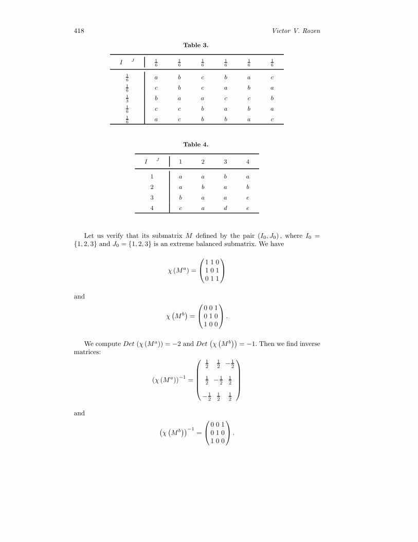
418 Victor V. Rozen
Table 3.
I J 16
16
16
16
16
16
16
a b c b a c
16
c b c a b a
13
b a a c c b
16
c c b a b a
16
a c b b a c
Table 4.
I J 1 2 3 4
1 a a b a
2 a b a b
3 b a a e
4 c a d e
Let us verify that its submatrix M defined by the pair (I0, J0) , where I0 ={1, 2, 3} and J0 = {1, 2, 3} is an extreme balanced submatrix. We have
χ (Ma) =
⎛⎝1 1 01 0 10 1 1
⎞⎠and
χ(M b)
=
⎛⎝0 0 10 1 01 0 0
⎞⎠ .
We compute Det (χ (Ma)) = −2 and Det(χ(M b))
= −1. Then we find inversematrices:
(χ (Ma))−1
=
⎛⎜⎜⎜⎜⎝12
12 −
12
12 −
12
12
− 12
12
12
⎞⎟⎟⎟⎟⎠and
(χ(M b))−1
=
⎛⎝0 0 10 1 01 0 0
⎞⎠ .
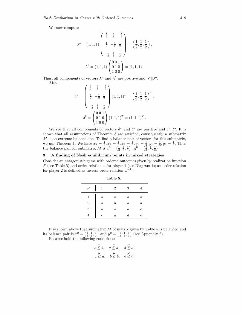
Nash Equilibrium in Games with Ordered Outcomes 419
We now compute
λa = (1, 1, 1)
⎛⎜⎜⎜⎜⎝12
12 −
12
12 −
12
12
− 12
12
12
⎞⎟⎟⎟⎟⎠ =
(1
2,
1
2,
1
2
),
λb = (1, 1, 1)
⎛⎝0 0 10 1 01 0 0
⎞⎠ = (1, 1, 1) .
Thus, all components of vectors λa and λb are positive and λa‖λb.Also
δa =
⎛⎜⎜⎜⎜⎝12
12 −
12
12 −
12
12
− 12
12
12
⎞⎟⎟⎟⎟⎠ (1, 1, 1)T
=
(1
2,
1
2,
1
2
)T,
δb =
⎛⎝0 0 10 1 01 0 0
⎞⎠ (1, 1, 1)T
= (1, 1, 1)T.
We see that all components of vectors δa and δb are positive and δa‖δb. It isshown that all assumptions of Theorem 3 are satisfied, consequently a submatrixM is an extreme balance one. To find a balance pair of vectors for this submatrix,we use Theorem 1. We have x1 = 1
3 , x2 = 13 , x3 = 1
3 , y1 = 13 , y2 = 1
3 , y3 = 13 . Thus
the balance pair for submatrix M is x0 =(13 ,
13 ,
13
), y0 =
(13 ,
13 ,
13
).
3. A finding of Nash equilibrium points in mixed strategies
Consider an antagonistic game with ordered outcomes given by realization functionF (see Table 5) and order relation ω for player 1 (see Diagram 1); an order relationfor player 2 is defined as inverse order relation ω−1.
Table 5.
F 1 2 3 4
1 a a b a
2 a b a b
3 b a a e
4 c a d e
It is shown above that submatrix M of matrix given by Table 5 is balanced andits balance pair is x0 =
(13 ,
13 ,
13
)and y0 =
(13 ,
13 ,
13
)(see Appendix 2).
Because hold the following conditions:
cω
� b, aω
� a, dω
� a;
aω
a, bω
b, eω
a,
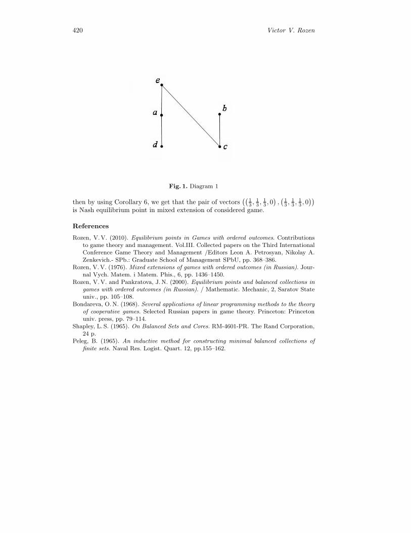
420 Victor V. Rozen
Fig. 1. Diagram 1
then by using Corollary 6, we get that the pair of vectors((
13 ,
13 ,
13 , 0),(13 ,
13 ,
13 , 0))
is Nash equilibrium point in mixed extension of considered game.
References
Rozen, V. V. (2010). Equilibrium points in Games with ordered outcomes. Contributionsto game theory and management. Vol.III. Collected papers on the Third InternationalConference Game Theory and Management /Editors Leon A. Petrosyan, Nikolay A.Zenkevich.- SPb.: Graduate School of Management SPbU, pp. 368–386.
Rozen, V. V. (1976). Mixed extensions of games with ordered outcomes (in Russian). Jour-nal Vych. Matem. i Matem. Phis., 6, pp. 1436–1450.
Rozen, V. V. and Pankratova, J. N. (2000). Equilibrium points and balanced collections ingames with ordered outcomes (in Russian). / Mathematic. Mechanic, 2, Saratov Stateuniv., pp. 105–108.
Bondareva, O. N. (1968). Several applications of linear programming methods to the theoryof cooperative games. Selected Russian papers in game theory. Princeton: Princetonuniv. press, pp. 79–114.
Shapley, L. S. (1965). On Balanced Sets and Cores. RM-4601-PR. The Rand Corporation,24 p.
Peleg, B. (1965). An inductive method for constructing minimal balanced collections offinite sets. Naval Res. Logist. Quart. 12, pp.155–162.

Cooperative Optimality Conceptsfor Games with Preference Relations
Tatiana F. Savina
Saratov State University,Faculty of Mechanics and Mathematics,
Astrakhanskaya St. 83, Saratov, 410012, RussiaE-mail: [email protected]
Abstract. In this paper we consider games with preference relations. Thecooperative aspect of a game is connected with its coalitions. The main opti-mality concepts for such games are concepts of equilibrium and acceptance.We introduce a notion of coalition homomorphism for cooperative gameswith preference relations and study a problem concerning connections be-tween equilibrium points (acceptable outcomes) of games which are in ahomomorphic relation. The main results of our work are connected withfinding of covariant and contrvariant homomorphisms.
Keywords: Nash equilibrium, Equilibrium, Acceptable outcome, Coalitionhomomorphism
1. Introduction
We consider a n-person game with preference relations in the form
G = 〈(Xi)i∈N , A, F, (ρi)i∈N 〉 (1)
where N = {1, . . . , n} is a set of players, Xi is a set of strategies of player i (i ∈ N),A is a set of outcomes, realization function F is a mapping of set of situationsX = X1 × . . . ×Xn in the set of outcomes A and ρi ⊆ A2 is a preference relationof player i. In general case each ρi is an arbitrary reflexive binary relation on A.
Assertion a1ρi
� a2 means that outcome a1 is less preference than a2 for player i.Given a preference relation ρi ⊆ A2, we denote by ρsi = ρi ∩ ρ−1
i its symmetric partand ρ∗i = ρi\ρsi its strict part (see Savina, 2010).
The cooperative aspect of a game is connected with its coalitions. In our casewe can define for any coalition T ⊆ N its set of strategies XT in the form
XT =∏i∈T
Xi. (2)
We construct a preference relation of coalition T with help of preference relationsof players which form the coalition. We denote a preference relation for coalition Tby ρT . The following condition is minimum requirement for preference of coalitionT :
a1ρT
� a2 ⇒ (∀i ∈ T )a1ρi
� a2. (3)
In section 2 we consider some important concordance rules. Let K be a fix collec-tion of coalitions. In section 3 we introduce the following cooperative optimality con-cepts: Nash K–equilibrium, K–equilibrium, quite K–acceptance, K–acceptance andconnections between these concepts are established in Theorem 1. In next sectionwe consider coalition homomorphisms. The main results of our paper are presentedin section 5.
422 Tatiana F. Savina
2. Concordance rules for preferences of players
To construct a preference relation for coalition T we need to have preference rela-tions of all players its coalition and also certain rule for concordance of preferencesof players. Such set of rules is called concordance rule. It is known that importantconcordance rules are the following.
2.1. Pareto concordance
Definition 1. Outcome a2 is said to (non strict) dominate by Pareto outcome a1for coalition T if a2 is better (not worse) than a1 for each i ∈ T, i.e.
a1ρT
� a2 ⇔ (∀i ∈ T )a1ρi
� a2. (4)
In this case symmetric part of preference relation for coalition T is defined bythe formula
a1ρT∼ a2 ⇔ (∀i ∈ T )a1
ρi∼ a2 (5)
and strict part is defined by the formula
a1ρT< a2 ⇔
⎧⎨⎩ (∀i ∈ T ) a1ρi
� a2,
(∃j ∈ T ) a1ρj< a2
(6)
Thus, outcome a2 dominate a1 if and only if a2 is better than a1 for all playersof coalition T and strictly better at least for one player j ∈ T.
2.2. Modified Pareto concordance
In this case strict part of preference relation ρT is defined by the equivalence
a1ρT< a2 ⇔ (∀i ∈ T )a1
ρi< a2, (7)
and symmetric part is given by
a1ρT∼ a2 ⇔ (∀i ∈ T )a1
ρi∼ a2. (8)
2.3. Concordance by majority rule
Outcome a2 is strictly better than outcome a1 for coalition T if and only if a2 isstrictly better than a1 for majority of players of coalition T , i.e.
a2ρT> a1 ⇔
∣∣∣{i ∈ T : a2ρi> a1
}∣∣∣ > ∣∣∣∣T2∣∣∣∣ .
For this rule, symmetric part of preference relation ρT is given by the equivalence
a1ρT∼ a2 ⇔
∣∣∣{i ∈ T : a1ρi∼ a2
}∣∣∣ > ∣∣∣∣T2∣∣∣∣ .
Cooperative Optimality Concepts for Games with Preference Relations 423
2.4. Concordance under summation of payoffs
For games with payoff functions in the form H =⟨(Xi)i∈N , (ui)i∈N
⟩, the following
concordance rule of preferences for coalition T is used
x1ρT
� x2 ⇔∑i∈T
ui(x1) ≤
∑i∈T
ui(x2) (9)
and the strict part of ρT is given by:
x1ρT< x2 ⇔
∑i∈T
ui(x1) <
∑i∈T
ui(x2).
In this case preference relation ρT and its strict part are transitive.
Remark 1. Let {T1, . . . , Tm} be partition of set N . Then collection of strategies ofthese coalitions (xT1 , . . . , xTm) define a single situation x ∈ X in game G. Namely,the situation x is such a situation that its projection on Tk is xTk (k = 1, . . . ,m).
Hence we can define a realization function F by the rule: F (xT1 , . . . , xTm)df= F (x) .
In particular if T is one fix coalition then the function F(xT , xN\T
)is defined.
Remark 2. Consider a game with payoff functions H =⟨(Xi)i∈N , (ui)i∈N
⟩where
ui :∏i∈N Xi → IR is a payoff function for players i. Then we can define the prefer-
ence relation of player i by the formula
x1ρi
� x2 ⇔ ui(x1) ≤ ui(x
2).
Let the preference relation of coalition T be Pareto dominance, i.e.
x1ρT
� x2 ⇔ (∀i ∈ T ) ui(x1) ≤ ui(x
2).
Then considered above concordance rules is becoming well known rules for co-operative games with payoff functions. (see Moulin, 1981).
3. Coalitions optimality concepts
In this part we consider games with preference relations of the form (1). For games ofthis class two types of optimality concepts are introduced and connections betweenthese concepts are established.
Let K be an arbitrary fixed family of coalitions of players N .
3.1. Equilibrium concepts
Definition 2. A situation x0 = (x0i )i∈N ∈ X is called Nash K–equilibrium (Nash
K–equilibrium point) if for any coalition T ∈ K and any strategy xT ∈ XT thecondition
F (x0 ‖ xT )ρT
� F (x0) (10)
holds.
Remark 3. 1. In the case K = {{1} , . . . , {n}}, Nash K–equilibrium is Nash equi-librium in the usual sense.

424 Tatiana F. Savina
2. In the case K = {N}, a situation x0 is Nash {N}–equilibrium means F(x0)
isgreatest element under preference ρT .
We now define some generalization of Nash equilibrium.A strategy x0
T ∈ XT is called a refutation of the situation x ∈ X by coalition Tif the condition
F (x ‖ x0T )
ρT> F (x) (11)
holds.
Definition 3. A situation x0 = (x0i )i∈N ∈ X is called K–equilibrium point if any
coalition T ∈ K does not have a refutation of this situation, i.e. for any coalitionT ∈ K and any strategy xT ∈ XT the condition
F (x0 ‖ xT )ρT≯ F (x0)
holds.
Remark 4. 1. In the case K = {{1} , . . . , {n}}, K–equilibrium is equilibrium inthe usual sense.
2. In the case K = {N}, K–equilibrium point is Pareto optimal.3. In the case K = 2N , K–equilibrium point is called strong equilibrium one.
3.2. Acceptable outcomes and acceptable situations
A strategy x0T ∈ XT is called a objection of coalition T against outcome a ∈ A if for
any strategy of complementary coalition xN\T ∈ XN\T the condition
F (x0T , xN\T )
ρT> a (12)
holds.
Definition 4. An outcome a ∈ A is called acceptable for coalition T if this coalitiondoes not have objections against this outcome.
An outcome a ∈ A is said to be K–acceptable if it is acceptable for all coalitionsT ∈ K, that is
(∀T ∈ K)(∀xT ∈ XT )(∃xN\T ∈ XN\T )F (xT , xN\T )ρT≯ a. (13)
A strategy x0T ∈ XT is called a objection of coalition T against situation x∗ ∈ X
if this strategy is an objection against outcome F (x∗) .We define also a quite acceptable concept by changing quantifiers: ∀xT ∃xN\T →
∃xN\T ∀xT .
Definition 5. An outcome a is called quite K-acceptable for family of coalitions Kif the condition
(∀T ∈ K)(∃xN\T ∈ XN\T )(∀xT ∈ XT )F (xN\T , xT )ρT≯ a (14)
holds.A situation x0 ∈ X is called quite K-acceptable if outcome F
(x0)
is quite K-acceptable one.

Cooperative Optimality Concepts for Games with Preference Relations 425
These optimality concepts are analogous to well known optimality concepts ofgames with payoff functions (see Moulin, 1981).
Now we consider connections between these optimality concepts.
Lemma 1. Nash K–equilibrium point is also a K–equilibrium point but converse isfalse.
Proof (of lemma). Let x0 = (x0i )i∈N be Nash K–equilibrium point then for any
coalition T ∈ K and any strategy xT ∈ XT the condition F (x0 ‖ xT )ρT
� F (x0)
holds. Suppose F (x0 ‖ xT )ρT> F (x0). The system of conditions⎧⎨⎩F (x0 ‖ xT )
ρT
� F (x0)
F (x0 ‖ xT )ρT> F (x0)
is false. Hence, F (x0 ‖ xT )ρT≯ F (x0). ��
Thus, Nash K–equilibrium is K–equilibrium. But the converse is false. Indeed,consider
Example 1. Consider an antagonistic game G whose realization function F is givenby Table 1 and preference relation for player 1 by Diagram 1; preference relation ofplayer 2 is given by inverse order, K = {{1} , {2}} .
Table 1. Realization function
F t1 t2
s1 a b
s2 c d
Situation (s1, t1) is K–equilibrium. Since F (s1, t1) = a and a‖b, a‖c (i.e. a and bis incomparable, a and c is incomparable) then (s1, t1) is not Nash K–equilibrium.
Remark 5. If all preference relations (ρT )T∈K is linear then Nash K–equilibriumand K–equilibrium are equivalent.
Proposition 1. An objection of coalition T against situation x∗ is also a refutationof this situation.
Proof (of proposition). Let x0T be an objection of coalition T against situation x∗.
Then according to definition of objection the strategy x0T is an objection of coalition
T against outcome F (x∗) , i.e. for any strategy of complementary coalition xN\T ∈XN\T the condition F (x0
T , xN\T )ρT> F (x∗) holds.
Let us take xN\T = x∗N\T as a strategy of complementary coalition, we have
F (x0T , x
∗N\T )
ρT> F (x∗) .
Since strategy xN\T is an arbitrary one then we get strategy x0T is a refutation
of this situation. ��
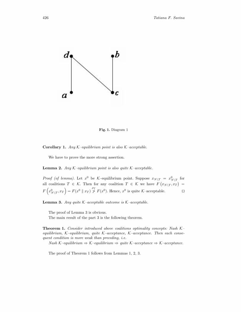
426 Tatiana F. Savina
Fig. 1. Diagram 1
Corollary 1. Any K–equilibrium point is also K–acceptable.
We have to prove the more strong assertion.
Lemma 2. Any K–equilibrium point is also quite K–acceptable.
Proof (of lemma). Let x0 be K–equilibrium point. Suppose xN\T = x0N\T for
all coalitions T ∈ K. Then for any coalition T ∈ K we have F(xN\T , xT
)=
F(x0N\T , xT
)= F (x0 ‖ xT )
ρT≯ F (x0). Hence, x0 is quite K–acceptable. ��
Lemma 3. Any quite K–acceptable outcome is K–acceptable.
The proof of Lemma 3 is obvious.
The main result of the part 3 is the following theorem.
Theorem 1. Consider introduced above coalitions optimality concepts: Nash K–equilibrium, K–equilibrium, quite K–acceptance, K–acceptance. Then each conse-quent condition is more weak than preceding, i.e.
Nash K–equilibrium ⇒ K–equilibrium ⇒ quite K–acceptance ⇒ K–acceptance.
The proof of Theorem 1 follows from Lemmas 1, 2, 3.

Cooperative Optimality Concepts for Games with Preference Relations 427
4. Coalition homomorphisms for games with preference relations
Let
G = 〈(Xi)i∈N , A, F, (ρi)i∈N 〉
and
Γ = 〈(Yi)i∈N , B, Φ, (σi)i∈N 〉
be two games with preference relations of the players N .Any (n + 1)–system consisting of mappings f = (ϕ1, . . . , ϕn, ψ) where for any
i = 1, . . . , n, ϕi : Xi → Yi and ψ : A→ B, is called a homomorphism from game Ginto game Γ if for any i = 1, . . . , n and any a1, a2 ∈ A the following two conditions
a1ρi
� a2 ⇒ ψ(a1)σi� ψ(a2), (15)
ψ(F (x1, . . . , xn)) = Φ(ϕ1(x1), ϕ2(x2), . . . , ϕn(xn)) (16)
are satisfied.A homomorphism f is said to be strict homomorphism if system of the conditions
a1ρi< a2 ⇒ ψ(a1)
σi< ψ(a2), (i = 1, . . . , n) (17)
a1ρi∼ a2 ⇒ ψ(a1)
σi∼ ψ(a2) (i = 1, . . . , n) (18)
holds instead of condition (15).A homomorphism f is said to be regular homomorphism if the conditions
ψ(a1)σi< ψ(a2) ⇒ a1
ρi< a2, (19)
ψ(a1)σi∼ ψ(a2) ⇒ ψ(a1) = ψ(a2) (20)
hold.A homomorphism f is said to be homomorphism ”onto”, if each ϕi (i = 1, . . . , n)
is a mapping ”onto”.Now we introduce a concept of coalition homomorphism.For the first step, we need to fix some rule for concordance of preferences; recall
that the preference relation for coalition T denoted by ρT .
Definition 6. A homomorphism f is said to be:
– a coalition homomorphism if it preserves preference relations for all coalitions,i.e. for any coalition T ⊆ N the condition
a1ρT
� a2 ⇒ ψ(a1)σT� ψ(a2) (21)
holds;– a strict coalition homomorphism if for any coalition T ⊆ N the system of the
conditions {a1
ρT< a2 ⇒ ψ(a1)
σT< ψ(a2),
a1ρT∼ a2 ⇒ ψ(a1)
σT∼ ψ(a2)(22)
is satisfied;
428 Tatiana F. Savina
– a regular coalition homomorphism if for any coalition T ⊆ N the system of theconditions {
ψ(a1)σT< ψ(a2)⇒ a1
ρT< a2,
ψ(a1)σT∼ ψ(a2)⇒ ψ(a1) = ψ(a2)
(23)
is satisfied.
It is easy to see that the following assertion is true.
Lemma 4. For Pareto concordance (and also for modified Pareto concordance),any surjective homomorphism from G into Γ is a surjective coalition homomor-phism.
Lemma 5. For Pareto concordance (and also for modified Pareto concordance),any strict homomorphism from G into Γ is a strict coalition homomorphism.
Proof (of lemma 5). We consider Pareto concordance for preferences as a concor-dance rule. Verify the conditions of system (22) for preference relation ρT . According
to defition of Pareto concordance the condition a1ρT< a2 is equivalent system⎧⎨⎩ (∀i ∈ T ) a1
ρi
� a2,
(∃j ∈ T ) a1ρj< a2.
Since strict homomorphism is homomorphism then from the first condition of
system it follows that (∀i ∈ T )ψ (a1)σi� ψ (a2). Since homomorphism f is strict then
(∃j ∈ T )ψ (a1)σi< ψ (a2) .
From last two conditions we get ψ (a1)σT< ψ (a2) .
Now according to definition of symmetric part of relation ρT we have
a1ρT∼ a2 ⇔ (∀i ∈ T ) a1
ρi∼ a2. Since homomorphism f is strict then we get
(∀i ∈ T )ψ (a1)σi∼ ψ (a2) , i.e. ψ (a1)
σT∼ ψ (a2) . ��
Now we consider modified Pareto concordance for preferences of players as aconcordance rule.
Lemma 6. For modified Pareto concordance, any regular homomorphism from Ginto Γ is a regular coalition homomorphism.
Proof (of lemma 6). Verify the condition (23) for strict part of preference relationσT . According to definition of modified Pareto concordance for preferences the con-
dition ψ (a1)σT< ψ (a2) is equivalent (∀i ∈ T )ψ (a1)
σi< ψ (a2). Since homomorphism
f is regular then we have (∀i ∈ T )a1ρi< a2, i.e. a1
ρT< a2.
Verify the condition (23) for symmetric part of σT . According to definition ofmodified Pareto concordance we have
ψ (a1)σT∼ ψ (a2)⇔ (∀i ∈ T )ψ (a1)
σi∼ ψ (a2) .
Since homomorphism f is regular then from the last condition it follows that(∀i ∈ T )ψ (a1) = ψ (a2), i.e. ψ (a1) = ψ (a2). ��
Cooperative Optimality Concepts for Games with Preference Relations 429
5. The main results
The main result states a correspondence between sets of K-acceptable outcomesand K-equilibrium situations of games which are in homomorphic relations underindicated types.
A homomorphism f is said to be covariant if f–image of any optimal solutionin game G is an optimal solution in Γ .
A homomorphism f is said to be contrvariant if f–preimage of any optimalsolution in game Γ is an optimal solution in G.
Theorem 2. For Nash K–equilibrium, any surjective homomorphism is covariantunder Pareto concordance and under modified Pareto concordance also.
Proof (of theorem 2). We consider Pareto concordance for preferences as a concor-dance rule. Let x0 be Nash K–equilibrium point in game G. We have to prove thatϕ(x0)
is Nash K–equilibrium point in game Γ .
We fix arbitrary strategy yT ∈ YT . Since f is homomorphism ”onto” thenaccording to Lemma 4 we obtain (∃x∗
T ∈ XT )ϕT (x∗T ) = yT . For any strat-
egy xT the condition F (xT , x0N\T )
ρT
� F (x0) holds. Hence, for strategy x∗T the
condition F (x∗T , x
0N\T )
ρT
� F (x0) is satisfied. Since f is homomorphism then
ψ(F (x∗
T , x0N\T )
) σT� ψ
(F (x0)
). By condition (16): Φ
(ϕT (x∗
T ) , ϕN\T
(x0N\T
)) σT�
Φ(ϕ(x0))
, i.e. Φ(yT , ϕN\T
(x0N\T
)) σT� Φ
(ϕ(x0))
.
Since strategy yT ∈ YT is arbitrary one then ϕ(x0)
is Nash K–equilibrium. ��
Theorem 3. For K–equilibrium, any strict surjective homomorphism is contrvari-ant under Pareto concordance and under modified Pareto concordance also.
Proof (of theorem 3). Consider Pareto concordance for preferences as a concor-dance rule. Let y0 be K–equilibrium point. We have to prove that situation x0 withϕ(x0)
= y0 is K–equilibrium point.
Suppose x0 =(x0i
)i∈N is not K–equilibrium then there exists coalition T ∈ K
and strategy x∗T ∈ XT such that F
(x∗T , x
0N\T
) ρT> F
(x0). Since homomorphism
f is strict then according to Lemma 5 we get ψ(F(x∗T , x
0N\T
))σT> ψ
(F(x0))
.
According to condition (16) we obtain Φ(ϕT (x∗
T ) , ϕN\T
(x0N\T
))σT> Φ
(ϕ(x0))
.
The last condition means Φ(ϕT (x∗
T ) , y0N\T
)σT> Φ
(y0). Thus, strategy ϕT (x∗
T )
is refutation of situation y0 by coalition T , which is contradictory with y0 is K–equilibrium point.
Hence, x0 is K–equilibrium point. ��
Theorem 4. For K–acceptance, any strict surjective homomorphism is contrvari-ant under Pareto concordance and under modified Pareto concordance also.
Proof (of theorem 4). Consider Pareto concordance for preferences as a concordancerule. Let outcome b with ψ (a) = b be K–acceptable one in game Γ . Assume that
430 Tatiana F. Savina
outcome a is not acceptable for all coalitions T ∈ K, i.e. there exists such strategyx0T ∈ XT that for any strategy xN\T ∈ XN\T the condition
F (x0T , xN\T )
ρT> a (24)
holds.Let yN\T = (yj)j∈N\T be arbitrary strategy of complementary coalition N \ T
in game Γ . Since f is homomorphism ”onto” then according to Lemma 4 we have(∃x∗
N\T ∈ XN\T
)ϕN\T
(x∗N\T
)= yN\T . By (24) the condition F (x0
T , x∗N\T )
ρT> a
holds. According to Lemma 5 we get ψ(F (x0
T , x∗N\T )
)σT> ψ (a) . By (16)
we have ψ(F (x0
T , x∗N\T )
)= Φ
(ϕT(x0T
), ϕN\T
(x∗N\T
)). Thus, the condition
Φ(ϕT(x0T
), yN\T
) σT> ψ (a) is satisfied. Hence, strategy ϕT
(x0T
)is objection of
coalition T against outcome b which is contadictory with b is K–acceptable out-come.
Hence, outcome a is K–acceptable. ��
Theorem 5. For K–equilibrium, any regular surjective homomorphism is covariantunder modified Pareto concordance.
Proof (of theorem 5). Let x0 be K–equilibrium. We have to prove that situationϕ(x0)
is K–equilibrium.
Suppose ϕ(x0)
is not K–equilibrium, i.e.
(∃T ∈ K) (∃yT ∈ YT ) Φ(ϕ(x0)‖yT) σT> Φ
(ϕ(x0))
(25)
Since homomorphism f is surjective then according to Lemma 4 we have
(∃x∗T ∈ XT )ϕT (x∗
T ) = yT . Hence, the condition Φ(ϕT (x∗
T ) , ϕN\T
(x0N\T
)) σT>
Φ(ϕ(x0))
holds. By (16) we get Φ(ϕT (x∗
T ) , ϕN\T
(x0N\T
))= ψ
(F(x∗T , x
0N\T
)).
Thus, ψ(F(x0‖x∗
T
)) σT> ψ
(F(x0))
. Because homomorphism f is regular then ac-
cording to Lemma 6 we obtain F(x0‖x∗
T
) ρT> F
(x0). Thus, strategy x∗
T is refutationof situation x0 by coalition T , which is contradictory with x0 is K–equilibrium.
Hence, ϕ(x0)
is K–equilibrium in game Γ . ��
Appendix
Consider the example conserning of concordance rules.Let G be a game of three players with set of outcomes A = {a, b, c, d, e}. Pref-
erence relations for each player are given by Diagrams 2,3,4.Using Diagrams 2 – 4 we can define preference relations in the following form:
ρ1 : a < b, b ∼ c, c ∼ d, b < eρ2 : a ∼ b, b ∼ c, c < d, e < dρ3 : a < c, b ∼ c, c < d, b ∼ e, d ∼ e.
Then according to Pareto concordance (see 2.1) for coalition T = {1, 2} we have
ρT : a � b, b � c, c � d where strict part consists of two conditions aρT< b, c
ρT< d and
symmetric part is bρT∼ c.

Cooperative Optimality Concepts for Games with Preference Relations 431
Fig. 2. Diagram 2
Fig. 3. Diagram 3
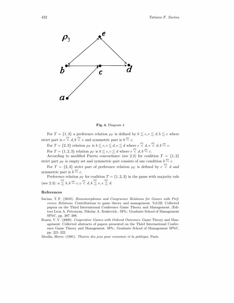
432 Tatiana F. Savina
Fig. 4. Diagram 4
For T = {1, 3} a preference relation ρT is defined by b � c, c � d, b � e where
strict part is cρT< d, b
ρT< e and symmetric part is b
ρT∼ c.
For T = {2, 3} relation ρT is b � c, c � d, e � d where cρT< d, e
ρT< d, b
ρT∼ c.
For T = {1, 2, 3} relation ρT is b � c, c � d where cρT< d, b
ρT∼ c.According to modified Pareto concordance (see 2.2) for coalition T = {1, 2}
strict part ρT is empty set and symmetric part consists of one condition bρT∼ c.
For T = {2, 3} strict part of preference relation ρT is defined by cρT< d and
symmetric part is bρT∼ c.
Preference relation ρT for coalition T = {1, 2, 3} in the game with majority rule
(see 2.3): aρT
� b, bρT∼ c, c
ρT< d, b
ρT
� e, eρT
� d.
References
Savina, T. F. (2010). Homomorphisms and Congruence Relations for Games with Pref-erence Relations. Contributions to game theory and management. Vol.III. Collectedpapers on the Third International Conference Game Theory and Management /Edi-tors Leon A. Petrosyan, Nikolay A. Zenkevich.- SPb.: Graduate School of ManagementSPbU, pp. 387–398.
Rozen, V. V. (2009). Cooperative Games with Ordered Outcomes. Game Theory and Man-agement. Collected abstracts of papers presented on the Third International Confer-ence Game Theory and Management. SPb.: Graduate School of Management SPbU,pp. 221–222
Moulin, Herve. (1981). Theorie des jeux pour economie et la politique. Paris.
A Fuzzy Cooperative Game Model for ConfigurationManagement of Open Supply
Networks�
Leonid B. Sheremetov1 and Alexander V. Smirnov2
1 Mexican Petroleum Institute,Av. Eje Central Lazaro Cardenas Norte, 152, Mexico, DF, CP 07730,
E-mail: [email protected] St. Petersburg Institute for Informatics and Automation, Russian Academy of Sciences,
Chetyrnadtsataya Liniya, 39, St. Petersburg, 199179, RussiaE-mail: [email protected]
Abstract. The paper considers the problem of open supply networks(OSNs) configuring in a highly dynamic economic environment. A novelcoalition formation mechanism is proposed, which helps to resolve conflic-tions between the objectives of the OSN participants and to agree uponeffective solutions. This mechanism is based on a generalized model of afuzzy cooperative game with core. The model was applied for configuring ofan automotive OSN. Simulation results are considered.
Keywords: cooperative game, core, supply network, configuring.
1. Introduction
In a todays highly competitive market manufacturers face the challenge of reducingmanufacturing cycle time, delivery lead-time and inventory. As a consequence, neworganizational forms of enterprise integration emerge to address these challenges re-sulting in more agile structures of federated enterprises known as adaptive, agile andopen supply chains and networks. These organizations are based on the principlesof partnership between the enterprises, agile network structures instead of linearchains and are driven by novel business strategies based on the product demand(Fig. 1.). In contrast to conventional chains and supply networks, such organizationscan be called open supply networks (OSNs), which are characterized by:
– Availability of alternative providers.– Availability of alternative configurations meeting orders specifications.– Expediency of dynamic configuration and reconfiguration of the network de-
pending on the order stream and economic benefit of every enterprise.– Conflicting objectives of each organization and non-integrated decision making
processes.
An OSN belongs to the class of systems with dynamically changing structures,which means that once a new order comes, a new configuration emerges. ThusOSN configuring can be considered one of the main supply chain management
� This work was supported by the European Commission under the Project FP6-IST-NMP 507592-2 ”ILIPT”, Russian Foundation for Basic Research under the grant No.08-07-00264 and by the Presidium of the Russian Academy of Sciences under the projectNo.213.
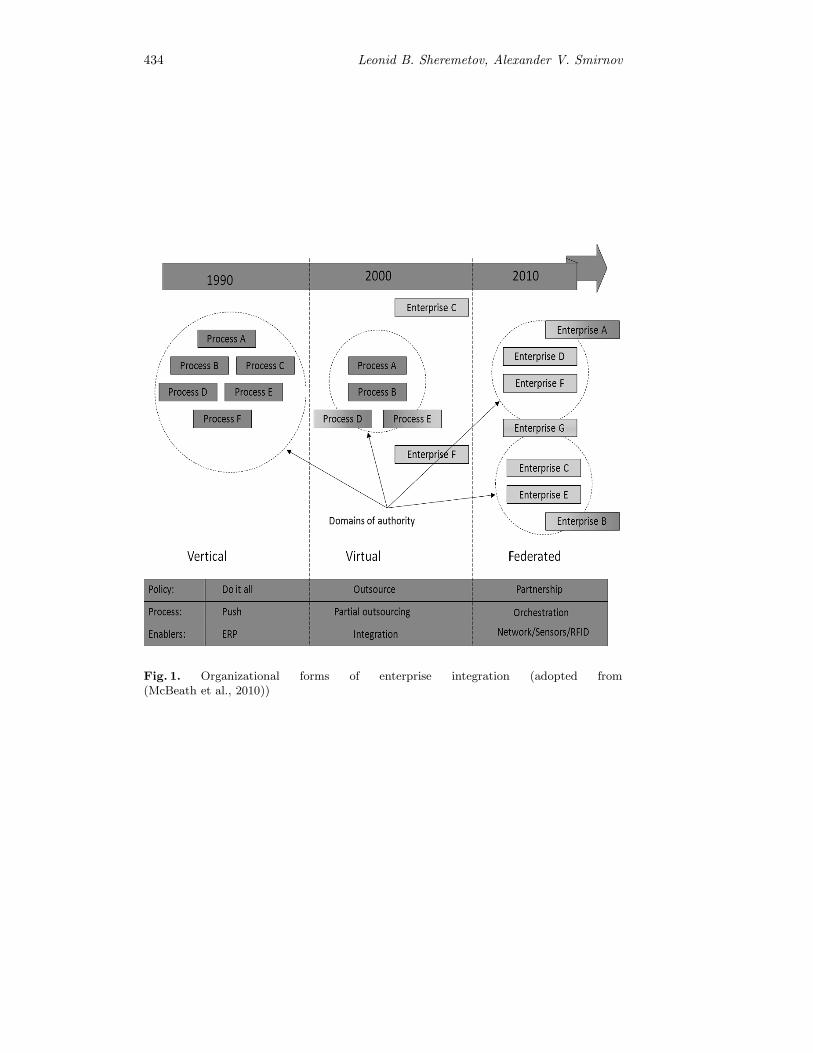
434 Leonid B. Sheremetov, Alexander V. Smirnov
Fig. 1. Organizational forms of enterprise integration (adopted from(McBeath et al., 2010))

A Fuzzy Cooperative Game Model 435
tasks (Garavelli, 2003; Chandra and Grabis, 2007). Traditionally, configuring hasbeen solved in a two-stage fashion: i) a structure of a network is formed at a strate-gic level and ii) its behavior is optimized at tactical and operational levels based ondemand forecast. Being suitable for vertical and even virtual enterprises (Fig. 1.),such practices, unfortunately, do not meet the requirements of a highly dynamicenvironment (Smirnov, 1999). One of the consequences is a so-called bullwhip ef-fect, when even small demand fluctuations in a loosely balanced forecast-drivendistribution systems lead to increased inventories, and, as a consequence, spatialconstraints, unused capital, obsolete inventories and so on (Suckya, 2009).
Federated enterprises composed of self-interested entities with probably conflict-ing goals require flexible dynamic configurations. Unfortunately, adoption of moreflexible and dynamic practices, like constraint satisfaction, auctions and knowledge-based approaches, which offer the prospect of better matches between suppliers andcustomers as market conditions change, has faced difficulties, due to the complex-ity of many supply chain relationships and the difficulty of effectively support-ing dynamic trading practices (Hosam and Khaldoun, 2006; Sandkuhl et al., 2007;Smirnov et al., 2006). Due to the conflictions among the objectives of each organi-zation and non-integrated decision making processes, there has been a need for newmechanisms, which help to resolve those conflictions and to agree upon effectivesolutions.
For advanced business strategies of OSN like demand-driven or build-to-orderSN, a task of configuring of virtual production channels can be defined as a coalitionformation task. The benefit distribution among the OSN members has proved to befuzzy, uncertain, and ambiguous (Roth, 1995). Using the theory of fuzzy cooperativegames (FCGs), we can process the uncertainty and pass from the introduction of afuzzy benefit concept through the bargaining process to the conclusion about thecorresponding fuzzy distribution of individual benefits among the coalition mem-bers.
In this paper, a game-theoretic approach is used to form coalitions: a class ofFCG with core is considered. The basic definition of the fuzzy core was proposed by(Mares, 2001) and extended to the area of multiagent systems by (Sheremetov andRomero-Cortes, 2003). In this paper, an extended definition of the core is considered.The definition introduces fuzzy individual payments and binary values ϕij addedto the fuzzy core to form the structure of effective coalitions.
The rest of the paper is structured as follows. In the next section, a OSN con-figuring task is defined as a problem of coalition formation. In section 3, differentapproaches to coalition formation in cooperative games theory are analyzed. In sec-tion 4, the mathematical structure of the model is described; it is shown that themodel represents an extension of the model proposed in (Mares, 2001). A case studyapplying the proposed approach is discussed in the context of OSNs in section 5. Aprototype consisting of seven enterprises and generating a structure of three coali-tions is considered. Finally, the results of the paper are discussed in Conclusionssection.
2. Supply network configuring as a coalition formation task
The task of configuring can be defined as a selection of those agents (enterprises),which have available competencies to complete the demand/order, and joining themtogether in the most efficient structure according to the selected criteria. The main
436 Leonid B. Sheremetov, Alexander V. Smirnov
components of the configuring task are: order, resource and configuration. Let usconsider that to fulfill the order T, I tasks should be executed: T={T1, T2,. . . , TI}.Each task Ti(i = 1, 2, . . . , I), is defined by a tuple 〈{BTi}, {PrefTi}〉, where {BTi} –is a vector of numerical values of the dimension r: {BTi} = (b1Ti , b
2Ti, . . . , brTi), b
kTi≥
0, characterizing a capacity on each competency k = 1, 2, . . . , r, required to performa task Ti. If the tasks are ordered, then T1 ' T2 ' . . . ' Tl ' Tm ' . . . ' TI , whereTl ' Tm means that Tl precedes the task Tm. The preferences vector PrefTi mayinclude additional parameters like the preferred lot size, penalties for backorders,etc. Fulfillment of each order and each task Ti implies a payoff: Payoff (Ti).
Example 1. Suppose that the order is to produce 100 products (cars of a specificmodel) per week. A car consists of four basic components: 1) the body T1 (14external tubes b1T1
and 5 exterior sheets b2T2); 2) the interior T2 (a dash board b1T2
, 3seats b2T2
: two front and one rear); 3) the chassis T3 (4 wheels b1T3, 2 axles b2T3
: a frontand a rear, 4 dampers b3T3
: two front and two rear); 4) the power train T4 (a motorb1T4
and a transmission b2T4). In other words: T = {T1, T2, T3, T4}, BT1 = (1400, 500),
BT2 = (100, 300), BT3 = (400, 200, 400), BT4 = (100, 100).
The enterprises of the supply network represent resources. Depending upon theirrole in the OSN, these resources can be suppliers of raw materials and components,assembly plants or warehouses. They are modeled as active autonomous entitieswith purposeful actions and, thus, may be called agents. Let us consider a finite setof agents Agent = {A1, A2, . . . , AN}. Then each agent Aj ∈ Agent(j = 1, 2, . . . , N)is defined as a tuple 〈{BAj}, {PrefAj}〉. For simplicity lets designate Aj as j. Then
Bj – is a vector of numerical values of the dimension r: Bj = (b1j , b2j , . . . , b
rj), b
k′j ≥ 0,
characterizing agents available capacity on each competency k′ = 1, 2, . . . , r. Thepreferences vector Prefk denote agents preferences on the lot size, orders time lag,etc.
Finally, a configuration is such a set of agents (resources) CT ⊆ Agent that theirjoint capacity of competencies satisfies the requirements of an order T . To solve theconfiguring task for the case when the agents and tasks competencies coincide (bkTiand bk
′j mean the capacities on the same competency) means to assign resources to
the tasks in such a way that the order T is fulfilled. Each agent Aj ∈ Agent may beassigned to a task Ti iff it has available capacities ∃k ∈ {1, 2, . . . , r}, bkj ≥ 0. Beingself-interested, each agent will try to optimize this assignment according to one ofthe following criteria:
– Maximize the use of his capacitiesr∑
k=1
(bkj − bkTi)→ min;
– To get the most profitable task (to increase the payoff)r∑
k=1
g(bkTi
) −r∑
k=1
fTi(bkj ) → max, where g(bk
Ti) – is a reward function associated
with the payoff Payoff (Ti), fTi(bkj ) – a cost of agents j ∈ Agent capacity bkj
required to fulfill the task Ti;
– Reduce the task Ti fulfillment time:r∑
k=1
tTi(bkj)→ min, where tTi
(bkj)
– time
of fulfillment of the task Ti by agent k ∈ Agent using his capacity bkj .
Agents can form coalitions to execute tasks. The notion of coalition is widely usedin organizational systems. A coalition can be defined as a group of self-interested

A Fuzzy Cooperative Game Model 437
agents that by means of negotiation protocols decide to cooperate in order to solvea problem or to achieve a goal (Gasser, 1991). Within the context of this paper, acoalition is defined as a group of agents joining their capacities for task Ti fulfillment.A coalition is described by a tuple: 〈KTi , alloc Ti, uTi〉, where KTi ⊆ Agent andKTi = ∅; alloc Ti – allocation function assigning each task i a group of m agents
such that alloc Ti = KTi , if∑m
bkm ≥ bkTi . If for each competency k, bkj ≥ bkTi ,
KTi may consist of a single agent j ∈ KTi , then alloc Ti = j. The coalition ofall agents involved in the orders T execution is called grand coalition KT . Theutility of a coalition is defined by a characteristic function: v(KTi) = Payoff (Ti)−∑k
∑j
fTi(bkj ) · ϕ(Ti, k, j), where ϕ – a binary variable, defining the fact that an agent
participates in the task execution with his capacity bkj :
ϕ(Ti, k, j) =
{−1, if an agent executes bkj
0, in the opposite case
The coalitions utility v(KTi) is distributed between the coalition members ac-
cording to the vector of payoff distribution uTi ={u1Ti, u2Ti, . . . , u
|KTi |Ti
}, where ujTi –
payoff of agent j ∈ Agent , and u|KTi |Ti
– coalition payoff. If within a coalition KTi ,
an agent j executes different competencies then ujTi =∑k
gj(bkTi
),
gj(bkTi
) =bkTir∑l=1
blTi
v(KTi) · ϕ(Ti, k, j) is fulfilled.
The grand coalition KT , joining together all the agents participating in theorders fulfillment corresponds to the configuration of the supply network CT . Thusto form a coalition means to find the appropriate coalition structure which permitsto maximize the payoff for all agents belonging to this structure.
3. Coalition formation in cooperative game theory
Taxonomy of coalition formation algorithms includes both distributed and central-ized algorithms. In this paper we restrict this analysis by those represented by thetheory of games (Aubin, 1981). Until recently, in the domain of supply chains andnetworks management, non-cooperative game theory was usually used for modelingof the competing enterprises as a game with zero-sum. In that context, all the play-ers are considered being self-interested trying to optimize their own profits withouttaking into account their effects on the other players. The main purpose of such agame is to find the optimal strategy for each player and determine if the obtainedstrategy coordinates the supply chain, i.e. maximizes the global profit. Nevertheless,the cooperative nature of federated enterprises causes necessity of considering OSNwithin the context of cooperative game theory in order to model and understandthe behavior of cooperating network partners. The principal difference between bothapproaches lies in different assumptions about the nature of the game and of therational behavior of the players. In other words, cooperative games are consideredin those cases when the players can form coalitions.
In the context of supply networks configuring, the theory of cooperative gamesoffers results that show the structure of possible interaction between partners andthe conditions required for it. The main questions to be answered are: what coali-tions will be formed, how the common wealth will be distributed and if the obtained

438 Leonid B. Sheremetov, Alexander V. Smirnov
coalition structure is stable. Cooperative game theory represents a variety of modelsand the selection of the appropriate approach for OSN configuring is a challengingtask. The models of coalition formation are usually classified based upon the typeof the environment and the principles of the payoff distribution (Fig. 3.). The envi-ronment can de superadditive and subadditive. Usually, coalitions joining togethercan increase the wealth of their players. If they form a single coalition (grand coali-tion), the only question is to find acceptable distributions of the payoff of the grandcoalition. But in the latter case, at least one coalition does not meet this condition.The payoff distribution should guarantee the stability of the coalition structurewhen no one player has an intention to leave a coalition because of the expectationto increase its payoff. Moreover, profit distribution can be fuzzy, uncertain, andambiguous (Mares, 2001). Using the theory of fuzzy cooperative games (FCGs),we can process the uncertainty and pass from the introduction of a fuzzy profitconcept through the bargaining process to the conclusion about the correspondingfuzzy distribution of individual payoffs.
Fig. 2. Cooperative games’ taxonomy
Due to the model complexity, most of the models of cooperative games havebeen developed for superadditive environments and for fuzzy settings allow us toconsider only linear membership functions. Nevertheless, for realistic applicationsadditive environments and the absence of the restrictions on the type of membershipfunctions is a time challenge.
According to (Kahan and Rapoport, 1984), cooperative games can be dividedinto two classes based on the way a solution of the game is obtained: gameswith a solution set and games with a single solution. To the former class belongthe approaches of the stable sets (Von Neumann and Morgenstern, 1944), the core(Gillies, 1953), the kernel (Davis and Maschler, 1965) and bargaining set(Aumann and Maschler, 1964). To the latter – Shapley value (Shapley, 1953),
A Fuzzy Cooperative Game Model 439
τ value in the TU-games (Tijs, 1981) and the nucleolus (Schmeidler, 1969). Coreand Stable sets are two widely used mechanisms for analyzing the possible set ofstable outcomes of cooperative games with transferable utilities. The concept of acore is attractive since it tends to maximize the so called social wealth, i.e. thesum of coalition utilities in the particular coalition structure. Such imputations arecalled C-stable. The core of a game with respect to a given coalition structure isdefined as a set of such imputations that prevent the players from forming smallcoalitions by paying off all the subsets an amount which is at least as much theywould get if they form a coalition. Thus the core of a game is a set of imputationswhich are stable. The problem of the core is that, on the one hand, the computa-tional complexity of finding the optimal structure is high since for the game with nplayers at least 2|n|−1 of the total |n||n|/2 coalition structures should be tested. Onthe other hand, for particular classes of the game a core can be empty. Because ofthese problems, using the C-stable coalition structures has been quite unpopular sofar (Klusch and Gerber, 2002). In this paper we show that these problems can besolved in a proposed generalized model of a FCG.
4. Generalized model of a fuzzy cooperative game with core
A FCG is defined as a pair (Agent, w), where Agent is nonempty and finite set ofplayers, subsets of Agent joining together to fulfil some task Ti are called coalitionsK, and w is called a characteristic function of the game, being w : 2n → )+
a mapping connecting every coalition K ⊂ Agent with a fuzzy quantity w(K) ∈ )+,with a membership function μK : R→ [0, 1]. A modal value of w(K) corresponds tothe characteristic function of the crisp game v(K): max μK (w (K)) = μK (v (K)).For an empty coalition w(∅) = 0. A fuzzy core for the game (Agent, w) with theimputation X = (xij)i∈I,j∈Agent ∈ )+ as a fuzzy subset CF of )+:
CF =
⎧⎪⎪⎪⎪⎪⎨⎪⎪⎪⎪⎪⎩xij ∈ )+: ν * (w(Agent),
∑i ∈ I,j ∈ Agent
xijϕij), minKi∈k
j∈Agent
(ν * (∑j∈Ki
xijϕij , w(Ki)) )
⎫⎪⎪⎪⎪⎪⎬⎪⎪⎪⎪⎪⎭, (1)
where xij is the fuzzy payment of an agent j participating in a coalition i, i =1, 2, . . . , I, j = 1, 2, . . . , N , k = [K1, K2, ..., Kl] is the ordered structure of effectivecoalitions; * – is a fuzzy partial order relation with a membership functionν * : R×R→ [0, 1], and ϕij is a binary variable such that:
ϕij =
{1, if an agent j participates in a coalition i;0, otherwise.
This variable can be considered as a result of some agents strategy on joining acoalition. A fuzzy partial order relation is defined as follows.
Definition 1. Let a, b be fuzzy numbers with membership functions μa and μbrespectively, then the possibility of partial order a * b is defined as v * (a, b) ∈ [0, 1]as follows: v * (a, b) = sup
x, y ∈ Rx ≥ y
(min(μa (x) , μb (y) )).

440 Leonid B. Sheremetov, Alexander V. Smirnov
The core CF is the set of possible distributions of the total payment achievableby the coalitions, and none of coalitions can offer to its members more than they canobtain accepting some imputation from the core. The first argument of the core CFindicates that the payments for the grand coalition are less than the characteristicfunction of the game. The second argument reflects the property of group rationalityof the players, that there is no other payoff vector, which yields more to each player.The membership function μCF : R→ [0, 1], is defined as:
μCF =min
⎧⎪⎪⎪⎪⎪⎨⎪⎪⎪⎪⎪⎩ν * (w(Agent),
∑i ∈ I,j ∈ Agent
xijϕij), minKi∈k
j∈Agent
(ν * (∑j∈Ki
xijϕij , w(Ki)) )
⎫⎪⎪⎪⎪⎪⎬⎪⎪⎪⎪⎪⎭, (2)
With the possibility that a non-empty core CF of the game (Agent , w) exists:
γCF (Agent, w) = sup (μCF (x) : x ∈ )n) (3)
The solution of a cooperative game is a coalition configuration (S, x) whichconsists of (i) a partition S of Agent, the so-called coalition structure, and (ii) anefficient payoff distribution x which assigns each agent in Agent its payoff out of theutility of the coalition it is member of in a given coalition structure S. A coalitionconfiguration (S, x) is called stable if no agent has an incentive to leave its coalitionin S due to its assigned payoff xi.
A game (Agent, w) is defined as superadditive, subadditive, or simply additivefor any two coalitions K,L ⊂ Agent, K ∩ L = ∅ as follows:
w(K ∪ L) * w(K)⊕ w(L) −superadditive,w∗(K ∪ L) ' w∗(K)⊕ w∗(L) −subadditive,w∗(K ∪ L) = w∗(K)⊕ w∗(L) −additive,
(4)
where ⊕ – is a sum of fuzzy numbers with a membership function defined as:μa⊕b(x) = sup
x,y∈R(min(μa(y), μb(x− y))), * defines superoptimal values of the corre-
sponding coalitions (Mares, 2001).The properties of the game are defined in three lemmas and two theorems
(Sheremetov and Romero-Cortes, 2003). One of them proves that the fuzzy set ofcoalition structures forming the game core represents a subset of the fuzzy set formedby the structure of effective coalitions. In turn, this inference allows us to specifythe upper possibility bound for the core, which is a very important condition forthe process of solution searching, because in this case, the presence of a solutionthat meets the efficiency condition may serve as the signal to terminate the searchalgorithm.
Definition 2. A coalition K is called effective if it can’t be eliminated from thecoalition structure by a subcoalition L ⊂ K. A set of effective coalitions is called acoalition structure. A possibility that a coalition K is effective is defined as follows:supx∈Rn(min(μk(x), μ∗
l (x) : L ⊂ K)).
Theorem 1. Let (Agent, w) be a fuzzy coalition game. Then for some structure ofeffective coalitions k, its possibility is at least equal to the possibility of forming thecore.
A Fuzzy Cooperative Game Model 441
Proof. From formula 2, if all ϕij are equal to 1, then we obtain the structure ofcoalitions that belong to the core; otherwise, the coalition structure corresponds tothe generalized model. In addition, the inequality ν * (
∑j∈Ki
xij ,∑j∈Ki
xijϕij , i ∈ I)
holds with positive possibility and, consequently, the possibility of the structure ishigher for the generalized model than for the basic one. ��
It should be noted that the above statements take into account only the char-acteristics of the game (Agent, w); therefore, any real argument can be introducedinto the fuzzy core. For example, such restrictions as a number of agents in eachcoalition and those defining coalitions to be overlapping or not or regulating thetasks order are admissible. This feature is very important for the application of themodel for OSN configuration management.
To find the analytical (exact) solution of the FCG, it is necessary to determinethe fuzzy super-optimum and the fuzzy relation of domination (Mares, 2001), whichis extremely difficult in real applications. Therefore, it is proposed to use a heuristictechnique of finding solutions that are close to the optimal one. In the consideredcase, the techniques of soft computing using genetic algorithms (GA) in the contextof fuzzy logic are applied. It is equivalent to binary encoding of the fuzzy core withthe fitness function equal to the supremum of all minimums of the membershipfunction. Application of GA allows one to obtain an approximate solution for thegames with a large number of players and a membership function of any type. Beingan anytime algorithm that steadily improves the solution, the GA can find the bestsolution under the time constraints.
5. Case study: a cooperative game for 3-echelons automotive OSN
The developed model of a cooperative game was used for configuring of an OSN’sproduction channel for a specific car’s model. The demand is represented by auniform distribution around the linear trend:
dt = a + b · t + σ · μ, (5)
where t – time, d – demand (dt corresponds to time interval [t − 1, t]), a – basisvalue, b – trend (equals 0 for a demand without trend), μ – random noise uniformlydistributed within [0,1], and σ – distribution amplitude. For the demand forecastingSimple Moving Average (SMA) is used:
ft+2 = ft+1 =
t∑i=t−n+1
di
n, (6)
where f – forecast, n – forecast base.Suppose that the OSN contains several enterprises capable of satisfying the
demand both in components’ production and vehicle’s assembly. The configuringtask can be defined as follows: to select an effective configuration of a productionchannel (both the enterprises and the demand’s distribution between them) suchthat an ordered quantity of vehicles (a = 100) can be produced on five consecutiveweek intervals (n = 5) with a low noise (σ = 5 ) and without fluctuations associatedwith storing and delivery of the final and intermediate products. The enterprisespursuit a goal of maximizing their payoffs. The following parameters are considered:
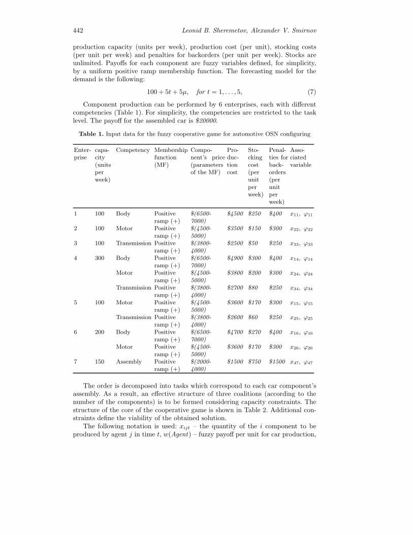
442 Leonid B. Sheremetov, Alexander V. Smirnov
production capacity (units per week), production cost (per unit), stocking costs(per unit per week) and penalties for backorders (per unit per week). Stocks areunlimited. Payoffs for each component are fuzzy variables defined, for simplicity,by a uniform positive ramp membership function. The forecasting model for thedemand is the following:
100 + 5t + 5μ, for t = 1, . . . , 5, (7)
Component production can be performed by 6 enterprises, each with differentcompetencies (Table 1). For simplicity, the competencies are restricted to the tasklevel. The payoff for the assembled car is $20000.
Table 1. Input data for the fuzzy cooperative game for automotive OSN configuring
Enter-prise
capa-city(unitsperweek)
Competency Membershipfunction(MF)
Compo-nent’s price(parametersof the MF)
Pro-duc-tioncost
Sto-ckingcost(perunitperweek)
Penal-ties forback-orders(perunitperweek)
Asso-ciatedvariable
1 100 Body Positiveramp (+)
$(6500-7000)
$4500 $250 $400 x11, ϕ11
2 100 Motor Positiveramp (+)
$(4500-5000)
$3500 $150 $300 x22, ϕ22
3 100 Transmission Positiveramp (+)
$(3800-4000)
$2500 $50 $250 x33, ϕ33
4 300 Body Positiveramp (+)
$(6500-7000)
$4900 $300 $400 x14, ϕ14
Motor Positiveramp (+)
$(4500-5000)
$3800 $200 $300 x24, ϕ24
Transmission Positiveramp (+)
$(3800-4000)
$2700 $80 $250 x34, ϕ34
5 100 Motor Positiveramp (+)
$(4500-5000)
$3600 $170 $300 x15, ϕ15
Transmission Positiveramp (+)
$(3800-4000)
$2600 $60 $250 x25, ϕ25
6 200 Body Positiveramp (+)
$(6500-7000)
$4700 $270 $400 x16, ϕ16
Motor Positiveramp (+)
$(4500-5000)
$3600 $170 $300 x26, ϕ26
7 150 Assembly Positiveramp (+)
$(2000-4000)
$1500 $750 $1500 x47, ϕ47
The order is decomposed into tasks which correspond to each car component’sassembly. As a result, an effective structure of three coalitions (according to thenumber of the components) is to be formed considering capacity constraints. Thestructure of the core of the cooperative game is shown in Table 2. Additional con-straints define the viability of the obtained solution.
The following notation is used: xijt – the quantity of the i component to beproduced by agent j in time t, w(Agent) – fuzzy payoff per unit for car production,

A Fuzzy Cooperative Game Model 443
Table 2. The structure of the core of the cooperative game
Core’s component Definition
C = {2500x11t + 2100x14t + 2300x16t + 1500x22t + 1200x24t + 1400x25t+1400x26t + 1500x33t + 2500x47t + 1300x34t + 1400x35t ≥(100 + 5t+ 5μ) w (Agent),
Constrainton the grandcoalition
2500x11t + 2100x14t + 2300x16t ≤ (100 + 5t+ 5μ) w (k1)1500x22t + 1200x24t + 1400x25t + 1400x26t ≤ (100 + 5t+ 5μ) w (k2)1500x33t + 1300x34t + 1400x35t ≤ (100 + 5t+ 5μ) w (k3)2500x47t ≤ (100 + 5t+ 5μ) w (k4)
Constraintson the com-ponents’coalitions
x11t + x14t + x16t ≤ 100 + 5t + 5μx22t + x24t + x25t + x26t ≤ 100 + 5t + 5μx33t + x34t + x35t ≤ 100 + 5t + 5μx47t ≤ 100 + 5t + 5μ
Constraintson the fore-casted de-mand for eachcomponent
x11t ≤ 100 x14t ≤ 300 x16t ≤ 200x22t ≤ 100 x24t ≤ 300 x25t ≤ 100 x26t ≤ 200x33t ≤ 100 x34t ≤ 300 x35t ≤ 100x47t ≤ 150
Capacityconstraints onthe payoffs
xijt ∈ R+, i = 1, ..., 4; j = 1, ..., 7 t = 1, ..., 5
w(k1) - fuzzy payoff per unit for Body Production, w(k2) - fuzzy payoff per unit forMotor Production, w(k3) - fuzzy payoff per unit for Transmission Production, w(k4)- fuzzy payoff per unit for car assembly, and μ - uniform random variable in [0,1].The solution of the game obtained using Evolver package and genetic algorithms isshown in Table 3.
Table 3. The coalition structure and the number of produced components for five timeintervals
t x11t x22t x33t x14t x24t x34t x25t x35t x16t x26t x47t
1 100 100 100 0 0 0 5,299 5,3 5,3 0,001 105,32 100 100 100 0 0 0 8,399 11,5 11,5 3,101 111,53 100 100 100 0 0 0 10,25 15,2 15,2 4,95 115,24 100 100 100 0 0 0 14,50 23,7 23,7 9,20 123,75 100 100 100 0 0 0 16,75 28,2 28,2 11,45 128,2
The common network payoffs per car obtained for each time interval are equal to7,578.46, 7,578.22, 7,578.22, 7,577.84, 7,577.84 respectively. The payoffs (p) of theparticipating enterprises per car/component are as follows: p1 = 2500; p2 = 1500; p3= 1500; p4 = 0; p5 = 1400 (motor and transmission); p6 = 2300 (body); p6 = 1400(motor); p7 = 2500. The same gross payoffs per enterprise were obtained for eachtime interval for each component: w(Agent) = 20,000; w(k1)= 7,000; w(k2)=5,000;w(k3)=4,000 w(k4)=4,000. The possibility of the fuzzy game γc(Agent , w) = 1.00(because of the simplicity of the case study), though the imputation obtained tookinto account the subjective estimations of the players defined by their fuzzy pay-ments.
444 Leonid B. Sheremetov, Alexander V. Smirnov
The analysis of the obtained solution shows the following. The constraint ca-pacity of the first 3 units though having minimal production costs, does not permitthem to satisfy all the demand. That is why, while demand is increasing, other en-terprises are involved in the production. In the case of Motor Production (k2), theincrementing production of this component is assigned to both enterprises 5 and 6(Table 3). If we compare the parameters of these enterprises (Table 2), it can beseen that they are the same both for the production cost ($3600 per motor) andfor stocking ($170 per motor /week). That means that the solution strategy looksfor a balanced final solution.
In the conducted experiments on model complexity the number of iterationsneeded to approach the optimal solution served as the investigated variable with thefollowing factors: the number of agents and coalitions, the accuracy, and the orderof fuzzy payments. Results show that the number of iterations (computation time)decreases or remains constant when the number of agents increases. In other words,it takes less time to form coalitions. On the other hand, the results demonstratealmost linear relation between the numbers of coalitions and agents. On the whole,the experiments justified that all factors are highly significant; the only surprise wasthat the order of fuzzy payments substantially influence the number of iterations(the convergence time).
6. Conclusions
In this paper, the approach to OSN configuration based on formation of enterprisecoalitions as a result of a fuzzy cooperative game was considered. Uncertainty inrealistic cooperation models occurs in two cases: when players participate in severalcoalitions, and when there exist fuzzy expectations of player and coalition benefits.The presented approach is mostly aimed at the latter case. This uncertainty ofthe agent payments may be caused by such dynamic events as production failures,changes in confidence estimations and reputations of potential coalition partners,and receiving unclear or even incomplete information and data during the taskperformance and negotiation.
The proposed model considers the coalitions’ efficiency by introducing binaryvariables ϕij into the fuzzy core. This permits not only to increase individual benefitsfor players but also the possibility to find an effective and stable agreement. Usingthe constraints of the application domain the number of viable coalitions can besignificantly decreased, thus reducing the algorithmic complexity of the problem.Though in the case study a positive ramp membership function was used (to be ableto use also conventional Excel solver), the general solution method (applying geneticalgorithms) permits the use of function of any type (linear or nonlinear, universalor not). Obviously, there is no guaranty that the obtained solution corresponds to aglobal optimum, but for a game with side payments, there is no algorithm to obtainthe optimal solution.
The fields of FCGs and dynamic coalition formation are still in their infancyand require further research efforts. For example, the notions of a superadditiveFCG and a “stable” distribution of fuzzy payments in the games using fuzzy exten-sion of the core and Shapley values were examined in (Mares, 2001). Some aspectsof application of the coalition game models to the development of dynamic coali-tion formation schemes were considered in (Klusch and Gerber, 2002). Nevertheless,sub-additive fuzzy games and the notions of “uncertain” stability and effective algo-

A Fuzzy Cooperative Game Model 445
rithms for FCGs represent the subjects for current research. In the future work, thedevelopment of algorithms for dynamic formation of fuzzy coalitions seems to be thepromising and challenging problem in the field of self-organizing system research.
Acknowlegments. The authors are very grateful to Dr. Andrew Krizhanovsky forhis help and assistance in the preparation of the final version of the paper.
References
Aubin, J. P. (1981). Cooperative Fuzzy Games. Math. Oper. Res., 6(1), 1–13.Aumann, R. J. and M. Maschler (1964). The bargaining set for cooperative games. Advances
in Game Theory (Dresher, M., Shapley, L.S. and Tucker A.W., eds). Series: Annals ofMathematics Studies, Princeton University Press., 52, 443–476.
Chandra, C. and J. Grabis (2007). Supply Chain Configuration: Concepts, Solutions, andApplications. Springer USA.
Davis, M. and M. Maschler (1965). The Kernel of a cooperative game. Naval ResearchLogistics Quarterly, 12, 223–259.
Garavelli, A. (2003). Flexibility configurations for the supply chain management. Int. J. ofProduction Economics, 85, 141–153.
Gasser, L. (1991). Social Conceptions of Knowledge and Action: DAI Foundations andOpen System Semantics. Artificial Intelligence, 47(1-3), 107–138.
Gillies, D. B. (1953). Some theorems on nperson games. Ph. D. thesis, Princeton UniversityPress. Princeton, New Jersey.
Hosam, H., Khaldoun, Z. (2006). Planning Coalition Formation under Uncertainty: Auc-tion Approach. In: 2nd Information and Communication Technologies, ICTTA ’06, 2,3013–3017.
Kahan, J. P. and Rapoport A. (1984). Theories of Coalition Formation. Lawrence ErlbaumAssociates, London.
Klusch, M. and Gerber A. (2002). Dynamic Coalition Formation Among Rational Agents.J. Intell. Syst., 17(3), 42–47.
Mares, M. (2001). Fuzzy Cooperative Games - Cooperation with Vague Expectations. Phys-ica Verlag.
McBeath, B., Childs, L. and A. Grackin (2010). Supply Chain Orchestrator – Man-agement of the Federated Business Model in this Second Decade. ChainLink Re-search. URL: http://www.clresearch.com/research/detail.cfm?guid=2158E97F-3048-79ED-9990-899769AF364C
Roth, A. (ed) (1995). Game-theoretic Models of Bargaining. Cambridge University Press,Cambridge.
Sandkuhl, K., Smirnov, A. and N. Shilov (2007). Configuration of Automotive CollaborativeEngineering and Flexible Supply Networks Expanding the Knowledge Economy Issues,Applications, Case Studies (Cunningham, P. and Cunningham, M., eds). IOS Press,Amsterdam (NL), 929–936.
Schmeidler, D. (1969). The nucleolus of a characteristic function game. SIAM Journal onApplied Mathematics, 17, 1163–1170.
Shapley, L. S. (1953). A value for nperson games. Contributions to the theory of gamesII, Annals of Mathematics Studies (Kuhn, H. W. and A.W. Tucker, eds), PrincetonUniversity Press. Princeton, 28, 307–317.
Sheremetov, L. B. and J. C. Romero-Cortes (2003). Fuzzy Coalition Formation AmongRational Cooperative Agents. Lecture Notes in Artificial Intelligence (Marik, J. Muller,and M. Pechoucek, eds). Springer, Berlin Heidelberg, 2691, 268–280.
Smirnov, A. (1999). Virtual Enterprise Configuration Management. In: 14th IFAC WorldCongress. Pergamon Press Beijing, China, A. 337–342.
Smirnov, A., Sheremetov, L., Chilov, N. and C. Sanchez-Sanchez (2006). Agent-BasedTechnological Framework for Dynamic Configuration of a Cooperative Supply Chain.

446 Leonid B. Sheremetov, Alexander V. Smirnov
Multiagent-based supply chain management (Chaib-draa, B., Mller, J. P., eds). Serieson Studies in Computational Intelligence, Springer, 28, 217–246.
Suckya, E. (2009). The bullwhip effect in supply chains - An overestimated problem? Int.J. of Production Economics, Elsevier B.V., 118(1), 311–322.
Tijs, S. H. (1981). Bounds for the core and the tvalue. Game Theory and MathematicalEconomics. North-Holland Publishing Company, Amsterdam, The Netherlands, 123–132.
Von Neumann, J. and O. Morgenstern (1944). Theory of Games and Economic Behavior.Princeton University Press.
Modeling of Environmental Projects under Conditionof a Random Time Horizon
Ekaterina Shevkoplyas and Sergey Kostyunin
1 St.Petersburg State University,Faculty of Applied Mathematics and Control Processes,
198904, Russia, St.Petersburg, Petrodvorets, University pr.,35E-mails: [email protected]
Abstract. One game-theoretical model of environmental project is consid-ered under condition of a random game duration. The game ends at therandom moment in time with Weibull distribution. According to Weibulldistribution form parameter, the game can be in one of 3 scenarios suchas ”an infant”, ”an adult” and ”an aged” scenario. The solutions obtainedwith a help of Pontryagin maximum principle both for non-cooperative andcooperative forms of the game are analyzed for each stage.Keywords:: differential games, environment, pollution control, random du-ration.
Introduction
The game-theoretical model of environmental project with 2 non-identical playershad been considered in the paper (Breton, Zaccour, Zahaf, 2005) under conditionthat the game has a fixed terminal time T . We consider the modification of thismodel with elements of stochastic framework, in the sense that the terminal timeT is a random value (see (Petrosjan, Murzov, 1966; Petrosjan, Shevkoplyas, 2003;Shevkoplyas, 2009)) in order to increase the realness of the modeling.
It turns out that this formulation of the game can be simplified to standardformulation for dynamic programming under some restrictions for instantaneousutility functions of the players.
With the help of Pontryagin maximum principle we find the solutions bothfor non-cooperative and cooperative forms of the game under condition of Weibulldistribution for the random value T . According to Weibull distribution form pa-rameter, the game can be in one of 3 scenarios such as ”an infant”, ”an adult” and”an aged” scenario. The solutions are analyzed for each stage of the game and theinterpretation in the context of the environmental economics is given.
The paper is structured as follows. Section 1 contains a general formulation ofdifferential games with random time horizon. Conditions for instanteneous utilityfunctions of the players to simplify this problem are investigated.
Section 2 is devoted to the modified differential game of pollution control.
1. Game Formulation
There are n players which participate in differential game Γ (x0). The game Γ (x0)with dynamics
x = g(x, u1, . . . , un), x ∈ Rn, ui ∈ U ⊆ compRl, (1)
x(t0) = x0.

448 Ekaterina Shevkoplyas, Sergey Kostyunin
starts from initial state x0 at the time instant t0. But here we supposethat the terminal time of the game is the random variable T with knownprobability distribution function F (t), t ∈ [t0,∞) (Petrosjan, Murzov, 1966;Petrosjan, Shevkoplyas, 2003).
Suppose, that for all feasible controls of players, participating the game, thereexists a continuous at least piecewise differentiable and extensible on [t0,∞) solutionof (1).
Denote the instantaneous payoff of player i at the time τ , τ ∈ [t0,∞) byhi(τ, x(τ), u1, . . . , un), or briefly hi(τ). Suppose, that for all feasible controls of play-ers which participate the game, the instantaneous payoff function of each player isbounded, piecewise continuous function of time τ (piecewise continuity is treatedas following: function hi(τ) could have only finitely many point of discontinuity oneach interval [t0, t] and bounded on this interval).
Thereby, the function hi(τ) is Riemann integrable on every interval [t0, t], in
other words for every t ∈ [t0,∞) there exists an integral∫ tt0hi(τ)dτ .
So, we have that the expected integral payoff of the player i can be representedas the following Lebesgue-Stieltjes integral:
Ki(x0, t0, u1, . . . , un) =
∞∫t0
t∫t0
hi(τ)dτdF (t), i = 1, . . . , n. (2)
1.1. Transformation of integral functional
The transformation of integral functional in the form of double in-tegral (2) to standard for dynamic programming form had been ob-tained in the paper (Burness, 1976) without details and in the papers(Boukas, Haurie and Michel, 1990, Chang, 2004) with the help of integration byparts. Now we obtain this result by interchanging the variables of integration. Herewe point some restrictions for utility function which were not stated before.
Nonnegative instantaneous payoff Suppose, that for any admissible strategies(controls) of each player instantaneous payoff is nonnegative function:
hi(τ, x(τ), u1, . . . , u2) ≥ 0, ∀ τ ∈ [t0,∞). (3)
We denote A ⊂ R2 as given below:
A = {(t, τ)|t ∈ [t0,∞], τ ∈ [t0, t]} .
Denote
At = {τ |(t, τ) ∈ A} ,Aτ = {t|(t, τ) ∈ A} .
Consider Lebesgue-Stieltjes measure μF , corresponding to the function F(Gelbaum, 1967, Zorich, 2002), and ordinary Lebesgue measure μt on [t0,∞].Rewrite (2) in a new form:
Ki(t0, x0, u1, . . . , un) =
∫[t0,∞]
⎡⎣ ∫At
hi(τ)dμτ
⎤⎦ dμF , i = 1, . . . , n. (4)

Modeling of Environmental Projects under Condition of a Random Time Horizon 449
Let us assume that integrals in the right side of (4) exist and condition (3) issatisfied, then Fubini’s theorem holds (Gelbaum, 1967, Zorich, 2002):∫
[t0,∞]
⎡⎣ ∫At
hi(τ)dμτ
⎤⎦ dμF =
∫[t0,∞]
⎡⎣ ∫Aτ
hi(τ)dμF
⎤⎦ dμτ , i = 1, . . . , n. (5)
Let us take the interior integral:∫[t0,∞]
⎡⎣ ∫Aτ
hi(τ)dμF
⎤⎦ dμτ =
∫[t0,∞]
[ hi(τ)μF (Aτ )] dμτ , i = 1, . . . , n.
Finally, we obtain∫[t0,∞]
[ hi(τ)μF (Aτ )] dμτ =
∞∫t0
hi(τ)(1 − F (τ))dτ, i = 1, . . . , n.
As it stated in (Gelbaum, 1967, Zorich, 2002), the existence of the integral aboveimplies the existence of the integral in the right side of (2).
Thus, the following proposition is proved.Proposition 1. Let the instantaneous payoff hi(t) be a bounded, piecewise
continuous function of time and satisfy the condition of nonnegativity (3). Thenthe expectation of integral payoff of player i (2) can be expressed in a simple form:
Ki(t0, x0, u1, . . . , un) =
∞∫t0
hi(τ)(1 − F (τ))dτ, i = 1, . . . , n. (6)
Moreover, integrals in (2) and (6) exist or do not exist simultaneously.Then we have the following formula for total expected payoff
General case Now we remove the condition (3) of nonnegativity of the function ofinstantaneous payoff. In this section we treat the integrals in the right side of (2) asRiemann integrals (or as nonintrinsic Riemann integrals). In this treatment the rightside (2) represents the expected payoff of player i in case of absolute convergenceof the outer integral. In other words, for the existence of the expectations in (2), itis necessary and sufficient that the following integrals exist in the sense of Riemannnonintrinsic integrals:
∞∫t0
∣∣∣∣∣∣t∫
t0
hi(τ)dτ
∣∣∣∣∣∣ dF (t) < +∞, i = 1, . . . , n. (7)
Let us define Hi(t) =∫ t0hi(τ)dτ . Here Hi(t), i = 1, . . . , n are piecewise differen-
tiable functions, because the functions hi(t) are assumed to be piecewise continuousfunction. Assume the existence of a continuous density of distribution of the ter-minal time of the game f(t) = F ′(t) on the interval [t0,∞). If (7) holds, then theexpected payoffs is given by:
Ki(t0, x0, u1, . . . , un) = limT→∞
T∫t0
Hi(t)dF (t), i = 1, . . . , n. (8)
450 Ekaterina Shevkoplyas, Sergey Kostyunin
Separately consider the integral in the (8), divided into a sum of integrals on theintervals of continuity of a function hi(t):
T∫t0
Hi(t)dF (t) =
NT∑k=0
θk+1∫θk
Hi(t)dF (t), (9)
there θ0 = t0, θNT+1 = T , θj , j = 1, . . . , NT — point of discontinuity of hi(t) onthe interval (t0, T ). On each interval, the integration by parts is used:
NT∑k=0
θk+1∫θk
Hi(t)dF (t) =
NT∑k=0
⎡⎣Hi(θk+1)F (θk+1)−Hi(θk)F (θk)−θk+1∫θk
hi(t)F (t)dt
⎤⎦ .
Substitute this representation into equation (9) and after transformations we obtain:
T∫t0
Hi(t)dF (t) = Hi(T )F (T )−T∫t0
hi(t)F (t)dt =
T∫t0
hi(t) [F (T )− F (t)] dt,
and further
T∫t0
hi(t) [F (T )− F (t)] dt =
T∫t0
hi(t) [F (T )− 1] dt +
T∫t0
hi(t) [1− F (t)] dt.
Thus, we have:
limT→∞
T∫t0
Hi(t)dF (t) = limT→∞
⎛⎝ T∫t0
hi(t) [F (T )− 1] dt +
T∫t0
hi(t) [1− F (t)] dt
⎞⎠ .
So, we can formulate the following proposition.Proposition 2. Under conditions (7) we can represent the expected payoff in
form (6), if the following condition holds:
limT→∞
(F (T )− 1)
T∫t0
hi(t)dt = 0. (10)
Proof. Indeed, if the conditions (7) hold, then the limit in (8) exists. In this case,the fullfilment of conditions (10) implies the existence of
limT→∞
∫ T
t0
hi(t) [1− F (t)] dt.
And this limit is equal to the limit in (8).This means that the expected payoff could be obtained by formula (6).Thus, if calculation of the expected payoff by formula (2) causes some difficulties,
but one can guarantee fulfillment of conditions (7) and (10), then the expectationof payoff could be find by more simply formula (6).
Modeling of Environmental Projects under Condition of a Random Time Horizon 451
1.2. Subgame
Let the game Γ (x0) develops along the trajectory x(t). Then at the each timeinstant ϑ, ϑ ∈ (t0;∞) players enter new game (subgame) Γ (x(ϑ)) with initial statex(ϑ) = x. Clearly, there is a probability F (ϑ) that the game Γ (x0) will be finishedbefore ϑ. Then the probability to start the subgame Γ (x(ϑ)) equals to (1− F (ϑ)).
Then the expected total payoff of the player i is calculated by following formula:
Ki(x, ϑ, u1, . . . , un) =
∫ ∞
ϑ
[∫ t
ϑ
hi(τ, x(τ), u1, . . . , un)dτ
]dFϑ(t), (11)
here Fϑ(t), t ≥ ϑ — conditionally probability distribution function of the ran-dom terminal time in the game Γ (x(ϑ)). In this paper we cosider only stationaryprocesses, so we have the following expression for Fϑ(t):
Fϑ(t) =F (t)− F (ϑ)
1− F (ϑ), t ∈ [ϑ,∞). (12)
Further we assume an existence of a density function f(t) = F ′(t). As above weget the formula for conditional density function:
fϑ(t) =f(t)
1− F (ϑ). (13)
Using (13), we get the total payoff for player i in the subgame Γ (x(ϑ)):
Ki(x, ϑ, u1, . . . , un) =1
1− F (ϑ)
∫ ∞
ϑ
∫ t
ϑ
hi(τ, x(τ), u1, . . . , un)dτ f(t)dt. (14)
Using the transformation of the integral payoff as above, within the the frame-work of restrictions on hi from Proposition 2, under condition of existence of thedensity function, we can rewrite (14) in the following form
Ki(x, ϑ, u1, . . . , un) =1
1− F (ϑ)
∫ ∞
ϑ
(1− F (τ))hi(τ, x(τ), u1, . . . , un)dτ. (15)
Let us remark, that using the Hazard function λ(ϑ) which is given by the fol-lowing definition:
λ(t) =f(t)
1− F (t), (16)
we can also rewrite the term (1 − F (τ)) from subintegral function of (15) as
1− F (τ) = e−
∫ τt0λ(t)dt
.
Then we can use another form of the expected payoff (15) of the player i:
Ki(x, ϑ, u1, . . . , un) = e∫ ϑt0λ(t)dt
∫ ∞
ϑ
e−
∫ τt0λ(t)dt
hi(τ, x(τ), u1, . . . , un)dτ. (17)
It is obviously, that for exponential distribution of the random value T we haveλ(t) = λ. That is why the problem with random duration under exponential dis-tribution of T equivalents to well-known deterministic problem with constant dis-counting of payoffs. This fact was marked in the paper (Haurie, 2005 ) for anotherconcepts of random game duration (a multigenerational game model).
452 Ekaterina Shevkoplyas, Sergey Kostyunin
1.3. Weibull distribution case
In mathematical reliability theory the Hazard function λ(t) (16) describing life circleof the system usually has the following characteristics: it is decreasing functionfor ”burn-in” period, it is near constant for ”adult” period (or regime of normalexploitation) and it is increasing function for ”wear-out” period. One of the mostimportant probability distribution describing three periods of life circles is WeibullLaw. Using Weibull distribution allows to consider three ”scenarios” of the game inthe sense of behaviour of the random variable T .
For Weibull distribution we have the following characteristics:
f(t) = λδ(t− t0)δ−1e−λ(t−t0)δ
; (18)
λ(t) = λδ(t− t0)δ−1;
t ≥ t0; λ > 0; δ > 0.
Here λ and δ are two parametres. δ < 1 corresponds to ”burn-in” period, δ = 1corresponds to ”adult” period and δ > 1 corresponds to ”wear-out” period. It isa well–known fact that the Weibull distribution for adult stage (δ = 1, λ(t) =λ = const) is equivalent to exponential distribution. Thus if we use exponentialdistribution for random final time instant T then we indeed consider the game in”adult” scenario.
2. Differential game of pollution control
2.1. Model
As an example we consider differential game with environmental context based onthe model (Breton, Zaccour, Zahaf, 2005).
There are 2 players (firms, countries) involved into the game of pollution control.Each player manage his emissions ei ∈ [0; bi], i = 1, 2.
Tne net revenue of player i at time instant t is given by quadratic functionalform:
R(ei(t)) = ei(t)(bi − 1/2ei(t)).
Denote the stock of accumulated net emissions by P (t). The dynamics of thestock is given by the following equation with initial condition:
P =
n∑i=1
ei(t), P (t0) = P0.
Costs of the player depend on the stock of pollution. Then, the instanteneousutility function of the player i is equal to R(ei(t)) − diP (t), di > 0.
Further we assume that the game of pollution control starts at the time instantt0 = 0 and then the game ends at the random moment in time T which is decsribedby Weibull distribution (18).
Then we have the following integral payoff for player i:
Ki(P0, 0, e1, . . . , en) =
∫ ∞
0
∫ t
0
(Ri(ei(τ)) − diP (τ)) λδtδ−1e−λtδ
dτdt. (19)

Modeling of Environmental Projects under Condition of a Random Time Horizon 453
2.2. Simplification of the problem
Let us prove that the integral payoff (19) can be rewriten in the simple form accord-ingly to (15). Without loss of generality we assume λ = 1, because λ is a parameterof scale. Moreover, we consider case of δ = 2 (Ralegh distribution, wear-out scenarioof the game).
Then from (19) we obtain the following form of payoff for player i:
Ki(0, P0, e1, . . . , en) =
∞∫0
t∫0
(Ri(ei(τ)) − diP (τ))dτ 2te−t2
dt, (20)
under condition of integral convergence
∞∫0
∣∣∣∣∣∣t∫
0
(Ri(ei(τ)) − diP (τ))dτ
∣∣∣∣∣∣ 2te−t2
dt. (21)
To prove the existence (21) we make the following estimation:
P (τ) ≤ P0 +
n∑i=1
biτ = P0 + Bτ,
Ri(ei(τ)) ≤ b2i2,
whereB =n∑i=1
bi.
We get the following estimation for (21):
∞∫0
∣∣∣∣∣∣t∫
0
(Ri(ei(τ)) − diP (τ))dτ
∣∣∣∣∣∣ 2te−t2
dt ≤∞∫0
t∫0
|(Ri(ei(τ)) − diP (τ))| dτ 2te−t2
dt ≤
≤∞∫0
t∫0
(|(Ri(ei(τ))|+|diP (τ))|)dτ 2te−t2
dt ≤∞∫0
⎛⎝ t∫0
Ri(ei(τ))dτ +
t∫0
diP (τ)dτ
⎞⎠ 2te−t2
dt.
Finally, we have the estimation for (21):
∞∫0
∣∣∣∣∣∣t∫
0
(Ri(ei(τ)) − diP (τ))dτ
∣∣∣∣∣∣ 2te−t2
dt ≤∞∫0
(b2i2t + di
(P0t +
Bt2
2
))2te−t
2
dt.
(22)The integral in the right-hand side of the inequality (22) is absolutely convergent
integral. Then integral (21) is convergent integral (see (Zorich, 2002)).So, we proved that for all controls the expression (20) is the mathematical ex-
pectation of the integral payoff of the player i.To prove the satisfaction of condition (10) let us rewrite the left-hand side for
Weibull distribution with λ = 1, δ = 2:
limT→∞
(F (T )− 1)
T∫0
hi(t)dt = limT→∞
e−T2
T∫0
(Ri(ei(τ)) − diP (τ))dτ.
454 Ekaterina Shevkoplyas, Sergey Kostyunin
Using above obtained estimations, we get:∣∣∣∣∣∣e−T 2
T∫0
(Ri(ei(τ)) − diP (τ))dτ
∣∣∣∣∣∣ ≤ e−T2
⎛⎝ T∫0
b2i2dτ +
T∫0
di(P0 + Bτ)dτ
⎞⎠ =
= e−T2
(b2i2T + di
(P0T +
BT 2
2
)).
It is clear that
limT→∞
e−T2
(b2i2T + di
(P0T +
BT 2
2
))= 0.
Then we get
limT→∞
e−T2
T∫0
(Ri(ei(τ)) − diP (τ))dτ = 0.
That is why the condition (10) holds and the payoff (20) can be rewritten in thefollowing simple form:
Ki(0, P0, e1, . . . , en) =
∞∫0
(Ri(ei(t))− diP (t)) e−t2
dt. (23)
Similar, we can proove that reordering of the integrals can be also used for theproblem with δ = 1, δ = 1/2.
2.3. Open–loop Nash equilibrium
To find the open–loop Nash equilibrium we use Pontryagin maximum principle.Each player i = 1, 2 solves the maximization problem:
maxei∈[0;bi]
Ki(P0, 0, e1, e2) =
∫ ∞
0
(Ri(e
Ni (t))− diP (t)
)e−λs
δ
ds.
The Hamiltonian for this problem is as follows:
Hi(Λ(t), P (t), ei(t)) =
(ei(t)
(bi −
1
2ei(t)
)− diP (t)
)e−λt
δ
+ Λ
2∑i=1
ei(t).
We have to find the maximum of Hamiltonian: maxei∈[0;bi]
Hi(Λ(t), P (t), ei).
Further we use short notations ei, λi, Λ for ei(t), λi(t), Λ(t) .We consider functional:
L(ei) = −Hi + λ1(−ei) + λ2(ei − bi).
For optimality of the control eNi it is necessary the fulfillment of the Karush – Kuhn– Tucker conditions:
1. Stationarity: minei
Li(ei) = Li(eNi ).
2. Complementary slackness: λ1(−eNi ) = 0; λ2(eNi − bi) = 0.3. Dual feasibility: λj ≥ 0, j = 1, 2.
Modeling of Environmental Projects under Condition of a Random Time Horizon 455
We have dLdei
= −(
(bi − ei)e−λtδ + Λ
)− λ1 + λ2, then from stationarity condition
we get:
−(
(bi − eNi )e−λtδ
+ Λ)− λ1 + λ2 = 0. (24)
Let us consider the following cases:
1. λ2(t) = 0 (from nonnegativity we can rewrite λ2(t) > 0.) Then from comple-mentary slackness condition (eNi (t) − bi) = 0 we get eNi (t) = bi and λ1 = 0.Then λ2(t) = Λ(t). As we will see below, Λ(t) ≤ 0, which is in contrast to λ2(t).That is why this assumption is wrong.
2. λ2(t) = 0. Then we get
−(
(bi − eNi (t))e−λtδ
+ Λ(t))− λ1(t) = 0.
Let us assume λ1(t) = 0, then from complementary slackness condition we
get eNi (t) = 0. Then we have λ1(t) = −(bie
−λtδ + Λ(t))
. If λ1(t) = 0 then
eNi (t) =(bie
−λtδ + Λ(t))et
2
. That is why following formula is true:
eNi (t) =
⎧⎨⎩bi + Λ(t)eλtδ
, if(bie
−λtδ + Λ(t))≥ 0,
0, if(bie
−λtδ + Λ(t))< 0.
Adjoint function Λ(t) we get from adjoint equation
Λ = −∂Hi
∂P.
Then we get differential equation Λ(t) = die−λtδ , and the solution for adjoint func-
tion:
Λ(t) = di
∫ t
0
e−λsδ
ds + c.
We consider problem with time t ∈ [0,∞) and the condition for Λ(t) has a form:
limt→∞
Λ(t) = 0.
Let us take the Weibull distribution for the Hazard function λ(t) (18). Thenwe obtain equillibrium emissions for three scenarios of the game (δ = 1, δ = 2,δ = 1/2).
For regim of normal exploitation of the environmental equipments (δ = 1) we
obtain Λ(t) = di∫ t0e−λs
δ
ds + c = − diλ e−λt + diλ + c. From condition lim
t→∞Λ(t) =
diλ + c = 0 we get c = − diλ . Then we have
Λ(t) = −diλe−λt.
Then the open–loop Nash emissions for the problem have form:
eNi (t) = bi + Λ(t)eλt = bi −diλ, i = 1, 2,
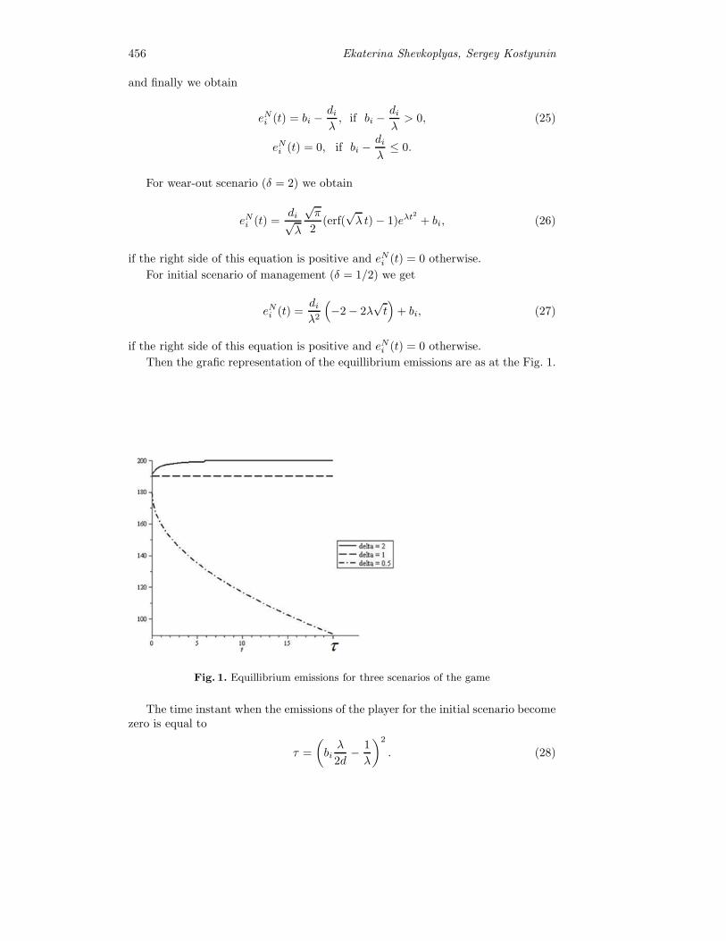
456 Ekaterina Shevkoplyas, Sergey Kostyunin
and finally we obtain
eNi (t) = bi −diλ, if bi −
diλ
> 0, (25)
eNi (t) = 0, if bi −diλ≤ 0.
For wear-out scenario (δ = 2) we obtain
eNi (t) =di√λ
√π
2(erf(√λ t)− 1)eλt
2
+ bi, (26)
if the right side of this equation is positive and eNi (t) = 0 otherwise.
For initial scenario of management (δ = 1/2) we get
eNi (t) =diλ2
(−2− 2λ
√t)
+ bi, (27)
if the right side of this equation is positive and eNi (t) = 0 otherwise.
Then the grafic representation of the equillibrium emissions are as at the Fig. 1.
Fig. 1. Equillibrium emissions for three scenarios of the game
The time instant when the emissions of the player for the initial scenario becomezero is equal to
τ =
(bi
λ
2d− 1
λ
)2
. (28)
Modeling of Environmental Projects under Condition of a Random Time Horizon 457
2.4. Cooperative solution
Suppose that players are agree to cooperate and maximize the total payoff:
max(e1;e2)∈[0;b1]×[0;b2]
(K1(P0, 0, e1, e2) + K2(P0, 0, e1, e2)) =∫ ∞
0
(R1(eC1 ) + R2(eC2 )− (d1 + d2)P
)e−λs
δ
ds.
Then by the similar way as for non–cooperative case we obtain optimal controls forplayers i = 1, 2.
Optimal emissions for cooperative version of ”adult” game:
eCi (t) = bi −d
λ, if bi −
d
λ> 0,
eCi (t) = 0, if bi −d
λ≤ 0,
where d = d1 + d2.
Optimal emissions for wear-out scenario of the game (Raleigh distribution, δ =2) are given by:
eCi (t) =d√λ
√π
2(erf(√λ t)− 1)eλt
2
+ bi,
if the right side of this equation is positive and eCi (t) = 0 otherwise.We have the following form for optimal emissions for burn-in scenario (δ = 1
2 ):
eCi (t) =d
λ2
(−2− 2λ
√t)
+ bi,
if the right side of this equation is positive and eCi (t) = 0 otherwise.One could compare the optimal emissions for cooperative and non-cooperative
form of the game. It can be easily proved that for each of considered shape pa-rameters δ = 1/2; 1; 2 the optimal emissions for cooperation are less then for non-cooperative version of the game:
eCi (t) < eNi (t).
The graphic representation of this fact is given for δ = 2 (see Fig. 2).Consider the example of ”adult” game with two asymetric agents. Let use take
the parameteres d1 = 2, b1 = 50, d2 = 1, b2 = 20. Let δ = 1 (exponential distributioncase, regime of normal work). Then we obtain the following numerical results.
i di bi eNi eCi KNi KC
i
1 2 50 48 47 1114 1117.52 1 20 19 17 132.5 131.5∑
1246.5 1249
This example demonstrates that the joint payoff for cooperative version is greaterthan for non-cooperative, but the optimal emissions are less.

458 Ekaterina Shevkoplyas, Sergey Kostyunin
Fig. 2. Comparison of cooperative and non–cooperative emissions for δ = 2
Acknowledgments
Many thanks to Prof. Leon A. Petrosyan for his valuable comments on the dif-ferential game theory and to Prof. Dmitry S. Chelkak for consultations on themathematical analysis.
References
Basar T., Olsder G. J. (1995). Dynamic Noncooperative Game Theory. 2nd Edn. AcademicPress. - London.
Breton M., Zaccour G., Zahaf M. (2005). A differential game of joint implementation ofenvironmental projects. Automatica, 41(10), 1737–1749.
Burness, H. Stuart (1976). A Note on Consistent Naive Intertemporal Decision Making andan Application to the Case of Uncertain Lifetime. The Review of Economic Studies,43(3), 547–549.
Boukas, E. K. and Haurie, A. and Michel, P. (1990). An Optimal Control Problem witha Random Stopping Time. Journal of optimizationa theory and applications, 64(3),471–480.
Chang, F. R. (2004). Stochastic Optimization in Continuous Time. Cambridge Univ. Press.Dockner, E. J., Jorgensen, S., N. van Long, Sorger, G. (2000). Differential Games in Eco-
nomics and Management Science. Cambridge University Press.Gelbaum, B., J. Olmsted (1967). Counterexamples in Analysis.Haurie, A. (2005). A Multigenerational Game Model to Analyze Sustainable Development.
Annals of Operations Research, 137(1), 369–386.Marin-Solano, J., Shevkoplyas, E. V. (2010). Non-constant discounting in differential games
with random duration. Contributions to Game Theory and Management, collected pa-pers of the Third International Conference Game Theory and Management, 2009. St.Petersburg, 267–280.
Petrosjan, L. A. and Murzov, N. V. (1966). Game-theoretic problems of mechanics. Litovsk.Mat. Sb. 6, 423–433 (in Russian).
Petrosjan, L. A., Shevkoplyas, E. V. (2003). Cooperative Solutions for Games with RandomDuration. Game Theory and Applications, Volume IX. Nova Science Publishers, pp.125–139.

Modeling of Environmental Projects under Condition of a Random Time Horizon 459
Shevkoplyas, E. V. (2009). The Hamilton-Jacobi-Bellman equation for differential gameswith random duration. Upravlenie bolshimi systemami, 26.1, M.:IPU RAN, pp. 385–408. (in Russian)
Shevkoplyas, E. V. (2010). The Shapley Value in cooperative differential games with randomduration. Advances in Dynamic Games. V. 11., part 4. Edt. by M.Breton and K.Szajowski, Springer’s imprint Birkhauser, Boston, 2011, pp. 359–373.
Yaari, M. E. (1965). Uncertain Lifetime, Life Insurance, and the Theory of the Consumer.The Review of Econimic Studies, 32(2) , 137–150.
Zorich, V. A. (2002). Mathematical analysis.

A Data Transmission Game in OFDM Wireless NetworksTaking into Account Power Unit Cost
Anton Toritsyn, Rimma Salakhieva and Andrey Garnaev
St.Petersburg State University,Faculty of Applied Mathematics and Control Processes,
Universitetskii prospekt 35, Petergof, St. Petersburg, 198504, RussiaE-mail: [email protected], [email protected]
Abstract. The goal of this work is to extend the model from Altman E.,Avrachenkov K., Garnaev A. ”Closed form solutions for water-filling prob-lems in optimization and game frameworks” for the case with different fadingchannel gains and also taking into account cost of power unit which can pro-duce essential impact on behaviour of users. The equilibrium strategies forthe extended model are found in closed form.Keywords: equilibrium strategies, resource allocation, OFDM.
1. Introduction
In wireless networks and DSL access networks the total available power for sig-nal transmission has to be distributed among several resources. In the context ofwireless networks, the resources may correspond to frequency bands (e.g. as inOFDM). This spectrum of problems can be considered in game-theoretical mul-tiusers scenario which leads to “Water Filling Game” or “Gaussian InterferenceGame”(Lai and Gamal, 2005; Popescu and Rose, 2003, 2004; Yu, 2002; Altman etal., 2007b, 2010), where each user perceives the signals of the other users as interfer-ence and maximizes a concave function of the noise to interference ratio. A naturalapproach in the non-cooperative setting is the application of the Iterative WaterFilling Algorithm (IWFA) (Yu et al., 2002). Recently, Luo and Pang (2006) provedthe convergence of IWFA under fairly general conditions. An interested reader canfind more references on non-cooperative power control in (Lai and Gamal, 2005).We would like to mention that the water filling problem and jamming games withtransmission costs have been analyzed in (Altman et al., 2007a). In (Altman et al.,2007b, 2010) a closed form approach to Nash equilibrium was developed for symmet-ric water filling game. The goal of this work is to extend this approach for scenariowith different fading channel gains and also taking into account cost of power unitwhich can produce essential impact on behaviour of users.
2. Two Players Game
In this section we consider game-theoretical formulation of the situation where twousers (transmitters) transmit signals through n sub-carriers taking into accounttariff assigned by provider. It is worth to note that this tariff can impact on theuser’s behavior essentially, namely, for big tariff users can reject from using providerat all, and of course for small tariff users will employ the network facilities in thefull range. A strategy of user j (j = 1, 2) is vector T j = (T j1 , . . . , T
jn), where T ji � 0
andn∑i=1
T ji T j,
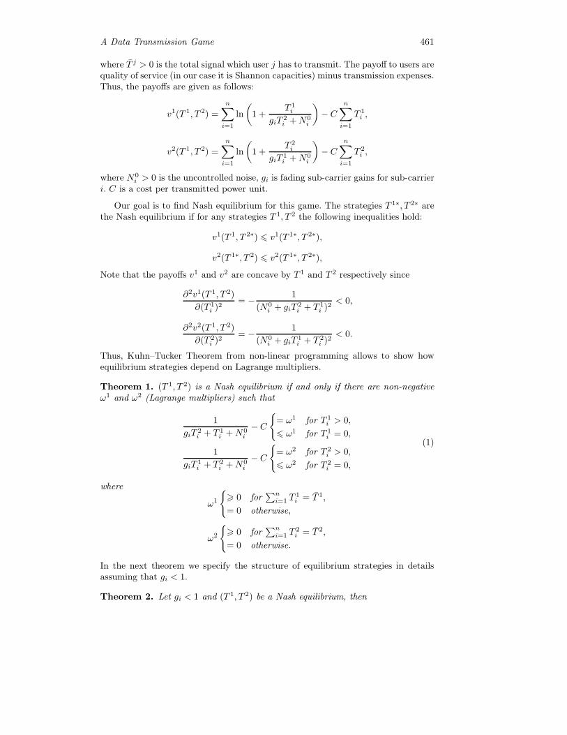
A Data Transmission Game 461
where T j > 0 is the total signal which user j has to transmit. The payoff to users arequality of service (in our case it is Shannon capacities) minus transmission expenses.Thus, the payoffs are given as follows:
v1(T 1, T 2) =
n∑i=1
ln
(1 +
T 1i
giT 2i + N0
i
)− C
n∑i=1
T 1i ,
v2(T 1, T 2) =n∑i=1
ln
(1 +
T 2i
giT 1i + N0
i
)− C
n∑i=1
T 2i ,
where N0i > 0 is the uncontrolled noise, gi is fading sub-carrier gains for sub-carrier
i. C is a cost per transmitted power unit.
Our goal is to find Nash equilibrium for this game. The strategies T 1∗, T 2∗ arethe Nash equilibrium if for any strategies T 1, T 2 the following inequalities hold:
v1(T 1, T 2∗) v1(T 1∗, T 2∗),
v2(T 1∗, T 2) v2(T 1∗, T 2∗),
Note that the payoffs v1 and v2 are concave by T 1 and T 2 respectively since
∂2v1(T 1, T 2)
∂(T 1i )2
= − 1
(N0i + giT 2
i + T 1i )2
< 0,
∂2v2(T 1, T 2)
∂(T 2i )2
= − 1
(N0i + giT 1
i + T 2i )2
< 0.
Thus, Kuhn–Tucker Theorem from non-linear programming allows to show howequilibrium strategies depend on Lagrange multipliers.
Theorem 1. (T 1, T 2) is a Nash equilibrium if and only if there are non-negativeω1 and ω2 (Lagrange multipliers) such that
1
giT 2i + T 1
i + N0i
− C
{= ω1 for T 1
i > 0,
ω1 for T 1i = 0,
1
giT 1i + T 2
i + N0i
− C
{= ω2 for T 2
i > 0,
ω2 for T 2i = 0,
(1)
where
ω1
{� 0 for
∑ni=1 T
1i = T 1,
= 0 otherwise,
ω2
{� 0 for
∑ni=1 T
2i = T 2,
= 0 otherwise.
In the next theorem we specify the structure of equilibrium strategies in detailsassuming that gi < 1.
Theorem 2. Let gi < 1 and (T 1, T 2) be a Nash equilibrium, then

462 Anton Toritsyn, Rimma Salakhieva, Andrey Garnaev
(a) if T 1i = T 2
i = 0 then i ∈ I00(ω1, ω2), where
I00(ω1, ω2) =
{i ∈ [1, n] :
1
ω1 + C N0
i ,1
ω2 + C N0
i
},
(b) if T 1∗i > 0 and T 2∗
i = 0 then
T 1i =
1
ω1 + C−N0
i
and i ∈ I10(ω1, ω2), where
I10(ω1, ω2) =
{i ∈ [1, n] :
1
ω1 + C> N0
i , gi
(1
ω1 + C−N0
i
)� 1
ω2 + C−N0
i
},
(c) if T 2i > 0 and T 1
i = 0 then
T 2i =
1
ω2 + C−N0
i
and i ∈ I01(ω1, ω2), where
I01(ω1, ω2) =
{i ∈ [1, n] : gi
(1
ω2 + C−N0
i
)� 1
ω1 + C−N0
i ,1
ω2 + C> N0
i
},
(d) if T 1i > 0 and T 2
i > 0 then
T 1i =
(1
ω1 + C−N0
i
)− gi
(1
ω2 + C−N0
i
)1− g2i
,
T 2i =
(1
ω2 + C−N0
i
)− gi
(1
ω1 + C−N0
i
)1− g2i
,
(2)
and i ∈ I11(ω1, ω2), where
I11(ω1, ω2) =
{i ∈ [1, n] : 0 < gi
(1
ω2 + C−N0
i
)<
1
ω1 + C−N0
i
1
ω1 + C−N0
i <1
gi
(1
ω2 + C−N0
i
)}
Proof. (a) Let T 1i = T 2
i = 0. Then, by (1),
1
giT 2i + T 1
i + N0i
=1
N0i
ω1 + C,
1
giT 1i + T 2
i + N0i
=1
N0i
ω2 + C.
Thus, i ∈ I00 and (a) follows.

A Data Transmission Game 463
(b) Let T 1i > 0, T 2
i = 0. Then, by (1),
1
giT 2i + T 1
i + N0i
=1
T 1i + N0
i
= ω1 + C,
1
giT 1i + T 2
i + N0i
=1
giT 1i + N0
i
ω2 + C.
The first relation implies
T 1i =
1
ω1 + C−N0
i (3)
and the second relation yields:
giT1i � 1
ω2 + C−N0
i ,
which jointly with (3) implies:
gi(1
ω1 + C−N0
i ) � 1
ω2 + C−N0
i . (4)
Besides, since T 1i > 0, (3) yields
1
ω1 + C> N0
i
which jointly with (4) implies that i ∈ I10 and (b) follows.
(c) follows from (b) by symmetry.
(d) Let T 1i > 0, T 2
i > 0. Then⎧⎪⎨⎪⎩giT
2i + T 1
i + N0i =
1
ω1 + C,
giT1i + T 2
i + N0i =
1
ω2 + C.
Solving this system of equations yields (2).
The facts that T 1i and T 2
i have to be positive and gi < 1 jointly with (2) impliesthat (
1
ω1 + C−N0
i
)> gi
(1
ω2 + C−N0
i
),
gi
(1
ω1 + C−N0
i
)<
(1
ω2 + C−N0
i
).
Thus, i ∈ I11 and Theorem 2 follows. ��
Now carry on investigation of the case gi < 1 for any i. Note that it is possible tosimplify the form of the sets I taking into account three possible combinations ofrelations between ω1 and ω2 as it is given in the following lemma.
Lemma 1. Let gi < 1.
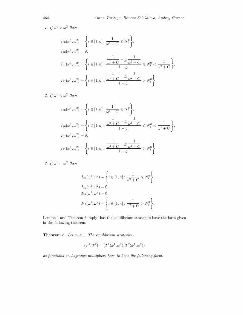
464 Anton Toritsyn, Rimma Salakhieva, Andrey Garnaev
1. If ω1 > ω2 then
I00(ω1, ω2) =
{i ∈ [1, n] :
1
ω2 + C N0
i
},
I10(ω1, ω2) = ∅,
I01(ω1, ω2) =
{i ∈ [1, n] :
1
ω1 + C− gi
1
ω2 + C1− gi
N0i <
1
ω2 + C
},
I11(ω1, ω2) =
{i ∈ [1, n] :
1
ω1 + C− gi
1
ω2 + C1− gi
> N0i
}
2. If ω1 < ω2 then
I00(ω1, ω2) =
{i ∈ [1, n] :
1
ω1 + C N0
i
},
I10(ω1, ω2) =
{i ∈ [1, n] :
1
ω2 + C− gi
1
ω1 + C1− gi
N0i <
1
ω1 + C
},
I01(ω1, ω2) = ∅,
I11(ω1, ω2) =
{i ∈ [1, n] :
1
ω2 + C− gi
1
ω1 + C1− gi
> N0i
}
3. If ω1 = ω2 then
I00(ω1, ω2) =
{i ∈ [1, n] :
1
ω2 + C N0
i
},
I10(ω1, ω2) = ∅,I01(ω1, ω2) = ∅,
I11(ω1, ω2) =
{i ∈ [1, n] :
1
ω2 + C> N0
i
}.
Lemma 1 and Theorem 2 imply that the equilibrium strategies have the form givenin the following theorem.
Theorem 3. Let gi < 1. The equilibrium strategies
(T 1, T 2) = (T 1(ω1, ω2), T 2(ω1, ω2))
as functions on Lagrange multipliers have to have the following form.
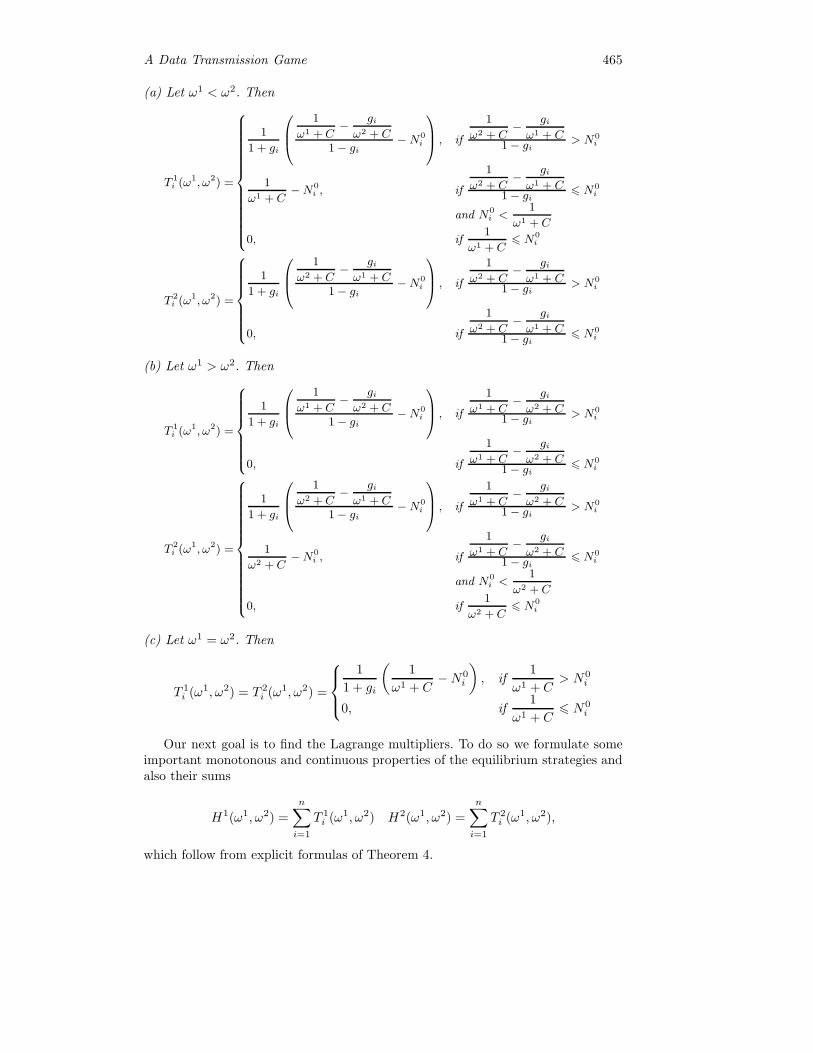
A Data Transmission Game 465
(a) Let ω1 < ω2. Then
T 1i (ω1, ω2) =
⎧⎪⎪⎪⎪⎪⎪⎪⎪⎪⎪⎪⎪⎪⎨⎪⎪⎪⎪⎪⎪⎪⎪⎪⎪⎪⎪⎪⎩
1
1 + gi
⎛⎜⎝
1
ω1 +C− giω2 +C
1 − gi−N0
i
⎞⎟⎠ , if
1
ω2 +C− giω1 + C
1 − gi> N0
i
1
ω1 +C−N0
i , if
1
ω2 +C− giω1 + C
1 − gi N0
i
and N0i <
1
ω1 +C
0, if1
ω1 +C N0
i
T 2i (ω1, ω2) =
⎧⎪⎪⎪⎪⎪⎪⎨⎪⎪⎪⎪⎪⎪⎩
1
1 + gi
⎛⎜⎝
1
ω2 +C− giω1 +C
1 − gi−N0
i
⎞⎟⎠ , if
1
ω2 +C− giω1 + C
1 − gi> N0
i
0, if
1
ω2 +C− giω1 + C
1 − gi N0
i
(b) Let ω1 > ω2. Then
T 1i (ω1, ω2) =
⎧⎪⎪⎪⎪⎪⎪⎨⎪⎪⎪⎪⎪⎪⎩
1
1 + gi
⎛⎜⎝
1
ω1 +C− giω2 +C
1 − gi−N0
i
⎞⎟⎠ , if
1
ω1 +C− giω2 + C
1 − gi> N0
i
0, if
1
ω1 +C− giω2 + C
1 − gi N0
i
T 2i (ω1, ω2) =
⎧⎪⎪⎪⎪⎪⎪⎪⎪⎪⎪⎪⎪⎪⎨⎪⎪⎪⎪⎪⎪⎪⎪⎪⎪⎪⎪⎪⎩
1
1 + gi
⎛⎜⎝
1
ω2 +C− giω1 +C
1 − gi−N0
i
⎞⎟⎠ , if
1
ω1 +C− giω2 + C
1 − gi> N0
i
1
ω2 +C−N0
i , if
1
ω1 +C− giω2 + C
1 − gi N0
i
and N0i <
1
ω2 +C
0, if1
ω2 +C N0
i
(c) Let ω1 = ω2. Then
T 1i (ω1, ω2) = T 2
i (ω1, ω2) =
⎧⎪⎨⎪⎩1
1 + gi
(1
ω1 + C−N0
i
), if
1
ω1 + C> N0
i
0, if1
ω1 + C N0
i
Our next goal is to find the Lagrange multipliers. To do so we formulate someimportant monotonous and continuous properties of the equilibrium strategies andalso their sums
H1(ω1, ω2) =
n∑i=1
T 1i (ω1, ω2) H2(ω1, ω2) =
n∑i=1
T 2i (ω1, ω2),
which follow from explicit formulas of Theorem 4.
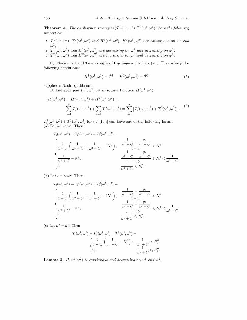
466 Anton Toritsyn, Rimma Salakhieva, Andrey Garnaev
Theorem 4. The equilibrium strategies (T 1(ω1, ω2), T 2(ω1, ω2)) have the followingproperties:
1. T 1(ω1, ω2), T 2(ω1, ω2) and H1(ω1, ω2), H2(ω1, ω2) are continuous on ω1 andω2,
2. T 1(ω1, ω2) and H1(ω1, ω2) are decreasing on ω1 and increasing on ω2,3. T 2(ω1, ω2) and H2(ω1, ω2) are increasing on ω1 and decreasing on ω2.
By Theorems 1 and 3 each couple of Lagrange multipliers (ω1, ω2) satisfying thefollowing conditions:
H1(ω1, ω2) = T 1, H2(ω1, ω2) = T 2 (5)
supplies a Nash equilibrium.To find such pair (ω1, ω2) let introduce function H(ω1, ω2):
H(ω1, ω2) = H1(ω1, ω2) + H2(ω1, ω2) =n∑i=1
T 1i (ω1, ω2) +
n∑i=1
T 2i (ω1, ω2) =
n∑i=1
[T 1i (ω1, ω2) + T 2
i (ω1, ω2)].
(6)
T 1i (ω1, ω2) + T 2
i (ω1, ω2) for i ∈ [1, n] can have one of the following forms.(a) Let ω1 < ω2. Then
Ti(ω1, ω2) = T 1
i (ω1, ω2) + T 2i (ω1, ω2) =⎧⎪⎪⎪⎪⎪⎪⎪⎪⎨
⎪⎪⎪⎪⎪⎪⎪⎪⎩
1
1 + gi
(1
ω1 + C+
1
ω2 + C− 2N0
i
),
1
ω2 +C− giω1 + C
1 − gi> N0
i
1
ω1 +C−N0
i ,
1
ω2 +C− giω1 + C
1 − gi N0
i <1
ω1 +C
0,1
ω1 +C N0
i .
(b) Let ω1 > ω2. Then
Ti(ω1, ω2) = T 1
i (ω1, ω2) + T 2i (ω1, ω2) =⎧⎪⎪⎪⎪⎪⎪⎪⎪⎨
⎪⎪⎪⎪⎪⎪⎪⎪⎩
1
1 + gi
(1
ω2 + C+
1
ω1 + C− 2N0
i
),
1
ω1 +C− giω2 + C
1 − gi> N0
i
1
ω2 +C−N0
i ,
1
ω1 +C− giω2 + C
1 − gi N0
i <1
ω2 +C
0,1
ω2 +C N0
i .
(c) Let ω1 = ω2. Then
Ti(ω1, ω2) = T 1
i (ω1, ω2) + T 2i (ω1, ω2) =⎧⎪⎨
⎪⎩2
1 + gi
(1
ω1 +C−N0
i
),
1
ω1 + C> N0
i
0,1
ω1 + C N0
i .
Lemma 2. H(ω1, ω2) is continuous and decreasing on ω1 and ω2.

A Data Transmission Game 467
In the next theorems we show such couple of Lagrange multipliers is unique aswell as Nash equilibrium. The first theorem deals with the situation where tariff isbig.
Theorem 5. Let gi < 1 for any i. If
H(0, 0) T 1 + T 2 (7)
then the game has unique Nash equilibrium (T 1, T 2), where(a) If H1(0, 0) T 1 and H2(0, 0) T 2 then (T 1, T 2) = (T 1(0, 0), T 2(0, 0).(b) If H1(0, 0) > T 1 and H2(0, 0) < T 2 then (T 1, T 2) = (T 1(ω1∗
10 , 0), T 2(ω1∗10 , 0)),
where ω1∗10 is unique solution of equation H1(ω1∗
10 , 0) = T 1.(c) If H1(0, 0) < T 1 and H2(0, 0) > T 2 then (T 1, T 2) = (T 1(0, ω2∗
01), T 2(0, ω2∗01)),
where ω2∗01 is unique solution of equation H2(0, ω2∗
01) = T 2.
Proof. By Lemma 2 H(ω1, ω2) is decreasing on ω1 and ω2. Thus, if H(0, 0) < T 1+T 2
then where is no solution of system 5.Therefore there are three possible situations.(a) ω1 = ω2 = 0. This holds only if H1(0, 0) T 1 and H2(0, 0) T 2.(b) ω1 > 0, ω2 = 0. Let ω1 = ω1∗
10 . Then H1(ω1∗10 , 0) = T 1 and H2(ω1∗
10 , 0) T 2. H1(ω1, ω2) is strictly decreasing on ω1, while it’s positive. Thus H1(0, 0) >H1(ω1∗
10 , 0) = T 1. Which jointly with (7) yields that H2(0, 0) < T 2.(c) ω1 = 0, ω2 > 0. Let ω2 = ω2∗
01 . Then H1(0, ω2∗01) T 1 and H2(0, ω2∗
01) =T 2. H2(ω1, ω2) is strictly decreasing on ω2, while it’s positive. Thus H2(0, 0) >H2(0, ω2∗
01) = T 2. Which jointly with (7) yields that H1(0, 0) < T 1. ��
Lemma 3. Let g < 1 and
H1(ω1, ω2) = T 1, H2(ω1, ω2) = T 2.
If T 2 > T 1 then ω1 > ω2.
Proof. Assume the contrary. Let T 2 > T 1, but ω1 < ω2 (equality is impossible herebecause in this case H1(ω1, ω2) = H2(ω1, ω2)). Then, for any i ∈ [1, n]
T 1i (ω1, ω2)−T 2
i (ω1, ω2) =⎧⎪⎪⎪⎪⎪⎪⎪⎪⎪⎪⎪⎪⎨⎪⎪⎪⎪⎪⎪⎪⎪⎪⎪⎪⎪⎩
1
1− gi
(1
ω1 + C− 1
ω2 + C
), if
1
ω2 + C− gi
ω1 + C1− gi
> N0i
1
ω1 + C−N0
i , if
1
ω2 + C− gi
ω1 + C1− gi
N0i
and N0i <
1
ω1 + C
0, if1
ω1 + C N0
i .
Thus, for any i ∈ [1, n] T 1i (ω1, ω2) − T 2
i (ω1, ω2) � 0. Therefore, H1(ω1, ω2) −H2(ω1, ω2) � 0. But this contradicts the condition that T 2 > T 1 and Lemma 3follows. ��
Without loss of generality further we assume that T 2 > T 1.
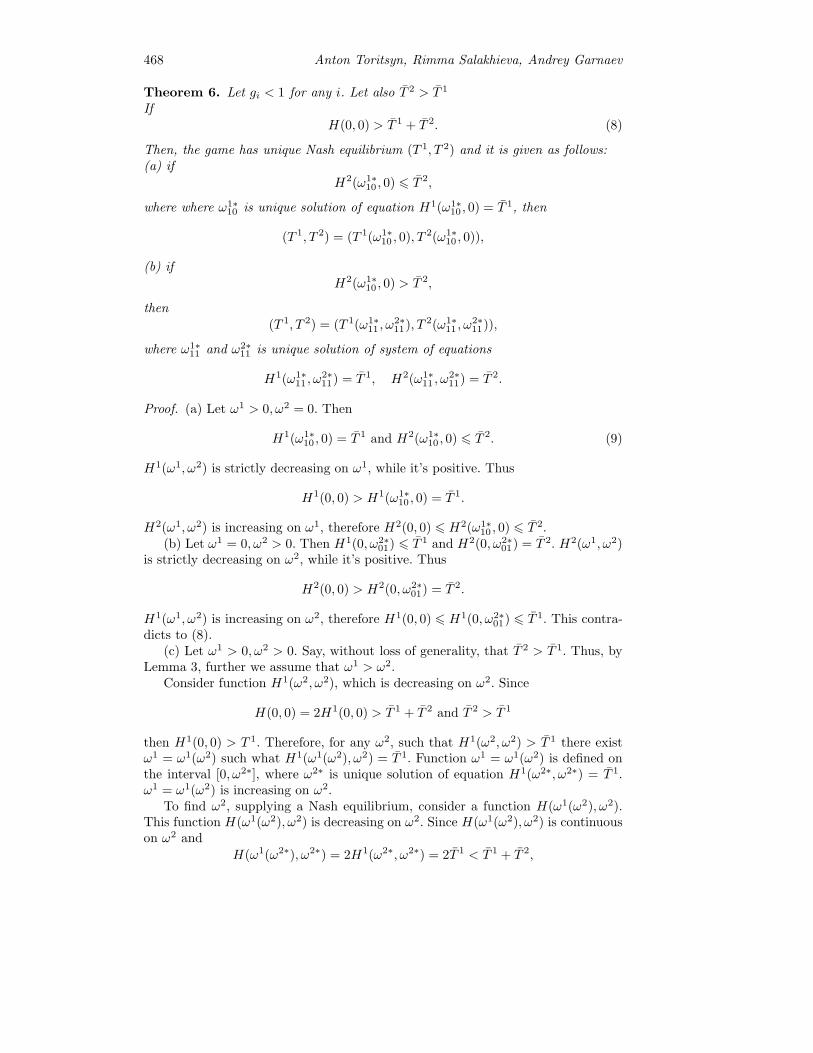
468 Anton Toritsyn, Rimma Salakhieva, Andrey Garnaev
Theorem 6. Let gi < 1 for any i. Let also T 2 > T 1
If
H(0, 0) > T 1 + T 2. (8)
Then, the game has unique Nash equilibrium (T 1, T 2) and it is given as follows:(a) if
H2(ω1∗10 , 0) T 2,
where where ω1∗10 is unique solution of equation H1(ω1∗
10 , 0) = T 1, then
(T 1, T 2) = (T 1(ω1∗10 , 0), T 2(ω1∗
10 , 0)),
(b) if
H2(ω1∗10 , 0) > T 2,
then
(T 1, T 2) = (T 1(ω1∗11 , ω
2∗11), T 2(ω1∗
11 , ω2∗11)),
where ω1∗11 and ω2∗
11 is unique solution of system of equations
H1(ω1∗11 , ω
2∗11) = T 1, H2(ω1∗
11 , ω2∗11) = T 2.
Proof. (a) Let ω1 > 0, ω2 = 0. Then
H1(ω1∗10 , 0) = T 1 and H2(ω1∗
10 , 0) T 2. (9)
H1(ω1, ω2) is strictly decreasing on ω1, while it’s positive. Thus
H1(0, 0) > H1(ω1∗10 , 0) = T 1.
H2(ω1, ω2) is increasing on ω1, therefore H2(0, 0) H2(ω1∗10 , 0) T 2.
(b) Let ω1 = 0, ω2 > 0. Then H1(0, ω2∗01) T 1 and H2(0, ω2∗
01) = T 2. H2(ω1, ω2)is strictly decreasing on ω2, while it’s positive. Thus
H2(0, 0) > H2(0, ω2∗01) = T 2.
H1(ω1, ω2) is increasing on ω2, therefore H1(0, 0) H1(0, ω2∗01) T 1. This contra-
dicts to (8).(c) Let ω1 > 0, ω2 > 0. Say, without loss of generality, that T 2 > T 1. Thus, by
Lemma 3, further we assume that ω1 > ω2.Consider function H1(ω2, ω2), which is decreasing on ω2. Since
H(0, 0) = 2H1(0, 0) > T 1 + T 2 and T 2 > T 1
then H1(0, 0) > T 1. Therefore, for any ω2, such that H1(ω2, ω2) > T 1 there existω1 = ω1(ω2) such what H1(ω1(ω2), ω2) = T 1. Function ω1 = ω1(ω2) is defined onthe interval [0, ω2∗], where ω2∗ is unique solution of equation H1(ω2∗, ω2∗) = T 1.ω1 = ω1(ω2) is increasing on ω2.
To find ω2, supplying a Nash equilibrium, consider a function H(ω1(ω2), ω2).This function H(ω1(ω2), ω2) is decreasing on ω2. Since H(ω1(ω2), ω2) is continuouson ω2 and
H(ω1(ω2∗), ω2∗) = 2H1(ω2∗, ω2∗) = 2T 1 < T 1 + T 2,
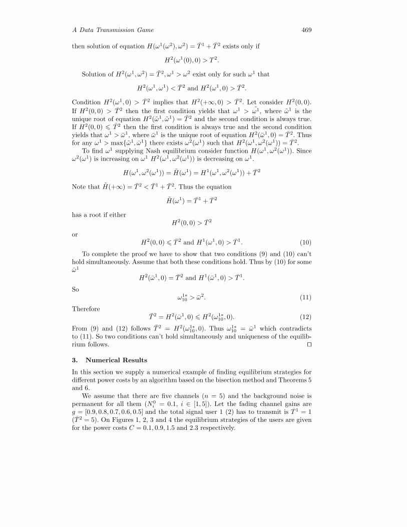
A Data Transmission Game 469
then solution of equation H(ω1(ω2), ω2) = T 1 + T 2 exists only if
H2(ω1(0), 0) > T 2.
Solution of H2(ω1, ω2) = T 2, ω1 > ω2 exist only for such ω1 that
H2(ω1, ω1) < T 2 and H2(ω1, 0) > T 2.
Condition H2(ω1, 0) > T 2 implies that H2(+∞, 0) > T 2. Let consider H2(0, 0).
If H2(0, 0) > T 2 then the first condition yields that ω1 > ω1, where ω1 is theunique root of equation H2(ω1, ω1) = T 2 and the second condition is always true.If H2(0, 0) T 2 then the first condition is always true and the second conditionyields that ω1 > ω1, where ω1 is the unique root of equation H2(ω1, 0) = T 2. Thusfor any ω1 > max{ω1, ω1} there exists ω2(ω1) such that H2(ω1, ω2(ω1)) = T 2.
To find ω1 supplying Nash equilibrium consider function H(ω1, ω2(ω1)). Sinceω2(ω1) is increasing on ω1 H2(ω1, ω2(ω1)) is decreasing on ω1.
H(ω1, ω2(ω1)) = H(ω1) = H1(ω1, ω2(ω1)) + T 2
Note that H(+∞) = T 2 < T 1 + T 2. Thus the equation
H(ω1) = T 1 + T 2
has a root if eitherH2(0, 0) > T 2
orH2(0, 0) T 2 and H1(ω1, 0) > T 1. (10)
To complete the proof we have to show that two conditions (9) and (10) can’thold simultaneously. Assume that both these conditions hold. Thus by (10) for someω1
H2(ω1, 0) = T 2 and H1(ω1, 0) > T 1.
Soω1∗10 > ω2. (11)
ThereforeT 2 = H2(ω1, 0) H2(ω1∗
10 , 0). (12)
From (9) and (12) follows T 2 = H2(ω1∗10 , 0). Thus ω1∗
10 = ω1 which contradictsto (11). So two conditions can’t hold simultaneously and uniqueness of the equilib-rium follows. ��
3. Numerical Results
In this section we supply a numerical example of finding equilibrium strategies fordifferent power costs by an algorithm based on the bisection method and Theorems 5and 6.
We assume that there are five channels (n = 5) and the background noise ispermanent for all them (N0
i = 0.1, i ∈ [1, 5]). Let the fading channel gains areg = [0.9, 0.8, 0.7, 0.6, 0.5] and the total signal user 1 (2) has to transmit is T 1 = 1(T 2 = 5). On Figures 1, 2, 3 and 4 the equilibrium strategies of the users are givenfor the power costs C = 0.1, 0.9, 1.5 and 2.3 respectively.
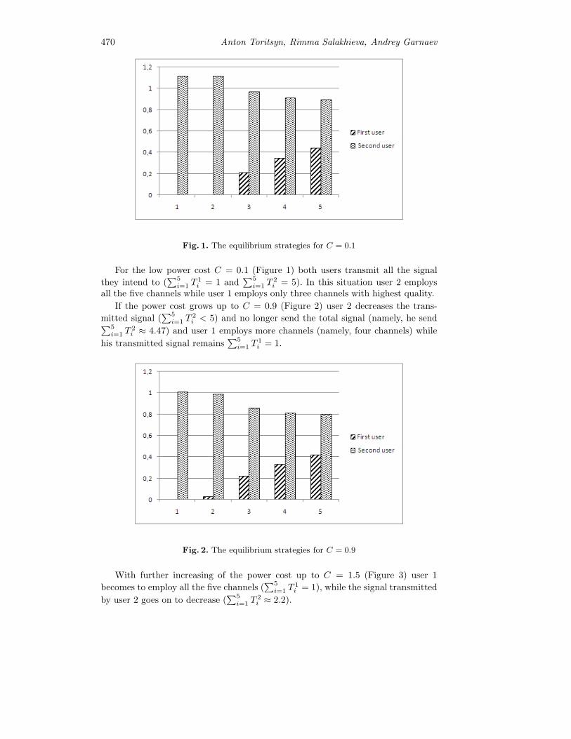
470 Anton Toritsyn, Rimma Salakhieva, Andrey Garnaev
Fig. 1. The equilibrium strategies for C = 0.1
For the low power cost C = 0.1 (Figure 1) both users transmit all the signal
they intend to (∑5
i=1 T1i = 1 and
∑5i=1 T
2i = 5). In this situation user 2 employs
all the five channels while user 1 employs only three channels with highest quality.
If the power cost grows up to C = 0.9 (Figure 2) user 2 decreases the trans-
mitted signal (∑5
i=1 T2i < 5) and no longer send the total signal (namely, he send∑5
i=1 T2i ≈ 4.47) and user 1 employs more channels (namely, four channels) while
his transmitted signal remains∑5i=1 T
1i = 1.
Fig. 2. The equilibrium strategies for C = 0.9
With further increasing of the power cost up to C = 1.5 (Figure 3) user 1
becomes to employ all the five channels (∑5
i=1 T1i = 1), while the signal transmitted
by user 2 goes on to decrease (∑5
i=1 T2i ≈ 2.2).
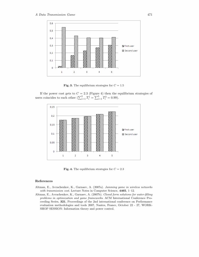
A Data Transmission Game 471
Fig. 3. The equilibrium strategies for C = 1.5
If the power cost gets to C = 2.3 (Figure 4) then the equilibrium strategies of
users coincides to each other (∑5
i=1 T1i =
∑5i=1 T
2i = 0.99).
Fig. 4. The equilibrium strategies for C = 2.3
References
Altman, E., Avrachenkov, K., Garnaev, A. (2007a). Jamming game in wireless networkswith transmission cost. Lecture Notes in Computer Science, 4465, 1–12.
Altman, E., Avrachenkov, K., Garnaev, A. (2007b). Closed form solutions for water-fillingproblems in optimization and game frameworks. ACM International Conference Pro-ceeding Series, 321, Proceedings of the 2nd international conference on Performanceevaluation methodologies and tools 2007, Nantes, France, October 22 - 27, WORK-SHOP SESSION: Information theory and power control.
472 Anton Toritsyn, Rimma Salakhieva, Andrey Garnaev
Altman, E., Avrachenkov, K., Garnaev, A. (2010). Closed form solutions for water-fillingproblem in optimization and game frameworks. Telecommunication Systems Journal,(forthcomming).
Lai, L. and H. El Gamal (2005). The water-filling game in fading multiple ac-cess channels, submitted to IEEE Trans. Information Theory, available athttp://www.ece.osu.edu/ helgamal/.
Lin, C. R. and M. Gerla (1997). Adaptive clustering for mobile wireless networks. IEEEJSAC, 15(7), 1265–1275.
Luo, Z.-Q. and J.-S. Pang (2006). Analysis of iterative waterfilling algorithm for multiuserpower control in digital subscriber lines. EURASIP Journal on Applied Signal Process-ing.
Popescu, O. and C. Rose (2003). Water filling may not good neighbors make in Proceedingsof GLOBECOM 2003, 3, 1766–1770.
Popescu, D.C., O. Popescu and C. Rose (2004). Interference avoidance versus iterativewater filling in multiaccess vector channels, in Proceedings of IEEE VTC 2004 Fall, 3,2058–2062.
Yu, W. (2002). Competition and cooperation in multi-user communication environements.PhD Thesis, Stanford University.
Yu, W., G. Ginis and J.M. Cioffi (2002). Distributed multiuser power control for digitalsubscriber lines. IEEE JSAC, 20, 1105–1115.
Strict Proportional Power and Fair Voting Rules inCommittees�
Frantisek Turnovec1
Charles University in Prague,Institute of Economic Studies,
Opletalova 26, 110 000 Prague 1, Czech RepublicE-mail: [email protected]
Abstract. In simple weighted committees with a finite number n of mem-bers, fixed weights and changing quota, there exists a finite number r ofdifferent quota intervals of stable power (r ≤ 2n − 1) with the same sets ofwinning coalitions for all quotas from each of them. If in a committee thesets of winning coalitions for different quotas are the same, then the powerindices based on pivots, swings, or minimal winning coalitions are also thesame for those quotas. If the fair distribution of voting weights is defined,then the fair distribution of voting power means to find a quota that mini-mizes the distance between relative voting weights and relative voting power(optimal quota). The problem of the optimal quota has an exact solutionvia the finite number of quotas from different intervals of stable power.
Keywords: Fairness, optimal quota, simple weighted committee, strict pro-portional power, voting and power indices
AMS Classification: 91A12, 91A40, 05C65
JEL Classification: C71, D72, H77
1. Introduction
Let us consider a committee with n members. Each member has some voting weight(number of votes, shares etc.) and a voting rule is defined by a minimal number ofweights required for passing a proposal. Given a voting rule, voting weights providecommittee members with voting power. Voting power means an ability to influencethe outcome of voting. Voting power indices are used to quantify the voting power.
The concept of fairness is being discussed related to the distribution of votingpower among different actors of voting. This problem was clearly formulated byNurmi (1982, p. 204): “If one aims at designing collective decision-making bodieswhich are democratic in the sense of reflecting the popular support in terms ofthe voting power, we need indices of the latter which enable us to calculate forany given distribution of support and for any decision rule the distribution of seatsthat is ‘just’. Alternatively, we may want to design decision rules that – given thedistribution of seats and support—lead to a distribution of voting power which isidentical with the distribution of support.”
Voting power is not directly observable: as a proxy for it voting weights areused. Therefore, fairness is usually defined in terms of voting weights (e.g. voting
� This research was supported by the Grant Agency of the Czech Republic, project No.402/09/1066 “Political economy of voting behavior, rational voters’ theory and modelsof strategic voting” and by the Max Planck Institute of Economics in Jena. The authorwould like to thank Manfred J. Holler for valuable comments to an earlier version of thepaper.

474 Frantisek Turnovec
weights are proportional to the results of an election). Assuming that a principleof fair distribution of voting weights is selected, we are addressing the question ofhow to achieve equality of voting power (at least approximately) to relative votingweights. The concepts of strict proportional power and the randomized decisionrule introduced by Holler (1982a, 1985, 1987), of optimal quota of S�lomczynski andZyczkowski (2007), and of intervals of stable power (Turnovec, 2008b) are used tofind, given voting weights, a voting rule minimizing the distance between actors’voting weights and their voting power.
Concept of fairness is frequently associated with so-called square root rule, at-tributed to British statistician Lionel Penrose (1946). The square root rule is closelyrelated to indirect voting power measured by the Penrose-Banzhaf power index.1
Different aspects of the square root rule have been analysed in Felsenthal and Ma-chover (1998, 2004), Laruelle and Widgren (1998), Baldwin and Widgren (2004),Turnovec (2009). The square root rule of “fairness” in the EU Council of Min-isters voting was discussed and evaluated in Felsenthal and Machover (2007),S�lomczynski and Zyczkowski (2006, 2007), Hosli (2008), Leech and Aziz (2008),Turnovec (2008a) and others. Nurmi (1997a) used it to evaluate the representationof voters’ groups in the European Parliament.
In the second section basic definitions are introduced and the applied powerindices methodology is shortly resumed. The third section introduces concepts ofquota intervals of stable power, index of fairness and exact optimal quota. While theframework of the analysis of fairness is usually restricted to the Penrose-Banzhafconcept of power, we are treating it in a more general setting and our results arerelevant for any power index based on pivots or swings and for any concept offairness.
2. Committees and Voting Power
A simple weighted committee is a pair [N,w], where N be a finite set of n committeemembers i = 1, 2, . . . , n, and w = (w1, w2, . . . , wn) be a nonnegative vector ofcommittee members’ voting weights (e.g. votes or shares). By 2N we denote thepower set of N (set of all subsets of N). By voting coalition we mean an elementS ∈ 2N , the subset of committee members voting uniformly (YES or NO), andw(S) =
∑i∈S
wi denotes the voting weight of coalition S. The voting rule is defined
by quota q satisfying 0 < q ≤ w(N), where q represents the minimal total weightnecessary to approve the proposal. Triple [N, q,w] we call a simple quota weighted
1 The square root rule is based on the following propositions: Let us assume n units withpopulation p1, p2, . . ., pn, and the system of representation by a super-unit committeewith voting weights w1, w2, . . ., wn of units’ representations. It can be rigorously provedthat for sufficiently large pi the absolute Penrose-Banzhaf power of individual citizenof unit i in unit’s referendum is proportional to the square root of pi. If the relativePenrose-Banzhaf voting power of unit i representation is proportional to its votingweight, then indirect voting power of each individual citizen of unit i is proportionalto the product of voting weight wi and square root of population pi. Based on theconjecture (not rigorously proved) that for n large enough the relative voting power isproportional to the voting weights, the square root rule concludes that the voting weightsof units’ representations in the super-unit committee proportional to square roots ofunits’ population lead to the same indirect voting power of each citizen independentlyof the unit she is affiliated with.

Strict Proportional Power and Fair Voting Rules in Committees 475
committee. The voting coalition S in committee [N, q,w] is called a winning one ifw(S) ≥ q and a losing one in the opposite case. The winning voting coalition S iscalled critical if there exists at least one member k ∈ S such that w(S\k) < q (wesay that k is critical in S). The winning voting coalition S is called minimal if anyof its members is critical in S.
A priori voting power analysis seeks an answer to the following question: Givena simple quota weighted committee [N, q,w], what is an influence of its membersover the outcome of voting? The absolute voting power of a member i is defined asa probability Πi[N, q,w] that i will be decisive in the sense that such a situationappears in which she would be able to decide the outcome of voting by her vote(Nurmi, 1997b and Turnovec, 1997), and a relative voting power as:
πi[N, q, w] =Πi[N, q, w]∑
k∈NΠk[N, q, w]
.
Three basic concepts of decisiveness are used: swing position, pivotal positionand membership in a minimal winning coalition (MWC position). The swing positionis an ability of an individual voter to change the outcome of voting by a unilateralswitch from YES to NO (if member j is critical with respect to a coalition S, we saythat he has a swing in S). The pivotal position is such a position of an individualvoter in a permutation of voters expressing a ranking of attitudes of members to thevoted issue (from the most preferable to the least preferable) and the correspondingorder of forming of the winning coalition, in which her vote YES means a YESoutcome of voting and her vote NO means a NO outcome of voting (we say thatj is pivotal in the permutation considered). The MWC position is an ability of anindividual voter to contribute to a minimal winning coalition (membership in theminimal winning coalition).
Let us denote by W (N, q,w) the set of all winning coalitions and by Wi(N, q,w)the set of all winning coalitions with i, C(N, q,w) as the set of all critical winningcoalitions, and by Ci(N, q,w) the set of all critical winning coalitions i has the swingin, by P (N, q,w) the set of all permutations of N and Pi(N, q,w), the set of allpermutations i is pivotal in, M(N, q,w) the set of all minimal winning coalitions,and Mi(N, q, w) the set of all minimal winning coalitions with i. By card(S) wedenote the cardinality of S, card(∅) = 0.
Assuming many voting acts and all coalitions equally likely, it makes sense toevaluate the a priori voting power of each member of the committee by the proba-bility to have a swing, measured by the absolute Penrose-Banzhaf (PB) power index(Penrose, 1946; Banzhaf, 1965):
ΠPBi (N, q, w) =
card(Ci)
2n−1,
(card(Ci) is the number of all winning coalitions the member i has the swing in and2n−1 is the number of all possible coalitions with i). To compare the relative powerof different committee members, the relative form of the PB power index is used:
πPBi (N, q, w) =card(Ci)∑
k∈Ncard(Ck)
.
While the absolute PB is based on a well-established probability model (seee.g. Owen, 1972), its normalization (relative PB index) destroys this probabilistic
476 Frantisek Turnovec
interpretation, the relative PB index simply answers the question of what is thevoter i’s share in all possible swings.
Assuming many voting acts and all possible preference orderings equally likely,it makes sense to evaluate an a priori voting power of each committee member bythe probability of being in pivotal situation, measured by the Shaply-Shubik (SS)power index (Shapley and Shubik, 1954):
ΠSSi (N, q, w) =
card(Pi)
n!,
(card(Pi) is the number of all permutations in which the committee member i ispivotal, and n! is the number of all possible permutations of committee members).Since
∑i∈N
card(Pi) = n! it holds that:
πSSi (N, q,w) =card(Pi)∑
k∈Ncard(Pk)
=card(Pi)
n!,
i.e. the absolute and relative form of the SS-power index is the same.2
Assuming many voting acts and all possible coalitions equally likely, it makessense to evaluate the voting power of each committee member by the probability ofmembership in a minimal winning coalition, measured by the absolute Holler-Packel(HP) power index:
ΠHPi (N, q,w) =
card(Mi)
2n,
(card(Mi) is the number of all minimal winning coalitions with i, and 2n is thenumber of all possible coalitions).3 Originally the HP index was defined and isusually being presented in its relative form (Holler, 1982b; Holler and Packel, 1983)
πHPi (N, q,w) =card(Mi)∑
k∈Ncard(Mk)
.
2 Supporters of the Penrose-Banzhaf power concept sometimes reject the Shapley-Shubikindex as a measure of voting power. Their objections to the Shapley-Shubik power con-cept are based on the classification of power measures on so-called I-power (voter’spotential influence over the outcome of voting) and P-power (expected relative share ina fixed prize available to the winning group of committee members, based on cooperativegame theory) introduced by Felsenthal et al. (1998). The Shapley-Shubik power indexwas declared to represent P-power and as such is unusable for measuring influence invoting. We tried to show in Turnovec (2007) and Turnovec et al. (2008) that objectionsagainst the Shapley-Shubik power index, based on its interpretation as a P-power con-cept, are not sufficiently justified. Both Shapley-Shubik and Penrose-Banzhaf measurecould be successfully derived as cooperative game values, and at the same time bothof them can be interpreted as probabilities of being in some decisive position (pivot,swing) without using cooperative game theory at all.
3 The definition of an absolute HP power index is provided by the author (a similardefinition of absolute PB power can be found in Brueckner (2001), the only differenceis that we relate the number of MWC positions of member i to the total number ofcoalitions, not to the number of coalitions of which i is a member).
Strict Proportional Power and Fair Voting Rules in Committees 477
Above definition of the absolute HP index allows a clear probabilistic interpretation.Multiplying and dividing it by the card(M), we obtain:
card(Mi)
card(M)
card(M)
2n.
In this breakdown the first term gives the probability of being a member ofa minimal winning coalition, provided the MWC is formed, and the second termthe probability of forming a minimal winning coalition assuming that all votingcoalitions are equally likely. The relative HP index has the same problem with aprobabilistic interpretation as the relative PB index.4
In the literature there are still two other concepts of power indices: the Johnston(J) power index based on swings, and the Deagan-Packel (DP) power index, basedon membership in minimal winning coalitions.
The Johnston power index (Johnston, 1978) measures the power of a member ofa committee as a normalized weighted average of the number of her swings, usingas weights the reciprocals of the total number of swings in each critical winningcoalition (the swing members of the same winning coalition have the same power,which is equal to 1/[number of swing members]).
The Deegan-Packel power index (Deegan and Packel, 1978) measures the powerof a member of a committee as a normalized weighted average of the number of min-imal critical winning coalitions he is a member of, using as weights the reciprocalsof the size of each MCWC
It is difficult to provide some intuitively acceptable probabilistic interpretationfor relative J and DP power indices. They provide a normative scheme of the divisionof rents in the committee rather than a measure of an a priori power (and in thesense of Felsenthal and Machover (1998) classification they can be considered asmeasures of P power).
It can be easily seen that for any α > 0 and any power index based on swings,pivots or MWC positions it holds that Πi[N,αq, αw] = Πi[N, q,w]. Therefore,without the loss of generality, we shall assume throughout the text that
∑i∈N wi = 1
and 0 < q ≤ 1, using only relative weights and relative quotas in the analysis.
3. Quota Intervals of Stable Power, Fairness and Strict ProportionalPower
Let us formally define a few concepts we shall use later in this paper:
Definition 1. A simple weighted committee [N,w] has a property of strict propor-tional power with respect to a power index π, if there exists a voting rule q∗ suchthat π[N, q∗,w] = w, i.e. the relative voting power of committee members is equalto their relative voting weights.
In general, there is no reason to expect that such a voting rule exists. Hollerand Berg extended the concept of a strict proportional power in the model withrandomized voting rule.
4 For a discussion about the possible probabilistic interpretation of the relative PB andHP see Widgren (2001).
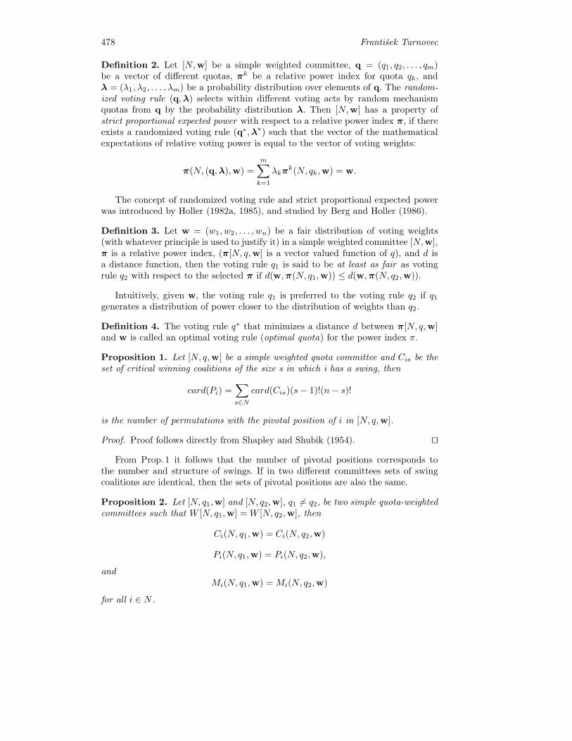
478 Frantisek Turnovec
Definition 2. Let [N,w] be a simple weighted committee, q = (q1, q2, . . . , qm)be a vector of different quotas, πk be a relative power index for quota qk, andλ = (λ1, λ2, . . . , λm) be a probability distribution over elements of q. The random-ized voting rule (q,λ) selects within different voting acts by random mechanismquotas from q by the probability distribution λ. Then [N,w] has a property ofstrict proportional expected power with respect to a relative power index π, if thereexists a randomized voting rule (q∗,λ∗) such that the vector of the mathematicalexpectations of relative voting power is equal to the vector of voting weights:
π(N, (q,λ),w) =m∑k=1
λkπk(N, qk,w) = w.
The concept of randomized voting rule and strict proportional expected powerwas introduced by Holler (1982a, 1985), and studied by Berg and Holler (1986).
Definition 3. Let w = (w1, w2, . . . , wn) be a fair distribution of voting weights(with whatever principle is used to justify it) in a simple weighted committee [N,w],π is a relative power index, (π[N, q,w] is a vector valued function of q), and d isa distance function, then the voting rule q1 is said to be at least as fair as votingrule q2 with respect to the selected π if d(w,π(N, q1,w)) ≤ d(w,π(N, q2,w)).
Intuitively, given w, the voting rule q1 is preferred to the voting rule q2 if q1generates a distribution of power closer to the distribution of weights than q2.
Definition 4. The voting rule q∗ that minimizes a distance d between π[N, q,w]and w is called an optimal voting rule (optimal quota) for the power index π.
Proposition 1. Let [N, q,w] be a simple weighted quota committee and Cis be theset of critical winning coalitions of the size s in which i has a swing, then
card(Pi) =∑s∈N
card(Cis)(s− 1)!(n− s)!
is the number of permutations with the pivotal position of i in [N, q,w].
Proof. Proof follows directly from Shapley and Shubik (1954). ��
From Prop. 1 it follows that the number of pivotal positions corresponds tothe number and structure of swings. If in two different committees sets of swingcoalitions are identical, then the sets of pivotal positions are also the same.
Proposition 2. Let [N, q1,w] and [N, q2,w], q1 = q2, be two simple quota-weightedcommittees such that W [N, q1,w] = W [N, q2,w], then
Ci(N, q1,w) = Ci(N, q2,w)
Pi(N, q1,w) = Pi(N, q2,w),
andMi(N, q1,w) = Mi(N, q2,w)
for all i ∈ N .

Strict Proportional Power and Fair Voting Rules in Committees 479
Proof. Without a loss of generality suppose q1 > q2. Assuming that the statement ofthe proposition is not true, i.e. a member k from S has a swing in S for quota q2 anddoes not have a swing for quota q1, we obtain w(S\k)−q2 < 0 and w(S\k)−q1 ≥ 0,hence S\k /∈W (N, q2, w) and S\k ∈W (N, q1, w), which contradicts the assumptionof Prop. 2 that the sets of winning coalitions are equal. From Prop. 1 it follows thatCi(N, q1,w) = Ci(N, q2,w) implies Pi(N, q1, w) = Pi(N, q2,w). In a similar way wecan prove identity for sets of minimal winning coalitions. Assuming that M is theminimal winning coalition for q2 and is not a minimal winning coalition for q1, wehave w(S)− q2 ≥ 0 and for any i ∈ S w(S\i)− q2 < 0, and there exists at least onek ∈ S such that w(S\k) − q1 ≥ 0. But in this case S\k is the losing coalition forq2 and the winning coalition for q1 what contradicts the assumption of Prop. 2 thatthe sets of winning coalitions are the same, hence Mi(N, q1,w) = Mi(N, q2,w). ��
From Prop. 2 it follows that in two different committees with the same set ofmembers, the same weights and the same sets of winning coalitions, the PB-powerindices, SS-power indices and HP-power indices are the same in both committees, in-dependently of quotas. Moreover, since the J-index is based on the concept of swingand the DP power index is based on membership in minimal winning coalitions, theJ and DP indices are also the same.
Proposition 3. Let [N, q,w] be a simple quota weighted committee with a quota q,
μ+(q) = minS∈W [N,q,w]
(w(S) − q)
andμ−(q) = min
S∈2N\W (N,q,w)(q − w(S)).
Then for any particular quota q we have W [N, q,w] = W [N, γ,w] for all γ ∈(q − μ−(q), q + μ+(q)].
Proof. (a) Let S ∈W [N, q,w], then from the definition of μ+(q)
w(S)− q ≥ μ+(q) ≥ 0⇒ w(S) − q − μ+(q) ≥ 0⇒ S ∈W (N, q + μ+, w),
hence S is winning for quota q + μ+(q). If S is winning for q + μ+(q), then it iswinning for any quota γ ≤ q + μ+(q).
(b) Let S ∈ 2N\W [N, q,w], then from the definition of μ−(q)
q −w(S) ≥ μ−(q) ≥ 0⇒ q − μ−(q)−w(s) ≥ 0⇒ S ∈ 2N\W (N, q − μ−(q), w),
hence S is losing for quota q − μ−(q). If S is losing for q − μ−(q), then it islosing for any quota γ ≥ q − μ−(q).
From (a) and (b) it follows that for any γ ∈ (q − μ−(q), (q − μ+(q)]
S ∈ W (N, q,w) ⇒ S ∈ W (N, γ,w)S ∈ {2N\W (N, γ,w)} ⇒ S ∈ {2N\W (N, q,w)}
which implies that W (N, q,w) = W (N, γ,w). ��
From Prop. 2 and 3 it follows that swing, pivot and MWC-based power indicesare the same for all quotas γ ∈ (q − μ−(q), q + μ+(q)]. Therefore the interval ofquotas (q− μ−(q), q + μ+(q)] we call an interval of stable power for quota q. Quotaγ∗ ∈ (q − μ−(q), q + μ+(q)] is called the marginal quota for q if μ+(γ∗) = 0.

480 Frantisek Turnovec
Example 1. Consider a committee [N, q,w] where n = 3, w1 = 0.1, w2 = 0.4, w3 =0.5. Then 2N = (∅, {1}, {2}, {3}, {1, 2}, {1, 3}, {2, 3}, {1, 2, 3}). Consider a simplemajority quota q = 0.51. Then:
W [N, q, w] = ({1, 3}, {2, 3}, {1, 2, 3})2N\W [N, q, w] = (∅, {1}, {2}, {3}, {1, 2})μ+(q) = min{w1 + w3 − 0.51 = 0.09, w2 + w3 − 0.51 = 0.39,
w1 + w2 + w3 − 0.51 = 0.49} = 0.09μ−(q) = min{0.51− w1 = 0.41, 0.51− w2 = 0.11, 0.51− w3 = 0.01,
0.51− w1 − w2 = 0.01} = 0.01
The quota interval of stable power for quota q = 0.51 is (0.5, 0.6]. The marginalquota for q = 0.51 is γ∗ = 0.6.
Now we define a partition of the power set 2N into equal weight classesΩ0, Ω1, . . . , Ωr (such that the weight of different coalitions from the same class isthe same and the weights of different coalitions from different classes are different).For the completeness set w(∅) = 0. Consider the weight-increasing ordering of equalweight classes Ω(0), Ω(1), . . . , Ω(r) such that for any t < k and S ∈ Ω(t), R ∈ Ω(k)it holds that w(S) < w(R). Denote qt = w(S) for any S ∈ Ω(t), t = 1, 2, . . . , r.
Proposition 4. Let Ω(0), Ω(1), . . . , Ω(r) be the weight-increasing ordering of theequal weight partition of 2N . Set qt = w(S) for any S ∈ Ω(t), t = 0, 1, 2, . . . , r.Then there is a finite number r ≤ 2n − 1 of marginal quotas qt and correspondingintervals of stable power (qt−1, qt] such that W [N, qt,w] ⊂W [N, qt−1,w].
Proof. Proof follows from the fact that card(2N ) = 2n and an increasing series of kreal numbers a1, . . . , ak subdivides interval (a1, ak] into k−1 segments. An analysisof voting power as a function of the quota (given voting weights) can be substitutedby an analysis of voting power in a finite number of marginal quotas. ��
From Prop. 4 it follows that there exists at most r distinct voting situationsgenerating r vectors of power indices.
Example 2. In the committee from Example 1 enumerate equal weight classes ofvoting coalitions in the weight-increasing order (see Table 1):
Table 1. Equal weight classes of coalitions
t W (t) w(S) Intervals Marginal quotas
0 ∅ 01 {1} 0.1 (0,0.1] 0.12 {2} 0.4 (0.1,0.4] 0.43 {1,2},{3} 0.5 (0.4,0.5] 0.54 {1,3} 0.6 (0.5,0.6] 0.65 {2,3} 0.9 (0.6,0.9] 0.96 {1,2,3} 1 (0.9,1] 1
In this committee we have seven classes of equal weight voting coalitions orderedby weights and r = 6 intervals of stable power and corresponding marginal quotas.
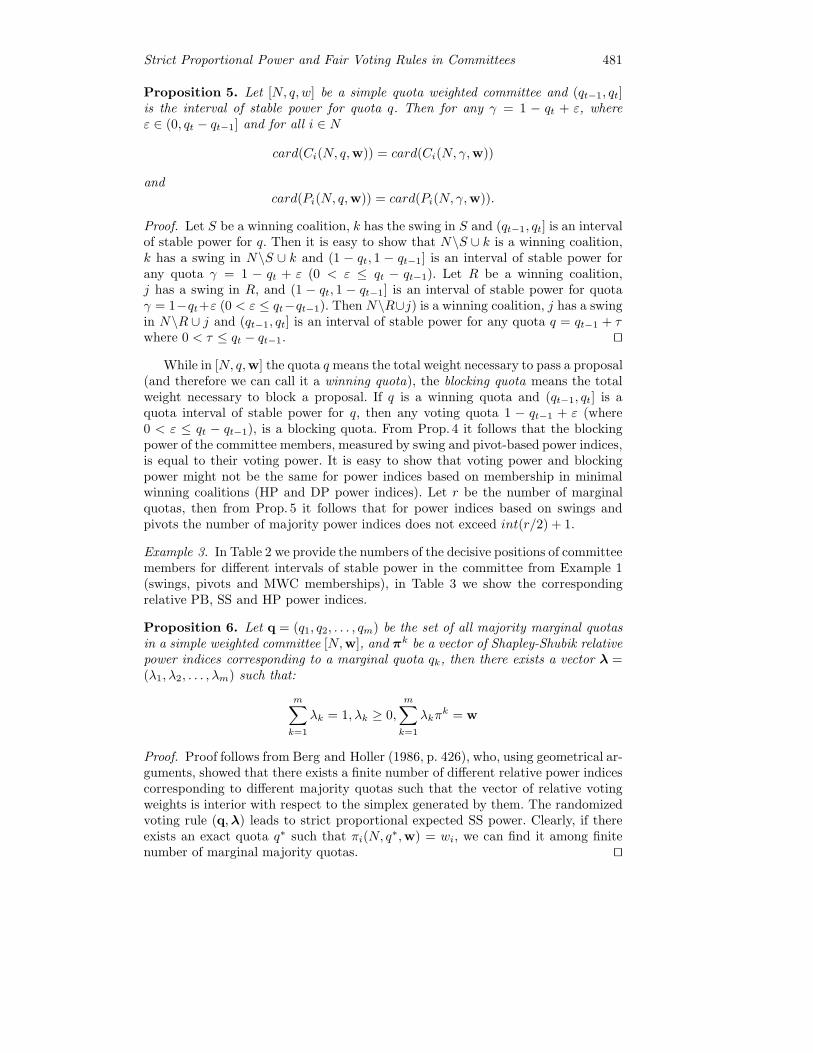
Strict Proportional Power and Fair Voting Rules in Committees 481
Proposition 5. Let [N, q, w] be a simple quota weighted committee and (qt−1, qt]is the interval of stable power for quota q. Then for any γ = 1 − qt + ε, whereε ∈ (0, qt − qt−1] and for all i ∈ N
card(Ci(N, q,w)) = card(Ci(N, γ,w))
andcard(Pi(N, q,w)) = card(Pi(N, γ,w)).
Proof. Let S be a winning coalition, k has the swing in S and (qt−1, qt] is an intervalof stable power for q. Then it is easy to show that N\S ∪ k is a winning coalition,k has a swing in N\S ∪ k and (1 − qt, 1 − qt−1] is an interval of stable power forany quota γ = 1 − qt + ε (0 < ε ≤ qt − qt−1). Let R be a winning coalition,j has a swing in R, and (1 − qt, 1 − qt−1] is an interval of stable power for quotaγ = 1−qt+ε (0 < ε ≤ qt−qt−1). Then N\R∪j) is a winning coalition, j has a swingin N\R ∪ j and (qt−1, qt] is an interval of stable power for any quota q = qt−1 + τwhere 0 < τ ≤ qt − qt−1. ��
While in [N, q,w] the quota q means the total weight necessary to pass a proposal(and therefore we can call it a winning quota), the blocking quota means the totalweight necessary to block a proposal. If q is a winning quota and (qt−1, qt] is aquota interval of stable power for q, then any voting quota 1 − qt−1 + ε (where0 < ε ≤ qt − qt−1), is a blocking quota. From Prop. 4 it follows that the blockingpower of the committee members, measured by swing and pivot-based power indices,is equal to their voting power. It is easy to show that voting power and blockingpower might not be the same for power indices based on membership in minimalwinning coalitions (HP and DP power indices). Let r be the number of marginalquotas, then from Prop. 5 it follows that for power indices based on swings andpivots the number of majority power indices does not exceed int(r/2) + 1.
Example 3. In Table 2 we provide the numbers of the decisive positions of committeemembers for different intervals of stable power in the committee from Example 1(swings, pivots and MWC memberships), in Table 3 we show the correspondingrelative PB, SS and HP power indices.
Proposition 6. Let q = (q1, q2, . . . , qm) be the set of all majority marginal quotasin a simple weighted committee [N,w], and πk be a vector of Shapley-Shubik relativepower indices corresponding to a marginal quota qk, then there exists a vector λ =(λ1, λ2, . . . , λm) such that:
m∑k=1
λk = 1, λk ≥ 0,
m∑k=1
λkπk = w
Proof. Proof follows from Berg and Holler (1986, p. 426), who, using geometrical ar-guments, showed that there exists a finite number of different relative power indicescorresponding to different majority quotas such that the vector of relative votingweights is interior with respect to the simplex generated by them. The randomizedvoting rule (q,λ) leads to strict proportional expected SS power. Clearly, if thereexists an exact quota q∗ such that πi(N, q∗,w) = wi, we can find it among finitenumber of marginal majority quotas. ��
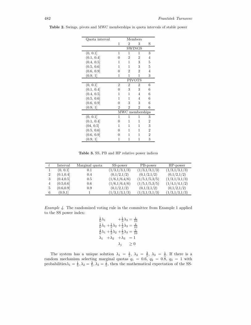
482 Frantisek Turnovec
Table 2. Swings, pivots and MWC memberships in quota intervals of stable power
Quota interval Members1 2 3 S
SWINGS
(0, 0.1] 1 1 1 3(0.1, 0.4] 0 2 2 4(0.4, 0.5] 1 1 3 5(0.5, 0.6] 1 1 3 5(0.6, 0.9] 0 2 2 4(0.9, 1] 1 1 1 3
PIVOTS
(0, 0.1] 2 2 2 6(0.1, 0.4] 0 3 3 6(0.4, 0.5] 1 1 4 6(0.5, 0.6] 1 1 4 6(0.6, 0.9] 0 3 3 6(0.9, 1] 2 2 2 6
MWC memberships
(0, 0.1] 1 1 1 3(0.1, 0.4] 0 1 1 2(04, 0.5] 1 1 1 3(0.5, 0.6] 0 1 1 2(0.6, 0.9] 0 1 1 2(0.9, 1] 1 1 1 3
Table 3. SS, PB and HP relative power indices
t Interval Marginal quota SS-power PB-power HP-power
1 (0, 0.1] 0.1 (1/3,1/3,1/3) (1/3,1/3,1/3) (1/3,1/3,1/3)2 (0.1,0.4] 0.4 (0,1/2,1/2) (0,1/2,1/2) (0,1/2,1/2)3 (0.4,0.5] 0.5 (1/6,1/6,4/6) (1/5,1/5,3/5) (1/3,1/3,1/3)4 (0.5,0.6] 0.6 (1/6,1/6,4/6) (1/5,1/5,3/5) (1/4,1/4,1/2)5 (0.6,0.9] 0.9 (0,1/2,1/2) (0,1/2,1/2) (0,1/2,1/2)6 (0.9,1] 1 (1/3,1/3,1/3) (1/3,1/3,1/3) (1/3,1/3,1/3)
Example 4. The randomized voting rule in the committee from Example 1 appliedto the SS power index:
16λ1 + 1
3λ3 = 110
16λ1 + 1
2λ2 + 13λ3 = 4
1046λ1 + 1
2λ2 + 13λ3 = 5
10
λ1 +λ2 +λ3 = 1
λj ≥ 0
The system has a unique solution λ1 = 15 , λ2 = 3
5 , λ3 = 15 . If there is a
random mechanism selecting marginal quotas q1 = 0.6, q2 = 0.8, q3 = 1 withprobabilitiesλ1 = 1
5 , λ2 = 35 , λ3 = 1
5 , then the mathematical expectation of the SS-

Strict Proportional Power and Fair Voting Rules in Committees 483
power of the members of the committee will be equal to their relative weights (weobtain the case of strict proportional power).
Although we can apply a randomized voting rule to any relative power index,based on pivots and swings, the problem is with the interpretation of what weget For instance, the relative PB index has no probabilistic interpretation, and therandomized voting rule calculated for it by Prop. 6 does not provide the mathemat-ical expectation of the number of swings, leading to a relative PB power equal toweights.
Example 5. We can easily verify that
λ1 =5
20, λ2 =
12
20, λ3 =
3
20
are the probabilities for a randomized voting rule equalizing relative PB power torelative voting weights in the committee from Example 1. The swings for majorityquotas and PB absolute power see in Table 4.
Table 4. Absolute PB power
SWINGS
Majority quotas Member 1 Member 2 Member 3 S
(0,5, 0,6] 1 1 3 5(0,6, 0,9] 0 2 2 4(0,9, 1] 1 1 1 3
ABSOLUTE PB POWER
(0,5, 0,6] 1/4 1/4 3/4 5/4(0,6, 0,9] 0 2/4 2/4 4/4(0,9, 1] 1/4 1/4 1/4 3/4
Applying a randomized voting rule equalizing the relative PB power to votingweights we obtain the mathematical expectation of absolute power⎛⎝1/4
1/43/4
⎞⎠ 5
20+
⎛⎝ 02/42/4
⎞⎠ 12
20+
⎛⎝1/41/41/4
⎞⎠ 3
20=
⎛⎝ 8/8032/8042/80
⎞⎠ ,
which yields an expected relative power⎛⎝ 8/8032/8042/80
⎞⎠ 1
82/80=
⎛⎝ 8/8232/8242/82
⎞⎠ =⎛⎝1/10
4/105/10
⎞⎠different from voting weights.
In general, the number of majority power indices can be greater than the numberof committee members, and the system
r∑k=1
λk = 1, λk ≥ 0,
r∑k=1
λkπk = w

484 Frantisek Turnovec
might not have the unique solution. To find the randomized voting rule leading tostrict proportional power we can use the following optimization problem:
minn∑i=1
abs(r∑k=1
πkλk − wi)
s.t.
r∑k=1
λk = 1, λk ≥ 0
that can be transformed into the equivalent linear programming problem(Gale, 1960):
minn∑i=1
yi
s.t.r∑
k=1
πki λk − yi ≤ wi for i = 1, . . . , n
r∑k=1
πki λk + yi ≥ wi for i = 1, . . . , n
r∑k=1
λk = 1
λk, yi ≥ 0 for k = 1, . . . , r, i = 1, . . . , n
This problem is easy to solve by standard linear programming simplex methods.One can hardly expect that randomized voting rules leading to the strict pro-
portional power would be adopted by actors in real voting systems. However, thedesign of a “fair” voting system can be based on an approximation provided bythe quota generating the minimal distance between vectors of power indices andweights, which is called an optimal quota.
The optimal quota was introduced by S�lomczynski and Zyczkowski (2006, 2007)as a quota minimizing the sum of square residuals between the power indices andthe voting weights by q ∈ (0.5, 1]
σ2(q) =∑i∈N
(πi[N, q,w]− wi)2.
S�lomczynski and Zyczkowski introduced the optimal quota concept within theframework of the so-called Penrose voting system as a principle of fairness in theEU Council of Ministers voting. Here power is measured by the Penrose-Banzhafpower index. The system consists of two rules (S�lomczynski and Zyczkowski, 2007,p. 393):
a) The voting weight attributed to each member of the voting body of size n isproportional to the square root of the population he or she represents;
b) The decision of the voting body is taken if the sum of the weights of memberssupporting it is not less than the optimal quota.
Looking for a quota providing a priori voting power “as close as possible” to thenormalized voting weights, S�lomczynski and Zyczkowski (2007) are minimizing thesum of square residuals between the power indices and voting power for q ∈ (0.5, 1].Using heuristic minimization of the sum of square residuals based on simulation

Strict Proportional Power and Fair Voting Rules in Committees 485
(with the data obtained numerically by averaging quotas over a sample of randomweights distributions), they propose the following heuristic approximation of thesolution for relative PB index:
q =1
2
(1 +
1√n
)≤ q ≤ 1
2
⎛⎝1 +
√∑i∈N
w2i
⎞⎠ = q.
Clearly q = q if and only if all the weights are equal, but in this case any majorityquota is optimal.
By the index of the fairness of a voting rule q in [N, q,w] we call:
ϕ(N, q,w) = 1−√
1
2
∑i
(πi[N, q,w]− wi)2.
It is easy to see that 0 ≤√
12
∑i
(πi[N, q,w]− wi)2 ≤ 1 (zero in the case of the
equality of weights and power, e.g. w1 = 1/2, w2 = 1/2, π1 = 1/2, π2 = 1/2, and1 in the case of an extreme inequality of weights and power, e.g. w1 = 1, w2 = 0,π1 = 0, π2 = 1), hence 0 ≤ ϕ(N, q, w) ≤ 1. We say that a voting rule q1 is “at leastas fair” as a voting rule q2 if ϕ(N, q1,w) ≥ ϕ(N, q2,w).5
Looking for a “fair” voting rule we can maximize ϕ, which is the same as tominimize σ2(q). Using marginal quotas and intervals of stable power we do notneed any simulation.
Proposition 7. Let [N, q, w] be a simple quota-weighted committee and πi(N, qt, w)be relative power indices for marginal quotas qt, and q∗t be the majority marginalquota minimizing ∑
i∈N(πi(N, qj ,w)− wi)
2
(j = 1, 2, . . . , r, r is the number of intervals of stable power such that qj are marginal
majority quotas), then the exact solution of S�lomczynski and Zyczkowski’s optimalquota (SZ optimal quota) problem for a particular power index used is any γ ∈(q∗t−1, q
∗t ] from the quota interval of stable power for q∗t .
Proof. Proof follows from the finite number of quota intervals of stable power(Prop. 5). The quota q∗ provides the best approximation of strict proportionalpower, that is related neither to a particular power measure nor to a specific prin-ciple of fairness. ��
Example 6. In Table 5 we provide the values of the index of fairness for the majoritymarginal quotas in the committee from Example 1.
The exact optimal marginal quota for the PB and SS power index is the same:q∗ = q5 = 0.9 (and all quotas q ∈ (0.6, 0.9]).
5 The index of fairness follows the same logic as measures of deviation from proportionalityused in political science to evaluate the difference between results of an election andthe composition of an elected body—e.g. Loosemore and Hanby (1971) is based on theabsolute values of the deviation metric, or Gallagher (1991) using a square roots metric.

486 Frantisek Turnovec
Table 5. Index of fairness
Shapley-Shubik relative powerMember Weight SS for q4=0.6 SS for q5=0.9 SS for q6=1
1 0.1 0.166667 0 0.3333332 0.4 0.166667 0.5 0.3333333 0.5 0.666667 0.5 0.333333∑
1 1 1 1
Index of fairness ϕ 0.791833 0.9 0.791833
Penrose-Banzhaf relative powerMember Weight PB for q4=0.6 PB for q5=0.9 PB for q6=1
1 0.1 0.2 0 0.3333332 0.4 0.2 0.5 0.3333333 0.5 0.6 0.5 0.333333∑
1 1 1 1
Index of fairness ϕ 0.826795 0.9 0.791833
The S�lomczynski and Zyczkowski heuristic approximation q = 0.79 ≤ q ≤ 0.82 =q is a part of the exact interval of the optimal quota, but the next example illustratesthat it might not be the case.
Example 7. Consider a committee of 4 members with weights (100/183, 49/183,25/183, 9/183) and majority marginal quotas q1 = 100/183, q2 = 109/183, q3 =125/183, q4 = 135/183, q5 = 149/183, q6 = 158/183, q7 = 174/183, q8 = 183/183.In Table 6 we provide the PB power indices for majority marginal quotas andcorresponding values of index of fairness ϕ.
Table 6. Heuristic optimal quota might not work
PB relative power indices for marginal quotasMembers q1 = 100
183q2 = 109
183q3 = 125
183q4 = 134
183q5 = 149
183q6 = 158
183q7 = 174
183q8 = 183
183
1 1 0.7 0.6 0.5 0.5 0.375 0.333 0.252 0 0.1 0.2 0.3 0.5 0.375 0.333 0.253 0 0.1 0.2 0.1 0 0.125 0.333 0.254 0 0.1 0 0.1 0 0.125 0 0.25
ϕ 0.726831 0.88205 0.94106 0.95781 0.8611 0.89186 0.84933 0.812
Comparing the values of index of fairness, we can see that optimal marginalquota in this case is q4 = 134/183 ≈ 0.3224, and the interval of stable power (opti-mal quotas) is (125/183, 134/183]≈ (0.68306, 0.73224), while the S�lomczynski andZyczkowski heuristic estimation gives an interval [0.75, 0.81283] that is completelyoutside of the exact solution.
4. Concluding Remarks
In simple quota weighted committees with a fixed number of members and votingweights there exists a finite number r of different quota intervals of stable power(r ≤ 2n − 1) generating a finite number of power indices vectors. For power indices
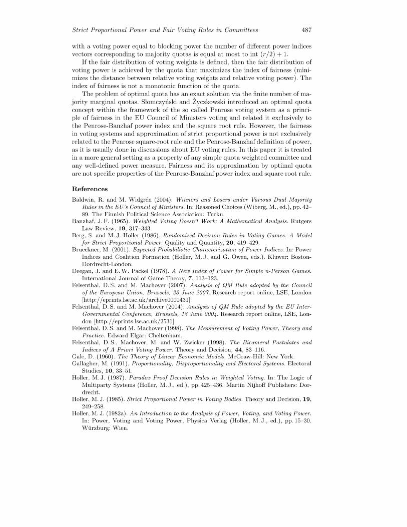
Strict Proportional Power and Fair Voting Rules in Committees 487
with a voting power equal to blocking power the number of different power indicesvectors corresponding to majority quotas is equal at most to int (r/2) + 1.
If the fair distribution of voting weights is defined, then the fair distribution ofvoting power is achieved by the quota that maximizes the index of fairness (mini-mizes the distance between relative voting weights and relative voting power). Theindex of fairness is not a monotonic function of the quota.
The problem of optimal quota has an exact solution via the finite number of ma-jority marginal quotas. S�lomczynski and Zyczkowski introduced an optimal quotaconcept within the framework of the so called Penrose voting system as a princi-ple of fairness in the EU Council of Ministers voting and related it exclusively tothe Penrose-Banzhaf power index and the square root rule. However, the fairnessin voting systems and approximation of strict proportional power is not exclusivelyrelated to the Penrose square-root rule and the Penrose-Banzhaf definition of power,as it is usually done in discussions about EU voting rules. In this paper it is treatedin a more general setting as a property of any simple quota weighted committee andany well-defined power measure. Fairness and its approximation by optimal quotaare not specific properties of the Penrose-Banzhaf power index and square root rule.
References
Baldwin, R. and M. Widgren (2004). Winners and Losers under Various Dual MajorityRules in the EU’s Council of Ministers. In: Reasoned Choices (Wiberg, M., ed.), pp. 42–89. The Finnish Political Science Association: Turku.
Banzhaf, J. F. (1965). Weighted Voting Doesn’t Work: A Mathematical Analysis. RutgersLaw Review, 19, 317–343.
Berg, S. and M. J. Holler (1986). Randomized Decision Rules in Voting Games: A Modelfor Strict Proportional Power. Quality and Quantity, 20, 419–429.
Brueckner, M. (2001). Expected Probabilistic Characterization of Power Indices. In: PowerIndices and Coalition Formation (Holler, M. J. and G. Owen, eds.). Kluwer: Boston-Dordrecht-London.
Deegan, J. and E. W. Packel (1978). A New Index of Power for Simple n-Person Games.International Journal of Game Theory, 7, 113–123.
Felsenthal, D. S. and M. Machover (2007). Analysis of QM Rule adopted by the Councilof the European Union, Brussels, 23 June 2007. Research report online, LSE, London[http://eprints.lse.ac.uk/archive0000431]
Felsenthal, D. S. and M. Machover (2004). Analysis of QM Rule adopted by the EU Inter-Governmental Conference, Brussels, 18 June 2004. Research report online, LSE, Lon-don [http://eprints.lse.ac.uk/2531]
Felsenthal, D. S. and M. Machover (1998). The Measurement of Voting Power, Theory andPractice. Edward Elgar: Cheltenham.
Felsenthal, D. S., Machover, M. and W. Zwicker (1998). The Bicameral Postulates andIndices of A Priori Voting Power. Theory and Decision, 44, 83–116.
Gale, D. (1960). The Theory of Linear Economic Models. McGraw-Hill: New York.Gallagher, M. (1991). Proportionality, Disproportionality and Electoral Systems. Electoral
Studies, 10, 33–51.Holler, M. J. (1987). Paradox Proof Decision Rules in Weighted Voting. In: The Logic of
Multiparty Systems (Holler, M. J., ed.), pp. 425–436. Martin Nijhoff Publishers: Dor-drecht.
Holler, M. J. (1985). Strict Proportional Power in Voting Bodies. Theory and Decision, 19,249–258.
Holler, M. J. (1982a). An Introduction to the Analysis of Power, Voting, and Voting Power.In: Power, Voting and Voting Power, Physica Verlag (Holler, M. J., ed.), pp. 15–30.Wurzburg: Wien.
488 Frantisek Turnovec
Holler, M. J. (1982b). Forming Coalitions and Measuring Voting Power. Political Studies,30, 262–271.
Holler, M. J. and E. Packel (1983). Power, Luck and the Right Index. Zeitschrift fur Na-tionalokonomie (Journal of Economics), 43, 21–29.
Hosli, M. O. (2008). Council Decision Rules and European Union Constitutional Design.AUCO Czech Economic Review, 2(1), 76–96.
Johnston, R. J. (1978). On the Measurement of Power: Some Reaction to Laver. Environ-ment and Planning, A10, 907–914.
Laruelle, A. and M. Widgren (1998). Is the Allocation of Voting Power among EU StatesFair?. Public Choice, 94, 317–339.
Leech, D. and H. Aziz (2008). The Double Majority Voting Rule of the EU Reform Treaty asa Democratic Ideal for an Enlarging Union: an Appraisal Using Voting Power Analysis.Presented at the 2008 EPCS meeting in Jena.
Loosemore, J. and V. J. Hanby (1971). The Theoretical Limits of Maximum Some Analyt-ical Expression for Electoral Systems. British Journal of Political Science, 1, 467–477.
Nurmi, H. (1982). The Problem of the Right Distribution of Voting Power. In: Power,Voting and Voting Power (Holler, M. J., ed.), pp. 203–212. Physica Verlag: Wurzburg,Wien.
Nurmi, H. (1997a). The Representation of Voter Groups in the European Parliament, APenrose-Banzhaf Index Analysis. Electoral Studies, 16, 317–322.
Nurmi, H. (1997b). On Power Indices and Minimal Winning Coalitions. Control and Cy-bernetics, 26(4), 609–611.
Owen, G. (1972). Multilinear Extensions of Games. Management Science, 18, 64–79.Penrose, L. S. (1946). The Elementary Statistics of Majority Voting. Journal of the Royal
Statistical Society, 109, 53–57.Shapley, L. S. and M. Shubik (1954). A Method for Evaluation the Distribution of Power
in a Committee System. American Political Science Review, 48, 787–792.S�lomczynski, W. and K. Zyczkowski (2007). From a Toy Model to Double Square Root
System. Homo Oeconomicus, 24(3-4), 381–400.S�lomczynski, W. and K. Zyczkowski (2006). Penrose Voting System and Optimal Quota.
Acta Physica Polonica B37(11), 3133–3143.Turnovec, F. (2009) Fairness and Squareness: Fair Decision Making Rules in the EU Coun-
cil. Badania Operacyjne i Decyzje, 4, 109–124.Turnovec, F. (2008a). National, Political and Institutional Influence in European Union
Decision Making. AUCO Czech Economic Review, 2(2), 154–173.Turnovec, F. (2008b). Efficiency of Fairness in Voting Systems. Homo Oeconomicus, 25(3-
4), 335–348.Turnovec, F. (2007). New Measure of Voting Power. AUCO Czech Economic Review, 1(1),
4–14.Turnovec, F., J. W Mercik and M. Mazurkiewicz (2008). Power Indices Methodology:
Decisiveness, Pivots and Swings. In: Power, Freedom and Voting, Essays in Honorof Manfred J. Holler (Braham, M. and F. Steffen, eds.), pp. 23–37. Springer Verlag:Berlin, Heidelberg.
Turnovec, F. (1997). Power, Power Indices and Intuition. Control and Cybernetics, 26(4),613–615.
Widgren, M. (2001). On the Probabilistic Relationship Between the Public Good Index andthe Normalized Banzhaf Index. In: Power Indices and Coalition Formation (Holler,M. J. and G. Owen, eds.). Kluwer: Boston-Dordrecht-London.

Subgame Consistent Solution for Random-HorizonCooperative Dynamic Games
David W.K. Yeung1 and Leon A. Petrosyan2
1 SRS Consortium for Advanced Study in Cooperative Dynamic GamesShue Yan University
andCenter of Game Theory, St Petersburg State University
E-mail: [email protected] Faculty of Applied Mathematics-Control Processes,
St Petersburg State UniversityE-mail: [email protected]
Abstract. In cooperative dynamic games a stringent condition – that ofsubgame consistency – is required for a dynamically stable cooperative solu-tion. In particular, a cooperative solution is subgame consistent if an exten-sion of the solution policy to a subgame starting at a later time with a statebrought about by prior optimal behavior would remain optimal. This paperextends subgame consistent solutions to dynamic (discrete-time) coopera-tive games with random horizon. In the analysis new forms of the Bellmanequation and the Isaacs-Bellman equation in discrete-time are derived. Sub-game consistent cooperative solutions are obtained for this class of dynamicgames. Analytically tractable payoff distribution mechanisms which lead tothe realization of these solutions are developed. This is the first time thatsubgame consistent solutions for cooperative dynamic games with randomhorizon are presented.
Keywords:Cooperative dynamic games, random horizon, subgame consis-tency.AMS Subject Classifications. Primary 91A12, Secondary 91A25.
1. Introduction
Cooperative games suggest the possibility of socially optimal and group efficientsolutions to decision problems involving strategic action. In cooperative dynamicgames a stringent condition – that of subgame consistency – is required for a dy-namically stable cooperative solution. In particular, a cooperative solution is sub-game consistent if an extension of the solution policy to a subgame starting at alater time with a state brought about by prior optimal behavior would remain op-timal. In particular dynamic consistency ensures that as the game proceeds playersare guided by the same optimality principle at each instant of time, and hence donot possess incentives to deviate from the previously adopted optimal behavior.A rigorous framework for the study of subgame-consistent solutions in cooperativestochastic differential games (which are in continuous-time) was established in Ye-ung and Petrosyan (2004 and 2006). A generalized theorem was developed for thederivation of an analytically tractable “payoff distribution procedure” leading todynamically consistent solutions. Cooperative games with subgame consistent so-lutions are presented in Petrosyan and Yeung (2007), Yeung (2007 and 2008), andYeung and Petrsoyan (2006).
490 David W.K. Yeung, Leon A. Petrosyan
In discrete-time dynamic games, Basar and Ho (1974) examined informationalproperties of the Nash solutions of stochastic nonzero-sum games and Basar (1978)developed equilibrium solution of linear-quadratic stochastic games with noisy ob-servation. Krawczyk and Tidball (2006) considered a dynamic game of water alloca-tion. Nie et al. (2006) considered dynamic programming approach to discrete timedynamic Stackelberg games. Dockner and Nishimura (1999) and Rubio and Ulph(2007) presented discrete-time dynamic game for pollution management. Dutta andRadner (2006) presented a discrete-time dynamic game used to study global warm-ing. Ehtamo and Hamalainen (1993) examined cooperative incentive equilibriumfor a dynamic resource game. Yeung and Petrosyan (2010) had developed a gener-alized theorem for the derivation of an analytically tractable “payoff distributionprocedure” leading to dynamically consistent solutions for cooperative stochasticdynamic games.
In this paper, we extend subgame consistent solutions to discrete-time dynamiccooperative games with random horizon. In many game situations, the terminaltime of the game is not known with certainty. Examples of this kind of problemsinclude uncertainty in the renewal of lease, the terms of offices of elected author-ities/directorships, contract renewal and continuation of agreements subjected toperiodic negotiations. Petrosyan and Murzov (1966) first developed the BellmanIsaacs equations under random horizon for zero-sum differential games. Petrosyanand Shevkoplyas (2003) gave the first analysis of dynamically consistent solutionsfor cooperative differential with random duration. Shevkoplyas (2011) consideredShapley value in cooperative differential games with random horizon. In this pa-per, a class of discrete-time dynamic games with random duration is formulated. Adynamic programming technique for solving inter-temporal problems with randomhorizon is developed to serve as the foundation of solving the game problem. Tocharacterize a noncooperative equilibrium, a set of random duration discrete-timeIsaacs-Bellman equations is derived.
Moreover, subgame consistent cooperative solutions are derived for dynamicgames with random horizon. Analytically tractable payoff distribution mechanismswhich lead to the realization of these solutions are derived. It represents the firstattempt to seek subgame consistent solution for cooperative dynamic games withrandom horizons. This analysis widens the application of cooperative dynamic gametheory to problems where the game horizon is random. The organization of the paperis as follows. Game formulation and derivation of dynamic programming techniquesfor random horizon problems are provided in Section 2. A feedback Nash equilibriumis characterized for dynamic games with random horizon in Section 3. Dynamiccooperation under random horizon is presented in Section 4. Subgame consistentsolutions and payment mechanism leading to these solutions are obtained in Section5. Concluding remarks are given in Section 6.
2. Game Formulation and Dynamic Programming with RandomHorizon
In this section, we first formulate a class of dynamic games with random duration.Then we develop a dynamic programming technique for solving inter-temporal prob-lems with random horizon which will serve as the foundation of solving the gameproblem.
Subgame Consistent Solution for Random-Horizon Cooperative Dynamic Games 491
2.1. Game Formulation
The n−person dynamic game to be considered is a T stage game where T is randomvariable with range {1, 2, · · · , T } and corresponding probabilities {θ1, θ2, · · · , θT }.Conditional upon the reaching of stage τ , the probability of the game would lastup to stages τ, τ + 1,· · · , T becomes respectively
θτT∑ζ=τ
θζ
,θτ+1
T∑ζ=τ
θζ
, · · · , θTT∑ζ=τ
θζ
.
The payoff of player i at stage k ∈ {1, 2, · · · , T } is gik[xk, u1k, u
2k, · · · , unk , xk+1].
When the game ends after stage T , player i will receive a terminal paymentqiT+1
(xT+1) in stage T + 1.
The state space of the game is X ∈ Rm and the state dynamics of the game ischaracterized by the difference equation:
xk+1 = fk(xk, u1k, u
2k, · · · , unk) (1)
,
for k ∈ {1, 2, · · · , T } ≡ T and x1 = x0,
where uik ∈ Rmi is the control vector of player i at stage k and xk ∈ X is thestate.
The objective of player i is
E
⎧⎨⎩T∑k=1
gik[xk, u1k, u
2k, · · · , unk , xk+1] + qi
T+1(xT+1)
⎫⎬⎭=
T∑T=1
θT
⎧⎨⎩T∑k=1
gik[xk, u1k, u
2k, · · · , unk , xk+1] + qi
T+1(xT+1)
⎫⎬⎭ , (2)
for i ∈ {1, 2, · · · , n} ≡ N .
In the continuous time Petrosyan and Shevkoplyas (2003) game the game horizoncan reach infinity. In the discrete-time game (1)-(2), the game horizon is randombut finite. To solve the game (1)-(2), we first have to derive a dynamic programmingtechnique for solving a random horizon problem.
2.2. Dynamic Programming for Random Horizon Problem
Consider the case when n = 1 in the system (1)-(2). The payoff at stage k ∈{1, 2, · · · , T } is gk[xk, uk, xk+1]. If the game ends after stage T , the decision maker
will receive a terminal payment qT+1
(xT+1
) in stage T + 1.
The problem can be formulized as the maximization of the expected payoff:

492 David W.K. Yeung, Leon A. Petrosyan
E
⎧⎨⎩T∑k=1
gk[xk, uk, xk+1] + qT+1(xT+1)
⎫⎬⎭=
T∑T=1
θT
⎧⎨⎩T∑k=1
gk[xk, uk, xk+1] + qT+1(xT+1)
⎫⎬⎭ , (3)
subject to the dynamics
xk+1 = fk(xk, uk), x1 = x0. (4)
Now consider the case when stage τ has arrived and the state is xτ . The problemcan formulized as the maximization of the payoff:
E
⎧⎨⎩T∑k=τ
gk[xk, uk, xk+1] + qT+1(xT+1)
⎫⎬⎭=
T∑T=τ
θTT∑ζ=τ
θζ
⎧⎨⎩T∑k=τ
gk[xk, uk, xk+1] + qT+1(xT+1)
⎫⎬⎭ , (5)
subject to the dynamics
xk+1 = fk(xk, uk), xτ = xτ . (6)
We define the value function V (τ, x) and the set of strategies { uk = ψk(x), fork ∈ {τ, τ + 1, · · · ,T} } which provides an optimal solution as follows:
V (τ, x) = maxuτ ,uτ+1,··· ,uT
E
⎧⎨⎩T∑k=τ
gk[xk, uk, xk+1] + qT+1(xT+1) |xτ = x
⎫⎬⎭= max
uτ ,uτ+1,··· ,uT
T∑T=τ
θTT∑ζ=τ
θζ
⎧⎨⎩T∑k=τ
gk[xk, uk, xk+1] + qT+1(xT+1) |xτ = x
⎫⎬⎭=
T∑T=τ
θTT∑ζ=τ
θζ
⎧⎨⎩T∑k=τ
gk[x∗k, ψk(xk), x∗
k+1] + qT+1(x∗T+1
) |x∗τ = x
⎫⎬⎭ , (7)
for τ ∈ T, where x∗k+1 = fk[x∗
k, ψk(x∗k)], x∗
1 = x0.
A Theorem characterizing an optimal solution to the random-horizon problem(3)-(4) is provided in the theorem below.

Subgame Consistent Solution for Random-Horizon Cooperative Dynamic Games 493
Theorem 1. A set of strategies {uk = ψk(x), for k ∈ T} provides an optimalsolution to the problem (3)-(4) if there exist functions V (k, x), for k ∈ T, such thatthe following recursive relations are satisfied:
V (T + 1, x) = qT+1(x),
V (T, x) = maxuT{gT [x, uT , fT (x, uT )] + V [T + 1, fT (x, uT )]} ,
V (τ, x) = maxuτ
⎧⎪⎪⎪⎨⎪⎪⎪⎩gτ [x, uτ , fτ (x, uτ )] +θτT∑ζ=τ
θζ
qτ+1[fτ (x, uτ )]
+
T∑ζ=τ+1
θζ
T∑ζ=τ
θζ
V [τ + 1, fτ(x, uτ )]
⎫⎪⎪⎪⎬⎪⎪⎪⎭ , for τ ∈ {1, 2, · · · , T − 1}.
(8)
Proof. By definition, the value function at stage T + 1 is
V (T + 1, x) = qT+1(x).
We first consider the case when the last stage T has arrived.
The problem then becomes
maxuT
{gT [xT , uT , xT+1] + qT+1(xT+1)
}
subject to
xT+1 = fT (xT , uT ), xT = xT . (9)
Using V (T + 1, x)=qT+1(x), the problem in (9) can be formulated as a singlestage problem
maxuT
{gT [xT , uT , fT (x, uT )] + V (T + 1, fT (x, uT )
},
with xT = x.
Hence we have V (T, x)= maxuT
{gT [x, uT , fT (x, uT )] + V [T + 1, fT (x, uT )]
}.
Now consider the problem in stage τ∈ {1, 2, · · · , T − 1} in which one have tomaximize

494 David W.K. Yeung, Leon A. Petrosyan
T∑T=τ
θTT∑ζ=τ
θζ
⎧⎨⎩T∑k=τ
gk[xk, uk, xk+1] + qT+1(xT+1)
⎫⎬⎭= gτ [xτ , uτ , xτ+1] +
θτT∑ζ=τ
θζ
qτ+1(xτ+1)
+
T∑ζ=τ+1
θT
T∑ζ=τ
θζ
⎧⎨⎩T∑
k=τ+1
gk[xk, uk, xk+1] + qT+1(xT+1)
⎫⎬⎭= gτ [xτ , uτ , xτ+1] +
θτT∑ζ=τ
θζ
qτ+1(xτ+1)
+
T∑ζ=τ+1
θζ
T∑ζ=τ
θζ
T∑ζ=τ+1
θT
T∑ζ=τ+1
θζ
⎧⎨⎩T∑
k=τ+1
gk[xk, uk, xk+1] + qT+1(xT+1)
⎫⎬⎭ . (10)
Using V (τ + 1, x) characterized, the problem (10) can be formulated as a singlestage problem
maxuτ
⎧⎪⎪⎪⎨⎪⎪⎪⎩gτ [x, uτ , fτ (x, uτ )] +θτT∑ζ=τ
θζ
qτ+1[fτ (x, uτ )] +
T∑ζ=τ+1
θζ
T∑ζ=τ
θζ
V [τ + 1, fτ (x, uτ )]
⎫⎪⎪⎪⎬⎪⎪⎪⎭ ,
(11)with xτ = x.Hence we have
V (τ, x) = maxuτ
⎧⎪⎪⎪⎨⎪⎪⎪⎩gτ [x, uτ , fτ (x, uτ )] +θτT∑ζ=τ
θζ
qτ+1[fτ (x, uτ )]
+
T∑ζ=τ+1
θζ
T∑ζ=τ
θζ
V [τ + 1, fτ (x, uτ )]
⎫⎪⎪⎪⎬⎪⎪⎪⎭ , for τ ∈ {1, 2, · · · , T − 2}. (12)
and Theorem 1 follows.
Theorem 1 yields a set of Bellman equations for random horizon problems (3)-(4).

Subgame Consistent Solution for Random-Horizon Cooperative Dynamic Games 495
3. Random Horizon Feedback Nash Equilibrium
In this subsection, we investigate the noncooperative outcome of the discrete-timegame (1)-(2). In particular, a feedback Nash equilibrium of the game can be char-acterized by the following theorem.
Theorem 2. A set of strategies {φik(x), for k ∈ T and i ∈ N} provides a feedbackNash equilibrium solution to the game (1)-(2) if there exist functions V i(k, x), fork ∈ T and i ∈ N , such that the following recursive relations are satisfied:
V i(T + 1, x) = qiT+1(x),
V i(T, x) = maxuiT
{giT [x, φ1
T (x), φ2T (x), · · · , φi−1
T (x), uiT , φi+1T (x), · · ·
· · · , φnT (x), f iT (x, uiT )] + qiT+1[f iT (x, uiT )]},V i(τ, x) = max
uiτ
{giτ [x, φ1
τ (x), φ2τ (x), · · · , φi−1
τ (x), uiτ , φi+1τ (x), · · ·
· · · , φnτ (x), f iτ (x, uiτ )] +θτT∑ζ=τ
θζ
qiτ+1[f iτ (x, uiτ )] +
T∑ζ=τ+1
θζ
T∑ζ=τ
θζ
V i[τ + 1, f iτ (x, uiτ )]},
for τ ∈ {1, 2, · · · , T − 1},(13)
where f ik(x, uik)= fk[x, φ1k(x), φ2
k(x), · · · , φi−1k (x), uik, φ
i+1k (x), · · · , φnk (x)].
Proof. The conditions in (13) shows that the random horizon dynamic programmingresult in Theorem 1 holds for each player given other players’ equilibrium strategies.Hence the conditions of a Nash (1951) equilibrium are satisfied and Theorem 2follows.
The set of equations in (13) represents the discrete analogue of the Isaacs-Bellmanequations under random horizon.
Substituting the set of feedback Nash equilibrium strategies {φik(x), for k ∈ Tand i ∈ N} into the players’ payoff yields
V i(τ, x) = E
⎧⎨⎩T∑k=τ
gik[xk, φ1k(xk), φ2
k(xk), · · · , φnk (xk), xk+1] + qiT+1
(xT+1)
⎫⎬⎭
=
T∑T=τ
θTT∑ζ=τ
θζ
⎧⎨⎩T∑k=τ
gik[xk, φ1k(xk), φ2
k(xk), · · · , φnk (xk), xk+1] + qiT+1
(xT+1)
⎫⎬⎭ , i ∈ N,
where xτ = x. The V i(τ, x) value function gives the expected game equilibriumpayoff to player i from stage τ to the end of the game.
496 David W.K. Yeung, Leon A. Petrosyan
4. Dynamic Cooperation under Random Horizon
Now consider the case when the players agree to cooperate and distribute the pay-off among themselves according to an optimality principle. Two essential propertiesthat a cooperative scheme has to satisfy are group optimality and individual ratio-nality.
4.1. Group Optimality
Maximizing the players’ expected joint payoff guarantees group optimality in a gamewhere payoffs are transferable. To maximize their expected joint payoff the playershave to solve the discrete-time dynamic programming problem of maximizing
E
⎧⎨⎩n∑j=1
⎡⎣ T∑k=1
gjk[xk, u1k, u
2k, · · · , unk , xk+1] + qj
T+1(xT+1)
⎤⎦⎫⎬⎭=
n∑j=1
T∑T=1
θT
⎧⎨⎩T∑k=1
gjk[xk, u1k, u
2k, · · · , unk , xk+1] + qj
T+1(xT+1)
⎫⎬⎭ (14)
subject to (1).Invoking the random horizon dynamic programming method in Theorem 1 we
can characterize an optimal solution to the problem (14)-(1) as
Corollary 1. A set of strategies {ui∗k = ψik(x), for k ∈ κ and i ∈ N} provides anoptimal solution to the problem (14)-(1) if there exist functions W (k, x), for k ∈ T,such that the following recursive relations are satisfied:
W (T + 1, x) =
n∑j=1
qjT+1(x),
W (T, x) = maxu1T ,u
2T ,··· ,unT
{n∑j=1
gjT [x, u1T , u
2T , · · · , unT , fT (x, uT , u
1T , u
2T , · · · , unT )]
+qT+1[fT (x, uT , u1T , u
2T , · · · , unT )]
},
W (τ, x) = maxu1τ ,u
2τ ,··· ,unτ
{n∑j=1
[gjτ [x, u1
τ , u2τ , · · · , unτ , fτ (x, u1
τ , u2τ , · · · , unτ )]
+θτT∑ζ=τ
θζ
qjτ+1[fτ (x, u1τ , u
2τ , · · · , unτ )]]
+
T∑ζ=τ+1
θζ
T∑ζ=τ
θζ
W [τ + 1, fτ(x, u1τ , u
2τ , · · · , unτ )]}, for τ ∈ {1, 2, · · · , T − 1}.
(15)
Substituting the optimal control {ψik(x), for k ∈ T and i ∈ N} into the statedynamics (1), one can obtain the dynamics of the cooperative trajectory as:
xk+1 = fk[xk, ψ1k(xk), ψ2
k(xk), · · · , ψnk (xk)], (16)
Subgame Consistent Solution for Random-Horizon Cooperative Dynamic Games 497
for k ∈ T and x1 = x0.We use x∗
k to denote the solution generated by (16).Using the set of optimal strategies {ψik(x∗
k), for k ∈ T and i ∈ N} one can obtainthe expected cooperative payoff as
W (τ, x) = E
⎧⎨⎩n∑j=1
⎡⎣ T∑k=τ
gjk[x∗k, φ
1k(x∗
k), φ2k(x∗
k), · · · , φnk (x∗k), x∗
k+1] + qjT+1
(x∗T+1
)
⎤⎦⎫⎬⎭=
n∑j=1
T∑T=τ
θTT∑ζ=τ
θζ
⎧⎨⎩T∑k=τ
gjk[x∗k, φ
1k(x∗
k), φ2k(x∗
k), · · · , φnk (x∗k), x∗
k+1] + qjT+1
(x∗T+1
)
⎫⎬⎭ .
(17)
4.2. Individual Rationality
The players then have to agree to an optimality principle in distributing the totalcooperative payoff among themselves. For individual rationality to be upheld theimputation (see von Neumann and Morgenstern (1944)) a player receives undercooperation have to be no less than his expected noncooperative payoff along thecooperative state trajectory.
Let ξ(·, ·) denote the imputation vector guiding the distribution of the totalcooperative payoff under the agreed-upon optimality principle along the coopera-tive trajectory {x∗
k }Tk=1. At stage τ , the imputation vector according to ξ(·, ·) is
ξ(τ, x∗τ )= [ξ1(τ, x∗
τ ), ξ2(τ, x∗τ ), · · · , ξn(τ, x∗
τ )], for τ ∈ T.There is a variety of imputations that the players can agree upon. For examples,
(i) the players may share the excess of the total cooperative payoff over the sum ofindividual noncooperative payoffs equally, or (ii) they may share the total coopera-tive payoff proportional to their noncooperative payoffs or a linear combination of(i) and (ii).
For individual rationality to be maintained throughout all the stages τ ∈ T, itis required that:
ξi(τ, x∗τ ) ≥ V i(τ, x∗
τ ), for i ∈ N and τ ∈ T.
To satisfy group optimality, the imputation vector has to satisfy
W (τ, x∗τ ) =
n∑j=1
ξj(τ, x∗τ ), for τ ∈ T.
5. Subgame Consistent Solutions and Payment Mechanism
To guarantee dynamical stability in a dynamic cooperation scheme, the solution hasto satisfy the property of subgame consistency. A cooperative solution is subgame-consistent if an extension of the solution policy to a subgame starting at a latertime with a state along the optimal cooperative trajectory would remain optimal.In particular, subgame consistency ensures that as the game proceeds players areguided by the same optimality principle at each stage of the game, and hence donot possess incentives to deviate from the previously adopted optimal behavior.
498 David W.K. Yeung, Leon A. Petrosyan
Therefore for subgame consistency to be satisfied, the imputation ξ(·, ·) accordingto the original optimality principle has to be maintained along the cooperativetrajectory { x∗
k }Tk=1. Let the imputation governed by the agreed upon optimality
principle be
ξ(k, x∗k) = [ξ1(k, x∗
k), ξ2(k, x∗k), · · · , ξn(k, x∗
k)] at stage k, for k ∈ T. (18)
Crucial to the analysis is the formulation of a payment mechanism so that theimputation in (18) can be realized as the game proceeds.
Following the analysis of Yeung and Petrosyan (2010), we formulate a discrete-time random-horizon Payoff Distribution Procedure (PDP) so that the agreed-uponimputations (18) can be realized. Let Bi
k(x∗k) denote the payment that player i will
received at stage k under the cooperative agreement.
The payment scheme involving Bik(x∗
k) constitutes a PDP in the sense that alongthe cooperative trajectory {x∗
k}Tk=1 the imputation to player i over the stages fromk to T can be expressed as:
ξi(τ, x∗τ ) = E
⎧⎨⎩T∑k=τ
Bik(x∗
k) + qiT+1
(x∗T+1
)
⎫⎬⎭=
T∑T=τ
θTT∑ζ=τ
θζ
⎧⎨⎩T∑k=τ
Bik(x∗
k) + qiT+1
(x∗T+1
)
⎫⎬⎭ , i ∈ N and k ∈ T. (19)
If the game lasts up to stage T , then at stage T+1, player i will receive a terminalpayment qiT+1(x∗
T+1) and BiT+1(x∗
T+1) = 0. Hence the imputation ξi(T + 1, x∗T+1)
equals qiT+1(x∗T+1).
Theorem 3. A payment equaling
Biτ (x∗
τ ) = ξi(τ, x∗τ )−
T∑ζ=τ+1
θζ
T∑ζ=τ
θζ
ξi(τ + 1, x∗τ+1)−
θτT∑ζ=τ
θζ
qiτ+1(x∗τ+1), for i ∈ N,
(20)
given to player i at stage τ ∈ T would lead to the realization of the imputationξ(τ, x∗
τ )in (18).
Proof. Using (19) we obtain

Subgame Consistent Solution for Random-Horizon Cooperative Dynamic Games 499
ξi(τ, x∗τ ) = Bi
τ (x∗τ )+
θτT∑ζ=τ
θζ
qiτ+1(x∗τ+1)+
T∑ζ=τ+1
θT
T∑ζ=τ
θζ
⎧⎨⎩T∑
k=τ+1
Bik(x∗
k) + qiT+1
(x∗T+1
)
⎫⎬⎭
= Biτ (x∗
τ )+θτT∑ζ=τ
θζ
qiτ+1(x∗τ+1)+
T∑ζ=τ+1
θζ
T∑ζ=τ
θζ
T∑ζ=τ+1
θT
T∑ζ=τ+1
θζ
⎧⎨⎩T∑
k=τ+1
Bik(x∗
k) + qiT+1
(x∗T+1
)
⎫⎬⎭ .
(21)
Invoking the definition of ξi(τ, x∗τ ) in (19), we can express (21) as
ξi(τ, x∗τ ) = Bi
τ (x∗τ ) +
θτT∑ζ=τ
θζ
qiτ+1(x∗τ+1) +
T∑ζ=τ+1
θζ
T∑ζ=τ
θζ
ξi(k + 1, x∗k+1). (22)
Using (22) one can readily obtain (20). Hence Theorem 3 follows.
Note that the payoff distribution procedure Biτ (x∗
τ ) in (20) would give rise tothe agreed-upon imputation
ξ(k, x∗k) = [ξ1(k, x∗
k), ξ2(k, x∗k), · · · , ξn(k, x∗
k)] at stage k, for k ∈ T.
Therefore subgame consistency is satisfied,When all players are using the cooperative strategies, the payoff that player i
will directly received at stage k∈ T is
gik[x∗k, ψ
1k(x∗
k), ψ2k(x∗
k), · · · , ψnk (x∗k), x∗
k+1].
However, according to the agreed upon imputation, player i is to received Bik(x∗
k)at stage k. Therefore a side-payment
%ik(x∗
k) = Bik(x∗
k)− gik[x∗k, ψ
1k(x∗
k), ψ2k(x∗
k), · · · , ψnk (x∗k), x∗
k], for k ∈ T and i ∈ N,(23)
will be given to player i.
6. Concluding Remarks
In this paper, we extend subgame consistent solutions to dynamic cooperative gameswith random horizon. Note that time consistency refers to the condition that theoptimality principle agreed upon at the outset must remain effective throughout thegame, at any instant of time along the optimal state trajectory. In the presence ofstochastic elements, subgame consistency is required. In particular, subgame consis-tency requires that the optimality principle agreed upon at the outset must remain
500 David W.K. Yeung, Leon A. Petrosyan
effective in any subgame with a later starting time and a realizable state broughtabout by prior optimal behavior along the optimal cooperative trajectory. However,the optimal cooperative trajectory (16) is a deterministic difference equation witha random stopping time k+1 ∈ {2, 3, · · ·T }. Hence the subgame consistency notionin this analysis is a form of optimal-trajectory-subgame consistency.
New forms of the Bellman equation and the Isaacs-Bellman equation are derived.Subgame consistent cooperative solutions are derived for dynamic games with ran-dom horizon. Analytically tractable payoff distribution mechanisms which lead tothe realization of these solutions are derived. The analysis widens the applicationof cooperative dynamic game theory to problems where the game horizon is ran-dom. Finally, this is the first time that subgame consistent solutions are derived forcooperative dynamic games with random horizon further research along this line isexpected.
AcknowledgementsFinancial support by the EU TOCSIN Project is gratefully acknowledged.
References
Basar, T. (1978). Decentralized Multicriteria Optimization of Linear Stochastic Systems.IEEE Transactions on Automatic Control, AC-23(2), 233–243.
Basar, T. and Ho., Y. C. (1974). Informational properties of the Nash solutions of twostochastic nonzero-sum games. Journal of Economic Theory, 7(4), 370—387.
Dockner, E., and Nishimura, K. (1999). Transboundary pollution in a dynamic game model.The Japanese Economic Review, 50(4), 443–456.
Dutta, P.-K. and Radner, R. (2006). Population growth and technological change in a globalwarming model. Economic Theory, 29(2), 251–270.
Ehtamo, H. and Hamalainen, R. (1993). A Cooperative Incentive Equilibrium for a Re-source Management. Journal of Economic Dynamics and Control, 17(4), 659–678.
Krawczyk, J. B. and Tidball, M. (2006). A Discrete-Time Dynamic Game of SeasonalWater Allocation. Journal of Optimization Theory and Application, 128(2), 411–429.
Nash, J. F. Jr. (1951). Noncooperative Games. Annals of Mathematics, 54, 286–295.Nie, P., Chen, L. and Fukushima M. (2006). Dynamic programming approach to discrete
time dynamic feedback Stackelberg games with independent and dependent followers.European Journal of Operational Research, 169, 310–328.
Petrosyan, L. A. and Murzov, N. V. (1966). Game Theoretic Problems in Mechanics. Litvsk.Math. Sb., N6, 423–433.
Petrosyan, L. A. and Shevkoplyas, E. V. (2003). Cooperative Solutions for Games WithRandom Duration. Game Theory and Applications IX, 125–139.
Petrosyan, L. A. and Yeung, D. W. K. (2007). Subgame-consistent Cooperative Solutionsin Randomly-furcating Stochastic Differential Games. International Journal of Math-ematical and Computer Modelling (Special Issue on Lyapunovs Methods in Stabilityand Control), 45, 1294–1307.
Rubio, S., and Ulph, A. (2007). An infinite-horizon model of dynamic membership of in-ternational environmental agreements. Journal of Environmental Economics and Man-agement, 54(3), 296–310.
Shevkoplyas, E. V. (2011). The Shapley Value in Cooperative Differential Games with Ran-dom Duration. Forthcoming in Annals of Dynamic Games.
von Neumann, J. and Morgenstern, O. (1944). Theory of Games and Economic Behavior,John Wiley and Sons, New York.
Yeung, D. W. K. (2007). Dynamically Consistent Cooperative Solution in a DifferentialGame of Transboundary Industrial Pollution. Journal of Optimization Theory andApplications, 134, 143–160.

Subgame Consistent Solution for Random-Horizon Cooperative Dynamic Games 501
Yeung, D. W. K. and Petrosyan, L. A. (2004). Subgame Consistent Cooperative Solutionsin Stochastic Differential Games. Journal of Optimization Theory Applications, 120,651–666.
Yeung, D. W. K. and Petrosyan, L. A. (2006). Cooperative Stochastic Differential Games,Springer-Verlag, New York.
Yeung, D. W. K. and Petrosyan, L. A. (2008). A Cooperative Stochastic Differential Gameof Transboundary Industrial Pollution. Automatica, 44(6) , 1532–1544.
Yeung, D. W. K. and Petrosyan, L. A. (2010). Subgame Consistent Solutions for cooperativeStochastic Dynamic Games. Journal of Optimization Theory and Applications, 145(3),579–596.

Efficient CS-Values Based on Consensus and Shapley Values
Alexandra B. Zinchenko, Polina P. Provotorova andGeorge V. Mironenko
South Federal University,Faculty of Mathematics, Mechanics and Computer Science,
Milchakova 8”a”, Rostov-on-Don, 344000, RussiaE-mail: [email protected]
Abstract. Two efficient values for transferable utility games with coalitionstructure are introduced and axiomatized by means of modified versions ofnull player property and four standard axioms (efficiency, additivity, externalsymmetry and internal symmetry). The first value uses the consensus valuein game between coalitions and the Shapley value in games within coalitions.The second one uses the consensus and Shapley values in inverse order.
Keywords: coalition structure, coalition value, consensus value, Shapleyvalue, axiomatization.
1. Introduction
In cooperative transferable utility games with coalition structure (CS-game) it issupposed that players are already partitioned into groups. As the allocation rule forsuch game a coalitional value (CS-value) can be chosen. If it is component efficient,the worth of every structural component is distributed among its members. Theplayer’s payoff does not depend on the coalitions formed by players outside hiscomponent. The efficient CS-values predict the grand coalition to form, i.e., thesum of individual payoffs equals to the grand coalition’s worth. The componentsof coalition structure are interpreted as a priori unions (blocks, pressure groups,superplayers) which make decisions as a single player.
In this paper, we focus on efficient CS-values. The first one, proposed by Owen(Owen, 1977), is a generalization of the Shapley value (Shapley, 1953) to the coali-tional context. Owen defined the CS-value by decomposing a CS-game into an ex-ternal game played by the structural components (quotient game) and an internalgame that is induced on the players within a component. The Owen value splitsthe grand coalition’s worth among the components and then total reward of eachcomponent is shared among its members. Both payoffs are given by the Shapleyvalue. In addition to efficiency, the Owen value is characterized by the additiv-ity, external symmetry, internal symmetry and null player property (every nullplayer gets nothing even though its coalition is in very strong position). But inreal life the null player axiom does not seem good (Ju, et al., 2006; Kamijo, 2009;Hernandez-Lamoneda, et al., 2008). After the Owen value alternative CS-valueshave been presented in the literature (their description can be found, for example,in (Gomez-Rua and Vidal-Puga, 2008)), however they either satisfy the null playeraxiom or do not reflect the outside options of players within the same structuralcoalition.
Efficient CS-Values Based on Consensus and Shapley Values 503
Recently, Kamijo (Kamijo, 2007; Kamijo, 2009) introduced and axiomatized twoefficient CS-values without null player property. They are called the two-step Shap-ley value and the collective value. An alternative characterization of the two-stepShapley value (Kamijo, 2009) is proposed in (Calvo and Gutierrez, 2010). The two-step Shapley value, as well as the Owen value, assumes that each structural compo-nent acts like a single player and receives its Shapley value in the quotient game forcoalitions. Firstly, every player gets his Shapley value in the game restricted withinhis structural component. Secondly, the pure surplus received by the component inthe quotient game is equally shared among the intra-coalition members. The collec-tive value (Kamijo, 2007) differs from the two-step Shapley value that the Shapleyvalue is replaced with weighed Shapley value. Both coalition values are insensitiveto outside options. Let’s assume that two players belong to the same structuralcomponent and one of them dominates another. If these players are symmetric inthe restricted game inside component, then according to the two-step Shapley valueand the collective value they receive equal payoffs.
The consensus CS-value proposed in (Zinchenko, et al., 2010) is Owen-type ex-tension of the consensus value (Ju, et al., 2006), i.e. this solution concept appliesthe consensus value to games inter- and intra-coalitions. The consensus CS-valuesatisfies the axioms that traditionally are used to characterize the Owen value ex-cept for the null player axiom. This axiom has been replaced the modified dummyplayer property. In present paper, we introduce two new solution concepts: theconsensus-Shapley CS-value and the Shapley-consensus CS-value. These CS-valuesare obtained by means of a composition of the consensus value with the Shap-ley value. Together with the Owen and consensus CS-values new concepts coverthe possible variations of the application of the consensus and Shapley values togames with coalition structure. For their characterization we introduce two axiomswhich can be seen as modifications of the classical null player property. For similarcharacterization all CS-values using the consensus value, we present also a thirdmodification of null player axiom.
The paper is divided into four sections. The next section contains notations anddefinitions which are needed in the paper. In section 3, we introduce new CS-values.Section 4 is devoted the axiomatic characterization of CS-values based on consensusand Shapley values.
2. Preliminaries
A cooperative game with transferable utility (TU-game) is a pair (N, ν) , whereN = {1, . . . , n} is a player set and ν ∈ GN , where
GN = {g : 2N → R | g(+) = 0},
is a characteristic function. A subset S ⊆ N of player set is called a coalition andν(S) is interpreted as the worth that is available to coalition S. The cardinality ofset S is written as s. A vector x ∈ RN is called a payoff vector and xi denotes thepayoff of player i. Given ∅ = T ⊆ N a T -unanimity game is denoted by (N, uT )and determined as: uT (S) = 1 if T ⊆ S and uT (S) = 0 otherwise. Given α ∈ R, let(N,αuT ) be the unanimity game multiplied by a scalar α, i.e. (αuT )(S) = αuT (S)for all S ⊆ N . The game (N, ν), determined by ν(S) = 0 for all S ⊆ N , is azero-game.
504 Alexandra B. Zinchenko, Polina P. Provotorova, George V. Mironenko
Two players i, j ∈ N are symmetric in (N, ν) if ν(S ∪ i) = ν(S ∪ j) for everyS ⊆ N \ {i, j}. We say that players of coalition S with s ≥ 2 are symmetric in(N, ν) if each pair of players of the coalition is symmetric in (N, ν). A player i ∈ Nis dummy in (N, ν) if he adds ν(i) to any coalition non-containing him. Denote by
Du(N, ν) = {i ∈ N | ν(S ∪ i)− ν(S) = ν(i), S ⊆ N \ i}
a set of all dummy players in (N, ν). A player i ∈ N is a null in (N, ν) if he addsnothing to any coalition non-containing him. Denote by
Nu(N, ν) = {i ∈ N | ν(S ∪ i) = ν(S), S ⊆ N \ i}
a set of all null players in (N, ν). For any set G ⊆ GN a value on G is a functionφ : G→ RN which assigns to every TU-game ν ∈ G a vector φ(N, ν), where φi(N, ν)represents the payoff to player i in (N, ν). Denote by Φ(N, ν) a set of all values ofgame (N, ν). Consider the following properties of value φ ∈ Φ(N, ν).
Axiom 2.1 (efficiency).∑
i∈N φi(N, ν) = ν(N) for all ν ∈ G.
Axiom 2.2 (additivity). For any two ν, ω ∈ G, ϕ(N, ν + ω) = ϕ(N, ν) + ϕ(N,ω),where (ν + ω)(S) = ν(S) + ω(S) for all S ⊆ N .
Axiom 2.3 (symmetry). For all ν ∈ G and every symmetric players i, j ∈ N in(N, ν), ϕi(N, ν) = ϕj(N, ν).
Axiom 2.4 (null player property). For all ν ∈ G and every i ∈ Nu(N, ν),φi(N, ν) = 0.
Axiom 2.5 (neutral dummy property) (Ju, et al., 2006). For all ν ∈ G and everyi ∈ Du(N, ν),
φi(N, ν) = ν(i) +ν(N)−
∑j∈N ν(j)
2n.
One of the most important values for GN is the Shapley value (Shapley, 1953)which is denoted as Sh. The Shapley value is given by
Shi(N, ν) =∑
S⊆N\ipns(ν(S ∪ i)− ν(S)), i ∈ N, (1)
where
ρlk =k!(l − k − 1)!
l!, k < l and k, l ∈ N.
The Shapley value is characterized by the axioms 2.1-2.4. For every ν ∈ GN theequal surplus division solution E ∈ Φ(N, ν) and the consensus value K ∈ Φ(N, ν)(Ju, et al., 2006) are given by the formulas
Ei(N, ν) = ν(i) +ν(N)−
∑j∈N ν(j)
n, i ∈ N, (2)
K(N, ν) =E(N, ν) + Sh(N, ν)
2, i ∈ N. (3)
Since the consensus value equals the average of the Shapley value and the equalsurplus solution, it: ′′takes a neutral stand between the two polar opinions of util-itarianism and egalitarianism, and balances the tensions of the four fundamentalprinciples of distributive justice′′ (Ju, et al., 2006). The consensus value is charac-terized by the axioms 2.1-2.3 and 2.5.

Efficient CS-Values Based on Consensus and Shapley Values 505
3. New coalition values
We shall recall some facts which are useful later. A coalition structure C = {C1, . . . ,Cm} on a player set is an exogenous partition of players into a set of groups, i.e.∪mi=1Ci = N and Ci ∩Cj = ∅ for i = j. The sets making up the partition are calledcomponents. We also assume Ce = ∅ for all Ce ∈ C. Denote by ,N a set of allcoalition structures on a fixed player set N . A TU-game with coalition structure(CS-game) (N, ν, C) consists of TU-game (N, ν), where ν ∈ GN , and the coalitionstructure C ∈ ,N . A family of all TU-games with coalition structure and playerset N is denoted by UN . For any set G ⊆ GN and any set , ∈ ,N a coalitionvalue (CS-value) on G is a function f : G × , → RN that associates with eachgame (N, ν, C) a vector f(N, ν, C) ∈ RN , where fi(N, ν, C) represents the playeri’s payoff in game (N, ν) with coalition structure C. Denote by F (N, ν, C) a set ofall CS-values of game (N, ν, C).
Let
M = {e | Ce ∈ C}
is a set of coalitional indices in C and let p ∈ M be fixed. For every S ∈ Cp ∈ Clet
CSp = {C1, . . . , Cp−1, S, Cp+1, . . . , Cm}
is a partition of set N \ (Cp \ S). Similarly (Owen, 1977) we consider the followingtypes of games.
1. Given a game (N, ν, C) ∈ UN the quotient game (or the external game) is theTU-game (M, νC) determined by
νC(Q) = ν(⋃e∈Q
Ce), Q ⊆M. (4)
This is interpreted as the game between the components of C in which each coalitionCp ∈ C acts as a player.
2. Given a game (N, ν, C) ∈ UN and a coalition ∅ = S ∈ Cp ∈ C the modifiedquotient game is the TU-game (M, νCSp ) determined by
νCSp (Q) = ν(S ∪⋃
e∈Q\pCe) for Q � p, νCSp (Q) = νC(Q) for Q ⊆M \ p. (5)
A game (M, νCSp ) is played between the subcoalition S of component Cp and theremaining components of structure C. Assume that as the solution concept of thisgame the value
ψ ∈ Φ(M, νCSp )
is chosen.3. Given a game (N, ν, C) ∈ UN and a component Cp the reduced game (or the
internal game) is the TU-game (Cp, νψp ) within coalition Cp. Worth νψp (S) of every
nonempty coalition S ⊆ Cp is equal to its payoff in the game (M, νCSp ) between
components of structure CSp , i.e. νψp (S) = ψp(M, νCSp ) , whenever ∅ = S ⊆ Cp.Assume that as the solution concept of this game the value
ϕ ∈ Φ(Cp, νψp )
506 Alexandra B. Zinchenko, Polina P. Provotorova, George V. Mironenko
is chosen. The corresponding CS-value ϕψ ∈ F (N, ν, C) is determined by
ϕψi(N, ν, C) = ϕ(Cp, νψp ), i ∈ Cp ∈ C. (6)
Let f ∈ F (N, ν, C). We will use the following translations of axioms 2.1-2.4 tothe coalitional framework.
Axiom 3.1 (efficiency). For all (N, ν, C) ∈ UN ,∑
i∈N fi(N, ν, C) = ν(N).
Axiom 3.2 (additivity). For any two (N, ν, C), (N,ω,C) ∈ UN , f(N, ν+ω,C) =f(N, ν, C) + f(N,ω,C).
Axiom 3.3 (external symmetry). For all (N, ν, C) ∈ UN and any two symmetricin (M, νC) players r, e ∈ M the total values for coalitions Cr, Ce, are equal, i.e.∑
i∈Cr fi(N, ν, C) =∑
i∈Ce fi(N, ν, C).
Axiom 3.4 (internal symmetry). For all (N, ν, C) ∈ UN , any two players i, jwho are symmetric in (N, ν) and belong to the same component in C, get the samepayoffs, i.e. fi(N, ν, C) = fj(N, ν, C).
Axiom 3.5 (null player property). For all (N, ν, C) ∈ UN and every i ∈Nu(N, ν), fi(N, ν, C) = 0.
The consensus CS-value (Zinchenko, et al., 2010) is obtained by replacing thefunctions ψ and ϕ in (6) by the consensus value.
Definition 1. The consensus CS-value KK for (N, ν, C) ∈ UN is determined by
KKi(N, ν, C) = K(Cp, νKp ), i ∈ Cp ∈ C,
where
νKp (S) = Kp(M, νCSp ), S ⊆ Cp ∈ C. (7)
So the consensus CS-value relates to the consensus value as the Owen valuerelates to the Shapley value. We can say that consensus CS-value is a compositionof the consensus value with itself. It is easily verified that the consensus CS-valuecoincides with the consensus value in case that all unions are singletons and sat-isfies the quotient game property (the total payoff assigned to the players of an acomponent equals the payoff of this component in the quotient game). The con-sensus CS-value is the unique value on the class of CS-games satisfying the axioms3.1-3.4 and modified dummy axiom (Zinchenko, et al., 2010). Similarly to consensusCS-value we will introduce two new value for games with coalition structure.
Definition 2. The consensus-Shapley CS-value KSh for (N, ν, C) ∈ UN is deter-mined by
KShi(N, ν, C) = Shi(Cp, νKp ), i ⊆ Cp ∈ C,
where function νKp is determined by (7).
The consensus-Shapley CS-value reflects the result of a bargaining procedure bywhich, in the quotient game, each a component receives a payoff determined bythe consensus value and, within each component, the members share this payoff in

Efficient CS-Values Based on Consensus and Shapley Values 507
accordance with the Shapley value. In the grand coalition, there are no outside op-tions, hence for trivial structure C = {N} the consensus-Shapley CS-value coincideswith the two-step Shapley value.
In order to axiomatize the consensus and the consensus-Shapley CS-values weneed to express νKp through characteristic functions of original game. For everycoalition ∅ = S ⊆ Cp we have
νKp (S)(7),(3)
=Ep(M, νCSp ) + Shp(M, νCSp )
2
(1),(2)=
1
2[νCSp (p) +
νCSp (M)−∑e∈M νCSp (e)
m+
∑Q⊆M\p
ρmq(νCSp (p ∪Q)− νCSp (Q))]
(5)=
1
2[ν(S) +
ν(S ∪ (N \ Cp))− ν(S)−∑e∈M\p ν(Ce)
m
+∑
Q⊆M\pρmq(ν(S ∪
⋃e∈Q
Ce)− ν(⋃e∈Q
Ce))].
Because ρmq = 1m for q = 0,
νKp (S) =mν(S) + ν(S ∪ (N \ Cp))−
∑e∈M\p ν(Ce)
2m
+∑
Q⊆M\pQ�=∅
ρmq2
(ν(S ∪⋃e∈Q
Ce)− ν(⋃e∈Q
Ce)), ∅ = S ⊆ Cp ∈ C. (8)
Definition 3. The Shapley-consensus CS-value ShK for (N, ν, C) ∈ UN , isdetermined by
ShKi(N, ν, C) = Ki(Cp, νShp ), i ⊆ Cp ∈ C,
where
νShp (S) = Shp(M, νCSp ), S ⊆ Cp ∈ C. (9)
Hence, the Shapley-consensus CS-value uses Shapley value in the quotient gamebetween components and the consensus value in reduced game within component.
4. Axiomatization
First, we introduce three modification of axiom 3.5.
Axiom 4.1 (first modified null player property). Let (N, ν, C) ∈ UN , Cp ∈ C andi ∈ Cp ∩Nu(N, ν) = ∅. Then
fi(N, ν, C) =Δp(M, νC)
2cpm, (10)
where
Δp(M, νC) = ν(N \ Cp)−∑
e∈M\pν(Ce). (11)
508 Alexandra B. Zinchenko, Polina P. Provotorova, George V. Mironenko
Axiom 4.2 (second modified null player property). Let (N, ν, C) ∈ UN , Cp ∈ Cand i ∈ Cp ∩Nu(N, ν) = ∅. Then
fi(N, ν, C) =Shp(M, νC)−
∑j∈Cp Shp(M, νCjp)
2cp.
Axiom 4.3 (third modified null player property). Let (N, ν, C) ∈ UN and Cp ∈ C.Then for every i ∈ Cp ∩Nu(N, ν) = ∅ it holds that:
(i) if Cp ⊆ Nu(N, ν), then fi(N, ν, C) is determined by (10),(ii) if Δp(M, νC) = 0 then
fi(N, ν, C) =Kp(M, νC)−
∑j∈Cp Kp(M, νCjp)
2cp. (12)
It is easily to prove that if both conditions Cp ⊆ Nu(N, ν) and Δp(M, νC) = 0hold for some p ∈ M , then formulas (10) and (12) are reduced to fi(N, ν, C) = 0,i ∈ Cp. The axioms 4.1-4.3 show that even a null player can receive some portion ofbargaining surplus if a coalition that he belongs to generates it. Notice, that axioms4,1 and 4.2 determine the payoffs of all null players in (N, ν), but the axiom 4.3determines payoffs of players which belong to null component Cp ⊆ Nu(N, ν) or arenull (see Lemma 2 below) in reduced game within Cp. The following lemma showsthat the null player i ∈ Cp ∩ Nu(N, ν) always is null in reduced game (Cp, ν
Shp )
inside his components Cp.
Lemma 1. Let (N, ν, C) ∈ UN , p ∈ M and i ∈ Cp ∩ Nu(N, ν) = ∅. Theni ∈ Nu(Cp, ν
Shp ).
Proof. We have to prove that under maded assumptions νShp (S ∪ i) = νShp (S) forall S ⊆ Cp \ i. Take S ⊆ Cp ∈ C, then
vShp (S)(9),(1)
=∑
Q⊆M\pρmq[νCSp (Q ∪ p)− νCSp (Q)]
(5)=
∑Q⊆M\p
ρmq[ν(S ∪⋃e∈Q
Ce)− ν(⋃e∈Q
Ce)],
vShp (S ∪ i)− vShp (S) =∑
Q⊆M\pρmq[ν(S ∪ i ∪
⋃e∈Q
Ce)− ν(S ∪⋃e∈Q
Ce)](i∈Nu(N,ν))
= 0
for all S ⊆ Cp \ i. ��
Next lemma gives the necessary and sufficient condition at which the null playerin (N, ν) remains null in reduced game within his component.
Lemma 2. Let (N, ν, C) ∈ UN , p ∈ M and i ∈ Cp ∩ Nu(N, ν) = ∅. Theni ∈ Nu(Cp, ν
Kp ) iff Δp(M, νC) = 0, where Δp(M, νC) is determined by (11).
Proof. It is sufficient to show that under maded assumptions νKp (S ∪ i) = νKp (S)for all S ∈ Cp \ i iff Δp(M, νC) = 0. We consider two cases.
Case (a). S = ∅, S ⊆ Cp \ i. Then
νKp (S∪ i)−νKp (S)(8)=
m[ν(S ∪ i) + ν(S)] + ν(S ∪ i ∪ (N \ Cp))− ν(S ∪ (N \ Cp))2m

Efficient CS-Values Based on Consensus and Shapley Values 509
+∑
Q⊆M\pQ�=∅
ρmq2
[ν(S ∪ i ∪⋃e∈Q
Ce)− ν(S ∪⋃e∈Q
Ce)](i∈Nu(N,ν))
= 0.
This gives
νKp (S ∪ i) = νKp (S), p ∈M, i ∈ Cp ∩Nu(N, ν), ∅ = S ∈ Cp \ i. (13)
Case (b). S = ∅. Then
νKp (S ∪ i) = νKp (i)(8)=
mν(i) + ν(i ∪ (N \ Cp))−∑
e∈M\p ν(Ce)
2m
+∑
Q⊆M\pQ�=∅
ρmq2
[ν(i ∪⋃e∈Q
Ce)− ν(⋃e∈Q
Ce)](i∈Nu(N,ν))
=ν(N \Cp)−
∑e∈M\p ν(Ce)
2m.
Hence,
νKp (i) =Δp(M, νC)
2m, i ∈ Cp ∩Nu(N, ν), p ∈M, (14)
i.e. νKp (i) = 0 iff Δp(M, νC) = 0. ��
Lemma 3. For any (N, ν, C) ∈ UN , the consensus CS-value KK ∈ F (N, ν, C)satisfies the axioms 3.1 - 3.4 and 4.3.
Proof. Because the consensus value satisfies the axioms 2.1 - 2.3, the consensusCS-value satisfies the axioms 3.1 - 3.4 (Gomez-Rua and Vidal-Puga, 2008). Let ussee that KK satisfies the axiom 4.3. Assume p ∈ M and Cp ∩ Nu(N, ν) = ∅. Weconsider two cases.
Case (a). Cp ⊆ Nu(N, ν). By Definition 1 and axiom 2.1, we have∑i∈Cp
KKi(N, ν, C) =∑i∈Cp
Ki(Cp, νKp ) = νKp (Cp)
(7)= Kp(M, νC).
Since Cp contains the null players only, the player p ∈ M is null in (M, νC). Byaxiom 2.5
Kp(M, νC) = νC(p) +νC(M)−
∑e∈M νC(e)
2m
(4)= ν(Cp) +
ν(N)−∑
e∈M ν(Ce)
2m
=ν(N \ Cp)−
∑e∈M\p ν(Ce)
2m
(11)=
Δp(M, νC)
2m.
All players of coalition Cp are symmetric in (N, ν), therefore
KKi(N, ν, C)(axiom 3.4)
=Kp(M, νC)
cp=
Δp(M, νC)
2cpm
for all i ∈ Cp, i.e. KK satisfies (10).Case (b). Δp(M, νC) = 0. Take i ∈ Cp ∩ Nu(N, ν). By Lemma 2 we have
i ∈ Nu(Cp, νKp ). As the consensus value satisfies the neutral dummy property and
Nu(Cp, νKp ) ⊆ Du(Cp, ν
Kp ), then
KKi(N, ν, C)(def.)
= Ki(Cp, νKp )
(axiom 2.5)= νKp (i) +
νKp (Cp)−∑
j∈Cp νKp (j)
2cp
510 Alexandra B. Zinchenko, Polina P. Provotorova, George V. Mironenko
for each i ∈ Cp ∩ Nu(N, ν). It is follows from νKp (i) = 0, νKp (Cp)(7)= Kp(M, νC)
and νKp (j)(7)= Kp(M, νCjp), j ∈ Cp, that KK satisfies (12). ��
We are going to characterize the consensus CS-value by replacing the modifieddummy axiom (Zinchenko, et al., 2010) by the third modified null player property(axiom 4.3).
Theorem 1. KK is the unique value on the class of CS-games UN satisfying theaxioms 3.1 - 3.4 and 4.3.
Proof. By Lemma 3 the consensus CS-value satisfies the axioms 3.1- 3.4 and 4.3.Using the standard scheme of characterization of CS-values through the additivityaxiom, we will prove that these properties uniquely determine the payoffs for (mul-tiplied) unanimity CS-game (N,αuT , C), where ∅ = T ⊆ N , α ∈ R. The theoremstatement will follows from that the set {uT}∅�=T⊆N form a basis for GN .
Let f be a CS-value on GN satisfying the mentioned axioms. First, we calculateΔp(M, νC), Kp(M, νC) and Kp(M, νCjp), j ∈ Cp, for (N,αuT , C). Denote
D = {e ∈M | Ce ∩ T = ∅.} (15)
It is follows from
(αuT )(Ce) =
{α, T ⊆ Ce,0, otherwise,
for all Ce ∈ C,
(αuT )(N \ Cp) =
{α, p ∈M \D,0, p ∈ D,
that
Δp(M, (αuT )C)(11)= (αuT )(N\Cp)−
∑e∈M\p
(αuT )(Ce) =
{α, p ∈M \D and d > 1,0, otherwise.
Hemce, in game (N,αuT , C) for everyone component Cp ∈ C at least one of condi-tions of axiom 4.3 holds true: Cp ⊆ Nu(N,αuT ) or Δp(M, (αuT )C) = 0. From (3)and following formulas
Shi(N,αuT ) =
{0, i ∈ N \ T,αt , i ∈ T,
Ei(N,αuT ) =
⎧⎨⎩0, i ∈ N \ T, t = 1,α, i ∈ T, t = 1,αn , i ∈ N, t > 1,
we have that
Ki(N,αuT ) =
⎧⎪⎪⎨⎪⎪⎩0, i ∈ N \ T, t = 1,α, i ∈ T, t = 1,α2n , i ∈ N \ T, t > 1,
α(n+t)2nt , i ∈ T, t > 1.
Clearly, the quotient game (M, (αuT )C) is (multiplied) D-unanimity game, i.e. thegames (M, (αuT )C) and (M,αuD) are equivalent. Therefore
Kp(M, (αuT )C) = Kp(M,αuD) for all p ∈M.

Efficient CS-Values Based on Consensus and Shapley Values 511
Since K(N,αν) = αK(N, ν) for all ν ∈ GN and α ∈ R, we have
Kp(M, (αuT )C) =
⎧⎪⎪⎨⎪⎪⎩0, p ∈M \D, d = 1,α, p ∈ D, d = 1,α2m , p ∈M \D, d > 1,
α(m+d)2md , p ∈ D, d > 1.
If j ∈ Cp ∈ C and structure Cjp = {C1, . . . , Cp−1, j, Cp+1, . . . , Cm} is received fromC by removal of the players belonging to coalition T (null players in (N,αuT )),then (M, (αuT )Cjp) coincides with (M, (αuT )C) and also with (M,αuD). Otherwise
(M, (αuT )Cjp) is zero-game. Thus
Kp(M, (αuT )Cjp) =
{Kp(M, (αuT )C), (Cp \ j) ∩ T = ∅,
0, otherwise,for al j ∈ Cp ∈ C.
Let’s show now that f(N,αuT , C) is uniquely determined by the axioms enu-merated in the theorem. By the axioms 3.3 and 3.1,∑
p∈D
∑i∈Cp
fi(N,αuT , C) +∑
p∈M\D
∑i∈Cp
fi(N,αuT , C)
= d∑i∈Cpp∈D
fi(N,αuT , C) + (m− d)∑i∈Cp
p∈M\D
fi(N,αuT , C) = α.
If p ∈M \D = ∅, then Cp ⊆ Nu(N,αuT ) and by the axiom 4.3
fi(N,αuT , C) =Δp(M, (αuT )C)
2cpm=
{0, d = 1,
α2cpm
, d > 1,for all i ∈ Cp, p ∈M \D.
Summing up fi(N,αuT , C) over i ∈ Cp gives∑i∈Cp
fi(N,αuT , C) =
{0, d = 1,α2m , d > 1,
for all p ∈M \D.
If p ∈ D, then Δp(M, (αuT )C) = 0 and by the axiom 4.3
fi(N,αuT , C) =Kp(M, (αuT )C)−
∑j∈Cp Kp(M, (αuT )Cjp)
2cp, i ∈ Cp \ T, p ∈ D
Denote tp = |Cp ∩ T |. From formulas for Kp(M, (αuT )C) and Kp(M, (αuT )Cjp) we
have that
fi(N,αuT , C) =
⎧⎪⎨⎪⎩0, tp = 1,α2cp
, tp > 1, d = 1,α(m+d)4cpmd
, tp > 1, d > 1,
for all i ∈ Cp \ T, p ∈ D.
All players of coalition Cp \ T are symmetric in (N,αuT ). By the axiom 3.4∑i∈Cp∩Tp∈D
fi(N,αuT , C)
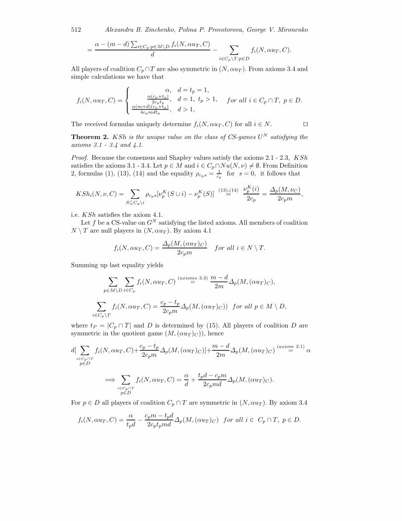
512 Alexandra B. Zinchenko, Polina P. Provotorova, George V. Mironenko
=α− (m− d)
∑i∈Cp:p∈M\D fi(N,αuT , C)
d−
∑i∈Cp\T :p∈D
fi(N,αuT , C).
All players of coalition Cp∩T are also symmetric in (N,αuT ). From axioms 3.4 andsimple calculations we have that
fi(N,αuT , C) =
⎧⎪⎨⎪⎩α, d = tp = 1,
α(cp+tp)2cptp
, d = 1, tp > 1,α(m+d)(cp+tp)
4cpmdtp, d > 1,
for all i ∈ Cp ∩ T, p ∈ D.
The received formulas uniquely determine fi(N,αuT , C) for all i ∈ N . ��
Theorem 2. KSh is the unique value on the class of CS-games UN satisfying theaxioms 3.1 - 3.4 and 4.1.
Proof. Because the consensus and Shapley values satisfy the axioms 2.1 - 2.3, KShsatisfies the axioms 3.1 - 3.4. Let p ∈M and i ∈ Cp∩Nu(N, ν) = ∅. From Definition2, formulas (1), (13), (14) and the equality ρcps = 1
cpfor s = 0, it follows that
KShi(N, ν, C) =∑
S⊆Cp\iρcps[ν
Kp (S ∪ i)− νKp (S)]
(13),(14)=
νKp (i)
2cp=
Δp(M, νC)
2cpm,
i.e. KSh satisfies the axiom 4.1.Let f be a CS-value on GN satisfying the listed axioms. All members of coalition
N \ T are null players in (N,αuT ). By axiom 4.1
fi(N,αuT , C) =Δp(M, (αuT )C)
2cpmfor all i ∈ N \ T.
Summing up last equality yields∑p∈M\D
∑i∈Cp
fi(N,αuT , C)(axioms 3.3)
=m− d
2mΔp(M, (αuT )C),
∑i∈Cp\T
fi(N,αuT , C) =cp − tp2cpm
Δp(M, (αuT )C)) for all p ∈M \D,
where tP = |Cp ∩ T | and D is determined by (15). All players of coalition D aresymmetric in the quotient game (M, (αuT )C)), hence
d[∑
i∈Cp∩Tp∈D
fi(N,αuT , C)+cp − tp2cpm
Δp(M, (αuT )C)]+m− d
2mΔp(M, (αuT )C)
(axiom 3.1)= α
=⇒∑
i∈Cp∩Tp∈D
fi(N,αuT , C) =α
d+
tpd− cpm
2cpmdΔp(M, (αuT )C).
For p ∈ D all players of coalition Cp ∩ T are symmetric in (N,αuT ). By axiom 3.4
fi(N,αuT , C) =α
tpd− cpm− tpd
2cptpmdΔp(M, (αuT )C) for all i ∈ Cp ∩ T, p ∈ D.

Efficient CS-Values Based on Consensus and Shapley Values 513
Since Cp ⊆ N \ T for p ∈ M \D, and Δp(M, (αuT )C) is determined uniquely forall p ∈ M (see the proof of Theorem 1), CS-value fi(N,αuT , C) is also determineuniquely for all i ∈ N . ��
Theorem 3. ShK is the unique value on the class of CS-games UN satisfying theaxioms 3.1 - 3.4 and 4.2.
Proof. The axiom 4.2, as well as the axiom 4.1, determines uniquely the payoffs ofall null players in (N, ν), therefore the proof of this theorem is similar to that ofTheorem 2. It only remains to show that ShK satisfies the axiom 4.2. Let p ∈ Mand i ∈ Cp ∩Nu(N, ν) = ∅. By Lemma 1 we have i ∈ Nu(Cp, ν
Shp ). Hence
ShKi(N, ν, C)(def.)
= Ki(Cp, νShp )
(axiom 2.5)= νShp (i) +
νShp (Cp) +∑j∈Cp ν
Shp (j)
2cp.
It is follows from νShp (i) = 0, νShp (Cp)(9)= Shp(M, νC) and νShp (j)
(9)= Shp(M, νCjp),
j ∈ Cp, that ShK satisfies the axiom 4.2. ��
Notice that KK and KSh do not satisfy the coalitional null player propertyintroduced in (Kamijo, 2009) to characterize the two-step Shapley value. Therefore,even the member of null component Cp ⊆ Nu(N, ν) can get a positive KK and KShCS-values.
References
Calvo, E. and P. E. Gutierrez (2010). Solidarity in games with a coalition structure. Dis-cussion Papers in Economic Behaviour, 8, 1–22.
Gomez-Rua, M. and J. Vidal-Puga (2008). The axiomatic approach to three values ingames with coalition structure. MPRA paper, 8904, 1–30. University of Munich Li-brary, Germany.
Hernandez-Lamoneda, L., R. Juarez and F. Sanchez-Sanchez (2008). Solutions withoutdummy axiom for TU cooperative games. Economics Bulletin, 3(1), 1–9.
Ju, Y., P. Born and P. Rays (2006). The consensus value: a new solution concept forcooperative games. Social Choice and Welfare, 28(4), 85–703.
Kamijo, Y. (2007). A collective value: a new interpretation of a value and a coalitionstructure. 21COE-GLOPE Working Paper Series, 27, 1–23. Waseda University, Japan.
Kamijo, Y. (2009). A two-step Shapley value for cooperative games with a coalition struc-tures. International Game Theory Review, 11(2), 207–214.
Owen, G. (1977). Values of games with a priory unions. In: Essays in mathematical eco-nomics and game theory (Henn R. and O.Moeschlin, eds.), pp. 76–88. Springer-Verlag,Berlin.
Shapley, L. S. (1953). A value for n-person games. In: Contributions to the theory ofgames II (H.W.Kuhn and A.W.Tucker, eds), pp. 307-317. Princeton University Press,Princeton, NJ.
Zinchenko, A. B., G. V. Mironenko and P. A. Provotorova (2010). A consensus value forgames with coalition structure. Mathematical games theory and applications, 2(1),93–106 (in Russian).
CONTRIBUTIONS TO GAME THEORY AND MANAGEMENT
Collected papers
Volume IV
presented on the Fourth International Conference Game Theory and Management
Editors Leon A. Petrosyan, Nikolay A. Zenkevich.
УСПЕХИ ТЕОРИИ ИГР И МЕНЕДЖМЕНТА
Сборник статей четвертой международной конференции по теории игр именеджменту
Выпуск 4
Под редакцией Л.А. Петросяна, Н.А. Зенкевича
Высшая школа менеджмента СПбГУ199044, С.-Петербург, Волховский пер., 3
тел. +7 (812) 323 [email protected]
www.gsom.pu.ru
Подписано в печать с оригинал-макета 16.06.2011Формат 70 ∗ 1001/16 . Печать офсетная. Усл. печ. л. 40,95. Уч.-изд.л. 34,5
Тираж 250 экз. Заказ № 559
Отпечатано с готового оригинал-макетав Центре оперативной полиграфии Высшей школы менеджмента СПбГУ
199004, С.-Петербург, Волховский пер., 3тел. (812) 323 8460
Copyright © 2022 FDOKUMEN