Game theory model for European government bonds market stabilization: a saving-State proposal


Game Theory

Hans Peters
Game Theory
A Multi-Leveled Approach

© 2008 Springer-Verlag Berlin Heidelberg
This work is subject to copyright. All rights are reserved, whether the whole or part of the material is concerned, specifically the rights of translation, reprinting, reuse of illustrations, recitation, broadcasting, reproduction on microfilm or in any other way, and storage in data banks. Duplication of this publication or parts thereof is permitted only under the provisions of the German Copyright Law of September 9, 1965, in its current version, and permission for use must always be obtained from Springer-Verlag. Violations are liable for prosecution under the German Copyright Law.
The use of general descriptive names, registered names, trademarks, etc. in this publication does not imply, even in the absence of a specific statement, that such names are exempt from the relevant protective laws and regulations and therefore free for general use.
Cover design: WMXDesign GmbH, Heidelberg, Germany
Printed on acid-free paper
9 8 7 6 5 4 3 2 1 0
springer.com
Dr. Hans PetersDepartment of Quantitative EconomicsUniversity of MaastrichtP.O. Box 6166200 MD MaastrichtThe Netherlands
ISBN 978-3-540-69290-4 e-ISBN 978-3-540-69291-1
Library of Congress Control Number: 2008930213

Voor Lenie, Nina and Remco

Preface
This book is a compilation of much of the material I used for various game theorycourses over, roughly, the past two decades. The first part, Thinking Strategically, isintended for undergraduate students in economics or business, but can also serve asan introduction for the subsequent parts of the book. The second and third parts godeeper into the various topics treated in the first part. These parts are intended formore mathematically oriented undergraduate students, or for graduate students in(for instance) economics. Part II is on noncooperative games and Part III on coop-erative games. Part IV is only a mathematical tools chapter. Every chapter has afinal section with problems. Selected hints, answers, and solutions to these prob-lems are given at the end of the book. Complete solutions can be obtained from theauthor.
The book claims neither originality nor completeness. As to originality, thematerial draws heavily on game theory texts developed by many others, often incollaboration. I mention in particular Jean Derks, Thijs Jansen, Andres Perea, TonStorcken, Frank Thuijsman, Stef Tijs, Dries Vermeulen, and Koos Vrieze. I am alsogreatly indebted to a large number of introductory, intermediate, and advanced textsand textbooks on game theory, and hope I have succeeded in giving sufficient creditto the authors of these works in all relevant places. As to completeness, the book isfar from achieving this quality but I trust that it presents at least the basics of gametheory. When writing and compiling the material I had ambitious plans for manymore chapters, and only hope that the phrase that all good things must come to anend applies here.
How to Use this Book
Part I of the book is intended, firstly, for undergraduate students in economics andbusiness and, secondly, as preparation and background for Parts II–IV. Part I is pre-ceded by Chap. 1, which is a general introduction to game theory by means ofexamples. The first chapter of Part I, Chap. 2 of the book, is on zero-sum games.This chapter is included, not only for historical reasons – the minimax theorem
vii

viii Preface
of von Neumann [140] was one of the first formal results in game theory – butalso because zero-sum games (all parlor games) require basic, strictly competitive,game-theoretic thinking. The heart of Part I consists of Chaps. 3–6 on noncoop-erative games and applications, and Chap. 9 as a basic introduction to cooperativegames. These chapters can serve as a basics course in game theory. Chapters 7 and8 on repeated games and evolutionary games can serve as extra material, as well asChap. 10 on cooperative game models and Chap. 11, which is an introduction to therelated area of social choice theory.
Although this book, in particular Part I, can be used for self-study, it is notintended to replace the teacher. Part I is meant for students who are knowledge-able in basic calculus, and does not try to avoid the use of mathematics on that basiclevel. There is, after all, a reason why we teach calculus courses to (for instance)undergraduate students in economics. Nevertheless, the mathematics in Part I doesnot go beyond such things as maximizing a quadratic function or elementary matrixnotation. In my own experience, the difficulties that students encounter when study-ing formal models are usually conceptual rather than mathematical, but they areoften confused with mathematical difficulties. A well recognized example is thedistinction between parameters and variables in a model. Another example is theuse of mathematical notation. Even in Part I of the book (almost) all basic gametheory models are described in a formally precise manner, although I am aware thatsome students may have a blind spot for mathematical notation that goes beyondsimple formulas for functions and equations. This formal presentation is includedespecially because many students have always been asking questions about it: leav-ing it out may lead to confusion and ambiguities. On the other hand, a teacher maydecide to drop these more formal parts and go directly to the examples of concretelyspecified games. For example, in Chap. 5, the game theory teacher may decide toskip the formal Sect. 5.1 and go directly to the worked out examples of games withincomplete information – and perhaps later return to Sect. 5.1.
I can be much shorter on Parts II–IV, which require more mathematical sophis-tication and are intended for graduate students in economics, or for an electivegame theory course for students in (applied) mathematics. In my experience again,it works well to couple the material in these parts to related chapters in Part I. In par-ticular, one can combine Chaps. 2 and 12 on zero-sum games, Chaps. 3 and 13 onfinite games, Chaps. 4, 5, and 14 on games with incomplete information and gamesin extensive form, and Chaps. 8 and 15 on evolutionary games.1 For cooperativegame theory, one can combine Chap. 9 with Part III.
Each chapter concludes with a problems section. Partial hints, answers and solu-tions are provided at the end of the book. For a complete set of solutions for teachers,please contact the author by email.2
1 Chapter 7 is on repeated games but no advanced chapter on this topic is included. See, e.g., [39],[75], or [88].2 [email protected].

Preface ix
References
This is a textbook and not a handbook, and consequently the list of references islimited and far from complete. In most cases references in the text are indicated bya number and only in some cases also by the name(s) of the author(s), for instancewhen a concept is named after a person.
Notation
I do not have much to say on notation. Bold letters are used to indicate vectors –while working on the book I came to regret this convention very much because ofthe extra work, but had already passed the point of no return. Transpose signs forvectors and matrices are only used when absolutely necessary. Vector inequalitiesuse the symbols > for all coordinates strictly larger and ≥ for all coordinates at leastas large – and of course their reverses.
Errors
All errors are mine, and I would appreciate any feedback. All comments, not onlythose on errors, are most welcome.
Maastricht Hans PetersMay 2008

Contents
1 Introduction . . . . . . . . . . . . . . . . . . . . . . . . . . . . . . . . . . . . . . . . . . . . . . . . . . . 11.1 A Definition . . . . . . . . . . . . . . . . . . . . . . . . . . . . . . . . . . . . . . . . . . . . . . . 11.2 Some History . . . . . . . . . . . . . . . . . . . . . . . . . . . . . . . . . . . . . . . . . . . . . . 11.3 Examples . . . . . . . . . . . . . . . . . . . . . . . . . . . . . . . . . . . . . . . . . . . . . . . . . 3
1.3.1 Zero-Sum Games . . . . . . . . . . . . . . . . . . . . . . . . . . . . . . . . . . . . 31.3.2 Nonzero-Sum Games . . . . . . . . . . . . . . . . . . . . . . . . . . . . . . . . . 51.3.3 Extensive Form Games . . . . . . . . . . . . . . . . . . . . . . . . . . . . . . . 81.3.4 Cooperative Games . . . . . . . . . . . . . . . . . . . . . . . . . . . . . . . . . . 121.3.5 Bargaining Games . . . . . . . . . . . . . . . . . . . . . . . . . . . . . . . . . . . 15
1.4 Cooperative vs. Noncooperative Game Theory . . . . . . . . . . . . . . . . . . 16Problems . . . . . . . . . . . . . . . . . . . . . . . . . . . . . . . . . . . . . . . . . . . . . . . . . . . . . . 16
Part I Thinking Strategically
2 Finite Two-Person Zero-Sum Games . . . . . . . . . . . . . . . . . . . . . . . . . . . . . 212.1 Basic Definitions and Theory . . . . . . . . . . . . . . . . . . . . . . . . . . . . . . . . . 212.2 Solving 2× n Games and m×2 Games . . . . . . . . . . . . . . . . . . . . . . . . 23
2.2.1 2×n Games . . . . . . . . . . . . . . . . . . . . . . . . . . . . . . . . . . . . . . . . 242.2.2 m× 2 Games . . . . . . . . . . . . . . . . . . . . . . . . . . . . . . . . . . . . . . . . 252.2.3 Strict Domination . . . . . . . . . . . . . . . . . . . . . . . . . . . . . . . . . . . . 27
Problems . . . . . . . . . . . . . . . . . . . . . . . . . . . . . . . . . . . . . . . . . . . . . . . . . . . . . . 28
3 Finite Two-Person Games . . . . . . . . . . . . . . . . . . . . . . . . . . . . . . . . . . . . . . . 313.1 Basic Definitions and Theory . . . . . . . . . . . . . . . . . . . . . . . . . . . . . . . . . 313.2 Finding Nash Equilibria . . . . . . . . . . . . . . . . . . . . . . . . . . . . . . . . . . . . . 33
3.2.1 Pure Nash Equilibria . . . . . . . . . . . . . . . . . . . . . . . . . . . . . . . . . 333.2.2 2×2 Games . . . . . . . . . . . . . . . . . . . . . . . . . . . . . . . . . . . . . . . . 353.2.3 Strict Domination . . . . . . . . . . . . . . . . . . . . . . . . . . . . . . . . . . . . 36
Problems . . . . . . . . . . . . . . . . . . . . . . . . . . . . . . . . . . . . . . . . . . . . . . . . . . . . . . 38
xi
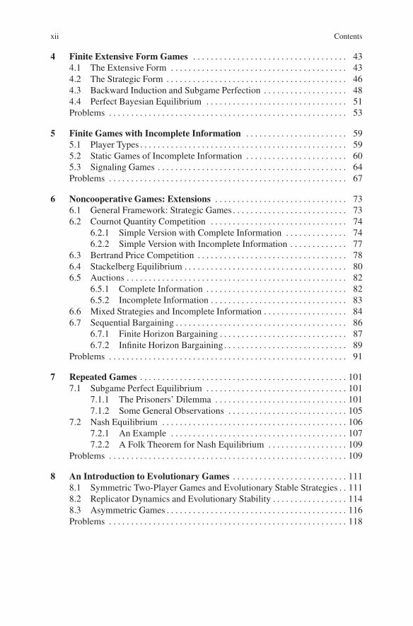
xii Contents
4 Finite Extensive Form Games . . . . . . . . . . . . . . . . . . . . . . . . . . . . . . . . . . . 434.1 The Extensive Form . . . . . . . . . . . . . . . . . . . . . . . . . . . . . . . . . . . . . . . . 434.2 The Strategic Form . . . . . . . . . . . . . . . . . . . . . . . . . . . . . . . . . . . . . . . . . 464.3 Backward Induction and Subgame Perfection . . . . . . . . . . . . . . . . . . . 484.4 Perfect Bayesian Equilibrium . . . . . . . . . . . . . . . . . . . . . . . . . . . . . . . . 51Problems . . . . . . . . . . . . . . . . . . . . . . . . . . . . . . . . . . . . . . . . . . . . . . . . . . . . . . 53
5 Finite Games with Incomplete Information . . . . . . . . . . . . . . . . . . . . . . . 595.1 Player Types . . . . . . . . . . . . . . . . . . . . . . . . . . . . . . . . . . . . . . . . . . . . . . . 595.2 Static Games of Incomplete Information . . . . . . . . . . . . . . . . . . . . . . . 605.3 Signaling Games . . . . . . . . . . . . . . . . . . . . . . . . . . . . . . . . . . . . . . . . . . . 64Problems . . . . . . . . . . . . . . . . . . . . . . . . . . . . . . . . . . . . . . . . . . . . . . . . . . . . . . 67
6 Noncooperative Games: Extensions . . . . . . . . . . . . . . . . . . . . . . . . . . . . . . 736.1 General Framework: Strategic Games . . . . . . . . . . . . . . . . . . . . . . . . . . 736.2 Cournot Quantity Competition . . . . . . . . . . . . . . . . . . . . . . . . . . . . . . . 74
6.2.1 Simple Version with Complete Information . . . . . . . . . . . . . . 746.2.2 Simple Version with Incomplete Information . . . . . . . . . . . . . 77
6.3 Bertrand Price Competition . . . . . . . . . . . . . . . . . . . . . . . . . . . . . . . . . . 786.4 Stackelberg Equilibrium . . . . . . . . . . . . . . . . . . . . . . . . . . . . . . . . . . . . . 806.5 Auctions . . . . . . . . . . . . . . . . . . . . . . . . . . . . . . . . . . . . . . . . . . . . . . . . . . 82
6.5.1 Complete Information . . . . . . . . . . . . . . . . . . . . . . . . . . . . . . . . 826.5.2 Incomplete Information . . . . . . . . . . . . . . . . . . . . . . . . . . . . . . . 83
6.6 Mixed Strategies and Incomplete Information . . . . . . . . . . . . . . . . . . . 846.7 Sequential Bargaining . . . . . . . . . . . . . . . . . . . . . . . . . . . . . . . . . . . . . . . 86
6.7.1 Finite Horizon Bargaining . . . . . . . . . . . . . . . . . . . . . . . . . . . . . 876.7.2 Infinite Horizon Bargaining . . . . . . . . . . . . . . . . . . . . . . . . . . . . 89
Problems . . . . . . . . . . . . . . . . . . . . . . . . . . . . . . . . . . . . . . . . . . . . . . . . . . . . . . 91
7 Repeated Games . . . . . . . . . . . . . . . . . . . . . . . . . . . . . . . . . . . . . . . . . . . . . . . 1017.1 Subgame Perfect Equilibrium . . . . . . . . . . . . . . . . . . . . . . . . . . . . . . . . 101
7.1.1 The Prisoners’ Dilemma . . . . . . . . . . . . . . . . . . . . . . . . . . . . . . 1017.1.2 Some General Observations . . . . . . . . . . . . . . . . . . . . . . . . . . . 105
7.2 Nash Equilibrium . . . . . . . . . . . . . . . . . . . . . . . . . . . . . . . . . . . . . . . . . . 1067.2.1 An Example . . . . . . . . . . . . . . . . . . . . . . . . . . . . . . . . . . . . . . . . 1077.2.2 A Folk Theorem for Nash Equilibrium . . . . . . . . . . . . . . . . . . 109
Problems . . . . . . . . . . . . . . . . . . . . . . . . . . . . . . . . . . . . . . . . . . . . . . . . . . . . . . 109
8 An Introduction to Evolutionary Games . . . . . . . . . . . . . . . . . . . . . . . . . . 1118.1 Symmetric Two-Player Games and Evolutionary Stable Strategies . . 1118.2 Replicator Dynamics and Evolutionary Stability . . . . . . . . . . . . . . . . . 1148.3 Asymmetric Games . . . . . . . . . . . . . . . . . . . . . . . . . . . . . . . . . . . . . . . . . 116Problems . . . . . . . . . . . . . . . . . . . . . . . . . . . . . . . . . . . . . . . . . . . . . . . . . . . . . . 118

Contents xiii
9 Cooperative Games with Transferable Utility . . . . . . . . . . . . . . . . . . . . . . 1219.1 Examples and Preliminaries . . . . . . . . . . . . . . . . . . . . . . . . . . . . . . . . . . 1219.2 The Core . . . . . . . . . . . . . . . . . . . . . . . . . . . . . . . . . . . . . . . . . . . . . . . . . . 1239.3 The Shapley Value . . . . . . . . . . . . . . . . . . . . . . . . . . . . . . . . . . . . . . . . . . 1259.4 The Nucleolus . . . . . . . . . . . . . . . . . . . . . . . . . . . . . . . . . . . . . . . . . . . . . 127Problems . . . . . . . . . . . . . . . . . . . . . . . . . . . . . . . . . . . . . . . . . . . . . . . . . . . . . . 129
10 Cooperative Game Theory Models . . . . . . . . . . . . . . . . . . . . . . . . . . . . . . . 13310.1 Bargaining Problems . . . . . . . . . . . . . . . . . . . . . . . . . . . . . . . . . . . . . . . . 133
10.1.1 The Nash Bargaining Solution . . . . . . . . . . . . . . . . . . . . . . . . . 13410.1.2 Relation with the Rubinstein Bargaining Procedure . . . . . . . . 137
10.2 Exchange Economies . . . . . . . . . . . . . . . . . . . . . . . . . . . . . . . . . . . . . . . 13810.3 Matching Problems . . . . . . . . . . . . . . . . . . . . . . . . . . . . . . . . . . . . . . . . . 14210.4 House Exchange . . . . . . . . . . . . . . . . . . . . . . . . . . . . . . . . . . . . . . . . . . . 145Problems . . . . . . . . . . . . . . . . . . . . . . . . . . . . . . . . . . . . . . . . . . . . . . . . . . . . . . 146
11 Social Choice . . . . . . . . . . . . . . . . . . . . . . . . . . . . . . . . . . . . . . . . . . . . . . . . . . 15111.1 Introduction and Preliminaries . . . . . . . . . . . . . . . . . . . . . . . . . . . . . . . . 152
11.1.1 An Example . . . . . . . . . . . . . . . . . . . . . . . . . . . . . . . . . . . . . . . . 15211.1.2 Preliminaries . . . . . . . . . . . . . . . . . . . . . . . . . . . . . . . . . . . . . . . . 153
11.2 Arrow’s Theorem . . . . . . . . . . . . . . . . . . . . . . . . . . . . . . . . . . . . . . . . . . 15411.3 The Gibbard–Satterthwaite Theorem . . . . . . . . . . . . . . . . . . . . . . . . . . 157Problems . . . . . . . . . . . . . . . . . . . . . . . . . . . . . . . . . . . . . . . . . . . . . . . . . . . . . . 159
Part II Noncooperative Games
12 Matrix Games . . . . . . . . . . . . . . . . . . . . . . . . . . . . . . . . . . . . . . . . . . . . . . . . . 16312.1 The Minimax Theorem . . . . . . . . . . . . . . . . . . . . . . . . . . . . . . . . . . . . . . 16312.2 A Linear Programming Formulation . . . . . . . . . . . . . . . . . . . . . . . . . . . 164Problems . . . . . . . . . . . . . . . . . . . . . . . . . . . . . . . . . . . . . . . . . . . . . . . . . . . . . . 166
13 Finite Games . . . . . . . . . . . . . . . . . . . . . . . . . . . . . . . . . . . . . . . . . . . . . . . . . . 16913.1 Existence of Nash Equilibrium . . . . . . . . . . . . . . . . . . . . . . . . . . . . . . . 16913.2 Bimatrix Games . . . . . . . . . . . . . . . . . . . . . . . . . . . . . . . . . . . . . . . . . . . . 170
13.2.1 Pure and Mixed Strategies in Nash Equilibrium . . . . . . . . . . . 17113.2.2 Extension of the Graphical Method . . . . . . . . . . . . . . . . . . . . . 17313.2.3 A Mathematical Programming Approach . . . . . . . . . . . . . . . . 17413.2.4 Matrix Games . . . . . . . . . . . . . . . . . . . . . . . . . . . . . . . . . . . . . . . 17613.2.5 The Game of Chess: Zermelo’s Theorem . . . . . . . . . . . . . . . . 177
13.3 Iterated Dominance and Best Reply . . . . . . . . . . . . . . . . . . . . . . . . . . . 17713.4 Perfect Equilibrium . . . . . . . . . . . . . . . . . . . . . . . . . . . . . . . . . . . . . . . . . 18013.5 Proper Equilibrium . . . . . . . . . . . . . . . . . . . . . . . . . . . . . . . . . . . . . . . . . 18413.6 Strictly Perfect Equilibrium . . . . . . . . . . . . . . . . . . . . . . . . . . . . . . . . . . 18513.7 Correlated Equilibrium . . . . . . . . . . . . . . . . . . . . . . . . . . . . . . . . . . . . . . 18613.8 A Characterization of Nash Equilibrium. . . . . . . . . . . . . . . . . . . . . . . . 189Problems . . . . . . . . . . . . . . . . . . . . . . . . . . . . . . . . . . . . . . . . . . . . . . . . . . . . . . 191

xiv Contents
14 Extensive Form Games . . . . . . . . . . . . . . . . . . . . . . . . . . . . . . . . . . . . . . . . . 19714.1 Extensive Form Structures and Games . . . . . . . . . . . . . . . . . . . . . . . . . 19714.2 Pure, Mixed and Behavioral Strategies . . . . . . . . . . . . . . . . . . . . . . . . . 19914.3 Nash Equilibrium and Refinements . . . . . . . . . . . . . . . . . . . . . . . . . . . . 202
14.3.1 Subgame Perfect Equilibrium . . . . . . . . . . . . . . . . . . . . . . . . . . 20414.3.2 Perfect Bayesian and Sequential Equilibrium . . . . . . . . . . . . . 204
Problems . . . . . . . . . . . . . . . . . . . . . . . . . . . . . . . . . . . . . . . . . . . . . . . . . . . . . . 209
15 Evolutionary Games . . . . . . . . . . . . . . . . . . . . . . . . . . . . . . . . . . . . . . . . . . . . 21315.1 Symmetric Two-Player Games . . . . . . . . . . . . . . . . . . . . . . . . . . . . . . . 213
15.1.1 Symmetric 2× 2 Games . . . . . . . . . . . . . . . . . . . . . . . . . . . . . . 21415.2 Evolutionary Stability . . . . . . . . . . . . . . . . . . . . . . . . . . . . . . . . . . . . . . . 214
15.2.1 Evolutionary Stable Strategies . . . . . . . . . . . . . . . . . . . . . . . . . 21415.2.2 The Structure of the Set ESS(A) . . . . . . . . . . . . . . . . . . . . . . . . 21515.2.3 Relations with Other Refinements . . . . . . . . . . . . . . . . . . . . . . 21515.2.4 Other Characterizations of ESS . . . . . . . . . . . . . . . . . . . . . . . . 216
15.3 Replicator Dynamics and ESS . . . . . . . . . . . . . . . . . . . . . . . . . . . . . . . . 21815.3.1 Replicator Dynamics . . . . . . . . . . . . . . . . . . . . . . . . . . . . . . . . . 21815.3.2 Symmetric 2× 2 Games . . . . . . . . . . . . . . . . . . . . . . . . . . . . . . 21915.3.3 Dominated Strategies . . . . . . . . . . . . . . . . . . . . . . . . . . . . . . . . . 22015.3.4 Nash Equilibrium Strategies . . . . . . . . . . . . . . . . . . . . . . . . . . . 22015.3.5 Perfect Equilibrium Strategies . . . . . . . . . . . . . . . . . . . . . . . . . 222
Problems . . . . . . . . . . . . . . . . . . . . . . . . . . . . . . . . . . . . . . . . . . . . . . . . . . . . . . 223
Part III Cooperative Games
16 TU-Games: Domination, Stable Sets, and the Core . . . . . . . . . . . . . . . . . 22916.1 Imputations and Domination . . . . . . . . . . . . . . . . . . . . . . . . . . . . . . . . . 22916.2 The Core and the Domination-Core . . . . . . . . . . . . . . . . . . . . . . . . . . . 23116.3 Simple Games . . . . . . . . . . . . . . . . . . . . . . . . . . . . . . . . . . . . . . . . . . . . . 23216.4 Stable Sets . . . . . . . . . . . . . . . . . . . . . . . . . . . . . . . . . . . . . . . . . . . . . . . . 23416.5 Balanced Games and the Core . . . . . . . . . . . . . . . . . . . . . . . . . . . . . . . . 235Problems . . . . . . . . . . . . . . . . . . . . . . . . . . . . . . . . . . . . . . . . . . . . . . . . . . . . . . 237
17 The Shapley Value . . . . . . . . . . . . . . . . . . . . . . . . . . . . . . . . . . . . . . . . . . . . . 24117.1 Definition and Shapley’s Characterization . . . . . . . . . . . . . . . . . . . . . . 24117.2 Other Characterizations . . . . . . . . . . . . . . . . . . . . . . . . . . . . . . . . . . . . . 246
17.2.1 Dividends . . . . . . . . . . . . . . . . . . . . . . . . . . . . . . . . . . . . . . . . . . 24617.2.2 Strong Monotonicity . . . . . . . . . . . . . . . . . . . . . . . . . . . . . . . . . 24717.2.3 Multilinear Extension . . . . . . . . . . . . . . . . . . . . . . . . . . . . . . . . . 248
17.3 Potential and Reduced Game . . . . . . . . . . . . . . . . . . . . . . . . . . . . . . . . . 25017.3.1 The Potential Approach to the Shapley Value . . . . . . . . . . . . . 25017.3.2 Reduced Games . . . . . . . . . . . . . . . . . . . . . . . . . . . . . . . . . . . . . 253
Problems . . . . . . . . . . . . . . . . . . . . . . . . . . . . . . . . . . . . . . . . . . . . . . . . . . . . . . 257

Contents xv
18 Core, Shapley Value, and Weber Set . . . . . . . . . . . . . . . . . . . . . . . . . . . . . . 25918.1 The Weber Set . . . . . . . . . . . . . . . . . . . . . . . . . . . . . . . . . . . . . . . . . . . . . 25918.2 Convex Games . . . . . . . . . . . . . . . . . . . . . . . . . . . . . . . . . . . . . . . . . . . . . 26118.3 Random Order Values . . . . . . . . . . . . . . . . . . . . . . . . . . . . . . . . . . . . . . . 26218.4 Weighted Shapley Values . . . . . . . . . . . . . . . . . . . . . . . . . . . . . . . . . . . . 266Problems . . . . . . . . . . . . . . . . . . . . . . . . . . . . . . . . . . . . . . . . . . . . . . . . . . . . . . 268
19 The Nucleolus . . . . . . . . . . . . . . . . . . . . . . . . . . . . . . . . . . . . . . . . . . . . . . . . . 27119.1 An Example . . . . . . . . . . . . . . . . . . . . . . . . . . . . . . . . . . . . . . . . . . . . . . . 27119.2 The Lexicographic Order . . . . . . . . . . . . . . . . . . . . . . . . . . . . . . . . . . . . 27219.3 The (Pre-)Nucleolus . . . . . . . . . . . . . . . . . . . . . . . . . . . . . . . . . . . . . . . . 27319.4 The Kohlberg Criterion . . . . . . . . . . . . . . . . . . . . . . . . . . . . . . . . . . . . . . 27519.5 Computation of the Nucleolus . . . . . . . . . . . . . . . . . . . . . . . . . . . . . . . . 27719.6 A Characterization of the Pre-Nucleolus . . . . . . . . . . . . . . . . . . . . . . . 280Problems . . . . . . . . . . . . . . . . . . . . . . . . . . . . . . . . . . . . . . . . . . . . . . . . . . . . . . 282
20 Special Transferable Utility Games . . . . . . . . . . . . . . . . . . . . . . . . . . . . . . . 28520.1 Assignment and Permutation Games. . . . . . . . . . . . . . . . . . . . . . . . . . . 28520.2 Flow Games . . . . . . . . . . . . . . . . . . . . . . . . . . . . . . . . . . . . . . . . . . . . . . . 28920.3 Voting Games: The Banzhaf Value . . . . . . . . . . . . . . . . . . . . . . . . . . . . 291Problems . . . . . . . . . . . . . . . . . . . . . . . . . . . . . . . . . . . . . . . . . . . . . . . . . . . . . . 294
21 Bargaining Problems . . . . . . . . . . . . . . . . . . . . . . . . . . . . . . . . . . . . . . . . . . . 29721.1 The Bargaining Problem . . . . . . . . . . . . . . . . . . . . . . . . . . . . . . . . . . . . . 29721.2 The Raiffa–Kalai–Smorodinsky Solution . . . . . . . . . . . . . . . . . . . . . . . 29921.3 The Egalitarian Solution . . . . . . . . . . . . . . . . . . . . . . . . . . . . . . . . . . . . . 30021.4 Noncooperative Bargaining . . . . . . . . . . . . . . . . . . . . . . . . . . . . . . . . . . 30221.5 Games with Non-Transferable Utility . . . . . . . . . . . . . . . . . . . . . . . . . . 303Problems . . . . . . . . . . . . . . . . . . . . . . . . . . . . . . . . . . . . . . . . . . . . . . . . . . . . . . 304
Part IV Tools
22 Tools . . . . . . . . . . . . . . . . . . . . . . . . . . . . . . . . . . . . . . . . . . . . . . . . . . . . . . . . . . 30922.1 Some Definitions . . . . . . . . . . . . . . . . . . . . . . . . . . . . . . . . . . . . . . . . . . . 30922.2 A Separation Theorem . . . . . . . . . . . . . . . . . . . . . . . . . . . . . . . . . . . . . . 31022.3 Lemmas of the Alternative . . . . . . . . . . . . . . . . . . . . . . . . . . . . . . . . . . . 31022.4 The Duality Theorem of Linear Programming . . . . . . . . . . . . . . . . . . . 31222.5 Some Fixed Point Theorems . . . . . . . . . . . . . . . . . . . . . . . . . . . . . . . . . 31322.6 The Birkhoff–von Neumann Theorem . . . . . . . . . . . . . . . . . . . . . . . . . 31422.7 The Max-Flow Min-Cut Theorem . . . . . . . . . . . . . . . . . . . . . . . . . . . . . 316Problems . . . . . . . . . . . . . . . . . . . . . . . . . . . . . . . . . . . . . . . . . . . . . . . . . . . . . . 319
Hints, Answers and Solutions . . . . . . . . . . . . . . . . . . . . . . . . . . . . . . . . . . . . . . . . 321
References . . . . . . . . . . . . . . . . . . . . . . . . . . . . . . . . . . . . . . . . . . . . . . . . . . . . . . . . . 357
Index . . . . . . . . . . . . . . . . . . . . . . . . . . . . . . . . . . . . . . . . . . . . . . . . . . . . . . . . . . . . . 363
Chapter 1Introduction
The best introduction to game theory is by way of examples. In this chapter westart with a global definition of the field in Sect. 1.1, collect some historical facts inSect. 1.2, and present examples in Sect. 1.3. In Sect. 1.4 we briefly comment on thedistinction between cooperative and noncooperative game theory.
1.1 A Definition
Game theory is a formal, mathematical discipline which studies situations of com-petition and cooperation between several involved parties. This is a broad definitionbut consistent with the large number of applications. These applications range fromstrategic questions in warfare to understanding economic competition, from eco-nomic or social problems of fair distribution to behavior of animals in competitivesituations, from parlor games to political voting systems – and this list is certainlynot exhaustive.
Although game theory is an official mathematical discipline (AMS1 Classifica-tion code 90D) it is applied mostly by economists. Many articles and books on gametheory and applications are found under the JEL2 codes C7x. The list of referencesat the end of this book contains many textbooks and other books on game theory.
1.2 Some History
In terms of applications, game theory is a broad discipline, and it is therefore notsurprising that ‘game-theoretic’ situations can be recognized in the Bible (see [17])or the Talmud (see [7]). Also the literature on strategic warfare contains many
1 American Mathematical Society.2 Journal of Economic Literature.
H. Peters, Game Theory – A Multi-Leveled Approach.c© Springer-Verlag Berlin Heidelberg 2008
1

2 1 Introduction
situations that could have been modelled using game theory: a very early reference,over 2,000 years old, is the work of the Chinese warrior-philosopher Sun Tzu (see[130]). Early works dealing with economic problems are the work of A. Cournoton quantity competition (see [21]) and J. Bertrand on price competition (see [11]).Some of the work of C.L. Dodgson (better known as Lewis Carroll, the writer ofAlice’s Adventures in Wonderland) is an early application of zero-sum games tothe political problem of parliamentary representation, see [32] and [12].
One of the first more formal works on game theory is the article of the logi-cian Zermelo, see [150]. He proved that in the game of chess either White has awinning strategy (i.e., can always win), or Black has a winning strategy, or eachplayer can always enforce a draw.3 Up to the present, however, it is still not knownwhich of these three cases is the true one. A milestone in the history of game the-ory is the work of von Neumann on zero-sum games [140], in which he proved thefamous minimax theorem for zero-sum games. This article was the basis for thebook Theory of Games and Economic Behavior by John von Neumann and OskarMorgenstern [141], by many regarded as the starting point of game theory. In thisbook the authors extended von Neumann’s work on zero-sum games and laid thegroundwork for the study of cooperative (coalitional) games.4
The title of the book of von Neumann and Morgenstern reveals the intention ofthe authors that game theory was to be applied to economics. Nevertheless, in thefifties and sixties the further development of game theory was mainly the domain ofmathematicians. Seminal articles in this period were the papers by John F. Nash5 onNash equilibrium and on bargaining (see [91] and [90]) and Shapley on the Shapleyvalue and the core for games with transferable utility (see [121] and [122]6). Apartfrom these articles, the foundations of much that was to follow later were laid in thecontributed volumes [68], [69], [33], [73], and [34].
In the late sixties and seventies of the previous century game theory becameaccepted as a new formal language for economics in particular. This develop-ment was stimulated by the work of John Harsanyi on modelling games withincomplete information (see [50]) and Reinhard Selten [117, 118] on (sub)gameperfect Nash equilibrium.7 From the eighties on, large parts of economics havebeen rewritten and further developed using the ideas, concepts and formal languageof game theory. Articles on game theory and applications can be found in manyeconomic journals. Journals focusing on game theory are the International Journalof Game Theory, Games and Economic Behavior, and International Game The-ory Review. Game theorists are organized within the Game Theory Society, seehttp://www.gametheorysociety.org/.
3 See Sect. 13.2.5.4 See [31] for a comprehensive history of game theory up to 1945.5 See [89] for a biography, and the later movie with the same title A Beautiful Mind.6 See also [16].7 In 1994, Nash, Harsanyi and Selten received the Nobel prize in economics for the mentionedwork in game theory.

1.3 Examples 3
1.3 Examples
Every example in this section is based on a ‘story’. Each time this story is presentedfirst and, next, it is translated into a formal mathematical model. Such a mathemat-ical model is an alternative description, capturing the essential ingredients of thestory with the omission of details that are considered unimportant: the mathemat-ical model is an ‘abstraction’ of the story. After having established the model, wespend some lines on how to ‘solve’ it: we try to say something about how the playersshould or would act. In more philosophical terms, these ‘solutions’ can be norma-tive or positive in nature, or somewhere in between, but often such considerationsare left as food for thought for the reader. As a general remark, a basic distinctionbetween optimization theory and game theory is that in optimization it is usuallyclear what is meant by the word ‘optimal’, whereas in game theory we deal withhuman (or, more generally, animal) behavior and then it is less clear what ‘optimal’means.8 Each example is concluded by further comments, possibly including a shortpreview on the treatment of the exemplified game in the book.
The examples are grouped in subsections on zero-sum games, nonzero-sumgames, extensive form games, cooperative games, and bargaining games.
1.3.1 Zero-Sum Games
The first example is taken from [106].
The Battle of the Bismarck Sea
Story The game is set in the South-Pacific in 1943. The Japanese admiral Imamurahas to transport troops across the Bismarck Sea to New Guinea, and the Americanadmiral Kenney wants to bomb the transport. Imamura has two possible choices: ashorter Northern route (2 days) or a larger Southern route (3 days), and Kenney mustchoose one of these routes to send his planes to. If he chooses the wrong route hecan call back the planes and send them to the other route, but the number of bombingdays is reduced by 1. We assume that the number of bombing days represents thepayoff to Kenney in a positive sense and to Imamura in a negative sense.
Model The Battle of the Bismarck Sea problem can be modelled as in the followingtable: (North South
North 2 2South 1 3
).
8 Feyerabend’s [35] ‘anything goes’ adage reflects a workable attitude in a young science like gametheory.

4 1 Introduction
This table represents a game with two players, namely Kenney and Imamura.Each player has two possible choices; Kenney (player 1) chooses a row, Imamura(player 2) chooses a column, and these choices are to be made independently andsimultaneously. The numbers represent the payoffs to Kenney. For instance, thenumber 2 up left means that if Kenney and Imamura both choose North, the payoffto Kenney is 2 and to Imamura −2. (The convention is to let the numbers denotethe payments from player 2 (the column player) to player 1 (the row player).) Thisgame is an example of a zero-sum game because the sum of the payoffs is alwaysequal to zero.
Solution In this particular example, it does not seem difficult to predict what willhappen. By choosing North, Imamura is always at least as well off as by choosingSouth, as is easily inferred from the above table of payoffs. So it is safe to assumethat Imamura chooses North, and Kenney, being able to perform this same kind ofreasoning, will then also choose North, since that is the best reply to the choice ofNorth by Imamura. Observe that this game is easy to analyze because one of theplayers has a weakly dominant choice, i.e., a choice which is always at least as good(giving always at least as high a payoff) as any other choice, no matter what theopponent decides to do.
Another way to look at this game is to observe that the payoff 2 resulting fromthe combination (North, North) is maximal in its column (2 ≥ 1) and minimal inits row (2 ≤ 2). Such a position in the matrix is called a saddlepoint. In such asaddlepoint, neither player has an incentive to deviate unilaterally.9 Also observethat, in such a saddlepoint, the row player maximizes his minimal payoff (because2 = min{2,2} ≥ 1 = min{1,3}), and the column player (who has to pay accordingto our convention) minimizes the maximal amount that he has to pay (because 2 =max{2,1} ≤ 3 = max{2,3}). The resulting payoff of 2 from player 2 to player 1 iscalled the value of the game.
Comments Two-person zero-sum games with finitely many choices, like the oneabove, are also called matrix games since they can be represented by a single matrix.Matrix games are studied in Chaps. 2 and 12. The combination (North, North) inthe example above corresponds to what happened in reality back in 1943. See thememoirs of Winston Churchill [20].10
Matching Pennies
Story In the two-player game of matching pennies, both players have a coin andsimultaneously show heads or tails. If the coins match, player 2 gives his coin toplayer 1; otherwise, player 1 gives his coin to player 2.
Model This is a zero-sum game with payoff matrix
9 As will become clear later, this implies that the combination (North, North) is a Nash equilibrium.10 In 1953, Churchill received the Nobel prize in literature for this work.

1.3 Examples 5
(Heads TailsHeads 1 −1Tails −1 1
).
Solution Observe that in this game no player has a (weakly) dominant choice, andthat there is no saddlepoint: there is no position in the matrix at which there is simul-taneously a minimum in the row and a maximum in the column. Thus, there doesnot seem to be a natural way to solve the game. Von Neumann [140] proposed tosolve games like this – and zero-sum games in general – by allowing the players torandomize between their choices. In the present example of matching pennies, sup-pose player 1 chooses heads or tails both with probability 1
2 . Suppose furthermorethat player 2 plays heads with probability q and tails with probability 1− q, where0 ≤ q ≤ 1. In that case the expected payoff for player 1 is equal to
12[q ·1 +(1−q) ·−1]+
12[q ·−1 +(1−q) ·1]
which is independent of q, namely, equal to 0. So by randomizing in this waybetween his two choices, player 1 can guarantee to obtain 0 in expectation (ofcourse, the actually realized outcome is always +1 or −1). Analogously, player 2,by playing heads or tails each with probability 1
2 , can guarantee to pay 0 in expec-tation. Thus, the amount of 0 plays a role similar to that of a saddlepoint. Again, wewill say that 0 is the value of this game.
Comments The randomized choices of the players are usually called mixed strate-gies. Randomized choices are often interpreted as beliefs of the other player(s) aboutthe choice of the player under consideration. See, e.g., Sect. 3.1.
Von Neumann [140] proved that every two-person matrix game has a value if theplayers can use mixed strategies: this is the minimax theorem.
1.3.2 Nonzero-Sum Games
Prisoners’ Dilemma
Story Two prisoners (players 1 and 2) have committed a crime together and areinterrogated separately. Each prisoner has two possible choices: he may ‘cooper-ate’ (C) which means ‘not betray his partner’ or he may ‘defect’ (D), which means‘betray his partner’. The punishment for the crime is 10 years of prison. Betrayalyields a reduction of 1 year for the traitor. If a prisoner is not betrayed, he isconvicted to 1 year for a minor offense.
Model This situation can be summarized as follows:
( C DC −1,−1 −10,0D 0,−10 −9,−9
).

6 1 Introduction
This table must be read in the same way as before, but now there are two payoffsat each position: by convention the first number is the payoff for player 1 and thesecond number is the payoff for player 2. Observe that the game is no longer zero-sum, and we have to write down both numbers at each matrix position.
Solution Observe that for both players D is a strictly dominant choice: for eachplayer, D is (strictly) the best choice, whatever the other player does. So it is naturalto argue that the outcome of this game will be the pair of choices (D,D), leadingto the payoffs −9,−9. Thus, due to the existence of strictly dominant choices, thePrisoners’ Dilemma game is easy to analyze.
Comments The payoffs (−9,−9) are inferior: they are not ‘Pareto optimal’, theplayers could obtain the higher payoff of −1 for each by cooperating, i.e., bothplaying C. There is a large literature on how to establish cooperation, e.g., by rep-utation effects in a repeated play of the game. See, in particular, Axelrod [8]. If thegame is played repeatedly, other (higher) payoffs are possible, see Chap. 7.
The Prisoners’ Dilemma is a metaphor for many economic situations. An out-standing example is the so-called tragedy of the commons ([47]; see also [45], p. 27,and Problem 6.26 in this book).
Battle of the Sexes
Story A man and a woman want to go out together, either to a soccer match or to aballet performance. They forgot to agree where they would go to that night, are indifferent places and have to decide on their own where to go; they have no meansto communicate. Their main concern is to be together, the man has a preference forsoccer and the woman for ballet.
Model A table reflecting the situation is as follows.
( Soccer BalletSoccer 2,1 0,0Ballet 0,0 1,2
).
Here, the man chooses a row and the woman a column.
Solution Observe that no player has a dominant choice. The players have to coor-dinate without being able to communicate. Now it may be possible that the nightbefore they discussed soccer at length; each player remembers this, may think thatthe other remembers this, and so this may serve as a ‘focal point’ (see Schelling11
[115] on the concept of focal points). In the absence of such considerations it is hardto give a unique prediction for this game. We can, however, say that the combina-tions (Soccer, Soccer) and (Ballet, Ballet) are special in the sense that the players’choices are ‘best replies’ to each other; if the man chooses Soccer (Ballet), thenit is optimal for the woman to choose Soccer (Ballet) as well, and vice versa. In
11 One of the winners of the 2005 Nobel prize in economics; the other one was R.J. Aumann.

1.3 Examples 7
literature, such choice combinations are called Nash equilibria. The concept of Nashequilibrium [91] is no doubt the main solution concept developed in game theory.
Comments The Battle of the Sexes game is metaphoric for problems of coordination.
Matching Pennies
Every zero-sum game is, trivially, a special case of a nonzero-sum game. Forinstance, the Matching Pennies game discussed in Sect. 1.3.1 can be representedas a nonzero-sum game as follows:
(Heads TailsHeads 1,−1 −1,1Tails −1,1 1,−1
).
Clearly, no player has a dominant choice and there is no combination of a row anda column such that each player’s choice is optimal given the choice of the otherplayer – there is no Nash equilibrium. If mixed strategies are allowed, then it canbe checked that if player 2 plays Heads and Tails each with probability 1
2 , then forplayer 1 it is optimal to do so too, and vice versa. Such a combination of mixedstrategies is again called a Nash equilibrium. Nash [91] proved that every game inwhich each player has finitely many choices – zero-sum or nonzero-sum – has aNash equilibrium in mixed strategies. See Chaps. 3 and 13.
A Cournot Game
Story Two firms produce a similar (‘homogenous’) product. The market price ofthis product is equal to p = 1−Q or zero (whichever is larger), where Q is the totalquantity produced. There are no production costs.
Model The two firms are the players, 1 and 2. Each player i = 1,2 chooses aquantity qi ≥ 0, and makes a profit of Ki(q1,q2) = qi(1 − q1 − q2) (or zero ifq1 + q2 ≥ 1).
Solution Suppose player 2 produces q2 = 13 . Then player 1 maximizes his own
profit q1(1 − q1 − 13 ) by choosing q1 = 1
3 . Also the converse holds: if player 1chooses q1 = 1
3 then q2 = 13 maximizes profit for player 2. This combination
of strategies consists of mutual best replies and is therefore again called a Nashequilibrium.
Comments Situations like this were first analyzed by Cournot [21]. The Nash equi-librium is often called Cournot equilibrium. It is easy to check that the Cournotequilibrium in this example is again not ‘Pareto optimal’: if the firms each wouldproduce 1
4 , then they would both be better off.

8 1 Introduction
The main difference between this example and the preceding ones is, that eachplayer here has infinitely many choices, also without including mixed strategies.
See further Chap. 6.
1.3.3 Extensive Form Games
All examples in Sects. 1.3.1 and 1.3.2 are examples of ‘one-shot games’. The playerschoose only once, independently and simultaneously. In parlor games as well asin games derived from real-life economic or political situations, this is often notwhat happens. Players may move sequentially, and observe or partially observe eachothers’ moves. Such situations are better modelled by ‘extensive form games’.
Sequential Battle of the Sexes
Story The story is similar to the story in Sect. 1.3.2, but we now assume that theman chooses first and the woman can observe the choice of the man.
Model This situation can be represented by the decision tree in Fig. 1.1. Player 1(the man) chooses first, player 2 (the woman) observes player 1’s choice and thenmakes her own choice. The first number in each pair of numbers is the payoff toplayer 1, and the second number is the payoff to player 2. Filled circles denotedecision nodes (of a player) or end nodes (followed by payoffs).
Solution An obvious way to analyze this game is to work backwards. If player 1chooses S, then it is optimal for player 2 to chooses S as well, and if player 1 choosesB, then it is optimal for player 2 to choose B as well. Given this choice behavior ofplayer 2 and assuming that player 1 performs this line of reasoning about the choicesof player 2, player 1 should choose S.
Comments What this simple example shows is that in such a so-called extensiveform game, there is a distinction between a play plan of a player and an actual moveor choice of that player. Player 2 has the plan to choose S (B) if player 1 has chosenS (B). Player 2’s actual choice is S – assuming as above that player 1 has chosen
� �����������������
������
���������������
������� � � �
1
22S B
S B S B
2,1 0,0 0,0 1,2
Fig. 1.1 The decision tree of sequential Battle of the Sexes

1.3 Examples 9
S. We use the word strategy to denote a play plan, and the word action to denotea particular move. In a one-shot game there is no difference between the two, andthen the word ‘strategy’ is used.
Games in extensive form are studied in Chaps. 4 and 14. The solution describedabove is an example of a so-called backward induction (or subgame perfect) (Nash)equilibrium. Such equilibria were first explicitly studied in [117]. There are otherequilibria as well. Suppose player 1 chooses B and player 2’s plan (strategy) is tochoose B always, independent of player 1’s choice. Observe that, given the strategyof the opponent, no player can do better, and so this combination is a Nash equilib-rium, although player 2’s plan is only partly ‘credible’: if player 1 would choose Sinstead of B, then player 2 would be better off by changing her choice to S.
Sequential Cournot
Story The story is similar to the story in Sect. 1.3.2, but we now assume that firm 1chooses first and firm 2 can observe the choice of firm 1.
Model Since each player i = 1,2 has infinitely many actions qi ≥ 0, we cannot drawa picture like Fig. 1.1 for the sequential Battle of the Sexes. Instead of straight lineswe use zigzag lines to denote a continuum of possible actions. For this example weobtain Fig. 1.2.
Player 1 moves first and chooses q1 ≥ 0. Player 2 observes player 1’s choice ofq1 and then chooses q2 ≥ 0.
Solution Like in the sequential Battle of the Sexes game, an obvious way to solvethis game is by working backwards. Given the observed choice q1, player 2’s opti-mal (profit maximizing) choice is q2 = 1
2(1− q1) or q2 = 0, whichever is larger.Given this ‘reaction function’ of player 2, the optimal choice of player 1 is obtainedby maximizing the profit function q1 �→ q1
(1−q1− 1
2 (1−q1)). The maximum is
obtained for q1 = 12 . Consequently, player 2 chooses q2 = 1
4 .
Comments The solution described here is another example of a backward induc-tion or subgame perfect equilibrium. It is also called ‘Stackelberg equilibrium’. See[142] and Chap. 6.
Entry Deterrence
Story An old question in industrial organization is whether an incumbent monop-olist can maintain his position by threatening to start a price war against any new
1� q1 ≥ 0 2� q2 ≥ 0 � q1(1−q1 −q2),q2(1−q1 −q2)
Fig. 1.2 The extensive form of sequential Cournot
10 1 Introduction
� �0,100
����������������
������
���������
� �
Entrant
IncumbentE O
C F
40,50 −10,0
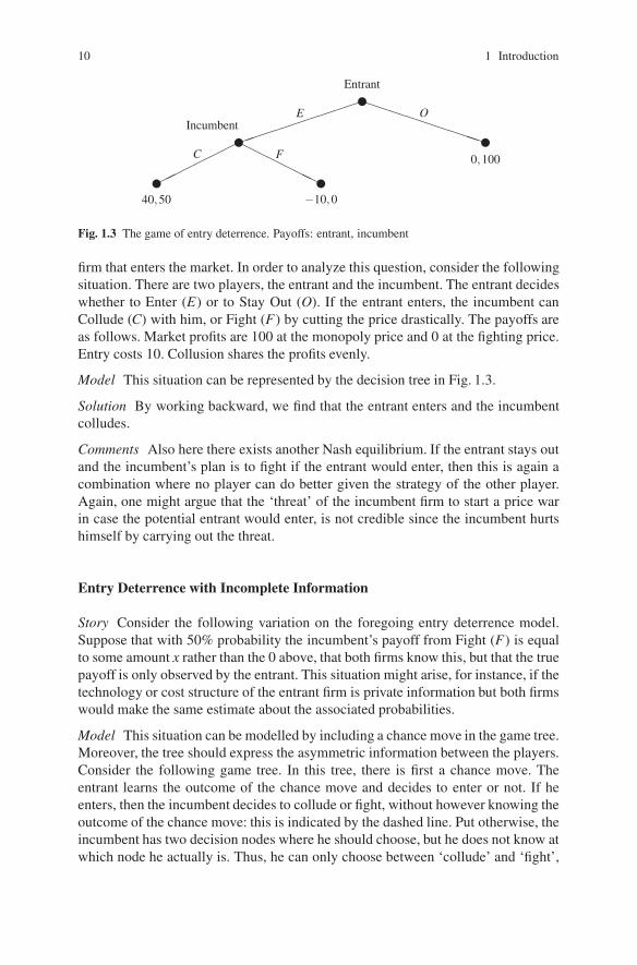
Fig. 1.3 The game of entry deterrence. Payoffs: entrant, incumbent
firm that enters the market. In order to analyze this question, consider the followingsituation. There are two players, the entrant and the incumbent. The entrant decideswhether to Enter (E) or to Stay Out (O). If the entrant enters, the incumbent canCollude (C) with him, or Fight (F) by cutting the price drastically. The payoffs areas follows. Market profits are 100 at the monopoly price and 0 at the fighting price.Entry costs 10. Collusion shares the profits evenly.
Model This situation can be represented by the decision tree in Fig. 1.3.
Solution By working backward, we find that the entrant enters and the incumbentcolludes.
Comments Also here there exists another Nash equilibrium. If the entrant stays outand the incumbent’s plan is to fight if the entrant would enter, then this is again acombination where no player can do better given the strategy of the other player.Again, one might argue that the ‘threat’ of the incumbent firm to start a price warin case the potential entrant would enter, is not credible since the incumbent hurtshimself by carrying out the threat.
Entry Deterrence with Incomplete Information
Story Consider the following variation on the foregoing entry deterrence model.Suppose that with 50% probability the incumbent’s payoff from Fight (F) is equalto some amount x rather than the 0 above, that both firms know this, but that the truepayoff is only observed by the entrant. This situation might arise, for instance, if thetechnology or cost structure of the entrant firm is private information but both firmswould make the same estimate about the associated probabilities.
Model This situation can be modelled by including a chance move in the game tree.Moreover, the tree should express the asymmetric information between the players.Consider the following game tree. In this tree, there is first a chance move. Theentrant learns the outcome of the chance move and decides to enter or not. If heenters, then the incumbent decides to collude or fight, without however knowing theoutcome of the chance move: this is indicated by the dashed line. Put otherwise, theincumbent has two decision nodes where he should choose, but he does not know atwhich node he actually is. Thus, he can only choose between ‘collude’ and ‘fight’,

1.3 Examples 11
Entrant
Entrant
Inc.
E
E
O
O
C
F
C
F
Chance
0,100
0,100
40,50
−10,0
40, 50
−10,x
50%
50%
Fig. 1.4 Entry deterrence with incomplete information
� �����������������
������
���������������
������� � � �
1
2
S B
S B S B
2,1 0,0 0,0 1,2
Fig. 1.5 Simultaneous Battle of the Sexes in extensive form
without making this choice contingent on the outcome of the chance move. SeeFig. 1.4.
Solution Clearly, if x ≤ 50 then an obvious solution is that the incumbent colludesand the entrant enters. Also the combination of strategies where the entrant stays outno matter what the outcome of the chance move is, and the incumbent fights, is aNash equilibrium. A complete analysis is more subtle and may include consideringprobabilistic information that the incumbent might derive from the action of theentrant in a so-called ‘perfect Bayesian equilibrium’, see Chaps. 5 and 14.
Comments The collection of the two nodes of the incumbent, connected by thedashed line, is usually called an ‘information set’. Information sets are used in gen-eral to model imperfect information. In the present example imperfect informationarises since the incumbent does not know the outcome of the chance move. Imper-fect information can also arise if some player does not observe some move of someother player. As a simple example, consider again the simultaneous move Battle ofthe Sexes game of Sect. 1.3.2. This can be modelled as a game in extensive form asin Fig. 1.5.
Hence, player 2, when he moves, does not know what player 1 has chosen. Thisis equivalent to players 1 and 2 moving independently and simultaneously.

12 1 Introduction
1.3.4 Cooperative Games
In a cooperative game the focus is on payoffs and coalitions, rather than on strate-gies. The prevailing analysis has an axiomatic flavor, in contrast to the equilibriumanalysis of noncooperative theory.
Three Cooperating Cities
Story Cities 1, 2 and 3 want to be connected with a nearby power source. Thepossible transmission links and their costs are shown in the following picture. Eachcity can hire any of the transmission links. If the cities cooperate in hiring the linksthey save on the hiring costs (the links have unlimited capacity). The situation isrepresented in Fig. 1.6.
Model The players in this situation are the three cities. Denote the player set by N ={1,2,3}. These players can form coalitions: any subset S of N is called a coalition.Table 1.1 presents the costs as well as the savings of each coalition. The numbersc(S) are obtained by calculating the cheapest routes connecting the cities in thecoalition S with the power source.12 The cost savings v(S) are determined by
v(S) := ∑i∈S
c({i})− c(S) for each nonempty S ⊆ N.
The cost savings v(S) for coalition S are equal to the difference in costs correspond-ing to the situation where all members of S work alone and the situation where allmembers of S work together. The pair (N,v) is called a cooperative game.
��
��
���
��� ��
�power
1
2
3
100 30
140 20
50��
���
�����
��
���
�����
Fig. 1.6 Situation leading to the three cities game
Table 1.1 The three cities game
S {1} {2} {3} {1,2} {1,3} {2,3} {1,2,3}c(S) 100 140 130 150 130 150 150v(S) 0 0 0 90 100 120 220
12 Cf. Bird [14].

1.3 Examples 13
Solution Basic questions in a cooperative game (N,v) are: which coalitions willactually be formed, and how should the proceeds (savings) of such a coalition bedistributed among its members? To form a coalition the consent of every member isneeded, but it is likely that the willingness of a player to participate in a coalitiondepends on what the player obtains in that coalition. Therefore, the second ques-tion seems to be the more basic one, and in this book attention is focussed on thatquestion. Specifically, it is usually assumed that the ‘grand’ coalition N of all play-ers is formed, and the question is then reduced to the problem of distributing theamount v(N) among the players. In the present example, how should the amount220 (=v(N)) be distributed among the three cities? In other words, we look for vec-tors x = (x1,x2,x3) ∈ R3 such that x1 + x2 + x3 = 220, where player i ∈ {1,2,3}obtains xi. One obvious candidate is to choose x1 = x2 = x3 = 220/3, but this doesnot really reflect the asymmetry of the situation: some coalitions save more thanothers. The literature offers many quite different solutions to this distribution prob-lem, among which are the core, the Shapley value, and the nucleolus. The core, forinstance, consists of those payoff distributions that cannot be improved upon by anysmaller coalition. For the three cities example, this means that the core consists ofthose vectors (x1,x2,x3) such that x1 + x2 + x3 = 220, x1,x2,x3 ≥ 0, x1 + x2 ≥ 90,x1 + x3 ≥ 100, and x2 + x3 ≥ 120. Hence, this is quite a big set and therefore ratherindeterminate as a solution to the game. In contrast, the Shapley value consists bydefinition of one point (vector), in this example the distribution (65,75,80). Alsothe nucleolus consists of one point, in this case the vector (56 2
3 ,76 23 ,86 2
3).13
Comments The implicit assumptions in a game like this are, first, that a coalitioncan make binding agreements on the distribution of its payoff and, second, that anypayoff distribution that distributes (or, at least, does not exceed) the savings or, moregenerally, worth of the coalition is possible. For these reasons, such games are calledcooperative games with transferable utility. See Chaps. 9 and 16–20.
The Glove Game
Story Assume there are three players, 1, 2, and 3. Players 1 and 2 each possess aright-hand glove, while player 3 has a left-hand glove. A pair of gloves has worth 1.The players cooperate in order to generate a profit.
Model The associated cooperative game is described by Table 1.2.
Table 1.2 The glove game
S {1} {2} {3} {1,2} {1,3} {2,3} {1,2,3}v(S) 0 0 0 0 1 1 1
13 The reader should take these claims for granted. Definitions of these concepts are provided inChap. 9. See also Chaps. 16–20.

14 1 Introduction
Table 1.3 Preferences for dentist appointments
Mon Tue Wed
Adams 2 4 8Benson 10 5 2Cooper 10 6 4
Table 1.4 The dentist game: a permutation game
S {1} {2} {3} {1,2} {1,3} {2,3} {1,2,3}v(S) 2 5 4 14 18 9 24
Solution The core of this game consists of exactly one vector (see Problem 1.5).The Shapley value assigns 2/3 to player 3 and 1/6 to both player 1 and player 2.The nucleolus is the unique element of the core.
A Permutation Game
Story (From [22], p. 54) Mr. Adams, Mrs. Benson, and Mr. Cooper have appoint-ments with the dentist on Monday, Tuesday, and Wednesday, respectively. Thisschedule not necessarily matches their preferences, due to different urgencies andother factors. These preferences (expressed in numbers) are given in Table 1.3.
Model This situation gives rise to a game in which the coalitions can gain by reshuf-fling their appointments. For instance, Adams (player 1) and Benson (player 2)can change their appointments and obtain a total of 14 instead of 7. A completedescription of the resulting game is given in the Table 1.4.
Solution The core of this game is the convex hull of the vectors (15,5,4), (14,6,4),(8,6,10), and (9,5,10). The Shapley value is the vector (9 1
2 ,6 12 ,8), and the nucle-
olus is the vector (11 12 ,5 1
2 ,7).14
A Voting Game
(From [98], p. 247: The United Nations Security Council.) The United nations Secu-rity Council consists of five permanent members (United States, Russia, Britain,France, and China) and ten other members. Motions must be approved by ninemembers, including all the permanent members. This situation gives rise to a 15-player so called voting game (N,v) with v(S) = 1 if the coalition S contains thefive permanent members and at least four nonpermanent members, and v(S) = 0otherwise. Such games are also called simple games. Coalitions with worth equal to1 are called winning, the other coalitions are called losing. Simple games are studiedin Chap. 16.
14 See Chap. 20 for an analysis of permutation games.

1.3 Examples 15
A solution to such a voting game is interpreted as representing the power of aplayer, rather than payoff (money) or utility.
1.3.5 Bargaining Games
Bargaining theory focusses on agreements between individual players.
A Division Problem
Story Consider the following situation. Two players have to agree on the division ofone unit of a perfectly divisible good, say a liter of wine. If they reach an agreement,say (α,β ) where α,β ≥ 0 and α +β ≤ 1, then they split up the one unit according tothis agreement; otherwise, they both receive nothing. The players have preferencesfor the good, described by utility functions.
Model To fix ideas, assume that player 1 has a utility function u1(α) = α and player2 has a utility function u2(α) =
√α . Thus, a distribution (α,1−α) of the good leads
to a corresponding pair of utilities (u1(α),u2(1−α)) = (α,√
1−α). By letting αrange from 0 to 1 we obtain all utility pairs corresponding to all feasible distributionsof the good, as in Fig. 1.7. It is assumed that also distributions summing to less thanthe whole unit are possible. This yields the whole shaded region.
Solution Nash [90] proposed the following way to ‘solve’ this bargaining prob-lem: maximize the product of the players’ utilities on the shaded area. Since thismaximum will be reached on the boundary, the problem is equivalent to
max0≤α≤1
α√
1−α.
The maximum is obtained for α = 23 . So the ‘solution’ of the bargaining problem
in utilities equals ( 23 , 1
3
√3), which is the point z in the picture above. This implies
Fig. 1.7 A bargaining game
1
0 1u1
u2
23
√13
z

16 1 Introduction
that player 1 obtains 23 of the 1 unit of the good, whereas player 2 obtains 1
3 . Asdescribed here, this solution comes out of the blue. Nash, however, provided anaxiomatic foundation for this solution (which is usually called the Nash bargainingsolution).
Comments The bargaining literature includes many noncooperative, strategicapproaches to the bargaining problem, including an attempt by Nash himself [92].An important, seminal article in this literature is Rubinstein [110], in which the bar-gaining problem is modelled as an alternating offers extensive form game. Binmoreet al. [13] observed the close relationship between the Nash bargaining solution andthe strategic approach of Rubinstein. See Chap. 10.
The bargaining game can be seen as a special case of a cooperative game withouttransferable utility. Also games with transferable utility form a subset of the moregeneral class of games without transferable utility. See also Chap. 21.
1.4 Cooperative vs. Noncooperative Game Theory
The usual distinction between cooperative and noncooperative game theory is that ina cooperative game binding agreements between players are possible, whereas this isnot the case in noncooperative games. This distinction is informal and also not verysharp: for instance, the core of a cooperative game has a clear noncooperative fla-vor; a concept like correlated equilibrium for noncooperative games (see Sect. 13.7)has a clear cooperative flavor. Moreover, quite some game-theoretic literature isconcerned with viewing problems both from a cooperative and a noncoopera-tive angle. This approach is sometimes called the Nash program; the bargainingproblem discussed above is a typical example. In a much more formal sense, the the-ory of implementation is concerned with representing outcomes from cooperativesolutions as equilibrium outcomes of specific noncooperative solutions.
A more workable distinction between cooperative and noncooperative games canbe based on the ‘modelling technique’ that is used: in a noncooperative game playershave explicit strategies, whereas in a cooperative game players and coalitions arecharacterized, more abstractly, by the outcomes and payoffs that they can reach.The examples in Sects. 1.3.1–1.3.3 are examples of noncooperative games, whereasthose in Sects. 1.3.4 and 1.3.5 are examples of cooperative games.
Problems
1.1. Battle of the Bismarck Sea
(a) Represent the ‘Battle of the Bismarck Sea’ as a game in extensive form.

Problems 17
(b) Now assume that Imamura moves first, and Kenney observes Imamura’s moveand moves next. Represent this situation in extensive form and solve by workingbackwards.
(c) Answer the same questions as under (b) with the roles of the players reversed.
1.2. Variant of Matching Pennies
Consider the following variant of the ‘Matching Pennies’ game
(Heads TailsHeads x −1Tails −1 1
),
where x is a real number. For which value(s) of x does this game have a saddlepoint,if any?
1.3. Mixed Strategies
Consider the following zero-sum game:
(L RT 3 2B 1 4
).
(a) Show that this game has no saddlepoint.
(b) Find a mixed strategy (randomized choice) of (the row) player 1 that makes hisexpected payoff independent of player 2’s strategy.
(c) Find a mixed strategy of player 2 that makes his expected payoff independent ofplayer 1’s strategy.
(d) Consider the expected payoffs found under (b) and (c). What do you concludeabout how the game could be played if randomized choices are allowed?
1.4. Three Cooperating Cities
Show that the Shapley value and the nucleolus of the ‘Three Cooperating CitiesGame’ are elements of the core of this game.
1.5. Glove Game
(a) Compute the core of the glove game.
(b) Is the Shapley value an element of the core?
1.6. Dentist Appointments
For the permutation (dentist appointments) game, check if the Shapley value andthe nucleolus are in the core of the game.

18 1 Introduction
1.7. Nash Bargaining
Verify the computation of the Nash bargaining solution for the division problem.
1.8. Variant of Glove Game
Suppose there are n = �+ r players, where � players own a left-hand glove and rplayers own a right-hand glove. Let N be the set of all players and let S ⊆ N be acoalition. As before, each pair of gloves has worth 1. Find an expression for v(S),i.e., the maximal profit that S can generate by cooperation of its members.
Chapter 2Finite Two-Person Zero-Sum Games
This chapter deals with two-player games in which each player chooses from finitelymany pure strategies or randomizes among these strategies, and the sum of the play-ers’ payoffs or expected payoffs is always equal to zero. Games like the ‘Battle ofthe Bismarck Sea’ and ‘Matching Pennies’, discussed in Sect. 1.3.1 belong to thisclass.
In Sect. 2.1 the basic definitions and theory are discussed. Section 2.2 showshow to solve 2× n and m× 2 games, and larger games by elimination of strictlydominated strategies.
2.1 Basic Definitions and Theory
Since all data of a finite two-person zero-sum game can be summarized in onematrix, such a game is usually called a ‘matrix game’.
Definition 2.1 (Matrix game). A matrix game is an m×n matrix A of real numbers,where the number of rows m and the number of columns n are integers greater thanor equal to 1. A (mixed) strategy of player 1 is a probability distribution p over therows of A, i.e., an element of the set
∆m := {p = (p1, . . . , pm) ∈ Rm |m
∑i=1
pi = 1, pi ≥ 0 for all i = 1, . . . ,m}.
Similarly, a (mixed) strategy of player 2 is a probability distribution q over thecolumns of A, i.e., an element of the set
∆n := {q = (q1, . . . ,qn) ∈ Rn |n
∑j=1
q j = 1, q j ≥ 0 for all j = 1, . . . ,n}.
H. Peters, Game Theory – A Multi-Leveled Approach.c© Springer-Verlag Berlin Heidelberg 2008
21

22 2 Finite Two-Person Zero-Sum Games
A strategy p of player 1 is called pure if there is a row i with pi = 1. This strategyis also denoted by ei. Similarly, a strategy q of player 2 is called pure if there is acolumn j with q j = 1. This strategy is also denoted by e j.
The interpretation of such a matrix game A is as follows. If player 1 plays row i (i.e.,pure strategy ei) and player 2 plays column j (i.e., pure strategy e j), then player 1receives payoff ai j and player 2 pays ai j (and, thus, receives −ai j), where ai j is thenumber in row i and column j of matrix A. If player 1 plays strategy1 p and player2 plays strategy q, then player 1 receives the expected payoff2
pAq =m
∑i=1
n
∑j=1
piq jai j,
and player 2 receives −pAq.For ‘solving’ matrix games, i.e., establishing what clever players would or should
do, the concepts of maximin and minimax strategies are important, as will beexplained below. First we give the formal definitions.
Definition 2.2 (Maximin and minimax strategies). A strategy p is a maximinstrategy of player 1 in matrix game A if
min{pAq | q ∈ ∆n} ≥ min{p′Aq | q ∈ ∆n} for all p′ ∈ ∆m.
A strategy q is a minimax strategy of player 2 in matrix game A if
max{pAq | p ∈ ∆m} ≤ max{pAq′ | p ∈ ∆m} for all q′ ∈ ∆n.
In words: a maximin strategy of player 1 maximizes the minimal (with respect toplayer 2’s strategies) payoff of player 1, and a minimax strategy of player 2 mini-mizes the maximum (with respect to player 1’s strategies) that player 2 has to payto player 1. Of course, the asymmetry in these definitions is caused by the fact that,by convention, a matrix game represents the amounts that player 2 has to pay toplayer 1.3
In order to check if a strategy p of player 1 is a maximin strategy it is sufficientto check that the first inequality in Definition 2.2 holds with e j for every j = 1, . . . ,ninstead of every q ∈ ∆n. This is not difficult to see but the reader is referred toChap. 12 for a more formal treatment. A similar observation holds for minimaxstrategies. In other words, to check if a strategy is maximin (minimax) it is sufficientto consider its performance against every pure strategy, i.e., column (row).
Why would we be interested in such strategies? At first glance, such strate-gies seem to express a very conservative or pessimistic, worst-case scenario atti-tude. The reason for considering maximin/minimax strategies is provided by von
1 Observe that here, by a ‘strategy’ we mean a mixed strategy: we add the adjective ‘pure’ if wewish to refer to a pure strategy.2 Since no confusion is likely to arise, we do not use transpose notations like pT Aq or pAqT .3 It can be proved by basic mathematical analysis that maximin and minimax strategies alwaysexist.

2.2 Solving 2×n Games and m×2 Games 23
Neumann [140]. Von Neumann shows4 that for every matrix game A there is a realnumber v = v(A) with the following properties:
1. A strategy p of player 1 guarantees a payoff of at least v to player 1 (i.e., pAq ≥ vfor all strategies q of player 2) if and only if p is a maximin strategy.
2. A strategy q of player 2 guarantees a payment of at most v by player 2 to player 1(i.e., pAq≤ v for all strategies p of player 1) if and only if q is a minimax strategy.
Hence, player 1 can obtain a payoff of at least v by playing a maximin strategy,and player 2 can guarantee to pay not more than v – hence secure a payoff of atleast −v – by playing a minimax strategy. For these reasons, the number v = v(A) isalso called the value of the game A – it represents the worth to player 1 of playingthe game A – and maximin and minimax strategies are called optimal strategies forplayers 1 and 2, respectively.
Therefore, ‘solving’ the game A means, naturally, determining the optimal strate-gies and the value of the game. In the ‘Battle of the Bismarck Sea’ in Sect. 1.3.1,the pure strategies N of both players guarantee the same amount 2. Therefore, thisis the value of the game and N is optimal for both players. The analysis of that gameis easy since it has a ‘saddlepoint’, namely position (1,1) with a11 = 2. The formaldefinition of a saddlepoint is as follows.
Definition 2.3 (Saddlepoint). A position (i, j) in a matrix game A is a saddlepoint if
ai j ≥ ak j for all k = 1, . . . ,m and ai j ≤ aik for all k = 1, . . . ,n,
i.e., if ai j is maximal in its column j and minimal in its row i.
Clearly, if (i, j) is a saddlepoint, then player 1 can guarantee a payoff of at least ai jby playing the pure strategy row i, since ai j is minimal in row i. Similarly, player 2can guarantee a payoff of at least −ai j by playing the pure strategy column j, sinceai j is maximal in column j. Hence, ai j must be the value of the game A: v(A) = ai j,ei is an optimal (maximin) strategy of player 1, and e j is an optimal (minimax)strategy of player 2.
2.2 Solving 2×n Games and m×2 Games
In this section we show how to solve matrix games where at least one of the playershas two pure strategies. We also show how the idea of strict domination can be ofhelp in solving matrix games.
4 See Chap. 12 for a more rigorous treatment of zero-sum games and a proof of von Neumann’sresult.

24 2 Finite Two-Person Zero-Sum Games
2.2.1 2×n Games
We demonstrate how to solve a matrix game with 2 rows and n columns graphically,by considering the following 2×4 example:
A =( e1 e2 e3 e4
10 2 4 12 10 8 12
).
We have labelled the columns of A, i.e., the pure strategies of player 2 for referencebelow. Let p = (p,1− p) be an arbitrary strategy of player 1. The expected payoffsto player 1 if player 2 plays a pure strategy are equal to:
pAe1 = 10p + 2(1− p)= 8p + 2pAe2 = 2p + 10(1− p)= 10−8p
pAe3 = 4p + 8(1− p)= 8−4p
pAe4 = p + 12(1− p)= 12−11p.
We plot these four linear functions of p in one diagram:
2
6
8
10
12
12
4
6
10
0 1p∗ = 12
e1
e3
e2
e4
In this diagram the values of p are plotted on the horizontal axis, and the four straightgray lines plot the payoffs to player 1 if player 2 plays one of his four pure strategies,respectively. Observe that for every 0≤ p≤ 1 the minimum payoff that player 1 mayobtain is given by the lower envelope of these curves, the thick black curve in thediagram: for any p, any combination (q1,q2,q3,q4) of the points on e1, e2, e3, ande4 with first coordinate p would lie on or above this lower envelope. Clearly, thelower envelope is maximal for p = p∗ = 1
2 , and the maximal value is 6. Hence,

2.2 Solving 2×n Games and m×2 Games 25
we have established that player 1 has a unique optimal (maximin) strategy, namelyp∗ = ( 1
2 , 12 ), and that the value of the game, v(A), is equal to 6.
What are the optimal or minimax strategies of player 2? From the theory of theprevious section we know that a minimax strategy q = (q1,q2,q3,q4) of player 2should guarantee to player 2 to have to pay at most the value of the game. Fromthe diagram it is clear that q4 should be equal to zero since otherwise the payoff toplayer 1 would be larger than 6 if player 1 plays ( 1
2 , 12 ), and thus q would not be a
minimax strategy. So a minimax strategy has the form q = (q1,q2,q3,0). Any suchstrategy, plotted in the diagram, gives a straight line that is a combination of thelines associated with e1, e2, and e3 and which passes through the point ( 1
2 ,6) sinceall three lines pas through this point. Moreover, for no value of p should this straightline exceed the value 6, otherwise q would not guarantee a payment of at most 6 byplayer 2. Consequently, this straight line has to be horizontal. Summarizing thisargument, we look for numbers q1,q2,q3 ≥ 0 such that
2q1 + 10q2 + 8q3 = 6 (left endpoint should be (0,6))10q1 + 2q2 + 4q3 = 6 (right endpoint should be (1,6))
q1 + q2 + q3 = 1 (q is a probability vector).
This system of equations is easily reduced5 to the two equations
3q1 −q2 = 1q1 + q2 + q3 = 1.
The first equation implies that if q1 = 13 then q2 = 0 and if q1 = 1
2 then q2 = 12 .
Clearly, q1 and q2 cannot be larger since then their sum exceeds 1. Hence the set ofoptimal strategies of player 2 is
{q = (q1,q2,q3,q4) ∈ ∆4 | 13≤ q1 ≤ 1
2, q2 = 3q1 −1, q4 = 0}.
2.2.2 m×2 Games
The solution method to solve m× 2 games is analogous. Consider the followingexample:
A =
⎛⎜⎜⎝e1 10 2e2 2 10e3 4 8e4 1 12
⎞⎟⎟⎠.
5 For instance, by substitution. In fact, one of the two first equations could be omitted to beginwith, since we already know that any combination of the three lines passes through ( 1
2 ,6), and twopoints are sufficient to determine a straight line.

26 2 Finite Two-Person Zero-Sum Games
Let q = (q,1− q) be an arbitrary strategy of player 2. Again, we make a diagramin which now the values of q are put on the horizontal axis, and the straight linesindicated by ei for i = 1,2,3,4 are the payoffs to player 1 associated with his fourpure strategies (rows) as functions of q. The equations of these lines are given by:
e1Aq = 10q + 2(1−q)= 8q + 2e2Aq = 2q + 10(1−q)= 10−8q
e3Aq = 4q + 8(1−q)= 8−4q
e4Aq = q + 12(1−q)= 12−11q.
The resulting diagram is as follows.
2
11819
8
10
12
12
4
11819
10
0 1q∗ = 1019
e1
e3
e2
e4
Observe that the maximum payments that player 2 has to make are now located onthe upper envelope, represented by the thick black curve. The minimum is reached atthe point of intersection of e1 and e4 in the diagram, which has coordinates ( 10
19 , 11819 ).
Hence, the value of the game is 11819 , and the unique optimal (minimax) strategy of
player 2 is q∗ = ( 1019 , 9
19).To find the optimal strategy or strategies p = (p1, p2, p3, p4) of player 1, it fol-
lows from the diagram that p2 = p3 = 0, otherwise for q = 1019 the value 118
19 of thegame is not reached, so that p is not a maximin strategy. So we look for a com-bination of e1 and e4 that gives at least 118
19 for every q, hence it has to be equalto 118
19 for every q. This gives rise to the equations 2p1 + 12p4 = 10p1 + p4 = 11819
and p1 + p4 = 1, with unique solution p1 = 1119 and p4 = 8
19 . So the unique optimalstrategy of player 1 is ( 11
19 ,0,0, 819).

2.2 Solving 2×n Games and m×2 Games 27
2.2.3 Strict Domination
The idea of strict domination can be used to eliminate pure strategies before thegraphical analysis of a matrix game. Consider the game
A =( e1 e2 e3 e4
10 2 5 12 10 8 12
),
which is almost identical to the game in Sect. 2.2.1, except that a13 is now 5 insteadof 4. Consider a strategy (α,1−α,0,0) of player 2. The expected payments fromthis strategy from player 2 to player 1 are 8α + 2 if player 1 plays the first rowand 10− 8α if player 1 plays the second row. For any value 1
4 < α < 38 , the first
number is smaller than 5 and the second number is smaller than 8. Hence, this isstrictly better for player 2 than playing his pure strategy e3, no matter what player 1does. But then, for any strategy q = (q1,q2,q3,q4) of player 2 with q3 > 0, theexpected payoff to player 2 would become strictly larger (his payment to player 1strictly smaller) by transferring the probability q3 to the first two pure strategiesin some right proportion α , i.e., by playing (q1 + αq3,q2 + (1−α)q3,0,q4) forsome 1
4 < α < 38 , instead of q. Hence, in an optimal (minimax) strategy we must
have q3 = 0. This implies that, in order to solve the above game, we can start bydeleting the third column of the matrix. In the diagram in Sect. 2.2.1, we do nothave to draw the line corresponding to e3. The value of the game is still 6, player 1still has a unique optimal strategy p∗ = ( 1
2 , 12 ), and player 2 now also has a unique
optimal strategy, namely the one where q3 = 0, which is the strategy ( 12 , 1
2 ,0,0).In general, strictly dominated pure strategies in a matrix game are not played
with positive probability in any optimal strategy and can therefore be deleted beforesolving the game. Sometimes, this idea can also be used to solve matrix games inwhich each player has more than two pure strategies (m,n > 2). Moreover, the ideacan be applied iteratively, that is, after deletion of a strictly dominated pure strategy,in the smaller game perhaps another strictly dominated pure strategy can be deleted,etc., until no more pure strategies are strictly dominated.6
We first provide a formal definition of strict domination for completeness’ sake,and then discuss another example where iterated elimination of strictly dominatedstrategies is applied.
Definition 2.4 (Strict domination). Let A be an m×n matrix game and i a row. Thepure strategy ei is strictly dominated if there is a strategy p = (p1, . . . , pm)∈∆m withpi = 0 such that pAe j > eiAe j for every j = 1, . . . ,n. Similarly, let j be a column.The pure strategy e j is strictly dominated if there is a strategy q = (q1, . . . ,qn) ∈ ∆n
with q j = 0 such that eiAq < eiAe j for every i = 1, . . . ,m.7
6 Of course, all this needs to be proved formally, but in this chapter it is just assumed. See Chap. 13for a more formal treatment.7 An equivalent definition is obtained if the conditions pi = 0 and q j = 0 are omitted.

28 2 Finite Two-Person Zero-Sum Games
Example 2.5. Consider the following 3×3 matrix game:
A =
⎛⎝6 0 20 5 43 2 1
⎞⎠.
For player 1, the third strategy e3 is strictly dominated by the strategy p = ( 712 , 5
12 ,0),since pA = (3 1
2 ,2 112 ,2 5
6) has every coordinate strictly larger than e3A = (3,2,1).Hence, in any optimal strategy player 1 puts zero probability on the third row.Elimination of this row results in the matrix
B =(
6 0 20 5 4
).
Now, player 2’s third strategy e3 is strictly dominated by the strategy q = ( 14 , 3
4 ,0),since Bq = ( 3
2 ,3 34), which has every coordinate strictly smaller than Be3 = (2,4).
Hence, in any optimal strategy player 2 puts zero probability on the third column.Elimination of this column results in the matrix
C =(
6 00 5
).
This is a 2× 2 matrix game, which can be solved by the method in Sect. 2.2.1 orSect. 2.2.2. See Problem 2.1(a).
Problems
2.1. Solving Matrix Games
Solve the following matrix games, i.e., determine the optimal strategies and thevalue of the game. Each time, start by checking if the game has a saddlepoint.
(a) (6 00 5
)What are the optimal strategies in the original matrix game A in Example 2.5?
(b) ⎛⎝ 2 −1 0 22 0 0 30 0 −1 2
⎞⎠

Problems 29
(c) ⎛⎝ 1 3 12 2 00 3 2
⎞⎠(d) ⎛⎜⎜⎝
16 12 22 6 168 8 60 7 8
⎞⎟⎟⎠(e) (
3 1 4 01 2 0 5
)(f) ⎛⎝ 1 0 2
4 1 13 1 3
⎞⎠2.2. Saddlepoints
(a) Let A be an arbitrary m× n matrix game. Show that any two saddlepoints musthave the same value. In other words, if (i, j) and (k, l) are two saddlepoints, showthat ai j = akl .
(b) Let A be a 4× 4 matrix game in which (1,1) and (4,4) are saddlepoints. Showthat A has at least two other saddlepoints.
(c) Give an example of a 4×4 matrix game with exactly three saddlepoints.
2.3. Rock–Paper–Scissors
In the famous Rock–Paper–Scissors two-player game each player has three purestrategies: Rock, Paper, and Scissors. Here, Scissors beats Paper, Paper beats Rock,Rock beats Scissors. Assign a 1 to winning, 0 to a draw, and −1 to losing. Modelthis game as a matrix game, try to guess its optimal strategies, and then show thatthese are the unique optimal strategies. What is the value of this game?

Chapter 3Finite Two-Person Games
In this chapter we consider two-player games where each player chooses fromfinitely many pure strategies or randomizes among these strategies. In contrast toChap. 2 it is no longer required that the sum of the players’ payoffs is zero (or,equivalently, constant). This allows for a much larger class of games, includingmany games relevant for economic or other applications. Famous examples are the‘Prisoners’ Dilemma’ and the ‘Battle of the Sexes’ discussed in Sect. 1.3.2.
In Sect. 3.1 we introduce the model and the concept of ‘Nash equilibrium’. Sec-tion 3.2 shows how to compute Nash equilibria in pure strategies for arbitrary games,all Nash equilibria in games where both players have exactly two pure strategies, andhow to use the concept of strict domination to facilitate computation of Nash equilib-ria and to compute equilibria also of larger games. The structure of this chapter thusparallels the structure of Chap. 2. For a deeper and more comprehensive analysis offinite two-person games see Chap. 13.
3.1 Basic Definitions and Theory
The data of a finite two-person game can be summarized by two matrices. Usu-ally, these matrices are written as one matrix with two numbers at each position.Therefore, such games are often called ‘bimatrix games’. The formal definition isas follows.
Definition 3.1 (Bimatrix game). A bimatrix game is a pair of m × n matrices(A,B), where m and n are integers greater than or equal to 1.
The interpretation of such a bimatrix game (A,B) is that, if player 1 (the row player)plays row i and player 2 (the column player) plays column j, then player 1 receivespayoff ai j and player 2 receives bi j, where these numbers are the correspondingentries of A and B, respectively. Definitions and notations for pure and mixed strate-gies, strategy sets and expected payoffs are similar to those for matrix games, see
H. Peters, Game Theory – A Multi-Leveled Approach.c© Springer-Verlag Berlin Heidelberg 2008
31

32 3 Finite Two-Person Games
Sect. 2.1, but for easy reference we repeat them here. A (mixed) strategy of player1 is a probability distribution p over the rows of A, i.e., an element of the set
∆m := {p = (p1, . . . , pm) ∈ Rm |m
∑i=1
pi = 1, pi ≥ 0 for all i = 1, . . . ,m} .
Similarly, a (mixed) strategy of player 2 is a probability distribution q over thecolumns of A, i.e., an element of the set
∆n := {q = (q1, . . . ,qn) ∈ Rn |n
∑j=1
q j = 1, q j ≥ 0 for all j = 1, . . . ,n} .
A strategy p of player 1 is called pure if there is a row i with pi = 1. This strategyis also denoted by ei. Similarly, a strategy q of player 2 is called pure if there is acolumn j with q j = 1. This strategy is also denoted by e j. If player 1 plays p andplayer 2 plays q then the payoff to player 1 is the expected payoff
pAq =m
∑i=1
n
∑j=1
piq jai j ,
and the payoff to player 2 is the expected payoff
pBq =m
∑i=1
n
∑j=1
piq jbi j .
As mentioned, the entries of A and B are usually grouped together in one(bi)matrix, by putting the pair ai j,bi j at position (i, j) of the matrix. Cf. the examplesin Sect. 1.3.2.
Central to noncooperative game theory is the idea of best reply. It says thata rational selfish player should always maximize his (expected) payoff, given hisknowledge of or conjecture about the strategies chosen by the other players.
Definition 3.2 (Best reply). A strategy p of player 1 is a best reply to a strategy qof player 2 in an m×n bimatrix game (A,B) if
pAq ≥ p′Aq for all p′ ∈ ∆m .
Similarly, q is a best reply of player 2 to p if
pBq ≥ pBq′ for all q′ ∈ ∆n .
In a ‘Nash equilibrium’, each player’s strategy is a best reply to the other player’sstrategy.
Definition 3.3 (Nash equilibrium). A pair of strategies (p∗,q∗) in a bimatrix game(A,B) is a Nash equilibrium if p∗ is a best reply of player 1 to q∗ and q∗ is a best
3.2 Finding Nash Equilibria 33
reply of player 2 to p∗. A Nash equilibrium (p∗,q∗) is called pure if both p∗ and q∗are pure strategies.
The concept of a Nash equilibrium can be extended to quite arbitrary games, includ-ing games with arbitrary numbers of players, strategy sets, and payoff functions. Wewill see a lot of examples in later chapters of this book. For finite two-person games,Nash [91] proved that every game has a Nash equilibrium in mixed strategies, i.e., aNash equilibrium according to Definition 3.3. See Sect. 13.1 for such a proof. Gener-ally speaking, the main concern with Nash equilibrium is not its existence but ratherthe opposite, namely its abundance, as well as its interpretation. In many games,there are many Nash equilibria, and then the questions of equilibrium selection andequilibrium refinement are relevant. With respect to interpretation, an old questionis how in reality the players would come to play a Nash equilibrium. The definitionof Nash equilibrium does not say anything about this.
For a Nash equilibrium in mixed strategies as in Definition 3.3, an additionalquestion is what the meaning of such a mixed strategy is. Does it mean that theplayers actually randomize when playing the game? A different and quite commoninterpretation is that a mixed strategy of a player, say player 1, represents the belief,or conjecture, of the other player, player 2, about what player 1 will do. Thus, itembodies the ‘strategic uncertainty’ of the players in a game, a term coined by vonNeumann and Morgenstern [141].
For now, we just leave these questions aside and take the definition of Nash equi-librium at face value. We show how to compute pure Nash equilibria in general, andall Nash equilibria in games where both players have two pure strategies. Just likein Chap. 2, we also consider the role of strict domination.
3.2 Finding Nash Equilibria
To find all Nash equilibria of an arbitrary bimatrix game is a difficult task. We referto Sect. 13.2.3 for more discussion on this problem. Here we restrict ourselves to,first, the much easier problem of finding all Nash equilibria in pure strategies of anarbitrary bimatrix game and, second, to showing how to find all Nash equilibria in2×2 games graphically. It is also possible to solve 2×3 and 3×2 games graphically,see Sect. 13.2.2. For larger games, graphical solutions are impractical or, indeed,impossible.
3.2.1 Pure Nash Equilibria
To find the pure Nash equilibria in a bimatrix game, one can first determine the purebest replies of player 2 to every pure strategy of player 1, and next determine thepure best replies of player 1 to every pure strategy of player 2. Those pairs of pure

34 3 Finite Two-Person Games
strategies that are mutual best replies are the pure Nash equilibria of the game. Toillustrate this method, consider the bimatrix game
⎛⎝W X Y Z
T 2,2 4,0 1,1 3,2M 0,3 1,5 4,4 3,4B 2,0 2,1 5,1 1,0
⎞⎠ .
First we determine the pure best replies of player 2 to every pure strategy of player1, indicated by the stars at the corresponding entries. This yields:
⎛⎝W X Y Z
T 2,2∗ 4,0 1,1 3,2∗M 0,3 1,5∗ 4,4 3,4B 2,0 2,1∗ 5,1∗ 1,0
⎞⎠ .
Next, we determine the pure best replies of player 1 to every pure strategy of player2, again indicated by the stars at the corresponding entries. This yields:
⎛⎝W X Y Z
T 2∗,2 4∗,0 1,1 3∗,2M 0,3 1,5 4,4 3∗,4B 2∗,0 2,1 5∗,1 1,0
⎞⎠ .
Putting the two results together yields:
⎛⎝W X Y Z
T 2∗,2∗ 4∗,0 1,1 3∗,2∗M 0,3 1,5∗ 4,4 3∗,4B 2∗,0 2,1∗ 5∗,1∗ 1,0
⎞⎠ .
We conclude that the game has three Nash equilibria in pure strategies, namely(T,W ), (T,Z), and (B,Y ). In mixed strategy notation, these are the pairs
(e1,e1),(
e1,e4), and(e3,e3), respectively. In more extensive notation: ((1,0,0),(1,0,0,0)),
((1,0,0),(0,0,0,1)), and ((0,0,1),(0,0,1,0)), respectively.Strictly speaking, one should also consider mixed best replies to a pure strategy
in order to establish whether this pure strategy can occur in a Nash equilibrium, butit is not hard to see that any mixed best reply is a combination of pure best repliesand, thus, can never lead to a higher payoff. For instance, in the example above,any strategy of the form (q,0,0,1− q) played against T yields to player 2 a payoffof 2 (= 2q + 2(1− q)) and is therefore a best reply, but does not yield a payoffhigher than W or Z. However, the reader can check that all strategy pairs of the form(T,(q,0,0,1−q)) (0 < q < 1) are also Nash equilibria of this game.
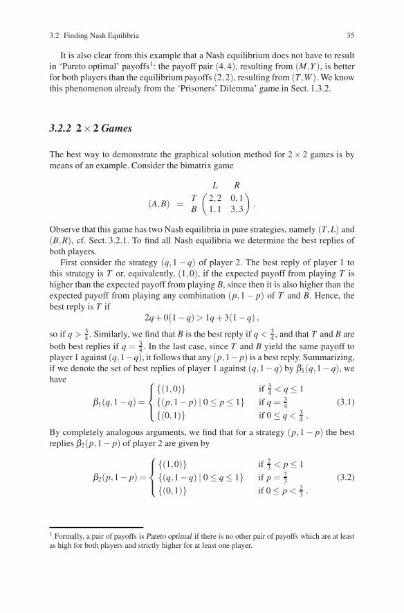
3.2 Finding Nash Equilibria 35
It is also clear from this example that a Nash equilibrium does not have to resultin ‘Pareto optimal’ payoffs1: the payoff pair (4,4), resulting from (M,Y ), is betterfor both players than the equilibrium payoffs (2,2), resulting from (T,W ). We knowthis phenomenon already from the ‘Prisoners’ Dilemma’ game in Sect. 1.3.2.
3.2.2 2×2 Games
The best way to demonstrate the graphical solution method for 2× 2 games is bymeans of an example. Consider the bimatrix game
(A,B) =( L R
T 2,2 0,1B 1,1 3,3
).
Observe that this game has two Nash equilibria in pure strategies, namely (T,L) and(B,R), cf. Sect. 3.2.1. To find all Nash equilibria we determine the best replies ofboth players.
First consider the strategy (q,1− q) of player 2. The best reply of player 1 tothis strategy is T or, equivalently, (1,0), if the expected payoff from playing T ishigher than the expected payoff from playing B, since then it is also higher than theexpected payoff from playing any combination (p,1− p) of T and B. Hence, thebest reply is T if
2q + 0(1−q)> 1q + 3(1−q) ,
so if q > 34 . Similarly, we find that B is the best reply if q < 3
4 , and that T and B areboth best replies if q = 3
4 . In the last case, since T and B yield the same payoff toplayer 1 against (q,1−q), it follows that any (p,1− p) is a best reply. Summarizing,if we denote the set of best replies of player 1 against (q,1−q) by β1(q,1−q), wehave
β1(q,1−q) =
⎧⎪⎨⎪⎩{(1,0)} if 3
4 < q ≤ 1{(p,1− p) | 0 ≤ p ≤ 1} if q = 3
4{(0,1)} if 0 ≤ q < 3
4 .
(3.1)
By completely analogous arguments, we find that for a strategy (p,1− p) the bestreplies β2(p,1− p) of player 2 are given by
β2(p,1− p) =
⎧⎪⎨⎪⎩{(1,0)} if 2
3 < p ≤ 1{(q,1− q) | 0 ≤ q ≤ 1} if p = 2
3{(0,1)} if 0 ≤ p < 2
3 .
(3.2)
1 Formally, a pair of payoffs is Pareto optimal if there is no other pair of payoffs which are at leastas high for both players and strictly higher for at least one player.

36 3 Finite Two-Person Games
By definition, the Nash equilibria of the game are the strategy combinations (p∗,q∗)such that p∗ ∈β1(q∗) and q∗ ∈β2(p∗), i.e., the points of intersection of the best replyfunctions in (3.1) and (3.2). A convenient way to find these points is by drawing thegraphs of β1(q,1−q) and β2(p,1− p). We put p on the horizontal axis and q on thevertical axis and obtain the following diagram.
0 p 2/3 1
q
3/4
1
�
��
The solid black curve is the best reply function of player 1 and the solid grey curveis the best reply function of player 2. The solid circles indicate the three Nashequilibria of the game: ((1,0),(1,0)), ((2/3,1/3),(3/4,1/4)), and ((0,1),(0,1)).
3.2.3 Strict Domination
The graphical method discussed in Sect. 3.2.2 is suited for 2× 2 games. It can beextended to 2× 3 and 3× 2 games as well, see Sect. 13.2.2.
In general, for the purpose of finding Nash equilibria the size of a game cansometimes be reduced by iteratively eliminating strictly dominated strategies. Welook for a strictly dominated (pure) strategy of a player, eliminate the associatedrow or column, and continue this procedure for the smaller game until there is nomore strictly dominated strategy. In fact, it can be shown (see Sect. 13.3) that nopure strategy that is eliminated by this procedure is ever played with positive prob-ability in a Nash equilibrium of the original game. Thus, no Nash equilibrium ofthe original game is eliminated. Also, no Nash equilibrium is added. It follows, inparticular, that the order in which strictly dominated strategies are eliminated doesnot matter.
For completeness we first repeat the definition of strict domination, formulatedfor a bimatrix game, and then present an example.
Definition 3.4 (Strict domination). Let (A,B) be an m × n bimatrix game andi a row. The pure strategy ei is strictly dominated if there is a strategy p =(p1, . . . , pm) ∈ ∆m with pi = 0 such that pAe j > eiAe j for every j = 1, . . . ,n. Sim-ilarly, let j be a column. The pure strategy e j is strictly dominated if there isa strategy q = (q1, . . . ,qn) ∈ ∆n with q j = 0 such that eiBq > eiBe j for everyi = 1, . . . ,m.

3.2 Finding Nash Equilibria 37
Consider the following bimatrix game
(A,B) =
⎛⎝W X Y Z
T 2,2 2,1 2,2 0,0M 1,0 4,1 2,4 1,5B 0,4 3,1 3,0 3,3
⎞⎠ .
Observe, first, that no pure strategy (row) of player 1 is strictly dominated by anotherpure strategy of player 1, and that no pure strategy (column) of player 2 is strictlydominated by another pure strategy of player 2. Consider the second pure strategy,X , of player 2. Then X is strictly dominated by any strategy of the form (q,0,1−q,0)with 1
4 < q < 34 . So X can be eliminated, to obtain
⎛⎝W Y Z
T 2,2 2,2 0,0M 1,0 2,4 1,5B 0,4 3,0 3,3
⎞⎠ .
Next, observe that, in this reduced game for player 1, pure strategy M is strictlydominated by any strategy of the form (p,0,1− p) with 1
2 < p < 23 . So M can be
eliminated to obtain ( W Y ZT 2,2 2,2 0,0B 0,4 3,0 3,3
).
Here, finally, Z can be eliminated since it is strictly dominated by W , and we are leftwith the 2×2 game ( W Y
T 2,2 2,2B 0,4 3,0
).
This game can be solved by using the graphical method of Sect. 3.2.2. Doing soresults in the diagram
0 p 1
q
1/3
1 �
�
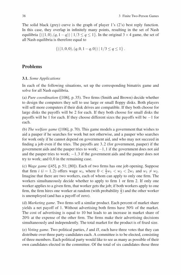
38 3 Finite Two-Person Games
The solid black (grey) curve is the graph of player 1’s (2’s) best reply function.In this case, they overlap in infinitely many points, resulting in the set of Nashequilibria {((1,0),(q,1− q)) | 1/3 ≤ q ≤ 1}. In the original 3× 4 game, the set ofall Nash equilibria is therefore equal to
{((1,0,0),(q,0,1−q,0)) | 1/3 ≤ q ≤ 1} .
Problems
3.1. Some Applications
In each of the following situations, set up the corresponding bimatrix game andsolve for all Nash equilibria.
(a) Pure coordination ([106], p. 35). Two firms (Smith and Brown) decide whetherto design the computers they sell to use large or small floppy disks. Both playerswill sell more computers if their disk drives are compatible. If they both choose forlarge disks the payoffs will be 2 for each. If they both choose for small disks thepayoffs will be 1 for each. If they choose different sizes the payoffs will be −1 foreach.
(b) The welfare game ([106], p. 70). This game models a government that wishes toaid a pauper if he searches for work but not otherwise, and a pauper who searchesfor work only if he cannot depend on government aid, and who may not succeed infinding a job even if the tries. The payoffs are 3,2 (for government, pauper) if thegovernment aids and the pauper tries to work; −1,1 if the government does not aidand the pauper tries to work; −1,3 if the government aids and the pauper does nottry to work; and 0,0 in the remaining case.
(c) Wage game ([45], p. 51; [80]). Each of two firms has one job opening. Supposethat firm i (i = 1,2) offers wage wi, where 0 < 1
2 w1 < w2 < 2w1 and w1 = w2.Imagine that there are two workers, each of whom can apply to only one firm. Theworkers simultaneously decide whether to apply to firm 1 or firm 2. If only oneworker applies to a given firm, that worker gets the job; if both workers apply to onefirm, the firm hires one worker at random (with probability 1
2 ) and the other workeris unemployed (and has a payoff of zero).
(d) Marketing game. Two firms sell a similar product. Each percent of market shareyields a net payoff of 1. Without advertising both firms have 50% of the market.The cost of advertising is equal to 10 but leads to an increase in market share of20% at the expense of the other firm. The firms make their advertising decisionssimultaneously and independently. The total market for the product is of fixed size.
(e) Voting game. Two political parties, I and II, each have three votes that they candistribute over three party-candidates each. A committee is to be elected, consistingof three members. Each political party would like to see as many as possible of theirown candidates elected in the committee. Of the total of six candidates those three

Problems 39
that have most of the votes will be elected; in case of ties, tied candidates are drawnwith equal probabilities.
3.2. Matrix Games
(a) Since a matrix game is a special case of a bimatrix game, it may be ‘solved’ bythe method graphical method of Sect. 3.2.2. Do this for the game in Problem 2.1(a).Compare your answer with what you found previously.
(b) Argue that a pair consisting of a maximin and a minimax strategy in a matrixgame is a Nash equilibrium; and that any Nash equilibrium in a matrix game mustbe a pair consisting of a maximin and a minimax strategy. (You may give all yourarguments in words.)
(c) A maximin strategy for player 1 in the bimatrix game (A,B) is a maximinstrategy in the matrix game A. Which definition is appropriate for player 2 in thisrespect? With these definitions, find examples showing that a Nash equilibrium in abimatrix game does not have to consist of maximin strategies, and that a maximinstrategy does not have to be part of a Nash equilibrium.
3.3. Strict Domination
Consider the bimatrix game
(A,B) =( W X Y Z
T 6,6 4,4 1,2 8,5B 4,5 6,6 2,8 4,4
).
(a) Which pure strategy of player 1 or player 2 is strictly dominated by a purestrategy?
(b) Describe all combinations of strategies W and Y of player 2 that strictlydominate X .
(c) Find all equilibria of this game.
3.4. Iterated Elimination (1)
Consider the bimatrix game (from [145], p. 65)
⎛⎜⎜⎝W X Y Z
A 5,4 4,4 4,5 12,2B 3,7 8,7 5,8 10,6C 2,10 7,6 4,6 9,5D 4,4 5,9 4,10 10,9
⎞⎟⎟⎠ .
(a) Find a few different ways in which strictly dominated strategies can be iteratedlyeliminated in this game.
(b) Find the Nash equilibria of this game.

40 3 Finite Two-Person Games
3.5. Iterated Elimination (2)
Consider the bimatrix game ⎛⎝ 2,0 1,1 4,23,4 1,2 2,31,3 0,2 3,0
⎞⎠ .
Find the Nash equilibria of this game.
3.6. Weakly Dominated Strategies
A pure strategy i of player 1 in an m×n bimatrix game (A,B) is weakly dominatedif there a strategy p = (p1, . . . , pm) ∈ ∆m with pi = 0 such that pAe j ≥ eiAe j forevery j = 1, . . . ,n, and pAe j > eiAe j for at least one j. The definition of a weaklydominated strategy of player 2 is similar. In words, a pure strategy is weakly domi-nated if there is some pure or mixed strategy that is always at least as good, and thatis better against at least one pure strategy of the opponent. Instead of iterated elim-ination of strictly dominated strategies one might also consider iterated eliminationof weakly dominated strategies. The advantage is that in games where no strategyis strictly dominated it might still be possible to eliminate strategies that are weaklydominated. The main disadvantages are that some Nash equilibria of the originalgame may be eliminated as well, and also that the order of elimination may matter.These issues are illustrated by the following examples.
(a) Consider the bimatrix game
⎛⎝X Y Z
A 11,10 6,9 10,9B 11,6 6,6 9,6C 12,10 6,9 9,11
⎞⎠ .
First, determine the pure Nash equilibria of this game. Next, apply iterated elim-ination of weakly dominated strategies to reduce the game to a 2 × 2 game anddetermine the unique Nash equilibrium of this game.
(b) Consider the bimatrix game
⎛⎝X Y Z
A 1,1 0,0 2,0B 1,2 1,2 1,1C 0,0 1,1 1,1
⎞⎠ .
Show that different orders of eliminating weakly dominated strategies may result indifferent Nash equilibria.

Problems 41
3.7. A Parameter Game
Consider the bimatrix game ( L RT 1,1 a,0B 0,0 2,1
),
where a ∈ R. Determine the Nash equilibria of this game for every possible valueof a.
3.8. Equalizing Property of Mixed Equilibrium Strategies
(a) Consider again the game of Problem 3.3, which has a unique Nash equilibriumin mixed strategies. In this equilibrium, player 1 puts positive probability p∗ on Tand 1− p∗ on B, and player 2 puts positive probability q∗ on W and 1− q∗ on Y .Show that, if player 2 plays this strategy, then both T and B give player 1 the sameexpected payoff, equal to the equilibrium payoff. Also show that, if player 1 playshis equilibrium strategy, then both W and Y give player 2 the same expected payoff,equal to the equilibrium payoff, and higher than the expected payoff from X orfrom Z.
(b) Generalize the observations made in (a), more precisely, give an argument forthe following statement:
Let (A,B) be an m×n bimatrix game and let (p∗,q∗) be a Nash equilibrium. Theneach row played with positive probability in this Nash equilibrium has the sameexpected payoff for player 1 against q∗ and this payoff is at least as high as thepayoff from any other row. Each column played with positive probability in thisNash equilibrium has the same expected payoff for player 2 against p∗ and thispayoff is at least as high as the payoff from any other column.
You may state your argument in words, without using formulas.

Chapter 4Finite Extensive Form Games
Most games derived from economic or political situations have in common withmost parlor games (like card games and board games) that they are not ‘one-shot’:players move sequentially, and one and the same player may move more often thanonce. Such games are best described by drawing a decision tree which tells us whosemove it is and what a player’s information is when that player has to make a move.
In this chapter these so-called ‘games in extensive form’ are studied. Attentionhere is restricted to games with finitely many players (usually two), finitely manydecision moments and finitely many moves. See Sect. 1.3.3 for a few examples.We also assume that each player has ‘complete information’, which – formally –boils down to either there being no chance move in the game or, if a chance moveoccurs, each player becoming informed about the outcome of that chance move.This excludes, for instance, the game of entry deterrence with incomplete infor-mation in Sect. 1.3.3: for the analysis of games with incomplete information seeChap. 5. Chapter 14 extends the analysis of the present and the next chapter.
The first section of this chapter introduces games in extensive form. In orderto avoid a load of cumbersome notation the treatment will be somewhat informalbut – hopefully – not imprecise. In Sect. 4.2 we define strategies and the ‘strategicform’ of a game: the definition of Nash equilibrium for extensive form games is thenpractically implied. The focus in this chapter is on pure Nash equilibrium.
In the third section the concept of Nash equilibrium is refined by consideringsubgame perfection (first introduced in [117] and [118]) and backward induction. Afurther important refinement, called ‘perfect Bayesian equilibrium’, is treated in thefourth section.
4.1 The Extensive Form
A game in extensive form is described by a game tree. Such a game tree is char-acterized by nodes and edges. Each node is either a decision node of a player, or achance node, or an end node. Each edge corresponds to either an action of a playeror a choice made by chance, sometimes called a ‘move of Nature’.
H. Peters, Game Theory – A Multi-Leveled Approach.c© Springer-Verlag Berlin Heidelberg 2008
43

44 4 Finite Extensive Form Games
� � � � � � � �
� � � �
��
1
A B CChance
1/4 3/4
22 1
U D
l r l r L R a b
(41
) (72
) (63
) (40
) (00
) (84
) (88
) (08
)Fig. 4.1 A game in extensive form
Figure 4.1 illustrates these and other concepts.The upper node in the tree, the root of the tree, is a decision node of player 1 and
the starting point of the game. Player 1 chooses between three actions, namely A, B,and C. Player 2 learns that player 1 has chosen either A or B, or C. The first eventis indicated by the dashed line connecting the two left decision nodes of player 2.In that case, player 2 has two actions, namely l and r. We call the two connectednodes an information set of player 2: player 2 knows that the play of the gamehas arrived at one of these nodes but he does not know at which one. The fact thatplayer 2 has the same set of actions at each of the two nodes in this informationset is a necessary consequence: if this were not the case, player 2 would know atwhich node he was (i.e., would know whether player 1 would have played A orB) by simply examining the set of available actions, which would go against theinterpretation of an information set. This last argument is one consequence of themore general assumption that the whole game tree is common knowledge betweenthe players: each player knows it, knows that the other player(s) know(s) it, knowsthat the other player(s) know(s) that he knows it, etc.
If player 1 plays C, then there is a chance move, resulting with probability 1/4in a decision node of player 2 (following U) and with probability 3/4 in a decisionnode of player 1 (following D). At player 2’s decision node this player has twoactions, namely L and R. At player 1’s decision node this player has also two actions,namely a and b. All the remaining nodes are end nodes, indicated by payoff pairs,where the upper number is the payoff to player 1 and the lower number the payoffto player 2. In this diagram, the payoffs are written as column vectors, but we alsowrite them as row vectors, whatever is convenient in a given situation.
We note that also the singleton decision nodes are called information sets. So inthis game, each player has two different information sets. Call an information setnontrivial if it consists of at least two nodes. Games with nontrivial information setsare called games with imperfect information. If a game has only trivial informationsets, then we say that it has perfect information. In the present example, if player 2

4.1 The Extensive Form 45
� � � � � � � �
� � � �
��
1
A B CChance
1/4 3/4
2 2 2 1U D
l r l r L R a b
(41
) (72
) (63
) (40
) (00
) (84
) (88
) (08
)Fig. 4.2 The game of Fig. 4.1, now with perfect information
��
��
2
1
2
1
(a)� � � �
���
� 1
1
(b)
Fig. 4.3 An example of a cycle (a), and of a game without perfect recall (b)
observes whether player 1 chooses A or B, then the game has perfect information.See Fig. 4.2.
The chance move in our example is not a particularly interesting one, since theplayers learn what the outcome of the chance move is.1
As mentioned before, we do not give a formal definition of a game in extensiveform: the examples in Figs. 4.1 and 4.2 illustrate the main ingredients of such agame.2 An important condition is that the game tree should be a tree indeed: itshould have a single root and no ‘cycles’. This means that a situation like forinstance in Fig. 4.3a is not allowed.
We also consider only games in extensive form that have perfect recall : eachplayer remembers what he did in the past. For instance, a situation like in Fig. 4.3b,
1 The situation is different if at least one player is not completely informed about the outcome of achance move and if this lack of information has strategic consequences. In that case, we talk aboutgames with ‘incomplete’ information, see Chap. 5.2 See Chap. 14 for a formal definition.

46 4 Finite Extensive Form Games
where player 1 at his lower information set does not recall which action he tookearlier, is not allowed.3
4.2 The Strategic Form
In a game in extensive form, it is extremely important to distinguish between‘actions’ and ‘strategies’. An action is a possible move of a player at an informationset. In the games in Figs. 4.1 and 4.2 player 1 has the actions A, B, and C, and a andb; and player 2 has the actions l and r, and L and R. In contrast:
A strategy is a complete plan to play the game.
This is one of the most important concepts in game theory. In the games in Figs. 4.1and 4.2, a possible strategy for player 1 is:
Start by playing C; if the chance move of the game results in D, then play b.
Another strategy of player 1 is:
Start by playing A; if the chance move of the game results in D, then play b.
The last strategy might look strange since player 1’s first action A excludes himhaving to take a further action. Nevertheless, also this plan is regarded as a possiblestrategy.4
A possible strategy for player 2 in the game of Fig. 4.1 is:
Play l if player 1 plays A or B, and play L if player 1 plays C and the chancemove results in U .
Note that player 2 cannot make his action contingent on whether player 1 plays Aor B, since player 2 does not have that information. In the perfect information gameof Fig. 4.2, however, player 2’s strategy should tell what player 2 plays after A andwhat he plays after B. A possible strategy would then be:
Play l if player 1 plays A, play r if player 1 plays B, and play L if player 1plays C and the chance move results in U .
A more formal definition of a strategy of a player is:
A strategy is a list of actions, exactly one at each information set of that player.
In both our examples, a strategy of player 1 is therefore a list of two actions sinceplayer 1 has two information sets. The number of possible strategies of player 1 isthe number of different lists of actions. Since player 1 has three possible actions at
3 The assumption of perfect recall plays a particular role for the relation between mixed andbehavioral strategies, see Chap. 14.4 Although there is not much lost if we would exclude such strategies – as some authors do.

4.2 The Strategic Form 47
his first information set and two possible actions at his second information set, thisnumber is equal to 3× 2 = 6. The strategy set of player 1 can be denoted, thus, as
{Aa,Ab,Ba,Bb,Ca,Cb} .
Similarly, in the imperfect information game in Fig. 4.1 player 2 has 2 × 2 = 4different strategies, and his strategy set can be denoted as
{lL, lR,rL,rR} .
In the perfect information game in Fig. 4.2 player 2 has three information sets andtwo actions at each information set, so 2× 2× 2 = 8 different strategies, and hisstrategy set can be denoted as
{llL, llR, lrL, lrR,rlL,rlR,rrL,rrR} ,
where the first letter is the action to be played if player 1 plays A and the secondletter is the action to be played if player 1 plays B.
There are several important reasons why we are interested in strategies. Themain reason is that by considering strategies the extensive form game is effectivelyreduced to a one-shot game. Once we fix a profile (in the present example, pair) ofstrategies we can compute the payoffs by following the path followed in the gametree. Consider for instance the strategy pair (Cb,rL) in the game in Fig. 4.1. Thenplayer 1 starts by playing C, and this is followed by a chance move; if the resultof this move is U , then player 2 plays L; if the result is D, then player 1 plays b.Hence, with probability 1/4 the resulting payoff pair is (0,0) and with probability3/4 the resulting payoff pair is (0,8). So the expected payoffs are 0 for player 1and 6 for player 2. In this way, we can compute the payoffs in the game of Fig. 4.1resulting from each of the 6× 4 possible strategy combinations. Similarly, for thegame in Fig. 4.2 we compute 6×8 payoff pairs. We next write these payoff pairs ina bimatrix, as in Chap. 3. The resulting bimatrix games are presented in Fig. 4.4.Such a bimatrix game is called the strategic form of the extensive form game. Thedefinition of Nash equilibrium of an extensive form game is then almost implied:
A Nash equilibrium of a game in extensive form is a Nash equilibrium of thestrategic form.
This definition holds for pure Nash equilibria and, more generally, Nash equilibriain mixed strategies, but in this chapter we restrict attention to pure strategies andpure strategy Nash equilibria.
The pure strategy Nash equilibria of the bimatrix games in Fig. 4.4 can be foundby using the method of Sect. 3.2.1. The equilibria correspond to the double-starredentries. Thus, the imperfect information game has six different Nash equilibria inpure strategies, and the perfect information game has ten different Nash equilibriain pure strategies.
In the next two sections we examine these Nash equilibria more closely anddiscuss ways to distinguish between them.

48 4 Finite Extensive Form Games
⎛⎜⎜⎜⎜⎜⎝
lL lR rL rRAa 4,1 4,1 7∗,2∗ 7,2∗Ab 4,1 4,1 7∗,2∗ 7,2∗Ba 6∗,3∗ 6,3∗ 4,0 4,0Bb 6∗,3∗ 6,3∗ 4,0 4,0Ca 6∗,6 8∗,7∗ 6,6 8∗,7∗Cb 0,6 2,7∗ 0,6 2,7∗
⎞⎟⎟⎟⎟⎟⎠
⎛⎜⎜⎜⎜⎜⎝
llL llR lrL lrR rlL rlR rrL rrRAa 4,1 4,1 4,1 4,1 7∗,2∗ 7,2∗ 7∗,2∗ 7,2∗Ab 4,1 4,1 4,1 4,1 7∗,2∗ 7,2∗ 7∗,2∗ 7,2∗Ba 6∗,3∗ 6,3∗ 4,0 4,0 6,3∗ 6,3∗ 4,0 4,0Bb 6∗,3∗ 6,3∗ 4,0 4,0 6,3∗ 6,3∗ 4,0 4,0Ca 6∗,6 8∗,7∗ 6∗,6 8∗,7∗ 6,6 8∗,7∗ 6,6 8∗,7∗Cb 0,6 2,7∗ 0,6 2,7∗ 0,6 2,7∗ 0,6 2,7∗
⎞⎟⎟⎟⎟⎟⎠
Fig. 4.4 The 6×4 strategic form of the game in Fig. 4.1 and the 6×8 strategic form of the gamein Fig. 4.2
� � � �
��
1
A B CChance
1/4 3/4U D(
72
) (63
) (84
) (88
)Fig. 4.5 The reduced game of Fig. 4.2
4.3 Backward Induction and Subgame Perfection
We first consider the perfect information game of Fig. 4.2. This game can be ana-lyzed using the principle of backward induction. This means that we start with thenodes preceding the end nodes, and turn them into end nodes with payoffs result-ing from choosing the optimal action(s). For the game under consideration thisyields the reduced game of Fig. 4.5. Note that player 2’s strategy has already beencompletely determined: it is the strategy rlR. Player 1 has chosen a at his lowerinformation set. Next, in this reduced game, player 1 chooses the action(s) thatyield(s) the highest payoff. Since A yields a payoff of 7, B a payoff of 6, and Ca(n expected) payoff of 1/4×8+3/4×8 = 8, it is optimal for player 1 to choose C.Hence, we obtain the strategy combination (Ca,rlR) with payoffs (8,7). This is oneof the ten Nash equilibria of the game (see Fig. 4.4). It is called backward inductionequilibrium. It can be shown that applying the backward induction principle always

4.3 Backward Induction and Subgame Perfection 49
results in a (pure) Nash equilibrium.5 As a by-product, we obtain that a game ofperfect information has at least one Nash equilibrium in pure strategies, which canbe obtained by backward induction.
It is important to distinguish between backward induction equilibrium (in thisgame, (Ca,rlR)) and backward induction outcome. The latter refers to the actualplay of the game or, equivalently, the equilibrium path, in this case (Ca,R). Observethat there are other Nash equilibria in this game that generate the same outcome orpath, namely (Ca, llR), (Ca, lrR), and (Ca,rrR): they all generate the path (Ca,R),but differ in the left part of the tree, where player 2 makes at least one subopti-mal decision. Hence, the principle of backward induction ensures that every playeralways takes an optimal action, even in parts of the game tree that are not actuallyreached when the game is played.
A more general way to do this is to use the idea of subgame perfection (firstexplicitly formulated by Selten [117]). The definition of a subgame is as follows:
A subgame is any part of the game tree, starting at a single decision node(trivial information set) of a player or a chance node, which is not connectedto the tree by any later information set.
The game in Fig. 4.2 has six different subgames, namely: the entire game; the gamestarting from the chance move; and the four games starting from the four nodespreceding the end nodes. The definition of a subgame perfect equilibrium is asfollows:
A subgame perfect equilibrium is a strategy combination that induces a Nashequilibrium in every subgame.
To see what this means, consider again the game in Fig. 4.2. In order for a strategycombination to be a subgame perfect equilibrium, it has to induce a Nash equi-librium in every subgame. Since the entire game is a subgame, a subgame perfectequilibrium has to be a Nash equilibrium in the entire game, and, thus, the ten Nashequilibria in this game are the candidates for a subgame perfect equilibrium. Thisis the case for any game, and therefore a subgame perfect equilibrium is alwaysa Nash equilibrium. A subgame perfect equilibrium also has to induce an equilib-rium in each of the four one-player subgames preceding the end nodes: althoughwe have not defined Nash equilibria for one-person games, the only reasonable def-inition is that a player should choose the action that is optimal. In the example,this means that (from left to right) the actions r, l, R, and a, should be chosen.This implies that the players choose optimally also in the subgame starting from thechance node. Summarizing, we look for the Nash equilibrium or equilibria that gen-erate the mentioned actions, and the only Nash equilibrium that does this is again(Ca,rlR). Hence, the unique subgame perfect equilibrium in this game is (Ca,rlR).It is not surprising that this is also the backward induction equilibrium: in games ofperfect information, backward induction equilibria and subgame perfect equilibriacoincide.
5 This result is intuitive but nevertheless not that easy to prove formally. See, e.g., [102], Chap. 3.

50 4 Finite Extensive Form Games
� � � �� �
� ��
⎛⎝ 331
⎞⎠ ⎛⎝ 000
⎞⎠ ⎛⎝ 000
⎞⎠ ⎛⎝ 113
⎞⎠
⎛⎝ 200
⎞⎠
1
2
3
A B
L R
l r l r
Fig. 4.6 A three-player game
Let us now consider the imperfect information version of the game in Fig. 4.1. In thiscase, backward induction cannot be applied to the left part of the game tree: sinceplayer 2 does not know whether player 1 has played A or B when he has to choosean action in his left information set, he cannot choose between l and r. In terms ofsubgames, the only subgames are now: the entire game; the two subgames followingU and D; and the subgame starting from the chance move. Hence, the restrictionsimposed by subgame perfection are that player 1 should play a, player 2 should playR, and the strategy combination should be a Nash equilibrium in the entire game.Of the six Nash equilibria of the game (see Fig. 4.4), this leaves the two equilibria(Ca, lR) and (Ca,rR). So these are the subgame perfect equilibria of the game inFig. 4.1.
We conclude this section with an example which shows more clearly than the pre-ceding example that subgame perfection can be more generally applied than thebackward induction principle. Consider the game in Fig. 4.6, which is a three playergame (for a change). Clearly, backward induction cannot be applied here. For sub-game perfection, notice that this game has only two subgames: the entire game, andthe game starting with player 2’s decision node. The latter game is a game betweenplayers 2 and 3 with strategic form
( l rL 3,1 0,0R 0,0 1,3
)which has two pure Nash equilibria, namely (L, l) and (R,r). Hence, a subgameperfect equilibrium has to induce one of these two equilibria in the subgame. Notethat if the first equilibrium is played, then player 1 should play A, yielding him apayoff of 3 rather than the payoff of 2 obtained by playing B. If the other equilibriumis played in the subgame, then player 1 should obviously play B since A now yieldsonly 1. So the two subgame perfect equilibria are (A,L, l) and (B,R,r).

4.4 Perfect Bayesian Equilibrium 51
Alternatively, one can first compute the (pure) Nash equilibria of the entire game.The strategic form of the game can be represented as follows, where the left matrixresults from player 1 playing A and the right matrix from player 1 playing B.
1 : A( l r
L 3∗,3∗,1∗ 0,0,0R 0,0,0 1,1∗,3∗
)1 : B
( l rL 2,0∗,0∗ 2∗,0∗,0∗R 2∗,0∗,0∗ 2∗,0∗,0∗
).
Best replies are marked by asterisks (for player 1 one has to compare the corre-sponding payoffs over the two matrices), and the pure Nash equilibria are (A,L, l),(B,L,r), (B,R, l), and (B,R,r). The subgame perfect equilibria are those where thecombination (L, l) or (R,r) is played, resulting in the two equilibria found above.
4.4 Perfect Bayesian Equilibrium
A further refinement of Nash equilibrium and of subgame perfect equilibrium is pro-vided by the concept of ‘perfect Bayesian equilibrium’. Consider an information setof a player in an extensive form game. A belief of that player is simply a probabilitydistribution over the nodes of that information set or, equivalently, over the actionsleading to that information set. Of course, if the information set is trivial (consistsof a single node) then also the belief is trivial, namely attaching probability 1 to theunique node. Our somewhat informal definition of a perfect Bayesian equilibriumis as follows.
A perfect Bayesian equilibrium in an extensive form game is a combination ofstrategies and a specification of beliefs such that two conditions are satisfied:
1. The beliefs are consistent with the strategies under consideration.2. The players choose optimally given the beliefs.
The first condition is a version of ‘Bayesian consistency of beliefs’ and the sec-ond condition is ‘sequential rationality’.6 The first condition says that the beliefsshould satisfy Bayesian updating with respect to the strategies whenever possible.The second condition says that a player should maximize his expected payoff givenhis beliefs. In order to see what these conditions mean exactly, we consider someexamples.
Consider the game in Fig. 4.1. This game has one nontrivial information set. Sup-pose player 2’s belief at this information set is given by the probabilities α at theleft node and 1−α at the right node, where 0 ≤ α ≤ 1. That is, if this informa-tion set is reached then player 2 attaches probability α to player 1 having playedA and probability 1−α to player 1 having played B. All the other information sets
6 In the expression ‘perfect Bayesian equilibrium’ the word ‘Bayesian’ refers to the meaning of‘consistency’, namely consistent with respect to Bayesian updating. There is also a stronger versionof consistency, resulting in ‘sequential equilibrium’. See [66] and Chap. 14.

52 4 Finite Extensive Form Games
are trivial and therefore the beliefs attach probability 1 to each of the correspond-ing nodes. Given these beliefs, applying condition (2) means that player 2 shouldchoose R and player 1 should choose a at the corresponding information sets. Atthe nontrivial information set, player 2 should choose the action that maximizes hisexpected payoff. The expected payoff from l is equal to α ·1+(1−α) ·3 = 3−2αand the expected payoff from r is α · 2 + (1−α) · 0 = 2α . Hence, l is optimal if3−2α ≥ 2α , i.e., if α ≤ 3/4 and r is optimal if α ≥ 3/4.
In this game, it is always optimal for player 1 to play C, given the actions R and afollowing the chance move: C yields 8 whereas A or B yield at most 7. But if player1 does not play A or B, then condition (1) above does not put any restriction on thebelief α of player 2. More precisely, if player 1 plays C then the nontrivial informa-tion set of player 2 is reached with zero probability, and therefore the probability αcannot by determined by Bayesian updating, that is, by computing the conditionalprobability of reaching the left (or right) node in player 2’s information set. Thismeans that α can be chosen in any way we like, but given α player 2 should chooseoptimally, as computed before. Hence, we have essentially two perfect Bayesianequilibria, namely (Ca, lL) with beliefs α ≤ 3/4 and (Ca,rL) with beliefs α ≥ 3/4.Note that these are also the subgame perfect equilibria, now ‘backed up’ by a beliefof player 2 on his nontrivial information set.
It is not difficult to see that a perfect Bayesian equilibrium is always subgameperfect, and therefore also a Nash equilibrium.7 In fact, by assigning probabilitiesto nodes in an information set, we essentially make it possible to apply backwardinduction again, as is clear from the example.
In order to show that the perfect Bayesian equilibrium requirement can havean additional impact compared to subgame perfection, consider the variation onthe game of Fig. 4.1, obtained by replacing the payoffs (4,1) after A and l by thepayoffs (4,3). One can check that the subgame perfect equilibria are still (Ca, lL)and (Ca,rL). Obviously, a rational player 2 would never play r at his nontrivialinformation set since l is always better, but subgame perfection does not rule thisout. But clearly, there is no belief that player 2 could have at this information setthat would make r optimal: if we denote player 2’s belief by (α,1−α) as before,then r yields 2α whereas l yields 3, which is always larger than 2α . Hence, theonly perfect Bayesian equilibrium is (Ca, lL), with arbitrary belief of player 2 at hisnontrivial information set.
As another example, consider again the game of Fig. 4.6, reproduced in Fig. 4.7 withbelief (α,1−α) attached to the nodes in the information set of player 3.
There are two ways to find the perfect Bayesian equilibria of this game. One canconsider the subgame perfect equilibria and find appropriate beliefs. Alternatively,one can start from scratch and apply a form of backward induction. To illustrate thelast method, start with player 3. If player 3 plays l then his (expected) payoff is α .If player 3 plays r then his (expected) payoff is 3− 3α . Therefore, l is optimal ifα ≥ 3/4 and r is optimal if α ≤ 3/4.
7 For a more formal treatment see Chap. 14.
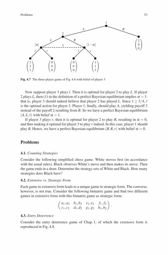
Problems 53
� � � �� �
� ��
⎛⎝ 331
⎞⎠ ⎛⎝ 000
⎞⎠ ⎛⎝ 000
⎞⎠ ⎛⎝ 113
⎞⎠
⎛⎝ 200
⎞⎠
1
2
3
A B
L R
l r l r
[α ] [1−α ]
Fig. 4.7 The three-player game of Fig. 4.6 with belief of player 3
Now suppose player 3 plays l. Then it is optimal for player 2 to play L. If player2 plays L, then (1) in the definition of a perfect Bayesian equilibrium implies α = 1:that is, player 3 should indeed believe that player 2 has played L. Since 1 ≥ 3/4, lis the optimal action for player 3. Player 1, finally, should play A, yielding payoff 3instead of the payoff 2 resulting from B. So we have a perfect Bayesian equilibrium(A,L, l) with belief α = 1.
If player 3 plays r, then it is optimal for player 2 to play R, resulting in α = 0,and thus making it optimal for player 3 to play r indeed. In this case, player 1 shouldplay B. Hence, we have a perfect Bayesian equilibrium (B,R,r) with belief α = 0.
Problems
4.1. Counting Strategies
Consider the following simplified chess game. White moves first (in accordancewith the usual rules). Black observes White’s move and then makes its move. Thenthe game ends in a draw. Determine the strategy sets of White and Black. How manystrategies does Black have?
4.2. Extensive vs. Strategic Form
Each game in extensive form leads to a unique game in strategic form. The converse,however, is not true. Consider the following bimatrix game and find two differentgames in extensive form with this bimatrix game as strategic form:(
a1,a2 b1,b2 e1,e2 f1, f2c1,c2 d1,d2 g1,g2 h1,h2
).
4.3. Entry Deterrence
Consider the entry deterrence game of Chap. 1, of which the extensive form isreproduced in Fig. 4.8.

54 4 Finite Extensive Form Games
� �0,100
�
� �
Entrant
IncumbentE O
C F
40,50 −10,0
Fig. 4.8 Entry deterrence, Problem 4.3
(a) Write down the strategic form of this game.
(b) Determine the Nash equilibria (in pure strategies). Which one is the backwardinduction equilibrium? Which one is subgame perfect? In which sense is the otherequilibrium based on an ‘incredible threat’?
4.4. Choosing Objects
Four objects O1, O2, O3, and O4 have different worths for two players 1 and 2, givenby the following table:
O1 O2 O3 O4
Worth for player 1: 1 2 3 4Worth for player 2: 2 3 4 1
Player 1 starts with choosing an object. After him player 2 chooses an object, thenplayer 1 takes his second object, and finally player 2 gets the object that is left.
(a) Draw the decision tree for this extensive form game.
(b) How many strategies does each player have?
(c) Determine the backward induction or subgame perfect equilibria (in pure strate-gies).
4.5. An Extensive Form Game
For the game in Fig. 4.9, write down the strategic form and compute all Nashequilibria, subgame perfect equilibria, and perfect Bayesian equilibria in purestrategies.
4.6. Another Extensive Form Game
For the game in Fig. 4.10, write down the strategic form and compute all Nashequilibria, subgame perfect equilibria, and perfect Bayesian equilibria in purestrategies.

Problems 55
� � � �
� �
� �
[α ] [1−α ]
1 R
L M
2
l r l r
(20
) (01
) (01
) (30
)
(22
)
Fig. 4.9 Extensive form game of Problem 4.5
� � � � � �
� �
� �
[α ] [1−α ]
1 R
L M
2
lm
r lm
r
(13
) (12
) (40
) (42
) (02
) (33
)
(24
)
Fig. 4.10 Extensive form game of Problem 4.6
4.7. A Centipede Game
In the centipede game, the two players move alternatingly. On each move, a playercan stop (S) or continue (C). On any move, a player is better off stopping the gamethan continuing if the other player stops immediately afterward, but is worse offstopping than continuing if the other player continues, regardless of the subsequentactions. The game ends after a finite number of periods. Consider an example of thisgame in Fig. 4.11.
(a) Determine the backward induction or subgame perfect equilibrium of this game.What is the associated outcome?
(b) Show that there are other Nash equilibria, but that these always result in the sameoutcome as the subgame perfect equilibrium.

56 4 Finite Extensive Form Games
S S S S S S
C C C C C C1 2 1 2 1 2
2,0 1,3 4,2 3,5 6,4 5,7
8,6
Fig. 4.11 The centipede game of Problem 4.7
4.8. Finitely Repeated Games
Consider the prisoners’ dilemma game of Chap. 1:
( C DC −1,−1 −10,0D 0,−10 −9,−9
).
Suppose that this game is played twice. After the first play of the game the playerslearn the outcome of that play.
(a) How many strategies does each player have in this game?
(b) Determine the subgame perfect equilibrium or equilibria of this game. What ifthe game is repeated more than twice but still finitely many times?
Consider, next, the following bimatrix game:
( L RT 2,1 1,0B 5,1 4,4
).
Suppose again that the game is played twice, and that after the first play of the gamethe players learn the outcome of that play.
(c) Determine the subgame perfect equilibrium or equilibria of this game. What ifthe game is repeated more than twice but still finitely many times?
(d) Exhibit a Nash equilibrium (of the twice repeated game) where (B,L) is playedin the first round.
Consider the following bimatrix game:
⎛⎝L M R
T 8,8 0,9 0,0C 9,0 0,0 3,1B 0,0 1,3 3,3
⎞⎠ .
(e) For the twice repeated version of this game, describe a subgame perfect equilib-rium in which (T,L) is played in the first round.

Problems 57
Consider, finally, the bimatrix game (cf. [9])
⎛⎝L M R
T 5,3 0,0 2,0C 0,0 2,2 0,0B 0,0 0,0 0,0
⎞⎠ .
(f) For the twice repeated version of this game, describe a subgame perfect equilib-rium in which (B,R) is played in the first round.

Chapter 5Finite Games with Incomplete Information
In a game of imperfect information players may be uninformed about the movesmade by other players. Every one-shot, simultaneous move game is a game of imper-fect information. In a game of incomplete information players may be uninformedabout certain characteristics of the game or of the players. For instance, a player mayhave incomplete information about actions available to some other player, or aboutpayoffs of other players. Following Harsanyi [50], we model incomplete informa-tion by assuming that every player can be of a number of different types. A type of aplayer summarizes all relevant information (in particular, actions and payoffs) aboutthat player. Furthermore, it is assumed that each player knows his own type and,given his own type, has a probability distribution over the types of the other play-ers. Often, these probability distributions are assumed to be consistent in the sensethat they are the marginal probability distributions derived from a basic commonlyknown distribution over all combinations of player types.
In this chapter we consider games with finitely many players, finitely many types,and finitely many strategies. These games can be either static (simultaneous, one-shot) or dynamic (extensive form games). A Nash equilibrium in this context isalso called ‘Bayesian equilibrium’, and in games in extensive form an appropriaterefinement is perfect Bayesian equilibrium. As will become clear, in essence theconcepts studied in Chaps. 3 and 4 are applied again.
In Sect. 5.1 we present a brief introduction to the concept of player types in agame. Section 5.2 considers static games of incomplete information, and Sect. 5.3discusses so-called signaling games, which is the most widely applied class ofextensive form games with incomplete information.
5.1 Player Types
Consider a set of players, say N = {1,2, . . . ,n}. For each player i∈N, there is a finiteset of types Ti which that player can have. If we denote by T = T1 ×T2 × . . .×Tnthe set
T = {(t1,t2, . . . ,tn) | t1 ∈ T1,t2 ∈ T2, . . . ,tn ∈ Tn} ,
H. Peters, Game Theory – A Multi-Leveled Approach.c© Springer-Verlag Berlin Heidelberg 2008
59

60 5 Finite Games with Incomplete Information
i.e., the set of all possible combinations of types, then a game with incomplete infor-mation specifies a separate game for every possible combination t = (t1,t2, . . . ,tn)∈T , in a way to be explained in the next sections. We assume that each player i knowshis own type ti and, given ti, attaches probabilities
p(t1, . . . ,ti−1,ti+1, . . . ,tn|ti)
to all type combinations t1 ∈ T1, . . ., ti−1 ∈ Ti−1, ti+1 ∈ Ti+1, . . ., tn ∈ Tn of the otherplayers.
Often, these probabilities are derived from a common probability distribution pover T , where p(t) is the probability that the type combination is t. This is also whatwe assume in this chapter. Moreover, we assume that every player i, apart from histype own type ti, also knows the probability distribution p. Hence, if player i hastype ti, then he can compute the probability that the type combination of the otherplayers is the vector (t1, . . . ,ti−1,ti+1, . . . ,tn). Formally, this probability is equal tothe conditional probability
p(t1, . . . ,ti−1,ti+1, . . . ,tn|ti) =p(t1, . . . ,ti−1,ti,ti+1, . . . ,tn)
∑ p(t ′1, . . . ,t′i−1,ti,t
′i+1, . . . ,t
′n)
where the sum in the denominator is taken over all possible types of the other play-ers, i.e., over all possible t ′1 ∈ T1, . . . ,t ′i−1 ∈ Ti−1,t ′i+1 ∈ Ti+1, . . . ,t ′n ∈ Tn. Hence, thesum in the denominator is the probability that player i has type ti.
Thus, a player in a game of incomplete information can make his actions depen-dent on his own type but not on the types of the other players. However, since heknows the probabilities of the other players’ types, he can compute the expectedpayoffs from taking specific actions. In the next two sections we will see how thisworks in static and in extensive form games.
5.2 Static Games of Incomplete Information
Instead of giving formal definitions we discuss a few examples.
Battle-of-the-Sexes with One-Sided Incomplete Information
The first example (taken from [96], p. 273) is a variant of the Battle-of-the-Sexes(see Sect. 1.3.2) in which player 1 (the man) does not know whether player 2 (thewoman) wants to go out with him or avoid him. More precisely, player 1 does notknow whether he plays the game y or the game n, where these games are as follows:
y :( S B
S 2,1 0,0B 0,0 1,2
)n :
( S BS 2,0 0,2B 0,1 1,0
).

5.2 Static Games of Incomplete Information 61
� � � � � � � �� � � �
� ��Chance
.5y
.5n2 2
S B S B1
S B S B S B S B
(21
) (00
) (00
) (12
) (20
) (01
) (02
) (10
)Fig. 5.1 An extensive form representation of the Battle-of-the-Sexes game with incompleteinformation
( SS SB BS BBS 2∗,0.5 1∗,1.5∗ 1∗,0 0,1B 0,0.5 0.5,0 0.5,1.5∗ 1∗,1
)Fig. 5.2 The strategic form of the game in Fig. 5.1. Player 1 is the row player
Player 1 attaches probability 1/2 to each of these games, and player 2 knows this.In the terminology of types, this means that player 1 has only one type, simplyindicated by ‘1’, and that player 2 has two types, namely y and n. So there are twotype combinations, namely (1,y) and (1,n), each occurring with probability 1/2.Player 2 knows player 1’s type with certainty, and also knows her own type, thatis, knows which game is actually being played. Player 1 attaches probability 1/2 toeach type of player 2.
What would be a Nash equilibrium in a game like this? To see this, it is helpfulto model the game as a game in extensive form, using the tree representation ofChap. 4. Such a tree representation is given in Fig. 5.1.
The game starts with a chance move which selects which of the two bimatrixgames is going to be played. In the terminology of types, it selects the type of player2. Player 2 is informed but player 1 is not. Player 2 has four different strategies butplayer 1 only two. From this strategic form it is apparent that every Nash equilibriumis subgame perfect, since there are no nontrivial subgames. Also, every Nash equi-librium is perfect Bayesian, since the only nontrivial information set (of player 1)is reached with positive probability for any strategy of player 2, and thus the beliefsare completely determined by player 2’s strategy through Bayesian updating.
The strategic form of the game is given in Fig. 5.2. There, the first letter in astrategy of player 2 says what player 2 plays if y is chosen by the Chance move, andthe second letter says what player 2 plays if n is chosen. Also the best replies areindicated.

62 5 Finite Games with Incomplete Information
From the strategic form it is apparent that the game has a unique Nash equi-librium in pure strategies, namely (S,SB).1 In this equilibrium player 1 plays S,type y of player 2 plays S and type n of player 2 plays B. Such an equilibrium is alsocalled Bayesian equilibrium but, clearly, it is a Nash equilibrium of an appropriatelyspecified extensive form (or strategic form) game.
The (pure) Nash equilibrium or equilibria of a game like this can also be foundwithout drawing the extensive form and computing the strategic form. Suppose firstthat player 1 plays S in an equilibrium. Then the best reply of player 2 is to playS if her type is y and B if here type is n. The expected payoff to player 1 is then1; playing B against this strategy of player 2 yields only 0.5. So (S,SB) is a Nashequilibrium. If, on the other hand, player 1 plays B, then the best reply of player 2if her type is y, is B and if her type is n it is S. This yields a payoff of 0.5 to player1, whereas playing S against this strategy of player 2 yields payoff 1. Hence, thereis no equilibrium where player 1 plays B. Of course, this is also apparent from thestrategic form, but the argument can be made without complete computation of thestrategic form.
Battle-of-the-Sexes with Two-Sided Incomplete Information
The next example (cf. [96], p. 277) is a further variation of the Battle-of-the-Sexesgame in which neither player knows whether the other player wants to be togetherwith him/her or not. It is based on the four bimatrix games in Fig. 5.3. These fourbimatrix games correspond to the four possible type combinations of players 1 and2. The probabilities of these four different combinations are given in Table 5.1.One way to find the Nash equilibria of this game is to draw the extensive form
y1y2 :( S B
S 2,1 0,0B 0,0 1,2
)y1n2 :
( S BS 2,0 0,2B 0,1 1,0
)
n1y2 :( S B
S 0,1 2,0B 1,0 0,2
)n1n2 :
( S BS 0,0 2,2B 1,1 0,0
)
Fig. 5.3 Payoffs for Battle-of-the-Sexes with two types per player
Table 5.1 Type probabilities for Battle-of-the-Sexes with two types per player
t y1y2 y1n2 n1y2 n1n2
p(t) 2/6 2/6 1/6 1/6
1 One may use the graphical method of Chap. 3 to find possible other, mixed strategy equilibria.Here we focus on pure Nash equilibrium.

5.2 Static Games of Incomplete Information 63
and compute the associated strategic form: see Problem 5.1. Alternatively, we cansystematically examine the sixteen possible strategy pairs, as follows.
The conditional type probabilities can easily be computed from Table 5.1. Forinstance,
p(y2|y1) =p(y1y2)
p(y1y2)+ p(y1n2)=
2/6(2/6)+ (2/6)
= 1/2.
The other conditional probabilities are computed in the same way, yielding:
p(n2|y1) = 1/2, p(y2|n1) = 1/2, p(n2|n1) = 1/2,
p(y1|y2) = 2/3, p(n1|y2) = 1/3, p(y1|n2) = 2/3, p(n1|n2) = 1/3.
Suppose player 1 plays the strategy SS, meaning that he plays S (the first letter) if histype is y1 and also S (the second letter) if his type is n1. (Throughout this argumentthe first letter of a strategy refers to the y-type and the second letter to the n-type.)Then the expected payoff for type y2 of player 2 if she plays S is (2/3) ·1 +(1/3) ·1 = 1 and if she plays B it is (2/3) ·0 +(1/3) ·0 = 0. Hence the best replay of typey2 is S. Similarly, for type n2 of player 2, playing S yields 0 and playing B yields 2,so that B is the best reply. Hence, player 2’s best reply against SS is SB. Suppose,now, that player 2 plays SB. Then playing S yields type y1 of player 1 an expectedpayoff of (1/2) ·2+(1/2) ·0= 1 and playing B yields (1/2) ·0+(1/2) ·1= 1/2, sothat S is the best reply for type y1 of player 1. Similarly, for type n1 playing S yields(1/2) ·0+(1/2) ·2 = 1 whereas playing B yields 1/2. Hence, S is the best reply fortype n1. Hence, player 1’s best reply against SB is SS. We conclude that (SS,SB) isa Nash equilibrium.
Next, suppose player 1 plays SB. Similar computations as before yield that player2 has two best replies, namely SB and BB. Against SB player 1’s best reply is SS(as established in the previous paragraph) and not SB, so this does not result in aNash equilibrium. Against BB player 1’s best reply is BS and not SB, so also thiscombination is not a Nash equilibrium.
Third, suppose that player 1 plays BS. Then player 2 has two best replies, namelyBS and BB. Against BS the best reply of player 1 is SS and not BS, so this combi-nation is not a Nash equilibrium. Against BB, player 1’s best reply is BS, so thecombination (BS,BB) is a Nash equilibrium.
Finally, suppose player 1 plays BB. Then player 2’s best reply is BS. Againstthis, player 1’s best reply is SS and not BB. So BB of player 1 is not part of a Nashequilibrium.
We conclude that the game has two Nash equilibria in pure strategies, namely:(1) both types of player 1 play S, type y2 of player 2 also plays S but type n2of player 2 plays B; (2) type y1 of player 1 plays B, type n1 plays S, and bothtypes of player 2 play B. Again, these equilibria are also called Bayesian Nashequilibria.

64 5 Finite Games with Incomplete Information
5.3 Signaling Games
The extensive form can be used to examine a static game of incomplete information,usually by letting the game start with a chance move that picks the types of theplayers (see Sect. 5.2). More generally, the extensive form can be used to describeincomplete information games where players move sequentially. An important classof such games is the class of signaling games. One of the first examples is the Spence[128] job market signaling model (see Problem 5.4).
A (finite) signaling game starts with a chance move that picks the type of player1. Player 1 is informed about his type but player 2 is not. Player 1 moves first, player2 observes player 1’s action and moves next, and then the game ends. Such a gameis called a signaling game because the action of player 1 may be a signal about histype: that is, from the action of player 1 player 2 may be able to infer somethingabout the type of player 1.
An Example
Consider the example in Fig. 5.4. (The numbers between square brackets at player2’s decision nodes are the beliefs of player 2, which are used in a perfect Bayesianequilibrium below.) In this game, player 1 learns the result of the chance move butplayer 2 does not. In the terminology of Sect. 5.1, there are two type combinations,namely (t,2) and (t ′,2), each one occurring with probability 1/2.
In order to analyze this game and find the (pure strategy) Nash equilibria, onepossibility is to first compute the strategic form. Both players have four strategies.Player 1 has strategy set
{LL,LR,RL,RR},
��
��
��
�
�
�
��
��
��
d
d
u
u
d
d
u
u
L
L
R
R
t ′
t
Chance
.5
.5
0,2
4,8
8,0
2,6
2,4
2,0
0,0
4,2
[1−α ]
[α ]
2 2
[1−β ]
[β ]
Fig. 5.4 A signaling game

5.3 Signaling Games 65
⎛⎜⎜⎝uu ud du dd
LL 3,7∗ 3∗,7∗ 4,1 4,1LR 2,3 2,5∗ 5∗,0 5∗,2RL 4∗,5∗ 2,4 2,2 0,1RR 3,1 1,2∗ 3,1 1,2∗
⎞⎟⎟⎠Fig. 5.5 The strategic form of the game in Fig. 5.4
where the first letter refers to the action of type t and the second letter to the actionof type t ′. Player 2 has strategy set
{uu,ud,du,dd} ,
where the first letter refers to the action played if player 1 plays L (hence, at player2’s left information set) and the second letter to the action played if player 1 playsR (hence, at player 2’s right information set). The (expected) strategic form of thegame can be computed in the usual way and is presented in Fig. 5.5. The (pure) bestreplies are marked with an asterisk. This shows that the game has two Nash equi-libria, namely (RL,uu) and (LL,ud). What else can be said about these equilibria?Observe that the only subgame of the game is the entire game, so that both equilibriaare trivially subgame perfect. Are they also perfect Bayesian?2
First consider the equilibrium (RL,uu). The consistency requirement on thebeliefs (see Sect. 4.4) requires α = 0 and β = 1. Given these beliefs, uu is indeedthe best reply of player 2. This should not come as a surprise, since it is implicit inthe computation of the strategic form. Thus, the pair (RL,uu) is a perfect Bayesianequilibrium with beliefs α = 0 and β = 1. Such an equilibrium is called separating:it separates the two types of player 1, since these types play different actions. In thisequilibrium, the action of player 1 is a signal for his type, and the equilibrium is‘information revealing’.
Next, consider the Nash equilibrium (LL,ud). Consistency of beliefs forcesα = 1/2: since each type of player 1 plays L, the conditional probabilities of the twodecision nodes in the left information set of player 2 are both equal to 1/2. Givenα = 1/2 it follows that u is optimal at player 2’s left information set (in fact, in thisgame u is optimal for any α), but again this already follows from the computationof the strategic form. The beliefs (β ,1−β ), however, are not restricted by the con-sistency requirement since, in equilibrium, the right information set is reached withprobability 0; but they should be such that player 2’s action d is optimal at player 2’sright information set, by the sequential rationality requirement. Hence, the expectedpayoff to player 2 from playing d should be at least as large as the expected payofffrom playing u, so 4(1−β )≥ 2β , which is equivalent to β ≤ 2/3. Thus, (LL,ud) isa perfect Bayesian equilibrium with beliefs α = 1/2 and β ≤ 2/3. Such an equilib-rium is called pooling, since it ‘pools’ the two types of player 1. In this equilibrium,the action of player 1 does not reveal any information about his type.
2 See Sect. 4.4.

66 5 Finite Games with Incomplete Information
The Intuitive Criterion
In a perfect Bayesian equilibrium the only requirement on a player’s beliefs is theconsistency requirement, saying that whenever possible a belief should assign theconditional probabilities to the nodes in an information set derived from the com-bination of strategies under consideration. In the literature, there are proposals forfurther restrictions on beliefs in order to exclude unreasonable or implausible ones.An important restriction is the intuitive criterion proposed in [19]. In words, thiscriterion says the following. Consider a perfect Bayesian equilibrium in a signal-ing game. Then a belief of player 2 (the uninformed player) on an information setshould attach probability zero to any type of player 1 that could never possibly gain(compared to the equilibrium payoff) by playing the action leading to this informa-tion set. In the case, however, that this would exclude all possible types of player 1,then the criterion does not put any restriction on player 2’s belief.
Let us apply this criterion to the perfect Bayesian equilibrium (LL,ud) of thegame in Fig. 5.4. The equilibrium payoff to type t of player 1 is equal to 2. Note thattype t of player 1 could have a reason to deviate to R, since then he could possiblyget a payoff of 4. The equilibrium payoff to type t ′ of player 1 is 4. Type t ′, however,could get at most 2 (in fact, would always get 2 in this game) by deviating to R. Theintuitive criterion now says that it is not reasonable for player 2 to assume that typet ′ would ever deviate to R. Formally, the intuitive criterion implies β = 1. With thisbelief, however, (LL,ud) is no longer a perfect Bayesian equilibrium.
Applied to a separating equilibrium like (RL,uu), the intuitive criterion has nobite, since there the beliefs are completely determined by the actions, which areoptimal in equilibrium.
Computing Perfect Bayesian Equilibria in the Extensive Form
The perfect Bayesian equilibria can also be found without first computing thestrategic form.
First, assume that there is an equilibrium where player 1 plays LL. Then α = 1/2by the consistency requirement, and player 2’s optimal action at the left informationset following L is u. At the right information set, player 2’s optimal action is u ifβ ≥ 2/3 and d if β ≤ 2/3. If player 2 would play u after R, then type t of player1 would improve by playing R instead of L, so this cannot be an equilibrium. Ifplayer 2 plays d after R, then no type of player 1 would want to play R instead of L.We have established that (LL,ud) with beliefs α = 1/2 and β ≤ 2/3 is a (pooling)perfect Bayesian equilibrium. (We have already seen above that it does not satisfythe intuitive criterion.)
Second, assume player 1 plays LR in equilibrium. Then player 2’s beliefs areα = 1 and β = 0, and player 2’s best reply is ud. But then type t of player 1 wouldgain by playing R instead of L, so this cannot be an equilibrium.
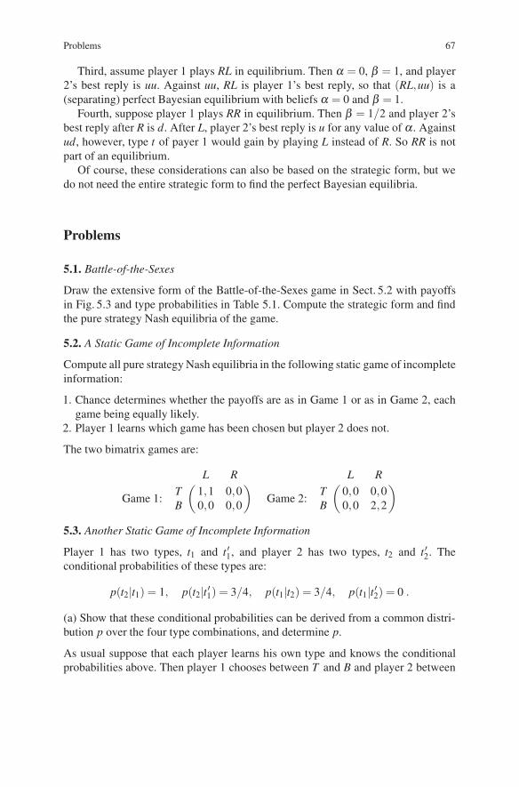
Problems 67
Third, assume player 1 plays RL in equilibrium. Then α = 0, β = 1, and player2’s best reply is uu. Against uu, RL is player 1’s best reply, so that (RL,uu) is a(separating) perfect Bayesian equilibrium with beliefs α = 0 and β = 1.
Fourth, suppose player 1 plays RR in equilibrium. Then β = 1/2 and player 2’sbest reply after R is d. After L, player 2’s best reply is u for any value of α . Againstud, however, type t of payer 1 would gain by playing L instead of R. So RR is notpart of an equilibrium.
Of course, these considerations can also be based on the strategic form, but wedo not need the entire strategic form to find the perfect Bayesian equilibria.
Problems
5.1. Battle-of-the-Sexes
Draw the extensive form of the Battle-of-the-Sexes game in Sect. 5.2 with payoffsin Fig. 5.3 and type probabilities in Table 5.1. Compute the strategic form and findthe pure strategy Nash equilibria of the game.
5.2. A Static Game of Incomplete Information
Compute all pure strategy Nash equilibria in the following static game of incompleteinformation:
1. Chance determines whether the payoffs are as in Game 1 or as in Game 2, eachgame being equally likely.
2. Player 1 learns which game has been chosen but player 2 does not.
The two bimatrix games are:
Game 1:( L R
T 1,1 0,0B 0,0 0,0
)Game 2:
( L RT 0,0 0,0B 0,0 2,2
)5.3. Another Static Game of Incomplete Information
Player 1 has two types, t1 and t ′1, and player 2 has two types, t2 and t ′2. Theconditional probabilities of these types are:
p(t2|t1) = 1, p(t2|t ′1) = 3/4, p(t1|t2) = 3/4, p(t1|t ′2) = 0 .
(a) Show that these conditional probabilities can be derived from a common distri-bution p over the four type combinations, and determine p.
As usual suppose that each player learns his own type and knows the conditionalprobabilities above. Then player 1 chooses between T and B and player 2 between

68 5 Finite Games with Incomplete Information
L and R, where these actions may be contingent on the information a player has.The payoffs for the different type combinations are given by the bimatrix games
t1t2 :( L R
T 2,2 0,0B 3,0 1,1
)t ′1t2 :
( L RT 2,2 0,0B 0,0 1,1
)t ′1t ′2 :
( L RT 2,2 0,0B 0,0 1,1
),
where the type combination (t1,t ′2) is left out since it has zero probability.
(b) Compute all pure strategy Nash equilibria for this game.
5.4. Job-Market Signaling
(Cf. [128].) A worker can have either high or low ability, each with probability 1/2.A worker knows his ability, but a firm which wants to hire the worker does not.The worker, whether a high or a low ability type, can choose between additionaleducation or not. Choosing additional education does not enlarge the worker’s pro-ductivity but may serve as a signal to the firm: a high ability worker can chooseeducation without additional costs, whereas for a low ability worker the cost of edu-cation equals e > 0. The firm chooses either a high or a low wage, having observedwhether the worker took additional education or not. The payoff to the firm equalsthe productivity of the worker minus the wage. The payoff to the worker equals thewage minus the cost of education; if, however, this payoff is lower than the worker’sreservation utility, he chooses not to work at all and to receive his reservation utility,leaving the firm with 0 payoff. Denote the productivities of the high and low abilityworker by pH and pL, respectively, and denote the high and low wages by wh andwl . Finally, let rH and rL denote the reservation utilities of both worker types. (Allthese numbers are fixed.)
(a) Determine the extensive form of this game.
Choose pH = 10, pL = 8, wh = 6, wl = 4, rH = 3, rL = 2, e = 3.
(b) Compute the strategic form of this game, and determine the pure strategy Nashequilibria. Also compute the perfect Bayesian equilibrium or equilibria in purestrategies, determine whether they are separating or pooling and whether they satisfythe intuitive criterion.
5.5. A Joint Venture
(Cf. [106], p. 65.) Software Inc. and Hardware Inc. are in a joint venture together.The parts used in the joint product can be defective or not; the probability of defec-tive parts is 0.7, and this is commonly known before the start of the game. Each canexert either high or low effort, which is equivalent to costs of 20 and 0. Hardwaremoves first, but software cannot observe his effort. Revenues are split equally at theend. If both firms exert low effort, total profits are 100. If the parts are defective, thetotal profit is 100; otherwise (i.e., if the parts are defective), if both exert high effort,profit is 200, but if only one player does, profit is 100 with probability 0.9 and 200

Problems 69
Entrant
Entrant
Inc.
E
E
O
O
C
F
C
F
Chance
0,100
0,100
40,50
−10,0
40,50
−10,x
50%
50%
Fig. 5.6 The entry deterrence game of Problem 5.6
with probability 0.1. Hardware discovers the truth about the parts by observationbefore he chooses effort, but software does not.
(a) Determine the extensive form of this game. Is this a signaling game?
(b) Determine the strategic form of this game.
(c) Compute the (pure) Nash equilibria? Which one(s) is (are) subgame perfect?Perfect Bayesian?
5.6. Entry Deterrence
The entry deterrence game of Chap. 1 is reproduced in Fig. 5.6. For this game, com-pute the pure strategy perfect Bayesian equilibria for every value of x ∈ R. Whichone(s) is (are) pooling or separating? Satisfy the intuitive criterion?
5.7. The Beer–Quiche Game
(Cf. [19].) Consider the following two-player signaling game. Player 1 is either‘weak’ or ‘strong’. This is determined by a chance move, resulting in player 1 being‘weak’ with probability 1/10. Player 1 is informed about the outcome of this chancemove but player 2 is not. Player 1 has two actions: either have quiche (Q) or havebeer (B) for breakfast. Player 2 observes the breakfast of player 1 and then decidesto duel (D) or not to duel (N) with player 1. The payoffs are as follows. If player 1is weak and eats quiche then D and N give him payoffs of 1 and 3, respectively; ifhe is weak and drinks beer, then these payoffs are 0 and 2, respectively. If player 1is strong, then the payoffs are 0 and 2 from D and N, respectively, if he eats quiche;and 1 and 3 from D and N, respectively, if he drinks beer. Player 2 has payoff 0from not duelling, payoff 1 from duelling with the weak player 1, and payoff −1from duelling with the strong player 1.
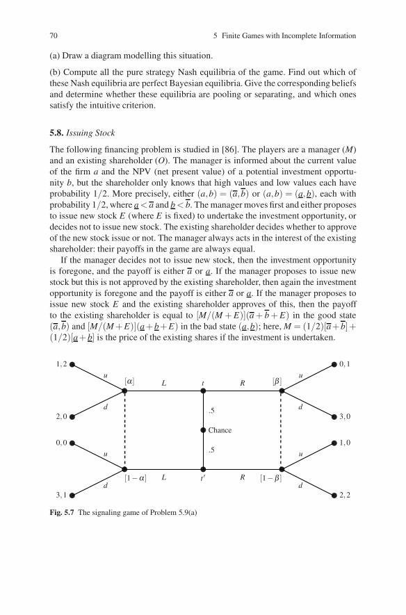
70 5 Finite Games with Incomplete Information
(a) Draw a diagram modelling this situation.
(b) Compute all the pure strategy Nash equilibria of the game. Find out which ofthese Nash equilibria are perfect Bayesian equilibria. Give the corresponding beliefsand determine whether these equilibria are pooling or separating, and which onessatisfy the intuitive criterion.
5.8. Issuing Stock
The following financing problem is studied in [86]. The players are a manager (M)and an existing shareholder (O). The manager is informed about the current valueof the firm a and the NPV (net present value) of a potential investment opportu-nity b, but the shareholder only knows that high values and low values each haveprobability 1/2. More precisely, either (a,b) = (a,b) or (a,b) = (a,b), each withprobability 1/2, where a < a and b < b. The manager moves first and either proposesto issue new stock E (where E is fixed) to undertake the investment opportunity, ordecides not to issue new stock. The existing shareholder decides whether to approveof the new stock issue or not. The manager always acts in the interest of the existingshareholder: their payoffs in the game are always equal.
If the manager decides not to issue new stock, then the investment opportunityis foregone, and the payoff is either a or a. If the manager proposes to issue newstock but this is not approved by the existing shareholder, then again the investmentopportunity is foregone and the payoff is either a or a. If the manager proposes toissue new stock E and the existing shareholder approves of this, then the payoffto the existing shareholder is equal to [M/(M + E)](a + b + E) in the good state(a,b) and [M/(M +E)](a+b+E) in the bad state (a,b); here, M = (1/2)[a+b]+(1/2)[a+ b] is the price of the existing shares if the investment is undertaken.
��
��
��
�
�
�
��
��
��
d
d
u
u
d
d
u
u
L
L
R
R
t ′
t
Chance
.5
.5
3,1
0,0
2,0
1,2
2,2
1,0
3,0
0,1
[1−α ]
[α ]
[1−β ]
[β ]
Fig. 5.7 The signaling game of Problem 5.9(a)
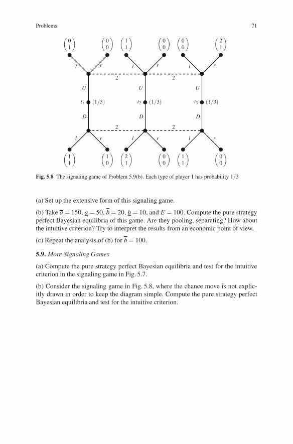
Problems 71
� � � � � �
� � � � � �
� � �
� � �
� � �
l l l
l l l
r r r
r r r
D D D
U U U
t1 t2 t3(1/3) (1/3) (1/3)
2 2
2 2
(11
) (10
) (21
) (00
) (11
) (00
)
(01
) (00
) (11
) (00
) (00
) (21
)
Fig. 5.8 The signaling game of Problem 5.9(b). Each type of player 1 has probability 1/3
(a) Set up the extensive form of this signaling game.
(b) Take a = 150, a = 50, b = 20, b = 10, and E = 100. Compute the pure strategyperfect Bayesian equilibria of this game. Are they pooling, separating? How aboutthe intuitive criterion? Try to interpret the results from an economic point of view.
(c) Repeat the analysis of (b) for b = 100.
5.9. More Signaling Games
(a) Compute the pure strategy perfect Bayesian equilibria and test for the intuitivecriterion in the signaling game in Fig. 5.7.
(b) Consider the signaling game in Fig. 5.8, where the chance move is not explic-itly drawn in order to keep the diagram simple. Compute the pure strategy perfectBayesian equilibria and test for the intuitive criterion.

Chapter 6Noncooperative Games: Extensions
In Chaps. 2–5 we have studied noncooperative games in which the players havefinitely many (pure) strategies. The reason for the finiteness restriction is that insuch games special results hold, like the existence of a value and optimal strategiesfor two-person zerosum games, and the existence of a Nash equilibrium in mixedstrategies for finite nonzerosum games.
The basic game-theoretical concepts discussed in these chapters can be appliedto much more general games. Once, in a game-theoretic situation, the players,their possible strategies, and the associated payoffs are identified, the concepts ofbest reply and of Nash equilibrium can be applied. Also the concepts of backwardinduction, subgame perfection, and perfect Bayesian equilibrium carry over to quitegeneral extensive form games. In games of incomplete information, the concept ofplayer types and the associated Nash equilibrium (Bayesian Nash equilibrium) canbe applied also if the game has infinitely many strategies.
The bulk of this chapter consists of various, diverse examples verifying theseclaims. The main objective of the chapter is, indeed, to show how the basic game-theoretic apparatus can be applied to various different conflict situations; and, ofcourse, to show these applications themselves.
In Sect. 6.1 we generalize some of the concepts of Chaps. 2–3. This section servesonly as background and general framework for the examples in the following sec-tions. Concepts specific to extensive form games and to incomplete informationgames are adapted later, when they are applied. In Sects. 6.2–6.7 we discuss, respec-tively, Cournot competition with complete and incomplete information, Bertrandcompetition, Stackelberg equilibrium, auctions with complete and incomplete infor-mation, mixed strategies with objective probabilities, and sequential bargaining.Variations on these topics and various other topics are treated in the problem section.
6.1 General Framework: Strategic Games
An n-person strategic game is a 2n + 1-tuple
G = (N,S1, . . . ,Sn,u1, . . . ,un) ,
H. Peters, Game Theory – A Multi-Leveled Approach.c© Springer-Verlag Berlin Heidelberg 2008
73

74 6 Noncooperative Games: Extensions
where
• N = {1, . . . ,n}, with n ∈ N, n ≥ 1, is the set of players;• for every i ∈ N, Si is the strategy set of player i;• for every i ∈ N, ui : S = S1 × ·· · × Sn → R is the payoff function of player i;
i.e., for every strategy combination (s1, . . . ,sn) ∈ S where s1 ∈ S1, . . ., sn ∈ Sn,ui(s1, . . . ,sn) ∈ R is player i’s payoff.
A best reply of player i to the strategy combination (s1, . . . ,si−1,si+1, . . . ,sn) of theother players is a strategy si ∈ Si such that
ui(s1, . . . ,si−1,si,si+1, . . . ,sn) ≥ ui(s1, . . . ,si−1,s′i,si+1, . . . ,sn)
for all s′i ∈ Si.A Nash equilibrium of G is a strategy combination (s∗1, . . . ,s
∗n) ∈ S such that for
each player i, s∗i is a best reply to (s∗1, . . . ,s∗i−1,s
∗i+1, . . . ,s
∗n).
A strategy s′i ∈ Si of player i is strictly dominated by si ∈ Si if
ui(s1, . . . ,si−1,si,si+1, . . . ,sn) > ui(s1, . . . ,si−1,s′i,si+1, . . . ,sn)
for all (s1, . . . ,si−1,si+1, . . . ,sn)∈ S1×·· ·×Si−1×Si+1×·· ·×Sn, i.e., for all strategycombinations of players other than i. Clearly, a strictly dominated strategy is neverused in a Nash equilibrium.
For completeness we also define weak domination. A strategy s′i ∈ Si of player iis weakly dominated by si ∈ Si if
ui(s1, . . . ,si−1,si,si+1, . . . ,sn) ≥ ui(s1, . . . ,si−1,s′i,si+1, . . . ,sn)
for all (s1, . . . ,si−1,si+1, . . . ,sn) ∈ S1 ×·· ·×Si−1 ×Si+1×·· ·×Sn, such that at leastonce this inequality is strict.
The reader should verify that matrix games (Chap. 2) and bimatrix games (Chap. 3)are special cases of this general framework. The same is true for the concepts ofNash equilibrium and domination discussed in these chapters.
6.2 Cournot Quantity Competition
6.2.1 Simple Version with Complete Information
In the simplest version of the famous Cournot [21] model, two firms producing ahomogenous good are competing in quantity. Each firm offers a quantity of thisgood on the market. The price of the good depends on the total quantity offered:the higher this quantity is, the lower the price of the good. The profit for each firmis equal to total revenue (price times quantity) minus total cost. This gives rise toa two-person game in which the players’ strategies are the quantities offered and

6.2 Cournot Quantity Competition 75
the payoff functions are the profit functions. In a simple version, the price dependslinearly on total quantity and marginal cost is constant while there are no fixed costs.Specifically, we study the following game:
(a) The set of players is N = {1,2}.(b) Each player i = 1,2 has set of strategies Si = [0,∞), with typical element qi.(c) The payoff function of player i is Πi(q1,q2) = qiP(q1,q2)− cqi, for all q1,q2 ≥
0, where
P(q1,q2) ={
a− q1−q2 if q1 + q2 ≤ a0 if q1 + q2 > a
is the market price of the good and c is marginal cost, with a > c ≥ 0.
A Nash equilibrium in this game is a pair (qC1 ,qC
2 ), with qC1 ,qC
2 ≥ 0, of mutually bestreplies, that is,
Π1(qC1 ,qC
2 ) ≥ Π1(q1,qC2 ), Π2(qC
1 ,qC2 ) ≥ Π2(qC
1 ,q2) for all q1,q2 ≥ 0 .
For obvious reasons, this equilibrium is also called Cournot equilibrium. To findthe equilibrium, we first compute the best reply functions, also called reaction func-tions. The reaction function β1(q2) of player 1 is found by solving the maximizationproblem
maxq1≥0
Π1(q1,q2)
for each given value of q2 ≥ 0. For q2 ≤ a this means maximizing the function
q1(a−q1−q2)− cq1 = q1(a− c−q1−q2)
for q1 ≥ 0. For q2 ≤ a − c, the maximum is obtained by setting the derivativewith respect to q1, namely the function a− 2q1 − q2 − c, equal to zero, yieldingq1 = (a− c− q2)/2.1 For a− c < q2 ≤ a, it is optimal to take q1 = 0 since other-wise the profit is negative. Note that, indeed, q1 + q2 ≤ a in these cases. If q2 > a,then P(q1,q2) = 0 independent of the choice of q1, and then player 1 maximizesprofit −cq1 by choosing q1 = 0 if c > 0 and q1 ∈ [0,∞) if c = 0. Summarizing,we have
β1(q2) =
⎧⎪⎪⎪⎨⎪⎪⎪⎩{ a−c−q2
2 } if q2 ≤ a− c{0} if a− c < q2 ≤ a{0} if a < q2 and c > 0[0,∞) if a < q2 and c = 0.
(6.1)
(Since, in all cases of interest, this reaction function is single-valued – if c = 0 anda < q2 we may just as well take q1 = 0 since this does not occur in equilibrium
1 The second derivative is equal to −2 so that, indeed, we have a maximum.

76 6 Noncooperative Games: Extensions
0 a−c2
a−c2
a − c
a − c
q2
q1
qC
Fig. 6.1 The Cournot model: the solid black curve is the reaction function of player 1 and the solidgray curve the reaction function of player 2. The point qC is the Nash–Cournot equilibrium. Thetwo isoprofit curves of the players through the Nash equilibrium are drawn, and the shaded areaconsists of the quantity combinations that Pareto dominate the equilibrium
anyway – usually the braces are omitted.) By completely symmetric arguments weobtain for the reaction function of player 2:
β2(q1) =
⎧⎪⎪⎨⎪⎪⎩{ a−c−q1
2 } if q1 ≤ a− c{0} if a− c < q1 ≤ a{0} if a < q1 and c > 0[0,∞) if a < q1 and c = 0.
(6.2)
These reaction functions are drawn in Fig. 6.1. The Nash equilibrium is the point ofintersection of the reaction functions. It is obtained by simultaneously solving thetwo equations q1 = (a− c− q2)/2 and q2 = (a− c−q1)/2, resulting in
(qC1 ,qC
2 ) = (a− c
3,
a− c3
) .
Pareto Optimality
A pair (q1,q2) of strategies is Pareto optimal if there is no other pair (q′1,q′2) such
that the associated payoffs are at least as good for both players and strictly better forat least one player. Not surprisingly, the equilibrium (qC
1 ,qC2 ) is not Pareto optimal.
For instance, both players can strictly benefit from joint profit maximization, bysolving the problem
maxq1,q2≥0
Π1(q1,q2)+ Π2(q1,q2) .
The first-order conditions, obtained by setting the partial derivatives with respect toq1 and q2 equal to zero, result in the equation a−2q1−2q2−c = 0, so that any pair

6.2 Cournot Quantity Competition 77
(q1,q2) ≥ 0 with q1 + q2 = (a− c)/2 is a solution (check again the second-orderconditions). Taking q1 = q2 = (a− c)/4 yields each player a profit of (a− c)2/8,whereas in the Nash equilibrium each player obtains (a− c)2/9. See also Fig. 6.1,where all points in the gray-shaded area ‘Pareto dominate’ the Nash equilibrium:the associated payoffs are at least as good for both agents and better for at least oneagent.
6.2.2 Simple Version with Incomplete Information
Consider the Cournot model of Sect. 6.2.1 but now assume that the marginal cost offirm 2 is either high, cH , or low, cL, where cH > cL ≥ 0. Firm 2 knows its marginalcost but firm 1 only knows that it is cH with probability ϑ or cL with probability1−ϑ . The cost of firm 1 is c and this is commonly known. In the terminology ofSect. 5.1, player 1 has only one type but player 2 has two types, cH and cL. Theassociated game is as follows:
(a) The player set is {1,2}.(b) The strategy set of player 1 is [0,∞) with typical element q1, and the strategy
set of player 2 is [0,∞)× [0,∞) with typical element (qH ,qL). Here, qH is thechosen quantity if player 2 is of type cH , and qL is the chosen quantity if player2 is of type cL.
(c) The payoff functions of the players are the expected payoff functions. These are
Πi(q1,qH ,qL) = ϑΠi(q1,qH)+ (1−ϑ)Πi(q1,qL) ,
for i = 1,2, where Πi(·, ·) is the payoff function from the Cournot model ofSect. 6.2.1.
To find the (Bayesian) Nash equilibrium, we first compute the best reply functionor reaction function of player 1, by maximizing Π1(q1,qH ,qL) over q1 ≥ 0, with qHand qL regarded as given. Hence, we solve the problem
maxq1≥0
ϑ [q1(a− c−q1−qH)]+ (1−ϑ) [q1(a− c−q1−qL)] .
Assuming qH ,qL ≤ a− c (this has to be checked later for the equilibrium), thisproblem is solved by setting the derivative with respect to q1 equal to zero, whichyields
q1 = q1(qH ,qL) =a− c−ϑqH − (1−ϑ)qL
2. (6.3)
Observe that, compared to (6.1), we now have the expected quantity ϑqH + (1−ϑ)qL instead of q2: this is due to the linearity of the model.
For player 2, we consider, for given q1, the problem
maxqH ,qL≥0
ϑ [qH(a− cH −q1 −qH)]+ (1−ϑ) [qL(a− cL−q1 −qL)] .

78 6 Noncooperative Games: Extensions
Since the first term in this function depends only on qH and the second term onlyon qL, solving this problem amounts to maximizing the two terms separately. Inother words, we determine the best replies of types cH and cL separately.2 Assumingq1 ≤ a− cH (and hence q1 ≤ a− cL) this results in
qH = qH(q1) =a− cH −q1
2(6.4)
and
qL = qL(q1) =a− cL−q1
2. (6.5)
The Nash equilibrium is obtained by simultaneously solving (6.3–6.5), using sub-stitution or linear algebra. The solution is the triple
qC1 =
a−2c + ϑcH +(1−ϑ)cL
3
qCH =
a−2cH + c3
+1−ϑ
6(cH − cL)
qCL =
a−2cL + c3
− ϑ6
(cH − cL) .
Assuming that the parameters of the game are such that these three values are non-negative and that q1 ≤ a−cH and qH ,qL ≤ a−c, this is the Bayesian Nash–Cournotequilibrium of the game. This solution should be compared with the Nash equilib-rium in the complete information model with asymmetric costs, see Problem 6.1.The high cost type of firm 2 produces more than it would in the complete informa-tion case: it benefits from the fact that firm 1 is unsure about the cost of firm 2 andtherefore produces less than it would if it knew for sure that firm 2 had high costs.Similarly, the low cost firm 2 produces less.
6.3 Bertrand Price Competition
Consider two firms who compete in the price of a homogenous good.3 Specifically,assume that the demand q for the good is given by q = q(p) = max{a− p,0} forevery p ≥ 0. The firm with the lower price serves the whole market; if prices areequal the firms share the market equally. Each firm has the same marginal cost0 ≤ c < a, and no fixed cost. If firm 1 sets a price p1 and firm 2 sets a price p2, thenthe profit of firm 1 is
2 This is generally so in a Bayesian, incomplete information game: maximizing the expected payoffof a player over all his types is equivalent to maximizing the payoff per type.3 See Problem 6.3(d)–(f) for an example of price competition with heterogenous goods.
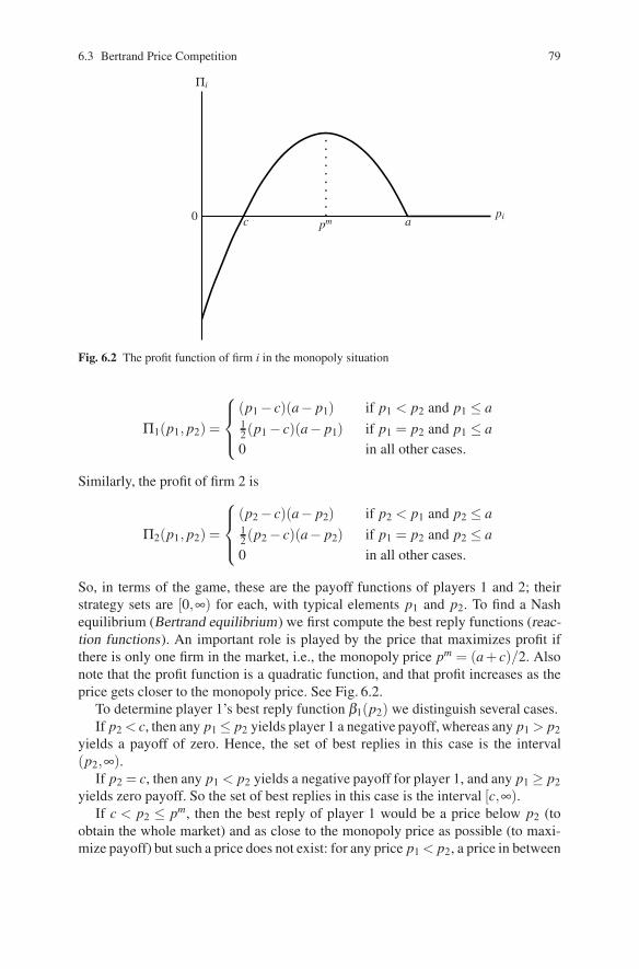
6.3 Bertrand Price Competition 79
0 c pm api
Πi
Fig. 6.2 The profit function of firm i in the monopoly situation
Π1(p1, p2) =
⎧⎪⎨⎪⎩(p1 − c)(a− p1) if p1 < p2 and p1 ≤ a12(p1 − c)(a− p1) if p1 = p2 and p1 ≤ a0 in all other cases.
Similarly, the profit of firm 2 is
Π2(p1, p2) =
⎧⎪⎨⎪⎩(p2 − c)(a− p2) if p2 < p1 and p2 ≤ a12(p2 − c)(a− p2) if p1 = p2 and p2 ≤ a0 in all other cases.
So, in terms of the game, these are the payoff functions of players 1 and 2; theirstrategy sets are [0,∞) for each, with typical elements p1 and p2. To find a Nashequilibrium (Bertrand equilibrium) we first compute the best reply functions (reac-tion functions). An important role is played by the price that maximizes profit ifthere is only one firm in the market, i.e., the monopoly price pm = (a + c)/2. Alsonote that the profit function is a quadratic function, and that profit increases as theprice gets closer to the monopoly price. See Fig. 6.2.
To determine player 1’s best reply function β1(p2) we distinguish several cases.If p2 < c, then any p1 ≤ p2 yields player 1 a negative payoff, whereas any p1 > p2
yields a payoff of zero. Hence, the set of best replies in this case is the interval(p2,∞).
If p2 = c, then any p1 < p2 yields a negative payoff for player 1, and any p1 ≥ p2yields zero payoff. So the set of best replies in this case is the interval [c,∞).
If c < p2 ≤ pm, then the best reply of player 1 would be a price below p2 (toobtain the whole market) and as close to the monopoly price as possible (to maxi-mize payoff) but such a price does not exist: for any price p1 < p2, a price in between

80 6 Noncooperative Games: Extensions
p1 and p2 would still be better. Hence, in this case the set of best replies of player 1is empty.4
If p2 > pm then the unique best reply of player 1 is the monopoly price pm.Summarizing we obtain
β1(p2) =
⎧⎪⎪⎨⎪⎪⎩{p1 | p1 > p2} if p2 < c{p1 | p1 ≥ c} if p2 = c/0 if c < p2 ≤ pm
{pm} if p2 > pm.
For player 2, similarly,
β2(p1) =
⎧⎪⎪⎨⎪⎪⎩{p2 | p2 > p1} if p1 < c{p2 | p2 ≥ c} if p1 = c/0 if c < p1 ≤ pm
{pm} if p1 > pm.
The point(s) of intersection of these best reply functions can be found by making adiagram or by direct inspection. We follow the latter method and leave the diagrammethod to the reader. If p2 < c then a best reply p1 satisfies p1 > p2. But then,according to β2(p1), we always have p2 ≥ p1 or p2 = pm, a contradiction. Therefore,in equilibrium, we must have p2 ≥ c. If p2 = c, then p1 ≥ c; if however, p1 > c thenthe only possibility is p2 = pm, a contradiction. Hence, p1 = c as well and, indeed,p1 = p2 = c is a Nash equilibrium. If p2 > c, then the only possibility is p1 = pm
but then p2 is never a best reply. We conclude that the unique Nash equilibrium(Bertrand equilibrium) is p1 = p2 = c.
It is also possible to establish this result without completely computing the best replyfunction. Suppose, in equilibrium, that p1 = p2, say p1 < p2. If p1 < pm then player1 can increase his payoff by setting a higher price still below p2. If p1 ≥ pm thenplayer 2 can increase his payoff by setting a price below p1, e.g., slightly below pm
if p1 = pm and equal to pm if p1 > pm. Hence, we must have p1 = p2 in equilibrium.If this common price is below c then each player can improve by setting a higherprice. If this common price is above c then each player can improve by setting aslightly lower price. Hence, the only possibility that remains is p1 = p2 = c, andthis is indeed an equilibrium, as can be verified directly.
6.4 Stackelberg Equilibrium
In the Cournot model of Sect. 6.2.1, the two firms move simultaneously. Considernow the situation where firm 1 moves first, and firm 2 observes this move and movesnext. This situation has already been mentioned in Chap. 1. The corresponding
4 If prices are in smallest monetary units this somewhat artificial consequence is avoided. SeeProblem 6.7.

6.4 Stackelberg Equilibrium 81
1� q1 ≥ 0 2� q2 ≥ 0 � q1(1−q1 −q2),q2(1−q1 −q2)
Fig. 6.3 Extensive form representation of the Stackelberg game with firm 1 as the leader
extensive form game is reproduced in Fig. 6.3. In this game, player 1 has infiniteaction/strategy set [0,∞), with typical element q1. In the diagram, we use a zigzagline to express the fact that the number of actions is infinite. Player 2 has the infi-nite set of actions [0,∞) with typical element q2, again represented by a zigzagline. A strategy of player 2 assigns to each information set, hence to each decisionnode – the game has perfect information – an action. Hence, a strategy of player2 is a function s2 : [0,∞) → [0,∞). Obviously, the number of strategies of player 2is infinite as well.5 The appropriate solution concept is the backward induction orsubgame perfect equilibrium. The subgames of this game are the entire game andthe infinite number of one-player games starting at each decision node of player 2,i.e., following each choice q1 of player 1. Hence, the subgame perfect equilibriumcan be found by backward induction, as follows. In each subgame for player 2, thatis, after each choice q1, player 2 should play optimally. This means that player 2should play according to the reaction function β2(q1) as derived in (6.2). Then,going back to the beginning of the game, player 1 should choose q1 ≥ 0 so as tomaximize Π1(q1,β2(q1)). In other words, player 1 takes player 2’s optimal reac-tion into account when choosing q1. Assuming q1 ≤ a− c – it is easy to verify thatq1 > a− c is not optimal – player 1 maximizes the expression
q1
(a− c−q1− a− c−q1
2
).
The maximum is obtained for q1 = (a− c)/2, and thus q2 = β2 ((a− c)/2) = (a−c)/4. Hence, the subgame perfect equilibrium of the game is
q1 = (a− c)/2, q2 = β2(q1) .
The subgame perfect equilibrium outcome is by definition the resulting play of thegame, that is, the actions chosen on the equilibrium path in the extensive form. Inthis case, the equilibrium outcome is
qS1 = (a− c)/2, qS
2 = (a− c)/4 .
The letter ‘S’ here is the first letter of ‘Stackelberg’, after whom this equilibrium isnamed (see [142]). More precisely, this subgame perfect equilibrium (or outcome)is called the Stackelberg equilibrium (or outcome) with player 1 as the leader andplayer 2 as the follower. Check that player 1’s profit in this equilibrium is higherand player 2’s profit is lower than in the Cournot equilibrium qC
1 = qC2 = (a− c)/3.
See also Problem 6.9.
5 In mathematical notation the strategy set of player 2 is the set [0,∞)[0,∞).

82 6 Noncooperative Games: Extensions
0 a−c2
a−c2
a− c
a− c
q2
q1
qS
Fig. 6.4 As before, the solid black curve is the reaction function of player 1 and the solid graycurve the reaction function of player 2. The point qS = ( a−c
2 , a−c4 ) is the Stackelberg equilibrium:
it is the point on the reaction curve of player 2 where player 1 maximizes profit. The associatedisoprofit curve of player 1 is drawn
The Stackelberg equilibrium is depicted in Fig. 6.4. Observe that player 1, theleader, picks the point on the reaction curve of player 2 which has maximal profitfor player 1. Hence, player 2 is on his reaction curve but player 1 is not.
6.5 Auctions
An auction is a procedure to sell goods among various interested parties, such thatthe prices are determined in the procedure. Examples range from selling a paintingthrough an ascending bid auction (English auction) and selling flowers through adescending bid auction (Dutch auction) to tenders for public projects and sellingmobile telephone frequencies. For a recent overview, see [78].
In this section we consider a few simple, classical auction models. We start withfirst and second-price sealed-bid auctions under complete information, and end witha first-price sealed bid auction with incomplete information. Some variations andextensions are discussed in Problems 6.10–6.13.
6.5.1 Complete Information
Consider n individuals who are interested in one indivisible object. Each individuali has valuation vi > 0 for the object. We assume without loss of generality v1 ≥ v2 ≥·· · ≥ vn. In a first-price sealed-bid auction each individual submits a bid bi ≥ 0 forthe object: the bids are simultaneous and independent (‘sealed bids’). The individual

6.5 Auctions 83
with the highest bid wins the auction and obtains the object at a price equal to hisown bid (‘first price’). In case there are more highest bidders, the bidder amongthese with the lowest number wins the auction and pays his own bid.
This gives rise to a game with player set N = {1,2, . . . ,n}, where each player ihas strategy set Si = [0,∞) with typical element bi. The payoff function to player i is
ui(b1,b2, . . . ,bi, . . . ,bn) ={
vi −bi if i = min{k ∈ N | bk ≥ b j for all j ∈ N}0 otherwise.
One Nash equilibrium in this game is the strategy combination (b1, . . . ,bn) =(v2,v2,v3, . . . ,vn). To check this one should verify that no player has a better bid,given the bids of the other players: see Problem 6.10. In this equilibrium, player 1obtains the object and pays v2, the second-highest valuation. Check that this is alsothe outcome one would approximately expect in an auction with ascending bids(English auction) or descending bids (Dutch auction).
This game has many Nash equilibria. In each of these equilibria, however, aplayer with a highest valuation obtains the object. Bidding one’s true valuationas well as bidding higher than one’s true valuation are weakly dominated strate-gies. Bidding lower than one’s true valuation is not weakly dominated (see Sect. 6.1for the definition of weak domination). Problem 6.10 is about proving all thesestatements.
A second-price sealed-bid auction differs from a first-price sealed-bid auction onlyin that the winner now pays the bid of the second highest bidder. In the case thattwo or more players have the highest bid the player with the lowest number winsand pays his own bid. The main property of this auction is that for each playeri, the strategy of bidding vi weakly dominates all other strategies. This and otherproperties are collected in Problem 6.11.
6.5.2 Incomplete Information
We consider the same setting as in Sect. 6.5.1 but now assume that each bidderknows his own valuation but has only a probabilistic estimate about the valuationsof the other bidders. In the terminology of types (cf. Sect. 5.1), a bidder’s valuationis his true type, and each bidder holds a probability distribution over the type com-binations of the other bidders. To keep things simple, we assume that every bidder’stype is drawn independently from the uniform distribution over the interval [0,1],that this is common knowledge, and that each bidder learns his true type. The auc-tion is a first-price sealed-bid auction. Of course, we can no longer fix the orderingof the valuations, but we can still employ the same tie-breaking rule in case of morethan one highest bid.
We discuss the case of two bidders and postpone the extension to n > 2 biddersuntil Problem 6.13. In the associated two-person game, a strategy of player i∈ {1,2}should assign a bid to each of his possible types. Since the set of possible types is

84 6 Noncooperative Games: Extensions
the interval [0,1] and it does not make sense to ever bid more than 1, a strategyis a function si : [0,1] → [0,1]. Hence, if player i’s type is vi, then bi = si(vi) ishis bid according to the strategy si. The payoff function ui of player i assigns toeach strategy pair (si,s j) (where j is the other player) player i’s expected payoff ifthese strategies are played. In a (Bayesian) Nash equilibrium of the game, player imaximizes this payoff function given the strategy of player j, and vice versa. Forthis, it is sufficient that each type of player i maximizes expected payoff given thestrategy of player j, and vice versa.
We claim that s∗1(v1) = v1/2 and s∗2(v2) = v2/2 is a Nash equilibrium of thisgame. To prove this, first consider type v1 of player 1 and suppose that player 2plays strategy s∗2. If player 1 bids b1, then the probability that player 1 wins theauction is equal to the probability that the bid of player 2 is smaller than or equalto b1. This probability is equal to the probability that v2/2 is smaller than or equalto b1, i.e., to the probability that v2 is smaller than or equal to 2b1. We may assumewithout loss of generality that b1 ≤ 1/2, since according to s∗2 player 2 will never bidhigher than 1/2. Since v2 is uniformly distributed over the interval [0,1] and 2b1 ≤ 1,the probability that v2 is smaller than or equal to 2b1 is just equal to 2b1. Hence, theprobability that the bid b1 of player 1 is winning is equal to 2b1 if player 2 plays s∗2,and therefore the expected payoff from this bid is equal to 2b1(v1 −b1) (if player 1loses his payoff is zero). This is maximal for b1 = v1/2. Hence, s∗1(v1) = v1/2 is abest reply to s∗2. The converse is almost analogous – the only difference being that forplayer 2 to win player 1’s bid must be strictly smaller due to the tie-breaking ruleemployed, but this does not change the associated probability under the uniformdistribution. Hence, we have proved the claim.
Thus, in this equilibrium, each bidder bids half his true valuation, and a playerwith the highest valuation wins the auction.
How about the second-price sealed-bid auction with incomplete information? This ismore straightforward since bidding one’s true valuation (si(vi) = vi for all vi ∈ [0,1])is a strategy that weakly dominates every other strategy, for each player i. Hence,these strategies still form a (Bayesian) Nash equilibrium. See Problem 6.11.
6.6 Mixed Strategies and Incomplete Information
Consider the bimatrix game (cf. Chap. 3)
G =( L R
T 2,1 2,0B 3,0 1,3
),
which has a unique Nash equilibrium ((p∗,1 − p∗),(q∗,1 − q∗)) with p∗ = 3/4and q∗ = 1/2. The interpretation of mixed strategies and of a mixed strategyNash equilibrium in particular is an old issue in the game-theoretic literature. Oneobvious interpretation is that a player actually plays according to the equilibrium

6.6 Mixed Strategies and Incomplete Information 85
probabilities. Although there is some empirical evidence that this may occur inreality (see [144]), this interpretation may not be entirely convincing, in particu-lar since in a mixed strategy Nash equilibrium a player is indifferent between allpure strategies played with positive probability in equilibrium (see Problem 3.8).An alternative interpretation – also mentioned in Sect. 3.1 – is that a mixed strategyof a player represents the belief(s) of the other player(s) about the strategic choiceof that player. For instance, in the above equilibrium, player 2 believes that player 1plays T with probability 3/4. The drawback of this interpretation is that these beliefsare subjective, and it is not explained how they are formed. Harsanyi [51] proposeda way to obtain a mixed strategy Nash equilibrium as the limit of pure (Bayesian)Nash equilibria in games obtained by adding some objective uncertainty about thepayoffs. In this way, the strategic uncertainty of players as expressed by their beliefsis replaced by the objective uncertainty of a chance move.
In the above example, suppose that the payoff to player 1 from (T,L) is the uncer-tain amount 2 + α and the payoff to player 2 from (B,R) is the uncertain amount3 + β . Assume that both α and β are (independently) drawn from a uniform distri-bution over the interval [0,x], where x > 0. Moreover, player 1 learns the true valueof α and player 2 learns the true value of β , and all this is common knowledgeamong the players. In terms of types, player 1 knows his type α and player 2 knowshis type β . The new payoffs are given by
( L RT 2 + α,1 2,0B 3,0 1,3 + β
).
A (pure) strategy of a player assigns an action to each of his types. Hence, for player1 it is a map s1 : [0,x] →{T,B} and for player 2 it is a map s2 : [0,x] → {L,R}.
To find an equilibrium of this incomplete information game, suppose that player2 has the following rather simple strategy: play L if β is small and R if β is large.Specifically, let b∈ [0,x] such that each type β ≤ b plays L and each type β > b playsR. Call this strategy s2(b). What is player 1’s best reply against s2(b)? Suppose thetype of player 1 is α . If player 1 plays T , then his expected payoff is equal to 2 + αtimes the probability that player 2 plays L plus 2 times the probability that player 2plays R. The probability that player 2 plays L, given the strategy s2(b), is equal to theprobability that β is at most equal to b, and this is equal to b/x since β is uniformlydistributed over [0,x]. Hence, the expected payoff to player 1 from playing T is
(2 + α) · bx
+ 2(1− bx) = 2 + α · b
x.
Similarly, the expected payoff to player 1 from playing B is
3 · bx
+ 1(1− bx) = 1 + 2 · b
x.
From this, it easily follows that T is at least as good as B if α ≥ (2b− x)/b. Hence,the following strategy of player 1 is a best reply against the assumed strategy of

86 6 Noncooperative Games: Extensions
player 2: play T if α ≥ a and play B if α < a, where a = (2b− x)/b. Call thisstrategy s1(a).
For the converse, assume that player 1 plays s1(a). To find player 2’s best replyagainst s1(a) we proceed similarly as above. If type β of player 2 plays L thenthe expected payoff is 1 times the probability that player 1 plays T , hence 1 times(x− a)/x. If type β of player 2 plays R then his expected payoff is equal to 3 + βtimes the probability that player 1 plays B, hence (3+β )a/x. So L is at least as goodas R if β ≤ (x−4a)/a. Hence, player 2’s best reply against s1(a) is the strategy s2(b)with b = (x−4a)/a.
Summarizing these arguments, we have that (s1(a),s2(b)) is a Nash equilibriumfor
a = (2b− x)/b, b = (x−4a)/a .
Solving these two equations simultaneously for solutions a,b ∈ [0,x] yields:
a = (1/4)(x + 4−√
x2 + 16), b = (1/2)(x−4 +√
x2 + 16) .
In this equilibrium, the a priori probability that player 1 will play T , that is, theprobability of playing T before he learns his type, is equal to (x− a)/x, hence to(√
x2 + 16+ 3x− 4)/4x. Similarly, the a priori probability that player 2 plays L isequal to b/x, hence to (x− 4 +
√x2 + 16)/2x. What happens to these probabilities
as the amount of uncertainty decreases, i.e., for x approaching 0? For player 1,
limx→0
√x2 + 16+ 3x−4
4x= lim
x→0
x/√
x2 + 16+ 34
=34
,
where the first identity follows from l’Hopital’s rule. Similarly for player 2:
limx→0
x−4 +√
x2 + 162x
= limx→0
1 + x/√
x2 + 162
=12
.
In other words, these probabilities converge to the mixed strategy Nash equilibriumof the original game.
6.7 Sequential Bargaining
In its simplest version, the bargaining problem involves two parties who have toagree on one alternative within a set of feasible alternatives. If they fail to reachan agreement, a specific ‘disagreement’ alternative is implemented. In the game-theoretic literature on bargaining there are two main strands, namely the cooperative,axiomatic approach as initiated by Nash in [90], and the noncooperative, strate-gic approach, with Nash [92] and Rubinstein [110] as seminal articles. These twoapproaches are not entirely disconnected and, in fact, there is a close relation-ship between the so-called Nash bargaining solution as proposed in [90] and the
6.7 Sequential Bargaining 87
Rubinstein subgame perfect equilibrium outcome in [110]. In this section the focusis on the strategic approach, but in Sect. 6.7.2 we also mention the connectionwith the Nash bargaining solution. For an introduction to the axiomatic bargainingapproach see Sect. 10.1.
6.7.1 Finite Horizon Bargaining
Consider the example in Sect. 1.3.5, where two players bargain over the division ofone unit of a perfectly divisible good, e.g., one liter of wine. If they do not reachan agreement, we assume that no one gets anything. To keep the problem as simpleas possible, assume that the preferences of the players are represented by u1(α) =u2(α) = α for every α ∈ [0,1]. That is, obtaining an amount α of the good hasutility α for each player. Observe that the picture of the feasible set in Sect. 1.3.5would become a triangle in this case.
To model the bargaining process we consider the following alternating offersprocedure. There are T ∈ N rounds. In round t = 0 player 1 makes a proposal, say(α,1−α), where α ∈ [0,1], meaning that he claims an amount α for himself, sothat player 2 obtains 1−α . Player 2 can either accept this proposal, implying thatthe proposal is implemented and the game is over, or reject the proposal. In the lattercase the next round t = 1 starts, and the first round is repeated with the roles of theplayers interchanged: player 2 makes the proposal and player 1 accepts or rejectsit. If player 1 accepts the proposal then it is implemented and the game is over; ifplayer 1 rejects the proposal then round t = 2 starts, and the roles of the players areinterchanged again. So at even moments, player 1 proposes; at odd moments, player2 proposes. The last possible round is round T : if this round is reached, then thedisagreement alternative (0,0) is implemented.
As assumed above, receiving an amount α at time (round) t has a utility of α foreach player, but this is the utility at time t. We assume that utilities are discountedover time, reflecting the fact that receiving the same amount earlier is more valuable.Specifically, there is a common discount factor 0 < δ < 1, such that receiving α attime t has utility δ tα at time 0.
In Fig. 6.5 this bargaining procedure is represented as a game in extensive form.Here, we assume that T is odd.
We look for a subgame perfect equilibrium of this game, which can be found bybackward induction. Note that subgames start at each decision node of a player, andthat, except at player 1’s decision node at t = 0, there are infinitely many subgamesstarting at each decision node since there are infinitely many possible proposals andtherefore infinitely many possible paths leading to a decision node.
To start the analysis, at the final decision node, player 2 accepts if α < 1 and isindifferent between acceptance and rejection if α = 1. In the subgame starting atround T −1 with a proposal of player 1, the only equilibrium therefore is for player1 to propose α = 1 and for player 2 to accept any proposal: if player 2 would rejectα = 1 then player 1 could improve by proposing 0 < α < 1, and given that player 2

88 6 Noncooperative Games: Extensions
� � � � � � � � � ��
� � � � �
· · ·
t = 0 t = 1 t = 2 t = T −1 t = T
1 2 2 1 1 2 2 1 1 2
α α α αR R R R R
A A A A A
(α ,1−α) δ (α ,1−α) δ 2(α ,1−α) δ T−2(α ,1−α) δ T−1(α ,1−α)
(0,0)
Fig. 6.5 The extensive form representation of the finite horizon bargaining procedure. The numberof rounds T is odd, α denotes the proposed amount for player 1, A is acceptance and R is rejection
� � � � � � � � �
� � � �
· · ·
t = 0 t = 1 t = 2 t = T −1
1 2 2 1 1 2 2 1
α α αR R R R
A A A A
(α ,1−α) δ (α ,1−α) δ 2(α ,1−α) δ T−2(α ,1−α)
(δ T−1,0)
Fig. 6.6 The game of Fig. 6.5 reduced by replacing rounds T −1 and T by the equilibrium payoffsof the associated subgames
accepts any proposal, α = 1 is optimal for player 1. Hence, we can replace the partof the game from round T −1 on by the pair of payoffs (δ T−1,0), as in Fig. 6.6.
Similarly, in this reduced game, in the complete subgame starting at roundT − 2 the only backward induction equilibrium is player 2 proposing α = δ andplayer 1 accepting this proposal or any higher α and rejecting any lower α ,since player 1 can always obtain δ T−1 = δ T−2δ by rejecting player 2’s proposal.Hence, we can replace this whole subgame by the pair of payoffs (δ T−1,δ T−2(1−δ )). Continuing this line of reasoning, in the subgame starting at round T − 3,player 1 proposes α = 1 − δ (1 − δ ), which will be accepted by player 2. Thisresults in the payoffs (δ T−3(1− δ (1− δ )),δ T−2(1− δ )). This can be written as(δ T−3(1− δ + δ 2),δ T−3(δ − δ 2)
). By backtracking all the way to round 0 (see
Table 6.1), we find that player 1 proposes 1 − δ + δ 2 − ·· ·+ δ T−1 and player 2accepts this proposal, resulting in the payoffs 1− δ + δ 2 − ·· ·+ δ T−1 for player1 and δ − δ 2 + · · · − δ T−1 for player 2. This is the subgame perfect equilibriumoutcome of the game and the associated payoffs. This outcome is the path of play,induced by the following subgame perfect equilibrium:
• At even rounds t, player 1 proposes α = 1−δ + · · ·+δ T−1−t and player 2 acceptsthis proposal or any smaller α , and rejects any larger α .

6.7 Sequential Bargaining 89
Table 6.1 The proposals made in the subgame perfect equilibrium
Round Proposer Share for player 1 Share for player 2
T 0 0T −1 1 1 0T −2 2 δ 1−δT −3 1 1−δ +δ 2 δ −δ 2
T −4 2 δ −δ 2 +δ 3 1−δ +δ 2 −δ 3
......
......
0 1 1−δ +δ 2 −·· ·+δ T−1 δ −δ 2 + · · ·−δ T−1
• At odd rounds t, player 2 proposes α = δ − δ 2 + · · ·+ δ T−1−t and player 1accepts this proposal or any larger α , and rejects any smaller α .
In Problem 6.15 some variations on this finite horizon bargaining game arediscussed.
6.7.2 Infinite Horizon Bargaining
In this subsection we consider the same bargaining problem as in the previous sub-section, but now we assume T = ∞: the number of rounds may potentially be infinite.If no agreement is ever reached, then no player obtains anything. This game, likethe finite horizon game, has many Nash equilibria: see Problem 6.15(f).
One way to analyze the game is to consider the finite horizon case and take thelimit as T approaches infinity: see Problem 6.15(e). In fact, the resulting distributionis the uniquely possible outcome of a subgame perfect equilibrium, as can be seenby comparing the answer to Problem 6.15(e) with the result presented below. Ofcourse, this claim is not proved by just taking the limit.
Note that a subgame perfect equilibrium cannot be obtained by backward induc-tion, since the game has no final decision nodes. Here, we will just describe a pairof strategies and show that they are a subgame perfect equilibrium of the game. Fora proof that the associated outcome is the unique outcome resulting in any subgameperfect equilibrium see [110].
Let x∗ = (x∗1,x∗2) and y∗ = (y∗1,y
∗2) such that x∗1,x
∗2,y
∗1,y
∗2 ≥ 0, x∗1 + x∗2 = y∗1 + y∗2 =
1, and moreover
x∗2 = δy∗2, y∗1 = δx∗1 . (6.6)
It is not difficult to verify that x∗ = (1/(1 + δ ),δ/(1 + δ )) and y∗ = (δ/(1 +δ ),1/(1 + δ )). Consider the following strategies for players 1 and 2, respectively:
(σ∗1 ) At t = 0,2,4, . . . propose x∗; at t = 1,3,5, . . . accept a proposal z = (z1,z2) of
player 2 if and only if z1 ≥ δx∗1.

90 6 Noncooperative Games: Extensions
(σ∗2 ) At t = 1,3,5, . . . propose y∗; at t = 0,2,4, . . . accept a proposal z = (z1,z2) of
player 1 if and only if z2 ≥ δy∗2.
These strategies are stationary: players always make the same proposals. Moreover,a player accepts any proposal that offers him at least the discounted value of his owndemand. According to (6.6), player 2 accepts the proposal y∗ and player 1 acceptsthe proposal x∗. Hence, play of the strategy pair (σ∗
1 ,σ∗2 ) results in player 1’s pro-
posal x∗ = (1/(1 + δ ),δ/(1 + δ )) being accepted at round 0, so that these are alsothe payoffs. We are going to show that (σ∗
1 ,σ∗2 ) is a subgame perfect equilibrium of
the game.To show this, note that there are two kinds of subgames: subgames where a player
has to make a proposal; and subgames where a proposal is on the table and a playerhas to choose between accepting and rejecting the proposal.
For the first kind of subgame we may without loss of generality consider theentire game, i.e., the game starting at t = 0. We have to show that (σ∗
1 ,σ∗2 ) is a Nash
equilibrium in this game. First, suppose that player 1 plays σ∗1 . By accepting player
1’s proposal at t = 0, player 2 has a payoff of δ/(1+δ ). By rejecting this proposal,the most player 2 can obtain against σ∗
1 is δ/(1 + δ ), by proposing y∗ in roundt = 1. Proposals z with z2 > y∗2 and thus z1 < y∗1 are rejected by player 1. Hence, σ∗
2is a best reply against σ∗
1 . Similarly, if player 2 plays σ∗2 , then the best player 1 can
obtain is x∗1 at t = 0 with payoff 1/(1 + δ ), since player 2 will reject any proposalthat gives player 1 more than this, and also does not offer more.
For the second kind of subgame, we may without loss of generality take t = 0and assume that player 1 has made some proposal, say z = (z1,z2) – the argumentfor t odd, when there is a proposal of player 2 on the table, is analogous. First,suppose that in this subgame player 1 plays σ∗
1 . If z2 ≥ δy∗2, then accepting thisproposal yields player 2 a payoff of z2 ≥ δy∗2 = δ/(1 + δ ). By rejecting, the mostplayer 2 can obtain against σ∗
1 is δ/(1 + δ ) by proposing y∗ at t = 1, which willbe accepted by player 1. If, on the other hand, z2 < δy∗2, then player 2 can indeedbetter reject z and obtain δ/(1 + δ ) by proposing y∗ at t = 1. Hence, σ∗
2 is a bestreply against σ∗
1 . Next, suppose player 2 plays σ∗2 . Then z is accepted if z2 ≥ δy∗2
and rejected otherwise. In the first case it does not matter how player 1 replies, andin the second case the game starts again with player 2 as the first proposer, and byan argument analogous to the argument in the previous paragraph, player 1’s bestreply is σ∗
1 .We have, thus, shown that (σ∗
1 ,σ∗2 ) is a subgame perfect equilibrium of the game.
In Problem 6.16 some variations on this game are discussed.Note, finally, that nothing in the whole analysis changes if we view the number
δ not as a discount factor but as the probability that the game continues to thenext round. Specifically, if a proposal is rejected, then assume that with probability1− δ the game stops and each player receives 0, and with probability δ the gamecontinues in the usual way. Under this alternative interpretation, the game ends withprobability 1 (Problem 6.16(e)), which makes the infinite horizon assumption moreacceptable.

Problems 91
Problems
6.1. Cournot with Asymmetric Costs
Consider the Cournot model of Sect. 6.2.1 but now assume that the firms have differ-ent marginal costs c1,c2 ≥ 0. Compute the Nash equilibrium: distinguish differentcases with respect to the values of c1 and c2.
6.2. Cournot Oligopoly
Consider the Cournot model of Sect. 6.2.1 but now assume that there are n firmsinstead of two. Each firm i = 1,2, . . . ,n offers qi ≥ 0 and the market price is
P(q1,q2, . . . ,qn) = max{a−q1−q2 −·· ·−qn,0} .
Each firm still has marginal cost c with a > c ≥ 0 and no fixed costs.
(a) Set up the game associated with this situation.
(b) Derive the reaction functions of the players.
(c) Derive a Nash equilibrium of the game by trying equal quantities offered. Whathappens if the number of firms becomes large?
(d) Show that the Nash equilibrium found in (c) is unique.
6.3. Quantity Competition with Heterogenous Goods
Suppose, in the Cournot model, that the firms produce heterogenous goods, whichhave different market prices. Specifically, suppose that these market prices aregiven by
p1 = max{5− 3q1−2q2,0}, p2 = max{4.5−1.5q1−3q2,0} .
The firms still compete in quantities.
(a) Formulate the game corresponding to this situation. In particular, write down thepayoff functions.
(b) Solve for the reaction functions and the Nash equilibrium of this game. Alsocompute the corresponding prices.
(c) Compute the quantities at which joint profit is maximized. Also compute thecorresponding prices.
In (d)–(f), we assume that the firms compete in prices.
(d) Derive the demands for q1 and q2 as a function of the prices. Set up the associatedgame where the prices p1 and p2 are now the strategic variables.
(e) Solve for the reaction functions and the Nash equilibrium of this game. Alsocompute the corresponding quantities.

92 6 Noncooperative Games: Extensions
(f) Compute the prices at which joint profit is maximized. Also compute thecorresponding quantities.
(g) Compare the results found under (b) and (c) with those under (e) and (f).6
6.4. A Numerical Example of Cournot with Incomplete Information
Redo the model of Sect. 6.2.2 for the following values of the parameters: a = 1,c = 0, ϑ = 1/2, cL = 0, cH = 1/4. Compute the Nash equilibrium and comparewith what was found in the text. Also compare with the complete information caseby using the answer to Problem 6.1.
6.5. Cournot with Two-Sided Incomplete Information
Consider the Cournot game of incomplete information of Sect. 6.2.2 and assume thatalso firm 1 can have high costs or low costs, say ch with probability π and cl withprobability 1−π . Set up the associated game and compute the (four) reaction func-tions. (Assume that the parameters of the game are such that the Nash equilibriumquantities are positive and the relevant parts of the reaction functions can be foundby differentiating the payoff functions (i.e., no corner solutions).) How can the Nashequilibrium be computed? (You do not actually have to compute it explicitly.)
6.6. Incomplete Information about Demand
Consider the Cournot game of incomplete information of Sect. 6.2.2 but now assumethat the incomplete information is not about the cost of firm 2 but about marketdemand. Specifically, assume that the number a can be either high, aH , with proba-bility ϑ , or low, aL, with probability 1−ϑ . Firm 2 knows the value for sure but firm1 only knows these probabilities. Set up the game and compute the reaction func-tions and the Nash equilibrium (make appropriate assumptions on the parametersaH , aL, ϑ , and c to avoid corner solutions).
6.7. Variations on Two-Person Bertrand
(a) Assume that the two firms in the Bertrand model of Sect. 6.3 have differentmarginal costs, say c1 ≤ c2 < a. Derive the best reply functions and find the Nash–Bertrand equilibrium or equilibria, if any.
(b) Reconsider the questions in (a) for the case where prices and costs are restrictedto integer values, i.e., p1, p2,c1,c2 ∈ {0,1,2, . . .}. Distinguish between the casesc1 = c2 and c1 < c2. (This reflects the assumption that there is a smallest monetaryunit.)
6.8. Bertrand with More Than Two Firms
Suppose that there are n > 2 firms in the Bertrand model of Sect. 6.3. Assume againthat all firms have equal marginal cost c, and that the firm with the lowest price gets
6 The goods in the model of this problem are strategic substitutes. In duopoly models like this thedistinction between strategic substitutes and strategic complements is important for the differencesbetween quantity and price competition. See, e.g., [137].

Problems 93
the whole market. In case of a tie, each firm with the lowest price gets an equal shareof the market. Set up the associated game and find all its Nash equilibria.
6.9. Variations on Stackelberg
(a) Suppose, in the model in Sect. 6.4, that the firms have different marginal costs c1and c2 (cf. Problem 6.1). Compute the Stackelberg equilibrium and outcome withfirm 1 as a leader and with firm 2 as a leader.
(b) Give a logical argument why the payoff of the leader in a Stackelberg equilib-rium is always at least as high as his payoff in the Cournot equilibrium. Can yougeneralize this to arbitrary games?
(c) Consider the situation in Sect. 6.4, but now assume that there are n firms, firm 1moves first, firm 2 second, etc. Assume again perfect information, and compute thesubgame perfect equilibrium.
6.10. First-Price Sealed-Bid Auction
Consider the game associated with the first-price sealed-bid auction in Sect. 6.5.1.
(a) Show that (b1, . . . ,bn) = (v2,v2,v3, . . . ,vn) is a Nash equilibrium in this game.
(b) Show that, in any Nash equilibrium of the game, a player with the highest valua-tion obtains the object. Exhibit at least two other Nash equilibria in this game, apartfrom the equilibrium in (a).
(c) Show that bidding one’s true valuation as well as bidding higher than one’s truevaluation are weakly dominated strategies. Also show that bidding lower than one’strue valuation is not weakly dominated. (Note: to show that a strategy is weaklydominated one needs to exhibit some other strategy that is always – that is, whateverthe other players do – at least as good as the strategy under consideration and at leastonce – that is, for at least one strategy combination of the other players – strictlybetter.)
(d) Show that, in any Nash equilibrium of this game, at least one player plays aweakly dominated strategy.
6.11. Second-Price Sealed-Bid Auction
Consider the game associated with the second price sealed bid auction in Sect. 6.5.1.
(a) Formulate the payoff functions in this game.
(b) Show that (b1, . . . ,bn) = (v1, . . . ,vn) is a Nash equilibrium in this game.
(c) Show, for each player, that bidding one’s true valuation weakly dominates anyother action (show that this holds even if each player only knows his own valuation).
(d) Show that (b1, . . . ,bn) = (v2,v1,0, . . . ,0) is a Nash equilibrium in this game.What about (b1, . . . ,bn) = (v1,0,0, . . . ,0)?
(e) Determine all Nash equilibria in the game with two players (n = 2). (Hint:compute the best reply functions and make a diagram.)
94 6 Noncooperative Games: Extensions
6.12. Third-Price Sealed-Bid Auction
In the auction of Sect. 6.5.1, assume that there are at least three bidders and that thehighest bidder wins and pays the third highest bid.
(a) Show that for any player i bidding vi weakly dominates any lower bid but doesnot weakly dominate any higher bid.
(b) Show that the strategy combination in which each player i bids his true valuationvi is in general not a Nash equilibrium.
(c) Find some Nash equilibria of this game.
6.13. n-Player First-Price Sealed-Bid with Incomplete Information
Consider the setting of Sect. 6.5.2 but now assume that the number of bidders/playersis n ≥ 2. Show that (s∗1, . . . ,s
∗n) with s∗i (vi) = (1− 1/n)vi for every player i is a
Nash equilibrium of this game. (Hence, for large n, each bidder almost bids his truevaluation.)
6.14. Mixed Strategies and Objective Uncertainty
Consider the bimatrix game
( L RT 4,1 1,3B 1,2 3,0
).
(a) Compute the Nash equilibrium of this game.
(b) Add some uncertainty to the payoffs of this game and find a pure (Bayesian)Nash equilibrium of the resulting game of incomplete information, such that theinduced a priori mixed strategies converge to the Nash equilibrium of the originalgame as the amount of uncertainty shrinks to 0.
6.15. Variations on Finite Horizon Bargaining
(a) Adapt the arguments and the results of Sect. 6.7.1 for the case where T is evenand the case where player 2 proposes at even rounds.
(b) Let T = 3 in Sect. 6.7.1 and suppose that the players have different discount fac-tors δ1 and δ2. Compute the subgame perfect equilibrium and the subgame perfectequilibrium outcome.
(c) Consider again the model of Sect. 6.7.1, let T = 3, but now assume that the utilityfunction of player 2 is u2(α) =
√α for all α ∈ [0,1]. Hence, the utility of receiving
α at time t for player 2 is equal to δ t√α . Compute the subgame perfect equilibriumand the subgame perfect equilibrium outcome.
(d) Suppose, in the model of Sect. 6.7.1, that at time T the ‘disagreement’ distribu-tion is s = (s1,s2) with s1,s2 ≥ 0 and s1 + s2 ≤ 1, rather than (0,0). Compute thesubgame perfect equilibrium and the subgame perfect equilibrium outcome.

Problems 95
(e) In (d), compute the limits of the equilibrium shares for T going to infinity.Do these limits depend on s?
(f) Show, in the game in Sect. 6.7.1, that subgame perfection really has a bite.Specifically, for every s = (s1,s2) with s1,s2 ≥ 0 and s1 + s2 = 1, exhibit a Nashequilibrium of the game in Fig. 6.5 resulting in the distribution s.
6.16. Variations on Infinite Horizon Bargaining
(a) Determine the subgame perfect equilibrium outcome and subgame perfect equi-librium strategies in the game in Sect. 6.7.2 when the players have different discountfactors δ1 and δ2.
(b) Determine the subgame perfect equilibrium outcome and subgame perfect equi-librium strategies in the game in Sect. 6.7.2 when player 2 proposes at even roundsand player 1 at odd rounds.
(c) Determine the subgame perfect equilibrium outcome and subgame perfect equi-librium strategies in the game in Sect. 6.7.2 when the ‘disagreement’ distribution iss = (s1,s2) with s1,s2 ≥ 0 and s1 + s2 ≤ 1, rather than (0,0), in case the game neverstops.
(d) Consider the game in Sect. 6.7.2, but now assume that the utility function ofplayer 2 is u2(α) =
√α for all α ∈ [0,1]. Hence, the utility of receiving α at time
t for player 2 is equal to δ t√α . Compute the subgame perfect equilibrium and thesubgame perfect equilibrium outcome. (Hint: first determine for this situation thevalues for x∗ and y∗ analogous to (6.6).)
(e) Interpret, as at the end of Sect. 6.7.2, the discount factor as the probability thatthe game continues to the next round. Show that the game ends with probabilityequal to 1.
6.17. A Principal–Agent Game
There are two players: a worker (the agent) and an employer (the principal). Theworker has three choices: either reject the contract offered to him by the employer,or accept this contract and exert high effort, or accept the contract and exert loweffort. If the worker rejects the contract then the game ends with a payoff of zeroto the employer and a payoff of 2 to the worker (his reservation payoff). If theworker accepts the contract he works for the employer: if he exerts high effort therevenues for the employer will be 10 with probability 0.8 and 6 with probability0.2; if he exerts low effort then these revenues will be 10 with probability 0.2 and6 with probability 0.8. The employer can only observe the revenues but not theeffort exerted by the worker: in the contract he specifies a high wage wH in casethe revenues equal 10 and a low wage wL in case the revenues are equal to 6. Thesewages are the respective choices of the employer. The final payoff to the employerif the worker accepts the contract will be equal to revenues minus wage. The workerwill receive his wage; his payoff equals this wage minus 3 if he exerts high effortand this wage minus 0 if he exerts low effort.

96 6 Noncooperative Games: Extensions
(a) Set up the extensive form of this game. Does this game have incomplete orimperfect information? What is the associated strategic form?
(b) Determine the subgame perfect equilibrium or equilibria of the game.
6.18. The Market for Lemons
(Cf. [1].) A buyer wants to buy a car but does not know whether the particular carhe is interested in has good or bad quality (a lemon is a car of bad quality). Abouthalf of the market consists of good quality cars. The buyer offers a price p to theseller, who is informed about the quality of the car; the seller may then either acceptof reject this price. If he rejects, there is no sale and the payoff will be 0 to both. Ifhe accepts, the payoff to the seller will be the price minus the value of the car, andto the buyer it will be the value of the car minus the price. A good quality car has avalue of 15,000, a lemon has a value of 5,000.
(a) Set up the extensive as well as strategic form of this game.
(b) Compute the subgame perfect equilibrium or equilibria of this game.
6.19. Corporate Investment and Capital Structure
(Cf. [45], p. 205.) Consider an entrepreneur who has started a company but needsoutside financing to undertake an attractive new project. The entrepreneur has pri-vate information about the profitability of the existing company, but the payoff ofthe new project cannot be disentangled from the payoff of the existing company –all that can be observed is the aggregate profit of the firm. Suppose the entrepreneuroffers a potential investor an equity stake in the firm in exchange for the necessaryfinancing. Under what circumstances will the new project be undertaken, and whatwill the equity stake be? In order to model this as a game, assume that the profit ofthe existing company can be either high or low: π = L or π = H, where H > L > 0.Suppose that the required investment for the new project is I, the payoff will be R,the potential investor’s alternative rate of return is r, with R > I(1+ r). The game isplayed as follows:
1. Nature determines the profit of the existing company. The probability that π = Lis p.
2. The entrepreneur learns π and then offers the potential investor an equity stake s,where 0 ≤ s ≤ 1.
3. The investor observes s (but not π) and then decides either to accept or to rejectthe offer.
4. If the investor rejects then the investor’s payoff is I(1 + r) − I and theentrepreneur’s payoff is π . If he accepts his payoff is s(π + R)− I and theentrepreneur’s is (1− s)(π + R).
(a) Set up the extensive form and the strategic form of this signaling game.
(b) Compute the weak sequential equilibrium or equilibria, if any.

Problems 97
6.20. A Poker Game
(Cf. [134].) Consider the following game. There are two players, I and II. Player Ideals II one of three cards – Ace, King, or Queen – at random and face down. IIlooks at the card. If it is an Ace, II must say ‘Ace’, if a King he can say ‘King’ or‘Ace’, and if a Queen he can say ‘Queen’ or ‘Ace’. If II says ‘Ace’ player I can eitherbelieve him and give him $1 or ask him to show his card. If it is an Ace, I must payII $2, but if it is not, II pays I $2. If II says ‘King’ neither side looses anything, butif he says ‘Queen’ II must pay player I $1.
(a) Set up the extensive form and the strategic form of this zerosum game.
(b) Determine its value and optimal strategies (cf. Chap. 2).
6.21. A Hotelling Location Problem
Consider n players each choosing a location in the interval [0,1]. One may thinkof n shops choosing locations in a street, n firms choosing product characteristicson a continuous scale from 0 to 1, or n political parties choosing positions on theideological scale. We assume that customers or voters are uniformly distributed overthe interval, with a total of 1. The customers go to (voters vote for) the nearest shop(candidate). E.g., if n = 2 and the chosen positions are x1 = 0.2 and x2 = 0.6, then 1obtains 0.4 and 2 obtains 0.6 customers (votes). In case two or more players occupythe same position they share the customers or voters for that position equally.
In the first scenario, the players care only about winning or loosing in terms of thenumber of customers or votes. This scenario may be prominent for presidential elec-tions, as an example. For each player the best alternative is to be the unique winner,the second best alternative is to be one of the winners, and the worst alternative isnot to win. For this scenario, answer questions (a) and (b).
(a) Show that there is a unique Nash equilibrium for n = 2.
(b) Exhibit a Nash equilibrium for n = 3.
In the second scenario, the payoffs of the players are given by the total numbers ofcustomers (or voters) they acquire. For this scenario, answer questions (c) and (d).
(c) Show that there is a unique Nash equilibrium for n = 2.
(d) Is there a Nash equilibrium for n = 3? How about n = 4?
6.22. Median Voting
Of the n persons in a room, each person has an ideal room temperature, and thefurther away (lower or higher) the room temperature is from the ideal, the worse itis for this person. Specifically, if the ideal temperature of person i is ti and the roomtemperature is x, then person i’s utility is equal to −|x− ti|. In order to find a com-promise, the janitor asks each person to propose a room temperature, and based onthe proposed temperatures a compromise is determined. Let the ideal temperaturesbe given by t1 ≤ t2 ≤ ·· · ≤ tn. The proposed temperatures are not necessarily equal

98 6 Noncooperative Games: Extensions
to the ideal temperatures. Only temperatures (proposed and ideal) in the interval0◦C–30◦C are possible.
(a) Suppose the janitor announces that he will take the average of the proposedtemperatures as the compromise temperature. Formulate this situation as an n persongame, that is, give the strategy sets of the players and the payoff functions. Does thisgame have a Nash equilibrium?
(b) Suppose n is odd, and suppose the janitor announces that he will take the medianof the proposed temperatures as the compromise temperature. Formulate this situa-tion as an n person game, that is, give the strategy sets of the players and the payofffunctions. Show that, for each player, proposing his ideal temperature weakly dom-inates any other strategy: thus, in particular, (t1, . . . ,tn) is a Nash equilibrium of thisgame. Does the game have any other Nash equilibria?
6.23. The Uniform Rule
An amount M ≥ 0 of a good (labor, green pea soup,. . . ) is to be distributed com-pletely among n persons. Each person i considers an amount ti ≥ 0 as the idealamount, and the further away the allocated amount is from this ideal, the worse itis. Specifically, if the amount allocated to person i is xi, then person i’s utility isequal to −|x− ti|. In order to find a compromise, each person is asked to reportan amount, and based on the reported amounts a compromise is determined. Letthe ideal amounts be given by t1 ≤ t2 ≤ ·· · ≤ tn. The reported amounts are notnecessarily equal to the ideal amounts.
(a) Suppose M is distributed proportionally to the reported amounts, that is, if thereported amounts are (r1, . . . ,rn), then person i receives xi =
(ri/∑n
j=1 r j
)M. (If all
r j are zero then take xi = M/n.) Formulate this situation as a game. Does this gamehave a Nash equilibrium?
Consider the following division rule, called the uniform rule, see [129]. Let(r1, . . . ,rn) denote the reported amounts. If M ≤ ∑n
j=1 r j, then each person i receives
xi = min{ri,λ} ,
where λ is such that ∑nj=1 x j = M. If M ≥ ∑n
j=1 r j, then each person i receives
xi = max{ri,λ} ,
where, again, λ is such that ∑nj=1 x j = M.
(b) Suppose that n = 3 and r1 = 1, r2 = 2, and r3 = 3. Apply the uniform rule forM = 4, M = 5, M = 5.5, M = 6, M = 6.5, M = 7, M = 8, M = 9.
(c) Suppose, for the general case, that the uniform rule is used to distribute theamount M. Formulate this situation as a game. Show that reporting one’s ideal
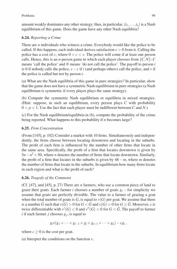
Problems 99
amount weakly dominates any other strategy: thus, in particular, (t1, . . . ,tn) is a Nashequilibrium of this game. Does the game have any other Nash equilibria?
6.24. Reporting a Crime
There are n individuals who witness a crime. Everybody would like the police to becalled. If this happens, each individual derives satisfaction v > 0 from it. Calling thepolice has a cost of c, where 0 < c < v. The police will come if at least one personcalls. Hence, this is an n-person game in which each player chooses from {C,N}: Cmeans ‘call the police’ and N means ‘do not call the police’. The payoff to person iis 0 if nobody calls the police, v− c if i (and perhaps others) call the police, and v ifthe police is called but not by person i.
(a) What are the Nash equilibria of this game in pure strategies? In particular, showthat the game does not have a symmetric Nash equilibrium in pure strategies (a Nashequilibrium is symmetric if every player plays the same strategy).
(b) Compute the symmetric Nash equilibrium or equilibria in mixed strategies.(Hint: suppose, in such an equilibrium, every person plays C with probability0 < p < 1. Use the fact that each player must be indifferent between C and N.)
(c) For the Nash equilibrium/equilibria in (b), compute the probability of the crimebeing reported. What happens to this probability if n becomes large?
6.25. Firm Concentration
(From [145], p. 102) Consider a market with 10 firms. Simultaneously and indepen-dently, the firms choose between locating downtown and locating in the suburbs.The profit of each firm is influenced by the number of other firms that locate inthe same area. Specifically, the profit of a firm that locates downtown is given by5n−n2 +50, where n denotes the number of firms that locate downtown. Similarly,the profit of a firm that locates in the suburbs is given by 48−m, where m denotesthe number of firms that locate in the suburbs. In equilibrium how many firms locatein each region and what is the profit of each?
6.26. Tragedy of the Commons
(Cf. [47], and [45], p. 27) There are n farmers, who use a common piece of land tograze their goats. Each farmer i chooses a number of goats gi – for simplicity weassume that goats are perfectly divisible. The value to a farmer of grazing a goatwhen the total number of goats is G, is equal to v(G) per goat. We assume that thereis a number G such that v(G) > 0 for G < G and v(G) = 0 for G ≥ G. Moreover, v istwice differentiable with v′(G) < 0 and v′′(G) < 0 for G < G. The payoff to farmeri if each farmer j chooses g j, is equal to
giv(g1 + · · ·+ gi−1 + gi + gi+1 + · · ·+ gn)− cgi ,
where c ≥ 0 is the cost per goat.
(a) Interpret the conditions on the function v.

100 6 Noncooperative Games: Extensions
(b) Show that the total number of goats in a Nash equilibrium (g∗1, . . . ,g∗n) of this
game, G∗ = g∗1 + · · ·+ g∗n, satisfies
v(G∗)+ (1/n)G∗v′(G∗)− c = 0.
(c) The socially optimal number of goats G∗∗ is obtained by maximizing Gv(G)−cGover G ≥ 0. Show that G∗∗ satisfies
v(G∗∗)+ G∗∗v′(G∗∗)− c = 0.
(d) Show that G∗ > G∗∗. (Hence, in a Nash equilibrium too many goats are grazed.)
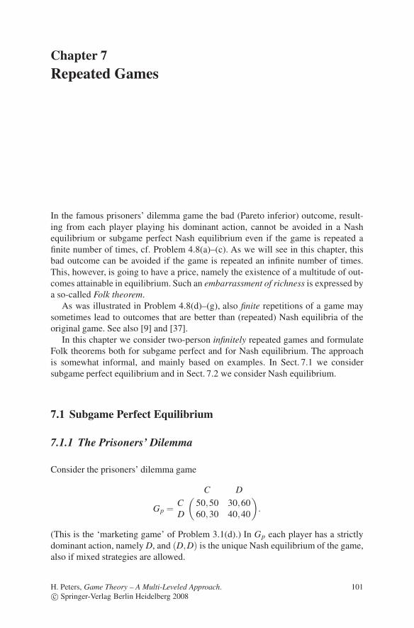
Chapter 7Repeated Games
In the famous prisoners’ dilemma game the bad (Pareto inferior) outcome, result-ing from each player playing his dominant action, cannot be avoided in a Nashequilibrium or subgame perfect Nash equilibrium even if the game is repeated afinite number of times, cf. Problem 4.8(a)–(c). As we will see in this chapter, thisbad outcome can be avoided if the game is repeated an infinite number of times.This, however, is going to have a price, namely the existence of a multitude of out-comes attainable in equilibrium. Such an embarrassment of richness is expressed bya so-called Folk theorem.
As was illustrated in Problem 4.8(d)–(g), also finite repetitions of a game maysometimes lead to outcomes that are better than (repeated) Nash equilibria of theoriginal game. See also [9] and [37].
In this chapter we consider two-person infinitely repeated games and formulateFolk theorems both for subgame perfect and for Nash equilibrium. The approachis somewhat informal, and mainly based on examples. In Sect. 7.1 we considersubgame perfect equilibrium and in Sect. 7.2 we consider Nash equilibrium.
7.1 Subgame Perfect Equilibrium
7.1.1 The Prisoners’ Dilemma
Consider the prisoners’ dilemma game
Gp =( C D
C 50,50 30,60D 60,30 40,40
).
(This is the ‘marketing game’ of Problem 3.1(d).) In Gp each player has a strictlydominant action, namely D, and (D,D) is the unique Nash equilibrium of the game,also if mixed strategies are allowed.
H. Peters, Game Theory – A Multi-Leveled Approach.c© Springer-Verlag Berlin Heidelberg 2008
101

102 7 Repeated Games
We assume now that Gp is played infinitely many times, at times t = 0,1,2, . . . ,and that after each play of Gp the players learn what has been played,1 i.e., theylearn which element of the set {(C,C), (C,D), (D,C), (D,D)} has occurred.2 Theserealizations induce an infinite stream of associated payoffs, and we assume that thereis a common discount factor 0 < δ < 1 such that the final payoff to each player isthe δ -discounted value of the infinite stream of payoffs. That is, player i (i = 1,2)obtains
∞
∑t=0
δ ti · (payoff from t-th play of the stage game),
where δi = δ for i = 1,2. Here, the expression stage game is used for the one-shotgame Gp in order to distinguish the one-shot game from the repeated game.
As always, a strategy of a player is a complete plan to play the game. Thismeans that, at each moment t, this plan should prescribe an action of a player –a mixed or pure strategy in Gp – for each possible history of the game up totime t, that is, an action for each sequence of length t of elements from the set{(C,C),(C,D),(D,C),(D,D)}. Clearly, such a strategy can be quite complicatedand the number of possible different strategies is enormous. We will be able,however, to restrict attention to quite simple strategies.
The infinite extensive form game just defined is denoted by G∞p (δ ). A natural
solution concept for this game is the concept of subgame perfect (Nash) equilibrium.Each subgame in G∞
p (δ ) is, basically, equal to the game G∞p (δ ) itself: the difference
between two subgames is the difference between the two histories leading to thosesubgames. For instance, at t = 6, there are 46 possible histories of play and thereforethere are 46 different subgames; each of these subgames, however, looks exactly likeG∞
p (δ ).
We will now exhibit a few subgame perfect equilibria of G∞p (δ ). First consider the
simple strategy:
D∞: play D at each moment t = 0,1,2, . . ., independent of the history of thegame.
First observe that D∞ is a well-defined strategy. If both players play D∞ then theresulting payoff is
∞
∑t=0
40 δ t = 40/(1− δ )
for each player. We claim that (D∞,D∞) is a subgame perfect equilibrium in G∞p (δ ).
Consider any t = 0,1, . . . and any subgame starting at time t. Then (D∞,D∞) inducesa Nash equilibrium in this subgame: given that player 2 always plays D, player 1cannot do better than always playing D as well, and vice versa. Hence, (D∞,D∞) is
1 In the marketing game, one can think of the game being played once per period – a week, month– each player observing in each period whether his opponent has advertised or not.2 Hence, a player does not learn the exact, possibly mixed, action of his opponent, but only itsrealization.

7.1 Subgame Perfect Equilibrium 103
a subgame perfect equilibrium. In this subgame perfect equilibrium, the players justplay the Nash equilibrium of the stage game at every time t.
We next exhibit another subgame perfect equilibrium. Consider the followingstrategy:
Tr(C): at t = 0 and at every time t such that in the past only (C,C) has occurredin the stage game: play C. Otherwise, play D.
Strategy Tr(C) is a so-called trigger strategy. A player playing this strategy startsplaying C and keeps on playing C as long as both players have only played C inthe past; after any deviation from this, however, this player plays D and keeps onplaying D forever. Again, Tr(C) is a well-defined strategy, and if both players playTr(C), then each player obtains the payoff
∞
∑t=0
50 δ t = 50/(1− δ ).
Is (Tr(C),Tr(C)) also a subgame perfect equilibrium? The answer is a qualifiedyes: if δ is large enough, then it is. The crux of the argument is as follows. At eachstage of the game, a player has an incentive to deviate from C and play his dominantaction D, thereby obtaining a momentary gain of 10. Deviating, however, triggerseternal ‘punishment’ by the other player, who is going to play D forever. The bestreply to this punishment is to play D as well, entailing an eternal loss of 10 from thenext moment on. So the discounted value of this loss is equal to 10δ/(1−δ ), and tokeep a player from deviating this loss should be at least as large as the momentarygain of 10. This is the case if and only if δ ≥ 1/2.
More formally, we can distinguish two kinds of subgames that are relevant forthe strategy combination (Tr(C),Tr(C)). One kind are those subgames where notalways (C,C) has been played in the past. In such a subgame, Tr(C) tells a playerto play D forever, and therefore the best reply of the other player is to do so aswell, i.e., to play according to Tr(C). So in this kind of subgame, (Tr(C),Tr(C))is a Nash equilibrium. In the other kind of subgame, no deviation has occurred sofar: in the past always (C,C) has been played. Consider this subgame at time T andsuppose that player 2 plays Tr(C). If player 1 plays Tr(C) as well, his payoff isequal to
T−1
∑t=0
50 δ t +∞
∑t=T
50 δ t .
If, instead, he deviates at time T to D, he obtains
T−1
∑t=0
50 δ t + 60 δ T +∞
∑t=T+1
40 δ t .

104 7 Repeated Games
Hence, to avoid deviation (and make Tr(C) player 1’s best reply in the subgame)we need that the first payoff is at least as high as the second one, resulting in theinequality
50 δ T /(1− δ )≥ 60 δ T + 40 δ T+1/(1− δ )
or, equivalently, δ ≥ 1/2 – as found before. We conclude that for every δ ≥ 1/2,(Tr(C),Tr(C)) is a subgame perfect equilibrium of the game G∞
p (δ ). The existenceof this equilibrium is a major reason to study infinitely repeated games. In popularterms, it shows that cooperation is sustainable if deviations can be credibly punished,which is the case if the future is sufficiently important (i.e., δ large enough).
To exhibit a subgame perfect equilibrium different from (D∞,D∞) and (Tr(C),Tr(C)), consider the following strategies:
Tr1: As long as the sequence (C,D), (D,C), (C,D), (D,C), (C,D), (D,C), . . .has occurred in the past from time 0 on, play C at t ∈ {0,2,4,6, . . .}; play Dat t ∈ {1,3,5,7, . . .}. Otherwise, play D.
Tr2: As long as the sequence (C,D), (D,C), (C,D), (D,C), (C,D), (D,C), . . .has occurred in the past from time 0 on, play D at t ∈ {0,2,4,6, . . .}; play Cat t ∈ {1,3,5,7, . . .}. Otherwise, play D.
Note that these are again ‘trigger strategies’: the players ‘tacitly’ agree on a certainsequence of play, but revert to playing D forever after a deviation. If player 1 playsTr1 and player 2 plays Tr2, then the sequence (C,D), (D,C), (C,D), (D,C), . . .,results. To see why (Tr1,Tr2) might be a subgame perfect equilibrium, note thaton average a player obtains 45 per stage, which is more than the 40 that would beobtained from deviating from this sequence and playing D forever. More precisely,suppose player 2 plays Tr2 and suppose player 1 considers a deviation from Tr1. Itis optimal to deviate at an even moment, say at t = 0. This yields a momentary gainof 10 and a discounted future loss of
20(δ 1 + δ 3 + δ 5 + · · ·)−10(δ 2 + δ 4 + δ 6 + · · ·).
To keep player 1 from deviating this loss should be at least as large as the gain of10, hence
20 δ1− δ 2 −
10 δ 2
1− δ 2 ≥ 10
which yields δ ≥ 1/2. We conclude (the formal argument is analogous to the onebefore) that for each δ ≥ 1/2, (Tr1,Tr2) is a subgame perfect equilibrium in G∞
p (δ ).
More generally, by playing appropriate sequences of elements from the set of possi-ble outcomes {(C,C),(C,D),(D,C),(D,D)} of the stage game Gp, the players canon average reach any convex combination of the associated payoffs in the long run.That is, take any such combination
α1(50,50)+ α2(30,60)+ α3(60,30)+ α4(40,40),

7.1 Subgame Perfect Equilibrium 105
(30,60)
(40,40)
(60,30)
(50,50)
Fig. 7.1 For every payoff pair in the shaded area there is a δ large enough such that this payoffpair can be obtained as the limiting (long run) average in a subgame perfect equilibrium of G∞
p (δ )
where αi ∈R, αi ≥ 0 for every i = 1, . . . ,4, and ∑4i=1 αi = 1. By choosing a sequence
of possible outcomes such that (C,C) occurs (in the long run) in a fraction α1 of thestages, (C,D) in a fraction α2, (D,C) in a fraction α3, and (D,D) in a fractionα4, then the above payoffs are reached as averages in the limit. As long as theselimiting average payoffs exceed 40 for each player, associated trigger strategies canbe formulated that lead to these payoffs and that trigger eternal play of (D,D) aftera deviation, similar to the strategies Tr(C), Tr1 and Tr2 above. For δ sufficientlyhigh, such strategies form again a subgame perfect equilibrium in G∞
p (δ ). Figure 7.1shows the payoffs that can be reached this way as limiting average payoffs in asubgame perfect equilibrium of G∞
p (δ ) for δ high enough.
7.1.2 Some General Observations
For the prisoners’ dilemma game we have established that each player playingalways D is a subgame perfect equilibrium of G∞
p (δ ) for every 0 < δ < 1. Thefollowing proposition follows from exactly the same simple logic.
Proposition 7.1. Let G be any arbitrary (not necessarily finite) n-person game, andlet the strategy combination s = (s1, . . . ,si, . . . ,sn) be a Nash equilibrium in G. Let0 < δ < 1. Then each player i playing si at every moment t is a subgame perfectequilibrium in G∞(δ ).3
3 We assume that G∞(δ ) is well-defined, in particular that the discounted payoff sums are finite.

106 7 Repeated Games
In particular, this proposition holds for any bimatrix game (see Definition 3.1) andany (at least any or pure) Nash equilibrium in this bimatrix game.
Let G = (A,B) be an m× n-bimatrix game. Let P(G) be the convex hull of the set{(ai j,bi j) ∈ R2 | i = 1, . . . ,m, j = 1, . . . ,n}. That is,
P(G) =
{m
∑i=1
n
∑j=1
αi j(ai j,bi j)⏐⏐⏐⏐ m
∑i=1
n
∑j=1
αi j = 1, ∀ i, j : αi j ≥ 0
}.
For the prisoners’ dilemma game Gp, P(Gp) is the quadrangle with (40,40),(30,60), (60,30), and (50,50) as vertices, see Fig. 7.1. The elements (payoff pairs)of P(G) can be obtained as limiting (long run) average payoffs in the infinitelyrepeated game G by an appropriate sequence of play.4 The following propositionsays that every payoff pair in P(G) that strictly dominates the payoffs associatedwith a Nash equilibrium of G can be obtained as limiting average payoffs in asubgame perfect equilibrium of G∞(δ ) for δ large enough. Such a proposition isknown as a Folk theorem.5 Its proof (omitted here) is somewhat technical but basi-cally consists of formulating trigger strategies in a similar way as for the prisoners’dilemma game above. In these strategies, after a deviation from the pattern leadingto the desired limiting average payoffs, players revert to the Nash equilibrium underconsideration of the stage game forever.6
Proposition 7.2 (Folk theorem for subgame perfect equilibrium). Let (p∗,q∗)be a Nash equilibrium of G, and let x = (x1,x2) ∈ P(G) such that x1 > p∗Aq∗ andx2 > p∗Bq∗. Then there is a 0 < δ ∗
x < 1 such that for every δ ≥ δ ∗x there is a subgame
perfect equilibrium in G∞(δ ) with limiting average payoffs x.7
7.2 Nash Equilibrium
In this section we consider the consequences of relaxing the subgame perfectionrequirement for a Nash equilibrium in an infinitely repeated game. When thinkingof trigger strategies as in Sect. 7.1, this means that deviations can be punished moreseverely, since the equilibrium does not have to induce a Nash equilibrium in the‘punishment subgame’.
4 P(G) is sometimes called the cooperative payoff space. Its elements are also attainable if theplayers could agree to pick payoff pairs randomly, i.e., to agree on some probability distribution –called correlated strategy – over the payoff pairs in the set {(ai j,bi j)}. See Sect. 13.7.5 This expression refers to the fact that results like this had been known among game theorists evenbefore they were formulated and written down explicitly. They belonged to the folklore of gametheory.6 For a stronger result see [38], where it is shown that Proposition 7.3 below also holds for subgameperfect Nash equilibrium if the dimension of the cooperative payoff space is equal to the number ofplayers. This, however, requires more sophisticated strategies. See also [39] for further references.7 Formally, if ξ0,ξ1,ξ2, . . . is a sequence of real numbers, then the limiting average is the numberlimT→∞
1T+1 ∑T
t=0 ξt , assuming that this limit exists.

7.2 Nash Equilibrium 107
For the infinitely repeated prisoners’ dilemma game this has no consequences.In the game G∞
p (δ ), each player can guarantee to obtain at least 40 at each stage,so that more severe punishments are not possible. In the following subsection weconsider a different example.
7.2.1 An Example
Consider the bimatrix game
G1 =( L R
U 1,1 0,0D 0,0 −1,4
).
The set P(G1) is the triangle with vertices (1,1), (0,0), and (−1,4). In the gameG1 the strategy U is a strictly dominant strategy for player 1. The unique Nashequilibrium is (U,L). Player 1 always playing U and player 2 always playing L isa subgame perfect equilibrium in G∞
1 (δ ) for every 0 < δ < 1, cf. Proposition 7.1.Proposition 7.2 does not add anything to this observation, since P(G1) does notcontain any payoff pair larger than (1,1) for each player.
Now consider the following strategies in the infinitely repeated game G∞1 (δ ):
N1: At t = 0 play D. After a history where (D,R) was played at t = 0,4,8,12, . . .and (U,L) at all other times: play D at t = 0,4,8,12, . . . and play U at all othertimes. After any other history play the mixed action ( 4
5 , 15 ), that is, play U with
probability 45 and D with probability 1
5 .N2: At t = 0 play R. After a history where (D,R) was played at t = 0,4,8,12, . . .
and (U,L) at all other times: play R at t = 0,4,8,12, . . . and play L at all othertimes. After any other history play R.
Note that these strategies are again trigger strategies. They induce a sequence ofplay in which within each four times, (D,R) is played once and (U,L) is playedthrice. After a deviation player 1 plays the mixed action ( 4
5 , 15 ) and player 2 the pure
action R forever. Thus, in a subgame following a deviation the players do not play aNash equilibrium: if player 2 plays R always, then player 1’s best reply is to play Ualways. Hence, (N1,N2) is not a subgame perfect equilibrium.
We claim, however, that (N1,N2) is a Nash equilibrium if δ is sufficiently large.First observe that player 2 can never gain from deviating since, if player 1 plays
N1, then N2 requires player 2 to play a best reply in the stage game at every momentt. Moreover, after any deviation player 1 plays ( 4
5 , 15) at any moment t, so that both
L and R have an expected payoff of 45 for player 2, which is less than 1 and less
than 4.Suppose player 2 plays N2. If player 1 wants to deviate from N1, the best moment
to do so is one where he is supposed to play D, so at t = 0,4, . . .. Without loss ofgenerality suppose player 1 deviates at t = 0. Then (U,R) results at t = 0, yieldingpayoff 0 to player 1. After that, player 2 plays R forever, and the best reply of

108 7 Repeated Games
player 1 to this is to play U forever, again yielding 0 each time. So his total payofffrom deviating is 0. Without deviation player 1’s total discounted payoff is equal to
−1(δ 0 + δ 4 + δ 8 + · · ·)+ 1(δ 1 + δ 2 + δ 3 + δ 5 + δ 6 + δ 7 + · · ·).
In order to keep player 1 from deviating this expression should be at least 0, i.e.
−11− δ 4 +
[1
1− δ− 1
1− δ 4
]≥ 0
which holds if and only if δ ≥ δ ∗ with δ ∗ ≈ 0.54.8 Hence, for these values ofδ , (N1,N2) is a Nash equilibrium in G∞
1 (δ ). The limiting average payoffs in thisequilibrium are equal to 3
4 (1,1)+ 14 (−1,4), hence to ( 1
2 , 74 ).
The actions played in this equilibrium after a deviation are, in fact, the actionsthat keep the opponent to his maximin payoff. To see this, first consider the actionof player 2, R. The payoff matrix of player 1 is the matrix A with
A =( L R
U 1 0D 0 −1
).
The value of the matrix game A, cf. Chap. 2, is equal to 0 – in fact, (U,R) is asaddlepoint of A – and, thus, player 1 can always obtain at least 0. By playing R,which is player 2’s optimal strategy in A, player 2 can hold player 1 down to 0.Hence, this is the most severe punishment that player 2 can inflict upon player 1after a deviation.
Similarly, if we view the payoff matrix B for player 2 as a zerosum game withpayoffs to player 2 and, following convention, convert this to a matrix game givingthe payoffs to player 1, we obtain
−B =( L R
U −1 0D 0 −4
).
In this game, ( 45 , 1
5 ) is an (the) optimal strategy for player 1, yielding the value ofthe game, which is equal to − 4
5 . Hence, player 2 can guarantee to obtain a payoffof 4
5 , but player 1 can make sure that player 2 does not obtain more than this byplaying ( 4
5 , 15 ). Again, this is the most severe punishment that player 1 can inflict
upon player 2 after a deviation.By using these punishments in a trigger strategy, the same logic as in Sect. 7.1
tells us that any pair of payoffs in P(G1) that strictly dominates the pair(v(A),−v(−B)) = (0, 4
5 ) can be obtained as limiting average payoffs in a Nashequilibrium of the game G∞
1 (δ ) for δ sufficiently large. This is illustrated in Fig. 7.2.
8 Found by solving a third degree equation.

Problems 109
(0,0)
(1,1)
(−1,4)
V
V = (0, 45 )
Fig. 7.2 For every payoff pair in the shaded area there is a δ large enough such that this payoffpair can be obtained as the limiting (long run) average in a Nash equilibrium of G∞
1 (δ )
7.2.2 A Folk Theorem for Nash Equilibrium
Let G = (A,B) be an arbitrary m× n bimatrix game. Let v(A) be the value of thematrix game A and let v(−B) be the value of the matrix game −B. As in Sect. 7.1 letP(G) be the cooperative payoff space. The following proposition generalizes whatwe found above for the game G1.
Proposition 7.3 (Folk theorem for Nash equilibrium). Let x = (x1,x2) ∈ P(G)such that x1 > v(A) and x2 > −v(−B). Then there is a 0 < δ ∗
x < 1 such that forevery δ ≥ δ ∗
x there is Nash equilibrium in G∞(δ ) with limiting average payoffs x.
Problems
7.1. On Discounting and Limiting Average
(a) In a repeated game, interpret the discount factor 0 < δ < 1 as the probabilitythat the game will continue, i.e., that the stage game will be played again. Showthat, with this interpretation, the repeated game will end with probability 1 (cf.Problem 6.16(e)).
(b) Can you give an example in which the limit that defines the long run averagepayoffs, does not exist? (cf. Footnote 7).
7.2. Nash and Subgame Perfect Equilibrium in a Repeated Game
Consider the following bimatrix game:
G = (A,B) =( L R
T 2,3 1,5B 0,1 0,1
).
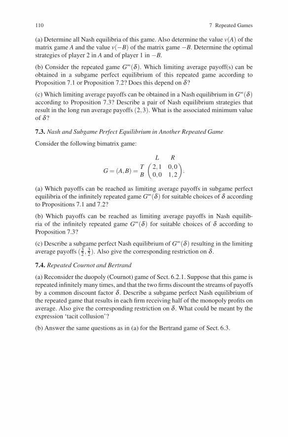
110 7 Repeated Games
(a) Determine all Nash equilibria of this game. Also determine the value v(A) of thematrix game A and the value v(−B) of the matrix game −B. Determine the optimalstrategies of player 2 in A and of player 1 in −B.
(b) Consider the repeated game G∞(δ ). Which limiting average payoff(s) can beobtained in a subgame perfect equilibrium of this repeated game according toProposition 7.1 or Proposition 7.2? Does this depend on δ?
(c) Which limiting average payoffs can be obtained in a Nash equilibrium in G∞(δ )according to Proposition 7.3? Describe a pair of Nash equilibrium strategies thatresult in the long run average payoffs (2,3). What is the associated minimum valueof δ?
7.3. Nash and Subgame Perfect Equilibrium in Another Repeated Game
Consider the following bimatrix game:
G = (A,B) =( L R
T 2,1 0,0B 0,0 1,2
).
(a) Which payoffs can be reached as limiting average payoffs in subgame perfectequilibria of the infinitely repeated game G∞(δ ) for suitable choices of δ accordingto Propositions 7.1 and 7.2?
(b) Which payoffs can be reached as limiting average payoffs in Nash equilib-ria of the infinitely repeated game G∞(δ ) for suitable choices of δ according toProposition 7.3?
(c) Describe a subgame perfect Nash equilibrium of G∞(δ ) resulting in the limitingaverage payoffs ( 3
2 , 32 ). Also give the corresponding restriction on δ .
7.4. Repeated Cournot and Bertrand
(a) Reconsider the duopoly (Cournot) game of Sect. 6.2.1. Suppose that this game isrepeated infinitely many times, and that the two firms discount the streams of payoffsby a common discount factor δ . Describe a subgame perfect Nash equilibrium ofthe repeated game that results in each firm receiving half of the monopoly profits onaverage. Also give the corresponding restriction on δ . What could be meant by theexpression ‘tacit collusion’?
(b) Answer the same questions as in (a) for the Bertrand game of Sect. 6.3.

Chapter 8An Introduction to Evolutionary Games
In an evolutionary game, players are interpreted as populations – of animals or indi-viduals. The probabilities in a mixed strategy of a player in a bimatrix game areinterpreted as shares of the population. Individuals within the same part of the pop-ulation play the same pure strategy. The main ‘solution’ concept is the concept ofan evolutionary stable strategy.
Evolutionary game theory originated in the work of the biologists Maynard Smithand Price [77]. Taylor and Jonker [133] and Selten [120], among others, played animportant role in applying the developed evolutionary biological concepts to bound-edly rational human behavior, and to establish the connection with dynamic systemsand with game-theoretic concepts like Nash equilibrium. A relatively recent andcomprehensive overview can be found in Weibull [147].
This chapter presents a short introduction to evolutionary game theory. For asomewhat more advanced continuation see Chap. 15.
In Sect. 8.1 we consider symmetric two-player games and evolutionary stablestrategies. Evolutionary stability is meant to capture the idea of mutation from thetheory of evolution. We also establish that an evolutionary stable strategy is part ofa symmetric Nash equilibrium. In Sect. 8.2 the connection with the so-called repli-cator dynamics is studied. Replicator dynamics intends to capture the evolutionaryidea of selection based on fitness. In Sect. 8.3 asymmetric games are considered.Specifically, a connection between replicator dynamics and strict Nash equilibriumis discussed.
8.1 Symmetric Two-Player Games and Evolutionary StableStrategies
A famous example from evolutionary game theory is the Hawk–Dove game:
(Hawk DoveHawk 0,0 3,1Dove 1,3 2,2
).
H. Peters, Game Theory – A Multi-Leveled Approach.c© Springer-Verlag Berlin Heidelberg 2008
111

112 8 An Introduction to Evolutionary Games
This game models the following situation. Individuals of the same large populationmeet randomly, in pairs, and behave either aggressively (Hawk) or passively (Dove)– the fight is about nest sites or territories, for instance. This behavior is geneti-cally determined, so an individual does not really choose between the two modesof behavior. The payoffs reflect (Darwninian) fitness, e.g., the number of offspring.In this context, players 1 and 2 are just two different members of the same popula-tion who meet: indeed, the game is symmetric – see below for the formal definition.A mixed strategy p = (p1, p2) (of player 1 or player 2) is naturally interpreted asexpressing the population shares of individuals characterized by the same type ofbehavior. In other words, p1 × 100% of the population are Hawks and p2 × 100%are Doves. In view of this interpretation, in what follows we are particularly inter-ested in symmetric Nash equilibria, i.e., Nash equilibria in which the players havethe same strategy. The Hawk–Dove game has three Nash equilibria, only one ofwhich is symmetric namely (( 1
2 , 12 ),( 1
2 , 12 )).1 The formal definitions of a symmetric
game and a symmetric Nash equilibrium are as follows.
Definition 8.1. Let G = (A,B) be an m× n-bimatrix game. Then G is symmetricif m = n and B = AT , where AT denotes the transpose of A.2 A Nash equilibrium(p∗,q∗) of G is symmetric if p∗ = q∗.
We state the following fact without a proof (see Chap. 15).
Proposition 8.2. Every symmetric bimatrix game G has a symmetric Nash equilib-rium.
With the interpretation above it is meaningful to consider symmetric Nash equilib-ria. In fact, we will require a little bit more.
Let G = (A,B) be a symmetric game. Knowing that the game is symmetric, it issufficient to give the payoff matrix A, since then B = AT . In what follows, when wetalk about a symmetric game A we mean the game G = (A, AT ). Let A be an m×m-matrix. Recall (cf. Chap. 2) that ∆m denotes the set of mixed strategies (for player 1or player 2). The following definition is due to Maynard Smith and Price [77].
Definition 8.3. A strategy x∈ ∆m is an evolutionary stable strategy (ESS) in A if forevery strategy y∈ ∆m, y = x, there exists some εy ∈ (0,1) such that for all ε ∈ (0,εy)we have
xA(εy+(1− ε)x) > yA(εy +(1− ε)x). (8.1)
The interpretation of an ESS x is as follows. Consider any small mutation εy+(1−ε)x of x. Condition (8.1) then says that against such a small mutation, the originalstrategy x is better than the mutant strategy y. In other words, if the population x
1 The Hawk–Dove game can also be interpreted as a Game of Chicken. Two car drivers approacheach other on a road, each one driving in the middle. The driver who is the first to return to hisown lane (Dove) ‘loses’ the game, the one who stays in the middle ‘wins’ (Hawk). With thisinterpretation also the asymmetric equilibria are of interest.2 Hence, bi j = a ji for all i, j = 1, . . .,m.
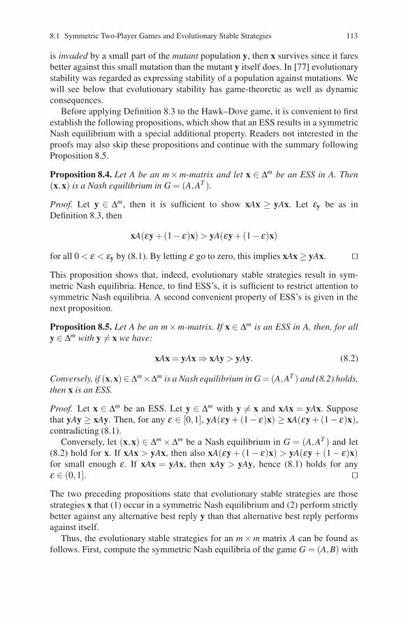
8.1 Symmetric Two-Player Games and Evolutionary Stable Strategies 113
is invaded by a small part of the mutant population y, then x survives since it faresbetter against this small mutation than the mutant y itself does. In [77] evolutionarystability was regarded as expressing stability of a population against mutations. Wewill see below that evolutionary stability has game-theoretic as well as dynamicconsequences.
Before applying Definition 8.3 to the Hawk–Dove game, it is convenient to firstestablish the following propositions, which show that an ESS results in a symmetricNash equilibrium with a special additional property. Readers not interested in theproofs may also skip these propositions and continue with the summary followingProposition 8.5.
Proposition 8.4. Let A be an m×m-matrix and let x ∈ ∆m be an ESS in A. Then(x,x) is a Nash equilibrium in G = (A,AT ).
Proof. Let y ∈ ∆m, then it is sufficient to show xAx ≥ yAx. Let εy be as inDefinition 8.3, then
xA(εy+(1− ε)x) > yA(εy+(1− ε)x)
for all 0 < ε < εy by (8.1). By letting ε go to zero, this implies xAx ≥ yAx. ��This proposition shows that, indeed, evolutionary stable strategies result in sym-metric Nash equilibria. Hence, to find ESS’s, it is sufficient to restrict attention tosymmetric Nash equilibria. A second convenient property of ESS’s is given in thenext proposition.
Proposition 8.5. Let A be an m×m-matrix. If x ∈ ∆m is an ESS in A, then, for ally ∈ ∆m with y = x we have:
xAx = yAx ⇒ xAy > yAy. (8.2)
Conversely, if (x,x)∈∆m×∆m is a Nash equilibrium in G = (A,AT ) and (8.2) holds,then x is an ESS.
Proof. Let x ∈ ∆m be an ESS. Let y ∈ ∆m with y = x and xAx = yAx. Supposethat yAy ≥ xAy. Then, for any ε ∈ [0,1], yA(εy +(1− ε)x) ≥ xA(εy +(1− ε)x),contradicting (8.1).
Conversely, let (x,x) ∈ ∆m ×∆m be a Nash equilibrium in G = (A,AT ) and let(8.2) hold for x. If xAx > yAx, then also xA(εy +(1− ε)x) > yA(εy + (1− ε)x)for small enough ε . If xAx = yAx, then xAy > yAy, hence (8.1) holds for anyε ∈ (0,1]. ��The two preceding propositions state that evolutionary stable strategies are thosestrategies x that (1) occur in a symmetric Nash equilibrium and (2) perform strictlybetter against any alternative best reply y than that alternative best reply performsagainst itself.
Thus, the evolutionary stable strategies for an m×m matrix A can be found asfollows. First, compute the symmetric Nash equilibria of the game G = (A,B) with

114 8 An Introduction to Evolutionary Games
B = AT . This can be done using the methods developed in Chap. 3. Second, foreach such equilibrium (x,x), check whether (8.2) holds. If it does, then x is anevolutionary stable strategy.
We apply this method to the Hawk–Dove game. For this game,
A =(Hawk Dove
Hawk 0 3Dove 1 2
).
The unique symmetric equilibrium strategy was x = ( 12 , 1
2). Let y = (y,1− y) be anarbitrary strategy, then the condition xAx = yAx in (8.2) is always satisfied. This canbe seen by direct computation but it also follows from the fact that (x,x) is a Nashequilibrium (how?). Hence, we have to check if
xAy > yAy
for all y = (y,1− y) = x. This inequality reduces (check!) to
4y2 −4y + 1 > 0,
which is true for all y = 12 . Thus, x = ( 1
2 , 12) is the unique ESS in A.
8.2 Replicator Dynamics and Evolutionary Stability
Central in the theory of evolution are the concepts of mutation and selection. Whilethe idea of mutation is meant to be captured by the concept of evolutionary sta-bility, the idea of selection is captured by the so-called replicator dynamics. Weillustrate the concept of replicator dynamics, introduced in [133], by consideringagain the Hawk–Dove game
(Hawk DoveHawk 0,0 3,1Dove 1,3 2,2
).
Consider a mixed strategy or, in the present context, vector of population sharesx = (x,1− x). Consider an arbitrary individual of the population. Playing ‘Hawk’against the population x yields an expected payoff or ‘fitness’ of
0 · x + 3 · (1− x)= 3(1− x)
and playing ‘Dove’ yields
1 · x + 2 · (1− x)= 2− x.

8.2 Replicator Dynamics and Evolutionary Stability 115
Hence, the average fitness of the population is
x ·3(1− x)+ (1− x) · (2− x)= 2−2x2.
We now assume that the population shares develop over time, i.e., that x is afunction of time t, and that the change in x, described by the time derivativex = x(t) = dx(t)/dt, is proportional to the difference with the average fitness. Thatis, we assume that x is given by the following equation
x(t) = dx(t)/dt = x(t)[3(1− x(t))− (2−2x(t)2)
]. (8.3)
Equation (8.3) is the replicator dynamics for the Hawk–Dove game. The equationsays that the population of Hawks changes continuously (described by dx(t)/dt),and that this change is proportional to the difference of the fitness at time t (whichis equal to 3(1− x(t))) with the average fitness of the population (which is equal to2−2x(t)2). Simplifying (8.3) and writing x instead of x(t) yields
x = dx/dt = x(x− 1)(2x−1).
This makes it possible to make a diagram of dx/dt as a function of x (a so-calledphase diagram). See Fig. 8.1. We see that this replicator dynamics has three differentroots, the so-called rest points3 x = 0, x = 1
2 , and x = 1. For these values of x, thederivative dx/dt is equal to zero, so the population shares do not change: the systemis at rest. In case x = 0 all members of the species are Doves, their fitness is equal tothe average fitness, and so nothing changes. This rest point, however, is not stable. Aslight disturbance, e.g., a genetic mutation resulting in a Hawk, makes the numberof Hawks increase because dx/dt becomes positive: see Fig. 8.1. This increase willgo on until the rest point x = 1
2 is reached. A similar story holds for the rest pointx = 1, where the population consists of only Hawks. Now suppose the system is atthe rest point x = 1
2 . Note that, after a disturbance in either direction, the system willmove back again to the state where half the population consists of Doves. Thus, ofthe three rest points, only x = 1
2 is stable.
0 x
x
12
> > < <1
Fig. 8.1 Replicator dynamics for the Hawk–Dove game
3 Also called equilibrium points, critical points, stationary points.

116 8 An Introduction to Evolutionary Games
Recall from the previous section that x = ( 12 , 1
2 ) is also the unique evolutionarystable strategy of the Hawk–Dove game. That this is no coincidence follows fromthe next proposition, which we state here without a proof (see Chap. 15 for a proof).
Proposition 8.6. Let A be a 2×2-matrix. Then:
(1) A has at least one evolutionary stable strategy.(2) x = (x,1− x) is an evolutionary stable strategy of A, if and only if x is a stable
rest point of the replicator dynamics.
For general m×m-matrices the set of completely mixed4 rest points of the replicatordynamics coincides with the set of completely mixed (symmetric) Nash equilibriumstrategies. There are also connections between stability of rest points and furtherproperties of Nash equilibria. See Chap. 15 for more details.
8.3 Asymmetric Games
The evolutionary approach to game theory is not necessarily restricted to sym-metric situations, i.e., bimatrix games of the form (A, AT ) in which the row andcolumn players play identical strategies. In biology as well as economics one canfind many examples of asymmetric situations. Think of two different species com-peting about territory in biology. As to economics, see for instance [42], Chap. 8 forsome applications. The following example is also taken from [42]. Here only theformal analysis is discussed.
Consider the 2×2-bimatrix game
(A,B) =( L R
T 0,0 2,2B 1,5 1,5
).
Think of two populations, the row population and the column population. In eachpopulation there are two different types: T and B in the row population and L andR in the column population. Individuals of one population are continuously andrandomly matched with individuals of the other population, and we are interestedagain in the development of the population shares. To start with, assume the sharesof T and B types in the row population are x and 1− x, respectively, and the sharesof L and R types in the column population are y and 1− y. The expected payoff of aT type individual is given by
0 · y + 2 · (1− y)= 2−2y.
For a B type individual it is
1 · y + 1 · (1− y)= 1.
4 I.e., all coordinates positive.

8.3 Asymmetric Games 117
For an L type individual it is
0 · x + 5 · (1− x)= 5−5x.
And for an R type individual:
2 · x + 5 · (1− x)= 5−3x.
The average of the row types is therefore:
x[2(1− y)]+ 1 · (1− x)
and the replicator dynamics for the population share x(t) of T individuals is givenby
dx/dt = x[2(1− y)− x[2(1− y)]− (1− x)]= x(1− x)(1−2y). (8.4)
Here, we write x and y instead of x(t) and y(t). Similarly one can calculate thereplicator dynamics for the column population (check this result!):
dy/dt = y(1− y)(−2x). (8.5)
We are interested in the rest points of the dynamical system described by (8.4) and(8.5), and, in particular, by the stable rest points. The easiest way is to make adiagram of the possible values of x and y, see Fig. 8.2. In this diagram, the blacklines are the values of x and y for which the derivative in (8.4) is equal to 0, i.e., forwhich the row population is at rest. The light gray lines are the values of x and y forwhich the derivative in (8.5) is equal to 0: there, the column population is at rest.The points of intersection are the points where the whole system is at rest; this is theset
{(0,y) | 0 ≤ y ≤ 1}∪{(1,0)}∪{(1,1)}. (8.6)
In Fig. 8.2, arrows indicate the direction in which x and y move. For instance, if1 > y ≥ 1
2 and 0 < x < 1 we have dx/dt < 0 and dy/dt < 0, so that in that region
Fig. 8.2 Phase diagram ofthe asymmetric evolutionarygame 0 1
1
x
y = 12
> >
< <
↓→
↓←
∨
∨

118 8 An Introduction to Evolutionary Games
x as well as y decrease. A stable rest point is a rest point such that, if the systemis slightly disturbed and changes to some point close to the rest point in question,then it should move back again to this rest point. In terms of the arrows in Fig. 8.2this means that a stable rest point is one where all arrows in the neighborhood pointtowards that point. It is obvious that in our example the point (1,0) is the only suchpoint. So the situation where the row population consists only of T type individuals(x = 1) and the column population consists only of R type individuals (y = 0) is theonly stable situation with respect to the replicator dynamics.
Is there a relation with Nash equilibrium? One can check (!) that the set of Nashequilibria in this example is the set:
{(T,R),(B,L)}∪{(B,(q,1−q)) | 12≤ q ≤ 1}.
So the stable rest point (T,R) is a Nash equilibrium. Furthermore, it has a specialcharacteristic, namely, it is the only strict Nash equilibrium of the game. A strictNash equilibrium in a game is a Nash equilibrium where each player not only doesnot gain but in fact strictly loses by deviating. For instance, if the row player deviatesfrom T in the Nash equilibrium (T,R) then he obtains strictly less than 2. All theother equilibria in this game do not have this property. For instance, if the columnplayer deviates from L to R in the Nash equilibrium (B,L), then he still obtains 5.
The observation that the stable rest point of the replicator dynamics coincideswith a strict Nash equilibrium is not a coincidence. The following proposition isstated without a proof (see [119] or [57]).
Proposition 8.7. In a 2×2 bimatrix game a pair of strategies is a stable rest pointof the replicator dynamics if, and only if, it is a strict Nash equilibrium. For largergames, any stable rest point of the replicator dynamics is a strict Nash equilibrium,but the converse does not necessarily hold.
In the literature the concept of evolutionary stable strategy is extended to asymmet-ric games. See the cited references for details.
Problems
8.1. Symmetric Games
Compute the evolutionary stable strategies for the following payoff matrices A.
(a) A =(
4 05 3
)(Prisoners’ Dilemma)
(b) A =(
2 00 1
)(Coordination game)

Problems 119
8.2. More Symmetric Games
For each of the following two matrices, determine the replicator dynamics, restpoints and stable rest points, and evolutionary stable strategies. Include phase dia-grams for the replicator dynamics. For the evolutionary stable strategies, provideindependent arguments to show evolutionary stability by using Propositions 8.4 and8.5; that is, without using the replicator dynamics.
A =(
0 11 0
), B =
(2 01 0
).
8.3. Asymmetric Games
For each of the following two asymmetric situations, determine the replicatordynamics, rest points and stable rest points, including phase diagrams. Also deter-mine all Nash and strict Nash equilibria.
(A,AT ) =(
0,0 1,11,1 0,0
), (B,BT ) =
(2,2 0,11,0 0,0
).
8.4. Frogs Call for Mates ([42], p. 215)
Consider the following game played by male frogs who Call or Don’t Call theirmates.
( Call Don’t CallCall P− z,P− z m− z,1−mDon’t Call 1−m,m− z 0,0
)The payoffs are in units of ‘fitness’, measured by the frog’s offspring. Here z denotesthe cost of Calling (danger of becoming prey, danger of running out of energy); andm is the probability that the male who calls in a pair of males, the other of whomis not calling, gets a mate. Typically, m ≥ 1
2 . Next, if no male calls then no femaleis attracted, and if both call returns diminish and they each attract P females with0 < P < 1.
(a) Show that there are several possible evolutionary stable strategies for this game,depending on the parameters (m,z,P).
(b) Set m = 0.6 and P = 0.8 . Find values for z for each of the following situations:(1) Don’t Call is an evolutionary stable strategy (ESS); (2) Call is an ESS; (3) Amixture of Call and Don’t Call is an ESS.

120 8 An Introduction to Evolutionary Games
(c) Suppose there are two kinds of frogs in Frogs call for mates. Large frogs havea larger cost of calling (z1) than do small frogs (z2). Determine the correspond-ing asymmetric bimatrix game. Determine the possible stable rest points of thereplicator dynamics.
8.5. Video Market Game ([42], pp. 229, 233).
Two boundedly rational video companies are playing the following asymmetricgame:
(Open system Lockout systemOpen system 6,4 5,5Lockout system 9,1 10,0
)Company I (the row company) has to decide whether to have an open system or alockout system. Company II (the column company) has to decide whether to createits own system or copy that of company I. What is a rest point of the replicatordynamics for this system?
Chapter 9Cooperative Games with Transferable Utility
The implicit assumption in a cooperative game is that players can form coalitionsand make binding agreements on how to distribute the proceeds of these coalitions.A cooperative game is more abstract than a noncooperative game in the sense thatstrategies are not explicitly modelled: rather, the game describes what each possiblecoalition can earn by cooperation. In a cooperative game with transferable utilityit is assumed that the earnings of a coalition can be expressed by one number. Onemay think of this number as an amount of money, which can be distributed amongthe players in any conceivable way – including negative payments – if the coalitionis actually formed. More generally, it is an amount of utility and the implicit assump-tion is that it makes sense to transfer this utility among the players – for instance,due to the presence of a medium like money, assuming that individual utilities canbe expressed in monetary terms.
This chapter presents a first acquaintance with the theory of cooperative gameswith transferable utility.1 A few important solution concepts – the core, the Shap-ley value, and the nucleolus – are briefly discussed in Sects. 9.2–9.4. We start withexamples and preliminaries in Sect. 9.1.
9.1 Examples and Preliminaries
In Chap. 1 we have seen several examples of cooperative games with transferableutilities: the three cities game, a glove game, a permutation game, and a votinggame. For the stories giving rise to these games the reader is referred to Sect. 1.3.4.Here we reconsider the resulting games.
In the three cities game, cooperation between cities leads to cost savingsexpressed in amounts of money, as in Table 9.1. In the first line of this table allpossible coalitions are listed. It important to note that the term ‘coalition’ is usedfor any subset of the set of players. So a coalition is not necessarily formed. The
1 See Chaps. 16–20 for a more advanced treatment.
H. Peters, Game Theory – A Multi-Leveled Approach.c© Springer-Verlag Berlin Heidelberg 2008
121

122 9 Cooperative Games with Transferable Utility
Table 9.1 The three cities game
S /0 {1} {2} {3} {1,2} {1,3} {2,3} {1,2,3}v(S) 0 0 0 0 90 100 120 220
Table 9.2 A glove game
S /0 {1} {2} {3} {1,2} {1,3} {2,3} {1,2,3}v(S) 0 0 0 0 0 1 1 1
Table 9.3 A permutation game
S /0 {1} {2} {3} {1,2} {1,3} {2,3} {1,2,3}v(S) 0 2 5 4 14 18 9 24
empty subset (empty coalition) has been added for convenience: it just is assignedthe number 0 by convention. The numbers in the second line of the table are calledthe ‘worths’ of the coalitions. For instance, coalition S = {1,2} has worth 90. Inthis particular example, 90 is the amount of cost savings earned by cities 1 and 2 ifthey cooperate. It is assumed that this amount can be split between the two players(cities) if the coalition is actually formed. That is, player 1 may receive x1 ∈ R andplayer 2 may receive x2 ∈ R such that x1 +x2 = 90 or, more generally, x1 +x2 ≤ 90.
In the glove game in Sect. 1.3.4 coalitions may make pairs of gloves. The gameis described in Table 9.2. In this game the worth 1 of the ‘grand coalition’ {1,2,3},for instance, means that this coalition can earn 1 by producing one pair of gloves.One can think of this number as expressing the monetary value of this pair of gloves.Alternatively, one can think of one pair of gloves having ‘utility’ equal to 1. Again,it is assumed that the players can split up this amount in any way they like. Soa possible distribution takes the form (x1,x2,x2) ∈ R3 such that x1 + x2 + x3 ≤ 1.For i = 1,2,3, the number xi may represent the money that player i receives, or (ifnonnegative) the percentage of time that player i is allowed to wear the gloves.
The permutation game (dentist game) of Sect. 1.3.4 is reproduced in Table 9.3.In this game, one could think of the worth of a coalition as expressing, for instance,savings of opportunity costs by having dentist appointments on certain days. Whatis important is that, again, these worths can be distributed in any way among theplayers of the coalitions.
For the voting game related to the UN Security Council, a table could be con-structed as well, but this table would be huge: there are 215 = 32,768 possiblecoalitions (cf. Problem 9.1). Therefore, it is more convenient to describe this gameas follows. Let the permanent members be the players 1, . . . ,5 and let the othermembers be the players 6, . . . ,15. Denote by N = {1,2, . . . ,15} the grand coalitionof all players and by v(S) the worth of a coalition S ⊆ N. Then
v(S) :={
1 if {1, . . . ,5} ⊆ S and |S| ≥ 9,0 otherwise,

9.2 The Core 123
where |S| denotes the number of players in S. In this case the number 1 indicatesthat the coalition is ‘winning’ and the number 0 that the coalition is ‘losing’. In ana-lyzing games like this the resulting numbers – e.g., nonnegative numbers x1, . . . ,x15summing to 1 – are usually interpreted as power indices, expressing the power of aplayer in some way or another.
We summarize the concepts introduced informally in the preceding examples for-mally within the following definition.
Definition 9.1. A cooperative game with transferable utility or TU-game is a pair(N,v), where N = {1,2, . . . ,n} with n ∈ N is the set of players, and v is a functionassigning to each coalition S, i.e., to each subset S ⊆ N a real number v(S), such thatv( /0) = 0. The function v is called the characteristic function and v(S) is called theworth of S. The coalition N is called the grand coalition. A payoff distribution forcoalition S is a vector of real numbers (xi)i∈S.
When analyzing a TU-game there are two important questions to answer: whichcoalitions are formed; and how are the worths of these coalitions distributed amongtheir members? In this chapter we assume that the grand coalition is formed and weconcentrate on the second question. This is less restrictive than it might seem at firstsight, since coalition formation depends, naturally, on how the proceeds of a coali-tion are going to be distributed among its members. Thus, also if smaller coalitionsare formed the distribution question has to be considered for these coalitions.
9.2 The Core
Consider the three cities game in Table 9.1, suppose that the grand coalition getstogether, and suppose that there is a proposal x1 = 40, x2 = 40, and x3 = 140 fordistribution of the savings v(N) = 220 on the bargaining table. One can imagine, forinstance, that player 3 made such a proposal. In that case, players 1 and 2 couldprotest successfully, since they can save v({1,2}) = 90 > 80 = x1 + x2 withoutplayer 3. We express this by saying that x = (x1,x2,x3) is not in the ‘core’ of thisgame. More generally, the core of the three cities game is the set of payoff distribu-tions for N = {1,2,3} such that the sum of the payoffs is equal to v(N) = 220 andeach nonempty coalition S obtains at least its own worth. Formally, it is the set
C = {(x1,x2,x3) ∈ R3 | x1,x2,x3 ≥ 0x1 + x2 ≥ 90, x1 + x3 ≥ 100, x2 + x3 ≥ 120x1 + x2 + x3 = 220} .
To obtain a better idea of how this set looks like, we can make a diagram. AlthoughC is a subset of R3, the constraint x1 + x2 + x3 = 220 makes that the C is containedin a two-dimensional subset of R3, i.e., the plane through the points (220,0,0),(0,220,0), and (0,0,220). The triangle formed by these three points is represented

124 9 Cooperative Games with Transferable Utility
(220,0,0)
(0,0,220)
(0,220,0)
(0,90,130)
(0,120,100)
(100,120,0)
(90,0,130)(100,0,120)
a
c b
Fig. 9.1 The set C – the core – of the three cities game. The line segment a corresponds to theconstraint x1 +x2 ≥ 90, the line segment b corresponds to the constraint x1 +x3 ≥ 100, and the linesegment c corresponds to the constraint x2 + x3 ≥ 120
in Fig. 9.1. Note that C is a subset of this triangle by the constraints xi ≥ 0 for everyi = 1,2,3, derived from the conditions xi ≥ v({i}) for i = 1,2,3. The set C is theshaded area bounded by the three constraints for the two-person coalitions.Hence, the core of the three cities game is the polygon with vertices (100,120,0),(0,120,100), (0,90,130), (90,0,130), and (100,0,120).
We now give the formal definition of the core and of some other related concepts.It will be convenient to use the notation x(S) := ∑i∈S xi for a payoff distributionx = (x1, . . . ,xn) ∈ Rn and a nonempty coalition S ⊆ N = {1, . . . ,n}.
Definition 9.2. For a TU-game (N,v), a payoff distribution x = (x1, . . . ,xn) ∈ Rn is
• Efficient if x(N) = v(N)• Individually rational if xi ≥ v({i}) for all i ∈ N• Coalitionally rational if x(S) ≥ v(S) for all nonempty coalitions S
The core of (N,v) is the set
C(N,v) = {x ∈ Rn | x(N) = v(N) and x(S) ≥ v(S) for all /0 = S ⊆ N} .
So the core of (N,v) is the set of all efficient and coalitionally rational payoffdistributions.
The core of a game can be a large set, like in the three cities game; a ‘small’ set, likein the glove game (see Problem 9.2); or it can be empty (see again Problem 9.2).Games with nonempty cores were characterized in [16] and [122]: see Chap. 16.In general, core elements can be computed by linear programming techniques. Forgames with two or three players the core can be computed graphically, as we didfor the three cities game. Sometimes, the core can be computed by using the specialstructure of a specific game under consideration.

9.3 The Shapley Value 125
9.3 The Shapley Value
The Shapley value [121] is a solution concept for TU-games that is quite differentfrom the core. Whereas the core is a (possibly empty) set, the Shapley value assignsa unique payoff distribution for the grand coalition to every TU-game. The Shapleyvalue is not so much based on strategic considerations but, rather, assigns to eachplayer his ‘average marginal contribution’ in the game.
Consider again the three cities game2 of Table 9.1. Imagine a setting wherethe players enter a bargaining room one by one, and upon entering each playerdemands and obtains his marginal contribution. Suppose that player 1 enters first,player 2 enters next, and player 3 enters last. Player 1 enters an empty room andcan take his ‘marginal contribution’ v({1})− v( /0) = 0 − 0 = 0. When player 2enters, player 1 is already present, and player 2 obtains his marginal contribu-tion v({1,2})− v({1}) = 90 − 0 = 90. When, finally, player 3 enters, then thecoalition {1,2} is already present. So player 3 obtains his marginal contributionv({1,2,3})− v({1,2})= 220− 90 = 130. Hence, this procedure results in the pay-off distribution (0,90,130), which is called a marginal vector. Of course, this payoffdistribution does not seem quite fair since it depends on the order in which theplayers enter the room, and this order is quite arbitrary: there are five other pos-sible orders. The Shapley value takes the marginal vectors of all six orders intoconsideration, and assigns to a TU-game their average. See Table 9.4.
For an arbitrary TU-game (N,v) with player set N = {1, . . . ,n} the Shapley valuecan be computed in the same way, by first computing the marginal vectors corre-sponding to the n! different orders of the players, and then taking the average – thatis, summing all marginal vectors and dividing the result by n! . If the number ofplayers is large, then this is a huge task. In the UN security council voting game ofSect. 9.1, for instance, this would mean computing 15! > 13×1011 marginal vectors.Fortunately, there is a more clever way to compute the total marginal contributionof a player.
Table 9.4 Computation of the Shapley value for the three cities game. The Shapley value isobtained by dividing the totals of the marginal contributions by 6
Order of entry 1 2 3
1,2,3 0 90 1301,3,2 0 120 1002,1,3 90 0 1302,3,1 100 0 1203,1,2 100 120 03,2,1 100 120 0
Total 390 450 480Shapley value 65 75 80
2 Cf. Bird [14].
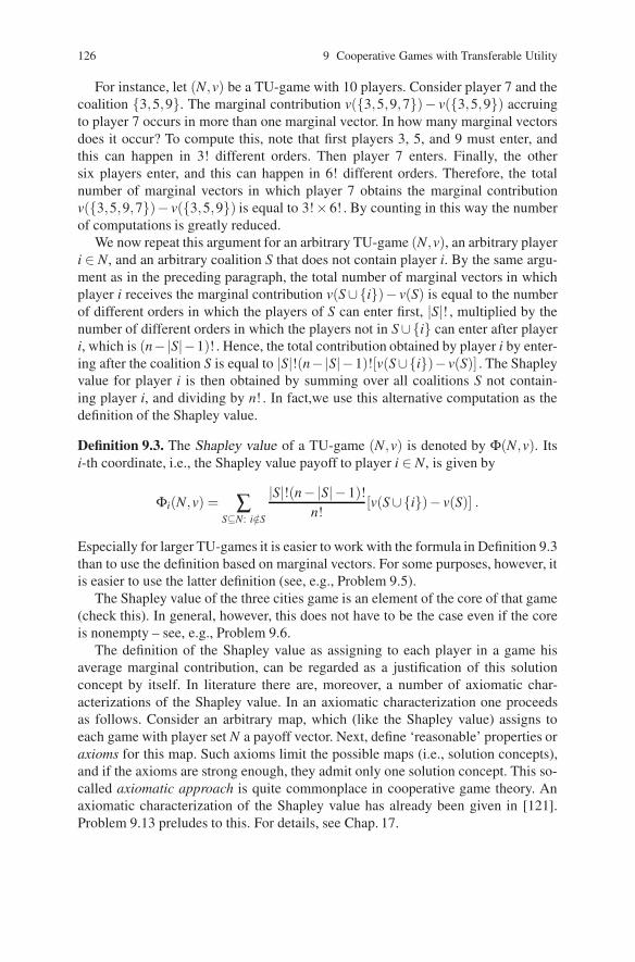
126 9 Cooperative Games with Transferable Utility
For instance, let (N,v) be a TU-game with 10 players. Consider player 7 and thecoalition {3,5,9}. The marginal contribution v({3,5,9,7})− v({3,5,9}) accruingto player 7 occurs in more than one marginal vector. In how many marginal vectorsdoes it occur? To compute this, note that first players 3, 5, and 9 must enter, andthis can happen in 3! different orders. Then player 7 enters. Finally, the othersix players enter, and this can happen in 6! different orders. Therefore, the totalnumber of marginal vectors in which player 7 obtains the marginal contributionv({3,5,9,7})− v({3,5,9}) is equal to 3!×6! . By counting in this way the numberof computations is greatly reduced.
We now repeat this argument for an arbitrary TU-game (N,v), an arbitrary playeri ∈ N, and an arbitrary coalition S that does not contain player i. By the same argu-ment as in the preceding paragraph, the total number of marginal vectors in whichplayer i receives the marginal contribution v(S∪{i})− v(S) is equal to the numberof different orders in which the players of S can enter first, |S|! , multiplied by thenumber of different orders in which the players not in S∪{i} can enter after playeri, which is (n−|S|−1)! . Hence, the total contribution obtained by player i by enter-ing after the coalition S is equal to |S|!(n−|S|−1)![v(S∪{i})−v(S)] . The Shapleyvalue for player i is then obtained by summing over all coalitions S not contain-ing player i, and dividing by n! . In fact,we use this alternative computation as thedefinition of the Shapley value.
Definition 9.3. The Shapley value of a TU-game (N,v) is denoted by Φ(N,v). Itsi-th coordinate, i.e., the Shapley value payoff to player i ∈ N, is given by
Φi(N,v) = ∑S⊆N: i/∈S
|S|!(n−|S|−1)!n!
[v(S∪{i})− v(S)] .
Especially for larger TU-games it is easier to work with the formula in Definition 9.3than to use the definition based on marginal vectors. For some purposes, however, itis easier to use the latter definition (see, e.g., Problem 9.5).
The Shapley value of the three cities game is an element of the core of that game(check this). In general, however, this does not have to be the case even if the coreis nonempty – see, e.g., Problem 9.6.
The definition of the Shapley value as assigning to each player in a game hisaverage marginal contribution, can be regarded as a justification of this solutionconcept by itself. In literature there are, moreover, a number of axiomatic char-acterizations of the Shapley value. In an axiomatic characterization one proceedsas follows. Consider an arbitrary map, which (like the Shapley value) assigns toeach game with player set N a payoff vector. Next, define ‘reasonable’ properties oraxioms for this map. Such axioms limit the possible maps (i.e., solution concepts),and if the axioms are strong enough, they admit only one solution concept. This so-called axiomatic approach is quite commonplace in cooperative game theory. Anaxiomatic characterization of the Shapley value has already been given in [121].Problem 9.13 preludes to this. For details, see Chap. 17.
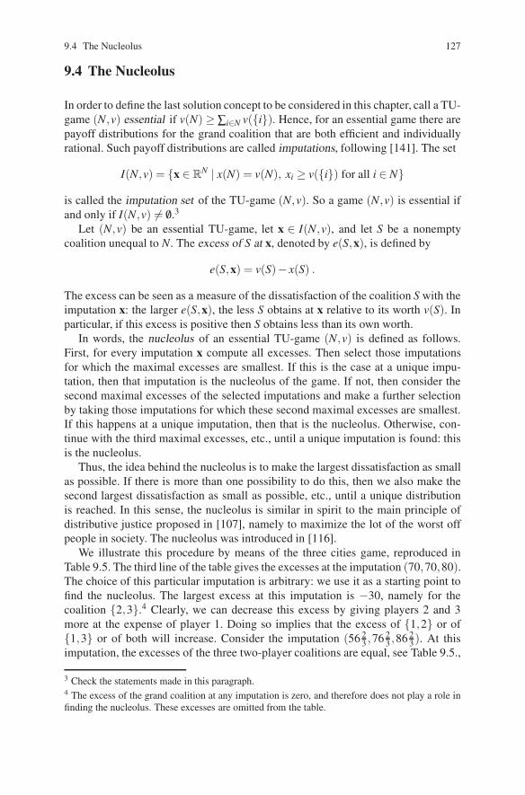
9.4 The Nucleolus 127
9.4 The Nucleolus
In order to define the last solution concept to be considered in this chapter, call a TU-game (N,v) essential if v(N) ≥ ∑i∈N v({i}). Hence, for an essential game there arepayoff distributions for the grand coalition that are both efficient and individuallyrational. Such payoff distributions are called imputations, following [141]. The set
I(N,v) = {x ∈ RN | x(N) = v(N), xi ≥ v({i}) for all i ∈ N}
is called the imputation set of the TU-game (N,v). So a game (N,v) is essential ifand only if I(N,v) = /0.3
Let (N,v) be an essential TU-game, let x ∈ I(N,v), and let S be a nonemptycoalition unequal to N. The excess of S at x, denoted by e(S,x), is defined by
e(S,x) = v(S)− x(S) .
The excess can be seen as a measure of the dissatisfaction of the coalition S with theimputation x: the larger e(S,x), the less S obtains at x relative to its worth v(S). Inparticular, if this excess is positive then S obtains less than its own worth.
In words, the nucleolus of an essential TU-game (N,v) is defined as follows.First, for every imputation x compute all excesses. Then select those imputationsfor which the maximal excesses are smallest. If this is the case at a unique impu-tation, then that imputation is the nucleolus of the game. If not, then consider thesecond maximal excesses of the selected imputations and make a further selectionby taking those imputations for which these second maximal excesses are smallest.If this happens at a unique imputation, then that is the nucleolus. Otherwise, con-tinue with the third maximal excesses, etc., until a unique imputation is found: thisis the nucleolus.
Thus, the idea behind the nucleolus is to make the largest dissatisfaction as smallas possible. If there is more than one possibility to do this, then we also make thesecond largest dissatisfaction as small as possible, etc., until a unique distributionis reached. In this sense, the nucleolus is similar in spirit to the main principle ofdistributive justice proposed in [107], namely to maximize the lot of the worst offpeople in society. The nucleolus was introduced in [116].
We illustrate this procedure by means of the three cities game, reproduced inTable 9.5. The third line of the table gives the excesses at the imputation (70,70,80).The choice of this particular imputation is arbitrary: we use it as a starting point tofind the nucleolus. The largest excess at this imputation is −30, namely for thecoalition {2,3}.4 Clearly, we can decrease this excess by giving players 2 and 3more at the expense of player 1. Doing so implies that the excess of {1,2} or of{1,3} or of both will increase. Consider the imputation (56 2
3 ,76 23 ,86 2
3). At thisimputation, the excesses of the three two-player coalitions are equal, see Table 9.5.,
3 Check the statements made in this paragraph.4 The excess of the grand coalition at any imputation is zero, and therefore does not play a role infinding the nucleolus. These excesses are omitted from the table.

128 9 Cooperative Games with Transferable Utility
Table 9.5 Heuristic determination of the nucleolus of the three cities game
S {1} {2} {3} {1,2} {1,3} {2,3} {1,2,3}v(S) 0 0 0 90 100 120 220e(S, (70,70,80)) −70 −70 −80 −50 −50 −30
e(S, (56 23 ,76 2
3 ,86 23 )) −56 2
3 −76 23 −86 2
3 −43 13 −43 1
3 −43 13
and these are also the maximal excesses. Now first observe that at this imputationthe maximal excess must be smallest. This is so since the sum of the excesses ofthe three two-player coalitions at any imputation must be the same, namely equal to−130, as follows from
e({1,2},x)+ e({1,3},x)+ e({2,3},x) = v({1,2})+ v({1,3})+ v({2,3})−2(x1 + x2 + x3)
= 310−2 ·220= −130 .
This implies that none of these excesses can be decreased without increasing at leastone other excess. Second, the imputation at which these three excesses are equal isunique, since the system
90− x1− x2 = 100− x1− x3
100− x1− x3 = 120− x2− x3
x1 + x2 + x3 = 220x1,x2,x3 ≥ 0
has a unique solution – namely, indeed, (56 23 ,76 2
3 ,86 23). So this imputation must be
the nucleolus of the three cities game.This example suggests that, at least for a three player TU-game, it is easy to
find the nucleolus, namely simply by equating the excesses of the three two-playercoalitions. Unfortunately, this is erroneous. It works if the worths of the two-playercoalitions are large relative to the worths of the single player coalitions, but other-wise it may fail to result in the nucleolus. Consider the three-player TU-game inTable 9.6, which is identical to the three cities game except that now v({1} = 20.The third line of the table shows the excesses at (56 2
3 ,76 23 ,86 2
3) in this TU-game(observe that this vector is still an imputation). The maximal excess is now −36 2
3for the single-player coalition {1}. Clearly, the original imputation is no longerthe nucleolus: the excess of {1} can be decreased by giving player 1 more at theexpense of players 2 and/or 3. Suppose we equalize the excesses of {1} and {2,3}by solving the equation 20− x1 = 120− x2 − x3. Together with x1 + x2 + x3 = 220this yields x1 = 60 and x2 + x3 = 160. Trying the imputation (60,75,85), obtainedby taking away the same amount from players 2 and 3, yields the excesses in thefourth line of Table 9.6. We claim that (60,75,85) is the nucleolus of this TU-game.

Problems 129
Table 9.6 Heuristic determination of the nucleolus in the three cities game with the worth ofcoalition {1} changed to 20
S {1} {2} {3} {1,2} {1,3} {2,3} {1,2,3}v(S) 20 0 0 90 100 120 220e(S, (56 2
3 ,76 23 ,86 2
3 )) −36 23 −76 2
3 −86 23 −43 1
3 −43 13 −43 1
3e(S, (60,75,85)) −40 −75 −85 −45 −45 −40
The maximal excess is −40, reached by the coalitions {1} and {2,3}, and thiscannot be decreased: decreasing the excess for one of the two coalitions impliesincreasing the excess for the other coalition. Hence, x1 has to be equal to 60 in thenucleolus. The second maximal excess is −45, reached by the coalitions {1,2} and{1,3}. Since x1 has already been fixed at 60, a decrease in the excess for one ofthese two coalitions implies an increase of the excess for the other coalition. Hence,also x2 and x3 are fixed, at 75 and 85, respectively.
These two examples indicate that it is not easy to compute the nucleolus. In general,it can be computed by solving a series of linear programs. The arguments used aboveto show that a particular imputation is indeed the nucleolus implicitly use a generalproperty of the nucleolus called the Kohlberg criterion. See Chap. 19 for a moredetailed study of the nucleolus.
In spite of its not being easy to compute the nucleolus is an attractive solution. Itassigns a unique imputation to every essential game and, moreover, if a game has anonempty core, the nucleolus assigns a core element: see Problem 9.9.
Problems
9.1. Number of Coalitions
Show that a set of n ∈ N elements has 2n different subsets.
9.2. Computing the Core
(a) Compute the core of the glove game of Table 9.2.
(b) Compute the core of the dentist game of Table 9.3.
(c) Compute the core of the UN security council voting game in Sect. 9.1.
(d) Consider the two-person game ({1,2}),v) given by v({1}) = a, v({2}) = b, andv({1,2}) = c, where a,b,c ∈ R. Give a necessary and sufficient condition on a, b,and c for the core of ({1,2},v) to be nonempty. Compute the core.
9.3. A Condition for Non-Emptiness of the Core of a Three-Person Game
Let ({1,2,3},v) be a three-person game which has a nonempty core. Show that2v({1,2,3}) ≥ v({1,2})+ v({1,3}) + v({2,3}). (Hint: Take a core element x =(x1,x2,x3) and write down the core constraints.)

130 9 Cooperative Games with Transferable Utility
9.4. ‘Non-Monotonicity’ of the Core
Consider the following four-person game: v({i}) = 0 for every i = 1, . . . ,4,v({1,2}) = v({3,4}) = 0, v(S) = 1 for all other two-person coalitions and for allthree-person coalitions, and v(N) = 2.
(a) Show that C(N,v) = {(α,α,1−α,1−α)∈ R4 | 0 ≤ α ≤ 1}.
(b) Consider the game (N,v′) equal to (N,v) except for v′({1,3,4}) = 2. Show thatthe core of (N,v′) consists of a single element. What about the payoff to player 1if core elements in (N,v) and (N,v′) are compared? Conclude that the core is not‘monotonic’ (cf. [82]).
9.5. Efficiency of the Shapley Value
Let (N,v) be an arbitrary TU-game. Show that the Shapley value Φ(N,v) is efficient.(Hint: take an order i1, i2, . . . , in of the players and show that the sum of the coor-dinates of the corresponding marginal vector is equal to v(N); use this to concludethat Φ(N,v) is efficient.)
9.6. Computing the Shapley Value
(a) Compute the Shapley value of the glove game of Table 9.2. Is it an element ofthe core?
(b) Compute the Shapley value of the dentist game of Table 9.3. Is it an element ofthe core?
(c) Compute the Shapley value of the UN security council voting game in Sect. 9.1.(Hint: observe the – more or less – obvious fact that the Shapley value assigns thesame payoff to all permanent members and also to all nonpermanent members. Usethe formula in Definition 9.3.) Is it an element of the core?
9.7. The Shapley Value and the Core
For every real number a the three-player TU-game va is given by: va({i}) = 0 fori = 1,2,3, va({1,2}) = 3, va({1,3}) = 2, va({2,3}) = 1, va({1,2,3}) = a.
(a) Determine the minimal value of a so that the TU-game va has a nonempty core.
(b) Calculate the Shapley value of va for a = 6.
(c) Determine the minimal value of a so that the Shapley value of va is a coredistribution.
9.8. Shapley Value in a Two-Player Game
Let (N,v) be a two-player TU-game, i.e., N = {1,2}. Compute the Shapley value(expressed in v({1}), v({2}), and v({1,2})), and show that it is in the core of thegame provided the core is nonempty.
9.9. The Nucleolus and the Core
Let (N,v) be an essential TU-game, and suppose that it has a nonempty core. Showthat the nucleolus of (N,v) is a core element.

Problems 131
9.10. Computing the Nucleolus
(a) Compute the nucleolus of the glove game of Table 9.2.
(b) Compute the nucleolus of the dentist game of Table 9.3.
(c) Compute the nucleolus of the UN security council voting game in Sect. 9.1.(Hint: use Problem 9.9.)
(d) Compute the nucleolus of the games (N,v) and (N,v′) in Problem 9.4.
9.11. Nucleolus of Two-Player Games
Let (N,v) be an essential two-player TU-game. Compute the nucleolus.
9.12. Computing the Core, the Shapley Value, and the Nucleolus
(a) Compute the Shapley value and the nucleolus in the three-player TU-gamegiven by: v({i}) = 1 for i = 1,2,3, v({1,2}) = 2, v({1,3}) = 3, v({2,3}) = 4,v({1,2,3}) = 6. Is the Shapley value a core element in this game?
(b) Compute the core of this game. Make a picture.
(c) Suppose we increase v({1}). What is the maximal value of v({1}) such that thegame still has a nonempty core?
9.13. Properties of the Shapley Value
The properties of the Shapley value described in (a)–(c) below are called symmetry,additivity, and dummy property, respectively. It can be shown (see Chap. 17) thatthe Shapley value is the unique solution concept that assigns exactly one payoffvector to each TU-game and has these three properties together with efficiency (cf.Problem 9.5). In other words, a solution concept has these four properties if, andonly if, it is the Shapley value. In this exercise you are asked to show the ‘easy’ partof this statement, namely the if-part.(Hint: in each case, decide which of the two formulas for the Shapley value is mostconvenient to use.)
(a) Let (N,v) be a TU-game, and suppose players i and j are symmetric in thisgame, i.e., v(S∪{i}) = v(S∪{ j}) for all coalitions S which do not contain i or j.Show that i and j obtain the same payoff from the Shapley value.
(b) Let (N,v) and (N,w) be two TU-games with the same player set N. Define thesum of these TU-games as the TU-game with player set N where the worth of eachcoalition S is given by v(S)+ w(S); denote this TU-game by (N,v + w). Show thatthe Shapley value assigns to this sum TU-game the payoff vector which is the sumof the Shapley values of (N,v) and (N,w).
(c) Call player i a dummy in the TU-game (N,v) if v(S∪{i}) = v(S)+ v({i}) forevery coalition S to which player i does not belong. Show that the Shapley valueassigns exactly the payoff v({i}) to player i.

Chapter 10Cooperative Game Theory Models
The common features of a cooperative game theory model – like the model of agame with transferable utility in Chap. 9 – include: the abstraction from a detaileddescription of the strategic possibilities of a player; instead, a detailed descriptionof what players and coalitions can attain in terms of outcomes or utilities; solutionconcepts based on strategic considerations and/or considerations of fairness, equity,efficiency, etc.; if possible, an axiomatic characterization of such solution concepts.For instance, one can argue that the core for TU-games is based on strategic con-siderations whereas the Shapley value is based on a combination of efficiency andsymmetry or fairness with respect to contributions. The latter is made precise by anaxiomatic characterization as in Problem 9.13.
In this chapter a few other cooperative game theory models are discussed:bargaining problems in Sect. 10.1, exchange economies in Sect. 10.2, matchingproblems in Sect. 10.3, and house exchange in Sect. 10.4.
10.1 Bargaining Problems
An example of a bargaining problem is the division problem in Sect. 1.3.5. Anoncooperative, strategic approach to such a bargaining problem can be found inSect. 6.7, see also Problems 6.15 and 6.16. In this section we treat the bargainingproblem from a cooperative, axiomatic perspective. Surprisingly, there is a closerelation between this approach and the strategic approach, as we will see below. InSect. 10.1.1 we discuss the Nash bargaining solution and in Sect. 10.1.2 its relationwith the Rubinstein bargaining procedure of Sect. 6.7.
H. Peters, Game Theory – A Multi-Leveled Approach.c© Springer-Verlag Berlin Heidelberg 2008
133

134 10 Cooperative Game Theory Models
10.1.1 The Nash Bargaining Solution
We start with the general definition of a two-person bargaining problem.1
Definition 10.1. A two-person bargaining problem is a pair (S,d), where
(1) S ⊆ R2 is a convex, closed and bounded set.2
(2) d = (d1,d2) ∈ S such that there is some point x = (x1,x2) ∈ S with x1 > d1 andx2 > d2.
S is the feasible set and d is the disagreement point.
The interpretation of a bargaining problem (S,d) is as follows. The two playersbargain over the feasible outcomes in S. If they reach an agreement x = (x1,x2) ∈ S,then player 1 receives utility x1 and player 2 receives utility x2. If they do not reachan agreement, then the game ends in the disagreement point d, yielding utility d1to player 1 and d2 to player 2. Note that this is an interpretation: the bargainingprocedure is not spelled out, so formally there is only the pair (S,d).
For the example in Sect. 1.3.5, the feasible set and the disagreement point aregiven by
S = {x ∈ R2 | 0 ≤ x1,x2 ≤ 1, x2 ≤√
1− x1}, d1 = d2 = 0.
See also Fig. 1.7. In general, a bargaining problem may look as in Fig. 10.1. The setof all such bargaining problems is denoted by B.
Nash [90] raised the following question: for any given bargaining problem (S,d),what is a good compromise? In formal terms, he was looking for a map F : B → R2
which assigns a feasible point to every bargaining problem, i.e., satisfies F(S,d)∈ Sfor every (S,d) ∈ B. Such a map is called a (two-person) bargaining solution.According to Nash, a bargaining solution should satisfy four conditions, namely:
Fig. 10.1 A two-personbargaining problem
d
S
1 We restrict attention here to two-person bargaining problems. For n-person bargaining problemsand, more generally, NTU-games, see Remark 10.3 and Chap. 21.2 A subset of Rk is convex if with each pair of points in the set also the line segment connectingthese points is in the set. A set is closed if it contains its boundary or, equivalently, if for everysequence of points in the set that converges to a point that limit point is also in the set. It is boundedif there is a number M > 0 such that |xi| ≤ M for all points x in the set and all coordinates i.

10.1 Bargaining Problems 135
d
(c)
S T
F(S,d)
F(T,d) dTS
F(T,d) = F(S,d)
(d)
dS
P(S) � F(S,d)
(a)
S
�d
(b)
Fig. 10.2 Illustration of the four conditions (‘axioms’) determining the Nash bargaining solution– cf. Theorem 10.2. In (a) the Pareto optimal subset of S is the thick black curve. The bargainingproblem (S,d) in (b) is symmetric, and symmetry of F means that F should assign a point of thethick black line segment. In (c), which illustrates scale covariance, we took d to be the origin,and T arises from S by multiplying all first coordinates by 2: then scale covariance implies thatF1(T,d) = 2F1(S,d). The independence of irrelevant alternatives axiom is illustrated in (d)
Pareto optimality, symmetry, scale covariance, and independence of irrelevant alter-natives. We discuss each of these conditions in detail. The conditions are illustratedin Fig. 10.2a–d.
For a bargaining problem (S,d) ∈ B, the Pareto optimal points of S are thosewhere the utility of no player can be increased without decreasing the utility of theother player. Formally,
P(S) = {x ∈ S | for all y ∈ S with y1 ≥ x1, y2 ≥ x2, we have y = x}
is the Pareto optimal (sub)set of S. The bargaining solution F is Pareto optimalif F(S,d) ∈ P(S) for all (S,d) ∈ B. Hence, a Pareto optimal bargaining solutionassigns a Pareto optimal point to each bargaining problem. See Fig. 10.2a for anillustration.
A bargaining problem (S,d) ∈ B is symmetric if d1 = d2 and if S is symmetricwith respect to the 45◦-line through d, i.e., if
S = {(x2,x1) ∈ R2 | (x1,x2) ∈ S}.

136 10 Cooperative Game Theory Models
In a symmetric bargaining problem there is no way to distinguish between the play-ers other than by the arbitrary choice of axes. A bargaining solution is symmetricif F1(S,d) = F2(S,d) for each symmetric bargaining problem (S,d) ∈ B. Hence, asymmetric bargaining solution assigns the same utility to each player in a symmetricbargaining problem. See Fig. 10.2b.
Observe that, for a symmetric bargaining problem (S,d), Pareto optimality andsymmetry of F would completely determine the solution point F(S,d), since thereis a unique symmetric Pareto optimal point in S.
The condition of scale covariance says that a bargaining solution should notdepend on the choice of the origin or on a positive multiplicative factor in theutilities. For instance, in the wine division problem in Sect. 1.3.5, it should not mat-ter if the utility functions were u1(α) = a1α + b1 and u2(α) = a2
√α + b2, where
a1,a2,b1,b2 ∈ R with a1,a2 > 0. Saying that this should not matter means that thefinal outcome of the bargaining problem, the division of the wine, should not dependon this. One can think of u1, u2 expressing the same preferences about wine as u1,u2in different units.3 Formally, a bargaining solution F is scale covariant if for all(S,d) ∈ B and all a1,a2,b1,b2 ∈ R with a1,a2 > 0 we have
F({(a1x1 + b1,a2x2 + b2) ∈ R2 | (x1,x2) ∈ S},(a1d1 + b1,a2d2 + b2)
)= (a1F1(S,d)+ b1,a2F2(S,d)+ b2).
For a simple case, this condition is illustrated in Fig. 10.2c.The final condition imposed by Nash [90] is also regarded as the most controver-
sial one. Consider a bargaining problem (S,d) with solution outcome z = F(S,d) ∈S. In a sense, z can be regarded as the best compromise in S according to F . Nowconsider a smaller bargaining problem (T,d) with T ⊆ S and z ∈ T . Since z was thebest compromise in S, it is should certainly be regarded as the best compromise inT : z is available in T and every point of T is also available in S. Thus, we shouldconclude that F(T,d) = z = F(S,d). As a less abstract example, suppose that in thewine division problem the wine is split fifty–fifty, with utilities (1/2,
√1/2). Sup-
pose now that no player wants to drink more than 3/4 liter of wine: more wine doesnot increase utility. In that case, the new feasible set is
T = {x ∈ R2 | 0 ≤ x1 ≤ 3/4, 0 ≤ x2 ≤√
3/4, x2 ≤√
1− x1}.
According to the argument above, the wine should still be split fifty–fifty: T ⊆ Sand (1/2,
√1/2) ∈ T . This may seem reasonable but it is not hard to change the
example in such a way that the argument is, at the least, debatable. For instance,suppose that player 1 still wants to drink as much as possible but player 2 does notwant to drink more than 1/2 liter. In that case, the feasible set becomes
T ′ = {x ∈ R2 | 0 ≤ x1 ≤ 1, 0 ≤ x2 ≤√
1/2, x2 ≤√
1− x1},
3 The usual assumption (as in [90]) is that the utility functions are expected utility functions, whichuniquely represent preferences up to choice of origin and scale.

10.1 Bargaining Problems 137
and we would still split the wine fifty–fifty. In this case player 2 would obtain hismaximal feasible utility: (1/2,
√1/2) no longer seems a reasonable compromise
since only player 1 makes a concession. This critique was formalized in [63], seeChap. 21.
Formally, a bargaining solution F is independent of irrelevant alternatives if forall (S,d),(T,d) ∈ B with T ⊆ S and F(S,d) ∈ T , we have F(T,d) = F(S,d). SeeFig. 10.2d for an illustration.
Nash [90] proved that these four conditions determine a unique bargaining solu-tion FNash, defined as follows. For (S,d) ∈ B, FNash(S,d) is equal to the unique pointz ∈ S with zi ≥ di for i = 1,2 and such that
(z1 −d1)(z2 −d2) ≥ (x1 −d1)(x2 −d2) for all x ∈ S with xi ≥ di, i = 1,2.
The solution FNash is called the Nash bargaining solution. Formally, the result ofNash is as follows.
Theorem 10.2. The Nash bargaining solution FNash is the unique bargaining solu-tion which is Pareto optimal, symmetric, scale covariant, and independent of irrele-vant alternatives.
For a proof of this theorem and the fact that FNash is well defined – i.e., the point zabove exists and is unique – see Chap. 21.
10.1.2 Relation with the Rubinstein Bargaining Procedure
In the Rubinstein bargaining procedure the players make alternating offers. SeeSect. 6.7.2 for a detailed discussion of this noncooperative game, and Problem 6.16dfor the application to the wine division problem of Sect. 1.3.5. Here, we use thisexample to illustrate the relation with the Nash bargaining solution.
The Nash bargaining solution assigns to this bargaining problem the point z =(2/3,
√1/3). This means that player 1 obtains 2/3 of the wine and player 2 obtains
1/3. According to the Rubinstein infinite horizon bargaining game with discountfactor 0 < δ < 1 the players make proposals x = (x1,x2) ∈ P(S) and y = (y1,y2) ∈P(S) such that
x2 = δy2, y1 = δx1, (10.1)
and these proposals are accepted in (subgame perfect) equilibrium. Setting x1 = αfor a moment, we obtain y1 = δα and thus
√1−α = x2 = δy2 =
√1− δα. This is
an equation in δ and α with solution (check!)
x1 = α =1− δ 2
1− δ 3 =1 + δ
1 + δ + δ 2 .

138 10 Cooperative Game Theory Models
Fig. 10.3 The wine divisionproblem. The disagreementpoint is the origin, and z isthe Nash bargaining solutionoutcome. The points x and yare the proposals of players1 and 2, respectively, in thesubgame perfect equilibriumof the Rubinstein bargaininggame for δ = 0.5
1
0 1u1
u2
23
√13
z
y
x
For δ = 0.5 the corresponding proposals x and y are represented in Fig. 10.3. Ingeneral, it follows from (10.1) that
(x1 −d1)(x2 −d2) = x1x2 = (y1/δ )(δy2) = y1y2 = (y1 −d1)(y2 −d2)
hence the Rubinstein proposals x and y have the same ‘Nash product’: see Fig. 10.3,where the level curve of this product through x and y is drawn. As δ increases to1, this level curve shifts up until it passes through the point z, since z = FNash(S,d)maximizes this product on the set S: see again Fig. 10.3.
We conclude that the subgame perfect equilibrium outcome of the infinite hori-zon Rubinstein bargaining game converges to the Nash bargaining solution outcomeas the discount factor δ approaches 1.
Remark 10.3. Two-person bargaining problems and TU-games (Chap. 9) are bothspecial cases of the general model of cooperative games without transferable utility,so-called NTU-games. In an NTU-game, a set of feasible utility vectors V (T ) isassigned to each coalition T of players. For a TU-game (N,v) and a coalition T ,this set takes the special form V (T ) = {x ∈ Rn | ∑i∈T xi ≤ v(T )}, i.e., a coalition Tcan attain any vector of utilities such that the sum of the utilities for the players inT does not exceed the worth of the coalition. In a two-player bargaining problem(S,d), one can set V ({1,2}) = S and V ({i}) = {α ∈ R | α ≤ di} for i = 1,2. Seealso Chap. 21.
10.2 Exchange Economies
In an exchange economy with n agents and k goods, each agent is initially endowedwith a bundle of goods. Each agent has preferences over different bundles of goods,expressed by some utility function over these bundles. By exchanging goods amongeach other, it is in general possible to increase the utilities of all agents. One wayto arrange this exchange is to introduce prices. For given prices the endowment of

10.2 Exchange Economies 139
each agent represents the agent’s income, which can be spent on buying a bundleof the goods that maximizes the agent’s utility. If prices are such that the marketfor each good clears – total demand is equal to total endowment – while each agentmaximizes utility, then the prices are in equilibrium: such an equilibrium is calledWalrasian or competitive equilibrium. Alternatively, reallocations of the goods canbe considered which are in the core of the exchange economy. A reallocation of thetotal endowment is in the core of the exchange economy if no coalition of agents canimprove the utilities of its members by, instead, reallocating the total endowment ofits own members among each other. It is well known that a competitive equilibriumallocation is an example of a core allocation.
This section is a first acquaintance with exchange economies. Attention isrestricted to exchange economies with two agents and two goods. We work outan example of such an economy. Some variations are considered in Problem 10.4.
There are two agents, A and B, and two goods, 1 and 2. Agent A has an endowmenteA = (eA
1 ,eA2 ) ∈ R2
+ of the goods, and a utility function uA : R2+ → R, representing
the preferences of A over bundles of goods.4 Similarly, agent B has an endowmenteB = (eB
1 ,eB2 ) ∈ R2
+ of the goods, and a utility function uB : R2+ → R. (Note that we
use superscripts to denote the agents and subscripts to denote the goods.) This is acomplete description of the exchange economy.
For our example we take eA = (2,3), eB = (4,1), uA(x1,x2) = x21x2 and
uB(x1,x2) = x1x22. Hence, the total endowment in the economy is e = (6,4), and
the purpose of the exchange is to reallocate this bundle of goods such that bothagents are better off.
Let p = (p1, p2) be a vector of positive prices of the goods. Given these prices,both agents want to maximize their utilities. Agent A has an income of p1eA
1 + p2eA2 ,
i.e., the monetary value of his endowment. Then agent A solves the maximizationproblem
maximize uA(x1,x2)subject to p1x1 + p2x2 = p1eA
1 + p2eA2 , x1,x2 ≥ 0.
(10.2)
The income constraint is called the budget equation. The solution of this maximiza-tion problem is a bundle xA(p) = (xA
1 (p),xA2 (p)), called agent A’s demand function.
Problem (10.2) is called the consumer problem (of agent A). Similarly, agent B’sconsumer problem is
maximize uB(x1,x2)subject to p1x1 + p2x2 = p1eB
1 + p2eB2 , x1,x2 ≥ 0.
(10.3)
For our example, (10.2) becomes
maximize x21x2
subject to p1x1 + p2x2 = 2p1 + 3p2, x1,x2 ≥ 0,
4 R2+ := {x = (x1,x2) ∈ R2 | x1, x2 ≥ 0}.

140 10 Cooperative Game Theory Models
which can be solved by using Lagrange’s method or by substitution. By using thelatter method the problem reduces to
maximize x21 ((2p1 + 3p2 − p1x1)/p2)
subject to x1 ≥ 0 and 2p1 +3p2 − p1x1 ≥ 0. Setting the derivative with respect to x1equal to 0 yields
2x1
(2p1 + 3p2 − p1x1
p2
)− x2
1
(p1
p2
)= 0,
which after some simplifications yields the demand function x1 = xA1 (p) = (4p1 +
6p2)/3p1. By using the budget equation, xA2 (p) = (2p1 +3p2)/3p2. Similarly, solv-
ing (10.3) for our example yields xB1 (p) = (4p1 + p2)/3p1 and xB
2 (p) = (8p1 +2p2)/3p2 (check this).
The prices p are Walrasian equilibrium prices if the markets for both goods clear.For the general model, this means that xA
1 (p)+xB1 (p) = eA
1 +eB1 and xA
2 (p)+xB2 (p) =
eA2 + eB
2 . For the example, this means
(4p1 + 6p2)/3p1 +(4p1 + p2)/3p1 = 6 and
(2p1 + 3p2)/3p2 +(8p1 + 2p2)/3p2 = 4.
Both equations result in the same condition, namely 10p1 − 7p2 = 0. This is nocoincidence, since prices are only relative, as is easily seen from the budget equa-tions. In fact, the prices represent the rate of exchange between the two goods, andare meaningful even if money does not exist in the economy. Thus, p = (7,10)(or any positive multiple thereof) are the equilibrium prices in this exchange econ-omy. The associated equilibrium demands are xA(7,10) = (88/21,22/15) andxB(7,10) = (38/21,38/15).
We now turn to the core of an exchange economy. A reallocation of the total endow-ments is in the core if no coalition can improve upon it. Basically, this is the samedefinition as in Chap. 9 for TU-games (Definition 9.2). In a two-person exchangeeconomy, there are only three coalitions (excluding the empty coalition), namely{A}, {B}, and {A,B}. Consider an allocation (xA,xB) with xA
1 + xB1 = eA
1 + eB1 and
xA2 + xB
2 = eA2 + eB
2 . To avoid that agents A or B can improve upon (xA,xB) we needthat
uA(xA) ≥ uA(eA), uB(xB) ≥ uB(eB), (10.4)
which are the individual rationality constraints. To avoid that the grand coalition{A,B} can improve upon (xA,xB) we need that
For no (yA,yB) with yA1 + yB
1 = eA1 + eB
1 and yA2 + yB
2 = eA2 + eB
2 we have:uA(yA) ≥ uA(xA) and uB(yB) ≥ uB(xB) with at least one inequality strict. (10.5)

10.2 Exchange Economies 141
In words, (10.5) says that there should be no other reallocation of the total endow-ments such that no agent is worse off and at least one agent is strictly better off. Thisis the efficiency or Pareto optimality constraint.
We apply (10.4) and (10.5) to our example. The individual rationality constraintsare
(xA1 )2xA
2 ≥ 12, xB1 (xB
2 )2 ≥ 4.
The Pareto optimal allocations, satisfying (10.5), can be computed as follows. Fixthe utility level of one of the agents, say B, and maximize the utility of A subjectto the utility level of B being fixed. By varying the fixed utility level of B we findall Pareto optimal allocations. In the example, we solve the following maximizationproblem for c ∈ R:
maximize (xA1 )2xA
2subject to xA
1 + xB1 = 6, xA
2 + xB2 = 4, xB
1 (xB2 )2 = c, xA
1 ,xA2 ,xB
1 ,xB2 ≥ 0.
By substitution this problem reduces to
maximize (xA1 )2xA
2subject to (6− xA
1)(4− xA2)2 = c, xA
1 ,xA2 ≥ 0.
The associated Lagrange function is (xA1 )2xA
2 −λ [(6−xA1)(4−xA
2)2−c] and the first-order conditions are
2xA1 x2
A + λ (4− xA2)2 = 0, (xA
1 )2 + 2λ (6− xA1)(4− xA
2) = 0.
Extracting λ from both equations and simplifying yields
xA2 =
4xA1
24−3xA1.
Thus, for any value of xA1 between 0 and 6 this equation returns the corresponding
value of xA2 , resulting in a Pareto optimal allocation with xB
1 = 6−xA1 and xB
2 = 4−xA2 .
It is straightforward to check by substitution that the Walrasian equilibrium allo-cation xA(7,10) = (88/21,22/15) and xB(7,10) = (38/21,38/15) found above, isPareto optimal. This is no coincidence: the First Welfare Theorem states that inan exchange economy like the one under consideration, a Walrasian equilibriumallocation is Pareto optimal.5
Combining the individual rationality constraint for agent A with the Pareto opti-mality constraint yields 4(xA
1 )3/(24− 3xA1 ) ≥ 12, which holds for xA
1 larger thanapproximately 3.45. For agent B, similarly, the individual rationality and Paretooptimality constraints imply
(6− xA1)(
96− 16xA1
24−3xA1
)2
≥ 4,
5 For a proof of this theorem, see for instance [59].

142 10 Cooperative Game Theory Models
A
B
0 60
46 0
0
4
e
c
c′
w
Fig. 10.4 The contract curve is the curve through c and c′. The point c is the point of intersectionof the contract curve and the indifference curve of agent A through the endowment point e. Thepoint c′ is the point of intersection of the contract curve and the indifference curve of agent Bthrough the endowment point e. The core consists of the allocations on the contract curve betweenc and c′. The straight line (‘budget line’) through e is the graph of the budget equation for A at theequilibrium prices, i.e., 7x1 + 10x2 = 44, and its point of intersection with the contract curve, w,is the Walrasian equilibrium allocation. At this point the indifference curves of the two agents areboth tangential to the budget line
which holds for xA1 smaller than approximately 4.88. Hence, the core of the exchange
economy in the example is the set
{(xA1 ,xA
2 ,xB1 ,xB
2 ) ∈ R4 | 3.45 ≤ xA1 ≤ 4.88,
xA2 = 4xA
124−3xA
1, xB
1 = 6− xA1 , xB
2 = 4− xA2}.
Clearly, the Walrasian equilibrium allocation is in the core, since 3.45 ≤ 88/21 ≤4.88, and also this is no coincidence (see for instance [59]). Thus, decentralizationof the reallocation process through prices leads to an allocation that is in the core.
For an exchange economy with two agents and two goods a very useful pictorialdevice is the Edgeworth box, see Fig. 10.4. The Edgeworth box consists of all pos-sible reallocations of the two goods. The origin for agent A is the South West cornerand the origin for agent B the North East corner. In the diagram, the indifferencecurves of the agents through the endowment point are plotted, as well as the con-tract curve, i.e., the set of Pareto optimal allocations. The core is the subset of thecontract curve between the indifference curves of the agents through the endowmentpoint.
10.3 Matching Problems
In a matching problem there is a group of agents that have to form couples. Exam-ples are: students who have to be coupled with schools; hospitals that have to becoupled with doctors; workers who have to be coupled with firms; men who have
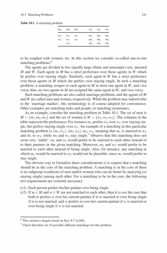
10.3 Matching Problems 143
Table 10.1 A matching problem
m1 m2 m3 w1 w2 w3
w2 w1 w1 m1 m2 m1w1 w2 w2 m3 m1 m3
w3 m2 m3 m2
to be coupled with women; etc. In this section we consider so-called one-to-onematching problems.6
The agents are divided in two equally large (finite and nonempty) sets, denotedM and W . Each agent in M has a strict preference over those agents in W whichhe prefers over staying single. Similarly, each agent in W has a strict preferenceover those agents in M which she prefers over staying single. In such a matchingproblem; a matching assigns to each agent in M at most one agent in W , and viceversa; thus, no two agents in M are assigned the same agent in W , and vice versa.
Such matching problems are also called marriage problems, and the agents of Mand W are called men and women, respectively. While the problem may indeed referto the ‘marriage market’, this terminology is of course adopted for convenience.Other examples are matching tasks and people, or matching roommates.
As an example, consider the matching problem in Table 10.1. The set of men isM = {m1,m2,m3} and the set of women is W = {w1,w2,w3}. The columns in thetable represent the preferences. For instance m1 prefers w2 over w1 over staying sin-gle, but prefers staying single over w3. An example of a matching in this particularmatching problem is (m1,w1), (m3,w2), m2, w3, meaning that m1 is married to w1and m3 to w2, while m2 and w3 stay single.7 Observe that this matching does notseem very ‘stable’: m1 and w2 would prefer to be married to each other instead ofto their partners in the given matching. Moreover, m2 and w3 would prefer to bemarried to each other instead of being single. Also, for instance, any matching inwhich m1 would be married to w3 would not be plausible, since m1 would prefer tostay single.
The obvious way to formalize these considerations is to require that a matchingshould be in the core of the matching problem. A matching is in the core of thereis no subgroup (coalition) of men and/or women who can do better by marrying (orstaying single) among each other. For a matching to be in the core, the followingtwo requirements are certainly necessary:
(c1) Each person prefers his/her partner over being single.(c2) If m ∈ M and w ∈ W are not matched to each other, then it is not the case that
both m prefers w over his current partner if m is married or over being singleif m is not married; and w prefers m over her current partner if w is married orover being single if w is not married.
6 This section is largely based on Sect. 8.7 in [96].7 Check that there are 34 possible different matchings for this problem.
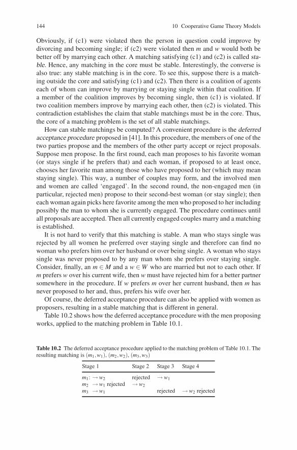
144 10 Cooperative Game Theory Models
Obviously, if (c1) were violated then the person in question could improve bydivorcing and becoming single; if (c2) were violated then m and w would both bebetter off by marrying each other. A matching satisfying (c1) and (c2) is called sta-ble. Hence, any matching in the core must be stable. Interestingly, the converse isalso true: any stable matching is in the core. To see this, suppose there is a match-ing outside the core and satisfying (c1) and (c2). Then there is a coalition of agentseach of whom can improve by marrying or staying single within that coalition. Ifa member of the coalition improves by becoming single, then (c1) is violated. Iftwo coalition members improve by marrying each other, then (c2) is violated. Thiscontradiction establishes the claim that stable matchings must be in the core. Thus,the core of a matching problem is the set of all stable matchings.
How can stable matchings be computed? A convenient procedure is the deferredacceptance procedure proposed in [41]. In this procedure, the members of one of thetwo parties propose and the members of the other party accept or reject proposals.Suppose men propose. In the first round, each man proposes to his favorite woman(or stays single if he prefers that) and each woman, if proposed to at least once,chooses her favorite man among those who have proposed to her (which may meanstaying single). This way, a number of couples may form, and the involved menand women are called ‘engaged’. In the second round, the non-engaged men (inparticular, rejected men) propose to their second-best woman (or stay single); theneach woman again picks here favorite among the men who proposed to her includingpossibly the man to whom she is currently engaged. The procedure continues untilall proposals are accepted. Then all currently engaged couples marry and a matchingis established.
It is not hard to verify that this matching is stable. A man who stays single wasrejected by all women he preferred over staying single and therefore can find nowoman who prefers him over her husband or over being single. A woman who stayssingle was never proposed to by any man whom she prefers over staying single.Consider, finally, an m ∈ M and a w ∈ W who are married but not to each other. Ifm prefers w over his current wife, then w must have rejected him for a better partnersomewhere in the procedure. If w prefers m over her current husband, then m hasnever proposed to her and, thus, prefers his wife over her.
Of course, the deferred acceptance procedure can also be applied with women asproposers, resulting in a stable matching that is different in general.
Table 10.2 shows how the deferred acceptance procedure with the men proposingworks, applied to the matching problem in Table 10.1.
Table 10.2 The deferred acceptance procedure applied to the matching problem of Table 10.1. Theresulting matching is (m1,w1), (m2,w2), (m3,w3)
Stage 1 Stage 2 Stage 3 Stage 4
m1: → w2 rejected → w1m2 → w1 rejected → w2m3 → w1 rejected → w2 rejected

10.4 House Exchange 145
There may be other stable matchings than those found by applying the deferredacceptance procedure with the men and with the women proposing. It can be shownthat the former procedure – with the men proposing – results in a stable matchingthat is optimal, among all stable matchings, from the point of view of the men,whereas the latter procedure – with the women proposing – produces the stablematching optimal from the point of view of the women. See also Problems 10.6and 10.7.
10.4 House Exchange
In a house exchange problem each one of finitely many agents owns a house, andhas a preference over all houses. The purpose of the exchange is to make the agentsbetter off. A house exchange problem is an exchange economy with as many goodsas there are agents, and where each agent is endowed with one unit of a different,indivisible good.8
Formally, the player set is N = {1, . . . ,n}, and each player i ∈ N owns house hi,and has a strict preference of the set of all (n) houses. In a core allocation, eachplayer obtains exactly one house, and there is no coalition that can make each ofits members strictly better off by exchanging their initially owned houses amongthemselves.
As an example, consider the house exchange problem in Table 10.3. In this prob-lem there are six possible different allocations of the houses. Table 10.4 lists theseallocations and also which coalition could improve by exchanging their own houses.
Table 10.3 A house exchange problem with three players. For instance, player 1 prefers the houseof player 3 over the house of player 2 over his own house
Player 1 Player 2 Player 3
h3 h1 h2h2 h2 h3h1 h3 h1
Table 10.4 Analysis of the house exchange problem of Table 10.3. There are two core allocations
Player 1 Player 2 Player 3 Improving coalition(s)
h1 h2 h3 {1,2}, {1,2,3}h1 h3 h2 {2}, {1,2}h2 h1 h3 None: core allocationh2 h3 h1 {2}, {3}, {2,3}, {1,2,3}h3 h1 h2 None: core allocationh3 h2 h1 {3}
8 This section is based largely on Sect. 8.5 in [96].
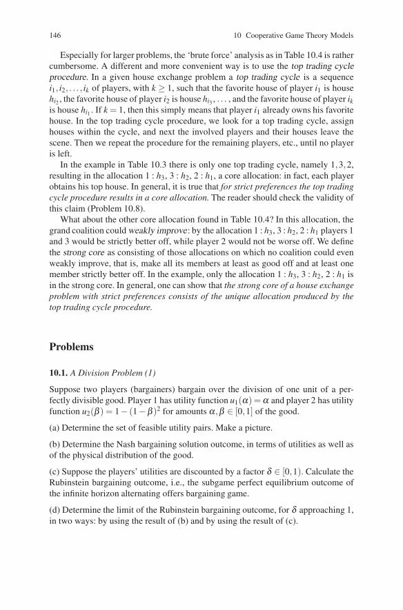
146 10 Cooperative Game Theory Models
Especially for larger problems, the ‘brute force’ analysis as in Table 10.4 is rathercumbersome. A different and more convenient way is to use the top trading cycleprocedure. In a given house exchange problem a top trading cycle is a sequencei1, i2, . . . , ik of players, with k ≥ 1, such that the favorite house of player i1 is househi2 , the favorite house of player i2 is house hi3 , . . . , and the favorite house of player ikis house hi1 . If k = 1, then this simply means that player i1 already owns his favoritehouse. In the top trading cycle procedure, we look for a top trading cycle, assignhouses within the cycle, and next the involved players and their houses leave thescene. Then we repeat the procedure for the remaining players, etc., until no playeris left.
In the example in Table 10.3 there is only one top trading cycle, namely 1,3,2,resulting in the allocation 1 : h3, 3 : h2, 2 : h1, a core allocation: in fact, each playerobtains his top house. In general, it is true that for strict preferences the top tradingcycle procedure results in a core allocation. The reader should check the validity ofthis claim (Problem 10.8).
What about the other core allocation found in Table 10.4? In this allocation, thegrand coalition could weakly improve: by the allocation 1 : h3, 3 : h2, 2 : h1 players 1and 3 would be strictly better off, while player 2 would not be worse off. We definethe strong core as consisting of those allocations on which no coalition could evenweakly improve, that is, make all its members at least as good off and at least onemember strictly better off. In the example, only the allocation 1 : h3, 3 : h2, 2 : h1 isin the strong core. In general, one can show that the strong core of a house exchangeproblem with strict preferences consists of the unique allocation produced by thetop trading cycle procedure.
Problems
10.1. A Division Problem (1)
Suppose two players (bargainers) bargain over the division of one unit of a per-fectly divisible good. Player 1 has utility function u1(α) = α and player 2 has utilityfunction u2(β ) = 1− (1−β )2 for amounts α,β ∈ [0,1] of the good.
(a) Determine the set of feasible utility pairs. Make a picture.
(b) Determine the Nash bargaining solution outcome, in terms of utilities as well asof the physical distribution of the good.
(c) Suppose the players’ utilities are discounted by a factor δ ∈ [0,1). Calculate theRubinstein bargaining outcome, i.e., the subgame perfect equilibrium outcome ofthe infinite horizon alternating offers bargaining game.
(d) Determine the limit of the Rubinstein bargaining outcome, for δ approaching 1,in two ways: by using the result of (b) and by using the result of (c).

Problems 147
10.2. A Division Problem (2)
Suppose that two players (bargainers) bargain over the division of one unit of aperfectly divisible good. Assume that player 1 has utility function u(α) (0 ≤ α ≤ 1)and player 2 has utility function v(α) = 2u(α) (0 ≤ α ≤ 1).
Determine the physical distribution of the good according to the Nash bargainingsolution. Can you say something about the resulting utilities? (Hint: use the relevantproperties of the Nash bargaining solution.)
10.3. A Division Problem (3)
Suppose that two players (bargainers) bargain over the division of two units of aperfectly divisible good. Assume that player 1 has a utility function u(α) = α
2 (0 ≤α ≤ 2) and player 2 has utility function v(α) = 3
√α (0 ≤ α ≤ 2).
(a) Determine the physical distribution of the good according to the Rubinsteinbargaining procedure, for any discount factor 0 < δ < 1.
(b) Use the result to determine the Nash bargaining solution distribution.
(c) Suppose player 1’s utility function changes to w(α) = α for 0 ≤ α ≤ 1.6 andw(α) = 1.6 for 1.6≤ α ≤ 2. Determine the Nash bargaining solution outcome, bothin utilities and in physical distribution, for this new situation.
10.4. An Exchange Economy
Consider an exchange economy with two agents A and B and two goods. Theagents are endowed with initial bundles eA = (3,1) and eB = (1,3). Their prefer-ences are represented by the utility functions uA(x1,x2) = ln(x1 + 1)+ ln(x2 + 2)and uB(x1,x2) = 3ln(x1 + 1)+ ln(x2 + 1).
(a) Compute the demand functions of the agents.
(b) Compute Walrasian equilibrium prices and the equilibrium allocation.
(c) Compute the contract curve and the core. Sketch the Edgeworth box.
(d) Show that the Walrasian equilibrium allocation is in the core.
(e) How would you set up a two-person bargaining problem associated with thiseconomy? Would it make sense to consider the Nash bargaining solution in order tocompute an allocation? Why or why not?
10.5. The Matching Problem of Table 10.1 Continued9
(a) Apply the deferred acceptance procedure to the matching problem of Table 10.1with the women proposing.
(b) Are there any other stable matchings in this example?
9 Problems 10.5–10.7 are taken from [96].

148 10 Cooperative Game Theory Models
Table 10.5 The matching problem of Problem 10.6
m1 m2 m3 w1 w2 w3
w1 w1 w1 m1 m1 m1w2 w2 w3 m2 m3 m2w3 w3 w2 m3 m2 m3
Table 10.6 The matching problem of Problem 10.7
m1 m2 m3 w1 w2 w3
w2 w1 w1 m1 m3 m1w1 w3 w2 m3 m1 m3w3 w2 w3 m2 m2 m2
10.6. Another Matching Problem
Consider the matching problem with three men, three women, and preferences as inTable 10.5.
(a) Compute the two matchings produced by the deferred acceptance procedure withthe men and with the women proposing.
(b) Are there any other stable matchings?
(c) Verify the claim made in the text about the optimality of the matchings in (a) forthe men and the women, respectively.
10.7. Yet Another Matching Problem: Strategic Behavior
Consider the matching problem with three men, three women, and preferences as inTable 10.6.
(a) Compute the two matchings produced by the deferred acceptance procedure withthe men and with the women proposing.
(b) Are there any other stable matchings?
Now consider the following noncooperative game. The players are w1, w2, and w3.The strategy set of a player is simply the set of all possible preferences over the men.(Thus, each player has 16 different strategies.) The outcomes of the game are thematchings produced by the deferred acceptance procedure with the men proposing,assuming that each man uses his true preference given in Table 10.6.
(c) Show that the following preferences form a Nash equilibrium: w2 and w3 usetheir true preferences, as given in Table 10.6; w1 uses the preference (m1,m2,m3).Conclude that sometimes it may pay off to lie about one’s true preference. (Hint: ina Nash equilibrium, no player can gain by deviating.)
10.8. Core Property of Top Trading Cycle Procedure
Show that for strict preferences the top trading cycle results in a core allocation.

Problems 149
Table 10.7 The house exchange problem of Problem 10.10
Player 1 Player 2 Player 3 Player 4
h3 h4 h1 h3h2 h1 h4 h2h4 h2 h3 h1h1 h3 h2 h4
10.9. House Exchange with Identical Preferences
Consider the n-player house exchange problem where all players have identicalstrict preferences. Find the house allocation(s) in the core.
10.10. A House Exchange Problem10
Consider the house exchange problem with four players in Table 10.7.Compute all core allocations and all strong core allocations.
10.11. Cooperative Oligopoly
Consider the Cournot oligopoly game with n firms with different costs c1,c2, . . . ,cn.(This is the game of Problem 6.2 with heterogenous costs.) As before, each firmi offers qi ≥ 0, and the price-demand function is p = max{0,a−∑n
i=1 qi}, where0 < ci < a for all i.
(a) Show that the reaction function of player i is
qi = max{0,a− ci−∑ j =i qi
2}.
(b) Show that the unique Nash equilibrium of the game is q∗ = (q∗1, . . . ,q∗n) with
q∗i =a−nci + ∑ j =i c j
n + 1,
for each i, assuming that this quantity is positive.
(c) Derive that the corresponding profits are
(a−nci + ∑ j =i c j)2
(n + 1)2
for each player i.
Let the firms now be the players in a cooperative TU-game with player set N ={1,2, . . . ,n}, and consider a coalition S ⊆ N. What is the total profit that S can makeon its own? This depends on the assumptions that we make on the behavior of the
10 Taken from [83].

150 10 Cooperative Game Theory Models
players outside S. Very pessimistically, one could solve the problem
maxqi:i∈S
minq j : j/∈S
∑i∈S
Pi(q1, . . . ,qn),
which is the profit that S can guarantee independent of the players outside S. Thisview is very pessimistic because it presumes maximal resistance of the outside play-ers, even if this means that these outside players hurt themselves. In the present caseit is not hard to see that this results in zero profit for S.
Two alternative scenarios are: S plays a Cournot–Nash equilibrium in the (n−|S|+1)-player oligopoly game against the outside firms as separate firms, or S playsa Cournot–Nash equilibrium in the duopoly game against N \S.
In the first case we in fact have an oligopoly game with costs c j for every playerj /∈ S and with cost cS := min{ci : i ∈ S} for ‘player’ (coalition) S.
(d) By using the results of (a)–(c) show that coalition S obtains a profit of
v1(S) =[a− (n−|S|+ 1)cS+ ∑ j/∈S c j]2
(n−|S|+ 2)2
in this scenario. Thus, this scenario results in a cooperative TU-game (N,v1).
(e) Assume n = 3, a = 7, and ci = i for i = 1,2,3. Compute the core, the Shapleyvalue, and the nucleolus for the TU-game (N,v1).
(f) Show that in the second scenario, coalition S obtains a profit of
v2(S) =(a− 2cS + cN−S)2
9,
resulting in a cooperative game (N,v2).
(g) Assume n = 3, a = 7, and ci = i for i = 1,2,3. Compute the core, the Shapleyvalue, and the nucleolus for the TU-game (N,v2).

Chapter 11Social Choice
Social choice theory studies the aggregation of individual preferences into a com-mon or social preference. It overlaps with several social science disciplines, such aspolitical theory (e.g., voting for Parliament, or for a president) and game theory (e.g.,voters may vote strategically, or candidates may choose positions strategically). Fora general overview see [3] and [4].
In the classical model of social choice, there is a finite number of agents whohave preferences over a finite number of alternatives. These preferences are eitheraggregated into a social preference according to a so-called social welfare function,or result in a common alternative according to a so-called social choice function.
The main purpose of this chapter is to review two classical results, namelyArrow’s [2] Theorem and Gibbard’s [44] and Satterthwaite’s [112] Theorem. Thefirst theorem applies to social welfare functions and says that, if the social prefer-ence between any two alternatives should only depend on the individual preferencesbetween these alternatives and, thus, not on individual preferences involving otheralternatives, then the social welfare function must be dictatorial. The second theo-rem applies to social choice functions and says that the only social choice functionsthat are invulnerable to strategic manipulation are the dictatorial ones. These resultsare often referred to as ‘impossibility theorems’ since dictatorships are generallyregarded undesirable.
Both results are closely related: indeed, the proof of the Theorem of Gibbard andSatterthwaite in [44] uses Arrow’s Theorem. The presentation in this chapter closelyfollows that in Reny [108], which is both simple and elegant, and which shows theclose relation between the two results. The approach in [108] is itself based on a fewother sources: see [108] for the references.
Section 11.1 is introductory. Section 11.2 discusses Arrow’s Theorem andSect. 11.3 the Gibbard–Satterthwaite Theorem.
H. Peters, Game Theory – A Multi-Leveled Approach.c© Springer-Verlag Berlin Heidelberg 2008
151

152 11 Social Choice
11.1 Introduction and Preliminaries
11.1.1 An Example
Suppose there are three agents (individuals, voters) who have strict preferences overa set of five alternatives (a1, . . . ,a5), as given in Table 11.1.
In this table the preferences of the players are represented by the Borda scores:the best alternative of an agent obtains 5 points, the second best 4 points, etc., untilthe worst alternative which obtains 1 point. So, for instance, agent 1 has the prefer-ence a1P1a5P1a3P1a4P1a2 in the notation to be introduced below. We use the Bordascores (Borda [25]) as a convenient way to represent these preferences and, moreimportantly, to obtain an example of a social welfare as well as a social choicefunction.
First, suppose that we want to extract a common social ranking of the alternativesfrom the individual preferences. One way to do this is to add the Borda scores peralternative. In the example this results in 9,7,11,8,10 for a1,a2,a3,a4,a5, respec-tively, resulting in the social ranking a3Pa5Pa1Pa4Pa2. If we just want to singleout one alternative, then we could take the one with the maximal Borda score, inthis case alternative a3. In the terminology to be introduced formally below, Bordascores give rise to a social welfare as well as a social choice function.1
One potential drawback of using Borda scores to obtain a social ranking is,that the ranking between two alternatives may not just depend on the individualpreferences between these two alternatives. For instance, suppose that agent 1’spreference would change to a1P1a4P1a5P1a3P1a2. Then the Borda scores wouldchange to 9,7,8,10,9 for a1,a2,a3,a4,a5, respectively, resulting in the social rank-ing a4Pa1Ia5Pa3Pa2 (where I denotes indifference). Observe that no agent’s prefer-ence between a1 and a4 has changed, but that socially this preference is reversed.This is not a peculiarity of using Borda scores: Arrow’s Theorem, to be discussedin Sect. 11.2, states that the only way to avoid this kind of preference reversal isto make one agent the dictator, i.e., to have the social preference coincide with thepreference of one fixed agent.
A potential drawback of using the Borda scores in order to single out a uniquealternative is that this method is vulnerable to strategic manipulation. For instance,suppose that agent 1 would lie about his true preference given in Table 11.1 and
Table 11.1 Borda scores
Agent a1 a2 a3 a4 a5
1 5 1 3 2 42 1 2 3 4 53 3 4 5 2 1
1 Note that ties may occur, but this need not bother us here.

11.1 Introduction and Preliminaries 153
claim that his preference is a1P1a5P1a2P1a4P1a3 instead. Then the Borda scoreswould change to 9,9,9,8,10 for a1,a2,a3,a4,a5, respectively, resulting in the cho-sen alternative a5 instead of a3. Since agent 1 prefers a5 over a3 according to histrue preference, he gains by this strategic manipulation. Again, this phenomenonis not a peculiarity of the Borda method: the Gibbard–Satterthwaite Theorem inSect. 11.3 shows that the only way to avoid it is (again) to make one fixed agent adictator.
11.1.2 Preliminaries
Let A = {a1, . . . ,am} be the set of alternatives. To keep things interesting we assumem ≥ 3.2 The set of agents is denoted by N = {1, . . . ,n}. We assume n ≥ 2.
A binary relation on A is a subset of A×A. In our context, for a binary relationR on A we usually write aRb instead of (a,b) ∈ R and interpret this as an agent orsociety (weakly) preferring a over b. Well-known conditions for a binary relation Ron A are:
(a) Reflexivity: aRa for all a ∈ A.(b) Completeness: aRb or bRa for all a,b ∈ A with a = b.(c) Antisymmetry: For all a,b ∈ A, if aRb and bRa, then a = b.(d) Transitivity: For all a,b,c ∈ A, aRb and bRc imply aRc.
A preference on A is a reflexive, complete and transitive binary relation on A. Fora preference R on A we write aPb if aRb and not bRa; and aIb if aRb and bRa.The binary relations P and I are called the asymmetric and symmetric parts ofR, respectively, and interpreted as strict preference and indifference. Check (seeProblem 11.1) that P is antisymmetric and transitive but not reflexive and notnecessarily complete, and that I is reflexive and transitive but not necessarily anti-symmetric and not necessarily complete. By L ∗ we denote the set of all preferenceson A, and by L ⊆ L ∗ the set of all antisymmetric (i.e., strict) preferences on A.In plain words, elements of L ∗ order the elements of A but allow for indifferences,while elements of L order the elements of A strictly.3
In what follows, it is assumed that agents have strict preferences whilesocial preferences may have indifferences. A strict preference profile is a list(R1, . . . ,Ri, . . . ,Rn), where Ri is the strict preference of agent i. Hence, L N denotesthe set of all strict preference profiles. A social choice function is a map f : L N →A,i.e., it assigns a unique alternative to every profile of strict preferences. A socialwelfare function is a map F : L N → L ∗, i.e., it assigns a (possibly non-strict)preference to every profile of strict preferences.
2 See Problem 11.7 for the case m = 2.3 Elements of L are usually called linear orders and those of L ∗ weak orders.

154 11 Social Choice
11.2 Arrow’s Theorem
In this section the focus is on social welfare functions. We formulate three propertiesfor a social welfare function F : L N → L ∗. Call F :
(1) Pareto Efficient (PE) if for each profile (R1, . . . ,Rn) ∈ L N and all a,b ∈ A,if aRib for all i ∈ N, then aPb, where P is the asymmetric part of R =F(R1, . . . ,Rn).
(2) Independent of Irrelevant Alternatives (IIA) if for all (R1, . . . ,Rn) ∈ L N and(R′
1, . . . ,R′n) ∈ L N and all a,b ∈ A, if aRib ⇔ aR′
ib for all i ∈ N, then aRb ⇔aR′b, where R = F(R1, . . . ,Rn) and R′ = F(R′
1, . . . ,R′n).
(3) Dictatorial (D) if there is an i ∈ N such that F(R1, . . . ,Rn) = Ri for all(R1, . . . ,Rn) ∈ L N .
Pareto Efficiency requires that, if all agents prefer an alternative a over an alternativeb, then the social ranking should also put a above b. Independence of IrrelevantAlternatives says that the social preference between two alternatives should onlydepend on the agents’ preferences between these two alternatives and not on theposition of any other alternative.4 Dictatoriality says that the social ranking is alwaysequal to the preference of a fixed agent, the dictator. Clearly, there are exactly ndictatorial social welfare functions.
The first two conditions are regarded as desirable but the third clearly not. Unfor-tunately, Arrow’s Theorem implies that the first two conditions imply the thirdone.5
Theorem 11.1 (Arrow’s Theorem). Let F be a Pareto Efficient and IIA socialwelfare function. Then F is dictatorial.
Proof.
Step 1. Consider a profile in L N and two distinct alternatives a,b ∈ A such thatevery agent ranks a on top and b at bottom. By Pareto Efficiency, the social rankingassigned by F must also rank a on top and b at bottom.
Now change agent 1’s ranking by raising b in it one position at a time. By IIA,a is ranked socially (by F) on top as long as b is still below a in the preference ofagent 1. In the end, if agent 1 ranks b first and a second, we have a or b on top of thesocial ranking by Pareto efficiency of F . If a is still on top in the social ranking, thencontinue the same process with agents 2,3, etc., until we reach some agent k suchthat b is on top of the social ranking after moving b above a in agent k’s preference.Tables 11.2 and 11.3 give the situations just before and just after b is placed abovea in agent k’s preference.6
4 Although there is some similarity in spirit, this condition is not in any formal sense related to theIIA condition in bargaining, see Sect. 10.1 or Chap. 21.5 For this reason the theorem is often referred to as Arrow’s Impossibility Theorem.6 In these tables and also the ones below, we generically denote all preferences by R1, . . .,Rn. Thelast column in every table will be used in Sect. 11.3.

11.2 Arrow’s Theorem 155
Table 11.2
R1 · · · Rk−1 Rk Rk+1 · · · Rn F f
b · · · b a a · · · a a aa · · · a b · · · · · ·· · · · · · · · · · · ·· · · · · · · · · · · b· · · · · · · · · · · ·· · · · · · b · · · b ·
Table 11.3
R1 · · · Rk−1 Rk Rk+1 · · · Rn F f
b · · · b b a · · · a b ba · · · a a · · · · · a· · · · · · · · · · · ·· · · · · · · · · · · ·· · · · · · · · · · · ·· · · · · · b · · · b ·
Table 11.4
R1 · · · Rk−1 Rk Rk+1 · · · Rn F f
b · · · b a · · · · · a a· · · · · b · · · · · b· · · · · · · · · · · ·· · · · · · a · · · a ·a · · · a · b · · · b ·
Table 11.5
R1 · · · Rk−1 Rk Rk+1 · · · Rn F f
b · · · b b · · · · · b b· · · · · a · · · · · ·· · · · · · · · · · · a· · · · · · a · · · a ·a · · · a · b · · · b ·
Step 2. Now consider Tables 11.4 and 11.5. The profile in Table 11.4 arises from theone in Table 11.2 by moving a to the last position for agents i < k and to the secondlast position for agents i > k. In exactly the same way, the profile in Table 11.5 arisesfrom the one in Table 11.3. Then IIA applied to Tables 11.3 and 11.5 implies that b issocially top-ranked in Table 11.5. Next, IIA applied to the transition from Table 11.5to Table 11.4 implies that in Table 11.4 b must still be socially ranked above everyalternative except perhaps a. But IIA applied to the transition from Table 11.2 toTable 11.4 implies that in Table 11.4 a must still be socially ranked above everyalternative. This proves that the social rankings in Tables 11.4 and 11.5 are correct.

156 11 Social Choice
Table 11.6
R1 · · · Rk−1 Rk Rk+1 · · · Rn F f
· · · · · a · · · · · a a· · · · · c · · · · · ·· · · · · b · · · · · ·c · · · c · c · · · c ·b · · · b · a · · · a ·a · · · a · b · · · b ·
Table 11.7
R1 · · · Rk−1 Rk Rk+1 · · · Rn F f
· · · · · a · · · · · a a· · · · · c · · · · · ·· · · · · b · · · · · cc · · · c · c · · · c ·b · · · b · b · · · b ba · · · a · a · · · a ·
Step 3. Consider a third alternative c distinct from a and b. The social ranking inTable 11.6 is obtained by from Table 11.4 by applying IIA.
Step 4. Consider the profile in Table 11.7, obtained from the profile in Table 11.6 byswitching a and b for agents i > k. By IIA applied to the transition from Table 11.6to Table 11.7, we have that a must still be socially ranked above every alternativeexcept possibly b. However, b must be ranked below c by Pareto efficiency, whichshows that the social ranking in Table 11.7 is correct.
Step 5. Consider any arbitrary profile in which agent k prefers a to b. Change theprofile by moving c between a and b for agent k and to the top of every other agent’spreference (if this is not already the case). By IIA this does not affect the socialranking of a vs. b. Since the preference of every agent concerning a and c is now asin Table 11.7, IIA implies that a is socially ranked above c, which itself is sociallyranked above b by Pareto Efficiency. Hence, by transitivity of the social ranking wemay conclude that a is socially ranked above b whenever it is preferred by agent kover b. By repeating the argument with the roles of b and c reversed, and recallingthat c was an arbitrary alternative distinct from a and b, we may conclude that thesocial ranking of a is above some alternative whenever agent k prefers a to thatalternative: k is a ‘dictator’ for a. Since a was arbitrary, we can repeat the wholeargument to conclude that there must be a dictator for every alternative. Since therecannot be distinct dictators for distinct alternatives, there must be a single dictatorfor all alternatives. ��

11.3 The Gibbard–Satterthwaite Theorem 157
11.3 The Gibbard–Satterthwaite Theorem
The Gibbard–Satterthwaite Theorem applies to social choice functions. We start bylisting the following possible properties of a social choice function f : L N → A.Call f :
(1) Unanimous (UN) if for each profile (R1, . . . ,Rn) ∈ L N and each a ∈ A, if aRibfor all i ∈ N and all b ∈ A\ {a}, then f (R1, . . . ,Rn) = a.
(2) Monotonic (MON) if for all profiles (R1, . . . ,Rn) ∈ L N and (R′1, . . . ,R
′n) ∈ L N
and all a ∈ A, if f (R1, . . . ,Rn) = a and aRib⇒ aR′ib for all b∈ A\{a} and i ∈ N,
then f (R′1, . . . ,R
′n) = a.
(3) Dictatorial (D) if there is an i ∈ N such that f (R1, . . . ,Rn) = a where aRib forall b ∈ A\ {a}, for all (R1, . . . ,Rn) ∈ L N .
(4) Strategy-Proof (SP) if for all profiles (R1, . . . ,Rn)∈L N and (R′1, . . . ,R
′n) ∈ L N
and all i ∈ N, if R′j = R j for all j ∈ N \ {i}, then f (R1, . . . ,Rn) Ri f (R′
1, . . . ,R′n).
Unanimity requires that, if all agents have the same top alternative, then this alter-native should be chosen. Monotonicity says that, if some alternative a is chosenand the profile changes in such a way that a is still preferred by every agent overall alternatives over which it was originally preferred, then a should remain to bechosen. Dictatoriality means that there is a fixed agent whose top element is alwayschosen. Strategy-Proofness says that no agent can obtain a better chosen alternativeby lying about his true preference.
In accordance with mathematical parlance, call a social choice function f :L N → A surjective if for every a ∈ A there is some profile (R1, . . . ,Rn) ∈ L N
such that f (R1, . . . ,Rn) = a. Hence, each a is chosen at least once.7 The Gibbard–Satterthwaite Theorem is as follows.
Theorem 11.2 (Gibbard–Satterthwaite Theorem). Let f : L N → A be a surjec-tive and strategy-proof social choice function. Then f is dictatorial.
We will prove the Gibbard–Satterthwaite Theorem by using the next theorem, whichis a variant of the Muller–Satterthwaite Theorem [84].
Theorem 11.3 (Muller–Satterthwaite). Let f : L N → A be a unanimous andmonotonic social choice function. Then f is dictatorial.
Proof of Theorem 11.2. We prove that f is unanimous and monotonic. The resultthen follows from Theorem 11.3.
Suppose that f (R1, . . . ,Rn) = a for some profile (R1, . . . ,Rn) ∈ L N and somealternative a ∈ A. Let i ∈ N and let (R′
1, . . . ,R′n) ∈ L N be a profile such that for
all j ∈ N \ {i} we have R′j = R j and for all b ∈ A \ {a} we have aR′
ib if aRib. Wewish to show that f (R′
1, . . . ,R′n) = a. Suppose, to the contrary, that f (R′
1, . . . ,R′n) =
b = a. Then SP implies aRib, and hence aR′ib. By SP, however, bR′
ia, hence, byantisymmetry of R′
i, a = b, a contradiction. This proves f (R′1, . . . ,R
′n) = a.
7 In the social choice literature this property is sometimes called citizen-sovereignty.

158 11 Social Choice
Now suppose that (R′1, . . . ,R
′n) ∈ L N is a profile such that for all i ∈ N and
all b ∈ A \ {a} we have aR′ib if aRib. By applying the argument in the preceding
paragraph n times, it follows that f (R′1, . . . ,R
′n) = a. Hence, f is monotonic.
To prove unanimity, suppose that (R1, . . . ,Rn) ∈ L N and a ∈ A such that aRibfor all i ∈ N and b ∈ A \ {a}. By surjectivity there is (R′
1, . . . ,R′n) ∈ L N with
f (R′1, . . . ,R
′n) = a. By monotonicity we may move a to the top of each agent’s
preference and still have a chosen. Next, again by monotonicity, we may changeeach agent i’s preference to Ri without changing the chosen alternative, i.e.,f (R1, . . . ,Rn) = a. Hence, f is unanimous. ��Proof of Theorem 11.3. The proof parallels the proof of Theorem 11.1 and usesanalogous steps and the same tables.
Step 1. Consider a profile in L N and two distinct alternatives a,b ∈ A such thatevery agent ranks a on top and b at bottom. By unanimity, f chooses a.
Now change agent 1’s ranking by raising b in it one position at a time. By MON,a is chosen by f as long as b is still below a in the preference of agent 1. In the end,if agent 1 ranks b first and a second, we have a or b chosen by f , again by MON. Ifa is still chosen, then continue the same process with agents 2,3, etc., until we reachsome agent k such that b is chosen after moving b above a in agent k’s preference.Tables 11.2 and 11.3 give the situations just before and just after b is placed abovea in agent k’s preference.
Step 2. Now consider Tables 11.4 and 11.5. The profile in Table 11.4 arises from theone in Table 11.2 by moving a to the last position for agents i < k and to the secondlast position for agents i > k. In exactly the same way, the profile in Table 11.5 arisesfrom the one in Table 11.3.
Then MON applied to Tables 11.3 and 11.5 implies that b is chosen in Table 11.5.Next, MON applied to the transition from Table 11.5 to Table 11.4 implies that inTable 11.4 the choice must be either b or a. Suppose b would be chosen. Then MONapplied to the transition from Table 11.4 to Table 11.2 implies that in Table 11.2b must be chosen as well, a contradiction. Hence, a is chosen in Table 11.4. Thisproves that the choices by f in Tables 11.4 and 11.5 are correct.
Step 3. Consider a third alternative c distinct from a and b. The choice in Table 11.6is obtained by from Table 11.4 by applying MON.
Step 4. Consider the profile in Table 11.7, obtained from the profile in Table 11.6 byswitching a and b for agents i > k. If the choice in Table 11.7 were some d unequalto a or b, then by MON it would also be d in Table 11.6, a contradiction. If it wereb, then by MON it would remain b even if c would be moved to the top of everyagent’s preference, contradicting unanimity. Hence, it must be a.
Step 5. Consider any arbitrary profile with a at the top of agent k’s preference. Sucha profile can always be obtained from the profile in Table 11.7 without worseningthe position of a with respect to any other alternative in any agent’s preference. ByMON therefore, a must be chosen whenever it is at the top of agent k’s preference,so k is a ‘dictator’ for a. Since a was arbitrary, we can find a dictator for every other

Problems 159
alternative but, clearly, these must be one and the same agent. Hence, this agent isthe dictator. ��There is a large literature that tries to escape the rather negative conclusions ofTheorems 11.1–11.3 by adapting the model and/or restricting the domain. Examplesof this are provided in Problems 6.22 and 6.23.
Problems
11.1. Preferences
Let R be a preference on A, with symmetric part I and asymmetric part P.
(a) Prove that P is antisymmetric and transitive but not reflexive and not necessarilycomplete.
(b) Prove that I is reflexive and transitive but not necessarily complete and notnecessarily antisymmetric.
11.2. Pairwise Comparison
For a profile r = (R1, . . . ,Rn) ∈ L N and a,b ∈ A define
N(a,b,r) = {i ∈ N | aRib} ,
i.e., N(a,b,r) is the set of agents who (strictly) prefer a to b in the profile r. Withr we can associate a binary relation C(r) on A by defining aC(r)b :⇔ |N(a,b,r)| ≥|N(b,a,r)| for all a,b ∈ A. If aC(r)b we say that ‘a beats b by pairwise majority’.
(a) Is C(r) reflexive? Complete? Antisymmetric?
(b) Show that C(r) is not transitive, by considering the famous Condorcet profile8
for N = {1,2,3} and A = {a,b,c}: aR1bR1c, bR2cR2a, cR3aR3b.
(c) Call a a Condorcet winner if |N(a,b,r)|> |N(b,a,r)| for all b ∈ A\{a}. Is therea Condorcet winner in the example in Sect. 11.1?
11.3. Independence of the Conditions in Theorem 11.1
Show that the conditions in Theorem 11.1 are independent. That is, exhibit a socialwelfare function that is Pareto efficient and does not satisfy IIA or dictatoriality, andone that satisfies IIA and is not dicatorial nor Pareto efficient.
11.4. Independence of the Conditions in Theorem 11.2
Show that the conditions in Theorem 11.2 are independent.
11.5. Independence of the Conditions in Theorem 11.3
Show that the conditions in Theorem 11.3 are independent.
8 See [27], and see [43] for a comprehensive study of this so-called Condorcet paradox.

160 11 Social Choice
11.6. Copeland Score and Kramer Score
The Copeland score of an alternative a ∈ A at a profile r = (R1, . . . ,Rn) ∈ L N isdefined by
c(a,r) = |{b ∈ A | N(a,b,r) ≥ N(b,a,r)}| ,i.e., the number of alternatives that a beats (cf. Problem 11.2). The Copeland rankingis obtained by ranking the alternatives according to their Copeland scores.
(a) Is the Copeland ranking a preference? Is it antisymmetric? Does the derivedsocial welfare function satisfy IIA? Pareto efficiency?
The Kramer score of an alternative a ∈ A at a profile r = (R1, . . . ,Rn) ∈ L N isdefined by
k(a,r) = minb∈A\{a}
|N(a,b,r)| ,
i.e., the worst score among all pairwise comparisons. The Kramer ranking isobtained by ranking the alternatives according to their Kramer scores.
(b) Is the Kramer ranking a preference? Is it antisymmetric? Does the derived socialwelfare function satisfy IIA? Pareto efficiency?
11.7. Two Alternatives
Show that Theorems 11.1–11.3 no longer hold if there are just two alternatives, i.e.,if m = 2.

Chapter 12Matrix Games
In this chapter we study finite two-person zerosum games – matrix games – morerigorously. In particular, von Neumann’s Minimax Theorem [140] is proved. Thechapter builds on Chap. 2 in Part I, and the reader is advised to read this chapter andin particular Definition 2.1 before continuing.
Section 12.1 presents a proof of the Minimax Theorem, and Sect. 12.2 showshow a matrix game can be solved – optimal strategies and the value of the game canbe found – by solving an associated linear programming problem.
12.1 The Minimax Theorem
Let A be an m× n matrix game. For any strategy p ∈ ∆m of player 1, let v1(p) =minq∈∆n pAq. It is easy to see that v1(p) = min j∈{1,...,n} pAe j, since pAq is a convexcombination of the numbers pAe j. In the matrix game A player 1 can guarantee apayoff of at least
v1(A) := maxp∈∆m
v1(p).
Similarly, for any strategy q ∈ ∆n of player 2 let v2(q) = maxp∈∆m pAq =maxi∈{1,...,m} eiAq, then player 2 can guarantee to have to pay at most
v2(A) := minq∈∆n
v2(q).
Intuitively, player 1 should not be able to guarantee to obtain more than what player2 can guarantee to pay maximally. Indeed, we have the following lemma.
Lemma 12.1. For any m× n matrix game, v1(A) ≤ v2(A).
Proof. Problem 12.1. ��The following theorem is due to von Neumann [140].
H. Peters, Game Theory – A Multi-Leveled Approach.c© Springer-Verlag Berlin Heidelberg 2008
163

164 12 Matrix Games
Theorem 12.2 (Minimax Theorem for Matrix Games). For any m × n matrixgame A, v1(A) = v2(A).
Proof. Suppose that A is any m × n matrix game. Then either (1) or (2) inLemma 22.3 has to hold.
First suppose that (1) holds. Then there are y ∈ Rn and z ∈ Rm with (y,z) ≥ 0,(y,z) = 0 and Ay+z = 0. It cannot be the case that y = 0, since that would imply thatalso z = 0, a contradiction. Hence ∑n
k=1 yk > 0. Define q ∈ ∆n by q j = y j/∑nk=1 yk
for every j = 1, . . . ,n. Then Aq = −z/∑nk=1 yk ≤ 0. Hence v2(q) ≤ 0, and therefore
v2(A) ≤ 0.Suppose instead that (2) holds. Then there is an x ∈ Rm with x > 0 and xA > 0.
Define p ∈ ∆m by p = x/∑mi=1 xi, then v1(p) > 0 and therefore v1(A) > 0.
We conclude that, for any matrix game A, it is not possible to have v1(A) ≤ 0 <v2(A).
Fix some matrix game B, and suppose that v1(B) < v2(B). We derive a contra-diction, and by Lemma 12.1 this completes the proof of the theorem.
Let A be the matrix game arising by subtracting the number v1(B) from all entriesof B. Then, clearly, v1(A) = v1(B)− v1(B) = 0 and v2(A) = v2(B)− v1(B) > 0.Hence, v1(A) ≤ 0 < v2(A), which is the desired contradiction. ��In view of Theorem 12.2 we can define the value of the game A by v(A) = v1(A) =v2(A). An optimal strategy of player 1 is a strategy p such that v1(p) ≥ v(A).Similarly, an optimal strategy of player 2 is a strategy q such that v2(q) ≤ v(A).Theorem 12.2 implies that v1(p) = v2(q) = v(A) for such optimal strategies. In par-ticular, the optimal strategies for player 1 are exactly the maximin strategies, and theoptimal strategies for player 2 are exactly the minimax strategies (cf. Definition 2.2).
For computation of optimal strategies and the value of matrix games in somespecial cases, see Chap. 2 and Problems 12.2 and 12.3. In general, matrix gamescan be solved by linear programming. This is demonstrated in the next section.
12.2 A Linear Programming Formulation
Let A be an m×n matrix game. Adding the same number to all entries of A changesthe value by that same number but not the optimal strategies of the players. So wemay assume without loss of generality that all entries of A are positive. We definethe (m+ 1)× (n + 1) matrix B as follows:
B =
⎛⎜⎜⎜⎜⎜⎝A
−1−1
...−1
−1 −1 · · · −1 0
⎞⎟⎟⎟⎟⎟⎠ .

12.2 A Linear Programming Formulation 165
Let b = (0, . . . ,0,−1) ∈ Rn+1 and c = (0, . . . ,0,−1) ∈ Rm+1. Define V := {x ∈Rm+1 | xB ≥ b, x ≥ 0} and W := {y ∈ Rn+1 | By ≤ c, y ≥ 0}. It is easy to check thatV,W = /0. The Duality Theorem of Linear Programming (Theorem 22.5) thereforeimplies:
Corollary 12.3. min{x · c | x ∈V} = max{b ·y | y ∈W}.
The minimum and maximum problems in this corollary are so-called linear pro-gramming (LP) problems. If we call the minimization problem the primal problem,then the maximization problem is the dual problem – or vice versa. The commonminimum/maximum is called the value of the LP, and x and y achieving the valueare called optimal solutions. Denote the sets of optimal solutions by Omin and Omax,respectively.
We shall prove the following result.
Theorem 12.4. Let A be an m×n matrix game with all entries positive.
(1) If p ∈ ∆m is an optimal strategy for player 1 and q ∈ ∆n is an optimal strategyfor player 2 in A, then (p,v(A)) ∈ Omin and (q,v(A)) ∈ Omax. The value of the LPis −v(A).
(2) If x = (x1, . . . ,xm,xm+1)∈ Omin and y = (y1, . . . ,yn,yn+1)∈ Omax, then (x1, . . . ,xm)is an optimal strategy for player 1 in A, (y1, . . . ,yn) is an optimal strategy forplayer 2 in A, and v(A) = xm+1 = yn+1.
Proof. (1) Let p ∈ ∆m and q ∈ ∆n be optimal strategies in the matrix game A. ThenpAe j ≥ v(A) and eiAq≤ v(A) for all i = 1, . . . ,m and j = 1, . . . ,n. Since all entries ofA are positive and therefore v(A) > 0, this implies (p,v(A)) ∈V and (q,v(A)) ∈W .Since (p,v(A)) · c = −v(A) and (q,v(A)) ·b = −v(A), Lemma 22.8 implies that thevalue of the LP is −v(A), (p,v(A)) ∈ Omin and (q,v(A)) ∈ Omax.
(2) Let x = (x1, . . . ,xm+1) ∈ Omin. Since x · c = −v(A) by (1), we have xm+1 =v(A). Since xB ≥ b, we have (x1, . . . ,xm)Ae j ≥ v(A) for all j = 1, . . . ,n, xi ≥ 0 forall i = 1, . . . ,m, and ∑m
i=1 xi ≤ 1. Suppose that ∑mi=1 xi < 1. Obviously, ∑m
i=1 xi > 0,otherwise x = (0, . . . ,0,v(A)) /∈ V since v(A) > 0. Then, letting t = (∑m
i=1 xi)−1 >1, we have tx ∈ V and tx · c = −t v(A) < −v(A), contradicting x ∈ Omin. Hence,∑m
i=1 xi = 1, and (x1, . . . ,xm) is an optimal strategy of player 1 in A.The proof of the second part of (2) is analogous. ��
The interest of this theorem derives from the fact that since the invention of the sim-plex algorithm by George Dantzig in 1947 (see any textbook on linear programmingor operations research) solving linear programming problems is a well establishedarea. Thus, one can apply any (computer) method for solving LPs to find the valueand optimal strategies of a matrix game.
Observe that, by slightly modifying part (2) of the proof of Theorem 12.4, wecan in fact derive the Minimax Theorem from the Duality Theorem (Problem 12.4).Conversely, with each LP we can associate a matrix game and thereby derive theDuality Theorem from the Minimax Theorem (see, e.g., [98]). This confirms the

166 12 Matrix Games
close relationship between linear programming (Duality Theorem) and the theoryof matrix games (Minimax Theorem).
Problems
12.1. Proof of Lemma 12.1
Prove Lemma 12.1.
12.2. 2× 2 Games
Consider the 2×2 matrix game
A =(
a11 a12a21 a22
).
Assume that A has no saddlepoints (cf. Definition 2.3).
(a) Show that we may assume, without loss of generality,
a11 > a12, a12 < a22, a21 < a22, a11 > a21.
(b) Show that the unique optimal strategies p and q and the value of the game aregiven by:
p =JA∗
JA∗JT , q =A∗JT
JA∗JT , v(A) =|A|
JA∗JT ,
where A∗ is the adjoint matrix of A, i.e.,
A∗ =(
a22 −a12−a21 a11
),
|A| is the determinant of A, and J := (1,1).1
12.3. Symmetric Games
An m×n matrix game A = (ai j) is called symmetric if m = n and ai j = −a ji for alli, j = 1, . . . ,m.
Prove that the value of a symmetric game is zero and that the sets of optimalstrategies of players 1 and 2 coincide.
12.4. The Duality Theorem Implies the Minimax Theorem
Modify the proof of part (2) of Theorem 12.4 in order to derive the Minimax The-orem from the Duality Theorem. (Hint: first show that the value of the LP must benegative.)
1 J denotes the row vector and JT the transpose, i.e., the column vector. In general, we omit thetranspose notation if confusion is unlikely.

Problems 167
12.5. Infinite Matrix Games
Consider the following two-player game. Each player mentions a natural number.The player with the highest number receives one Euro from the player with thelowest number. If the numbers are equal then no player receives anything.
(a) Write this game in the form of an infinite matrix game A.
(b) Compute supp infq pAq and infq supp pAq, where p and q are probability distri-butions over the rows and the columns of A, respectively. (Conclude that this gamehas no ‘value’.)
12.6. Equalizer Theorem
Let v be the value of the m×n-matrix game A, and suppose that pAen = v for everyoptimal strategy p of player 1. Show that player 2 has an optimal strategy q withqn > 0 (cf. Chap. 20 in [6]).

Chapter 13Finite Games
This chapter builds on Chap. 3, where we studied finite two person games – bimatrixgames. The reader is advised to (re)read this chapter before continuing. The presentchapter offers a more rigorous treatment of finite games, i.e., games with finitelymany players – often two – who have finitely many pure strategies over which theycan randomize.1
In Sect. 13.1 a proof of Nash’s existence theorem is provided. Section 13.2 goesdeeper into bimatrix games. In Sect. 13.3 the notion of iterated dominance is stud-ied, and its relation with rationalizability indicated. Sections 13.4–13.6 present somebasics about refinements of Nash equilibrium. Section 13.7 is on correlated equilib-rium in bimatrix games, and Sect. 13.8 concludes with an axiomatic characterizationof Nash equilibrium based on a reduced game (consistency) condition.
13.1 Existence of Nash Equilibrium
A finite game is a 2n + 1-tuple
G = (N,S1, . . . ,Sn,u1, . . . ,un),
where
• N = {1, . . . ,n}, with n ∈ N, n ≥ 1, is the set of players.• for every i ∈ N, Si is the finite pure strategy set of player i.• for every i ∈ N, ui : S = S1 ×·· ·×Sn → R is the payoff function of player i; i.e.,
for every pure strategy combination (s1, . . . ,sn) ∈ S where s1 ∈ S1, . . ., sn ∈ Sn,ui(s1, . . . ,sn) ∈ R is player i’s payoff.
This definition is identical to the definition of an n-person game in Chap. 6, exceptthat the pure strategy sets are now finite. The elements of Si are the pure strategies
1 We only discuss games with complete information. In the terminology of Chap. 5, each playerhas only one type.
H. Peters, Game Theory – A Multi-Leveled Approach.c© Springer-Verlag Berlin Heidelberg 2008
169

170 13 Finite Games
of player i. A (mixed) strategy of player i is a probability distribution over Si. Theset of (mixed) strategies of player i is denoted by ∆(Si). Observe that, whenever wetalk about a strategy, we mean a mixed strategy (which may of course be pure).
Let (σ1, . . . ,σn)∈∆(S1)× . . .×∆(Sn) be a strategy combination. Player i’s payofffrom this strategy combination is defined to be his expected payoff. With some abuseof notation this is also denoted by ui(σ1, . . . ,σn). Formally,
ui(σ1, . . . ,σn) = ∑(s1,...,sn)∈S
(∏i∈N
σi(si)
)ui(s1, . . . ,sn).
For a strategy combination σ and a player i ∈ N we denote by (σ ′i ,σ−i) the strategy
combination in which player i plays σ ′i ∈ ∆(Si) and each player j = i plays σ j.
A best reply of player i to the strategy combination σ−i of the other players is astrategy σi ∈ ∆(Si) such that ui(σi,σ−i) ≥ ui(σ ′
i ,σ−i) for all σ ′i ∈ ∆(Si).
A Nash equilibrium of G is a strategy combination σ∗ ∈ ∏i∈N ∆(Si) such that foreach player i, σ∗
i is a best reply to σ∗−i.As in Chaps. 3 and 6, βi denotes player i’s best reply correspondence. That is, βi :
∏ j∈N, j =i ∆(S j) → ∆(Si) assigns to each strategy combination of the other playersthe set of all best replies of player i.
Nash [91] proved that every finite game has a Nash equilibrium in mixed strategies.Formally:
Theorem 13.1 (Existence of Nash equilibrium). Every finite game G = (N,S1, . . . ,Sn,u1, . . . ,un) has a Nash equilibrium.
The proof of this theorem is based on Kakutani’s fixed point theorem. Readers notfamiliar with this theorem should consult Sect. 22.5 first.
Proof of Theorem 13.1. Consider the correspondence
β : ∏i∈N
∆(Si) → ∏i∈N
∆(Si), (σ1, . . . ,σn) �→ ∏i∈N
βi(σ1, . . . ,σi−1,σi+1, . . . ,σn).
This correspondence is convex-valued and upper semi-continuous (Problem 13.1).By Kakutani’s fixed point theorem (Theorem 22.10) it has a fixed point σ∗. Bydefinition of β , any fixed point is a Nash equilibrium of G. ��
13.2 Bimatrix Games
Two-person finite games – bimatrix games – were studied in Chap. 3. Here wepresent some extensions. In Sect. 13.2.1 we give some formal relations between pureand mixed strategies in a Nash equilibrium. In Sect. 13.2.2 we extend the graphi-cal method for computing Nash equilibria (cf. Sect. 3.2.2). In Sect. 13.2.3 a generalmathematical programming method is described by which equilibria of bimatrix

13.2 Bimatrix Games 171
games can be found. Section 13.2.4 reconsiders matrix games as a special kind ofbimatrix games. Section 13.2.5 is about Zermelo’s theorem on the game of chess.
13.2.1 Pure and Mixed Strategies in Nash Equilibrium
Let (A,B) be an m×n bimatrix game (Definition 3.1). The first lemma says that todetermine whether a strategy pair is a Nash equilibrium it is sufficient to comparethe expected payoff of a (mixed) strategy with the payoffs of pure strategies.
Lemma 13.2. Strategy combination (p∗,q∗) ∈ ∆m × ∆n is a Nash equilibrium of(A,B) if and only if p∗Aq∗ ≥ eiAq∗ for all i = 1, . . . ,m and p∗Aq∗ ≥ p∗Be j for allj = 1, . . . ,n.
Proof. Problem 13.2. ��The next lemma says that a player always has a pure best reply against any strategyof the opponent.
Lemma 13.3. Let p ∈∆m and q ∈∆n. Then there is an i∈ {1, . . . ,m} with ei ∈ β1(q)and a j ∈ {1, . . . ,n} with e j ∈ β2(p).
Proof. Problem 13.3. ��In light of these lemmas it makes sense to introduce the pure best reply correspon-dences.
Definition 13.4. Let (A,B) be an m× n bimatrix game and let p ∈ ∆m and q ∈ ∆n.Then
PB1(q) = {i ∈ {1, . . . ,m} | eiAq = maxk
ekAq}
is the set of pure best replies of player 1 to q and
PB2(p) = { j ∈ {1, . . . ,n} | pAe j = maxk
pAek}
is the set of pure best replies of player 2 to p.
Observe that, with some abuse of notation, the pure best replies in this definition arelabelled by the row and column numbers.
The carrier C(p) of a mixed strategy p∈∆k, where k ∈N, is the set of coordinatesthat are positive, i.e.,
C(p) = {i ∈ {1, . . . ,k} | pi > 0}.
The next lemma formalizes the observation used already in Chap. 3, namely thatin a best reply a player puts positive probability only on those pure strategies thatmaximize his expected payoff (cf. Problem 3.8).

172 13 Finite Games
Lemma 13.5. Let (A,B) be an m× n bimatrix game, p ∈ ∆m and q ∈ ∆n. Then
p ∈ β1(q) ⇔C(p) ⊆ PB1(q)
andq ∈ β2(p) ⇔C(q) ⊆ PB2(p).
Proof. We only show the first equivalence.First let p ∈ β1(q), and assume i ∈C(p) and, contrary to what we want to prove,
that eiAq < maxk ekAq. Then
pAq = maxk
ekAq =m
∑k=1
pk maxk
ekAq >m
∑k=1
pk ekAq = pAq,
where the first equality follows from Lemma 13.3. This is a contradiction, henceeiAq = maxk ekAq and i ∈ PB1(q).
Next, assume that C(p) ⊆ PB1(q). Then
pAq = ∑i
pi eiAq = ∑i∈C(p)
pi eiAq = ∑i∈C(p)
pi maxk
ekAq = maxk
ekAq.
So pAq ≥ eiAq for all i = 1, . . . ,m, which by Lemma 13.2 implies p ∈ β1(q). ��The following corollary is an immediate consequence of Lemma 13.5. It is, inprinciple, helpful to find Nash equilibria or to determine whether a given strategycombination is a Nash equilibrium. See Example 13.7.
Corollary 13.6. A strategy pair (p,q) is a Nash equilibrium in a bimatrix game(A,B) if and only if C(p) ⊆ PB1(q) and C(q) ⊆ PB2(p).
Example 13.7. Consider the bimatrix game
(A,B) =
⎛⎜⎜⎝1,1 0,1 0,1 0,11,1 1,1 0,1 0,11,1 1,1 1,1 0,11,1 1,1 1,1 1,1
⎞⎟⎟⎠and the strategies p = (0, 1
3 , 13 , 1
3 ) and q = ( 12 , 1
2 ,0,0). Since
Aq =
⎛⎜⎜⎝12111
⎞⎟⎟⎠ and pB =(
1 1 1 1),
PB1(q) = {2,3,4} and PB2(p) = {1,2,3,4}. Since C(p) = {2,3,4} and C(q) ={1,2}, we have C(p) ⊆ PB1(q) and C(q) ⊆ PB2(p). So Corollary 13.6 implies that(p,q) is a Nash equilibrium.

13.2 Bimatrix Games 173
13.2.2 Extension of the Graphical Method
In Sect. 3.2.2 we learnt how to solve 2× 2 bimatrix games graphically. We nowextend this method to 2×3 and 3×2 games. For larger games it becomes impracticalor impossible to use this graphical method.
As an example consider the 2× 3 bimatrix game
(A,B) =(
2,1 1,0 1,12,0 1,1 0,0
).
The Nash equilibria of this game are elements of the set ∆2 × ∆3 of all possiblestrategy combinations. This set can be represented as in Fig. 13.1.Here player 2 chooses a point in the triangle with vertices e1,e2 and e3, while player1 chooses a point of the horizontal line segment with vertices e1 and e2.
In order to determine the best replies of player 1 note that
Aq =(
2q1 + q2 + q32q1 + q2
).
As e1Aq = e2Aq ⇔ q3 = 0, it follows that
β1(q) ={{e1} if q3 > 0
∆2 if q3 = 0.
This yields the best reply correspondence represented in Fig. 13.2.Similarly,
pB =(
p1 p2 p1)
Fig. 13.1 The set ∆2 ×∆3 e1
e3
e2
e2

174 13 Finite Games
Fig. 13.2 The best replycorrespondence of player 1(shaded)
e1
e3
e2
e2
Fig. 13.3 The best replycorrespondence of player 2(shaded/thick)
e1
e3
e2
e2( 12 , 1
2 )
implies
β2(p) =
⎧⎪⎨⎪⎩{e2} if p1 < p2
∆3 if p1 = p2
{q ∈ ∆3 | q2 = 0} if p1 > p2.
This yields the best reply correspondence represented in Fig. 13.3.Figure 13.4 represents the intersection of the two best reply correspondences and,
thus, the set of Nash equilibria.
13.2.3 A Mathematical Programming Approach
In Sect. 12.2 we have seen that matrix games can be solved by linear programming.Nash equilibria of an m× n bimatrix game (A,B) can be found by considering the

13.2 Bimatrix Games 175
Fig. 13.4 The set of Nashequilibria
e1
e3
e2
e2( 12 , 1
2 )
following quadratic programming problem (cf. Mangasarian and Stone [76]):
maxp∈∆m, q∈∆n, a,b∈R
f (p,q,a,b) := pAq+ pBq−a−b
subject to eiAq ≤ a for all i = 1,2, . . . ,mpBe j ≤ b for all j = 1,2, . . . ,n.
(13.1)
Theorem 13.8. (p,q,a,b) is a solution of (13.1) if and only if (p,q) is a Nashequilibrium of (A,B), a = pAq, b = pBq.
Proof. Problem 13.7. ��If (A,B) is a zero-sum game, i.e., if B = −A, then (13.1) reduces to
maxp∈∆m, q∈∆n, a,b∈R
−a−b
subject to eiAq ≤ a for all i = 1,2, . . . ,m−pAe j ≤ b for all j = 1,2, . . . ,n.
(13.2)
Program (13.2) can be split up into two independent programs
maxq∈∆n, a∈R
−a
subject to eiAq ≤ a for all i = 1,2, . . . ,m (13.3)
andmin
p∈∆m, b∈Rb
subject to pAe j ≥−b for all j = 1,2, . . . ,n. (13.4)
One can check that these problems are equivalent to the LP and its dual for matrixgames in Sect. 12.2, see Problem 13.8.
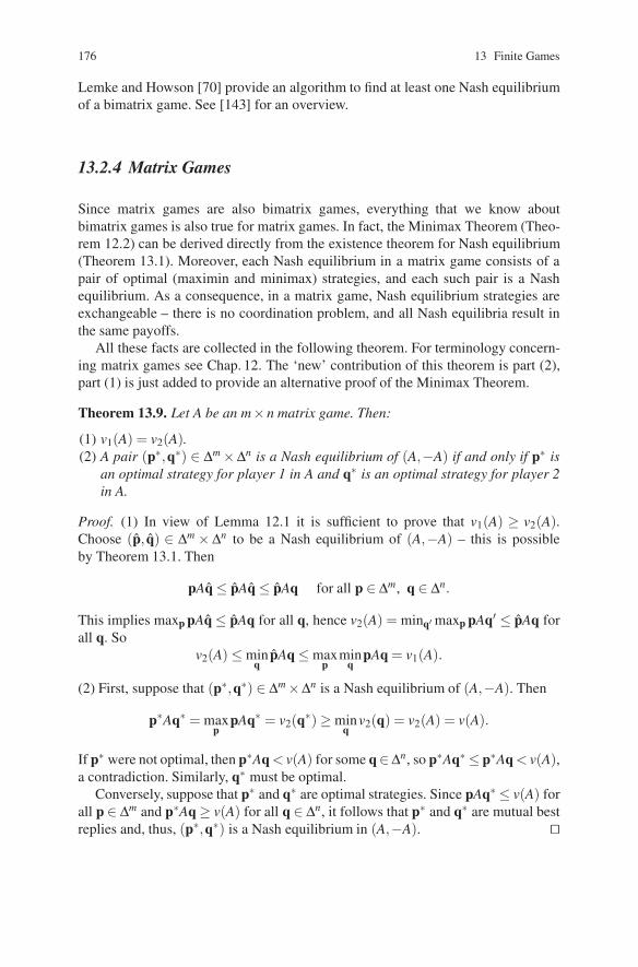
176 13 Finite Games
Lemke and Howson [70] provide an algorithm to find at least one Nash equilibriumof a bimatrix game. See [143] for an overview.
13.2.4 Matrix Games
Since matrix games are also bimatrix games, everything that we know aboutbimatrix games is also true for matrix games. In fact, the Minimax Theorem (Theo-rem 12.2) can be derived directly from the existence theorem for Nash equilibrium(Theorem 13.1). Moreover, each Nash equilibrium in a matrix game consists of apair of optimal (maximin and minimax) strategies, and each such pair is a Nashequilibrium. As a consequence, in a matrix game, Nash equilibrium strategies areexchangeable – there is no coordination problem, and all Nash equilibria result inthe same payoffs.
All these facts are collected in the following theorem. For terminology concern-ing matrix games see Chap. 12. The ‘new’ contribution of this theorem is part (2),part (1) is just added to provide an alternative proof of the Minimax Theorem.
Theorem 13.9. Let A be an m×n matrix game. Then:
(1) v1(A) = v2(A).(2) A pair (p∗,q∗) ∈ ∆m ×∆n is a Nash equilibrium of (A,−A) if and only if p∗ is
an optimal strategy for player 1 in A and q∗ is an optimal strategy for player 2in A.
Proof. (1) In view of Lemma 12.1 it is sufficient to prove that v1(A) ≥ v2(A).Choose (p, q) ∈ ∆m × ∆n to be a Nash equilibrium of (A,−A) – this is possibleby Theorem 13.1. Then
pAq ≤ pAq ≤ pAq for all p ∈ ∆m, q ∈ ∆n.
This implies maxp pAq ≤ pAq for all q, hence v2(A) = minq′ maxp pAq′ ≤ pAq forall q. So
v2(A) ≤ minq
pAq ≤ maxp
minq
pAq = v1(A).
(2) First, suppose that (p∗,q∗) ∈ ∆m ×∆n is a Nash equilibrium of (A,−A). Then
p∗Aq∗ = maxp
pAq∗ = v2(q∗) ≥ minq
v2(q) = v2(A) = v(A).
If p∗ were not optimal, then p∗Aq < v(A) for some q∈∆n, so p∗Aq∗ ≤ p∗Aq < v(A),a contradiction. Similarly, q∗ must be optimal.
Conversely, suppose that p∗ and q∗ are optimal strategies. Since pAq∗ ≤ v(A) forall p ∈ ∆m and p∗Aq ≥ v(A) for all q ∈ ∆n, it follows that p∗ and q∗ are mutual bestreplies and, thus, (p∗,q∗) is a Nash equilibrium in (A,−A). ��

13.3 Iterated Dominance and Best Reply 177
13.2.5 The Game of Chess: Zermelo’s Theorem
On of the earliest formal results in game theory is Zermelo’s Theorem on the gameof chess, published in [150]. In this subsection we provide a simple proof of thistheorem, based on Theorem 13.9.
The game of chess is a classical example of a zero-sum game. There are three possi-ble outcomes: a win for White, a win for Black, and a draw. Identifying player 1 withWhite and player 2 with Black, we can associate with these outcomes the payoffs(1,−1), (−1,1), and (0,0), respectively. In order to guarantee that the (extensiveform) game stops after finitely many moves, we assume the following stopping rule:if the same configuration on the chess board has occurred more than twice, the gameends in a draw. Since there are only finitely many configurations on the chess board,the game must stop after finitely many moves. Note that the chess game is a finiteextensive form game of perfect information and therefore has a Nash equilibrium inpure strategies – see Sect. 4.3. To be precise, this is a pure strategy Nash equilibriumin the associated matrix game, where mixed strategies are allowed as well.
Theorem 13.10 (Zermelo’s Theorem). In the game of chess, either White has apure strategy that guarantees a win, or Black has a pure strategy that guarantees awin, or both players have pure strategies that guarantee at least a draw.
Proof. Let A = (ai j) denote the associated matrix game, and let row i∗ and columnj∗ constitute a pure strategy Nash equilibrium. We distinguish three cases.
Case 1. ai∗ j∗ = 1, i.e., White wins. By Theorem 13.9, v(A) = 1. I.e., White has apure strategy that guarantees a win, namely play row i∗.
Case 2. ai∗ j∗ = −1, i.e., Black wins. By Theorem 13.9, v(A) = −1. I.e., Black hasa pure strategy that guarantees a win, namely play column j∗.
Case 3. ai∗ j∗ = 0, i.e., the game ends in a draw. By Theorem 13.9, v(A) = 0. Hence,both White and Black can guarantee at least a draw by playing row i∗ and columnj∗, respectively. ��
13.3 Iterated Dominance and Best Reply
A pure strategy of a player in a finite game is strictly dominated if there is another(mixed or pure) strategy that yields always – whatever the other players do – astrictly higher payoff. Such a strategy is not played in a Nash equilibrium, andcan therefore be eliminated. In the smaller game there may be another pure strat-egy of the same or of another player that is strictly dominated and again may beeliminated. This way a game may be reduced to a smaller game for which it is eas-ier to compute the Nash equilibria. If the procedure results in a unique survivingstrategy combination then the game is called dominance solvable, but this is a rareexception.

178 13 Finite Games
We applied these ideas before, in Chaps. 2 and 3. In this section we show,formally, that by this procedure of iterated elimination of strictly dominated strate-gies no Nash equilibria of the original game are lost, and no Nash equilibria areadded.
For iterated elimination of weakly dominated strategies the situation is differ-ent: Nash equilibria may be lost, and the final result may depend on the order ofelimination. See Problem 3.6.
We start with repeating the definition of a strictly dominated strategy for an arbitraryfinite game.
Definition 13.11. Let G = (N,S1, . . . ,Sn,u1, . . . ,un) be a finite game, i ∈ N, si ∈ Si.Strategy si is strictly dominated by strategy σi ∈ ∆(Si) if ui(σi,σ−i) > ui(si,σ−i) forall σ−i ∈ ∏ j =i ∆(S j). Strategy si ∈ Si is strictly dominated if it is strictly dominatedby some strategy σi ∈ ∆(Si).
The fact that iterated elimination of strictly dominated strategies does not essentiallychange the set of Nash equilibria of a game is a straightforward consequence of thefollowing lemma.
Lemma 13.12. Let G = (N,S1, . . . ,Sn,u1, . . . ,un) be a finite game, i∈ N, and let si ∈Si be strictly dominated. Let G′ = (N,S1, . . . ,Si−1,Si \ {si},Si+1, . . . ,Sn,u′1, . . . ,u
′n)
be the game arising from G be eliminating si from Si and restricting the utilityfunctions accordingly. Then:
(1) If σ is a Nash equilibrium in G, then σi(si) = 0 (where σi(si) is the probabilityassigned by σi to pure strategy si ∈ Si ) and σ ′ is a Nash equilibrium in G′,where σ ′
j = σ j for each j ∈ N \ {i} and σ ′i is the restriction of σi to Si \ {si}.
(2) If σ ′ is a Nash equilibrium in G′, then σ is a Nash equilibrium in G, whereσ j = σ ′
j for each j ∈ N \ {i} and σi(ti) = σ ′i (ti) for all ti ∈ Si \ {si}.
Proof. (1) Let σ be a Nash equilibrium in G, and let τi ∈ ∆(Si) strictly dominate si.If σi(si) > 0, then
ui(σi + σi(si)τi,σ−i) > ui(σi,σ−i),
where σi : Si →R is defined by σi(ti) = σi(ti) for all ti ∈ Si\{si} and σi(si) = 0. Thiscontradicts the assumption that σ is a Nash equilibrium in G. Therefore, σi(si) = 0.With σ ′ and G′ as above, we have
u′i(σ′1, . . . ,σ
′i−1,τ
′i ,σ
′i+1, . . . ,σ
′n) = ui(σ1, . . . ,σi−1, τ ′i ,σi+1, . . . ,σn),
for every τ ′i ∈ ∆(Si \ {si}), where τ ′i ∈ ∆(Si) assigns 0 to si and is equal to τ ′i other-wise. From this it follows that σ ′
i is still a best reply to σ ′−i. It is straightforward thatalso for each j = i, σ ′
j is still a best reply to σ ′− j. Hence σ ′ is a Nash equilibriumin G′.
(2) Let σ ′ and σ be as above in (2). Obviously, for every player j = i, σ j is still abest reply in σ since σi(si) = 0, i.e., player i puts zero probability on the new purestrategy si. For player i, σi is certainly a best reply among all strategies that put zero

13.3 Iterated Dominance and Best Reply 179
probability on si. But then, σi is a best reply among all strategies, since strategiesthat put nonzero probability on si can never be best replies by the first argument inthe proof of (1). Hence, σ is a Nash equilibrium in G. ��Obviously, a strictly dominated pure strategy is not only never played in a Nashequilibrium, but, a forteriori, is never (part of) a best reply. Formally, we say that apure strategy si of player i in the finite game G = (N,S1, . . . ,Sn,u1, . . . ,un) is nevera best reply if for all (σ j) j =i and all σi ∈ βi((σ j) j =i), we have σi(si) = 0. Thefollowing result (cf. [99]) shows that for two-player games also the converse holds.
Theorem 13.13. In a finite two-person game every pure strategy that is never a bestreply, is strictly dominated.
Proof. Let (A,B) be an m × n bimatrix game and suppose without loss of gen-erality that pure strategy e1 ∈ ∆m of player 1 is never a best reply. Let b =(−1,−1, . . . ,−1) ∈ Rn.
Let A be the (m−1)×n matrix with i-th row equal to the first row of A minus thei+ 1-th row of A, i.e., ai j = a1 j −ai+1, j for every i = 1, . . . ,m−1 and j = 1, . . . ,n.The assumption that the pure strategy e1 of player 1 is never a best reply is equivalentto the statement that the system
Aq ≥ 0, q ∈ ∆n
has no solution. This, in turn, is equivalent to the statement that the system
Aq ≥ 0, q ≥ 0, q ·b < 0
has no solution. This means that the system in (2) of Lemma 22.6 (with A instead ofA there) has no solution. Hence, this lemma implies that the system
x ∈ Rm−1, xA ≤ b, x ≥ 0
has a solution. By definition of b and A we have for such a solution x = (x2, . . . ,xm):
x ≥ 0 andm
∑i=2
xi eiA ≥m
∑i=2
xi e1A +(1, . . . ,1).
This implies that x = 0 and therefore that e1 is strictly dominated by the strategy
(0,x2/m
∑i=2
xi, . . . ,xm/m
∑i=2
xi) ∈ ∆m.
Hence, e1 is strictly dominated. ��For games with more than two players Theorem 13.13 does not hold, see Prob-lem 13.11 for a counterexample.
The concept of ‘never a best reply’ is closely related to the concept of rationalizabil-ity (Bernheim [10], Pearce [99]). Roughly, rationalizable strategies are strategies

180 13 Finite Games
that survive a process of iterated elimination of strategies that are never a best reply.Just like the strategies surviving iterated elimination of strictly dominated strategies,rationalizable strategies constitute a set-valued solution concept. The above theoremimplies that for two-player games the two solution concepts coincide. In general, theset of rationalizable strategies is a subset of the set of strategies that survive iteratedelimination of strictly dominated strategies.
The implicit assumption justifying iterated elimination of strategies that are domi-nated or never a best reply is quite demanding. Not only should a player believe thatsome other player will not play a such a strategy, but he should also believe that theother player believes that he (the first player) believes this and, in turn, will not usesuch a strategy in the reduced game, etc.2
13.4 Perfect Equilibrium
Since a game may have many, quite different Nash equilibria, literature has focusedsince a long time on so-called refinements of Nash equilibrium. We have seenexamples of this in extensive form games, such as subgame perfect equilibriumand perfect Bayesian equilibrium (Chaps. 4, 5). One of the earliest and best knownrefinements of Nash equilibrium in strategic form games is the concept of ‘trem-bling hand perfection’, introduced by Selten [118]. This refinement excludes Nashequilibria that are not robust against ‘trembles’ in the players’ strategies.
Formally, let G = (N,S1, . . . ,Sn,u1, . . . ,un) be a finite game and let µ be an errorfunction, assigning a number µih ∈ (0,1) to every i ∈ N and h ∈ Si, such that∑h∈Si µih < 1 for every player i. The number µih is the minimum probability withwhich player i is going to play pure strategy h, perhaps by ‘mistake’ (‘tremblinghand’). Let, for each i ∈ N, ∆(Si,µ) = {σi ∈ ∆(Si) | σi(h) ≥ µih for all h ∈ Si}, andlet G(µ) denote the game derived from G by assuming that each player i may onlychoose strategies from ∆(Si,µ). The game G(µ) is called the µ-perturbed game.Denote the set of Nash equilibria of G by NE(G) and of G(µ) by NE(G(µ)).
Lemma 13.14. For every error function µ , NE(G(µ)) = /0.
Proof. Analogous to the proof of Theorem 13.1. ��A perfect Nash equilibrium is a Nash equilibrium that is the limit of some sequenceof Nash equilibria of perturbed games. Formally:
Definition 13.15. A strategy combination σ ∈ NE(G) is perfect if there is asequence G(µ t), t ∈ N of perturbed games with µ t → 0 for t → ∞ and a sequenceof Nash equilibria σ t ∈ G(µ t) such that σ t → σ for t → ∞.
2 See [132] or [102].

13.4 Perfect Equilibrium 181
As follows from the proof of Theorem 13.17 below, a perfect strategy combinationis indeed a Nash equilibrium.
Call a strategy combination σ in G completely mixed if σi(h) > 0 for all i ∈ N andh ∈ Si.
Lemma 13.16. A completely mixed Nash equilibrium of G is perfect.
Proof. Problem 13.12. ��Also if a game has no completely mixed Nash equilibrium, it still has a perfect Nashequilibrium.
Theorem 13.17. Every finite game G = (N,S1, . . . ,Sn,u1, . . . ,un) has a perfect Nashequilibrium.
Proof. Take any sequence (G(µ t))µt→0 of perturbed games and σ t ∈ NE(G(µ t))for each t ∈ N. Since ∏i∈N ∆(Si) is a compact set we may assume without loss ofgenerality that the sequence (σ t)t∈N converges to some σ ∈ ∏i∈N ∆(Si). It is easy toverify that σ ∈ NE(G), hence, σ is a perfect Nash equilibrium. ��The following lemma relates the Nash equilibria of a perturbed game to pure bestreplies in such a game.
Lemma 13.18. Let G(µ) be a perturbed game and σ a strategy combination inG(µ).
(1) If σ ∈ NE(G(µ)), i ∈ N, h ∈ Si, and σi(h) > µih, then h ∈ βi(σ−i).(2) If for all i ∈ N and h ∈ Si, σi(h) > µih implies h ∈ βi(σ−i), then σ ∈ NE(G(µ)).
Proof. (1) Let σ ∈ NE(G(µ)), i ∈ N, h ∈ Si, and σi(h) > µih. Suppose, contrary towhat we wish to prove, that h /∈ βi(σ−i). Take h′ ∈ Si with h′ ∈ βi(σ−i). (Such anh′ exists by an argument similar to the proof of Lemma 13.3.) Consider the strategyσ ′
i defined by σ ′i (h) = µih, σ ′
i (h′) = σi(h′) + σi(h)− µih, and σ ′
i (k) = σi(k) forall k ∈ Si \ {h,h′}. Then σ ′
i ∈ ∆(Si,µ) and ui(σ ′i ,σ−i) > ui(σ), contradicting the
assumption σ ∈ NE(G(µ)).
(2) Let i ∈ N. The condition in (2) implies that, if h ∈ Si and h /∈ βi(σ−i), thenσi(h) = µih. This implies that σi is a best reply to (σ j) j =i. Thus, σ ∈ NE(G(µ)). ��Below we present two characterizations of perfect Nash equilibrium that both avoidsequences of perturbed games. The first one is based on the notion of ε-equilibrium,introduced in [87].
Let ε > 0. A strategy combination σ ∈ ∏i∈N ∆(Si) is an ε-perfect equilibrium ofG if it is completely mixed and σi(h)≤ ε for all i∈N and all h∈ Si with h /∈ βi(σ−i).
An ε-perfect equilibrium of G need not be a Nash equilibrium of G, but it putsprobabilities of at most ε on pure strategies that are not best replies.
The announced characterizations are collected in the following theorem.3
3 This theorem is based on [118] and [87] and appears as Theorem 2.2.5 in [138].

182 13 Finite Games
Theorem 13.19. Let G = (N,S1, . . . ,Sn,u1, . . . ,un) and σ ∈ ∏i∈N ∆(Si). The follow-ing statements are equivalent:
(1) σ is a perfect Nash equilibrium of G;(2) σ is a limit of a sequence of ε-perfect equilibria σε of G for ε → 0;(3) σ is a limit of a sequence of completely mixed strategy combinations σε for
ε → 0, where σi ∈ βi(σε−i) for each i ∈ N and each σε in this sequence.
Proof. (1) ⇒ (2): Take a sequence of perturbed games G(µ t), t ∈ N with µ t → 0and a sequence σ t ∈ NE(G(µ t)) with σ t → σ . For each t define εt ∈ R by εt =max{µih | i ∈ N, h ∈ Si}. Then, by Lemma 13.18(1), σ t is an εt -equilibrium forevery t. So (2) follows.
(2) ⇒ (3): Take a sequence of ε-equilibria σε as in (2) converging to σ for ε → 0.Let i ∈ N. By the definition of ε-perfect equilibrium, if σi(h) > 0 for some h ∈ Si,then for ε sufficiently small we have h ∈ βi(σ−i). This implies σi ∈ βi(σ−i). So (3)follows.
(3) ⇒ (1): Let σεt(t ∈ N) be a sequence as in (3) with εt → 0 and σεt → σ as
t → ∞. For each t ∈ N, i ∈ N and h ∈ Si define µ tih = σεt
i (h) if σi(h) = 0 and µ tih =
εt otherwise. Then, for εt sufficiently small, µ t is an error function, G(µ t) is aperturbed game, and σεt
is a strategy combination in G(µ t). By Lemma 13.18(2),σεt ∈ NE(G(µ t )). So σ is a perfect Nash equilibrium of G. ��There is a close relation between the concept of domination and the concept of per-fection. We first extend the concept of (weak) domination to mixed strategies. In thegame G = (N,S1, . . . ,Sn,u1, . . . ,un), call a strategy σi ∈ ∆(Si) (weakly) dominatedby σ ′
i ∈ ∆(Si) if ui(σi,σ−i) ≤ ui(σ ′i ,σ−i) for all σ−i ∈ ∏ j =i ∆(S j), with at least one
inequality strict. (Observe that it is actually sufficient to check this for combinationss−i ∈ ∏ j =i Si.) Call σi undominated if there is no σ ′
i by which it is dominated, andcall a strategy combination σ undominated if σi is undominated for every i ∈ N. Wenow have:
Theorem 13.20. Every perfect Nash equilibrium in G is undominated.
Proof. Let σ be a perfect Nash equilibrium and suppose that (say) σ1 is dominated.Then there is a σ ′
1 ∈ ∆(S1) such that u1(σ1,s−1) ≤ u1(σ ′1,s−1) for all s−1 ∈ ∏n
i=2 Si,with at least one inequality strict. Take a sequence (σ t)t∈N of strategy combinationsas in (3) of Theorem 13.19, converging to σ . Then, since every σ t is completelymixed, we have u1(σ1,σ t
−1) < u1(σ ′1,σ t
−1) for every t. This contradicts the fact thatσ1 is a best reply to σ t
−1. ��The converse of Theorem 13.20 is only true for two-person games. For a
counterexample involving three players, see Problem 13.13.For proving the converse of the theorem for bimatrix games, we use the following
auxiliary lemma. In this lemma, for a matrix game A, C2(A) denotes the set of allcolumns of A that are in the carrier of some optimal strategy of player 2 in A.
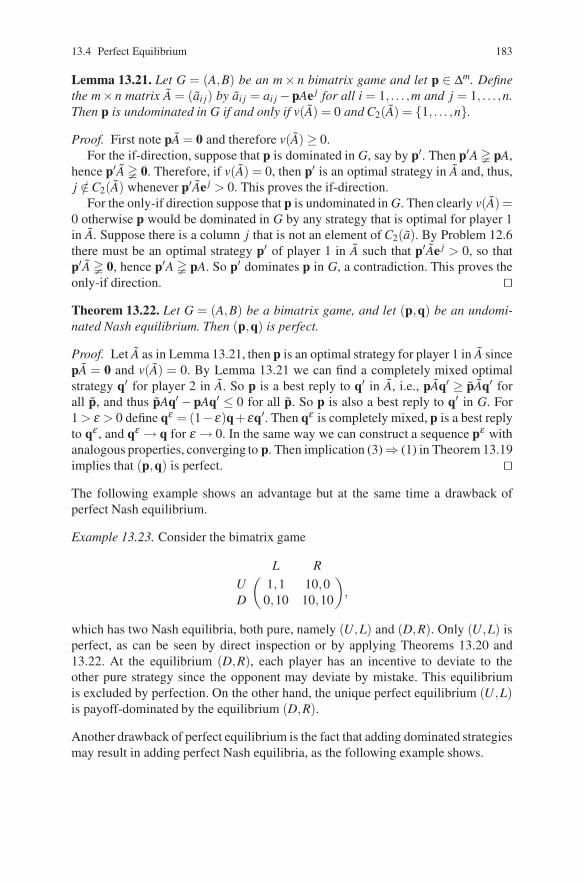
13.4 Perfect Equilibrium 183
Lemma 13.21. Let G = (A,B) be an m× n bimatrix game and let p ∈ ∆m. Definethe m×n matrix A = (ai j) by ai j = ai j −pAe j for all i = 1, . . . ,m and j = 1, . . . ,n.Then p is undominated in G if and only if v(A) = 0 and C2(A) = {1, . . . ,n}.
Proof. First note pA = 0 and therefore v(A) ≥ 0.For the if-direction, suppose that p is dominated in G, say by p′. Then p′A � pA,
hence p′A � 0. Therefore, if v(A) = 0, then p′ is an optimal strategy in A and, thus,j /∈C2(A) whenever p′Ae j > 0. This proves the if-direction.
For the only-if direction suppose that p is undominated in G. Then clearly v(A) =0 otherwise p would be dominated in G by any strategy that is optimal for player 1in A. Suppose there is a column j that is not an element of C2(a). By Problem 12.6there must be an optimal strategy p′ of player 1 in A such that p′Ae j > 0, so thatp′A � 0, hence p′A � pA. So p′ dominates p in G, a contradiction. This proves theonly-if direction. ��Theorem 13.22. Let G = (A,B) be a bimatrix game, and let (p,q) be an undomi-nated Nash equilibrium. Then (p,q) is perfect.
Proof. Let A as in Lemma 13.21, then p is an optimal strategy for player 1 in A sincepA = 0 and v(A) = 0. By Lemma 13.21 we can find a completely mixed optimalstrategy q′ for player 2 in A. So p is a best reply to q′ in A, i.e., pAq′ ≥ pAq′ forall p, and thus pAq′ −pAq′ ≤ 0 for all p. So p is also a best reply to q′ in G. For1 > ε > 0 define qε = (1−ε)q+εq′. Then qε is completely mixed, p is a best replyto qε , and qε → q for ε → 0. In the same way we can construct a sequence pε withanalogous properties, converging to p. Then implication (3)⇒ (1) in Theorem 13.19implies that (p,q) is perfect. ��The following example shows an advantage but at the same time a drawback ofperfect Nash equilibrium.
Example 13.23. Consider the bimatrix game
( L RU 1,1 10,0D 0,10 10,10
),
which has two Nash equilibria, both pure, namely (U,L) and (D,R). Only (U,L) isperfect, as can be seen by direct inspection or by applying Theorems 13.20 and13.22. At the equilibrium (D,R), each player has an incentive to deviate to theother pure strategy since the opponent may deviate by mistake. This equilibriumis excluded by perfection. On the other hand, the unique perfect equilibrium (U,L)is payoff-dominated by the equilibrium (D,R).
Another drawback of perfect equilibrium is the fact that adding dominated strategiesmay result in adding perfect Nash equilibria, as the following example shows.

184 13 Finite Games
Example 13.24. In the game
⎛⎝L C R
U 1,1 0,0 −1,−2M 0,0 0,0 0,−2D −2,−1 −2,0 −2,−2
⎞⎠,
there are two perfect Nash equilibria, namely (U,L) and (M,C). If we reduce thegame by deleting the pure strategies D and R, the only perfect equilibrium thatremains is (U,L).
This motivated the introduction of a further refinement called proper Nash equilib-rium in [87]. See the next section.
13.5 Proper Equilibrium
A perfect equilibrium is required to be robust only against some ‘trembles’ and,moreover, there are no further conditions on these trembles. Myerson [87] proposesthe additional restriction that trembles be less probable if they are more ‘costly’.
Given some ε > 0, call a strategy combination σ in the game G = (N,S1, . . . ,Sn,u1, . . . ,un) an ε-proper equilibrium if σ is completely mixed and for all i ∈ Nand h,k ∈ Si we have
ui(h,σ−i) < ui(k,σ−i) ⇒ σi(h) ≤ εσi(k).
Observe that an ε-proper equilibrium does not have to be a Nash equilibrium.
Definition 13.25. A strategy combination σ in G is proper if, for some sequenceεt → 0, there exist εt -proper equilibria σ(εt ) such that σ(εt) → σ .
Since, in a proper strategy combination σ , a pure strategy h of a player i that isnot a best reply to σ−i is played with probability 0, it follows that a proper strategycombination is a Nash equilibrium.4 Moreover, since it is straightforward by thedefinitions that an ε-proper equilibrium is also an ε-perfect equilibrium, it followsfrom Theorem 13.19 that a proper equilibrium is perfect. Hence, properness is arefinement of perfection. Example 13.24 shows that this refinement is strict: theNash equilibrium (M,C) is perfect but not proper. To see this, note that in an ε-proper equilibrium (p,q) we must have at least q3 ≤ εq1. But then U is a best replyof player 1, hence it is not possible that a sequence of such ε-proper equilibriaconverges to (M,C).
4 Note that, by replacing the word ‘proper’ by ‘perfect’ in Definition 13.25, we obtain an alternativedefinition of perfect (Nash) equilibrium. This follows from Theorem 13.19.

13.6 Strictly Perfect Equilibrium 185
A proper Nash equilibrium always exists:
Theorem 13.26. Let G = (N,S1, . . . ,Sn,u1, . . . ,un) be a finite game. Then G has aproper Nash equilibrium.
Proof. It is sufficient to show that for ε > 0 close to 0 there exists an ε-properequilibrium of G. Let 0 < ε < 1 and define the error function µ by µik = ε |Si|/|Si|for all i ∈ N and k ∈ Si. For every i ∈ N and σ ∈ ∏ j∈N ∆(S j,µ) define
Fi(σ) = {τi ∈ ∆(Si,µ) | ∀k, l ∈ Si [ui(k,σ−i) < ui(l,σ−i) ⇒ τi(k) ≤ ετi(l)]}.
Then Fi(σ) = /0 as can be seen as follows. Define
vi(σ ,k) = |{l ∈ Si | ui(k,σ−i) < ui(l,σ−i)}|,
for all k ∈ Si, and τi(k) = εvi(σ ,k)/∑l εvi(σ ,l) for all k ∈ Si. Then τi ∈ Fi(σ). Considerthe correspondence
F : ∏j∈N
∆(S j,µ) → ∏j∈N
∆(S j,µ), σ �→ ∏i∈N
Fi(σ).
Then F satisfies the conditions of the Kakutani fixed point theorem (Theorem 22.10)– see Problem 13.14. Hence, F has a fixed point, and each fixed point of F is anε-proper equilibrium of G. ��In spite of the original motivation for introducing properness, this concept suffersfrom the same deficit as perfect equilibrium: adding strictly dominated strategiesmay enlarge the set of proper Nash equilibria. See Problem 13.15 for an example ofthis.
13.6 Strictly Perfect Equilibrium
Another refinement of perfect equilibrium is obtained by requiring robustness of aNash equilibrium with respect to all ‘trembles’. This results in the concept of strictlyperfect equilibrium (Okada [95]).
Definition 13.27. A strategy combination σ in the game G = (N,S1, . . . ,Sn,u1, . . . ,un) is strictly perfect if, for every sequence {G(µ t)}µt→0 of perturbed gamesthere exist profiles σ t ∈ NE(G(µ t)) such that σ t → σ .
Clearly, a strictly perfect strategy combination is a perfect Nash equilibrium.For some further observations concerning strictly perfect equilibrium seeProblem 13.16.

186 13 Finite Games
13.7 Correlated Equilibrium
In the preceding sections we studied several refinements of Nash equilibrium. Inthis section the set of Nash equilibria is extended in a way to become clear below.It is, however, not the intention to enlarge the set of Nash equilibria but rather toenable the players to reach better payoffs by allowing some communication device.This is going to result in the concept of correlated equilibrium, introduced in [5].Attention in this section is restricted to bimatrix games, and we closely follow thepresentation in [98].
In order to fix ideas, consider the situation where two car drivers approach aroad crossing. Each driver has two pure strategies: ‘stop’ (s) or ‘cross’(c). Thepreferences for the resulting combinations are as expressed by the following table:
(A,B) =( c s
c −10,−10 5,0s 0,5 −1,−1
).
This bimatrix game has two asymmetric and seemingly unfair pure Nash equilibria,and one symmetric mixed Nash equilibrium ((3/8,5/8),(3/8,5/8)), resulting in anexpected payoff of −5/8 for both, and therefore also not quite satisfying.
Now suppose that traffic lights are installed that indicate c (‘green’) or s (‘red’)according to the probabilities in the following table:
( c sc 0.00 0.55s 0.40 0.05
).
E.g., with probability 0.55 (55% of the time) the light is green for driver 1 and redfor driver 2. Assume that the players (drivers) are not forced to obey the traffic lightsbut know the probabilities as given in the table. We argue that it is in each player’sown interest to obey the lights if the other player does so.
If the light is green for player 1 then player 1 knows with certainty that the lightis red for player 2. So if player 2 obeys the lights and stops, it is indeed optimal forplayer 1 to cross. If the light is red for player 1, then the conditional probability thatplayer 2 crosses (if he obeys the lights) is equal to 0.4/0.45 ≈ 0.89 and the condi-tional probability that player 2 stops is 0.05/0.45 ≈ 0.11. So if player 1 stops, hisexpected payoff is 0.89 ·0+0.11 ·−1 =−0.11, and if he crosses his expected payoffis 0.89 ·−10 + 0.11 ·5 = −8.35. Clearly, it is optimal for player 1 to obey the lightand stop. For player 2 the argument is similar, so that we can indeed talk of an equi-librium: such an equilibrium is called a correlated equilibrium. Note that there is nomixed strategy combination in the game (A,B) that induces these probabilities. Interms of the situation in the example, this particular equilibrium cannot be reachedwithout traffic lights serving as a communication device between the players. Theoverall expected payoffs of the players are 0.55 ·5+0.05 ·−1 = 2.7 for player 1 and

13.7 Correlated Equilibrium 187
0.40 · 5 + 0.05 ·−1 = 1.95 for player 2, which is considerably better for both thanthe payoffs in the mixed Nash equilibrium.
In general, let (A,B) be an m× n bimatrix game. A correlated strategy is an m× nmatrix P = (pi j) with ∑m
i=1 ∑nj=1 pi j = 1 and pi j ≥ 0 for all i = 1, . . . ,m, j = 1, . . . ,n.
A correlated strategy P can be thought of as a communication device: the pair (i, j)is chosen with probability pi j, and if that happens, player 1 receives the signal i andplayer 2 the signal j. Suppose player 2 obeys the signal. If player 1 receives signal iand indeed plays i, his expected payoff is
n
∑j=1
pi jai j/∑ n
j=1 pi j,
and if he plays row k instead, his expected payoff is
n
∑j=1
pi jak j/∑ n
j=1 pi j.
So to keep player 1 from disobeying the received signal, we should have
n
∑j=1
(ai j −ak j)pi j ≥ 0 for all i,k = 1, . . . ,m. (13.5)
The analogous condition for player 2 is
m
∑i=1
(bi j −bil)pi j ≥ 0 for all j, l = 1, . . . ,n. (13.6)
Definition 13.28. A correlated equilibrium in the bimatrix game (A,B) is a corre-lated strategy P = (pi j) satisfying (13.5) and (13.6).
For the two-driver example conditions (13.5) and (13.6) result in four inequalities,which are not difficult to solve (Problem 13.17). In general, any Nash equilibriumof a bimatrix game results in a correlated equilibrium (Problem 13.18), so existenceof a correlated equilibrium is not really an issue.
The set of correlated equilibria is convex (Problem 13.19), so the convex hull ofall payoff pairs corresponding to the Nash equilibria of a bimatrix game consists ofpayoff pairs attainable in correlated equilibria. Problem 13.20 presents an exampleof a game in which some payoff pairs can be reached in correlated equilibria but notas convex combinations of payoff pairs of Nash equilibria.
In general, correlated equilibria can be computed using linear programming. Specifi-cally, let (A,B) be an m×n bimatrix game. We associate with (A,B) an mn×(m(m−1)+n(n−1)) matrix C as follows. For each pair (i, j)of a row and a column in (A,B)

188 13 Finite Games
we have a row in C, and for each pair (h,k) of two different rows in (A,B) or twodifferent columns in (A,B) we have a column in C. We define
c(i, j)(h,k) =
⎧⎨⎩ai j −ak j if i = h ∈ {1, . . . ,m} and k ∈ {1, . . . ,m}bi j −bih if j = k ∈ {1, . . . ,n} and h ∈ {1, . . . ,n}0 otherwise.
Consider C as a matrix game. By construction of C and (13.5) and (13.6), any cor-related equilibrium P = (pi j) of (A,B) viewed as a strategy p of player 1 in C (notto be confused with player 1 in (A,B)) has an expected payoff vector pC ≥ 0, andtherefore v(C), the value of the matrix game C, is nonnegative. In particular, thisimplies that any optimal strategy of player 1 in C is a correlated equilibrium in(A,B). If v(C) = 0 then any correlated equilibrium in (A,B) is an optimal strategyof player 1 in C, but if v(C) > 0 then there may be correlated equilibria in (A,B)that are not optimal strategies for player 1 in C – they may only guarantee zero. Thelatter is the case in the two-drivers example (Problem 13.21).
Matrix games can be solved by linear programming, see Sect. 12.2.We conclude with an example5 in which the described technique is applied.
Example 13.29. Consider the bimatrix game
(A,B) =( 1′ 2′ 3′
1 3,1 2,5 6,02 1,4 3,3 2,6
).
The associated matrix game C is as follows.
⎛⎜⎜⎜⎜⎜⎜⎝
(1,2) (2,1) (1′,2′) (1′,3′) (2′,1′) (2′,3′) (3′,1′) (3′,2′)(1,1′) 2 0 −4 1 0 0 0 0(1,2′) −1 0 0 0 4 5 0 0(1,3′) 4 0 0 0 0 0 −1 −5(2,1′) 0 −2 1 −2 0 0 0 0(2,2′) 0 1 0 0 −1 −3 0 0(2,3′) 0 −4 0 0 0 0 2 3
⎞⎟⎟⎟⎟⎟⎟⎠.
It can be checked that this game has value 0, by using the optimal strategies
P =( 1′ 2′ 3′
1 0 0.3 0.0752 0 0.5 0.125
)for player 1 in C and (0,0,1/2,1/2,0,0,0,0) for player 2 in C. The optimal strategyfor player 1 in C is unique, and since v(C) = 0 this implies that the game (A,B) hasa unique correlated equilibrium. Consequently, this must correspond to the unique
5 This is Example VIII.4.4 in [98].

13.8 A Characterization of Nash Equilibrium 189
Nash equilibrium of the game. Indeed, ((3/8,5/8),(0,4/5,1/5)) is the unique Nashequilibrium of (A,B) and it results in the probabilities given by P.
13.8 A Characterization of Nash Equilibrium
The concept of Nash equilibrium requires strong behavioral assumptions about theplayers. Each player should be able to guess what other players will do, assume thatother players know this and make similar conjectures, etc., and all this should bein equilibrium. The basic difficulty is that Nash equilibrium is a circular concept.Not surprisingly, theories of repeated play or learning or, more generally, dynamicmodels that aim to explain how players in a game come to play a Nash equilibrium,have in common that they change the strategic decision into a collection of single-player decision problems.6
In this section (based on [101]) we review a different approach, which is axiomaticin nature. The Nash equilibrium concept is viewed as a solution concept: a corre-spondence which assigns to any finite game a set of strategy combinations. One ofthe conditions (axioms) put on this correspondence is a condition of consistencywith respect to changes in the number of players: if a player leaves the game, leav-ing his strategy as an input behind, then the other players should not want to changetheir strategies. This is certainly true for Nash equilibrium, but can be put as anabstract condition on a solution correspondence. By assuming that players in single-player games – hence, in ‘simple’ maximization problems – behave rationally, andby adding a converse consistency condition, it follows that the solution correspon-dence must be the Nash equilibrium correspondence. We proceed with a formaltreatment of this axiomatic characterization.
Let Γ be a collection of finite games of the form G = (N,S1, . . . ,Sn, u1, . . . ,un). (It isimplicit that also the set of players N may vary in Γ .) A solution on Γ is a functionϕ that assigns to each G ∈ Γ a set of strategy combinations ϕ(G) ⊆ ∏i∈N ∆(Si).7 Aparticular solution is the Nash correspondence NE , assigning to each G ∈ Γ the setNE(G) of all Nash equilibria in G.
Definition 13.30. The solution ϕ satisfies one-person rationality (OPR) if for everyone-person game G = ({i},Si,ui) in Γ
ϕ(G) = {σi ∈ ∆(Si) | ui(σi) ≥ ui(τi) for all τi ∈ ∆(Si)}.
The interpretation of OPR is clear and needs no further comments.Let G = (N,S1, . . . ,Sn, u1, . . . ,un) be a game, /0 = M ⊆ N, and let σ be a strategy
combination in G. The reduced game of G with respect to M and σ is the gameGM,σ = (M,(Si)i∈M,(uσ
i )i∈M), where uσi (τ) = ui(τ,σN\M) for all τ ∈ ∏ j∈M ∆(S j).8
6 See, e.g., [149].7 The presentation in [101] is for more general games.8 For a subset T ⊆ N, denote (σ j) j∈T by σT .
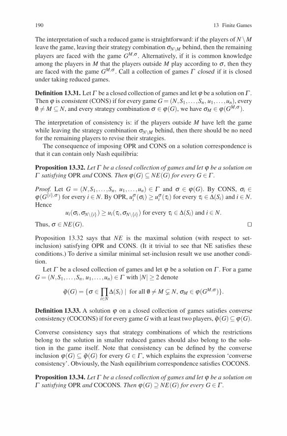
190 13 Finite Games
The interpretation of such a reduced game is straightforward: if the players of N \Mleave the game, leaving their strategy combination σN\M behind, then the remainingplayers are faced with the game GM,σ . Alternatively, if it is common knowledgeamong the players in M that the players outside M play according to σ , then theyare faced with the game GM,σ . Call a collection of games Γ closed if it is closedunder taking reduced games.
Definition 13.31. Let Γ be a closed collection of games and let ϕ be a solution on Γ .Then ϕ is consistent (CONS) if for every game G = (N,S1, . . . ,Sn, u1, . . . ,un), every/0 = M ⊆ N, and every strategy combination σ ∈ ϕ(G), we have σM ∈ ϕ(GM,σ ).
The interpretation of consistency is: if the players outside M have left the gamewhile leaving the strategy combination σN\M behind, then there should be no needfor the remaining players to revise their strategies.
The consequence of imposing OPR and CONS on a solution correspondence isthat it can contain only Nash equilibria:
Proposition 13.32. Let Γ be a closed collection of games and let ϕ be a solution onΓ satisfying OPR and CONS. Then ϕ(G) ⊆ NE(G) for every G ∈ Γ .
Proof. Let G = (N,S1, . . . ,Sn, u1, . . . ,un) ∈ Γ and σ ∈ ϕ(G). By CONS, σi ∈ϕ(G{i},σ ) for every i ∈ N. By OPR, uσ
i (σi) ≥ uσi (τi) for every τi ∈ ∆(Si) and i ∈ N.
Henceui(σi,σN\{i}) ≥ ui(τi,σN\{i}) for every τi ∈ ∆(Si) and i ∈ N.
Thus, σ ∈ NE(G). ��Proposition 13.32 says that NE is the maximal solution (with respect to set-inclusion) satisfying OPR and CONS. (It it trivial to see that NE satisfies theseconditions.) To derive a similar minimal set-inclusion result we use another condi-tion.
Let Γ be a closed collection of games and let ϕ be a solution on Γ . For a gameG = (N,S1, . . . ,Sn, u1, . . . ,un) ∈ Γ with |N| ≥ 2 denote
ϕ(G) = {σ ∈ ∏i∈N
∆(Si) | for all /0 = M � N, σM ∈ ϕ(GM,σ )}.
Definition 13.33. A solution ϕ on a closed collection of games satisfies converseconsistency (COCONS) if for every game G with at least two players, ϕ(G)⊆ϕ(G).
Converse consistency says that strategy combinations of which the restrictionsbelong to the solution in smaller reduced games should also belong to the solu-tion in the game itself. Note that consistency can be defined by the converseinclusion ϕ(G) ⊆ ϕ(G) for every G ∈ Γ , which explains the expression ‘converseconsistency’. Obviously, the Nash equilibrium correspondence satisfies COCONS.
Proposition 13.34. Let Γ be a closed collection of games and let ϕ be a solution onΓ satisfying OPR and COCONS. Then ϕ(G) ⊇ NE(G) for every G ∈ Γ .

Problems 191
Proof. The proof is by induction on the number of players. For one-person gamesthe inclusion follows (with equality) from OPR. Assume that NE(G) ⊆ ϕ(G) forall t-person games in Γ where t ≤ k and k ≥ 1. Let G0 be a k + 1-person game inΓ . Note that NE(G0) ⊆ NE(G0) by CONS of NE . By the induction hypothesis,NE(G0) ⊆ ϕ(G0) and by COCONS, ϕ(G0) ⊆ ϕ(G0). Thus, NE(G0) ⊆ ϕ(G0). ��Corollary 13.35. Let Γ be a closed family of games. The Nash equilibrium corre-spondence is the unique solution on Γ satisfying OPR, CONS, and COCONS.
It can be shown that the axioms in Corollary 13.35 are independent (Problem 13.23).The consistency approach fails when applied to refinements of Nash equilibrium,
see [93] for details. For instance, Problem 13.24 shows that the correspondence ofperfect equilibria is not consistent.
Problems
13.1. Existence of Nash Equilibrium
Prove that the correspondence β in the proof of Theorem 13.1 is upper semi-continuous and convex-valued. Also check that every fixed point of β is a Nashequilibrium of G.
13.2. Lemma 13.2
Prove Lemma 13.2.
13.3. Lemma 13.3
Prove Lemma 13.3.
13.4. Dominated Strategies
Let (A,B) be an m×n bimatrix game. Suppose there exists a q ∈ ∆n such that qn = 0and Bq > Ben (i.e., there exists a mixture of the first n−1 columns of B that is strictlybetter than playing the n-th column).
(a) Prove that q∗n = 0 for every Nash equilibrium (p∗,q∗).
Let (A′,B′) be the bimatrix game obtained from (A,B) be deleting the last column.
(b) Prove that (p∗,q′) is a Nash equilibrium of (A′,B′) if and only if (p∗,q∗) is aNash equilibrium of (A,B), where q′ is the strategy obtained from q∗ by deletingthe last coordinate.

192 13 Finite Games
13.5. A 3×3 Bimatrix Game
Consider the 3×3 bimatrix game
(A,B) =
⎛⎝ 0,4 4,0 5,34,0 0,4 5,33,5 3,5 6,6
⎞⎠.
Let (p,q) be a Nash equilibrium in (A,B).
(a) Prove that {1,2} � C(p).
(b) Prove that C(p) = {2,3}.
(c) Find all Nash equilibria of this game.
13.6. A 3× 2 Bimatrix Game
Use the graphical method to compute the Nash equilibria of the bimatrix game
(A,B) =
⎛⎝ 0,0 2,12,2 0,22,2 0,2
⎞⎠.
13.7. Proof of Theorem 13.8
Prove Theorem 13.8.
13.8. Matrix Games
Show that the pair of linear programs (13.3) and (13.4) is equivalent to the LP andits dual in Sect. 12.2 for solving matrix games.
13.9. Tic-Tac-Toe
The two-player game of Tic-Tac-Toe is played on a 3× 3 board. Player 1 starts byputting a cross on one of the nine fields. Next, player 2 puts a circle on one of theeight remaining fields. Then player 1 puts a cross on one of the remaining sevenfields, etc. If player 1 achieves three crosses or player 2 achieves three circles ina row (either vertically or horizontally or diagonally) then that player wins. If thisdoes not happen and the board is full, then the game ends in a draw.
(a) Design a pure maximin strategy for player 1. Show that this maximin strategyguarantees at least a draw to him.
(b) Show that player 1 cannot guarantee a win.
(c) What is the value of this game?
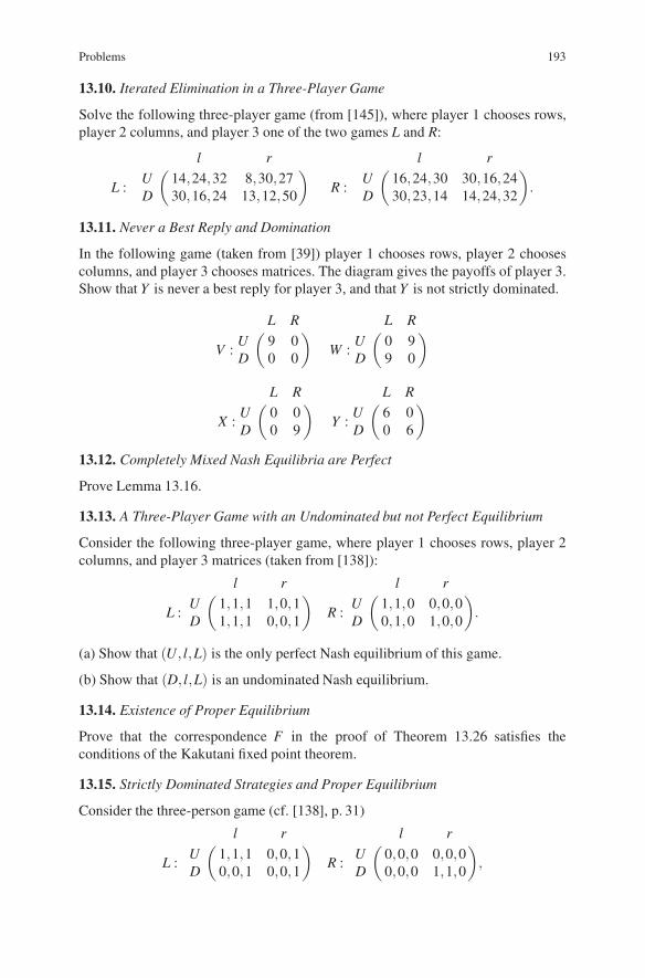
Problems 193
13.10. Iterated Elimination in a Three-Player Game
Solve the following three-player game (from [145]), where player 1 chooses rows,player 2 columns, and player 3 one of the two games L and R:
L :( l r
U 14,24,32 8,30,27D 30,16,24 13,12,50
)R :
( l rU 16,24,30 30,16,24D 30,23,14 14,24,32
).
13.11. Never a Best Reply and Domination
In the following game (taken from [39]) player 1 chooses rows, player 2 choosescolumns, and player 3 chooses matrices. The diagram gives the payoffs of player 3.Show that Y is never a best reply for player 3, and that Y is not strictly dominated.
V :( L R
U 9 0D 0 0
)W :
( L RU 0 9D 9 0
)
X :( L R
U 0 0D 0 9
)Y :
( L RU 6 0D 0 6
)13.12. Completely Mixed Nash Equilibria are Perfect
Prove Lemma 13.16.
13.13. A Three-Player Game with an Undominated but not Perfect Equilibrium
Consider the following three-player game, where player 1 chooses rows, player 2columns, and player 3 matrices (taken from [138]):
L :( l r
U 1,1,1 1,0,1D 1,1,1 0,0,1
)R :
( l rU 1,1,0 0,0,0D 0,1,0 1,0,0
).
(a) Show that (U, l,L) is the only perfect Nash equilibrium of this game.
(b) Show that (D, l,L) is an undominated Nash equilibrium.
13.14. Existence of Proper Equilibrium
Prove that the correspondence F in the proof of Theorem 13.26 satisfies theconditions of the Kakutani fixed point theorem.
13.15. Strictly Dominated Strategies and Proper Equilibrium
Consider the three-person game (cf. [138], p. 31)
L :( l r
U 1,1,1 0,0,1D 0,0,1 0,0,1
)R :
( l rU 0,0,0 0,0,0D 0,0,0 1,1,0
),

194 13 Finite Games
where player 1 chooses rows, player 2 chooses columns, and player 3 choosesmatrices.
(a) First assume that player 3 is a dummy and has only one strategy, namely L.Compute the perfect and proper Nash equilibrium or equilibria of the game.
(b) Now suppose that player 3 has two pure strategies. Compute the perfect andproper Nash equilibrium or equilibria of the game. Conclude that adding a strictlydominated strategy (namely, R) has resulted in an additional proper equilibrium.
13.16. Strictly Perfect Equilibrium
(a) Show that a completely mixed Nash equilibrium in a finite game G is strictlyperfect.
(b) Show that a strict Nash equilibrium in a game G is strictly perfect. (A Nashequilibrium is strict if any unilateral deviation of a player leads to a strictly lowerpayoff for that player.)
(c) Compute all Nash equilibria, perfect equilibria, proper equilibria, and strictlyperfect equilibria in the following game, where α,β > 0. (Conclude that strictlyperfect equilibria may fail to exist.)
(A,B) =( L M R
U 0,β α,0 0,0D 0,β 0,0 α,0
).
13.17. Correlated Equilibria in the Two-Driver Example (1)
Compute all correlated equilibria in the game
(A,B) =( c s
c −10,−10 5,0s 0,5 −1,−1
),
by using the definition of correlated equilibrium.
13.18. Nash Equilibria are Correlated
Let (p,q) be a Nash equilibrium in the m× n bimatrix game (A,B). Let P = (pi j)be the m×n matrix defined by pi j = piq j for all i = 1, . . . ,m and j = 1, . . . ,n. Showthat P is a correlated equilibrium.
13.19. The Set of Correlated Equilibria is Convex
Show that the set of correlated equilibria in a bimatrix game (A,B) is convex.
13.20. Correlated vs. Nash Equilibrium
Consider the bimatrix game (cf. [5])
(A,B) =
(6,6 2,7
7,2 0,0
)

Problems 195
and the correlated strategy
P =
(13
13
13 0
).
(a) Compute all Nash equilibria of (A,B).
(b) Show that P is a correlated equilibrium and that the associated payoffs falloutside the convex hull of the payoff pairs associated with the Nash equilibria of(A,B).
13.21. Correlated Equilibria in the Two-Driver Example (2)
Consider again the game of Problem 13.17 and set up the associated matrix C as inSect. 13.7. Show that the value of the matrix game C is equal to 3, and that player 1 inC has a unique optimal strategy. (Hence, this method gives one particular correlatedequilibrium.)
13.22. Finding Correlated Equilibria
Compute (the) correlated equilibria in the following game directly, and by using theassociated matrix game.
(A,B) =( 1′ 2′
1 5,2 1,32 2,3 4,1
).
13.23. Independence of the Axioms in Corollary 13.35
Show that the three conditions in Corollary 13.35 are independent: for each pair ofconditions, exhibit a solution that satisfies these two conditions but not the third one.
13.24. Inconsistency of Perfect Equilibria
Consider the three-person game G0
D :( L R
T 1,1,1 1,0,1B 1,1,1 0,0,1
)U :
( L RT 0,1,0 0,0,0B 1,1,0 0,0,0
)where player 1 chooses rows, player 2 columns, and player 3 matrices. Let Γ consistof this game and all its reduced games. Use this collection to show that the perfectNash equilibrium correspondence is not consistent.

Chapter 14Extensive Form Games
A game in extensive form specifies when each player in the game is to move, whathis information is about the sequence of previous moves, which chance moves occur,and what the final payoffs are. Such games are discussed in Chaps. 4 and 5, and alsooccur in Chaps. 6 and 7. The present chapter extends the material introduced in thefirst two mentioned chapters, and the reader is advised to (re)read these chaptersbefore continuing.
Section 14.1 formally introduces extensive form structures and games, andSect. 14.2 introduces behavioral strategies and studies the relation between behav-ioral and mixed strategies. Section 14.3 is on Nash equilibrium and its mainrefinements, namely subgame perfect equilibrium and sequential equilibrium. Formore about refinements and some relations with refinements of Nash equilibrium instrategic form games see [138] and [102].
14.1 Extensive Form Structures and Games
An extensive form game1 is based on a directed rooted tree. A directed rooted treeis a pair T = (X ,E), where:
• X is a finite set with |X | ≥ 2. The elements of X are called nodes.• E is a subset of X ×X . The elements of E are called edges. An edge e = (x,y)∈ E
is called an outgoing edge of x and an ingoing edge of y.• There is an x0 ∈ X , called the root, such that for each x ∈ X \ {x0} there is
a unique path from x0 to x. Here, a path from x0 to x is a series of edges(x0,x1),(x1,x2), . . . ,(xk−1,xk),(xk,x) for some k ≥ 0.
• x0 has no ingoing edges.
These conditions imply that each node which is not the root, has exactly one ingoingedge. Moreover, there are nodes which have no outgoing edges. These nodes arecalled end nodes. The set of end nodes is generally denoted by Z (⊆ X).
1 The presentation in this section is based on Perea [102].
H. Peters, Game Theory – A Multi-Leveled Approach.c© Springer-Verlag Berlin Heidelberg 2008
197

198 14 Extensive Form Games
An extensive form structure is a tuple S = (T,N,P,H ,A ,τ), where:
• T = (X ,E) is a directed rooted tree with root x0 and set of end nodes Z.• N = {1, . . . ,n} with n ≥ 1 is the set of players.• P : X \Z → N ∪{C} is a function assigning to each non-end node either a player
or Chance C. If P(x) is a player, then node x is a decision node of player P(x),otherwise x is a chance node.
• H = (Hi)i∈N where for each i ∈ N, Hi is a partition of the set P−1(i) of decisionnodes of player i. The sets h ∈ Hi are called information sets of player i. Eachh ∈ Hi is assumed to satisfy (1) every path in T intersects Hi at most once and (2)every node in h has the same number of outgoing edges.
• A = (A(h))h∈H , where H =∪i∈NHi, and for each h∈H, A(h) is a partition of theset of edges outgoing from nodes x ∈ h. The partition A(h) is such that for eachx ∈ h and each a ∈ A(h), a contains exactly one edge outgoing from x. Every seta ∈ A(h) is called an action at h. It is assumed that |A(h)| ≥ 2 for each h ∈ H.
• τ assigns to each chance node a probability distribution over set of the outgoingedges, where it is assumed that all these probabilities are positive.
In Fig. 14.1 – which is a partial reproduction of Fig. 4.1 – these concepts areillustrated.
In this extensive form structure, the directed rooted tree has 14 nodes x0,x1, . . . ,x13and, consequently, 13 edges. The set of end nodes is Z = {x6, . . . ,x13} and the playerset is N = {1,2}. The function P : {x0, . . . ,x5}→{1,2}∪{C} is defined by P(x) = 1for x ∈ {x0,x5}, P(x) = 2 for x ∈ {x2,x3,x4}, and P(x1) = C. The information setsare {x0},{x5} ∈ H1 and {x2,x3},{x4} ∈ H2. The actions for player 1 are: {(x0,x2)},{(x0,x3)}, {(x0,x1)} ∈ A({x0}) and {(x5,x12)}, {(x5,x13)} ∈ A({x5}). The actionsfor player 2 are: {(x2,x6),(x3,x8)}, {(x2,x7),(x3,x9)} ∈ A({x2,x3}) and {(x4,x10)},{(x4,x11)} ∈ A({x4}). Finally, τ(x1) = (1/4,3/4), where 1/4 is the probability of(x1,x4) and 3/4 is the probability of (x1,x5).
Clearly, this formal notation is quite cumbersome and we try to avoid its use asmuch as possible. It is only needed to give precise definitions and proofs.
� � � � � � � �
� � � �
��
x2 x3 x4 x5
1 x0
A B CChancex1
1/4 3/4
22 1
U D
l r l r L R a b
x6 x7 x8 x9 x10 x11 x12 x13
Fig. 14.1 An extensive form structure
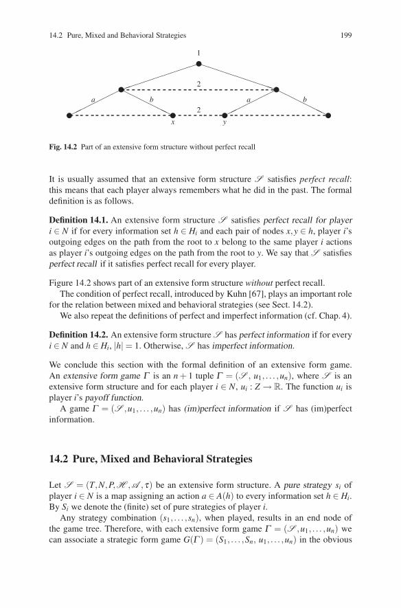
14.2 Pure, Mixed and Behavioral Strategies 199
� �����������������
������
���������������
������� � � �
1
2
2a b a b
x y
Fig. 14.2 Part of an extensive form structure without perfect recall
It is usually assumed that an extensive form structure S satisfies perfect recall:this means that each player always remembers what he did in the past. The formaldefinition is as follows.
Definition 14.1. An extensive form structure S satisfies perfect recall for playeri ∈ N if for every information set h ∈ Hi and each pair of nodes x,y ∈ h, player i’soutgoing edges on the path from the root to x belong to the same player i actionsas player i’s outgoing edges on the path from the root to y. We say that S satisfiesperfect recall if it satisfies perfect recall for every player.
Figure 14.2 shows part of an extensive form structure without perfect recall.The condition of perfect recall, introduced by Kuhn [67], plays an important role
for the relation between mixed and behavioral strategies (see Sect. 14.2).We also repeat the definitions of perfect and imperfect information (cf. Chap. 4).
Definition 14.2. An extensive form structure S has perfect information if for everyi ∈ N and h ∈ Hi, |h| = 1. Otherwise, S has imperfect information.
We conclude this section with the formal definition of an extensive form game.An extensive form game Γ is an n + 1 tuple Γ = (S , u1, . . . ,un), where S is anextensive form structure and for each player i ∈ N, ui : Z → R. The function ui isplayer i’s payoff function.
A game Γ = (S ,u1, . . . ,un) has (im)perfect information if S has (im)perfectinformation.
14.2 Pure, Mixed and Behavioral Strategies
Let S = (T,N,P,H ,A ,τ) be an extensive form structure. A pure strategy si ofplayer i ∈ N is a map assigning an action a ∈ A(h) to every information set h ∈ Hi.By Si we denote the (finite) set of pure strategies of player i.
Any strategy combination (s1, . . . ,sn), when played, results in an end node ofthe game tree. Therefore, with each extensive form game Γ = (S ,u1, . . . ,un) wecan associate a strategic form game G(Γ ) = (S1, . . . ,Sn, u1, . . . ,un) in the obvious

200 14 Extensive Form Games
way. A (mixed) strategy of player i ∈ N is an element of ∆(Si), i.e., a probabilitydistribution over the elements of Si.
When considering an extensive form game (structure) it seems more natural toconsider, instead of mixed strategies, so-called behavioral strategies. A behavioralstrategy of a player assigns to each information set of that player a probability dis-tribution over the actions at that information set. Formally, we have the followingdefinition.
Definition 14.3. Let S = (T,N,P,H ,A ,τ) be an extensive form structure. Abehavioral strategy of player i ∈ N is a map bi assigning to each information seth ∈ Hi a probability distribution over the set of actions A(h).
Given a behavioral strategy there is an obvious way to define an associated mixedstrategy: for each pure strategy, simply multiply all probabilities assigned by thebehavioral strategy to the actions occurring in the pure strategy. Consider forinstance the extensive form structure in Fig. 14.3. In this diagram a behavioralstrategy b1 of player 1 is indicated. The associated mixed strategy σ1 assigns theprobabilities σ1(A, l) = 1
2 · 13 = 1
6 , σ1(A,r) = 12 · 2
3 = 13 , σ1(B, l) = 1
2 · 13 = 1
6 , andσ1(B,r) = 1
2 · 23 = 1
3 . Strategy σ1 is the ‘right’ mixed strategy associated with b1in the following sense. Suppose player 2 plays the mixed or behavioral strategy –there is no difference in this case – which puts probability α on L and 1−α on R.If player 1 plays the behavioral strategy b1 then the probability distribution gener-ated over the end nodes of the game is x5 �→ 1
6 ·α , x6 �→ 13 ·α , x7 �→ 1
6 · (1−α),x8 �→ 1
3 · (1−α). The same distribution is generated by the mixed strategy σ1. E.g.,the probability that x5 is reached equals σ1(A, l) ·α = 1
6 ·α , etc. We call b1 and σ1outcome equivalent. Obviously, it would have been sufficient to check this for thetwo pure strategies L and R for player 2.
We summarize these considerations in a definition and a proposition, which ispresented without a formal proof.
Definition 14.4. Two (behavioral or mixed) strategies of player i in S are out-come equivalent if for each pure strategy combination s−i of the other playersthe probability distributions generated by the two strategies over the end nodes areequal.
� � � �� �
� ��
x5 x6 x7 x8
x2
1 x0
2x1
1
A12
B12
L R
l13
23
13
23
r l r
x3 x4
Fig. 14.3 From behavioral to mixed strategies

14.2 Pure, Mixed and Behavioral Strategies 201
Proposition 14.5. Let bi be a behavioral strategy of player i in S . Then there isa mixed strategy σi of player i that is outcome equivalent to bi. Such a strategyσi is obtained by assigning to each pure strategy si of player i the product of theprobabilities assigned by bi to the actions chosen by si.
It should be noted that there is not necessarily a unique mixed strategy that is out-come equivalent to a given behavioral strategy. For instance, in the example above,if we change the behavioral strategy of player 1 such that it assigns probability 0 toaction A and probability 1 to action B at information set {x0}, then any mixed strat-egy which puts zero probability on (A, l) and (A,r) is outcome equivalent, resultingin each end node other than x2 with zero probability.
Also for the converse question it is not hard to figure out a procedure. Suppose thatσ1 is a mixed strategy of player i, h is an information set of player i, and a is anaction in h. First, let Si(h) denote the set of pure strategies of player i such thatthe play of the game possibly reaches h, in other words, such that there exists apath through h containing the actions prescribed by the pure strategy under consid-eration. Then σi(Si(h)) is the total probability assigned by σi to this set of purestrategies. Within this set, consider those pure strategies that assign a to h anddivide their total probability by σi(Si(h)) if σi(Si(h)) > 0: the result is defined to bebi(h)(a). If σi(Si(h)) = 0 then we can choose bi(h) arbitrary. This way, we constructa behavioral strategy bi that is outcome equivalent to the mixed strategy σi.
As an illustration consider the extensive form structure in Fig. 14.4, which is thesame as the one in Fig. 14.3. Consider the mixed strategy σ1 of player 1 defined by:(A, l) �→ 1
5 , (A,r) �→ 110 , (B, l) �→ 2
5 , (B,r) �→ 310 . Following the above procedure we
obtainb1(A) = σ1(A,l)+σ1(A,r)
1 = 15 + 1
10 = 310
b1(B) = σ1(B,l)+σ1(B,r)1 = 2
5 + 310 = 7
10
b1(l) = σ1(A,l)σ1(A,l)+σ1(A,r) = 1/5
1/5+1/10 = 23
b1(r) = σ1(A,r)σ1(A,l)+σ1(A,r) = 1/10
1/5+1/10 = 13 .
� � � �� �
� ��
x5 x6 x7 x8
x2
1 x0
2x1
1
A B
L R
l r l r
x3 x4
Fig. 14.4 From mixed to behavioral strategies

202 14 Extensive Form Games
It is straightforward to verify that b1 and σ1 are outcome equivalent.Outcome equivalence is not guaranteed without perfect recall: see Problem 14.2
for an example. With perfect recall, we have the following theorem.2
Theorem 14.6 (Kuhn). Let the extensive form structure S satisfy perfect recall.Then, for every player i and every mixed strategy σi there is a behavioral strategybi that is outcome equivalent to σi.3
14.3 Nash Equilibrium and Refinements
Let Γ = (S ,(ui)i∈N) be an extensive form game with associated strategic formgame G(Γ ) = ((Si)i∈N ,(ui)i∈N). We assume that S satisfies perfect recall.
A pure strategy Nash equilibrium of Γ is defined to be a pure strategy Nashequilibrium of G(Γ ). Note that, if Γ has perfect information, then a pure strategyNash equilibrium exists (cf. Chap. 4).
A mixed strategy Nash equilibrium of Γ is defined to be a (mixed strategy) Nashequilibrium of G(Γ ). By Theorem 13.1 such an equilibrium always exists.
Consider, now, a behavioral strategy combination b = (bi)i∈N in Γ . Such a strat-egy combination generates a probability distribution over the end nodes and, thus,an expected payoff for each player. We call bi a best reply of player i ∈ N to thestrategy combination b−i if there is no other behavioral strategy b′i of player i suchthat (b′i,b−i) generates a higher expected payoff for player i. We call b a Nash equi-librium (in behavioral strategies) of Γ if bi is a best reply to b−i for every playeri ∈ N.
Let σ be a mixed strategy Nash equilibrium of Γ . By Theorem 14.6 there is a behav-ioral strategy combination b that is outcome equivalent to σ . We claim that b is aNash equilibrium of Γ . Suppose not, then there is a player i ∈ N and a behavioralstrategy b′i that gives player i a higher expected payoff against b−i. By Proposi-tion 14.5 there is a mixed strategy σ ′
i that is outcome equivalent to b′i. Consequently,σ ′
i gives player i a higher expected payoff against σ−i, a contradiction. We have thusproved:
Theorem 14.7. Every extensive form game has a Nash equilibrium.
In fact, a similar argument as the one leading to this theorem can be applied to showthat every Nash equilibrium (in behavioral strategies) results in a Nash equilibriumin mixed strategies. Hence, one way to find the (behavioral strategy) Nash equilibriaof an extensive form game is to determine all (mixed strategy) Nash equilibria of theassociated strategic form game. Which way is most convenient depends on the gameat hand. In particular for refinements it is often easier to compute behavioral equilib-rium strategies directly, without first computing the mixed strategy Nash equilibria.Before discussing these refinements we first consider an example.
2 For a proof see [67] or [102], Theorem 2.4.4.3 The behavioral strategy bi can be constructed as described in the text.
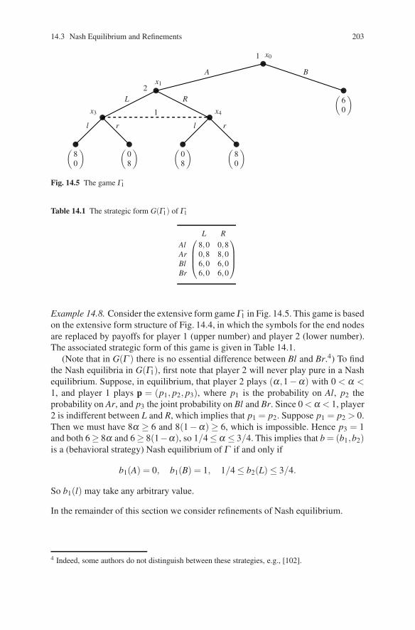
14.3 Nash Equilibrium and Refinements 203
� � � �� �
� ��
(80
) (08
) (08
) (80
)
(60
)
1 x0
2x1
1
A B
L R
l r l r
x3 x4
Fig. 14.5 The game Γ1
Table 14.1 The strategic form G(Γ1) of Γ1
⎛⎜⎜⎝L R
Al 8,0 0,8Ar 0,8 8,0Bl 6,0 6,0Br 6,0 6,0
⎞⎟⎟⎠
Example 14.8. Consider the extensive form game Γ1 in Fig. 14.5. This game is basedon the extensive form structure of Fig. 14.4, in which the symbols for the end nodesare replaced by payoffs for player 1 (upper number) and player 2 (lower number).The associated strategic form of this game is given in Table 14.1.
(Note that in G(Γ ) there is no essential difference between Bl and Br.4) To findthe Nash equilibria in G(Γ1), first note that player 2 will never play pure in a Nashequilibrium. Suppose, in equilibrium, that player 2 plays (α,1−α) with 0 < α <1, and player 1 plays p = (p1, p2, p3), where p1 is the probability on Al, p2 theprobability on Ar, and p3 the joint probability on Bl and Br. Since 0 < α < 1, player2 is indifferent between L and R, which implies that p1 = p2. Suppose p1 = p2 > 0.Then we must have 8α ≥ 6 and 8(1−α) ≥ 6, which is impossible. Hence p3 = 1and both 6 ≥ 8α and 6 ≥ 8(1−α), so 1/4≤ α ≤ 3/4. This implies that b = (b1,b2)is a (behavioral strategy) Nash equilibrium of Γ if and only if
b1(A) = 0, b1(B) = 1, 1/4 ≤ b2(L) ≤ 3/4.
So b1(l) may take any arbitrary value.
In the remainder of this section we consider refinements of Nash equilibrium.
4 Indeed, some authors do not distinguish between these strategies, e.g., [102].

204 14 Extensive Form Games
14.3.1 Subgame Perfect Equilibrium
Let x be a non-end node in an extensive form structure S and let T x = (V x,Ex) bethe subtree starting from x – i.e., V x is the subset of V consisting of all nodes of Vthat can be reached by a path starting from x, and Ex is the subset of E of all edgeswith endpoints in V x. Assume that every information set of S is contained eitherin V x or in V \V x. (This implies, in particular, that {x} is a singleton informationset.) Let S x denote the substructure obtained by restricting S to T x. Then, for theextensive form game Γ = (S ,(ui)i∈N), the game Γ x = (S x,(ux
i )i∈N) is defined byrestricting the payoff functions to the end nodes still available in V x. We call Γ x
a subgame of Γ . For a behavioral strategy combination b = (bi)i∈N we denote bybx = (bx
i )i∈N the restriction to Γ x.
Definition 14.9. A behavioral strategy combination b in Γ is a subgame perfectequilibrium if bx is a Nash equilibrium for every subgame Γ x.
Clearly, this definition extends the definition of subgame perfection for pure strategycombinations given in Chap. 4.
Since the whole game Γ is a subgame (Γ = Γ x0 , where x0 is the root of the gametree), every subgame perfect equilibrium is a Nash equilibrium. By carrying out abackward induction procedure as in Sect. 4.3, it can be seen that a subgame perfectequilibrium exists in any extensive form game.5
Subgame perfection often implies a considerable reduction of the set of Nashequilibria. The following example is the continuation of Example 14.8.
Example 14.10. To find the subgame perfect equilibria in Γ1, we only have to ana-lyze the subgame Γ x1
1 . It is easy to see that this subgame has a unique Nashequilibrium, namely player 2 playing L and R each with probability 1/2, and player1 playing l and r each with probability 1/2. This results in a unique subgame perfectequilibrium b = (b1,b2) given by
b1(B) = 1, b1(l) = 1/2, b2(L) = 1/2 .
14.3.2 Perfect Bayesian and Sequential Equilibrium
In games without proper subgames and in games of imperfect information the sub-game perfection requirement may not have much bite (see the examples in Chaps. 4and 5). The concept of sequential equilibrium allows to distinguish between Nashequilibria by considering beliefs of players on information sets.
5 This is intuitive but not trivial. See, e.g., [102].

14.3 Nash Equilibrium and Refinements 205
Consider an extensive form structure S = (T,N,P,H ,A ,τ). A belief system βassigns to every information set h ∈ H = ∪i∈NHi a probability distribution βh overthe nodes in h. An assessment is a pair (b,β ) of a behavioral strategy combinationb = (bi)i∈N and a belief system β .
For any node x in the game tree T , let Pb(x) denote the probability that x isreached given b, that is, Pb(x) is the product of the probabilities of all edges on theunique path form the root x0 to x: these probabilities are given by b, or by τ in caseof a chance node on the path. For h ∈ H, Pb(h) = ∑x∈h Pb(x) is the probability thatthe information set h is reached, given b.
The next definition is the formal version of the consistency requirement intro-duced already in Chap. 4.
Definition 14.11. An assessment (b,β ) in S is Bayesian consistent if βh(x) =Pb(x)/Pb(h) for all h ∈ H for which Pb(h) > 0 and all x ∈ h.
By Bayesian consistency the players’ beliefs are determined by the behavioralstrategies on all information sets that are reached with positive probability. In gen-eral, this requirement is quite weak and does not imply, for instance, that the beliefsof one and the same player are internally consistent. Consider the extensive formstructure in Fig. 14.6. Suppose that player 1 plays a and player 2 plays e. Then thebeliefs of player 2 at the information sets {x1,x2} and {x3,x4} are not restrictedby Bayesian consistency. Moreover, a belief β (x1) = β (x4) = 1 is allowed, whichmeans that player 2’s beliefs are not internally consistent.
In many applications this drawback does not occur, and Bayesian consistency isstrong enough. For instance, in signaling games (see Chap. 5) Bayesian consistencyimplies the usual stronger versions like consistency in the sense of Kreps and Wilson[66] below. See Problem 14.4.
In the literature6 the condition of updating consistency has been proposed toremedy the indicated defect. In the example above, with player 1 playing a and
Fig. 14.6 If player 1 playsa, then player 2’s beliefsat {x1,x2} and {x3,x4} areindependent under Bayesianconsistency
�
�
��
��
��
��
�
�1
a
2 2
b
c
d
d
f
f
e
e
g
g
x1 x3
x2 x4
6 See [102] and the references therein.

206 14 Extensive Form Games
player 2 playing e, updating consistency would imply that β (x3) = β (x1), as seemsnatural.
A much stronger requirement is the original consistency condition in [66]. Call abehavioral strategy bi of player i completely mixed if bi(h)(x) > 0 for each h ∈ Hiand x ∈ h. A behavioral strategy combination b = (bi)i∈N is completely mixed if biis completely mixed for every i ∈ N. Observe that, if b is completely mixed and theassessment (b,β ) is Bayesian consistent, then β is uniquely determined by b.
Definition 14.12. An assessment (b,β ) in S is consistent if there exists a sequence(bm,β m)m∈N of Bayesian consistent assessments with each bm completely mixedand limm→∞(bm,β m) = (b,β ).
Consistency implies Bayesian consistency (Problem 14.3). Consistency is clearlystronger than Bayesian consistency. For instance, in the extensive form structureof Fig. 14.6, it is easily seen that consistency requires player 2 to have identicalbeliefs on his two information sets, i.e., β (x1) = β (x3). This is true even if on hisright information set player 2 is replaced by some other player 3, as in Fig. 14.7. Itshows that (this strong form of) consistency is stronger than Bayesian consistencycombined with ‘updating consistency’, since the latter condition would only requirea player to ‘update’ his own earlier beliefs.
Consider now an extensive form game Γ = (S ,(ui)i∈N). Let (b,β ) be an assess-ment. Let i ∈ N, h ∈ Hi, a ∈ A(h), and x ∈ h. Suppose player i is at node x and takesaction a. This corresponds to an edge (x,y) in the game tree. Then each end nodeon a path starting from x and passing though y is reached with a probability that isequal to the product of the probabilities of all edges on this path following y, givenby b, and the probabilities of eventual chance nodes on this path. This way, we cancompute the expected payoff to player i from playing a, conditional on being at nodex: denote this payoff by ui(a|b,x). Player i’s expected payoff from action a, giveninformation set h, is then equal to ∑x∈h β (x)ui(a|b,x).
Fig. 14.7 Under consistency,the beliefs of players 2 and 3are identical: β (x1) = β (x3)
�
�
��
��
��
��
�
�1
a
2 3
b
c
d
d
f
f
e
e
g
g
x1 x3
x2 x4

14.3 Nash Equilibrium and Refinements 207
Definition 14.13. An assessment (b,β ) in Γ = (S ,(ui)i∈N) is sequentially rationalif for every i ∈ N, h ∈ Hi, and a ∈ A(h) we have
bi(h)(a) > 0 ⇒ ∑x∈h
β (x)ui(a|b,x) = maxa′∈A(h)
∑x∈h
β (x)ui(a′|b,x).
Sequential rationality of an assessment (b,β ) means that a player puts only posi-tive probability on those actions at an information set h that maximize his expectedpayoff, given h and his belief {β (x)|x ∈ h}.
Definition 14.14. An assessment (b,β ) in Γ = (S ,(ui)i∈N) is a sequential equilib-rium if it is sequentially rational and consistent.
Sequential equilibria were introduced in [66].7
Theorem 14.15. Every sequential equilibrium is subgame perfect and, in particular,a Nash equilibrium.
For a proof of this theorem (which is somewhat cumbersome in terms of notation),see [102], Lemma 4.2.6, or [138], Theorem 6.3.2.
In Chap. 4 we introduced, somewhat informally, the notion of perfect Bayesian equi-librium. An assessment (b,β ) is a perfect Bayesian equilibrium if the beliefs βsatisfy Bayesian updating in the extensive form structure ‘as much as possible’,given the behavioral strategy combination b, and if it is sequentially rational. Thereis no unified definition in the literature of the expression ‘as much as possible’. Itimplies at least Bayesian consistency, but it should also imply, for instance, that thebeliefs on the information set {x3,x4} are identical to the beliefs on the informationset {x1,x2} in Figs. 14.6 and 14.7. It should imply Bayesian consistency of beliefson subgames (cf. the game in Fig. 4.7 in Chap. 4), and it should imply subgameperfection. The main motivation for considering perfect Bayesian equilibrium is toavoid the condition involving limiting assessments in the definition of consistency.8
In this chapter we stick to sequential equilibrium but keep in mind that, in order tocompute sequential equilibria for a given game, the method of Bayesian updating‘as much as possible’ is a good heuristic.
There is hardly any general method available to compute sequential equilibria: itdepends very much on the game at hand what the best way is. We consider oneexample and refer to the problem section for other examples.
Example 14.16. Consider the three-player game in Fig. 14.8. To find the sequentialequilibria of this game, first observe that consistency requires the beliefs of players 2
7 Actually, the definition of sequential rationality in Definition 14.13 is called ‘local’ sequentialrationality. Together with consistency, it implies the sequential rationality condition in [66]. It is,however, easier to apply. See also [102], Chap. 4, or [138], Chap. 6. See the same sources for aproof that sequential equilibria always exist.8 For instance, Fudenberg and Tirole [40] provide two definitions of perfect Bayesian equilibriumfor different classes of games and show that their concepts coincide with sequential equilibrium.

208 14 Extensive Form Games
1
a b
[β ] [1−β ]2
d
⎛⎝210
⎞⎠
d
⎛⎝110
⎞⎠[β ′]
c c
[1−β ′]3
fe fe
⎛⎝103
⎞⎠ ⎛⎝130
⎞⎠ ⎛⎝200
⎞⎠ ⎛⎝231
⎞⎠Fig. 14.8 Sequential equilibrium analysis in a three-player game
and 3 to be the same, so β = β ′. Denote behavioral strategies of the players by b1(a)and b1(b) = 1−b1(a), b2(c) and b2(d)= 1−b2(c), and b3(e) and b3( f ) = 1−b3(e).
Starting with player 3, sequential rationality requires b3(e) = 1 if β > 14 , b3(e) =
0 if β < 14 , and 0 ≤ b3(e) ≤ 1 if β = 1
4 .Using this, if β > 1
4 then playing c yields 0 for player 2 and playing d yields 1.Therefore b2(c) = 0. Similarly, b2(c) = 1 if β < 1
4 . If β = 14 then d yields 1 whereas
c yields 3b3( f ). Hence, b2(c) = 0 if β = 14 and b3( f ) < 1
3 ; b2(c) = 1 if β = 14 and
b3( f ) > 13 ; and 0 ≤ b2(c) ≤ 1 if β = 1
4 and b3( f ) = 13 .
We finally consider player 1. If b1(a) > 14 then consistency requires β = b1(a) >
14 and therefore b2(c) = 0. So player 1 obtains 2b1(a)+ 1(1− b1(a)) = 1 + b1(a),which is maximal for b1(a) = 1. Obviously, player 1 cannot improve on this. So wehave the following sequential equilibrium:
b1(a) = 1, b2(c) = 0, b3(e) = 1, β = β ′ = 1.
If b1(a) < 14 then β = b1(a) < 1
4 and therefore b2(c) = 1 and b3(e) = 0. Soplayer 1 obtains 1b1(a)+2(1−b1(a)) = 2−b1(a), which is maximal for b1(a) = 0.Obviously again, player 1 cannot improve on this. So we have a second sequentialequilibrium:

Problems 209
b1(a) = 0, b2(c) = 1, b3(e) = 0, β = β ′ = 0 .
If b1(a) = 14 then player 1 must be indifferent between a and b. This implies that
the expected payoff from a should be equal to the expected payoff from b, hencethat 2(1−b2(c))+1b2(c) = 2b2(c)+1(1−b2(c)) which is true for b2(c) = 1
2 . Thepreceding analysis for player 2 shows that for player 2 to play completely mixed weneed b3(e) = 2
3 . So we have a third sequential equilibrium
b1(a) =14, b2(c) =
12, b3(e) =
23, β = β ′ =
14
.
Problems
14.1. Mixed and Behavioral Strategies
Determine all mixed strategies that are outcome equivalent with the behavioralstrategy represented in the following one-player extensive form structure.
x01
z3
12 L R
12
1 x1
14
L′34
R′
z1 z2
14.2. An Extensive form Structure Without Perfect Recall
Consider the following extensive form structure:
� � � �� �
�
x3 x4 x5 x6
1x0
1L R
l r l r
x1 x2
(a) Show that this one-player extensive form structure has no perfect recall.(b) Consider the mixed strategy σ1 that assigns probability 1/2 to both (L, l) and(R,r). Show that there is no behavioral strategy that generates the same probabilitydistribution over the end nodes as σ1 does.

210 14 Extensive Form Games
14.3. Consistency Implies Bayesian Consistency
Let (b,β ) be a consistent assessment in an extensive form structure S . Show that(b,β ) is Bayesian consistent.
14.4. (Bayesian) Consistency in Signaling Games
Prove that Bayesian consistency implies consistency in a signaling game.
[A general definition of a signaling game (cf. also Chap. 5) is as follows. The set ofplayers is N = {1,2} and for the extensive form structure S we have:
(1) The directed rooted tree is T = (X ,E) with root x0,
X = {x0,x1, . . . ,xk,xi1, . . . ,xil ,xi j1, . . . ,xi jm | i = 1, . . . ,k, j = 1, . . . , l},
where k, l,m ≥ 2,
E = {(x0,xi),(xi,xi j),(xi j,xi j j′) | i = 1, . . . ,k, j = 1, . . . , l, j′ = 1, . . . ,m}.
HenceZ = {xi j j′ | i = 1, . . . ,k, j = 1, . . . , l, j′ = 1, . . . ,m}.
(2) The chance and player assignment P is defined by P(x0) = C, P(xi) = 1 for alli = 1, . . . ,k, P(xi j) = 2 for all i = 1, . . . ,k, j = 1, . . . , l.
(3) The information sets are
H1 = {{x1}, . . . ,{xk}}, H2 = {{x1 j, . . . ,xk j} | j = 1, . . . , l}.
(4) The action sets are
A({xi}) = {{(xi,xi j)} | j = 1, . . . , l} for every i = 1, . . . ,k
for player 1 and
A({x1 j, . . . ,xk j}) = {{(x1 j,x1 j j′), . . . ,(xk j,xk j j′)} | j′ = 1, . . . ,m}
for every j = 1, . . . , l, for player 2.(5) The map τ assigns a positive probability to each edge in the set{(x0,x1), . . . ,(x0,xk)}. (Player 1 has k ‘types’.)
Finally, the players have payoff functions u1,u2 : Z → R.]
14.5. Computation of Sequential Equilibrium (1)
Compute the sequential equilibrium or equilibria in the game Γ1 in Fig. 14.5.
14.6. Computation of Sequential Equilibrium (2)
Consider the following extensive form game.

Problems 211
R (22
)x1
L M
y1 y22
l r l r
(41
) (00
) (30
) (01
)(a) Determine the strategic form of this game.
(b) Determine all Nash and subgame perfect Nash equilibria of this game.
(c) Determine all sequential equilibria of this game.
14.7. Computation of Sequential Equilibrium (3)
Consider the following extensive form game below.
(a) Determine the strategic form of this game.
(b) Compute the Nash equilibria and subgame perfect Nash equilibria.
(c) Compute the sequential equilibria.
R (22
)x1
L M
y1 y22
l r l r
(30
) (01
) (01
) (30
)

212 14 Extensive Form Games
14.8. Computation of Sequential Equilibrium (4)
Consider the following extensive form game.
R (24
)x1
L M
y1 y22
l m r l m r
(13
) (12
) (40
) (42
) (02
) (33
)Compute all sequential equilibria of this game.
14.9. Computation of Sequential Equilibrium (5)
Compute all Nash, subgame perfect and sequential equilibria in the following game.
1
D
R(
44
)
2
l r
[β ] [1−β ]1
A B A B
(22
) (00
) (30
) (66
)

Chapter 15Evolutionary Games
In this chapter we go somewhat deeper into evolutionary game theory. The conceptsof evolutionary stable strategy and replicator dynamics, introduced in Chap. 8, arefurther explored, and proofs of results mentioned in that chapter are provided. Weadvise the reader to study Chap. 8 first, although the present chapter is largely self-contained.
This chapter is based mainly on [147]. In Sect. 15.1 we briefly review sym-metric two-player games. Section 15.2 discusses evolutionary stable strategies andSect. 15.3 replicator dynamics.
15.1 Symmetric Two-Player Games
Much of evolutionary game theory is concerned with symmetric two-player games.A (finite) symmetric two-player game is completely determined by a pair of m×mpayoff matrices (A,B) such that B = AT , i.e., B = (bi j)m
i, j=1 is the transpose of A =(ai j)m
i, j=1. In other words, for all i, j ∈ {1,2, . . . ,m}, we have bi j = a ji.In such a game we are particularly interested in symmetric (pure and mixed strat-
egy) Nash equilibria. A Nash equilibrium (σ1,σ2) is symmetric if σ1 = σ2. Wedenote by NE(A,AT ) the set of all Nash equilibria of (A,AT ) and by
NE(A) = {x ∈ ∆m | (x,x) ∈ NE(A,AT )}
the set of all strategies that occur in a symmetric Nash equilibrium. By a standardapplication of Kakutani’s fixed point theorem we prove that this set is nonempty.
Proposition 15.1. For any m×m-matrix A, NE(A) = /0.
Proof. For each x ∈ ∆m, viewed as a strategy of player 2 in (A,AT ), let β1(x) be theset of best replies of player 1 in (A,AT ). Then the correspondence x �→ β1(x) is uppersemi-continuous and convex-valued (check this), so that by the Kakutani Fixed PointTheorem 22.10 there is an x∗ ∈ ∆m with x∗ ∈ β1(x∗). Since player 2’s payoff matrix
H. Peters, Game Theory – A Multi-Leveled Approach.c© Springer-Verlag Berlin Heidelberg 2008
213

214 15 Evolutionary Games
is the transpose of A, it follows that also x∗ ∈ β2(x∗). Hence, (x∗,x∗) ∈ NE(A,AT ),so x∗ ∈ NE(A). ��
15.1.1 Symmetric 2×2 Games
For later reference it is convenient to have a classification of symmetric 2×2 gameswith respect to their symmetric Nash equilibria. Such a game is described by thepayoff matrix
A =(
a11 a12a21 a22
).
For the purpose of Nash equilibrium analysis, we may consider without loss ofgenerality (check!) the matrix
A′ =(
a11 −a21 a12 −a12a21 −a21 a22 −a12
)=(
a11 −a21 00 a22 −a12
)=(
a1 00 a2
),
where a1 := a11−a21 and a2 := a22−a12. For a generic matrix A, implying a1,a2 =0, there are essentially three different cases:
(1) a1 < 0, a2 > 0. In this case, NE(A′) = {e2}, i.e., each player playing the secondstrategy is the unique symmetric Nash equilibrium.
(2) a1,a2 > 0. In this case, NE(A′) = {e1,e2, x}, where x = (a2/(a1 +a2),a1/(a1 +a2)).
(3) a1,a2 < 0. In this case, NE(A′) = {x} with x as in (2).
15.2 Evolutionary Stability
15.2.1 Evolutionary Stable Strategies
In evolutionary game theory the interpretation of a symmetric two-person gameis that players in a possibly large population randomly meet in pairs. Let such agame be described by A, then a mixed strategy x ∈ ∆m is interpreted as a vectorof population shares: for each k, xk is the share of the population that ‘plays’ purestrategy k. Such a strategy is called evolutionary stable if it performs better againsta small ‘mutation’ than that mutation itself. For convenience the formal definition isreproduced here (cf. [77] and Definition 8.3).
Definition 15.2. A strategy x ∈ ∆m is an evolutionary stable strategy (ESS) in Aif for every strategy y ∈ ∆m, y = x, there exists some εy ∈ (0,1) such that for allε ∈ (0,εy) we have
xA(εy+(1− ε)x) > yA(εy +(1− ε)x). (15.1)

15.2 Evolutionary Stability 215
The set of all ESS is denoted by ESS(A).Evolutionary stable strategies can be characterized as follows.
Proposition 15.3. Let A be a symmetric m×m game. Then
ESS(A) = {x ∈ NE(A) | ∀y ∈ ∆m,y = x [xAx = yAx ⇒ xAy > yAy]} .
This proposition follows from Propositions 8.4 and 8.5.From Problems 15.1–15.3 it follows that the concept of ESS does not ‘solve’
the prisoners’ dilemma nor the ‘coordination problem’. Also, an ESS may becompletely mixed (Hawk–Dove), or fail to exist (Rock–Paper–Scissors).
15.2.2 The Structure of the Set ESS(A)
Let x be an ESS and let y ∈ ∆m, y = x such that the carrier1 of y is contained in thecarrier of x, i.e., C(y) ⊆ C(x). Since x ∈ NE(A) by Proposition 15.3, this impliesxAx = yAx and hence, again by Proposition 15.3, xAy > yAy. We have established:
Proposition 15.4. If x ∈ ESS(A) and y ∈ ∆m with y = x and C(y) ⊆ C(x), theny /∈ NE(A).
This implies the following corollary (check!):
Corollary 15.5. The set ESS(A) is finite. If x ∈ ESS(A) is completely mixed, thenESS(A) = {x}.
15.2.3 Relations with Other Refinements
If x ∈ NE(A) is weakly dominated by y ∈ ∆m, then xAx = yAx and yAy ≥ xAy;so by Proposition 15.3, x /∈ ESS(A). Therefore, if x ∈ ESS(A), then (x,x) is anundominated equilibrium and hence perfect by Theorem 13.22. It can even be shownthat (x,x) is proper (see [138]). The next proposition summarizes these facts.
Proposition 15.6. If x ∈ ESS(A), then (x,x) ∈ NE(A,AT ) is undominated, perfectand proper.
The unique (symmetric) equilibrium in the Rock–Paper–Scissors game in Prob-lem 15.3 is proper (why?), but the associated equilibrium strategy is not ESS, sothe converse of Proposition 15.6 does not hold.
1 Recall – see Chap. 13 – that the carrier of y, C(y), is the set {i ∈ {1, . . . ,m} | yi > 0}.
216 15 Evolutionary Games
15.2.4 Other Characterizations of ESS
Uniform Invasion Barriers
The number εy in the definition of an ESS can be interpreted as an ‘invasion barrier’:if the share of the mutant strategy y is smaller than εy, then the ‘incumbent’ strategyx fares better against the mutated population than the mutant y itself does, so thatthe mutant strategy becomes extinct. In a large but finite population, it would notmake sense if this invasion barrier could become arbitrarily small since then the‘mutant’ population would sometimes have to consist of less than one individualto guarantee survival of the strategy x under consideration. This gives rise to thefollowing definition (from [139]).
Definition 15.7. A strategy x ∈ ∆m has a uniform invasion barrier if there exists anε ∈ (0,1) such that (15.1) holds for all strategies y = x and every ε ∈ (0, ε).
It turns out that possessing a uniform invasion barrier characterizes an evolutionarystable strategy.
Proposition 15.8. For each x ∈ ∆m, x ∈ ESS(A) if and only if x has a uniforminvasion barrier.
Proof. Let x ∈ ∆m. If x has a uniform invasion barrier ε , then clearly x is an ESS bychoosing, in (15.1), εy = ε for each y ∈ ∆m.
Conversely, let x be an ESS. Define the function b : ∆m \ {x}→ [0,1] by
b(y) = sup{δ ∈ [0,1] | ∀ε ∈ (0,δ ) [(x−y)A(εy+(1− ε)x) > 0]}
for all y ∈ ∆m \ {x}. We first consider the function b on the compact set Z = {z ∈∆m | zi = 0 for some i ∈C(x)}. Consider y ∈ Z. Since x is an ESS, we have that (x−y)A(εy +(1− ε)x) is positive for small positive values of ε . Since this expressiondepends linearly on ε , this implies that there can be at most one value of ε , whichwe denote by εy, such that (x− y)A(εy + (1− ε)x) = 0. If εy ∈ (0,1), then (x−y)A(εyy+(1− εy)x) = 0 implies that (x−y)A(x−y) = 0, since otherwise
0 = (x−y)A(εyy+(1− εy)x) = (x−y)Ax
and, thus, (x−y)A(εy+(1−ε)x) = 0 for all ε , a contradiction. Hence, in that case,b(y) = εy = (x− y)Ax/(x− y)A(x− y); otherwise, b(y) = 1. It is not hard to seethis implies that b is a continuous function. Since b is positive and Z is compact,miny∈Z b(y) > 0. Hence, x has a uniform invasion barrier, namely this minimumvalue, on the set Z.
Now suppose that y ∈ ∆m, y = x. We claim that there is a λ ∈ (0,1] such thaty = λ z +(1−λ )x for some z ∈ Z. To see this, first note that we can take λ = 1 ify ∈ Z. If y /∈ Z then consider, for each µ ≥ 0, the point z(µ) = (1− µ)x+ µy, andlet µ ≥ 1 be the largest value of µ such that z(µ) ∈ ∆m. Then there is a coordinatei ∈ {1, . . . ,m} with zi(µ) = 0, zi(µ) > 0 for all µ < µ , and zi(µ) < 0 for all µ > µ .
15.2 Evolutionary Stability 217
Clearly, this implies xi > yi, hence i ∈C(x), and thus z(µ) ∈ Z. Then, for z = z(µ)and λ = 1/µ, we have y = λ z+(1−λ )x.
By straightforward computation we have
(x− y)A(εy+(1− ε)x) = λ (x− z)A(ελ z +(1− ελ )x)
for each ε > 0, so that b(y) = min{b(z)/λ ,1} ≥ b(z).We conclude that ε = miny∈Z b(y) is a uniform invasion barrier for x. ��
Local Superiority
By Proposition 15.3, a completely mixed ESS earns a higher payoff against anymutant than such a mutant earns against itself. This global superiority property canbe generalized to the following local version [56].
Definition 15.9. The strategy x ∈ ∆m is locally superior if it has an open neighbor-hood U such that xAy > yAy for all y ∈U \ {x}.
The local superiority condition provides another characterization of ESS.
Proposition 15.10. For each x ∈ ∆m, x ∈ ESS(A) if and only if x is locally superior.
Proof. Let x ∈ ∆m.First suppose that x is locally superior, and let U be as in Definition 15.9. Let z ∈
∆m\{x} and define for each 0 < ε < 1 the point w(ε) by w(ε) = εz+(1−ε)x. Thenthere is εz > 0 such that w(ε) ∈U for all ε ∈ (0,εz), hence xAw(ε) > w(ε)Aw(ε).This implies xAw(ε) > zAw(ε) for all ε ∈ (0,εz). In particular, we have
εxAz+(1− ε)xAx > εzAz+(1− ε)zAx
for all ε ∈ (0,εz), hence xAx ≥ zAx. So x ∈ NE(A). Suppose now that zAx = xAx.Then, for ε ∈ (0,εz),
εxAz = xAw(ε)− (1− ε)xAx> zAw(ε)− (1− ε)xAx= εzAz+(1− ε)zAx− (1− ε)xAx= εzAz ,
so that x is an ESS.Conversely, let x be an ESS with uniform invasion barrier (cf. Proposition 15.8)
ε ∈ (0,1), and let Z be as in the proof of Proposition 15.8. Let
V = {y ∈ ∆m | y = εz +(1− ε)x for some z ∈ Z and ε ∈ [0, ε)}.
Since Z is closed and x /∈ Z, there is an open neighborhood U of x such that U ∩∆m ⊆ V . Suppose that y = x, y ∈ U ∩∆m. Then y ∈ V , and by Proposition 15.8,

218 15 Evolutionary Games
zAy = zA(εz +(1− ε)x) < xA(εz +(1− ε)x) = xAy, with z as in the definition ofV . This implies yAy = εzAy+(1− ε)xAy < xAy. ��
Local Strict Efficiency
Consider the special case of a symmetric game (A,B) with AT = A, hence A is itselfsymmetric and B = A. Call such a game doubly symmetric.
Definition 15.11. A strategy x ∈ ∆m is locally strictly efficient if it has an openneighborhood U such that xAx > yAy for all y ∈U \ {x}.
For doubly symmetric games, local strict efficiency characterizes ESS ([57]).
Proposition 15.12. Let A = AT . Then x ∈ ESS(A) if and only if x is locally strictlyefficient.
Proof. Let x ∈ ∆m. For any y = x and z = 12 x+ 1
2 y, we have
yAy = xAx−2xAz−2zAx+ 4zAz .
Hence, using the symmetry of A,
xAx− yAy = 4 [xAz− zAz] .
If x is locally strictly efficient, then this identity implies that x is locally superior,and conversely. By Proposition 15.10, it follows that x is an ESS if and only if x islocally strictly efficient. ��
15.3 Replicator Dynamics and ESS
The concept of an evolutionary stable strategy is based on the idea of mutation.Incorporation of the evolutionary concept of selection calls for a more explicitlydynamic approach.
15.3.1 Replicator Dynamics
As before, consider a symmetric game described by the m×m matrix A. A mixedstrategy x ∈ ∆m can be interpreted as a vector of population shares (a state) over thepure strategies, evolving over time. To express time dependence, we write x = x(t).For each pure strategy i, the expected payoff of playing i when the population is instate x is equal to eiAx, hence the average population payoff is equal to ∑m
i=1 xieiAx =

15.3 Replicator Dynamics and ESS 219
xAx. In the replicator dynamics ([133]) it is assumed that population shares developaccording to the differential equation
xi = dxi(t)/dt =[eiAx−xAx
]xi (15.2)
for each pure strategy i = 1,2, . . . ,m, where dependence on t is (partly) suppressedfrom the notation. In other words, the share of the population playing strategy ichanges with rate proportional to the difference between the expected payoff of i(individual fitness) and the average population payoff (average fitness).
To study the replicator dynamics in (15.2) one needs to apply the theory of dif-ferential equations and dynamical systems (e.g., [55]). For a first analysis we canrestrict attention to a few basic concepts and facts.
For each initial state x(0) = x0 ∈ ∆m, the system (15.2) induces a solution ortrajectory ξ (t,x0) in ∆m. Call state x a stationary point of the dynamics (15.2) ifx = (x1, . . . , xm) = (0, . . . ,0). If m = 2 then x1 = 0 or x2 = 0 is sufficient for x to bea stationary point, since (15.2) implies the natural condition ∑m
i=1 xi = 0. Note thatany ei is a stationary point – this is a more or less artificial property of the replicatordynamics. A state x is Lyapunov stable if every open neighborhood B of x containsan open neighborhood B0 of x such that ξ (t,x0)∈ B for all x0 ∈B0 and t ≥ 0. A statex asymptotically stable if it is Lyapunov stable and it has an open neighborhood B∗such that limt→∞ ξ (t,x0) = x for all x0 ∈ B∗. It is not hard to show that Lyapunovstability implies stationarity.
15.3.2 Symmetric 2×2 Games
In order to analyze the replicator dynamics for symmetric 2×2 games correspond-ing to A, we can without loss of generality restrict attention again to the normalizedgame
A′ =(
a1 00 a2
).
Now (15.2) reduces tox1 = [a1x1 −a2x2]x1x2 (15.3)
(and x2 = −x1). For case I (a1 < 0 and a2 > 0) the stationary points of the dynam-ics are x = e1 and x = e2. For all other x, x1 < 0, which implies that the systemthen converges to e2, the unique ESS. Hence, the (unique) ESS is also the (unique)asymptotically stable state.
From the answers to Problems 15.5 and 15.6 we have:
Proposition 15.13. Let A be a generic 2×2 matrix and let x∈ ∆2. Then x ∈ ESS(A)if and only if x is an asymptotically stable state of the replicator dynamics.
Note that this proposition implies Proposition 8.6(2). Part (1) of Proposition 8.6follows from Problem 15.2.

220 15 Evolutionary Games
15.3.3 Dominated Strategies
Does the replicator dynamics discard of dominated strategies? One answer to thisquestion is provided by the following proposition, which states that if we start froma completely mixed strategy eventually all strictly dominated pure strategies vanish,i.e., their population shares converge to zero.
By ∆m0 we denote the (relative) interior of the set ∆m, i.e., ∆m
0 = {x ∈ ∆m | x > 0}is the set of completely mixed strategies or states.
Proposition 15.14. Let x0 ∈ ∆m be completely mixed and let pure strategy i bestrictly dominated. Then limt→∞ ξi(t,x0) = 0 .
Proof. Let i be strictly dominated by y ∈ ∆m and let
ε = minx∈∆m
yAx− eiAx .
By continuity of the expected payoff function and compactness of ∆m, ε > 0. Definevi : ∆m
0 → R by vi(x) = lnxi −∑mj=1 y j ln(x j). The function vi is differentiable, with
time derivative at any point x = ξ (t,x0) equal to
vi(x) =[
dvi(ξ (t,x0))dt
]ξ (t,x0)=x
=m
∑j=1
∂vi(x)∂x j
x j
=xi
xi−
m
∑j=1
y jx j
x j
= (ei −x)Ax−m
∑j=1
y j(e j −x)Ax
= (ei −y)Ax ≤−ε < 0 .
Hence, vi(ξ (t,x0)) decreases to minus infinity as t → ∞. This impliesξi(t,x0) → 0. ��Proposition 15.14 remains true for pure strategies i that are iteratively strictly dom-inated (see [111]). For weakly dominated strategies several things may happen, seeProblem 15.7.
15.3.4 Nash Equilibrium Strategies
Consider again the finite symmetric two-player game with payoff matrix A. Whatis the relation between the replicator dynamics and Nash equilibrium strategies?

15.3 Replicator Dynamics and ESS 221
The answer is given by the following proposition, where ST (A) denotes the set ofstationary states, hence (check!):
ST (A) = {x ∈ ∆m | ∀i ∈C(x) [eiAx = xAx]} . (15.4)
Proposition 15.15. For any finite symmetric two-player game with payoff matrix Awe have:
(1) {e1, . . . ,em}∪NE(A) ⊆ ST (A).(2) ST (A)∩∆m
0 = NE(A)∩∆m0 .
(3) ST (A)∩∆m0 is a convex set and if z ∈ ∆m is a linear combination of states in this
set, then z ∈ NE(A).
Proof. It is straightforward from (15.2) that ei ∈ ST(A) for every pure strategy i. Ifx ∈ NE(A), then every i ∈C(x) is a pure best reply, hence eiAx = xAx; for i /∈C(x),xi = 0. Hence, x ∈ ST (A). This proves (1). Also (2) is immediate since eiAx = xAxfor every x ∈ ST (A)∩∆m
0 and every x ∈ NE(A)∩∆m0 .
It remains to prove the last claim. Let x and y be completely mixed stationarypoints, and let α,β ∈ R and z = αx+ β y ∈ ∆m. For any pure strategy i we have
eiAz = αeiAx+ β eiAy = αxAx+ β yAy
since x,y ∈ ST (A)∩∆m0 . This implies that actually eiAz = zAz for all pure strategies
i, hence z is stationary. If z is completely mixed, then we are done by part (2).Otherwise, z is a boundary point of ST(A)∩∆m
0 and hence of NE(A)∩∆m0 , so z ∈
NE(A) since NE(A) is a closed set. Finally, since ∆m is convex and z ∈ ST (A)∩∆m0
for all α,β ≥ 0 with α + β = 1, ST(A)∩∆m0 is a convex set. ��
Proposition 15.15 implies that every (symmetric) Nash equilibrium is stationary.The weakest form of dynamical stability, Lyapunov stability, leads to a refinementof Nash equilibrium, as the next result shows.
Proposition 15.16. Let x ∈ ∆m be a Lyapunov stable stationary state. Then x ∈NE(A).
Proof. Suppose x /∈ NE(A). Then eiAx−xAx > 0 for some i /∈C(x). By continuity,there is a δ > 0 and an open neighborhood U of x such that eiAy−yAy ≥ δ for ally ∈ U ∩∆m. But then ξi(t,x0) ≥ x0
i exp(δ t) for all x0 ∈ U ∩∆m and t ≥ 0 such thatξ (t,x0) ∈ U ∩∆m.2 So ξi(t,x0) increases exponentially from any x0 ∈ U ∩∆m
0 withx0
i > 0 whereas xi = 0. This contradicts Lyapunov stability of x. ��The final result in this section says that if a trajectory of the replicator dynamicsstarts from an interior (completely mixed) state and converges, then the limit stateis a Nash equilibrium strategy.
Proposition 15.17. Let x0 ∈ ∆m0 and x ∈ ∆m such that x = limt→∞ ξ (t,x0). Then
x ∈ NE(A).
2 This follows from the fact that the system y = δ y with initial condition y(0) = y0 has solutiony(t) = y0 exp(δ t).

222 15 Evolutionary Games
Proof. Suppose that x /∈NE(A). Then there is a pure strategy i and an ε > 0 such thateiAx−xAx = ε . Hence, there is a T ∈ R such that eiAξ (t,x0)− ξ (t,x0)Aξ (t,x0) >ε/2 for all t ≥ T . By (15.2), xi > xi ε/2 for all t ≥ T , and hence ξi(t,x0) >ξi(T,x0)exp(ε(t−T )/2) for all t ≥ T . Since ξi(T,x0) > 0, this implies ξi(t,x0)→∞as t → ∞, a contradiction. ��
15.3.5 Perfect Equilibrium Strategies
In the preceding subsection we have seen that Lyapunov stability implies Nashequilibrium. What are the implications of asymptotic stability?
First, asymptotic stability implies Lyapunov stability and therefore also Nashequilibrium. Since Nash equilibrium implies stationarity, however, it must be thecase that an asymptotically stable Nash equilibrium strategy is isolated, meaningthat it has an open neighborhood in which there are no other Nash equilibrium strate-gies. If not, there would be arbitrarily close stationary states, which conflicts withasymptotic stability.
Second, asymptotic stability also implies perfection ([15]).
Proposition 15.18. Let x ∈ ∆m be asymptotically stable. Then (x,x) ∈ NE(A,AT ) isisolated and perfect.
Proof. We still have to prove that (x,x) ∈ NE(A) is a perfect equilibrium. Supposenot. Then x is weakly dominated by some y ∈ ∆m \ {x}, see Theorem 13.22. HenceyAz ≥ xAz for all z ∈ ∆m. Define v : ∆m → R by
v(z) = ∑i∈C(z)
(yi − xi) ln(zi)
for all z ∈ ∆m. Similarly as in the proof of Proposition 15.14, we obtain that v isnondecreasing along all interior solution trajectories of (15.2), i.e., at any z ∈ ∆m
0 ,
v(z) = ∑i∈C(z)
(yi − xi)zi
zi=
m
∑i=1
(yi − xi)[eiAz− zAz] = (y−x)Az ≥ 0.
Since x is asymptotically stable, it has an open neighborhood U such that ξ (t,x0)→x for all x0 ∈ U ∩ ∆m. By nondecreasingness of v along all interior solution tra-jectories this implies v(x) ≥ v(z) for all z ∈ U ∩∆m
0 . We will construct, however,a z in U ∩ ∆m
0 with v(z) > v(x). This is a contradiction and, hence, x must beperfect.
To construct z, define for δ ∈ (0,1), w ∈ ∆m0 , and ε > 0,
z = (1− ε)[(1− δ )x+ δy]+ εw .

Problems 223
For ε sufficiently small, we have yi > xi ⇒ zi > xi and yi < xi ⇒ zi < xi. Moreover
v(z)− v(x) =m
∑i=1
(yi − xi) ln(zi)− ∑i∈C(x)
(yi − xi) ln(xi)
= ∑i∈C(x)
(yi − xi)[ln(zi)− ln(xi)]+ ∑i/∈C(x)
yi ln(zi).
The second term in the expression after the last equality sign is zero. To see this,it is sufficient to show that C(y) ⊆ C(x). Suppose that j ∈ C(y) and j /∈ C(x). Byasymptotic stability of x, ξ (t,x0) → x for all x0 ∈ U ∩∆0. In particular, v(ξ (t,x0))is nondecreasing with t. However, ξ j(t,x0) → x j = 0 whereas y j > 0, so for someconstant γ we have v(ξ (t,x0)) ≤ γ + y j ln(ξ j(t,x0)) →−∞, a contradiction.
So we have v(z) > v(x), which completes the proof. ��
Problems
15.1. Computing ESS in 2× 2 Games (1)
Compute ESS(A) for the following payoff matrices A.
(a) A =(
4 05 3
)(Prisoners’ Dilemma)
(b) A =(
2 00 1
)(Coordination game)
(c) A =(−1 4
0 2
)(Hawk–Dove game)
15.2. Computing ESS in 2× 2 Games (2)
Compute ESS(A′) for each of the cases (1), (2), and (3) in Sect. 15.1.1. Comparewith your answers to Problem 15.1.
15.3. Rock–Paper–Scissors (1)
Show that the Rock–Paper–Scissors game
A =
⎛⎝1 2 00 1 22 0 1
⎞⎠has no ESS.
15.4. Uniform Invasion Barriers
Find the maximal value of the uniform invasion barrier for the ESS’s in each of thecases (1), (2), and (3) in Sect. 15.1.1.

224 15 Evolutionary Games
15.5. Replicator Dynamics in Normalized Game (1)
Show that A and A′ (see Sect. 15.3.2) result in the same replicator dynamics.
15.6. Replicator Dynamics in Normalized Game (2)
(a) Simplify the dynamics (15.3) for case (1) in Sect. 15.1.1 by substituting x2 =1− x1 and plot x1 as a function of x1 ∈ [0,1].
(b) Carry out this analysis also for cases (2) and (3). What is your conclusion?
15.7. Weakly Dominated Strategies and Replicator Dynamics
(a) Consider the matrix
A =(
0 10 0
).
Investigate the trajectories of the replicator dynamics.
(b) Consider the matrix
A =
⎛⎝ 1 1 11 1 00 0 0
⎞⎠ .
Investigate the trajectories of the replicator dynamics.
(Cf. Proposition 15.14 and for more on weakly dominated strategies see [147],p. 83.)
15.8. Stationary Points and Nash Equilibria
Consider the two-person symmetric game with payoff matrix
A =
⎛⎝0 2 02 0 01 1 0
⎞⎠ .
(a) Compute NE(A).
(b) Compute ST(A).
15.9. Lyapunov Stable States in 2×2 Games
Consider the normalized two-player symmetric 2× 2 game A′. Compute the Lya-punov stable states for cases (1), (2), and (3).
15.10. Nash Equilibrium and Lyapunov Stability
Consider the symmetric game with payoff matrix
A =
⎛⎝0 1 00 0 20 0 1
⎞⎠ .
Compute NE(A). Show that the unique element in this set is not Lyapunov stable(see [147], Sect. 3.3.2 for more on this).

Problems 225
15.11. Rock–Paper–Scissors (2)
Consider the generalized Rock–Paper–Scissors game with payoff matrix
A =
⎛⎝ 1 2 + a 00 1 2 + a
2 + a 0 1
⎞⎠where a ∈ R.
(a) Write down the three equations of the replicator dynamics.
(b) Define h(x) = ln(x1x2x3) for x positive and show that h(x) = 3 + a−3xAx.
(c) Show that the average payoff is equal to
xAx = 1 +a2(1−||x||2)
for each x ∈ ∆3, where ||x|| is the Euclidean norm of x. Conclude that h(x) =a2
(3||x||2 −1
).
(d) Show that h( 13 , 1
3 , 13 ) = 0 and h(x) has the same sign as a for other x ∈ ∆m.
(e) Show that the unique Nash equilibrium in this game is (1) asymptotically stablefor a > 0; (2) Lyapunov but not asymptotically stable for a = 0; (3) not Lyapunovstable for a < 0.

Chapter 16TU-Games: Domination, Stable Sets,and the Core
In a game with transferable utility (TU-game) each coalition (subset of players) ischaracterized by its worth, i.e., a real number representing the payoff or utility thatthe coalition can achieve if it forms. It is assumed that this payoff can be freelydistributed among the members of the coalition in any way desired.
For some examples the reader is referred to Chap. 1. Chapter 9 presents a firstacquaintance with transferable utility games. Although the present chapter and thefollowing ones are self-contained, it may be helpful to study the relevant parts ofChaps. 1 and 9 first.
In this chapter the focus is on the core of a transferable utility game. Section 16.1starts with a weaker concept, the imputation set, and introduces the concept of dom-ination. Section 16.2 introduces the domination core and the core. Section 16.3studies these solution concepts for a special class of TU-games called simplegames. In Sect. 16.4 we briefly review von Neumann and Morgenstern’s stablesets, which are also based on the concept of domination. Section 16.5, finally,presents a characterization of games with non-empty cores in terms ofbalancedness.
16.1 Imputations and Domination
We start with repeating the definition of a game with transferable utility (cf.Definition 9.1).
Definition 16.1. A cooperative game with transferable utility or TU-game is a pair(N,v), where N = {1,2, . . . ,n} with n ∈ N is the set of players, and v is a functionassigning to each coalition S, i.e., to each subset S ⊆ N a real number v(S), such thatv( /0) = 0. The function v is called the characteristic function and v(S) is called theworth of S. The coalition N is called the grand coalition. A payoff distribution forcoalition S is a vector of real numbers (xi)i∈S.
H. Peters, Game Theory – A Multi-Leveled Approach.c© Springer-Verlag Berlin Heidelberg 2008
229

230 16 TU-Games: Domination, Stable Sets, and the Core
The set of coalitions is also denoted by 2N , so that a TU-game is a pair (N,v) withv : 2N → R such that v( /0) = 0. The game (N,v) is often denoted by v if no confu-sion about the set of players is likely to arise. Also, for a coalition {i, j, . . . ,k} wesometimes write v(i j . . .k) instead of v({i, j, . . . ,k}). By G N the set of all TU-gameswith player set N is denoted.
We frequently use the notation x(S) := ∑i∈S xi for a payoff distribution x =(x1, . . . ,xn) ∈ RN and a coalition S ⊆ N.
Let (N,v) be a TU-game. A vector x ∈ RN is called an imputation if
(1) x is individually rational, i.e.
xi ≥ v(i) for all i ∈ N,
(2) x is efficient i.e.x(N) = v(N).
The set of imputations of (N,v) is denoted by I(v). An element x ∈ I(v) is a payoffdistribution of the worth v(N) of the grand coalition N which gives each player i apayoff xi which is at least as much as he can obtain when he operates alone.
Example 16.2. A game v is called additive if v(S∪T ) = v(S)+ v(T) for all disjointcoalitions S and T . Such a game is completely determined by the worths of the one-person coalitions v(i) (i ∈ N), since v(S) = ∑i∈S v(i) for every coalition S. For anadditive game v, I(v) consists of one point: I(v) = {(v(1),v(2), . . . ,v(n))}.
Note that for a game v
I(v) = /0 if and only if v(N) ≥n
∑i=1
v(i).
For an essential game v, that is, a game with v(N)≥∑ni=1 v(i), I(v) is the convex hull
of the points: f1, f2, . . . , fn where f ik := v(k) if k = i and f i
i := v(N)−∑k∈N\{i} v(k)(see Problem 16.1).
Example 16.3. Let (N,v) be a three-person game with v(1) = v(3) = 0, v(2) = 3,v(1,2,3) = 5. Then I(v) is the triangle with vertices f1 = (2,3,0), f2 = (0,5,0) andf3 = (0,3,2) (see Fig. 16.1).
The following concept was already introduced in [141].
Definition 16.4. Let (N,v) be a game. Let y, z ∈ I(v), S ∈ 2N \ { /0}. Then ydominates z via coalition S, denoted by ydomS z, if
(1) yi > zi for all i ∈ S,(2) y(S) ≤ v(S).
For y,z ∈ I(v), y is said to dominate z (notation: ydomz) if there is an S ∈ 2N \{ /0}such that ydomS z.
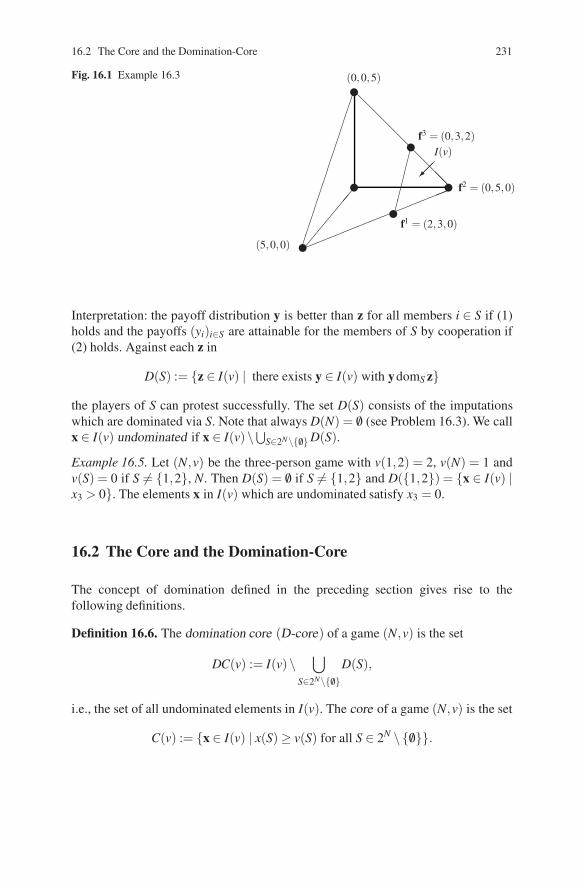
16.2 The Core and the Domination-Core 231
Fig. 16.1 Example 16.3
��
��
��
��
������������
��
�
�����
(0,0,5)
f3 = (0,3,2)
f2 = (0,5,0)
f1 = (2,3,0)
(5,0,0)
I(v)
�
�
�
�
Interpretation: the payoff distribution y is better than z for all members i ∈ S if (1)holds and the payoffs (yi)i∈S are attainable for the members of S by cooperation if(2) holds. Against each z in
D(S) := {z ∈ I(v) | there exists y ∈ I(v) with ydomS z}
the players of S can protest successfully. The set D(S) consists of the imputationswhich are dominated via S. Note that always D(N) = /0 (see Problem 16.3). We callx ∈ I(v) undominated if x ∈ I(v)\⋃S∈2N\{ /0}D(S).
Example 16.5. Let (N,v) be the three-person game with v(1,2) = 2, v(N) = 1 andv(S) = 0 if S = {1,2}, N. Then D(S) = /0 if S = {1,2} and D({1,2}) = {x ∈ I(v) |x3 > 0}. The elements x in I(v) which are undominated satisfy x3 = 0.
16.2 The Core and the Domination-Core
The concept of domination defined in the preceding section gives rise to thefollowing definitions.
Definition 16.6. The domination core (D-core) of a game (N,v) is the set
DC(v) := I(v)\⋃
S∈2N\{ /0}D(S),
i.e., the set of all undominated elements in I(v). The core of a game (N,v) is the set
C(v) := {x ∈ I(v) | x(S) ≥ v(S) for all S ∈ 2N \ { /0}}.

232 16 TU-Games: Domination, Stable Sets, and the Core
If x ∈C(v), then no coalition S = N has an incentive to split off if x is the proposedpayoff distribution in N, because the total amount x(S) allocated to S is not smallerthan the amount v(S) which the players in S can obtain by forming the coalition S.
For the game in Example 16.5 the D-core is nonempty and the core is empty. Ingeneral the following holds.
Theorem 16.7. The core is a subset of the D-core for each TU-game.
Proof. Let (N,v) be a game and x ∈ I(v), x ∈ DC(v). Then there is a y ∈ I(v)and a coalition S such that ydomS x. Thus, v(S) ≥ y(S) > x(S), which implies thatx ∈C(v). ��Elements of C(v) can easily be obtained because the core is defined with the aidof linear inequalities. The core is a polytope. Also the D-core is a convex set: seeProblem 16.2.
A natural question that arises is: for which games is the core equal to the D-core?Consider the following condition on a game (N,v):
v(N) ≥ v(S)+ ∑i∈N\S
v(i) for all S ∈ 2N \ { /0}. (16.1)
It turns out that this condition is sufficient for the equality of core and D-core.
Theorem 16.8. Let (N,v) be a game satisfying (16.1). Then DC(v) = C(v).
Proof. In view of Theorem 16.7 it is sufficient to show that DC(v) ⊆C(v).Claim. Let x ∈ I(v) with x(S) < v(S) for some S, then there is a y ∈ I(v) such thatydomS x.
To prove this claim, define y as follows. If i∈ S, then yi := xi + |S|−1(v(S)−x(S)).If i ∈ S, then yi := v(i)+(v(N)−v(S)−∑i∈N\S v(i))|N \S|−1. Then y ∈ I(v), whereyi ≥ v(i) for i ∈ N \ S follows from (16.1). Furthermore, ydomS x. This proves theclaim.
To prove DC(v) ⊆ C(v), suppose x ∈ DC(v). Then there is no y ∈ I(v) withydomx. In view of the Claim it follows that x(S)≥ v(S) for all S ∈ 2N \{ /0}. Hence,x ∈C(v). ��Many games v derived from practical situations have the following property:
v(S∪T ) ≥ v(S)+ v(T) for all disjoint S,T ⊆ N. (16.2)
A game satisfying (16.2) is called super-additive. Observe that (16.2) implies (16.1),so that Theorem 16.8 holds for super-additive games in particular.
16.3 Simple Games
In this section we study the core and D-core of simple games. Simple games arisein particular in political situations, see for instance the United Nations SecurityCouncil example in Chap. 1.
16.3 Simple Games 233
Definition 16.9. A simple game (N,v) is a game where every coalition has eitherworth 0 or worth 1, and the grand coalition N has worth 1. Coalitions with worth1 are called winning, the other coalitions are called losing. A minimal winningcoalition is a winning coalition for which every proper subset is losing. A player i iscalled a dictator in a simple game (N,v) if v(S) = 1 if and only if i ∈ S. A player iis called a veto player in a simple game (N,v) if i belongs to all winning coalitions.The set of veto players of v is denoted by veto(v). Hence,
veto(v) =⋂{S ∈ 2N | v(S) = 1}.
The next example suggests that non-emptiness of the core has something to do withthe existence of veto players.
For each i ∈ N let ei ∈ Rn denote the vector with i-th coordinate equal to 1 andall other coordinates equal to 0.
Example 16.10. (1) For the dictator game δi, which is the simple game with δi(S) =1 if and only if i∈ S one has I(δi) = {ei}, veto(δi) = {i} and C(δi) = DC(δi) = {ei}.(2) For the three-person majority game with v(S) = 1 if |S| ∈ {2,3} and v(S) = 0 if|S| ∈ {0,1} one has:
{1,2}∩{1,3}∩{2,3}∩{1,2,3}= /0 = veto(v)
andC(v) = DC(v) = /0.
(3) For the T -unanimity game uT , which is the simple game with uT (S) = 1 if andonly if T ⊆ S, veto(uT ) = T and
C(uT ) = DC(uT ) = conv{ei | i ∈ T}.
The following theorem shows that the core of a simple game is nonempty if and onlyif the game has veto players. Furthermore, core elements divide the total amountv(N) = 1 of the grand coalition among the veto players. The D-core is equal to thecore for simple games except in one case where there is exactly one k ∈ N withv(k) = 1 and k is not a veto player. See also Example 16.12 below.
Theorem 16.11. Let (N,v) be a simple game. Then:
(1) C(v) = conv{ei ∈ Rn | i ∈ veto(v)}.(2) If veto(v) = /0 and {i ∈ N | v(i) = 1} = {k}, then C(v) = /0 and DC(v) = {ek}.
Otherwise, DC(v) = C(v).
Proof. (a) Suppose i ∈ veto(v). Let S ∈ 2N \ { /0}. If i ∈ S then ei(S) = 1 ≥ v(S),otherwise ei(S) = 0 = v(S). Obviously, ei(N) = 1 = v(N). So ei ∈C(v). This provesthe inclusion ⊇ in (1) because C(v) is a convex set.
(b) To prove the inclusion ⊆ in (1), let x ∈ C(v). It is sufficient to prove: i ∈veto(v) ⇒ xi = 0. Suppose, to the contrary, that xi > 0 for some non-veto playeri. Take S with v(S) = 1 and i ∈ S (such an S exists otherwise i would be a veto
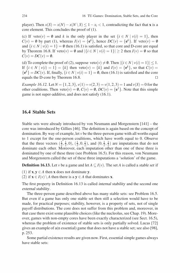
234 16 TU-Games: Domination, Stable Sets, and the Core
player). Then x(S) = x(N)− x(N \ S)≤ 1− xi < 1, contradicting the fact that x is acore element. This concludes the proof of (1).
(c) If veto(v) = /0 and k is the only player in the set {i ∈ N | v(i) = 1}, thenC(v) = /0 by part (1), whereas I(v) = {ek}, hence DC(v) = {ek}. If veto(v) = /0and {i ∈ N | v(i) = 1} = /0 then (16.1) is satisfied, so that core and D-core are equalby Theorem 16.8. If veto(v) = /0 and |{i ∈ N | v(i) = 1}| ≥ 2 then I(v) = /0 so thatC(v) = DC(v) = /0.
(d) To complete the proof of (2), suppose veto(v) = /0. Then |{i∈ N | v(i) = 1}| ≤ 1.If {i ∈ N | v(i) = 1} = {k} then veto(v) = {k} and I(v) = {ek}, so that C(v) ={ek} = DC(v). If, finally, {i ∈ N | v(i) = 1}= /0, then (16.1) is satisfied and the coreequals the D-core by Theorem 16.8. ��Example 16.12. Let N = {1,2,3}, v(1)= v(2,3)= v(1,2,3)= 1 and v(S)= 0 for theother coalitions. Then veto(v) = /0, C(v) = /0, DC(v) = {e1}. Note that this simplegame is not super-additive, and does not satisfy (16.1).
16.4 Stable Sets
Stable sets were already introduced by von Neumann and Morgenstern [141] – thecore was introduced by Gillies [46]. The definition is again based on the concept ofdomination. By way of example, let v be the three-person game with all worths equalto 1 except for the one-person coalitions, which have worth equal to 0. Observethat the three vectors ( 1
2 , 12 ,0), ( 1
2 ,0, 12 ), and (0, 1
2 , 12 ) are imputations that do not
dominate each other. Moreover, each imputation other than one of these three isdominated by one of these three (see Problem 16.5). For this reason, von Neumannand Morgenstern called the set of these three imputations a ‘solution’ of the game.
Definition 16.13. Let v be a game and let A ⊆ I(v). The set A is called a stable set if
(1) if x,y ∈ A then x does not dominate y.(2) if x ∈ I(v)\A then there is a y ∈ A that dominates x.
The first property in Definition 16.13 is called internal stability and the second oneexternal stability.
The three-person game described above has many stable sets: see Problem 16.5.But even if a game has only one stable set then still a selection would have to bemade, for practical purposes; stability, however, is a property of sets, not of singlepayoff distributions. The core does not suffer from this problem and, moreover, inthat case there exist some plausible choices (like the nucleolus, see Chap. 19). More-over, games with non-empty cores have been exactly characterized (see Sect. 16.5),whereas the problem of existence of stable sets is only partially solved. Lucas [72]gives an example of a(n essential) game that does not have a stable set; see also [98],p. 253.
Some partial existence results are given now. First, essential simple games alwayshave stable sets:

16.5 Balanced Games and the Core 235
Theorem 16.14. Let v be a simple game and let S be a minimal winning coalition.Let ∆S be the set of those imputations x with xi = 0 for every i ∈ S. Then, if ∆S = /0,it is a stable set.
Proof. Problem 16.8. ��A game (N,v) is called a zero-one game if all one-person coalitions have worth 0and the grand coalition N has worth 1. In the following example symmetric three-person zero-one games are considered.
Example 16.15. Let (N,v) be a game with N = {1,2,3} and v(i) = 0 for all i ∈ N,v(N) = 1, and v(S) = α for every two-person coalition S, where 0 ≤ α ≤ 1. Then:
(a) Let α ≥ 23 . Then
{(x,x,1−2x),(x,1−2x,x),(1−2x,x,x) | α2≤ x ≤ 1
2} (16.3)
is a stable set.(b) For α < 2
3 , the set in (16.3) is internally but not externally stable. The union ofthis set with the core of the game is a stable set.
(c) For α ≤ 12 the core is a (the unique) stable set.
For the proofs of these statements see Problem 16.9.
The next theorem gives the relation between the domination core and stable sets.
Theorem 16.16. Let (N,v) be a game. Then:
(a) The D-core of v is a subset of any stable set.(b) Suppose the D-core of v is a stable set. Then it is the unique stable set of the
game.
Proof. Problem 16.10. ��
16.5 Balanced Games and the Core
In this section we derive the Bondareva–Shapley ([16], [122]) Theorem which char-acterizes games with non-empty cores in terms of balancedness. First, the conceptsof balanced maps, collections, and games are introduced.
Let N := {1,2, . . . ,n}. A map λ : 2N \ { /0} → R+ := {t ∈ R | t ≥ 0} is called abalanced map if
∑S∈2N\{ /0}
λ (S)eS = eN .
Here eS is the characteristic vector for coalition S with
eSi = 1 if i ∈ S and eS
i = 0 if i ∈ N \S.

236 16 TU-Games: Domination, Stable Sets, and the Core
A collection B of coalitions is called a balanced collection if there is a balanced mapλ such that
B = {S ∈ 2N | λ (S) > 0}.Example 16.17. (1) Let N1,N2, . . . ,Nk be a partition of N, i.e., N =
⋃kr=1 Nr, Ns ∩
Nt = /0 if s = t. Then {N1,N2, . . . ,Nk} is a balanced collection, corresponding to thebalanced map λ with λ (S) = 1 if S ∈ {N1,N2, . . . ,Nk} and λ (S) = 0, otherwise.
(2) For N = {1,2,3} the set B = {{1,2}, {1,3}, {2,3}} is balanced and correspondsto the balanced map λ with
λ (S) = 0 if |S| ∈ {1,3} and λ (S) =12
if |S| = 2.
In order to have an interpretation of a balanced map, one can think of each playerhaving one unit of time (or perhaps energy, labor) to spend. Each player candistribute his time over the various coalitions of which he is a member. Such adistribution is ‘balanced’ if it corresponds to a balanced map λ , where λ (S) is inter-preted as the length of time that the coalition S exists (‘cooperates’); balancednessof λ means that each player spends exactly his one unit of time over the variouscoalitions.
Definition 16.18. A game (N,v) is called a balanced game if for each balanced mapλ : 2N \ { /0}→ R+ we have
∑S
λ (S)v(S)≤ v(N). (16.4)
Extending the interpretation of a balanced map in terms of a distribution of time toa game, balancedness of a game could be interpreted as saying that it is at least asproductive to have the grand coalition operate during one unit of time as to have abalanced distribution of time over various smaller coalitions – worths of coalitionsbeing interpreted as productivities. Thus, in a balanced game, it seems advantageousto form the grand coalition. Indeed, technically the importance of the notion ofbalancedness follows from Theorem 16.21, proved by Bondareva [16] and Shapley[122]; this theorem characterizes games with a nonempty core. Its proof is based onthe following duality theorem.
For x,y ∈ Rn, x ·y denotes the usual inner product: x ·y = ∑ni=1 xiyi.
Theorem 16.19. Let A be an n× p-matrix, b ∈ Rp and c ∈ Rn, and let {x ∈ Rn |xA ≥ b} = /0 and {y ∈ Rp | Ay = c,y ≥ 0} = /0. Then
min{x · c | xA ≥ b} = max{b ·y | Ay = c,y ≥ 0}.
Proof. Problem 16.13. ��Remark 16.20. In Theorem 16.19 also the following holds: if one of the programsis infeasible (i.e., one of the two sets in the theorem is empty), then both programsdo not have an optimal solution (i.e., neither the minimum nor the maximum areattained). See Problem 16.14 for a proof.

Problems 237
Theorem 16.21. Let (N,v) be a TU-game. Then the following two assertions areequivalent:
(1) C(v) = /0.(2) (N,v) is a balanced game.
Proof. First note that C(v) = /0 if and only if
v(N) = min{n
∑i=1
xi | x ∈ RN , x(S) ≥ v(S) for all S ∈ 2N \ { /0}}. (16.5)
By the duality theorem, Theorem 16.19, equality (16.5) holds if and only if
v(N) = max{∑λ (S)v(S) | ∑λ (S)eS = eN ,λ ≥ 0}. (16.6)
(Take for A the matrix with the characteristic vectors eS as columns, let c := eN andlet b be the vector of coalitional worths. Obviously, the non-emptiness conditions inTheorem 16.19 are satisfied.) Now (16.6) holds if and only if (16.4) holds. Hence(1) and (2) are equivalent. ��
Problems
16.1. Imputation Set of an Essential Game
Prove that for an essential game v, I(v) is the convex hull of the points f1, f2, . . . , fn,as claimed in Sect. 16.1.
16.2. Convexity of the Domination Core
Prove that for each game the domination core is a convex set.
16.3. Dominated Sets of Imputations
(1) Prove that for each game (N,v), D(S) = /0 if |S| ∈ {1,n}.
(2) Determine for each S the set D(S) for the cost savings game (three communitiesgame) in Chap. 1. Answer the same questions for the glove game in Chap. 1.
16.4. The Domination Relation
(1) Prove that dom and domS are irreflexive relations and that domS is transitiveand antisymmetric.1
(2) Construct a game (N,v) and imputations x and y such that xdomy and ydomx.
(3) Construct a game (N,v) and x,y,z ∈ I(v) with xdomy and ydomz and notxdomz.
1 See Sect. 11.1 for definitions.

238 16 TU-Games: Domination, Stable Sets, and the Core
16.5. Stable Sets in a Three-Person Game
Let ({1,2,3},v) be the game with all worths equal to 1 except for the one-personand the empty coalitions, which have worth equal to 0.
(1) Prove that each element of the imputation set of this game is dominated byanother element.
(2) Prove that in this game each x ∈ I(v) \A is dominated by an element of A :={( 1
2 , 12 ,0), ( 1
2 ,0, 12 ), (0, 1
2 , 12 )}.
(3) If c ∈ [0, 12 ) and B := {x ∈ I(v) | x3 = c}, then each element of I(v) \ B is
dominated by an element of B. Show this.
16.6. Singleton Stable Set
Prove that if a game (N,v) has a one-element stable set then v(N) = ∑i∈N v(i) (from[81]).
16.7. A Glove Game
Consider the three-person simple game v defined by
v(S) :={
1 if S = {1,2} or {2,3} or {1,2,3}0 otherwise.
(a) Show that any imputation (x1,x2,x3) that is not equal to e2 is dominated byanother imputation.
(b) Compute the core and the domination core.
(c) Show that the domination core is not a stable set.
(d) Show that
B := {(λ ,1−2λ ,λ ) | 0 ≤ λ ≤ 12}
is a stable set.
16.8. Proof of Theorem 16.14
Prove Theorem 16.14.
16.9. Example 16.15
Prove the statements in Example 16.15.
16.10. Proof of Theorem 16.16
Prove Theorem 16.16. Does this theorem also hold for the core instead of theD-core?
16.11. Core and D-core
Is (16.1) also a necessary condition for equality of the core and the D-core? (cf.Theorem 16.8).

Problems 239
16.12. Strategic Equivalence
Let (N,w) be strategically equivalent to (N,v), that is, there are k ∈ R, k > 0 anda ∈ RN such that for each coalition S: w(S) = kv(S)+ a(S). Show that
(1) C(w) = kC(v)+ a (:= {x ∈ RN | x = ky+ a for some y ∈C(v)})(2) DC(w) = kDC(v)+ a.
(The equalities (1) and (2) express that the core and the D-core are covariant w.r.t.strategic equivalence.)
16.13. Proof of Theorem 16.19
Prove Theorem 16.19. (Hint: use Theorem 22.5.)
16.14. Infeasible Programs in Theorem 16.19
Prove the claim made in Remark 16.20. Hint: Suppose, say, that there is no y ≥ 0with Ay = c. Then, certainly, the max-program does not have an optimal solution.Use Farkas’ Lemma (Lemma 22.4) to conclude that there exists a vector z withzA ≥ 0 and z · c < 0. Suppose the min-program is feasible, i.e., there is an x withxA ≥ b. Then, show that the min-program does not have an optimal solution byconsidering the vectors x+ tz for t ∈ R, t > 0.
16.15. Balanced Maps and Collections
(1) Show that for any balanced map λ one has ∑S λ (S) ≥ 1, with equality if andonly if the corresponding balanced collection equals {N}.
(2) If B is a balanced collection unequal to {N}, then
Bc := {S ∈ 2N \ { /0} | N \S ∈ B}
is also a balanced collection. Give the corresponding balanced map.
(3) Let S ∈ 2N \ { /0,N}. Prove that {S,(N \ {i})i∈S} is balanced collection.
(4) Prove that the balanced maps form a convex set Λn.
16.16. Minimum of Balanced Games
Show that the minimum of two balanced games is again balanced.
16.17. Balanced Simple Games
A simple game has a non-empty core if and only if it has veto players, cf. Theo-rem 16.11(1). Derive this result from Theorem 16.21.

Chapter 17The Shapley Value
In Chap. 16 set-valued solution concepts for games with transferable utilities werestudied: the imputation set, core, domination core, and stable sets. In this chapter,a one-point (single-valued) solution concept is discussed: the Shapley value. It mayagain be helpful to first study the relevant parts of Chaps. 1 and 9.
Section 17.1 introduces the Shapley value by several formulas and presents (avariation on) Shapley’s axiomatic characterization using additivity. In Sect. 17.2 wepresent three other characterizations of the Shapley value: a description in terms ofHarsanyi dividends; an axiomatic characterization of Young based on strong mono-tonicity; and Owen’s formula for the Shapley value based on a multilinear extensionof games. Section 11.3 discusses Hart and Mas-Colell’s approach to the Shapleyvalue based on potential and reduced games.
17.1 Definition and Shapley’s Characterization
The Shapley value is one of the most interesting solution concepts in cooperativegame theory. The seminal paper [121] is the starting point of a large literature onthis solution concept and related concepts. For overviews see [109] and Chaps. 53and 54 in [6].
Let (N,v) be a TU-game and let σ : N → N be a permutation of the player set.Imagine that the players enter a room one by one in the ordering σ(1), σ(2), . . . ,σ(n) and give each player the marginal contribution he creates in the game. To bemore specific, let the set of predecessors of i in σ be the coalition
Pσ (i) := {r ∈ N | σ−1(r) < σ−1(i)}.
For example, if N = {1,2,3,4,5} and σ(1) = 2, σ(2) = 5, σ(3) = 4, σ(4) = 1, andσ(5) = 3, player 2 enters first, next players 5, 4, 1, and 3. So Pσ (1) = {2,5,4}.
Define the marginal vector mσ by
mσi = v(Pσ (i)∪{i})− v(Pσ(i)). (17.1)
H. Peters, Game Theory – A Multi-Leveled Approach.c© Springer-Verlag Berlin Heidelberg 2008
241

242 17 The Shapley Value
Thus, the marginal vector mσ gives each player his marginal contribution to thecoalition formed by his entrance, according to the ordering σ .1
Definition 17.1. The Shapley value Φ(v) of a game (N,v) is the average of themarginal vectors of the game, i.e.
Φ(v) :=1n! ∑
σ∈Π(N)mσ . (17.2)
(Here Π(N) denotes the set of permutations of N.)
Example 17.2. (1) For a two-person game (N,v) the Shapley value is
Φ(v) =(
v(1)+v(N)− v(1)− v(2)
2,v(2)+
v(N)− v(1)− v(2)2
).
(2) Let (N,v) be the three-person game with v(1) = v(2) = v(3) = 0, v(1,2) = 4,v(1,3) = 7, v(2,3) = 15, v(1,2,3) = 20. Then the marginal vectors are given in theTable 17.1. The Shapley value of this game is equal to 1
6 (21,45,54), as one easilyobtains from this table.
(3) The Shapley value Φ(v) for an additive game is equal to (v(1),v(2), . . . , v(n)).
Based on (17.2), a probabilistic interpretation of the Shapley value is as follows.Suppose we draw from an urn, containing the elements of Π(N), a permutation σ(probability (n!)−1). Then let the players enter a room one by one in the order σ andgive each player the marginal contribution created by him. Then the i-th coordinateΦi(v) of Φ(v) is the expected payoff to player i according to this random procedure.
Using (17.1) formula (17.2) can be rewritten as
Φi(v) =1n! ∑
σ∈Π(N)v(Pσ (i)∪{i})− v(Pσ(i)). (17.3)
The terms at the right hand side of the summation sign are of the form v(S∪{i})−v(S), where S is a subset of N not containing i. For how many orderings does
Table 17.1 Example 17.2(2)
(σ (1),σ (2),σ (3)) mσ1 mσ
2 mσ3
(1,2,3) 0 4 16(1,3,2) 0 13 7(2,1,3) 4 0 16(2,3,1) 5 0 15(3,1,2) 7 13 0(3,2,1) 5 15 0
∑ 21 45 54
1 Of course, mσ depends on the game v.

17.1 Definition and Shapley’s Characterization 243
one have Pσ (i) = S? The answer is |S|!(n− 1− |S|)!, where the first factor |S|!corresponds to the number of orderings of S and the second factor (n−1−|S|)! tothe number of orderings of N \ (S∪{i}). Hence, (17.3) can be rewritten to obtain
Φi(v) = ∑S:i∈S
|S|!(n− 1−|S|)!n!
(v(S∪{i})− v(S)). (17.4)
Note that |S|!(n−1−|S|)!n!
=1n
(n−1|S|)−1
.
This gives rise to a second probabilistic interpretation of the Shapley value. Con-struct a subset S to which i does not belong, as follows. First, draw at random anumber from the urn containing the numbers (possible sizes) 0,1,2, . . . ,n−1, whereeach number has probability n−1 to be drawn. If size s is chosen, draw a set fromthe urn containing the subsets of N \{i} of size s, where each set has the same prob-ability
(n−1s)−1 to be drawn. If S is drawn with |S|= s, then pay player i the amount
v(S∪{i})− v(S). Then, in view of (17.4), the expected payoff for player i in thisrandom procedure is the Shapley value for player i of the game (N,v).
Shapley [121] gave an axiomatic characterization of the Shapley value. That is,he formulated a number of properties that a one-point solution should (or might)have and then showed that the Shapley value is the only solution with these prop-erties. This characterization – in a somewhat different form – is the next subject ofthis section.
Definition 17.3. A value on G N is a map ψ : G N → RN .2
The following axioms for a value ψ : G N → RN are used in the announced charac-terization of the Shapley value.
Efficiency (EFF): ∑ni=1 ψi(v) = v(N) for all v ∈ G N .
The efficiency (sometimes called Pareto optimality or Pareto efficiency) axiomneeds no further explanation.
Call a player i in a game (N,v) a null-player if v(S∪ i)−v(S) = 0 for every coali-tion S ∈ 2N . Such a player does not contribute anything to any coalition, in particularalso v(i) = 0. So it seems reasonable that such a player obtains zero according to thevalue. This is what the following axiom requires.
Null-player Property (NP): ψi(v) = 0 for all v ∈ G N and all a null-players i in v.
Call players i and j symmetric in the game (N,v) if v(S∪ i) = v(S∪ j) for everycoalition S ⊆ N \{i, j}. Symmetric players have the same contribution to any coali-tion, and therefore it seems reasonable that they should obtain the same payoffaccording to the value. That is the content of the following axiom.
Symmetry (SYM): ψi(v) = ψ j(v) for all v ∈ G N and all symmetric players i and jin v.
2 Occasionally, also the word solution will be used.

244 17 The Shapley Value
The last axiom needed in the announced characterization can be interpreted asfollows. Suppose the game (N,v) is played today and the game (N,w) tomorrow.If the value ψ is applied then player i obtains in total: ψi(N,v)+ψi(N,w). One mayalso argue that, in total, the game (N,v + w) is played and that, accordingly, playeri should obtain ψi(N,v + w). The following axiom expresses the possible point ofview that these two evaluations should not make a difference.
Additivity (ADD): ψ(v + w) = ψ(v)+ ψ(w) for all v,w ∈ G N .
The announced characterization is the following theorem.
Theorem 17.4. Let ψ : G N → RN be a value. Then ψ satisfies EFF, NP, SYM, andADD, if, and only if, ψ is the Shapley value Φ.
The proof of Theorem 17.4 uses, through the additivity axiom, the fact that G N is alinear space, with addition defined by (v+w)(S) = v(S)+w(S) and scalar multipli-cation (αv)(S) = αv(S) for all v,w ∈ G N , S ∈ 2N , and α ∈ R. An obvious basis forG N is the set {1T ∈ G N | T ∈ 2N \{ /0}}, where 1T is the game defined by 1T (T ) = 1and 1T (S) = 0 for all S = T (cf. Problem 17.1). This basis is not very well suitedfor the present purpose because the Shapley value Φ(1T ) (T ∈ 2N \ { /0}) cannoteasily be determined from the axioms in Theorem 17.4: for example, there is nonull-player in the game 1T (cf. Problem 17.1).
Another basis is the collection of unanimity games {uT ∈ G N | T ∈ 2N \ { /0}},see Example 16.10(3) for the definition, and Problem 17.2. This basis is used in thefollowing proof.
Proof of Theorem 17.4. That the Shapley value satisfies the four axioms in thetheorem is the subject of Problem 17.3.
Conversely, suppose ψ satisfies the four axioms. It has to be proved that ψ = Φ.Take v ∈ G N . Then there are unique numbers cT (T = /0) such that v = ∑T = /0 cT uT(cf. Problem 17.2). By ADD of ψ and Φ it follows that
ψ(v) = ∑T = /0
ψ(cT uT ), Φ(v) = ∑T = /0
Φ(cT uT ).
So it is sufficient to show that for all T = /0 and c ∈ R :
ψ(cuT ) = Φ(cuT ). (17.5)
Take T = /0 and c ∈ R. Note first that for all i ∈ N \T :
cuT (S∪{i})− cuT(S) = 0 for all S,
implying that i is a null-player in cuT . So, by NP of ψ and Φ:
ψi(cuT ) = Φi(cuT ) = 0 for all i ∈ N \T. (17.6)
Now suppose that i, j ∈ T , i = j. Then, for every coalition S⊆N \{i, j}, cuT (S∪ i) =cuT (S∪ j) = 0, which implies that i and j are symmetric in cuT . Hence, by SYM ofψ and Φ:
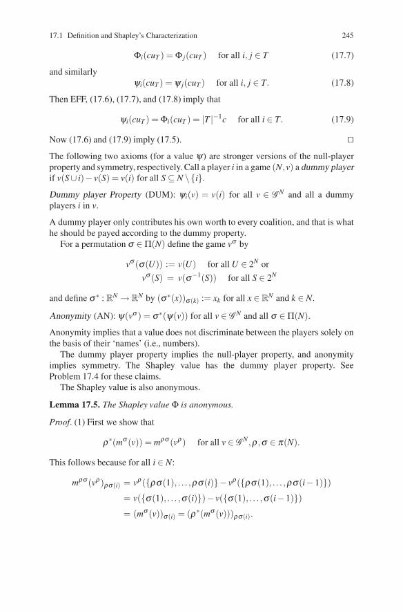
17.1 Definition and Shapley’s Characterization 245
Φi(cuT ) = Φ j(cuT ) for all i, j ∈ T (17.7)
and similarlyψi(cuT ) = ψ j(cuT ) for all i, j ∈ T. (17.8)
Then EFF, (17.6), (17.7), and (17.8) imply that
ψi(cuT ) = Φi(cuT ) = |T |−1c for all i ∈ T. (17.9)
Now (17.6) and (17.9) imply (17.5). ��The following two axioms (for a value ψ) are stronger versions of the null-playerproperty and symmetry, respectively. Call a player i in a game (N,v) a dummy playerif v(S∪ i)− v(S) = v(i) for all S ⊆ N \ {i}.
Dummy player Property (DUM): ψi(v) = v(i) for all v ∈ G N and all a dummyplayers i in v.
A dummy player only contributes his own worth to every coalition, and that is whathe should be payed according to the dummy property.
For a permutation σ ∈ Π(N) define the game vσ by
vσ (σ(U)) := v(U) for all U ∈ 2N orvσ (S) = v(σ−1(S)) for all S ∈ 2N
and define σ∗ : RN → RN by (σ∗(x))σ(k) := xk for all x ∈ RN and k ∈ N.
Anonymity (AN): ψ(vσ ) = σ∗(ψ(v)) for all v ∈ G N and all σ ∈ Π(N).
Anonymity implies that a value does not discriminate between the players solely onthe basis of their ‘names’ (i.e., numbers).
The dummy player property implies the null-player property, and anonymityimplies symmetry. The Shapley value has the dummy player property. SeeProblem 17.4 for these claims.
The Shapley value is also anonymous.
Lemma 17.5. The Shapley value Φ is anonymous.
Proof. (1) First we show that
ρ∗(mσ (v)) = mρσ (vρ) for all v ∈ G N ,ρ ,σ ∈ π(N).
This follows because for all i ∈ N:
mρσ (vρ)ρσ(i) = vρ({ρσ(1), . . . ,ρσ(i)}− vρ({ρσ(1), . . . ,ρσ(i−1)})= v({σ(1), . . . ,σ(i)})− v({σ(1), . . . ,σ(i−1)})= (mσ (v))σ(i) = (ρ∗(mσ (v)))ρσ(i).

246 17 The Shapley Value
(2) Take v ∈ G N and ρ ∈ Π(N). Then (1), the fact that ρ �→ ρσ is a surjection onΠ(N) and the linearity of ρ∗ imply
Φ(vρ) =1n! ∑
σ∈Π(N)mσ (vσ ) =
1n! ∑
σmρσ (vρ)
=1n! ∑
σρ∗(mσ (v)) = ρ∗(
1n! ∑
σmσ ) = ρ∗(Φ(v)).
This proves the anonymity of Φ. ��As is clear by now the Shapley value has many appealing properties. In the followingsections more properties and characterizations of the Shapley value are considered.However, it also has some drawbacks. In a balanced game the Shapley value does notnecessarily assign a core element. Also, it does not have to be individually rational(cf. Problem 17.5).
Variations of the Shapley value, obtained by omitting the symmetry (oranonymity) requirement in particular, are discussed in Chap. 18.
17.2 Other Characterizations
In this section three other characterizations of the Shapley value are discussed: thedividend approach, the axiomatization of Young [148] based on strong monotonic-ity, and the multilinear approach of Owen [97].
17.2.1 Dividends
Harsanyi [48] has introduced the following concept.
Definition 17.6. Let (N,v) be game. For each coalition T the dividend ∆v(T ) isdefined, recursively, as follows.
∆v( /0) := 0∆v(T ) := v(T )− ∑
S:S�T
∆v(S) if |T | ≥ 1.
The relation between dividends and the Shapley value is described in the next theo-rem. The Shapley value of a player in a game turns out to be the sum of all equallydistributed dividends of coalitions to which the player belongs.
Theorem 17.7. Let v = ∑T∈2N\{ /0} cT uT (as in Problem 17.2). Then:
(1) ∆v(T ) = cT for all T = /0.

17.2 Other Characterizations 247
(2) The Shapley value Φi(v) for player i is equal to the sum of the equally distributeddividends of the coalitions to which player i belongs i.e.,
Φi(v) = ∑T :i∈T
∆v(T )|T | .
Proof. In the proof of Theorem 17.4 it was shown that Φ(cT uT ) = |T |−1cT eT foreach T , so by ADD, Φ(v) = ∑T = /0 cT |T |−1eT .
Hence, Φi(v) = ∑T :i∈T cT |T |−1. The only thing left to show is that
cT = ∆v(T ) for all T = /0. (17.10)
The proof of this is done by induction. If |T | = 1, say T = {i}, then cT = v(i) =∆v(T ). Suppose (17.10) holds for all S � T . Then ∆v(T ) = v(T )−∑S�T ∆v(S) =v(T )−∑S�T cS = cT because v(T ) = ∑S⊆T cS. ��The concept of coalitional dividend is important not only for the Shapley value butfor a wider range of solution concepts. See [30].
17.2.2 Strong Monotonicity
The Shapley value obviously has the property that if a player contributes at least asmuch to any coalition in a game v than in a game w, then his payoff from the Shapleyvalue in v is at least as large as that in w. Formally, the Shapley value satisfies thefollowing axiom for a value ψ : G N → RN ; a proof is immediate from (17.4).
Strong Monotonicity (SMON): ψi(v) ≥ ψi(w) for all v, w ∈ G N that satisfy
v(S∪{i})− v(S)≥ w(S∪{i})−w(S) for all S ∈ 2N .
Young [148] has proved that together with efficiency and symmetry this axiomcharacterizes the Shapley value.
Theorem 17.8. Let ψ : G N → RN be a value. Then ψ satisfies EFF, SYM, andSMON, if and only if ψ is the Shapley value Φ.
Proof. Obviously, Φ satisfies the three axioms. Conversely, suppose ψ satisfies thethree axioms:
(1) Let z be the game that is identically zero. In this game, all players are symmetric,so SYM and EFF together imply ψ(z) = 0.
(2) Let i be a null-player in a game v. Then the condition in SMON applies to zand v with all inequalities being equalities. So SMON yields ψi(v) ≥ ψi(z) andψi(z) ≥ ψi(v). Hence by (1), ψi(v) = 0.
(3) Let c ∈ R and T ∈ 2N \ { /0}. Then (2) implies ψi(cuT ) = 0 for every i ∈ N \T .This, SYM, and EFF imply ψi(cuT ) = c|T |−1 for every i ∈ T . Hence, ψ(cuT ) =c|T |−1eT .

248 17 The Shapley Value
(4) Each v ∈ G N can be written in a unique way as a linear combination of {uT |T ∈ 2N \ { /0}} (see Problem 17.2). So v is of the form ∑cT uT . The proof ofψ(v) = Φ(v) will be completed by induction on the number α(v) of terms in∑cT uT with cT = 0.
From (1), ψ(v) = Φ(v) = 0 if α(v) = 0, and from (3), ψ(v) = Φ(v) if α(v) = 1because Φ(cuT ) = c|T |−1eT . Suppose ψ(w) = Φ(w) for all w ∈ G N with α(w) < k,where k ≥ 2. Let v be a game with α(v) = k. Then there are coalitions T1, T2, . . . ,Tk and real numbers c1, c2, . . . , ck, unequal to zero, such that v = ∑k
r=1 cruTr . LetD := ∩k
r=1Tr.For i ∈ N \ D, define wi := ∑r:i∈Tr cruTr . Because α(wi) < k, the induction
hypothesis implies: ψi(wi) = Φi(wi). Further, for every S ∈ 2N :
v(S∪ i)− v(S) =k
∑r=1
cruTr(S∪ i)−k
∑r=1
cruTr(S)
= ∑r:i∈Tr
cruTr(S∪ i)− ∑r:i∈Tr
cruTr(S)
= wi(S∪ i)−wi(S),
so that, by SMON of ψ and Φ, it follows that ψi(v) = ψi(wi) = Φi(wi) = Φi(v). So
ψi(v) = Φi(v) for all i ∈ N \D. (17.11)
(17.11) and EFF for ψ and Φ yield
∑i∈D
ψi(v) = ∑i∈D
Φi(v). (17.12)
Let i, j ∈ D, then for every S ⊆ N \ {i, j}:
(0 =) v(S∪ i) =k
∑r=1
cruTr(S∪ i) =k
∑r=1
cruTr(S∪ j) = v(S∪ j),
so i and j are symmetric. Hence, by SYM of ψ and Φ:
ψi(v) = ψ j(v), Φi(v) = Φ j(v). (17.13)
Now ψ(v) = Φ(v) follows from (17.11), (17.12) and (17.13). ��
17.2.3 Multilinear Extension
The Shapley value of a game may also be described by means of the multilinearextension of a game (cf. [97, 98]). Let (N,v) be game. Consider the function f :[0,1]N → R on the hypercube [0,1]N , defined by

17.2 Other Characterizations 249
f (x1,x2, . . . ,xn) = ∑S∈2N
(∏i∈S
xi ∏i∈N\S
(1− xi)
)v(S). (17.14)
Observe that the set of extreme points of [0,1]N , ext([0,1]N), is equal to {eS | S ∈2N}. By Problem 17.8(1),
f (eS) = v(S) for each S ∈ 2N . (17.15)
So f can be seen as an extension of v: ext([0,1]N) → R with v(eS) := v(S). In viewof Problem 17.8, f is called the multilinear extension of (v or) v.
One can give a probabilistic interpretation of f (x). Suppose that each of theplayers i ∈ N, independently, decides whether to cooperate (probability xi) or not(probability 1−xi). So with probability ∏i∈S xi ∏i∈N\S (1−xi) the coalition S forms,which has worth v(S). Then f (x) as given in (17.14) can be seen as the expectationof the worth of the formed coalition.
Another interpretation is to see x ∈ [0,1]N as a fuzzy set, where xi is the intensityof availability of player i and to see f as a characteristic function, defined for fuzzycoalitions in N.
Denote by Dk f (x) the derivative of f w.r.t. the k-th coordinate in x. The followingresult [97] provides another description of the Shapley value, as the integral alongthe main diagonal of [0,1]N of Dk f .
Theorem 17.9. Φk(v) =∫ 1
0 (Dk f )(t,t, . . . ,t)dt for each k ∈ N.
Proof.
Dk f (x) = ∑T :k∈T
[∏
i∈T\{k}xi ∏
i∈N\T(1− xi)
]v(T )
− ∑S:k ∈S
[∏i∈S
xi ∏i∈N\(S∪{k})
(1− xi)
]v(S)
= ∑S:k ∈S
[∏i∈S
xi ∏i∈N\(S∪{k})
(1− xi)
](v(S∪{k})− v(S)).
Hence,∫ 1
0 (Dk f )(t,t, . . . ,t)dt = ∑S:k ∈S (∫ 1
0 t |S|(1− t)n−|S|−1dt) (v(S∪{k})− v(S)).Using the well-known (beta-)integral formula∫ 1
0t |S|(1− t)n−|S|−1dt =
|S|!(n−|S|−1)!n!
it follows that∫ 1
0 (Dk f )(t,t, . . . ,t)dt = ∑S:k ∈S|S|!(n−|S|−1)!
n! (v(S ∪ {k})− v(S)) =Φk(v) by (17.4). ��Example 17.10. Let (N,v) be the three-person game with v(1) = v(2) = v(3) =v(1,2) = 0, v(1,3) = 1, v(2,3) = 2, v(N) = v(1,2,3) = 4. Then f (x1,x2,x3) =x1(1− x2)x3 + 2(1− x1) x2x3 + 4x1x2x3 = x1x3 + 2x2x3 + x1x2x3 for all x ∈ [0,1]N .

250 17 The Shapley Value
So D1 f (x) = x3 + x2x3, D2 f (x) = 2x3 + x1x3, D3 f (x) = x1 + 2x2 + x1x2. Theo-rem 17.9 implies
Φ1(v) =∫ 1
0D1 f (t,t,t)dt =
∫ 1
0(t + t2)dt =
56,
Φ2(v) =∫ 1
0(2t + t2)dt = 1
13, Φ3(v) =
∫ 1
0(3t + t2)dt = 1
56.
17.3 Potential and Reduced Game
This section starts off with discussing the potential approach to the Shapley value.The potential is, in a sense, dual to the concept of dividends. Next, reduced gamesare considered, which leads to another axiomatic characterization of the Shapleyvalue. This section is based on [52].
17.3.1 The Potential Approach to the Shapley Value
Denote by G is the family of all games (N,v) with an arbitrary finite (player) setN (not necessarily the set of the first n natural numbers). It is convenient to includealso the game ( /0,v), with empty player set. Thus,
G =⋃
N⊆N, |N|<∞G N .
Definition 17.11. A potential (Hart and Mas-Colell [52]) is a function P : G → Rsatisfying
P( /0,v) = 0 (17.16)
∑i∈N
DiP(N,v) = v(N) for all (N,v) ∈ G . (17.17)
Here DiP(N,v) := P(N,v)−P(N \{i},v) with v the restriction to N \{i} in the lastexpression.
If P is a potential then (17.17) says that the ‘gradient’ gradP(N,v) := (DiP(N,v))i∈Nis an efficient payoff vector for the game (N,v).
Note that
P({i},v) = v({i})P({i, j},v) =
12(v({i, j})+ v({i})+ v({ j}))
if P is a potential. More generally, it follows from (17.17) that
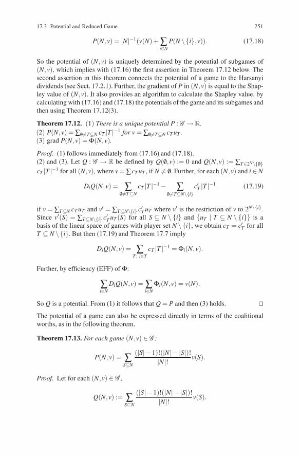
17.3 Potential and Reduced Game 251
P(N,v) = |N|−1(v(N)+ ∑i∈N
P(N \ {i},v)). (17.18)
So the potential of (N,v) is uniquely determined by the potential of subgames of(N,v), which implies with (17.16) the first assertion in Theorem 17.12 below. Thesecond assertion in this theorem connects the potential of a game to the Harsanyidividends (see Sect. 17.2.1). Further, the gradient of P in (N,v) is equal to the Shap-ley value of (N,v). It also provides an algorithm to calculate the Shapley value, bycalculating with (17.16) and (17.18) the potentials of the game and its subgames andthen using Theorem 17.12(3).
Theorem 17.12. (1) There is a unique potential P : G → R.(2) P(N,v) = ∑ /0 =T⊆N cT |T |−1 for v = ∑ /0 =T⊆N cT uT .(3) grad P(N,v) = Φ(N,v).
Proof. (1) follows immediately from (17.16) and (17.18).(2) and (3). Let Q : G → R be defined by Q( /0,v) := 0 and Q(N,v) := ∑T∈2N\{ /0}cT |T |−1 for all (N,v), where v = ∑cT uT , if N = /0. Further, for each (N,v) and i ∈ N
DiQ(N,v) = ∑/0 =T⊆N
cT |T |−1 − ∑/0 =T⊆N\{i}
c′T |T |−1 (17.19)
if v = ∑T⊆N cT uT and v′ = ∑T⊆N\{i} c′T uT where v′ is the restriction of v to 2N\{i}.Since v′(S) = ∑T⊆N\{i} c′T uT (S) for all S ⊆ N \ {i} and {uT | T ⊆ N \ {i}} is abasis of the linear space of games with player set N \ {i}, we obtain cT = c′T for allT ⊆ N \ {i}. But then (17.19) and Theorem 17.7 imply
DiQ(N,v) = ∑T : i∈T
cT |T |−1 = Φi(N,v).
Further, by efficiency (EFF) of Φ:
∑i∈N
DiQ(N,v) = ∑i∈N
Φi(N,v) = v(N).
So Q is a potential. From (1) it follows that Q = P and then (3) holds. ��The potential of a game can also be expressed directly in terms of the coalitionalworths, as in the following theorem.
Theorem 17.13. For each game (N,v) ∈ G :
P(N,v) = ∑S⊆N
(|S|−1)!(|N|− |S|)!|N|! v(S).
Proof. Let for each (N,v) ∈ G ,
Q(N,v) := ∑S⊆N
(|S|−1)!(|N|− |S|)!|N|! v(S).
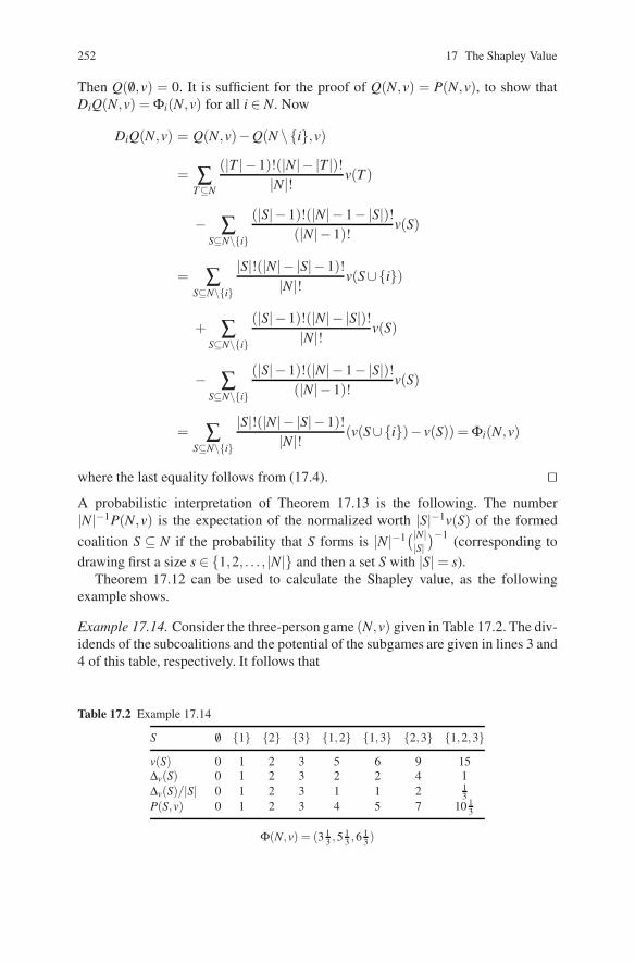
252 17 The Shapley Value
Then Q( /0,v) = 0. It is sufficient for the proof of Q(N,v) = P(N,v), to show thatDiQ(N,v) = Φi(N,v) for all i ∈ N. Now
DiQ(N,v) = Q(N,v)−Q(N \ {i},v)
= ∑T⊆N
(|T |−1)!(|N|− |T|)!|N|! v(T )
− ∑S⊆N\{i}
(|S|−1)!(|N|−1−|S|)!(|N|−1)!
v(S)
= ∑S⊆N\{i}
|S|!(|N|− |S|−1)!|N|! v(S∪{i})
+ ∑S⊆N\{i}
(|S|−1)!(|N|− |S|)!|N|! v(S)
− ∑S⊆N\{i}
(|S|−1)!(|N|−1−|S|)!(|N|−1)!
v(S)
= ∑S⊆N\{i}
|S|!(|N|− |S|−1)!|N|! (v(S∪{i})− v(S)) = Φi(N,v)
where the last equality follows from (17.4). ��A probabilistic interpretation of Theorem 17.13 is the following. The number|N|−1P(N,v) is the expectation of the normalized worth |S|−1v(S) of the formedcoalition S ⊆ N if the probability that S forms is |N|−1(|N|
|S|)−1 (corresponding to
drawing first a size s ∈ {1,2, . . . , |N|} and then a set S with |S| = s).Theorem 17.12 can be used to calculate the Shapley value, as the following
example shows.
Example 17.14. Consider the three-person game (N,v) given in Table 17.2. The div-idends of the subcoalitions and the potential of the subgames are given in lines 3 and4 of this table, respectively. It follows that
Table 17.2 Example 17.14
S /0 {1} {2} {3} {1,2} {1,3} {2,3} {1,2,3}v(S) 0 1 2 3 5 6 9 15∆v(S) 0 1 2 3 2 2 4 1∆v(S)/|S| 0 1 2 3 1 1 2 1
3P(S,v) 0 1 2 3 4 5 7 10 1
3
Φ(N,v) = (3 13 ,5 1
3 ,6 13 )

17.3 Potential and Reduced Game 253
Φ(N,v) = (D1P(N,v),D2P(N,v),D3P(N,v))
= (1013−7,10
13−5,10
13−4) = (3
13,5
13,6
13)
Φ({2,3},v) = (7− 3,7−2)= (4,5).
17.3.2 Reduced Games
To introduce the concept of a reduced game, consider the game in Example 17.14.Suppose that the players agree on using the Shapley value, and consider the coalition{1,2}. If players 1 and 2 pool their Shapley value payoffs then together they have3 1
3 + 5 13 = 8 2
3 . Another way to obtain this amount is to take the worth of the grandcoalition, 15, and to subtract player 3’s payoff, 6 1
3 . Consider {1} as a subcoalitionof {1,2}. Player 1 could form a coalition with player 3 and obtain the worth 6, buthe would have to pay player 3 according to the Shapley value of the two-playergame ({1,3},v), which is the vector (2,4); recall that the players agree on usingthe Shapley value. So player 1 is left with 6−4 = 2. Similarly, player 2 could forma coalition with player 3 and obtain v(2,3) = 9 minus the Shapley value payofffor player 3 in the game ({2,3},v), which is 5. So player 2 is left with 9− 5 = 4.So a ‘reduced’ game ({1,2}, v) has been constructed with v(1) = 2, v(2) = 4, andv(1,2) = 8 2
3 . The Shapley value of this game is the vector (3 13 ,5 1
3). Observe thatthese payoffs are equal to the Shapley value payoffs in the original game. This is nota coincidence; the particular way of constructing a reduced game as illustrated hereleaves the Shapley value invariant.
A general game theoretic principle is the following. Suppose in a game a subsetof the players consider the game arising among themselves; then, if they apply thesame ‘solution rule’ as in the original game, their payoffs should not change – theyshould have no reason to renegotiate. Of course, the formulation of this principleleaves open many ways to define ‘the game arising among themselves’. Differentdefinitions correspond to different solution rules. Put differently, there are many waysto define reduced games, leading to many different ‘reduced game properties’ asspecific instances of the above general game theoretic principle. Instead of ‘reducedgame property’ also the term ‘consistency’ is used. This concept has been very fruitfulover the past decades – in cooperative as well as noncooperative game theory.3
For the Shapley value the following reduced game turns out to be relevant. It isthe reduced game applied in the example above.
Definition 17.15. Let ψ be a value, assigning to each element (N,v) of G a vectorψ(N,v) ∈ RN . For (N,v) ∈ G and U ⊆ N, U = /0, the game (N \U,vU,ψ) is definedby vU,ψ( /0) = 0 and
vU,ψ (S) := v(S∪U)− ∑k∈U
ψk(S∪U,v) for all S ∈ 2N\U \ { /0}.
vU,ψ is called the (U,ψ)-reduced game of v.
3 Cf. Sect. 13.8.

254 17 The Shapley Value
Thus, the worth of coalition S in the game vU,ψ is obtained by subtracting from theworth of S∪U in the game (S∪U,v) the payoffs of the players in U according tothe value ψ . The reduced game property or consistency property for a value ψ on Gbased on this reduced game is the following.
HM-consistency (HMC)4: for all games (N,v) and all U ⊆ N, U = /0
ψi(N \U,vU,ψ) = ψi(N,v) for all i ∈ N \U. (17.20)
The following lemma is used in the proof of HM-consistency of the Shapley value.
Lemma 17.16. Let (N,v) ∈ G . Suppose Q : 2N → R satisfies
∑i∈S
(Q(S)−Q(S\ {i})) = v(S) for each S ∈ 2N \ { /0}.
Then for each S ∈ 2N:Q(S) = P(S,v)+ Q( /0). (17.21)
Proof. The proof of (17.21) is by induction on |S|. Obviously, (17.21) holds if|S| = 0. Take T with |T | > 0 and suppose (17.21) holds for all S with |S| < |T |.Then
Q(T ) = |T |−1(v(T )+ ∑i∈T
Q(T \ {i}))
= |T |−1(v(T )+ |T |Q( /0)+ ∑i∈T
P(T \ {i},v))
= Q( /0)+ |T |−1(v(T )+ ∑i∈T
P(T \ {i},v))
= Q( /0)+ P(T,v). ��
Lemma 17.17. The Shapley value Φ is HM-consistent.
Proof. Take (N,v) in G , and /0 = U ⊆ N. We have to prove that
Φi(N \U,vU,Φ) = Φi(N,v) for all i ∈ N \U. (17.22)
Note that, in view of the definition of vU,Φ, efficiency of Φ, and Theorem 17.12(3),we have for all S ⊆ N \U :
vU,Φ(S) = v(S∪U)− ∑i∈U
Φi(S∪U,v) = ∑i∈S
Φi(S∪U,v)
= ∑i∈S
P(S∪U,v)−P((S∪U)\ {i},v). (17.23)
4 Named after Hart and Mas-Colell.

17.3 Potential and Reduced Game 255
For S ∈ 2N\U define Q(S) := P(S∪U,v). Then, by Lemma 17.16, with N \U andvU,Φ in the roles of N and v, (17.23) implies
Q(S) = P(S,vU,Φ)+ Q( /0) = P(S,vU,Φ)+ P(U,v)
for all S ⊆ N \U . Hence, by the definition of Q:
P(S∪U,v) = P(S,vU,Φ)+ P(U,v). (17.24)
(17.24) and Theorem 17.12(3) imply
Φi(N \U,vU,Φ) = P(N \U,vU,Φ)−P((N \U)\ {i},vU,Φ)= P(N,v)−P(N \ {i},v) = Φi(N,v).
So (17.22) holds. ��Call a value ψ standard for two-person games if for all ({i, j},v)
ψi({i, j},v) =12(v(i, j)+ v(i)− v( j)),
ψ j({i, j},v) =12(v(i, j)− v(i)+ v( j)).
Note that the Shapley value is standard for two-person games. It turns out that thisproperty, together with HM-consistency, characterizes the Shapley value.
Theorem 17.18. Let ψ be a value on G . Then ψ is standard for two-person gamesand HM-consistent if, and only if, ψ is the Shapley value.
Proof. (a) By Lemma 17.17, Φ is HM-consistent. Further, Φ is standard for two-person games.
(b) For the proof of the converse, assume ψ has the two properties in the theorem. Itwill first be proved that ψ is efficient. For two-person games this is true by standard-ness. Let ({i},v) be a one-person game. To prove that ψi({i},v) = v(i), construct atwo-person game ({i, j},v∗) (with j = i) by defining
v∗(i) := v(i), v∗( j) := 0, v∗(i, j) := v(i).
From the standardness of ψ it follows that
ψi((i, j),v∗) = v(i),ψ j((i, j),v∗) = 0. (17.25)
The definition of v∗j,ψ and (17.25) imply: v∗j,ψ (i) = v∗(i, j)−ψ j((i, j), v∗) = v(i)−0 = v(i). So
({i},v∗j,ψ) = ({i},v). (17.26)
Then, by (17.26), the consistency of ψ and (17.25):
ψi({i},v) = ψi({i},v∗j,ψ) = ψi({i, j},v∗) = v(i).

256 17 The Shapley Value
So for one- and two-person games the rule ψ is efficient. Take a game (S,v) with|S| ≥ 3 and suppose that for all games (T,v) with |T | < |S| the rule ψ is efficient.Take k ∈ S. Then the consistency of ψ implies
∑i∈S
ψi(S,v) = ψk(S,v)+ ∑i∈S\{k}
ψi(S,v)
= ψk(S,v)+ ∑i∈S\{k}
ψi(S \ {k},vk,ψ)
= ψk(S,v)+ vk,ψ(S \ {k})= v(S).
Hence, ψ is an efficient rule.
(c) If a Q : G → R can be constructed with Q( /0,v) = 0 and
ψi(N,v) = Q(N,v)−Q(N \ {i},v) (17.27)
for all (N,v) in G and i ∈ N, then by (b) and Theorem 17.12(1), Q = P and thenψi(N,v) = Φi(N,v) by Theorem 17.12(3).
Hence, the only thing to do is to construct such a Q. Start with Q( /0,v) := 0,Q({i},v) := v(i), Q({i, j},v) := 1
2 (v(i, j)+ v(i)+ v( j)) and continue in a recursiveway as follows. Let (N,v) ∈ G , |N| ≥ 3 and suppose Q with property (17.27) hasbeen defined already for games with less than |N| players. Then one can defineQ(N,v) := α if, and only if
α −Q(N \ {i},v) = ψi(N,v) for all i ∈ N.
This implies that the proof is complete if it can be shown that
ψi(N,v)+ Q(N \ {i},v) = ψ j(N,v)+ Q(N \ { j},v) for all i, j ∈ N. (17.28)
To prove (17.28) take k ∈ N \ {i, j}(|N| ≥ 3). Then
ψi(N,v)−ψ j(N,v) = ψi(N \ {k},vk,ψ)−ψ j(N \ {k},vk,ψ)
= Q(N \ {k},vk,ψ)−Q(N \ {k, i},vk,ψ)
−Q(N \ {k},vk,ψ)+ Q(N \ {k, j},vk,ψ)
= (−Q(N \ {k, i},vk,ψ)+ Q(N \ {i, j,k},vk,ψ ))
+ Q(N \ {k, j},vk,ψ)−Q(N \ {i, j,k},vk,ψ)
= −ψ j(N \ {k, i},vk,ψ)+ ψi(N \ {k, j},vk,ψ)
= −ψ j(N \ {i},v)+ ψi(N \ { j},v)= −Q(N \ {i},v)+ Q(N \ {i, j},v)
+ Q(N \ { j},v)−Q(N \ {i, j},v)= Q(N \ { j},v)−Q(N \ {i},v),

Problems 257
where HM-consistency of ψ is used in the first and fifth equality and (17.27) forsubgames in the second, fourth and sixth equality.
This proves (17.28). ��
Problems
17.1. The Games 1T
(a) Show that {1T ∈ G N | T ∈ 2N \ { /0}} is a basis for G N .
(b) Show that there is no null-player in a game (N,1T ) (T = /0).
(c) Determine the Shapley value Φ(N,1T ).
17.2. Unanimity Games
(a) Prove that the collection of unanimity games {uT | T ∈ 2N \ { /0}} is a basis forG N . (Hint: In view of Problem 17.1(a) it is sufficient to show linear independence.)
(b) Prove that for each game v ∈ G N :
v = ∑T∈2N\{ /0}
cT uT with cT = ∑S:S⊆T
(−1)|T |−|S|v(S).
17.3. Necessity of the Axioms in Theorem 17.4
Show that the Shapley value satisfies EFF, NP, SYM, and ADD.
17.4. Dummy Player Property and Anonymity
Show that DUM implies NP, and that AN implies SYM, but that the converses ofthese implications do not hold. Show that the Shapley value has the dummy playerproperty.
17.5. Shapley Value, Core, and Imputation Set
Show that the Shapley value of a game does not have to be an element of the core orof the imputation set, even if these sets are non-empty. How about the case of twoplayers?
17.6. Shapley Value as a Projection
The Shapley value Φ : G N → RN can be seen as a map from G N to the space AN ofadditive games by identifying RN with AN .
Prove that Φ : G N → AN is a projection i.e. Φ◦Φ = Φ.
17.7. Shapley Value of Dual Game
The dual game (N,v∗) of a game (N,v) is defined by v∗(S) = v(N)− v(N \ S) forevery S ⊆ N. Prove that the Shapley value of v∗ is equal to the Shapley value of v.(Hint: If v = ∑αT uT , then v∗ = ∑αT u∗T .)

258 17 The Shapley Value
17.8. Multilinear Extension
(1) Prove (17.15).
(2) Show that f in (17.14) is a multilinear function. (A function g : Rn → R is calledmultilinear if g is of the form g(x) = ∑T⊆N cT (∏i∈T xi) for arbitrary real numberscT .)
(3) Prove that f is the unique multilinear extension of v to [0,1]N .
17.9. The Beta-Integral Formula
Prove the beta-integral formula used in the proof of Theorem 17.9.
17.10. Path Independence of Φ
Let (N,v) ∈ G N with N = {1,2, . . . ,n}. Prove that for each permutation τ : N → Nwe have
n
∑k=1
Φτ(k)({τ(1),τ(2), . . . ,τ(k)},v) =n
∑k=1
Φk({1,2, . . . ,k},v).
17.11. An Alternative Characterization of the Shapley Value
Let ψ be a value on G . Prove: ψ = Φ if and only if ψ has the following fourproperties:
(1) ψ is HM-consistent.
(2) ψ is efficient for two-person games.
(3) ψ is anonymous for two-person games.
(4) ψ is relative invariant w.r.t. strategic equivalence for two-person games. (Thismeans: (ψi(v),ψ j(v)) = α(ψi(v),ψ j(v)) + (βi,β j) whenever v(S) = αv(S) +∑i∈S βi for every coalition S, where α > 0 and βi,β j ∈ R.)

Chapter 18Core, Shapley Value, and Weber Set
In Chap. 17 we have seen that the Shapley value of a game does not have to bein the core of the game, nor even an imputation (Problem 17.5). In this chapterwe introduce a set-valued extension of the Shapley value, the Weber set, and showthat it always contains the core (Sect. 18.1). Next, we study so-called convex gamesand show that these are exactly those games for which the core and the Weber setcoincide. Hence, for such games the Shapley value is an attractive core selection(Sect. 18.2). Finally, we study random order values (Sect. 18.3), which fill out theWeber set, and the subset of weighted Shapley values, which still cover the core(Sect. 18.4).
18.1 The Weber Set
Let (N,v) ∈ G N . Recall the definition of a marginal vector from Sect. 17.1.
Definition 18.1. The Weber set of a game (N,v) ∈ G N is the convex hull of itsmarginal vectors:
W (v) := conv{mσ (v) | σ ∈ Π(N)} .
Example 18.2. Consider the three-person game ({1,2,3},v) defined by v(12) =v(13)= 1, v(23)=−1, v(123)= 3, and v(i) = 0 for every i∈ {1,2,3}. The marginalvectors of this game, the core and the Weber set are given in Fig. 18.1.
We show now that the core is always a subset of the Weber set (Weber [146]; theproof is from Derks [29]).
Theorem 18.3. Let (N,v) ∈ G N. Then C(v) ⊆W (v).
Proof. Suppose there is an x∈C(v)\W (v). By a separation theorem (Theorem 22.1),there exists a vector y∈RN such that w ·y > x·y for every w∈W (v). In particular,
mσ ·y > x ·y for every σ ∈ Π(N) . (18.1)
H. Peters, Game Theory – A Multi-Leveled Approach.c© Springer-Verlag Berlin Heidelberg 2008
259

260 18 Core, Shapley Value, and Weber Set
(σ (1),σ (2),σ (3)) mσ1 mσ
2 mσ3
(1,2,3) 0 1 2(1,3,2) 0 2 1(2,1,3) 1 0 2(2,3,1) 4 0 −1(3,1,2) 1 2 0(3,2,1) 4 −1 0
� ��
�
�������������
�����������
�
��
��
� � ����
��
�
��������
��
��
��
(0,−1,4)
(0,4,−1)(5,−1,−1)
(0,1,2)
(0,2,1)
(4,−1,0)
(4,0,−1)
C(v)W (v) �
Fig. 18.1 Example 18.2. The core is the convex hull of the vectors (3,0,0), (1,2,0), (0,2,1),(0,1,2), and (1,0,2). The Weber set is the convex hull of the six marginal vectors
Let π ∈ Π(N) with yπ(1) ≥ yπ(2) ≥ ·· · ≥ yπ(n). Since x ∈C(v),
mπ ·y =n
∑i=1
yπ(i)(v(π(1),π(2), . . . ,π(i))− v(π(1),π(2), . . . ,π(i−1)))
= yπ(n)v(N)− yπ(1)v( /0)+n−1
∑i=1
(yπ(i) − yπ(i+1))v(π(1),π(2), . . . ,π(i))
≤ yπ(n)
n
∑j=1
xπ( j) +n−1
∑i=1
(yπ(i)− yπ(i+1))i
∑j=1
xπ( j)
=n
∑i=1
yπ(i)
i
∑j=1
xπ( j)−n
∑i=2
yπ(i)
i−1
∑j=1
xπ( j)
=n
∑i=1
yπ(i)xπ(i) = x ·y
contradicting (18.1). ��

18.2 Convex Games 261
18.2 Convex Games
For the coincidence of core and Weber set the following possible property of a gameplays a crucial role.
Definition 18.4. A TU-game (N,v) is convex if the following condition holds forall S,T ⊆ N:
v(S)+ v(T) ≤ v(S∪T )+ v(S∩T) . (18.2)
Observe that convexity of a game implies super-additivity (cf. (16.2)): v is super-additive if (18.2) holds whenever S and T have empty intersection. The intuitionis similar: larger coalitions have a relatively larger worth. This intuition is alsoapparent in the following condition:
For all i ∈ N and S ⊆ T ⊆ N \ {i}: v(S∪ i)− v(S)≤ v(T ∪ i)− v(T) . (18.3)
Lemma 18.5. A game (N,v) ∈ G N is convex if and only if it satisfies (18.3).
Proof. Let v ∈ G N . Obviously, (18.3) follows from (18.2) by taking, for S and T in(18.2), S∪ i and T from (18.3), respectively.
In order to derive (18.2) from (18.3), first take S0 ⊆ T0 ⊆ N and R ⊆ N \T0, sayR = {i1, . . . , ik}. By repeated application of (18.3) one obtains
v(S0 ∪ i1)− v(S0) ≤ v(T0 ∪ i1)− v(T0)v(S0 ∪ i1i2)− v(S0∪ i1) ≤ v(T0 ∪ i1i2)− v(T0 ∪ i1)
...v(S0 ∪ i1 · · · ik)− v(S0 ∪ i1 · · · ik−1) ≤ v(T0 ∪ i1 · · · ik)− v(T0 ∪ i1 · · · ik−1) .
Adding these inequalities yields
v(S0 ∪R)− v(S0) ≤ v(T0 ∪R)− v(T0)
for all R ⊆ N \T0. Applying this inequality to arbitrary S,T by setting S0 = S∩T ,T0 = T , and R = S\T , yields (18.2). ��The importance of convex games for the relation between the core and the Weberset follows from the following theorem (Shapley [124]; Ichiishi [58]).
Theorem 18.6. Let v ∈ G N. Then v is convex if and only if C(v) = W (v).
Proof. (a) Suppose v is convex. For the ‘only if’ part it is, in view of Theorem 18.3and convexity of the core, sufficient to prove that each marginal vector mπ(v) of v isin the core. In order to show this, assume for notational simplicity that π is identity.Let S ⊆ N be an arbitrary coalition, say S = {i1, . . . , is}. Then, for 1 ≤ k ≤ s, by(18.3):
v(i1, . . . , ik)− v(i1, . . . , ik−1) ≤ v(1,2, . . . , ik)− v(1,2, . . . , ik −1) = mπik(v) .

262 18 Core, Shapley Value, and Weber Set
Summing these inequalities from k = 1 to k = s yields
v(S) = v(i1, . . . , is) ≤s
∑k=1
mπik(v) = ∑
i∈Smπ
i (v) ,
which shows mπ(v) ∈C(v).
(b) For the converse, suppose that all marginal vectors of v are in the core. LetS,T ⊆ N be arbitrary. Order the players of N as follows:
N = {i1, . . . , ik︸ ︷︷ ︸S∩T
, ik+1, . . . , i�︸ ︷︷ ︸T\S
, i�+1, . . . , is︸ ︷︷ ︸S\T
, is+1, . . . , in︸ ︷︷ ︸N\(S∪T )
} .
This defines an ordering or permutation π with corresponding marginal vectorm(v) = mπ(v). Since m(v) ∈C(v),
v(S) ≤ ∑i∈S
mi(v)
=k
∑j=1
mij (v)+s
∑j=�+1
mij (v)
= v(i1, . . . , ik)+ [v(i1, . . . , i�+1)− v(i1, . . . , i�)]+ [v(i1, . . . , i�+2)− v(i1, . . . , i�+1]+ · · · [v(i1, . . . , is)− v(i1, . . . , is−1]
= v(S∩T )+ v(S∪T)− v(T ) ,
which implies (18.2). So v is a convex game. ��An immediate consequence of Theorem 18.6 and the definition of the Shapley value(Definition 17.1) is the following corollary.
Corollary 18.7. Let v ∈ G N be convex. Then Φ(v) ∈C(v), i.e., the Shapley value isin the core.
18.3 Random Order Values
A value ψ : G N → RN is called a random order value if there is a probabilitydistribution p over the set of permutations Π(N) of N such that
ψ(N,v) = ∑π∈Π(N)
p(π)mπ(N,v)
for every (N,v) ∈ G N . In that case, we denote ψ by Φp. Observe that Φp is theShapley value Φ if p(π) = 1/n! for every π ∈ Π(N). Obviously,
W (v) = {x ∈ RN | x = Φp(v) for some p}.

18.3 Random Order Values 263
Random order values satisfy the following two conditions.
Monotonicity (MON): ψ(v) ≥ 0 for all monotonic games v ∈ G N . [The game v ismonotonic if S ⊆ T implies v(S) ≤ v(T ) for all S,T ⊆ N.]
Linearity (LIN): ψ(αv + β w) = αψ(v)+ β ψ(w) for all v,w ∈ G N , and α,β ∈ R(where, for each S, (αv + β w)(S) = αv(S)+ β w(S)).
Monotonicity says that in a monotonic game, where larger coalitions have higherworths, i.e., all marginal contributions are nonnegative, every player should receive anonnegative payoff. Linearity is a strengthening of additivity. The main result in thissection is the following characterization of random order values (see Problem 18.7for a strengthening of the ‘only if’ part of this theorem).
Theorem 18.8. Let ψ : G N →RN be a value. Then ψ satisfies LIN, DUM, EFF, andMON if and only if it is a random order value.
The proof of Theorem 18.8 is based on a sequence of propositions and lemmas,which are of independent interest.
Proposition 18.9. Let ψ : G N → RN be a linear value. Then there is a collection ofconstants {ai
T ∈ R | i ∈ N, /0 = T ⊆ N} such that ψi(v) = ∑ /0 =T⊆N aiT v(T ) for every
v ∈ G N and i ∈ N.
Proof. Let aiT := ψi(1T ) for all i ∈ N and /0 = T ⊆ N (cf. Problem 17.1). For every
v ∈ G N we have v = ∑T = /0 v(T )1T . The desired conclusion follows from linearityof ψ . ��Proposition 18.10. Let ψ : G N → RN be a linear value satisfying DUM. Then thereis a collection of constants {pi
T ∈ R | i ∈ N, T ⊆ N \ i}1 with ∑T⊆N\i piT = 1 for all
i ∈ N, such that for every v ∈ G N and every i ∈ N:
ψi(v) = ∑T⊆N\i
piT [v(T ∪ i)− v(T)] .
Proof. Let v ∈ G N and i ∈ N. By Proposition 18.9 there are aiT such that ψi(v) =
∑ /0 =T⊆N aiT v(T ). Then 0 = ψi(uN\i) = ai
N + aiN\i, where the first equality follows
from DUM. Assume now as induction hypothesis that aiT∪i +ai
T = 0 for all T ⊆N \ iwith |T | ≥ k ≥ 2 (we have just established this for k = n−1), and let S ⊆ N \ i with|S|= k−1. Then
0 = ψi(uS)= ∑
T :S⊆Tai
T
= ∑T :S�T⊆N\i
(aiT∪i + ai
T )+ aiS∪i + ai
S
= aiS∪i + ai
S ,
1 As before, we write N \ i instead of N \{i} (etc.) for brevity.

264 18 Core, Shapley Value, and Weber Set
where the last equality follows by induction and the first one by DUM. Hence, wehave proved that ai
T∪i + aiT = 0 for all T ⊆ N \ i with 0 < |T | ≤ n−1. Now define,
for all i ∈ N and all such T , piT := ai
T∪i =−aiT , and define pi
/0 := ai{i}. Then for every
v ∈ G N and i ∈ N:
ψi(v) = ∑/0 =T⊆N
aiT v(T ) = ∑
T⊆N\ipi
T [v(T ∪ i)− v(T )] .
Finally, by DUM,1 = u{i}(i) = ψi(u{i}) = ∑
T⊆N\ipi
T ,
which completes the proof of the proposition. ��Proposition 18.11. Let ψ : G N → RN be a linear value satisfying DUM and MON.Then there is a collection of constants {pi
T ∈R | i ∈ N, T ⊆ N \ i} with ∑T⊆N\i piT =
1 and piS ≥ 0 for all S ⊆ N \ i and i ∈ N, such that for every v ∈ G N and every i ∈ N:
ψi(v) = ∑T⊆N\i
piT [v(T ∪ i)− v(T)] .
Proof. In view of Proposition 18.10 we only have to prove that the weights piT are
nonnegative. Let i ∈ N and T ⊆ N \ i and consider the game uT assigning worth 1 toall strict supersets of T and 0 otherwise. Then ψi(uT ) = pi
T by Proposition 18.10.Since uT is a monotonic game, this implies pi
T ≥ 0. ��Lemma 18.12. Let ψ : G N → RN be a value and {pi
T ∈ R | i ∈ N, T ⊆ N \ i} be acollection of constants such that for every v ∈ G N and every i ∈ N:
ψi(v) = ∑T⊆N\i
piT [v(T ∪ i)− v(T)] .
Then ψ is efficient if and only if ∑i∈N piN\i = 1 and ∑i∈T pi
T\i = ∑ j∈N\T p jT for all
/0 = T = N.
Proof. Let v ∈ G N . Then
ψ(v)(N) = ∑i∈N
∑T⊆N\i
piT [v(T ∪ i)− v(T )]
= ∑T⊆N
v(T )
(∑i∈T
piT\i − ∑
j∈N\Tp j
T
).
Clearly, this implies efficiency of ψ if the relations in the lemma hold. Conversely,suppose that ψ is efficient. Let /0 = T ⊆ N and consider the games uT and uT . Thenthe preceding equation implies that
ψ(uT )(N)−ψ(uT )(N) = ∑i∈T
piT\i − ∑
j∈N\Tp j
T .

18.3 Random Order Values 265
The relations in the lemma now follow by efficiency of ψ , since uT (N)− uT (N) isequal to 1 if T = N and equal to 0 otherwise. ��We are now sufficiently equipped to prove Theorem 18.8.
Proof of Theorem 18.8. We leave it to the reader to verify that random order valuessatisfy the four axioms in the theorem. Conversely, let ψ satisfy these four axioms.By Proposition 18.11 there is a collection of constants {pi
T ∈ R | i ∈ N, T ⊆ N \ i}with ∑T⊆N\i pi
T = 1 and piS ≥ 0 for all S⊆N \ i and i∈ N, such that for every v∈ G N
and every i ∈ N:ψi(v) = ∑
T⊆N\ipi
T [v(T ∪ i)− v(T)] .
For all i ∈ N and T ⊆ N \ i define A(T ) := ∑ j∈N\T p jT and A(i;T ) := pi
T /A(T )if A(T ) = 0, A(i;T ) := 0 if A(T ) = 0. For any permutation π ∈ Π(N) writeπ = (i1, . . . , in) (that is, π(k) = ik for all k ∈ N). Define
p(π) = pi1/0 A(i2;{i1})A(i3;{i1, i2}) · · ·A(in;{i1, . . . , in−1}) .
Then it can be verified (Problem 18.8) that
∑π∈Π(N)
p(π) = ∑i∈N
pi/0 . (18.4)
We claim that for every 0 ≤ t ≤ n− 1 we have
∑T :|T |=t
∑i∈N\T
piT = 1 . (18.5)
To prove this, first let t = n−1. Then the sum on the left-hand side of (18.5) is equalto ∑i∈N pi
N\i, which is equal to 1 by Lemma 18.12. Now as induction hypothesisassume that (18.5) holds for t + 1. Then
∑T :|T |=t
∑i∈N\T
piT = ∑
T :|T |=t+1∑i∈T
piT\i
= ∑T :|T |=t+1
∑i∈N\T
piT
= 1 ,
where the second equality follows by Lemma 18.12 and the last equality by induc-tion. This proves (18.5). In particular, for t = 0, we have ∑i∈N pi
/0 = 1. Together with(18.4) this implies that p(·) as defined above is a probability distribution on Π(N).
In order to complete the proof, it is sufficient to show that ψ = Φp. For every gamev ∈ G N and i ∈ N we can write
Φpi (v) = ∑
π∈Π(N)p(π)[v(Pπ(i)∪ i)− v(Pπ(i))] ,

266 18 Core, Shapley Value, and Weber Set
where Pπ(i) denotes the set of predecessors of player i under the permutation π (cf.Sect. 17.1). Hence, it is sufficient to prove that for all i ∈ N and T ⊆ N \ i we have
piT = ∑
π∈Π(N): T=Pπ (i)p(π) . (18.6)
This is left as an exercise (Problem 18.9) to the reader. ��
18.4 Weighted Shapley Values
The Shapley value is a random order value that distributes the dividend of eachcoalition equally among all the members of that coalition (see Theorem 17.7). Inthis sense, it treats players consistently over coalitions. This is not necessarily thecase for every random order value. To be specific, consider Example 18.2. The pay-off vector (2.5,−0.5,1) is a point of the Weber set that can be obtained uniquelyas Φp(v), where the probability distribution p assigns weights 1/2 to the permuta-tions (3,2,1) and (2,1,3). If we look at the distribution of dividends resulting fromthe associated marginal vectors (cf. Problem 18.1), we obtain that ∆v(123) is splitequally between players 1 and 3 (they are the only ones that occur last in the two per-mutations), whereas ∆v(23) is split equally between players 2 and 3. (∆v(12) goesto player 1 and ∆v(13) is split evenly between players 1 and 3.) Hence, whereasplayer 2 has zero power compared to player 3 in distributing ∆v(123), they haveequal power in distributing ∆v(23). In this respect, players 2 and 3 are not treatedconsistently by Φp.
In order to formalize the idea of consistent treatment, we first define positivelyweighted Shapley values. Let ω ∈ RN with ω > 0. The positively weighted Shap-ley value Φω is defined as the unique linear value which assigns to each unanimitygame (N,uS):
Φωi (uS) =
{ωi/ω(S) for i ∈ S0 for i ∈ N \S . (18.7)
Owen [97] has shown that these positively weighted values are random order values.More precisely, define independently distributed random variables Xi (i ∈ N) on[0,1] by their cumulative distribution functions [0,1] � t �→ tω i
(that is, Xi ≤ t withprobability tω i
). Then, define the probability distribution pω by
pω(π) =∫ 1
0
∫ tn
0
∫ tn−1
0· · ·∫ t2
0dtω1
1 · · ·dtωn−2n−2 dtωn−1
n−1 dtωnn (18.8)
for every permutation π = (i1, i2, . . . , in). That is, pω(π) is defined as the probabilitythat i1 comes before i2, i2 before i3, etc., evaluated according to the independentrandom variables Xi. Then we have
Theorem 18.13. For every ω ∈ RN with ω > 0, Φω = Φpω.

18.4 Weighted Shapley Values 267
Proof. Let S be a nonempty coalition and i ∈ S. It is sufficient to prove thatΦpω
i (uS) = ωi/ω(S). Note that
Φpω
i (uS) = ∑π :S\i⊆Pπ (i)
pω(π) ,
and, the right-hand side of this identity is equal to∫ 1
0
∫ ti
0dtω(S\i)dtωi
i ,
which, in turn, is equal to ωi/ω(S). ��Next, we extend the concept of weighted Shapley value to include zero weights.Consider for instance, the three-person random order value that puts weight 1/2 onthe permutations (1,2,3) and (1,3,2). Then (cf. again Problem 18.1) the dividend∆v(12) goes to player 2, the dividend ∆v(13) to player 3, and the dividends ∆v(23)and ∆v(123) are split equally between players 2 and 3. Thus, this random ordervalue treats players consistently but we cannot just formalize this by giving player1 weight 0 since player 1 does obtain ∆v(1).
To accommodate this kind of random order values we introduce the concept of aweight system. A weight system w is an ordered partition (S1, . . . ,Sk) of N togetherwith a vector ω ∈ RN such that ω > 0. The weighted Shapley value Φw is definedas the unique linear value which assigns to each unanimity game uS ∈ G N :
Φwi (uS) =
{ωi/ω(S∩Sm) for i ∈ S∩Sm and m = max{h : Sh ∩S = /0}0 otherwise. (18.9)
Hence, Sh is more powerful as h is larger; for each coalition S we consider the subsetof the most powerful players S∩ Sm, where m is the largest index h such that theintersection of Sh with S is nonempty, and they distribute the dividend of coalitionS according to their (relative) weights ωi/ω(S∩Sm). Clearly, for k = 1 we obtain apositively weighted Shapley value as defined above.
Weighted Shapley values are again random order values. For a weight system wwith ordered partition (S1, . . . ,Sk) we only assign positive probability to those per-mutations in which all players of S1 enter before all players of S2, all players of S2enter before all players of S3, etc. Given such a permutation we can assign proba-bility p1(π) to the order induced by π on S1 in the same way as we did above in(18.8); similarly, we assign probabilities p2(π), . . . , pk(π) to the orders induced onS2, . . . ,Sk, respectively. Then we define
pw(π) =k
∏h=1
ph(π) .
It can be shown again that Φw = Φpw.
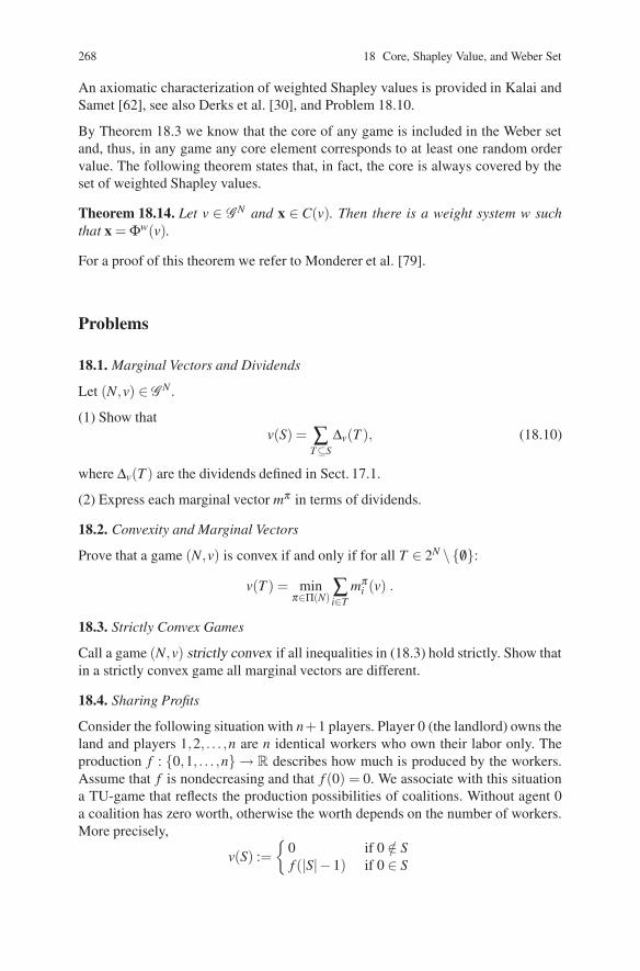
268 18 Core, Shapley Value, and Weber Set
An axiomatic characterization of weighted Shapley values is provided in Kalai andSamet [62], see also Derks et al. [30], and Problem 18.10.
By Theorem 18.3 we know that the core of any game is included in the Weber setand, thus, in any game any core element corresponds to at least one random ordervalue. The following theorem states that, in fact, the core is always covered by theset of weighted Shapley values.
Theorem 18.14. Let v ∈ G N and x ∈ C(v). Then there is a weight system w suchthat x = Φw(v).
For a proof of this theorem we refer to Monderer et al. [79].
Problems
18.1. Marginal Vectors and Dividends
Let (N,v) ∈ G N .
(1) Show thatv(S) = ∑
T⊆S∆v(T ), (18.10)
where ∆v(T ) are the dividends defined in Sect. 17.1.
(2) Express each marginal vector mπ in terms of dividends.
18.2. Convexity and Marginal Vectors
Prove that a game (N,v) is convex if and only if for all T ∈ 2N \ { /0}:
v(T ) = minπ∈Π(N)
∑i∈T
mπi (v) .
18.3. Strictly Convex Games
Call a game (N,v) strictly convex if all inequalities in (18.3) hold strictly. Show thatin a strictly convex game all marginal vectors are different.
18.4. Sharing Profits
Consider the following situation with n+1 players. Player 0 (the landlord) owns theland and players 1,2, . . . ,n are n identical workers who own their labor only. Theproduction f : {0,1, . . . ,n} → R describes how much is produced by the workers.Assume that f is nondecreasing and that f (0) = 0. We associate with this situationa TU-game that reflects the production possibilities of coalitions. Without agent 0a coalition has zero worth, otherwise the worth depends on the number of workers.More precisely,
v(S) :={
0 if 0 /∈ Sf (|S|−1) if 0 ∈ S

Problems 269
for every coalition S ⊆ {0,1, . . . ,n}.
(a) Compute the marginal vectors and the Shapley value of this game.
(b) Compute the core of this game.
(c) Give a necessary and sufficient condition on f such that the game is convex. (Soin that case, the core and the Weber set coincide and the Shapley value is in thecore.)
18.5. Sharing Costs
(Cf. [71].) Suppose that n airlines share the cost of a runway. To serve the planes ofcompany i, the length of the runway must be ci, which is also the cost of a runwayof that length. Assume 0 ≤ c1 ≤ c2 ≤ ·· · ≤ cn. The cost of coalition S is defined ascS = maxi∈S ci for every nonempty coalition S.
(a) Model this situation as a cost savings game (cf. the three communities game inChap. 1).
(b) Show that the resulting game is convex, and compute the marginal vectors, theShapley value, and the core.
18.6. Independence of the Axioms in Theorem 18.8
Show that the axioms in Theorem 18.8 are independent.
18.7. Null-Player in Theorem 18.8
Show that Theorem 18.8 still holds if DUM is replaced by NP.
18.8. Equation (18.4)
Prove (18.4).
18.9. Equation (18.6)
Prove (18.6).
18.10. Characterization of Weighted Shapley Values
Say that a value ψ : G N → RN satisfies the Partnership axiom if ψi(ψ(uT )(S)uS) =ψi(uT ) for all S ⊆ T ⊆ N and all i ∈ S. Prove that a value ψ satisfies LIN, DUM,EFF, MON, and Partnership, if and only if it is a weighted Shapley value.
18.11. Core and Weighted Shapley Values in Example 18.2
In Example 18.2, determine for each x ∈ C(v) a weight system w such that x =Φw(v).

Chapter 19The Nucleolus
The core of a game with transferable utility can be a large set, but it can also beempty. The Shapley value assigns to each game a unique point, which, however,does not have to be in the core.
The nucleolus (Schmeidler [116]) assigns to each game with a nonempty impu-tation set a unique element of that imputation set; moreover, this element is in thecore if the core of the game is nonempty. The pre-nucleolus always exists (and doesnot have to be an imputation, even if this set is nonempty), but for balanced gamesit coincides with the nucleolus.
In this chapter, which is partially based on the treatment of the subject in [100]and [98], we consider both the nucleolus and the pre-nucleolus. The reader isadvised to read the relevant part of Chap. 9 first.
In Sect. 19.1 we start with an example illustrating the (pre-)nucleolus andKohlberg’s balancedness criterion (Kohlberg [65]). Section 19.2 introduces the lexi-cographic order, on which the definition of the (pre-)nucleolus in Sect. 19.3 is based.Section 19.4 presents the Kohlberg criterion, which is a characterization of the (pre-)nucleolus in terms of balanced collections of coalitions. Computational aspects arediscussed in Sect. 19.5, while Sect. 19.6 presents Sobolev’s [127] characterizationof the pre-nucleolus based on a reduced game property.
19.1 An Example
Consider the three-person TU-game given by Table 19.1. It is easy to see thatthis game has a nonempty core; for instance, (8,8,8) is a core element. Let x =(x1,x2,x3) be an arbitrary efficient payoff distribution. For a nonempty coalition S,define the excess of S at x as e(S,x) := v(S)− x(S). For an efficient vector x theexcess of the grand coalition N is always zero, and is therefore omitted from con-sideration. The idea underlying the nucleolus is as follows. For an arbitrary efficientvector consider the corresponding vector of excesses. Among all imputations (andfor the pre-nucleolus: among all efficient vectors) find those where the maximalexcess is minimal. If this set consists of one point, then this is the (pre-)nucleolus.Otherwise, continue by minimizing the second largest excess, etc. Note that if a
H. Peters, Game Theory – A Multi-Leveled Approach.c© Springer-Verlag Berlin Heidelberg 2008
271

272 19 The Nucleolus
Table 19.1 The example of Sect. 19.1
S /0 {1} {2} {3} {1,2} {1,3} {2,3} {1,2,3}v(S) 0 4 4 4 8 12 16 24e(S, (8,8,8)) −4 −4 −4 −8 −4 0e(S, (6,9,9)) −2 −5 −5 −7 −3 −2e(S, (6,8,10)) −2 −4 −6 −6 −4 −2
game has a nonempty core then every core element has by definition only non-positive excesses, whereas efficient payoff vectors outside the core have at least onepositive excess. This implies that for balanced games the successive minimization ofexcesses can be restricted to core elements, and the pre-nucleolus and the nucleoluscoincide.
In order to illustrate these ideas, consider again Table 19.1, where the excessesof some core vectors for this example are calculated. The highest excess for thecore vector (8,8,8) is equal to zero, attained for the coalition {2,3}. Obviously, thisexcess can be decreased by increasing the payoff for players 2 and 3 together, atthe expense of player 1, who has an excess of −4. Thus, a next ‘try’ is the payoffvector (6,9,9), which indeed has maximal excess −2 reached for coalitions {1} and{2,3}. It is then obvious that this is indeed the minimal maximal excess, because theexcess for coalition {1} can only be decreased by increasing the excess for {2,3},and vice versa. Observe that the collection {{1},{2,3}} is balanced (in particular,it is a partition).1 At (6,9,9) the second maximal excess is equal to −3, reachedby the coalition {1,3}. Again, this might be decreased by improving the payofffor players 1 and 3 together at the expense of player 2. Because the payoff forplayer 1 has already been fixed at 6, this means that the payoff for player 3 has tobe increased and that of player 2 has to be decreased. These observations lead to thenext ‘try’ (6,8,10), where the maximal excess is still equal to −2, and the secondmaximal excess equals −4, reached by the coalitions {2} and {1,3}. It is obviousthat this second maximal excess, as well as the third maximal excess of −6, cannotbe decreased any further. Observe that also the collections {{1},{2,3},{2},{1,3}}and {{1},{2,3},{2},{1,3},{3},{1,2}} are all balanced.
It follows that (6,8,10) is the (pre-)nucleolus of this game. Moreover, theexcesses are closely related to balanced collections of coalitions; this will appearto be a more general phenomenon, known as the Kohlberg criterion.
19.2 The Lexicographic Order
The definition of the nucleolus is based on a comparison of vectors by means of thelexicographic order. We briefly discuss this order and examine some of its proper-ties. Let Rk be the real vector space of dimension k. A binary relation � on Rk thatsatisfies:
1 See Chap. 16.

19.3 The (Pre-)Nucleolus 273
(1) Reflexivity: x � x for all x ∈ Rk
(2) Transitivity: x � z for all x,y,z ∈ Rk with x � y and y � z
is called a partial order. For a partial order �, we write x � y to indicate that x � yand y � x. A partial order � is called a weak order if it satisfies
(3) Completeness: x � y or y � x for all x,y ∈ Rk with x = y
If also
(4) Antisymmetry: x = y for all x,y ∈ Rk with x � y and y � x
the relation is called a linear order.2
On the vector space Rk we define the linear order �lex as follows. For any twovectors x and y in RK , x is lexicographically larger than or equal to y – notation:x �lex y – if either x = y, or x = y and for
i = min{ j ∈ {1, . . . ,k} | x j = y j}we have that xi > yi. In other words, x should assign a higher value than y to thefirst coordinate on which x and y are different. For obvious reasons the order �lex iscalled the lexicographic order on Rk.
The lexicographic order cannot be represented by a continuous utility function(cf. Problem 19.5). In fact, it can be shown that the lexicographic order on Rk cannotbe represented by any utility function (cf. Problem 19.6).
19.3 The (Pre-)Nucleolus
Let (N,v) be a TU-game and let X ⊆ RN be some set of payoff distributions. Forevery non-empty coalition S ⊆ N and every x ∈ X the excess of S at x is the number
e(S,x,v) := v(S)− x(S).
This number can be interpreted as the dissatisfaction (complaint, regret) of the coali-tion S if x is the payoff vector. For every x∈ X let θ (x) denote the vector of excessesat x arranged in non-increasing order, hence
θ (x) = (e(S1,x,v), . . . ,e(S2n−1,x,v))
such that e(St ,x,v) ≥ e(Sp,x,v) for all 1 ≤ t ≤ p ≤ 2n − 1. Let �lex be the lexico-graphic order on R2n−1, as defined in Sect. 19.2. The nucleolus of (N,v) with respectto X is the set
N (N,v,X) := {x ∈ X | θ (y) �lex θ (x) for all y ∈ X}.
2 See also Chap. 11. Here, we repeat some of the definitions for convenience.

274 19 The Nucleolus
So the nucleolus consists of all payoff vectors in X at which the excess vectors arelexicographically minimized. The motivation for this is that we first try to mini-mize the dissatisfaction of those coalitions for which this is maximal, next for thosecoalitions that have second maximal excess, etc.
We first establish conditions under which the nucleolus with respect to a set X isnon-empty.
Theorem 19.1. Let X be non-empty and compact. Then N (N,v,X) = /0 for everygame v.
Proof. First observe that all excess functions e(S, ·,v) are continuous and thereforeθ (·) is continuous. Define X0 := X and, recursively,
Xt := {x ∈ Xt−1 | θt(y) ≥ θt(x) for all y ∈ Xt−1}for all t = 1,2, . . . ,2n − 1. Since θ (·) is continuous, Weierstrass’ Theorem impliesthat every Xt is a non-empty compact subset of Xt−1. This holds in particular fort = 2n −1 and, clearly, X2n−1 = N (N,v,X). ��We will show that, if X is, moreover, convex, then the nucleolus with respect to Xconsists of a single point. We start with the following lemma.
Lemma 19.2. Let X be convex, x,y ∈ X, and 0 ≤ α ≤ 1. Then
αθ (x)+ (1−α)θ (y) �lex θ (αx+(1−α)y). (19.1)
Proof. Let S1, . . . ,S2n−1 be an ordering of the non-empty coalitions such that
θ (αx +(1−α)y) = (e(S1,αx +(1−α)y,v), . . . ,e(S2n−1,αx+(1−α)y,v)).
The right-hand side of this equation is equal to αa + (1 − α)b, where a =(e(S1,x,v), . . . ,e(S2n−1,x,v)) and b = (e(S1,y,v), . . . ,e(S2n−1,y,v)). Sinceθ (x) �lex a and θ (y) �lex b it follows that
αθ (x)+ (1−α)θ (y) �lex αa +(1−α)b = θ (αx+(1−α)y),
hence (19.1) holds. ��
Remark 19.3. Formula (19.1) shows that θ (·) is quasi-convex with respect to theordering �lex.
Theorem 19.4. Let X be non-empty, compact, and convex. Then, for every game(N,v), the nucleolus with respect to X consists of a single point.
Proof. By Theorem 19.1 the nucleolus is non-empty. Let x,y ∈ N (N,v,X) and0 < α < 1. Then θ (x) = θ (y). By Lemma 19.2,
θ (αx+(1−α)y) = αθ (x)+ (1−α)θ (y).

19.4 The Kohlberg Criterion 275
Hence θ (αx+(1−α)y)= θ (x)= θ (y) and therefore θ (x)= θ (y)= αa+(1−α)b,with a and b as in the proof of Lemma 19.2. Since θ (x) �lex a and θ (y) �lex b itfollows that a = θ (x) and b = θ (y). In a and b the coalitions are ordered in thesame way and therefore this is also the case in θ (x) and θ (y). Hence x and y haveall excesses equal, and thus x = y. ��Well-known choices for the set X are the imputation set I(N,v) of a game (N,v) andthe set of efficient payoff distributions I∗(N,v) = {x ∈ RN | x(N) = v(N)}. For anessential game (N,v) the set I(N,v) is non-empty, compact and convex, and there-fore Theorem 19.4 implies that the nucleolus with respect to I(N,v) consists of asingle point, called the nucleolus of (N,v), and denoted by ν(N,v). Although theset I∗(N,v) is not compact, the nucleolus of (N,v) with respect to this set existsand is also single-valued (see Problem 19.7): its unique member is called the pre-nucleolus of (N,v), denoted by ν∗(N,v). In Problem 19.8 the reader is asked toshow that both points are in the core of the game if this set is non-empty, and thencoincide.
19.4 The Kohlberg Criterion
In this section we derive the so-called Kohlberg criterion for the pre-nucleolus,which characterizes this solution in terms of balanced sets (cf. Chap. 16). A sim-ilar result can be derived for the nucleolus, see Problem 19.9, but the formulationfor the pre-nucleolus is slightly simpler.
We start, however, with Kohlberg’s characterization in terms of side-payments.A side-payment is a vector y ∈ RN satisfying y(N) = 0. Let (N,v) be a game andfor every α ∈ R and x ∈ RN denote by
D(α,x,v) = {S ⊆ N \ { /0} | e(S,x,v) ≥ α}the set of coalitions with excess at least α at x.
Theorem 19.5. Let (N,v) be a game and x ∈ I∗(N,v). Then the following twostatements are equivalent.
(1) x = ν∗(N,v).(2) For every α such that D(α,x,v) = /0 and for every side-payment y with y(S)≥ 0
for every S ∈ D(α,x,v) we have y(S) = 0 for every S ∈ D(α,x,v).
Proof. Assume that x = ν∗(N,v) and that the conditions in (2) are fulfilled for x, α ,and y. Define zε = x+ εy for every ε > 0. Then zε ∈ I∗(N,v). Choose ε∗ > 0 suchthat, for all S ∈ D(α,x,v) and non-empty T /∈ D(α,x,v),
e(S,zε∗ ,v) > e(T,zε∗ ,v). (19.2)

276 19 The Nucleolus
For every S ∈ D(α,x,v),
e(S,zε∗ ,v) = v(S)− (x(S)+ ε∗y(S))= e(S,x,v)− ε∗y(S)≤ e(S,x,v). (19.3)
Assume, contrary to what we want to prove, that y(S) > 0 for some S ∈ D(α,x,v).Then, by (19.2) and (19.3), θ (x) �lex θ (zε∗), a contradiction.
Next, let x ∈ I∗(N,v) satisfy (2). Let z = ν∗(N,v). Denote
{e(S,x,v) | S ∈ 2N \ { /0}}= {α1, . . . ,αp}with α1 > · · · > αp. Define y = z−x. Hence, y is a side-payment. Since θ (x) �lexθ (z), we have e(S,x,v) = α1 ≥ e(S,z,v) for all S ∈ D(α1,x,v) and thus
e(S,x,v)− e(S,z,v) = (z− x)(S) = y(S) ≥ 0.
Therefore, by (2), y(S) = 0 for all S ∈ D(α1,x,v).Assume now that y(S) = 0 for all S ∈ D(αt ,x,v) for some 1 ≤ t ≤ p. Then, sinceθ (x) �lex θ (z),
e(S,x,v) = αt+1 ≥ e(S,z,v) for all S ∈ D(αt+1,x,v)\D(αt ,x,v).
Hence y(S)≥ 0 and thus, by (2), y(S) = 0 for all y∈D(αt+1,x,v). We conclude thaty(S) = 0 for all S ∈ 2N \ { /0}, so y = 0 and x = z. ��We can now prove Kohlberg’s characterization of the pre-nucleolus by balancedcollections.
Theorem 19.6 (Kohlberg). Let (N,v) be a game and x ∈ I∗(N,v). Then the follow-ing two statements are equivalent.
(1) x = ν∗(N,v).(2) For every α , D(α,x,v) = /0 implies that D(α,x,v) is a balanced collection.
Proof. Assume that x satisfies (2). Let α ∈ R such that D(α,x,v) = /0, and let ybe a side-payment with y(S) ≥ 0 for all S ∈ D(α,x,v). Since, by (2), D(α,x,v) isbalanced there are numbers λ (S) > 0, S ∈ D(α,x,v), such that
∑S∈D(α ,x,v)
λ (S)eS = eN .
By taking the product on both sides with y this implies
∑S∈D(α ,x,v)
λ (S)y(S) = y(N) = 0.
Therefore y(S) = 0 for every S ∈ D(α,x,v). Thus, Theorem 19.5 implies x =ν∗(N,v).

19.5 Computation of the Nucleolus 277
Assume next that x = ν∗(N,v). Let α ∈ R such that D(α,x,v) = /0. Consider thelinear program
max ∑S∈D(α ,x,v)
y(S) subject to −y(S) ≤ 0, S ∈ D(α,x,v), and y(N) = 0. (19.4)
This program is feasible and, by Theorem 19.5, its value is 0. Hence (see Prob-lem 19.10) its dual is feasible, that is, there are λ (S) ≥ 0, S ∈ D(α,x,v), andλ (N) ∈ R such that
− ∑S∈D(α ,x,v)
λ (S)eS + λ (N)eN = ∑S∈D(α ,x,v)
eS.
Hence λ (N)eN = ∑S∈D(α ,x,v)(1 + λ (S))eS. Since 1 + λ (S) > 0 for everyS ∈ D(α,x,v), we have λ (N) > 0 and thus D(α,x,v) is balanced. ��
19.5 Computation of the Nucleolus
For two-person games, the (pre-)nucleolus is easy to compute (see Problem 19.13).In general, the computation of the nucleolus can be based on the subsequent deter-mination of the sets X0,X1,X2, . . . in Theorem 19.1, but this may not be easy, as thefollowing example shows.
Example 19.7. Consider the TU-game v with player set N = {1,2,3,4} defined by3
v(S) =
⎧⎪⎪⎪⎪⎪⎨⎪⎪⎪⎪⎪⎩
20 if S = N8 if S = {1,2}8 if S = {3,4}4 if S = {1}2 if S = {3}0 otherwise.
First observe that it is easy to find some imputation (e.g., x = (6,4,5,5)) such thatthe excesses of {1,2} and {3,4} are both equal to −2 and all other excesses are atmost −2. Clearly, this must be the minimal (over all imputations) maximal excessattainable, since decreasing the excess of {1,2} implies increasing the excess of{3,4} by efficiency, and vice versa. Thus,
X1 = {x ∈ I(v) | θ (x)1 = −2},and X2 = X1 since the excess of −2 is reached at the two coalitions {1,2)} and{3,4}. Consistently with the Kohlberg criterion, these coalitions form a balancedcollection. Next, observe that the remaining excesses are always at most as large asat least one of the excesses of the four one-person coalitions. So we can find the
3 Observe that this game has a non-empty core and therefore the nucleolus and pre-nucleoluscoincide and are elements of the core. Cf. Problem 19.8.

278 19 The Nucleolus
second-highest excess by minimizing α subject to the constraints4⎧⎪⎪⎪⎪⎪⎪⎨⎪⎪⎪⎪⎪⎪⎩
8− x1 − x2 = −28− x3 − x4 = −2
4− x1 ≤ α−x2 ≤ α
2− x3 ≤ α−x4 ≤ α .
This can be rewritten as the system⎧⎪⎪⎪⎪⎪⎪⎨⎪⎪⎪⎪⎪⎪⎩
x1 + x2 = 10x3 + x4 = 10
x1 ≥ 4−αx2 ≥ −αx3 ≥ 2−αx4 ≥ −α
with an obvious minimum value α = −3. So the next two coalitions of which theexcesses become fixed are {1} and {2}, and, thus, the nucleolus allocates x1 = 7 toplayer 1 and x2 = 3 to player 2. The third step in the computation is to decrease αeven further subject to the constraints⎧⎨⎩
x3 + x4 = 10x3 ≥ 2−αx4 ≥ −α.
(Note that the constraints that only refer to x1 and x2 have become superfluous.) Thislinear program has an obvious solution α = −4, which yields x3 = 6 and x4 = 4.Thus, the (pre-)nucleolus of this game is
ν(v) = ν∗(v) = (7,3,6,4).
It is interesting to see that, even though at first glance player 4 does not seem tohave any noticeable advantage over player 2, he is still doing better in the nucleolus.This is due to the fact that early on in the process player 4 was grouped togetherwith player 3, who has a lower individual value than player 1, with whom player 2becomes partnered. Thus, player 4 obtains a bigger slice of the cake of size 10 thathe has to share with player 3, than player 2 does in a similar situation.
This example raises the question how the nucleolus of a given TU-game can becomputed in a systematic way. More generally, let (N,v) be a game. In order tocompute the nucleolus N (N,v,X) for X ⊆ RN a convex polyhedral set, determinedby a system of linear (in)equalities, we can start by solving the linear program5
Minimize α subject to x(S)+ α ≥ v(S), ∀ /0 = S ∈ 2N , x ∈ X .
4 The game v is omitted from the notation.5 Under appropriate restrictions this program is feasible and bounded.

19.5 Computation of the Nucleolus 279
Let α1 denote the minimum of this program and let X1 ⊆ X be the set of pointswhere the minimum is obtained. If |X1| = 1 then N (N,v,X) = X1. Otherwise, letB1 be the set of coalitions S such that e(S,x,v) = α1 for all x ∈ X1, and solve thelinear program
Minimize α subject to x(S)+ α ≥ v(S), ∀ /0 = S ∈ 2N \B1, x ∈ X1.
Continuing in this way, we eventually reach a unique point which constitutes thenucleolus of v with respect to X (cf. Theorem 19.4). The following example (takenfrom [98]) illustrates this.
Example 19.8. Let N = {1,2,3,4} and v(N) = 100, v(123) = 95, v(124) = 85,v(134) = 80, v(234) = 55, v(i j) = 50 for all i = j, v(i) = 0 for all i. We computethe pre-nucleolus (which will turn out to be an imputation and therefore equal to thenucleolus). We start with the linear program
Minimize α
subject tox1 + x2 + x3 + α ≥ 95x1 + x2 + x4 + α ≥ 85x1 + x3 + x4 + α ≥ 80
x2 + x3 + x4 + α ≥ 55xi + x j + α ≥ 50xi + α ≥ 0
x1 + x2 + x3 + x4 = 100.
Solving this program results in α1 = 10, obtained over the set X1 given by
x1 + x2 = 60, x1 ≥ 30, x2 ≥ 25, x3 = 25, x4 = 15,
andB1 = {123,124,34},
which is a balanced set, as was to be expected (cf. Theorem 19.6).The second linear program is now
Minimize α
subject tox1 + x3 + x4 + α ≥ 80
x2 + x3 + x4 + α ≥ 55x1 + x3 + α ≥ 50x1 + x4 + α ≥ 50
x2 + x3 + α ≥ 50x2 + x4 + α ≥ 50
xi + α ≥ 0x ∈ X1.

280 19 The Nucleolus
By some simplifications this program reduces to
Minimize α
subject tox1 + α ≥ 40x2 + α ≥ 35x1 + x2 = 60
x1 ≥ 30x2 ≥ 25,
with solution α2 = 7.5, x1 = 32.5, x2 = 27.5. Hence, the (pre-)nucleolus of thisgame is
ν(N,v) = ν∗(N,v) = (32.5,27.5,25,15),
and B1 = {123,124,34}, B2 = {134,234}. By Theorem 19.6 it can be verified thatwe have indeed found the pre-nucleolus (Problem 19.15).
19.6 A Characterization of the Pre-Nucleolus
The pre-nucleolus is a single-valued solution concept, defined for any game (N,v).Hence, it is an example of a value on G (see Chap. 17). In this section we provide acharacterization based on a reduced game property. This characterization was pro-vided by Sobolev [127]; here, we follow the presentation of [100]. We will not givea complete proof of this characterization but, instead, refer the reader to the citedliterature.
Let ψ be a value on G , and let x ∈ RN . Let S be a non-empty coalition. The DMreduced game for S at x is the game (S,vS,x) ∈ G S defined by
vS,x(T ) :=
⎧⎨⎩0 if T = /0v(N)− x(N \ S) if T = SmaxQ⊆N\S v(T ∪Q)− x(Q) otherwise.
This reduced game was introduced by Davis and Maschler [24]. Its interpretation isas follows. Suppose x is the payoff vector for the grand coalition. The coalition Scould renegotiate these payoffs among themselves. Assume that the outside playersare happy with x. Hence, S has v(N)− x(N \ S) to redistribute. Any smaller coali-tion T , however, could cooperate with zero or more outside players and pay themaccording to x: then vS,x(T ) as defined above is the maximum they could get. Hence,the redistribution game takes the form vS,x.
The following axiom for a value ψ on G requires the outcome of the redistribu-tion game for S to be equal to the original outcome.
Davis–Maschler consistency (DMC) ψi(S,vS,x) = ψi(N,v) for every (N,v) ∈ G ,/0 = S ⊆ N, x = ψ(N,v) and i ∈ S.
The announced characterization is based on two other axioms, namely Anonymity(AN, see Sect. 17.1) and the following axiom.

19.6 A Characterization of the Pre-Nucleolus 281
Covariance (COV) ψ(N,αv + b) = αψ(N,v)+ b for all (N,v) ∈ G , every α ∈ R,α > 0, and every b ∈ RN , where (αv + b)(S) := αv(S)+ b(S) for every non-emptycoalition S ⊆ N.
Remark 19.9. Covariance requires that the value ψ respects strategic equivalence ofgames, cf. Problem 16.12.
We first prove that the pre-nucleolus is Davis–Maschler consistent.
Lemma 19.10. The pre-nucleolus, as a value on G , is Davis–Maschler consistent.
Proof. Let (N,v)∈G , x = ν∗(N,v) and /0 = S⊆N. Let xS ∈RS be the restriction of xto S, then we have to prove that xS = ν∗(S,vS,x). Let α ∈ R with D(α,xS,vS,x) = /0and let yS ∈ RS be a side-payment with yS(Q) ≥ 0 for every Q ∈ D(α,xS,vS,x)then, in view of Theorem 19.5 it is sufficient to prove that yS(Q) = 0 for everyQ ∈ D(α,xS,vS,x). Note that
{T ∩S | T ∈ D(α,x,v), /0 = T ∩S = S} = D(α,xS,vS,x)\ {S}. (19.5)
Extend yS to a vector y ∈ RN by setting yi = 0 for all i ∈ N \ S. Then y(N) = 0 and,by (19.5), y(Q)≥ 0 for all Q∈D(α,x,v). By Theorem 19.5, it follows that y(Q) = 0for all Q ∈D(α,x,v). Hence, by (19.5), yS(Q) = 0 for all Q ∈ D(α,xS,vS,x), whichcompletes the proof. ��As an additional result, we prove that COV and DMC imply Efficiency (EFF).
Lemma 19.11. Let ψ be a value on G satisfying COV and DMC. Then ψ satisfiesEFF.
Proof. Let ({i},v) be a one-person game. If v(i) = 0 then, by COV, ψ({i},0) =ψ({i},2 ·0) = 2ψ({i},0), hence ψ({i},0) = 0. Again by COV,
ψ({i},v) = ψ({i},0 + v) = ψ({i},0)+ v(i) = v(i),
so EFF is satisfied. Now let (N,v) ∈G with at least two players. Let x = ψ(N,v) andi ∈ N. By DMC, xi = ψ({i},v{i},x). Hence, xi = v{i},x(i) = v(N)−x(N \{i}), wherethe second equality follows by definition of the reduced game. Thus, x(N) = v(N)and the proof is complete. ��The announced characterization of the pre-nucleolus by Sobolev [127] is as follows.
Theorem 19.12. A value ψ on G satisfies COV, AN, and DMC if and only if it is thepre-nucleolus.
Proof. COV and AN of the pre-nucleolus follow from Problem 19.17. DMC followsfrom Lemma 19.10. For the (quite involved) proof of the only-if statement we referthe reader to [127] or [100]. ��Snijders [126] provides a characterization of the nucleolus on the class of all gameswith non-empty imputation set by modifying the Davis–Maschler consistencycondition.

282 19 The Nucleolus
Problems
19.1. Binary Relations
Give an example of a relation that satisfies (1)–(3), but not (4) in Sect. 19.2. Alsofind an example that only violates (3), and one that only violates (2). What about(1)? Give an example of a partial order that is neither antisymmetric nor complete.
19.2. Linear Orders
Let � be a linear order. Show that x � y holds if and only if x � y and x = y.
19.3. The Lexicographic Order (1)
Show that �lex is indeed a linear order.
19.4. The Lexicographic Order (2)
Find the set of points (x1,x2) in R2 for which (x1,x2) �lex (3,1). Draw this set inthe Cartesian plane. Is this set closed?
19.5. Representability of Lexicographic Order (1)
Let u:Rn → R be a continuous function. Define �u by x �u y if and only if u(x) ≥u(y). Use Problem 19.4 to show that �u =�lex.
19.6. Representability of Lexicographic Order (2)
Show that the lexicographic order cannot be represented by any utility function.[Hint: take the lexicographic order on R2 and argue that representability impliesthat for each real number t we can find a rational number q(t) such that q(t) = q(s)whenever t = s. Hence, we have uncountably many different rational numbers, acontradiction.]
19.7. Single-Valuedness of the Pre-Nucleolus
Prove that the nucleolus of any game (N,v) with respect to I∗(N,v) is single-valued.
19.8. (Pre-)nucleolus and Core
Let (N,v) be a game with C(N,v) = /0. Prove that ν(N,v) = ν∗(N,v) ∈C(N,v).
19.9. Kohlberg Criterion for the Nucleolus
Let (N,v) be a game satisfying I(N,v) = /0, and let x∈ I(N,v). Prove that x = ν(N,v)if and only if for every α ∈ R: if D(α,v,x) = /0 then there exists a set E (α,x,v) ⊆{{ j} | j ∈ N, x j = v( j)} such that D(α,x,v)∪E (α,x,v) is balanced.
19.10. Proof of Theorem 19.6
In the proof of Theorem 19.6, determine the dual program and conclude that it isfeasible. Hint: use Theorem 16.19 and Remark 16.20.

Problems 283
19.11. Nucleolus of a Three-Person Game (1)
Compute the nucleolus of the three-person game v defined by
S {1} {2} {3} {1,2} {1,3} {2,3} {1,2,3}v(S) 4 3 2 4 3 2 12
19.12. Nucleolus of a Three-Person Game (2)
(a) Compute the nucleolus of the three-person TU-game defined by
S {1} {2} {3} {1,2} {1,3} {2,3} {1,2,3}v(S) 0 0 1 7 5 3 10
(b) Make a graphical representation of the sets X0,X1,X2, . . .
19.13. Nucleolus of a Two-Person Game
Compute the pre-nucleolus of a two-person game and the nucleolus of an essentialtwo-person game.
19.14. Individual Rationality Restrictions for the Nucleolus
Compute the nucleolus and the pre-nucleolus of the three-person TU-game definedby v(12) = v(13) = 2, v(123) = 1 and v(S) = 0 for all other coalitions.
19.15. Example 19.8
Verify that (32.5,27.5,25,15) is indeed the pre-nucleolus of the game in Exam-ple 19.8, by applying Theorem 19.6.
19.16. (Pre-)nucleolus of a Symmetric Game
Let v be an essential game. Suppose that v is symmetric (meaning that there exists afunction f :R → R such that v(S) = f (|S|) for every coalition S.)
(a) Prove that the (pre-)nucleolus is symmetric, that is, ν(v)i = ν(v) j and ν∗(v)i =ν∗(v) j for all players i, j ∈ N. Give a formula for the (pre-)nucleolus.
(b) Prove that X1 (cf. Theorem 19.1) is a singleton set. Which coalitions havemaximal excess in the (pre-)nucleolus?
19.17. COV and AN of the Pre-Nucleolus
Prove that the pre-nucleolus satisfies COV and AN.
19.18. Apex Game
Consider the five-person apex game (N,v) with N = {1,2,3,4,5} and v(S) = 1 if1 ∈ S and |S| ≥ 2 or if |S| ≥ 4, and v(S) = 0 otherwise. Compute the (pre-)nucleolusof this game.

284 19 The Nucleolus
19.19. Landlord Game
Consider the landlord game in Problem 18.4. (See also [82].)
(a) Assume that for all i = 1, . . . ,n− 1 we have f (i)− f (i− 1) ≥ f (i + 1)− f (i).Show that the (pre-)nucleolus of this game assigns f (n)− n
2 [ f (n)− f (n−1)] to thelandlord. Compare with the Shapley value.
(b) Assume that for all i = 1, . . . ,n− 1 we have f (i)− f (i− 1) ≤ f (i + 1)− f (i),and that 1
n+1 f (n) ≤ 12 [ f (n)− f (n− 1)]. Show that the (pre-)nucleolus of this game
treats all players (including the landlord) equally.
19.20. Game in Sect. 19.1
Use the algorithm of solving successive linear programs to find the (pre-)nucleolusof the game discussed in Sect. 19.1. Use Theorem 19.6 to verify that the (pre-)nucleolus has been found.
19.21. The Prekernel
For a game (N,v) define the pre-kernel K ∗(N,v) ⊆ I∗(N,v) by
K ∗(N,v) = {x ∈ I∗(N,v) | maxS⊆N\{ j}, i∈S
e(S,x,v)
= maxS⊆N\{i}, j∈S
e(S,x,v) for all i, j ∈ N}.
Prove that ν∗(N,v) ∈ K ∗(N,v).

Chapter 20Special Transferable Utility Games
In this chapter we consider several classes of games with transferable utility whichare derived from specific economic (or political) models or combinatorial problems.In particular, we study assignment and permutation games, flow games, and votinggames.1
20.1 Assignment and Permutation Games
An example of a permutation game is the ‘dentist game’ described in Sect. 1.3.4. Anexample of an assignment game is the following (from [22]).
Example 20.1. Vladimir (player 1), Wanda (player 2), and Xavier (player 3) eachown a house that they want to sell. Yolanda (player 4) and Zarik (player 5) eachwant to buy a house. Vladimir, Wanda, and Xavier value their houses at 1, 1.5, and2, respectively (each unit is 100,000 Euros). The worths of their houses to Yolandaand Zarik, respectively, are 0.8 and 1.5 for Vladimir’s house, 2 and 1.2 for Wanda’shouse, and 2.2 and 2.3 for Xavier’s house.
This situation gives rise to a five-player TU-game, where the worth of each coali-tion is defined to be the maximal surplus that can be generated by buying and sellingwithin the coalition. For instance, in the coalition {2,3,5} the maximum surplus isgenerated if Zarik buys the house of Xavier, namely 2.3−2 = 0.3, which is greaterthan the 1.2− 1.5 = −0.3 that results if Zarik buys Wanda’s house. Each coalitioncan generate a payoff of at least 0 because it can refrain from trading at all. Thecomplete game is described in Table 20.1, where coalitions with only buyers oronly sellers are left out. A game like this is called an assignment game.
We will examine such games in detail,2 starting with the basic definitions.
1 Both our choice of topics and our treatment of these are limited. There is a large literature oncombinatorial games and on voting games.2 The presentation is mainly based on [22], Chap. 3.
H. Peters, Game Theory – A Multi-Leveled Approach.c© Springer-Verlag Berlin Heidelberg 2008
285

286 20 Special Transferable Utility Games
Table 20.1 An assignment game
S v(S) S v(S) S v(S)
14 0 125 0.5 345 0.315 0.5 134 0.2 1,234 0.524 0.5 135 0.5 1,235 0.525 0 145 0.5 1,245 134 0.2 234 0.5 1,345 0.735 0.3 235 0.3 2,345 0.8
124 0.5 245 0.5 12,345 1
Let M and P be two finite, disjoint sets. For each pair (i, j) ∈ M×P the numberai j ≥ 0 is interpreted as the value of the matching between i and j. With this situationa cooperative game (N,v) can be associated, as follows. The player set N is the setM∪P. For each coalition S⊆N the worth v(S) is the maximum that S can achieve bymaking pairs among its own members. Formally, if S ⊆ M or S ⊆ P then v(S) := 0,because no pairs can be formed at all. Otherwise, v(S) is equal to the value of thefollowing integer programming problem.
max ∑i∈M ∑ j∈P ai jxi j
subject to ∑ j∈P xi j ≤ 1S(i) for all i ∈ M
∑i∈M xi j ≤ 1S( j) for all j ∈ P (20.1)xi j ∈ {0,1} for all i ∈ M, j ∈ P.
Here, 1S(i) := 1 if i ∈ S and equal to zero otherwise. Games defined by (20.1) arecalled assignment games. These games were introduced by Shapley and Shubik[125]. Verify that in Example 20.1 the numbers ai j are given by ai j = max{hi j −ci,0}, where hi j is the value of the house of player i to player j and ci is the value ofthe house of player i for himself.
As will become clear below, a more general situation is the following. For eachi ∈ N = {1,2, . . . ,n} let kiπ(i) be the value placed by player i on the permutationπ ∈ Π(N). (The implicit assumption is that kiπ(i) = kiσ(i) whenever π(i) = σ(i).)Each coalition S ⊆ N may achieve a permutation π involving only the players of S,that is, π(i) = i for all i ∈ S. Let Π(S) denote the set of all such permutations. Thena game v can be defined by letting, for each nonempty coalition S, the worth
v(S) := maxπ∈Π(S)
∑i∈S
kiπ(i). (20.2)
The game thus obtained is called a permutation game, introduced in [136]. Alter-natively, the worth v(S) in such a game can be defined by the following integerprogramming problem.
max ∑i∈N ∑ j∈N ki jxi j
subject to ∑ j∈N xi j = 1S(i) for all i ∈ N
20.1 Assignment and Permutation Games 287
∑i∈N xi j = 1S( j) for all j ∈ N (20.3)xi j ∈ {0,1} for all i, j ∈ N.
The two definitions are equivalent, and both can be used to verify that the ‘dentistgame’ of Sect. 1.3.4 is indeed a permutation game (Problem 20.1).
The relation between the class of assignment games and the class of permutationgames is a simple one. The former class is contained in the latter, as the followingtheorem shows.
Theorem 20.2. Every assignment game is a permutation game.
Proof. Let v be an assignment game with player set N = M ∪P. For all i, j ∈ Ndefine
ki j :={
ai j if i ∈ M, j ∈ P0 otherwise.
Let w be the permutation game defined by (20.3) with ki j as above. Note that thenumber of variables in the integer programming problem defining v(S) is |M|× |P|,while the number of variables in the integer programming problem defining w(S)is (|M|+ |P|)2. For S ⊆ M or S ⊆ P, w(S) = 0 = v(S). Let now S ⊆ N with S ⊆M and S ⊆ P. Let x ∈ {0,1}|M|×|P| be an optimal solution for (20.1). Define x ∈{0,1}(|M|+|P|)2
by
xi j := xi j if i ∈ M, j ∈ P
xi j := x ji if i ∈ P, j ∈ M
xii := 1S(i)− ∑j∈P
xi j if i ∈ M
x j j := 1S( j)− ∑i∈M
xi j if j ∈ P
xi j := 0 in all other cases.
Then x satisfies the conditions in problem (20.3). Hence, for every S,
w(S) ≥ ∑i∈N
∑j∈N
ki jxi j = ∑i∈M
∑j∈P
ai jxi j = v(S).
On the other hand, let z ∈ {0,1}(|M|+|P|)2be an optimal solution for (20.3). Define
z ∈ {0,1}|M|×|P| byzi j := zi j for i ∈ M, j ∈ P.
Then z satisfies the conditions in problem (20.1). Hence, for every S,
v(S) ≥ ∑i∈M
∑j∈P
ai jzi j = ∑i∈M
∑j∈P
ki jzi j = w(S).
Consequently, v = w . ��The converse of Theorem 20.2 is not true, as the following example shows. As amatter of fact, a necessary condition for a permutation game to be an assignment
288 20 Special Transferable Utility Games
game is the existence of a partition of the player set N of the permutation game intotwo subsets N1 and N2, such that the value of a coalition S is 0 whenever S ⊆ N1 orS ⊆ N2. The example shows that this is not a sufficient condition.
Example 20.3. Let N = {1,2,3} and let v be the permutation game with the numberski j given in the following matrix: ⎛⎝ 0 2 1
1 0 02 0 0
⎞⎠ .
Then v(i) = 0 for every i ∈ N, v(1,2) = v(1,3) = 3, v(2,3) = 0, and v(N) = 4.Note that this game satisfies the condition formulated above with N1 = {1} andN2 = {2,3}, but it is not an assignment game (Problem 20.2).
The main purpose of this section is to show that permutation games and, hence,assignment games are balanced and, in fact, totally balanced. A TU-game (N,v) istotally balanced if the subgame (M,v) – where v is the restriction to M – is balancedfor every M ⊆ N. Balanced games are exactly those games that have a non-emptycore, see Chap. 16.
Theorem 20.4. Assignment games and permutation games are totally balanced.
Proof. In view of Theorem 20.2, it is sufficient to prove that permutation games aretotally balanced. Because any subgame of a permutation game is again a permuta-tion game (see Problem 20.3), it is sufficient to prove that any permutation game isbalanced.
Let (N,v) be a permutation game, defined by (20.3). By the Birkhoff–vonNeumann Theorem (Theorem 22.11) the integer restriction can be dropped so thateach v(S) is also defined by the following program:
max ∑i∈N ∑ j∈N ki jxi j
subject to ∑ j∈N xi j = 1S(i) for all i ∈ N
∑i∈N xi j = 1S( j) for all j ∈ N (20.4)xi j ≥ 0 for all i, j ∈ N.
Note that this is a linear programming problem of the same format as the maximiza-tion problem in Theorem 16.19. Namely, with notations as there, take
y = (x11, . . . ,x1n,x21, . . . ,x2n, . . . ,xn1, . . . ,xnn)b = (k11, . . . ,k1n,k21, . . . ,k2n, . . . ,kn1, . . . ,knn)c = (1S,1S).
Further, let A be the 2n × n2-matrix with row k ∈ {1, . . . ,n} containing a 1 atcolumns k,k + n,k + 2n, . . . ,k + (n− 1)n and zeros otherwise; and with row k + n(k ∈ {1, . . . ,n}) containing a 1 at columns (k− 1)n + 1, . . . ,kn and zeros otherwise.

20.2 Flow Games 289
The corresponding dual problem, the minimization problem in Theorem 16.19, thenhas the form:
min ∑i∈N
1S(i)yi + ∑j∈N
1S( j)z j
subject to yi + z j ≥ ki j for all i, j ∈ N. (20.5)
Let (y, z) be an optimal solution of problem (20.5) for S = N. Then, by Theo-rem 16.19 and the fact that the maximum in problem (20.4) for S = N is equalto v(N) by definition, it follows that
∑i∈N
(yi + zi) = v(N).
Since (y, z) satisfies the restrictions in problem (20.5) for every S⊆N, it furthermoreholds that for every S ⊆ N,
∑i∈S
(yi + zi) = ∑i∈N
1S(i)yi + ∑i∈N
1S(i)zi ≥ v(S).
Therefore, u ∈ RN defined by ui := yi + zi is in the core of v. ��
20.2 Flow Games
In this section another class of balanced games is considered. These games arederived from the following kind of situation. There is a given capacitated network,the edges of which are controlled by subsets of players. These coalitions can senda flow through the network. The flow is maximal if all players cooperate, and thenthe question arises how to distribute the profits. One can think of an almost literalexample, where the edges represent oil pipelines, and the players are in power indifferent countries through which these pipelines cross. Alternatively, one can thinkof rail networks between cities, or information channels between different users.
Capacitated networks are treated in Sect. 22.7, which should be read beforecontinuing.
Consider a capacitated network (V,E,k) and a set of players N := {1,2, . . . ,n}.Suppose that with each edge in E a simple game is associated.3 The winning coali-tions in this simple game are supposed to control the corresponding edge; thecapacitated network is called a controlled capacitated network. For any coalitionS ⊆ N consider the capacitated network arising from the given network by deletingthe edges that are not controlled by S. A game can be defined by letting the worth ofS be equal to the value of a maximal flow through this restricted network. The gamethus arising is called a flow game.
3 See Sect. 16.3.
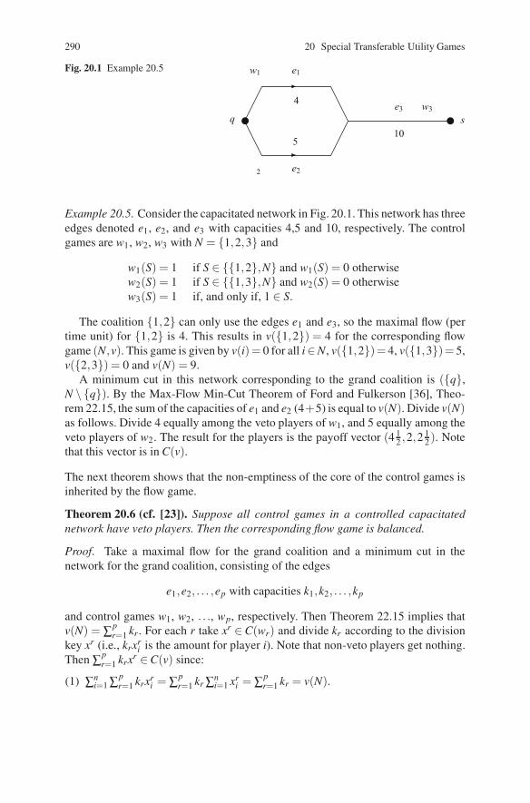
290 20 Special Transferable Utility Games
Fig. 20.1 Example 20.5
q s
e1
e2
e34
510
w1
2
w3
Example 20.5. Consider the capacitated network in Fig. 20.1. This network has threeedges denoted e1, e2, and e3 with capacities 4,5 and 10, respectively. The controlgames are w1, w2, w3 with N = {1,2,3} and
w1(S) = 1 if S ∈ {{1,2},N} and w1(S) = 0 otherwisew2(S) = 1 if S ∈ {{1,3},N} and w2(S) = 0 otherwisew3(S) = 1 if, and only if, 1 ∈ S.
The coalition {1,2} can only use the edges e1 and e3, so the maximal flow (pertime unit) for {1,2} is 4. This results in v({1,2}) = 4 for the corresponding flowgame (N,v). This game is given by v(i)= 0 for all i∈N, v({1,2})= 4, v({1,3})= 5,v({2,3}) = 0 and v(N) = 9.
A minimum cut in this network corresponding to the grand coalition is ({q},N \ {q}). By the Max-Flow Min-Cut Theorem of Ford and Fulkerson [36], Theo-rem 22.15, the sum of the capacities of e1 and e2 (4+5) is equal to v(N). Divide v(N)as follows. Divide 4 equally among the veto players of w1, and 5 equally among theveto players of w2. The result for the players is the payoff vector (4 1
2 ,2,2 12). Note
that this vector is in C(v).
The next theorem shows that the non-emptiness of the core of the control games isinherited by the flow game.
Theorem 20.6 (cf. [23]). Suppose all control games in a controlled capacitatednetwork have veto players. Then the corresponding flow game is balanced.
Proof. Take a maximal flow for the grand coalition and a minimum cut in thenetwork for the grand coalition, consisting of the edges
e1,e2, . . . ,ep with capacities k1,k2, . . . ,kp
and control games w1, w2, . . ., wp, respectively. Then Theorem 22.15 implies thatv(N) = ∑p
r=1 kr. For each r take xr ∈ C(wr) and divide kr according to the divisionkey xr (i.e., krxr
i is the amount for player i). Note that non-veto players get nothing.Then ∑p
r=1 krxr ∈C(v) since:
(1) ∑ni=1 ∑p
r=1 krxri = ∑p
r=1 kr ∑ni=1 xr
i = ∑pr=1 kr = v(N).

20.3 Voting Games: The Banzhaf Value 291
(2) For each coalition S, the set
ES := {er : r ∈ {1, . . . p},wr(S) = 1}is associated with a cut of the network, governed by the coalition S.
Hence, ∑i∈S ( ∑pr=1 krxr
i ) = ∑pr=1 kr ∑i∈S xr
i ≥ ∑pr=1 krwr (S) = ∑er∈ES
kr =capacity(ES) ≥ v(S), where the last inequality follows from Theorem 22.15. ��The next theorem is a kind of converse to Theorem 20.6.
Theorem 20.7. Each nonnegative balanced game arises from a controlled capaci-tated network where all control games possess veto players.
Proof. See Problem 20.5. ��
20.3 Voting Games: The Banzhaf Value
Voting games constitute another special class of TU-games. Voting games are simplegames which reflect the distribution of voting power within, for instance, politicalsystems. There is a large body of work on voting games within the political scienceliterature. In this section we restrict ourselves to a brief discussion of a well-knownexample of a power index, to so-called Banzhaf–Coleman index and the associatedvalue, the Banzhaf value.
A power index is a value applied to voting (simple) games. The payoff vec-tor assigned to a game is interpreted as reflecting power distribution – e.g., theprobability of having a decisive vote – rather than utility.
We start with an illustrating example.
Example 20.8. Consider a parliament with three parties 1, 2, and 3. The numbersof votes are, respectively, 50, 30, and 20. To pass any law, a two-third majorityis needed. This leads to a simple game with winning coalitions {1,2}, {1,3}, and{1,2,3}. The Shapley value4 of this game is ( 2
3 , 16 , 1
6 ), as can easily be checked.By definition of the Shapley value this means that in four of the six permutationsplayer 1 makes the coalition of his predecessors winning by joining them, whereasfor players 2 and 3 this is only the case with one permutation for each. The coalitionsthat are made winning by player 1 if he joins, are {2}, {3}, and {2,3}. In the Shapleyvalue the last coalition is counted double. It might be more natural to count thiscoalition only once. This would lead to an outcome ( 3
5 , 15 , 1
5 ), instead of the Shapleyvalue. The associated value is called the normalized Banzhaf–Coleman index.
For a simple game (N,v), the normalized Banzhaf–Coleman index can be definedas follows. Define a swing for player i as a coalition S ⊆ N with i ∈ S, S wins, andS\ {i} loses. Let θi be the number of swings for player i, then define the numbers
4 Also called the Shapley–Shubik power index in this context.

292 20 Special Transferable Utility Games
βi(N,v) :=θi
∑nj=1 θ j
.
The vector β (N,v) is the normalized Banzhaf–Coleman index of the simple game(N,v).
For a general game (N,v) write
θi(v) := ∑S⊂N: i∈S
[v(S∪ i)− v(S)].
For a simple game v this number θi(v) coincides with the number θi above.Next, define the value Ψ : G N → RN by
Ψi(v) :=θi(v)2|N|−1 = ∑
S⊂N: i∈S
12|N|−1 [v(S∪ i)− v(S)]. (20.6)
The value Ψ is called the Banzhaf value. The remainder of this section is devoted toan axiomatic characterization of this value. In the literature many characterizationsare available. The one presented below is based on Nowak [94]. The characteriza-tion uses the axioms SYM (Symmetry), SMON (Strong Monotonicity), and DUM(Dummy Property), which were all introduced in Chap. 17. Besides, it uses a kindof ‘reduced game’ or ‘amalgamation’ property, as follows.
For a game (N,v) (with at least two players) and different players i, j put p ={i, j} and define the game ((N \ p)∪{p},vp) by
vp(S) = v(S) and vp(S∪{p}) = v(S∪ p), for any S ⊆ N \ p. (20.7)
Thus, vp is an (n− 1)-person game obtained by amalgamating players i and j in vinto one player p in vp.
Let ψ be an arbitrary value (on the class G of all games with arbitrary player set).The announced axiom is as follows.
2-Efficiency (2-EFF): ψi(v)+ ψ j(v) = ψp(vp) for all v, i, j, p,vp as above.
The following theorem gives a characterization of the Banzhaf value.
Theorem 20.9. The value ψ on G satisfies 2-EFF, SYM, DUM, and SMON, if andonly if ψ is the Banzhaf value Ψ .
Proof. That the Banzhaf value satisfies the four axioms in the theorem is the subjectof Problem 20.9. For the converse, let ψ be a value satisfying the four axioms. Weprove that ψ = Ψ .
Step 1: Let uT be a unanimity game. We first show that
ψi(uT ) = 1/2|T |−1 if i ∈ T and ψi(uT ) = 0 if i ∈ T . (20.8)
If |T |= 1 then every player is a dummy, so that (20.8) follows from DUM. Suppose(20.8) holds whenever |T | ≤ k or |N| ≤ m, and consider a unanimity game uT wherenow the number of players is m+ 1, and T contains k + 1 players. Let i, j ∈ T , put

20.3 Voting Games: The Banzhaf Value 293
p = {i, j} and consider the game (uT )p. Then (uT )p is the m-person unanimity gameof the coalition T ′ = (T \ p)∪{p}, and |T ′| = k. By the induction hypothesis
ψp((uT )p) = 1/2|T′|−1 = 1/2k−1.
By 2-EFF this impliesψi(uT )+ ψ j(uT ) = 1/2k−1.
From this and SYM it follows that
ψi(uT ) = 1/2k = 1/2|T |−1, i ∈ T,
and by DUM, ψ j(uT ) = 0 when j ∈ T . Thus, ψ is the Banzhaf value on unanimitygames for any finite set of players. In the same way, one shows that this is true forany real multiple cuT of a unanimity game.
Step 2: For an arbitrary game v write v = ∑ /0 =T cT uT , and let α(v) denote the numberof nonzero coefficients in this representation. The proof will be completed by induc-tion on the number α(v) and the number of players. For α(v) = 1 Step 1 impliesψ(v) = Ψ(v) independent of the number of players. Assume that ψ(v) = Ψ (v) onany game v with at most n players, and also any game v with α(v) ≤ k for somenatural number k and with n+1 players, and let v be a game with n+1 players andwith α(v) = k + 1. There are k + 1 different nonempty coalitions T1, . . . ,Tk+1 with
v =k+1
∑r=1
cTr uTr ,
where all coefficients are nonzero. Let T := T1 ∩ . . .∩Tk+1. Because k + 1 ≥ 2, itholds that N \T = /0. Assume i ∈ T . Define the game w by
w = ∑r: i∈Tr
cTr uTr .
Then α(w) ≤ k and v(S∪ i)− v(S) = w(S∪ i)−w(S) for every coalition S not con-taining player i. By SMON and the induction hypothesis it follows that ψi(v) =ψi(w) = Ψi(w) = Ψi(w). Hence,
ψi(v) = Ψi(v) for every i ∈ N \T . (20.9)
Let j ∈ T and i ∈ N \T , put p = {i, j}, and consider the game vp. Because the gamevp has n players the induction hypothesis implies
ψp(vp) = Ψp(vp). (20.10)
Applying axiom 2-EFF to both ψ and Ψ yields
ψp(vp) = ψi(v)+ ψ j(v) and Ψp(vp) =Ψi(v)+Ψj(v). (20.11)

294 20 Special Transferable Utility Games
Combining (20.9), (20.10), and (20.11) implies ψ j(v) = Ψj(v) for every j ∈ T .Together with (20.9) this completes the induction argument, and therefore theproof. ��
Problems
20.1. The Dentist Game
Show that (20.2) and (20.3) are equivalent, and use each of these to verify that the‘dentist game’ of Sect. 1.3.4 is a permutation game.
20.2. Example 20.3
Show that the game in Example 20.3 is not an assignment game.
20.3. Subgames of Permutation Games
Prove that subgames of permutation games are again permutation games. Is this alsotrue for assignment games?
20.4. A Flow Game
Consider the network in Fig. 20.2. Suppose that this is a controlled capacitated net-work with player set N = {1,2,3,4}, suppose that all edges have capacity 1 and thatw1 = δ1, w2 = δ2, w3 = δ3 and w4(S) = 1 iff S ∈ {{3,4},N}. (Here, δi is the simplegame where a coalition is winning if, and only if, it contains player i.)
(1) Calculate the corresponding flow game (N,v).
(2) Calculate C(v).
(3) The proof of Theorem 20.6 describes a way to find core elements by looking atminimum cuts and dividing the capacities of edges in the minimum cut in some wayamong the veto players of the corresponding control game. Which elements of C(v)can be obtained in this way?
20.5. Every Nonnegative Balanced Game is a Flow Game
Prove that every nonnegative balanced game is a flow game. (Hint. Use the followingresult (cf. [28]): every nonnegative balanced game can be written as a positive linearcombination of balanced simple games.)
Fig. 20.2 The network ofProblem 20.4
q s
e1 e3
e2 e4

Problems 295
Fig. 20.3 The networkof Problem 20.6 1
10
10
w1
w2
w3
Fig. 20.4 The networkof Problem 20.7
q s
w1
w2
w3
20.6. On Theorem 20.6 (1)
(1) Consider a controlled capacitated network with a minimum cut, where all controlgames corresponding to the edges in this minimum cut (connecting vertices betweenthe two sets in the cut) have veto players. Prove that the corresponding flow game isbalanced.
(2) Show that the flow game, corresponding to Fig. 20.3, where the winning coali-tions of w1 are {1,3}, {2,4} and N = {1,2,3,4}, where the winning coalitions ofw2 are {1,2} and N and of w3 {3,4} and N and where the capacities are 1, 10,10 respectively, has a nonempty core. Note that there is no minimum cut where allcontrol games have veto players.
20.7. On Theorem 20.6 (2)
Prove that the two-person flow game corresponding to the controlled capacitatednetwork of Fig. 20.4 has an empty core, where w1 = δ1, w2 = δ2, w3(S) = 1 ifS = /0, and where the capacities of the edges are equal to 1.
20.8. Totally Balanced Flow Games
(Cf. [64].) Let (N,v) be the flow game corresponding to a controlled capacitatednetwork where all control games are dictatorial games (games of the form δi, seeProblem 20.4). Prove that each subgame (S,vS) (where vS is the restriction of v to2S) has a nonempty core, i.e., that the game (N,v) is totally balanced.
20.9. If-Part of Theorem 20.9
Prove that the Banzhaf value satisfies 2-EFF, SYM, DUM, and SMON. Is it possibleto weaken DUM to NP (the null-player property) in Theorem 20.9? Give an exampleshowing that the Banzhaf value is not efficient.

Chapter 21Bargaining Problems
The game-theoretic literature on bargaining can be divided in two strands: thecooperative and the noncooperative approach. Here, the focus is on the coopera-tive approach, which was initiated by Nash [90] and which is axiomatic in nature.1
A seminal article on noncooperative bargaining is Rubinstein [110]. The basic ideaof that paper is briefly repeated below, see Sect. 6.7 for a more elaborate discussion.We conclude the chapter with a few remarks on games with non-transferable utility(NTU-games).
21.1 The Bargaining Problem
Bargaining problems2 were introduced by Nash [90]. A two-person bargaining prob-lem is a pair (S,d) where S is a compact convex nonempty subset of R2 and d isan element of S such that x > d for some x ∈ S. The elements of S are called out-comes and d is the disagreement outcome. The interpretation of such a problem(S,d) is as follows. Two bargainers, 1 and 2, have to agree on some outcome x ∈ S,yielding utility xi to bargainer i. If they fail to reach such an agreement, they end upwith the disagreement utilities d = (d1,d2). B denotes the family of all two-personbargaining problems.
A (bargaining) solution is a map F : B → R2 such that F(S,d) ∈ S for all(S,d) ∈ B. Nash [90] proposed to characterize such a solution by requiring it tosatisfy certain axioms. More precisely, he proposed the following axioms.3
Weak Pareto Optimality (WPO): F(S,d) ∈ W (S) for all (S,d) ∈ B, where W (S) :={x ∈ S | ∀y ∈ R2 : y > x ⇒ y ∈ S} is the weakly Pareto optimal subset of S.
1 For comprehensive surveys see [103] or [135].2 See Sect. 10.1 for a first discussion.3 See Fig. 10.2 for an illustration of these axioms. In Sect. 10.1 the stronger Pareto Optimality isimposed instead of Weak Pareto Optimality. In the diagram – panel (a) – that does not make adifference.
H. Peters, Game Theory – A Multi-Leveled Approach.c© Springer-Verlag Berlin Heidelberg 2008
297

298 21 Bargaining Problems
Symmetry (SYM): F1(S,d) = F2(S,d) for all (S,d) ∈ B that are symmetric, i.e.,d1 = d2 and S = {(x2,x1) ∈ R2 | (x1,x2) ∈ S}.
Scale Covariance (SC): F(aS + b,ad + b) = aF(S,d)+ b for all (S,d) ∈ B, whereb ∈ R2, a ∈ R2
++, ax := (a1x1,a2x2) for all x ∈ R2, and aS := {ax | x ∈ S}.
Independence of Irrelevant Alternatives (IIA): F(S,d) = F(T,e) for all (S,d),(T,e) ∈ B with d = e, S ⊆ T , and F(T,e) ∈ S.
Weak Pareto Optimality says that it should not be possible for both bargainers togain with respect to the solution outcome. If a game is symmetric, then there isno way to distinguish between the bargainers, and a solution should not do thateither: that is what Symmetry requires. Scale Covariance requires the solution to becovariant under positive affine transformations: the underlying motivation is that theutility functions of the bargainers are usually assumed to be of the von Neumann–Morgenstern type, which implies that they are representations of preferences uniqueonly up to positive affine transformations (details are omitted here). Independenceof Irrelevant Alternatives requires the solution outcome not to change when the setof possible outcomes shrinks, the original solution outcome still remaining feasible.
The Nash (bargaining) solution N : B → R2 is defined as follows. For every(S,d) ∈ B,
N(S,d) = argmax{(x1 −d1)(x2 −d2) | x ∈ S,x ≥ d}.That the Nash bargaining solution is well defined, follows from Problem 21.3.
Nash [90] proved the following theorem.
Theorem 21.1. Let F : B → R2 be a bargaining solution. Then the following twostatements are equivalent:
(1) F = N.(2) F satisfies WPO, SYM, SC, IIA.
Proof. The implication (1)⇒(2) is the subject of Problem 21.4. For the implication(2)⇒(1), assume F satisfies WPO, SYM, SC, and IIA. Let (S,d) ∈ B, and z :=N(S,d). Note that z > d. Let T := {((z1 − d1)−1, (z2 − d2)−1)(x−d) | x ∈ S}. BySC,
F(T,0) = ((z1 −d1)−1,(z2 −d2)−1)F(S,d)− ((z1 −d1)−1,(z2 −d2)−1)d (21.1)
andN(T,0) = ((z1 −d1)−1,(z2 −d2)−1)(z−d) = (1,1). (21.2)
Hence, in order to prove F(S,d) = N(S,d), it is, in view of (21.1) and (21.2),sufficient to show that F(T,0) = (1,1). By (21.2) and Problem 21.5, there is a sup-porting line of T at (1,1) with slope −1. So the equation of this supporting line isx1 + x2 = 2. Choose α > 0 so large that T ⊆ D := conv{(−α,−α), (−α,2 + α),(2 + α,−α)}. Cf. Fig. 21.1.
Then (D,0) ∈ B, (D,0) is symmetric, and W (D) = conv{(−α,2 + α), (2 +α,−α)}. Hence by SYM and WPO of F :

21.2 The Raiffa–Kalai–Smorodinsky Solution 299
D
D
0T
T(1,1)
(−α ,2+α)
(2+α ,−α)(−α ,−α)
Fig. 21.1 Proof of Theorem 21.1
F(D,0) = (1,1). (21.3)
Since T ⊆ D and (1,1) ∈ T , we have by IIA and (21.3): F(T,0) = (1,1). Thiscompletes the proof. ��
21.2 The Raiffa–Kalai–Smorodinsky Solution
Kalai and Smorodinsky [63] replaced Nash’s IIA (the most controversial axiom inTheorem 21.1) by the following condition. For a problem (S,d) ∈ B,
u(S,d) := (max{x1 | x ∈ S,x ≥ d},max{x2 | x ∈ S,x ≥ d})is called the utopia point of (S,d).
Individual Monotonicity (IM): Fj(S,d) ≤ Fj(T,e) for all (S,d), (T,e) ∈ B and i, j ∈{1,2} with i = j, d = e, S ⊆ T , and ui(S,d) = ui(T,e).
The Raiffa–Kalai–Smorodinsky solution (Raiffa [105]) R : B → R2 is defined asfollows. For every (S,d) ∈ B, R(S,d) is the point of intersection of W (S) with thestraight line joining d and u(S,d).
The following theorem is a modified version of the characterization theoremobtained by Kalai and Smorodinsky [63]. In order to understand the proof it isadvisable to draw pictures, just as in the proof of the characterization of the Nashbargaining solution.

300 21 Bargaining Problems
Theorem 21.2. Let F : B → R2 be a bargaining solution. Then the following twostatements are equivalent:
(1) F = R.(2) F satisfies WPO, SYM, SC, and IM.
Proof. The implication (1)⇒(2) is the subject of Problem 21.7. For the converseimplication, assume F has the four properties stated. Let (S,d) ∈ B and let T :={ax+b | x ∈ S} with a := ((u1(S,d)−d1)−1, (u2(S,d)−d2)−1), b := −ad. By SCof R and F , R(T,0) = aR(S,d)+b and F(T,0) = aF(S,d)+b. Hence, for F(S,d) =R(S,d), it is sufficient to prove that R(T,0) = F(T,0).
Since u(T,0) = (1,1), R(T,0) is the point of W (T ) with equal coordinates, soR1(T,0) = R2(T,0). If R(T,0) = (1,1) = u(T,0), then let L := conv{(0,0),(1,1)}.Then by WPO, F(L,0) = (1,1), so by IM, F(T,0) ≥ F(L,0), hence F(T,0) =F(L,0) = R(T,0).
Next assume R(T,0) < (1,1). Let T := {x ∈ R2 | y ≤ x ≤ z for some y,z ∈ T}.Clearly T ⊆ T and u(T ,0) = u(T,0) = (1,1) so by IM:
F(T ,0) ≥ F(T,0), (21.4)
and further, since R(T,0) ∈W (T ) and R1(T ,0) = R2(T ,0),
R(T ,0) = R(T,0). (21.5)
Let V := conv{0,R(T,0),(1,0),(0,1)}. By WPO and SYM, F(V,0) = R(T,0). ByV ⊆ T , u(V,0) = u(T ,0) = (1,1), and IM, we have F(T ,0) ≥ F(V,0) = R(T,0),hence F(T ,0) = R(T,0). Combined with (21.4), this implies R(T,0) ≥ F(T,0),hence R(T,0) = F(T,0) by WPO and the fact R(T,0) < (1,1). This completes theproof. ��
21.3 The Egalitarian Solution
Consider the following two properties for a bargaining solution F .
Pareto Optimality (PO): F(S,d) ∈ P(S) for all (S,d) ∈ B, where P(S) := {x ∈ S |∀y ∈ S : y ≥ x ⇒ y = x} is the Pareto optimal subset of S.
Monotonicity (MON): F(S,d) ≤ F(T,e) for all (S,d), (T,e) ∈ B with S ⊆ T andd = e.
Clearly, P(S) ⊆ W (S) for every (S,d) ∈ B, and Pareto optimality is a strongerrequirement than Weak Pareto Optimality. The Nash and Raiffa solutions are Paretooptimal, and therefore WPO can be replaced by PO in Theorems 21.1 and 21.2.Monotonicity is much stronger than Individual Monotonicity or Restricted Mono-tonicity (see Problem 21.8 for the definition of the last axiom) and in fact it isinconsistent with Weak Pareto Optimality (see Problem 21.10).

21.3 The Egalitarian Solution 301
Call a problem (S,d) ∈ B comprehensive if z ≤ y ≤ x implies y ∈ S for all z, x ∈ S,y ∈ R2. By Bc we denote the subclass of comprehensive problems.
The egalitarian solution E : Bc → R2 assigns to each problem (S,d) ∈ Bc thepoint E(S,d) ∈W (S) with E1(S,d)−d1 = E2(S,d)−d2.
The following axiom is a weakening of Scale Covariance.
Translation Covariance (TC): F(S + e,d + e) = F(S,d)+ e for all problems (S,d)and all e ∈ R2.
The following theorem gives a characterization of the egalitarian solution based onMonotonicity.
Theorem 21.3. Let F : Bc → R2 be a bargaining solution. Then the following twostatements are equivalent:
(1) F = E.(2) F satisfies WPO, MON, SYM, and TC.
Proof. The implication (1)⇒(2) is the subject of Problem 21.11. For the converseimplication, let (S,d) ∈ Bc. We want to show F(S,d) = E(S,d).
In view of TC of F and E , we may assume d = 0. Let V := {x ∈ R2 | 0 ≤ x ≤E(S,0)}. Clearly, (V,0) ∈ Bc is a symmetric problem, so F(V,0) = E(S,0) by SYMand WPO of F . By MON,
F(S,0) ≥ F(V,0) = E(S,0). (21.6)
If E(S,0) ∈ P(S), then (21.6) implies F(S,0) = E(S,0), so we are done. Now sup-pose E(S,0) ∈W (S)\P(S). Without loss of generality, assume E1(S,0) = u1(S,0),i.e., E1(S,0) = max{x1 | x ∈ S, x ≥ 0}. Hence, E1(S,0) = F1(S,0) by (21.6).
Suppose F2(S,0) > E2(S,0). The proof will be finished by contradiction. Let α >0 with E2(S,0) < α < F2(S,0). Let T := conv(S∪{(α,0), (α,α)}). Then (T,0) ∈Bc and E(T,0) = (α,α) ∈ P(T ), so F(T,0) = (α,α) by our earlier argument (seethe line below (21.6)). On the other hand, by MON, F2(T,0) ≥ F2(S,0) > α , acontradiction. ��An alternative characterization of the egalitarian solution can be obtained by usingthe following axioms.
Super-Additivity (SA): F(S+T,d+e)≥ F(S,d)+F(T,e) for all (S,d), (T,e)∈ Bc.Here, S + T := {x+ y | x ∈ S, y ∈ T}.
Individual Rationality (IR): F(S,d) ≥ d for all (S,d) ∈ B.
Theorem 21.4. Let F : Bc → R2 be a bargaining solution. Then the following twostatements are equivalent:
(1) F = E.(2) F satisfies WPO, SA, SYM, IR, and TC.
302 21 Bargaining Problems
Proof. (1)⇒(2) follows from Theorem 21.3 and Problem 21.12. For the converseimplication, let (S,d) ∈ Bc. We wish to show F(S,d) = E(S,d). In view of TC ofF and E we may assume d = 0. For every 1 > ε > 0 let V ε := {x ∈ R2 | 0 ≤ x ≤(1− ε)E(S,0)}. Then (V ε ,0) ∈ Bc and F(V ε ,0) = E(V ε ,0) = (1− ε)E(S,0) byWPO and SYM of F and E . Since S = V ε +(S−V ε ), we have by SA:
F(S,0) ≥ (1− ε)E(S,0)+ F(S−V ε ,0). (21.7)
Letting ε decrease to 0, we obtain by (21.7) and IR:
F(S,0) ≥ E(S,0). (21.8)
If E(S,0) ∈ P(S), then (21.8) implies F(S,0) = E(S,0) and we are done. Otherwise,suppose without loss of generality that E1(S,0) = max{x1 | x ∈ S,x ≥ 0}. Let zbe the point of P(S) with z1 = E1(S,0), hence α := E2(S,0)− z2 < 0 since, byassumption, E(S,0) ∈ P(S). For ε > 0, let Rε := conv{(0,ε), (0,α), (ε,α)}. Then(Rε ,0) ∈ Bc. Further, let Tε := S + Rε . By construction, E(Tε ,0) ∈ P(Tε), hence, asbefore, F(Tε ,0) = E(Tε ,0). If ε approaches 0, F(Tε ,0) converges to E(S,0) and bySA and IR, F(Tε ,0) ≥ F(S,0). So E(S,0) ≥ F(S,0). Combined with (21.8), thisgives F(S,0) = E(S,0). ��
21.4 Noncooperative Bargaining
A different approach to bargaining is obtained by studying it a as strategic process.In this section we discuss the basics of the model of Rubinstein [110] in an informalmanner.4
Point of departure is a bargaining problem (S,d) ∈ B. Assume d = 0 andwrite S instead of (S,d). Suppose bargaining takes place over time, at momentst = 0,1,2, . . . At even moments, player 1 makes some proposal x = (x1,x2) ∈ P(S)and player 2 accepts or rejects it. At odd moments, player 2 makes some proposalx = (x1,x2) ∈ P(S) and player 1 accepts or rejects it. The game ends as soon as aproposal is accepted. If a proposal x = (x1,x2) is accepted at time t, then the play-ers receive payoffs (δ t x1,δ t x2). Here 0 < δ < 1 is a so called discount factor; itreflects impatience of the players, for instance because of foregone interest pay-ments (‘shrinking cake’). If no proposal is ever accepted, then the game ends withthe disagreement payoffs of (0,0).
Suppose player 1 has in mind to make some proposal y = (y1,y2) ∈ P(S), andthat player 2 has in mind to make some proposal z = (z1,z2) ∈ P(S). So player 1offers to player 2 the amount y2. Player 2 expects to get z2 if he rejects y, but hewill get z2 one round later. So player 1’s proposal y will be rejected by player 2 ify2 < δ z2; on the other hand, there is no need to offer strictly more than δ z2. Thisleads to the equation
y2 = δ z2. (21.9)
4 See also Sect. 6.7.

21.5 Games with Non-Transferable Utility 303
By reversing in this argument the roles of players 1 and 2 one obtains
z1 = δy1. (21.10)
These two equations define unique points y and z in P(S). The result of the Rubin-stein bargaining approach is that player 1 starts by offering y, player 2 accepts, andthe game ends with the payoffs y = (y1,y2).
This description is informal. Formally, one defines a dynamic noncooperativegame and looks for the (in this case) subgame perfect Nash equilibria of this game.It can be shown that all such equilibria result in the payoffs y (or in z if player 2would start instead of player 1).5
The surprising fact is that, although at first sight the Rubinstein approach is quitedifferent from the axiomatic approach by Nash (Theorem 21.1) the resulting out-comes turn out to be closely related. From (21.9), (21.10) one derives easily thaty1y2 = z1z2, i.e., the points y and z are on the same level curve of the functionx = (x1,x2) �→ x1x2, which appears in the definition of the Nash bargaining solu-tion. Moreover, if the discount factor δ approaches 1, the points y and z converge toone another on the curve P(S), and hence to the Nash bargaining solution outcome.In words, as the players become more patient, the outcome of the Rubinstein modelconverges to the Nash bargaining solution outcome.6
21.5 Games with Non-Transferable Utility
Both TU-games and bargaining problems are special cases of NTU-games, gameswith non-transferable utility. In an NTU-game, the possibilities from cooperation foreach coalition are described by a set, rather than a single number. For a TU-game(N,v) those sets can be defined as
V (S) = {x ∈ RS | x(S) ≤ v(S)}for every coalition S. For a two-person bargaining problem (S,d) the set of feasiblepayoffs is S for the grand coalition {1,2} and (−∞,di] for each player i.
The core concept can be extended to NTU-games (for two- or n-person bargain-ing problems it is just the part of the Pareto optimal set weakly dominating thedisagreement outcome). Also the balancedness concept can be extended; the mainresult here is that balanced games have a nonempty core, but the converse is not true(Scarf [114]).
Most other solution concepts for NTU-games (in particular the Harsanyi [49] andShapley [123] NTU-values, and the consistent value of Hart and Mas-Colell [53])extend the Nash bargaining solution as well as the Shapley value for TU-games.An exception are the monotonic solutions of Kalai and Samet [61], which extend
5 For a proof of this fact, see Rubinstein [110] or Sutton [131]. For a relatively recent and elaboratediscussion of noncooperative bargaining models see Muthoo [85].6 See also Binmore et al. [13].

304 21 Bargaining Games
the egalitarian solution of the bargaining problem. See de Clippel et al. [26] for anoverview of various axiomatic characterizations of values for NTU-games, and seePeters [104] for an overview of NTU-games in general.
Most (though not all) results of this chapter on bargaining can be extended tothe n-person case without too much difficulty. This is not true for the Rubinsteinapproach, the extension of which is not obvious. One possibility is presented byHart and Mas-Colell [53].
Problems
21.1. Anonymity and Symmetry
Call a two-person bargaining solution anonymous if F1(S′,d′) = F2(S,d) andF2(S′,d′) = F1(S,d) whenever (S,d), (S′,d′)∈B with S′ = {(x2,x1)∈R2 | (x1,x2)∈S} and (d′
1,d′2) = (d2,d1). Prove that Anonymity implies Symmetry but not vice
versa.
21.2. Revealed Preference
Let B0 = {(S,d) ∈ B | d = (0,0), S is zero-comprehensive} where S is zero-comprehensive if for all x ∈ S and y ∈ R2
+ with y ≤ x we have y ∈ S. Write Sinstead of (S,0). Let � be a binary relation on R2 and F : B0 → R2 a solution. Saythat � represents F if for every S ∈ B0:
{F(S)} = {x ∈ S | x � y for every y ∈ S},i.e., if F uniquely maximizes � on S. Prove: F satisfies IIA if and only if F can berepresented by a binary relation �.
21.3. The Nash Solution is Well-defined
Show that N is well defined, i.e., that the function (x1 − d1)(x2 − d2) takes itsmaximum on {x ∈ S | x ≥ d} at a unique point.
21.4. (1) ⇒ (2) in Theorem 21.1
Show that N satisfies the properties WPO, SYM, SC, and IIA.
21.5. Geometric Characterization of the Nash Bargaining solution
Show that, for every (S,d) ∈ B, N(S,d) = z > d if and only if there is a supportingline of S at z with slope the negative of the slope of the straight line through d and z.
21.6. Strong Individual Rationality
Call a solution F strongly individually rational (SIR) if F(S,d)> d for all (S,d)∈B.The disagreement solution D is defined by D(S,d) := d for every (S,d) ∈ B. Showthat the following two statements for a solution F are equivalent:

Problems 305
(1) F = N or F = D.
(2) F satisfies IR, SYM, SC, and IIA.
Derive from this that N is the unique solution with the properties SIR, SYM, SC,and IIA. (Hint: For the implication (2)⇒(1), show that, for every (S,d) ∈ B, eitherF(S,d) = d or F(S,d) ∈ W (S). Also show that, if F(S,d) = d for some (S,d) ∈ B,then F(S,d) = d for all (S,d) ∈ B.)
21.7. (1) ⇒ (2) in Theorem 21.2
Show that the Raiffa–Kalai–Smorodinsky solution has the properties WPO, SYM,SC, and IM.
21.8. Restricted Monotonicity
Call a solution F : B → R2 restrictedly monotonic (RM) if F(S,d) ≤ F(T,e)whenever (S,d), (T,e) ∈ B, d = e, S ⊆ T , u(S,d) = u(T,e).
(1) Prove that IM implies RM.
(2) Show that RM does not imply IM.
21.9. Global Individual Monotonicity
For a problem (S,d) ∈ B, g(S) := (max{x1 | x ∈ S}, max{x2 | x ∈ S}) is called theglobal utopia point of S. Global Individual Monotonicity (GIM) is defined in thesame way as IM, with the condition “ui(S,d) = ui(T,e)” replaced by: gi(S) = gi(T ).The solution G : B →R2 assigns to each (S,d) ∈ B the point of intersection of W (S)with the straight line joining d and g(S). Show that G is the unique solution with theproperties WPO, SYM, SC, and GIM.
21.10. Monotonicity and (weak) Pareto Optimality
(1) Show that there is no solution satisfying MON and WPO.
(2) Show that, on the subclass B0 introduced in Problem 21.2, there is no solutionsatisfying MON and PO. Can you find a solution on this class with the propertiesMON and WPO?
21.11. The Egalitarian Solution (1)
(1) Show that E satisfies MON, SYM, and WPO (on Bc).
(2) Show that E is translation covariant on Bc.
21.12. The Egalitarian Solution (2)
Show that the egalitarian solution is super-additive.
21.13. Independence of Axioms
In the characterization Theorems 21.1–21.4, show that none of the axioms used canbe dispensed with.

306 21 Bargaining Games
21.14. Nash and Rubinstein
Suppose two players (bargainers) bargain over the division of one unit of a perfectlydivisible good. Player 1 has utility function u1(α) = α and player 2 has utility func-tion u2(α) = 1− (1−α)2 for amounts α ∈ [0,1] of the good. If they do not reachan agreement on the division of the good they both receive nothing.
(a) Determine the set of feasible utility pairs. Make a picture.
(b) Determine the Nash bargaining solution outcome, in terms of utilities as well asof the physical distribution of the good.
(c) Suppose the players’ utilities are discounted by a factor δ ∈ (0,1). Calculate theRubinstein bargaining outcome.
(d) Determine the limit of the Rubinstein bargaining outcome, for δ approaching 1,in two ways: by using the result of (b) and by using the result of (c).

Chapter 22Tools
This chapter collects some mathematical tools used in this book: (direct) convexseparation results in Sects. 22.2 and 22.6; Lemmas of the Alternative, in partic-ular Farkas’ Lemma in Sect. 22.3; the Linear Duality Theorem in Sect. 22.4; theBrouwer and Kakutani Fixed Point Theorems in Sect. 22.5; the Krein–Milman The-orem and the Birkhoff–von Neumann Theorem in Sect. 22.6; and the Max-FlowMin-Cut Theorem of Ford and Fulkerson in Sect. 22.7.
22.1 Some Definitions
A subset Z ⊆ Rn is convex if with any two points x,y ∈ Z, also the line segmentconnecting x and y is contained in Z. Formally:
∀ x,y ∈ Z ∀ 0 ≤ λ ≤ 1 : λ x+(1−λ )y∈ Z.
If Z is a closed set1 then for convexity it is sufficient to check this condition forλ = 1/2 (see Problem 22.1). It is easy to see that a set Z ⊆ Rn is convex if andonly if ∑k
j=1 λ jx j ∈ Z for all x1, . . . ,xk ∈ Z and all nonnegative λ1, . . . ,λk ∈ R with∑k
j=1 λ j = 1. Such a sum ∑kj=1 λ jx j is called a convex combination of the x j.
For vectors x = (x1, . . . ,xn), y = (y1, . . . ,yn) ∈ Rn,
x ·y :=n
∑i=1
xiyi
denotes the inner product of x and y, and
||x−y|| :=
√n
∑i=1
(xi − yi)2
1 A set Z ⊆ Rn is closed if it contains the limit of every converging sequence in Z.
H. Peters, Game Theory – A Multi-Leveled Approach.c© Springer-Verlag Berlin Heidelberg 2008
309

310 22 Tools
is the Euclidean distance between x and y. A set C ⊆ Rn is a (convex) cone if, witheach x,y ∈C and λ ∈ R, λ ≥ 0, also λ x ∈C and x+ y ∈C.
22.2 A Separation Theorem
In this section we derive the simplest version of a separation result, namely separat-ing a point from a convex set.
Theorem 22.1. Let Z ⊆ Rn be a closed convex set and let x ∈ Rn \Z. Then there isa y ∈ Rn with y · z > y ·x for every z ∈ Z.
Thus, this theorem states the geometrically obvious fact that a closed convex set anda point not in that set can be separated by a hyperplane (with normal y).
Proof of Theorem 22.1. Let z′ ∈ Z such that 0 < ||x− z′|| ≤ ||x− z|| for all z ∈ Z.Such a z′ exists by the Theorem of Weierstrass, since the Euclidean distance fromx is a continuous function on the set Z, and for the minimum of z → ||x− z|| on Zattention can be restricted to a compact subset of Z. Let y = z′ − x. Let z ∈ Z. Forany α , 0 ≤ α ≤ 1, convexity of Z implies z′ + α(z− z′) ∈ Z, and thus
||z′ + α(z− z′)−x||2 ≥ ||z′ −x||2.Hence,
2α(z′ −x) · (z− z′)+ α2||z− z′||2 ≥ 0.
Thus, letting α ↓ 0, it follows that (z′ − x) · (z− z′) ≥ 0. From this, (z′ − x) · z ≥(z′ −x) · z′ = (z′ −x) ·x+(z′ −x) · (z′ −x) > (z′ −x) ·x.
Because z was arbitrary, it follows that y · z > y ·x for every z ∈ Z. ��Remark 22.2. A consequence of Theorem 22.1 is that there are real numbers α andβ satisfying y ·z > α and y ·x < α , and y ·z > β and y ·x = β , for all z∈ Z (notationsas in the Lemma).
22.3 Lemmas of the Alternative
Theorem 22.1 can be used to derive several lemmas of the alternative. These lemmashave in common that they describe two systems of linear inequalities and equations,exactly one of which has a solution.
Lemma 22.3 (Theorem of the Alternative for Matrices). Let A be an m × nmatrix. Exactly one of the following two statements is true:
(1) There are y ∈ Rn and z ∈ Rm with (y,z) ≥ 0, (y,z) = 0 and Ay+ z = 0.(2) There is an x ∈ Rm with x > 0 and xA > 0.

22.3 Lemmas of the Alternative 311
Proof. We leave it to the reader to prove that at most one of the systems in (1) and(2) has a solution (Problem 22.2).
Now suppose that (1) is not true. It is sufficient to prove that the system in (2)must have a solution. Observe that (1) implies that 0 is a convex combination of thecolumns of A and the set {e j ∈ Rm | j = 1, . . . ,m}. This follows from dividing bothsides of the equation Ay + z = 0 by ∑n
j=1 y j + ∑mi=1 zi. Hence, the assumption that
(1) is not true means that 0 /∈ Z, where Z ⊆ Rm is the convex hull of the columnsof A and the set {e j ∈ Rm | j = 1, . . . ,m}. By Theorem 22.1 and Remark 22.2 thereis an x ∈ Rm and a number β ∈ R such that x · z > β for all z ∈ Z and x · 0 = β .Hence, β = 0 and, in particular, xA > 0 and x > 0 since the columns of A and all e j
for j = 1, . . . ,m are elements of Z. Thus, (2) is true. ��Another lemma of the alternative is Farkas’s Lemma.
Lemma 22.4 (Farkas’ Lemma). Let A be an m×n matrix and b ∈ Rn. Exactly oneof the following two statements is true:
(1) There is an x ∈ Rm with x > 0 and xA = b.(2) There is a y ∈ Rn with Ay ≥ 0 and b ·y < 0.
Proof. We leave it to the reader to show that at most one of the two systems in (1)and (2) can have a solution (Problem 22.3). Assume that the system in (1) does nothave a solution. It is sufficient to prove that the system in (2) must have a solution.
The assumption that the system in (1) does not have a solution is equivalent tothe statement b ∈ Z where
Z = {z ∈ Rn | there exists an x ∈ Rm, x ≥ 0 with z = xA}.Observe that Z is a closed convex set. By Theorem 22.1 and Remark 22.2 it followsthat there is a y ∈Rn and an α ∈ R with y ·b < α and y ·z > α for all z ∈ Z. Because0 ∈ Z it follows that α < y · 0 = 0, hence y · b < α < 0. To prove that the systemin (2) has a solution, it is sufficient to prove that Ay ≥ 0. Suppose not, i.e., there isan i with (Ay)i < 0. Then eiAy < 0, so (Mei)Ay → −∞ as R � M → ∞. Observe,however, that (Mei)A ∈ Z for every M > 0, so that (Mei)Ay > α for every such M.This contradiction completes the proof of the lemma. ��These lemmas can be interpreted geometrically. We show this for Farkas’ Lemma inFig. 22.1. Consider the row vectors ri of A as points in Rn. The set of all nonnegativelinear combinations of the ri forms a cone C. The statement that the system in (1)in Lemma 22.4 has no nonnegative solution means that the vector b does not lie inC. In this case, the lemma asserts the existence of a vector y which makes an obtuseangle with b and a nonobtuse angle with each of the vectors ri. This means thatthe hyperplane L orthogonal to y has the cone C on one side and the point b on theother.

312 22 Tools
�
����������������
������
���
����
��������������
��������������
��
��
��
���
�������
L
C
r1
y
r2
r3
b
Fig. 22.1 Geometric interpretation of Farkas’ Lemma
22.4 The Duality Theorem of Linear Programming
In this section we prove the following theorem.
Theorem 22.5 (Duality Theorem of Linear Programming). Let A be an n× pmatrix, b ∈ Rp, and c ∈ Rn. Suppose V := {x ∈ Rn | xA ≥ b, x ≥ 0} = /0 and W :={y ∈ Rp | Ay ≤ c, y ≥ 0} = /0. Then min{x · c | x ∈V} = max{b ·y | y ∈W}.
To prove this theorem, we first prove the following variant of Farkas’ Lemma.
Lemma 22.6. Let A be an m× n matrix and b ∈ Rn. Exactly one of the followingtwo statements is true:
(1) There is an x ∈ Rm with xA ≤ b and x ≥ 0.(2) There is a y ∈ Rn with Ay ≥ 0, b ·y < 0, and y ≥ 0.
Proof. Problem 22.4. ��The following three lemmas are further preparations for the proof of the DualityTheorem.
Lemma 22.7. Let x ∈V and y ∈W (cf. Theorem 22.5). Then x · c ≥ b ·y.
Proof. x · c ≥ xAy ≥ b ·y. ��Lemma 22.8. Let x ∈V, y ∈W with x ·c = b · y. Then x ·c = min{x ·c | x ∈V} andb · y = max{b ·y | y ∈W}.
Proof. By Lemma 22.7, for every x ∈V : x ·c ≥ b · y = x ·c. Similarly, b ·y ≤ x ·c =b · y for every y ∈W . ��Proof of Theorem 22.5. In view of Lemmas 22.7 and 22.8, it is sufficient to showthe existence of x ∈V and y ∈W with x ·c ≤ b · y. So it is sufficient to show that thesystem

22.5 Some Fixed Point Theorems 313
(x,y)(−A 0 c
0 At −b
)≤ (−b,c,0), x ≥ 0,y ≥ 0
has a solution. Suppose this is not the case. By Lemma 22.6, there exists a vector(z,w,t) ∈ Rp ×Rn ×R with
(−A 0 c0 At −b
)⎛⎝ zwt
⎞⎠≥ 0, (−b,c,0) · (z,w,t) < 0, z ≥ 0, w ≥ 0, t ≥ 0.
Hence
Az ≤ tc (22.1)wA ≥ tb (22.2)c ·w < b · z. (22.3)
If t = 0, then Az ≤ 0, wA ≥ 0, hence, for x ∈V and y ∈W :
b · z ≤ xAz ≤ 0 ≤ wAy ≤ w · ccontradicting (22.3). If t > 0, then by (22.1) and (22.2), t−1z ∈ W and t−1w ∈ V .By (22.3), b · (t−1z) > (t−1w) · c, which contradicts Lemma 22.7. Hence, the firstsystem above must have a solution. ��
22.5 Some Fixed Point Theorems
Let Z ⊆ Rn be a nonempty convex and compact set.2 Let f : Z → Z be a continuousfunction. A point x∗ ∈ Z is a fixed point of f if f (x∗) = x∗.
If n = 1, then Z is a closed interval of the form [a,b] ⊆ R, and then it is clearfrom intuition that f must have a fixed point: formally, this is a straightforwardimplication of the intermediate-value theorem.
More generally, Brouwer [18] proved the following theorem. For a proof, see e.g.[113].
Theorem 22.9 (Brouwer Fixed Point Theorem). Let Z ⊆ Rn be a nonempty com-pact and convex set and let f : Z → Z be a continuous function. Then f has a fixedpoint.
A generalization of Brouwer’s fixed point theorem is Kakutani’s fixed point theorem[60]. Let F : Z → Z be a correspondence, i.e., F(x) is a nonempty subset of Z forevery x ∈ Z. Call F convex-valued if F(x) is a convex set for every x ∈ Z. CallF upper semi-continuous if the following holds: for every sequence (xk)k∈N in Zconverging to x ∈ Z and for every sequence (yk)k∈N in Z converging to y ∈ Z, if
2 A set Z ⊆ Rn is compact if it is closed and bounded. A set Z ⊆Rn is bounded if there is an M > 0such that ||x||< M for all x ∈ Z.

314 22 Tools
yk ∈ F(xk) for every k ∈ N, then y ∈ F(x). A point x∗ ∈ Z is a fixed point of Z ifx∗ ∈ F(x∗).
Theorem 22.10 (Kakutani Fixed Point Theorem). Let Z ⊆ Rn be a nonemptycompact and convex set and let F : Z → Z be an upper semi-continuous andconvex-valued correspondence. Then F has a fixed point.
One way to prove this theorem is to derive it from the Brouwer fixed point Theorem:see, e.g., [54].
22.6 The Birkhoff–von Neumann Theorem
Let C be a convex set in some linear space V . An element e ∈ C is called anextreme point of C if for all x,y ∈C with e = 1
2 (x + y) it holds that x = y (= e). Byext(C) the set of extreme points of C is denoted. See Problem 22.5 for alternativecharacterizations of extreme points.
An n×n-matrix D is called doubly stochastic if 0 ≤ di j ≤ 1 for all i, j = 1, . . . ,n,∑n
j=1 di j = 1 for all i, and ∑ni=1 di j = 1 for all j. If moreover di j ∈ {0,1} for all
i, j = 1, . . . ,n, then D is called a permutation matrix. Let Dn×n denote the set of alln×n doubly stochastic matrices, and let Pn×n denote the set of all n×n permutationmatrices. Note that Dn×n is a convex compact set, and that Pn×n is a finite subset ofDn×n. The following theorem gives the exact relation.
Theorem 22.11 (Birkhoff–von Neumann).
(1) ext(Dn×n) = Pn×n(2) Dn×n = conv(Pn×n).
Part (2) of Theorem 22.11 follows from the Theorem of Krein–Milman (Theo-rem 22.13 below). In the proof of the latter theorem the dimension of a subset of alinear space V plays a role. A subset of V of the form a + L where a ∈ V and L isa linear subspace of V , is called an affine subspace. Check that a subset A of V isaffine if, and only if, with any two different elements x and y of A, also the straightline through x and y is contained in A (Problem 22.6). For an affine subspace a + Lof V the dimension is defined to be the dimension of the linear subspace L. For anarbitrary subset A of V , its dimension dim(A) is defined to be the dimension of thesmallest affine subspace of V containing the set A.
The following separation lemma is used in the proof of the Theorem of Krein–Milman.
Lemma 22.12. Let C be a nonempty convex subset of Rn and a ∈ Rn \C. Then thereexists a p ∈ Rn \ {0} with p ·a ≤ p · c for every c ∈C.
Proof. We distinguish two cases: a ∈ clo(C) and a ∈ clo(C) (clo denotes thetopological closure).

22.6 The Birkhoff–von Neumann Theorem 315
(1) Suppose a ∈ clo(C). Then the result follows from Theorem 22.1, with clo(C) inthe role of the set Z there.
(2) Suppose a ∈ clo(C). Because a ∈ C it follows that a is not in the interior ofC. Hence, there is a sequence a1,a2, . . . ∈ Rn \ clo(C) converging to a. By The-orem 22.1 again, for each k there is a pk ∈ Rn \ {0} with pk · ak ≤ pk · c for allc ∈ clo(C), and we can take these vectors pk such that ||pk|| = 1 for every k (|| · ||denotes the Euclidean norm). Because {x ∈ Rn | ||x|| = 1} is a compact set, thereexists a converging subsequence pk(1),pk(2), . . . of p1,p2, . . . with limit, say, p. Thenp ·a = lim�→∞ pk(�) ·ak(�) ≤ lim�→∞ pk(�) · c = p · c for all c ∈ clo(C). ��Theorem 22.13 (Krein–Milman). Let C be a nonempty compact and convex subsetof Rn. Then ext(C) = /0 and C = conv(ext(C)).
Proof. (1) Because C is compact and x �→ ||x|| (where || · || denotes the Euclideannorm) is continuous, there exists by the Theorem of Weierstrass an e∈C with ||e||=maxx∈C ||x||. Then e ∈ ext(C), which can be proved as follows. Suppose that e =12(x1 + x2) for some x1,x2 ∈C. Then
||e|| = ||12(x1 + x2)|| ≤ 1
2||x1||+ 1
2||x2|| ≤ 1
2||e||+ 1
2||e||
implies ||x1|| = ||x2|| = || 12(x1 + x2)||. By definition of the Euclidean norm this is
only possible if x1 = x2 = e. This shows e ∈ ext(C). Hence, ext(C) = /0.
(2) The second statement in the theorem will be proved by induction on dim(C).
(a) If dim(C) = 0, then C = {a} for some a ∈ Rn, so ext(C) = {a} andconv(ext(C)) = {a} = C.
(b) Let k ∈ N, and suppose that conv(ext(D)) = D for every nonempty compact andconvex subset D of Rn with dim(D) < k. Let C be a k-dimensional compact convexsubset of Rn. Obviously, conv(ext(C)) ⊆C. So to prove is still: C ⊆ conv(ext(C)).Without loss of generality assume 0 ∈C (otherwise, shift the whole set C). Let W bethe smallest affine (hence, linear) subset of Rn containing C. Hence, dim(W ) = k.From part (1) of the proof there is an e ∈ ext(C). Let x ∈ C. If x = e then x ∈conv(ext(C)). If x = e then the intersection of the straight line through x and e withC is a line segment of which one of the endpoints is e. Let b be the other endpoint.Then b is a boundary point of C. Then, by Lemma 22.12, there is a linear functionf : W → R with f (b) = min{ f (c) | c ∈C} and f = 0 (check this).
Let D := {y ∈ C | f (y) = f (b)}. Then D is a compact and convex subset ofC. Because f = 0 it follows that dim(D) < k. By the induction hypothesis, D =conv(ext(D)). Also, ext(D) ⊆ ext(C), see Problem 22.7. Hence, b ∈ D = conv(ext(D)) ⊆ conv(ext(C)). Further, e ∈ ext(C). Because x ∈ conv{b,e} it followsthat x ∈ conv(ext(C)). So C ⊆ conv(ext(C)). ��Proof of Theorem 22.11. Because Dn×n is compact and convex, part (2) followsfrom part (1) and Theorem 22.13. So only (1) still has to be proved.
(a) We first prove that Pn×n ⊆ ext(Dn×n). Let P = [pi j]ni, j=1 be a permutation matrixwith P = 1
2(A + B) for some A,B ∈ Dn×n. Then pi j = 12 (ai j + bi j) and pi j ∈ {0,1}
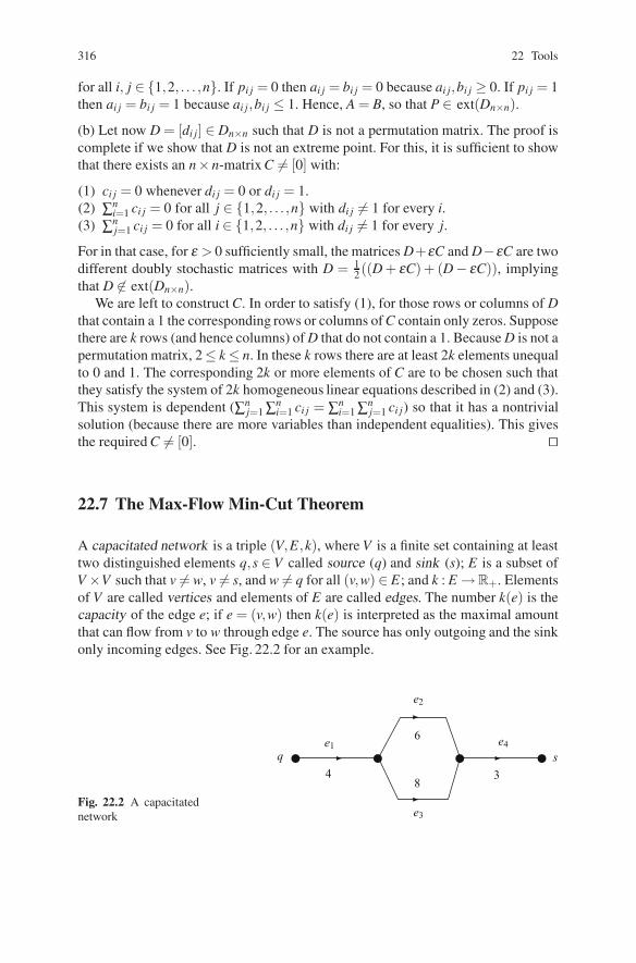
316 22 Tools
for all i, j ∈ {1,2, . . . ,n}. If pi j = 0 then ai j = bi j = 0 because ai j,bi j ≥ 0. If pi j = 1then ai j = bi j = 1 because ai j,bi j ≤ 1. Hence, A = B, so that P ∈ ext(Dn×n).
(b) Let now D = [di j] ∈ Dn×n such that D is not a permutation matrix. The proof iscomplete if we show that D is not an extreme point. For this, it is sufficient to showthat there exists an n× n-matrix C = [0] with:
(1) ci j = 0 whenever di j = 0 or di j = 1.(2) ∑n
i=1 ci j = 0 for all j ∈ {1,2, . . . ,n} with di j = 1 for every i.(3) ∑n
j=1 ci j = 0 for all i ∈ {1,2, . . . ,n} with di j = 1 for every j.
For in that case, for ε > 0 sufficiently small, the matrices D+εC and D−εC are twodifferent doubly stochastic matrices with D = 1
2((D + εC)+ (D− εC)), implyingthat D ∈ ext(Dn×n).
We are left to construct C. In order to satisfy (1), for those rows or columns of Dthat contain a 1 the corresponding rows or columns of C contain only zeros. Supposethere are k rows (and hence columns) of D that do not contain a 1. Because D is not apermutation matrix, 2≤ k ≤ n. In these k rows there are at least 2k elements unequalto 0 and 1. The corresponding 2k or more elements of C are to be chosen such thatthey satisfy the system of 2k homogeneous linear equations described in (2) and (3).This system is dependent (∑n
j=1 ∑ni=1 ci j = ∑n
i=1 ∑nj=1 ci j) so that it has a nontrivial
solution (because there are more variables than independent equalities). This givesthe required C = [0]. ��
22.7 The Max-Flow Min-Cut Theorem
A capacitated network is a triple (V,E,k), where V is a finite set containing at leasttwo distinguished elements q,s ∈ V called source (q) and sink (s); E is a subset ofV ×V such that v = w, v = s, and w = q for all (v,w) ∈ E; and k : E → R+. Elementsof V are called vertices and elements of E are called edges. The number k(e) is thecapacity of the edge e; if e = (v,w) then k(e) is interpreted as the maximal amountthat can flow from v to w through edge e. The source has only outgoing and the sinkonly incoming edges. See Fig. 22.2 for an example.
Fig. 22.2 A capacitatednetwork
q se1 e4
e2
e3
4
6
83
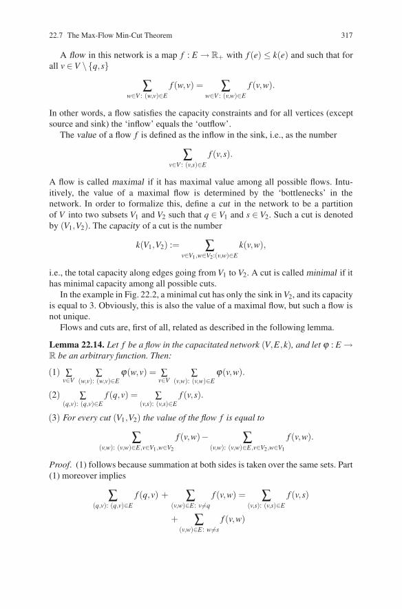
22.7 The Max-Flow Min-Cut Theorem 317
A flow in this network is a map f : E → R+ with f (e) ≤ k(e) and such that forall v ∈V \ {q,s}
∑w∈V : (w,v)∈E
f (w,v) = ∑w∈V : (v,w)∈E
f (v,w).
In other words, a flow satisfies the capacity constraints and for all vertices (exceptsource and sink) the ‘inflow’ equals the ‘outflow’.
The value of a flow f is defined as the inflow in the sink, i.e., as the number
∑v∈V : (v,s)∈E
f (v,s).
A flow is called maximal if it has maximal value among all possible flows. Intu-itively, the value of a maximal flow is determined by the ‘bottlenecks’ in thenetwork. In order to formalize this, define a cut in the network to be a partitionof V into two subsets V1 and V2 such that q ∈ V1 and s ∈ V2. Such a cut is denotedby (V1,V2). The capacity of a cut is the number
k(V1,V2) := ∑v∈V1,w∈V2:(v,w)∈E
k(v,w),
i.e., the total capacity along edges going from V1 to V2. A cut is called minimal if ithas minimal capacity among all possible cuts.
In the example in Fig. 22.2, a minimal cut has only the sink in V2, and its capacityis equal to 3. Obviously, this is also the value of a maximal flow, but such a flow isnot unique.
Flows and cuts are, first of all, related as described in the following lemma.
Lemma 22.14. Let f be a flow in the capacitated network (V,E,k), and let ϕ : E →R be an arbitrary function. Then:
(1) ∑v∈V
∑(w,v): (w,v)∈E
ϕ(w,v) = ∑v∈V
∑(v,w): (v,w)∈E
ϕ(v,w).
(2) ∑(q,v): (q,v)∈E
f (q,v) = ∑(v,s): (v,s)∈E
f (v,s).
(3) For every cut (V1,V2) the value of the flow f is equal to
∑(v,w): (v,w)∈E,v∈V1,w∈V2
f (v,w)− ∑(v,w): (v,w)∈E,v∈V2,w∈V1
f (v,w).
Proof. (1) follows because summation at both sides is taken over the same sets. Part(1) moreover implies
∑(q,v): (q,v)∈E
f (q,v) + ∑(v,w)∈E: v=q
f (v,w) = ∑(v,s): (v,s)∈E
f (v,s)
+ ∑(v,w)∈E: w=s
f (v,w)

318 22 Tools
which implies (2) because ∑(v,w)∈E: v=q f (v,w) = ∑(v,w)∈E: w=s f (v,w) by definitionof a flow (‘inflow’ equals ‘outflow’ at every vertex that is not the source and not thesink). For part (3), let (V1,V2) be a cut of the network. Then
∑(v,w)∈E: v∈V1,w∈V2
f (v,w) = ∑(v,w)∈E: v∈V1
f (v,w)− ∑(v,w)∈E: v,w∈V1
f (v,w)
= ∑(v,w)∈E: v=q
f (v,w)+ ∑(v,w)∈E: w∈V1
f (v,w)
− ∑(v,w)∈E: v,w∈V1
f (v,w)
= ∑(v,w)∈E: v=q
f (v,w)+ ∑(v,w)∈E: v∈V2,w∈V1
f (v,w)
= ∑(v,w)∈E: w=s
f (v,w)+ ∑(v,w)∈E: v∈V2,w∈V1
f (v,w).
This implies part (3) of the lemma. ��The following theorem is the famous Max-Flow Min-Cut Theorem of Ford andFulkerson [36].
Theorem 22.15. Let (V,E,k) be a capacitated network. Then the value of a maximalflow is equal to the capacity of a minimal cut.
Proof. Let f be a maximal flow. (Note that f is an optimal solution of a fea-sible bounded linear program, so that existence of f is guaranteed.) Part (3) ofLemma 22.14 implies that the value of any flow is smaller than or equal to thecapacity of any cut, so that it is sufficient to find a cut of which the capacity is equalto the value of f .
For points v,w in the network define a path as a sequence of different non-directed edges starting in v and ending in w; ‘non-directed’ means that for any edge(x,y) ∈ E , (x,y) as well as (y,x) may be used in this path. Such a path may bedescribed by a sequence v = x1,x2, . . . ,xm = w with (xi,xi+1) ∈ E or (xi+1,xi) ∈ Efor every i = 1, . . . ,m−1. Call such a path non-satiated if for every i = 1, . . . ,m−1 itholds that f (xi,xi+1) < k(xi,xi+1) if (xi,xi+1) ∈ E , and f (xi+1,xi) > 0 if (xi+1,xi) ∈E . In other words, the flow is below capacity in edges that are traversed in the ‘right’way, and positive in edges that are traversed in the ‘wrong’ way.
Define V1 to be the set of vertices x for which there is a non-satiated path from qto x, together with the vertex q, and let V2 be the complement of V1 in V . Then s ∈V2because otherwise there would be a non-satiated path from q to s, implying that fwould not be maximal; the flow f could be increased by increasing it in edges onthis path that are traversed in the right way and decreasing it in edges along the paththat are traversed in the wrong way, without violating the capacity constraints or theinflow–outflow equalities. Hence (V1,V2) is a cut in the network.
Let (x,y) ∈ E with x ∈ V1 and y ∈ V2. Then f (x,y) = k(x,y) because otherwisethere would be a non-satiated path from q to a vertex in V2. Similarly, f (x′,y′) = 0whenever (x′,y′) ∈ E with x′ ∈V2 and y′ ∈V1. By Lemma 22.14, part (3), the valueof the flow f is equal to

Problems 319
∑(v,w): (v,w)∈E,v∈V1,w∈V2
f (v,w)− ∑(v,w): (v,w)∈E,v∈V2,w∈V1
f (v,w)
hence to ∑(v,w): (v,w)∈E,v∈V1,w∈V2
k(v,w), which is by definition the capacity of the cut
(V1,V2). This completes the proof. ��Observe that the proof of Theorem 22.15 suggests an algorithm to determine a max-imal flow, by starting with an arbitrary flow, looking for a non-satiated path, andimproving this path. By finding an appropriate cut, maximality of a flow can bechecked. Theorem 22.15 is actually a (linear) duality result, but the above proof iselementary.
Problems
22.1. Convex Sets
Prove that a closed set Z ⊆ Rn is convex if and only if 12 x+ 1
2 y ∈ Z for all x,y ∈ Z.
22.2. Proof of Lemma 22.3
Prove that at most one of the systems in Lemma 22.3 has a solution.
22.3. Proof of Lemma 22.4
Prove that at most one of the systems in Lemma 22.4 has a solution.
22.4. Proof of Lemma 22.6
Prove Lemma 22.6.
22.5. Extreme Points
Let C be a convex set in a linear space V and let e∈C. Prove that the following threestatements are equivalent:
(1) e ∈ ext(C).(2) For all 0 < α < 1 and all x,y ∈C, if x = y then e = αx +(1−α)y.(3) C \ {e} is a convex set.
22.6. Affine Subspaces
Prove that a subset A of a linear space V is affine if, and only if, with any twodifferent elements x and y of A, also the straight line through x and y is containedin A.
22.7. The Set of Sup-Points of a Linear Function on a Convex Set
Let f : Rn → Rn be a linear function. Let C be a convex subset of Rn andα := sup{ f (x) | x ∈ C}, D := {x ∈ C | f (x) = α}. Show that D is convex and thatext(D) ⊆ ext(C).
Hints, Answers and Solutions
Problems of Chap. 1
1.2 Variant of Matching PenniesThere are saddlepoint(s) if and only if x ≤−1.
1.3 Mixed Strategies(b) (3/4,1/4).
(c) (1/2,1/2).
(d) By playing (3/4,1/4) player 1 obtains 10/4 = 2.5 for sure (independent of whatplayer 2 does). Similarly, by playing (1/2,1/2), player 2 is sure to pay 2.5. So 2.5is the value of this game. Given a rational opponent, no player can hope to do betterby playing differently.
1.5 Glove Game(a) (0,0,1) is the unique vector in the core of the glove game.
1.6 Dentist AppointmentsThe Shapley value (9 1
2 ,6 12 ,8) is not in the core of this game. The nucleolus is in the
core of the game.
1.7 Nash BargainingThe problem to solve is max0≤α≤1 α
√1−α. Obviously, the solution must be inte-
rior: 0 < α < 1. Set the first derivative equal to 0, solve, and check that the secondderivative is negative.
1.8 Variant of Glove GameThe worth of a coalition S depends on the minimum of the numbers of right-handand left-hand players in the coalition. Write N = L∪R and find a formal expressionfor v(S).
321

322 Hints, Answers and Solutions
Problems of Chap. 2
2.1 Solving Matrix Games(a) The optimal strategies are (5/11,6/11) for player 1 and (5/11,6/11) for player2. The value of the game is 30/11. In the original game the optimal strategies are(5/11,6/11,0) for player 1 and (5/11,6/11,0) for player 2.
(b) The value of the game is 0. The unique maximin strategy is (0,1,0). Theminimax strategies are (0,q,1− q,0) for any 0 ≤ q ≤ 1.
(c) The value of the game is 1, the unique minimax strategy is (1/2,0,1/2), and themaximin strategies are: (p,(1− p)/2,(1− p)/2) for 0 ≤ p ≤ 1.
(d) The value of the game is 9 and player 1’s maximin strategy is (1/2,1/2,0,0).The set of all minimax strategies is {(α, 7−14α
10 , 3+4α10 ) ∈ R3 | 0 ≤ α ≤ 1/2}.
(e) The value is 8/5. The unique maximin strategy is (2/5,3/5) and the uniqueminimax strategy is (0,4/5,1/5,0).
(f) The value is equal to 1, player 2 has a unique minimax strategy namely (0,1,0),and the set of maximin strategies is {(0, p,1− p) | 0 ≤ p ≤ 1}.
2.2 Saddlepoints(b) There are saddlepoints at (1,4) and at (4,1).
2.3 Rock–Paper–ScissorsThe associated matrix game is
⎛⎝R P S
R 0 −1 1P 1 0 −1S −1 1 0
⎞⎠.
Problems of Chap. 3
3.1 Some Applications(a) Let Smith be the row player and Brown the column player, then the bimatrixgame is ( L S
L 2,2 −1,−1S −1,−1 1,1
).
(b) Let the government be the row player and the pauper the column player. Thebimatrix game is ( work not
aid 3,2 −1,3not −1,1 0,0
).
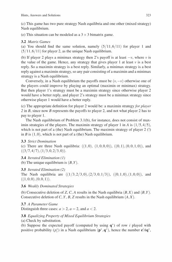
Hints, Answers and Solutions 323
(c) This game has two pure strategy Nash equilibria and one other (mixed strategy)Nash equilibrium.
(e) This situation can be modeled as a 3×3 bimatrix game.
3.2 Matrix Games(a) You should find the same solution, namely (5/11,6/11) for player 1 and(5/11,6/11) for player 2, as the unique Nash equilibrium.
(b) If player 2 plays a minimax strategy then 2’s payoff is at least −v, where v isthe value of the game. Hence, any strategy that gives player 1 at least v is a bestreply. So a maximin strategy is a best reply. Similarly, a minimax strategy is a bestreply against a maximin strategy, so any pair consisting of a maximin and a minimaxstrategy is a Nash equilibrium.
Conversely, in a Nash equilibrium the payoffs must be (v,−v) otherwise one ofthe players could improve by playing an optimal (maximin or minimax) strategy.But then player 1’s strategy must be a maximin strategy since otherwise player 2would have a better reply, and player 2’s strategy must be a minimax strategy sinceotherwise player 1 would have a better reply.
(c) The appropriate definition for player 2 would be: a maximin strategy for player2 in B, since now B represents the payoffs to player 2, and not what player 2 has topay to player 1.
The Nash equilibrium of Problem 3.1(b), for instance, does not consist of max-imin strategies of the players. The maximin strategy of player 1 in A is (1/5,4/5),which is not part of a (the) Nash equilibrium. The maximin strategy of player 2 (!)in B is (1,0), which is not part of a (the) Nash equilibrium.
3.3 Strict Domination(c) There are three Nash equilibria: ((1,0), (1,0,0,0)), ((0,1),(0,0,1,0)), and((3/7,4/7),(1/3,0,2/3,0)).
3.4 Iterated Elimination (1)(b) The unique equilibrium is (B,Y ).
3.5 Iterated Elimination (2)The Nash equilibria are ((1/3,2/3,0),(2/3,0,1/3)), ((0,1,0),(1,0,0)), and((1,0,0),(0,0,1)).
3.6 Weakly Dominated Strategies
(b) Consecutive deletion of Z, C, A results in the Nash equilibria (B,X) and (B,Y ).Consecutive deletion of C, Y , B, Z results in the Nash equilibrium (A,X).
3.7 A Parameter GameDistinguish three cases: a > 2, a = 2, and a < 2.
3.8 Equalizing Property of Mixed Equilibrium Strategies(a) Check by substitution.(b) Suppose the expected payoff (computed by using q∗) of row i played withpositive probability (p∗i ) in a Nash equilibrium (p∗,q∗), hence the number eiAq∗,

324 Hints, Answers and Solutions
would not be maximal. Then player 1 would improve by adding the probability p∗ito some row j with higher expected payoff e jAq∗ > eiAq∗, and in this way increasehis payoff, a contradiction. A similar argument can be made for player 2 and thecolumns.
Problems of Chap. 4
4.1 Counting StrategiesWhite has 20 possible opening moves, and therefore also 20 possible strategies.Black has many more strategies.
4.2 Extensive vs. Strategic FormOne possibility is the following extensive form game. Player 1 starts and has twopossible actions, say U and D (corresponding to the two rows of player 1). Theseactions lead to the unique information set of player 2. At each of the two nodes inthis information set, player 2 has four actions, namely C1, C2, C3, and C4 (corre-sponding to the four columns of player 2). The payoffs following U are (a1,a2),(b1,b2), (e1,e2), and ( f1, f2), respectively. The payoffs following D are (c1,c2),(d1,d2), (g1,g2), and (h1,h2), respectively.
Another possibility is to switch the roles of the players. Player 2 starts and hasfour actions C1, C2, C3, and C4. Player 1 has one information set with four nodesand at each node the actions U and D. The payoffs (following U and D) are: (a1,a2)and (c1,c2); (b1,b2) and (d1,d2); (e1,e2) and (g1,g2); and ( f1, f2) and (h1,h2),respectively.
If, for instance, bi = ai, fi = ei, gi = ci, and hi = di for i = 1,2, then the followingextensive form game of perfect information is possible. Player 1 starts and has twoactions, U and D. After U player 2 has two actions, say L and R, and after D player2 has again two actions, say l and r. The path U,L is followed by the payoff pair(a1,a2), the path U,R by (e1,e2), the path D, l by (c1,c2), and the path D,r by(d1,d2).
Still another possibility is to let player 2 start with two possible actions, leading toone information set of player 1 with two actions at each of the two nodes. Finally, allthe actions of player 1 result in one information set of player 2 at which this playerhas again two actions. Formally, this extensive form is not allowed since player 2has imperfect recall.
4.4 Choosing Objects(c) In any subgame perfect equilibrium the game is played as follows: player 1 picksO3, then player 2 picks O2 or O1, and finally player 1 picks O4. These are the (two)subgame perfect equilibrium outcomes of the game. Due to ties (of player 2) thereis more than one subgame perfect equilibrium, namely eight in total. All subgameperfect equilibria result in the same distribution of the objects.

Hints, Answers and Solutions 325
4.5 An Extensive Form GameThere is a unique pure strategy Nash equilibrium, which is also subgame perfect.This equilibrium is perfect Bayesian for an appropriate choice of player 2’s belief.
4.6 Another Extensive Form GameThere is a unique Nash equilibrium (in pure strategies). This equilibrium is notperfect Bayesian.
4.7 A Centipede Game(b) Consider any strategy combination. The last player that has continued whenplaying his strategy could have improved by stopping if possible. Hence, in equilib-rium the play of the game must have stopped immediately.
To exhibit a non-subgame perfect Nash equilibrium, assume that player 1 alwaysstops, and that player 2 also always stops except at his second decision node. Checkthat this is a Nash equilibrium. (One can also write down the strategic form, whichis an 8× 8 bimatrix game.)
4.8 Finitely Repeated Games(c) The unique subgame perfect Nash equilibrium is where player 1 always plays Band player 2 always R. This is true for any finite repetition of the game.
(e) Player 1: play T at the first stage. Player 2: play L at the first stage. Second stageplay is given by the following diagram:
⎛⎝L M R
T B,R C,R C,RC B,M B,R B,RB B,M B,R B,R
⎞⎠.
For instance, if first stage play results in (C, L), then player 1 plays B and player 2plays M at stage 2. Verify that this defines a subgame perfect equilibrium in which(T , L) is played at the second stage. (Other solutions are possible, as long as players1 and 2 are punished for unilateral deviations at stage 1.)
Problems of Chap. 5
5.1 Battle-of-the-SexesThe strategic form is a 4×4 bimatrix game. List the strategies of the players as in thetext. We can then compute the expected payoffs. E.g., if the first row corresponds tostrategy SS of player 1 and strategies SS, SB, BS, and BB of player 2, then the payoffsare, respectively, 1/6 times (8,3), (6,9), (6,0), and (4,6). The (pure strategy) Nashequilibria are (SS,SB) and (BS,BB).
5.2 A Static Game of Incomplete InformationThere are three pure Nash equilibria: (T T,L), (TB,R), and (BB,R). (The first letterin a strategy of player 1 applies to Game 1, the second letter to Game 2.)

326 Hints, Answers and Solutions
5.3 Another Static Game of Incomplete Information(b) The unique pure strategy Nash equilibrium is: t1 and t ′1 play B, t2 and t ′2 play R.
5.4 Job-Market Signaling(b) There is a pooling equilibrium where both worker types take no education, andwages are always low. This equilibrium is sustained by the firm’s belief that aneducated worker is of the high type with probability at least 1/2. It survives theintuitive criterion if the firm believes that an educated worker is of the high typewith probability 1.
There is also a separating equilibrium in which the high type takes education andthe low type doesn’t. Both types get offered the low wage.
5.5 A Joint Venture(c) There is a unique Nash equilibrium (even in mixed strategies). This is alsosubgame perfect and perfect Bayesian.
5.6 Entry DeterrenceFor x≤ 100 the strategy combination where the entrant always enters and the incum-bent colludes is a perfect Bayesian equilibrium. For x ≥ 50, the combination wherethe entrant always stays out and the incumbent fights is a perfect Bayesian equilib-rium if the incumbent believes that, if the entrant enters, then fighting yields 0 withprobability at most 1− 50
x . Both equilibria satisfy the intuitive criterion.
5.7 The Beer–Quiche Game(b) There are two perfect Bayesian equilibria, both of which are pooling. In the firstone, player 1 always eats quiche. This equilibrium does not survive the intuitivecriterion. In the second one, player 1 always drinks beer. This equilibrium doessurvive the intuitive criterion.
5.8 Issuing Stock(b) There is a pooling equilibrium in which the manager never proposes to issue newstock, and such a proposal would not be approved of by the existing shareholderssince they believe that this proposal signals a good state with high enough proba-bility. (The background of this is that a new stock issue would dilute the value ofthe stock of the existing shareholders in a good state of the world, see the originalarticle for details.) This equilibrium (just about) survives the intuitive criterion.
There is also a separating equilibrium in which a stock issue is proposed in thebad state but not in the good state. If a stock issue is proposed, then it is approvedof.
Finally, there is a separating equilibrium in which a stock issue is proposed inthe good state but not in the bad state. If a stock issue is proposed, then it is notapproved of.
(c) In this case, a stock issue proposal would always be approved of, so the ‘badnews effect’ of a stock issue vanishes. The reason is that the investment opportunityis now much more attractive.

Hints, Answers and Solutions 327
5.9 More Signaling Games(a) There is a unique, pooling perfect Bayesian equilibrium. This equilibrium doesnot survive the intuitive criterion.
(b) There are two strategy combinations that are perfect Bayesian. Only one of themsurvives the intuitive criterion.
Problems of Chap. 6
6.1 Cournot with Asymmetric CostsThe Nash equilibrium is q1 = (a−2c1 +c2)/3 and q2 = (a−2c2 +c1)/3, given thatthese amounts are nonnegative.
6.2 Cournot Oligopoly(b) The reaction function of player i is: βi(q1, . . . ,qi−1,qi+1, . . . ,qn) = (a − c −∑ j =i q j)/2 if ∑ j =i q j ≤ a− c, and βi(q1, . . . ,qi−1,qi+1, . . . ,qn) = 0 otherwise.
(c) One should compute the point of intersection of the n reaction functions.This amounts to solving a system of n linear equations in n unknowns q1, . . . ,qn.Alternatively, one may guess that there is a solution q1 = q2 = . . . = qn. Thenq1 = (a − c − (n − 1)q1)/2, resulting in q1 = a−c
n+1 . Hence, each firm producinga−cn+1 is a Nash equilibrium. If the number of firms becomes large then this amountconverges to 0, which is no surprise since demand is bounded by a.
(d) To show that this equilibrium is unique, one may first argue that it is unique giventhat all equilibrium outputs are positive (e.g., by showing that the given systemof n linear equations has a unique solution by computing the determinant of thecoefficient matrix). Moreover, in equilibrium there is at least one firm producing apositive output and having positive profit. If there would be some other firm withzero output, then that firm could improve by producing a small amount and makingpositive profit.
6.3 Quantity Competition with Heterogenous Goods(a) Πi(q1,q2) = qipi(q1,q2)− cqi for i = 1,2.
(b) The equilibrium is: q1 = (21− 4c)/33, q2 = (13− 3c)/22, p1 = (21 + 7c)/11,p2 = (39 + 13c)/22.
(c) q1 = (57− 10c)/95, q2 = (38− 10c)/95, p1 = (228 + 50c)/95, p2 = (228 +45c)/95.
(d) q1 = max{1− 12 p1 + 1
3 p2,0}, q2 = max{1− 12 p2 + 1
4 p1}. The profit functionsare now Π1(p1, p2) = p1q1 − cq1 and Π2(p1, p2) = p2q2 − cq2, with q1 and q2 asgiven.
(e) The equilibrium is p1 = 16+8c11 , p2 = 30+15c
22 . Note that these prices are differentfrom the ones in (c).
(f) These are the same prices and quantities as under (c).(g) See the answers to (e) and (f).

328 Hints, Answers and Solutions
6.4 A Numerical Example of Cournot with Incomplete Informationq1 = 18/48, qH = 9/48, qL = 15/48. In the complete information case with low costwe have q1 = q2 = 16/48, with high cost it is q1 = 20/48 and q2 = 8/48. Note thatthe low cost firm ‘suffers’ from incomplete information since firm 1 attaches somepositive probability to firm 2 having high cost and therefore has higher supply. Forthe high cost firm the situation is reversed: it ‘benefits’ from incomplete information.
6.5 Cournot with Two-sided Incomplete InformationSimilar to (6.3) we derive
q� = q�(qH ,qL) =a− c�−ϑqH − (1−ϑ)qL
2,
qh = qh(qH ,qL) =a− ch−ϑqH − (1−ϑ)qL
2,
qL = qL(qh,q�) =a− cL−πqh− (1−π)q�
2,
qH = qH(qh,q�) =a− cH −πqh− (1−π)q�
2.
Here, q� and qh correspond to the low and high cost types of firm 1 and qL, andqH correspond to the low and high cost types of firm 2. The (Bayesian) Nashequilibrium follows by solving these four equations in the four unknown quantities.
6.6 Incomplete Information about DemandThe equilibrium is: q1 = ϑaH+(1−ϑ )aL−c
3 , qH = aH−c3 + 1−ϑ
6 (aH −aL), qL = aL−c3 −
ϑ6 (aH −aL). (Assume that all these quantities are positive.)
6.7 Variations on Two-person Bertrand(a) If c1 < c2 then there is no Nash equilibrium. (Write down the reaction functionsor – easier – consider different cases.)
(b) If c1 = c2 = c < a− 1 then there are two equilibria, namely p1 = p2 = c andp1 = p2 = c+1. (If c = a−1 then there are two additional equilibria, namely p1 =c, p2 = c+1 and p1 = c+1, p2 = c.) Assume c1 < c2. There are several cases. E.g., ifc1 < c2 −1 and a > 2c2 −c1 then there are two equilibria, namely p1 = c2 −1, p2 =c2 and p1 = c2, p2 = c2 + 1.
6.8 Bertrand with More than Two FirmsA strategy combination is a Nash equilibrium if and only if at least two firms chargea price of c and the other firms charge prices higher than c.
6.9 Variations on Stackelberg(a) With firm 1 as a leader we have q1 = (1/2)(a− 2c1 + c2) and q2 = (1/4)(a +2c1 − 3c2). With firm 2 as a leader we have q2 = (1/2)(a− 2c2 + c1) and q1 =(1/4)(a + 2c2−3c1).
(b) The leader in the Stackelberg game can always play the Cournot quantity: sincethe follower plays the best reply, this results in the Cournot outcome. Hence, the

Hints, Answers and Solutions 329
Stackelberg equilibrium – where the leader maximizes – can only give a higherpayoff. (This argument holds for an arbitrary game where one player moves firstand the other player moves next, having observed the move of the first player.)
(c) qi = (1/2i)(a− c) for i = 1,2, . . . ,n.
6.10 First-price Sealed-bid Auction(b) Suppose that in some Nash equilibrium player i wins with valuation vi < v1.Then the winning bid bi must be at most vi otherwise player i makes a negativeprofit and therefore can improve by bidding (e.g.) vi. But then player 1 can improveby bidding higher than bi (and win) but lower than v1 (and make positive profit).Other Nash equilibria: (v1,v1,0,0, . . . ,0), (b,b,b, . . . ,b) with v1 ≥ b ≥ v2, etc.
(d) If not, then there would be a Nash equilibrium in which – in view of (c) – allplayers bid below their valuations. By (b) a player with the highest valuation winsthe auction, so this must be player 1 if each player bids below his true valuation. Butthen player 1 can improve if b1 ≥ v2 and player 2 can improve if b1 < v2.
6.11 Second-price Sealed-bid Auction(d) Also (v1,0 . . . ,0) is a Nash equilibrium.
(e) The equilibria are: {(b1,b2) | b2 ≥ v1, 0 ≤ b1 ≤ v2} ∪ {(b1,b2) | b1 ≥ v2, b2 ≤b1, 0 ≤ b2 ≥ v1}.
6.12 Third-price Sealed-bid Auction(b) Suppose v1 > v2 > v3 > · · ·, then bidder 2 could improve by bidding higher thanv1.
(c) Everybody bidding the highest valuation v1 is a Nash equilibrium. Also every-body bidding the second highest valuation v2 is a Nash equilibrium. (There are manymore!)
6.13 n-Player First-price Sealed-bid with Incomplete InformationSuppose every player j = i plays s∗j . If player i’s type is vi and he bids bi (which canbe assumed to be at most 1−1/n since no other bidder bids higher than this) then theprobability of winning the auction is equal to the probability that very bid b j, j = i, isat most bi (including equality since this happens with zero probability). In turn, thisis equal to the probability that v j ≤ n/(n− 1)bi for every j = i. Since the players’svaluations are independently drawn from the uniform distribution, the probabilitythat player i wins the auction is equal to (n/(n− 1)bi)n−1, hence player i shouldmaximize the expression (vi −bi)(n/(n−1)bi)n−1, resulting in bi = (1−1/n)vi.
6.14 Mixed Strategies and Objective Uncertainty(a) ((1/2,1/2),(2/5,3/5)).
6.15 Variations on Finite Horizon Bargaining(a) Adapt Table 6.1 for the various cases.
(b) The subgame perfect equilibrium outcome is: player 1 proposes (1 − δ2 +δ1δ2,δ2 − δ1δ2) at t = 0 and player 2 accepts.

330 Hints, Answers and Solutions
(c) The subgame perfect equilibrium outcome in shares of the good is: player 1proposes (1− δ 2
2 + δ1δ 22 ,δ 2
2 − δ1δ 22 ) at t = 0 and player 2 accepts.
(d) The subgame perfect equilibrium outcome is: player 1 proposes (1− δ + δ 2 −. . .+ δ T−1 − δ T s1,δ − δ 2 + . . .− δ T−1 + δ T s1) at t = 0 and player 2 accepts.
(e) The limits are ( 11+δ , δ
1+δ ), independent of s.
6.16 Variations on Infinite Horizon Bargaining(a) Conditions (6.6) are replaced by x∗2 = δ2y∗2 and y∗1 = δ1x∗1. This implies x∗1 =
1−δ21−δ1δ2
and y∗1 = δ1−δ1δ21−δ1δ2
. In the strategies (σ∗1 ) and (σ∗
2 ), replace δ by δ1 andδ2, respectively. The equilibrium outcome is that player 1’s proposal x∗ at t = 0is accepted.
(b) Nothing essential changes. Player 2’s proposal y∗ is accepted at t = 0.
(c) Nothing changes compared to the situation in the text, since s is only obtained att = ∞.
(e) Let p denote the probability that the game ends. Then p is also the probabilitythat the game ends given that it does not end at t = 0. Hence, p = (1− δ )+ δ p, sothat p = 1.
6.17 A Principal–agent Game(a) This is a game of complete information. The employer starts and has an infinitenumber of actions available, namely any pair (wL,wH) of nonnegative wages. Aftereach of these actions, the worker has three possible actions: reject, resulting in 0for the employer and 2 for the worker; accept and exert high effort, resulting inthe (expected) payoffs of 9.2− 8wH+2wL
10 for the employer and 8wH+2wL10 − 3 for the
worker; accept and exert low effort, resulting in the (expected) payoffs of 6.8−2wH+8wL
10 for the employer and 2wH+8wL10 for the worker. The actions of the employer
are also his strategies. A strategy for the worker is a function (wL,wH) �→ { reject(r), accept and exert high effort (h), accept and exert low effort (l) }.
(b) Any pair of wages (wL,wH) with 2wH+8wL10 = 2 and wH ≤ wL + 5, together
with the worker choosing a payoff maximizing action but certainly l if l is pay-off maximizing following any wage offer package (wL,wH), is a subgame perfectequilibrium. All these equilibria result in the worker accepting and exerting loweffort, and final payoffs of 4.8 for the employer and 2 for the worker.
6.18 The Market for Lemons(b) There are many subgame perfect equilibria: the buyer offers p ≤ 5,000 and theseller accepts any price of at least 5,000 if the car is bad and of at least 15,000 if thecar is good. All these equilibria result in expected payoff of zero for both. There areno other subgame perfect equilibria.
6.19 Corporate Investment and Capital Structure(b) Suppose the investor’s belief that π = L after observing s is equal to q. Then theinvestor accepts s if and only if
s[qL+(1− q)H + R] ≥ I(1 + r). (∗)

Hints, Answers and Solutions 331
The entrepreneur prefers to receive the investment if and only if
s ≤ R/(π + R), (∗∗)for π ∈ {L,H}.
In a pooling equilibrium, q = p. Note that (∗∗) is more difficult to satisfy forπ = H than for π = L. Thus, (∗) and (∗∗) imply that a pooling equilibrium existsonly if
I(1 + r)pL+(1− p)H + R
≤ RH + R
.
A separating equilibrium always exists. The low-profit type offers s = I(1 +r)/(L + R), which the investor accepts, and the high-profit type offers s < I(1 +r)/(H + R), which the investor rejects.
6.20 A Poker Game(a) The strategic form of this game is as follows:
( aa aq ka kqbelieve −1,1 −1/3,1/3 −2/3,2/3 0,0show 2/3,−2/3 1/3,−1/3 0,0 −1/3,1/3
).
Here, ‘believe’ and ‘show’ are the strategies of player I. The first letter in any strat-egy of player II is what player II says if the dealt card is a King, the second letter iswhat II says if the dealt card is a Queen – if the dealt card is an Ace player II has nochoice.
(b) Player I has a unique optimal (maximin) strategy and player 2 has a uniqueoptimal (minimax) strategy. The value of the game is −2/9.
6.21 A Hotelling Location Problem(a) x1 = x2 = 1
2 .
(c) x1 = x2 = 12 .
6.22 Median Voting(a) The strategy set of each player is the interval [0,30]. If each player i plays xi, thenthe payoff to each player i is −| x1+...+xn
n − ti|. A Nash equilibrium always exists.
(b) The payoff to player i is now −|med(x1, . . . ,xn)− ti|, where med(·) denotes themedian. For each player, proposing a temperature different from his true ideal tem-perature either leaves the median unchanged or moves the median farther away fromthe ideal temperature, whatever the proposals of the other players. Hence, proposingone’s ideal temperature is a weakly dominant strategy.
6.23 The Uniform Rule(b) M = 4 : (1,3/2,3/2), M = 5 : (1,2,2), M = 5.5 : (1,2,5/2), M = 6 : (1,2,3),M = 7 : (2,2,3), M = 8 : (5/2,5/2,3), M = 9 : (3,3,3).
(c) If player i reports ti and receives si > ti then, apparently the total reported quan-tity is above M and thus, player i can only further increase (hence, worsen) his

332 Hints, Answers and Solutions
share by reporting a different quantity. If player i reports ti and receives si < ti then,apparently the total reported quantity is below M and thus, player i can only furtherdecrease (hence, worsen) his share by reporting a different quantity.
There exist other Nash equilibria, but they do not give different outcomes(shares). E.g., if M > ∑n
j=1 t j, then player 1 could just as well report 0 insteadof t1.
6.24 Reporting a Crime
(b) p = 1− (cv
) 1n−1 .
(c) The probability of the crime being reported in this equilibrium is 1− (1− p)n =1− ( c
v
) nn−1 . This converges to 1− (c/v) for n going to infinity. Observe that both p
and the probability of the crime being reported decrease if n becomes larger.
6.25 Firm ConcentrationLet, in equilibrium, n firms locate downtown and m firms in the suburbs, with n = 6and m = 4.
6.26 Tragedy of the Commons(d) Suppose, to the contrary, G∗ ≤ G∗∗. Then v(G∗) ≥ v(G∗∗) since v′ < 0, and0 > v′(G∗) ≥ v′(G∗∗) since v′′ < 0. Also, G∗/n < G∗∗. Hence
v(G∗)+ (1/n)G∗v′(G∗)− c > v(G∗∗)+ G∗∗v′(G∗∗)− c,
a contradiction since both sides should be zero.
Problems of Chap. 7
7.1 On Discounting and Limiting Average(a) See the solution to Problem 6.16(e).
(b) A sequence like 1,3,5,7, . . . has a limiting average of infinity. More interestingly,one may construct a sequence containing only the numbers +1 and −1 of which thefinite averages ‘oscillate’, e.g., below −1/2 and above +1/2, so that the limit doesnot exist.
7.2 Nash and Subgame Perfect Equilibrium in a Repeated Game(a) The unique Nash equilibrium is (T,R); v(A) = 1 and the minimax strategy in Ais R; v(−B) = −1 and the maximin strategy in −B is row B.
(b) Only (1,5), independent of δ .
(c) δ ≥ 12 , to keep player 2 from deviating to R.
7.3 Nash and Subgame Perfect Equilibrium in Another Repeated Game(a) The limiting average payoffs (2,1), (1,2), and (2/3,2/3), resulting from play-ing, respectively, the Nash equilibria (T,L), (B,R), and ((2/3,1/3),(1/3,2/3)) atevery stage; and all payoffs (x1,x2) with x1,x2 > 2/3.

Hints, Answers and Solutions 333
(b) v(A) = 2/3 and −v(−B) = 2/3. Hence, all payoffs (x1,x2) with x1,x2 > 2/3.
7.4 Repeated Cournot and Bertrand(a) The relevant restriction on δ is given by 1
8 ≥ 964(1 − δ ) + 1
9 δ , which yieldsδ ≥ 9
17 .
(b) δ ≥ 12 .
Problems of Chap. 8
8.1 Symmetric Games(a) (0,1) is the only ESS.
(b) Both (1,0) and (0,1) are ESS. The (Nash equilibrium) strategy (1/3,2/3) is notan ESS.
8.2 More Symmetric GamesThe replicator dynamics in the matrix A is p = p(p− 1)(p− 1
2 ), with rest pointsp = 0,1, 1
2 , of which only p = 12 is stable. The game (A,AT ) has a unique symmetric
Nash equilibrium, namely (( 12 , 1
2),( 12 , 1
2)). The unique ESS is ( 12 , 1
2 ).
8.3 Asymmetric GamesIn (B,BT ), the replicator dynamics is given by the equations p = pq(1− p) andq = pq(1− q). There is one stable rest point, namely p = q = 1, corresponding tothe unique strict Nash equilibrium ((1,0),(1,0)) of the game. The other rest pointsare all points in the set
{(p,q) | p = 0 and 0 ≤ q ≤ 1 or q = 0 and 0 ≤ p ≤ 1}.8.4 Frogs Call for MatesNote that for (a) and (b) Proposition 8.6 can be used. Similarly, for (c) we can useProposition 8.7, by stating the conditions under which each of the four pure strategycombinations is a strict Nash equilibrium: if z1 < P+m−1 and z2 < P+m−1 then(Call, Call) is a strict Nash equilibrium, etc.
8.5 Video Market GameThere are four rest points, of which only one is stable.
Problems of Chap. 9
9.2 Computing the Core(a) {(0,0,1)}; (b) polygon with vertices (15,5,4), (9,5,10), (14,6,4), and (8,6,10).
9.4 ‘Non-monotonicity’ of the Core(b) The core of (N,v′) is the set {(0,0,1,1)} (use the fact that C(N,v′) ⊆C(N,v)).Hence, player 1 can only obtain less in the core although the worth of coalition{1,3,4} has increased.

334 Hints, Answers and Solutions
9.5 Efficiency of the Shapley ValueConsider an order i1, i2, . . . , in of the players. The sum of the coordinates of the asso-ciated marginal vector is [v({i1})− v( /0)]+ [v({i1, i2})− v({i1})]+ [v({i1, i2, i3})−v({i1, i2})]+ · · ·+[v(N)−v(N\{in})] = v(N)−v( /0)= v(N). Hence, every marginalvector is efficient, so the Shapley value is efficient since it is the average of themarginal vectors.
9.6 Computing the Shapley Value(a) Φ(N,v) = (1/6,1/6,2/3) /∈C(N,v); (b) (9 1
2 ,6 12 ,8), not in the core.
9.7 The Shapley Value and the Core(a) a = 3 (use Problem 9.3).
(b) (2.5,2,1.5).
(c) The Shapley value is (a/3 + 1/2,a/3,a/3− 1/2). The minimal value of a forwhich this is in the core is 15/4.
9.8 Shapley Value in a Two-player GameΦ(N,v) = (v({1})+ v({1,2})−v({1})−v({2})
2 ,v({2})+ v({1,2})−v({1})−v({2})2 ).
9.9 The Nucleolus and the CoreUse the fact that at a core element all excesses are nonpositive.
9.10 Computing the Nucleolus(a) (0,0,1).
(b) (11.5,5.5,7).
(c) (1/5,1/5,1/5,1/5,1/5,0, . . .,0) ∈ R15.
(d) In (N,v): (1/2,1/2,1/2,1/2); in (N,v): (0,0,1,1).
9.11 Nucleolus of Two-player GamesThe nucleolus is (v({1})+ v({1,2})−v({1})−v({2})
2 ,v({2})+ v({1,2})−v({1})−v({2})2 ).
9.12 Computing the Core, the Shapley Value, and the Nucleolus(a) The nucleolus and Shapley value coincide and are equal to (1.5,2,2.5).
(c) The maximal value of v({1}) is 2. For that value the unique core element is(2,2,2).
9.13 Properties of the Shapley Value(a) In Φi(N,v) the term v(S∪{i})− v(S) occurs the same number of times as theterm v(S∪ { j})− v(S) in Φ j(N,v), for every coalition S ⊆ N \ {i, j}. Let S be acoalition with i ∈ S and j /∈ S. Then v(S \ {i}∪{ j}) = v(S\ {i}∪{i}), so that
v(S∪{ j})− v(S) = v((S\ {i}∪{ j})∪{i})− v((S\{i})∪{i})= v((S\ {i}∪{ j})∪{i})− v((S \{i})∪{ j}),
and also these expressions occur the same umber of times. Similarly for coalitionsS that contain j but not i.
(b) This is obvious from Definition 9.3.

Hints, Answers and Solutions 335
(c) Observe that it is sufficient to show ∑S:i/∈S
|S|!(n−|S|−1)!n! = 1. To show this, note that
|S|!(n−|S|−1)!n! = 1
n
(n−1|S|)−1
, so that
∑S:i/∈S
|S|!(n−|S|−1)!n!
=1n ∑
s=0,1,...,n−1
(n−1
s
)(n−1
s
)−1
=1n·n = 1.
Problems of Chap. 10
10.1 A Division Problem (1)(b) In terms of utilities: ( 1
3
√3, 2
3 ), in terms of distribution: ( 13
√3,1− 1
3
√3).
(c) The Rubinstein outcome is x∗ where x∗1 =√
11+δ+δ 2 and x∗2 = 1− 1
1+δ+δ 2 .
(d) limδ→1 x∗1 = 13
√3, consistent with what was found under (a).
10.2 A Division Problem (2)Use symmetry, Pareto optimality and covariance of the Nash bargaining solution.
10.3 A Division Problem (3)(a) The distribution of the good is
(2 1−δ 3
1−δ 4 ,2−2 1−δ 3
1−δ 4
). In utility terms this is(
1−δ 3
1−δ 4 , 3√
2−2 1−δ 3
1−δ 4
).
(b) By taking the limit for δ → 1 in (b), we obtain (1.5,0.5) as the distributionassigned by the Nash bargaining solution. In utilities: (0.75, 3√0.5).
10.4 An Exchange Economy(a) xA
1 (p1, p2) = (3p2 +2p1)/2p1, xA2 = (4p1− p2)/2p2, xB
1 = (p1 +6p2)/2p1, xB2 =
p1/2p2.
(b) (p1, p2) = (9,5) (or any positive multiple thereof); the equilibrium allocation is((33/18,31/10),(39/18,9/10)).
(c) The (non-boundary part of the) contract curve is given by the equation xA2 =
(17xA1 + 5)/(2xA
1 + 8). The core is the part of this contract curve such that ln(xA1 +
1) + ln(xA2 + 2) ≥ ln4 + ln3 = ln12 (individual rationality constraint for A) and
3ln(5− xA1 )+ ln(5− xA
2 ) ≥ 3ln2 + ln4 = ln12 (individual rationality constraint forB).
(d) The point xA = (33/18,31/10) satisfies the equation xA2 = (17xA
1 +5)/(2xA1 +8).
(e) For the disagreement point d one can take the point (ln12, ln12). The set Scontains all points u ∈ R2 that can be obtained as utilities from any distribution ofthe goods that does not exceed total endowments e = (4,4). Unlike the Walrasian

336 Hints, Answers and Solutions
equilibrium allocation, the allocation obtained by applying the Nash bargainingsolution is not independent of arbitrary monotonic transformations of the utilityfunctions. It is a ‘cardinal’ concept, in contrast to the Walrasian allocation, which is‘ordinal’.
10.5 The Matching Problem of Table 10.1 Continued(a) The resulting matching is (w1,m1), (w2,m2), w3 and m3 remain single.
10.6 Another Matching Problem(a) With the men proposing: (m1,w1), (m2,w2), (m3,w3). With the women propos-ing: (m1,w1), (m2,w3), (m3,w2).
(b) Since in any stable matching we must have (m1,w1), the matchings found in (a)are the only stable ones.
(c) Obvious: every man weakly or strongly prefers the men proposing matching in(a); and vice versa for the women.
10.7 Yet Another Matching Problem: Strategic Behavior(b) There are no other stable matchings.
(c) The resulting matching is (m1,w1), (m2,w3), (m3,w2). This is clearly betterfor w1.
10.8 Core Property of Top Trading Cycle ProcedureAll players in a top trading cycle get their top houses, and thus none of these playerscan be a member of a blocking coalition, say S. Omitting these players and theirhouses from the problem, by the same argument none of the players in a top tradingcycle in the second round can be a member of S: the only house that such a playermay prefer is no longer available in S; etc.
10.9 House Exchange with Identical PreferencesWithout loss of generality, assume that each player has the same preferenceh1h2 . . .hn. Show that in a core allocation each player keeps his own house.
10.10 A House Exchange ProblemThere are three core allocations namely: (1) 1 : h3, 2 : h4, 3 : h1, 4 : h2; (2) 1 : h2,2 : h4, 3 : h1, 4 : h3; (3) 1 : h3, 2 : h1, 3 : h4, 4 : h2. Allocation (1) is in the strong core.
10.11 Cooperative Oligopoly(a)–(c) Analogous to Problems 6.1, 6.2. Parts (d) and (f) follow directly from (c).For parts (e) and (g) use the methods of Chap. 9.
Problems of Chap. 11
11.1 Preferences(a) If a = b and aRb and bRa then neither aPb nor bPa, so P is not necessarilycomplete.
(b) I is not complete unless aRb for all a,b ∈ A. I is only antisymmetric if R is alinear order.

Hints, Answers and Solutions 337
11.2 Pairwise Comparison(a) C(r) is reflexive and complete but not antisymmetric.
(c) There is no Condorcet winner in this example.
11.3 Independence of the Conditions in Theorem 11.1The social welfare function based on the Borda scores is Pareto efficient but doesnot satisfy IIA and is not dictatorial (cf. Sect. 11.1). The social welfare function thatassigns to each profile of preferences the reverse preference of agent 1 satisfies IIAand is not dicatorial but also not Pareto efficient.
11.4 Independence of the Conditions in Theorem 11.2A constant social welfare function (i.e., always assigning the same fixed alternative)is strategy-proof and nondictatorial but not surjective. The social welfare functionthat always assigns the bottom element of agent 1 is surjective, nondictatorial, andnot strategy-proof.
11.5 Independence of the Conditions in Theorem 11.3A constant social welfare function (i.e., always assigning the same fixed alternative)is monotonic and nondictatorial but not unanimous. A social welfare function thatassigns the common top alternative to any profile where all agents have the sametop alternative, and a fixed constant alternative to any other profile, is unanimousand nondictatorial but not monotonic.
11.6 Copeland Score and Kramer Score(a) The Copeland ranking is a preference. The Copeland ranking is not antisym-metric. It is easy to see that the Copeland ranking is Pareto efficient. By Arrow’sTheorem therefore, it does not satisfy IIA.
(b) The Kramer ranking is a preference. The Kramer ranking is not antisymmetricand not Pareto efficient. It violates IIA.
11.7 Two AlternativesConsider the social welfare function based on majority rule, i.e., it assigns aPb if|N(a,b,r)| > |N(b,a,r)|; bPa if |N(a,b,r)| < |N(b,a,r)|; and aIb if |N(a,b,r)| =|N(b,a,r)|.
Problems of Chap. 12
12.2 2×2 Games(a) To have no saddlepoints we need a11 > a12 or a11 < a12. Assume the first, thenthe other inequalities follow.
(b) For optimal strategies p = (p,1− p) and q = (q,1−q) we must have 0 < p < 1and 0 < q < 1. Then use that p should be such that player 2 is indifferent betweenthe two columns and q such that player 1 is indifferent between the two rows.

338 Hints, Answers and Solutions
12.3 Symmetric GamesLet x be optimal for player 1. Then xAy ≥ v(A) for all y; hence yAx = −xAy ≤−v(A) for all y; hence (take y = x) v(A)≤−v(A), so v(A)≤ 0. Similarly, derive theconverse inequality by considering an optimal strategy for player 2.
12.4 The Duality Theorem Implies the Minimax TheoremLet A be an m×n matrix game. Without loss of generality assume that all entries ofA are positive. Consider the associated LP as in Sect. 12.2.
Consider the vector x = (1/m, . . . ,1/m,η) ∈ Rm+1 with η > 0. Since all entriesof A are positive it is straightforward to check that x ∈ V if η ≤ ∑m
i=1 ai j/m forall j = 1, . . . ,n. Since x · c = −η < 0, it follows that the value of the LP must benegative.
Let x ∈ Omin and y ∈ Omax be optimal solutions of the LP. Then −xm+1 =−yn+1 <0 is the value of the LP. We have xi ≥ 0 for every i = 1, . . . ,m, ∑m
i=1 xi ≤ 1, and(x1, . . . ,xm)Ae j ≥ xm+1 (> 0) for every j = 1, . . . ,n. Optimality in particular implies∑m
i=1 xi = 1, so that v1(A) ≥ (x1, . . . ,xm)Ae j ≥ xm+1 for all j, hence v1(A) ≥ xm+1.Similarly, it follows that v2(A)≤ yn+1 = xm+1, so that v2(A)≤ v1(A). The MinimaxTheorem now follows.
12.5 Infinite Matrix Games(a) A is an infinite matrix game with for all i, j ∈ N: ai j = 1 if i > j, ai j = 0 if i = j,and ai j = −1 if i < j.
(b) Fix a mixed strategy p = (p1, p2, . . .) for player 1 with pi ≥ 0 for all i ∈ N and∑∞
i=1 pi = 1. If player 2 plays pure strategy j, then the expected payoff for player 1is equal to −∑ j−1
i=1 pi +∑∞i= j+1 pi. Since ∑∞
i=1 pi = 1, this expected payoff convergesto −1 as j approaches ∞. Hence, infq pAq = −1, so supp infq pAq = −1. Similarly,one shows infq supp pAq = 1, hence the game has no ‘value’.
12.6 Equalizer TheoremAssume, without loss of generality, v = 0. It is sufficient to show that there exists q∈Rn with q ≥ 0, Aq ≤ 0, and qn = 1. The required optimal strategy is then obtainedby normalization.
This is equivalent to existence of a vector (q,w) ∈ Rn+1 with q ≥ 0, w ≥ 0, suchthat (
A Ien 0
)(qw
)=(
01
),
where row vector en ∈ Rn, I is the m×m identity matrix, 0 is an 1×m vector onthe left hand side and an m×1 vector on the right hand side. Thus, we have to showthat the vector x := (0,1) ∈ Rm+1 is in the cone spanned by the columns of the(m+ 1)× (n + m) matrix on the left hand side. Call this matrix B and call this coneZ. Assume x /∈ Z and derive a contradiction using Theorem 22.1.

Hints, Answers and Solutions 339
Problems of Chap. 13
13.1 Existence of Nash EquilibriumFor upper semi-continuity of β , take a sequence σ k converging to σ , a sequenceτk ∈ β (σ k) converging to τ , and show τ ∈ β (σ).
13.2 Lemma 13.2The only-if direction is straightforward from the definition of Nash equilibrium.
13.3 Lemma 13.3Take i such that eiAq ≥ ekAq for all k = 1, . . . ,m. Then, clearly, eiAq ≥ p′Aq for allp′ ∈ ∆m, so ei ∈ β1(q). The second part is analogous.
13.4 Dominated Strategies(b) Denote by NE(A,B) the set of Nash equilibria of (A,B). Then
(p∗,q∗) ∈ NE(A,B) ⇔ (p∗,(q′,0)) ∈ NE(A,B) where (q′,0) = q∗
⇔ ∀p ∈ ∆m,q ∈ ∆n−1[p∗A(q′,0) ≥ pA(q′,0),p∗B(q′,0) ≥ p∗B(q,0)]
⇔ ∀p ∈ ∆m,q ∈ ∆n−1[p∗A′q′ ≥ pAq′,p∗B′q′ ≥ p∗Bq]
⇔ (p∗,q′) ∈ NE(A′,B′).
Note that the first equivalence follows by part (a).
13.5 A 3×3 Bimatrix Game(c) The unique Nash equilibrium is ((0,0,1),(0,0,1)).
13.6 A 3×2 Bimatrix GameThe set of Nash equilibria is {(p,q)∈∆3×∆2 | p1 = 0, q1 ≥ 1
2}∪{((1,0,0),(0,1))}.
13.7 Proof of Theorem 13.8‘If’: conditions (13.1) are satisfied and f = 0, which is optimal since f ≤ 0 always.‘Only-if’: clearly we must have a = pAq and b = pBq (otherwise f < 0 whichcannot be optimal). From the conditions (13.1) we have p′Aq≤ a = pAq and pBq′ ≤b = pBq for all p′ ∈ ∆m and q′ ∈ ∆n, which implies that (p,q) is a Nash equilibrium.
13.8 Matrix GamesThis is a repetition of the proof of Theorem 12.4. Note that the solutions of program(13.3) give exactly the value of the game a and the optimal (minimax) strategies ofplayer 2. The solutions of program (13.4) give exactly the value of the game −b andthe optimal (maximin) strategies of player 1.
13.9 Tic-Tac-Toe(a) Start by putting a cross in the center square. Then player 2 has essentially twopossibilities for the second move, and it is easy to see that in each of the two casesplayer 1 has a forcing third move. After this, it is equally easy to see that player 1can always enforce a draw.
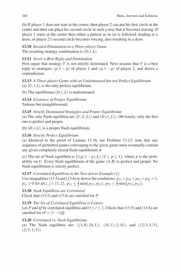
340 Hints, Answers and Solutions
(b) If player 1 does not start at the center, then player 2 can put his first circle at thecenter and then can place his second circle in such a way that it becomes forcing. Ifplayer 1 starts at the center then either a pattern as in (a) is followed, leading to adraw, or player 2’s second circle becomes forcing, also resulting in a draw.
13.10 Iterated Elimination in a Three-player GameThe resulting strategy combination is (D, l,L).
13.11 Never a Best Reply and DominationFirst argue that strategy Y is not strictly dominated. Next assume that Y is a bestreply to strategies (p,1− p) of player 1 and (q,1− q) of player 2, and derive acontradiction.
13.13 A Three-player Game with an Undominated but not Perfect Equilibrium(a) (U, l,L) is the only perfect equilibrium.
(b) The equilibrium (D, l,L) is undominated.
13.14 Existence of Proper EquilibriumTedious but straightforward.
13.15 Strictly Dominated Strategies and Proper Equilibrium(a) The only Nash equilibria are (U, l(,L)) and (D,r(,L)). Obviously, only the firstone is perfect and proper.
(b) (D,r,L), is a proper Nash equilibrium.
13.16 Strictly Perfect Equilibrium(a) Identical to the proof of Lemma 13.16, see Problem 13.12: note that anysequence of perturbed games converging to the given game must eventually containany given completely mixed Nash equilibrium σ .
(c) The set of Nash equilibria is {((p,1− p),L) | 0 ≤ p ≤ 1}, where p is the prob-ability on U . Every Nash equilibrium of the game (A,B) is perfect and proper. NoNash equilibrium is strictly perfect.
13.17 Correlated Equilibria in the Two-driver Example (1)Use inequalities (13.5) and (13.6) to derive the conditions: p11+ p12 + p21+ p22 = 1,pi j ≥ 0 for all i, j ∈ {1,2}, p11 ≤ 3
5 min{p12, p21}, p22 ≤ 53 min{p12, p21}.
13.18 Nash Equilibria are CorrelatedCheck that (13.5) and (13.6) are satisfied for P.
13.19 The Set of Correlated Equilibria is ConvexLet P and Q be correlated equilibria and 0 ≤ t ≤ 1. Check that (13.5) and (13.6) aresatisfied for tP+(1− t)Q.
13.20 Correlated vs. Nash Equilibrium(a) The Nash equilibria are: ((1,0),(0,1)), ((0,1),(1,0)), and ((2/3,1/3),(2/3,1/3)).
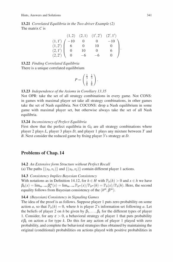
Hints, Answers and Solutions 341
13.21 Correlated Equilibria in the Two-driver Example (2)The matrix C is
⎛⎜⎜⎝(1,2) (2,1) (1′,2′) (2′,1′)
(1,1′) −10 0 0 −10(1,2′) 6 0 10 0(2,1′) 0 10 0 6(2,2′) 0 −6 −6 0
⎞⎟⎟⎠.
13.22 Finding Correlated EquilibriaThere is a unique correlated equilibrium
P =
(13
13
16
16
).
13.23 Independence of the Axioms in Corollary 13.35Not OPR: take the set of all strategy combinations in every game. Not CONS:in games with maximal player set take all strategy combinations, in other gamestake the set of Nash equilibria. Not COCONS: drop a Nash equilibrium in somegame with maximal player set, but otherwise always take the set of all Nashequilibria.
13.24 Inconsistency of Perfect EquilibriaFirst show that the perfect equilibria in G0 are all strategy combinations whereplayer 2 plays L, player 3 plays D, and player 1 plays any mixture between T andB. Next consider the reduced game by fixing player 3’s strategy at D.
Problems of Chap. 14
14.2 An Extensive form Structure without Perfect Recall(a) The paths {(x0,x1)} and {(x0,x2)} contain different player 1 actions.
14.3 Consistency Implies Bayesian ConsistencyWith notations as in Definition 14.12, for h ∈ H with Pb(h) > 0 and x ∈ h we haveβh(x) = limm→∞ β m
h (x) = limm→∞ Pbm(x)/Pbm(h) = Pb(x)/Pb(h). Here, the secondequality follows from Bayesian consistency of the (bm,β m).
14.4 (Bayesian) Consistency in Signaling GamesThe idea of the proof is as follows. Suppose player 1 puts zero probability on someaction a, so that Pb(h) = 0, where h is player 2’s information set following a. Letthe beliefs of player 2 on h be given by β1, . . . ,βk for the different types of player1. Consider, for any ε > 0, a behavioral strategy of player 1 that puts probabilityεβk on action a for type k. Do this for any action of player 1 played with zeroprobability, and complete the behavioral strategies thus obtained by maintaining theoriginal (conditional) probabilities on actions played with positive probabilities in

342 Hints, Answers and Solutions
the original assessment. Letting ε go to zero, we have a sequence of completelymixed Bayesian consistent assessments converging to the original assessment.
14.5 Computation of Sequential Equilibrium (1)The unique sequential equilibrium consists of the behavioral strategies where player1 plays B with probability 1 and l with probability 1/2, and player 2 plays L withprobability 1/2; and player 1 believes that x3 and x4 are equally likely.
14.6 Computation of Sequential Equilibrium (2)(b) The Nash equilibria are (L, l), and (R,(α,1−α)) for all α ≤ 1/2, where α isthe probability with which player 2 plays l.
(c) Let π be the belief player 2 attaches to node y1. Then the sequential equilibriaare: (L, l) with belief π = 1; (R,r) with belief π ≤ 1/2; and (R,(α,1−α)) for anyα ≤ 1/2 with belief π = 1/2.
14.7 Computation of Sequential Equilibrium (3)(b) The Nash equilibria are (R,(q,1− q)) with 1/3 ≤ q ≤ 2/3. (The conditions onq keep player 1 from deviating to L or M.)
14.8 Computation of Sequential Equilibrium (4)The Nash equilibria in this game are: (R,(q1,q2,q3)) with q3 ≤ 1/3 and q1 ≤1/2− (3/4)q3, where q1,q2,q3 are the probabilities put on l,m,r, respectively; and((1/4,3/4,0),(1/4,0,3/4) (probabilities on L,M,R and l,m,r, respectively).
Let π be the belief attached by player 2 to y1. Then with π = 1/4 the equilibrium((1/4,3/4,0),(1/4,0,3/4) becomes sequential. The first set of equilibria containsno equilibrium that can be extended to a sequential equilibrium.
14.9 Computation of Sequential Equilibrium (5)The Nash equilibria are: (DB,r); ((R,(s,1− s)),(q,1−q)) with 0 ≤ s ≤ 1 and q ≥1/3, where s is the probability on A and q is the probability on l. The subgameperfect equilibria are: (DB,r); (RA, l); ((R,(3/4,1/4)),(3/5,2/5)). The first onebecomes sequential with β = 0; the second one with β = 1; and the third one withβ = 3/5.
Problems of Chap. 15
15.1 Computing ESS in 2× 2 Games (1)ESS(A) can be computed using Proposition 15.3.(a) ESS(A) = {e2}. (b) ESS(A) = {e1,e2}. (c) ESS(A) = {(2/3,1/3)}.
15.2 Computing ESS in 2× 2 Games (2)Case (1): ESS(A′) = {e2}; case (2): ESS(A′) = {e1,e2}; case (3): ESS(A′) = {x} ={(a2/(a1 + a2),a1/(a1 + a2))}.
15.3 Rock–Paper–Scissors (1)The unique Nash equilibrium is ((1/3,1/3,1/3),(1/3,1/3,1/3)), which is sym-metric. But (1/3,1/3,1/3) is not an ESS.

Hints, Answers and Solutions 343
15.4 Uniform Invasion BarriersCase (1), e2: maximal uniform invasion barrier is 1.Case (2), e1: maximal uniform invasion barrier is a1/(a1 + a2).Case (2), e2: maximal uniform invasion barrier is a2/(a1 + a2).Case (3), x: maximal uniform invasion barrier is 1.
15.5 Replicator Dynamics in Normalized Game (1)Straightforward computation.
15.6 Replicator Dynamics in Normalized Game (2)The replicator dynamics can be written as x = [x(a1 + a2)−a2]x(1− x), where x =x1. So x = 0 and x = 1 are always stationary points. In case I the graph of x on (0,1)is below the horizontal axis. In case II there is another stationary point, namely atx = a2/(a1 +a2); on (0,a2/(a1 +a2)) the function x is negative, on (a2/(a1 +a2),1)it is positive. In case III the situation of case II is reversed: the function x is positiveon (0,a2/(a1 + a2)) and negative on ((a2/(a1 + a2),1).
15.7 Weakly Dominated Strategies and Replicator Dynamics(b) The stationary points are e1, e2, e3, and all points with x3 = 0. Except e3, allstationary points are Lyapunov stable. None of these points is asymptotically stable.Also, e3 is strictly dominated (by e1). (One can also derive d(x1/x2)/dt = x1x3/x2 >0 at completely mixed strategies, i.e., at the interior of ∆3. Hence, the share of sub-population 1 grows faster than that of 2 but this difference goes to zero if x3 goes tozero [e2 is weakly dominated by e1].)
15.8 Stationary Points and Nash Equilibria(a) NE(A) = {(α,α,1−2α) | 0 ≤ α ≤ 1/2}.
(b) By Proposition 15.15 and (a) it follows that {(α,α,1− 2α) | 0 ≤ α ≤ 1/2}∪{e1,e2,e3} ⊆ ST (A), and that possibly other stationary points must be boundarypoints of ∆3. By considering the replicator dynamics it follows that there are noadditional stationary points. All stationary points except e1 and e2 are Lyapunovstable, but no point is asymptotically stable.
15.9 Lyapunov Stable States in 2× 2 GamesCase (1): e1; case (2): e1 and e2; case (3): x (cf. Problem 15.6).
15.10 Nash Equilibrium and Lyapunov StabilityNE(A) = {e1}. If we start at a completely mixed strategy close to e1, then first x3increases, and we can make the solution trajectory pass e3 as closely as desired. Thisshows that e1 is not Lyapunov stable.
15.11 Rock–Paper–Scissors (2)(e) Follows from (d). If a > 0 then any trajectory converges to the maximum pointof x1x2x3, i.e., to (1/3,1/3,1/3). If a = 0 then the trajectories are orbits (x1x2x3constant) around (1/3,1/3,1/3). If a < 0 then the trajectories move outward, awayfrom (1/3,1/3,1/3).

344 Hints, Answers and Solutions
Problems of Chap. 16
16.1 Imputation Set of an Essential GameNote that I(v) is a convex set and fi ∈ I(v) for every i = 1, . . . ,n. Thus, I(v) containsthe convex hull of {fi | i ∈ N}. Now let x ∈ I(v), and write x = (v(1), . . . ,v(n))+(α1, . . . ,αn), where ∑i∈N αi = v(N)−∑i∈N v(i) =: α .
16.2 Convexity of the Domination CoreFirst prove the following claim: For each x ∈ I(v) and /0 = S ⊆ N we have
∃z ∈ I(v) : zdomSx ⇔ x(S) < v(S) and x(S) < v(N)−∑i/∈S
v(i).
Use this claim to show that I(v)\D(S) is a convex set. Finally, conclude that DC(v)must be convex.
16.3 Dominated Sets of Imputations(2) In both games, D(i j) = {x ∈ I(v) | xi + x j < v(i j)}, i, j ∈ {1,2,3}, i = j.
16.7 A Glove Game(b) The core and the domination core are both equal to {(0,1,0)}, cf. Theo-rem 16.11.
16.11 Core and D-coreCondition (16.1) is not a necessary condition for equality of the core and the D-core. To find a counterexample, first note that if C(v) = /0 then (16.1) must hold.Therefore, a counterexample has to be some game with empty core and D-core.
16.12 Strategic EquivalenceStraightforward using the definitions.
16.13 Proof of Theorem 16.19
Write B =(
A−A
). Then
max{b ·y | Ay = c,y ≥ 0} = max{b ·y | By ≤ (c,−c),y ≥ 0}= min{(c,−c) · (x,z) | (x,z)B ≥ b,(x,z) ≥ 0}= min{c · (x− z) | (x− z)A ≥ b,(x,z) ≥ 0}= min{c ·x′ | x′A ≥ b}.
The second equality follows from Theorem 22.5.
16.14 Infeasible Programs in Theorem 16.19Follow the hint.
16.16 Minimum of Balanced GamesFollows by using the definition of balancedness or by Theorem 16.21.

Hints, Answers and Solutions 345
16.17 Balanced Simple GamesLet (N,v) be a simple game.
Suppose i is a veto player. Let B be a balanced collection with balanced map λ .Then
∑S∈B
λ (S)v(S) = ∑S∈B:i∈S
λ (S)v(S)≤ 1 = v(N),
since i is a veto player. Hence, v is balanced.For the converse, suppose v is balanced, and distinguish two cases:
Case 1: There is an i with v({i}) = 1. Show that i is a veto player.Case 2: v({i}) = 0 for every i ∈ N. Show that also in this case v has veto players.
Problems of Chap. 17
17.1 The Games 1T(c) For i ∈ T : Φi(1T ) = (|T |−1)!(n−|T |)!
n! .
17.2 Unanimity Games(a) Suppose ∑T = /0 αT uT = 0, where 0 means the zero-game, for some αT ∈R. Showthat all αT are zero by induction, starting with one-person coalitions.
(b) Let W ∈ 2N , then show
∑T = /0
cT uT (W ) = v(W )+ ∑S: S�W
v(S) ∑T :S⊆T⊆W
(−1)|T |−|S|.
It is sufficient to show that the second term of the last expression is equal to 0, hencethat ∑T :S⊆T⊆W (−1)|T |−|S| = 0.
17.3 Necessity of the Axioms in Theorem 17.4EFF, NP and ADD are straightforward. SYM needs more attention. Let i, j be sym-metric in v. Note that for S ⊆ N with i /∈ S and j ∈ S we have v((S∪ i) \ j) = v(S)by symmetry of i and j, since v((S∪ i)\ j) = v((S\ j)∪ i) and v(S) = v((S\ j)∪ j).Use this to show Φi(v) = Φ j(v) by collecting terms in a clever way.
17.4 Dummy Player Property and AnonymityThat DUM implies NP and the Shapley value satisfies DUM is straightforward. ANimplies SYM: Let i and j be symmetric players, and let the value ψ satisfy AN.Then consider the permutation σ with σ(i) = j, σ( j) = i, and σ(k) = k otherwise.
17.5 Shapley Value, Core, and Imputation SetIn the case of two players the core and the imputation set coincide. If the core is notempty then the Shapley value is in the core, cf. Example 17.2. In general, considerany game with v(1) = 2, v(N) = 3, and v(S) = 0 otherwise. Then the Shapley valueis not even in the imputation set as soon as n ≥ 3.
17.6 Shapley Value as a ProjectionIf a is an additive game then Φ(a) = (a(1),a(2), . . . ,a(n)). For a general game v letav be the additive game generated by Φ(v). Then Φ(av) = (av(1), . . . ,av(n)) = Φ(v).

346 Hints, Answers and Solutions
17.7 Shapley Value of Dual GameFollow the hint, or give a direct proof by using (17.4).
17.8 Multilinear Extension(3) Let g be another multilinear extension of v to [0,1]n, say g(x) = ∑T⊆N bT(∏i∈T xi). Show bT = cT for all T by induction, starting with one-player coalitions.
17.9 The Beta-integral FormulaApply partial integration.
17.10 Path Independence of ΦUse Theorem 17.12(3).
17.11 An Alternative Characterization of the Shapley ValueThe Shapley value satisfies all these conditions. Conversely, (2)–(4) imply standard-ness for two-person games, so the result follows from Theorem 17.18.
Problems of Chap. 18
18.1 Marginal Vectors and Dividends(2) For each i ∈ N, mπ
i = ∑T⊆Pπ (i)∪i, i∈T ∆v(T ).
18.2 Convexity and Marginal VectorsUse Theorems 18.3 and 18.6.
18.3 Strictly Convex GamesLet π and σ be two different permutations and suppose that k ≥ 1 is the minimalnumber such that π(k) = σ(k). Then show that mπ
π(k)(v) < mσπ(k)(v). Hence, mπ =
mσ .
18.4 Sharing Profits(a) For the landlord: Φ0(v) = 1
n+1 [∑ns=0 f (s)].
(c) Extend f to a piecewise linear function on [0,n]. Then v is convex if and only iff is convex.
18.5 Sharing Costs(a) For every nonempty coalition S, v(S) = ∑i∈S ci −max{ci | i ∈ S}. If we regardc = (c1, . . . ,c2) as an additive game we can write v = c− cmax, where cmax(S) =max{ci | i ∈ S}.
18.6 Independence of the Axioms in Theorem 18.8(1) Consider the value which, for every game v, gives each dummy player his indi-vidual worth and distributes the rest, v(N)− ∑i∈D v(i) where D is the subset ofdummy players, evenly among the players. This value satisfies all axioms exceptLIN.
(2) Consider the value which, for every game v, distributes v(N) evenly among allplayers. This value satisfies all axioms except DUM.

Hints, Answers and Solutions 347
(3) The value which gives each player his individual worth satisfies all axiomsexcept EFF.
(4) Consider any set of weights {απ | π ∈ Π(N)} with απ ∈ R for all π and∑π∈Π(N) απ = 1. The value ∑π∈Π(N) απ mπ satisfies LIN, DUM and EFF, but notMON unless all weights are nonnegative.
18.7 Null-player in Theorem 18.8Check that the dummy axiom in the proof of this theorem is only used for unanimitygames. In those games, dummy players are also null-players, so it is sufficient torequire NP. Alternatively, one can show that DUM is implied by ADD (and, thus,LIN), EFF and NP.
18.8 Equation (18.4)When considering the sum ∑π∈Π(N) p(π) we may leave out any π with p(π) = 0.This means in particular that in what follows all expressions A(·; ·) are positive. Now
∑π∈Π(N)
p(π) = ∑i1∈N
∑i2∈N\i1
· · · ∑in−1∈N\i1···in−2
pi1/0 A(i2;{i1})×A(i3;{i1, i2})
×·· ·×A(in−1;{i1, . . . , in−2})×A(in;{i1, . . . , in−1})= ∑
i1∈N∑
i2∈N\i1
· · · ∑in−2∈N\i1···in−3
pi1/0 A(i2;{i1})×A(i3;{i1, i2})
×·· ·×A(in−2;{i1, . . . , in−3})
×(
p�N\i1···in−2
p�N\i1···in−2
+ pkN\i1···in−2
+pk
N\i1···in−2
p�N\i1···in−2
+ pkN\i1···in−2
)= ∑
i1∈N∑
i2∈N\i1
· · · ∑in−2∈N\i1···in−3
pi1/0 A(i2;{i1})×A(i3;{i1, i2})
×·· ·×A(in−2;{i1, . . . , in−3})= ∑
i1∈N∑
i2∈N\i1
· · · ∑in−3∈N\i1···in−4
pi1/0 A(i2;{i1})×A(i3;{i1, i2})
×·· ·×A(in−3;{i1, . . . , in−4})= · · ·= ∑
i1∈Npi1
/0 ,
where after the first equality sign, in ∈ N \ {i1, . . . , in−1}, and A(in; {i1, . . . , in−1})= 1 by definition; after the second equality sign �,k ∈ N \ {i1, . . . , in−2} with � = k;the third equality sign follows since the sum involving � and k is equal to 1; theremaining equality signs follow from repetition of this argument.
18.9 Equation (18.6)Let |T | = t. By using a similar argument as for the proof of (18.4) in the solution toProblem 18.8, we can write

348 Hints, Answers and Solutions
∑π :T=Pπ (i)
p(π) = ∑i1∈T
∑i2∈T\i1
· · · ∑it∈T\i1i2···it−1
pi1/0 A(i2;{i1}) · · ·A(it ;T \ {it})
×A(i;T ).
Hence,
∑π :T=Pπ (i)
p(π) =pi
T
∑ j∈N\T p jT
× ∑it∈T
pitT\it
∑ j∈(N\T )∪it p jT\it
× ∑it−1∈T\it
pit−1T\it it−1
∑ j∈(N\T )∪it it−1 p jT\it it−1
×·· ·× ∑i1∈T\it ···i2
pi1/0
=pi
T
∑ j∈T p jT\ j
× ∑it∈T
pitT\it
∑ j∈T\it p j(T\it)\ j
× ∑it−1∈T\it
pit−1T\it it−1
∑ j∈T\it it−1 p j(T\it it−1)\ j
×·· ·× ∑i1∈T\it ···i2
pi1/0
= piT .
Here, the first equality sign follows from rearranging terms and substituting theexpressions for A(·; ·); the second equality sign follows from Lemma 18.12; thefinal equality sign follows from reading the preceding expression from right to left,noting that the remaining sum in each enumerator cancels against the precedingdenominator.
18.10 Characterization of Weighted Shapley ValuesCheck that every weighted Shapley value satisfies the Partnership axiom. Con-versely, let ψ be a value satisfying the Partnership axiom and the four other axioms.Let S1 := {i ∈ N | ψi(uN) > 0} and for every i ∈ S1 let ωi := ψi(uN). Define, recur-sively, Sk := {i ∈ N \ (S1∪·· ·∪Sk−1) | ψi(uN\(S1∪···∪Sk−1)) > 0} and for every i ∈ Sk
let ωi := ψi(uN\(S1∪···∪Sk−1)). This results in a partition (S1, . . . ,Sm) of N. Now definethe weight system w by the partition (S1, . . . ,Sm) with S1 := Sm, S2 := Sm−1, . . .,Sm := S1, and the weights ω . Then it is sufficient to prove that for each coalitionS and each player i ∈ S we have ψi(uS) = Φw
i (uS). Let h := max{ j | S∩ S j = /0},then with T = N \ (Sh+1 ∪ ·· · ∪ Sm) we have by the Partnership axiom: ψi(uS) =
1ψ(uT )(S)ψi(uT ). If i /∈ Sh then ψi(uT ) = 0, hence ψi(uS) = 0 = Φw
i (uS). If i ∈ Sh thenψi(uS) = ωi
∑ j∈S∩Shω j
= Φwi (uS).

Hints, Answers and Solutions 349
18.11 Core and Weighted Shapley Values in Example 18.2First write the game as a sum of unanimity games:
v = u{1,2}+ u{1,3}−u{2,3}+ 2uN.
Then consider all possible ordered partitions of N, there are 13 different ones,and associated weight vectors. This results in a description of all payoff vectorsassociated with weighted Shapley values, including those in the core of the game.
Problems of Chap. 19
19.1 Binary RelationsNot (4): � on R defined by x � y ⇔ x2 ≥ y2.Not (3): ≥ on R2.Not (2): � on R defined by: for all x,y, x ≥ y, let x � y if x− y ≥ 1, and let y � x ifx− y < 1.Not (1): > on R.The ordering on R, defined by [x � y] ⇔ [x = y or 0 ≤ x,y ≤ 1] is reflexive andtransitive but not complete and not anti-symmetric.
19.2 Linear OrdersIf x � y then by definition x � y and not y � x: hence x = y since otherwise y � xby reflexivity.If x � y and x = y then not y � x since otherwise x = y by anti-symmetry. Hencex � y.
19.3 The Lexicographic Order (1)Check (1)–(4) in Sect. 19.2 for �lex. Straightforward.
19.4 The Lexicographic Order (2)This is the set {(x1,x2) ∈ R2 | [x1 = 3, x2 ≥ 1] or [x1 > 3]}. This set is not closed.
19.5 Representability of Lexicographic Order (1)Consider Problem 19.4. Since (α,0) �lex (3,1) for all α > 3, we have u(α,0) ≥u(3,1) for all α > 3 and hence, by continuity of u, limα↓3 u(α,0) ≥ u(3,1).Therefore (3,0) �lex (3,1), a contradiction.
19.6 Representability of Lexicographic Order (2)Suppose that u represents �lex on R2, that is, x �lex y if and only if u(x) ≥ u(y)for all x,y ∈ R2. Then for any t ∈ R let q(t) be a rational number in the interval[u(t,0),u(t,1)]. Since (t,α) �lex (s,β ) and hence u(t,α) > u(s,β ) for all t > s andall α,β ∈ [0,1], we have [u(t,0),u(t,1)]∩ [u(s,0),u(s,1)] = /0 for all t = s. Hence,q(t) = q(s) for all t = s. Therefore, we have found uncountably many differentrational numbers, a contradiction.
19.7 Single-valuedness of the Pre-nucleolusConsider the pre-nucleolus on a suitable compact convex subset and apply Theo-rem 19.4.

350 Hints, Answers and Solutions
19.8 (Pre-)nucleolus and CoreUse the fact that core elements have all excesses non-positive.
19.9 Kohlberg Criterion for the NucleolusFirst observe that the following modification of Theorem 19.5 holds:
Theorem 19.5′ Let (N,v) be a game and x ∈ I(N,v). Then the following twostatements are equivalent:
(1) x = ν(N,v).
(2) For every α such that D(α,x,v) = /0 and for every side-payment y with y(S)≥ 0for every S ∈ D(α,x,v) and with yi ≥ 0 for all i ∈ N with xi = v(i) we havey(S) = 0 for every S ∈ D(α,x,v).
The proof of this theorem is almost identical to the proof of Theorem 19.5. In thesecond sentence of the proof, note that zε ∈ I(N,v) for ε small enough. In the secondpart of the proof, (2) ⇒ (1), note that yi = zi − xi ≥ 0 whenever xi = v(i).
For the ‘if’-part of the statement in this problem, let x ∈ I(N,v), D(α,x,v) = /0,and E (α,x,v) such that D(α,x,v)∪E (α,x,v) is balanced. Consider a side-paymenty with y(S)≥ 0 for every S ∈ D(α,x,v) and yi ≥ 0 for every i with xi = v(i) (hencein particular for every i with {i} ∈ E (α,x,v)). The argument in the first part of theproof of Theorem 19.6 now applies to D(α,x,v)∪E (α,x,v), and Theorem 19.5′implies x = ν(N,v).
For the ‘only-if’ part, consider the program (19.4) in the second part of the proofof Theorem 19.6 but add the constraints −yi ≤ 0 for every i ∈ N with xi = v(i).Theorem 19.5′ implies that the dual of this program is feasible, that is, there areλ (S) ≥ 0, S ∈ D(α,x,v), λ ({i}) ≥ 0, i such that xi = v(i), and λ (N) ∈ R suchthat
− ∑i∈N: xi=v(i)
λ ({i})e{i} − ∑S∈D(α ,x,v)
λ (S)eS + λ (N)eN = ∑S∈D(α ,x,v)
eS.
Hence λ (N)eN = ∑S∈D(α ,x,v)(1 + λ (S))eS + ∑i∈N: xi=v(i) λ ({i})e{i}. Let E (α,x,v)consist of those one-person coalitions {i} with xi = v(i) and λ ({i}) > 0, thenD(α,x,v)∪E (α,x,v) is balanced.
19.10 Proof of Theorem 19.6To formulate the dual program, use for instance the formulation in Theorem 16.19.For instance, the primal (19.4) can be converted to the minimization problemin Theorem 16.19; then the dual corresponds to the maximization problem inTheorem 16.19. Feasibility of the dual follows from Problem 16.14.
19.11 Nucleolus of a Three-person Game (1)The nucleolus is (5,4,3).
19.12 Nucleolus of a Three-person Game (2)The (pre-)nucleolus is (5,3,2).

Hints, Answers and Solutions 351
19.14 Individual Rationality Restrictions for the NucleolusThe nucleolus is (1,0,0). The pre-nucleolus is (5/3,−1/3,−1/3).
19.15 Example 19.8The set B1 = {123,124,34} is balanced with weights all equal to 1/2. The setB1 ∪B2 = {123,124,34,134,234} is balanced with weights, respectively, equal to5/12, 5/12, 3/12, 2/12, 2/12.
19.16 (Pre-)nucleolus of a Symmetric Game(a) ν(v) = ν∗(v) = (v(N)/n)eN .
(b) The maximal excess is reached by all coalitions S for which f (|S|)−(|S|/n) f (n)is maximal.
19.17 COV and AN of the Pre-nucleolusCovariance of the pre-nucleolus follows since applying a transformation as inthe definition of this property changes all excesses (only) by the same positive(multiplicative) factor.
Anonymity of the pre-nucleolus follows since a permutation of the players doesnot change the ordered vectors θ (x), but only permutes the coalitions to which theexcesses correspond.
19.18 Apex GameThe (pre-)nucleolus is (3/7,1/7,1/7,1/7,1/7). This can easily be verified usingthe Kohlberg criterion.
19.19 Landlord Game(a) By anonymity, each worker is assigned 1
2 [ f (n)− f (n− 1)]. By computing theexcesses, it follows that among all coalitions containing the landlord, with thispayoff vector the maximal excesses are reached by the coalitions containing n− 1workers, and further also by the coalitions consisting of a single worker and not thelandlord. By the Kohlberg criterion this immediately implies that the given vector isthe (pre-)nucleolus. For the Shapley value, see Problem 18.4.
(b) Compute the excesses for the payoff vector f (n)n+1 e{0,1,...,n}, and apply the Kohlberg
criterion.
19.20 Game in Sect. 19.1The first linear program is: minimize α subject to the constraints xi + α ≥ 4 fori = 1,2,3, x1 + x2 + α ≥ 8, x1 + x3 + α ≥ 12, x2 + x3 + α ≥ 16, x1 + x2 + x3 = 24.The program has optimal value α = −2, reached for x1 = 6 and x2,x3 ≥ 6.
In the second program x1 has been eliminated. This program reduces to: mini-mize α subject to x2 + α ≥ 4, x2 ≤ 12 + α , x2 + x3 = 18. This has optimal valueα = −4, reached for x2 = 8, x3 = 10.
19.21 The PrekernelFor i, j ∈ N denote by Ti j those coalitions that contain player i and not player j.For a payoff vector x denote by si j(x,v) the maximum of e(S,x,v) over all S ∈Ti j.

352 Hints, Answers and Solutions
Let now x be the pre-nucleolus and suppose, contrary to what has to be proved,that there are two distinct players k, � such that sk�(x,v) > s�k(x,v). Let δ =(sk�(x,v)− s�k(x,v))/2 and define y by yk = xk + δ , y� = x� − δ , and yi = xi forall i = k, �. Denote S = {S ∈ 2N \Tk� | e(S,x,v) ≥ skl(x,v)} and s = |S|. Thenθs+1(x) = sk�(x,v). For S ∈ 2N \ (Tk� ∪T�k), we have e(S,x,v) = e(S,y,v). ForS ∈ Tk� we have e(S,y,v) = e(S,x,v)− δ . Finally, for S ∈ T�k we have
e(S,y,v) = e(S,x,v)+ δ ≤ s�k(x,v)+ δ = sk�(x,v)− δ .
Thus, θt(y) = θt(x) for all t ≤ s and θs+1(y) < sk�(x,v) = θs+1(x). Hence θ (x)�lexθ (y), a contradiction.
Problems of Chap. 20
20.2 Example 20.3Argue that a12 = a13 = 3 if v were an assignment game. Use this to derive acontradiction.
20.3 Subgames of Permutation GamesThat a subgame of a permutation game is again a permutation game follows imme-diately from the definition: in (20.3) the worth v(S) depends only on the numbers ki jfor i, j ∈ S. By a similar argument (consider (20.1)) this also holds for assignmentgames.
20.4 A Flow Game(3) (1,1,0,0), corresponding to the minimum cut through e1 and e2; {(0,0,1 +α,1−α) | 0 ≤ α ≤ 1}, corresponding to the minimum cut through e3 and e4.
20.5 Every Nonnegative Balanced Game is a Flow GameLet v be a nonnegative balanced game, and write (following the hint to the problem)v = ∑k
r=1 αrwr, where αr > 0 and wr a balanced simple game for each r = 1, . . . ,k.Consider the controlled capacitated network with two vertices, the source and thesink, and k edges connecting them, where each edge er has capacity αr and iscontrolled by wr. Then show that the associated flow game is v.
20.6 On Theorem 20.6 (1)(1) This follows straightforwardly from the proof of Theorem 20.6.
(2) E.g., each player receiving 5 14 is a core element.
20.7 On Theorem 20.6 (2)In any core element, player should 1 receive at least 1 and player 2 also, but v(N) =1. Hence the game has an empty core.
20.8 Totally Balanced Flow GamesThis follows immediately from Theorem 20.6, since every dictatorial game isbalanced, i.e., has veto players.

Hints, Answers and Solutions 353
20.9 If-part of Theorem 20.9
We show that the Banzhaf value satisfies 2-EFF (the other properties are obvious).With notations as in the formulation of 2-EFF, we have
ψp(vp) = ∑S⊆(N\p)∪{p}: p/∈S
12|N|−2 [vp(S∪{p})− vp(S)]
= ∑S⊆N\{i, j}
12|N|−2 [v(S∪{i j})− v(S)]
= ∑S⊆N\{i, j}
12|N|−1 [2v(S∪{i j})−2v(S)].
The term in brackets can be written as
[v(S∪{i, j})− v(S∪{i})+ v(S∪{ j})− v(S)]+ [v(S∪{i, j})− v(S∪{ j})+ v(S∪{i})− v(S)],
hence ψp(vp) = ψ j(v)+ ψi(v).Show that DUM cannot be weakened to NP by finding a different value satisfying
2-EFF, SYM, NP, and SMON.
Problems of Chap. 21
21.1 Anonymity and SymmetryAn example of a symmetric but not anonymous solution is as follows. To symmetricproblems, assign the point in W (S) with equal coordinates; otherwise, assign thepoint of S that is lexicographically (first player 1, then player 2) maximal.
21.3 The Nash Solution is Well-definedThe function x �→ (x1−d1)(x2−d2) is continuous on the compact set {x∈ S | x≥ d}and hence attains a maximum on this set. We have to show that this maximumis attained at a unique point. In general, consider two points z,z′ ∈ {x ∈ S | x ≥ d}with (z1−d1)(z2−d2) = (z′1−d1)(z′2−d2) = α . Then one can show that at the pointw = 1
2 (z+ z′) ∈ S one has (w1 −d1)(w2 −d2) > α . This implies that the maximumis attained at a unique point.
21.4 (1) ⇒ (2) in Theorem 21.1WPO and IIA are straightforward by definition, and SC follows from an easy com-putation. For SYM, note that if N(S,d) = z for a symmetric problem (S,d), thenalso (z2,z1) = N(S,d) by definition of the Nash bargaining solution. Hence, z1 = z2by uniqueness.
21.5 Geometric Characterization of the Nash Bargaining SolutionLet (S,d) ∈ B and N(S,d) = z. The slope of the tangent line � to the graph of thefunction x1 �→ (z1 − d1)(z2 − d2)/(x1 − d1) + d2 (which describes the level set of

354 Hints, Answers and Solutions
x �→ (x1 − d1)(x2 − d2) through z) at z is equal to −(z2 − d2)(z1 − d1), i.e., thenegative of the slope of the straight line through d and z. Clearly, � supports S at z:this can be seen by invoking a separating hyperplane theorem, but also as follows.Suppose there were some point z′ of S on the other side of � than d. Then there is apoint w on the line segment connecting z′ and z (hence, w ∈ S) with (w1 −d1)(w2 −d2) > (z1 − d1)(z2 − d2), contradicting z = N(S,d). The existence of such a pointw follows since otherwise the straight line through z′ and z would also be a tangentline to the level curve of the Nash product at z.
For the converse, suppose that at a point z there is a supporting line of S withslope −(z2 − d2)(z1 − d1). Clearly, this line is tangent to the graph of the functionx1 �→ (z1 −d1)(z2 −d2)/(x1 −d1)+ d2 at z. It follows that z = N(S,d).
21.6 Strong Individual RationalityThe implication (1) ⇒ (2) is straightforward. For (2) ⇒ (1), if F is also weaklyPareto optimal, then F = N by Theorem 21.1. So it is sufficient to show that, ifF is not weakly Pareto optimal then F = D. Suppose that F is not weakly Paretooptimal. Then there is an (S,d) ∈ B with F(S,d) /∈W (S). By IR, F(S,d) ≥ d. Sup-pose F(S,d) = d. By SC, we may assume w.l.o.g. d = (0,0). Let α > 0 be suchthat F(S,(0,0)) ∈ W ((α,α)S). Since F(S,(0,0)) /∈ W (S), α < 1. So (α,α)S ⊆ S.By IIA, F((α,α)S,(0,0)) = F(S,(0,0)), so by SC, F((α,α)S,(0,0)) = (α,α)F(S,(0,0)) = F(S,(0,0)), contradicting α < 1. So F(S,(0,0)) = (0,0). SupposeF(T,(0,0)) = (0,0) for some (T,(0,0)) ∈ B. By SC we may assume (0,0) =F(T,(0,0)) ∈ S. By IIA applied twice, (0,0) = F(S ∩ T,(0,0)) = F(T,(0,0)) =(0,0), a contradiction. Hence, F = D.
21.7 (1) ⇒ (2) in Theorem 21.2Straightforward. Note in particular that in a symmetric game the utopia point is alsosymmetric, and that the utopia point is ‘scale covariant’.
21.8 Restricted Monotonicity(1) Follows from applying IM twice.
(2) For (S,d) with d = (0,0) and u(S,d) = (1,1), let F(S,d) be the lexicographically(first player 1, then player 2) maximal point of S∩R2
+. Otherwise, let F be equal toR. This F satisfies RM but not IM.
21.9 Global Individual MonotonicityIt is straightforward to verify that G satisfies WPO, SYM, SC, and GIM. For the con-verse, suppose that F satisfies these four axioms, let (S,d) ∈ B and z := G(S,d). BySC, w.l.o.g. d = (0,0) and g(S) = (1,1). Let α ≤ 0 such that S ⊆ S where S := {x ∈R2 | (α,α) ≤ x ≤ y for some y ∈ S}. In order to prove F(S,(0,0)) = G(S,(0,0)) itis sufficient to prove that F(S,(0,0)) = G(S,(0,0)) (in view of GIM and WPO).Let T = conv{z,(α,g2(S)),(g1(S),α)} = conv{z,(α,1),(1,α)}. By SYM andWPO, F(T,(0,0)) = z. By GIM, F(S,(0,0)) ≥ F(T,(0,0)) = z = G(S,(0,0)) =G(S,(0,0)), so by WPO: F(S,(0,0)) = G(S,(0,0)). (Make pictures. Note that thisproof is analogous to the proof of Theorem 21.2.)

Hints, Answers and Solutions 355
21.10 Monotonicity and (weak) Pareto Optimality(1) Consider problems of the kind (conv{d,a},d) for some a > d.
(2) The egalitarian solution E satisfies MON and WPO on B0.
21.11 The Egalitarian Solution (1)Straightforward.
21.12 The Egalitarian Solution (2)Let z := E(S,d)+ E(T,e). Then it is straightforward to derive that z1 − (d1 + e1) =z2−(d2 +e2). Since E(S+T,d +e) is the maximal point x such that x1−(d1 +e1) =x2 − (d2 + e2), it follows that E(S + T,d + E)≥ z.
21.13 Independence of AxiomsTheorem 21.1:
WPO, SYM, SC: F = R; WPO, SYM, IIA: F = L, where L(S,d) is the point ofP(S) nearest to the point z ≥ d with z1 −d1 = z2 −d2 measured along the boundaryof S; WPO, SC, IIA: F = D1, where D1(S,d) is the point of {x ∈ P(S) | x ≥ d} withmaximal first coordinate; SYM, SC, IIA: F = D (disagreement solution).Theorem 21.2:
WPO, SYM, SC: F = N; WPO, SYM, IM: F = L; WPO, SC, IM: if d = (0,0) andu(S,d) = (1,1), let F assign the point of intersection of W (S) and the line segmentconnecting (1/4,3/4) and (1,1) and, otherwise, let F be determined by SC; SYM,SC, IM: F = D.Theorem 21.2:
WPO, MON, SYM: F(S,d) is the maximal point of S on the straight line throughd with slope 1/3 if d = (1,0), F(S,d) = E(S,d) otherwise; WPO, MON, TC:F(S,d) is the maximal point of S on the straight line through d with slope 1/3;WPO, SYM, TC: F = N; MON, SYM, TC: F = D.
21.14 Nash and Rubinstein(b) The Nash bargaining solution outcome is ( 1
3
√3, 2
3), hence ( 13
√3,1− 1
3
√3) is
the resulting distribution of the good.
(c) The Rubinstein bargaining outcome is(√
1−δ1−δ 3 , δ−δ 3
1−δ 3
).
(d) The outcome in (c) converges to the outcome in (b) if δ converges to 1.
Problems of Chap. 22
22.1 Convex SetsThe only-if part is obvious. For the if-part, for any two vectors x and y in Z thecondition implies that k
2m x + 2m−k2m y ∈ Z for every m ∈ N and k ∈ {0,1, . . . ,2m}. By
closedness of Z, this implies that conv{x,y} ⊆ Z, hence Z is convex.

356 Hints, Answers and Solutions
22.2 Proof of Lemma 22.3Suppose that both systems have a solution, say (y,z) ≥ 0, (y,z) = 0, Ay + z = 0,x > 0, xA > 0. Then xAy+x ·z = x(Ay+z) = 0, hence y = 0 and z = 0 since x > 0,xA > 0. This contradicts (y,z) = 0.
22.3 Proof of Lemma 22.4Suppose that both systems have a solution, say x > 0, xA = b, Ay ≥ 0, b · y < 0.Then xAy < 0, contradicting x > 0 and Ay ≥ 0.
22.4 Proof of Lemma 22.6(a) If x ≥ 0, xA ≤ b, y ≥ 0 and b ·y < 0 then xAy ≤ b ·y < 0, so Ay ≥ 0. This showsthat at most one of the two systems has a solution.(b) Suppose the system in (1) has no solution. Then also the system xA + zI = b,
x ≥ 0, z ≥ 0 has no solution. Hence, by Farkas’ Lemma the system(
AI
)y ≥ 0,
b ·y < 0 has a solution. Therefore, the system in (2) has a solution.
22.5 Extreme PointsThe implication (2) ⇒ (1) follows by definition of an extreme point.
For the implication (1) ⇒ (3), let x,y ∈C \{e} and 0 < λ < 1. Let z = λ x+(1−λ )y. If z = e then z ∈C \{e} by convexity of C. Suppose now that z = e. W.l.o.g. letλ ≥ 1/2. Then e = λ x+(1−λ )y = (1/2)x+(1/2)[µx+(1−µ)y] for µ = 2λ −1.Since µx+(1−µ)y∈C, this implies that e is not an extreme point of C. This provesthe implication (1) ⇒ (3).
For the implication (3) ⇒ (2), let x,y ∈C, x = y, and 0 < α < 1. If x = e or y = ethen clearly αx +(1−α)y = e. If x = e and y = e then αx +(1−α)y ∈C \ {e} byconvexity of C \ {e}, hence αx +(1−α)y = e as well.
22.6 Affine SubspacesLet A = a+L be an affine subspace, x,y∈A, and λ ∈R. Write x = a+ x and y = a+ yfor x, y ∈ L, then λ x+(1−λ )y = a+λ x+(1−λ )y∈ A since λ x+(1−λ )y∈ L (Lis a linear subspace).
Conversely, suppose that A contains the straight line through any two of its ele-ments. Let a be an arbitrary element of A and let L := {x−a | x ∈ A}. Then it followsstraightforwardly that L is a linear subspace of V , and thus A = a + L is an affinesubspace.
22.7 The Set of Sup-points of a Linear Function on a Convex SetIn general, linearity of f implies that, if f (x) = f (y), then f (λ x + (1 − λ )y) =f (x) = f (y) for any two points of C and 0 < λ < 1. It follows, in particular, that theset D is convex.
Let e ∈ ext(D) and suppose e = (1/2)x + (1/2)y for some x,y ∈ C. Then bylinearity of f , f (e) = (1/2) f (x)+ (1/2) f (y), hence x,y ∈ D since e ∈ D. So e =x = y since e is an extreme point of D. Thus, e is also an extreme point of C.

References
1. Akerlof G (1970) The market for lemons: quality uncertainty and the market mechanism.Quarterly Journal of Economics 84:488–500
2. Arrow KJ (1963) Social choice and individual values, 2nd edition. Wiley, New York3. Arrow KJ, Sen AK, Suzumura K, eds (2002) Handbook of social choice and welfare,
volume 1. North-Holland, Amsterdam4. Arrow KJ, Sen AK, Suzumura K, eds (2007) Handbook of social choice and welfare,
volume 2. North-Holland, Amsterdam (forthcoming)5. Aumann RJ (1974) Subjectivity and correlation in randomized strategies. Journal of Mathe-
matical Economics 1:67–966. Aumann RJ, Hart S, eds (1992, 1994, 2002) Handbook of game theory with economic
aplications, volumes 1–3. North-Holland, Amsterdam7. Aumann RJ, Maschler M (1985) Game theoretic analysis of a bankruptcy problem from the
Talmud. Journal of Economic Theory 36:195–2138. Axelrod R (1984) The evolution of cooperation. Basic Books, New York9. Benoit J-P, Krishna V (1985) Finitely repeatd games. Econometrica 53:905–922
10. Bernheim (1984) Rationalizable strategic behavior. Econometrica 52:1007–102811. Bertrand J (1883) Review of Walras’s ‘Theorie mathematique de la richesse sociale’ and
Cournot’s ‘Recherches sur les principes mathematiques de la theorie des richesses’. Journaldes Savants 499–508, translated by M. Chevaillier and reprinted in [74], 646–653
12. Black D (1969) Lewis Carroll and the theory of games. American Economic Review,Proceedings 59:206–210
13. Binmore K, Rubinstein A, Wolinsky A (1986) The Nash bargaining solution in economicmodelling. Rand Journal of Economics 17:176–188
14. Bird CG (1976) On cost allocation for a spanning tree: a game theoretic approach. Networks6:335–350
15. Bomze I (1986) Non-cooperative two-person games in biology: a classification. InternationalJournal of Game Theory 15:31–57
16. Bondareva ON (1962) Theory of the core in the n-person game. Vestnik LeningradskiiUniversitet 13:141–142 (in Russian)
17. Brams SJ (1980) Biblical games: a strategic analysis of stories in the Old Testament. MIT,Cambridge, MA
18. Brouwer LEJ (1912) Uber Abbildung von Mannigfaltigkeiten. Mathematische Annalen71:97–115
19. Cho IK, Kreps DM (1987) Signalling games and stable equilibria. Quarterly Journal ofEconomics 102:179–221
20. Churchill W (1983) Second world war. Houghton Mifflin, Boston21. Cournot A (1838) Recherches sur les principes mathematiques de la theorie des richesses.
English translation (1897) Researches into the mathematical principles of the theory ofwealth. Macmillan, New York
357

358 References
22. Curiel I (1997) Cooperative game theory and applications: cooperative games arising fromcombinatorial optimization problems. Kluwer, Boston
23. Curiel I, Derks J, Tijs SH (1986) On balanced games and games with committee control.Operations Research Spektrum 11:83–88
24. Davis M, Maschler M (1965) The kernel of a cooperative game. Naval Research LogisticsQuarterly 12:223–259
25. de Borda JC (1781) Memoires sur les elections au scrutin. Histoire de l’Academie Royaledes Sciences, Paris
26. de Clippel G, Peters H, Zank H (2004) Axiomatizing the Harsanyi solution, the symmet-ric egalitarian solution, and the consistent solution for NTU-games. International Journal ofGame Theory 33:145–158
27. de Condorcet M (1785) Essai sur l’application de l’analyse a la probabilite des decisionsrendues a la pluralite des voix. Imprimerie Royale, Paris
28. Derks J (1987) Decomposition of games with non-empty core into veto-controlled simplegames. Operations Research Spektrum 9:81–85
29. Derks J (1992) A short proof of the inclusion of the core in the Weber Set. InternationalJournal of Game Theory 21:149–150
30. Derks J, Haller H, Peters H (2000) The Selectope for cooperative games. InternationalJournal of Game Theory 29:23–38
31. Dimand MA, Dimand RW (1996) The history of game theory, volume 1: from the beginningsto 1945. Routledge, London
32. Dodgson CL (1884) The principles of parliamentary representation. Harrison, London33. Dresher M, Tucker AW, Wolfe P, eds (1957) Contributions to the theory of games III (Annals
of Mathematics Studies 39). Princeton University Press, Princeton, NJ34. Dresher M, Shapley LS, Tucker AW, eds (1964) Advances in game theory (Annals of
Mathematics Studies 52). Princeton University Press, Princeton, NJ35. Feyerabend PK (1974) Against method. New Left Books, London36. Ford LR, Fulkerson DR (1956) Maximal flow through a network. Canadian Journal of
Mathematics 8:399–40437. Friedman JW (1985) Cooperative equilibria in finite horizon noncooperative supergames.
Journal of Economic Theory 35:390–39838. Fudenberg D, Maskin E (1986) The folk theorem in repeated games with discounting or with
incomplete information. Econometrica 54:533–55639. Fudenberg D, Tirole J (1991) Game theory. MIT, Cambridge, MA40. Fudenberg D, Tirole J (1991) Perfect Bayesian equilibrium and sequential equilibrium.
Journal of Economic Theory 53:236–26041. Gale D, Shapley LS (1962) College admissions and the stability of mariage. American
Mathematical Monthly 69:9–1542. Gardner R (1995) Games for business and economics. Wiley, New York43. Gehrlein WV (2006) Condorcet’s paradox. Springer, Berlin44. Gibbard A (1973) Manipulation of voting schemes: a general result. Econometrica 41:587–
60145. Gibbons R (1992) A primer in game theory. Harvester Wheatsheaf, Hertfordshire46. Gillies DB (1953) Some theorems on n-person games. Ph.D. Thesis, Princeton University
Press, Princeton, NJ47. Hardin G (1968) The tragedy of the commons. Science 162:1243–124848. Harsanyi, JC (1959) A bargaining model for the cooperative n-person game. In:
Contributions to the Theory of Games 4, 324–356. Princeton University Press, Princeton, NJ49. Harsanyi JC (1963) A simplified bargaining model for the n-person cooperative game.
International Economic Review 4:194–22050. Harsanyi JC (1967, 1968) Games with incomplete information played by “Bayesian” players
I, II, and III. Management Science 14:159–182, 14:320–334, 14:486–50251. Harsanyi JC (1973) Games with randomly disturbed payoffs: a new rationale of mixed
strategy equilibrium points. International Journal of Game Theory 2:1–23

References 359
52. Hart S, Mas-Colell A (1989) Potential, value, and consistency. Econometrica 57:589–61453. Hart S, Mas-Collel A (1996) Bargaining and value. Econometrica 64:357–38054. Hildenbrand H, Kirman AP (1976) Introduction to equilibrium analysis. North-Holland,
Amsterdam55. Hirsch M, Smale S (1974) Differential equations, dynamical systems, and linear algebra.
Academic, San Diego56. Hofbauer J, Schuster P, Sigmund K (1979) A note on evolutionary stable strategies and game
dynamics. Journal of Theoretical Biology 81:609–61257. Hofbauer J, Sigmund K (1988) The theory of evolution and dynamical systems. Cambridge
University Press, Cambridge58. Ichiishi T (1981) Super-modularity: applications to convex games and to the greedy
algorithm for LP. Journal of Economic Theory 25:283–28659. Jehle GA, Reny PJ (2001) Advanced microeconomic theory. Addison Wesley, Boston60. Kakutani S (1941) A generalization of Brouwer’s fixed point theorem. Duke Mathematical
Journal 8(3):457–45961. Kalai E, Samet D (1985) Monotonic solutions to general cooperative games. Econometrica
53:307–32762. Kalai E, Samet D (1987) On weighted Shapley values. International Journal of Game Theory
16:205–22263. Kalai E, Smorodinsky M (1975) Other solutions to Nash’s bargaining problem. Econometrica
43:513–51864. Kalai E, Zemel E (1982) Totally balanced games and games of flow. Mathematics of
Operations Research 7:476–47865. Kohlberg E (1971) On the nucleolus of a characteristic function game. SIAM Journal of
Applied Mathematics 20:62–6666. Kreps DM, Wilson RB (1982) Sequential equilibria. Econometrica 50:863–89467. Kuhn HW (1953) Extensive games and the problem of information. In: [69], 193–21668. Kuhn HW, Tucker AW, eds (1950) Contributions to the theory of games I (Annals of
Mathematics Studies 24). Princeton University Press, Princeton, NJ69. Kuhn HW, Tucker AW, eds (1953) Contributions to the theory of games II (Annals of
Mathematics Studies 28). Princeton University Press, Princeton, NJ70. Lemke CE, Howson JT (1964) Equilibrium points of bimatrix games. Journal of the Society
for Industrial and Applied Mathematics 12:413–42371. Littlechild SC, Owen G (1974) A simple expression for the Shapley Value in a special case.
Management Science 20:370–37272. Lucas WF (1969) The proof that a game may not have a solution. Transactions of the
American Mathematical Society 136:219–22973. Luce RD, Tucker AW, eds (1958) Contributions to the theory of games IV (Annals of
Mathematics Studies 40). Princeton University Press, Princeton, NJ74. Magnan de Bornier J (1992) The ‘Cournot–Bertrand debate’: a historical perspective. History
of Political Economy 24:623–65675. Mailath GJ, Samuelson L (2006) Repeated games and reputations. Oxford University Press,
New York76. Mangasarian OL, Stone H (1964) Two-person nonzero-sum games and quadratic program-
ming. Journal of Mathematical Analysis and Applications 9:348–35577. Maynard Smith J, Price GR (1973) The logic of animal conflict. Nature 246:15–1878. Milgrom P (2004) Putting auction theory to work. Cambridge University Press, Cambridge79. Monderer D, Samet D, Shapley LS (1992) Weighted values and the core. International
Journal of Game Theory 21:27–3980. Montgomery J (1991) Equilibrium wage dispersion and interindustry wage differentials.
Quarterly Journal of Economics 106:163–19781. Morris P (1994) Introduction to game theory. Springer, New York82. Moulin H (1988) Axioms of cooperative decision making. Cambridge University Press,
Cambridge

360 References
83. Moulin H (1995) Cooperative microeconomics: a game-theoretic introduction. PrenticeHall/Harvester Wheatsheaf, Hemel Hempstead
84. Muller E, Satterthwaite MA (1977) The equivalence of strong positive association andstrategy-proofness. Journal of Economic Theory 14:412–418
85. Muthoo A (1999) Bargaining theory with applications. Cambridge University Press,Cambridge
86. Myers SC, Majluf NS (1984) Corporate financing and investment decisions when firms haveinformation that investors do not have. Journal of Financial Economics 13:187–221
87. Myerson RB (1978) Refinements of the Nash equilibrium concept. International Journal ofGame Theory 7:73–80
88. Myerson RB (1991) Game theory, analysis of conflict. Harvard University Press, Cambridge,MA
89. Nasar S (1998) A beautiful mind. Faber and Faber, London90. Nash JF (1950) The bargaining problem. Econometrica 18:155–16291. Nash JF (1951) Non-cooperative games. Annals of Mathematics 54:286–29592. Nash JF (1953) Two-person cooperative games. Econometrica 21:128–14093. Norde H, Potters J, Reijnierse H, Vermeulen D. (1996) Equilibrium selection and consis-
tency. Games and Economic Behavior 12:219–22594. Nowak AS (1997) On an axiomatization of the Banzhaf value without the additivity axiom.
International Journal of Game Theory 26:137–14195. Okada A (1981) On stability of perfect equilibrium points. International Journal of Game
Theory 10:67–7396. Osborne MJ (2004) An introduction to game theory. Oxford University Press, New York97. Owen G (1972) Multilinear extensions of games. Management Science 18:64–7998. Owen G (1995) Game theory, 3rd edition. Academic, San Diego, CA99. Pearce D (1984) Rationalizable strategic behavior and the problem of perfection. Economet-
rica 52:1029–1050100. Peleg B, Sudholter P (2003) Introduction to the theory of cooperative games. Kluwer, Boston101. Peleg B, Tijs S (1996) The consistency principle for games in strategic form. International
Journal of Game Theory 25:13–34102. Perea A (2001) Rationality in extensive form games. Kluwer, Boston103. Peters H (1992) Axiomatic bargaining game theory. Kluwer, Dordrecht104. Peters H (2003) NTU-Games. In: Derigs U (ed), Optimization and Operations Research.
Encyclopedia of Life Support Systems (EOLSS). Eolss, Oxford, http://www.eolss.net105. Raiffa H (1953) Arbitration schemes for generalized two-person games. Annals of Mathe-
matics Studies 28:361–387106. Rasmusen E (1989) Games and information: an introduction to game theory, 2nd edition.
Basil Blackwell, Oxford107. Rawls J (1971) A Theory of Justice. Harvard University Press, Cambridge, MA108. Reny PJ (2001) Arrow’s theorem and the Gibbard–Satterthwaite theorem: a unified approach.
Economics Letters 70:99–105109. Roth AE, ed (1988) The Shapley value, essays in honor of Lloyd S. Shapley. Cambridge
University Press, Cambridge110. Rubinstein A (1982) Perfect equilibrium in a bargaining model. Econometrica 50:97–109111. Samuelson L, Zhang J (1992) Evolutionary stability in asymmetric games. Journal of
Economic Theory 57:363–391112. Satterthwaite MA (1975) Strategy-proofness and Arrow’s conditions: existence and corre-
spondence theorems for voting procedures and social welfare functions. Journal of EconomicTheory 10:187–217
113. Scarf HE (1973) The computation of economic equilibria. Cowles Foundation, Yale Univer-sity Press, New Haven, CT
114. Scarf HE (1976) The core of an n-person game. Econometrica 35:50–69115. Schelling TC (1960) The strategy of conflict. Harvard University Press, Cambridge, MA116. Schmeidler D (1969) The nucleolus of a characteristic function game. SIAM Journal on
Applied Mathematics 17:1163–1170

References 361
117. Selten R (1965) Spieltheoretische Behandlung eines Oligopolmodels mit Nachfragezeit.Zeitschrift fur Gesammte Staatswissenschaft 121:301–324
118. Selten R (1975) Reexamination of the perfectness concept for equilibrium points in extensivegames. International Journal of Game Theory 4:25–55
119. Selten R (1980) A note on evolutionary stable strategies in asymmetric animal conflicts.Journal of Theoretical Biology 84:93–101
120. Selten R (1983) Evolutionary stability in extensive-form two-person games. MathematicalSocial Sciences 5:269–363
121. Shapley LS (1953) A value for n-person games. In: Tucker AW, Kuhn HW (eds), Contribu-tions to the theory of games II. Princeton University Press, Princeton, NJ, 307–317
122. Shapley LS (1967) On balanced sets and cores. Naval Research Logistics Quarterly 14:453–460
123. Shapley LS (1969) Utility comparisons and the theory of games. In: Guilbaud GTh (ed), LaDecision. Paris, CNRS, 251–263
124. Shapley LS (1971) Cores of convex games. International Journal of Game Theory 1:11–26125. Shapley LS, Shubik M (1972) The assignment game I: the core. International Journal of
Game Theory 1:111–130126. Snijders C (1995) Axiomatization of the nucleolus. Mathematics of Operations Research
20:189–196127. Sobolev AI (1975) Characterization of the principle of optimality through functional
equations. Mathematical Methods in the Social Sciences 6:92–151128. Spence AM (1973) Job market signalling. Quarterly Journal of Economics 87:355–374129. Sprumont Y (1991) The division problem with single-peaked preferences: a characterization
of the uniform allocation rule. Econometrica 59:509–520130. Sun Tzu (1988) The art of war. Translated by Thomas Cleary. Shambala, Boston131. Sutton J (1986) Non-cooperative bargaining theory: an introduction. Review of Economic
Studies 53:709–724132. Tan T, Werlang SRC (1988) The Bayesian foundations of solution concepts of games. Journal
of Economic Theory 45:370–391133. Taylor P, Jonker L (1978) Evolutionary stable strategies and game dynamics. Mathematical
Biosciences 40:145–156134. Thomas LC (1986) Games, theory and applications. Ellis Horwood, Chichester135. Thomson W (1994) Cooperative models of bargaining. In: Aumann RJ, Hart S (eds), Hand-
book of game theory with economic applications, volume 2. North-Holland, Amsterdam136. Tijs SH, Parthasarathy T, Potters JAM, Rajendra Prasad V (1984) Permutation games:
another class of totally balanced games. Operations Research Spektrum 6:119–123137. Tirole J (1988) The theory of industrial organization. MIT, Cambridge, MA138. van Damme EC (1991) Stability and perfection of Nash equilibria. Springer, Berlin139. Vickers G, Cannings C (1987) On the definition of an evolutionarily stable strategy. Journal
of Theoretical Biology 132:387–408140. von Neumann J (1928) Zur Theorie der Gesellschaftsspiele. Mathematische Annalen
100:295–320141. von Neumann J, Morgenstern O (1944, 1947) Theory of games and economic behavior.
Princeton University Press, Princeton, NJ142. von Stackelberg HF (1934) Marktform und Gleichgewicht. Julius Springer, Wien143. von Stengel B (2002) Computing equilibria for two-person games. In: Aumann R, Hart S
(eds), Handbook of game theory with economic applications, volume 3. North-Holland,Amsterdam
144. Walker M, Wooders J (2001) Minimax play at Wimbledon. American Economic Review91:1521–1538
145. Watson J (2002) Strategy, an introduction to game theory. Norton, New York146. Weber RJ (1988) Probabilistic values for games. In: [109], 101–119147. Weibull JW (1995) Evolutionary game theory. MIT, Cambridge, MA148. Young HP (1985) Monotonic solutions of cooperative games. International Journal of Game
Theory 14:65–72

362 References
149. Young HP (2004) Strategic learning and its limits. Oxford University Press, Oxford150. Zermelo E (1913) Uber eine Anwendung der Mengenlehre auf die Theorie des Schachspiels.
Proceedings Fifth International Congress of Mathematicians 2:501–504

Index
2-Efficiency, 294
additivity (TU-game), 232Additivity (TU-value), 246airport game, 271Anonymity (bargaining), 306Anonymity (TU-value), 247, 282antisymmetry, 155, 275apex game, 285Arrow’s Impossibility Theorem, 156assignment game, 288asymptotic stability, 221auction, 84
backward induction, 51balanced collection, 238balanced game, 238balanced map, 237balancedness (NTU-game), 305Banzhaf value, 294bargaining problem, 17, 135, 299bargaining solution, 136, 299battle of the sexes, 7, 62, 69Bayesian consistency (of beliefs), 207Bayesian equilibrium, 64, 79beer–quiche game, 71behavioral strategy, 202Bertrand competition, 80, 112Bertrand equilibrium, 81best reply, 34, 76, 172best reply correspondence, 172bimatrix game, 33, 172Birkhoff–von Neumann Theorem,
290, 316Borda score, 154Brouwer Fixed Point Theorem, 315
capacitated network, 291, 318carrier, 173centipede game, 57completeness, 155, 275Condorcet paradox, 161Condorcet winner, 161Consistency (Davis–Maschler), 282Consistency (Hart–Mas-Colell), 256Consistency
(Nash equilibrium), 192consistency (of beliefs), 208Converse Consistency (Nash equilibrium), 192convex (TU-)game, 263convex combination, 311convex cone, 312convex set, 311cooperative game, 13, 125cooperative oligopoly, 151Copeland score, 162core (exchange economy), 142core (house exchange), 147core (matching problem), 145core (NTU-game), 305core (TU-game), 126, 233correlated equilibrium, 188Cournot competition, 8, 76, 112Cournot equilibrium, 77Covariance (TU-value), 283
deferred acceptance procedure, 146dictator game, 235disagreement solution, 306dividend, 248domination (TU-game), 233domination core, 233dual (TU-)game, 259
363

364 Index
Duality Theorem of Linear Programming, 238,314
Dummy player Property (TU-value), 247
Efficiency (TU-value), 126, 245egalitarian solution, 303entry deterrence, 11, 55, 71essential game, 129, 232evolutionary game, 113, 215evolutionary stable strategy, 114, 217excess of a coalition, 129, 275exchange economy, 140extensive form game, 8, 45, 201extensive form structure, 199
Farkas’ Lemma, 313finite game, 171flow game, 291Folk theorem, 108, 111
Gibbard–Satterthwaite Theorem, 159Global Individual Monotonicity (bargaining),
307, 356glove game, 15, 124, 240
hawk–dove game, 116Hotelling problem, 99house exchange, 147
imperfect information, 46, 201imputation, 129, 232incomplete information, 62Independence of Irrelevant Alternatives
(bargaining), 139, 300Independence of Irrelevant Alternatives
(social welfare function), 156Individual Monotonicity, 301Individual Rationality (bargaining), 303Individual Rationality (TU-value), 126information set, 46, 200inner product, 312intuitive criterion, 68iterated dominance, 41, 179, 222
job market signaling, 70
Kakutani Fixed Point Theorem, 172, 215, 316Kohlberg criterion, 131, 277Kramer score, 162Krein–Milman Theorem, 317Kuhn’s Theorem, 204
landlord game, 270, 286lexicographic order, 275
linear order, 275linear programming (matrix games), 166Linearity (TU-value), 265local strict efficiency, 220local superiority, 219Lyapunov stability, 221
marginal vector, 127, 243market for lemons, 98matching pennies, 5, 7matching problem, 145mathematical programming (Nash
Equilibrium), 177matrix game, 4, 23, 41, 165, 178Max-Flow Min-Cut Theorem, 292, 320maximin strategy, 24, 166median voting, 99minimax strategy, 24, 166Minimax Theorem for Matrix Games, 166Monotonicity (bargaining), 302Monotonicity (social choice function), 159Monotonicity (TU-value), 265multilinear extension, 251
Nash bargaining solution, 18, 139, 300Nash equilibrium, 34, 49, 76, 204, 222Nash equilibrium (existence), 172never a best reply, 181nonzero-sum game, 6, 33normalized Banzhaf–Coleman index, 293nucleolus, 129, 275, 277Null-player Property (TU-value), 245
One-Person Rationality (Nash equilibrium),191
optimal strategy, 25, 166
Pareto Efficiency (social welfare function),156
Pareto Optimality (bargaining), 137, 302Pareto optimality (in Cournot competition), 78partial order, 275perfect Bayesian equilibrium, 53, 67, 209perfect equilibrium, 182, 217, 224perfect information, 46, 201perfect recall, 46, 201permutation game, 16, 124, 288player type, 61pooling perfect Bayesian equilibrium, 67potential, 252power index, 293pre-nucleolus, 277prekernel, 286principal–agent game, 97

Index 365
prisoners’ dilemma, 6, 103proper equilibrium, 186, 217
Raiffa–Kalai–Smorodinsky solution, 301random order value, 264rationalizable strategies, 182reaction function, 77reduced game (Davis–Maschler), 282reduced game (Hart–Mas-Colell), 255reflexivity, 155, 275repeated game, 58, 103replicator dynamics, 116, 221Restricted Monotonicity (bargaining), 307, 356revealed preference, 306rock–paper–scissors, 31, 225, 227
saddlepoint, 25, 168Scale Covariance (bargaining), 138, 300separating perfect Bayesian equilibrium, 67sequential bargaining, 88, 139, 304sequential equilibrium, 209sequential rationality, 209Shapley value, 127, 244, 264Shapley–Shubik power index, 293side-payment, 277signaling game, 66simple game, 235, 291social choice function, 155social welfare function, 155stable matching, 146stable set (TU-game), 236Stackelberg competition, 11, 82Stackelberg equilibrium, 82standardness (two-person games), 257strategic equivalence (TU-game), 241strategic form, 49strategic game, 75strategy (extensive form game), 48Strategy-Proofness (social choice function),
159strict domination, 29, 38, 76, 222strict Nash equilibrium, 120strictly perfect equilibrium, 187strong core (house exchange), 148Strong Individual Rationality (bargaining),
306, 356
Strong Monotonicity (TU-value), 249subgame (in extensive form game), 51subgame (of a TU-game), 254, 290subgame perfect equilibrium, 51, 206Super-Additivity (bargaining), 303super-additivity (TU-game), 234symmetric game, 114, 168, 215symmetric Nash equilibrium, 215Symmetry (bargaining), 138, 300Symmetry (TU-value), 245
Tic-Tac-Toe, 194top trading cycle, 148totally balanced, 290tragedy of the commons, 101transitivity, 155, 275Translation Covariance (bargaining), 303trigger strategy, 105TU-game, 125, 231
Unanimity (social choice function), 159unanimity game, 235, 246undominated equilibrium, 184, 217uniform invasion barrier, 218uniform rule, 100upper semi-continuity, 316utopia point, 301
value (matrix game), 25, 166value (TU-game), 245veto player, 235voting game, 125, 293
Walrasian equilibrium, 142weak domination, 42, 76weak order, 275Weak Pareto Optimality (bargaining), 299Weber set, 261weight system, 269weighted Shapley value, 268
Zermelo’s Theorem, 179zero-one game, 237zero-sum game, 3, 23, 110, 165
Copyright © 2022 FDOKUMEN