Game Theory in Business Applications

Feryal Erhun

Management Science and Engineering

Stanford University, Stanford, CA 94305-4026

Pınar Keskinocak∗

School of Industrial and Systems Engineering

Georgia Institute of Technology, Atlanta, GA, 30332-0205

First Draft: August 2003

∗Pınar Keskinocak is supported by NSF Career Award DMI-0093844. The authors would like to thank Ozgen

Karaer for her valuable comments on an earlier version of this chapter.

1

Contents

1 Another Perspective: Game Trees 6

2 Games of Strategy 8

3 Static Games of Complete Information 10

4 Dynamic Games of Complete Information 16

4.1 Repeated Games . . . . . . . . . . . . . . . . . . . . . . . . . . . . . . . . . . . . . 21

5 Price and Quantity Competition 27

6 Supply Chain Coordination 36

6.1 Revenue Sharing Contract . . . . . . . . . . . . . . . . . . . . . . . . . . . . . . . . 40

6.2 Buyback Contract . . . . . . . . . . . . . . . . . . . . . . . . . . . . . . . . . . . . 42

6.3 Two-Part Tariff . . . . . . . . . . . . . . . . . . . . . . . . . . . . . . . . . . . . . . 43

6.4 Quantity Discount Contract . . . . . . . . . . . . . . . . . . . . . . . . . . . . . . . 44

7 Games of Incomplete Information 46

8 Principal-Agent Problem 51

9 Concluding Remarks 59

What is business all about? Some will say it is all about providing a service that the customers

like. Some will say it is all about innovation, developing cutting-edge technology. Some will

say it is all about being first to the market. Some will say it is all about reaching the right

people. Some will say it is all about building value for customers and managing risk. Some will

say it is all about partnerships. Some will say it is all about being ahead of your competitors.

The overarching theme in all of these statements is “interactions.” In any business, interactions

with customers, suppliers, other business partners, and competitors, as well as interactions across

people and different organizations within the firm, play an integral role in any decision and

its consequences. Advances in information technology (IT) and e-commerce further enrich and

broaden these interactions, by increasing the degree of connectivity between different parties

involved in commerce. Thanks to globalization, now the entire world is the playground for many

firms, increasing the complexity of these interactions.

Given that each firm is part of a complex web of interactions, any business decision or action

taken by a firm impacts multiple entities that interact with or within that firm, and vice versa.

Ignoring these interactions could lead to unexpected and potentially very undesirable outcomes.

Our goal in this chapter is to provide an introduction to game theory, which is a very useful

tool for studying interactive decision-making, where the outcome for each participant or “player”

depends on the actions of others. Each decision maker, such as yourself, is a player in the game

of business; hence, when making a decision or choosing a strategy you must take into account

the potential choices of others, keeping in mind that while making their choices, other players are

likely to think about and take into account your strategy as well.

Most firms certainly consider other players’ actions, particularly competitors’, while choosing their

own. Let us look at the following example which illustrates how competitors’ choices impact a

firm’s decisions.

“Advanced Micro Devices (AMD) has slashed prices of its desktop and mobile Athlon

processors just days after a similar move by rival Intel. ‘We’re going to do what it takes

to stay competitive’ on prices, said an AMD representative. [...] AMD’s aggressive

price-chopping means the company doesn’t want to give up market share gains, even

at the cost of losses on the bottom line, analysts said.” (CNet News.com, May 30,

2002.) [36]

1

In this example, the companies compete on price in order to gain market share. Interestingly, the

product under question is not a commodity, it is highly specialized, requiring a significant amount

of innovation. As a result of price cuts, during the first quarter of 2002, AMD increased processor

shipments from the fourth quarter of 2001, topping 8 million, but processor revenue declined by

3%. In effect, the company sold more chips for less money than in the fourth quarter. Competing

companies who go into such price wars do rarely, if ever, benefit from such competition. Clearly,

rather than engaging in mutual price cuts, both Intel and AMD would have done better if they

kept their prices higher. Cutting prices slightly might increase the overall market potential, i.e.,

the “pie” might get bigger. But decreasing the prices beyond a certain limit has a diminishing

impact on the market potential. Hence, eventually the size of the pie does not increase anymore

and firms have to fight even harder to get a bigger portion of the pie by slashing prices, and

profits. Why do firms behave this way? In this situation, and in many others, firms are caught

in what is known as the “prisoner’s dilemma,” discussed in Section 3.

Example 1 Prisoner’s dilemma

Two criminal accomplices are arrested and interrogated separately. Each suspect can either

confess with a hope of a lighter sentence (defect) or refuse to talk (cooperate). The police does

not have sufficient information to convict the suspects, unless at least one of them confesses. If

they cooperate, then both will be convicted to minor offense and sentenced to a month in jail.

If both defect, then both will be sentenced to jail for six months. If one confesses and the other

does not, then the confessor will be released immediately but the other will be sentenced to nine

months in jail. The police explains these outcomes to both suspects and tells each one that the

other suspect knows the deal as well. Each suspect must choose his action without knowing what

the other will do.

A close look at the outcomes of different choices available to the suspects reveals that regardless

of what one suspect chooses, the other suspect is better off by choosing to defect. Hence, both

suspects choose to defect and stay in jail for six months, opting for a clearly less desirable outcome

than only a month in jail, which would be the case if both chose to cooperate.

There are many examples of the prisoner’s dilemma in business. Given such cut-throat compe-

tition, how can companies stay in business and make money? One key concept not captured in

the prisoner’s dilemma example is the repetition of interactions (Section 4.1). In most business

2

dealings, the players know that they will be in the same “game” for a long time to come, and

hence they may choose to cooperate or act nice, especially if cooperation today would increase

the chances of cooperation tomorrow. With their repeated actions, companies build a reputation

which influences the actions of others in the future. For example, a restaurant might make a

higher profit today by selling leftover food from yesterday, but the consequences of such an action

could be very costly as it could mean losing many customers in the future due to bad reputation

about the freshness of the food.

Companies act strategically in their relations not only with their competitors but with their supply

chain partners as well. Given that each participant in a supply chain acts on self interest, the

individual choices of the participants collectively do not usually lead to an “optimal” outcome

for the supply chain. That is, the total profits of a typical “decentralized” supply chain which

is composed of multiple, independently managed companies, is less than the total profits of the

“centralized” version of the same chain, if such a chain could exist and be managed optimally by a

single decision-maker to maximize the entire chain’s profits. The inefficiencies in supply chains due

to the participants’ self-centered decision-making is generally known as “double marginalization.”

One possible strategy for reducing such inefficiencies is “vertical integration,” where a company

owns every part of its supply chain, including the raw materials, factories, and stores. An excellent

example of vertical integration was Ford Motor Co. early in the 20th century. In addition to

automobile factories, Henry Ford owned a steel mill, a glass factory, a rubber tree plantation, and

an iron mine. Ford’s focus was on “mass production,” making the same car, at that time Model

T, cheaper and faster. This approach worked very well at the beginning. The price of Model T fell

from $850 in 1908 to $290 in 1924. By 1914, Ford had a 48% share of the American market, and

by 1920 Ford was producing half the cars made worldwide. Vertical integration allows a company

to obtain raw materials at a low cost, and exert more control over the entire supply chain, both in

terms of lead times and quality. However, we do not see many examples of vertically integrated

companies today. Why? Mainly because in today’s fast paced economy, where customers’ needs

and tastes change overnight, companies which focus on core competencies and are nimble are

more likely to stay ahead of competition and succeed. Hence, we see an increasing trend towards

“virtual integration,” where supply chains are composed of independently managed but tightly

linked companies. Innovative practices, such as information sharing or vendor managed inventory

(VMI), are successfully used by some companies such as Dell Corporation to get closer to virtual

3

integration [17]. However, most companies are still reluctant to changing their supply chain

practices, and in such cases it is desirable to design contracts (defining the terms of trade) or

change the terms of existing contracts, to align incentives and reduce inefficiencies due to double

marginalization. This is known as “supply chain coordination” and is discussed in Section 6.

Similar concepts apply to independently managed divisions within a company as well.

In many business “games” the actions of some players have direct consequences for other players.

For example, the performance of a company, and in turn, the value to the shareholders, depends

on the actions of the managers and workers that are part of the company. In recent years, we have

seen examples where top management engaged in misconduct to increase their own compensation

while hurting both the shareholders and the workers.

“While demanding that workers accept cuts, [chief executive of American Airlines]

was giving retention bonuses to seven executives if they stayed through January 2005.

American also made a $41 million pretax payment last October to a trust fund estab-

lished to protect the pensions of 45 executives in the event of bankruptcy. This is an

industry that is steadily eroding the pensions of ordinary employees. (The Arizona

Republic, April 24, 2003) [38]

Since most shareholders are not directly involved in the operations of a company, it is important

that compensation schemes align the interests of the workers and managers with those of the

shareholders. This situation falls into the framework of “principal-agent” problems1 (Section 8).

The principal (shareholders) cannot directly control or monitor the actions of the agent (managers

and workers), but can do so through incentives. Many business situations fall into the principal-

agent framework, such as the relationships between auto manufacturers and dealers, prospective

home buyers and real estate agents, franchisers and franchisees, and auctioneers and bidders.

Airlines received billions of dollars in federal loan guarantees after the terrorist at-

tacks. This produces what economists call moral hazard2. Executives realize they are1Principal-agent problems fall under the more general topic of information economics, which deals with situations

where there is lack of information on the part of some market participants, such as what others know, or what

others are doing.2Authors’ note: Moral hazard occurs when the agent takes an action that affects his utility as well as the

principal’s in a setting where the principal can only observe the outcome, but not the action of the agent. Agent’s

action is not necessarily to the principal’s best interest (Salanie [33]).

4

ultimately using other people’s money, and their accountability shrinks. The result is

an industry in crisis.” (The Arizona Republic, April 24, 2003) [38]

Game theory improves strategic decision-making by providing valuable insights into the interac-

tions of multiple self-interested agents and therefore it is increasingly being used in business and

economics.

“Scheduling interviews for [Wharton’s] 800 grads each spring has become so complex

that Degnan has hired a game theory optimization expert to sort it all out.” (Business

Week, May 30, 2003) [23]

“Even the federal government is using game theory. The Federal Communications

Commission (FCC) recently turned to game theorists to help design an auction for

the next generation of paging services. [...] The auction’s results were better than

expected.” (The Wall Street Journal, October 12, 1994) [10]

“When companies implement major strategies, there is always uncertainty about how

competitors and potential new market entrants will react. We have developed ap-

proaches based on game theory to help clients better predict and shape these com-

petitive dynamics. These approaches can be applied to a variety of strategic issues,

including pricing, market entry and exit, capacity management, mergers and acquisi-

tions, and R&D strategy. We sometimes use competitive ‘war games’ to help client

executives ‘live’ in their competitors’ shoes and develop new insights into market dy-

namics.” (www.mckinsey.com)

In Section 1 we discuss the difference between game theory and decision analysis, another method-

ology which allows us to model other player’s decisions. In Section 2 we provide the basic building

blocks of a game, followed by static and dynamic games of complete information in Sections 3

and 4. The application of complete information games in general market settings and supply

chains are discussed in Sections 5 and 6. We continue with games of incomplete information in

Section 7 and their applications within the principal-agent framework in Section 8. We conclude

in Section 9.

5

The content of this chapter is based on material from Tirole [39], Fudenberg and Tirole [21],

Gibbons [22], Mas-Colell, Whinston, and Green [28], Dixit and Skeath [18], Salanie [33], Cachon

[12], and Tsay, Nahmias, and Agrawal [40]. For a compact and rigorous analytical treatment of

game theory, we refer the readers to Cachon and Netessine [14]. For an in-depth analysis, any of

the above books on game theory would be a good start.

1 Another Perspective: Game Trees

What makes game theory different than other analytical tools such as decision trees or optimiza-

tion? Most analytical tools either take other parties’ actions as given, or try to model or predict

them. Hence, their analysis focuses on optimizing from the perspective of one player and does

not endogenize the strategic behavior of other players.3

Example 2 Entry and exit decisions

The manager of a firm is considering the possibility of entering a new market, where there is

only one other firm operating. The manager’s decision will be based on the profitability of the

market, which in turn heavily depends on how the incumbent firm will react to the entry. The

incumbent firm could be accommodating and let the entrant grab his share of the market or

she could respond aggressively, meeting the entrant with a cut-throat price war. Another factor

that affects the revenue stream is the investment level of the entering firm. The manager of the

firm may invest to the latest technology and lower his operating costs (low cost case) or he may

go ahead with the existing technology and have higher operating costs (high cost case). The

manager estimates that if his firm enters the market and the incumbent reacts aggressively, the

total losses will be $7 million in low cost case and $10 million in high cost case. If the incumbent

accommodates, however, the firm will enjoy a profit of $6 million in low cost case and $4 million

in high cost case.

One possible approach for studying this problem is “decision analysis,” which requires us to assess

the probabilities for the incumbent being aggressive and accommodating. Assume that in this

case, the manager thinks there is an equal chance of facing an aggressive and an accommodating

rival. Given the estimated probabilities, we can draw the decision tree:3The discussion in this section is partially based on a Harvard Business Review article by Krishna [26].

6

Do not enter

Enter withhigh costs

Aggressive

Accommodating

0

-10

4

-7

6

[.5]

[.5]

Enter withlow costs

Aggressive

Accommodating

[.5]

[.5]

When we look at the profits, it is easy to see that if the manager chooses to enter he should invest

to the latest technology. But still with a simple analysis, we see that it does not make sense

to enter the new market, as in expectation, the company loses $0.5 million. Can we conclude

that the firm should not enter this market? What if the probabilities were not equal, but the

probability of finding an accommodating rival were 0.55? The point is, the manager’s decision is

very much dependent on the probabilities that he assessed for the incumbent’s behavior.

As an alternative approach, we can use game theory. The best outcome for the incumbent is

when she is the only one in the market (Section 5). In this case, she would make a profit of,

say $15 million. If she chooses to be accommodating, her profits would be $10 if the entrant

enters with the existing technology, i.e., high cost case, and $8 million if he enters with the latest

technology, i.e., low cost case. If she chooses to be aggressive, her profits would be $3 and $1

million, respectively. Using the new information, we can draw a new tree, a game tree (Figure 1).

We can solve this problem by folding the tree backwards. If the firm were to enter, the best

strategy for the incumbent is to accommodate. Knowing that this would be the case, entering

this new market would be worthwhile for the entrant.

The idea here is simple: We assume that the incumbent is rational and interested in maximizing

her profits. As Krishna [26] states “This simple example illustrates what is probably the key

feature of game theory: the assumption that all actors in a strategic situation behave as rationally

7

Entrant

Incumbent

Do not enter

Enter, high cost

Aggressive

Enter, low cost

AggressiveAccommodating Accommodating

0, 15

-10, 3 4, 10 -7, 1 6, 8

Figure 1: Game tree for the entry-exit model.

as you did. In other words, while thinking strategically, there is no reason to ascribe irrational

behavior to your rivals.”

2 Games of Strategy

We discussed various business scenarios where game theory could be useful in analyzing and

understanding the involved parties’ decisions and actions. But we did not formally define game

theory so far. What is game theory anyway? There are several different answers to this question.

Game theory is ...

• ... a collection of tools for predicting outcomes of a group of interacting agents where an

action of a single agent directly affects the payoff of other participating agents.

• ... the study of multiperson decision problems. (Gibbons [22])

• ... a bag of analytical tools designed to help us understand the phenomena that we observe

when decision-makers interact. (Osborne and Rubinstein [32])

• ... the study of mathematical models of conflict and cooperation between intelligent rational

decision-makers. (Myerson [31])

8

Game theory studies interactive decision-making and our objective in this chapter is to understand

the impact of interactions of multiple players and the resulting dynamics in a market environment.

There are two key assumptions that we will make throughout the chapter:

1. Each player in the market acts on self-interest. They pursue well-defined exogenous ob-

jectives; i.e., they are rational. They understand and seek to maximize their own payoff

functions.

2. In choosing a plan of action (strategy), a player considers the potential responses/reactions

of other players. She takes into account her knowledge or expectations of other decision

makers’ behavior; i.e., she reasons strategically.

These two assumptions rule out games of pure chance such as lotteries and slot machines where

strategies do not matter and games without strategic interaction between players, such as Solitaire.

A game describes a strategic interaction between the players, where the outcome for each player

depends upon the collective actions of all players involved. In order to describe a situation of

strategic interaction, we need to know:

1. The players who are involved.

2. The rules of the game that specify the sequence of moves as well as the possible actions and

information available to each player whenever they move.

3. The outcome of the game for each possible set of actions.

4. The (expected) payoffs based on the outcome.

Each player’s objective is to maximize his or her own payoff function. In most games, we will

assume that the players are risk neutral, i.e., they maximize expected payoffs. As an example,

a risk neutral person is indifferent between $25 for certain or a 25% chance of earning $100 and

a 75% chance of earning $0.

An important issue is whether all participants have the same information about the game, and

any external factors that might affect the payoffs or outcomes of the game. We assume that the

rules of the game are common knowledge. That is, each player knows the rules of the game,

say X, and that all players know X, that all players know that all players know X, that all players

9

know that all players know that all players know X and so on, . . ., ad infinitum. In a game of

complete information the players’ payoff functions are also common knowledge. In a game of

incomplete information at least one player is uncertain about another player’s payoff function.

For example, a sealed bid art auction is a game of incomplete information because a bidder does

not know how much other bidders value the item on sale, i.e., the bidders’ payoff functions are

not common knowledge.

Some business situations do not allow for a recourse, at least in the short term. The decisions are

made once and for all without a chance to observe other players’ actions. Sealed-bid art auctions

are classical examples of this case. Bids are submitted in sealed envelopes and the participants do

not have any information about their competitors’ choices while they make their own. In the game

theory jargon these situations are called static (or simultaneous move) games. In contrast,

dynamic or (sequential move) games have multiple stages, such as in chess or bargaining.

Even though static games are also called simultaneous move games, this does not necessarily

refer to the actual sequence of the moves but rather to the information available to the players

while they make their choices. For example, in a sealed-bid auction that runs for a week, the

participants may submit their bids on any day during that week, resulting in a certain sequence

in terms of bid submission dates and times. However, such an auction is still a simultaneous move

game because the firms do not know each others’ actions when they choose their own.

Finally, in game theory, one should think of strategy as a complete action plan for all possible

ways the game can proceed. For example, a player could give this strategy to his lawyer, or write

a computer code, such that the lawyer or the computer would know exactly what to play in all

possible scenarios every time the player moves.

3 Static Games of Complete Information

As in the case of art auctions, most business situations can be modelled by incomplete information

games. However, to introduce basic concepts and building blocks for analyzing more complex

games, we start our discussion with static games of complete information in this section.

We can represent a static game of complete information with three elements: the set of players,

the set of strategies, and the payoff functions for each player for each possible outcome (for every

possible combination of strategies chosen by all players playing the game). Note that in static

10

-1, -1

0, -9

-9, 0

-6, -6

Prisoner 2

Cooperate (C) Defect (D)

C

DPris

oner

1

Figure 2: Prisoner’s dilemma in normal form.

games, actions and (pure, i.e., deterministic) strategies coincide as the players move once and

simultaneously. We call a game represented with these three elements a game in normal form.

Example 1 Prisoner’s dilemma (continued)

The prisoner’s dilemma game is a static game, because the players simultaneously choose a strat-

egy (without knowing the other player’s strategy) only once, and then the game is over. There

are two possible actions for each player: cooperate or defect. The payoffs for every possible

combination of actions by the players is common knowledge, hence, this is a game of complete

information. Figure 2 shows the normal form representation of this game.

Having defined the elements of the game, can we identify how each player will behave in this

game, and the game outcome? A closer look at the payoffs reveals that regardless of the strategy

of player 1, player 2 is better off (receives a higher payoff) by choosing to defect. Similarly,

regardless of the strategy of player 2, player 1 is better off by choosing to defect. Therefore, no

matter what his opponent chooses, “defect” maximizes a player’s payoff.

Definition 3 A strategy si is called a dominant strategy for player i, if no matter what the

other players choose, playing si maximizes player i’s payoff. A strategy si is called a strictly

dominated strategy for player i, if there exists another strategy si such that no matter what

the other players choose, playing si gives player i a higher payoff than playing si.

In the prisoner’s dilemma game, “defect” is a dominant strategy and “cooperate” is a strictly

dominated strategy for both players.

11

Dominant or dominated strategies do not always exist in a game. However, when they do, they

greatly simplify the choices of the players and the determination of the outcome. A rational player

will never choose to play a strictly dominated strategy, hence, such strategies can be eliminated

from consideration. In the prisoner’s dilemma game, by eliminating the action “cooperate”, which

is a strictly dominated action, from the possible choices of both players, we find that (D, D) is

the only possible outcome of this game. Alternatively, a strictly dominant strategy, if it exists for

a player, will be the only choice of that player.

In the prisoner’s dilemma game, the outcome (D,D) makes both players worse off than the outcome

(C,C).

Definition 4 An outcome A Pareto dominates an outcome B, if at least one player in the

game is better off in A and no other player is worse off.

One might find the outcome of the prisoner’s dilemma game very strange, or counterintuitive.

The players act such that the game results in a Pareto dominated outcome (and the players end

up in jail for six months), whereas they would both be better off by cooperating and staying only

one month in jail.

“ ‘It’s a prisoner’s dilemma,’ says Carl Steidtmann, chief retail economist with Price-

waterhouseCoopers. ‘It’s the same problem that OPEC has. You benefit if you cheat

a little bit, but if everyone cheats a little bit, everyone gets hurt.’ ” (The Street.com,

November 22, 2000) [24]

Now let us modify the payoffs of the prisoner’s dilemma game so that if one of the suspects

confesses and the other does not, then the confessor will be released immediately but the other

will be sentenced to 3 months in jail (Figure 3).

In this modified game, the players no longer have a dominated strategy. If prisoner 1 cooperates,

the best response for prisoner 2 is to defect. If prisoner 1 defects, however, prisoner 2 is better off

by cooperating.

Definition 5 The strategy si which maximizes a player’s payoff, given a set of strategies s−i

chosen by the other players, is called the best response of player i. Formally, in an N player

12

-1, -1

0, -3

-3, 0

-6, -6

Prisoner 2

Cooperate (C) Defect (D)

C

DPris

oner

1

Figure 3: Modified prisoner’s dilemma in normal form. In this modified game, there are no

dominant or dominated strategies.

game, the best response function of player i is such that

Ri(s−i) = argmax πi (si, s−i)

where πi (si, s−i) is the payoff function of player i for the strategy profile (si, s−i).

In the modified prisoner’s dilemma game, we cannot predict the final outcome of the game by

simply eliminating the strictly dominated strategies as before (since there are no dominated

strategies), hence, we need a stronger solution concept:

“The theory constructs a notion of ‘equilibrium,’ to which the complex chain of think-

ing about thinking could converge. Then the strategies of all players would be mutually

consistent in the sense that each would be choosing his or her best response to the

choices of the others. For such a theory to be useful, the equilibrium it posits should

exist. Nash used novel mathematical techniques to prove the existence of equilibrium

in a very general class of games. This paved the way for applications.” (The Wall

Street Journal, October 12, 1994) [10]

Definition 6 A Nash Equilibrium (NE) is a profile of strategies(s∗i , s

∗−i

)such that each

player’s strategy is an optimal response to the other players’ strategies:

πi(s∗i , s∗−i) ≥ πi(si, s

∗−i)

13

In a Nash equilibrium, no player will have an incentive to deviate from his strategy. Gibbons [22]

calls this a strategically stable or self-enforcing outcome. He also argues that “... if a convention

is to develop about how to play a given game then the strategies prescribed by the convention

must be a Nash equilibrium, else at least one player will not abide by the convention.” Therefore,

a strategic interaction has an outcome only if a Nash equilibrium exist. That is why the following

theorem is very important.

Theorem 7 (Nash 1950) Every finite normal form game4 has at least one Nash equilibrium.

Example 8 Matching pennies

Consider a game where two players choose either Head or Tail simultaneously. If the choices

differ, player 1 pays player 2 a dollar; if they are the same, player 2 pays player 1 a dollar. The

normal form representation of this game is as follows:

1, -1

-1, 1

-1, 1

1, -1

Player 2

Head (H) Tail (T)

H

T

Play

er 1

This is a zero-sum game where the interests of the players are diametrically opposed. When we

look at the best responses of the players, it seems like the game does not have a Nash equilibrium

outcome. Regardless of what actions the players choose, in the final outcome at least one player

will have an incentive to “deviate” from that outcome. For example, if they play (H,H), then

player 2 has an incentive to deviate and switch to T. But if they play (H,T), then player 1 has

an incentive to switch to T, and so on. Theorem 7 tells us that every finite normal form game

has at least one Nash equilibrium. The reason we could not find one in this game is because we4A normal form game is finite if it has finite number of players and each player has a finite set of strategies.

14

limited ourselves to pure strategies so far, i.e., we considered only those strategies where each

player chooses a single action.

The players’ decisions in this game are very similar to that of a penalty kicker’s and a goalkeeper’s

in soccer who have to choose between right and left. If the penalty kicker has a reputation of

kicking to the goalkeeper’s right or left (i.e., adopts a pure strategy) he will fare poorly as the

opponent will anticipate and counter the action. In games like these, a player may want to

consciously randomize his strategies, so that his action is unpredictable.

Definition 9 A mixed strategy σ is a probability distribution over the set of pure strategies.

Assume that player 2 plays H with probability q and T with probability 1− q. Player 1’s payoff

if he plays H is q − (1 − q) = 2q − 1. His payoff if he plays T is −q + (1 − q) = 1 − 2q. Player

1 plays H if q > 12 and T if q < 1

2 . When q = 12 , he is indifferent between playing H or T. A

similar argument applies to player 2. Assume that player 1 plays H with probability p and T with

probability 1− p. Player 2’s payoff if she plays H is −p + (1− p) = 1− 2p. Her payoff if she plays

T is p− (1− p) = 2p− 1. Player 2 plays T if p > 12 and H if p < 1

2 . When p = 12 , she is indifferent

between playing H or T. We can now use these best response functions to find all Nash equilibria

of this game graphically. The best response function of player 1 is given by the dashed line; that

of player 2 is given by the solid line. The Nash equilibrium is the point where the best response

functions intersect.

(H)

(T)

p½ 1

1

½

(T) (H)

q

1, -1

-1, 1

-1, 1

1, -1

Player 2Head (H) Tail (T)

H

TPlay

er 1

q 1-q

p

1-p

15

Notice that in the mixed strategy Nash equilibrium, the players mix their strategies such that the

opponent is indifferent between playing H and T.

Before we complete this section, we revisit the modified prisoner’s dilemma game and find its

Nash equilibria:

p

q

3/4 1

1

3/4

(C)

(D)

(D) (C)

-1, -1

0, -3

-3, 0

-6, -6

Prisoner 2Cooperate (C) Defect (D)

C

DPriso

ner 1

q 1-q

p

1-p

The game has two pure and one mixed Nash equilibria: (D, C), (C, D), and((

34C, 1

4D)

,(

34C, 1

4D))

.

Therefore, if we go back to Gibbons’ convention concept “there may be games where game the-

ory does not provide a unique solution and no convention will develop. In such games, Nash

equilibrium loses much of its appeal as a prediction of play.” (Gibbons [22])

4 Dynamic Games of Complete Information

In the previous section, we discussed simultaneous move games. However, most of the real-life

situations do not require “simultaneous” moves. In contrast, most business games are played in

multiple stages where players react to other players’ earlier moves:

“Dell Computer is known for ruthlessly driving down PC prices, but competitors

are working hard this week to catch up with the worldwide market leader. Possibly

sparked by a 10 percent price cut on Dell corporate desktops earlier in the week,

16

Compaq and Hewlett-Packard have fought back with sizable cuts of their own. [...]

HP announced Thursday that it would cut prices on corporate desktop PCs by as

much as 28 percent. Compaq Computer reduced PC prices by as much as 31 percent

Tuesday.” (CNet News.com News, May 3, 2001) [35]

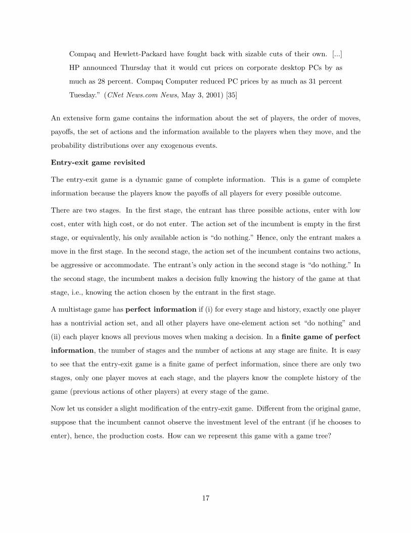
An extensive form game contains the information about the set of players, the order of moves,

payoffs, the set of actions and the information available to the players when they move, and the

probability distributions over any exogenous events.

Entry-exit game revisited

The entry-exit game is a dynamic game of complete information. This is a game of complete

information because the players know the payoffs of all players for every possible outcome.

There are two stages. In the first stage, the entrant has three possible actions, enter with low

cost, enter with high cost, or do not enter. The action set of the incumbent is empty in the first

stage, or equivalently, his only available action is “do nothing.” Hence, only the entrant makes a

move in the first stage. In the second stage, the action set of the incumbent contains two actions,

be aggressive or accommodate. The entrant’s only action in the second stage is “do nothing.” In

the second stage, the incumbent makes a decision fully knowing the history of the game at that

stage, i.e., knowing the action chosen by the entrant in the first stage.

A multistage game has perfect information if (i) for every stage and history, exactly one player

has a nontrivial action set, and all other players have one-element action set “do nothing” and

(ii) each player knows all previous moves when making a decision. In a finite game of perfect

information, the number of stages and the number of actions at any stage are finite. It is easy

to see that the entry-exit game is a finite game of perfect information, since there are only two

stages, only one player moves at each stage, and the players know the complete history of the

game (previous actions of other players) at every stage of the game.

Now let us consider a slight modification of the entry-exit game. Different from the original game,

suppose that the incumbent cannot observe the investment level of the entrant (if he chooses to

enter), hence, the production costs. How can we represent this game with a game tree?

17

Entrant

Incumbent

Do not enter

Enter, high cost

Aggressive

Enter, low cost

AggressiveAccommodating Accommodating

0, 15

-10, 3 4, 10 -7, 1 6, 8

Notice that in the original game when it is the incumbent’s turn to move, she is able to observe

the entrant’s moves. In the modified game, however, this is not the case; the incumbent cannot

observe the investment level of the entrant. The extensive form of the game is very similar to

that of the original game (Figure 1) except that we have drawn dashed lines around incumbent’s

decision nodes to indicate that these nodes are in a single information set. This means that

when it is the incumbent’s turn to play, she cannot tell which of these nodes she is at because

she has not observed the entrant’s investment level. Due to the definition of information sets, at

every node within a given information set, a player must have the same set of possible actions.

Note that a game is one of perfect information if each information set contains a single decision

node.

It is easy to see that the outcome of the original entry-exit game is for the entrant to enter the

market with the latest technology (low cost case) and the incumbent to accommodate, i.e., (Enter

with low cost, Accommodate). However, this game has another pure strategy Nash equilibrium:

(Do not enter, Aggressive). This profile is a Nash equilibrium because given that the entrant does

not enter, the incumbent’s information set is not reached and she loses nothing by being aggressive.

But this equilibrium is not “credible” because it is an “empty threat” by the incumbent to play

aggressive. (We know that if the entrant chooses to enter, the best response of the incumbent is

to accommodate.) Credibility is a central issue in all dynamic games:

18

“Coca-Cola is developing a vanilla-flavored version of its best-selling flagship cola, a

report says, extending the company’s palette of flavorings from Cherry Coke and Diet

Coke with lemon. [...] But don’t expect to see a vanilla-flavored Pepsi anytime soon.

‘It’s not something we’re looking at,’ said spokesman Larry Jabbonsky of Pepsi. ‘We

think it’s a bit vanilla.’ ” (USA Today, April 01, 2002) [1]

“PepsiCo [...] is launching Pepsi Vanilla and its diet version in stores across the

country this weekend. [...] Coke came out with Vanilla Coke in May 2002 and it was

a resounding success, selling 90 million cases, according to trade publication Beverage

Digest. [...] ‘We’re a little surprised that Pepsi decided to enter the vanilla segment,’

said Mart Martin, spokesman for Coca-Cola. ‘When we came out with Vanilla Coke,

Pepsi originally said the idea sounded ‘a bit vanilla.’ But, whatever.’ ” (CNN/Money,

August 8, 2003) [11]

The non-credible equilibrium (Do not enter, Aggressive) of the entry-exit game suggests that we

need to have a concept to deal with the non-credible “threats” in dynamic games. This concept

is the subgame perfect Nash equilibrium (SPNE).

First let us define what a subgame is. A subgame is any part of a game that remains to be

played after a series of moves and it starts at a point where both players know all the moves that

have been made up to that point (Colman [15]). Formally,

Definition 10 A subgame is an extensive form game that (a) begins at a decision node n that

is a singleton information set, (b) includes all the decision and terminal nodes following n in the

game, and (c) does not cut any information sets.

According to this definition, we can make three observations. A game is a subgame of itself.

Every subgame taken by itself is a game. In a finite game of perfect information, every node in

the game tree starts a subgame.

The logic of subgame perfection is simple: replace any proper subgame of the tree with one of

its Nash equilibrium payoffs and perform backwards induction on the reduced tree. In backwards

induction we start by solving for the optimal choice (best response) of the last mover for each

possible situation she might face. Once we solve for the last stage, we move to the second-to-last

19

stage and given the best response functions at the last stage, compute the optimal choice for the

player in this stage. We continue in this manner till we solve for all stages:

• Determine the optimal action(s) in the final stage K for each possible history hK .

• For each stage j = K−1, . . . , 1: Determine the optimal action(s) in stage j for each possible

history hj given the optimal actions determined for stages j + 1, . . . ,K.

Definition 11 A strategy profile s of an extensive form game is a subgame perfect Nash

equilibrium if the restriction of s is a Nash equilibrium of G for every proper subgame of G.

The SPNE outcome does not involve non-credible threats as at each move the players respond

optimally.

In dynamic games, even if the players have similar action sets, the sequence in which the play-

ers move significantly impacts the equilibrium outcome of the game and the players’ payoffs in

equilibrium.

“... the concept of ‘first mover advantage.’ It goes like this: The first one to establish

a viable business in any new Internet category takes all the marbles. It worked for

Amazon.com and eBay.” (USA Today, February 6, 2002) [27]

Although being the first mover is advantageous in some business games, this is not always the

case.

“In the early 1990s J. Daniel Nordstrom wanted to make [...] Nordstrom department

stores a powerhouse in the next big thing – shopping via interactive TV. Instead he got

a front-row seat when the glitzy idea imploded. His conclusion: ‘It’s very expensive

and time-consuming to be at the absolute leading edge. I want to be the first guy to

be second. It’s much more efficient for me to ride in the draft.’ ” (Forbes Magazine,

July 24, 2000) [16]

Example 12 Is being the first-mover always advantageous?

20

Two firms are competing against each other based on product quality. Let qj be the quality level

set by firm j. The payoff functions for the firms are:

Π1(q1, q2) = 5q1 + 2q1q2 − 5q21

Π2(q1, q2) = 4q2 + 11q1q2 − 4q22

Assuming that firm j is the first mover, the equilibrium quality levels can be determined using

backwards induction.

Follower’s best Profit

First mover response function Outcome Firm 1 Firm 2

Firm 1 q2(q1) = 4+11q1

8

(q1 = 4

3 , q2 = 73

)4 ≈ 13

Firm 2 q1(q2) = 5+2q2

10

(q1 = 37

36 , q2 = 9536

)5.38 ≈ 22

Therefore, given the choice, firm 1 would actually prefer to be the follower. This is a phenomenon

known as the “first-mover disadvantage.”

“You can ascribe TiVo’s struggles to the business axiom known as ‘first-mover dis-

advantage.’ Technology pioneers typically get steamrollered, then look on helplessly

from the sidelines as a bunch of Johnny-come-latelies make billions. First movers,

the theory goes, are too smart for their own good, churning out gizmos that are too

expensive or too complex for the average consumer’s taste. The big boys survive their

gun-jumping – think of Apple and its proto-PDA, the Newton, which might have

dusted the rival PalmPilot had the company merely waited a year or two to iron out

its kinks.” (MSN News, October 9, 2002) [25]

4.1 Repeated Games

One key concept we have not captured so far is the repetition of interactions. Especially in the

prisoner’s dilemma type business dealings, the players know that they will be in the same “game”

21

for a long time to come, and hence they may think twice before they defect based on short-term

incentives, especially if cooperation today would increase the chances of cooperation tomorrow.

In general, players choose their actions considering not only short-term interests, but rather long

term relationships and profitability.

Most business interactions, such as the ones between manufacturers and suppliers, and sellers and

customers, are repetitive in nature. In such situations, as long as both parties continue to benefit,

the relationships are maintained. Hence, the dependency of future actions on past outcomes plays

an important role in the current choices of the players. That is why many suppliers strive for

consistently achieving high quality levels, or why e-tailers put a high emphasis on the speed and

quality of their customers’ online shopping experience.

“Intel Corp. [...] uses its much envied supplier ranking and rating program – which

tracks a supplier’s total cost, availability, service and support responsiveness, and

quality – to keep its top suppliers on a course for better quality. ‘We reward suppliers

who have the best rankings and ratings with more business,’ says Keith Erickson,

director of purchasing [...] As an added incentive, Intel occasionally plugs high-quality

suppliers in magazine and newspaper advertisements. The company even lets its top-

performing suppliers publicize their relationship with Intel. That’s a major marketing

coup, considering that Intel supplies 80% of chips used in PCs today and is one of the

most recognized brand names in the world.

Seagate Technology [...] takes a similar approach to continuous improvement. ‘Quality

goals are set for each component and are measured in defective parts per million,’

says Sharon Jenness, HDA mechanical purchasing manager at Seagate’s design center.

‘Suppliers who consistently [beat their quality] goals and maintain a high quality

score are rewarded with an increased share of our business.’ ” (Purchasing, January

15, 1998) [29]

“Customer retention is the key for e-commerce firms hoping to eventually make a

profit. [...] A 10% increase in repeat customers would mean a 9.5% increase in

the corporate coffers, according to McKinsey’s calculations.” (The Industry Standard,

March 20, 2000) [30]

22

In this section, we will find out when, if at all, repeating the interactions help the firms collaborate

to achieve mutually beneficial outcomes.

Example 13 Repeated prisoner’s dilemma game

Recall the prisoner’s dilemma game displayed in Figure 2. The unique equilibrium outcome of

this game is (D, D) with payoffs (−6,−6). This outcome is Pareto dominated by (C, C), which

results in payoffs (−1,−1), i.e., the prisoners settle for an inferior outcome by selfishly trying to

get better at the expense of the other.

Now suppose that this game is repeated T times, i.e., consider the dynamic version of this game

with T stages. For simplicity, consider T = 2. The prisoners observe the outcomes of all preceding

stages before they engage in the current stage of the game. The payoffs for the repeated game

are simply the sum of the payoffs from all the stages of the game. The question is: Can repeating

the same game help the players to achieve a better outcome?

In order to find the equilibrium outcome of this new game, we can use the idea of subgame perfect

equilibrium and start analyzing the second stage of the game. In the second stage, regardless of

the first stage, there is a unique Nash equilibrium (D, D). After solving the second stage, we can

roll back and analyze the first stage of the game. We already know that regardless of the outcome

in this stage we will have an equilibrium payoff of (−6,−6) from the second stage; we might as

well decrease the first stage payoffs by 6 for each outcome and just look at this modified single

stage game instead.

-7, -7

-6, -15

-15, -6

-12, -12

Prisoner 2

Cooperate (C) Defect (D)

C

DPriso

ner 1

This modified single stage game has a unique Nash equilibrium: (D, D). Thus, the unique SPNE

23

of the two-stage prisoner’s dilemma game is (D, D) in the first stage, followed by (D, D) in the

second stage. Unfortunately, cooperation cannot be achieved in either stage of the SPNE. The

result would be the same if the game was repeated for any finite number of times.

What would happen if we repeat this game infinitely many times? Adding the payoffs of all

stages would not work here, because the sum of the payoffs would go to (negative) infinity no

matter what the outcome is. Since future payoffs are in general worth less today, it is reasonable

to look at discounted payoffs, or the net present value of payoffs. Let δ be the value today of a

dollar to be received one stage later, e.g., δ = 1/(1 + r) where r is the interest rate per stage.

Given the discount factor δ the present value of the infinite sequence of payoffs π1, π2, π3, . . .

is π1 + δπ2 + δ2π3 + . . . =∑∞

t=1 δt−1πt. If the payoff is the same in each stage, then we have

π + δπ + δ2π3 + . . . =∑∞

t=1 δt−1π = π1−δ .

Consider the following strategy for the infinitely repeated prisoner’s dilemma game: Play C in the

first stage. In the t-th stage, if the outcome of all t−1 preceding stages has been (C,C), then play

C; otherwise, play D. Such strategies are called trigger strategies because a player cooperates

until someone fails to cooperate, which triggers a switch to non-cooperation (punishment) forever

after.

We see many examples of such trigger strategies in business. For example, a manufacturer and a

supplier will continue to do business as long as the supplier meets certain quality standards and

the manufacturer pays a good price and provides sufficient volume.

“Suppliers who consistently rank poorly in quality measurements are often placed on

some type of probation, which can include barring them from participating in any

new business. [...] If for some reason quality improvement is not achievable with a

particular supplier, PPG is free to let that supplier go.” (Purchasing, January 15,

1998) [29]

If we assume prisoner 1 adopts this trigger strategy, what is the best response of prisoner 2 in

stage t + 1? If the outcome in stage t is any other than (C,C), then she would play D at stage

t + 1 and forever. If the outcome of stage t is (C,C), she has two alternatives – she can either

continue to cooperate or she can defect. If she defects, i.e., plays D, she will receive 0 in this stage

24

and she will switch to (D,D) forever after, leading to the following net present value:

V = 0 + δ.(−6) + δ2.(−6) + δ3.(−6) + · · · = (−6)δ

(1− δ).

If she cooperates, i.e., plays C, she will receive -1 in this stage and she will face the exact same

game (same choices) in the upcoming stage, leading to a net present value below:

V = −1 + δV ⇒ V =−1

1− δ.

For prisoner 2, playing C is optimal if

−11− δ

≥ (−6)δ

(1− δ)⇒ δ ≥ 1

6.

Therefore, it is a Nash equilibrium for both prisoners to cooperate if δ ≥ 16 . If δ is small, then

future earnings are not worth much today. Hence, players act myopically to maximize current

payoffs and choose to defect rather than cooperate. However, when δ is large (in this case larger

than or equal to 16), the players value future earnings highly and hence they choose to cooperate.

Next, we will argue that such a Nash equilibrium is subgame-perfect. Recall the definition of

SPNE: A Nash equilibrium is subgame-perfect if the players’ strategies are a Nash equilibrium in

every subgame. In this game there are two classes of subgames: Subgames where the outcomes

of all previous stages have been (C,C) and subgames where the outcome of at least one earlier

stage differs from (C,C). The trigger strategies are Nash equilibrium for both of these cases.

In the prisoner’s dilemma game, repeating the game finitely many times does not help the prisoners

achieve cooperation. However, when δ ≥ 16 , the outcome of the infinitely repeated prisoner’s

dilemma is to cooperate in all stages. That is, the credible threat of defect helps the players to

coordinate their acts.

So the idea is simple: Repeating a game with a unique Nash equilibrium finitely many times

would lead to a unique SPNE where the Nash equilibrium is played at every stage of the game. If

the same game is repeated infinitely many times, however, the repeated game may have a SPNE

which is not a Nash equilibrium of the original game. This result has captured some discussions

among the game theorists and one such discussion can be found in Osborne and Rubinstein [32]

among the authors of the book:

25

“[A. Rubinstein] In a situation that is objectively finite, a key criterion that determines

whether we should use a model with a finite or an infinite horizon is whether the last

period enters explicitly into the players’ strategic considerations. For this reason,

even some situations that involve a small number of repetitions are better analyzed

as infinitely repeated games. For example, when laboratory subjects are instructed to

play the Prisoner’s Dilemma twenty times [...], I believe that their lines of reasoning

are better modeled by an infinitely repeated game than by a 20-period repeated game,

since except very close to the end of the game they are likely to ignore the existence

of the final period.

[M.J. Osborne] [...] The experimental results definitely indicate that the notion of

subgame perfect equilibrium in the finitely repeated Prisoner’s Dilemma does not

capture human behavior. However, this deficiency appears to have more to do with

the backwards induction inherent in the notion of subgame perfect equilibrium than

with the finiteness of the horizon per se.”

Recall that repeating a game with a unique Nash equilibrium finitely many times leads us to the

same outcome at every stage. Then would it ever benefit the players to repeat a game finitely many

times? The answer is yes. If there are multiple Nash equilibria in a game, then finite repetition

might make it possible in certain stages to achieve outcomes which are not Nash equilibria in the

single-stage game.

Example 14 Finitely repeated game with multiple static Nash equilibria5.

Consider the game below with two players, where each player has three possible actions.

1, 1

0, 5

5, 0

4, 4

Player 2Left Center Right

Top

Middle

Bottom

Play

er 1

0, 0

0, 0

0, 0 0, 0 3, 3

5This example is taken from Gibbons [22].

26

The game has two Nash equilibria: (Top, Left) and (Bottom, Right). Note that, (Middle, Center)

Pareto dominates both of these equilibria, but it is not a Nash equilibrium itself. Suppose this

game is played twice, with the first stage outcome observed before the second stage begins, and

the players play according to the following strategy: Play (Bottom, Right) in the second stage if

the first stage outcome is (Middle, Center); otherwise, play (Top, Left) in the second stage.

We can modify the payoffs of the first stage based on this strategy. If the players play anything

other than (Middle, Center) in the first stage, the second stage payoffs will be (1, 1). If the first

stage outcome is (Middle, Center), then the second stage payoffs will be (3, 3). Therefore, we can

modify the first stage by adding (3, 3) to the payoffs of outcome (Middle, Center) and by adding

(1, 1) to the payoffs of all other outcomes.

2, 2

1, 6

6, 1

7, 7

Player 2Left Center Right

Top

Middle

Bottom

Play

er 1

1, 1

1, 1

1, 1 1, 1 4, 4

The modified first stage game has 3 pure-strategy Nash equilibria: (Top, Left), (Middle, Center),

and (Bottom, Right). Thus, the SPNE of the two-stage game are [(Top, Left), (Top, Left)],

[(Bottom, Right), (Top, Left)] and [(Middle, Center), (Bottom, Right)]. Note that (Middle,

Center) is not an equilibrium in the single stage game, but it is a part of SPNE. In this example,

we have seen a credible promise, which resulted in an equilibrium outcome that is good for all

parties involved. If the stage game has multiple equilibria, players may devise strategies in order

to achieve collaboration in a finitely repeated game.

5 Price and Quantity Competition

For most manufactures and retailers, key business decisions include what to produce/procure and

sell, how much, and at what price. Hence, we commonly see competitive interactions around these

decisions. Given their importance within the business world, we devote this section to well-known

27

game theoretic models that focus on price and quantity decisions.

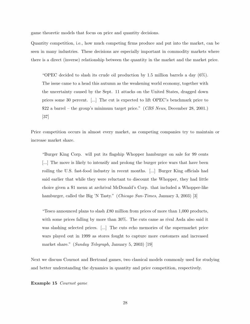
Quantity competition, i.e., how much competing firms produce and put into the market, can be

seen in many industries. These decisions are especially important in commodity markets where

there is a direct (inverse) relationship between the quantity in the market and the market price.

“OPEC decided to slash its crude oil production by 1.5 million barrels a day (6%).

The issue came to a head this autumn as the weakening world economy, together with

the uncertainty caused by the Sept. 11 attacks on the United States, dragged down

prices some 30 percent. [...] The cut is expected to lift OPEC’s benchmark price to

$22 a barrel – the group’s minimum target price.” (CBS News, December 28, 2001.)

[37]

Price competition occurs in almost every market, as competing companies try to maintain or

increase market share.

“Burger King Corp. will put its flagship Whopper hamburger on sale for 99 cents

[...] The move is likely to intensify and prolong the burger price wars that have been

roiling the U.S. fast-food industry in recent months. [...] Burger King officials had

said earlier that while they were reluctant to discount the Whopper, they had little

choice given a $1 menu at archrival McDonald’s Corp. that included a Whopper-like

hamburger, called the Big ’N Tasty.” (Chicago Sun-Times, January 3, 2003) [3]

“Tesco announced plans to slash £80 million from prices of more than 1,000 products,

with some prices falling by more than 30%. The cuts came as rival Asda also said it

was slashing selected prices. [...] The cuts echo memories of the supermarket price

wars played out in 1999 as stores fought to capture more customers and increased

market share.” (Sunday Telegraph, January 5, 2003) [19]

Next we discuss Cournot and Bertrand games, two classical models commonly used for studying

and better understanding the dynamics in quantity and price competition, respectively.

Example 15 Cournot game

28

Consider a market with two competing firms selling a homogeneous good. Let q1 and q2 denote the

quantities produced by firms 1 and 2, respectively. Suppose that the firms choose their production

quantities simultaneously. This game is known as the Cournot game. It is a static game with two

players, where the players’ action sets are continuous (each player can produce any non-negative

quantity).

Let P (Q) = a − bQ be the market-clearing price when the aggregate quantity on the market is

Q = q1 + q2. Assume that there are no fixed costs and the total cost of producing quantity qi is

ciqi. In order to avoid the trivial cases, in the rest of this section, we will assume that a > 2ci.

To illustrate this game – and the other games in this section – numerically, consider an example

where a = 130, b = 1, and c1 = c2 = 10.

Before we consider the Cournot game, we will analyze the monopoly setting as a benchmark

model. A monopolist sets his production quantity qM to maximize his profit:

ΠM = max0≤qM≤∞

(a− bqM ) qM − cMqM = (130− qM − 10) qM

Notice that ΠM is concave in qM , therefore we can use the first-order condition (FOC) to find the

optimal monopoly quantity:

∂ΠM

∂qM= a− 2bqM − cM = 0 ⇒ q∗M =

a− cM

2b= 60.

The monopolist’s profit is ΠM = (a−cM )2

4b = 3600.

Now, let us go back to the Cournot game. The payoff functions for players for strategy profile

s = (q1, q2) are

Π1(s) = (a− b (q1 + q2)) q1 − c1q1 = (130− (q1 + q2)− 10) q1 (1)

Π2(s) = (a− b (q1 + q2)) q2 − c2q2 = (130− (q1 + q2)− 10) q2 (2)

In the Cournot game, in order to find the best response functions of the players, we need to solve

each player’s optimization problem:

Π1 = max0≤q1≤∞

(a− b (q1 + q2)− c1) q1 = max0≤q1≤∞

(120− (q1 + q2)) q1

Π2 = max0≤q2≤∞

(a− b (q1 + q2)− c2) q2 = max0≤q2≤∞

(120− (q1 + q2)) q2

29

FOC for the optimization problems are as follows:

∂Π1(s)∂q1

= a− 2bq1 − bq2 − c1 = 120− 2q1 − q2 = 0

∂Π2(s)∂q2

= a− 2bq2 − bq1 − c2 = 120− 2q2 − q1 = 0

Notice that, the objective functions in this case are concave and therefore we can use FOC to find

the best response functions:

R1(q2) =(

a− c1

2b− q2

2

)+

=(

60− q2

2

)+

R2(q1) =(

a− c2

2b− q1

2

)+

=(

60− q1

2

)+

When we solve these reaction functions together, we get the Cournot equilibrium:

q∗1 =a− 2c1 + c2

3b= 40

q∗2 =a− 2c2 + c1

3b= 40

When we compare this outcome with the monopoly result, we see that companies, when engaged

in competition, end up producing less than what they would produce otherwise. However, the

total quantity to the market q∗1 + q∗2 would be higher than what a monopolist would produce and

sell, q∗M . As the number of firms in the market increases, each firm’s profitability decreases. The

firms begin to have smaller market shares and the end-customers benefit more and more from the

tough competition.

Example 16 Infinitely repeated Cournot game

Let us consider the infinitely repeated version of the static Cournot duopoly model. Each firm

has a marginal cost of c and both firms have a discount factor of δ. Assume that the firms play

the following trigger strategy.

Produce half the monopoly quantity, qM/2, in the first stage. In the tth stage, produce

qM/2 if both firms have produced qM/2 in all previous stages; otherwise, produce qC .

Each firm’s profit when they both produce half the monopoly quantity,( qM

2 = a−c4b = 30

), is

(a−c)2

8b = 1800. If both produce the Cournot quantity,(qC = a−c

3b = 40), the profit of each is

(a−c)2

9b = 1600. We want to compute the values of δ for which this trigger strategy is a SPNE.

30

If the outcome in stage t is other than (qM/2, qM/2), then firm i’s best response in stage t + 1

(and forever) is to produce qC . If the outcomes of stages 1, · · · , t are (qM/2, qM/2), however, he

has two choices. He may deviate or he may continue to cooperate. If he deviates, he will produce

the quantity that maximizes the current period’s profit in stage t+1 and then produce qC forever:

max0≤qi≤∞

(a− bqi −

a− c

4− c

)qi.

The quantity is qi = 3(a−c)8b = 45 with a profit of 9(a−c)2

64b = 2025. The discounted profit is:

V =9(a− c)2

64b+

((a− c)2

9b

)(δ

1− δ

)= 2025 + 1600

(δ

1− δ

).

If he continues to cooperate, he will produce qM/2 and receive (a−c)2

8b = 1800 in this stage and he

will face the exact same game (same choices) in stage t + 2.

V =(a− c)2

8b+ δ.V ⇒ V =

(a− c)2

8b(1− δ)=

18001− δ

.

Therefore, producing qM/2 is optimal if

18001− δ

≥ 2025 + 1600(

δ

1− δ

)⇒ δ ≥ 9

17.

This is a tacit collusion to raise the prices to the jointly optimal level and it is called cartel. A

cartel “is a combination of producers of any product joined together to control its production,

sale, and price, so as to obtain a monopoly and restrict competition in any particular industry or

commodity.” (http://www.legal-database.com) As the example above shows, cartels can be quite

unstable. At each stage, the players have a huge incentive to cheat, especially when they think it

can go unnoticed.

“The coffee bean cartel, the Association of Coffee Producing Countries, whose mem-

bers produce 70% of the global supply, will shut down in January after failing to

control international prices. [...] Mr Silva also said the failure of member countries to

comply with the cartel’s production levels was a reason for the closure.” (BBC News,

October 19, 2001) [8]

“[...] But the oil market is notoriously difficult to balance – demonstrated by the

rollercoaster of prices over the last few years. [...] Member states of OPEC do not

31

necessarily have identical interests and often find it difficult to reach consensus on

strategy. Countries with relatively small oil reserves [...] are often seen as ‘hawks’

pushing for higher prices. Meanwhile, producers [...] with massive reserves and small

populations fear that high prices will accelerate technological change and the devel-

opment of new deposits, reducing the value of their oil in the ground.” (BBC News,

February 12, 2003) [2]

Example 17 Bertrand game

Bertrand game models situations where firms choose prices rather than quantities as in Cournot’s

model. Assume that two firms produce identical goods which are perfect substitutes from the

consumers’ perspective, i.e., consumers buy from the producer who charges the lowest price. If

the firms charge the same price, they will split the market evenly. There are no fixed costs of

production and the marginal costs are constant at c. As in the Cournot game, the firms act

simultaneously.

The profit of firm i when it chooses the price pi is

Πi(pi, pj) = (pi − c)Di(pi, pj),

where the demand of firm i as a function of prices is given by

Di(pi, pj) =

D(pi) pi < pj

12D(pi) pi = pj

0 pi > pj

This time the strategies available to each firm are the different prices it might charge, rather than

the quantities it might produce. The Bertrand paradox states that the unique equilibrium has

the firms charge the competitive price: p∗1 = p∗2 = c.

To see why, first observe that for each firm, any strategy which sets the price pi lower than the

marginal cost c is strictly dominated by pi = c, and hence can be eliminated. Therefore, in the

equilibrium pi ≥ c. Now assume that firm 1 charges higher than firm 2, which charges higher than

the marginal cost; i.e. p∗1 > p∗2 > c. Then firm 1 has no demand and its profits are zero. On the

other hand, if firm 1 charges p∗2− ε, where ε is positive and small, it obtains the entire market and

32

has a positive profit margin of p∗2− ε− c. Therefore, p∗1 > p∗2 > c cannot be an equilibrium as firm

1 is not acting in its best interest. Similar arguments can be applied to cases where p∗1 = p∗2 > c

and p∗1 > p∗2 = c to show that neither of these cases can be an equilibrium. Hence, the only

possible outcome is p∗1 = p∗2 = c. Therefore, when the costs and the products are identical, there

exits a unique equilibrium in which all output is sold at the price which is equal to the marginal

cost.

The Bertrand game suggests that when the firms compete on prices (and the costs are symmetric)

we obtain a perfectly competitive market even in a duopoly situation. However, in real life, most

customers do not only choose based on price, but also based on other factors such as quality

and convenience of location. For example, Wendy’s, the other large player in fast-food industry,

decided to stay out of the Burger King-McDonald’s price war and aimed at gaining market share

by offering higher-quality products.

In many business situations, firms choose their actions sequentially rather than simultaneously.

To be more precise, one firm chooses its action after it observes another firm’s action and responds

to it. The next game that we will look at considers the quantity competition when one firm reacts

to another.

Example 18 Stackelberg game

Let us modify the Cournot model so that firms move sequentially rather than simultaneously.

Firm 1 moves first and chooses her quantity to sell q1. We call firm 1 the “Stackelberg leader.”

Firm 2 observes q1 before choosing his own output level q2. We call firm 2 the “Stackelberg

follower.” The total market demand is Q = q1 + q2. Both firms seek to maximize their profits.

This game is known as Stackelberg game, and it is a dynamic game of complete and perfect

information. The game has two players and two stages. In stage 1, player 1’s action set is [0,∞),

as player 1 can produce any non-negative quantity, whereas player 2’s only available action is “do

nothing.” In stage 2, player 2’s action set is [0,∞), and player 1’s only available action is “do

nothing.”

The players’ payoffs as a function of the moves that were made are given in Equations 1 and 2.

We can find the outcome of the Stackelberg game by using backwards induction, starting at stage

33

2. Firm 2’s best response function is

R2(q1) =(

a− c2

2b− q1

2

)+

.

We can plug in this function into firm 1’s optimization problem in order to find the outcome:

q1 =a− 2c1 + c2

2b= 60 q2 =

a + 2c1 − 3c2

4b= 30

Table below summarizes the outcomes of the Cournot, the Stackelberg, and the Bertrand games

when the production costs of the two firms are equal. Note that firm 2 does worse in the Stackel-

berg game than in the Cournot game, even though it has more “information” in the Stackelberg

game while choosing its production quantity, as it observes firm 1’s decision before making its

own. This illustrates an important difference between single- and multi-person decision problems.

In single-person decision theory, having more information can never make the decision maker

worse off. In game theory, however, having more information (or, more precisely, having it known

to the other players that one has more information) can make a player worse off.

Monopoly Cournot Stackelberg Bertrand

Price c + a−c2 = 70 c + a−c

3 = 50 c + a−c4 = 40 c = 10

Quantity a−c2b = 60 2(a−c)

3b = 80 3(a−c)4b = 90 a−c

b = 120(a−c2b = 60, a−c

4b = 30)

Total Firm (a−c)2

4b = 3600 2(a−c)2

9b = 3200 3(a−c)2

16b = 2700 0

Profits(

(a−c)2

8b = 1800, (a−c)2

16b = 900)

Let us look at two other measures. Total consumer surplus is consumers’ willingness to pay that

is not captured by the firm. It is positive if the firm sells below consumers’ willingness to pay.

Deadweight loss is demand that is not satisfied by the firm and is positive if the firm sells below

34

130

q13090

P=130-QP

MC=10

Consumer surplus=4050

40Firm profits=2700

Deadweight loss=450

Stackelberg Duopoly Model

P

q

MC=10

130

130

60

70

Consumer surplus=1800

Deadweight loss=1800

Firm profits=3600

P=130-QMonopoly

q130120

P=130-Q

MC=10

130

Consumer surplus=7200

Bertrand Duopoly ModelP

130

80

P=130-Q

MC=10

130

90

40

50

Consumer surplus=3200

Firm profits=3200

Deadweight loss=800

P Cournot Duopoly Model

q

Figure 4: Division of the total potential surplus in the market among the participants.

the maximum market demand. Consumer surplus is highest in the Bertrand model ($7200) and

lowest in the monopoly model ($1800). This confirms our intuition that price competition always

benefits the consumer.

In our example, the size of the entire “pie” in the market is $7200, which is the total potential

surplus. Figure 4 shows the division of the “pie” among the market participants. In the Bertrand

model, the consumers get the entire pie. As we move from Bertrand to Stackelberg to Cournot

to Monopoly, the portion of the pie allocated to the consumers gets smaller, as the portion of

the pie allocated to the firms get bigger. The deadweight loss increases at the same time; this

means that the decrease in the consumer surplus surpasses the increase in the firms’ profits and

the surplus obtained by the firms and the consumers together decreases. Hence, part of the pie

remains unused, benefiting neither the firms nor the consumers.

35

6 Supply Chain Coordination

In a supply chain (SC), there are multiple firms owned and operated by different parties, and

each of these firms take decisions which are in line with their own goals and objectives. As in

all decentralized systems, the actions chosen by SC participants might not always lead to the

“optimal” outcome if one considers the supply chain as one entity. That is, since each player acts

out of self-interest, we usually see inefficiencies in the system, i.e., the results look different than

if the system was managed “optimally” by a single decision-maker who could decide on behalf

of these players and enforce the type of behavior dictated by this globally (or centrally) optimal

solution.

In this section, we will take a look at the nature of inefficiencies that might result from the

decentralized decision-making in supply chains, and if and how one can design contracts such

that even though each player acts out of self interest, the decentralized solution might approach

the centralized optimal solution. For excellent reviews on SC contracts and coordination we refer

the reader to Tsay, Nahmias and Agrawal [40] and Cachon [12].

To better formalize these ideas, we will look at a simple stylized two-stage supply chain with one

supplier and one retailer, where the retailer buys goods from the supplier and sells them in the

end market:

Supplier End marketRetailer

Wholesale price, w

Marketprice, P

For simplicity, assume that the supplier is uncapacitated, and has unit cost of production c. The

retailer faces a market where the price is inversely related to the quantity sold. For simplicity, let

us assume a linear demand curve P = a − bq where P is the market price and q is the quantity

sold by the retailer6. Assume that all of this information is common knowledge.

First let us consider the simple “wholesale price” contract where the supplier charges the retailer6Note that in such a deterministic environment, the retailer will always purchase from the supplier exactly as

much as he will sell in the market.

36

Table 1: Wholesale price contract versus CSC.

DSC CSC

Supplier’s wholesale price (w) w = (a + c)/2 w

Retailer’s quantity (q) q = (a− c)/4b q∗ = (a− c)/2b

Market Price (P ) P = (3a + c)/4 P ∗ = (a + c)/2

Supplier’s profit (ΠS) ΠS = (a− c)2/8b Π∗S = (w − c)q

Retailer’s profit (ΠR) ΠR = (a− c)2/16b Π∗R = (P − w)q

Total SC profits (Π) Π = 3(a− c)2/16b Π∗ = (a− c)2/4b

w per unit. The supplier’s and the retailer’s profits are ΠS = (w − c)q and ΠR = (a− bq − w)q,

respectively. The supply chain’s profits are Π = ΠS + ΠR = (a − bq − c)q. Note that the choice

of w only indirectly affects the total SC profits, since the choice of w impacts the choice of q.

Decentralized Supply Chain (DSC): As in most real-world supply chains, suppose that the

supplier and the retailer are two independently owned and managed firms, where each party is

trying to maximize his/her own profits. The supplier chooses the unit wholesale price w and

after observing w, the retailer chooses the order quantity q. Note that this is a dynamic game of

complete information with two players, supplier and retailer, where the supplier moves first and

the retailer moves second. Hence, we can solve this game using backwards induction.

Given a w, first we need to find the retailer’s best response q(w). The retailer will choose q to

maximize ΠR = (a− bq − w)q. This is a concave function of q, and hence from FOC we get

∂ΠR

∂q= a− 2bq − w = 0 ⇒ q(w) =

a− w

2b.

Next, given the retailer’s best response q(w) = (a−w)/2b, the supplier maximizes ΠS = (w−c)q =

(w − c)(a− w)/2b. This is a concave function of w and from FOC we get

∂ΠS

∂w= a− w − w + c = 0 ⇒ w =

a + c

2.

The equilibrium solution for this decentralized supply chain is given in the second column of

Table 1. In this contractual setting, the supplier gets two-thirds of the SC profits, the retailer

gets only one-third. This is partly due to the first-mover advantage of the supplier.

37

Now, let us consider a centralized (integrated) supply chain (CSC) where both the retailer and

the supplier are part of the same organization and managed by the same entity.

Centralized Supply Chain (CSC): In this case there is a single decision-maker who is con-

cerned with maximizing the entire chain’s profits Π = (a− bq− c)q. This is a concave function of

q and from FOC we get

∂Π∂q

= a− 2bq − c = 0 ⇒ q∗ =a− c

2b.

The solution for the CSC is given in the third column of Table 1.

From Table 1 we see that the quantity sold as well as the profits are higher and the price is lower

in the CSC than in the DCS. Hence, both the supply chain and the consumers are better off in

the CSC.

What about the retailer and the supplier? Are they both better off, or is one of them worse off

in the CSC? What is the wholesale price? How does the choice of w affect the market price,

quantity, and the supply chain profits? A closer look would reveal that w has no impact on these

quantities. Any positive w would result in the same outcome for the CSC because the firm would

be paying the wholesale price to itself! However, the choice of w in the CSC is still very important

as it determines how the profits will be allocated between the supplier and the retailer. We can

interpret w as a form of transfer payment from the retailer to the supplier. What is the minimum

w that is reasonable? For positive supplier profits, we need w ≥ c. If we set w = c, the supplier’s

profits are zero whereas the retailer captures the entire supply chain’s profits. What is the w

that splits the SC profits equally between the retailer and the supplier? If we set w = (a + 3c)/4,

w− c = P −w = (a− c)/4 and each party’s profits are (a− c)2/8b. Note that this is the same as

the supplier’s profits in the DSC. Hence, if the supplier and the retailer split the profits equally

in the CSC, the supplier is at least as good, and the retailer is strictly better off than in the DCS.

In the DSC, the outcomes are worse for all the parties involved (supplier, retailer, supply chain,

and consumer) compared to the CSC, because in the DSC both the retailer and the supplier

independently try to maximize their own profits, i.e., they each try to get a margin, P − w and

w − c, respectively. This effect is called “double marginalization” (DM).

In a serial supply chain with multiple firms there is coordination failure because each

firm charges a margin and neither firm considers the entire supply chain’s margin when

38

making a decision (Spengler [34]).

In this stylized model, the profit loss in the DSC due to DM is 25% (also referred to as the DM

loss). It is clearly in the firms’ interest to eliminate or reduce double marginalization, especially if

this can be done while allocating the additional profits to the firms such that both firms benefit.

This simple model suggests that vertical integration could be one possible way of eliminating

double marginalization. However, for reasons we discussed at the beginning of this chapter,

vertical integration is usually not desirable, or not practical. Then the question is, can we change

the terms of the trade so that independently managed companies act as if they are vertically

integrated? This is the concept known as “supply chain coordination.” In this stylized model, the

retailer should choose q∗ = (a− c)/2b in any coordinating contract.

One can easily think of some very simple alternative contracts to eliminate double marginalization:

Take-it-or-leave-it-contract: The supplier offers the following contract to the retailer: Buy q∗

at the wholesale price w = (a + c)/2, or nothing. In this case the supplier’s profit is Π∗, i.e., the

supplier captures 100% of the CSC profits.

Marginal pricing: The supplier sets w = c. In this case, the retailer’s profit is Π∗, i.e., the

retailer captures 100% of the CSC profits.

Note that the take-it-or-leave-it contract would require a very powerful supplier whereas the

marginal pricing contract would require a very powerful retailer. In practice, neither the supplier

nor the retailer is so powerful in general to dictate such contract terms. Hence, we need to

consider alternative contracts that coordinate the supply chain. In general, the following aspects

are important in (coordinating) contracts (Cachon [12]):

• Profitability: Achieve profits close to optimum.

• Fairness and flexibility: Allow for flexible division of profits.

• Implementability: Should be easy and low-cost to administer.

Next, we will discuss alternative contracts which have these desirable properties.

39

6.1 Revenue Sharing Contract

One alternative contract which has these desirable properties is revenue sharing (Cachon and

Lariviere [13]) which we discuss next.

In a revenue sharing contract, the retailer shares a fraction α < 1 of his revenues with the supplier.

To study this contract, we will consider a slight variation of our earlier simple two-stage supply

chain model. Let cS and cR denote the unit costs of the supplier and the retailer, respectively.

Let c = cS + cR be the cost of each unit sold (the supply chain’s total unit cost). The retailer’s

revenue as a function of quantity q is given by a function R(q), which is concave and increasing

in q.

First, consider the centralized supply chain. In the CSC, the profits are given by Π = R(q)− cq,

and from FOC we have ∂R(q)∂q = c. This means that in the CSC, the marginal revenue is equal to

the marginal cost at the optimal quantity.

Next, consider the DSC under the wholesale price contract as before. The retailer’s profits are

ΠR = R(q) − (w + cR)q. From FOC, ∂R(q)∂q = w + cR. Note that q < q∗ if w > c − cR, i.e.,

unless the supplier sells at marginal cost, the retailer orders less than the optimal CSC quantity

resulting in double marginalization.

Finally, consider the revenue sharing contract. The retailer’s profits in a revenue sharing contract

are ΠR(q) = αR(q)−(w+cR)q. From FOC, α∂R(q)∂q = w+cR and ∂R(q)

∂q = (w+cR)/α. Recall that

we had ∂R(q)∂q = c in the integrated chain. Hence, by setting the two right hand sides equal to each

other, we can achieve the same quantities in the CSC and the DSC. That is, if w + cR = αc, i.e.,

w = αc−cR, we have marginal revenue equal to the marginal cost in the DSC as well, and q = q∗.

In this case, the retailer’s profit is ΠR(q) = αR(q) − (αc − cR)q − cRq = α(R(q∗) − cq∗) = αΠ∗,

i.e., the retailer captures α fraction of the optimal SC profits. Similarly, the supplier captures

(1 − α) fraction of the SC profits. Note that in the revenue sharing contract, the retailer’s

objective function becomes an affine transformation of the supply chain’s objective function, i.e.,

the retailer’s and the supply chain’s objectives are perfectly aligned.

Since the total SC profits are higher compared to the traditional wholesale price contract, partners

can choose α such that both parties benefit. The choice of α depends on several factors, including

the bargaining power of the supplier and the retailer.

This simple model is motivated by revenue sharing contracts implemented in practice, in par-

40

ticular by the agreements between Blockbuster and the movie studios. Blockbuster is a retailer,

which purchases movies from the studios (suppliers) and rents them to customers. The supplier’s

wholesale price impacts how many videos Blockbuster orders and hence, how many units are

eventually rented by customers. Before 1998, the price of purchasing a tape from the studio was

very high, around $65. Given that rental fees are in the order of $3-4, Blockbuster could purchase

only a limited number of videos and this resulted in lost demand; especially during the initial

release period, where the demand was high (peak demand usually lasts less than 10 weeks), 20%

of customers could not find what they were looking for on the shelf. Hence, the studio’s high

wholesale price impacted the quantity purchased by Blockbuster, and in turn, the revenues and

the profitability of both firms. Seeing this problem, Blockbuster and the studios went into a

revenue sharing agreement. According to this, Blockbuster pays only $8 per tape initially, but

then gives a portion (somewhere around 30 to 45%) of the revenues generated from that tape

back to the supplier. Since this agreement reduces Blockbuster’s initial investment in movies, it

orders more tapes from the studio, hence, is able to meet more demand, generate more revenues,

and give back a portion of those revenues back to the supplier. Blockbuster increased its overall

market share from 25% to 31% and its cash flow by 61% using this agreement. This is clearly a

win-win situation. The supplier might be better off even if he sells each unit below its production

cost. A similar agreement is used between studios and theaters as well. (CNet News.com, October

18, 2000) [7]

One of the potential drawbacks of such an agreement is the additional cost and administrative

burden it creates compared to the straightforward wholesale price contract. Revenue sharing

takes an organizational effort to set up the deal and follow its progress. It is worthwhile to go

into such an agreement only if the increase in profits is relatively large compared to the additional

cost and the administrative effort.

In our analysis of the revenue sharing contract, we considered a single supplier and a single

retailer. It turns out that in case of multiple retailers, coordination is not guaranteed unless the

supplier has the flexibility to offer different contracts to different retailers. Unfortunately, such

“discrimination” might not always be possible due to legal considerations. Another issue is the

impact of such an agreement on the behavior of a retailer who sells competing goods and also sets

prices. In such a case, the retailer may have an incentive to use the goods under revenue sharing

agreement as loss leaders, to drive the traffic to the store and increase overall sales. Finally,

41

revenue sharing loses its appeal if the revenues depend on the retailer’s sales effort. For a retailer

who is taking only a fraction of the revenues he generates, the incentive to improve sales goes

down. While revenue sharing helps to ensure that the retailers buy and sell the “right” quantity,

it hurts their sales effort. This is especially true in retail industries such as automobile sales,

where a retailer’s sales effort makes a big difference in the overall sales rate.

6.2 Buyback Contract

Revenue sharing is just one of many different alternative contract types to coordinate a supply

chain. We observed that in the decentralized chain under wholesale price contract, the retailer

orders less than the optimal quantity. This was mainly due to double marginalization. An

additional reason for ordering less than the optimal quantity could be the risk of excess inventory.

For example, consider a newsvendor type model, where there is a single selling opportunity and

the seller needs to procure/produce before knowing the demand. This is the case for most fashion

retailers, where products need to be ordered months in advance, due to long lead times, way

before the demand is known and the actual selling season begins. Whatever is not sold at the end

of the selling season is salvaged, and the retailer bears the cost of having excess inventory.

Buyback contracts allocate the inventory risk between the supplier and the retailer. Retailer can

return the goods to the supplier and get some money back. Specifically, in the buyback contract

the supplier purchases leftover units at the end of the selling season for $b per unit, where b < w.

The retailer’s revenue is R(q) = pS(q), where p is the unit selling price (given, i.e., not a decision

variable) and S(q) is the total amount of sales made by the retailer. Note that S(q) ≤ q, i.e., the

retailer cannot sell more than what he orders. As before, the total unit cost of the supply chain

is c = cS + cR.

In the DSC, the retailer’s profit is

ΠR = revenue + returns− cost− purchase cost

= R(q) + b

(q − R(q)

p

)− (cR + w)q = R(q)

(1− b

p

)− (cR + w − b) q.

Recall that in revenue sharing contracts we have ΠR = αΠ∗ = α (R(q∗)− cq∗), i.e., the retailer’s

profit is an affine transformation of the centralized supply chain’s profits. Hence, the retailer’s

optimal quantity is the same as the centralized supply chain’s optimal quantity.

42

For a similar situation to hold in buyback contracts, the retailer’s revenue should be equal αΠ∗,

i.e., R(q) (1− b/p)−(cR +w−b)q = αΠ∗ and we need to have (cR +w−b) = αc and (1−b/p) = α:(1− b

p

)= α ⇒ b = p(1− a)

cR + w − b = αc ⇒ wb = αc + b− cR = p(1− α) + αc− cR.

Hence, if the supplier chooses w and b in this fashion, the retailer will get a fraction of the CSC’s

profits.

In revenue sharing contracts, we had w = αc − cR. In buyback contracts, we have wb = p(1 −

α) + αc− cR and b = p(1− α). That is, wb = b + w. Hence, in the buyback contract the supplier

charges a little more for the wholesale price and in return guarantees to give back b for any unit

that is not sold.

In revenue sharing contracts the wholesale price did not depend on the selling price. But in a

buyback contract, the wholesale price and the return price depend on the selling price. Hence, in

a buyback contract the supplier should set w and b as functions of the selling price p.

Is the buyback contract flexible in terms of how the profits are shared between the supplier and

the retailer? The answer is yes. Actually, our analysis so far tells us that for every revenue sharing

contract, there is an equivalent buyback contract and vice versa.

Does buyback make sense in the video rental setting? The retailer always has q units remaining

at the end of the selling season, hence, is guaranteed to get back $b for every unit he purchases.

Hence, the buyback contract reduces to a revenue sharing contract.

6.3 Two-Part Tariff

In a two-part tariff, the supplier charges a fixed fee F and a wholesale price w per unit. The

following is an example of two-part tariffs from fractional aircraft ownership:

“For travellers who value flexibility and the increased security of knowing everyone

on the flight, there is a compelling incentive for opting for fractional ownership. [...]

Under NetJets’ scheme, a one-sixteenth share of a small Cessna Encore, which seats

seven passengers, costs $487,500 plus a monthly management fee of $6,350 and an

occupied hourly fee of $1,390 for each of the allotted 50 hours.” (Financial Times,

December 12, 2001) [20]

43

In this section, we will answer the following questions: Does a two-part tariff contract coordinate

the supply chain? If yes, how should the supplier choose F and w? How are the profits allocated

between the supplier and the retailer?

Recall that in the CSC, the optimality condition is ∂R(q)∂q = c = cR + cS , i.e., marginal revenue is

equal to marginal cost.

In the DSC, under two-part tariff the retailer’s profit is ΠR = R(q) − (w + cR)q − F . From the

FOC

∂ΠR

∂q=

∂R(q)∂q

− w − cR = 0 ⇒ ∂R(q)∂q

= w + cR.

In order to have the CSC solution, we need w = cS , i.e., supplier must sell at cost. In this case

the retailer gets ΠR = R(q∗)− (w + cR)q∗ − F = R(q∗)− (cS + cR)q∗ − F = Π∗ − F . Supplier’s

profit is ΠS = F + (w − cS)q∗ = F .

Notice that F determines the allocation of profits between the supplier and the retailer. This is

a flexible contract as any allocation is possible.

6.4 Quantity Discount Contract

So far we assumed that w is fixed per unit. However, in many applications suppliers offer quantity

discounts.

“We offer a quantity discount for orders of 10 pieces and more of the same products.”

(www.decor24.com)

“Server quantity discounts start at 10 units, with further breaks at 25, 50, 100, 250

and above.” (www.greyware.com)

“Quantity discounts on miscellaneous accessories: 0 - 4 = 0%; 5 - 9 = 5%; 10 - 24 =

10%; 25 - 49 = 15%; 50 - up = 20%” (www.frye.com)

In quantity discount contracts, if you purchase more units, the unit price goes down. Therefore,

the supplier charges w(q) where w is a decreasing function of q. In general, w(q) is a step function

as seen in the examples above, but for simplicity, we will assume it is continuous and differentiable.

44

The retailer’s profit in the DSC is ΠR = R(q)− (w(q) + cR)q. We observed earlier that the DSC

has the same optimal quantity as the CSC, if ΠR is an affine transformation of Π. Hence, we need

ΠR = R(q∗)− (w(q∗) + cR)q∗ = α(R(q∗)− cq∗) ⇒ w(q∗) = (1− α)(

R(q∗)q∗

)− cR + αc

If the supplier sets the wholesale price as w(q) = (1− α)(

R(q)q

)− cR + αc, there is a tradeoff for

the retailer: If he chooses q < q∗, he will pay too much per unit, increasing his marginal cost. If

he chooses q > q∗, then the unit price will decrease but the marginal revenue will decrease more,

making the extra unit unprofitable. Hence, the optimal quantity choice for the retailer is q∗.

The supplier’s profit in this case is

ΠS = (w − cS)q∗ =(

(1− α)R(q∗)q∗

− cR + αc− cS

)q∗ = (1− α)R(q∗)− (1− α)q∗c = (1− α)Π

How is the quantity discount contract related to the revenue sharing contract? In both contracts

the retailer’s (and the supplier’s) revenue is proportional to the centralized supply chain’s profit.

If there is demand uncertainty, in a quantity discount contract the retailer bears the risk. The

retailer orders the quantity that maximizes the expected supply chain profits, hence the supplier

always gets 1− α fraction of the expected profits. But depending on the demand realization, the

retailer may earn more or less than an α fraction of the expected profits. In a revenue sharing

contract, however, the retailer shares revenues after the sales are made. Since sharing occurs

on realized, not expected, revenues, in case of uncertainty, both the supplier and the retailer

bear the risk. Recall that revenue sharing does not coordinate the chain if the effort level is a

decision variable. One can show that the quantity discount contract coordinates the chain with an

effort- and quantity-dependent wholesale price w(q) = (1−α)R(q∗,e∗)q − cR + αc + (1−α)g(e∗)

q , where

e∗ denotes the optimal effort level and g(e∗) denotes the cost of exerting effort e∗ (g(e) is an

increasing, differentiable, convex function of e). Hence, coordination is possible under a quantity

discount contract when both the effort level and the quantity are decision variables.

So far we assumed that the price is exogenously determined, and given a price, revenues depend

only on quantity. What if price is also a decision variable? Would these contracts still coordinate?

In revenue sharing, quantity discount, and two-part tariff, since the retailer’s profit is an affine

transformation of the centralized supply chain’s profits, the retailer will choose the optimal price-

quantity pair. However, in the buyback contract, the coordinating wholesale price depends on

45

the selling price. Unless the supplier can quote such price-dependent contract parameters, when

the selling price is a decision variable, it has been shown that buyback contracts coordinate only

if the supplier earns zero profit. In quantity discount contract, price, effort level, and quantity

can all be decision variables, and the contract will still coordinate.

7 Games of Incomplete Information

Most business interactions do not take place under complete information, i.e., the players’ payoff

functions are not necessarily common knowledge. For example, unlike the Cournot models that

we have analyzed, the firms may not know each other’s costs for sure. Similarly, in a sealed-bid

auction, each bidder knows his/her own valuation but does not know any other bidder’s valuation.

Situations like these can be analyzed by using games of incomplete information, where at least

one player is uncertain about another player’s payoff function.

Example 19 Cournot duopoly model under asymmetric information

Let us modify the Cournot duopoly model such that there is an information asymmetry. The

marginal cost of producing each unit of the good is c1 and c2 for firm 1 and 2, respectively. Firm

1’s cost c1 is common knowledge, however c2 is known only by firm 2. Firm 1 believes that c2 is

“high” cH with probability p and “low” cL with probability (1 − p). Firm 1’s belief about firm

2’s cost is common knowledge. What is the outcome of this game?

First note that firm 2’s strategy must specify its actions for each of its “types,” i.e., cH and cL.

That is, even though firm 2 knows its own cost, it still needs to devise an action plan for the

other cost as well. Let qH2 and qL

2 denote firm 2’s quantity choices for each of its types, and q1

denote firm 1’s single quantity choice. The payoff functions of the players for strategy profile

s = (q1, qH2 , qL

2 ) are

Π1(s) = (P − c1)q1 = p[a− (q1 + qH2 )]q1 + (1− p)[a− (q1 + qL

2 )]q1 − c1q1

Πt2(s) =

(a−

(q1 + qt

2

))qt2 − ctq

t2 t ∈ {H,L}

46

Note that firm 1’s payoff function is an expectation over firm 2’s possible types. From the FOC

of the maximization problems of firm 1 and firm 2, we get the following best-response functions7:

q1 = p

(a− c1

2− qH

2

2

)+

+ (1− p)

(a− c1

2− qL

2

2

)+

qH2 =

(a− cH

2− q1

2

)+

qL2 =

(a− cL

2− q1

2

)+

We can solve these equations together to find the outcome:

q1 =a− 2c1 + pcH + (1− p)cL

3

qH2 =

a− 2cH + c1

3+

1− p

6(cH − cL)

qL2 =

a− 2cL + c1

3− p

6(cH − cL)

Let us compare these results to the Cournot equilibrium under complete information with costs c1

and c2. In this case, the equilibrium quantities are q∗i = a−2ci+cj

3 . In the incomplete information

case, qH2 > q∗2 and qL

2 < q∗2. Firm 2 not only tailors its quantity to its cost but also responds to

the fact that firm 1 cannot do so.

Cournot duopoly model under asymmetric information is a static game of incomplete information.

Harsanyi proposed that the way to model and understand the games of this kind is to introduce a

prior move by nature that determines player 2’s “type,” in the Cournot example her cost. Then,

we can analyze the game with the following alternative timing: First, nature draws the type vector

t = (t1, · · · , tn), where ti is drawn from the set of possible types Ti, and reveals ti to player i but

not to any other player. Players do not know each other’s types, but given her own type, each

player has a “belief” about the other players’ types. The players simultaneously choose actions and

payoffs are received. Once this common-prior assumption is imposed, we have a standard game,

which we can use the concept of Nash equilibrium. The Bayesian equilibrium (or Bayesian

Nash equilibrium) is precisely the Nash equilibrium of a static incomplete information game.

We can represent a static game of incomplete information with five elements: the set of players,

the type spaces of players, the set of strategies, the belief of each player on other players’ types,

and the payoff functions for each player. Each player i’s type ti is a member of the set of possible7For simplicity assume that a > 2max{cH , c1}.

47

types Ti, is privately known by the player i, and determines the player’s payoff function. Player

i’s belief pi(t−i|ti) describes i’s uncertainty about the other players’ possible types t−i, given i’s

own type ti.

We need to modify our definition of strategy as well. In a static Bayesian game, a strategy for

player i is a function si(ti), where for each type ti in Ti, si(ti) specifies the action from the feasible

set Ai that type i would choose if drawn by nature.

Definition 20 In the static Bayesian game, the strategies s∗ = (s∗1, · · · , s∗n) are a (pure strategy)

Bayesian Nash equilibrium if for each player i and for each of i’s types ti on Ti, s∗i (ti) solves

maxai∈Ai

∑t−i∈T−i

ui(s∗1(t1), · · · , s∗i−1(ti−1), ai, s∗i+1(ti+1), · · · , s∗n(tn); t)pi(t−i|ti)

That is, no player wants to change his/her strategy, even if the change involves only one action

by one type.

Example 21 First-price sealed-bid auctions

Consider a case where two bidders are bidding for one good. Bidder i’s valuation for the good

is vi and is known only by bidder i. Let us assume that the valuations are independently and

uniformly distributed on [0,1]. Each bidder i submits a nonnegative bid bi. The higher bidder

wins and pays his bid. The other bidder pays and receives nothing. In case of a tie, the winner is

determined by a coin flip. Bidder i’s payoff, if wins and pays p, is vi − p. Bidders are risk-neutral

and all of this information is common knowledge.

First, let us specify the action and type spaces, beliefs, and expected payoff functions for each

player. Each player can bid any non-negative quantity, therefore, the action spaces are A1 = A2 =

[0,∞). The type spaces for the players are given as T1 = T2 = Uniform[0, 1]. The valuations

are independently distributed, so the beliefs are p1(t2|t1) = p1(t2) and p2(t1|t2) = p2(t1). Finally,

player i’s (expected) payoff function is

π1(b1, b2; v1, v2) =

vi − bi if bi > bj

vi−bi2 if bi = bj

0 if bi < bj

48

Before searching for an equilibrium, we need to construct the players’ strategy spaces as well.

Recall that a strategy is a function from types to actions. Strategy for player i specifies the bid

(action) of player i for each of player i’s types, bi(vi). Recall that in a Bayesian Nash equilibrium,

each player’s strategy is a best response to the other players’ strategies. Therefore, strategies

(b1(v1), b2(v2)) are a Bayesian Nash equilibrium if for each vi in [0,1], bi(vi) solves8

max (vi − bi)Prob (bi > bj(vj)) +(vi − bi)Prob (bi = bj(vj))

2

Function bi(vi) could take any form. The higher a player bids, the higher the chances of winning,

but the lower the payoff. Given that valuations are uniformly distributed, we might expect the

rate of increase in the probability of winning to be proportional to the increase in the bid. Hence,

let us try bids that are linear functions of the valuations:

bi(vi) = ai + civi

Assuming player j adopts the strategy bj(vj) = aj + cjvj , player i’s best response is:

max (vi − bi)Prob (bi > bj(vj)) = (vi − bi)Prob (bi > aj + cjvj)

Since bidder i would never bid above his own valuation, the problem can be rewritten as follows:

max (vi − bi)

(bi − aj

cj

)s.t. bi ≤ vi

From FOC, we get

bi =

vi if vi ≤ aj

vi+aj

2 otherwise

What are the possible values for aj such that this strategy would make sense? If aj is between 0

and 1, there are some values of aj such that vi ≤ aj , which means that the response function is flat

at first and slopes later, which violates the linearity assumption. Similarly, aj cannot be greater

than 1, as in this case bj(vj) = aj + cjvj > 1 which violates the constraint that a bidder would

not bid higher than his own valuation. Therefore, aj is non-positive and the bidding strategy is

bi(vi) = ai + civi =vi + aj

28Note that Prob(bi = bj(vj)) = 0 since the valuations are uniformly distributed.

49

It is easy to see that ai = aj

2 and ci = 12 . Similarly, aj = ai

2 and cj = 12 . Therefore, we get

ai = aj = 0, ci = cj = 12 , and bi(vi) = vi

2 . Note that, player i would never bid above player j’s

maximum bid, which is aj +cj = 12 . Each player bids half his/her valuation to balance the amount

of payment and the chances of winning. This is a “symmetric” Bayesian equilibrium since each

player has the same strategy.

Most business games are dynamic in nature, where the game has multiple stages or is repetitive

in nature and the players devise their strategies under incomplete information. In this section

we focused on static games of incomplete information whereas earlier in Section 4 we studied

dynamic games of complete information. Building on these earlier discussions, next we turn to

dynamic games of incomplete information.

Recall that an important concept in dynamic games is the credibility of the threats and promises.

In dynamic games of complete information, we addressed this issue using the concepts of subgame

and subgame perfect Nash equilibrium (SPNE). In dynamic games of incomplete information, the

continuation game is similar to a subgame, but it can begin at any complete information set

(whether singleton or not), rather than only at a singleton information set. Similar to SPNE,

the players’ strategies in a dynamic game of incomplete information induce a perfect Bayesian

Nash equilibrium (PBE), if they constitute a Bayesian Nash equilibrium in every continuation

game as well as the entire game.

At each information set, the player with the move must have a belief about which node in the

information set has been reached by the play of the game. For a nonsingleton information set,

a belief is a probability distribution over the nodes in the information set. Therefore, for a

singleton information set, the player’s belief puts probability one on the single decision node.

PBE differentiates between the information sets that are on the equilibrium path and off the

equilibrium path. An information set is on (off) the equilibrium path if it will be (if it is not to

be) reached with positive probability if the game is played according to the equilibrium strategies.

Given their beliefs, the players’ strategies must be sequentially rational. That is, at each

information set the action taken by the player with the move (and the player’s subsequent strategy)

must be optimal given the player’s belief at that information set and the other players’ subsequent

information strategies.

In the following section, we discuss applications of dynamic games of incomplete information

within the principal-agent framework.

50

8 Principal-Agent Problem

Principal-agent problems fall under the more general topic of information economics, which deals

with situations where there is lack of information on the part of some market participants, such as

what others know (“hidden information”), or what others are doing (“hidden actions”). According

to Salanie [33], it is a simplifying device that models the bargaining situation that is inherent in

the bilateral monopolies by allocating the power to one of the parties. Salanie classifies this

general set of problems into three families:

• The models where the principal faces hidden information, i.e., she is imperfectly informed

of the characteristics of the agent and she moves first. These type of models are known as

adverse selection models.

• The models where the principal faces hidden information and the agent moves first. These

type of models are known as signaling models.

• The models where the principal faces hidden action, i.e., she is imperfectly informed of the

actions of the agent and she moves first. These type of models are known as moral hazard

models.

Next, we provide examples for each of these families and discuss how the principal may choose

the right contract to offer under each case.

Example 22 Moral hazard: Contract between a firm and a salesman

Consider a small firm selling specialized medical equipment via a sales force, which currently

consists of a single salesman. The salesman (agent) represents the firm owner (principal) to the

clients. The total amount of sales, and hence, the firm’s revenues, depend on the efforts of the

salesman. If the salesman does not work hard, the sales volumes from the new contracts are

low, or potential customers are lost to competitors. Thus, the firm owner would like to design

a contract and offer it to the salesman with the goal of providing an incentive to the salesman

to work hard, such that both parties will mutually benefit. This situation is an example of the

principal-agent problem: The principal designs the terms of the contract and offers it to the

agent. The agent decides whether or not to accept the contract. Should the agent accept the

51

contract, he or she decides on the level of effort to exert. The firm’s revenue is observed, and the

principal pays the agent based on the terms agreed upon in the contract.

Suppose one of the following three possible outcomes are realized based on the effort level of the

salesman: (i) The client places no order. (ii) The client places a “small” order, resulting in $100

revenues. (iii) The client places a “large” order, resulting in $400 revenues. The probabilities for

these different outcomes under each effort level chosen by the salesman is given as follows:

No order Small order Large order Expected$0 $100 $400 revenues

High effort 0.1 0.3 0.6 $270

Low effort 0.6 0.3 0.1 $70

The agent estimates his disutility (cost) for exerting high effort (working hard) as $25. He incurs

no cost or disutility for exerting low effort. If the agent would work somewhere else, rather than

working for this firm, he estimates that he would get at least $81 (for an amount of work that

would correspond to his engagement with a potential new client); this is the reservation utility of

the agent.

What kind of contract should the principal (firm owner) offer to the agent (salesman)? The prin-

cipal’s revenues (on expectation) are $270 if the agent works hard, and $70, otherwise. Therefore,

employing this agent is worthwhile to the principal only if the agent works hard; otherwise, the

principal gets, on expectation, at most $70-$81=-$11, i.e., loses money. Hence, the principal

should design a contract that provides an incentive to the agent to work hard.

First note that the agent will not accept the offer unless his utility from the wage offered exceeds

his reservation utility. Let U(w, e) denote the agent’s utility for receiving wage w and exerting

effort e. In this example, suppose the agent’s utility is linear in the wage, i.e., U(w, e) = w − e.

For the agent to work hard, his utility from working hard should exceed his reservation utility. We

have w − $25 ≥ $81 ⇒ w ≥ $106. This is called the individual rationality or participation

constraint of the agent, i.e., the agent will not accept the offer unless this offer makes him better

off than (or at least as good as) his other alternative, whose value is measured by the reservation

utility9.9For simplicity, we will assume that the agent will accept a contract even if his (expected) payoff is equal to,

i.e., does not strictly exceed, his reservation utility.

52

The “first-best” alternative for the principal would be to offer $106 (or slightly above it) to the

agent since this would maximize the principal’s expected profits. However, how can the principal

ensure that the agent will work hard? Should she just “trust” the agent and hope that he will

work hard? Given that the principal offers him a wage of $106, what is the action that maximizes

the agent’s utility? The answer is simple: not working hard. No matter what wage the principal

offers the agent, as long as the wage is fixed, the best response of the agent is to exert low effort.

This situation is known as the moral hazard: The agent takes a decision or action that affects

his or her utility as well as the principal’s. The principal only observes the “outcome” (as an

imperfect signal of the action taken), and the agent does not necessarily choose the action in the

interest of the principal.

One issue with the fixed wage contract is that once the wage is offered, the agent does not have

an incentive to work hard. One alternative is to offer a contract where the wage depends on the

effort level. For example, the principal could offer two wage rates: wH if the agent exerts high

effort, and wL if the agent exerts low effort. How should the principal choose wH and wL such

that accepting the offer and working hard is desirable for the agent? We know that from the

individual rationality constraint wH−25 ≥ 81. In addition, once the agent chooses to participate,

his utility from working hard should exceed his utility from not working hard. The agent’s utility

if he chooses not to work hard is wL−0, i.e., we need wH−25 ≥ wL for the agent to prefer working

hard. This is known as the incentive (incentive compatibility or truth-telling) constraint.

From the individual rationality and incentive constraints, we find that wH ≥ max{106, wL + 25}.

Hence, choosing wH a little above $106 and wL = 0 (or any number below $81) would maximize

the principal’s profits.

Unfortunately, this contract would not be “implementable” in most business situations, because

the effort level is either not directly observable, or even if it can be observed, it is very difficult,

if not impossible, to enforce. For example, a sales level of $400 indicates that high effort is more

likely, but is not conclusive. Similarly, no sales indicates a high probability of low effort, but

again, it is not conclusive. The principal may hire someone else to monitor the agent, but then

this means she has another agent to pay and manage, and those two agents might collude against

the principal, resulting in further complications and losses in revenue.

While the principal cannot observe the effort level, she can observe the final outcome of the effort,

i.e., the output. In this example, the output is the type of order (if any) placed by the client,

53

which can be observed and measured easily. Hence, a contract that conditions the wages on the

output, rather than effort level, can provide an incentive to the agent to work hard, and would

be easy to implement and enforce.

Consider the following contract offered by the principal to the agent10. If the client does not place

an order, the wage is -$164, i.e., the agent pays the principal $164. If the client places a small

order, the wage is -$64. If the client places a large order, the wage is $236.

First, let us look at whether the agent would accept this contract, and how he would behave in

case of accepting. If the agent rejects the contract, he is left with his reservation utility of $81. If

he accepts the contract and does not work hard, his expected payoff is:

(0.1)(236) + (0.3)(−64) + (0.6)(−164)− 0 = −$94

If the agent accepts the contract and works hard, his expected payoff is:

(0.6)(236) + (0.3)(−64) + (0.1)(−164)− 25 = $81

Hence, accepting the contract and working hard is the best choice for the agent, resulting in a

payoff equal to his reservation utility.

What about the principal’s payoffs? In case of no order, the principal gets $0-($164)=$164. In

case of a small order, she gets $100-($64)=$164. Finally, in case of a large order, she gets $400-

$236=$164. Hence, the principal always gets $164 no matter what the outcome. Note that the

principal’s expected revenue under high effort is $270 and the minimum wage we computed in the

first-best solution was $106. Hence, the principal’s maximum (expected) profit is $270-$106=$164

under any contract, which is actually achieved in this contract. In general, it is desirable to design

implementable contracts that achieve the first-best solution.

In practice, it is unusual to have contracts with negative wages, where workers pay employers

under certain outcomes. Hence, let us consider an alternative contract where the wages are

always nonnegative regardless of the outcome. In general, how do we find the wages for different

output levels to maximize the principal’s profits?10This is an unusual contract in which the agent pays the principal under certain outcomes. It could be modified

such that the agent’s wage is always positive. Nevertheless we will first use this version of the contract to better

illustrate our point.

54

Let w0, wS and wL denote the wages corresponding to no order, small order and large order

outcomes. The principal’s objective is:

max 0.6(400− wL) + 0.3(100− wS) + 0.1(0− w0).

Equivalently, the principal wants to minimize 0.6wL+0.3wS +0.1w0. The solution needs to satisfy

the following constraints:

0.6wL + 0.3wS + 0.1w0 − 25 ≥ 81 Participation constraint

0.6wL + 0.3wS + 0.1w0 − 25 ≥ 0.6w0 + 0.3wS + 0.1wL Incentive constraint

w0, wS , wL ≥ 0 Nonnegativity constraints

This is a linear program and can be solved easily by known methods or a software, such as Cplex

or Lindo. This particular example has multiple alternative optimal solutions, e.g., wL = 118,

wS = 117, and w0 = 1. Note that the high wage is higher than the first-best wage, $106.

Our simple example about the firm owner and the salesman illustrates why fixed wages sometimes

lead to low productivity, and why firms offer bonus payments and other incentives tying the wages

to the output levels.

“In most cases, good customer service comes down to managing people. Some airlines

run employee incentive schemes that rely on input from customers [...] Incentives also

work well when the employee himself can capture part of the profit. In shops, for

example, an employee who is on commission is more likely to force a smile from the

most demanding customer than one who is not.” (The Economist, July 12, 1997) [4]

Examples of the principal-agent framework exists in other business interactions as well. For

example, a manufacturer (principal) would prefer its supplier (agent) to exert effort, e.g., by

investing in new technologies, to improve the quality of the products.

“Many purchasing organizations have gone a step further, allowing top-performing

suppliers to reap a portion of the benefits gained through quality and other improve-

ments. ‘When suppliers increase quality and drive down the total cost of a product,

55

[PPG Industries Inc.] will split the benefits of those efforts with them, 50-50,’ says

Ludlow [vice president of purchasing and distribution].” (Purchasing, January 15,

1998) [29]

It is interesting to note the common theme in the above examples of the principal-agent problem

and in supply chain coordination. In both cases, the design of the contracts aligns the incentives

of the participants with the overall goals of the system.

Example 23 Adverse selection: Contract between a monopolist and his customer

Consider a local monopolist wine seller who can produce wine of any quality q ∈ (0,∞)11. The

cost of producing a bottle of wine with quality q is C(q), where C is twice differentiable, strictly

convex, C′(0) = 0, and C

′(∞) = ∞. The price she charges per bottle is t dollars, therefore, her

profit is t− C(q).

A customer is planning to buy a bottle of wine and visits the local monopolist. His utility U

from a bottle of wine of quality q is a function of his taste for quality θ and the price of the wine,

i.e., U = θq − t, where θ is a positive parameter. If he decides not to buy any wine, his utility

is 0. The consumer can either be a coarse customer (which we index by “1”) or he may be a

sophisticated customer (which we index by “2”). The values of θ are such that θ1 < θ2 and the

prior probability that the consumer is of type 1 is p.

This is a dynamic game of incomplete information where the seller moves first and offers a contract

(possibly a collection of (price, quality) pairs). The seller does not know an arriving customer’s

type, and hence needs to make a decision based on her beliefs about the customer’s type. The

customer moves next and chooses the (price, quality) pair that maximizes his utility.

Ideally, the seller would like to offer a (price, quality) pair to each consumer depending on the

consumer’s type, to achieve maximum profitability. Such a “first-best” solution could be achieved

if the seller had complete information about each customer’s type, and this solution would provide

an upper bound to the seller’s profits for the more interesting incomplete information case.

Complete Information: If the seller knows the type θi of the consumer, she will solve the following

optimization problem:

maxqi,ti

(ti − C(qi))

11Based on an example from Salanie [33].

56

s.t. θiqi − ti ≥ 0

The Lagrangean for this problem is Li = (ti − C(qi)) + λi (θiqi − ti):

∂Li

∂qi= −C ′(qi) + λiθi = 0

∂Li

∂λ= θiqi − ti = 0

Therefore, the monopolist will offer a quality level qi = q∗i such that C′(q∗i ) = λiθi and θiq

∗i = t∗i .

At optimality, the customer’s utility will be equal to 0 and the monopolist will extract all the

surplus. This is called first-degree price discrimination and is analogous to the “first-best”

solution in Example 22.

Incomplete Information: Now, let us consider the original problem where the seller does not know

the actual type of the customer but knows that the proportion of coarse consumers is p. Let us

assume that she proposes the first-best contracts (q∗1, t∗1) and (q∗2, t

∗2) and lets the consumers choose

whichever contract they prefer. In this case a sophisticated consumer will not choose (q∗2, t∗2) since

he gets a higher utility by buying the low quality wine:

θ2q∗1 − t∗1 = (θ2 − θ1)q∗1 > 0 = θ2q

∗2 − t∗2

Therefore, both types of customers will choose to buy the low quality wine and the seller will not

be able to separate the two types. He has to reformulate his optimization problem and make sure

that he can separate the customer types. The principal’s objective is:

maxq1,t1,q2,t2

p (t1 − C(q1)) + (1− p) (t2 − C(q2)) .

The solution needs to satisfy the following constraints:

θ1q1 − t1 ≥ θ1q2 − t2 (IC1) Incentive constraint for type 1

θ2q2 − t2 ≥ θ2q1 − t1 (IC2) Incentive constraint for type 2

θ1q1 − t1 ≥ 0 (IR1) Participation constraint for type 1

θ2q2 − t2 ≥ 0 (IR2) Participation constraint for type 2

q1, t1, q2, t2 ≥ 0 Nonnegativity constraints

In the optimal contract (IR1) is active, i.e., t1 = θ1q1, (IC2) is active, i.e., t2 − t1 = θ2(q2 − q1),

and q2 ≥ q1. We can neglect (IC1) and (IR2). Furthermore, sophisticated consumers buy the

57

efficient quality, i.e., q2 = q∗2. Therefore, at optimality t1 = θ1q1 and t2 = θ1q1 + θ2(q∗2 − q1). We

can substitute these values in the expression of the monopolist’s profit and solve

maxq1≥0

{p (θ1q1 − C(q1)) + (1− p) (θ2 − θ1) q1}

From FOC, we get

C′(q1) = θ1 −

(1− p

p

)(θ2 − θ1).

As θ2 > θ1, we get C′(q1) < θ1. Therefore, the quality sold to the coarse consumer is inefficient.

Example 24 Signaling: Used car market

Assume that you are selling your used car through an internet site. The used cars can be of

two types, good-quality and lemon, and your’s is good-quality. From your preliminary market

analysis, you know that the average buyer would be willing to pay $5,000 for a good-quality car

and $3,000 for a lemon. As for you, the value of your car is $4500.

As the potential buyers will not be able to observe the quality of your car, their valuation of your

car will not be $5000. Assume that they believe there is a 50% chance that any used car on this

site is a lemon. Therefore, the buyers will not offer more than 5000+30002 = $4000. This amount is

below your valuation, and therefore, as a seller of a good-quality car, you will end up not selling

your product, but a lemon owner will be able to sell his.

“Signalling is used in many markets, wherever a person, company or government wants

to provide information about its intentions or strengths indirectly. Taking on debt

might signal that a company is confident about future profits. Brands send valuable

signals to consumers precisely because they are costly to create, and thus will not be

lightly abused by their creators.” (The Economists, October 11, 2001) [6]

Now let us go back to our example and assume that as a signal of the quality of his car, the seller

may post an evaluation of his car by a well-known mechanics chain. We can represent this game

with the following extensive form:

58

QS No QS

QS* No QS

buy

notbuy

buy

notbuy

buy

notbuy

buy

notbuy

Nature

Lemon

High quality

Seller

Seller

Buyer Buyer

[0.5]

[0.5]

[p]

[1-p]

[q]

[1-q]

* QS: Quality signal

In a pooling strategy the agent would play the same strategy regardless of his type. In our

example, if the seller sends the quality signal when he has a quality car as well as a lemon, then

this would be a pooling strategy. In a separating strategy the agent would choose different

actions for different types. In our example, the seller may choose to send the quality signal when

he has a quality car, but not when he has a lemon and this would be a separating strategy.

9 Concluding Remarks

Game theory helps us model, analyze, and understand the behavior of multiple self-interested

agents who interact while making their decisions. In particular, it is a powerful tool for analyz-

ing situations where the agents strive to maximize their (expected) payoffs while choosing their

strategies, and each agent’s final payoffs depend on the profile of strategies chosen by all agents.

Most business situations can be modelled by a “game,” since in any business interaction involving

two or more participants the payoffs of each participant depend on the other participants’ actions.

The general methods and concepts offered by game theory, such as strategies and equilibrium,

can be applied and provide useful insights in many applications of business and social sciences.

In this chapter we provided an introductory overview of basic concepts in game theory and gave

examples of their applications in supply chain management and other business settings.

59

“Having game theory in your corporate ‘bag of tricks’ can mean the difference between

success and failure.” (Investor’s Business Daily, January 25, 1996) [9]

“Managers have much to learn from game theory – provided they use it to clarify

their thinking, not as a substitute for business experience.” (The Economist, June 15,

1996) [5]

There are many powerful tools, such as simulation, optimization, and decision analysis, which

could aid managers in their decisions. We believe the use of game theory along with these other

tools and the managers’ business experience could significantly improve the managers’ under-

standing of the dynamics in business interactions and lead to higher quality and more informed

decisions.

60

References

[1] Vanilla Coke in the wings? USA Today, April 01, 2002.

[2] OPEC: The oil cartel. BBC News, February 12, 2003.

[3] Burger King escalates hamburger price war. Chicago Sun-Times, January 3, 2003.

[4] Service with a smile: How do you get your employees to care about their customers? The

Economist, July 12, 1997.

[5] It’s only a game. The Economist, June 15, 1996.

[6] The lemon dilemma. The Economist, October 11, 2001.

[7] Revenue-sharing contracts boost supply chain performance. CNet News.com, October 18,

2000.

[8] Coffee cartel shuts up shop. BBC News, October 19, 2001.

[9] G.A. Achstatter. Let game theory begin: Anticipating your rival. Investor’s Business Daily,

January 25, 1996.

[10] A. Bennett. Nobel in economics is awarded to three for pioneering work in game theory. The

Wall Street Journal, October 12, 1994.

[11] P. Bhatnagar. Joy of (Vanilla) Pepsi? CNN/Money, August 8, 2003.

[12] G.P. Cachon. Supply chain coordination with contracts. Working paper, The Wharton School

of Business, University of Pennsylvania, Philadelphia, PA, 2001.

[13] G.P. Cachon and M. Lariviere. Supply chain coordination with revenue sharing: strengths

and limitations. Working paper, The Wharton School of Business, University of Pennsylvania,

Philadelphia, PA, 2000.

[14] G.P. Cachon and S. Netessine. Game theory in supply chain analysis. Working paper, The

Wharton School of Business, University of Pennsylvania, Philadelphia, PA, 2003.

[15] A.M. Colman. Game Theory & its Applications. Routledge, New York, NY, 1999.

[16] E. Corcoran. The E gang. Forbes Magazine, July 24, 2000.

61

[17] M. Dell and J. Magretta. The power of virtual integration: An interview with Dell Computer’s

Michael Dell. Harvard Business Review, page 75, March 1998.

[18] A.K. Dixit and S. Skeath. Games of Strategy. W.W. Norton & Company, New York, NY,

1999.

[19] R. Fletcher. Tesco and Asda launch new price war. Sunday Telegraph, January 5, 2003.

[20] L. Foster. Reaping the benefits while sharing costs. Financial Times, December 12, 2001.

[21] D. Fudenberg and J. Tirole. Game Theory. MIT Press, Cambridge, MA, 1991.

[22] R. Gibbons. Game Theory for Applied Economists. Princeton University Press, Princeton,

NJ, 1992.

[23] B. Hindo. The jobs wizard of Wharton? Business Week, May 30, 2003.

[24] K. Hobson. The malls get decked: Retailers minding too many stores. The Street.com,

November 22, 2000.

[25] B.I. Koerner. Tivo, we hardly knew ye. MSN News, October 9, 2002.

[26] V. Krishna. Games of strategy: An introduction. Harvard Business Review, 9-187-159.

[27] K. Maney. Once ridiculed, he’s now carving out dot-com niche. USA Today, February 6,

2002.

[28] A. Mas-Colell, M. Whinston, and J. Green. Microeconomic Theory. Oxford University Press,

New York, NY, 1995.

[29] T. Minahan. Purchasing needs to do more than measure. Purchasing, January 15, 1998.

[30] M.A. Mowrey. Thank you, please come again. The Industry Standard, March 20, 2000.

[31] R.B. Myerson. Game Theory: Analysis of Conflict. Harvard University Press, Cambridge,

MA, 1997.

[32] M.J. Osborne and A. Rubinstein. A Course in Game Theory. MIT Press, Cambridge, MA,

1994.

[33] B. Salanie. The Economics of Contracts: A Primer. MIT Press, Cambridge, MA, 1997.

62

[34] J. Spengler. Vertical integrations and anti-trust policy. Journal of Political Economy, 58:347–

352, 1950.

[35] J.G. Spooner. HP, Compaq follow Dell with price cuts. CNet News.com, May 3, 2001.

[36] J.G. Spooner. Chip price war redux: AMD follows Intel. CNet News.com, May 30, 2002.

[37] B. Stanley. OPEC slashes oil production. CBS News, December 28, 2001.

[38] J. Talton. Sad reality behind the American (Airlines) way. The Arizona Republic, April 24,

2003.

[39] J. Tirole. The Theory of Industrial Organizations. MIT Press, Cambridge, MA, 1988.

[40] A.A. Tsay, S. Nahmias, and N. Agrawal. Chapter 10: Modeling supply chain contracts: A

review. In S. Tayur, R. Ganeshan, and M. Magazine, editors, Quantitative Models for Supply

Chain Management. Kluwer Academic Publishers, 1998.

63