Game Theory and effort dynamics GAMEFISTO model - CORE
217
Simulation techniques for the bioeconomic analysis of Mediterranean fisheries: Game Theory and effort dynamics GAMEFISTO model PhD. Thesis Gorka Merino Cabrera Director: Co-Director: Francesc Maynou i HernÆndez Jose Antonio Garca-Olivares brought to you by CORE View metadata, citation and similar papers at core.ac.uk provided by Digital.CSIC
-
Upload
khangminh22 -
Category
Documents
-
view
3 -
download
0
Transcript of Game Theory and effort dynamics GAMEFISTO model - CORE

Simulation techniques for the bioeconomic analysis of Mediterranean fisheries: Game Theory and effort dynamics
GAMEFISTO model
PhD. Thesis
Gorka Merino Cabrera
Director: Co-Director:
Francesc Maynou i Hernández Jose Antonio García-Olivares
brought to you by COREView metadata, citation and similar papers at core.ac.uk
provided by Digital.CSIC


Acknowledgements
En primer lugar de este apartado quiero agradecer la confianza que Francesc Maynou ha depositado en mí durante estos cuatro años, así como su paciencia y todas las enseñanzas en relación a la bioeconomía pesquera y al trabajo en equipo. Quien conoce las dificultades de encontrar una oportunidad en este mundo sabe lo que significa quien nos la otorga.
Además de Francesc, he contado con la ayuda de Antonio Gracía-Olivares como codirector determinante para una colaboración interdisciplinaria muy productiva y espero que duradera.
Durante estos cuatro años he contado también con la inestimable colaboración del Dr. Lleonart, quien me ha cedido despacho, ordenador y todos los medios que he necesitado así como valiosos consejos sobre economía pesquera.
También agradezco al tutor de estudios de doctorado Dr. Miquel Alcaraz por su atención.
La iniciación a la Teoría de Juegos la llevé a cabo en el Institut National de Recherche en Informatique et en Automatique (INRIA) de Sophie Antipolis con la la doctora Odile Pourtallier. Je te remercie donc Odile et j�espère sincèrement de futures collaborations.
La discusión de la tesis que se presenta se escribió íntegramente en Atenas donde tuve la oportunidad de pasar un mes gracias a la doctora Constantina Karlou-Riga en el Hellenic Republic Ministry of Rural Development & Food Fisheries Laboratory. Ioanna, Triadaphilos y Addonis.
En el Instituto de Ciencias del Mar de Barcelona, durante mis cinco años de estancia, he contado con la ayuda de mucha gente entre los que se encuentran el Dr. Lloris y el Dr. Palanques en mis inicios, las jefas de departamento Dra. Isabel Palomera, Dra. Pilar Olivar y Dra. Pilar Sánchez, así como el aliento de casi todo el Departamento de Recursos Marinos y Renovables: Dr. Company por permitirme acercarme a la pesquería de Blanes, Dr. Bas, Dr. Sardá, Dra. Martín, Dra. Demestre entre otros; el Dr. Pelegrí del Departamento de Oceanografía Física y el Dr. Piera de la Unidad de Tecnología Marítima con quien espero poder producir el software que incluya el modelo que aquí presento.
Al Patrón Mayor de la Cofradía de Blanes y patrón del Marroi, Eusebi Esgleas, y a toda su tripulación por permitirme contrastar mis modelos con sus experiencias.
Los consejos de los doctores Rashid U. Sumaila y Gordon Munro del Fisheries Centre en Vancouver, del Dr. Jose Miguel Pacheco y el Dr. Jose Juan Castro de la Facultad de Ciencias del Mar de la ULPGC, del Dr. Franquesa y Jordi Guillén del GEMUB, del Dr. Graham Pilling de CEFAS y de todos aquellos con quienes he compartido discusiones sobre economía pesquera han sido determinantes para la consecución de este trabajo.

Agradezco a Jose María Anguita y a Mia por el diseño de la portada.
Je remercie Geneviève Grambois conservateur en chef au Département Littérature et Art de la Bibliothèque Nationale de France pour avoir cherché et trouvé la citation de Henri Charrière utilisée pour introduire ce travail.
En cuanto a mis compañeros en el Instituto de Ciencias del Mar a quienes recordaré como amigos: Angel y Toni, por constante ayuda con mapas y guerras contra mi PC, Silvia, Marta, Laia, Eva, Joan Riba (si, ya lo se� folio y medio), Angèle, Marta Rufino, Jordi, Arianna, David, Loli y Rosario, Elena, Magda, Noelia, Merche, Mar, Jose Antonio, Jorge, Sergio y Enric les agradezco su incansable apoyo.
Quiero agradecer también al personal de conserjería del instituto, Dolors, Laia, Katy, Antonia y Rosana. A Conchita Borruel, Marta Ezpeleta y a Jordi Estaña entre otros por su ayuda y en la UPC a Genoveva Comas por su impagable apoyo en asuntos burocráticos.
Fuera del ámbito de trabajo me gustaría agradecer a mis padres y a mi hermana por su eterna comprensión y apoyo y mandar un especial abrazo a mi amona y a mi tío Chano, así como al resto de las familias Merino y Cabrera.
Quiero mencionar muy especialmente al Marqués de Argentera, ente abstracto imposible de definir pero comprendido por todos sus caballeros: Jose, Andrés, Carles y Eva, Falcón, Urtzi, Julia, Julia Spaet, Alejandro, Nikki y Zorana que han hecho que estos años hayan sido sin duda los mejores (hasta ahora) y que espero que siga su camino aunque sus fundadores hayamos partido a tierras lejanas. Se que será imposible no recordar las mil y una aventuras en el lugar al que siempre me gustará volver.
Quiero recordar también a un montón de amigos que he encontrado estos últimos tiempos como María, Eneko, Jose, Isadora, Modow y Sydix Sow, Yannis, Toni, Elisa, Marta Mejía, Xanci, Pierina, Bruno, Xabi y Mireya, Nuria, Ursu y a muchos otros que aunque ahora no están en mi cabeza están sin duda en mi corazón.
Mis amigos de siempre Fer, Andrés, Bittor, Intza y Sala han estado presentes todos y cada uno de los días de estos cinco años en Barcelona y estarán también en mi próximo destino.
Quiero terminar este capítulo agradeciendo a John F. Nash y a todos aquellos genios que nos regalaron su salud mental para que pudiésemos comprender la realidad que nos rodea.

A la memoria de mi abuela y mi abuelo, mi aitona
y mi primo


INDEX
0. INTRODUCTION. OBJECTIVES AND HYPOTHESES��������������5
I. STATE OF THE ART��������������������������......19BASIC MODELS
A. Population Dynamics B. Gordon-Schaefer bioeconomic model
EXTERNALITIES A. Dynamics of fishing mortality: effort and catchability B. Price Dynamics C. Secondary species
WHAT CAN GO WRONG?
II. EFFORT DYNAMICS. A GAME THEORETIC APPROACH�����������.53 THEORETICAL INTRODUCTION TO GAME THEORY IN FISHERIES
A. Game types B. Informational considerations
�RATIONAL BEHAVIOUR� AND �BOUNDED RATIONALITY�
III. PARAMETER ESTIMATION TECHNIQUES�����������������89 A. Biomass dynamics parameters B. Vessels characterization
IV. THE SIMULATION. INTRODUCING GAMEFISTO�������������...101 THE GAMEFISTO MODEL
A. The resource box B. The economic submodel C. The decision box
V. CASE STUDY. GAMEFISTO IN BLANES������������������123 VALIDATION
A. Parameter estimation B. Effort dynamics
SIMULATION WITH THE GAMEFISTO MODEL A. Initialization
B. Simulation output and results
VI. DISCUSSION. CASE STUDY AND METHODOLOGY�����������..�177 METHODOLOGY
CASE STUDY. THE SCENARIOS FISHERMEN�S PERSPECTIVE AND RATIONALITY
VII. CONCLUSSIONS��������������������������..�199
REFERENCES������������������������������...203


Chapter 0
Introduction
Objectives and Hypotheses


Chapter 0 Introduction. Objectives and hypotheses
5
0. INTRODUCTION. OBJECTIVES AND HYPOTHESES
The words by Herman Melville and Henri Charrière summarize two perspectives
about the limits and the vulnerability of natural and marine environments and allow us
to introduce some ideas about the sustainability of the human exploitation of natural
resources discussed in the present work.
The roles of the natural environment and, especially, of marine systems do not
need to be argued here. They may be related to the exploitation of their renewable and
non renewable resources, their function as regulator of earth�s physical and chemical
conditions and as biodiversity depository. Advising on the conservation of the oceans
conditions to guarantee these roles is one of the tasks that natural scientists are involved
in (ROYCE 1996) and is one of the motivations of this work. The role of the marine
environment as a climate regulator, red-ox system, ecological reserve and human
economic resource is seen in danger in the last decades as a consequence of natural
climate fluctuations and a non-responsible use of its resources for anthropogenic
exploitation (LAEVASTU 1993;
PAULY et al. 2002).
One of the anthropogenic
uses of the ocean is fishing, an
ancient activity based on the
extraction of aquatic living
resources that became an
economic activity, at present
threatening most of the marine
exploited populations throughout
the world.
�How I spurned that turnpike earth! - that common highway all over dented with the marks of slavish heels and hoofs; and turned me to admire the magnanimity of the sea which will permit no records�
Herman Melville, �Moby Dick�
�Un seul ennemi compte en brousse: la bête des bêtes, la plus intelligente, la plus cruelle, la plus mauvaise, la plus cupide, la plus odieuse et la plus merveilleuse aussi: l'homme�
Henri Charrière, �Banco�
Figure 0.1. An ancient Mediterranean trawler. Source: Merino, 1997.

Simulation techniques for the bioeconomic analysis of Mediterranean fisheries Game Theory and Effort Dynamics
6
Fishing is the catching of aquatic wildlife (PAULY et al. 2002). A fishery is
defined as the act, process, occupation, or season of taking fish or other sea products
(MERRIAM-WEBSTER 1993).
The harm produced by the incorrect fisheries exploitation is related to the
depletion of the living resources but also to the loss of biodiversity (PAULY et al. 2002)
and the economic crises produced on fishing communities (BEVERTON and HOLT 1957;
HILBORN and WALTERS 1992).
Fishery science has two meanings following Royce (1996): First, it is a body of
scientific knowledge pertaining to the fisheries and their environment. Second, it is a
profession that expands and uses the body of scientific fishery knowledge to obtain
optimal benefits from the living resources of the waters.
Fishery science is involved in improving the current knowledge about the
behaviour of fishing systems. The fishing activity is based on the extraction of some
living resources but its economic motivation must be addressed in order to understand
its evolution. A powerful tool that scientific community uses for this purpose is the
bioeconomic modelling (GORDON 1954; SMITH 1969).
Figure 0.2. Global capture production historical trend. Source: www.FAO.org.

Chapter 0 Introduction. Objectives and hypotheses
7
Fisheries jointly with aquaculture production provided in 2002 direct
employment and revenue to 38 million people worldwide and marine capture fisheries
production in 2004 was 96.4 million tonnes (FAO 2004).
The global catch trends (Figure 0.2) show an increase of world�s landings
between the 1950�s decade and 1985, basically due to technological improvements and
the discovery of new fishing grounds. The production has been maintained near the 90
million tonnes, in spite of the continuous increase in technology and economic
investments (FAO 2004; PAULY et al. 2002). This stagnation in fisheries production is
caused by the depletion of the traditional fishing grounds (mainly on the North
Atlantic). FAO reports estimate that 70% of the stocks throughout the world are fully
exploited, overexploited or depleted (FAO 2004).
The Sea resources were considered non exhaustible in the XIX century. The
mechanisation of the fishing fleets at the end of the XIX century and beginning of the
XX century alerted the scientific community about the state of fish resources, especially
in the North Sea. The development of simple biological models in the first decades of
the XX century (BARANOV 1918; BERTALANFFY 1938; THOMPSON et al. 1931)
established the grounds for changing concepts towards the need of managing renewable
resources, such as fisheries. Further methodological advances and more solid theoretical
foundations of fisheries science were laid in the 1950�s with the seminal works of
Ricker (1954), Gordon (1954), Schaefer (1954, 1957), Beverton and Holt (1957),
among others with the development of the first conceptual fisheries models of the
1950�s decade.
The first big collapse in world�s fisheries was the Peruvian anchoveta fishery of
Peru (LAEVASTU 1993; SHANNON et al. 1984). It was the first, but not the last, crisis in
world�s fisheries (e.g. collapse of cod in Canada in the 1990�s) and was accompanied by
an increase of knowledge about the fisheries systems that confirmed the idea that oceans
resources are exhaustible and need to be managed.
The Mediterranean Sea is not an exception in world�s fisheries (see Figure 0.3)
but it has its own particularities (LLEONART and MAYNOU 2003). FAO�s �The State of
Worlds Fisheries and Aquaculture� 2004 report states that among the stocks considered
depleted, the Mediterranean jointly with the Black Sea and Northeast Atlantic is one of

Simulation techniques for the bioeconomic analysis of Mediterranean fisheries Game Theory and Effort Dynamics
8
the areas where stocks have the greatest need for recovery. The Mediterranean Sea is a
closed sea (see Figure 0.4), with insufficient exchange with world�s oceans. Pollutants
can be found at concentrations that exceed the natural load, suggesting that not only
overfishing is the cause of the crisis of Mediterranean fisheries, but also pollutants from
industrial sources, agricultural runoff, tourism or others (FAO 2004).
Mediterranean and Black Sea fisheries production was 1.5 million tonnes, 1.6 %
of the world�s production in 2004 (www.FAO.org). The main target species are tuna,
red shrimp, red mullet, hake, anchovy and sardine. The fishing gears found in
Mediterranean are many but the fleets that operate the most important fisheries can be
divided in trawlers, purse seines and longliners, among some other artisanal gears, such
as gillnet (FARRUGIO et al. 1993; LLEONART and MAYNOU 2003).
Mediterranean countries are gathered for the scientific analysis of their fisheries
through different organisms, such as the Subgroup on the Mediterranean Sea (SGMED)
of the European Commission, the General Fisheries Commission for the Mediterranean
Figure 0.3. Mediterranean capture production historical trend. Source: www.FAO.org.

Chapter 0 Introduction. Objectives and hypotheses
9
(GFCM) with its Scientific Advisory Committee (SAC). The reports of the last years of
these organisms alert (ESRI 2004)bout the necessity of reducing fishing pressure in
most of the stocks in the Mediterranean. Overall, the results of scientific advice based
on management measures, such as effort reduction or selectivity measures, point
towards the biological and economic positive effects in the mid and long term (EU
2004).
In the report of its 18th plenary session, the STECF (Scientific, Technical and
Economic Committee for Fisheries of the European Commission) defined some terms
of reference highlighting the importance of reporting, evaluating and commenting as
appropriate the relationships between fishing effort, fishing mortality and catch rates for
the most important fisheries. The need of evaluating the alternative options (Alternative
Management Strategies, AMS) to fishing effort reduction to achieve equivalent
reduction of fishing mortality to keep the stocks at healthy (profitable) conditions is also
mentioned (EU 2004). The fishing effort and its relation with fishing mortality are thus
emphasized. In this work these concepts are approached with the construction of a
bioeconomic model for Mediterranean fisheries.
As the fishing activity in Mediterranean fisheries is supposed to be
motivated by economic income, some economic perspective must be addressed to
understand the observed trends in fishing effort and mortalities. Once the
mechanisms directing effort and mortality trends are understood, the effects of some
proposed management measures can be forecast.
Figure 0.4. The Mediterranean Sea (source: ArcGIS (ESRI 2004) and Toni Cruz).

Simulation techniques for the bioeconomic analysis of Mediterranean fisheries Game Theory and Effort Dynamics
10
The economic and biological objectives of the mentioned organizations suggest
the need of a bioeconomic perspective of Mediterranean fisheries. The bioeconomic
approach followed here is based on bioeconomic models dating back to Gordon and
Schaefer�s model (1954-57). Mathematical bioeconomic modelling implies some
description of population dynamics and economic dynamics. The equations that are the
basis of the current modelling are introduced in chapter I. Some remarks about the
problematic with these classical equations are made. Mediterranean particularities and
recent advances justify the improvements to the simulation techniques presented here.
Bioeconomic simulation models have recently been used to investigate the
effects of different management measures in fisheries throughout the world (GRANT et
al. 1981; GRIFFIN 2003; ISAKSON et al. 1982; SPARRE 2001; ULRICH et al. 2002a).
Bioeconomic simulation tools have been demonstrated to be a very useful tool for the
analysis of fisheries throughout the world including the Mediterranean (LAEVASTU
1993; LLEONART et al. 2003; PLACENTI et al. 1995). On the contrary, there are some
aspects such as the dynamics of individual vessels that the current simulation models do
not approach and that are investigated in this work. The GAMEFISTO simulation
model is presented in chapter IV with the objective of improving the current simulation
techniques of the Mediterranean fisheries.
Mediterranean fisheries have the main particularity of being managed through an
input management scheme (except for large pelagics, which are managed through quota
or output system) that regulates the fishing effort and the technical improvements of the
vessels. Many of the world�s fisheries are regulated with an output management
scheme, with quotas (Total Allowable Catch, TAC). The Mediterranean management
system motivates discussing fishermen�s behaviour, what in this work are named
fishing strategies. For a Mediterranean fisherman his strategy is related to the decisions
to make under the rules of the Mediterranean regulation that limits the time spent
fishing and the technological investments. As it is extensively explained later, this is a
determinant point for the construction of the GAMEFISTO simulation model.
Any simulation model for the Mediterranean fisheries must also address the
economic characteristics and costs structure affecting fishermen (FRANQUESA 2001).

Chapter 0 Introduction. Objectives and hypotheses
11
Mediterranean fisheries are composed by vessels that usually do not exceed 25
of length and that can be considered small scale compared to those in the North
Atlantic. Mediterranean fishing fleets are usually composed of very heterogeneous
vessels, i.e., some old wooden vessels share the same fishery with some modern and
powerful polyester vessels. This heterogeneity has suggested that the bioeconomic
analysis of a Mediterranean fishery should be approached at vessel level (LLEONART et
al. 1999; LLEONART et al. 2003). As it is introduced in the next paragraph, the word
�shared� is the quid of a new perspective of Mediterranean fisheries and the
GAMEFISTO simulation model.
A property of fisheries systems that motivated in part the present work was
intuited after the lecture of the �Tragedy of the Commons� by Garret Hardin (1968).
This work introduces the idea of ruin as the destiny of any shared system whose
decision agents strive to maximize their own benefits. The philosophical thoughts by
Hardin around the strategic interaction between agents sharing a common good were
explained in terms of ethical arguments but had some mathematical formulation since
von Neumans �Zur Theorie der Gesellschaftsspiele� in 1928 and much more
systematically with Nash�s �Non Cooperative Games� in 1951. The main idea behind
these works is that any strategic interaction may be modelled through a game theoretic
analysis. Following Mesterton-Gibbons (1993) �A game in mathematical sense is a
model of strategic interaction, which arises whenever the outcome of an individual�s
actions depends on actions to be taken by other individuals�. As a consequence, the
main idea or hypothesis presented in the present work was suggested: modelling a
Mediterranean fishery as a non cooperative game. Following this idea, the observed
overcapitalization and effort trends in Mediterranean fisheries may be calculated or
even discussed in game theoretic terms.
Mediterranean fisheries can easily be observed as a shared good. Many countries
share stocks inhabiting neighbour territories, different gears share the same population
with different fishing patterns or vessels of a fleet sharing a single exploited population.
The effect of those interactions may be described through game theoretic analysis.
As it will be shown in chapter II, the ruin predicted by Hardin is easily deduced
with a game theoretic analysis when agents sharing a fishery are symmetric. Vessels
heterogeneity introduces some hypothesis about the outcome of a fishing system. Can

Simulation techniques for the bioeconomic analysis of Mediterranean fisheries Game Theory and Effort Dynamics
12
vessels heterogeneity avoid the tragedy predicted by Hardin? This hypothesis is
conveniently explained in chapter II and discussed for the case study in chapters V and
VI.
Another particularity of Mediterranean fisheries is the multispecies characteristic
of its landings (see Figure 0.5). The single species models may indicate that a fishery is
non profitable due to overexploitation. In contrast, it may ignore that the same gear
fishing on the same ground may fish a high variety of species, some that may be
overexploited and some that may not. As a consequence, a multispecific model needs
to be performed adequate to Mediterranean fisheries.
Relating models to data is not only a matter of the chosen models. Parameter
estimation is a necessary step for a bioeconomic simulation. The scarcity of reliable data
series in the Mediterranean highlights the need of some modern parameter estimation
techniques (CADDY 1993; FARRUGIO et al. 1993; LLEONART and MAYNOU 2003;
Figure 0.5. Multispecific landings in a Mediterranean vessel.

Chapter 0 Introduction. Objectives and hypotheses
13
LLEONART et al. 2003). Mediterranean fisheries information is usually related to
commercial data series with a large amount of flaws. Parameter estimation with short
and non reliable data series has become a very complicated issue with the available
methodologies (HILBORN and WALTERS 1992; SCHNUTE and RICHARDS 2004). Chapter
III is dedicated to review the current parameter estimation techniques and to introduce
some modern methodology. As it will be conveniently discussed, the only modern
techniques that improved the current quality of parameter estimation process
were genetic algorithms.
The Mediterranean fisheries are being observed as declining by the scientific
community and by the fishing sector (personal communication by Mr. Eusebi Esgleas,
president of Blanes fishermen association and skipper). The increase of the fishing costs
derived by the overcapitalization of the fleets and the collapse of some exploited
populations are transforming the Mediterranean fisheries into non attractive activities
with an uncertain future. The increase in the costs of fishing is caused by an exogenous
variable such as the fuel price derived from international bargains. It has been reported
by the fishing sector as the main threat to the profitability of its activity and the
simulation model constructed here is used to test these perceptions. The influence of
the fuel price on fishermen fishing strategy will also be investigated.
The future perspectives, the bioeconomic effects of some management actions
and the validity of the proposed methodology are investigated in chapter V through a
particular fishery located on the north-western Mediterranean: Blanes trawling fleet�s
red shrimp fishery.
Another aspect of Mediterranean fisheries is the fresh consumption of the
product and its impact in price formation. The markets in Mediterranean can be
considered local and offer-demand functions are supposed to control the price of the
landings (GUILLEN et al. 2004). As it will be conveniently discussed, in a globalization
background any local market is affected by general economic and market rules.
Catalonia, located in the North of Spanish Mediterranean, landed 33 thousand
tons in 2005, producing an income of 116 million �. The main species caught by the
regional fleets are red shrimp, sardine, anchovy, hake and red mullet. The most

Simulation techniques for the bioeconomic analysis of Mediterranean fisheries Game Theory and Effort Dynamics
14
profitable species is red shrimp, caught by the trawling fleet and that in 2005 brought
the 7 % of the total income of Catalan fisheries.
The Blanes port is the matter of the analysis performed in the last part of this
work. The Blanes port landed the 6.5 % of the total landings and the 7.2 % of the
fisheries income in Catalonia. For the Blanes fleet, 23 % of the incomes came in 2005
from red shrimp landings. For the Blanes trawling fleet, the income from red shrimp
represents the 50% of the total. These arguments, jointly with the available data
motivated the election of the Blanes trawling fleet targeting red shrimp as the case study
to test the methodologies investigated in the present work.
The objectives and hypothesis introduced and that will be conveniently
discussed throughout the work and explicitly in chapter VI are listed here:
General Objectives
I. Description of the fishing activity by means of the strategic interactions derived
from being a shared resource.
II. Introduce game theory as a valid method to explain the observed temporal trends
of fishing effort in Mediterranean fisheries.
III. Investigation of modern techniques to improve the parameter estimation process
in Mediterranean fisheries. Genetic algorithms, Bayesian techniques and other
mathematical tools.
IV. Development of a bioeconomic simulation model adequate to Mediterranean
fisheries including the new methodologies proposed.
V. Simulation of the effects of some management decisions on the exploited
populations and the fishing fleets.
VI. Testing some hypotheses about the methodology and the case study with the
proposed methodology.

Chapter 0 Introduction. Objectives and hypotheses
15
Hypotheses
I. Are the effort dynamics a result of net profits (Smith, 1969)?
Working hypothesis: Profits as a valid evaluation function.
II. Can a game theoretic model explain and predict the dynamics of fishing effort?
Working hypothesis: Fishermen as non cooperative players.
III. Can the overcapitalization of the fleets be explained and discussed through game
theoretic analysis?
Working hypothesis: Fishing power vs. economic efficiency.
IV. Can the Mediterranean fleet�s heterogeneity avoid the �Tragedy of the
Commons�? Does the system tend to the ruin predicted by Hardin (1968) or as a
consequence of vessels differences the fishing mortality tends to reduction and
self management with no regulation?
Working hypothesis: Heterogeneity as a key aspect of self-regulation.
V. Is the fishing intensity of the Mediterranean fleets determined by variable costs
(fuel price)?
Working hypothesis: Engine horsepower and fuel price as key factors.
VI. Effects of the multi-specificity of Mediterranean fisheries. The overexploitation
of some species is sustained with the reasonable exploitation level of others?
Working hypothesis: Red shrimp (Aristeus antennatus) as a paradigmatic
example.
VII. Is the GAMEFISTO model a valid tool to describe a Mediterranean fishery and
to test some management measures in a European context?
Working hypothesis: GAMEFISTO as a valid bioeconomic simulation tool for
Mediterranean fisheries.


Chapter I
State of the art


Chapter I State of the art
19
I. STATE OF THE ARTThe Management of renewable living resources implies both the objectives of
the conservation of a population and the maximization of the benefits coming from its
exploitation. These two objectives are not necessarily opposed, especially on the long
term, although the transition from an overexploited system to an optimal exploitation
regime implies some controversy (TOUZEAU and GOUZÉ 2001). The biological models
presented in the following chapters aim to explain the implications of the interaction
between fishing and populations, with the main objective of achieving a stable
equilibrium where the sustainable extraction of a fraction of the population is
maximum, i.e. the maximum sustainable yield (MSY). On the other hand, the
bioeconomic models analyse the implications of the exploitation also from an economic
point of view, where the maximum profits from the activity are searched, the maximum
economic yield (MEY). The catches described by the biomass models supply fish for
markets for human consumption (or other) and this supply is transformed into revenues
through some economic rules. These revenues are balanced with the costs generated by
the activity such as fuel consumption, license and salaries. One of the hypothesis
presented in the present work states that the economic balance (profits) determines
the exploitation strategy of a fishery under different assumptions, and therefore it is
necessary to explain some principles of bioeconomic modelling.
The bioeconomic simulation models describe the transformation of landings into
net profits through some dynamic variables such as fishing effort, catchability, price of
the products and available biomass. Each of these components can be described with
different submodels. In this chapter, the classic Gordon-Schaefer (1954) model is
presented for general introduction. Later on, some alternative models are described and
the assumptions made on the simulation procedure are conveniently argued (GORDON
1954).
BASIC MODELS
The simulation procedure is based on the same formulation used for
bioeconomic analysis and fisheries assessment, and implies the construction of a model
with different levels. The population dynamics of the species studied are controlled by
the fishing mortality that translates a part of the living biomass from the ecosystem into
landings (MURRAY 2002).

Simulation techniques for the bioeconomic analysis of Mediterranean fisheries Game Theory and Effort Dynamics
20
These landings are converted into revenues under a set of market functions, and
at last, these revenues become profits (or fisheries rent) once the costs incurred by the
activity are deducted.
The population dynamics are described by two types of models. The surplus
production or biomass dynamic models assume that a fish stock has been adapted to
mortality causes such as the pressure produced by a fishing fleet, and responds to this
mortality with an increase of productivity, that is named �surplus production� (SCHNUTE
and RICHARDS 2004). On the other hand, the age structured population models include
explicitly the age structure of a population and the processes that alter it. In these
models age is associated to individual growth, recruitment, fecundity and vulnerability
(HILBORN and WALTERS 1992; SEIJO et al. 1997).
The economic part of the simulation model presented in chapter IV starts with
the sale of the landings that brings revenues to fishermen, as it happens in other
bioeconomic models (LLEONART et al. 2003; SPARRE 2001; ULRICH et al. 1999; ULRICH
et al. 2002a). These revenues can vary as a result of some price dynamics defined by
supply-demand, size, import-export functions and some seasonal variability. The
balance between gross revenues and the cost structure results in the net profits and their
maximisation is considered to be the motivation for the decision of an effort
strategy throughout the work.
The bioeconomic simulation is related to a specific case study in chapter V
where the equations described in this section are applied in an appropriate manner. The
details of the assumptions and other considerations to the equations presented here are
explained in the following chapters.
A. Population dynamics The basis of any population model relies on four primary factors, such as
recruitment, growth, natural and fishing mortality, ignoring the immigration and
emigration factors.
Stock: The group of individuals of the same species whose gains by immigration
and losses by emigration are negligible compared to the gains by recruitment and
growth and losses by natural mortality (GUERRA and SANCHEZ-LIZASO 1998). An

Chapter I State of the art
21
alternative definition: A group of organisms of one species, having the same growth and
mortality parameters, and inhabiting a particular geographical area. Stocks are discrete
groups of animals which show little mixing with adjacent groups (SPARRE and
WILLMAN 1993a). Cushing defines a fish stock as one that has a single spawning ground
to which the adults return year after year (CUSHING 1968). Larkin (1972), defines a
stock as a population of organisms which, sharing a common gene pool, is sufficiently
discrete to warrant consideration as a self-perpetuating system which can be managed
(LARKIN 1972).
Combining recruitment and growth into a single term, we describe production,
used for the first formulation of a production model.
1) Biomass dynamic models
The simplest stock biological models are commonly called biomass production
models, production or surplus production models. These models represent an attempt to
assess directly the relationship between the sustainable yield of a stock and the stock
size and its use requires the definition of some terms.
Biomass at time t = Biomass at time t-1 + production � natural mortality � catch
The difference between production and natural mortality is commonly known as
surplus production and can also be defined as the increase of productivity by the stock
in order to compensate the fishing mortality (HILBORN and WALTERS 1992; SCHNUTE
and RICHARDS 2004).
Biomass at time t = Biomass at time t-1 + surplus production � catch
The first surplus production model was presented by Schaefer in 1954 and
extended in 1957, based on the logistic growth of a stock and a catch term. It is usually
formulated as:
CKBrB
dtdB
−⎟⎠⎞
⎜⎝⎛ −= 1 {eq.1.1}

Simulation techniques for the bioeconomic analysis of Mediterranean fisheries Game Theory and Effort Dynamics
22
where r represents intrinsic growth of the exploited population, K is carrying
capacity, while B and C are biomass and catch, measured as a rate (eg. tons/year).
The model assumes that the catch rate is proportional to the stock size through
the fishing mortality (F) composed by the fishing effort (E), and a catchability
parameter (q). Dividing catch by effort we obtain the catch per unit of effort (cpue).
qBECcpueqEBFBC ==→== / {eq.1.2}
Four implicit assumptions limit the model (SCHAEFER 1957):
1) The rate of natural increase responds immediately to changes in population density.
Delay effects are ignored.
2) The rate of natural increase and fishing mortality are independent of the age
composition of the population.
3) Environmental variations are ignored, as carrying capacity K is assumed constant.
4) Catchability parameter is considered constant, or independent of effort changes.
5) The model ignores spatial distribution and seasonal effects on the stock.
Later studies showed that the catchability parameter actually depends on many
factors, including biological and socio-economic factors. For instance, in the
Mediterranean catchability is presumed to be increasing due to subsidies to engine
changes or modernization, which results in efficiency increase. This assumption will be
revised for simulation purposes.
A more general model was formulated as (PELLA and TOMLINSON 1969):
qEBBKrrB
dtdB m −−= {eq.1.3}
Note that when m=2, the Pella and Tomlinson model is identical to Schaefer�s
model. The latter model describes the surplus production perfectly symmetric to stock
size, while the former allows production to be skewed to the left (m<2) or to the right
(m>2), see Figure I.1. The assumptions considered by Schaefer are the same used by
Pella and Tomlinson.

Chapter I State of the art
23
Equilibrium solutions
The Pella and Tomlinson model presents some stable situations for a given level
of exploitation (fishing effort) and a constant catchability parameter. Catch is assumed
to be the same to the surplus production of the population, so that equilibrium biomass
and catches are obtained (Figure I.1).
( ) 1/1
0−
⎟⎠⎞
⎜⎝⎛ −
=→=m
eq rKqErB
dtdB
{eq.1.4.a}
( ) 1/1 −
⎟⎠⎞
⎜⎝⎛ −
=m
eq rKqErqEC {eq.1.4.b}
The equilibrium solutions show different catches obtained for each effort level.
The influence of the m parameter of the Pella and Tomlinson model can also be
observed, note that for m=2, we obtain the Schaefer�s model. The equilibrium solutions
presented here introduce the first Reference Point: we define Maximum sustainable
yield (MSY) as the maximum catch at equilibrium.
Effort level
Cat
ch a
t equ
ilibr
ium
m=2m>2
m<2
Figure I.1. Equilibrium catch at effort for different m parameter of Pella and Tomlinson�s model.
MSY

Simulation techniques for the bioeconomic analysis of Mediterranean fisheries Game Theory and Effort Dynamics
24
Equations 1.4.a.1 and 1.4.b.1 are the equilibrium solutions for Schaefer�s model:
( )⎟⎠⎞
⎜⎝⎛ −
=→=r
KqErBdtdB
eq0 {eq.1.4.a.1}
( )⎟⎠⎞
⎜⎝⎛ −
=r
KqErqECeq {eq.1.4.b.1}
The two models presented have been extended and transformed by many authors
(FOX 1970; JENSEN 1984; LLEONART and SALAT 1989; PRAGER 1994; WALTER 1973).
Extensions to biomass dynamic models
1) Observations of catch per unit of effort (cpue) at equilibrium suggested Fox
(1970) that this variable decreased exponentially as effort increased, and proposed a
new model, a special case of Pella and Tomlinson�s model, when m=1.
bEecpuecpueEC −
∞== {eq.1.5}
2) The delay of the effects of a change in effort on a population has been studied by
many authors in order to make biomass dynamic models more realistic. The first one
was proposed by Walter (1973), followed by Marchesseault et al. (1976) and by
Lleonart and Salat (1989) including a new term named inertia to describe the time
needed by the population to react after an effort variation.
3) Explicit terms of recruitment and natural mortality were added to a biomass
production model, under the assumption that recruitment and mortality on early life
stages were the main factors affecting the dynamics of a population. Walter (1978)
developed a surplus production model incorporating a recruitment function, and Jensen
(1984), incorporated Ricker�s recruitment relationship with a parabolic approximation.
Application of biomass dynamic models to simulation procedures
For simulation purposes two different approaches were used with the Schaefer�s
model. First, a difference equation with annual time steps was performed following
Walters and Hilborn (1976), and second, the solution to the differential equation for a
given time, as was introduced by Pella (1967) and Prager (1994). As it will be explained

Chapter I State of the art
25
later, for parameter estimation purposes, the procedure proposed by Prager (1994) was
followed.
Difference equations of the Schaefer�s model
Walters and Hilborn used a simple difference equation of the Schaefer�s model :
tt
ttt CKBrBBB −⎟
⎠⎞
⎜⎝⎛ −+=+ 11 {eq.1.6}
where Bt is biomass at time t, and Ct is the catch during the time t, which is
defined as:
ttttt BqEBFC == {eq.1.7}
q is assumed to be constant for this initial models but it is not a necessary
condition as will be explained later. The difference equation will only be used for the
solution of Nash�s non cooperative equilibria (see chapters II and IV).
Pella�s solution (1967)
Pella transforms the three parameter equation by Schaefer into a two parameter
differential equation.
Starting from the differential equation by Schaefer, the notation is simplified
defining =r-F and =r/K. Adding temporal indices to fishing effort and biomass, and
assuming constant catchability, we obtain (PRAGER 1994):
2ttt
t BBdt
dBβα −= {eq.1.8}
The solution to this differential equation, after a given interval (t, t+) starting
with a Bt biomass level at time t is:
)1( −+=+ δα
δα
δ βαα
t
t
eBeBB
tt
ttt {eq.1.9}

Simulation techniques for the bioeconomic analysis of Mediterranean fisheries Game Theory and Effort Dynamics
26
Modelling catch during the time interval (t, t+) involves the following integral,
where Ft is the constant fishing mortality rate during the time period:
⎥⎦
⎤⎢⎣
⎡ −−== ∫
+
t
ttt
tttt
teBLnFdtBFCα
ββ
δαδ )1(1 {eq.1.10}
This equation was firstly presented by Pella (1967) and a similar one by Schnute
(1977) (PRAGER 1994) and was used both for parameter estimation, optimization and
simulation purposes in the present work.
For simulation purposes and in order to minimise the discretization error, we
tested the results obtained for (1/10000) years time intervals with the simulations made
with Pella�s solution to the differential equation (PELLA 1967; PRAGER 1994). Note that
this approach allows us to avoid the use of average biomass and catch in a time interval
(Table I.1).
Simulated catch (kg)
Difference equation Pella�s solution
55536.84 55536.84
52818.13 52818.13
50271.93 50271.93
47883.68 47883.68
45640.37 45640.38
43530.40 43530.40
41543.32 41543.32
39669.77 39669.77
37901.28 37901.28
36230.19 36230.20
The simulation works with Pella�s solution except for Nash�s non cooperative
solution of the decision box (see chapters II and IV).
Table I.1. Simulated landings (kg) of a virtual fishery simulated with the two solution concepts.

Chapter I State of the art
27
Production functions
Another approach to modelling fish production (or catch), followed by classical
economists, is to use production functions. These functions relate the physical quantity
of output of goods (Y) and specific combinations of physical quantity of inputs (X) used
in a production process. In the fishery context, the outputs (landings: in weight or value)
are considered to be determined by the level of the stock and the use of inputs such as
capacity and labour (GAMBINO 2003). The models present the variables in logarithmic
form and deal with economic arguments to explain catches through different factors, not
only effort and catchability coefficient. The production functions presented are based on
the Schaefer static and dynamic models in logarithmic formulation and the Cobb-
Douglas production function (COBB and DOUGLAS 1928).
Static Schaefer�s model:
∑∑==
++=k
iii
k
iii XcXccY
1
2,2
1,10 lnln)ln( {eq.1.6.a}
Schaefer�s dynamic model:
∑ ∑∑=
−=
−=
++++=k
it
k
iititi
k
iitit YXXcXccY
11
1,1
2,,2
1,,10 lnlnlnln)ln( {eq.1.6.b}
Cobb Douglas model:
∑=
+=k
iii XccY
1,10 ln)ln( {eq.1.6.c}
The parameters defining the production functions (ci) implicitly contain
information of the stock and gear, such as growth parameters and catchability. These
models are a good tool for choosing adequate effort variables determining production,
through a statistical procedure, which can be very useful for fisheries management and
effort control.
Production functions are the models most frequently used by economists but
their formulation is not commonly used in biomass dynamic modelling. Their current
implementation is problematic due to multicollinearity issues (GAMBINO 2003).
The parameters and variables for biomass dynamic models introduced and the
equations where they are firstly presented are shown in Table I.2.

Simulation techniques for the bioeconomic analysis of Mediterranean fisheries Game Theory and Effort Dynamics
28
Symbol Equation Meaning
B 1.1 Biomass
C 1.1 Catch
r 1.1 Inrinsic growth parameter
K 1.1 Carrying capacity
t 1.1 Time
F 1.2 Fishing mortality
cpue 1.2 Catch per unit of effort
E 1.2 Effort
q 1.2 Catchability parameter
m 1.3 Parameter defining the shape of the production curve
cpue 1.5 Catch per unit of effort at pristine levels
b 1.5 Parameter relating effort level to decrease of cpue in Fox�s model
1.8 r-F, for Pella�s solution
1.8 r/K, for Pella�s solution
1.8 Time step for Pella�s solution
ci 1.6 Production function parameters
2) Age-structured models
Recruitment, growth and survival
Stock dynamics as stated previously rely on four terms, ignoring migration
processes: Population increases through individual growth and recruitment and
decreases as a consequence of natural and fishing mortalities. Biomass dynamic models
include recruitment, growth and natural mortality factors into growth and environmental
parameters and the models explained in this section focus the attention on the different
factors affecting the population as a function of the age of the individuals. Starting from
survival equations a complete population is described through the formulation described
in this section based on Schnute (1985). Later on, a comparison between the Schnute
(1985) and Schaefer (1954) models is presented.
Table I.2. Variables and parameters of the surplus production models.

Chapter I State of the art
29
Formulation
The number of individuals of a year-class (cohort) a+1 at time t+1, Na+1,t+1, will
be a function of the number of individuals of the previous year-class before a time step
(Na,t) and the survival rate of the individuals of the previous year-class at the previous
time (a,t). This is known as a survival equation.
tatata NN ,,1,1 τ=++ {eq.1.11}
This assumption introduces the concepts of mortality and survival rates. The
survival rate is composed by the product of two terms, the survival to natural mortality
( ta,σ ) and to fishing ( ta,φ ).
tatata ,,, φστ = {eq.1.12}
As survival to fishing is defined, immediately the concept of number of
individuals of a year class (a) caught at a time t is obtained (Ca,t).
tatata NC ,,, )1( φ−= {eq.1.13}
Many methods have been employed to approach this equation: the survival rates
are chosen under different assumptions about the moment when fishing mortality is
applied. Although Beverton and Holt (1957), and Ricker (1975) assume that fishing and
natural mortalities take place simultaneously, the two most frequently used models will
be presented here. First, assuming that fishing occurs immediately after recruitment,
fishing and natural survival rates are described as a function of the instantaneous natural
mortality rate (Ma,t), age dependent catchability parameter (qa,t) and fishing effort (Et).
⎭⎬⎫
−=
−=
)exp()exp(
,,
,,
ttata
tata
EqM
φσ
{eq.1.14.a and 1.14.b}

Simulation techniques for the bioeconomic analysis of Mediterranean fisheries Game Theory and Effort Dynamics
30
The survival equation 1.11, describes the number of individuals as a result of the
survival of the individuals of the previous year class. This assumption presents an easily
deducted limit: At the age of recruitment, some input of individuals is needed.
This is approximated by the stock recruitment relationships, which define the
number of individuals recruited to a population at time t, as a function of the spawning
stock biomass (S) present in the population at time t-k. The age of recruitment of a fish
to a population is k.
( ) γγβα /1)1( ktkttktt SSSfR −−− −== {eq.1.15}
The parameters of the equations are: t is the recruitment productivity parameter,
is the recruitment optimality parameter and is the recruitment limitation parameter
(SCHNUTE 1985). The general function that relates the number of recruits at time t to the
spawning stock biomass at time t-k, was proposed by Schnute (1985), and contains
some classic stock-recruitment models as special cases:
Figure I.2. Stock-Recruitment models. Schnute�s (=-), Berverton and Holt�s (=-1), Ricker�s (=0) and Schaefer�s (=1) models.
spawning stock biomass
num
ber o
f rec
ruits
SchnuteBeverton-HoltRickerSchaefer

Chapter I State of the art
31
ktt StR −=→−∞= αγ }{ {eq.1.15.a}
)1/(}{1 ktktt SStR −− −=→−= βαγ {eq.1.15.b}
)exp(}{0 ktktt SStR −−=→= βαγ {eq.1.15.c}
)1(}{1 ktktt SStR −− −=→= βαγ {eq.1.15.d}
The models presented are the constant productivity model (eq.1.15.a, (SCHNUTE
1985), Beverton and Holt�s model (eq.1.15.b, 1957), Ricker�s model (eq.1.15.c, 1954)
and Schaefer�s model (eq.1.15.d, 1954) (see Figure I.2).
The number of individuals is transformed into biomass through growth models
that assign a weight to each age class. The general form of a discrete growth model is:
ρρ−
−−+=
−+
−−− 11)(
1
,
ka
atatatta vVvw {eq.1.16}
where wa,t is the weight of a fish of age a, vt-a is the pre-recruitment weight, Vt-a
is the recruitment weight of a fish born in year t, is the Ford�s growth coefficient, and
k again is the recruitment age of a fish.
The most used solution of the general equation 1.16 is the von Bertalanffy
(1938) growth model that describes the weight of an individual of age a as a function of
its age and some species parameters, such as Brody�s growth coefficient (K=-log()),
the extrapolated asymptotic weight (Wt-a= (Vt-a � vt-a) / (1- )) and the extrapolated age
when a fish born in year t-a has weight 0 (a0), (SCHNUTE 1985).
( ))(exp(1 ,0, atatta aaKWw −− −−−= {eq.1.16.a}
Schnute prefers a simpler form of the general equation 1.16 with some
constraints proposed by Deriso (1980) assuming the prerecruitment weight vt-a=0, that
adopts the following form:
( )ρ
ρ−
−=
−+
+− 11 1
,,
ka
katkta ww {eq.1.16.b}

Simulation techniques for the bioeconomic analysis of Mediterranean fisheries Game Theory and Effort Dynamics
32
The biomass of an age class of a population (Ba,t) comes immediately:
tatata NwB ,,, = {eq.1.17}
The total biomass (B,t) of a population in a given time t:
∑=
=max
,
a
katat BB {eq.1.18}
Schnute (1985) proposed a two age-class model for catch and effort data
analysis with a stock recruitment relationship that can be compared with a biomass
dynamic model such as Schaefer�s (Figure I.3). The data used are total catch and effort
annual data from the Barcelona�s red shrimp (Aristeus antennatus) fishery from 1992 to
2002.
Figure I.3. Schnute�s and Schaefer�s models approaching an observed catch data series.
1992 1994 1996 1998 2000 2002
010
000
2000
030
000
4000
050
000
6000
0
years of simulation
Cat
ch
Schaefer's modelSchnute's modelobservations

Chapter I State of the art
33
The parameters and variables for age structured models introduced and the
equations where they are firstly presented are shown in Table I.3.
Symbol Equation Meaning
a 1.11 Age class, cohort
Na 1.11 Number of individuals of a cohort
a 1.12 Survival rate of a cohort
a 1.12 Survival to natural mortality of a cohort
aφ 1.12 Survival to fishing mortality of a cohort
Ma 1.14.a Natural mortality of a cohort
R 1.15 Number of recruits
S 1.15 Spawning stock biomass
1.15 Recruitment productivity parameter
1.15 Recruitment optimality parameter
1.15 Recruitment limitation parameter
wa 1.16 Weight of an individual of age a
v 1.16 Prerecruitment weight
V 1.16 Recruitment weight
1.16 Ford�s growth coefficient
k 1.16. Recruitment age of a fish
K 1.16.a Brody�s growth coefficient
W 1.16.a Extrapolated asymptotic weight
Ba 1.17 Biomass of the individuals of a cohort
B. Gordon-Schaefer bioeconomic model A derivation into economics of the Schaefer (1954) model was presented by
Gordon in 1954. The model explains the equilibrium profits () coming from a fishery
as the balance between revenues (Y) coming from the sale of the catch at equilibrium
(surplus production=C) at constant price (p) and some activity costs (c2), related to
effort (E). The model ignores any price dynamics and costs independent of effort, such
as licenses or taxes. The first formulation of the model is:
Table I.3. Variables and parameters of the age structured models.

Simulation techniques for the bioeconomic analysis of Mediterranean fisheries Game Theory and Effort Dynamics
34
cECpcEY −=−=π {eq.1.19}
Introducing catch at equilibrium from Schaefer�s model (eq.1.4.a for m=2):
EcpqBeq )( −=π {eq.1.20}
Equilibrium conditions are assumed for the achievement of sustainable profits at
long term. The model considers economic equilibrium as the point where revenues
equal total costs, and moreover assuming biomass at equilibrium, conditions of
bioeconomic equilibrium (BEE) are defined. The biomass related to a fishery at BEE is
easily described by:
qpcBEcpqB EBEeq /0)( =→=−=π {eq.1.20}
The model states that overexploitation is identified when the total costs line
crosses the revenues curve with an effort level higher to the needed for maximum
sustainable yield. On the other hand, it suggests that the resource will never become
extinct, because before it is completely depleted, fishing becomes non profitable and the
effort applied to the resource will be reduced.
The equilibrium profits of a fishery as a function of the sustained effort level
applied are shown in Figure I.4. The bioeconomic equilibrium is achieved with a
maintained effort level (EBEE) and it is defined combining equation 1.4.a with m=2 and
the assumption of economic equilibrium of eq.1.20.
⎟⎟⎠
⎞⎜⎜⎝
⎛−=→=⎟
⎠⎞
⎜⎝⎛ −
−=−=
pqKc
qrEcE
rKqErpqEEcpqB EBEeq 10)()(π
{eq.1.21}
Representing total equilibrium profits and total costs as a function of the effort
level (Figure I.4) the identification of the maximum sustainable yield, the maximum
economic yield where net profits are maximized and the bioeconomic equilibrium points
is straightforward.

Chapter I State of the art
35
As it was stated in the introduction of the chapter, one of the objectives of a
manager of a renewable resource is the maximization of the total profits coming from its
exploitation, through the control of effort. The effort level that maximizes the profits
from the activity is obtained after the following derivation:
⎟⎟⎠
⎞⎜⎜⎝
⎛−=→=−−=∂∂
pqKc
qrEcE
rKpqqpKE MEY 1
202/
2
π {eq.1.22.a}
Biomass at equilibrium at the MEY point:
)(21
, qpcKB MSYeq += {eq.1.22.b}
The Gordon-Schaefer�s model assumes that the resource immediately responds
to effort changes, that total costs increase linearly with effort increase and ignores
biological cycles such as the ones caused by variability in recruitment, as seen in
Schaefer�s model.
Figure I.4. Gordon-Schaefer�s model at equilibrium
Effort level
euro
s
MEY
MSY
BEE
revenuescosts

Simulation techniques for the bioeconomic analysis of Mediterranean fisheries Game Theory and Effort Dynamics
36
Extensions to Gordon�s model
The optimal harvest policy (CLARK 1976) introduces the maximisation of a
fishery in a time interval, so equilibrium conditions are avoided. For forecasting
simulation purposes profit is not the concept to maximize but the net present value
(NPV) of a fishery. The formulation chosen by Clark includes the discount rate () into
the economic balance through time. This parameter is used to discount net benefits that
will accrue in the future compared with net benefits that can be achieved today (HEAL
1997; KOOPMANS 1960; SUMAILA 2004). The first approach was to maximize the net
present value into a non limited time interval but here it will be referred to a finite time
interval , equation 1.23.
dtCxcpeNPVtt
ttt ⋅⋅−= ∫
=
−τ
δ
0
))((maxmax {eq.1.23}
where c(xt) is the harvesting cost as a function of the available biomass, Ct is the
catch rate, price (p) is assumed constant.

Chapter I State of the art
37
EXTERNALITIES
Clark (1976) defines an externality as �a cost or benefit that is imposed on
others as a result of a particular activity�. The models explained in earlier sections deal
with closed systems with no conflicts of interest among fishermen, no market dynamics
and no inter-specific interactions, neither in ecological nor in economic sense.
The fundamental externality of a common property, that is considered a fishery,
was introduced by Hardin in 1968 in the document �The Tragedy of the Commons�
(HARDIN 1968). The article deals with a definitely pessimistic view of the common pool
resources use and argues the benefit for a single exploiter of increasing the exploitation
rate applied to a common good even if the system will be directed towards the ruin. One
of the ideas presented by Hardin was explained by Oakerson (1992): �what one user
appropriates is unavailable for other users� and that is known as the stock or dynamic
externality. In other words �one exploiter�s reduction of the stock increases unit
harvesting costs for other exploiters� (MESTERTON-GIBBONS 1993). The landings that
one fisherman obtains depend on the mortality rate applied by him and by on the
available biomass which depends on the total exploitation rate. The mortality rate
applied by a fisherman depends both on its catchability and on the effort applied. The
effort strategy decided by each fisherman will be analyzed by means of a game theoretic
analysis in chapter II and the technological improvement of a vessel is explained below
as a technological externality (technological �creep�).
In recent years the increase in technology has transformed many fisheries
improving the efficiency of the vessels and attaining an increase in their costs of fishing.
The investment in technology is related to a catchability increase through higher engine
powers and improvement of fishing gears. These technologic improvements introduce
another externality: The increase of the mortality generated by an effort unit of each
vessel. It can be named a technological externality. The present factor is discussed in
terms of competitiveness, i.e. comparing the profits of vessels with highest catchability
coefficients (the most improved vessels) with the ones obtained by the economically
most efficient vessels through a new parameter that relates catchability to costs and that
will be explained for the case study in chapter V. On the other hand, the catchability

Simulation techniques for the bioeconomic analysis of Mediterranean fisheries Game Theory and Effort Dynamics
38
coefficient depends on many factors that need to be explained in detail, which will be
done on the next paragraphs.
Fishermen do not share only a resource but a market and an ecosystem. The
market externality is introduced at the moment that price is related to an offer-demand
function where an increase of the landings by the whole fleet will determine the sale
price of the product sold by each single fisherman. The fishermen that are able to fish
more will be the ones that determine the market price of the product while the fishermen
with smaller catchability will not be determinant for the final price. An increase on
biomass will be positive for increasing landings but will make the price decrease and it
should also be computed for the design of an effort strategy.
Multi-specificity of fisheries incorporates a new handicap for modelling natural
resources exploitation. Here we present a case study where the activity of a
Mediterranean trawl fleet is analyzed. The fleet operates with red shrimp (Aristeus
antennatus) as target species and it includes a pool of secondary species with a high
economic value. Red shrimp is the most profitable fishery in the western Mediterranean
(IRAZOLA et al. 1996). A possible hypothesis is that red shrimp profitability �pays� the
extreme overexploitation of some species included on the landings when red shrimp is
searched.
Ecosystem considerations deal with the effects of increasing or decreasing a
fishing mortality rate of a target species on the species cohabiting in the ecosystem.
These species could be objective species for other fleets. This interaction could also be
important for conservationist purposes of non exploited populations. Ecological models
such as Ecopath With Ecosim (CHRISTENSEN and WALTERS 2004; PAULY et al. 2000)
deal with these inter-specific relationships but are ignored here. The ecosystem
approach is not tackled in this work as it may introduce a large amount of complexity,
while not improving the predictability of the model. Some discussion about models
complexity is done in chapter VI. The environmental variability and its effects on the
exploited populations and fishing conditions will not be analysed here for the same
reason.

Chapter I State of the art
39
A. Dynamics of fishing mortality: effort and catchability ��nothing except a high cost of catching the last viable animal protects wild
animal stocks that are hunted freely from being hunted to the extinction� (HANNESSON
2004).
1) Fishing effort:
Fishing effort is one of the easiest concepts to understand and most difficult to
define and quantify in fishery science. Fishing effort depends on the fishing systems
used for fishing, on their amount and the manner that they are applied on time and space
(GUERRA and SANCHEZ-LIZASO 1998). Effort converts fishing activity into fishing
mortality and costs of fishing (SPARRE 2001).
As stated earlier we hypothesize that fishing effort behaves as a function of
profits, either recent profits or profit expectation. This dependency has been focused
firstly with the extension of the Gordon-Schaefer�s model proposed by Smith (1969).
Smith describes a parameter that relates profits to effort (eq.1.24), through a constant
catchability parameter q, a constant price of the product and a cost exclusively related to
fishing effort. Smith hypothesizes that the effort applied in fishing is done not with the
aim of maintaining a tradition or a social function but exclusively in order to obtain
Figure I.5. Smith�s (1969) model for effort dynamics.
Effort
euro
s
effort dynamicsrevenues at equilibriumcosts at equilibrium

Simulation techniques for the bioeconomic analysis of Mediterranean fisheries Game Theory and Effort Dynamics
40
profits. If the profits are positive an increase in fishing effort will be observed; if
negative, effort will decrease (see Figure I.5). Smith initially considers effort as the
number of vessels, and as a consequence, the increase or decrease of effort means
vessels entering or leaving the fishery.
ttt EcpqBtE )()(/ −==∂∂ ϕπϕ {eq.1.24}
In conditions of free access fisheries, where there are no limitations to entry of
vessels to the fishery, the system tends to the bioeconomic equilibrium where revenues
are balanced with costs of effort (HANNESSON 1993).
Real fisheries present some differences with the conceptual approach of free
access and the particular regulations and management procedures of the system studied
should be detailed. The entry and exit of vessels in a fishery are not instantaneous: there
is some delay from profits to effort, which is not reflected in Smith�s model.
The fleet dynamics parameter () may be derived under different considerations,
such as the recent year profit variation, the profit expectation in short or long run and
some dynamics included such as temporal increase in catchability and some price
dynamics.
Fisheries management can be focused on the control of the output from the
system, as it happens in many Atlantic and Pacific fisheries, or on the input to the
system, as happens in Mediterranean fisheries (with the exception of the large migratory
pelagic fishes). Output control means the regulation of the product extracted, viz.
catches, from the system and is commonly made by defining catch quotas, or TAC
(Total Allowable Catch). On the other hand input control implies the regulation of
effort, viz. the number of boats, days at the sea, size of gears and power of engines
operating a fishery.
Mediterranean fisheries have some particularities that justify the analysis of such
fisheries at vessel level (LLEONART et al. 1999). Spanish Mediterranean fisheries are
closed to new vessels until some vessels that sum the same horsepower of the one to
enter are dismissed. The decision variable of the agents on the system is effort in terms
of activity, translated as the number of days fishing within the limits imposed by the

Chapter I State of the art
41
management agents. Each fisherman decides its effort strategy as a function of its profit
expectation. The decision of fishermen is a function of the effort strategies adopted by
the other fishermen and the interactions of such elections (externalities) are approached
here by means of game theory (LUCE and RAIFFA 1989; VON NEUMANN and
MORGENSTERN 1944; VON NEUMANN and MORGENSTERN 1947). Some realistic and
some theoretical considerations that are proposed for the solution of such a system as
well as an optimization procedure will be explained in chapter II.
2) Catchability:
We define catchability as the fraction of fishing mortality produced by unit of
effort. This parameter links resource abundance and gear and reflects some measure of
efficiency of the fishing gear. There are some associated concepts that need to be
explained to understand the significance of this parameter, such as selection, selectivity,
accessibility, vulnerability and fishing power (ARREGUÍN-SÁNCHEZ 1996).
Selection (s): Retention probability of individuals of a given age class of a given
species by a specific gear. This parameter reflects the specific efficiency of a given gear
for the exploitation of an age class of a population.
Selectivity (S=qs): Property of relative retention capacity that fishing gears
present in relation to the size of the individuals. For a selection parameter equal to 1,
catchability and selectivity have the same significance, which is the case for biomass
dynamic models (equation 1.25.a). For age structured models, an age specific selectivity
parameter is considered, so that captures of a given age class (a) are defined by equation
1.25.b.
ttttt BEqsC ⋅⋅⋅= {eq.1.25.a}
tatttata BEqsC ,,, ⋅⋅⋅= {eq.1.25.b}
where B is the average biomass in the time interval t+dt.
The Catchability coefficient q includes some sources of variability derived both
from factors related to the exploited population (availability) and to the technological
efficiency (fishing power) .
Availability depends on the interaction between the resource and the fishing
gear. This term is independent of the behaviour of fishermen and includes two new

Simulation techniques for the bioeconomic analysis of Mediterranean fisheries Game Theory and Effort Dynamics
42
concepts (accessibility and vulnerability). Accessibility is related to the geographical
distribution of the fishing effort and to the spatial behaviour of the population such as
migrations and seasonal displacements. Vulnerability is referred to the encounter
probability of the gear and an individual of the exploited population. It depends on some
specific behaviour of the stocks, such as aggregation (ARREGUÍN-SÁNCHEZ 1996).
The measure of the efficiency of capture of individuals of a given population
depends also on technological efficiency (fishing power), that depends on factors such
as fishing strategies and gears employed. This concept includes also the knowledge of
the fisherman and the experience in a given fishery (MAYNOU et al. 2003).
Empirical models
The influence of the factors in explaining catches or catch rates in different
fisheries has been a matter of many studies in recent years. Empirical models relate an
increase in abundance with an exponential decrease of the catchability parameter
(CSIRKE 1989; MACCALL 1990). The influence of environmental conditions on
catchability was investigated in Peruvian and western African coastal fisheries (PAULY
and TSUKAYAMA 1987). Density dependent factors were investigated by Gordoa and
Pereira (1987) and catchability differences due to different human and technical factors
were investigated by General Linear Models in the Mediterranean by Maynou et al.
(2003), among others (VIGNAUX 1996).
Here we consider a closed spatial distribution of the populations analyzed
(defined by the concept of stock) and a homogeneous distribution that ignores fishing
behaviour such as aggregation. Changes on catchability are assumed to be exclusively
related to technical efficiency for modelling purposes.
The simulation analysis at the vessel level proposed here suggests the
importance of accounting for differences in technical efficiency between the vessels,
that was demonstrated an important factor for Aristeus antennatus (MAYNOU et al.
2003). The average catchability coefficient was estimated with parameter estimation
techniques explained in chapter III and it includes all the biological specific factors
related to a population. The vessels catchability parameter is calculated with the average

Chapter I State of the art
43
catchability parameter and individual catch per unit of effort (cpue) data (ARREGUÍN-
SÁNCHEZ 1996).
Lleonart et al. (1999) proposed a catchability dynamic model depending on
changes in vessels capital (Kv,t, as a proxy for investment) and on time (t) through some
parameters ( 0,0 ,,, KhQ v τ ), equation 1.25.c.
v
vt
hK
hKt
vvt eeQq
,0
,
11
,0, −
−
−−
= τ {eq.1.25.c}
The model was tested for the case studies, but the difficulties in the
parameterization suggested a simplification, including only a time dependent increase in
catchability model, equation 1.25.d.
tvvt Qq τ,0, = {eq. 1.25.d}
Under this assumption, catchability is supposed to increase constantly and
continuously in time (HADDON 2001), which is a strong assumption arising from the
difficulties to allocate in time possible investments in technology. For simulation
purposes different temporal increases were tested based on empirical analysis (LINDEBO
1999; PHILLIPS and MELVILLE-SMITH 2005).
B. Price dynamics (Market externality)The Gordon-Schaefer�s model describes a system with a constant price of the
fish, which seems not realistic. The price of the first sale of the product depends on
many factors and in a different manner in each country or fishery, such as the date of
sale, the supply and demand function, size of the fish or imports and exports. The
market externality will be treated with two price dynamic models that reflect some
particular conditions of the studied fisheries.
One of the Mediterranean fisheries particularities is price formation. The price
dynamics chosen for the simulations depend exclusively on the offer. It means that the
annual average price will decrease as the yearly landings of the fleet increase.

Simulation techniques for the bioeconomic analysis of Mediterranean fisheries Game Theory and Effort Dynamics
44
The supply at the local market is assumed to be exclusively the total catch of the
studied species by the local fleet and the manner that it influences the price is described
with two alternative models (see Figure I.6):
1) Linear model (eq.1.26.a) allows the simulation of the price of a weight unit of the
species of interest (p) depending on the total offer through two parameters: is the
extrapolation of the linear regression fit to market data and is the slope of the change
in price as offer increases. Usually price decreases with the offer (<0).
CCp ωλ +=)( {eq.1.26.a}
2) Power model (eq.1.26.b) describes price dynamics as a power function where is
considered as a shadow price or the value of the last living biomass unit on the sea, and
is the named price elasticity (LLEONART et al. 1999; LLEONART et al. 2003).
ωλCCp =)( {eq.1.26.b}
Figure I.6. Linear and power models fitted to observed landings and prices of red shrimp.
0 10 20 30 40 50
020
4060
8010
0
landings (tonnes)
pric
e (e
uros
/kg)
observationslinear modelpower model

Chapter I State of the art
45
The two models present some advantages and disadvantages to the simulation
process. As it is easily deduced, linear model tends to negative prices as supply
increases, something that can not happen with the power model. On the other hand, the
power model describes a high shadow price that will balance the loss of the decrease in
catches, i.e., even if the population is extremely overexploited, the shadow price is able
to make its exploitation profitable. As an example of fit of both models, different
average annual prices are plotted as a function of the total annual landings of red shrimp
Aristeus antenatus in Blanes (Figure I.6).
For the simulation analysis power model was chosen and the bioeconomic
discussion of the results is made acknowledging its limitations.
C. Secondary species The income from by-catch species (Ysec) needs to be computed for the
economic balance in Mediterranean fisheries (IRAZOLA et al. 1996; LLEONART et al.
1999; LLEONART et al. 2003). The catch of secondary species (Csec, which may include
a pool of such species) is determined by empirical relationships with each main species.
A linear function is used to relate secondary species landings to target species
(LLEONART et al. 1999; LLEONART et al. 2003):
CC ⋅+= υμsec {eq.1.27}
represent the constant landings of secondary species when no target species
has been caught and the landed units of secondary per unit of target species. These
two parameters are estimated by simple linear regression.
The price of the secondary species (ps) is derived from the available data series
and multiplied to their catch, which allows the estimation of the income from secondary
species (Ysec).
secsec CpsY ⋅= {eq.1.28}

Simulation techniques for the bioeconomic analysis of Mediterranean fisheries Game Theory and Effort Dynamics
46
WHAT CAN GO WRONG? INTRODUCING STRATEGIC INTERACTIONS
A fishery can be observed as the result of the interactions between the different
entities that are involved in it (Figure I.7). These entities may be classified in three
levels: Exploiters, managers and scientists.
1) Exploiters: Fishermen and fishing corporations: Their motivations may
be different depending on their characteristics. Corporations investing large
amount of capital in fisheries may intend to maximize their own benefits without
attending to any other social or traditional factor. Single fishermen will try to
maximize their own profits but will probably be interested in the maintenance of
the activity with tradition and employment purposes. In a Mediterranean context,
without big corporations and with small scale vessels some interaction between
fishermen can be observed. They share a finite resource and the fish caught by
one will affect the fishing strategies of the others. Fishermen are not
homogeneous in Mediterranean fisheries and as a consequence their behaviours
are expected to differ. On the other hand, they will also interact with the two
other levels of agents involved in a fishery.
2) Managers: International, national or regional administrators. The
willingness of politicians will not be discussed in the present document but apart
from the classical intention of maximizing the profits they will perceive the
interaction with the two other levels of the fishery. They will probably try to
avoid any confrontation with the exploiters, which may complicate their re-
election, but on the contrary they will (should) try to incorporate scientists
warnings and advice as management actions. Moreover, managers have their
own interactions according to their single characteristics: a young politician in
the national government will avoid any controversial decision in a fishery
affecting the sectors in the region where he will try to be voted for the next
election and an old politician may be interested to be known as the man who
made a radical change in fisheries economic situation with no worries about the
unpopularity it may bring. Controversies between international, national and
regional administrations are observed day by day in the newspapers but are not
tackled in the present document. Managers need the interaction with scientists
(advice) and their decisions affect exploiters.

Chapter I State of the art
47
3) Scientists: Initially they work as single descriptors of the systems but
actually they interact with the two other agent levels. Politicians want from
scientists certain predictions about the outcome of a management action. On the
other hand, fishermen want certainty about what they are observing in the
fishing systems; why they are catching less and less and they want to know what
kind of solution exists for their objectives. Scientists receive information from
exploiters and translate it to managers. Scientists also interact between them
attending to their differences; young theoretical scientists may be more
interested in publishing as much as possible to improve their position, while an
experimental biologist that worked for many years in situ data collection distrust
about that young ones that may use their knowledge. Moreover, they may avoid
any advice that damages his relationship with the exploiters.
EXPLOITERS
Companies Fleet
Vessel
RESOURCE
MANAGERS
International National
Local
REGULATION
SCIENCE
Theoretic Empiric
Economists
PREDICTION
EXPLOITERS
Companies Fleet
Vessel
RESOURCE
EXPLOITERS
Companies Fleet
Vessel
RESOURCE
Companies Fleet
Vessel
RESOURCE
MANAGERS
International National
Local
REGULATION
MANAGERS
International National
Local
REGULATION
International National
Local
REGULATION
SCIENCE
Theoretic Empiric
Economists
PREDICTION
SCIENCE
Theoretic Empiric
Economists
PREDICTION
Theoretic Empiric
Economists
PREDICTION
Figure I.7. Strategic interactions in a fishery.

Simulation techniques for the bioeconomic analysis of Mediterranean fisheries Game Theory and Effort Dynamics
48
The classification above is nothing but a simplification of the amount of
interactions that take place in a fishery and that need to be taken into account to
understand some events such as the crisis of Newfoundland�s Northern Cod in the early
1990�s. The book by A.C. Finlayson, Fishing for truth (1994), analyzes from a
sociological perspective such interactions to explain the pool of wrong decisions that
directed the Northern Cod fishery into the collapse. Following his arguments, the
collapse was not produced by a wrong assessment made by scientists, nor by a single
decision by a manager but as a result of the multiple interactions between the agents that
needed to be understood from a sociological perspective. The manner in which the
uncertainty of the scientific predictions was used by each agent according to its own
objectives was determinant for the crisis.
The battle for the uncertainty Every agent involved in the fishery (players) manipulated the uncertainty in a
self rewarding manner. After the introduction of the 200 mile regulation for inshore
countries, scientists were asked for certainty and they could only provide assessments
with some uncertainty from 1976 to 1989. Companies made pressure to increase and
maintain TACs (Total Allowable Catch), inshore and offshore fishermen invested in
new technology based on their �own� vision of the uncertainty in the Northern cod
stocks projections and the administrations used the most optimistic view of that
uncertainty for a socially well received management.
�Were all those warnings just formalities, or did the scientists really believe
there was significant uncertainty about the future trajectory of the stock? If they really
did believe in the uncertainty, how loud a warning should they have issued? I guess the
later question is the key one�. J. Rice in Fishing for truth (FINLAYSON 1994).
To sum up, it was the subject of a game, a finite number of players or agents
involved played a role and interacted. To understand the crisis of the Northern cod in
the 1990�s it is necessary to understand their strategic interactions.

Chapter I State of the art
49
Micro-scale observations for the construction of a macro-reality A good understanding of a fishing system needs the understanding of the
objectives of each single agent involved in, so that their actions may be described as
�rational� and predictable. The macro-reality observed needs to be explained
through a micro-level analysis, i.e. through a sum of observed micro-realities
(FINLAYSON 1994).
One of the aims of the present work is to introduce that sociological perspective
to one part of fisheries analysis. We are not interested in the interactions between
managers, between scientists or among them, but we propose that the strategic
interactions between the single fishermen and their response to management
actions by legislators will direct the evolution of the bioeconomic indicators of a
fishery.
Three different types of fleets are observed in the Mediterranean: artisanal,
industrial and semi-industrial. In the European side, there are 45 different gear types and
at least 100 target species (LLEONART and MAYNOU 2003). As a conclusion we can state
that Mediterranean fleets are very heterogeneous and attending to that heterogeneity,
fishermen will act in a different manner. The methodologies proposed in the next
sections assume that they all want to maximize their own profits. As stated, we are
concerned to the strategic interactions between fishermen and a game theoretic
approach is proposed for the analysis of such interactions.


Chapter II
Effort dynamics
A game theoretic approach


Chapter II Effort dynamics. A game theoretic approach
53
II. EFFORT DYNAMICS. A GAME THEORETIC APPROACH
The fishing mortality applied to a population is composed by a catchability
coefficient and a fishing effort term. The first has been defined as the mortality
generated by a unit of fishing effort and its dynamics have already been explained
(chapter I). The total fishing mortality suffered by an exploited population (FT) is the
sum of the mortalities generated by each fisherman (Fi) and each of them is the product
of the individual catchability (qi) and the individual activity or effort (Ei).
∑∑==
==N
iii
N
iiT EqFF
11 {eq.2.0}
The effort applied by each exploiter is considered its fishing strategy. The
election of an exploitation strategy implies some decision and the present chapter deals
with such a decision. The concept of effort will be treated here in terms of activity (e.g.
number of days at sea) for convenience.
The decision of an effort strategy adopted by each fisherman implies the
evaluation of the payoff obtained with each of the possible strategies and the analysis of
the motivations that fishermen have for fishing. The analysis of these motivations
means the construction of an evaluation function, that is, a function that makes it
possible to quantify the consequences of the effort strategy adopted. The main
hypothesis since Smith (1969) assumes that the motivation of the fishing activity is the
profit obtained from its exploitation. Some simulation models as MEFISTO (LLEONART
et al. 1999; LLEONART et al. 2003) assume that the effort applied by a fisherman is a
consequence of its past profits; on the contrary, the main assumption made here is that
profit expectation directs the fishing activity. The GBFSM simulation model (GRANT
and GRIFFIN 1979; ISAKSON et al. 1982) constraints the effort applied to a population
with some Total Allowable Catch (TAC). The BECHAMEL simulation model (ULRICH
The main objective of the present chapter is the development of a model that allows
the simulation of the fishing mortality applied to a population through the dynamics
of one of its components, the fishing effort. As a result, a completely autonomous
bioeconomic simulation system may be performed.

Simulation techniques for the bioeconomic analysis of Mediterranean fisheries Game Theory and Effort Dynamics
54
et al. 1999; ULRICH et al. 2002a) uses observed data as input variable of effort and
BEAM (SPARRE 2001) also does it for different scenarios design with spatial allocation
of effort. EMMFID introduces effort reductions as management actions to be tested
(FROST and KJÆRSGAARD 2003).
The profit expectation was modelled in equilibrium firstly with the Gordon-
Schaefer�s model in 1969 (eq.1.20) and out of the equilibrium in an infinite time
interval by Clark in 1976 (eq.1.23). The mentioned models are useful tools for the
optimization of a fishery where a named centralized agent may control the total effort
applied to a population. The Mediterranean fisheries present some particularities that
need to be considered for a correct understanding of its bioeconomic dynamics. One of
these particularities is the heterogeneity of the fleets where very modern vessels share
the same stock and market with older boats; big vessels fish the same as smaller ones.
As a result of such heterogeneity, it is not strange that fishermen choose different effort
strategies based on their own characteristics. The objective of all fishermen is supposed
to be the same, i.e. profit maximization. Each fisherman strives to maximize its
profits choosing an effort strategy.
As a result of the previously described stock and market externalities, the
strategy adopted by a fisherman has its effects not only on its profits but also in the
strategy and the profits of the others. We can say that there�s some strategic interaction
and this justifies the performance of a game theoretic analysis.
Game theory in a fishery system
Game theory is a formal tool for analysing the strategic interaction between a
finite number of agents (SUMAILA 1997; SUMAILA 1999). Strategic interaction in
fisheries is interpreted as the way in which the harvest by one agent highly affects the
fishing strategy of other agents (GRØNBÆK 2000; POURTALLIER and MERINO 2003).
Game theory models have been applied to different cases in fisheries, such as
equilibrium global models with symmetrical agents (HANNESSON 1997), dynamic age
�A game in mathematical sense is a model of strategic interaction, which arises
whenever the outcome of an individual�s actions depends on actions to be taken by
other individuals� (MESTERTON-GIBBONS 1993).

Chapter II Effort dynamics. A game theoretic approach
55
structured models in different fleet conflicts (SUMAILA 1997) conflicts between
countries sharing migratory species (ARNASON et al. 1999), international policy making
(MUNRO 2006), economic implications of the conflicts between countries about fishing
rights (LEVHARI and MIRMAN 1980), high sea fisheries (KAITALA and LINDROOS 1998),
or suitability of cooperative or non cooperative behaviours in the management of shared
fisheries (HANNESSON 1995).
The construction of a game requires the definition of a common property good,
the description of the agents that share the rights of its exploitation, a set of possible
strategies and rewards or expected payoffs to each agent from each potential
combination of strategies.
The decision agents in a fishery system are the exploiters that share the resource.
Typically, in Mediterranean fisheries, each vessel is the property of one owner and each
owner has only one vessel, hence the owners are the ones to decide an effort strategy in
terms of activity, i.e each owner decides the number of days at the sea. As a
consequence, fishermen or more exactly, vessel owners are considered the decision
agents for the rest of the present work. It is evident that fishermen are not the sole
owners of a resource, and that administrations have some decision responsibility on the
activity. This responsibility or decision making in Mediterranean fisheries consists in
placing some limits to the activity, such as the number of vessels and the maximum
days at the sea, which are fixed by the administration. The possible game performed
between fishermen and managers is not tackled here. The action of the managers is
reduced to what we can call the design of the field where the game is played. The effect
of the possible measures, such as the increase of the maximum days at sea and the
increase of costs derived from the removal of subsidies or the increase of fuel price on
fishermen�s behaviour, are also tested on the case study.
As stated before, the common good is supposed to be a pool of population or
stocks to be exploited by the finite and controlled number of fishermen. The possible
strategies that fishermen can choose are related to the number of fishing days, which are
positive and constrain the range of effort. The payoff or reward expected is the
quantification of the effects of each of the possible strategies that will be considered the
evaluation or payoff function. As the hypothesis presented earlier states, the motivation

Simulation techniques for the bioeconomic analysis of Mediterranean fisheries Game Theory and Effort Dynamics
56
of the activity is the expected profits. As a consequence, the payoff function evaluates
the expected profit return of every possible strategy to choose.
The objective of each agent is individual profit maximization, as stated
previously. Faced with this assumption the results obtained if fishermen act
cooperatively are tested and compared with the more realistic non cooperative
behaviour. All the assumptions made allow the performance of a game and different
solution concepts.
The game theoretic analysis is explained focusing
different considerations related to fishermen behaviour,
effect of price elasticity, increase of agents sharing a
resource and solution concepts developed by John F. Nash
(photo). Moreover, the construction of a realistic game is
performed starting from the easiest case, two symmetric
players sharing a resource with a constant price model in an
equilibrium population towards a stylized model of N non
symmetrical agents with a price dynamic function sharing a
dynamic population.
THEORETICAL INTRODUCTION TO GAME THEORY IN FISHERIES
A. Game types 1) The number of players
Game of two symmetric players in equilibrium conditions
For the first formulation of a game we consider that a renewable resource is
shared by two symmetrical agents (POURTALLIER and MERINO 2003). The symmetry is
related to their costs of activity (ci) and to their catchability parameter (qi). The
population dynamics (dB/dt) are represented with the Schaefer�s model and are
considered to be in equilibrium conditions (eq.1.4.a), where r is the intrinsic growth rate
of the population and K is the carrying capacity:
( )⎟⎠⎞
⎜⎝⎛ −
=→=r
KqErBdtdB
eq0 {eq.1.4.a}
and for two agents:
John F. Nash (1928-)

Chapter II Effort dynamics. A game theoretic approach
57
( )⎟⎠⎞
⎜⎝⎛ −−
=r
KEqEqrBeq2211 {eq.2.1}
The production functions for each agent:
( )
( )⎪⎪⎭
⎪⎪⎬
⎫
⎟⎠⎞
⎜⎝⎛ −−
==
⎟⎠⎞
⎜⎝⎛ −−
==
rKEqEqrEqBEqC
rKEqEqrEqBEqC
eqeq
eqeq
22112222,2
22111111,1
{eq.2.2}
And the profits for each of the agents:
( )
( )⎪⎪⎭
⎪⎪⎬
⎫
−⎟⎠⎞
⎜⎝⎛ −−
=
−⎟⎠⎞
⎜⎝⎛ −−
=
222211
22,2
112211
11,1
)(
)(
EcCpr
KEqEqrEq
EcCpr
KEqEqrEq
eqeq
eqeq
π
π {eq.2.3}
Equations 2.3 represent the payoff function of each fisherman, i.e. the profits
they expect for each of the possible effort strategies adopted. Note that the price of the
product is expressed with an offer function, p(Ceq), that is simplified to a constant price
model for easier solution p(Ceq)=. The payoff function when price is constant as it is
observed is a second order function on the control variable (individual effort, Ei), and as
a consequence it has only one maximum or minimum. The system can easily be solved
based on some possible behaviour. If fishermen consider that their own profits are the
variable to maximize, we will say that they behave non cooperatively and if their
objective is the maximization of the total profits from the activity, we will consider that
we are faced with a cooperative game. The two possible behaviours have a pool of
possible solutions.
Non-Cooperation in a two symmetrical agent game
The solution concept that we search for a non cooperative game is Nash
equilibrium (NASH 1951): A pair of strategies satisfying that each player�s strategy is a

Simulation techniques for the bioeconomic analysis of Mediterranean fisheries Game Theory and Effort Dynamics
58
best response to the other�s strategy, that is, a strategy combination from which no
player has a unilateral incentive to depart. The profile of efforts ( *2
*1 , EE ) will be said a
Nash equilibrium if the following holds true (FUDENBERG and TIROLE 1984; LUCE and
RAIFFA 1989; POURTALLIER and MERINO 2003):
* * *1 1 2 1 1 2
* * *2 1 2 2 1 2
( , ) ( , )
( , ) ( , )
E E E EE E E E
π π
π π
⎧ ≥⎪⎨
≥⎪⎩ , for every E1 and E2 {eq.2.4}
To compute this equilibrium, the following system of equations must be solved:
⎪⎩
⎪⎨⎧
=∂∂
=∂∂
0/),(
0/),(
),(2212
),(1211
*2
*1
*2
*1
EE
EE
EEE
EEE
π
π {eq.2.5}
This system can be solved for unconstrained effort values, and for the special
cases where the solutions are inside the effort bounds. Second derivatives should be
checked to be negative, in order to confirm that fishermen are maximizers. As stated
earlier the first approach is made with a constant price of the product, p(Ceq)=.
The solution of the system proposed on eq.2.5 with a constant price is the
following:
2**
2*1 33 i
i
ii Kq
rcqrEEE
λ−=== {eq.2.6}
Nash equilibrium for 2 symmetric players with a constant price leads the
biomass to a new equilibrium, (note that qi=q and ci=c) substituting eq.2.6 on eq.2.1:
)2(31)(),(
*2
*1*
2*1 λq
cKr
KqEqErEEBeq +=−−
= {eq.2.7}
The equilibrium catches obtained by each agent are obtained substituting 2.1 and
2.7 on 2.2:

Chapter II Effort dynamics. A game theoretic approach
59
qcr
KqrcKrEEC eqi λλ 99
29
),( 22
2*2
*1, +−= {eq.2.8}
And finally, profits at equilibrium for each player are the following:
qcr
KqrcKrEEieq 9
299
),( 2
2*2
*1, ++=
λλπ {eq.2.9}
The solution presented here, with no price elasticity and a population in
equilibrium is unique.
Non cooperation behaviour can be tackled with some solution concepts different
from Nash�s. Stackelberg (1934) describes a non cooperative solution concept with
different roles for each player, named the leader and follower behaviours. This solution
concept is rarely used in Game Theory applied to Natural Resources and will be ignored
here.
Cooperation in a two symmetric agent game
Two solution concepts will be explored for cooperative cases. First is Nash�s
bargaining solution (NASH 1950) and second is the maximization of the global profits
coming from the activity. In cooperative strategies, agents are supposed to act as a
single agent maximizing the total income from the activity. Bargain comes from the
conditions of such agreement. Sumaila in 1997 proposed different solutions to the
cooperative strategy as dependent on the proportional share of the profits for each agent.
In our case the share of the profits are not the quid. The conditions of Nash�s bargaining
solution are related to a homogeneous effort strategy, i.e., maximizing the total activity
under the condition that all the agents will fish the same number of days. As it is
straightforward, fishing the same number of days for symmetrical agents will have the
same payoff for all the agents but it does not happen when players are non symmetric.
The second cooperative solution investigated is what could be considered a
centralized decision agents strategy, which means the maximization of the global
activity ignoring if the strategy vector proposed brings negative or positive profits to
some vessels.

Simulation techniques for the bioeconomic analysis of Mediterranean fisheries Game Theory and Effort Dynamics
60
For the first solution concept of Nash�s bargaining in the presented two
symmetrical players game in equilibrium conditions, and a non elastic price model, the
system to solve is:
º º1 2 1 2º º
1 2 1 2
( , ) ( , )
( , ) ( , )T T
T T
E E E EE E E E
π π
π π
⎧ ≥⎪⎨
≥⎪⎩ , for every E1 and E2 {eq.2.10}
To compute this equilibrium, the following system of equations must be solved:
⎪⎩
⎪⎨⎧
=∂∂
=∂∂
0/),(
0/),(
),(221
),(121
º2
º1
º2
º1
EET
EET
EEE
EEE
π
π {eq.2.11}
with the condition that 21 EE = .
The unique solution of such a system is:
2ºº
2º
1 44 Kqcr
qrEEE i λ
−=== {eq.2.12}
For symmetric players, Nash�s bargaining solution proposed is a particular case
of the solution for global maximization, what we name a centralized decision. The
formulation of the problem is equation 2.11 without the constraint that 21 EE = .
Effort solution for this problem +iE is not unique but a relationship of the form:
iji EKqrc
qrE ≠
+ −−= 222 λ {eq.2.13}
For the condition º2
º1 EE = we obtain solution 2.12.
For the case where we consider games with symmetrical agents, cooperation will
be explained with Nash�s bargaining solution. The effort solutions for a two symmetric
cooperative game can be observed in Figure II.1.

Chapter II Effort dynamics. A game theoretic approach
61
Using the effort solution in equation 2.12 we can obtain biomass, catch and
expected equilibrium profits for each agent:
)(21),( º
2º
1 λqcKEEBeq += {eq.2.14}
And the catch for each player:
22
2º2
º1, 88
),(KqrcKrEEC eqi λ
−= {eq.2.15}
And profits:
qcr
KqrcKrEEieq 488
),( 2
2º2
º1, −+=
λλπ {eq.2.16}
After the description of the concepts of cooperative Nash�s bargaining and non
cooperative solutions is introduced, some conclusions are presented in the following
table for two symmetrical agents (see Table II.1).
Figure II.1. Cooperation solutions for a two symmetric player game. The red dot is Nash�s bargaining solution.
Effort of player 1
Effo
rt of
pla
yer 2

Simulation techniques for the bioeconomic analysis of Mediterranean fisheries Game Theory and Effort Dynamics
62
Non Cooperation
Nash (1951)
Cooperation
Nash�s bargaining (1950)
Effortplayer 2*
33 Kq
rcqrEi
λ−= 2
º
44 Kqcr
qrEi λ
−=
Profitsplayer qcr
KqrcKr
ieq 92
99 2
2*
,−+=
λλπ
qcr
KqrcKr
ieq 488 2
2º
, −+=λ
λπ
ProfitsTotal qcr
KqrcKr
Teq 94
92
92
2
2*
, −+=λ
λπq
crKqrcKr
Teq 244 2
2º
, −+=λ
λπ
Biomasseq
)2(31*
λqcKBeq += )(
21º
λqcKBeq +=
Some conclusion can be extracted from the presented table. The first is that the
effort under cooperation behaviour will always be lower than that reached with no
cooperation. As a consequence, biomass levels will be always higher for cooperative
systems. Looking to the profitability, both individual and collective profits are increased
under cooperation behaviour. To sum up, we can say that for a two symmetric player
game with no elasticity function under biological equilibrium, cooperation appears to
be more convenient both for conservationist and economic purposes.
The following paragraphs describe the effects of increasing the number of
players, of including a price elasticity function and asymmetry of the agents.
Game with N symmetric players under biologic equilibrium conditions
In order to test the consequences of the increase in the decision agents involved
in the exploitation of a living resource the formulation of N-symmetrical agents is
performed. Symmetry assumptions and biomass dynamics are the same used for the
two-symmetric game, which are derived from equations 2.1, 2.2 and 2.3.
r
KEqrB
N
iii
eq
⎟⎠
⎞⎜⎝
⎛−
=∑=1 {eq.2.17}
Table II.1. Biological and economic variables at biologic equilibrium in a two symmetric players game for its Cooperation and Non Cooperation solutions.

Chapter II Effort dynamics. A game theoretic approach
63
The production functions for each agent:
r
KEqrEqBEqC
N
iii
iieqiieqi
⎟⎠
⎞⎜⎝
⎛−
==∑=1
, {eq.2.18}
And the profits for each of the agents:
ii
N
iii
iieqi Ecr
KEqrEq −
⎟⎠
⎞⎜⎝
⎛−
=∑= λπ 1
, {eq.2.19}
Non-Cooperation in an N symmetrical agent game
The problem again is reduced to the system proposed in equations 2.4 and 2.5
for N agents. The price is also considered constant in this case.
The concept of Nash equilibrium (1951) is also used for the non cooperative
solution and is represented by a set of N effort levels ),...,...( ***1 Ni EEE that satisfy:
* * * * *1 1 1 1 1
* * * * *1 2 1 2
( ,.., ,.., ) ( ,.., ,.., ), for every ................................................
( ,.., ,.., ) ( ,.., ,.., ), for every ........................................
i N i N
i i N i N
E E E E E E E
E E E E E E E
π π
π π
≥
≥
* * * * *1 1
........( ,.., ,.., ) ( ,.., ,.., ), for every N i N N i N NE E E E E E Eπ π
⎧⎪⎪⎪⎨⎪⎪⎪ ≥⎩
{eq.2.20}
To compute this equilibrium, the following system of equations must be solved:

Simulation techniques for the bioeconomic analysis of Mediterranean fisheries Game Theory and Effort Dynamics
64
⎪⎪⎪⎪
⎩
⎪⎪⎪⎪
⎨
⎧
=∂∂
=∂∂
=∂∂
0/),..,,..,(
................................................
0/),..,,..,(
................................................
0/),..,,..,(
),..,,..,(1
),..,,..,(1
),..,,..,(111
***1
***1
***1
Ni
Ni
Ni
EEENNiN
EEEiNii
EEENi
EEEE
EEEE
EEEE
π
π
π
{eq.2.20.b}
Introducing the symmetry property that qi=q and ci=c. For the general case of N
symmetric players the unique Nash equilibrium solution obtained is:
2*
)1()1( KqNcr
qNrEi λ+
−+
= {eq.2.21}
And corresponding biomass level, individual catch and profits are:
⎟⎟⎠
⎞⎜⎜⎝
⎛+
+=
λqcNK
NBeq )1(
1* {eq.2.22}
222*, )1(
))((qNK
cNqKcqKrC eqi ++−
=λ
λλ {eq.2.23}
22
2*, )1(
)(NKq
qKcreqi +
−=
λλπ {eq.2.24}

Chapter II Effort dynamics. A game theoretic approach
65
The effect of increasing the number of players on the individual and total efforts,
biomass at equilibrium and individual and total profits can be observed in Figure II.2.
As it is observed the increase of symmetrical decision agents in a non
cooperative game does not bring any positive effect both for the sustainability of the
population and for the profitability of the activity as it was described by Hardin (1968)
as the �Tragedy of the Commons�.
Figure II.2: Bioeconomic effects of increasing the number of agents sharing a fishery in a Non Cooperative scheme at equilibrium conditions.
Number of players
equi
libria
individual effort total effort
biomass level individual catch
individual profits total profits

Simulation techniques for the bioeconomic analysis of Mediterranean fisheries Game Theory and Effort Dynamics
66
Cooperation in a N symmetrical agent game
The maximization of the profits from the fishery is obtained solving equation
2.25:
⎪⎪⎪⎪
⎩
⎪⎪⎪⎪
⎨
⎧
=∂∂
=∂∂
=∂∂
+++
+++
+++
0/),..,,..,(
................................................
0/),..,,..,(
................................................
0/),..,,..,(
),..,,..,(1
),..,,..,(1
),..,,..,(11
1
1
1
Ni
Ni
Ni
EEENNiT
EEEiNiT
EEENiT
EEEE
EEEE
EEEE
π
π
π
{eq.2.25}
That is solved with a general expression:
∑=
≠+ −−=
N
jiji E
Kqrc
qrE
1222 λ
{eq.2.26}
This solution is equivalent to 2.13 for the centralized agent. As stated earlier for
symmetrical players we are interested in Nash�s bargaining solution that means some
constraint to the centralized decision. This constraint again is that all the agents apply
the same effort Ei=Ej. Solving the system with this constraint, the effort applied by each
fisherman is:
2º
)2()2( KqNcr
qNrEi λ
−= {eq.2.27}
while the stock biomass at equilibrium, the individual catch and individual profits are:
⎟⎟⎠
⎞⎜⎜⎝
⎛+=
λqcKBeq 2
1º {eq.2.28}
22º, 4
))((KNq
cNqKcqKrC eqi λλλ +−
= {eq.2.29}

Chapter II Effort dynamics. A game theoretic approach
67
2
2º, 4
)(KqN
qKcreqi λ
λπ −= {eq.2.30}
For N symmetrical players Table II.2 show the effort equilibria, the individual
and total profits and the biomass reached under non cooperation and cooperation.
Non Cooperation
Nash (1951)
Cooperation
Nash�s bargaining (1950)
Effortplayer 2*
)1()1( KqNcr
qNrEi λ+
−+
= 2º
)2()2( KqNcr
qNrEi λ
−=
Profitsplayer 22
2*, )1(
)(KqN
qKcreqi λ
λπ+
−= 2
2º, 4
)(KqN
qKcreqi λ
λπ −=
ProfitsTotal 22
2*
, )1()(
NKqqKcNr
eqT +−
=λ
λπ 2
2º, 4
)(KqqKcr
eqi λλπ −
=
Biomasseq⎟⎟⎠
⎞⎜⎜⎝
⎛+
+=
λqcNK
NBeq )1(
1*⎟⎟⎠
⎞⎜⎜⎝
⎛+=
λqcKBeq 2
1º
In spite of the more complex formulation of the analytical results, it can easily
be deduced that as *ºii EE << for N>1, biomass levels remain higher for Nash�s
bargaining solution º*eqeq BB << and regarding the profits, individual profits are always
larger than in non cooperation solution (Figure II.3).
Note that for cooperation solution exploitation is situated in the Maximum
Economic Yield point (Equations, 1.22.a and b) where profits from the activity are
maximized. The only effect of increasing players is related to the amount of agents to
share these maximum profits. As a consequence, biomass and total profits are constant
independently of the number of agents, but individual profits decrease as the number of
agents increases.
Table II.2. Biological and economic variables at biologic equilibrium in a N symmetric players game for its Cooperation and Non Cooperation solutions.

Simulation techniques for the bioeconomic analysis of Mediterranean fisheries Game Theory and Effort Dynamics
68
The analytical solutions developed previously had the objective to describe the
effects of cooperative and non cooperative solutions and the influence of the number of
agents sharing a resource as a consequence of the named stock externality. This has
been done with the simplest models and some useful analytical solutions. Some realism
will be introduced to such an idealized model.
As a conclusion, we can state that the increase of the number of
symmetrical decision agents never brings positive results neither from a
conservationist nor from an economic perspective. This conclusion was
described by Hardin in 1968 as �The Tragedy of the Commons�.
Figure II. 3. The effect of increasing the number of agents in a Cooperative and in a Non Cooperative game at equilibrium conditions in individual profits.
Number of players
Indi
vidu
al p
rofit
sCooperationNon Cooperation

Chapter II Effort dynamics. A game theoretic approach
69
Agents exploiting the same resource do not share only a population but a market,
i.e. the production of each agent will influence the price for the others and this will be
evaluated by each player at the time of designing an effort strategy.
On the other hand, as Mediterranean fisheries have been demonstrated to be very
heterogeneous, that is, fishermen are nothing but asymmetric, results expected for the
system may change and some consideration should be added.
Finally, as stated by Hilborn and Walters �(�) constancy is an exception rather
than a rule, and we should expect that fish populations will change in abundance with
or without fishing� (HILBORN and WALTERS 1992), considering this idea, a dynamic
population is introduced with a non equilibrium population model.
2) Effect of price dynamics on a game theoretic analysis
For a constant price model, the evaluation function of each fisherman was a
quadratic expression with respect to its optimization variable, its effort. Adding some
price dynamics profits change to a different function. The Gordon-Schaffer model will
be analyzed with a price dynamic for a single exploiter. Starting from the biomass at
equilibrium described in equation 1.4.a and equilibrium catch from equation 1.4.b. The
price dynamics for analytical description is a linear model, equation 1.26.a that included
in equation 1.20 results in:
( )r
KqErBeq−
= {eq.1.4.a}
( )⎟⎠⎞
⎜⎝⎛ −
=r
KqErqECeq {eq.1.4.b}
eqeq CCp ωλ −=)( {eq.1.26.a}
EcqBCp eqeq ))(( −=π {eq.2.31}
is the elasticity of price due to offer and is the price of the last biomass unit
of the product. Substituting 1.4.a and b, and 1.26.a in 2.31, we get the new evaluation

Simulation techniques for the bioeconomic analysis of Mediterranean fisheries Game Theory and Effort Dynamics
70
function for a single agent that is a polynomial of 4th degree with respect to effort. Its
derivative is of third degree, i.e. it presents three critical points.
2222222323424 )(2 rqKECrErKqrKqErKqEKq λλωωωπ +−+−+−=
{eq.2.32}
22222223324 )(264/ CrErKqrKqErKqEKqE −+−+−=∂∂ λωωωπ
{eq.2.33}
The effect of elasticity in a single agents evaluation function is observed in
Figure II.4. For values of =0 constant price model is observed, (GORDON 1954).
The effect of increasing elasticity and the change from one maximum to two
maxima and one minimum profit function can be observed in Figure II. 4. For some
values of elasticity, the evaluation function has three real solutions (a global maximum,
a local maximum and a local minimum), while for others it has one real solution and
Effort
, elasticity
revenues
Figure II.4. Revenues as a function of fishing effort and the influence of price elasticity.

Chapter II Effort dynamics. A game theoretic approach
71
two imaginary solutions. Mathematical properties of the equations are ignored here but
their effect on the cooperation and non cooperation equilibria are investigated.
Two symmetrical players with price elasticity
The payoff functions for each agent from eq.2.3 are:
( )
( )22
221122,2
112211
11,1
)(
)(
EcCpr
KEqEqrEq
EcCpr
KEqEqrEq
eqeq
eqeq
−⎟⎠⎞
⎜⎝⎛ −−
=
−⎟⎠⎞
⎜⎝⎛ −−
=
π
π {eq.2.3}
Adding the linear price dynamics of equation 1.26.a the equations are formulated
as:
( )
( )22
221122,2
112211
11,1
)(
)(
EcCr
KEqEqrEq
EcCr
KEqEqrEq
eqeq
eqeq
−−⎟⎠⎞
⎜⎝⎛ −−
=
−−⎟⎠⎞
⎜⎝⎛ −−
=
ωλπ
ωλπ {eq.2.34}
Non Cooperation
The system to solve is:
⎪⎩
⎪⎨⎧
=∂∂
=∂∂
0/),(
0/),(
),(2212
),(1211
*2
*1
*2
*1
EE
EE
EEE
EEE
π
π {eq.2.5}
Noting the symmetry of the agents, it becomes a third order equation:
0)(31620 22*22*233*24 =−++−+− crrqKErKKrqErKqEKq λλωωω
{eq.2.35}

Simulation techniques for the bioeconomic analysis of Mediterranean fisheries Game Theory and Effort Dynamics
72
Equation 2.35 may have either one real solution and two imaginary solutions, or
three real solutions, two for each corresponding local maxima. The correct solution will
be conveniently chosen for the case study. However, some conclusions may be
extracted comparing equation 2.35 to the case of cooperation.
Cooperation
Nash�s bargaining solution will be considered again.
The equation to solve is:
⎪⎩
⎪⎨⎧
=∂∂
=∂∂
0/),(
0/),(
),(221
),(121
º2
º1
º2
º1
EET
EET
EEE
EEE
π
π {eq.2.11}
With the bargaining constraint that 21 EE = . This implies:
0)(44 22º22º233º24 =−++−+− crrqKErKKrqErKqEKq λλωωω {eq.2.36}
The equation may have again one real solution (and two imaginary solutions), or
three real solutions, two for each corresponding local maximum.
Analytical solving of equations 2.35 and 2.36 is not useful for the purpose of this
chapter and the effect of price dynamics will be related to the idea that price elasticity
will make possible some phenomena, such as the increase of the profits with lower
catches, due to the increase in price and the reduction of activity costs. On the other
side, an overexploited resource where production decreases may maintain the profits
due to the increase of price. These two aspects are evaluated by each agent for its
decision making.
On the other side, *ºii EE << can be observed after studying equations 2.35 and
2.36. As a consequence, again º*eqeq BB << and o
ii ππ <<* .

Chapter II Effort dynamics. A game theoretic approach
73
3) Effect of asymmetry on game theoretic analysis
Game of two asymmetric players in equilibrium conditions
The tendency of a common property resource to the so-called �Tragedy of the
Commons� (HARDIN 1968) is more persistent and most transparent for a symmetric
agents game (MESTERTON-GIBBONS 1993). The Gordon model (GORDON 1954) is
among the first models of fishery economics illustrating how an unregulated or open
access fishery is expected to lead to economic in-efficiency (GRØNBÆK 2000).
Asymmetry can be understood as competitive conditions, i.e. individual catchability (qi)
and costs of effort (ci), and their differences with the other player�s will determine
individual profits and effort decision. Analytical solution of a two non symmetrical
agent game with no price dynamics in a biomass equilibrium situation enable us to
make hypotheses on the effects of asymmetry on game�s solutions.
Non Cooperation in a non symmetrical agent game
The effects of a two player game and a more general solution for N players are
investigated in the following paragraphs:
Taking equation 2.3:
( )
( )22
221122,2
112211
11,1
)(
)(
EcCpr
KEqEqrEq
EcCpr
KEqEqrEq
eqeq
eqeq
−⎟⎠⎞
⎜⎝⎛ −−
=
−⎟⎠⎞
⎜⎝⎛ −−
=
π
π {eq.2.3}
and solving equation 2.5:
⎪⎩
⎪⎨⎧
=∂∂
=∂∂
0/),(
0/),(
),(2212
),(1211
*2
*1
*2
*1
EE
EE
EEE
EEE
π
π {eq.2.5}
Two non symmetrical players Nash equilibrium results in:

Simulation techniques for the bioeconomic analysis of Mediterranean fisheries Game Theory and Effort Dynamics
74
122
121221*2
221
212112*1
3)2(
3)2(
qKqrqKqqcqcE
qKqrqKqqcqcE
λλ
λλ
+−=
+−=
{eq.2.37}
That can be written in a general form:
ji
j
i
i
ii qKq
rcKqc
qrE
λλ 32
13
* +⎟⎟⎠
⎞⎜⎜⎝
⎛−= {eq.2.38}
It is important to note that the effort equilibria will be determined by the
catchability coefficients and the costs of fishing of the individuals. It allows us to
discuss the trends of individual fishing effort in terms of competitiveness.
The corresponding solution for a N non symmetrical players game is the
following:
⎥⎥⎥
⎦
⎤
⎢⎢⎢
⎣
⎡+⎟⎟
⎠
⎞⎜⎜⎝
⎛−
+= ∑
≠=
N
ijj j
j
i
i
ii Kq
cKqNc
qNrE
1
* 1)1( λλ
{eq.2.39}
As stated earlier, the individual effort of player i is a function of its catchability
(qi) and costs (ci) and the differences with the others (qj and cj). For some
competitiveness values Nash equilibrium solution for a particular player may be to leave
the activity and as the number of players decreases, the resource should tend to higher
biomass equilibrium and to a more profitable situation.
For the case study it will be noted that for some vessels non cooperation will be
more profitable than cooperation.
As a consequence, it may be hypothesized that asymmetry between
players (see Figure II.5) may avoid the Tragedy of the Commons (HARDIN 1968)
and bring positive effects both for conservationist and economic purposes in a
Non Cooperative system.

Chapter II Effort dynamics. A game theoretic approach
75
The introduction of a N>2 game with price dynamics and a dynamic biomass
will enable us to test such a controversial hypothesis on the case study.
Cooperation in a two non symmetrical agent game
Asymmetry on the agents introduces some consequences on the resolution of
cooperative games. Two solution concepts will be analyzed: Global maximization and
Nash�s bargaining solution. With the objective of maximizing total profits, it seems
understandable that the agents that fish more with lower costs will be the ones to apply
more effort. Again some solution depending on competitiveness of both players is
reached.
Global maximization:
For a two player scheme the system to be solved is equation 2.11.
⎪⎩
⎪⎨⎧
=∂∂
=∂∂
++
++
0/),(
0/),(
),(221
),(121
21
21
EET
EET
EEE
EEE
π
π {eq.2.11}
For two non symmetrical players there is not a unique solution but a relationship
of the form:
Figure II.5. Two very different vessels that share Blanes red shrimp fishery.

Simulation techniques for the bioeconomic analysis of Mediterranean fisheries Game Theory and Effort Dynamics
76
i
jj
i
i
ii q
EqKqc
qrE −⎟⎟
⎠
⎞⎜⎜⎝
⎛−=+
λ1
2 {eq.2.40}
And for N players it is the following relationship:
∑≠=
+ −⎟⎟⎠
⎞⎜⎜⎝
⎛−=
N
ijj i
jj
i
i
ii q
EqKqc
qrE
11
2 λ {eq.2.41}
Adding Nash�s bargaining constraint that ººji EE = , a unique solution is
obtained ºiE , for every i player. Nash�s bargaining solution:
⎟⎟⎟⎟⎟
⎠
⎞
⎜⎜⎜⎜⎜
⎝
⎛
−=
∑
∑
∑=
=
=
N
jj
N
jj
N
jj
i
qK
c
q
rE
1
1
1
º 12 λ
{eq.2.42}
Observing the two solutions obtained, some considerations are suggested, as
follows:
Competitiveness of the players is the determinant factor for the design of a
cooperative strategy. Player�s catchability coefficient and costs relationships are the
terms that quantify this competitiveness.
For global maximization the effort that leads the system to the maximum
economic yield will be computed and the agents chosen to apply such an effort will be
those with higher catchability coefficient and lower costs, as will be seen with some
realistic results in the case study.
4) Effect of dynamic biomass on a game theoretic analysis (Static, dynamic and
quasi-static games)
The previous sections explained the effects of sharing a resource and a market of
a population under equilibrium conditions (eq.1.4.a).

Chapter II Effort dynamics. A game theoretic approach
77
A more realistic approach is performed here modelling profits in a time interval.
Biomass, catchability and effort are related to time. The dynamics of catchability have
already been explained and biomass and effort dynamics in time are discussed here.
The games described in the first part of this chapter are named static, the stock
does not evolve in time, and strategies remain constant (MESTERTON-GIBBONS 1993).
Dynamic game is considered when stock evolves and effort strategies change as
a result of such an evolution.
First, modelling biomass dynamics with the Schaefer�s model and temporal
reference to the mentioned variables:
ttttt BEqKBrBtB −−=∂∂ )/1(/ {eq.2.43}
Profits are assumed to be evaluated each year, and as a consequence time
references (t) are related to years. Using the difference equation described by Walters
and Hilborn (1976, 1992) (see eq.1.6 and 1.7 with a dynamic catchability coefficient qt):
tttt CKBrBB −−=+ )/1(1 {eq.1.6}
tttt BEqC = {eq.1.7.b}
Biomass dynamic equation 1.6 needs to reflect the dependency not of a single
effort maker, but as shared resource. From the two equations above we obtain for N
agents exploiting a resource:
∑=
+ −−=N
ittitittt BEqKBrBB
1,,1 )/1( {eq.2.44}
The stock externality is observed on the previous equation, i.e. the actions of an
agent in a time interval will have their consequences on the available biomass to other
agents at the next time step.
We can write such a dependency in terms of:

Simulation techniques for the bioeconomic analysis of Mediterranean fisheries Game Theory and Effort Dynamics
78
)......,.......,,,( 1,1,1,11,1,1,11 −−−−−−− tNtittNtittt EEEqqqKrBB {eq.2.45}
As stated earlier catchability dynamics are related to time and if we consider
intrinsic growth rate r and carrying catchability K as constants, we can reduce the
dependency to:
)......,( 1,1,1,11 −−−− tNtittt EEEBB {eq.2.45.b}
We can thus apply that dependency to the production function:
)......,( 1,1,1,11,,, −−−−= tNtittttititi EEEBBEqC {eq.2.46}
Price externality can also be time dependent. The total yearly landings will
determine yearly average price. Using a linear price model:
)......,(()(1
1,1,1,11,,1
, ∑∑=
−−−−=
−=N
itNtittttiti
N
itit EEEBBEqCp ωλ {eq.2.47}
Continuing with the description of the model, once having described the yearly
price, landings and effort, yearly profits for each player can be modelled. Note that costs
of effort are assumed to be constant in time:
iti
N
itittiti cECpC ,
1,,, )( −= ∑
=
π {eq.2.48}
Once described the yearly profits it is possible to construct an evaluation
function. The function to maximize is the profit in a time interval . For non cooperation
solution, each player will maximize its net present value (NPV) and for cooperation,
both Nash�s bargain and global maximization solution are searched for the total net
present value of the exploitation. Net present value is obtained through a discount factor
described in equation 1.23.
For each player thus, its NPV in a time interval is:

Chapter II Effort dynamics. A game theoretic approach
79
dtcECCpeNPVtt
iti
N
ititit
ti ⋅−= ∫ ∑
= =
−τ
δ
0
,1
,, )( {eq.2.49}
For the sake of convenience, the system is simplified considering that players
design an effort strategy for the entire time interval, i.e. the effort they choose will be
the same for the projected period iti EE =, . Due to this constraint we name the proposed
system as quasi-static (MESTERTON-GIBBONS 1993).
A quasi static N asymmetric players game
Non Cooperation
The players are supposed to maximize their NPV in a time interval choosing an
effort strategy. Finding a Nash�s solution means finding a set of effort
strategies )......( ***1 Ni EEE that satisfies:
⎪⎪⎪
⎭
⎪⎪⎪
⎬
⎫
⎪⎪⎪
⎩
⎪⎪⎪
⎨
⎧
≥
≥
≥
),...,...(),...,...(...................................................................
),...,...(),...,...(....................................................................
),...,...(),...,...(
**1
***1
**1
***1
**11
***11
NiNNiN
NiiNii
NiNi
EEENPVEEENPV
EEENPVEEENPV
EEENPVEEENPV
{eq.2.50}
The number of possible strategies is finite, i.e. the possible strategies evaluated
by each agent must be inside a range, 0 E Emax. This condition is assumed to be the
same for all the players and makes the previous system not always possible to solve in
the same way that was made in previous sections. The derivatives of the evaluation
functions may not have any zeros on the effort range provided and in those cases all the
possible combinations must be solved numerically.
The solution of this system is performed using a discrete equation of the
Schaefer�s model as it was commented in chapter I.

Simulation techniques for the bioeconomic analysis of Mediterranean fisheries Game Theory and Effort Dynamics
80
Cooperation
Finding a global maximization (optimization) solution means finding a set of
effort strategies ),...,...( 1+++Ni EEE that satisfies:
∑∑==
+++ ≥N
iNii
N
iNii EEENPVEEENPV
11
11 ),...,...(),...,...( {eq.2.51}
This ignores if some agents may be at maximum effort levels and others out of
the activity. As explained for equilibrium non symmetric games, the agents that produce
more with less cost would be the ones to operate in order to maximize global profits.
Moreover the solution may not be unique.
For Nash�s bargaining solution an effort set ),...,...( ººº1 Ni EEE has to be found that
satisfies:
∑∑==
≥N
iNii
N
iNii EEENPVEEENPV
11
1
ººº1 ),...,...(),...,...( {eq.2.52}
with Nash�s bargaining constraint that ººji EE = .
Effort solution for Nash�s bargaining is unique and a numerical solution is
provided for the case study.
A realistic model is performed in chapter IV for Mediterranean fisheries
economic model (including a more complex cost structure) for the simulation. The
results of this analysis will be discussed, now that some idealized systems have been
explained in order to observe the effects of price and stock externality on the
exploitation of a shared living renewable resource.
B. Informational considerations At the time of decision making, players need some information. For dynamic
games agents predict the evolution of the stock after having chosen their strategy and
knowing the others� strategy. This requires some residual cooperation, i.e. each player
evaluates its function knowing the effect of others� strategy. Although Mesterton-

Chapter II Effort dynamics. A game theoretic approach
81
Gibbons (1993) affirms that this residual cooperation is not needed, for the numeric
resolution made here we suppose that each fisherman maximizes its NPV knowing the
others� effort strategy, predicting that they will behave non cooperatively and the effects
it will produce on the evolution of the system. This assumption is perfectly reasonable
given the process of information exchange that takes place daily during the fishing
operations and the sale of the catch, at least for Mediterranean fisheries.
Open loop information in dynamic games indicates that agents do not observe
the evolution of the system after they have decided an effort strategy. A slightly
modified version of the open loop solution allows players to observe the state of the
system after time equals to zero, but the players are not able to change strategies
(MESTERTON-GIBBONS 1993). The latter is the solution concept used in our analysis.
In closed loop games players have full information about the development of the
game and are allowed to change their strategy (GRØNBÆK 2000). The feedback structure
allows to introduce more players� rationality but due to the difficulty of computing these
solutions, there has been a tendency in the literature to use open solution concepts
(SUMAILA 1999).

Simulation techniques for the bioeconomic analysis of Mediterranean fisheries Game Theory and Effort Dynamics
82
�RATIONAL BEHAVIOUR� AND �BOUNDED RATIONALITY�
In a Nash�s non cooperation equilibrium model the following assumptions are
satisfied (FUDENBERG and TIROLE 1991; LUCE and RAIFFA 1989; MESTERTON-GIBBONS
1993; NASH 1951):
1) There is a pool of agents that strive to maximize their own benefit, �rational
behaviour� and know other agents strategies.
2) This knowledge allows the iterative method to approach Nash equilibrium
solution for all the agents.
3) Some possible behaviours such as joint strategies between agents or
imitation behaviours that may deviate the equilibrium solution concept from
Nash equilibrium are avoided. The agents are supposed to be �self-
regarding� and no �reciprocators� (CAMERER and FEHR 2006), that may
expect any ethical behaviour from their competitors. As a consequence, the
behaviour of every agent is exclusively motivated by an increase in its own
profit expectancy.
4) Any influence in other agents behaviour through complaints, ethical
arguments or threats is considered to be marginal for the dynamics of the non
cooperative game and consequently of the realistic dynamics of the fishing
effort.
In a good review of �rational behaviour� and �bounded rationality� Camerer and
Fehr (2006) have shown that in many situations people violate the �self-regarding�
behaviour preference and rationality that are routinely assumed in economics. Among
other things, people do not form rational beliefs, objectively irrelevant contextual details
affect their behaviour in systematic ways, they prefer to be treated fairly and resist
unfair outcomes, and they not always choose what seems to be in their best interest. If
individuals exhibit systematically biased beliefs about external events or other people�s
behaviour or if they systematically deviate from the action that best satisfies their
preferences, we speak about �bounded rationality�.
This is in part due to the fact that social groups are more realistically described
as a mixture of �self-regarding� individuals and �strong-reciprocators�. The latter show
a combination of altruistic rewarding, which is a predisposition to reward others for
cooperative, norm�abiding behaviours, and altruistic punishment, which is a propensity

Chapter II Effort dynamics. A game theoretic approach
83
to impose sanctions on others for norm violations, even if they obtain no individual
economic gains from their acts.
In this context, and following Camerer and Fehr�s review (2006) a useful pair of
concepts for understanding when aggregate behaviour is, or is not, consistent with full
economic rationality are �strategic substitutability� and �strategic complementarities�
(BULOW et al. 1985; FUDENBERG and TIROLE 1984). Strategies are complemented if
agents have an incentive to match the strategies of other players. Strategies are
substitutes if agents have an incentive to do the opposite of what the other players are
doing.
When economic choices are substitutes, then rational agents have an incentive to
behave in the opposite way to that of less-rational agents. Therefore, the rational agent�s
behaviour will counter-act the impact of less-rational agents on aggregate behaviour.
However, when choices are complements, then it pays for rational agents to mimic the
behaviour of the less-rational agents which is amplified.
There is, in fact, evidence indicating that under strategic substitutability, a
minority of rational individuals may suffice to generate aggregate outcomes that are
predicted by a fully rational model whereas under strategic complementarity, a small
minority of irrational individuals may cause outcomes that are completely at odds with
the rational model.
When neither strategic substitutability nor strategic complementarity are present
we can define the situation as strategic neutrality. In strategic neutrality the a priori
expectations on the behaviour of other agents has no strong influence in the behaviour
of the agent.
Strategic neutrality is apparently the case in the fisheries analyzed in this work,
since the agents have no a priori profit in imitating the behaviour of other agents except
if it increases its own economic reward, which is something that is not clear from the
very beginning. In addition, even �strong-reciprocator� agents have no way to penalize
�unmoral� behaviour of agents, as e.g. excessive overfishing made by large vessels. In
fact, this kind of penalization is implemented from time to time by the regulator in the
form of laws and periods of close seasons or any other control on effort.

Simulation techniques for the bioeconomic analysis of Mediterranean fisheries Game Theory and Effort Dynamics
84
In this situation, where the agents behaviour is mainly a function of the
perceived own profit and where �strong-reciprocators� have no way to behave
differently to completely �self-regarding� agents, Nash equilibrium is expected to be a
good model of the aggregate behaviour in this effort dynamics context.
This expectation has been confirmed by the validation implemented in chapter V
by comparing the effort values obtained by Nash equilibrium with the effort observed
since 1997 to 2004. In other words, Nash equilibrium computed for effort dynamics in
1997 compares favourably to the observed.
As it is conveniently demonstrated in chapter V and discussed in chapter VI,
Nash equilibrium for non cooperative agents is considered to be a good tool to simulate
effort dynamics in a Mediterranean context and jointly with some theoretical scenarios
such as alternative management actions and cooperation behaviour solutions is
implemented in the GAMEFISTO simulation models decision box presented in chapter
IV.


Chapter III
Parameter estimation techniques


Chapter III Parameter estimation techniques
89
III. PARAMETER ESTIMATION TECHNIQUES
The models presented in previous chapters are theoretical exercises about how a
fishery may work. However, models are a necessary tool for making predictions on how
a fishery will respond to management actions (in spite of being abstractions of reality).
To be useful, models must simulate a real system to some degree of precision and after
selecting a model structure discussed in chapters I and II, the user must select an
appropriate set of parameters (HILBORN and WALTERS 1992). The type of models to use
will be constrained by several factors, among which we may cite type of data available
and management structure (i.e. management based on input or output controls).
The process of estimating parameters is divided in two main tasks here: First,
population dynamics parameters are estimated following different classical methods and
introducing genetic algorithms as the main novelty. Second, as justified previously, as
the analysis is made at vessel level, each of them needs to be characterized according to
its catchability parameter and to its costs of fishing. The individual catchability
parameter is estimated following a simple method relying on the observed differences in
catch per unit of effort data. Costs of fishing as well as the rest of the economic
parameters are taken from available published data and are estimated with simple
regressions that are not explained in the present chapter.
A. Biomass dynamics parameters The parameter selection is performed under a criterion of goodness of fit, the
sum of squares (SS) that compares the observed catch with the estimated catch based on
the chosen model and parameter sets.
2,,
1
)( obstestt
T
tCCSS −= ∑
=
{eq.3.1}
The ability of the models chosen as simulation procedures needs to be tested
confronting them to real fisheries data and for that purpose a set of parameter values
needs to be estimated.

Simulation techniques for the bioeconomic analysis of Mediterranean fisheries Game Theory and Effort Dynamics
90
The parameter set to choose is the one that minimizes the sum of squares in a
time interval (T) with the selected model. Some techniques to find parameters of
biomass dynamic models frequently used in fisheries science are presented and tested
here.
1) Linear regression. Schnute (1977) described a method to transform the Schaefer
equation into a linear dynamic equation (HILBORN and WALTERS 1992; SCHNUTE 1977;
SCHNUTE and RICHARDS 2004), and fitting by linear regression the annual catch per unit
of effort (cpue) and effort series:
⎟⎠⎞
⎜⎝⎛ +
−⎟⎠⎞
⎜⎝⎛ +
−=⎟⎟⎠
⎞⎜⎜⎝
⎛ +++
22111 tttt
t
t cpuecpueqKrEE
qrcpue
cpueLn {eq.3.2}
The dependent variable of the regression is an index of relative population
change and the independent variables represent catch per unit of effort (cpue) as an
average relative abundance and fishing effort (E) over each year.
This method is based on the assumption that the observations are made without
error and that all of the error occurs in the process of change of population size
(POLACHECK et al. 1993).
Walters and Hilborn (1976) constructed another linear regression based on
Schaefer�s model expressed in difference equations. Using annual catch and effort data:
ttt
t cpueqKrqEr
cpuecpue
−−=−+ 11 {eq.3.3}
As was discussed in Hilborn and Walters (1992), these estimation methods
provided negative parameters in some cases, which is biologically impossible. Hilborn
and Walters suggest that the most apparent model failures are derived from observation
errors.
2) Maximum likelihood. The basic idea behind this technique relies on searching the
parameter set for which the observed data are most likely. Likelihood methods allow to
calculate confidence bounds on parameters and to test hypotheses in the traditional

Chapter III Parameter estimation techniques
91
manner. Different possible parameter sets are the hypotheses to test and the maximum
likelihood estimate will be the parameter set that makes the likelihood of the observed to
estimated data as large as possible. The key distinction between likelihood and
probability is that with probability the hypothesis is known and the data are unknown,
whereas with likelihood the data are known and the hypotheses unknown. In general,
the likelihood of the data, given an hypothesis, is proportional to the probability of
observing data with the selected model (HILBORN and MANGEL 1997). The process of
estimating parameters is straightforward following some steps: First, some set of
possible values for the parameters to estimate is proposed. Second, estimations for the
observed variable are calculated for each year and for every parameter set. Third, the set
of parameters that make the observed variable most likely is chosen as the valid
hypothesis.
This method has been used in some fisheries analysis (DE LA MARE 1986) but it
is not used in the present work.
3) Bayesian approach. Based on Bayes theorem (BAYES 1764) and in maximum
likelihood techniques, it introduces a prior or a probability function of the parameters to
estimate. The Bayesian approach to stock assessment determines the probabilities of
alternative hypotheses using information for the stock in question and from inferences
for other stocks/species. This method allows using a full range of uncertainty and using
the collective historical experience of fisheries science when analysing a fishing system.
For the performance of a Bayesian analysis a range of hypotheses needs to be proposed
with different probabilities associated. Once tested the outcome with the chosen model,
a probability distribution is assigned to each hypothesis. Two sources of information are
used in Bayesian stock assessment methods: One consists of observations on catch and
effort and the second is based on inferences for other stocks/species. The first one is
represented in the form of a likelihood function and the second through prior probability
distributions. Bayes theorem is used to combine both information sources (PUNT and
HILBORN 1997). The Bayesian approach thus, can be used to account for and convey the
full range of uncertainties related to the models and parameters used (BERGER 1985;
HAMMOND and O'BRIEN 2001; MCALLISTER and KIRKWOOD 1998; PUNT and
BUTTERWORTH 1996). Moreover, Bayesian methods can be used to implement a

Simulation techniques for the bioeconomic analysis of Mediterranean fisheries Game Theory and Effort Dynamics
92
precautionary approach to fishery management (FAO 1995; MCALLISTER and
KIRKWOOD 1998).
The major inconvenience of using Bayesian approach, not only for parameter
estimation but also for decision analysis and assessment, comes from the difficulties in
choosing prior distributions (BERGER 1985; BUTTERWORTH 1995; BUTTERWORTH and
PUNT 1995; MCALLISTER and KIRKWOOD 1998; PUNT and BUTTERWORTH 1996). One
of the main advantages of Bayesian approach over maximum likelihood methods is the
avoidance of convergence problems (RAFTERY et al. 1992). For biomass model
estimation a procedure has been recently tested (MCALLISTER and KIRKWOOD 1998;
MEYER and MILLAR 1999). The application of Bayesian techniques for parameter
estimation was attempted in the present study, but did not provide satisfactory results as
will be shown in chapter V, probably due to the problems derived from the election of
priors, but it is suggested to be a powerful method for parameter estimation and
uncertainty analysis.
4) Fitting data series. What are now considered to be the best methods for estimating
production model parameters are called observation error time-series fitting methods,
which were firstly proposed and used by Pella and Tomlinson (1969). Observations are
time series that are distinguished from �standard� data in that in time series there is no
functional independence of one observation from previous observations (HILBORN and
WALTERS 1992). Different forms of the Schaefer�s model are used to fit catch and effort
data series. Prager (1994) proposed a method using the solution of the differential
equation (Pella�s solution) for biomass at any time t+, after applying ( tt Eqr ⋅−=α )
explained in chapter I.
)1( −+=+ δα
δα
δ βαα
t
t
eBeBB
tt
ttt {eq.1.9}
Modelling the catch during the period (t, t+):
⎥⎦
⎤⎢⎣
⎡ −−== ∫
+
t
ttt
tttt
teBLnFdtBFCα
ββ
δαδ )1(1 {eq.1.10}

Chapter III Parameter estimation techniques
93
Starting from initial biomass (t=0) the population is projected in time following
equation 1.9 and its corresponding yield is calculated with equations 1.9 and 1.10.
A multiplicative error structure on yield is proposed by Prager and minimization
of that error is the objective function to construct using catch and effort data. The main
assumption in this method is that the equation of population dynamics is deterministic
and that all the error occurs in the observation.
The objective function to minimize is:
2))ln()(ln(min∑ − tt YC {eq.3.4}
where the sum applies to a discrete set of periods.
4.1. ASPIC (PRAGER 2005) program estimates the parameter set with some
accuracy, once given some approximate starting guesses using a lognormal error
structure. The results obtained with the mentioned software were compared to an
alternative error minimization method, the genetic algorithm �gafortran� (CARROLL
2001) for parameter estimation.
4.2. Genetic algorithm as a tool for parameter estimation was proposed in order
to avoid convergence to spurious local minima in the error function which was observed
to be a problem with the ASPIC software. Traditional optimization techniques such as
the gradient method and local variations are essentially local methods (CHERRUAULT
1999). These methods present some problems of convergence when the amount of local
minima in the evaluation function is large and when the starting guesses for the
parameters to be estimated is poor. In these situations, a global minimization technique
is much more indicated (CHERRUAULT 1999).
Two main kinds of global optimization methods can be distinguished: space
filling curves based methods and iterated hill climbing. The first method is based on
deterministically exploring the parameters space with curves that fill the space with a
certain density. If the distance between maxima is known to be larger than a given
quantity, this method can be preferred to the iterated hill climbing since it is more
exhaustive in the space exploration.

Simulation techniques for the bioeconomic analysis of Mediterranean fisheries Game Theory and Effort Dynamics
94
However, the most frequently used global method is the �iterated hill climbing�
which essentially consists in using iteratively a local optimization method across the
whole parameter space. The iterated simplex method is a good example of this kind of
methods. The main problem with iterated simplex is that it is very demanding in
function evaluations and it does not scale well as dimensionality (number of parameters)
is increased. The challenge in developing a global method able to outperform the
iterated hill climbing consists in introducing in the method some kind of transfer of
information between trial solutions. A well-known method that often achieves this
reliably is simulated annealing (METROPOLIS et al. 1953; PRESS et al. 1986). The
problem with this method is that it requires the specification of a �cooling schedule�
which is far from trivial in order to grant the convergence. The genetic algorithms
achieve the same goal but are inspired by the exchange of (genetic) information
occurring in a breeding population subjected to natural selection.
The genetic algorithm-based optimizers, are a class of search techniques that
use simplified forms of the biological processes of selection/inheritance/variation that
were found to be appropriate for biomass dynamic models parameter estimation with no
approximated knowledge about them (CHARBONNEAU 2002).
In the genetic algorithm a population consists of a large set (typically 100 to
1000 members) of different combinations of values for the N parameters to be fitted
(N=4 in our case and N=5 for a special case explained later). A top-level view of the
basic genetic algorithm is as follows:
(1) Randomly initialize population and evaluate fitness of its members.
(2) Breed selected members of current population to produce offspring population
(selection based on fitness). Here is where information is passed across population
members.
(3) Replace current population by offspring population. Some degree of crossover
between the traits (parameter values) of the selected population is allowed.
(4) Evaluate fitness of new population members.
(5) Repeat steps (2) through (4) until the fittest member of the current population
is deemed fit enough.
The application of genetic algorithms for fisheries analysis is related to
optimization procedures, for parameter estimation purposes (GOLIKOV et al. 1995), for

Chapter III Parameter estimation techniques
95
multivariate analysis (D'ANGELO et al. 1995) and bioeconomic analysis of fisheries
(MARDLE et al. 1998).
Two genetic algorithm software were tested: �pikaia� (CHARBONNEAU 2002)
and �gafortran� (CARROLL 2001) with different results. Both provided us with valid
parameters but �gafortran� was the one that provided some stability on the estimations.
As a consequence, �gafortran� genetic algorithm was used for biomass dynamic models
parameter estimation.
The application of such a technique was performed in two different manners. For
the first one, Prager (1994) method was used for the four parameters of Schaefer�s
model and after obtaining them, temporal variability in the catchability coefficient was
tested. Empirical literature cites some acceptable increase from 1 to 3 % of annual
increase in catchability (LINDEBO 1999; VIGNAUX 1996) and some tests were tried in
order to improve the estimates obtained. The best fit was obtained with an annual
increase of 3%.
For the second application of the technique, five parameters were searched, the
classic four parameters mentioned earlier and an annual increase in catchability . A
new projection of biomass and catch was performed under the assumption that an
annual catchability increase took place in the fishery. Equation 2.5 related to
catchability increase at vessel level was applied for the entire fleet.
tt Qq τ0= {eq.2.5.b}
Note that for this new projection, )( ttt Eqr −=α in equation 1.10.
As it is discussed later, the first method was considered to be the best parameter
estimation method for the available catch and effort data.
B. Vessels characterization The present analysis is performed under the assumption that Mediterranean
fisheries studies need some analysis at vessel level (as justified in Chapter II). The fleet
heterogeneity is assumed to be reflected by the vessels fishing capacity or catchability
parameter and some particular costs of fishing. These two factors are relevant for the
simulation of the landings and cost/benefit balance of each vessel and moreover are the

Simulation techniques for the bioeconomic analysis of Mediterranean fisheries Game Theory and Effort Dynamics
96
quid of the hypothesis done for the simulation of the effort dynamics through game
theory.
As was previously explained, the fishing mortality applied to a population by a
N vessel fleet, is the sum of the mortalities applied by each vessel i (eq.2.0).
∑∑==
==N
iii
N
iiT EqFF
11
{eq.2.0}
The population dynamics parameter estimation is performed with total catch and
effort data series, and as a result, equation 2.0 can be transformed into equation 3.5.
∑=
=N
iimT EqF
1 {eq.3.5}
Taking into account that the parameter estimation is performed with the sum of
efforts, it is straightforward that the catchability parameter obtained (qm) is the
catchability coefficient of an average vessel of the fleet. Consequently it can be
formulated that for a N vessel fleet:
Nqqq
N
qq N
N
ii
m)...( 211 +++
==∑= {eq.3.6}
The estimation of individual catchability is thus related to the previously
estimated average catchability parameter. On the other hand, the differences between
vessels are derived from individual catch and effort data series by means of the
following procedure: (Note that qBcpue = from eq.1.2).
1) First, each vessels catch per unit of effort (cpuev) is calculated:
vvv ECcpue /= {eq.3.7}

Chapter III Parameter estimation techniques
97
2) Second, each vessels cpue is referred to a particular one, that may be the
vessel with highest cpue or to any other one. In our case, we refer all the vessels to
vessel 1. As a consequence:
BqcpueECcpue vvvvv 11/ ηη === {eq.3.7}
As the cpuev and cpue1 are known, we obtain, the relative v values that allow
the comparison between vessels cpue that is used to obtain each particular catchability
parameter. For that purpose, we demonstrate that the relative v values between cpues
are also relative values between catchability coefficients.
N
Bq
N
cpue
N
cpue
N
cpuecpue
N
ii
N
ii
N
ii
N
ii
m
∑∑∑∑==== ==== 1
11
11
11
ηηη {eq.3.8}
∑=
=→=N
iimm
m
Nqqq
Bcpue
1
1 η {eq.3.9}
The only unknown in equation 3.9 is the reference catchability parameter q1.
After that, easily we obtain the vessel catchabilities:
1qq vv η= , for every v from 1 to N.
A similar method of vessel description or characterization was performed in the
BEAM 4 model (SPARRE and WILLMAN 1993a), in spite of relating the standardization
of fishing effort at vessel level through differences in fishing power.


Chapter IV
The Simulation
Introducing GAMEFISTO


Chapter IV The simulation: Introducing GAMEFISTO
101
IV. THE SIMULATION. INTRODUCING GAMEFISTO
Natural resources management implies the confrontation of multiple
sensitivities. The different perspectives concerning a resource need to be analyzed in
order that the administrations involved can make appropriate decisions. A fishery
system includes ecological, socio-cultural, economic and politic aspects among others
that need to be explored so that the consequences of any management action can be
foreseen.
The fishing activity can be considered as an economic activity relying on a
natural living resource, and the simulation techniques all along the present work are
related to its bioeconomics. However, socio-cultural aspects have been suggested as an
important aspect of fisheries in many parts of the world (IRAZOLA et al. 1996;
KRAUTHAMMER et al. 1987; MAYNOU et al. 2003; MERINO 1997) and to be related to
some variables usually concerning to bioeconomics. Moreover, politic perspectives are
frequently another factor determining manager�s decisions (EU 1995-2006; FROST and
KJÆRSGAARD 2003).
Bioeconomic models attempt to establish functional relationships between
exploited natural resources and the Man�s activities to obtain optimum use of them.
Bioeconomic models must address three basic questions (SPARRE and WILLMAN
1993a):
1) To explain quantitatively the evolution patterns of a fishery.
2) To help to identify and select policy measures to achieve social an economic
objectives.
3) Determining the optimum application manner of the selected management
measures.
The use of biological and economic models jointly in bioeconomic simulation
procedures promotes the collaboration between two important fields involved in natural
�A bioeconomic simulation model can be understood as a set of tools designed to
make projections of a set of biological and economic variables into the future (at
specified time intervals t)� (MAYNOU 2005)

Simulation techniques for the bioeconomic analysis of Mediterranean fisheries Game Theory and Effort Dynamics
102
resource management and improves the quality of policies. Moreover it allows a better
design of data collection programmes needed for the administration�s rational decision
making (SPARRE and WILLMAN 1993a).
Some simulation tools have been developed recently (GRANT et al. 1981;
ISAKSON et al. 1982; LLEONART et al. 2003; MARDLE and PASCOE 2002; SPARRE and
WILLMAN 1993a; ULRICH et al. 1999). The purpose of these tools is to facilitate the
analysis of the consequences and risks of different management measures (LLEONART et
al. 2003). Each of these models emerges as adaptations of simulation techniques to the
particularities of different fishing systems, to available data and to the contemporary
computer technology available.
The first idea of a general bioeconomic fisheries simulation model was
conceived with the aim of evaluating the management policies proposed by the Gulf of
Mexico Fishery Management Council. Griffin and Grant developed the GBFSM model
and applied it to some fisheries during the early eighties (GRANT and GRIFFIN 1979;
GRANT et al. 1981; ISAKSON et al. 1982; KRAUTHAMMER et al. 1987) and more recently
(GRIFFIN 2003; GRIFFIN et al. 1999; GRIFFIN et al. 1997) with considerable
improvements. The GBFSM is a multi-species, multiple length-based model using
cohort analysis and instantaneous mortality. The biological submodel represents the
movement of fish between the various compartments of a given fishery and the
economic submodel represents the flow of information between the harvesting and
policy sectors. In this model, nominal fishing effort and vessel characteristics are
exogenous for the initialization and become real fishing effort and vessels catchability
coefficients. The model includes some price dynamics through an elasticity parameter
equal to the used in the present work. The cost of fishing depends on the unit cost of
effort and crew shares that are basically similar to our model. The model accounts also
for the fixed costs of the activity.
The GBFSM model allows testing different policies such as closures to fishing
by area, species, depth and season; limits on effort and Total Allowable Catch (TAC);
allocation control on markets and policies directed to reduce by-catch and selectivity
patterns. The analysis is performed at the lowest level of vessel class, a partition of a
fishing fleet depending in some characteristic vessel sizes.

Chapter IV The simulation: Introducing GAMEFISTO
103
The BEAM 4 bioeconomic simulation model (SPARRE and WILLMAN 1993a;
SPARRE and WILLMAN 1993b) allows the assessment of the biological end economic
consequences of different management measures including effort control, gear
regulations, closing areas and seasons and economic incentives/disincentives. The
biologic submodel of BEAM 4 is a multi-stock, age structured algorithm that includes
growth, recruitment and natural and fishing mortality processes. The smallest time step
considered is one month but the model allows using other time steps, such as two, three,
four, six months or a year. The economic analysis is performed at fleet level, assuming a
fleet as a group of uniform boats (the same size and using the same gears). The link
between these submodels is fishing mortality and it is introduced in the biological
submodel as the sum of the mortalities generated by each fleet. Fishing mortality is
assumed to be proportional to the fishing effort through a fleet level constant
catchability parameter. Within a fleet, boats are considered to be identical. Effort units
are �boats-day� expressed in �standard boat units� in order to avoid the possible
distortion adding two vessels fishing days if their technical differences are significant.
Effort in the BEAM 4 simulation model is a �decision variable� and is exogenous to the
model contrary to what happens with the effort dynamics submodel present in this work.
BEAM 4 was primarily designed for tropical fisheries, mainly composed of
different species of shrimps (WILLMAN and GARCIA 1985). The model can account with
migration of the species as well as seasonality of recruitment. The landings become
profits immediately with a constant price model, based on the fact that this fishery is
directed towards international markets and the amount of suppliers and buyers avoid
significant impacts on price derived from the increase or decrease of the landings of the
studied fleet (FROST and KJÆRSGAARD 2003).
The economics of the model are based on the difference between the revenues
and the costs generated by the activity. The costs are separated in costs of fish
harvesting, processing costs, foreign exchange costs and opportunity costs. The effect of
taxes and subsidies is also considered.
These two earlier models dealt with high levels of complexity regarding the
structure of the models. Both deal with spatial distributions of the exploited populations
and the description of different habitats where processes like recruitment, nursery or
fishing occur. Working with such models requires a considerable amount of information

Simulation techniques for the bioeconomic analysis of Mediterranean fisheries Game Theory and Effort Dynamics
104
(data) so that a complete description of the fishery is performed both with initialization
and validation purposes. Most of the fisheries of EU countries present alarming lack of
data to tackle the high complexity of the mentioned models, especially in the
Mediterranean region. On the other hand, some of the models adapted to the local
realities started their development under the financial support of the EU.
Frost and Kjærsgaard in 2003 reviewed the bioeconomic simulation models
applied in different EU countries. The economic impacts of management policies are
the focus in the simulation model for the Measurement of Economic Impacts in Specific
Fleet Sectors (KLEPPER and LASCH 1998) for homogeneous fleet segments regarding
fishing areas, effort time and species. The model is non-parametric and contains an
optimization algorithm for the economic output while the role of biological variables is
to provide some constraint to the activity. An optimization model for costs minimization
and profit and employment maximization was performed in Germany (BRODERSEN et
al. 1998) with fleet size and configuration as control variables, constrained by a quotas
management regime. Plaice and sole fisheries in the North Sea were modelled with the
FLATFISH spatial simulation model (PASTOORS et al. 1997) with two objectives: First,
investigating the relationship between the biology of the fish stocks and the economy
and second, using the FLATFISH model as a decision support to analyse the effects of
different management actions. The biological submodel includes growth, migration and
mortality while the economics are analyzed through catch, fleets capacity and price. The
EIAA model (SALZ and FROST 2000) takes into consideration the consequences of
quota advices for the fleet segment and EMMFID, also produced in Denmark, (FROST
and KJÆRSGAARD 2003), aims to describe and model fishing activities in such a way
that economic consequences due to interaction of industry activities and regulation of
fishing resources considering sustainability of stocks can be clarified.
The impact of the fishing activity and regulation can be modelled with a more
ecological perspective. ECOSIM-ECOPATH simulation models (CHRISTENSEN and
WALTERS 2004; PAULY et al. 2000; POLOVINA 1984; SUMAILA 2004; WALTERS et al.
1997) take into account the trophic interactions when considering the consequences of
the fishing activity and the different management policies in an ecosystem. The policies
that have been simulated with these models are related to fishing pressure regulations
(CHRISTENSEN 1995; COLL 2006) and to the creation of Marine Protected Areas (MPA)

Chapter IV The simulation: Introducing GAMEFISTO
105
in many parts of the world (BEATTIE et al. 2002; SUMAILA 1998). These models do not
consider single species but exploited ecosystems and they need large amounts of
information about the species involved in order to fill the complete trophic matrix that
describes all the inter-specific interactions between the populations.
A fishery is composed of various components, i.e. different resources, different
fleets or gears. The BECHAMEL bioeconomic simulation model (ULRICH et al. 1999;
ULRICH et al. 2002a) analyzes the technical interactions between these components
related to the presence of a fishing unit on the ground where another fishes or different
fishing units exploiting the same stock. Technical interactions are measured through the
variation of biological or economic outputs of fleets of interest. The aim of this model is
the analysis of the long term consequences of various management alternatives in the
economic situation of the English and French fleets fishing in the English Channel and
in the exploited resources. The model deals with equilibrium solutions for the biological
and the economic submodels, related to long-term production and profit estimations.
The biological submodel does not take into account biological interactions, but focuses
on competition among fleets. The simulation model is a static, multi-species, multi-fleet
equilibrium model composed of three main components: The fishing effort, the
populations and the economic component.
The model was designed to solve some specific problems derived from the
particular characteristics of the English Channel, such as being a small scale fishery
where conflicts between countries, between fishing gears and metiers arise and where
the amount of target species recommends the avoidance of single species models.
The fishing effort is used in its nominal form so that costs derived by the activity
may be calculated and on the other hand, it is standardized across length classes within a
fleet using fishing powers derived from observations of catch per unit of effort (cpue),
to convert it into fishing mortality through a constant catchability parameter.
The management actions to be tackled with this model are related to effort
reductions in a fleet segment, reducing the number of boats or the number of days
fishing.
The BECHAMEL simulation model at the scale of whole fishery scale leads to
define classifications of fleets and metiers, based on their level of interactions (ULRICH
et al. 1999; ULRICH et al. 2002a; ULRICH et al. 2002b).

Simulation techniques for the bioeconomic analysis of Mediterranean fisheries Game Theory and Effort Dynamics
106
The main improvements of the BECHAMEL model compared to the previous
ones are: It models a fishery including many fleets, gears, species and life history
characteristics with low available data and it highlights the potential benefits of a multi-
disciplinary and international collaborative work (ULRICH et al. 2002a). The model does
not attempt to model fleet behaviour and endogenous allocation of effort.
The simulation models presented previously were conceived to solve specific
problems of some fisheries in different parts of the world depending on some
particularities that make each model appropriate for a specific fishery. Mediterranean
fisheries present also some particular characteristics which have been studied during the
late nineties and the first years of the present century with the purpose of fisheries
bioeconomic modelling (LLEONART et al. 2003; MAYNOU et al. 2006).
European Mediterranean fisheries present some differences with other fisheries
which justify building specific models for bioeconomic analysis. Management of
Mediterranean fisheries is based on input management, in contrast to most of the
Atlantic fisheries that are managed through output measures such as Total Allowable
Catch (TAC). Input management means regulating the fishing mortality applied to a
population through some control on one or both of its two main components: fishing
effort and catchability. Fishing effort can be limited by means of restrictions on the
number of boats and the number of fishing days and catchability can be regulated
through limitations on engine powers and fishing gears.
MOSES bioeconomic simulation and optimization model (PLACENTI et al. 1992;
PLACENTI et al. 1995) aims to the maximization of the value added from the activity.
Particularly, the objective is to determine the optimal distribution of fishing effort that
fulfils the maximum economic result compatible with the need of species preservation
(biological constraint) and the optimization of socio-economic aspects, such as a
realistic redistribution of the productive structure (COPPOLA and PLACENTI 2002).
MOSES model is composed of a multi-species biologic submodel with biomass
dynamic and partially age-structured populations and the economic analysis is
concerned with fleet segments with some exogenous economic variables: unit cost for
fishing activity, average price for species in a given area and effort allocation through
the optimization procedure. The MOSES model refers to the whole fishery and all

Chapter IV The simulation: Introducing GAMEFISTO
107
stocks in Italian fishery. To sum up, it may be said that the model suggests the best
effort allocation (and optimal size of the fleet) for management policy purposes when
prices, unit costs and effort dynamics are given.
The strengths and weaknesses of the MOSES model are described by Frost and
Kjærsgaard (2003) in the following way:
a. Strengths: 1) It allows drawing up of a management scheme analysing fleet
segments for administrative areas. 2) It allows to build the model with the
possible lack of biological data. 3) It considers different non-equilibrium
effort allocation by gear and area considering the population constraints and
the economic structure. 4) It considers explicitly biological, social and
economic constraints. 5) It allows for evaluation of impacts emerging from
the different management schemes particularly different allocation and effort
variation.
b. Weaknesses: 1) It does not consider functioning of market (price formation,
cost of factors). 2) It does not consider species interactions and migrations
over fishing areas. 3) Objective functions of individual vessels in a fleet are
considered as given and constant. 4) The biological parameters are estimated
from single species/areas catch and effort time series. 5) It optimizes fishing
effort distribution and is not intended to offer solutions for the management
of the whole industry.
Mediterranean fleets are very heterogeneous, small vessels share stocks with
larger ones (see Figure IV.1) and old wooden boats share market with modern fibre
ones. Such heterogeneity implies some technical interaction at vessel level that should
be accounted and suggests that Mediterranean fisheries bioeconomic analysis should be
Figure IV.1. Vessels heterogeneity in Mediterranean fleets. Trawlers in Blanes.

Simulation techniques for the bioeconomic analysis of Mediterranean fisheries Game Theory and Effort Dynamics
108
performed at vessel level (LLEONART et al. 1999; LLEONART et al. 2003; MAYNOU et al.
2003; MAYNOU et al. 2006). The MEFISTO bioeconomic simulation model
characterizes a fishery through the description of each of its vessels in order to perform
the economic analysis and the decision of each vessel and conforms another fleet level
in order to describe its interaction with the exploited populations. It is a multi-species,
multi-fleet and vessel level simulation model with different layers. MEFISTO allows
testing different management actions at each of these layers, i.e., changing the fuel price
for the fleets operating in a country that shares a fishery with others, reducing the annual
fishing effort of a fleet of a given country, deactivating vessels, increasing the
decommission price for a given fleet or changing the selectivity of a given gear, for
instance, increasing the mesh size of the trawlers of a given country. The selected
measures are input as initializing conditions or as events in a selected time of the
simulation. The biological submodel (Stock Box) is age structured and not only the
dynamics of target species are modelled but the secondary or by-catch species landings
are simulated with linear or exponential relations. Price dynamics (Market Box) are also
considered with optional models accounting for the effects of offer-demand, imports-
exports and size of the product.
The output of the MEFISTO simulation model allows forecasting the effects of
the selected measures at different levels and for different purposes: conservationist,
predicting the population�s behaviour; vessel level economics, modelling the revenues
and profits of a single vessel and fleet or country level economics, modelling the
number of boats, revenues, profits and some economic indicators.
The MEFISTO model introduces a decision scheme for the effort dynamics of
the fishery. This endogenous dynamics is related to a set of decision rules conforming
the Fishermen Box, which after making individual economic balance permits the
fisherman increasing its fishing effort, investing in technology (which may increase
catchability), asking for a credit or leaving the fishery.
The model allows the introduction of uncertainty in the recruitment process. As
a consequence, the outputs are provided with different confidence intervals.

Chapter IV The simulation: Introducing GAMEFISTO
109
THE GAMEFISTO MODEL
The theoretical methodology investigated in the previous chapters is applied on
the construction of a technical simulation tool for the analysis of the Mediterranean
fisheries. The main assumption in the simulation model is that a fishery is an economic
activity based on the exploitation of marine renewable resources that are shared by
many agents (fishermen).
The independent simulation model for the bioeconomic analysis of
Mediterranean fisheries (GAMEs in MEditerranean FIsheries Simulation TOols)
introduces an effort dynamics submodel based on game theory as its main novelty. The
exploited resource is described with classical biomass surplus models and the economic
submodel is based on the cost structure adopted to produce the Annual Economic
Report of European Union Fisheries (2000), applied to the specific conditions of the
Mediterranean (EU 2000).
The simulation is structured in three well differentiated frames: the resource box,
the economic submodel and the decision box (Figure IV.2).
The main objective of the simulation model presented here is the description of
the processes that direct the evolution of the fishing mortality in Mediterranean
fisheries and its consequences on the exploited resources and on its economic
indicators.
Figure IV.2. Basic flowchart of GAMEFISTO model.
Resource Box Economic submodel
Decision Box

Simulation techniques for the bioeconomic analysis of Mediterranean fisheries Game Theory and Effort Dynamics
110
The interaction between the resource and the economic outcome of the activity
is the main characteristic of bioeconomic simulation models (ISAKSON et al. 1982;
LLEONART et al. 1999; SPARRE and WILLMAN 1993a; ULRICH et al. 1999) and it is
modelled by means of the fishing mortality term. As it has been explained in earlier
chapters, the fishing mortality is dependent on a catchability term and on the fishing
effort. These two factors are usually introduced into the bioeconomic models as possible
management actions and the consequences of such management actions (effort
reductions, changes in catchability patterns, investments in technology) are analyzed on
the exploited populations and on the economic output.
The GAMEFISTO simulation model tackles the fishing mortality as an
endogenous variable. The decision submodel simulates the effort strategy adopted by a
single fisherman with a game theoretic approach and the average catchability coefficient
is introduced as a parameter in the simulation and recalculated for each vessel with
some catch per unit of effort data and allowed to evolve in time.
Similarly to other simulation models (ISAKSON et al. 1982; LLEONART et al.
1999; SPARRE and WILLMAN 1993a; ULRICH et al. 1999), another objective of the
GAMEFISTO model is providing a tool for the analysis of the consequences of some
management measures on the fishing system. It accommodates to Mediterranean
regulation with some effort dynamics presented in chapter II, and the bioeconomic
analysis is performed at vessel level. The management actions to be tested with the
GAMEFISTO model are: the reduction or enlargement of the period allowed for
fishing; the reduction or increase of the costs of effort derived from the removal of
subsidies or changes in fuel price; the proposition of increasing the decommission prices
to motivate a reduction of effort among others. These management actions are
performed in realistic scenarios and compared to some theoretical optimization and
cooperation exercises.
A more detailed explanation of the three parts of the model is presented in
Figure IV.3:

Chapter IV The simulation: Introducing GAMEFISTO
111
A. The resource box The model considers the resource as a pool of marine species that can be
commercialized. Some of these species are formulated as renewable resources, i.e.,
some explicit population dynamics determine its abundance in the exploited ecosystem.
The species that are explicitly modelled by population dynamics are the ones that the
user considers target species, which can be chosen based on different arguments: it can
be considered a target species the one that brings higher revenues, the species that
conforms the main part of the landings or the species whose conservation the user is
interested in.
The target species are modelled with a biomass surplus production model
presented in chapter I (eq.1.1) (SCHAEFER 1954; SCHAEFER 1957) and Pella�s solution
concept (eq.1.9) (PELLA 1967).
.
TargetPopulations
Secondary
Economic submodel
(Expected net profits & scenarios)
- Nash equilibrium (Non Cooperation )- Nash bargaining solution (Cooperation )- Optimization
varis
Price dynamics: f(landings)
Revenues � Cost structure
NET PROFITS
FISHING MORTALITY
Effort Strategy&
Dynamic catchability
LANDINGSResource Box
Decision Box
Figure IV.3. Complete flowchart of GAMEFISTO simulation model.

Simulation techniques for the bioeconomic analysis of Mediterranean fisheries Game Theory and Effort Dynamics
112
CKBrB
dtdB
−⎟⎠⎞
⎜⎝⎛ −= 1 {eq.1.1}
)1( −+=+ δα
δα
δ βαα
t
t
eBeBB
tt
ttt {eq.1.9}
where t=r-Ft and =r/K.
The catches of the selected species s of a v vessel are modelled from eq.1.10.
For a N vessel system, the result for each vessel v is the following (eq.10.a):
⎥⎥⎦
⎤
⎢⎢⎣
⎡ −−== ∫
+
ts
tss
s
tvst
ttstvstvs
tseBLn
FdtBFC
,
,,,,,,,,
)1(1
,
αβ
β
δαδ
{eq.1.10.a}
Equation 1.10.a is equation 1.10 adapted to each fisherman�s catches Cs,v,t..
Apart from a pool of target species, the income from what we name secondary
species needs to be accounted (LLEONART and MAYNOU 2003; LLEONART et al. 1999).
The secondary species are those that observations show that are present in the fishing
gears mixed with the target species. Neither their population dynamics nor the
ecological interactions between species are explicitly modelled, but their landings are
related to the catch of target species of each vessel through a linear relation adapted
from equation 1.27 (eq.1.27.a).
tvssstvs CC ,,,,sec ⋅+= υμ {eq.1.27.a}
The parameters and are empirically estimated for each target species.
Observations of market statistics suggest that there is a pool of landings that
provide considerable revenues to the fleets operating in the Mediterranean and that are
not directly associated to landings of target and secondary species. The revenues

Chapter IV The simulation: Introducing GAMEFISTO
113
coming from these species (YVaris) are modelled as an economic input (Varis)
associated to an effort unit of each vessel in the simulation through a previously non
presented equation: (eq.1.29).
tvvtv EVarisYVaris ,, ⋅= {eq.1.29}
B. The economic submodel. The economic submodel describes the transformation of landings into net profits
for each fisherman. The landings of each fisherman, become revenues through some
market rules related to the dynamics of the price of the product, formulated as the
previously explained equation 1.26.a, adapted to the vessel level analysis. Note that total
landings are the sum of the catches of each fisherman v, and the number of fishermen is
N:
, , , ,1
( )s
s
N
s t s s t s s v tv
p C TC Cω
ωλ λ=
⎛ ⎞= ⋅ = ⎜ ⎟⎝ ⎠∑ {eq.1.26.a.1}
The simulation is performed with the selected price dynamics.
The income from the secondary species is calculated through an empirically
observed constant price for each vessel (eq.1.28.a).
tvsstvs CpsY ,,,, secsec ⋅= {eq.1.28.a}
The income from a mixture of species related to an effort unit is presented in
equation 1.29.
To sum up, the revenues from the total landings of the S species of a vessel are:
∑ ∑= =
⋅++⋅+⋅=S
s
N
vtvvtvsssstvstvstv EVarisCpsCCpY
1 1,,,,,,,, )()( υμ {eq.4.1}
All the variables at vessel level are also computed at total level:

Simulation techniques for the bioeconomic analysis of Mediterranean fisheries Game Theory and Effort Dynamics
114
∑=
=N
vtvsts CTC
1,,, {eq.4.2}
∑=
=N
vtvsts CTC
1,,, secsec {eq.4.3}
∑=
=N
vtvt YTY
1, {eq.4.4}
Continuing with the economic submodel, and after computing the total revenues
perceived by each fisherman, the economic balance needs to be done in order to
compute the net benefits at vessel level. The cost structure used is similar to the applied
in MEFISTO simulation model (EU 2000; LLEONART and MAYNOU 2003; LLEONART et
al. 1999).
The costs that GAMEFISTO accounts for are divided in four groups:
1) Trade costs (C1). All the costs that can be expressed as a percentage of the
Total Revenues of each vessel. It includes fishermen association taxes and
sale process or commercialization taxes. The trade costs are expressed as a
percentage of the total revenues and this percentage is considered to be the
same for the whole fleet (c1).
100/11 ,, tvtv YcC ⋅= {eq.4.5}
2) Daily costs (C2). These costs are directly caused by the activity of fishing.
Include fuel costs, net mending, daily food expenses, ice and other daily
costs excluding labour costs. They are a function of fishing effort (E, the
number of days fishing) and include maintenance costs such as net mending.
The cost of one day fishing (c2) is different for each vessel and is a key
parameter to reflect differences in economic efficiency between vessels that
results in Decision Box explained the later on.
tvvtv EcC ,, 22 = {eq.4.6}

Chapter IV The simulation: Introducing GAMEFISTO
115
3) Labour costs (C3). These are composed by the share (c3) corresponding to
the crew in function of the remaining money after discounting Trade and
Daily costs, i.e., what in Spain is known as �Monte Menor (MM)�. The share
is considered to be the same for every vessel.
tvtvtvtv CCYMM ,,,, 21 −−= {eq.4.7}
tvtv MMcC ,, 33 ⋅= {eq.4.8}
4) Compulsory costs (C4). Harbour costs, license, insurance and yearly costs
supposed to be constant and expressed at vessel level so that they can also
reflect the heterogeneity of Mediterranean fleets.
GAMEFISTO model does not compute opportunity or financial costs nor credit
applications or another economic strategy computed by a fisherman, out of the
mentioned effort and catchability dynamics.
C. The decision box The output of the economic submodel is the net profits, both total (T) and at
vessel level (v). Individual net profits are supposed to be the evaluation function of a
fisherman at the time of designing an effort strategy when considering a non
cooperative game (chapter II) and total net profits considering an effort strategy for the
fleet in a cooperative game. More specifically, as the future net profits are expected, the
evaluation functions are the individual and total Net Present Values (eq.2.49.a and
2.49.b), adapted from equation 2.49.
0
tv v
t t
NPV e dtτ
δ π−
=
= ⋅∫ {eq.2.49.a}
0
tT T
t t
NPV e dtτ
δ π−
=
= ⋅∫ {eq.2.49.b}

Simulation techniques for the bioeconomic analysis of Mediterranean fisheries Game Theory and Effort Dynamics
116
Considering all the principles explained in chapter II, the decision is performed
under two main perspectives: non cooperation and cooperation between fishermen. The
first is proposed as a realistic method to explain the trends of fishing effort in
Mediterranean fisheries and moreover a tool to predict the evolution of the system after
some management actions and scenarios proposed. The second are theoretical exercises
about what the outcome of the exploitation of a renewable living marine resource would
be under some agreement or a centralized decision scheme.
The heterogeneity observed in Mediterranean fisheries is reflected in the
catchability coefficients (qv) and the costs, both daily (C2v) and compulsory (C3v), of
the analyzed vessels. The fishery is supposed to be a finite renewable resource shared
by the N asymmetric vessels exploiting a shared resource (see chapter II).
The model considers the fishing system as a N-asymmetrical players game
sharing a dynamic multispecific resource with a dynamic market, which needs to be
solved following some considerations.
The solution concepts searched in the decision box are of two types:
1) Solutions under Non Cooperation.
Each fisherman strives to maximize its own NPV in a time interval that in the
current version of the simulator is ten years. The solution we are searching is Nash
equilibrium solution (NASH 1951) for an N-asymmetrical players game sharing a
dynamic resource with a dynamic market, i.e., solving equation 2.50 is finding a set
of effort strategies ( ***1 ,...,... Ni EEE ) that satisfies the following condition:
⎪⎪⎪
⎭
⎪⎪⎪
⎬
⎫
⎪⎪⎪
⎩
⎪⎪⎪
⎨
⎧
≥
≥
≥
),...,...(),...,...(...................................................................
),...,...(),...,...(....................................................................
),...,...(),...,...(
**1
***1
**1
***1
**11
***11
NvNNvN
NvvNvv
NvNv
EEENPVEEENPV
EEENPVEEENPV
EEENPVEEENPV
{eq.2.50}
with the condition that 0 Ei Emax. The most realistic approach is when
Emax=240 days; fishing is allowed from Monday to Friday except festivities. The effort
strategy is constant during the simulation time, i.e. the game is quasi-static (see chapter
II).

Chapter IV The simulation: Introducing GAMEFISTO
117
Some different assumptions to the system to be solved allow us simulating some
management actions. Solving eq.2.50 is what is supposed to simulate real conditions at
the time of designing an effort strategy by each fisherman. Two more cases of non
cooperation are proposed simulating two possible management actions: First, Nash
equilibrium is computed when a decommission price is introduced, i.e., when a
fisherman computes the money it would receive for each ton of vessel decommissioned
in contrast with its expected profits and decides leaving or continuing the activity. The
second is changing the number of days allowed to fish in the studied fishery. In its
current version, it simulates the effect of permitting fishing the 365 days of the year.
This scenario will help us answering the hypothesis that states that if completely
liberalizing the number of fishing days (effort) would direct the recovery of the
populations and a correct exploitation of the resource as the less competitive vessels can
not afford such an increase of costs to fish every day. The solution of non cooperative
systems is performed with the discrete equation of Schaefer�s model (eq.1.6 and eq.1.7).
2) Solutions under Cooperation.
The two solution concepts explained for cooperation behaviour in chapter II are
used here: Global maximization (optimization) and Nash�s bargaining solution (NASH
1950). Cooperation behaviour means maximizing the total net present value from the
fishery in a ten years time interval. Optimization solution is the set of effort strategies
(E+) that allows obtaining the maximum outcome from the activity even if some agents
(vessels) are not allowed to fish (eq.2.51). The second solution (NASH 1950) is used to
simulate the optimization of the net present value of the exploitation after some
bargaining between the fishermen. The result of that bargaining in the reviewed
literature is related to the distribution of the expected profits between the agents, but in
the present work it is associated to some condition that the net present value is
maximized, i.e., with the constraint that all the fishermen apply the same effort strategy
Eº (eq.2.52).
∑∑==
+++ ≥N
vNvv
N
vNvv EEENPVEEENPV
11
11 ),...,...(),...,...( {eq.2.51}
∑∑==
≥N
vNvv
N
vNvv EEENPVEEENPV
11
1
ººº1 ),...,...(),...,...( , ºº
vjv EE ≠= {eq.2.52}

Simulation techniques for the bioeconomic analysis of Mediterranean fisheries Game Theory and Effort Dynamics
118
The five solution concepts presented are the output of the Decision Box and
jointly with the vessels dynamic catchability coefficients form the fishing mortality
applied to the target populations. It will determine the populations dynamics and
landings that later on are transformed into revenues and net profits. As a result, the
consequences of the conditions to decide an effort strategy are investigated with the
GAMEFISTO model.
The time scale
The complete process of the simulation is separated in two steps. First, decision
making is performed for a ten year expectative and it is calculated once for each
scenario. Once the effort sets are defined, the bioeconomic loop is completed in a year
time step. The output variables, both biological and economic are displayed in a yearly
scale.
The initial conditions and data requirements
The model input is related to population and different level economic
characteristics. It will be exhaustively explained for the case study in chapter V.
Uncertainty
The stochastic simulation seeks to analyze the effects of uncertainty of one or
several parameters (LLEONART et al. 1999; LLEONART et al. 2003). The GAMEFISTO
model assumes uncertainty on two processes, population dynamics and decision
making.
The uncertainty on the surplus production models has widely been studied
(HADDON 2001; POLACHECK et al. 1993). The uncertainty observed on biomass models
parameter estimation is focused on two aspects: a process error related to the population
model and an observation error derived from the uncertainty of the available data that
most of the times represents the main source of error in fishery science (HILBORN and
WALTERS 1992). The process error is considered with a lognormal error structure at the
moment of calculating catches, while the observation uncertainty is tackled with a
normal distribution of observed error in the same catch equation (eq.4.9). The first is
multiplicative, i.e., a lognormal random variable is multiplied by the calculated catch
value to avoid negative values. The parameter m1 is the median slope relating predicted

Chapter IV The simulation: Introducing GAMEFISTO
119
to observed catch, and n1, is the standard deviation of the slopes. Both parameters can
be calculated by means of their corresponding maximum likelihood estimators. The
observation error is considered additive and normally distributed, with a mean error (1)
and a standard deviation ( 1σ ). A random normal distributed value is added to the
calculated value. The mean and the variance of both errors are calculated by the user
after the parameter estimation process as it will be done for the case study.
),()ln,(ln 1111 σλNnmLCCsim +⋅= {eq.4.9}
The uncertainty on the decision making simulates the non controllable processes
for the application of effort, i.e., environmental conditions that make impossible the
activity or another exogenous variable that is not described by the model. Each value of
temporal effort at vessel level is calculated assigning a lognormal multiplicative error
and a normally distributed additive error (eq.4.10). The parameter m2 is the median
slope relating predicted to observed effort, and n2 its standard deviation. The
observation error again is considered additive and normally distributed, with a mean
error (2) and a standard deviation ( 2σ ). These two errors are calculated after validating
the first non cooperation solution with the observed effort trends (see chapter V).
),()ln,(ln 2222 σλNnmLEEsim +⋅= {eq.4.10}
The simulation presented is performed attending to this uncertainty with a pool
of iterations that are aggregated in mean and 5 and 95 % quantile iterations.


Chapter V
Case study
GAMEFISTO in Blanes
Photo: Sardá


Chapter V Case study: GAMEFISTO in Blanes
123
V. CASE STUDY. GAMEFISTO IN BLANES
Introduction The first part of the present chapter is dedicated to the validation of the
methodology investigated in chapters II and III and to some discussion on the general
hypothesis related to them proposed in the introduction. For the validation of game
theory as a valid tool to predict effort dynamics, a Mediterranean fishery is described as
a non cooperative game where each fisherman strives to maximize its own profits which
are formulated with a bioeconomic fisheries model and the solution concept of Nash
equilibrium (NASH 1951). Nash equilibrium solution of such a system is compared to
the observed individual vessels fishing effort.
For the validation of some modern techniques on parameter estimation of
Mediterranean exploited populations that are not usually well reported and that are
analyzed through very small data series and low previous knowledge, the observed and
the estimated landings during the period from 1997 to 2004 will be compared with
several methods. As it will be discussed, genetic algorithms appear to be a powerful tool
to tackle the limitations of Mediterranean data series.
The second part of the present chapter is a complete simulation of realistic and
some theoretical scenarios of the fishery analyzed for 10 years, from 2004 to 2014. The
output variables and the discussion on the case study and on the simulation model will
be related to economic and biological indicators and they will be adequately explained.
The simulation is performed with the presented GAMEFISTO model that incorporates
the previously validated methodology and that will be used for the analysis of the
consequences of some proposed management actions.
The theoretical methodology and the technical tools presented need to be confronted
to reality. For such a purpose the analysis proposed in the present chapter is divided
in two main parts: Validation of the proposed methodology and its implementation in
the GAMEFISTO simulation model using data series from 1997 to 2004 and on the
other side, a complete simulation exercise from 2004 to 2014 under different
scenarios.

Simulation techniques for the bioeconomic analysis of Mediterranean fisheries Game Theory and Effort Dynamics
124
Justification of the use of the described methodology 1) Mediterranean management scheme
The Blanes harbour in the Northwestern Mediterranean is regulated through an
input management scheme, common to Mediterranean fisheries (EU 2000) that allows
fishermen to decide a fishing strategy based on two main aspects: First, fishermen can
improve their vessels with a limit on their engine power and second, fishermen are
allowed to fish twelve hours per day and five days per week except festivities. The
decision of a fisherman thus, is related to invest on technical improvements and to
decide an effort strategy, understood as the decision of practicing a given fishery or not.
The first possibility is assumed to result in a constant increase of the catchability
coefficient of each vessel explained in chapter I and the second decision is proposed to
follow a game theoretic non cooperation scheme (chapter II).
2) Vessel level analysis
The need of vessel level analysis in Mediterranean fisheries was explained by
Lleonart et al. (2003), and this need suggests fishermen to be the players (the decision
agents) in a game theoretic analysis.
Similarly to what happens in most of the Mediterranean fisheries, the trawling
fleet in Blanes port presents some vessel heterogeneity where modern and powerful
vessels share their activity with smaller and older vessels. This heterogeneity makes in
principle this fishery an adequate case study for the use of game theoretic analysis. As it
was explained in chapter II, different strategies arise due to the differences in vessels
technical characteristics and costs and to the fact that fishermen share the exploitation of
a population (red shrimp, Aristeus antennatus) and a local market; stock and market
externalities are thus the quid of the proposed analysis.
3) Stock and market externalities
The Blanes trawling fleet shares a red shrimp stock and the local market. A
single fisherman perceives that �what one user appropriates is unavailable for other
users� (OAKERSON 1992), and moreover, the price of the product landed will vary as a
function of the landings of other users. As a consequence, the stock and market
externalities need to be described in the analysis (see chapter I).

Chapter V Case study: GAMEFISTO in Blanes
125
Description of the case study
Located in northern Catalonia (see Figure V.1), on the north-western
Mediterranean, Blanes harbour was in 2004 the sixth port in term of revenue of
Catalonia. The main target species of the local trawling fleet is the red shrimp (Aristeus
antennatus, Risso, 1816) that represents almost the 50 % of its total income. The red
shrimp (Figure V.2) is one of the most important resources for the bottom trawl fleets in
the Northwestern Mediterranean, both in terms of catch and economic value (SARDÁ et
al. 2004). Recent studies on population dynamics and assessments of Spanish
Mediterranean stocks of A. antennatus showed that this species is slightly
overexploited. The data series of catches at the Blanes port report landings around 60
tonnes annually from 1997 to 2004.
The bottom-trawl fleet of Blanes is
composed by twelve vessels that operate near
the Blanes submarine canyon from 400 to 800
m depths (BAS et al. 2003; DEMESTRE and
LLEONART 1993; DEMESTRE and MARTIN
1993; SARDÁ 1993; SARDÁ et al. 2003)
targeting red shrimp and some accessory
species. Figure V.2. Aristeus antennatus
Figure V.1. Map locating Blanes port in the Mediterranean. (source: ArcGIS (ESRI 2004), Google Earth http://earth.google.es and Toni Cruz).

Simulation techniques for the bioeconomic analysis of Mediterranean fisheries Game Theory and Effort Dynamics
126
The accessory species caught jointly with the red shrimp (see Figure V.3) are
mainly composed by Norway lobster (Nephrops norvegicus), blue whiting
(Micromesistius poutassou), hake (Merluccius merluccius), squid (Loligo vulgaris),
greater forkbeard (Phycis blennoides) and angler (Lophius piscatorius), that represent
almost 36 % of the total revenues of the trawling fleet, and some other species.
The vessels operate with crews of four or five people, in addition to the owner
who usually is also the skipper and who makes any decision in terms of fishing
strategies.
Figure V.3. The crew of Marroi classifying the multispecific landings.

Chapter V Case study: GAMEFISTO in Blanes
127
VALIDATION OF THE PRESENTED METHODOLOGY
The data series The statistical analysis is performed based on the daily landings and sales time
series of the Blanes fishermen association aggregated in a yearly scale for the estimation
of the biological parameters, for the relation between the target and the secondary
species and for the vessels characterization, that as it was explained in chapter III, is
based on individual vessels catch per unit of effort data. Price dynamics parameters
were also estimated from these data series.
On the other side, vessel level economic data were obtained from the COCTEL
project (SARDÁ 2000) and were used to calculate the cost of unit of effort and fixed
costs for every vessel.
The remaining macroeconomic parameters such as fuel price or the
commercialization taxes were obtained from the Catalan Government web page
(www.gencat.es).
A. Parameter estimation Based on yearly total catch and effort data, the techniques explained in chapter
III were used for the estimation of biological parameters, first with a constant
catchability coefficient and later on with some constant increase of catchability.
Biomass dynamic parameters
The population dynamics of the red shrimp are described with Schaefer�s model
explained in chapter I. This model requires four parameters when a constant catchability
coefficient is used and five when catchability is considered to evolve with time. The
methodologies investigated for the parameter estimation are explained in chapter III and
the results obtained for the case study and some discussion about the utility of the ones
that provided us with better estimates are commented here.
The biomass dynamic parameters are the intrinsic growth coefficient r, the
carrying capacity K, the average catchability coefficient of the fleet q, the annual
catchability increase q, and the initial biomass at the first year of the data series, B0.
The methods tested for the estimation of the biomass dynamic parameters that
are highlighted here were five: Linear regression, ASPIC software by Prager (2005),

Simulation techniques for the bioeconomic analysis of Mediterranean fisheries Game Theory and Effort Dynamics
128
two applications with the genetic algorithm �gafortran� (CARROLL 2001) and a
Bayesian approach with the WinBUGS 1.4 software (SPIEGELHALTER et al. 2003).
The linear regression method by Schnute (1977), the Bayesian approach and the
ASPIC software assume a constant catchability coefficient. The �gafortran� genetic
algorithm was used in two manners. First, based on empirical catchability increases on
the literature (LINDEBO 1999; VIGNAUX 1996), the best fit was selected for an annual
catchability increase of 3 %. After selecting the most appropriate annual increase, the
other four parameters were estimated. Second, the genetic algorithm was used for the
estimation of the five parameters that allowed the best fit observed but that was rejected
due to realistic considerations argued later. The parameters obtained with the four
methods are shown in Table V.1. The fits obtained with each method are shown in
Figure V.4. The fits obtained are compared with their average percentage of error as it is
observed in Table V.2. The fits are shown in Figure V.4.
method r(year-1) K (kg) B0 (kg) q (10-4)day-1 q (%)
Linear regression 1.7572 146437.7 41257.22 8.148 0
ASPIC 1.4180 270600.0 51481.65 8.147 0
�gafortran� 3% 0.9626 327700.0 75200.00 4.805 3
�gafortran� non restricted 0.6202 267300.0 184360.00 1.776 20
WinBUGS 0.8721 467000.0 94987.80 4.335 0
Method Av. % of error
Linear regression 10.812
ASPIC 10.536
�gafortran� 3% 9.916
�gafortran� non restricted 8.559
WinBUGS 26.400
Table V.2. Average percentage of error of the four methods tested.
Table V.1. The five parameters of Schaefer�s model with the tested methods

Chapter V Case study: GAMEFISTO in Blanes
129
The set of parameters that allows a better fit (lowest average percentage of error)
with the adjusted data series is the unrestricted �gafortran� genetic algorithm. However,
the catchability coefficient increase that allows this fit (20%) is absolutely unrealistic
according to the observed evolution of the fishing fleet and the values reported in the
literature. As a consequence, the set of parameters selected for the simulation analysis
and for the effort dynamics calculations was the obtained with the �gafortran� with a
realistic annual catchability increase of 3%. The method has been found very powerful
both due to the fit obtained and to the very low previous information requirements for
its use. The use of ASPIC software that in this case was successfully applied only after
the results of the linear regression provided with some approximated values of the
parameters used as prior information. As it will be conveniently argued in the
discussion, one of the Mediterranean fisheries problems is the lack of previous
knowledge about many exploited species which makes it difficult to provide any
method that needs approximated values for the parameters.
The validation of �gafortran� as valid tool for Mediterranean population
parameter estimation is finished with the Pearson�s correlation between the observed
and the predicted landings that is shown in Figure V.5 and with some statistical
parameters in Table V.3.
Figure V.4. Fits obtained with the methods tested and the observed landings.
1997 1998 1999 2000 2001 2002 2003 2004
020
000
4000
060
000
8000
0
years
Cat
ch (k
g)
observationslinear regressionASPICgafortran 3%gafortran qdinWinBUGS

Simulation techniques for the bioeconomic analysis of Mediterranean fisheries Game Theory and Effort Dynamics
130
Av. % error slope 2 St. error R2 cor p() 10-8
9.916 1.0131 6209.147 0.04204 0.9864 0.87 5.387
The linear regression relating the predicted and the observed values is actually
the model to simulate landings in the GAMEFISTO model. It was chosen to cross the
point (0,0) to avoid some undesirable result as positive catches (intercept) when a
fisherman is not fishing. The predicted values are projected into the linear regression
and some uncertainty, based on the standard error and the statistical parameters of the
regression, is added for simulation procedures.
Table V.3. Statistical parameters to validate the genetic algorithms as a powerful method for Schaefer�s model parameter estimation.
Figure V.5. Estimated and observed catch. The slope of the linear regression is 1.0131. The statistical parameters are shown in Table V.3.
0 20000 40000 60000 80000
020
000
4000
060
000
8000
0
estimated catch by gafortran 3%
obse
rved
cat
ch
As a conclusion, we can state that the genetic algorithm �gafortran� (CARROLL 2001)
is a useful tool for parameter estimation of Mediterranean fisheries.

Chapter V Case study: GAMEFISTO in Blanes
131
Vessels characterization
Following the methodology explained in chapter III and starting from the
average catchability coefficient of the fleet and the individual data of catch per unit of
effort, the total fleet is characterized (equations 3.6 to 3.9). Vessels technical
characteristics such as catchability coefficient (q), gross tonnage (gt), daily (c2) and
fixed costs are also shown in Table V.4.
vessel q (10-4) day-1 c2(�/day) fixed (�/year) gt (tons)
Bahia de Blanes 0.97 211 51860 54.40
Blanda II 5.53 565 75080 106.90
Blanda III 5.13 374 66815 99.18
Es Niell 6.78 384 75080 143.74
Mariner 2.38 324 50335 93.08
Marroi 7.39 511 69487 126.79
Montse III 4.37 385 75080 143.74
Nova Rosa Mari 5.88 276 50900 24.00
Nuria 2.03 115 67571 21.24
Peret 7.65 493 51137 145.37
Punta Santa Ana 2.39 286 64719 76.05
Verge del Vilar 7.16 433 75080 97.58
Table V.4. Each vessels technical charcteristics.

Simulation techniques for the bioeconomic analysis of Mediterranean fisheries Game Theory and Effort Dynamics
132
Price dynamics
The price dynamics is expressed in terms of a supply-demand function (eq.5.3),
where some effects, such as the size of the product or the effect of imports are ignored.
The only factor to determine the price of the red shrimp is its landings at the local port.
As it will be conveniently discussed, this assumption is not as realistic as it should be.
The observed price of the red shrimp was related to the landings in a yearly scale so that
the price dynamics parameters were obtained. The shadow value () and the price
elasticity () for a power price dynamic model (see chapter I) for the red shrimp are
shown in Table V.5.
Species Shadow price (�) Elasticity
Red shrimp 2973.8 -0.4198
Secondary species
The landings of red shrimp were associated to the landings of secondary species
with the equations presented in chapter IV and that need to be parameterised (eq.1.27).
It is renamed for the case study as eq.5.4. The secondary species parameters are and
that are respectively, the landings units caught when no target species is fished and the
number of weight units caught per target species unit caught by a vessel. The secondary
species equations are related to each target species, in this case only red shrimp and to
the whole fleet. The data series of Blanes was also used to the estimation of the
averaged price of a secondary species landings unit, ps. The parameters related to
secondary species are shown in Table V.6. The species defined as varis in the
simulation (chapter IV) are ignored in the present case study.
ps (�s/kg) (kg of sel) (kg of sec/kg of target)
5.091 24732.0 2.9632
Table V.5. Power price dynamic�s model�s parameters for the red shrimp.
Table V.6. Secondary species equations parameters.

Chapter V Case study: GAMEFISTO in Blanes
133
B. Effort dynamics The main novelty presented in this work and included in the GAMEFISTO
simulation model as the Decision Box (chapter IV) is related to a game theoretic
approach for the simulation of effort dynamics at vessel level. The next paragraphs are
dedicated to the validation of this technique with the case study of Blanes trawling fleet.
The decision model The introductory concepts related to a game theoretic approach have been
extensively explained in chapter II. As a consequence, the model described here is
nothing but the application of those concepts in a case study.
The individual effort trends observed are compared with the effort sets resulting
from the next models application. The bioeconomic model is the same used for the
GAMEFISTO projections but only the decision scheme is validated here.
In the Blanes trawl fleet fishery, a single stock (red shrimp) is exploited by
twelve vessels that are characterized by their catchability coefficient, calculated earlier
following the method explained in chapter III and by their variable and fixed costs. The
stock is modelled with the Schaefer�s model (1954, 1957), where the parameters,
variables and solution concepts have been explained in chapter I.
∑=
=
−⎟⎠⎞
⎜⎝⎛ −=
12
11
v
vvv Eq
KBrB
dtdB {eq.5.1}
The solution of this equation at annual scale is performed with the difference
equation shown in chapter I (eq.1.6) for all the vessels that are supposed to fish at the
same time. Every time unit (year) is divided in 10000 steps in order to avoid
discretization errors as it was explained in chapter I. Finally:
ttvtv BFC ,, = {eq.5.2}
where, Fv,t is the fishing mortality applied by each fisherman at time t, and Ft is
the total fishing mortality suffered by the population at time t. Note that ∑=
=
=12
1,
v
vtvt FF .

Simulation techniques for the bioeconomic analysis of Mediterranean fisheries Game Theory and Effort Dynamics
134
The economic submodel starts when individual landings become individual
revenues through some price dynamics depending on total landings. The price dynamics
used here is the power model (eq.5.3) with the parameters shown in Table V.5.
ωλ ttt CCp ⋅=)( {eq.5.3}
The price of the product at time t, depends on the shadow price () and the
elasticity parameter ().
The GAMEFISTO model is multispecific and as a consequence, it allows
modelling the dynamics of more than one species s. However, in this case, as it will be
conveniently discussed, the most reliable results were obtained with an algorithm for a
single species joint with some secondary species associated to it. Apart from the
revenues coming from the commercialization of the target species s, fishermen perceive
some revenues from secondary species associated to target populations and some
revenues not directly related to any target species but to some revenues associated to a
fishing effort unit, equations 1.27, 1.28.a and 1.29, renamed here as 5.4, 5.5 and 5.6.
tvssstvs CC ,,,,sec ⋅+= υμ {eq.5.4}
tvsstvs CpsY ,,,, secsec ⋅= {eq.5.5}
tvvtv EVarisYVaris ,, ⋅= {eq.5.6}
The revenues obtained by each vessel at time t are thus:
∑ ∑= =
⋅++⋅+⋅=S
s
N
vtvvtvsssstvstvstv EVarisCpsCCpY
1 1,,,,,,,, )()( υμ {eq.5.7}
The economic balance made by each fisherman turns the revenues into profits
after the cost structure explained in chapter IV (Equations 4.5 to 4.8).
The total profits after the costs structure shown in chapter IV are:

Chapter V Case study: GAMEFISTO in Blanes
135
vtvtvtvtvtv CCCCY 4321 ,,,,, −−−−=π {eq.5.8}
The stock and market externalities are reflected in equations 5.2 and 5.3 and
these equations let us consider the red shrimp fishery in Blanes as a fishery with 12
asymmetric vessels sharing the same stock and the same local market. Each of these
vessels will strive to maximize its profits in a medium time interval, what is called the
Net Present Value (NPV), that in our case are the discounted profits in a ten year time
horizon. The discount rate is 4%, i.e. =0.04.
∫=
−=τ
δ π0
,tt
tvt
v dteNPV {eq.5.9}
These previous considerations are reflected on the next formulation, called Nash
equilibrium and that has been conveniently explained in chapter II. Some constraints are
introduced, such as that effort is supposed to be constant in the studied period and the
existence of minimum and maximum effort levels. Finding a Nash equilibrium means
finding a set of effort strategies ),...,...( ***1 Ni EEE that satisfies:
⎪⎪⎪
⎭
⎪⎪⎪
⎬
⎫
⎪⎪⎪
⎩
⎪⎪⎪
⎨
⎧
≥
≥
≥
),...,...(),...,...(...................................................................
),...,...(),...,...(....................................................................
),...,...(),...,...(
**1
***1
**1
***1
**11
***11
NvNNvN
NvvNvv
NvNv
EEENPVEEENPV
EEENPVEEENPV
EEENPVEEENPV
{eq.5.10}
The numeric solution of such a system with some constraints of minimum and
maximum effort levels (0 and 240 days, permitted by the authorities) and the condition
that effort is measured by integer numbers do not allow us to analytically assure that
Nash equilibrium solution exists nor that it is unique.
Nash�s non cooperative solutions were obtained with a successive approximation
method to iteratively approximate solutions for the twelve equilibrium equations.
The numeric results obtained were unique for the different algorithms to solve it.
As a consequence the robustness of the solution is validated. The numeric results

Simulation techniques for the bioeconomic analysis of Mediterranean fisheries Game Theory and Effort Dynamics
136
obtained with this methodology are assumed to be a valid tool to predict the effort level
applied by each fisherman. As a consequence, the methodology is validated comparing
the effort solutions from the formulated Nash equilibrium and the observed average
effort applied by each fisherman during the period between 1997 and 2004. The relation
between the estimated and observed relative effort strategies can be observed in Figure
V.6. Note that the linear regression between the predicted and observed relative effort
values is forced to start at point (0,0). The intention of this is to simulate null effort
values when the non cooperative decision submodel produces null values. As a
consequence three main conceptual effort strategies can be observed: Vessels that leave
the activity (effort=0); those that find an average effort strategy and those vessels that
will fish intensively.
Some statistical parameters between the observed and the estimated relative
effort values to support this validation are shown in Table V.7.
linear reg. slope St. error R2 cor p()
Eest vs Eobs 0.662 0.1120 0.739 0.56 0.000101
Table V.7. Statistics to support that estimated Nash equilibrium describes the selected case studies effort dynamics.
0.0 0.2 0.4 0.6 0.8 1.0
0.0
0.2
0.4
0.6
0.8
1.0
Non Coop predicted relative effort
obse
rved
ave
rage
rela
tive
effo
rt
Figure V.6. Estimated with Nash equilibrium and observed relative effort strategies.

Chapter V Case study: GAMEFISTO in Blanes
137
The linear regression presented is the model that is used for simulation purposes
later on. It is a linear regression that crosses the point (0,0) to allow the model to
simulate vessels that leave the activity. On the other hand, the uncertainty added to the
predictions of effort for the projections into the future may lead to simulate negative
values of effort. In that case, the computational algorithm recalculates any negative
value of effort. As a consequence, the observed linear model crossing the point (0,0)
will be slightly modified to generate positive but presumably low values of effort to
those vessels initially predicted to choose a null effort strategy in the decision submodel.
It is the best solution to allow the null effort strategy to be modelled and when it
happened, to assign some probability to a low level effort instead of the withdrawal that
in our case study it is not observed. The vessels predicted to fish a low number of days
are currently exploiting another species.
The R2 parameter estimation has been observed to be controversial for the
regressions crossing the point (0,0) (CADE and TERRELL 1997). The method used to
calculate it is based on the algorithm used by the R statistical computing software (R-
PROJECT.ORG 2006), as well as the significance parameter. The correlation between
Nash equilibrium and observed effort levels presented is Pearson�s coefficient.
The values obtained for the R2 and for the correlation coefficient, jointly with
the rest of statistical parameters, indicate that the process of choosing an effort
strategy by a fisherman can be described considering Mediterranean fishermen as
Non Cooperative players sharing some resource and market. This allowed us to
validate this methodology for the effort dynamics used for simulation purposes in the
GAMEFISTO simulation model.

Simulation techniques for the bioeconomic analysis of Mediterranean fisheries Game Theory and Effort Dynamics
138
SIMULATION WITH THE GAMEFISTO MODEL
A. Initialization
Some changes on the fleet in 2004. For the simulation to be constructed in the time interval from 2004 to 2014 some
changes in state variables such as the incorporation of new vessels to the fishery or
changes on fuel price need to be accounted for a correct projection of the biological and
economic variables into the future.
The new available data are related to the economic parameters of two vessels
introduced recently. The owners of the Peret and Montse III , decommissioned them
and constructed the new vessels Peret II and Marroi II. The catchability coefficients do
not need to be estimated again knowing that average catchability increased constantly
since 1997, i.e., Peret II enters the fishery with catchability of Peret increased annually
in a 3 % rate. The same occurs with the catchability of Marroi II and Montse III. The
economic data for these vessels were obtained directly from personal communication
with the Blanes Fishermen Association�s president. The two vessels were operative
since 2005 but are included in the simulation as they were in 2004.
Another significant parameter that changed the last years is the increase of fuel
price that in 2005 brought some controversy to Mediterranean fisheries that was well
reported by daily press (El País, 24-X-2005). The fuel price has been almost duplicated
and increased the daily costs of fishing of each vessel in 170 %. The fishing sector
affirms that the activity is becoming non profitable and the GAMEFISTO simulation
model is used to support or reject these claim. Moreover, a scenario will be tested to
hypothesize about the future perspective of the activity if subsidies would be removed.
Currently, fuel is subsidized amounting to 50 % of the price for the fishermen. This
removal of subsidies may turn in an increase of daily costs of 150 %.
The validation of effort dynamics was done considering a Mediterranean fishery
as a non cooperatively exploited resource shared by N fishermen. Some scenarios were
also performed to test some changes on the Mediterranean regimes that may increase
the profitability of the activity. These scenarios will be adequately explained later.

Chapter V Case study: GAMEFISTO in Blanes
139
New vessels
The economic data of the new vessels incorporated to the fishery were provided
by Mr. Eusebi Esgleas, president of the Fishermen Association of Blanes. The two new
vessels catchability coefficients do not need to be calculated again, because the annual
increase in catchability is supposed to include the technical improvements that take
place in the moment of incorporating a new vessel in a continuous manner. The data
needed are related to its gross tonnage (gt) and its costs of fishing. Its fixed costs are
supposed to keep constant. The variable costs were found to be the same, probably due
to their similar engine power, as suggested by personal communication by Mr. Eusebi
Esgleas.
The tonnage and daily costs of the new two vessels are shown in Table V.8.
gt (tonnes) Variable cost (�/day)
Marroi II 138.5 950
Peret II 169.3 950
The increase of fuel price and its effects on the daily costs
As has been previously explained, one of the main differences with the 1997
fishery is the increase of fuel price due to external macroeconomic factors. The increase
of fuel price has approximately increased the costs of fishing of a vessel in 170 % and
has become a very important factor at the time of designing an effort strategy. The stock
in 2004 is at lower levels and the increase of costs may induce some fishermen to leave
the activity. From a mathematical point of view, Nash equilibrium should be reached to
be a null effort level for some vessels, which may not necessarily be a negative
consequence for the regulation of the fishery. It may be hypothesized that as the
profitability of some vessels decreases, they may leave the activity and the stocks may
recover and increase the economic balance of the remaining vessels.
This hypothesis is also tested for the case that costs increase even more in the
absence of subsidies, with some economic motivation to dismiss a vessel or with some
change in the management regimes that may permit fishing the 365 days of the year.
Table V.8. Two new vessels technical characteristics.

Simulation techniques for the bioeconomic analysis of Mediterranean fisheries Game Theory and Effort Dynamics
140
The biological parameters
The catch and effort projections with the selected parameters in the previous
section are used to estimate the stock level for 2004. The intrinsic growth rate r and the
carrying capacity K are considered to be constant and the catchability coefficients of the
vessels are described by the temporal dynamics started from their values in 1997 (Table
V.9).
r (year-1) K (kg) q2004 10-4 (day-1) q (%) B2004 (kg)
0.9626 327700.0 5.909 3 47846.2
Scenarios The evolution of the fishery with the current conditions is not the only
possibility with the GAMEFISTO simulation model. Actually, ten different scenarios
will be tested. The most realistic non cooperation effort solution concept was searched
not only for the current economic scenario but for two hypothetical ones. The first is
finding a Nash equilibrium solution and its effects on the economic and biologic
parameters for the case that there exists some motivation for the decommission of
vessels, i.e., some money related to each ton dismissed that may induce a fisherman to
invest in another activity (in our case, it was 7,000 � for ton). The second non
cooperation solution is less realistic and it is related to decreasing the control on effort.
Operationally, is nothing but finding a less constrained Nash equilibrium permitting
fishermen fish 365 days per year.
Apart from the non cooperation solution concepts, the effects of cooperation and
completely centralized decision scheme are also tested to compare the potential
profitability of the fishery with the current one. The first solution is Nash�s bargaining
solution concept (NASH 1950) explained in chapter II, where the bargain is related to the
fact that the fisheries profits will be maximized (NPVT) with the condition that every
fisherman will apply the same effort level (Equation 5.11). The other is maximizing the
total profits (NPVT) from the activity even if some vessels activity may be forbidden
(Equation 5.12).
Table V.9. Biologic parameters for the simulation from 2004 to 2014.

Chapter V Case study: GAMEFISTO in Blanes
141
These five scenarios were tested for the actual fuel price and for the hypothetical
daily costs when no subsidies were allowed.
A summary of the scenarios is provided in Table V.10.
1.a. Current regime simulation.
Non Cooperation in a subsidized system.
1.b. Non Cooperation in a non subsidized
system.
2.a. Non Cooperation in a subsidized system
with decommission price.
2.b. Non Cooperation in a non subsidized
system with decommission price.
3.a. Non Cooperation in a subsidized system
with effort constraint of 365 days.
3.b. Non Cooperation in a non subsidized
system with effort constraint of 365 days.
4.a. Cooperation in a subsidized system. 4.b. Cooperation in a non subsidized system.
5.a. Optimization of the actually subsidized
system. 5.b. Optimization of a non subsidized system.
The mathematical systems to solve are three with some variants. The non
cooperation solution concepts of Nash equilibrium are three sets of efforts
),...,...( ***1 Nv EEE that satisfy:
⎪⎪⎪
⎭
⎪⎪⎪
⎬
⎫
⎪⎪⎪
⎩
⎪⎪⎪
⎨
⎧
≥
≥
≥
),...,...(),...,...(...................................................................
),...,...(),...,...(....................................................................
),...,...(),...,...(
**1
***1
**1
***1
**11
***11
NvNNvN
NvvNvv
NvNv
EEENPVEEENPV
EEENPVEEENPV
EEENPVEEENPV
{eq.5.10}
With the effort constraints of Emax=240 for the scenarios 1.a, 1.b, 2.a, 2.b, and
with Emax=365 for the scenarios 3.a and 3.b.
Table V.10. List of the scenarios performed with the GAMEFISTO model for the period 2004 to 2014.

Simulation techniques for the bioeconomic analysis of Mediterranean fisheries Game Theory and Effort Dynamics
142
The bargaining cooperation effort solution concept is an effort set
),...,...( ººº1 Nv EEE that satisfies (4.a and 4.b):
⎪⎪⎪
⎭
⎪⎪⎪
⎬
⎫
⎪⎪⎪
⎩
⎪⎪⎪
⎨
⎧
≥
≥
≥
),...,...(),...,...(...................................................................
),...,...(),...,...(....................................................................
),...,...(),...,...(
ºº1
ºº1
ºº1
ººº1
ºº1
ººº1
NvTNvT
NvTNvT
NvTNvT
EEENPVEEENPV
EEENPVEEENPV
EEENPVEEENPV
{eq.5.11}
with the constraint that ººji EE =
And the completely centralized agent solution concept is the effort set
),...,...( 1+++Nv EEE maximizing the NPVT with no constraints (5.a and 5.b).
⎪⎪⎪
⎭
⎪⎪⎪
⎬
⎫
⎪⎪⎪
⎩
⎪⎪⎪
⎨
⎧
≥
≥
≥
+++++
+++++
+++++
),...,...(),...,...(...................................................................
),...,...(),...,...(....................................................................
),...,...(),...,...(
11
11
11
NvTNvT
NvTNvT
NvTNvT
EEENPVEEENPV
EEENPVEEENPV
EEENPVEEENPV
{eq.5.12}
As it is straightforward, the ten scenarios will have ten different effort solution
concepts and its biologic and economic variables projections will be shown, compared
and discussed.
Nash�s bargaining cooperation and optimization solutions were obtained with
the genetic algorithm �pikaia� (Charbonneau, 2002) for global maximization. Nash�s
non cooperative solutions were obtained with a successive approximation method to
iteratively approximate solutions for the twelve equilibrium equations and the discrete
solution of Schaefer�s model which was demonstrated to lead to almost identical results
as the more complex Pella�s solution (see chapter I).

Chapter V Case study: GAMEFISTO in Blanes
143
The uncertainty Two sources of uncertainty are considered: Uncertainty on the parameter
estimation and uncertainty on effort prediction. Both are tackled with some stochastic
variables on the calculations. For the first, catch equations generated simulations were
performed adding noise to the predicted catch at vessel level using a normal (N) and a
lognormal (L) distribution of error. The first is supposed to be additive and as a
consequence is added to the estimated catch and the second is supposed to be
multiplicative and multiplies the model predicted catch. It is important to remark that in
our analysis, the process error is considered constant, i.e., the model predicted catch
value is multiplied by logarithm of the slope of the linear regression between observed
and estimated landings and a normal error is added. As a consequence, n1 is 1.
),()ln,(ln 1111 σλNnmLCCsim +⋅= {eq.5.13}
where m1 is the slope of the linear regression that relates estimated to observed
landings (Fig V.5), is the mean error observed and is the standard deviation (Table
V.11) obtained after the mentioned regression.
The uncertainty on effort prediction may be related to several factors, such as the
impossibility of modelling all the factors in fishermen�s decisions, the environmental
factors that may make temporarily impossible the activity and other external factors.
The uncertainty is tackled similarly to the case of catch equation. Again, the process
error is considered constant, i.e., the model predicted effort values are multiplied by
logarithm of the slope of the linear regression between observed and estimated effort
levels and a normal error is added. As a consequence, n2 is 1.
),()ln,(ln 2222 σλNnmLEEsim +⋅= {eq.5.14}
It is important to remark that uncertainty is given to effort dynamics when the
objective is to simulate fishermen�s decision under the three assumptions of non
cooperation. The cooperation and optimization scenarios (Scenarios 4.a, 5.a, 4.b and
5.b) are simulated with a symbolic uncertainty related to the impossibility of assuring

Simulation techniques for the bioeconomic analysis of Mediterranean fisheries Game Theory and Effort Dynamics
144
that fishermen will fish the indicated number of days. Uncertainty on effort in the cited
scenarios was approached with an additive variability of 5 % of the days imposed,
which is considered to be caused by implementation uncertainty (HAUGE 2002). The
major part of the uncertainty in these scenarios is related to catch equations.
The calculations of the two variables are made for several iterations and
simulation results are provided in terms of mean and 5 and 95 % probabilities.
The parameters for the calculations were extracted from the validations and are
shown in Table V.11:
m1 n1 1 1 m2 n1 2 2
1.03131 1 -605.6562 6209.147 0.6622 1 15.24 35.05
Table V.11. Statistical parameters to simulate uncertainty in effort dynamics and catch equations.

Chapter V Case study: GAMEFISTO in Blanes
145
B. Simulation output and results The results of the simulations performed with the GAMEFISTO simulation
model for the presented case study start with a description of the vessels in terms of
economic efficiency parameter () and technical efficiency (catchability, q). Table V.12
shows its absolute and relative values in 2004 that will be determinant for the discussion
of the individual level behaviour for the different scenarios. As it will be adequately
discussed, these parameters will determine the Decision box that will direct the
evolution of the biological and economic indicators of the analyzed fishery.
The Decision box was simulated with Fortran 7.0 with a method to iteratively
approximate solutions for the non cooperative solutions and the �pikaia� genetic
algorithm (CHARBONNEAU 2002) for the bargaining cooperation and optimization
solutions.
The projection into the future of the bioeconomic variables for the different
scenarios was programmed with the R language from the R Foundation for Statistical
Computing (R-PROJECT.ORG 2006).
The most illustrative results will be commented in order to validate or reject
some hypothesis about the adequacy of the management actions tested.
In chapter VI, some discussion about the future outcome of the Blanes red
shrimp fishery under difference scenarios will be presented jointly with a general
discussion about the usefulness of the methodologies investigated and the
GAMEFISTO model.
It is important to remark that the annual average sum of the individual vessels
effort from 1997 to 2004 was 1597 days.
Vessels competitiveness The first result obtained is the term that defines the fishing mortality generated
by an investment unit (efficiency parameter). It is calculated dividing the mortality
generated by an effort unit (catchability) by the costs of a unit of effort (c2v) for each
vessel in the year 2004. Vessels are described by means of their economic efficiency and
catchability parameters.

Simulation techniques for the bioeconomic analysis of Mediterranean fisheries Game Theory and Effort Dynamics
146
vessel =(q/c2)10-7 Relative Catchability (q)10-4 Relative q
Bahia de Blanes 0.3335 0.2164 1.1957 0.1270
Blanda II 0.7085 0.4597 6.8052 0.7230
Blanda III 0.9918 0.6435 6.3094 0.6703
Es Niell 1.2750 0.8273 8.3354 0.8856
Mariner 0.5301 0.3439 2.9222 0.3105
Marroi 1.0468 0.6792 9.0866 0.9654
Marroi II 0.5652 0.3667 5.3689 0.5704
Nova Rosa Mari 1.5412 1.000 7.2289 0.7680
Nuria 1.2775 0.8289 2.4977 0.2354
Peret II 0.9908 0.6429 9.4126 1
Punta Santa Ana 0.6054 0.3928 2.9460 0.3130
Verge del Vilar 1.1955 0.7757 8.8060 0.9356
Table V.12. Vessels catchability and economic efficiency parameter absolute and relative values in 2004.
0
0.5
1
Bah
ia d
e B
lane
s
Bla
nda
II
Bla
nda
III
Es
Nie
ll
Mar
iner
Mar
roi
Mar
roi I
I
Nov
a R
osa
Mar
i
Nur
ia
Per
et II
Pun
ta S
anta
Ana
Ver
ge d
el V
ilar
relative economic efficiency relative catchability
Figure V. 8. Relative economic efficiency and catchability parameters for each vessel.

Chapter V Case study: GAMEFISTO in Blanes
147
Projections into the future
The scenarios presented in Table V.10 provided ten projections for several
bioeconomic indicators based on 1000 iterations. The large amount of results production
led us to decide a uniform scheme of results for every scenario and to consider three
levels of analysis. First, the individual decision of effort strategy and the total efforts are
provided in a table. Second, biomass, catch, fishing mortality and total profits trends are
displayed for all the scenarios. Third, for the scenarios that are considered useful for the
ongoing discussion, vessels profits and price trends are also shown.
Scenario 1.a. Non cooperation in a subsidized system
This scenario is considered to simulate the expected outcome of the Blanes red
shrimp fishery if no management action is taken. The individual effort estimated with
Nash equilibrium solution showed that five vessels should tend to leave the activity as
their costs of fishing exceed their expected profits. Two vessels should tend to fish the
most intensively (note that these two vessels are the ones with the highest economic
efficiency parameter, Table V.12).
Vessel Effort (days fishing)
Bahia de Blanes 0
Blanda II 0
Blanda III 155
Es Niell 196
Mariner 0
Marroi 124
Marroi II 0
Nova Rosa Mari 240
Nuria 240
Peret II 103
Punta Santa Ana 0
Verge del Vilar 168
Total Effort 1226
Table V.13. Yearly vessels and total effort (days fishing) for scenario 1.a.

Simulation techniques for the bioeconomic analysis of Mediterranean fisheries Game Theory and Effort Dynamics
148
The first result to be highlighted is the effort reduction expected due to the
decision of five of the vessels to withdraw from the fishery. As a consequence, a
reduction of fishing mortality and a slight recovery of the red shrimp population is
expected as it is shown in Output 1.a.
The slight recovery of the population should bring a slight increase of catch in
the middle term. The recovery of the population is stopped as the catchability increase
replaces the effect of effort reduction and in the middle and long terms no recovery is
appreciated. The profitability of the activity is shown to be decreasing constantly in
spite of the effort reduction. The discount rate that penalizes the future profits also tends
to reduce the expected slight increase in fisheries profitability.
Scenario 1.a
Year
050
100
biomass (tonnes)
020
4060
8010
0
catch (tonnes)
0.0
0.5
1.0
1.5
2004 2006 2008 2010 2012
Fishing mortality
-0.5
0.0
0.5
1.0
2004 2006 2008 2010 2012
discounted profits (M euros)
Output 1.a. Bioeconomics of scenario 1.a.

Chapter V Case study: GAMEFISTO in Blanes
149
The vessels in this scenario are:
As it is easily observed, looking to the vessels that should remain active, Nova
Rosa Mari, the vessel with the highest efficiency parameter is the one that obtains
constant and high profits. Note that the uncertainty considered in effort dynamics led to
assign some activity to the vessels that were supposed to be dismissed. The vessels that
remain active are benefited by the withdrawal or effort reduction of the vessels
supposed to remain inactive.
Catch trends do not show any important variation and no important effect on red
shrimp price is deduced. Price trends have no interest for the following discussion and
will not be displayed.
Output 1.a.v. Vessels economic outcome in scenario 1.a.
vessels profits Scenario 1.a
Year
Pro
fits
(th. e
uros
)-5
00
5010
015
020
0
Bahia de Blanes
-50
050
100
150
200
Blanda II
-50
050
100
150
200
Blanda III
-50
050
100
150
200
Es Niell
-50
050
100
150
200
Mariner
-50
050
100
150
200
Marroi
-50
050
100
150
200
Marroi II
-50
050
100
150
200
Nova Rosa Mari
-50
050
100
150
200
Nuria
-50
050
100
150
200
2004 2006 2008 2010 2012
Peret II
-50
050
100
150
200
2004 2006 2008 2010 2012
Punta Santa Ana-5
00
5010
015
020
0
2004 2006 2008 2010 2012
Verge del Vilar

Simulation techniques for the bioeconomic analysis of Mediterranean fisheries Game Theory and Effort Dynamics
150
Scenario 2.a. Non cooperation in a subsidized system with some decommission price
Looking at the resulting effort vector supposed to simulate fishermen�s decision
when a decommission price of 7,000 � was offered, it can be observed that eight from
the twelve vessels decide to leave the activity. It is important to remark that the effort
dynamics for the present scenario were not as stable as others, i.e. depending on the
individual initial effort level there was some variability and vessel four (Es Niell, the
one with the second efficiency parameter) stayed fishing while vessel ten and twelve
(Peret II and Verge del Vilar) were dismissed. However, the solution that was more
frequently found is shown in Table V.14. The fishery should tend to a significant effort
reduction due to the facilities to dismiss vessels. The total effort reduction is
compensated with an increase of individual effort of the remaining vessels and specially
Peret II and Verge del Vilar whose catchability is relatively high (see Table V.4.). As a
consequence, the expected reduction of fishing mortality is limited.
Vessel Effort (days fishing)
Bahia de Blanes 0
Blanda II 0
Blanda III 0
Es Niell 0
Mariner 0
Marroi 0
Marroi II 0
Nova Rosa Mari 240
Nuria 240
Peret II 230
Punta Santa Ana 0
Verge del Vilar 240
Total Effort 950
Moreover, the uncertainty assumed by the decision model for Nash equilibrium
solutions gives some probability to the activity of a vessel when the deterministic
decision model states that a vessel should be dismissed. This fact needs to be considered
at the discussion of the results and is the main cause that mortality does not decrease as
Table V.14. Yearly vessels and total effort (days fishing) for scenario 2.a.

Chapter V Case study: GAMEFISTO in Blanes
151
much as it would be expected looking to the effort decision outputs. In spite of this, the
reduction in fishing mortality brings some slight recovery of the population and some
constant landings. The effort reduction is thus followed by an increase of biomass. This
landings constancy brings positive economic effects that appear to be equilibrated until
the effect of the discount rate seems to devaluate the expected profits.
Vessel level and price analysis are not shown for the present case study. The
total profits are received by only four vessels that are the exclusive owners of the
exploitation. In competitive terms, it may be suggested that the competition is reduced
as eight vessels are dismissed. The four vessels remaining active are the most benefited
by this management action. At present, European Commission plans (IFOP) have been
Scenario 2.a
Year
050
100
150
biomass (tonnes)
020
4060
8010
0
catch (tonnes)
0.0
0.5
1.0
1.5
2004 2006 2008 2010 2012
Fishing mortality
-0.5
0.0
0.5
1.0
2004 2006 2008 2010 2012
discounted profits (M euros)
Output 2.a. Bioeconomics of scenario 2.a.

Simulation techniques for the bioeconomic analysis of Mediterranean fisheries Game Theory and Effort Dynamics
152
implemented to promote the decommission of some vessels, but there are some social
factors that lead them to remain in the fishery (personal communication by Mr.
Esgleas).
Scenario 3.a. Non cooperation in a subsidized system with no effort constraint
The most liberal management proposals tested here (scenarios 3.a and 3.b)
hypothesizes that allowing fishermen to fish the whole year should make the most
competitive vessels increase their effort while the less efficient would leave the activity.
It is suggested that the resource should act as a self regulating system that would remain
exploited by the most efficient ones. Moreover, as the number of agents should tend to
decrease, the system would be more efficiently managed. This hypothesis can be
rejected with the results obtained in our analysis. The effort set is shown in Table V.15.
Vessel Effort (days fishing)
Bahia de Blanes 0
Blanda II 0
Blanda III 139
Es Niell 187
Mariner 0
Marroi 114
Marroi II 0
Nova Rosa Mari 274
Nuria 365
Peret II 94
Punta Santa Ana 0
Verge del Vilar 160
Total Effort 1332
Although the management measure proposed in scenario 3.a brings a reduction
of more that 200 boat days, the fishing mortality is very slightly reduced as it is
observed in output 3.a. The initial slight fishing mortality reduction is compensated due
to the constant increase in catchability. The stock does not stop its continuous reduction
until an expected average population biomass of 11 tonnes, which is 3.5% of its
Table V.15. Yearly vessels and total effort (days fishing) for scenario 3.a.

Chapter V Case study: GAMEFISTO in Blanes
153
carrying capacity (K). It is not necessary to address that from a conservationist
perspective this management action is far from being adequate, with a high risk of stock
collapse. Moreover, as the stock is approaching extinction, the landings are also
decreasing and the profitability of the activity is considerably reduced.
Scenario 3.a
Year
050
100
150
biomass (tonnes)
020
4060
8010
0
catch (tonnes)
0.0
0.5
1.0
1.5
2004 2006 2008 2010 2012
Fishing mortality
-0.5
0.0
0.5
1.0
2004 2006 2008 2010 2012
discounted profits (M euros)
Output 3.a. Bioeconomics of scenario 3.a.

Simulation techniques for the bioeconomic analysis of Mediterranean fisheries Game Theory and Effort Dynamics
154
Vessels and price dynamics are not interesting for the present scenario, and
although the landings decrease should bring some increase in prices that may
compensate the economic looses, output 3.a shows that it has no significant effect.
Scenario 4.a. Bargaining cooperation in a subsidized system
The cooperation scenario with Nash�s bargaining solution should lead a manager
to optimize the expected discounted profits from the activity in a ten year horizon with
the condition of equal effort for each fisherman. As it is observed in Table V.16, the
system is improved with a significant effort reduction. Each vessel should fish 49 days.
It brings a reduction to 37 % of the previous total effort and brings obvious positive
effects for conservationist purposes.
Vessel Effort (days fishing)
Homogeneous effort 49
Total Effort 588
Conservationist objectives are fully satisfied with the present scenario. In the
long run 175 tonnes of average estimated biomass are predicted, which is 53% of its
carrying capacity (K). The decrease in landings in a very short run are rapidly
compensated due to the biological characteristics of red shrimp, which can be
considered a fast growing species considering its intrinsic growth rate (r, see Table
V.9). The lower fishing mortality brings an increase of catches due to the significant
recovery of the population. The adequacy of this scenario both for collective
conservationist and economic outcome is out of question but it must be observed in the
short, mid and long runs for each vessel. Collective social objectives as it is deduced
should also be positive.
Table V.16. Yearly vessels and total effort (days fishing) for scenario 4.a.

Chapter V Case study: GAMEFISTO in Blanes
155
It may be argued that the economic positive effects should only be perceived in
the long term but as can be observed in price dynamics (output 4.a.p), the initial
reduction of landings is compensated with a considerable increase of the price of the
product that brings positive economic outcome in a short-mid term. Long term profits
tend to stabilize and even decrease due to the effect of discounting.
Scenario 4.a
Year
050
100
150
biomass (tonnes)
020
4060
8010
0
catch (tonnes)0.
00.
51.
01.
5
2004 2006 2008 2010 2012
Fishing mortality
-0.5
0.0
0.5
1.0
2004 2006 2008 2010 2012
discounted profits (M euros)
Output 4.a. Bioeconomics for scenario 4.a.

Simulation techniques for the bioeconomic analysis of Mediterranean fisheries Game Theory and Effort Dynamics
156
The vessel level analysis provides us with an interesting result for the ongoing
discussion in chapter VI when dealing with the adequacy of collective decision making
within the fishermen of a single port. As it is observed in Output 4.a.v, all the vessels
perceive positive effects from cooperative behaviour. On the other hand, the most
competitive vessels (Nova Rosa Mari, Verge del Vilar and Es Niell) are initially the
ones to avoid any cooperation, at least on the short run (see Output 1.a.v). We exclude
the very efficient vessel from this appreciation; Nuria is a very competitive vessel in
terms of economic efficiency but has a very low catchability coefficient. It also suggests
some discussion about competitiveness not only in terms of economic efficiency but
also in terms of technological efficiency (catchability). On the long run, all the vessels
price dynamics in Scenario 4.a
Year
3040
5060
70
2004 2006 2008 2010 2012
price (euros/kg)
Output 4.a.p Price dynamics for scenario 4.a.

Chapter V Case study: GAMEFISTO in Blanes
157
are benefited and the sum of the annual profits for all of them is better than the obtained
in scenario 1.a except for Nova Rosa Mari.
Output 4.a.v. Vessels economic outcome in scenario 4.a.
vessels profits Scenario 4.a
Year
Pro
fits
(th. e
uros
)0
5010
015
020
0
Bahia de Blanes
050
100
150
200
Blanda II
050
100
150
200
Blanda III
050
100
150
200
Es Niell0
5010
015
020
0
Mariner
050
100
150
200
Marroi
050
100
150
200
Marroi II
050
100
150
200
Nova Rosa Mari
050
100
150
200
Nuria
050
100
150
200
2004 2006 2008 2010 2012
Peret II
050
100
150
200
2004 2006 2008 2010 2012
Punta Santa Ana
050
100
150
200
2004 2006 2008 2010 2012
Verge del Vilar

Simulation techniques for the bioeconomic analysis of Mediterranean fisheries Game Theory and Effort Dynamics
158
Scenario 5.a. Optimization of a subsidized system
The theoretical exercise presented here proposes an effort reduction to 33 % of
the current fishing activity level. Effort and fishing mortality should be reduced and
applied by two vessels, Nova Rosa Mari and Es Niell. Note that the vessel with the
second largest relative economic efficiency parameter is Nuria, but in contrast, it is a
vessel with very low catchability coefficient. It may take us to some discussion about
the efficiency in terms of catchability and economic efficiency parameter. The
remaining ten vessels should be dismissed. Social objectives suggest the rejection of
this management action but it illustrates the inadequate exploitation pattern of the
Blanes red shrimp fishery where too much is fished and it is done by the wrong vessels.
vessel Effort (days fishing)
Bahia de Blanes 0
Blanda II 0
Blanda III 0
Es Niell 229
Mariner 0
Marroi 0
Marroi II 0
Nova Rosa Mari 240
Nuria 0
Peret II 0
Punta Santa Ana 0
Verge del Vilar 0
Total Effort 469
The fishing mortality reduction brings obvious positive effects into the
population that reaches 168 tonnes which is 51 % of its carrying capacity. Profits are
increased in a similar manner to scenario 4.a but in this case they are shared by the
selected two single vessels. As a consequence, vessel level analysis is ignored here. The
effect of price dynamics is to that of scenario 4.a and it will not be explained again.
Output 5.a shows the optimal economic exploitation trend. The decommission of ten
vessels brings a considerable cost reduction and jointly with the initial increase in red
Table V.17. Yearly vessels and total effort (days fishing) for scenario 5.a.

Chapter V Case study: GAMEFISTO in Blanes
159
shrimps price due to the landings decrease, no negative economic result is observed in
the short run, contrarily to what may be expected.
Scenario 5.a
Year
050
100
150
biomass (tonnes)
020
4060
8010
0
catch (tonnes)
0.0
0.5
1.0
1.5
2004 2006 2008 2010 2012
Fishing mortality
-0.5
0.0
0.5
1.0
2004 2006 2008 2010 2012
discounted profits (M euros)
Output 5.a. Bioeconomics for scenario 5.a.

Simulation techniques for the bioeconomic analysis of Mediterranean fisheries Game Theory and Effort Dynamics
160
Scenario 1.b. Non cooperation in a non subsidized system
This is the most realistic scenario if the current subsidies to fuel were removed.
This management action is supposed to increase each vessels cost of effort (c2) in 150
%. The increase in the costs of fishing should lead to most of the vessels to reduce its
effort level comparing to the election in scenario 1.a. Nova Rosa Mari and Nuria are the
only two vessels that maintain their effort level (see Table V. 13). The effort strategies
in the case of the removal of the subsidies is shown in Table V. 18.
vessel Effort (days fishing)
Bahia de Blanes 0
Blanda II 0
Blanda III 110
Es Niell 171
Mariner 0
Marroi 96
Marroi II 0
Nova Rosa Mari 240
Nuria 240
Peret II 74
Punta Santa Ana 0
Verge del Vilar 143
Total Effort 1074
Focusing on the global system, the first consequence of the removal of the
subsidies is a total effort reduction to the 67 % of the average effort observed during
1997 to 2004. This effort reduction should lead to a slight recovery of the population.
On the contrary, the catchability increase should limit this increase. The initial decrease
in catches due to the effort reduction is compensated in the short-mid run with the
biomass recovery and the increase in catchability. The profitability of the activity is
observed to be stabilized in the middle term, but no significant improvement seems to
be obtained with the proposed management measure. Discount rate devaluates profits in
the long run.
Table V.18. Yearly vessels and total effort (days fishing) for scenario 1.b.

Chapter V Case study: GAMEFISTO in Blanes
161
The vessel level analysis is interesting to observe if the decommission of some
vessels brings positive effects to the ones remaining in spite of the absence of subsidies.
Comparing vessels profits with scenario 1.a and 1.b it is not observed a remarkable
decrease in vessels profitability. The reduction of effort produces a recovery in the
population and, as a consequence, the recovery of the population compensates their
costs increase due to the removal of subsidies. This observation will lead to some
discussion when analysing the adequacy of this management action in chapter VI.
Scenario 1.b
Year
050
100
150
biomass (tonnes)
020
4060
8010
0
catch (tonnes)0.
00.
51.
01.
5
2004 2006 2008 2010 2012
Fishing mortality
-0.5
0.0
0.5
1.0
2004 2006 2008 2010 2012
discounted profits (M euros)
Output 1.b. Bioeconomics for scenario 1.b.

Simulation techniques for the bioeconomic analysis of Mediterranean fisheries Game Theory and Effort Dynamics
162
Total landings are maintained at almost constant levels and no effect in price
dynamics is suggested. The price dynamics for the present scenario does not bring any
remarkable discussion and will not be displayed.
vessels profits Scenario 1.b
Year
Pro
fits
(th. e
uros
)-5
00
5010
015
020
0
Bahia de Blanes
-50
050
100
150
200
Blanda II
-50
050
100
150
200
Blanda III
-50
050
100
150
200
Es Niell
-50
050
100
150
200
Mariner
-50
050
100
150
200
Marroi
-50
050
100
150
200
Marroi II
-50
050
100
150
200
Nova Rosa Mari
-50
050
100
150
200
Nuria
-50
050
100
150
200
2004 2006 2008 2010 2012
Peret II
-50
050
100
150
200
2004 2006 2008 2010 2012
Punta Santa Ana-5
00
5010
015
020
0
2004 2006 2008 2010 2012
Verge del Vilar
Output 1.b.v. Vessels economic outcome in scenario 1.b.

Chapter V Case study: GAMEFISTO in Blanes
163
Scenario 2.b. Non cooperation, non subsidized system and some decommission price
The combined effect of removing subsidies and offering a decommission price
can be observed in Table V.19. As it was explained for the scenario 2.a, the resulting
effort set in this scenario is the result that presents more uncertainty. The effort solution
sets vary when changing the initial effort levels of the fishermen.
vessel Effort (days fishing)
Bahia de Blanes 0
Blanda II 0
Blanda III 0
Es Niell 0
Mariner 0
Marroi 0
Marroi II 0
Nova Rosa Mari 240
Nuria 0
Peret II 196
Punta Santa Ana 0
Verge del Vilar 240
Total Effort 676
The fishery should tend to a significant effort reduction due to the facilities to
dismiss vessels and the increase of costs. The effort reduction brings a slight recovery of
the population and some positive increase of landings in the middle and long terms, also
due to the increase in catchability. On the contrary, in the short term, the time spent by
the population to recover and by the catches to increase may be four to five years. As a
consequence, the profitability of the activity is not improved in the middle run. When
the positive effect of the increase in expected landings is expected, the discount rate
limits the profitability of the exploitation. It may be suggested that the positive effects
of these combined management actions will be observed in the long term. As it is
modelled with the discount rate, the short and middle term outcomes are more reliable
than the long runs. Moreover, on the long run, the increase in catchability returns
Table V.19. Yearly vessels and total effort (days fishing) for scenario 2.b.

Simulation techniques for the bioeconomic analysis of Mediterranean fisheries Game Theory and Effort Dynamics
164
fishing mortality to the levels in 2004 and population is suggested to start a slight
decrease.
The uncertainty assumed by the decision model for this scenario gives some
probability to the activity of a vessel even when the deterministic decision model states
that a vessel should be dismissed. This fact needs to be considered at the discussion of
the results and is the main cause that mortality does not decrease as much as it would be
expected if we observe the effort decision outputs.
Three vessels remain in the activity with the effort prediction results. In spite of
this, the increase in costs does not improve exploitations profitability. The vessels that
remain active are benefited with this management action but no global economic and
biological indicators are improved.
Scenario 2.b
Year
050
100
150
biomass (tonnes)
020
4060
8010
0
catch (tonnes)
0.0
0.5
1.0
1.5
2004 2006 2008 2010 2012
Fishing mortality
-0.5
0.0
0.5
1.0
2004 2006 2008 2010 2012
discounted profits (M euros)
Output 2.b. Bioeconomics for scenario 2.b.

Chapter V Case study: GAMEFISTO in Blanes
165
Scenario 3.b. Non cooperation, non subsidized system with no effort constraint
The combined effect of opening the fishery to 365 days and removing subsidies
can be observed as a scenario where the administrators play no role. The increase in
costs and the competition among fishermen should lead the less competitive ones to
leave the activity and it will be tested if it would bring positive effects both from
conservationist and economic views. The effort sets obtained are shown in Table V.20.
vessel Effort (days fishing)
Bahia de Blanes 0
Blanda II 0
Blanda III 99
Es Niell 164
Mariner 0
Marroi 88
Marroi II 0
Nova Rosa Mari 253
Nuria 365
Peret II 67
Punta Santa Ana 0
Verge del Vilar 137
Total Effort 1173
The combined management actions in scenario 3.b bring a reduction to the 83 %
of the total average effort from 1997 to 2004. The reduction predicted is larger than the
predicted with the scenario 3.a but the fishing mortality is not considerably reduced (see
output 3.b). The output does not show positive effects neither in a conservationist nor in
an economic perspective. Vessels and price dynamics are not interesting for the present
scenario.
Table V.20. Yearly vessels and total effort (days fishing) for scenario 3.b.

Simulation techniques for the bioeconomic analysis of Mediterranean fisheries Game Theory and Effort Dynamics
166
Scenario 3.b
Year
050
100
150
biomass (tonnes)
020
4060
8010
0
catch (tonnes)0.
00.
51.
01.
5
2004 2006 2008 2010 2012
Fishing mortality
-0.5
0.0
0.5
1.0
2004 2006 2008 2010 2012
discounted profits (M euros)
Output 3.b. Bioeconomics for scenario 3.b.

Chapter V Case study: GAMEFISTO in Blanes
167
Scenario 4.b. Bargaining cooperation in a non subsidized system
The cooperation scenario is tested here with no subsidies to observe if a
cooperative management of the Blanes red shrimp fishery could save large amounts of
money to the administration and moreover bring positive results for conservationist
objectives. The homogeneous effort level is shown in Table V.21.
vessel Effort (days fishing)
Homogeneous effort 45
Total Effort 540
Table V.21. Yearly vessels and total effort (days fishing) for scenario 4.b.
Scenario 4.b
Year
050
100
150
biomass (tonnes)
020
4060
8010
0
catch (tonnes)
0.0
0.5
1.0
1.5
2004 2006 2008 2010 2012
Fishing mortality
-0.5
0.0
0.5
1.0
2004 2006 2008 2010 2012
discounted profits (M euros)
Output 4.b. Bioeconomics for scenario 4.b.

Simulation techniques for the bioeconomic analysis of Mediterranean fisheries Game Theory and Effort Dynamics
168
The increase in costs will recommend a homogeneous effort strategy just four
days lower than cooperation in the subsidized system. The conservationist and
economic analysis (Output 4.a) show the convenience of this management measures and
suggests that no significant negative effect would be appreciated if fishermen acted
cooperatively (compare discount profits in scenarios 4.a and 4.b). The removal of
subsidies for cooperative scenarios would decrease profits from scenario 4.a in a 12 %.
Looking at the population, it will constantly increase until the long term estimation of
57 % of its carrying capacity. Profits are increased and stabilized in the middle term in
spite of being devaluated by the discount rate in the long run. However, the health of the
fishery is suggested to be assured, especially after the recovery of the population.
vessels profits Scenario 4.b
Year
Pro
fits
(th. e
uros
)0
5010
015
020
0
Bahia de Blanes
050
100
150
200
Blanda II
050
100
150
200
Blanda III
050
100
150
200
Es Niell
050
100
150
200
Mariner
050
100
150
200
Marroi
050
100
150
200
Marroi II
050
100
150
200
Nova Rosa Mari
050
100
150
200
Nuria
050
100
150
200
2004 2006 2008 2010 2012
Peret II
050
100
150
200
2004 2006 2008 2010 2012
Punta Santa Ana
050
100
150
200
2004 2006 2008 2010 2012
Verge del Vilar
Output 4.b.v. Vessels economic outcome in scenario 4.b.

Chapter V Case study: GAMEFISTO in Blanes
169
In summary, this scenario is predicted to be very satisfactory from social, global
and individual economic and conservationist purposes. Moreover, the savings of the
subsidies (that are not explicitly computed) should be accounted for ongoing discussion.
All the vessels are benefited from this management action except Nova Rosa Mari and
Nuria on the short run (see Output 4.b.v).
Scenario 5.b. Optimization of a non subsidized system
The theoretical exercise presented here proposes an effort reduction to 27% of
the average effort level observed from 1997 to 2004. Effort and fishing mortality are
significantly reduced and again applied by two vessels, Nova Rosa Mari and Es Niell.
The effort change from scenario 5.a is simply a reduction of 30 days by the vessel Es
Niell (see Table V.22). As it is deduced again, subsidies removal has always a positive
effect for conservationist purposes.
vessel Effort (days fishing)
Bahia de Blanes 0
Blanda II 0
Blanda III 0
Es Niell 199
Mariner 0
Marroi 0
Marroi II 0
Nova Rosa Mari 240
Nuria 0
Peret II 0
Punta Santa Ana 0
Verge del Vilar 0
Total Effort 439
The fishing mortality reduction brings obvious positive effects into the
population, that reaches 180 tonnes which is 55 % of its carrying capacity. Catches are
also increased similarly to what happened in scenarios 4.a., 4,b. and 5.a. The global
economic effect of removing subsidies from scenario 5.a is a reduction of profits of
Table V.2. Yearly vessels and total effort (days fishing) for scenario 5.b.

Simulation techniques for the bioeconomic analysis of Mediterranean fisheries Game Theory and Effort Dynamics
170
10%. As it happened in scenario 4.a, no administrations subsidies savings are computed
but in contrast, no management costs that may be accounted are computed in the
subsidized scenarios. It is also suggested that social objectives tend to reject this
optimization but it is also suggested that a large amount of money could be saved by
avoiding subsidies. The large increase in profits is modelled to be obtained by two
fishermen that are obviously the most benefited by this management action and no side
payments are calculated. Side payments may be an adequate form to share the
profitability of this scenario.
No vessels profits and price dynamics are shown for this scenario.
Scenario 5.b
Year
050
100
150
biomass (tonnes)0
2040
6080
100
catch (tonnes)
0.0
0.5
1.0
1.5
2004 2006 2008 2010 2012
Fishing mortality
-0.5
0.0
0.5
1.0
2004 2006 2008 2010 2012
discounted profits (M euros)
Output 5.b. Bioeconomics for scenario 5.b.

Chapter V Case study: GAMEFISTO in Blanes
171
Equilibrium solutions
The Gordon Schaefer�s model (1954-1957) is used here (Figure V.9) to illustrate
the equilibrium situations in the ten scenarios simulated and the equilibrium reached if
the average effort level from 1997 to 2004 (y04) was maintained and the average
catchability coefficient was constant.
Figure V. 9. Equilibrium solutions for the proposed scenarios (see Table V.10). Blue line =Subsidized systems costs, Red line=Non subsidized systems costs.
This model at equilibrium is far from being as realistic as a model out of the
equilibrium but it may be illustrative to understand the outcome of the Blanes red
shrimp fishery under the different management actions tested.
It is straightforward that subsidies removal provokes an effort reduction in any
scenario and moreover, that the observed effort trends until 2004 were directing red
shrimp to an alarming overexploitation level. Moreover, recent observations of fishing
effort in 2005 show a total effort level of 1065 days (unpublished data). It may be
suggested with these last data that the system tends to an effort reduction with no
management actions, result that agree with scenario 1.a but with a larger reduction of
effort.
Total Effort
M e
uros
0.0
0.5
1.0
1.5
2.0
2.5
0 500 1000 1500
Gordon-Schaefer equilibriums
1.a
2.a
3.a
4.a
5.a
y04
1.b
2.b
3.b4.b
5b

Simulation techniques for the bioeconomic analysis of Mediterranean fisheries Game Theory and Effort Dynamics
172
On the other hand, it suggests that scenario 3.a may be close to the bioeconomic
equilibrium (BEE) in an open access fishery as it was modelled by Gordon in 1954. The
cooperation scenarios should tend the exploitation to levels near the maximum economic
yield (MEY). These two reference points were explained in chapter I (see Figure I.4).


Chapter VI
Discussion
Case study and methodology


Chapter VI Discussion: Case study and methodology
177
VI. DISCUSSION: CASE STUDY AND METHODOLOGY
The first section in chapter V is dedicated to the validation of two parts of the
presented model to be incorporated to the current simulation techniques of
Mediterranean fisheries. The first validation held is the genetic algorithm �gafortran�
(CARROLL 2001) and later on, the effort strategies resulting from the description of the
Blanes red shrimp fishery as a non cooperative game (NASH 1951), where players tend
to maximize their profits knowing that they share a finite resource, are compared to the
observed effort from 1997 to 2004.
The parameter estimation process for the case study analyzed faced us with a
common problem in Mediterranean fisheries: the lack of reliable and long enough data
series (CADDY 1993; LLEONART and MAYNOU 2003). These are the only sources of
information about the exploited species. The information available needs to be used in
the most efficient manner so that the biomass dynamic models can be applied
successfully. The methods investigated in chapter III were tested with different results.
The parameters obtained with the genetic algorithm �gafortran� were the ones that best
fitted the observed data and the inclusion of this technique when dealing with biomass
dynamic models is suggested.
Game theory as a valid tool to describe the mechanisms directing and describing
the evolution of Mediterranean fishing systems is one of the main challenges and
matters of discussion of the present work. As it is derived from validation of effort
dynamics in chapter V, it is accepted as a valid methodology to incorporate in
Mediterranean simulation systems. A wider discussion for that validation is given in the
next paragraphs.
These two validations lead us to the implementation of such techniques in the
GAMEFISTO simulation model. This simulation model resulting from the
The present chapter deals with the discussion about the tools presented in this
work and their utility for the analysis of a Mediterranean case study based on
the results of the Blanes red shrimp fishery in chapter V. Some background about the
problems with the available methodology and the aspects that this work may tackle is
given.

Simulation techniques for the bioeconomic analysis of Mediterranean fisheries Game Theory and Effort Dynamics
178
investigations during the present study is used for the bioeconomic analysis of the
Blanes red shrimp fishery with the data and assumptions widely explained in chapter V.
The results of the simulations presented in the second section of chapter V start
with the effort solutions found for each scenario. The effort strategies will be
determined by some competitiveness concept between the vessels. The competitiveness
may be related to their catchability coefficient (mortality generated by unit of effort) or
to their economic efficiency parameter (mortality generated by � invested). These effort
solutions direct the evolution of the biological indicators such as biomass, catch and
profits shown in the output graphs.
These output graphs make possible some qualitative analysis and discussion
about the competitiveness of different agents sharing a Mediterranean fishery. First, the
effort strategies adopted by each fisherman will be analyzed for the most realistic
Scenario 1.a jointly with the expected future outcome of the Blanes red shrimp fishery.
Vessels strategies and profits are analyzed with regard to their characteristics, which is a
straightforward consequence derived from the theoretical demonstrations showed in
chapter II and will lead to some foregoing conceptual discussion about the observed and
expected effort trends and moreover it will be a valid result to understand the
overcapitalization of fishing fleets which has been considered an alarming problem in
Mediterranean fisheries (BAS et al. 2003; LLEONART and MAYNOU 2003). The
consequences of the heterogeneity of Mediterranean fishing fleets will also be
discussed.
On the other hand, the different scenarios give us some perspective about the
profitability of Mediterranean fisheries under different management actions. The
simulations performed with the GAMEFISTO model represent the evolution of the
bioeconomic and biological indicators after some decision resulting from the
background described by each scenario. The effort solution concepts for each scenario
will also be discussed both from a mathematical (attending to their uniqueness and
robustness) and a conceptual perspective (qualitative analysis of individual behaviour,
rationality etc.).
The biological and economic variables are determined by the management
actions and by fishermen�s response to them. In other words, the user designs the field

Chapter VI Discussion: Case study and methodology
179
where the game is played and players take their own decisions, except for the case of
global maximization of the fishery where players are forced to an effort strategy (see
chapter V, scenarios 5.a and 5.b). The scenarios include two main groups, cooperation
and non cooperation. The differences and the adequacy of both may lead to a deeper
discussion about the management regimes in Mediterranean fisheries.
Some other factors, such as price dynamics, the observed overcapitalization of
the fishing fleets, the effect of subsidies, multi-specificity and particular questions such
as the effect of the increase of fuel price are also discussed in the next lines.
Finally, some brief paragraphs around the rational behaviour jointly with some
notes about the interview with Mr. Eusebi Esgleas, President of the Blanes fishermen�s
association will be commented as the last perspective about the present work with the
objective of, later on, tackle its final conclusions.
METHODOLOGY
The need of new perspectives The classic Gordon Schaeffer (1954) bioeconomic model and the ones derived
from it, Smith (1969), Clark (1976), Hannesson (1993), etc. describe the evolution of
the bioeconomic indicators of a whole fishery. The main novelty present in this work
states that the evolution of such indicators will be the result of the sum of a number of
willingness.
The different agents involved in the management of a fishery may be classified
at different levels: At the lowest level of this description we find fishermen, which in a
Mediterranean fishing system are the ones who fix the amount of fishing mortality
introduced in the exploited populations under a pool of restrictions. These restrictions
are related to the next level of agents involved in a fishery, the managers. The
authorities regulating the Mediterranean fisheries are the European Commission,
national and regional administrations that interact among them. As their decisions may
be probably related to political motivations between countries and governments, we will
not discuss them. On the contrary, the decision making of these authorities affects
fishermen and usually is assessed by another level of implication in fisheries, science.

Simulation techniques for the bioeconomic analysis of Mediterranean fisheries Game Theory and Effort Dynamics
180
The scientists working in fisheries may be classified as experimental or theoretical,
independent or involved, economists, biologists or a mix of them.
The agents interact at different levels in a determinant manner that directs the
outcome of the biological and economic indicators of a fishery. The interaction referred
to is between levels but, also between the agents at the same level. The uncertainty
generated between the agents involved and the ignorance about their motivations may
lead to a bioeconomic collapse of a whole fishery.
A detailed analysis of these interactions and the problems related to them was
made by A.C. Finlayson (1994) in a book named Fishing for truth. The book refers to
the interaction between the agents involved in the Northern cod stock collapse in the
early 1990�s through a detailed description of the decisions taken since the 200 mile law
was introduced in the Newfoundland region (Canada). A chapter of this book is related
to the interaction between science and fishermen. Under the question �Is there a place
for fishermen in Fisheries Science?� some words about this challenge are introduced:
�The objective is to understand what�s going on and try to explain what�s going
on. It is to relate. It is to go out there and say �What do you see? What�s your
explanation of what�s going on? We�ll go and check it out�. And we must go and check
it out.� J.J. Maguire in Fishing for truth (FINLAYSON 1994).
The presented simulation model is an attempt to simulate fishermen�s behaviour
as a result of the reality they perceive.
The effort dynamics, what does it explain? A game theoretic approachGame theory is a tool used here for the analysis of the strategic interaction
between the agents sharing a finite resource (MESTERTON-GIBBONS 1993). The game
theoretic approach is made in a mathematical language that is used to formulate what
fishermen perceive (essentially the named stock externality but also the market and
technological externalities widely explained in chapters I and II). The present game
theoretic model tackles with the interactions between two main levels of a fishery:
Managers that fix the limits to fishing effort and fishermen that find a fishing strategy
within these limits. Science is thus used to analyze the evolution of a fishery shared by a
finite number of fishermen (which take their own decisions) that also interact with

Chapter VI Discussion: Case study and methodology
181
managers. More explicitly, game theoretic algorithms are used to make predictions
about single fishermen�s actions under the rules that managers make. The result of both
levels of interactions is the matter of this approach. The science is thus involved in the
outcome of the fishery as a single observateur, descriptor and predictor.
��the language of science is mathematics. Even if there is willingness on the
part of science to incorporate this knowledge [fishermen�s], it would be very difficult.
It�s like speaking Mandarin Chinese and English. They are two different systems of
knowing. Different evaluative traditions that seem almost mutually exclusive�.
(FINLAYSON 1994).
The challenge was to express in mathematical language the perception of
fishermen and their consequent actions in response to the constraints imposed by the
administrations.
The incorporation of these perceptions into the mathematical analysis is made by
means of Nash�s solutions (1951) for non cooperative games. The model assumes that
fishermen are interested in the maximization of their own profits and this motivation
will lead to the election of a fishing strategy. The numeric solutions were used to predict
fishing strategies in terms of fishing days but as it will be widely discussed, this game
theoretic approach will also lead us to qualitatively discuss the observed
overcapitalization of the Mediterranean fishing fleets.
After all the conceptual justification of the game theoretic approach in
Mediterranean fisheries, a numerical result needed to be provided as a demonstration of
its adequacy. This was shown in chapter V and as a result, game theory is accepted as a
valid effort dynamics predictor and incorporated to the GAMEFISTO simulation model.

Simulation techniques for the bioeconomic analysis of Mediterranean fisheries Game Theory and Effort Dynamics
182
Parameter estimation techniques The models chosen to describe any system need to be confronted to reality
through a set of numeric parameters. These parameters incorporate the available
knowledge about the mechanisms involved in the dynamics of the predicted variable
and the manner they are related.
In Mediterranean fisheries, as it has been explained repeatedly, the available
information of the exploited species to parameterize their dynamics is very scarce and
new methodologies are urgently needed.
A pool of techniques was tested for the case study, some classic such as linear
regressions and ASPIC software (PRAGER 2005) and some modern, such as genetic
algorithms and a Bayesian approach. The results were not definitive but for the case
study, the method that best fit the models predictions to the available information from
catch and effort data series was the algorithm constructed with the �gafortran�
(CARROLL 2001) genetic algorithm. Its validation in chapter V seems enough to
recommend its incorporation to the available estimation techniques in
Mediterranean fisheries.
About the complexity Looking to the three frames that compose the GAMEFISTO simulation model,
some discussion about the distribution of complexity can be done. The biological
growth models are the simplest in fishery science and were chosen precisely for that
simplicity and the data needed for its parameterization, which are catch and effort
series. In the future, more complex biological models could be included, such as age-
structured models (see chapter I). On the other hand, the economic model that
transforms landings into net profits is well known and does not include new knowledge.
In contrast, the main novelty of GAMEFISTO simulation model is the decision
algorithm to simulate the fishing effort. When dealing with the distribution of
complexity we can state that the simulation model aggregates complexity in the
decision submodel.
Complexity may not only be discussed in terms of its distribution but also
attending to a qualitative amount of complexity included in any mathematical model.
From our perspective, the level of complexity in any simulation model must be chosen
attending to two aspects. The first is the knowledge of the factors affecting the variable

Chapter VI Discussion: Case study and methodology
183
intended to simulate, which will provide us with information about the analyzed
systems and the mechanisms determining them. The increase in the number of equations
and independent variables in a given system is supposed to approach us to the real
behaviour of the analyzed phenomenon. This is true when the available information is
enough for a correct parameterization of the mechanisms described by the equations. On
the contrary, modelling real systems demonstrates that the increase in structural
complexity usually brings an increase of uncertain parameters. The available
quantitative information that makes the parameterization of the models possible needs
to be evaluated. As a result, sometimes it is more appropriate to use simpler models
with less variables (and consequently, less parameters) than to use complex models.
This is usually the case for those systems that are difficult to measure, such as the
fishing activity. Moreover, Mediterranean fisheries are characterized by an alarming
lack of reliable data series. As a consequence, some equilibrium between models
complexity and available data needs to be reached in order to optimize the quality of the
predictions done with such models.
The equilibrium we are talking about is described by Figure VI.1 (SUGIHARA et
al. 1984):
Figure VI.1. Models inaccuracy as a sum of observation (measurement) and process errors (systematic bias) as a function of models complexity (SUGIHARA et al. 1984).
MODEL COMPLEXITY

Simulation techniques for the bioeconomic analysis of Mediterranean fisheries Game Theory and Effort Dynamics
184
This paragraph may be finished stating that a Mediterranean simulation models
optimum level of complexity would probably be situated at low levels of complexity,
maximizing the predictability of a fishing system and minimizing the sum of the process
error, related to complexity, and observation error, related to the available information.
GAMEFISTO: Why does it improve current simulation knowledge? The main �product� of the present work is its simulation model. It presents some
properties that make it useful for Mediterranean fisheries.
1) It is an autonomous simulation model, i.e., it calculates its own effort
dynamics and the scenarios design is only related to some background of
the fishery.
2) It includes fishermen�s perception and may be a good tool to understand as
�rational� some observed dynamics in Mediterranean fisheries, such as
observed effort trends and overcapitalization.
3) It is based on Schaefer�s biomass dynamic model for the target species,
which allows to be initialized out of the equilibrium and moreover its
parameterization is possible based on global catch and effort data sets.
4) It is multispecific, i.e., a finite number of target species can be described.
Moreover, a pool of secondary species related to its landings is considered
and also some revenues not directly related to any target species.
5) It is designed at vessel level, it simulates fishermen�s behaviour at its
lowest scale and the consequences of these micro scale behaviours in the
outcome of the whole fishery at macro scale are predicted.
6) It is adequate to Mediterranean fisheries cost structure.
7) It includes some scenarios which enables us to evaluate the effects of some
management actions such as effort regulations in a single fishery.
8) It is stochastic. It allows the inclusion of some uncertainty in the catch
equation and effort decision algorithm. As a consequence, simulations can
be run with the desired number of iterations and thus, an uncertainty
distribution of the results can be obtained.

Chapter VI Discussion: Case study and methodology
185
CASE STUDY. THE SCENARIOS
The scenarios proposed in the GAMEFISTO simulation model are ten. Some are
related to the realistic situation of the Blanes red shrimp fishery and some are nothing
but theoretical exercises about the potential profitability of the fishery under alterbative
management strategies. Each scenario starts with a set of individual effort strategies that
will direct the bioeconomic indicators outcome. The first three scenarios are described
by Nash�s solutions for a non cooperative game with N non symmetrical players. The
fourth and the fifth scenarios are aimed to test the effect of a cooperative strategy in the
fishery. The fourth starts with Nash�s bargaining solution accepting that fishermen
maximize the total profits from the fishery under the bargain consisting in an agreement
to choose the same fishing strategy. The fifth is a global optimization exercise where
profits are maximized regardless whether some vessels are prohibited to fish and others
to maximize the allowed fishing effort.
The five scenarios are tested for the current subsidies system and with the
hypothetical situation removing subsidies to fuel consumption. The simulations for each
scenario for the Blanes red shrimp fishery jointly with the equilibrium solutions (Figure
V.9) suggest some considerations for the case study but also to similar Mediterranean
fisheries that are explained in the next paragraphs. These results will lead to some
general conclusions as the last task of the present work.
Scenario 1.a and 1.b. Non cooperation
The effort solutions predicted a slight decrease in the total effort observed from
1997 to 2004. On the contrary, the uncertainty algorithm in the effort solution equation
for the non cooperative game assigns some positive effort to the vessels initially
predicted to choose the null effort strategy. The present scenario is supposed to be the
most realistic projection of the bioeconomic indicators. It simulates the projection of
biomass, fishing mortality, catch and profits with the current management scheme.
The bioeconomic indicators suggest a slight effort reduction that is in agreement
with recent observations and a consequent slight recovery of the red shrimp population.
On the contrary, the constant increase of catchability stops stock recovery and increases
catches in the middle term. The profitability of the fishery is maintained both by the
recovery of the population and the increase of catchability. In the long run, the

Simulation techniques for the bioeconomic analysis of Mediterranean fisheries Game Theory and Effort Dynamics
186
profitability is expected to decay as the fishing mortality is increased by the mentioned
technological improvement.
The vessel level analysis of this scenario (Output 1.a.v) shows the expected
profits for the individual vessels sharing the red shrimp fishery. The analysis of their
profits, jointly with their effort solutions will lead us to a discussion about the decisions
by each fisherman depending on their technical characteristics. As it is observed, vessels
heterogeneity leads to different strategies that was indicated as a key factor for the
profitability of the activity by the president of the Blanes Fishermen�s Association
(personal communication).
Plotting the effort level against vessels catchability (q) and against their
economic efficiency parameter () in Figure VI.2, it can be observed that the intensity
of the individual effort level is well correlated to the vessels economic efficiency
parameter and no so well to their catchability coefficient. In other words, the ones that
fish the most for � invested will be the ones to fish more days and probably will be the
last ones to leave the activity. On the other side, according to Figure VI.3, the vessels
profits expectation is similarly related both to their catchability parameter and to
their economic efficiency.
It is nothing new to say that fishermen go fishing for money and not to fish more
days, i.e., fishermen become more competitive (higher profits) when their catchability
relative catchability
rela
tive
effo
rt0.
00.
20.
40.
60.
81.
0
0.2 0.4 0.6 0.8 1.0
effort vs catchability
relative economic efficiency
rela
tive
effo
rt0.
00.
20.
40.
60.
81.
0
0.2 0.4 0.6 0.8 1.0
effort vs economic efficiency
Figure VI.2. Predicted effort strategies compared to vessels characteristics.
cor= 0.41 cor= 0.95

Chapter VI Discussion: Case study and methodology
187
coefficients and their economic efficiency are higher than the others. On the contrary, as
stated earlier, the vessels with the highest economic efficiency parameters will be the
ones remaining in the fishery when its profitability decreases.
Observations of Mediterranean fisheries state that larger and more powerful
vessels have been observed since recent years (BAS 2006; CADDY 1993; LLEONART and
MAYNOU 2003). Catchability coefficient is defined as the fishing mortality generated
per unit of effort. It is straightforward that it is related to the amount of catch produced
in a day, and according to observations it is related to size and to investments in
technology. Many fisheries scientists wonder why fishermen invest in higher engine
powers, modern technology and gears when the perspectives for the activities
profitability seem negative. This result may help us to understand this phenomenon: for
competitive purposes investments both in increasing catchability and in reducing
costs seem rational. Investments in fishing power and increase of catchability are
the cause of the observed overcapitalization of Mediterranean fishing fleets.
Recently, the fishing sector has requested an increase in the subsidies from the
administration arguing that the increase in fuel price derived from the international
bargains during the last decade are making their activity non profitable. The effort
solution for this scenario accepts partially these complaints but suggests that
administrations could make good use of this fact and promote an effort reduction. If
relative economic efficiency
rela
tive
prof
its0.
00.
20.
40.
60.
81.
0
0.2 0.4 0.6 0.8 1.0
profits vs economic efficiency
relative catchability
rela
tive
prof
its0.
00.
20.
40.
60.
81.
0
0.2 0.4 0.6 0.8 1.0
profits vs catchability
Figure VI.3. Expected profits compared to vessels characteristics.
cor= 0.72 cor=0.81

Simulation techniques for the bioeconomic analysis of Mediterranean fisheries Game Theory and Effort Dynamics
188
fishing is not profitable for some vessels, they should be motivated to leave the activity
which would lead the exploitation to a more sustainable effort level (see Figure V.9).
On the other side, scenario 1.b represents the same situation but with an increase
of the costs of the activity. The vessels that have the highest catchability coefficients are
usually the largest, and as a consequence, they also are the ones with the highest costs.
It may be hypothesized that they would be the most affected ones if a sudden increase of
costs (derived for example from the increase in fuel price) or the removal of subsidies to
fuel consumption occurred. The costs increase in the GAMEFISTO model represents
the removal of the subsidies to fuel consumption.
The same figures showed for scenario 1.a are used to reject this hypothesis.
Output 1.b.v shows that vessels with the highest catchability coefficient continue being
the ones with the highest profits. Moreover, the removal of subsidies does not have the
expected impact in fishermen economic outcome and it may be taken to account by the
administration to tackle the expected complaints from the sector that this measure (fuel
price increase) would probably bring.
Scenarios 2.a and 2.b. Non cooperation with decommission price
The effort solutions for these cases are not as robust as the other ones. The
numeric solution varied when the players to play first in the approximate iteration
model varied. Nash�s solution for this non cooperative case where fishermen are forced
to leave the fishery when their expected profits are less than the money for the
withdrawal, suggests that a large part of the fleet should leave the activity. Scenario 2.a
is actually the most realistic scenario. There are some incentives for fishermen to leave
the activity but actually it rarely happens. This may be a result of two different factors:
First, empirical observations state that a part of their revenues are not accounted by the
model. Fishermen sell the biggest red shrimps to restaurants in order to avoid the
commercialization taxes and consequently, when the model calculates lower profits than
the received from the withdrawal, it is underestimating profits. On the other hand,
Mediterranean fisheries can be considered small scale fisheries that must not only be
observed as an economic activity but also as a traditional and social activity. Fishermen
prefer maintaining their activity even if it is not the best investment for their capital so
that they can assure their employment and a way of life for their descendents.

Chapter VI Discussion: Case study and methodology
189
Scenarios 3.a and 3.b. Non cooperation and no effort constraint
These may be named as the most liberal scenarios. It may be hypothesized that
removing the limits to fishing effort could make the most efficient vessels (in terms of
catchability and economic efficiency) to out compete the least efficient ones which
would promote an overall decrease in the effort applied to the population and a recovery
of red shrimp. As a consequence, an increase in the profitability might be reached.
Actually, this theoretic scenario is the contrary to what the hypothesis predicts.
According to our simulation, only five vessels choose the null effort. A low level of
effort is assigned to these vessels with the uncertainty model and moreover, the other
vessels increase their effort levels or decrease them very slightly. As a consequence, the
fishing mortality applied practically does not decrease and, with the temporal technical
improvements, it would increase to very dangerous levels. The population level and
catches show a decreasing trend that may lead to collapse. The profitability of the
activity is suggested to follow the same negative tendency. As a consequence, this
management action cannot be recommended.
The removal of subsidies does not seem to motivate fishermen to reduce their
efforts and the same tendency observed for scenario 3.a is followed in scenario 3.b.
Scenarios 4.a and 4.b. Bargaining cooperation
Nash�s solution for a bargaining cooperative game suggests that a homogeneous
effort reduction would lead the exploitation to a more sustainable and profitable level.
Population recovery and catches increase indicate the convenience of cooperation from
a conservationist perspective. Moreover, the total profits from the activity should reach
a clearly more profitable sustained level. This profitable level is not higher due to price
dynamics. The increase in the total landings should make the prices to decay. Fishermen
state (see conversation with E. Esgleas) that price is not a result of an offer demand
function but it is determined by larger scale market bargains. Assuming that price would
not decrease, the expected profits with this management action would be even higher.
The individual vessels analysis (Output 4.a.v) shows that this cooperation
behaviour is not only profitable according to the total profitability but also in most of
the cases to the individual profitability too. Note that Nova Rosa Mari vessel is the only
one damaged by the cooperation scenario. This vessel is the one with the highest

Simulation techniques for the bioeconomic analysis of Mediterranean fisheries Game Theory and Effort Dynamics
190
economic efficiency parameter (see Table V.8) and it is expected to be the only one not
interested in cooperation.
As a consequence, cooperation is observed as a valid management action for
stock recovery purposes and also for economic purposes except for one vessel.
Scenario 4.b shows similar results. The homogeneous effort solution is slightly
lower than 4.a but the bioeconomic indicators and vessel level analysis are very similar.
Thus it may be stated that the removal of the subsidies to fuel consumption would not
cause a significant damage to the trawling fleet and on the contrary it would save
significant amount of money to the administrations under a cooperation scheme.
Scenario 5.a. and 5.b. Optimization
The global optimization exercise through the management of individual effort
strategies is nothing but a theoretical approach to investigate the potential profitability
of the analyzed fishery. The vessels eto remain in the fishery are Es Niell and Rosa
Mari. Nova Rosa Mari is the one with the highest economic efficiency parameter (see
Table V.8) but the second in terms of economic efficiency is Nuria that has a very low
catchability coefficient. Es Niell has the third economic efficiency parameter (almost
identical to Nuria) but a catchability coefficient significantly higher. It can be concluded
that the profitability of a fishery is maximized not only by the most economically
efficient vessels but that it is a more important factor than the highest catchability
parameter. This may be a significant result for the management of the
administrations subsidies for technical improvements. It seems more appropriate
to subsidy vessels investments in reducing costs than investments in improving
their fishing power. The most illustrative of these last investments are the
investments in engines with high horsepower observed in Mediterranean ports.
From a social perspective, the global optimization scenario seems obviously
inappropriate since it suggests ten of the twelve vessels to be removed from the fishery.
On the contrary, scenario 4.a shows similar global results and seems much more
acceptable by the fishing sector.
Scenario 5.b does not present impressive results, but it confirms that any
removal of subsidies should promote a slight effort reduction.

Chapter VI Discussion: Case study and methodology
191
Effects of multispecificity Red shrimp catch generates the 50% of the Blanes trawler fleet total income.
The activity of this fleet is basically based on shrimp�s exploitation and thus it is very
dependent on this species population evolution. The collapse of red shrimp would
probably turn trawlers activity unprofitable. The population in 2004 was about 14.7% of
its virgin biomass level, which can be stated as moderately overexploited. On the
contrary, one of the secondary species, hake, has been reported to be in alarming levels
of overexploitation. A single species assessment of hake population indicates that its
exploitation is not profitable. It is profitable actually, only because it comes as bycatch
with the red shrimp. In other words, hake will be overexploited while the global
trawling fishery is profitable. It can be stated that the profitability of red shrimp pays the
extreme overexploitation of hake and other continental shelf stocks.
This case is mentioned here as a consequence of the multispecific characteristic
of Mediterranean fisheries that demonstrates the need of multispecific analysis of
Mediterranean fisheries and the construction of tools that tackle this particularity.
The complexity when tackling our case study The use of the GAMEFISTO simulation model enables the user to decide in the
level of complexity to be assumed for the analyzed case study. The different trials done
with the Blanes red shrimp fishery are discussed as an example.
The Blanes trawling fleet does not only fish red shrimp. As it has been described
in the first section in chapter V, Norway lobster (Nephrops norvegicus) and hake
(Merluccius merluccius) are part of their landings. Thus the Blanes red shrimp fishery
may be proposed as a case study with more than one target species. However, when we
first tried to classify this fishery as a two, three and eight target species exploitation we
faced the problem of the parameterization of these species.
The parameter estimation methods tested for red shrimp were also tested for the
rest of the species with worse results. Moreover, the solutions for Nash equilibria were
not as comparable to the observed ones as they were when only red shrimp was
considered. Following with the brief discussion about the complexity some pages
above, we can state that we searched for the optimum level of complexity also in the
case study, i.e., we chose a complexity level for our case study based on the available
previous information (observations, data series) that led us to the less uncertain

Simulation techniques for the bioeconomic analysis of Mediterranean fisheries Game Theory and Effort Dynamics
192
description of the bioeconomic indicators, which in our case are the catch and effort
time series.
FISHERMEN�S PERSPECTIVE AND RATIONALITY
Due to the described stock and market externalities, fishermen may be the
victims of their own �positive management action�, i.e., individual fishermen perceive
that the fish that they do not fish -for its conservation- is caught by other fishermen.
This perception has been heard to the fishing sector and the presented GAMEFISTO
model intends to incorporate it in mathematical language through Nash equilibria
(chapter II). Moreover, the model assumes that fishermen decide their individual effort
strategies determined by these perceptions. After these words and according to the
solution concepts shown in chapter II and the results in chapter V, we can understand as
�rational� the behaviour of a single fisherman in spite of being directing the stocks that
feed itself and its family towards the ruin predicted by Hardin in his �Tragedy of the
commons� (1968). Obviously, this analysis requires the removal of any moral
judgement into fishermen�s decision, which according to my own experience is not an
easy thing for fisheries scientists.
In contrast, a more liberal perspective may state that fishermen�s perceptions
should determine some fishermen to leave their exploitation according to the
profitability of the fishery compared to any other economic activity to invest in. The
projected scenarios 2.a and 2.b can be used to discuss those liberal thoughts. Actually,
scenario 2.a is the most realistic description of the present reality, i.e., currently there is
some money for the withdrawal of vessels that could be used by fishermen in order to
invest in another activity. However, the observations demonstrate that this decision is
not adopted by fishermen. Again, some investigation on fishermen�s perception should
be done to understand this behaviour. In words of the Blanes fishermen�s association
president, Mr. Esgleas, social factors such as tradition and personal knowledge make the
withdrawal to be the last option to be chosen by a fisherman. It can be stated that
fishermen do not act as a mere economic rational agent (CAMERER and FEHR 2006), and
that some other factors drive their decision.
As a conclusion about this reference to fishermen�s rational behaviour, we may
conclude that scenarios 1.a and 2.a are the most representative of the current situation.
In the first one, fishermen regulate their effort level in order to maximize their profits.

Chapter VI Discussion: Case study and methodology
193
The null effort strategy would be adopted by five vessels, without receiving any reward
for it. However, the five vessels choosing effort zero are not leaving the activity
according to the simulation model, because the uncertainty added into the model make
these vessels to choose a low effort strategy. In reality, this means that they concentrate
their effort on other fisheries. The validation in Figure V.6 shows that the vessels
predicted to choose the null effort decision do not really stop their activity but in general
they are the vessels with the lowest effort strategies. This validation allows to conclude
that fishermen act in an �economic rational� behaviour when determining their effort
level. However, when comparing the really observed behaviour with the results of
scenario 2.a it may be stated that fishermen do not act in such an �economic rational
way�. In scenario 2.a, players are forced to act rationally, i.e., to leave the activity if the
amount received for the withdrawal is more than their profit expectation in the fishing
activity but real fishermen maintain a low level of apparently not profitable activity. The
explanations for this are two: The first is that they earn much more money than they
declare and even if they regulate their effort level to maximize their profits following
some non cooperative scheme, they do not leave the activity. The second may be related
to social factors such as tradition. The words by Dr. Ragnar Arnason summarize this last
argument (ARNASON and KOHOLKA 2003): �There are indications that certain group of
fishers may be motivated more by tradition or the desire of minimum income than strict
profit maximization�.
One of the motivations of the present work was to translate to scientific language
some perceptions of the fishing sector. The ideas behind the construction of the
presented model were discussed with a member of the fishing sector, the President of
the Blanes Fishermen�s Association Mr. Eusebi Esgleas. As a result of that conversation
that took place the 6th of July of 2006 onboard of the Marroi trawler, some notes are
highlighted as the final outlook to the present work.

Simulation techniques for the bioeconomic analysis of Mediterranean fisheries Game Theory and Effort Dynamics
194
Ideas from the interview with the President of the Blanes Fishermen Association
The discussion that took place onboard the Marroi trawler the 6th of July of 2006
with the President of the Blanes fishermen association was a good opportunity to
contrast the ideas introduced in the GAMEFISTO model. The conclusions were diverse;
the idea of fishermen sharing a resource and the perception that the fish not caught by a
vessel would be caught by the others was accepted. Moreover, this aspect was suggested
to be a key factor to understand the observed evolution of fishing mortality.
The heterogeneity of the fishing fleets was mentioned by Mr. Esgleas as another
important factor for the conservation of the fishing activity. The roles in the Blanes
fishery seemed to be well delimited. Some vessels fished almost every day in a well
identified area while some others fished in those grounds only in some cases. In words
by Mr. Eusebi Esgleas, the homogenization of the fleet would lead the system to a
collapse. This idea was straightforward associated to Hardin�s �Tragedy of the
Commons�.
Fishermen stay at the harbour when the previous days they have observed that
the landings of red shrimp were not large enough to compensate the daily investment in
fuel. The fuel price increase makes that fishermen need some certainty about the
expected revenues to go fishing.
The dynamics of the price of red shrimp are probably the least realistic
assumption in the presented model. Mr. Eusebi Esgleas stated that the price of the
product is exogenous and fixed by economic agents before the arrival to the harbour.
The investments are directed both to more powerful vessels but also to more
efficient ones. Investments in materials to reduce the resistance of the sea water that will
reduce fuel consumption are observed jointly with equipments to increase their fishing
mortality by effort unit (catchability) and high engine powers.
Some interaction between fishing fleets was also detected. Some complaints
about the fishing mortality applied by the beach trawlers and another factors such as
pollution effects were reported.


Chapter VII
Conclusions


Chapter VII Conclusions
199
VII. CONCLUSIONS 1) The strategic interactions within a fishery suggest the need of a micro-
level analysis to understand the observed macro-reality of Mediterranean
fisheries.
2) The description of a fishery by means of the strategic interactions
derived from being a shared resource allows us to construct a game
theoretic model where fishermen are considered to be a finite number of
asymmetric non cooperative players that strive to maximize their own
profits sharing a finite population.
3) The Mediterranean input management scheme has been justified to be a
determinant factor to suggest the adequacy of a game theoretic analysis
in Mediterranean fisheries.
4) Game theory has been shown to be a valid tool to describe and predict
temporal trends of fishing effort in Mediterranean fisheries.
5) The Mediterranean fleet�s heterogeneity has been demonstrated to be an
important but not sufficient factor for the conservation of the fishing
resources and the increase of the profitability of the activity in a
Mediterranean context.
6) The genetic algorithm �gafortran� (CARROLL 2001) has been verified to
be a useful tool to improve the current parameter estimation techniques
for the Mediterranean exploited species.
7) The GAMEFISTO simulation model is presented as a result of the
investigations on the simulation techniques for the bioeconomic analysis
of Mediterranean fisheries and it has been used to test some management
actions in the Blanes red shrimp fishery.
8) The presented simulation model and the parameter estimation techniques
are an attempt to optimize the predictability of the Mediterranean
fisheries taking into account the minimization of the observation and
process error in the current bioeconomic simulation techniques.
9) The GAMEFISTO simulation model predicts an effort reduction for the
Blanes red shrimp fishery that will lead some slight recovery of the
population in the short run but due to the continuous improvement of
vessels technology the population will decrease in the long run.

Simulation techniques for the bioeconomic analysis of Mediterranean fisheries Game Theory and Effort Dynamics
200
10) The GAMEFISTO simulation model predicts the effort dynamics to be
related to the described economic efficiency parameter defined here as
=q/c2. On the contrary the fishermen�s expected profits are related both
to the economic efficiency parameter and to the catchability coefficient
(q). This result has been concluded to be a key factor to understand and
explain the observed overcapitalization of the Mediterranean fishing
fleets.
11) The best management action for the conservation and optimization of the
Blanes red shrimp fishery appears to be Nash�s bargaining solution with
an homogeneous effort reduction that should direct the population to a
significant recovery and to the increase of the activities profitability on
the middle and long term. Moreover, it would be a positive management
scenario for all the vessels except one that should be interested in a non
cooperation scenario.
12) The collective decision making has been demonstrated to be more
appropriate for all the management objectives than a �self-regarding�
strategy.
13) The results obtained for the scenarios run in absence of subsidies to fuel
price show that the effort strategies are designed according to the costs of
individual vessels but rejects the complains of the fishing sector. The
economic outcome of the fishery is predicted to be similar to the one in a
subsidized system. This result is suggested to be very useful for the
administrations.
14) The red shrimp is fished jointly with an extremely overexploited species
such as hake. The profitability of red shrimp supports the trawling
activity and the overexploitation of hake and it may be stated to be
maintained with the profits from red shrimp and its secondary species.
15) The future improvement of the current simulation techniques of
Mediterranean fisheries is related both to the increase of the complexity
in the simulation models and the experimental knowledge of the
exploited populations. This argument should be taken into account by the
pertinent administrations at the time of designing plans for the
development of such a techniques.


References
203
REFERENCES
ARNASON, R., and B. KOHOLKA, 2003 M-country, N-fleet, L-stock fishery: A modelling outline. BEMMFISH project, 2nd progress report: 14-31.
ARNASON, R., G. MAGNUSSON and S. AGNARSSON, 1999 The Atlanto-Scandian herring fishery: Toward a stylized model, pp. 1-21 in The management of straddling and highly migratory fish stocks, and the UN agreement, Bergen.
ARREGUÍN-SÁNCHEZ, F., 1996 Catchability. A key parameter for fish stock assessment. Reviews in fish biology and fisheries 6: 241-256.
BARANOV, T. I., 1918 On the question of the biological basis of fisheries. Nauchn issledov. Ikhtiologicheskii Inst. Izv. 1: 81-128.
BAS, C., 2006 The Mediterranean Sea: Living resources and exploitation, Zaragoza, Spain.
BAS, C., F. MAYNOU, F. SARDÁ and J. LLEONART, 2003 Variacions Demogràfiques a les Poblacions d'espècies Demersals Explotades. Els Darrers Quaranta Anys a Blanes i Barcelona, Barcelona.
BAYES, T., 1764 A essay toward solving a problem in the doctrine of chances. Philosphical Transactions of the Royal Society of London 53: 370-418.
BEATTIE, A., U. R. SUMAILA, U. V. CHRISTENSEN and D. PAULY, 2002 A model for the bioeconomic evaluation of marine protected area size and placement in the North Sea. Natural Resource Modeling 15: 413-437.
BERGER, J. O., 1985 Statistical decision theory and Bayesian analysis. Springer-Verlag, New York.
BERTALANFFY, L. V., 1938 A quantitative theory of organic growth. Human Biology 10(2): 181-213.
BEVERTON, R. J., and S. J. HOLT, 1957 On the dynamics of exploited fish populations, London.
BRODERSEN, C. M., H. F. CAMBELL and C. H. HANF, 1998 Adjusting fleet size and structure to catch quotas: A mathematical programming model of the German North sea and Baltic fisheries, pp. in IIFET'98 Tromsø Proceedings, edited by A. E. T. VASSDAL.
BULOW, J. I., J. D. GEANAKOPLOS and P. D. KLEMPERER, 1985 Multimarket oligopoly. Journal of Political Economy 93: 488-511.
BUTTERWORTH, D. S., 1995 On reservations concerning the results of the Bayesian synthesis analysis, given approach used to develop prior distributions for natural mortality rates. Report to the International Whaling Commission 45: 163-164.
BUTTERWORTH, D. S., and A. E. PUNT, 1995 On the Bayesian approach suggested for the assessment of the Bering-Chukchi-Beaufort Seas stock of bowhead whales. Report to the International Whaling Commission 45: 303-311.
CADDY, J. F., 1993 Some future perspectives for assessment and management of Mediterranean fisheries. Scientia Marina 57(2-3).
CADE, B. S., and J. W. TERRELL, 1997 Cautions on forcing regression equations through the origin. North American journal of fisheries management 17: 225-227.
CAMERER, C. F., and E. FEHR, 2006 When does "economic man" dominate social behaviour? Science 311: 47-52.
CARBONELL, A., M. CARBONELL, M. DEMESTRE, A. GRAU and S. MONTSERRAT, 1999 The red shrimp Aristeus antennatus (Risso, 1816) fishery and biology in the Balearic islands, western Mediterranean. Fisheries Research 44: 1-13.

Simulation techniques for the bioeconomic analysis of Mediterranean fisheries Game Theory and Effort Dynamics
204
CARROLL, D. L., 2001 gafortran, pp. Genetic algorithm approach for parameter estimation, Urbana.
CHARBONNEAU, P., 2002 An introduction to genetic algorithms for numerical optimization, Boulder, Colorado.
CHERRUAULT, Y., 1999 Optimisation. Methodes locales et globales. Presses Universitaires de France, Paris.
CHRISTENSEN, U. V., 1995 A model of trophic interactions in the North Sea in 1981, The year of the stomach. Dana 11(1): 1-28.
CHRISTENSEN, U. V., and C. J. WALTERS, 2004 Ecopath with Ecosim: methods, capabilities and limitations. Ecological modeling 172: 109-139.
CLARK, C. W., 1976 Mathematical bioeconomics. The optimal management of renewable resources, New York.
COBB, C. W., and P. H. DOUGLAS, 1928 A theory of production. American Economic Review, Papers and Proceedings 18 (Supl.): 139-165.
COLL, M., 2006 Modelización de flujos tróficos y uso de indicadores ecológicos como aproximación al estudio de las pesquerías mediterráneas, pp. 538. Universitat Autónoma de Barcelona, Barcelona.
COPPOLA, G., and V. PLACENTI, 2002 Bioeconomic model for fisheries: A survey. BEMMFISH project. First intermediate report: 198 pp.
CSIRKE, J., 1989 Changes in the catchability coefficient in the preuvian anchoveta (Engraulis ringens) fishery, pp. 207-219 in The Peruvian upwelling ecosystem: Dynamics and interactions, edited by A. PAULY, P. MUCK, J. MENDO and I.TSUKAYAMA. Instituto del Mar del Peru (IMARPE), Deutsche Gesellschaft für Technische Zusammenarbeit (GTZ), International Center for Aquatic Resources management (ICLARM), Manila.
CUSHING, D. H., 1968 Fisheries biology: A study in populations dynamics. University of Wisconsin Press, Madison.
D'ANGELO, J. D., L. M. HOWARD, J. L. MEYER, S. V. GREGORY and L. R. ASHKENAS, 1995 Ecological uses for genetic algorithms: predicting fish distributions in complex physical habitats. Canadian Journal of Fisheries and Aquatic Science 52: 1893-1908.
DE LA MARE, W. K., 1986 Fitting population models to time series of abundance data. Report to the International Whaling Commission 36: 399-418.
DEMESTRE, M., and J. LLEONART, 1993 Population dynamics of Aristeus antennatus (Decapoda: Dendrobranchiata) in the northwestern Mediterranean. Scientia Marina 57: 183-189.
DEMESTRE, M., and P. MARTIN, 1993 Optimum exploitation of a demersal resource in the western Mediterranean: the fishery of the deep-water shrimp Aristeus antennatus (Risso, 1916). Scientia Marina 57: 175-182.
ESRI, 2004 ArcGIS 9.0, pp. EU, 1995-2006 The mission of the Directorate General for Fisheries and Maritime
Affairs. Directorates-General and Services, pp. EU, 2000 Annual Economic Report of European Union Fisheries. Economic
Performance of Selected European Fishing Fleets. Concert Action FAIR PL97-3591, pp., The Hague, Netherlands.
EU, 2004 European Union Mediterranean Fisheries and exploited resources. Report of the subgroup on the Mediterranean Sea (SGMED) of the scientific, technical and economic comittee for fisheries (STECF), pp.

References
205
FAO, 1995 Precautionary approach to fisheries, pp. in Document ST/95/FS.61 (E), edited by F. A. A. O. O. T. U. NATIONS, Rome.
FAO, 2004 The State of World Fisheries and Aquaculture. FARRUGIO, H., P. OLIVER and F. BIAGI, 1993 An overview of the history, knowledge,
recent and future research trends in Mediterranean fisheries. Scientia Marina 57(2-3): 105-119.
FINLAYSON, A. C., 1994 Fishing for truth: A sociological analysis of northern cod stock assessments from 1977-1990. Memorial University of Newfoundland, St. John's, Newfoundland, Canada.
FOX, W. W., 1970 An exponential surplus-yield model for optimizing exploited fish populations. Transactions of the American Fisheries Society 99: 80-88.
FRANQUESA, R., 2001 Methodology and use of Socio-Economic indicators for managing fisheries, pp. 22. OECD Fishing Committee, AGR/FI(2001)12/Part 1.
FROST, H., and J. KJÆRSGAARD, 2003 Numerical allocation problems and introduction to the Economic Management Model for Fisheries in Denmark, pp. 43. Fødevareøkonomisk Institut, Copenhagen.
FUDENBERG, D., and J. TIROLE, 1984 The fat-cat effect, the puppy-dog ploy, and the lean and hungry look. The American Economic Review 74: 361-366.
FUDENBERG, D., and J. TIROLE, 1991 Game Theory. GAMBINO, M., 2003 Harvest production functions. BEMMFISH project, 2nd progress
report: 43-51. GOLIKOV, S. Y., K. SAKURAMOTO, T. KITAHARA and Y. HARADA, 1995 Lenght-
frequency analysis using the genetic algorithms. Fishery science 61: 37-42. GORDON, H. S., 1954 The economic theory of a common-property resource: the fishery.
Journal of Political Economics 82. GRANT, W. E., and W. L. GRIFFIN, 1979 A bioeconomic model for the Gulf of Mexico
shrimp fishery. Transactions of the American Fisheries Society 108: 1-13. GRANT, W. E., K. G. ISAKSON and W. L. GRIFFIN, 1981 A general bioeconomic
simulation model for annual-crop marine fisheries. Ecological modeling 13:195-219.
GRIFFIN, W. L., 2003 A General Bioeconomic Fisheries Simulation Model: Description, Calibration, Validation, and Application, pp. 97-112. in Proceedings of the First North American Fisheries Economics Forum.
GRIFFIN, W. L., D. GILLIG and T. OZUNA, 1999 An economic assessment of Gulf of Mexico red snapper management policies, pp., edited by D. O. COMMERCE. National Oceanic and Atmospheric Administration.
GRIFFIN, W. L., J. WARD and J. NANCE, 1997 A bioeconomic analysis of management alternatives to control sea turtle mortality in the Gulf of Mexico shrimp fishery. proceedings on the fisheries bycatch: consequences and management: 97-102.
GRØNBÆK, L., 2000 Fishery Economics and Game Theory, Esberj. GUERRA, A., and J. L. SANCHEZ-LIZASO, 1998 Fundamentos de explotación de recursos
vivos marinos, Zaragoza. GUILLEN, J., R. FRANQUESA and I. SOLE, 2004 Price relationships on the Spanish hake
market, pp. 13 in IIFET 2004, Japan Proceedings. HADDON, M., 2001 Modelling and quantitative methods in fisheries. Chapman & Hall,
Boca Ratón, Florida. HAMMOND, T. R., and C. M. O'BRIEN, 2001 An application of the Bayesian approach to
stock assessment model uncertainty. ICES Journal of Marine Science 58: 648-656.

Simulation techniques for the bioeconomic analysis of Mediterranean fisheries Game Theory and Effort Dynamics
206
HANNESSON, R., 1993 Bioeconomic analysis of fisheries, Oxford. HANNESSON, R., 1995 Sequential fishing: cooperative and non-cooperative equilibria.
Natural Resource Modeling 9: 51-59. HANNESSON, R., 1997 Fishing as a Supergame. Journal of environmental economics and
management 32: 309-322. HANNESSON, R., 2004 The economics of fisheries, pp. 249-269 in Handbook of fish
biology and fisheries, edited by P. J. B. HART and J. D. REYNOLDS. Blackwell Publishing, Oxford.
HARDIN, G., 1968 The tragedy of the commons. Science 162: 1243-1248. HAUGE, K. H., 2002 Communication of uncertainty in science for policy. Report to the
first meeting of BEMMFISH (Bio-economic modelling of mediterranean fisheries) in Barcelone, 14-16th of January 2002: 6.
HEAL, G. M., 1997 Discounting and climate change. Climate Change 37: 335-343. HILBORN, R., and M. MANGEL, 1997 The ecological detective: Confronting models with
data. Princeton University Press, Princeton. HILBORN, R., and C. J. WALTERS, 1992 Quantitative Fisheries Stock Assessment:
Choice, Dynamics and Uncertainty, London. IRAZOLA, M., A. LUCCHETTI, J. LLEONART, A. OCAÑA, J. M. TAPIA et al., 1996 La Pesca
en el siglo XXI. Propuestas para una gestión pesquera en Catalunya, Barcelona. ISAKSON, K. G., W. E. GRANT and W. L. GRIFFIN, 1982 General Bioeconomic Fisheries
Simulation Model: A detailed model documentation. Journal of International Society. Ecological Modelling 4.
JENSEN, A. L., 1984 Logistic surplus-production model with explicit terms for growth, mortality, and recruitment. Transactions of the American Fisheries Society 113:617-626.
KAITALA, V. T., and M. LINDROOS, 1998 Sharing the benefits of cooperation in high seas fisheries: A characteristic function game approach. Natural Resource Modeling 11: 275-299.
KLEPPER, R., and R. LASCH, 1998 A simulation model for the measurement of economic impacts in specific fleet sectors, pp. in IIFET'98 Tromsø Proceedings, edited by A. E. T. VASSDAL.
KOOPMANS, T. C., 1960 Stationary ordinal utility and impatience. Econometrica 28:287-309.
KRAUTHAMMER, J. T., W. E. GRANT and W. L. GRIFFIN, 1987 A socionioeconomic mode: The Texas inshore shrimp fishery. Ecological modeling 35: 275-307.
LAEVASTU, T., 1993 Marine climate, weather and fisheries. Fishing news books. LARKIN, P. A., 1972 The stock concept and management of Pacific salmon. University
of British Columbia Press, Vancouver. LEVHARI, D., and L. J. MIRMAN, 1980 The great fish war: An example using a dynamic
Cournot-Nash solution. The Bell Journal of Economics 11: 322-334. LINDEBO, E., 1999 Capacity indicators of the European fishing fleet: Analytical
approaches and data aggregation, pp. 8 in EAFE 2003 Proceedings: the fifteenth annual conference of European Association of Fisheries, Economists, Ifremer, Brest, France.
LLEONART, J., and F. MAYNOU, 2003 Fish stock assessments in the Mediterranean: state of the art. Scientia Marina 67: 37-49.
LLEONART, J., F. MAYNOU and R. FRANQUESA, 1999 A bioeconomic model for Mediterranean fisheries, the hake off Catalonia (western Mediterranean) as a case study. Fisheries Economics Newsletter 48: 1-16.

References
207
LLEONART, J., F. MAYNOU, L. RECASENS and R. FRANQUESA, 2003 A bioeconomic model for Mediterranean fisheries, the hake off Catalonia (western Mediterranean) as a case study. Scientia Marina 67: 337-351.
LLEONART, J., and J. SALAT, 1989 A dynamic approach to catch-effort data analysis using a new concept: the inertia of the stock. Canadian Journal of Fisheries and Aquatic Science 46: 1367-1374.
LUCE, R. D., and H. RAIFFA, 1989 Games and Decisions. Introduction and Critical Survey, New York.
MACCALL, A. D., 1990 Dynamic geography of Marine Fish Populations. Washington Sea grant program, Seattle.
MARDLE, S., and S. PASCOE, 2002 Modelling the effects of trade-offs between long and short-term objectives in fisheries management. Journal of Environmental Management 65: 49-62.
MARDLE, S., S. PASCOE and M. TAMIZ, 1998 An investigation of genetic algorithms for the optimization of multi-objective fisheries bioeconomic models, pp. 14 in CEMARE Research paper.
MAYNOU, F., 2005 Bioeconomic modelling of Mediterranean Fisheries. Final Report, Barcelona.
MAYNOU, F., M. DEMESTRE and P. SÁNCHEZ, 2003 Analysis of catch per unit of effort by multivariate analysis and generalised linear models for deep-water crustacean fisheries off Barcelona (NW Mediterranean). Fisheries Research 65: 257-269.
MAYNOU, F., F. SARDÁ, S. TUDELA and M. DEMESTRE, 2006 Management strategies for red shrimp (Arsiteus antennatus) fisheries in the Catalan sea (NW Mediterranean) based on bioeconomic simulation models. Aquatic Living Resources 19: 161-171.
MCALLISTER, K. M., and G. P. KIRKWOOD, 1998 Bayesian stock assessment: a review and example application using the logistic model. ICES Journal of Marine Science 55: 1031-1060.
MERINO, J. M., 1997 La Pesca, Vitoria. MERRIAM-WEBSTER, 1993 Webster's Third New International Dictionary of the English
Language unabridged. Merriam-Webster Inc., Springfield, Massachussetts. MESTERTON-GIBBONS, M., 1993 Game-Theoretic resource modeling. Natural Resource
Modeling 7(2): 93-147. METROPOLIS, N., A. A. ROSENBLUTH, M. ROSENBLUTH, A. H. TELLER and E. TELLER,
1953 Equation of state calculations by fast computing machines. Journal of Chemical Physics 21: 1087-1092.
MEYER, R., and R. B. MILLAR, 1999 BUGS in Bayessian stock assessments. Canadian Journal of Fisheries and Aquatic Science 56.
MUNRO, G. R., 2006 Game Theory and the development of resource management policy: The case of international fisheries, pp. in 6th meeting on game Theory and Practice Dedicated to Development, Natural Resources and the Environment. IAMZ, Zaragoza (Spain).
MURRAY, J. D., 2002 Mathematical Biology I: An Introduction, New York. NASH, J. F., 1950 The bargaining problem. Econometrica 18: 155-162. NASH, J. F., 1951 Non-cooperative games. Annals of Mathematics 54: 286-295. OAKERSON, R. J., 1992 Analyzing the commons: A framework, pp. 41-59 in Making the
commons work: Theory, practice and policy, edited by D. W. BROMLEY. ICS Press, San Franciso, California.

Simulation techniques for the bioeconomic analysis of Mediterranean fisheries Game Theory and Effort Dynamics
208
PASTOORS, M. A., W. DOL and A. D. RIJNSDORP, 1997 FLATFISH 2.0, A bio-economic spatial simulation model for plaice (Pleuronectes platessa) and sole (Solea solea) in the North Sea, pp. in User manual report 97.005 RIVO-DLO.
PAULY, D., U. V. CHRISTENSEN, S. GUÉNETTE, T. PITCHER, U. R. SUMAILA et al., 2002 Toward sustainability in world fisheries. Nature 428: 689-695.
PAULY, D., U. V. CHRISTENSEN and C. J. WALTERS, 2000 Ecopath, Ecosim, and Ecospace as tools for evaluating ecosystem impacts of fisheries. ICES Journal of Marine Science 57: 697-706.
PAULY, D., and I. TSUKAYAMA (Editors), 1987 The Peruvian Upwelling Ecosystem: Three decades of change, Manila.
PELLA, J. J., 1967 A study of methods to estimate the Schaefer model parameters with special reference to the yellowfin tuna fishery in the eastern tropical Pacific ocean. University of Washington, Seattle.
PELLA, J. J., and P. K. TOMLINSON, 1969 A generalized stock production model. Bulletin of the Inter-American Tropical Tuna Commission 13: 419-496.
PHILLIPS, B. F., and R. MELVILLE-SMITH, 2005 Sustainability of the Western rock lobster fishery: A review of past progress and future challenges. Bulletin of Marine Science 76(2): 485-500.
PLACENTI, V., G. RIZZO and M. SPAGNOLO, 1992 A bioeconomic model for the optimisation of multispecies, multigear fishery: The Italian case. Marine resource economics 74: 275-295.
PLACENTI, V., G. RIZZO and M. SPAGNOLO, 1995 A Bio-Economic model for The Mediterranean Fisheries, Final report, pp. in Directorate General XIV Fisheries (MA-2.585), IREPA, edited by E. COMMISSION.
POLACHECK, T., R. HILBORN and A. E. PUNT, 1993 Fitting surplus production models: Comparing methods and measuring uncertainty. Canadian Journal of Fisheries and Aquatic Science 50: 2597-2607.
POLOVINA, J. J., 1984 Model of a coral reef ecosystem. I. Ecopath model and its application to French Frigate Shoals. Coral Reefs 3: 1-11.
POURTALLIER, O., and G. MERINO, 2003 Game Theory in simple bioeconomic models. BEMMFISH project, 2nd progress report: 121-132.
PRAGER, M. H., 1994 A suite of extensions to a nonequilibrium surplus-production model. U. S. Fishery Bulletin 92: 374-389.
PRAGER, M. H., 2005 User's Manual for ASPIC: A stock-production model incorporating covariates (ver. 5) and auxiliary programs, pp.
PRESS, W. H., B. P. FLANNERY, S. A. TEUKOLSKY and W. T. VETTERLING, 1986 Numerical Recipes - The Art of Scientific Computing. Cambridge University Press.
PUNT, A. E., and D. S. BUTTERWORTH, 1996 Further remarks on the Bayesian approach for assessing the Bering-Chukchi-Beaufort Seas stock of bowhead whales. Report to the International Whaling Commission 46: 481-491.
PUNT, A. E., and R. HILBORN, 1997 Fisheries stock assesment and decision analysis: the Bayessian approach. Reviews in fish biology and fisheries 7: 35-63.
RAFTERY, A. E., G. H. GIVENS and J. H. ZEH, 1992 Inference from a deterministic population dynamics model for bowhead whales. Journal of the American statistical association 90: 402-416.
ROYCE, W. F., 1996 Introduction to the practice of fishery science. Academic Press Limited, San Diego, California.

References
209
R-PROJECT.ORG, 2006 R: A language and environment for statistical computing. ISBN 3-900051-07-0, pp. http://www.R-project.org., edited by R. D. C. T. R. F. F. S.COMPUTING, Vienna (Austria).
SALZ, P., and H. FROST, 2000 Model for economic interpretation of the ACFM advice (EIAA), pp. in Proceedings of the XIIth Annual Conference of the European Association of Fisheries Economists (EAFE), edited by E. V. LINDEBO, N, University of Southern Denmark.
SARDÁ, F., 1993 Bio-ecological aspects of the decapod crustacean fisheries in the Western Mediterranean. Aquatic Living Resources 6: 299-305.
SARDÁ, F., 2000 Analysis of the Mediterranean (including North Africa) deep-sea shrimp fishery : evolution, catches, efforts and economics" DG XIV/97/0018. E.U.
SARDÁ, F., J. B. COMPANY and F. MAYNOU, 2003 Deep-sea Shrimp Aristeus antennatus Risso 1816 in the Catalan Sea, a review and perspectives. Journal of Northwestern atlantic fishery science 31: 127-136.
SARDÁ, F., G. D'ONGHIA, C. Y. POLITOU, J. B. COMPANY, P. MAIORANO et al., 2004 Deep-sea distribution, biological and ecological aspects of Aristeus antennatus (Risso, 1816) in the western and central Mediterranean Sea. Scientia Marina 68, Suppl. 3: 117-127.
SCHAEFER, M. B., 1954 Some aspects of the dynamics of populations important to the management of commercial marine fisheries. Bulletin of the Inter-American Tropical Tuna Commission 1: 27-56.
SCHAEFER, M. B., 1957 A study of the dynamics of fishery for yellowfin tuna in the Eastern Tropical Pacific Ocean. Bulletin of the Inter-American Tropical Tuna Commission 2: 247-285.
SCHNUTE, J., 1977 Improved estimates from the Schaefer production model: theoretical considerations. Journal of the Fisheries Research Board of Canada 34: 583-603.
SCHNUTE, J., 1985 A general theory for analysis of catch and effort data. Canadian Journal of Fisheries and Aquatic Science 42: 414-429.
SCHNUTE, J., and L. RICHARDS, 2004 Surplus production models, pp. 105-126 in Handbook of fish biology and fisheries, edited by P. J. B. HART and J. D.REYNOLDS. Blackwell Publishing, Oxford.
SEIJO, J. C., O. DEFEO and S. SALAS, 1997 Bioeconomía pesquera. teoría, modelación y manejo, Rome.
SHANNON, L. V., R. J. M. CRAWFORD and D. C. DUFFY, 1984 Pelagic fisheries and warm events: A comparative study. South African Journal of Science 80: 50-60.
SMITH, V. L., 1969 On models of potential fishing. Journal of Political Economy 77:181-198.
SPARRE, P. J. (Editor), 2001 Simulation model for evaluation of effort and catch quota management regimes using the methodology of ICES. Danish Institute for Fisheries Research, Charlottenlund.
SPARRE, P. J., and R. WILLMAN, 1993a Software for bio-economic analysis of fisheries. BEAM 4. Analytical Bio-economic Simulation of Space-structured Multispecies and Multi-fleet Fisheries. Vol. 1. Description of the model, pp. 186 in Computerized information series (Fisheries), edited by FAO. Food and Agriculture Organization, Rome.
SPARRE, P. J., and R. WILLMAN, 1993b Software for bio-economic analysis of fisheries. BEAM 4. Analytical Bio-economic Simulation of Space-structured Multispecies and Multi-fleet Fisheries. Vol. 2. User's manual, pp. 46 in Computerized
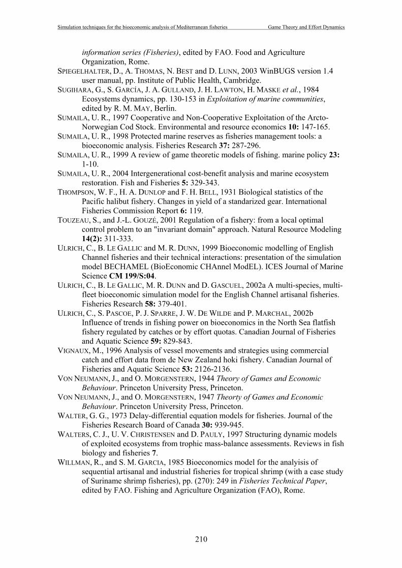
Simulation techniques for the bioeconomic analysis of Mediterranean fisheries Game Theory and Effort Dynamics
210
information series (Fisheries), edited by FAO. Food and Agriculture Organization, Rome.
SPIEGELHALTER, D., A. THOMAS, N. BEST and D. LUNN, 2003 WinBUGS version 1.4 user manual, pp. Institute of Public Health, Cambridge.
SUGIHARA, G., S. GARCÍA, J. A. GULLAND, J. H. LAWTON, H. MASKE et al., 1984 Ecosystems dynamics, pp. 130-153 in Exploitation of marine communities, edited by R. M. MAY, Berlin.
SUMAILA, U. R., 1997 Cooperative and Non-Cooperative Exploitation of the Arcto-Norwegian Cod Stock. Environmental and resource economics 10: 147-165.
SUMAILA, U. R., 1998 Protected marine reserves as fisheries management tools: a bioeconomic analysis. Fisheries Research 37: 287-296.
SUMAILA, U. R., 1999 A review of game theoretic models of fishing. marine policy 23:1-10.
SUMAILA, U. R., 2004 Intergenerational cost-benefit analysis and marine ecosystem restoration. Fish and Fisheries 5: 329-343.
THOMPSON, W. F., H. A. DUNLOP and F. H. BELL, 1931 Biological statistics of the Pacific halibut fishery. Changes in yield of a standarized gear. International Fisheries Commission Report 6: 119.
TOUZEAU, S., and J.-L. GOUZÉ, 2001 Regulation of a fishery: from a local optimal control problem to an "invariant domain" approach. Natural Resource Modeling 14(2): 311-333.
ULRICH, C., B. LE GALLIC and M. R. DUNN, 1999 Bioeconomic modelling of English Channel fisheries and their technical interactions: presentation of the simulation model BECHAMEL (BioEconomic CHAnnel ModEL). ICES Journal of Marine Science CM 199/S:04.
ULRICH, C., B. LE GALLIC, M. R. DUNN and D. GASCUEL, 2002a A multi-species, multi-fleet bioeconomic simulation model for the English Channel artisanal fisheries. Fisheries Research 58: 379-401.
ULRICH, C., S. PASCOE, P. J. SPARRE, J. W. DE WILDE and P. MARCHAL, 2002b Influence of trends in fishing power on bioeconomics in the North Sea flatfish fishery regulated by catches or by effort quotas. Canadian Journal of Fisheries and Aquatic Science 59: 829-843.
VIGNAUX, M., 1996 Analysis of vessel movements and strategies using commercial catch and effort data from de New Zealand hoki fishery. Canadian Journal of Fisheries and Aquatic Science 53: 2126-2136.
VON NEUMANN, J., and O. MORGENSTERN, 1944 Theory of Games and Economic Behaviour. Princeton University Press, Princeton.
VON NEUMANN, J., and O. MORGENSTERN, 1947 Theorty of Games and Economic Behaviour. Princeton University Press, Princeton.
WALTER, G. G., 1973 Delay-differential equation models for fisheries. Journal of the Fisheries Research Board of Canada 30: 939-945.
WALTERS, C. J., U. V. CHRISTENSEN and D. PAULY, 1997 Structuring dynamic models of exploited ecosystems from trophic mass-balance assessments. Reviews in fish biology and fisheries 7.
WILLMAN, R., and S. M. GARCIA, 1985 Bioeconomics model for the analyisis of sequential artisanal and industrial fisheries for tropical shrimp (with a case study of Suriname shrimp fisheries), pp. (270): 249 in Fisheries Technical Paper, edited by FAO. Fishing and Agriculture Organization (FAO), Rome.

References
211
View publication statsView publication stats