Prehispanic and Colonial Maya Subsistence and Migration: Contributions from Stable Sulfur Isotope Analysis

by © Asta Jade Rand

A dissertation submitted to the School of Graduate Studies in partial fulfillment of the requirements for the degree of

Doctor of Philosophy

Department of Archaeology Faculty of Humanities and Social Sciences

Memorial University of Newfoundland

June 2021

St. John’s, Newfoundland and Labrador, Canada

ii

ABSTRACT

The Maya who inhabited southeastern Mesoamerica from the Preclassic to Colonial

periods (1000 BCE to 1821 CE) have been the focus of intensive archaeological study for

over a century. Recent theoretical and methodological developments have contributed to

nuanced understandings of Maya migration and subsistence practices. Stable sulfur isotope

(δ34S) analysis of bone collagen is a novel technique that has been applied to Maya skeletal

collections, although the variation in environmental δ34S values throughout the Maya

region has yet to be systematically characterized. This research presents the first Maya

faunal sulfur isotope baseline based on the δ34S values of 148 archaeological faunal remains

from 13 sites in the Northern and Southern Lowlands. As expected, terrestrial animals in

coastal areas had elevated δ34S due to sea spray. However, those from inland sites had

unexpectedly high δ34S values that varied depending on the age of the underlying limestone.

Although the δ34S values of marine animals were lower than expected, similarly low values

in freshwater animals permits the differentiation of freshwater and terrestrial animals at

inland sites. These data demonstrate that sufficient variation in δ34S values exists in the

Maya region to identify sources of protein and nonlocal animals, which speaks to

prehispanic Maya animal exchange and interregional interaction. The δ34S values of 49

humans from seven Maya sites ranging from the Preclassic to Colonial periods were also

interpreted using the faunal baseline. The spatial distribution of human δ34S values differed

from that of the terrestrial fauna, demonstrating sociocultural variation in Maya resource

procurement in addition to underlying environmental influences. A comparison of carbon

and nitrogen data from the same individuals also revealed the consumption of protein from

different catchments. Nonlocal δ34S values show three individuals migrated near the end of

iii

their lives, and when integrated with childhood strontium and oxygen isotope data from

tooth enamel, demonstrate a more robust means of investigating the length of residence and

potentially the extent of integration into the receiving community. Finally, a case study of

the prehispanic Maya from Nakum, Guatemala, demonstrates the contributions of stable

sulfur isotope analysis to the interpretation of Maya subsistence strategies and migration

when integrated into a multi-isotopic approach.

iv

GENERAL SUMMARY

Although the Maya who lived in Central America from 1000 BCE to 1821 CE have

been studied by archaeologists for over a century, new theories and methods have changed

how archaeologists understand Maya migration and diet. Stable sulfur isotope values of

animal and human bone come from the protein in their diet and show where they obtained

their food. Researchers must therefore know the sulfur isotope values of plants and animals

throughout a region to see if people consumed freshwater, marine, or terrestrial animals

and if they moved to an area with different sulfur isotope values before they died. This

method has been used in Maya archaeology, but the sulfur isotope values in this area are

not well known.

This research analyzed sulfur isotopes in 148 archaeological animal bones from 13

sites to understand how they change throughout the Maya region. Marine and freshwater

animals had lower values than terrestrial animals, allowing different types of protein in

human diets to be identified. The terrestrial animal sulfur isotope values also relate to the

age of limestone in an area, so that animals acquired nonlocally could be differentiated

from local ones. The animal values provided a baseline for interpreting those of 49 human

bones from seven inland Maya sites. Lower sulfur values from human tissues suggest the

consumption of more freshwater animals. However, when interpreted with carbon and

nitrogen isotope data, it seems the Maya ate plants and animals from different areas

compared to the terrestrial animals. Three people also migrated to the sites where they were

buried because their sulfur isotope values differed from the remaining individuals at each

site. The length of time they lived where they were buried, and therefore their relationship

with local people, was investigated by combining their sulfur isotope values with strontium

v

and oxygen isotope values from childhood, as well as archaeological data. A case study

from the site of Nakum, Guatemala, shows how the analysis of sulfur isotopes and other

data helps archaeologists understand what Maya people ate, if they moved, and how they

lived in the past.

vi

CO-AUTHORSHIP STATEMENT

Because this dissertation was written in a manuscript style, the chapters are in

various stages of publication, several of which were written in collaboration with coauthors.

The dissertation author was the primary author of the chapters presented within this

dissertation, and is the primary author of all resulting publications, excluding that of the

human sulfur isotope values from the Eastern Lowlands (see below for details). While the

coauthors of Chapters 3 and 5 provided samples, resources, supervision, and comments on

previous drafts, the dissertation author was responsible for the research design, sample

acquisition and preparation, data interpretation, manuscript drafting and editing the

chapters of this dissertation, submitting the resulting manuscripts for review, and

incorporating reviewer and coauthor comments into subsequent drafts prior to publication.

Details regarding the co-authors and publication venues for the data presented within this

dissertation are provided below.

The author intends to submit Chapter 2 in the form of a review article to the Journal

of Archaeological Research as the sole author. The faunal sulfur isotope baseline for the

Maya region presented in Chapter 3 was coauthored with Dr. Carolyn Freiwald (University

of Mississippi) and Dr. Vaughan Grimes (Memorial University of Newfoundland) and has

been published in the Journal of Archaeological Science: Reports (Rand et al. 2021a).

While the dissertation author was the sole author of Chapter 4, the data presented

therein will be distributed among several publication venues. For example, the human

isotopic values from sites located in the Belize Valley and surrounding areas were included

in a comprehensive analysis of sulfur isotopes from Maya remains in the Eastern Lowlands

entitle “Paleodietary reconstruction and human mobility from the Preclassic through

vii

Colonial periods in the Eastern Maya lowlands” currently under review by PLoS One

(Manuscript #: PONE-D-21-05019) in collaboration with principle author Dr. Claire Ebert

(University of Pittsburgh), as well as co-authors Dr. Kirsten Green-Mink (University of

Montana), Dr. Julie Hoggarth (Baylor University), Dr. Freiwald, Dr. Jaime Awe (Northern

Arizona University), Dr. Willa Trask (Defence POW/MIA Accounting Agency), Dr. Jason

Yaeger (The University of Texas at San Antonio), Dr. M. Kathryn Brown (The University

of Texas at San Antonio), Dr. Christophe Helmke (University of Copenhagen), Rafael

Guerra (Institute of Archaeology, Belize), Dr. Marie Danforth (University of Southern

Mississippi), and Dr. Douglas Kennett (University of California, Santa Barbara) (Ebert et

al. under review).

The human isotopic data from Caledonia were also presented as a paper at the 48th

Annual Meeting of the Canadian Association for Physical Anthropology in November 2020

co-authored with Dr. Freiwald and Dr. Grimes (Rand et al. 2020b). Similarly, the results

from Xunantunich and San Lorenzo were presented at the first annual Bioarchaeology

Early Career Conference (BECC) 2021 on March 25, 2021, with co-authors Dr. Freiwald,

Dr. Yaeger, Dr. Brown, and Dr. Grimes (Rand et al. 2021b).

The human isotopic data from the Chac II and Calakmul have been submitted as

reports to the Instituto Nacional de Antropología e Historia (INAH), and the author intends

to publish those from Mission San Bernabé in Guatemala in collaboration with Dr.

Freiwald, Dr. Katherine Miller Wolf (University of West Florida), and Dr. Timothy Pugh

(City University of New York).

Finally, the isotopic case study from Nakum presented in Chapter 5 was published

as a research article in the Journal of Archaeological Science: Reports (Rand et al. 2020a)

viii

and was coauthored with Varinia Matute (Universidad de San Carlos de Guatemala), Dr.

Grimes, Dr. Freiwald, Dr. Jarosław Źrałka (Uniwersytet Jagielloński), and Dr. Wiesław

Koszkul (Uniwersytet Jagielloński). The Nakum data are also presented in a chapter in a

monograph about the site and is currently in review (Rand and Freiwald n.d.).

ix

ACKNOWLEDGEMENTS

An endeavour such as this could not have been undertaken without the help, advice,

and support of many people. I would first and foremost like to thank my supervisors, Dr.

Vaughan Grimes (Memorial University of Newfoundland (MUN)) and Dr. Carolyn

Freiwald (University of Mississippi). Dr. Grimes inspired me to investigate the application

of sulfur isotope analysis in Maya archaeology and this project would never have come to

fruition without the generosity of Dr. Freiwald. I am indebted to you both for your

invaluable mentorship, support, training, and guidance throughout this process.

The Department of Archaeology, Memorial Applied Archaeological Sciences

Laboratory, and School of Graduate Studies provided resources, assistance, and funding

during my tenure at MUN, and I am grateful to the faculty and staff of each. I am

particularly thankful for my supervisory and comprehensive exam committee members, Dr.

Meghan Burchell (MUN), Dr. Michael Deal (MUN), Dr. Lisa Rankin (MUN), Dr. Kathryn

Reese-Taylor (University of Calgary), and Dr. Peter Whitridge (MUN). I would also like

to thank my defence examiners, Dr. Andrew Scherer (Brown University), Dr. Andrew

Somerville (Iowa State University), and Dr. Whitridge, for your detailed comments on an

earlier draft of this dissertation and stimulating questions during my defence. The

thoughtful and constructive comments and advice from the members of my supervisory,

comprehensive exam, and defence committees on earlier drafts of the chapters included in

this dissertation has strengthened this research into a cohesive whole.

This work was also financially supported through several sources, including a

Social Sciences and Humanities Research Council (SSHRC) of Canada Joseph-Armand

Bombardier Canadian Graduate Scholarship (CGS) Doctoral Award (#767-2014-2712), as

x

well as a Scholarship in the Arts Doctoral Completion Award from the MUN Faculty of

Social Sciences, a MUN Scotiabank Bursary for International Study, and a FA Aldrich

Fellowship from the MUN School of Graduate Studies (SGS). Funding for the preparation

and analysis of the Nakum human and faunal remains was provided to Dr. Jarosław Źrałka

(Jagiellonian University) by the National Science Centre, Poland (under the agreement no.

UMO-2014/14/E/HS3/00534).

This research would also not have been possible without the collaboration of

numerous researchers who kindly provided samples for analyses. Dr. Paul Healy and Kate

Dougherty of the Department of Anthropology at Trent University provided the human and

faunal samples from Caledonia, Pacbitun, and Moho Cay, Belize. I am thankful to Dr.

Healy for allowing me to continue my work with the Caledonia collection and for the

opportunity to visit Trent again. Dr. Marilyn Masson (State University of New York at

Albany) provided faunal samples from Caye Coco, Caye Muerto, Chanlacan, and the

Laguna de On Island and Shore settlements. The human and faunal remains from

Xunantunich and San Lorenzo in Belize were provided by Dr. Jason Yaeger (The

University of Texas at San Antonio) and Dr. M. Kathryn Brown (The University of Texas

at San Antonio), and the faunal remains from Caracol, Belize, were provided by Dr. Jaime

Awe (Northern Arizona University). Dr. Źrałka provided the human and faunal samples

from Nakum, Guatemala and generously provided lodging while I stayed in Flores

analyzing the Nakum faunal collection. The human samples from Mission San Bernabé and

faunal specimens from Tayasal, Guatemala, were provided by Dr. Timothy Pugh (City

University of New York) and Evelyn Chan Nieto (Centro Universitario de Petén). The

faunal remains from Oxtankah, San Miguelito, and Ichpaatun in Mexico were provided by

xi

Dr. Allan Ortega Muñoz (Instituto Nacional de Antropología e Historia (INAH) of

Mexico), and Dr. Jeffery Glover (Georgia State University) provided the faunal samples

from Vista Alegre, Mexico. Finally, the human samples from Calakmul and Chac in

Mexico were provided by Dr. Vera Tiesler (Universidad Autónoma de Yucatán) and Dr. T.

Douglas Price (University of Wisconsin-Madison). I would also like to thank the Belize

Institute of Archaeology (IOA), the Guatemalan Instituto de Antropología e Historia

(IDAEH), and INAH for granting permission for the export and subsequent analyses of the

samples included in this research, and Dr. Ortega Muñoz whose guidance and assistance in

obtaining permission from INAH was indispensable.

The data presented in this dissertation was analyzed by several laboratories and I

would like to extend my thanks to each. I am indebted to Alison Pye (MUN CREAIT –

TERRA Facility) for her help and patience as I weighed samples for analysis, and for our

lovely coffee chats. I would also like to thank Hilary Keats and Geert Van Bisen (MUN

CREAIT – TERRA Facility) as well as Rebecca Lam (MUN CREAIT – MAF Facility) and

Rachelle Brydon (MUN Archaeology Department) for their assistance with sample analysis

at MUN. Unfortunately, all good things must come to an end and the TERRA Facility’s

MAT 252 mass spectrometer was sadly retired early in my tenure at MUN. Fortunately,

Anthony Faiia (Department of Earth and Planetary Sciences Stable Isotope Laboratory,

University of Tennessee Knoxville) and Paul Middlestead (Ján Veizer Stable Isotope

Laboratory, University of Ottawa) agreed to analyze the stable sulfur isotopes of the

remaining samples included in this dissertation, and I am indeed grateful for their

collaboration.

xii

There are several other people whose advice, guidance, and generosity have greatly

contributed to the quality of this dissertation research. First, I would like to thank Susana

Vallejos (MUN) for her assistance with editing the Spanish versions of my research

proposals. As a novice zooarchaeologist, I would also like to thank Elizabeth Ojeda

Rodriguez (Universidad de Granada) for providing invaluable resources for the

identification of faunal species, as well as Arianne Boileau (University of Florida) and

Deirdre Elliot (MUN) for their assistance with species identification. I would also like to

thank Nathalie Vanasse (MUN Department of Chemistry) and Dr. Guangju Zhai and

Maggie Liu (MUN Discipline of Genetics, Faculty of Medicine) for assistance with

grinding collagen samples for analysis. Dr. Gyles Iannone (Trent University) kindly

provided the original Social Archaeology Research Project (SARP) map that was used to

create Figure 4.3, and Dr. Źrałka provided the images of Nakum’s Burial 8 included in

Figure 5.3. I am also deeply indebted to Bryn Trapper (MUN) for his assistance with

creating the geological baseline maps in Figures 1.1, 3.1, and 4.1, as I appear to be more

proficient with isotope analysis than navigating the depths of ArcGIS™. Similarly, Dr. Jan

Romaniszyn’s (Adam Mickiewicz University) talent with Corel® far exceeds my own

experience with MS Paint, and I am deeply grateful for his assistance with editing the

figures included herein. Dr. Claire Ebert and Dr. Kirsten Green-Mink have also provided

invaluable support for this research. They shared data and insights that have changed the

way I think about sulfur isotope analysis and the Maya, and I will be forever grateful for

their collaboration and support.

The faculty, staff, and fellow graduate students in the Department of Archaeology

also made my time at MUN unforgettable. I want to express my deep gratitude to the

xiii

Awesome Isotope Peoples, Dr. Megan Bower, Jess Munkittrick, Dr. Alison Harris,

Rachelle Brydon, Megan Garlie, and Dr. Maddie Mant for your friendship, simulating

conversation, and shared passion for archaeological chemistry. Donna Teasdale and Alexa

Spiwak also provided invaluable materials, advice, and support, and I thank you both for

your assistance while I navigated the Conservation Laboratory.

I would additionally like to thank the MUN Department of Archaeology and

Writing Centre for the opportunity to gain valuable tutoring and teaching experience. As a

Teaching and Research Assistant, and later as a Per Course Instructor in the Department of

Archaeology, I was able to conduct research and teach topics beyond those covered in this

dissertation. I would also like to express my gratitude to Ginny Ryan and Diane Ennis of

the MUN Writing Centre who inspired my passion for tutoring and made me feel at home.

The results of this dissertation research have been and will be published in peer-

reviewed venues, and I would like to thank my coauthors here. Dr. Freiwald and Dr. Grimes

have been infinitely patient while commenting on various article drafts, and I thank them

for their insightful suggestions and for their confidence in my work. I would also like to

thank the coauthors of the Nakum publication (Rand et al. 2020a), Dr. Źrałka, Varinia

Matute (Universidad de San Carlos de Guatemala), and Dr. Wiesław Koszkul (Jagiellonian

University) for their assistance with funding, resources, samples, and analyses, and for their

helpful comments on previous drafts of the manuscript. I would like to thank Dr. Ebert for

the opportunity to include the Maya sulfur isotope data from several sites analyzed in this

dissertation in a broader study of sulfur isotope variation across the Eastern Lowlands,

along with coauthors, Dr. Kirsten Green-Mink (University of Montana), Dr. Julie Hoggarth

(Baylor University), Dr. Freiwald, Dr. Jaime Awe (Northern Arizona University), Dr. Willa

xiv

Trask (Defence POW/MIA Accounting Agency), Dr. Christophe Helmke (University of

Copenhagen), Rafael Guerra (Institute of Archaeology, Belize), Dr. Marie Danforth

(University of Southern Mississippi), Dr. Jason Yaeger (The University of Texas at San

Antonio), Dr. M. Kathryn Brown (The University of Texas at San Antonio), and Dr.

Douglas Kennett (University of California, Santa Barbara). I would also like to thank Dr.

Freiwald, Dr. Grimes, Dr. Yaeger, and Dr. Brown for agreeing to coauthor and making

insightful comments and suggestions on papers presented at the annual meeting of the

Canadian Association for Physical Anthropology (CAPA 2020) and Bioarchaeology Early

Career Conference (BECC 2021).

Numerous people have provided friendship and support over the last seven years

beyond that of research and academia. I send a warm and special thanks to my second

family, the Kellys, especially Linda and Shawn, who always made sure I had a safe place

to stay. I would also like to thank Jess Munkittrick, John Campbell, Chelsee Arbour, Alexa

Spiwak, Heather Zanzerl, Ryan Zier-Vogal, Megan Bower, Laura McIntosh, Derek Kelly,

Alanah Kelly, Rachel Kelly, Theresa Kelly, Andrew McCuaig, Maddison Payne, Alyssa

Brown, and Jan Romaniszyn. Despite my ineptitude at board games, Game Nights at

Megan’s, Heather and Ryan’s, and later JJ’s provided spirited competition and much

needed breaks from academia. Maddie, although we lived at opposite ends of the country

and I have been a little distracted over the last seven years, I know we will make it to

Scotland one day. Alyssa, to be fair, I would never have survived my last year in St. John’s

without your friendship and I cannot wait for the next time we order all the food and binge

watch our favourite shows. And Jasiu, my dearest friend, I am eternally thankful for your

xv

friendship and cannot find the words to express what your encouragement, confidence, and

advice have meant to me over the years.

Finally, I am forever grateful for the love and support of my family. My parents,

Paul and Leah, nurtured my enthusiasm and thirst for knowledge from a young age while

encouraging me to pursue opportunities they did not have. Although the three of us are very

different, my siblings, Casey and Aubrey, have always been supportive and encouraging,

and in their brilliance remind me there is more to life than academia. You are all “super

green” for believing in me, especially when I had trouble believing in myself.

xvi

LIST OF CONTRIBUTIONS

Peer Reviewed Journal Articles 2021 Rand AJ, Freiwald C, Grimes V. A multi-isotopic (δ13C, δ15N, and δ34S) faunal

baseline for Maya subsistence and migration studies. Journal of Archaeological Science Reports 37:102977. doi: 10.1016/j.jasrep.2021.102977.

2020 Freiwald C, Miller Wolf KA, Pugh T, Rand A, Fullagar P. Early colonialism

and population movement at the Mission of San Bernabé, Guatemala. Ancient Mesoamerica. 31(3):543-553. doi: 10.1017/S0956536120000218.

2020 Rand AJ, Matute V, Grimes V, Freiwald C, Źrałka J, Koszkul W. Prehispanic

Maya diet and Mobility at Nakum, Guatemala: A multi-isotopic approach. Journal of Archaeological Science: Reports 32C: 102374. doi: 10.1016/j.jasrep.2020.102374.

2015 Rand A, Bower M, Munkittrick J, Harris A, Burchell M, Grimes V.

Comparison of three bone collagen extraction procedures: The effect of preservation on δ13C and δ15N values. North Atlantic Archaeology 4:93-113.

2015 Rand AJ, Healy PF, Awe JJ. Stable Isotopic Evidence of Ancient Maya Diet at

Caledonia, Cayo District, Belize. The International Journal of Osteoarchaeology 25:401-413. doi: 10.1002/oa.2308.

In review Ebert C, Rand A, Green-Mink K, Hoggarth J, Freiwald C, Awe J, Trask W, J

Yaeger, MK Brown, Helmke C, Guerra R, Danforth M, Kennett D. Applying sulfur isotopes to paleodietary reconstruction and human mobility from the Preclassic through Colonial periods in the Eastern Maya lowlands. PLoS ONE. Manuscript #: PONE-S-21-05019.

Sections in Edited Volumes 2018 Rand AJ, Nehlich O. Diet and sulfur isotopes. In: López-Varela S, editor. The

Encyclopedia of Archaeological Sciences. Wiley-Blackwell. doi: 10.1002/9781119188230.saseas0186.

2017 Rand AJ. Ancient Maya mobility at Caledonia, Cayo District, Belize: Evidence

from stable oxygen isotopes. In: Patton, M., Manion J., editors. Trading Spaces: The Archaeology of Interaction, Migration and Exchange. Proceedings of the 46th Annual Chacmool Conference. Calgary, AB: Chacmool Archaeology Association, the University of Calgary. p. 32-43.

Accepted Freiwald C, Rand A, Belanich J. What’s new in molecular approaches to bones,

inside and out. In Tiesler V, editor. Handbook of Mesoamerican Bioarchaeology. Routledge. To be published in 2021.

In review Rand A, Freiwald C. Reconstructing the isotopic life histories of the Nakum

Maya. In The Nakum Archaeological Project Monograph Series, edited by J Źrałka. Cracow: Jagiellonian University Press. To be published in 2021.

xvii

Conference Abstracts 2017 Rand A, Grimes V. The environmental sulfur isotope composition of the Maya

Region: A working model and preliminary results. American Journal of Physical Anthropology 162(S64):327. doi: 10.1002/ajpa.23210

Presented Papers 2021 Rand AJ, Freiwald C, Yaeger J, Brown MK, Grimes V. Interpreting Maya

migration from birth to death: A multi-isotopic case study from Xunantunich and San Lorenzo, Belize. Paper presented synchronically at the Bioarchaeology Early Career Conference (BECC) 2021, March 25-28.

2020 Rand AJ, Freiwald C, Grimes V. Ancient Maya Catchment Use: Stable Sulfur

Isotopic Evidence from Caledonia, Cay District, Belize. Paper presented synchronically at the 48th Annual Meeting of the Canadian Association for Physical Anthropology, November 4-6.

2018 Freiwald C, Green K, Rand A, Trask W, Novotny A. Maya Mobility: Isotopes,

Molecules and Migration in Belize. Paper presented at the 16th Annual Belize Archaeology Symposium, San Ignacio, Belize, June 27-29.

2015 Bower M, Rand A. Contemplating the Relationship between Mobility Theory

and Bioarchaeology: Past and Present Behaviours. Paper presented at the 47th Annual Meeting of the Canadian Archaeological Association, Memorial University of Newfoundland, St. John’s, NL, April 29 – May 3.

2013 Rand A. Characterizing Human Mobility at Caledonia, Cayo District, Belize:

Evidence from Stable Oxygen Isotope Analysis. Paper presented at the 46th Annual Chacmool Archaeology Conference, University of Calgary, Calgary, AB, November 7-9.

2011 Rand A. Isotopic Investigations of Diet at Caledonia, Cayo District, Belize.

Paper presented at the 39th annual meeting of the Canadian Association for Physical Anthropology, Montreal, QC, October 26-29.

Presented Posters 2017 Rand A, Grimes V. The Environmental Sulfur Isotope Composition of the Maya

Region: A Working Model and Preliminary Results. Poster presented at the 86th annual meeting of the American Association of Physical Anthropologists, New Orleans, LA, April 20.

2014 Rand A, Munkittrick J, Harris A, Bower M, Burchell M, Grimes V. Comparing

Three Collagen Extraction Procedures for Stable Carbon and Nitrogen Isotope Analysis of Archaeological and Modern Bone. Poster presented at the 42nd annual meeting of the Canadian Association for Physical Anthropology, Fredericton, NB, November 6-9.

xviii

TABLE OF CONTENTS ABSTRACT ii GENERAL SUMMARY iv CO-AUTHORSHIP STATEMENT vi ACKNOWLEDGEMENTS ix LIST OF CONTRIBUTIONS xvi TABLE OF CONTENTS xviii LIST OF TABLES xxii LIST OF FIGURES xxvi CHAPTER 1: Introduction 1

1.1 A Brief Introduction to the Maya 2 1.2 Applications of Sulfur Isotope Analysis in Archaeology 8 1.3 Chapter Descriptions 14

CHAPTER 2: Contributions of Isotopic Analyses to Conceptualizations of

Migration in Maya (Bio)archaeology 19 2.1 Migration in (Bio)archaeological Thought 21

2.1.1 Conceptualizing Migration in Archaeology 22 2.1.2 Conceptualizing Migration in Bioarchaeology 29

2.2 Methodological Implications for Conceptualizations of Migration in Bioarchaeology 32

2.2.1 Biodistance Analyses of Migration 34 2.2.2 Identifying Nonlocal Individuals Using Isotopic Analyses 35

2.3 Defining Migration in (Bio)archaeological Isotope Studies 40 2.4 Contributions of Stable Isotope Analysis to Understandings of Maya

Migration 46 2.4.1 Initial Interpretations of Migration in the Maya Region 46 2.4.2 Bioarchaeological Evidence for Maya Migration 48 2.4.3 Isotopic Approaches to Maya Migration 50

2.5 Chapter 2 Summary 61 CHAPTER 3: A Multi-Isotopic (δ34S, δ13C, and δ15N) Faunal Baseline for Maya

Subsistence and Migration Studies 63 3.1 Principles of Stable Isotope Analysis 65 3.2 Expected Variability of Environmental δ34S values in the Maya Region 69 3.3 Materials and Methods 77

xix

3.4 Results 80 3.4.1 Stable Carbon and Nitrogen Isotope Analysis 81 3.4.2 Stable Sulfur Isotope Analysis 83

3.5 Discussion 92 3.5.1 Variation of Faunal δ34S Values in the Maya Region 92 3.5.2 Implications for Studies of Maya Diet, Animal Exchange, and

Migration 98 3.6 Chapter 3 Summary and Conclusions 100

CHAPTER 4: Stable Sulfur Isotope Evidence of Subsistence Practices and

Migration among the Maya 103 4.1 Principles of Stable Isotope Analysis 104 4.2 Site and Sample Description 108

4.2.1 Xunantunich and San Lorenzo, Belize 108 4.2.2 Pacbitun, Belize 114 4.2.3 Caledonia, Cayo District, Belize 115 4.2.4 Nakum, Guatemala 117 4.2.5 Mission San Bernabé, Guatemala 118 4.2.6 Calakmul, Mexico 119

4.3 Methods 120 4.4 Results 123

4.4.1 Data Comparability 123 4.4.2 Sample Integrity 124 4.4.3 Isotopic Results 125

4.5 Discussion 134 4.5.1 Spatial Distribution of Sulfur Isotope Values 135 4.5.2 Isotopic Evidence for Maya Subsistence Practices 137

4.5.2.1 Prehispanic Maya Subsistence Practices 137 4.5.2.2 Colonial Period Maya Subsistence Practices 143

4.5.3 Nonlocal Individuals at Maya Sites 145 4.5.3.1 Local Individuals in Formal Funerary Contexts at

Prehispanic Maya Sites 146 4.5.3.2 Nonlocal Individuals in Non-Funerary Deposits at

Prehispanic Maya Sites 148 4.5.3.3 Nonlocal Individuals in Funerary Contexts at

Prehispanic Maya Sites 153 4.5.3.4 Colonial Impacts on Maya Migration 154

4.6 Chapter 4 Summary and Conclusions 156 CHAPTER 5: Prehispanic Maya Diet and Mobility at Nakum, Guatemala: A

Multi-Isotopic Approach 160 5.1 Archaeological and Environmental Context 161 5.2 Principles of Isotopic Analyses in Bioarchaeology 165 5.3 Materials and Methods 170 5.4 Results 175

xx

5.5 Discussion 183 5.5.1 Diet at Prehispanic Nakum 183 5.5.2 Mobility at Prehispanic Nakum 186

5.6 Chapter 5 Summary and Conclusions 192 CHAPTER 6: Summary and Conclusions 194

6.1 Recommendations for Future Research 201 REFERENCES CITED 207 APPENDIX A: Detailed Methodology 276

A.1 Introduction 277 A.2 Sample Acquisition and Previous Analyses 277 A.3 Nakum Faunal Species Identification and Sample Selection 281 A.4 Sample Preparation and Analysis 282

A.4.1 Bone Collage Preparation and Analysis 282 A.4.2 Nakum Bone and Tooth Enamel Bioapatite Preparation and

Analysis 287 A.4.3 Strontium Isotope Preparation and Analysis of the Nakum Tooth

Samples 288 A.5 Analytical Uncertainty 289 A.6 Identifying Diagenesis 292

A.6.1 Bone Collagen 293 A.5.2 Bone and Tooth Enamel Bioapatite 294

A.7 Establishing Environmental Isotopic Baseline Values for Identifying Nonlocal Individuals 295

A.8 Statistical Analyses 300 APPENDIX B: Intra- and Inter-Laboratory Comparability of Isotopic Results 303

B.1 Introduction 304 B.2 Materials and Methods 304 B.3 Results 307

B.3.1 Intra-Sample Variation of Stable Carbon and Nitrogen Results from Samples Treated with and without Sodium Hydroxide 307

B.3.2 Intra-Laboratory Variation of Stable Sulfur Isotope Values 311 B.3.3 Inter-Laboratory Variation of Stable Sulfur Isotope Values 317

B.4 Summary and Conclusions 319 APPENDIX C: Analytical Uncertainty of the Isotopic Measurements 322

C.1 Introduction 323 C.2 Stable Carbon and Nitrogen Isotope Analysis of Bone Collagen 323

C.2.1 Stable Isotope Laboratory, Memorial University of Newfoundland 323 C.2.2 Ján Veizer Stable Isotope Laboratory, University of Ottawa 326

C.3 Sulfur Isotope Analysis of Bone Collagen 329 C.3.1 Stable Isotope Laboratory, Memorial University of Newfoundland 329

xxi

C.3.2 Stable Isotope Laboratory, University of Tennessee Knoxville 330 C.3.3 Ján Veizer Stable Isotope Laboratory, University of Ottawa 333

C.4 Calibration and Analytical Uncertainty of the Nakum Isotopic Measurements 334

C.4.1 Carbon and Nitrogen Isotope Analysis of the Nakum Bone Collagen Samples 334

C.4.2 Sulfur Isotope Analysis of the Nakum Bone Collagen Samples 336 C.4.3 Oxygen and Carbon Isotope Analysis of the Nakum Bone and

Tooth Enamel Bioapatite Samples 338 C.5 Discussion and Conclusion 339

APPENDIX D: Species, Contextual, and Isotopic Data of the Maya Faunal Samples 344 APPENDIX E: Osteological, Contextual, and Isotopic Data of the Maya Human

Samples 359

xxii

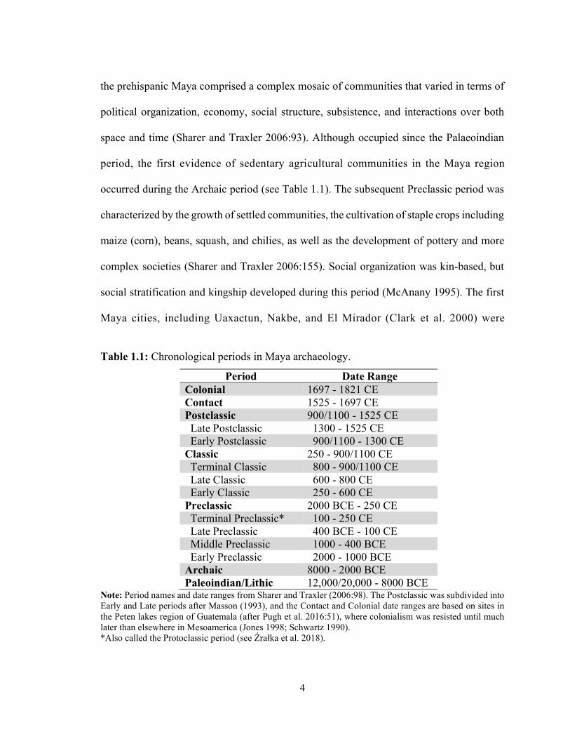
LIST OF TABLES Table 1.1 Chronological periods in Maya archaeology. 4 Table 3.1 Average and standard deviation of the δ13C and δ15N values of

freshwater, terrestrial, and marine fauna. The values of individual samples can be found in Appendix D1. 82

Table 3.2 Summary statistics of the faunal δ34S values from each site by source

of dietary protein. All values are in ‰ relative to VCDT excluding the number of samples, n. IQR = Interquartile range. 84

Table 3.3 Average and standard deviation of the δ34S values of terrestrial,

freshwater, and marine fauna by age of underlying geology and distance of each site from the coast. 90

Table 4.1 Summary of the osteological and contextual data of the Maya human

samples included in this study by site. 111 Table 4.2 Summary statistics of the human δ13C, δ15N, and δ34S values by site. 126 Table 4.3 Significance (p-value) of the post hoc pairwise comparisons of the

Kruskal-Wallis test of the δ13C values among sites. 127 Table 4.4 Significance (p-value) of the post hoc pairwise comparisons of the

Kruskal-Wallis test of the δ15N values among sites. 127 Table 4.5 Number of individuals with nonlocal δ34S values from the sites included

in this study. 130 Table 4.6 Local ranges of δ34S values for sites included in the study determined

as falling within two standard deviations of the mean when the outlying values from Xunantunich/San Lorenzo, Pacbitun, and Caledonia are removed. 131

Table 4.7 Significance (p-value) of the Games-Howell post hoc evaluation of the

one-way ANOVA of the δ34S values among sites. 131 Table 4.8 Average and standard deviation of δ34S values of human, terrestrial,

and freshwater animals from Nakum, Xunantunich/San Lorenzo, and Pacbitun 134

Table 4.9 Bone collagen δ13C and δ15N values from Contact and Colonial period

Maya sites. 144 Table 5.1 Contextual, species, and biographical data for the Nakum fauna samples. 171 Table 5.2 Contextual and biographical data of the Nakum human samples. 172 Table 5.3 Stable carbon, nitrogen, sulfur, and oxygen isotope, concentration,

and quality data from bone samples. 177

xxiii

Table 5.4 Stable carbon, oxygen, and strontium isotope data from Nakum tooth samples. 180

Table B.1 Stable carbon and nitrogen isotope and concentration values of the

Caledonia samples organized by collagen extraction method that included or excluded a NaOH treatment and by laboratory that conducted the analyses. 308

Table B.2 Stable sulfur isotope and concentration values of the Caledonia

samples organized by laboratory and analytical session. 309

Table B.3 Intra-sample variability of δ13C and δ15N values from Caledonia samples of the same bone treated with and without NaOH during collagen extraction. 310

Table B.4 Shapiro-Wilk test for normality of the Caledonia samples prepared with

and without a NaOH treatment. 310 Table B.5 Paired samples t-test results of values from original samples and

resamples. 310 Table B.6 The δ34S and wt. %S of samples run in duplicate by lab and session. 313 Table B.7 Results of the Shapiro-Wilk (W) test for normality of δ34S and %S of

samples run in duplicate by analytical session. 315

Table B.8 Results of paired samples t-test for the δ34S and %S values of samples analyzed in duplicate. 315

Table B.9 Results of the Wilcoxon Signed Rank Test of the δ34S and %S values of samples run in duplicate. 316

Table B.10 The δ34S and wt. %S values for sample aliquots analyzed at MUN, Tennessee, and Ottawa. 318

Table C.1 Standard reference materials used for calibration of δ13C relative to

VPDB and δ15N relative to AIR and to monitor (check) internal accuracy and precision by the Stable Isotope Lab (MUN). 324

Table C.2 Mean and standard deviation of all check and calibration standards for

all carbon and nitrogen analytical sessions conducted by the Stable Isotope Lab (MUN). 325

Table C.3 Stable carbon and nitrogen isotopic compositions for all samples

analyzed in triplicate by the Stable Isotope Lab (MUN). 326 Table C.4 Standard reference materials used for calibration of δ13C relative to

VPDB and δ15N relative to AIR and to monitor (check) internal accuracy and Precision by the Ján Veizer Lab (University of Ottawa). 327

xxiv

Table C.5 Mean and standard deviation of the check standard included in an unknown number of carbon and nitrogen analytical sessions at the Ján Veizer Lab (University of Ottawa). 328

Table C.6 Stable carbon and nitrogen isotopic compositions for all samples

analyzed in duplicate by the Ján Veizer Lab (University of Ottawa). 328 Table C.7 Standard reference materials used for calibration of δ34S relative to

VCDT and to monitor (check) internal accuracy and precision by the Stable Isotope Lab (MUN). 329

Table C.8 Mean and standard deviation of all check and calibration standards for all sulfur analytical sessions at the Stable Isotope Lab (MUN). 329

Table C.9 Stable sulfur isotopic compositions for all samples analyzed in

duplicate by the Stable Isotope Lab (MUN). 330 Table C.10 Standard reference materials used for calibration of δ34S relative to

VCDT at the Stable Isotope Lab (University of Tennessee Knoxville). 331 Table C.11 Mean and standard deviation of all calibration standards for all sulfur

analytical sessions at the Stable Isotope Lab (University of Tennessee Knoxville). 331

Table C.12 Stable sulfur isotopic compositions for all samples analyzed in

duplicate or triplicate at the Stable Isotope Lab (University of Tennessee Knoxville). 332

Table C.13 Standard reference materials used to monitor (check) internal

accuracy and precision at the Ján Veizer Lab (University of Ottawa). 333 Table C.14 Mean and standard deviation of all check standards for all sulfur

analytical sessions at the Ján Veizer Lab (University of Ottawa). 333 Table C.15 Standard reference materials used for calibration of δ13C relative to

VPDB and δ15N relative to AIR during analysis of the Nakum bone collagen samples. 334

Table C.16 Standard reference materials used to monitor internal accuracy and

precision for all carbon and nitrogen isotope values of the Nakum bone collagen samples. 335

Table C.17 Mean and standard deviation of all check and calibration standards

for all carbon and nitrogen analytical sessions of the Nakum bone collagen samples. 335

Table C.18 Stable carbon and nitrogen isotopic compositions for all Nakum

bone collagen samples analyzed in duplicate. 336 Table C. 19 Standard reference materials used for calibration of δ34S relative to

VCDT during analysis of the Nakum bone collagen samples. 336

xxv

Table C.20 Mean and standard deviation of all check and calibration standards for all sulfur analytical sessions of the Nakum bone collagen samples. 337

Table C.21 Stable sulfur isotopic compositions for all Nakum bone collagen

samples analyzed in duplicate. 337 Table C.22 Standard reference materials used for calibration of δ13C and δ18O

relative to VPDB and to monitor (check) internal accuracy and precision by the SIL at MUN during analysis of the Nakum samples. 338

Table C.23 Mean and standard deviation of all check and calibration standards

for carbon and oxygen analytical sessions for the Nakum samples. 339 Table C.24 Stable carbon and oxygen isotopic compositions for all Nakum

samples analyzed in duplicate. 339 Table C.25 Measurements of analytical uncertainty for each isotope measurement

by laboratory. 340 Table D.1 Species and contextual data for the Maya faunal samples. 345 Table D.2 Isotopic and compositional data for individual Maya faunal samples. 352 Table E.1 Osteological and contextual data for the Maya human samples. 360 Table E.2 Isotopic and compositional data for individual Maya human samples 364

xxvi

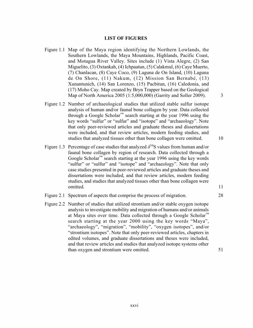
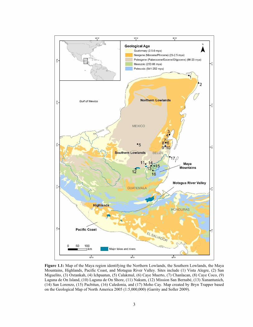
LIST OF FIGURES Figure 1.1 Map of the Maya region identifying the Northern Lowlands, the

Southern Lowlands, the Maya Mountains, Highlands, Pacific Coast, and Motagua River Valley. Sites include (1) Vista Alegre, (2) San Miguelito, (3) Oxtankah, (4) Ichpaatun, (5) Calakmul, (6) Caye Muerto, (7) Chanlacan, (8) Caye Coco, (9) Laguna de On Island, (10) Laguna de On Shore, (11) Nakum, (12) Mission San Bernabé, (13) Xunantunich, (14) San Lorenzo, (15) Pacbitun, (16) Caledonia, and (17) Moho Cay. Map created by Bryn Trapper based on the Geological Map of North America 2005 (1:5,000,000) (Garrity and Soller 2009). 3

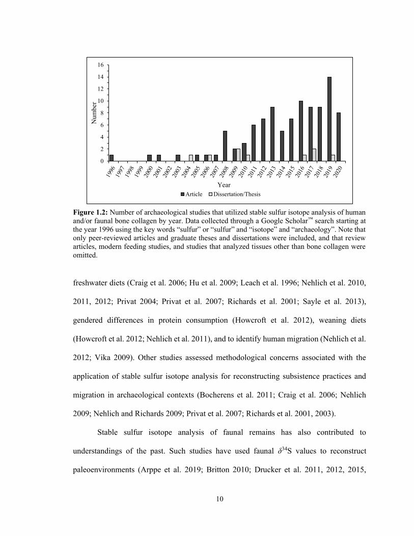
Figure 1.2 Number of archaeological studies that utilized stable sulfur isotope

analysis of human and/or faunal bone collagen by year. Data collected through a Google Scholar™ search starting at the year 1996 using the key words “sulfur” or “sulfur” and “isotope” and “archaeology”. Note that only peer-reviewed articles and graduate theses and dissertations were included, and that review articles, modern feeding studies, and studies that analyzed tissues other than bone collagen were omitted. 10

Figure 1.3 Percentage of case studies that analyzed δ34S values from human and/or faunal bone collagen by region of research. Data collected through a Google Scholar™ search starting at the year 1996 using the key words “sulfur” or “sulfur” and “isotope” and “archaeology”. Note that only case studies presented in peer-reviewed articles and graduate theses and dissertations were included, and that review articles, modern feeding studies, and studies that analyzed tissues other than bone collagen were omitted. 11

Figure 2.1 Spectrum of aspects that comprise the process of migration. 28 Figure 2.2 Number of studies that utilized strontium and/or stable oxygen isotope

analysis to investigate mobility and migration of humans and/or animals at Maya sites over time. Data collected through a Google Scholar™ search starting at the year 2000 using the key words “Maya”, “archaeology”, “migration”, “mobility”, “oxygen isotopes”, and/or “strontium isotopes”. Note that only peer-reviewed articles, chapters in edited volumes, and graduate dissertations and theses were included, and that review articles and studies that analyzed isotope systems other than oxygen and strontium were omitted. 51

xxvii

Figure 3.1 Geological map of the Maya region wherein colours represent the age of the underlying geology and location of major lakes and rivers. The hypothesized δ34S values for different subregions discussed in the text are also indicated, as are the locations of the sites included in this study: (1) Vista Alegre, (2) San Miguelito, (3) Oxtankah, (4) Ichpaatun, (5) Caye Muerto, (6) Chanlacan, (7) Caye Coco, (8) Laguna de On Island, (9) Laguna de On Shore, (10) Nakum, (11) Pacbitun, (12) Xunantunich, and (13) Moho Cay. Map created by Bryn Trapper based on the Geological Map of North America 2005 (1:5,000,000) (Garrity and Soller 2009). 71

Figure 3.2 Food web reconstructed from published faunal δ13C and δ15N values from the Maya region (boxes) with data from this study plotted. Boxes represent average and one standard deviation of data compiled from multiple studies (Keegan and DeNiro 1988; Norr 1991; White and Schwarcz 1989; White et al. 1993; Williams et al. 2009; Wright 2006). The δ13C values of modern samples were corrected for the fossil fuel (Seuss) effect by +1.5 ‰ (Marino and McElroy 1991) and more information can be found in Rand (2012). Individual species identifications, δ13C, and δ15N values for the samples analyzed in this study can be found in Appendix D. 82

Figure 3.3 Boxplots of the faunal δ34S values from the sites listed in Table 3.2

arranged by distance from the coast in km beneath site name. Individual data points (circles) have been superimposed over the boxplots, outliers are identified as larger filled circles that fall beyond the whiskers, and extreme outliers are identified as filled stars (see Appendix A for how outliers were identified using the IQR method). 85

Figure 3.4 Boxplots of the faunal δ34S values from each site arranged by distance

from the coast in kilometers (km) beneath the site name and grouped by source of dietary protein (terrestrial, freshwater, or marine) based on taxa identification. Circles indicate outliers whereas stars represent extreme outliers (see Appendix A for details). See Table 3.2 for the number of samples in each category for each site. 86

Figure 3.5 The δ34S values from fauna reliant on marine protein by site and taxa

plotted against (A) δ15N and (B) δ13C values from the same samples. 87 Figure 3.6 The δ34S values from fauna reliant on freshwater protein by site and

taxa plotted against (A) δ15N and (B) δ13C values from the same samples. 88

xxviii

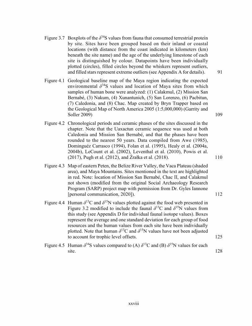
Figure 3.7 Boxplots of the δ34S values from fauna that consumed terrestrial protein by site. Sites have been grouped based on their inland or coastal locations (with distance from the coast indicated in kilometers (km) beneath the site name) and the age of the underlying limestone of each site is distinguished by colour. Datapoints have been individually plotted (circles), filled circles beyond the whiskers represent outliers, and filled stars represent extreme outliers (see Appendix A for details). 91

Figure 4.1 Geological baseline map of the Maya region indicating the expected

environmental δ34S values and location of Maya sites from which samples of human bone were analyzed: (1) Calakmul, (2) Mission San Bernabé, (3) Nakum, (4) Xunantunich, (5) San Lorenzo, (6) Pacbitun, (7) Caledonia, and (8) Chac. Map created by Bryn Trapper based on the Geological Map of North America 2005 (1:5,000,000) (Garrity and Soller 2009) 109

Figure 4.2 Chronological periods and ceramic phases of the sites discussed in the

chapter. Note that the Uaxactun ceramic sequence was used at both Caledonia and Mission San Bernabé, and that the phases have been rounded to the nearest 50 years. Data compiled from Awe (1985), Dominguéz Carrasco (1994), Folan et al. (1995), Healy et al. (2004a, 2004b), LeCount et al. (2002), Leventhal et al. (2010), Powis et al. (2017), Pugh et al. (2012), and Źrałka et al. (2018). 110

Figure 4.3 Map of eastern Peten, the Belize River Valley, the Vaca Plateau (shaded area), and Maya Mountains. Sites mentioned in the text are highlighted in red. Note: location of Mission San Bernabé, Chac II, and Calakmul not shown (modified from the original Social Archaeology Research Program (SARP) project map with permission from Dr. Gyles Iannone [personal communication, 2020]). 112

Figure 4.4 Human δ13C and δ15N values plotted against the food web presented in

Figure 3.2 modified to include the faunal δ13C and δ15N values from this study (see Appendix D for individual faunal isotope values). Boxes represent the average and one standard deviation for each group of food resources and the human values from each site have been individually plotted. Note that human δ13C and δ15N values have not been adjusted to account for trophic level offsets. 125

Figure 4.5 Human δ34S values compared to (A) δ13C and (B) δ15N values for each

site. 128

xxix

Figure 4.6 Boxplots of the human δ34S values. Boxes represent the interquartile range (IQR), black bars represent the median, and whiskers represent the IQR*1.5 subtracted from the first quartile and added to the third. Transparent circles within the boxes and whiskers represent individual data points, filled circles beyond the whiskers represent outliers that fall beyond the IQR*1.5 subtracted from the first quartile or added to the third, and stars represent extreme outliers that fall beyond the IQR*3 subtracted from the first quartile or added to the third. 129

Figure 4.7 Boxplot of the δ34S values of the Epicentre and Core Zone Burials from Pacbitun. Boxes represent the interquartile range (IQR), black bars represent the median, and whiskers represent the IQR*1.5 subtracted from the first quartile and added to the third. Transparent circles within the boxes and whiskers represent individual data points and stars represent extreme outliers that fall beyond the IQR*3 subtracted from the first quartile or added to the third. 129

Figure 4.8 Boxplots of the δ34S values by site after the outlying values from

Xunantunich/San Lorenzo, Caledonia, and Pacbitun are removed arranged by underlying geology. Boxes represent the interquartile range (IQR), black bars represent the median, and whiskers represent the IQR*1.5 subtracted from the first quartile and added to the third. Transparent circles within the boxes and whiskers represent individual data points. 132

Figure 4.9 Significantly positive correlation (dotted line) between the δ34S and

δ13C values from Caledonia (excluding the nonlocal individual). 133 Figure 4.10 Boxplots of human, terrestrial fauna, and freshwater fauna δ34S values

from Nakum, Pacbitun, and Xunantunich. Boxes represent the interquartile range (IQR), black bars represent the median, and whiskers represent the IQR*1.5 subtracted from the first quartile and added to the third. Stars represent extreme outliers that fall beyond the IQR*3 subtracted from the first quartile and added to the third. 133

Figure 4.11 Statistically significant positive correlation (dotted line) between the

δ34S and δ13C values from Caledonia (excluding the nonlocal individual). Elevated values indicate consumption of maize-based protein from limestone areas whereas lower values indicate the consumption of terrestrial animals from the Maya Mountains. 142

Figure 5.1 Geological map of the Maya region indicating the location of Nakum

and other sites mentioned in the text (adapted from Sharpe et al. (2016) and the U.S. Geological Survey Geological Map of North America [Reed et al. 2005]). 162

Figure 5.2 Map of Nakum located on the Holmul River illustrating the northern

and southern sectors of the site (Źrałka and Hermes 2012:163). 163

xxx

Figure 5.3 Plan and cross-section of Nakum Burial 8, an example of a richly furnished vaulted tomb located within a large pyramidal temple (Str. X), possibly the resting place of one of Nakum’s kings who reigned during the transition from the Early to Late Classic periods (A.D. 500/550-600). Note the presence of stingray spines in vessel PANC046. Image courtesy of Dr. Jarosław Źrałka and the PAN. 164

Figure 5.4 The δ13C and δ15N values of the fauna and human bone collagen from

Nakum. Humans are identified by laboratory number whereas fauna are identified by species. Note: WTD = white-tailed deer. 176

Figure 5.5 The δ13Cap and δ18Oap values of bone and tooth enamel samples from

Nakum. The shaded area represents the local range of δ18O values determined from the mean and two standard deviations of all human enamel and bone samples with viable collagen excluding the two outliers (x̅ ± 2σ = –3.9 ± 1.6 ‰). 179

Figure 5.6 Human and faunal δ34S values relative to (A) δ13C and (B) δ15N values from the same individual. Humans are identified by Lab # whereas fauna are identified by species. The shaded area represents the local range of δ34S values as determined from the faunal data (x̅ ± 2σ = +13.6 ± 1.4 ‰). 181

Figure 5.7 The δ18O and 87Sr/86Sr values of three human and one canine tooth

enamel samples from Nakum. The shaded area represents the local range of δ18O values (see text and Fig. 5.5 for details) and does not reflect local 87Sr/86Sr values. 182

Figure A.1 Accuracy versus precision. (A) No accuracy or precision; (B) Precision but no accuracy; (C) Accuracy but no precision; and (D) Accuracy and precision. 290

Figure B.1 Stable sulfur isotope values for the same sample analyzed at different

laboratories. 319

1

CHAPTER 1

INTRODUCTION

Evidence of human migration and subsistence practices in past cultures are of

archaeological interest as these data provide insight into broader cultural processes such as

social differentiation, economics, trade, and politics (Anthony 1990; Cameron 2013;

Hastorf 2017; Sharpe and Emery 2015; White 2005; White et al. 2006; Wright et al. 2010).

The investigation of these topics has benefited from the isotopic analysis of archaeological

human and faunal remains because they can directly assess the types of foods consumed

and whether individuals were born near the site where they were buried. Among the

prehispanic and Colonial period Maya1 who lived in northwestern Central America, stable

carbon (δ13C) and nitrogen (δ15N) isotope analyses have revealed the amount of maize

(corn) and animal protein in the diet (Somerville et al. 2013; Tykot 2002; White and

Schwarcz 1989), and radiogenic strontium (87Sr/86Sr) and stable oxygen (δ18O) isotope

analyses have successfully identified nonlocal humans and animals at Maya sites (Freiwald

and Pugh 2018; Freiwald et al. 2014; Price et al. 2008, 2014; Scherer et al. 2015; Thornton

2011; Wright 2012).

1 The term “Mayan” refers to the language spoken by Maya people, whereas “Maya” is used to refer to all other aspects of these people and their culture, past and present (Sharer and Traxler 2006:23).

2

The analysis of stable sulfur isotope (δ34S) values from human and animal bone

collagen offers a complementary isotopic technique that differentiates between the

consumption of terrestrial, freshwater, and marine protein, and identifies nonlocal

individuals in archaeological contexts (Nehlich 2015). Stable sulfur isotope analysis has

recently revealed subsistence practices and residency at the Maya sites of Cahal Pech (n =

5; Awe et al. 2017; Green 2016) and Caledonia (n = 14; Rand and Grimes 2017). However,

these studies are limited to the analysis of small human skeletal collections (n < 15) from

two sites in western Belize that primarily date to the Classic period. Thus, the objective of

this doctoral research is to expand upon these preliminary studies and establish the utility

of stable sulfur isotope analysis for contributing to archaeological interpretations of

prehispanic and Colonial period Maya subsistence strategies and migration.

1.1 A Brief Introduction to the Maya

Archaeologically, the Mesoamerican culture region includes southern Mexico, the

Yucatan Peninsula, Guatemala, El Salvador, and parts of Honduras (Joyce 2003). As

illustrated in Figure 1.1, the subregion inhabited by the prehispanic and Colonial Maya

encompasses the modern countries of Belize and Guatemala, as well as southeastern

Mexico, western Honduras, and El Salvador (Sharer and Traxler 2006:26). The Maya

region may be further divided into six geocultural areas: The Northern Lowlands, the

Southern Lowlands, the Maya Mountains, the Motagua River Valley, the Highlands, and

the Pacific Coast (Hodell et al. 2004; Sharer and Traxler 2006:29-53).

While the Maya region was characterized by common sociocultural features, such

as related languages, iconography, ideology, architectural styles, and settlement patterns,

3

Figure 1.1: Map of the Maya region identifying the Northern Lowlands, the Southern Lowlands, the Maya Mountains, Highlands, Pacific Coast, and Motagua River Valley. Sites include (1) Vista Alegre, (2) San Miguelito, (3) Oxtankah, (4) Ichpaatun, (5) Calakmul, (6) Caye Muerto, (7) Chanlacan, (8) Caye Coco, (9) Laguna de On Island, (10) Laguna de On Shore, (11) Nakum, (12) Mission San Bernabé, (13) Xunantunich, (14) San Lorenzo, (15) Pacbitun, (16) Caledonia, and (17) Moho Cay. Map created by Bryn Trapper based on the Geological Map of North America 2005 (1:5,000,000) (Garrity and Soller 2009).

4

the prehispanic Maya comprised a complex mosaic of communities that varied in terms of

political organization, economy, social structure, subsistence, and interactions over both

space and time (Sharer and Traxler 2006:93). Although occupied since the Palaeoindian

period, the first evidence of sedentary agricultural communities in the Maya region

occurred during the Archaic period (see Table 1.1). The subsequent Preclassic period was

characterized by the growth of settled communities, the cultivation of staple crops including

maize (corn), beans, squash, and chilies, as well as the development of pottery and more

complex societies (Sharer and Traxler 2006:155). Social organization was kin-based, but

social stratification and kingship developed during this period (McAnany 1995). The first

Maya cities, including Uaxactun, Nakbe, and El Mirador (Clark et al. 2000) were

Table 1.1: Chronological periods in Maya archaeology.

Period Date Range Colonial 1697 - 1821 CE Contact 1525 - 1697 CE Postclassic 900/1100 - 1525 CE Late Postclassic 1300 - 1525 CE Early Postclassic 900/1100 - 1300 CE Classic 250 - 900/1100 CE Terminal Classic 800 - 900/1100 CE Late Classic 600 - 800 CE Early Classic 250 - 600 CE Preclassic 2000 BCE - 250 CE Terminal Preclassic* 100 - 250 CE Late Preclassic 400 BCE - 100 CE Middle Preclassic 1000 - 400 BCE Early Preclassic 2000 - 1000 BCE Archaic 8000 - 2000 BCE Paleoindian/Lithic 12,000/20,000 - 8000 BCE

Note: Period names and date ranges from Sharer and Traxler (2006:98). The Postclassic was subdivided into Early and Late periods after Masson (1993), and the Contact and Colonial date ranges are based on sites in the Peten lakes region of Guatemala (after Pugh et al. 2016:51), where colonialism was resisted until much later than elsewhere in Mesoamerica (Jones 1998; Schwartz 1990). *Also called the Protoclassic period (see Źrałka et al. 2018).

5

established around 750 BCE, and by 500 BCE they were characterized by monumental

architecture such as large temples covered with stucco façades. Material culture also

evidences a high degree of interregional interaction during the Middle Preclassic period

(Rice 2015). This was followed by the development of hieroglyphic writing by the 3rd

century BCE and the establishment of divine kingship and the proliferation of large centres

in Peten, Guatemala, in the lowlands (McKillop 2004:8; Sharer and Traxler 2006:155).

The florescence of the Maya civilization in Peten during the Classic period was

defined by the expansion of the social processes that originated during the Preclassic period

and the appearance of stone sculptures (stelae) with Long Count dates. While kinship

continued to serve as the primary means of social organization, social stratification and

kingship that appeared during the Late and Terminal Preclassic periods grew increasingly

important during the Classic period (McAnany 1995; Reese-Taylor and Walker 2002).

Classic period rule was based on the concept of divine kingship, where rulers acted as

mediators between the Maya people and the supernatural. During this period, the Maya

were organized into highly stratified, competitive city-states, comprised of a city

surrounded by supporting hinterland communities, such as at Caracol, Lamanai,

Kaminaljuyu, Copan, Tikal, and Calakmul (Martin and Grube 2008). These city-states had

complex relationships involving allegiances, rivalries, warfare, and trade arrangements that

waxed and waned over the Classic period (Chase and Chase 1998; Martin and Grube 2008).

The elite members of these societies were wealthy, as evidenced by the goods

included in their mortuary contexts (Fitzsimmons 2009), and likely exercised control over

many aspects of Maya life. Building on developments during the Preclassic period, Classic

period Maya participated in far reaching Mesoamerican trade networks, exchanging both

6

exotic (i.e., obsidian, green stone, etc.) and mundane (i.e., salt, grinding stones) goods (see

Masson and Freidel 2002; Sharer and Traxler 2006:660-664). They also believed in a

multifaceted religion, involving ancestor veneration, human and auto-sacrifice, and

participation in elaborate rituals (Fitzsimmons 2009; McAnany 1995; Sharer and Traxler

2006:719-756). It is this period that has defined the traditional representation of prehispanic

Maya culture. However, during the Terminal Classic period, Classic Maya society began

to decline in the Southern Lowlands due to various complex and often debated causes (e.g.,

Iannone et al. 2016; Kennett et al. 2012; Wright and White 1996), leading to the

abandonment of the large Classic period centres in what has been uncritically termed the

“collapse” of Maya civilization (Demarest 2004:242).

The discontinuance of Classic period hallmarks, including divine kingship and

Long Count dates, caused researchers to initially view the Postclassic period as one of

decline and impoverishment (Demarest 2004:277). However, the Maya continued to thrive

in the Northern Lowlands and Highlands, as well as at certain sites in the Southern

Lowlands during the Postclassic period (McKillop 2004:14). The Maya states that arose

during this period were based on more flexible political and economic institutions that

replaced divine kingship (Demarest 2004:277). Local economies also became less self-

sufficient and were more focused on the overproduction of commodities for trade. Warfare

and tribute continued to be important but involved longstanding feuds among lineages

rather than the prestige of a single ruler (Demarest 2004:278).

In the sixteenth century, the Spanish first made contact with Maya populations. The

impact of this was initially indirect, including the introduction of new diseases such as

smallpox, which devastated Maya populations and destabilized political systems (Lovell

7

1992). Subsequent attempts by the Spaniards to conquer the Maya were met with resistance

that was much more effective than in other areas of Mesoamerica (Jones 1998). Eventually,

Maya resistance to colonial rule was overcome, and they were assimilated into Spanish

colonial culture (Jones 1998; Schwartz 1990). Despite the horrific impact of conquest and

domination on the Colonial period Maya, their traditions continued to evolve and thrive

through their descendants who live in the region today (Demarest 2004:286-289).

The prehispanic Maya have been the centre of archaeological study for well over a

century (Demarest 2004; Evans 2004; McKillop 2004; Sharer and Traxler 2006). Studies

of material culture (i.e., artifacts, architecture, epigraphy, iconography, etc.) and human

osteology have greatly contributed to current understandings of prehispanic Maya life. For

example, prehispanic Maya subsistence practices are evidenced by the recovery of

botanical and faunal remains from archaeological sites, assessment of pathological

conditions on human skeletons, artifact analysis, linguistic studies, and analogy (Götz and

Emery 2013; Staller and Carrasco 2010; White 1999). Similarly, the movement of

individuals throughout the Maya region has been reconstructed using the appearance of

foreign artifacts and architecture, cranial and dental modification, and the distribution of

sites, material culture, and genetic traits (Bove and Medrano Busto 2003; Braswell 2003;

Cucina 2015a; Domínguez Carrasco and Folan Higgins 2015; Inomata 2004; Rice 2015;

Smyth and Rogart 2004; Tiesler 2015).

The development of isotopic techniques over the last 30 years have also contributed

to the reconstruction of prehispanic Maya subsistence practices and migration because they

directly assess the types of foods individuals consumed as well as whether they relocated

from an isotopically distinct area. Stable carbon and nitrogen isotope analysis have been

8

used to investigate the amount of maize and meat in Maya diets, and whether these

proportions varied by age, sex, and social status, and across time and space (Tykot 2002;

White 1999). The analysis of animal remains has also provided insights into domestication

and animal management among the Maya (Thornton 2011; Sharpe et al. 2018). Isotopic

studies further demonstrate that the prehispanic Maya traded faunal resources over long

distances, although they were also experts at utilizing those present in the local environment

(Götz 2008; Emery 2004a; Sharpe and Emery 2015; Thornton 2011; Whittington and Reed

1997a), and that the Maya themselves were more mobile than originally thought (Freiwald

2011a; Freiwald et al. 2014; Miller 2015; Miller Wolf and Freiwald 2018; Ortega-Muñoz

et al. 2019; Price et al. 2014, 2018a, 2018b, 2019; Somerville et al. 2016; Suzuki et al.

2018, 2020; Wright 2005a, 2012). These studies have facilitated nuanced interpretations of

Maya migration, including whether nonlocal individuals varied by age, sex, or social status.

More detailed examinations of sociocultural processes, including economics and exchange,

captive-taking, and political organization among the prehispanic Maya have also been

investigated (Cucina 2015a; Price et al. 2008, 2010; Wright 2012; Wright et al. 2010;

Freiwald et al. 2014). Overall, these studies provide an excellent framework within which

the utility of stable sulfur isotope analysis in the Maya region may be evaluated.

1.2 Applications of Sulfur Isotope Analysis in Archaeology

Stable sulfur isotope analysis of human and faunal bone has recently emerged as a

useful technique for addressing archaeological questions related to subsistence and

migration (Nehlich 2015). The sulfur isotope values of human and animal bone collagen

are derived from dietary protein (Brosnan and Brosnan 2006; Ingenbleek 2006), which in

9

turn is assimilated from inorganic sulfate from the environment into amino acids

(methionine and cystine) by plants at the base of the food chain (Monaghan et al. 1999;

Trust and Fry 1992). Environmental δ34S values are primarily determined by the underlying

geology (Krouse et al. 1991; Hitchon and Krouse 1972; Krouse and Levinson 1984),

although biological processes such as the reduction and re-oxidation of sulfur by bacteria

(Jørgensen et al. 2019) and atmospheric sulfate sources, such as sea spray in coastal areas

(Coulson et al. 2005; McArdle et al. 1998; Wadleigh et al. 1994), can also influence

environmental δ34S values, and therefore those of plants and their consumers.

Although initially employed to study ecological relationships in various modern

environments (Chukhrov et al. 1980; Fry et al 1982; Hobson 1999; Krouse and Grinenko

1991; Peterson and Fry 1987; Trust and Fry 1992), the potential of δ34S values from bone

collagen for reconstructing archaeological human diets was noted in the 1980s (DeNiro

1987:190; Krouse et al. 1987). The first studies to analyze δ34S values from archaeological

humans sampled hair (Aufderheide et al. 1994; Macko et al. 1999) because it has a higher

concentration of sulfur than does bone and early methods required large samples for

analysis (Leach et al. 1996; Udea and Krouse 1986). Subsequent analytical improvements

(Giesemann et al. 1994) now allow for the analysis of much smaller samples of bone (≤15

mg), making this technique viable in archaeological research (Richards et al. 2001).

Over the past 20 years there has been a significant increase in the number of

archaeological studies that have analyzed sulfur isotopes from bone collagen (Fig. 1.2),

typically in conjunction with the analysis of other isotope systems, such as carbon, nitrogen,

oxygen, and strontium. Initial studies applied stable sulfur isotope analysis of human and

animal bone collagen to address archaeological questions related to marine, terrestrial, or

10

Figure 1.2: Number of archaeological studies that utilized stable sulfur isotope analysis of human and/or faunal bone collagen by year. Data collected through a Google Scholar™ search starting at the year 1996 using the key words “sulfur” or “sulfur” and “isotope” and “archaeology”. Note that only peer-reviewed articles and graduate theses and dissertations were included, and that review articles, modern feeding studies, and studies that analyzed tissues other than bone collagen were omitted.

freshwater diets (Craig et al. 2006; Hu et al. 2009; Leach et al. 1996; Nehlich et al. 2010,

2011, 2012; Privat 2004; Privat et al. 2007; Richards et al. 2001; Sayle et al. 2013),

gendered differences in protein consumption (Howcroft et al. 2012), weaning diets

(Howcroft et al. 2012; Nehlich et al. 2011), and to identify human migration (Nehlich et al.

2012; Vika 2009). Other studies assessed methodological concerns associated with the

application of stable sulfur isotope analysis for reconstructing subsistence practices and

migration in archaeological contexts (Bocherens et al. 2011; Craig et al. 2006; Nehlich

2009; Nehlich and Richards 2009; Privat et al. 2007; Richards et al. 2001, 2003).

Stable sulfur isotope analysis of faunal remains has also contributed to

understandings of the past. Such studies have used faunal δ34S values to reconstruct

paleoenvironments (Arppe et al. 2019; Britton 2010; Drucker et al. 2011, 2012, 2015,

0

2

4

6

8

10

12

14

16

Num

ber

YearArticle Dissertation/Thesis

11

2018a; Fuller et al. 2020; Jones et al. 2018; Swift et al. 2017), and to investigate animal

husbandry (Fraser et al. 2017; Guiry et al. 2015; Towers et al. 2011) and management

(Madgwick et al. 2013; Valenzuela et al. 2016), as well as the production and exchange of

worked bone artifacts (Sayre et al. 2016) in archaeological societies. The analysis of faunal

remains for establishing comparative bioavailable δ34S baseline values (Bocherens et al.

2015; Nehlich et al. 2013; Sparks and Crowley 2018) is also necessary for the interpretation

of human values.

Most research now incorporates sulfur isotope analysis of both human and faunal

bone collagen into multi-isotopic investigations of diet and/or mobility in archaeological

case studies (Fig. 1.3), particularly of sites in Europe (Athfield et al. 2008; Bollongino et

al. 2013; Bollongino et al. 2013; Bonilla et al. 2019; Bonsall et al. 2015; Bownes et al.2017;

Figure 1.3: Percentage of case studies that analyzed δ34S values from human and/or faunal bone collagen by region of research. Data collected through a Google Scholar™ search starting at the year 1996 using the key words “sulfur” or “sulfur” and “isotope” and “archaeology”. Note that only case studies presented in peer-reviewed articles and graduate theses and dissertations were included, and that review articles, modern feeding studies, and studies that analyzed tissues other than bone collagen were omitted.

Europe65%

Asia16%

South Pacific8%

Mesoamerica5%

North America4%

Andes1%

Caribbean 1%

12

Colleter et al. 2019; Craig et al. 2010; Curto et al. 2019; Drucker et al. 2018a, 2020; Dury

et al. 2018; Eriksson et al. 2013, 2018; Fornander 2013; Fornander et al. 2008; Goude et al.

2019, 2020a, 2020b; Hamilton et al. 2019; Hemer et al. 2017; Howcroft et al. 2012; Jay

2013; Jovanović et al. 2019; Lamb et al. 2012; Le Huray 2006; Lelli et al. 2012; Linderholm

and Kjellström 2011; Linderholm et al. 2008a, 2008b, 2014; Lopez Aceves 2019;

MacRoberts et al. 2020; Madgwick et al. 2019a, 2019b; Moghaddam et al. 2016, 2018;

Nehlich et al. 2010, 2011, 2014; Oelze et al. 2012a, 2012b; Palomäki 2009; Parker Pearson

et al. 2016; Rey et al. 2019; Richards et al. 2001, 2008; Smits et al. 2010; Sundman 2018;

van der Sluis et al. 2016; Vika 2009). Other case studies focus on sites in China (Cheung

et al. 2017a, 2017b; Guo et al. 2018; Hu et al. 2009; Ma et al. 2016), Japan (Tsutaya et al.

2016, 2019), Korea (Choy et al. 2015), Turkey (Caldeira 2017; Irvine and Erdal 2020;

Irvine et al. 2019; Lösch et al. 2014), and Siberia (Svyatko et al. 2017), as well as in the

south Pacific (Kinaston et al. 2013a, 2013b, 2014; Leach et al. 1996, 2000, 2003; Stantis et

al. 2015), Iceland (Hamilton and Sayle 2019; Sayle et al. 2014, 2016; Walser et al. 2020),

California (Eerkens et al. 2016), Canada (Bocherens et al. 2016; Diaz 2019), Peru (Gerdau-

Radonićet al. 2015), and the Caribbean (Sparks and Crowley 2018). In addition to case

studies, other research has recently integrated stable sulfur, carbon, and nitrogen isotope

analysis into Bayesian mixing models to better understand individual diets and the

influence of freshwater and marine resources on radiocarbon dates (Bocherens et al. 2016;

Bownes et al. 2017; Dury et al. 2018; Hamilton and Sayle 2019; Petchey and Green 2005;

Sayle et al. 2014).

Most of these studies have been conducted in temperate regions of the world,

particularly in Europe (see Fig. 1.3). Few studies have applied sulfur isotope analysis in

13

tropical areas, all of which have analyzed skeletal collections from tropical islands that

often exhibit elevated δ34S values due to the influence of sea spray (Kinaston et al. 2013a,

2013b, 2014; Leach et al. 1996, 2000, 2003; Sparks and Crowley 2018; Stantis et al. 2015).

The initial studies that have analyzed the stable sulfur isotopes of archaeological Maya

skeletal collections (Awe et al. 2017; Green 2016; Rand and Grimes 2017; Rand et al.

2020a, 2020b; this study) represent the first application of this technique in an inland,

continental, and tropical archaeological culture area. Building upon the findings of

archaeological and modern sulfur isotope studies applied elsewhere in the world, as well as

the pioneering studies in the Maya region, the goals of this doctoral research were to:

(1) Define the variation in δ34S values among different environments in the Maya

region by establishing a baseline from the values of archaeological fauna.

(2) Evaluate the faunal baseline through the analysis of stable sulfur isotopes from

archaeological human remains from Maya sites.

(3) Demonstrate the contributions of stable sulfur isotope analysis for interpretations of

Maya migration and subsistence practices through a comparison of the results with

those of other isotopic assays, archaeological data, and ethnohistoric accounts.

This dissertation is written in a manuscript style so that individual chapters

represent stand-alone manuscripts drafted for publication in peer-reviewed venues.

However, each chapter addresses the goals of this doctoral research and thus contributes to

the cohesiveness of the dissertation. The dissertation author was the principal author of all

chapters and details regarding the publication venues and roles of coauthors can be found

in the Co-Authorship Statement as well as in the footnotes provided at the beginning of

each chapter.

14

1.3 Chapter Descriptions

Following this introduction, Chapter 2 describes how isotopic techniques have

contributed to archaeological understandings of migration in past societies, including the

Maya. The conceptualization of migration in both archaeology and bioarchaeology has

been influenced not only by fluctuations in predominant disciplinary theoretical paradigms

(Adams et al. 1978; Agarwal and Glencross 2011; Anthony 1990, 1992; Burmeister 2000;

Washburn 1951; Zuckerman and Armelagos 2011) but also by the methods available for

identifying migration in archaeological contexts (Hakenbeck 2008; Scharlotta et al. 2018).

The ability to directly assess whether an individual moved to the place he or she was buried

using isotopic techniques has led me to redefine isotopically identifiable migration in

archaeological contexts as the relocation of a sampled individual to an isotopically distinct

environment at least once during his or her life (Chapter 2:41). Stable isotope analyses are

not only useful for reconstructing the migration histories of individuals, but also for

understanding aspects of the process of migration in archaeological societies when the

results are properly contextualized using multiple lines of evidence, as illustrated in a

review of isotopically identified migration in the Maya region.

The extensive application of isotopic techniques in the Maya region, combined with

the rich archaeological record from this culture area, permits a critical evaluation of the

utility of stable sulfur isotope analysis for identifying Maya migration and subsistence

strategies. The variation in biologically available (bioavailable) stable sulfur isotope values

throughout the Maya region, however, must first be determined. Thus, Chapter 3 presents

the stable sulfur, carbon, and nitrogen isotope values of 148 archaeological animal bone

15

samples from 13 Maya sites to assess the variability in environmentally bioavailable δ34S

values in the Maya region modelled by Rand and Grimes (2017). This also represents the

first extensive faunal sulfur baseline for this culture area. As elsewhere in the world,

terrestrial, freshwater, and marine animals exhibit different δ34S values, although some

unexpected variation was observed. While the δ34S values of terrestrial animals from

coastal sites were elevated due to sea spray sulfate as predicted, marine taxa had

unexpectedly low δ34S values, perhaps due to the consumption of plants that assimilated

sulfur from sulfide produced from microbial dissimilatory sulfate reduction (DSR) or

subsequently re-oxidized sulfate from anaerobic environments, or those influenced by

freshwater with lower δ34S values. In contrast, terrestrial animals from inland sites had

much higher δ34S values than expected due to the underlying limestone geology of much

of the Yucatan Peninsula, although these values did vary based on the age of the underlying

limestone. The lower δ34S values of freshwater species are likely due to DSR in anerobic

freshwater sediments, as well as differences in the δ34S values deposited by various inputs

along the course of rivers. When the data sets from each site were subdivided into

terrestrial, freshwater, and marine species, the δ34S values of nine fauna were identified as

outliers. Although a freshwater turtle from Vista Alegre had a very low, DSR-influenced

δ34S value, eight terrestrial animals from six sites were nonlocal, providing insights into

Maya exchange of faunal resources, and therefore interregional interaction. Importantly,

the faunal data demonstrate there is sufficient variation in δ34S values throughout the Maya

region to investigate human subsistence practices and migration.

Using the baseline faunal sulfur data from Chapter 3, prehispanic and Colonial

period Maya subsistence practices and migration were interpreted based on the δ34S values

16

of 49 humans from seven Maya sites in Chapter 4. At two of the three sites for which human

and fauna samples were analyzed, the human δ34S values were lower, suggesting the

consumption of freshwater fish or reliance on lime-processed maize irrigated with DSR-

influenced water. The spatial distribution of human and faunal δ34S values also differed,

reflecting sociocultural variation in Maya use of multiple catchments with different

environmental δ34S values. For example, comparison of the δ34S and δ13C values at

Caledonia revealed some Maya consumed maize-based protein from the limestone Vaca

Plateau, whereas others were more reliant on animal protein from the Mountain Pine Ridge

of the Maya Mountains or the Macal River, although it was not possible to identify this at

other sites due to equifinality, whereby different areas or environments exhibit overlapping

isotope values. The isotopic data also revealed temporal variation in subsistence practices,

wherein the Colonial period individuals from Mission San Bernabé had elevated and

homogenous δ34S, δ13C, and δ15N values compared to the Maya of earlier periods,

indicative of dietary change resulting from Colonialism. It was also possible to identify

recent migrants to Xunantunich, Caledonia, and Pacbitun as individuals with statistically

outlying δ34S values. The comparison of the bone δ34S values that reflect place of residence

during adulthood with childhood residence indicated by tooth enamel 87Sr/86Sr and δ18O

values from the same individual, combined with contextual data, also provided insights into

the length of time individuals lived at their place of burial and the degree to which nonlocal

individuals were integrated into prehispanic Maya communities.

The utilization of an archaeologically contextualized multi-isotopic approach to

understandings of Maya subsistence practices and migration is illustrated in a case study

from Nakum, Guatemala, and presented in Chapter 5. Stable carbon, nitrogen, and sulfur

17

isotope analyses of 16 faunal specimens provided baseline values with which the values

from five human bone collagen samples were compared. These data suggest the Nakum

individuals consumed a typical Maya diet dependent on maize supplemented with other

plants and animal protein. Although the faunal δ34S values were higher than expected at an

inland site due to the underlying limestone geology, one deer with an unusually low value

was likely imported to the site from near the Maya Mountains. Additional carbon and

oxygen isotope values from the bone apatite of the Nakum Maya, combined with the

analysis of oxygen and strontium isotopes from the enamel of seven teeth from different

contexts, also provided information on human migration to the site. Although the Nakum

Maya exhibited local 87Sr/86Sr and δ34S values, the very low δ18O values from a deciduous

tooth recovered from a context with Central Mexican aspects suggest this individual’s

mother moved to Nakum from beyond the Maya region. The nonlocal δ18O value of a bone

sample from a Terminal Classic termination deposit also provides insights into

sociocultural interactions between local Nakum Maya and other areas during a turbulent

period in the site’s history, while circumventing equifinality in the δ34S values. Overall, the

case study demonstrates the strengths of an archaeologically contextualized multi-isotopic

approach that analyzes fauna and multiple human tissues and integrates sulfur isotope data

with those of more established isotopic techniques for the interpretation of Maya resource

procurement and interregional interaction at Nakum.

Chapter 6 concludes the dissertation by summarizing the results and recommending

areas for future research. Following the list of references cited within this dissertation,

several appendices provide more detail on certain aspects of the research presented in the

chapters. For example, because the same methodology was applied in Chapters 3, 4, and 5,

18

it is described in detail in Appendix A. Furthermore, the comparability of stable sulfur

isotope values analyzed by different laboratories is considered in Appendix B. The

analytical accuracy and precision of the isotopic data generated by each lab was calculated

using the recommendations of Szpak and colleagues (2017a) and is presented in Appendix

C. Finally, because of the large sample size included in this study, the contextual and

isotopic data of the faunal samples are presented in Appendix D, and those for the human

samples are presented in Appendix E.

19

CHAPTER 2

CONTRIBUTIONS OF ISOTOPIC ANALYSES TO CONCEPTUALIZATIONS OF MIGRATION IN MAYA

(BIO)ARCHAEOLOGY2

Migration is an intrinsic aspect of human behaviour and is an important

demographic and sociopolitical process in both modern and ancient societies (Baker and

Tsuda 2015a; Brettell and Hollifield 2000a). However, the conceptualization of migration

has a turbulent history in archaeological thought, related to paradigm shifts within the

discipline (Adams et al. 1978; Cabana 2011; Chapman and Hamerow 1997a; Hakenbeck

2008; Peregrine et al. 2009; Section 2.1.1) that are paralleled in bioarchaeological theory

(Agarwal and Glencross 2011; Armelagos and Van Gerven 2003; Hens and Godd 2008;

Washburn 1951; Wood et al. 1992; Zuckerman and Armelagos 2011; Section 2.1.2). Much

theoretical debate has centred on the traditional archaeological definition of “migration” as

a rapid, unidirectional, and permanent relocation event involving a vast number of people,

as well as the inability to identify migration in archaeological contexts (Burmeister 2000;

Clark 1994; Hakenbeck 2008). Considerations of perspectives from related disciplines have

helped to redefine migration in archaeological research (Anthony 1990; Cabana and Clark

2 The author intends to publish the contents of this chapter as a review article to be submitted to the Journal of Archaeological Research.

20

2011a; Champion 1990; Kardulias and Hall 2007; Kristiansen 1989; Sjögren et al. 2016:3;

Tsuda et al. 2015), as have advances in methods for identifying archaeological migration.

Although the archaeological study of human migration has long been informed by

bioarchaeological data, methodological developments in genetics and biogeochemistry

now provide direct evidence of human movement in the past and have substantially

contributed to the revitalization of migration as a legitimate subject of study in archaeology

(Hakenbeck 2008; Scharlotta et al. 2018). Isotopic analyses in particular have been viewed

as a “way out” for archaeologists who have struggled to unequivocally prove human

movement in the past (Hakenbeck 2008:19; Section 2.2). It is, however, necessary to

recognize the inherent assumptions and limitations associated with these techniques to

provide accurate interpretations of archaeological migration from isotopic data (Section

2.2.1). For example, although isotopic analyses identify migration as an event during the

life of one individual, when these data are properly contextualized, it is possible to elucidate

aspects of migratory processes from isotopically identified nonlocal individuals in

archaeological contexts.

These theoretical and methodological advancements have contributed to better

understandings of migration in Maya archaeology. As reviewed below, Maya migration

has long been informed by archaeological and biodistance studies and despite the

challenges associated with analyzing Maya skeletal collections, to date 50 published

articles and chapters in edited volumes and 14 unpublished graduate theses and

dissertations have successfully utilized isotope analysis to investigate human and animal

movement to Maya sites. Initial isotopic studies not only established this technique in Maya

archaeology, but also contributed to the debate regarding the influence of individuals from

21

the Central Mexican site of Teotihuacan in the Maya region (Buikstra et al. 2004; Price et

al. 2010; White et al. 2000, 2001; Wright 2005a, 2005b, 2012; Wright and Bachand 2009;

Wright et al. 2010). Subsequent studies have further developed these techniques, and

interdisciplinary research that incorporates isotopic analyses has contributed to

understandings of identity, social organization, and interaction within and beyond the Maya

region in both prehispanic and Colonial periods (Freiwald et al. 2014; Cucina et al. 2015;

Olsen et al. 2014; Ortega-Muñoz et al. 2019; Price et al. 2018a, 2018b; Sierra Sosa et al.

2014; Somerville et al. 2016 Suzuki et al. 2018; Tielser et al. 2010; Trask et al. 2012).

2.1 Migration in (Bio)archaeological Thought

Change in theoretical orientations have influenced archaeological

conceptualizations of migration (Adams et al. 1978; Cabana 2011; Chapman and Hamerow

1997a; Chapman 1997; Clark 1994; Hakenbeck 2008; Kristiansen 1989; Peregrine et al.

2009; Sellet et al. 2006). Parallel developments in bioarchaeological methods and theory

have been identified (e.g., Agarwal and Glencross 2011; Armelagos and van Gerven 2003;

Ellison 2018; Hens and Godde 2008; Márquez-Grant et al. 2016; Walker 2008; Zuckerman

and Armelagos 2011), but bioarchaeological conceptualization of past human movements

have not been similarly evaluated (but see Meiggs and Freiwald 2014). The purpose of the

following review is not to critique various models applied in archaeological understandings

of migration, but rather to demonstrate how conceptualizations of past human movements

reflect dominant theoretical perspectives and available methodology in both archaeology

and bioarchaeology.

22

2.1.1 Conceptualizing Migration in Archaeology

Prehistoric archaeology developed in the nineteenth century as a rationalist study

of cultural evolution based on Enlightenment ideals that equated technological progress

identified in material culture to social and moral evolution. Cultural evolutionary

archaeologists grouped past peoples based on their material culture, who were then ranked

not just chronologically but also according to their perceived level of advancement with

clear racial biases and motivations (Trigger 2006). Archaeological groups perceived as

more advanced could independently develop, although Indigenous societies were viewed

as static, and evidence of culture change in the archaeological record was thus attributed to

prehistoric migrations (Trigger 2006:207).

In the late nineteenth century, culture-historical archaeology developed as a

response to challenges to the benefits of technological progress and increasing nationalism

and racism, and placed ethnicity as the driving factor that shaped human history (Trigger

2006:211). Culture-historians rejected evolutionism and proposed that because innovation

was rare in the past, ideas spread from a single place of origin through culture contact and

exchange (i.e., diffusion) or replacement (i.e., migration) (Trigger 2006:217-221). The

opposition to evolutionism also fit well with concepts developed by cultural anthropologist

Franz Boas, who emphasized cultural relativism and viewed the ethnographic culture as a

basic unit of study (Stocking 1966). Ongoing archaeological research had also revealed

temporal changes that could not be simply explained by the replacement of one group of

people by another and archaeologists instead argued diffusion was the driving force behind

culture change, as proposed by Boasian anthropologists (Trigger 2006:279). Other cultural-

historical archaeologists such as Gustaf Kossinna and V. Gordon Child assumed that

23

material culture was produced by distinct ethnic groups (Trigger 2006:308). Kossinna

(1911), however, rejected the role of diffusion in the spread of material culture in favour of

migration, as he viewed inferior groups as being incapable of adopting cultural aspects from

superior ethnic groups (Trigger 2006). Child (1925) accepted Kossinna’s basic concept of

culture but without the racist undertones and proposed that both migration and diffusion

caused material culture change that could be identified archaeologically.

However, migration was not systematically assessed as it was in related disciplines

(e.g., Ravenstein 1885, 1889) nor was it defined. Instead it was uncritically invoked as an

atheoretical explanation for the sudden appearance of “foreign” styles of artifacts,

architecture, site distributions, funerary patterns, and linguistic traits (Adams et al. 1978).

While individuals buried with “foreign” funerary objects were identified as migrants, the

primary methods involved comparing available data sets of material culture and human

remains, which permitted the identification of migration at the population level. In this

context, migration was conceptualized as an event involving the rapid, long-range,

unidirectional, and permanent relocation of a substantial number of people into a new area

at the expense of local populations (Adams et al. 1978:486; Chapman and Hamerow 1997b;

Childe 1950; Clark 1994:306, 309-310; Rouse 1986). Although other researchers argued

that the same data could be explained by either in situ cultural evolution or the diffusion of

cultural elements from one group to another without the movement of people, diffusionism

via migration remained the primary explanatory principle for archaeological material

culture change well into the twentieth century (Chapman 1997:12; Trigger 2006:217).

By the mid-twentieth century, various scholars demonstrated the inadequacies

inherent in the culture history approach, and processualism emerged as the dominant

24

paradigm in North American anthropologically oriented archaeology. Processual

archaeology, which developed from the cultural evolutionary approach, stressed the

importance of the scientific method and hypothetico-deductive models. Adherents of this

theoretical paradigm perceived diffusion and migration as inadequate explanations for

culture change because people could adopt material culture independent of migration.

Processualists critiqued cultural history approaches for perceiving cultures as bounded,

homogenous, and normative (Chapman and Hamerow 1997a:4), and so adopted alternative

explanatory strategies based on in situ cultural development (e.g., Binford 1968; Renfrew

1973). This followed critiques from archaeologists such as Clark (1966:189), who argued

that migration should be demonstrated archaeologically and not simply assumed. As a

result, North American processualist archaeologists largely avoided migration as

conceptualized in the culture historic framework altogether (Adams et al. 1978). This was

not, however, the case for all researchers, particularly in continental Europe and Eurasia,

where archaeology is viewed as a historical discipline and migration continued to be an

important research topic (Härke 1998; Frachetti 2011; see also Burmeister 2000:539;

Chapman 1997:12-13). Researchers working under the processualist paradigm avoided

migration in part because they lacked methods to identify it, but also because they rejected

the cultural historic approach and instead adopted evolutionary paradigms (Burmeister

2016:43).

Processual archaeologists did, however, accept mobility as a defining characteristic

of hunter-gather groups. Although often conflated with migration, mobility refers more

broadly to the ability of a person or people to move (Close 2000:49-50; Inomata 2004:179).

In archaeological contexts, mobility traditionally refers to non-sedentary hunter-gatherer

25

groups who frequently move their settlements/camps (Kelly 1992; Kent 1992; Sellet et al.

2006), rather than the permanent relocation of individuals within sedentary societies. One

way in which processual mobility studies differentiated themselves from culture historic

conceptualizations of migration was to develop typologies and specific definitions for

differing types of mobility (Binford 1980).

During the 1980s, archaeologists began to criticize processualist approaches for

attempting to generalize human experiences and instead focused on the influence of social

phenomena and individual experiences in the past (see Cowgill 1993; Hodder 1985;

Patterson 1990). Rather than adopting a single overarching paradigm, postprocessual

approaches rejected universal laws and general processes and turned to the historically

contingent character of past phenomena and social aspects of identity (e.g., gender, age,

status, ethnicity etc.) in conceptualizations of past cultural phenomena (Trigger 2006:445-

478), including human movement (Chapman and Hamerow 1997a:4). Such frameworks

allowed postprocessual researchers to avoid the ethnocentric perspectives that dominated

previous archaeological interpretations (Cobb 2005; Stein 2002). The postprocessual

paradigm also encouraged reflexivity, and it is now recognized that the life experiences of

researchers influence their interpretations of human behaviour in the past, including

migration (Burmeister 2016; Champion 1990:215; Härke 1998; Kristiansen 1989, 2004).

While postprocessualism is certainly not embraced by every archaeologist, this paradigm

shift prompted researchers to revisit the potential of studying human movement in

archaeological interpretations of the past (Anthony 1990, 1992; Champion 1990;

Kristiansen 1989; Osborne 1991; Otte and Keeley 1990).

26

Resistance to the reintegration of migration in archaeology was fueled by academic

emphasis on economics as a driving force of modern migration at that time, as well as the

assumption that generalized models of migration based on modern, globally connected

populations were inappropriate for interpretations of population movement among

preindustrial societies (Chapman and Dolukhanov 1992; Clark 1994; Clark and Lindly

1991; Rouse 1986:161-163). Others, however, have convincingly argued that although the

scale and scope of migration has changed, there are sufficient similarities in past and

present population movements to allow their patterns and dynamics to be compared

(Anthony 1990, 1992; Baker and Tsuda 2015b:4; Burmeister 2000; Cabana and Clark

2011a:4; Cameron 1995; Campbell and Crawford 2012:2; Chapman 1997; Duff 1998:32;

Manning 2006:48; O’Rourke 2012; Sanjek 2003; Tsuda 2011). It is now understood that

perspectives of migration from other fields not only contribute to archaeological

understandings of this process, but that archaeological studies also offer an important

framework for contextualizing modern migration (Baker and Tsuda 2015b; Cabana and

Clark 2011a:4; Campbell and Crawford 2012; Cresswell 2010; Sanjek 2003).

Proponents of the study of migration in archaeology argue that traditional

archaeological definitions ignore the processes of migration that have long been observed

in related disciplines (e.g., Brettell and Hollifield 2000a; Ravenstein 1885; 1889) and have

encouraged the incorporation of theoretical concepts and models from studies of modern

migrations (Anthony 1990, 1992; Burmeister 2000; Kristiansen 1989). Such research

recognizes migration as a complex process, with a multitude of societal, cultural, political,

economic, and biological aspects, that was primarily undertaken by small groups of people

or individuals (Anthony 1990; Burmeister 2000; Smith 2014; Tsuda 2011:321). Negative

27

(push) conditions in the home region and positive (pull) conditions in the destination,

combined with acceptable transportation costs and information about the destination known

from previous migrants through established communication channels lead to migration

(summarized in Anthony 1990:899). Long-term or permanent migration patterns can

include stepwise migration, chain migration, return migration, and channelized migration,

all of which are interrelated, and short term or temporary migration may include internal

migration (e.g., tourism, pilgrimage), as well as seasonal migrations between two regions

(transhumance, pastoralism, etc.).

Ass seen in Figure 2.1, variation in migration in different contexts is caused by

numerous factors, including permanency (temporary or permanent), directionality

(unidirectional or multidirectional), temporality (one generation or multigenerational),

spatial extent (long or short distance; within or among regions), and the mode of the

movement itself. Other factors relate to reasons people moved, ranging from how

(voluntary/forced), and why (warfare, climate change), to characteristics of migrants

themselves, including their ages, genders, or social situations, (Cabana and Clark 2011a;

Champion 1990; Kardulias and Hall 2007; Kristiansen 1989; Sjögren et al. 2016:3). Many

include ecological and economic factors, as well as the independent ones, such as time,

physical constraints of the human body, load carrying, topography, and access to resources

during travel. Sociocultural factors such as symbolic navigation are also important, as are

terrestrial navigation, geographical knowledge, and the relationships among individuals

and communities (Cameron 2013; Murrieta-Flores 2009), although not all may be

identifiable archaeologically.

Nuanced frameworks are also being incorporated into multidisciplinary research,

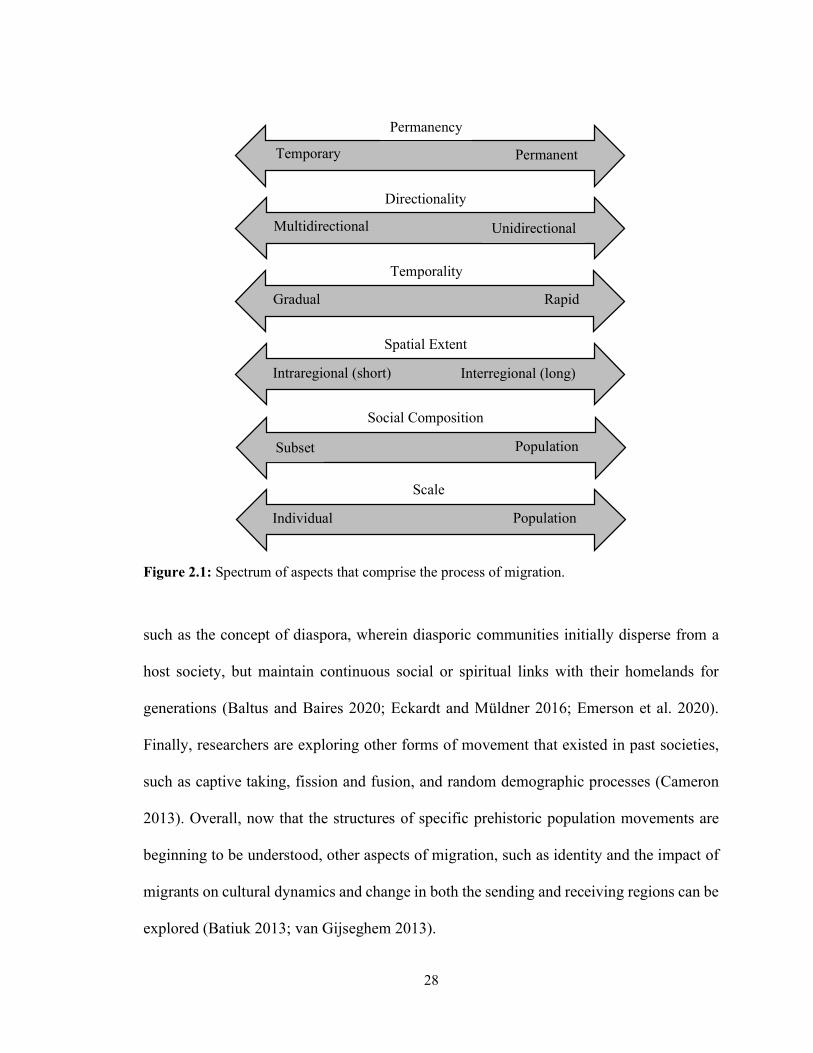
28

Figure 2.1: Spectrum of aspects that comprise the process of migration.

such as the concept of diaspora, wherein diasporic communities initially disperse from a

host society, but maintain continuous social or spiritual links with their homelands for

generations (Baltus and Baires 2020; Eckardt and Müldner 2016; Emerson et al. 2020).

Finally, researchers are exploring other forms of movement that existed in past societies,

such as captive taking, fission and fusion, and random demographic processes (Cameron

2013). Overall, now that the structures of specific prehistoric population movements are

beginning to be understood, other aspects of migration, such as identity and the impact of

migrants on cultural dynamics and change in both the sending and receiving regions can be

explored (Batiuk 2013; van Gijseghem 2013).

Scale

Individual Population

Social Composition

Subset Population

Temporality

Rapid Gradual

Directionality

Multidirectional Unidirectional

Spatial Extent

Intraregional (short) Interregional (long)

Temporary Permanent

Permanency

29

2.1.2 Conceptualizing Migration in Bioarchaeology

Bioarchaeology is an interdisciplinary subfield of biological (physical)

anthropology3 that studies human remains from archaeological contexts to reconstruct past

behaviour (Larsen 2014), including migration. Biological anthropology began in the

nineteenth century, and much like early archaeological studies, the first biological

anthropological studies focused on description and the development of racial classifications

for living and skeletal humans (Marks 1995). The few skeletal studies conducted at that

time consisted of measuring the skull using craniometric or anthropometric techniques that

related brain size to hierarchies of racial types (e.g., Morton 1839) with little interest in

evolution or scientific hypothesis testing (Little and Sussman 2010:14). Racial categories

were based on physically visible traits as well as non-biological, socially constructed racial

attitudes (Hagen 1996:569) and racial prejudice was heavily influenced by political and

cultural factors that contributed to both social and scientific perspectives at that time (Brace

2010:25; Ortner 2010:103). Some, however, attempted to differentiate physical

anthropology from racism (e.g., Boas 1934; Hooton 1936; Montagu 1942).

These early osteological studies were central to the use of migration as an

explanation for culture change because if “the spatial (and temporal) distribution of cranial

types could be assumed to result from the movement of culturally and biologically distinct

3 The identifiers “physical” and “biological” are often used interchangeably when referring to the diverse subfield of anthropology that applies archaeological theory to address the biological basis of human behaviour, diversity, and evolution (Turner 2005). However, the former term is reminiscent of the prejudice beliefs that emphasis physical traits of human beings that motivated the origins of this subdiscipline (see the text). Therefore, biological anthropology is used here, as it is not only more inclusive and applicable to diverse areas of research, but it also demonstrates “the [sub]discipline’s emphasis on the population and its biocultural aspect in addition to the evolutionary history of the entire species as the object of study, rather than on physical types of humans” (DiGangi and Moore 2013:7; see also Martin et al. 2013:31).

30

peoples, both biological and culture history could be reconstructed from similarities and

differences in cranial morphology” (Adams et al. 1978:513). Although researchers such as

Boas (1912) quickly realized that the shape of the cranial vault is influenced by both genetic

and environmental factors, such uncritical and racist craniometric studies persisted into the

mid-twentieth century (see Adams et al. 1978: 514-522; Walker 2008:8-9). Biological

anthropologists have since acknowledged and critiqued the racism and cultural biases that

characterized these early biological anthropological studies (Armelagos and Goodman

1998; Armelagos and van Gerven 2003; Blakey 1998). Although skeletal measurements

continue to form the basis of quantitative research, such studies are informed by

anthropological and biological theory and employ a biocultural model that uses metric

measures to address the influences of environment and culture on skeletal growth and

development (Martin et al. 2013:28-31).

The “New Physical Anthropology” advocating theory-driven research and

hypothesis testing subsequently emerged (Washburn 1951) but did not take hold until the

1960s (see Zuckerman and Armelagos 2011). The term bioarchaeology, or the

interdisciplinary study of human remains from archaeological sites, was also first coined

during this time (Buikstra 1977). This period represents the first wave of theoretical

engagement in bioarchaeology (Agarwal and Glencross 2011:1-2) and parallels the interest

of processual archaeologists in universal models and in situ cultural development (e.g.,

Lasker 1970). As with processual archaeology, the ecological approach in anthropology

greatly contributed to bioarchaeological concepts in the latter half of the twentieth century

(Zuckerman and Armelagos 2011:18).

31

Interest in understanding population demographics from archaeological skeletal

remains (e.g., Haviland 1967) continued to use morphological similarity in cranial types

but substituted “gene flow” for migration and began to use increasingly complex statistical

analyses (Adams et al. 1978:516). However, influenced by processualism, these studies

focused on the analysis of in situ biological evolution (Adams et al. 1978:517) and

considered populations as stationary (i.e., closed to both inbound and outbound migration),

which ignored the impact of human movement on demographic reconstructions (Wood et

al. 1992).

Following the development of postprocessual archaeological discourse, the second

wave of bioarchaeological theoretical engagement largely involved critical assessment of

assumptions and methodology (Agarwal and Glencross 2011:2). For example, researchers

began to question whether archaeological skeletal assemblages accurately represent the

populations from which they derive (Bocquet-Appel and Masset 1982; Jackes 2011; Wood

et al. 1992). Novel scientific techniques, including isotopic analysis of human migration,

were also critiqued for being primarily descriptive rather than theorizing explanations for

the processes observed (Armelagos and Van Gerven 2003; Hens and Godde 2008), as were

individual-based mortuary studies (Gillespie 2001).

This was followed by the third and most recent wave of theoretical engagement in

bioarchaeology, which seeks to contextualize skeletal studies, including those that utilize

novel techniques, through the integration of biological, behavioral, ecological, and social

research (Agarwal and Glencross 2011:3; Zuckerman and Armelagos 2011:19). As in

archaeology, bioarchaeologists are also beginning to explore the broader sociocultural

impacts of migration, including how local and nonlocal individuals negotiated identity

32

(e.g., Knudson 2011; Knudson and Stojanowski 2008, 2009; Zakrzewski 2011).

Archaeological isotope studies are also beginning to engage with theorizations of migration

in the past, as recently evidenced by Eckardt and Müldner (2016), who contextualized

isotopic data using epigraphic and material culture to interpret migration in Roman Britain

within the framework of diaspora. Both the second and third wave of bioarchaeological

theoretical engagement reflect the development of postprocessualism in archaeology that

challenged the infallibility of scientific methods and replaced universal models with more

context-driven research focused on the social aspects of identity of people, including those

of migrants, in the past.

2.2 Methodological Implications for Conceptualizations of Migration in

Bioarchaeology

Methodological approaches to migration in archaeology should be founded on

theoretical understandings of migration as a process (Anthony 1990, 1992), as

developments in method and theory are interconnected (Burmeister 2000:540; Adams et al.

1978:523). Indeed, methodology based on solid theoretical foundations has led to nuanced

understandings of past human movements (e.g., Burmeister 2000; Close 2000), just as the

expansion of data sets and advancement of methodological approaches for identifying this

phenomenon in the archaeological record have refined theoretical understandings of what

constituted migration in the past and its interpretation in specific contexts (Hakenbeck

2008; Scharlotta et al. 2018).

Archaeological conceptualizations of migration are also linked to the scale of

analysis, which is largely dictated by available data sets and methods. Foreign grave goods

included in funerary contexts have been used to identify individuals as potential migrants

33

(Burmeister 2016; Kristiansen et al. 2017:336), although it is possible for people to adopt

material culture independently of migration (Hodder 1982; Price et al. 2010; White et al.

2001; Wright 2005b). Other methods for identifying migration in archaeological contexts

based on the material record preclude the identification of individual movement, as only

long-term population movements over large distances that create significant change in

material culture, settlement patterns, language, or genetics are visible (Adams et al.

1978:488-489; Anthony 1990:901-902; Beekman 2019; Beekman and Christensen

2003:154-155; Bolnick 2011; Burmeister 2000:547; Cameron 1995; Clark 2001; Huntley

et al. 2016; Tsuda 2011; Tsuda et al. 2015:19). Essentially, it is “the social practices created

or disturbed by a migration rather than migration itself that are visible in the archaeological

record” (Beekman and Christensen 2011:147). Archaeologists have therefore struggled

with developing a means of unequivocally identifying the varying types and scales of

human movement from the archaeological record, although a variety of techniques have

been explored (e.g., Abell 2014; Burmeister 2000; Close 2000; Crawford 1997; Emerson

and Hargrave 2000; Hamerow 1997; Inomata 2004; Otte and Keeley 1990; Peregrine et al.

2009; Zakrzewski 2011). Consequently, archaeologists have adopted macrolevel

techniques to analyze the aggregate culmination of individual movements that occurred

over long periods of time (Burmeister 2000:547; Clark and Lindly 1991:582; Leppard

2014:486-487).

Fortunately, theoretical paradigm shifts in archaeology have been accompanied by

methodological advancements (Kristiansen 2014, 2017; but see Armelagos and Van

Gerven 2003:60). In archaeological studies of human movement, the reconceptualization

of what constitutes migration in past cultures have been subsequently validated by

34

osteological (biodistance), biogeochemical (isotopic), and genetic studies in

bioarchaeology (Frachetti 2011; Meiggs and Freiwald 2014; see also Section 2.3.1).

2.2.1 Biodistance Analyses of Migration

Biological distance, or biodistance, refers to the comparison of phenotypic traits

(morphological and metric skeletal and dental characteristics) among skeletal populations

to identify their genetic relatedness. This in turn can speak to population history and

structure within and among archaeological culture areas, as shared ancestry and gene flow

cause different skeletal populations to be morphometrically similar (Hefner et al. 2016).

While physical anthropology was primarily focused on using metric and nonmetric

aspects of the cranium and dentition to arrange human groups into typologies throughout

the 1930s and 1940s (Hefner et al. 2016), this changed with the introduction of the New

Physical Anthropology by Washburn (1951). The emphasized hypothesis testing,

biochemical mechanisms in human evolution, and other processual perspectives of human

evolution led biological anthropologists to apply increasingly complex statistical analyses

to biological data derived from archaeological skeletal remains at the population level to

address biocultural aspects of past societies (e.g., Buikstra 1977). Advances since the 1970s

have now grounded metric and nonmetric analyses of cranial and dental remains from

archaeological skeletal assemblages in anthropological and biological theory and when

coupled with robust statistical techniques, these methods provide insights into the complex

relationships between and within human populations (Hefner et al. 2016). Advances in

biodistance studies have also been accompanied by developments in the analysis of modern

and ancient DNA that have revived genetic-based understandings of inter- and intra-

35

population relationships (e.g., Bolnick 2011; Fix 2011; Hervella et al. 2015; Renfrew

2000). Both types of genetic techniques interpret biological affinity as the result of gene

flow, which is equated with the migration of people, whereas genetic drift causes isolated

populations to be genetically dissimilar (Raghavan 2018).

Biodistance and genetic studies are also typically conducted at the level of the

population, which allows migration to be studied within and between regions. However,

such an approach risks presenting “past peoples as homogenous and indistinguishable”

(Geller 2012:257). With increasing interest in individual identities and “peopling the past”

(Buikstra 2006:xix), bioarchaeologists have also pursued various means of conducting

research at the level of the individual (e.g., Stodder and Palkovich 2012). Isotopic analyses

specifically address microscalar migration in the past by directly identifying nonlocal

individuals in a skeletal collection. As such, “[s]table isotope analysis provides a ‘bottom-

up’ evidence-driven approach to mobility, and it thus has the potential to bridge [t]he gap

between large-scale patterns of mobility and the small-scale effects of mobility on

individuals and their burial contexts” (Hakenbeck 2008:19; see also Burmeister 2016:44;

Laffoon 2013:426; van Dommelen 2014:479).

2.2.1 Identifying Nonlocal Individuals using Isotopic Analyses

Strontium (87Sr/86Sr) and stable oxygen (δ18O) isotopes are most commonly

analyzed in studies of past migrations, and their application in archaeology has been

extensively reviewed and critiqued elsewhere (Bentley 2006; Lightfoot and O’Connell

2016; Makarewicz and Sealy 2015; Montgomery 2010; Pederzani and Britton 2019;

Scherer et al. 2015; Schwarz et al. 2010). Stable sulfur isotope (δ34S) analysis has also been

36

established as a means of investigating archaeological migration (Nehlich 2015) but has

only recently been applied in Maya archaeology (Awe et al. 2017; Green 2016; Rand and

Grimes 2017; Rand et al. 2020a, 2020b, 2021a, 2021b).

The utilization of isotopic analyses for identifying nonlocal individuals is dependent

upon the spatial heterogeneity of the isotopic values from subsistence resources among

different regions. The isotopic compositions of bones and teeth are derived from an

individual’s diet and drinking water, which in turn reflect those of the local environment

(Bentley 2006; Longinelli 1984; Nehlich 2015). Based on the assumption that people

obtained the majority of their food and water near where they lived, nonlocal individuals

are identified as those whose bone and/or tooth enamel isotope values differ from those

expected in the local environment. In the Maya region, there is sufficient variation in

biologically available (bioavailable) 87Sr/86Sr and δ18O values among different regions to

identify nonlocal individuals, and local isotopic baselines that characterize regional

variation have been developed for much of this area (Hodell et al. 2004; Freiwald 2011a;

Lachniet and Patterson 2009; Miller Wolf and Freiwald 2018; Price et al. 2007, 2008, 2010,

2015; Thornton 2011; Trask et al. 2012). Preliminary evidence indicates that lead isotopes

(Sharpe et al. 2016) and δ34S values (Green 2016; Rand and Grimes 2017) may also provide

insights into human migration in the Maya region. In some cases, stable carbon (δ13C) and

nitrogen (δ15N) isotope analyses, which are most commonly used to examine diet, may also

help identify nonlocal individuals as those with atypical diets (Gerry and Krueger 1997;

Hedman et al. 2002; but see Schwarcz et al. 2010:340), particularly when combined with

other isotopic data (Freiwald 2011a; Price et al. 2014; Suzuki et al. 2020; Wright et al.

2010; Wrobel et al. 2017).

37

There are several methods for establishing whether individuals migrated to the sites

where they were buried using the isotopic values of their tissues (see Appendix A for a

detailed discussion). For example, a difference in the isotope values of bones and teeth from

the same individual that form at different stages of life indicate whether he or she migrated

from isotopically distinct regions in the intervening period between tissue formation

(Agarwal 2016; Buikstra et al. 2004; Hrnčíř and Laffoon 2019; Montgomery 2010;

Montgomery et al. 2000; Schroeder et al. 2009; Schweissing and Grupe 2003; White et al.

2000). Individuals with isotopic values that fall beyond the range of local baseline values

developed from archaeological and modern flora, fauna, water, and geological samples

(Grimstead et al. 2017; Hodell et al. 2004; Lachniet and Patterson 2009; Makarewicz and

Sealy 2015; Price et al. 2002; Sillen et al. 1998) as well as published values (Lightfoot and

O’Connell 2016; Price et al. 2007, 2008, 2010) are also interpreted as having moved to

their place of burial. When baseline and comparative human isotopic data from other sites

are unavailable, nonlocal individuals may also be identified as those whose isotopic values

are statistical outliers from the human data set of interest (Burton and Hahn 2016:119;

Freiwald 2011a; Laffoon and Hoogland 2012; Lightfoot and O’Connell 2016; Montgomery

et al. 2007; Knudson 2011; Wright 2005a; Chapters 4 and 5).

The postmortem alteration of the chemical composition of bone, or diagenesis, is

another concern in isotopic studies of human movement, as interpretations are dependent

on the preservation of biogenic (i.e., those formed during life) isotope values. While criteria

have been established for evaluating whether the δ34S values of the organic portion of bone

(i.e., collagen) have been diagenetically altered (Nehlich and Richards 2009), it is more

difficult to evaluate the preservation of the mineral component of bone (i.e., bioapatite).

38

Because bone is less mineralized and therefore more susceptible to diagenetic alteration

than is enamel, many researchers prefer to sample tooth enamel for strontium and stable

oxygen isotope analysis (Budd et al. 2000; Hoppe et al. 2003; see Appendix A).

Another concern is the principle of equifinality, whereby multiple regions share

similar isotopic signatures, precluding the identification of the exact place from which a

nonlocal individual originated (Laffoon 2013:420). However, establishing finer-grained

isotopic baselines and analyzing multiple isotopes from the same individual have

contributed to narrowing down potential places of origin (Freiwald 2011a; Laffoon

2013:420), and the nearest isotopic region with values comparable to those of a nonlocal

individual is typically parsimoniously proposed as the likely place of origin. Furthermore,

because isotopic analyses may only detect the movement of individuals from isotopically

distinct geographical areas, this technique will underestimate the number of nonlocal

individuals who migrated from isotopically similar regions (Eckardt and Müldner

2016:209; Freiwald 2011a:303).

Despite these limitations, when interpreted in conjunction with other lines of

evidence, isotopic analyses of multiple individuals can provide information about the

permanency, directionality, temporality, spatial extent, social composition, and scale of

migration into a community. While it is not possible to detect the intent of an individual to

permanently relocate, the analysis of multiple isotopes of the tissues from the same

individual that form at different ages (e.g., tooth enamel and bone) and the analysis of

multiple samples from the same tooth that form at different times (i.e., intra-tooth analysis)

can also provide insights into the length of time an individual resided in an area, whether

he or she moved from isotopically distinct regions multiple times during his or her life, and

39

potential areas from which he or she may have originated. However, isotopic analysis

cannot evidence short term mobility, such as seasonal rounds, pilgrimages, or trips (e.g.,

Sellet et al. 2006), because these would be masked by environment isotopic values derived

from more permanent places of residence.

In terms of temporality, isotopic analyses detect relocations during the lifetime of

one individual. However, when combined with chronological evidence from ceramic

sequences and radiometric dating the analysis of multiple individuals from different time

periods can provide insights into the frequency of migration over time, which in turn can

speak to the temporality of the migration process in specific contexts (e.g., Suzuki et al.

2020). Similarly, although the spatial extent of migration is difficult to assess because

places of origin are difficult to determine, the development of isotopic baselines throughout

a region combined with the analysis of multiple individuals can provide insights into the

regions from which nonlocal individuals originated and whether nonlocal individuals

arrived from multiple different areas (Freiwald 2011a; Freiwald et al. 2014; Miller Wolf

and Freiwald 2018; Price et al. 2014; Somerville et al. 2016). Finally, the analysis of

multiple individuals of varying ages, sexes, and statuses allows for the social profile of

nonlocal individuals to be investigated, as well as the scale of migration based on the

percentage of individuals who are identified as nonlocal (Freiwald 2011a, 2011b; Miller

2015; Ortega-Muñoz et al. 2019; Price et al. 2018a; Suzuki et al. 2018).

Overall, isotopic analyses of human remains are invaluable tools in archaeological

reconstructions of human migration. This is because isotopic analyses allow migration to

be directly identified from the physical remains of an individual, while avoiding “the

associative inferences between material culture, language, and people that are necessary to

40

migration arguments in archaeology and linguistic anthropology” (Knudson 2011:232).

Thus, isotope analysis can provide proof of archaeological migration unobtainable using

other techniques. Although isotopic values cannot themselves identify the factors,

processes, and consequences of migration on isotopically nonlocal individuals, their

place(s) of origin, or the receiving community, insights into these aspects can be elucidated

through contextualizing isotope results using multiple lines of evidence. Thus, by necessity,

isotopic studies of human remains are embedded within broader (bio)archaeological

analyses of human migration and are inherently interdisciplinary.

2.3 Defining Migration in (Bio)archaeological Isotope Studies

Despite theoretical and methodological advances, the uncritical utilization of terms

such as migration and mobility without proper definition in archaeological discourse has

caused difficulties in the study of past human movements (Cabana and Clark 2011a;

Champion 1990:214; Clark 1994:309; Clark and Lindly 1991; Close 2000:49-50).

Although operational definitions of migration and other types of human movement are

necessary before these concepts can be identified and interpreted archaeologically, clear

definitions have not been forthcoming. For example, although it was often cited as an

explanation for culture change, culture historians never explicitly defined migration. Much

later, migration was clearly defined in an archaeological sense as “the simultaneous and

permanent movement of substantial numbers of people … which might be expected to leave

measurable traces in the cultural, the linguistic, and the skeletal record of peoples or areas”

(Adams et al. 1978:486). Thus, human migration was viewed as only archaeologically

41

visible at the population level (Burmeister 2000:547; Clark and Lindly 1991:582; Leppard

2014:486-487).

Alternative terms have also been proposed in the literature, most of which address

the spatial and temporal scale, intent, permanency, and social impact of population level

migration. For example, population movement was originally defined as the long-distance

movement of a large wave of people into a new area at the expense of local inhabitants

(Rouse 1986:176) but is now used in place of migration because it is considered neutral

and encompasses the diversity inherent in various types of human movements (Kristiansen

1989:219). Other terms instead imply the result of migration, such as colonization, wherein

people establish themselves (permanently or semi-permanently) in a new area (see Giovas

and Fitzpatrick 2014:570; Rockman 2003) and invasionism, which “envisions hostile

migrations, either temporary or permanent, the effect of which is primarily negative:

sudden culture loss and/or the abandonment of sites” (Adams et al. 1978:488).

Borrowing from related disciplines, typologies of various forms of human

movement (Aimers 2015; Wells and Stock 2012:36-39) and the people who moved (e.g.,

Tsuda et al. 2015:21) have also been developed. While such typologies are useful heuristic

devices for directing research in living populations (Brettell 2000:102), the incomplete

nature of the archaeological material record precludes the classification of ancient

migration into discrete categories (Nelson and Schachner 2002). Furthermore, the creation

of these typologies and the definitions associated with the terms included therein hazard

the incorporation of theoretical conclusions into definitions and the projection of modern

biases onto archaeological societies (Kardulias and Hall 2007:5).

42

Mobility has thus been proposed as a more neutral term for discussing past human

movements (Hakenbeck 2008:19; Leary 2014). In archaeology, the term mobility has

conventionally referred to non-sedentary hunter-gatherer groups who frequently moved

their settlements/camps (e.g., Kelly 1992; Sellet et al. 2006). Although studies of sedentary

archaeological cultures have instead focused on permanent relocations from a homeland to

a distant location (see chapters in Baker and Tsuda 2015a; Cabana and Clark 2011b;

Crawford and Campbell 2012), mobility is fundamentally defined as a physical movement

from one place to another that involves the embodied practice of movement within specific

contexts (Beaudry and Parno 2013; see also Creswell 2010:19). In Mesoamerica, for

example, mobility within a local area was likely high among lower status Aztec people

(Smith 2014), and Maya of lower status had the ability to “vote with their feet” in times of

political or environmental stress (Inomata 2004; Webb 1973:401). Thus, “[n]o society is

sedentary … people just move in different ways” (Kelly 1992:60; see also Sheller and Urry

2006). While mobility is a helpful framework for discussing the movement of people (and

things) in past societies without invoking a specific type (i.e., immigration, emigration,

transhumance, pilgrimage, trade, diaspora, exogamy, etc.) and is a popular alternative to

migration commonly used in isotope studies of archaeological cultures (e.g., Rand et al.

2020a; Scharlotta et al. 2018; see also Chapter 5), it is unspecific and cannot speak to the

migration process in a sociocultural sense.

With the nuanced understanding of migration as a complicated sociocultural

process of varying scales and temporal and spatial extents, others have argued for a

redefinition of migration itself in archaeology (Cabana and Clark 2011a; Hofman et al.

2014:595; Tsuda et al. 2015). For example, Tsuda and colleagues define migration as “the

43

movement of people across significant socio-cultural, political, or environmental

boundaries that involves uprooting and long-term relocation” (2015:19, original

emphasis). While it is important to differentiate migration from temporary movements (i.e.,

visits, pilgrimage, seasonal rounds), such a definition continues to emphasize the “large-

scale, long-distance, and long-term nature” of migrations and excludes “internal, localized

movements within a cultural/political/environmental boundary” (Tsuda et al. 2015:19). To

avoid assumptions about the causes or consequences of migration and to acknowledge their

multiscalar nature, Cabana and Clark have proposed a minimum definition of migration as

“a one-way residential relocation to a different “environment” by at least one individual”

(2011a:5, original emphasis), that is intended to be expanded upon within individual

research contexts. Although these minimal definitions continue to focus on the aspect of

permanency in relation to migration with terms such as “long-term relocation” and “one-

way”, they still offer the most grounded yet flexible means of conceptualizing the dynamic

process of past human migrations.

Isotopic studies of archaeological migration have been similarly plagued with a lack

of definition, uncritical appropriation of migration and related terminology, and the

conflation of terms (Scharlotta et al. 2018:867). For example, isotopic analyses are

sometimes referred to as proveniencing studies (e.g., Suzuki et al. 2020), although this term

is inappropriate given that an individual’s provenience (place of origin) cannot be

determined isotopically due to equifinality. Similarly, the term residential mobility refers

to movement within urban areas in modern migration scholarship (Quigley and Weinberg

1977; Zimmer 1973) and was originally adopted to define the movement of a group of

hunter-gatherers from one camp to another in archaeological discourse (Binford 1980).

44

Despite the differing meanings of residential mobility, this term is frequently used to refer

generally to isotopically identified human movement in isotopic studies (e.g., Knudson and

Price 2006; Laffoon 2013; Price et al. 1994; Somerville et al. 2016). Some

bioarchaeologists have therefore suggested the use of the term relocation in place of

residential mobility to refer to the isotopically identified movement of an individual over

any distance (after Knudson 2011:231).

Although the reconceptualization of migration in archaeology has been driven by

both theoretical and methodological advances, migration is rarely defined in archaeological

isotope studies (but see Freiwald 2011a:16; 2020:204, 2021). The minimal definition of

migration proposed by Cabana and Clark (2011a:5) is appealing in isotopic studies at the

individual level because it acknowledges the multiscalar nature of past migrations while

providing a framework in which to conceptualize migration rather than mobility in general.

The characterization of migration as the relocation across a boundary4 (e.g., Anthony

1990:902; Cabana and Clark 2011a:6; Tsuda et al. 2015:19) is also relevant, as isotopic

analyses detect individuals who have moved from isotopically distinct regions. Thus, an

isotopically detectable migration is minimally defined here as the relocation of a sampled

individual to an isotopically distinct environment at least once during his or her life (c.f.

Freiwald 2011a:16; Somerville et al. 2016:157). In this sense, migration is identified as an

event within one person’s life rather than a process, but when properly contextualized as

discussed above, it is possible to elucidate aspects of migratory processes from isotopically

4 Note that boundaries are defined as separating “different environmental, cultural, linguistic, economic, or political areas or zones and generally permit more flexible movement across them”, whereas a border is “a type of boundary that delineates political territories, such as those found between nation-states, polities and empires” (Tsuda et al. 2015:20).

45

identified nonlocal individuals. As such, this is a minimum definition that should be

expanded in specific archaeological contexts using archaeological, epigraphic,

ethnohistoric, genetic, linguistic, osteological, and other data (c.f. Cabana and Clark

2011a).

It is also necessary to define the terminology used to describe the people who moved

in the past. For example, modern migrants are individuals who have crossed an

international political border (Brettell and Hollifield 2000b:20), although in archaeology

migrant may refer to any person who has moved, regardless of the distance or boundaries

involved. Other terms, such as foreigner, alien, settler, colonist, and sojourner, are less

common in the archaeological isotope literature but imply aspects of the person moving

that can mean different things to different researchers. Methodological limitations should

also be considered in such definitions. Isotopic techniques, for example, identify

individuals with statistically distinct values as having moved to an isotopically distinct area,

and so only immigrants are isotopically visible in archaeological studies. Thus, in this study

the term nonlocal refers to individuals whose isotopic values are statistical outliers from

the sample population, whereas local individuals are those who fall within the statistically

determined local range (Freiwald 2021).

However, just as people with nonlocal isotopic signatures may not have been

understood as outsiders, an isotopically “local” individual may not have been considered a

local member of the community because vast areas can exhibit similar isotopic values (i.e.,

equifinality; see Section 2.3.1). Isotopic boundaries among regions are also better

understood as gradients or mosaics and may not correspond to the often archaeologically

elusive perception of boundaries held by people in the past (Cabana and Clark 2011a:9).

46

Therefore, the terms nonlocal and local refer only to isotope values in this study, which

may or may not reflect how individuals viewed themselves or were recognized by the

receiving community (Knudson 2011:232). Fortunately, interdisciplinary research has

begun to examine the identity of both isotopically identified nonlocal individuals and

receiving communities in archaeological contexts (Freiwald et al. 2014; Cucina et al. 2015;

Olsen et al. 2014; Ortega-Muñoz et al. 2019; Price et al. 2014, 2018a, 2018b; Sierra Sosa

et al. 2014; Suzuki et al. 2018; Trask et al. 2012; Zakrzewski 2011).

2.4 Prehispanic and Colonial Period Migration in the Maya Region

Migration, as traditionally defined in archaeology, has been a common explanation

of culture change in the Maya region, with many of the early studies suggesting the Maya

themselves did not move but instead were invaded by more militaristic populations from

Central Mexico. However, as elsewhere, the conceptualization of migration in Maya

archaeology has changed over time. Developments in biological anthropological methods

and theoretical understandings of migration have contributed to the increasing number of

studies that have successfully applied isotopic analyses to address questions related to

migration in Maya archaeology.

2.4.1 Initial Interpretations of Migration in the Maya Region

During the early and mid-twentieth century, migration, specifically invasion, was

frequently cited as an explanation for culture change at the end of the Classic and

Postclassic periods. For example, it was proposed that individuals from Central Mexico

(e.g., the Toltecs) or “Mexicanized” Maya from the Gulf Coast of Veracruz, Mexico (e.g.,

the Putun or Itza) invaded Chichen Itza in the Northern Lowlands and sites such as Seibal

47

in the southwestern Peten region of present-day Guatemala (Morley 1946; Roys 1966;

Sabloff and Willey 1967; Thompson 1966). These arguments were, however, based on (1)

Indigenous and Spanish historical sources written centuries after the events in question

(Cobos 2015:51); (2) biased conceptualizations that Classic Maya society comprised a

peaceful priesthood that was susceptible to domination by militaristic groups from Central

Mexico (Jones 1997); and (3) the presence of “foreign” material culture such as fine paste

ceramics and artistic styles (Sabloff and Willey 1967). Although researchers such as

Andrews (1960) provided evidence against these sensationalized invasion hypotheses over

sixty years ago, it is only within the last few decades that they are beginning to be

discredited in the archaeological literature with subsequent analyses of multiple lines of

evidence. For example, interpretations of hieroglyphics at Seibal now indicate the site was

instead revitalized by Wat’ul Chatel, a Terminal Classic representative of Ucanal, another

Maya site to the east (Tourtellot and González 2004) and the large-scale trade of fine wares

manufactured in the Gulf Coast region throughout the Maya region was more complex than

previously thought (Jiménez Alvarez 2015).

With the reconceptualization of migration that accompanied the rise of

postprocessualism in archaeology, the deciphering of Mayan texts that record the

movement of Maya elite, and the development of novel techniques for identifying nonlocal

individuals, understandings of the movement of people and cultural interaction within and

beyond the Maya region have changed drastically. This is particularly well demonstrated

in isotopic contributions to understandings of the relationship between the Maya and

individuals from Teotihuacan in Central Mexico. While nuanced studies of human

movement among the Maya continues to be investigated using archaeological data (Aimers

48

2015; Arnauld et al. 2017; Rice 2015; Scherer et al. 2018), bioarchaeological approaches

including biodistance studies and isotopic techniques have been very useful in re-evaluating

and further contributing to archaeological perspectives on prehispanic and Colonial period

Maya migration.

2.4.2 Bioarchaeological Evidence for Maya Migration

Initial biological studies of Maya skeletal assemblages were focused on description

and development of typologies (e.g., Hooton 1940). Following predominant theoretical

trends posited by the New Archaeology and New Physical Anthropology, biological

anthropology assessments of Maya skeletal assemblages of the 1960s and 1970s focused

on in situ demographic change and ignored migration as an influencing factor (e.g.,

Haviland 1967; Rathje and Sabloff 1973). Bioarchaeological research on Maya human

skeletons now contributes to understandings of prehispanic Maya health, diet, social

change, inequality, migration, mobility, war, violence, interregional interaction, and ritual

practice (e.g., Cucina 2015b; Cucina and Tiesler 2005; Scherer 2017; Tiesler and Cucina

2014; White 1999; Whittington and Reed 1997b; Wright 2004, 2006; Wright and White

1996; Wrobel 2014a). While several aspects of human skeletal remains have been used to

identify nonlocal individuals in Maya archaeological contexts, such as cranial and dental

modifications (e.g., Tiesler 2015), biodistance and isotopic analyses are the most

commonly employed.

In terms of migration, biological distance (biodistance) studies have been useful for

elucidating general patterns of population level migration within the Maya region and

beyond. Biodistance studies of Maya skeletal assemblages typically focus on the metric

49

and nonmetric characteristics of the dentition because teeth preserve better than bone in

tropical areas and cultural practices such as cranial modification can obscure phenotypic

expression in the cranium (Scherer 2007; Wrobel 2003). In general, these studies have

identified a high degree of biological affinity compared to other Mesoamerican populations

indicative of extensive migration within the Maya region that was fairly consistent over

time (Aubry 2019; Cucina 2015b; Cucina and Tiesler 2004; Jacobi 1997; Scherer 2007;

Wrobel 2003). The analysis of DNA from both modern Maya people and the ancient DNA

(aDNA) of Maya skeletal samples are also useful for reconstructing population structure in

the past (González-Oliver et al. 2001, 2018; Merriwether et al. 1997).

While genetic studies of Maya skeletal assemblages reveal interesting patterns of

population dynamics that can be reconstructed from a general perspective both within and

between sites (Austin 1978; Cucina and Tiesler Blos 2004; Cucina et al. 2018; Serafin et

al. 2014, 2015; Wrobel and Graham 2015), they can only examine migration at the

population level. Although these techniques are not suited for identifying migration at the

level of the individual, the understandings of population structure throughout the Maya

region and over time provided by biodistances analyses can assist with the interpretation of

individual migration offered by isotopic analyses.

However, biological anthropological analyses of Maya skeletal assemblages,

including those that utilize isotopic analyses, are challenging for several reasons (see

Wrobel 2014b:2-5). For example, the prehispanic Maya did not use formal cemeteries, and

instead select individuals were buried within structures that continued to be used by the

living, suggesting that decedents were afforded social viability and descendants engaged in

ongoing dialogues with their ancestors (McAnany 1995; Gillespie 2001). This selectivity,

50

however, reduces the number of individuals available for analysis and brings into question

the representativeness of Maya skeletal samples (Jackes 2011; Wright and Yoder 2003:44).

The posthumous manipulation of bodies by the Maya, including the extraction or

introduction of skeletal elements to burial contexts, individual and collective reburial, and

the reuse of bones as relics (Tiesler 2007:18; see also McAnany 1995:60; McAnany et al.

1999; Tiesler and Cucina 2007), is also a concern because isotopic analyses cannot

differentiate between people who migrated during life and those whose remains were

moved following their deaths (Freiwald 2011a:61). This is further complicated by the

generally poor preservation of organic material, including human bone, at Maya sites that

decreases the amount and quality of material for analysis. With these caveats in mind, the

application of isotopic approaches to questions of migration within the Maya region are

reviewed below.

2.4.3 Isotopic Approaches to Maya Migration

Despite the challenges associated with analyzing Maya skeletal assemblages,

researchers have successfully identified nonlocal individuals at numerous sites from

varying time periods using isotopic techniques and have greatly contributed to

understandings of migration among the Maya. Strontium and oxygen are the most widely

used isotope systems for investigating the movement of both humans and animals in past

societies and as illustrated in Figure 2.2, they have been extensively applied in the Maya

region (Buikstra et al. 2004; Cucina et al. 2015; Freiwald 2011a, 2011b, 2020; Freiwald

and Pugh 2018; Freiwald et al. 2014, 2020; Hoffmeister 2019; Micklin 2015; Miller 2015;

Mitchell 2006; Negrete et al. 2020; Novotny 2015; Ortega-Muñoz et al. 2019; Patterson

51

Figure 2.2: Number of studies that utilized strontium and/or stable oxygen isotope analysis to investigate mobility and migration of humans and/or animals at Maya sites over time. Data collected through a Google Scholar™ search starting at the year 2000 using the key words “Maya”, “archaeology”, “migration”, “mobility”, “oxygen isotopes”, and/or “strontium isotopes”. Note that only peer-reviewed articles, chapters in edited volumes, and graduate dissertations and theses were included, and that review articles and studies that analyzed isotope systems other than oxygen and strontium were omitted.

and Freiwald 2016; Price et al. 2006, 2008, 2010, 2013, 2014, 2015, 2018a, 2018b, 2019;

Rand 2017; Rand et al. 2020a; Scherer and Wright 2015; Sharpe et al. 2018; Sierra Sosa et

al. 2014; Somerville et al. 2016; Sugiyama et al. 2018; Sutinen 2014; Suzuki et al. 2018,

2020; Thornton 2011; Thornton et al. 2016; Tiesler et al. 2010; Trask et al. 2012; White et

al. 2000, 2001; Wright 2005a, 2005b, 2012, 2013a; Wright and Bachand 2009; Wright et

al. 2010; Wrobel et al. 2014, 2017; Yaeger and Freiwald 2009).

Although isotopically nonlocal individuals were not identified at Actuncan

(Micklin 2015) and Actun Uayazba Kab (Wrobel et al. 2017) in Belize, and El Meco in

Mexico (Ortega-Muñoz et al. 2019), the remainder of the isotopic studies cited above report

a high degree of mobility at Maya sites, where up to 50% of sampled individuals were

0

1

2

3

4

5

6

7

8

9

10

Num

ber

of P

ubli

catio

ns

Year

Articles/Chapters Dissertations/Theses

52

identified as nonlocal (Freiwald 2011a, 2011b; Freiwald et al. 2014; Price et al. 2018a,

2018b). Nonlocal individuals at many sites have also been found to have originated from

multiple isotopically distinct localities (Freiwald 2011a, 2011b; Freiwald et al. 2014; Miller

2015; Miller Wolf and Freiwald 2018; Negrete et al. 2020; Ortega-Muñoz et al. 2019; Price

et al. 2014, 2018a, 2018b, 2019; Somerville et al. 2016; Suzuki et al. 2018, 2020; Wright

2005a, 2012).

Initial isotopic studies assessed the utility of this technique for identifying nonlocal

individuals at Maya sites, critiqued aspects of the methodology, such as how to define

baseline values, and suggested reasons for discrepancies in the data sets, such as the

consumption of imported salt and water from different sources (Buikstra et al. 2004; Price

et al. 2007, 2008; Scherer et al. 2015; White et al. 2000, 2001; Wright 2005a, 2005b).

Subsequent studies have further investigated these issues and contributed to better

understandings of baseline values in the Maya region (Fenner and Wright 2014; Freiwald

et al. 2019; Price et al. 2010; Miller Wolf and Freiwald 2018; Scherer et al. 2015). Now

that these methods are firmly established, they are regularly integrated into interdisciplinary

studies of the impact of migration on Maya culture, as discussed below.

The first isotopic case studies of skeletal collections from Maya sites addressed a

long-standing debate in Mesoamerican archaeology: the degree to which Central Mexican-

style material culture and epigraphic evidence represents the migration of people from

Teotihuacan to Maya sites during the Early Classic period and the nature of this contact

(Braswell 2003). Teotihuacan, located in the Valley of Mexico, was the largest city in

Mesoamerica and reached its zenith during the Proto- and Early Classic periods. The

appearance of material culture from this Central Mexican city (i.e., green obsidian), as well

53

as the import or emulation of artifacts (i.e., tripod cylindrical vases, shell “goggles”) and

architecture (i.e., talud-tablero platforms) at Maya sites, combined with militaristic

symbolism at Teotihuacan itself, led researchers to question the extent of the presence and

influence of Teotihuacanos at Maya sites during the Early Classic period (Braswell 2003).

Based on the epigraphic evidence from several sites, Stuart (2000) has proposed that

Teotihuacan played a direct and disruptive role in the political history of sites in the central

Peten, particularly Tikal and Uaxactun, in the Early Classic period, but that this direct

contact waned and, following the fall of Teotihuacan, Late Classic rulers across the

lowlands appropriated Central Mexican styles and material culture as prestigious or

legitimating symbolism and militaristic ideology.

Epigraphic evidence from Tikal, Uaxactun, Bejucal, and Río Azul in the central

Peten has been interpreted as some to support “the establishment of a New Order in the

central lowlands, with Teotihuacan or its agents subordinating or reconfiguring certain

Maya regimes to its liking” (Martin 2020:241; see also Martin and Grube 2008:29-33;

Martin 2001:111). Such interpretations of a Central Mexican Entrada into the Central

Lowlands focus on the documented arrival of a lord called Sivah K’ak’ (formerly “Smoking

Frog”)5 clothed in Teotihuacan military attire who presided over the installations of kings

at those centres, although researchers do suggest it is possible that he was an ethnically

Maya general under the auspices of Teotihuacan (Martin and Grube 2008:31; see also

Kováč et al. 2019; Stuart 2000). This evidence suggests that a second individual involved

in the Entrada was “Spear-Thrower Owl” (Martin and Grube 2008:30), the father of Nun

5 Mayan names are used for individuals whose glyphs can now be read and English nicknames assigned by epigraphers are used in quotation marks for individuals whose glyphs have not yet been deciphered.

54

Yax Ayin, the king installed at Tikal in 379 CE. The texts note that Spear-Thrower Owl

was made king in 374 CE but not of Tikal. Based on his Central Mexican garb, Stuart

(2000:483) speculates that he was the ruler of Teotihuacan, although he recognizes this is

not currently substantiated by the evidence. A third individual, K’inich Mo’, who appears

on a mural at Uaxactun has been interpreted as a Teotihuacan military captain or

representative of Sivah K’ak’ who aided the ethnically Maya “Sunraiser” in taking control

of that site and founding a new dynasty in 378 CE (Kováč et al. 2019). The problem with

these interpretations is that all of the event glyphs in the texts come from a limited number

of sites in central Petén and are read hul-iy, interrupted as “he/she/it arrived” (Stuart

2000:477), meaning there is no direct, unequivocal epigraphic evidence that states these

arrivals were associated with military interference at Maya sites.

The isotopic evidence suggests that this “New Order” was installed without the

movement of Teotihuacanos, as few individuals from Maya sites have isotopic values

consistent with those of Central Mexico (see Chinchilla Mazariegos et al. 2015; Rand et al.

2020a; Wright et al. 2010; see also Chapter 5) and most nonlocal individuals at Maya sites

originated from elsewhere in the Maya region (Price et al. 2010; White et al. 2000, 2001;

Wright 2005a, 2005b, 2010, 2012; Wright and Bachand 2009). For example, although

epigraphic evidence suggests Yax Nuun Ayiin I was born in Teotihuacan because he

“arrived” at Tikal to be crowned king in 379 CE, his local first molar enamel 87Sr/86Sr value

(0.70828) instead indicates he was born and lived near Tikal during childhood (Wright

2005b).

Similarly, material evidence initially suggested that individuals from Teotihuacan

invaded Kaminaljuyu (Kidder et al. 1946; Sanders and Michels 1978); however, of the 63

55

teeth from 24 Early Classic burials analyzed by Wright and colleagues (2010), only the

third molar δ18O (–6.8 ‰) and 87Sr/86Sr (0.70492) values of one adult of unknown sex

(Tomb A-V-1) are consistent with those of Central Mexico. The isotopic values of the first

molar (δ18O = –4.2 ‰, 87Sr/86Sr = 0.70465) and third premolar (δ18O = –4.5 ‰) from this

individual are local, indicating he or she was born in Kaminaljuyu, spent his or her later

childhood elsewhere, perhaps in Central Mexico, and returned to the Highland Maya site

prior to death (White et al. 2000; Wright et al. 2010).

Finally, Late Classic rulers of Copan recorded how the founder of their dynasty,

K’inich Yax K’uk’ Mo’, arrived at the site in 426 CE and depict him in Teotihuacan regalia;

however, a portrait of the dynastic founder commissioned by his son during the Early

Classic does not depict him in Central Mexican garb, suggesting his association with

Teotihuacan was elaborated upon by later kings to demonstrate their affiliation with Central

Mexico (Stuart 2000:500). Other lines of evidence suggest that he instead originated from

the central Peten, possibly from Tikal or Caracol, and was ethnically Maya with a political

identity rooted in Teotihuacan (Stuart 2007), although the texts that describe him were

written centuries after his death. Isotopic analyses of his remains confirm this interpretation

whereby the 87Sr/86Sr (0.70844) and δ18O (–3.4 ‰) values of his first molar enamel and

show he spent his childhood in the central Peten, moved to another location around aged

11 based on the values of his third molar (0.70736 and –4.0 ‰, respectively), and had

moved closer to Copan by adolescence based on the 87Sr/86Sr value of his fibula (0.70633;

Buikstra et al. 2004; Price et al. 2010).

The lack of isotopically identified individuals from Central Mexico may represent

a sampling bias, whereby individuals from Teotihuacan have not been subjected to isotopic

56

analyses, or that the invading Teotihuacanos chose to install local Maya as their ruling

vassals. Regardless, the lack of isotopic evidence for the presence of individuals from

Teotihuacan at Maya sites refutes positions that emphasize direct Teotihuacan military

imperialism, and instead supports arguments that Teotihuacano impact at many sites was

indirect or that the appearance of Central Mexican stylistic traits in the Maya region may

instead represent the emulation of Teotihuacano ideology and symbolism by Early Classic

Maya rulers and their Late Classic successors to enhance their own power or status (e.g.,

Price et al. 2010; White et al. 2001; Wright 2005b). Furthermore, it appears that the

relationship between individuals from Teotihuacan and the Maya region was reciprocal,

multidimensional, and variable across time and space (Estrada-Belli et al. 2017; Marcus

2003).

Early isotopic studies in Maya archaeology also focused on confirming the

epigraphic evidence for the origins of other royal individuals at large, intensively studied

centres, including Tikal, Copan, and Palenque (Price et al. 2010; Wright 2005a, 2012).

Subsequent research now additionally analyzes individuals from smaller hinterland sites

and has revealed that migration was not restricted to large Maya centres, but also occurred

in rural communities. For example, nearly a quarter of sampled individuals from different

sized sites in the Belize Valley relocated at least once during their lives (Freiwald 2011a;

also see Freiwald 2011b, 2021; Green 2016; Micklin 2015; Mitchell 2006; Novotny 2015;

Rand 2017; Spotts 2013; Wrobel et al. 2014, 2017). As with contemporary migration, most

individuals appear to have relocated over short distances, which can be isotopically visible

if there is sufficiently diverse geology within one region, such as the Belize Valley and

surrounding area, or by sampling multiple isotopes and tissues from the same individual

57

(Freiwald 2011a; Freiwald et al. 2014; Miller Wolf and Freiwald 2018; Patterson and

Freiwald 2016; Price et al. 2018a; Rand 2017).

A major area of research in bioarchaeological isotope studies of Maya migration

concerns interregional interaction, although the Maya themselves were diverse and

intraregional migration is also an important area of study. Contact between the Maya and

other Mesoamerican peoples, particularly from Teotihuacan in Central Mexico, has been

extensively investigated in isotopic studies, as discussed above. Researchers are also

beginning to examine the integration of non-Maya people from western/central Honduras

in the Maya centre of Copan (Miller Wolf and Freiwald 2018; Suzuki et al. 2020). However,

the Maya were not ethnically homogenous, and although archaeological discourse often

conflates the various peoples who inhabited the Maya region into a single culture group

based on similar languages, genetics, and material culture, the people who lived in this area

were, and their descendants are, ethnically diverse (Price et al. 2018b:70; Scherer et al.

2018). Furthermore, because ethnicity and identity are social constructs, it is likely that

they changed over time and throughout a person’s lifetime (Díaz-Andreu and Lucy 2005:2).

While it can be challenging to etically reconstruct prehispanic and Colonial Maya ethnicity

and identity, and how people in one Maya polity perceived those in another, important

insights have been gained through the examination of archaeological evidence (Díaz-

Andreu et al. 2005), ethnographic analogy and material culture (Scherer et al. 2018), as

well as bioarcheological studies (e.g., Tiesler 2013; Willermet and Cucina 2018).

Recently, isotopic investigations of migration at Maya sites have contributed to

reconstructions of the identity of nonlocal individuals. Place of origin is not the only aspect

of individual identity, but is one that may be inferred through an interdisciplinary isotopic

58

approach that considers how the identity of nonlocal individuals was expressed in their

funerary contexts, and other aspects of identity and group affiliation such as cranial and

dental modifications (Freiwald et al. 2014; Cucina et al. 2015; Green 2016; Novotny 2015;

Olsen et al. 2014; Ortega-Muñoz et al. 2019; Price et al. 2014, 2018a, 2018b; Sierra Sosa

et al. 2014; Suzuki et al. 2018; Trask et al. 2012).

Another aspect of identity is gender, although bioarchaeological approaches are

limited to the identification of biological sex (i.e., males and females; Geller 2008; Walker

and Collins Cook 1998). Migratory differences between males and females attributed to

relocations for marriage were proposed among the prehispanic Maya based on epigraphic

evidence and Colonial exogamy patterns (Martin and Grube 2008; Robinson 1981). At

Copan, isotopic analyses found sex-related differences in mobility within specific

neighbourhoods and that males and females may have come from different regions (Miller

2015). It also appears that males from western Honduras moved to Pusilha in southern

Belize to marry into the royal family (Somerville et al. 2016). However, most isotopic

studies to date have found that Maya of both sexes moved to numerous sites in similar

proportions (Freiwald 2011a; Miller 2015; Ortega-Muñoz et al. 2019; Price et al. 2018b;

Suzuki et al. 2018), confirming that prehispanic Maya post-marital residence preferences

were complex, as they were in the Colonial period and are today (Wilk 1988:139-140). The

balanced sex ratio may further indicate Maya people moved not as individuals, but in

familial groups or possibly as part of larger groups (e.g., lineages) that were unrelated to

marriage patterns (Scherer, personal communication, 2021).

Social status, as inferred from mortuary contexts, is another aspect of identity that

may be correlated with an individual’s nonlocal origin. Despite the early focus on the

59

movement of elites at major sites, isotopic analyses have confirmed that isotopically

identifiable migration also regularly occurred among lower status Maya at many sites

(Freiwald 2011a; Mitchell 2006; Price et al. 2008, 2010; Suzuki et al. 2018; Wright 2005a;

Wright et al. 2010). It also appears that nonlocal origins may have been an important factor

for the inclusion of individuals in sacrificial contexts (Chinchilla Mazariegos et al. 2015;

Freiwald et al. 2014; Price et al. 2007, 2019) and as trophy skulls (Price et al. 2018b; Tiesler

et al. 2010). Isotopic data also indicate that local elites at Cahal Pech may have emulated

nonlocal burial orientations and styles as a means of associating themselves with more

powerful centres (Novotny et al. 2018). Conversely, nonlocal individuals buried using local

mortuary customs at Xunantunich indicate the social integration of nonlocal individuals

into the local community at this site (Freiwald et al. 2014).

Beyond reconstructing the identity of nonlocal individuals, the incorporation of

isotopic analyses into interdisciplinary research projects offers the opportunity to broaden

conceptual frameworks for explaining past political, economic, and social networks,

population dynamics, and site formation processes. While exact places of origin cannot be

determined, the general places of origin of nonlocal individuals can be narrowed down and

are important for reconstructing the directionality of migration flows. This in turn speaks

to the interactions among particular areas throughout the wider Maya area, providing

insights into sociopolitical, kin-based, and trade networks (Cucina et al. 2015; Miller 2015;

Novotny et al. 2018; Price et al. 2014, 2018a; Sierra Sosa et al. 2014; Somerville et al.

2016). Similarly, the role of migration and other demographic processes in the formation

and expansion of sites and changes in sociopolitical networks can be explored by examining

when nonlocal individuals were buried (Scherer and Wright 2015; Wright 2012; Suzuki et

60

al. 2020). The identification of nonlocal animals at Maya sites also provides insights into

trade and exchange, economics, and catchment use (Freiwald and Pugh 2018; Sharpe et al.

2018; Sugiyama et al. 2018; Thornton 2011; Thornton et al. 2016; Yaeger and Freiwald

2009).

It should also be noted that most isotope studies in the Maya region have focused

on skeletal collections dating to the Classic period, predominantly the Late Classic period.

This is largely an artifact of archaeological sampling bias and preservation. However, the

isotopic examination of skeletal remains from later time periods, such as those from

Colonial period cemeteries, provides important insights into the impact of European

colonialism on the movement of resources as well as people of Maya, European, and

African descent in Spanish colonies (Freiwald and Pugh 2018; Freiwald et 2020; Price et

al. 2006, 2013; Trask 2018).

Finally, the extensive body of isotopic research in the Maya region provides an

excellent foundation for the application of novel techniques, such as stable sulfur isotope

analyses. Expected variation in the δ34S values throughout the Maya region appears to

complement that of strontium and oxygen isotope systems (Rand and Grimes 2017).

Importantly, unlike strontium and oxygen isotopes, which are primarily analyzed from

tooth enamel that forms in childhood, sulfur isotope values of bone collagen reflect dietary

averages from adolescence until the end of life, depending on the bone and individual

physiology in bone turnover rates (Hedges et al. 2007; Matsubayashi and Tayasu 2019;

Parfitt 2001). Researchers can therefore identify relocation in the final years of life, a

contrast to childhood isotopic values that also can elucidate the number of times individuals

moved over their lifetimes and how long they may have resided in a region prior to death.

61

This is, of course, only possible if the individual migrated from isotopically distinct regions.

Regardless, it appears as though sulfur isotope analysis has the potential to contribute to

understandings of human movement at Maya sites.

2.5 Chapter 2 Summary

Although mobility is a common aspect of human behaviour, archaeological

migration was traditionally uncritically invoked as a post hoc explanation for change in

material culture or differences in cranial shape. With their interest in in situ development,

processualists largely ignored migration as a demographic process, as did many

bioarchaeologists of the time (Adams et al. 1978; but see Buikstra 1977). With the advent

of postprocessual perspectives, researchers revived migration as an important aspect of past

societies but struggled to develop an archaeological proof of migration (Anthony 1990;

Burmeister 2000). Theoretical developments are intertwined with available methods and

data sets, and the development of isotopic techniques for identifying nonlocal individuals

have transformed archaeological understandings of past human migration. For example,

isotopic analyses revealed that elite individuals interred at Maya sites with Teotihuacan-

style material culture were from the Maya region, which changed archaeological

understandings of the nature of interaction between these two regions of Mesoamerica

(Price et al. 2010; White et al. 2001; Wright 2005b).

Every analytical technique is, however, accompanied by assumptions and

limitations that must be acknowledged. The minimum definition of isotopically identifiable

migration as occurring when individuals moved from isotopically distinct regions at least

once during their lives acknowledges both the strengths and limitations of this technique

62

for understanding past migrations and can be modified to accommodate specific

archaeological contexts. Despite the challenges associated with bioarchaeological studies

of human remains from Maya sites (Wrobel 2014b), the integration of isotopic analyses

into interdisciplinary research can not only reconstruct individual life histories and

identities, but also contribute to broader understandings of sociopolitical organization,

interaction, and change over time (Freiwald et al. 2014; Cucina et al. 2015; Ortega-Muñoz

et al. 2019; Price et al. 2014, 2018a, 2018b; Sierra Sosa et al. 2014; Suzuki et al. 2018;

Trask et al. 2012). Building on this theoretical framework, the utility of stable sulfur isotope

analyses for identifying the movement of people and resource acquisition in archaeological

studies of both migration and subsistence practices among the Maya is explored in the

following chapters.

63

CHAPTER 3

A MULTI-ISOTOPIC (δ34S, δ13C, AND δ15N) FAUNAL BASELINE FOR MAYA SUBSISTENCE AND MIGRATION STUDIES6

Stable sulfur isotope (δ34S) analysis is a useful technique for studying differential

consumption of terrestrial, marine, and freshwater protein, as well as detecting nonlocal

humans and animals in archaeological contexts (Nehlich 2015; Rand and Nehlich 2018).

This is possible because sulfur isotope values in bone collagen reflect those of the

environment from which dietary protein is derived (i.e., terrestrial, freshwater, or marine)

and are influenced by the underlying geology, atmospheric deposition, and biological

processes (see Nehlich 2015). Most archaeological applications of sulfur isotope analysis,

however, have focused on temperate regions in Europe and Asia (Cheung et al. 2017a;

Craig et al. 2006; Curto et al. 2019; Fornander et al. 2008; Linderholm et al. 2008b;

Madgwick et al. 2019a; Nehlich et al. 2010, 2011, 2012; Privat et al. 2007; Richards et al.

2001) and tropical islands in Oceania and the Caribbean (Kinaston et al. 2014; Leach et al.

1996; Sparks and Crowley 2018; Stantis et al. 2015).

6 A version of this chapter has been published in the Journal of Archaeological Science: Reports co-authored with Dr. Carolyn Freiwald and Dr. Vaughan Grimes (Rand et al. 2021a). CF and VG provided samples, resources, supervision, and comments on previous drafts of this chapter. However, as the principal author, AR was responsible for the research design, acquiring samples, preparing and weighing the samples for analysis, analyzing and interpreting the results, drafting the original manuscript, editing various drafts, and submitting the final manuscript for publication and inclusion in this dissertation.

64

In Mesoamerica, prehispanic Maya subsistence has been extensively studied using

multiple techniques, including stable carbon (δ13C) and nitrogen (δ15N) isotope analysis

(Somerville et al. 2013; Tykot 2002; White 1999; White et al. 2006). Human migration and

animal trade in this region have been similarly investigated through multidisciplinary

approaches that include strontium (87Sr/86Sr) and stable oxygen (δ18O) isotope analysis

(Cucina et al. 2015; Price et al. 2010; Thornton 2011; Wright et al. 2010). These studies

provide the basis for evaluating the utility of stable sulfur isotope analysis in Maya

archaeology. Indeed, preliminary stable sulfur isotope analyses of Maya diet and mobility

show promising results (Awe et al. 2017; Green 2016; Rand and Grimes 2017; Rand et al.

2020a), but with only a small number of human and faunal baseline samples, more research

is needed.

This study assessed whether the differing δ34S values of the heterogeneous

environments of the Maya region of Central America can address archaeological questions

of subsistence, movement, and animal exchange in tropical coastal and continental

contexts. The expected variability in environmental δ34S values throughout the Maya region

is hypothesized using an extensive literature review. The diets of 148 fauna specimens from

13 Maya sites are assessed by comparing their δ13C and δ15N values to other isotopic studies

of Maya faunal assemblages. The faunal δ34S values are compared to the hypothesized

environmental variation in the Eastern and Northern Lowlands, creating the first extensive

δ34S baseline in Mesoamerica and a tropical continent setting more generally. The results

show that multi-isotopic studies that incorporate stable sulfur isotope analysis can further

contribute to archaeological understandings of Maya subsistence and the movement of both

humans and animals at multiple sites.

65

3.1 Principles of Stable Isotope Analysis

Carbon (12C/13C), nitrogen (14N/15N), and sulfur (32S/34S) isotope analysis measures

the ratio of the two most abundant stable isotopes in a sample material (e.g., bone collagen)

relative to their ratio in a standard reference material (Vienna Peedee Belemnite (VPDB),

atmospheric N2 (AIR), and Vienna Cañon Diablo Troilite (VCDT), respectively; Böhlke et

al. 1993; Coplen and Krouse 1998; Coplen et al. 2006) and the results are reported using

the delta (δ) notation in per mil (‰) units. The δ13C, δ15N, and δ34S values of bone collagen

primarily reflect the isotopic composition of dietary protein consumed from adolescence to

the end of life, depending on which bone was sampled and individual physiological

turnover rates (Ambrose and Norr 1993; Hedges et al. 2007; Howland et al. 2003; Jim et

al. 2004; Matsubayashi and Tayasu 2019; Richards et al. 2003; Webb et al. 2017) and each

reveals different aspects of diet, as described below.

Bone collagen δ13C values provide information on the types of plants and animal

proteins a population consumed. Most plants use the C3 photosynthetic pathway and have

a modern global average δ13C value of a –26.5 ‰, whereas C4 plants such as maize from

Mesoamerican archaeological sites range from –12.5 ‰ to –9.0 ‰ (O’Leary 1988; Smith

and Epstein 1971; Tieszen and Fagre 1993; Warinner et al. 2013). Although some plants in

this region utilize the Crassulacean acid metabolism (CAM) photosynthetic pathway and

have intermediate δ13C values, it is unlikely they were consumed in significant quantities

by the Maya (Powis et al. 1999; White 2005). Carbon isotope ratios minimally increase at

each level of the food chain so that consumer bone collagen δ13C values indicate whether

dietary protein was derived from C3 or C4 plants (Ambrose and Norr 1993; Bocherens and

Drucker 2003; Schoeninger and DeNiro 1984).

66

Most wild terrestrial game species consumed by the Maya, including white-tailed

deer (Odocoileus virginianus), brocket deer (Mazama sp.), peccary (Tayassuidae), tapir

(Tapirus bairdii), lowland paca (Cuniculus paca), agouti (Dasyprocta sp.), turkeys

(Meleagris sp.), and nine-banded armadillo (Dasypus novemcinctus), as well as edible

freshwater species including various turtles (Trachemys venusta and other Emydidae,

Kinosternidae), mussels (Nephronaias sp.), jute snails (Pachychilus ssp.), and to a lesser

extent crocodiles (Crocodylidae), exhibit low δ13C values (~ –22 to –19 ‰) consistent with

diets from ecosystems based on C3 plants (Tykot et al. 1996; White and Schwarcz 1989;

Williams et al. 2009; Wright 2006). However, some archaeological deer and peccary as

well as domesticated dogs (Canis lupus familiaris) and turkeys that were consumed by the

Maya have more elevated δ13C values between –17.5 and –8.2 ‰, indicating these animals

consumed maize (Sharpe et al. 2018; Thornton et al. 2016; White et al. 2001).

Archaeological evidence demonstrates that marine taxa, such as sea turtles (e.g.,

Caretta caretta), various fish and shellfish, and to a lesser extent manatee (Trichechus

manatus) were consumed at coastal Maya sites (McKillop 1985; Williams et al. 2009).

Although marine animals, particularly mollusks, were traded inland, they were likely

imported as artifacts signifying status rather than as sources of food (Sharpe and Emery

2015). Marine resources consumed by the Maya typically exhibit δ13C values above –10

‰ (Keegan and DeNiro 1988; Tykot et al. 1996; van der Merwe et al. 2002; Williams et

al. 2009). Because marine-based diets have δ13C values that overlap those of maize-based

diets in the Maya region, additional isotope systems are required to differentiate between

the two.

Stable nitrogen isotope values increase between 3 and 6 ‰ with each trophic level

67

in the food chain so that the δ15N values of herbivores are lower than those of carnivores

(Delwiche and Steyn 1970; Hedges and Reynard 2007; O’Connell et al. 2012; Schoeninger

and DeNiro 1984). The δ15N values of bone may also be influenced by environmental

factors including climate, precipitation, aridity, and soil nitrates (Ambrose 1991, 2000), as

well as physiological conditions such as nutritional stress and pregnancy (Fuller et al. 2004,

2005). Bone δ15N values may also differ between archaeological human populations with

marine and terrestrial diets (Schoeninger and DeNiro 1984; Schoeninger et al. 1983)

because aquatic food webs comprise between four and six trophic levels, whereas terrestrial

food chains generally contain only three (Hairston and Hairston 1993). Humans typically

consume terrestrial herbivores that occupy the second trophic level and marine fauna that

fall within the third to fifth trophic levels (Bonhommeau et al. 2013), so that terrestrial-

based human diets exhibit lower δ15N values than those based on marine protein from

higher trophic level fauna.

However, the δ15N values of higher trophic level marine animals typically

consumed by the Maya (+7.7 ± 3.2‰, n = 44; Keegan and DeNiro 1988; Williams et al.

2009) are lower than those of marine species elsewhere in the world (e.g., average δ15N of

+11.8 ‰ in Belgium; Fuller et al. 2012). As a result, the δ15N values of marine fauna in this

region overlap those of terrestrial game animals consumed by the Maya, such as white-

tailed deer and peccary (+4 to +6 ‰), as well as higher values (~+10 ‰) reported from

omnivorous domesticated dogs and turkeys in Maya faunal assemblages (Sharpe et al.

2018; Thornton et al. 2016; Tykot et al. 1996; van der Merwe et al. 2002; Wright 2006).

The Maya who consumed higher trophic level marine animals may therefore exhibit both

δ13C and δ15N values that are indistinguishable from those produced by a terrestrial maize-

68

based diet. Stable sulfur isotope analysis has successfully been used to differentiate the

consumption of marine, terrestrial, and freshwater resources in archaeological contexts in

Europe, Asia, Oceania, and the Caribbean (Craig et al. 2006; Curto et al. 2019; Fornander

et al. 2008; Kinaston et al. 2014; Leach et al. 1996; Linderholm et al. 2008b; Madgwick et

al. 2019a; Nehlich et al. 2010, 2011, 2012; Privat et al. 2007; Richards et al. 2001; Sparks

and Crowley 2018; Stantis et al. 2015), and may also be useful for identifying dietary

protein sources in tropical continental contexts such as the Maya region.

Plants assimilate most of their sulfur from inorganic sulfate (SO42–) derived from the

underlying geology or dissolved in aquatic environments (Monaghan et al. 1999; Noji and

Saito 2003; Trust and Fry 1992), although wet (i.e., sea spray) and dry deposition (i.e., SO2

gas) as well as microbial activity can also contribute sulfur to plant tissues (Agrawal 2003;

Jørgensen et al. 2019; Krouse and Grinenko 1991). Plants convert assimilated sulfate into

various sulfur-containing molecules including methionine (C5H11NO2S) with minimal

fractionation7 so that the δ34S values of plant tissues reflect those of environmental sulfate

(Peterson et al. 1985; Tanz and Schmidt 2010). Methionine is an essential amino acid and

the only one to contain sulfur in bone collagen (Nehlich and Richards 2009). Animals

cannot synthesize methionine and must obtain it from dietary protein that is ultimately

derived from plants at the base of the food chain (Brosnan and Brosnan 2006; Ingenbleek

2006; Tanz and Schmidt 2010). The trophic level fractionation associated with δ34S values

is considered negligible (+0.5 ± 2.4 ‰; Nehlich 2015; but see Webb et al. 2017) so that the

bone collagen values of carnivores are indistinguishable from those of their prey (Krajcarz

7 The heavier and lighter isotopes of an element react differently during chemical reactions due to mass differences, which causes the isotopic compositions of reactants and products to differ (Fry 2006:12).

69

et al. 2019).

Because the δ34S values of bone collagen methionine reflect those of dietary protein

derived from plants at the base of the food chain, they will be unaffected by biologically

unavailable sulfur inputs from drinking water or food preparation techniques utilized by

humans, such as the processing of maize with lime (i.e., nixtamalization) or the addition of

salt. Nixtamalization does, however, double the amount of digestible methionine available

from maize (Ellwood et al. 2013; Katz et al. 1974), meaning that a greater amount of sulfur

in human bone collagen may be derived from lime-processed maize relative to animal

protein, which otherwise would be equal (Young and Pellet 1994). This is unlikely to

influence the results of the current study, as most sampled archaeological faunal species

are unlikely to have consumed lime-processed maize. However, studies of human δ34S

values in cultures where nixtamalization was a common food processing technique would

need to take this into consideration.

3.2 Expected Variability of Environmental δ34S Values in the Maya Region

To interpret the δ34S values of archaeological bone collagen samples, it is necessary

to understand the expected values of various environments in the region of study (Nehlich

2015). As with strontium isotope (87Sr/86Sr) values, environmental δ34S values are largely

influenced by the type and age of the underlying geology (Krouse et al. 1991). Therefore,

the distinct geologic zones of the Maya region used to predict strontium isotope variability

(e.g., Hodell et al. 2004) are useful for predictions of the variability of environmental δ34S

values. However, distance from the coast and microbial activity also impact δ34S values

(Jørgensen et al. 2019; Wadleigh et al. 1996). Drawing on sulfur isotope literature from

70

various disciplines, the expected variability of δ34S values in the Northern and Southern

Lowlands, Motagua Valley, Maya Mountains, Highlands, and coastal areas of the Maya

region are hypothesized below and summarized in Figure 3.1.

Modern seawater represents a well-mixed sulfur reservoir with an average

worldwide dissolved sulfate δ34S value of +21 ‰ (Böttcher et al. 2007; Rees et al. 1978).

Planktonic algae, seaweeds, and other modern marine plants generally have δ34S values

(+17 to +21 ‰) similar to seawater sulfate (Peterson and Fry 1987), and controlled feeding

experiments demonstrate that their δ34S values are incorporated into the tissues of marine

consumers with similarly little fractionation (±1 ‰; Barnes and Jennings 2007; Kanaya et

al. 2008; McCutchan et al. 2003). Based on the analysis of modern and archaeological

faunal remains, Nehlich and Richards (2009) suggest that offshore marine fish and

mammals such as whales and seals as well as humans and animals that live in coastal

regions or consume large quantities of seafood will have δ34S values that range from +14

to +19 ‰ (see also Fornander et al. 2008; Peterson et al. 1986).

The δ34S values of coastal marine animals may, however, be lower than those that

live in the open ocean due to the input of freshwater in coastal areas (Böttcher et al. 2007;

Yamanaka et al. 2000; see discussion below) and microbial dissimilatory sulfate reduction

(DSR; Canfield 2001; Jørgensen et al. 2019). DSR is the process by which microbes reduce

sulfate and produce sulfide with δ34S values between +3 and –50 ‰ (Thode 1991). DSR

occurs in the anaerobic sediments of not only mangrove forests and mud-bottom habitats,

both of which are common along the coast of Belize (High 1975), but also in cenotes

(sinkholes), marshes, and rivers (Böttcher et al. 2007; Fry et al. 1982; Kanaya et al. 2008;

Socki et al. 2002; Mizota et al. 1999; Yamanaka et al. 2000). Some flood adapted plants,

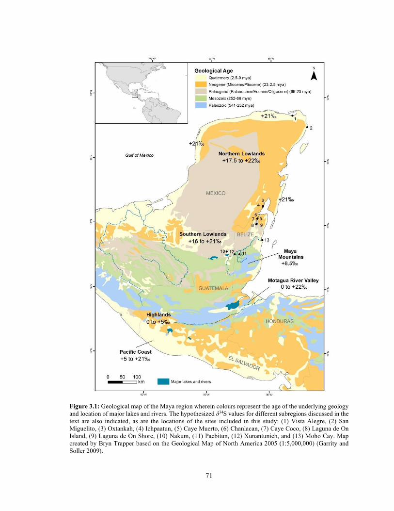
71

Figure 3.1: Geological map of the Maya region wherein colours represent the age of the underlying geology and location of major lakes and rivers. The hypothesized δ34S values for different subregions discussed in the text are also indicated, as are the locations of the sites included in this study: (1) Vista Alegre, (2) San Miguelito, (3) Oxtankah, (4) Ichpaatun, (5) Caye Muerto, (6) Chanlacan, (7) Caye Coco, (8) Laguna de On Island, (9) Laguna de On Shore, (10) Nakum, (11) Pacbitun, (12) Xunantunich, and (13) Moho Cay. Map created by Bryn Trapper based on the Geological Map of North America 2005 (1:5,000,000) (Garrity and Soller 2009).

72

including several species of grasses (e.g., Spartina sp.) and mangroves (e.g., Rhizophora

sp.), can assimilate sulfide-derived sulfur into their tissues, although it is toxic to most

plants that instead assimilate sulfate (Lamers et al. 2013). Most sulfide produced through

DSR is, however, reoxidized into sulfate with minimal fractionation (Jørgensen et al. 2019),

and modern experiments show that plants in anoxic aquatic environments can exhibit δ34S

values that are low relative to dissolved marine sulfate (+21 ‰; Böttcher et al. 2007; Rees

et al. 1978) that are subsequently passed on to their consumers (Fry et al. 1982; Holmer

and Hasler Sheetal 2014; Mizota et al. 1999; Oakes and Connolly 2004; Peterson et al.

1986; Yamanaka et al. 2000).

Over the oceans, marine sulfur from sea salt and dimethyl sulfide (C2H6S) with δ34S

values near those of oceanic sulfate (~+21 ‰) is incorporated into the atmosphere (Amrani

et al. 2013; Gravenhorst 1978; Nielsen 1974). The analysis of modern aerosols and peat in

coastal areas show that the sea spray effect caused by atmospheric circulation deposits

sulfur with elevated δ34S values in soils up to 30 km inland (Coulson et al. 2005; McArdle

et al. 1998; Wadleigh et al. 1994). This makes it difficult to differentiate between the

consumption of marine resources and terrestrial diets in coastal regions using δ34S values

alone (Guiry and Szpak 2020). Local climatic factors, such as seasonality, prevailing wind

directions, precipitation, and topography (e.g., the presence of mountains, plains, or

watersheds) also influence the impact of sea spray δ34S values on those of inland

environments (Bottrell et al. 2000; Sparks et al. 2019; Thode 1991; Wadleigh et al. 1994,

1996; Wakshal and Nielsen 1982).

Atmospheric circulation in the Maya region is dominated by northeasterly winds

(Barlow et al. 1998) that carry air masses originating over the Caribbean Sea west across

73

the Yucatan Peninsula. Air masses originating above the Pacific Ocean travel east and are

forced to ascend the Highlands, which are comprised of cordilleras situated parallel to the

Pacific Coast. In this mountainous region, rainfall is quickly fed into stream systems where

runoff is high (Bethune et al. 2007), although these air masses may reach the Southern

Lowlands during the dry season when the wind patterns reverse (Lachniet and Patterson

2009; Tankersley et al. 2016). While sea spray deposits sulfur with elevated δ34S values

near +21 ‰ in coastal areas (Coulson et al. 2005; McArdle et al. 1998; Wadleigh et al.

1994), studies of modern aerosols, precipitation, soils, and vegetation also show that

atmospheric δ34S values decrease as air masses move inland and rise in elevation, thus

contributing sulfur with lower δ34S values (+2 ‰ to +16 ‰) to inland soils and freshwater

catchments (Bern et al. 2015; Wadleigh et al. 1994, 1996; Wakshal and Nielsen 1982).

In contrast, the gaseous sulfur emitted from volcanoes has δ34S values around 0‰

(Bottrell and Newton 2006; Holser and Kaplan 1966:94; Nielsen et al. 1991:124), although

the average δ34S value of total volcanic sulfur, including ash particles, is approximately

+5‰ (Nielsen et al. 1991:125). If an eruption is particularly volatile, various geological

strata with differing δ34S values may be pulverized and added to the atmosphere (Nielsen

et al. 1991:121). Most volcanic activity in the Highlands has, however, consisted of

relatively non-explosive eruptions (van Wyk de Vries et al. 2007) and the primary volcanic

contribution of sulfur to the atmosphere in this region is likely in gaseous form. This

gaseous volcanic sulfur with δ34S values near 0 ‰ is then deposited in the environment as

dry fall or in precipitation, which may extend north into the Southern Lowlands (Tankersley

et al. 2016).

However, in humid climates such as those throughout much of the Maya region, the

74

δ34S values of the underlying geology overwhelms those from atmospheric inputs in inland

environments (Sharp 2007:263). The heterogeneous geology of the Maya region should

also exhibit different environmental δ34S values (Bundschuh et al. 2007). For example,

volcanic rocks typically have δ34S values between 0 ‰ and +5 ‰ (Holser and Kaplan 1966;

Labidi et al. 2013), and sulfur with similar values is hypothesized to occur in the volcanic-

derived soils of the Highlands, which are deposited down slope into Pacific Coast soils

through erosion (van Wyk de Vries et al. 2007). Because the Pacific Coast should also be

influenced by sea spray, environmental δ34S values in this subregion are hypothesized to

be intermediate between those of marine- and volcanic-derived sulfur (+5 to +21 ‰; Fig.

3.1).

The Maya lowlands are characterized by a karst limestone geology that formed

during the evaporation of prehistoric seas (Day 2007), and the δ34S values of the Yucatan

Peninsula should decrease from north to south with the increasing age of the underlying

limestone (Fig. 3.1). Because the δ34S values of oceanic sulfate fluctuated over time

(Bottrell and Newton 2006; Claypool et al. 1980), the δ34S values from limestone that dates

to the Mesozoic (252–66 mya; +16 to +21 ‰) in the south should exhibit lower values than

those of the Paleogene/Neogene (66–2.5 mya; +17.5 to +22 ‰) farther north. The

Quaternary limestones (2.5–0 mya) that line much of the Yucatan coast formed most

recently and should have δ34S values near +22 ‰ (Bottrell and Newton 2006; Claypool et

al. 1980).

The Motagua Valley of eastern Guatemala is characterized by diverse geology,

including volcanic, sedimentary, intrusive, and metamorphic lithologies (Reed et al. 2005).

This diversity is hypothesized to contribute variable δ34S values between 0 and +21 ‰ to

75

terrestrial soils in this subregion. This area is also crossed by the Motagua and Polochic

Rivers that drain the interior Highlands and flow east to the Caribbean (Marshall 2007),

which may deposit dissolved volcanic sulfate with low δ34S values from the Highlands into

the Motagua Valley region.

The Maya Mountains of southwestern Belize and northern Guatemala are a fault-

bounded highland with diverse lithology consisting of late Paleozoic sedimentary and

volcanic rock (Alvarado et al. 2007; Marshall 2007). Most of this lithology should have a

narrow range of δ34S values near 0 ‰ (Thode 1991), and preliminary results from human

bone collagen from the Mountain Pine Ridge subregion are around +8.5 ‰ (Ebert et al.

under review). However, deposits rich in gypsum (Alvarado and Mota 2007) should exhibit

higher values (δ34S = +20 ‰), as will the Vaca Plateau due to the underlying Mesozoic

limestone that characterizes the geology within this subarea of the Maya Mountains.

In the Northern Lowlands, cenotes provide access to the underground karst aquifer

of freshwater overlying seawater (Perry et al. 2002). The rivers and lakes flowing through

limestones in karst environments elsewhere are characterized by high sulfate

concentrations with elevated δ34S values (Thode 1991). However, DSR in the anaerobic

sediments of cenotes produces sulfide with much lower δ34S values (–34.0 to –2.5 ‰; Socki

et al. 2002). Thus, plants in the Northern Lowlands that rely on water from cenotes should

exhibit δ34S values lower than those of seawater sulfate (+21 ‰; Böttcher et al. 2007; Rees

et al. 1978) due to the influence of DSR in these environments. Aquatic plants in the surface

lakes and rivers that dissect the Southern Lowlands are also hypothesized to have δ34S

values distinguishably lower than that of modern seawater due to various sulfur inputs.

Although rivers that flow through karst landscapes typically acquire higher δ34S values

76

from sulfate minerals such as gypsum (Cortecci et al. 2002), it is unclear how much sulfate

from limestone contributes to freshwater ecosystems in the Maya region (Hu et al. 2005;

Williams et al. 1960; Williams and Steinbergs 1962). Major river system catchments in the

Southern Lowlands also originate from precipitation with lower δ34S values deposited in

the Highlands or Maya Mountains, regions with underlying geologies that should also

exhibit lower δ34S values. Finally, DSR may also contribute sulfide with lower δ34S values

to anaerobic freshwater environments such as lagoons and cenotes. As a result of the

accumulation of sulfur from various sources, not only will rivers exhibit variable δ34S

values along their lengths (Hitchon and Krouse 1972; Longinelli and Cortecci 1970;

Peterson et al. 1985; Trembaczowski and Halas 1992), but estuaries will also deposit

freshwater with lower δ34S values into coastal waters (Böttcher et al. 2007).

In this study, archaeological faunal specimens from Maya sites in the Northern

Lowlands and the Eastern lowland subregion of the Southern Lowlands were sampled to

test the hypothesized variability of sulfur isotope values in this part of the Maya region.

Similar studies of the variability of strontium, lead, and stable oxygen isotope ratios

throughout the Maya region have analyzed modern geological, water, plant, and animal

samples (Freiwald 2011a; Hodell et al. 2004; Lachniet and Patterson 2009; Miller Wolf

and Freiwald 2018; Price et al. 2008, 2015; Sharpe et al. 2016; Suzuki et al. 2015;

Wassenaar et al. 2008). However, due to contamination from the recent burning of fossil

fuels, modern analogues are inappropriate for the evaluation of bioavailable δ34S values in

archaeological settings (Richards et al. 2001; Trust and Fry 1992). Furthermore, although

fertilizers are known to influence δ34S values (Gröcke et al. 2020; Hosono et al. 2007;

Mizota and Sasaki 1996; Szpak et al. 2019), the extent to which the prehispanic or Colonial

77

period Maya used this agricultural technique requires further study (but see Fedick and

Morrison 2004; Morrison and Cózatl-Manzano 2003). Zooarchaeological and isotopic

analyses also show that although the Maya exchanged animals over varying distances, they

primarily consumed locally available animals (Götz 2008; Jiménez Cano and Sierra Sosa

2015; Rand et al. 2020a; Thornton 2011; Yaeger and Freiwald 2009). Thus, the δ34S values

of Maya archaeological faunal assemblages should reflect those of locally bioavailable

sources of sulfur and demonstrate the variability of environmental δ34S values throughout

the Maya region.

3.3 Materials and Methods

The stable carbon, nitrogen, and sulfur isotopes of 148 archaeological bone samples

from 13 sites were analyzed, and although 48 additional samples were prepared, they were

excluded from this study due to poor preservation, diagenesis, or insufficient collagen (see

Results for details). The sites primarily dated to the Classic (250–900/1100 CE), Postclassic

(900/1100–1500 CE), or Colonial (after 1500 CE) periods, although specimens from

various time periods were sampled from each site. The sample mainly included terrestrial

species, which comprise the majority of most Maya faunal assemblages (Emery 2004a). In

all, the faunal specimens include 116 terrestrial, 25 freshwater, and 7 marine taxa, including

66 artiodactyls (deer and peccary), 30 medium mammals (agouti, paca, armadillo,

opossum, and rabbit), 5 dogs, 13 turkeys, 21 turtles (including 4 sea turtles), 4 crocodiles,

4 birds, and less common prey species such as a manatee, marine mammal, and marine fish

(snapper) and carnivores such as a felid and weasel (see Appendix D for detail). Whenever

possible, well-preserved specimens identified to the genus or species level without

78

evidence of cooking or burning were selected for analysis. Although a number of specimens

were identified to the family level or higher, this should not have a significant impact on

the results as the general habitats used by these taxa (i.e., terrestrial, freshwater, or marine)

can still be inferred.

Samples were cleaned, prepared, and analyzed using methods described in detail

elsewhere (Rand et al. 2020a; see also Appendix A). Collagen was extracted using a

modified Longin (1971) method whereby samples demineralized in hydrochloric acid

(HCl) were treated with sodium hydroxide (NaOH) and hydrolysed, ultrafiltered, and

lyophilized prior to analysis (Honch et al. 2006; Nehlich and Richards 2009; Szpak et al.

2017b). Although ultrafiltration is not necessary for the preparation of bulk bone collagen

samples for stable carbon and nitrogen isotope analysis (Jørkov et al. 2007), it was used in

this study to remove exogenous sulfur and retain well preserved collagen for sulfur isotope

analysis (Nehlich and Richards 2009; Privat et al. 2007). Additionally, fish specimens were

delipidized in 2:1 chloroform:methanol (Guiry et al. 2016; Miller et al. 2010), because

lipids present in bone collagen systematically decrease collagen δ13C values by 1.6 ‰

(Guiry et al. 2016) and fish bone contains a higher proportion of lipids than mammalian

bone (Szpak 2011; Toppe et al. 2007). To the best of my knowledge, no study has yet

examined the influence of lipid extraction on δ34S values.

The samples were sent to three laboratories for analysis. Pestle et al. (2014) found

that interlaboratory δ13C and δ15N values are generally comparable, although this depends

on the laboratory. To date, no study has systematically examined the interlaboratory

variability of δ34S values from archaeological bone collagen, but preliminary evidence in

Appendix B indicates the results from labs with similar analytical procedures are

79

comparable. Analytical uncertainty associated with each isotope system and laboratory was

calculated using the method proposed by Szpak et al. (2017a) and is detailed in Appendix

C. The carbon and nitrogen isotope analyses of the samples from Pacbitun, Moho Cay,

Laguna de On Island and Shore sites, Caye Coco, and Chanlacan were conducted by

CREAIT’s Stable Isotope Laboratory at Memorial University, with a standard uncertainty

of ±0.28 ‰ for δ13C and ±0.24 ‰ for δ15N (Appendix C). The carbon and nitrogen isotopes

of the Vista Alegre, Oxtankah, Ichpaatun, San Miguelito, and Xunantunich samples were

analyzed by the Ján Veizer Stable Isotope Laboratory at the University of Ottawa with an

analytical uncertainty of ±0.11 ‰ for δ13C and ±0.08 ‰ for δ15N (Appendix C). The sulfur

isotopes of all but two samples were analyzed by the Stable Isotope Laboratory of the

Department of Earth and Planetary Sciences at the University of Tennessee. Although

standard uncertainty could not be calculated following Szpak et al. (2017a), analytical

precision was ±1.00 ‰ for δ34S (Appendix C). Finally, the sulfur isotopes of two samples

from Xunantunich were analyzed by the Ján Veizer SIL Stable Isotope Laboratory at the

University of Ottawa with a standard uncertainty of ±0.32 ‰ (Appendix C).

Statistical analyses were performed in SPSS version 25 for Windows (IBM®). The

distribution of the data was tested for normality using the Shapiro-Wilk test prior to

calculating comparative statistics. Small and highly skewed data sets such as those common

in archaeological isotope studies are best evaluated using robust, nonparametric statistical

techniques (Lightfoot and O’Connell 2016; Pearson and Grove 2013). The interquartile

range (IQR) method was therefore used to identify nonlocal individuals as those with

statistically outlying δ34S values that fell beyond the IQR multiplied by 1.5 subtracted from

the first quartile and added to the third, and extreme outliers fell beyond the IQR multiplied

80

by 3 subtracted from the first quartile and added to the third (Tukey 1977). Nonlocal

individuals are assumed to have originated from an isotopically distinct region, so their δ34S

values were excluded from the calculation of local δ34S ranges for each site, as has been

suggested elsewhere for 87Sr/86Sr values (Blank et al. 2018; Pacheco-Forés et al. 2020; Price

et al. 2002). Differences in the isotopic values between two groups (e.g., sites, taxa) were

evaluated using the Student’s t-test for normally distributed data and the Mann-Whitney U

test for nonparametric data and for data sets with less than eight samples (Pearson and

Grove 2013). Due to the small sample sizes and nonparametric distribution of data,

differences among the isotopic values of three or more groups were evaluated using

Kruskal-Wallis H tests, and the significances of the pairwise comparisons were

automatically adjusted by the Bonferroni correction for multiple tests in SPSS. The results

of all tests were deemed to be statistically significant when p < 0.05 (see Appendix A for

details).

3.4 Results

A total of 148 samples from the original 196 that were prepared for analysis produced

sufficient collagen for stable sulfur, carbon, and nitrogen isotope analysis. Of the 48

samples excluded from this study, 15 did not produce collagen, 25 did not produce

sufficient collagen for sulfur isotope analysis, and 8 had more than one diagenetic indicator

that fell beyond acceptable parameters (Ambrose 1990; Nehlich and Richards 2009; Rand

et al. 2015a; van Klinken 1999) and so were excluded from the following interpretations of

the results.

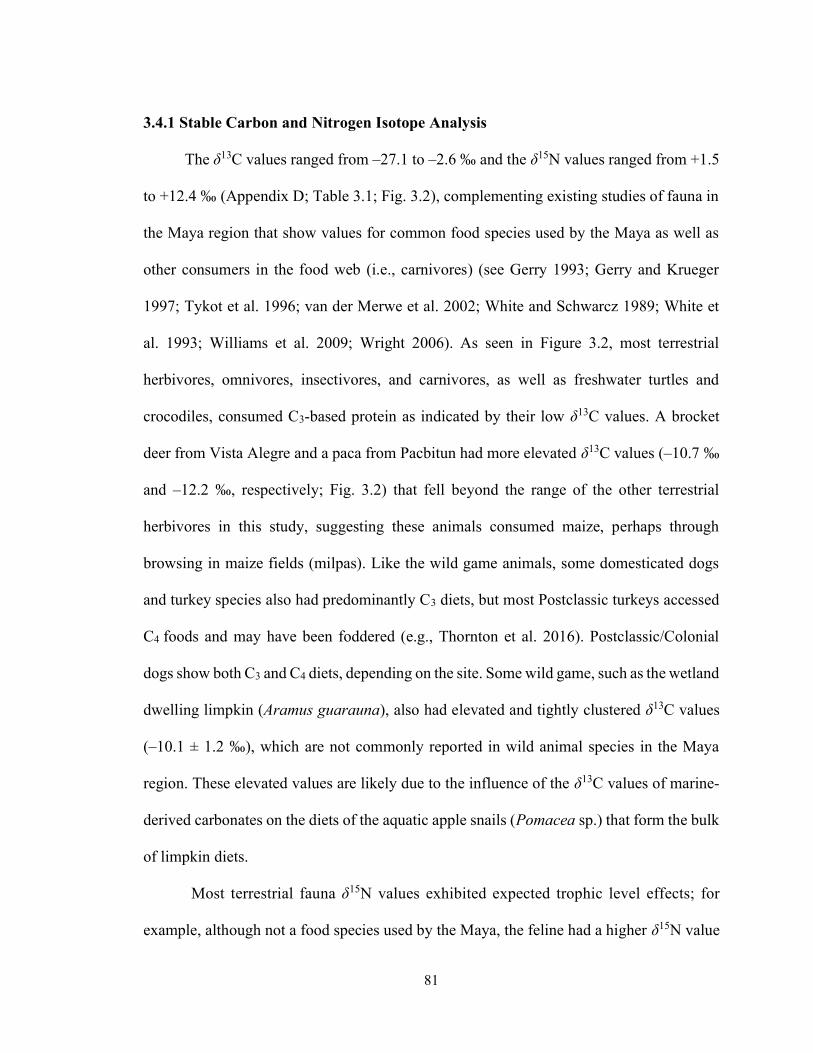
81

3.4.1 Stable Carbon and Nitrogen Isotope Analysis

The δ13C values ranged from –27.1 to –2.6 ‰ and the δ15N values ranged from +1.5

to +12.4 ‰ (Appendix D; Table 3.1; Fig. 3.2), complementing existing studies of fauna in

the Maya region that show values for common food species used by the Maya as well as

other consumers in the food web (i.e., carnivores) (see Gerry 1993; Gerry and Krueger

1997; Tykot et al. 1996; van der Merwe et al. 2002; White and Schwarcz 1989; White et

al. 1993; Williams et al. 2009; Wright 2006). As seen in Figure 3.2, most terrestrial

herbivores, omnivores, insectivores, and carnivores, as well as freshwater turtles and

crocodiles, consumed C3-based protein as indicated by their low δ13C values. A brocket

deer from Vista Alegre and a paca from Pacbitun had more elevated δ13C values (–10.7 ‰

and –12.2 ‰, respectively; Fig. 3.2) that fell beyond the range of the other terrestrial

herbivores in this study, suggesting these animals consumed maize, perhaps through

browsing in maize fields (milpas). Like the wild game animals, some domesticated dogs

and turkey species also had predominantly C3 diets, but most Postclassic turkeys accessed

C4 foods and may have been foddered (e.g., Thornton et al. 2016). Postclassic/Colonial

dogs show both C3 and C4 diets, depending on the site. Some wild game, such as the wetland

dwelling limpkin (Aramus guarauna), also had elevated and tightly clustered δ13C values

(–10.1 ± 1.2 ‰), which are not commonly reported in wild animal species in the Maya

region. These elevated values are likely due to the influence of the δ13C values of marine-

derived carbonates on the diets of the aquatic apple snails (Pomacea sp.) that form the bulk

of limpkin diets.

Most terrestrial fauna δ15N values exhibited expected trophic level effects; for

example, although not a food species used by the Maya, the feline had a higher δ15N value

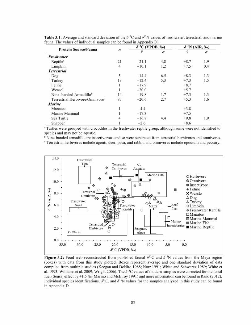
82

Table 3.1: Average and standard deviation of the δ13C and δ15N values of freshwater, terrestrial, and marine fauna. The values of individual samples can be found in Appendix Dl.

Protein Source/Fauna n δ13C (VPDB, ‰) δ15N (AIR, ‰)

x̄ σ x̄ σ Freshwater Reptilea 21 –21.1 4.8 +8.7 1.9 Limpkin 4 –10.1 1.2 +7.5 0.4 Terrestrial Dog 5 –14.4 6.5 +8.3 1.3 Turkey 13 –12.4 5.3 +7.3 1.5 Feline 1 –17.9 +8.7 Weasel 1 –20.0 +5.7 Nine–banded Armadillob 14 –19.8 1.7 +7.3 1.3 Terrestrial Herbivore/Omnivorec 83 –20.6 2.7 +5.3 1.6 Marine Manatee 1 –4.4 +3.8 Marine Mammal 1 –17.3 +7.5 Sea Turtle 4 –16.8 4.4 +9.8 1.9 Snapper 1 –2.6 +8.6

a Turtles were grouped with crocodiles in the freshwater reptile group, although some were not identified to species and may not be aquatic. b Nine-banded armadillo are insectivorous and so were separated from terrestrial herbivores and omnivores. c Terrestrial herbivores include agouti, deer, paca, and rabbit, and omnivores include opossum and peccary.

Figure 3.2: Food web reconstructed from published faunal δ13C and δ15N values from the Maya region (boxes) with data from this study plotted. Boxes represent average and one standard deviation of data compiled from multiple studies (Keegan and DeNiro 1988; Norr 1991; White and Schwarcz 1989; White et al. 1993; Williams et al. 2009; Wright 2006). The δ13C values of modern samples were corrected for the fossil fuel (Seuss) effect by +1.5 ‰ (Marino and McElroy 1991) and more information can be found in Rand (2012). Individual species identifications, δ13C, and δ15N values for the samples analyzed in this study can be found in Appendix D.

83

+8.7 ‰) than its potential prey, including terrestrial herbivores/omnivores (+5.3 ± 1.6 ‰)

and the insectivorous nine-banded armadillo (+7.3 ± 1.3 ‰). However, many of the

omnivorous peccaries had low δ15N values that fell within the lower range for terrestrial

and freshwater animals (Fig. 3.2), suggesting these peccaries derived more dietary protein

from plants. In contrast, the freshwater reptiles, including various turtles and crocodiles,

had the most variable δ13C and δ15N values (δ13C = –21.1 ± 4.8 ‰, δ15N = +8.7 ± 1.9 ‰;

Table 3.1), reflecting their diverse dietary preferences.

The marine fauna also showed a wide range of δ13C and δ15N values. The sea turtles

(three loggerhead sea turtles and one unidentified Cheloniidae) had δ13C values lower than

those previously reported for marine plants and fish (Fig. 3.2) and two had values that fell

within the range of freshwater reptiles (Table 3.1). A marine mammal from Oxtankah,

possibly a species of whale (Appendix D), also had a δ13C value (–17.3 ‰) that plots among

the terrestrial fauna (Fig. 3.2), although the δ15N value (+7.5 ‰) of this specimen falls

within the range of marine animals from Maya faunal assemblages (Fig. 3.2). Other marine

fauna such as the Atlantic snapper (Lutianidae) and manatee (Trichechus manatus manatus)

exhibited δ13C values (–2.6 ‰ and –4.4 ‰, respectively) and δ15N values (+8.6 ‰ and +3.8

‰, respectively) consistent with their expected diets and trophic levels, as explained in the

Discussion section.

3.4.2 Stable Sulfur Isotope Analysis

The δ34S values of the 148 faunal samples were variable, ranging from –1.3 to

+18.8 ‰ (Appendix D) and reflect dietary and locational differences. Summary statistics

of the faunal δ34S values reveal average values for each site and catchment type (Table 3.2,

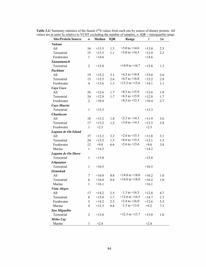
84

Table 3.2: Summary statistics of the faunal δ34S values from each site by source of dietary protein. All values are in units ‰ relative to VCDT excluding the number of samples, n. IQR = interquartile range.

Site/Protein Source n Median IQR Range x̄ 1σ

Nakum All 16 +13.5 1.3 +5.0 to +14.6 +13.0 2.3 Terrestrial 15 +13.5 1.1 +5.0 to +14.5 +12.9 2.3 Freshwater 1 +14.6 +14.6 Xunantunich Terrestrial 2 +15.8 +14.9 to +16.7 +15.8 1.3 Pacbitun All 19 +15.2 3.1 +6.5 to +18.8 +15.0 2.6 Terrestrial 15 +15.5 2.6 +6.5 to +18.8 +15.2 2.8 Freshwater 4 +13.6 1.3 +13.3 to +15.6 +14.1 1.1 Caye Coco All 26 +12.6 1.7 +8.5 to +15.9 +12.6 1.8 Terrestrial 24 +12.9 1.7 +8.5 to +15.9 +12.8 1.7 Freshwater 2 +10.4 +8.5 to +12.3 +10.4 2.7 Caye Muerto Terrestrial 1 +13.3 +13.3 Chanlacan All 18 +13.2 1.4 +2.3 to +14.3 +11.9 3.6 Terrestrial 17 +13.2 1.2 +3.0 to +14.3 +12.5 2.8 Freshwater 1 +2.3 +2.3 Laguna de On Island All 37 +13.3 3.2 +2.6 to +15.5 +11.8 3.1 Terrestrial 24 +13.5 1.5 +8.6 to +15.5 +13.1 1.5 Freshwater 12 +9.8 6.6 +2.6 to +13.6 +9.0 3.8 Marine 1 +14.2 +14.2 Laguna de On Shore Terrestrial 1 +15.8 +15.8 Ichpaatun Terrestrial 1 +16.5 +16.5 Oxtankah All 7 +16.0 0.8 +14.8 to +18.0 +16.2 1.0 Terrestrial 6 +16.0 0.8 +14.8 to +18.0 +16.2 1.0 Marine 1 +16.1 +16.1 Vista Alegre All 17 +14.2 2.5 –1.3 to +16.5 +12.8 4.7 Terrestrial 8 +15.0 1.7 +12.6 to +16.5 +14.7 1.3 Freshwater 5 +14.2 2.5 +3.4 to +16.0 +12.6 5.3 Marine 4 +12.3 8.6 –1.3 to +13.6 +9.2 7.1 San Miguelito Terrestrial 2 +13.0 +12.3 to +13.7 +13.0 1.0 Moho Cay Marine 1 +2.4 +2.4

85

Fig. 3.3). Sixteen outlier values are present at seven of the sites (Fig. 3.3); however, when

the fauna from each site were categorized by source of their dietary protein (i.e., terrestrial,

freshwater, or marine), only nine δ34S values are statistical outliers (Fig. 3.4). Eight

terrestrial animals with outlying δ34S values may represent nonlocal individuals from

isotopically distinct regions and one freshwater animal with an outlying value at Vista

Alegre likely reflects species differences in sources of dietary protein.

The δ34S values of freshwater fauna were generally lower than those of terrestrial

taxa from the same site, although the sample size of marine animals from most sites was

too small for comparison (Table 3.2). When the statistically outlying values were removed,

this difference was statistically significant at Laguna de On Island (t = –3.898, df = 12.036,

Figure 3.3: Boxplots of the faunal δ34S values from the sites listed in Table 3.2 arranged by distance from the coast in km beneath site name. Individual data points (circles) have been superimposed over the boxplots, outliers are identified as larger filled circles that fall beyond the whiskers, and extreme outliers are identified as filled stars (see Appendix A for how outliers were identified using the IQR method).

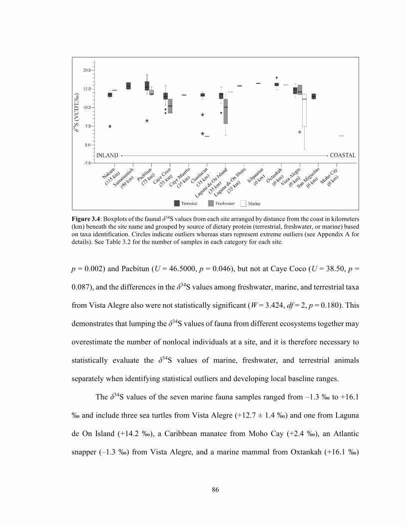
86

Figure 3.4: Boxplots of the faunal δ34S values from each site arranged by distance from the coast in kilometers (km) beneath the site name and grouped by source of dietary protein (terrestrial, freshwater, or marine) based on taxa identification. Circles indicate outliers whereas stars represent extreme outliers (see Appendix A for details). See Table 3.2 for the number of samples in each category for each site.

p = 0.002) and Pacbitun (U = 46.5000, p = 0.046), but not at Caye Coco (U = 38.50, p =

0.087), and the differences in the δ34S values among freshwater, marine, and terrestrial taxa

from Vista Alegre also were not statistically significant (W = 3.424, df = 2, p = 0.180). This

demonstrates that lumping the δ34S values of fauna from different ecosystems together may

overestimate the number of nonlocal individuals at a site, and it is therefore necessary to

statistically evaluate the δ34S values of marine, freshwater, and terrestrial animals

separately when identifying statistical outliers and developing local baseline ranges.

The δ34S values of the seven marine fauna samples ranged from –1.3 ‰ to +16.1

‰ and include three sea turtles from Vista Alegre (+12.7 ± 1.4 ‰) and one from Laguna

de On Island (+14.2 ‰), a Caribbean manatee from Moho Cay (+2.4 ‰), an Atlantic

snapper (–1.3 ‰) from Vista Alegre, and a marine mammal from Oxtankah (+16.1 ‰)

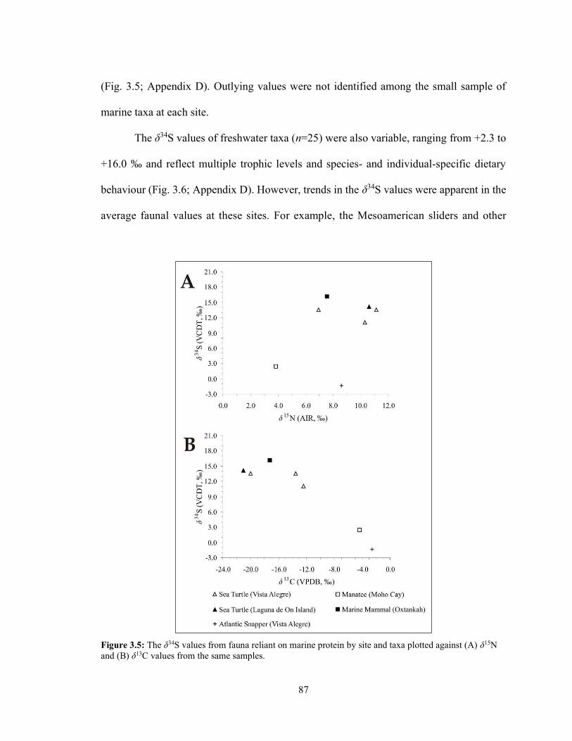
87

(Fig. 3.5; Appendix D). Outlying values were not identified among the small sample of

marine taxa at each site.

The δ34S values of freshwater taxa (n=25) were also variable, ranging from +2.3 to

+16.0 ‰ and reflect multiple trophic levels and species- and individual-specific dietary

behaviour (Fig. 3.6; Appendix D). However, trends in the δ34S values were apparent in the

average faunal values at these sites. For example, the Mesoamerican sliders and other

Figure 3.5: The δ34S values from fauna reliant on marine protein by site and taxa plotted against (A) δ15N and (B) δ13C values from the same samples.

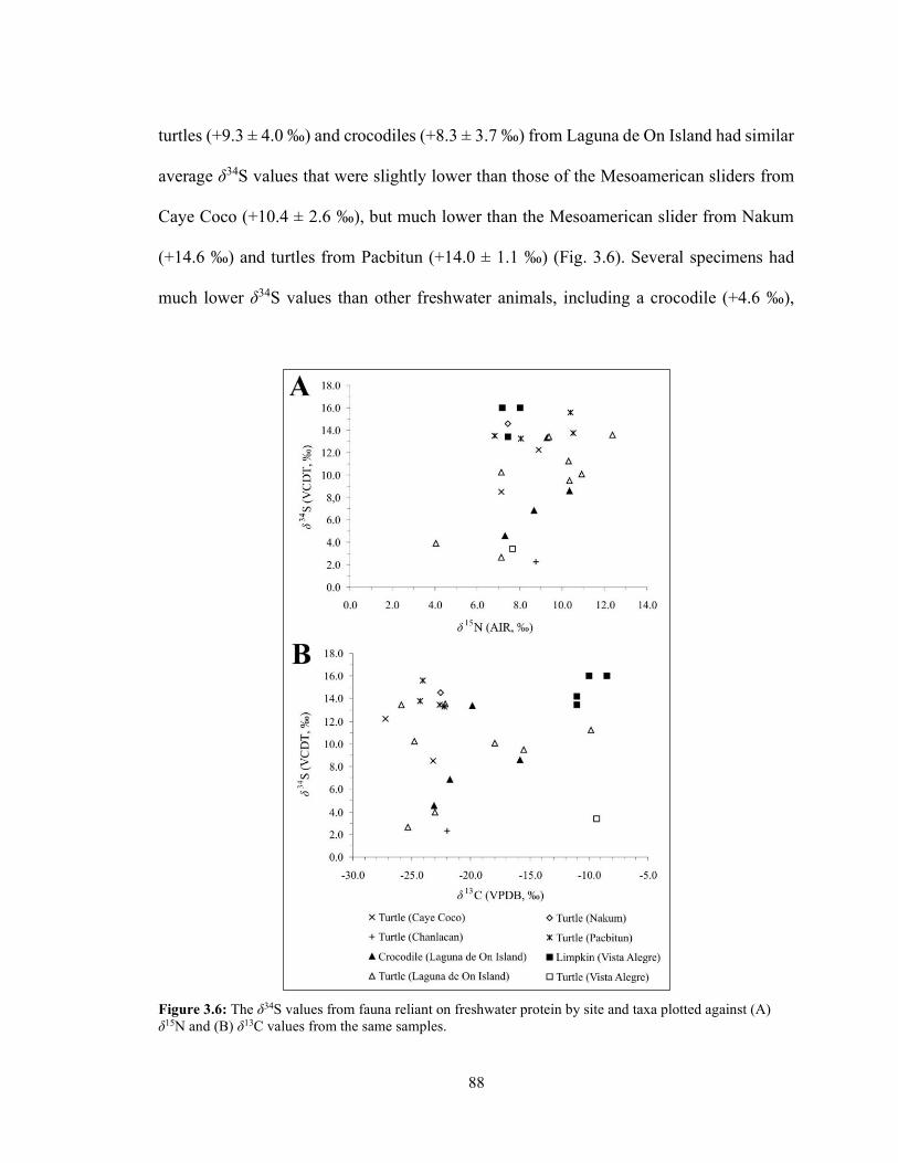
88

turtles (+9.3 ± 4.0 ‰) and crocodiles (+8.3 ± 3.7 ‰) from Laguna de On Island had similar

average δ34S values that were slightly lower than those of the Mesoamerican sliders from

Caye Coco (+10.4 ± 2.6 ‰), but much lower than the Mesoamerican slider from Nakum

(+14.6 ‰) and turtles from Pacbitun (+14.0 ± 1.1 ‰) (Fig. 3.6). Several specimens had

much lower δ34S values than other freshwater animals, including a crocodile (+4.6 ‰),

Figure 3.6: The δ34S values from fauna reliant on freshwater protein by site and taxa plotted against (A) δ15N and (B) δ13C values from the same samples.

89

Mesoamerican slider (+2.6 ‰), and another turtle (+3.9 ‰) from Laguna de On Island, a

pond turtle from Chanlacan (+2.3 ‰), and a Mesoamerican slider from Vista Alegre (+3.4

‰). Finally, the average δ34S value of the four Vista Alegre limpkins (+14.9 ± 1.3 ‰) was

elevated compared to that of the turtle (+3.4 ‰; Fig. 3.4), reflecting differing sources of

dietary protein for these freshwater species.

The δ34S values of the terrestrial fauna (n = 116) ranged from +3.3 to +18.8 ‰

(Appendix D) and were significantly different (H = 37.712, df = 3, p < 0.001) among sites

depending on the age of the underlying geology and distance from the coast (Table 3.3,

Fig. 3.7). The limestone bedrock beneath the sites included in this study dates to three

different periods, which from oldest to youngest are Mesozoic (Pacbitun and Xunantunich),

Paleogene/Neogene (Caye Coco, Caye Muerto, Chanlacan, Laguna de On Island and Shore,

Nakum, Oxtankah, and Ichpaatun), and Quaternary (Vista Alegre and San Miguelito). Vista

Alegre, San Miguelito, Oxtankah, and Ichpaatun are considered coastal while the remaining

sites are classified as inland (i.e., ≥ 20 km from the coast; Richards et al. 2001). Terrestrial

fauna from most coastal sites exhibited δ34S values influenced by sea spray sulfate that

were significantly higher (p < 0.001) than values of terrestrial fauna from inland sites

located on Paleogene/Neogene limestones (Table 3.3, Fig. 3.7). Faunal δ34S values from

sites located on Quaternary limestones did not significantly differ from those on

Paleogene/Neogene limestones in coastal (p = 0.323) or inland (p = 0.216) locations. The

faunal δ34S values from inland sites on Mesozoic limestone were statistically similar to

those from coastal sites on Quaternary (p = 0.792) or Paleogene/Neogene (p = 1.000)

limestone and were significantly higher than those from inland sites on younger

Paleogene/Neogene limestones (p < 0.001; Fig. 3.7).

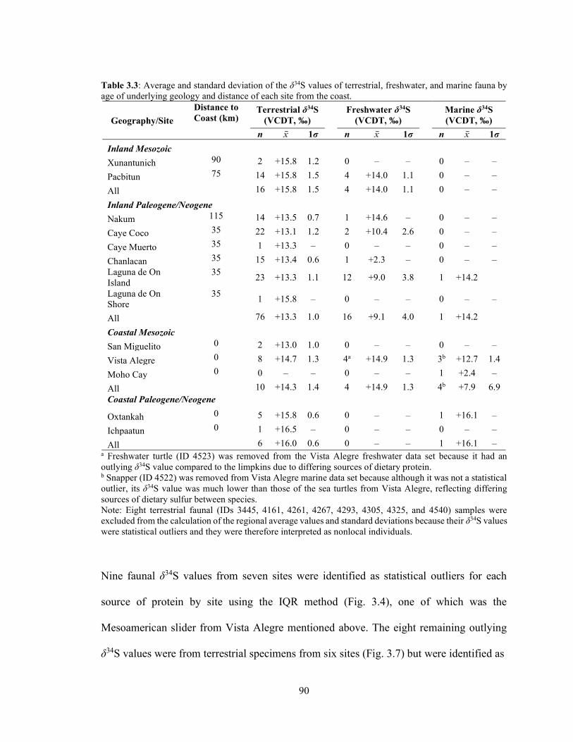
90

Table 3.3: Average and standard deviation of the δ34S values of terrestrial, freshwater, and marine fauna by age of underlying geology and distance of each site from the coast.

Geography/Site

Distance to Coast (km)

Terrestrial δ34S (VCDT, ‰)

Freshwater δ34S

(VCDT, ‰)

Marine δ34S (VCDT, ‰)

n x̄ 1σ n x̄ 1σ n x̄ 1σ

Inland Mesozoic

Xunantunich 90 2 +15.8 1.2 0 – – 0 – –

Pacbitun 75 14 +15.8 1.5 4 +14.0 1.1 0 – –

All 16 +15.8 1.5 4 +14.0 1.1 0 – –

Inland Paleogene/Neogene

Nakum 115 14 +13.5 0.7 1 +14.6 – 0 – –

Caye Coco 35 22 +13.1 1.2 2 +10.4 2.6 0 – –

Caye Muerto 35 1 +13.3 – 0 – – 0 – –

Chanlacan 35 15 +13.4 0.6 1 +2.3 – 0 – – Laguna de On Island

35 23 +13.3 1.1 12 +9.0 3.8 1 +14.2

Laguna de On Shore

35 1 +15.8 – 0 – – 0 – –

All 76 +13.3 1.0 16 +9.1 4.0 1 +14.2

Coastal Mesozoic

San Miguelito 0 2 +13.0 1.0 0 – – 0 – –

Vista Alegre 0 8 +14.7 1.3 4a +14.9 1.3 3b +12.7 1.4

Moho Cay 0 0 – – 0 – – 1 +2.4 –

All 10 +14.3 1.4 4 +14.9 1.3 4b +7.9 6.9 Coastal Paleogene/Neogene

Oxtankah 0 5 +15.8 0.6 0 – – 1 +16.1 –

Ichpaatun 0 1 +16.5 – 0 – – 0 – –

All 6 +16.0 0.6 0 – – 1 +16.1 – a Freshwater turtle (ID 4523) was removed from the Vista Alegre freshwater data set because it had an outlying δ34S value compared to the limpkins due to differing sources of dietary protein. b Snapper (ID 4522) was removed from Vista Alegre marine data set because although it was not a statistical outlier, its δ34S value was much lower than those of the sea turtles from Vista Alegre, reflecting differing sources of dietary sulfur between species. Note: Eight terrestrial faunal (IDs 3445, 4161, 4261, 4267, 4293, 4305, 4325, and 4540) samples were excluded from the calculation of the regional average values and standard deviations because their δ34S values were statistical outliers and they were therefore interpreted as nonlocal individuals. Nine faunal δ34S values from seven sites were identified as statistical outliers for each

source of protein by site using the IQR method (Fig. 3.4), one of which was the

Mesoamerican slider from Vista Alegre mentioned above. The eight remaining outlying

δ34S values were from terrestrial specimens from six sites (Fig. 3.7) but were identified as

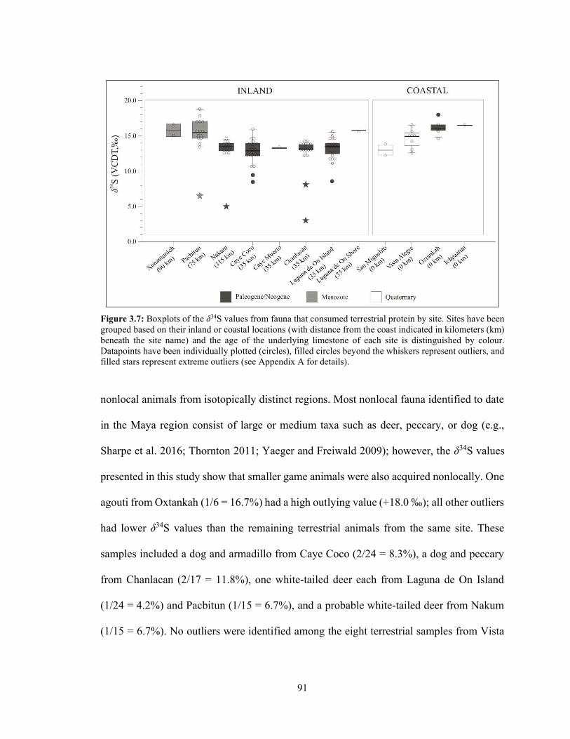
91

Figure 3.7: Boxplots of the δ34S values from fauna that consumed terrestrial protein by site. Sites have been grouped based on their inland or coastal locations (with distance from the coast indicated in kilometers (km) beneath the site name) and the age of the underlying limestone of each site is distinguished by colour. Datapoints have been individually plotted (circles), filled circles beyond the whiskers represent outliers, and filled stars represent extreme outliers (see Appendix A for details).

nonlocal animals from isotopically distinct regions. Most nonlocal fauna identified to date

in the Maya region consist of large or medium taxa such as deer, peccary, or dog (e.g.,

Sharpe et al. 2016; Thornton 2011; Yaeger and Freiwald 2009); however, the δ34S values

presented in this study show that smaller game animals were also acquired nonlocally. One

agouti from Oxtankah (1/6 = 16.7%) had a high outlying value (+18.0 ‰); all other outliers

had lower δ34S values than the remaining terrestrial animals from the same site. These

samples included a dog and armadillo from Caye Coco (2/24 = 8.3%), a dog and peccary

from Chanlacan (2/17 = 11.8%), one white-tailed deer each from Laguna de On Island

(1/24 = 4.2%) and Pacbitun (1/15 = 6.7%), and a probable white-tailed deer from Nakum

(1/15 = 6.7%). No outliers were identified among the eight terrestrial samples from Vista

92

Alegre, and it was not possible to identify outliers from Xunantunich, Caye Muerto, Laguna

de On Shore, Ichpaatun, or San Miguelito due to small sample sizes.

3.5 Discussion

3.5.1 Variation of Faunal δ34S Values in the Maya Region

The faunal δ34S values from Maya sites are variable but show patterns among the

marine, freshwater, and terrestrial species. Specifically, marine animals in this study

exhibited lower δ34S values than hypothesized, those of freshwater species varied by

location and the dietary preferences of specific species, and after removing nonlocal values,

the local terrestrial fauna δ34S values differed based on the distance from the coast and the

age of the underlying limestone.

Archaeological marine fish and mammals from the open ocean typically exhibit δ34S

values between +14 to +19 ‰ (Nehlich and Richards 2009; see also Fornander et al. 2008);

however, only the values of the marine mammal from Oxtankah (+16.1 ‰) and the sea

turtle from Laguna de On Island (+14.2 ‰) fell within this range. Instead, most marine taxa

from Maya sites had δ34S values less than +14 ‰, likely reflecting the influence of DSR or

freshwater discharge on the δ34S values of plants at the base of some marine food chains,

as has been found in modern saltmarsh and estuarian ecosystems (Kanaya et al. 2008;

Mizota et al. 1999; Peterson et al. 1986; Yamanaka et al. 2000). For example, manatee are

herbivorous generalized mixed feeders that consume seagrass and other submerged aquatic

vegetation, including macroalgae and mangroves (MacFadden et al. 2004; McKillop 1985),

all of which exhibit low modern δ34S values due to DSR (Canfield 2001; Fry et al. 1982,

1988; Raven and Scrimgeour 1997). Manatee, which are rare in Maya faunal assemblages,

93

also frequent estuarine areas (McKillop 1985) that are likely to have lower bioavailable

δ34S values resulting from freshwater discharge, as has been found in other archaeological

studies (Craig et al. 2006; Fornander et al. 2008; Linderholm et al. 2008b). The Atlantic

snapper had the lowest δ34S value in this study (–1.3 ‰), although its elevated δ13C and

δ15N values are consistent with those of other archaeological carnivorous reef fish

(Williams et al. 2009). Snappers frequent reefs, but also mud-bottom habitats (Gallaway et

al. 2009; Szedlmayer and Lee 2004) with anaerobic substrates that facilitate DSR (Kanaya

et al. 2008; Yamanaka et al. 2000), which would explain the low δ34S value of this

specimen. Finally, the more variable δ34S values among the loggerhead sea turtles reflect

their diets as generalist carnivores that feed on seasonally diverse foods (Hatase et al. 2002;

Plotkin et al. 1993; Tucker et al. 2014; Vander Zanden et al. 2010). As with the marine

animals from Maya sites, an archaeological marine turtle had a lower δ34S value (+8.8 ‰)

relative to that of a dolphin in Trinidad (+17.0 ‰; Sparks and Crowley 2018:973), further

indicating that dietary differences among marine species consumed by archaeological

humans must be considered when interpreting stable sulfur isotope values.

Although the δ34S values of freshwater taxa were variable depending on site

location and the diets of individual specimens, they were generally lower than those of both

terrestrial and marine animals from the same site (Table 3.2). Other studies have found the

δ34S values of archaeological freshwater fauna vary depending on the geology underlying

the freshwater ecosystem. For example, freshwater fish from the sulfur-poor clays near

Oxfordshire, UK during the Roman period had δ34S values as low as –20.9 to –17.3 ‰

(Nehlich et al. 2011), whereas those from freshwater lakes and rivers throughout the

Quaternary sediments near Late Bronze Age Chicha in Siberia were higher, ranging from

94

+14.8 to +21.8 ‰ (Privat et al. 2007). While the underlying limestone geology has also

influenced the δ34S values of the freshwater taxa included in this study, the variability

among individuals reflects individual dietary preferences as well as the numerous sulfate

inputs in freshwater ecosystems. The turtles from Pacbitun had the highest and least

variable δ34S of the freshwater reptiles, likely because they were acquired from nearby well-

oxygenated springs, creeks, and streams (Emery and Healy 2014). The more varied reptile

values from Caye Coco, Chanlacan, and Laguna de On Island, which included some of the

lowest reported in this study, show that the diets of some freshwater animals were

influenced by DSR in the sediments of nearby lagoons (Masson 2004), while others with

comparatively elevated values were not. This is also evident at Vista Alegre, where the δ34S

value of the Mesoamerican slider (+3.4 ‰) was considerably lower than those of the

limpkins (+14.7 ± 1.3‰). The environment of this coastal port site is characterized by a

flooded mangrove forest as well as wetlands (Beddows et al. 2016), and it appears that the

dietary sulfur of the turtle was derived from a wetland or mangrove ecosystem influenced

by DSR, whereas the diets of the freshwater apple snails consumed by the limpkins may

have been influenced by the elevated δ34S values of marine sulfate.

Before the terrestrial fauna δ34S values can be used to evaluate the hypothesized

variation in δ34S values in the Northern and Eastern Lowlands, it is necessary to identify

nonlocal animals so their values can be removed prior to calculating the local range for

each site. The presence of nonlocal taxa at a site identified zooarchaeologically, such as the

presence of a sea turtle at the inland Laguna de On Island site or a brocket and white-tailed

deer at the island site of San Miguelito off the coast of Cancun, is clear evidence for the

exchange of animal resources from different environments. Stable sulfur isotope analysis

95

offers an additional means of identifying nonlocal animals from isotopically distinct

regions that may otherwise be considered locally acquired.

Nonlocal terrestrial animals were distinguished by their outlying δ34S values at 6 of

the 13 sites included in this study, comprising between 4.2 % and 16.7 % of the sampled

faunal assemblages. The extremely high δ34S value of the agouti from Oxtankah (+18.0 ‰)

was notable, given that the diets of the local animals were already substantially elevated at

this coastal site due to sea spray (+15.8 ± 0.6 ‰). Due to the considerable overlap of the

δ34S values (i.e., equifinality) between coastal fauna and those located on sites underlain

by limestone, it is difficult to propose a probable place of origin for this specimen as this

time. However, the extremely low δ34S values of the deer, peccary, and armadillo from the

remaining sites are unlikely to have been derived from an area underlain by limestone, and

instead reflect the origin of these animals from an area where the geology is hypothesized

to exhibit lower δ34S values, such as the Maya Mountains or Highlands (Fig. 3.1). Based

on proximity, Rand et al. (2020a) proposed that the probable white-tailed deer from Nakum

may have been imported from the Maya Mountains. These data support a previous

hypothesis that specialized hunting of wild terrestrial game may have been practiced in less

populated areas, including the Maya Mountains (McAnany 1989; Yaeger and Freiwald

2009), and the procured animals may have been exchanged as food, tribute, or ritual items

(Thornton 2011).

Most of the nonlocal animals identified in this study belong to species (i.e., deer,

dog, and peccary) that strontium and oxygen isotope data show were acquired nonlocally

by the Maya (Sharpe et al. 2018; Sugiyama et al. 2018; Thornton 2011; Thornton et al.

2016; Yaeger and Freiwald 2009). This is the first study to isotopically identify a nonlocal

96

agouti and armadillo, which was surprising given the assumption that the Maya obtained

small animals locally. It is unlikely that the nonlocal δ34S values of these specimens reflect

differential dietary preferences among terrestrial species, as both have values that differ

from others of their species from the same site. This demonstrates that caution is necessary

when assuming that small mammals with narrow home ranges will represent local isotopic

baselines, especially when small sample sizes are considered.

When the eight nonlocal values are removed from the data set, the patterns in the

δ34S values of the local terrestrial fauna from coastal sites analyzed in this study are

consistent with the hypothesized elevated values in coastal areas (Fig. 3.1). The average

δ34S values of terrestrial fauna from Vista Alegre, Oxtankah, and Ichpaatun exceed +14 ‰

(Table 3.3), evidencing the influence of sea spray on dietary sulfur at these coastal sites, as

has been found at other coastal archaeological contexts (Fornander et al. 2008; Kinaston et

al. 2014; Richards et al. 2001; Stantis et al. 2015). The slightly lower δ34S values from the

brocket deer (+13.7 ‰) and white-tailed deer (+12.3 ‰) from San Miguelito (see Fig. 3.7)

suggest these animals may have been hunted in an inland area less influenced by sea spray

sulfate and were subsequently transported to this island site.

The local δ34S values of terrestrial fauna from inland Maya sites also varied

depending on the age of the underlying geology, although not as expected. Rather than

having lower δ34S values as hypothesized in Section 3 and Figure 3.1, sites located on

Mesozoic limestone (Xunantunich and Pacbitun) had the highest average terrestrial fauna

δ34S values, which were indistinguishable from those at coastal sites. The Xunantunich

specimens were analyzed at a different laboratory, which may introduce some variation;

however, the values from Pacbitun remain significantly elevated (H(3) = 37.862, p <

97

0.001), specifically relative to Inland Paleogene/Neogene (p < 0.001) and Coastal

Quaternary (p < 0.001) sites and are indistinguishable from Coastal Paleogene/Neogene

sites (p = 1.000). The elevated δ34S values of animals from sites underlain by Mesozoic

limestone were unexpected, given that older limestones typically exhibit slightly lower but

overlapping values with Paleogene/Neogene and Quaternary evaporites (Bottrell and

Newton 2006; Claypool et al. 1980; Fig. 3.1). Sea spray is an unlikely explanation for these

elevated values, given that the sampled sites were located a considerable distance from any

coast. It is also unlikely that all of these animals were imported from coastal areas, as the

Maya typically utilized local faunal resources (Götz 2008; Jiménez Cano and Sierra Sosa

2015; but see Thornton 2011; Yaeger and Freiwald 2009). Rather, it is possible that these

elevated δ34S values were derived from plants that assimilated sulfur from gypsum deposits

that are commonly found throughout the Mesozoic soils of the Yucatan (Perry et al. 2009).

The elevated terrestrial faunal δ34S values from inland Maya sites also demonstrate

why it is necessary to establish local baselines for specific regions. For example, the local

terrestrial faunal δ34S values from inland Maya sites (+10.7 to +18.8 ‰) were elevated

compared those reported from inland archaeological contexts from Europe (-13.5 to +13.7

‰; Fornander et al. 2008; Linderholm et al. 2008b; Nehlich et al. 2010, 2011; Richards et

al. 2001), Asia (+3.0 to +10.6 ‰; Guo et al. 2018; Irvine and Erdal 2020; Privat et al. 2007)

and the Caribbean (+2.4 to +9.2 ‰; Sparks and Crowley 2018). It has been previously

proposed that human or animal bone collagen from inland sites with δ34S values that exceed

+14 ‰ represent nonlocal individuals from coastal areas whose diets were influenced by

sea spray (Madgwick et al. 2019a; Richards et al. 2001). While this certainly holds true for

inland sites located on lithologies with lower δ34S values, the results of this study

98

demonstrate this is not applicable in regions underlain by marine evaporites such as

limestone that exhibit elevated values, as has been observed elsewhere (Curto et al. 2019;

Privat et al. 2007). This emphasizes the necessity of establishing local baseline δ34S values

for the interpretation of subsistence, migration, and animal exchange in the past.

3.5.2 Implications for Studies of Maya Diet, Animal Exchange, and Migration

Archaeological studies elsewhere in the world have investigated the use of sulfur

isotope analysis for distinguishing between terrestrial, freshwater, and marine protein in

human diets (Craig et al. 2006; Curto et al. 2019; Leach et al. 1996; Nehlich et al. 2010,

2011, 2012; Privat et al. 2007; Richards et al. 2001; Sayle et al. 2013). At Maya sites in the

Eastern and Northern Lowlands, sulfur isotope analysis appears useful for identifying the

consumption of freshwater protein but may be inappropriate for differentiating terrestrial

and marine diets. This is because the elevated δ34S values from terrestrial animals derived

from the underlying limestone geology overlapped with the values of marine fauna, many

of which had lower δ34S values than expected for archaeological marine taxa (+14 to +19

‰; Nehlich and Richards 2009; Fornander et al. 2008) likely due to the influence of DSR.

This suggests that it will be difficult to differentiate between marine- and terrestrial-based

diets among the Maya. However, future studies should consider that the δ34S values of

methionine from lime-processed maize may overwhelm those derived from animal protein

in Maya bone collagen.

In contrast, freshwater fauna generally had lower δ34S values than terrestrial and

marine animals, indicating sulfur isotope analysis may be useful for distinguishing Maya

freshwater protein consumption, as has been observed in other archaeological contexts

99

(Nehlich et al. 2010; Privat et al. 2007). This is an important area for future research, as

Maya reliance on freshwater resources has been relatively understudied. For example,

turtles are recognized food taxa, as is the freshwater jute snail (Pachychilus ssp.) but both

are interpreted as supplemental rather than as primary sources of dietary protein (Boileau

and Stanchly 2020; Healy et al. 1990; Masson 2004). Fish remains are found at sites

adjacent to lakes, estuaries, or the sea (e.g., Götz 2008; Jiménez Cano and Sierra Sosa 2015;

Masson 2004; Thornton 2011) but are notably absent from sites located near rivers

(Freiwald 2010). This cannot be fully explained by recovery methods (see Emery 2004b;

Masson 2004) and may reflect the poor preservation of archaeological fish bone (Szpak

2011), cultural practices such as filleting or salting fish where consumption and preparation

locations differed (Pohl 1983; but see McKillop and Aoyama 2018), or even a real cultural

aversion to fish as a food source (Pohl 1983). The application of stable sulfur isotope

analysis as well as compound-specific isotopic analysis of individual amino acids (Webb

et al. 2015) may address some of these questions, providing additional insights into Maya

freshwater protein consumption.

Stable sulfur isotope analysis has successfully identified nonlocal individuals as

those with statistically distinct δ34S values in other archaeological contexts (Nehlich et al.

2012; Vika 2009). Based on the identification of nonlocal faunal specimens in this study

(see also Rand et al. 2020a), it is also reasonable to propose that nonlocal Maya individuals

may be similarly identified. Importantly, sulfur isotope analysis tracks migration near the

end of life because bone collagen δ34S values represent an average derived from dietary

protein consumed from adolescence to the end of life, depending on which bone is sampled

and individual physiology in bone turnover rates (Hedges et al. 2007; Matsubayashi and

100

Tayasu 2019; Parfitt 2001; Richards et al. 2003; Webb et al. 2017). In contrast, strontium

and stable oxygen isotope analysis are typically conducted on tooth enamel due to issues

of diagenesis (Budd et al. 2000; Hoppe et al. 2003), and thus identify nonlocal individuals

who consumed isotopically distinct food and water during the period in childhood when

their teeth formed (Moradian-Oldak 2009). Thus, a multi-isotopic approach that

incorporates data from tissues that form at different periods can contribute to a more

detailed understanding of migration over the life course of an individual. Using multiple

isotopic analyses can also circumvent the limitations associated with the equifinality of δ34S

values (as well as strontium and oxygen isotope values; see Price et al. 2010) over large

regions of the Northern and Southern Lowlands to provide additional means for identifying

nonlocal individuals whose δ34S values may fall within the local range.

3.6 Chapter 3 Summary and Conclusions

The δ13C and δ15N results from the faunal samples analyzed here are consistent with

those reported in previous studies, and the faunal δ34S values provide important insights

into the variation of environmental δ34S values throughout the Maya region. The δ34S values

of marine animals were lower than expected and were likely influenced by DSR and

freshwater discharge into coastal ecosystems. The low yet variable δ34S values of

freshwater taxa are likely derived from DSR, the catchments and sulfur sources of

freshwater systems, and the individual dietary preferences of the sampled animals. As

observed in other contexts, sea spray elevated the δ34S values of coastal terrestrial animals;

however, inland terrestrial fauna from sites on Mesozoic limestone also had elevated values

rendering them indistinguishable from values at coastal sites. Importantly, these results

101

demonstrate the necessity of establishing separate ranges of local δ34S values for terrestrial,

freshwater, and marine protein sources at any given site.

The faunal results indicate that stable sulfur isotope analysis offers a potential tool

for differentiating terrestrial and freshwater diets at inland sites, although this is

complicated by factors that influence faunal δ34S values, including the type and age of the

underlying geology, distance from the coast and sea spray, DSR in aquatic environments,

riverine sulfate from multiple sources, and the diets of individual organisms. However, the

identification of nonlocal animals at six of the thirteen sites in this study also demonstrates

the potential of this technique not only for studies of animal exchanged for both subsistence

but also as organic artifacts but also migration among the Maya. The nonlocal δ34S values

of small mammals show that the Maya acquired fauna from diverse catchments and that

animal exchange extended to more species than previously known. The identification of

nonlocal faunal indicates this technique will be similarly useful for identifying nonlocal

Maya individuals. The analysis of stable sulfur isotopes from human bone collagen in

conjunction with strontium and stable oxygen isotope analysis of tooth enamel from the

same individual may also provide insight into movement at the end of life, or even if an

individual moved multiple times, and can help circumvent equifinality associated with any

one isotope system.

Stable sulfur isotope analysis is a relatively new method in archaeological studies

compared to more established techniques such as strontium and stable carbon, nitrogen,

and oxygen isotope analysis. As such, more research is needed to understand the influence

of preparation techniques and interlaboratory analyses on archaeological bone collagen

δ34S values. Additional research is also necessary to better characterize the δ34S values of

102

marine, freshwater, and terrestrial resources in the Maya region to improve understandings

of the food webs at each site and provide baseline isotopic data for studies of human diet

and movement. Expanding this research into the Highlands, Pacific Coast, Motagua Valley,

and the Maya Mountains will also reveal how much variation in δ34S values exists in the

Maya region, and more broadly across Mesoamerica. This study represents the first step in

a region-wide analysis of the utility of stable sulfur isotope analysis in Maya archaeology

and the application of this technique in a tropical continental archaeological context more

generally. Future multi-isotopic studies that include stable sulfur isotope analysis will

undoubtedly contribute to archaeological interpretations of Maya subsistence practices and

migration.

103

CHAPTER 4

STABLE SULFUR ISOTOPE EVIDENCE OF SUBSISTENCE PRACTICES AND MIGRATION AMONG THE MAYA8

Isotopic techniques offer an important tool for the study of subsistence strategies

and migration in archaeological contexts and therefore contribute to broader interpretations

of sociocultural processes in past societies (Anthony 1990; Cabana and Clark 2011a;

Gumerman 1997; Hastorf 2017; van der Veen 2003). In the Maya region, stable carbon

(δ13C) and nitrogen (δ15N) isotope analyses have been extensively used to investigate Maya

consumption of maize and animal protein (Somerville et al. 2013; Tykot 2002), and stable

oxygen (δ18O) and radiogenic strontium (87Sr/86Sr) isotope analyses have contributed to

8 This chapter was written solely by the author, although the results will be published in several venues. The data from Xunantunich, San Lorenzo, Caledonia, and Pacbitun is included in an article currently under review by PLoS ONE coauthored with principal author Dr. Claire Ebert, and coauthors Dr. Kirsten Green-Mink, Dr. Julie Hoggarth, Dr. Carolyn Freiwald, Dr. Jaime Awe, Dr. Willa Trask, Dr. Jason Yaeger, Dr. M. Kathryn Brown, Dr. Christophe Helmke, Rafael Guerra, Dr. Marie Danforth, and Dr. Douglas Kennett as part of a broader study of stable sulfur isotope analysis of human remains from Maya sites located in the Belize Valley and surrounding area (Ebert et al. in review). The Caledonia data was presented as a paper at the 48th Annual Meeting of the Canadian Association for Physical Anthropology in November 2020 coauthored by Dr. Freiwald and Dr. Vaughan Grimes (Rand et al. 2020b), and the Xunantunich and San Lorenzo data was also presented at the Bioarchaeology Early Career Conference (BECC) 2021 and coauthored with Dr. Freiwald, Dr. Jason Yaeger, Dr. M. Kathryn Brown, and Dr. Grimes (Rand et al. 2021b). The human isotopic data from Chac and Calakmul are detailed in a report submitted to Mexico’s Instituto Nacional de Antropología e Historia (INAH). The author also intends to publish the data from Mission San Bernabé in collaboration with Dr. Freiwald, Dr. Kathrine Miller Wolf, and Dr. Timothy Pugh as part of a multidisciplinary study of diet and health during the Colonial period. Finally, the Nakum data has been incorporated into a multi-isotopic case study of subsistence and migration at the site presented in Chapter 5 and published in the Journal of Archaeological Science: Reports (Rand et al. 2020a) in collaboration with Varinia Matute, Dr. Grimes, Dr. Freiwald, Dr. Jarosław Źrałka, and Dr. Wiesław Koszkul.

104

reconstructing migration to Maya sites (Price et al. 2008; Scherer et al. 2015; Wright 2012;

see Chapter 2).

Stable sulfur isotope (δ34S) analysis is a relatively new technique that has been

increasingly applied to the study of subsistence and migration in archaeological societies

(Nehlich 2015; see also Chapter 1). The considerable archaeological and isotopic databases

available in the Maya region provide an excellent framework in which to test the utility of

stable sulfur isotope analysis for identifying Maya diet and migration. Indeed, recent sulfur

isotope analysis of human bone collagen from Cahal Pech and Caledonia have

demonstrated the potential of this technique in Maya archaeology (Awe et al. 2017; Green

2016; Rand and Grimes 2017). Drawing on previously published isotopic and

archaeological evidence, as well as the faunal isotopic baseline data from Chapter 3 (Rand

et al. 2021a), this chapter interprets new δ13C, δ15N, and δ34S values from 49 Maya

individuals from seven Maya sites ranging from the Preclassic to Colonial periods. The

results demonstrate how the integration of sulfur isotope analyses into a multi-isotopic

approach provides new insights into Maya subsistence strategies and migration.

4.1 Principles of Stable Isotope Analysis

Because the isotopic values of consumer tissues reflect those of protein in their diets

(Ambrose and Norr 1993; Richards et al. 2003; Webb et al. 2017), these techniques are

useful for reconstructing past subsistence practices as well as the source of dietary protein.

The systematics of stable sulfur, carbon, and nitrogen isotope analyses and how they vary

in the Maya region are briefly reviewed here and are discussed in detail in Chapter 3.

Stable carbon isotope (δ13C) analysis is used to differentiate between sources of

105

dietary protein derived from plants at the base of the food chain that use the C3 (Calvin-

Benson) and C4 (Hatch-Slack) photosynthetic pathways (Smith and Epstein 1971; van der

Merwe 1982). The δ13C values of plants are passed on to their consumers, although

metabolic fractionation causes the values of consumer tissues to be 5 ‰ higher than those

of plants (Caut et al. 2009). C3 plants are the dominant species in the Maya lowlands, with

δ13C values –26.5 ‰ (O’Learly 1988), although local environmental conditions, such as

the canopy effect, can cause these values to vary (Drucker et al. 2008; van der Merwe &

Medina 1991). The most abundant C4 plant consumed by the Maya was maize (Zea mays),

with δ13C values near –12.5 ‰ (O’Leary 1988; Smith and Epstein 1971). Although marine

species also have elevated δ13C values that overlap with the range of terrestrial C4 plants in

the Maya region (Keegan and DeNiro 1988; Rand et al. 2021a), it is unlikely they formed

a significant part of the diet at the inland sites considered in this study.

Stable nitrogen isotope (δ15N) values increase stepwise by 3 to 5 ‰ at each level of

the food chain (Delwiche and Steyn 1970; Hedges and Reynard 2007; O’Connell et al.

2012) and indicate the trophic level of consumers. Thus, human diets that included

terrestrial animal protein will have elevated bone collagen δ15N values relative to

herbivores. This also allows breastfeeding infants to be identified as those with elevated

δ15N values relative to their mothers (Fuller et al. 2006). Terrestrial plants have δ15N values

around +3 ‰, although legumes that directly fix nitrogen have values close to 0 ‰

(Delwiche and Steyn 1970; Wada et al. 1975). Environmental factors such as precipitation,

aridity, and soil nitrates (Ambrose 2001; Somerville et al. 2018) and cultural factors such

as agricultural practices (Szpak 2014) can further influence human bone collagen δ15N

values. As with δ13C values, the δ15N values of marine species tend to overlap with those

106

of terrestrial species in the Maya region (Rand et al. 2021a; Sharpe et al. 2018; Thornton et

al. 2016), although this is unlikely to be a concern in this study, as explained above. Finally,

both the δ13C and δ15N values of freshwater species are not well known in the Maya region,

but preliminary analyses suggest they are highly variable and reflect the diverse dietary

preferences of freshwater species (Rand et al. 2021a).

Sulfur isotope values in archaeological skeletal tissues have been used to

differentiate between the consumption of terrestrial, freshwater, and marine resources and

can be useful for identifying nonlocal individuals in archaeological contexts (Nehlich

2015). Bone collagen δ34S values are derived from dietary methionine, which is assimilated

from environmental sulfur by plants at the base of the food chain (Brosnan and Brosnan

2006; Ingenbleek 2006). Because animals cannot synthesize this essential amino acid

internally, it must be obtained from dietary protein (Brosnan and Brosnan 2006; Ingenbleek

2006; Tanz and Schmidt 2010). While the offset between the δ34S values of consumer

tissues and their diet (Δ34Stissue-diet) is assumed to be below the level of analytical uncertainty

and therefore inconsequential for dietary interpretation (i.e., +0.5 ± 2.4 ‰; Nehlich

2015:Table 2; see also Krajcarz et al. 2019), other research indicates it may be more

substantial (i.e., –1.5 ‰; Webb et al. 2017; see also Tanz and Schmidt 2010). Culinary

practices, such as the addition of salt or processing maize with lime (i.e., nixtamalization),

may also complicate the interpretation of human δ34S values. While these techniques may

introduce exogenous sulfur to foods, this sulfur has not been assimilated into methionine

by plants and therefore is not bioavailable for incorporation into consumer bone collagen.

Nixtamalization does, however, double the amount of digestible methionine available from

107

maize (Ellwood et al. 2013; Katz et al. 1974), and so the δ34S values of Maya bone collagen

may be preferentially derived from processed maize over animal protein.

Marine sulfate has uniform δ34S values around +21 ‰ (Böttcher et al. 2007; Rees

et al. 1978), which is also deposited into coastal soils due to the sea spray effect

(Gravenhorst 1978; Wakshal and Nielsen 1982). Freshwater rivers and lakes contribute

lower δ34S values to aquatic plants and their consumers in the Maya region, and the

consumption of terrestrial animals from the granitic Mountain Pine Ridge of the Maya

Mountains or volcanic Maya Highlands are also expected to contribute lower values to

human tissues in these regions (Chapter 3; Rand et al. 2021a). Indeed, two humans from

Peligroso and Ramonal in the Mountain Pine Ridge area both had δ34S values of +8.5 ‰

(Ebert et al. under review). Although the Yucatan Peninsula exhibits higher δ34S values

than in other inland archaeological contexts due to the limestone geology, they vary

depending on the age of formation and distance from the coast, permitting the identification

of nonlocal individuals from isotopically distinct regions (Chapter 3; Rand et al. 2021a).

Finally, the residential history throughout an individual’s life course may be

reconstructed through a comparison of multiple isotopic assays of tissues that form at

different ages. It is difficult to assess the influence of diagenesis on 87Sr/86Sr and δ18O

values and therefore enamel is preferentially sampled over bone, as it is less susceptible to

diagenesis (Hoppe et al. 2003). Enamel forms during childhood and does not subsequently

remodel (AlQahtani et al. 2010; Moradian-Oldak 2009), so that the 87Sr/86Sr and δ18O

values of enamel indicate the source of foods and water consumed during childhood. In

contrast, because bone remodels throughout life, the δ34S values of collagen will represent

an average of dietary protein consumed from adolescence to the end of life, depending on

108

which bone is sampled and individual physiological variation in bone turnover rates

(Hedges et al. 2007; Matsubayashi and Tayasu 2019; Parfitt 2001). Thus, a comparison of

isotopic techniques applied to tissues from the same individual that form at different ages

may therefore reveal whether her or she migrated multiple times as well as the length of

time he or she resided in the place of burial prior to death.

4.2 Site and Sample Description

Samples of human bone from seven sites (Fig. 4.1), including Xunantunich (n =

11), San Lorenzo (n = 7), Pacbitun (n = 26), and Caledonia (n = 24) in western Belize, as

well as Nakum (n = 9) and San Bernabé (n = 10) in Peten, Guatemala, and Calakmul (n =

10) in southern Campeche, Mexico were selected for analysis. Although nine bone samples

from Chac in western Yucatan, Mexico, were also prepared, they were too poorly preserved

for stable sulfur isotope analysis (Appendix E) and so this site is not discussed further. The

remaining sites are described below, their chronologies are presented in Figure 4.2, and

details regarding specific archaeological projects can be found in Appendix A. The samples

from each site that provided sufficient collagen (i.e., at least 16 mg) for stable carbon,

nitrogen, and sulfur isotope analyses (n = 49) are also summarised here and in Table 4.1,

and the details of individual samples can be found in Appendix E.

4.2.1 Xunantunich and San Lorenzo, Belize

Xunantunich is one of the largest sites in the Belize Valley (see Figure 4.3),

consisting of a core of four monumental groups (Groups A to D) that cover 0.14 km2 on

top of a hill east of the Mopan River. While there is evidence of a small Early and Middle

Preclassic settlement at the site, Xunantunich was established as a major center at the

109

Figure 4.1: Geological baseline map of the Maya region indicating the expected environmental δ34S values and location of Maya sites from which samples of human bone were analyzed: (1) Calakmul, (2) Mission San Bernabé, (3) Nakum, (4) Xunantunich, (5) San Lorenzo, (6) Pacbitun, (7) Caledonia, and (8) Chac. Map created by Bryn Trapper based on the Geological Map of North America 2005 (1:5,000,000) (Garrity and Soller 2009).

110

Figure 4.2: Chronological periods and ceramic phases of the sites discussed in the chapter. Note that the Uaxactun ceramic sequence was used at both Caledonia and Mission San Bernabé, and that the phases have been rounded to the nearest 50 years. Data compiled from Awe (1985), Domínguez Carrasco (1994), Folan et al. (1995), Healy et al. (2004a, 2004b), LeCount et al. (2002), Leventhal et al. (2010), Powis et al. (2017), Pugh et al. (2012), and Źrałka et al. (2018).

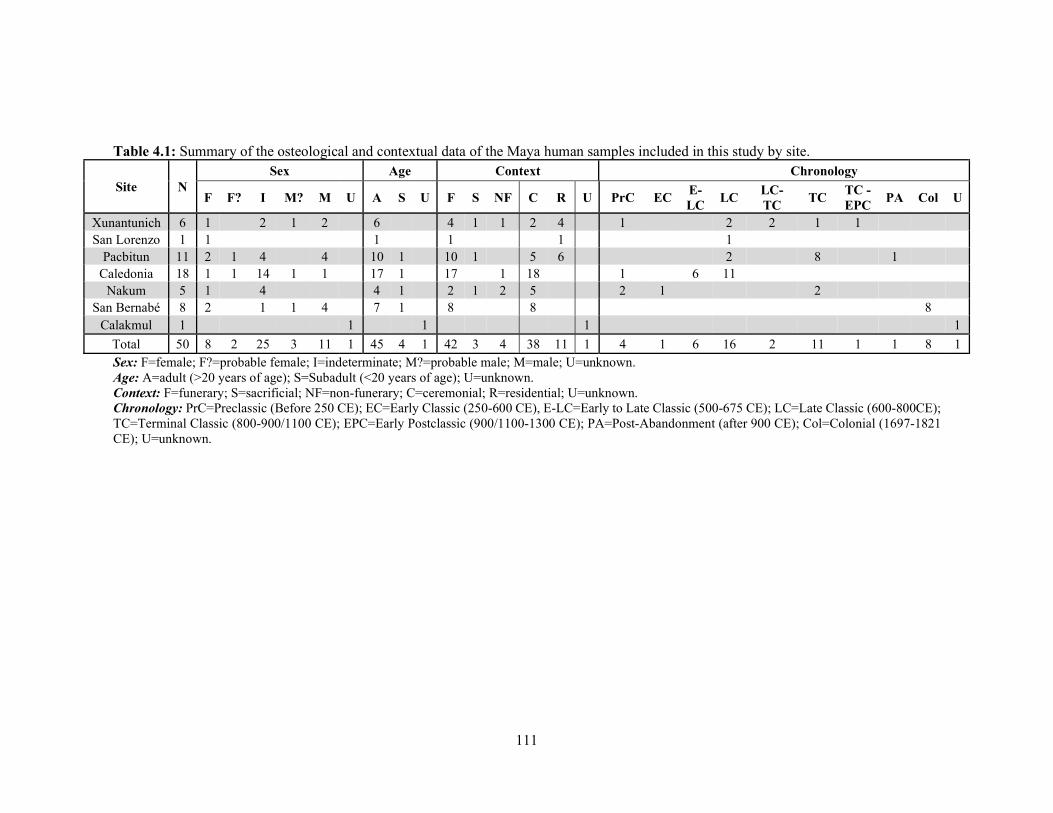
111

Table 4.1: Summary of the osteological and contextual data of the Maya human samples included in this study by site.

Site N Sex Age Context Chronology

F F? I M? M U A S U F S NF C R U PrC EC E-LC

LC LC-TC

TC TC - EPC

PA Col U

Xunantunich 6 1 2 1 2 6 4 1 1 2 4 1 2 2 1 1

San Lorenzo 1 1 1 1 1 1

Pacbitun 11 2 1 4 4 10 1 10 1 5 6 2 8 1

Caledonia 18 1 1 14 1 1 17 1 17 1 18 1 6 11

Nakum 5 1 4 4 1 2 1 2 5 2 1 2

San Bernabé 8 2 1 1 4 7 1 8 8 8

Calakmul 1 1 1 1 1

Total 50 8 2 25 3 11 1 45 4 1 42 3 4 38 11 1 4 1 6 16 2 11 1 1 8 1 Sex: F=female; F?=probable female; I=indeterminate; M?=probable male; M=male; U=unknown. Age: A=adult (>20 years of age); S=Subadult (<20 years of age); U=unknown. Context: F=funerary; S=sacrificial; NF=non-funerary; C=ceremonial; R=residential; U=unknown. Chronology: PrC=Preclassic (Before 250 CE); EC=Early Classic (250-600 CE), E-LC=Early to Late Classic (500-675 CE); LC=Late Classic (600-800CE); TC=Terminal Classic (800-900/1100 CE); EPC=Early Postclassic (900/1100-1300 CE); PA=Post-Abandonment (after 900 CE); Col=Colonial (1697-1821 CE); U=unknown.

112

Figure 4.3: Map of eastern Peten, the Belize River Valley, the Vaca Plateau (shaded area), and Maya Mountains. Sites mentioned in the text are highlighted in red. Note: location of Mission San Bernabé, Chac II, and Calakmul not shown (modified from the original Social Archaeology Research Program (SARP) project map with permission from Dr. Gyles Iannone [personal communication, 2020]). beginning of the Late Classic period around 600/670 CE (LeCount et al. 2002), likely

through its mutual ties to Naranjo (LeCount and Yaeger 2010; LeCount et al. 2002;

Leventhal et al. 2010). By the beginning of the Late Classic II phase (670-780 CE: see Fig.

4.2), the site had reached is peak in terms of population and architecture. With the fall of

Naranjo around 820 CE, a new autonomous ruling family took charge at Xunantunich

(LeCount and Yaeger 2010; Leventhal et al. 2010).

113

San Lorenzo was a small community located on a ridge approximately 1.6 km

northeast of Xunantunich on the east bank of the Mopan River (Yaeger 2000). This

community consisted of five spatially discrete settlement clusters, numerous isolated

mounds, and a ritual-administrative group (SL-13). These structures primarily date to the

Late and Terminal Classic periods (600-890 CE), although a community existed at the site

in earlier periods (Yaeger 2000). This site has been interpreted as a rural community in the

hinterland of Xunantunich with social and economic ties to the larger centre (Yaeger 2000).

As at Xunantunich, it appears that occupation at San Lorenzo rapidly grew during the Late

Classic I phase (600-670 CE), peaked during the Late Classic II phase, after which it

experienced a decline and eventual abandonment in the Terminal Classic (Yaeger 2000).

Based on archaeological and isotopic evidence, the residents of Xunantunich and

San Lorenzo likely obtained most subsistence resources locally, farming in the alluvial

floodplain of the Mopan River and the limestone uplands and obtaining faunal resources

from the uplands and the river (Fedick 1995; Yaeger 2010:234). The river also facilitated

trade and travel (LeCount and Yaeger 2010; Yaeger 2005:5, 2010). Indeed, isotopic

analysis found that animal resources were brought to the site from the Vaca Plateau and

Macal River regions to the south and east (Yaeger and Freiwald 2009), and that 50% of

sampled individuals from Xunantunich and 30% from San Lorenzo were born in

isotopically distinct regions (Freiwald 2011a, 2011b; Freiwald et al. 2014), perhaps

reflecting rapid site growth in the Late Classic period (Whitridge, personal communication,

2021).

Because San Lorenzo is a hinterland community of Xunantunich, their data sets

have been combined in this study. A total of 6 adult individuals from Xunantunich and 1

114

from San Lorenzo are considered in this study, including two females, two males, one

probable male, and two individuals of indeterminate sex. Five came from formal funerary

contexts, one came from a termination deposit, and one was from a non-funerary context.

Two of these individuals were interred in ceremonial structures and five in residential

complexes. Finally, one dates to the Late Preclassic, two dates to the Late Classic II period,

two date to the Late Classic II or Terminal Classic periods, one dates to the Terminal

Classic, and one dates to the Terminal Classic or Early Postclassic period (see Table 4.1

and Appendix E).

4.2.2 Pacbitun, Belize

Pacbitun is a medium-sized regional centre located in the limestone foothills 1 km

to the north of the Maya Mountains (Figs. 4.1 and 4.3). The site epicenter comprises five

primary plaza groups (A to E) with a total of 40 major masonry structures (Healy et al.

2004b, 2007), and is part of the broader core zone that contains numerous small and

medium-sized structures likely representing commoner households (Healy et al. 2004b,

2007). Pacbitun was occupied from the Middle Preclassic (~900 BCE) to the end of the

Classic period. During the Early Classic period, the site may have been politically linked

with Caracol on the Vaca Plateau, although most of the material culture from Pacbitun in

the Late Classic is more similar to that from Xunantunich (Healy et al. 2004b). During the

Late and Terminal Classic periods (550-900 CE), population and monumental construction

at Pacbitun reached their florescence before the site was abandoned around 900 CE,

although there is also at least one post-abandonment burial from the site (Healy et al. 2004b,

2007).

115

The location of the site near the intersection of the tropical broadleaf rainforest and

the Mountain Pine Ridge region of the Maya Mountains provided access to numerous

resources, fertile agricultural land, as well as various animal species for local use or export

(Emery and Healy 2014; Healy 1990). Archaeological evidence also indicates that long-

distance trade networks were established by about 500 BCE (Awe and Healy 1994). Due

to population increase during the Late Classic period, agricultural terraces were built in the

limestone hills to increase agricultural production (Healy et al. 1980). Indeed, stable carbon

and nitrogen isotope analysis of twenty burials from Pacbitun revealed that maize

consumption increased during the Early and Late Classic periods and decreased during the

Terminal Classic (Coyston et al. 1999; White et al. 1993).

Eleven Pacbitun individuals were analyzed in this study. One was a subadult and

ten were adults, including two females, one probable female, four males, and three

individuals of indeterminate sex. The five formal burials from four funerary and one

dedicatory deposit interred in ceremonial architecture in the epicentre are presumed to be

of higher status than the six formal burials from residential contexts in the core zone

(Robertson 2011). Eight date to the Terminal Classic period, whereas two date to the Early

Classic period, and one was buried after the site was abandoned (Table 4.1; Appendix E).

4.2.3 Caledonia, Cayo District, Belize

Caledonia was a minor Maya centre located on the west bank of the Macal River at

the intersection of the limestone Vaca Plateau and metamorphic Pine Ridge region of the

Cayo District in Belize (Figs. 4.1 and 4.3). The site consists of four plazas arranged into

two groups located on slight hills separated by a creek (Awe 1985). Although Caledonia

116

was first settled during the Preclassic period around 100 CE and continuously occupied, it

primarily dates to the second half of the Classic period (600-1000 CE; Awe 1985:388) and

was abandoned in the Terminal Classic or Early Postclassic periods (900-1000 CE).

Caledonia was likely under the influence, if not actual control, of a larger primary centre,

most likely nearby Caracol (Awe 1985). Based on the ceramic assemblage, Awe (1985)

proposed that Caledonia, through Caracol, was influenced by sites located in the central

Peten until the early Late Classic period, after which some influence appears to have come

from the Belize Valley before the site was again affiliated with those in Peten.

Previous carbon and nitrogen isotope analyses found these individuals consumed a

maize-based diet with contributions from C3 plants and terrestrial herbivores, and possibly

freshwater snails and/or molluscs (Rand 2012; Rand et al. 2015b). While stable oxygen

isotope analysis indicates all individuals were local, the elevated values from the six

individuals interred in Burial 1 suggest they may have relied on a different source of

drinking water or moved from a nearby area, as did one individual from Burial 3 who had

enamel and bone values that differed from those oft the other three individuals from this

burial (Rand 2017). This dissertation research builds upon preliminary sulfur isotope results

that suggest these individuals obtained their protein locally, although variation was present

(Rand and Grimes 2017).

Eighteen individuals from Caledonia were analyzed in this study, including one

female, one probable female, thirteen individuals of indeterminate sex, one probable male,

and one male, all of whom were adults. An additional subadult could not be sexed. All were

from funerary contexts in ceremonial architecture in the site core, excluding an adult third

metatarsal recovered from within Vessel 3 in Burial 1. While I have interpreted the latter

117

as a “finger bowl”, it is unlike finger bowls from non-funerary caches at nearby Caracol

that consist of small unslipped dishes set lip-to-lip containing metacarpals or phalanges of

the hand (Chase and Chase 2017:213). One individual dates to the Preclassic period, six

date to the transition between the Early and Late Classic periods, and the remaining 11

individuals date to the Late Classic period (Table 4.1; Appendix E).

4.2.4 Nakum, Guatemala

Nakum is located on the bank of the Holmul River in Peten region of Guatemala

(Fig. 4.1 and 4.3). The site is divided into a Northern and Southern Sector that are connected

by the Perigny Causeway (Źrałka and Hermes 2012). Nakum was continuously occupied

from the Middle Preclassic through to the Terminal Classic period, and following a brief

hiatus, there is some evidence for Postclassic occupation at the site (Koszkul et al. 2006,

2009; Źrałka and Hermes 2012; Źrałka and Koszkul 2007; Źrałka et al. 2014, 2017, 2018).

Throughout the Late Classic period, Nakum was likely subordinate to Tikal or Naranjo,

although the decline of these centres during the Terminal Classic allowed Nakum to

experience architectural and political growth, and possibly the arrival of migrants from

surrounding sites, until the site was ultimately abandoned around 950 CE (Źrałka and

Hermes 2012).

The Holmul River was an important trade route between the Caribbean and Central

Peten and was likely intermittently controlled by Tikal and Naranjo prior to their decline

during the Terminal Classic, when individuals from Nakum took control of the trade route

(Źrałka and Hermes 2012:178). The location on the river would have facilitated the

transport of goods, foodstuffs, and people to and from Nakum. The subsistence base for the

118

population of Nakum was probably facilitated by agriculture in fields underlain by

Palaeogene and Quaternary limestones and animals hunted in the surrounding region,

although at least one deer was brought to the site, perhaps from the Maya Mountains (Rand

et al. 2020a, 2021a; Chapters 3 and 5).

Five Nakum individuals provided sufficient collagen for analysis, including one

adult female and three adults of indeterminate sex, and one subadult who could not be

sexed. All five came from ceremonial structures in the site core, two of which were formal

funerary contexts, one was interpreted as a termination deposit, and two were non-funerary

in nature. Finally, two individuals date to the Preclassic period, one dates to the Early

Classic, and two date to the Terminal Classic period (Table 4.1; Appendix E).

4.2.5 Mission San Bernabé, Guatemala

Unlike the other sites included in this study, Mission San Bernabé was a Colonial

period Spanish mission established near the Postclassic Itza Maya site of Tayasal on Lake

Peten Itza in central Peten, Guatemala (Fig. 4.1). Following their defeat of the Itza in 1697

CE, the Spaniards built a presidio (fortified administrative centre) on the ruins of the Itza

capital of Nojpeten on Flores Island (Jones 1998) and forcibly relocated Maya populations

to reducciones around Lake Peten Itza (Jones 1998; Pugh et al. 2012, 2016; Schwartz

1990). Mission San Bernabé was one such reduccion built by at least 1712 CE on a Late

Preclassic site close to Tayasal that was intensively reused during the Late to Terminal

Classic periods (Pugh et al. 2012). However, by 1778 CE, the site was abandoned (Caso

Barrera 2002:352 Table VII.1; Jones 1998: Table 15.4).

In terms of subsistence, historical documents suggest the Spaniards encouraged

119

Peten Maya to cultivate maize and beans and discouraged them from relying on forest and

garden resources (Schwartz 1990:48-49, 62). Although deer, peccary, and turtles were

important in earlier periods, Colonial Mission San Bernabé residents preferred cows and

pigs, although aquatic species remained important (Freiwald 2012, n.d.; Freiwald and Pugh

2018; Pugh et al. 2016). Isotopic analyses suggest that European domesticates were raised

locally but were likely foddered in different ways (Freiwald under review; Freiwald and

Pugh 2018). Strontium and stable oxygen isotope analysis also suggest that most of the

residents of Mission San Bernabé were local and probably Maya (Freiwald et al. 2020),

although people of Spanish and African descent also likely lived in settlements around the

lake (Pugh et al. 2012).

Eight individuals interred in the church of Mission San Bernabé were analyzed in

the current study, including a subadult, two adult females, four adult males, and one adult

who was probably male. All were interred in Christian style burials within and to the east

of the Mission San Bernabé church during the Colonial period (Table 4.1; Appendix E).

4.2.6 Calakmul, Mexico

Calakmul is located in the southeastern part of Campeche, Mexico (Fig. 4.1) on a

35 m rise east of a large bajo (seasonal swamp). The core area comprises 975 structures

within 1.75 km2, while smaller residential mounds extend for an additional 20 km2 from

the site core (Folan et al. 1995; Martin and Grube 2008; Sharer and Traxler 2006:356).

Calakmul was likely established during the Middle Preclassic but rose to prominence as a

large civic-ceremonial centre in the Late Preclassic period. The fall of nearby El Mirador

in the Late Preclassic was likely a turning point for Calakmul, and by the Early Classic the

120

site had emerged as a powerful regional capital. Throughout the Early Classic, Calakmul

was at the centre of regional politics in the lowlands, competing with Tikal for alliances

with sites such as Yaxchilan, Caracol, and Naranjo (Folan et al. 1995; Martin and Grube

2008). At the beginning of the Late Classic period, the Kaanul dynasty moved from the site

of Dzibanche to Calakmul (Martin 2020:391), transforming the site into one of the most

important centres in the lowland Maya region, with a regional state covering at least 80,000

km2 that included numerous secondary centres. The site continued to be occupied into the

Terminal Classic period and the last datable stela from Calakmul was dedicated in 810 CE

prior to the abandonment of the site (Folan et al. 1995).

Archaeological evidence indicates that the rich soils along the margin of

the bajo were used for agriculture following droughts that dropped the water level after 200

CE (Domínguez Carrasco and Folan 1996). Due to the location of Calakmul in an area with

limited surface water, residents relied on complex hydraulics to irrigate agricultural fields

and trade to obtain additional subsistence resources and raw materials (Gunn et al. 2002).

Previous isotope analysis found that the Calakmul individuals consumed a typical Classic

Maya maize-based diet supplemented with other plant and animal resources, and that over

two thirds of the population was local (Price et al. 2018a). Ten human bone samples were

prepared for analysis, although only one sample from an individual of unknown age and

sex (F5335; Ent. 2 Caja 10) was sufficiently preserved for isotopic analyses in this study

(Appendix E).

4.3 Methods

Originally, 106 human bone samples were prepared for stable isotopic analyses,

121

including 11 from Xunantunich, 7 from San Lorenzo, 26 from Pacbitun, 24 from Caledonia,

9 from Nakum, 10 from Mission San Bernabé, 10 from Calakmul, and 9 from Chac II

(Appendix E)9. Samples were cleaned, prepared, and analyzed using the same methods

applied to the faunal remains in Chapter 3 and described in detail in Appendix A. Briefly,

a modified Longin (1971) method was used to extract collagen, wherein samples were first

demineralized in hydrochloric acid (0.5 M HCl) and treated with sodium hydroxide (0.1 M

NaOH; excluding the initial Caledonia samples, see Appendix A and B for details) prior to

being hydrolysed, ultrafiltered, and freeze-dried (Honch et al. 2006; Nehlich and Richards

2009; Szpak et al. 2017b).

Collagen was successfully extracted from 70 of the 106 samples (Appendix E),

which is unsurprising given that Maya skeletal samples are often poorly preserved. All 70

samples were subjected to stable carbon and nitrogen isotope analysis because of the low

amount of collagen (1 mg) required for these analyses, but also because these data are

necessary to evaluate whether the δ34S values have been influenced by diagenesis (Nehlich

and Richards 2009) and to interpret the δ34S results. Unlike stable carbon and nitrogen

isotope analysis, stable sulfur isotope analysis requires larger collagen samples (5 to 50 mg

depending on the laboratory; Appendix A), and only 56 of the 70 samples yielded sufficient

collagen for this procedure.

Carbon and nitrogen isotopes and concentrations from the Caledonia, Pacbitun, and

Nakum samples were analyzed in CREAIT’s Stable Isotope Laboratory at Memorial

9 Sample selection was determined by the principal investigators of individual archaeological projects and were largely chosen to address research questions specific to each project. Poor bone preservation typical of the Maya region also dictated which burials and elements were included in this study. These factors combined influenced the final number of samples included in this study.

122

University (MUN; see Appendix A for details) with a standard uncertainty of ±0.28 ‰ for

δ13C and ±0.24 ‰ for δ15N (Appendix C). Samples from Caledonia were also analyzed in

the Ján Veizer Stable Isotope Laboratory at the University of Ottawa (Ottawa), as were

samples from San Lorenzo, Xunantunich, Mission San Bernabé, Chac II, and Calakmul

(see Appendix A) with a standard uncertainty of ±0.11 ‰ for δ13C and ±0.08 ‰ for δ15N

(Appendix C).

The stable sulfur isotopes and concentrations from the original Caledonia samples

prepared without a NaOH step were also analyzed at MUN (see Appendix A) with a

standard uncertainty of ±1.24 ‰ for δ34S (Appendix C). The original samples and

resamples from Caledonia, as well as the samples from Pacbitun and Nakum were analyzed

by the Stable Isotope Laboratory in the Department of Earth and Planetary Sciences at the

University of Tennessee (Tennessee; Appendices A and B). Measurement precision was

±1.00 ‰ for δ34S, although analytical accuracy and standard uncertainty could not be

assessed as check standards were not included in the analyses (Appendix C). Finally, one

sample from Caledonia, as well as the samples from Xunantunich, San Lorenzo, Mission

San Bernabé, and Calakmul were analyzed at Ottawa (Appendix A) with a standard

uncertainty of ±0.32 ‰ for δ34S (Appendix C).

Stable sulfur isotope analysis can identify nonlocal individuals as those with δ34S

values that differ from those expected from locally available sources of protein. While

faunal baselines are useful for approximating local δ34S values (Chapter 3), faunal remains

were not available from all seven sites from which human remains were analyzed. Instead,

outliers were identified as those with δ34S values that fell beyond the interquartile range

(IQR) multiplied by 1.5 subtracted from the first quartile and added to the third quartile of

123

the data set from each site (see Appendix A). These outlying δ34S values were then

removed, and the local range of δ34S values was calculated as falling within two standard

deviations of the mean (x̄ ± 2σ) of the remaining values (after Price et al. 2002; see

Appendix A). The distribution of the δ13C, δ14N, and δ34S values by site were assessed using

the Shapiro-Wilk test (W), and appropriate comparative statistical methods were then

applied to explore correlations and differences within, between, and among the data sets

(Appendix A). All statistical analyses were performed in SPSS version 25 for Windows

(IBM®) and the results were considered statistically significant when p < 0.05.

4.4 Results

Forty-nine samples provided sufficiently preserved collagen for stable carbon,

nitrogen, and sulfur isotope analysis. Following a short description of data comparability

among laboratories and the removal of diagenetically altered samples, the isotopic values

of the remaining samples from each site are described and statistically compared with an

emphasis on the stable sulfur isotope results.

4.4.1 Data Comparability

Although the interlaboratory variability of δ13C, δ15N, %C and %N is considered

negligible (Pestle et al. 2014), the comparability of the δ34S and %S values of sample

aliquots analyzed by different laboratories has yet to be evaluated. Preliminary comparisons

of the Caledonia bone collagen samples analyzed at both MUN and Tennessee found no

statistically significant differences in the δ34S and %S values (W = – 0.85, p = 0.40 and W

= –0.65, p = 0.51, respectively; Appendix B). Only one sample (Caledonia Burial 1 Vessel

3, Lab # 4406) was analyzed at both Tennessee and Ottawa, and the difference in the δ34S

124

values of this sample obtained from these laboratories (+2.52 ‰) exceeded that of the

average pairwise difference between samples analyzed at MUN and Tennessee (+0.23 ±

0.93 ‰; Appendix B) as well as the analytical uncertainty determined for all three

laboratories (Appendix C). Unfortunately, this comparison is based on a single sample and

cannot be used to represent the true variability in isotopic measurements between these

laboratories. Therefore, although the stable carbon, nitrogen, and sulfur isotope results

obtained from MUN, Tennessee, and Ottawa are compared in this study, the results and

interpretations presented here may change as understandings of interlaboratory

comparability of sulfur isotope results develop further.

4.4.2 Sample Integrity

Diagenesis was assessed using established criteria, including wt. %C, wt. %N, wt.

%S, C:N, C:S, and N:S (Ambrose 1990; DeNiro 1985; Nehlich and Richards 2009; van

Klinken 1999; see Appendix A). Excluding three samples that had C:N values above 3.6

DeNiro 1985), all other diagenetic indicators of the remaining 67 collagen samples

subjected to stable carbon and nitrogen isotope analyses fell within acceptable parameters

and were deemed sufficiently preserved for interpretation (Appendix E). Fifty-six collagen

samples were large enough for sulfur isotope analysis, one of which was excluded from

interpretation because it had a C:S value above 900 (Nehlich and Richards 2009). Two

additional samples were excluded because they were not subjected to stable carbon and

nitrogen isotope analysis and therefore could not be diagenetically evaluated (Appendix E).

Finally, the isotopic values of four mandibles from Caledonia are presented in Appendix E

but were removed from the statistical calculations and interpretation because they likely

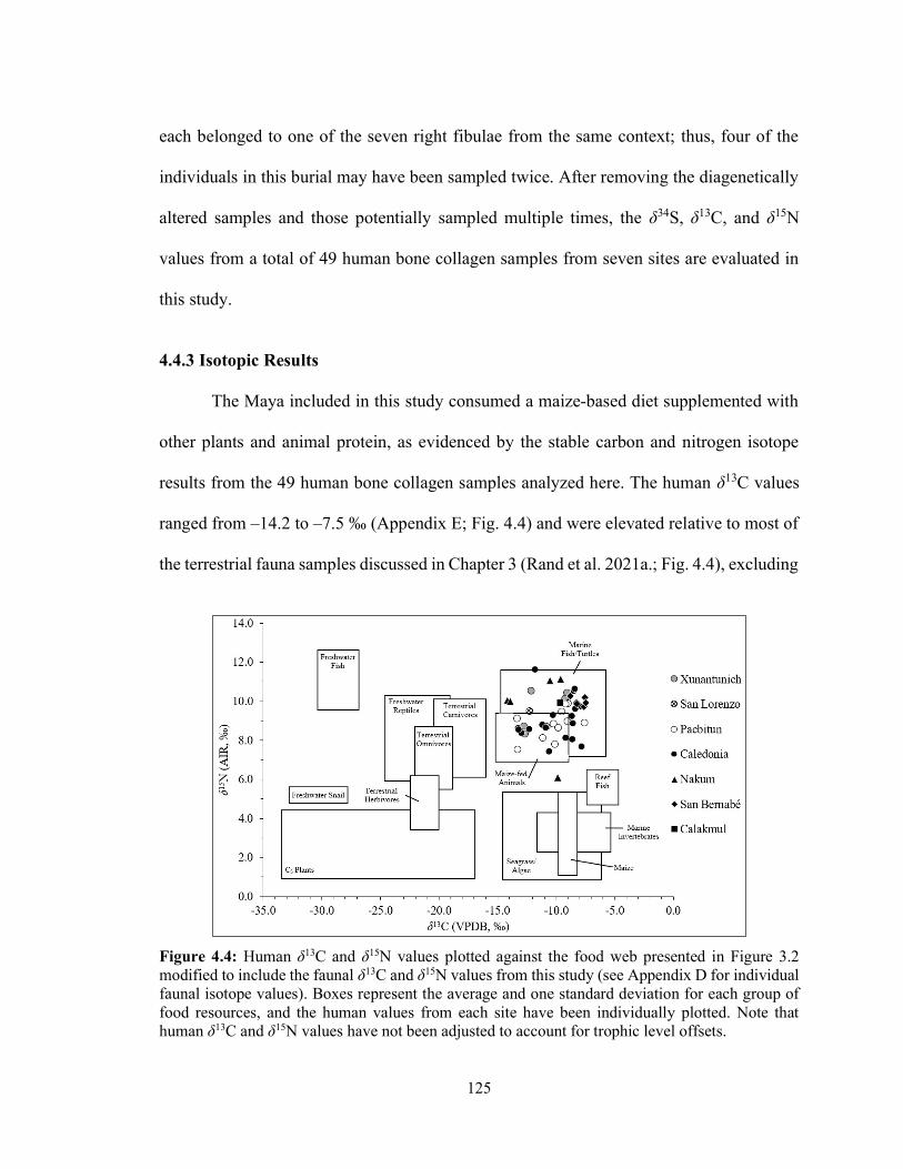
125

each belonged to one of the seven right fibulae from the same context; thus, four of the

individuals in this burial may have been sampled twice. After removing the diagenetically

altered samples and those potentially sampled multiple times, the δ34S, δ13C, and δ15N

values from a total of 49 human bone collagen samples from seven sites are evaluated in

this study.

4.4.3 Isotopic Results

The Maya included in this study consumed a maize-based diet supplemented with

other plants and animal protein, as evidenced by the stable carbon and nitrogen isotope

results from the 49 human bone collagen samples analyzed here. The human δ13C values

ranged from –14.2 to –7.5 ‰ (Appendix E; Fig. 4.4) and were elevated relative to most of

the terrestrial fauna samples discussed in Chapter 3 (Rand et al. 2021a.; Fig. 4.4), excluding

Figure 4.4: Human δ13C and δ15N values plotted against the food web presented in Figure 3.2 modified to include the faunal δ13C and δ15N values from this study (see Appendix D for individual faunal isotope values). Boxes represent the average and one standard deviation for each group of food resources, and the human values from each site have been individually plotted. Note that human δ13C and δ15N values have not been adjusted to account for trophic level offsets.

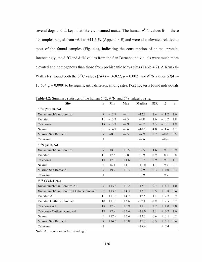
126

several dogs and turkeys that likely consumed maize. The human δ15N values from these

49 samples ranged from +6.1 to +11.6 ‰ (Appendix E) and were also elevated relative to

most of the faunal samples (Fig. 4.4), indicating the consumption of animal protein.

Interestingly, the δ13C and δ15N values from the San Bernabé individuals were much more

elevated and homogenous than those from prehispanic Maya sites (Table 4.2). A Kruskal-

Wallis test found both the δ13C values (H(4) = 16.822, p = 0.002) and δ15N values (H(4) =

13.634, p = 0.009) to be significantly different among sites. Post hoc tests found individuals

Table 4.2: Summary statistics of the human δ13C, δ15N, and δ34S values by site.

Site n Min Max Median IQR x̄ σ

δ13C (VPDB, ‰)

Xunantunich/San Lorenzo 7 –12.7 –9.1 –12.1 2.4 –11.2 1.6

Pacbitun 11 –13.3 –7.5 –9.8 1.6 –10.2 1.8

Caledonia 18 –13.2 –7.9 –9.7 3.3 –10.1 1.9

Nakum 5 –14.2 –9.6 –10.5 4.0 –11.6 2.2

Mission San Bernabé 7 –8.8 –7.5 –7.9 0.7 –8.0 0.5

Calakmul 1 –9.6 –9.6

δ15N (AIR, ‰)

Xunantunich/San Lorenzo 7 +8.3 +10.5 +9.5 1.6 +9.5 0.9

Pacbitun 11 +7.5 +9.8 +8.9 0.9 +8.8 0.8

Caledonia 18 +7.0 +11.6 +8.7 0.9 +9.0 1.1

Nakum 5 +6.1 +11.1 +10.0 1.1 +9.7 2.1

Mission San Bernabé 7 +9.7 +10.3 +9.9 0.3 +10.0 0.3

Calakmul 1 +9.9 +9.9

δ34S (VCDT, ‰)

Xunantunich/San Lorenzo All 7 +13.3 +16.2 +13.7 0.7 +14.1 1.0

Xunantunich/San Lorenzo Outliers removed 6 +13.3 +14.3 +13.7 0.5 +13.8 0.4

Pacbitun All 11 +11.5 +14.7 +12.5 1.1 +12.7 0.9

Pacbitun Outliers Removed 10 +11.5 +13.6 -12.4 0.9 +12.5 0.7

Caledonia All 18 +7.9 +15.9 +11.1 2.2 +11.0 2.0

Caledonia Outliers Removed 17 +7.9 +13.4 +11.0 2.1 +10.7 1.6

Nakum 5 +12.9 +13.4 +13.1 0.4 +13.1 0.2

Mission San Bernabé 7 +14.6 +15.8 +15.3 0.5 +15.1 0.4

Calakmul 1 +17.4 +17.4

Note: All values are in ‰ excluding n.

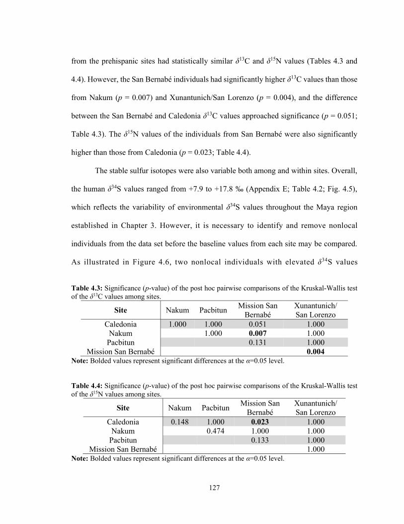
127

from the prehispanic sites had statistically similar δ13C and δ15N values (Tables 4.3 and

4.4). However, the San Bernabé individuals had significantly higher δ13C values than those

from Nakum (p = 0.007) and Xunantunich/San Lorenzo (p = 0.004), and the difference

between the San Bernabé and Caledonia δ13C values approached significance (p = 0.051;

Table 4.3). The δ15N values of the individuals from San Bernabé were also significantly

higher than those from Caledonia (p = 0.023; Table 4.4).

The stable sulfur isotopes were also variable both among and within sites. Overall,

the human δ34S values ranged from +7.9 to +17.8 ‰ (Appendix E; Table 4.2; Fig. 4.5),

which reflects the variability of environmental δ34S values throughout the Maya region

established in Chapter 3. However, it is necessary to identify and remove nonlocal

individuals from the data set before the baseline values from each site may be compared.

As illustrated in Figure 4.6, two nonlocal individuals with elevated δ34S values

Table 4.3: Significance (p-value) of the post hoc pairwise comparisons of the Kruskal-Wallis test of the δ13C values among sites.

Site Nakum Pacbitun Mission San

Bernabé Xunantunich/ San Lorenzo

Caledonia 1.000 1.000 0.051 1.000 Nakum 1.000 0.007 1.000

Pacbitun 0.131 1.000 Mission San Bernabé 0.004

Note: Bolded values represent significant differences at the α=0.05 level.

Table 4.4: Significance (p-value) of the post hoc pairwise comparisons of the Kruskal-Wallis test of the δ15N values among sites.

Site Nakum Pacbitun Mission San

Bernabé Xunantunich/ San Lorenzo

Caledonia 0.148 1.000 0.023 1.000 Nakum 0.474 1.000 1.000

Pacbitun 0.133 1.000 Mission San Bernabé 1.000

Note: Bolded values represent significant differences at the α=0.05 level.

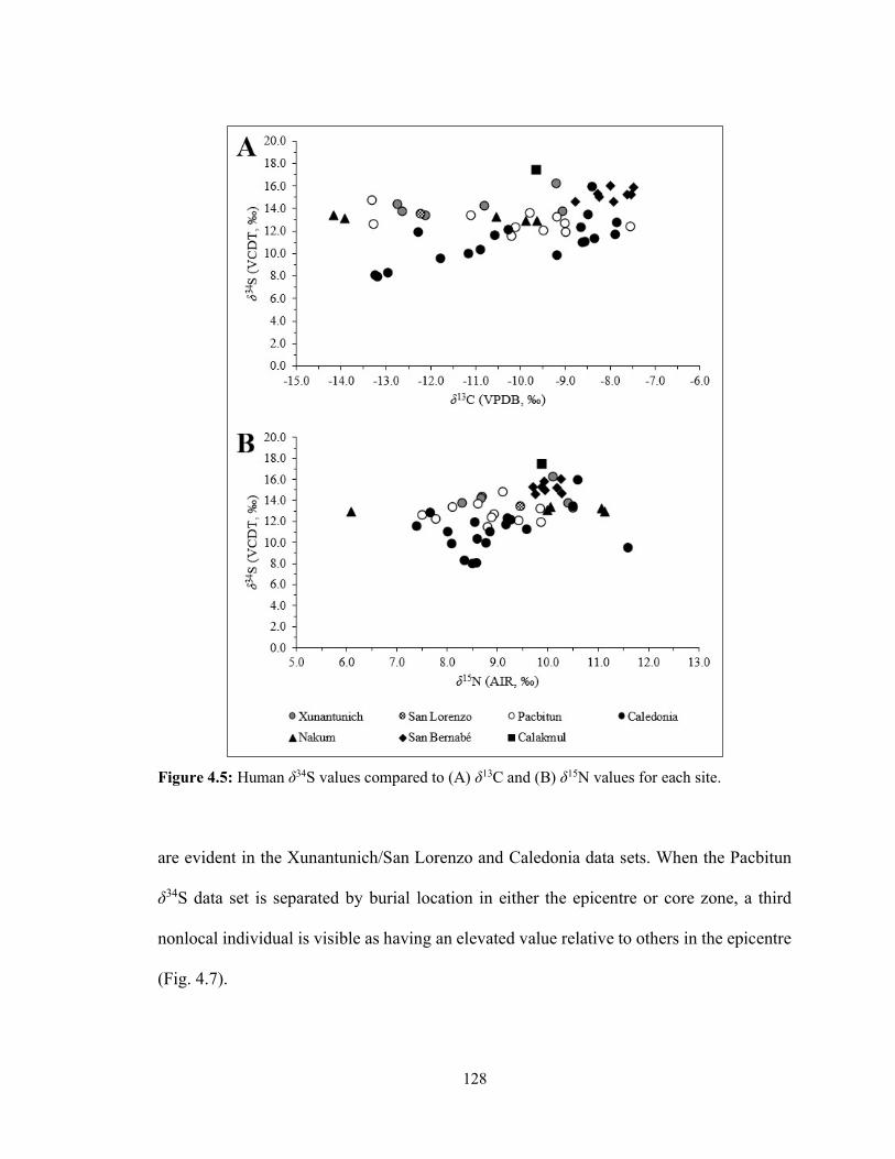
128

Figure 4.5: Human δ34S values compared to (A) δ13C and (B) δ15N values for each site.

are evident in the Xunantunich/San Lorenzo and Caledonia data sets. When the Pacbitun

δ34S data set is separated by burial location in either the epicentre or core zone, a third

nonlocal individual is visible as having an elevated value relative to others in the epicentre

(Fig. 4.7).

129

Figure 4.6: Boxplots of the human δ34S values. Boxes represent the interquartile range (IQR), black bars represent the median, and whiskers represent the IQR*1.5 subtracted from the first quartile and added to the third. Transparent circles within the boxes and whiskers represent individual data points, filled circles beyond the whiskers represent outliers that fall beyond the IQR*1.5 subtracted from the first quartile or added to the third, and stars represent extreme outliers that fall beyond the IQR*3 subtracted from the first quartile or added to the third.

Figure 4.7: Boxplot of the δ34S values of the Epicentre and Core Zone Burials from Pacbitun. Boxes represent the interquartile range (IQR), black bars represent the median, and whiskers represent the IQR*1.5 subtracted from the first quartile and added to the third. Transparent circles within the boxes and whiskers represent individual data points and stars represent extreme outliers that fall beyond the IQR*3 subtracted from the first quartile or added to the third.

δ34S

(V

CD

T, ‰

)

130

The subdivision of the Caledonia δ34S values by burial type identified no further outlying

values, and the remaining data sets were statistically too small to assess differences in δ34S

values by age, sex, social status, burial location, or chronology. Thus, a total of three

nonlocal individuals were identified in this study, indicating that between 5.6 and 14.3 %

of the population migrated to their place of burial later in their lives (Table 4.5).

As with the faunal data presented in Chapter 3, the local ranges of human δ34S

values (Table 4.6) varied among sites. While many of the ranges overlapped, particularly

those from sites in western Belize and Nakum, an ANOVA found the δ34S values to be

statistically different among sites (F(4, 39) = 21.911, p < 0.000). The δ34S values from

Caledonia were significantly lower than those from all other sites, while those from Mission

San Bernabé were significantly higher (Table 4.7). The δ34S values from the Xunantunich/

San Lorenzo individuals were also significantly higher than those from Pacbitun, but not

Nakum, and the δ34S values of individuals from Pacbitun and Nakum were also not

significantly different from one another (Table 4.7).

It also appears that, like the faunal values, the human δ34S values are dependent

upon the underlying geology. Individuals from sites underlain by Paleogene/Neogene

Table 4.5: Number of individuals with nonlocal δ34S values from the sites included in this study.

Site # Nonlocal δ34S Values # Samples % Xunantunich/San Lorenzo 1 7 14.3 Pacbitun 1 11 9.1 Caledonia 1 18 5.6 Nakum 0 5 0.0 Mission San Bernabé 0 7 0.0 Calakmul1 ? 1 ?

1Calakmul is represented by a single sample so it is not possible to evaluate whether this sample truly represents the local δ34S values for the site or whether it is an outlier if additional samples were to be analyzed.

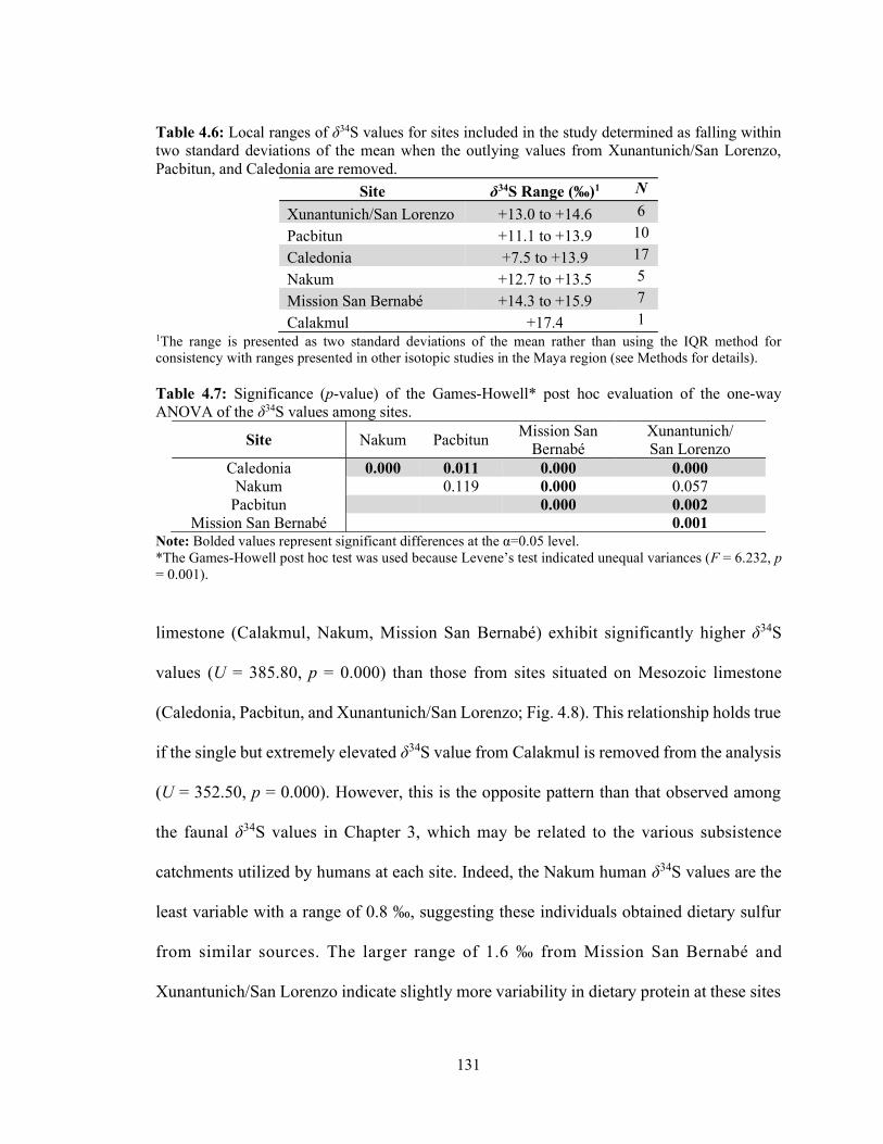
131

Table 4.6: Local ranges of δ34S values for sites included in the study determined as falling within two standard deviations of the mean when the outlying values from Xunantunich/San Lorenzo, Pacbitun, and Caledonia are removed.

Site δ34S Range (‰)1 N

Xunantunich/San Lorenzo +13.0 to +14.6 6

Pacbitun +11.1 to +13.9 10

Caledonia +7.5 to +13.9 17

Nakum +12.7 to +13.5 5

Mission San Bernabé +14.3 to +15.9 7

Calakmul +17.4 1 1The range is presented as two standard deviations of the mean rather than using the IQR method for consistency with ranges presented in other isotopic studies in the Maya region (see Methods for details). Table 4.7: Significance (p-value) of the Games-Howell* post hoc evaluation of the one-way ANOVA of the δ34S values among sites.

Site Nakum Pacbitun Mission San

Bernabé Xunantunich/ San Lorenzo

Caledonia 0.000 0.011 0.000 0.000 Nakum 0.119 0.000 0.057

Pacbitun 0.000 0.002 Mission San Bernabé 0.001

Note: Bolded values represent significant differences at the α=0.05 level. *The Games-Howell post hoc test was used because Levene’s test indicated unequal variances (F = 6.232, p = 0.001).

limestone (Calakmul, Nakum, Mission San Bernabé) exhibit significantly higher δ34S

values (U = 385.80, p = 0.000) than those from sites situated on Mesozoic limestone

(Caledonia, Pacbitun, and Xunantunich/San Lorenzo; Fig. 4.8). This relationship holds true

if the single but extremely elevated δ34S value from Calakmul is removed from the analysis

(U = 352.50, p = 0.000). However, this is the opposite pattern than that observed among

the faunal δ34S values in Chapter 3, which may be related to the various subsistence

catchments utilized by humans at each site. Indeed, the Nakum human δ34S values are the

least variable with a range of 0.8 ‰, suggesting these individuals obtained dietary sulfur

from similar sources. The larger range of 1.6 ‰ from Mission San Bernabé and

Xunantunich/San Lorenzo indicate slightly more variability in dietary protein at these sites

132

Figure 4.8: Boxplots of the δ34S values by site after the outlying values from Xunantunich/San Lorenzo, Caledonia, and Pacbitun are removed arranged by underlying geology. Boxes represent the interquartile range (IQR), black bars represent the median, and whiskers represent the IQR*1.5 subtracted from the first quartile and added to the third. Transparent circles within the boxes and whiskers represent individual data points.

or perhaps variability in the underlying geology. The range of human δ34S values from

Pacbitun was higher at 2.8 ‰, although the greatest variability was evident in the values

from Caledonia, which had a range of 6.4 ‰, indicating the individuals at this site had

access to dietary protein sources with differing δ34S values. Interestingly, the local

Caledonia data set was the only one to exhibit a statistically significant positive relationship

between the human δ34S and δ13C values (r(17) = 0.755, p = 0.000), suggesting that dietary

carbon and sulfur came from the same source (Fig. 4.9). No other correlations between

sulfur, carbon, or nitrogen isotope values were identified in any of the data sets.

As seen in Figure 4.10, the human δ34S values are also generally lower than those

of fauna from the three sites for which both were sampled, although this is variable (Table

4.8). At Nakum, the humans and terrestrial faunal had statistically similar δ34S values (U =

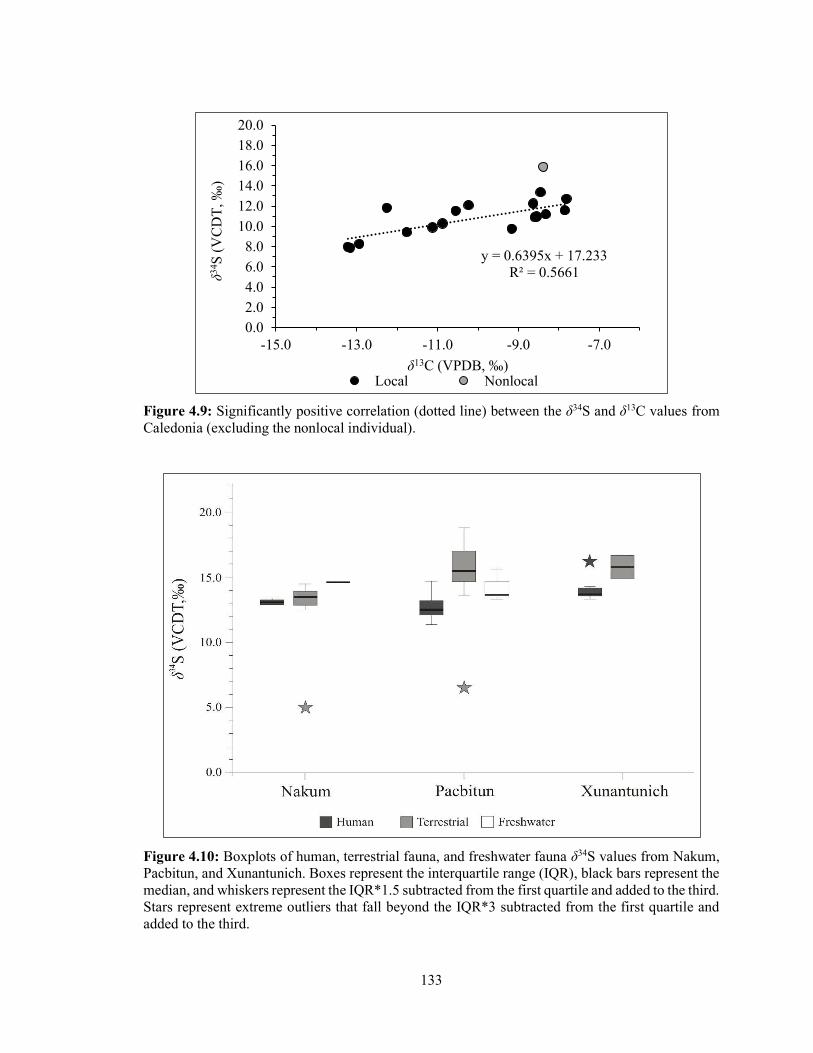
133

Figure 4.9: Significantly positive correlation (dotted line) between the δ34S and δ13C values from Caledonia (excluding the nonlocal individual).

Figure 4.10: Boxplots of human, terrestrial fauna, and freshwater fauna δ34S values from Nakum, Pacbitun, and Xunantunich. Boxes represent the interquartile range (IQR), black bars represent the median, and whiskers represent the IQR*1.5 subtracted from the first quartile and added to the third. Stars represent extreme outliers that fall beyond the IQR*3 subtracted from the first quartile and added to the third.

y = 0.6395x + 17.233R² = 0.5661

0.02.04.06.08.0

10.012.014.016.018.020.0

-15.0 -13.0 -11.0 -9.0 -7.0

δ34S

(VC

DT

, ‰)

δ13C (VPDB, ‰)Local Nonlocal

134

Table 4.8: Average and standard deviation of δ34S values of human, terrestrial, and freshwater animals from Nakum, Xunantunich/San Lorenzo, and Pacbitun.

Site Taxa N δ34S (VCDT, ‰)

x̄ σ

Nakum Human 5 +13.1 0.2 Terrestrial 14 +13.5 0.7 Freshwater 1 +14.6

Xunantunich/San Lorenzo Human 6 +13.8 0.4

Terrestrial 2 +15.8 1.2

Pacbitun Human 10 +12.5 0.7

Terrestrial 13 +15.6 1.3 Freshwater 4 +14.0 1.1

Note: Individuals with outlying δ34S values have been removed.

45.000, p = 0.553). In contrast, the average human δ34S value is 2.0 ‰ lower than that of

the fauna at Xunantunich, although this difference is also not statistically significant (U =

12.00, p = 0.071). There was, however, a statistically significant difference between the

groups of taxa at Pacbitun (F(2) = 21.439, p = 0.000), whereby human δ34S values were

significantly lower than those of terrestrial fauna (p = 0.000), but not freshwater turtles (p

= 0.111).

4.5 Discussion

Drawing on archaeological and historical evidence, in conjunction with the faunal

δ34S values discussed in Chapter 3 and previously published strontium (87Sr/86Sr) and stable

oxygen (δ18O) isotope values for several of the individuals, the following discussion

contextualizes the δ34S, δ13C, and δ15N values presented above. The spatial distribution of

human δ34S values across the sites included in this study differ from those evidenced by the

faunal baseline data presented in Chapter 3 (Rand et al. 2021a). The subsistence practices

135

at Maya sites revealed through the human isotopic data are thus explored to better

understand the utilization of multiple catchments. Despite this variability, it is still possible

to identify nonlocal individuals at Maya sites using stable sulphur isotope values and to

reveal human migration later in life than previously possible using 87Sr/86Sr and δ18O values

from bone and dental enamel.

4.5.1 Spatial Distribution of Sulfur Isotope Values

As was the case with the faunal remains considered in Chapter 3 (Rand et al. 2021a),

the range of δ34S values of humans from inland sites (+7.9 to +16.2 ‰; Table 4.2) were

higher than expected based on previous studies in other archaeological contexts (e.g., 2.3

to 14.2 ‰ at sites in the Danube Gorges; Nehlich et al. 2010). As all seven Maya sites are

located considerably inland, it is unlikely the δ34S values were influenced by the sea spray

effect. Furthermore, although marine resources were traded to inland sites, it is unlikely

they were consumed in sufficient quantities to influence isotopic values (Somerville et al.

2013:1548). Rather, these elevated δ34S values are attributed to the underlying limestone

geology, which formed through the evaporation of ancient seas (Day 2007) and thus has

higher δ34S values than other types of inland geology (Bottrell and Newton 2006; Claypool

et al. 1980; Nielsen et al. 1991). However, unlike the faunal δ34S values presented in

Chapter 3 (Rand et al. 2021a), the human δ34S values from sites located on

Paleogene/Neogene limestones (Calakmul, Mission San Bernabé, and Nakum) were

significantly higher than those located on Mesozoic limestones (Xunantunich/San Lorenzo,

Pacbitun, and Caledonia). This may be explained by either methodological (i.e., differing

analytical methods or sampling strategies) or Maya cultural factors.

136

First, it is possible that the human samples analyzed at one lab have higher δ34S

values than they would if analyzed at a different lab (Appendix B). This, however, seems

unlikely, given that the δ34S values from Nakum, a site located on Palaeogene/Neogene

limestone, were statistically similar to those analyzed at the same laboratory from Pacbitun,

located on Mesozoic limestone, and both were similar to samples analyzed by a different

laboratory from Xunantunich and San Lorenzo, which is also located on Mesozoic

limestone (Table 4.7).

A second explanation relates to sampling bias, wherein the sites from which the

human samples originated were located on Paleogene/Neogene soils in Peten and southern

Campeche, whereas the majority of faunal remains from sites on this lithology were

situated in northern Belize near the Caribbean coast (Chapter 3). However, the proximity

of the Belizean sites to the Caribbean coast would likely cause the faunal δ34S values from

the sites located on Paleogene/Neogene soils to be higher due to the sea spray effect

(Gravenhorst 1978; Wakshal and Nielsen 1982), when in fact they are lower than those

from Mesozoic sites.

The final explanation is that the terrestrial faunal remains accurately reflect

environmental δ34S values throughout the Maya region, and that the Maya values differ

from the faunal baselines due to human subsistence practices, which were influenced by

available foods and well as changing political, social, and cultural situations. In general,

the human δ34S values are also more homogenous than those of the fauna, indicating use of

a broader dietary niche and possibly reliance on lime-processed maize grown in designated

areas at each site. Because various Maya subsistence practices are the most likely

explanation, these are explored in more detail below.

137

4.5.2 Isotopic Evidence for Maya Subsistence

The combination of stable sulfur, carbon, and nitrogen isotope analysis revealed

that the Maya included in this study consumed a maize-based diet supplemented with other

plants and animal protein that was largely derived from catchments near the sites at which

they lived. The human δ13C and δ15N values in this study are consistent with those

previously reported from Caledonia (Rand 2012; Rand et al. 2015b), Pacbitun (Coyston et

al. 1999; White et al. 1993), Xunantunich and San Lorenzo (Freiwald 2011a, 2011b), and

Calakmul (Price et al. 2018a). They are also in agreement with studies of Maya subsistence

practices at other prehispanic sites, where elevated human δ13C and δ15N values relative to

those of analyzed fauna have been interpreted as resulting from the consumption of a maize-

based diet supplemented by C3 plants and animal protein (Ebert et al. 2019; Gerry and

Krueger 1997; Somerville et al. 2013; Tykot 2002; Whittington and Reed 1997a; Wright

2006). Because stable sulfur isotope values vary depending on the underlying geology as

well as by ecosystem (i.e., terrestrial versus freshwater), the combined interpretation of

δ34S, δ13C, and δ15N values from humans and fauna reported in this study provide novel

insights into Maya subsistence practices.

4.5.2.1 Prehispanic Maya Subsistence Practices

Although the terrestrial fauna species from three of the sites included here have

elevated δ34S values due to the underlying limestone, the consumption of freshwater

animals and those imported from the Maya Mountains may contribute lower δ34S values to

Maya tissues (Chapter 3). The average human δ34S values from Xunantunich/San Lorenzo,

Nakum, and Pacbitun were consistently lower than those of the terrestrial fauna from these

138

sites, which may initially appear to be the result of the consumption of freshwater protein.

However, the average human δ34S values were also lower than the values of freshwater

turtles at both Nakum and Pacbitun (Table 4.6).

Rather than the consumption of freshwater resources, the trophic level offset in δ34S

values caused by fractionation during the incorporation of dietary sulphur into consumer

tissues (Δ34Stissue-diet) may be larger than the typically cited +0.5 ± 2.4 ‰ (Nehlich 2015:6).

This value was calculated by compiling data primarily from whole insects, as well as the

muscle, hair, and cartilage of terrestrial mammals (see Nehlich 2015:6) and may not

accurately reflect the offset associated with the incorporation of sulfur into the bone

collagen of mammals such as humans. Indeed, a controlled feeding experiment has found

that pig bone collagen δ34S values are on average 1.5 ‰ lower than those of the diet (Webb

et al. 2017). Because breastfeeding children are a trophic level above their mothers, their

δ34S values may be lower than that of adults from the same site. The δ15N value (+11.6 ‰)

of a 3- to 5-year-old from Burial 1 at Caledonia was elevated relative to the average of the

adults (x̄ = +8.3 ± 0.7 ‰, n = 5) from the same context, suggesting this subadult was

breastfeeding (Fuller et al. 2006). Interestingly, the δ34S value (+9.4 ‰) of this subadult

was 1.6 ‰ lower than the average value of five adults (x̄ = +11.0 ± 0.7 ‰) from the same

context. At Roman period Oxfordshire, Nehlich et al. (2011) attributed lower δ34S values

of subadults aged 2 to 4 years to a weaning diet based on freshwater fish, although this

could instead represent a larger trophic level shift in δ34S values than previously thought.

However, the study by Webb et al. (2017) analyzed the δ34S values of the whole

diet consumed by the pigs, rather than methionine from the protein component that is routed

to collagen, which may explain the larger offset they observed. More recently, the δ34S

139

values of the bone collagen of ancient foxes and their prey were found to be

indistinguishable (Krajcarz et al. 2019), supporting the original interpretation that the

trophic level offset minimally influences δ34S values.

The Δ34Stissue-diet is an important area of future research, as it can alter the

interpretations of sulphur isotopic results. For example, the Xunantunich/San Lorenzo

individuals were likely reliant on both maize and terrestrial animal protein based on their

elevated δ13C and δ15N values, respectively, and because their average δ34S value

(x̄=+13.8±0.4‰) is more elevated than would be expected from the consumption of

freshwater resources (see Chapter 3). However, the human δ34S value is 2‰ lower than the

average of two terrestrial faunal samples from Xunantunich. While this may be explained

by the trophic level offset in δ34S values, there are alternative explanations, including the

consumption of freshwater resources as well as nixtamalized maize.

First, it is possible the Maya from these sites consumed freshwater resources or

animals imported from the Maya Mountains in sufficient quantities to lower their δ34S

values relative to the locally available fauna. Alternatively, because riverine sulphate has

been found to influence terrestrial δ34S values (Nehlich et al. 2011), it is possible that lower

δ34S values were incorporated into maize cultivated on the floodplains of the Mopan River,

or otherwise irrigated with river water, that was then consumed by the individuals from

Xunantunich and San Lorenzo. Because nixtamalization doubles the amount of

bioavailable methionine in maize (Katz et al. 1974), lower δ34S values from river-irrigated

maize may outweigh the sulfur derived from animal protein in Maya diets, which otherwise

would contribute equal amounts of dietary methionine (Young and Pellett 1994). This

example is, however, based on a comparison with two terrestrial animals who may not

140

accurately reflect the local variability of δ34S values and could also benefit from the analysis

of freshwater species from these sites. Regardless, a clearer understanding of Δ34Stissue-diet

values could help differentiate among these possibilities.

The diet of the Nakum Maya is also difficult to interpret without a clearer

understanding of variability in δ34S values. The small sample of humans from Nakum (n =

5) had the most variable δ13C and δ15N values (Table 4.2), likely reflecting dietary

differences over time and space, as well as among people of differing age, gender, and

social status (Ebert et al. 2019; Freiwald 2011a; Gerry 1997; Gerry and Chesson 2000;

White 2005). However, the human δ34S values from Nakum were the least variable of all

sites included in this study and were very similar to those of the terrestrial and freshwater

fauna from this site. One explanation for this is that the trophic effect on δ34S values is

indeed negligible. Alternatively, it is possible that the humans were more reliant on

freshwater resources with δ34S values elevated relative to terrestrial fauna. The lower δ13C

values but elevated δ15N and slightly elevated δ34S values from Burials 4 and 7, for

example, would be consistent with a diet based on freshwater protein if this were the case.

However, this also seems unlikely, as the sulphur baseline for freshwater resources at

Nakum is based on a single turtle (Trachemys venusta) sample with an unusually elevated

δ34S value (+14.6 ‰) relative to the average of the terrestrial animals from this site (x̄ =

+13.5 ± 0.7; Chapter 3; Rand et al. 2021a). Thus, the most plausible explanation for the

elevated human δ34S values is that the agricultural fields of the Nakum Maya were situated

on nearby Quaternary limestone bedrock, which are expected to have much higher sulphur

values than the Paleogene/Neogene limestones (Chapter 3; Rand et al. 2021a) on which

most terrestrial fauna consumed by the Nakum Maya obtained their food. As at

141

Xunantunich and San Lorenzo, nixtamalization may also have increased the contribution

of methionine from maize in the bone collagen of individuals from Nakum. Regardless, a

clearer understanding of the degree to which δ34S values fractionate when they are

incorporated into the tissues of large mammals is necessary to clarify the relationship

among the δ34S values of faunal baselines and humans from the same site.

The combined data sets of δ34S, δ13C, and δ15N values from human and fauna bone

collagen also provide direct evidence of the utilization of catchments with divergent δ34S

values. For example, the lower average δ34S values of the local Caledonia (x̄ = +10.7 ± 1.6

‰) and Pacbitun (x̄ = +12.5 ± 0.7 ‰) individuals relative to the other Maya included in

this study suggest their protein was acquired from the Maya Mountains or, at Caledonia,

the Macal River. When the Pacbitun human δ34S values are compared with the faunal

baseline, it initially appears as though the Pacbitun Maya were more reliant on freshwater

fauna than terrestrial animals, if Δ34Stissue-diet = –1.5 ‰ (Webb et al. 2017) is applied. It is,

however, unlikely that freshwater resources made up a considerable component of the diet

based on the elevated average human δ13C values and because the δ15N values are lower

than expected for diets based on C3-freshwater resources (Guiry 2019; Winemiller et al.

2011). A significant negative correlation between the δ15N and δ34S values is also expected

if freshwater resources with lower δ34S and higher δ15N values compared to terrestrial

animals were consumed in large quantities (Curto et al. 2019), but there is no such

correlation in any of the Maya data sets analyzed here. It is also unlikely that the maize

consumed by the Pacbitun and Caledonia individuals was irrigated with river water because

Pacbitun is not situated on a large water course and the steep banks of the turbulent Macal

River near Caledonia would have been difficult to farm compared to the calmer Mopan

142

River (Smith 1997). Both sites are also surrounded by agricultural terraces that undoubtedly

provided the main subsistence base for these communities (Awe 1985:32; Healy et al. 1980,

2007).

Instead, it is possible that the lower human δ34S values of the Caledonia and

Pacbitun Maya are derived from protein acquired from the Maya Mountains. This is

supported by the significantly positive relationship between the δ13C and δ34S values of the

Caledonia Maya, demonstrating that C3-based protein was acquired from the Maya

Mountains whereas C4-based protein was acquired from areas underlain by limestone, most

likely the Vaca Plateau (Fig. 4.10). It is unlikely that maize was grown in the Mountain

Pine Ridge region of the Maya Mountains, given its acidic soils derived from granite, shale,

sandstone, quartzite, and some limestone (Wright et al. 1959). The region was, however,

Figure 4.11: Statistically significant positive correlation (dotted line) between the δ34S and δ13C values from Caledonia (excluding the nonlocal individual). Elevated values indicate consumption of maize-based protein from limestone areas whereas lower values indicate the consumption of terrestrial animals from the Maya Mountains.

y = 0.6395x + 17.233R² = 0.5661

0.0

2.0

4.0

6.0

8.0

10.0

12.0

14.0

16.0

18.0

20.0

-15.0 -13.0 -11.0 -9.0 -7.0

δ34 S

(V

CD

T, ‰

)

δ13C (VPDB, ‰)Local Nonlocal

Limestone

Maya Mountains

C3 Protein C4 Protein

143

an excellent source of granite for manufacturing manos and metates, pine for torches and

pine resin for pitch and incense, as well as mammals, namely deer (Awe 1985:32). Indeed,

most nonlocal fauna in this study, including a deer from Pacbitun with a low δ34S value,

(+6.5‰; Appendix D) were likely obtained from the Maya Mountains (Chapter 3; Rand et

al. 2021a). However, the large degree of variability in δ34S values at Caledonia may reflect

not only the use of multiple catchments, but also the relatively large sample size from this

site. It is possible that the analysis of additional samples at other sites may also result in a

greater range of δ34S values and is an important avenue of future research. Regardless, the

isotopic evidence presented here indicates that although the Maya at Caledonia and

Pacbitun obtained most of their subsistence resources from the limestone environments

surrounding their sites, they also obtained subsistence resources from the Maya Mountains.

Access to multiple ecozones may also have been the reason why these sites were initially

settled (Awe 1985; Healy 1990), an advantage the Maya continued to utilize throughout

the occupation of these sites.

4.5.2.2 Colonial Period Maya Subsistence Practices

The individuals from Colonial period Mission San Bernabé had much more

restricted diets than the prehispanic Maya included in this study, evidenced by their

elevated and homogenous δ13C, δ15N, and δ34S values. Colonial records state that the

Spaniards restricted Maya diets, encouraging the rearing of cattle and cultivation of maize

and beans and discouraging the use of more varied resources from the forest and home

gardens (Schwartz 1990:54, 62). Although freshwater resources such as snails and turtles

continued to be important in Colonial period Maya diets (Freiwald 2012; Freiwald and

144

Pugh 2018), the low δ13C and high δ15N values expected from freshwater resources were

probably overridden by the consumption of maize-fed beef or dairy products with high δ13C

values and beans with low δ15N values. Furthermore, reliance on freshwater fish is expected

to be evidenced by lower δ34S values, but the Mission San Bernabé individuals have the

most elevated δ34S values in this study other than the single individual from Calakmul. This

suggests that although they may have consumed freshwater resources, but not in large

quantities, and reliance on resources grown or reared on limestone with elevated δ34S values

was more important in the San Bernabé diet. The elevated δ13C and δ15N values indicate

that dietary protein was not only acquired from the consumption of maize, but also likely

European domesticates such as cows (Bos taurus) and pigs (Sus scrofa) foddered on maize.

To better understand the influence of Colonialism on Maya consumption patterns,

the δ13C and δ15N values of the Colonial period (1697 – 1821 CE; Table 1.1) individuals

from Mission San Bernabé were compared with those of individuals from the Contact

period (1525 – 1697 CE; Table 1.1) at Tipu (Harvey 2018) and Lamanai (White et al. 1994)

in Belize, and Campeche (Price et al. 2012) in Mexico. The δ13C and δ15N values of the

San Bernabé individuals are elevated and more homogenous than the Contact period

individuals (Table 4.9). While the variability in the isotopic values observed at Tipu may

be the result of the larger sample size, similar variability is seen in the smaller samples of

Table 4.9: Bone collagen δ13C and δ15N values from Contact and Colonial period Maya sites.

Site Time

Period δ13Ccol (‰, VPDB) δ15N (‰, AIR)

Source N Mean SD N Mean SD

San Bernabé Colonial 7 –8.0 0.5 7 +10.0 0.3 This study Tipu Contact 42 –9.8 1.2 11 +9.2 0.7 Harvey (2018)

Lamanai Contact 11 –9.9 0.9 9 +9.7 0.6 White et al. (1994) Campeche Contact 3 –9.7 1.9 3 +9.5 0.5 Price et al. (2012)

145

individuals from Lamanai and Campeche (Table 4.9), although the variability in the

Campeche sample may be due to the presence of nonlocal individuals from Europe or

Africa (Price et al. 2012). Regardless, it appears that the Colonial period Maya at Tipu and

Lamanai enjoyed a more varied diet and consumption patterns at these sites were not

influenced by the presence of the Spaniards (Harvey 2018:285; White et al. 1994:141). This

is likely because the individuals from Tipu, Lamanai, and Campeche predate those from

Mission San Bernabé, and thus the more restricted diets of the San Bernabé individuals

may reflect increased Spanish control over Maya populations, including their subsistence

patterns in later periods. It is thus evident from the isotopic evidence presented here that

the arrival of the Spaniards was associated with a drastic dietary shift in Peten relative to

prehispanic Maya subsistence practices and those at earlier Contact period sites in Belize

and Mexico, which restricted access to traditional sources of protein while introducing new

ones. The analysis of additional individuals from sites that date to the Contact and Colonial

periods will further elucidate the impact of Spanish influence on Maya subsistence patterns.

4.5.3 Nonlocal Individuals at Maya Sites

In addition to subsistence practices, it is also possible to identify nonlocal

individuals as those with δ34S values that differ from individuals who consumed local

sources of protein. While faunal baselines are useful for approximating local δ34S values

(Chapter 3), the unknown offset between diet and consumer tissues combined with human

utilization of multiple dietary catchments precludes the identification of nonlocal humans

using local faunal δ34S values at this time. Rather, nonlocal humans were identified as

having δ34S values that were statistically different from those of other humans from the

146

same site. As a result, it is not possible to comment on the origin of the individual from

Calakmul, as this site is represented by a single sample. However, three individuals, one

each from Xunantunich, Pacbitun, and Caledonia, were identified as nonlocal individuals

with δ34S values that fell beyond two standard deviations of the mean of their respective

sites (Table 4.5).

As discussed in Chapter 2, the isotopic analysis of multiple individuals in

conjunction with other lines of evidence can elucidate the structure of past migrations (Fig.

2.1). Investigations of the temporality, spatial extent, social composition, and scale of

migration require the analysis of large numbers of nonlocal individuals, which were not

identified in this study. The analysis of multiple isotopes of tissues from the same individual

that form at different ages can, however, indicate potential places of origin and the length

of time an individual resided in an area prior to death. Despite equifinality, the multi-

isotopic approach allowed potential places of origin from which several of the nonlocal

individuals identified in this study originated to be inferred. Furthermore, a consideration

of the burial contexts of individuals with both local and nonlocal individuals that relocated

at different periods during life indicates the length of time they resided at their places of

burial before death. Combined, these data are interpreted below and provide additional

insight into prehispanic Maya conceptualizations of identity and broader sociopolitical

aspects of the deposition of the dead as well as the impact of contact with Europeans on

Maya migration patterns.

4.5.3.1 Local Individuals in Formal Funerary Contexts at Prehispanic Maya Sites

As mentioned in Chapter 2, the Maya did not use cemeteries to inter their dead, and

147

instead select individuals were interred within site architecture. Such contexts include

formal burials of revered ancestors, dedicatory and termination deposits, and nonfunerary

deposits that include human remains (Tiesler 2007; Welsh 1988). The inclusion of local

individuals in formal funerary contexts within both ceremonial and residential complexes

in particular may reflect not only ancestor veneration but also attempts by local lineages to

solidify their legitimacy in the face of foreign influences (McAnany 1995).

At Xunantunich, for example, two burials from elite residential Group D, one of an

older adult male buried in a chultun during the Late Preclassic period (Op. 21C Individual

1) and another adult buried in front of Str. D6 during the Late Classic period (Op. 74R) had

local enamel 87Sr/86Sr (0.70903 and 0.70865, respectively) and δ18O values (–1.4 ‰ and –

2.8 ‰, respectively; Freiwald 2011a; Freiwald et al. 2014), as well as sulfur isotope values

(+14.3 ‰ and +13.3 ‰, respectively). Similarly, all individuals with local δ34S values from

the Pacbitun Epicentre regardless of time period were interred in the Eastern Triadic

Assemblage, reflecting their status as ancestors (Awe et al. 2016). This pattern may have

been emulated by lower status individuals in the core zone of Pacbitun during the Terminal

Classic, who also buried individuals with local δ34S values in eastern structures at this time.

Furthermore, all individuals from formal funerary contexts at Nakum had local δ34S values,

despite their varied contexts, biological profiles, and chronologies.

All of the local individuals from Caledonia were also interred in formal funerary

contexts, including those from multiple burials. While the presence of multiple individuals

in the same burial was initially interpreted as representing individuals sacrificed for

inclusion with a primary individual, revaluation of these contexts indicates multiple

individuals could also represent secondary funeral rites, ongoing tomb use, and skeletal

148

curation and reuse of bones (Weiss-Krejci 2003). Indeed, both Burial 1 and Burial 4 at

Caledonia contained the remains of multiple individuals and are interpreted as sequentially

used family tombs (Healy et al. 1998; Rand 2012; Rand et al. 2015b), whereas Burial 3

may represent an intrusive sacrificial burial, although perimortem trauma was not identified

on any of the four individuals from this burial (Awe 1985:110-111; Rand et al. 2015b).

Regardless, all individuals excluding one from Burial 4, discussed in more detail below,

had local δ34S values and their δ18O values indicate origins near the site (Rand 2017). The

continued use of tombs by individuals from local lineages illustrates their ties to the

community and the centre of Caledonia.

It should be noted that most of these individuals were identified as local based on

δ34S values from their bone collagen, and it is not possible to determine if they lived

elsewhere as children or if they resided in a different region with similar environmental

sulfur isotope values prior to burial. Regardless, it appears that the individuals interred in

formal funerary contexts lived near the sites where they were buried for many years prior

to death, and the social practice of local ancestor veneration that began in the Late

Preclassic period lasted throughout the subsequent Classic period.

4.5.3.2 Nonlocal Individuals in Non-Funerary Deposits at Prehispanic Maya Sites

At Maya archaeological sites, human remains may also be recovered from contexts

that lack a clear funerary status (i.e., non-funerary deposits; Tiesler 2007). For example,

“problematic deposits” (PDs) may or may not contain human remains, but those that do are

classified as neither a cache nor burial, as the behaviours that led to their formation are

often difficult to discern (Aimers et al. 2020; Moholy-Nagy 2020; Tiesler 2007). Tiesler

149

(2007) further differentiates PDs (containing scattered human remains) from primary

disposals (disturbed or undisturbed skeletons that lack evidence for ancestral treatment,

often uncritically identified as sacrificial victims), although the PD subcategories of

termination and dedicatory deposits recently reassessed in the literature (e.g., Aimers et al.

2020; Moholy-Nagy 2020; Newman 2019) will be explored here.

Human remains from PDs at Maya sites are not typically subjected to isotopic

analyses, as such contexts are difficult to interpret, and researchers tend to focus on the

analysis of remains from formal funerary contexts (but see Freiwald et al. 2014; Rand et al.

2020a). However, as discussed below, the nonlocal origins of all three individuals sampled

from termination and dedicatory deposits in this study demonstrates how isotopic analysis

can contribute to the interpretation of the behaviours that led to the formation of such

deposits.

Termination deposits refer to numerous assemblages and depositional behaviours

generally associated with ritual deactivation of structures or sites (Aimers et al. 2020;

Newman 2019). Such contexts typically show evidence of the destruction of material

culture (e.g., ceramics, architecture, etc.), and human remains may be found in these

deposits as both scatters of bone, perhaps indicative of ancestor bundles, as well as

complete and articulated human burials (Aimers et al. 2020:71-72). While termination

deposits are variable and their interpretation in Maya archaeology has recently been

reassessed (Newman 2019), researchers generally further subdivide termination deposits to

those that are reverential and those that are desecratory (Aimers et al. 2020; Newman 2019;

Pagliaro et al. 2003; Tsukamoto 2017). Reverential termination deposits are viewed as

intermediate between dedication and termination deposits and involve ancestor veneration,

150

including the “movement of human bones from their primary interment into a secondary

location [and] inclusion of human bone within ritual contexts” (Aimers et al. 2020:72). The

two individuals recovered from termination deposits included in this study instead come

from desecratory termination deposits that are typically associated with the decommission

of buildings and spaces and “may involve the purposeful disturbance and/or desecration of

elite burials as well as the remains of ritually sacrificed elite inhabitants of a Maya

community” (Pagliaro et al. 2003:80).

The young adult male from a Late Classic II or Terminal Classic termination deposit

in Str. A11 at Xunantunich (Op. 302G) falls into the desecratory termination deposit

category or Tiesler’s (2007) primary disposal category. The context, osteological profile,

and position of the body associates the deposition of the individual with destruction of parts

of the structure, ritual activity, and violence (Freiwald et al. 2014; Yaeger 2005; see also

Berryman 2007:394), although no perimortem trauma was noted on the skeleton.

Importantly, his nonlocal enamel 87Sr/86Sr (0.70797) and δ18O (–0.32 ‰) values are typical

of the central Peten, indicating he originated elsewhere (Freiwald 2011a). However,

because enamel forms during childhood, it was difficult to discern whether he was a recent

arrival, which would support the possibility that he was a captive, or if he had resided at

Xunantunich for some time prior to death (Freiwald 2011a:144). His elevated, nonlocal

δ34S value (+16.2 ‰) is also consistent with those from Peten and reveals that he was indeed

a recent arrival to Xunantunich.

While it is not possible to unequivocally state this young man was captured and

brought to his final resting place as a sacrificial victim, his inclusion in a termination deposit

during a dramatic political change at Xunantunich may represent a severing of ties with his

151

place of origin (Freiwald et al. 2014) and/or the demonstration and legitimization of elite

power through the sacrifice of their rivals (Demarest 1984; Inomata and Triadan 2003:204).

Thus, this desecratory termination deposit represents the political motivations behind those

who included him in the deposit at a time of uncertainty at Xunantunich.

Similarly, an adult interred as part of a termination deposit at the summit of Str. 99

(III-1-2) at Nakum during the Terminal Classic period (Źrałka et al. 2014) falls into the

desecratory category. However, unlike the Xunantunich individual, the bones of the Nakum

individual were not articulated and therefore would constitute Tiesler’s (2007) isolated

bone scatter category. This individual had a nonlocal bone apatite δ18O value (–8.7 ‰),

suggesting he/she was a recent arrival from central or southwestern Mexico, the

Guatemalan Highlands, or along the Pacific Coast (Chapter 5; Rand et al. 2020a). Although

his or her δ34S value (+13.3 ‰) fell within the local range, similar values may also be found

in central and southwestern Mexico and perhaps along the Pacific coast (Chapter 3; Rand

and Grimes 2017; Rand et al. 2021a). The multi-isotopic approach applied here helped

circumvent the equifinality of δ34S values in various parts of the Maya region and

successfully identified this individual as nonlocal. As with the termination deposit at

Xunantunich (Freiwald et al. 2014), it is not possible to determine if this individual was a

war captive or if he/she was sacrificed, but the inclusion of a nonlocal individual in the

termination deposit on Str. 99 at Nakum may reflect the severing of ties with that person’s

place of origin during a time of political turmoil (Chapter 3; Rand et al. 2020a).

It is also possible that an individual’s nonlocal origin was important for his or her

inclusion in other non-funerary deposits. Dedication deposits, for example, are related to

the ritual consecration of structures and spaces to ensoul built places and are often

152

associated with renovation or rededication but not destructive behaviour (Aimers et al.

2020:71; Pagliaro et al. 2003:76). For example, an adult of indeterminate sex interred in

Burial 2, a dedicatory context beneath Stela 2 at the base of Str. 5 (BU 5-2) at Pacbitun

during the Terminal Classic was interpreted as sacrificial (Healy et al. 2004b:215;

Robertson 2011). As with the termination deposits from Xunantunich and Nakum, this

dedicatory burial had a nonlocal δ34S value (+14.7 ‰) and was interred during a period of

sociopolitical change at Pacbitun just prior to the abandonment of the site. Unfortunately,

the reason for the placement of Stela 2 in front of the E Group during the Terminal Classic

is unknown because it was not carved and therefore the “sub-stela interment may have been

placed as a dedication to honor the ancestors, a cycle of time, architectural renewal, or even

to commemorate the erection of the stelae itself” (Micheletti 2016:78).

Burial activity associated with dedicatory deposits may also serve to reinforce

ancestral ties to land or legitimate power (McAnany 1995). The nonlocal origin of the

Pacbitun individual within a dedication deposit may therefore represent a strengthening of

foreign ties during a turbulent period in the site history, in contrast to the severing of foreign

ties possibly represented by the inclusion of nonlocal individuals in desecratory termination

deposits (Freiwald et al. 2014; Rand et al. 2020a; see also Chapter 5). A study of oxygen

isotope values, however, found both local and nonlocal individuals among dedicatory

burials at Altun Ha, although the inclusion of nonlocal individuals appears to have

increased from the Preclassic to Terminal Classic periods (Olsen et al. 2014). This suggests

that the relationship between origin and inclusion in dedicatory deposits is complicated and

the importance of including nonlocal individuals in these contexts varied over time.

153

Overall, an individual’s nonlocal origin appears to correlate with nonfunerary

contexts and may symbolize the strengthening or severing of ties with their place of origin.

While isotopic studies do not typically focus on individuals from nonfunerary contexts, the

results presented here demonstrate that the analysis of such individuals can provide more

detailed interpretations of the behaviours that contributed to the formation of nonfunerary

and “problematic” deposits containing human remains.

4.5.3.3 Nonlocal Individuals in Funerary Contexts at Prehispanic Maya Sites

Although the majority of nonlocal individuals identified in this study came from

non-funerary contexts, the degree to which nonlocal individuals were incorporated into

receiving communities may also be elucidated from their burial in formal funerary contexts

within ceremonial architecture at Maya sites. For example, an adult of indeterminate sex

interred in Burial 4 at Caledonia (C2-4 F6) during the Late Classic period. This individual’s

δ34S value (+15.9 ‰) exceeded the broad local range for Caledonia and suggests an origin

in Peten or possibly a coastal region. Although this individual’s bone apatite δ18O (–4.3 ‰;

Rand 2017) appears too low for him/her to have originated to the west, when it is adjusted

by +1.7 ‰ to make it comparable to the δ18O values of tooth enamel (Warinner and Tuross

2009), it falls within the range of values reported in Peten (Price et al. 2008, 2010; Wright

2012; Wright et al. 2000). Caledonia Burial 4 was initially interpreted as a tomb containing

two primary burials and two sacrificial burials (Awe 1985:115), although as mentioned

above, reanalysis of the skeletal remains and archaeological context indicate it was a

sequentially used tomb that contained the remains of at least seven individuals (Rand 2012;

Rand et al. 2015b). It is similar to Burial 1 at Caledonia (Healy et al. 1998), and if it is also

154

a family tomb, then the inclusion of a nonlocal individual may reflect a nonlocal person

who was integrated into the Caledonia community.

Similarly, a middle-aged female interred in SL -13 Str. 6 at San Lorenzo during the

Late Classic I period (Op. 243 LL/3) likely grew up near the Macal River based on her

enamel 87Sr/86Sr value (0.70938; Freiwald 2011a:149-152). The problem of equifinality

precludes identifying whether she was a recent migrant, as her sulfur value (+13.4 ‰) falls

within the local ranges of both Xunantunich/San Lorenzo as well as Caledonia, the latter

of which is situated on the Macal River. However, her burial in the only ceremonial

structure at the site (Yaeger 2000) may indicate that despite having resided elsewhere as a

child, she had become fully integrated into the local community regardless of the length of

time she resided at San Lorenzo prior to death.

While nonlocal individuals may have been preferentially included in nonfunerary

context, a nonlocal origin did not necessary preclude individuals from being integrated into

receiving communities, as in our own. These results confirm that identity construction

among the Maya was complex and future multi-isotopic analysis of individuals from both

funerary and nonfunerary contexts at Maya sites will provide greater insights into Maya

perspectives of identity and the sociopolitical factors that caused some individuals to be

included in specific contexts.

4.5.3.4 Colonial Impacts on Maya Migration

Finally, the Colonial period individuals from Mission San Bernabé appear to have

lived either at the site or in a nearby area with similarly elevated δ34S values for several

years prior to being buried in the church. Missions established along the banks of the Peten

155

lakes during the early Colonial period involved both the concentration of small but

dispersed local groups as well as the relocation of entire settlements from farther away

(Gasco 2005). For example, following British incursions along the Belize River Valley, the

Spaniards moved the Maya from Tipu in Belize to the shores of Lake Peten Itza in 1707

CE (Graham et al. 1985:207-210). Mission San Bernabé was established prior to 1712 CE,

several years after the other missions in the region (Jones 1998:Table 15.4).

Given the local δ34S values from the Mission San Bernabé individuals presented

here, combined with the local 87Sr/86Sr and δ18O values of most of the individuals analyzed

by Freiwald and colleagues (2020), it is likely the mission comprised the concentration of

local individuals, rather than the relocation of those from distinct isotopic regions. The

burials included here also span the occupation history of the site and it is possible that many

residents were descended from migrants to the region.

Interestingly, the enamel of the second maxillary molar from a young adult male

from Burial 18, one of the first to be interred in the church based on its western location

(Pugh et al. 2016), had a δ18O value (+2.8 ‰) that fell within the local range, but a nonlocal

87Sr/86Sr value (0.708489), indicating he spent his childhood from 2.5 to 8 years of age

(AlQahtani et al. 2010) to the east (Freiwald et al. 2020). However, the δ34S (+14.6 ‰) of

his right clavicle fall within the local range presented in Table 4.6, and the δ18O (–3.8 ‰)

of his bone apatite also falls within the range (Freiwald et al. 2020: Table 1), even when

adjusted for comparison with enamel (–2.1 ‰; Warinner and Tuross 2009), indicating he

lived at the site for many years prior to his death. The potential early date of his burial

combined with the isotopic data suggest this young man may have relocated from an area

to the east, possibly from Tipu in 1707 CE or perhaps earlier as part of ongoing population

156

exchange that predated the arrival of the Spanish and establishment of missions in the

region (Freiwald et al. 2020). Regardless, the isotopic data demonstrate that he lived

elsewhere as a child and had resided in the area surrounding Lake Peten Itza many years

prior to his death.

While isotopic evidence suggests a high degree of mobility at Colonial period Tipu

due to Maya resistance to Spanish colonialism (Trask 2018), there is considerably less

isotopic and archaeological evidence for migration to Mission San Bernabé (Freiwald et al.

2020). This may be because the extensive population movement that frustrated Spanish

officials (Farriss 1984; Restall 1997) occurred over short distances or within isotopically

similar regions, or that Maya resistance to Spanish colonialism via migration lessened over

time. It is nevertheless apparent that the arrival of Europeans significantly altered the nature

of migration throughout the Maya region (Trask 2018) and the analysis of additional

individuals from Contact and Colonial period sites will further contribute to understandings

of how the arrival of Europeans disrupted Maya migration patterns.

4.6 Chapter 4 Summary and Conclusions

The stable sulfur isotope analysis of 49 humans from seven Maya sites has

contributed to new understandings of Maya subsistence strategies and migration. The

spatial distribution of δ34S values in human and terrestrial faunal values differed, most

likely reflecting social, political, and economic factors that influenced Maya use of

isotopically distinct subsistence catchments near different sites and possibly Maya

consumption of lime-processed maize. Although the offset in δ34S values of consumer

tissues and their diets are not well defined, consideration of the δ13C and δ15N values

157

revealed that lower human δ34S values are unlikely to be from the consumption of

substantial amounts of freshwater protein. Instead, subsistence strategies, such as the

cultivation of maize crops on floodplains at Xunantunich and the consumption of terrestrial

fauna from the Maya Mountains at Caledonia and Pacbitun may explain the lower human

δ34S values from these sites. The isotopically homogenous diet of the Colonial period

individuals from Mission San Bernabé also show that the arrival of Europeans disrupted

Maya subsistence patterns established during earlier periods.

Despite the variability caused by Maya utilization of multiple resource catchments

that complicates interpretations of subsistence, the identification of three nonlocal

individuals with outlying δ34S values indicates this technique is useful for studies of

migration in the past. While small sample sizes precluded a detailed assessment of the

structure of Maya migration proposed in Chapter 2, the comparison of the δ34S values with

previously published strontium and oxygen values from the same individuals that reflect

childhood migration reveals the length of time people lived in their place of burial prior to

death. For example, a young man from Colonial period Mission San Bernabé (Burial 18)

appears to have spent his childhood in an isotopically distinct region but had lived near

Lake Peten Itza long enough to have developed local bone δ34S values. Because his burial

is one of the oldest in the mission church, it is possible that he represents a migrant from

the east who possibly relocated as a result of the resettlement of Maya populations in the

Peten Lakes region by the Spaniards during the early Colonial period.

These data may also reveal the degree to which nonlocal individuals were integrated

into prehispanic Maya communities. For example, a young male who was included in a

desecratory termination deposit (Op. 302G) was a recent migrant to Xunantunich, and his

158

nonlocal origin may have signified the severing of ties between this site and his place of

origin. Although equifinality indicated another individual from a desecratory termination

deposit at Nakum had a local δ34S value, his/her nonlocal bone δ18O value indicates he/she

was indeed a recent migrant to the site. Conversely, a recent migrant to Pacbitun (BU 5-2)

suggests that origin may also have been important in dedicatory contexts, representing the

strengthening of ties between regions. Nonlocal individuals were not, however, solely

interred in non-funerary deposits, and the inclusion of an individual born elsewhere in

formal funerary contexts, such as a sequentially used family tomb along with local

ancestors at Caledonia and in the only ceremonial context at San Lorenzo speaks to the

integration of these individual into receiving communities. It is also important to consider

the impact that contact with Europeans had on disrupting long-established migration

patterns in the Maya lowlands.

The results presented herein highlight a number of factors that influence the δ34S

values of Maya collagen and must be considered when interpreting these data in future

studies. As previously demonstrated in Chapter 3, bioavailable δ34S values vary depending

on the type and age of the underlying geology and distance from the coast, although

equifinality currently prevents identification of specific places of origin. The analysis of

additional human and faunal bone collagen samples from areas underrepresented in this

study, including the Northern Lowlands, central Peten, Highlands, and western Honduras,

will undoubtedly reveal the degree of spatial variability in δ34S values across the Maya

region, further contributing to the identification of nonlocal individuals who recently

migrated from isotopically distinct areas.

159

However, the geospatial distribution of δ34S values is not the only factor to consider

when interpreting the values of human bone collagen. For example, the diets of organisms

affect the δ34S of their consumers, as seen in the marine-influenced limpkin diets at Vista

Alegre presented in Chapter 3 and Maya consumption of freshwater animals discussed in

this chapter. The consumption of fauna from multiple isotopically distinct catchments at

Caledonia and the possible location of agricultural fields in alluvial soils near the

Xunantunich polity also demonstrate how social and economic factors can influence δ34S

values of Maya bone collagen away from underlying baseline assumptions derived from

environmental parameters. Better characterization of methionine routing from different

dietary components (i.e., protein from animal tissues versus lime-processed maize) and

trophic level offsets (i.e., Δ34Stissue-diet) between the diets of large mammals and their bone

collagen could also help to further differentiate the type of dietary protein consumed by the

Maya. Thus, researchers should identify potential dietary sources of isotopic variation in

addition to geospatial factors when interpreting the δ34S values of human bone collagen.

Nevertheless, this study demonstrates how the integration of stable sulfur and other

isotope analyses in a multi-isotopic, multi-tissue, biocultural approach complements and

expands upon current understandings of Maya subsistence practices and migration. The

case study presented in the following chapter illustrates the potential of using such an

approach in conjunction with archaeological data to reconstruct dietary practices and

identify nonlocal individuals at Nakum, Guatemala.

160

CHAPTER 5

PREHISPANIC MAYA DIET AND MOBILITY AT NAKUM, GUATEMALA: A MULTI-ISOTOPIC APPROACH10

Human subsistence strategies and mobility are socially mediated practices, and their

study provides insights into myriad sociocultural aspects of past societies (Anthony 1990;

Cucina 2015a; Gumerman 1997; Hastorf 2017; van der Veen 2003). Isotopic techniques

are advantageous in archaeological studies because they provide direct evidence for

mobility and diet at the individual level. Stable carbon (δ13C) and nitrogen (δ15N) isotope

analyses are well-established methods for investigating diet among the prehispanic Maya

(see Somerville et al. 2013; Tykot 2002), as are strontium (87Sr/86Sr) and stable oxygen

(δ18O) isotope techniques for identifying nonlocal individuals at Maya sites (Price et al.

2008; Scherer et al. 2015; Wright 2012). Stable sulfur (δ34S) isotope analysis is a relatively

novel technique for investigating both diet and mobility in the past (Craig et al. 2010;

10 A version of this chapter was co-authored with Varinia Matute as well as Drs. Vaughan Grimes, Carolyn Freiwald, Jarosław Źrałka, and Wiesław Koszkul and published in the Journal of Archaeological Science: Reports (Rand et al. 2020a). JZ and WK provided samples for analysis, VM conducted osteological analyses, VG and CF provided resources and supervision, and all co-authors provided comments on initial drafts of this chapter. The Nakum isotope data is also presented in a chapter in a monograph of the site that is currently under review (Rand and Freiwald under review). The dissertation author is the primary author of both publications and was responsible for the research design, preparing and weighing the samples for isotopic analysis, analysing and interpreting the results, writing the original manuscripts, editing various drafts, and submitting the manuscripts for publication.

161

Drucker et al. 2018b; Nehlich 2015; Nehlich et al. 2010; Privat et al. 2007; Rand and

Nehlich 2018; Richards et al. 2001) and offers a promising corroborative technique in the

Maya region (Awe et al. 2017; Green 2016; Rand and Grimes 2017).

Nakum is a prehispanic Maya centre in the Peten region of northeastern Guatemala

that was occupied from the Middle Preclassic period (c. 800–300 BCE), through the

Protoclassic (100/50 BC-AD 250/300), Early Classic (AD 300–600), and Late Classic (AD

600–800) periods before it was abandoned during the Terminal Classic (AD 800–950)

period (Koszkul et al. 2006, 2009; Źrałka and Hermes 2012; Źrałka and Koszkul 2007;

Źrałka et al. 2014, 2017, 2018). However, little is known of the diets or mobility histories

of the prehispanic Maya who lived at the site, which can provide broader insights into

subsistence practices and interregional interaction. This study demonstrates how the

combination of isotopic assays – a multi-isotope approach – identified the long-distance

migration of humans to Nakum from multiple locations while characterizing the use of

local and regional catchments as well as imported animal resources.

5.1 Archaeological and Environmental Context

Nakum is situated on the banks of the Holmul River, 25 km east of Tikal and 11 km

north of Lake Yaxha in the Peten region of Guatemala (Fig. 5.1). Peten has a humid tropical

climate and experiences a dry season from December to May, followed by a wet season

from June to November punctuated by a midsummer drought (Magaña et al. 1999). The

average temperature is 25 °C and the average annual precipitation varies from 900 to 2500

mm with a regional mean of 1601 mm (Deevey et al. 1980). Nakum is underlain by

Paleocene limestone bedrock and is generally level with an average elevation of 200 m

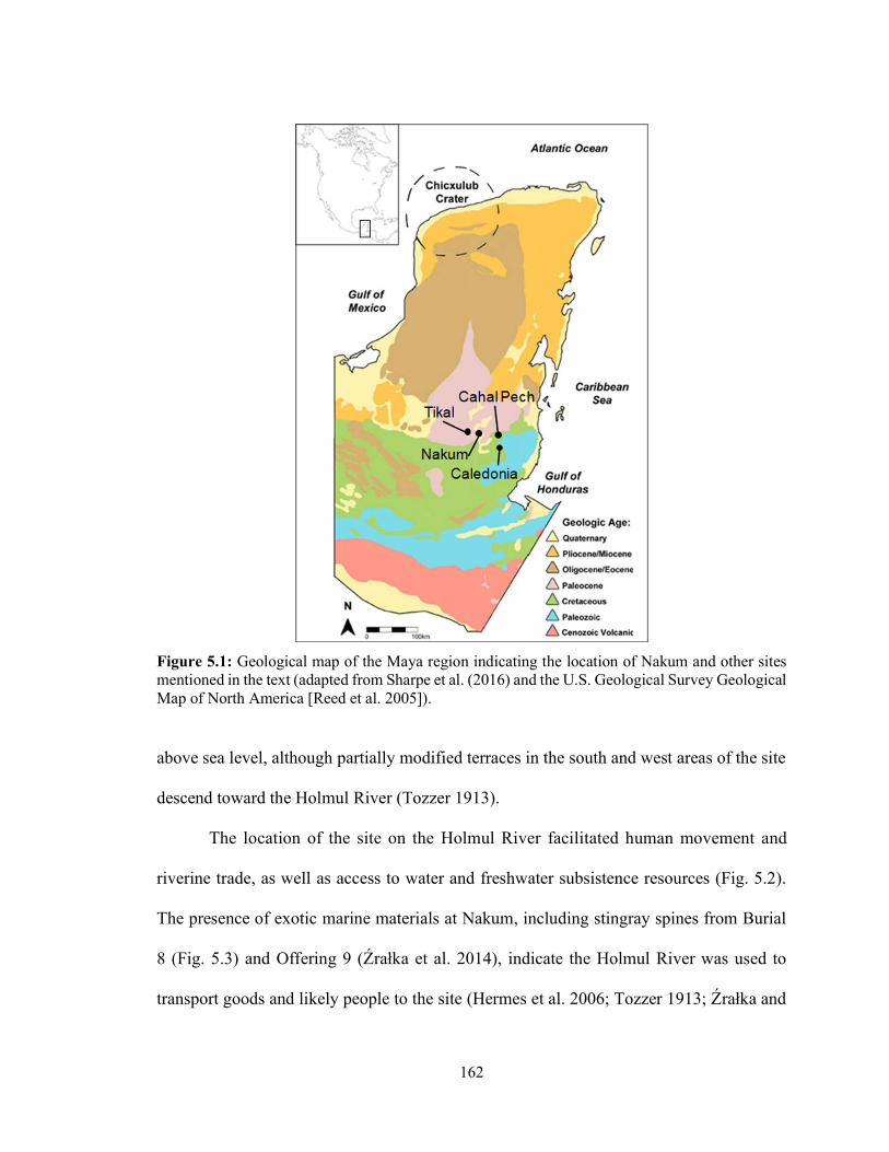
162

Figure 5.1: Geological map of the Maya region indicating the location of Nakum and other sites mentioned in the text (adapted from Sharpe et al. (2016) and the U.S. Geological Survey Geological Map of North America [Reed et al. 2005]).

above sea level, although partially modified terraces in the south and west areas of the site

descend toward the Holmul River (Tozzer 1913).

The location of the site on the Holmul River facilitated human movement and

riverine trade, as well as access to water and freshwater subsistence resources (Fig. 5.2).

The presence of exotic marine materials at Nakum, including stingray spines from Burial

8 (Fig. 5.3) and Offering 9 (Źrałka et al. 2014), indicate the Holmul River was used to

transport goods and likely people to the site (Hermes et al. 2006; Tozzer 1913; Źrałka and

163

Figure 5.2: Map of Nakum located on the Holmul River illustrating the northern and southern sectors of the site (Źrałka and Hermes 2012:163).

164

Figure 5.3: Plan and cross-section of Nakum Burial 8, an example of a richly furnished vaulted tomb located within a large pyramidal temple (Str. X), possibly the resting place of one of Nakum’s kings who reigned during the transition from the Early to Late Classic periods (A.D. 500/550-600). Note the presence of stingray spines in vessel PANC046. Image courtesy of Dr. Jarosław Źrałka and the PAN.

165

Hermes 2012), as it is part of a larger trade network that connected sites from Central Peten

to the Caribbean coast. The proximity of Nakum to the river also provided access to riverine

subsistence resources, although the diet of the Nakum residents was most likely based on

maize agriculture supplemented with other cultigens, wild plants, and animal resources, as

was the case elsewhere in the Maya region (e.g., Price et al. 2018a; Rand et al. 2015b;

Somerville et al. 2013; Tykot 2002; White 1999).

As at Tikal and other Maya sites (Braswell 2003; Price et al. 2010; Smyth and

Rogart 2004; Wright et al. 2010), the presence of talud-tablero architecture in Nakum’s

South Sector, artifacts made from Central Mexican green obsidian, and locally made

cylindrical tripod vessels have been interpreted as evidence of contact between people from

Teotihuacan in Central Mexico and those at Nakum during the Early Classic period

(Hermes et al. 2006; Koszkul et al. 2006; Źrałka and Koszkul 2007). Nearly all isotopic

studies of Maya mobility have identified nonlocal individuals; however, the results suggest

that long distance migration is less common than movement over short distances, with

limited evidence that individuals from beyond the Maya region moved to Maya centres

(Freiwald 2011a; Miller 2015; Patterson and Freiwald 2016; Price et al. 2008; Wright

2005a). This study assesses mobility to Nakum by comparing strontium and stable oxygen

and sulfur isotope values in human tooth and bone to faunal baseline values that also serve

to establish local and nonlocal foods in the diet and their potential contribution to human

isotopic values.

5.2 Principles of Isotopic Analyses in Bioarchaeology

Stable isotopic analyses of diet are based on the premise that the δ13C, δ15N, and

166

δ34S values of a consumer’s tissues reflect those of their diet. Nitrogen and sulfur present

in the organic portion of bone (i.e., collagen) are derived from dietary protein (Ambrose

and Norr 1993; Richards et al. 2003; Tanz and Schmidt 2010; Webb et al. 2017). When

protein consumption is adequate, carbon in collagen (δ13Ccol) is derived primarily from

dietary protein, whereas carbon in bone mineral (i.e., bioapatite; δ13Cap) is derived from the

whole diet (Ambrose and Norr 1993; Howland et al. 2003; Jim et al. 2004). Because bone

remodels throughout life, δ13Ccol, δ13Cap, δ18Oap, δ15N, and δ34S values will represent dietary

averages from adolescence until the end of life. The rate of bone turnover does, however,

vary depending on individual physiology and the bone sampled; for example, adult femoral

cortical bone collagen can maintain isotopic values from foods consumed during

adolescence (Hedges et al. 2007; Matsubayashi and Tayasu 2019). Unlike bone, tooth

enamel does not remodel (Moradian-Oldak 2009), so its carbon, oxygen, and strontium

isotope (δ13Cen, δ18Oen, 87Sr/86Sren) values reflect those of resources consumed when the

enamel formed during childhood.

Stable carbon isotope analysis is used to differentiate the types of plants consumed

by an individual. Most plants use the C3 photosynthetic pathway and have an average δ13C

value of –26.5 ‰, whereas C4 plants such as maize have an average value of –12.5 ‰

(O’Leary 1988; Smith and Epstein 1971). Although some plants use a third photosynthetic

pathway (CAM) with intermediate values, it is unlikely they were consumed to any

significant degree by the prehispanic lowland Maya (Powis et al. 1999; White 2005).

Terrestrial plants typically exhibit an average δ15N value of +3 ‰, while those that

directly fix nitrogen (i.e., legumes) have values close to 0 ‰ (Delwiche and Steyn 1970;

Wada et al. 1975). Because δ15N values increase between 3 ‰ and 6 ‰ at each trophic

167

level (Delwiche and Steyn 1970; Hedges and Reynard 2007; O’Connell et al. 2012),

humans with an omnivorous diet will have elevated δ15N values relative to those of prey

animals from the same region. Likewise, nursing infants will have δ15N values one trophic

level above those of their mothers (Fuller et al. 2006). However, physiological factors such

as pregnancy and disease can influence δ15N values in human tissues (Fuller et al. 2004,

2005; Katzenberg and Lovell 1999; Nitsch et al. 2010; White and Armelagos 1997), and

the δ15N values throughout a region can vary by temperature, aridity, and proportion of soil

nitrates (Ambrose 1991, 2000; Cormie and Schwarcz 1996; Heaton et al. 1986; Sealy et al.

1987; Somerville et al. 2018).

Stable sulfur isotope analysis has recently emerged as a promising technique for

differentiating the consumption of terrestrial, freshwater, and marine dietary protein, and

for identifying movement in prehistoric populations (Nehlich 2015; Rand and Nehlich

2018; Richards et al. 2001). Modern oceanic sulfate has a relatively uniform δ34S value

around +21 ‰ (Böttcher et al. 2007; Rees et al. 1978), whereas bedrock values vary based

on rock type and age so that volcanic rocks exhibit an average δ34S value around 0 ‰ and

ocean evaporates (e.g., limestone) have higher values around +20 ‰ (Nehlich 2015).

Because the δ34S values of oceanic sulfate have fluctuated over time, the value of the inland

Paleocene limestone surrounding Nakum is expected to be near +19 ‰ (Claypool et al.

1980). Although soil sulfate is primarily derived from bedrock weathering, atmospheric

deposition may also occur (Bern and Townsend 2008). Sea spray, for example, causes

coastal plants and their consumers up to 30 km inland to exhibit δ34S values similar to those

of marine resources (Gravenhorst 1978; Wakshal and Nielsen 1982).

Plants assimilate inorganic soil sulfate into the amino acids methionine and cysteine

168

(Brosnan and Brosnan 2006) and exhibit δ34S values 1.5 ‰ lower than those of the

environment in which they grow (Trust and Fry 1992). Animals must obtain methionine

from dietary protein (Brosnan and Brosnan 2006; Ingenbleek 2006), and although the offset

between the δ34S values of consumer tissues and their dietary protein is thought to be

minimal (+0.5 ± 2.4 ‰; Nehlich 2015:6; see also Krajcarz et al. 2019), the bone collagen

of larger mammals may exhibit δ34S values 1.5 ‰ lower than those of the foods they

consume (Webb et al. 2017). Therefore, human δ34S values should be lower than those in

the local environment and values that are significantly different suggest that dietary protein

was acquired from an isotopically distinct region and the individuals were therefore

nonlocal (Nehlich 2015).

Stable oxygen isotope (δ18O) analysis is similarly useful for identifying nonlocal

individuals (see Pederzani and Britton (2019) for a recent review). Drinking water δ18O

values are a function of the local climate, whereby higher values are associated with higher

amounts of precipitation, increasing distance from the sea, higher altitudes, increasing

humidity, and decreasing temperature (Rozanski et al. 1993). In the Maya region, the

highest modern surface water δ18O values come from the Peten Lakes region of Guatemala,

followed by those along the Caribbean coast, while the lowest δ18O values occur in the

Highlands (Lachniet and Patterson 2009; Marfia et al. 2004). In general, higher values are

found in the lowlands relative to the highlands, and the Yucatan has generally higher δ18O

values than those present in central or southwestern Mexico (Wassenaar et al. 2009).

Although inhaled and consumed oxygen is also incorporated into body tissues, the δ18O

values in tooth enamel (δ18Oen) and bone apatite (δ18Oap) primarily reflect those of water

imbibed during childhood and in later in life, respectively (Longinelli 1984). Thus,

169

movement from an isotopically distinct region prior to death may be inferred if an

individual’s δ18O values differ significantly from those of local drinking water sources.

However, this may be complicated by growth-related stress (Warinner and Tuross 2010)

and cultural practices such as cooking (Brettell et al. 2012), fermenting (Gagnon et al.

2015), or storing water (Scherer et al. 2015). Thus, it is best to interpret δ18O values in

conjunction with other isotopic assays (Pederzani and Britton 2019; Price et al. 2010).

Strontium isotope analysis measures the ratio between the stable isotope 86Sr and

the radiogenic isotope 87Sr, which varies in the environment due to the age and composition

of underlying geology (Faure and Powell 1972). Over time, rubidium-87 (87Rb) in the

Earth’s crust decays into 87Sr, causing older metamorphic rocks to have much higher

87Sr/86Sr values than younger volcanic rocks, while limestone exhibits intermediate values

reflecting those of seawater at the time it formed (Bentley 2006; Hodell et al. 2004, 2007;

Palmer and Elderfield 1985). In the Maya region, there is a gradual decrease in the range

of limestone 87Sr/86Sr values from 0.7092 in the Eocene-Oligocene-Miocene-Pliocene

carbonates of the northern and coastal Yucatan to 0.7071 in the Cretaceous and Paleocene

limestones of the Southern Lowlands, while the volcanic rocks of the Guatemala Highlands

and Pacific Coast to the south have much lower 87Sr/86Sr values between 0.7038 and 0.7050

(Hodell et al. 2004; Palmer and Elderfield 1985). The highest 87Sr/86Sr values occur in the

Maya Mountains, where the metamorphic highlands contain pockets of relatively ancient

rocks that have values that exceed 0.711 (Hodell et al. 2004; Freiwald 2011a).

Dietary strontium is primarily derived from plant foods, and substitutes for calcium

in bone and tooth enamel bioapatite. Tooth enamel is the preferred sample material for

strontium isotope analysis because strontium in bone is more susceptible to diagenetic

170

alteration (Hoppe et al. 2003). Because biological processes fractionate 87Sr/86Sr values

below levels detectable by instrumentation, the ratios in human samples will represent those

of the geological substrate from which food was acquired (Flockhart et al. 2015; Lewis et

al. 2017). Thus, 87Sr/86Sr values from tooth enamel reflect those of the dietary catchment

during the period in childhood when the tooth formed.

5.3 Materials and Methods

Pollution since the industrial revolution has altered modern δ34S values, and so it is

necessary to sample archaeological fauna to generate environmental baseline values for

archaeological applications (Richards et al. 2001; Trust and Fry 1992). Therefore, eighteen

archaeological faunal bone samples and one tooth (Table 5.1) recovered from Nakum were

analyzed to provide isotopic baseline data. Nine archaeological human bones and seven

teeth were also sampled, the contextual and biographical data of which can be found in

Table 5.2. These samples come from multiple time periods and represent both higher status

individuals interred in formal tombs (Burials 1 and 8) and crypts (Burials 2 and 5) and

lower status individuals from an unfurnished grave (Burial 4) and a dedicatory burial

(Burial 7), as well as isolated elements from varying contexts (see Table 5.2). Age and sex

estimations (Table 5.2) were conducted by Matute using standard techniques (Buikstra and

Ubelaker 1994). Poor preservation dictated the sampling of the most well-preserved

elements from each context.

Each specimen was thoroughly cleaned and dried prior to preparation (see

Appendix A for details). Bone collagen was extracted following standard procedures

(Honch et al. 2006; Nehlich and Richards 2009; Rand et al. 2015a), details of which can

171

Table 5.1: Contextual, species, and biographical data for the Nakum fauna samples.

Lab # Sample ID Context Common Name Taxon Age Element Period

4315 MOF4 VI-20-3-3 cf. White-tailed

deer cf. Odocoileus

virginianus Adult Ulna Terminal Classic

4316 MOF10 VI-21-6-2 cf. White-tailed

deer cf. Odocoileus

virginianus Adult

Left humerus

Terminal Classic

4317 MOF1 III-5-2-2 cf. White-tailed

deer cf. Odocoileus

virginianus Adult Metacarpal Late to Terminal Classic

4318 MOF11 VI-22-5 Mesoamerican

slider Trachemys

venusta Adult Femur Terminal Classic

4319 MOF14 VI-4-2-4 cf. White-tailed

deer cf. Odocoileus

virginianus Adult Metacarpal Late Classic

4320 MOF9 VI-28-8-4 cf. White-tailed

deer cf. Odocoileus

virginianus Adult Tibia Terminal Classic

4321 MOF18 XXII-3-3 cf. White-tailed

deer cf. Odocoileus

virginianus Adult Metatarsal Late Classic

4322 MOF6 VI-22-5 Deer Capreolinae Subadult Mandible Terminal Classic

4323 MOF12 VI-12-1 cf. White-tailed

deer cf. Odocoileus

virginianus Adult Tibia Late Classic

4324 MOF3 VI-22-1-7 Deer Capreolinae Adult Mandible Late Classic

4325 MOF15 VI-2-6 cf. White-tailed

deer cf. Odocoileus

virginianus Adult Metapodial Late Classic

4326 MOF16 VI-31A-12-

3 cf. White-tailed

deer cf. Odocoileus

virginianus Adult Long bone Early Classic

4327 MOF13 VI-6A-2 Brocket deer Mazama sp. Adult Calcaneus Protoclassic

4328 MOF8 VI-28-2-7 cf. White-tailed

deer cf. Odocoileus

virginianus Adult Left ilium Terminal Classic

4329 MOF17 XIII-3-1-9 cf. White-tailed

deer cf. Odocoileus

virginianus Adult Scapula Terminal Classic

4330 MOF5 VI-22-5-1 Turkey Meleagris sp. Adult Tibiotarsus Terminal Classic

4331 MOF2 VI-20-2-5 Deer Capreolinae Adult Metacarpal Terminal Classic

4332 MOF7 VI-20-2-4 Deer Capreolinae Adult Metacarpal Late Classic

4495 PANE3 I-12-3-9 Dog Canis familiaris Adult Left

carnassial Middle Preclassic

be found in Appendix A. For stable carbon and nitrogen isotope analysis, samples were

analyzed using a Thermo Scientific Delta V Plus I Gas Source Isotope Ratio Mass

Spectrometer (IRMS) coupled via continuous flow to a Carlo Erba NA 1500 Series II

Elemental Analyzer (EA) in the CREAIT Network’s Stable Isotope Laboratory (SIL) at

Memorial University of Newfoundland (MUN) (see Appendix A). Analytical precision

and accuracy were calculated following the technique outlined in Szpak et al. (2017a) and

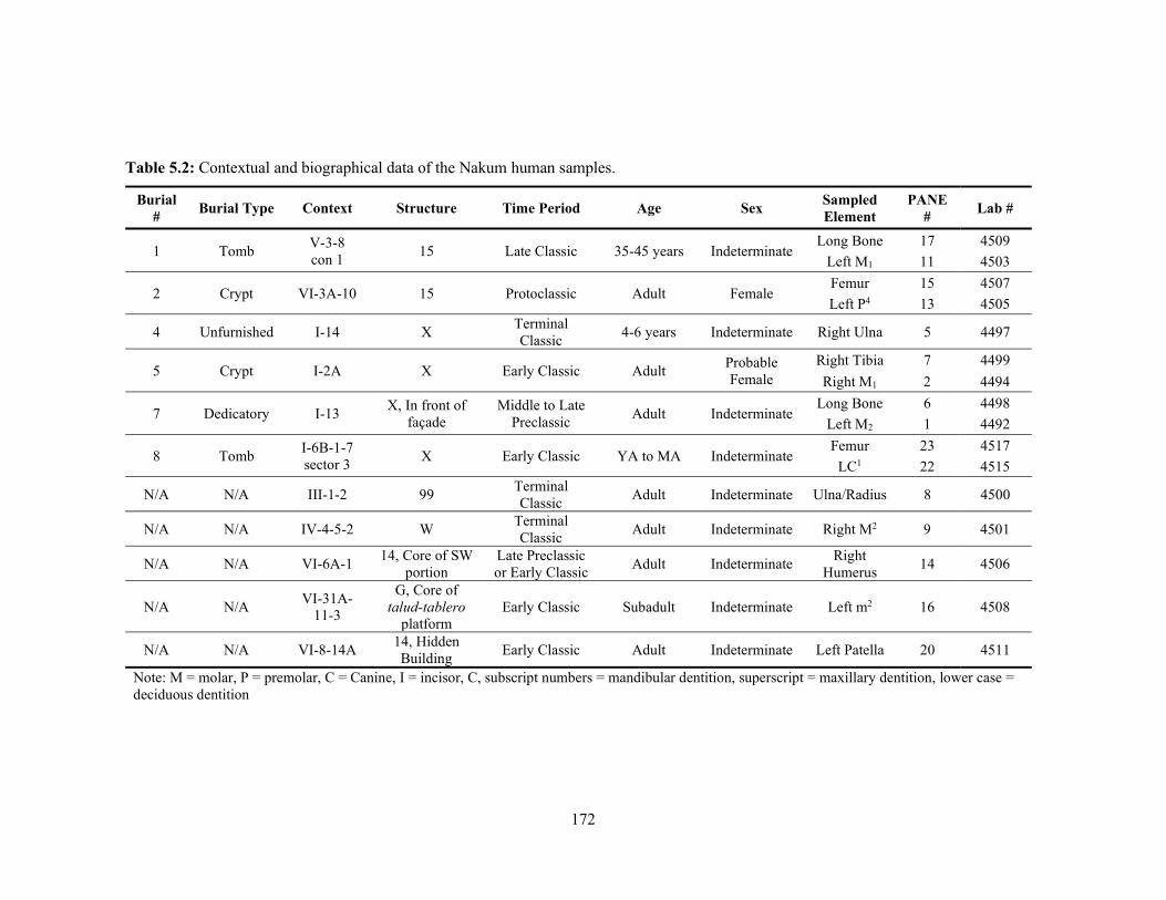
172

Table 5.2: Contextual and biographical data of the Nakum human samples.

Burial #

Burial Type Context Structure Time Period Age Sex Sampled Element

PANE #

Lab #

1 Tomb V-3-8 con 1

15 Late Classic 35-45 years Indeterminate Long Bone 17 4509

Left M1 11 4503

2 Crypt VI-3A-10 15 Protoclassic Adult Female Femur 15 4507

Left P4 13 4505

4 Unfurnished I-14 X Terminal Classic

4-6 years Indeterminate Right Ulna 5 4497

5 Crypt I-2A X Early Classic Adult Probable Female

Right Tibia 7 4499

Right M1 2 4494

7 Dedicatory I-13 X, In front of

façade Middle to Late

Preclassic Adult Indeterminate

Long Bone 6 4498

Left M2 1 4492

8 Tomb I-6B-1-7 sector 3

X Early Classic YA to MA Indeterminate Femur 23 4517

LC1 22 4515

N/A N/A III-1-2 99 Terminal Classic

Adult Indeterminate Ulna/Radius 8 4500

N/A N/A IV-4-5-2 W Terminal Classic

Adult Indeterminate Right M2 9 4501

N/A N/A VI-6A-1 14, Core of SW

portion Late Preclassic or Early Classic

Adult Indeterminate Right

Humerus 14 4506

N/A N/A VI-31A-

11-3

G, Core of talud-tablero

platform Early Classic Subadult Indeterminate Left m2 16 4508

N/A N/A VI-8-14A 14, Hidden Building

Early Classic Adult Indeterminate Left Patella 20 4511

Note: M = molar, P = premolar, C = Canine, I = incisor, C, subscript numbers = mandibular dentition, superscript = maxillary dentition, lower case = deciduous dentition

173

details can be found in Appendices A and C. Analytical precision was ±0.21 ‰ for δ13C

and ±0.16 ‰ for δ15N based on repeated measurements of calibration standards, check

standards, and sample replicates (see Appendix C). Analytical accuracy was ±0.21 ‰ for

δ13C and ±0.20 ‰ for δ15N based on the difference between the observed and known δ13C

and δ15N values of the check standards and their long-term standard deviations (Appendix

C). Considering both analytical accuracy and precision, the standard uncertainty11 was

±0.30 ‰ for δ13C and ±0.25 ‰ for δ15N (Appendix C).

Stable sulfur isotopes were analyzed on a Thermo Scientific Delta V Plus IRMS

coupled via continuous flow to a Costech EA (ECS4010) at the Stable Isotope Laboratory

in the Department of Earth and Planetary Sciences, University of Tennessee Knoxville (see

Appendix A). Analytical precision was ±1.00 ‰, although analytical accuracy could not

be calculated as check standards were not included in the analysis (Szpak et al. 2017a;

Appendix C).

Bioapatite was isolated from powdered bone and tooth enamel samples following

standard procedures (Garvie-Lok et al. 2004) and stable carbon and oxygen isotopes were

analyzed on a Thermo Scientific Delta V IRMS coupled to a Gas Bench via a continuous-

flow interface in the CREAIT Network’s SIL facility at MUN (Appendix A). Using the

method of Szpak et al. (2017a) and data provided in Appendix C, the measurement

precision was ±0.16 ‰ for δ13C and ±0.31 ‰ for δ18O and analytical accuracy was ±0.08

‰ for δ13C and ±0.09 ‰ for δ18O. Considering both precision and accuracy, the overall

standard uncertainty was ±0.18 ‰ for δ13C and ±0.32 ‰ for δ18O.

11 In Rand et al. (2020a), the analytical accuracy (uc) and measurement precision (ssrm), which is calculated from the calibration and check standards, were reported to be consistent with earlier studies.

174

Strontium was extracted from one faunal and three human teeth samples using ion-

exchange chromatography (Copeland et al. 2008; Madgwick et al. 2017), and details can

be found in Appendix A. Enamel was sampled because it is resilient against postmortem

chemical alteration (i.e., diagenesis) and so will accurately reflect the 87Sr/86Sr values

during life. The 87Sr/86Sr values of tooth dentine were also analyzed as proxies for the local

range of values because dentine is more susceptible to diagenetic uptake of soil-derived

strontium (Budd et al. 2000) and therefore is assumed to reflect local soluble strontium in

the burial environment (Montgomery et al. 2007). All purified Sr solutions were analyzed

on a Thermo Scientific Neptune™ multi-collector inductively coupled plasma mass

spectrometer (MC-ICP-MS) within the Micro Analysis Facility (MAF) of CREAIT at

MUN along with the analytical standard NIST SRM 987, procedural standards, and blanks.

The deviation of the average value for SRM 987 during the analytical session was used to

correct all sample values (see Appendix A). Finally, the signal intensities of total procedural

blanks were considered negligible (<0.1 %) when compared to the typical 88Sr intensities

of the samples and standards.

Isotopic values that fell beyond the interquartile range (IQR) multiplied by 1.5

subtracted from the first quartile and added to the third of the data set were interpreted as

nonlocal individuals. These outlying values were removed prior to calculating local

isotopic baseline values as falling within two standard deviations of the mean of the

trimmed data set (see Appendix A). All statistical analyses were performed in SPSS version

25 for Windows (IBM®). Due to small sample sizes and the nonparametric distribution of

the data, statistical differences and correlations between sample values were tested using

175

nonparametric statistical tests interpreted at the 95% significance level (i.e., p = 0.05) (see

Appendix A for more detail).

5.4 Results

The average δ13Ccol (–21.1 ± 0.9 ‰) and δ15N (+5.6 ± 1.2 ‰) values of the 16 faunal

remains with collagen sufficiently preserved for interpretation (Ambrose 1990; DeNiro

1985; Nehlich and Richards 2009; van Klinken 1999) indicate that the majority of the

animals consumed C3-based diets typical of deer, turtles, and wild turkeys in the Maya

region (Table 5.3; Fig. 5.4). The turkey’s δ13Ccol (–21.3 ‰) and δ15N (+6.1 ‰) values fall

within the range of the terrestrial mammals (i.e., deer), suggesting it consumed a terrestrial

C3-based diet. The Mesoamerican slider turtle’s negative δ13Ccol value (–22.6 ‰) reflects a

C3-based diet, with an elevated δ15N value (+7.5 ‰) that indicates the consumption of fish,

other turtles, and invertebrates. When the turtle’s elevated δ15N value is excluded, the

average fauna δ15N value (+5.4 ± 1.1 ‰) suggests that the remaining specimens were

herbivores, as expected based on the species identifications.

Table 5.3 presents the results from the five human collagen samples that were

preserved well enough for analysis (Ambrose 1990; DeNiro 1985; Nehlich and Richards

2009; van Klinken 1999). Due to differences in preparation and analysis (see Pestle et al.

2014), the δ13C and δ15N values previously obtained by Matute (unpublished data) are

included in Table 5.3 but were excluded from statistical analyses and interpretations. The

average human δ13C value (–11.6 ± 2.2 ‰; Table 5.3, Fig. 5.4) is significantly more positive

than that of the fauna (U = 0.000, p = 0.001), demonstrating the importance of C4 plants,

probably maize, in the Nakum diet. These individuals also relied on terrestrial animal

176

protein, given that their average δ15N value (+10.2 ± 1.0 ‰; Fig. 5.4, Table 5.3) is

significantly elevated relative to that of the fauna (U = 0.000, p = 0.001).

Due to potential diagenetic alteration, only the carbonate data from the five bone

samples that yielded sufficient collagen for analysis are considered in this study (Table 5.3,

Fig. 5.5). This is because the preservation of collagen and apatite are linked (Kendall et al.

2018), and samples that lacked collagen in this study had significantly higher δ13Cap values

than those with well-preserved collagen (U = 0.000, p = 0.014). This suggests that samples

with poorly preserved collagen were diagenetically contaminated by exogenous carbon

enriched in 13C, and so they were removed from the following interpretations. The human

bone δ13Cap values of the five samples with well preserved collagen (–7.6 ± 1.3‰; see Table

5.3) is consistent with a whole diet dependent on maize but also supplemented with C3-

based foods.

Figure 5.4: The δ13C and δ15N values of the fauna and human bone collagen from Nakum. Humans are identified by laboratory number whereas fauna are identified by species. Note: WTD = white-tailed deer.

0.0

2.0

4.0

6.0

8.0

10.0

12.0

-24.0 -22.0 -20.0 -18.0 -16.0 -14.0 -12.0 -10.0 -8.0

δ15N

(A

IR, ‰

)

δ13Ccol (VPDB, ‰)

Brocket Deer

cf. WTD

Deer

Turkey

Turtle

4497

4498

4500

4506

4511

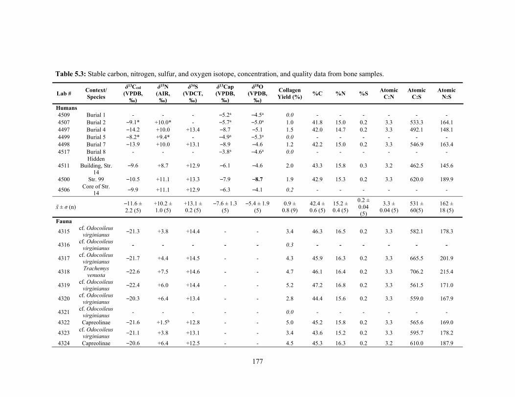
177

Table 5.3: Stable carbon, nitrogen, sulfur, and oxygen isotope, concentration, and quality data from bone samples.

Lab # Context/ Species

δ13Ccol (VPDB,

‰)

δ15N (AIR,

‰)

δ34S (VDCT,

‰)

δ13Cap (VPDB,

‰)

δ18O (VPDB,

‰)

Collagen Yield (%)

%C %N %S Atomic

C:N Atomic

C:S Atomic

N:S

Humans

4509 Burial 1 - - - –5.2a –4.5a 0.0 - - - - - - 4507 Burial 2 –9.1* +10.0* - –5.7a –5.0a 1.0 41.8 15.0 0.2 3.3 533.3 164.1 4497 Burial 4 –14.2 +10.0 +13.4 –8.7 –5.1 1.5 42.0 14.7 0.2 3.3 492.1 148.1 4499 Burial 5 –8.2* +9.4* - –4.9a –5.3a 0.0 - - - - - - 4498 Burial 7 –13.9 +10.0 +13.1 –8.9 –4.6 1.2 42.2 15.0 0.2 3.3 546.9 163.4 4517 Burial 8 - - - –3.8a –4.6a 0.0 - - - - - -

4511 Hidden

Building, Str. 14

–9.6 +8.7 +12.9 –6.1 –4.6 2.0 43.3 15.8 0.3 3.2 462.5 145.6

4500 Str. 99 –10.5 +11.1 +13.3 –7.9 –8.7 1.9 42.9 15.3 0.2 3.3 620.0 189.9

4506 Core of Str.

14 –9.9 +11.1 +12.9 –6.3 –4.1 0.2 - - - - - -

x̄ ± σ (n) –11.6 ± 2.2 (5)

+10.2 ± 1.0 (5)

+13.1 ± 0.2 (5)

–7.6 ± 1.3 (5)

–5.4 ± 1.9 (5)

0.9 ± 0.8 (9)

42.4 ± 0.6 (5)

15.2 ± 0.4 (5)

0.2 ± 0.04 (5)

3.3 ± 0.04 (5)

531 ± 60(5)

162 ± 18 (5)

Fauna

4315 cf. Odocoileus

virginianus –21.3 +3.8 +14.4 - - 3.4 46.3 16.5 0.2 3.3 582.1 178.3

4316 cf. Odocoileus

virginianus - - - - - 0.3 - - - - - -

4317 cf. Odocoileus

virginianus –21.7 +4.4 +14.5 - - 4.3 45.9 16.3 0.2 3.3 665.5 201.9

4318 Trachemys

venusta –22.6 +7.5 +14.6 - - 4.7 46.1 16.4 0.2 3.3 706.2 215.4

4319 cf. Odocoileus

virginianus –22.4 +6.0 +14.4 - - 5.2 47.2 16.8 0.2 3.3 561.5 171.0

4320 cf. Odocoileus

virginianus –20.3 +6.4 +13.4 - - 2.8 44.4 15.6 0.2 3.3 559.0 167.9

4321 cf. Odocoileus

virginianus - - - - - 0.0 - - - - - -

4322 Capreolinae –21.6 +1.5b +12.8 - - 5.0 45.2 15.8 0.2 3.3 565.6 169.0

4323 cf. Odocoileus

virginianus –21.1 +3.8 +13.1 - - 3.4 43.6 15.2 0.2 3.3 595.7 178.2

4324 Capreolinae –20.6 +6.4 +12.5 - - 4.5 45.3 16.3 0.2 3.2 610.0 187.9

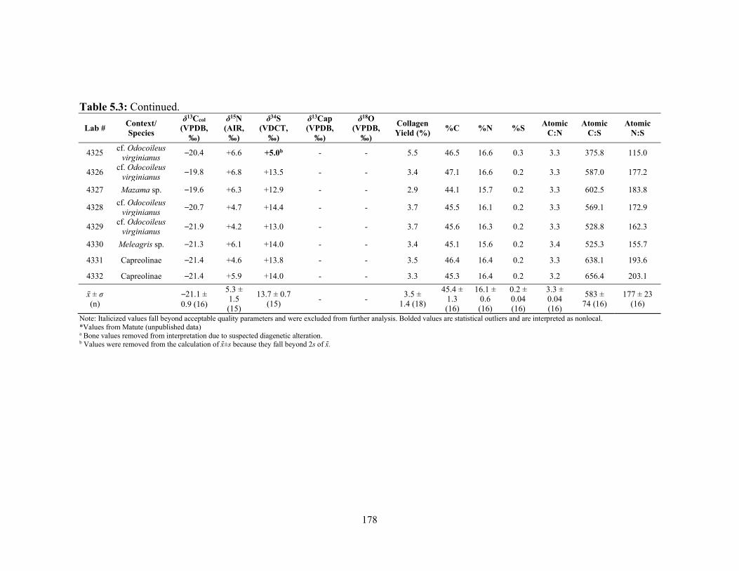
178

Table 5.3: Continued.

Lab # Context/ Species

δ13Ccol (VPDB,

‰)

δ15N (AIR,

‰)

δ34S (VDCT,

‰)

δ13Cap (VPDB,

‰)

δ18O (VPDB,

‰)

Collagen Yield (%)

%C %N %S Atomic

C:N Atomic

C:S Atomic

N:S

4325 cf. Odocoileus

virginianus –20.4 +6.6 +5.0b - - 5.5 46.5 16.6 0.3 3.3 375.8 115.0

4326 cf. Odocoileus

virginianus –19.8 +6.8 +13.5 - - 3.4 47.1 16.6 0.2 3.3 587.0 177.2

4327 Mazama sp. –19.6 +6.3 +12.9 - - 2.9 44.1 15.7 0.2 3.3 602.5 183.8

4328 cf. Odocoileus

virginianus –20.7 +4.7 +14.4 - - 3.7 45.5 16.1 0.2 3.3 569.1 172.9

4329 cf. Odocoileus

virginianus –21.9 +4.2 +13.0 - - 3.7 45.6 16.3 0.2 3.3 528.8 162.3

4330 Meleagris sp. –21.3 +6.1 +14.0 - - 3.4 45.1 15.6 0.2 3.4 525.3 155.7

4331 Capreolinae –21.4 +4.6 +13.8 - - 3.5 46.4 16.4 0.2 3.3 638.1 193.6

4332 Capreolinae –21.4 +5.9 +14.0 - - 3.3 45.3 16.4 0.2 3.2 656.4 203.1

x̄ ± σ (n)

–21.1 ± 0.9 (16)

5.3 ± 1.5 (15)

13.7 ± 0.7 (15)

- - 3.5 ±

1.4 (18)

45.4 ± 1.3 (16)

16.1 ± 0.6 (16)

0.2 ± 0.04 (16)

3.3 ± 0.04 (16)

583 ± 74 (16)

177 ± 23 (16)

Note: Italicized values fall beyond acceptable quality parameters and were excluded from further analysis. Bolded values are statistical outliers and are interpreted as nonlocal. *Values from Matute (unpublished data) a Bone values removed from interpretation due to suspected diagenetic alteration. b Values were removed from the calculation of x̄±s because they fall beyond 2s of x̄.

179

Figure 5.5: The δ13Cap and δ18Oap values of bone and tooth enamel samples from Nakum. The shaded area represents the local range of δ18O values determined from the mean and two standard deviations of all human enamel and bone samples with viable collagen excluding the two outliers (x̅ ± 2σ = –3.9 ± 1.6 ‰).

Maize appears to have been an important component of childhood diet as well, as

most individuals had δ13Cen values that were elevated relative to the single dog tooth (–9.1

‰; Table 5.4, Fig. 5.5), suggesting the consumption of maize when their teeth formed.

However, the δ13Cen value from Burial 7 (–8.8 ‰) and that of sample 4508 (–12.2 ‰) are

more negative, suggesting more C3-based foods in the childhood diets of these individuals.

The human bone δ13Cap values are more negative than those of the teeth (Fig. 5.5), which

may indicate differential fractionation of carbon isotopes during incorporation into the

apatite of bones and teeth, differences in maize consumption from childhood to adulthood,

or possible diagenetic alteration of the bone values. The last possibility is unlikely,

however, as the δ13C values of the five well-preserved human collagen and apatite samples

are significantly positively correlated (rs = 0.9000, p = 0.037), indicating a shared source

of carbon (i.e., maize).

-11.0

-10.0

-9.0

-8.0

-7.0

-6.0

-5.0

-4.0

-3.0

-2.0

-1.0

-14.0 -12.0 -10.0 -8.0 -6.0 -4.0 -2.0

δ18O

(V

PD

B, ‰

)

δ13Cap (VPDB, ‰)

Human Bone

Human Tooth Enamel

Dog Tooth Enamel

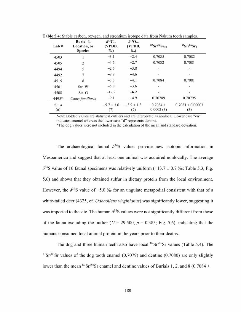
180

Table 5.4: Stable carbon, oxygen, and strontium isotope data from Nakum tooth samples.

Lab # Burial #,

Location, or Species

δ13Cen (VPDB,

‰)

δ18Oen (VPDB,

‰)

87Sr/86Sren 87Sr/86Srd

4503 1 –3.1 –2.4 0.7085 0.7082

4505 2 –4.5 –2.7 0.7082 0.7081

4494 5 –2.5 –3.8 - -

4492 7 –8.8 –4.6 - -

4515 8 –3.3 –4.1 0.7084 0.7081

4501 Str. W –5.8 –3.6 - -

4508 Str. G –12.2 –6.2 - -

4495* Canis familiaris –9.1 –4.9 0.70789 0.70795

x̄ ± σ (n)

–5.7 ± 3.6 (7)

–3.9 ± 1.3 (7)

0.7084 ± 0.0002 (3)

0.7081 ± 0.00003 (3)

Note: Bolded values are statistical outliers and are interpreted as nonlocal. Lower case “en” indicates enamel whereas the lower case “d” represents dentine. *The dog values were not included in the calculation of the mean and standard deviation.

The archaeological faunal δ34S values provide new isotopic information in

Mesoamerica and suggest that at least one animal was acquired nonlocally. The average

δ34S value of 16 faunal specimens was relatively uniform (+13.7 ± 0.7 ‰; Table 5.3, Fig.

5.6) and shows that they obtained sulfur in dietary protein from the local environment.

However, the δ34S value of +5.0 ‰ for an ungulate metapodial consistent with that of a

white-tailed deer (4325, cf. Odocoileus virginianus) was significantly lower, suggesting it

was imported to the site. The human δ34S values were not significantly different from those

of the fauna excluding the outlier (U = 29.500, p = 0.385; Fig. 5.6), indicating that the

humans consumed local animal protein in the years prior to their deaths.

The dog and three human teeth also have local 87Sr/86Sr values (Table 5.4). The

87Sr/86Sr values of the dog tooth enamel (0.7079) and dentine (0.7080) are only slightly

lower than the mean 87Sr/86Sr enamel and dentine values of Burials 1, 2, and 8 (0.7084 ±

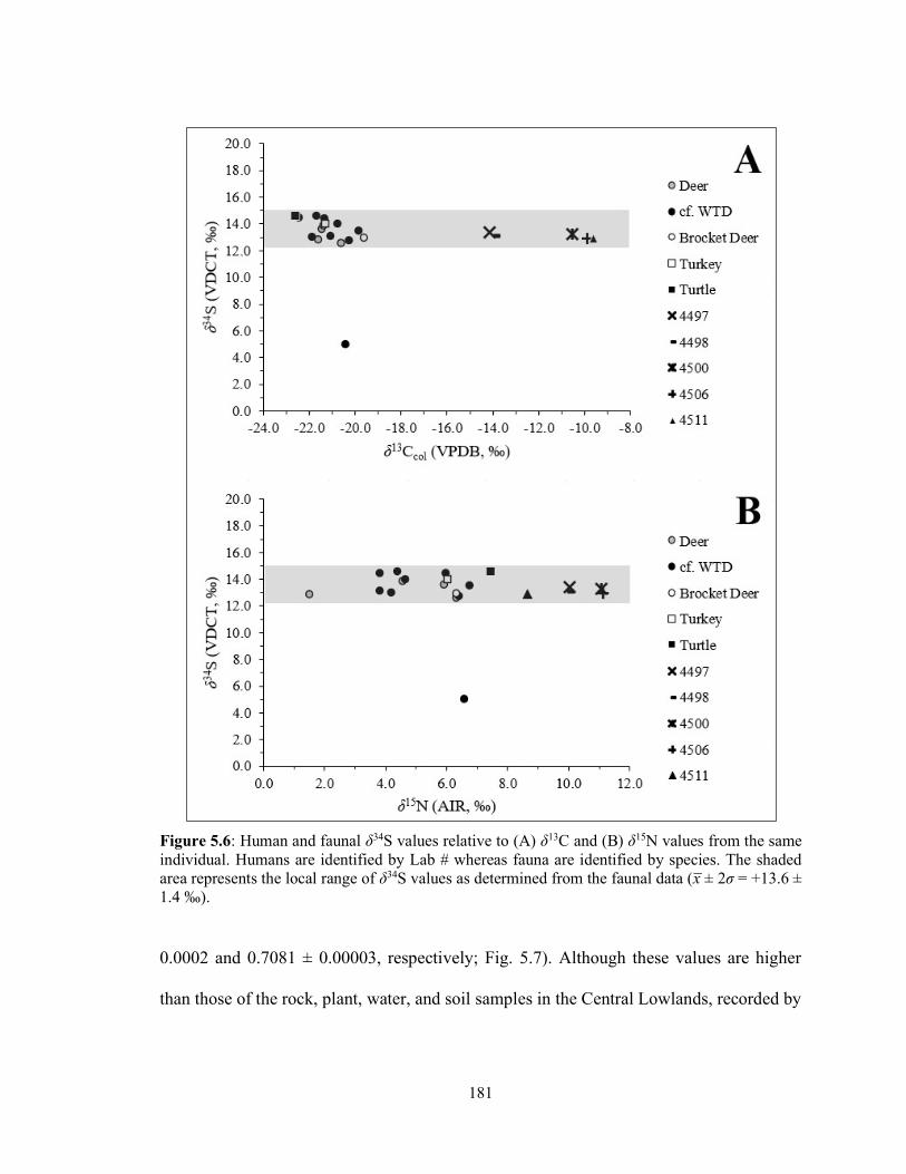
181

Figure 5.6: Human and faunal δ34S values relative to (A) δ13C and (B) δ15N values from the same individual. Humans are identified by Lab # whereas fauna are identified by species. The shaded area represents the local range of δ34S values as determined from the faunal data (x̅ ± 2σ = +13.6 ± 1.4 ‰).

0.0002 and 0.7081 ± 0.00003, respectively; Fig. 5.7). Although these values are higher

than those of the rock, plant, water, and soil samples in the Central Lowlands, recorded by

182

Figure 5.7: The δ18O and 87Sr/86Sr values of three human and one canine tooth enamel samples from Nakum. The shaded area represents the local range of δ18O values (see text and Fig. 5.5 for details) and does not reflect local 87Sr/86Sr values.

Hodell and colleagues (2004), they are similar to biologically available 87Sr/86Sr values

identified at San Bartolo (Davies 2012), Naranjo (Freiwald et al. 2014), and many other

sites to the east (Freiwald 2011a; Sutinen 2014), suggesting the Nakum individuals

represent a local population that mainly consumed local resources during childhood.

The δ18Oen results (Table 5.4) support this interpretation and suggest that most

individuals drank local water during childhood, although there are two statistical outliers

(Fig. 5.5). The average values of human bone (–5.4 ± 1.9 ‰) were lower than those of the

teeth (–3.9 ± 1.3 ‰), which likely reflects the incorporation of oxygen from milk enriched

in 18O into the teeth while the enamel formed during breastfeeding (Wright and Schwarcz

1998, 1999). Although δ18O values are species-specific (Iacumin et al. 1996; Longinelli

1984), that of the dog tooth enamel (–4.9 ‰) is intermediate to the average values of human

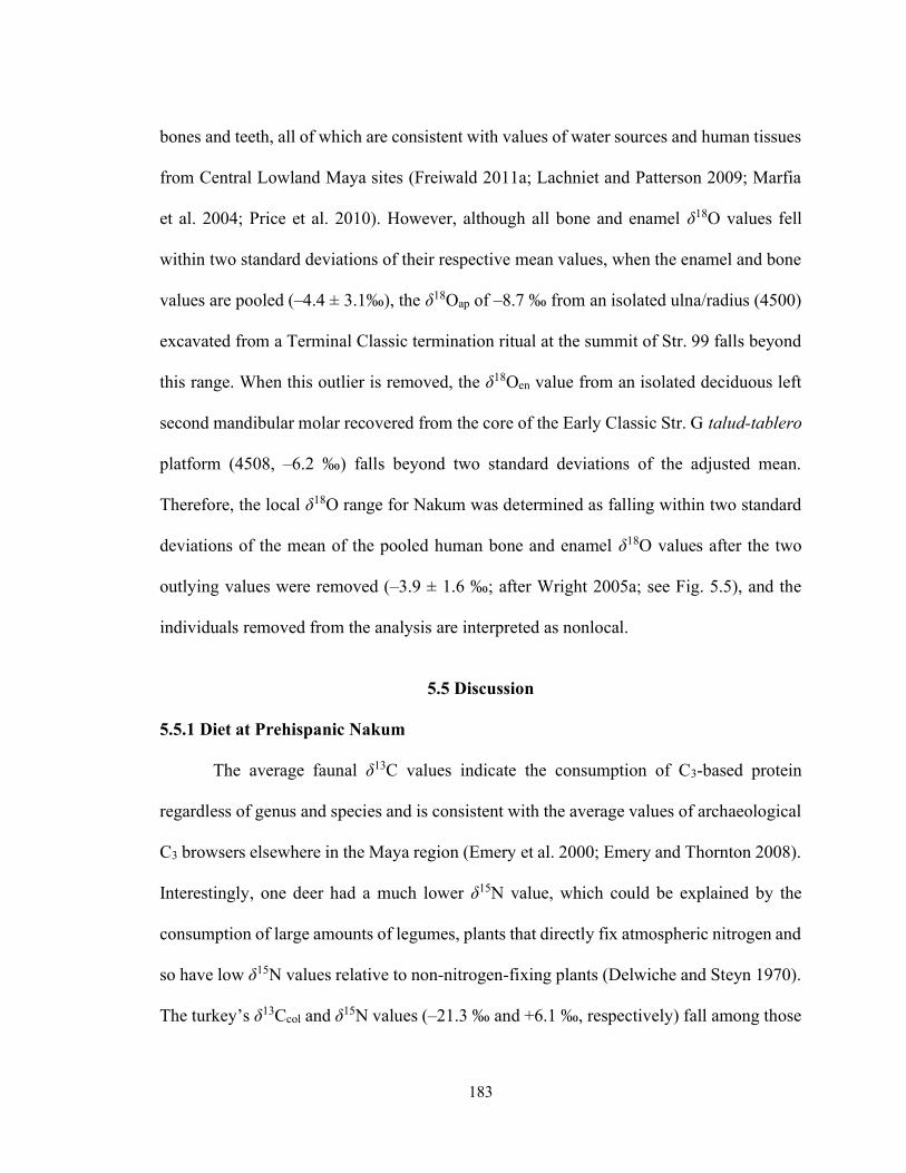
183

bones and teeth, all of which are consistent with values of water sources and human tissues

from Central Lowland Maya sites (Freiwald 2011a; Lachniet and Patterson 2009; Marfia

et al. 2004; Price et al. 2010). However, although all bone and enamel δ18O values fell

within two standard deviations of their respective mean values, when the enamel and bone

values are pooled (–4.4 ± 3.1‰), the δ18Oap of –8.7 ‰ from an isolated ulna/radius (4500)

excavated from a Terminal Classic termination ritual at the summit of Str. 99 falls beyond

this range. When this outlier is removed, the δ18Oen value from an isolated deciduous left

second mandibular molar recovered from the core of the Early Classic Str. G talud-tablero

platform (4508, –6.2 ‰) falls beyond two standard deviations of the adjusted mean.

Therefore, the local δ18O range for Nakum was determined as falling within two standard

deviations of the mean of the pooled human bone and enamel δ18O values after the two

outlying values were removed (–3.9 ± 1.6 ‰; after Wright 2005a; see Fig. 5.5), and the

individuals removed from the analysis are interpreted as nonlocal.

5.5 Discussion

5.5.1 Diet at Prehispanic Nakum

The average faunal δ13C values indicate the consumption of C3-based protein

regardless of genus and species and is consistent with the average values of archaeological

C3 browsers elsewhere in the Maya region (Emery et al. 2000; Emery and Thornton 2008).

Interestingly, one deer had a much lower δ15N value, which could be explained by the

consumption of large amounts of legumes, plants that directly fix atmospheric nitrogen and

so have low δ15N values relative to non-nitrogen-fixing plants (Delwiche and Steyn 1970).

The turkey’s δ13Ccol and δ15N values (–21.3 ‰ and +6.1 ‰, respectively) fall among those

184

of the mammals (i.e., deer), indicating a terrestrial diet. The turkey’s low δ13Ccol also

suggests it was probably wild, as domesticated turkeys at other Maya sites have been found

to have isotopic values comparable to those of humans due to the consumption of maize

(i.e., elevated δ13C and δ15N values; Sharpe et al. 2018; Thornton et al. 2016).

The Nakum faunal δ34S values were surprisingly elevated relative to those from

inland sites elsewhere in the world and approach values expected in marine or coastal

environments (i.e., greater than +14‰; Nehlich and Richards 2009; Richards et al. 2001).

Similarly elevated δ34S values at Thebes, Greece (Vika 2009), and Romiot, Italy (Craig et

al. 2010) have been attributed to the underlying limestone geology, which is derived from

marine evaporates that reflect the δ34S values of oceanic sulfate at their time of formation

(Claypool et al. 1980). It also appears that any sulfur deposited from atmospheric sources

with lower δ34S values (i.e., volcanic ash fall; Tankersley et al. 2016) has been obscured by

values derived from the limestone bedrock. Thus, the narrow range of faunal δ34S values

from Nakum (excluding the outlying value of +5.0 ‰ from 4325) indicate a shared source

of dietary sulfur obtained from plants that assimilated inorganic sulfate from the limestone

soils surrounding the site.

Interestingly, although the Mesoamerican slider (Trachemys venusta) exhibited a

δ34S value (+14.6 ‰) similar to that of the terrestrial animals, it has elevated δ15N (+7.5

‰) and low δ13Ccol (–22.6 ‰) values that are indicative of a freshwater diet. This is because

freshwater ecosystems have more negative δ13C values and more trophic levels than

terrestrial ecosystems, which lead to elevated δ15N values in higher-order animals (Guiry

2019; Winemiller et al. 2011). This genus is, however, an opportunistic feeder, omnivorous

on both land and water, and its diet may vary by age and sex (Bouchard and Bjorndal 2005;

185

Dreslik 1999). Therefore, the elevated δ13C value of this individual may instead reflect a

diet based on terrestrial C3 plants influenced by the “canopy effect”, wherein recycled CO2

causes more negative δ13C values (van der Merwe and Medina 1991). Although differential

δ34S values have been used to distinguish terrestrial from freshwater diets elsewhere

(Drucker et al. 2018b; Nehlich et al. 2010), the values from these ecosystems may also

overlap (Privat et al. 2007). Therefore, although the turtle’s δ34S value is indistinguishable

from those of the terrestrial animals, it is not possible to determine whether it consumed a

mainly terrestrial or freshwater diet without additional freshwater baseline δ34S values.

As at other Maya sites (see Somerville et al. 2013), elevated δ13C from both the

apatite and collagen of the five human bone samples indicate the Nakum Maya consumed

maize, supplemented with C3 plants, whereas the elevated δ15N values relative to those of

the sampled fauna suggest the consumption of animal protein. While the average human

δ13C values from Nakum are somewhat more negative than elsewhere in the Maya

lowlands, there exists variation over time and space, as well as among elite and non-elite

populations, among other variables (Ebert et al. 2019; Freiwald 2011a; Gerry 1993;

Somerville et al. 2013). At Nakum, for example, there are differences in the source of

dietary protein, as the individuals from Burials 4 (4497) and 7 (4498) likely consumed more

C3-based animal protein, as evidenced by their relatively lower δ13Ccol values and elevated

δ15N values. Conversely, an isolated ulna/radius from Str. 99 (4500) and an isolated

humerus from Str. 14 (4506) had elevated δ13Ccol values and consumed C4-based protein,

possibly from animals that consumed maize, as they had the highest δ15N values at Nakum.

Finally, an isolated patella recovered form the Hidden Building in Str. 14 (4511) with

186

similarly elevated δ13Ccol values has a δ15N value nearly a trophic level below the other two,

indicating the direct consumption of maize protein.

Interestingly, it appears as though sulfur in the Nakum Maya bone collagen samples

was derived from maize rather than animal protein. Because nitrogen is derived from

multiple amino acids and reflects animal consumption (Hare et al. 1991), a correlation

between the δ15N and δ34S values would be expected if sulfur were similarly derived from

animal protein. However, no such correlation is present in the Nakum data (rs = –0.119, p

= 0.661), indicating that sulfur came from a different protein source. Although animal and

cereal plant proteins contribute roughly equal amounts of methionine to human tissues

(Young and Pellett 1994), lime treatment increases the amount of methionine provided by

maize (Katz et al. 1974), thus increasing the amount of maize-derived dietary sulfur in

Maya bone collagen. It is, however, important to note that the biologically unavailable

sulfur present in the lime used to treat maize itself will not contribute to Maya bone collagen

δ34S values because sulfur must first be assimilated into methionine by plants for it to

become bioavailable to humans (Brosnan and Brosnan 2006; see also Rand and Nehlich

2018). Thus, it is possible that nitrogen in human bone collagen from Nakum was derived

from the consumption of animals, whereas a significant source of dietary sulfur was

methionine derived from lime-treated maize.

5.5.2 Mobility at Prehispanic Nakum

To detect nonlocal individuals isotopically, it is necessary to establish baseline

values from the surrounding environment with which human values may be compared.

Unfortunately, the δ18O values of the faunal bone specimens were not analyzed in this study

187

and thus the faunal baseline consists of a single value of –4.9 ‰ from the enamel of one

dog tooth. Studies of modern water in the Maya region provide general spatial distributions

of δ18O values (Lachniet and Patterson 2009; Marfia et al. 2004; Wassenaar et al. 2009),

although comparison of drinking and body water values requires conversion equations

(e.g., Coplen 1988; Iacumin et al. 1996) that may introduce compounding error (Lightfoot

and O’Connell 2016; Pollard et al. 2011). Climatic δ18O values have also fluctuated over

time (e.g., Medina-Elizalde et al. 2010), and individuals may have used different water

sources at a given site (Scherer et al. 2015). The local δ18O range of–5.5 to –2.3 ‰ for

Nakum developed from the human bone and enamel samples is, however, consistent with

the general trends observed from modern water samples (Lachniet and Patterson 2009;

Marfia et al. 2004; Wassenaar et al. 2009) and the δ18O values from other Maya sites in the

Southern Lowlands, which typically range from –5 to 0 ‰ (Price et al. 2010).

The δ18O values of two Nakum samples fell well below the local range for the site,

suggesting that these individuals lived elsewhere when their tooth enamel and bone formed.

The first came from an isolated deciduous second mandibular molar (4508) recovered from

an Early Classic context in the core of Str. G. The enamel of this tooth forms in utero

(Nelson and Ash 2010), and therefore the nonlocal δ18O value of –6.2 ‰ indicates that the

mother of this individual resided in an isotopically distinct region while he/she was in utero

and may reflect either the movement of this individual, or possibly his/her mother to Peten.

The closest known areas with similarly low values are located beyond the Maya lowlands,

revealing long distance migration. This sample was recovered from the talud-tablero

platform of Str. G during the period in which contact between Nakum and Teotihuacan is

proposed (Hermes et al. 2006; Koszkul et al. 2006; Źrałka and Koszkul 2007). For many

188

years, scholars have debated the degree to which talud-tablero architecture and other

Central Mexican elements represent the actual presence of Teotihuacanos at Maya sites

(Braswell 2003). Although individuals with δ18O values consistent with those from Central

Mexico have been identified at other Maya sites, most individuals interred with

Teotihuacan-style elements have been identified as local to the Maya region (White et al.

2000, 2001; Wright 2005b; Wright et al. 2010; but see Chinchilla Mazariegos et al. 2015).

While the nonlocal δ18O value of the deciduous molar from Nakum is within the range of

values in Central Mexico (Price et al. 2010, 2014; White et al. 2004), it is not possible to

exclude other areas, including the Guatemala Highlands and areas outside the Maya region,

such as southwestern Mexico and along the Pacific Coast, that also exhibit low δ18O values

(Metcalfe et al. 2009; White et al. 1998). Strontium isotope analysis of this tooth in the

future may shed further light on the origins of this individual’s mother.

A second low δ18O value (–8.7 ‰) came from an adult ulna/radius (4500) recovered

from a possible termination event at the summit of Str. 99 dating to the Terminal Classic

period (Źrałka et al. 2014). Because bone turns over during life, this indicates this person

did not live at Nakum long enough for his/her bone collagen to turn over and equilibrate

with local bioavailable δ18O values. As with the tooth sample, it is not possible to identify

an exact place of origin, although the low value is consistent with areas in central and

southwestern Mexico, the Guatemala Highlands and along the Pacific Coast (Metcalfe et

al. 2009; Price et al. 2010, 2014; White et al. 1998, 2004). At Xunantunich, Belize, a

nonlocal individual recovered from a Late Classic termination event was interpreted as

representing a severing of ties between that site and the place where the individual

originated in Central Peten as part of broader political changes in the region (Freiwald et

189

al. 2014; see also Pagliaro et al. 2003). Incorporating the remains of an individual with a

nonlocal δ18O value in Str. 99 may similarly represent the disassociation of Nakum with

that individual’s place of origin when the site’s power grew following the decline of major

centers such as Tikal during the Terminal Classic period (Źrałka and Hermes 2012).

Unfortunately, the δ34S value from this individual cannot corroborate a nonlocal origin, as

it may be derived from the limestone-rich soils throughout much of the Maya lowlands or

from soils influenced by the sea spray effect. Future stable sulfur isotope analysis of

archaeological bone from coastal sites and those in the Guatemalan Highlands is necessary

to fully understand the range of δ34S values present throughout the Maya region.

As with the δ18O values, the local 87Sr/86Sr faunal baseline for Nakum is limited to

a single dog tooth (0.7079). Therefore, the 87Sr/86Sr values of dentine from the dog tooth

and those of three humans were also analyzed as proxies for local soluble strontium in the

burial environment (Montgomery et al. 2007) under the premise they were influenced by

diagenetic uptake of soil-derived strontium (Budd et al. 2000). The homogenous dentine

87Sr/86Sr values (0.7081 ± 0.00003) are consistent with those of modern limestone, water,

and plant samples collected from nearby Tikal (0.7078 to 0.7081; Hodell et al. 2004). The

human enamel 87Sr/86Sr values were slightly higher and more variable (0.7084 ± 0.0002)

than the dentine values, although this was not statistically significant (U = 1.0, p = 0.121),

suggesting the enamel values were derived from local dietary strontium sources near

Nakum. A local origin is also supported by the δ18Oen values from these same teeth (Fig.

5.7).

Although all enamel values fell within the local 87Sr/86Sr range (0.7081 ± 0.00019)

proposed for nearby Tikal (Wright 2005a; Fig. 5.7), the Tikal range was based on a very

190

large sample size and the elevated 87Sr/86Sr values in human enamel relative to those

expected near the site may be due to numerous factors, including the dietary catchment area

and cultural practices (e.g., the consumption of imported salt; Fenner and Wright 2014;

Wright 2005a; but see Freiwald et al. 2019). The Nakum Maya enamel 87Sr/86Sr values are

also similar to those from other sites in the eastern Peten, such as Holmul, Ucanal, and

possibly Naranjo (Cormier 2018; Davies 2012; Flynn-Arajdal et al. 2019; Freiwald et al.

2014), which generally are higher than predicted by local baseline samples (e.g., Hodell et

al. 2004; also see Wright 2005a). These values are also more similar to those identified in

the Belize River Valley and parts of the Yucatan Peninsula than to those in the Peten Lakes

district, where lower human and faunal values (which were identical) are found (Freiwald

2020). Therefore, while all three individuals sampled from Nakum obtained their dietary

strontium from a similar source local to Nakum when their teeth formed, probably lime-

processed maize, future studies should sample a larger number of burials and baseline data

to assess this interpretation.

While δ18O and 87Sr/86Sr values in tooth enamel reflect drinking water and dietary

catchments, respectively, during childhood, δ34S values in bone collagen offer the

opportunity to assess movement later in life. Using archaeological faunal remains, which

are less likely to be influenced by pollutant sulfur since the industrial revolution (Richards

et al. 2001; Trust and Fry 1992), the local range of environmental δ34S values (excluding

the nonlocal fauna specimen 4325) for Nakum ranges from +12.2 to +15.0 ‰. The human

δ34S values fell within this range, showing that all humans sampled in this study obtained

their protein from Nakum or an area with a similar underlying geology in the years prior to

their deaths, and is consistent with previous literature that argues most dietary resources

191

were locally obtained by the Maya (e.g., Emery et al. 2013; Götz 2008; but see Yaeger and

Freiwald 2009; Thornton 2011).

However, this isotopically “local” area could be large, given that much of the

Yucatan Peninsula is underlain by limestone that exhibits similar δ34S values. To

understand variability in δ34S values in the Maya region, the Nakum values were compared

with those of human bone from Cahal Pech (Awe et al. 2017; Green 2016) and Caledonia

(Rand and Grimes 2017), both situated on the Macal River in Belize (see Fig. 5.1). The

average δ34S values from Cahal Pech (+10.9 ± 2.3 ‰, n = 5) and Caledonia (+11.0 ± 2.0

‰, n = 18) had much larger standard deviations than that of the Nakum human samples

(+13.1 ± 0.2 ‰, n = 5). As at Nakum, most sampled individuals from Caledonia and Cahal

Pech derived their protein from an area with 34S-enriched soils, which is expected, given

that all three sites are situated on limestone. However, some individuals at Cahal Pech and

Caledonia had much lower δ34S values, which may be due to their proximity to the Macal

River, which originates in the sulfur-poor Maya Mountains that are expected to exhibit

relatively low environmental δ34S values (Rand and Grimes 2017). It is therefore possible

that the individuals from Cahal Pech and Caledonia with low δ34S values were locals who

consumed either terrestrial protein brought to their respective sites from the Maya

Mountains or locally available freshwater species influenced by 34S-depleted sulfate carried

downstream. Alternatively, it is possible that these individuals originated in the Maya

Mountains and moved to these sites later in life, although the 87Sr/86Sr values from four of

the Cahal Pech individuals indicate they were local to the area (Green 2016). A larger

sample size and faunal δ34S baseline values from Caledonia and Cahal Pech, in addition to

192

strontium isotope analysis of the Caledonia dentition, would help to improve these

preliminary observations.

Finally, a metapodial (4325) consistent with that from a white-tailed deer (i.e., cf.

Odocoileus virginianus) recovered from a Late Classic context at Nakum exhibited a δ34S

value of +5.0 ‰, much lower than all other values from the site. Because the Maya are

known to have traded animal resources over varying distances (Emery 2004a; Götz 2008;

Götz and Emery 2013; Sharpe and Emery 2015; Sharpe et al. 2018; Thornton 2011; Yaeger

and Freiwald 2009), this outlier may have been imported to the site from a region with 34S-

depleted soils, such as the Maya Mountains or the Guatemalan Highlands. Individuals at

Nakum had access to resources from the Maya Mountains via trade along the Belize and

Holmul Rivers and it is possible this specimen was obtained from this region. If from the

Maya Mountains, this non-local deer recovered from Nakum corroborates archaeological

evidence that individuals from Nakum utilized trade routes along the Holmul River prior

to gaining direct control over these routes during the Terminal Classic following the decline

of Tikal and Naranjo (Koszkul et al. 2009). The presence of nonlocal faunal also indirectly

implies mobility of either harvesters or intermediary traders that would have to have moved

to facilitate the transport of animals throughout the Maya region.

5.6 Chapter 5 Summary and Conclusions

This study presents a multi-isotopic approach to the interpretation of diet and

mobility at the prehispanic Maya centre of Nakum. The δ13C and δ15N values indicate that

the Nakum Maya consumed a maize-based diet supplemented with other plants as well as

animals that consumed a C3-based diet. Although the isotopic values of some individuals

193

suggest they consumed more maize or maize-fed animals than others, the sample size was

too small to evaluate sociocultural differences based on age, sex, social status, or time

period. While most Nakum humans and animals exhibited local δ18O, 87Sr/86Sr, and δ34S

values, it was possible to identify three outliers. Specifically, one individual included in a

Late Classic termination ritual and the mother of an individual whose isolated deciduous

molar was recovered from an Early Classic context at Nakum were identified as having

come to the site from outside the Maya region, possibly from central or southwestern

Mexico, the Guatemalan Highlands or the Pacific coast. Finally, the low δ34S value from a

possible white-tailed deer suggests that it was imported to the site from either a volcanic

region such as the Guatemalan highlands or, more likely, from the sulfur-poor Maya

Mountains.

Finally, this study demonstrates how the analysis of stable sulfur isotope ratios in

conjunction with other isotopic assays offers a more nuanced interpretation of protein

routing in Maya bone collagen and provides the first faunal baseline δ34S values in

Mesoamerica. Importantly, sampling faunal δ34S values at Nakum revealed much higher

values in the underlying limestone of the Maya region than those at inland sites elsewhere

in the world and demonstrates the necessity of obtaining local isotopic baseline data prior

to the interpretation of human values.

194

CHAPTER 6

SUMMARY AND CONCLUSIONS

Isotopic analyses have greatly contributed to the interpretation of Maya subsistence

practices and migration during the prehispanic and Colonial periods. Stable carbon (δ13C)

and nitrogen isotope (δ15N) analyses have revealed Maya consumption of maize and animal

protein (Somerville et al. 2013; Tykot 2002), while strontium (87Sr/86Sr) and stable oxygen

isotope (δ18O) analyses have successfully been used to investigated migration and trade

within and beyond the Maya region (Freiwald et al. 2014; Price et al. 2008; Scherer et al.

2015; Thornton 2011; Wright 2012). Stable sulfur isotope (δ34S) analysis is a novel yet

complementary technique for differentiating among sources of dietary protein and

identifying nonlocal individuals in archaeological contexts (Nehlich 2015) that has recently

been applied in the Maya region (Awe et al. 2017; Green 2006; Rand and Grimes 2017).

Building upon these pioneering studies and the rich archaeological and isotopic

databases from the Maya region, the objective of this study was to establish the utility of

stable sulfur isotope analysis for understanding prehispanic and Colonial Maya migration

and subsistence practices. The research goals were to:

(1) Characterize the variability of environmentally bioavailable δ34S values throughout

the Maya region by establishing a baseline from the values of archaeological fauna.

195

(2) Test this faunal baseline through the analysis of archaeological human remains from

various sites throughout the Maya region.

(3) Demonstrate the contributions and limitations of stable sulfur isotope analysis for

the interpretation of Maya migration and subsistence practices.

As this dissertation was written in a “Manuscript Style”, the chapters have been prepared

separately for publication in various peer-reviewed outlets, but each contributes to a

cohesive dissertation.

The theoretical framework necessary for the interpretation of migration and isotopic

data in archaeological contexts generally, and in the Maya region specifically, is presented

in Chapter 2. Although the conceptualization of migration has fluctuated in conjunction

with predominant theoretical paradigms within archaeology and bioarchaeology (Adams et

al. 1978; Agarwal and Glencross 2011; Washburn 1951; Zuckerman and Armelagos 2011),

advances in method and theory have contributed to a reconceptualization of migration as

an important sociocultural process in past societies (Anthony 1990, 1992; Burmeister 2000;

Hakenbeck 2008; Scharlotta et al. 2018). Although every method is associated with

assumptions and limitations, isotopic techniques have been particularly useful for directly

identifying migration to archaeological sites (Hakenbeck 2008; Scharlotta et al. 2018). A

minimum definition of isotopically identifiable migration that recognizes both the strengths

and limitations of this technique is proposed as the relocation of a sampled individual to

an isotopically distinct environment at least once during his or her life (Chapter 2:44).

Importantly, although isotopic techniques are useful for reconstructing the life histories and

identities of individuals, broader aspects of the migration process, including permanency,

directionality, temporality, spatial extent, social composition, and scale, may be elucidated

196

in archaeological contexts when isotopic results are contextualized using multiple lines of

evidence.

The identification of migration using stable sulfur isotope analysis is, however,

dependent upon variation in environmental δ34S values throughout an area. This is because

the δ34S values of human and animal bone collagen come from dietary protein (Brosnan

and Brosnan 2006; Ingenbleek 2006), which are ultimately derived from environmental

sulfate assimilated into amino acids by plants at the base of the food chain (Krouse et al.

1991; Trust and Fry 1992). Based on δ34S values from similar environments elsewhere in

the world, those of the Maya region appear to be sufficiently divergent to identify

individuals who migrated among isotopically distinct areas (Rand and Grimes 2017).

Indeed, the δ34S values of 148 archaeological fauna specimens from 13 Maya sites

presented in Chapter 3 generally confirm this model, although several results were

unexpected (Rand et al. 2021a).

While terrestrial animals in coastal areas had elevated δ34S values due to the

influence of sea spray, marine animals had lower values than predicted, likely due to the

influence of microbic dissimilatory sulfate reduction (DSR) in anerobic coastal sediments

(Jørgensen et al. 2019) and the input of freshwater from estuarian regions. The δ34S values

of freshwater animals were variable, as expected due to the multiple sulfur inputs along

watersheds. However, they were also lower than those of terrestrial animals from the same

sites, the elevated δ34S values of a turtle from Nakum, and the limpkins from Vista Alegre.

There also exists variability between terrestrial faunal δ34S values based on the age of the

underlying limestone, wherein animals from areas underlain by older Mesozoic limestone

had elevated values compared to those from Paleogene/Neogene regions. These results

197

indicate that the δ34S values of terrestrial animals are primarily influenced by the underlying

geology, and atmospheric sulfate deposition appears to have a minimal impact on inland

δ34S values. Fauna from inland areas underlain by limestone had elevated δ34S values that

varied based on the age of the lithology, and additional research that builds upon this study

of sulfur isotope values throughout the Maya lowlands will verify additional variation

proposed herein, such as lower expected δ34S values of fauna from the Maya Mountains.

The elevated δ34S values of terrestrial animals from inland Maya sites also question the

proposition that δ34S values in excess of +14‰ represent nonlocal individuals from the

coast (Madgwick et al. 2019a; Richards et al. 2001) in areas underlain by marine

evaporates, such as the Maya region. Local δ34S values based on archaeological fauna from

a variety of catchments are therefore critical for characterizing local variation in

environmental δ34S values, although they may not be appropriate for identifying nonlocal

humans, due to variable Maya subsistence practices (e.g., location of agricultural fields in

distinct geological zones, nixtamalization, etc.) and because the degree to which sulfur

isotopes fractionate at each trophic level may be larger than originally proposed (Webb et

al. 2017; but see Krajcarz et al. 2019).

Sulfur isotope analysis provided additional insights into the exchange of animals

through the identification of nonlocal fauna. Animals with low δ34S values were likely

obtained from the Mountain Pine Ridge region of the Maya Mountains, which supports

previous propositions for specialized hunting of wild game in this region (McAnany 1989;

Yaeger and Freiwald 2009). While most animals with nonlocal 87Sr/86Sr and δ18O values

are large game species or domesticates (Sharpe et al. 2018; Thornton 2011; Yaeger and

Freiwald 2009), the presence of a nonlocal agouti and armadillo indicate caution is

198

necessary when assuming that small mammals with narrow home ranges will represent

local isotopic baselines (Price et al. 2002), especially when samples sizes are small.

Regardless, the ability of sulfur isotope data to differentiate among sources of dietary

protein and to identify nonlocal individuals among the faunal specimens not only provides

evidence for Maya trade and interaction, but also demonstrates the potential for this

technique to identify migration and subsistence strategies among the Maya themselves.

The faunal sulfur baseline developed in Chapter 3 provided a foundation for the

interpretation of the δ34S values of 49 humans from seven Maya sites in Chapter 4. The

spatial distribution of the human δ34S values differed from those of terrestrial animals at

inland sites, indicating social and economic influences on Maya consumption of protein

from multiple, isotopically distinct subsistence catchments. For example, lower human δ34S

values at Caledonia and Pacbitun may be influenced by the consumption of protein from

the granitic Mountain Pine Ridge of the Maya Mountains or the consumption of freshwater

animals. Colonialism also profoundly impacted Maya subsistence practices, as the Colonial

period individuals from Mission San Bernabé in Guatemala had much more elevated and

homogenous δ34S values than individuals from earlier periods included in this study. A

comparison with Contact period individuals from several sites in Belize and Mexico also

suggests dietary shifts became more pronounced over time and the degree to which the

Spanish presence influenced Maya diets offers an important avenue for future study.

Although sulfur isotope analysis provided interesting insights into prehispanic and

Colonial period subsistence practices, this study identified several factors that complicate

dietary interpretations of δ34S values from human bone collagen. First, the analysis of both

humans and fauna in this study demonstrate that δ34S values vary depending on the type

199

and age of the underlying limestone and distance from the coast. Various human

subsistence practices, such as the consumption of freshwater fish or the location of

agricultural fields and hunting regions in distinct sulfur isotope zones may also impact

human δ34S values, as will the individual diets of the consumed organisms. The impact of

trophic level fractionation and food processing techniques such as nixtamalization on

human bone collagen δ34S values also require further study.

Despite these interpretive challenges, this study successfully used stable sulfur

isotope analysis to identify human migration to Maya sites. While the small sample of

isotopically identified nonlocal individuals precluded assessing the migration process, the

analysis of additional individuals from multiple Maya sites will provide the basis upon

which the theoretical concepts explore in Chapter 2 may be applied in future studies.

Interestingly, sulfur isotope analysis identified migration at a much lower frequency

than has been identified using strontium and stable oxygen isotope analyses (Freiwald

2011a; Freiwald et al. 2014; Price et al. 2018a). However, these isotope systems represent

different periods of life; the 87Sr/86Sr and δ18O values of enamel were formed during

childhood and this tissue does not remodel (Moradian-Oldak 2009), whereas bone collagen

δ34S values reflect dietary averages from adolescence to the end of life, depending on the

sampled bone and individual physiology in turnover rates (Hedges et al. 2007;

Matsubayashi and Tayasu 2019; Parfitt 2001). Thus, the discrepancy in the frequency of

identified migrants may be because individuals moved more often early in life.

Alternatively, individuals may have been migrants but lived in the region long enough for

their bone δ34S values to equilibrate with those of the local environment. Finally, if large

areas have overlapping δ34S values (i.e., equifinality), this technique alone is insufficient to

200

characterize the degree of migration throughout the Maya region. It is therefore necessary

to analyze multiple isotopes from varying tissues to properly characterize the frequency of

migration in past populations, including the Maya.

A multi-isotopic approach not only offers the opportunity to conduct multivariate

statistical analyses but also provides insight into the length of time individuals stayed where

they were buried and in turn how they were integrated into receiving communities. As has

been previously proposed, an individual’s nonlocal origin was an important determinant

for his or her inclusion in non-funerary ritual contexts at Maya sites (Freiwald et al.

2014:129; Olsen et al. 2014). In this study, the nonlocal individuals from desecratory

termination deposits at Xunantunich and Nakum and a dedication deposit at Pacbitun were

recent arrivals (either voluntary or involuntary) to these sites and were perhaps included in

these rituals to represent a change in the relationship between their place of origin and

where they were buried. Conversely, the inclusion of nonlocal individuals in formal

funerary contexts within both ceremonial and residential architecture along with local

ancestors speaks to their integration into the receiving community, regardless of how long

they had lived at their place of burial.

The insights developed in Chapters 2, 3, and 4, were integrated into a multi-isotopic

biocultural case study of Maya subsistence practices and migration at prehispanic Nakum,

Guatemala. The bone collagen δ34S, δ13C, and δ15N values of 16 archaeological fauna

provided a baseline with which the values of five humans were compared. Of these animals,

a turtle had an unexpectedly elevated δ34S value for freshwater animals that was

indistinguishable from the terrestrial animals, and one deer had a much lower δ34S value

indicating it was traded to the site, perhaps from the Mountain Pine Ridge area of Belize.

201

Although the human δ13C and δ15N values were variable, their δ34S values were quite

homogenous and indistinguishable from those of the animals from the site, indicating the

consumption of local protein. Although the strontium isotope values were similarly

interpreted as local, the analysis of bone δ18O values found an individual from a Terminal

Classic termination ritual mentioned above was a recent migrant to the site. The δ18O value

of a deciduous molar from a Central Mexican context at Nakum was consistent with values

from Teotihuacan (Price et al. 2010, 2014), but other regions cannot be ruled out due to

equifinality. This case study illustrates that a multi-isotopic biocultural approach that

considers the archaeological context can circumvent the issue of equifinality and provide

important insights into subsistence strategies, migration, and interregional interaction and

relations in the Maya region.

6.1 Recommendations for Future Research

Because sulfur isotope analysis is a relatively new technique in archaeological

studies, there are multiple opportunities for future research. These include methodological

research in both the Maya region and in the archaeological application of stable sulfur

isotope analysis more generally. Beyond methodology, archaeological isotope studies

would also benefit from greater engagement with theoretical conceptualizations of

migration in past and present societies.

This dissertation research has demonstrated how stable sulfur isotope analysis can

provide important insights into prehispanic Maya subsistence strategies and migration,

although the sample size was limited. The analysis of stable sulfur isotope analysis of

additional human and faunal remains from Maya archaeological contexts will expand upon

202

this dissertation research and better characterize the variation of δ34S values over time and

space. For example, the faunal samples included in this study were predominantly from

terrestrial animals, and additional analysis of freshwater and, particularly, marine species

will provide greater insights into Maya use of diverse resource catchments. Similarly, the

analysis of samples from underrepresented regions with diverse geologies, including the

Northern Lowlands, Maya Mountains, Motagua Valley, Highlands, and Pacific coast will

better characterize the variability of δ34S values throughout the Maya region, providing

additional insights into long distance trade and migration. Furthermore, most human and

faunal samples included here date to the Late Classic period, and the sulfur isotope analysis

of human and faunal remains from multiple periods will clarify how subsistence practices

and migration varied over time.

More generally, the archaeological application of stable sulfur isotope analysis

would benefit from better understandings of sulfur in the biosphere, as well as the

comparability of results from different studies. For example, although the difference

between the δ34S values of consumers and their diets (Δ34Stissue-diet) were initially assumed

to be negligible (Peterson and Fry 1987), the fractionation associated with higher trophic

levels is now known to be variable, depending on the sampled tissue, species, metabolic

processes of individual consumers, and the amount of protein in the diet (McCutchan et al.

2003; Richards et al. 2003; Tanz and Schmidt 2010). Dietary studies specifically designed

to identify the offset between the δ34S values of the bone collagen from large mammals and

their diets, as has recently been explored by Webb and colleagues (2017), will contribute

to refined interpretations of human subsistence practices in archaeological contexts,

including those in the Maya region.

203

It is also necessary to establish the amount of sulfur derived from different sources

of dietary protein. For example, although animal and cereal plant proteins contribute nearly

equal amounts to dietary protein (Young and Pellet 1994), lime treatment (i.e.,

nixtamalization) increases the amount of methionine available from maize (Ellwood et al.

2013; Katz et al. 1974). Therefore, the δ34S of Maya bone collagen may preferentially

reflect the consumption of maize rather than animal protein, complicating the interpretation

of human diet and migration through comparison with baselines developed from faunal

δ34S values.

Establishing the comparability of δ34S values generated by different laboratories is

also necessary. Pestle and colleagues (2014) found interlaboratory δ13C and δ15N values to

be generally comparable, but that there were significant differences in δ18O values analyzed

by different laboratories. An interlaboratory comparison of δ34S values has not yet been

published; however, the preliminary results presented in Appendix B indicate that

laboratories that analyze similar amounts of collagen combined with the same catalyst

reactant (e.g., V2O5) prior to combustion produced comparable δ34S values. However,

additional work is needed, as the data generated from laboratories that analyze larger

amounts of sample combined with different catalysts (e.g., sucrose) may produce

incomparable values. It is therefore important to establish the interlaboratory comparability

of δ34S values, especially given recent interest in large-scale meta-analyses of

archaeological culture areas that compile data from multiple isotopic studies (Szpak et al.

2017a) that can be facilitated through large, publicly available online databases, such as

IsoArcH (https://isoarch.eu/).

204

Multi-isotopic approaches to migration that incorporate sulfur isotope analyses are

another fruitful avenue for future research. For example, although the principle of

equifinality precludes the proveniencing of nonlocal individuals, the integration of multiple

isotopic analyses can narrow down potential areas of origin (Freiwald 2011a; Laffoon

2013:420). The multi-isotopic analyses of multiple tissues from the same individual that

form at different periods (e.g., enamel and bone collagen) also allows more detailed

reconstructions of migration across the lifetime of an individual (Rand et al. 2021b).

Finally, a multi-isotopic approach offers the opportunity to employ multivariate statistical

techniques to develop quantitative isoscapes of the Maya region, as has recently been done

for western Europe (Bataille et al. 2021).

While isotopic techniques are invaluable tools in archaeology because they provide

direct evidence for migration that is otherwise elusive in other data sets (Hakenbeck 2008;

Knudson 2011:232), researchers must be aware of the limitations associated with these

techniques and avoid uncritically applying terminology in studies of the past (Scharlotta et

al. 2018). Archaeological isotope studies also need to move beyond simply identifying

nonlocal individuals to actively engaging with theoretical perspectives to reconstruct the

sociocultural processes of past migrations. The incorporation of the diaspora framework

into isotopic studies of past migrations (Baltus and Baires 2020; Eckardt and Müldner 2016;

Emerson et al. 2020), is one such example, although this may not be applicable in all

contexts, such as in the Maya region.

Such interdisciplinary approaches can provide insights into various aspects of

migration in the past, such as their permanency, directionality, temporality, spatial extent,

social composition, and scale. For example, ceramic sequences and radiometric dating of

205

multiple nonlocal individuals will help to reconstruct how migration streams from certain

areas fluctuated over time in conjunction with changing sociopolitical conditions, thus

providing important insights into interregional interaction over time. Although the small

sample of nonlocal individuals precluded assessing migration processes in this study, a

multi-isotopic approach that considered the archaeological and historical contexts of the

individuals and sites elucidated the length of time individuals lived at the site where they

were buried and the degree to which nonlocal individuals were integrated into receiving

communities. Thus, a greater engagement with archaeological conceptualizations of the

process of migration in the past will enhance the interpretive potential of isotopic

techniques, especially when incorporated into future interdisciplinary studies.

In conclusion, this doctoral research demonstrates that the analysis of stable sulfur

isotopes from archaeological human and faunal bone collagen contributes meaningful

insights into Maya subsistence practices and migration. Building upon pioneering studies

of sulfur isotope analyses in this culture region (Awe et al. 2017; Green 2016; Rand and

Grimes 2017), the faunal baseline confirms that there exists sufficient variation in

bioavailable δ34S values throughout the Maya region to identify subsistence strategies and

migration in this culture area. The identification of animals with nonlocal δ34S values also

provides insight into Maya resource procurement and animal trade. A comparison of the

human δ34S values with faunal baselines allows more detailed understandings of Maya

utilization of multiple resource catchments, as does the interpretation of δ13C and δ15N

values from the same individuals. Nonlocal individuals that moved later in life were

identifiable as those with distinct bone collagen δ34S values, and the combination of

87Sr/86Sr and δ18O values from enamel representing childhood residence with the δ18O and

206

δ34S values from bone hydroxyapatite (bioapatite) and collagen, respectively, also allowed

the length of time a nonlocal individual resided in an area prior to death to be explored,

providing insights into interregional interaction and how migrants were integrated into

receiving communities. Thus, this dissertation has established that stable sulfur isotope

analysis offers a robust yet complementary tool for archaeological investigations of Maya

subsistence practices, animal exchange, and migration.

207

REFERENCES CITED

Abell N. 2014. Migration, mobility and craftspeople in the Aegean Bronze Age: A case study from Ayia Irini on the island of Kea. World Archaeology 46(4):551-568. Adams B. 1998. Analysis of the Xunantunich Archaeological Project (XAP) Human Skeletal Remains. Report on File with the Belize Institute of Archaeology, Belmopan. Adams WY, Van Gerven DP, Levy RS. 1978. The retreat from migrationism. Annual Review of Anthropology 7:483-532. Agarwal SC. 2016. Bone morphologies and histories: Life course approaches in bioarchaeology. Yearbook of Physical Anthropology 159:S130-S149. Agrawal M. 2003. Plant responses to atmospheric sulphur. In Sulphur in Plants, edited by YP Abrolamd A Ahmad, pp. 279-293. Dordrecht, Netherlands: Springer. Agarwal SC, Glencross BA. 2011. Building a social bioarchaeology. In Social Bioarchaeology, edited by SC Agarwal, BA Glencross, pp. 1-11. Chichester: Wiley-Blackwell. Aimers JJ. 2015. Maya migration revisited. In Trading Spaces: The Archaeology of Interaction, Migration and Exchange. Proceedings of the 46th Annual Chacmool Archaeology Conference, edited by M Patton, J Manion, pp. 8-18. Calgary: Chacmool Archaeology Association, University of Calgary. Aimers JJ, Hoggarth JA, Awe JJ. 2020. Decoding the archaeological significance of problematic deposits in the Maya lowlands. Ancient Mesoamerica 31:67-75. AlQahtani SJ, Hector MP, Liversidge HM. 2010. Brief communication: The London atlas of human tooth development and eruption. American Journal of Physical Anthropology 142:481-490. Alvarado F, Mota B. 2007. Industrial minerals. In Central America: Geology, Resources and Hazards, Volume 2, edited by G Bundschuh, GE Alvarado, pp. 963-1014. London: Tayler & Francis. Alvarado GE, Dengo C, Martens U, Bundschuh J, Aguilar T, Bonis SB. 2007. Stratigraphy and geologic history. In Central America: Geology, Resources and Hazards, Volume 1, edited by G Bundschuh, GE Alvarado, pp. 345-394. London: Tayler & Francis. Ambrose SH. 1990. Preparation and characterization of bone and tooth collagen for isotopic analysis. Journal of Archaeological Science 17:431-451.

208

Ambrose SH. 1991. Effects of diet, climate and physiology on nitrogen isotope abundances in terrestrial foodwebs. Journal of Archaeological Science 18(3):293-317. Ambrose SH. 2000. Controlled diet and climate experiments on nitrogen isotope ratios of rats. In Biogeochemical Approaches to Paleodietary Analysis, edited by Ambrose SH, Katzenberg MA, pp. 243-259. New York: Kluwer Academic/Plenum Publishers. Ambrose SH, Norr L. 1993. Experimental evidence for the relationship of the carbon isotope ratios of whole diet and dietary protein to those of bone collagen and carbonate. In Prehistoric Human Bone: Archaeology at the Molecular Level, edited by Lambert JB, Grube G, pp. 1-37. Berlin: Springer-Verlag. Amrani A, Said-Ahmad W, Shaked Y, Kiene RP. 2013. Sulfur isotope homogeneity of oceanic DMSP and DMS. Proceedings of the National Academy of Sciences 110(46):18413-18418. Andrews EW IV. 1960. Excavations at Dzibilchaltún, northwestern Yucatán, Mexico. Proceedings of the American Philosophical Society, Volume 104, pp. 254-265. Philadelphia: American Philosophical Society. Anthony, David W. 1990. Migration in archaeology: The baby and the bathwater. American Anthropologist 92(4):895-913. Anthony, David W. 1992. The bath refilled: Migration in archaeology again. American Anthropologist 94(1):174-176. Armelagos GJ, Goodman AH. 1998. Race, racism, and anthropology. In Building a New Biocultural Synthesis: Political-Economic Perspectives on Human Biology, edited by AH Goodman, TL Leatherman, pp. 359-377. Ann Arbor, MI: University of Michigan Press. Armelagos GJ, van Gerven DP. 2003. A century of skeletal biology and paleopathology: Contrasts, contradictions, and conflicts. American Anthropologist 105(1):53-64. Arnauld MC, Lemonnier E, Forné M, Sion J, Ponciano Alvarado E. 2017. Early to Late Classic population mobility in the Maya site of La Joyanca and hinterlands, northwestern Petén, Guatemala. Journal of Anthropological Archaeology 45:15-37. Arppe L, Karhu JA, Vartanyan S, Drucker DG, Etu-Sihvola H, Bocherens H. 2019. Thriving or surviving? The isotopic record of the Wrangel Island woolly mammoth population. Quaternary Science Reviews 222:105884. Athfield NB, Green RC, Craig J, McFadgen B, Bickler S. 2008. Influence of marine sources on 14C ages: Isotopic data from Watom Island, Papua New Guinea inhumations and pig teeth in light of new dietary standards. Journal of the Royal Society of New Zealand 38(1):1-23.

209

Aubry BS. 2019. Classic period Migration in the Maya area: A morphometric analysis. In Migration in Late Mesoamerica, edited by CS Beekman, pp. 173-204. Gainesville: University Press of Florida. Audet CM. 2006. Political Organization in the Belize Valley: Excavations at Baking Pot, Cahal Pech, and Xunantunich. Unpublished PhD Dissertation, Vanderbilt University. Aufderheide AC, Kelley MA, Rivera M, Gray L, Tieszen LL, Iversen E, Krouse HR, Carevic A. 1994. Contributions of chemical dietary reconstruction to the assessment of adaptation by ancient highland immigrants (Alto Ramirez) to coastal conditions at Pisagua, North Chile. Journal of Archaeological Science 21:515-524. Austin DM. 1978. The biological affinity of the ancient populations of Altar de Sacrificos and Seibal. Estudios de Cultura Maya 11:57-73. Avanzinelli R, Boari E, Conticelli S, Francalanci L, Guarnieri L, Perini G, Petrone CM, Tommasini S, Ulivi M. 2005. High precision Sr, Nd, and Pb isotopic analyses using the new generation Thermal Ionisation Mass Spectrometer ThermoFinnigan Tirton-Ti®. Periodio di Mineralogia 74(3):147-166. Awe JJ. 1985. Archaeological Investigations at Caledonia, Cayo District, Belize. Unpublished MA Thesis, Department of Anthropology, Trent University. Awe JJ, Healy PF. 1994. Flakes to blades? Middle Formative development of obsidian artifacts in the Upper Belize River Valley. Latin American Antiquity 5(3):193-205. Awe JJ, Ebert CE, Freiwald C, Green K. 2017 The dead do tell tales: Unravelling the case of Cahal Pech’s Jane or John Doe. Research Reports in Belizean Archaeology 14:213-225. Awe JJ, Hoggarth JA, Aimers JJ. 2016. Of apples and oranges: The case of E-Groups and Eastern Triadic Architectural Assemblages in the Belize River Valley. In Early Maya E Groups, Solar Calendars, and the Role of Astronomy in the Rise of Lowland Maya Urbanism, by DA Freidel, AF Chase, A Dowd, J Murdock, pp. 412-449. Gainesville: University Press of Florida. Baker P. 1988. Pacbitun, 1987: Faunal Report. Manuscript on file, Department of Anthropology. Peterborough, ON: Trent University. Baker BJ, Tsuda T (Eds.). 2015a. Migrations and Disruptions: Toward a Unifying Theory of Ancient and Contemporary Migrations. Gainesville: University Press of Florida. Baker BJ, Tsuda T. 2015b. Bridging the past and present in assessing migration. In In Migrations and Disruptions: Toward a Unifying Theory of Ancient and Contemporary Migrations, BJ Baker and T Tsuda (eds.), pp. 3-14. Gainesville: University Press of Florida.

210

Baltus MR, Baires SE. 2020. Creating and abandoning “homeland”: Cahokia as place of origin. Journal of Archaeological Method and Theory 27:111-127. Barlow M, Nigam S, Berbery EH. 1998. Evolution of the North American monsoon system. Journal of Climate 11:2238-2257. Barnes C, Jennings S. 2007. Effect of temperature, ration, body size and age on sulphur isotope fractionation in fish. Rapid Communications in Mass Spectrometry 21:1461-1467. Bataille CP, Jaouen K, Milano S, Trost M, Steinbrenner S, Crubézy É, Colleter R. 2021. Triple sulfur-oxygen-strontium isotopes probabilistic geographic assignment of archaeological remains using a novel sulfur isoscape of western Europe. PLoS ONE 16(5):e0250383. Batiuk SD. 2013. The fruits of migration: Understanding the ‘longue durée’ and the socio-economic relations of the Early Transcaucasian Culture. Journal of Anthropological Archaeology 32:449-477. Beasley MM, Bartelink EJ, Taylor L, Miller RM. 2014. Comparison of transmission FTIR, ATR, and DRIFT spectra: Implications for assessment of bone bioapatite diagenesis. Journal of Archaeological Science 46:16-22. Beaudry MC, Parno TG. 2013. Introduction: Mobilities in contemporary and historical archaeology. In Archaeologies of Mobility and Movement, edited by MC Beaudry, TG Parno, pp. 1-14. Contributions to Global Historical Archaeology 35. New York: Springer Science. Beddows PA, Glover JB, Rissolo D, Carter AM, Jaijel R, Smith DM, Goodman-Tchernov B. 2016. The Proyecto Costa Escondida: Recent interdisciplinary research in search of freshwater along the North Coast of Quintana Roo, Mexico. Wiley Interdisciplinary Reviews: Water 3(5):749-761. Beekman CS (Ed.). 2019. Migrations in Late Mesoamerica. Gainesville: University Press of Florida. Beekman CS, Christensen AF. 2003. Controlling for doubt and uncertainty through multiple lines of evidence: A new look at the Mesoamerican Nahua migrations. Journal of Archaeological Method and Theory 10(2):111-164. Beekman CS, Christensen AF. 2011. Power, agency, and identity: Migration and aftermath in the Mezquital area of north-central Mexico. In Rethinking Anthropological Perspectives on Migration, edited by GS Cabana and JJ Clark, pp. 147-171. Gainesville: University Press of Florida.

211

Bentley RA. 2006. Strontium isotopes from the earth to the archaeological skeleton: A review. Journal of Archaeological Method and Theory 13(3):135-187. Bern CR, Townsend AR. 2008. Accumulation of atmospheric sulfur in some Costa Rican soils. Journal of Geophysical Research 113:G03001 Bern CR, Chadwick OA, Kendall C, Pribil MJ. 2015. Steep spatial gradients of volcanic and marine sulfur in Hawaiian rainfall and ecosystems. Science of the Total Environment 514:250-260. Berryman CA. 2007. Captive sacrifice and trophy taking among the ancient Maya: An evaluation of the bioarchaeological evidence and its sociopolitical implications. In The Taking and Displaying of Human Body Parts as Trophies by Amerindians, edited by RJ Chacon, DH Dye, pp. 377-399. New York: Springer. Bethune D, Ryan C, Losilla M, Krasny J. 2007. Hydrogeology. In Central America: Geology, Resources, Hazards, Vol. 2, edited by J Bundschuh, GE Alvarado, pp. 665-686. London: Tyler & Francis. Binford LR. 1968. Some comments on historical versus processual archaeology. Southwestern Journal of Anthropology 24(3):267-275. Binford LR. 1980. Willow smoke and dogs’ tails: Hunter-gatherer settlement systems and archaeological site formation. American Antiquity 45(1):4-20. Blakey ML. 1998. Beyond European enlightenment: Toward a critical and humanistic human biology. In Building a New Biocultural Synthesis: Political-Economic Perspectives on Human Biology, edited by AH Goodman, TL Leatherman, pp. 379-405. Ann Arbor, MI: University of Michigan Press. Blank M, Sjögren K-G, Knipper C, Frei KM, Storå J. 2018. Isotope values of the bioavailable strontium in inland southwestern Sweden – A baseline for mobility studies. PLoS ONE 13(10:e0204649. Boas F. 1912. Changes in the bodily form of descendants of immigrants. American Anthropologist 14(3):530-562. Boas F. 1934. Aryans and Non-Aryans. New York: Information and Service Associates. Bocherens H, Drucker DG, Taublad H. 2011. Preservation of bone collagen sulphur isotopic compositions in an early Holocene river-bank archaeological site. Palaeogeography, Palaeoclimatology, Palaeoecology 310:32-38. Bocherens H, Drucker DG, Germonpré M, Lázničková-Galetová M, Naito YI, Wissing C, Brůžek J, Oliva M. 2015. Reconstruction of the Gravettian food-web at Předmostí I using

212

multi-isotopic tracking (13C, 15N, 34S) of bone collagen. Quaternary International 359-360:211-228. Bocherens H, Drucker DG, Haidle MN, Müller-Beck H, Münzel S, Naito YI. 2016. Isotopic evidence (C, N, S) for a high aquatic dietary contribution for a pre-Dorset muskox hunter from Umigmak (Banks Island, Canada). Journal of Archaeological Science: Reports 6:700-708. Bocquet-Appel J-P, Masset C. 1982. Farewell to palaeodemography. Journal of Human Evolution 11(4):321-333. Böhlke JK, Gwinn CJ, Coplen. 1993. New reference materials for nitrogen-isotope-ratio measurements. Geostandards Newsletter 17(1):159-164. Boileau A, Stanchly N. 2020. Middle Preclassic faunal utilisation at Pacbitun, Belize: Evidence for social differentiation, exchange, and craft specialisation. In An Archaeological Reconstruction of Ancient Maya Life at Pacbitun, Belize, edited by TG Powis, S Skaggs, G Micheletti, pp. 41-54. Archaeology of the Maya. Oxford: BAR Publishing. Bollongino R, Nehlich O, Richards MP, Orschiedt J, Thomas MG, Sell C, Fajkošová Z, Powell A, Burger J. 2013. 2000 years of parallel societies in Stone Age central Europe. Science 342:479-481. Bolnick DA. 2011. Continuity and change in anthropological perspectives on migration: Insights from molecular anthropology. In Rethinking Anthropological Perspectives on Migration, edited by GS Cabana, JJ Clark, pp. 262-277. Gainesville: University Press of Florida. Bonhommeau S, Dubroca L, Le Pape O, Barde J, Kaplan DM, Chassot E, Nieblas A-E. 2013. Eating up the world’s food web and the human trophic level. Proceedings of the National Academy of Sciences 110(51):20617-20620. Bonilla MD-Z, Aranda Jiménez G, Bocherens H, Escudero Carrillo J, Sánchez Romero M, Lozano Medina Á, Alarcón García E, Milesi García L. 2019. Multi-isotopic diet analysis of south-eastern Iberian megalithic populations: the cemeteries of El Barranquete and Panoría. Archaeological and Anthropological Sciences 11(1):3681-3698. Bonsall C, Cook G, Pickard C, McSweeney K, Sayle K, Bartosiewicz L, Radovanović I, Higham T, Soficaru A, Boroneanţ A. 2015. Food for thought: Re-assessing Mesolithic diets in the Iron Gates. Radiocarbon 57(4):689-699. Böttcher ME, Brumsack H-J, Dürselen C-D. 2007. The isotopic composition of modern seawater sulfate: I. Coastal waters with special regard to the North Sea. Journal of Marine Systems 67:73-82.

213

Bottrell SH, Newton RJ. 2006. Reconstruction of changes in global sulfur cycling from marine sulfate isotopes. Earth-Science Reviews 75:59-83. Bottrell SH, Webber N, Gunn J, Worthington SRH. 2000. The geochemistry of sulphur in a mixed allogenic-autogenic karst catchment, Castleton, Derbyshire, UK. Earth Surface Processes and Landforms 25:155-165. Bouchard S, Bjorndal K. 2005. Ontogenic diet shifts and digestive constraints in the omnivorous freshwater turtle Trachmys scripta. Physiological and Biochemical Zoology 79(1):150-158. Bove FJ, Medrano Busto S. 2003. Teotihuacan, militarism, and pacific Guatemala. In The Maya and Teotihuacan: Reinterpreting Early Classic Interaction, edited by GE Braswell, pp. 45-79. Austin: University of Texas Press. Bownes JM, Ascough PL, Cook GT, Murray I, Bonsall C. 2017. Using stable isotopes and a Bayesian mixing model (FUITS) to investigate diet at the Early Neolithic site of Carding Mill Bay, Scotland. Radiocarbon 59:1275-1294. Brace CL. 2010. “Physical” anthropology at the turn of the last century. In Histories of American Anthropology in the Twentieth Century, edited by MA Little and A Kennedy, pp. 25-53. Lanham: Lexington Books. Braswell GE (Ed). 2003. The Maya and Teotihuacan: Reinterpreting Early Classic Interaction. Austin: University of Texas Press. Brettell CB. 2000. Theorizing migration in anthropology: The social construction of networks, identities, communities, and globalscapes. In Migration Theory: Talking Across Disciplines, edited by CB Brettell, JF Hollifield, pp. 97-135. New York: Routledge. Brettell CB, Hollifield JF (Eds.). 2000a. Migration Theory: Talking Across Disciplines. New York: Routledge. Brettell CB, Hollifield JF. 2000b. Introduction Migration Theory: Talking Across Disciplines. In Migration Theory: Talking Across Disciplines, edited by CB Brettell, JF Hollifield, pp. 1-26. New York: Routledge. Brettell R, Montgomery J, Evans J. 2012. Brewing and stewing: The effect of culturally mediated behaviour on the oxygen isotope composition of ingested fluids and the implications for human provenance studies. Journal of Analytical Atomic Spectrometry 27(5):778-785. Britton KH. 2010. Multi-Isotope Analysis and the Reconstruction of Prey Species Palaeomigrations and Palaeoecology. Unpublished PhD Dissertation, Durham University.

214

Brock F, Bronk Ramsey C, Higham T. 2007. Quality assurance of ultrafiltered bone dating. Radiocarbon 49(2):187-192. Brock F, Geoghegan V, Thomas B, Jurkschat K, Higham TFG. 2013. Analysis of bone “collagen” extraction products for radiocarbon dating. Radiocarbon 55(2-3):445-463. Bronk Ramsey C, Pettitt PB, Hedges REM, Hodgins GWL, Owen DC. 2000. Radiocarbon dates from the Oxford AMS system: Archaeometry datelist 30. Archaeometry 42(2):549-479. Bronk Ramsey C, Higham T, Bowles A, Hedges R. 2004. Improvements to the pretreatment of bone at Oxford. Radiocarbon 46(1):155-163. Brosnan JT, Brosnan ME. 2006. The sulfur-containing amino acids: An overview. The Journal of Nutrition 136(6):1636S-1640S. Brown MK. 2013. Missing persons: The role of ancestors in the rise of complexity. Research Reports in Belizean Archaeology 10:57-65. Budd P, Montgomery J, Barreiro B, Thomas RG. 2000. Differential diagenesis of strontium in archaeological human dental tissues. Applied Geochemistry 15:687-694. Buikstra JE. 1977. Biocultural dimensions of archaeological study: A regional perspective. In Biocultural Adaptation in Prehistoric America, edited by RL Blakely, pp. 67-84. Proceedings of the Southern Anthropological Society No. 11. Athens, GA: University of Georgia Press. Buikstra JE. 2006. Preface. In Bioarchaeology: The Contextual Analysis of Human Remains, edited by JE Buikstra, LA Beck, pp. xvii-xx. Burlington, MA: Academic Press. Buikstra JE, Ubelaker DH. 1994. Standards for Data Collection from Human Skeletal Remains. Research Series 44. Fayetteville: Arkansas Archaeological Survey. Buikstra JE, Price TD, Wright LE, Burton JA. 2004. Tombs from the Copan Acropolis: A life history approach. In Understanding Early Classic Copan, edited by EE Bell, MA Canuto, RJ Sharer, pp. 191-212. Philadelphia: University of Pennsylvania Museum of Archaeology and Anthropology. Bundschuh J, Winogrand M, Day M, Alvarado GE. 2007. Stratigraphy and geological history. In Central America: Geology, Resources, Hazards, Volume 1, edited by J Bundschuh and GE Alvarado, pp. 1-52. London: Taylor & Francis. Burmeister S. 2000. Archaeology and migration: Approaches to an archaeological proof of migration. Current Anthropology 41(4):539-567.

215

Burmeister S. 2016. Archaeological research on migration as a multidisciplinary challenge. Medieval Worlds 4:42-64. Burton JH, Hahn R. 2016. Assessing the “local” 87Sr/86Sr ratio for humans. In Isotopic Landscapes in Bioarchaeology, edited by G Grupe, GC McGlynn, pp. 113-121. Berlin: Springer-Verlag. Cabana GS. 2011. The problematic relationship between migration and culture change. In Rethinking Anthropological Perspectives on Migration, edited by GS Cabana and JJ Clark, pp. 16-28. Gainesville: University Press of Florida. Cabana GS, Clark JJ. 2011a. Migration in anthropology: Where we stand. In Rethinking Anthropological Perspectives on Migration, GS Cabana and JJ Clark (eds.), pp. 1-15. Gainesville: University Press of Florida. Cabana GS, Clark JJ (Eds). 2011b. Rethinking Anthropological Perspectives on Migration. Gainesville: University Press of Florida. Caldeira CFN. 2017. Application of δ13C, δ15N and δ34S for the Reconstruction of Diet and Migration at Boğazköy, Central Anatolia. Unpublished PhD Dissertation, The University of Edinburgh. Cameron CM. 1995. Migration and the movement of Southwestern Peoples. Journal of Anthropological Archaeology 14(2):104-124. Cameron CM. 2013. How people moved among ancient societies: Broadening the view. American Anthropologist 115(2):218-231. Campbell BC, Crawford MH. 2012. Perspectives on human migration: Introduction. In Causes and Consequences of Human Migration: An Evolutionary Perspective, MH Crawford and BC Campbell (eds.), pp. 1-8. New York: Cambridge University Press. Campbell-Trithart M. 1990. Ancient Maya Settlement at the Site of Pacbitun, Belize. Unpublished MA Thesis, Department of Anthropology, Trent University. Canfield DE. 2001. Isotope fractionation by natural populations of sulfate-reducing bacteria. Geochimica et Cosmochimica Acta 65(7):1117-1124. Carrasco Vargas R, Colón González M. 2006. Proyecto Arqueológico Calakmul: Una revaloración de la conservación en la arqueología. In XIX Simposio de Investigaciones Arqueológicas en Guatemala, 2005, edited by JP Laporte, B Arroyo, and H Mejía, pp. 393-405. Guatemala: Museuo Nacional de Arqueología y Etnología.

216

Caso Barrera L. 2002. Caminos en la selva. Migración, comercio, y resistencia. Mayas yucatecos e itzaes, siglos XVII-XIX. Colegio de México and Fondo De Cultura Económica, México City. Caut S, Angulo E, Courchamp F. 2009. Variation in discrimination factors (Δ15N and Δ13C): The Effect of diet isotopic values and applications for diet reconstruction. Journal of Applied Ecology 46: 443-453. Champion T. 1990. Migration revived. Journal of Danish Archaeology 9(1):214-218. Chapman J. 1997. The impact of modern invasions and migrations on archaeological explanation. In: Migrations and Invasions in Archaeological Explanation, edited by J Chapman and H Hamerow, pp. 11-20. BAR International Series, 664. Oxford, Archaeopress. Chapman J, Dolukhanov PM. 1992. The baby and the bathwater: Pulling the plug on migrations. American Anthropologist 94(1):169-174. Chapman J, Hamerow H. 1997a. On the move again: Migrations and invasions in archaeological explanation. In Migrations and Invasions in Archaeological Explanation, J Chapman and H Hamerow (eds), pp. 1-10. British Archaeological Reports International Series 664. Oxford: Archaeopress. Chapman J, Hamerow H (Eds). 1997b. Migrations and Invasions in Archaeological Explanation. BAR International Series, 664. Oxford, Archaeopress. Chase S. 1992. South Group Plaza 1 and Nabitunich Plaza Group. In Xunantunich Archaeological Project 1992 Field Season, pp. 35-55. Belmopan: Belize Institute of Archaeology, National Institute of Culture and History. Chase AF, Chase DZ. 1998. Late Classic Maya Political Structure, Polity Size and Warfare arenas. Anatomía de una Civilización: Aproximaciones Interdisciplinarias a la Cultura Maya, edited by A Ciudad Ruiz, Y Fernández Marquínez, JM García Campillo, MJI Ponce de León, AL García-Gallo, LT Sanz Castro, pp. 11-30. Madrid: Sociedad Española de Estudios Mayas. Chase DZ, Chase AF. 2017. Caracol, Belize, and changing perceptions of ancient Maya society. Journal of Archaeological Research 25:185-249. Chesson LA, Kenyhercz MW, Reagan LA, Berg GE. 2019. Addressing data comparability in the creation of combined data sets of bioapatite carbon and oxygen isotopic compositions. Archaeometry 61(5):1193-1206. Cheung C, Jing Z, Tang J, Richards MP. 2017a. Social dynamics in early Bronze Age China: A multi-isotopic approach. Journal of Archaeological Science: Reports 16:90-101.

217

Cheung C, Jing Z, Tang J, Weston DA, Richards MP. 2017b. Diets, social roles, and geographical origins of sacrificial victims at the royal cemetery at Yinxu, Shang China: New evidence from stable carbon, nitrogen, and sulfur isotope analysis. Journal of Anthropological Archaeology 48:28-45. Childe VG. 1925. The Dawn of European Civilization. London: Kegan Paul. Childe VG. 1950. Prehistoric Migrations in Europe. Oslo: Aschehough. Chinchilla Mazariegos O, Tiesler V, Gómez O, Price TD. 2015. Myth, ritual and human sacrifice in Early Classic Mesoamerica: Interpreting a cremated double burial from Tikal, Guatemala. Cambridge Archaeology Journal 25(1):187-210. Choy K, Jung S, Nehlich O, Richards MP. 2015. Stable isotopic analysis of human skeletons from the Sunhung Mural Tomb, Yeongju, Korea: Implications for human diet in the Three Kingdoms Period. International Journal of Osteoarchaeology 25(3):313-321. Chukhrov FV, Ermilova LP, Churikov VS, Nosik LP. 1980. The isotopic composition of plant sulfur. Organic Geochemistry 2:69-750 Clark C, Hortsmann L, De Vernal A, Jensen A, Misarti N. 2019. Pacific walrus diet across 4000 yeas of changing sea ice conditions. Quaternary Research, 1-17. Clark G. 1966. The invasion hypothesis in British archaeology. Antiquity 40(159):172-189. Clark GA. 1994. Migration as an explanatory concept in Paleolithic Archaeology. Journal of Archaeological Method and Theory 1(4):305-343. Clark GA, Lindly JM. 1991. On paradigmatic biases and Paleolithic research traditions. Current Anthropology 32(5):577-587. Clark JE, Hansen RD, Pérez Suárez T. 2000. La zona maya en el Preclásico. In Historia Antigua de México, Vol. 1: El México Antiguo, sus Áreas Culturales, los Orígenes y el Horizonte Preclásico, edited by L Manzanilla, L López Luján,pp. 436-510. México: Instituto Nacional de Antropología e Historia. Clark JJ. 2001. Tracking prehistoric migrations: Pueblo settlers among the Tonto Basin Hohokam. Anthropological Papers of the University of Arizona 65. Tucson: University of Arizona Press. Claypool GE, Holser WT, Kaplan IR, Sakai H, Zak I. 1980. The age curves of sulfur and oxygen isotopes in marine sulfate and their mutual interpretation. Chemical Geology 28:199-260.

218

Close AE. 2000. Reconstructing movement in prehistory. Journal of Archaeological Method and Theory 7(1):49-77. Cobb CR. 2005. Archaeology and the “Savage Slot”: Displacement and emplacement in the premodern world. American Anthropologist 107(4):562-574. Cobos R. 2015. The historic presence of Itza, Putun, and Toltec in the Maya lowlands a the end of the Classic and Postclassic periods. In Archaeology and Bioarchaeology of Population Movement among the Prehispanic Maya, edited by A Cucina, pp. 51-58. New York: Springer. Colleter R, Clavel B, Pietrzak A, Duchesne S, Schmitt L, Richards MP, Telmon N, Grubézy É, Jaouen K. 2019. Social status in late medieval and early modern Brittany: Insights from stable isotope analysis. Archaeological and Anthropological Sciences 11:823-837. Copeland SR, Sponheimer M, le Roux PJ, Grimes V, Lee-Thorp JA, de Ruiter DJ, Richards MP. 2008. Strontium isotope ratios (87Sr/86Sr) of tooth enamel: A comparison of solution and laser ablation multicollector inductively coupled plasma mass spectrometry methods. Rapid Communications in Mass Spectrometry 22:3187-3194. Coplen TB. 1988. Normalization of oxygen and hydrogen isotope data. Chemical Geology (Isotope Geoscience Section) 72:293-297. Coplen TB. 1994. Reporting of stable hydrogen, carbon, and oxygen isotopic abundances. Pure and Applied Chemistry 68(2):273-276. Coplen TB, Krouse HR. 1998. Sulphur isotope data consistency improved. Nature 392:32. Coplen TB, Brand WA, Gehre M, Gröning M, Meijer HAJ, Toman B, Verkouteren RM. 2006. New guidelines for δ13C measurements. Analytical Chemistry 78:2439-2441. Cormie AB, Schwarcz HP. 1996. Effects of climate on deer bone δ15N and δ13C: Lack of precipitation effects on δ15N for animals consuming low amounts of C4 plants. Geochimica et Cosmochimica Acta 60(21):4161-4166. Cormier AA. 2018. Maya Osteobiographies of the Holmul Region, Guatemala: Curating Life Histories through Bioarchaeology and Stable Isotope Analysis. Unpublished PhD Dissertation, Boston University. Cortecci G, Dinelli E, Bencini A, Adorni-Braccesi A, La Ruffa G. 2002. Natural and anthropogenic SO4 sources in the Arno river catchment, northern Tuscany, Italy: A chemical and isotopic reconnaissance. Applied Geochemistry 17:79-92. Coulson JP, Bottrell SH, Lee JA. 2005. Recreating atmospheric sulphur deposition histories from peat stratigraphy: Diagenetic conditions required for signal preservation and

219

reconstruction of past sulphur deposition in the Derbyshire Peak District, UK. Chemical Geology 218(3-4):223-248. Cowgill GL. 1993. Distinguished lecture in archaeology: Beyond criticizing New Archaeology. American Anthropologist 95(3):551-573. Coyston S, White CD, Schwarcz HP. 1999. Dietary carbonate analysis of bone and enamel for two sites in Belize. In Reconstructing Ancient Maya Diet, edited by CD White, pp. 221-243. Salt Lake City: The University of Utah Press. Craig OE, Biazzo M, Colonese AC, Di Giuseppe Z, Martinez-Labarga C, Lo Ventro D, Lelli R, Martinit F, Rickards O. 2010. Stable isotope analysis of Late Upper Palaeolithic human and faunal remains from Grotta del Romito (Cosenza), Italy. Journal of Archaeological Science 37:2504-2512. Craig OE, Ross R, Andersen SH, Milner N, Bailey GN. 2006. Focus: Sulphur isotope variation in archaeological marine fauna from northern Europe. Journal of Archaeological Science 33:1642-1646. Crawford S. 1997. Britons, Anglo-Saxons and the Germanic burial ritual. In: Migrations and Invasions in Archaeological Explanation, edited by J Chapman, H Hamerow, pp. 45-72. BAR International Series, 664. Oxford, Archaeopress. Crawford MH, Campbell BC (Eds.). 2012. Causes and Consequences of Human Migration: An Evolutionary Perspective. Cambridge: Cambridge University Press. Cresswell T. 2010. Towards a politics of mobility. Environment and Planning D: Society and Space 28:17-31. Cucina A (Ed). 2015a. Archaeology and Bioarchaeology of Population Movement among the Prehispanic Maya. Cham: Springer. Cucina A. 2015b. Population dynamics during the Classic and Postclassic Period Maya in the Northern Maya Lowlands: The analysis of dental morphological traits. In Archaeology and Bioarchaeology of Population Movement among the Prehispanic Maya, edited by A Cucina, pp. 71-83. New York: Springer. Cucina A, Tiesler Blos V. 2004. Dental morphometry and biological affinity in pre-contact and contact Maya populations from the Peninsula of Yucatan. Mexicon 26(1):14-19. Cucina A, Tiesler V. 2005. Past, present and future itineraries in Maya bioarchaeology. Journal of Anthropological Sciences 83:1-11. Cucina A, Price TD, Magaña Peralta E, Sierra Sosa T. 2015. Crossing the peninsula: The role of Noh Bec, Yucatán, in ancient Maya classic period population dynamics from an

220

analysis of dental morphology and Sr isotopes. American Journal of Human Biology 27:767-778. Cucina A, Ortega Muñoz A, Elizalde Rodarte SV. 2018. Coastal northern populations of Yucatán at the end of the Postclassic period: Demic considerations. In Bioarchaeology of Pre-Columbian Mesoamerica: An Interdisciplinary Approach, edited by C Willermet and A Cucina, pp. 99-129. Gainesville: University Press of Florida. Curto A, Maurer A-F, Barrocas-Dias C, Mahoney P, Fernandes T, Fahy GE. 2019. Did military orders influence the general population diet? Stable isotope analysis from Medieval Tomar, Portugal. Archaeological and Anthropological Sciences 11:3797-3809. Davies D. 2012. Past Identities, Present Legitimation: The Reuse of a Late Preclassic Residential Group at the Maya Site of San Bartolo, Guatemala. Unpublished PhD Dissertation, Tulane University. Day MJ. 2007. Karst landscapes. In Central America: Geology, Resources, Hazards, Volume 1, edited by J Bundschuh, GE Alvarado, pp. 155-170. London: Taylor & Francis. De Muynck D, Huelga-Suarex G, Van Heghe L, Degryse P, Vanhaecke F. 2009. Systematic evaluation of a strontium-specific extraction chromatographic resin for obtaining a purified Sr fraction with quantitative recovery from complex and Ca-rich matrices. Journal of Analytical Atomic Spectrometry 24:1498-1510. de Vega Nova H, Ortega Muñoz A, Ontiveros Ortíz MT. 2013. Proyecto de Investigación y Conservación del Sitio Arqueológico Oxtankah, Quintana Room, México y Proyecto Arqueológico Oxtankah. Informe Osteológico de la camp 2010. Report submited to the Instituto Nacional de Antropología e Historia, México. Deevey ES, Brenner M, Flannery MS, Yezdani GH. 1980. Lakes Yaxha and Sacnab, Peten, Guatemala: Limnology and hydrology. Archives of Hydrobiology 57:419-460. Delu AM, Russell BW, Masson MA (Eds). 2002. Belize Postclassic Project 2011: Investigations at Caye Coco and the Shore Settlements of Progresso Lagoon. Report to the Department of Archaeology, Belmopan, Belize. Occasional Publication No. 7. Albany NY: Institute for Mesoamerican Studies, The University at Albany – SUNY. Delwiche CC, Steyn PL. 1970. Nitrogen isotope fractionation in soils and microbial reactions. Environmental Science and Technology 4:929-935. Demarest AA. 1984. Overview: Mesoamerican human sacrifice in evolutionary perspective. In Ritual Human Sacrifice in Mesoamerica, edited by EH Boone, pp. 227-247. Washington DC: Dumbarton Oaks.

221

Demarest A. 2004. Ancient Maya: The Rise and Fall of a Rainforest Civilization. Cambridge: Cambridge University Press. DeNiro MJ. 1985. Postmortem preservation and alteration of in vivo bone collagen isotope ratios in relation to palaeodietary reconstruction. Nature 314:806-809. DeNiro MJ. 1987. Stable isotopy and archaeology. American Scientist 75(2):182-191. Diaz AL. 2019. Resource Relationships along the Fraser River: A Stable Isotope Analysis of Archaeological Foodways and Paleoecological Interactions. Unpublished PhD Dissertation, The University of British Columbia. Díaz-Andreu M, Lucy S. 2005. Introduction. In The Archaeology of Identity: Approaches to Gender, Age, Status, Ethnicity and Religion, edited by M Díaz-Andreu, S Lucy, S Babić, DN Edwards, pp. 1-12. New York: Routledge. Díaz-Andreu M, Lucy S, Babić S, Edwards DN (Eds). 2005. The Archaeology of Identity: Approaches to Gender, Age, Status, Ethnicity and Religion. New York: Routledge. DiGangi E, Moore M. 2013. Introduction to skeletal biology. In Research Methods in Human Skeletal Biology, edited by E DiGangi and M Moore, pp. 3-28. Oxford: Academic Press. Domínguez Carrasco MR. 1994. Calakmul, Campeche: Un análisis de la cerámica. Colección Arqueología 4. Campeche, México: Centro de Investigaciones Históricas y Sociales, Universidad Autónoma de Campeche. Domínguez Carrasco MR, Folan WJ. 1996. Calakmul, México: Aguadas, bajos, precipitación y asentamiento en el Petén Campechano. In Proceedings of the IX Simposio de Investigaciones Arqueológicas en Guatemala, edited by J Laporte, H Escobedo (pp. 171-193). Guatemala: Museo Nacional de Arqueología y Etnología. Domínguez Carrasco MR, Folan Higgins WJ. 2015. Ceramic traditions in the Calakmul region: An indicator of the movement of ideas or populations? In Archaeology and Bioarchaeology of Population Movement among the Prehispanic Maya, edited by A Cucina, pp. 13-24. Cham: Springer. Dreslik M. 1999. Dietary notes on the red-eared slider (Trachemys scripta) and river cooter (Pseudomys concinna) from southern Illinois. Transactions from the Illinois State Academy of Science 92(3/4):233-241. Drucker DG, Bridault A, Cupillard C. 2012. Environmental context of the Magdalenian settlement in the Jura Mountains using stable isotope tracking (13C, 15N, 34S) of bone collagen from reindeer (Rangifer tarandus). Quaternary International 272-273:322-332.

222

Drucker DG, Bridault A, Cupillard C, Hujic A, Bocherens H. 2011. Evolution of habitat and environment of red deer (Cervus elaphus) during the Late-glacial and early Holocene in eastern France (French Jura and the western Alps) using multi-isotope analysis (δ13C, δ15N, δ18O, δ34S) of archaeological remains. Quaternary International 245:268-278. Drucker DG, Bridault A, Ducrocq T, Baumann C, Valentin F. 2020. Environment and human subsistence in Northern France at the Late Glacial to early Holocene transition. Archaeological and Anthropological Sciences 12:194. Drucker DG, Bridault A, Hobson KA, Szuma E, Bocherens H. 2008. Can carbon-13 in large herbivores reflect the canopy effect in temperate and boreal ecosystems? Evidence from modern and ancient ungulates. Palaeogeography, Palaeoclimatology, Palaeoecology 266:69-82. Drucker DG, Stevens RE, Germonpré M, Sablin MV, Péan S, Bocherens H. 2018a. Collagen stable isotopes provide insights into the end of the mammoth steppe in the central East European plains during the Epigravettian. Quaternary Research 90:457-469. Drucker DG, Valentin F, Thevenet C, Mordant D, Cottiaux R, Delsate D, Van Neer W. 2018b. Aquatic resources in human diet in the Late Mesolithic in Northern France and Luxembourg: Insights from carbon, nitrogen and sulphur isotope ratios. Archaeological and Anthropological Sciences 10(2):351-368. Drucker DG, Vercoutère C, Chiotti L, Nespoulet R, Crépin L, Conard NJ, Münzel S, Higham T, van der Plicht J, Lázničková-Galetová M, Bocherens H. 2015. Tracking possible decline of woolly mammoth during the Gravettian in Dordogne (France) and the Ach Valley (Germany) using multi-isotope tracking (13C, 14C, 15N, 34S, 18O). Quaternary International 359:304-317. Duff A. 1998. The process of migration in the Late Prehistoric Southwest. In Migration and Reorganization: The Pueblo IV Period in the American Southwest, KA Spielmann (ed.), pp. 31-52. Arizona State University Anthropological Research Papers 51. Tempe: Department of Anthropology, Arizona State University. Dury JPR, Eriksson G, Fjellström M, Wallerström T, Lidén K. 2018. Consideration of freshwater and multiple marine reservoir effects: Dating of individuals with mixed diets from northern Sweden. Radiocarbon 60(5):1561-1585. Ebert CE, Hoggarth JA, Awe JJ, Culleton BJ, Kennett DJ. 2019. The role of diet in resilience and vulnerability to climate change among early agricultural communities in the Maya Lowlands. Current Anthropology 60(4):589-601. Ebert CE, Rand AR, Green-Mink K, Hoggarth J, Freiwald C, Awe J, Trask W, Helmke C, Guerra R, Danforth M, Kennett D. Under review. Applying sulfur isotopes to paleodietary

223

reconstruction and human mobility from the Preclassic through Colonial periods in the Eastern Maya lowlands. PLoS ONE. Manuscript #: PONE-S-21-05019. Eckardt H, Müldner G. 2016. Mobility, migration, and diasporas in Roman Britain. In The Oxford Handbook of Roman Britain, edited by M Millett, L Revell, A Moore, pp. 203-223. Oxford: Oxford University Press. Eerkens JW, Carlson T, Malhi RS, Blake J, Bartelink EJ, Barfod GH, Estes A, Garibay R, Glessner J, Greenwald AM, Lentz K, Li H, Marshall CK. 2016. Isotopic and genetic analyses of a mass grave in central California: Implications for precontact hunter-gatherer warfare. American Journal of Physical Anthropology 159:116-125. Ellison PT. 2018. The evolution of physical anthropology. American Journal of Physical Anthropology 165:615-625. Ellwood EC, Scott MP, Lipe WD, Matson RG, Jones JG. 2013. Stone-boiling maize with limestone: Experimental results and implications for nutrition among SE Utah preceramic groups. Journal of Archaeological Science 40:35-44. Emerson TE, Hargrave E. 2000. Strangers in paradise? Recognizing ethnic mortuary diversity on the fringes of Cahokia. Southeastern Archaeology 19:1-23. Emerson TE, Hedman KM, Brennan TK, Betzenhauser AM, Alt SM, Pauketat TR. 2020. Interrogating diaspora and movement in the greater Cahokian world. Journal of Archaeological Method and Theory 27:54-71. Emery KF. 1987. Faunal Report: Pacbitun, Belize, Central America. Manuscript on file, Department of Anthropology. Peterborough, ON: Trent University. Emery KF (Ed.). 2004a. Maya Zooarchaeology: New Directions in Method and Theory. Monograph 51. Los Angeles: Costen Institute of Archaeology, University of California. Emery KF. 2004b. In search of assemblage comparability: Methods in Maya zooarchaeology. In Maya Zooarchaeology: New Directions in Method and Theory, edited by KF Emery, pp. 15-33. Monograph 51. Lost Angeles: Costen Institute of Archaeology University of California. Emery KF, Baker P. 2014. Vertebrate animal remains from Classic period Pacbitun. In Zooarchaeology of the Ancient Maya Centre of Pacbitun (Belize), edited by PF Healy, KF Emery, pp. 34-55. Department of Anthropology Occasional Papers in Anthropology No. 16. Peterborough, ON: Trent University. Emery KF, Healy PF. 2014. A history of animal use at the ancient Maya site of Pacbitun. In Zooarchaeology of the Ancient Maya Centre of Pacbitun (Belize), edited by PF Healy

224

and KF Emery, pp. 152-176. Occasional Papers in Anthropology No. 16. Peterborough: Trent University Department of Anthropology. Emery KF, Thornton EK. 2008. A regional perspective on biotic change during the Classic Maya occupation using zooarchaeological isotopic chemistry. Quaternary International 191:131-143. Emery KF, Thornton EK, Cannarozzi NR, Houston S, Escobedo H. 2013. Archaeological animals of the southern Maya Highlands: Zooarchaeology of Kaminaljuyu. In The Archaeology of Mesoamerican Animals, edited by CM Götz, KF Emery, pp. 381-416. Atlanta: Lockwood Press. Emery KF, Wright LE, Schwarcz H. 2000. Isotopic analysis of ancient deer bone: Biotic stability in Collapse Period Maya land-use. Journal of Archaeological Science 27:537-550. Eriksson G, Papmehl-Dufay L, Lidén K. 2013. Cultural interaction and change: A multi-isotopic approach to the Neolithization in coastal areas. World Archaeology 45(3):430-446. Eriksson G, Margarita Frei K, Howcroft R, Gummesson S, Molin F, Lidén K, Frei R, Hallgren F. 2018. Diet and mobility among Mesolithic hunter-gatherers in Motala (Sweden) – The isotopic perspective. Journal of Archaeological Science Reports 17:904-918. Estrada-Belli F, Tokovinine A, Foley JM, Hurst H, Ware GA, Stuart D, Grube N. 2017. A Maya palace at Holmul, Peten, Guatemala and the Teotihuacan “Entrada”: Evidence from Murals 7 and 9. Latin American Antiquity 20(1):228-259. Evans ST. 2004. Ancient Mexico & Central America: Archaeology and Culture History. London: Thames & Hudson. Farriss N. 1984. Maya Society under Colonial Rule. Princeton: Princeton University Press. Faure G, Powell JL. 1972 Strontium Isotope Geology. Springer-Verlag, Heidelberg. Fedick SL. 1995. Land evaluation and ancient Maya land use in the Upper Belize River area, Belize, Central America. Latin American Antiquity 6(1):16-34. Fedick SL, Morrison BA. 2004. Ancient use and manipulation of landscape in the Yalahau region of the northern Maya lowlands. Agriculture and Human Values 21(2):207-219. Fenner JN, Wright LE. 2014. Revisiting the strontium contribution of sea salt in the human diet. Journal of Archaeological Science 44:99-103. Ferguson JM, Oland MH, Masson M. 2003. Belize Postclassic Project 2002: Investigation of the Shore Settlements of Progresso Lagoon, and San Estevan. Report to the Department

225

of Archaeology, Belmopan, Belize. Institute of Mesoamerican Studies Occasional Publication No. 9. Albany: The University at Albany – SUNY. Fitzsimmons JL. 2009. Death and the Classic Maya Kings. Austin: University of Texas Press. Fix AG. 2011. Migration in anthropological genetics. In Rethinking Anthropological Perspectives on Migration, edited by GS Cabana, JJ Clark, pp. 248-262. Gainesville: University Press of Florida. Flockhart DT, Kurt Kyser TT, Chipley D, Miller NG, Norris DR. 2015. Experimental evidence shows no fractionation of strontium isotopes (87Sr/86Sr) among soil, plants, and herbivores: Implications for tracking wildlife and forensic science. Isotopes in Environmental and Health Studies 51(3):372-381. Florida Museum of Natural History. 2018 Environmental Archaeology Image Search. Online Database, University of Florida. Available: https://www.floridamuseum.ufl.edu/envarch-gallery/, accessed June 2017. Flynn-Arajdal Y, Miller Wolf K, Freiwald C, Halperin C. 2019. Isotopic analysis and social identities from Classic Period (ca. 300-900 CE) burials at the Maya site of Ucanal, Peten, Guatemala. Poster presented at the 2019 Society for American Archaeology symposium. Albuquerque, NM. Folan WJ, Marcus J, Pincemin S, Domínguez Carrasco MR, Fletcher L, Moralez Lopez A. 1995. Calakmul: New data from an ancient Maya capital in Campeche, Mexico. Latin American Antiquity 6(4):310-334. Fornander E. 2013. Dietary diversity and moderate mobility – isotope evidence from Scanian Battle Axe Cultural Burials. Journal of Nordic Archaeological Science 18:13-29. Fornander E, Eriksson G, Lidén K. 2008. Wild at heart: Approaching pitted ware identity, economy and cosmology through stable isotopes in skeletal material from the Neolithic site Korsnäs in Eastern Central Sweden. Journal of Anthropological Archaeology 27:281-297. Frachetti MD. 2011. Migration concepts in Central Eurasian archaeology. Annual Review of Anthropology 40:195-212. France DL. 2009 Human and Nonhuman Bone Identification: A Color Atlas. CRC Press, Boca Raton, Florida. France CAM, Owsley DW. 2015. Stable carbon and oxygen isotope spacing between bone and tooth collagen and hydroxyapatite in human archaeological remains. International Journal of Osteoarchaeology 25:299-312.

226

Fraser S, Elsner J, Hamilton WD, Sayle KL, Schlumbaum A, Bartosiewicz L. 2017. Matrilines in Neolithic cattle from Orkney, Scotland reveals complex husbandry patterns of ancestry. Journal of Archaeological Science: Reports 14:46-54. Freiwald C. 2010. Dietary diversity in the Upper Belize River Valley: Interpreting the Late Classic foodways using chemistry and zooarchaeology at Xunantunich. In Pre-Columbian Foodways: Interdisciplinary Approaches to Food, Culture, and Markets in Ancient Mesoamerica, edited by JE Staller, M Carrasco, pp. 399-420. New York: Springer Verlag. Freiwald C. 2011a. Maya Migration Networks: Reconstructing Population Movement in the Belize River Valley during the Late and Terminal Classic. Unpublished Ph.D. Dissertation, Madison, WI: University of Wisconsin-Madison. Freiwald C. 2011b. Patterns of population movement at Xunantunich, Cahal Pech, and Baking Pot during the Late and Terminal Classic (AD 600-900). Research Reports in Belizean Archaeology 9:89-100. Freiwald CF. 2012. Resultados iníciales del análisis de fauna. In Proyecto Arqueológico Tayasal: Informe Preliminar presentado al Instituto de Antropología e Historia de Guatemala de las Temporadas de Investigaciones 2010-2011, edited by TW Pugh and JR Sánchez Polo, pp. 104-117. Unpublished manuscript on file, Department of Anthropology, Queens College. Freiwald C. 2020. Migration and mobility in the eastern Maya lowlands. In The Maya World, edited by SR Hutson, T Ardren, pp. 203-222. London: Routledge. Freiwald C. 2021. Barton Ramie and in-migration to the Belize River Valley: Strontium isotopes and burial patterns. In Mobility and Migration in Ancient Mesoamerican Cities, MC Arnauld, C Beekman, G Pereira (Eds). Colorado: University Press. Freiwald C. Under review. Changes and continuity in animal use in early Colonial households at San Bernabé, Tayasal, Guatemala. In Colonialism at Tayasal, Petén, Guatemala, edited by T Pugh. University of Colorado Press. Freiwald C, Pugh T. 2018. The origins of early Colonial cows at San Bernabé, Guatemala: Strontium isotope values at an Early Spanish Mission in the Petén Lakes region of northern Guatemala. Environmental Archaeology 23(1):80-96. Freiwald CF, Miller Wolf KA, Pugh T, Rand AJ, Fullagar PD. 2020. Early colonialism and population movement at the Mission San Bernabé, Guatemala. Ancient Mesoamerica 31(3):543-553. Freiwald C, Woodfill BKS, Mills RD. 2019. Chemical signatures of salt sources in the Maya world: Implications for isotopic signals in ancient consumers. Journal of Archaeological Science: Reports 27:101990.

227

Freiwald C, Yaeger J, Awe J, Piehl J. 2014. Isotopic insights into mortuary treatment and origin at Xunantunich, Belize. In The Bioarchaeology of Space and Place: Ideology, Power, and Meaning in Maya Mortuary Contexts, edited by GD Wrobel, pp. 107-139. New York: Springer. Fry B. 2006. Stable Isotope Ecology. New York: Springer. Fry B, Scalan RS, Winters JK, Parker PL. 1982. Sulphur uptake by salt grasses, mangroves, and seagrasses in anaerobic sediments. Geochimica et Cosmochimica Acta 46:1121-1124. Fry B, Gest H, Mayes JM. 1988. 34S/32S fractionation in sulfur cycles catalyzed by anaerobic bacteria. Applied and Environmental Microbiology 54(1):250-256. Fuller BT, Fuller JL, Harris DA, Hedges REM. 2006. Detection of breastfeeding and weaning in modern human infants with carbon and nitrogen stable isotope ratios. American Journal of Physical Anthropology 129 (2):279–293. Fuller BT, Fuller JL, Sage NE, Harris DA, O’Connell TC, Hedges REM. 2004. Nitrogen balance and δ15N: Why you’re not what you eat during pregnancy. Rapid Communications in Mass Spectrometry 18:2889-2896. Fuller BT, Fuller JL, Sage NE, Harris DA, O’Connell TC, Hedges REM. 2005. Nitrogen balance and δ15N: Why you’re not what you eat during nutritional stress. Rapid Communications in Mass Spectrometry 19:2497-2506. Fuller BT, Fahrni SM, Harris JM, Farrell AB, Cotrain JB, Gerhart LM, Ward JK, Taylor RE, Southon JR. 2014. Ultrafiltration for asphalt removal from bone collagen for radiocarbon dating and isotopic analysis of Pleistocene fauna at the tar pits of Rancho la Brea, Los Angeles, California. Quaternary Geochronology 22:85-98. Fuller BT, Müldner G, Van Neer W, Ervynck A, Richards MP. 2012. Carbon and nitrogen stable isotope ratio analysis of freshwater, brackish and marine fish from Belgian archaeological sites (1st and 2nd millennium AD). Journal of Analytical Atomic Spectrometry 27(5):807-820. Fuller BT, Southon JR, Fahrni SM, Farrell AB, Takeuchi GT, Nehlich O, Guiry EJ, Richards MP, Lindsey EL, Harris JM. 2020. Pleistocene paleoecology and feeding behavior of terrestrial vertebrates recorded in a pre-LGM asphaltic deposit at Rancho La Brea, California. Palaeogeography, Palaeoclimatology, Palaeoecology 537:109383. Fülöp R-H, Heinze S, John S, Rethemeyer J. 2013. Ultrafiltration of bone samples is neither the problem nor the solution. Radiocarbon 55(2-3):491-500.

228

Gagnon CM, Andrus CFT, Ida J, Richardson N. 2015. Local water source variation and experimental Chicha de Maíz brewing: Implications for interpreting human hydroxyapatite δ18O values in the Andes. Journal of Archaeological Science: Reports 4:174-181. Gallaway BJ, Szedlmayer ST, Gazey WJ. 2009. A life history review for red snapper in the Gulf of Mexico with an evaluation of the importance of offshore petroleum platforms and other artificial reefs. Reviews in Fisheries Science 17(1):48-67. Garrity CP, Soller DR. 2009. Database of the Geological Map of North America: Adapted from the map by J.C. Reed, Dr. and others (2005). U.S. Geological Survey Data Series 424. Available from https://pubs.usgs.gov/ds/424/ . Garvie-Lok SJ, Varney TL, Katzenberg MA. 2004. Preparation of bone carbonate for stable isotope analysis: the effects of treatment time and acid concentration. Journal of Archaeological Science 31:763-776. Gasco J. 2005. The consequences of Spanish Colonial rule for the Indigenous peoples of Chiapas, Mexico. In The Postclassic to Spanish-Era Transition in Mesoamerica, edited by S Kepecs, R Alexander, pp. 77–96. The University of New Mexico Press, Albuquerque. Geller PL. 2008. Conceiving sex: Fomenting a feminist bioarchaeology. Journal of Social Archaeology 8:113-138. Geller PL. 2012. From cradle to grave and beyond: A Maya life and death. In The Bioarchaeology of Individuals, edited by ALW Stodder, AM Palkovich, pp. 255-270. Gainesville: University Press of Florida. Gerdau-Radonić K, Goude G, Castro de la Mata P, André G, Schutkowski H, Makowski K. 2015. Diet in Peru’s pre-Hispanic central coast. Journal of Archaeological Science: Reports 4:371-386. Gerry JP. 1993. Diet and Status among the Classic Maya: An Isotopic Perspective. Unpublished PhD Dissertation, Harvard University. Gerry JP. 1997. Bone isotope ratios and their bearing on elite privilege among the Classic Maya. Geoarchaeology: An International Journal 12(1):41-69. Gerry JP, Chesson MS. 2000. Classic Maya diet and gender relationships. In Gender and Material Culture in Archaeological Perspective, edited by M Donald, L Hurcombe (pp. 250-264). New York: Palgrave MacMillan. Gerry JP, Krueger HW. 1997. Regional diversity in Classic Maya. In Bones of the Maya: Studies of Ancient Skeletons, edited by SL Wittington, DM Reed, pp. 196-207. Tuscaloosa: The University of Alabama Press.

229

Giesemann A, Jager HJ, Norman AL, Krouse HR, Brand WA. 1994. On-line sulphur-isotope determination using an elemental analyzer coupled to a mass spectrometer. Analytical Chemistry 66(18):262-277. Gillespie SD. 2001. Personhood, agency, and mortuary ritual: A case study from the ancient Maya. Journal of Anthropological Archaeology 20:73-112. Giovas CM, Fitzpatrick SM. 2014. Prehistoric migration in the Caribbean: Past perspectives, new models and the ideal free distribution of West Indian colonization. World Archaeology 46, 569-589. Glimcher MJ, Bonar LC, Grynpas MD, Landis WJ, Roufosse AH. 1981. Recent studies of bone mineral: Is the amorphous calcium phosphate theory valid? Journal of Crystal Growth 53:100-119. Glover JB, Rissolo D. 2004. Recent Reconnaissance of the site of Vista Alegre, Quintana Roo, Mexico. Mexicon 26:22-23. Glover JB, Rissolo D, Mathews JP (Eds.). 2013. El Proyecto Costa Escondida: Una Investigación Paleoambiental y Arqueológica del Puerto Maya Vista Alegre y la Costa Norte de Quintana Roo, México. Temporada de Campo 2011 y Análisis 2012 – Informe Técnico Anual. Report prepared for the Consejo de Arqueología del Instituto Nacional de Antropología e Historia, México. Goedert J, Amiot R, Berthet D, Fourel F, Simon L, Lécuyer C. 2020. Combined oxygen and sulphur isotope analysis – a new tool to unravel vertebrate (paleo)-ecology. The Science of Nature 107:10. González-Oliver A, Pineda-Vázquez D, Garfias-Morales E, de la Cruz-Laina I, Medrano-González L, Márquez-Morfín L, Ortega-Muñoz A. 2018. Genetic overview of the Maya populations: Mitochondrial DNA haplogroups. Human Biology 90(4):281-300. González-Oliver A, Márquez-Morfín L, Jiménez JC, Torre-Blanco A. 2001. Founding Amerindian mitochondrial DNA lineages in ancient Maya from Xcaret, Quintana Roo. American Journal of Physical Anthropology 116:230-235. Götz CM. 2008. Coastal and inland patterns of faunal exploitation in the prehispanic northern Maya lowlands. Quaternary International 191:154-169. Götz CM, Emery KF (Eds.). 2013 The Archaeology of Mesoamerican Animals. Atlanta: Lockwood Press. Goude G, Salazar-García DC, Power RC, Terrom J, Rivollat M, Deguilloux M-F, Pemonge M-H, Le Bailly M, Andre G, Coutelas A, Hauzeur A. 2019. A multidisciplinary approach to Neolithic life reconstruction. Journal of Archaeological Method and Theory 26:537-560.

230

Goude G, Dori I, Sparacello VS, Starnini E, Varalli. 2020a. Multi-proxy stable isotope analysis of dentine microsections reveal diachronic changes in life history adaptations, mobility, and tuberculosis-induced wasting in prehistoric Liguria (Finale Ligure, Italy, northwestern Mediterranean). International Journal of Paleopathology 28:99-111. Goude G, Salazar-García DC, Power RC, Rivollat M, Gourichon L, Degilloux M-F, Pemonge M-H, Bouby L, Binder D. 2020b. New insights on Neolithic food and mobility patterns in Mediterranean coastal populations. American Journal of Physical Anthropology 173(2):218-235. Graham EA, Jones GD, Kautz RR. 1985. Archaeology and ethnohistory on a Spanish Colonial frontier: An interim report on the Macal-Tipu Project in western Belize. In The Lowland Maya Postclassic, edited by AF Chase, PM Rice, pp. 206-214. Austin: University of Texas Press. Gravenhorst G. 1978. Maritime sulfate over the North Atlantic. Atmospheric Environment 12:707-713. Green KA. 2016. The Use of Stable Isotope Analysis on Burials at Cahal Pech, Belize in order to Identify Trends in Mortuary Practices over Time and Space. Unpublished PhD Dissertation. Missoula: University of Montana. Grimstead DN, Nugent S, Whipple J. 2017. Why a standardization of strontium isotope baseline environmental data is needed and recommendations for methodology. Advances in Archaeological Practice 5(2):184-195. Gröcke, D.R., Treasure, E.R., Lester, J.J., Gron, K.J., Church, M.J., 2020. Effects of marine biofertilisation on Celtic bean carbon, nitrogen and sulphur isotopes: implications for reconstructing past diets and farming practices. Rapid Communications in Mass Spectrometry 35:e8985. Guiry E. 2019. Complexities of stable carbon and nitrogen isotope biogeochemistry in ancient freshwater ecosystems: Implications for the study of past subsistence and environmental change. Frontiers in Ecology and Evolution 7:313 Guiry EJ, Szpak P. 2020. Seaweed-eating sheep show that δ34S evidence for marine diets can be fully masked by sea spray effects. Rapid Communications in Mass Spectrometry 34:e8868. Guiry EJ, Staniforth M, Nehlich O, Grimes V, Smith C, Harpley B, Noël S, Richards MP. 2015. Tracing historic animal husbandry, meat trade, and food provisioning: A multi-isotopic approach to the analysis of shipwreck faunal remains from the William Salthouse, Port Phillip, Australia. Journal of Archaeological Science: Reports 1:21-28.

231

Guiry EJ, Szpak P, Richards MP. 2016. Effects of lipid extraction and ultrafiltration on stable carbon and nitrogen isotopic compositions of fish bone collagen. Rapid Communications in Mass Spectrometry 30:1591-1600. Guiry EJ, Buckley M, Orchard TJ, Hawkins AL, Needs-Howarth S, Holm E, Szpak P. 2020. Deforestation caused abrupt shift in Great Lakes nitrogen cycle. Limnology and Oceanography 65(8):1921-1935. Gumerman IV G. 1997. Food and complex societies. Journal of Archaeological Method and Theory 4(2):105-139. Gunn JD, Foss JE, Folan WJ, Domínguez Carrasco MR, Faust BB. 2002. Bajo sediments and the hydraulic system of Calakmul, Campeche, Mexico. Ancient Mesoamerica 13:297-315. Guo Y, Fan Y, Hu Y, Zhu J, Richards MP. 2018. Diet transition or human migration in the Chinese Neolithic? Dietary and migration evidence from the stable isotope analysis of humans and animals from the Qinglongquan site, China. International Journal of Osteoarchaeology 28:85-94. Hagen H. 1996. APA statement on biological aspects of race. American Journal of Physical Anthropology 101(4):569-570. Hairston Jr NG, Hairston Sr NG. 1993. Cause-effect relationships in energy flow, trophic structure, and interspecific interactions. The American Naturalist 142(3):379-411. Hakenbeck S. 2008. Migration in archaeology: Are we nearly there yet? Archaeological Review from Cambridge 23(2):9-26. Hamerow H. 1997. Migration theory and the Anglo-Saxon “identity crisis”. In Migrations and Invasions in Archaeological Explanation, edited by J Chapman, H Hamerow, pp. 33-44. BAR International Series 664. Oxford: Archaeopress. Hamilton WD, Sayle KL. 2019. Stable isotopes, chronology, and Bayesian models for the Viking archaeology of North-East Iceland. The Journal of Island and Coastal Archaeology 14(1):71-81. Hamilton WD, Sayle KL, Boyd MOE, Haselgrove CC, Cook GT. 2019. ‘Celtic cowboys’ reborn: Application of multi-isotopic analysis (δ13C, δ15N, and δ34S) to examine mobility and movement of animals within an Iron Age British society. Journal of Archaeological Science 101:189-198. Hare PE, Fogel ML, Stafford TW Jr, Mitchell AD, Hoering T. 1991. The isotopic composition of carbon and nitrogen in individual amino acids isolated from modern and fossil proteins. Journal of Archaeological Science 18:277-292.

232

Härke, Heinrich. 1998. Archaeologists and migrations: A problem attitude? Current Anthropology 39(1):19-45. Harris AJT, Elliott DA, Guiry EJ, Von Tersch M, Rankin R, Whitridge P, Alexander M, Eriksson G, Grimes V. 2020. Diversity in Labrador sled dog diets: Insights from δ13C and δ15N analysis of dog bone and dentine collagen. Journal of Archaeological Science: Reports 32:102424. Harvey AH (2018). An analysis of Maya foodways: Stable isotopes and oral indicators of diet in west central Belize. Unpublish PhD Dissertation, University of Nevada, Reno. Hastorf CA. 2017. The Social Archaeology of Food: Thinking about Eating from Prehistory to the Present. Cambridge: Cambridge University Press. Hatase H, Takai N, Matsuzawa Y, Skamoto W, Omuta K, Goto K, Arai N, Fujiwara T. 2002. Size-related differences in feeding habitat use of adult female loggerhead turtles Caretta caretta around Japan determined by stable isotope analysis and satellite telemetry. Marine Ecology Progress Series 233:273-281. Haviland WA. 1967. Stature at Tikal, Guatemala: Implications for ancient Maya demography and social organization. American Antiquity 32(3):316-325. Healy PF. 1990. Excavations at Pacbitun, Belize: Preliminary report on the 1986 and 1987 investigations. Journal of Field Archaeology 17(3):247-262. Healy PF, McKillop H. 1980. Moho Cay, Belize: A preliminary report on the 1979 archaeological season. Belizean Studies 8:10-16. Healy PF, Awe JJ, Helmuth H. 1998. An ancient Maya multiple burial at Caledonia, Cayo District, Belize. Journal of Field Archaeology 25(3):261-274. Healy PF, Cheetham D, Powis, Awe JJ. 2004a. Cahal Pech: The Middle Formative Period. In The Ancient Maya of the Belize Valley: Half a Century of Archaeological Research, edited by JF Garber, pp. 103-124. Gainesville: University Press of Florida. Healy PF, Emery K, Wright LE. 1990. Ancient and modern Maya exploitation of the jute snail (Pachychilus). Latin American Antiquity 1(2):170-183. Healy PF, Helmke CGB, Awe JJ, Sunahara KS. 2007. Survey, settlement, and population history at the ancient Maya site of Pacbitun, Belize. Journal of Field Archaeology 32(1):17-39. Healy PF, Hohmann B, Powis TG. 2004b. The Ancient Maya Center of Pacbitun. In Ancient Maya of the Belize Valley: Half a Century of Archaeological Research, edited by James F. Garber, pp. 207-227. Gainesville: University Press of Florida.

233

Healy PF, van Waarden C, Anderson TJ. 1980. Nueva evidencia de antiguas Terrazas Mayas en Belice. Américan Indígena 40:773-796. Heaton THE, Vogel JC, von la Chevallerie G, Collett G. 1986. Climatic influence on the isotopic composition of bone nitrogen. Nature 322:822-823. Hedges REM, Reynard LM. 2007. Nitrogen isotopes and the trophic level of humans in archaeology. Journal of Archaeological Science 34(8):1240-1251. Hedges REM, Clement JG, Thomas CDL, O’Connell TC. 2007. Collagen turnover in the adult femoral mid-shaft: Modeled from anthropogenic radiocarbon tracer measurements. American Journal of Physical Anthropology 133:808-816. Hedman K, Hargrave EA, Ambrose SH. 2002. Late Mississippian diet in the American Bottom: Stable isotope analysis of bone collagen and apatite. Midcontinental Journal of Archaeology 27(2):237-271. Hefner JT, Pilloud MA, Buikstra JE, Vogelsberg CCM. 2016. A brief history of biological distance analysis. In Biological Distance Analysis: Forensic and Bioarchaeological Perspectives, edited by MA Pilloud and JT Hefner, pp. 3-15. London: Academic Press. Hemer KA, Lamb AL, Chenery CA, Evans JA. 2017. A multi-isotope investigation of diet and subsistence amongst island and mainland populations from early medieval western Britain. American Journal of Physical Anthropology 162(3):423-440. Hens SM, Godde K. 2008. Brief Communication: Skeletal biology past and present: Are we moving in the right direction? American Journal of Physical Anthropology 137:234-239. Hermes B, Koszkul W, Calderón Z. 2006. Los Mayas y la cultura Teotihuacana: Descubrimientos en Nakum, Peten. In XIX Simposio de Investigaciones Arqueológicas en Guatemala, 2005, Laporte JP, Arroyo B, Mejía HE (Eds.), pp. 972-989. Museo Nacional de Arqueología y Etnología, Guatemala. Hervella M, Rotea M, Izagirre N, Constantinescu M, Alonso S, Ioana M, Lazăr C, Ridiche F, Soficaru AD, Netea MG, de-le-Rua C. 2015. Ancient DNA from south-east Europe reveals different events during Early and Middle Neolithic influencing the European Genetic Heritage. PLoS ONE 10(6):e0128810. High Jr LR. 1975. Geomorphology and sedimentology of Holocene coastal deposits, Belize. In Belize Shelf – Carbonate Sediments, Clastic Sediments, and Ecology: Studies in Geology 2, edited by KF Wantland, WC Pusey, pp. 53-96. Tulsa: American Association of Petroleum Geologists.

234

Higham TFG, Jacobi RM, Bronk Ramsey C. 2006. AMS radiocarbon dating of ancient bone using ultrafiltration. Radiocarbon 48(2):179-195. Hitchon B, Krouse HR. 1972. Hydrogeochemistry of the surface waters of the Mackenzie River drainage basin, Canada – III. Stable isotopes of oxygen, carbon and sulphur. Geochimica et Cosmochimica Acta 36(12):1337-1357. Hobson KA. 1999. Tracing origins and migration of wildlife using stable isotopes: A review. Oecologia 120(3):314-326. Hodder I. 1982. Symbols in Action: Ethnoarchaeological Studies of Material Culture. Cambridge: Cambridge University Press. Hodder I. 1985. Postprocessual archaeology. Advances in Archaeological Method and Theory 8:1-26. Hodell DA, Quinn RL, Brenner M, Kamenov G. 2004. Spatial variation of strontium isotopes (87Sr/86Sr) in the Maya Region: A tool for tracking ancient human migration. Journal of Archaeological Science 31:585-601. Hodell DA, Kamenov GD, Hathorne EC, Zachos JC, Röhl U, Westerhold T. 2007. Variations in the strontium isotope composition of seawater during the Paleocene and Early Eocene from ODP Leg 208 (Walvis Ridge). Geochemistry, Geophysics, Geosystems 8(9):Q09001 Hoffmeister KK. 2019. The Relationship Between Sociopolitical Transitions and Mortuary Behavior Among the Maya in Northern Belize. Unpublished PhD Dissertation, Texas A&M University. Hofman C, Mol A, Hooglan M, Valcárcel Rojas R. 2014. Stage of encounters: Migration, mobility and interaction in the pre-colonial and early colonial Caribbean. World Archaeology 46(4):590-609. Holmer M, Hasler-Sheetal H. 2014. Sulfide intrusion in seagrasses assessed by stable sulfur isotopes – a synthesis of current results. Frontiers in Marine Science 1:64. Holser WT, Kaplan IR. 1966. Isotope geochemistry of sedimentary sulfates. Chemical Geology 1:93-135. Honch NV, Higham TFG, Chapman J, Gaydarska B, Hedges REM. 2006. A palaeodietary investigation of carbon (13C/12C) and nitrogen (15N/14N) in human and faunal bones from the Copper Age cemeteries of Varna I and Durankulak, Bulgaria. Journal of Archaeological Science 33:1493-1504. Hooton EA. 1936. Plain statement about race. Science 83:511-513.

235

Hooton EA. 1940. Skeletons from the cenote of sacrifice at Chichén Itzá. In The Maya and Their Neighbors: Essays on Middle American Anthropology and Archaeology, edited by CL Ray, RL Linton, SK Lothrop, HL Shapiro, GC Valliant, pp. 272-280. New York: Appleton Century. Hoppe KA, Koch PL, Furutani TT. 2003. Assessing the preservation of biogenic strontium Fossil bones and tooth enamel. International Journal of Osteoarchaeology 13(1-2):20-28. Horwitz EP, Chiarizia R, Dietz M. 1992. A novel strontium-selection extraction chromatographic resin. Solvent Extraction and Ion Exchange 10:313-336. Hosono T, Nakano T, Igeta A, Tayasu I, Tanaka T, Yachi S. 2007. Impact of fertilizer on a small watershed of Lake Biwa: Use of sulfur and strontium isotopes in environmental diagnosis. Science of the Total Environment 384(1-3):342-354. Howcroft R, Eriksson G, Lidén K. 2012. Conformity in diversity? Isotopic investigations of infant feeding practices in two Iron Age populations form southern Öland, Sweden. American Journal of Physical Anthropology 149:217-230. Howland MR, Corr LT, Young SMM, Jones Vs, Jim S, van der Merwe NJ, Mitchell AD, Evershed RP. 2003. Expression of the dietary isotope signal in the compound-specific δ13C values of pig bone lipids and amino acids. International Journal of Osteoarchaeology 13:54-65. Hrnčíř V, Laffoon JE. 2019. Childhood mobility revealed by strontium isotope analysis: A review of the multiple tooth sampling approach. Archaeological and Anthropological Sciences 11(1):5301-5316. Hu ZY, Zhao FJ, McGrath SP. 2005. Sulphur fractionation in calcareous soils and bioavailability to plants. Plant and Soil 268:103-109. Hu Y, Shang H, Tong H, Nehlich O, Liu W, Zhao C, Yu J, Wang C, Trinkaus E, Richards MP. 2009. Stable isotope dietary analysis of the Tianyuan 1 early modern human. PNAS 106(27):10971-10974. Huntley DL, Clark JJ, Ownby MF. 2016. Movement of people and pots in the Upper Gila region of the American Southwest. In Exploring Cause and Explanation: Historical Ecology, Demography, and Movement in the American Southwest, edited by CL Herhahn, AF Ramenofsky. Boulder: University of Colorado. Iacumin P, Bocherens H, Mariotti A, Longinelli A. 1996. Oxygen isotope analysis of co-existing carbonate and phosphate in biogenic apatite: A way to monitor diagenetic alteration of bone phosphate? Earth and Planetary Science Letters 142:1-6.

236

Iannone G, Houk BA, Schwake SA (Eds). 2016. Ritual, Violence, and the Fall of the Classic Maya Kings. Gainesville: University Press of Florida. Ingenbleek Y. 2006. The nutritional relationship linking sulfur to nitrogen in living organisms. The Journal of Nutrition 136(6 Suppl):1641S-1651S. Inomata T. 2004. The spatial mobility of non-elite populations in Classic Maya society and its political implications. In Ancient Maya Commoners, edited by JC Lohse, F Valdez, pp. 175-196. Austin TX: University of Texas Press. Inomata T, Traidan D. 2002. El espectáculo de la muerta en las Tierras Bajas Mayas. In Antropología de la Eternidad, edited by A Ciudad Ruiz, MH Ruz Sosa, Ponce de León JI, pp. 195-207. Sociedad Española de Estudios Mayas, Publicación No. 7. Madrid: Universidad Complutense. Irvine B, Erdal YS, Richards MP. 2019. Dietary habits in the Early Bronze Age (3rd millennium BC) of Anatolia: A multi-isotopic approach. Journal of Archaeological Science: Reports 24:253-263. Irvine B, Erdal YS. 2020. Multi-isotopic analysis of dietary habits and mobility at third millennium BC Bakla Tepe, West Anatolia. Archaeological and Anthropological Sciences 12:111. Jackes M. 2011. Representativeness and bias in archaeological skeletal samples. In: Social Bioarchaeology, edited by SC Agarwal, Glencross BA, 107-146. Chichester: Wiley-Blackwell. Jacobi KP. 1997. Dental genetic structuring of a Colonial Maya cemetery, Tipu, Belize. In Bones of the Maya: Studies of Ancient Skeletons, edited by SL Whittington and DM Reed, pp. 138-153. Washington: Smithsonian Institute Press. Jacobi RM, Higham TFG, Bronk Ramsey C. 2006. AMS radiocarbon dating of Middle and Upper Palaeolithic bone in the British Isles: Improved reliability using ultrafiltration. Journal of Quaternary Science 21(5):557-573. Jardine TD, Cunjak RA. 2005. Analytical error in stable isotope ecology. Oecologia 144:528-533. Jay M, Montgomery J, Nehlich O, Towers J, Evans J. 2013. British Iron Age chariot burials of the Arras culture: A multi-isotope approach to investigating mobility levels and subsistence practices. World Archaeology 45(3):473-491. Jim S, Ambrose SH, Evershed RP. 2004. Stable carbon isotopic evidence for differences in the dietary origin of bone cholesterol, collagen and apatite: Implications for their use in palaeodietary reconstruction. Geochimica et Cosmochimica Acta 68(1):61-72.

237

Jiménez Alvarez SdP. 2015. Cultural interchange regarding the distribution of fine paste ceramics. In Archaeology and Bioarchaeology of Population Movement among the Prehispanic Maya, edited by A Cucina, pp. 25-35. New York: Springer. Jiménez Cano NG, Sierra Sosa T. 2015. Fishing in the northern Maya lowlands AD 250-750: Preliminary analysis of fish remains from Xcambo, Yucatán, Mexico. Environmental Archaeology 21(2):172-181. Jones L. 1997. Conquests of the imagination: Maya-Mexican polarity and the story of Chichén Itzá. American Anthropologist 99(2):275-290. Jones G. 1998. The Conquest of the Last Maya Kingdom. Stanford: Stanford University Press. Jones JR, Richards MP, Reade H, Bernaldo de Quirós F, Marín-Arroyo AB. 2018. Multi-isotope investigations of ungulate bones and teeth from El Castillo and Covalejos caves (Cantabria, Spain): Implications for paleoenvironment reconstructions across the Middle-Upper Palaeolithic transition. Journal of Archaeological Science: Reports 23:1029-1042. Jørgensen BB, Findlay AJ, Pellerin A. 2019. The biogeochemical sulfur cycle of marine sediments. Frontiers in Microbiology 10:849. Jørkov MLS, Heinemeier J, Lynneryup N. 2007. Evaluating bone collagen extraction methods for stable isotope analysis in dietary studies. Journal of Archaeological Science 34(11):1824-1829. Jovanović J, de Becelièvre C, Stefanović I, Dimitrijević V, Goude G. 2019. Last hunters-first famers: New insight into subsistence strategies in the Central Balkans through multi-isotopic analyses. Archaeological and Anthropological Sciences 11:3279-2398. Joyce RA. 2003. Mesoamerica: A working model for archaeology. In Mesoamerican Archaeology, edited by JA Hendon, R Joyce. Oxford: John Wiley and Sons. Junk G, Svec HJ. 1958. The absolute abundance of the nitrogen isotopes in the atmosphere and compressed gas from various sources. Geochimica et Cosmochimica Acta 14(3):234-243. Kanaya G, Nobata E, Maki Y, Kikuchi E, Mizota C. 2008. Low sulfur isotopic signatures (δ34S) of macrozoobenthos from a brackish lagoon: Contribution of microbially reduced sulfides. Northeast Asian Studies 12:133-142. Kardulias PN, Hall TD. 2007. A world-systems view of human migration past and present: Providing a general model for understanding the movement of people. Forum on Public Policy 3:1-33. Available: https://forumonpublicpolicy.com/archivesum07/kardulias.pdf.

238

Katz SH, Hediger ML, Valleroy LA. 1974. Traditional maize processing techniques in the New World. Science 184(4138):765-773. Katzenberg MA, Lovell NC. 1999. Stable isotope variation in pathological bone. International Journal of Osteoarchaeology 9:316-324. Keegan WF, DeNiro MJ. 1988. Stable carbon- and nitrogen-isotope ratios of bone collagen used to study coral-reef and terrestrial components of prehistoric Bahamian diet. American Antiquity 53(2):320-336. Kelly RL. 1992. Mobility/sedentism: Concepts, archaeological measures, and effects. Annual Review of Anthropology 21:43-66. Kendall C, Høier Eriksen AM, Kontopoulos I, Collins MJ, Turner-Walker G. 2018. Diagenesis of archaeological bone and tooth. Palaeogeography, Palaeoclimatology, Palaeoecology 491:21-37. Kennett DJ, Breitenbach SFM, Aquino VV, Asmerom Y, Awe J, Baldini JUL, Bartlein P, Culleton BJ, Ebert C, Jazwa C, Macri MJ, Marwan N, Polyak V, Prufer KM, Ridley HE, Sodemann H, Winterhalder B, Haug GH. 2012. Development and disintegration of Maya political systems in response to climate change. Science 338:788-791. Kent S. 1992. Studying variability in the archaeological record: An ethnoarchaeological model for distinguishing mobility patterns. American Antiquity 57(4):635-660. Kidder AV, Jennings JD, Shook EM. 1946. Excavations at Kaminaljuyu, Guatemala. Publication 561. Washington D.C.: Carnegie Institute of Washington. Kinaston RL, Buckley HR, Gray A. 2013a. Diet and social status on Taumako, a Polynesian outlier in the southeastern Solomon Islands. American Journal of Physical Anthropology 151:589-603. Kinaston R, Buckley H, Gray A, Shaw B, Mandui H. 2013b. Exploring subsistence and cultural complexes on the south coast of Papua New Guinea using palaeodietary analysis. Journal of Archaeological Science 40:904-913. Kinaston R, Buckley H, Valentin F, Bedford S, Spriggs M, Hawkins S, Herrscher E. 2014. Lapita diet in remote Oceania: New stable isotope evidence from the 3000-year-old site, Efate Island, Vanuatu. PLoS ONE 9(3): e90376. Kline RB. 2004. Beyond Significance Testing: Reforming Data Analysis Methods in Behavioral Research. Washington DC: American Psychological Association. Knudson KJ. 2011. Identifying archaeological human migration using biogeochemistry: Cas studies from the south-central Andes. In Rethinking Anthropologic Perspectives on

239

Migration, edited by GS Cabana, JJ Clark, pp. 231-247. Gainesville: University Press of Florida. Knudson KJ, Price TD. 2006. Utility of multiple chemical techniques in archaeological residential mobility studies: Case studies from Tiwanaku- and Ciribaya-affiliated sites in the Andes. American Journal of Physical Anthropology 132(1):25-39. Knudson KJ, Stojanowski CM. 2008. New directions in bioarchaeology: Recent contributions to the study of human social identities. Journal of Archaeological Research 16:397-432. Knudson KJ, Stojanowski CM (Eds). 2009. Bioarchaeology and Identity in the Americas. Gainesville: University of Florida Press. Koch PL, Tuross N, Fogel ML. 1997. The effects of sample treatment and diagenesis on the isotopic integrity of carbonate in biogenic hydroxylapatite. Journal of Archaeological Science 24:417-429. Kossinna G. 1911. Die Herkunft der Germanen. Leipzig: Kabitzsch. Koszkul W, Hermes B, Calderón Z. 2006. Teotihuacan-related finds from the Maya site of Nakum, Peten, Guatemala. Mexicon 28(6):117–127. Koszkul W, Źrałka J, Hermes B. 2009. Archaeological investigations at Nakum, Peten, Guatemala: New data on the site’s development and the discovery of a royal tomb. In: Recherches Archéologiques Nouvelle Serie 1 edited by W Blajer, pp. 509-541. Kraków: The Institute of Archaeology of Jagiellonian University. Kováč M, Believe D, Špoták J, Safronov A. 2019. Uaxactun after the conquest by Teotihuacanos as told by the mural from Palace B-XIII. Contributions in New World Archaeology 13:37-66. Krajcarz MT, Krajcarz M, Drucker DG, Bocherens H. 2019. Pre-to-fox isotopic enrichment of 34S in bone collagen: Implications for paleoecological studies. Rapid Communications in Mass Spectrometry 33(16):1311-1317. Kristiansen K. 1989. Prehistoric migrations – the case of the Single Grave and Corded Ware cultures. Journal of Danish Archaeology 8(1):211-225. Kristiansen K. 2004. Genes versus agents. A discussion of the widening theoretical gap in archaeology. Archaeological Dialogues 11(2):77-99. Kristiansen K. 2014. Towards a new paradigm? The Third Science Revolution and its possible consequences in archaeology. Current Swedish Archaeology 22:11-71.

240

Kristiansen K, Allentoft ME, Frei KM, Iversen R, Johannsen NN, Kroonen G, Pospieszny Ł, Price TD, Rasmussen, Sjögren K-G, Sikora M, Willerslev E. 2017. Re-theorising mobility and the formation of culture and language among the Corded Ware Culture in Europe. Antiquity 91(356):334-347. Krouse HR, Grinenko VA. 1991. Stable Isotopes: Natural and Anthropogenic Sulphur in the Environment. SCOPE No. 43. Chichester UK: John Wiley and Sons. Krouse HR, Levinson AA. 1984. Geographical trends of carbon and sulphur isotope abundances in human kidney stones. Geochimica et Cosmochimica Acta 48(1):187-191. Krouse HR, Levinson AA, Piggott D, Ueda A. 1987. Further stable isotope investigations of human urinary stones: Comparison with other body components. Applied Geochemistry 2:205-211. Krouse HR, Stewart JWB, Grinenko VA. 1991. Pedosphere and biosphere. In Stable Isotopes: Natural and Anthropogenic Sulphur in the Environment, SCOPE 43, edited by HR Krouse and VA Grinenko, pp. 267-306. Chichester, UK: John Wiley and Sons. Krueger HW. 1991. Exchange of carbon with biological apatite. Journal of Archaeological Science 18:355-361. Labidi J, Cartigny P, Moreira M. 2013. Non-chondritic sulphur isotope composition of the terrestrial mantle. Nature 501:208-211. Lachniet MS, Patterson WP. 2009. Oxygen isotope values of precipitation and surface waters in northern Central America (Belize and Guatemala) are dominated by temperature and amount effects. Earth and Planetary Science Letters 284:435-446. Laffoon JE. 2013. Paleomobility research in Caribbean contexts: New perspectives from isotope analysis. In The Oxford Handbook of Caribbean Archaeology, edited by WF Keegan, CL Hofman, R Rodríguez Ramos, pp. 418-135 Oxford: Oxford University Press. Laffoon JE, Hoogland MLP. 2012. Migration and mobility in the Circum-Caribbean: Integrating archaeology and isotopic analysis. In Population Dynamics in Prehistory and Early History: New Approaches Using Stable Isotopes and Genetics, edited by E Kaiser, J Burger, W Schier, pp. 337-353. Berlin Studies of the Ancient World 5. Berlin: de Gruyter TOPOI. Lamb AL, Melikian M, Ives R, Evans J. 2012. Multi-isotope analysis of the population of the lost medieval village of Auldhame, East Lothian, Scotland. Journal of Analytical Atomic Spectrometry 27:765-777.

241

Lamers LPM, Govers LL, Janssen ICJM, Geurts JJM, Van der Welle MEW, Van Katwijk MM, Van der Heide T, Roelofs JGM, Smolders AJP. 2013. Sulfide as a soil phytotoxin – a review. Frontiers in Plant Science 4:268. Larsen CS. 2014. Bioarchaeology: Definition. In Encyclopedia of Global Archaeology, edited by C Smith, pp. 888-889. New York: Springer. Lasker GW. 1970. Physical anthropology: The search for general processes and principles. American Anthropologist 72(1):1-8. Le Huray J. 2006. Dietary Reconstruction and Social Stratification during the Iron Age in Central Europe: An Examination of Palaeodiet, Migration, and the Diagenesis using Stable Isotope and Trace Element Analysis of Archaeological Bone Samples from the Czech Republic. Unpublished PhD Dissertation, University of Bradford. Leach F, Quinn CJ, Lyon GL. 1996. A stochastic approach to the reconstruction of prehistoric human diet in the Pacific region from bone isotope signatures. Tuhinga: Records of the Museum of New Zealand Te Papa Tongarewa 8:1-54. Leach F, Quinn C, Morrison J, Lyon G. 2003. The use of multiple isotope signatures in reconstructing prehistoric human diet from archaeological bone from the Pacific and New Zealand. New Zealand Journal of Archaeology 23:31-98. Leach F, Quinn C, Morrison J, Lyon G, Haystead A, Myers DB. 2000. Evidence of prehistoric Lapita diet at Watom Island, Papua New Guinea, using stable isotopes. New Zealand Journal of Archaeology 20:149-159. Leary J. 2014. Past mobility: An introduction. In Past Mobilities: Archaeological Approaches to Movement and Mobility, edited by J Leary, pp. 1-19. Surrey: Ashgate. LeCount L, Yaeger J. 2010. A brief description of Xunantunich. In Classic Maya Provincial Politics: Xunantunich and Its Hinterlands, edited by L LeCount, J Yaeger, pp. 67-78. Tucson: University of Arizona Press. LeCount LJ, Yaeger J, Leventhal RM, Ashmore W. 2002. Dating the rise and fall of Xunantunich, Belize. Ancient Mesoamerica 13:41-63. Lee-Thorp JA, van der Merwe NJ. 1991. Aspects of the chemistry of modern and fossil biological apatites. Journal of Archaeological Science 18:343-354. Lelli R, Allen R, Biondi G, Calattini M, Conati Barbaro C, Gorgoglione MA, Manfredini A, Martínez-Labarga C, Radina F, Silvestrini M, Tozzi C, Rickards O, Craig OE. 2012. Examining dietary variability of the earliest farmers of south-eastern Italy. American Journal of Physical Anthropology 149:380-390.

242

Leppard TP. 2014. Mobility and migration in the Early Neolithic of the Mediterranean: Questions of motivation and mechanism. World Archaeology 46(4):484-501. Leventhal RM, Ashmore W, LeCount LJ, Yaeger J. 2010. The Xunantunich Archaeological Project, 1991-1997. In Classic Maya Provincial Politics: Xunantunich and its Hinterlands, edited by LJ LeCount and J Yaeger, pp. 1-19. Tucson: The University of Arizona Press. Lewis J, Pike AWG, Coath CD, Evershed RP. 2017. Strontium concentration, radiogenic (87Sr/86Sr) and stable (δ88Sr) strontium isotope systematics in a controlled feeding study. STAR: Science & Technology of Archaeological Research 3(1):45-57. Liden K, Takahashi C, Nelson DE. 1995. The effects of lipids in stable carbon isotope analysis and the effects of NaOH treatment on the composition of extracted bone collagen. Journal of Archaeological Science 22(2):321-326. Lightfood E, O’Connell TC. 2016. On the use of biomineral oxygen isotope data to identify human migrants in the archaeological record: Intra-sample variation, statistical methods and geographic considerations. PLoS ONE 11(4):e0153580. Linderholm A, Kjellström A. 2011. Stable isotope analysis of a medieval skeletal sample indicative of systemic disease from Sigtuna Sweden. Journal of Archaeological Science 38:925-933. Linderholm A, Andersson K, Mörth C-M, Grundberg L, Hårding B, Lidén K. 2008a. An early Christian cemetery at Björned in northern Sweden: Stable isotope analyses of skeletal material. Fornvännen 103(3):176-189. Linderholm A, Hedenstierna Jonson C, Svensk O, Lidén K. 2008b. Diet and status at Birka: Stable isotopes and grave goods compared. Antiquity 82:446-461. Linderholm A, Fornander E, Eriksson G, Mörth C-M, Lidén K. 2014. Increasing mobility at the Neolithic/Bronze Age Transition – sulphur isotope evidence from Öland, Sweden. Internet Archaeology 37. DOI: http://dx.doi.org/10.11141/ia.37.10. Little M, Sussman R. 2010. History of biological anthropology. In Companion to Biological Anthropology, edited by CS Larsen, pp. 13-38. Chichester: Wiley-Blackwell. Longin R. 1971. New method of collagen extraction for radiocarbon dating. Nature 230:241-242. Longinelli A. 1984. Oxygen isotopes in mammal bone phosphate: A new tool for palaeohydrological and palaeoclimatological research? Geochimica et Cosmochimica Acta 48(8):1689-1693.

243

Longinelli A, Cortecci G. 1970. Isotopic abundance of oxygen and sulfur in sulfate ions from river water. Earth and Planetary Science Letters 7:376-380. Lopez Aceves JM. 2019. Diet and Dynamic of the Last Muslims in Algarve during the 12th-13th AD. Unpublished MS Thesis, Universidad de Évora. Lösch S, Moghaddam N, Grossschmidt K, Risser DU, Kanz F. 2014. Stable isotope and trace element studies on gladiators and contemporary Romans from Ephesus (Turkey, 2nd and 3rd ct. AD) – Implications for differences in diet. PLoS ONE 9(10): e110489. Lovell WG. 1992. Disease and depopulation in Early Colonial Guatemala. In “Secret Judgements of God”: Old World Disease in Colonial Spanish America, edited by ND Cook, WG Lovell, pp. 49-83. Norman: University of Oklahoma Press. Ma Y, Fuller BT, Wei D, Shi L, Zhang X, Hu Y, Richards MP. 2016. Isotopic perspectives (δ13C, δ15N, δ34S) of diet, social complexity, and animal husbandry during the Proto-Shang period (ca. 2000-1600 BC) of China. American Journal of Physical Anthropology 160(3):433-445. MacFadden BJ, Higgins P, Clementz MT, Jones DS. 2004. Diets, habitat preferences, and niche differentiation in Cenozoic sirenians from Florida: Evidence from stable isotopes. Paleobiology 30(2):297-324. Macko SA, Engel MH, Andrusevich V, Lubec G, O’Connell TC, Hedges REM. 1999. Documenting the diet in ancient human populations through stable isotope analysis of hair. Philosophical Transactions of the Royal Society of London B 354:65-76. MacRoberts RA, Barrocas Dias CM, Matos Fernandes T, Santos AL, Umbelino C, Gonçalves A, Santos J, Ribeiro S, Schöne BR, Barros F, Correia F, Vasconcelos Vilar H, Maurer A-F. 2020. Diet and mobility during the Christian conquest of Iberia: The multi-isotopic investigation of a 12th-13th century military order in Évora, Portugal. Journal of Archaeological Science: Reports 30:102210. Madgwick R, Grimes V, Lamb AL, Nederbragt AJ, Evans JA, McCormick F. 2019b. Feasting and mobility in Iron Age Ireland: Multi-isotopic analysis reveals the vast catchment of Navan Fort, Ulster. Scientific Reports 9(1):1-14. Madgwick R, Lamb AL, Sloane H, Nederbragt AJ, Albarella U, Parker Pearson M, Evans JA. 2019a. Multi-isotopic analysis reveals that feasts in the Stonehenge environs and across Wessex drew people and animals from throughout Britain. Science Advances 5:eaau6078. Madgwick R, Lewis J, Grimes V, Guest P. 2017. On the hoof: Exploring the supply of animals to the Roman legionary fortress at Caerleon using strontium (87Sr/86Sr) isotope analysis. Archaeological and Anthropological Sciences 11(1):223-235.

244

Madgwick R, Skyes N, Miller H, Symmons R, Morris J, Lamb A. 2013. Fallow deer (Dama dama dama) management in Roman south-east Britain. Archaeological and Anthropological Sciences 5:111-122. Madrigal L. 1995. Statistics for Anthropology. Cambridge: Cambridge University Press. Magaña V, Amador JA, Medina S. 19993 The midsummer drought over Mexico and Central America. Journal of Climate 12:1577-1588. Makarewicz CA, Sealy J. 2015. Dietary reconstruction, mobility, and the analysis of ancient skeletal tissues: Expanding the prospects of stable isotope research in archaeology. Journal of Archaeological Science 56:146-158. Manning P. 2006. Cross-community migration: A distinctive human pattern. Social Evolution & History 5(2):24-54. Marcus J. 2003. The Maya and Teotihuacan. In The Maya and Teotihuacan: Reinterpreting Early Classic Interaction, edited by GE Braswell, pp. 337-356. Austin: University of Texas Press. Marfia AM, Krishnamurthy RV, Atekwana EA, Panton WF. 2004. Isotopic and geochemical evolution of ground and surface waters in a karst dominated geological setting: A case study from Belize, Central America. Applied Geochemistry 19:937-946. Marino BD, McElroy MB. 1991. Isotopic composition of atmospheric O2 inferred from carbon in C4 plant cellulose. Nature 349:127-131. Marks J. 1995. Human Biodiversity: Genes, Race, and History. New York: Aldine de Gruyter. Marquez-Grant N, Webster H, Truesdell J, Fibiger L. 2016. Physical anthropology and osteoarchaeology in Europe: History, current trends and challenges. International Journal of Osteoarchaeology 26(6):1078-1088. Marshall JS. 2007. Geomorphology and physiographic provinces. In: Central America: Geology, Resources, Hazards, Volume 1, edited by J Bundschuh, GE Alvarado GE, pp. 75-122. London: Taylor & Francis. Martin DL, Harrod RP, Pérez VR. 2013. Bioarchaeology: An Integrated Approach to Working with Human Remains. New York: Springer. Martin S. 2001. The power in the west – The Maya and Teotihuacan. In Maya: Divine Kings of the Rainforest, edited by N Grube, pp. 98-111. Cologne: Könemann.

245

Martin S. 2020. Ancient Maya Politics: A Political Anthropology of the Classic Period 150-900 CE. Cambridge: Cambridge University Press. Martin S, Grube N. 2008. Chronicle of the Maya Kings and Queens: Deciphering the Dynasties of the Ancient Maya. London: Thames & Hudson. Masson MA. 1993. Changes in Maya Community Organization from the Classic to Postclassic Periods: A view from Laguna de On, Belize. Unpublish PhD Dissertation, The University of Texas at Austin. Masson MA. 1999. Postclassic Maya communities at Progresso Lagoon and Laguna Seca, Northern Belize. Journal of Field Archaeology 26(3):285-306. Masson MA. 2004. Fauna exploitation from the Preclassic to the Postclassic periods at four Maya settlements in northern Belize. In Maya Zooarchaeology: New Directions in Method and Theory, edited by KF Emery, pp. 97-122. Monograph 51. Lost Angeles: Costen Institute of Archaeology University of California. Masson MA, Freidel DA. 2002. An argument for Classic era Maya market exchange. Journal of Anthropological Archaeology 31(4):455-484. Masson MA, Rosenswig RM (Eds.). 1997. The Belize Postclassic Project: Laguna de On Island Excavations 1996. Report to the Department of Archaeology Belmopan, Belize. Occasional Publication No. 1. Albany: Institute for Mesoamerican Studies, The University at Albany SUNY. Masson MA, Rosenswig RM (Eds.). 1998. The Belize Postclassic Project 1997: Laguna de On, Progresso Lagoon, Laguna Seca. Report to the Department of Archaeology Belmopan, Belize. Occasional Publication No. 2. Albany: Institute for Mesoamerican Studies, The University at Albany SUNY. Masson MA, Rosenswig RM (Eds.). 1999. The Belize Postclassic Project 1998: Investigations at Progresso Lagoon. Report to the Department of Archaeology Belmopan, Belize. Occasional Publication No. 3. Albany: Institute for Mesoamerican Studies, The University at Albany SUNY. Matsubayashi J, Tayasu I. 2019. Collagen turnover and isotopic records in cortical bone. Journal of Archaeological Science 106:37-44. McAnany PA. 1989. Economic foundations of prehistoric Maya society: paradigms and concepts. In Prehistoric Maya Economies of Belize, edited by PA McAnany and BL Isaac, pp. 347-372. Greenwich: JAI Press. McAnany PA. 1995. Living with the Ancestors: Kinship and Kingship in Ancient Maya Society. Austin: University of Texas Press.

246

McAnany PA, Storey R, Lockard AK. 1999. Mortuary ritual and family politics at Formative and Early Classic K’axob, Belize. Ancient Mesoamerica 10:129-146. McArdle N, Liss P, Dennis P. 1998. An isotopic study of atmospheric sulphur at three sites in Wales and at Mace Head, Eire. Journal of Geophysical Research 103(D23):31,079-31,094. McCutchan JH Jr, Lewis WM Jr, Kendall C, McGrath CC. 2003. Variation in trophic shift for stable isotope ratios of carbon, nitrogen, and sulfur. Oikos 102:378-390. McKillop HI. 1980. Moho Cay, Belize: Preliminary Investigations of Trade, Settlement, and Marine Resource Exploitation. Unpublished MA Thesis, Trent University. McKillop H. 1984. Prehistoric Maya reliance on marine resources: Analysis of a midden from Moho Cay, Belize. Journal of Field Archaeology 11(1):25-35. McKillop HI. 1985. Prehistoric exploitation of the manatee in the Maya and circum-Caribbean areas. World Archaeology 16(3):337-353. McKillop H. 2004. The Ancient Maya: New Perspectives. New York: WW Norton & Company. McKillop H, Aoyama K. 2018. Salt and marine products in the Classic Maya economy from use-wear study of stone tools. Proceedings of the National Academy of Sciences 115(43):10948-10952. Medina-Elizalde M, Burns SJ, Lea DW, Asmerom Y, von Gunten L, Polyak V, Vuille M, Karmalkar A. 2010. High resolution stalagmite climate record from the Yucatán Peninsula spanning the Maya Terminal Classic period. Earth and Planetary Science Letters 298:255-262. Meiggs DC, Freiwald C. 2014. Human migration: Bioarchaeological approaches. In Encyclopedia of Global Archaeology, edited by C Smith, pp. 3538-3545. New York: Springer. Merriwether AD, Reed DM, Ferrell RE. 1997. Ancient and contemporary mitochondrial DNA variation in the Maya. In Bones of the Maya: Studies of Ancient Skeletons, edited by SL Whittington and DM Reed, pp. 208-217. Tuscaloosa: The University of Alabama Press. Metcalfe JZ, Mead JI. 2019. Do uncharred plants preserve original carbon and nitrogen isotope compositions? Journal of Archaeological Method and Theory 26:844-872.

247

Metcalfe JZ, Longstaffe FJ, White CD. 2009. Method-dependent variations in stable isotope results for structural carbonate in bone bioapatite. Journal of Archaeological Science 36:110-121. Micheletti G. 2016. Identifying Archetypal Attributes of Maya Ceremonial Architecture: Clues to the Late Classic Sociopolitical Status of Pacbitun, Belize. Unpublished MA Thesis, University of Central Florida, Orlando. Micklin DA. 2015. Using Isotope Analysis to Understand the Interaction between Migration and Burial at the Eastern Structure of Group 1 at Actuncan, A Maya Archaeological Site. Unpublished MA Thesis, The University of Texas at Arlington. Miller KA. 2012. Análisis de los entierros, huesos humanos. In Proyecto Arqueológico Tayasal: Informe Preliminar presentado al Instituto de Antropología e Historia de Guatemala de las Temporadas de Investigaciones 2010-2011, edited by TW Pugh and JR Sánchez Polo, pp. 83-103. Unpublished manuscript on file, Department of Anthropology, Queens College. Miller KA. 2015. Family, ‘Foreigners’, and Fictive Kinship: A Bioarchaeological Approach to Social Organization in Late Classic Copan. Unpublished Doctoral Dissertation, Arizona State University. Miller MJ, Capriles JM, Hastorf CA. 2010. The fish of Lake Titicaca: Implications for archaeology and changing ecology through stable isotope analysis. Journal of Archaeological Science 37:317-327. Miller Wolf KA, Freiwald C. 2018. Re-interpreting ancient Maya mobility: A strontium isotope baseline for Western Honduras. Journal of Archaeological Science: Reports 20:799-807. doi: 10.1016/j.jasrep.2018.04.023. Mitchell PT. 2006. The Royal Burials of Buenavista del Cayo and Cahal Pech: Same Lineage, Different Places. Unpublished MA Thesis, San Diego State University. Mizota C, Sasaki A. 1996. Sulfur isotope composition of soils and fertilizers: Differences between Norther and Southern hemispheres. Geoderma 71(1–2):77–93. Mizota C, Shimoyama S, Yamanaka T. 1999. An isotopic characterization of sulfur uptake by benthic animals from Tsuyazaki Inlet, Korthern Kyushu, Japan. Benthos Research 54(2):81–85. Moghaddam N, Müller F, Hafner A, Lösch S. 2016. Social stratigraphy in Late Iron Age Switzerland: Stable carbon, nitrogen and sulphur isotope analysis of human remains from Münsingen. Archaeological and Anthropological Sciences 8:149-160.

248

Moghaddam N, Müller, Lösch S. 2018. A bioarchaeological approach to the Iron Age in Switzerland: Stable isotope analyses (δ13C, δ15N, δ34S) of human remains. Archaeological and Anthropological Sciences 10:1067-1085. Moholy-Nagy H. 2020. Problematic deposits at Tikal, Guatemala: Content, context, and intent. Ancient Mesoamerica 31:47-63. Monaghan JM, Scrimgeour CM, Stein WM, Zhao FJ, Evans EJ. 1999. Sulphur accumulation and redistribution in wheat (Triticum aestivum): A study using stable sulphur isotope ratios as a tracer system. Plant, Cell and Environment 22:831-839. Montagu A. 1942. Man’s Most Dangerous Myth: The Fallacy of Race. New York: Columbia University Press. Montgomery J. 2010. Passports from the past: Investigating human dispersals using strontium isotope analysis of tooth enamel. Annals of Human Biology 37(3):325-346. Montgomery J, Budd P, Evans J. 2000. Reconstructing the lifetime movements of ancient people: A Neolithic case study from southern England. European Journal of Archaeology 3(3):370-385. Montgomery J, Evans JA, Cooper RE. 2007. Resolving archaeological populations with Sr-isotope mixing models. Applied Geochemistry 22(7):1502-1514. Moorrees CFA, Fanning EA, Hunt EE Jr. 1963a. Age variation of formation stages for ten permanent teeth. Journal of Dental Research 42(6):1490-1502. Moorrees CFA, Fanning EA, Hunt EE Jr. 1963b. Formation and resorption of three deciduous teeth in children. American Journal of Physical Anthropology 21(1):205-213. Moradian-Oldak J. 2009. The regeneration of tooth enamel. Dimensions of Dental Hygiene 7(8):12-15. Morley SG. 1946. The Ancient Maya. Stanford: Stanford University Press. Morrison, B.A., Cózatl-Manzano, R., 2003. Initial evidence for use of periphyton as an agricultural fertilizer by the ancient Maya associated with the El Edén wetland, Northern Quintana Roo, Mexico. In The Lowland Maya Area: Three Millennia at the Human-Wildland Interface, edited by A Gómez-Pompa, MF Allen, SL, Fedick, JJ Jiménez-Osornio, pp. 401-413. New York: The Haworth Press. Morton SG. 1839. Crania Americana; or, a comparative view of the skulls of various aboriginal nations of North and South America: to which is prefixed an essay on the varieties of the human species. Philadelphia: J. Dobson.

249

Munkittrick TJA, Varney TL, Pike K-A, Grimes V. 2019. Life histories from the Southside Cemetery, St. John’s, Newfoundland: Insights into Royal Naval diet using stable isotopes. Journal of Archaeological Science: Reports 24:815-828. Murrieta-Flores PA. 2009. Traveling in a prehistoric landscape: Exploring the influences that shaped human movement. In Making History Interactive: Computer Applications and Quantitative Methods in Archaeology, edited by BD Frischer, JW Crawford, D Koller, pp. 249-267. Proceedings of the 37th International Conference, Williamsburg, VA. BAR International Series 2079. Oxford: Archaeopress. Negrete SS, Casar I, Somerville AD, Morales P, Liendo Stuardo R. 2020. Diet and residential mobility within the Late Classic elite Maya households of Chinikiha, Chiapas, Mexico. Archaeological and Anthropological Sciences 12:246. Nehlich O. 2009. Sulphur Isotope Analysis of Archaeological Tissues: A New Method for Reconstructing Past Human and Animal Diet and Mobility. Unpublished PhD Dissertation, University of Leipzig. Nehlich O. 2015. The application of sulphur isotope analyses in archaeological research: A review. Earth-Science Reviews 142:1-17. Nehlich O, Richards MP. 2009. Establishing collagen quality criteria for sulphur isotope analysis of archaeological bone collagen. Archaeological and Anthropological Sciences 1:59-75. Nehlich O, Barrett JH, Richards MP. 2013. Spatial variability in sulphur isotope values of archaeological and modern cod (Gadus morhua). Rapid Communications in Mass Spectrometry 27:2255-2262. Nehlich O, Borić D, Stefanović S, Richards MP. 2010. Sulphur isotope evidence for freshwater fish consumption: A case study from the Danube Gorges, SE Europe. Journal of Archaeological Science 37:1131-1139. Nehlich O, Fuller BT, Jay M, Mora A, Nicholson RA, Smith CI, Richards MP. 2011. Application of sulphur isotope ratios to examine weaning patterns and freshwater fish consumption in Roman Oxfordshire, UK. Geochimica et Cosmochimica Acta 75:4963-4977. Nehlich O, Fuller BT, Márquez-Grant N, Richards MP. 2012. Investigation of diachronic dietary patterns on the islands of Ibiza and Formentera, Spain: Evidence from sulfur stable isotope ratio analysis. American Journal of Physical Anthropology 149:115-124. Nehlich O, Oelze VM, Jay M, Conrad M, Stäuble H, Teegen W-R, Richards MP. 2014. Sulphur isotope ratios of multi-period archaeological skeletal remains from central Germany: A dietary and mobility study. Anthropogie LII(1):15-33.

250

Nelson SJ, Ash Major M. Jr. 2010. Wheeler’s Dental Anatomy, Physiology, and Occlusion. 9th ed. St. Louis, Missouri: Saunders Elsevier. Nelson MC, Schachner G. 2002. Understanding abandonments in the North American southwest. Journal of Archaeological Research 10(2):167-206. Newman SE. 2019. Rubbish, reuse, and ritual at the ancient Maya site of El Zotz, Guatemala. Journal of Archaeological Method and Theory 26:806-843. Nielsen H. 1974. Isotopic composition of the major contributors to atmospheric sulfur. Tellus XXVI(1-2):213-221. Nielsen H, Pilot J, Grinenko LN, Grinenko VA, Lein AY, Smith JW, Pankina RG. 1991. Lithospheric sources of sulfur. In Stable Isotopes in the Assessment of Natural and Anthropogenic Sulfur in the Environment, edited by HR Krouse, VS Grinenko, pp. 65-132. Chichester: John Wiley & Sons. Nielson-Marsh CM, Hedges REM. 2000. Patterns of diagenesis in bone I: The effects of site environments. Journal of Archaeological Science 27:1139-1150. Nitsch EK, Humphrey LT, Hedges REM. 2010. The effect of parity status on δ15N: looking for the “pregnancy effect” in 18th and 19th century London. Journal of Archaeological Science 37:3191-3199. Noji M, Saito K. 2003. Sulphur amino acids: Biosynthesis of cysteine and methionine. In Sulphur in Plants, edited by YP Abrol and A Ahmad, pp. 135-144. Dordrecht, Netherlands: Springer. Norr L. 1991. Nutritional Consequences of Prehistoric Subsistence Strategies in Lower Central America. Unpublished PhD Dissertation, University of Illinois. Novotny AC. 2015. Creating Community: Ancient Maya Mortuary Practice at Mid-Level Sites in the Belize River Valley, Belize. Unpublished PhD Dissertation, Arizona State University. Novotny AC, Awe JJ, Santasilia CE, Knudson KJ. 2018. Ritual emulation of ancient Maya elite mortuary traditions during the Classic period (AD 250-900) at Cahal Pech, Belize. Latin American Antiquity 29(4):641-659. O’Connell TC, Kneale CJ, Tasevska N, Kuhnle GGC. 2012. The diet-body offset in human nitrogen isotopic values: A controlled dietary study. American Journal of Physical Anthropology 149:426-434. O’Leary MH. 1988. Carbon isotopes in photosynthesis. BioScience 38(5):328-336.

251

O’Rourke DH. 2012. Why do we migrate? A Retrospective. In Causes and Consequences of Human Migration: An Evolutionary Perspective, MH Crawford and BC Campbell (eds.), pp. 527-536). New York: Cambridge University Press. Oakes, J.M., Connolly, 2004. Causes of sulfur isotope variability in the seagrass, Zostera capricorni. Journal of Experimental Marine Biology and Ecology 302:153–164. Oelze VM, Koch JK, Kupke K, Nehlich O, Zäuner S, Wahl J, Weise SM, Rieckhoff S, Richards MP. 2012a. Multi-isotopic analysis reveals individual mobility and diet at the Early Iron Age monumental tumulus of Magdalenenberg, Germany. American Journal of Physical Anthropology 148:406-421. Oelze VM, Nehlich O, Richards MP. 2012b. ‘There’s no place like home’ – No isotopic evidence for mobility at the Early Bronze Age cemetery of Singen, Germany. Archaeometry 54(4):752-778. Olsen KC, Cleland SA, White CD, Longstaffe FJ. 2014. Human dedicatory burials from Altun Ha, Belize: Exploring residential history through enamel microwear and tissue isotopic compositions. In The Bioarchaeology of Space and Place: Ideology, Power, and Meaning in Maya Mortuary Contexts, edited by GD Wrobel, pp. 169-192. New York: Springer. Ortega-Muñoz A, Escobedo-Cabrera E, González Gadeñanez KN, and de Vega Nova H. 2014. Estudio arqueozoológico de mamíferos en Oxtankah. In Del Proyecto Arqueológico Oxtankah correspondiente a la sétima temporada de campo 2010, pp. 1-38. Unpublished manuscript on file at the Archivo Técnico del Centro INAH Quintana Roo, Chetumal. Ortega-Muñoz A, Price TD, Burton JH, Cucina A. 2019. Population movements and identity in Postclassic Yucatan. Bioarchaeological analysis of human remains from the East Coast of the Yucatan Peninsula. Journal of Archaeological Science: Reports 23:490-500. Ortner DJ. 2010. Aleš Hrdlička and the founding of the American Journal of Physical Anthropology: 1918. In Histories of American Physical Anthropology in the Twentieth Century, edited by MA Little and KA Kennedy, pp. 87-104. Lanham: Lexington Books. Osborne R. 1991. The potential mobility of human populations. Oxford Journal of Archaeology 10(2):231-252. Otárola-Castillo E, Torquato MG. 2018. Bayesian statistics in archaeology. Annual Review of Anthropology 47:435-453. Otte M, Keeley LH. 1990. The impact of regionalism on Palaeolithic studies. Current Anthropology 31(5):577-582.

252

Pacheco-Forés SI, Gordon GW, Knudson KJ. 2020. Expanding radiogenic strontium isotope baseline data for central Mexican paleomobility studies. PLoS One 15 (2):e0229687. Pagliaro JB, Garber JF, Stanton TW. 2003. Evaluating the archaeological signatures of Maya ritual and conflict. In Ancient Mesoamerican Warfare, MK Brown and TW Stanton (Eds.), pp. 75-89. Walnut Creek, CA: Altamira Press. Palmer MR, Elderfield H. 1985. Sr isotope composition of sea water over the past 75 Myr. Nature 314:526-528. Palomäki E. 2009. Children’s Weaning Patterns and Diet: Stable Carbon, Nitrogen and Sulphur Isotopic Analyses Conducted on Inhumations from the from the Roman Iron Age site Smörkullen 24:1, Alvastra in Östergötland. Unpublished MA Thesis, Stockholm University. Parfitt AM. 2001. Skeletal heterogeneity and the purposes of bone remodelling: Implications for the understanding of osteoporosis. In Osteoporosis, 2nd R Marcus, D Feldman, J Kelsey, pp. 433-447. San Diego: Academic. Parker Pearson M, Chamberlain A, Jay M, Richards M, Sheridan A, Curtis N, Evans J, Gibson A, Hutchinson M, Mahoney P, Marshall P, Montgomery J, Needham S, O’Mahoney S, Pellegrini M, Wilkin N. 2016. Beaker people in Britain: Migration, mobility and diet. Antiquity 90(351):620-637. Patterson TC. 1990. Some theoretical tensions within and between the processual and postprocessual archaeologies. Journal of Anthropological Archaeology 9(2):189-200. Patterson E, Freiwald C. 2016. Migraciones regionales en las Tierras Bajas Centrales: Nuevos valores de isótopos de estroncio en La Corona y El Perú-Waka. In XXIX Simposio de Investigaciones Arqueológicas en Guatemala 2015, Tomo II, edited by B Arroyo, L Méndez Salinas, y G Ajú Álvarez, pp. 797-807. Guatemala: Ministerio de Cultura y Deportes, Instituto de Antropología e Historia, Asociación Tikal. Pearson J, Grove M. 2013. Counting sheep: Sample size and statistical inference in stable isotope analysis and palaeodietary reconstruction. World Archaeology 45(3):373-387. Pederzani S, Britton K. 2019. Oxygen isotopes in bioarchaeology: Principles and applications, challenges and opportunities. Earth-Science Reviews 188:77-107 Pendergast DM, Graham E. 1981. Fighting a looting battle: Xunantunich, Belize. Archaeology 34(4):12-19. Peregrine PN, Peiros I, Feldman M (Editors). 2009. Ancient Human Migrations: A Multidisciplinary Approach. Salt Lake City: The University of Utah Press.

253

Perry E, Velazquez-Oliman G, Marin L. 2002. The hydrogeochemistry of the karst aquifer system of the northern Yucatan Peninsula, Mexico. International Geology Review 44:191-221. Perry E, Paytan A, Pedersen B, Velazquez-Oliman G. 2009. Groundwater geochemistry of the Yucatan Peninsula, Mexico: Constraints on stratigraphy and hydrogeology. Journal of Hydrology 367:27-40. Pestle WJ, Crowley BE, Weirauch MT. 2014. Quantifying inter-laboratory variability in stable isotope analysis of ancient skeletal remains. PLoS ONE 9(7)e102844. Petchey F, Green R. 2005. Use of three isotopes to calibrate human bone radiocarbon determinations from Kainapirina (SAC), Watom Island, Papua New Guinea. Radiocarbon 47(2):181-192. Peterson BJ, Fry B. 1987. Stable isotopes in ecosystem studies. Annual Review of Ecology and Systematics 18:293-320. Peterson BJ, Howarth RW, Garritt RH. 1985. Multiple stable isotopes used to trace the flow of organic matter in estuarine food webs. Science 227(4692):1361-1363. Peterson BJ, Howarth RW, Garritt RH. 1986. Sulfur and carbon isotopes as tracers of salt-marsh organic matter flow. Ecology 67(4):865-874. Plotkin PT, Wicksten MK, Amos AF. 1993. Feeding ecology of the loggerhead sea turtle Caretta caretta in the northwestern Gulf of Mexico. Marine Biology 115:1-15. Pohl M. 1983. Maya ritual faunas: Vertebrate remains from burials, caches, caves, and cenotes in the Maya lowlands. In Civilizations in the Ancient Americas: Essays in Honor of Gordon R. Willey, edited by R Leventhal and A Kolata, pp. 55-103. Albuquerque: University of New Mexico Press. Pollard AM, Pellegrini M, Lee-Thorp JA. 2011. Technical Note: Some observations on the conversion of dental enamel δ18Op values to δ18Ow to determine human mobility. American Journal of Physical Anthropology 145:499-504. Powis TG, Stanchly N, White CD, Healy PF, Awe JJ, Longstaffe F. 1999. A reconstruction of Middle Preclassic subsistence economy at Cahal Pech, Belize. Antiquity 73:364-376. Powis TG, Spenard J, Skaggs S, Micheletti GJ, Helmke C. 2017. An ancient Maya city living on the edge: The culture history of Pacbitun, Belize. Research Reports in Belizean Archaeology 14:191-212. Price TD, Burton JH, Bentley RA. 2002. The characterization of biologically available strontium isotope ratios for the study of prehistoric migration. Archaeometry 44:117-135.

254

Price TD, Burton JH, Cucina A, Zabala P, Frei R, Tykot RH, Tiesler V. 2012. Isotopic studies of human skeletal remains from a sixteenth to seventeenth century AD churchyard in Campeche, Mexico. Current Anthropology 53(4):396-433. Price TD, Burton JH, Fullagar PD, Wright LE, Buikstra JE, Tiesler V. 2008. Strontium isotopes and the study of human mobility in ancient Mesoamerica. Latin American Antiquity 19(2):167-180. Price TD, Burton JH, Fullagar PD, Wright LE, Buikstra JE, Tiesler V. 2015. Strontium isotopes in the study of human mobility among the ancient Maya. In Archaeology and Bioarchaeology of Population Movement among the Prehispanic Maya, edited by A Cucina, pp. 119-132. Cham: Springer. Price TD, Burton JH, Sharer RJ, Buikstra JE, Wright LE, Traxler LP, Miller KA. 2010. Kings and commoners at Copan: Isotopic evidence for origins and movement in the Classic Maya period. Journal of Anthropological Archaeology 29(1):15-32. Price TD, Burton JH, Wright LE, White CD, Longstaffe FJ. 2007. Victims of sacrifice: Isotopic evidence for place of origin. In New Perspectives on Human Sacrifice and Ritual Body Treatments in Ancient Maya Society, edited by V Tiesler, A Cucina, pp. 263-292. New York: Springer. Price TD, Johnson CM, Ezzo JA, Ericson J, Burton JH. 1994. Residential mobility in the prehistoric Southwest United States: A preliminary study using strontium isotope analysis. Journal of Archaeological Science 21:315-330. Price TD, Nakamura S, Suzuki S, Burton JH, Tiesler V. 2014. New isotope data on Maya mobility and enclaves at Classic Copan, Honduras. Journal of Anthropological Archaeology 36:32-47. Price TD, Stanton TW, Cucina A. 2018b. Isotopes, dental morphology, and human provenience at the Maya site of Yaxuná, Yucatán, Mexico: Mobility, interaction, and ethnicity. In Bioarchaeology of Pre-Columbian Mesoamerica: An Interdisciplinary Approach, edited by C Willermet and A Cucina, pp. 70-98. Gainesville: University Press of Florida. Price TD, Tiesler V, Burton JH. 2006. Early African diaspora in colonial Campeche, Mexico: Strontium isotopic evidence. American Journal of Physical Anthropology 130(4):485-490. Price TD, Tiesler V, Freiwald C. 2019. Place of origin of the sacrificial victims in the sacred Cenote, Chichén Itzá, Mexico. American Journal of Physical Anthropology 170(1):98-115.

255

Price TD, Tiesler V, Folan WJ, Tykot RH. 2018a. Calakmul as a central place: Isotopic insights on urban Maya mobility and diet during the first millennium AD. Latin American Antiquity 29(3):439-454. Privat K. 2004. Investigation of the Diet of Eurasian Bronze and Iron Age Populations, Focusing on Terrestrial versus Freshwater Resources. Unpublished PhD Dissertation, University of Oxford. Privat KL, O’Connell TC, Hedges REM. 2007. The distinction between freshwater- and terrestrial-based diets: Methodological concerns and archaeological applications of sulphur stable isotope analysis. Journal of Archaeological Science 34:1197-1204. Pugh TW, Rómulo Sánchez J, Shiratori Y. 2012. Contact and Missionization at Tayasal, Petén, Guatemala. Journal of Field Archaeology 37(1):3–19. Pugh TW, Miller Wolf K, Freiwald C, Rice PM. 2016. Technologies of domination at Mission San Bernabé, Petén, Guatemala. Ancient Mesoamerica 27(1):49-70. Quade J, Cerling, TE, Barry JC, Morgan ME, Pilbeam DR, Chivas AR, Lee-Thorp JA, van der Merwe NJ. 1992. A 16-Ma record of paleodiet using carbon and oxygen isotopes in fossil teeth from Pakistan. Isotope Geoscience 94:183-192. Quigley JM, Weinberg DH. 1977. Intra-urban residential mobility: A review and synthesis. International Regional Science Review 2:41-66. Raghavan M. 2018. Migration/gene flow. In The International Encyclopedia of Biological Anthropology, edited by W Trevathan. Hoboken: John Wiley & Sons. https://doi.org/10.1002/9781118584538.ieba0319. Rand AJ. 2012. Ancient Maya Diet at Caledonia, Cayo District, Belize: The Isotopic Evidence. Unpublished MA Thesis, Trent University, Peterborough. Rand AJ. 2017. Ancient Maya mobility at Caledonia, Cayo District, Belize: Evidence from stable oxygen isotopes. In Trading Spaces: The Archaeology of Interaction, Migration and Exchange, edited by M Patton, J Manion, pp. 32-43. Proceedings of the 46th Annual Chacmool Conference. Calgary: Chacmool Archaeology Association, the University of Calgary. Rand A, Grimes V. 2017. The environmental sulphur isotope composition of the Maya Region: A working model and preliminary results. Poster presented at the 86th Annual Meeting of the American Association of Physical Anthropologists, April 20. Rand A, Freiwald C. Under review. Reconstructing the isotopic life histories of the Nakum Maya. In The Nakum Archaeological Project Monograph Series, edited by J Źrałka. Cracow: Jagiellonian University Press. To be published in 2021.

256

Rand AJ, Nehlich O. 2018. Diet and sulfur isotopes. In The Encyclopedia of Archaeological Sciences, SL López Varela (Ed.). Chichester, West Sussex: Wiley Blackwell. doi: 10.1002/978119188230.saseas0186. Rand A, Bower M, Munkittrick J, Harris A, Burchell M, Grimes V. 2015a. Comparison of three bone collagen extraction procedures: The effect of preservation on δ13C and δ15N values. North Atlantic Archaeology 4:93-113. Rand AJ, Freiwald C, Grimes V. 2020b. Ancient Maya Catchment Use: Stable Sulfur Isotopic Evidence from Caledonia, Cay District, Belize. Paper presented synchronically at the 48th Annual Meeting of the Canadian Association for Physical Anthropology, November 4-6. Rand AR, Freiwald C, Grimes V. 2021a. A multi-isotopic (δ13C, δ15N, and δ34S) faunal baseline for Maya subsistence and migration studies. Journal of Archaeological Science Reports 37:102977. doi: 10.1016/j.jasrep.2021.102977. Rand AR, Freiwald C, Yaeger J, Brown MK, Grimes V. 2021b. Interpreting Maya migration from birth to death: A multi-isotopic case study from Xunantunich and San Lorenzo, Belize. Paper presented synchronically at the Bioarchaeology Early Career Conference (BECC), March 25-28. Rand AJ, Healy PF, Awe JJ. 2015b. Stable isotopic evidence of ancient Maya diet at Caledonia, Cayo District, Belize. International Journal of Osteoarchaeology 25:401-413. Rand AJ, Matute V, Grimes V, Freiwald C, Źrałka J, Koszkul W. 2020a. Prehispanic Maya diet and migration at Nakum, Guatemala: A multi-isotopic approach. Journal of Archaeological Science: Reports 32:102374. Rathje WL, Sabloff JA. 1973. Ancient Maya commercial systems: A research design for the island of Cozumel, Mexico. World Archaeology 5(2):221-231. Raven JA, Scrimgeour CM. 1997. The influence of anoxia on plants of saline habitats with special reference to the sulphur cycle. Annals of Botany 79(Supplement A):79-86. Ravenstein EG. 1885. The laws of migration. Journal of the Statistical Society of London 48(2):167-235. Ravenstein EG. 1889. The laws of migration. Journal of the Statistical Society of London 52(2):241-305. Reed JC Jr, Wheeler JO, Tucholke BE. 2005. Decade of North American Geology: Geological Map of North America – Perspectives and explanation. Boulder Colorado: The Geological Society of America.

257

Rees CE, Jenkins WJ, Monster J. 1978. The sulphur isotopic composition of ocean water sulphate. Geochimica et Cosmochimica Acta 42:377-381. Reese-Taylor K, Walker DS. 2002. The passage of the Late Preclassic into the Early Classic. Ancient Maya Political Economies. In Ancient Maya Political Economies, edited by MA Masson, DA Freidel, pp. 87-122. Walnut Creek: AltaMira Press. Renfrew C. 1973. Before Civilization: The Radiocarbon Revolution and Prehistoric Europe. Ann Arbor, MI: University of Michigan Press. Renfrew C. 2000. Archaeogenetics: Towards a population prehistory of Europe. In: Archaeogenetics: DNA and the Population Prehistory of Europe, edited by C Renfrew, K Boyle, pp. 3-11. Cambridge: McDonald Institute for Archaeological Research. Restall M. 1997. The Maya World: Yucatec Culture and Society 1550-1850. Stanford: Stanford University Press. Rey L, Salazar-García DC, Chambon Ph, Santos F, Rottier S, Goude G. 2019. A multi-isotope analysis of Neolithic human groups in the Yonne valley, Northern France: Insights into dietary patterns and social structure. Archaeological and Anthropological Sciences 11:5591-5616. Rice PM. 2015. Middle Preclassic interregional interaction and the Maya lowlands. Journal of Archaeological Research 23:1-47. Richards MP, Fuller BT, Hedges REM. 2001. Sulphur isotopic variation in ancient bone collagen from Europe: Implications for human palaeodiet, residence mobility, and modern pollutant studies. Earth and Planetary Science Letters 191:185-190. Richards MP, Fuller BT, Sponheimer M, Robinson T, Ayliffe L. 2003. Sulphur isotopes in palaeodietary studies: A review and results from a controlled feeding experiment. International Journal of Osteoarchaeology 13:37-45. Richards MP, Montgomery J, Nehlich O, Grimes V. 2008. Isotopic analysis of humans and animals from Vedrovice. Anthropologie XLVI(2-3):185-194. Rissolo D, Glover JB. 2006. La Costa Escondida: An Archaeological Investigation of the Ancient Maya Port of Vista Alegre, Quintana Roo, Mexico. Final Report submitted to the Foundation for the Advancement of Mesoamerican Studies, Inc. (FAMSI). Robertson C. 2011. Mortuary Behaviour of the Ancient Maya at Pacbitun, Belize. Unpublished MA Thesis, Trent University. Robinson DJ. 1981. Indian migration in eighteenth century Yucatan: The open nature of the closed corporate community. In Studies in Spanish American Population History, edited

258

by DJ Robinson, pp. 149–173. Dellplain Latin American Studies No. 8. Boulder: Westview Press. Rockman M. 2003. Knowledge and learning in the archaeology of colonization. In Colonization of Unfamiliar Landscapes: The Archaeology of Adaptation, edited by M Rockman, J Steele, pp. 3-24. London: Routledge. Rosenswig RM, Masson MA. 2000. Belize Postclassic Project 1999: Continued Investigations at Progresso Lagoon and Laguna Seca. Report to the Department of Archaeology, Belmopan, Belize. Occasional Publication No. 5. Albany: Institute for Mesoamerican Studies, The University at Albany SUNY. Rosenswig RM, Masson MA. 2001. Belize Postclassic Project 2000: Investigations at Caye Coco and the Shore Settlements of Progresso Lagoon. Report to the Department of Archaeology, Belmopan, Belize. Occasional Publication No. 6. Albany: Institute for Mesoamerican Studies, The University at Albany SUNY. Rouse I. 1986. Migrations in Prehistory: Inferring Population Movement from Cultural Remains. New Haven: Yale University Press. Roys RL. 1966. Native empires in Yucatan, the Maya-Toltec empire. Revista Mexicana de Estudios Antropológicos XX:153-177. Rozanski K, Araguás-Araguás L, Gonfinantini R. 1993. Isotope patterns in modern global precipitation. In Climate Change in Continental Isotope Records, PK Stewart, KC Lohmann, J McKenzie, S Savin (Eds.), pp. 1-3. Geophysical Monograph Series 78. American Geophysical Union, Washington D.C. Sabloff JA, Willey GR. 1967. The collapse of Maya civilization in the Southern lowlands: A consideration of history and process. Southwestern Journal of Anthropology 23(4):311-336. Sanders WT, Michels JW (Eds). 1977. Teotihuacan and Kaminaljuyu: a Study in Prehistoric Cultural Contact. Pennsylvania State University Press Monograph Series on Kaminaljuyu. University Park: Pennsylvania State University Press. Sanjek R. 2003. Rethinking migration, ancient to future. Global Networks 3:315-336. Sayle KL, Cook GT, Ascough PL, Hastie HR, Einarsson Á, McGovern TH, Hicks MT, Edwald Á, Friðriksson A. 2013. Application of 34S analysis for elucidating terrestrial, marine and freshwater ecosystems: Evidence of animal movement/husbandry practices in an early Viking community around Lake Mývatn, Iceland. Geochimica et Cosmochimica Acta 120:531-544.

259

Sayle KL, Cook GT, Ascough PL, Gestsdóttir H, Hamilton WD, McGovern TH. 2014. Utilization of δ13C, δ15N, and δ34S analyses to understand 14C dating anomalies within a Late Viking Age community in northeast Iceland. Radiocarbon 56(2):811-821. Sayle KL, Hamilton WD, Cook GT, Ascough PL, Gestsdóttir H, McGovern TH. 2016. Deciphering diet and monitoring movement: Multiple stable isotope analysis of the Viking Age settlement at Hofstaðir, Lake Mývatn, Iceland. American Journal of Physical Anthropology 160:126-136. Sayre MP, Miller MJ, Rosenfeld SA. 2016. Isotopic evidence for the trade and production of exotic marine mammal bone artifacts at Chavín de Huántar, Peru. Archaeological and Anthropological Sciences 8:403-417. Scharlotta I, Safi K, Griedman LG. 2018. Flexible approaches: Adapting analytical techniques and research designs to suit variable landscapes and cultural structures [Editorial]. Journal of Archaeological Science: Reports 17:865-870. Scherer AK. 2007. Population structure of the Classic period Maya. American Journal of Physical Anthropology 132:367-380. Scherer AK. 2017. Bioarchaeology and the skeletons of the pre-Columbian Maya. Journal of Archaeological Research 25:133-184. Scherer AK, Wright LE. 2015. Dental morphometric and strontium isotope evidence for population history at Tikal, Guatemala. In Archaeology and Bioarchaeology of Population Movement among the Prehispanic Maya, edited by A Cucina, pp. 109-118. Cham: Springer. Scherer AK, de Carteret A, Newman S. 2015. Local water resource variability and oxygen isotope reconstructions of mobility: A case study from the Maya area. Journal of Archaeological Science: Reports 2:666-676. Scherer AK, Golden C, Houston S. 2018. True people, foreigners, and the framing of Maya morality. In Bioarchaeology of Pre-Columbian Mesoamerica: An Interdisciplinary Approach, edited by C Willerment and A Cucina, pp. 159-191. Gainesville: University Press of Florida. Schoeninger MJ, DeNiro MJ. 1984. Nitrogen and carbon isotopic compositions of bone collagen from marine and terrestrial animals. Geochimica et Cosmochimica Acta 48:625-639. Schoeninger MJ, DeNiro MJ, Tauber H. 1983. Stable nitrogen isotope ratios of bone collagen reflect marine and terrestrial components of prehistoric human diet. Science 220(4604):1381-1383.

260

Schoeninger MJ, Hallin K, Reeser H, Valley JW, Fournelle J. 2003. Isotopic alteration of mammalian tooth enamel. International Journal of Osteoarchaeology 13:11-19. Schroeder H, O’Connell TC, Evans JA, Shuler KA, Hedges REM. 2009. Trans-Atlantic slavery: Isotopic evidence for forced migration to Barbados. American Journal of Physical Anthropology 139:547-557. Schwarcz HP, White CD, Longstaffe FJ. 2010. Stable and radiogenic isotopes in biological archaeology: Some applications. In Isoscapes: Understanding Movement, Pattern, and Process on Earth through Isotope Mapping, edited by JB West, GJ Bowen, TE Dawson, KP Tu, pp. 335-356. New York: Springer. Schwartz NB. 1990. Forest Society: A Social History of Petén, Guatemala. Philadelphia: University of Pennsylvania Press. Schweissing MM, Grupe G. 2003. Tracing migration events in man and cattle by stable strontium isotope analysis of appositionally grown mineralized tissue. International Journal of Osteoarchaeology 13:96-103. Sealy J, Johnson M, Richards MP, Nehlich O. 2014. Comparison of two methods of extracting bone collagen for stable carbon and nitrogen isotope analysis: comparing whole bone demineralization with gelatinization and ultrafiltration. Journal of Archaeological Science 47: 64-69. Sealy JC, van der Merwe NJ, Lee-Thorp JA, Lanham J. 1987. Nitrogen isotope ecology in southern Africa: Implications for environmental and dietary tracing. Geochimica et Cosmochimica Acta 51:2707-2717. Sellet F, Greaves R, Yu P-L (Editors). 2006. Archaeology and Ethnoarchaeology of Mobility. Gainesville: University Press of Florida. Serafin S, Peraza Lope, Uc González E, Delgado Kú P. 2014. Ondontometric investigation of the origin of freestanding shrine ossuaries at Mayapan. In The Bioarchaeology of Space and Place: Ideology, Power, and Meaning in Maya Mortuary Contexts, edited by GD Wrobel, pp. 141-167. New York: Springer. Serafin S, Peraza Lope C, Cucina A. 2015. Dental nonmetric investigation of population dynamics at Mayapan. In Archaeology and Bioarchaeology of Population Movement among the Prehispanic Maya, edited by A Cucina, pp. 97-107. Cham: Springer. Shapiro SS, Wilk MB. 1965. An analysis of variance test for normality (complete samples). Biometrika 52(3-4):591-611. Sharer RJ, Traxler LP. 2006. The Ancient Maya, 6th Edition. Stanford: Stanford University Press.

261

Sharp Z. 2007. Principles of Stable Isotope Geochemistry. Upper Saddle River, NJ: Pearson/Prentice Hall. Sharpe AS, Emery KF. 2015. Differential animal use within three Late Classic Maya states: Implications for politics and trade. Journal of Anthropological Archaeology 40:280-301. Sharpe AE, Kamenov G, Gilli A, Hodell DA, Emery KF, Brenner M, Krigbaum J. 2016. Lead (Pb) isotope baselines for studies of ancient human migration and trade in the Maya Region. PLoS ONE 11(11):e0164871. Sharpe AE, Emery KF, Inomata T, Triadan D, Kamenov GD, Krigbaum HJ. 2018. Earliest isotopic evidence in the Maya Region for animal management and long-distance trade at the site of Ceibal, Guatemala. Proceedings of the National Academy of Sciences 115(14):3506-3610. Sheller M, Urry J. 2006. The new mobilities paradigm. Environment and Planning A 38(2):207-226. Shennan S. 1988. Quantifying Archaeology. Edinburgh: Edinburgh University Press. Sierra Sosa T, Cucina A, Price TD, Burton JH, Tiesler V. 2014. Maya coastal production, exchange, life style, and population mobility: A view from the port of Xcambo, Yucatan, Mexico. Ancient Mesoamerica 25:221-238. Sillen A, Sealy JC. 1995. Diagenesis of strontium in fossil bone: A reconsideration of Nelson et al. (1986). Journal of Archaeological Science 22:312-320. Sillen A, Hall G, Richardson S, Armstrong R. 1998. 87Sr/86Sr ratios in modern and fossil food-webs of the Sterkfontein Valley: Implications for early hominid habitat preference. Geochimica et Cosmochimica Acta 62:2463-2478. Sjögren, K.-G., T. D. Price, and K. Kristiansen. (2016). Diet and mobility in the Corded Ware of Central Europe. PLoS ONE 33:e0155083. Smith JR. 1997. Geology and hydrology of the Lower Mopan and Macal River Valleys. In Xunantunich Archaeological Project: 1997. The Final Field Season, edited by RM Leventhal, WA Ashmore, pp. 174-196. Unpublished report on file at the Belize Department of Archaeology in Belmopan and the UCLA Costen Institute of Archaeology Los Angeles. Smith ME. 2014. Peasant mobility, local migration and premodern urbanism. World Archaeology 46(4):516-533. Smith BN, Epstein S. 1971. Two categories of 13C/12C ratios for higher plants. Plant Physiology 47(3):380-384.

262

Smits E, Millard AR, Nowell GM, Pearson DG. 2010. Isotopic investigation of diet and residential mobility in the Neolithic of the Lower Rhine Basin. European Journal of Archaeology 13(1):5-31. Smyth MP, Rogart D. 2004. A Teotihuacan presence at Chac II, Yucatan, Mexico: Implications for early political economy of the Puuc region. Ancient Mesoamerica 15(1):17-47. Smyth MP, Ligorred Perramon J, Ortegón Zapata D, Farrell P. 1998. An Early Classic center in the Puuc region: New data from Chac II, Yucatán, Mexico. Ancient Mesoamerica 9(2):233-257. Socki RA, Perry EC Jr., Romanek CS. 2002. Stable isotope systematics of two cenotes from the northern Yucatan Peninsula, Mexico. Limnology and Oceanography 47(6):1808-1818. Somerville AD, Fauvelle M, Froehle AW. 2013. Applying new approaches to modeling diet and status: Isotopic evidence for commoner resiliency and elite variability in the Classic Maya lowlands. Journal of Archaeological Science 40:1539-1553. Somerville AD, Froehle AW, Schoeninger MJ. 2018. Environmental influences on rabbit and hare bone isotope abundances: Implications for paleoenvironmental research. Palaeogeography, Palaeoclimatology, Palaeoecology 497:91-104. Somerville AD, Schoeninger MJ, Braswell GE. 2016. Political alliance, residential mobility, and diet at the ancient Maya city of Pusilha, Belize. Journal of Anthropological Archaeology 41:147-158. Sparks JM, Crowley BE. 2018. Where did people forage in prehistoric Trinidad? Testing the utility of a multi-isotope approach for tracking the origins of terrestrial prey. Journal of Archaeological Science: Reports 19:968-978. Sparks JM, Crowley BE, Rutherford MG, Jaggernauth D. 2019. Coastal proximity, orientation, and precipitation amount drive spatial variability in δ34S values on the Caribbean island of Trinidad. Applied Geochemistry 108:104372. Sponheimer M, Lee-Thorp JA. 1999. Alteration of enamel carbonate environments during fossilization. Journal of Archaeological Science 26:143-150. Spotts JM. 2013. Local Achievers or Immigrant Elites? Ancestral Relics or Warrior Trophies? Some Classic Period Cultural Historical Questions Addressed through Strontium Isotope Analysis of Burials from Western Belize. Unpublished MA Thesis, San Diego State University.

263

Staller JE, Carrasco MD (Eds.). 2010. Pre-Columbian Foodways in Mesoamerica: Interdisciplinary Approaches to Food, Culture, and Markets in Ancient Mesoamerica. New York: Springer Verlag. Stantis C, Kinaston RL, Richards MP, Davidson JM, Buckley HR. 2015. Assessing human diet and movement in the Tongan Maritime Chiefdom using isotopic analysis. PLoS ONE 10(3):e0123156. Stein GJ. 2002. From passive periphery to active agents: Emerging perspectives in the archaeology of interregional interaction. American Anthropologist 104(3):903-916. Stocking GW Jr. 1966. Franz Boas and the culture concept in historical perspective. American Anthropologist 68(4):867-882. Stodder ALW, Palkovich AM (Eds). 2012. The Bioarchaeology of Individuals. Gainesville: University Press of Florida. Stuart D. 2000. The arrival of strangers: Teotihuacan and Tollan in Classic Maya History. In D Carrasco, L Jones, JS Sessions (Eds), Mesoamerica’s Classic Heritage: From Teotihuacan to the Aztecs, pp. 465-513. Boulder: University Press of Colorado. Stuart D. 2007. The origin of Copan’s founder. Maya Decipherment. Available: https://mayadecipherment.com/2007/06/25/the-origin-of-copans-founder/, accessed April 2021. Sugiyama N, Fash WL, France CAM. 2018. Jaguar and puma captivity and trade among the Maya: Stable isotope data from Copan, Honduras. PLoS ONE 13(9):e0202958. Sunahara, Kay. 1995. Ancient Maya Settlement: The Western Zone of Pacbitun. Unpublished MA Thesis, Department of Anthropology, Trent University. Sundman EA. 2018. Masculinities and diet: An analysis of skeletal materials from the Dominican priory in Medieval Västerås, Sweden. Norwegian Archaeological Review 51(2-1):95-111. Sutinen J. 2014. Identifying Non-Local Individuals at the Ancient Maya Centre of Minanha, Belize through the use of Strontium Isotope Analysis. Unpublished MA Thesis, Department of Anthropology, Trent University, Peterborough. Suzuki S, Paredes FA, Price TD, Burton JH, Vides FA. 2015. Georreferencia isotópica de El Salvador: un fundamento para futuros estudios bioarqueológicos en El Salvador. Anales 54:112–128. Suzuki S, Tiesler V, Price TD. 2018. Human migration and ethnic expression in the southeastern borderland of Mesoamerica: A bioarchaeological perspective from Copan,

264

Honduras. In Bioarchaeology of Pre-Columbian Mesoamerica, edited by C Willermet and A Cucina, pp. 192-222. Gainesville: University Press of Florida. Suzuki S, Nakamura S, Price TD. 2020. Isotopic proveniencing at Classic Copan: A new perspective on multi-ethnic society. Journal of Anthropological Archaeology 60:101228. Svyatko SV, Hoper St. T, Reimer PJ, Reimer RW. 2012. The Use of Hot-Washed Vivaspin™ Filters for Pretreatment Of Bone Collagen For Radiocarbon And Stable Isotope Analysis: An Updated Methodology. Radiocarbon Conference 2012, Paris. S03-P-035. Svyatko SV, Polyakov AV, Soenov VI, Stepanova NF, Reimer PJ, Ogle N, Tyurina EA, Grushin SP, Rykun MP. 2017. Stable isotope palaeodietary analysis of the Early Bronze Age Afanasyevo Culture in the Altai Mountains, southern Siberia. Journal of Archaeological Science: Reports 14:65-75. Swift JA, Miller MJ, Kirch PV. 2017. Stable isotope analysis of Pacific rat (Rattus exulans) from archaeological sites in Mangareva (French Polynesia): The use of commensal species for understanding human activity and ecosystem change. Environmental Archaeology 22(3):283-297. Sword C. 2014. A Late to Terminal Classic Household in the Shadows of the Ancestors: A View from Group E, Xunantunich. Unpublished MA Thesis, The University of Texas at San Antonio. Szedlmayer ST, Lee JD. 2004. Diet shifts of juvenile red snapper (Lutjanus campechanus) with changes in habitat and fish size. Fishery Bulletin 102:366-375. Szpak P. 2011. Fish bone chemistry and ultrastructure: Implications for taphonomy and stable isotope analysis. Journal of Archaeological Science 38:3358-3372. Szpak P. 2014. Complexities of nitrogen isotope biogeochemistry in plant-soil systems: Implications for the study of ancient agricultural and animal management practices. Frontiers in Plant Science 5:288. Szpak P, Valenzuela D. 2020. Camelid husbandry in the Atacama Desert? A stable isotope study of camelid bone collagen and textiles from the Lluta Camarones Valleys, northern Chile. PLoS One 15(3):e0228332. Szpak P, Longstaffe FJ, Macdonald R, Millaire J-F, White CD, Richards MP. 2019. Plant sulfur isotope compositions are altered by marine fertilizers. Archaeological and Anthropological Sciences 11:2989–2999.

265

Szpak P, Metcalfe JZ, Macdonald RA. 2017a. Best practices for calibrating and reporting stable isotope measurements in archaeology. Journal of Archaeological Sciences: Reports 13:609-616. Szpak P, Krippner K, Richards MP. 2017b. Effects of sodium hydroxide treatment and ultrafiltration on the removal of humic contaminants from archaeological bone. International Journal of Osteoarchaeology 27(6):1070-177. Tankersley KB, Dunning NP, Scarborough V, Huff WD, Lentz DL, Carr C. 2016. Catastrophic volcanism and its implication for agriculture in the Maya lowlands. Journal of Archaeological Science: Reports 5:465-470. Tanz N, Schmidt H-L. 2010. δ34S-value measurements in food origin assignments and sulfur isotope fractionations in plants and animals. Journal of Agricultural Food Chemistry 58:3139-3146. Thode HG. 1991. Sulphur isotopes in nature and the environment: An overview. In Stable Isotopes in the Assessment of Natural and Anthropogenic Sulphur in the Environment, edited by HR Krouse and VA Grinenko, pp. 1-26. Chichester, UK: Wiley and Sons. Thompson JES. 1966. The Rise and Fall of Maya Civilization. Norman: University of Oklahoma Press. Thornton EK. 2011. Reconstructing ancient Maya animal trade through strontium isotopes (87Sr/86Sr) analysis. Journal of Archaeological Science 38(12):3254-3263. Thornton E, Emery KF, Speller C. 2016. Ancient Maya turkey husbandry: Testing theories through stable isotope analysis. Journal of Archaeological Science: Reports 10:584-595. Tiesler Blos V. 1999. Reporte del Análisis de los Restos Humanos, Recuperados Como Parte de las Excavaciones en el Sitio de Chac, Yucatán: Temporada 1999. México City: Instituto Nacional de Antropología e Historia. Tiesler Blos V. 2001.Reporte del Análisis de los Restos Humanos, Recuperados como Parte de las Excavaciones en el Sitio de Chac, Yucatán: Temporada 2001. México City: Instituto Nacional de Antropología e Historia. Tiesler V. 2007. Funerary or nonfunerary? New references in identifying ancient Maya sacrificial and postsacrifical behaviors from human assemblages. In New Perspectives on Human Sacrifice and Ritual Body Treatments in Ancient Maya Society, edited by V Tiesler, A Cucina, pp. 14-45. New York: Springer Sciences. Tiesler V. 2013. The Bioarchaeology of Artificial Cranial Modifications: New Approaches to Head Shaping and its Meanings in Pre-Columbian Mesoamerica and Beyond. New York: Springer.

266

Tiesler V. 2015. Shifts in artificial head forms, population movements, and ethnicity among the Postclassic Maya. In Archaeology and Bioarchaeology of Population Movement among the Prehispanic Maya, edited by A Cucina, pp. 143-154. Cham: Springer. Tiesler V, Cucina A (Eds). 2007. New Perspectives on Human Sacrifice and Ritual Body Treatments in Ancient Maya Society. New York: Springer. Tiesler V, Cucina A. 2014. Past, present and future perspectives in Maya bioarchaeology: A view from Yucatan, Mexico. In Archaeological Human Remains, edited by B O’Donnabhain, MC Lozada, pp. 165-176. New York: Springer. Tiesler V, Cucina A, Manaha TK, Price TD, Ardren T, Burton JH. 2010. A taphonomic approach to Late Classic Maya mortuary practices at Xuenkal, Yucatán, Mexico. Journal of Field Archaeology 35(4):365-379. Tieszen LL, Fagre T. 1993. Carbon isotopic variability in modern and archaeological maize. Journal of Archaeological Science 20:25-40. Toppe J, Albrektsen S, Hope B, Aksnes A. 2007. Chemical composition, mineral content and amino acid and lipid profiles in bones from various fish species. Comparative Biochemistry and Physiology, Part B 146:395-401. Tourtellot G, González JJ. 2004. The last hurrah: Continuity and transformation at Seibal. In The Terminal Classic in the Maya Lowlands: Collapse, Transition, and Transformation, edited by AA Demarest, PM Rice, and DS Rice, pp. 60-82. Boulder: University Press of Colorado. Towers J, Jay M, Mainland I, Nehlich O, Montgomery J. 2011. A calf for all seasons? The potential of stable isotope analysis to investigate prehistoric husbandry practices. Journal of Archaeological Science 38:1858-1868. Tozzer AM. 1913. A Preliminary Study of the Prehistoric Ruins of Nakum, Guatemala. Memoirs of the Peabody Museum of American Archaeology and Ethnology Vol. 5, No. 3. Cambridge: Harvard University Trask WR. 2018. Missionization and Shifting Mobility on the Southeastern Maya-Spanish Frontier: Identifying Immigration to the Maya site of Tipu, Belize through the Use of Strontium and Oxygen Isotopes. Unpublished PhD Dissertation, Texas A&M University. Trask WR, Wright L, Prufer KM. 2012. Isotopic evidence for mobility in the southeastern Maya periphery: Preliminary evidence from Uxbenká, Toledo District, Belize. Research Reports in Belizean Archaeology 9:61-74.

267

Trautz OR. 1967. Crystalline organization of dental mineral. In Structural and Chemical Organization of Teeth, Vol. 2, edited by AED Miles, pp. 165-200. New York: Academic Press. Trembaczowski A, Halas S. 1993. Sulphur and oxygen isotopes in sulphates in natural waters: (1) surface waters of relatively unpolluted terrains. Isotopes in Environmental and Health Studies 28(3-4):215-228. Trigger BG. 2006. A History of Archaeological Thought, 2nd Edition. Cambridge: Cambridge University Press. Trust BA, Fry B. 1992. Stable sulphur isotopes in plants: A review. Plant, Cell and Environment 15:1105-1110. Tsuda T. 2011. Modern perspectives on ancient migrations. In Rethinking Anthropological Perspectives on Migration, GS Cabana and JJ Clark (eds.), pp. 313-338. Gainesville: University Press of Florida. Tsuda T, Baker BJ, Eder JF, Knudson KJ, Maupin J, Meierotto L, Scott RE. 2015. Unifying themes in studies of ancient and contemporary migrations. In Migrations and Disruptions: Toward a Unifying Theory of Ancient and Contemporary Migrations, BJ Baker and T Tsuda (eds.), pp. 15-30. Gainesville: University Press of Florida. Tsukamoto K. 2017. Reverential abandonment: A termination ritual at the ancient Maya polity of El Palmar. Antiquity 91(360):1630-1646. Tsutaya T, Miyamoto H, Uno H, Omori T, Gakuhari T, Inahara A, Nagaoka T, Abe M, Yoneda M. 2016. From cradle to grave: Multi-isotopic investigations on the life history of a higher-status female from Edo-period Japan. Anthropological Science 124(3):185-197. Tsutaya T, Yoneda M, Abe M, Nagaoka T. 2019. Carbon, nitrogen, and sulfur stable isotopic reconstruction of human diet in a mountainous woodland village in Sendaiji in premodern Japan. Anthropological Science 127(2):131-138. Tucker AD, MacDonald BD, Seminoff JA. 2014. Foraging site fidelity and stable isotope values of loggerhead turtles tracked in the Gulf of Mexico and northwest Caribbean. Marine Ecology Progress Series 502:267-279. Tukey JW. 1977. Exploratory Data Analysis. Reading MA: Addison-Wesley. Turner T. 2005. Introduction: Ethical concerns in biological anthropology. In Biological Anthropology and Ethics: From Repatriation to Genetic Identity, edited by T Turner, pp. 1-14. Albany, NY: State University of New York Press. Tykot RH. 2002. Contribution of stable isotope analysis to understanding dietary

268

variation among the Maya. In Archaeological Chemistry: Materials, Methods and Meaning, edited by KA Jakes (pp. 214-230). Washington, DC: American Chemical Society. Tykot RH, van der Merwe NJ, Hammond N. 1996. Stable isotope analysis of bone collagen, bone apatite, and tooth enamel in the reconstruction of human diet: A case study from Cuello, Belize. In Archaeological Chemistry: Organic, Inorganic and Biochemical Approaches, edited by MV Orna, pp. 355-365. ACS Symposium Series No. 625. Washington, DC: American Chemical Society. Udea A, Krouse HR. 1986. Direct conversion of sulphide and sulphate minerals to SO2 for isotope analysis. Geochemical Journal 20:209-212. Vaiglova P, Gardeisen A, Buckley M, Cavanagh W, Renard J, Lee-Thorp J, Bogaard A. 2020. Further insight into Neolithic agricultural management at Kouphovouno, southern Greece: Expanding the isotopic approach. Archaeological and Anthropological Sciences 12:43. Valenzuela A, Baker K, Carden RF, Evans J, Higham T, Hoelzel AR, Lamb A, Madgwick R, Miller H, Alcover JA, Ángel Cau M, Sykes N. 2016. Both introduced and extinct: The fallow deer of Roman Mallorca. Journal of Archaeological Science: Reports 9:168-177. van der Merwe NJ. 1982. Carbon isotopes, photosynthesis, and archaeology. American Scientist 70:596-606. van der Merwe NJ, Medina E. 1991. The canopy effect, carbon isotope ratios and foodwebs in Amazonia. Journal of Archaeological Science 18(3):249-259. van der Merwe NJ, Tykot RH, Hammond N, Oakberg K. 2002. Diet and animal husbandry of the Preclassic Maya at Cuello, Belize: Isotopic and zooarchaeological evidence. In Biogeochemical Approaches to Paleodietary Analysis edited by SH Ambrose and MA Katzenberg, pp. 23-38. Advances in Archaeological and Museum Science Vol. 5. New York: Springer. van der Sluis LG, Hollund HI, Kars H, Sandvik PU, Denham SD. 2016. A palaeodietary investigation of a multi-period churchyard in Stavanger, Norway, using stable isotopic analyses (C, N, H, S) on bone collagen. Journal of Archaeological Science: Reports 9:120-133. van der Veen M. 2003. When is food a luxury? World Archaeology 34(3):405-427. van Dommelen P. 2014. Moving on: Archaeological perspectives on mobility and migration. World Archaeology 46(4):477-483.

269

van Gijseghem H. 2013. Our children might be strangers: Frontier migration and the meeting of cultures across generations. Archaeological Review from Cambridge 28(1):169-189. van Klinken GJ. 1999. Bone collagen quality indicators for palaeodietary and radiocarbon measurements. Journal of Archaeological Science 36:2024-2028. van Wyk de Vries B, Grosse P, Alvarado GE. 2007. Volcanism and volcanic landforms. In Central America: Geology, Resources, Hazards (Vol. 1), edited by J Bundschuh, GE Alvarado, pp. 123-154. London: Tylor & Francis. Vander Zanden HB, Bjorndal KA, Reich KJ, Bolten AB. 2010. Individual specialists in a generalist population: Results from a long-term stable isotope series. Biology Letters 6:711-714. VanPool TL, Leonard RD. 2011. Quantitative Analysis in Archaeology. Malden, MA: Wiley-Blackwell. Vika E. 2009. Strangers in the grave? Investigating local provenance in a Greek Bronze Age mass burial using δ34S analysis. Journal of Archaeological Science 36:2024-2028. Wada E, Kadonaga T, Matsuo S. 1975. 15N abundance in nitrogen of naturally occurring substance and global assessment of denitrification from isotopic viewpoint. Geochemical Journal 9:139-148. Wadleigh MA, Schwarcz HP, Kramer JR. 1994. Sulphur isotope tests of seasalt correction factors in precipitation: Nova Scotia, Canada. Water, Air and Soil Pollution 77:1-16. Wadleigh MA, Schwarcz HP, Kramer JR. 1996. Isotopic evidence for the origin of sulphate in coastal rain. Tellus 48B:44-59. Wakshal E, Nielsen H. 1982. Variations of δ34S (SO4), δ18O (H2O) and CI/SO4 ration in rainwater over northern Israel, from the Mediterranean Coast to Jordan Rift Valley and Golan Heights. Earth and Planetary Science Letters 61(2):272-282. Walker PL. 2008. Bioarchaeological ethics: A historical perspective on the value of human remains. In Biological Anthropology of the Human Skeleton, 2nd Edition, edited by MA Katzenberg, SR Saunders, pp. 3-40. Hoboken NJ: John Wiley & Sons. Walker PL and Collins Cook D. 1998. Brief communication: Gender and sex: Vive la difference. American Journal of Physical Anthropology 106:255-259. Walser JW III, Kristjánsdóttir S, Gröcke DR, Gowland RL, Jakob T, Nowell GM, Ottley CJ, Montgomery J. 2020. At the world’s edge: Reconstructing diet and geographic origins

270

in medieval Iceland using isotope and trace element analysis. American Journal of Physical Anthropology 171:142-163. Warinner C, Tuross N. 2009. Alkaline cooking and stable isotope tissue-diet spacing in swine: Archaeological implications. Journal of Archaeological Science 36:1690-1697. Warinner C, Robles Garcia N, Tuross N. 2013. Maize, beans and the floral isotopic diversity of highland Oaxaca, Mexico. Journal of Archaeological Science 40:868-873. Washburn SL. 1951. The new physical anthropology. Transactions of the New York Academy of Sciences Series II 13(7):298-304. Wassenaar LI, Van Wilgenburg SL, Larson K, Hobson KA. 2009. A groundwater isoscape (δD, δ18O) for Mexico. Journal of Geochemical Exploration 102:123-136. Webb EC, Honch NV, Dunn PJH, Eriksson G, Lidén K, Evershed RP. 2015. Compound-specific amino acid isotopic proxies for detecting freshwater resource consumption. Journal of Archaeological Science: Reports 63:104–114. Webb EC, Newton J, Lewis J, Stewart A, Miller B, Tarlton JF, Evershed RP. 2017. Sulphur-isotope compositions of pig tissues from a controlled feeding study. STAR: Science & Technology of Archaeological Research 3(1):87-95. Webb MC. 1973. The Petén Maya decline viewed in the perspective of state formation. In The Classic Maya Collapse, edited by TP Culbert, pp. 367-404. Albuquerque: University of New Mexico press. Wells JCK, Stock JT. 2012. The biology of human migration: The ape that won’t commit? In Causes and Consequences of Human Migration: An Evolutionary Perspective, edited by MH Crawford and BC Campbell, pp. 21-44. Cambridge: Cambridge University Press. Weiss-Krejci E. 2003. Victims of human sacrifice in multiple tombs of the ancient Maya: A critical review. In Antropología de la eternídad: La muerte en la cultura maya, edited by Ciudad Ruiz A, Mario Humberto R, Iglesias Ponce de León Ma J, pp. 355-381. Publicaciones de la SEEM No. 7. Madrid: Sociedad Española de Estudios Mayas/Centro de Estudios Mayas, Universidad Nacional Autónoma de México. Welsh WBM. 1988. An Analysis of Classic Lowland Maya Burials. BAR International Series 409. Oxford: British Archaeological Reports. White CD (Ed). 1999. Reconstructing Ancient Maya Diet. Salt Lake City: The University of Utah Press. White CD. 2005. Gendered food behaviour among the Maya: Time, place, status and ritual. Journal of Social Archaeology 5:356-382.

271

White CD, Armelagos GJ. 1997. Osteopenia and stable isotope ratios in bone collagen of Nubian female mummies. American Journal of Physical Anthropology 103(2):185-99 White CD, Schwarcz HP. 1989. Ancient Maya diet: As inferred from isotopic and elemental analysis of human bone. Journal of Archaeological Science 16:451-474. White CD, Healy PF, Schwarcz HP. 1993. Intensive agriculture, social status, and Maya diet at Pacbitun, Belize. Journal of Anthropological Research 49(4):347-375. White CD, Longstaffe FJ, Law KR. 2001. Revisiting the Teotihuacan connection at Altun Ha: Oxygen-isotope analysis of Tomb F-8/1. Ancient Mesoamerica 12:65-72. White CD, Longstaffe FJ, Schwarcz HP. 2006. Social directions in the isotopic anthropology of maize in the Maya Region. In Histories of Maize: Multidisciplinary Approaches to the Prehistory, Linguistics, Biogeography, Domestication, and Evolution of Maize, edited by J Staller, R Tykot, B Benz, pp. 143-159. Amsterdam: Elsevier. White CD, Spence MW, Longstaffe FJ, Law KR. 2000. Testing the nature of Teotihuacán imperialism at Kaminaljuyú using phosphate oxygen-isotope ratios. Journal of Anthropological Research 56:535-558. White CD, Spence MW, Longstaffe FJ, Law KR. 2004. Demography and ethnic continuity in the Tlailotlacan enclave of Teotihuacan: The evidence from stable oxygen isotopes. Journal of Anthropological Archaeology 23:385-403. White CD, Spence MW, Stuart-Williams HLQ, Schwarcz HP. 1998. Oxygen isotopes and the identification of geographical origins: The Valley of Oaxaca versus the Valley of Mexico. Journal of Archaeological Science 25:643-655. White CD, Wright LE, Pendergast DM. 1994. Biological disruption in the Early Colonial period at Lamanai. In In the Wake of Contact: Biological Responses to Conquest, edited by C Spencer Larsen, GR Milner, pp. 135-145. New York: Wiley-Liss. Whittington SL, Reed DM. 1997a. Commoner diet at Copán: Insights form stable isotopes and porotic hyperostosis. In Bones of the Maya: Studies of Ancient Skeletons, edited by SL Whittington, DM Reed, pp. 157-170. Tuscaloosa: The University of Utah Press. Whittington SL, Reed DM (Eds). 1997b. Bones of the Maya: Studies of Ancient Skeletons. Tuscaloosa: The University of Alabama Press. Wilk R. 1998. Mya household organization: Evidence and analogies. In Household and Community in the Mesoamerican Past, edited by RR Wilk, W Ashmore, pp. 135-151. Albuquerque: University of New Mexico Press.

272

Willermet C, Cucina A (Eds). 2018. Bioarchaeology of Pre-Columbian Mesoamerica. Gainesville: University Press of Florida Williams CH, Steinbergs A. 1962. The evaluation of plant-available sulphur in soils. I. The Chemical Nature of Sulphate in Some Australian Soils. Plant and Soil XVII(3):279-294. Williams CH, Williams EG, Scott NM. 1960. Carbon, nitrogen, sulphur, and phosphorous in some Scottish soils. Journal of Soil Science 11(2):334-346). Williams JS, White CD, Longstaffe FJ. 2009. Maya marine subsistence: Isotopic evidence from Marco Gonzalez and San Pedro, Belize. Latin American Antiquity 20(1):37-56. Winemiller KO, Hoeinghaus DJ, Pease AA, Esselman PC, Honeycutt RL, Gbanaador D, Garrera E, Payne J. 2011. Stable isotope analysis reveals food web structure and watershed impacts along the fluvial gradient of a Mesoamerican coastal river. River Research and Applications 27 (6), 791–80

Wood JW, Milner GR, Harpending HC, Weiss KM. 1992. The Osteological Paradox: Problems of inferring prehistoric health from skeletal samples. Current Anthropology 33:343-370. Wood RE, Bronk Ramsey C, Higham TFG. 2010. Refining background corrections for radiocarbon dating of bone collagen at ORAU. Radiocarbon 52(2-3):600-611. Wright ACS, Romney DH, Arbuckle RH, Vial VE. 1959. Land in British Honduras: Report of the British Honduras Land Use Survey Team. The Colonial Office, Colonial Research Publication 24. London: Her Majesty’s Stationery Office. Wright LE. 2004. Osteological investigations of ancient Maya lives. In Continuities and Changes in Maya Archaeology: Perspectives at the Millennium, edited by CW Golden, G Borgstede, pp. 179-192. New York: Routledge. Wright LE. 2005a. Evidence from oxygen and strontium isotopes in identifying immigrants to Tikal, Guatemala: Defining local variability in strontium isotope ratios of human tooth enamel. Journal of Archaeological Science 32:555-566. Wright LE. 2005b. In search of Yax Nuun Ayiin I: Revisiting the Tikal Project’s Burial 10. Ancient Mesoamerica 16:89-100. Wright LE. 2006. Diet, Health, and Status among the Pasión Maya: A Reappraisal of the Collapse. Vanderbilt Institute of Mesoamerican Archaeology Series Vol. 2. Nashville: Vanderbilt University Press. Wright LE. 2012. Immigration to Tikal, Guatemala: Evidence from stable strontium and oxygen isotopes. Journal of Anthropological Archaeology 31:334-352.

273

Wright LE. 2013a. An isotope study of childhood diet and mobility at Copan, Honduras. In The Dead Tell Tales: Essays in Honour of Jane E. Buikstra, edited by MC Lozada, B O’Donnabhain, pp. 95-105. Monograph 76. Los Angeles: Costen Institute of Archaeology Press, University of California, Los Angeles. Wright LE. 2013b. Examining childhood diets at Kaminaljuyu, Guatemala, through stable isotopic analysis of sequential enamel microsamples. Archaeometry 55(1):13-133. Wright LE, Bachand BR. 2009. Strontium isotope identification of an Early Classic migrant to Punta de Chimino, Guatemala. Maya Archaeology 1, edited by C Golden, S Houston, J Skidmore, pp. 28-35. San Francisco: Precolumbian Mesoweb Press. Wright LE, Schwarcz HP. 1996. Infrared and isotopic evidence for diagenesis of bone apatite at Dos Pilas, Guatemala: Palaeodietary implications. Journal of Archaeological Science 23:933-944. Wright LE, Schwarcz HP. 1998. Stable carbon and oxygen isotopes in human tooth enamel: Identifying breastfeeding and weaning in Prehistory. American Journal of Physical Anthropology 106:1-18. Wright LE, Schwarcz HP. 1999. Correspondence between stable carbon, oxygen and nitrogen isotopes in human tooth enamel and dentine: Infant diets at Kaminaljuyú. Journal of Archaeological Science 26:1159-1170. Wright LE, White CD. 1996. Human biology in the Classic Maya collapse: Evidence from paleopathology and paleodiet. Journal of World Prehistory 10(2):147-198. Wright LE, Yoder CJ. 2003. Recent progress in bioarchaeology: Approaches to the Osteological Paradox. Journal of Archaeological Research 11(1):43-70. Wright L, Schwarcz H, Acevedo R. 2000. La dieta de los habitantes de Topoxté, una reconstrucción isotópica. En El Sitio de Topoxté: Investigaciones en una Isla de Lago Yaxha, Peten, Guatemala, edited by W Wurster, pp. 158-164. Mainz, Germany: Verlag Phillip von Zabern. Wright LE, Valdés JA, Burton JH, Price TD, Schwarcz HP. 2010. The children of Kaminaljuyu: Isotopic insight into diet and long distance interaction in Mesoamerica. Journal of Anthropological Archaeology 29:155-178. Wrobel GDG. 2003. Metric and Nonmetric Dental Variation among the Ancient Maya of Northern Belize. Unpublished Doctoral Dissertation, Indiana University. Wrobel GD (Ed). 2014a. The Bioarchaeology of Space and Place: Ideology, Power, and Meaning in Maya Mortuary Contexts. New York: Springer.

274

Wrobel GD. 2014b. Introduction. In The Bioarchaeology of Space and Place: Ideology, Power, and Meaning in Maya Mortuary Contexts, edited by GD Wrobel, pp. 1-14. New York: Springer. Wrobel GD, Graham E. 2015. The Buk Phase burials of Belize: Testing genetic relatedness among Early Postclassic groups in northern Belize using dental morphology. In Archaeology and Bioarchaeology of Population Movement among the Prehispanic Maya, pp. 85-95. Cham: Springer. Wrobel GD, Freiwald C, Michael A, Helmke C, Awe J, Kennett DJ, Gibbs S, Ferguson JM, Griffith C. 2017. Social identity and geographic origin of Maya burials at Actun Uayazba Kab, Roaring Creek Valley, Belize. Journal of Anthropological Archaeology 45:98-114. Wrobel GD, Helmke C, Freiwald C. 2014. A case study of funerary cave use from J’reftheel, central Belize. In The Bioarchaeology of Space and Place: Ideology, Power, and Meaning in Maya Mortuary Contexts, edited by GD Wrobel, pp. 77-106. New York: Springer. Yaeger J. 2000. Changing Patterns of Social Organization: The Late and Terminal Classic Communities at San Lorenzo, Cayo District, Belize. Unpublished PhD Dissertation, University of Pennsylvania. Yaeger J. 2005. Revisiting the Xunantunich Palace. The 2003 Excavations. http://www.famsi.org/reports/02082/section02.htm Yaeger J. 2010. Landscapes of the Xunantunich hinterlands. In Classic Maya Provincial Politics: Xunantunich and Its Hinterlands, edited by LJ LeCount, J Yaeger, pp. 233-249. Tucson: The University of Arizona Press. Yaeger J, Freiwald C. 2009. Complex ecologies: Human and animal responses to ancient landscape change in central Belize. Research in Belizean Archaeology 6:83-91. Yaeger J, Villamil LP. 1996. The 1996 excavations at San Lorenzo. Xunantunich Archaeological Project 1996 Field Season, edited by RM Leventhal, pp. 124-151. Manuscript on file at the University of California, Los Angeles. Yamanaka T, Shimoyama S, Mizota C, 2000. An evaluation of source sulfur in soft tissues of marine and freshwater benthic animals from Japan using stable isotope analysis. Benthos Research 55(1):17–22. Yoder CJ, Bartelink EJ. 2010. Effects of different sample preparation methods on stable carbon and oxygen isotope values of bone apatite: A comparison of two treatment protocols. Archaeometry 52(10):115-130.

275

Young VR, Pellet PL. 1994. Plant proteins in relation to human protein and amino acid nutrition. The American Journal of Clinical Nutrition 59:1203S-1212S. Zakrzewski, Sonia. 2011. Population migration, variation, and identity: An Islamic population in Iberia. In Social Bioarchaeology, edited by SC Agarwal, BA Glencross, pp. 183-211. Malden: Wiley-Blackwell. Zimmer BG. 1973. Residential mobility and housing. Land Economics 49(3):344-350. Zimmerman DW, Zumbo BD. 1993. The relative power of parametric and nonparametric statistical methods. In A Handbook for Data Analysis in the Behavioral Sciences: Methodological Issues, edited by G Keren, C Lewis, pp. 481-517. Hillsdale, NJ: Lawrence Erlbaum Associates. Źrałka J, Hermes B. 2012. Great development in troubled times: The Terminal Classic at the Maya site of Nakum, Peten, Guatemala. Ancient Mesoamerica 23:161-187. Źrałka J, Koszkul W. 2007. The Nakum Archaeological Project: Investigations on the Banks of the Holmul River, Guatemala. Report on file with the Foundation for the Advancement of Mesoamerican Studies, Inc. Available: http://www.famsi.org/reports/06022/index.html. Accessed Oct. 29, 2018. Źrałka J, Koszkul W, Radnicka K, Sotelo Santos LE, Hermes B. 2014. Excavations in Nakum Structure 99: New data on Protoclassic rituals and Precolumbian Maya beekeeping. Estudios de Cultura Maya 44:85–117. Źrałka J, Koszkul W, Hermes B, Velásquez JL, Matute V, Pilarski B. 2017. From EGroup to funerary pyramid: Mortuary cults and ancestor veneration in the Maya centre of Nakum, Peten, Guatemala. Cambridge Archaeology Journal 27(3):451–478. Źrałka J, Hermes B, Koszkul W. 2018. The Maya “Protoclassic” from the perspective of recent research at Nakum, Peten, Guatemala. Journal of Field Archaeology 43(3):236-256. Źrałka J, Koszkul W, Matute V, Hermes B. n.d. Los entierros de Nakum. In Nakum Archaeological Project Monograph. Cracow: Jagiellonian University Press. Zuckerman MK, Armelagos GJ. 2011. The origins of biocultural dimensions in bioarchaeology. In Social Bioarchaeology edited by SC Agarwal, BA Glencross, pp. 15-43. Chichester: Willey-Blackwell.

276

APPENDIX A

DETAILED METHODOLOGY

277

A.1 Introduction

Numerous researchers and projects generously provided human and faunal bone

samples for this study. The projects during which the materials were excavated are

described in more detail in section A.2. In most cases, the human and faunal remains have

been previously analysed by project osteologists and zooarchaeologists, respectively, and

these researchers and studies are cited in Section A.2. The Nakum faunal collection had not

yet been subjected to zooarchaeological analysis, and so its analysis by the author is

described in more detail in Section A.3. The methods used to clean, prepare, and analyze

human and faunal bone collagen samples are described in Section A.4.1. The preparation

and analysis of the stable carbon and oxygen isotopes of bone and tooth enamel bioapatite

and strontium isotopes from tooth enamel and dentine from the Nakum samples (Chapter

5) are described in Sections A.4.2 and A.4.3, respectively. The method used to calculate

analytical uncertainty is described in Section A.5, and the detection of samples that were

diagentically altered is discussed in section A.6. Finally, the methods used to calculate local

baseline ranges are reviewed in section A.7, and the statistical techniques employed in this

dissertation are described in section A.8.

A.2 Sample Acquisition and Previous Analyses

Caledonia, Cayo District, Belize, was excavated by the Trent-Cayo Archaeological

Project directed by Dr. Paul Healy (Trent University) and by Dr. Jaime Awe (Northern

Arizona University) as part of his MA research under the supervision of Dr. Healy (Awe

1985). Dr. Herman Helmuth (Trent University) performed the osteological analyses of the

human remains from Caledonia (Awe 1985; Healy et al. 1998), and the author analyzed the

278

stable carbon, nitrogen, and oxygen isotopes of these remains as part of her MA research

(Rand 2012, 2017; Rand et al. 2015b). Dr. Healy granted permission for the Caledonia

human remains to be reanalyzed in this study.

The human and faunal remains from Pacbitun, Belize, were excavated during Trent

University’s Pacbitun Archaeological Project directed by Dr. Healy (Campbell-Trithart

1990; Sunahara 1995). Osteological analyses were performed by Dr. Helmuth, and these

data were compiled by Robertson (2011). Zooarchaeological analysis were conducted by

Dr. Kitty Emery (Florida State Museum, University of Florida) and Polydora Baker

(Historic England; Baker 1988; Emery 1987; Emery and Baker 2014). Carbon and nitrogen

isotope analyses of the human remains have been previously conducted (Coyston 1999;

White et al. 1993), and Dr. Healy granted permission for their reanalysis.

The midden from Moho Cay, Belize, was excavated by the Moho Cay

Archaeological Project under the direction of Dr. Healy as part of Dr. Heather McKillop’s

(Louisiana State University) Master’s research (Healy and McKillop 1980; McKillop 1980,

1984). Dr. McKillop conducted the zooarchaeological analysis (McKillop 1984) and Dr.

Healy granted permission for isotopic analyses.

The faunal material from Laguna de On Shore and Island, Caye Coco, Caye Muerto,

and Chanlacan in Belize were recovered as part of Dr. Marilyn Masson’s (University at

Albany, State University of New York) doctoral research (Masson 1993) and her

subsequent Belize Postclassic Project excavations (Delu et al. 2002; Ferguson et al. 2003;

Masson and Rosenswig 1997, 1998, 1999; Rosenswig and Masson 2000, 2001). Dr.

Masson conducted the zooarchaeological analysis (Masson 1993, 1999, 2004) and granted

permission for the isotopic analysis of these specimens.

279

The two faunal specimens from Caracol, Belize, were excavated by the Tourism

Development Project under the direction of Dr. Awe, and Dr. Freiwald performed the

species identifications. Permission to export the samples for isotopic analysis was granted

by the Belize Institute of Archaeology (IOA) to Dr. Awe, who provided the samples for

this project.

The human and faunal remains from Xunantunich and San Lorenzo in Belize were

excavated by several projects, and Drs. Jason Yaeger and M. Kathryn Brown (The

University of Texas at San Antonio) granted permission for their analysis. Specifically, the

samples were recovered during a rescue excavation by Drs. David Pendergast (Royal

Ontario Museum) and Elizabeth Graham (University Collagen London) (Pendergast and

Graham 1981), the Xunantunich Archaeological Project (XAP) led by Drs. Richard

Leventhal (University of Pennsylvania) and Wendy Ashmore (University of California,

Riverside), the Xunantunich Settlement Survey (XSS) led by Dr. Ashmore (Leventhal et

al. 2010), the Tourism Development Project (TDP) directed by Drs. Awe and Allan Moore

(IOA; Audet 2006; Yaeger 2005), and the Mopan Valley Preclassic Project (MVPP) under

the direction of Dr. Brown (Brown 2013; Sword 2014). San Lorenzo was excavated from

1991 to 1996 by XAP and for Dr. Yaeger’s doctoral research (Chase 1992; Yaeger 2000;

Yaeger and Villamil 1996). Dr. Bradley Adams (New York University Langone Health)

performed the osteological analysis of the human remains excavated by XAP (Adams 1998;

Yaeger 2000), and Dr. Freiwald is currently conducting the osteological analysis of the

human skeletons excavated by the more recent projects (personal communication, 2018).

Dr. Freiwald also conducted the zooarchaeological analysis and the isotopic analysis of the

human and faunal remains from Xunantunich and San Lorenzo (Freiwald 2010, 2011a,

280

2011b; Freiwald et al. 2014; Yaeger and Freiwald 2009). Permission to export the samples

for analysis was granted by the Belize Institute of Archaeology (IOA).

The faunal specimens from Vista Alegre were excavated by the Proyecto Costa

Escondida under the direction of Dr. Jeffrey Glover (Georgia State University; Glover and

Rissolo 2013; Glover et al. 2013; Rissolo and Glover 2006). Zooarchaeological analyses

were conducted by Elizabeth Ojeda Rodriguez (Universidad de Granada), and Dr. Glover

provided the samples for this study. The Instituto Nacional de Antropología e Historia

(INAH) of Mexico granted permission for the author to export these samples to Canada for

isotopic analysis.

The faunal remains from Oxtankah, Ichpaatun, and San Miguelito, in Mexico were

provided by Dr. Allan Ortega Muñoz (INAH) and were excavated by the Proyecto

Arqueológico Oxtankah (de Vega Nova et al. 2013). Dr. Ortega-Muñoz conducted

zooarchaeological analyses (Ortega-Muñoz et al. 2014) and provided the samples for

analysis. The author was granted permission by the INAH to export the samples for isotopic

analysis.

The human materials from Chac, Mexico, were excavated as part of the Early Puuc

Urbanism at Chac II archaeological project directed by Dr. Michael Smyth (Rollins

College; Smyth et al. 1998). Those from Calakmul were excavated by the Proyecto

Arqueológico Calakmul under the direction of Ramón Carrasco Vargas (Instituto Nacional

de Antropología e Historia; Carrasco Vargas and Colón González 2006). Osteological

analyses of the human remains from both sites were conducted by Dr. Vera Tiesler

(Universidad Autónoma de Yucatan), and the strontium, carbon, oxygen and nitrogen

isotopes of the Calakmul human remains have been previously analyzed (Price et al. 2018a;

281

Tiesler 1999, 2001). Dr. Tiesler granted permission for the isotopic analyses of these

samples.

Finally, the fauna specimens from Tayasal and human samples from Mission San

Bernabé, Guatemala, were excavated by the Itza Archaeology project directed by Dr.

Timothy Pugh (City University of New York) and Evelyn Chan Nieto (Centro Universitario

de Peten; Pugh et al. 2016). Dr. Freiwald conducted the zooarchaeological and isotopic

analysis of the faunal remains (Freiwald 2012; Freiwald and Pugh 2018). Dr. Katherine

Miller Wolf (University of West Florida) performed the osteological analysis of the human

material (Miller 2012), and the strontium and oxygen isotopes from these remains have

been previously analyzed (Freiwald et al. 2020). Permission to export these samples for

isotopic analysis was granted by the Guatemalan Instituto de Antropología e Historia

(IDAEH) to Dr. Pugh, Ms. Chan Nieto, and Dr. Miller Wolf.

A.3 Nakum Faunal Species Identification and Sample Selection

Permission to sample the Nakum faunal remains was granted by Dr. Jarosław Źrałka

(Uniwersytetu Jagiellońskiego), although they had not yet been subjected to

zooarchaeological analysis. In June 2017, the author conducted preliminary faunal species

identifications at the Proyecto Arqueológico Nakum (PAN) Field Laboratory based on

visual and descriptive comparisons (Florida Museum of Natural History 2018; France

2009), as a comparative collection was unavailable. Helpful insights and resources were

provided by Ms. Ojeda Rodriguez and Deirdre Elliot (Department of Archaeology,

Memorial University of Newfoundland). The identification of the Mazama sp. calcaneus

(4327) was confirmed through a comparison with identified specimens from the Laguna de

282

On faunal collection provided by Dr. Masson, and the Canis lupus familiaris left carnassial

from Nakum (4495) was identified through comparison with a specimen available in the

Memorial Applied Archaeological Sciences (MAAS) Laboratory. Finally, the

identifications the Trachemys venusta femur (4318) and a metacarpal (4325) consistent in

size and shape to that of Odocoileus virginianus were conducted by Arianne Boileau

(Department of Anthropology, University of Florida).

The human remains from Nakum were analyzed by the project osteologist Varinia

Matute (Źrałka et al. under review). Based on preservation, context, and species

identification, 18 faunal bone samples and one faunal tooth were selected by AR for

isotopic analysis. Sixteen human bone and tooth samples were selected by Dr. Źrałka based

on preservation and the broader research goals of the Proyecto Arqueológico Nakum

(PAN).

A.4 Sample Preparation and Analysis

A.4.1 Bone Collagen Preparation and Analysis

Bone and tooth specimens were ultrasonicated in deionized (DI) water (18 MΩ;

Zeneer Power I Integrate, Human Corporation®, Republic of Korea) for 5 minutes, the

water was decanted and replaced, the specimen was again ultrasonicated, and this process

was repeated until no precipitate was observed. The cleaned specimens were then placed

in a 40°C oven (VWR Gravity Convection Oven 3.7 CF) to dry overnight. Approximately

1 g of bone was then removed from each specimen using a rotary tool (Jobmate® Model

No: 54-4777-0) and the surfaces were cleaned using an air abrasion system (S.S. White

Airbrasive® 6500 System, AccuFlo Micro-Abrasive Blaster Simoom Technology®).

283

Collagen was extracted from the bone samples using a modified version of the

Longin (1971) method (Honch et al. 2006; Nehlich and Richards 2009; Rand et al. 2015a)

to maximize the quantity and quality of collagen obtained from poorly preserved bone that

is typical of tropical environments, including the Maya region. The bone samples were

weighed into labelled screw-cap test tubes and demineralized in 0.5 M hydrochloric acid

(HCl) for several days at 4°C. The acid was changed every two days until effervescence

ceased and demineralization was complete, which took between four and thirty days. Once

demineralized, the samples were rinsed three times in deionized water (DI H2O) to reach a

neutral pH. The samples were centrifuged between rinses and the washings were removed

using glass Pasteur pipettes to minimize sample loss. To remove carbon-containing humic

contaminants that influence the δ13C and wt %C values, the demineralized samples were

submerged in 8 ml of 0.1 M sodium hydroxide (NaOH) for successive 20-minute intervals

until a colour change in the solution was no longer apparent (Szpak et al. 2017b). The

original samples from Caledonia were not treated with NaOH, but the resulting isotopic

values from these and resamples from the same specimens prepared with a NaOH treatment

were not statistically different (Appendix B). Following treatment, the samples were

thoroughly rinsed by removing the solution using pipettes, adding DI H2O and centrifuging

until a neutral pH of 7 was obtained. The vials were filled with DI H2O and drops of 0.5 M

HCl were added using a pipette until a pH of 3 was obtained before the residues were

gelatinized at 70°C by placing the sealed vials in a heating block for 48 hours. This causes

the soluble collagen to go into solution, leaving non-collagenous material as a “pellet” in

the bottom of the tube.

284

Next, the samples were centrifuged to thoroughly separate the pellet from solution,

the latter of which was pipetted into a test tube and the former was discarded. To remove

particulates, the solution was then passed through Ezee-Filter™ particle filters (Elkay

Laboratory Products) previously cleaned by ultrasonication in DI H2O for 20 minutes

(Brock et al. 2007, 2013; Wood et al. 2010). The filtered liquid was poured into the sample

chamber of a 30 kDA MWCO (30,000 Dalton molecular weight cut off) ultrafilter (Pall

Laboratory Microsep™ Advance Centrifugal Filters and Sartorius Vivaspin®

Ultrafiltration Concentrators) cleaned by centrifuging three times in DI H2O for 5 minutes

at 2300 rpm, followed by a heated ultrasonic bath (70°C) in DI H2O for one hour, and

centrifuging an additional two times in DI H2O. This cleaning method is a modified version

of that used by the Oxford Radiocarbon Accelerator Unit (Brock et al. 2007; Bronk Ramsey

et al. 2000, 2004; Higham et al. 2006; Jacobi et al. 2006) with the additional step of heating

the ultrasonic bath (Fülöp et al. 2013; Svyatko et al. 2012). Because the ultrafilter sample

chambers only accommodate 6 ml, the first half of the sample was centrifuged in the

ultrafilters to separate the degraded short chain amino acids and inorganic sulfur

components from the well-preserved collagen (Nehlich et al. 2011:4969). The purified

collagen was poured from the ultrafilter sample chamber into a labelled Pyrex test tube,

and the process repeated for the second half of the sample. Any material that passed through

the ultrafilter was discarded.

The Pyrex test tubes were then covered with parafilm that was punctured to allow

for evaporation and then placed in a test tube rack in a –20 °C freezer for 24 hours. The

rack was placed at an acute angle so that the liquid froze as a thinly distributed layer along

the tube with no more than 10 mm at the thickest part to increase surface area during

285

lyophilisation. The tubes were then transferred to a glass beaker and placed in a –60 °C

ultra-low temperature freezer (VWR) for 24 hours. After freezing, the samples were

lyophilized in a –80 °C freeze dryer (Virtis® Benchtop 2K) at < 20 mTorr for 48 hours.

The dry samples were then carefully weighed into labelled 2 ml plastic centrifuge tubes to

calculate collagen yield.

The stable sulfur isotope ratios and concentrations of the initial samples from

Caledonia prepared without a NaOH treatment were analyzed at the Stable Isotope

Laboratory of the CREAIT Network’s TERRA Facility at Memorial University of

Newfoundland (MUN). Samples of collagen weighing approximately 15 mg were weighed

into tin capsules with 1 mg vanadium pentoxide (V2O5) and combusted in a Carlo Erba

NA1500 Series II elemental analyzer (EA) (Thermo Scientific) and channelled to at MAT

252 isotope ratio mass spectrometer (IRMS) (Thermo Scientific) via a ConFlo III interface

(Thermo Scientific) for analysis. Analytical uncertainty is presented in Appendix C.

Six of the original Caledonia bone samples prepared without a NaOH treatment and

13 resamples, as well as samples from Pacbitun, Moho Cay, Laguna de On Island and

Shore, Caye Coco, Caye Muerto, Chanlacan, Nakum, Vista Alegre, Oxtankah, Ichpaatun,

and San Miguelito prepared with a NaOH treatment were sent to the Stable Isotope

Laboratory in the Department of Earth and Planetary Sciences at the University of

Tennessee Knoxville for stable sulfur isotope analysis. Five milligrams of collagen were

weighed into tin capsules with 1 mg V2O5 then combusted in an EC S4010 EA (Costech)

and analyzed on a Delta V Plus IRMS (Thermo). The analytical uncertainty is presented in

Appendix C.

286

The stable sulfur isotope ratios and concentrations of the samples from San

Lorenzo, Xunantunich, San Bernabé, and Calakmul were analyzed by the Ján Veizer Stable

Isotope Laboratory, University of Ottawa. Approximately 20 to 50 mg of collagen was

mixed with at least twice its weight of sucrose and combusted in an Isotope Cube EA

(Elementar) coupled to a Delta Plus XP IRMS (Thermo Scientific) via a ConFlo IV

(Thermo Scientific) interface. Due to the large amount of collagen needed for analysis,

samples were not analyzed in duplicate. Analytical uncertainty associated with this analysis

are presented in Appendix C.

The stable carbon and nitrogen isotope ratios and concentrations of the original

Caledonia samples, as well as the samples from Pacbitun, Moho Cay, Laguna de On Island

and Shore, Caye Coco, Chanlacan, Caye Muerto, and Nakum were analyzed at MUN.

Approximately 1 mg of collagen was weighed into tin capsules and flash combusted in a

Carlo Erba NA 1500 Series II EA (Thermo Scientific) and transferred to a Delta V-Plus

IRMS (Thermo Scientific) IRMS for analysis via continuous flow (Finnigan™ ConFlo III,

Thermo Scientific). Eight of the original samples and eight resamples from Caledonia, as

well as samples from Vista Alegre, Oxtankah, Ichpaatun, San Miguelito, San Lorenzo,

Xunantunich, San Bernabé, Tayasal, Caracol, Chac II, and Calakmul were sent to the Ján

Veizer Stable Isotope Laboratory at the University of Ottawa for stable carbon and nitrogen

isotope analysis. Samples of bone collagen weighing approximately 1 mg were measured

into tin capsules and combusted in a Vario EL Cube (Elementar, Germany) EA coupled to

a Delta Advantage IRMS (Thermo, Germany) via a Conflo III (Thermo, Germany)

interface. Ten samples were run in duplicate and analytical uncertainty is presented in

Appendix C.

287

A.4.2 Nakum Bone and Tooth Enamel Bioapatite Preparation and Analysis The bioapatite of bone (n = 9) and tooth enamel (n = 7) samples from Nakum was

prepared for stable carbon and oxygen isotope analysis following established procedures

(Garvie-Lok et al. 2004; Koch et al. 1997; Lee-Thorp and van der Merwe 1991). Samples

weighing 15 mg were powdered from the cleaned bone and enamel specimens using a

microdrill (Gorbet USA Micromotor drill base unit and handle 110/220 V) fitted with

diamond tipped burrs. Bone samples were placed in labelled 2 ml microcentrifuges tube

and treated with 1.8 ml of bleach (NaOCl, ~1.7% v/v) under constant agitation for 3 hours

or until the reaction ceased, whereas enamel samples were left to react under constant

agitation for no more than 25 minutes. The samples were centrifuged at 10,500 rpm for 2

minutes, the solution was decanted and replaced with DI H2O, the samples were

centrifuged, and the process repeated for a total of three DI H2O rinses. The samples were

then treated with 1 ml of 0.1 M acetic acid (CH3COOH) for 8 minutes, before immediately

being centrifuged at 10,500 rpm for 2 minutes. The solution was then decanted, and the

samples were rinsed by centrifuging in DI H2O three times before being placed in a freezer

overnight and lyophilized in a –80°C freeze dryer (Virtis® Benchtop 2K) at < 20 mTorr

for 48 hours.

Two milligrams of prepared bone or tooth enamel bioapatite samples were then

weighed into capped glass vials in the SIL at MUN. The vials were placed in a GasBench

II (Thermo, Germany) where they were flushed with helium prior to injection with

phosphoric acid. The generated CO2 gas was transferred to a Delta V-Plus IRMS via a

Conflo III interface for analysis. Analytical uncertainty is presented in Appendix C.

288

A.4.3 Strontium Isotope Preparation and Analysis of the Nakum Tooth Samples

Four teeth from Nakum (3 human and 1 dog) were prepared for strontium isotope

analysis following standard procedures (Copeland et al. 2008; Madgwick et al. 2017).

Samples of enamel and dentine were removed from each tooth using a microdrill with a

diamond-tipped bit (Gorbet USA Micromotor drill base unit and handle 110/220V),

ultrasonicated in DI H2O (18.3 ΜΩ) and rinsed with acetone (C3H6O). The dry enamel (20

mg) and dentine (10 mg) samples were weighed into clean 3 ml Savillex™ (Minnetonka,

MN, USA) vials and closed-vessel digested in 1.5 ml of 8 M nitric acid (HNO3) on a hot

plate at 100 °C.

Strontium was extracted from the samples via ion-exchange chromatography. First,

pre-made 2 ml pipette tip columns containing a polyethylene (PE) frit were cleaned with

successive 1 ml rinses of DI H2O (18.3 ΜΩ), 6 M HCl, and 8 M HNO3 before 200 μl of

pre-cleaned Eichrom Sr-Spec resin (Lisle, Illinois, USA) was added and successively rinsed

three times each with 6 M HCl, DI H2O, and 8 M HNO3 (De Muynk et al. 2009; Horwitz

et al. 1992). The digested samples were transferred directly onto the resin bed and rinsed

three times with 8 M HNO3 before strontium was eluted from the resin with 2 ml of DI

H2O. The solution was reloaded onto the resin from the original Savillex™ sample vial and

the process repeated to maximize strontium recovery before the sample was acidified with

75 μl 8 M HNO3 to make a 3% solution. All acids (e.g., HCl and HNO3) in the strontium

isotope preparation method were purchased as high purity grade and were single distilled

prior to use. Finally, both a procedural standard (NIST SRM 1400, Bone Ash) and a

289

procedural blank were included in the analysis of each batch of sample column Sr

extractions (n = 8).

Samples were analyzed at CREAIT Network’s Micro Analysis Facility (MAF) at

MUN, where they were diluted in 3 % HNO3 prior to analysis on a Thermo Scientific

Neptune™ multi-collector inductively coupled plasma mass spectrometer (MC-ICP-MS).

The analytical standard NIST SRM 987 was measured along with the samples, procedural

standard, and blank at a ratio of 1:6. The deviation of the average value for SRM 987 during

the analytical session from the reported value of 0.710248 (Avanzinelli et al. 2005) was

used to correct all sample values, which resulted in an 87Sr/86Sr value adjustment to the

samples of -0.000031. The long-term average 87Sr/86Sr values of SRM 987 is 0.713145 ±

0.000008 (2σ, n = 73) over 50 static cycles of data collection. Finally, the signal intensities

of total procedural blanks gave 88Sr = 0.017 V and are considered negligible (<0.1 %) when

compared to the typical 88Sr intensities of the samples and standards.

A.5 Analytical Uncertainty

Comprehensive reporting of analytical uncertainty is necessary for comparing

isotopic data generated by different laboratories under different conditions, especially

given the trend towards meta-analyses of data from specific archaeological regions and

time periods (Szpak et al. 2017a). It is, however, important to recognize that different

measurements, for example analytical precision and accuracy, do not represent the same

aspects of analytical uncertainty (Fig. A.1). When isotopic measurements are tightly

clustered, they are precise (i.e., repeatable) but may not necessarily be accurate reflections

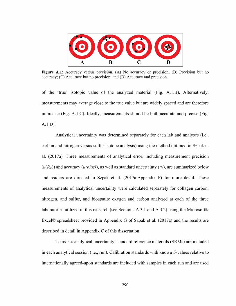
290

Figure A.1: Accuracy versus precision. (A) No accuracy or precision; (B) Precision but no accuracy; (C) Accuracy but no precision; and (D) Accuracy and precision. of the ‘true’ isotopic value of the analyzed material (Fig. A.1.B). Alternatively,

measurements may average close to the true value but are widely spaced and are therefore

imprecise (Fig. A.1.C). Ideally, measurements should be both accurate and precise (Fig.

A.1.D).

Analytical uncertainty was determined separately for each lab and analyses (i.e.,

carbon and nitrogen versus sulfur isotope analysis) using the method outlined in Szpak et

al. (2017a). Three measurements of analytical error, including measurement precision

(u(Rw)) and accuracy (u(bias)), as well as standard uncertainty (uc), are summarized below

and readers are directed to Szpak et al. (2017a:Appendix F) for more detail. These

measurements of analytical uncertainty were calculated separately for collagen carbon,

nitrogen, and sulfur, and bioapatite oxygen and carbon analyzed at each of the three

laboratories utilized in this research (see Sections A.3.1 and A.3.2) using the Microsoft®

Excel® spreadsheet provided in Appendix G of Szpak et al. (2017a) and the results are

described in detail in Appendix C of this dissertation.

To assess analytical uncertainty, standard reference materials (SRMs) are included

in each analytical session (i.e., run). Calibration standards with known δ-values relative to

internationally agreed-upon standards are included with samples in each run and are used

291

to calculate a two-point calibration curve that anchors the raw isotopic values at both the

high- and low-ends of the range of δ-values (Coplen et al. 2006; Szpak et al. 2017a).

Internationally agreed-upon isotopic measurement scales include Vienna PeeDee

Belemnite (VPDB) for carbon, air N2 (AIR) for nitrogen, Vienna Cañon Diablo Troilite

(VCDT) for sulfur, and Vienna Standard Mean Ocean Water (VSMOW) or VPDB for

oxygen (Coplen 1994; Coplen et al. 2006; Coplen and Krouse 1998; Junk and Svec 1958).

Because internationally certified SRMs are calibrated to the appropriate isotopic

measurement scale and are assigned accepted values, they are preferred for calibration of

the isotopic data. In contrast, the isotopic compositions of internal (i.e., in-house) standards

represent long-term averages obtained from a specific laboratory that have been calibrated

to the internationally agreed upon SRMs. Internal SRMs are more appropriate as check

standards and should be matrix-matched, meaning that they are composed of materials that

have similar chemical compositions to those of the samples being analyzed (Szpak et al.

2017a).

Analytical precision (u(Rw)) reflects the repeatability of measurements and the

presence of random error. In isotopic analysis, precision is evaluated using the variation in

the measurements of standard reference materials (e.g., calibration or check standards) with

or without assigned δ-values as well as repeated measurements of sample aliquots

(replicates) from the same analytical session. Analytical precision was calculated from the

pooled standard deviation of all repeated measurements during the relevant analytical

sessions at each laboratory, including those of check and calibration standards (ssrm) and

sample replicates (srep) (Szpak et al. 2017a:Appendix F).

292

Analytical accuracy (u(bias)) refers to measurement bias or systematic errors in

measurement and how close a measurement is to the “true” value of the analyte. The

accuracy of isotopic measurements can only be evaluated by including check standards in

each analytical session that are not used for calibration of the results, because the δ-values

of calibration standards are calibrated to known values (Szpak et al. 2017a:611). The degree

to which the measured δ-values of the check standards deviate from their known values

indicates the degree to which the measured δ-values of the samples deviate from their “true”

value. Analytical accuracy therefore represents systematic errors in the measurements

caused, for example, by instrumental drift (Szpak et al. 2017a:611). Here, measurement

accuracy was calculated by factoring in the long-term uncertainty in the known isotopic

measurements of the check standards by calculating the root-mean-square of the difference

between their observed mean and known values (Szpak et al. 2017a).

Finally, Szpak et al. (2017a) advise researchers to report the total analytical

uncertainty, or standard uncertainty (uc). This measurement combines the calculations of

precision (u(Rw)) and accuracy (u(bias)) into a more comparable measurement of analytical

uncertainty applicable across studies (Szpak et al. 2017a:Appendix F) and this approach

was adopted in this research.

A.6 Identifying Diagenesis

Diagenesis is the postmortem alteration of the chemical composition of bones and

teeth as a result of the burial environment. Diagenesis is problematic because it causes the

isotopic composition of sampled tissues to differ from those obtained during life (i.e.,

biogenic values). Specifically, unidentified diagenetic effects on isotopic values can have

293

a profound influence on the interpretation of isotopic results and the resulting

archaeological understandings of mobility and diet in the past (Krueger 1991; Lee-Thorp

and van der Merwe 1991; Wright and Schwarcz 1996). Thus, it is necessary to minimize

the influence of diagenesis using appropriate sample preparation and analytical techniques

and to identify and remove diagenetically altered values prior to interpretation. The

precautions taken to identify and limit the effects of diagenesis used in this study are

described below for bone collagen, bone bioapatite, and tooth enamel bioapatite.

A.6.1 Bone Collagen

The presence of diagenesis in bone collagen samples was assessed using established

criteria, including percent by weight of carbon (wt. %C), nitrogen (wt. %N), and sulfur (wt.

%S), as well as the atomic carbon-to-nitrogen (C:N), carbon-to-sulfur (C:S), and nitrogen-

to-sulfur (N:S) ratios in each sample (Ambrose 1990; DeNiro 1985; Nehlich and Richards

2009; van Klinken 1999). The wt. %C, wt. %N, and wt. %S values of each sample were

analyzed during the isotopic analyses and provided by the laboratories. Atomic ratios were

calculated using the following formulae:

C:N = wt. %C

12.01

wt. %N

14.01 (A.1)

C:S = wt. %C

12.01

wt. %S

32.07 (A.2)

N:S =wt. %N

14.01

wt. %S

32.07 (A.3)

Carbon and nitrogen values were considered to be uninfluenced by diagenesis if wt. %C

was above 13 %, wt. %N was above 4.8 %, and C:N fell between 2.9 and 3.6 (Ambrose

1990; DeNiro 1985; van Klinken 1999). The sulfur values of mammalian bone collagen

294

were considered well preserved if wt. %S was between 0.15 and 0.35 %, C:S was between

300 and 900, and N:S was between 100 and 300 (Nehlich and Richards 2009). Because

there is a higher amount of sulfur in fish bone collagen, these samples were considered well

preserved if wt. %S was between 0.40 and 0.85 %, C:S was between 125 and 225, and N:S

was between 40 and 80 (Nehlich and Richards 2009). The δ13C, δ15N, and δ34S values of

samples were removed from subsequent analyses if two or more indicators fell beyond

acceptable values (Rand et al. 2015a). Finally, although previous studies have suggested

that collagen yields below 1 % are too poorly preserved for analysis (van Klinken 1999;

White et al. 1993), ultrafiltration is known to reduce collagen yields while producing viable

collagen (Jørkov et al. 2007) and so this indicator was not used to detect diagenesis in this

study.

A.6.2 Bone and Tooth Enamel Bioapatite

The mineral portions of bone and teeth are referred to as bioapatite. Bone bioapatite

is a calcium phosphate similar in composition and structure to poorly crystalline

hydroxyapatite (Glimcher et al. 1981). Because bone bioapatite is easily altered (Glimcher

et al. 1981), it is more susceptible to diagenesis than is collagen (Krueger 1991).

Researchers have proposed a number of techniques for establishing the integrity of bone

apatite isotope values, including conducting Fourier Transform Infrared (FTIR)

spectroscopy to measure the integrity of its crystalline structure (Nielsen-Marsh and

Hedges 2000; Sillen and Sealy 1995; Wright and Schwarcz 1996), and similar techniques

using attenuated total reflection (ATR) and diffuse reflectance infrared Fourier transform

(DRIFT) spectroscopy have also been proposed (Beasley et al. 2014).

295

In this study, FTIR spectroscopy was unavailable and so it was not possible to assess

the influence of diagenesis on the Nakum human bone and enamel samples. However, the

preservation of bone apatite has been linked to collagen preservation (Kendall et al. 2018),

and so only the oxygen and carbon values in bioapatite from bone samples that also

produced viable collagen assessed using the techniques described in Section A.6.2 were

considered for interpretation.

Finally, unlike bone bioapatite, tooth enamel is nonporous and has larger apatite

crystals that makes it resistant to diagenesis (Quade et al. 1992; Trautz 1967). While some

diagenesis may occur in tooth enamel (Schoeninger et al. 2003; Sponheimer and Lee-Thorp

1999), it is the preferred tissue for oxygen and strontium isotope analysis in archaeological

investigations of human movement because it is more resistant than is bone apatite (Hoppe

et al. 2003).

A.7 Establishing Environmental Isotopic Baseline Values for Identifying Nonlocal

Individuals

The isotopic compositions of an individual’s bones and teeth are derived from his

or her diet and drinking water, which in turn reflect those of the local environment (Bentley

2006; Longinelli 1984; Richards et al. 2003; Nehlich 2015). Thus, the identification of

nonlocal individuals from the isotopic values of archaeological human tissues is contingent

upon known biologically available (bioavailable) isotope values in local environments as

well as those from more distant areas. It is also necessary to remove nonlocal values from

the data set to establish locally bioavailable isotopic baselines.

In the Maya region, there is sufficient variation in bioavailable 87Sr/86Sr and δ18O

values among different regions to permit identification of nonlocal individuals and local

296

isotopic baselines that characterize regional variation have been developed for much of this

area (Hodell et al. 2004; Freiwald 2011a, 2011b; Lachniet and Patterson 2009; Miller Wolf

and Freiwald 2018; Price et al. 2007, 2008, 2010, 2015; Trask et al. 2012). The predicted

variability of δ34S values throughout the Maya region has also recently been hypothesized

(Rand and Grimes 2017). There are, however, several techniques for identifying nonlocal

individuals, the efficiency of which are dependent upon the isotopic system of study.

One method for identifying whether an individual migrated is to identify a

discrepancy between the isotopic values of his or her bones and teeth. This is because tooth

enamel forms during childhood and therefore reflect the isotopic values of diet during the

period of amelogenesis (AlQahtani et al. 2010; Moorrees et al. 1963a, 1963b; Nelson and

Ash 2010), whereas bone remodels throughout life and therefore reflects the average

isotopic values of foods and drinking water consumed from adolescence to the end of life,

depending on the sampled bone and individual physiology in bone turnover rates (Hedges

et al. 2007; Matsubayashi and Tayasu 2019; Parfitt 2001). However, isotopic fractionation

may occur as elements are incorporated into different body tissues (Warinner and Tuross

2009), and this technique is only applicable to δ18O values because sulfur isotopic studies

in archaeology typically analyzed bone collagen (but see Goedert et al. 2020) and strontium

present in bone bioapatite is highly susceptible to diagenesis (Budd et al. 2000; Hoppe et

al. 2003). These limitations can be overcome through the comparison of the isotopic values

of teeth that form at different ages, micro-samples of the same tooth, and bones that

turnover at different rates from the same individual to identify whether he or she relocated

multiple times during life (Agarwal 2016; Buikstra et al. 2004; Hrnčíř and Laffoon 2019;

297

Montgomery 2010; Montgomery et al. 2000; Schroeder et al. 2009; Schweissing and Grupe

2003; White et al. 2000; Wright 2013b).

Nonlocal individuals may also be identified as having bone and/or tooth enamel

isotope values that differ from the isotopic baselines established for the burial location (see

Grimstead et al. 2017). While isotopic baselines may be developed by analyzing modern

geology, soil, plant, and water samples, bioavailable values are more accurately assessed

by analyzing modern and archaeological animal tissues (Grimstead et al. 2017; Makarewicz

and Sealy 2015; Price et al. 2002; Sillen et al. 1998). A baseline is conventionally developed

by calculating the mean and two standard deviations of organic and inorganic

environmental samples, and nonlocal individuals are identified as those who fall beyond

this range (Price et al. 2002). While the same principle applies to stable sulfur isotope

analysis, pollution since the industrial revolution has influenced modern δ34S values, and

so it is necessary to sample archaeological faunal bone to establish locally bioavailable

sulfur isotope values (Richards et al. 2001; Trust and Fry 1992). Environmental baselines

are useful for establishing bioavailable isotope values throughout a region; however, they

may not always accurately reflect the human values due, for example, to the consumption

of imported foods, marine foods, or foods grown in coastal areas influenced by marine

isotope values deposited by sea spray (e.g., Fenner and Wright 2014; Grimstead et al. 2017;

Freiwald et al. 2019; Guiry and Szpak 2020; Trask et al. 2012; Wright 2005a) and by

imbibing different sources of water (Scherer et al. 2015).

298

The development of baselines for inferring human migration are also based on the

understanding of how isotopes fractionate12 during incorporation into consumer tissues,

also known as diet-to-consumer offsets. Although strontium isotopes are fractionated

during this process, it occurs below the level of detection using current instrumentation, so

the isotopic values of human tissues directly reflect those of the environment in which the

subsistence resources were obtained. Conversely, the diet-to-consumer offsets of stable

oxygen isotopes are substantial and vary depending on the sampled tissue (France and

Owsley 2015; Warinner and Tuross 2009). The fractionation of sulfur isotopes between

diet and bone collagen (Δ34Stissue-diet) requires further exploration. The original offset of +0.5

± 2.4‰ compiled by Nehlich (2015:6) was based primarily on the offset between the diet

and soft tissues of numerous species, mostly insects and fish, which may be inappropriate

proxies for human Δ34Stissue-diet values. A more recent feeding experiment analyzing

omnivorous pigs found a more substantial offset, wherein their femoral bone δ34S values

were 1.5 ‰ lower than the values of their diets (Webb et al. 2017). However, this study

analyzed the δ34S values of the whole diet, rather than just dietary methionine, and so the

elevated δ34S values of the feed could be caused by sulfur in carbohydrates or lipids.

Finally, a study that specifically compared the bone collagen δ34S values of ancient foxes

and their prey from a sealed deposit found an average Δ34Stissue-diet value of –0.51 ± 0.03 ‰,

which was considered negligible because it fell near or below analytical error (Krajcarz et

al. 2019). Thus, sulfur isotope baselines developed from the δ34S values of archaeological

12 In kinetic reactions, the light isotopes react faster than the heavy isotopes, whereas in exchange reactions, the heavy isotopes concentrate where bonds are strongest (Fry 2006:12). This is called fractionation and it causes the isotopic values of the reactant and product entities to differ.

299

faunal remains are useful for characterizing isotopic variation throughout a region but may

not accurately identify nonlocal human values until the sulfur isotope offset between diet

and consumer tissues is better characterized.

Another approach to identifying nonlocal isotope values is comparison with

previously published values from the same region, although this is only applicable in

regions for which large databases are available (Lightfoot and O’Connell 2016:5). In the

Maya region, numerous studies have resulted in compilations of strontium and oxygen

values from different areas (Price et al. 2007, 2008, 2010). Unfortunately, the application

of sulfur isotope analysis in the Maya region is in its infancy and comparative data sets are

limited to a handful of studies (Awe et al. 2017; Green 2016; Rand et al. 2020a).

Finally, when baseline and comparative human data is unavailable, nonlocal

individuals may be identified as those whose isotopic values are statistical outliers from the

remaining values (Burton and Hahn 2016:119; Freiwald 2011a; Laffoon and Hoogland

2012; Lightfoot and O’Connell 2016; Montgomery et al. 2007; Knudson 2011; Wright

2005a; Chapters 3 and 4). As with local baselines developed from organic and inorganic

environmental samples, nonlocal individuals are commonly identified as those whose

isotopic values fall beyond two standard deviations of the mean of the human isotopic data

set. However, when identifying nonlocal individuals using statistical techniques, it is

important to note that the method, sample size, and distribution of the data will influence

the number of outliers in a data set (Lightfoot and O’Connell 2016:6). For example, the

presence of extreme outliers will skew the mean value, and so outliers should be removed

prior to establishing a local baseline. Preferably, statistical techniques that are robust

against outliers (e.g., interquartile range; see below) should be used to detect nonlocal

300

individuals in small and highly skewed data sets (Lightfoot and O’Connell 2016; Pearson

and Grove 2013). This approach was used to identify and remove nonlocal individuals from

the data sets prior to developing local δ34S baseline values in this dissertation research.

A.8 Statistical Analyses

The specific statistical approaches and tests used in this research are summarized

below, and readers are directed elsewhere for more detailed descriptions of these tests

(Madrigal 1995; Otárola-Castillo and Torquato 2018; Shennan 1988; VanPool and Leonard

2011). All statistical analyses were performed in SPSS version 25 for Windows (IBM®).

Prior to analyzing comparative statistics, the distribution of the data was first tested

for normality using the Shapiro-Wilk test (W; Shapiro and Wilk 1965). Most archaeological

isotope studies are conducted on small data sets, the distribution of which are more

influenced by the presence of outlying values, causing them to deviate from a normal,

Gaussian distribution. Thus, nonparametric statistical tests were used for all data sets that

did not follow a Gaussian distribution and for data sets that included less than eight values

(Pearson and Grove 2013; see also Zimmerman and Zumbo 1993).

To identify outlying isotopic values, the interquartile range (IQR) rule was used, as

it is more robust against the presence of outliers in small data sets. First, a boxplot was

created in SPSS wherein the median is displayed as a solid line within the box, the

interquartile range (IQR) between the first quartile (Q1) and third quartile (Q3) is

represented by a box containing 50% of the data points, and the whiskers represent the IQR

multiplied by 1.5 (IQR*1.5) subtracted from Q1 and added to Q3. Using the IQR rule,

301

outliers were identified as those that fell beyond the whiskers (i.e., IQR*1.5 – Q1 or

IQR*1.5 + Q3) and extreme outliers fell beyond IQR*3 – Q1 or IQR*3 + Q3 (Tukey 1977).

To assess the correlation between groups (i.e., carbon and sulfur isotope values),

the Pearson correlation coefficient (r) was used for normally distributed data and the

Spearman’s rank-order correlation (ρ) was used for data sets that did not follow a Gaussian

distribution. A paired samples t-test (t) was performed to assess intra- and interlaboratory

differences in normally distributed isotopic values from the same sample in Appendix B.

If the groups did not follow a Gaussian distribution, or if there were fewer than eight

samples in a group (Pearson and Grove 2013; see also Zimmerman and Zumbo 1993), the

Wilcoxon signed-rank test (W) was used.

To evaluate differences in isotopic values between two groups (i.e., sites, protein

source, etc.) the Independent Samples t-test (t) was used for normally distributed data and

the Mann-Whitney U (U) test was used for non-parametric data. To evaluated differences

between three or more groups, analysis of variance (ANOVA; F) was used for normally

distributed data, and the Tukey and Games-Howell post hoc tests were used to identify

differences between group pairs when variances were determined equal and unequal,

respectively, using Levene’s Tests for Equal Variances. To evaluated differences between

three or more groups that were not normally distributed, the Kruskal-Wallis H (H) was

used, and the significance of the resulting pairwise comparisons were automatically

adjusted by the Bonferroni correction for multiple tests in SPSS.

Scholars have recently called into question the validity of null hypothesis

significance testing (NHST) in archaeology and other disciplines and have explored

alternative statistical tests such as bootstrapping and Bayesian statistics (Kline 2004;

302

Otárola-Castillo and Torquato 2018). However, these NHST approaches are the most

commonly applied means of identifying differences in archaeological isotopic data

analyses and were used in this research for comparability purposes. The confidence levels

for these tests were set to 95 %, with resulting significance levels of α = 0.05. Therefore,

the null hypothesis (i.e., a data set followed a normal distribution, samples were derived

from the same population, etc.) was rejected if the p-value was less than 0.05 and the

statistical test was considered significant.

303

APPENDIX B

INTRA- AND INTER-LABORATORY COMPARABILITY OF

ISOTOPIC RESULTS

304

B.1 Introduction

The assessment of isotopic data for the reconstruction of archaeological human

movement and diet is based on the premise that results from samples prepared using

different methods and obtained from different laboratories are directly comparable. The

comparability of stable carbon, nitrogen, and oxygen isotopic results produced using

different collagen extraction techniques (Fuller et al. 2014; Guiry et al. 2016; Jørkov et al.

2007; Liden et al. 1995; Rand et al. 2015a; Sealy et al. 2014; Szpak et al. 2017b; Yoder and

Bartelink 2010) and among laboratories (Pestle et al. 2014) have been previously explored.

However, the comparability of stable sulfur isotope values obtained within and among labs

have yet to be assessed. Because collagen samples were prepared both with and without a

sodium hydroxide (NaOH) treatment and analyzed by three different laboratories, it was

necessary to assess the degree of intra-sample, as well as intra-laboratory and inter-

laboratory variation in the isotopic results prior to their interpretation.

B.2 Materials and Methods

As part of a pilot study (Rand and Grimes 2017), the collagen of 20 human bone

specimens from Caledonia was extracted for stable sulfur isotope analysis in 2015 using

the methods described in Appendix A, excluding a NaOH treatment. The samples were

analyzed at the Stable Isotope Laboratory (SIL) of Memorial University of Newfoundland

(MUN; see Appendix A) and the analytical uncertainty is discussed in Appendix C.

Stable carbon and nitrogen isotope data from the same sample are necessary to

evaluate whether the δ34S results have been diagenetically altered (Nehlich and Richards

2009), and so previously published stable carbon and nitrogen isotope results (Rand 2012;

305

Rand et al. 2015b) were compared to the stable sulfur isotope results (Rand and Grimes

2017). However, stable carbon and nitrogen isotopic values may vary depending on how

the collagen is extracted from the bone sample (Fuller et al. 2014; Guiry et al. 2016; Jørkov

et al. 2007; Rand et al. 2015a; Sealy et al. 2014; Szpak et al. 2017b), and so the δ13C and

δ15N values were reanalyzed from aliquots of the collagen samples prepared for stable

sulfur isotope analysis. Six samples (2514, 2515, 2520, 2521, 2526, and 2528) had enough

remaining collagen following stable sulfur isotope analysis for the analysis of stable carbon

and nitrogen isotope ratios and concentrations. These, as well as collagen samples from

Pacbitun, Moho Cay, Laguna de On Island and Shore, Caye Coco, Chanlacan, Caye

Muerto, and Nakum were analyzed at MUN (Appendix A), and analytical uncertainty is

described elsewhere (Appendix C). One sample was run in duplicate during the same

analytical session and another nine were run in duplicate during different analytical

sessions (Table B.1).

Because little or no collagen remained from the Caledonia samples following

isotopic analysis at MUN, the collagen of 15 bone specimens (2516, 2517, 2518, 2519,

2522, 2523, 2525, 2527, 2528, 2530, 2531, 2532, 2533, 2535, and 2536) were again

prepared for both carbon and nitrogen isotopic analysis and to assess inter-laboratory

comparability of the isotopic results. The resamples have been assigned the designator “B”

(i.e., 2518B) to differentiate them from the original collagen samples from the same bone

specimen. The resamples were prepared in the same manner as the originals, but were

treated with 0.1 M NaOH prior to gelatinization, as this treatment removes humic

contaminants that influence δ13C values (Ambrose 1990; Jørkov et al. 2007; Rand et al.

306

2015a; Sealy et al. 2014; Szpak et al. 2017b). The influence of a NaOH treatment on δ34S

values is, however, unknown.

Eight of the 15 original samples (2516, 2518, 2522, 2530, 2531, 2532, 2533, and

2535) had enough remaining collagen (1 mg) for stable carbon and nitrogen isotope

analysis at the Ján Veizer Stable Isotope Laboratory at the University of Ottawa, along with

eight Caledonia resamples (2517B, 2519B, 2523B, 2525B, 2527B, 2528B, 2529B, and

2534B), and samples from Vista Alegre, Oxtankah, Ichpaatun, San Migeulito, San Lorenzo,

Xunantunich, San Bernabé, Tayasal, Caracol, Chac II, and Calakmul (Appendix A).

Analytical uncertainty is discussed elsewhere (Appendix C).

Based on previous studies, it is assumed that stable carbon and nitrogen results

obtained from different labs are directly comparable (Pestle et al. 2014). To examine

interlaboratory variability in stable sulfur isotope analysis, aliquots of six original

Caledonia bone collagen samples (2514, 2515, 2516, 2517, 2521, and 2526) and 13

resamples (2518B, 2519B, 2522B, 2523B, 2525B, 2527B, 2528B, 2530B, 2531B, 2532B,

2533B, 2535B, and 2536B) were sent to the Stable Isotope Laboratory in the Department

of Earth and Planetary Sciences at the University of Tennessee for stable sulfur isotope

analysis. Collagen samples from Pacbitun, Moho Cay, Laguna de On Island and Shore,

Caye Coco, Caye Muerto, Chanlacan, Nakum, Vista Alegre, Oxtankah, Ichpaatun, and San

Migeulito were also analyzed at Tennessee (Appendix A). Two samples were run in

duplicate during the same analytical session and another 28 were run in duplicate during

different analytical sessions (Table B.1).

Finally, the δ34S and wt. % S values of the San Lorenzo, Xunantunich, San Bernabé,

and Calakmul samples were analyzed by the Ján Veizer Stable Isotope Laboratory,

307

University of Ottawa (Appendix A). Analytical uncertainly was calculated in Appendix C,

and no samples were run in duplicate due to the large amount of sample needed for analysis.

A Shapiro-Wilk test (W) was performed to determine whether the samples were

normally distributed, after which paired samples t-tests (t) were performed to test whether

the values of the same sample obtained by the same laboratory during different analytical

sessions or from two different laboratories were significantly different. If the groups did

not follow a Gaussian distribution, or if there were less than five samples in a group, the

Wilcoxon signed-rank test (W) was used. All statistics were calculated in SPSS version 25

for Windows (IBM®) and results were considered statistically significant when p < 0.05.

B.3 Results

The stable carbon and nitrogen isotope results and concentrations of the Caledonia

collagen samples prepared with and without a NaOH step and analyzed by two different

laboratories are presented in Table B.1, and the stable sulfur isotope results and

concentrations of the same samples analyzed by three laboratories are presented in Table

B.2. The intra-sample, intra-laboratory, and inter-laboratory variation are discussed in more

detail in the following sections.

B.3.1 Intra-Sample Variation of Stable Carbon and Nitrogen Results from Samples

Treated with and without Sodium Hydroxide

Of the 15 Caledonia bone specimens that were resampled, seven (see Table B.3)

had sufficient collagen remaining to assess the intra-sample variation in δ13C, δ15N, wt.

%C, and wt. %N caused by differences in preparation methods. Only samples analyzed at

the Ján Veizer SIL at the University of Ottawa are considered in the intra-sample variation

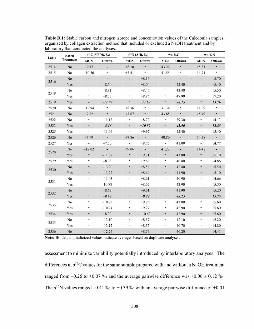
308

Table B.1: Stable carbon and nitrogen isotope and concentration values of the Caledonia samples organized by collagen extraction method that included or excluded a NaOH treatment and by laboratory that conducted the analyses.

Lab # NaOH

Treatment

δ13C (VPDB, ‰) δ15N (AIR, ‰) wt. %C wt. %N

MUN Ottawa MUN Ottawa MUN Ottawa MUN Ottawa

2514 No –9.17 - +8.10 - 43.26 - 15.31 -

2515 No –10.56 - +7.41 - 41.55 - 14.71 -

2516 No - - - +8.16 - - - - 15.70

Yes - –8.60 - +8.04 - 42.40 - 15.40

2518 No - –8.81 - +8.45 - 43.40 - 15.50

Yes - –8.55 - +8.86 - 47.90 - 17.20

2519 Yes - –11.77 - +11.62 - 38.25 - 13.76

2520 No –12.94 - +8.36 - 31.34 - 11.09 -

2521 No –7.82 - +7.67 - 43.65 - 15.49 -

2522 No - –11.13 - +8.79 - 39.30 - 14.13

2523 Yes - –8.46 - +10.52 - 43.90 - 15.85

2525 Yes - –11.09 - +9.92 - 42.40 - 15.40

2526 No –7.99 - +7.86 - 40.80 - 14.38 -

2527 Yes - –7.70 - +8.75 - 41.00 - 14.77

2528 No –12.02 - +9.06 - 41.22 - 14.48 -

Yes - –11.67 - +9.71 - 41.80 - 15.10

2529 Yes - –8.33 - +9.60 - 40.80 - 14.86

2530 No - –13.20 - +8.56 - 42.80 - 15.50

Yes - –13.22 - +8.60 - 41.90 - 15.10

2531 No - –11.03 - +8.61 - 40.90 - 14.66

Yes - -10.88 - +8.62 - 42.90 - 15.50

2532 No - –8.69 - +9.61 - 41.90 - 15.20

Yes - –8.64 - +9.22 - 43.25 - 15.75

2533 No - –10.23 - +9.26 - 43.00 - 15.60

Yes - –10.24 - +9.27 - 42.90 - 15.60

2534 Yes - –8.39 - +10.62 - 42.90 - 15.60

2535 No - –13.10 - +8.57 - 42.10 - 15.20

Yes - –13.17 - +8.52 - 40.70 - 14.80

2536 No - –12.26 - +8.56 - 40.20 - 14.41

Note: Bolded and italicized values indicate averages based on duplicate analyses.

assessment to minimize variability potentially introduced by interlaboratory analyses. The

differences in δ13C values for the same sample prepared with and without a NaOH treatment

ranged from –0.26 to +0.07 ‰ and the average pairwise difference was +0.06 ± 0.12 ‰.

The δ15N values ranged –0.41 ‰ to +0.39 ‰ with an average pairwise difference of +0.01

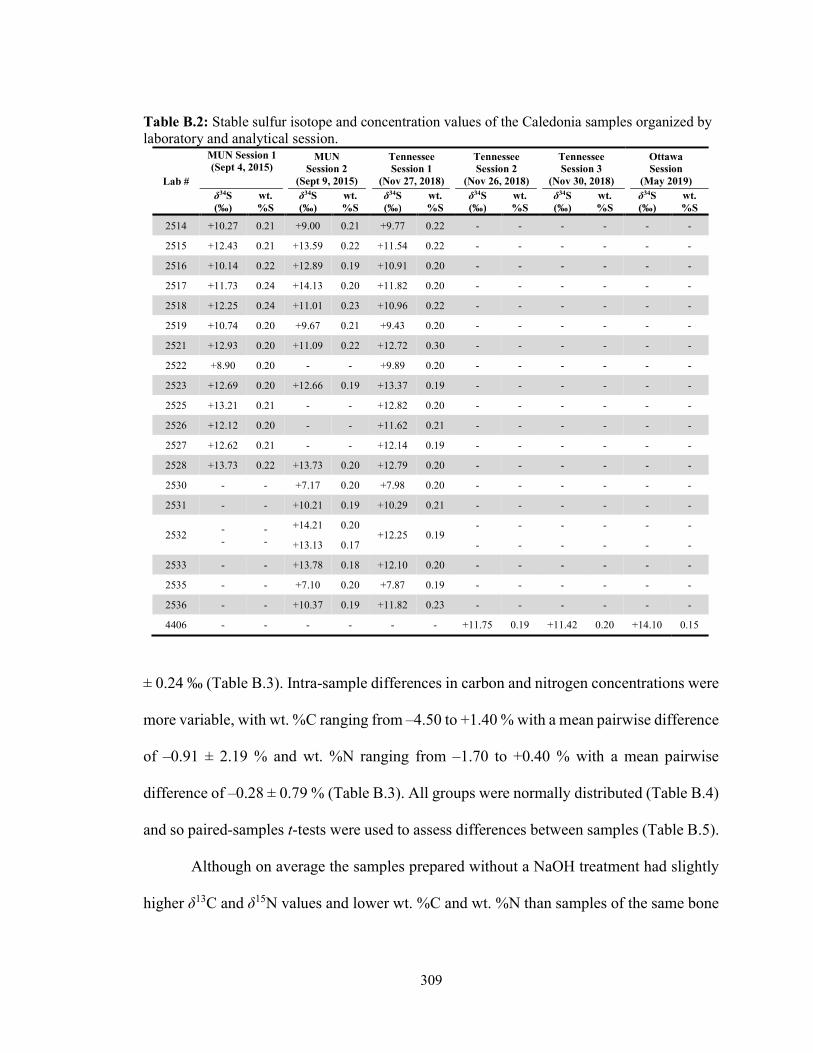
309

Table B.2: Stable sulfur isotope and concentration values of the Caledonia samples organized by laboratory and analytical session.

Lab #

MUN Session 1 (Sept 4, 2015)

MUN Session 2

(Sept 9, 2015)

Tennessee Session 1

(Nov 27, 2018)

Tennessee Session 2

(Nov 26, 2018)

Tennessee Session 3

(Nov 30, 2018)

Ottawa Session

(May 2019) δ34S (‰)

wt.%S

δ34S (‰)

wt.%S

δ34S (‰)

wt.%S

δ34S (‰)

wt.%S

δ34S (‰)

wt.%S

δ34S (‰)

wt.%S

2514 +10.27 0.21 +9.00 0.21 +9.77 0.22 - - - - - -

2515 +12.43 0.21 +13.59 0.22 +11.54 0.22 - - - - - -

2516 +10.14 0.22 +12.89 0.19 +10.91 0.20 - - - - - -

2517 +11.73 0.24 +14.13 0.20 +11.82 0.20 - - - - - -

2518 +12.25 0.24 +11.01 0.23 +10.96 0.22 - - - - - -

2519 +10.74 0.20 +9.67 0.21 +9.43 0.20 - - - - - -

2521 +12.93 0.20 +11.09 0.22 +12.72 0.30 - - - - - -

2522 +8.90 0.20 - - +9.89 0.20 - - - - - -

2523 +12.69 0.20 +12.66 0.19 +13.37 0.19 - - - - - -

2525 +13.21 0.21 - - +12.82 0.20 - - - - - -

2526 +12.12 0.20 - - +11.62 0.21 - - - - - -

2527 +12.62 0.21 - - +12.14 0.19 - - - - - -

2528 +13.73 0.22 +13.73 0.20 +12.79 0.20 - - - - - -

2530 - - +7.17 0.20 +7.98 0.20 - - - - - -

2531 - - +10.21 0.19 +10.29 0.21 - - - - - -

2532 - -

- -

+14.21 0.20 +12.25 0.19

- - - - - -

+13.13 0.17 - - - - - -

2533 - - +13.78 0.18 +12.10 0.20 - - - - - -

2535 - - +7.10 0.20 +7.87 0.19 - - - - - -

2536 - - +10.37 0.19 +11.82 0.23 - - - - - -

4406 - - - - - - +11.75 0.19 +11.42 0.20 +14.10 0.15

± 0.24 ‰ (Table B.3). Intra-sample differences in carbon and nitrogen concentrations were

more variable, with wt. %C ranging from –4.50 to +1.40 % with a mean pairwise difference

of –0.91 ± 2.19 % and wt. %N ranging from –1.70 to +0.40 % with a mean pairwise

difference of –0.28 ± 0.79 % (Table B.3). All groups were normally distributed (Table B.4)

and so paired-samples t-tests were used to assess differences between samples (Table B.5).

Although on average the samples prepared without a NaOH treatment had slightly

higher δ13C and δ15N values and lower wt. %C and wt. %N than samples of the same bone

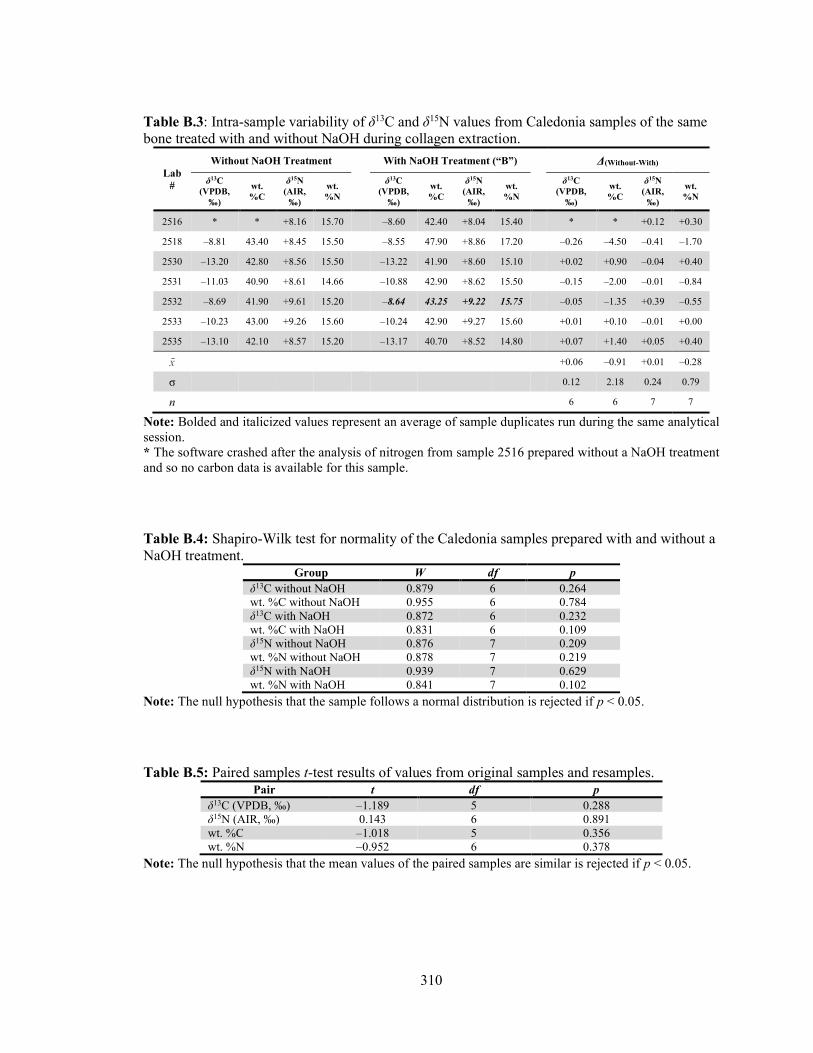
310

Table B.3: Intra-sample variability of δ13C and δ15N values from Caledonia samples of the same bone treated with and without NaOH during collagen extraction.

Lab #

Without NaOH Treatment

With NaOH Treatment (“B”)

Δ(Without-With)

δ13C (VPDB,

‰)

wt. %C

δ15N (AIR,

‰)

wt. %N

δ13C (VPDB,

‰)

wt. %C

δ15N (AIR,

‰)

wt. %N

δ13C (VPDB,

‰)

wt. %C

δ15N (AIR,

‰)

wt. %N

2516 * * +8.16 15.70 –8.60 42.40 +8.04 15.40 * * +0.12 +0.30

2518 –8.81 43.40 +8.45 15.50 –8.55 47.90 +8.86 17.20 –0.26 –4.50 –0.41 –1.70

2530 –13.20 42.80 +8.56 15.50 –13.22 41.90 +8.60 15.10 +0.02 +0.90 –0.04 +0.40

2531 –11.03 40.90 +8.61 14.66 –10.88 42.90 +8.62 15.50 –0.15 –2.00 –0.01 –0.84

2532 –8.69 41.90 +9.61 15.20 –8.64 43.25 +9.22 15.75 –0.05 –1.35 +0.39 –0.55

2533 –10.23 43.00 +9.26 15.60 –10.24 42.90 +9.27 15.60 +0.01 +0.10 –0.01 +0.00

2535 –13.10 42.10 +8.57 15.20 –13.17 40.70 +8.52 14.80 +0.07 +1.40 +0.05 +0.40

x̄ +0.06 –0.91 +0.01 –0.28

σ 0.12 2.18 0.24 0.79

n 6 6 7 7

Note: Bolded and italicized values represent an average of sample duplicates run during the same analytical session. * The software crashed after the analysis of nitrogen from sample 2516 prepared without a NaOH treatment and so no carbon data is available for this sample.

Table B.4: Shapiro-Wilk test for normality of the Caledonia samples prepared with and without a NaOH treatment.

Group W df p δ13C without NaOH 0.879 6 0.264 wt. %C without NaOH 0.955 6 0.784 δ13C with NaOH 0.872 6 0.232 wt. %C with NaOH 0.831 6 0.109 δ15N without NaOH 0.876 7 0.209 wt. %N without NaOH 0.878 7 0.219 δ15N with NaOH 0.939 7 0.629 wt. %N with NaOH 0.841 7 0.102

Note: The null hypothesis that the sample follows a normal distribution is rejected if p < 0.05. Table B.5: Paired samples t-test results of values from original samples and resamples.

Pair t df p δ13C (VPDB, ‰) –1.189 5 0.288 δ15N (AIR, ‰) 0.143 6 0.891 wt. %C –1.018 5 0.356 wt. %N –0.952 6 0.378

Note: The null hypothesis that the mean values of the paired samples are similar is rejected if p < 0.05.

311

prepared with the treatment (Table B.3), these differences were not statistically significant

(Table B.5). Therefore, it was determined that the δ13C and δ15N values from samples of

collagen from the same bone prepared with and without a NaOH treatment are statistically

comparable in this study.

Unfortunately, insufficient collagen remained from the original samples to test the

relationship between δ34S and %S of samples treated with and without a NaOH step during

collagen extraction. Based on the carbon and nitrogen results, the sulfur values are assumed

to be comparable between treatment methods pending further experimental investigation.

B.3.2 Intra-Laboratory Variation of Stable Sulfur Isotope Values

Intra-laboratory variation in isotopic and concentration values is monitored using

replicates of check standards and samples during each analytical session. Szpak et al.

(2017a) provide a detailed methodology for calculating analytical precision based on

replicate analyses. However, most replicate analyses of stable sulfur isotopes and

concentrations included in this study were run during separate analytical sessions at both

MUN and Tennessee. Intra-laboratory variation was thus assessed by analyzing aliquots of

samples prepared using the same technique at the same laboratory but during separate

analytical sessions. As a result, the Caledonia samples prepared without a NaOH step were

used to assess the intra-laboratory variation of sulfur isotopes and concentrations at MUN,

but samples from multiple Maya sites prepared at MUN using a NaOH treatment were used

to assess the intra-laboratory variation at Tennessee. The inclusion or exclusion of a NaOH

treatment should not impact the assessment of intra-laboratory variation.

312

Although, sample replicates analyzed during the same session are included in Table

B.6 along with the duplicates run during separate analytical sessions, the former were

excluded from the intra-laboratory assessment presented here, as they speak to the precision

specific to the samples discussed by Szpak et al. (2017a) and presented in Appendix C. It

is assumed that the duplicate samples run for stable carbon and nitrogen isotope analysis at

Ottawa were analyzed during the same analytical session and so the discussion of intra-

laboratory variation presented here is restricted to stable sulfur isotope values and

concentrations.

Duplicate samples run at each lab were grouped by analytical session (i.e., samples

whose duplicates were run on Nov. 28 and Nov. 30 versus samples whose duplicates were

run on Nov. 26 and Nov. 30) for statistical comparison. The δ34S values of five pairs of

groups and the %S of three were normally distributed (Table B.7) and assessed using the

paired samples t-test (Table B.8). Two of the five comparisons of the δ34S values and one

of the three comparisons of wt. %S values between normally distributed groups were

statistically significant (Table B.9); however, the sample sizes were small (n < 5) and so

they were reassessed using the nonparametric Wilcoxon signed rank test (Pearson and

Grove 2013).

The differences in δ34S values from the nine samples run during different analytical

session at MUN ranged from –2.75 to +1.84 ‰ with a mean pairwise difference of –0.10

± 1.67 ‰, while the wt. %S were more homogenous, ranging from –0.02 to +0.04 % with

a mean pairwise difference of +0.01 ± 0.02 %. The differences in δ34S values from the 14

samples analyzed with and without dilution at Tennessee ranged from –1.98 to +3.01 ‰

with a mean pairwise difference of +0.32 ± 1.16 ‰ for the 11 samples run on Nov. 8 and

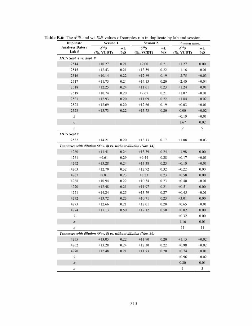
313

Table B.6: The δ34S and wt. %S values of samples run in duplicate by lab and session. Duplicate

Analyses Dates / Lab #

Session 1 Session 2 Δsession1-session2

δ34S (‰, VCDT)

wt. %S

δ34S (‰, VCDT)

wt. %S

δ34S (‰, VCDT)

wt. %S

MUN Sept. 4 vs. Sept. 9

2514 +10.27 0.21 +9.00 0.21 +1.27 0.00

2515 +12.43 0.21 +13.59 0.22 –1.16 –0.01

2516 +10.14 0.22 +12.89 0.19 –2.75 +0.03

2517 +11.73 0.24 +14.13 0.20 –2.40 +0.04

2518 +12.25 0.24 +11.01 0.23 +1.24 +0.01

2519 +10.74 0.20 +9.67 0.21 +1.07 –0.01

2521 +12.93 0.20 +11.09 0.22 +1.84 –0.02

2523 +12.69 0.20 +12.66 0.19 +0.03 +0.01

2528 +13.73 0.22 +13.73 0.20 0.00 +0.02

x̄ –0.10 +0.01

σ 1.67 0.02

n 9 9

MUN Sept 9

2532 +14.21 0.20 +13.13 0.17 +1.08 +0.03

Tennessee with dilution (Nov. 8) vs. without dilution (Nov. 14)

4260 +11.41 0.24 +13.39 0.24 –1.98 0.00

4261 +9.61 0.29 +9.44 0.28 +0.17 +0.01

4262 +13.28 0.24 +13.38 0.23 –0.10 +0.01

4263 +12.70 0.32 +12.92 0.32 –0.22 0.00

4267 +8.81 0.23 +8.23 0.23 +0.58 0.00

4268 +10.94 0.22 +10.54 0.23 +0.40 –0.01

4270 +12.48 0.21 +11.97 0.21 +0.51 0.00

4271 +14.24 0.25 +13.79 0.27 +0.45 –0.01

4272 +13.72 0.23 +10.71 0.23 +3.01 0.00

4273 +12.66 0.21 +12.01 0.20 +0.65 +0.01

4274 +17.13 0.50 +17.12 0.50 +0.02 0.00

x̄ +0.32 0.00

σ 1.16 0.01

n 11 11

Tennessee with dilution (Nov. 8) vs. without dilution (Nov. 30)

4255 +13.05 0.22 +11.90 0.20 +1.15 +0.02

4262 +13.28 0.24 +12.30 0.22 +0.98 +0.02

4270 +12.48 0.21 +11.73 0.20 +0.74 +0.01

x̄ +0.96 +0.02

σ 0.20 0.01

n 3 3

314

Table B.6 Continued. Duplicate

Analyses Dates / Lab #

Session 1 Session 2 Δsession1-session2

δ34S (‰, VCDT)

%S δ34S

(‰, VCDT) %S

δ34S (‰, VCDT)

%S

Tennessee Nov. 14 vs. Nov. 30

4320 +13.40 0.21 +12.03 0.21 +1.37 +0.01

4328 +14.40 0.21 +13.47 0.20 +0.93 +0.01

2462 +13.38 0.23 +12.30 0.22 +1.08 +0.01

4270 +11.97 0.21 +11.73 0.20 +0.23 +0.01

x̄ +0.90 +0.01

σ 0.48 0.00

n 4 4

Tennessee Nov. 25 vs. Nov. 30

4294 +14.18 0.20 +13.27 0.18 +0.91 +0.02

4303 +14.12 0.21 +13.53 0.18 +0.60 +0.03

4305 +9.38 0.22 +6.77 0.20 +2.61 +0.01

x̄ +1.37 +0.02

σ 1.08 0.01

n 3 3

Tennessee Nov. 26 vs. Nov. 30

4332 +14.02 0.18 +13.06 0.20 +0.96 –0.01

4406 +11.75 0.19 +11.42 0.20 +0.33 –0.01

4522 -0.18 0.49 -2.34 0.50 +2.16 –0.01

4533 +13.14 0.23 +12.14 0.24 +1.00 –0.01

x̄ +1.11 –0.01

σ 0.76 0.00

n 4.00 4.00

Tennessee Nov. 27 vs. Nov. 30

4553 –1.14 0.34 –4.47 0.40 +3.33 –0.06

4555 +13.24 0.26 +11.27 0.26 +1.97 0.00

x̄ +2.65 –0.03

σ 0.96 0.04

n 2.00 2.00

Tennessee Nov. 28 vs. Nov. 30

2558 +11.82 0.20 +11.08 0.19 +0.74 +0.01

2561 +13.42 0.19 +13.17 0.18 +0.25 +0.01

3451 +16.71 0.21 +14.20 0.20 +2.51 +0.02

3458 +13.30 0.18 +13.22 0.16 +0.08 +0.02

4155 +14.66 0.21 +13.67 0.19 +0.99 +0.02

x̄ +0.91 +0.01

σ 0.96 0.00

n 5.00 6.00

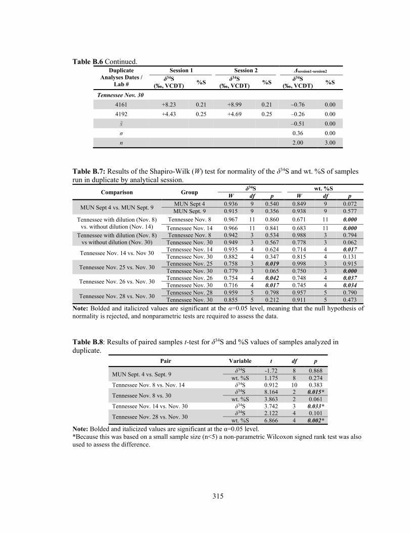
315

Table B.6 Continued. Duplicate

Analyses Dates / Lab #

Session 1 Session 2 Δsession1-session2

δ34S (‰, VCDT)

%S δ34S

(‰, VCDT) %S

δ34S (‰, VCDT)

%S

Tennessee Nov. 30

4161 +8.23 0.21 +8.99 0.21 –0.76 0.00

4192 +4.43 0.25 +4.69 0.25 –0.26 0.00

x̄ –0.51 0.00

σ 0.36 0.00

n 2.00 3.00

Table B.7: Results of the Shapiro-Wilk (W) test for normality of the δ34S and wt. %S of samples run in duplicate by analytical session.

Comparison Group δ34S wt. %S

W df p W df p

MUN Sept 4 vs. MUN Sept. 9 MUN Sept 4 0.936 9 0.540 0.849 9 0.072 MUN Sept. 9 0.915 9 0.356 0.938 9 0.577

Tennessee with dilution (Nov. 8) vs. without dilution (Nov. 14)

Tennessee Nov. 8 0.967 11 0.860 0.671 11 0.000

Tennessee Nov. 14 0.966 11 0.841 0.683 11 0.000 Tennessee with dilution (Nov. 8)

vs without dilution (Nov. 30) Tennessee Nov. 8 0.942 3 0.534 0.988 3 0.794

Tennessee Nov. 30 0.949 3 0.567 0.778 3 0.062

Tennessee Nov. 14 vs. Nov 30 Tennessee Nov. 14 0.935 4 0.624 0.714 4 0.017 Tennessee Nov. 30 0.882 4 0.347 0.815 4 0.131

Tennessee Nov. 25 vs. Nov. 30 Tennessee Nov. 25 0.758 3 0.019 0.998 3 0.915 Tennessee Nov. 30 0.779 3 0.065 0.750 3 0.000

Tennessee Nov. 26 vs. Nov. 30 Tennessee Nov. 26 0.754 4 0.042 0.748 4 0.037 Tennessee Nov. 30 0.716 4 0.017 0.745 4 0.034

Tennessee Nov. 28 vs. Nov. 30 Tennessee Nov. 28 0.959 5 0.798 0.957 5 0.790 Tennessee Nov. 30 0.855 5 0.212 0.911 5 0.473

Note: Bolded and italicized values are significant at the α=0.05 level, meaning that the null hypothesis of normality is rejected, and nonparametric tests are required to assess the data. Table B.8: Results of paired samples t-test for δ34S and %S values of samples analyzed in duplicate.

Pair Variable t df p

MUN Sept. 4 vs. Sept. 9 δ34S -1.72 8 0.868

wt. %S 1.175 8 0.274 Tennessee Nov. 8 vs. Nov. 14 δ34S 0.912 10 0.383

Tennessee Nov. 8 vs. 30 δ34S 8.164 2 0.015*

wt. %S 3.863 2 0.061 Tennessee Nov. 14 vs. Nov. 30 δ34S 3.742 3 0.033*

Tennessee Nov. 28 vs. Nov. 30 δ34S 2.122 4 0.101

wt. %S 6.866 4 0.002*

Note: Bolded and italicized values are significant at the α=0.05 level. *Because this was based on a small sample size (n<5) a non-parametric Wilcoxon signed rank test was also used to assess the difference.

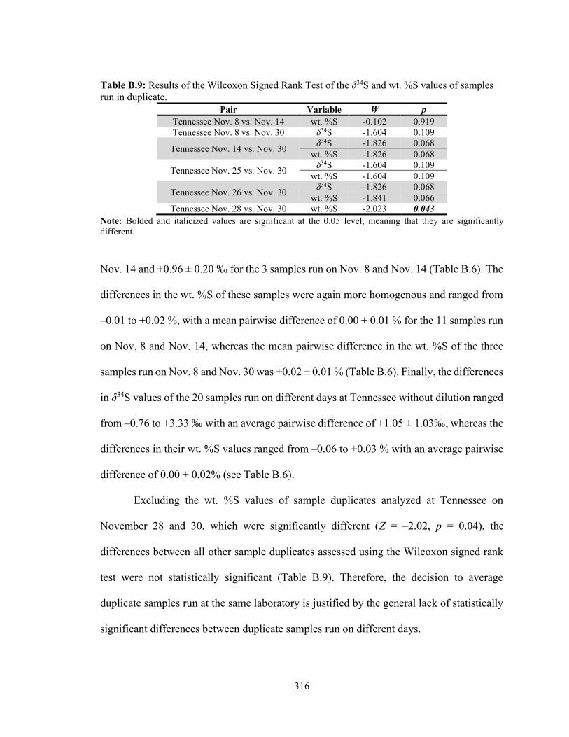
316

Table B.9: Results of the Wilcoxon Signed Rank Test of the δ34S and wt. %S values of samples run in duplicate.

Pair Variable W p Tennessee Nov. 8 vs. Nov. 14 wt. %S -0.102 0.919 Tennessee Nov. 8 vs. Nov. 30 δ34S -1.604 0.109

Tennessee Nov. 14 vs. Nov. 30 δ34S -1.826 0.068

wt. %S -1.826 0.068

Tennessee Nov. 25 vs. Nov. 30 δ34S -1.604 0.109

wt. %S -1.604 0.109

Tennessee Nov. 26 vs. Nov. 30 δ34S -1.826 0.068

wt. %S -1.841 0.066 Tennessee Nov. 28 vs. Nov. 30 wt. %S -2.023 0.043

Note: Bolded and italicized values are significant at the 0.05 level, meaning that they are significantly different.

Nov. 14 and +0.96 ± 0.20 ‰ for the 3 samples run on Nov. 8 and Nov. 14 (Table B.6). The

differences in the wt. %S of these samples were again more homogenous and ranged from

–0.01 to +0.02 %, with a mean pairwise difference of 0.00 ± 0.01 % for the 11 samples run

on Nov. 8 and Nov. 14, whereas the mean pairwise difference in the wt. %S of the three

samples run on Nov. 8 and Nov. 30 was +0.02 ± 0.01 % (Table B.6). Finally, the differences

in δ34S values of the 20 samples run on different days at Tennessee without dilution ranged

from –0.76 to +3.33 ‰ with an average pairwise difference of +1.05 ± 1.03‰, whereas the

differences in their wt. %S values ranged from –0.06 to +0.03 % with an average pairwise

difference of 0.00 ± 0.02% (see Table B.6).

Excluding the wt. %S values of sample duplicates analyzed at Tennessee on

November 28 and 30, which were significantly different (Z = –2.02, p = 0.04), the

differences between all other sample duplicates assessed using the Wilcoxon signed rank

test were not statistically significant (Table B.9). Therefore, the decision to average

duplicate samples run at the same laboratory is justified by the general lack of statistically

significant differences between duplicate samples run on different days.

317

B.3.3 Inter-Laboratory Variation of Stable Sulfur Isotope Values Finally, it was necessary to assess variation in the isotopic results among

laboratories to ensure that δ34S and wt. %S values obtained from different labs are

comparable. Based on the lack of statistically significant differences between the δ34S and

%S values from duplicate samples analyzed during separate sessions, the values from the

sample replicates analyzed during separate sessions at MUN were averaged to obtain a

single value. Similarly, the lack of statistically significant differences between the δ34S and

wt. %S values from the original samples prepared without a NaOH step and the resamples

prepared with the NaOH step justify their comparison in the following assessment, because

although only the originals were analyzed at MUN, both were analyzed at Tennessee. The

compared values can be found in Table B.10 and are visualized in Figure B.1. Only a single

sample was analyzed at both Tennessee and Ottawa, and so it was excluded from further

statistical analyses.

The difference in the δ34S values between the 19 samples run at MUN and

Tennessee ranged from –1.45 to +1.68 ‰ with a mean pairwise difference of +0.23 ± 0.93

‰ and the differences in wt. %S for the same samples ranged from –0.09 to +0.02 % with

a mean pairwise difference of –0.01 ± 0.02 % (Table B.10). The pairwise difference in the

δ34S value of the only sample run at Tennessee and Ottawa was –2.52 ‰ and the difference

in the wt. %S was +0.04 % (Table B.10).

Shapiro-Wilk tests for normality found that although the wt. %S values from MUN

(W(19) = 0.964, p = 0.643) and δ34S values from Tennessee (W(19) = 0.924, p = 0.135)

were normally distributed, the wt. %S values from Tennessee (W(19) = 0.671, p = 0.000)

and the δ34S values from MUN (W(19) = 0.901, p = 0.050) were not. Therefore, the

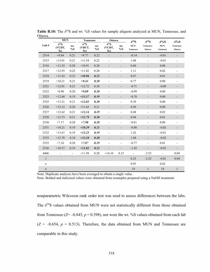
318

Table B.10: The δ34S and wt. %S values for sample aliquots analyzed at MUN, Tennessee, and Ottawa.

Lab #

MUN Tennessee Ottawa Δ34S MUN-

Tennessee

Δ34S Tennessee-

Ottawa

Δ%S MUN-

Tennessee

Δ%S Tennessee-

Ottawa

δ34S (VCDT,

‰)

wt. %S

δ34S (VDCT,

‰)

wt. %S

δ34S (VCDT,

‰)

wt. %S

2514 +9.64 0.21 +9.77 0.22 - - –0.14 - –0.01 -

2515 +13.01 0.21 +11.54 0.22 - - 1.48 - –0.01 -

2516 +11.52 0.20 +10.91 0.20 - - 0.60 - 0.00 -

2517 +12.93 0.22 +11.82 0.20 - - 1.11 - 0.02 -

2518 +11.63 0.23 +10.96 0.22 - - 0.67 - 0.01 -

2519 +10.21 0.21 +9.43 0.20 - - 0.77 - 0.00 -

2521 +12.01 0.21 +12.72 0.30 - - –0.71 - –0.09 -

2522 +8.90 0.20 +9.89 0.20 - - –0.99 - 0.00 -

2523 +12.68 0.19 +13.37 0.19 - - –0.70 - 0.00 -

2525 +13.21 0.21 +12.82 0.20 - - 0.39 - 0.00 -

2526 +12.12 0.20 +11.62 0.21 - - 0.50 - 0.00 -

2527 +12.62 0.21 +12.14 0.19 - - 0.48 - 0.02 -

2528 +13.73 0.21 +12.79 0.20 - - 0.94 - 0.01 -

2530 +7.17 0.20 +7.98 0.20 - - –0.81 - 0.00 -

2531 +10.21 0.19 +10.29 0.21 - - –0.08 - –0.02 -

2532 +13.67 0.19 +12.25 0.19 - - 1.42 - –0.01 -

2533 +13.78 0.18 +12.10 0.20 - - 1.68 - –0.02 -

2535 +7.10 0.20 +7.87 0.19 - - –0.77 - 0.01 -

2536 +10.37 0.19 +11.82 0.23 - - –1.45 - –0.03 -

4406 - - +11.58 0.20 +14.10 0.15 - –2.52 - 0.04

x̄ 0.23 –2.52 –0.01 0.04

σ 0.93 0.02

n 19 1 19 1

Note: Duplicate analyses have been averaged to obtain a single value. Note: Bolded and italicized values were obtained from resamples prepared using a NaOH treatment.

nonparametric Wilcoxon rank order test was used to assess differences between the labs.

The δ34S values obtained from MUN were not statistically different from those obtained

from Tennessee (Z= –0.845, p = 0.398), nor were the wt. %S values obtained from each lab

(Z = –0.654, p = 0.513). Therefore, the data obtained from MUN and Tennessee are

comparable in this study.

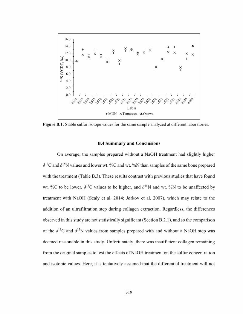
319

Figure B.1: Stable sulfur isotope values for the same sample analyzed at different laboratories.

B.4 Summary and Conclusions

On average, the samples prepared without a NaOH treatment had slightly higher

δ13C and δ15N values and lower wt. %C and wt. %N than samples of the same bone prepared

with the treatment (Table B.3). These results contrast with previous studies that have found

wt. %C to be lower, δ13C values to be higher, and δ15N and wt. %N to be unaffected by

treatment with NaOH (Sealy et al. 2014; Jørkov et al. 2007), which may relate to the

addition of an ultrafiltration step during collagen extraction. Regardless, the differences

observed in this study are not statistically significant (Section B.2.1), and so the comparison

of the δ13C and δ15N values from samples prepared with and without a NaOH step was

deemed reasonable in this study. Unfortunately, there was insufficient collagen remaining

from the original samples to test the effects of NaOH treatment on the sulfur concentration

and isotopic values. Here, it is tentatively assumed that the differential treatment will not

0.0

2.0

4.0

6.0

8.0

10.0

12.0

14.0

16.0

δ34 S

(V

CD

T, ‰

)

Lab #

MUN Tennessee Ottawa

320

significantly influence the sulfur results, although future experimentation is required to

justify this assumption.

Although sample replicates should be analysed in the same analytical sequence

(Jardine and Cuniak 2005), the majority of the δ34S and wt. %S values of duplicate samples

were analyzed during different analytical sessions at both MUN and Tennessee.

Fortunately, the differences between the duplicate values were not found to be statistically

significant (Section B.2.2) and so it was deemed appropriate to average the duplicate values

from sample replicates run at the same lab regardless of analytical session, to generate a

single value for each sample.

Finally, it was necessary to ascertain whether values from the same sample analyzed

by different labs were comparable. After averaging the δ34S and wt. %S values from the

duplicate analyses at each lab, no statistically significant differences were found between

the δ34S and wt. %S values from the same sample analyzed at MUN and Tennessee (Section

B.2.3). Therefore, the isotopic values obtained from aliquots of the same bone sample

analyzed at different laboratories are considered comparable in this study. The stable sulfur

isotopes of only one sample were analyzed by both Tennessee and Ottawa, and although

the difference in the wt. %S from each lab was low (+0.04 %), the difference between the

δ34S values was the largest reported in this study (–2.52 ‰) and exceeded the analytical

uncertainty of all analyses (Appendix C). The difference may be the result of differing

analytical approaches, as both MUN and Tennessee combusted samples of collagen

weighing 5 to 15 mg with 1 mg vanadium pentoxide (V2O5) and had comparable results,

whereas 25 to 55 mg of sample was combusted with at least twice its weight of sucrose at

the University of Ottawa. Thus, the δ34S values from bone collagen samples analyzed at

321

MUN and Tennessee are considered directly comparable, whereas the values from samples

analyzed at Ottawa may be slightly higher. However, this observation is based on a single

sample and additional research is necessary to further investigate interlaboratory

comparability of δ34S and %S values from archaeological bone collagen.

322

APPENDIX C

Analytical Uncertainty of the Isotopic Measurements

323

C.1 Introduction

Reporting analytical uncertainty is necessary for comparing isotopic data generated

by separate laboratories under differing conditions (Szpak et al. 2017a). This is because

differences among isotopic values, whether among individuals or sites, must exceed

analytical uncertainty to be meaningfully interpretable rather than the result of analytical

or human error. Analytical uncertainty was calculated following the method proposed by

Szpak et al. (2017a) and is explained in detail in Appendix A. Briefly, analytical accuracy

(u(bias)) reflects systematic measurement errors and the degree to which the δ-values of

check standards deviate from their known values. Analytical precision (u(Rw) reflects the

repeatability of measurements and is calculated using the variation of δ-values from both

standards (measurement precision; ssrm) and sample replicates (precision specific to sample

replicates; srep) included in the analytical sessions. The analytical precision and accuracy

are then used to calculate total standard uncertainty (uc). Using the analytical data provided

by each laboratory and presented in the following tables, the total analytical uncertainty for

each laboratory at which samples in this dissertation were analyzed is presented below.

C.2 Stable Carbon and Nitrogen Isotope Analysis of Bone Collagen

C.2.1 Stable Isotope Laboratory, Memorial University of Newfoundland

Stable carbon and nitrogen isotopic and elemental compositions of six Caledonia

samples prepared without a NaOH treatment (Lab #s 2514, 2515, 2520, 2521, 2526, and

2528), as well samples from as Pacbitun (n = 34), Moho Cay (n = 1), Laguna de On Island

(n = 46), Laguna de On Shore (n = 1), Caye Coco (n = 33), Chanlacan (n = 19), Caye

324

Muerto (n = 3), and Nakum (n = 22) were analyzed at the Stable Isotope Laboratory (SIL)

at the Memorial University of Newfoundland (MUN; see Appendix A).

Stable carbon and nitrogen isotope compositions were calibrated relative to VPDB

(δ13C) and AIR (δ15N) using EDTA #2, USGS62, and IAEA-N-2 (Table C.1). The internal

standards listed in Table C.1 were used to monitor internal accuracy and precision. Their

isotopic compositions represent long term averages calibrated to VPDB and AIR with

USGS62 and EDTA #2 (Alison Pye, personal communication 2018). The means and

standard deviations of the δ13C and δ15N values for the check and calibration standards as

well as the number of standards included in each analytical session are presented in Table

C.2. Measurement precision (ssrm) as calculated by repeated measurements of the standards

was ±0.15 ‰ for δ13C (df = 134) and ±0.10 ‰ for δ15N (df = 135) and measurement

accuracy (u(bias)) was ±0.23 ‰ for δ13C and ±0.20 ‰ for δ15N.

The carbon and nitrogen isotope ratios and compositions of one bone sample was

analyzed in triplicate in each of the six analytical session (6/146), the results of which are

presented in Table C.3. The measurement precision specific to the samples was ±0.10 ‰

for δ13C and ±0.12 ‰ for δ15N (df = 12). Based on the pooled standard deviations of all

Table C.1: Standard reference materials used for calibration of δ13C relative to VPDB and δ15N relative to AIR and to monitor (check) internal accuracy and precision by the Stable Isotope Lab (MUN).

Standard Material Type Accepted δ13C

(‰, VPDB) Accepted δ15N

(‰, AIR) EDTA #2 EDTA Calibration -40.38±0.01 –0.83 ± 0.04 USGS-62 Caffeine Calibration -14.79±0.04 +20.17 ± 0.06 IAEA-N-2 Ammonium Sulfate Calibration +20.32 ± 0.09

G-9 L-glutamic acid Check -26.74±0.06 –2.77 ± 0.18 G-32 Sulfanilamide Check -28.96±0.22 –3.62 ± 0.25 G-40 B2155 (protein) Check -27.03±0.13 +5.97 ± 0.08

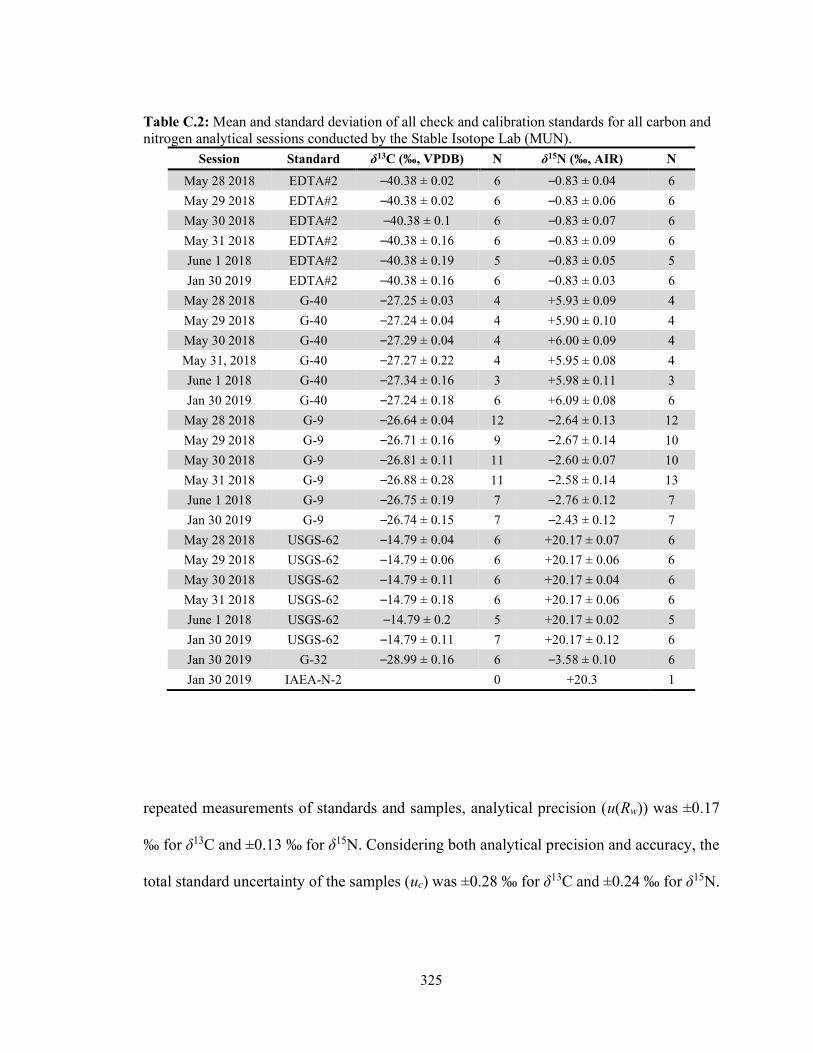
325

Table C.2: Mean and standard deviation of all check and calibration standards for all carbon and nitrogen analytical sessions conducted by the Stable Isotope Lab (MUN).

Session Standard δ13C (‰, VPDB) N δ15N (‰, AIR) N

May 28 2018 EDTA#2 –40.38 ± 0.02 6 –0.83 ± 0.04 6

May 29 2018 EDTA#2 –40.38 ± 0.02 6 –0.83 ± 0.06 6

May 30 2018 EDTA#2 –40.38 ± 0.1 6 –0.83 ± 0.07 6

May 31 2018 EDTA#2 –40.38 ± 0.16 6 –0.83 ± 0.09 6

June 1 2018 EDTA#2 –40.38 ± 0.19 5 –0.83 ± 0.05 5

Jan 30 2019 EDTA#2 –40.38 ± 0.16 6 –0.83 ± 0.03 6

May 28 2018 G-40 –27.25 ± 0.03 4 +5.93 ± 0.09 4

May 29 2018 G-40 –27.24 ± 0.04 4 +5.90 ± 0.10 4

May 30 2018 G-40 –27.29 ± 0.04 4 +6.00 ± 0.09 4

May 31, 2018 G-40 –27.27 ± 0.22 4 +5.95 ± 0.08 4

June 1 2018 G-40 –27.34 ± 0.16 3 +5.98 ± 0.11 3

Jan 30 2019 G-40 –27.24 ± 0.18 6 +6.09 ± 0.08 6

May 28 2018 G-9 –26.64 ± 0.04 12 –2.64 ± 0.13 12

May 29 2018 G-9 –26.71 ± 0.16 9 –2.67 ± 0.14 10

May 30 2018 G-9 –26.81 ± 0.11 11 –2.60 ± 0.07 10

May 31 2018 G-9 –26.88 ± 0.28 11 –2.58 ± 0.14 13

June 1 2018 G-9 –26.75 ± 0.19 7 –2.76 ± 0.12 7

Jan 30 2019 G-9 –26.74 ± 0.15 7 –2.43 ± 0.12 7

May 28 2018 USGS-62 –14.79 ± 0.04 6 +20.17 ± 0.07 6

May 29 2018 USGS-62 –14.79 ± 0.06 6 +20.17 ± 0.06 6

May 30 2018 USGS-62 –14.79 ± 0.11 6 +20.17 ± 0.04 6

May 31 2018 USGS-62 –14.79 ± 0.18 6 +20.17 ± 0.06 6

June 1 2018 USGS-62 –14.79 ± 0.2 5 +20.17 ± 0.02 5

Jan 30 2019 USGS-62 –14.79 ± 0.11 7 +20.17 ± 0.12 6

Jan 30 2019 G-32 –28.99 ± 0.16 6 –3.58 ± 0.10 6

Jan 30 2019 IAEA-N-2 0 +20.3 1

repeated measurements of standards and samples, analytical precision (u(Rw)) was ±0.17

‰ for δ13C and ±0.13 ‰ for δ15N. Considering both analytical precision and accuracy, the

total standard uncertainty of the samples (uc) was ±0.28 ‰ for δ13C and ±0.24 ‰ for δ15N.

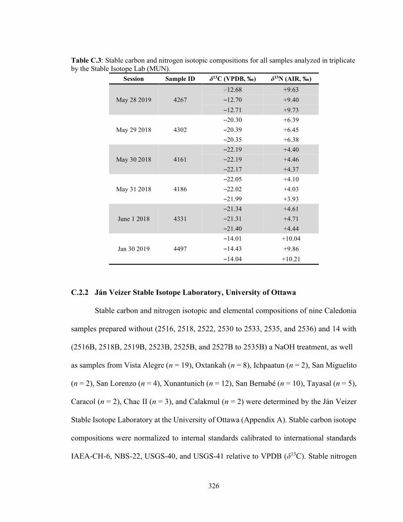
326

Table C.3: Stable carbon and nitrogen isotopic compositions for all samples analyzed in triplicate by the Stable Isotope Lab (MUN).

Session Sample ID δ13C (VPDB, ‰) δ15N (AIR, ‰)

May 28 2019 4267

–12.68 +9.63

–12.70 +9.40

–12.71 +9.73

May 29 2018 4302

–20.30 +6.39

–20.39 +6.45

–20.35 +6.38

May 30 2018 4161

–22.19 +4.40

–22.19 +4.46

–22.17 +4.37

May 31 2018 4186

–22.05 +4.10

–22.02 +4.03

–21.99 +3.93

June 1 2018 4331

–21.34 +4.61

–21.31 +4.71

–21.40 +4.44

Jan 30 2019 4497

–14.01 +10.04

–14.43 +9.86

–14.04 +10.21

C.2.2 Ján Veizer Stable Isotope Laboratory, University of Ottawa

Stable carbon and nitrogen isotopic and elemental compositions of nine Caledonia

samples prepared without (2516, 2518, 2522, 2530 to 2533, 2535, and 2536) and 14 with

(2516B, 2518B, 2519B, 2523B, 2525B, and 2527B to 2535B) a NaOH treatment, as well

as samples from Vista Alegre (n = 19), Oxtankah (n = 8), Ichpaatun (n = 2), San Miguelito

(n = 2), San Lorenzo (n = 4), Xunantunich (n = 12), San Bernabé (n = 10), Tayasal (n = 5),

Caracol (n = 2), Chac II (n = 3), and Calakmul (n = 2) were determined by the Ján Veizer

Stable Isotope Laboratory at the University of Ottawa (Appendix A). Stable carbon isotope

compositions were normalized to internal standards calibrated to international standards

IAEA-CH-6, NBS-22, USGS-40, and USGS-41 relative to VPDB (δ13C). Stable nitrogen

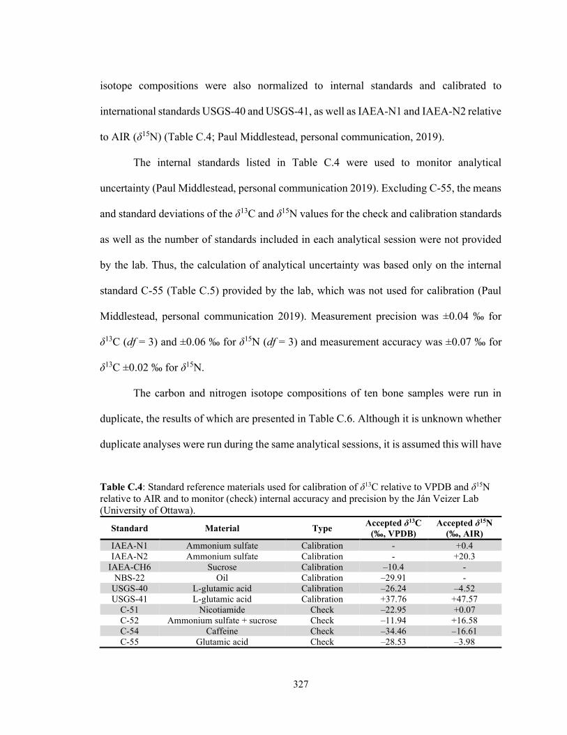
327

isotope compositions were also normalized to internal standards and calibrated to

international standards USGS-40 and USGS-41, as well as IAEA-N1 and IAEA-N2 relative

to AIR (δ15N) (Table C.4; Paul Middlestead, personal communication, 2019).

The internal standards listed in Table C.4 were used to monitor analytical

uncertainty (Paul Middlestead, personal communication 2019). Excluding C-55, the means

and standard deviations of the δ13C and δ15N values for the check and calibration standards

as well as the number of standards included in each analytical session were not provided

by the lab. Thus, the calculation of analytical uncertainty was based only on the internal

standard C-55 (Table C.5) provided by the lab, which was not used for calibration (Paul

Middlestead, personal communication 2019). Measurement precision was ±0.04 ‰ for

δ13C (df = 3) and ±0.06 ‰ for δ15N (df = 3) and measurement accuracy was ±0.07 ‰ for

δ13C ±0.02 ‰ for δ15N.

The carbon and nitrogen isotope compositions of ten bone samples were run in

duplicate, the results of which are presented in Table C.6. Although it is unknown whether

duplicate analyses were run during the same analytical sessions, it is assumed this will have

Table C.4: Standard reference materials used for calibration of δ13C relative to VPDB and δ15N relative to AIR and to monitor (check) internal accuracy and precision by the Ján Veizer Lab (University of Ottawa).

Standard Material Type Accepted δ13C

(‰, VPDB) Accepted δ15N

(‰, AIR) IAEA-N1 Ammonium sulfate Calibration - +0.4 IAEA-N2 Ammonium sulfate Calibration - +20.3

IAEA-CH6 Sucrose Calibration –10.4 - NBS-22 Oil Calibration –29.91 -

USGS-40 L-glutamic acid Calibration –26.24 –4.52 USGS-41 L-glutamic acid Calibration +37.76 +47.57

C-51 Nicotiamide Check –22.95 +0.07 C-52 Ammonium sulfate + sucrose Check –11.94 +16.58 C-54 Caffeine Check –34.46 –16.61 C-55 Glutamic acid Check –28.53 –3.98

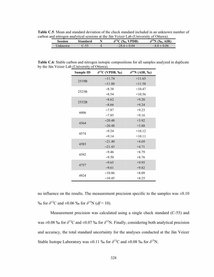
328

Table C.5: Mean and standard deviation of the check standard included in an unknown number of carbon and nitrogen analytical sessions at the Ján Veizer Lab (University of Ottawa).

Session Standard N δ13C (‰, VPDB) δ15N (‰, AIR) Unknown C-55 4 –28.6 ± 0.04 –4.0 ± 0.06

Table C.6: Stable carbon and nitrogen isotopic compositions for all samples analyzed in duplicate by the Ján Veizer Lab (University of Ottawa).

Sample ID δ13C (VPDB, ‰) δ15N (AIR, ‰)

2519B –11.74 +11.65

–11.80 +11.58

2523B –8.38 +10.47

–8.54 +10.56

2532B –8.62 +9.20

–8.66 +9.24

4406 –7.87 +9.23

–7.85 +9.16

4564 –20.48 +3.92

–20.48 +3.88

4574 –9.24 +10.12

–9.14 +10.11

4585 –21.40 +4.69

–21.43 +4.71

4592 –9.46 +8.79

–9.50 +8.76

4757 –9.65 +9.95

–9.61 +9.82

4924 –10.86 +8.09

–10.45 +8.25

no influence on the results. The measurement precision specific to the samples was ±0.10

‰ for δ13C and ±0.06 ‰ for δ15N (df = 10).

Measurement precision was calculated using a single check standard (C-55) and

was ±0.08 ‰ for δ13C and ±0.07 ‰ for δ15N. Finally, considering both analytical precision

and accuracy, the total standard uncertainty for the analyses conducted at the Ján Veizer

Stable Isotope Laboratory was ±0.11 ‰ for δ13C and ±0.08 ‰ for δ15N.

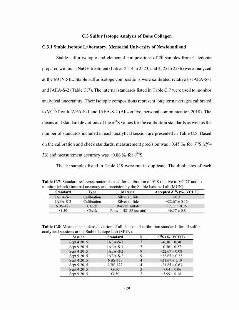
329

C.3 Sulfur Isotope Analysis of Bone Collagen

C.3.1 Stable Isotope Laboratory, Memorial University of Newfoundland

Stable sulfur isotopic and elemental compositions of 20 samples from Caledonia

prepared without a NaOH treatment (Lab #s 2514 to 2523, and 2525 to 2536) were analyzed

at the MUN SIL. Stable sulfur isotope compositions were calibrated relative to IAEA-S-1

and IAEA-S-2 (Table C.7). The internal standards listed in Table C.7 were used to monitor

analytical uncertainty. Their isotopic compositions represent long term averages calibrated

to VCDT with IAEA-S-1 and IAEA-S-2 (Alison Pye, personal communication 2018). The

means and standard deviations of the δ34S values for the calibration standards as well as the

number of standards included in each analytical session are presented in Table C.8. Based

on the calibration and check standards, measurement precision was ±0.45 ‰ for δ34S (df =

36) and measurement accuracy was ±0.86 ‰ for δ34S.

The 10 samples listed in Table C.9 were run in duplicate. The duplicates of each

Table C.7: Standard reference materials used for calibration of δ34S relative to VCDT and to monitor (check) internal accuracy and precision by the Stable Isotope Lab (MUN).

Standard Type Material Accepted δ34S (‰, VCDT) IAEA-S-1 Calibration Silver sulfide –0.3 IAEA-S-2 Calibration Silver sulfide +22.67 ± 0.15 NBS-127 Check Barium sulfate +21.1 ± 0.36

G-50 Check Protein B2155 (casein) +6.57 ± 0.8

Table C.8: Mean and standard deviation of all check and calibration standards for all sulfur analytical sessions at the Stable Isotope Lab (MUN).

Session Standard N δ34S (‰, VCDT) Sept 4 2015 IAEA-S-1 7 –0.30 ± 0.30 Sept 9 2015 IAEA-S-1 7 –0.36 ± 0.27 Sept 4 2015 IAEA-S-2 9 +22.67 ± 0.08 Sept 9 2015 IAEA-S-2 9 +22.67 ± 0.22 Sept 4 2015 NBS-127 4 +21.67 ± 1.19 Sept 9 2015 NBS-127 4 +21.85 ± 0.63 Sept 4 2015 G-50 2 +7.04 ± 0.06 Sept 9 2015 G-50 2 +5.99 ± 0.18

330

Table C.9: Stable sulfur isotopic compositions for all samples analyzed in duplicate by the Stable Isotope Lab (MUN).

Sample ID δ34S (VCDT, ‰)

Sept. 4, 2015 Sept. 9, 2015 2514 +10.27 +9.00 2515 +12.43 +13.59 2516 +10.14 +12.89 2517 +11.73 +14.13 2518 +12.25 +11.01 2519 +10.74 +9.67 2521 +12.93 +11.09 2523 +12.69 +12.66 2528 +13.73 +13.73

2532 +13.13 +14.21

sample except 2532 were run in different sessions; however, their values were not

statistically different (see Appendix B), and so they were included in the calculation of

measurement precision specific to the samples, which was ±1.08 ‰ for δ34S (df = 10).

Based on the pooled standard deviations of all repeated measurements of standards and

samples, analytical precision was ±0.89 ‰ for δ34S and the total standard uncertainty (uc)

was ±1.24 ‰ for δ34S.

C.3.2 Stable Isotope Laboratory, University of Tennessee Knoxville

Stable sulfur isotopic and elemental compositions of samples from Caledonia

prepared without (n = 8) and with (n = 9) a NaOH step, as well as samples from Pacbitun

(n = 31), Moho Cay (n = 1), Laguna de On Island (n = 42), Laguna de On Shore (n = 1),

Caye Coco (n = 27), Chanlacan (n = 18), Caye Muerto (n = 1), Nakum (n = 22), Vista

Alegre (n = 18), Oxtankah (n = 7), Ichpaatun (n = 2), and San Miguelito (n = 2) were

analyzed in the Stable Isotope Laboratory at the University of Tennessee Knoxville. Stable

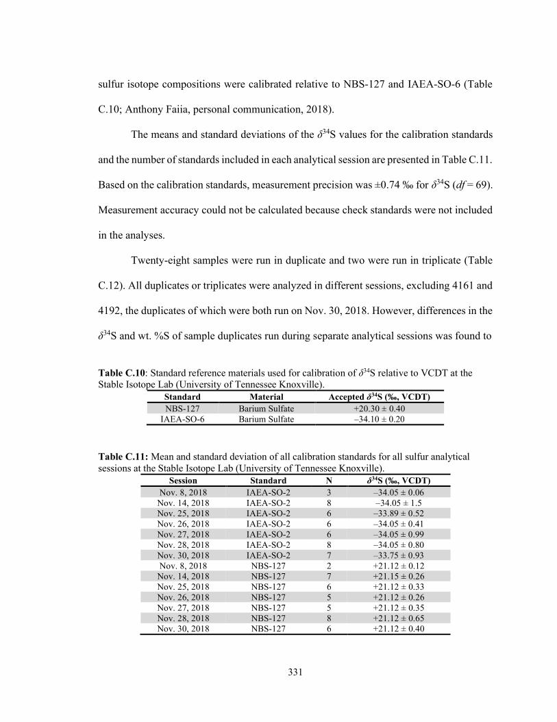
331

sulfur isotope compositions were calibrated relative to NBS-127 and IAEA-SO-6 (Table

C.10; Anthony Faiia, personal communication, 2018).

The means and standard deviations of the δ34S values for the calibration standards

and the number of standards included in each analytical session are presented in Table C.11.

Based on the calibration standards, measurement precision was ±0.74 ‰ for δ34S (df = 69).

Measurement accuracy could not be calculated because check standards were not included

in the analyses.

Twenty-eight samples were run in duplicate and two were run in triplicate (Table

C.12). All duplicates or triplicates were analyzed in different sessions, excluding 4161 and

4192, the duplicates of which were both run on Nov. 30, 2018. However, differences in the

δ34S and wt. %S of sample duplicates run during separate analytical sessions was found to

Table C.10: Standard reference materials used for calibration of δ34S relative to VCDT at the Stable Isotope Lab (University of Tennessee Knoxville).

Standard Material Accepted δ34S (‰, VCDT) NBS-127 Barium Sulfate +20.30 ± 0.40

IAEA-SO-6 Barium Sulfate –34.10 ± 0.20

Table C.11: Mean and standard deviation of all calibration standards for all sulfur analytical sessions at the Stable Isotope Lab (University of Tennessee Knoxville).

Session Standard N δ34S (‰, VCDT) Nov. 8, 2018 IAEA-SO-2 3 –34.05 ± 0.06

Nov. 14, 2018 IAEA-SO-2 8 –34.05 ± 1.5 Nov. 25, 2018 IAEA-SO-2 6 –33.89 ± 0.52 Nov. 26, 2018 IAEA-SO-2 6 –34.05 ± 0.41 Nov. 27, 2018 IAEA-SO-2 6 –34.05 ± 0.99 Nov. 28, 2018 IAEA-SO-2 8 –34.05 ± 0.80 Nov. 30, 2018 IAEA-SO-2 7 –33.75 ± 0.93 Nov. 8, 2018 NBS-127 2 +21.12 ± 0.12

Nov. 14, 2018 NBS-127 7 +21.15 ± 0.26 Nov. 25, 2018 NBS-127 6 +21.12 ± 0.33 Nov. 26, 2018 NBS-127 5 +21.12 ± 0.26 Nov. 27, 2018 NBS-127 5 +21.12 ± 0.35 Nov. 28, 2018 NBS-127 8 +21.12 ± 0.65 Nov. 30, 2018 NBS-127 6 +21.12 ± 0.40

332

Table C.12: Stable sulfur isotopic compositions for all samples analyzed in duplicate or triplicate at the Stable Isotope Lab (University of Tennessee Knoxville).

Sample ID δ34S (VCDT, ‰)

Session 1 Session 2 Session 3 2558 +11.82 +11.08 2561 +13.42 +13.17 3451 +16.71 +14.20 3458 +13.30 +13.22 4155 +14.66 +13.67 4161 +8.23 +8.99 4192 +4.43 +4.69 4255 +13.05 +11.90 4260 +11.41 +13.39 4261 +9.61 +9.44 4262 +13.28 +13.38 +12.30 4263 +12.70 +12.92 4267 +8.81 +8.23 4268 +10.94 +10.54 4270 +12.48 +11.97 +11.73 4271 +14.24 +13.79 4272 +13.72 +10.71 4273 +12.66 +12.01 4274 +17.13 +17.12 4294 +14.18 +13.27 4303 +14.12 +13.53 4305 +9.38 +6.77 4320 +13.40 +12.03 4328 +14.40 +13.47 4332 +14.02 +13.06 4406 +11.75 +11.42 4522 -0.18 -2.34 4533 +13.14 +12.14 4553 -1.14 -4.47 4555 +13.24 +11.27

Note: Sessions 1, 2, and 3, are specific to each sample, as not every sample was run during each analytical session. be statistically insignificant (see Appendix B), and so they were included in the calculation

of measurement precision specific to the samples, which was ±0.96 ‰ for δ34S (df = 32).

Based on the pooled standard deviations of all repeated measurements of the

calibration standards and samples, analytical precision was ±1.00 ‰ for δ34S. However,

because analytical accuracy could not be calculated, neither could the standard uncertainty.

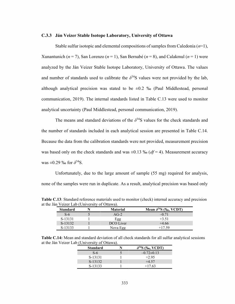
333

C.3.3 Ján Veizer Stable Isotope Laboratory, University of Ottawa

Stable sulfur isotopic and elemental compositions of samples from Caledonia (n=1),

Xunantunich (n = 7), San Lorenzo (n = 1), San Bernabé (n = 8), and Calakmul (n = 1) were

analyzed by the Ján Veizer Stable Isotope Laboratory, University of Ottawa. The values

and number of standards used to calibrate the δ34S values were not provided by the lab,

although analytical precision was stated to be ±0.2 ‰ (Paul Middlestead, personal

communication, 2019). The internal standards listed in Table C.13 were used to monitor

analytical uncertainty (Paul Middlestead, personal communication, 2019).

The means and standard deviations of the δ34S values for the check standards and

the number of standards included in each analytical session are presented in Table C.14.

Because the data from the calibration standards were not provided, measurement precision

was based only on the check standards and was ±0.13 ‰ (df = 4). Measurement accuracy

was ±0.29 ‰ for δ34S.

Unfortunately, due to the large amount of sample (55 mg) required for analysis,

none of the samples were run in duplicate. As a result, analytical precision was based only

Table C.13: Standard reference materials used to monitor (check) internal accuracy and precision at the Ján Veizer Lab (University of Ottawa).

Standard N Material Mean δ34S (‰, VCDT) S-6 5 AG-2 –0.71

S-13131 1 Egg +3.51 S-13132 1 DCO Liver +4.66 S-13133 1 Nova Egg +17.59

Table C.14: Mean and standard deviation of all check standards for all sulfur analytical sessions at the Ján Veizer Lab (University of Ottawa).

Standard N δ34S (‰, VCDT) S-6 5 –0.72±0.13

S-13131 1 +2.95 S-13132 1 +4.57 S-13133 1 +17.63

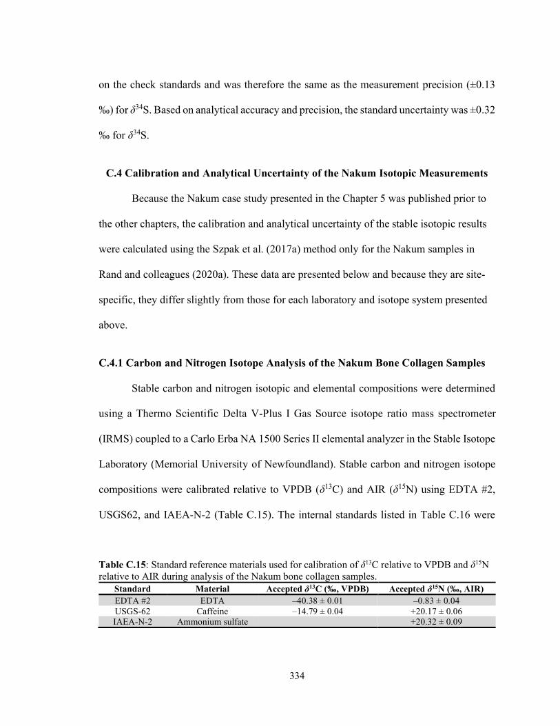
334

on the check standards and was therefore the same as the measurement precision (±0.13

‰) for δ34S. Based on analytical accuracy and precision, the standard uncertainty was ±0.32

‰ for δ34S.

C.4 Calibration and Analytical Uncertainty of the Nakum Isotopic Measurements

Because the Nakum case study presented in the Chapter 5 was published prior to

the other chapters, the calibration and analytical uncertainty of the stable isotopic results

were calculated using the Szpak et al. (2017a) method only for the Nakum samples in

Rand and colleagues (2020a). These data are presented below and because they are site-

specific, they differ slightly from those for each laboratory and isotope system presented

above.

C.4.1 Carbon and Nitrogen Isotope Analysis of the Nakum Bone Collagen Samples

Stable carbon and nitrogen isotopic and elemental compositions were determined

using a Thermo Scientific Delta V-Plus I Gas Source isotope ratio mass spectrometer

(IRMS) coupled to a Carlo Erba NA 1500 Series II elemental analyzer in the Stable Isotope

Laboratory (Memorial University of Newfoundland). Stable carbon and nitrogen isotope

compositions were calibrated relative to VPDB (δ13C) and AIR (δ15N) using EDTA #2,

USGS62, and IAEA-N-2 (Table C.15). The internal standards listed in Table C.16 were

Table C.15: Standard reference materials used for calibration of δ13C relative to VPDB and δ15N relative to AIR during analysis of the Nakum bone collagen samples.

Standard Material Accepted δ13C (‰, VPDB) Accepted δ15N (‰, AIR) EDTA #2 EDTA –40.38 ± 0.01 –0.83 ± 0.04 USGS-62 Caffeine –14.79 ± 0.04 +20.17 ± 0.06 IAEA-N-2 Ammonium sulfate +20.32 ± 0.09

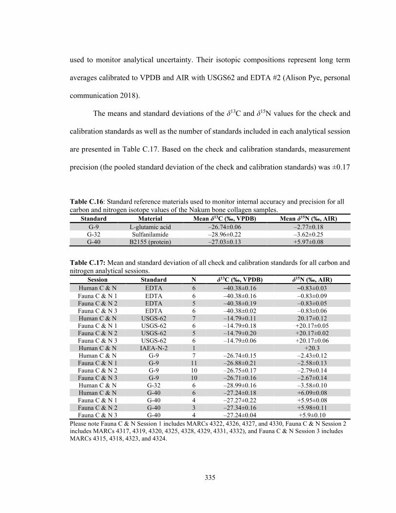
335

used to monitor analytical uncertainty. Their isotopic compositions represent long term

averages calibrated to VPDB and AIR with USGS62 and EDTA #2 (Alison Pye, personal

communication 2018).

The means and standard deviations of the δ13C and δ15N values for the check and

calibration standards as well as the number of standards included in each analytical session

are presented in Table C.17. Based on the check and calibration standards, measurement

precision (the pooled standard deviation of the check and calibration standards) was ±0.17

Table C.16: Standard reference materials used to monitor internal accuracy and precision for all carbon and nitrogen isotope values of the Nakum bone collagen samples.

Standard Material Mean δ13C (‰, VPDB) Mean δ15N (‰, AIR) G-9 L-glutamic acid –26.74±0.06 –2.77±0.18

G-32 Sulfanilamide –28.96±0.22 –3.62±0.25 G-40 B2155 (protein) –27.03±0.13 +5.97±0.08

Table C.17: Mean and standard deviation of all check and calibration standards for all carbon and nitrogen analytical sessions.

Session Standard N δ13C (‰, VPDB) δ15N (‰, AIR) Human C & N EDTA 6 –40.38±0.16 –0.83±0.03 Fauna C & N 1 EDTA 6 –40.38±0.16 –0.83±0.09 Fauna C & N 2 EDTA 5 –40.38±0.19 –0.83±0.05 Fauna C & N 3 EDTA 6 –40.38±0.02 –0.83±0.06 Human C & N USGS-62 7 –14.79±0.11 20.17±0.12 Fauna C & N 1 USGS-62 6 –14.79±0.18 +20.17±0.05 Fauna C & N 2 USGS-62 5 –14.79±0.20 +20.17±0.02 Fauna C & N 3 USGS-62 6 –14.79±0.06 +20.17±0.06 Human C & N IAEA-N-2 1 +20.3 Human C & N G-9 7 –26.74±0.15 –2.43±0.12 Fauna C & N 1 G-9 11 –26.88±0.21 –2.58±0.13 Fauna C & N 2 G-9 10 –26.75±0.17 –2.79±0.14 Fauna C & N 3 G-9 10 –26.71±0.16 –2.67±0.14 Human C & N G-32 6 –28.99±0.16 –3.58±0.10 Human C & N G-40 6 –27.24±0.18 +6.09±0.08 Fauna C & N 1 G-40 4 –27.27±0.22 +5.95±0.08 Fauna C & N 2 G-40 3 –27.34±0.16 +5.98±0.11 Fauna C & N 3 G-40 4 –27.24±0.04 +5.9±0.10

Please note Fauna C & N Session 1 includes MARCs 4322, 4326, 4327, and 4330, Fauna C & N Session 2 includes MARCs 4317, 4319, 4320, 4325, 4328, 4329, 4331, 4332), and Fauna C & N Session 3 includes MARCs 4315, 4318, 4323, and 4324.

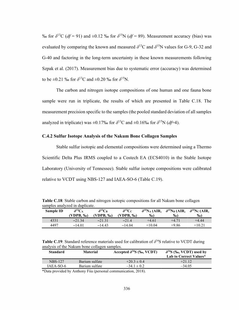
336

‰ for δ13C (df = 91) and ±0.12 ‰ for δ15N (df = 89). Measurement accuracy (bias) was

evaluated by comparing the known and measured δ13C and δ15N values for G-9, G-32 and

G-40 and factoring in the long-term uncertainty in these known measurements following

Szpak et al. (2017). Measurement bias due to systematic error (accuracy) was determined

to be ±0.21 ‰ for δ13C and ±0.20 ‰ for δ15N.

The carbon and nitrogen isotope compositions of one human and one fauna bone

sample were run in triplicate, the results of which are presented in Table C.18. The

measurement precision specific to the samples (the pooled standard deviation of all samples

analyzed in triplicate) was ±0.17‰ for δ13C and ±0.16‰ for δ15N (df=4).

C.4.2 Sulfur Isotope Analysis of the Nakum Bone Collagen Samples

Stable sulfur isotopic and elemental compositions were determined using a Thermo

Scientific Delta Plus IRMS coupled to a Costech EA (ECS4010) in the Stable Isotope

Laboratory (University of Tennessee). Stable sulfur isotope compositions were calibrated

relative to VCDT using NBS-127 and IAEA-SO-6 (Table C.19).

Table C.18: Stable carbon and nitrogen isotopic compositions for all Nakum bone collagen samples analyzed in duplicate.

Sample ID δ13CA (VDPB, ‰)

δ13CB (VDPB, ‰)

δ13CC (VDPB, ‰)

δ15NA (AIR, ‰)

δ15NB (AIR, ‰)

δ15NC (AIR, ‰)

4331 –21.34 –21.31 –21.4 +4.61 +4.71 +4.44 4497 –14.01 –14.43 –14.04 +10.04 +9.86 +10.21

Table C.19: Standard reference materials used for calibration of δ34S relative to VCDT during analysis of the Nakum bone collagen samples.

Standard Material Accepted δ34S (‰, VCDT) δ34S (‰, VCDT) used by Lab to Correct Values*

NBS-127 Barium sulfate +20.3 ± 0.4 +21.12 IAEA-SO-6 Barium sulfate –34.1 ± 0.2 –34.05

*Data provided by Anthony Fiia (personal communication, 2018).

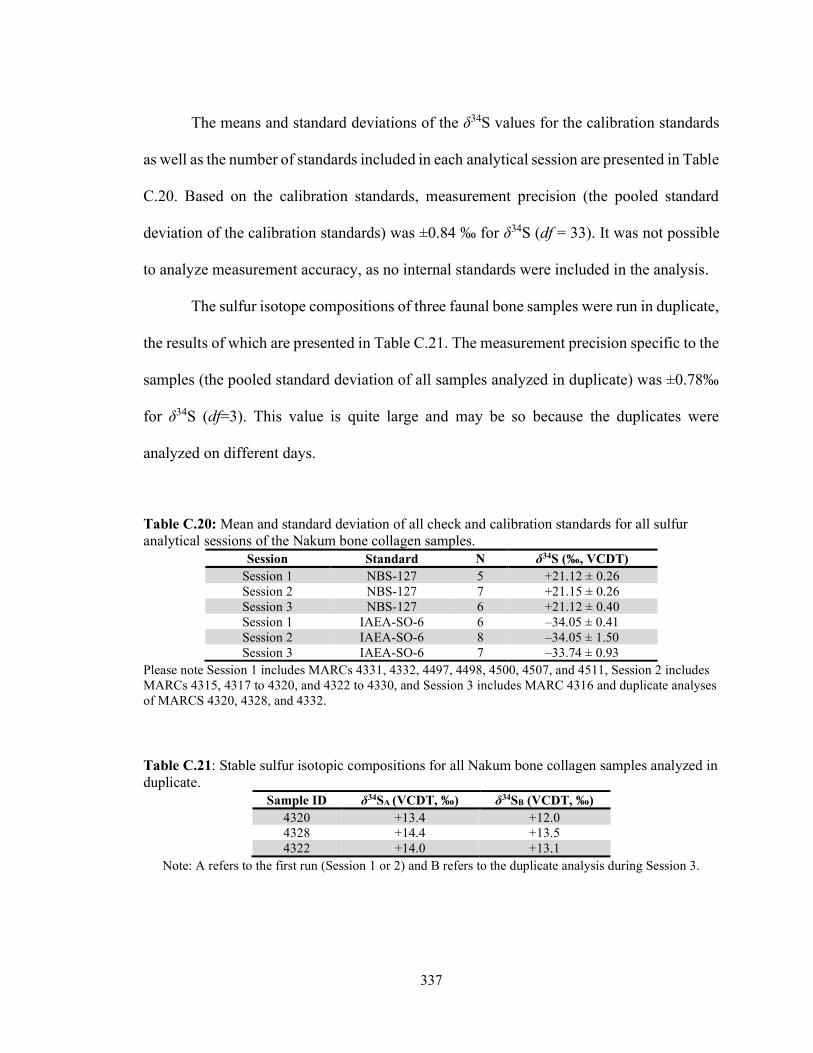
337

The means and standard deviations of the δ34S values for the calibration standards

as well as the number of standards included in each analytical session are presented in Table

C.20. Based on the calibration standards, measurement precision (the pooled standard

deviation of the calibration standards) was ±0.84 ‰ for δ34S (df = 33). It was not possible

to analyze measurement accuracy, as no internal standards were included in the analysis.

The sulfur isotope compositions of three faunal bone samples were run in duplicate,

the results of which are presented in Table C.21. The measurement precision specific to the

samples (the pooled standard deviation of all samples analyzed in duplicate) was ±0.78‰

for δ34S (df=3). This value is quite large and may be so because the duplicates were

analyzed on different days.

Table C.20: Mean and standard deviation of all check and calibration standards for all sulfur analytical sessions of the Nakum bone collagen samples.

Session Standard N δ34S (‰, VCDT) Session 1 NBS-127 5 +21.12 ± 0.26 Session 2 NBS-127 7 +21.15 ± 0.26 Session 3 NBS-127 6 +21.12 ± 0.40 Session 1 IAEA-SO-6 6 –34.05 ± 0.41 Session 2 IAEA-SO-6 8 –34.05 ± 1.50 Session 3 IAEA-SO-6 7 –33.74 ± 0.93

Please note Session 1 includes MARCs 4331, 4332, 4497, 4498, 4500, 4507, and 4511, Session 2 includes MARCs 4315, 4317 to 4320, and 4322 to 4330, and Session 3 includes MARC 4316 and duplicate analyses of MARCS 4320, 4328, and 4332. Table C.21: Stable sulfur isotopic compositions for all Nakum bone collagen samples analyzed in duplicate.

Sample ID δ34SA (VCDT, ‰) δ34SB (VCDT, ‰) 4320 +13.4 +12.0 4328 +14.4 +13.5 4322 +14.0 +13.1

Note: A refers to the first run (Session 1 or 2) and B refers to the duplicate analysis during Session 3.

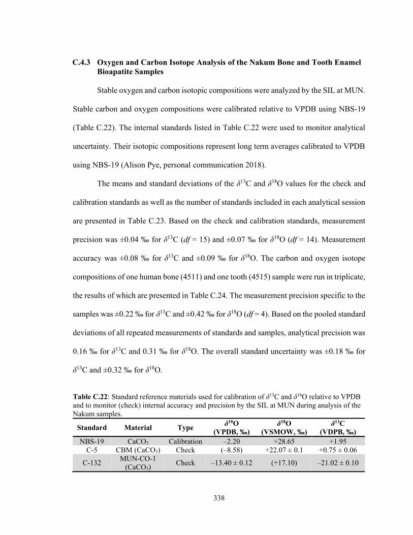
338

C.4.3 Oxygen and Carbon Isotope Analysis of the Nakum Bone and Tooth Enamel Bioapatite Samples

Stable oxygen and carbon isotopic compositions were analyzed by the SIL at MUN.

Stable carbon and oxygen compositions were calibrated relative to VPDB using NBS-19

(Table C.22). The internal standards listed in Table C.22 were used to monitor analytical

uncertainty. Their isotopic compositions represent long term averages calibrated to VPDB

using NBS-19 (Alison Pye, personal communication 2018).

The means and standard deviations of the δ13C and δ18O values for the check and

calibration standards as well as the number of standards included in each analytical session

are presented in Table C.23. Based on the check and calibration standards, measurement

precision was ±0.04 ‰ for δ13C (df = 15) and ±0.07 ‰ for δ18O (df = 14). Measurement

accuracy was ±0.08 ‰ for δ13C and ±0.09 ‰ for δ18O. The carbon and oxygen isotope

compositions of one human bone (4511) and one tooth (4515) sample were run in triplicate,

the results of which are presented in Table C.24. The measurement precision specific to the

samples was ±0.22 ‰ for δ13C and ±0.42 ‰ for δ18O (df = 4). Based on the pooled standard

deviations of all repeated measurements of standards and samples, analytical precision was

0.16 ‰ for δ13C and 0.31 ‰ for δ18O. The overall standard uncertainty was ±0.18 ‰ for

δ13C and ±0.32 ‰ for δ18O.

Table C.22: Standard reference materials used for calibration of δ13C and δ18O relative to VPDB and to monitor (check) internal accuracy and precision by the SIL at MUN during analysis of the Nakum samples.

Standard Material Type δ18O

(VPDB, ‰) δ18O

(VSMOW, ‰) δ13C

(VDPB, ‰) NBS-19 CaCO3 Calibration –2.20 +28.65 +1.95

C-5 CBM (CaCO3) Check (–8.58) +22.07 ± 0.1 +0.75 ± 0.06

C-132 MUN-CO-1

(CaCO3) Check –13.40 ± 0.12 (+17.10) –21.02 ± 0.10

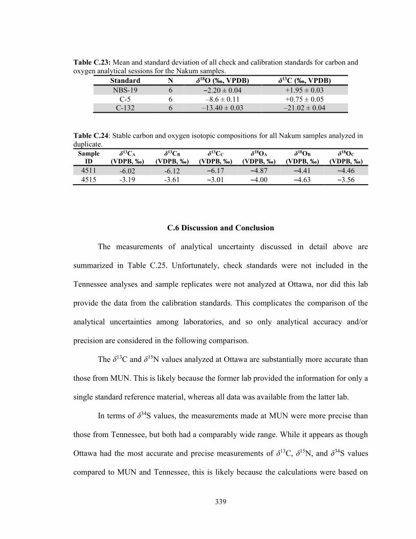
339

Table C.23: Mean and standard deviation of all check and calibration standards for carbon and oxygen analytical sessions for the Nakum samples.

Standard N δ18O (‰, VPDB) δ13C (‰, VPDB) NBS-19 6 –2.20 ± 0.04 +1.95 ± 0.03

C-5 6 –8.6 ± 0.11 +0.75 ± 0.05 C-132 6 –13.40 ± 0.03 –21.02 ± 0.04

Table C.24: Stable carbon and oxygen isotopic compositions for all Nakum samples analyzed in duplicate.

Sample ID

δ13CA

(VDPB, ‰) δ13CB

(VDPB, ‰) δ13CC

(VDPB, ‰) δ18OA

(VDPB, ‰) δ18OB

(VDPB, ‰) δ18OC

(VDPB, ‰)

4511 -6.02 -6.12 –6.17 –4.87 –4.41 –4.46 4515 -3.19 -3.61 –3.01 –4.00 –4.63 –3.56

C.6 Discussion and Conclusion

The measurements of analytical uncertainty discussed in detail above are

summarized in Table C.25. Unfortunately, check standards were not included in the

Tennessee analyses and sample replicates were not analyzed at Ottawa, nor did this lab

provide the data from the calibration standards. This complicates the comparison of the

analytical uncertainties among laboratories, and so only analytical accuracy and/or

precision are considered in the following comparison.

The δ13C and δ15N values analyzed at Ottawa are substantially more accurate than

those from MUN. This is likely because the former lab provided the information for only a

single standard reference material, whereas all data was available from the latter lab.

In terms of δ34S values, the measurements made at MUN were more precise than

those from Tennessee, but both had a comparably wide range. While it appears as though

Ottawa had the most accurate and precise measurements of δ13C, δ15N, and δ34S values

compared to MUN and Tennessee, this is likely because the calculations were based on

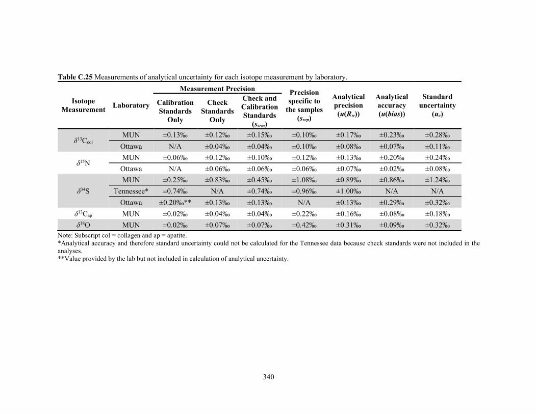
340

Table C.25 Measurements of analytical uncertainty for each isotope measurement by laboratory.

Isotope Measurement

Laboratory

Measurement Precision Precision specific to

the samples (srep)

Analytical precision (u(Rw))

Analytical accuracy (u(bias))

Standard uncertainty

(uc)

Calibration Standards

Only

Check Standards

Only

Check and Calibration Standards

(ssrm)

δ13Ccol MUN ±0.13‰ ±0.12‰ ±0.15‰ ±0.10‰ ±0.17‰ ±0.23‰ ±0.28‰

Ottawa N/A ±0.04‰ ±0.04‰ ±0.10‰ ±0.08‰ ±0.07‰ ±0.11‰

δ15N MUN ±0.06‰ ±0.12‰ ±0.10‰ ±0.12‰ ±0.13‰ ±0.20‰ ±0.24‰

Ottawa N/A ±0.06‰ ±0.06‰ ±0.06‰ ±0.07‰ ±0.02‰ ±0.08‰

δ34S

MUN ±0.25‰ ±0.83‰ ±0.45‰ ±1.08‰ ±0.89‰ ±0.86‰ ±1.24‰

Tennessee* ±0.74‰ N/A ±0.74‰ ±0.96‰ ±1.00‰ N/A N/A

Ottawa ±0.20‰** ±0.13‰ ±0.13‰ N/A ±0.13‰ ±0.29‰ ±0.32‰

δ13Cap MUN ±0.02‰ ±0.04‰ ±0.04‰ ±0.22‰ ±0.16‰ ±0.08‰ ±0.18‰

δ18O MUN ±0.02‰ ±0.07‰ ±0.07‰ ±0.42‰ ±0.31‰ ±0.09‰ ±0.32‰ Note: Subscript col = collagen and ap = apatite. *Analytical accuracy and therefore standard uncertainty could not be calculated for the Tennessee data because check standards were not included in the analyses. **Value provided by the lab but not included in calculation of analytical uncertainty.

341

limited data. Specifically, the calculation of analytical uncertainty for the δ13C and δ15N

values from Ottawa were based on 10 replicate samples, but the mean and standard

deviation of only a single check standard were provided by the lab. Similarly, the

calculation of analytical uncertainty for δ34S values from Ottawa was based on the means

and standard deviations of four check standards provided by the lab rather than the

individual values of these standards obtain in each run and no calibration standards or

sample replicates were included in these calculations. The overall lack of information about

the standard reference materials included in the analytical sessions therefore make it

difficult to comprehensively evaluate the analytical uncertainty associated with the isotopic

measurements made at Ottawa.

The analytical uncertainty associated with δ34S values is higher than those of δ13C,

δ15N, and δ18O values (Table C.25). Other archaeological studies that have analyzed sulfur

isotopes also found elevated levels of uncertainty, although the analytical precision of the

δ34S analyzed by MUN (±0.89 ‰) and Tennessee (±1.00 ‰) are much broader than those

reported in other studies which range from ±0.20 to ±0.60 ‰ (Craig et al. 2006; Fornander

et al. 2008; Linderholm et al. 2008b; Nehlich et al. 2010; Privat et al. 2007; Richards et al.

2001, 2003; Sayle et al. 2013). This is likely because precision reported in other studies is

based on the measurement precision of the calibration standards analyzed with the samples,

whereas analytical precision calculated using the method of Szpak et al. (2017a) includes

the variability of the calibration standards as well as check standards and sample replicates.

When the measurement precisions of only the calibration standards are considered, the

“precision” of the MUN (±0.22 ‰) and Ottawa (±0.20 ‰) analyses are comparable with

the values reported in other studies (Table C.25). This indicates that the exclusion of the

342

variability of additional standards as well as sample replicates from the calculation of

analytical uncertainty superficially increases precision.

To investigate this further, the sample replicates were removed from the calculation

of analytical precision for the MUN and Tennessee analyses. As a result, the precision of

the MUN analyses improved from ±0.89 to ±0.45 ‰ as did that of the Tennessee analyses

from ±1.00 to ±0.74 ‰. As has been observed elsewhere (Jardine and Cunjak 2005), this

demonstrates that although the inclusion of sample replicates in the calculation of analytical

precision appears to be less precise, it is in reality more robust in terms of reflecting the

true uncertainty in the isotopic values obtained from heterogeneous sample materials such

as bone collagen. Researchers should therefore request the necessary data from the

laboratories at which their data is generated and use a standardized method to calculate

analytical uncertainty (e.g., Szpak et al. 2017a) to ensure comparability among studies.

As researchers are becoming more aware that differing preparation and analytical

methods can influence the comparability of isotopic data sets (Chesson et al. 2019; Pestle

et al. 2014), it is also important to provide comparable measures of the analytical

uncertainty associated with the analyses, as has been proposed by Szpak et al. (2017a).

However, since the guidelines by Szpak and colleagues (2017a) were published, few

archaeological isotope studies have reported analytical uncertainty using their

methodology. Furthermore, most studies that did use this method primarily examined

archaeological plants (Metcalfe and Mead 2019; Vaiglova 2020) or animals (Fuller et al.

2020; Guiry et al. 2020; Harris et al. 2020; Szpak and Valenzuela 2020), and rarely humans

(but see Munkittrick et al. 2019). Other studies utilized the methodology proposed by Szpak

et al. (2017a) but reported measurement precision and analytical accuracy rather than the

343

overall analytical uncertainty for consistency with earlier studies (Clark et al. 2019; Rand

et al. 2020a). Future utilization of the standardized analytical uncertainty proposed by

Szpak et al. (2017a) will increase the comparability of isotopic data produced by different

labs using different techniques.

344

APPENDIX D

SPECIES, CONTEXTUAL, AND ISOTOPIC DATA OF THE MAYA

FAUNAL SAMPLES

345

Table D.1: Contextual and species data for the Maya faunal samples.

Lab # Site Common Name Scientific Name Time

Period Context Age Skeletal Element

2575 Pacbitun Deer Cervidae PreC 4:328 A Fragment

3443 Pacbitun White-tailed deer Odocoileus virginianus C 1:283:1 A Tibia

3444 Pacbitun White-tailed deer Odocoileus virginianus C 4:155:1 A Fragment

3445 Pacbitun White-tailed deer Odocoileus virginianus C 38:202:7 A Femur

3446 Pacbitun White-tailed deer Odocoileus virginianus C 38:238:3 A Ulna

3447 Pacbitun White-tailed deer Odocoileus virginianus C 38:244:1 A Fragment

3448 Pacbitun Brocket deer Mazama sp. C 15:236:6 A Fragment

3449 Pacbitun Brocket deer Mazama sp. LPreC 23:104:23 A Metapodial

3450 Pacbitun Lowland paca Cuniculus paca C 1:3:1 A Tibia

3451 Pacbitun Lowland paca Cuniculus paca C 23:102:1 A Fragment

3452 Pacbitun Lowland paca Cuniculus paca C 15:236:1 A Fragment

3453 Pacbitun Agouti Dasyprocta sp. LPreC 23:103:4 A Ulna

3454 Pacbitun Peccary Tayassuidae C 2:16:1 A Fragment

3455 Pacbitun White-lipped peccary Tayassu pecari LPreC 23:103:2 A Fragment

3456 Pacbitun Turkey Meleagris sp. C 2:18:4 A Fragment

3457 Pacbitun Feline Felidae C 2:34:B2-3 A Proximal Phalanx

3458 Pacbitun Turtle Testudines C 2:55:1 A Fragment

3459 Pacbitun Turtle Testudines C 4:12:24 A Fragment

3460 Pacbitun Turtle Kinosternidae C 4:212:16 A Fragment

3461 Pacbitun Turtle Kinosternidae C 15:236:11 A Fragment

3462 Moho Cay Caribbean manatee Trichechus manatus manatus E-LC 95 A Rib

4150 Laguna de On

Island Weasel Mustelidae E-LPC 2:2 A L Calcaneus

4152 Laguna de On

Island Opossum Didelphidae E-LPC 5:12 A R Mandible

4153 Laguna de On

Island Wild turkey Meleagris gallopavo E-LPC 16C:260 A Ulna

4154 Laguna de On

Island Wild turkey Meleagris gallopavo E-LPC 5:9 A Proximal tibiotarsus

4155 Laguna de On

Island Sea turtle Cheloniidea E-LPC 17:221 A Carapace

4157 Laguna de On

Island Dog Canis lupus familiaris E-LPC 17B:277 A L Humerus

4159 Laguna de On

Island White-tailed deer Odocoileus virginianus E-LPC

5D:211 A

L 1st Phalanx

4160 Laguna de On

Island White-tailed deer Odocoileus virginianus E-LPC

5N:337 A

R 4th Phalanx

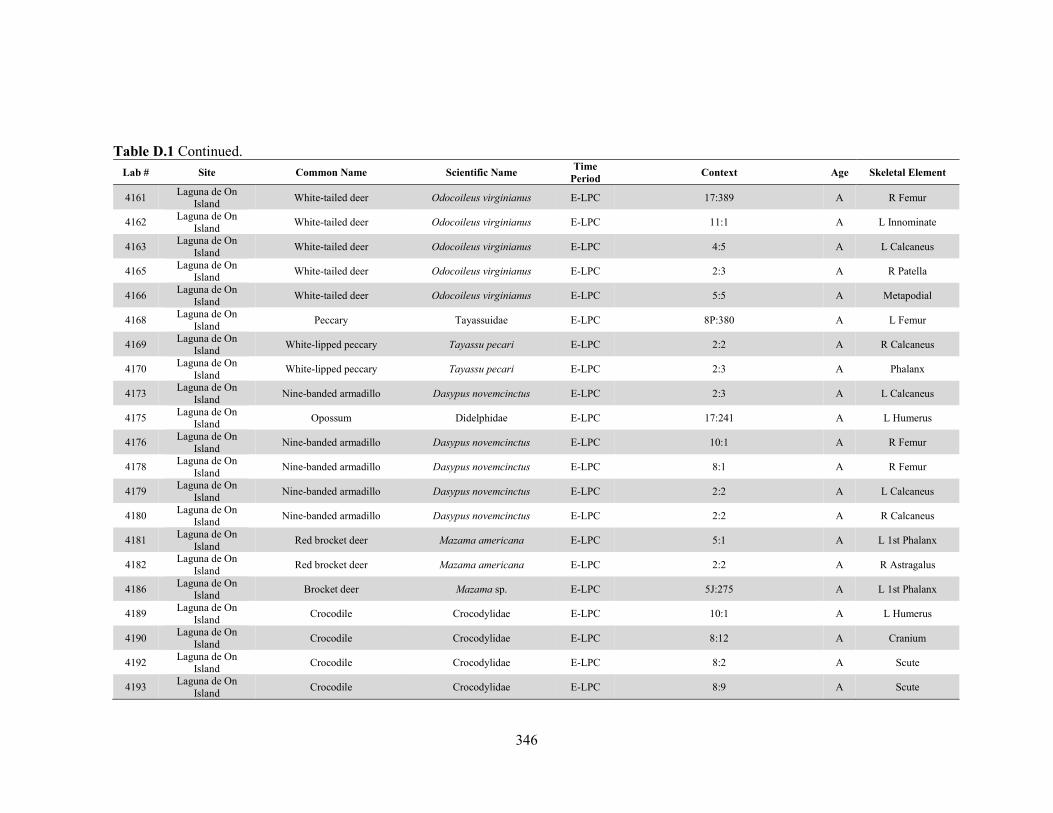
346

Table D.1 Continued. Lab # Site Common Name Scientific Name

Time Period

Context Age Skeletal Element

4161 Laguna de On

Island White-tailed deer Odocoileus virginianus E-LPC 17:389 A R Femur

4162 Laguna de On

Island White-tailed deer Odocoileus virginianus E-LPC 11:1 A L Innominate

4163 Laguna de On

Island White-tailed deer Odocoileus virginianus E-LPC 4:5 A L Calcaneus

4165 Laguna de On

Island White-tailed deer Odocoileus virginianus E-LPC 2:3 A R Patella

4166 Laguna de On

Island White-tailed deer Odocoileus virginianus E-LPC 5:5 A Metapodial

4168 Laguna de On

Island Peccary Tayassuidae E-LPC 8P:380 A L Femur

4169 Laguna de On

Island White-lipped peccary Tayassu pecari E-LPC 2:2 A R Calcaneus

4170 Laguna de On

Island White-lipped peccary Tayassu pecari E-LPC 2:3 A Phalanx

4173 Laguna de On

Island Nine-banded armadillo Dasypus novemcinctus E-LPC 2:3 A L Calcaneus

4175 Laguna de On

Island Opossum Didelphidae E-LPC 17:241 A L Humerus

4176 Laguna de On

Island Nine-banded armadillo Dasypus novemcinctus E-LPC 10:1 A R Femur

4178 Laguna de On

Island Nine-banded armadillo Dasypus novemcinctus E-LPC 8:1 A R Femur

4179 Laguna de On

Island Nine-banded armadillo Dasypus novemcinctus E-LPC 2:2 A L Calcaneus

4180 Laguna de On

Island Nine-banded armadillo Dasypus novemcinctus E-LPC 2:2 A R Calcaneus

4181 Laguna de On

Island Red brocket deer Mazama americana E-LPC 5:1 A L 1st Phalanx

4182 Laguna de On

Island Red brocket deer Mazama americana E-LPC 2:2 A R Astragalus

4186 Laguna de On

Island Brocket deer Mazama sp. E-LPC 5J:275 A L 1st Phalanx

4189 Laguna de On

Island Crocodile Crocodylidae E-LPC 10:1 A L Humerus

4190 Laguna de On

Island Crocodile Crocodylidae E-LPC 8:12 A Cranium

4192 Laguna de On

Island Crocodile Crocodylidae E-LPC 8:2 A Scute

4193 Laguna de On

Island Crocodile Crocodylidae E-LPC 8:9 A Scute

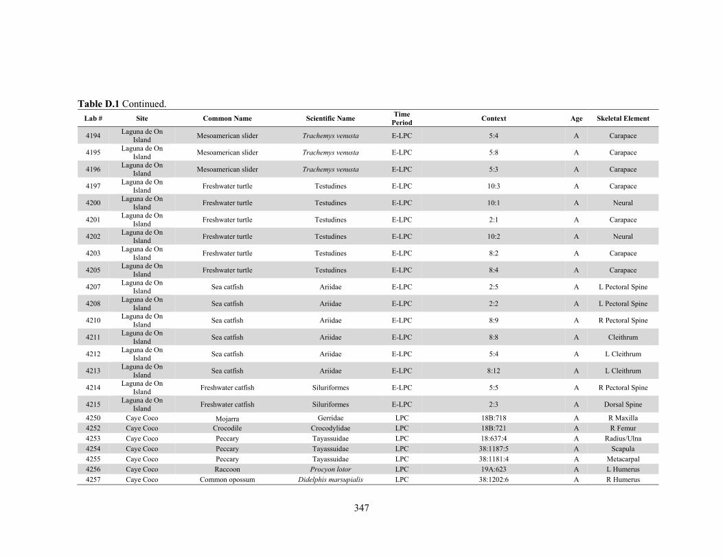
347

Table D.1 Continued. Lab # Site Common Name Scientific Name

Time Period

Context Age Skeletal Element

4194 Laguna de On

Island Mesoamerican slider Trachemys venusta E-LPC 5:4 A Carapace

4195 Laguna de On

Island Mesoamerican slider Trachemys venusta E-LPC 5:8 A Carapace

4196 Laguna de On

Island Mesoamerican slider Trachemys venusta E-LPC 5:3 A Carapace

4197 Laguna de On

Island Freshwater turtle Testudines E-LPC 10:3 A Carapace

4200 Laguna de On

Island Freshwater turtle Testudines E-LPC 10:1 A Neural

4201 Laguna de On

Island Freshwater turtle Testudines E-LPC 2:1 A Carapace

4202 Laguna de On

Island Freshwater turtle Testudines E-LPC 10:2 A Neural

4203 Laguna de On

Island Freshwater turtle Testudines E-LPC 8:2 A Carapace

4205 Laguna de On

Island Freshwater turtle Testudines E-LPC 8:4 A Carapace

4207 Laguna de On

Island Sea catfish Ariidae E-LPC 2:5 A L Pectoral Spine

4208 Laguna de On

Island Sea catfish Ariidae E-LPC 2:2 A L Pectoral Spine

4210 Laguna de On

Island Sea catfish Ariidae E-LPC 8:9 A R Pectoral Spine

4211 Laguna de On

Island Sea catfish Ariidae E-LPC 8:8 A Cleithrum

4212 Laguna de On

Island Sea catfish Ariidae E-LPC 5:4 A L Cleithrum

4213 Laguna de On

Island Sea catfish Ariidae E-LPC 8:12 A L Cleithrum

4214 Laguna de On

Island Freshwater catfish Siluriformes E-LPC 5:5 A R Pectoral Spine

4215 Laguna de On

Island Freshwater catfish Siluriformes E-LPC 2:3 A Dorsal Spine

4250 Caye Coco Mojarra Gerridae LPC 18B:718 A R Maxilla

4252 Caye Coco Crocodile Crocodylidae LPC 18B:721 A R Femur

4253 Caye Coco Peccary Tayassuidae LPC 18:637:4 A Radius/Ulna

4254 Caye Coco Peccary Tayassuidae LPC 38:1187:5 A Scapula

4255 Caye Coco Peccary Tayassuidae LPC 38:1181:4 A Metacarpal

4256 Caye Coco Raccoon Procyon lotor LPC 19A:623 A L Humerus

4257 Caye Coco Common opossum Didelphis marsupialis LPC 38:1202:6 A R Humerus

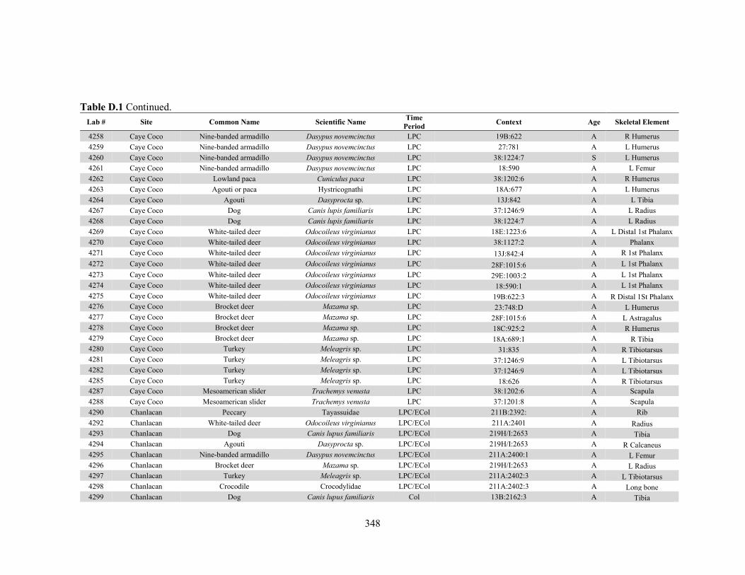
348

Table D.1 Continued. Lab # Site Common Name Scientific Name

Time Period

Context Age Skeletal Element

4258 Caye Coco Nine-banded armadillo Dasypus novemcinctus LPC 19B:622 A R Humerus

4259 Caye Coco Nine-banded armadillo Dasypus novemcinctus LPC 27:781 A L Humerus

4260 Caye Coco Nine-banded armadillo Dasypus novemcinctus LPC 38:1224:7 S L Humerus

4261 Caye Coco Nine-banded armadillo Dasypus novemcinctus LPC 18:590 A L Femur

4262 Caye Coco Lowland paca Cuniculus paca LPC 38:1202:6 A R Humerus

4263 Caye Coco Agouti or paca Hystricognathi LPC 18A:677 A L Humerus

4264 Caye Coco Agouti Dasyprocta sp. LPC 13J:842 A L Tibia

4267 Caye Coco Dog Canis lupis familiaris LPC 37:1246:9 A L Radius

4268 Caye Coco Dog Canis lupis familiaris LPC 38:1224:7 A L Radius

4269 Caye Coco White-tailed deer Odocoileus virginianus LPC 18E:1223:6 A L Distal 1st Phalanx

4270 Caye Coco White-tailed deer Odocoileus virginianus LPC 38:1127:2 A Phalanx

4271 Caye Coco White-tailed deer Odocoileus virginianus LPC 13J:842:4 A R 1st Phalanx

4272 Caye Coco White-tailed deer Odocoileus virginianus LPC 28F:1015:6 A L 1st Phalanx

4273 Caye Coco White-tailed deer Odocoileus virginianus LPC 29E:1003:2 A L 1st Phalanx

4274 Caye Coco White-tailed deer Odocoileus virginianus LPC 18:590:1 A L 1st Phalanx

4275 Caye Coco White-tailed deer Odocoileus virginianus LPC 19B:622:3 A R Distal 1St Phalanx 4276 Caye Coco Brocket deer Mazama sp. LPC 23:748:D A L Humerus 4277 Caye Coco Brocket deer Mazama sp. LPC 28F:1015:6 A L Astragalus 4278 Caye Coco Brocket deer Mazama sp. LPC 18C:925:2 A R Humerus 4279 Caye Coco Brocket deer Mazama sp. LPC 18A:689:1 A R Tibia 4280 Caye Coco Turkey Meleagris sp. LPC 31:835 A R Tibiotarsus 4281 Caye Coco Turkey Meleagris sp. LPC 37:1246:9 A L Tibiotarsus 4282 Caye Coco Turkey Meleagris sp. LPC 37:1246:9 A L Tibiotarsus 4285 Caye Coco Turkey Meleagris sp. LPC 18:626 A R Tibiotarsus 4287 Caye Coco Mesoamerican slider Trachemys venusta LPC 38:1202:6 A Scapula

4288 Caye Coco Mesoamerican slider Trachemys venusta LPC 37:1201:8 A Scapula

4290 Chanlacan Peccary Tayassuidae LPC/ECol 211B:2392: A Rib

4292 Chanlacan White-tailed deer Odocoileus virginianus LPC/ECol 211A:2401 A Radius 4293 Chanlacan Dog Canis lupus familiaris LPC/ECol 219H/I:2653 A Tibia 4294 Chanlacan Agouti Dasyprocta sp. LPC/ECol 219H/I:2653 A R Calcaneus 4295 Chanlacan Nine-banded armadillo Dasypus novemcinctus LPC/ECol 211A:2400:1 A L Femur 4296 Chanlacan Brocket deer Mazama sp. LPC/ECol 219H/I:2653 A L Radius 4297 Chanlacan Turkey Meleagris sp. LPC/ECol 211A:2402:3 A L Tibiotarsus 4298 Chanlacan Crocodile Crocodylidae LPC/ECol 211A:2402:3 A Long bone 4299 Chanlacan Dog Canis lupus familiaris Col 13B:2162:3 A Tibia

349

Table D.1 Continued. Lab # Site Common Name Scientific Name

Time Period

Context Age Skeletal Element

4300 Chanlacan Rabbit Leporidae Col 1A:6 A Humerus 4301 Chanlacan Nine-banded armadillo Dasypus novemcinctus Col 1A:6 A Ulna 4302 Chanlacan Nine-banded armadillo Dasypus novemcinctus Col 13B:2157:2 A L Femur 4303 Chanlacan White-tailed deer Odocoileus virginianus TC 1A:2000 A Phalanx 4304 Chanlacan Brocket deer Mazama sp. Col 13C:2175:3 A Metacarpal 4305 Chanlacan Peccary Tayassuidae Col 13E:2244:4 A Distal Metapodial 4306 Chanlacan Peccary Tayassuidae Col 13C:2175:3 A Scapula 4307 Chanlacan Turkey Meleagris sp. Col 1E:2022 A Tarsometatarsus 4308 Chanlacan Pond turtle Emydidae Col 1E:2022 A Os coxa 4311 Chanlacan White-tailed deer Odocoileus virginianus PC 915A:2802:3 A 1st Phalanx

4309 Laguna de On

Shore Nine-banded armadillo Dasypus novemcinctus C 3:1B A Maxilla

4312 Caye Muerto White-tailed deer Odocoileus virginianus EPC 5:3008 A Fragment

4313 Caye Muerto Turkey Meleagris sp. EPC 5:2014 A L Tibiotarsus

4314 Caye Muerto Crocodile Crocodylidae EPC 5:3011 A Cranium

4315 Nakum cf. White-tailed deer cf. Odocoileus virginianus TC VI-20-3-3 A Ulna

4316 Nakum cf. White-tailed deer cf. Odocoileus virginianus TC VI-21-6-2 A L Humerus

4317 Nakum cf. White-tailed deer cf. Odocoileus virginianus L-TC III-5-2-2 A Metacarpal 4318 Nakum Mesoamerican Slider Trachemys venusta TC VI-22-5 A Femur 4319 Nakum cf. White-tailed deer cf. Odocoileus virginianus TC VI-4-2-4 A Metacarpal 4320 Nakum White-tailed deer Odocoileus virginianus TC VI-28-8-4 A Tibia 4322 Nakum Deer Cervidae TC VI-22-5 S Mandible 4323 Nakum White-tailed deer Odocoileus virginianus LC VI-12-1 A Tibia 4324 Nakum Deer Cervidae LC VI-22-1-7 A Mandible 4325 Nakum White-tailed deer Odocoileus virginianus LC VI-2-6 A Metacarpal 4326 Nakum cf. White-tailed deer cf. Odocoileus virginianus EC VI-31A-12-3 A Long Bone 4327 Nakum Brocket deer Mazama sp. ProtoC VI-6A-2 A Cranium 4328 Nakum cf. White-tailed deer cf. Odocoileus virginianus TC VI-28-2-7 A L Innominate 4329 Nakum White-tailed deer Odocoileus virginianus TC XIII-3-1-9 A Scapula 4330 Nakum Turkey Meleagris sp. TC VI-22-5-1 A Tibiotarsus 4331 Nakum Deer Cervidae TC VI-20-2-5 A Metacarpal 4332 Nakum Deer Cervidae LC VI-20-2-4 A Metacarpal 4519 Vista Alegre Loggerhead sea turtle Caretta PC 3A-3-2 A Neural

4520 Vista Alegre Red brocket deer Mazama americana PC 3A-3-2 A Astragalus

4521 Vista Alegre Ocellated turkey Meleagris ocellata PC 3A-3-2 A Femur

350

Table D.1 Continued. Lab # Site Common Name Scientific Name

Time Period

Context Age Skeletal Element

4522 Vista Alegre Atlantic snapper Lutjanidae PC 3A-6-1 A Caudal Vertebra

4523 Vista Alegre Mesoamerican slider Trachemys venusta PC 3A-6-1 A Long Bone

4524 Vista Alegre Limpkin Aramus guarauna PC 3A-6-1 A Tibiotarsus

4525 Vista Alegre Ocellated turkey Meleagris ocellata PC 3A-6-1 A Tarsometatarsus

4526 Vista Alegre Limpkin Aramus guarauna PC 3A-6-1 A Tibiotarsus

4527 Vista Alegre Brocket deer Mazama sp. PC 3A-6-1 A Mandible

4528 Vista Alegre Loggerhead sea turtle Caretta caretta PC 3A-6-1 A Rib

4529 Vista Alegre Limpkin Aramus guarauna PC 3A-7-1 A Tibiotarsus

4530 Vista Alegre White-tailed deer Odocoileus virginianus PC 3A-7-2 A Femur

4531 Vista Alegre Crevalle jack Caranx hippos PC 3A-7-3 A Vertebra

4532 Vista Alegre Limpkin Aramus guarauna PC 3A-7-4 A Tibiotarsus

4533 Vista Alegre White-tailed deer Odocoileus virginianus PC 1:Pozo2:3 A Phalanx

4534 Vista Alegre Loggerhead sea turtle Caretta caretta PC 1:Pozo2:3 A Fibula

4535 Vista Alegre White-tailed deer Odocoileus virginianus PC 3B-2-1 A Phalanx

4536 Vista Alegre Ocellated turkey Meleagris ocellata PC 3B-2-1 A Femur

4537 Vista Alegre Ocellated turkey Meleagris ocellata PC 3B-2-1 A Femur

4539 Oxtankah Lowland paca Cuniculus paca EC Chultun 1 Level II A Mandible

4540 Oxtankah Central American agouti Dasyprocta punctata EC Chultun 1 Level II A Mandible

4541 Oxtankah Central American agouti Dasyprocta punctata EC Chultun 1 Level II A Cranium

4542 Oxtankah Virginia opossum Didelphis virginiana EC Chultun 1 Level III A Mandible

4544 Oxtankah Grey four-eyed opossum Philander opossum EC Chultun 1 Level II A Mandible

4545 Oxtankah Brocket deer Mazama sp. EC Chultun 1 Level II A Astragalus

4546 Oxtankah White-tailed deer Odocoileus virginianus EC Chultun 1 Level II A Phalanx

4549 Oxtankah Marine mammal Mammalia EC Chultun 1 Level II A Rib

4551 Ichpaatun Nine-banded armadillo Dasypus novemcinctus PC C5 A Femur

4553 Ichpaatun Loggerhead sea turtle Caretta caretta PC B:4 A Scapula

4554 San Miguelito Brocket deer Mazama sp. PC 2M A Mandible

4555 San Miguelito White-tailed deer Odocoileus virginianus PC 45 A Humerus

4563 Caracol White-tailed deer Odocoileus virginianus TC CD 3A/16B4 s. wall A L Mandible

4564 Caracol White-tailed deer Odocoileus virginianus TC CD 3A/27 B4 s. wall A R Mandible

4584 Xunantunich Turkey Meleagris sp. LC Op. 196 J123 Deposit 2 Tunnel in Castillo A L Ulna

4585 Xunantunich White-tailed deer Odocoileus virginianus LC Op. 141 K/5 A&A17 Intersection A L Humerus

4586 Xunantunich Collared Peccary Pecari tajacu LC Op. 1E 7/6 x41b A R Radius

4587 Tayasal Central American river turtle Dermatemys mawii PC/Col T33 2042-1391 *1)#510 A Plastron

4588 Tayasal Brocket deer Mazama sp. PC/Col T52 1875-1747 n. 2 #3271 A Metacarpal

351

Table D.1 Continued. Lab # Site Common Name Scientific Name

Time Period

Context Age Skeletal Element

4589 Tayasal White-tailed deer Odocoileus virginianus PC/Col T52 1879-1750 (2) A Metacarpal

4590 Tayasal Collared peccary Pecari tajacu PC/Col T52 n2 #360 A Humerus

4591 Tayasal Mexican musk turtle Staurotypus triporcatus PC/Col T53 n. 2 1874-1734 A Costal

Time periods: PreC=Preclassic; LPreC=Late Preclassic; ProtoC=ProtoClassic; C=Classic; EC=Early Classic; E-LC=Early to Late Classic Transition; LC=Late Classic; L-TC=Late to Terminal Classic; TC=Terminal Classic; PC=Postclassic; EPC=Early Postclassic; E-LPC=Early to Late Postclassic Transition; LPC=Late Postclassic; PC-Col=Postclassic to Colonial Transition; Col=Colonial; ECol=Early Colonial Age: A=Adult; S=Subadult Skeletal Element: L=Left; R=Right

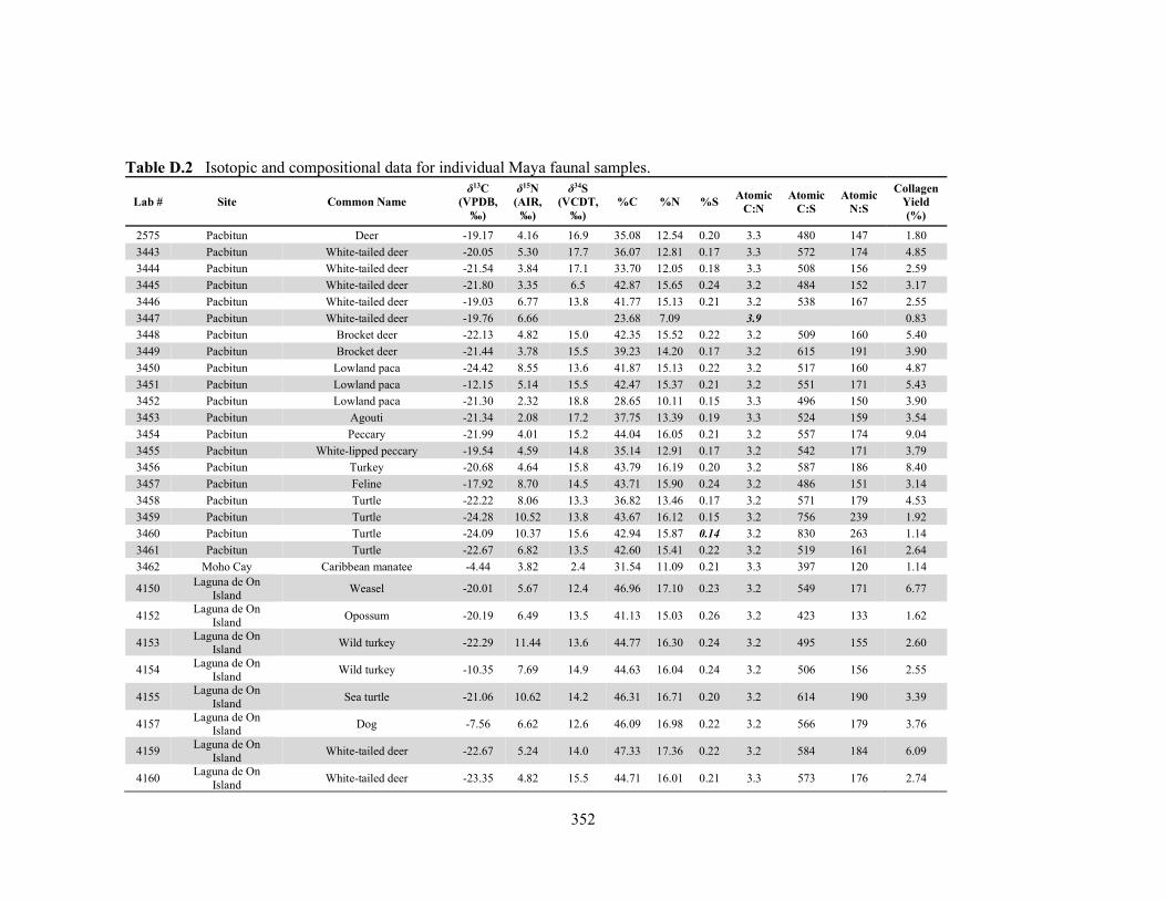
352

Table D.2 Isotopic and compositional data for individual Maya faunal samples.

Lab # Site Common Name δ13C

(VPDB, ‰)

δ15N (AIR,

‰)

δ34S (VCDT,

‰) %C %N %S

Atomic C:N

Atomic C:S

Atomic N:S

Collagen Yield (%)

2575 Pacbitun Deer -19.17 4.16 16.9 35.08 12.54 0.20 3.3 480 147 1.80

3443 Pacbitun White-tailed deer -20.05 5.30 17.7 36.07 12.81 0.17 3.3 572 174 4.85

3444 Pacbitun White-tailed deer -21.54 3.84 17.1 33.70 12.05 0.18 3.3 508 156 2.59

3445 Pacbitun White-tailed deer -21.80 3.35 6.5 42.87 15.65 0.24 3.2 484 152 3.17

3446 Pacbitun White-tailed deer -19.03 6.77 13.8 41.77 15.13 0.21 3.2 538 167 2.55

3447 Pacbitun White-tailed deer -19.76 6.66 23.68 7.09 3.9 0.83

3448 Pacbitun Brocket deer -22.13 4.82 15.0 42.35 15.52 0.22 3.2 509 160 5.40

3449 Pacbitun Brocket deer -21.44 3.78 15.5 39.23 14.20 0.17 3.2 615 191 3.90

3450 Pacbitun Lowland paca -24.42 8.55 13.6 41.87 15.13 0.22 3.2 517 160 4.87

3451 Pacbitun Lowland paca -12.15 5.14 15.5 42.47 15.37 0.21 3.2 551 171 5.43

3452 Pacbitun Lowland paca -21.30 2.32 18.8 28.65 10.11 0.15 3.3 496 150 3.90

3453 Pacbitun Agouti -21.34 2.08 17.2 37.75 13.39 0.19 3.3 524 159 3.54

3454 Pacbitun Peccary -21.99 4.01 15.2 44.04 16.05 0.21 3.2 557 174 9.04

3455 Pacbitun White-lipped peccary -19.54 4.59 14.8 35.14 12.91 0.17 3.2 542 171 3.79

3456 Pacbitun Turkey -20.68 4.64 15.8 43.79 16.19 0.20 3.2 587 186 8.40

3457 Pacbitun Feline -17.92 8.70 14.5 43.71 15.90 0.24 3.2 486 151 3.14

3458 Pacbitun Turtle -22.22 8.06 13.3 36.82 13.46 0.17 3.2 571 179 4.53

3459 Pacbitun Turtle -24.28 10.52 13.8 43.67 16.12 0.15 3.2 756 239 1.92

3460 Pacbitun Turtle -24.09 10.37 15.6 42.94 15.87 0.14 3.2 830 263 1.14

3461 Pacbitun Turtle -22.67 6.82 13.5 42.60 15.41 0.22 3.2 519 161 2.64

3462 Moho Cay Caribbean manatee -4.44 3.82 2.4 31.54 11.09 0.21 3.3 397 120 1.14

4150 Laguna de On

Island Weasel -20.01 5.67 12.4 46.96 17.10 0.23 3.2 549 171 6.77

4152 Laguna de On

Island Opossum -20.19 6.49 13.5 41.13 15.03 0.26 3.2 423 133 1.62

4153 Laguna de On

Island Wild turkey -22.29 11.44 13.6 44.77 16.30 0.24 3.2 495 155 2.60

4154 Laguna de On

Island Wild turkey -10.35 7.69 14.9 44.63 16.04 0.24 3.2 506 156 2.55

4155 Laguna de On

Island Sea turtle -21.06 10.62 14.2 46.31 16.71 0.20 3.2 614 190 3.39

4157 Laguna de On

Island Dog -7.56 6.62 12.6 46.09 16.98 0.22 3.2 566 179 3.76

4159 Laguna de On

Island White-tailed deer -22.67 5.24 14.0 47.33 17.36 0.22 3.2 584 184 6.09

4160 Laguna de On

Island White-tailed deer -23.35 4.82 15.5 44.71 16.01 0.21 3.3 573 176 2.74

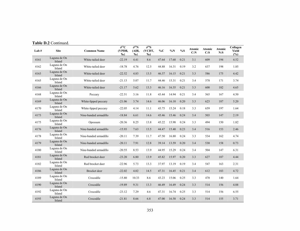
353

Table D.2 Continued.

Lab # Site Common Name δ13C

(VPDB, ‰)

δ15N (AIR,

‰)

δ34S (VCDT,

‰) %C %N %S

Atomic C:N

Atomic C:S

Atomic N:S

Collagen Yield (%)

4161 Laguna de On

Island White-tailed deer -22.19 4.41 8.6 47.64 17.68 0.21 3.1 609 194 4.52

4162 Laguna de On

Island White-tailed deer -18.78 4.76 12.5 44.88 16.31 0.19 3.2 637 198 1.85

4163 Laguna de On

Island White-tailed deer -22.52 4.83 13.5 46.37 16.15 0.21 3.3 586 175 4.42

4165 Laguna de On

Island White-tailed deer -21.13 5.07 11.7 44.46 15.31 0.21 3.4 578 171 3.74

4166 Laguna de On

Island White-tailed deer -21.17 5.62 13.3 46.16 16.35 0.21 3.3 600 182 4.65

4168 Laguna de On

Island Peccary -22.51 3.16 11.8 43.44 14.94 0.21 3.4 565 167 4.50

4169 Laguna de On

Island White-lipped peccary -21.06 3.74 14.6 46.06 16.10 0.20 3.3 623 187 5.20

4170 Laguna de On

Island White-lipped peccary -22.05 4.14 11.1 43.75 15.24 0.18 3.3 659 197 1.64

4173 Laguna de On

Island Nine-banded armadillo -18.84 6.61 14.6 45.46 15.46 0.24 3.4 503 147 2.19

4175 Laguna de On

Island Opossum -20.36 8.25 13.8 45.22 15.98 0.24 3.3 494 150 1.82

4176 Laguna de On

Island Nine-banded armadillo -15.93 7.63 13.5 44.47 15.40 0.23 3.4 516 153 2.46

4178 Laguna de On

Island Nine-banded armadillo -20.11 7.39 11.7 47.50 16.80 0.24 3.3 534 162 4.74

4179 Laguna de On

Island Nine-banded armadillo -20.11 7.91 12.8 39.14 13.59 0.20 3.4 530 158 0.73

4180 Laguna de On

Island Nine-banded armadillo -20.55 8.53 13.9 44.95 15.29 0.24 3.4 504 147 6.31

4181 Laguna de On

Island Red brocket deer -23.20 6.80 13.9 45.82 15.97 0.20 3.3 627 187 4.44

4182 Laguna de On

Island Red brocket deer -22.96 5.73 13.3 37.97 13.19 0.19 3.4 547 163 2.31

4186 Laguna de On

Island Brocket deer -22.02 4.02 14.5 47.31 16.45 0.21 3.4 612 183 4.72

4189 Laguna de On

Island Crocodile -15.80 10.33 8.6 43.23 15.06 0.25 3.3 470 140 1.64

4190 Laguna de On

Island Crocodile -19.89 9.31 13.3 46.49 16.49 0.24 3.3 514 156 4.88

4192 Laguna de On

Island Crocodile -23.12 7.29 4.6 47.31 16.74 0.25 3.3 514 156 6.55

4193 Laguna de On

Island Crocodile -21.81 8.66 6.8 47.00 16.58 0.24 3.3 514 155 3.71

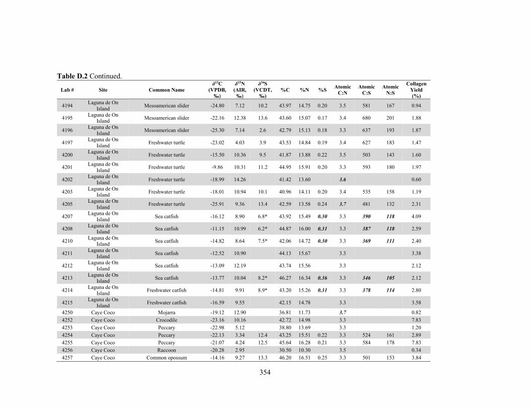
354

Table D.2 Continued.

Lab # Site Common Name δ13C

(VPDB, ‰)

δ15N (AIR,

‰)

δ34S (VCDT,

‰) %C %N %S

Atomic C:N

Atomic C:S

Atomic N:S

Collagen Yield (%)

4194 Laguna de On

Island Mesoamerican slider -24.80 7.12 10.2 43.97 14.75 0.20 3.5 581 167 0.94

4195 Laguna de On

Island Mesoamerican slider -22.16 12.38 13.6 43.60 15.07 0.17 3.4 680 201 1.88

4196 Laguna de On

Island Mesoamerican slider -25.30 7.14 2.6 42.79 15.13 0.18 3.3 637 193 1.87

4197 Laguna de On

Island Freshwater turtle -23.02 4.03 3.9 43.53 14.84 0.19 3.4 627 183 1.47

4200 Laguna de On

Island Freshwater turtle -15.50 10.36 9.5 41.87 13.88 0.22 3.5 503 143 1.60

4201 Laguna de On

Island Freshwater turtle -9.86 10.31 11.2 44.95 15.91 0.20 3.3 593 180 1.97

4202 Laguna de On

Island Freshwater turtle -18.99 14.26 41.42 13.60 3.6 0.60

4203 Laguna de On

Island Freshwater turtle -18.01 10.94 10.1 40.96 14.11 0.20 3.4 535 158 1.19

4205 Laguna de On

Island Freshwater turtle -25.91 9.36 13.4 42.59 13.58 0.24 3.7 481 132 2.31

4207 Laguna de On

Island Sea catfish -16.12 8.90 6.8* 43.92 15.49 0.30 3.3 390 118 4.09

4208 Laguna de On

Island Sea catfish -11.15 10.99 6.2* 44.87 16.00 0.31 3.3 387 118 2.59

4210 Laguna de On

Island Sea catfish -14.82 8.64 7.5* 42.06 14.72 0.30 3.3 369 111 2.40

4211 Laguna de On

Island Sea catfish -12.52 10.90 44.13 15.67 3.3 3.38

4212 Laguna de On

Island Sea catfish -13.09 12.19 43.74 15.56 3.3 2.12

4213 Laguna de On

Island Sea catfish -13.77 10.04 8.2* 46.27 16.34 0.36 3.3 346 105 2.12

4214 Laguna de On

Island Freshwater catfish -14.81 9.91 8.9* 43.20 15.26 0.31 3.3 378 114 2.80

4215 Laguna de On

Island Freshwater catfish -16.59 9.55 42.15 14.78 3.3 3.58

4250 Caye Coco Mojarra -19.12 12.90 36.81 11.73 3.7 0.82

4252 Caye Coco Crocodile -23.16 10.16 42.72 14.98 3.3 7.83

4253 Caye Coco Peccary -22.98 5.12 38.80 13.69 3.3 1.20

4254 Caye Coco Peccary -22.13 3.34 12.4 43.25 15.51 0.22 3.3 524 161 2.89

4255 Caye Coco Peccary -21.07 4.24 12.5 45.64 16.28 0.21 3.3 584 178 7.83

4256 Caye Coco Raccoon -20.28 2.95 30.50 10.30 3.5 0.34

4257 Caye Coco Common opossum -14.16 9.27 13.3 46.20 16.51 0.25 3.3 501 153 3.84

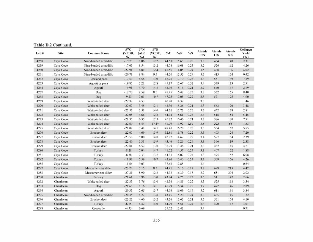
355

Table D.2 Continued.

Lab # Site Common Name δ13C

(VPDB, ‰)

δ15N (AIR,

‰)

δ34S (VCDT,

‰) %C %N %S

Atomic C:N

Atomic C:S

Atomic N:S

Collagen Yield (%)

4258 Caye Coco Nine-banded armadillo -19.78 8.06 12.2 44.53 15.63 0.26 3.3 464 140 2.31

4259 Caye Coco Nine-banded armadillo -17.03 8.54 13.2 44.78 16.08 0.23 3.2 526 162 4.26

4260 Caye Coco Nine-banded armadillo -22.91 6.81 12.4 41.55 14.05 0.24 3.5 468 136 4.02

4261 Caye Coco Nine-banded armadillo -20.71 8.84 9.5 44.20 15.55 0.29 3.3 413 124 0.42

4262 Caye Coco Lowland paca -17.50 6.58 13.0 47.75 17.10 0.23 3.3 551 169 7.59

4263 Caye Coco Agouti or paca -19.87 5.21 12.8 45.17 15.67 0.32 3.4 379 113 2.91

4264 Caye Coco Agouti -19.91 4.70 14.8 42.09 15.16 0.21 3.2 540 167 2.19

4267 Caye Coco Dog -12.70 9.59 8.5 45.45 16.42 0.23 3.2 532 165 8.40

4268 Caye Coco Dog -9.23 7.61 10.7 47.75 17.05 0.22 3.3 571 175 4.90

4269 Caye Coco White-tailed deer -22.32 4.53 40.90 14.39 3.3 1.46

4270 Caye Coco White-tailed deer -22.62 3.45 12.1 43.30 15.26 0.21 3.3 562 170 3.48

4271 Caye Coco White-tailed deer -22.52 3.51 14.0 44.21 15.73 0.26 3.3 452 138 2.81

4272 Caye Coco White-tailed deer -22.08 4.66 12.2 44.94 15.61 0.23 3.4 518 154 5.45

4273 Caye Coco White-tailed deer -21.35 6.35 12.3 45.82 16.46 0.21 3.2 586 180 7.91

4274 Caye Coco White-tailed deer -22.60 5.44 17.1* 41.79 13.92 0.50 3.5 222 63 1.53

4275 Caye Coco White-tailed deer -21.02 7.41 14.1 47.41 16.70 0.23 3.3 554 167 5.85

4276 Caye Coco Brocket deer -22.67 4.69 13.9 32.81 11.78 0.22 3.3 403 124 7.20

4277 Caye Coco Brocket deer -23.50 5.00 14.0 42.92 14.62 0.22 3.4 527 154 2.39

4278 Caye Coco Brocket deer -22.40 5.33 15.9 43.46 15.26 0.29 3.3 396 119 2.38

4279 Caye Coco Brocket deer -22.81 6.52 13.0 38.29 13.48 0.21 3.3 482 145 4.21

4280 Caye Coco Turkey -8.28 7.04 14.7 41.52 14.57 0.27 3.3 407 122 1.88

4281 Caye Coco Turkey -8.38 7.33 13.7 44.91 16.07 0.24 3.3 495 152 6.08

4282 Caye Coco Turkey -11.93 7.59 10.7 45.80 16.40 0.24 3.3 509 156 4.26

4285 Caye Coco Turkey -11.66 9.03 37.68 12.85 3.4 0.64

4287 Caye Coco Mesoamerican slider -23.23 7.15 8.5 44.41 16.16 0.17 3.2 689 215 4.42

4288 Caye Coco Mesoamerican slider -27.21 8.90 12.3 44.93 16.39 0.18 3.2 651 204 2.92

4290 Chanlacan Peccary -21.61 3.96 13.0 43.84 14.75 0.23 3.5 511 147 2.66

4292 Chanlacan White-tailed deer -22.33 3.76 13.0 42.34 14.85 0.22 3.3 525 158 3.54

4293 Chanlacan Dog -21.68 8.16 3.0 45.29 16.34 0.26 3.2 472 146 2.89

4294 Chanlacan Agouti -20.33 2.65 13.7 44.08 16.09 0.19 3.2 611 191 3.84

4295 Chanlacan Nine-banded armadillo -20.35 8.22 13.8 43.45 15.20 0.24 3.3 485 145 1.72

4296 Chanlacan Brocket deer -23.25 4.60 13.2 43.36 15.65 0.21 3.2 561 174 4.10

4297 Chanlacan Turkey -6.75 6.42 14.0 44.29 15.51 0.24 3.3 490 147 3.01

4298 Chanlacan Crocodile -4.33 6.69 35.72 12.42 3.4 0.71

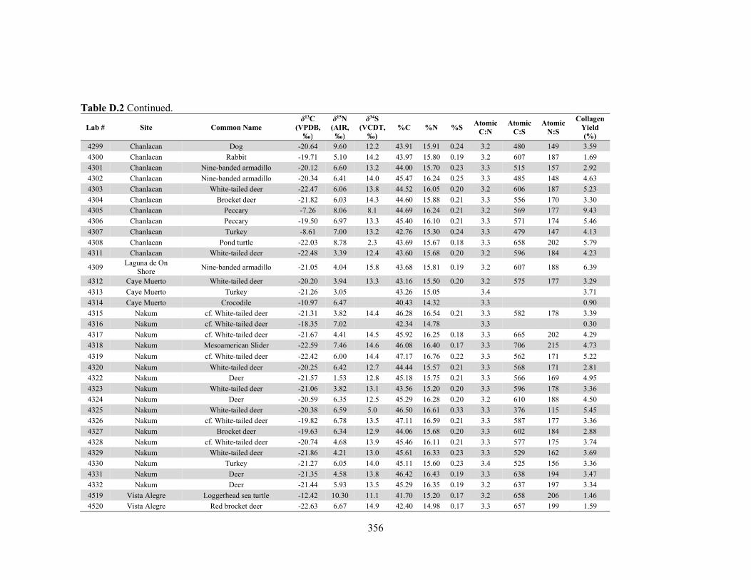
356

Table D.2 Continued.

Lab # Site Common Name δ13C

(VPDB, ‰)

δ15N (AIR,

‰)

δ34S (VCDT,

‰) %C %N %S

Atomic C:N

Atomic C:S

Atomic N:S

Collagen Yield (%)

4299 Chanlacan Dog -20.64 9.60 12.2 43.91 15.91 0.24 3.2 480 149 3.59

4300 Chanlacan Rabbit -19.71 5.10 14.2 43.97 15.80 0.19 3.2 607 187 1.69

4301 Chanlacan Nine-banded armadillo -20.12 6.60 13.2 44.00 15.70 0.23 3.3 515 157 2.92

4302 Chanlacan Nine-banded armadillo -20.34 6.41 14.0 45.47 16.24 0.25 3.3 485 148 4.63

4303 Chanlacan White-tailed deer -22.47 6.06 13.8 44.52 16.05 0.20 3.2 606 187 5.23

4304 Chanlacan Brocket deer -21.82 6.03 14.3 44.60 15.88 0.21 3.3 556 170 3.30

4305 Chanlacan Peccary -7.26 8.06 8.1 44.69 16.24 0.21 3.2 569 177 9.43

4306 Chanlacan Peccary -19.50 6.97 13.3 45.40 16.10 0.21 3.3 571 174 5.46

4307 Chanlacan Turkey -8.61 7.00 13.2 42.76 15.30 0.24 3.3 479 147 4.13

4308 Chanlacan Pond turtle -22.03 8.78 2.3 43.69 15.67 0.18 3.3 658 202 5.79

4311 Chanlacan White-tailed deer -22.48 3.39 12.4 43.60 15.68 0.20 3.2 596 184 4.23

4309 Laguna de On

Shore Nine-banded armadillo -21.05 4.04 15.8 43.68 15.81 0.19 3.2 607 188 6.39

4312 Caye Muerto White-tailed deer -20.20 3.94 13.3 43.16 15.50 0.20 3.2 575 177 3.29

4313 Caye Muerto Turkey -21.26 3.05 43.26 15.05 3.4 3.71

4314 Caye Muerto Crocodile -10.97 6.47 40.43 14.32 3.3 0.90

4315 Nakum cf. White-tailed deer -21.31 3.82 14.4 46.28 16.54 0.21 3.3 582 178 3.39

4316 Nakum cf. White-tailed deer -18.35 7.02 42.34 14.78 3.3 0.30

4317 Nakum cf. White-tailed deer -21.67 4.41 14.5 45.92 16.25 0.18 3.3 665 202 4.29

4318 Nakum Mesoamerican Slider -22.59 7.46 14.6 46.08 16.40 0.17 3.3 706 215 4.73

4319 Nakum cf. White-tailed deer -22.42 6.00 14.4 47.17 16.76 0.22 3.3 562 171 5.22

4320 Nakum White-tailed deer -20.25 6.42 12.7 44.44 15.57 0.21 3.3 568 171 2.81

4322 Nakum Deer -21.57 1.53 12.8 45.18 15.75 0.21 3.3 566 169 4.95

4323 Nakum White-tailed deer -21.06 3.82 13.1 43.56 15.20 0.20 3.3 596 178 3.36

4324 Nakum Deer -20.59 6.35 12.5 45.29 16.28 0.20 3.2 610 188 4.50

4325 Nakum White-tailed deer -20.38 6.59 5.0 46.50 16.61 0.33 3.3 376 115 5.45

4326 Nakum cf. White-tailed deer -19.82 6.78 13.5 47.11 16.59 0.21 3.3 587 177 3.36

4327 Nakum Brocket deer -19.63 6.34 12.9 44.06 15.68 0.20 3.3 602 184 2.88

4328 Nakum cf. White-tailed deer -20.74 4.68 13.9 45.46 16.11 0.21 3.3 577 175 3.74

4329 Nakum White-tailed deer -21.86 4.21 13.0 45.61 16.33 0.23 3.3 529 162 3.69

4330 Nakum Turkey -21.27 6.05 14.0 45.11 15.60 0.23 3.4 525 156 3.36

4331 Nakum Deer -21.35 4.58 13.8 46.42 16.43 0.19 3.3 638 194 3.47

4332 Nakum Deer -21.44 5.93 13.5 45.29 16.35 0.19 3.2 637 197 3.34

4519 Vista Alegre Loggerhead sea turtle -12.42 10.30 11.1 41.70 15.20 0.17 3.2 658 206 1.46

4520 Vista Alegre Red brocket deer -22.63 6.67 14.9 42.40 14.98 0.17 3.3 657 199 1.59

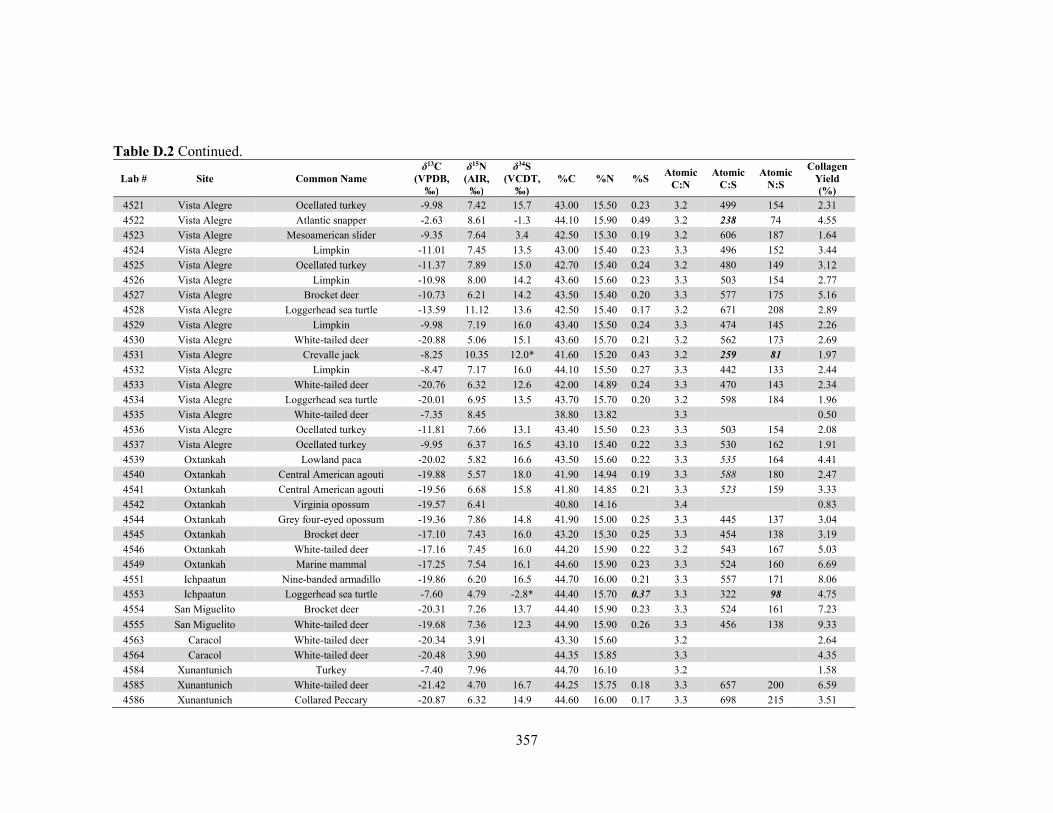
357

Table D.2 Continued.

Lab # Site Common Name δ13C

(VPDB, ‰)

δ15N (AIR,

‰)

δ34S (VCDT,

‰) %C %N %S

Atomic C:N

Atomic C:S

Atomic N:S

Collagen Yield (%)

4521 Vista Alegre Ocellated turkey -9.98 7.42 15.7 43.00 15.50 0.23 3.2 499 154 2.31

4522 Vista Alegre Atlantic snapper -2.63 8.61 -1.3 44.10 15.90 0.49 3.2 238 74 4.55

4523 Vista Alegre Mesoamerican slider -9.35 7.64 3.4 42.50 15.30 0.19 3.2 606 187 1.64

4524 Vista Alegre Limpkin -11.01 7.45 13.5 43.00 15.40 0.23 3.3 496 152 3.44

4525 Vista Alegre Ocellated turkey -11.37 7.89 15.0 42.70 15.40 0.24 3.2 480 149 3.12

4526 Vista Alegre Limpkin -10.98 8.00 14.2 43.60 15.60 0.23 3.3 503 154 2.77

4527 Vista Alegre Brocket deer -10.73 6.21 14.2 43.50 15.40 0.20 3.3 577 175 5.16

4528 Vista Alegre Loggerhead sea turtle -13.59 11.12 13.6 42.50 15.40 0.17 3.2 671 208 2.89

4529 Vista Alegre Limpkin -9.98 7.19 16.0 43.40 15.50 0.24 3.3 474 145 2.26

4530 Vista Alegre White-tailed deer -20.88 5.06 15.1 43.60 15.70 0.21 3.2 562 173 2.69

4531 Vista Alegre Crevalle jack -8.25 10.35 12.0* 41.60 15.20 0.43 3.2 259 81 1.97

4532 Vista Alegre Limpkin -8.47 7.17 16.0 44.10 15.50 0.27 3.3 442 133 2.44

4533 Vista Alegre White-tailed deer -20.76 6.32 12.6 42.00 14.89 0.24 3.3 470 143 2.34

4534 Vista Alegre Loggerhead sea turtle -20.01 6.95 13.5 43.70 15.70 0.20 3.2 598 184 1.96

4535 Vista Alegre White-tailed deer -7.35 8.45 38.80 13.82 3.3 0.50

4536 Vista Alegre Ocellated turkey -11.81 7.66 13.1 43.40 15.50 0.23 3.3 503 154 2.08

4537 Vista Alegre Ocellated turkey -9.95 6.37 16.5 43.10 15.40 0.22 3.3 530 162 1.91

4539 Oxtankah Lowland paca -20.02 5.82 16.6 43.50 15.60 0.22 3.3 535 164 4.41

4540 Oxtankah Central American agouti -19.88 5.57 18.0 41.90 14.94 0.19 3.3 588 180 2.47

4541 Oxtankah Central American agouti -19.56 6.68 15.8 41.80 14.85 0.21 3.3 523 159 3.33

4542 Oxtankah Virginia opossum -19.57 6.41 40.80 14.16 3.4 0.83

4544 Oxtankah Grey four-eyed opossum -19.36 7.86 14.8 41.90 15.00 0.25 3.3 445 137 3.04

4545 Oxtankah Brocket deer -17.10 7.43 16.0 43.20 15.30 0.25 3.3 454 138 3.19

4546 Oxtankah White-tailed deer -17.16 7.45 16.0 44.20 15.90 0.22 3.2 543 167 5.03

4549 Oxtankah Marine mammal -17.25 7.54 16.1 44.60 15.90 0.23 3.3 524 160 6.69

4551 Ichpaatun Nine-banded armadillo -19.86 6.20 16.5 44.70 16.00 0.21 3.3 557 171 8.06

4553 Ichpaatun Loggerhead sea turtle -7.60 4.79 -2.8* 44.40 15.70 0.37 3.3 322 98 4.75

4554 San Miguelito Brocket deer -20.31 7.26 13.7 44.40 15.90 0.23 3.3 524 161 7.23

4555 San Miguelito White-tailed deer -19.68 7.36 12.3 44.90 15.90 0.26 3.3 456 138 9.33

4563 Caracol White-tailed deer -20.34 3.91 43.30 15.60 3.2 2.64

4564 Caracol White-tailed deer -20.48 3.90 44.35 15.85 3.3 4.35

4584 Xunantunich Turkey -7.40 7.96 44.70 16.10 3.2 1.58

4585 Xunantunich White-tailed deer -21.42 4.70 16.7 44.25 15.75 0.18 3.3 657 200 6.59

4586 Xunantunich Collared Peccary -20.87 6.32 14.9 44.60 16.00 0.17 3.3 698 215 3.51

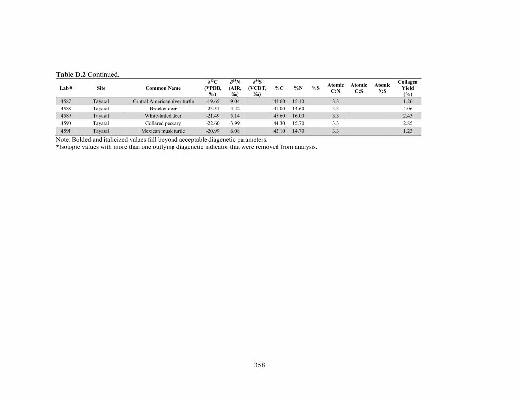
358

Table D.2 Continued.

Lab # Site Common Name δ13C

(VPDB, ‰)

δ15N (AIR,

‰)

δ34S (VCDT,

‰) %C %N %S

Atomic C:N

Atomic C:S

Atomic N:S

Collagen Yield (%)

4587 Tayasal Central American river turtle -19.65 9.04 42.60 15.10 3.3 1.26

4588 Tayasal Brocket deer -23.51 4.42 41.00 14.60 3.3 4.06

4589 Tayasal White-tailed deer -21.49 5.14 45.60 16.00 3.3 2.43

4590 Tayasal Collared peccary -22.60 3.99 44.30 15.70 3.3 2.85

4591 Tayasal Mexican musk turtle -20.99 6.08 42.10 14.70 3.3 1.23

Note: Bolded and italicized values fall beyond acceptable diagenetic parameters. *Isotopic values with more than one outlying diagenetic indicator that were removed from analysis.

359

APPENDIX E

OSTEOLOGICAL, CONTEXTUAL, AND ISOTOPIC DATA FOR

THE MAYA HUMAN SAMPLES

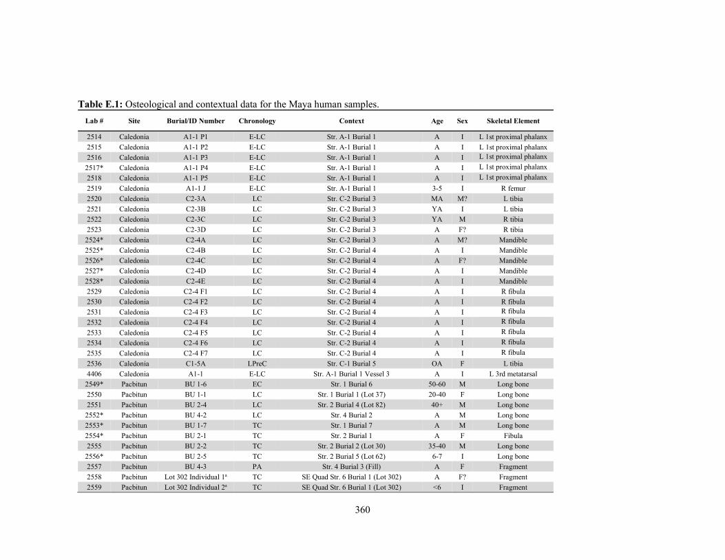
360

Table E.1: Osteological and contextual data for the Maya human samples.

Lab # Site Burial/ID Number Chronology Context Age Sex Skeletal Element

2514 Caledonia A1-1 P1 E-LC Str. A-1 Burial 1 A I L 1st proximal phalanx

2515 Caledonia A1-1 P2 E-LC Str. A-1 Burial 1 A I L 1st proximal phalanx

2516 Caledonia A1-1 P3 E-LC Str. A-1 Burial 1 A I L 1st proximal phalanx

2517* Caledonia A1-1 P4 E-LC Str. A-1 Burial 1 A I L 1st proximal phalanx

2518 Caledonia A1-1 P5 E-LC Str. A-1 Burial 1 A I L 1st proximal phalanx

2519 Caledonia A1-1 J E-LC Str. A-1 Burial 1 3-5 I R femur

2520 Caledonia C2-3A LC Str. C-2 Burial 3 MA M? L tibia

2521 Caledonia C2-3B LC Str. C-2 Burial 3 YA I L tibia

2522 Caledonia C2-3C LC Str. C-2 Burial 3 YA M R tibia

2523 Caledonia C2-3D LC Str. C-2 Burial 3 A F? R tibia

2524* Caledonia C2-4A LC Str. C-2 Burial 3 A M? Mandible

2525* Caledonia C2-4B LC Str. C-2 Burial 4 A I Mandible

2526* Caledonia C2-4C LC Str. C-2 Burial 4 A F? Mandible

2527* Caledonia C2-4D LC Str. C-2 Burial 4 A I Mandible

2528* Caledonia C2-4E LC Str. C-2 Burial 4 A I Mandible

2529 Caledonia C2-4 F1 LC Str. C-2 Burial 4 A I R fibula

2530 Caledonia C2-4 F2 LC Str. C-2 Burial 4 A I R fibula

2531 Caledonia C2-4 F3 LC Str. C-2 Burial 4 A I R fibula

2532 Caledonia C2-4 F4 LC Str. C-2 Burial 4 A I R fibula

2533 Caledonia C2-4 F5 LC Str. C-2 Burial 4 A I R fibula

2534 Caledonia C2-4 F6 LC Str. C-2 Burial 4 A I R fibula

2535 Caledonia C2-4 F7 LC Str. C-2 Burial 4 A I R fibula

2536 Caledonia C1-5A LPreC Str. C-1 Burial 5 OA F L tibia

4406 Caledonia A1-1 E-LC Str. A-1 Burial 1 Vessel 3 A I L 3rd metatarsal

2549* Pacbitun BU 1-6 EC Str. 1 Burial 6 50-60 M Long bone

2550 Pacbitun BU 1-1 LC Str. 1 Burial 1 (Lot 37) 20-40 F Long bone

2551 Pacbitun BU 2-4 LC Str. 2 Burial 4 (Lot 82) 40+ M Long bone

2552* Pacbitun BU 4-2 LC Str. 4 Burial 2 A M Long bone

2553* Pacbitun BU 1-7 TC Str. 1 Burial 7 A M Long bone

2554* Pacbitun BU 2-1 TC Str. 2 Burial 1 A F Fibula

2555 Pacbitun BU 2-2 TC Str. 2 Burial 2 (Lot 30) 35-40 M Long bone

2556* Pacbitun BU 2-5 TC Str. 2 Burial 5 (Lot 62) 6-7 I Long bone

2557 Pacbitun BU 4-3 PA Str. 4 Burial 3 (Fill) A F Fragment

2558 Pacbitun Lot 302 Individual 1a TC SE Quad Str. 6 Burial 1 (Lot 302) A F? Fragment

2559 Pacbitun Lot 302 Individual 2a TC SE Quad Str. 6 Burial 1 (Lot 302) <6 I Fragment

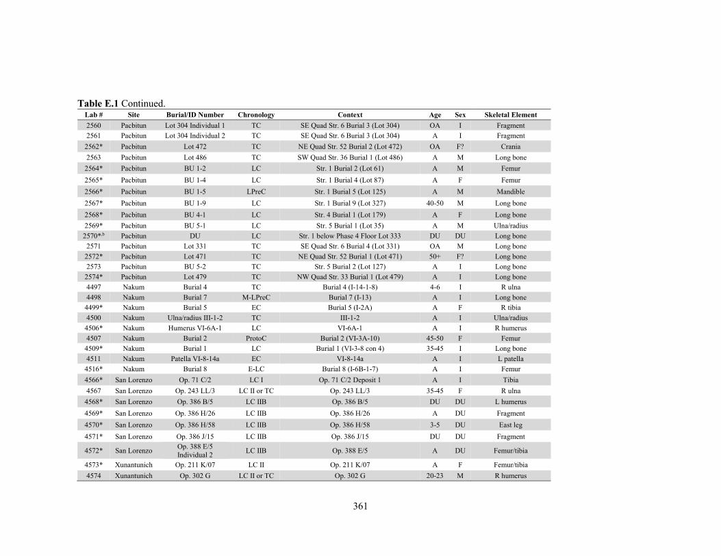
361

Table E.1 Continued. Lab # Site Burial/ID Number Chronology Context Age Sex Skeletal Element

2560 Pacbitun Lot 304 Individual 1 TC SE Quad Str. 6 Burial 3 (Lot 304) OA I Fragment

2561 Pacbitun Lot 304 Individual 2 TC SE Quad Str. 6 Burial 3 (Lot 304) A I Fragment

2562* Pacbitun Lot 472 TC NE Quad Str. 52 Burial 2 (Lot 472) OA F? Crania

2563 Pacbitun Lot 486 TC SW Quad Str. 36 Burial 1 (Lot 486) A M Long bone

2564* Pacbitun BU 1-2 LC Str. 1 Burial 2 (Lot 61) A M Femur

2565* Pacbitun BU 1-4 LC Str. 1 Burial 4 (Lot 87) A F Femur

2566* Pacbitun BU 1-5 LPreC Str. 1 Burial 5 (Lot 125) A M Mandible

2567* Pacbitun BU 1-9 LC Str. 1 Burial 9 (Lot 327) 40-50 M Long bone

2568* Pacbitun BU 4-1 LC Str. 4 Burial 1 (Lot 179) A F Long bone

2569* Pacbitun BU 5-1 LC Str. 5 Burial 1 (Lot 35) A M Ulna/radius

2570*,b Pacbitun DU LC Str. 1 below Phase 4 Floor Lot 333 DU DU Long bone

2571 Pacbitun Lot 331 TC SE Quad Str. 6 Burial 4 (Lot 331) OA M Long bone

2572* Pacbitun Lot 471 TC NE Quad Str. 52 Burial 1 (Lot 471) 50+ F? Long bone

2573 Pacbitun BU 5-2 TC Str. 5 Burial 2 (Lot 127) A I Long bone

2574* Pacbitun Lot 479 TC NW Quad Str. 33 Burial 1 (Lot 479) A I Long bone

4497 Nakum Burial 4 TC Burial 4 (I-14-1-8) 4-6 I R ulna

4498 Nakum Burial 7 M-LPreC Burial 7 (I-13) A I Long bone

4499* Nakum Burial 5 EC Burial 5 (I-2A) A F R tibia

4500 Nakum Ulna/radius III-1-2 TC III-1-2 A I Ulna/radius

4506* Nakum Humerus VI-6A-1 LC VI-6A-1 A I R humerus

4507 Nakum Burial 2 ProtoC Burial 2 (VI-3A-10) 45-50 F Femur

4509* Nakum Burial 1 LC Burial 1 (VI-3-8 con 4) 35-45 I Long bone

4511 Nakum Patella VI-8-14a EC VI-8-14a A I L patella

4516* Nakum Burial 8 E-LC Burial 8 (I-6B-1-7) A I Femur

4566* San Lorenzo Op. 71 C/2 LC I Op. 71 C/2 Deposit 1 A I Tibia

4567 San Lorenzo Op. 243 LL/3 LC II or TC Op. 243 LL/3 35-45 F R ulna

4568* San Lorenzo Op. 386 B/5 LC IIB Op. 386 B/5 DU DU L humerus

4569* San Lorenzo Op. 386 H/26 LC IIB Op. 386 H/26 A DU Fragment

4570* San Lorenzo Op. 386 H/58 LC IIB Op. 386 H/58 3-5 DU East leg

4571* San Lorenzo Op. 386 J/15 LC IIB Op. 386 J/15 DU DU Fragment

4572* San Lorenzo Op. 388 E/5 Individual 2

LC IIB Op. 388 E/5 A DU Femur/tibia

4573* Xunantunich Op. 211 K/07 LC II Op. 211 K/07 A F Femur/tibia

4574 Xunantunich Op. 302 G LC II or TC Op. 302 G 20-23 M R humerus

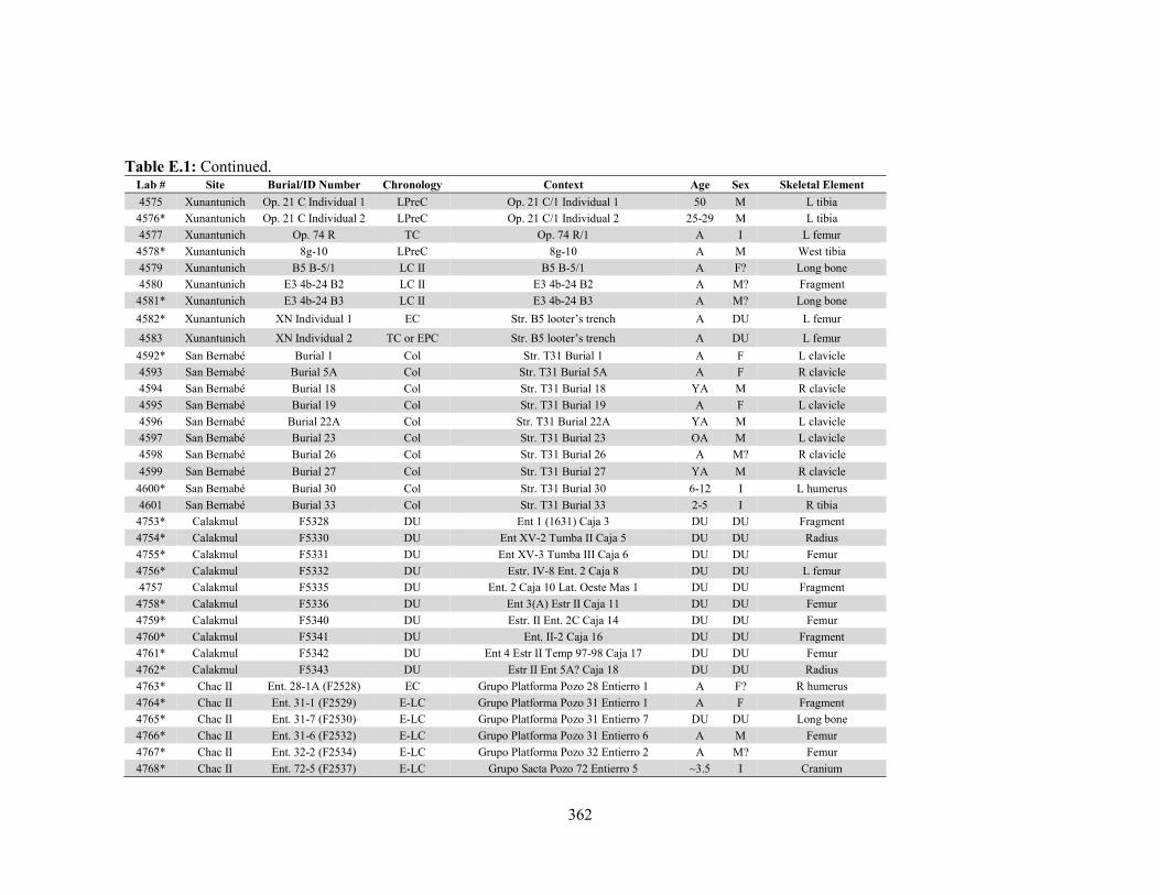
362

Table E.1: Continued. Lab # Site Burial/ID Number Chronology Context Age Sex Skeletal Element

4575 Xunantunich Op. 21 C Individual 1 LPreC Op. 21 C/1 Individual 1 50 M L tibia

4576* Xunantunich Op. 21 C Individual 2 LPreC Op. 21 C/1 Individual 2 25-29 M L tibia

4577 Xunantunich Op. 74 R TC Op. 74 R/1 A I L femur

4578* Xunantunich 8g-10 LPreC 8g-10 A M West tibia

4579 Xunantunich B5 B-5/1 LC II B5 B-5/1 A F? Long bone

4580 Xunantunich E3 4b-24 B2 LC II E3 4b-24 B2 A M? Fragment

4581* Xunantunich E3 4b-24 B3 LC II E3 4b-24 B3 A M? Long bone

4582* Xunantunich XN Individual 1 EC Str. B5 looter’s trench A DU L femur

4583 Xunantunich XN Individual 2 TC or EPC Str. B5 looter’s trench A DU L femur

4592* San Bernabé Burial 1 Col Str. T31 Burial 1 A F L clavicle

4593 San Bernabé Burial 5A Col Str. T31 Burial 5A A F R clavicle

4594 San Bernabé Burial 18 Col Str. T31 Burial 18 YA M R clavicle

4595 San Bernabé Burial 19 Col Str. T31 Burial 19 A F L clavicle

4596 San Bernabé Burial 22A Col Str. T31 Burial 22A YA M L clavicle

4597 San Bernabé Burial 23 Col Str. T31 Burial 23 OA M L clavicle

4598 San Bernabé Burial 26 Col Str. T31 Burial 26 A M? R clavicle

4599 San Bernabé Burial 27 Col Str. T31 Burial 27 YA M R clavicle

4600* San Bernabé Burial 30 Col Str. T31 Burial 30 6-12 I L humerus

4601 San Bernabé Burial 33 Col Str. T31 Burial 33 2-5 I R tibia

4753* Calakmul F5328 DU Ent 1 (1631) Caja 3 DU DU Fragment

4754* Calakmul F5330 DU Ent XV-2 Tumba II Caja 5 DU DU Radius

4755* Calakmul F5331 DU Ent XV-3 Tumba III Caja 6 DU DU Femur

4756* Calakmul F5332 DU Estr. IV-8 Ent. 2 Caja 8 DU DU L femur

4757 Calakmul F5335 DU Ent. 2 Caja 10 Lat. Oeste Mas 1 DU DU Fragment

4758* Calakmul F5336 DU Ent 3(A) Estr II Caja 11 DU DU Femur

4759* Calakmul F5340 DU Estr. II Ent. 2C Caja 14 DU DU Femur

4760* Calakmul F5341 DU Ent. II-2 Caja 16 DU DU Fragment

4761* Calakmul F5342 DU Ent 4 Estr II Temp 97-98 Caja 17 DU DU Femur

4762* Calakmul F5343 DU Estr II Ent 5A? Caja 18 DU DU Radius

4763* Chac II Ent. 28-1A (F2528) EC Grupo Platforma Pozo 28 Entierro 1 A F? R humerus

4764* Chac II Ent. 31-1 (F2529) E-LC Grupo Platforma Pozo 31 Entierro 1 A F Fragment

4765* Chac II Ent. 31-7 (F2530) E-LC Grupo Platforma Pozo 31 Entierro 7 DU DU Long bone

4766* Chac II Ent. 31-6 (F2532) E-LC Grupo Platforma Pozo 31 Entierro 6 A M Femur

4767* Chac II Ent. 32-2 (F2534) E-LC Grupo Platforma Pozo 32 Entierro 2 A M? Femur

4768* Chac II Ent. 72-5 (F2537) E-LC Grupo Sacta Pozo 72 Entierro 5 ~3.5 I Cranium

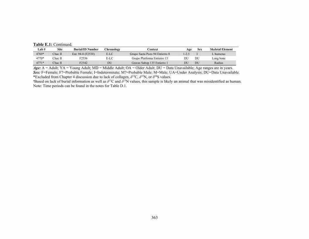
363

Table E.1: Continued. Lab # Site Burial/ID Number Chronology Context Age Sex Skeletal Element

4769* Chac II Ent. 94-8 (F2538) E-LC Grupo Sacta Pozo 94 Entierro 8 1-2.5 I L humerus

4770* Chac II F2536 E-LC Grupo Platforma Entierro 13 DU DU Long bone

4771* Chac II F2542 DU Grecas Subop 135 Entierro 1 DU DU Radius

Age: A = Adult; YA = Young Adult; MD = Middle Adult; OA = Older Adult; DU = Data Unavailable; Age ranges are in years. Sex: F=Female; F?=Probable Female; I=Indeterminate; M?=Probable Male; M=Male; UA=Under Analysis; DU=Data Unavailable. *Excluded from Chapter 4 discussion due to lack of collagen, δ13C, δ15N, or δ34S values. aBased on lack of burial information as well as δ13C and δ15N values, this sample is likely an animal that was misidentified as human. Note: Time periods can be found in the notes for Table D.1.

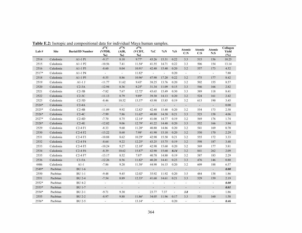
364

Table E.2: Isotopic and compositional data for individual Maya human samples.

Lab # Site Burial/ID Number δ13C

(VPDB, ‰)

δ15N (AIR,

‰)

δ34S (VCDT,

‰) %C %N %S

Atomic C:N

Atomic C:S

Atomic N:S

Collagen Yield (%)

2514 Caledonia A1-1 P1 -9.17 8.10 9.77a 43.26 15.31 0.22 3.3 515 156 10.25

2515 Caledonia A1-1 P2 -10.56 7.41 11.54a 41.55 14.71 0.22 3.3 506 154 13.14

2516 Caledonia A1-1 P3 -8.60 8.04 10.91a 42.40 15.40 0.20 3.2 557 173 4.52

2517* Caledonia A1-1 P4 - - 11.82a - - 0.20 - - - 7.80

2518 Caledonia A1-1 P5 -8.55 8.86 10.96a 47.90 17.20 0.22 3.2 575 177 8.42

2519 Caledonia A1-1 J -11.77 11.62 9.43a 38.25 13.76 0.20 3.2 502 155 8.57

2520 Caledonia C2-3A -12.94 8.36 8.25b 31.34 11.09 0.15 3.3 546 166 2.82

2521 Caledonia C2-3B -7.82 7.67 12.72a 43.65 15.49 0.30 3.3 389 118 8.41

2522 Caledonia C2-3C -11.13 8.79 9.89a 39.30 14.13 0.20 3.2 524 161 2.42

2523 Caledonia C2-3D -8.46 10.52 13.37a 43.90 15.85 0.19 3.2 613 190 3.45

2524* Caledonia C2-4A - - - - - - - - - 0.00

2525* Caledonia C2-4B -11.09 9.92 12.82a 42.40 15.40 0.20 3.2 554 173 2.58

2526* Caledonia C2-4C -7.99 7.86 11.62a 40.80 14.38 0.21 3.3 523 158 4.06

2527* Caledonia C2-4D -7.70 8.75 12.14a 41.00 14.77 0.19 3.2 569 176 1.74

2528* Caledonia C2-4E -12.02 9.06 12.79a 41.22 14.48 0.20 3.3 552 166 3.94

2529 Caledonia C2-4 F1 -8.33 9.60 11.20a 40.80 14.86 0.20 3.2 541 169 0.70

2530 Caledonia C2-4 F2 -13.22 8.60 7.98a 41.90 15.10 0.20 3.2 550 170 2.29

2531 Caledonia C2-4 F3 -10.88 8.62 10.29a 42.90 15.50 0.21 3.2 555 172 3.33

2532 Caledonia C2-4 F4 -8.64 9.22 12.25a 43.25 15.75 0.19 3.2 598 187 3.48

2533 Caledonia C2-4 F5 -10.24 9.27 12.10b 42.90 15.60 0.20 3.2 569 177 3.81

2534 Caledonia C2-4 F6 -8.39 10.62 15.87b 42.90 15.60 0.14 3.2 841 262 2.09

2535 Caledonia C2-4 F7 -13.17 8.52 7.87a 40.70 14.80 0.19 3.2 587 183 2.29

2536 Caledonia C1-5A -12.26 8.56 11.82a 40.20 14.41 0.23 3.3 476 146 0.80

4406 Caledonia A1-1 -7.86 9.20 11.58a 44.90 16.15 0.20 3.2 609 188 6.57

2549* Pacbitun BU 1-6 - - - - - - - - - 0.00

2550 Pacbitun BU 1-1 -9.48 9.45 12.02a 35.92 11.92 0.20 3.5 484 138 1.86

2551 Pacbitun BU 2-4 -7.54 8.89 12.33a 41.68 14.61 0.21 3.3 529 159 2.19

2552* Pacbitun BU 4-2 - - - - - - - - - 0.00

2553* Pacbitun BU 1-7 - - - - - - - - - 0.01

2554* Pacbitun BU 2-1 -9.71 9.30 - 23.77 7.37 - 3.8 - - 1.86

2555 Pacbitun BU 2-2 -8.97 9.88 11.86a 34.05 11.96 0.17 3.3 531 160 1.58

2556* Pacbitun BU 2-5 - - 13.14a - - 0.20 - - - 0.46

365

Table E.2 Continued.

Lab # Site Burial/ID Number δ13C

(VPDB, ‰)

δ15N (AIR,

‰)

δ34S (VCDT,

‰) %C %N %S

Atomic C:N

Atomic C:S

Atomic N:S

Collagen Yield (%)

2557 Pacbitun BU 4-3 -13.26 7.52 12.52a 35.12 12.17 0.20 3.4 471 140 5.93

2558 Pacbitun Lot 302 Individual 1d -10.19 8.83 11.45a 42.03 15.10 0.19 3.2 581 179 3.64

2559 Pacbitun Lot 302 Individual 2d -10.09 7.79 12.20a 42.15 14.86 0.22 3.3 513 155 3.10

2560 Pacbitun Lot 304 Individual 1 -8.99 8.95 12.62a 40.79 14.56 0.21 3.3 508 155 3.02

2561 Pacbitun Lot 304 Individual 2 -11.10 8.12 13.29a 34.96 12.24 0.18 3.3 507 152 3.48

2562* Pacbitun Lot 472 - - - - - - - - - 0.39

2563 Pacbitun Lot 486 -9.16 9.85 13.13a 34.72 12.23 0.19 3.3 490 148 5.12

2564* Pacbitun BU 1-2 - - - - - - - - - 0.00

2565* Pacbitun BU 1-4 - - - - - - - - - 0.01

2566* Pacbitun BU 1-5 - - - - - - - - - 0.00

2567* Pacbitun BU 1-9 - - - - - - - - - 0.00

2568* Pacbitun BU 4-1 - - - - - - - - - 0.34

2569* Pacbitun BU 5-1 - - - - - - - - - 0.17

2570*,e Pacbitun N/A -21.46 3.47 - 43.07 15.64 - 3.2 - - 1.54

2571 Pacbitun Lot 331 -9.78 8.64 13.56a 34.12 10.77 0.24 3.7 387 105 1.28

2572* Pacbitun Lot 471 -11.42 9.52 - 34.21 12.35 - 3.2 - - 0.79

2573 Pacbitun BU 5-2 -13.30 9.11 14.73a 33.03 11.97 0.18 3.2 498 155 1.64

2574* Pacbitun Lot 479 - - - - - - - - - 0.00

4497 Nakum Burial 4 -14.16 10.04 13.40a 41.52 14.58 0.23 3.3 492 148 1.48

4498 Nakum Burial 7 -13.91 10.00 13.11a 42.25 14.73 0.21 3.3 547 163 1.16

4499* Nakum Burial 5 - - - - - - - - - 0.00

4500 Nakum Ulna/Radius III-1-2 -10.54 11.06 13.25a 42.08 15.04 0.18 3.3 620 190 1.91

4506* Nakum Humerus VI-6A-1 - - - - - - - - - 0.16

4507 Nakum Burial 2 -9.88 6.09 12.93a 41.60 13.18 0.21 3.7 533 145 0.97

4509* Nakum Burial 1 - - - - - - - - - 0.00

4511 Nakum Patella VI-8-14a -9.63 11.13 12.89a 43.36 14.93 0.25 3.4 463 137 1.97

4516* Nakum Burial 8 - - - - - - - - - 0.00

4566* San Lorenzo Op. 71 C/2 - - - - - - - - - 0.42

4567 San Lorenzo Op. 243 LL/3 -12.21 9.47 13.44c 44.40 16.10 0.15 3.2 794 247 3.64

4568* San Lorenzo Op. 386 B/5 -9.85 7.88 - 44.30 15.90 - 3.3 - - 6.81

4569* San Lorenzo Op. 386 H/26 -13.52 9.65 - 44.90 16.10 - 3.3 - - 6.27

4570* San Lorenzo Op. 386 H/58 -9.24 9.94 - 42.80 15.40 - 3.2 - - 5.86

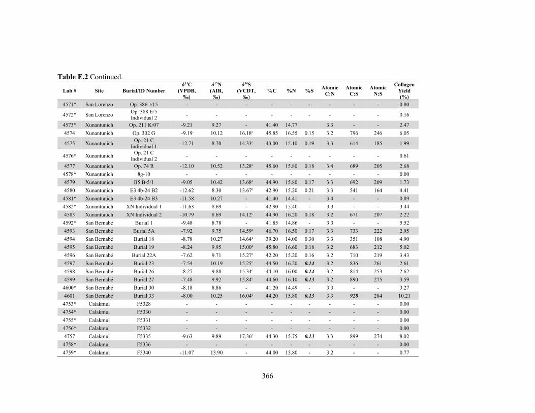
366

Table E.2 Continued.

Lab # Site Burial/ID Number δ13C

(VPDB, ‰)

δ15N (AIR,

‰)

δ34S (VCDT,

‰) %C %N %S

Atomic C:N

Atomic C:S

Atomic N:S

Collagen Yield (%)

4571* San Lorenzo Op. 386 J/15 - - - - - - - - - 0.80

4572* San Lorenzo Op. 388 E/5 Individual 2

- - - - - - - - - 0.16

4573* Xunantunich Op. 211 K/07 -9.21 9.27 - 41.40 14.77 3.3 - - 2.47

4574 Xunantunich Op. 302 G -9.19 10.12 16.18c 45.85 16.55 0.15 3.2 796 246 6.05

4575 Xunantunich Op. 21 C

Individual 1 -12.71 8.70 14.33c 43.00 15.10 0.19 3.3 614 185 1.99

4576* Xunantunich Op. 21 C

Individual 2 - - - - - - - - - 0.61

4577 Xunantunich Op. 74 R -12.10 10.52 13.28c 45.60 15.80 0.18 3.4 689 205 2.68

4578* Xunantunich 8g-10 - - - - - - - - - 0.00

4579 Xunantunich B5 B-5/1 -9.05 10.42 13.68c 44.90 15.80 0.17 3.3 692 209 1.73

4580 Xunantunich E3 4b-24 B2 -12.62 8.30 13.67c 42.90 15.20 0.21 3.3 541 164 4.41

4581* Xunantunich E3 4b-24 B3 -11.58 10.27 - 41.40 14.41 - 3.4 - - 0.89

4582* Xunantunich XN Individual 1 -11.63 8.69 - 42.90 15.40 - 3.3 - - 3.44

4583 Xunantunich XN Individual 2 -10.79 8.69 14.12c 44.90 16.20 0.18 3.2 671 207 2.22

4592* San Bernabé Burial 1 -9.48 8.78 - 41.85 14.86 - 3.3 - - 5.52

4593 San Bernabé Burial 5A -7.92 9.75 14.59c 46.70 16.50 0.17 3.3 733 222 2.95

4594 San Bernabé Burial 18 -8.78 10.27 14.64c 39.20 14.00 0.30 3.3 351 108 4.90

4595 San Bernabé Burial 19 -8.24 9.95 15.00c 45.80 16.60 0.18 3.2 683 212 5.02

4596 San Bernabé Burial 22A -7.62 9.71 15.27c 42.20 15.20 0.16 3.2 710 219 3.43

4597 San Bernabé Burial 23 -7.54 10.19 15.25c 44.50 16.20 0.14 3.2 836 261 2.61

4598 San Bernabé Burial 26 -8.27 9.88 15.34c 44.10 16.00 0.14 3.2 814 253 2.62

4599 San Bernabé Burial 27 -7.48 9.92 15.84c 44.60 16.10 0.13 3.2 890 275 3.59

4600* San Bernabé Burial 30 -8.18 8.86 - 41.20 14.49 - 3.3 - - 3.27

4601 San Bernabé Burial 33 -8.00 10.25 16.04c 44.20 15.80 0.13 3.3 928 284 10.21

4753* Calakmul F5328 - - - - - - - - - 0.00

4754* Calakmul F5330 - - - - - - - - - 0.00

4755* Calakmul F5331 - - - - - - - - - 0.00

4756* Calakmul F5332 - - - - - - - - - 0.00

4757 Calakmul F5335 -9.63 9.89 17.36c 44.30 15.75 0.13 3.3 899 274 8.02

4758* Calakmul F5336 - - - - - - - - - 0.00

4759* Calakmul F5340 -11.07 13.90 - 44.00 15.80 - 3.2 - - 0.77

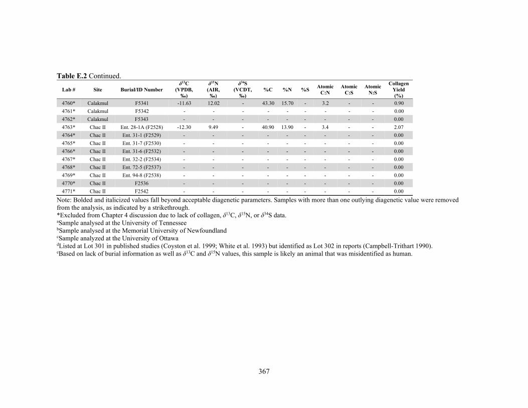
367

Table E.2 Continued.

Lab # Site Burial/ID Number δ13C

(VPDB, ‰)

δ15N (AIR,

‰)

δ34S (VCDT,

‰) %C %N %S

Atomic C:N

Atomic C:S

Atomic N:S

Collagen Yield (%)

4760* Calakmul F5341 -11.63 12.02 - 43.30 15.70 - 3.2 - - 0.90

4761* Calakmul F5342 - - - - - - - - - 0.00

4762* Calakmul F5343 - - - - - - - - - 0.00

4763* Chac II Ent. 28-1A (F2528) -12.30 9.49 - 40.90 13.90 - 3.4 - - 2.07

4764* Chac II Ent. 31-1 (F2529) - - - - - - - - - 0.00

4765* Chac II Ent. 31-7 (F2530) - - - - - - - - - 0.00

4766* Chac II Ent. 31-6 (F2532) - - - - - - - - - 0.00

4767* Chac II Ent. 32-2 (F2534) - - - - - - - - - 0.00

4768* Chac II Ent. 72-5 (F2537) - - - - - - - - - 0.00

4769* Chac II Ent. 94-8 (F2538) - - - - - - - - - 0.00

4770* Chac II F2536 - - - - - - - - - 0.00

4771* Chac II F2542 - - - - - - - - - 0.00

Note: Bolded and italicized values fall beyond acceptable diagenetic parameters. Samples with more than one outlying diagenetic value were removed from the analysis, as indicated by a strikethrough. *Excluded from Chapter 4 discussion due to lack of collagen, δ13C, δ15N, or δ34S data. aSample analysed at the University of Tennessee bSample analysed at the Memorial University of Newfoundland cSample analyzed at the University of Ottawa dListed at Lot 301 in published studies (Coyston et al. 1999; White et al. 1993) but identified as Lot 302 in reports (Campbell-Trithart 1990). eBased on lack of burial information as well as δ13C and δ15N values, this sample is likely an animal that was misidentified as human.