Contribution of FACTS devices in power systems security ...

IET Generation, Transmission & Distribution

Research Article

Contribution of FACTS devices in powersystems security using MILP-based OPF

ISSN 1751-8687Received on 5th June 2018Accepted on 5th June 2018doi: 10.1049/iet-gtd.2018.0376www.ietdl.org

Ahmad Nikoobakht1, Jamshid Aghaei2 , Masood Parvania3, Mostafa Sahraei-Ardakani31Department of Electrical Engineering, Higher Education Center of Eghlid, Eghlid, Iran2Department of Electrical and Electronics Engineering, Shiraz University of Technology, Shiraz, Iran3Department of Elect and Computer Engineering, University of Utah, Salt Lake City, UT 84112-9057, USA

E-mail: [email protected]

Abstract: Traditionally, electric system operators have dispatched generation to minimise total production costs ignoring theflexibility of the AC transmission system (ACTS). One available option to enhance power system security is to harness theflexibility of the ACTS, where a variety of flexible AC transmission system (FACTS) devices can be incorporated in the ACTS.However, utilisation of FACTS devices is limited today due to the complexities that these devices introduce to the AC optimalpower flow (ACOPF) problem. The mathematical representation of the full ACOPF problem, with the added modelling of FACTSdevices, is a non-linear programming (NLP) optimisation problem, which is computationally burdensome for large-scalesystems. This study presents a method to convert this NLP problem into a mixed-integer linear program (MILP) where a certainlevel of solution accuracy can be achieved for a time budget. In this regard, this study first proposes a linear AC OPF model,using which the OPF solution with the operation of FACTS devices is obtained. In addition, the loadability of the power systemsis utilised to quantify the impacts of FACTS devices on improving the security of system. The OPF problem including FACTSdevices based on a linearised model is tested on a 6-bus and the IEEE 118-bus test systems.

NomenclatureIndices

g index for generating unitsn/m indices for system busesk index for lineℓ index for angle piecei/ j indices for breakpoint, the TCSC/SVC devicess index for load (or/and contingency state) stress condition( ⋅ )s index-related stress condition

Sets

χn set of thermal units which are connected to bus nΩn set of lines which are connected to bus nΩn

SVC set of buses with SVCs

Continuous variables

δnm( ⋅ ) phase angle difference across line (n, m)

Pg( ⋅ )/Qg

( ⋅ ) active/reactive power output of thermal unit gVn

( ⋅ ) voltage magnitude at bus nPnm

( ⋅ ) /Qnm( ⋅ ) active/reactive power flow on line (n, m)

Pnm(ℓ)/Qnm(ℓ) active/reactive power flow on the ℓth linearblock of line (n, m)

Pnm( ⋅ )(ℓ, i)/Qnm

( ⋅ )(ℓ, i) active/reactive power flow on the ℓth/ithlinear block/breakpoint of line (n, m)

Δ̄Pg( ⋅ )/ΔPg

( ⋅ ) active power increase/decrease in thermal unitg for security purposes

QnSVC reactive power injected by the SVC device at

bus nBn

SVC susceptance of the SVC device at bus nxnm

TCSC reactance of the TCSC device connected toline (n, m)

TC total cost of the operation of system

Note that the normal condition s = 0 relates to the first stage.

Binary variables

unm(ℓ) status of the ℓth linear block of line (n, m)utscs(i)/usvc( j) binary variables to represent the xnm

TCSC/BnSVC at the

i/ jth breakpoints

Constants

δnmmax max angle difference across a line (n, m)

δ̄nm(ℓ) tangent point of the ℓth piecewise linear blockof angle difference across a line (n, m)

αnm(ℓ)/α~nm(ℓ) slope of the ℓth piecewise linear block of thelinearised F(δnm(ℓ))/F~(δnm(ℓ)) relative to theline (n, m) in tangent point δ̄nm(ℓ)

βnm(ℓ)/β~

nm(ℓ) value of the linearised F(δnm(ℓ))/F~(δnm(ℓ))relative to the ℓth piecewise linear block ofthe line (n, m) in tangent point δ̄nm(ℓ)

αnm(ℓ, i)/α~nm(ℓ, i) slope of the ℓ/ith piecewise linear block/breakpoint of the linearisedF δ̄nm(ℓ), g(i), b(i) /F~ δ̄nm(ℓ), g(i), b(i)relative to the line (n, m) with TCSC device

βnm(ℓ, i)/β~

nm(ℓ, i) value of the linearisedF δ̄nm(ℓ), g(i), b(i) /F~ δ̄nm(ℓ), g(i), b(i)relative to the ℓ/ith piecewise linear block/breakpoint of the line (n, m) with TCSCdevice

b̄n/bn max/min susceptance of the SVC at bus nx̄k /xk max/min reactance of the TCSC at line kCg/Cg

s cost of normal/stress condition of thermal unitg

Skmax maximum magnitude of apparent power of

line k, MVAψDn power factor angle of load nUg/Uk simulated (line k)/(unit g) outage statusΔRg

± ramp up/down limit of thermal unit g at stresscondition

Qgmax/Qg

min max/min reactive power output of thermal unitg

IET Gener. Transm. Distrib.© The Institution of Engineering and Technology 2018

1

PDn/QDn active/ reactive power demand of load nΔδ length of each piecewise linear block (in

radians)M disjunctive factor, a large positive valuegk conductance of line k, a non-negative valuebk /bk0 series/shunt admittance of line k, a negative

valueΔg

LAC reactive power generation calculation error forLACOPF model for unit g

ΔnmLAC reactive power flow calculation error for

LACOPF model in line (n, m)bn

SVC( j)/xnmTCSC(i) value of the xnm

TCSC/BnSVC at the i/ jth

breakpointsgnm(i)/bnm(i) value of the gnm/bnm at the i/ jth breakpoints

1 Introduction1.1 Motivation and aims

Today's power grids are driven closer to their transfer capacitiesdue to the increased consumption and power transfers which resultsin endangering the power system security. Accordingly,maintaining the security of electric power system has increasinglybecome a challenging task. As a countermeasure against this issue,flexible AC transmission system (FACTS) devices have beendeveloped [1]. FACTS devices can help reduce line flow on fullyloaded transmission branches, which would lead to enhancedloadability of the power system, improved security, and eventuallya further energy-efficient transmission system. Thus, this paperinvestigates the utilisation of FACTS devices, such as static VARcompensator (SVC) and thyristor-controlled series capacitor(TCSC), to maximise power transfer transactions during a highlystressed one that simulates a load increase under transmission lineand/or thermal unit outage. Unfortunately, the FACTS devicedeployment are limited today due to the complexities that thesedevices introduce to the AC optimal power flow (ACOPF)problem. Besides, the optimal adjustment of FACTS devicesintroduces non-linearities in the ACOPF problem; hence,employing a non-linear solver does not guarantee to find a globaloptimum solution, especially when the scale of the problem is large[2]. Therefore, in order to overcome these challenges, in our paper,a linearised AC optimal power flow (LACOPF) model as well aslinearised SVC and TCSC models, as target FACTS devices in thiswork, have been proposed.

1.2 Literature review

During the last decade, FACTS devices are broadly used formaximising the loadability of the existing power transmissionnetworks. The possibility of operating the power system at theminimum cost whereas satisfying the network and generationconstraints is one of the main issues in increasing transmissioncapacity by the use of FACTS [3, 4]. The FACTS devices havebeen effectively used in several OPF problems to reducecongestion [5], enhance security [6] and improve the voltageprofile [7, 8]. It is expected that FACTS devices could increase thetransfer capability over the existing transmission lines by 50% [4,9], if deployed optimally. Major challenges that prevent betterutilisation of FACTS devices in power systems are computationalcomplexities of incorporating these devices in ACOPF problem [9–11]. In general, the ACOPF problem incorporating FACTS devicesis a large-scale non-convex optimisation problem [11]. This non-convexity partly is due to the non-linearity in the active andreactive power flow equations which raise the likelihood ofconvergence to local optimal solutions for ACOPF problemsincorporating FACTS devices [12]. There are few works in the areato address this computational challenge. For instance, the authorsin [11, 13] propose various methods to include FACTS operation inOPF problem for a variety of applications. Moreover, theformulation developed in [11, 13] is computationally expensiveand will not be applicable to large-scale power systems. A mixed-integer linear program (MILP)-based DC OPF model is proposedin [9, 10] to provide suggestions to the operator regarding the

operation of FACTS devices and upgrading the usage oftransmission capacity.

Moreover, in [9], the TCSC device has been included in the DCoptimal power flow problem (DCOPF). Accordingly, themathematical representation of the DCOPF, with the addedmodelling of TCSC device, is a non-linear program (NLP). Thisreference presents a method to convert this NLP into an MILP. It isworth mentioning that the operation of the FACTS devices basedon DCOPF cannot consider ACOPF feasibility, which hinders theexploitation of the benefits of these devices, i.e. the TCSC andSVC, in power system operations.

However, the FACTS devices models based on DCOPF areunsatisfactory for the following reasons. First, the DC networkmodel is essentially an approximation of the AC model by relaxingthe reactive power and voltage constraints. These relaxations tendto create a ‘gap’ between the solutions obtained from the DCmodel and the AC model. In some cases, the gap could be largeand result in an OPF solution that is problematic in the ACnetwork. Also, because the DC model's solutions cannot considerAC feasibility, system security might be jeopardised whenimplementing the FACTS devices [7, 11]. Second, the inaccuracyof the DCOPF may lead to model solutions, with the TCSC and/orSVC devices, that underestimate security cost savings or, worseyet, security cost increases [1, 12, 14]. Third, the FACTS devicesmodel based on DCOPF cannot be used to grasp other potentialbenefits of FACTS devices action, such as correcting temporaryvoltage violations [7]. Also, in the previous works mentionedabove, the linear programming approach has been used based onthe linearised power flow that provides only the active power of thenetwork. The use of only active power in the OPF model with theFACTS devices action causes enormous error in power systemstudies, especially for SVC device where the voltage magnitudeplays a critical role [9, 10]. Also, maximising the loadability andminimising security cost of an AC power system are directlyrelated to the reactive power sufficiency and voltage security in ACnetwork which are relaxed in DCOPF model [11]. Thesedrawbacks suggest that the development of FACTS devices basedon the AC network security constraints is of great significance andmotivate the research described in this paper.

In some papers, the Newton–Raphson method has been used[15, 16]; however, this method depends essentially on the initialconditions and has difficulties in handling inequality constraints. Inaddition, many heuristic methods, such as genetic algorithm [4],particle swarm optimisation [17], Tabu search [18], artificial beecolony [19] among the others, were successfully applied to theOPF problem incorporating FACTS devices. However, theseheuristic methods do not guarantee to obtain the global optimumsolution and consequently, they are not effective methods to solvethe above-mentioned problem, particularly once the scale of thepower system is large. Also, the linearisation process in this paper,for the linearised AC model and TCSC and SVC device models,involves many techniques including Taylor series expansion theory,binary expansion discretisation approach, piecewise linear (PWL)approximation, and other simple techniques [12]. The proposedlinearisation method has many applications in power systemproblems such as a unified power flow controller (or UPFC)device, static synchronous compensator (STATCOM), and a staticsynchronous series compensator (SSSC) [6]. Also, the UPFCdevice is a combination of a STATCOM and an SSSC coupled viaa common DC voltage link. It might be necessary to employfurther linearisation methods in order to apply the presented workto these devices [17]. The main advantage of the UPFC is tocontrol the active and reactive power flows in the transmission line.The controllable parameters of the UPFC are reactance in the line,phase angle, and voltage. Since the presented work considers bothreactive power and voltage, the linear UPFC device model can beimplemented in the proposed OPF model. However, it should behighlighted that in an optimisation problem for the OPF problem,bus voltage magnitudes may differ more significantly from 1 p.u.which can affect the accuracy of the proposed method toimplement the linear UPFC, STATCOM, and SSSC devices'models. Hence, to assess the preciseness, feasibility, and

2 IET Gener. Transm. Distrib.© The Institution of Engineering and Technology 2018

applicability of the proposed method to this area, many numericalstudies have to be done.

Table 1 shows the taxonomy of the proposed LACOPF modelincorporating linear FACTS (LFACTS) devices model, namelyTSCS and SVC, in previous literatures.

1.3 Contributions

Considering the above literature review, which summarised theexisting literature and identified the state-of-the-art challenges, thenovelty of this work are twofold:

i. The paper develops a linearised AC model incorporatinglinearised FACTS devices model, such as SVC and TCSC, inwhich bus voltage magnitudes and reactive power are takeninto account. Based on this linearised AC model, a novel OPFformulation with LFACTS devices is proposed.

ii. The proposed method enables the utilisation of FACTS devices(such as TCSC and SVC) based on the LAC power flowmodel, to enhance the system security under stressed loadingconditions and system contingencies.

To the best of the authors' knowledge, no reference has providedthe MILP formulation for ACOPF model with linearised FACTSdevices model (i.e. TCSC and SVC models), in the presence of thestressed loading condition under contingency state.

2 Linearisation of the full AC power flow withFACTS devices modelThis section presents a linear approximation to AC power flow inwhich voltage and reactive power are modelled. The linearisationprocess in this section, for the linearised AC power flow model andTCSC and SVC device models, involves many techniquesincluding Taylor series expansion theory, binary expansiondiscretisation approach, PWL approximation, and other simpletechniques [12]. Furthermore, the linearisation process in this paperfor the following assumptions is assumed to be valid:

i. The phase difference between the voltages at both ends ofevery existing or constructed lines is small enough, i.e.δnm ≃ 0 − 34∘. This implies validation of PWL approximationof sine and cosine functions in δnm < δnm < δ̄nm. Also, atδnm = 34∘, the difference between sin δnm and δnm is 2.43%, sothe fourth assumption (sin δnm ≃ δnm) is quite reasonable.

ii. The voltage magnitudes are nearly 1 p.u. for all buses. Theseassumptions are practically true for large-scale systems,maintaining the system far from instability and other securitylimits.

2.1 Linearisation of the AC power flow equations

If the phase shifters and off-nominal transformer turns ratios areignored, the active and reactive AC power flow in transmission linek between buses n and m is written as follows:

Pnm = gkVn2 − VnVm gkcos δnm + bksin δnm

F(δnm)(1a)

Qnm = − bk + bk0 Vn2 + VnVm bkcos δnm − gksin δnm

F~(δnm)

(1b)

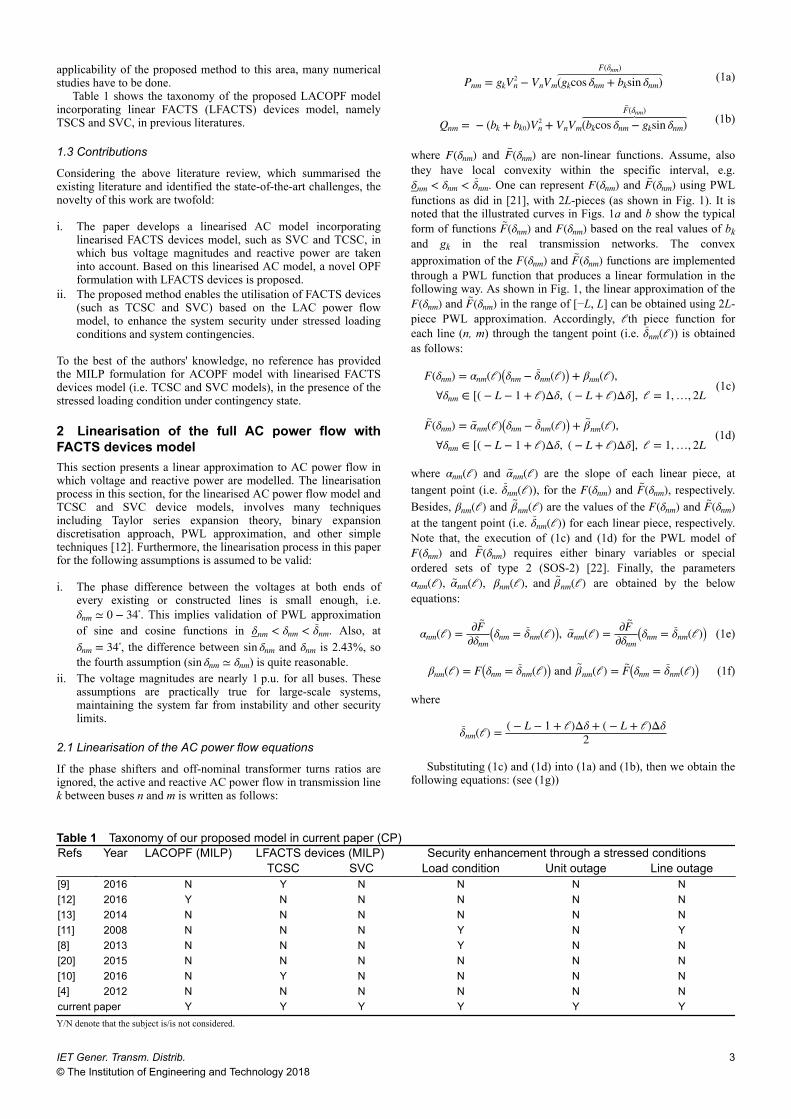
where F(δnm) and F~(δnm) are non-linear functions. Assume, also

they have local convexity within the specific interval, e.g.δnm < δnm < δ̄nm. One can represent F(δnm) and F

~(δnm) using PWLfunctions as did in [21], with 2L-pieces (as shown in Fig. 1). It isnoted that the illustrated curves in Figs. 1a and b show the typicalform of functions F

~(δnm) and F(δnm) based on the real values of bkand gk in the real transmission networks. The convexapproximation of the F(δnm) and F

~(δnm) functions are implementedthrough a PWL function that produces a linear formulation in thefollowing way. As shown in Fig. 1, the linear approximation of theF(δnm) and F

~(δnm) in the range of [−L, L] can be obtained using 2L-piece PWL approximation. Accordingly, ℓth piece function foreach line (n, m) through the tangent point (i.e. δ̄nm(ℓ)) is obtainedas follows:

F(δnm) = αnm(ℓ) δnm − δ̄nm(ℓ) + βnm(ℓ),∀δnm ∈ ( − L − 1 + ℓ)Δδ, ( − L + ℓ)Δδ , ℓ = 1, …, 2L

(1c)

F~(δnm) = α~nm(ℓ) δnm − δ̄nm(ℓ) + β

~nm(ℓ),

∀δnm ∈ ( − L − 1 + ℓ)Δδ, ( − L + ℓ)Δδ , ℓ = 1, …, 2L(1d)

where αnm(ℓ) and α~nm(ℓ) are the slope of each linear piece, attangent point (i.e. δ̄nm(ℓ)), for the F(δnm) and F

~(δnm), respectively.Besides, βnm(ℓ) and β

~nm(ℓ) are the values of the F(δnm) and F

~(δnm)at the tangent point (i.e. δ̄nm(ℓ)) for each linear piece, respectively.Note that, the execution of (1c) and (1d) for the PWL model ofF(δnm) and F

~(δnm) requires either binary variables or specialordered sets of type 2 (SOS-2) [22]. Finally, the parametersαnm(ℓ), α~nm(ℓ), βnm(ℓ), and β

~nm(ℓ) are obtained by the below

equations:

αnm(ℓ) = ∂F~

∂δnmδnm = δ̄nm(ℓ) , α~nm(ℓ) = ∂F

~

∂δnmδnm = δ̄nm(ℓ) (1e)

βnm(ℓ) = F δnm = δ̄nm(ℓ) and β~

nm(ℓ) = F~

δnm = δ̄nm(ℓ) (1f)

where

δ̄nm(ℓ) = ( − L − 1 + ℓ)Δδ + ( − L + ℓ)Δδ2

Substituting (1c) and (1d) into (1a) and (1b), then we obtain thefollowing equations: (see (1g))

Table 1 Taxonomy of our proposed model in current paper (CP)Refs Year LACOPF (MILP) LFACTS devices (MILP) Security enhancement through a stressed conditions

TCSC SVC Load condition Unit outage Line outage[9] 2016 N Y N N N N[12] 2016 Y N N N N N[13] 2014 N N N N N N[11] 2008 N N N Y N Y[8] 2013 N N N Y N N[20] 2015 N N N N N N[10] 2016 N Y N N N N[4] 2012 N N N N N Ncurrent paper Y Y Y Y Y YY/N denote that the subject is/is not considered.


3

Qnm(ℓ) ≃ − bk + bk0 Vn2 + VnVm α~nm

ℓ δnm − δ̄nm(ℓ) + β~

nm(ℓ)= − bk + bk0 Vn

2 + VnVmα~nm(ℓ)δnm

−VnVmα~nm(ℓ)δ̄nm(ℓ) + VnVmβ~

nm(ℓ)(1h)

Notice that (1g) and (1h) still contain some non-linear terms likeVnVm, VnVmδnm, and Vn

2. These non-linear terms can be linearisedby their Taylor series expansion around 1, for bus voltage, andabout δ̄nm(ℓ), for line angle, as presented in Table 2.

Table 2 gives the maximum absolute errors for each of theconstituent terms with respect to the linearised forms, over atypical range of operating voltages and angles, i.e.0.95 ≤ Vn ≤ 1.05 at the end of each line, and δnm ≤ 34∘. Themaximum absolute errors for each of the linearised term in Table 2,

over a maximum range of operating voltages and angles, i.e.Vn

max = 1.05, δ̄nmmax(ℓ) = 10∘, and δnm = 10 − 15∘, are obtained from:

i. Vnmax 2 − 2Vn

max − 1 ≃ 0.0025,ii. Vn

maxVmmax − Vn

max + Vmmax − 1 ≃ 0.0025,

iii. VnmaxVm

maxδnmmax − δ̄nm

max(ℓ)(Vnmax + Vm

max − 1) + (δnmmax − δ̄nm

max(ℓ))≃ 0.0050

.

Subsequently, the PWL approximation of active and reactive ACpower flow equations for line (n, m) metered at bus n for the ℓthangle piece (or through the tangent point, i.e. δ̄nm(ℓ)) are obtainedas follows, respectively:

Pnm(ℓ) = gk 2Vn − 1 − αnm(ℓ) δnm − δ̄nm(ℓ)−βnm(ℓ) Vn + Vm − 1

(1i)

Qnm(ℓ) = − bk + bk0 2Vn − 1 + α~nm(ℓ) δnm − δ̄nm(ℓ)+β

~nm(ℓ) Vn + Vm − 1

(1j)

2.2 Linearisation of TCSC equations

The model of the TCSC device used in this paper is a variablereactance connected in series with a transmission line [23]. Themain idea behind power flow control with the TCSC device is tochange the whole transmission line's effective series impedance, byadding inductive or capacitive impedance. That is

zk = rk + j(xk + xTCSC) = 1gk + jbk

, k ∈ (n, m) (2a)

The resulting conductance and susceptance are as follows,respectively:

gnm = rnm

rnm2 + xnm + xnm

TCSC 2 , xnmTCSC ∈ xk, x̄k (2b)

bnm = − xnm + xnmTCSC

rnm2 + xnm + xnm

TCSC 2 , xnmTCSC ∈ xk, x̄k (2c)

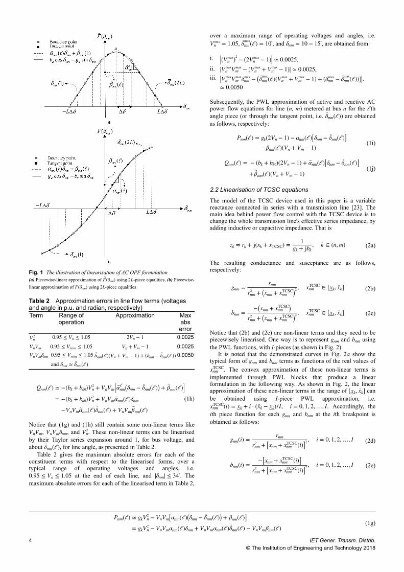
Notice that (2b) and (2c) are non-linear terms and they need to bepiecewisely linearised. One way is to represent gnm and bnm usingthe PWL functions, with I-pieces (as shown in Fig. 2).

It is noted that the demonstrated curves in Fig. 2a show thetypical form of gnm and bnm terms as functions of the real values ofxnm

TCSC. The convex approximation of these non-linear terms isimplemented through PWL blocks that produce a linearformulation in the following way. As shown in Fig. 2, the linearapproximation of these non-linear terms in the range of xk, x̄k canbe obtained using I-piece PWL approximation, i.e.xnm

TCSC(i) = xk + i ⋅ x̄k − xk /I, i = 0, 1, 2, …, I. Accordingly, theith piece function for each gnm and bnm at the ith breakpoint isobtained as follows:

gnm(i) = rnm

rnm2 + xnm + xnm

TCSC(i) 2 , i = 0, 1, 2, …, I (2d)

bnm(i) = − xnm + xnmTCSC(i)

rnm2 + xnm + xnm

TCSC(i) 2 , i = 0, 1, 2, …, I (2e)

Fig. 1 The illustration of linearisation of AC OPF formulation(a) Piecewise-linear approximation of F~(δnm) using 2L-piece equalities, (b) Piecewise-linear approximation of F(δnm) using 2L-piece equalities

Pnm(ℓ) ≃ gkVn2 − VnVm αnm(ℓ) δnm − δ̄nm(ℓ) + βnm(ℓ)

= gkVn2 − VnVmαnm(ℓ)δnm + VnVmαnm(ℓ)δ̄nm(ℓ) − VnVmβnm(ℓ)

(1g)

Table 2 Approximation errors in line flow terms (voltagesand angle in p.u. and radian, respectively)Term Range of

operationApproximation Max

abserror

Vn2 0.95 ≤ Vn ≤ 1.05 2Vn − 1 0.0025

VnVm 0.95 ≤ Vn/m ≤ 1.05 Vn + Vm − 1 0.0025VnVmδnm 0.95 ≤ Vn/m ≤ 1.05

and δnm ≈ δ̄nm(ℓ)δ̄nm(ℓ)(Vn + Vm − 1) + (δnm − δ̄nm(ℓ)) 0.0050


where gnm(i) and bnm(i) are chosen such that the approximationcoincides with gnm and bnm at breakpoints

xnmTCSC(0), xnm

TCSC(1), …, xnmTCSC(I) .

Accordingly, the power flow equations of the lines with TCSCcan be written as follows:

Pnm(ℓ, i) = gk(i)(2Vn − 1) − αnm(ℓ, i) δnm − δ̄nm(ℓ)−βnm(ℓ, i)(Vn + Vm − 1)

(2f)

Qnm(ℓ, i) = − bk(i) + bk0 (2Vn − 1) + α~nm(ℓ, i) δnm − δ̄nm(ℓ)+β

~nm(ℓ, i)(Vn + Vm − 1)

(2g)

Equations (2f) and (2g) are modelled similar to that of (1i)–(1j).The main difference between (2f) and (2g) and (1i) and (1j) is thatthe gk(i), αnm(ℓ, i)/α~nm(ℓ, i), and βnm(ℓ, i)/β

~nm(ℓ, i) will be specified

at the ith breakpoint. The active and reactive power flow in a linewith TCSC device for each of the ℓth piece then can bereformulated in the form of MILP (M is a large number) as follows:

PnmTCSC(ℓ, i) − M 1 − uTCSC(i) ≤ Pnm(ℓ) ≤ Pnm

TCSC(ℓ, i)+ M 1 − uTCSC(i)

(2h)

QnmTCSC(ℓ, i) − M 1 − uTCSC(i) ≤ Qnm(ℓ) ≤ Qnm

TCSC(ℓ, i)+ M 1 − uTCSC(i)

(2i)

Constraints (2h) and (2i) are calculated at one of the breakpoints,i.e. xnm

TCSC(0), xnmTCSC(1), …, xnm

TCSC(I), for a line with TCSC device ateach of the ℓ th piece. Here, uTCSC(i) is a binary variable to selectone of xnm

TCSC(0), xnmTCSC(1), …, xnm

TCSC(I), and M is a sufficiently largepositive scalar.

Equations (2j)–(2m) are modelled similar to that of (1c)–(1f).The main difference between these equations and (1c)–(1f) are theexistence of the g(i) and b(i) in these equations, which aredependent on the ith piece

F δ̄nm(ℓ), g(i), b(i) = αnm(ℓ, i) δnm − δ̄nm(ℓ) + βnm(ℓ, i)∀δnm ∈ ( − L − 1 + ℓ)Δδ, ( − L + ℓ)Δδ , ℓ = 1, …, 2L

(2j)

F~

δ̄nm(ℓ), g(i), b(i) = α~nm(ℓ, i) δnm − δ̄nm(ℓ) + β~

nm(ℓ, i)∀δnm ∈ ( − L − 1 + ℓ)Δδ, ( − L + ℓ)Δδ , ℓ = 1, …, 2L

(2k)

αnm(ℓ, i) = ∂Fℓ

∂δnmδ̄nm(ℓ), g(i), b(i)

and α~nm(ℓ, i) = ∂F~ℓ

∂δnmδ̄nm(ℓ), g(i), b(i)

(2l)

βnm(ℓ, i) = F δ̄nm(ℓ), g(i), b(i)and β

~nm(ℓ, i) = F

~δ̄nm(ℓ), g(i), b(i)

(2m)

The above-mentioned formulations, i.e. (1) and (2), are valid foreach segment of the δnm (where( − L − 1 + ℓ)Δδ < δnm < ( − L + ℓ)Δδ, ℓ ∈ −L, L ), or close toeach tangent point (i.e. δ̄nm(ℓ)), as shown in Fig. 1. Note that thelength of each segment of angle is Δδ (as shown in Fig. 1). Moredetails about piecewise linearisation can be found in [21]. Itessentially introduces 2L new binary variables and 2L newinequalities, all being linear. To ensure which segment of the PWLblocks is selected, a binary variable unm(ℓ) is used as follows:

( − L − 1 + ℓ)Δδ − M 1 − unm(ℓ) < δnm < ( − L + ℓ)Δδ+M 1 − unm(ℓ) (2n)

∑ℓ

unm(ℓ) = 1 (2o)

Note that, each angle difference across a line (n, m) metered at busn only can be placed on one linear piece as done by (2o), where,the active or reactive line flows for line (n, m) metered at bus n areobtained as follows:

Pnm(ℓ) − M 1 − unm(ℓ) ≤ Pnm ≤ Pnm(ℓ) + M 1 − unm(ℓ) ,k ∈ (n, m)

(2p)

Qnm(ℓ) − M 1 − unm(ℓ) ≤ Qnm ≤ Qnm(ℓ) + M 1 − unm(ℓ) ,k ∈ (n, m)

(2q)

Here, unm(ℓ) is a binary variable, and M a sufficiently large positivescalar. However, adding the binary variables (especially, inconstraint (2p)) is likely to complicate the resultant model andmakes it inefficient once the problem is implemented for a large-scale system. For this reason, if (1i) approximated with one blockangle at zero tangent point (i.e. δ̄nm(ℓ) = 0), then (1i) becomes aconvex equation and no binary variable is needed. Accordingly,constraint (2p) could be removed from the problem. In addition, bythis action, the proposed model can be relaxed, which is namedrelaxed method (RM) approach, to make trade-off between themodel accuracy and the computation time.

Fig. 2 Piecewise linearisation of:(a) gnm and bnm for TCSC, and (b)Bn

SVC for SVC model


5

2.3 Linearisation of the SVC equations

The SVC device is a variable shunt susceptance that may have twomodes: inductive or capacitive [24]. Hence, the reactive powerinjected by the SVC device at bus n is:

QnSVC = − Bn

SVCVn2, n ∈ Ωn

SVC (3a)

bn ≤ BnSVC ≤ b̄n, n ∈ Ωn

SVC (3b)

Notice that (3a) is non-convex and non-linear owing to themultiplication of variables like Vn

2 and BnSVC, thus, it is needed to be

piecewisely linearised. Non-linear term of Vn2 in this equation can

be linearised by linear approximation as presented in Table 2.Moreover, as shown in Fig. 2b, the continuous variable Bn

SVC canbe represented by j pieces, i.e. multiplication of parameter bn

SVC( j)and binary variable uSVC( j) represent the Bn

SVC, which is denoted bythe below equations

BnSVC = uSVC(0) ⋅ b(0) + uSVC(1) ⋅ b(1) + ⋯ + uSVC(J) ⋅ b(J),

j = 0, 1, . . . , J(3c)

b( j) = bn + b̄n − bnJ ⋅ j, j = 0, 1, …, J (3d)

In (3c), the BnSVC is expressed as one linear piece of bn

SVC( j) andthis linear piece is specified by a binary variable, i.e. uSVC( j). Also,the value of parameter b( j) is specified by (3d) for index j.Constraint (3e) guarantees that just one linear piece (i.e. oneparameter value of bn

SVC( j)) is selected by binary variable uSVC( j).For instance, if the first piece is selected, i.e. usvc(1) = 1, thenuSVC( j) = 0, ∀ j ≠ 1. Accordingly, we have

∑j

uSVC( j) ≤ 1 (3e)

Substituting (3c) and linear approximation of Vn2 (i.e. 2Vn − 1), into

(3a) then (3f) is obtained as

QnSVC = − 2Vn − 1 ⋅ ∑

ju( j) ⋅ bn

SVC( j) , n ∈ ΩnSVC

(3f)

Nevertheless, (3f) still is a non-linear equation, because it includesthe multiplication of [u( j) ⋅ bn

SVC( j)] and (2Vn − 1) terms. Thus, thesubsequent ACOPF becomes an MINLP. However, this equationcan be rewritten as a disjunctive linear constraint to avoid the non-linearity without loss of generality as follows:

−bnSVC( j) 2Vn − 1 − M 1 − usvc( j) ≤ Qn

SVC ≤ − bnSVC( j) 2Vn − 1

+M 1 − usvc( j) , n ∈ ΩnSVC

(3g)

3 Model descriptionThis section describes in detail all constraints used in the proposedLACOPF problem incorporating linearised FACTS model.Accordingly, the proposed formulation for LACOPF is addressedin the following subsections by (4) and (5). In these formulations,the total cost (TC) of the system is considered as the objectivefunction as mentioned in (4a), which is subjected to the first- andsecond-stage constraints, (4) and (5), respectively

min TC = ∑g

CgPg0 + Cg

s ΔPgs + Δ̄Pg

s(4a)

The objective function consists of two main parts: first-stage andsecond-stage parts. The first-stage part refers to offered generation

cost at the base case (or normal condition), (i.e. CgPg0). Besides, the

second-stage part mentions the cost of power adjustments (i.e.Cg

s(ΔPgs + Δ̄Pg

s)) that ensures a secure operation in the stressedcondition. Indeed, the stressed condition represents theup anddown power adjustments of thermal units to handle the energyimbalance owing to the stressed loading condition through a unit/line outage in real-time condition. Subsequently, the first-stageconstraints are:

Pgmin ≤ Pg

0 ≤ Pgmax, ∀g (4b)

Qgmin ≤ Qg

0 ≤ Qgmax, ∀g (4c)

∑g ∈ χn

Pg0 + ∑

m ∈ Ωn

Pnm0 = PDn, ∀n, k ∈ (n, m) (4d)

∑g ∈ χn

Qg0 + ∑

m ∈ Ωn

Qnm0 + Qn

SVC = QDn = PDntan(ψDn),

∀n, k ∈ (n, m)(4e)

Pnm0 2 + Qnm

0 2 ≤ Skmax 2, ∀k ∈ (n, m) (4f)

Vnmin ≤ Vn ≤ Vn

max, ∀n (4g)

(1i) − (1j), (2f) − (2i), (2n) − (2q), (3e), (3g) (4h)

Constraints (4b) and (4c) force the limits of active and reactivepower generation for thermal units, respectively. Constraints (4d)and (4e) denote the linearised active/reactive power balance atnormal condition at each bus. In constraint (4f), since Pnm

0 and Qnm0

are linearised, the MVA limit for line k can be written as a second-order cone constraint. Notice that (4f) is still convex equation andcan be handled by most commercial linear solvers such as Gurobi[25]. Nevertheless, if a solver requires the constraint to be strictlylinear, a piecewise linearised version for (4f) can also be derived[12]. Constraint (4h) corresponds to power flow equations relatedto transmission lines and buses that host TCSC and SVC devices,respectively.

The second-stage constraints are:

Pgs = Ug(Pg

0 + Δ̄Pgs − ΔPg

s), ∀g (5a)

QgminUg ≤ Qg

s ≤ QgmaxUg, ∀g (5b)

∑g ∈ χn

Pgs + ∑

m ∈ Ωn

Pnms Uk = (1 + λ)PDn, ∀n, k ∈ (n, m) (5c)

∑g ∈ χn

Qgs + ∑

m ∈ Ωn

Qnms Uk + Qn

SVCs= (1 + λ)PDn ⋅ tan(ψDn),

∀n, k ∈ (n, m)(5d)

Pnms Uk

2 + Qnms Uk

2 ≤ SkmaxUk

2, ∀k ∈ (n, m) (5e)

Vnmin ≤ Vn

s ≤ Vnmax, ∀n (5f)

(1i) − (1j), (2f) − (2i), (2n) − (2q), (3e), (3g) (5i)

Pg0 − Pg

s ≤ ΔRg±, ∀g (5j)

Constraint (5a) links between the normal and stressed conditions ofthermal units to enforce corrective actions by up/down poweroutput adjustments, i.e. Δ̄Pg

s /ΔPgs. Constraint (5b) is similar to (4c)

but for stressed conditions. The power flow equations for thestressed loading condition are specified by (5c) and (5d). A scalarloading margin λ is an arbitrary choice to force stress on loadingfor each load. Constraints (5b) and (5j) have the same expressionsas (4c) and (4h), respectively, where the variables Pg

0, Qg0, Pnm

0 , Qnm0 ,


Vn0, and Qn

SVC are replaced by Pgs, Qg

s, Pnms , Qnm

s , Vns, and Qn

SVCs,

respectively. The changes in the generation of thermal units arelimited by ramp constraint as mentioned in (5j). Noted that, thebinary parameter Ug/Uk forces the thermal unit generation/line'spower flow to be zero within (5a), (5b)/(5c), (5e) once the unit/lineis in the contingency state.

The ΔRg± represents physically the acceptable adjustments of

power output of thermal units in 10 min (i.e. 10/60 of hourlyramping of thermal units) to guarantee the desired security margin.

4 Case studyA modified six-bus system and the IEEE-118 bus system are usedto analyse the proposed LAC and full AC power flow model forthe OPF problem with operation of FACTS devices, i.e. the SVCand the TCSC devices. Problem for full AC power flow is a non-convex one, thus no NLP solver can generally guarantee to find theglobal optimum. However, using different starting points, nodifferent solutions were found. Thus, the solutions provided in thepaper are feasible for full AC power flow and appropriate fromboth the economical and the technical point of views. The OPFresults for LAC and full AC power flow models are obtained usingGAMS–CPLEX [26] and GAMS–CONOPT [27] that are suitablesolvers for MILP and NLP problems, respectively. The proposedLACOPF model and full AC model were solved on an Intel i7, 8-core CPU at 3.40 GHz with 32 GB of RAM.

4.1 Modified six-bus system

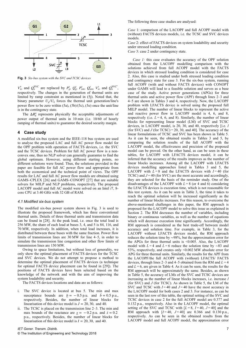
The modified six-bus power system shown in Fig. 3 is used toillustrate the proposed framework, which has three conventionalthermal units. Details of three thermal units and transmission datacan be found in [28]. At the peak load, i.e. once the total load is256 MW, the share of each load at buses 3, 4, and 5 is 84, 116, and70 MW, respectively. In addition, when total load increases, it isdistributed between these buses with the same fraction. Power flowlimits of transmission lines are 30 MW for line 4–5, in order tosimulate the transmission line congestion and other flow limits oftransmission lines are 150 MW.

Owing to space limitations, but without loss of generality, weonly show the optimal placement of FACTS devices for the TCSCand SVC devices. We do not attempt to propose a method todetermine the optimal placement of FACTS devices (a techniquefor optimal FACTS device placement can be found in [29]). Thepositions of FACTS devices have been selected based on theknowledge of the network and with the aim of improving thesystem loadability and security.

The FACTS devices locations and data are as follows:

i. The SVC device is located at bus 5. The min and maxsusceptance bounds are b = − 0.5 p.u. and b̄ = 0.5 p.u.,respectively. Besides, the number of linear blocks forlinearisation of this device model is J = 20, 30, and 40.

ii. The TCSC is placed on the transmission line 2–3. The min andmax bounds of the reactance are x = − 0.2 p.u. and x̄ = 0.2 p.u., respectively. Besides, the number of linear blocks forlinearisation of this device model is I = 20, 30, and 40.

The following three case studies are analysed:

Case 1: comparison of the LACOPF and full ACOPF model with(without) FACTS devices models, i.e. the TCSC and SVC devicesmodels.Case 2: effect of FACTS devices on system loadability and securityunder stressed loading condition.Case 3: case 2 under contingency state.

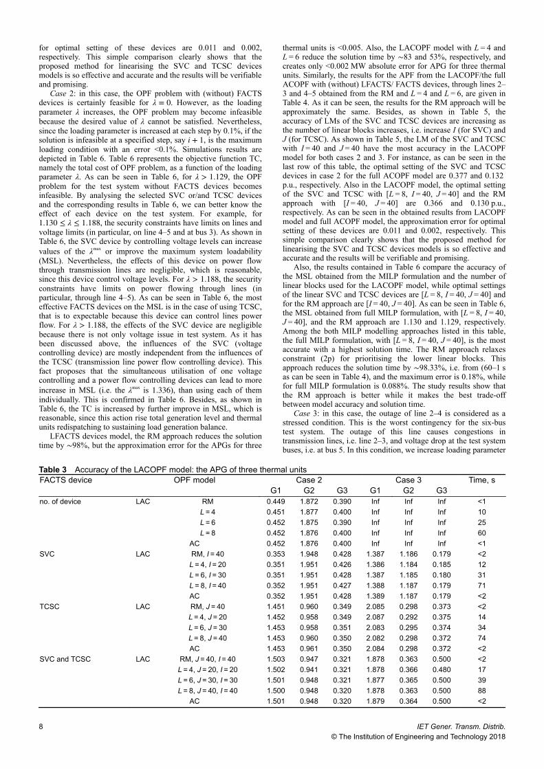
Case 1: this case evaluates the accuracy of the OPF solutionobtained from the LACOPF modelling comparison with thesolutions achieved from full ACOPF model with the FACTSdevices in which stressed loading condition is considered for case2. Also, this case is studied under both stressed loading conditionand contingency state for case 3. For the six-bus system, runningfull ACOPF (with and without FACTS devices) with CONOPTunder GAMS will lead to a feasible solution and serves as a basecase of the study. Active power generations (APGs) for threethermal units and active power flow (APF) through lines 2–3 and4–5 are shown in Tables 3 and 4, respectively. Now, the LACOPFproblem with LFACTS device is solved using the proposed fullMILP model. The number of linear blocks to represent the activeand reactive power flow in LACOPF model is 4, 6, and 8,respectively (i.e. L = 4, 6, and 8). Similarly, the number of linearblocks for representing linear model (LM) of SVC and TCSCdevices, in LACOPF model, is 20, 30, and 40, respectively [i.e. I(for SVC) and J (for TCSC) = 20, 30, and 40]. The accuracy of thelinear formulations of TCSC and SVC has been shown in Table 5.As it can be seen, the obtained results in Tables 3 and 5, bycomparing the solution results of the full ACOPF with theLACOPF model, the effectiveness and precision of the proposedmodel can be proved. On the other hand, as can be seen in thesetables, for LACOPF with LFACTS devices model, it can beinferred that the accuracy of the results improves as the number oflinear blocks increases. Among all the LACOPF with LFACTSdevices modelling approaches listed in Tables 3 and 5, theLACOPF with L = 8 and the LFACTS devices with I = 40 (forTCSC) and J = 40 (for SVC) are the most accurate and accordingly,they are selected for the basis of the reminder study. One of thedisadvantages of the LACOPF with L = 8 (or 4 and 6) consideringthe LFACTS devices is execution time, which is not reasonable forthis test system. As it can be seen in Table 3, the time it takes toreach the optimal solution will be increased significantly as thenumber of linear blocks increases. For this reason, to overcome theabove-mentioned challenges in this paper, the RM approach isproposed for the LACOPF model to solve this issue as explained inSection 2. The RM decreases the number of variables, includingbinary or continuous variables, as well as the number of equationswhich will decrease execution time significantly. Accordingly, theRM approach is considered as the best trade-off between modelaccuracy and solution time. For example, in Table 3, for theLACOPF without LFACTS devices model, the RM approachreduces the solution time by ∼98%, but the approximation error forthe APGs for three thermal units is <0.005. Also, the LACOPFmodel with L = 4 and L = 6 reduce the solution time by ∼83 and53%, respectively, and creates only <0.002 MW absolute error forAPG for three thermal units. Similarly, the results for the APF fromthe LACOPF/the full ACOPF with (without) LFACTS/ FACTSdevices, through lines 2–3 and 4–5 obtained from the RM and L = 4and L = 6, are given in Table 4. As it can be seen, the results for theRM approach will be approximately the same. Besides, as shownin Table 5, the accuracy of LMs of the SVC and TCSC devices areincreasing as the number of linear blocks increases, i.e. increase I(for SVC) and J (for TCSC). As shown in Table 5, the LM of theSVC and TCSC with I = 40 and J = 40 have the most accuracy inthe LACOPF model for both cases 2 and 3. For instance, as can beseen in the last row of this table, the optimal setting of the SVC andTCSC devices in case 2 for the full ACOPF model are 0.377 and0.132 p.u., respectively. Also in the LACOPF model, the optimalsetting of the SVC and TCSC with [L = 8, I = 40, J = 40] and theRM approach with [I = 40, J = 40] are 0.366 and 0.130 p.u.,respectively. As can be seen in the obtained results from theLACOPF model and full ACOPF model, the approximation error

Fig. 3 Six-bus system with the SVC and TCSC devices


7

for optimal setting of these devices are 0.011 and 0.002,respectively. This simple comparison clearly shows that theproposed method for linearising the SVC and TCSC devicesmodels is so effective and accurate and the results will be verifiableand promising.

Case 2: in this case, the OPF problem with (without) FACTSdevices is certainly feasible for λ = 0. However, as the loadingparameter λ increases, the OPF problem may become infeasiblebecause the desired value of λ cannot be satisfied. Nevertheless,since the loading parameter is increased at each step by 0.1%, if thesolution is infeasible at a specified step, say i + 1, is the maximumloading condition with an error <0.1%. Simulations results aredepicted in Table 6. Table 6 represents the objective function TC,namely the total cost of OPF problem, as a function of the loadingparameter λ. As can be seen in Table 6, for λ > 1.129, the OPFproblem for the test system without FACTS devices becomesinfeasible. By analysing the selected SVC or/and TCSC devicesand the corresponding results in Table 6, we can better know theeffect of each device on the test system. For example, for1.130 ≤ λ ≤ 1.188, the security constraints have limits on lines andvoltage limits (in particular, on line 4–5 and at bus 3). As shown inTable 6, the SVC device by controlling voltage levels can increasevalues of the λmax or improve the maximum system loadability(MSL). Nevertheless, the effects of this device on power flowthrough transmission lines are negligible, which is reasonable,since this device control voltage levels. For λ > 1.188, the securityconstraints have limits on power flowing through lines (inparticular, through line 4–5). As can be seen in Table 6, the mosteffective FACTS devices on the MSL is in the case of using TCSC,that is to expectable because this device can control lines powerflow. For λ > 1.188, the effects of the SVC device are negligiblebecause there is not only voltage issue in test system. As it hasbeen discussed above, the influences of the SVC (voltagecontrolling device) are mostly independent from the influences ofthe TCSC (transmission line power flow controlling device). Thisfact proposes that the simultaneous utilisation of one voltagecontrolling and a power flow controlling devices can lead to moreincrease in MSL (i.e. the λmax is 1.336), than using each of themindividually. This is confirmed in Table 6. Besides, as shown inTable 6, the TC is increased by further improve in MSL, which isreasonable, since this action rise total generation level and thermalunits redispatching to sustaining load generation balance.

LFACTS devices model, the RM approach reduces the solutiontime by ∼98%, but the approximation error for the APGs for three

thermal units is <0.005. Also, the LACOPF model with L = 4 andL = 6 reduce the solution time by ∼83 and 53%, respectively, andcreates only <0.002 MW absolute error for APG for three thermalunits. Similarly, the results for the APF from the LACOPF/the fullACOPF with (without) LFACTS/ FACTS devices, through lines 2–3 and 4–5 obtained from the RM and L = 4 and L = 6, are given inTable 4. As it can be seen, the results for the RM approach will beapproximately the same. Besides, as shown in Table 5, theaccuracy of LMs of the SVC and TCSC devices are increasing asthe number of linear blocks increases, i.e. increase I (for SVC) andJ (for TCSC). As shown in Table 5, the LM of the SVC and TCSCwith I = 40 and J = 40 have the most accuracy in the LACOPFmodel for both cases 2 and 3. For instance, as can be seen in thelast row of this table, the optimal setting of the SVC and TCSCdevices in case 2 for the full ACOPF model are 0.377 and 0.132 p.u., respectively. Also in the LACOPF model, the optimal settingof the SVC and TCSC with [L = 8, I = 40, J = 40] and the RMapproach with [I = 40, J = 40] are 0.366 and 0.130 p.u.,respectively. As can be seen in the obtained results from LACOPFmodel and full ACOPF model, the approximation error for optimalsetting of these devices are 0.011 and 0.002, respectively. Thissimple comparison clearly shows that the proposed method forlinearising the SVC and TCSC devices models is so effective andaccurate and the results will be verifiable and promising.

Also, the results contained in Table 6 compare the accuracy ofthe MSL obtained from the MILP formulation and the number oflinear blocks used for the LACOPF model, while optimal settingsof the linear SVC and TCSC devices are [L = 8, I = 40, J = 40] andfor the RM approach are [I = 40, J = 40]. As can be seen in Table 6,the MSL obtained from full MILP formulation, with [L = 8, I = 40,J = 40], and the RM approach are 1.130 and 1.129, respectively.Among the both MILP modelling approaches listed in this table,the full MILP formulation, with [L = 8, I = 40, J = 40], is the mostaccurate with a highest solution time. The RM approach relaxesconstraint (2p) for prioritising the lower linear blocks. Thisapproach reduces the solution time by ∼98.33%, i.e. from (60–1 sas can be seen in Table 4), and the maximum error is 0.18%, whilefor full MILP formulation is 0.088%. The study results show thatthe RM approach is better while it makes the best trade-offbetween model accuracy and solution time.

Case 3: in this case, the outage of line 2–4 is considered as astressed condition. This is the worst contingency for the six-bustest system. The outage of this line causes congestions intransmission lines, i.e. line 2–3, and voltage drop at the test systembuses, i.e. at bus 5. In this condition, we increase loading parameter

Table 3 Accuracy of the LACOPF model: the APG of three thermal unitsFACTS device OPF model Case 2 Case 3 Time, s

G1 G2 G3 G1 G2 G3no. of device LAC RM 0.449 1.872 0.390 Inf Inf Inf <1

L = 4 0.451 1.877 0.400 Inf Inf Inf 10L = 6 0.452 1.875 0.390 Inf Inf Inf 25L = 8 0.452 1.876 0.400 Inf Inf Inf 60

AC 0.452 1.876 0.400 Inf Inf Inf <1SVC LAC RM, I = 40 0.353 1.948 0.428 1.387 1.186 0.179 <2

L = 4, I = 20 0.351 1.951 0.426 1.386 1.184 0.185 12L = 6, I = 30 0.351 1.951 0.428 1.387 1.185 0.180 31L = 8, I = 40 0.352 1.951 0.427 1.388 1.187 0.179 71AC 0.352 1.951 0.428 1.389 1.187 0.179 <2

TCSC LAC RM, J = 40 1.451 0.960 0.349 2.085 0.298 0.373 <2L = 4, J = 20 1.452 0.958 0.349 2.087 0.292 0.375 14L = 6, J = 30 1.453 0.958 0.351 2.083 0.295 0.374 34L = 8, J = 40 1.453 0.960 0.350 2.082 0.298 0.372 74AC 1.453 0.961 0.350 2.084 0.298 0.372 <2

SVC and TCSC LAC RM, J = 40, I = 40 1.503 0.947 0.321 1.878 0.363 0.500 <2L = 4, J = 20, I = 20 1.502 0.941 0.321 1.878 0.366 0.480 17L = 6, J = 30, I = 30 1.501 0.948 0.321 1.877 0.365 0.500 39L = 8, J = 40, I = 40 1.500 0.948 0.320 1.878 0.363 0.500 88

AC 1.501 0.948 0.320 1.879 0.364 0.500 <2


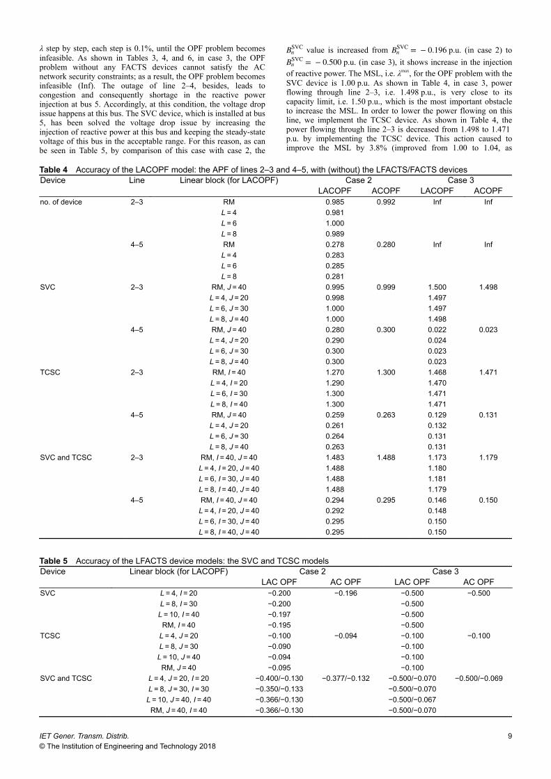
λ step by step, each step is 0.1%, until the OPF problem becomesinfeasible. As shown in Tables 3, 4, and 6, in case 3, the OPFproblem without any FACTS devices cannot satisfy the ACnetwork security constraints; as a result, the OPF problem becomesinfeasible (Inf). The outage of line 2–4, besides, leads tocongestion and consequently shortage in the reactive powerinjection at bus 5. Accordingly, at this condition, the voltage dropissue happens at this bus. The SVC device, which is installed at bus5, has been solved the voltage drop issue by increasing theinjection of reactive power at this bus and keeping the steady-statevoltage of this bus in the acceptable range. For this reason, as canbe seen in Table 5, by comparison of this case with case 2, the

BnSVC value is increased from Bn

SVC = − 0.196 p.u. (in case 2) toBn

SVC = − 0.500 p.u. (in case 3), it shows increase in the injectionof reactive power. The MSL, i.e. λmax, for the OPF problem with theSVC device is 1.00 p.u. As shown in Table 4, in case 3, powerflowing through line 2–3, i.e. 1.498 p.u., is very close to itscapacity limit, i.e. 1.50 p.u., which is the most important obstacleto increase the MSL. In order to lower the power flowing on thisline, we implement the TCSC device. As shown in Table 4, thepower flowing through line 2–3 is decreased from 1.498 to 1.471 p.u. by implementing the TCSC device. This action caused toimprove the MSL by 3.8% (improved from 1.00 to 1.04, as

Table 4 Accuracy of the LACOPF model: the APF of lines 2–3 and 4–5, with (without) the LFACTS/FACTS devicesDevice Line Linear block (for LACOPF) Case 2 Case 3

LACOPF ACOPF LACOPF ACOPFno. of device 2–3 RM 0.985 0.992 Inf Inf

L = 4 0.981L = 6 1.000L = 8 0.989

4–5 RM 0.278 0.280 Inf InfL = 4 0.283L = 6 0.285L = 8 0.281

SVC 2–3 RM, J = 40 0.995 0.999 1.500 1.498L = 4, J = 20 0.998 1.497L = 6, J = 30 1.000 1.497L = 8, J = 40 1.000 1.498

4–5 RM, J = 40 0.280 0.300 0.022 0.023L = 4, J = 20 0.290 0.024L = 6, J = 30 0.300 0.023L = 8, J = 40 0.300 0.023

TCSC 2–3 RM, I = 40 1.270 1.300 1.468 1.471L = 4, I = 20 1.290 1.470L = 6, I = 30 1.300 1.471L = 8, I = 40 1.300 1.471

4–5 RM, J = 40 0.259 0.263 0.129 0.131L = 4, J = 20 0.261 0.132L = 6, J = 30 0.264 0.131L = 8, J = 40 0.263 0.131

SVC and TCSC 2–3 RM, I = 40, J = 40 1.483 1.488 1.173 1.179L = 4, I = 20, J = 40 1.488 1.180L = 6, I = 30, J = 40 1.488 1.181L = 8, I = 40, J = 40 1.488 1.179

4–5 RM, I = 40, J = 40 0.294 0.295 0.146 0.150L = 4, I = 20, J = 40 0.292 0.148L = 6, I = 30, J = 40 0.295 0.150L = 8, I = 40, J = 40 0.295 0.150

Table 5 Accuracy of the LFACTS device models: the SVC and TCSC modelsDevice Linear block (for LACOPF) Case 2 Case 3

LAC OPF AC OPF LAC OPF AC OPFSVC L = 4, I = 20 −0.200 −0.196 −0.500 −0.500

L = 8, I = 30 −0.200 −0.500L = 10, I = 40 −0.197 −0.500RM, I = 40 −0.195 −0.500

TCSC L = 4, J = 20 −0.100 −0.094 −0.100 −0.100L = 8, J = 30 −0.090 −0.100

L = 10, J = 40 −0.094 −0.100RM, J = 40 −0.095 −0.100

SVC and TCSC L = 4, J = 20, I = 20 −0.400/−0.130 −0.377/−0.132 −0.500/−0.070 −0.500/−0.069L = 8, J = 30, I = 30 −0.350/−0.133 −0.500/−0.070

L = 10, J = 40, I = 40 −0.366/−0.130 −0.500/−0.067RM, J = 40, I = 40 −0.366/−0.130 −0.500/−0.070


9

observed in Table 5). It can be inferred from Table 5, the SVC andTCSC devices cannot improve the MSL significantly. However, inthe case of simultaneous implementation of the SVC and TCSCdevices, there is a significant decrease in power flowing throughline 2–3 by TCSC device (i.e. >21%), and more increase inreactive power injection at bus 5 resulting in voltage improvementat this bus by SVC device. This fact is shown in Table 5 byincreasing the Bn

SVC value. Finally, in the case of concurrentoperation of SVC and TCSC, the MSL is improved by 10 and 6.4%with respect to using individual SVC or TCSC, respectively.

4.2 Modified IEEE 118-bus system

The modified IEEE 118-bus system has 54 thermal units, 186 lines,and 91 load buses. The parameters of transmission network, loadprofiles, and thermal units are given in motor.ece.iit.edu/data/SCUC_118. The peak load is 7306 MW. Also in this test system,the line limits for a few transmission lines are reduced to 100 MWin order to simulate the transmission system congestion. TheFACTS devices are located in their corresponding optimallocations in the modified IEEE 118-bus test system. Hence, all theFACTS devices are located independently at a single location andits impact on the MSL is investigated [29].

Based on load flow analysis, the heavily loaded lines with lowcapacity in the modified IEEE 118-bus system are lines [11 (buses5–11), 55 (buses 39–40), 70 (buses 49–50), 136 (buses 85–89), and168 (buses 104–105)] where the series devices TCSC are located.The limitation of the effective reactance of each TCSC device is setto 90% capacitive and 40% inductive of the original reactance ofthe transmission line where the TCSC device is located. Also, thebuses that need more reactive power compensation are buses 7, 69,77, 49, 34, and 106 where the shunt devices SVC are located. Themin and max susceptance bounds for each SVC devices are similarto the previous test system. Four cases are considered here, thatcases 1–3 are similar to cases 1–3 of the previous test system.

Case 1: the simulations are performed to obtain the APF and theAPG using the LACOPF model and the full ACOPF model.Furthermore, we consider the SVC and TCSC devicessimultaneously in both the OPF models. The number of linearblocks for representing the active and reactive power flow inLACOPF model is 4, which is named LM here, is considered forthe modified IEEE 118-bus system. Similarly, the number of linearblocks to represent the LM of the SVC and the TCSC devices forboth models mentioned for the LACOPF model, i.e. the LM andthe RM models, is I and J = 30.

Considering the full ACOPF results as the reference, thecalculation errors are given by:

ΔnmLAC = Pnm

AC − PnmLAC (6a)

ΔgLAC = Pg

AC − PgLAC (6b)

Equation (6a) is the calculation error of the APF in line (n, m)which are obtained from both models of the LACOPF, i.e. the LMand RM, and the full ACOPF solution, respectively. Also, (6b) isthe calculation error of the APG from thermal unit g similar to (6a).As can be seen in Fig. 4, the maximum value of the error calculatedfor Δnm

LAC, for the LM and RM models, are 0.0092 and 0.0252 p.u.,respectively. Also, the mean value of error calculated for Δnm

LAC, forthese models are 0.018 and 0.052 p.u., respectively. Similarly, inFig. 5, the maximum Δg

LAC value for the LM and RM models are0.017 and 0.0477 p.u., respectively. In addition, the mean value ofΔg

LAC for these models is 0.0012 and 0.00617 p.u., respectively.These results indicate that the APF through the lines and the APGof thermal units obtained by the proposed LACOPF model providemore precise for large-scale systems. The elapsed time to solve theLACOPF problem by the LM approach is about >700 s and by theRM approach is about <10 s. These results indicate the accuracy ofRPF and RPG for the LM approach, which is calculated by theLACOPF model, is increased on large-scale system. However, thisshould be taken into account that with the LM approach, thesolution time is increased. The results show that the RM approachhas the best trade-off between model accuracy and solution timefor the large-scale systems.

Also, in this case, the λmax and the TC obtained from the fullACOPF model with (without) FACTS devices are given in Table 7.The same results are approximately obtained by the proposedmethod using the LACOPF with (without) LFACTS devices. Notedthat, the LACOPF model in Table 7 is modelled by the RMapproach. For this approach, the λmax and the TC are given inTable 7 and the written program has 84,353 single equations,96,630 single variables, and 1116 binary variables. As it can beseen in Table 7, the calculation error of the obtained results fromthe LACOPF model (modelled by RM) and the ACOPF model arevery small, i.e. for the λmax and TC are <0.005, which is a veryworthy precise. The elapsed time to solve the OPF problem with(without) FACTS devices by the full ACOPF approach is ∼20 sand by LACOPF (by RM method) approach is <10 s. Finally, asthe results show, the LACOPF that is modelled by the RM methodis completely accepted from our OPF problem with (without)FACTS devices and has a reasonable run time.

Case 2: this case is similar to case 2 in the previous test system.Therefore, as can be seen in Table 7, the OPF problem is feasiblefor no FACTS devices and the value of λmax is 1.208. Note, thisvalue, λmax = 1.208, is served as reference for the MSL. In thiscase, the loading parameter is increased similar to the previous testsystem and maximum loading condition is obtained. Simulations

Table 6 MSL and the TC for the six-bus system for cases 2 and 3Device Linear block (for LACOPF) LACOPF ACOPF

λmax TC λmax TCcase 2 no. of device L = 8 1.130 7518.126 1.131 7520.896

RM 1.129 7515.086SVC L = 8, I = 40 1.189 7856.382 1.191 7861.432

RM, I = 40 1.188 7853.432TCSC L = 8, J = 40 1.336 8412.120 1.337 8418.897

RM, J = 40 1.334 8407.170SVC and TCSC L = 8, J = 40, I = 40 1.338 8378.134 1.338 8379.875

RM, J = 40, I = 40 1.336 8370.775case 3 no. of device L = 8 Inf Inf Inf Inf

RM Inf InfSVC L = 10, I = 40 1.000 6139.340 1.000 6141.780

RM, I = 40 1.000 6135.600TCSC L = 10, J = 40 1.045 6389.125 1.050 6392.160

RM, J = 40 1.040 6388.270SVC and TCSC L = 10, J = 40, I = 40 1.107 6985.676 1.109 6992.175

RM, J = 40, I = 40 1.112 6986.135


results are illustrated in Table 7. This table represents the TC andthe MSL. As can be seen from this table, if we compare the TCSCand SVC for the modified 118-bus network, we see that by usingthe TCSC device, we have ∼16.70% loadability improvementwhile with the SVC, the rate is ∼7%. Comparing the results forTCSC and SVC devices, it can be inferred that the TCSC devicewould be more effective than the SVC in improving the MSL.Finally, we have the most improve MSL, for modified 118-bus testsystem, once that the TCSC and SVC devices are consideredsimultaneously. In this situation, as it clear from Table 7, we have∼21% improvement in the MSL.

Case 3: this case is similar to case 3 in the previous test system.Here, three simultaneous contingencies are considered. Thecontingencies include outages of thermal unit 28, transmissionlines 75–77, and 85–89. The first OPF problem is feasible for theoutage of transmission line 75–77. Therefore, the contingency oftransmission line 75–77 is controllable without FACTS devices.Since the OPF solution cannot lead to a feasible solution for theoutages of unit 28 and transmission line 85–89, these contingenciesare uncontrollable without FACTS devices. The value of λmax, forthe OPF problem with the SVC device, is 1.042. Also, we have∼10% improvement in the MSL with the TCSC device. The resultsof concurrent operation of the SVC and TCSC devices arepresented in Table 7, which show ∼16.23% improvement in the

MSL. Finally, the simulation results in this table show that theconcurrent operation of these devices have the most efficiency inincreasing the MSL under contingency state.

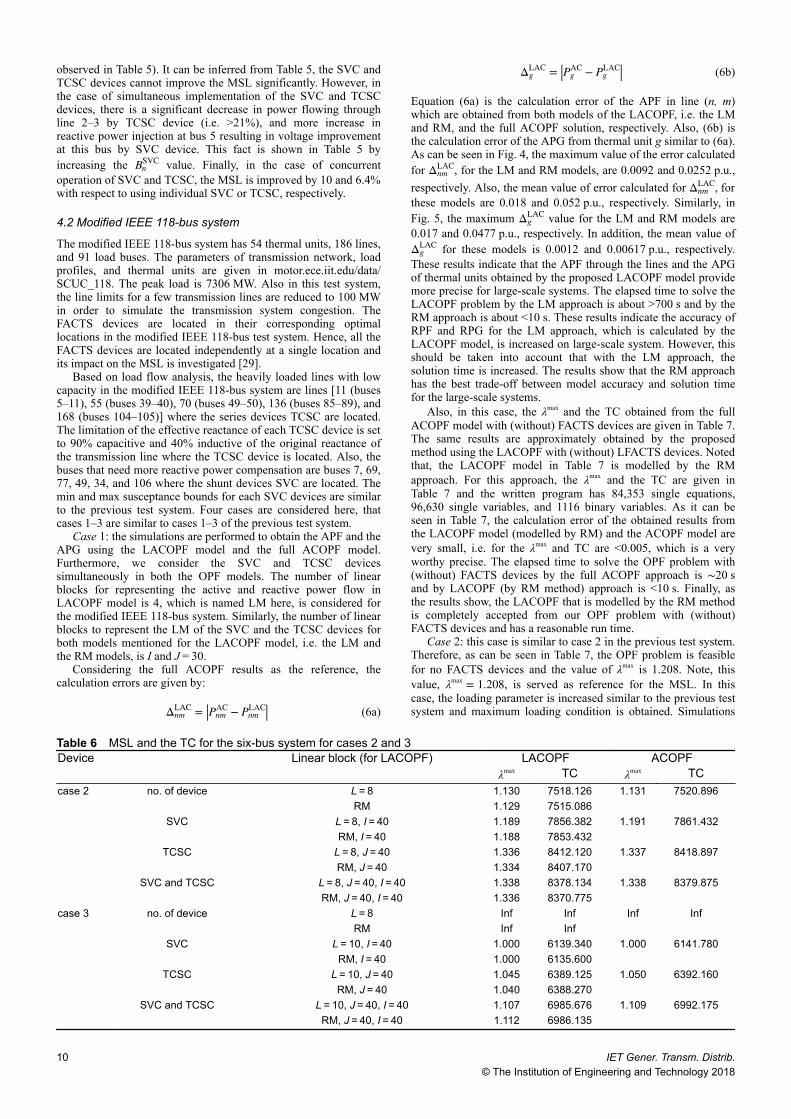
Case 4: in this case, the effect of the number of FACTS devices(TCSC and SVC) on the number of congested lines has beenstudied. As can be seen in Fig. 6, the number of congestedtransmission lines is reduced by increasing the number of TCSCsand SVCs from 1 to 5 and 1 to 6, respectively, in the test system.Figs. 3a and b show how the congestion of transmission linesdecreases as more FACTS devices are allowed to be used. Thisfigure shows that the congestion reduction in transmission lines ismore significant for the first few FACTS (especially for the TCSCdevices) and then the congestion curves are going to be saturated.On the other hand, as shown in Figs. 3a and b, the TCSC is moreeffective on congestion reduction in transmission lines than theSVC. For this reason, the voltage support provided by the SVCdoes not reduce the number of congested lines. Nonetheless, theTCSC is able to reduce the number of congested lines since itdecrease the series impedance of the congested transmission lines,hence allows reducing congestion of transmission lines. For theIEEE 118-bus system, the binding constraints are mainly the limitson transmission lines. As expected, the effective FACTS devicesamong TCSC and SVC on the number of congested lines are theTCSC device because this device has better control on line power

Fig. 4 APF calculation error for the IEEE 118-bus system for LACOPF modelled by the LM and the RM approaches

Fig. 5 APG calculation error for the IEEE 118-bus system for LACOPF modelled by the LM and the RM approaches

Table 7 MSL and TC for the IEEE 118-bus system for cases 2 and 3Device LACOPF ACOPF

λmax TC λmax TCcase 2 no. of device 1.212 165,889.152 1.208 165,371.231

SVC 1.301 181,319.669 1.298 179,057.655TCSC 1.454 208,232.502 1.451 207,699.471

SVC and TCSC 1.533 222,347.340 1.529 221,628.968case 3 no. of device Inf Inf Inf Inf

SVC 1.044 159,340.413 1.042 158,824.548TCSC 1.151 169,172.709 1.153 168,653.863

SVC and TCSC 1.251 190,053.951 1.244 189,528.350


11

flows. For this test system, the effects of the SVC are negligiblebecause there is no voltage problem. Accordingly, as shown in Fig.6a, the number of this device has a small effect on the congestedlines. However, when the number of TCSC and SVC devices isincreased, from 1 up to 5, the number of congested lines has notchanged. This is basically due to the fact that the TCSC and SVCdevices reach their control limits.

5 ConclusionsThis paper provides a methodology to maximise system loadabilityand system security using an OPF with FACTS devices. The OPFproblem presented in this paper is based on a new LACOPF modelwith linearised FACTS devices model. Among FACTS devices,SVC and TCSC are selected for this study. The proposed LACOPFand LFACTS models approximate the full AC network constraintsand the non-linear nature of the SVC and TCSC devices moreaccurately, and therefore provide more realistic operation solutions.The paper shows that full ACOPF with SVC and TCSC devices isan NLP problem that is transformed into an MILP by the proposedmethod. Therefore, the LACOPF problem with LFACTS devicescan be solved by available efficient commercial-grade software.Since this paper reformulated the problem as an MILP, the globaloptimal solution of the approximated model is guaranteed to befound as revealed in the simulation results. The simulation resultson the modified IEEE-118 bus system show that the proposedLACOPF model can be applied to solve OPF problems withLFACTS devices, to more accurately approximate the AC networkwith FACTS devices compared to a DCOPF model.

6 References[1] Lehmkoster, C.: ‘Security constrained optimal power flow for an economical

operation of FACTS-devices in liberalized energy markets’, IEEE Trans.Power Deliv., 2002, 17, pp. 603–608

[2] Bertsekas, D. P.: ‘Nonlinear programming’ (Athena Scientific Belmont,Nashua, NH, USA, 1999)

[3] Mukherjee, A., Mukherjee, V.: ‘Solution of optimal power flow with FACTSdevices using a novel oppositional krill herd algorithm’, Int. J. Electr. PowerEnergy Syst., 2016, 78, pp. 700–714

[4] Nireekshana, T., Rao, G. K., Raju, S. S. N.: ‘Enhancement of ATC withFACTS devices using real-code genetic algorithm’, Int. J. Electr. PowerEnergy Syst., 2012, 43, pp. 1276–1284

[5] Pillay, A., Karthikeyan, S. P., Kothari, D.: ‘Congestion management in powersystems – a review’, Int. J. Electr. Power Energy Syst., 2015, 70, pp. 83–90

[6] Berizzi, A., Delfanti, M., Marannino, P., et al.: ‘Enhanced security-constrained OPF with FACTS devices’, IEEE Trans. Power Syst., 2005, 20,pp. 1597–1605

[7] Gasperic, S., Mihalic, R.: ‘The impact of serial controllable FACTS deviceson voltage stability’, Int. J. Electr. Power Energy Syst., 2015, 64, pp. 1040–1048

[8] Ghahremani, E., Kamwa, I.: ‘Optimal placement of multiple-type FACTSdevices to maximize power system loadability using a generic graphical userinterface’, IEEE Trans. Power Syst., 2013, 28, pp. 764–778

[9] Sahraei-Ardakani, M., Hedman, K.W.: ‘A fast LP approach for enhancedutilization of variable impedance based FACTS devices’, IEEE Trans. PowerSyst., 2016, 31, pp. 2204–2213

[10] Sahraei-Ardakani, M., Hedman, K. W.: ‘Day-ahead corrective adjustment ofFACTS reactance: a linear programming approach’, IEEE Trans. Power Syst.,2016, 31, pp. 2867–2875

[11] Zarate-Minano, R., Conejo, A., Milano, F.: ‘OPF-based security redispatchingincluding FACTS devices’, IET Gener. Transm. Distrib., 2008, 2, pp. 821–833

[12] Akbari, T., Bina, M. T.: ‘Linear approximated formulation of AC optimalpower flow using binary discretisation’, IET Gener. Transm. Distrib., 2016,10, pp. 1117–1123

[13] Nasri, A., Conejo, A. J., Kazempour, S. J., et al.: ‘Minimizing wind powerspillage using an OPF with FACTS devices’, IEEE Trans. Power Syst., 2014,29, pp. 2150–2159

[14] Henneaux, P., Kirschen, D. S.: ‘Probabilistic security analysis of optimaltransmission switching’, IEEE Trans. Power Syst., 2016, 31, pp. 508–517

[15] Nagalakshmi, S., Kamaraj, N.: ‘On-line evaluation of loadability limit forpool model with TCSC using back propagation neural network’, Int. J. Electr.Power Energy Syst., 2013, 47, pp. 52–60

[16] Zhang, H., Heydt, G. T., Vittal, V., et al.: ‘An improved network model fortransmission expansion planning considering reactive power and networklosses’, IEEE Trans. Power Syst., 2013, 28, pp. 3471–3479

[17] Jordehi, A. R.: ‘Particle swarm optimisation (PSO) for allocation of FACTSdevices in electric transmission systems: a review’, Renew. Sust. Energy Rev.,2015, 52, pp. 1260–1267

[18] Ongsakul, W., Bhasaputra, P.: ‘Optimal power flow with FACTS devices byhybrid TS/SA approach’, Int. J. Electr. Power Energy Syst., 2002, 24, pp.851–857

[19] Khorsandi, A., Hosseinian, S., Ghazanfari, A.: ‘Modified artificial bee colonyalgorithm based on fuzzy multi-objective technique for optimal power flowproblem’, Electr. Power Syst. Res., 2013, 95, pp. 206–213

[20] Sahraei-Ardakani, M., Blumsack, S. A.: ‘Transfer capability improvementthrough market-based operation of series FACTS devices’, 2015

[21] Misener, R., Floudas, C.: ‘Piecewise-linear approximations ofmultidimensional functions’, J. Optim. Theory Appl., 2010, 145, pp. 120–147

[22] Beale, E., Forrest, J. J.: ‘Global optimization using special ordered sets’,Math. Program., 1976, 10, pp. 52–69

[23] Fuerte-Esquivel, C., Acha, E., Ambriz-Perez, H.: ‘A thyristor controlledseries compensator model for the power flow solution of practical powernetworks’, IEEE Trans. Power Syst., 2000, 15, pp. 58–64

[24] Ambriz-Perez, H., Acha, E., Fuerte-Esquivel, C.: ‘Advanced SVC models forNewton–Raphson load flow and Newton optimal power flow studies’, IEEETrans. Power Syst., 2000, 15, pp. 129–136

[25] Gurobi Optimization, Gurobi Optimizer Reference Manual. [Online].Available at http://www.gurobi.com

[26] CPLEX, GAMS. The Solver Manuals. GAME/CPLEX, 1996 [Online].Available at http://www.gams.com/

[27] Drud, A. S.: GAMS/CONOPT. ARKI consulting and development,Bagsvaerd, Denmark, 1996 [Online]. Available at http://www.gams.com/

[28] Khodaei, A., Shahidehpour, M.: ‘Transmission switching in security-constrained unit commitment’, IEEE Trans. Power Syst., 2010, 25, pp. 1937–1945

[29] Duong, T., JianGang, Y., Truong, V.: ‘Application of min cut algorithm foroptimal location of FACTS devices considering system loadability and cost ofinstallation’, Int. J. Electr. Power Energy Syst., 2014, 63, pp. 979–987

Fig. 6 Number of congested lines versus(a) Number of TCSC devices, (b) Number of SVC devices in the IEEE-118 bussystem


http://www.gurobi.com

http://www.gams.com/

http://www.gams.com/

Contribution of FACTS devices in power systems security ...

Documents

Transcript of Contribution of FACTS devices in power systems security ...