International Journal of Engineering Research and Development

e-ISSN: 2278-067X, p-ISSN: 2278-800X, www.ijerd.com

Volume 11, Issue 12 (December 2015), PP.01-12

1

Co-ordinated control of FACTS Devices using Optimal Power

Flow Technique

S. Raghavendra Rao1, Ch. Padmanabha Raju

2

1PG Scholar, Department of Electrical & Electronics Engineering, P.V.P. Siddhartha Institute of Technology,

Vijayawada, A.P-520007 2Professor, Department of Electrical & Electronics Engineering, P.V.P. Siddhartha Institute of Technology

Vijayawada, A.P -520007

Abstract:-The Optimal Power Flow (OPF) plays an important role in power system operation and control due

to depleting energy resources, and increasing power generation cost and ever growing demand for electrical

energy. Here FACTS devices are effectively used for power flow control, voltage regulation, improvement of

power system stability, minimization of losses. The FACTS devices that we use are SVC and UPFC. For power

flow studies, the modeling of FACTS devices is discussed. The SVC is good at voltage regulation and UPFC is

good at balancing the reactive power in the system. In this paper, PSO based approach is presented to solve the

Optimal Power Flow to satisfy objectives such as minimizing generation cost and transmission line loss. The

proposed PSO algorithm is tested on IEEE 30 bus system.

Keywords:- Mathematical model of OPF, SVC, UPFC, Co-ordinate control, PSO, Cost of generation.

I. INTRODUCTION The rapid growth of heavy loads in the system and high power transfer on the line makes it

uncomfortable. Due to this the line may get damage and construction of additional lines or siting new generation

is very difficult. For avoiding these problem FACTS devices is introduced. FACTS technology makes power

system easy to transfer the active power without overloading the line. FACTS devices can be effectively used

for power flow control, voltage regulation, improvement of power system stability, minimization of losses. In

the power system cost is also the main thing that we need take into the consideration .In order to investigate the

effects of FACTS devices in steady-state, appropriate models are needed capturing the influences of the devices

on power flows and voltages. Various models for SVC, and UPFC are conceivable and applied in different

studies. In Sect. II, the modelling of FACTS devices that we used in this paper and how they are incorporated

into the power flow calculations are described.

A static VAR compensator is a set of electrical devices for providing fast-acting reactive

power on high-voltage electricity transmission networks. SVCs are part of the Flexible AC transmission system

device family, regulating voltage, power factor, and harmonics and stabilizing the system. Unlike a synchronous

condenser which is a rotating electrical machine, a static VAR compensator has no significant moving parts

(other than internal switchgear). Prior to the invention of the SVC [1], power factor compensation was the

preserve of large rotating machines such as synchronous condensers or switched capacitor banks.

A combination of static synchronous compensator (STATCOM) and a static synchronous series

compensator (SSSC) which are coupled via a common dc link, to allow bidirectional flow of real power

between the series output terminals of the SSSC and the shunt output terminals of the STATCOM, and are

controlled to provide concurrent real and reactive series line compensation without an external electric energy

source. The UPFC, by means of angularly unconstrained series voltage injection, is able to control, concurrently

or selectively, the transmission line voltage, impedance, and angle or, alternatively, the real and reactive power

flow in the line. The UPFC may also provide independently controllable shunt reactive compensation. In section

III it shows about the mathematical formulation of the optimal power flow of the system.

In sec IV the influences of FACTS devices are not confined to one bus or line. Changing the voltage at

a certain bus or the power flow on a line also modifies the power flow in the surrounding grid. If a FACTS

device is placed in the vicinity of another, mutual influences may arise which could vitiate the positive impacts

of a single device. So by using this Co-ordinate control on the FACTS devices we can reduce the influence of

one device on another. Therefore the sec V invesgates about the different cases there first we consider the

normal case means without introducing FACTS devices and in the next case by introducing single and multiple

FACTS devices we calculate cost of generation, power losses, sum of squares of voltage stability indices and

CPU time in each case.

Co-ordinated control of FACTS Devices using Optimal Power Flow Technique

2

II. MATHEMATICAL MODEL OF FACTS DEVICES

2.1 Modelling of SVC:

According to IEEE the definition of the SVC [1],[2] is as follows “A shunt connected static var

generator or absorber whose output is adjusted to exchange capacitive or inductive current so as to maintain or

control specific parameters (typically bus voltage) of the electrical power system.

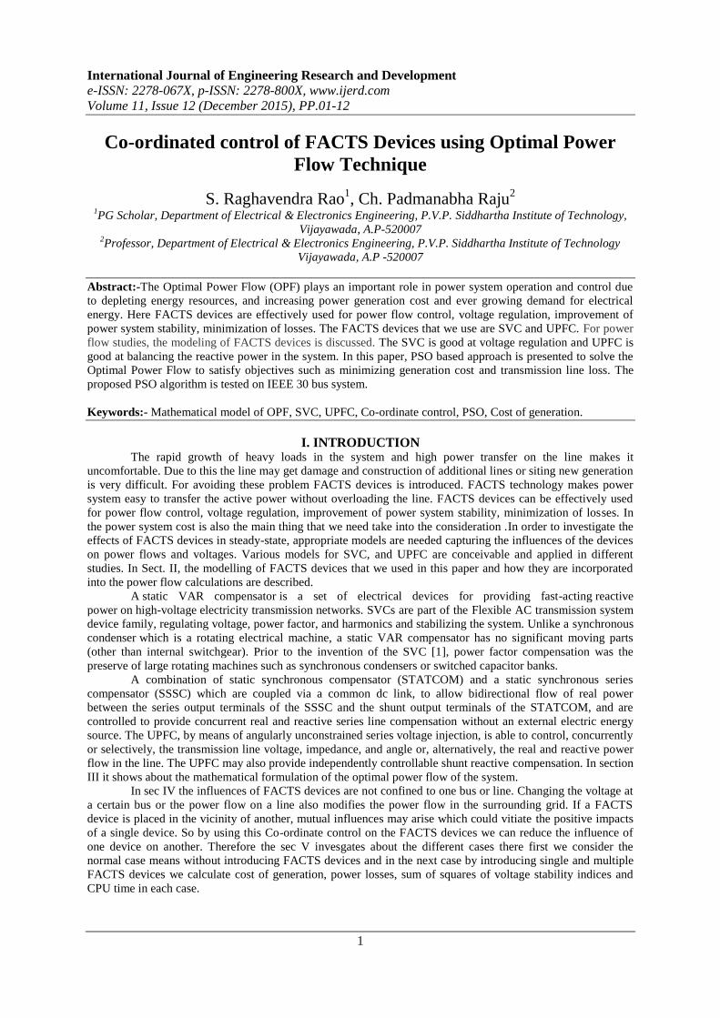
SVC device is a parallel combination of thyristor controlled reactor with a bank of capacitors. It’s a

shunt connected variable reactance, which either generates or absorbs reactive power in order to regulate the

voltage magnitude where it is connected to the AC network. Mainly used for voltage regulation. As an important

component for voltage control, it is usually installed at the receiving node of the transmission lines.

Fig 1 FC-TCR structure of SVC. Fig 2 Variable-Shunt Susceptance.

With reference to the above figure, the current drawn by the SVC is

𝐼𝑠𝑣𝑐 = 𝑗𝐵𝑠𝑣𝑐𝑉𝑘 (1)

and the reactive power drawn by the SVC, which is also the reactive power injected at bus k, is

𝑄𝑠𝑣𝑐 = 𝑄𝑘 = −𝑉𝑘2𝐵𝑠𝑣𝑐 (2)

where the equivalent Susceptance 𝐵𝑠𝑣𝑐 is taken to be the state variable

∆𝑃𝑘

∆𝑄𝑘

(𝑖)

= 0 00 𝑄𝑘

(𝑖)

∆𝜃𝑘

∆𝐵𝑠𝑣𝑐 𝐵𝑠𝑣𝑐

(𝑖)

(3)

At the end of iteration (i), the variable shunt susceptance 𝐵𝑠𝑣𝑐 is updated according to

𝐵𝑠𝑣𝑐(𝑖)

= 𝐵𝑠𝑣𝑐(𝑖−1)

+ ∆𝐵𝑠𝑣𝑐

𝐵𝑠𝑣𝑐

(𝑖)

𝐵𝑠𝑣𝑐(𝑖)

(4)

The changing susceptance represents the total SVC susceptance necessary to maintain the nodal

voltage magnitude at the specified value. Once the level of compensation has been computed then the thyristor

firing angle can be calculated. However, the additional calculation requires an iterative solution because the

SVC susceptance and thyristor firing angle are nonlinearly related.

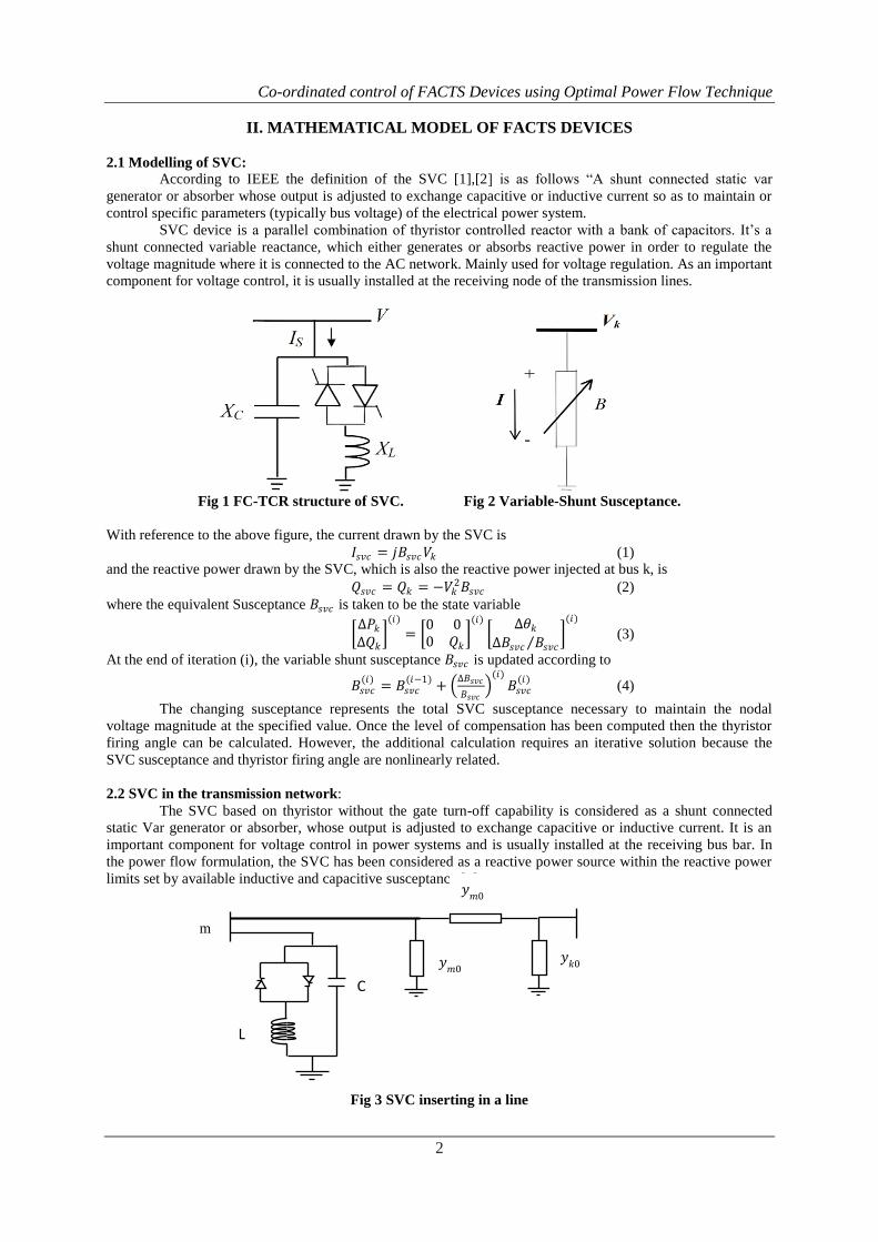
2.2 SVC in the transmission network:

The SVC based on thyristor without the gate turn-off capability is considered as a shunt connected

static Var generator or absorber, whose output is adjusted to exchange capacitive or inductive current. It is an

important component for voltage control in power systems and is usually installed at the receiving bus bar. In

the power flow formulation, the SVC has been considered as a reactive power source within the reactive power

limits set by available inductive and capacitive susceptance [3].

Fig 3 SVC inserting in a line

𝑦𝑚0

L

𝑦𝑘0

C

𝑦𝑚0

m

Co-ordinated control of FACTS Devices using Optimal Power Flow Technique

3

SVC placed at the beginning of the line

For an SVC connected at a bus bar m of a line section represented by the quadruple (𝑦𝑚𝑜 ,𝑦𝑚𝑘 , 𝑦𝑘𝑜 ) as

shown in figure, the contribution of the SVC to the new admittance matrix relates to the element shunt. It results

in the admittance matrix of the line.

𝑌𝑛𝑒𝑤𝑙𝑖𝑛𝑒 =

𝑦𝑚𝑘 + 𝑦𝑚𝑜 + 𝑦𝑠𝑣𝑐 −𝑦𝑚𝑘

−𝑦𝑚𝑘 𝑦𝑚𝑘 + 𝑦𝑘𝑜

(5)

We know such that

𝐵𝑠𝑣𝑐 =1

𝑋𝑠𝑣𝑐

𝐵𝑠𝑣𝑐 =1

𝑋𝐶𝑋𝐿 𝑋𝐿 −

𝑋𝐶

𝜋 2 𝜋 − 𝛼 + sin 2𝛼 (6)

The SVC reactance is given as following

𝑋𝑠𝑣𝑐(𝛼) =𝜋𝑋𝐿

2 𝜋−𝛼 +sin 2𝛼 −𝜋𝑋𝐿𝑋𝐶

(7)

Influence of the SVC on the network

It results from these modifications on the nodal admittances matrix and from the Jacobian. These modifications

are detailed in what follows.

Modification of the admittances matrix:

We modelled the SVC as being a variable transverse admittance which is connected to a bus m of the network.

Thus, the effect of this is based only on the modification of the element y in the admittances matrix. The new

modified matrix is written as follows:

𝑌𝑛𝑒𝑤 =

𝑌11

⋮𝑌𝑚1

⋮𝑌𝑛1

⋯⋱⋯⋰⋯

𝑌1𝑚

⋮𝑌𝑚𝑚

𝑜𝑙𝑑 + 𝑌𝑠𝑣𝑐⋮

𝑌𝑛𝑚

⋯⋰⋯⋱⋯

𝑌1𝑛

⋮𝑌𝑚𝑛

⋮𝑌𝑛𝑛

(8)

This new matrix is used to calculate the new power transit. By varying the firing angle of the SVC “α”,

it is possible to plot the curves of voltages variation at the buses. They allow locating the best point of

compensation of the network. The variation curves of the powers losses in the lines can be obtained according to

“α” which makes it possible to measure the impact of the SVC device on these lines. These curves will be

studied for the compensation of a network in the overvoltage.

The impact of the nature of the load and its importance will be observed by studying two loading cases

purely active and reactivate respectively. While varying the load at the bus to which the SVC is connected and

by maintaining “α” constant, the curves of voltages variation as well as those of the power losses will be plotted.

Modification of the Jacobian matrix:

To take into account the introduction of the SVC as a voltage regulator and thus to allow the program

to calculate the ideal firing angle to maintain the bus voltage where it is inserted to a consign value, it is

necessary to introduce modifications into the Jacobian matrix.

When the SVC is inserted in a bus, this is controlled, and thus its voltage is maintained in magnitude

with a fixed value (value consigns) this makes it possible to eliminate the term ∆𝑉𝑘 = 0(such as k is the

controlled bus index). This term is substituted the difference “α” which will allows to have, after convergence,

the firing angle of the thrusters which allows the maintenance of the consign voltage.

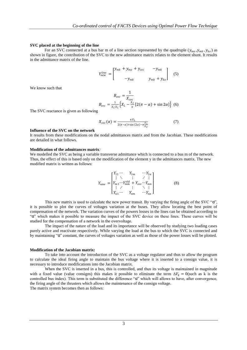
The matrix system becomes then as follows:

Co-ordinated control of FACTS Devices using Optimal Power Flow Technique

4

∆𝑃1

⋮

∆𝑃𝑘

⋮

∆𝑃𝑛

⋮

∆𝑄1

⋮

∆𝑄𝑘

⋮

∆𝑄𝑛

=

𝜕𝑃1

𝜕𝛿1

⋮𝜕𝑃𝑘

𝜕𝛿1

⋮𝜕𝑃𝑛

𝜕𝛿1

𝜕𝑄1

𝜕𝛿1

⋮𝜕𝑄𝑘

𝜕𝛿1

⋮𝜕𝑄𝑛

𝜕𝛿1

⋯

⋮

⋯

⋮

⋯

⋯

⋮

⋯

⋮

⋯

𝜕𝑃1

𝜕𝛿𝑘

⋮𝜕𝑃𝑘

𝜕𝛿𝑘

⋮𝜕𝑃𝑛

𝜕𝛿𝑘

𝜕𝑄1

𝜕𝛿𝑘

⋮𝜕𝑄𝑘

𝜕𝛿𝑘

⋮𝜕𝑄𝑛

𝜕𝛿𝑘

⋯

⋮

⋯

⋮

⋯

⋯

⋮

⋯

⋮

⋯

𝜕𝑃1

𝜕𝛿𝑛

⋮𝜕𝑃𝑘

𝜕𝛿𝑛

⋮𝜕𝑃𝑛

𝜕𝛿𝑛

𝜕𝑄1

𝜕𝛿𝑛

⋮𝜕𝑄𝑘

𝜕𝛿𝑛

⋮𝜕𝑄𝑛

𝜕𝛿𝑛

𝜕𝑃1

𝜕𝑉1

⋮𝜕𝑃𝑘

𝜕𝑉1

⋮𝜕𝑃𝑛

𝜕𝑉1

𝜕𝑄1

𝜕𝑉1

⋮𝜕𝑄𝑘

𝜕𝑉1

⋮𝜕𝑄𝑛

𝜕𝑉1

⋯

⋮

⋯

⋮

⋯

⋯

⋮

⋯

⋮

⋯

0

⋮

0

⋮

0

0

⋮𝜕𝑄𝑘

𝜕𝛼

⋮

0

⋯

⋮

⋯

⋮

⋯

⋯

⋮

⋯

⋮

⋯

𝜕𝑃1

𝜕𝑉𝑛

⋮𝜕𝑃𝑘

𝜕𝑉𝑛

⋮𝜕𝑃𝑛

𝜕𝑉𝑛𝜕𝑄1

𝜕𝑉𝑛

⋮𝜕𝑄𝑘

𝜕𝑉𝑛

⋮𝜕𝑄𝑛

𝜕𝑉𝑛

∆𝛿1

⋮

∆𝛿𝑘

⋮

∆𝛿𝑛

⋮

∆𝑉1

⋮

∆𝛼

⋮

∆𝑉𝑛

(9)

By knowing that

𝑄𝑘 = 𝑄𝑘𝑜𝑙𝑑 + 𝑄𝑠𝑣𝑐 (10)

Then

𝜕𝑄𝑘

𝜕𝛼=

𝜕𝑄𝑘𝑜𝑙𝑑

𝜕𝛼+

𝜕𝑄𝑠𝑣𝑐

𝜕𝛼 (11)

And as 𝑄𝑘 depend only on the angle “α”,

𝜕𝑄𝑘

𝜕𝛼=

𝜕𝑄𝑠𝑣𝑐

𝜕𝛼 (12)

𝑤𝑖𝑡𝑕𝑄𝑠𝑣𝑐 = 𝑄𝑘 = −𝑉𝑘2𝐵𝑠𝑣𝑐 , then

𝑄𝑠𝑣𝑐 = −𝑉𝑘

2

𝑋𝐶𝑋𝐿 𝑋𝐿 −

𝑋𝐶

𝜋 2 𝜋 − 𝛼 + sin 2𝛼 (13)

Finally, the expression after derivation 𝜕𝑄𝑘

𝜕𝛼=

2𝑉𝑘2

𝜋𝑋𝐿 cos(2𝛼𝑠𝑣𝑐) − 1 (14)

The same case studies will be carried out as for an SVC at the beginning of line. The results obtained

will be compared for the two cases of placements; and conclude if an SVC in middle of a line can ensure the

compensation with the same effectiveness as two SVC placed in ends of line.

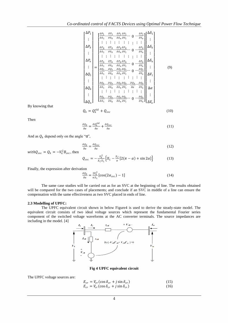
2.3 Modelling of UPFC:

The UPFC equivalent circuit shown in below Figure4 is used to derive the steady-state model. The

equivalent circuit consists of two ideal voltage sources which represent the fundamental Fourier series

component of the switched voltage waveforms at the AC converter terminals. The source impedances are

including in the model. [4]

Fig 4 UPFC equivalent circuit

The UPFC voltage sources are:

𝐸𝑣𝑟 = 𝑉𝑣𝑟 cos𝛿𝑣𝑟 + 𝑗 sin 𝛿𝑣𝑟 (15)

𝐸𝑐𝑟 = 𝑉𝑐𝑟 cos𝛿𝑐𝑟 + 𝑗 sin 𝛿𝑐𝑟 (16)

Co-ordinated control of FACTS Devices using Optimal Power Flow Technique

5

Where 𝑉𝑣𝑟 and 𝛿𝑣𝑟 are the controllable magnitude 𝑉𝑣𝑟𝑚𝑖𝑛 ≤ 𝑉𝑣𝑟 ≤ 𝑉𝑣𝑟𝑚𝑎𝑥 and phase angle

0 ≤ 𝛿𝑣𝑟 ≤ 2𝜋 of the voltage source representing the shunt converter. The magnitude 𝑉𝑐𝑟 and phase angle 𝛿𝑐𝑟

of the voltage source representing the series converter are controlled between limits 𝑉𝑐𝑟𝑚𝑖𝑛 ≤ 𝑉𝑐𝑟 ≤ 𝑉𝑐𝑟𝑚𝑎𝑥

and phase angle 0 ≤ 𝛿𝑐𝑟 ≤ 2𝜋 , respectively.

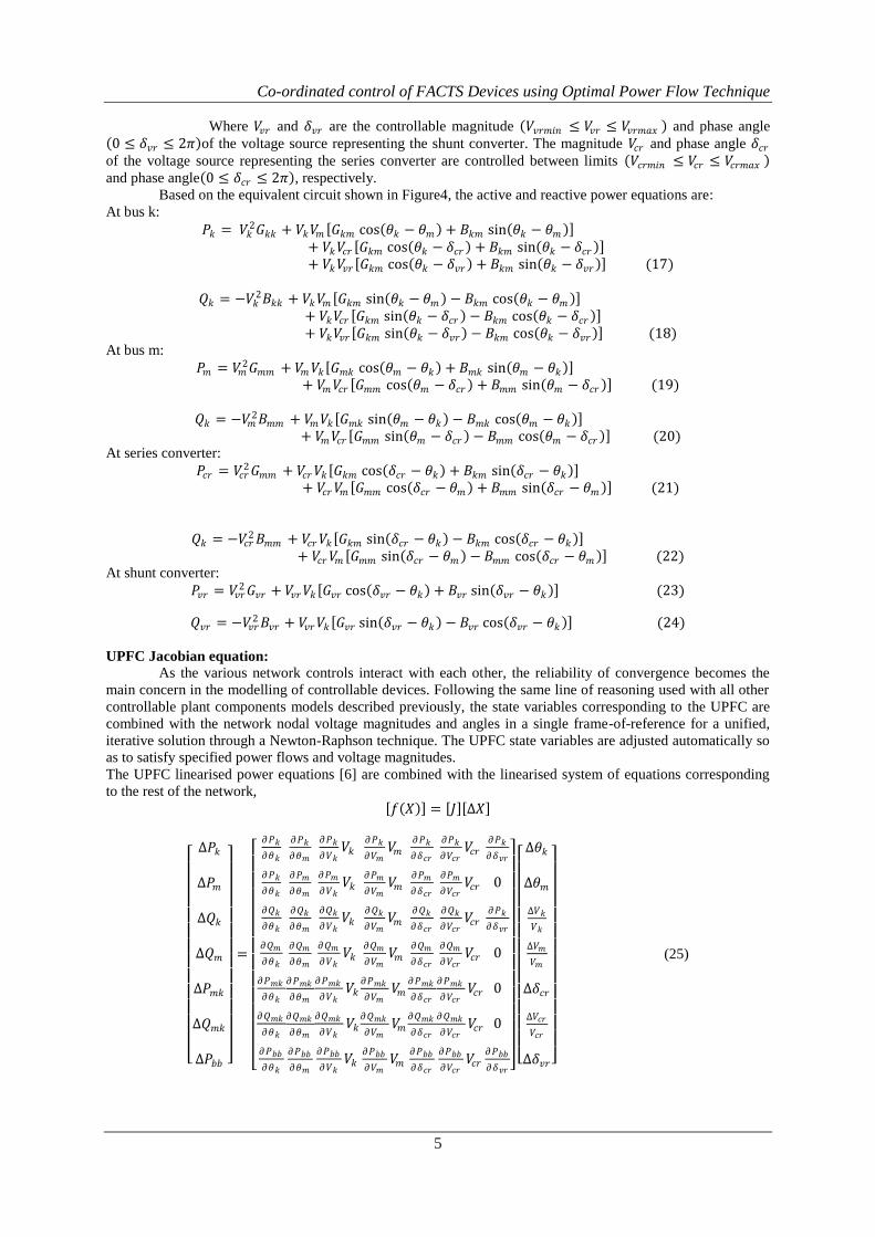
Based on the equivalent circuit shown in Figure4, the active and reactive power equations are:

At bus k:

𝑃𝑘 = 𝑉𝑘2𝐺𝑘𝑘 + 𝑉𝑘𝑉𝑚 𝐺𝑘𝑚 cos 𝜃𝑘 − 𝜃𝑚 + 𝐵𝑘𝑚 sin 𝜃𝑘 − 𝜃𝑚

+ 𝑉𝑘𝑉𝑐𝑟 𝐺𝑘𝑚 cos 𝜃𝑘 − 𝛿𝑐𝑟 + 𝐵𝑘𝑚 sin 𝜃𝑘 − 𝛿𝑐𝑟 + 𝑉𝑘𝑉𝑣𝑟 𝐺𝑘𝑚 cos 𝜃𝑘 − 𝛿𝑣𝑟 + 𝐵𝑘𝑚 sin 𝜃𝑘 − 𝛿𝑣𝑟 (17)

𝑄𝑘 = −𝑉𝑘2𝐵𝑘𝑘 + 𝑉𝑘𝑉𝑚 𝐺𝑘𝑚 sin 𝜃𝑘 − 𝜃𝑚 − 𝐵𝑘𝑚 cos 𝜃𝑘 − 𝜃𝑚

+ 𝑉𝑘𝑉𝑐𝑟 𝐺𝑘𝑚 sin 𝜃𝑘 − 𝛿𝑐𝑟 − 𝐵𝑘𝑚 cos 𝜃𝑘 − 𝛿𝑐𝑟 + 𝑉𝑘𝑉𝑣𝑟 𝐺𝑘𝑚 sin 𝜃𝑘 − 𝛿𝑣𝑟 − 𝐵𝑘𝑚 cos 𝜃𝑘 − 𝛿𝑣𝑟 (18)

At bus m:

𝑃𝑚 = 𝑉𝑚2𝐺𝑚𝑚 + 𝑉𝑚𝑉𝑘 𝐺𝑚𝑘 cos 𝜃𝑚 − 𝜃𝑘 + 𝐵𝑚𝑘 sin 𝜃𝑚 − 𝜃𝑘

+ 𝑉𝑚𝑉𝑐𝑟 𝐺𝑚𝑚 cos 𝜃𝑚 − 𝛿𝑐𝑟 + 𝐵𝑚𝑚 sin 𝜃𝑚 − 𝛿𝑐𝑟 (19)

𝑄𝑘 = −𝑉𝑚2𝐵𝑚𝑚 + 𝑉𝑚𝑉𝑘 𝐺𝑚𝑘 sin 𝜃𝑚 − 𝜃𝑘 − 𝐵𝑚𝑘 cos 𝜃𝑚 − 𝜃𝑘

+ 𝑉𝑚𝑉𝑐𝑟 𝐺𝑚𝑚 sin 𝜃𝑚 − 𝛿𝑐𝑟 − 𝐵𝑚𝑚 cos 𝜃𝑚 − 𝛿𝑐𝑟 (20)

At series converter:

𝑃𝑐𝑟 = 𝑉𝑐𝑟2𝐺𝑚𝑚 + 𝑉𝑐𝑟𝑉𝑘 𝐺𝑘𝑚 cos 𝛿𝑐𝑟 − 𝜃𝑘 + 𝐵𝑘𝑚 sin 𝛿𝑐𝑟 − 𝜃𝑘

+ 𝑉𝑐𝑟𝑉𝑚 𝐺𝑚𝑚 cos 𝛿𝑐𝑟 − 𝜃𝑚 + 𝐵𝑚𝑚 sin 𝛿𝑐𝑟 − 𝜃𝑚 (21)

𝑄𝑘 = −𝑉𝑐𝑟2𝐵𝑚𝑚 + 𝑉𝑐𝑟𝑉𝑘 𝐺𝑘𝑚 sin 𝛿𝑐𝑟 − 𝜃𝑘 − 𝐵𝑘𝑚 cos 𝛿𝑐𝑟 − 𝜃𝑘

+ 𝑉𝑐𝑟𝑉𝑚 𝐺𝑚𝑚 sin 𝛿𝑐𝑟 − 𝜃𝑚 − 𝐵𝑚𝑚 cos 𝛿𝑐𝑟 − 𝜃𝑚 (22) At shunt converter:

𝑃𝑣𝑟 = 𝑉𝑣𝑟2𝐺𝑣𝑟 + 𝑉𝑣𝑟𝑉𝑘 𝐺𝑣𝑟 cos 𝛿𝑣𝑟 − 𝜃𝑘 + 𝐵𝑣𝑟 sin 𝛿𝑣𝑟 − 𝜃𝑘 (23)

𝑄𝑣𝑟 = −𝑉𝑣𝑟2 𝐵𝑣𝑟 + 𝑉𝑣𝑟𝑉𝑘 𝐺𝑣𝑟 sin 𝛿𝑣𝑟 − 𝜃𝑘 − 𝐵𝑣𝑟 cos 𝛿𝑣𝑟 − 𝜃𝑘 (24)

UPFC Jacobian equation:

As the various network controls interact with each other, the reliability of convergence becomes the

main concern in the modelling of controllable devices. Following the same line of reasoning used with all other

controllable plant components models described previously, the state variables corresponding to the UPFC are

combined with the network nodal voltage magnitudes and angles in a single frame-of-reference for a unified,

iterative solution through a Newton-Raphson technique. The UPFC state variables are adjusted automatically so

as to satisfy specified power flows and voltage magnitudes.

The UPFC linearised power equations [6] are combined with the linearised system of equations corresponding

to the rest of the network,

𝑓 𝑋 = 𝐽 ∆𝑋

∆𝑃𝑘

∆𝑃𝑚

∆𝑄𝑘

∆𝑄𝑚

∆𝑃𝑚𝑘

∆𝑄𝑚𝑘

∆𝑃𝑏𝑏

=

𝜕𝑃𝑘

𝜕𝜃𝑘

𝜕𝑃𝑘

𝜕𝜃𝑘

𝜕𝑄𝑘

𝜕𝜃𝑘

𝜕𝑄𝑚

𝜕𝜃𝑘

𝜕𝑃𝑚𝑘

𝜕𝜃𝑘

𝜕𝑄𝑚𝑘

𝜕𝜃𝑘

𝜕𝑃𝑏𝑏

𝜕𝜃𝑘

𝜕𝑃𝑘

𝜕𝜃𝑚

𝜕𝑃𝑚

𝜕𝜃𝑚

𝜕𝑄𝑘

𝜕𝜃𝑚

𝜕𝑄𝑚

𝜕𝜃𝑚

𝜕𝑃𝑚𝑘

𝜕𝜃𝑚

𝜕𝑄𝑚𝑘

𝜕𝜃𝑚

𝜕𝑃𝑏𝑏

𝜕𝜃𝑚

𝜕𝑃𝑘

𝜕𝑉𝑘𝑉𝑘

𝜕𝑃𝑚

𝜕𝑉𝑘𝑉𝑘

𝜕𝑄𝑘

𝜕𝑉𝑘𝑉𝑘

𝜕𝑄𝑚

𝜕𝑉𝑘𝑉𝑘

𝜕𝑃𝑚𝑘

𝜕𝑉𝑘𝑉𝑘

𝜕𝑄𝑚𝑘

𝜕𝑉𝑘𝑉𝑘

𝜕𝑃𝑏𝑏

𝜕𝑉𝑘𝑉𝑘

𝜕𝑃𝑘

𝜕𝑉𝑚𝑉𝑚

𝜕𝑃𝑚

𝜕𝑉𝑚𝑉𝑚

𝜕𝑄𝑘

𝜕𝑉𝑚𝑉𝑚

𝜕𝑄𝑚

𝜕𝑉𝑚𝑉𝑚

𝜕𝑃𝑚𝑘

𝜕𝑉𝑚𝑉𝑚

𝜕𝑄𝑚𝑘

𝜕𝑉𝑚𝑉𝑚

𝜕𝑃𝑏𝑏

𝜕𝑉𝑚𝑉𝑚

𝜕𝑃𝑘

𝜕𝛿𝑐𝑟

𝜕𝑃𝑚

𝜕𝛿𝑐𝑟

𝜕𝑄𝑘

𝜕𝛿𝑐𝑟

𝜕𝑄𝑚

𝜕𝛿𝑐𝑟

𝜕𝑃𝑚𝑘

𝜕𝛿𝑐𝑟

𝜕𝑄𝑚𝑘

𝜕𝛿𝑐𝑟

𝜕𝑃𝑏𝑏

𝜕𝛿𝑐𝑟

𝜕𝑃𝑘

𝜕𝑉𝑐𝑟𝑉𝑐𝑟

𝜕𝑃𝑚

𝜕𝑉𝑐𝑟𝑉𝑐𝑟

𝜕𝑄𝑘

𝜕𝑉𝑐𝑟𝑉𝑐𝑟

𝜕𝑄𝑚

𝜕𝑉𝑐𝑟𝑉𝑐𝑟

𝜕𝑃𝑚𝑘

𝜕𝑉𝑐𝑟𝑉𝑐𝑟

𝜕𝑄𝑚𝑘

𝜕𝑉𝑐𝑟𝑉𝑐𝑟

𝜕𝑃𝑏𝑏

𝜕𝑉𝑐𝑟𝑉𝑐𝑟

𝜕𝑃𝑘

𝜕𝛿𝑣𝑟

0

𝜕𝑃𝑘

𝜕𝛿𝑣𝑟

0

0

0

𝜕𝑃𝑏𝑏

𝜕𝛿𝑣𝑟

∆𝜃𝑘

∆𝜃𝑚

∆𝑉𝑘

𝑉𝑘

∆𝑉𝑚

𝑉𝑚

∆𝛿𝑐𝑟

∆𝑉𝑐𝑟

𝑉𝑐𝑟

∆𝛿𝑣𝑟

(25)

Co-ordinated control of FACTS Devices using Optimal Power Flow Technique

6

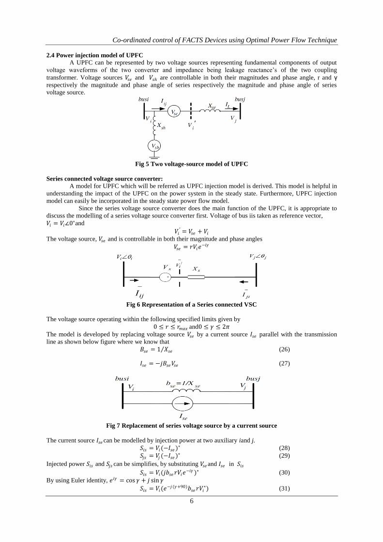
2.4 Power injection model of UPFC

A UPFC can be represented by two voltage sources representing fundamental components of output

voltage waveforms of the two converter and impedance being leakage reactance’s of the two coupling

transformer. Voltage sources 𝑉𝑠𝑒 and 𝑉𝑠𝑕 are controllable in both their magnitudes and phase angle, r and γ

respectively the magnitude and phase angle of series respectively the magnitude and phase angle of series

voltage source.

Fig 5 Two voltage-source model of UPFC

Series connected voltage source converter:

A model for UPFC which will be referred as UPFC injection model is derived. This model is helpful in

understanding the impact of the UPFC on the power system in the steady state. Furthermore, UPFC injection

model can easily be incorporated in the steady state power flow model.

Since the series voltage source converter does the main function of the UPFC, it is appropriate to

discuss the modelling of a series voltage source converter first. Voltage of bus iis taken as reference vector,

𝑉𝑖 = 𝑉𝑖∠0∘and

𝑉𝑖′ = 𝑉𝑠𝑒 + 𝑉𝑖

The voltage source, 𝑉𝑠𝑒 and is controllable in both their magnitude and phase angles

𝑉𝑠𝑒 = 𝑟𝑉𝑖𝑒−𝑖𝛾

Fig 6 Representation of a Series connected VSC

The voltage source operating within the following specified limits given by

0 ≤ 𝑟 ≤ 𝑟𝑚𝑎𝑥 and0 ≤ 𝛾 ≤ 2𝜋

The model is developed by replacing voltage source 𝑉𝑠𝑒 by a current source 𝐼𝑠𝑒 parallel with the transmission

line as shown below figure where we know that

𝐵𝑠𝑒 = 1 𝑋𝑠𝑒 (26)

𝐼𝑠𝑒 = −𝑗𝐵𝑠𝑒𝑉𝑠𝑒 (27)

Fig 7 Replacement of series voltage source by a current source

The current source 𝐼𝑠𝑒can be modelled by injection power at two auxiliary iand j.

𝑆𝑖𝑠 = 𝑉𝑖(−𝐼𝑠𝑒 )∗ (28)

𝑆𝑗𝑠 = 𝑉𝑗 (−𝐼𝑠𝑒 )∗ (29)

Injected power 𝑆𝑖𝑠 and 𝑆𝑗𝑠 can be simplifies, by substituting 𝑉𝑠𝑒and 𝐼𝑠𝑒 in 𝑆𝑖𝑠

𝑆𝑖𝑠 = 𝑉𝑖(𝑗𝑏𝑠𝑒𝑟𝑉𝑖𝑒−𝑖𝛾 )∗ (30)

By using Euler identity, 𝑒𝑖𝛾 = cos 𝛾 + 𝑗 sin 𝛾

𝑆𝑖𝑠 = 𝑉𝑖(𝑒−𝑗 (𝛾+90)𝑏𝑠𝑒𝑟𝑉𝑖

∗) (31)

Co-ordinated control of FACTS Devices using Optimal Power Flow Technique

7

𝑆𝑖𝑠 = 𝑉𝑖2𝑏𝑠𝑒𝑟 cos −𝛾 − 90 + 𝑗 sin −𝛾 − 90 (32)

By using trigonometric identities the equation is reduced to

𝑆𝑖𝑠 = −𝑟𝑏𝑠𝑒𝑉𝑖2 sin 𝛾 − 𝑗𝑟𝑏𝑠𝑒𝑉𝑖

2 cos 𝛾 (33)

The decomposed real and imaginary components of 𝑆𝑖𝑠

𝑆𝑖𝑠 = 𝑃𝑖𝑠 + 𝑗𝑄𝑖𝑠 ,where

𝑃𝑖𝑠 = −𝑟𝐵𝑠𝑒𝑉𝑖2 sin 𝛾 (34)

𝑄𝑖𝑠 = −𝑟𝐵𝑠𝑒𝑉𝑖2 cos 𝛾 (35)

Similar modification can be applied to 𝑆𝑗𝑠 then the final equation is

𝑆𝑗𝑠 = 𝑉𝑖𝑉𝑗𝐵𝑠𝑒𝑟 sin 𝜃𝑖 − 𝜃𝑗 + 𝛾 + 𝑗𝑉𝑖𝑉𝑗𝐵𝑠𝑒𝑟 cos 𝜃𝑖 − 𝜃𝑗 + 𝛾 (36)

The above equation is decomposed into its real and imaginary parts

𝑆𝑗𝑠 = 𝑃𝑗𝑠 + 𝑗𝑄𝑗𝑠 , where

𝑃𝑗𝑠 = 𝑉𝑖𝑉𝑗𝐵𝑠𝑒𝑟 sin 𝜃𝑖 − 𝜃𝑗 + 𝛾 (37)

𝑄𝑗𝑠 = 𝑉𝑖𝑉𝑗𝐵𝑠𝑒𝑟 cos 𝜃𝑖 − 𝜃𝑗 + 𝛾 (38)

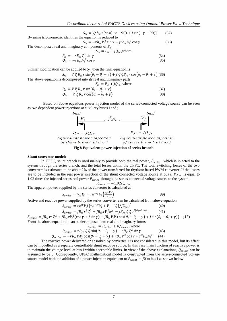
Based on above equations power injection model of the series-connected voltage source can be seen

as two dependent power injections at auxiliary buses i and j.

Fig 8 Equivalent power injection of series branch

Shunt converter model:

In UPFC, shunt branch is used mainly to provide both the real power, 𝑃𝑠𝑒𝑟𝑖𝑒𝑠 which is injected to the

system through the series branch, and the total losses within the UPFC. The total switching losses of the two

converters is estimated to be about 2% of the power transferred for thyristor based PWM converter. If the losses

are to be included in the real power injection of the shunt connected voltage source at bus i, 𝑃𝑠𝑕𝑢𝑛𝑡 is equal to

1.02 times the injected series real power 𝑃𝑠𝑒𝑟𝑖𝑒𝑠 through the series connected voltage source to the system.

𝑃𝑠𝑕𝑢𝑛𝑡 = −1.02𝑃𝑠𝑒𝑟𝑖𝑒𝑠 The apparent power supplied by the series converter is calculated as

𝑆𝑠𝑒𝑟𝑖𝑒𝑠 = 𝑉𝑠𝑒 𝐼𝑖𝑗∗ = 𝑟𝑒−𝑖𝛾𝑉𝑖

𝑉𝑖′−𝑉𝑗

𝑗𝑋𝑠𝑒 (39)

Active and reactive power supplied by the series converter can be calculated from above equation

𝑆𝑠𝑒𝑟𝑖𝑒𝑠 = 𝑟𝑒𝑖𝛾𝑉𝑖 𝑟𝑒−𝑖𝛾𝑉𝑖 + 𝑉𝑖 − 𝑉𝑗 𝑗𝑋𝑠𝑒

∗ (40)

𝑆𝑠𝑒𝑟𝑖𝑒𝑠 = 𝑗𝐵𝑠𝑒𝑟2𝑉𝑖

2 + 𝑗𝐵𝑠𝑒𝑟𝑉𝑖2𝑒𝑗𝛾 − 𝑗𝐵𝑠𝑒𝑉𝑖𝑉𝑗𝑒

𝑗 𝜃𝑖−𝜃𝑗 +𝛾 (41)

𝑆𝑠𝑒𝑟𝑖𝑒𝑠 = 𝑗𝐵𝑠𝑒𝑟2𝑉𝑖

2 + 𝑗𝐵𝑠𝑒𝑟𝑉𝑖2 cos 𝛾 + 𝑗 sin 𝛾 − 𝑗𝐵𝑠𝑒𝑉𝑖𝑉𝑗 cos 𝜃𝑖 − 𝜃𝑗 + 𝛾 + 𝑗 sin 𝜃𝑖 − 𝜃𝑗 + 𝛾 (42)

From the above equation it can be decomposed into real and imaginary forms

𝑆𝑠𝑒𝑟𝑖𝑒𝑠 = 𝑃𝑠𝑒𝑟𝑖𝑒𝑠 + 𝑗𝑄𝑠𝑒𝑟𝑖𝑒𝑠 , where

𝑃𝑠𝑒𝑟𝑖𝑒𝑠 = 𝑟𝐵𝑠𝑒𝑉𝑖𝑉𝑗 sin 𝜃𝑖 − 𝜃𝑗 + 𝛾 − 𝑟𝐵𝑠𝑒𝑉𝑖2 sin 𝛾 (43)

𝑄𝑠𝑒𝑟𝑖𝑒𝑠 = −𝑟𝐵𝑠𝑒𝑉𝑖𝑉𝑗 cos 𝜃𝑖 − 𝜃𝑗 + 𝛾 + 𝑟𝐵𝑠𝑒𝑉𝑖2 cos 𝛾 + 𝑟2𝐵𝑠𝑒𝑉𝑖

2 (44)

The reactive power delivered or absorbed by converter 1 is not considered in this model, but its effect

can be modelled as a separate controllable shunt reactive source. In this case main function of reactive power is

to maintain the voltage level at bus i within acceptable limits. In view of the above explanations, 𝑄𝑠𝑕𝑢𝑛𝑡 can be

assumed to be 0. Consequently, UPFC mathematical model is constructed from the series-connected voltage

source model with the addition of a power injection equivalent to 𝑃𝑠𝑕𝑢𝑛𝑡 + 𝑗0 to bus i as shown below

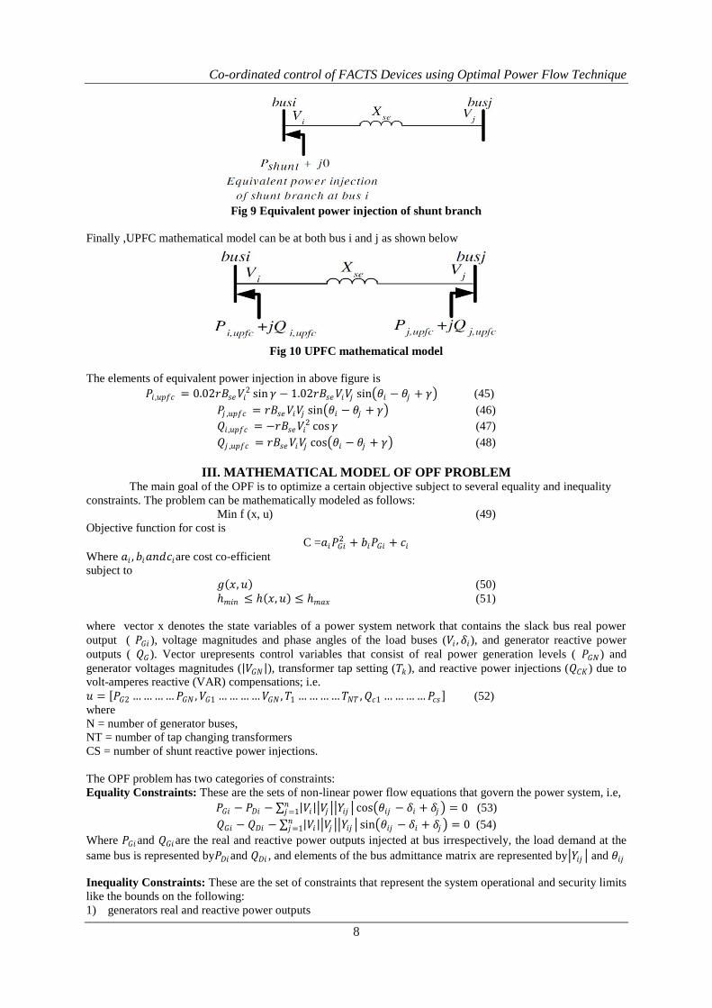
Co-ordinated control of FACTS Devices using Optimal Power Flow Technique

8

Fig 9 Equivalent power injection of shunt branch

Finally ,UPFC mathematical model can be at both bus i and j as shown below

Fig 10 UPFC mathematical model

The elements of equivalent power injection in above figure is

𝑃𝑖 ,𝑢𝑝𝑓𝑐 = 0.02𝑟𝐵𝑠𝑒𝑉𝑖2 sin 𝛾 − 1.02𝑟𝐵𝑠𝑒𝑉𝑖𝑉𝑗 sin 𝜃𝑖 − 𝜃𝑗 + 𝛾 (45)

𝑃𝑗 ,𝑢𝑝𝑓𝑐 = 𝑟𝐵𝑠𝑒𝑉𝑖𝑉𝑗 sin 𝜃𝑖 − 𝜃𝑗 + 𝛾 (46)

𝑄𝑖 ,𝑢𝑝𝑓𝑐 = −𝑟𝐵𝑠𝑒𝑉𝑖2 cos 𝛾 (47)

𝑄𝑗 ,𝑢𝑝𝑓𝑐 = 𝑟𝐵𝑠𝑒𝑉𝑖𝑉𝑗 cos 𝜃𝑖 − 𝜃𝑗 + 𝛾 (48)

III. MATHEMATICAL MODEL OF OPF PROBLEM The main goal of the OPF is to optimize a certain objective subject to several equality and inequality

constraints. The problem can be mathematically modeled as follows:

Min f (x, u) (49)

Objective function for cost is

C =𝑎𝑖𝑃𝐺𝑖2 + 𝑏𝑖𝑃𝐺𝑖 + 𝑐𝑖

Where 𝑎𝑖 , 𝑏𝑖𝑎𝑛𝑑𝑐𝑖are cost co-efficient

subject to

𝑔 𝑥, 𝑢 (50)

𝑕𝑚𝑖𝑛 ≤ 𝑕 𝑥, 𝑢 ≤ 𝑕𝑚𝑎𝑥 (51)

where vector x denotes the state variables of a power system network that contains the slack bus real power

output ( 𝑃𝐺𝑖 ), voltage magnitudes and phase angles of the load buses (𝑉𝑖 , 𝛿𝑖), and generator reactive power

outputs ( 𝑄𝐺 ). Vector urepresents control variables that consist of real power generation levels ( 𝑃𝐺𝑁 ) and

generator voltages magnitudes ( 𝑉𝐺𝑁 ), transformer tap setting (𝑇𝑘 ), and reactive power injections (𝑄𝐶𝐾) due to

volt-amperes reactive (VAR) compensations; i.e.

𝑢 = 𝑃𝐺2 …………𝑃𝐺𝑁 , 𝑉𝐺1 …………𝑉𝐺𝑁 , 𝑇1 …………𝑇𝑁𝑇 , 𝑄𝑐1 …………𝑃𝑐𝑠 (52)

where

N = number of generator buses,

NT = number of tap changing transformers

CS = number of shunt reactive power injections.

The OPF problem has two categories of constraints:

Equality Constraints: These are the sets of non-linear power flow equations that govern the power system, i.e,

𝑃𝐺𝑖 − 𝑃𝐷𝑖 − 𝑉𝑖 𝑉𝑗 𝑌𝑖𝑗 𝑛𝑗=1 cos 𝜃𝑖𝑗 − 𝛿𝑖 + 𝛿𝑗 = 0 (53)

𝑄𝐺𝑖 − 𝑄𝐷𝑖 − 𝑉𝑖 𝑉𝑗 𝑌𝑖𝑗 𝑛𝑗=1 sin 𝜃𝑖𝑗 − 𝛿𝑖 + 𝛿𝑗 = 0 (54)

Where 𝑃𝐺𝑖and 𝑄𝐺𝑖are the real and reactive power outputs injected at bus irrespectively, the load demand at the

same bus is represented by𝑃𝐷𝑖and 𝑄𝐷𝑖 , and elements of the bus admittance matrix are represented by 𝑌𝑖𝑗 and 𝜃𝑖𝑗

Inequality Constraints: These are the set of constraints that represent the system operational and security limits

like the bounds on the following:

1) generators real and reactive power outputs

Co-ordinated control of FACTS Devices using Optimal Power Flow Technique

9

𝑃𝐺𝑖𝑚𝑖𝑛 ≤ 𝑃𝐺𝑖 ≤ 𝑃𝐺𝑖

𝑚𝑎𝑥 , 𝑖 = 1, … . , 𝑁 (55)

𝑄𝐺𝑖𝑚𝑖𝑛 ≤ 𝑄𝐺𝑖 ≤ 𝑄𝐺𝑖

𝑚𝑎𝑥 , 𝑖 = 1, … . , 𝑁 (56)

2) voltage magnitudes at each bus in the network

𝑉𝑖𝑚𝑖𝑛 ≤ 𝑉𝑖 ≤ 𝑉𝑖

𝑚𝑎𝑥 , 𝑖 = 1, … , 𝑁𝐿 (57)

3) transformer tap settings

𝑇𝑖𝑚𝑖𝑛 ≤ 𝑇𝑖 ≤ 𝑇𝑖

𝑚𝑎𝑥 , 𝑖 = 1, … , 𝑁𝑇 (58)

4) reactive power injections due to capacitor banks

𝑄𝐶𝑖𝑚𝑖𝑛 ≤ 𝑄𝐶𝑖 ≤ 𝑄𝐶𝑖

𝑚𝑎𝑥 , 𝑖 = 1, … , 𝐶𝑆 (59)

5) transmission lines loading

𝑆𝑖 ≤ 𝑆𝑖𝑚𝑎𝑥 , 𝑖 = 1, … . , 𝑛𝑙 (60)

IV. CO-ORDINATE CONTROL As these devices are controlled locally so far, they do not take into account their influences on other

lines or buses. Thus, a control action which is reasonable for the line or bus where the device is located might

cause another line to be overloaded or voltages to take unacceptable values. Additionally, if devices are located

close to each other the action of one controller can lead to a counteraction of the other controller possibly

resulting in a conflicting situation. For these reasons, coordination is necessary [7], [8] and [9], especially when

the number of devices increases and the distance among them decreases. Here we use Artificial Intelligence for

this coordinate control. In this Artificial Intelligence Particle swam optimization is used to keep FACTS at

random buses in the system and then find cost and take minimum cost.

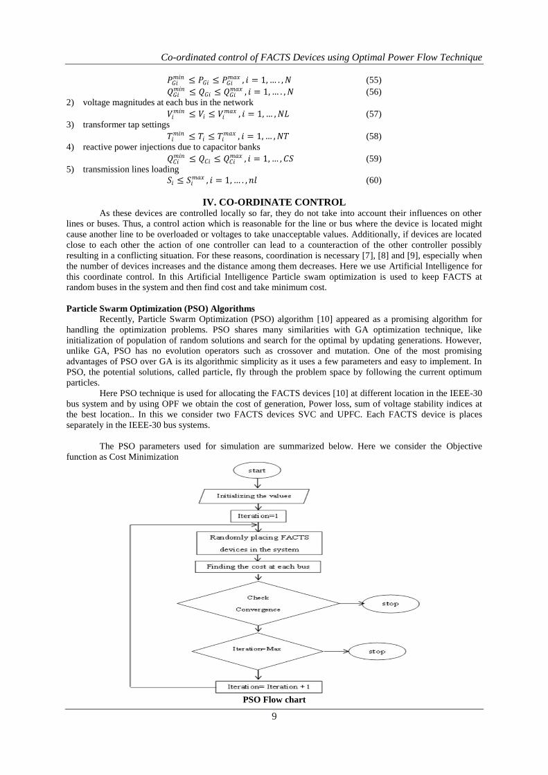
Particle Swarm Optimization (PSO) Algorithms

Recently, Particle Swarm Optimization (PSO) algorithm [10] appeared as a promising algorithm for

handling the optimization problems. PSO shares many similarities with GA optimization technique, like

initialization of population of random solutions and search for the optimal by updating generations. However,

unlike GA, PSO has no evolution operators such as crossover and mutation. One of the most promising

advantages of PSO over GA is its algorithmic simplicity as it uses a few parameters and easy to implement. In

PSO, the potential solutions, called particle, fly through the problem space by following the current optimum

particles.

Here PSO technique is used for allocating the FACTS devices [10] at different location in the IEEE-30

bus system and by using OPF we obtain the cost of generation, Power loss, sum of voltage stability indices at

the best location.. In this we consider two FACTS devices SVC and UPFC. Each FACTS device is places

separately in the IEEE-30 bus systems.

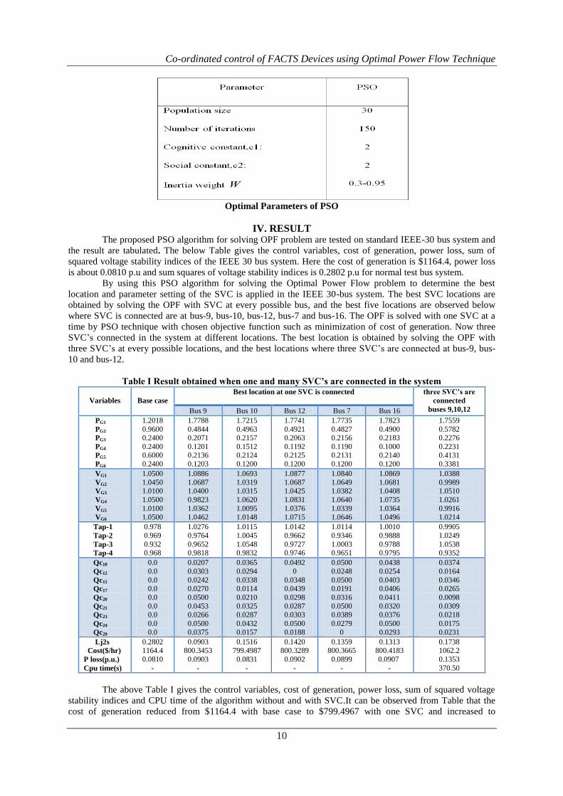
The PSO parameters used for simulation are summarized below. Here we consider the Objective

function as Cost Minimization

PSO Flow chart

Co-ordinated control of FACTS Devices using Optimal Power Flow Technique

10

Optimal Parameters of PSO

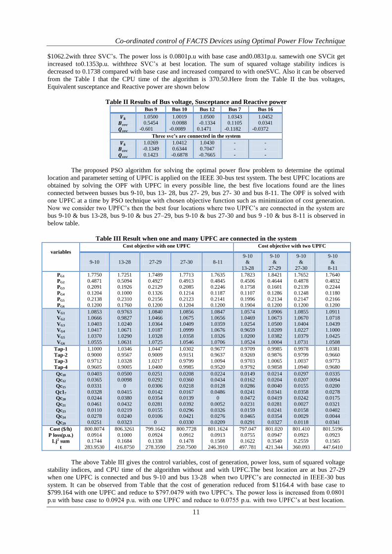
IV. RESULT The proposed PSO algorithm for solving OPF problem are tested on standard IEEE-30 bus system and

the result are tabulated. The below Table gives the control variables, cost of generation, power loss, sum of

squared voltage stability indices of the IEEE 30 bus system. Here the cost of generation is $1164.4, power loss

is about 0.0810 p.u and sum squares of voltage stability indices is 0.2802 p.u for normal test bus system.

By using this PSO algorithm for solving the Optimal Power Flow problem to determine the best

location and parameter setting of the SVC is applied in the IEEE 30-bus system. The best SVC locations are

obtained by solving the OPF with SVC at every possible bus, and the best five locations are observed below

where SVC is connected are at bus-9, bus-10, bus-12, bus-7 and bus-16. The OPF is solved with one SVC at a

time by PSO technique with chosen objective function such as minimization of cost of generation. Now three

SVC’s connected in the system at different locations. The best location is obtained by solving the OPF with

three SVC’s at every possible locations, and the best locations where three SVC’s are connected at bus-9, bus-

10 and bus-12.

Table I Result obtained when one and many SVC’s are connected in the system

Variables

Base case

Best location at one SVC is connected three SVC’s are

connected

buses 9,10,12 Bus 9 Bus 10 Bus 12 Bus 7 Bus 16

PG1

PG2

PG3

PG4

PG5

PG6

1.2018

0.9600 0.2400

0.2400 0.6000

0.2400

1.7788

0.4844 0.2071

0.1201 0.2136

0.1203

1.7215

0.4963 0.2157

0.1512 0.2124

0.1200

1.7741

0.4921 0.2063

0.1192 0.2125

0.1200

1.7735

0.4827 0.2156

0.1190 0.2131

0.1200

1.7823

0.4900 0.2183

0.1000 0.2140

0.1200

1.7559

0.5782 0.2276

0.2231 0.4131

0.3381

VG1

VG2

VG3

VG4

VG5

VG6

1.0500

1.0450 1.0100

1.0500

1.0100

1.0500

1.0886

1.0687 1.0400

0.9823

1.0362

1.0462

1.0693

1.0319 1.0315

1.0620

1.0095

1.0148

1.0877

1.0687 1.0425

1.0831

1.0376

1.0715

1.0840

1.0649 1.0382

1.0640

1.0339

1.0646

1.0869

1.0681 1.0408

1.0735

1.0364

1.0496

1.0388

0.9989 1.0510

1.0261

0.9916

1.0214

Tap-1

Tap-2

Tap-3

Tap-4

0.978

0.969

0.932 0.968

1.0276

0.9764

0.9652 0.9818

1.0115

1.0045

1.0548 0.9832

1.0142

0.9662

0.9727 0.9746

1.0114

0.9346

1.0003 0.9651

1.0010

0.9888

0.9788 0.9795

0.9905

1.0249

1.0538 0.9352

Qc10

Qc12

Qc15

Qc17

Qc20

Qc21

Qc23

Qc24

Qc29

0.0

0.0

0.0 0.0

0.0

0.0 0.0

0.0

0.0

0.0207

0.0303

0.0242 0.0270

0.0500

0.0453 0.0266

0.0500

0.0375

0.0365

0.0294

0.0338 0.0114

0.0210

0.0325 0.0287

0.0432

0.0157

0.0492

0

0.0348 0.0439

0.0298

0.0287 0.0303

0.0500

0.0188

0.0500

0.0248

0.0500 0.0191

0.0316

0.0500 0.0389

0.0279

0

0.0438

0.0254

0.0403 0.0406

0.0411

0.0320 0.0376

0.0500

0.0293

0.0374

0.0164

0.0346 0.0265

0.0098

0.0309 0.0218

0.0175

0.0231

Lj2s

Cost($/hr)

P loss(p.u.)

Cpu time(s)

0.2802 1164.4

0.0810

-

0.0903 800.3453

0.0903

-

0.1516 799.4987

0.0831

-

0.1420 800.3289

0.0902

-

0.1359 800.3665

0.0899

-

0.1313 800.4183

0.0907

-

0.1738 1062.2

0.1353

370.50

The above Table I gives the control variables, cost of generation, power loss, sum of squared voltage

stability indices and CPU time of the algorithm without and with SVC.It can be observed from Table that the

cost of generation reduced from $1164.4 with base case to $799.4967 with one SVC and increased to

Co-ordinated control of FACTS Devices using Optimal Power Flow Technique

11

$1062.2with three SVC’s. The power loss is 0.0801p.u with base case and0.0831p.u. samewith one SVCit get

increased to0.1353p.u. withthree SVC’s at best location. The sum of squared voltage stability indices is

decreased to 0.1738 compared with base case and increased compared to with oneSVC. Also it can be observed

from the Table I that the CPU time of the algorithm is 370.50.Here from the Table II the bus voltages,

Equivalent susceptance and Reactive power are shown below

Table II Results of Bus voltage, Susceptance and Reactive power Bus 9 Bus 10 Bus 12 Bus 7 Bus 16

𝑽𝒌

𝑩𝒔𝒗𝒄

𝑸𝒔𝒗𝒄

1.0500

0.5454 -0.601

1.0019

0.0088 -0.0089

1.0500

-0.1334 0.1471

1.0343

0.1105 -0.1182

1.0452

0.0341 -0.0372

Three svc’s are connected in the system

𝑽𝒌

𝑩𝒔𝒗𝒄

𝑸𝒔𝒗𝒄

1.0269 -0.1349

0.1423

1.0412 0.6344

-0.6878

1.0430 0.7047

-0.7665

- -

-

- -

-

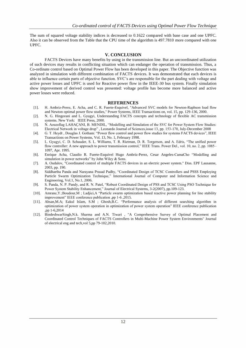
The proposed PSO algorithm for solving the optimal power flow problem to determine the optimal

location and parameter setting of UPFC is applied on the IEEE 30-bus test system. The best UPFC locations are

obtained by solving the OPF with UPFC in every possible line, the best five locations found are the lines

connected between busses bus 9-10, bus 13- 28, bus 27- 29, bus 27- 30 and bus 8-11. The OPF is solved with

one UPFC at a time by PSO technique with chosen objective function such as minimization of cost generation.

Now we consider two UPFC’s then the best four locations where two UPFC’s are connected in the system are

bus 9-10 & bus 13-28, bus 9-10 & bus 27–29, bus 9-10 & bus 27-30 and bus 9 -10 & bus 8-11 is observed in

below table.

Table III Result when one and many UPFC are connected in the system

variables

Cost objective with one UPFC Cost objective with two UPFC

9-10

13-28

27-29

27-30

8-11

9-10 &

13-28

9-10 &

27-29

9-10 &

27-30

9-10 &

8-11

PG1

PG2

PG3

PG4

PG5

PG6

1.7750

0.4871 0.2091

0.1204

0.2138 0.1200

1.7251

0.5094 0.1926

0.1000

0.2310 0.1760

1.7489

0.4927 0.2129

0.1326

0.2156 0.1200

1.7713

0.4913 0.2085

0.1214

0.2123 0.1204

1.7635

0.4845 0.2246

0.1187

0.2141 0.1200

1.7823

0.4506 0.1758

0.1107

0.1996 0.1904

1.8421

0.4644 0.1601

0.1286

0.2134 0.1200

1.7652

0.4878 0.2139

0.1248

0.2147 0.1200

1.7640

0.4832 0.2244

0.1180

0.2166 0.1200

VG1

VG2

VG3

VG4

VG5

VG6

1.0853

1.0666

1.0403 1.0417

1.0370

1.0555

0.9763

0.9827

1.0240 1.0671

1.0290

1.0631

1.0840

1.0466

1.0364 1.0187

1.0328

1.0725

1.0856

1.0675

1.0409 1.0999

1.0358

1.0546

1.0847

1.0656

1.0359 1.0676

1.0326

1.0706

1.0574

1.0469

1.0254 0.9659

1.0200

1.0524

1.0906

1.0673

1.0500 1.0209

1.0382

1.0004

1.0855

1.0670

1.0404 1.0227

1.0379

1.0731

1.0911

1.0718

1.0439 1.1000

1.0425

1.0508

Tap-1

Tap-2

Tap-3

Tap-4

1.1000 0.9000

0.9712

0.9605

1.0346 0.9567

1.0328

0.9005

1.0447 0.9009

1.0217

1.0400

1.0302 0.9151

0.9799

0.9985

0.9677 0.9637

1.0094

0.9520

0.9709 0.9269

0.9703

0.9792

0.9985 0.9876

1.0065

0.9858

0.9978 0.9799

1.0037

1.0940

1.0381 0.9660

0.9773

0.9680

Qc10

Qc12

Qc15

Qc17

Qc20

Qc21

Qc23

Qc24

Qc29

0.0403 0.0365

0.0331

0.0328 0.0244

0.0461

0.0110 0.0278

0.0251

0.0500 0.0098

0

0.0415 0.0380

0.0432

0.0219 0.0240

0.0323

0.0251 0.0292

0.0306

0.0142 0.0354

0.0281

0.0155 0.0106

0

0.0208 0.0360

0.0218

0.0167 0.0139

0.0392

0.0296 0.0421

0.0330

0.0224 0.0434

0.0128

0.0486 0

0.0052

0.0326 0.0276

0.0209

0.0149 0.0162

0.0286

0.0241 0.0472

0.0231

0.0159 0.0465

0.0291

0.0214 0.0204

0.0040

0.0341 0.0419

0.0281

0.0241 0.0354

0.0327

0.0297 0.0207

0.0155

0.0358 0.0242

0.0027

0.0158 0.0029

0.0118

0.0335 0.0094

0.0200

0.0278 0.0175

0.0321

0.0402 0.0044

0.0341

Cost ($/h)

P loss(p.u.)

Lj2 sum

t

800.8074

0.0914 0.1744

283.9530

806.3261

0.1000 0.1684

416.8750

799.1642

0.0924 0.1338

278.3590

800.7728

0.0912 0.1478

250.7500

801.1624

0.0913 0.1508

246.3910

797.047

0.0755 0.1622

497.781

801.020

0.0947 0.3540

421.344

801.410

0.0923 0.2559

360.093

801.5196

0.0923 0.1565

447.6410

The above Table III gives the control variables, cost of generation, power loss, sum of squared voltage

stability indices, and CPU time of the algorithm without and with UPFC.The best location are at bus 27-29

when one UPFC is connected and bus 9-10 and bus 13-28 when two UPFC’s are connected in IEEE-30 bus

system. It can be observed from Table that the cost of generation reduced from $1164.4 with base case to

$799.164 with one UPFC and reduce to $797.0479 with two UPFC’s. The power loss is increased from 0.0801

p.u with base case to 0.0924 p.u. with one UPFC and reduce to 0.0755 p.u. with two UPFC’s at best location.

Co-ordinated control of FACTS Devices using Optimal Power Flow Technique

12

The sum of squared voltage stability indices is decreased to 0.1622 compared with base case and one UPFC.

Also it can be observed from the Table that the CPU time of the algorithm is 497.7810 more compared with one

UPFC.

V. CONCLUSION FACTS Devices have many benefits by using in the transmission line. But an uncoordinated utilization

of such devices may results in conflicting situation which can endanger the operation of transmission. Thus, a

Co-ordinate control based on Optimal Power Flow has been developed in this paper. The Objective function was

analyzed in simulation with different combination of FACTS devices. It was demonstrated that each devices is

able to influence certain parts of objective function. SVC’s are responsible for the part dealing with voltage and

active power losses and UPFC is used for Reactive power flow in the IEEE-30 bus system. Finally simulation

show improvement of derived control was presented: voltage profile has become more balanced and active

power losses were reduced.

REFERENCES [1]. H. Ambriz-Perez, E. Acha, and C. R. Fuerte-Esquivel, "Advanced SVC models for Newton-Raphson load flow

and Newton optimal power flow studies," Power Systems, IEEE Transactions on, vol. 15, pp. 129-136, 2000.

[2]. N. G. Hingorani and L. Gyugyi, Understanding FACTS concepts and technology of flexible AC transmission

systems. New York: IEEE Press, 2000.

[3]. N. Aouzellag LAHAÇANI, B. MENDIL, “Modelling and Simulation of the SVC for Power System Flow Studies:

Electrical Network in voltage drop” , Leonardo Journal of Sciences,issue 13, pp. 153-170, July-December 2008

[4]. G. T. Heydt , Douglas J. Gotham: “Power flow control and power flow studies for systems FACTS devices”, IEEE

Transactions on Power Systems, Vol. 13, No. 1, February 1998.

[5]. L. Gyugyi, C. D. Schauder, S. L. Williams, T. R. Rietman, D. R. Torgerson, and A. Edris, “The unified power

flow controller: A new approach to power transmission control,” IEEE Trans. Power Del., vol. 10, no. 2, pp. 1085–

1097, Apr. 1995.

[6]. Enrique Acha, Claudio R. Fuerte-Esquivel Hugo Ambriz-Perez, Cesar Angeles-CamaCho “Modelling and

simulation in power networks” by John Wiley & Sons.

[7]. A. Oudalov, "Coordinated control of multiple FACTS devices in an electric power system." Diss. EPF Lausanne,

2003, pp. 190.

[8]. Siddhartha Panda and Narayana Prasad Padhy, “Coordinated Design of TCSC Controllers and PSSS Employing

Particle Swarm Optimization Technique,” International Journal of Computer and Information Science and

Engineering, Vol.1, No.1, 2006.

[9]. S. Panda, N. P. Pandy, and R. N. Patel, “Robust Coordinated Design of PSS and TCSC Using PSO Technique for

Power System Stability Enhancement,” Journal of Electrical Systems, 3-2(2007), pp.109-123.

[10]. Amrane,Y.;Boudour,M ; Ladjici,A “Particle swarm optimization based reactive power planning for line stability

improvement” IEEE conference publication ,pp 1-6 ,2015.

[11]. Ahsan,M.A; Eakul Islam, S.M ; Ghosh,B.C. “Performance analysis of different searching algorithm in

optimization of power system operation in optimization of power system operation” IEEE conference publication

,pp 1-6,2014

[12]. BindeshwarSingh,N.k. Sharma and A.N. Tiwari , "A Comprehensive Survey of Optimal Placement and

Coordinated Control Techniques of FACTS Controllers in Multi-Machine Power System Environments" Journal

of electrical eng and tech,vol 5,pp 79-102,2010.