Contents - CCSE
154
-
Upload
khangminh22 -
Category
Documents
-
view
0 -
download
0
Transcript of Contents - CCSE


International Business Research April, 2008
1
Contents
A Profile of Innovative Women Entrepreneurs 3
Aida Idris
FDI and Economic Growth Relationship: an Empirical Study on Malaysia 11
Har Wai Mun, Teo Kai Lin, Yee Kar Man
Forecasting Growth of Australian Industrial Output Using Interest Rate Models 19
Lin Luo
A Mean- maximum Deviation Portfolio Optimization Model 34
Wu Jinwen
Post-IPO Operating Performance and Earnings Management 39
Nurwati A. Ahmad-Zaluki
Research on the Acquirement Approach of Enterprise Competitiveness Based on the Network View 49
Shuzhen Chu & Zhijun Han
The Exercise of Social Power and the Effect of Ethnicity: Evidence from Malaysian’s Industrial
Companies
53
Kim Lian Lee & Guan Tui Low
Literature Review on the Management Control System of Joint Ventures 66
Linjuan Mu & Guliang Tang
The Role of Trading Cities in the Development of Chinese Business Cluster 69
Zhenming Sun & Martin Perry
The Financial Process Reengineering Based on the Value Chain 82
Yinzhuang Zi & Yongping Liu
Modeling the Intraday Return Volatility Process in the Australian Equity Market: An Examination of the
Role of Information Arrival in S&P/ASX 50 Stocks
87
Andrew C. Worthington & Helen Higgs
On the Values of Corporate Visual Identify 95
Bo Pang
The Fisher Effect in an Emerging Economy: The Case of India 99
Milind Sathye, Dharmendra Sharma, Shuangzhe Liu
Problems in China’s Private Enterprises after They Realize Financing by Going Public and Precautions 105
Chengfeng Long & Shuqing Li
An Understanding towards Organisational Change in Swimming in the United Kingdom 110
Ian Arnott
The Analyze on Accounting Information System of Third-party Logistics Enterprise 124
Su Yan
Intranet Redesign and Change Management: Perspectives on Usability 128
Des Flanagana, Thomas Acton, Michael Campiona, Seamus Hilla, Murray Scotta
Actuality Analysis and Development Measures of China Enterprise Credit Rating 136
Haiqing Shao

Vol. 1, No. 2 International Business Research
2
Contents
Efficiency of Rural Banks: The Case of India 140
Dilip Khankhoje & Milind Sathye
Unfair System: Allocate According to Employees’ Status 150
Liangqun Qian

International Business Research April, 2008
3
A Profile of Innovative Women Entrepreneurs
Aida Idris
Department of Business Policy and Strategy
Faculty of Business and Accountancy
University of Malaya, 50603 Kuala Lumpur, Malaysia.
Tel: 603-7967-3994 E-mail: [email protected]
Abstract
Women entrepreneurs, mainly as a result of culture, have been found to have traits different from their male
counterparts and yet they grapple with similar business issues including the need to continuously change and innovate.
It is therefore striking that very little is known about the innovative practices of women entrepreneurs, especially those
in developing countries. In the study attempt is made to generate a profile of innovative women entrepreneurs based
on their personal and business characteristics. Data are compiled from a sample of 138 women entrepreneurs in
Peninsular Malaysia, and analysed using ANOVA to determine any correlation between the independent and dependent
variables. The results indicate that women’s entrepreneurial innovativeness is very much affected by their age and
education, as well as the type, location and size of business. The study then proceeds with the development of their
profile and concludes with several research and managerial implications.
Keywords: Women entrepreneurs, Innovation, Culture, Malaysia
1. Introduction
In Malaysia, issues surrounding women’s development have always been central to nation-building. Since women
comprise approximately half of the population (Department of Statistics, 2003), their social position greatly affects the
country’s political and economic scenario. Certainly in the area of management, scholars (Lang & Sieh, 1994;
Fontaine and Richarson, 2003; Ong & Sieh, 2003) generally admit that more studies on Malaysian women’s
participation are needed to help in the formulation of effective socio-economic policies and programmes. From the
entrepreneurial point of view, findings of the sort will have many strategic implications on the management of a firm
operating in a gender-sensitive society.
The current study aims to add to the general understanding of women entrepreneurs in Malaysia, particularly in relation
to innovation. The objective of the research is to generate a profile of innovative Malaysian women entrepreneurs
based on certain personal (such as age, level of education, and marital status) and business (such as type, location and
duration) characteristics. The quantitative approach is adopted due to its mathematical advantage in handling a larger
sample.
2. Literature Review
In Can Capitalism Survive, Joseph Schumpeter (1952) argues that the function of an entrepreneur is to reform or
revolutionize the pattern of production by exploiting new or untried technology and processes. The notion of the
entrepreneur as an innovator is thus believed (Hisrich & Peters, 1998) to have been conceived by Schumpeter. Since
then, innovative skills have generally been accepted as one of the critical attributes of successful entrepreneurs (Chell,
2001; Johnson, 2001). Some of the most profitable companies in the world have associated their growth with
innovation, which they perceive as the ability to change and reinvent themselves as a way to exploit opportunities.
In most studies on entrepreneurial innovation (Gudmundson et al, 2003; Hayton et al, 2002; Shane, 1993; Thomas &
Mueller, 2000), two common characteristics have been observed: One, men are the majority respondents and two, there
is no attempt to distinguish male and female responses to a particular stimulus. Sociologists (Best & Williams, 1997;
Hofstede, 1998) have often described behavioural differences between men and women in certain cultural settings.
Masculine societies, in particular, expect men to be aggressive and women to be passive. They consistently emphasise
male-female differences in social status and roles; as a result men and women choose different subjects at school and
different careers, and they treat sons and daughters differently at home. Thus through this “social conditioning”
process, masculinity - as a cultural value - induces gender differentiated behaviours. With this in mind, any research
which combines men and women as a single sample is believed to be seriously misleading.
Research on Malaysian entrepreneurs supports the notion that male and female entrepreneurs possess different personal

Vol. 1, No. 2 International Business Research
4
and business characteristics. Abdul Rashid (1995) finds in his study of 115 successful entrepreneurs that more women
enter business at an older age than men, and more women are either divorced or separated. The women are also more
highly educated, and found in less diverse industries. In addition while the women place a higher value on interpersonal
relationships, men perceive controlling as a more important function. With such arresting revelations, it is a wonder
that related studies have not caught on among local researchers and thus existing literature provide only snapshots of
gender differences in the society. Other scholars such as Ong and Sieh (2003) and Sieh et al (1991) have made a more
in-depth examination of the characteristics of Malaysian women entrepreneurs but not included innovation issues in
their analysis - a gap which the current study sees fit to fill.
The issue of innovation has certainly gained momentum in Malaysia over the last decade, so much so that The Ministry
of Science, Technology and Innovation (MOSTI) was set up in 2003 with the objective of promoting the scientific and
innovative culture among Malaysians. Working together with other related agencies, MOSTI is responsible for some of
Malaysia’s most outstanding scientific activities including the joint space project with Russia, and the exhibition on
Scientific Excellence in Islamic Civilisation in Kuala Lumpur. It is unfortunate, however, that in Malaysia there is a
tendency (Nun, 1988; Chik and Abdullah, 2002) to equate innovation with high technology and ignore the development
of novelties in the administrative areas of entrepreneurship such as marketing and human resource. It is of utmost
urgency that this malpractice is addressed if the country is really serious about building its competitive advantages.
When applying the concept of innovation to entrepreneurs, the general definition offered by Zaltman et al (1973) is
perhaps the most relevant to the current study as it includes individuals as a possible unit of analysis; by so doing the
authors have made the measuring of innovation much easier as the degree of novelty or newness may be measured
based only on the entrepreneur’s perception. It is concurrent with the definition proposed by Rogers and Shoemaker
(1971) in the sense that something is an innovation if the individual himself/herself sees it as new, regardless of how
other members of the society perceive it. The description is also useful in that it takes into account other forms of
novelty than product, such as practices and ideas. Thus based on these earlier works, Johanessen et al (1998) are able
to offer a more comprehensive definition of innovation for entrepreneurs - one which considers a whole range of
business elements including the product and/or service, supplies, marketing, process and general administration. A
more contemporary concept (Damanpour & Gopalakrisnan, 2001; Kanter, 2001; Gudmundson et al, 2003) of
entrepreneurial innovation also includes the notion of adding value for the consumers as well as achieving higher
efficiency and effectiveness or some other business objectives.
In the present context, entrepreneurial innovativeness is defined as follows. This definition is considered appropriate as
it reflects novelties which have already been carried out by the entrepreneur, instead of a personality inclined towards
innovation (Thomas & Mueller, 2000) which is even more intangible and difficult to measure: “The level of novelty
implemented by an entrepreneur with regards to the products, services, processes, technologies, ideas or strategies in
various functions of the business which may facilitate the realization of its objectives. The degree of novelty or newness
is as perceived by the individual entrepreneur.”
3. Research Methodology
The quantitative research process begins with the formulation of a questionnaire which consists of 2 sections: Personal
and Business Background, and Implementation of Innovations. The questionnaire is then judged for content validity and
pre-tested on a group of conveniently selected respondents to assess its clarity and ease of completion. Based on the
recommendations received, it is modified and subsequently mailed to the study sample; a period of 2 months is
allocated for the questionnaires to be returned. Data are then entered into the computer and henceforth analysed using
the Statistical Package for Social Sciences (SPSS) application.
The first part of the survey instrument consists of 9 items which have been adapted from Sieh et al (1991), and are
intended to capture the personal and business background of the respondents. These variables are: Age Group, Marital
Status, Highest Educational Attainment, Form of Ownership, Type of Business, Duration of Business, Business
Location, Average Annual Income and Number of Full-time Employees. The answer options are designed to yield either
nominal or ordinal data, which are often useful as descriptive statistics (Zikmund, 2003). The fifteen items used to
measure entrepreneurial innovativeness represent changes and novelties which have been observed to be common
among Malaysian women entrepreneurs such as introducing new products or services, opening up new branches, using
new technology or machinery, and changing the organization structure. The five-point Likert scale ranges from
1=Never implemented to 5=Continuously implemented, with 3=Not sure as the mid-point. The level of innovativeness
is measured by totaling up the mean scores of the fifteen items. The total means are then compared using ANOVA for
the various respondent categories to determine any significant relationships between innovativeness and the 9
categorical variables.
In the study, the population is defined as women who fulfill the ensuing criteria. One, they are business owners or
shareholders actively involved in the operation and decision-making of the said business; those who are mere investors
are not included as it is unlikely that they are wholly familiar with the strategic initiatives of the business. Two, they

International Business Research April, 2008
5
are registered as at November, 2006, with either the Small and Medium Industries Development Corporation (SMIDEC)
or the Ministry of Entrepreneur and Cooperative Development (MECD); these databases are chosen because they
contain all the necessary background information on the entrepreneurs including their position in the organization, full
address and contact number as well as the nature of their business. And finally, three, due to financial and time
constraints only those based in Peninsular Malaysia are considered. After filtering out incomplete addresses and double
entries, the sampling frame consists of 1,021 units.
4. Discussion of Results
Prior to the conduct of further statistical tests, two criteria – scale reliability and normality of data – first need to be met
to produce results which are meaningful and genuine. The Cronbach’s alpha statistics are used to determine the
internal consistency of the entrepreneurial innovativeness (EI) scale. The standardized alpha of 0.871 falls within the
acceptable range of > 0.7 thus assuring the reliability of the scale. Normality of data is checked through the inspection
of Kolmogorov-Smirnov (p > 0.05), skewness (-2.0 to +2.0) and kurtosis (-2.0 to +2.0) statistics, as well as the
normality plots. The results demonstrate that the EI data have passed the Kolmogorov-Smirnov criterion where p >
0.200. Inspection of skewness and kurtosis statistics shows that both values fall within the range -2.0 to +2.0, thus
indicating that the data do approach normality. Moreover the normal, detrended normal and boxplots indicate that the
data have not violated the assumption of normality (Pallant, 2001).
4.1 Frequency Analysis
Table 1 presents the results of frequency analysis conducted on the sample (See Table 1). Based on the mode values for
all the other nine variables, it may be said that most of the respondents:
• are in their 30s,
• are married and have children,
• hold either SPM or STPM,
• are sole proprietors,
• are in the consumer services sector,
• have been operating for 1 to 5 years,
• are located in the city,
• earn less than RM200,000 per annum, and
• have between 1 to 4 employees.
The current findings imply that the growth of Malaysian women entrepreneurs has been somewhat sluggish. For
instance, similar to the situation fifteen years ago (Sieh et al, 1991), most women entrepreneurs today are still small
operators both in terms of income and number of employees. They are also still predominantly found in the services
sector, implying that women entrepreneurs have not really achieved much in penetrating a wider range of industries.
One explanation which may be offered for the slow growth is the economic crisis of the late 1990s which forced many
Malaysian businesses into depression; in those circumstances women-owned enterprises, due to related problems such
as difficulty in obtaining loans, could have faced extreme difficulty to survive, much less grow. The other reason is
that perhaps Malaysian women entrepreneurs are, above all else, wives and mothers; the percentage of respondents who
are married, either with or without children, appears to remain high throughout the studies (consistently more than 60%).
It is believed that family commitments may have limited their ability to maximise their business potential. On a more
positive note, some development in educational attainment may be deduced. In the study by Sieh et al (1991),
approximately 13% of the corresponding sample had received only primary school education; here those
who fall into the same category make up just 8% of the total sample. The difference of 5% seems to be due to a rise - by
roughly the same amount - in the secondary school category.
4.2 ANOVA with Post-Hoc Tests
ANOVA tests are handy in determining the significance of mean differences across groups. In the study it is employed
to examine innovative differences across the various groups of respondents structured according to the nine categorical
variables. As the size of the data is very large, here only the significant results are discussed further; significant
differences are observed for six categorical variables i.e. Age, Educational Attainment, Type of Business, Location of
Business, Annual Income and Number of Employees. At the outset it must also be stated that the p-values of the
Levene’s tests for homogeneity of variance indicate that the criterion has not been violated in all the ANOVA
procedures.
4.2.1 Age

Vol. 1, No. 2 International Business Research
6
The p-value of the ANOVA test is 0.027 (< 0.05) which indicates a significant difference(s) among the four groups of
age. Further inspection of the post-hoc test results shows that the differences, significant at the 95% confidence
interval, lie between the 50+ yrs group and two others (the 30-39 years and 40-49 years age groups). The mean score
for EI appears to be the lowest for the 50+ yrs age group (40.4000) and highest for those in their 40s (48.5610).
4.2.2 Educational Attainment
The ANOVA test yields a p-value < 0.05, indicating at least one significant difference amongst the five groups. The
post-hoc test results reveal that these differences exist between those with primary education and two other groups, i.e.
those with SPM/STPM and those with a degree/diploma. The EI mean is lowest for the primary school leavers (35.7273)
and highest for those with SPM/STPM (49.0333) followed by degree holders (48.6000).
4.2.3 Type of Business
The ANOVA p-value of 0.028 implies the existence of significant difference(s) among the five business sectors. Based
on the post-hoc results, the difference appears to be between the manufacturing and distribution groups. The EI mean
score is highest for the distributors (50.5250) and lowest for manufacturers (38.4167).
4.2.4 Location of Business
Significant difference(s) is observed amongst the five groups, since p-value of the ANOVA test is > 0.05. Post-hoc data
indicates that these differences exist between those located in villages and three other groups (those in cities, those in
large towns and those in small towns). The EI score is lowest for those operating in villages (36.3333) and highest for
the city-dwellers (48.3273) and followed by those in large towns (48.2105).
4.2.5 Annual Income
The p-value of the ANOVA test is 0.001 (< 0.05) which indicates a significant difference(s) among the five groups of
income. Further inspection of the post-hoc test results shows that the differences, significant at the 95% confidence
interval, lie between the < RM200, 000 group and two others (the RM200, 000 – 500,000 and the > RM5,000,000
income groups). The mean score for EI appears to be lowest for the< RM200, 000 group (43.7640) and highest for
those earning > RM5,000,000 (58.0000).
4.2.6 Number of Employees
The ANOVA test yields a p-value < 0.05, indicating at least one significant difference amongst the four groups. The
post-hoc test results reveal that these differences exist between those with no employee and two other groups, i.e. those
with 1-4 employees and those with 20-50 employees. In this case, those with no employee have the lowest score of EI
(39.3429) while those with 20-50 employees have the highest (55.8000).
4.3 Innovation Differentials
Table 2 displays the mean scores for each of the fifteen items used to measure EI (See Tabke 2). Based on these mean
values, it may be said that the three most popular forms of innovation among the women are:
• Item 3: Promote existing products or services to new target markets,
• Item 6: Improve the quality of existing products or services,
• Item 15: Develop new promotional techniques,
On the other hand the three least popular are:
• Item 5: Move to a new location,
• Item 8: Open new branches,
• Item 13: Reorganise the departments/functions in your organization.
Hence it seems that innovations which involve product development and promotion activities are preferred to those
which necessitate physical mobility. It is quite likely that women tend to avoid the latter due to their higher
commitment to domestic affairs; strategies such as relocating to a new premise might require them to uproot the entire
family or force them to be apart from the children and must therefore be minimized.
5. Conclusion
Results of the ANOVA have provided some preliminary statistical evidence showing that the entrepreneurial
innovativeness of these women is associated with their age, educational attainment, type and location of business,
annual income and number of employees. Innovative women entrepreneurs tend to be in their 40s, and have at least
pre-university education. They are most likely to be operating in the distribution sector, located in the city, earning
more than RM5, 000,000 per annum and have 20-50 employees. Their most common methods of innovating involve
product development and promotional activities, and they tend to shy away from innovations which require physical
mobility.

International Business Research April, 2008
7
The results indicate that the most innovative women will have had enough experience in life and business, yet not so old
that they may no longer have the drive and stamina to change. Those with higher education have the greatest
advantage probably because of the more sophisticated training they receive; likewise, city-dwellers have the full benefit
of more advanced infrastructure. The high score obtained by the distributors may be due to their greater flexibility in
time-management as most are perhaps direct selling agents. Last but not least, larger sales and manpower also appear
to give advantage because of the resources required in carrying out innovations.
The above findings have several research and managerial implications. For academics, the interest must surely be in
determining the generalisability of such conclusions to women from other cultures. Cross-cultural studies involving
samples from other developing countries, as well as developed ones, are particularly encouraged. Also, it would be
interesting to conduct the same study on a male sample and find out whether any significant difference exists between
male and female responses. In particular, researchers may want to determine whether the aversion to relocating is a
unique female characteristic or applicable also to Malaysian men.
Worthy of further inspection is the non-significant relationship between marital status and innovativeness. For so long,
research has shown that work-family conflict (Lee & Choo, 2001) is a substantial issue for women. Personal or family
commitments are often used to explain why women lag behind their male counterparts in terms of performance (Gregg,
1985; Neider, 1987). Yet in this study the data do not support that notion. Could it be that women have moved with
the times and found some ingenious ways to cope with their personal commitments so that they no longer hamper their
performance? Or is it merely the inadequate sample size that has produced this rather unexpected outcome? Or
perhaps there are other mediating and moderating variables which, if included in the research, may explain better the
situation.
From the practical point of view, the study reinforces the need for all relevant parties to acknowledge the importance of
all types of innovation, not just product and technological ones. Malaysian women entrepreneurs, as shown in the
study, exhibit creativity and innovativeness not only through new products, but also by developing new marketing
techniques, administrative procedures and flexible operating hours. Since these alternative methods of innovation also
contribute to the overall success of the business, it would be foolish for business players, trainers and policy-makers
alike to ignore their significance in all managerial tasks. Certainly where women are concerned, traditional Malaysian
perspectives of innovation may no longer be sufficient.
References
Abdul Rashid, M.Z. (1995). A comparative study of successful male and female entrepreneurs in Malaysia.
Malaysian Journal of Small and Medium Enterprises, 6, 19-30.
Best, D.L. and Williams, J.E. (1997). Sex, gender and culture. In J.W. Berry, M.H. Segall and C. Kagitcibasi,
(Eds.), Handbook of Cross-cultural Psychology Volume 3 Social Behavior and Applications. Needham Heights:
Allyn and Bacon. pp.163-212 .
Chell, E. (2001). Entrepreneurship: Globalisation, Innovation and Development. London: Thomson Learning.
Chik, R. and Abdullah, H.S. (2002). A Study of the Senior Managers’ Perceptions of Innovation Management
in a Large Multi-business Conglomerate. Malaysian Management Review, 37(1), 53-66.
Damanpour, F., Szabat, K.A. and Evan, W.M. (1989). The Relationship Between Types of Innovation and
Organizational Performance. Journal of Management Studies, 26(6), 587-601.
Department of Statistics, Malaysia, (2003). Labour Force Survey Report. Kuala Lumpur.
Fontaine, R. and Richardson, S. (2003). Cross-cultural Research in Malaysia. Cross-cultural Management,
10(2), 75-89.
Gregg, G. (1985). Women entrepreneurs: The second generation. Across the Board, January, 1-18.
Gudmundson, D., Tower, C.B. and Hartman, E.A. (2003). Innovation in Small Businesses: Culture and
Ownership Structure Do Matter. Journal of Developmental Entrepreneurship, 8(1), 1-17.
Hayton, J.C., George, G. and Zahra, S.A. (2002). National Culture and Entrepreneurship: A Review of
Behavioral Research. Entrepreneurship Theory and Practice, Summer, 33-52.
Hisrich, R.D. and Peters, M.P. (1998). Entrepreneurship (4th. ed.). Boston: Irwin/McGraw-Hill.
Hofstede, G. (Ed.) (1998). Masculinity and Femininity: The Taboo Dimension of National Cultures.
Thousand Oaks: Sage.
Johannessen, J-A., Olsen, B. and Lumpkin, G.T. (1998). Innovation as newness: what is new, how new and
new to whom? European Journal of Innovation Management, 4(1), 20-31.
Johnson, D. (2001). What is innovation and entrepreneurship? Lessons for larger organsiations. Industrial

Vol. 1, No. 2 International Business Research
8
and Commercial Training, 33(4), 135-140.
Kanter, R.M. (2001). Evolve! Succeeding in the digital culture of tomorrow. Boston: Harvard Business
School Press.
Lang, C.Y. and Sieh, L.M.L. (1994). Women in Business: Corporate Managers and Entrepreneurs. In Jamilah
Ariffin (Ed.), Readings on Women and Development in Malaysia. Kuala Lumpur: Population Studies Unit,
University of Malaya.
Lee, J.S.K. and Choo, S.L. (2001). Work family conflict of women entrepreneurs in Singapore. Women in
Management Review, 16(5), 204-221.
Neider, L. (1987). A preliminary investigation of female entrepreneurs in Florida. Journal of Small
Business Management, July, 22-29.
Nun, M.A. (1988). Entrepreneurship, Innovation and Technology for a Competitive Malaysian Electronics
Industry, paper presented at the Seminar on Changing Dimensions in the Electronics Industry in Malaysia,
Malaysian Institute of Economic Research, Kuala Lumpur, 14-15 March.
Ong, F.S. and Sieh, L.M.L. (2003). Women managers in the new millennium: Growth strategies. In Roziah
Omar and Azaizah Hamzah (eds.), Women in Malaysia. Kuala Lumpur: Utusan.
Pallant, J. (2001). SPSS Survival Manual. New South Wales: Allen and Unwin.
Rogers, E.M. and Shoemaker, F.F. (1971). Communications of Innovations: A Cross-Cultural Approach. New
York: Free Press.
Schumpeter, J. (1952). Can Capitalism Survive? New York: Harper and Row.
Shane, S. (1993). Cultural influences on national rates of innovation. Journal of Business Venturing, 8,
59-73.
Sieh, L.M.L., Lang, C.Y., Phang, S. N. and Norma Mansor (1991) Women Managers of Malaysia. Kuala
Lumpur: Faculty of Economics and Administration, University of Malaya.
Thomas, A.S. and Mueller, S.L (2000). A case for comparative entrepreneurship: Assessing the relevance of
culture. Journal of International Business Studies, 31, 287-301.
Zikmund, W.G. (2003). Business Research Methods, (7th.ed.). Mason: Thomson-South Western.

International Business Research April, 2008
9
Table 1. Results of the Frequency Analysis
Variable Frequency % Cumulative %
Age- 20 to 29 yrs - 30 to 39 yrs - 40 to 49 yrs - 50 and above
Marital status - Single - Married and w/out children - Married and with children - Divorced/widowed
Educational attainment - Degree/diploma - STPM/SPM- SRP- Primary school - Others
Form of ownership - Sole proprietorship - Partnership - Company
Type of business - Manufacturing - Business services - Consumer services - Distribution - Others
Duration of business - Less than 1 yr - 1 to 5 yrs - More than 5 to 10 yrs - More than 10 yrs
Location of business - City- Large town - Small town - Village - Others
Annual income - Less than RM200, 000 - RM200, 000 – 500,000 - RM501, 000 – 1,000,000 - RM1, 000,001 – 5,000,000 - More than RM5, 000,000
Number of employees - None - 1-4 - 5-19 - 20-50
23494125
278967
40602111 6
115 1310
122657403
12563238
551944155
8928786
3576225
16.7 35.5 29.7 18.1
19.6 5.8 69.6 5.1
29.0 43.5 15.2 8.0 4.3
83.3 9.4 7.2
8.7 18.8 41.3 29.0 2.2
8.7 40.6 23.2 27.5
39.9 13.8 31.9 10.9 3.6
64.5 20.3 5.1 5.8 4.3
25.4 55.1 15.9 3.6
16.7 52.2 81.9 100.0
19.6 25.4 94.9 100.0
29.0 72.5 87.7 95.7 100.0
83.3 92.8 100.0
8.7 27.5 68.8 97.8 100.0
8.7 49.3 72.5 100.0
39.9 53.6 85.5 96.4 100.0
64.5 84.8 89.9 95.7 100.0
25.4 80.4 96.4 100.0

Vol. 1, No. 2 International Business Research
10
Table 2. Entrepreneurial Innovativeness
Item Mean Score
1. Introduce new products or services within the same industry.
2. Engage new suppliers..
3. Promote existing products or services to new target markets.
4. Develop new uses for existing products or services.
5. Move to a new location.
6. Improve the quality of existing products or services.
7. Use new technology or machinery in your work processes.
8. Open new branches.
9. Using new raw materials or supplies.
10. Change the way you lead or communicate with your employees.
11. Change the appearance or packaging of existing products or services.
12. Change your business operating hours.
13. Restructure the functions/departments in your organisation.
14. Change the price of existing products or services.
15. Develop new promotional techniques.
3.3188
3.1449
3.5580
3.2536
2.4203
3.8623
3.2899
2.5290
3.000
3.0652
3.1594
3.0145
2.3478
3.1667
3.3986

International Business Research April, 2008
11
FDI and Economic Growth
Relationship: An Empirical Study on Malaysia
Har Wai Mun
Faculty of Accountancy and Management
Universiti Tunku Abdul Rahman
Bander Sungai Long
43000 Selangor, Malaysia
Email: [email protected]
Teo Kai Lin
Faculty of Accountancy and Management
Universiti Tunku Abdul Rahman
Bander Sungai Long
43000 Selangor, Malaysia
Yee Kar Man
Faculty of Accountancy and Management
Universiti Tunku Abdul Rahman
Bander Sungai Long
43000 Selangor, Malaysia
Abstract
Foreign direct investment (FDI) has been an important source of economic growth for Malaysia, bringing in capital
investment, technology and management knowledge needed for economic growth. Thus, this paper aims to study the
relationship between FDI and economic growth in Malaysia for the period 1970-2005 using time series data. Ordinary
least square (OLS) regressions and the empirical analysis are conducted by using annual data on FDI and economy
growth in Malaysia over the 1970-2005 periods. The paper used annual data from IMF International Financial Statistics
tables, published by International Monetary Fund to find out the relationship between FDI and economic growth in
Malaysia case. Results show that LGDP, LGNI and the LFDI series in Malaysia are I(1) series. There is sufficient
evidence to show that there are significant relationship between economic growth and foreign direct investment inflows
(FDI) in Malaysia. FDI has direct positive impact on RGDP, which FDI rate increase by 1% will lead to the growth rate
increase by 0.046072%. Furthermore, FDI also has direct positive impact on RGNI because when FDI rate increase by
1 %, this will lead the growth increase by 0.044877%.
Keywords: Growth, FDI inflows, FDI and growth relationship, Malaysia’s economy
1. Introduction
This paper defines foreign direct investment (FDI) as international capital flows in which a firm in one country creates
or expands a subsidiary in another. It involves not only a transfer of resource but also the acquisition of control. Since
the 1990s, FDI has been a source of economic growth for Malaysia, believing that besides needed capital, FDI brings in
several benefits. The most important benefit for a developing country like Malaysia is that FDI could create more
employment. In addition, technology transfer is another benefit for the host countries. When the foreign factories are set
up in their countries, they will expose to higher technology production and efficiency in management. Once in future,
they able to produce goods and services as competitive as foreigners do. Nevertheless, insufficient funds for investment
are the main reason to seek FDI. Usually many less-developed countries lack of fund for investment. Foreign direct

Vol. 1, No. 2 International Business Research
12
investment can help them to develop their country and improve their standard of living by creating more employment.
According to Mohd Nazari Ismail (2001), he finds that foreign direct investment play a significant role in the Malaysian
economy especially in the electronic industry. In addition to creating more jobs and generating export,the foreign
multinationals have also contributed to the development of the technical capabilities of the locals. This is through the
process of technology transfer.
2. Trends and Patterns of FDI Flow in Malaysia
Figure 1 presents the trend of FDI inflow to Malaysia, during 1970 to 2004. For the past two decade, Malaysia was
receiving a lot FDI. FDI stock in Malaysia starts to grow up slowly by 1970s. FDI inflows had increased almost
twenty-fold during 1970s to 1990s, from $94 million dollar in 1970s to $2.6 billion dollar by 1990s, although there was
some fluctuation between the years. Even though the FDI was increased over the year, however, since the early of 1990s,
there have been several periods of slowdown. In 1993, FDI drop drastically dropped drastically due to a slowdown in
investments from two main sources of investments for Malaysia - Japan and Taiwan. One of the main reasons for this
slowdown is the rise in wage rates in Malaysia relative to other Asian countries (such as China, Vietnam and Indonesia).
The total FDI flows in Malaysia was peaked at 1996, when it achieve $7.3 billion dollar. The financial crisis of 1997
that affected most of the Southeast Asia also serves to reduce FDI into Malaysia. Since the early of 2000s, the FDI
flows in Malaysia tend to inconsistent and fluctuate randomly, however it also achieve an average inflows of
US$3billion per year.
0
1 000
2 000
3 000
4 000
5 000
6 000
7 000
8 000
1970
1972
1974
1976
1978
1980
1982
1984
1986
1988
1990
1992
1994
1996
1998
2000
2002
2004
YEAR
FD
I (m
illio
n o
f dolla
r)
Figure 1. FDI Inflows to Malaysia, (in million dollars) 1970-2004
Source: United Nations Conference on Trade and Development (UNCTAD), various issues.
In general, Malaysia is the second fastest growing economy in the South East Asian region with an average Gross
National Product (GNP) growth of eight-plus percent per year in the last seven years. Since independence in 1957,
Malaysia has moved from an agriculturally based economy to a more diversified and export oriented one. The
Malaysian market is fairly openly oriented, with tariffs only averaging approximately fifteen percent and almost
non-existent non-tariff barriers and foreign exchange controls. With a stable political environment, increasing per capita
income, and the potential for regional integration throughout the Association of South East Asian Nations (ASEAN),
Malaysia is an attractive prospect for FDI.
The key success factor of the FDI contributes to the economic growth in Malaysia because of the good environment. If
the environment not suitable, it will not encourage foreign investors come to invest. Good favorable conditions make
investors face fewer problems because all investors can run their business conveniently in order to make more profit
with life safety. Few vital clues for foreign direct investment include political stability, economic stability, lower wages,
and easy accessibility to plentiful raw material, special rights, and person safety.
Long term political stability makes foreign investors confident with theirs businesses will succeed and remain profitable.
Besides, economic instability like inflation, foreign exchange fluctuation and economic crisis also another important
environment factor for investor to consider because can cause the business lose without knowing in advance.
Furthermore, foreign investors try to search the country with lower wages to reduce average cost of production and
hence strongly persuade foreigners to invest in that country. A country with plenty of raw materials necessary for the
production attracts investors more than a country without it and personal safety also vital to foreign investors because

International Business Research April, 2008
13
life is more valuable than money, nobody like to take risk as being killed or kidnapped in foreign country.
3. Objective of Study
The main objective in this paper, therefore aims to study the relationship between FDI and economic growth in
Malaysia for the period 1970-2005 using time series data. The rest of the paper is structured as follow: Section 2, there
will have review on the empirical literature done on FDI and economic growth. Section 3 will be the data and
methodology. Section 4 will be the result and interpretation and finally is Section 5 will be the findings from this study.
4. Literature Review
Foreign direct investment (FDI) has played a leading role in many of the economies of the region. There is a widespread
belief among policymakers that foreign direct investment (FDI) enhances the productivity of host countries and
promotes development. There are several studies done on FDI and economic growth. Some of the studies testing the
relationship between FDI and economic growth while some are find out the causality between two variables. Their
findings are varies from different method use on their research such as some of the researchers found that FDI has a
positive effect on economic growth. For example is Balasubramanyam et al (1996) analyses how FDI affects economic
growth in developing economies. Using cross-section data and OLS regressions he finds that FDI has a positive effect
on economic growth in host countries using an export promoting strategy but not in countries using an import
substitution strategy.
Olofsdotter (1998) provides a similar analysis. Using cross sectional data she finds that an increase in the stock of FDI
is positively related to growth and that the effect is stronger for host countries with a higher level of institutional
capability as measured by the degree of property rights protection and bureaucratic efficiency in the host country.
Besides that, Borensztein et.al (1998) examine the effect of foreign direct investment(FDI) on economic growth in a
cross country regression framework, utilizing data on FDI flows from industrial countries to 69 developing countries
over the last two decades. Their outcome of this study is that FDI is an important vehicle for the transfer of technology,
contributing relatively more to growth than domestic investment. However, the higher productivity of FDI holds only
when the host country has a minimum threshold stock of human capital. Thus, FDI contributes to economic growth only
when a sufficient absorptive capability of the advanced technologies is available in the host economy. Another study
based on developing economies is Borensztein et al (1998) that examines the role of FDI in the process of technology
diffusion and economic growth. The paper concludes that FDI has a positive effect on economic growth but that the
magnitude of the effect depends on the amount of human capital available in the host country. In contrast to the
preceding studies, De Mello (1999) only finds weak indications of a positive relationship between FDI and economic
growth despite using both time series and panel data fixed effects estimations for a sample of 32 developed and
developing countries.
On the other hand, Zhang (2001) and Choe (2003) analyses the causality between FDI and economic growth. Zhang
uses data for 11 developing countries in East Asia and Latin America. Using cointegration and Granger causality tests,
Zhang (2001) finds that in five cases economic growth is enhanced by FDI but that host country conditions such as
trade regime and macroeconomic stability are important. According to the findings of Choe (2003), causality between
economic growth and FDI runs in either direction but with a tendency towards growth causing FDI; there is little
evidence that FDI causes host country growth. Rapid economic growth could result in an increase in FDI inflows.
There is further study done by Chowdhury and Mavrotas (2003) which examine the causal relationship between FDI
and economic growth by using an innovative econometric methodology to study the direction of causality between the
two variables. The study involves time series data covering the period from 1969 to 2000 for three developing countries,
namely Chile, Malaysia and Thailand, all of them major recipients of FDI with different history of macroeconomic
episodes, policy regimes and growth patterns. Their empirical findings clearly suggest that it is GDP that causes FDI in
the case of Chile and not vice versa while for both Malaysia and Thailand, there is a strong evidence of a bi-directional
causality between the two variables. The robustness of the above findings is confirmed by the use of a bootstrap test
employed to test the validity of the result. In addition, Frimpong and Abayie (2006) examine the causal link between
FDI and GDP growth for Ghana for the pre and post structural adjustment program (SAP) periods and the direction of
the causality between two variables.
Annual time series data covering the period from 1970 to 2005 was used. The study finds no causality between FDI and
growth for the total sample period and the pre-SAP period. FDI however caused GDP growth during the post –SAP
period.
Finally, Bengoa and Sanchez-Robles (2003) investigate the relationship between FDI, economic freedom and economic
growth using panel data for Latin America. Comparing fixed and random effects estimations they conclude that FDI has
a significant positive effect on host country economic growth but similar to Borensztein et al (1998) the magnitude
depends on host country conditions. Carkovic and Levine (2002) use a panel dataset covering 72 developed and
developing countries in order to analyse the relationship between FDI inflows and economic growth. The study

Vol. 1, No. 2 International Business Research
14
performs both a cross-sectional OLS analysis as well as a dynamic panel data analysis using GMM. The paper
concludes that there is no robust link running from inward FDI to host country economic growth.
5. Data and Methodology
This section describes the econometrics methods that we use to access the relationship between FDI and economic
growth. We use simple ordinary least square (OLS) regressions and the empirical analysis is conducted by using annual
data on FDI and economy growth in Malaysia over the 1970-2005 periods. We use annual data from IMF International
Financial Statistics tables, published by International Monetary Fund to find out the relationship between FDI and
economic growth in Malaysia case.
5.1 OLS framework
Growthi = + FDIi + i (i)
Where the dependent variable, Growth, equals to real GDP growth or real GNP growth, and FDI is gross private capital
inflows to a country. We use both GDP and GNP for dependent variables in order to test the robustness of the findings.
From the equation above, the positive sign of coefficient for FDI represent that there is positive relationship between
FDI and economy growth. If there is an increase in FDI inflow, there will led and enhance the economic growth in
Malaysia. In contrast, if the FDI is negative correlation to economic growth, it will not help in GDP growth in a country.
The hypothesis is stated as below
Hypothesis 1:
H0: = 0
H1: 0
The null hypothesis = 0 (there are no relationship between foreign direct investment (FDI) and real gross domestic
production (RGDP) ) or real Gross National Income(RGNI) against its alternative 0, if less than lower bound
critical value (0.05), then we do not reject the null hypothesis. Conversely, if the t-statistic value greater than 5 percent
critical value, then we reject the null hypothesis and conclude that there are significant relationship between
independent variable and dependent variable.
5.2 Diagnostic Testing
On the other hand, we also apply the diagnostic testing to test the series whether the series are free from autocorrelation,
heteroscedasticity and normality problem.
Hypothesis 2:
H0: There are autocorrelation between members of series of observations ordered in time.
H1: There are not autocorrelation between members of series of observations ordered in time.
Hypothesis 3:
H0: There are constant variances for the residual term.
H1: There are no constant variance for the residual term.
The null hypothesis from hypothesis two and three are do not existing autocorrelation and heteroscedasticity against its
alternative do existing autoregression and heteroscedasticity. If the computed p-value is greater than 0.05 significant
levels, then we do not reject the null hypothesis and conclude that there does not existing autocorrelation and
heteroscedasticity. Conversely, if the computed p-value is less than 0.05 significant levels, the we reject the null
hypothesis and conclude that there are existing autocorrelation and heteroscedasticity problem.
5.3 Unit Root Test
The first step of constructing a time series data is to determine the non-stationary property of each variables, we must
test each of the series in the levels (log or real GDP or GNP and log of FDI) and in the first difference (growth and FDI
rate).
First, the ADF test with and without a time trend. The latter allows for higher autocorrelation in residuals. That is,
consider an equation of the form:
Xt= 1+ 1Xt-1 +=
n
i 1
1 Xt-i + 1t (ii)
However, as pointed out earlier, the ADF tests are unable to discriminate well between non-stationary and stationary
series with a high degree of autoregression.
In consequences, the Phillips –Perron (PP) test (Phillips and Perron, 1988) is applied. The PP test has an advantage over

International Business Research April, 2008
15
the ADF test as it gives robust estimates when the series has serial correlation and time-dependent heteroscedasticity.
For the PP test, estimate the equation as below:
Xt= + 2Xt-1 + (t-2
T) +
=
m
i 1
i Xt-i + 2t (iii)
In both equations (ii) and (iii), is the first difference operator and 1t and 2t are covariance stationary random error
terms. The lag length n is determined by Akaike’s Information Criteria (AIC) (Akaike,1973 )to ensure serially
uncorrelated residuals (for PP test) is decided according to Newley-West’s (Newley and West, 1987) suggestions.
Hypothesis 4:
H0: Series contains a unit root
H1: Series is stationary
In ADF and Phillips Perron tests, the null hypothesis of non-stationarity is tested the t-statistic with critical value
calculated by MacKinnon (1991). The outcome suggests that reject null hypothesis which can conclude the series is
stationary. Both ADF and PP test are applied following Engle and Granger (1987) and Granger (1986) and subsequently
supplemented by the PP test following West (1988) and Culver and Papell(1997).
Besides that, Kwiatkowski, Phillips, Schmidt, and Shin (1992) introduce such a test, and do it by choosing a component
representation in which the time series under study is written as the sum of a deterministic trend, a random walk, and a
stationary error. The null hypothesis of trend stationary corresponds to the hypothesis that the variance of the random
walk equals zero. As one could expect, their results are frequently supportive of the trend stationarity hypothesis
contrary to those traditional unit root tests.
Hypothesis 5:
H0: Series is stationary
H1: Series contains a unit root
In KPSS test, the null hypothesis of stationarity is tested. The outcome suggests that do not reject hypothesis, which can
conclude the series is stationary. Besides, testing for stationarity is so important in time series data is to avoid spurious
regression problem and violate of assumption of the Classical Regression Model.
6. Results and interpretation
Economic growth rates (y) are calculated in logs of real gross domestic product (GDP) or gross national income (GNI).
Likewise, FDI equals to FDI inflows as a share of GDP are calculated in the logarithms form respectively for Malaysia.
The empirical results are reported in three steps. First we test for the order of integration for both GDP and FDI in
Malaysia. In the second step, we difference the data to test the relationship between FDI and economic growth to avoid
spurious regression problem. Finally, we conduct the simple Ordinary Least Square (OLS) test to seek the relationship
between FDI and economic growth in Malaysia. To stage the unit root test, the order of integration of the variables is
initially determined using the Augmented Dickey-Fuller (ADF) tests. The unit root tests are performed sequentially. The
result show that LGDP or LGNI and the LFDI series in Malaysia are I(1) series. The null hypothesis of a unit root is not
rejected. To check the robustness of the ADF test results, Phillip-Perron test and KPSS test are applied. The results are
shown in Table 1 and 2 on the level form and first difference form. Given the results of the ADF and Phillips Perron
tests, it is concluded that all variables in this study are integrated of order one except for KPSS test, all variables are not
stationary at first difference since the limitation of the data collection, so the results from KPSS test are not consistent
with the ADF and Phillip Perron test. These three unit root tests are employed to make any estimated relationship
between the growth and FDI inflow for Malaysia would not be spurious.
Table 1. Results for Natural Logarithms of RGDP
Augmented Dickey-Fuller, Phillips-Perron and KPSS tests
for unit root on the natural logarithms of RGDP, RGNI and FDI of Malaysia
for the period 1970-2005
with trend without trend
Variable ADF PP KPSS ADF PP KPSS
RGDP -3.2278(2)*** -2.3349 0.0606 -0.5427(1) -0.5390 0.7534*
RGNI -1.1915(1) -2.3213 0.0595* -1.1915(1) -0.4771 0.7536*
FDI -1.7764(1) -2.9309 0.0883 -1.7764(1) -1.6890 0.5656***

Vol. 1, No. 2 International Business Research
16
Table 2. Results for natural First Difference of RGDP
Augmented Dickey-Fuller, Phillips-Perron and KPSS tests
for unit root on the first difference of RGDP, RGNI and FDI of Malaysia
for the period 1970-2005.
with trend without trend
Variable ADF PP KPSS ADF PP KPSS
RGDP -5.6050(1)* -5.6050* 0.0586 -5.5760(1)* -5.5760* 0.0644
RGNI -5.1337(1)* -5.1382* 0.0533 -5.1337(1)* -5.1480* 0.0560**
FDI -7.2547(2)* -7.2691* 0.0602 -7.3832(2)* -7.5855* 0.0606
For instance, to test the relationship between FDI inflow and growth, ordinary least square (OLS) method is used to
estimate it.
Estimate Model for the Malaysia Growth Function:
I) Estimate Model
Dependent variable: LRGDP
Variable Coefficient t-Statistic
LFDI 0.046072 2.468048**
C 0.063571 5.740936*
(I) Model Criteria / Goodness of Fit
R-squared 0.173583
Adjusted R-squared 0.145086
F-statistic 6.091259*
(II) Diagnostic Checking
a) Autocorrelation (Breusch-Godfrey Serial Correlation LM Test)
F-statistic 1.503516 [0.240381]
Obs* R-squared 3.106538 [0.211555]
b) ARCH Test:
F-statistic 1.755810 [0.195860]
Obs* R-squared 1.770219 [0.183355]
c) Jarque-Bera 0.543344[0.762104]
Estimate Model for the Malaysia Growth Function
II) Estimate Model
Dependent variable: LRGNI
Variable Coefficient t-Statistic
LFDI 0.044877 2.431024**
C 0.063488 5.797811*
(I) Model Criteria / Goodness of Fit
R-squared 0.169290
Adjusted R-squared 0.140644
F-statistic 5.909879**
(II) Diagnostic Checking
a) Autocorrelation (Breusch-Godfrey Serial Correlation LM Test)
F-statistic 1.181906 [0.322065]
Obs* R-squared 2.495526 [0.287146]

International Business Research April, 2008
17
b) ARCH Test:
F-statistic 1.641160 [0.210676]
Obs* R-squared 1.661028 [0.197465]
c) Jarque-Bera 0.603123[0.739662]
Note: Lag length given in ( ) and probability value stated in [ ].
*, ** and *** indicate significant at 0.1, 0.05 and 0.01 marginal level.
For Breusch-Godfrey Serial Correaltion LM Test, we are testing for correlation at the 0.05 significant level.
For ARCH Test, we are testing for heteroscedasticity at the 0.05 significant level.
The result from diagnostic checking show the model does not suffer from autocorrelation and heteroscedasticity and the
series is normally distributed. It can conclude that result from both equations are reliable, where their computed
t-statistics are greater than t-critical value in 5 percent level, therefore, we can conclude that there is sufficient evidence
to show that there are significant relationship between economic growth and foreign direct investment inflows (FDI) in
Malaysia. Since the sign is positive, so there is positive relationship between these two variables in Malaysia. FDI has
direct positive impact on RGDP because when FDI rate increase by 1 %, this will lead the growth rate increase by
0.046072%. Furthermore, FDI has direct positive impact on RGNI because when FDI rate increase by 1 %, this will
lead the growth increase by 0.044877%. Therefore, the results obtained are consistent with our expected results, which
mentioned in the previous section, where FDI inflows will contribute to the economic growth in Malaysia.
7. Conclusion
As a conclusion, foreign direct investment has continued to play a significant role in the Malaysia’s economy. Through
the empirical result, the analysis shows that there is a positive relationship between the FDI and economic growth,
which the relationship is found to be significant. The robustness of the result has been test using GNI as dependent
variable. These findings have important policy implication where the government has to concern the importance of the
FDI contributed to economic growth. Economy development of a country can be achieve by encourage more foreign
direct investment, which it can help to create more employment in the country. In addition, advance technology in
production will trained more skilled labor; therefore it will enhance the productivity and fulfil the satisfaction and
demand from the consumers. But, there is negative effect on domestic producer, because they losing the market power,
since the foreign investor become monopoly in the market. This indirectly will make the domestic producer facing the
difficulties to survive in the market in the long term as foreign companies can achieve economy of scale with advance
technology.
Therefore, government should impose the relevant policies likes joint venture in order to give opportunities to the
domestic producer become one of the part and enjoy the profit together with foreign direct investors. This will benefit to
local partner as they are expose to higher technology. Besides, government plays an important role in maintaining
political stability. Because if a new government come in with highly different policies, foreign direct investors need to
adjust their strategies in accordance with those new policies. In some cases, bribery may start and causing higher costs
to investors. This will decelerate the growth in a country. Furthermore, economic instability likes higher inflation and
fluctuation in exchange rate in a country also one of the important factor to discourage foreign direct investments.
Reference
Akaike, H. 1973. Information theory and the extension of the maximum likelihood principle, in B. N. Petrov and F.
Csaki, eds. Proceedings of the Second International Symposium on Information Theory, Budapest, 267-281.
Balasubramanyam, V. N. & Salisu, M. & Dapsoford, D. 1996. Foreign direct investment and growth in EP and IS
countries. Economic Journal, 106,. 92-105.
Bengoa, M. & Sanchez-Robles, B. 2003. Foreign direct investment, economic freedom and growth: new evidence
from Latin America. European Journal of Political Economy, 19, 529-545.
Borensztein, E. & De Gregorio, J. & J.W. Lee. 1998. How does foreign investment affect growth?. Journal of
International Economics, 45.
Carkovic, M. & Levine, R. 2002. Does foreign direct investment accelerate economic growth?. Working paper of
University of Minnesota. Source: http://www.worldbank.org/research/conferences/financial_globalization/fdi.pdf.
Access date: 8 August 2007.
Choe, J.I. 2003. Do foreign direct investment and gross domestic investment promote economic growth? Review of
Development Economics, 7(1), 44-57
Chowdhury, A & Mavrotas. 2003. FDI and growth: What cause what?. WIDER conference on ‘Sharing Global
Prosperity’.

Vol. 1, No. 2 International Business Research
18
Culver, E. S., & Papell, H. D. 1997. Is there a unit root in the inflation rate? Evidence from sequential break and panel
data models. Journal of Applied Econometrics, 12, 435-444.
De Mello, L. 1999. Foreign direct investment led growth: Evidence from time-series and panel data. Oxford
Economic Papers, 51, 133-151.
Engle, R. F., & Granger, C. W. J. 1987. Co-integration and error correction:Representation, estmation and testing.
Econometrica, 55, 1-87.
Frimpong, J. M & Abayie, E. F. O 2006. Bivariate causality analysis between FDI inflows and economic growth in
Ghana.
Granger, C. W. J. 1986. Development in the study of cointegrated economic variables. Oxford Bulletin of Economics
and Statistics, 48, 213-228.
Kwiatkowski, D., P. Phillips, P. Schmidt, & Y. Shin. 1992. Testing the null hypothesis of stationarity against the
alternative of a unit root. Journal of Econometrics, 54, 159-178.
Mackinnon, J. 1991. Critical values for cointegration tests. In R. F. Engel and C. W. J. Granger, eds, long run economic
relationships: Readings in cointegration, Oxford: Oxford University Press.
Mohd, N. I. 2001. Foreign direct investment and development: The Malaysian electronics sector. WP 2001:4.
Chr.Michelsen Institute Development Studies and Human Rights.
Newley, W. K., & West, K. D. 1987. A simple, positive semi-definite, heteroscedasticity and autocorrelation consistent
covariance matrix. Econometrica, 55, 703-708.
Olofsdotter, K. 1998. Foreign direct investment, country capabilities and economic growth, Weltwirtschaftliches
Archiv, 134(3), 534-547
Phillips, P. C. B., & Perron, P. (1988). Testing for unit root in time series regression. Biometrica, 75, 335-346.
United Nations Conference on Trade and Development (UNCTAD). 2003. World investment report. Various issues.
West, K. D. 1988. On the interpretation of near random walk behavior in GNP. American Economic Review, 78,
202-209.
Zhang, K.H. 2001. Does foreign direct investment promote economic growth? Evidence from East Asia and Latin
America, Contemporary Economic Policy, 19(2), 175-185

International Business Research April, 2008
19
Forecasting Growth of Australian
Industrial Output Using Interest Rate Models
Lin Luo
Department of Econometrics, Monash University
Building 11, Monash University, Clayton 3800, Vic. Australia
Tel: 61-3-9905-5843 E-mail: [email protected]
Abstract
We examine the ability of short rates and yield spreads to forecast the growth in Australian industrial output. We find
that since 1990, the short rate has a significant increase in its predictive power for forecasting output growth in many
industries. We document this increase. The yield spread, on the other hand, is useful in predicting the growth of
industries with a `longer' production cycle, such as manufacturing and wholesale trade. Hence, the predictive power of
the yield spread on total GDP, is mainly from its ability to forecast these industries. Our out-of-sample forecasts show
that yield spread is a good forecasting device for many industries, particular for output growth over longer horizons.
Keywords: Forecasting, Industrial outputs, Yield spreads.
1. Introduction
The predictive power of yield spreads of interest rates on GDP growth has been well studied in recent years. Some
notable literature include Stock and Watson (1989), Estrella and Hardouvelis (1991) and Ang, Piazzesi and Wei (2006).
Empirical evidence has proven that the predictive power varies for different countries and from period to period. One
extension of theses studies could be to examine the predictive power of yield spread on industrial level GDPs. This kind
of research will not only provide forecasts for different industrial GDPs but also help us to understand the forecast
ability of yield spreads on overall GDP growth. By decomposing the total GDP into different industries, we are able to
determine which industries in the economy are more predictable by yield spreads, and therefore help us to understand
about the forecasting ability of yield spreads in more detail.
Unfortunately this kind of study is not able to be done across different countries. One of the difficulties is the
availability of data. Many countries do not provide quarterly GDP data for different industries. Hejazi and Pasalis (2000)
have done the study using monthly data for Canada. They found that the predictive power of the term structure was
mainly for manufacturing and service industries.
We want to further extend this study to the Australian economy. In particular, we wish to examine the forecast abilities
for short and long interest rates as well as the difference of the two, the yield spread on industrial level output growth.
Our study includes all major GDP components. This allows us to investigate the details of why yield spreads can predict
future growth in GDP. In particular, we find the following results. First, there is evidence in our result that Australian's
economy has been through different regimes between 1980s and the early 1990s. In the new regime, the short rate
becomes very effective in carrying out monetary policies, thus its predictive power on the outputs of most industries is
largely improved. Second, the predictive power of the short rate and of the yield spread varies to different industries.
The short rate is more useful in predicting industries such as construction and retail trade. On the other hand, the yield
spread provides additional explanatory power to the industries which have a longer production cycle, such as
manufacturing and wholesale trade. As a result of this, we find that the predictive power in yield spread on the total
GDP is from its ability to predict the output growth in manufacturing and wholesale trade. Third, our out-of-sample
forecasts show that yield spread is particularly useful when predicting output growth over longer horizons.
The structure of the article is as follows: Section 2 discusses the industry output data used in this study. Section 3
reviews some basic relationships between the yield from long bond and that from short bond. Section 4 discusses the
estimation results using the entire sample. Section 5 discusses the possible regime changes and re-estimates the model
using the data from the new regime. Section 6 further investigates the differences of the forecast ability between short
rate and yield spread. Section 7 calculates the out-of-sample forecasts and evaluate their results and the last section
concludes the paper.
2. Data for industry outputs

Vol. 1, No. 2 International Business Research
20
The data we used was specially prepared for us by the Australian Bureau of Statistics (ABS). It contains the quarterly
industrial level of outputs between 1974 Q3-2005 Q4. Table 1 lists the names of those industries. Some of the industries
are aggregated to form a bigger section of industry. For example, primary industry is an aggregation of agriculture,
forestry and fishing and mining and the utility component includes services of electricity, gas and water. Most of the
industries have a self-explanatory name. The business and property services industry include both the business and
property services. The property services include service provided by property operators, developers, real estate agents
and so on. The activity of owner occupiers renting or leasing their own dwellings to themselves is put under the name of
ownership of dwellings.
We would like to have a data set in which the spending by public sectors is separated from those by private sectors,
since they are expected to behave differently in respond to changes in interest rates. Unfortunately the separation is not
available in Australia. Nevertheless, we believe industries such as education, health and community services and
government administration and defence, consists of a large portion of services provided by the public sectors. Therefore,
the estimation results for these industries should be interpreted with caution.
Table 1 lists the percentage shares of each industry component to total GDP output for different periods and the
averages over the sample. As can be seen, most of the components retain their shares over time. However the
manufacturing industry in Australia is continuously declining in our sample period. Its shares drop from about 22% to
about 12% from 1974 to 2005. The lost shares are mainly picked up by the service industry, in which the share
increased from about 66% to about 73% for the same time period.
We want to focus our study on those major industries, in particular those industries whose average share in our sample
is above 5%. The government administration and defence is also included, since it is interesting to see how these public
financed sectors react to interest rate changes. Finally, for completeness and comparison, we also estimated the models
for total service industry and total GDP.
3. Some Reviews
Before we move on to the models and results, it is worthwhile to review the relationships between short rate, long yield
and yield spread and the mechanism that how the slope of the yield spread is related to economic activity. Let Rt¹ be the
yield of a 1 period zero coupon bond and Rtk be the yield of a k period zero coupon bond. Then the yield spread
between these two yields at any given time t is just ( Rtk - Rt
1 ). The relationship between these two yields is that the k
period yield can be approximated by a weighted average of the expected future 1 period yield plus a term premium
(Campbell, Lo and MacKinlay, 1997). In particular, we have the following equation,
R tk =
k
t
k
i t TPEk +−
= +1
0
1
itR)/1( , (3.1)
Where k
tTP is term premium. Therefore, the k period yield (or the long yield, as it is often referred as) contains the
current 1 period yield (or the short rate, as often referred to as) and future expected 1 period yields. From (3.1), we can
obtain the expression for yield spread (Rtk - Rt
¹ ) by subtracting the current 1 period yield Rt¹ from both sides of the
equation,
R tk – R t
¹ =k
t
k
i tt TPREk +−−
= + )(R)/1(1
1
11
it . (3.2)
Hence, (3.2) states that yield spread ( Rtk - Rt
¹ ) can be interpreted as an average of the expected change between future
short rates to the current short rate plus a term premium. In other words, the yield spread contains the information of
people's expectation about future short rate movements relative to the current one, or more directly, yield spread
contains information of people's expectation about future economic conditions. As will be seen later, this interpretation
is very important for some of our results.
What is the relationship between economic activity and yield spread? A common explanation using the effects of
monetary policy is that, to respond to an increase in the current short rate, the economic agents realize that the future
short rates do not increase as much as the current short rate, or they may even decrease (Campbell, 1998), given that the
future inflation pressure is eased. This expected movements in the future short rates causes the long yield to decrease.
Hence the slope of the yield spread at a given time would be flatter or even negative sloping. Meanwhile, the increase in
the interest rate causes a reduction in economic activity. Later on, we will argue that this explanation may be misleading.
It does not emphasis the fact that the yield spread contains information bout the expected future economic conditions. In
a later section, our results will show that this information is quite useful to some industries in making their production
decisions.
4. The model and estimation results using the whole sample
To test how industry outputs respond to the changes in short rate, long yield and yield spread, we first use these three
variables separately as the explanatory variables in three simple regressions,

International Business Research April, 2008
21
y t+ k = 0 + 1x t + t, (4.1)
where y t+ k is the kth quarter growth rate of the corresponding industrial outputs and x t represents the short rate Rt¹, the
long yield R tk or the yield spread (R t
k – R t¹) respectively. The short rate is used to capture the change in current
monetary policy. The long yield and the yield spread are used since they both have information about future economic
conditions. We use 3-month treasury bills for the short rate and the 10 year government bonds for the long yield. Both
series can be found on line in the Reserve Bank's data set.
The growth rates on the LHS of the models are overlapping. When overlapping data is used for a set of explanatory
variables consisting of information at time t, the forecasting errors are serially correlated. In fact, it is not difficult to
show that the error is a moving average (MA) of order k-1 process. The OLS estimator is no longer efficient but is still a
consistent estimator is this case. Moreover, the independent variable x t in (4.1) cannot be assumed to be strictly
exogenous. To see this, note that strict exogneity requires that the future x t is not correlated with past and future t
(Hansen and Hodrick, 1980), which is certainly not true in our case given the fact that our dependent variable is
overlapping. Thus, we cannot use the generalized least squares (GLS) estimator to estimate the model, since the GLS
estimator is inconsistent when the dependent variable is not strictly exogenous. We overcome this problem by using the
traditional OLS estimator to obtain consistent estimates and use the Newey-West estimator to correct the standard errors
(Newey and West, 1987).
We report the results for the output growth over 1 - 8 quarters for each industry in Table 2. We can conclude from the
results that firstly, some of the industries do not show any relationship to the three explanatory variables. For example,
some of those industries are education, health and community service and government administration and defence. This
is as expected, since we argued previously that a large amount of spending in these industries is possibly from the
public sector and therefore insensitive to interest rate changes. The growth in primary industry output is also not
correlated to any of the three explanatory variables. Again, this result is in line with our expectation, since production in
primary industry is mainly due to factors such as weather and basic demands from both domestic and international
markets. Given that Australia is a large primary resource and agriculture product net exporter, the outputs in the primary
industry may be more related to overseas economic conditions rather than those of the local economy. The next two
industries which are insensitive to rate changes are bit surprising. They are the growth rates for industries of business
and property service and finance and insurance. We can see that the reported adjusted R²s are very low for all growth in
both industries, indicating that there is little explanatory power by the three explanatory variables. It is difficult to
interpret the result, since given the nature of these two industries, they should be, at least, highly correlated with the
change in the short rate.
Secondly, the models are good for the industries of ownership of dwellings, retail and wholesale trade and construction.
The three variables, the short rate, the long yield and the yield spread are in general, significant at the conventional level
for growth in most of these industries, with an exception of the yield spread, which seems not be able to predict the
growth in ownership of dwellings. The R²s are in general, reasonable and it seems that it is improving as we try to
predict the growth rates over longer horizons.
Thirdly, for the manufacturing industry and total service and total GDP, the results are mixed. The short rate and the
long yield are not very significant in all the models. Again this result is difficult to explain. The short rate captures the
current monetary policy and therefore, it is hard to imagine that the total service industry and total GDP do not respond
to its changes. The yield spread, on the other hand, showed some significant explanatory power for some of the growth
rates in manufacturing and total
GDP. However, the corresponding R²s are in general, poor. The highest R²s for manufacturing and total GDP are only 7
and 12%, respectively.
In summary, our first estimation results are not as good as we initially expected. Some of the industrial outputs which
are supposed to be highly predictable by these interest rate models are in fact, not successful predicted. In the next
section, we give a possible explanation of why this happened.
5. Possible regime switches and estimation results in the new regime
The Australian monetary policy has gone through many significant changes from mid 70s to early 90s. According to
former Reserve Bank of Australia Governor, Ian Macfarlane, there were 4 regime changes in monetary policy over that
period: First, the fixed exchange rate regime, which finished in the early 70s. Second, the monetary targeting regime
between 1976 and 1985 to reflect the change from a fixed exchange regime to the floating exchange rate regime. Third,
a transitional period, during which the economy moved away from the monetary targeting system and lasted until the
early 90s, and four, the inflation targeting regime, since 1993 until the present (Macfarlane, 1997). Not all of these
monetary policy changes have a long impact on the behaviors of economic agents. However, some of these changes are
so great that they might have changed people's behavior in the long run. Hence, we may have possible regime changes
in our sample data between 70s and early 90s. Moreover, there is literature, for example Smith and Summers (2002),

Vol. 1, No. 2 International Business Research
22
that find the GDP growth volatility in Australia has been reduced dramatically since 1984, which is coincide to the
above time that monetary policy changes. Therefore, the evidences point to a possible regime change between 1984 -
1993.
Knowing that we might have a possible regime change, we need to re-examine the models for different regimes. Hence,
we re-estimated the model using sample data from 1990 - 2005. The reason that we choose 1990 as the new starting
point is not only that it is between 1984 - 1993, but more importantly, beginning from 1990, the Reserve Bank of
Australia started to use the targeting rate to implement the monetary policy. That is, the Reserve Bank set a target for the
cash rate in the over-night money market and let the market forces to determine the quantity of money demanded and
supplied. We believe that this is a more effective way to implement the monetary policy in the new economic
environment faced at that time. Thus, 1990 is chosen as the starting point for the new sample. Furthermore, using data
from 1990 rather than say, from 1993, allows us to include the 1992 `we had to have' recession, and hence allows more
variations in the data.
Table 3 reports the re-estimation results (Note 1) for all the industries we estimated in the previous section. As can be
seen that the estimation results improve significantly using the new samples. Perhaps the most obvious change is for the
short rate model. The short rate became a significant factor for output growth over all horizons of manufacturing,
business and property services, ownership of dwellings, finance and insurance, retail and wholesale trade, construction,
total service and total GDP. The corresponding t statistics yield some very large values, indicating the importance of the
short rate in predicting output growth in those industries. We can also see the improvement from the adjusted R²s. For
example, in manufacturing industry, previously the adjusted R²s were about 6 - 7%, now they are about 20 - 30% in the
short rate model. This result is consistent with the argument we gave above that since switching to the targeting rate
system, short rates become more effective in carrying out monetary policy.
Of course, we still have the industries of primary, education and government administration and defence, in which the
growth rates do not respond to changes in the short rate. But this is as expected for the reasons discussed previously.
Interestingly, the short rate seems can predict the growth rates over 7 and 8 quarters for the health and community
service industry. The adjusted R² increases to 24% for the 8-quarter growth.
All of these indicate that using different samples does make the estimation results change dramatically, which in turn,
makes us to believe that an important regime switch did occur around the time we discussed above. Therefore, from
now on, we will restrain our analysis on the sample between 1990-2005.
The results also show that the long yield and the yield spread are useful for predicting the growth in some industries. In
particular, it seems the long yield can predict the growth for ownership of dwellings, finance and insurance, retail trade
and construction. The yield spread seems to be useful in predicting the output growth for manufacturing, wholesale
trade, total service and total GDP. From the reviews in section 3, we know that the long yield consists of both the
current short rate and future expected short rates. Hence, we cannot identify whether the predictive power in the long
yield is from the current short rate or the future expected short rates, or both. The next section will explore the
relationship in more detail.
6. Does yield spread provide extra information for prediction
Different industries may react differently to the current short rate changes. For example, we would expect that the
growth in the construction industry to be more dependent upon the current interest rate changes rather than the expected
changes in future short rates, since its production cycle is relatively short compared to the industries such as
manufacturing. In the manufacturing industry, when firms facing a current short rate change, they will react
(particularly when the short rate has become very effective now). However, parts of their production may not be able to
adjust immediately given the inflexibility of investment and plans. Hence, their production decisions need to be
forwarding looking. This is when the information about future economic conditions becomes important. The yield
spread which summaries the expected future short rate movements certainly provides such information and thus, is a
useful device in predicting the production growth. Generally, we would expect that industries with longer production
cycle share the same situation and hence yield spreads should be useful for the prediction of the growth as well. On the
other hand, for the industries which have relatively short production cycle, such as construction, their growth depends
on future economic conditions to a less extent, therefore it is more appropriate to use the short rate to forecast it.
The important lesson here is that when discussing the predictive power of yield spread, the explanations given by many
text books may be blurred. They normally give the following story: When there is a interest rate hike, the long yield will
decrease for the reasons discussed in section 2, hence, the yield spread will be flatter or downward slopping. Meanwhile,
economic activities is suppressed as a result of the rate hike. Therefore, the relationship between the yield spread and
the economic activities is positive. This explanation sometimes could be confusing as it may sound like that the
predictive power of the yield spreads comes only from short rates. This is not true as we discussed above. The results
presented later will also support our argument here, which is, yield spreads provide additional explanatory power to

International Business Research April, 2008
23
short rates on the growth of certain industries because they contain future economic information.
To test the above discussion, a common method is to run a regression that includes both terms of the short rate and the
yield spread. That is, to run the following regression,
yt+k= 0 + 1Rt1 + 2( Rt
k - Rt1 ) + t. (6.1)
If the coefficient of the yield spread is still significant in this regression, then it really indicates that the future short rate
movements contained in the yield spread, plays an important role in predicting output growth. On the other hand, if the
yield spread lost its predictive power while the short rate is also present as an explanatory variable, it indicates that the
growth is more dependent upon the changes in current short rate. We ran (6.1) for all the industries except for education,
health and community services and government administration and defence, since a large proportion of output in those
industries involves spending from public sectors and their estimation results were shown to be, in general, insignificant
in the previous section. The regression is again estimated for the growth over 1 to 8 quarters. The results are reported in
Table 4.
Looking at the results for manufacturing industry, we see that the short rate is as expected, still a significant factor in
determining the growth over all periods. The coefficients of the yield spread are not as significant as their counterparts
in the simple yield spread only regression. Only the coefficient in the 1 quarter growth regression has a t statistics over
2. Does this mean that the predictive power of the yield spread is only from the short rate, that the growth in
manufacturing industry depends only on the current economic condition but not the future? One problem with using this
type of analysis is that the short rate and the yield spread may be correlated, causing the multicollinearity problem in
estimation. To give a general idea, the correlation of the two in our sample between 1990:Q1 and 2005:Q4 is about
-0.33, which may cause the t statistics to be smaller. In fact, if we look at the adjusted R²s, we can see that they are all
improved from those of simple regressions, (alternatively, the t statistics of the yield spread coefficients are all above 1).
The highest adjusted R² can go up to 41% compared to the 31% in the simple regression case. This indicates that the
yield spread is adding explanatory power to the model. Hence, we conclude that the lower values in the t statistics are
due to the correlations between the two independent variables. The yield spread actually adds more explanatory power
to the model in the presence of the short rate. This is consistent with our expectations that the growth in the
manufacturing industry depends on both the change in the current short rate as well as the future expected short rate
movements. An example that shows the yield spread does more than the short rate in prediction.
An alternative way to draw the similar conclusion is to use the three regression estimation results we had in the previous
section and note the equation (<ref>ly</ref>), which again, states that yield spread contains the expected changes of
future short rates from the current one. If, for example, the short rate coefficient is significant in model 1 and the long
yield coefficient is significant in model 2 , then the explanatory power could be from the short rate or from both the
short rate and the expected changes of future short rates. If however, the short rate coefficient is significant, the long
yield coefficient is not significant, but the yield spread coefficient is significant, then it clearly shows that the predictive
power is from both the current short rate and the expected changes of future short rates. For example, looking at the
manufacturing outputs in Table 3, we find that the coefficients for the short rate and the yield spread are about 5%
significant for output growth over all different periods. On the other hand, the coefficients for the long yield are in
general, not significant (with an exception for output growth over 2 period perhaps). Hence, it indicates that both of the
current short rate and the expected changes in the future short rates have explanatory power on output growth in
manufacturing.
Using the above analysis, we find that the wholesale industry is similar to the manufacturing industry, in which both the
short rate and the yield spread show explanatory power for output growth. The adjusted R² can go as high as 58%
compared to 42% in the case of the short rate only model. On the other hand, the yield spread seems not adding much
predictive power for output growth in the industries of property and business services, finance and insurance, retail
trade and construction. These results are in line with our expectations, since the production cycle in these industries are
shorter than that in manufacturing and wholesale trade. Therefore, firms in these industries are more subject to the
current economic conditions rather than the future ones and consequently, the output growth in these industries is more
related to the short rate, rather than the yield spread. Note that this analysis is only based on the static regression result
we presented in Table 3 and 4. In the next section, when we calculate the out-of-sample forecasts for these industries,
we will see that the future expected economic conditions contained in the yield spread, are sometimes quite useful in
predicting the output growth in these industries.
The results for ownership of dwellings are a bit special. The adjusted R²s are somewhat increased using model (6.1)
comparing to the short rate only model, particularly for output growth over 4 and 5 periods. Therefore, we have some
evidence that the yield spread provides additional prediction power for output growth. However, the signs on the
coefficients of the yield spread are all negative. In general, they should be positive as argued before that a rate hike
causes a pessimistic sentiment about the future, hence reduces economic activities. One possible explanation could be
that, since the activities in ownership of dwellings are owners renting the premises to themselves, during bad economic

Vol. 1, No. 2 International Business Research
24
times, people are likely to do business at home. Therefore we see the negative relationship between the output growth
and the yield spread.
The yield spread can also provide extra information to explain the growth in the total service and the total GDP. We can
see this by the improvement in the adjusted R²s for the two variables. The highest adjusted R² for total service increased
to 58% in model (6.1) from 49% in the short rate only model. For total GDP, the increase in the highest adjusted R² is
from 49% to 57%. This is not surprising since some of their components are highly correlated with the yield spread.
From this result, we can further conclude that the predictive power of the yield spread on the future growth in GDP is
from its ability to predict the growth in manufacturing, wholesale and possibly ownership of dwellings components.
This information helps us to understand more about the relationship between the yield spread and the growth in total
GDP. For example, if the predictive power of the yield spread on GDP growth is mainly due to its ability to predict the
manufacturing component in total GDP, and if the shares of the manufacturing component is continuously declining,
just as it is in our sample between 1974 - 2005, we may see that the predictive ability of the yield spread on GDP
growth becomes smaller and smaller in the future.
Our estimation results using the new sample period are, in general, very good. We have seen the relative strong
predictive power from the short rate and the yield spread on output growths of many industries. We are now ready to
evaluate the goodness of the forecasts from the above models and see which model is more suitable to make the forecast
in practice for different industries.
7. The out of sample forecasting
In this section, we compare the out-of-sample forecasts from those models we discussed above with the forecasts from a
benchmark forecasting models. In particular, we compare the forecasts from five models. Model 1 - 3 is (4.1) with the
short rate, the long yield and the yield spread to be the independent variable respectively. Model 4 is (6.1), which has
both the short rate and the yield spread as the explanatory variables. Model 5 is similar to (4.1) with the independent
variable being the lagged growth rate of GDP. Some industry components might be better forecasted by the lagged GDP
growth. Note that the number of lags in GDP growth depends on the growth period in the model. Thus, to forecast one
quarter growth, the GDP growth is lagged one, for two quarter growth, the GDP growth is lagged two and so on. Finally,
we also calculated the forecasts from a simple AR (1) model. To compare these results, we calculate the root mean
square errors (RMSE) for those forecasts errors. We then take ratios of the RMSEs to those of the AR(1) forecasts. Thus,
the AR (1) model is used as the bench mark. If the calculated ratio is greater than one, then it indicates that the forecast
is worse than that from the AR (1) model. Of course, the smallest ratio indicates that the forecast from that model
outperforms the forecasts from other models.
Forecasts are made for all industries except for health and community service, education and government administration
and defence, for the same reasons mentioned before. We include primary industry in this analysis, because although its
growth is not sensitive to rate changes, it may be better forecasted by the lagged GDP growth model. Similar to the
previous sections, we include the forecasts for the output growth of total services and total GDP. Given that we don't
have a large sample size, only 20 quarters out-of-sample forecasts were made. The first forecast was made for the
March quarter in 2001. We then moved forward by one quarter, and included the March quarter 2001 data in the
estimation and forecasting for the next quarter growth. Our forecast horizons are for output growth over 1, 4 and 8
quarters. Table 5 reports the RMSE ratios for these forecasts.
In general, the forecasts from model 1 - 5 are better than their counterparts from the simple AR (1) model, as most of
the RMSE ratios are less than a unit. Of course, if the ratio is very close to 1, say 0.99, we cannot conclude that the
forecast from that model is better than that from the AR (1) model. Focusing on growth rates over 4 and 8 quarters, the
forecasts from model 3, the yield spread only model, seem to be the best for most of the industries. The RMSE ratios of
model 3 are smallest for the industries of manufacturing, property and business services, finance and insurance, retail
trade, wholesale trade, total service and total GDP. The results are a little surprising for two reasons. First, we did not
expect that the yield spread would give better forecasts than the short rate for the industries of property and business
services, finance and insurance and retail trade, since in the previous section, we have seen that the growth rates in these
industries are more correlated to the short rate, rather than the yield spread. Here we found that the yield spread gave the
best out-of-sample forecast for these industries. Second, it seems that for output growth over 4 and 8 quarters (Note 2),
at least in our sample, model 4, the model which includes both the short rate and the yield spread, does not necessarily
give better out-of-sample forecasts. It seems the yield spread can do a better job by its own. Therefore, these results
show that the out-of-sample forecast results could be different from the results from the static regressions we presented
previously. It is difficult to say whether this unexpected difference is due to the small forecasting samples we are using.
For the primary, the ownership of dwellings and the construction industries, it is the short rate only model that yields the
best forecast for their growth over 4 and 8 quarters. This result is not surprising for the ownership of dwellings and the
construction industries, since their output growth is highly correlated to changes in the short rate. For the primary
industry, although its growth does not seem to be sensitive to any rate changes, the short rate model still give better

International Business Research April, 2008
25
forecasts than the model using lagged GDP growth or the AR (1) model.
If we focus on the forecasts for the growth over a 1 quarter period, then, there is no model that outperforms the others
for all industries. The short rate model is still the best for the construction industry. The yield spread model gives better
forecasts for finance and insurance and retail trade industries. Model 4 which includes both the short rate and the yield
spread, gives the smallest RMSE ratio for the industries of manufacturing, wholesale trade, total service and total GDP.
Finally model 5, the lagged GDP growth model, provides better forecasts for growth in ownership of dwellings and
primary industry output. This result is not surprising, since growth over a 1 quarter period is subject to the changes of
many short term factors, which makes it very volatile and therefore, difficult to predict.
In summary, the out-of-sample analysis indicates that the yield spread is an important device in predicting the output
growth for most industries and total GDP. This is particularly true when the
growth rates are over longer horizons such as 4 or 8 quarters. The growth rate over shorter periods such as 1 quarter is
difficult to predict and no simple model can give a satisfactory result. Of course, our conclusion is based on only 20
out-of-sample forecasts. In the future, when more data is available, the results could be more convincing. Nevertheless,
it is a still useful information for forecasting.
8. Conclusion
We examined the predictive power of the short rate, the long yield and the yield spread for industry level output growths
in Australia. Through this study, we find that firstly, the short rate and the yield spread are useful in predicting output
growth for many, but not all industries. In particular, output in the primary industry and the services that are largely
provided by public sectors, are unlikely to be predictable by the interest rate models. Secondly, ever since the Reserve
Bank of Australia switched to the targeting cash rate system as the way to implement monetary policies from the
beginning of 1990, short rates became very effective tools for influencing the output growth in many industry
components. In other words, the predictive power of the short rate has significantly increased since 1990. This is shown
in our estimation results using samples after 1990. Thirdly, the yield spread can also help to predict the growth in some
industries, but it works for a different reason to that for the short rate. Since it contains the information about the
expected future economic conditions, it is useful for the industries which are more dependent upon the future economic
information, for example, manufacturing and wholesale trade. On the other hand, industries such as construction and
retail trade are more affected by the current short rate changes and not by the yield spread.
As a result of the above conclusion, we can see that the predictive power of yield spread on total GDP is mainly from its
predictability on the manufacturing and wholesale industries. We note that the shares of the manufacturing in total GDP
are continuously declining over time in Australia. We would suspect that the predictive power of the yield on total GDP
may be reduced as a result of this in the future.
The out-of-sample forecast analysis shows that it is difficult to forecast the growth over shorter horizons such as 1
quarter, given that output growth is often affected by many short term factors. For the growth rates over longer horizons
such as 4 quarter or 8 quarters, the yield spread seems to outperform the short rate in terms of RMSEs, even for the
industries in which the yield spread was not particularly useful in the static regression analysis. This is an interesting
result, but we need to be cautious since our results are based on a relative small number of out-of-sample forecasts.
References
Ang, A., Piazzesi, M., & Wei, M. (2006), What does the Yield Curve Tell us about GDP Growth? Journal of
Econometrics, 131, 359-403.
Campbell, J. Y., Lo, A. W., & MacKinlay, C. (1997), The Econometrics of Financial Markets, Princeton, NJ: Princeton
University Press. pp. 417- 419.
Estrella, A., & Hardouvelis, G. (1991), The Term Structure as a Predictor of Real Economic Activity. Journal of Finance,
46, 555-576.
Hansen, L. P., & Hodrick, R. J. (1980), Forward Exchange Rates as Optimal Predictors of Future Spot Rates: An
Econometric Analysis. Journal of Political Economy, 88, 829-853.
Hejazi, W. & Pasalis, J. (2000), Term-Structure Forecasts of Canadian Industry-Level GDP. University of Toronto at
Scarborough Working Paper No. 2001-1.
Macfarlane, I. (1997), Monetary Policy Regimes: Past and Future. Opening Address by the Governor, Mr. I.J.
Macfarlane, to the 26th Conference of Economists, Hobart, 29 September 1997.
Newey, W., & West, K. (1987), A simple Positive Semi-Definite, Heteroscedasticity and Autocorrelation Consistent
Covariance Matrix. Econometrica 55, 703-708.
Smith, P. A., & Summers, P. M. (2002), Regime Switches in GDP Growth and Volatility: Some International Evidence
and Implications for Modeling Business Cycles. Melbourne Institute of Applied Economic and Social Research, The

Vol. 1, No. 2 International Business Research
26
University of Melbourne, Working Paper No. 21/02.
Stock, J., & Watson, W. (1989). New Indexes of Coincident and Leading Indicators. In Oliver Blanchard and Stanley
Fischer (eds.), NBER Macroeconomics Annual 4, pp. 351-394.
Notes
Note 1. We also estimated the model using the cash rate as the short rate. The results are very similar to the results using
the 3-month treasury bills.
Note 2. For the 4 quarter growth, the yield spread only model gives a slightly better RMSE ratio than the short rate only
model in ownership of dwellings. However, for the growth over 8 quarter, the short rate model gives a much smaller
RMSE ratio than that from the yield spread model.
Table 1: Percentage Shares of Industry Components
Industries Sep 74 Dec 85 Dec 95 Dec 05 Average
Manufacturing 22.07% 16.99% 14.52% 12.02% 16.23%
Property and business services 8.71% 9.58% 11.13% 12.61% 10.42%
Ownership of dwellings 7.29% 8.43% 8.41% 8.96% 8.46%
Primary industries 7.52% 8.32% 8.82% 7.77% 8.34%
Finance and insurance 5.91% 6.11% 7.42% 7.62% 6.85%
Retail trade 7.63% 7.33% 6.18% 6.20% 6.69%
Construction 7.08% 6.72% 5.90% 7.15% 6.50%
Health and community services 5.09% 5.95% 6.40% 6.80% 6.07%
Wholesale trade 7.08% 5.42% 5.15% 5.11% 5.52%
Education 4.66% 5.83% 5.50% 4.69% 5.49%
Government spending 5.11% 5.10% 4.69% 4.28% 4.84%
Transport and storage 4.22% 4.75% 4.77% 4.84% 4.59%
Utility 2.74% 3.16% 3.06% 2.35% 2.96%
Accommodation, cafes and restaurants 2.44% 2.20% 2.18% 2.22% 2.27%
Personal 2.28% 2.00% 1.98% 1.90% 2.03%
Communication 1.11% 1.44% 2.45% 3.19% 1.95%
Cultural 1.32% 1.56% 1.43% 1.62% 1.47%
Total service 66.00% 68.78% 70.94% 73.05% 69.77%
GDP residual -2.66% -0.81% -0.18% 0.00% -0.84%
Total GDP 100.00% 100.00% 100.00% 100.00% 100.00%

International Business Research April, 2008
27
Table 2: Summary of Estimation Results for Different Industries and Total GDP Using the Sample of 1974 - 2005 (con'd)
1 - Qtr 2 - Qtr 3 - Qtr 4 - Qtr 5 - Qtr 6 - Qtr 7 - Qtr 8 - Qtr
Retail trade Short rate model
Coefficient -0.27 -0.24 -0.24 -0.26 -0.27 -0.27 -0.26 -0.25
t stats -1.96 -2.67 -2.77 -3.14 -3.66 -4.05 -4.34 -4.66
Adjusted R2 0.03 0.07 0.10 0.15 0.21 0.25 0.27 0.29
Long yield model
Coefficient -0.25 -0.23 -0.24 -0.25 -0.25 -0.26 -0.26 -0.25
t stats -1.76 -2.03 -2.13 -2.27 -2.37 -2.53 -2.62 -2.73
Adjusted R2 0.01 0.03 0.06 0.09 0.12 0.15 0.18 0.19
Yield spread model
Coefficient 0.48 0.43 0.40 0.45 0.50 0.46 0.41 0.40
t stats 1.47 2.07 2.04 2.41 2.93 2.95 3.08 3.55
Adjusted R2 0.02 0.04 0.05 0.10 0.15 0.16 0.15 0.16
Construction Short rate model
Coefficient -0.67 -0.72 -0.76 -0.77 -0.75 -0.71 -0.66 -0.62
t stats -2.36 -2.63 -2.67 -2.71 -2.66 -2.49 -2.35 -2.17
Adjusted R2 0.03 0.07 0.11 0.15 0.18 0.18 0.19 0.19
Long yield model
Coefficient -0.74 -0.78 -0.82 -0.82 -0.80 -0.75 -0.70 -0.65
t stats -1.84 -1.98 -2.05 -2.07 -2.02 -1.93 -1.87 -1.82
Adjusted R2 0.02 0.05 0.08 0.11 0.13 0.13 0.13 0.13
Yield spread model
Coefficient 0.81 0.92 0.99 1.05 1.08 1.04 0.97 0.90
t stats 1.26 1.64 2.06 2.73 2.82 2.53 2.14 1.84
Adjusted R2 0.00 0.02 0.03 0.05 0.07 0.08 0.08 0.08
Health & Short rate model
community Coefficient 0.02 0.02 0.00 -0.01 -0.02 -0.01 0.00 -0.01
service t stats 0.15 0.20 -0.07 -0.26 -0.31 -0.19 -0.09 -0.15
Adjusted R2 -0.01 -0.01 -0.01 -0.01 -0.01 -0.01 -0.01 -0.01
Long yield model
Coefficient 0.02 0.01 0.00 0.00 0.01 0.01 0.01 0.01
t stats 0.11 0.11 0.03 0.06 0.11 0.15 0.18 0.21
Adjusted R2 -0.01 -0.01 -0.01 -0.01 -0.01 -0.01 -0.01 -0.01
Yield spread model
Coefficient -0.03 -0.04 0.03 0.08 0.09 0.07 0.05 0.07
t stats -0.12 -0.23 0.20 0.68 0.91 0.74 0.55 0.66
Adjusted R2 -0.01 -0.01 -0.01 0.00 0.00 0.00 0.00 0.00
Wholesale Short rate model
trade Coefficient -0.50 -0.54 -0.59 -0.60 -0.59 -0.56 -0.52 -0.48
t stats -2.80 -2.94 -2.91 -2.86 -2.88 -2.74 -2.45 -2.20
Adjusted R2 0.04 0.09 0.15 0.19 0.22 0.23 0.24 0.24
Long yield model
Coefficient -0.50 -0.53 -0.57 -0.56 -0.55 -0.53 -0.50 -0.48
t stats -1.97 -2.00 -2.07 -2.13 -2.18 -2.20 -2.19 -2.17
Adjusted R2 0.02 0.05 0.09 0.11 0.12 0.13 0.14 0.15
Yield spread model
Coefficient 0.74 0.87 0.99 1.08 1.08 1.01 0.89 0.79
t stats 1.46 1.91 2.71 3.13 3.02 2.62 2.12 1.76
Adjusted R2 0.01 0.04 0.09 0.13 0.16 0.16 0.15 0.14
Education Short rate model
Coefficient 0.12 0.07 0.07 0.07 0.06 0.06 0.05 0.05
t stats 0.92 0.61 0.63 0.62 0.65 0.68 0.57 0.54
Adjusted R2 0.00 0.00 0.00 0.00 0.00 0.00 0.00 0.00
Long yield model
Coefficient 0.11 0.09 0.10 0.10 0.10 0.11 0.11 0.13
t stats 0.76 0.69 0.74 0.73 0.79 0.91 1.03 1.20
Adjusted R2 0.00 0.00 0.00 0.00 0.00 0.01 0.01 0.02
Yield spread model
Coefficient -0.21 -0.04 -0.02 -0.01 0.00 0.03 0.11 0.16
t stats -0.70 -0.16 -0.10 -0.07 0.02 0.25 0.80 1.21
Adjusted R2 0.00 -0.01 -0.01 -0.01 -0.01 -0.01 0.00 0.01

Vol. 1, No. 2 International Business Research
28
Government Short rate model
administration & Coefficient -0.10 -0.08 -0.06 -0.04 -0.02 0.00 0.02 0.03
defence t stats -0.88 -0.73 -0.55 -0.41 -0.21 0.03 0.25 0.49
Adjusted R2 0.00 0.00 0.00 -0.01 -0.01 -0.01 -0.01 0.00
Long yield model
Coefficient -0.05 -0.05 -0.03 -0.01 0.01 0.03 0.04 0.05
t stats -0.37 -0.35 -0.26 -0.10 0.08 0.24 0.45 0.59
Adjusted R2 -0.01 -0.01 -0.01 -0.01 -0.01 -0.01 0.00 0.00
Yield spread model
Coefficient 0.31 0.23 0.15 0.14 0.11 0.06 0.05 0.01
t stats 1.18 0.94 0.65 0.62 0.54 0.34 0.28 0.09
Adjusted R2 0.00 0.00 0.00 0.00 0.00 0.00 -0.01 -0.01
Total service Short rate model
Coefficient -0.07 -0.09 -0.10 -0.11 -0.11 -0.11 -0.10 -0.10
t stats -1.23 -1.25 -1.27 -1.40 -1.49 -1.48 -1.42 -1.35
Adjusted R2 0.00 0.02 0.04 0.06 0.08 0.09 0.09 0.10
Long yield model
Coefficient -0.09 -0.09 -0.10 -0.11 -0.11 -0.10 -0.10 -0.09
t stats -1.08 -0.99 -1.04 -1.11 -1.14 -1.16 -1.14 -1.11
Adjusted R2 0.00 0.01 0.02 0.04 0.04 0.05 0.05 0.05
Yield spread model
Coefficient 0.08 0.11 0.13 0.17 0.19 0.19 0.19 0.19
t stats 0.50 0.80 1.06 1.52 1.73 1.62 1.51 1.43
Adjusted R2 -0.01 0.00 0.01 0.03 0.05 0.06 0.07 0.08
Total GDP Short rate model
Coefficient -0.11 -0.14 -0.16 -0.16 -0.15 -0.14 -0.13 -0.12
t stats -1.39 -1.48 -1.51 -1.55 -1.55 -1.54 -1.46 -1.32
Adjusted R2 0.01 0.03 0.05 0.07 0.08 0.09 0.09 0.09
Long yield model
Coefficient -0.11 -0.13 -0.13 -0.13 -0.12 -0.11 -0.10 -0.09
t stats -0.98 -0.90 -0.94 -0.97 -0.95 -0.92 -0.89 -0.87
Adjusted R2 0.00 0.01 0.02 0.03 0.03 0.03 0.03 0.03
Yield spread model
Coefficient 0.13 0.26 0.32 0.33 0.32 0.32 0.31 0.29
t stats 0.68 1.47 2.12 2.36 2.27 2.16 1.93 1.64
Adjusted R2 0.00 0.02 0.04 0.06 0.08 0.10 0.11 0.12

International Business Research April, 2008
29
Table 3: Summary of Estimation Results for Different Industries and Total GDP Using the Sample of 1990 - 2005
1 - Qtr 2 - Qtr 3 - Qtr 4 - Qtr 5 - Qtr 6 - Qtr 7 - Qtr 8 - Qtr
Manufacturing Short rate model
Coefficient -0.69 -0.65 -0.61 -0.58 -0.52 -0.46 -0.39 -0.33
t stats -3.64 -3.70 -4.08 -4.85 -4.63 -4.04 -3.28 -2.86
Adjusted R2 0.09 0.16 0.20 0.26 0.31 0.31 0.29 0.24
Long yield model
Coefficient -0.42 -0.43 -0.41 -0.38 -0.34 -0.29 -0.25 -0.21
t stats -1.92 -1.97 -1.81 -1.65 -1.42 -1.20 -1.05 -0.98
Adjusted R2 0.02 0.05 0.07 0.09 0.10 0.09 0.08 0.07
Yield spread model
Coefficient 1.36 1.22 1.15 1.14 1.06 1.01 0.90 0.78
t stats 3.06 2.44 2.00 2.07 2.18 2.37 2.16 1.96
Adjusted R2 0.08 0.12 0.15 0.21 0.27 0.31 0.31 0.27
Property & Short rate model
business Coefficient -0.68 -0.63 -0.56 -0.56 -0.52 -0.47 -0.39 -0.29
services t stats -2.15 -2.68 -2.44 -2.91 -2.68 -2.44 -2.11 -1.69
Adjusted R2 0.05 0.10 0.11 0.15 0.19 0.21 0.18 0.11
Long yield model
Coefficient -0.49 -0.50 -0.46 -0.47 -0.43 -0.39 -0.31 -0.21
t stats -1.35 -1.77 -1.55 -1.57 -1.39 -1.31 -1.11 -0.84
Adjusted R2 0.02 0.05 0.06 0.09 0.10 0.11 0.08 0.04
Yield spread model
Coefficient 1.04 0.85 0.71 0.71 0.71 0.69 0.65 0.56
t stats 1.53 1.55 1.33 1.32 1.35 1.24 1.25 1.24
Adjusted R2 0.02 0.03 0.03 0.04 0.06 0.08 0.09 0.08
Onwership Short rate model
of Dwellings Coefficient -0.13 -0.13 -0.13 -0.13 -0.12 -0.11 -0.10 -0.10
t stats -4.15 -3.53 -3.59 -4.08 -4.48 -3.97 -3.22 -2.91
Adjusted R2 0.08 0.10 0.13 0.16 0.19 0.21 0.22 0.24
Long yield model
Coefficient -0.14 -0.15 -0.16 -0.16 -0.16 -0.14 -0.12 -0.11
t stats -3.71 -3.33 -3.53 -3.86 -4.20 -4.15 -3.41 -2.68
Adjusted R2 0.09 0.12 0.17 0.22 0.27 0.30 0.28 0.26
Yield spread model
Coefficient 0.00 -0.01 -0.03 -0.05 -0.06 -0.04 -0.01 0.03
t stats -0.02 -0.08 -0.31 -0.45 -0.44 -0.33 -0.10 0.23
Adjusted R2 -0.02 -0.02 -0.02 -0.01 -0.01 -0.01 -0.02 -0.01
Primary Short rate model
Coefficient 0.33 0.31 0.26 0.22 0.18 0.09 0.05 0.01
t stats 0.68 0.77 0.65 0.55 0.48 0.28 0.19 0.03
Adjusted R2 -0.01 -0.01 -0.01 -0.01 -0.01 -0.02 -0.02 -0.02
Long yield model
Coefficient 0.11 0.13 0.12 0.17 0.21 0.20 0.20 0.13
t stats 0.18 0.23 0.26 0.39 0.48 0.48 0.51 0.38
Adjusted R2 -0.02 -0.02 -0.02 -0.01 -0.01 -0.01 0.00 -0.01
Yield spread model
Coefficient -1.02 -0.87 -0.72 -0.34 -0.03 0.37 0.56 0.51
t stats -0.65 -0.73 -0.81 -0.55 -0.07 0.79 1.21 0.98
Finance & Adjusted R2 -0.01 0.00 0.00 -0.01 -0.02 -0.01 0.01 0.01
Insurance Short rate model
Coefficient -0.69 -0.70 -0.72 -0.75 -0.76 -0.75 -0.72 -0.66
t stats -3.32 -2.67 -2.80 -3.59 -4.79 -6.06 -6.68 -6.71
Adjusted R2 0.15 0.22 0.29 0.36 0.43 0.49 0.52 0.51
Long yield model
Coefficient -0.67 -0.69 -0.72 -0.75 -0.74 -0.71 -0.66 -0.60
t stats -3.22 -2.82 -2.88 -3.17 -3.29 -3.27 -3.14 -2.99
Adjusted R2 0.13 0.19 0.25 0.30 0.34 0.37 0.37 0.35
Yield spread model
Coefficient 0.36 0.39 0.40 0.48 0.59 0.71 0.78 0.80
t stats 0.97 1.02 0.96 1.05 1.24 1.52 1.77 1.93
Adjusted R2 -0.01 0.00 0.00 0.02 0.04 0.07 0.11 0.14

Vol. 1, No. 2 International Business Research
30
Retail trade Short rate model
Coefficient -0.53 -0.52 -0.53 -0.45 -0.37 -0.32 -0.31 -0.31
t stats -2.26 -2.37 -2.76 -2.98 -3.73 -5.65 -6.60 -6.79
Adjusted R2 0.08 0.17 0.23 0.25 0.26 0.27 0.34 0.41
Long yield model
Coefficient -0.48 -0.48 -0.49 -0.44 -0.39 -0.34 -0.32 -0.30
t stats -1.83 -1.82 -2.02 -2.35 -2.90 -3.43 -3.22 -2.83
Adjusted R2 0.05 0.12 0.17 0.21 0.24 0.26 0.29 0.31
Yield spread model
Coefficient 0.40 0.43 0.45 0.32 0.19 0.15 0.21 0.30
t stats 1.03 0.91 0.84 0.64 0.46 0.45 0.73 1.16
Adjusted R2 0.00 0.01 0.02 0.01 0.00 -0.01 0.02 0.06
Construction Short rate model
Coefficient -2.17 -1.93 -1.92 -1.81 -1.63 -1.40 -1.15 -0.97
t stats -2.96 -3.23 -4.48 -5.74 -5.31 -4.34 -3.50 -3.03
Adjusted R2 0.13 0.16 0.24 0.28 0.29 0.26 0.21 0.19
Long yield model
Coefficient -1.69 -1.62 -1.71 -1.68 -1.55 -1.37 -1.13 -0.95
t stats -2.52 -2.87 -3.48 -3.60 -3.25 -2.75 -2.21 -1.83
Adjusted R2 0.06 0.09 0.16 0.20 0.22 0.21 0.17 0.14
Yield spread model
Coefficient 2.83 2.21 1.94 1.67 1.42 1.15 0.98 0.93
t stats 1.98 1.74 1.69 1.55 1.26 0.96 0.84 0.83
Adjusted R2 0.04 0.03 0.04 0.04 0.03 0.02 0.02 0.02
Health & Short rate model
community Coefficient 0.01 -0.04 -0.06 -0.10 -0.14 -0.18 -0.23 -0.25
service t stats 0.06 -0.31 -0.42 -0.68 -1.11 -1.91 -4.03 -5.90
Adjusted R2 -0.02 -0.02 -0.01 0.00 0.03 0.08 0.19 0.24
Long yield model
Coefficient -0.02 -0.07 -0.12 -0.16 -0.18 -0.20 -0.24 -0.25
t stats -0.10 -0.42 -0.74 -1.04 -1.35 -1.78 -2.63 -3.58
Adjusted R2 -0.02 -0.01 -0.01 0.02 0.04 0.08 0.16 0.20
Yield spread model
Coefficient -0.14 -0.08 -0.22 -0.19 -0.07 0.07 0.16 0.19
t stats -0.23 -0.20 -0.68 -0.80 -0.34 0.34 0.70 0.87
Adjusted R2 -0.02 -0.02 -0.01 -0.01 -0.02 -0.01 0.00 0.01
Wholesale Short rate model
trade Coefficient -1.52 -1.39 -1.29 -1.13 -0.97 -0.88 -0.78 -0.70
t stats -5.89 -5.67 -5.10 -4.47 -4.45 -4.48 -4.02 -3.58
Adjusted R2 0.21 0.34 0.42 0.38 0.38 0.39 0.35 0.34
Long yield model
Coefficient -1.09 -0.96 -0.90 -0.80 -0.67 -0.57 -0.48 -0.40
t stats -2.60 -2.13 -1.95 -1.80 -1.65 -1.48 -1.26 -1.05
Adjusted R2 0.09 0.14 0.17 0.16 0.14 0.12 0.10 0.08
Yield spread model
Coefficient 2.38 2.38 2.31 2.05 1.91 1.94 1.82 1.79
t stats 3.12 2.90 2.69 2.61 2.85 3.44 3.86 4.37
Adjusted R2 0.11 0.22 0.29 0.26 0.30 0.39 0.40 0.47
Education Short rate model
Coefficient -0.19 -0.14 -0.10 -0.07 0.00 0.09 0.16 0.21
t stats -1.18 -0.82 -0.53 -0.34 -0.01 0.47 1.02 1.57
Adjusted R2 0.01 0.00 -0.01 -0.01 -0.02 0.00 0.07 0.17
Long yield model
Coefficient -0.02 0.01 0.03 0.05 0.10 0.17 0.22 0.26
t stats -0.09 0.03 0.13 0.19 0.44 0.89 1.53 2.39
Adjusted R2 -0.02 -0.02 -0.02 -0.01 0.00 0.04 0.11 0.22
Yield spread model
Coefficient 0.76 0.67 0.60 0.52 0.41 0.25 0.10 0.03
t stats 1.88 1.51 1.40 1.34 1.26 1.03 0.64 0.22
Adjusted R2 0.06 0.07 0.07 0.07 0.05 0.01 -0.01 -0.02

International Business Research April, 2008
31
Government Short rate model
administration Coefficient - 0 . 0 8 - 0 . 0 8 - 0 . 0 3 0 . 0 0 0 . 0 2 0 . 0 5 0 . 0 5 0 . 0 3
& defence t stats - 0 . 5 3 - 0 . 5 9 - 0 . 2 6 0 . 0 4 0 . 2 5 0 . 9 7 1 . 3 5 1 . 1 6
Adjusted R2 - 0 . 0 1 - 0 . 0 1 - 0 . 0 2 - 0 . 0 2 - 0 . 0 2 - 0 . 0 1 - 0 . 0 1 - 0 . 0 1
Long yield model
Coefficient - 0 . 1 0 - 0 . 1 4 - 0 . 1 3 - 0 . 0 9 - 0 . 0 6 - 0 . 0 2 0 . 0 1 0 . 0 1
t stats - 0 . 4 1 - 0 . 8 0 - 0 . 7 5 - 0 . 5 8 - 0 . 4 6 - 0 . 1 6 0 . 1 2 0 . 0 7
Adjusted R2 - 0 . 0 1 - 0 . 0 1 0 . 0 0 - 0 . 0 1 - 0 . 0 1 - 0 . 0 2 - 0 . 0 2 - 0 . 0 2
Yield spread model
Coefficient - 0 . 0 3 - 0 . 2 1 - 0 . 3 7 - 0 . 3 7 - 0 . 3 2 - 0 . 3 0 - 0 . 1 8 - 0 . 1 3
t stats - 0 . 0 4 - 0 . 4 0 - 0 . 9 1 - 0 . 9 8 - 0 . 9 8 - 0 . 9 8 - 0 . 6 5 - 0 . 5 2
Adjusted R2 - 0 . 0 2 - 0 . 0 1 0 . 0 1 0 . 0 2 0 . 0 3 0 . 0 4 0 . 0 1 0 . 0 0
Total service Short rate model
Coefficient - 0 . 4 3 - 0 . 4 2 - 0 . 4 0 - 0 . 3 7 - 0 . 3 4 - 0 . 3 1 - 0 . 2 8 - 0 . 2 5
t stats - 6 . 4 7 - 8 . 2 6 - 7 . 7 0 - 6 . 7 3 - 5 . 5 9 - 4 . 9 5 - 4 . 3 8 - 3 . 9 3
Adjusted R2 0 . 2 5 0 . 3 8 0 . 4 4 0 . 4 7 0 . 4 9 0 . 4 9 0 . 4 8 0 . 4 5
Long yield model
Coefficient - 0 . 3 1 - 0 . 3 1 - 0 . 3 1 - 0 . 3 0 - 0 . 2 7 - 0 . 2 4 - 0 . 2 1 - 0 . 1 8
t stats - 2 . 9 0 - 2 . 7 5 - 2 . 5 8 - 2 . 4 2 - 2 . 1 3 - 1 . 8 9 - 1 . 6 3 - 1 . 4 2
Adjusted R2 0 . 1 1 0 . 1 8 0 . 2 2 0 . 2 5 0 . 2 6 0 . 2 4 0 . 2 1 0 . 1 8
Yield spread model
Coefficient 0 . 6 6 0 . 6 4 0 . 5 9 0 . 5 4 0 . 5 1 0 . 5 1 0 . 5 1 0 . 5 0
t stats 2 . 6 1 3 . 0 8 2 . 7 2 2 . 3 1 2 . 2 6 2 . 3 5 2 . 5 4 2 . 7 8
Adjusted R2 0 . 1 3 0 . 1 9 0 . 2 0 0 . 2 0 0 . 2 3 0 . 2 7 0 . 3 1 0 . 3 7
Total GDP Short rate model
Coefficient - 0 . 5 3 - 0 . 5 0 - 0 . 4 8 - 0 . 4 6 - 0 . 4 1 - 0 . 3 7 - 0 . 3 3 - 0 . 2 9
t stats - 5 . 6 1 - 5 . 4 1 - 5 . 9 7 - 5 . 9 9 - 5 . 0 2 - 4 . 3 9 - 3 . 9 0 - 3 . 6 5
Adjusted R2 0 . 2 3 0 . 3 1 0 . 4 0 0 . 4 7 0 . 4 9 0 . 4 9 0 . 4 6 0 . 4 4
Long yield model
Coefficient - 0 . 4 0 - 0 . 3 9 - 0 . 3 9 - 0 . 3 7 - 0 . 3 3 - 0 . 2 9 - 0 . 2 4 - 0 . 2 1
t stats - 3 . 0 7 - 2 . 8 1 - 2 . 6 4 - 2 . 3 4 - 1 . 9 9 - 1 . 7 2 - 1 . 4 9 - 1 . 3 6
Adjusted R2 0 . 1 1 0 . 1 6 0 . 2 2 0 . 2 6 0 . 2 6 0 . 2 4 0 . 2 0 0 . 1 7
Yield spread model
Coefficient 0 . 7 4 0 . 6 9 0 . 6 4 0 . 6 3 0 . 6 2 0 . 6 3 0 . 6 2 0 . 5 9
t stats 2 . 4 8 2 . 3 2 2 . 1 4 2 . 1 3 2 . 1 5 2 . 2 4 2 . 3 8 2 . 5 2
Adjusted R2 0 . 0 9 0 . 1 2 0 . 1 4 0 . 1 8 0 . 2 2 0 . 2 8 0 . 3 3 0 . 3 6

Vol. 1, No. 2 International Business Research
32
Table 4: Results for the Model Including both Short Rate and Yield Spread Using Sample 1990 - 2005
1 - Qtr 2 - Qtr 3 - Qtr 4 - Qtr 5 - Qtr 6 - Qtr 7 - Qtr 8 - Qtr
Manufacturing
Short rate -0.53 -0.51 -0.48 -0.44 -0.39 -0.32 -0.27 -0.23
t stats -2.36 -2.35 -2.54 -3.10 -3.28 -2.85 -2.32 -1.97
Yield spread 0.98 0.84 0.78 0.78 0.74 0.73 0.65 0.57
t stats 2.03 1.59 1.31 1.46 1.62 1.85 1.71 1.56
Ajusted R2 0.12 0.20 0.25 0.34 0.41 0.44 0.43 0.36
Property &
business Short rate -0.58 -0.56 -0.50 -0.51 -0.46 -0.41 -0.33 -0.22
services t stats -1.64 -2.09 -1.90 -2.18 -2.04 -1.91 -1.59 -1.14
Yield spread 0.63 0.43 0.32 0.30 0.32 0.33 0.36 0.35
t stats 0.87 0.74 0.57 0.59 0.72 0.74 0.79 0.82
Ajusted R2 0.05 0.10 0.10 0.15 0.19 0.21 0.19 0.13
Onwership
of Dwellings Short rate -0.14 -0.15 -0.16 -0.16 -0.16 -0.14 -0.12 -0.11
t stats -3.96 -3.48 -3.66 -4.02 -4.23 -3.98 -3.41 -2.99
Yield spread -0.10 -0.12 -0.16 -0.18 -0.19 -0.17 -0.12 -0.07
t stats -1.19 -1.25 -1.71 -1.98 -2.01 -1.93 -1.70 -1.28
Ajusted R2 0.07 0.11 0.15 0.21 0.26 0.29 0.27 0.25
Primary
Short rate 0.19 0.18 0.16 0.19 0.21 0.19 0.18 0.12
t stats 0.32 0.36 0.34 0.41 0.48 0.48 0.53 0.40
Yield spread -0.89 -0.74 -0.59 -0.19 0.14 0.54 0.72 0.62
t stats -0.50 -0.52 -0.56 -0.25 0.21 0.81 1.07 0.84
Ajusted R2 -0.02 -0.02 -0.02 -0.03 -0.03 -0.02 0.00 0.00
Finance &
Insurance Short rate -0.71 -0.72 -0.75 -0.78 -0.77 -0.74 -0.69 -0.62
t stats -3.25 -2.74 -2.89 -3.48 -4.15 -4.72 -4.97 -4.92
Yield spread -0.15 -0.16 -0.19 -0.15 -0.05 0.06 0.17 0.23
t stats -0.35 -0.34 -0.41 -0.34 -0.14 0.19 0.69 1.12
Ajusted R2 0.14 0.21 0.28 0.35 0.42 0.48 0.52 0.51
Retail trade
Short rate -0.52 -0.51 -0.52 -0.46 -0.40 -0.35 -0.33 -0.30
t stats -2.04 -2.19 -2.59 -2.87 -3.43 -4.17 -4.39 -4.31
Yield spread 0.02 0.05 0.04 -0.05 -0.15 -0.15 -0.08 0.02
t stats 0.06 0.11 0.10 -0.14 -0.48 -0.60 -0.33 0.08
Ajusted R2 0.06 0.15 0.22 0.24 0.25 0.27 0.33 0.40
Construction
Short rate -1.93 -1.78 -1.83 -1.77 -1.62 -1.41 -1.17 -0.97
t stats -2.48 -2.81 -4.04 -4.86 -4.42 -3.57 -2.78 -2.25
Yield spread 1.45 0.88 0.49 0.24 0.06 -0.08 -0.06 0.04
t stats 0.95 0.66 0.51 0.35 0.09 -0.11 -0.07 0.04
Ajusted R2 0.12 0.15 0.23 0.27 0.28 0.25 0.20 0.17
Wholesale
trade Short rate -1.28 -1.13 -1.03 -0.90 -0.75 -0.63 -0.53 -0.44
t stats -4.41 -5.25 -5.25 -4.77 -4.95 -5.45 -4.74 -3.69
Yield spread 1.46 1.53 1.49 1.32 1.28 1.39 1.35 1.39
t stats 2.13 2.70 2.80 2.99 3.66 5.18 6.01 6.92
Ajusted R2 0.24 0.42 0.52 0.47 0.49 0.55 0.54 0.58
Total service
Short rate -0.37 -0.36 -0.35 -0.33 -0.29 -0.26 -0.23 -0.19
t stats -4.61 -5.74 -5.69 -5.49 -4.85 -4.50 -4.09 -3.66
Yield spread 0.39 0.38 0.32 0.27 0.27 0.28 0.31 0.33
t stats 1.57 2.30 2.26 2.13 2.44 2.90 3.37 3.99
Ajusted R2 0.29 0.43 0.48 0.51 0.54 0.56 0.57 0.58
Total GDP
Short rate -0.46 -0.44 -0.43 -0.40 -0.36 -0.31 -0.26 -0.22
t stats -3.92 -3.84 -4.48 -4.97 -4.58 -4.30 -3.88 -3.62
Yield spread 0.41 0.36 0.31 0.30 0.32 0.36 0.39 0.39
t stats 1.36 1.31 1.39 1.85 2.48 3.09 3.43 3.82
Ajusted R2 0.25 0.33 0.42 0.50 0.54 0.57 0.57 0.57

International Business Research April, 2008
33
Table 5: RMSE Ratios for Out-Of-Sample Forecasts
1-Qtr 4-Qtr 8-Qtr
Manufacturing Model 1 1 . 0 3 0 . 9 0 0 . 9 0
Model 2 1 . 0 8 0 . 9 1 0 . 9 1
Model 3 0 . 9 1 0 . 8 0 0 . 8 0
Model 4 0 . 8 9 0 . 8 2 0 . 8 2
Model 5 1 . 1 2 0 . 9 5 0 . 9 6
Property & Model 1 1 . 0 3 1 . 0 1 1 . 0 2
business Model 2 1 . 0 2 0 . 9 9 0 . 9 9
services Model 3 0 . 9 9 0 . 9 5 0 . 9 5
Model 4 0 . 9 9 0 . 9 7 0 . 9 7
Model 5 0 . 9 3 0 . 9 6 0 . 9 6
Onwership Model 1 0 . 5 6 0 . 6 2 0 . 4 8
of Dwellings Model 2 0 . 9 2 1 . 0 5 1 . 0 5
Model 3 0 . 6 6 0 . 6 0 0 . 6 9
Model 4 0 . 9 7 1 . 1 6 1 . 4 3
Model 5 0 . 5 2 1 . 0 1 0 . 8 0
Primary Model 1 0 . 9 7 0 . 7 9 0 . 7 6
Model 2 1 . 0 1 0 . 8 2 0 . 7 8
Model 3 1 . 0 2 0 . 8 5 0 . 8 1
Model 4 1 . 0 2 0 . 8 3 0 . 8 0
Model 5 0 . 9 1 0 . 8 3 0 . 8 1
Finance & Model 1 1 . 4 4 1 . 1 6 0 . 8 2
Insurance Model 2 1 . 3 3 1 . 3 6 1 . 2 9
Model 3 0 . 9 0 0 . 6 6 0 . 3 5
Model 4 1 . 4 0 1 . 2 7 1 . 1 7
Model 5 1 . 4 4 0 . 8 7 0 . 5 2
Retail trade Model 1 0 . 9 3 0 . 9 1 0 . 8 9
Model 2 0 . 8 9 0 . 8 8 0 . 8 8
Model 3 0 . 8 7 0 . 8 4 0 . 8 2
Model 4 0 . 8 8 0 . 8 6 0 . 8 6
Model 5 0 . 9 0 0 . 8 9 0 . 8 9
Construction Model 1 0 . 4 5 0 . 4 9 0 . 4 9
Model 2 0 . 5 3 0 . 5 2 0 . 5 5
Model 3 0 . 8 9 0 . 6 7 0 . 5 6
Model 4 0 . 6 3 0 . 6 2 0 . 6 0
Model 5 0 . 7 7 0 . 5 5 0 . 5 3
Wolesale Model 1 1 . 0 1 1 . 0 1 1 . 0 5
trade Model 2 1 . 0 4 1 . 0 4 1 . 1 1
Model 3 0 . 9 8 0 . 9 4 0 . 9 0
Model 4 0 . 9 5 0 . 9 7 0 . 9 8
Model 5 1 . 0 1 0 . 9 8 1 . 0 0
Total service Model 1 1 . 0 3 1 . 0 7 1 . 1 5
Model 2 1 . 0 1 1 . 0 8 1 . 2 4
Model 3 0 . 9 9 0 . 9 4 0 . 9 3
Model 4 0 . 9 4 0 . 9 8 1 . 0 8
Model 5 1 . 1 5 1 . 1 1 1 . 1 3
Total GDP Model 1 0 . 8 1 0 . 8 0 0 . 8 3
Model 2 0 . 8 0 0 . 8 1 0 . 8 6
Model 3 0 . 8 5 0 . 7 6 0 . 7 6
Model 4 0 . 7 8 0 . 7 8 0 . 8 1
Model 5 1 . 0 0 0 . 8 7 0 . 8 9
Model 1: Short rate model Model 2: Long yield model
Model 3: Yield spread model Model 4: Short rate & yield spread model
Model 5: Lagged GDP growth model

Vol. 1, No. 2 International Business Research
34
A Mean- maximum Deviation Portfolio Optimization Model
Wu Jinwen
School of Economic and Management, South China Normal University
Guangzhou 510006, China
Tel: 86-138-0299-1363 E-mail: [email protected]
Abstract
The essay makes a thorough and systematic study about a mean- maximum deviation portfolio optimization model.
First, we make a careful analysis about the problem and build a model about this kind of problem. The essay gives two
kind of different and characteristic solutions—linear programming solution and critical line solution.
Key words: Expected yield rate, Risk, Critical line, Maximum risk-measurement
1. Introduction
In the path-breaking work on Portfolio Selection, Markowitz (1952) developed the concept of an efficient portfolio in
terms of the expected return and standard deviation of return. Modern Portfolio Theory (MPT) has become one of the
most important bases in modern capital market, and been applied widely in the practice of investment. In the absence of
specific knowledge of investor’s preference, however, it cannot be determined which of any two efficient portfolios is
better. Baumel (1963) replaced the ),( σE criteria with the ),( σkEE − criteria, where k stands for the investor’s
attitude toward risk. Baumol demonstrated that his ),( σkEE − criteria yield a smaller efficient set, which is a subset
of the Markowitz efficient set, and therefore reduces the range of alternatives from which the investor has to select his
portfolio. Recently, Li (2000) studied the optimal portfolio selection with transaction costs. Hiroshi Konno discussed
the mean-absolute deviation portfolio optimization model and its applications.
In this paper we discuss the mean- maximum deviation portfolio optimization model. More precisely, we seek to define
portfolio that produces maximal yield and at the same time satisfies constraints on minimum risk. Our aim is to develop
a theory similar to Markowitz theory for optimal mean-variance portfolios and provide algorithmic tools for computing
such portfolios. Our emphasis here is on algorithms because, unlike optimal mean-variance portfolios, the mean-
maximum deviation portfolio optimization model generally defy analysis with simple analytical tools.
Let’s consider such a problem; assume a company selects kinds of securities iS ),,2,1( ni Λ= to invest. The expected
yield rate of iS is
iR , and the risk of iS is
iq . The company defines that the total risk of portfolio is measured by
the maximum risk of iS . Assume the interest rate is
0r at the same period and without any risk. How to define the
investing weight of the a kinds of securities to make the expected yield rate of the portfolio to possible maximum, and
the total risk to possible minimum.
Denote the risk of portfolio is cq , the expected yield rate of the portfolio is
cR .ix is the investing weight of bought
assetsiS ),,2,1( ni Λ= ,
0x is the investing weight of bank savings. Then
),,2,1,0(01210 nixxxxx in ΛΛ =≥=++++
According to the requirements of the problem, we can get the following model:
=≥
=++++
++++=
=≤≤
),2,1,0(0
1..
}{maxmin
)(
210
22110
1
nix
xxxx
RxRxRxrxR
ts
qxq
I
i
n
nnc
iini
c
Λ
Λ
Λ
or

International Business Research April, 2008
35
=≥
=++++
=
++++=
≤≤
),2,1,0(0
1
}{max
..
max
)(
210
1
22110
nix
xxxx
qxq
ts
RxRxRxrxR
II
i
n
iini
c
nnc
Λ
Λ
Λ
2. The linear programming solution of the model
Now let's consider the model )(I only.
(a) Denote
≥=+=++++∈===
+ 0,,1),,,(1
00210
1
10 xRRxrxxxxxRxxxxX c
n
i
iin
n
n ΛΛ
Then we know that the feasible set X is a closed bounded polyhedral convex set.
(b) { } ( )( )niqqxq iiini
c ,,2,1,1,0max1
Λ=∈=≤≤
cq is the point supreme of n linear functions in X . So it's a continuous bounded linear convex function.
According to (a)(b), c
Xxq
∈min must have the optimal solution.
(c) Solution: Denote
{ }nniiiiiiiiiiiini qxqxqxqxqxqxqxqxXxxxxX ≥≥≥≥∈== −−−− ,,,,,),,,( 11111110 ΛΛΛ
ni ,,2,1 Λ=
Then iic qxq = in
iX .
Solve n problems of linear programming iLP separately:
∈ i
ii
Xxts
qx
..
min
Apparently all these problems have optimal solutions. Suppose the optimal solution of iLP is *ix , the optimal value is
i
i
ii qxq ∗=* ni ,,2,1 Λ=
Here, ∗iix is the i th component of *ix .
Denotek
k
kkini
qxqq ∗
≤≤== **
1min , then *kx is the optimal solution of )(I , and
k
k
kk qxq ∗=* is the optimal value of )(I .
Using this method, under a group of given expected yield rate of the portfolio, we can get a relevant group of optimal
weights to minimum its risk.
3. The critical line solution of the model
Now we consider the model )(I and )(II .
Suppose nqqq <<<< Λ210 , and nRRRr <<<< Λ210
.For x x x xn0 1 2 1+ + + + =Λ , we have
x x x xn0 1 21− − − −Λ . So the expected yield rate and risk of portfolio is respectively:
{ } )2(
)1(
max
)(
1
1
001100
=
−+=+++=
≤≤
=
iini
c
n
i
iinnc
qxq
xrRrRxRxrxR Λ
Similarly, we can define the concepts of iso-expected-yield-rate super-plane of portfolio, iso-risk super-curved-surface
of portfolio, critical line, etc.
Difinition 1: In the weight space ),,,( 21 nxxx Λ , given the expected yield rate of portfolio cR , the super-plane
defined by the equation (1) is called an iso-expected-yield-rate super-plane of portfolio. All the portfolios on this

Vol. 1, No. 2 International Business Research
36
super-plane have the same expected yield rate. With different cR , we can get a family parallel iso-expected-yield
super-plane such as 1f or
3f in figure 1. With the increasing of 1x , the yield rate is presented by the
iso-expected-yield-rate line increase steadily.
Difinition 2: In the weight space ),,,( 21 nxxx Λ , given the risk of portfolio cq , the super-curved-surface defined by
the equation (2) is called an iso-risk super-curved-surface of portfolio. All the portfolios on this super-curved-surface
have the same risk. With different cq , we can get a family parallel iso-risk super-curve such as 1b or
5b in figure 1.
With the line segment OB from O to B, the risk presented by the iso-risk line increases steadily.
Denote a iso-expected-yield super-plane (such as 3f in figure 1). Above the segment OB, the risk on the
so-expected-yield super-plane decrease from the top down to the point of intersection (point M) of this plane and the segment OB. Below the segment OB, the risk on this plane decreases from the right to the left, until to the point of intersection (point M) of this plane and the segment OB. We call the point of intersection the first kind of tangency point of the so-expected-yield super-plane and the iso-risk super-curve; we call the locus of these points of intersection the first kind critical line. Its equation is
nn qxqxqxqx ==== Λ332211.
In the weight space ),,,( 21 nxxx Λ , the first kind critical line intersects with the boundary of investment area at point
1H . For he same reason, we can define the second critical line, and its equation is
x q x q x q
x x x
n n
n
2 2 3 3
1 2 1
= = =+ + + =
ΛΛ
Furthermore, we can get the equation of the k th critical line:
x q x q x q
x x x
x x x
k k k k n n
k
k k n
= = == = = =
+ + + =
+ +
−
−
1 1
1 2 2
1
0
1
ΛΛΛ
When the given iso-expected-yield super-plane does not intersect the segment OB in OAB∆ , the plane should intersect
the line BC (such as 6f ), which the decreasing of 2x , the risk on the plane decrease steadily and come to min at the
point of intersection (point B) of the plane and the segment BC. We call this point the n th point of tangency of the
iso-expected-yield super-plane and the iso-risk super curve, and call the locus of those points of tangency the n th
critical line. Its equation is:
x x x
x x
n
n n
1 2 2
1
0
1
= = = =+ =
−
−
Λ
The first critical line, the second critical line, …, the n th critical line are all called the critical line of portfolio.
According to the definition, the critical line of portfolio is a continuous space broken line, we mark the broken point respectively as:
1H , Λ,2H ,1−nH .
According the definition of critical line, given any an expected yield rate, we can
find the optimal weight of portfolio, which make the risk minimum on critical line. At the same time, given any a denoted risk of portfolio, we can find the optimal weight of portfolio that can make the expected yield rate maximum on critical line. So we need only to solve the critical line equation of portfolio, in order to find the solution of model )(I
or )(II .
According to the definition of critical line, the risk, the expected yield rate and the weight at point
kH )1,,2,1( −= nk Λ should be respectively:
=
−=n
ki i
k
cq
q 1)1
( (3)
Rq
qR
q
qR
q
qRc
k c
k
k
kc
k
k
kc
k
n
n= + + ++
+1
1 Λ (4)
( )x x x xq
q
q
q
q
qk n
c
k
k
c
k
k
c
k
n
0 1
1
0 0, , , , , , , , , , ,Λ Λ Λ Λ=+
(5)
4. An Example

International Business Research April, 2008
37
Suppose there are four securities: 1S ,
2S ,3S ,
4S , their expected yield rate and risks are:
434.0,339.0,281.0,074.0 4321 ==== RRRR
According to equations (3), (4), (5), we know:
At point1H , 0869.01 =cq , 2376.01 =cR , ( ) ( )1448.0,2173.0,2602.0,3778.0,0,,, 410 =xxx Λ .
At point2H , 1397.02 =cq , 337.02 =cR , ( ) ( )2328.0,3493.0,4183.0,0,0,,, 410 =xxx Λ .
At point3H , 24.03 =cq , 377.03 =cR , ( ) ( )4.0,6.0,0,0,0,,, 410 =xxx Λ
So the critical line should be:
The first critical line equation is: 4321 6.04.0334.023.0 xxxx === .
The second critical line equation is: =+++==
1
6.04.0334.0
4321
432
xxxx
xxx
The third critical line equation is:
==++
=
0
1
6.04.0
1
432
43
x
xxx
xx
The forth critical line equation is: =+
=143
21
xx
xx
With differentcR or
cq , using critical line equation (1) or (2), we can find respectively their optimal weight (See Table
1 or 2). With different cR , using the linear programming solution, we can find their optimal weight (Table 1).
5. Conclusion
Our essay gives two ways to solve a mean- maximum deviation portfolio optimization model. One is the linear
programming solution. The other is the critical line solution. Both of the solution can find the optimal solution of the
problem, and both the simulated numbers results are identical. The linear programming solution can only find the
optimal weight of portfolio which make the risk to minimum while given the expected yield rate, but it is helpless to
find the optimal weight of portfolio which make the expected yield rate to maximum while given the risk. And the
linear programming solution can only find the solution under given data. However, the critical line solution can resolve
both of these problems.
Reference
Harry. Markowitz, Portfolio Selection, Journal of Finance, March 1952, 77-91
Baumol W J, An Expected Gain-Confidence Limit Criterion for Portfolio Selection, Management Science, 1963, 10.
174-182.
Li Z F, Wang S Y and Deng X T, A Linear Programming Algorithm for Optimal Portfolio Selection with Transaction
Costs, International Journal of Systems Science, 2000, 31(1). 107-117.
Hiroshi Konno and Annista Wijayanayake, Mean-Absolute Deviation Portfolio Optimization Model under Transaction
Costs, Journal of the Operations Research Society of Japan, 1999, 42(4). 422-435.
Table 1. Given different cR , the optimal weight of portfolio and its min-risk
cR 0.22 0.23755 0.26 0.28 0.30 0.32 0.33686 0.36 0.377 0.4
0x 0.09359 0 0 0 0 0 0 0 0 0
1x 0.34243 0.37779 0.29240 0.21632 0.14023 0.06414 0 0 0 0
2x 0.23581 0.26816 0.29586 0.32767 0.35949 0.39130 0.41812 0.17708 0 0
3x 0.19698 0.21723 0.24704 0.27361 0.30017 0.32674 0.34913 0.49375 0.6 0.35790
4x 0.13127 0.14482 0.16470 0.18241 0.20011 0.21782 0.23275 0.32917 0.4 0.64211
cq 0.07876 0.08689 0.09882 0.10944 0.12007 0.13069 0.13965 0.19750 0.24 0.38526

Vol. 1, No. 2 International Business Research
38
Table 2. Given different cq , the optimal weight of portfolio and its max-expected-yield-rate
cq 0.05 0.07 0.08689 0.10 0.12 0.13965 0.16 0.20 0.24 0.28
0x 0.42458 0.19441 0 0 0 0 0 0 0 0
1x 0.21739 0.30435 0.37779 0.28393 0.14072 0 0 0 0 0
2x 0.14970 0.20958 0.26016 0.29940 0.35928 0.41812 0.33333 0.16667 0 0
3x 0.125 0.175 0.21723 0.25 0.3 0.34913 0.4 0.5 0.6 0.53333
4x 0.08333 0.11667 0.14482 0.16667 0.2 0.23275 0.26667 0.33333 0.4 0.46667
cR 0.15792 0.20109 0.23755 0.26223 0.29988 0.33686 0.345 0.361 0.377 0.38333
Figure 1.

International Business Research April, 2008
39
Post-IPO Operating Performance and Earnings Management
Nurwati A. Ahmad-Zaluki
Banking and Finance Building, College of Business
Universiti Utara Malaysia, 06010 Sintok
Kedah, Malaysia
Tel: 60-4-928-6451 E-mail: [email protected]
Abstract
The present study investigates the operating performance and the existence of earnings management for a sample of 254
Malaysian IPO companies over the period 1990-2000. Using accrual-based measure of operating performance, this
study finds strong evidence of declining performance in the IPO year and up to three years following IPOs relative to
the pre-IPO period. This finding is consistent with the results of prior studies documenting the long run
underperformance of IPO companies. The results also confirm that the decline in post-IPO operating performance is
due to the existence of earnings manipulation by the IPO manager at the time of going public.
Keywords: Initial public offerings, Operating performance, Earnings management
1. Introduction
Existing international studies of initial public offering (IPO) companies find that operating performance had declined in
the post-IPO period (Jain and Kini, 1994; Mikkelson et al, 1997; Kim et al., 2004). The majority of prior studies are
based on the accrual measure of accounting profits which are potentially subject to accounting manipulation by
managers, for example through working capital adjustments (Teoh et al., 1998).
The most recent study of operating performance of Malaysian IPO companies was undertaken by Ahmad and Lim
(2005) using a sample of 162 IPO companies during the period 1996 to 2000. Using the accrual-based operating
performance measure, they found that there was a significant decline in the operating performance after the companies
went public. They also found that only company size and pre-IPO profitability have significant influences on the
post-IPO operating performance. Due to the fact that the Malaysian economy suffered an economic crisis in 1997 and
1998, with most companies suffering a decline in profitability (Note 1), the present study addresses the earnings
management issue and re-examines the robustness of existing Malaysian evidence by using a larger sample (254
companies) and a longer time period (1990-2000).
This paper makes several contributions to the IPO and earnings management literatures. First, it investigates long run
operating performance in a developing market whereas most prior research had focused on developed markets.
Second, it extends prior operating performance literature by investigating the existence of earnings management at the
time of the IPO. This will enable the assessment as to whether the post-IPO performance is potentially related to the
reversal of pre-IPO accruals. Third, in addition to the post-IPO vs pre-IPO comparison made in prior studies to
discover whether there is a change in operating performance following IPOs, the timing of changes in performance is
also identified by comparing year-to-year performance. Finally, the sample is large and incorporates both private IPOs
and privatisation IPOs, so it is more likely to be representative of the population of IPOs in the Malaysian market. (Note
2) In addition, a longer time period for the sample is used, therefore the results are not time period or crisis event
specific.
The results provide evidence of deterioration in operating performance of IPO companies relative to matching
companies following IPOs. Further investigation shows that earnings management exists at the time of IPOs. It
suggests that erosion in operating performance is due to the result of the reversal of pre-IPO accruals that have been
used by IPO managers to overstate pre-IPO earnings.
The remainder of this paper proceeds as follows. Section 2 provides a brief review of the literature concerning IPO
operating performance and earnings management. Section 3 describes the sample selection and data. Section 4
outlines the research method. Section 5 reports the results of the empirical study. Finally, Section 6 summarises the
results of the study.
2. Literature review

Vol. 1, No. 2 International Business Research
40
Among the relatively few studies that have focused on the accounting-based operating performance of IPOs, among
others Jain and Kini (1994), Cai and Wei (1997), Mikkelson et al., (1997), Pagano et al., (1998), Kutsuna et al., (2002),
Chan et al., (2003), Balatbat et al., (2004), Ahmad and Lim (2005) and Wang (2005). In general, most of these studies
find poor operating performance in the post-IPO period.
The first study that examines the operating performance of IPO companies is undertaken by Jain and Kini (1994).
They analyse the change in operating performance of 682 IPO companies in the US for the period 1976 to 1988. They
find a significant decline in both operating performance measures for a period of three to five years subsequent to the
IPO relative to the one-year pre-IPO level performance, both before and after industry adjustment. They argue that the
declining operating performance in the post-IPO period cannot be attributed to a decline in business activity such as
lack of growth in sales or cutbacks in post-IPO capital expenditure. This is because they also find that their sample of
IPO companies displayed strong growth in sales and capital expenditure following the IPOs. Similar results are also
found by Chan et al. (2003) for Chinese IPO companies.
Teoh et al. (1998), while mainly focusing on earnings management and long run share price performance in the US,
also provide evidence on the time-series distribution of accounting performance. They find that the median return on
assets is significantly positive in year 0 but then declines, to be significantly negative, by year four.
The observed decline in the operating performance of IPO companies in general may not be too surprising. As pointed
out by Jain and Kini (1994), managers may time their issues to follow periods of extraordinarily good performance.
Investors may be overly optimistic about their companies’ future performance based on the performance observed at the
time of the IPO. Managers take advantage of this overvaluation by issuing equity when their equity is ‘overvalued’,
thereby reducing their overall cost of equity. As a result of the ‘overoptimism’ hypothesis, Jain and Kini (1994) argue
that IPOs are followed by significant declines in operating performance.
The earnings management hypothesis also suggests a potential explanation for poor post-IPO performance. According
to this hypothesis, investors may overvalue new issues because of misinterpreted high earnings reported at the time of
offerings, and that they fail to realise that the earnings management symbolises a transitory increase in earnings (Teoh
et al., 1998). Therefore, investors are likely to be disappointed by the declining post-IPO operating performance and
adjust their valuation downwards, which in turn causes the poor stock market performance. Existing literature in the
US and the Netherlands (e.g., Teoh et al., 1998; Roosenboom et al., 2003) provides evidence in support of this
hypothesis.
Empirical studies that focus on the relationship between earnings management and the performance of IPO companies
began to appear in the late 1990s (e.g., Teoh et al., 1998; DuCharme et al., 2001, 2004; Roosenboom et al., 2003;
Abdul Rahman and Wan Abdullah, 2005). In Malaysia, a paper by Abdul Rahman and Wan Abdullah (2005) is the
only study that investigates earnings management by companies involved in IPOs. It finds evidence to support the
existence of earnings management prior to the IPO, but no significant relationship between earnings management and
post-IPO long run stock market performance for a sample period up to the year 1998. The present study builds on the
study of Ahmad and Lim (2005) and Abdul Rahman and Wan Abdullah (2005) by investigating whether the operating
performance of Malaysian IPO companies deteriorates in the post-IPO period, and if so, is the deterioration due to
earnings management at the time of going public?
3. Sample selection and data
3.1 Data sources
Data were collected from various sources. (Note 3) Pre-IPO data were hand-collected from the offering prospectuses.
The data were then cross-checked with the first published annual reports of the newly-listed companies which show
comparative figures for the pre-IPO year and IPO year (immediately before and after listing). Post-IPO data were
collected from different sources including Datastream, the Pacific-Basin Capital Markets (PACAP) database, the annual
reports of the companies obtained from the Bursa Malaysia website at www.klse.com.my and the Public Information
Centre of Bursa Malaysia.
3.2 Sample selection
3.2.1 Selecting IPO companies
There were 543 new companies listed on the KLSE during the period 1990 to 2000. This period is selected to
encompass recent IPOs and to have sufficient data on post-IPO operating performance.
For an IPO company to be included in the sample, the company had to be included in the Datastream database.
Financial companies, companies that were listed via an ‘introduction’, companies that made a combination offering and
companies that change their fiscal year end were all excluded from the sample. (Note 4) The final sample consists of
254 IPO companies after considering the availability of the first and subsequent published public annual reports, and an
unchanged financial year end. (Note 5) The final sample comprised 508 companies, 254 IPO companies and their 254
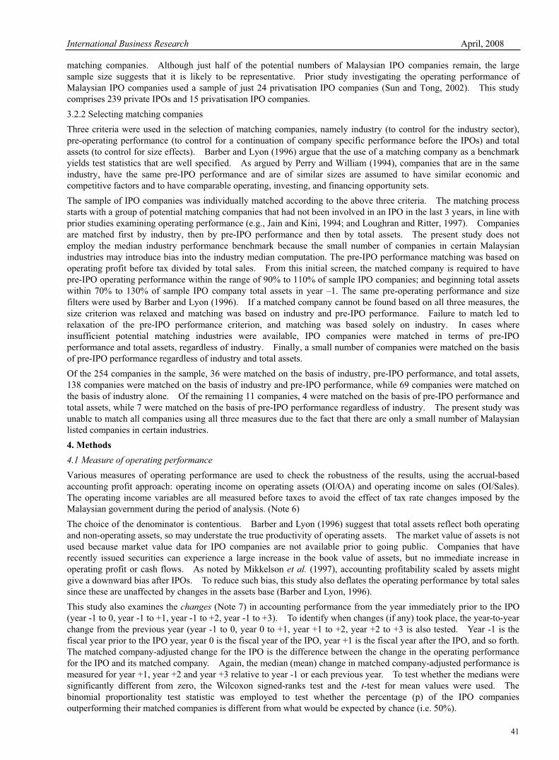
International Business Research April, 2008
41
matching companies. Although just half of the potential numbers of Malaysian IPO companies remain, the large
sample size suggests that it is likely to be representative. Prior study investigating the operating performance of
Malaysian IPO companies used a sample of just 24 privatisation IPO companies (Sun and Tong, 2002). This study
comprises 239 private IPOs and 15 privatisation IPO companies.
3.2.2 Selecting matching companies
Three criteria were used in the selection of matching companies, namely industry (to control for the industry sector),
pre-operating performance (to control for a continuation of company specific performance before the IPOs) and total
assets (to control for size effects). Barber and Lyon (1996) argue that the use of a matching company as a benchmark
yields test statistics that are well specified. As argued by Perry and William (1994), companies that are in the same
industry, have the same pre-IPO performance and are of similar sizes are assumed to have similar economic and
competitive factors and to have comparable operating, investing, and financing opportunity sets.
The sample of IPO companies was individually matched according to the above three criteria. The matching process
starts with a group of potential matching companies that had not been involved in an IPO in the last 3 years, in line with
prior studies examining operating performance (e.g., Jain and Kini, 1994; and Loughran and Ritter, 1997). Companies
are matched first by industry, then by pre-IPO performance and then by total assets. The present study does not
employ the median industry performance benchmark because the small number of companies in certain Malaysian
industries may introduce bias into the industry median computation. The pre-IPO performance matching was based on
operating profit before tax divided by total sales. From this initial screen, the matched company is required to have
pre-IPO operating performance within the range of 90% to 110% of sample IPO companies; and beginning total assets
within 70% to 130% of sample IPO company total assets in year –1. The same pre-operating performance and size
filters were used by Barber and Lyon (1996). If a matched company cannot be found based on all three measures, the
size criterion was relaxed and matching was based on industry and pre-IPO performance. Failure to match led to
relaxation of the pre-IPO performance criterion, and matching was based solely on industry. In cases where
insufficient potential matching industries were available, IPO companies were matched in terms of pre-IPO
performance and total assets, regardless of industry. Finally, a small number of companies were matched on the basis
of pre-IPO performance regardless of industry and total assets.
Of the 254 companies in the sample, 36 were matched on the basis of industry, pre-IPO performance, and total assets,
138 companies were matched on the basis of industry and pre-IPO performance, while 69 companies were matched on
the basis of industry alone. Of the remaining 11 companies, 4 were matched on the basis of pre-IPO performance and
total assets, while 7 were matched on the basis of pre-IPO performance regardless of industry. The present study was
unable to match all companies using all three measures due to the fact that there are only a small number of Malaysian
listed companies in certain industries.
4. Methods
4.1 Measure of operating performance
Various measures of operating performance are used to check the robustness of the results, using the accrual-based
accounting profit approach: operating income on operating assets (OI/OA) and operating income on sales (OI/Sales).
The operating income variables are all measured before taxes to avoid the effect of tax rate changes imposed by the
Malaysian government during the period of analysis. (Note 6)
The choice of the denominator is contentious. Barber and Lyon (1996) suggest that total assets reflect both operating
and non-operating assets, so may understate the true productivity of operating assets. The market value of assets is not
used because market value data for IPO companies are not available prior to going public. Companies that have
recently issued securities can experience a large increase in the book value of assets, but no immediate increase in
operating profit or cash flows. As noted by Mikkelson et al. (1997), accounting profitability scaled by assets might
give a downward bias after IPOs. To reduce such bias, this study also deflates the operating performance by total sales
since these are unaffected by changes in the assets base (Barber and Lyon, 1996).
This study also examines the changes (Note 7) in accounting performance from the year immediately prior to the IPO
(year -1 to 0, year -1 to +1, year -1 to +2, year -1 to +3). To identify when changes (if any) took place, the year-to-year
change from the previous year (year -1 to 0, year 0 to +1, year +1 to +2, year +2 to +3 is also tested. Year -1 is the
fiscal year prior to the IPO year, year 0 is the fiscal year of the IPO, year +1 is the fiscal year after the IPO, and so forth.
The matched company-adjusted change for the IPO is the difference between the change in the operating performance
for the IPO and its matched company. Again, the median (mean) change in matched company-adjusted performance is
measured for year +1, year +2 and year +3 relative to year -1 or each previous year. To test whether the medians were
significantly different from zero, the Wilcoxon signed-ranks test and the t-test for mean values were used. The
binomial proportionality test statistic was employed to test whether the percentage (p) of the IPO companies
outperforming their matched companies is different from what would be expected by chance (i.e. 50%).

Vol. 1, No. 2 International Business Research
42
4.2 Measure of earnings management
The present study also predicts that managers are most likely to positively manipulate earnings at the time of IPOs in
order to increase their offering proceeds and maintain a high market price after IPOs. Following Teoh et al, (1998),
among others, earnings management is measured using discretionary accruals. As argued by DuCharme et al. (2001),
‘accruals not only reflect the choice of accounting methods but also the effect of recognition timing for revenues and
expenses, asset write-downs, and changes in accounting estimates’ (p.376). Since managers have more discretion over
short term than over long term accruals (Teoh et al., 1998), this paper employs discretionary current accruals (DCA) to
proxy for earnings management, as also used by Roosenboom et al. (2003) and DuCharme et al. (2001, 2004).
Using the accruals model as suggested by Dechow et al. (1995), the expected current accruals for each of the IPO
sample companies in a given year are estimated using an estimation portfolio of all level 3 industry peers available on
the Datastream and PACAP databases using the following cross-sectional model:
portfolioestimationjTA
Sales
TATA
CAtj
tj
tj
tjtj
tj ∈+∆
+=−−−
,
1,
,
1
1,
0
1,
, 1 εαα
where CA is current accrual; j is companies which are in the same level 3 Datastream industry subsector but excludes
the issuer and companies involved in an IPO in the previous three years; Salesj,t is change in sales for company j in the
industry estimation portfolio in year t; TAj,t-1 is lagged total assets for company j in the industry estimation portfolio;
tj ,ε is regression disturbances, assumed cross-sectionally uncorrelated and normally distributed with zero means.
Similar to prior studies (e.g., Teoh et al., 1998; Roosenboom et al., 2003; DuCharme et al., 2004) all the variables are
scaled by lagged total assets to reduce heteroscedasticity and to control for differences in company size. The change
in sales is included to control for changes in nondiscretionary accruals caused by the change of economic conditions.
A cross-sectional regression is performed separately in each fiscal year for each industry portfolio to estimate the
coefficients 0 and 1, to control for changes in nondiscretionary accruals and to allow the nondiscretionary accruals to
vary from period to period for different industries. Thus, the effect of changes in industry-wide economic
circumstances in each specific year on current accruals is controlled. In addition, the coefficients 0 and 1 are allowed
to change across years to allow for possible structural changes, such as management changes (DeFond and Jiambalvo,
1994).
An estimation portfolio is assigned for each of the IPO companies in the sample in order to estimate the coefficients 0
and 1. The present study restricts the analysis to estimating industry portfolios that consist of 10 companies or more
in the same level 3 Datastream industrial classification of the IPO companies in the same fiscal year. IPO companies
and companies that made an IPO in the previous three years are excluded from the industry portfolios. Due to the
shortage of companies in certain industries, several similar industries are combined together. This results in six
industry groups: (i) Basic; (ii) Consumer Goods (Cyclical and Non Cyclical); (iii) Services (Cyclical and Non Cyclical);
(iv) General Industrials and Information Technology; (v) Resources and Utilities; and (vi) Real Estate Development.
After estimating the coefficients 0 and 1 from the current accruals model, the nondiscretionary accruals for each IPO
company in each year are then predicted using the estimated coefficients 0 and 1 from each industry-year estimation
portfolio. The nondiscretionary (expected) current accruals are the portion of current accruals that are not influenced
by managerial discretion but are driven by the companies’ sales growth.
Following Dechow et al. (1995) the change in trade receivables is subtracted from the change in sales to control for the
possibility of credit sales manipulation by the issuer. The approach assumes that any change in the level of credit sales
during the period reflects earnings management activity (Young, 1999). The nondiscretionary current accruals are
then calculated as:
where 0 is estimated intercept; 1 is the slope coefficient for IPO company i in year t; Salesi,t is the change in sales
for IPO company i in year t; TRi,t is the change in trade receivables for IPO company i in year t; TAi,t-1 is lagged total
assets for IPO company i in year t.
Finally, the discretionary current accruals (DCA), which are subject to managerial manipulation, are calculated as the
difference between total current accruals and nondiscretionary current accruals. If non-zero DCA is observed, it can be
interpreted that earnings management exists during the year. Positive DCA can be interpreted as income-increasing
earnings management, and vice versa. The definition is:
tiNDCA
TA
CADCA
ti
ti
ti ,
1,
,
, −=−
∆−∆+=
−
∧
−
∧
1,
,,1
1,
0,
1
ti
titi
ti
tiTA
TRSales
TANDCA αα

International Business Research April, 2008
43
where CAi,t is current accruals of IPO company i in year t; TAi,t-1 is lagged total assets for IPO company i in year t; and
NDCAi,t is nondiscretionary current accruals for IPO company i in year t.
5. Results
5.1 Descriptive statistics
Table 1 presents the descriptive statistics for 254 IPOs and 254 matched companies. The information is pre-IPO, with
market value measured on the flotation date. The median (mean) operating return on sales (OI/Sales) for the sample of
IPO and matched companies is 13.9% (16.3%) and 13.6% (15.3%), respectively. These are expected to be similar
since the IPO companies have been matched primarily on OI/Sales. While the difference between medians is not
statistically significant, the difference between means OI/Sales is statistically significant at the 5% level. There is a
wide variation in this operating margin; IPO companies range between -24% and 63% and the matched companies
between -26% and 52%. The skewness (and kurtosis) is typical for company size measures generally, but also suggest
a larger positive tail with greater central clustering for IPO companies.
The absolute figures of operating profit before tax, total sales, total assets, equity capital and reserves, market value, and
total debt show some differences between IPO and matched companies. There are significant differences in both
median and mean values at the 1% level. For example, the median (mean) total sales for IPO companies is RM65
million (RM125 million) compared with RM137 million (RM784 million) for matched companies. The difference is
partly a function of the procedure used in size matching, since IPO companies were usually matched with the nearest
larger non-IPO company in terms of size, even though size range between 70% and 130% of IPO company was used.
Similar observations occur for the other size measures. The highest market value of RM26,250 million for IPO
companies is observed for Tenaga Nasional Berhad. Meanwhile, the lowest market value of RM24 million is observed
for Carpet International Malaysia Berhad.
While the total debt of IPO companies is also smaller than for their matched companies, the gearing levels are
significantly higher at the 1% (10%) level for medians (means). The median (mean) debt/equity ratio is 40% (64%)
for IPO companies compared with 24% (49%) for matched companies. This is not surprising given the desire to raise
new equity finance expressed in the IPOs.
5.2 Level of operating performance
Prior to investigating the changes in the operating performance of Malaysian IPO companies, it is useful to consider the
level of operating performance of IPO companies and their respective matched companies over time for the pre-IPO
year, the IPO year, and the post-IPO years. The analysis of performance is conducted to identify any differences
between IPO companies and matched companies throughout the years -1, 0, +1, +2, and +3. Similar to Jain and Kini
(1994), Mikkelson et al. (1997), and Kim et al. (2004), this paper focuses on median performance due to the tendency
of accounting ratios to contain outliers in the data. However, for completeness, the results based on means are also
reported.
As can be seen from Table 2, both the median levels of operating performance measures (OI/OA and OI/Sales) of the
IPO companies are higher than those of the matched companies in the year prior to the IPO and the IPO year. Both
measures are significantly different at the 1% level except for the pre-IPO median level of OI/Sales. These results are
confirmed by a significant percentage positive, with more than 50% observed in year -1 and 0. While the median
levels of OI/OA of the IPO companies continue to outperform the matched companies up to year +2, the levels are not
significantly different. The OI/Sales measure shows that the IPO companies underperform the matched companies
subsequent to year 0. Both accrual-based measures show that IPO companies significantly underperformed the
matched companies in the third year following the IPOs at the 1% level. (Note 8)
5.3 Change in operating performance
Reported in Table 3 are the median and mean changes in operating performance for IPO companies and matched
company-adjusted results. Panel A reports the results of the pre- and post-IPO changes, while Panel B provides the
results of the year-to-year changes.
As can be seen in Panel A of Table 3, all of the median OI/OA values decline from their pre-IPO levels. All of them
are significantly different from zero at the 1% level. The results are consistent with US studies by Jain and Kini (1994)
who found a decline of 9.09% in return on assets three years after the IPO, and by Kim et al. (2004). The matched
company-adjusted results control for economy-wide, industry-wide, pre-event performance and size and exhibit a
decline throughout all performance windows from year 0 onwards. The median matched company-adjusted changes
range from -0.1% to -8.1% and all except the first are statistically significant, indicating that IPO companies have a
higher rate of decline than that of their matched companies. This shows that the decline in post-IPO OI/OA is not
simply due to an industry-effect, mean reversion or size. The decline in OI/OA from year -1 suggests that the IPO
companies may time their issues to occur after good performance. Interestingly, results for changes in the less

Vol. 1, No. 2 International Business Research
44
downward-biased measures, OI/Sales, show that there is a slight improvement in performance in year 0 relative to year
-1 for the IPO companies. However, this improvement is not statistically significant. Subsequent to the IPO, there is
a significant decline in performance in OI/Sales for IPO companies.
The year-to-year changes in OI/OA reported in Panel B also show significant declines in performance, with the rate of
decline slowing down somewhat over time. After controlling for companies matched by similar industry, pre-IPO
performance and size, the changes in OI/OA still show significant declines except for the change from year -1 to 0.
Thus, it is clear that IPOs in Malaysia do show deterioration in accruals-based returns on operating assets for the three
post-IPO years.(Note 9) Contrary to expectation, this study did not find a large decline in OI/OA in the year -1 to 0,
although this was observed in year 0 to +1. The median OI/Sales for the IPO companies peaks in the IPO year and
then declines following the IPO. Consistent with the OI/OA results, the highest decline occurs in the year immediately
following the IPO (year 0 to +1).
In sum, the evidence suggests that the accrual-based operating performance of IPO companies is higher prior to the IPO
but declines thereafter, subject to a slight improvement in operating margins in the IPO year (year -1 to 0). This
suggests that Malaysian companies may time their IPOs to coincide with peak performance and/or may increase their
assets more rapidly than sales. There is also evidence that IPO companies underperform their matched companies
from the year following the IPO. Moreover, the evidence is consistent with previous empirical results (e.g., Jain and
Kini, 1994, and Kim et al., 2004) which reported a deterioration in accrual-based operating performance following
IPOs.
Overall, it is clear that both accrual performance measures show higher pre-IPO performance, consistent with Kim et
al.’s (2004) study on the Thailand market. There is evidence of post-IPO underperformance relative to control
matched companies, consistent with the Mikkelson et al.’s (1997) study on the US market and the findings of Cai and
Wei (1997) based on the Japanese market. The deterioration in performance may be the result of the reversal of
pre-event accruals that have been used by IPO managers to overstate pre-IPO earnings. Therefore, in the next section,
an analysis of the potential earnings manipulation of IPO managers is provided.
5.4 Earnings management
Table 4 presents the evidence for the likelihood of earnings management, proxied by the discretionary current accruals
(DCA), at the time of the IPOs (year 0) classified by year of listing. All values are expressed as a percentage of lagged
total assets.
The present study relies on the medians for statistical inference since some skewness is indicated in the sample by a
higher mean measure than median measure in year 0. In addition, the test of normality based on the
Kolmogorov-Smirnov statistic of 0.156 (p-value = 0.000) indicates that the data differs significantly from a normal
distribution, thus violating one of the assumptions of parametric tests.
The median (mean) DCA is higher at the time of the IPOs (year 0), at 3.24% (5.74%) of lagged total assets. The
results of the present study strongly support the likelihood of earnings management at the time of IPOs, indicated by a
significant positive (at the 1% level) DCA. The level of earnings management at the time of IPO is slightly lower than
the results observed by Teoh et al. (1998) and Roosenboom et al. (2003), who reported median values of 5.5% and
3.9%. Teoh et al. (1998) confine their study to conditions in US whereas Roosenboom et al. (2003) focus on the
Netherlands. However, as reported by Roosenboom et al. (2003), other studies have observed similar levels of
earnings management, ranging from 1.5% to more than 5% of lagged total assets. Overall, the evidence reported in
Table 4 is consistent with Teoh et al. (1998) and Roosenboom et al. (1003) and suggests that the managers of
Malaysian IPO companies opportunistically advance accruals in an attempt to improve earnings during the IPO year.
Thus, the evidence provides a possible explanation for the observed decline in operating performance reported in the
previous section.
6. Summary
This paper is the first detailed, large sample study of the long run operating performance and earnings management of
Malaysian IPO companies, and covers the period 1990 to 2000. The main results of this study can be summarised as
follows. First, comparison of pre- and post IPO accounting-based operating performance in terms of levels and
changes provides some interesting findings. There is moderate evidence supporting the view that the average IPO
company in Malaysia underperforms seasoned companies over the three year post-IPO period. However, there is strong
evidence of declining performance in the IPO year and up to three years following the IPO. The year-to-year analysis
reveals that the decline in performance is greatest in the year immediately following the IPO. This finding is consistent
with the results of prior studies documenting the long run underperformance of IPOs. The results also confirm that the
deterioration in the post-IPO operating performance is due to earnings management by IPO managers at the time of
going public.
References

International Business Research April, 2008
45
Abdul Rahman, R., & Wan Abdullah, W.R. (2005). The new issue puzzle in Malaysia: performance and earnings
management. National Accounting Research Journal, 3, pp. 91-110.
Ahmad, Z., & Lim, S.M. (2005). Operating performance of initial public offerings in Malaysia. Capital Market Review,
13, pp. 21-32.
Balatbat, M.C.A., Taylor, S.L., & Walter, T.S. (2004). Corporate governance, insider ownership and operating
performance of Australian initial public offerings. Accounting and Finance, 44, pp. 299-328.
Barber, B. M., & Lyon, J. D. (1996). Detecting abnormal operating performance: The empirical power and specification
of test statistics. Journal of Financial Economics, 41, pp. 359-399.
Cai, J., & Wei, K.C. J. (1997). The investment and operating performance of Japanese initial public offerings.
Pacific-Basin Finance Journal, 5, pp. 389-417.
Chan, K., Wang, J., & Wei, K.C. J. (2003), Underpricing and long-term performance of IPOs in China. Journal of
Corporate Finance, 10, pp. 409-430.
Dechow, P.M., Sloan, R.G., & Sweeney, A.P. (1995). Detecting earnings management. Accounting Review, 70, pp.
193-225.
DeFond, M.L., & Jiambalvo, J. (1994). Debt covenant violation and manipulation of accruals. Journal of Accounting
and Economics, 17, pp. 145-176.
DeGeorge, F., & Zeckhauser, R. (1993). The reverse LBO decision and firm performance: theory and evidence. Journal of
Finance, 48, pp. 1323-1348.
Jain, B.A., & Kini, O. (1994). The post-issue operating performance of IPO firms. Journal of Finance, 49, pp.
1699-1726.
Kaplan, S.N. (1989). The effects of management buyouts on operating performance and value. Journal of Financial
Economics, 24, pp. 217-254.
Kim, K.A., Kitsabunnarat, P., & Nofsinger, J.R. (2004). Ownership and operating performance in an emerging market:
evidence from Thai IPO firms. Journal of Corporate Finance, 10, pp. 355-381.
Kutsuna, K., Okamura, H., & Cowling, M. (2002). Ownership structure pre- and post-IPOs and the operating
performance of JASDAQ companies. Pacific-Basin Finance Journal, 10, pp. 163-181.
Loughran, T., & Ritter, J.R. (1997). The operating performance of firms conducting seasoned equity offerings. Journal
of Finance, 52, pp. 1823-1850.
Mikkelson, W.H., Partch, M.M., & Shah, K. (1997). Ownership and operating performance of companies that go public.
Journal of Financial Economics, 44, pp. 281-307.
Mohd Saleh, N., & Ahmed, K. (2005). Earnings management of distressed firms during debt renegotiation. Accounting
and Business Research, 35, pp. 69-86.
Pagano, M., Panetta, F., & Zingales, L. (1998). Why do companies go public? An empirical analysis. Journal of
Finance, 53, pp. 27-64.
Roosenboom, P., van der Goot, T., & Mertens, G. (2003). Earnings management and initial public offerings: evidence
from the Netherlands. International Journal of Accounting, 38, pp. 243-266.
Sun, Q., & Tong, W.H.S. (2002). Malaysia privatization: a comprehensive study. Financial Management, 31, pp.
79-105.
Teoh, S.H., Welch, I., & Wong, T.J. (1998). Earnings management and the long-run market performance of initial public
offerings. Journal of Finance, 53, pp. 1935-1974.
Wang, C. (2005). Ownership and operating performance of Chinese IPOs. Journal of Banking and Finance, 29, pp.
1835-1856.
Young, S. (1999). Systematic measurement error in the estimation of discretionary accruals: an evaluation of alternative
modeling procedures. Journal of Business Finance and Accounting, 26, pp. 833-862.
Notes
Note 1. Overall, the total earnings after tax of listed non-financial companies declined by RM3 billion and RM14 billion
in 1997 and 1998, respectively (Mohd Saleh and Ahmed, 2005).
Note 2. Sun and Tong (2002) investigate the operating performance of 24 privatisation IPOs (PIPOs) in Malaysia for the
period 1983-1997. However, their small sample is not representative of the overall population of IPOs which consist
of both private and previously state-owned companies. In addition, they did not investigate the existence of earnings

Vol. 1, No. 2 International Business Research
46
management. The term PIPO is used to refer to situations when a public listing is used to transform part or all of the
government’s ownership in state-owned enterprises into private ownership.
Note 3. Five years of data on each proxy variable had to be available for each company and matched company to
examine the pre- and post IPO changes, and year-to-year changes in performance. The periods examined are the
pre-IPO year, the IPO year, and each of the three post-IPO years.
Note 4. Companies that are listed under Finance, Trust and Closed-End Funds sectors are excluded. The Properties
sector was included in the sample because it is not classified in the financial sector by the KLSE. The companies that
are listed via ‘introduction’ are excluded because they are not strictly IPOs. The company that issue debt together with
equity are excluded to avoid any confounding effects of debt issue.
Note 5. There is no accounting data for a particular year when a company changes its fiscal year end. In addition, the
data were reported inconsistently due to the fact that the financial statements were presented for periods with varying
time-spans, which limits the comparability of the accounting measures. However, if this occurred to the matched
company, it was removed and the process of finding another matching company was repeated.
Note 6. The corporate tax rate was 35%, 34%, 32%, 30%, and 28% in the years 1989-1992, 1993, 1994, 1995-1997, and
1998-2004 respectively (The Malaysian Inland Revenue Board).
Note 7. A similar method to measure change has been used by Kaplan (1989) and Degeorge and Zeckhauser (1993) on
leverage buyout (LBOs), and by Jain and Kini (1994) on IPOs. The absolute change rather than the percentage change
is used to avoid the negative denominator problem, whereby companies with poor performance (negative value) need to
be removed from the calculation of percentage change.
Note 8. For comparison with prior studies, the unreported results on the operating return on total assets are qualitatively
similar with the results based on the operating return on operating assets.
Note 9. To test the robustness of the results, operating return on total assets was also measured and the unreported
results show similar patterns.
Table 1. Descriptive statistics for 254 IPO companies and 254 matched companies
Mean Median Std Dev Min Max
IPO 16.32b 13.93 10.20 -24.32 62.90 OI/Sales (%)
Matched 15.33 13.56 10.05 -26.32 52.08
IPO 18a 9a 56 -21 702 Operating profit before
tax (million RM) Matched 113 20 274 -19 2376
IPO 125a 65a 295 9 3702 Total sales
(million RM) Matched 784 137 1733 7 10780
IPO 219a 70a 1086 2 14855 Total assets
(million RM) Matched 1342 275 3676 30 26526
IPO 91a 31a 431 -11 6071 Equity capital and
reserves (million
RM) Matched 616 155 1486 -27 14459
IPO 545a 180a 2051 25 36166 MV at flotation
(million RM) Matched 1538 389 3699 18 28134
IPO 71a 11a 455 0 5670 Total debt
(million RM) Matched 377 40 1658 0 15023
IPO 64c 40a 139 -11 1938 Total debt/equity (%)
Matched 49 24 77 -334 538
This table presents the descriptive statistics for 254 IPOs and 254 matched companies. The information is based on
pre-IPO date, except for market value data that is measured on the flotation date. a, b IPO and matched company values significantly different at the 0.01 and 0.05 level respectively, using a two-tailed
test.

International Business Research April, 2008
47
Table 2. The median and mean levels of operating performance
Median level (%)
n=254
Mean level (%)
n=254
IPO – Non-IPO
n=254
Fiscal Year
Relative to
IPO
IPO Non-IP
O
Z-stat IPO Non-IP
O
t-stat % tve Z-stat
Panel A:
OI/OA
-1 14.28 9.62 6.71a 18.02 11.34 5.05a 70.08 6.40a
0 12.91 7.50 7.39a 15.08 8.52 4.99a 72.83 7.28a
1 8.22 6.64 1.52 9.50 6.59 2.30b 53.15 1.00
2 6.89 6.27 0.13 6.94 5.72 0.90 49.61 -0.13
3 4.89 6.04 -3.40a 1.47 6.88 -2.71a 40.16 -3.14a
Panel B:
OI/Sales
-1 13.93 13.56 0.82 16.32 15.33 2.18b 50.39 0.13
0 14.25 12.38 4.31a 16.92 16.48 0.12 59.84 3.14a
1 9.75 10.28 -0.64 11.59 9.00 0.80 45.67 -1.38
2 8.97 10.17 -1.12 8.19 5.37 0.79 44.88 -1.63
3 5.94 9.89 -3.60a 1.90 5.80 -0.81 38.98 -3.51a
This table reports the median levels of operating performance measures (OI/OA and OI/Sales) of the IPO companies
and matching companies in the year prior to the IPO (year -1) up to three years following IPOs. OI/OA is measured by
operating profit before tax/(total assets-cash and equivalents), while OI/Sales is based on operating profit before
tax/(total sales). a, b, c denote significantly different from zero at the 0.01, 0.05, and 0.10 level respectively, using a two-tailed test.
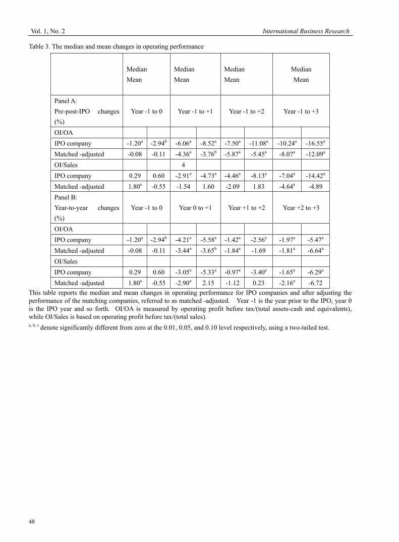
Vol. 1, No. 2 International Business Research
48
Table 3. The median and mean changes in operating performance
Median
Mean
Median
Mean
Median
Mean
Median
Mean
Panel A:
Pre-post-IPO changes
(%)
Year -1 to 0 Year -1 to +1 Year -1 to +2 Year -1 to +3
OI/OA
IPO company -1.20a -2.94b -6.06a -8.52a -7.50a -11.08a -10.24a -16.55a
Matched -adjusted -0.08 -0.11 -4.36a -3.76b -5.87a -5.45a -8.07a -12.09a
OI/Sales 4
IPO company 0.29 0.60 -2.91a -4.73a -4.46a -8.13a -7.04a -14.42a
Matched -adjusted 1.80a -0.55 -1.54 1.60 -2.09 1.83 -4.64a -4.89
Panel B:
Year-to-year changes
(%)
Year -1 to 0 Year 0 to +1 Year +1 to +2 Year +2 to +3
OI/OA
IPO company -1.20a -2.94b -4.21a -5.58a -1.42a -2.56a -1.97a -5.47a
Matched -adjusted -0.08 -0.11 -3.44a -3.65b -1.84a -1.69 -1.81a -6.64a
OI/Sales
IPO company 0.29 0.60 -3.05a -5.33a -0.97a -3.40a -1.65a -6.29a
Matched -adjusted 1.80a -0.55 -2.90a 2.15 -1.12 0.23 -2.16a -6.72
This table reports the median and mean changes in operating performance for IPO companies and after adjusting the
performance of the matching companies, referred to as matched -adjusted. Year -1 is the year prior to the IPO, year 0
is the IPO year and so forth. OI/OA is measured by operating profit before tax/(total assets-cash and equivalents),
while OI/Sales is based on operating profit before tax/(total sales). a, b, c denote significantly different from zero at the 0.01, 0.05, and 0.10 level respectively, using a two-tailed test.

International Business Research April, 2008
49
Research on the Acquirement Approach of
Enterprise Competitiveness Based on the Network View
Shuzhen Chu
Economics and Management School, Nanjing University of Science and Technology
Nanjing 210094, China
School of International Pharmaceutical Business, China Pharmaceutical University
Nanjing 211198, China
Zhijun Han
Economics and Management School, Nanjing University of Science and Technology
Nanjing 210094, China
Tel: 86-135-1253-5022 E-mail: [email protected], [email protected]
Abstract
Under the market situation of economic globalization, the premise of enterprise existence and development is to foster
the competitiveness of enterprise. Starting from the network view, this article will confirm the interest relatives of
enterprise and systematically discuss the approach of enterprise competitiveness through such aspects as the formation
of enterprise competitive potential, the increase of enterprise competitiveness and the continual renovation of
competitiveness.
Keywords: Network, Interest relative, Competitiveness, Approach
The western corporate network theory thinks that the enterprise is not opposite with the market, and their relation is
mutually connected and osmotic, and the technology needed by the enterprise is acquired through the cooperation and
development of the enterprise and exterior institutions to large extents. Since China joined WTO, China enterprises
would enter into increasingly drastic international competition. Under this situation, the independent and close
traditional enterprise innovation mode has not adapted the requirement of present global competition, and enterprises
need to integrate exterior resources through innovation network to enhance innovation ability of enterprise and remedy
the deficiency of innovation resources.
1. Analysis of enterprise interest relatives in the network
The network is the sum of various relationships happened and established when various principal parts of activities
change and transmit resources. These relationships may be informal relationships based on corporate social and cultural
backgrounds and mutual trusts, and may be normal relationships happened in the creation process of market trading,
knowledge and technology (Gai, 2002, p.47-118). The network is composed by principal part, resource and activity. The
principal part of activity in the network includes enterprises, colleges, research institutions, local governments, financial
institutions and agencies. Resources include hardware basic establishments, financial capital, human resources.
Activities mainly mean the reciprocity among principal parts of activity in the interior of the network (Lei, 2004,
p.60-63).
In the network, enterprise is the most important economic unit, and the most direct economical part to create values and
actualize increment of value. According to the activity situation among principal parts and in interiors of principal part,
we confirm these interest relatives of enterprise, which are seen in Figure 1. The so-called interest relative means any
relative influenced by organizational decisions and activities in the exterior environment of the organization. These
relative groups are closely linked with the organization, or the organizational activity would strongly influence them
(Stephen, 2003, p.78).
The key for enterprise to strengthen competitiveness relies on such aspects as how to select the appropriate cooperant
object in its interest relatives such as same industrial competitors, research institutions, financial institutions,
governments and agents and suppliers (Chen, 2002, p.14-16), how to select the appropriate coupling strategy on the
ligament bases of social relations and information network, how to select the appropriate network cooperation

Vol. 1, No. 2 International Business Research
50
innovation mode based on effectively utilizing interior and exterior innovation resources.
2. Formation of enterprise competitive potential
The competitive potential of enterprise is the base of enterprise competitiveness, and only the enterprise with certain
potentials can form enterprise competitiveness and actualize competitive predominance through available approaches.
The acquirement of enterprise competitive potential is realized through three processes including industrial cluster,
embeddedness, and netting, which are seen in Figure 2.
2.1 Industrial cluster makes enterprise obtain the predominance of space competition.
The industrial cluster is the aggregation composed by a group of relative enterprises in a same geographical region
(Chenery, 1996, p.95). The industrial cluster can strengthen the function assembling space of the region, and create
conditions to actualize regional scale economy and implement large scale customized production. The industrial cluster
can improve exterior scale economy and exterior scope economy of single enterprise, and reduce its production costs
and form price predominance. The industrial cluster also can establish mutually trusting economic network under same
industrial background, can promote that transnational groups spread and diffuse knowledge and technology to local
medium and small enterprises, and accordingly bring the space competitive predominance for the enterprises in the
region to actualize the innovation of products.
2.2 Embeddedness makes enterprise actualize localization.
The character of embeddedness roots in economic sociology, which means that economic activities are deeply
embedded in the social relation. Those enterprises in the cluster not only possess the geographical predominance, but
they have strong local relations which are presented not only in economy, but also in many aspects such as politics,
society, and culture. Mutual social cultural environment will produce trust and understanding, and mutual cooperation,
mutual trust and satisfaction will become the most valuable resources in the region. Embeddedness is the important
process in the development of network. Eenterprises from outside, especially those transnational enterprises take the
relation localization as their core, take the product localization as their support, depend the market localization to win
regional customers, utilize employee and research localization to foster local human resource (Zhou, 2003, p.34-35),
and this series of embeddedness processes make enterprises from outside and local enterprises form fixed industrial
chain and continually implement the adjustment of industrial structure, contribute for the development of local industry,
and accordingly drive the increase of enterprise competitiveness in the region.
2.3 The development of network improves the total enhancement of regional competitiveness.
The network relation is divided into normal relation and informal relation. The normal relation presents the relation
formed through various formal contracts among various activity principle parts. The informal network relation presents
the relative stable relation formed in non-contractual and long-term communicational process. The government
specially supports the enterprise which has development future for the local region. The financial institution notices and
participates in the research works of new product through offering loans with low interests to local enterprises.
Academies and scientific research institutions offer persons with ability and intelligent supports. Suppliers and agents
compel enterprises in the region expedite technical update, improve management methods and enhance the production
level of enterprises through putting forward technical requirements and product performance indexes to regional
enterprises. All these measures make enterprises in the center status of network benefit more.
3. Strengthening of enterprise competitiveness
The increase of competitive strength of certain industry in the region happens in the flexible associations among every
enterprise with other interest relatives, and enterprises can realize the increase of competitive strength through fully
utilizing rich resources in the network.
3.1 Competing with competitors and actualizing the heterogeneity of enterprise
Because information among enterprises in the network are symmetrical, so trades among enterprises possess durative,
which decides that the competitions among enterprises are infinite repeated games, and enterprises generally dare not
breach contracts, so good cooperation can be implemented favorably (Liu, 2006, p.73-78).
Cooperation is the good premise to implement competition. Enterprises should take competition as the impetus of
continual improvement and innovation, and to avoid being annexed or eliminated, they must continually enhance the
level of production technology, improve the management mode, reduce various production fees, and advance their own
competitive ability. As viewed from a short term, the competitiveness of enterprise comes from the price and
performance of present product. As viewed from a long term, the competitiveness of enterprise comes from lower costs
comparing with competitors and the ability to rapidly foster product, i.e. the core ability, which requires enterprises in
the network to gradually form their own core ability and actualize the heterogeneity in the long-term cooperation and
competition.

International Business Research April, 2008
51
3.2 Depending on the support and service of the government, enhancing the innovation ability of enterprise
The principal parts of interest in the network all enjoy rights brought by the network when they perform their own
obligations. When enterprises bring revenues for regional government, the government also actively influences the
innovation of enterprises. Though the government in the region can not directly create new knowledge, technology and
product, it can offer a good environment for the transmission of interior knowledge and information in the network,
offer a sort of mechanism to promote affiliations of enterprises in the network with other principal parts of activity,
enhance the cooperant efficiency among enterprises, compensate the deficiency of market forces, and drive the
development of enterprises. For example, the government can inspirit the development and innovation of science and
technology, ensure the favorable currency of technical innovative factors through the establishment of leading policies.
Those main enterprises in the network can fully utilize various policies and measures implemented by the government,
which aims to improve the development of enterprise and enhance the ability of innovation.
3.3 Utilizing capital market and forming the financial support to enterprise
Financial institutions in the network generally include local state-owned banks, regional merchant banks, various funs,
institutions of loan capital, risk investment institutions. At present, the capitals needed by enterprises to implement
innovation are more and more, and the capital deficiency is the main bottlenecks to limit enterprises (especially those
medium and small enterprises) to develop new products. Under this situation, enterprises in the network can establish
the cooperation with the capital market to compensate their own capital deficiency, and they can get loan from financial
institutions, and they can also implement financing by bonds, stocks or issuing international stocks and bonds in the
international capital market, and theses diversifications of financing approach will offer enough capital supports for
enterprises.
3.4 Strengthening the cooperation with scientific research academies and acquiring technical resources
The cooperation of enterprise with scientific research institutions can better acquire valuable knowledge, information
and technology, and enhance the learning ability and the innovation ability. This sort of cooperation is the typical
cooperation of production, learning and research, and the process of cooperation is the process of knowledge
transformation (He, 2006, p.63-68). To high technical industry, this cooperation has strong complementarity, especially
under the situation that many enterprises only possess low technical innovation ability, and the cooperation with
scientific research academies is the important approach to acquire technical resource. This sort of cooperation can be
implemented not only by the commercial channels such as technical consultation, technical franchise, and derived
enterprises which can transfer college techniques, but also by non-commercial channels. For example, the scientific
research academies offer scientists and engineers with high quality for the enterprise, and the scientific research
academies implement inventions through scientific theses and patents, and both parties’ personnel exchanges and
communication without day.
3.5 Establishing good relations with suppliers and customers, reducing costs and fostering customer group
The relations of enterprise with suppliers, customers is mainly embodied in the relation of upper and lower parts on the
industrial chain, because for any enterprise, enterprise is not only the supplier, but also the customers, and the relation
between supplier or customers is generally embodied in the trading relation, that is to say, enterprise exchanges raw
materials or components with suppliers, and trades products and services with customers. In the network, the relation
between supplier and customer comes from the support of three spaces including economic space, social space, and
geographical space. In the process to promote enterprise innovation and development and regional economic
development, these three spaces exert functions at the same time, and the supplier and the customer not only can trade
through market rule in the market, but also establish long-term cooperation after many times trades (Gai, 2002,
p.47-118). The enterprise and supplier can utilize geographical predominance, fully exert the functions of timely
production technique and transportation system, reduce production costs each other. Except for reducing costs of raw
materials and components, suppliers can actively participate in the total process from product design to product making,
and enterprises can enhance suppliers’ enthusiasm to implement product innovation and technical innovation through
adding orders. In the day of buyer’s market, competition is not only the competition of price, but the competition of
quality and diversity. Therefore, enterprises should increase the communication with customers, know and fulfill
customers’ real demands, and foster customers’ loyalty to enterprises.
4. Continual renovation of enterprise competitiveness
The innovation of enterprise should take employees’ knowledge absorption, intercommunion and sharing as the base.
The organizational learning is the necessary condition for the innovation of enterprise, and the result of enterprise
innovation is embodied in the recombination of original knowledge and the appearance of new knowledge, i.e. the
increase and accumulation of enterprise knowledge. The entrepreneur’s innovative spirit is the essential impetus to
organize leaning and knowledge accumulation for the enterprise, and the essential aim of learning and absorption,
intercommunion and sharing of enterprise knowledge is to support the enterprise innovation based on entrepreneur’s

Vol. 1, No. 2 International Business Research
52
spirit, and foster sustainable competitive predominance (Jin, 2003).
To enterprises in the network, the developmental policies of enterprise can be acquired from policy perferrence of the
government, and the technique to develop new product can be introduced from scientific research institutions and
colleges, and capitals in the process of product development and production can be acquired from many financing
channels in financial institutions, and the long-term development of enterprise needs brainy entrepreneur’s layout with
employees together. The entrepreneur’s innovative decisions should be established on the forecast of grasp and future
development of market opportunity, and new competitive predominance source can be realized. At the same time, the
entrepreneur’s innovative decision also can destroy present competitive predominance. Just because of the existence of
theses entrepreneurs’ innovative decisions, present sources of innovative predominance are continually destroyed and
new innovative predominance continually occurs, and the enterprise competitiveness is updated continually. For
entrepreneurs, they should possess not only innovative abilities, but also destroyable ability to original things. For
employees, enterprise can strengthen employees’ loyalty through good enterprise culture, establish perfect training
system to train various talents for the enterprise, and establish effective stimulation system to exert employees’
enthusiasm to large extents. Enterprises also should establish the platform on which employees can absorb, exchange
and share knowledge to actualize continual innovation of enterprise.
References
Chenery H. (1996). Comparative Research on the Industrialization and Economic Increase. Shanghai: Shanghai Joint
Publishing Company. p.95.
Chen, Xinyue, Yang, Deli & Dong, Yizhe. (2002). The Choice of Enterprise Innovation Network Model. Scientific
Management Research. No.20 (6). p.14-16.
Gai, Wenqi. (2002). Innovation Network: New Thinking of Regional Economy. Beijing: Beijing University Press.
p.47-118.
He, Yaqiong, Ge, Zhongfeng & Sujun. (2006). A Research on Studying Mechanism among Organizations in the
Network of Regional Innovation. Academic Exchange. No.143 (2). p.63-68.
Jinbei. (2003). Economics of Competitiveness. Guangzhou: Guangdong Economy Press. No.4.
Lei, Ruqiao, Chen, Jixiang & Liuqin. (2004). Research on the Interaction Mechanism of Cluster’s Networks. Science of
Science and Management of S. & T.. No.12. p.60-63.
Liu, Aixiong, Zhang, Gaoliang & Zhubin. (2006). Analysis of the Origin of Industrial Clusters Competitiveness. Science
of Science and Management of S. & T.. No.1. p.73-78.
Stephen P. Robbins, Mary Coulter. (2003). Management. Beijing: China Renmin University Press. p.78.
Zhou, Lianxi. (2003). The Countermeasures of Multinational Corporation in Localilzation Strategy and China Local
Enterprises. Journal of Business Economics. No.9. p.34-35.
Figure 1. Interest Relatives of Enterprise in the Region
Note: The item added “*” is the important interest relative in Figure 1.
Figure 2. Acquirement Process of Enterprise Competitive Potential
International Business Research April, 2008
53
The Exercise of Social Power and the Effect of
Ethnicity: Evidence from Malaysian’s Industrial Companies
Kim Lian Lee (Corresponding author)
Faculty of Management & Information Technology, University College Sedaya International
3, Jalan Jenaris 2/1, Taman Jenaris 2, Kajang, Selangor, Malaysia
E-mail: [email protected]
Guan Tui Low
E-mail: [email protected]
Abstract
The writers investigated the managerial power bases on work autonomy and supervisory satisfaction in Malaysian
industrial environment. The effect of ethnicity was also explored. Data from 210 respondents from technical and
non-technical staff of manufacturing companies indicated that supervision of industrial people were most acceptable
through the practice of referent, expert and reward power. Among the power bases, reward power was most often
exercised when high work autonomy was accorded. The work autonomy was found to be positively correlated with
the satisfaction with supervision. Along the racial line, the Malays rated their superior more positively on the referent
power base than Chinese, while the Chinese rated their superior as more coercive than did the Malays
Keywords: Management, Organizational Behavior, Power Bases, Work Autonomy, Satisfaction, Managerial
Supervision, Ethnicity
1. Introduction
The purpose of this research is to examine the impact of power relationships upon subordinates’ work autonomy and
satisfaction with supervision. The central constructs whose relationships we will be explore in this research are power,
work autonomy and satisfaction with supervision. Power is said to be a “part of the larger study of the determinant of
human behaviour” (Cartwright, 1965, p.3). The organizational power relationships include top management, middle
level managers and support staff. The main issue is then the interpersonal relationships that occur across
organizational level as termed as “superior-subordinate dyadic relationships”. In today’s organizations, managers need
to be aware of the sources of power in work situations and how they affect employees’ satisfaction since dissatisfied
subordinates could lead to poor work performance, absenteeism or high turnover (Churchill, Ford & Walker, 1976;
Rahim & Buntzman, 1989).
Besides that, work autonomy as a variable for organizational study has been well-known as antecedents or
consequences of power. Spector’s (1986) reviewed more than 40 studies point out that work autonomy to be strongly
related to staff turnover, absent from work, performance, motivation, physical ailments, emotional distress and
dissatisfaction.
Moreover, most of the research attention was in the context of job design or job characteristics and less attention has
been given in linking the types of power applications and work autonomy. Knowing how power affects work
autonomy and satisfaction will allow superiors to change or maintain their power bases to achieve desirable outcomes.
1.1 Objectives of the Study
The fundamental of this study is lie on the interaction of key variables as shown in Figure 1 (Note 1). The study also
analyzed the effect of ethnicity on power bases, work autonomy and satisfaction. Another objective of this study is to
compare the consequences of social power relationship in this Malaysian work setting with those reported happening in
the West. In this region, the educational level specialized work experience, and expertise of superiors are often more
limited than those in the developed countries. The culture is characterised by strong traditional values according to
which deep commitment to friends, superiors and relatives is the locus of social relations among individuals. These
cultural and environmental factors are likely to influence the outcomes of the different bases of superior power and also
in the manner in which other contingent factors affect the acquisition and use of these powers.

Vol. 1, No. 2 International Business Research
54
The main instruments used in this study were developed and had undergone rigorous validation processes and proven to
have superior psychometric integrity than instruments used in many earlier research. Thus, the present study s also
aimed at providing research results from which the results of the earlier research may be compared and their general
applicability assessed.
2. Literature Review
The classic formulation of power, authority and legitimacy appeared in the work of Weber (1947) who analyzed power
according to the way in which it was legitimized among followers: by appeal to rationality, by tradition, or by the
transcendent claims of charisma. This work however presented the typology rather than an organized theory of power.
The notable development of the concept of power began with the work of Lasswell and Kaplan (1950) who considered
both the base and goal of influence in order to generate 64 different forms of the influence process or power. Two
main streams of thought have emerged from there. One is based on political science and game theory: it includes most
notably, articles by Dahl (1957), Harsanyi (1962) and Kornberg and Perry (1966). The second centres on social
psychology and is represented by French and Raven (1959), Cartwright (1965), Thibaut and Kelly (1959), and Emerson
(1962).
Many power theoreticians (Dahl 1957; Emerson, 1962; Kornberg & Perry, 1966; Nagel, 1968; Wrong, 1968) stressed
that power should be conceptualized as a relationship between or among persons and not an attribute or possession of a
person or group. Within organizational context, theorists largely agree that individual power in organization is the
ability to control others, to exercise discretion, to get one’s own way.
2.1 The Bases of Power
Numerous categorizations have been used in differentiating bases of social power in organizations (Peabody, 1961;
Etzioni 1964; Patchen, 1974; Twomey, 1978; Kipnis, Schmidt & Wilkinson, 1980; Shukla, 1982; Rahim, 1989).
However, French and Raven (1959) typology of power is still the most popularly used in research work (Cobb, 1980;
Frost & Stahelski, 1988; Rahim, 1989; Rahim, Antonioni, Krumov, & Illieva, 2000). French and Raven defined bases
of power as below:
2.1.1 Coercive Power
Coercive power involves the concept of influence based upon “the expectation of punishment for failure to conform to
an influence attempt”. The strength of coercive power depends on the magnitude of the “negative valence of the
threatened punishment multiplied by the perceived probability that a power recipient can avoid the punishment by
conformity’. One of the key elements is that people subject to coercive power are either indifferent to, or opposed to,
the wielder of authority.
2.1.2 Expert Power
This power usually manifests in information, knowledge and wisdom, in good decision, in sound judgment and in
accurate perception of reality. Expert power is restricted to particular areas as the “expert” tends to be specialised.
The extent of expert power is not clearly a function of the face-to-face interaction or the personal quality of that
interaction between role partners; it may be a function of the knowledge possessed by the power wielder, not of his
presence.
2.1.3 Reward Power
Reward power is derived from the ability to facilitate the attainment of desired outcomes by others. In a sense, this
form of social power is closely related to coercive power. If one conforms to gain acceptance, reward power is a work.
However, if conformity takes place to forestall rejection, coercive power has to be exercised. In accordance to French
and Raven, reward power depends on the power wielder (individual or group) administering “positive valences and
reducing or removing negative valences”.
2.1.4 Referent Power
This involves the concept of “identification”, which French and Raven (1959) define as “a feeling of oneness or a desire
for such an identity”. If referring to a group, then an individual seeks membership in such group or has a desire to
remain in an association already established.
2.1.5 Legitimate Power
Closely tied to the Weberian concept of “legitimate authority”, legitimate power is induced by norms or values of a
group that individuals accept by virtue of their socialisation in the group. By the French-Raven, definition, this power
“stems from internalised values which dictate that there is a legitimate right to influence and an obligation to accept this
influence”.
2.2 Work Autonomy

International Business Research April, 2008
55
The type of power used to exercise control will impact upon the type of involvement on the part of the controlled
subordinates. One variable that is likely to be affected by the variation in the exercise of self-control of the
subordinates is work autonomy. Breaugh (1985) described work autonomy facets as follows:
(1) Work Method Autonomy
The degree of discretion/choice individuals have regarding the procedures/methods they utilise in going about their
work.
(2) Work Scheduling Autonomy
The extent to which workers feel they can control the scheduling/sequencing/timing of their work activities.
(3) Work Criteria Autonomy
The degree to which workers have the ability to modify or choose the criteria used for evaluating their performance.
It should be emphasized that the essence of these definitions lies on employee’s perceptions as regardless of the amount
of autonomy subordinate really has in their work, it is how much they perceive that they have which affects their
reactions to the job. Autonomy has received considerable attention in the context of job characteristics (Hackman &
Oldham, 1976; Sims, Szilagyi, & Keller, 1976). Loher, Noe, Moeller, and Fitzgerald (1985) have meta-analyse the
relationship between job characteristics and job satisfaction, and found autonomy to be highly related to job satisfaction
than any of the other job characteristics. Based on the above mentioned findings, it is anticipated that in the present
study, job autonomy as one consequence of the various types of power applications should co-vary with satisfaction
with supervision.
2.3 Satisfaction with Supervision
Job satisfaction is a collection of feelings or affective responses of the organizational members which are associated
with the job situation within the organization. Smith, Kendal and Hulin (1969), in their well documented measure, the
Cornell JDI (Cornell Job Descriptive Index) described five areas of satisfaction: the work itself, the supervision, the
co-workers, the pay, and the opportunities for promotion on the job. Since the present study is on the
superior-subordinate relationships, the job-facet satisfaction is most relevant to satisfaction with supervision.
Obviously, from human relations perspectives, supervisory satisfaction is related to the personality traits of the superior
which as his/her temperament, openness, industriousness, pleasantness etc. The positive side of all of these traits can
enhance satisfaction. Related to the personal resourcefulness, supervisory satisfaction is also dependent on the
superior’s distinguishing qualities and abilities such as intelligence and knowledge.
2.4 Ethnicity
In the multi racial society like Malaysia, employees bring into the organisation differing systems of values. The
heterogeneous value profiles may transcend into different beliefs and attitudes which determine expressive and
perceptual responses toward organisational systems and work. For example, the work of Ismail (1988) advanced the
notion that Malay managers are different from their Chinese counterparts in their view toward leadership style and job
freedom. Differences in the perception of power bases, work autonomy and satisfaction with supervision along the
racial line will be investigated in the present study.
3. Hypotheses to be tested
The following hypotheses were formulated for the study.
H1a: Superiors’ expert, referent, reward and legitimate are positively associated with the subordinates’
satisfaction with supervision
H1b: Superiors’ coercive base of social power is negatively associated with the subordinates’ satisfaction with
supervision.
H2: Subordinates’ work autonomy is significantly and positively related to the development of reward and referent
bases of social power in the relationship with superiors.
H3: Work autonomy is significantly and positively related to the satisfaction with supervision.
H4: There are no differences between Malay and Chinese subordinates’ perceptions of power bases, work
autonomy and satisfaction with supervision
4. Research Methodology
4.1 Sampling Design
The sample for this study comprises of the technical and non-technical staff in the manufacturing companies.
Stratified random sampling technique was used to select companies with a number of employees more than 25. This

Vol. 1, No. 2 International Business Research
56
number was arbitrarily chosen but the intention here was to include only establishments where a more formal
organizational structure and system of supervision more likely to exist and function.
The factories that met the above criteria were selected from the registry of members of the Federation of Malaysian
Manufacturers.
4.2 Research Instruments
All data used in the study consist of responses to questionnaire items. Measures of relevant constructs were discussed
here.
4.2.1 Bases of Supervisory Power
The five French-Raven bases of supervisory power were measured by using the Rahim Leader Power Inventory (RLPI)
(Rahim, 1988). This multi-item instrument uses a 5-point Likert scale to measure perceptions of subordinates
regarding their superiors’ bases of power. The instrument comprises of 29 items.
4.2.2 Work Autonomy
Work autonomy was conducted using the instrument developed by Breaugh (1985, 1989) and Breaugh and Becker
(1987). The instrument is capable of measuring three facets: method, scheduling, and criteria of work autonomy,
comprises of 9 items.
4.2.3 Satisfaction with Supervision
The instrument used to measure satisfaction with supervision is the updated version of the original Job Descriptive
Index (JDI; Smith at el., 1969) which was later revised by Roznowski (1989). The instrument is made up of 18 items.
4.3 Data Analysis Techniques
Reliability and factor analysis was used to check the consistency and dimensionality of the scale items. Multiple
regression analysis is performed to check the criterion-related validity of the scale items. Pearson Intercorrelation was
used to measure the associations among the social power bases, work autonomy and satisfaction with supervision.
Paired T-Test was conducted to contrast the Malay-Chinese on the perception of power bases, work autonomy and
satisfaction with supervision.
5. Research Results and Discussions
5.1 Sample Characteristics
Data from 230 respondents were received and only 210 data were usable. By ethnic group, 72% of the respondents were
Chinese, 18% were Malay, and 8% were Indian, while other races made up the rest. Attempts to obtain more female
respondent to test male-female differences were not successful due to the much smaller proportion of female taking
supervisory roles in the factories. A mere 7% female respondent reflects the male domination in the industrial sector.
More than 60% of the respondents were from factories located in the state of Selangor where factories were largely
concentrated in the Klang Valley. Other states like Perak, Penang, Kedah and Perlis account for only 20% of the total
respondents. The remaining respondents were from factories scattered in the states of Johore, Negeri Sembilan, Malacca
and Pahang.
In terms of age, the highest proportion of respondents fell into the 31-40 years age group. They accounted for 50% of
the total number of respondents. This was followed by the 20-30 years age group (34%), while those above 41 years old
accounted for the remaining.
On the whole, the education level of the respondents was high. Nearly 61% of the respondents had education up to
university in technical field while 15% received university education in non-technical field. Only 24% of the
respondents had no tertiary education. The high educational level was reflected in the position or the type of
occupation held by the majority of the respondents i.e. 5 Assistant General Managers, 54 Divisional Manager and
Assistants, 74 Engineers and Assistants, 11 Chemists, 32 Supervisors, 12 Plant Operators and the rest comprised of
System Analysts, Draughtsmen, Quality Control Inspectors etc.
The average salary of the respondents was higher than the population’s average. The survey data showed that 29% of
the respondents earned more than RM5000 per month, 12% earned RM4001 to RM5000 per month, 16% earned
RM3001 to RM4000 per month, and 13% earned RM2001 to RM3000 per month.
On average, the respondents had worked in the present company for 7 years. It was noted that 22% of the total
respondents had worked for one year or less in the present company, 23% had worked between 2 to 4 years, 21% had
worked between 5 to 8 years, and 17% had worked between 8 and 12 years, while only 12% of the respondents had
worked longer than 12 years in the present company.
In terms of the organizational size, the survey had selected sample which represents the medium to large sized

International Business Research April, 2008
57
Malaysian manufacturing companies. The average number of employees of the factory sample as 275. It was found that
41% of the factories had 25 to 100 employees, 24% had 101 to 200 employees, 14% had 201 to 400 employees, 10%
had 401 to 1000 employees and 11% had more than 1000 employees.
Classifying the factories according to the type of business revealed that a greater portion of the factories manufactured
machinery (29%), followed by food (13%), chemical (13%) and the rest manufactured non-metal, basic metal, textile,
wood and paper.
The survey also revealed the information about the respondent’s superiors. Almost all of the superiors reported in the
survey were males with the exception of one female. A majority of them were holding medium to high management
positions. Racial composition of the superiors was: 76% Chinese, 7% Malay, 7% Indian and 10% from other races.
On average, the superiors had worked in the organization for 11 years – far longer than the subordinates’ average.
Only 9% had worked for less than a year, 16% had worked between 1 and 5 years, 34% had worked between 6 and 10
years, 15% had worked between 11 to 15 years, 15% had worked between 16 to 20 years and the remaining 11% had
worked more than 20 years in the present company. Most of the superiors were holding high positions in the company
with 36% of them in the first hierarchical level, 31% in the second level, and 24% in the third level, while only a
fraction of them were in the lower management positions. Their educational level was also strikingly high, with 70%
of them having had tertiary education in technical field and 12% having had tertiary education in non-technical field.
Only 18% had up to either primary or secondary education. By designation, 40 of the superiors were the Directors of
companies, 32 were the General Manager, 89 were the Divisional Managers and the rest consisted of Assistant Manager,
Engineers, Supervisors etc.
5.2 Validating the Scales
The data on the 29 power items from the sample of 210 respondents were factor-analyzed. The selection of a factor
and an item was guided by the criteria: eigenvalue > 1.0 and Scree Plot and factor loading > 0.4, respectively (Ford,
MacCallum & Tait, 1986). Based on these criteria, the first five factors were selected (result not shown).
Considering that the result as a whole supported the a priori grouping of items, it can be concluded that the power scale
developed by Rahim (1988) was suitable for application to the present data although some purification was necessary to
improve its accuracy. The indices of the five power bases were computed by averaging the samples responses to the
items in each factor. This resulted in the creation of five continuous subscales.
The mean, standard deviation and standardized Cronbach Alpha and the corrected item-total correlation for each
subscale is provided in Table 1 (Note 2). The internal consistency reliability coefficients for all the scales were
satisfactory (Nunnally, 1978). All the scales had coefficient Cronbach Alpha greater than .70. A corrected item-total
correlation is a correlation between an item’s score and subscale score computed from the remaining items in the set.
The item-total correlations for the five scales ranged between .29 and .76.
A multiple regression analysis was run to test the relationship between the five bases of leader power and the
subordinates’ satisfaction with supervision. The results are presented in Table 2 (Note 3). The results showed that
the referent, expert, and reward power bases positively influenced satisfaction with supervision. The five power bases
together explained about 45% of the variance in satisfaction. The relations between the five power bases and the
“theoretically-related” dependent variable supported the criterion related validity of the power scale.
5.3 Testing of Hypotheses
H1a & H1b: Power Bases and Supervisory Satisfaction
The correlational results in Table 3 (Note 4) provided good support for H1a. The non-coercive bases of social power
(expert, referent, reward and legitimate) showed positive relationships with satisfaction with supervision. Referent
power ranked highest among other power exercises (coefficient .64). This was followed by expert power and reward
power which both had coefficients of correlation of 0.47. The ranking of intercorrelation was somewhat similar to the
study of Rahim and Buntzman (1989) conducted on respondents with post graduate working experiences. It was
expected that referent and expert power represent a high level of internalisation or inner acceptance. In the exercise of
referent power, internalisation derived from the identification of power recipient with the wielder of referent power – a
personalised commitment to the group or its representative. As Raven (1974) found out, the exercise of referent power
tends to encourage a more satisfied, cooperative and prolonged relationships between superiors and subordinates.
Expert power benefits from an umbrella of authority which may go beyond superiors’ specialised skills. Among
technical staff, expertise emerges as a very important cue for acceptance and recognition of the superiors’ direction as
reflected in the present result. It most likely gains their compliance and least likely to provoke their resistance
(Podsakoff & Schriesheim, 1985). Similarly, greater satisfaction with supervision among subordinates may lead to
greater cooperation and heightened dependence.
Both referent and expert power were labelled by Yukl (1981) as “personal” form of power. The present results supported

Vol. 1, No. 2 International Business Research
58
the general view that “personal” power has a positive effect on the leader-subordinate relationship. The high degree of
intercorrelations among the referent, expert and reward power bases served to temper the previous discussions and
tended to suggest that while referent power emerged as the dominant explanatory power base, its effective utilisation
might be tied, to some extend, to the superiors’ exercise of a combination of other power bases i.e. in this case, expert
and reward power bases.
Although earlier findings (Warren, 1968) acknowledged that reward power shows less inner acceptance, the present
correlational results indicated a high level of satisfaction with supervision. This power derives from control over
positive or rewarding outcomes for subordinates is expected to be an effective means of influence to increase
productivity in the organisation. Schopler and Layton (1974) held that the use of reward power is likely to increase the
attraction between the manager and subordinates while coercive power is likely to decrease it. Too much emphasis of
this power base, however, should be guarded against, since the withdrawal of positive sanctions is apt to result in the
subordinates’ reversion to their previous behaviour. Further, the effect of the inducement, even if continued, is subject
to diminishing utility.
The legitimate power showed relatively lower correlation with the satisfaction with supervision. In the exercise of
legitimate power, subordinates’ responses tended to be dependent on the normative acceptance of the position and
prerogatives of the organization at large including its leadership. The present result concurred with the conclusion made
by Yukl (1981) that “position” power such as legitimate and coercive are less effective means of influence attempt.
The result for coercive power was not exactly consistent with hypotheses H1b. The study indicated that the amount of
coercive power perceived to be held by a superior was not associated with supervisory satisfaction when it was earlier
hypothesized to have negative association. However, the result failed to reach statistical significance. Past
researchers also had mixed results with regard to this correlation. For example, Rahim and Buntzman (1988) – weak
positive; Busch (1980), Hinkin and Schriesheim (1989) – negative. The coercive power which is derived from control
over negative or punishing outcomes for other does not appear to be a suitable power base for dealing with subordinates.
The traditionalists believed that punishment is ineffective and can lead to discontinuation of social interaction. The
present results however, neither confirmed nor disproved the effectiveness of punitive treatments to get things done but
it was obvious that this power exercise should not lead to subordinates’ satisfaction. Moreover, people could not be
coerced into a deep-seated acceptance of organizational requirements.
H2: Power Bases and Work Autonomy
The relationship as appeared in Table 3 (Note 4) between the perceptions of supervisory power bases and the perceived
amount of work autonomy given was significantly distinct where in the relationship with all but coercive power had
been significance. The relationship was strongest with reward power (r = .37) followed by referent (r = .21),
legitimate (r = .19), and expert power (r = .16). As autonomy is related to the organizational control - the ability to
control over work method, work scheduling and work criteria, a basic premise of the argument that follows is the
association of interrelationship between power bases and control. Autonomy provides an opportunity for subordinates
to exercise influence on decisions relating to their work. Hence, it enhances their relative ability to control in the
organization. The present result pointed to the conclusion that superiors who were perceived to exercise coercive
power would tend to exercise greater management control, possibly by application of autocratic techniques. The
reason for this was not conclusive. Many plausible explanations were possible, but it was believed that superiors who
exercised coercive power held to the traditional view that power has a fixed value, and a function of organizational
structure and formal authority, unilateral and vertical in direction. Thus, subordinates’ attempts to exercise greater
influence may be seen as a threat to superiors’ control and power. Furthermore, as the power gap between superiors
and subordinates will even likely to increase as a direct consequence of punitive treatments, the subordinates tend to
prefer to avoid participation. The above explanation is in similar vein as the conclusion made by Gardell (1977) about
the relationship between work autonomy and industrial democracy.
The non-coercive power bases correlate better with the work autonomy. Strong relationship between reward power and
work autonomy implied that those who exercised control over positive and rewarding outcome accorded greater work
autonomy to the subordinates. Though the degree of commitment toward work by the exercise of reward power has
been questioned (Warren, 1968; Gemmill & Wilemon, 1972) the rewards at least provide incentives for the subordinates
to perform beyond the line of duty. The substantive outcome is visible only when one produces work beyond the
normal expectations and control of the superior, otherwise reward is not necessary. The calculative involvement of
subordinates to the application of this power underscores the importance of work autonomy in eliciting employees’
responses. This conclusion was drawn from the assumption that people generally prefer greater work autonomy than
less and that work autonomy can provide opportunities for greater outcomes. It appeared from this study that
individual freedom and autonomy was contingent upon the exercise of reward power. In retrospect, it was
inconceivable that reward power was exercised with no allowance for work autonomy in the present context.
The referent power which stems from a feeling on the part of the subordinates identify with the superior indicates

International Business Research April, 2008
59
subordinates’ agreement with superiors in personal characteristics, decision style, etc. If the desire for work autonomy
and the actual work autonomy given is aligned, the perception of referent power is reinforced. The referent power
base helps to build trust in a relationship (Busch, 1980). This trust is reciprocal and thus we would expect that those
who exercise referent power will accord sufficient work autonomy to their subordinates.
The relationship between legitimate power and autonomy was significant although not strongly correlated (r = 0.19).
This power is more dependent on the authority relationship (position power) than the individually-based power style.
This managerial style were regarded as “traditional” by many management theorists as the superior-subordinate
relationship is perceived to follow rigid hierarchical line and employees tend to have little say in the conduct of their
work.
It was interesting to note that even though the expert power was highly correlated with satisfaction with supervision, its
correlation with work autonomy (r = 0.16) was not as pronounced as one would expect. This finding plays down the
importance of work autonomy in contributing to the satisfaction with supervision that lead one to think that work
autonomy may not be as important as the perception of power style in ensuring employees’ satisfaction. It is obvious
that professional expertise is not strongly related to work autonomy. Intuitively, if the subordinate perceived that the
superior has greater expertise than himself/herself, he/she will tend to down rate his/her own capability at least in
comparison with the superior’s. Such perception will suppress the motivation for anticipation in decision making, the
reciprocal of this might also be true, i.e. if the superior perceive his/her subordinate to be incompetent and lacking in
skills, little autonomy will be accorded to them. This finding is consistent with the work of Fiorelli (1988) and
Bennett (1982).
Overall, the results agreed with hypothesis H2. However, the present result should be used with caution as the
measurement of both construct was not based on the objective measurement but on individual perceptions. Individual
differences such as desire for power equalization, inner motivation, etc might intervene in the relationship between
power and work autonomy.
H3: Work Autonomy and Supervisory Satisfaction
The relationship between work autonomy and satisfaction with supervision was not as strong as one would expect (r
= .23). This was probably due to the reason that work autonomy and satisfaction with supervision was not very much
a related concept. The former measured job characteristic from the perspectives of internalized pattern of self
determination while the latter measured one’s feelings about the nature of supervision at work. Nonetheless, an
important common element appeared to exist between them that explained their positive and statistically significant
relationship. It was assumed that the common element would be the degree or quality of supervision. The right
degree of perceived supervision is synonymous with the quality of supervision perceived. Conceptually, satisfaction
with supervision may be considered, in special cases, as a consequence of work autonomy, but it is not the action of
work autonomy itself. Work autonomy may result in satisfaction or frustration with supervision. Blake and Mouton
(1964) suggested that subordinates should be given greater power in decision making if they are exceptionally skilled,
the superiors should exercise power in decision making in times of crises or when subordinates lack skills and abilities.
The work autonomy is valued to the extent that it is within the capability of the participant. Moreover, satisfaction
with supervision has a more general meaning which includes factors other than quality and amount of supervision. It
includes personal traits of the superior, his/her knowledge and specialized skills, habits and personal disposition. Thus
it can be concluded that all other factors being equal, increased autonomy when accorded within the decision making
capabilities of subordinates is accompanied by greater satisfaction with supervision.
H4: Power Bases, Work Autonomy, Supervisory Satisfaction and Ethnicity
The results of contrasting Malay and Chinese (H4) on the perception of the power bases, work autonomy and
satisfaction with supervision are shown in Table 4 (Note 5). Other races were deliberately left out of the analysis
because they offered a sample size too small for significant results. With exceptions of referent and coercive power
bases, the test of no difference held true for all other variables. The results brought forth some interesting findings.
The Malays scored higher in their perception of referent power base implying that in general term the Malay
subordinates esteemed and valued their leader more than the Chinese for such esteem and value are highly related to the
leader’s referent power. In the light of the a priori expectation that Malays are fatalistic, shy (“segan” and “malu”) or
an easily embarrassed group of people, and Chinese are diligent, aggressive and wealth seeking (Charlesworth, 1974),
one would expect the Malay subordinates to be more conformist and more sociocentric than the Chinese. These
dominant values would have accentuated the differences in the perception of referent power base. One also need to
consider other indirect evidence of referent power that concerns ingratiation and the desire for acceptance by leader
which may reciprocate in efficacious responses on the part of the superior leading to a greater perception of referent
power. However, firm conclusions cannot be made from these findings alone as interactions with other variables not
included in the study are possible.

Vol. 1, No. 2 International Business Research
60
The Chinese rated their superiors more ‘coercive’ as compared to the Malays. Since the sample were selected from the
basis of similarity in salary (Chi-Square = .44, p = .99), age (Chi-Square = .12, p = .99), and number of previous jobs
(Chi-Square = 2.85, p = .83), the differences noted may be attributed to factors external to those considered here.
Again, subcultural influences may be one of the reasons behind these differences. The more subtle uses of power to
coerce the Malay may also indicate that the Malay subordinates are more conformist and do not require threat and
punishment to comply with the superiors’ wishes. This is again a presumption as the inherent limitations of the study
unable us to distinguish the cause from effect (of the power exercise). Precise explanations of the above findings should
await further research works taking into account value systems and ethnicity in the study.
6. Conclusion
In general, the results of this study in relation to the administration of industrial people were quite consistent with our
hypotheses based upon other organizational studies involving qualified and professional people. The instruments used
in the study were tested and found to be applicable to our work environment. The results provided some tentative, but
hopefully useful guidance for industrial administrators.
Intercorrelations among the five power bases showed that French and Raven (1959) power bases are not mutually
exclusive. Reward and referent power bases were the most closely related followed by expert and referent power bases.
The results revealed that referent power, expert power and to some degree reward power and legitimate power are found
to be in association with each form of power. On the other hand, coercive power was the least correlated with all other
power bases and most often stands alone. Among all of the power bases, coercive power was most related to reward
power. It indicates that reward and coercive power tend to be used interchangeably. Though not considered as a serious
disadvantage, notable intercorrelations among the five power bases denote the difficulty of finding power typology
which is both exhaustive and conceptually distinct.
In assessing the effectiveness of the various influence attempts, the results suggested that referent, expert and reward
power should be emphasized to ensure subordinate acceptance. Coercive power should be minimised in any influence
attempt except in situation that call for such approach (e.g. time of crisis, low performance etc). The position of
legitimate power was the lowest among the non-coercive power bases in influencing subordinates’ behaviour for the
case of management of technical and professional staff. Comparative studies revealed an interesting difference in the
rank ordering of bases of the superiors’ influence attempts. While the present study and Rahim and Buntzman (1989)
study ranked referent and expert power as the most favourable and legitimate power the lowest among the non-coercive
power bases in eliciting subordinates’ acceptance, results of a survey conducted on account executives, office managers
and public administrators (Bachman, Smith & Slesinger, 1966) considered legitimate power as the most prominent or
second in place. The results suggested a notion that the effectiveness of power influence does relate to the situation and
context of the work environment.
The amount of autonomy given by superior was dependent on his/her willingness to delegate decision making down to
the subordinate. The manner in which, control over individual’s conduct of work lives was found to influence the
individual’s perception of the source of control. Superior who was perceived to exercise coercive power tends to
exercise greater management control – giving little opportunity for the subordinates to be personally responsible for a
meaningful portion of their works. The reward power is often used in exchange for compliance by subordinates. The
subordinate’s performance beyond the line of duty is made possible under high autonomy situations. The referent power
tends to build trust in the interpersonal relationship and thus naturally more autonomy will be given by the superior to
the subordinates. The perception of referent power is reinforced when one’s desire for work autonomy and the actual
work autonomy given is aligned. Management style that firmly rests on the legitimacy of authority usually offers
inadequate work autonomy as rigid hierarchical structure limits and inhibits the subordinates’ freedom in the conduct of
their work.
Even though autonomy is said to be highly favoured for job involvement and also aspiration toward increased work
participation at both the personal and group level, the present study showed that work autonomy may not result in
exceptionally greater satisfaction with supervision. It was concluded that the work autonomy will lead to greater
satisfaction with supervision only if the subordinates feel that the degree of work autonomy is appropriate, within the
capability of the subordinates and fits that psychological needs of the subordinates. Generally, the results of the study
did support the idea that the employees’ satisfaction with supervision is favoured by a design of jobs that allow for high
autonomy and high demands on skills and cooperation.
Along the racial line, the Malays tended to rate their superiors more positively on referent power than the Chinese while
the Chinese rated their superiors as more “coercive” than the Malays. Heterogeneous value profiles of the Malay and
Chinese were suspected to have bearings on the perceptions of these power bases. However, there was no noticeable
distinction between their perception of superiors’ work autonomy and their satisfaction with supervision.
References

International Business Research April, 2008
61
Bachman, J.G., Smith, C.G. & Slesinger, J.A. (1966). Control, performance, and satisfaction: An analysis of structural
and individual effects. Journal of Personality and Social Psychology, 4, 127-136.
Bennett, F.C. (1982). The pediatrician and the interdisciplinary process. Exceptional Children, 48, 306-314.
Blake, R.R. & Mouton, J.S. (1964). The Managerial Grid. Houston, Texas: Gulf Publishing Co.
Breaugh, J.A. (1985). The measurement of work autonomy. Human Relations, 38, 551-570.
Breaugh, J.A. (1989). The work autonomy scales: additional validity evidence. Human Relations, 42, 1033-1056.
Breaugh, J.A. & Becker, A.S. (1987). Further examination of the work autonomy scales: Three studies. Human
Relations, 40, 381-400.
Busch, P. (1980). The sales managers’ bases of social power and influence upon the sales force. Journal of Marketing,
44(4), 91-101.
Cartwright, D. (1965). Influence, leadership, and control. In March, J. (Ed.), Handbook ofOrganizations, Chicago:
Rand McNally, 1-17.
Charlesworth, H.K. (1974). Role strain in Bumiputra Entrepreneur: Can it be overcome? Unplublished paper submitted
to MARA Institute of Technology, Malaysian.
Churchill, G.A., Ford, N.M., Jr., & Walker, O.C., Jr. (1976). Organizational climate and job satisfaction in the sales
force. Journal of Marketing Research, 13, 323-332
Cobb, A.T. (1980). The sales managers’ bases of social power and influence upon the sales force. Journal of
marketing, 44 (4), 91-101.
Dahl, R.A. (1957). The concept of power. Behavioral Science, 2, 201-218.
Emerson, R.M. (1962). Power-dependence relations. American Sociological Review, 27, 31-41.
Etzioni, A. (1964). Modern Organizations, Englewood Cliffs, New Jersey: Prentice Hall, 58-64.
Fiorelli, J.S. (1988). Power in work groups: Team member’s perspectives. Human Relations, 41(1), 1-12.
Ford, J.K., MacCallum & Tait, M. (1986). The application of exploratory factor analysis in applied psychology: A
critical review and analysis. Personnel Psychology, 39, 291-314.
French, J.R.P. & Raven, N. (1959). The bases of social power. In D. Cartwright (Ed.), Studies in Social Power, Ann
Arbor: University of Michigan Press, pp.150-167.
Frost, D.E. & Stahelski, A.J. (1988). The systematic measurement of French and Raven’s bases of social power in
workgroups. Journal of Applied Social Psychology, 18, 375-389.
Gardell, B. (1977). Autonomy and participation at work. Human Relations, 30(6), 515-533.
Gemmil, G.R. & Wilemon, D. (1972). The product manager as an influence agent. Journal of Marketing, 36(1), 26-30.
Hackman, J.R. & Oldham, G.R. (1976). Motivation through the design of work: test of a theory. Organizational
Behavior and Human Performance, 16, 250-279.
Harsanyi, J.C. (1962). Measurement of social power, opportunity casts, and the theory of two person bargaining games.
Behavioral Science, 7, 67-80.
Hinkin, T.R. & Schriesheim, C.A. (1989). Development and application of new scales to measure the French and Raven
(1959) bases of social power. Journal of Applied Psychology, 74(4), 561-567.
Kipnis, D., Schmidt, S.M. & Wilkinson, I. (1980). Intraorganizational influence tactics: Explorations in getting one’s
way. Journal of Applied Psychology, 65, 440-452.
Kornberg, A & Perry, S.D. (1966). Conceptual models of power and their applicability to empirical research in politics.
Political Science, 18(3), 52-70.
Lasswell, H.D. & Kaplan, A. (1950). Power and Society. New Haven Yale University Press.
Loher, B.T., Noe, R.A., Moeller, N.L. & Fitzgerald, M.P. (19850. A meta–analysis of the relation of job characteristics
to job satisfaction. Journal of Applied Psychology, 70, 280-289.
Nagel, J.H. (1968). Some questions about the concept of power. Behavioural Sciences, 13(3), 129-137.
Nunnally, J.C. (1978). Psychometric Theory, New York: McGraw-Hill.
Patchen, M. (1974). The locus and basis of influence on organizational decisions. Organizational Behavior and Human
Performance, 11, 195-221.
Peabody, R.L (1961). Perceptions of organizational authority: A comparative analysis. Administrative Science Quarterly,

Vol. 1, No. 2 International Business Research
62
6(4), 463-482.
Podsakoff, P.M., & Schriesheim, C.A. (1985). Field studies of French and Raven’s bases of power: Critique,
reanalysis and suggestion for future research. Psychological Bulletin, 97, 387-411.
Rahim, M.A., (1988). The development of a leader power inventory. Multivariate Behavioral Research, 23, 491-502.
Rahim, M.A. (1989). Relationships of leader power to compliance and satisfaction with supervision, evidence from a
national sample of managers. Journal of Management. 15, 545-557.
Rahim, M.A. & Buntzman, G.F. (1989). Supervisory power bases, styles of handling conflict with subordinates, and
subordinate compliance and satisfaction. Journal of Psychology, 123, 95-210.
Rahim, M.A., Antonioni, D., Krumov, K. & Illieva, S. (2000). Power, conflict, and effectiveness: a cross-cultural study
in the United States and Bulgaria. European Psychologist, 5 (10), 28-33.
Raven, B.H. (1974). The comparative analysis of power and influence. In J.T. Tedeschi (Ed.), Perspective on Social
Power, Chicago: Aldine.
Roznowski, M. (1989). Examination of the measurement properties of the job descriptive index with experimental items.
Journal of Applied Psychology, 74(5), 805-814.
Schopler, J. & Layton, B. (1974). Attributions of interpersonal power. In J. Tedeschi, (Ed.), Perspectives on Social
Power. Chicago: Aldine.
Shukla, R.K. (1982). Influence of power bases in organizational decision making: A Contingent Model. Decision
Sciences, 13, 450-470.
Sims, H.P., Szilagyi, A. & Keller, R.T. (1976). The measurement of job characteristics. Academy of Management
Journal, 19, 196-213.
Smith, P.C., Kendall, L.M. & Hulin, C.L. (1969). The Measurement of Satisfaction in Work and Retirement: A Strategy
for the Study of Attitudes, Chicago: Rand McNally.
Spector, P.E. (1986). Perceived control by employees: A meta-analysis of studies concerning autonomy and
participation at work. Human Relations, 39, 1005-1016.
Thibaut, J.W. & Kelly, H.H. (1959). The social psychology of groups. New York Wiley.
Twomey, D.F. (1978). The effects of power properties on conflict resolution. Academy of Management Review, 21,
144-150.
Warren, D.I. (1968). Power, visibility, and conformity in formal organizations. American Sociological Review, 33,
951-970.
Weber, M. (1947). The theory of social and economic organization. New York: Oxford University Press.
Wrong, D.H. (1968). Some problems in defining social power. American Journal of Sociology, 73(5), 673-681.
Yukl, G.A. (1981). Leadership in Organizations. Englewood Cliffs, N.J.: Prentice Hall.
Notes
Note 1. Supervisory Power Bases, Work Autonomy and Satisfaction with Supervision
Note 2. Reliability of Scales: Power Bases, Work Autonomy and Satisfaction with Supervision
Note 3. Multiple Regression Analysis: Power Bases and Satisfaction with Supervision
Note 4. Pearson Correlations among Key Variables
Note 5. Paired T-Test for Contrasts of Malay-Chinese on the Perception of Power Bases, Work Autonomy and
Satisfaction with Supervision

International Business Research April, 2008
63
Table 1. Reliability of Scales: Power Bases, Work Autonomy and Satisfaction with Supervision
ScalesNo. of
Items M SD
Item-Total
Correlation
Cronbach
Alpha
Expert 6 3.45 .76 .46 to .71 .84
Reward 5 3.82 .75 .57 to .76 .85
Referent 5 3.56 .77 .57 to .72 .84
Coercive 5 3.71 .71 .40 to .60 .76
Legitimate 6 3.88 .53 .37 to .54 .73
Work Autonomy 9 3.82 .58 .42 to .74 .85
Satisfaction with
Supervision18 13.10 4.30 .29 to .64 .86
SDS 10 6.26 2.00 - -
This table shows the mean, standard deviation and standardized Cronbach Alpha and the corrected item-total correlation
for each subscale.
Table 2. Multiple Regression Analysis: Power Bases and Satisfaction with Supervision Dependent variable: Satisfaction
with supervision
F = 34.749 Significance F < 0.0001
R (adjusted) = .447
Intercept: a = - 1.738
* p < .0001
** p < .05
Multiple regression analysis was performed to test the criterion related validity of the power scales in relation to its
predictive relationship with satisfaction with supervision.
Predicted Variables b Standard
Error
Beta T
Value
Legitimate - .348 .451 - .043 - .772
Coercive - .049 .323 - .008 - .152
Referent 2.689 .359 .486 7.486 *
Expert 1.055 .350 .188 3.020 **
Reward .818 .364 .142 2.248 **

Vol. 1, No. 2 International Business Research
64
Table 3. Pearson Intercorrelations of Main Variables of Interest
Variables 1 2 3 4 5 6 7
1 Expert Power 1.000 .41 .48 .07 .33 .16 .47
2 Reward Power 1.000 .53 .21 .21 .37 .47
3 Referent Power 1.000 .14 .20 .21 .64
4 Coercive Power 1.000 .16 .05 .09
5 Legitimate Power 1.000 .19 .15
6 Work Autonomy 1.000 .23
7 Satisfaction with
supervision
1.000
Note: r’s > .11 is significant at p < .05
r’s > .21 is significant at p < .001
This table shows the intercorrelations among key variables.
Table 4. Paired T-Test for Contrasts of Malay-Chinese on the Perception of Power Bases, Work Autonomy and
Satisfaction with Supervision
* Significant at 0.05 level (two-tailed test)
** Significant at 0.005 level (two-tailed test)
Degree of freedom 36
Variables Malay Mean Chinese Meant-value
Expert 3.57 3.52 .41
Reward 3.96 3.82 1.18
Referent 3.84 3.52 2.41*
Coercive 3.58 4.01 -3.16**
Legitimate 3.94 3.75 1.52
Work Autonomy 3.78 3.83 - .47
Satisfaction with Supervision 14.48 13.30 1.49

International Business Research April, 2008
65
Bases of Supervisory Power
Figure 1. Supervisory Power Bases, Work Autonomy and Satisfaction with Supervision
Supervisory Bases of Power and its interactions variables involving work autonomy and satisfaction with supervision.
SATISFACTION
WITH
SUPERVISION
WORK
AUTONOMY COERCIVE
REWARD
LEGITIMATE
EXPERT
REFERENT

Vol. 1, No. 2 International Business Research
66
Literature Review on the
Management Control System of Joint Ventures
Linjuan Mu
Associate Professor of Beijing Technology and Business University, China
Postgraduate Candidate of Central University of Finance and Economic, China
Tel: 86-136-4108-4469 Email: [email protected]
Guliang Tang
Professor of University of International Business and Economics, China
Tel: 86-138-0125-1642 Email: [email protected]
Abstract
The author will review literatures analyzing the characteristics on management control mechanism and pattern in joint
venture. According to the actual situation and the subject we going on studying, materials mainly are collected from
Accounting and the Tax English database and Uygur Pu Chinese periodical database. We will make contribution to the
literature study which research on its factors about the controlling and management problems in joint venture, and has
an important guiding significance to the future study, especially in China.
Key words: Literature Review, Joint Venture, Management Control System
1. Introduction
Along with global economic integration, the management control system of joint venture is pay attention by the
domestic and foreign scholars. This paper reviews the recent year researches. On the basis of literature review, we could
find the characteristics of management control system of joint venture. How profound influence the different country
special economy system factors have, and so on. Moreover we try to find the insufficiency of the study at present, in
order to find the goals at future research.
Our materials mainly are collected from Accounting and the Tax English database and Uygur Pu Chinese periodical
database. Accounting & Tax based on Accountants' Index and Accountant database. It included 2174 kinds of important
international publication and index of accounting, audit and corporate financial issues. The Uygur Pu Chinese periodical
database included 9000 kinds of Chinese publication of economics, management, science, education, and so on. That
can help the researchers found the articles most conform to the need.
2. Research Achievement
2.1 About Joint Venture
Joint venture, emerged in the 1950s, gradually evolved to be one of the operating fundamental mode of the
Multinational corporate. Compares with the sole ownership subsidiary company, Joint venture’ status in developing
country is important day by day (Beamish, 1988). Since US to Europe’s reconstruction aid established US and Europe
Joint venture after the World War II, so the early research mainly discussed the motive difference, unique management
issues and organizational structure issues on the American enterprise and the Europe domestic enterprise establishing
joint ventures. Since the 1970s, the scholars started from the angle of Multinational corporate to study motive which the
Joint venture establishes. (Reus & Tchiem, 2004) thought that the pressure from the government, the risk dispersion and
the gain specific resources and so on are the dominant motive of Multinational corporation establishing joint ventures.
After the 1980s, the research on the joint venture started to develop, transforms from the initial descriptive research to
the comprehensive construction research theory and the frame. Hennart (1988) using the transaction cost theory analysis
why the enterprises are favorite to the stockholder’s rights investments. Kogut (1988) advanced the organization theory
of learning in joint venture. But, as a result to the theory and experience research technique multiplicity, as well as
conducts the research from the different angle and the different analysis level, cause the research to lack the unity
(Robsonetal, 2002). Reus (2004) thought because joint venture’s operating would be influenced by the cooperation of
the partner, contribution of the group and the mobility of area environment factors. Therefore, the research subject on

International Business Research April, 2008
67
the joint venture could be divided into three different analysis levels which are the joint venture partner, the holding
company and the environment factors. Also the research subject on the joint venture could be divided into three aspect
issues which are the creation of the joint venture, the management and control system in the joint venture, the
performance appraisal of operating of the joint venture.
2.2 About Management Control System in Joint Venture
Theoretically, the control issues of joint venture involves in topics at two levels. One is joint venture how to implement
controls to protect the integrity of its resources. The other is how to design the joint venture management control system
to promote enterprise accountability of enterprise managers and upgrade enterprise performance (Child and Faulkner,
1998). No matter on which level, features of joint ventures control system can be reflected by three areas: the extent of
the control, the focus of the control and the choice of control mechanism (Geringer and Hebert, 1989; Grout and
Mechant, 2000). The current literature is focused on studies of the first level about control characteristics and impact
factors. Traditional studies, abroad China, mainly concern joint venture enterprises in developed countries. Using
transaction cost theory and negotiating capacity theory, they find out impact factors of joint ventures control mode are
equity shareholding, bargaining power and commit key resources (such as Beamish, 1988; King, 1983; Glaister, 1995).
Some research confirmed the more influence factors nearly. As a result, managers of early-stage firms introduce formal
management control systems (hereafter, MCS), which are “formal (written and standardized) information-based
procedures and statements, used by managers to monitor and influence the behavior and activities in a firm” (Simons,
1994). Groot and Merchant (2000) studied three Europe and America joint venture’s control system, found these factors
including confidence level on the cooperation both sides, goal orientation, specialized quality and so on would influence
the extent, the focus and the mechanism of the control. Davila and Foster (2005) find that age, size, the presence of
outside investors, a change in CEO, CEO experience, and a planning culture, are positively associated with the rate of
adoption and the sequence of introduction of different categories of MCS. Kamminga & Meer Kooistra (2007), by
analyzing transaction and relation characteristics of a joint venture, further divided three control modes, including
content-based control pattern, consultation-based control pattern and context-based control pattern.
With the economic development of all over the world, especially in China, the economy in the developing countries
plays more important role in world economy. Scholars also gradually shift the focus from the developed countries to
developing countries. For example, Yan & Gray (1994, 1996) did some case studies and questionnaires on the
relationship between negotiating capacity and control model. From four Sino-US joint ventures, they confirmed that the
negotiating capacity of Chinese and foreign sides determined the model characteristics of their control, and this
situation affected the performance of enterprises. Luo (2001) surveyed the management situation of the construction
industry, the structure of ownership, management control system and company performance which be found existing
the notable relevance. By studying Chinese-foreign joint ventures, Child &Yan (2003) found the main factors that
decides Sino-foreign joint venture enterprise performance, including foreign transnational operation and the joint
venture experience, the quality of foreign investment (such as capital, equipment and management, etc.). When foreign
invest the high quality resources, share with the Chinese side, they can also bring high performance levels. Calantone &
zhao (2001) had a comparative study on the objectives, the relationship between control and the performance in
Sino-US, Sino-Japanese and Sino-South Korea joint venture. The relationship was very different among the different
types of culture in joint ventures. They suggested people should concern the impact of different management thinking
and culture. Chalos & Connor (2004) discovered, through on-the-spot investigation in Sino-US joint venture, the
knowledge and the appropriation property investment of the partner deciding the different control mechanism utilization,
such as sending administrative persons, releasing decision-making power, reporting system to the Group, etc.
Chinese scholars Mao Yunshi, & Li Xinjia, etc. (2005) had a system study on the foreign enterprises polices, in China,
about investment, operation and finance. They found that investment projects has a vertical integration tendency,
increasing their investment and accelerating the pace of sole proprietorship, making full use of overseas resources to
plan global supply chain system for chips. Xie Wei (2006) confirmed the five key differences between the local
enterprises and joint ventures on learning and innovation strategy. Pei Changhong (2007) pointed out interstate merger
and acquisition at important industry could make monopoly, maybe endangers the state economy security.
3. The Insufficiency of the Present Research
The literatures show the formation and the influencing factors of control systems in joint venture. But the researcher
still had the insufficiency. Firstly, most studies focus on the control problem between the two sides of joint ventures,
such as the restrictions on the controlled percent of share in joint venture. But the study on the management control
system is not enough. The latter is very essential on the implementation of joint ventures control and enhancing
business performance. Secondly, every study has only focused on certain aspects (such as supply chain, technology
introduction, culture), so it exist the issues lack of systematic and in-depth analysis. Thirdly, about the research
methodology, most study used questionnaires lack of systematic and in-depth analysis to the joint venture control mode.
Finally, the empirical study result of the control model and influence factor are varies, some even mutually

Vol. 1, No. 2 International Business Research
68
contradictory. It needs analysis further thoroughly.
We hoped this article which has done the literature summary is helpful to the researcher to open field of vision,
understanding most recent development and direction of the research on the management control system, and could
makes the theory and the empirical study contribution.
Reference
Calantone & Zhao, 2001, Joint Ventures in China: a comparative study of Japanese, Korea and U.S partners, Journal of
international Marketing, 9.1.
Chalos &Connor, 2004, Determines of the use of various control mechanism in US-Chinese Joint Ventures, Accounting,
Organization and Society, 29.
Chen Futian, 2006, The research on Relationship between Subsidiary Company and Group, Chinese Industry &
Economy, 2006.1, 64-71.
Chen hall R H. 2003, Management control systems design within organizational context, findings from
contingence-based research and direction for the future. [J] Accounting, Organizations and Society. (28): 127- 168.
Child & Yan, 2003, Predict the performance of international joint ventures: An Investigation in China, Journal of
Management Studies, 40.2.
Chow C.W, Kato Y, Merchant K, 1996. The use of organizational controls and their effects on data manipulation and
management myopia: a Japan vs. U.S. comparison [J]. Organizations and Society, 21, 175-192.
Dent G. Strategy organization and control: Some possibility for accounting research [J]. Accounting Organization and
Society, 1990(15): 3-25.
Fisher J., Frederickson J., Peter S., 2002. The effect of information asymmetry on negotiated budgets: an empirical
investigation [J]. Organizations and Society, 27, 27-43.
Foster, G &Young, S.M, 1997, Frontiers of management accounting research, Journal of Management Accounting
Research, 63-78.
Geringer & Hebert, 1989, Control and performance of international joint venture, Journal of International Business
Study. Summer, 235-254.
Groot & Merchant, Control of international joint ventures, Accounting, organizations and Society, 25.
Jun Luo, 2001, Assessing management and performance of Sino-foreign construction joint ventures, Construction
management and economic, 19.
Kamminga & Meer- Kooistra, 2007, Management control patterns in joint venture relationships: a model and
exploratory study, Accounting, organization and Society. 32.
Langeld Smith K., 1997. Management control systems and strategy, a critical review [J]. Accounting, Organizations
and Society, 22(02), 207-232.
Li Xinjia, 2006. Financing Strategy of Multinational Corporation in China, Chinese Finance & Economical Press.
Liu Aidong, 2006, Performance Management in Joint Venture in China, Fudan University Press.
Robert Simons. 1995. Control in an Age of empowerment, Harvard business review March-April.
Sunder S., 2002. Management control, expectations, Conlmon knowledge, and culture [J]. Journal of Management
Accounting Research, Vo1. 14.
Wang Xiaoxiang 2006, Method of Inter-costing Control in ChangAn Ford Limited Co., Finance and Accounting,
2006.7, 30-31.
Xie Wei, 2006. The Chinese Auto Industry in Global Production Network, Management World, 2006, 67-87.
Yang Guang 2006. The Charming of Manufacture at Toyota Moto Co., Sino-foreign Management, 2006. 9, 56-64.

International Business Research April, 2008
69
The Role of Trading Cities in the
Development of Chinese Business Cluster
Zhenming Sun (Corresponding author)
Department of Management, Massey University, Private Box 756
Wellington, New Zealand
Tel: 64-4-801-5799 ext 6740 Fax: 64-4-802-0290 E-mail: [email protected]
Martin Perry
Department of Management, Massey University, Private Box 756
Wellington, New Zealand
Tel: 64-4-801-5799 ext 6815 Fax: 64-4-802-0290 E-mail: [email protected]
Abstract
Purpose-designed trading cities are a unique but under-researched feature of many of China’s business clusters. Trading
cities have evolved as an outcome of the larger reform of China’s distribution system. During the reform process
economic planners have managed the evolution of market relationships. In this context, trading cities have also become
a deliberate strategy for enhancing enterprise clusters. In China, as in other low income countries, attachment to
international supply chains is a double-edged process: initial opportunities for business growth are balanced against
challenges to upgrade business capacity. Developing trading cities as focal points within enterprise clusters has been
viewed as one way of strengthening the position of Chinese producers in value chains controlled by buyers in high
income countries. This paper draws on existing literature to examine trading city linked to a number of different
business clusters. We identify four types of trading cities: real-estate, cluster-induced, hub and spoke and incubator.
Four case studies highlight the differences and similarities of each type of trading city and provides guidance on the
potential future of trading cities.
Key words: clusters, China, distribution, economic reform, trading city, enterprise cluster
Introduction
An enterprise cluster is generally understood to be a ‘geographically proximate group of interconnected companies and
associated institutions in a particular field, linked by commonalities and complementarities’ (Porter, 1998, p.199). In
China, it is possible to find such business clusters that have existed for many centuries. A pottery and porcelain cluster,
for example, has existed in Jingdezhen for more than 1400 yeas (P. Qian, 2003). A silk cluster has existed in Shengze
Town, Wujiang in Jiangsu Province for 800 years (D. Qian, 2004). Despite their capacity for survival, it is generally
not these historical accumulations of industry expertise that excite contemporary interest in China’s business clusters.
Rather, it is the clusters that have taken shape in the last two or three decades that are of most interest (Wang, 2001).
This interest stems from the exceptional levels of business concentration. In some cases a recently formed cluster has
grown to account for a substantial share of the world industry as well as within China’s economy. Wenzhou, for
example, accounts for over 70% of the world’s production of cigarette lighters (FRC, 2006); Datang town produces over
60% of the world’s socks (Sheng & Zheng, 2004; Wang, Zhu, & Tong, 2005); and Shengzhou makes more than 30% of
the world’s neckties (FRC, 2006).
A feature of many of China’s recently developed mega clusters is the presence of a trading city to facilitate the
distribution of the cluster’s products to domestic and international markets. These trading cities function as a form of
wholesale market but their significance is more than simply being a place where buyers and sellers can interact. Trading
cities provide a managed market place that requires suppliers to abide by rules and conventions overseen by a trading
city management committee that includes local government representative. In this way, trading city contribute to the
more orderly development of industries than might otherwise occur. In addition to rules governing the conditions of sale
and supply contracts, trading cities may provide services more usually delivered by municipal authorities or utility
companies such as security, policing, waste collection and disposal. At the same time they provide a way for small
enterprises to reach distant markets and to this extent can slow the consolidation of industry ownership and enable a

Vol. 1, No. 2 International Business Research
70
wide range of enterprises to survive in the content of rapid market expansion.
Trading cities typically provide space for hundreds if not thousands of shop fronts or booths at which individual
producers are represented, either directly or through a trader. Haining China Leather Market in Zhejiang province, for
example, has a floor space of 160,000 square meters with more than 1,300 booths at which 8,000 trading firms are
represented (J. Yang & Chen, 2006). Individual booths can be rented by anything from a sales office to large wholesale
operations. The physical infrastructure is usually funded by local government or private enterprise firms or a
combination of both (Cheng, 2003). They facilitate the entry into international business by small scale enterprise. In
2003, within Zhejiang province’s trading cities alone there were estimated to be 20,328 booth keepers engaging in
international business with an export value of US$27.27 billion (Xu, 2004). Trade shows organized by trading city
managers are a particularly important mechanism for encouraging international connections. It is estimated, for example,
that 10,000 international buyers visited the seventh Sock City (2006) trading show in Datang and that 50 investment
projects with a value of $US357 million were agreed at the show (www.dtsocks.com).
Trading cities are a unique phenomenon of interest in their own right but in this paper we are primarily concerned with
what they indicate about the emergence of business clusters in China. There is an interactive process in which trading
cities arise to support the agglomeration of enterprise activity but increasingly they have been deliberately planned as
mechanisms to encourage industry cooperation. In this way trading cities raise the question as to what extent enterprise
clustering in China is simply another manifestation of the advantages of agglomeration or whether they are better
viewed as a reflection of distinctive development constraints and opportunities. In this regard, the paper commences by
first explaining how trading cities are part of the larger reform of the distribution system in China designed to manage
the transition from centrally planned to market economy.
1. Reform of China’s distribution system
The emergence of trading cities can be understood partly in terms of the larger reform of China’s distribution system (Y.
Chen & Zeng, 2005; Ding, 2006; Luk, 1998). From 1949-1978, the distribution and production of manufactured
goods was governed by a centrally planned economy in which the institutions associated with market economies were
largely absent. The centrally planned economy relied on two types of institution (Koziara & Yan, 1983; Luk, 1998;
Taylor, 2003) (See Figure 1):
(1) Planning and management organizations from departments of the central government and various levels of local
governments. Such organizations were in charge of offering production inputs to the formulation of the national
economy plan as well as being involved in co-ordinating the relevant business functions. Such kinds of organizations
included the Commercial Bureau, the Commercial Office, the Municipal Commercial Official and the County
Commercial Office;
(2) Wholesale functional organizations were in charge of the implementation of the state’s economic plan. Within every
ministerial system, this distribution network was divided into Level I wholesale stations (Beijing, Guangzhou, Shanghai
and Tianjin), Level II wholesale stations (provincial capitals), Level III wholesale stations (medium-sized cities) and
Level IV wholesale stations (smaller cities and towns).
The distribution system serving the centrally planned economy was a top-down hierarchy operating according to
predetermined production targets and geographically constrained marketing channels (Luk, 1998; Taylor, 2003).The
operation of this distribution system suffered from various shortcomings associated with the need for a massive
bureaucracy that was frequently ineffective at balancing supply and demand in individual regions (Ding, 2006; Holton
& Sicular, 1991; B. Jiang & Prater, 2002; Luk, 1998; Taylor, 2003). At the same time, factories were deprived of direct
access to markets for raw materials and other production inputs and had little scope to satisfy differences in consumer
preferences. Overseas suppliers had to work through international business agents affiliated with the various
government ministries. The shift from planned to market economy has required a fundamental reorganisation of the
mechanisms for distributing products to buyers. The reform process occurred in two stages.
In 1986, the central government took the first steps to creating a market distribution system by permitting manufacturers
to sell directly to retailers (Luk, 1998; Taylor, 2003). With the exception of strategic goods like agricultural
commodities, manufacturers were partly freed from the state controlled system. After supplying a certain quantity of
goods to the state as specified in the production plan, they could determine a supplementary plan according to their
estimate of market demands leading to a dual distribution system (Luk, 1998; Taylor, 2003). Further transformation
occurred after 1989 when the former Chinese President, Jiang Zemin declared a need to reform the economic order
particularly in terms of the distribution of goods and services (Z. Jiang, 1989). This led first to a decentralization of
price controls to regional governments. During the 1990s reforms went further and allowed some commercial firms and
large scale firms to have greater autonomy in the handling of import and export transactions (P. Li, 1995).
Reform of the distribution system gave local governments the authority to intervene in the development of market
relationships (Cheng, 2003). In the context of economic reform encouraging the expansion of agricultural production

International Business Research April, 2008
71
and emergence new industrial enterprise, local governments were attracted to the development of trading cities (Q. Yang,
2005; Yu, 2006). Trading cities were typically attractive to them as projects that would assist in meeting local economic
targets and construction plans as well as in facilitating the imposition of market regulations to ensure the orderly
development of an enterprise economy (Cheng, 2003).
The reform of the distribution system provides one context explaining the origins of trading cities. As well they
responded to the limited capacity of China’s fledging private enterprise economy. Much private enterprise has only
recently been established and is lacking in the experience to engage in marketing as well as production activities.
Enterprise clusters frequently started in poor rural areas focussing on basic consumer goods whose competitiveness was
determined solely by price. The initial marketing mechanism employed included the recruitment of farmers as ‘peasant
troops’ to act as travelling salespersons (Cheng, 2003). Due to a lack of marketing experience and mature marketing
regulation, the transaction costs were frequently very high. Trading cities provided a commonly shared marketing
network that offered a more effective distribution system that was able to exploit a locality’s reputation as a producer of
particular commodity. Cheng (2003) estimated that the transaction costs in trading cites could be 30% lower than
those faced by enterprises without access to such a market place.
Equally significant, trading cities have been viewed as a mechanism through which the prices of locally consumed
goods can be kept within reach of China’s own population which remains predominantly on low incomes consumers
(See Table 1).
2. Relationship between trading city and cluster
Two main types of trading city are the cluster-embedded and multi-cluster trading city (See Figure 2). A
cluster-embedded trading city serves an individual cluster whereas a multi-cluster trading city handles produce from
several clusters that typically encompass a wider range of products than in a cluster-embedded trading city. This can be
a range of unconnected products. For example, in Yiwu China Commodity City, according to the types of products sold,
the trading city is divided into: 17 Grade I trading divisions; 68 Grade II trading divisions; over 100 Grade III trading
divisions and 1066 Grade IV trading divisions (Sun, Gu, & Xu, 2004). Such a classification represents 2443 various
products which are sold in the trading city.
An embedded trading city may be established before or after the emergence of a cluster. The former are referred to as a
‘real-estate’ trading city and are typically established to support the formation of a cluster. For example, regional
governments may identify an emerging agglomeration of enterprises and sponsor or approve other investors to establish
a trading city with the aim of attracting enterprises to that locality. The trading city is then designed as a platform to
enhance the emergence and growth of local clusters. In Zhejiang province, such government policies mean that, “an
establishment of one trading city is to prosper one industry or a cluster, then enrich local people” (Cheng, 2003; Q. Yang,
2005). In Wenling City, under the advocacy of Yiwun yipin, yizhen yi ye (every village specialized in one product, every
township specialized in one industry), the local government cooperated with private firms and households to establish
specialized markets (a kind of trading city) to foster and development of clusters (Guanmin, 2004).
A cluster-induced trading city, on the other hand, is established after a cluster is already well established. This form of
trading city can arise through one of three processes. It may be formed spontaneously as cluster producers ‘naturally’
congregate together around a physical location that becomes informally or formally recognised as a market place.
Alternatively, a local government agency or the cluster enterprises themselves may sponsor the building of a trading
city once they have become aware of the emergence of an enterprise cluster. The electronic trading city in
Zhuangguancun Hi-tech cluster is one formed after the local government became aware of the spontaneous growth of
electronic enterprise (R. Lu, 2002). Ironically, the emergence of some spontaneous trading cities occurred because of a
want to avoid institutional intervention. In Shaoxing textile cluster, a spontaneous textile disposal trading city grew in
the Dudaoshan Community, Kyan Sub-district (M. Wei, 2007). The emergence of this trading city was because the
booth-keepers wanted to reduce the transaction costs and to avoid paying higher rent fees in a separate government
sponsored trading city.
Another distinction is between a trading city serving a single cluster and ones serving multiple clusters, with further
distinctions possible among the latter type. A multi-cluster trading city can be either a hub and spoke trading city or an
incubator trading city. The hub and spoke trading city acts as a cross-region distribution centre by having connections to
suppliers in widely dispersed locations. This type of trading city is one where the reputation of the market is used to
attract suppliers so that the trading city rather than any individual cluster is the main focus of development. In contrast,
an incubator trading city is linked to a local economy that contains multiple relatively small scale enterprise clusters.
Incubator trading cities arise in regions where multiple clusters consume the same types of raw materials or production
inputs. Haining Leather City and Yongkang China Science & Technology City are two examples of incubator trading
cites in which a range of enterprises are found united by a common raw material (leather or metal). Through the trading
cities local governments in both regions seek to enhance their region’s association with the particular commodity (A.
Wu & Zhang, 2006; Q. Wu, 2004).

Vol. 1, No. 2 International Business Research
72
3. Case studies
The case studies are all selected from Zhejiang Province as this is the province with the most pronounced enterprise
clusters and where trading cities first emerged. A wide range of literature shows that the development of Zhejiang’s
economy can be characterized as ‘xiao qiye, da jiqun’ (small firms, big clusters) (Hendrischke, 2003; Sin, 2004; Sonobe,
Hu, & Otsuka, 2004; Sonobe, Hu, & Otsuka, 2002; Y. D. Wei & Ye, 2004; R. Zhang & Cha, 2002). Around 85% of the
individual private industrial and commercial enterprises and private run enterprises in Zhejiang are concentrated in 110
business clusters. In turn, the province’s almost 4,000 trading cities are concentrated within these clusters (Yang 2005).
In 2003, the number of trading cities with sales of over $US120,000, $US1.2 million and $US12 million was 463; 93
and 9 respectively (Q, Yu, 2006). Of this revenue, 4% direct came from export sales (Yu, 2006).
The growth path of Zhejiang trading cities can be divided into four phases (Yu, 2006).
(1) Emergence phase (1978-1984): with the success of rural reform, a large number of ‘street markets’ occurred in rural
areas of Zhejiang in which peasants sold their produce.
(2) Growth phase (1985-1995): over this period trading cities obtained more scope to grow with the reform of the
distribution system. With the rapid industrialization of rural regions, rural trading cities grew quickly while urban
trading cities also began to grow as demand for manufactured products expanded.
(3) Mature and transition phase (1996-2002): during this period a large number of trading markets were established with
competition between them. Rationalisation occurred with the closure of some small and medium-sized markets. As a
consequence, the number of trading cities and the total value of transactions decreased while the capacity of surviving
cities frequently improved.
(4) Internationalization process (2002- ): after access to the WTO, Zhejiang trading cities have made great efforts to
explore international markets. Some local governments have established new markets to service international markets
and in the process were developed as multi-functional locations, for example, including entertainment centres,
warehousing and other functions to attract foreign visitors. At the same time, some Zhejiang enterprises have invested in
trading cities outside China.
The cases selected give representation to different types of trading city as defined by the typology presented above. In
addition, active, large scale and well documented cases were sought that could give representation to cities linked to a
variety of markets and industrial sectors (See Table 2). Through the case studies we seek to investigate under what
conditions a trading city is able to reinforce the growth of its associated business cluster or clusters and thus when
investment in them might be considered a viable local economic development strategy. First, a brief summary of each of
the cases is given to draw out some of the differences in origin, scale and growth path.
4. Yuyao Plastic City
Yuyao Plastic City in Ningbo Municipal region is China’s largest centre for trading in plastic consumer goods. The
original cluster of plastic-using enterprise formed spontaneously with the accumulation of plastic product makers in
Yuyao during the 1980s when the number of predominantly small private firms in the sector reached about 1000. With
the increasing demand for raw materials, raw material suppliers (of which there were around 100 enterprises) clustered
to form a specialized street in 1991. Yuyao government recognizing this emerging industry used the emerging cluster as
a platform to further encourage the concentration of plastic firms in their region. Plastic model manufacturing grew
especially strongly and in 1997 the China Light Industry (Yuyao) Moulds City was established. In the same year,
Taiwanese investment funded the establishment of the Zhejiang Far East Industrial City in which over 50 foreign firms
have since established operations. Beyond, the original plastic city Yuyao government has established other trading
cities as a strategy for deepening the plastic industry value chain in their region. This is reflected in the establishment of
the China Light Industry (Yuyao) Moulds City. The Yuyao Plastic City is an example of the real-estate trading city
arising from the Yuyao government’s development strategy. Government policy continues to emphasise support to
trading cities, as in the 2006 report Some Policy Suggestion on Enhancing Development of Yuyao Plastic City.
5. Datang Sock City
Datang Sock City is embedded into the Datang sock cluster city which is located in Zhuji county-level City. This
locality experienced a rapid expansion of capacity over a number of locations, originally giving rise to a number of
trading centres that took on different specializations. These included a textile raw materials market, a sock
manufacturing equipment market and a logistics service market. The Datang township government believed that market
duplication was obstructing information communication and adding to logistic costs and so it sought to encourage the
consolidation of trading activity at one location. Four specialized trading cities were brought together to create Datang
Sock City as a comprehensive pan-industry trading city. In this way, the development of Sock City followed the growth
of the local sock cluster and played an important role in facilitating the expansion of the cluster as a whole (Feng, 2006)
(See Table 3).

International Business Research April, 2008
73
6. Yiwu China Commodity City
Yiwu China Commodity City is located in Jinhua municipal city. The establishment of this trading city continues the
local long tradition of peddling low value consumer goods. Initially, this trading city was an informal periodic market.
With Yiwu government support, the market developed through three phases from the initial street market, to a shed
market and now as a daily, indoor market. Since 1991, this market has been China’s largest industrial products market.
Compared with the other case study trading cities, Yiwu trading city is relatively independent of any local industry
clusters although this is starting to occur as booth keepers in the city recognise opportunities to establish manufacturing
operations to support their trading activity. Clusters based on keys, printing, socks, shirts, wool, accessories, toys and
zippers are among the emerging clusters (Ding, 2007). Nonetheless, this trading city is mainly a product of enterprise
growth elsewhere in Zhejiang (Ding, 2006). In this way, Yiwu is an example of a “hub & spoke” trading city with it
now a significant channel for selling commodities nationwide (See Table 4).
It has been argued that because many of the booth keepers in the city originally came from outside of Yiwu they have
had opportunity to establish cooperation more widely than is the case with most other cities. In turn, a diverse marketing
network has increased the flow of marketing information to the city and helped it expand within China and
internationally (L. Chen & Bai, 2000). Export sales are now made to all regions of the world through a network of over
600 overseas trading agents using the city.
Since its establishment, Yiwu China Commodity City has become the centre of a trading-city cluster now comprising
three separate cities each with their own niche (See Table 5). Recognising the success of the original trading city, the
Yiwu government successively built Huangyuan Market of China Commodities City and Bingwang Market of China
Commodity City in the 1990s (Sun et al., 2004). This expansion partly reflected the Yiwu government’s optimism that
WTO accession would facilitate more international marketing linkages to be capitalized upon of which the latest
manifestation is the Yiwu International Trading City established in 2002. As well, the original trading city has built
linkages with foreign distribution cities and trading markets, such as China Trading City in Cambodia; China Trading
City in Brazil; China Town in Italy; Exchange Centre of Chinese products in United Arab Emirates; China Door in
South Africa.
7. Yongkang China Science & Technology Hardware City
Yongkang China Science & Technology Hardware City was established in 1992. The history of metal processing and
manufacturing in Yongkang dates from over 1000 years ago. With the post 1980s economic reform, several hardware
clusters developed rapidly as private enterprise increased. In order to extend the market share and raw material supply
for the groups of clusters, the local government has sought to reinforce Yongkang as the “China Hardware Capital” with
the Yongkang China Science & Technology Hardware City being one of its projects to this end.
The Yongkang China Science& Technology Hardware city serves multiple enterprise clusters with different
specializations in the hardware sector (See Table 6) (F. Lu, 2002; Q. Wu, 2004). The project has differed from other
trading cities in seeking to become a centre for industry expertise and innovation rather than simply being a trading
centre. This is reflected in two features of the city.
(1) A concentration on technology innovation. Having identified a need to support technology innovation, in 1995 the
Yongkang government formed an alliance with China Science &Technology Association of the Financial Risk
Investment Profession Committee, China Venture Technology Development centre and China Rural Technology
Development Centre (X. Zhu, 2004; Q. Wu, 2004).) In 1999, the Yongkang Hardware Technology Innovation Service
Centre was set with the support of these agencies and it now offers technology support for 95% of locally clustered
SMEs in the hardware sector (Dong & Ye, 2001).
(2) Celebrating and promoting industrial heritage. The trading city also focuses on exploring culture and history, such as,
the establishment of the China hardware museum; exhibition halls of well-known Yongkang hardware products;
exhibition halls of foreign hardware products; newspapers titled China technology hardware city ; and other cultural
activities (X. Zhu, 2004). Through these activities, the city seeks to reinforce Yongkang marketing reputation a
“hardware city” (Z. Zhu, 2004).
8. Conditions for successful trading cities
Based on the experience of trading cities such as the four just examined, trading city complexes have been established
in numerous locations to capitalise on emerging enterprise clusters or to further stimulate fledgling clusters or both.
Whether this strategy will prove effective is the key question to consider. In this regard it is important to recognise three
conditions that have shaped the success of the first trading cities.
First, trading cities emerged against the context of a comparative lack of intervention by central government agencies.
This allowed local governments to develop projects that high level government agencies may have questioned. For
example,

Vol. 1, No. 2 International Business Research
74
prior to the establishment of the Datang sock machinery market Datang’s producers purchased machinery through the
Yiwu market (Zhou, 2006). If central government had taken interest in this trade the likely strategy would have been
to enhance the trading relationship rather than facilitate establishment of a separate trading complex in Datang. Such a
decision would have been consistent with the general approach of conserving resources and exploiting economies of
scale.
Second, local government involvement in the establishment of trading cities and interaction with clusters was part of the
legacy of the planned economy era. Generally, people were prohibited from engaging in commercial activities so that
‘flexible’ attitudes by local governments could be critical in allowing the formation of incipient trading cities. The Yiwu
government especially was flexible in deregulating such private businesses allowing trading in products such as chicken
feathers where it was possible to find some particular community advantage (in this case solving a waste problem). By
1980, the Yiwu government had issued over 7000 trading licenses (Ding, 2006). In 1982 when economic reform was
gathering pace, the Yiwu government announced a policy called sige yunxu (four permissions) to enhance the
development of the private sector. These permissions effectively allowed peasants to engage in commerce, permitted in
long-distance exchange, allowed the opening of urban markets and permitted private enterprise competition with
publicly owned firms. It was against this reform context that an informal periodic market transferred to a daily
commodity market and fledging trading city. With what may be called a ‘first-mover’ advantage, the market expanded
rapidly. Similarly, in Yuyao while the central government was constraining raw material supply the local government
issued business licences under the justification of waste material recycling (Liu, 2006).
Third, the early trading cities would not have happened without particular local cultures favouring individual enterprise.
In one sense, for example, the emergence of the sock cluster in Datang was an accident. During a visit to Shanghai, one
staff member from a township firm in Datang met a factory manager from a Shanghai sock plant. Through the meeting,
this person realized that sock manufacturing was profitable and required only a small amount of investment. Once this
idea was taken back, Datang’s entrepreneurial ethos meant that the industry rapidly took root (Wang et al., 2005). In
Yuyao, the entrepreneurial culture was reflected in the methods used by the first wave of modern entrepreneurs to obtain
raw plastic materials that variously made use of Pitiaozi (government officials issued introduction letters to people to
obtain state controlled materials), personal relations with people from state-owned enterprises and smuggling (Liu,
2006). Yiwu is known for its long tradition of peddling dating back to the Qing dynasty in the late 1800s and that by
the 1920s saw memberships of Qiaotang Bang (Note 1) reach 7000-8000. This traditional exchange was closed down
but it only renedered the entrepreneurial spirit dormant (Ding, 2006). As noted in the case study, Yongkang draws on
several centuries of association with hardware (Q. Wu, 2004).
Trading cities that follow the early examples are emerging without these ‘natural’ advantages and so are less well placed
to face up to challenges emerging for all trading cities. Chinese manufacturing as a whole must make the transition from
the ‘low road’ to the ‘high road’ of international competition and move into market niches based on high quality and
high value (Q. Yang & Yao, 2005). In contrast, most trading cities continue to rely on low quality products and the
counterfeiting of well known brands (Liu, 2006; Q. Yang & Yao, 2005). Within China advantage has shifted from some
of the original trading cities in Zhejiang to those in western China where labour costs are lower (Q. Yang & Yao, 2005).
It is also becoming clear that the entrepreneurial capacity to survive relies on individuals with the capacity to develop
their own marketing networks rather than relying on location in a trading city (Q. Yang, 2005). For the present, trading
cities are challenged to offer a high level of marketing support when there remains a shortage of experienced
international marketing personnel. The major purpose of the Yiwu International Trading City, for example, was to serve
the international market but there remain only a limited number of foreign traders in this market, so the ambition has yet
to be realized (Zhi & Liu, 2003).
Conclusions
The emergence and development of trading cities reflects the distinctive character of China’s economic transition from a
planned to a market economy. To some extent, trading cites are a method of product exchange that fits the primary
phase of industrialization. During the Tang Dynasty, a lot of trading cities existed, such as the silk market in southern
China and the grain market in central China. Similarly, in Europe trading markets existed during the period of the
industrial revolution that have long since disappeared as the capacity of individual enterprise to organize trade increased.
Dominance by small private firms means there is a low degree of the industrial concentration, short value chains and
small production capacities. Such conditions explain why trading cities exist.
The demise of trading cities has been potentially hastened by China’s entry to the WTO. In fact, the ‘wolves’ have
already arrived in China. The Japanese investor, Dailei, for example, opened supermarkets in Beijing and Tianjing,
while the American giant, Walmart has started its operations in a number of markets (Taylor, 2003). These foreign
investments have certain advantages over Chinese competitors and the wherewithal, superior managerial and
technological skills to compete without engaging directly with trading cities. With the reform of the state-owned sector
and the entry of international supermarkets after WTO accession, the position of trading cities will be further challenged

International Business Research April, 2008
75
as more modern and advanced exchange methods grow.
While it seems likely that there will be significant challenges to overcome, trading city managers are pursuing strategies
to maintain their relevance in a changing marketplace. It may, therefore, be wrong to expect their sudden demise. Based
on the four case studies, it is possible to identify two transitions that may help to maintain the role of trading city
complexes. The first involves a shift from ‘quantitative’ growth to ‘qualitative growth’ where the emphasis is on using
the trading centre to promote the sharing of industry knowledge in the hope that this will stimulate innovation and
enterprise upgrading. To this extent, trading cities are evolving into a new model of industrial districts with the trading
city serving a geographically expanding region. For example, the Datang sock cluster now comprises of enterprise in 11
neighbouring towns as well as Datang (Feng, 2006). One of the main purposes of the establishment of the Datang Sock
City is to encourage clustering supporting services as well as the sock producers. Feng (2006) argues that such action
has greatly contributed to the sock cluster through the linkages between the trading city and clustered firms from 11
neighbouring towns. This requires trading cities to transcend the constraints of local political jurisdictions and build
cooperation across government boundaries. Ultimately this may see the creation of more government sponsored
industrial parks or districts.
The development of enterprise clusters is clearly related to the strong support that has been given to trading cities in
Zhejiang. Such a phenomenon has been called the, “ Zhejiang cluster growth model” (Liu, 2006; Q. Yang, 2005; Q.
Yang & Yao, 2005). As a result, some local governments are interested in copying the Zhejiang model by building
trading cities as a platform to enhance or foster their own local clusters. This has not all always succeeded as in the
case of the Haikou government project to replicate the Yiwu Commodity City by constructing the Yiwu commodity
Southern Ocean City with an investment of US$24 million. By the end of 2006, over 90% of booths in this trading city
were empty (Su, 2007). The Zhejiang model is associated with a number of issues such as a special historical period and
deeply embedded local culture supporting entrepreneurial activity. With the development of economies and changed
circumstance, the Zhejiang model has been challenge, and it may be questioned whether there is merit in trying to
further replicate the trading city model. A possible exception are the new cities developed in western regions to
capitalize on labour cost advantages over the costal regions but their reliance on low quality and cheap price means that
they too will ultimately be exposed to competition form other low cost locations.
References:
Chen, L., & Bai, X. (2000). Cong jimao huantang dao qiye jiqun: zailun 'yiwu moshi'. Caimao Jingji 11, 64-70.
Chen, Y., & Zeng, Y. (2005). Shichang qunluo yanjiu zhong de jige wenti. Business Economics and Administration 15,
22-26.
Cheng, L. (2003). Zhejiang sheng zhuanye shichang shengchuang yuanyin jieduanxing tezheng ji fazhan duice yantao.
Commercial Research 18.
Datang Sock City Website: www.datangsocks.com
China Year book, (2006). Bejing: China Bureau of Statistics of China.
Ding, K. (2006). Distribution System of China’s Industrial Clusters: Case Study of Yiwu China Commodity City.
Discussion Papers are preliminary materials circulated to stimulate discussions and critical comments. Institute of
Development Economies.
Ding, K. (2007). Domestic market-based industrial cluster development in Modern China Discussion Papers 88.
East Asian Studies Group, Frea Studies Center, IDE.
Dong, K., & Ye, C. (2001). Zhongxiao qiye chuanxin fazhan de yaolan: Yongkang kji chuangxin fuwu zhongxin de
diaoyan baogao. Jiri Keji (3), 26-27.
Feng, B. (2006). Chanyejiqun dui yuyujingji fazhan de ijngzhengli yanjiu: yi datang waye jiqun weili. . Unpublished
Master thesis University of Anhui, Hefei.
FRC, L. (2006). Overview of the cluster in China. Li & Fung research center (L& FRC ) Industrial Cluster Series (1).
Guanmin, Q. (2004). Wenling fei gongyouzhi jingji fazhan yu chengshihua yanjiu. Economic Geography 24(2),
241-245.
Hendrischke, H. (2003). How local are local enterprises? Privatisation and translocality of small firms in Zhejiang and
Jiangsu. Provincial China, 8(1), 27-39.
Holton, R. H., & Sicular, T. (1991). Economic reform of the distribution sector in China. American Economic Review,
81(2), 212.
Jiang, B., & Prater, E. (2002). Distribution and logistics development in China: The revolution has begun
International Journal of Physical Distribution & Logistics Management, 32(9), 783-798.

Vol. 1, No. 2 International Business Research
76
Jiang, Z. (1989). Speech at the Meeting in Celebration of Fortieth Anniversary of the Founding of the People's Republic
of China, 29 September
Koziara, E. C., & Yan, C.-S. (1983). The Distribution System for Producers' Goods in China. The China Quarterly, 96,
689-702.
Li, P. (1995). Report on government annual work .
Li, X., Cao, X., Zhao, Z., & Han, B. (2002). Shehui zhuyi shichang jingji de chenggong shijian: Zhejiang jingji diaocha
yanjiu baogao , shang. Trends in theoretical development (1551), 1-18.
Liu, Z. (2006). Zhuanye shichang zhudao xia de chanye jiqun; Zhejiangsheng yuyao shi suliao chanye jiqun fazhan
lujing he jingzheng youshi fenxi. Chinese Public Affairs Quarterly 1(4), 351-387.
Lu, F. (2002). Yongkang wujin Chanye jiqun jingzhengli yu fazhan yanjiu. Zhonggong Hangzhou Shiwei Dangxiao
Xuebao (4), 34-37.
Luk, S. T. K. (1998). Structural changes in China’s distribution system. International Journal of Physical Distribution
& Logistics Management, 28(1).
Porter, M. E. 1998. The Competitive Advantage of Nations. , New York: The Free Press.
Qian, D. (2004). Chanye jiqun yu Jiangsu quyu jingji jingzhengli: meigguo jiazhou chanye jiqun moshi de jiejian .
Modern Economic Research (6), 44-47.
Qian, P. (2003). Woguo chanye jiqun de fazhan zhuangkuang tedian he wenti. Economic Theory and Business
Management (12), 26-31.
Sheng, S., & Zheng, W. (2004). "Zhejiang xianxiang" Chanye jiqun yu quyu jingji fazhan. Beijing: Qinghua Daxue
Chuban She.
Sonobe, T., Hu, D., & Otsuka, K. (2004). From inferior to superior products: an inquiry into the Wenzhou model of
industrial development in China. Journal of Comparative Economics, 32(3), 542-563.
Sonobe, T., Hu, D., & Otsuka, K. ( 2002). Process of Cluster Formation in China: a case study of a garment Town. The
Journal of Development Studies, 39(1), 118–139.
Su, G. (2007, 29 January 2007). Touzi liangyi yuan Houkou yiwu xiaoshangpincheng zaoyu 'huatielu'.. Hainan
Economy Newspaper
Sun, J., Gu, K., & Xu, T. (2004). Jingzheng youshi,wubujingji yu dad quyu shichang ke chixu fazhan: yi zhejiang yixu
xiao shangpin shichang weili.. China Soft Science (10), 121-125.
Taylor, R. (2003). China’s Consumer Revolution: Distribution Reform, Foreign Investment and the Impact of the WTO.
Asian Business & Management, 2, 184-207.
Wang, J. (2001). Chuangxin de kongjian: chanye jiqun yu yuqufan.. Beijing Beijing University Press.
Wang, J., Zhu, H., & Tong, X. (2005). Industrial districts in a transiitonal economy: the case of Datang Sock and
Stocking industry in Zhejiang, China In A. Lagendijk & P. Oinas (Eds.), Proximity, distance and diversity: issues on
economic interaction and local development (pp. 26-47). Burlington Ashgate Publishing Company
Wei, M. (2007). Shaoxing xifa xingcheng chulibu shichang. Shaoxing County Newspaper
Wei, Y. D., & Ye, X. (2004). Regional Inequality in China: A Case Study of Zhejiang Province (Vol. 95, pp. 44-60).
Wu, A., & Zhang, X. (2006). Chanye jiqun shengji zhong de pipei xing zhengfu xingwei: yi zhejiang haining pige
chanye jiqun weili. Studies in Science of Science 24(6), 878-885.
Wu, Q. (2004). Zhongxiao qiye jiqun chengzhang de yingxiang yinsu jiqi zhisheng yanjiu: yi yongkang xiao wujin
chanye weili. Zhejiang Social Sciences (5), 73-78.
Yang, J., & Chen, L. (2006). Haining pige maixiang "pinpai jingji". Beijing Leahter: China and Foreign Leather
Information 2, 28-29.
Yang, Q. (2005). Chanye jiqun yu zhuanye shichang zhenghe fazhan duice yanjiu : yi zhenjiang chanye jiqun yu
zhuanye shichang hudong fazhan weili.Shangchagn Xiandai Hua 4, 137-138.
Yang, Q., & Yao, G. (2005). Chanye jiqun yu zhuanye shichang de hudong fazhan. Jingji Zongheng (6), 99-100.
Yu, Y. (2006). Zhejiang zhuanyehua shichang guojihua yanjiu. Forum of economy & trade (5), 21-23.
Zhang, R., & Cha, Z. (2002). Zhejiang's Urbanization. Chinese Economy, 35(2), 63.
Zhang, Y., & Wan, G. (2006). The impact of growth and inequality on rural poverty in China. Journal of Comparative
Economics, 34(4), 694-712.

International Business Research April, 2008
77
Zhi, N., & Liu, S. (2003). "Xiao zuofang" moshi de yiwu: weishenme shengyi yuelai yue nanzuo?. from
http://finance.tom.com
Zhou, Y. (2006). Datang waye chanye jiqun shengji yu zhengfu lujing. from
http://www.chinamishu.net/lwzx/jjgl/jjx/hyjj/200612/39181.html
Zhu, X. (2004). Zhejiang yongkang quanli dazao zhongguo wujin cheng. from
http://unn.people.com.cn/GB/22220/39486/39500/2928505.html
Zhuji official website (www.zhuji.gov.cn)
Zhu, Z. (2004). Tisheng zhongguo keji wujincheng jingzhengli de duice tantao:zhongguo keji wujincheng de diaocha
baogao. Jingji (2), 53-54.
Notes
Note 1. Qiaotang Bang can be regarded as a kind of embryonic trade association. Qiaotang means chicken feather
exchanges for sugar (dealing method). Bang means club or association. Qiaoang Bang can be explained as Chicken
feather for sugar pedders from Yiwu did business across the whole China. They spontaneously organized a townee club
with the functions of trade association in order to help each other in an unfamiliar business circumstance.
Note 2. In the cases of Datang and Yongkang, data is collected from the year of 2005; in other twos cases, data is
collected from the year of 2004.
Table 1. Per capita annual income (US$) of urban and rural areas by regions in 2005
Urban areas Rural areas
Eastern region 1,763.55 752.91
Central region 1,135.81 489.93
Western region 1,138.85 440.87
Northeast region 1,124.01 699.35
Source: China Statistical Yearbook (2006).

Vol. 1, No. 2 International Business Research
78
Table 2. Four cases by type in this research
Cluster-embedded Multi-cluster
“Real-estate” Cluster-induced Hub and Spoke Incubator Item
Yuyao plastic City Datang Sock City Yiwu China
Commodity City
Yongkang China
Science&
Technology
Hardware City
Location
(Municipal) Ningbo Shaoxing Jinhua Jinhua
Growth pattern
From an
individual trading
city to a trading
city group
From a trading
city to an
individual trading
city
From an
individual trading
city to a trading
city group
‘Quality’ focus,
not ‘quantitative’
(infrastructure
expansion)
Construction
area (square
meter) 168,000 53,000 Over 800,000 45,000
Number of
booth
About 1300 5,238 34,000 4,500
Total
investment
($US million) 78.5 24.1 N/A 40.2
Total
transaction
value ($US
billion)
2.5 2.3 3.4 0.7
Daily visitors 20,000 70,000 200,000 100,000
Source: Data collected from the government official websites of cases and authors’ summarized
Table 3. The impacts of trading cities on the sock cluster
Cluster developing phase The establishment of trading
city
Addressed issues
Expanding Datang textile raw material
market
Raw material supply
Adjusting Datang Sock-making market;
Consign market
Technology upgrading;
Marketing expansion
Upgrading Datang sock City Further inserting international
market
Source: based on Feng (2006).

International Business Research April, 2008
79
Table 4. Domestic linkages between Yiwu China Commodities City and Chinese trading cities (outside of Zhejiang
Province) in 2004
Item Number
Number of provinces 25
Number of trading cities or wholesale markets 49
Number of trading cities with over 50%
merchandise from Yiwu China commodity
City
40
Source: Yiwu New, (2005), http://www.ywnews.cn
Table 5. Main indicators of three divisions of Yiwu Trading City in 2006
Market
Clusters
Yiwu International
Trading City
Huangyuan Market of
China Commodities
City
Bingwang Market of
China Commodities
City
Departmental store Over 9000 15000 9000
Daily guests 40,000 30000
Markets 140 overseas nations
and regions
162 overseas nations
and regions
N/A
Construction
Area
340,000
square meters
160,000 square meters 320,000
Total Investment
($US million)
72.5 N/A 50.7
Percent of overseas
trading
60 N/A N/A
Main products
Craftwork;
Decorations; Toys;
and flowers
100, 000 kinds of
products, including
wool, stationery,
textile, shoes, buttons,
glasses)
17 industrial sectors,
such as furniture, textile
and food.
Percent of
departmental stores
involved exporting
activities
90 N/A N/A
Establishment 2002 1992 1995
Source: Yiwu News. From www. eyiwu. gov. cn
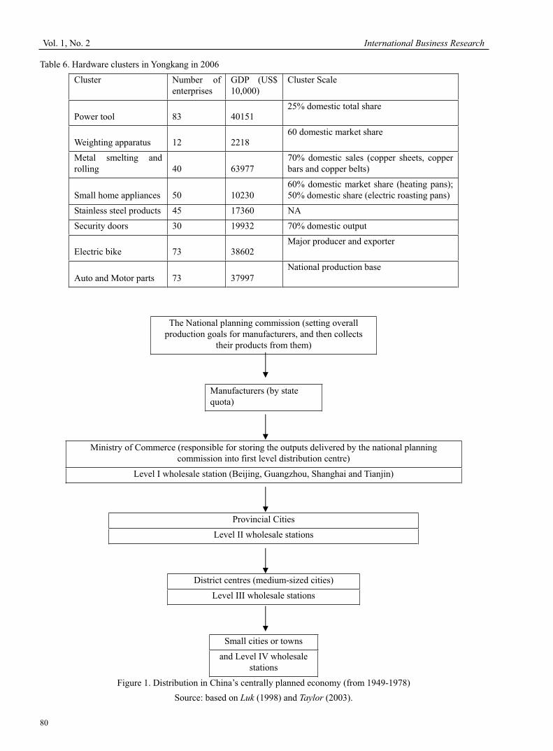
Vol. 1, No. 2 International Business Research
80
Table 6. Hardware clusters in Yongkang in 2006
Cluster Number of
enterprises
GDP (US$
10,000)
Cluster Scale
Power tool 83 40151 25% domestic total share
Weighting apparatus 12 2218 60 domestic market share
Metal smelting and
rolling 40 63977
70% domestic sales (copper sheets, copper
bars and copper belts)
Small home appliances 50 10230
60% domestic market share (heating pans);
50% domestic share (electric roasting pans)
Stainless steel products 45 17360 NA
Security doors 30 19932 70% domestic output
Electric bike 73 38602 Major producer and exporter
Auto and Motor parts 73 37997
National production base
The National planning commission (setting overall
production goals for manufacturers, and then collects
their products from them)
Manufacturers (by state
quota)
Ministry of Commerce (responsible for storing the outputs delivered by the national planning
commission into first level distribution centre)
Level I wholesale station (Beijing, Guangzhou, Shanghai and Tianjin)
Provincial Cities
Level II wholesale stations
District centres (medium-sized cities)
Level III wholesale stations
Small cities or towns
and Level IV wholesale
stations
Figure 1. Distribution in China’s centrally planned economy (from 1949-1978)
Source: based on Luk (1998) and Taylor (2003).

International Business Research April, 2008
81
Figure 2. The types of trading cities
Source: Authors’ design
Trading city market is associated with a
cluster or clusters
Multi-cluster trading city
(market services multiple
clusters
Hub and Spoke
Trading City:
(market is
service local
and non-local
clusters
Real-estate
trading city:
(market contribute
to local clusters)
Embedded trading city
(market is embedded within
an individual cluster)
Real-estate
trading city
(market is
established to
faster a local
cluster )
Cluster-induced
(market is
established to
service the
existing clusters

Vol. 1, No. 2 International Business Research
82
The Financial Process Reengineering Based on the Value Chain
Yinzhuang Zi & Yongping Liu
College of Economic and Trade, Shihezi University
Shihezi 832003, China
Tel: 86-130-3133-5750 E-mail: [email protected]
Abstract
The theory of the value chain management emphasizes to optimize and reorganize the internal resources of the
enterprise, so that the enterprise can establish its long-term and stable competitive advantage. In order to gain a Larger
share in the increasingly fierce and competitive market, most enterprises have adopted the value chain theory for
reengineering business processes, so the financial Process Reengineering based on the value chain was studied.
Key words: value chain, value chain management, financial process
With the arrival of world economic integration, the competition among enterprises is increasingly fierce. Facing a new
competitive environment, and in order to establish a long-term competitive advantage not easy to be imitated, the
enterprises begin to re-examine the core elements, such as their operating mechanism, business processes and
organizational structure, and so on, and apply the advanced management thinking -“Value Chain Management” to
reorganize the business process. As an important component of the business process, the introduction of the value
chain management will have a profound impact on the financial management process of the enterprise.
1. The connotation of the value chain and its evolution
In 1985, an American scholar named Michael Porter, proposed the concept of the value chain first in his book
"Competitive Advantage". He described the value chain as internal processes or operations of an enterprise for the
"design, production, marketing, delivery and the maintenance of its product", he emphasized on the business valuable
activities and possible links among enterprises, suppliers and customers from the perspective of a single enterprise, so
as to train and gain its competitive advantage.
After Michael Porter, an English man named Peter Hines defined the value chain as "transportation lines of the value of
integrated materials ", and he converted the raw materials and customers into his value chain, and stressed the
cross-functional of the basic activities, and classified the information technology as complementary activities, and
established the position of information technology in the value chain. Then, the Jefferey F. Rayport and John J. Sviokla
from America proposed the "virtual value chain", and believed that any enterprise organization is in competition in two
different worlds: one is visible and tangible physical World to the manager, and the other is the virtual world made of
messages. The emergence of the virtual world led e-commerce ——a new place to create value. These enterprises in the
two worlds implemented value creation activities through different value chains.
2. The features of value chain management
Value chain management is the management for the value chain, and it is a management methodology which combines
a series of activities in the value chain organically, and through the use of modern management thinking, methods,
information technology, network technology, and combines the characteristics of the different value chains at the same
time to design, control economic activities, and plan, coordinate, organize and control the logistics, capital flow, and
information flow. In fact, it is for creating or maintaining the competitive advantage of enterprises to achieve the
ultimate goal of business——enterprise value maximization.
(1) Reengineering Business Process is the basis of the value chain management. Value chain management have changed
the traditional management theory, it not only stresses the decomposition of the value activities to achieve the
competitive advantages of a single link, but also stresses the integration of all aspects to rely on the overall synergies; it
considers not only the optimization of resources within the systems of enterprises, but also the sharing of all relevant
resources without the systems. To achieve the objective of value chain management, we must reengineer the business
process, and structure management platform for the value chain management.
(2) Compressing the worthless value-added parts of the value chain to realize value-added value of the entire value
chain, is the main task of value chain management. From the supplier to the enterprise and to customers, not every link
will achieve the aim of value-added value. And we divide it into value-added parts and non-value added parts.

International Business Research April, 2008
83
Procurement, production and sales belong to the value-added parts, while inventory, backlog of goods are
non-value-added. The main task of value chain management is how to eliminate this non-value-added parts and reduce
inventory to a minimum, so that the commodities can be delivered to customers in the shortest time to realize value.
As a virtual Combination, the value chain makes the compression of non-value-added parts possible. In the value chain,
the relationship between suppliers and the companies have undergone a qualitative change, and the relation between
suppliers and business is no longer competing interests, but Collaborating to create value. This allows the vendor supply
materials on time, low-priced and high-quality, so that we can reduce business inventory, and reduce time and space
used by non-value-added parts.
The value chain establishes a mutually trust commonwealth between enterprises and customers, which can increase
their common values. The focus of the value chain shifts from the traditional "enterprise production" to "customer
demand-oriented". Enterprises are no longer selling products by production, but according to customer’s needs to
convert products fast, conveniently and timely to customers, and this greatly reduces the time and volume of the
backlog of product, and compresses the occupied resources of the non-value-added parts.
(3) The value chain is the information chain. Value Chain Management uses information technology to secure the
timeliness and visibility of the access for information. With the core of a leading enterprise, it fully acquires the needs
of users, and coordinates with providers in the operation, so as to achieve information sharing and integration.
(4) The value chain is a virtual chain. Among the market, production processes and distribution links, the value chain
establishes a dynamic business enterprises Union (or virtual companies) which relates to the business, and the essence
of it is the expansion of virtual supply chain. It not only makes each enterprise maintain their own individual advantage,
but also enjoy other resources in the Union.
3. Principles based on reorganization of financial processes of value chain
(1) The business processes, accounting operations and optimizing the value chain which are enterprise-oriented.
Operating is the basic unit for a business process, and is also the foundation of consumption of resources and formation
of value. The main elements of reengineering financial business process are the collection of business data, accounting
the interest rates of products and customers in activity-based costing, evaluating the performances of the suppliers and
the processes, and strengthening the management of the processes through the analyses for causing resources and
operating, so as to realize the optimization for the value chain and enhance their competitive advantage eventually.
(2) Reengineering by combination of economic business processes of the enterprise. Economic business is the source of
financial information systems, and reengineering for economic business processes will inevitably change the path for
transmitting the original business data, so reengineering the financial business processes must match with it, and
achieve the integration of finance and operation. On the other hand, one of the aims of reengineering financial business
processes is to improve the economic business processes continuously, optimize the process structures, and increase
efficiency. Only relying on the cooperation and efforts of the financial personnel and operational staffs, we can control
the procedures of the economic business processes.
(3) Processing information is put into the actual work for the information. In many enterprises, finance is regarded as a
professional, highly confidential work, and operations departments must put all business data together to the financial
sector and these business data must be processed in the financial sector. With the application of IT and the improvement
of the quality of the staff, parts of the conventional work for information processing can be given to the staff from
operating layer to complete.
(4) The principle is that the overall is optimal. Reengineering the financial business process is not tinkering with the
original processes, not optimizing a single link or operation, but stress that the overall finance must be optimal. It
requires that we must consider the overall situation, screen the value-added or non-value-added operations of the
financial process, eliminate selfishness, and straighten out the whole process.
(5) The cost-effective principle. Weighing the cost-effectiveness is an economic factor of the process reorganization to
consider. For example, the division of operating is not the finer, the better; an operation not only contains a mandate; the
distribution from resources - operation - products or services is not the more accurate, the better, but take into account
the actual needs of management and the interest it brought about is greater than the cost, or not.
4. The implementation of the reorganization of the financial process based on the value chain
The course of restructuring financial process must cause many changes of the enterprise. In addition to the business
processes, other organizational structures which are related to the processes and the corporate culture, must be updated
accordingly, but this article only talks about the reorganization of the financial business processes. Following, we
reconstruct the procedure of collection, processing, output of the financial business information using the value chain
theory.
4.1Financial data collection systems approach

Vol. 1, No. 2 International Business Research
84
In traditional financial business processes finance officers acquire data in accordance with the accounting principles
confirmed by manual screening, and record, transmit the data with paper documents, but this tend to cause
inconsistency between the date of recordation in finance and the date of doing the economic business. In the other hand,
traditional financial information processing system is isolated, not to be integrated with other management subsystems,
so the recordation of the data is duplicated in relevant departments, and the data of every management subsystem can’ t
be shared directly by the financial processes. The traditional process of financial data acquisition is shown in Figure 4.1:
(see figure4.1)
For the defects of current financial information processing, according to the thinking of the value chain, we reorganize
the business process, and make use of information technology to collect information in accordance with the objectives
and requirements of the system, and this way to collect information is called systematic collection. The main principle
of this method is to set up LAN for an enterprise, to integrate financial information processing with other management
systems by applying software and network technology. Web servers can be used for the various departments within the
enterprise to provide and gather information, that is when the incident occurs, operations departments should input
original data by a certain code, and store it in a shared database of the LAN, so that the finance department can directly
fetch the data from the database for processing when the data is needed. After using network technology to collect
financial data, not only greatly have reduced the labor strength of the financial, but also have made the collection of the
financial data greatly be improved in the scope, volume and efficiency, and this assures the depth and intensity of the
financial monitoring, so the financial sector can monitor operations at all times, and be able to monitor a variety of
original business documents, and ensure that the accounts are in line. As gathering the external information, because the
enterprise LAN can be conveniently connected to the Internet, we can make full use of e-mail and file transferring
functions to collect information related to corporate decision-making from the external of the enterprise extensively,
highly efficiently and by low-cost, so as to play the roles of finance in the management and policy-making. The data
acquisition of financial process in the value chain perspective is shown as Figure 4.2: (see figure4.2)
4.2 Event-driven financial approach
Traditional financial information processing is function-driven, namely, the provisions of the various functions in
methods of processing and outputting data. Function-driven financial information processing has a big flaw in
information processing, that is, it only reflects the results of economic activities, and the entire process of each
economic activity, implementation and completion can’t be reflected; in the other hand, it only adopts a single
disclosure of the information about value, and can only meet the users with the information which is needed commonly.
However, with the change of economic environment, the primary and the secondary may be transformed into each other;
so, the main message and secondary information are often difficult to divide, particularly in the decision-making, the
special information stresses a single point of information disclosure model more than the general information, and all
financial information is regularly deposited in a few fixed financial statements, but only provide the original
information. In view of the above problems, event-driven approach can be a better financial settlement. The principle of
the event-driven processing of financial information is shown in Figure4.3: (see figure4.3)
The interactive is the most important feature of the new process, and it makes the customization of information for users
realized. On one hand, modeling tools including the processing model library and the report generation can meet a
variety of needs for users; on the other hand, the users may feed back weaknesses of the processing model to the
financial sector by the report generator at any time, and require a new type, when no suitable model for the process,.
The secondly more important is its integration. Enterprises integrate every information system through the network, and
this makes the original data collection decentralized, but makes data processing and storage centralized, so as to achieve
the synergy between finance and operation. Therefore, the financial sector extends to every business department of the
enterprise, and the financial officers’ horizons will not be limited only on financial issues, but extended to operational
issues, and the real-time information can be used to control economic operations, such as procurement, sales, so the
goals of controlling the finance process are attained really. (see figure 4.3)
4.3 Financial information output——real-time report through network
The information processing and output in event-driven processing of financial information is completed in the blink of
an eye, that is, processing and output are combined into a process, so when we design the event-driven processing
model and the report generator, we must be associated to consider the characteristics of the report of the real-time
network:
(1) Timeliness. At any point of time, user of information on the network can access enterprise latest financial report, and
do not have to wait until the end of a financial period. At the same time, the network wait to produce a financial report
for users at any time.
(2) Comprehensiveness. Information systems own massive storage space and real-time reporting of the network can
produce a large of information, systems can provide other information in addition to financial information.

International Business Research April, 2008
85
(3) Interactivity. Because it is easy to generate contradictions between comprehensiveness and correlation, useful
information that is submerged in the massive data, users are unable or difficult to find it, real-time reporting system
processing model should be combined with the design of some kind of intelligence procedures, interactive way.
(4) Security. Information is valuable, but users do not gain all information access to information. Once realizing the
sharing of information resource, and real-time reporting system will expose to risk. The main risk come from the
computer fraud and hack from the outside. Network Real-time reporting system should have adequate security
mechanism, we should reinforce management at these aspects of software and hardware.
Reference
Michael Porter. (1997). Competitive Advantage.The HuaXia Press, 1997
Papinniemi J. (1997). “Creating a Model of Process Innovation for Reengineering of Business and Manufacturing ”.
International Journal of Production Economics, (January, 1997)
Davenport T H. (1999). “The New Industrial Engineering: Information Technology and Business Process
Redesign”.Sloan Manmgement Review, (June 1999)
Jun Wang. & Xin Cui. (2007).“A Study of the Value Chain Accounting Content based on the Value Chain
Management”.Value Engineering, (September,2007)
Figure 4.1 Financial data collection in the traditional financial business process
Collecting
Sales Data
Collecting
Financial Data
Economic
BusinessOriginal
Receipts
Collecting
Procurement Data
Collecting
Production Data
Collecting
Warehousing Data
Collecting
Personnel Data
Collecting
Other Data
Procurement
Management System
Production
Management System
Sales
Management System
Treasury
Management System
Personnel
Management System
Other
Management System
Financial
Management System

Vol. 1, No. 2 International Business Research
86
Figure 4.2 data collection based on the financial value chain processes
Figure 4.3 the principle of the event-driven processing of financial information
Business
Events
Database
Business
Departments
Dealing
According to
Business
Rules
Business
Event data
Economic
Business
Filtering data
Filtering data
Filtering data
Filtering data
Filtering data
Filtering data
Filtering data Other
Management System
Production Management System
Procurement Management System
Sales Management System
Treasury Management System
Personnel Management System
Financial Management System
Dealing
According
to
Business
Rules
Model toolsInformation
Users
Business
EventBusiness
Events
Database
Business
Event data
Issued directives
Access Information

International Business Research April, 2008
87
Modeling the Intraday Return Volatility Process
in the Australian Equity Market: An Examination of
the Role of Information Arrival in S&P/ASX 50 Stocks
Andrew C. Worthington (Corresponding author)
Department of Accounting, Finance and Economics, Griffith University
171 Kessels Road, Nathan QLD 4111, Australia
Tel: 61-7-3735-4273 E-mail: [email protected]
Helen Higgs
Department of Accounting, Finance and Economics, Griffith University
University Drive, Meadowbrook QLD 4131, Australia
Tel: 61-7-3735-7732 E-mail: [email protected]
Abstract
This paper examines the intraday return volatility process in Australian company stocks. The data set employed consists
of five-minute returns, trading volumes and bid-ask spreads over the period 31 December 2002 to 4 March 2003 for the
fifty national and multinational stocks comprising the S&P/ASX 50 index. The GARCH and asymmetric GARCH
namely Threshold ARCH (TARCH) processes are used to model the time-varying variance in the intraday return series
and the inclusion of news arrival as proxied by the contemporaneous and lagged volume of trade and bid-ask spread
together with day-of-week effects are used as exogenous explanatory variables. The results indicate strong persistence
in volatility for the fifty stocks even with the day-of-week effects and contemporaneous and lagged volume of trade and
bid-ask spread included as explanatory variables in the models. Overall, while there is much variation among the stocks
included in terms of the role of the irregular arrival of new information in generating GARCH effects and the degree of
persistence, all of the volatility processes are mean reverting.
Keywords: Intraday return volatility, Volume of trade, Bid-ask spreads
1. Introduction
It goes without saying that knowledge of stock return volatility is important. In any number of asset pricing and
portfolio management problems this knowledge, as encapsulated in volatility models, is used to make predictions that
help market actors make better financial decisions. And already a number of stylized facts are known about stock return
volatility and the best models to capture and reflect these stylized facts. In the first instance, these include volatility
clustering, persistence and mean reversion whereby volatility shocks today will influence the expectation of volatility in
the future, though with some more normal level to where it will eventually return. In the second instance, the
autoregressive conditional heteroskedasticity (ARCH) model and its various extensions has been shown to provide a
good fit for many financial return series where an autoregressive structure is imposed on the conditional variance. These
allow the volatility shocks to persist over time and to revert to that more normal level. It also captures both the
propensity of returns to cluster in time and helps explain the well-documented non-normality and non-stability of stock
return distributions.
The empirical literature underlying this knowledge of stock return volatility is voluminous. Unfortunately, much of this
knowledge has been garnered from just a few contexts. First, most of what we know about financial return volatility in
general has been based on studies employing interday returns. Given that financial markets display high speeds of
adjustment, studies based on daily (or longer) observations may fail to capture critical information contained in intraday
price movements. Moreover, of that small number of studies that are concerned with intraday data, almost all addresses
foreign exchange or futures market volatility [see, for instance, Baillie & Bollerslev (1990), Locke & Sayers (1993),
Andersen & Bollerslev (1997), Tse (1999)] and much less in stock markets. Second, within the small intraday stock
return volatility literature, most studies have concentrated on indexes or index futures contracts with less attention

Vol. 1, No. 2 International Business Research
88
directed to the intraday return volatility of individual securities [see, for instance, Baillie & DeGennaro (1990), Kim &
Kon (1994), Kyriacou & Sarno (1999) , Walsh & Quek (1999)]. Because it is likely that volatility effects vary across
individual securities in much the same manner as they do across markets, the analysis of stock return volatility at the
company level would throw light on the characteristics of volatility within a single market.
Third, the bulk of volatility modeling has been concerned with univariate characteristics such that the volatility of a
return series is related only to information in its own history. As Bollerslev et al. (1992: 32) notes: “the widespread
existence of ARCH effects and the persistence of stock return volatility have led researchers to search for it origin(s).
[Since] the GARCH (p,q) model can be viewed as a reduced form of a more complicated dynamic structure for the
time-varying conditional second-order moments…interpretations and explanatory variables for the observed ARCH
effects have been proposed both on the micro and macro level…”. However, while the macro level has received a good
deal of attention, including the influence of other financial assets and exogenous deterministic events such as
macroeconomic and company announcements on the volatility process, much less has been directed to micro level
influences [for exceptions, see Lamoureux & Lastrapes (1990), Kim & Kon (1994) , Rahman et al. (2002)]. Finally,
only a few ARCH-type studies of stock return volatility have been undertaken in Australia, and as far as the authors are
aware, none using intraday data at the individual security level. Following Bollerslev’s et al. (1992: 31) suggestion it
would “…be interesting to use different data sets to further assess the degree of persistence on stock return volatility
[since] with very few exceptions, most current studies use data from the US stock market”.
The overall hypothesis is to assess return and volatility and relationships in fifty Australian stocks by incorporating new
arrival of information namely, the inclusion of news arrival as proxied by the contemporaneous and lagged volume of
trade, bid-ask spread together with day-of-week and information asymmetry effects are used as exogenous explanatory
variables. These allow the estimation of volatility clustering over time, and to determine whether shocks persist over
time, and/or revert to a more normal level. The outcomes of these analyses will provide useful models and forecasts for
investors, funds managers and financial institutions.
Accordingly, the purpose of this paper is to investigate the intraday return volatility process in Australian stocks. The
remainder of the paper is divided into four sections. The second section explains the data employed in the analysis and
presents some brief summary statistics. The third section discusses the methodology employed. The results are dealt
with in the fourth section. The paper ends with some brief concluding remarks.
2. Data and summary statistics
The data employed in the study consists of last price, trading volumes and bid-ask spreads for the five-minute intervals
from 31 December 2002 to 4 March 2003 for the national and multinational stocks included in the S&P/ASX 50 index.
The sample period is used because it is the longest period available for each of the 50 Australian stocks. The S&P/ASX
50 index comprises the fifty largest stocks by market capitalization in Australia and currently accounts for some
seventy-five percent of the market capitalization of domestic equities listed on the Australian Stock Exchange (ASX).
The criteria for inclusion in the index place an emphasis on liquidity and investability and together the high frequency
of information arrivals and volume of trading in these securities are likely to reduce measurement error problems. All
data is obtained electronically from Bloomberg. Each of the trading days in the analysis is portioned into five-minute
intervals beginning with the opening of the market at 9:00 a.m. Australian Eastern Standard Time (AEST). The natural
log of the relative price is computed for the five-minute intervals to produce a time series of continuously compounded
five-minute returns, such that rt = log(pt/pt-1) × 100, where pt and pt-1 represent the stock price at time t and t-1,
respectively. By way of comparison, Chan et al. (1995) and Rahman et al. (2002) also specified five-minute returns
when modeling intraday return volatility in US listed stocks.
Table 1 presents the summary of descriptive statistics of the five-minute returns for the fifty stocks. Sample means,
medians, maximums, minimums, standard deviations, skewness, kurtosis and the Jacque-Bera statistic and first-order
autocorrelation coefficient and their p-values are reported. It should first be noted that over the relatively short sample
period the Australian equity market generally declined, with forty-four of the stocks (eight-eight percent) producing
negative mean returns. The lowest mean returns were for ALL and AMP with -0.0300 and -0.0161 percent, respectively.
However, six stocks had positive average returns over this same period ranging from 0.0005 (WOW) to 0.0029 (CCL).
The largest five-minute returns were for CCL (0.0209) and MBL (0.0017). The standard deviations of returns range
from 0.144 (MGR) to 1.053 (ALL). On this basis, of the fifty stocks AGL, CBA, MGR, NAB, SGB and SGP are the
least volatile, with ALL, SRP and MIM being the most volatile.
Mostly, the distributional properties of all fifty return series appear non-normal. Twenty-seven of the return series are
negatively skewed, ranging from -0.1297 (STO) to -35.1062 (ALL), indicating the greater probability of large deceases
in returns than rises. The remaining return series are positively skewed, also suggestive of volatility clustering in
intraday stock returns. The asymptotic sampling distribution of skewness is normal with mean 0 and standard deviation
of, where T is the sample size. Since the sample size for all the return series is 3,215 then the standard error under the
null hypothesis of normality is 0.0432: all estimates of skewness are significant at the .10 level or lower. The kurtosis,

International Business Research April, 2008
89
or degree of excess, in all stock returns is also large, ranging from 5.6283 for MIM to1647.6950 for ALL, thereby
indicating leptokurtic distributions. Given the sampling distribution of kurtosis is normal with mean 0 and standard
deviation of, then all estimates are once again statistically significant at any conventional level.
The calculated Jarque-Bera statistics and corresponding p-values in Table 1 are used to test the null hypotheses that the five-minute distribution of stock returns is normally distributed. All p-values are smaller than the .01 level of significance suggesting the null hypothesis can be rejected. These stock returns are then not well approximated by the normal distribution. To test for the presence of autocorrelation in the five-minute interval series, the first order autocorrelation coefficients are also calculated and presented in Table 1 along with their corresponding p-values. The
asymptotic distribution of 1ρ̂ is normally distributed with a mean of 0 and a standard error of 0176.031261 = . On
this basis, first-order autocorrelation is evident in the intraday return series for the Australian stocks selected at the .05 level or lower, with the exception of CSL, QBE, RMD and WPL.
3. Model specificationN
The distributional properties of Australian company intraday stock returns indicates that generalized autoregressive
conditional heteroskedastistic (GARCH) models can be used to examine the dynamics of the return volatility process.
Autoregressive conditional heteroscedasticity (ARCH) models (as introduced by Engle (1982)) and generalised ARCH
(GARCH) models (as presented by Bollerslev (1986)) that take into account the time-varying variances of financial
time series data have already been widely employed. Suitable surveys of ARCH modeling in general and/or its
widespread use in finance applications may be found in Bera and Higgins (1993) and Bollerslev et al. (1992; 1994).
Pagan (1996) also contains discussion of developments in this ever-expanding literature.
The first methodological requirement is to remove the predictable component of returns so as to produce a return
innovation, et, with a conditional mean of zero before a GARCH equation is specified for the variance. One common
method to produce an uncorrelated process in the five-minute returns is to assume that the level of returns follow an
AR(1) process. The following conditional expected returns equation accommodates each stock’s own returns and its
returns lagged one period:
ttt err ++= −110 αα (1)
where rt is the return for each stock in the current period and rt-1 an n x 1 vector of the returns lagged one period, 0
represents the long-term drift coefficient and 1 is the degree of mean spillover effect across time, or put differently, whether the lagged can be used to predict the current return and et, the random error or innovation at time t, is approximately distributed ),0(~ tt hNe .
The second methodological requirement is to model the variance of the return innovation itself. A GARCH process of orders p and q, denoted as GARCH(p,q), for the conditional variance (volatility) of et at time t can then be represented as:
=−
=− ++=
q
i
iti
p
i
itit heh11
2
0 γββ (2)
where ht is the conditional variance volatility of et at time t, β0 is a constant, βi and γi are coefficients that are associated
with the past values of innovation and volatility spillovers to the current volatility, and thereby represent news about the
degree of innovation from previous periods (ARCH terms) and previous period’s forecast volatility spillover effects
(GARCH terms), and all other variables are as previously defined.
One important and well-founded characteristic of stock returns is the tendency for volatility clustering to be found, such
that large changes in returns are often followed by other changes, and small changes in returns are often followed by yet
more small changes. The implication of such volatility clustering is that volatility shocks today will influence the
expectation of volatility many periods in the future. The aggregation of βi and γi coefficients measures this degree of
continuity or persistence in volatility. If the degree of persistence is close to one, this implies that the current volatility
of intraday returns is affected by past volatility that tends to persist over time: the actual persistence of volatility must
depend on the persistence of the exogenous variables. Further, volatility clustering also implies that volatility will come
and go. Accordingly, a period of high volatility in stock returns will eventually give way to a more normal (lower) level
of volatility and a lower period of volatility will be replaced with a more normal (higher) level of volatility. This process
of reversion to a normal or mean level of volatility implies that even if volatility persistence exists, so long as the sum
of the βi and γi coefficients is significantly less than one the volatility process, while having a long memory, will still be
mean reverting or stationary.
A concern with the volatility generation process as defined is that current volatility is only related to the past values of
innovation and volatility spillovers from previous periods. It is likely that variables other than these may contain
information relevant for the volatility of stock returns and a possibility is that the incidence of time varying conditional
heteroskedasticity could be due instead to an increase in the variability in returns following the arrival of new and

Vol. 1, No. 2 International Business Research
90
irregular information. This is important because the GARCH effects often observed in stocks returns is likely the
outcome of the stochastic properties of these factors. Lamoureux and Lastrapes (1990) and Rahman et al. (2002), for
example, argue that an appealing explanation for the presence of GARCH effects is that the rate of information arrival is
the stochastic mixing variable that generates stock returns. For daily, weekly and monthly data, variables such as
macroeconomic and company announcements may be major influences. However, for high-frequency intraday data the
variables likely to be of most influence relate to trade information.
One means of proxying the arrival of this trade information is to introduce the volume of trade into the conditional
variance equation. Lamoureux and Lastrapes (1990), for example, showed that with the introduction of the
contemporaneous and lagged volume of trade (indicating a greater amount of information) the GARCH effect in US
stock returns became insignificant for the majority of securities, with the estimated coefficients on trade volume being
significant, though small. Alternatively, Najand and Yung (1991), Foster (1995) Rahman et al. (2002) found that the
GARCH effects remained strongly significant with the inclusion of the current volume of trade in the conditional
variance equation. Another way of including this information arrival follows past evidence of a high correlation
between intraday return volatility and intraday variation of bid-ask spreads (Copeland & Galai, 1983; Grossman &
Miller, 1988; McInish & wood, 1992; Walsh & Quek, 1999 and Wang and Yau 2000). For instance, Rahman et al. (2002)
introduced the bid-ask spread as a measure of information that flows into the market with the argument that bid-ask
spreads narrow when information flow increases and widen when information flow decreases. In this study,
day-of-week effects have also been introduced in the conditional variance equation to take account of the intraday
patterns in the high frequency data. It is widely known that the stock prices tend to be higher at the beginning of the
week than any other trading days.
The final methodological requirement is then to incorporate the arrival of exogenous information in the volatility return
generating process in Equation (2). Since the incidence of the time varying conditional heteroskedasticity could be due
to an increase in the contemporaneous and/or lagged volume of trading and/or bid-ask spread and day-of-week effects
following the simultaneous arrival of new information, the conditional variance equation is reformulated as:
=−−−− +++++++=
5
2
14312111
2
110
i
iittttttt dssvvheh ηδδδδγββ (3)
where vt and vt-1 and st and st-1 represent the volume of trade (v), bid-ask-spreads (s) in period t and t-1, di are dummy
variables for each of the day-of-week effect having values of 1 for d2 (Tuesday) and 0 otherwise,… having values of 1
for the d5 (Friday) and 0 otherwise. To avoid the multicollinearity trap, Monday (d1) is chosen to be the reference
category for the interday effects, ηi are coefficients that are associated with the dummy variables day-of-week effects.
All other variables are as previously defined.
The standard GARCH model assumes that the impact of news has a symmetric effect on volatility. Glosten et al. (1993)
extends the symmetric into asymmetric GARCH also known as Threshold ARCH (TARCH) model to capture the
asymmetric response of the conditional response of the volatility of news arrival. Antoniou et al. (1998) and Rahman et
al. (2002) use variations of the GARCH models which incorporate for the asymptotic responses of vitality to news
arrival on stock markets. The asymmetric GARCH model includes along with the standard variables, the squared values
of et-1 when et-1 is negative.
=−−−−− ++++++++=
5
2
143121
2
1111
2
110
i
iittttttttt dssvveaheh ηδδδδτγββ (4)
where otherwise.0,,0if,1 1 =<= − ttt aea
This allows the squared residuals to have a different impact on the conditional volatility when the lagged residuals are
negative than when the lagged residuals are positive. That is, it is assumed that positive news (where return changes in
an upward direction and residuals are positive) alters return volatility differently to negative news (where return changes
are in a downward direction and the residuals are negative).
4. Empirical results
The estimated coefficients and standard errors for the conditional mean return equations are presented in Table 2.
Different GARCH(p,q) models were initially fitted to the data (results not shown) and compared on the basis of the
Akaike and Schwarz Information Criteria (AIC and SIC) from which a GARCH(1,1) model was deemed most
appropriate for modelling the five-minute return process for all fifty stocks. All the same, Rahman et al. (2002: 165)
confined “…estimation to the GARCH(1,1) specification since it has been shown to be a parsimonious representation of
conditional variance that adequately fit many high-frequency time series”. For simplicity, this paper only focuses on the
GARCH(1,1) and asymmetric GARCH(1,1) models with no higher orders to be estimated. Of the fifty stocks,
forty-eight (ninety-six percent) exhibit a significant own mean spillover from their own lagged return with the exception

International Business Research April, 2008
91
of RMD and WSF at the 0.10 level of significance and lower. In all significant cases, the mean spillovers are negative.
For example, and during this particular sample period, a 1.00 cent increase in MIM’s own return will Granger cause a
decrease of 0.36 cents in its return over the next five-minutes. Likewise, a 1.00 cent increase in returns for CSL will
Granger cause a 0.05 cent decrease over the next five-minutes.
Also included in Table 2 are details for AIC and SIC comparing the performance of asymmetric GARCH(1,1) models
including information arrival and day-of-week effects as exogenous variables in the variance equation with those
obtained from a simple GARCH(1,1) process. These model selection criteria are used to test the proposition that the
occurrence of time-dependent conditional heteroskedasticity could be due, at least in part, to an increased volume of
trading and/or variability of prices following the arrival of new information in the market. In the current analysis, the
arrival of new information is proxied by including trading volume and bid-ask spread, asymmetric and day-of-week
effects in the variance equation.
The values for AIC and SIC in Table 2 indicate that in nine of the stocks the intraday return volatility process could be
appropriately modelled employing a simple GARCH process, whereas in the remaining forty-one stocks the rate of
information arrival together with the asymmetry effect have some significant role in generating intraday returns. For
example, for JHX the lower values for AIC and SIC (-0.0889 and -0.0795) compared to AIC( ) and SIC( ) (-0.0670 and
-0.0405) indicate that a GARCH model with no allowance for exogenous variables and asymmetry is a more
comprehensive and parsimonious representation of the return generation process, whereas for NCP the lower values for
AIC( ) and SIC( ) (-0.1778 and -0.1513) as compared to AIC and SIC (0.0819 and 0.0913) indicate the reverse. By
way of comparison, Lamoureux and Lastrapes (1990) found that that GARCH effects found in their US actively traded
securities were due to time dependencies in the process generating information flows, whereas Rahman et al. (2002)
concluded that even after proxying information arrival, GARCH effects prevailed in NASDAQ stock returns. The
results in Table 2 indicate that, at least for actively traded Australian stocks, there is much variation in the role of
information arrival as a means of generating the commonly found GARCH effects with it having a critical role for some
stocks, but not for others.
Initially a TARCH(1,1) model without news information is estimated for the fifty stocks. The ARCH effects are all
significant as are the GARCH effects with the exception of ALL. The basic model is then augmented with the inclusion
of contemporaneous bid-ask spread followed by the contemporaneous volume of trade. In the interests of conciseness,
the results for these three models are not reported, but can be supplied on request. With the inclusion of the
contemporaneous bid-ask spread in the TARCH(1,1) model, the results show that the GARCH effects remain strongly
significant with the exception of GPT. Similarly, the ARCH effects also remain strongly significant with the exception
of ALL. There is a significant negative relationship between the contemporaneous bid-ask spread and return volatility
for twenty-six of the twenty-eight coefficients. For lagged bid-ask spread, eighteen of the twenty-two positive
relationships are significant. These results indicate that the contemporaneous bid-ask spread is negatively related to
return volatility but positively related to lagged bid-ask spread. Rahman et al. (2002) use a GARCH(1,1) model and find
that all but eight of the thirty NASDAQ stocks exhibit a positive relationship between lagged bid-ask spread and return
volatility. The significance of the positive results indicates that “…information arrival would be expected to induce an
increase in volatility and this would in turn have the effect of widening the bid-ask spread” (Rahman et al. 2002). The
difference appears to lie in that this study includes both contemporaneous and lagged bid-ask spread, whereas Rahman’s
et al. (2002) results are referenced only to lagged values.
Rahman et al. (2002) also point out that the standard GARCH model assumes that the impact of news arrival on
volatility is symmetrical; with Antoniou et al. (1998) suggesting the model is misspecified if news information has an
asymmetric effect on volatility. The TARCH model with the inclusion of bid-ask spread should then be more reliable for
forecasting stock returns. The introduction of the contemporaneous volume of trade to the TARCH(1,1) model suggests
that contemporaneous volume is positive and significantly related to return volatility for all fifty stocks. The ARCH
effects remain significant and the GARCH effects are also significant with the exception of MAY, MGR and NCP. The
contemporaneous volume of trade can then also be considered as an important proxy for news information.
Table 3 presents the estimated coefficients for the conditional variance equations in the TARCH model. The coefficients
of the conditional variance equations are all significant at the 0.01 level or lower for the innovations and volatility
spillovers for the fifty stocks indicating the presence of strong ARCH and GARCH effects. The own-innovation
spillovers in all stocks are significant indicating the presence of strong ARCH effects. These own-innovation spillover
effects range from 0.0143 in RIO to 0.2286 in SRP. In the GARCH set of parameters, all fifty of the estimated
coefficients are also significant. The lagged volatility spillover effects range from 0.3502 for BHP to 0.7801 for AMC.
This implies that the past volatility shocks in AMC have the greatest effect on its future volatility shocks than for any
other stocks included in the analysis during the sample period.
The next coefficient examined is that corresponding to the asymmetric volatility response ( 1) to positive and negative
shocks such that volatility tends rise in response to ‘bad news’ and fall in response to ‘good news’. Of the fifty stocks,

Vol. 1, No. 2 International Business Research
92
thirty-one (sixty-two percent) exhibit a significant asymmetric effect at the 0.10 level of significance and lower. This
follows eighteen stocks with significant asymmetric effects are negative thus observing that downward movements in
the market (falling returns) are followed by higher volatility. And also, the estimated asymmetric coefficients are
significant and positive for thirteen stocks indicating the reverse that positive shocks (increasing returns) are associated
with higher volatility. As hypothesised by Antoniou et al. (1998) and Rahman et al. (2002) amongst others, positive
news causes a different volatility response than negative news, a more comprehensive understanding of Australian
intraday stock return volatility has resulted from the application of the asymmetric GARCH or Threshold ARCH
(TARCH) model as first proposed by Glosten et al. (1993).
According to the TARCH process, the sum of the ARCH, GARCH and a half of the asymmetric coefficient measures
the overall persistence in each market. A value of less than one indicate a mean reverting conditional volatility process
in which shocks are transitory in nature. All fifty stocks display strong own persistence volatility ranging from 0.4092
for GPT to 0.8432 for AMC. Thus, AMC has the highest lead-persistence volatility spillover effect as compared to the
other stocks included in the analysis. The average persistence across the stocks is 0.6472 and this implies a volatility
half-life, defined as the time taken for the volatility to move halfway back towards it unconditional mean following a
deviation from it, of 1.5931 periods or about 8 minutes, where. This impact decays geometrically. This implies that for
many of the stocks included in the analysis volatility shocks will tend to persist over what seems only a relatively short
period of time. By way of comparison, the volatility half-life for the stock with the longest lead-persistence is nearly 20
minutes and that for the shortest is just 4 minutes, while for a comparable international study Rahman et al. (2000)
provided tables suggesting a mean volatility half-life of 13 minutes in a sample of NASDAQ stocks (as calculated by
the authors). Other stocks that have a relatively higher level of persistence in volatility over time (and their half-lives)
include AMC (0.8432 and 20 minutes), TLS (0.8351 and 19 minutes) and CCL (0.7907 and 15 minutes) while those
with a lower level of persistence include GPT (0.4092 and 4 minutes), BHP (0.4132 and 4 minutes), and CSL (0.4861
and 5 minutes). Nonetheless, although the returns volatility in these stocks appears to have a quite long memory, at least
in terms of high frequency data, they are still mean reverting.
Table 4 includes the estimated coefficients, standard errors and p-values for the variables used to proxy the irregular
arrival of new information: namely, contemporaneous and lagged volume of trade and contemporaneous and lagged
bid-ask spread. To start with, there is a significant, and almost always positive, relationship between the return volatility
and the contemporaneous volume of trade for all stocks with the exception of WFA which exhibit a significant negative
relationship. The contemporaneous volume of trade ranges from -0.0007 (WFA) to 0.2841 (CSL). As expected, this
would indicate the increase of new information, as proxied by trade volume, is associated with an increase in return
volatility. This at once lies counter to early work by Lamoureux and Lastrapes (1990) who found that the introduction of
contemporaneous volume into the conditional variance equations made the GARCH effects disappear for the majority
of US securities or Lee et al. (2001) who found that daily trading volume used as proxy for information arrival had no
significant explanatory power for the conditional volatility of Chinese daily returns. They are, however, broadly
comparable to work by Najand and Yung (1991), Foster (1995) and Rahman et al. (2002).
At the same time, thirty-five stocks have a significant relationship between return volatility and lagged volume of trade
where eighteen of these stocks (some fifty-one percent) are negative. This would suggest that following the role of new
information in the current period to increase return volatility; information in the lagged period has the role of reducing
return volatility. This is perhaps an indication of the ability of the equity market to process high-frequency information
whereby adjustments are made to over and under-reaction in the current period on the basis of historical information.
Nevertheless, the magnitude of all contemporaneous and lagged volume coefficients, whether positive or negative, is
relatively small, and their impact on the GARCH effect is minimal.
With the inclusion of contemporaneous bid-ask spread as yet another measure of information flow, the estimated
coefficients for forty-five of the stocks (ninety percent) are significant. All of the significant coefficients indicate a
negative relationship between return volatility and contemporaneous bid-ask spread with the exception of CSL, NCPD
and WFA. For the most part, this would suggest that as bid-ask spreads widen (less new information) return volatility
will decrease, while a narrowing of bid-ask spreads (more new information) is associated with an increase in return
volatility. Forty-four stocks (eighty-eight percent) also show a significant relationship between return volatility and
lagged bid-ask spread of which thirty-eight cases are positive. Interestingly, the coefficients for the contemporaneous
and lagged bid-ask spreads are larger in magnitude than the coefficients for either the contemporaneous or lagged
volume of trade. These results would lead us to suspect that bid-ask spread may be a more appropriate proxy for
information arrival, at least for a select number of stocks. However, information arrival as proxied by the volume of
trade is spread across almost all of the stocks, indicating the information proxied by the volume of trade is more general
than specific than that provided by bid-ask spread. Moreover, the fact that most of the estimated coefficients are
significant indicates that the simultaneity problem between prices, volume and bid-ask spread though present, is not too
serious.
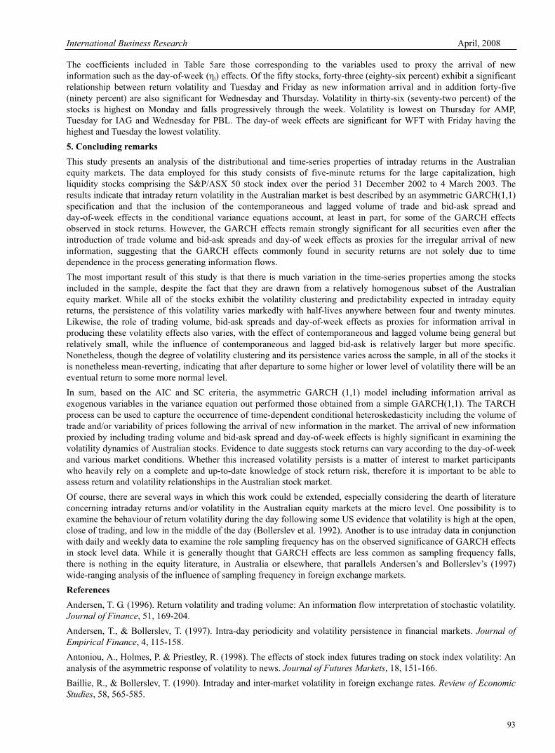
International Business Research April, 2008
93
The coefficients included in Table 5are those corresponding to the variables used to proxy the arrival of new
information such as the day-of-week ( i) effects. Of the fifty stocks, forty-three (eighty-six percent) exhibit a significant
relationship between return volatility and Tuesday and Friday as new information arrival and in addition forty-five
(ninety percent) are also significant for Wednesday and Thursday. Volatility in thirty-six (seventy-two percent) of the
stocks is highest on Monday and falls progressively through the week. Volatility is lowest on Thursday for AMP,
Tuesday for IAG and Wednesday for PBL. The day-of week effects are significant for WFT with Friday having the
highest and Tuesday the lowest volatility.
5. Concluding remarks
This study presents an analysis of the distributional and time-series properties of intraday returns in the Australian
equity markets. The data employed for this study consists of five-minute returns for the large capitalization, high
liquidity stocks comprising the S&P/ASX 50 stock index over the period 31 December 2002 to 4 March 2003. The
results indicate that intraday return volatility in the Australian market is best described by an asymmetric GARCH(1,1)
specification and that the inclusion of the contemporaneous and lagged volume of trade and bid-ask spread and
day-of-week effects in the conditional variance equations account, at least in part, for some of the GARCH effects
observed in stock returns. However, the GARCH effects remain strongly significant for all securities even after the
introduction of trade volume and bid-ask spreads and day-of week effects as proxies for the irregular arrival of new
information, suggesting that the GARCH effects commonly found in security returns are not solely due to time
dependence in the process generating information flows.
The most important result of this study is that there is much variation in the time-series properties among the stocks
included in the sample, despite the fact that they are drawn from a relatively homogenous subset of the Australian
equity market. While all of the stocks exhibit the volatility clustering and predictability expected in intraday equity
returns, the persistence of this volatility varies markedly with half-lives anywhere between four and twenty minutes.
Likewise, the role of trading volume, bid-ask spreads and day-of-week effects as proxies for information arrival in
producing these volatility effects also varies, with the effect of contemporaneous and lagged volume being general but
relatively small, while the influence of contemporaneous and lagged bid-ask is relatively larger but more specific.
Nonetheless, though the degree of volatility clustering and its persistence varies across the sample, in all of the stocks it
is nonetheless mean-reverting, indicating that after departure to some higher or lower level of volatility there will be an
eventual return to some more normal level.
In sum, based on the AIC and SC criteria, the asymmetric GARCH (1,1) model including information arrival as
exogenous variables in the variance equation out performed those obtained from a simple GARCH(1,1). The TARCH
process can be used to capture the occurrence of time-dependent conditional heteroskedasticity including the volume of
trade and/or variability of prices following the arrival of new information in the market. The arrival of new information
proxied by including trading volume and bid-ask spread and day-of-week effects is highly significant in examining the
volatility dynamics of Australian stocks. Evidence to date suggests stock returns can vary according to the day-of-week
and various market conditions. Whether this increased volatility persists is a matter of interest to market participants
who heavily rely on a complete and up-to-date knowledge of stock return risk, therefore it is important to be able to
assess return and volatility relationships in the Australian stock market.
Of course, there are several ways in which this work could be extended, especially considering the dearth of literature
concerning intraday returns and/or volatility in the Australian equity markets at the micro level. One possibility is to
examine the behaviour of return volatility during the day following some US evidence that volatility is high at the open,
close of trading, and low in the middle of the day (Bollerslev et al. 1992). Another is to use intraday data in conjunction
with daily and weekly data to examine the role sampling frequency has on the observed significance of GARCH effects
in stock level data. While it is generally thought that GARCH effects are less common as sampling frequency falls,
there is nothing in the equity literature, in Australia or elsewhere, that parallels Andersen’s and Bollerslev’s (1997)
wide-ranging analysis of the influence of sampling frequency in foreign exchange markets.
References
Andersen, T. G. (1996). Return volatility and trading volume: An information flow interpretation of stochastic volatility.
Journal of Finance, 51, 169-204.
Andersen, T., & Bollerslev, T. (1997). Intra-day periodicity and volatility persistence in financial markets. Journal of
Empirical Finance, 4, 115-158.
Antoniou, A., Holmes, P. & Priestley, R. (1998). The effects of stock index futures trading on stock index volatility: An
analysis of the asymmetric response of volatility to news. Journal of Futures Markets, 18, 151-166.
Baillie, R., & Bollerslev, T. (1990). Intraday and inter-market volatility in foreign exchange rates. Review of Economic
Studies, 58, 565-585.

Vol. 1, No. 2 International Business Research
94
Baillie, R. & DeGennaro, R. (1990). Stock returns and volatility. Journal of Financial and Quantitative Analysis, 25,
203-214.
Bera, A. K. & Higgins, M. L. (1993). ARCH models: properties, estimation and testing. Journal of Economic Surveys, 7,
305-366.
Bollerslev, T. (1990). Modeling the coherence in short-run nominal exchange rates: a multivariate generalized ARCH
model. Review of Economics and Statistics, 73, 498-505.
Bollerslev, T., Chou, R. Y., & Kroner, K. F. (1992). ARCH modeling in finance: a review of the theory and empirical
evidence. Journal of Econometrics, 52, 5-59.
Chan, K., Christie, W., & Schultz, P. (1995). Market structure and intraday pattern of bid-ask spreads for NASDAQ
securities. Journal of Business, 68, 35-60.
Copeland, T. & Galai, D. (1983). Information effects on bid-ask spread. Journal of Finance, 38, 1457-1469.
Engle, R. F. & Ng, V. K. (1993). Measuring and testing the impact of news on volatility. Journal of Finance, 48,
1749-1778.
Foster, A. (1995). Volume volatility relationships for crude oil futures markets. Journal of Futures Markets, 15,
929-951.
Glosten, L. R., Jaganathan, R., & Runkle, D. (1993). On the relationship between the expected value and the volatility
of the normal excess return on stocks. Journal of Finance, 48, 1779-1801.
Grossman, S., & Miller, M. (1988). Liquidity and market structure. Journal of Finance, 43, 617-633.
Kim, D., & Kon, S. (1994). Alternative models for the conditional heteroskedasticity of stock returns. Journal of
Business, 67, 563-598.
Kyriacou, K., & Sarno, L. (1999). The temporal relationship between derivatives trading and spot market volatility in
the UK: An empirical investigation. Journal of Futures Markets, 19, 245-270.
Lamoureux, C., & Lastrapes, W. (1990). Heteroskedasticity in stock return data: Volume verses GARCH effects.
Journal of Finance, 45, 221-229.
Lee, C. F., Chen, G. M., & Rui, O. M. (2001). Stock returns and volatility on China’s stock markets. Journal of
Financial Research, 24, 523-543.
Locke, P., & Sayers, C. (1993). Intraday futures price volatility: Information effects and variance persistence. Journal of
Applied Econometrics, 8, 15-30.
McInish, T., & Wood, R. (1992). An analysis of intraday patterns in bid-ask spreads for NYSE stocks. Journal of
Finance, 47, 753-764.
Najand, M., & Yung, K. (1991). A GARCH examination of the relationship between volume and price volatility in
futures markets. Journal of Futures Markets, 11, 613-621.
Pagan, A. (1996). The econometrics of financial markets. Journal of Finance, 3, 15-102.
Rahman, S., Lee, C. F., & Ang, K. P. (2002). Intraday return volatility process: Evidence from NASDAQ stocks. Review
of Quantitative Finance and Accounting, 19, 155-180.
Smith, B. F., White, R., Robinson, M., & Nason, R. (1997). Intraday volatility and trading volume after takeover
announcements. Journal of Banking and Finance, 21, 337-368.
Tse, Y. (1999). Price discovery and volatility spillovers in the DJIA and futures markets. Journal of Futures Markets, 19,
911-930.
Walsh, D. M., & Quek, J. (1999). An empirical examination of the SIMEX Nikkei 225 futures contract around the Kobe
earthquake and the Barings bank collapse. Journal of Futures Markets, 19, 1-29.
Wang, G.. & Yau, J. (2000). Trading volume, bid-ask spread, and price volatility in future markets. Journal of Futures
Markets, 20, 943-970.

International Business Research April, 2008
95
On the Values of Corporate Visual Identify
Bo Pang
College of Art and Appareluages, Tianjin Polytechnic University, Tianjin 300000, China
Tel: 86-137-0212-7567 E-mail: [email protected]
Abstract
CIS (Corporate Identity System) is introduced from western countries in early 80s in 20th century. CIS, as the practical
science, has important significance in western modern corporate management. It does exert imaginable effects on the
operation of general corporate marketing.
Keywords: Corporate visual identify, CI system, Added value
1. Enter the non-material times -- the identity system
In the ring of new century, people pack off the 20th century that has ever created the splendid material civilization and
greet the new mystery 21st century that will bring people into an unheard-of non-material society. What is on earth
“non-material society”? The so-called non-material society refers to the digital society, the information society, or the
service-oriented society that has been mentioned frequently. In this society, the proportion of information industry
increases to a great degree. Differing from the original society and the industrial society in which the value of products
includes the value of materials and labors, the economic value and the social value in the non-material society are
assessed by the proportion of advanced knowledge in consumption product and new service, which indicates that the
society has already turned into a kind of “software form” from the former kind of “hardware form”. The theory of
corporate identity system emerged in 50s in 20th century is a real portraiture for this social change. Corporate identity
system, as an important component of information revolution and a signal, is an inevitable trend in the development of
human society and material civilization. By means of prominent, unique, and touching visual signals, corporate identity
system can transfer the spirit of corporation, and help the corporation to communicate with people and society. By this
way, it can help to enhance the cohesion among employees and improve the quality of employees. Corporate identity
system has already become a powerful weapon that helps corporation to improve its fame in fierce market competition
and generate a brand effect. As a result, the corporation can distinguish itself from traditional material industry, making
its corporate culture permeate into the society. By this way, the corporation will occupy the market and win people’s
heart.
Facing the trend of market competition, corporations introduce the corporate identity system (CIS) into their
management. Therefore, from the brand consciousness at the consumption level to the identity consciousness at the
business level, it becomes an important phenomenon in today’s economic development.
Then, what is the corporate virtual asset identity system?
Corporate identity system is the CI system in essence. Corporate is the subject, including enterprises, institutions,
nations, and even individuals. Anything has its identity no matter what it is a nation, an enterprise, or an individual.
Identity indicates other’s evaluation and expression toward certain subject. At the economic times, corporate identity
becomes an important competitive way. Identity, in English, means identification, generalization, and stabilization,
which are also the fundamental principles of CI system. The three principles can help enterprises improve their business,
cultivating unique corporate identities, by mutual cooperation. The perfection of corporate business idea is the spirit of
corporate identity system, and also the original force that drive the operation of corporate identity system. The internal
power can affect enterprises’ activities, systems, managements, and education. And its influences may spread into the
society and the consumers. Finally, the organizational, systematic, and general visual identity plan can transfer
enterprises’ operation information, cultivating unique corporate identities, achieving the goal of corporate identity.
Therefore, an enterprise with perfect organization and system should pursue a balance development in all aspect as it
chooses to introduce or develop an identity system. By this way, a wonderful corporate identity may come into being.
2. A general introduction to CIS
CIS is composed of mind identity (MI), behavior identity (BI), and visual identity (VI). (1) Mind identity (MI) can help
an enterprise establish its unique business idea in design, scientific research, production, marketing, service, and
management. It generally programs and defines an enterprise’s today’s and future’s business aims, ideas, marketing
channels, and forms. It chiefly includes the corporate spirit, values, principles, operation tenets, policies, market

Vol. 1, No. 2 International Business Research
96
position, industrial composing, organizational system, social responsibility, and development program. It belongs to the
consciousness scope of corporate culture. (2) Behavior identity (BI) is a dynamic identify system. It provides with
principles of business operation and corporate culture for an enterprise, and it also helps to make a general
programming for the operation of enterprise. Based on business idea, MI can help to construct perfect organizational
system, management codes, employees’ education, behavior rules, and benefit system internally, and explore market
investigation, develop new products, and transfer the corporate idea by social activities, common relations, and
marketing externally. By this way, BI can help an enterprise gain a wide social acceptance. (3) Visual identity (VI) can
help an enterprise shape its unique corporate identity by turning corporate idea, culture, service, and principles into
specific signals. It is a complete visual transferring system that is based on corporate logo, standard word style, and
standard colors. VI includes the basic factor system and the applicable factor system. Basic factor system chiefly
includes name, logo, word style, color, pattern, and marketing report. The applicable factor system chiefly includes
office products, production facilities, environment, package, media, communication tools, clothes, flags, and display
windows. VI is the most important part in CIS. It has a great influencing power and people would like to accept it. The
static visual transfer can help to create a unique identity for an enterprise. The business idea and corporate spirit belong
to the level of cultural consciousness. And the internal management of personnel, organization, and system and the
external management of social activities belong to dynamic activities. MI is at the spiritual level. It reflects the nature
and the meaning of the spirit. BI is at the dynamic level. It emphasizes on the process. But no visual result can value its
results. In CIS, the VI has most direct and specific power in advertising. It can completely express the essence of CIS,
namely the uniqueness of an enterprise. And VI can help consumers to easily understand the information transferred in
it. Besides, the power of CIS can be determined by the frequency and the intensity of BI and VI. But the decisive factor
belongs to VI, because the specific signals and the meanings transferred by VI can directly enter people’s mind, creating
the identity of an enterprise. However, the content of business idea and the characteristics of products and even the
culture of corporate spirit have to be transferred through the whole system. Especially for some expressive visual
signals, they must combine the spirits of enterprise with their visual forms together to transfer information and leads to
a series of action: (1) arouse attention; (2) generate interests; (3) produce desire; (4) imposing memory; (5) take action,
and achieve successful marketing. Besides, according to theories of psychology, it is easy for people recalling
information that has been obtained through eyes. Therefore, it is the most effective way to build up the fame and the
identity for an enterprise by cooperating with visual media to develop a visual-signal design system, and transfer the
corporate spirit and business idea. In a sense, MI cherishes “personality”, and BI “unity”, and VI “identity”. Only when
the corporate business idea possesses unique personality, can it generate harmonious corporate activities and
easy-to-identify visual identity. Once an enterprise has a stable mode of spiritual culture, anyone who enters this mode
will be assimilated. Environment changes people, and people create nice environment. The corporate beauty created by
CI system exerts a fundamental effect on the social humanism environment. In an economic society, enterprises are the
main body. Therefore, a corporate spirit that respects people’s needs and emphasizes on culture can drive the
development of corporate culture and social civilization. CI system liberates enterprises from purely pursuing profits.
Enterprises began to shoulder more social responsibilities and contribute a lot to the new civilization.
3. The effects of CIS on human life
At the very beginning, “Coca-Cola”, the king of the carbonated drinks, has taken the handwriting of Frank Robinson as
the brand. After a whole century’s development, the brand is widely known. And it becomes the unique signal of
Coca-Cola. In 1965, the decision-maker of Coca-Cola hatched a new program that almost influences the world drink
market. The new program is Coca-Cola’s new corporate identity system. At that time, they determined the standard
word style and the waving form of the Coca-Cola brand, and took the red color as the standard color to unify the
identity of brand. Every year, Coca-Cola spends hundreds of millions of dollars to advertise its new identity theme: the
drink for the youth. After decades of years’ hard work, Coca-Cola transfers the old history tradition and creates a new
identity at the new times by its impacting visual signals. That is the CI system of Coca-Cola. As the largest CIS,
Coca-Cola’s new program gains a great success.
According to data in 1990, the virtual asset of Coca-Cola’s brand was 22.4 billion dollars in evaluation, being three
times of yearly income 8.4 billion dollars. In 1994, the number reached 35.9 billion dollars. These data prove that CI
system is an effective corporate strategy. It is a set of theoretical and practical comprehensive strategy.
How much is a brand worth?
According to data in 1995, the Nestle coffee is worth 8.5 billion dollars, and Coca-Cola 24.4 billion dollars, and
Marlboro 31 billion dollars. What’s the power behind the tremendous values?
Considering the psychological effect of corporate identity, the value of identity cannot be estimated, just as the power of
spirits. “The power of examples is infinite.” As a matter of fact, examples are to transform the abstract spirits into the
specific identity modes.
To construct the tenets or the spirits that completely embody enterprises’ general values is the core of CI system and the

International Business Research April, 2008
97
source of brand power.
The “quality + service + sanitation” business idea created by Mcdonald’s becomes the top spirit of whole snack industry.
The founder of Sony Company has said that our idea is: never follow others and do similar things.
“To shape the abstract ideas into an identity, and turn into practical action” is the true significance of CI system.
In America with developed automobile culture, all communication marks and service signals from the eastern of North
America to the western are same, exerting the identity effect of environment. Visual identity design can transfer
information fast and clearly at modern information times. Figures and signals, as the common world language, can not
be substituted by any other languages. To transfer information by simple figures and signals is the need of fast social
life rhythm.
In CI system, the VI design is the most effective way that can reflect enterprises’ spirits and uniqueness. And it is also
the fast way to cultivate a clear corporate identity. A nice corporate signal should reflect an enterprise’s business idea,
management quality, and cultural personality.
Meanwhile, the effect of identity is determined by the application. An enterprise should make best use of any kind of
self media, such as business cards, envelops, reticules, cars, employee’s work suits, and corporate buildings, to make
advertisements.
Sending a business card is an advertisement. Wherever people take the reticule, it is an advertisement. The car with
corporate logo is the best billboard. The popularization of corporate brand can improve the value of virtual asset. It is
better for an enterprise to adopt the VI design to build up an excellent corporate identity. And the standard manual of
corporate visual identity system is the tools for corporate management, which can help an enterprise to popularize its
identity. As we notice the “Benz”, “BMW”, “Toyota”, and “Lincoln”, most can know which one is German car, which
one is American car, and which one is Japanese car at the first glance. Our brains have been impressed with amounts of
world famous companies’ identities. But we do not know much about China’s companies’ identities. At present, China’s
CI system is still at the initial stage of VI. Domestic enterprises have an urgent demand for VI design, which is in
accord with the standardization stage of VI in the development of early CI. It is a normal objective phenomenon in
development. Along with the adjustment of economic structure, the emphasis of enterprises will change from VI design
toward corporate ideas and other deepening fields.
For example, I programmed a set of VI for the Jinbin Digital Electric Co. Ltd in Tianjin Development Zone in May,
2000. This company focuses on IT. It possesses the largest portal website in Tianjin Development Zone. And it is the
second company that lists in the stock market. It possesses strong economic foundation. Driving by China’s economic
tide, the company finds that it is necessary to set up a strategic plan in order to gain sustainable economic increase.
Therefore, Jinbin Digital began from the corporate identity. A nice enterprise should have a nice brand. I designed a
meaningful and unique signal for Jinbin Digital. Centering on the signal, I completed my design. The corporate colors
are the blue and the red. And the former is the major color, and the later minor. The blue stands for preciseness,
deepness, and information. The red stands for corporate vitality and energy. The wave serves as the assistant form. The
simple, clear, and gentle corporate identity, getting rid of former unclear image, has won praises among customers. At
the same time, the new corporate identity drives the development of the enterprise. Till late 2000, Jinbin Digital is more
popular in the development zone than last year. And its economy is better than that in 1999. This example illustrates that
CIS is a best way for an enterprise realizing the survival and gaining further development.
At the beginning of the reform and open policy, enterprises are wild about introducing sets of production lines, large
equipments, and other hardware. They seldom consider the corporate identity, the corporate management, and other
software issues. In late 80s, as many domestic enterprises did not know anything about CI, some enterprises began to
accept CI system and gained benefits from it.
As the value of virtual assets is increasing, the value of material assets is decreasing due to outdated technologies, and
discount.
In former planning economy, corporate identity is not matter. In today’s market economy, an enterprise that neglects
corporate identity will cannot survival.
Why these foresighted enterprises in China introduce the CI is the long-term effect generated by CI system. The CI can
exert a long-term effect but not a short one. For the long run, the sooner the enterprise takes the brand idea, the more
virtual benefits the enterprise will gain.
Some people may regard CI system as a useless method. On one hand, this idea is not the whole fact. But on the other
hand, CI system is not a panacea. To magnify the effect of CI is undoubtedly harmful for an enterprise, because the
survival and development of an enterprise concern with many rings, including materials, production, sale, and after-sale
service. Many factors, such as corporate mechanism, business management, scientific and technological application,
production scale, technological power, service level, quality guarantee, and market exploration, relate directly with an

Vol. 1, No. 2 International Business Research
98
enterprise’s essential issues. CI system merely deals with the issue of corporate identity. It cannot solve any problem in
production and sale.
CI system contributes to an enterprise’s survival and development. In today’s fast developing economy, CI system is a
best value-added strategy for an enterprise. As it generates a favorable environment for an enterprise’s survival and
development, it also creates a rich material base for the human society.
At this time, whether we have already noticed that the splendid sunlight of non-material society had covered the land
with saint dowry of new century.
Reference
Chen, Pai’ai. (2001). Advertisement and Plan. Beijing: China Commerce Publishing House. October.
Li, Wei. (2002). Advertisement Strategy for Super Brands. Chongqing: Chongqing University Press. April.
Lin, Pancong. (1986). Corporate Identity System. Taipei: Yifengtang Publishing House.
Wu, Guoxin. (June 1, 2005). Design of Sign (2nd edition). Beijing: People’s Fine Arts Publishing House.

International Business Research April, 2008
99
The Fisher Effect in an Emerging Economy: The Case of India
Milind Sathye (Corresponding author)
School of Business, University of Canberra
Canberra, Australia
Tel: 612-6201-5489 E-mail: [email protected]
Dharmendra Sharma
School of Information Sciences and Engineering, University of Canberra
Canberra, Australia
E-mail: [email protected]
Shuangzhe Liu
School of Information Sciences and Engineering, University of Canberra
Canberra, Australia
Abstract
The objective of this study is to test the relationship between short-term nominal interest rate and inflation in the context
of the Indian financial market. To achieve this objective we perform Augmented Dickey-Fuller unit root test to check
for stationarity and thereafter we test for co-integration using the Engle-Granger method and further corroborate the
findings of this test with the Johansen-Juselius method. Lastly, we perform the Granger causality test. Monthly data
of inflation and nominal short term interest rates for the period from April 1996 to August 2004 were used. We find
that expected inflation and nominal short-term interest rates are co-integrated in the Indian context. Thus, the present
study doesn’t reject the Fisher effect in the Indian financial market. This test shows that expected inflation is Granger
caused by nominal short term interest rates. These findings are important in the context of financial market policies in
emerging economies like India.
Keywords: Co-integration, Fisher effect, Indian economy, Engle-Granger
1. Introduction
The objective of this study is to test the relationship between nominal short-term interest rate (NSTIR) and inflation in
the context of the Indian financial market. To achieve this objective we perform Augmented Dickey-Fuller (ADF) and
the Phillips-Perron (PP) test on these two time series to diagnose their stationarity. Where a unit root is found the
series is first differenced. Thereafter we test for co-integration using the Engle-Granger method and further corroborate
the findings of this test with the Johansen-Juselius method. We find that inflation and nominal short-term interest rates
are co-integrated in the Indian context. Thus, the present study doesn’t reject the Fisher effect in the Indian financial
market. Lastly, we perform the Granger causality test. This test shows that inflation is Granger caused by NSTIR.
The motivation for the study comes from two perspectives. Firstly, India is an emerging economy and findings of the
study would help policy makers to take suitable policy initiatives in that economy. U
Secondly, all empirical studies concerning the
Fisher hypothesis have primarily focused on US and European economies. No published study to our knowledge
exists that has examined the relationship in the context of an emerging economy like India. The paper is organized as
follows: the next section is a snapshot of the Indian economy, section 3 reviews literature on the Fisher hypothesis,
section 4 is about data and methods, section 5 presents the findings of the study and section 6 concludes.
2. A snapshot of the Indian economy
The Indian economy achieved a growth rate of 8.2 per cent in the financial year 2004 and is considered to be the fastest
growing free-market democracy in the world. It is one of the world's largest food producers, which produces 600
million tonnes of food grains every year holding a buffer stock of nearly 50 million tonnes of food grains (wheat and
rice) in 2003-2004. It is also the second largest exporter of rice and the fifth largest exporter of wheat in the world; its
agricultural exports account for nearly 14.2 percent of its total exports. The Indian services sector is growing

Vol. 1, No. 2 International Business Research
100
consistently at a rate of 7 percent per annum and accounted for almost half of the country's GDP in the 2004 financial
year. India's foreign exchange reserves stood at a record high of $120.78 billion in July 2004.
The financial markets and financial institutions in India are quite well developed. The financial institutions in India
comprise deposit taking institutions like commercial banks and cooperative banks, long-term financial institutions like
the Industrial Development Bank of India (IDBI), savings institutions like the Unit Trust of India (UTI), life and general
insurance companies, superannuation funds and non-bank financing companies. Commercial banks dominate the
financial sector in India. The assets of Indian commercial banks formed 64% of the total assets of the financial
institutions in India. As at the end of June 2003, there were 295 commercial banks comprising 27 public sector banks,
32 private sector banks, 40 foreign banks and 196 regional rural banks. The cooperative banking sector consisted of
52 urban cooperative banks and 16 state cooperative banks (RBI-RTPB, 2003). The following financial indicators of
Indian commercial banks may be of interest.
Even prior to India’s political independence in August 1947, she had a well-developed stock market. India’s major
financial markets could be grouped under five broad categories: the money market, foreign exchange market, debt
market (government securities market), equity market and the derivatives market.
3. Literature on the Fisher effect
The Fisher’s hypothesis is regarded as one of the most important hypotheses in macroeconomics. Fisher (1930)
postulated that the nominal interest rate consists of an expected ‘real’ rate plus an expected inflation rate. He claimed a
one-to-one relationship between inflation and interest rates. Real interest rates he claimed were unrelated to the
expected rate of inflation and were determined entirely by the real factors in an economy, such as the productivity of
capital and investor time preference.
It has implications in the context of real purchasing power of money, asset valuation and capital market efficiency, and
is important
Many studies in the United States and Europe have tested the Fisher hypothesis over the years. These studies have
yielded mixed results. The studies of Fama (1975), Atkins (1989), Mishkin (1992) and Crowder and Hoffman (1996)
found support for the Fisher hypothesis but studies such as those by Mishkin (1981, 1984), Barthold and Dougan (1996)
and Rose (1988) have shown contradictory results. Some other studies like those of MacDonald and Murphy (1989),
Wallace and Warner (1993) and Engsted (1996) found that findings varied with time periods and across countries. As
already noted these studies were in the context of US and Europe. Almost all the studies have examined the
relationship between NSTIR and inflation and no strong evidence of the existence of the Fisher effect was noticed in
these studies. In the context of emerging economies like India, Thomas Paul (1984) examined the Fisher effect. It has
been more than two decades now and important changes have taken place in the Indian economy. When the Thomas
Paul study was conducted, the economy was very much repressed. However, since 1991, the government has followed a
policy of market liberalisation. The economic situation in India has changed dramatically. Many regulations have been
removed and the economy is on a high growth rate path. Consequently, there is a need to examine the Fisher effect in
changed economic conditions. However, we have not come across any study that has done this in recent years, that is,
after the Thomas Paul Study. This study thus bridges a major gap in the literature by examining the Fisher hypothesis in
an emerging economy and could help guide further research in this area.
4. Data and methods
The data required for the study was collected from the Handbook on Indian Statistics published by the Reserve Bank of
India which is available at their website. Monthly consumer price index values and monthly yield rates on Treasury
bills of 90 days were used. The period covered was from April 1996 to August 2004 (101 months) as the data of these
years is available at the Reserve Bank of India website. Monthly inflation rates were calculated as the first difference
of the natural logarithm of the consumer price index. Almost all the previous studies on the Fisher hypothesis have
examined the relationship between NSTIR and inflation. The question that this study addresses is similar to that of
Engsted (1996): whether or not nominal short-term interest rates reflect expected inflation. The procedure that we
follow to investigate this phenomenon follows. Firstly, we examine whether the two series under investigation are
stationary. We do this by applying the ADF unit root test. Secondly, we examine if the first difference of these series is
stationary and in that case perform the Engle-Granger test of co-integration. Thereafter we investigate the relationship
between NSTIR and inflation by ordinary least squares regression. Such regressions include ‘the possibility of
obtaining spurious or dubious results in the sense that superficially the results look good but on further probing they
look suspect’ (Gujarati, 1995, p. 724). This situation has also been described by Granger and Newbold (1974) and by
Phillips (1986). Thirdly, we perform the Johansen-Juselius (1990) procedure to further confirm results of the above

International Business Research April, 2008
101
Engle-Granger test of co-integration. Finally, we run the Engle-Granger Causality test together with the Error
Correction Model to examine whether the two series display any causal relationship. The present study is different from
the Engsted (1996) study as it uses monthly data and represents a longer time series than does Engsted’s study, which
used quarterly data.
5. Empirical Results
5.1 Unit root test
Table 2 reports the results of the ADF unit root test. The results reveal that the null hypothesis of unit root can’t be
rejected at the levels for inflation rate series and short-term interest rate series. However, the results of ADF for both
the series at first difference show that the series are now stationary. Thus NSTIR and inflation rate are both I (1)
processes.
5.2 Co-integration Tests: The Engle-Granger Method
Given that both the processes are of the same order of integration, one can now proceed to test for co-integration. We
estimate the long-term relationship in linear form by the ordinary least squares method and present the results in Table 3
below.
The model is not a good fit when the inflation series is regressed on NSTIR in level. The values of R2 and adjusted R2
are insignificant. The coefficients are not significant either. We conclude that the standard regression interpretation of
the coefficients is not valid. This leads us to the Engle-Granger test of the residuals from this regression. The ADF
and the PP unit root test were applied to the residuals. The results from these tests are presented in Table 4 below and
suggest that the residuals are strongly stationary and the series are co-integrated.
5.3 Co-integration Tests: The Johansen-Juselius Method
For bi-variate time series, the Engle-Granger co-integration method described above should be adequate. However, to
further corroborate the above results we apply a more general technique developed by Johansen (1988, 1991) and by
Johansen and Juselius (1990). They proposed a maximum likelihood estimation procedure, which allows researchers
to estimate simultaneously the system involving two or more variables.
To test the hypothesis of no co-integrating relations (r = 0) against the general alternative of r > 0 the trace test statistic
has a calculated value of 30.044. The 10% critical value is 28.4 and so the null is rejected. To test the null that r = 0
against the alternative that r = 1, the maximum eigenvalue test statistic is reported as 22.506; again this is more than the
10% critical value of 19.0. The general conclusion is that there is evidence to support the co-integrating relation in the
data series. These findings are similar to that of the Thomas Paul (1984) study.
5.4 Granger causality
The fact that the two series are co-integrated doesn’t mean that one causes the other. To test whether NSTIR causes
expected inflation needs to be checked. We deploy the test of Granger causality to check this. We perform two tests.
In test 1 our null hypothesis is that NSTIR doesn’t Granger cause expected inflation. For test 2 our null hypothesis is
that expected inflation doesn’t Granger cause NSTIR. We include the relevant error correction term. The results are as
shown in Table 5.
In summary, Granger causality test results show that short-term nominal interest rates help in predicting future inflation.
6. Conclusion
This study examined the relevance of the Fisher effect in the context of an emerging economy like India. Data
required for the study was available from the Handbook on Statistics of the Reserve Bank of India. The period
covered was from April 1996 to August 2004 (100 months observations). The ADF unit root test showed that the
series of expected inflation and nominal short-term interest rates are not stationary at levels but are both I (1) processes.
Thereafter the co-integration test (Engle-Granger method) was used which showed that the series are co-integrated. This
finding was confirmed by the Johansen-Juselius method. Finally we used the Granger causality test with error
correction model to determine the direction of the relationship. The results showed that short-term nominal interest rates
do help in predicting future inflation in the Indian context.
References
Atkins, F. J. (1989). Co-integration, error correction and the Fisher effect, Applied Economics, vol. 21, 1611-1620
Barthold, T. and Dougan, W. (1986). The Fisher hypothesis under different monetary regimes, Review of Economics and
Statistics, November, pp. 674-679
Crowder, W. and Hoffman, D. (1996). The long run relationship between nominal interest rates and inflation: The Fisher
equation revisited, Journal of Money, Credit and Banking, vol. 28, 102-118

Vol. 1, No. 2 International Business Research
102
Engsted, T. (1996). Does the long-term interest rate predict future inflation? A multi-country analysis, Review of
Economics and Statistics, 42-54
Fama, E. F. (1975). Short-term interest rate and inflation, American Economic Review, June, 269-282
Fisher, I. (1930). The theory of interest, New York: Macmillan.
Granger, C. W. and Newbold, P. (1974). Spurious regression in econometrics, Journal of Econometrics, vol. 2, 11-20
Gujarati, D. N. (1995) Basic econometrics, New York: McGraw-Hill.
Indian Banks’ Association, 2003. Performance highlights of banks: public sector banks, Indian Banks’ Association,
Mumbai.
Johansen, S. (1988). Statistical analysis of co-integrating vectors, Journal of Economic Dynamics and Control, vol. 12,
June-Sept., 231-254
Johansen, S. (1991). Estimation and hypothesis testing of co-integration vectors in Gaussian vector autoregressive
models, Econometrica, vol. 59, Nov. 1551-1580
Johansen, S., and Juselius, K. (1990). Maximum likelihood estimation and interference on co-integration with
applications to demand for money, Oxford Bulletin of Economics and Statistics, vol. 52, May, 169-210
MacDonald, R. and Murphy, P. D. (1989). Testing for the long-run relationship between nominal interest rates and
inflation using cointegration technique, Applied Economics, vol 21, 439-447
Mishkin, F. S. (1984) The real interest rate: a multi-country empirical study, Canadian Journal of Economics, vol. 17,
283-311
Mishkin, F. S. (1992). Is the Fisher effect for real, Journal of Monetary Economics, vol. 30, 195-215
Phillips, P. C. B. (1986). Understanding spurious regression in econometrics, Journal of Econometrics, vol. 33, 311-340
Reserve Bank of India (RBI). 2003. Report on trend and progress of banking in India (RTPB), Reserve Bank of India,
Mumbai.
Reserve Bank of India (RBI). 2004. Handbook on statistics relating to Indian economy, Reserve Bank of India,
Mumbai.
Rose, A. (1988). Is the real interest rate stable? Journal of Finance, vol. 43, 1095-1112
Thomas Paul, M. (1984). Interest rates and the fisher effect in India: An empirical study, Economics Letters, 1984, vol.
14, issue 1, 17-22
Wallace, M. and Warner, J. (1993). The Fisher effect and the term structure of interest rates: tests of cointegration, The
Review of Economics and Statistics, 320-324
Table 1. Financial indicators of banks in India
As of June 2003
Number of Commercial banks 295
Number of branches of State Cooperative Banks 66,514
Total deposits Rs trillion 12.43@
Total loans and advances Rs trillion 7.14@
Total Assets (Rs trillion) 15.35
Net Profit after provisions (Rs trillion) 0.17
Provision for NPAs (Non Performing Assets) 0.22
Total staff (Public Sector Banks only) 755,437
Return on Assets (Ratio of operating profit to total assets) range 0.024
Population per branch 16,000
@ As of September 2003. (Source: Reserve Bank of India (RBI). 2003. Report on Trend and Progress of Banking in

International Business Research April, 2008
103
India (RTPB), Reserve Bank of India, Mumbai. Indian Banks’ Association, 2003. Performance Highlights of Banks:
Public Sector Banks, Indian Banks’ Association, Mumbai)
Table 2. Results of ADF test
Level 1st difference
t-statistics Prob t-statistics Prob
NSTIR -3.089 0.1154 -12.99 0.0001
CPI (Inflation rate) -2.34 0.407 -8.64 0.0000
Table 3. Results of co-integrating equation
Variables Co-integrating equation
NSTIR 0.578 (1.102)
Constant 0.437 (0.108)
R2 0.0125
Adjusted R2 0.0022
SEE 110.24
Table 4. Results of ADF and PP Tests on the Residuals from Long-run Regression
ADF test PP test
Variable Level Critical value Level Critical value
Residuals -4.1074* -3.13 -8.7394* -3.13
* Significant at 10% level
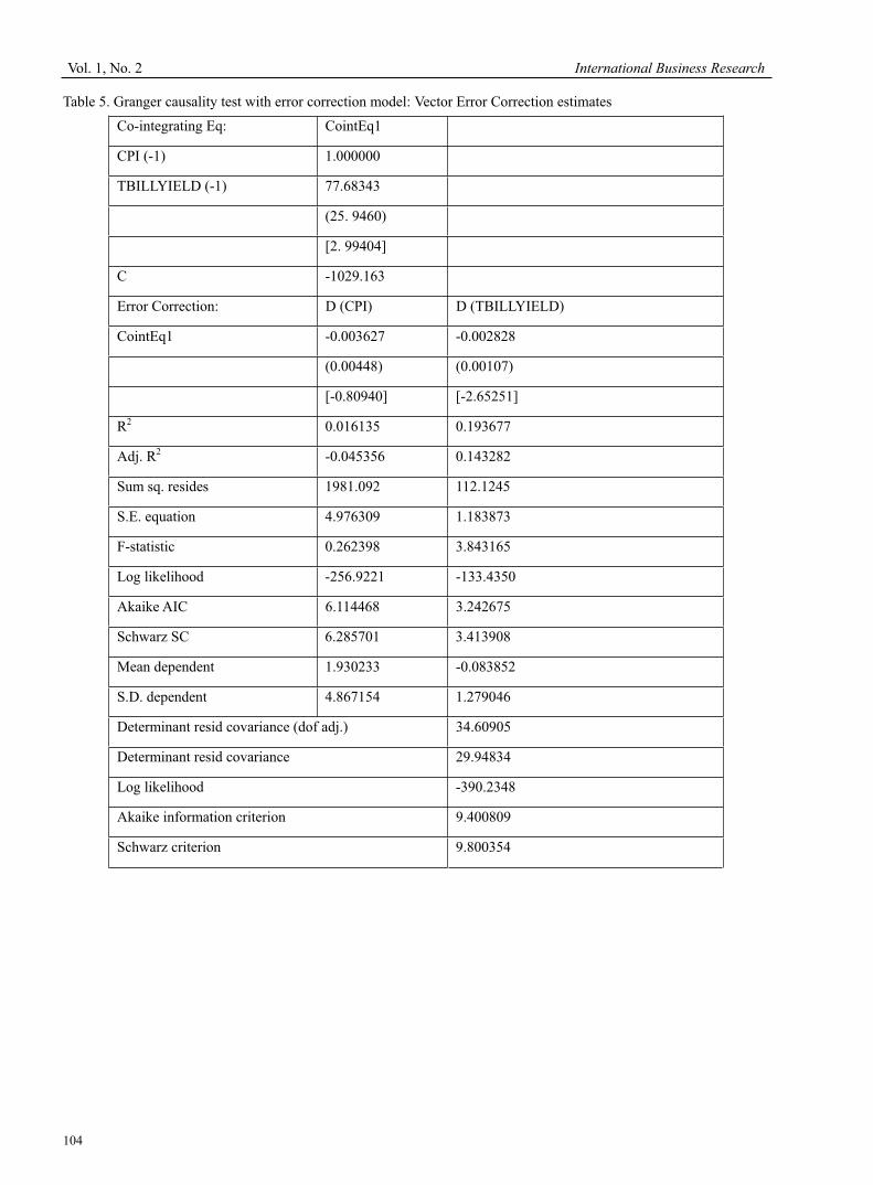
Vol. 1, No. 2 International Business Research
104
Table 5. Granger causality test with error correction model: Vector Error Correction estimates
Co-integrating Eq: CointEq1
CPI (-1) 1.000000
TBILLYIELD (-1) 77.68343
(25. 9460)
[2. 99404]
C -1029.163
Error Correction: D (CPI) D (TBILLYIELD)
CointEq1 -0.003627 -0.002828
(0.00448) (0.00107)
[-0.80940] [-2.65251]
R2 0.016135 0.193677
Adj. R2 -0.045356 0.143282
Sum sq. resides 1981.092 112.1245
S.E. equation 4.976309 1.183873
F-statistic 0.262398 3.843165
Log likelihood -256.9221 -133.4350
Akaike AIC 6.114468 3.242675
Schwarz SC 6.285701 3.413908
Mean dependent 1.930233 -0.083852
S.D. dependent 4.867154 1.279046
Determinant resid covariance (dof adj.) 34.60905
Determinant resid covariance 29.94834
Log likelihood -390.2348
Akaike information criterion 9.400809
Schwarz criterion 9.800354

International Business Research April, 2008
105
Problems in China’s Private Enterprises after
They Realize Financing by Going Public and Precautions
Chengfeng Long
School of Business Administration, North China Electric Power University
Beijing 100029, China
Tel: 86-10-8462-3371 E-mail: [email protected]
Shuqing Li
School of Business Administration, North China Electric Power University
Beijing 100029, China
Abstract
Most private enterprises face many problems after going public, such as the honesty and credit issue, private
entrepreneurs robbing the listed companies’ capitals, and amounts of disposable capitals. All these problems are rooted
in private listed companies’ irrational stock structure, poor financial management, and imperfect system. In order to
avoid these problems in private enterprises after going public, it is necessary to perfect these private listed companies’
stock structure and stock relationship, improve their financial management, and execute strict and rational system.
Keywords: Private enterprises, Financing by going public, Problems, Precautions
In May, 2003, Hongkong High Court declared that Euro-Asia Agricultural (Holdings) Ltd. was in formal liquidation.
Next, Jiangsu Qionghua, Zhengzhong Pharmaceutical, Shanghai Real Estate, China Special Fibrin, Far-East Pharmacy,
Dongda Bright, and many other enterprises are mentioned in the black list for their cheating behaviors. What are the
problems in private enterprises after financing by going public? And what are the essential reasons for these problems?
How to avoid these problems at the very beginning? All these issues win great attentions from private enterprises that
plan to go public and their entrepreneurs. This paper will chiefly analyze these issues.
1. Problems in private listed companies
1.1 Honesty and credit
Public enterprises should take honesty and credit as their base because investors usually make investment decisions
according to their disclosed information. However, in China’s most private listed companies, the only big stock is
popular. Entrepreneurs control the listed companies and gain most interests. Therefore, they have stronger motivations
to achieve financing by cheating or artificially steer the stock price.
The honesty and credit risk in private enterprises is chiefly originated from their casual development process. Problems
of honesty and credit after going public mainly include: (1) Overrated contribution. For example, Nongkai Group went
public in Hongkong was stopped in Sep, 2003, because it overrated enrolled capitals. (2) Hide sensitive information or
untimely disclose sensitive information. For example, in less than half month after going public, Jiangsu Qionghua was
criticized in public by Shenzhen Stock Exchange due to its fake information. (3) The financing capitals are not used
properly according to the initial public offerings. For example, Ufida Software has gained nearly one billion Yuan by
IPO. In its IPO introduction, it listed 29 investment projects and declared that the project budget that had passed state
approval was 803 million Yuan. But later, it claimed that in order to improve the use efficiency of short-term capitals,
the board had determined to invest no more than 300 million Yuan (32.7 percent of total capital offerings) in national
bond. It means the 300 million Yuan will not be used according to the IPO introduction.
Along with the frequent emergence of problems in private listed companies, investors question their honesty and credit.
The trust risk almost reaches a top. This kind of trust risk has already generated negative effects on private enterprises
that plan to go or have already gone public. Many private enterprises that plan to go public have to defer or even cancel
their schemes.
1.2 Big shareholders robbing capitals in private listed companies

Vol. 1, No. 2 International Business Research
106
In China, most private enterprises begin from family businesses. After a period of development, they choose to found
enterprises and even go public, gaining more attentions. But, most of private enterprises still sustain their traditional
management even after going public. It is the private entrepreneur who makes all decisions. Some private entrepreneurs
directly possess capitals of enterprises, thinking that everything in enterprises belongs to them. They can use them as
they like. In recent years, more severe punishment and media supervision focus on big shareholders who may rob
enterprises’ capitals. Therefore, rational big shareholders may obtain enterprises’ capitals by editing fake accounting,
associative transaction, and illegal guarantee, instead of directly occupying capitals in enterprises. For example, from
1999 to July, 2004, Zonglin Xu, Diamond’s board present, illegally occupied more than 483 million Yuan.
According to data issued by China Securities Regulatory Commission, till 30th, June, 2006, 149 listed companies have
capitals’ illegal occupation issue, and the illegally-occupied capitals totally reach 32.8 billion Yuan. Thereof, the number
of private listed companies is 62, and relevant illegally-occupied capitals reach 13.5 billion Yuan. Apparently, the
problem of big shareholders occupying enterprises’ capitals is not solved completely, which has already strongly
affected listed companies’ daily business operation. Once the behaviors of big shareholders who robbed listed
companies’ capitals are disclosed, investors will sale their stocks of these kinds of enterprises. As a result, these kinds of
listed companies will face price slumping or even stock sign. According to an investigation on investors, once the big
shareholders occupies capitals in listed companies, 77.05 percent of investors will sale their stocks, and 18.53 percent of
investors will choose to protect their right by legal procedures, and even 91.29 percent of investors take this problem as
one of the most important factors in their investment.
1.3 Without right investment project and amounts of disposable capitals
Disposable capitals have strong liquidity but poor profitability. A large quantity of disposable capitals will affect the
profitability of listed companies and the safety of assets. Presently, many private enterprises can not find proper
investment project though they successfully collect capitals by IPO. How to spend money becomes a difficulty for
private entrepreneurs. For example, since Taitai Pharmaceutical (600380) going public in 2001, Baoguo Zhu, as the
present, has always faced the pressure of spending money. Among the collected 1.69 billion Yuan, nearly 1 billion has
already invested in 11 projects. However, two years later, all these 11 projects failed to achieve former expectations.
Thereof, 6 projects had to be stopped due to smaller market shares, and waste of fixed assets. Today, Baoguo Zhu has
nearly 700 million Yuan, the collected capitals, and 500 million Yuan, the operation cash. As the No.36 in Forbes’ list,
Baoguo Zhu is in a trouble of spending money.
As a result, many private listed companies choose entrusted financing. However, this investment behavior brings about
more severe loss for private listed companies. For example, the son limited companies of Lanzhou Huanghe River,
namely Huanghe River High-Efficient Agricultural Development Ltd. Co. and Lanzhou Huanghe River Science &
Technology Venture Ltd. Co. changed their two kinds of national bonds into other enterprises’ stocks in 2004, which
caused a loss of 13,822,200 Yuan. It affected the whole operation performance of the enterprise in 2004. Lanzhou
Huanghe River that has been expected to achieve a greater improvement became a tiny-profit enterprise.
Some private listed companies usually adopt the high-cash payout ratio policy as an important way to solve the
disposable capitals. For example, Kangmei Pharmacy that has 0.41 Yuan earnings per share in 2001 set up a
two-Yuan-every-ten-shares dividend scheme. Taitai Pharmaceutical that has 0. 391 Yuan earnings per share set up a
three-Yuan-each-share dividend scheme. Lutai Group that has 0. 42 Yuan earnings per share set up a 3.18 Yuan every
ten shares dividend scheme. Ufida Software that has 0. 70 Yuan earnings per share set a six-Yuan-every-ten-shares
dividend scheme. Relevant data show that in Europe, 30% or 40% of after-tax profits in listed companies are used for
dividends. And in Japan, the percent is from 10% to 15%. In contrast, the dividend proportion of private listed
companies in China is relatively high. High cash dividend serves as a cause for private listed companies failing to find
right investment projects. As a result, potential investors may question the development future of private listed
companies, which will further affect the stock prices. When Ufida Software publicized its high dividend policy in 2001,
its stock price decreased sharply.
2. Probe into causes for problems in private listed companies
Problems emerged in private listed companies heavily hurt investors’ trust and expectations for them. In frustration,
people may want to know what reasons are for these problems. As a matter of fact, these problems are caused by not
only enterprises themselves but also the system.
2.1 Irrational stock structure
Issuing stocks in public is an important way for private enterprises breaking up close stock structure and play roles in
society. After issuing part of stocks in public, family members will hold less stock. But families still refuse to give up
the absolute control over enterprises. Therefore, in order to hide the fact of families’ absolute control over enterprises,
they choose to hold an absolute large percent of stocks, usually higher than 50 percent. As a result, the former
family-complete-hold stock structure turns into the present family-big-stock structure. Take Chuanhua Stock in SEM

International Business Research April, 2008
107
board for example. Chuanhua Xu, Guanju Xu, and Guanbao Xu, father and sons, directly hold 42 million shares,
accounting for 70% of the total shares, 60 million shares. Another case for example, 69.09% of shares of Xinhecheng in
SEM board are held by Xinchang Chemical Enterprise.
One-big-shareholder stock structure can help to enhance the close connection between corporate interests and family
interests. Under this stock structure, family managers can realize strategic program, operation management, and internal
control over enterprises easily. However, in modern market economy, the stock structure serves as not only the
precondition for stock market, but also the logical start for corporate governance structure. The stock structure
determines the governance structure. Data show that the one-big-shareholder phenomenon is popular in China’s private
listed companies, which may lead to incomplete governance structure, and the right of the board may controlled by the
board present solely. Lots of small and medium shareholders can not say any word in corporate management due to
their smaller shares. Besides, the independent present is determined by the one big shareholder in private listed
enterprise at present. All these factors cause to a failure of restriction mechanism. The board is completely controlled by
the president. As the core of corporate governance, once the board is controlled by one person, it may pass any kind of
decisions that may hurt small and medium shareholders’ interests but benefit the president self, such as untimely
disclosing or refusing to disclose information that is supposed to be known by small and medium investors or potential
investors, manipulating listed companies’ profits, robbing their capitals, and hurting interests of small and medium
shareholders.
2.2 Poor financial management
Before going public, it is enough for the accounting reports in private enterprises merely to satisfy taxes payment and
business management. It is the private entrepreneur who makes the financial management decisions. Therefore, the
financial workers just complete necessary accounting what private entrepreneur want.
After going public, private enterprises have to obey a series of regulations and requirements finance, and information
publication set up by the stock exchange. According to relevant laws and regulations, listed companies in China have to
publicize their annual report, half-year report, and seasonal report. The annual report concerns with investment, finance,
operations, profits division, associated transactions, audited financial reports, and additions. These contents include
finance analysis, financial management, investment, operational capitals’ management, dividend allocation, capital
operation, accounting, and integrated reports. Besides, many factors should be taken into consideration in
decision-making that is an extremely complex process. Therefore, the requirements for finance managers become higher.
However, most private entrepreneurs grow from technology and sale fields. They usually focus on these two fields but
neglect the finance management field, including the management idea, and the employees. In a sense, the position of
finance management and the quality of finance workers fail to achieve same progresses along with the listed companies.
Poor finance management in private listed companies may cause a series of problems, including the imperfect finance
management system, poor consciousness of risks, inefficient investment decision, amounts of disposable capitals, and
many other issues. For example, as Jiangsu Qionghua was found its 35.55 million Yuan invested in national bonds, it
protested that the board did not know everything about entrusted finance. It was the finance branch that made the
investment. And after the board approved the investment in national bonds, the board mistook it as the investment was
from self operation. Apparently, all these problems will directly affect enterprises’ values and profitability, which will
arouse reflection in capital market.
2.3 Reasons in history and system aspect
Because of history reasons, private listed companies are chiefly in production and process fields. And most of them
have not advantage of scale and belong to competitive industries, such as small home machines, food process, and
textile process. In market operation, private listed companies merely occupy one or few segment market. Even they
have capitals, their market is limited. Because of their industries, many private listed companies could not find rational
investment projects, which leads to a large amount of disposable capital.
Present system makes it more difficulty for private enterprises gaining opportunities of issuing initial public offerings
(IPO). Therefore, purchasing a shell company becomes an important way for private enterprises going public. Purchaser
must have powerful capitals in order to purchase a shell company. It may cost millions of Yuan or even billions of Yuan,
which may make private enterprises face greater challenges since their capitals are always insufficient. Moreover, the
banking industry in China is used to providing loan for state-owned companies. It is hard for private enterprises to
obtain loans from banks, not mention other financing way. Therefore, private enterprises have to find a new way out of
difficult financing. They can realize financing by purchasing a shell company, which can help them obtain capitals by
legal or illegal way, such as Delong Series, Taiyue Series, and Yongjin Series.
Besides, in China there are no specific suit laws and regulations to protect small shareholders’ interests or punishment
measures, and no measures to punish big shareholders if they commit mistakes. Once illegal behaviors happen, the most
severe punishment imposed by Shenzhen Stock Exchange or Shanghai Stock Exchange is nothing but criticize it in

Vol. 1, No. 2 International Business Research
108
public. Data show that since April, 2001, 61 listed companies have been criticized in public by Shanghai Stock
Exchange. However, because of the weak supervision and management, and lagged-behind legal procedure, the public
criticism fails to generate ideal effects. For the behavior of big shareholders robbing listed companies’ capitals, the
punishment imposed by present laws in China is relatively light. They merely shoulder administrative responsibilities. If
a case is more serious, the main responsible man may have to leave, and other top managers can escape from
punishment. Therefore, the weak power of public criticism can not exert a warning effect on other listed companies.
3. Precautions for problems in private listed companies after they realize financing by going public
Keeping away from problems in private listed companies after they realize financing by going public can not only
benefit their development, but also help to protect the interests of small and medium investors, and the healthy
development of stock market, considering the fast development of private enterprises.
3.1 Improve private listed companies’ stock structure and stock relationship
In private listed companies, the one-big-shareholder holds the capitals and the control right over production and
operation. Moreover, differing from state-owned listed companies, the private enterprises have not restriction
mechanism, which makes it become a blank part in capital market. It may lead to such a result that is more serious than
that in state-owned listed companies. Therefore, it is urgent to change private listed companies’ stock structure,
separating and dividing the stock right of family big shareholders, changing an absolute control into a relative control.
In specific, it is to institute relevant laws and regulations on securities and stocks. As private enterprises apply for going
public, they must absorb some non-family investors, and each of them should hold certain stocks, which can separate
the stock right effectively. Private enterprises that have already achieved separate stock right can relative- easily obtain
approval.
As private enterprises choose to go public in China, they should avoid circulative, multi-level, and complex stock
structure as much as possible. Under present imperfect supervision, complicated stock structure is easy to be abused by
the big shareholders who may obtain cashes by associated transactions or illegal guarantees. But in western countries,
family enterprises usually have simple stock structure as they go public. For example, the controlling shareholder of
Microsoft Ltd. Co. is not Microsoft Group but Gates himself. And the controlling shareholder of Dell Ltd. Co. is not
Dell Group but Dell himself. By taking reference from foreign countries, we can guide private enterprises to form
simple stock relationship during their foundation and development.
3.2 Improve private listed companies’ finance management level
It can focus on these aspects as follow.
3.2.1 Enhance capital management
Based on experiences and lessons in recent years, it is common for private listed companies being hurt by finance traps,
such as big shareholders robbing capitals, debt risks from providing guarantee for other enterprises, and failures in
investment. The loss may reach millions of or ten millions of Yuan. Therefore, it is vital to enhance listed companies’
finance management. In author’s opinion, it can focus on three aspects: (1) budget management; (2) risk management;
(3) daily management.
3.2.2 Properly deal with the relationship between initial financing and re-financing
After obtaining capitals by initial public offerings, if private listed companies can provide with ideal returns for
shareholders and its values realize a constant increase, it can achieve re-financing by issuing more offerings. Therefore,
as private enterprises apply for going public, they should avoid unreal advertising or unpractical promise, which can
help them to set up an honesty and credit image in investors. After going public, they should focus on businesses and
management, trying to renew finance indexes, improve profit ratio, adopt proper dividend allocation policy, and pursue
re-financing.
3.2.3 Re-build an internal finance management structure in private listed companies and improve finance workers’
quality
Finance management is the core in private listed companies. Separation and specification between financing and
accounting become a universal trend. As an optimized corporate organization, private listed companies should perfect
the internal finance branches, forming two sets of institutions. One focuses on collecting and allocating capitals,
financing programming and decision-making, evaluating investment schemes, and constituting investment strategies.
The other focuses on enterprises’ internal operations, checking, information process, and financing supervision. At the
same time, the successful capital management in private listed companies must based on a team of managers who are
good at manipulating capitals, and possess competitive consciousness, knowledge, and ability that can help them
manage enterprises properly.
3.3 Avoid problems emerged in private listed companies from the system aspect

International Business Research April, 2008
109
3.3.1 Supervise private listed companies and force them to execute relevant laws and regulations
In order to regulate listed companies’ governance structure, China Securities Regulatory Commission and State
Economic and Trade Commission issued the Code of Corporate Governance for Listed Companies in China on 7th, Jan.
2002, which is first file that generally and systematically regulates listed companies’ behaviors. Its constitution is based
on principles established by Law of Company, Law of Securities, and other relevant laws and regulations, and
referencing from standards that are acceptable by foreign companies. This code is right for China’s listed companies,
including private listed companies surely.
3.3.2 Take reference from foreign experiences and continue to perfect relevant system
In general, America and Japan have relatively perfect laws. In America, the effects of laws on family listed companies
are chiefly in two aspects. (1) Support. America has a nice legal environment. Private assets are protected by
constitution. Its perfect legal system provides with sufficient credit source for private listed companies, simplifying
transaction and improving efficiency. (2) Restriction. On one hand, the Anti-Trust Law restricts the family monopoly. In
late 10th century, America made up Anti-Trust Law. Its execution weakens American family enterprises’ control right
and separates their stock right. On the other hand, the collective lawsuit right of small shareholders protects interests of
small and medium shareholders. This right ensures that the benefits of every shareholder in wining a lawsuit will be
shared by all shareholders. Therefore, as American family enterprises go public, no listed companies rob external small
and medium shareholders by stock market, which is different from the fact in Asia or other regions and countries.
Focusing on problems emerged in private listed companies in China we can take reference from these successful
experiences and perfect the legal system.
Reference
Gu, Yinkuan., Zhang, Tiesheng & Wang, Minghu. (2004). Financial Issues in Listed Companies. Beijing: Economy &
Management Publishing House. July.
Ling, Weijia. (2005). Diamond’s former board present is forbidden to go public forever. Beijing Daily. 6th, Feb.
Wang, Xiu & Zhu, Baoguo. (2003). Worry about spending money. China Economic Times. 19th, Feb.
Xiang, Ming. (2005). How Hongkong deal with listed companies that produce fake information. China Audit Paper.
26th, Apr.

Vol. 1, No. 2 International Business Research
110
An Understanding towards Organisational
Change in Swimming in the United Kingdom Ian Arnott
Teesside Business School, University of Teesside
Middlesbrough, Tees Valley, TS1 3BA, UK
Tel: 44-1642-342809 Email: [email protected]
Abstract
Sports all over the world have evolved considerably over the last two decades due to their increased popularity through
various marketing communication channels and the mass media coverage. Because of this they have had take on what
was originally an amateur role to more a professionalised role dealing with increased governmental pressure and also in
some cases quality frameworks which they once did not have. Because of this a lot of National Governing bodies who
came from predominantly voluntary roles are now paid and also working with highly trained staff.
Because of this change it could be argued there has been a great deal of resistance to this which inherently has impacted
the growth and development of the grass roots stages that feed into sport (Not-for –profit sports clubs). Some key
researchers such as Hoye (2004, 2002), Kikulis, (2000), Kikulis., Slack,, & Hinings . (1995) have been the lead
people with in this field to look at models like Laughlins (1991), Dawsons (1996) and many other theorists’ models that
have been adopted when they have been going through the change process. Some of the sports that have been looked at
when they have been going through this change process are NSO’s in Canada and also Rugby in Australia. However
there has been very little work done on sport with in the United Kingdom.
This paper looks at the Formerly Amateur swimming Association now British Swimming on how they have gone
through change and in what this has impacted there grass roots development. It also looks at 30 clubs in particular on
how they have embraced this change.
Key words: Organisational design, Environmental disturbances, Professinalised, Development
1. Introduction
Organisations are in a constant state of change; new people enter the organisations, some leave, parts of the organisation,
and new programs or product lines are developed (Slack, 1997). The paradoxical nature of change stems from the fact
for any organisation to remain competitive they must make change (Peters, 1990). At the same time managers need to
look for new markets, new technology, and innovative means for service delivery, therefore in the service industry they
must find that stability (Miller, 1990).
Achieving a balance between stability and change is not an easy task (Slack, 1997). The organisation must recognise the
need for change and understand how it can be successfully implemented and managed. Changes in the environment
and technology will impact the amount of change a service industry sector organisation will require. Those
organisations that operate in stable environments with routine technologies will require less change than those facing
dynamic environments with non routine technology (Zucker, 1989). It could be argued due to the development of
technologies and the changes in the organisations environments, change could be forced upon them and subsequently
there me be some resistance to this. Some examples of this are sports organisations (Miller, 1990). Due to the
development and advancement of some of the organisations with in this particular area they go through what Kimberley
(1980) highlights is the life cycle approach. Kimberley (1980) goes onto describe these as the creation, transformation
and decline (pg 217); birth, growth, maturity, old age and death (Adizes, 1979); the entrepreneurial stage, the
collectively stage, the formalisation and control stage; the elaboration of structure stage, (Cameron & Whetton, 1983a).
Where as Institutional theorists (Oliver, 1991, Zucker, 1983 &1987); suggest that organisations change their formal
structure to conform to expectations within their institutional environment about appropriate organisational design.
Many countries such as England in athletic games pay high attention to organisational design in the way sport is
managed (Laois, 1995). However, this maybe so, it does inhibit the development of an area that services people and
other organisations with in it. Therefore for an organisation to change and conform to the expectations of their
institutional environment especially such areas as a service it must do so in a legitimate way, and thus to ensure a
continued flow of management and resources necessary for their operations (Hinings and Greenwood, 1988). Another
example of this is the Canadian national sports organisations in the period 1984-1988 when the Canadian government

International Business Research April, 2008
111
agency Sport Canada created institutional pressures for these organisations to adopt a more professional and
bureaucratic structure (Slack & Hinnings, 1992, Macintosh & Whitson, 1990). Also it has been identified in recent
studies is that these static models on organisational design and structure are being displaced by dynamic models,
reflecting a discontinuous nature of organisational change (Nelson, 2003, Fomburn, 1992, Greenwood and Hinnings,
1988 & Pettigrew, 1985). In the service industry such as sport, change cannot be relied upon to occur at a steady state,
rather than that there are periods of incremental change sandwiched between more violent periods of change which have
contributed to the illusion of stability once assumed to be the case (Nelson, 2003). It must be then thought of because of
the changing dynamics and environment of the service industry, organisations must adopt change.
1.1 Organisational Change, its development with in the field of the service industry
Organisational change has received a great deal of attention in the field of organisational design and management and
structure (Kikiluis, Slack & Hinings 1995, Skinner, Stewart & Edwards, 1999 and Rowley, 2004). It is essential to
understand why organisations might change with in this sector of the industry, and possibly what specific areas they
might need to change?
The service industry is very diverse in nature and crosses a multitude of providers from private, for profit settings and
public and non-profit settings (Ferkins, Shilbury & Mcdonald, 2005). There is a well established body of literature on
the differences between public sector companies as it pertains governance, delivery, service and reputation explains
these distinctions (Miller-Millliesen, 2003, Miller, 2002, Olsen 2000, Forbes & Milliken, 1999, Gopinath, Siciliano, &
Murray 1994). According to Shilbury (2001), the key distinction can be found in the purpose for existence. Financial
motives and the responsibility to create shareholder wealth dominate the mission of for profit organisations. Non-profit
organisations, in contrast, are motivated by preponderance of goals and outcomes (Perkins, Shilbury & Mcdonald,
(2005) such as increased members to the organisation or fundraising similar to an organisational model presented by
Pettigrew (1985) (Figure 1).
Unfortunately Pettigrews (1985) model does not allow for the comprehensive environment externally and has a stronger
bearing on the internal mechanisms that drive the organisation at that given time. It could be argued that the whole
process is still dynamic and therefore it could be applicable to providers in the voluntary capacity of the service industry
such as sport (Nelson, 2003).
A number of studies have focused on the mechanics of change in the professionalisation and the bureaucratization that
has occurred within voluntary (not for profit) sport organisations that has taken place over the last two decades (Hoye,
2004, Kikulis, Slack and Hinings, 1995a, 1995b, 1995c; Slack and Hinnings 1994, 1992, Thibault, Slack and Hinnings,
1991, Slack, 1985). In addition to a concern with the patterns of change, there has also been some theorising about, and
investigation of, the extent to which organisational change is likely to take place in some elements of structure and
systems rather than others (Hinnings and Greenwood, 1988; Kanter, 1983). Some organisational elements may be
particularly difficult to change because of the embodiment of deeply held values, yet may need specifically changing in
order to signal the purpose and seriousness of change (Schein, 1985; Kanter 1984) within their environment. Dawson
(1996) provides a framework in some way to attempt to discuss this (figure 2). His approach, displays a number of
bundles offering components of change, which he refers to as determinants.
However, a weakness of the model of change is that it does not take into account the dynamic quality of change that
Pettigrews (1985) model does. It has a static approach and does not support any type of dynamic movement forward.
So far the argument has been in general terms with regards to change (Kikulis, Slack & Hinnings, 1995). It is important,
however to recognise that different sectors are seen to carry different organisational design and functional requirements
(Child and Smith, 1987). One constantly evolving sector is the provision of sport in the changing dimensions of how it
is managed and developed. Sport because of its unique environment has encountered a number of disturbances because
of this process (Skinner, Stewart & Edwards, 1999), especially in the United Kingdom. Sport and there National
Governing Bodies (NSO’s) have and are still going through systematic and environmental change because of having to
take a more business type approach and generate their own funding. Therefore they having to work in an environment
with more professionalised staff and develop newer departments such as Public Relations and more.
1.2 Environmental Disturbances in Sport
One of the studies that was undertaken by Kikluis, Slack and Hinnings (1992) was when they identified specific
environmental disturbances in their analysis of institutionally specific organisations (Skinner, Stewart and Edwards,
1999). It was discovered institutionally specific sports organisations (NSO’s) create their own values, rules, myths and
symbols, which strongly influence the way they respond to the demands of new environmental conditions. Also Hoye
and Stewart (2002) highlighted that a large proportion of these sports organisations draw upon forms of power from
volunteers, especially during periods of organisational change. Therefore it could be argued that if organisations are a
not for profit, traditionally like NSO’s in the UK, how would they be able to adapt to a more competitive and dynamic
environment which then becomes more complex in nature similar to the design presented by Dawson (1996)? Also

Vol. 1, No. 2 International Business Research
112
because of this complexity there is more beaucracy to deal with. Furthermore if there is a degree of professionalisation
how will this affect the effectiveness and efficiency on what has been seen predominantly voluntary in nature where
there is no payment to the employee’s? Studies have explored the nature of this change (Hoye, 2004, Skinner, Stewart
and Edwards, 1999, Kikulis, Slack and Hinnings, 1995), the sources of commitment and also the resistance to change
subsequently developing bureaucracy with in the sports organisation, therefore slowing down the decision making and
evolution of the NSO’s.
1.3 Evolving National Sports Organisations
During the 1980’s and the early 1990’s National Sports Organisations (NSOs) have had to make adaptations in their
programmes in an effort to enhance the effectiveness of the delivery of amateur sports services (Kikulis et al, 1995).
This marked the beginning of a movement from simply structured and volunteered –governed organisations towards a
more professional and beaurcratic form. Furthermore other studies have focused exclusively on decision making and
particularly on the distributions of influence among board members and executives within the formal structure of
voluntary sports organisations (Auld and Godbey, 1998, Auld, 1997; Inglis, 1997; Macintosh and Whitson, 1990). These
studies however illustrated the complex nature of decision making with in the voluntary sports organisations and
furthermore suggested that perceived control over decision making has the potential to be a major source of conflict
between voluntary board members and executives (Hoye, 2004). However the traditional values of voluntary
governance that underpinned the structures and systems of these organisations were subject to change (Kikulis et al,
1995). In a fast moving environment, governance remains central to the effective and efficient management of sport
organisations (Hoye & Auld, 2001).
Changes in sport management (e.g., the shift from a committee or council of representatives to a modern board of
directors, the introduction of paid executives, player payments, increases in income and expenditure, media scrutiny and
a wider range of stakeholder interests) have presented major strategic issues to those responsible for governing sport
organisations (Ferkins, Shilbury & Mcdonald, 2005, ii). So as well the dynamics of the organisation changing to a new
environment and adopting a more professionalised approach bringing in paid staff, so have board members.
Traditionally being of a voluntary nature and the devolution of power being held by the volunteers, the paid
professional now takes on that power and facing resistance. Thibault, Slack & Hinnings (1991) investigated structural
changes in Canadian National Sport Organisations (NSOs) that occurred as a result of the introduction of paid
professional staff. There research found that following the hiring of professional staff, the pattern of centralisation
initially increased and decreased (Hoye & Cuskelly, 2003). This pattern can be attributed to volunteers initially fearing
the challenge that the professional poses to the culture of voluntary sports organisations (Thibault et al., 1991, p 93).
However Inglis (1997) found that volunteers and paid staff still preferred to be involved in the decision making within a
board setting, and also on the nature of decisions being made. This was imperative to the nature of decision making and
supports theory suggested by Taylor and Ho (2005) who indicate that change is imperative for sport and is unique to all
the sports organisations especially with in the environment it operates.
Other sport literature suggests that while sport organisations have traditionally had relatively unsophisticated
management systems, change is becoming common practise. Therefore organisations are having to become more
‘professional’ in the way they approach people management issues (Chelladurai, 1999). Because of this change studies
such as Kikulis et al (1995), Slack and Hinnings (1992 & 1994)) Thibault et al (1991) and Slack (1985) have explored
the nature of professionalisation, the sources of commitment and resistance to change, and the impact
professionalisation has had upon decision-making structures with the organisation. One example of this was research
carried out by Hoye and Cuskelly (2003) who commented on the pressure faced by voluntary sport organisations to
adopt a centrally derived model and how this related to the performance of a board in their decision making process.
1.4 Sports Organisational Structural change; rhetoric or the future on decision making
Kilkulis et al (1995) categorised sport organisations into three different organisational archetypes; the traditional
kitchen-table style, the transitional boardroom, and the business like executive office. Taylor and Ho (2005) go onto
describe in the kitchen-table archetype volunteer management is paramount and the selection is based on organisational
loyalty and there is little formal planning or policies. The boardroom archetype is dominated by a volunteer controlled
hierarchy, but is supported by professional staff. Development of technical expertise among professional staff and
increasing administrative efficiency is practised in this type. In the executive –office archetype, technical expertise is
required in both professionals and volunteers (Taylor and Ho, 2005; 113). What is clearly evident is that historically
National Sports Organisations (NSO’s) have relied on typical situations where resources are scarce (Reilly and Knight,
2007). Work is volunteer –driven despite the fact that there should be a local responsibility for keeping up to date with
coaching techniques, and current world performance standards and the requirements of memberships is significant
(Seguin, Teed and O Reilly, 2005; Berrett and Slack, 2001).
Archetype approaches are fine and well being, but due to the changing face of sport where adaptability and innovation
are important to NSO’s, particularly in the realm of Olympic sports where funding is based on results (O Reilly and

International Business Research April, 2008
113
Knight, 2007) there could be concerns with patterns of archetypal change (Kiklulis et al, 1995). In short, whether
organisational structure and operations that are more susceptible or resistant to change (Kikulis et al, 1995)? Some
organisational elements may be particularly difficult to change because they embody deeply held value, yet it may be
these specifically that need changing in order to signal the purpose and seriousness of change (Schein, 1985; Kanter,
1984). Greenwood and Hinings (1988) theorised this approach similar to that of Pettigrew (1985) and Dawson (1996) in
presenting a model for the dynamics of organisational change (Figure 3). This model suggests that the archetype
adopted has separation from the three areas that may influence it, or the symbiotic bounding by the change process. As
with the model of Dawson (1996), this model does not convey the idea of the dynamics of change over time (Nelson,
2003) and subsequently this is essential for National Governing Bodies in sport who are developing radically day by
day to government and also there lead authorities in sport such the International Olympic funding Committee.
As O Reilly and Knight (2007) have indicated there is and ever increasing demand on National Governing Bodies/
NSO’s to produce results in this area in an environment where funding is spouse. Because of this demand once what has
traditionally been regarded as not-for-profit service sector area of sport has to become more effective in all areas
moving outside of its status quo/ equilibrium. Laughlin (1991) indicates that it is the environmental disturbances that
can consequently cause a sports organisation to move out of its equilibrium. Laughlin (1991) goes on further to suggest
that the organisation will either absorb the disturbance or maintain its previous equilibrium or, as a result of shift its
design archetype, sub system elements and interpretive schemes and develop a new equilibrium. This forms the basis to
provide a typology describing the complexity of organisational change (Skinner, Stewart & Edwards, 1999).
1.5 Typology Organisational Change in Sports Organisations
Laughlins (1991) Suggested that an organisation will change only when disturbed, kicked or forced into doing
something. Once the organisation undergoes an environmental disturbance the type of change can either be first or
second order change (see table 1) (Skinner, Stewart & Edwards, 1999).
Laughlin (1991) draws upon work of Smith (1982) and Robb (1988) to put forward the notion as morphastasis (first
order) or morphogensis (second order) change
According to Laughlin (1991) an organisation is assumed to be in a state of inertia and is operating in equilibrium
before disturbance arrives. However what is clearly apparent is that NSO’s (not-for-profit) have generally comprised of
heterogeneous groups, from what has historically being renowned from small local associations managed by few
volunteers. But because of the environmental disturbances that a sport has had and is still going through these
volunteers are now becoming accountable to chief executives. This then could be argued that not for profit NSO’s have
to now operate in similar environments as the profit world, and as such require managerial tools and tactics that are
specific to their area (O Reilly and Knight, 2007).
This reorientation which is in the first order of Gray, Walters and Bebbington and Thompson’s (1995) model is the
result of a disturbance that cannot be rebutted but has to be accepted or internalised into the workings of the
organisation (Skinner, Stewart and Edwards, 1999) Gray et al (1995) theorise that in this instance that the “real heart” of
the organisations is basically unaffected. In other words change is effectively resisted by the volunteers with in the
organisation and they wish to stay in inertia. So with in the sports organisation creates conflict. Gray et al (1995) further
argues that Laughlin’s (1991) model is too rigid. It does not allow for that conflict, ambiguity or contradiction.
Specifically, Gray et. al (1995) criticised the models inability to recognise disturbances a priori (i.e., in advance of the
event occurring), to assess what constitutes real morphogenetic change the second order of change.
Examining archetypes Amis, Slack and Hinnings (2002) found that organisations with members in amateur sports who
held values congruent with the prescribed changes engaged in the transition process, while those members who opposed
the changes only superficially conformed.
The concept of design archtype stipulates that structure and expression of values which serve particular interests
(Kikulis et al, 1995). Greenwood and Hinnings (1988,1993), Laughlin (1991), Nadler and Tushman (1989), Ranson et
al (1980, and Tushman and Romanelli (185) have all in their own way argued that the difficulty in reorientation or
organisational change is the attachment of value established organisations. Thus movement between archetype is
difficult (KIkulis et al, 1995). What clearly must be noted is that for such change to take place they must abandon their
strong values towards the institution. In the case of amateur sport organisations, it has been argued that voluntary led
decision making structures symbolise the legitimate, rational way to organise this sector of sport (Kikulis et al, 1995).
By embracing this process it may reduce the bureaucratisation in the professionalisation of sport, Slack (1985) found
that while bureaucratic characteristics existed within sport organisations, these did not all emerge because of this.
1.6 Transitional period moving from Amateurism to Professionalism
Slacks (1985) study focused on the Canadian Amateur Swimming Association and it showed that during the early stages
of its development the only bureaucratic manifestations exhibited by voluntary sport organisations were a functional
division of labour and a control system which took the form of a set of rules and regulations. As the organisations grew,

Vol. 1, No. 2 International Business Research
114
so did the complexity of manifestations (Ferkins et al, 2005). These findings go some way in describing the changing
nature of sport organisations as they exhibit aspects of a bureaucracy and the nature of change that is a piece meal
approach according to internal external environmental disturbances.
Subsequent studies have focused on the professionalisation of sport organisations that have moved from entities
administered by volunteers to those managed predominantly by paid staff (Shilbury, 2001: 53). Evidence for this
assertion comes from Slack and Hinnings (1992) in a study examining change in Canadian National Sport
Organisations. It was noted a trend towards a professional bureaucratically structured design, but reluctance on behalf of
the volunteers to cede decision making control to paid staff. The research showed that such change appeared to
challenge the traditional volunteer based culture of these organisations. This was further supported by Shilbury (2001)
who concluded that reluctance on behalf of volunteers to cede decision making control has been the short comings of
the professionalisation process of sport.
What is clearly evident is that there needs to be a clearer understanding of the roles and functions of boards of directors
in sports organisations to better understand the dynamics of this change process (Ferkins et al, 2005). Furthermore a
better understanding of this dynamisms needs to be understood and its impact on the development of sports. It could be
argued because of this bureaucracy, resistance to change decision making gets slowed down, which in some cases
reflects the future of sport and where it could be today. One such sport in the United Kingdom could be the Amateur
Swimming Association.
The Amateur Swimming Association is the English National Governing Body for swimming, diving, water polo, open
water and synchronised swimming (Amateur Swimming Association (ASA), 2007). The ASA supports 1,600 affiliated
swimming clubs through a National/ Regional/ County Structure (Figure, 4)
The ASA Council commissioned a review of the membership of the specific aim of answering the questions “what is a
member”? The responsibility for conducting that review was delegated, by Council Regionalisation’s Project Board
(RPB)”. The report was written by members of the board who have striven to maintain their independence and
accessibility to whole of sport (ASA Committee, 2004). This was very similar in the research conducted by Kikulis et al
(1995) where the Canadian National Sports Organisations made adaptations in their programmes in an effort to enhance
their effectiveness of the delivery of amateur sport services. Slack (1985), highlighted, though there was a general
conformity to make amateur sport more efficient and effective, they still held bureaucratic characteristics which in
essence may hold up the development of the sport? This then contravenes what government has set about in the United
Kingdom (UK) in the development of regionalisation, where they stipulate by doing so will allow sport to be well
managed to the success in world competitions (ASA, 2004).
What is clearly evident that this was marked as movement from sport and the ASA from a simply structured and
volunteered-governed organisations towards a more professional and bureaucratic form (Kikulis et al, 1995). What now
can clearly be established in the United Kingdom is due to the sport of swimming becoming a complex organisation,
has this inhibited or assisted the sport developing? More over because of the change in design archetypes, do NSO’s
still carry the core values and expressions of originally volunteered formed organisations (Kikulis et al, 1995). Many
theorists have argued this (Hoye and Cuskelly, 2003, Kikulis et al, 1995, Greenwood and Hinnings, 1993 & 1988,
Laughlin, 1991; Nadler and Tushman, 1989; Tushman and Romanelli, 1985; Ranson et al, 1980). To achieve such a
change requires the abandoning existing values for which they hold. In the case of the Amateur Swimming Association,
it has been argued that voluntary-led decision making structures symbolise the legitimate rational way to organise
decision making in this sector (Kikulis et al, 1995).
Therefore this study will look at the impact that these changes.
2. Research Analysis
The method that was employed to unearth such findings was a quantitative approach. The organisations that were
chosen operate in a highly knowledgeable and intensive environment (OReilly and Knight, 2007).Thirty Swimming
Clubs were randomly selected to participate in this study (Fink, Pastore and Riemer,2003). This number ensured that the
sample proportion would be within 0.05 of the population proportion, with a 95% level of confidence (Issac & Michael,
1984).
Following a similar approach by Fraenkel and Wallen (2000), where they used an intact cluster associated to athletic
departments. Executive committee members (Head Coaches, Chairman’s and club secretaries, etc) from each of the
thirty clubs they were sent a covering letter explaining the aim of the research project, a statement ensuring
confidentiality of their responses. Instruction of completing the questionnaire, the contact details of the researcher
(Hoye, 2004) and a self- administered questionnaire. This type of method was used by Herman and Renz (1997) who
determined it to be a reliable and valid measure on organisational performance.
The data collection involved the distribution of the self administered questionnaires to a specific board executive (N=30)
on the committees of the swimming clubs. This was a very similar approach adopted by Hoye (2004) & Hoye and

International Business Research April, 2008
115
Cuskelly (2003) where they distributed self administered questionnaires to all the board members (N=50) of a selected
number of voluntary sports organisations. The data that was being collected (as will be seen by the results) identified
that a number of the clubs are still going through a change period (i.e. real time data analysis). This method was
employed also by Kikulis et al (1995) & Pettigrew (1987) where they felt it was important to conduct a real time
longitudinal study to best capture the variety or organisation design patterns of change.
2.1 Method of Analysis
The method of analysis used to identify if changes with in National Governing body of swimming with in the United
Kingdom has had an impact on structural change with in the foundations of the sport (clubs that hold the sport together
and develop the swimmers from the grass roots level) was the Statistical package for the social sciences (SPSS 13.0).
All thirty respondent questionnaires from the clubs that were randomly selected were inputted and analysed through this
method. The main descriptive and inferential findings are discussed in the results section.
3 Analysis Findings
The descriptive statistics (i.e. means, frequencies) are used to describe the main variables of interest (Fink, Pastore and
Riemer, 2003). Then a one way anova test was conducted along with a non-parametric analysis of variance
(Kruskal-Wallsis test) of mean scores (Hoye and Cuskelly, 2003) of the year the clubs were formed impacted their
Swim 21 (National Accreditation of Quality and Change) and also employing (paid) staffs.
Table 2 highlights the year the swimming clubs were formed. With a valid per cent of 100 (N=30), what is clearly
evident that most clubs were formed/ founded between 1966-1975 which accounts for 30% of the clubs used in the
research.
The histogram in figure 5 supports table of the years the clubs were founded because it is demonstrating that standard
deviation from the mean is 3.34 (.9>.5). This indicates that the normal distribution of the curve is wider than normal.
Because of this it determines which of non-parametric and parametric tests will be used at the 95% level.
Figure 6 displays the means of the clubs who have a paid employee with in their organisation. A total of 18 of the 30
clubs used in the research have a paid person. Who tended to be the head coach, this was at 60%. This indicates that a
further 40% still do not have paid positions with in their organisations and work mainly on a voluntary basis.
Table 3 highlights that most of the clubs that were identified had management committees (27 = 90%). What is clearly
evident from this response rate that clubs do rely heavily on this type of voluntary management with in their
organisation and environment that they operate in at present?
Using a one way anova statistical test see if there is relationship between the year a club was formed impacted their
decision to have paid employees or not the a result displayed in table demonstrates a difference of at < 0.05 = 95% of
0.41 displaying there was no relationship because of the year they were formed.
Using a Kruskal Wallis Test figure 7 shows from 1971-1990 = 53% (P= 0.095 > 0.05) have or are working towards the
Swim 21 accreditation. This indicates that the clubs that have been formed for approximately 30+ years are going
through or have gone through organisational change over the last three decades.
Table 5 demonstrates that though the management committees are made up of volunteers there is no relationship
between the choice of having paid employees (P= 0.20 > 0.05) or a club work towards or having Swim 21 accreditation.
In recent years change has become an increasingly prevalent feature of organisational life (Amis, Slack & Hinings,
2004). Concomitantly, and not surprisingly, the study of transitions between organisations has become a popular topic
for academic research (Slack et al, 2002,Kikulis, 2000, Hinings, Thibault, Slack, & Kikulis, 1996, Kikulis, Slack &
Hinings, 1992,1995a, 1995b; Macintosh & Whitson, 1990; Slack, T & Hinings, 1992 & 1994). To date a lot of this
research has focused on the structural change, but very little has focused on the impact it has had on those who serve as
foundation to National Governing Bodies in sport. And incrementally what impact has this radical transformation had
on those who servos the sport (Kikulis et al, 1995, Stevens and Slack, 1995)?
What is clearly evident that change has not had a great deal of impact to those who servos the sport. Some of the key
arguments developed through this paper were, what impact would change have from Amateur (volunteerism) to be more
professionalised (Hoye, 2004, Skinner, Stewart and Edwards, 1999, Kikulis et al, 1995)? And can volunteers work in
harmony with paid employees (Inglis, 1997,Thibault, Slack & Hinings, 1991)? Also can those who have, what Kikulis
(1995), Schein, (1985) & Kanter, (1984) call “deeply held values” from years of being amateur in operation cope with
systems of change.
There is now evidence to suggest because of NGB’s changing and adopting a new structure it has not inhibited those
who hold the foundation of and development of the sport. Figure 6 demonstrates that most swimming clubs still operate
collectively with paid staff, e.g. Head Coaches and a voluntary management committee. This is further demonstrated in
table 3 where most of the clubs researched are made up of volunteers (N=27 = 90%). So though it has been stated by

Vol. 1, No. 2 International Business Research
116
Taylor and Ho (2005) that they must change, what is clearly apparent they can change? Arguably, before the
introduction of paid staff, the management committee would be and in some cases is still the leader in most of the clubs
explored in this study (Hoye, 2004). But any change must be incremental and also be symbiotic in this process. Taylor
and Ho (2005) go onto further describe this as a boardroom archetype and is still held with in a volunteer controlled
hierarchy, but also is supported by professional staff (Head Coach). This would then reinforce as Seguin, Teed and O
Reilly, (2005) and Berrett and Slack (2001) suggest that the club and the head coach can keep on developing and
staying abreast of the latest coaching techniques and swimming development areas such as Swim 21 accreditation. This
would be in some cases a model of change similar to that of Pettigrews (1985) (Figure 1) model where they want to be
part of dynamic change, which is not the models presented by Dawson (1996) and Greenwood and Hinings (1988).
What has clearly been demonstrated from this research that change in structures where organisations have to work in
harmony with paid employees that the board members are embracing this, though some areas are still slow in movement?
All clubs have to move towards a change in the adoption to volunteer roles in achieving Swim 21 status with in the
sport, a quality and organisational change award to improve the future of swimming. Which Pettigrews (1985) model
demonstrates that are components that convey the idea of movement and variability which precede outcomes (Nelson,
2003). This is also what Laughlin (1991) puts down to as a disturbance or having to now do something different.
Laughlins (1991) model (Table 1) in the inertia stage is clearly apparent and relevant to those clubs formed before 1971
(figure 7). Where as a large number of clubs that were founded from 1971 -1990 (53%) or going through that typology
of change morphostatic (first order) and morphogentic (second order). Those that have been founded through the era
1981-1990 have achieved that level and now hold the accredited award.
It seems to be prevalent with in the sport that is those pre 1971 still hold what Gray et al (1995) describes as the deeply
held values, but he then argues that Laughlins (1991) model is to rigid? But it could be argued that with in sport it forms
the basis for this research similar to Pettigrews (1985) outcome variability model. So it is relevant to the sport of
swimming because of its structure with in the United Kingdom. Also as Skinner et al (1999) states the model is useful
as it provides a way of putting particular changes (Swim 21 accreditation) into conceptual categories or compartments.
Though his model is useful it must be identified that because of the emergence of what Bergquist (1993) “post modern
management structures” organisations adopting Laughlin’s (1991) model needed to be a little bit more flexible. This
implies that to achieve Swim 21 accreditation a number of quite different changes could be occurring at any one time in
the organisation, each influencing the other and leading to turbulent backwashes (Skinner et al, 1999) therefore it could
be argued that this is similar to Dawsons (1996) (figure 2) framework. However to deal with these backwashes, it must
be noted that the possibility of the application of Llewellyns (1994) model on boundary management along with
working in conjunction of Laughlins (1991) model of the typology of change would be useful. Llewellyns first
addresses the boundaries of closed systems and suggest that the boundaries of these systems are relatively impermeable
to the forces of their surrounding environments (Skinner et al, 1999). Cooper (1990) likens this to a container of holding
things in.
These two models would be clearly be suitable in working together because of the environmental disturbances that
swimming with in the United Kingdom has and are going through. Because of the distinct changes the regions of British
Swimming are going through it is essential that the organisations that hold this together react and adopt change also. As
at present most post modern swimming clubs (figure 7) have adopted this change, (Laughlins, 1991, second and third).
However pre 1971 there is still is some resistance.
3.1 The Evolutionary Change in a competitive environment
Never before have sport organisation had to change and work in an ever changing competitive environment (Davakos,
2006). In such an environment, only the best prepared organisations will survive and continue to prosper. What is
clearly evident today that swimming with in the United Kingdom has gone through and is still going through change
with in the environment that it operates? This has been clearly seen that the hierarchy of the sport (NGB) over the last
two/ three decades has had to adopt change and this has then filtered down to what Skinner et al (1999) refers to as the
grass roots level or foundation.
Models of change such as Dawsons (1996),Laughlins (1991), Greenwood and Hinnings (1988) and Pettigrews (1985)
can in essence help clubs to understand how to deal with change or the factors that affect them. Each model identifies
the clear determinants of change and most importantly some of the factors that will or possibly affect them in the future.
Also Nelson (2003) has indicated that change cannot be relied upon to occur at a steady state any longer and that all
organisations not just in sport must be aware of this. She further goes onto to express that from a viewpoint, even for
sports clubs/ organisations to maintain viability they need to incrementally change in what Tushman, Newman and
Romanelli (1986) convergent change.
References
Adzies, I. (1979) Organisational passages: Diagnosing and treating life cycle problems of organisations. Organisations

International Business Research April, 2008
117
Dynamics, 8, 3-25
Amateur Swimming Association (2007) The History of the Amateur swimming Association. Accessed, 15th May, 2.30pm,
www.britishswimming.org
Amateur Swimming Association Committee (2004) Membership Review/ Regionalisation. Accessed, 15th May, 2.35pm,
www.britishswimming.org
Amis, J., Slack, T. & Hinings, C.R. (2004) Strategic Change and the Role of Interests, Power and Organisational
Capacity, Journal of Sport Management, 18,(2) 158-198
Amis, J., Slack, T. and Hinings, C.R. (2002) Values and organisational change, The Journal of Applied Behavioural
Science, (38), 4, 436-466
Bergquist, W. (1993) The post-modern. organisation; Mastering the art of irreversible change. San Francisco;
Jossey-Bass
Berrett, T. and Slack, T. (2001) A Framework for the analysis of strategic approaches employed by non-profit sport
organisations in seeking corporate sponsorship, Sport Management Review (4) 21-45
Cameron, K.S., & Whetten, D.A. (1983a). Models of organisational life cycle: Application to higher education. Review
of Higher education, 6, 269-299
Chelladurai, P. (1999) Human Resource Management in Sport and Recreation, Champaign IL, Human Kinetics
Child, J. and Smith, C. (1987) The context and process of organisational transformation- Cadbury Limited in its Sector.
Journal of Management Studies, 24, 565-93
Cooper, R. (1990) Organisations/disorganisations. In J. Hassard & D. Pym (eds), The Theory and philosophy of
organisations (pp167-197) London: Routledge
Dawson, P. (1996) Beyond convential change models: a processual perspective” In Nelson, L (2003) A case study in
organisational change: implications for theory. The Learning organisation
Davakos, H. (2006) An integral part of strategic planning for sport organisations: training employees. International
Journal of Sport Management and Marketing 1 (4) 390-397
Ferkins, L., Shilbury, D. & Mcdonald, G. (2005, i) The Role of the Board in Building Strategic Capability: Towards and
Integrated Model of Sport Governance Research. Sport Management Review (8) 195-225
Ferkins, L., Shilbury, D. & Mcdonald, G. (2005, ii) The Role of the Board in Building Strategic Capability: Towards and
Integrated Model of Sport Governance Research. Sport Management Review (8) 195-225
Fink, J.S. & Pastore, D.L. (2003) Managing Employee Diversity: Perceived Practices and Organisational Outcomes in
NCAA Division III Athletic Departments, Sport Management Review, 6, 147-168
Fomburn, C.J. (1992) Turning Points, MCgraw Hill, New York
Forbes, D.P. & Milliken, F.J. (1999) Cognition and corporate governance: Understanding boards of directors as
strategic decision making groups. Academy of Management Review, 24, 489-505
Fraenkel, J.R., & Wallen, N.E. (2000). How to design and evaluate research in education. New York: Mcgraw Hill
Gopinath, C., Siciliano, J.l. & Murray, R.L. (1994) Changing Role of the Board of Directors’: In search of a new
strategic identity? Mid Atlantic Journal of Business 30 (2) 175-183
Gray, G., Walters., Bebbington, J., and Thompson, I. (1995) The greening of enterprise; An exploration of the (non) role
of environmental accounting and environmental accountants in organisational change. Critical perspectives on
Accounting, G, 211-239
Greenwood, R and Hinnings, C.R. (1988) Organisational design types, tracks and the dynamics of strategic change.
Organisation Studies, (, (3) 293-316
Greenwood, R and Hinnings C.R (1993) Understanding Strategic change; The contribution to archetypes. Academy of
Management Journal , 36, 1052-81
Herman,R.D & Renz, D.O (1997) Multiple constituencies and social construction of nonprofit organisational
effectiveness. Nonprofit and Voluntary Sector Quarterly, 26, 185-206
Hinings,C.R., Thibualt, L., Slack, T., & Kikulis, L.M, (1996) Values and Organisational Structure. Human Relations, 49,
885-916
Hinings, C.R & Greenwood, R (1988) The dynamics of strategic change. Oxford: Basil Blackwell
Hoye, R, (2004) Leader-Member Exchanges and Board Performance of Voluntary Sports Organisations. Nonprofit

Vol. 1, No. 2 International Business Research
118
Management and Leadership, 15 (1) 55-67
Hoye, R., and Cuskelly, G (2003) Board – Executive Relationships within Voluntary Sport Organisations, Sports
Management Review, 6, 53-74
Hoye, R., and Stewart, R., (2002) Power and Organisational Change: The Case of Melbourne Women’s Hockey
Association 1995-1998. Sporting Traditions, 18 (2) 47-65
Hoys, R., & Auld, C (2001) Measuring board performance within voluntary sport organisations. Australian Journal of
Volunteering, 6 (2) 53-74
Issac, S/., & Michael, W.B (1984) Handbook in Research in organisations and evaluation. San Diego CA: Edits
Publishers
Kanter, R.M (1984) Managing transition in organisational culture: the case of participative management ay Honeywell.
In Kimberley, J.R and Quinn, R.E (Eds) Managing Organisational Transition. Homewood, Ill: Irwin, 195-217
Kanter, R.M (1984) Managing transitions in organisational culture; the case of participative management at Honeywell,
IN Kimberley, J.R and Quinn, R.E (eds) Managing Organisational Transitions. Homewood,IL; Irwin, 195-217
Kanter, R.M (1983) The Change Masters. New York: Simon and Schuster
Kimberley, J.R (1987) The life cycle analogy and the study of organisations: Introduction, In Kimberley, J.R & Miles,
R.H (eds) The Organisational Life cycle (pp 1-14). San Francisco: Jossey-Bass
Kikulis, L.M (2000) Continuity and Change in Governance and Decision Manking in National Sport Organisations:
Institutional explanations. Journal of Sport Management, 14, 293-320
Kikulis, L.M., Slack, T, & Hinings, C.R. (1995a) Sector specific patterns of organisational design change. Journal of
Management Studies, 32 (1) 65-95
Kikulis,L.M, Slack., T and Hinings, B (1995b) Does Decision Making Make a Difference? Patterns of Change Within
National Sport Organisations. Journal of Management Studies, 9, 273-299
Kikulis, L.M., Slack, T, & Hinings, C.R. (1995c) Sector specific patterns of organisational design change. Journal of
Management Studies, 32 (1) 67-100
Kikulis, L.M., Slack, T, & Hinings, B. (1995d) Toward an Understanding of the Role of Agency Choice in the Changing
Structure of Canada’s National Sport Organisations. Journal of Sport Management, 9, 135-152
Laios, A, (1995) School versus non-school sports; structure, organisation and function in Greece, Europe and the USA,
International Journal of Educational Management, 9, 1 pg 4-9
Laughlin, R.C (1991) Environmental disturbances and organisational transitions and transformations; Some
alternative models. Organisation Studies, 12, 209-232
Llewellyn, S. (1994) Managing the boundary; How accounting is implicated in maintaining the organisation. In
Skinner, J, Stewart, & Edwards, A (eds) Amateurism to Professionalism: Modelling Organisational Change in Sport
Organisations. (pp 173-192) Sport Management Review
Macintosh, D & Whitson, D.J (1990). The game planners transforming Canada’s sport system. Montreal & Kingston:
McGill-Queen University Press
Miller, D, (1990) The Icarus paradox: How exceptional companies bring about their own downfall. New York, Harper
Collins
Miller-Millese, J.L (2003) Understanding the behaviour of non-profit boards of directors: A theory based approach.
Non-profit and Voluntary Sector Quarterly, 32, 521-547
Miller, J.L (2002) The board as a monitor of organisational activity: The applicability of agency theory to non-profit
boards. Non-profit Management and Leadership, 12, 429-450
Nalder, D.A and Tushman, M.L (1989) Organisational frame bending: principles for managing reorientation. Academy
of Management Executive, 3, 194-204
Nelson, L (2003) A case study in organisational change: implications for theory. The learning Organisation, 10 (1)
18-30
Oliver,C (1991) Strategic Responses to institutional processes, Academy of Management Review, 16, 145-179
Ranson, S, Hinnings, C.R., Greenwood, R and Walsh, K (1980) Value preferences and tensions in the organisation of
local government. In Dunkerley, D and Salaman, G (eds). The international Yearbook of Organisational Studies.
London: Routledge and Kegan Paul 197-221
O’Reilly, N.J and Knight, P (2007) Knowledge management best practices in national sport organisations, International

International Business Research April, 2008
119
Journal Sport Management and Marketing (2), 3, 264-273
Rowley, J (2004) Researching people and Organisations, Library Management, 15 (4) 208-214
Peters, T (1990) Get innovative or get dead, California Management review, 33, 9-26
Pettigrew, A (1987) Context and action in the transformation of the firm. Journal of Management Studies, 24, 649-670
Pettigrew, A (1985) A wakening giant: continuity and change in ICI, Basil Blackwell, Oxford In Nelson, L (eds) A Case
Study in Organisational Change. The Learning Organisation.
Schein, E (1985) Organisational Culture and Leadership. San Francisco: Jossey-Bass
Seguin, B., Teed, K. and O Reilly, N (2005) National sport organisations and sponsorship; an identification of best
practices’ International journal of sport Management and marketing (1) , 2, 69-92
Shilbury, D (2001) Examining board member roles, functions and influence: A study of Victorian sporting organisations.
International Journal of Sport Management, 2, 253-281
Skinner, J., Stewart, B. & Edwards, A (1999) Amateurism to Professionalism: Modelling Organisational Change in
Sporting Organisations, Sport Management Review, (2) 173-192
Slack, T (1985) The beaucratisation of a voluntary sports organisation, International review for the Sociology of sport,
(20) 145-166
Slack, T and Hinnings, B(1992) Understanding Change in National Sport Organisations; an integration of theoretical
perspectives; Journal of Sport Management. (6), 114--132
Slack, T., & Hinnings, B (1994) Institutional Pressures and Isomorphic Change: An Empirical Test, Organisation
Studies 15 (6) 803-827
Slack, T, (1997) Change in Sports Organisations, Understanding Sport Organisations. Champaign IL, Human Kinetics,
pg211-217
Smith, K.K (1982) Philosophical problems in thinking about organisational change. In Goodman, P.S & Associates
(eds) Change in organisations 316-374 San Francisco: Jossey _Bass
Stevens, J.A & Slack, T. (1998) Integrating social action and structural constraints. International Review for the
Sociology of Sport, 33, 143-154
Robb, F.F (1988) Morphostasis and morphogenesis: Contexts of participative design inquiry in the design of systems of
learning and human development. Unpublished Discussion paper. University of Edinburgh
Taylor, T., and Ho, C (2005) Global Human Resource Management Influences on Local Sport Organisations.
International Journal of Sport Management and Marketing (1) 1,2, 110-120Thibault, L., Slack, T., and Hinnings, B
(1991) Professionalism, Structures and Systems: the impact of Professional Staff on Voluntary Sport Organisations.
International Review for the Sociology of Sport, 26 (2), 83-97
Tushman, M.L and Romanelli, E (1985) Organisational Evolution; a metamorphosis model of convergence and
reorientation. In Cummings, L.L and Staw, B.M (eds) Research in Organisational Behaviour, 7, Greenwich, Conn: Jai
Press, 171-222
Zucker, L.G (1989) Combining institutional theory and population ecology: No legitimacy, no history. American
Sociological Review, 54, 542-545
Table 1. Laughlins (1991) Typology of Organisational Change (adapted from Gray, Walters, Bebbington and Thompson,
1995)
No Change “ Inertia”
(1) “ Rebuttal” First Order Change
(Morphostatic) (2) “ Reorientation”
(1) “Colonisation” Second Order Change
(Morphogenetic) (2) “Evolution”

Vol. 1, No. 2 International Business Research
120
Table 2. Year in Which the Club was Founded
Frequency Percent Valid Percent
Cumulative
Percent
Valid 1940-1945 4 13.3 13.3 13.3
1956-1960 1 3.3 3.3 16.7
1961-1965 1 3.3 3.3 20.0
1966-1970 3 10.0 10.0 30.0
1971-1975 6 20.0 20.0 50.0
1976-1980 2 6.7 6.7 56.7
1981-1985 4 13.3 13.3 70.0
1986-1990 4 13.3 13.3 83.3
1991-1995 1 3.3 3.3 86.7
1996-2000 4 13.3 13.3 100.0
Total 30 100.0 100.0
Table 3. Clubs with management committees formed made up of volunteers
Frequency Percent Valid Percent
Cumulative
Percent
Yes 27 90.0 90.0 90.0
No 3 10.0 10.0 100.0
Valid
Total 30 100.0 100.0
Table 4. Year in which the club was formed impacting if the organisation has paid employee’s.
Year in Which the Club was founded
Sum of
Squares df Mean Square F Sig.
Between Groups 8.022 1 8.022 .712 .406
Within Groups 315.444 28 11.266
Total 323.467 29
Table 5. The Management Committee mad of Volunteers impacting decisions of paying employees and undertaking
Swim 21 accreditation
Paid Positions
with in the club
Hold Swim 21
Accreditation
Chi-Square 1.645 .264
df 1 1
Asymp. Sig. .200 .607
a Kruskal Wallis Test
b Grouping Variable: Management Committee Made up of Volunteers

International Business Research April, 2008
121
Outer Context
Outcome Variability
Inner Context
Historical Present Future
Figure 1 Components of Analysis: context and process (Adapted from Pettigrew (1985) in Nelson 2003)
Figure 2 Determinants of Organisational Change (Adapted from Dawson, 1996)
Figure 3. The dynamics of Organisational Change (Adapted from Greenwood and Hinings, 1988)
Context of change
(past, present &
future)
Politics of change
(External and Internal
political activity The
Change
Process
Substance of change (Type
and Scale of change)
Contingencies e.g. size
environment Power dependencies
Organisation Design
Archetype
Interpretive Schemes (pattern of
commitments)
Context and process variability over time

Vol. 1, No. 2 International Business Research
122
Figure 4. Amateur Swimming Association Regional Structure
(adapted from Institute of Swimming, 2006)
12.0010.008.006.004.002.000.00
10
8
6
4
2
0
Fre
qu
en
cy
Mean = 7.4667Std. Dev. = 3.33976N = 30
Histogram
Figure 5. Year in Which the Club was Founded
Amateur Swimming
Association
East
Midlands
North
East
West
Midlands
North
West
South
West
South
East
East London
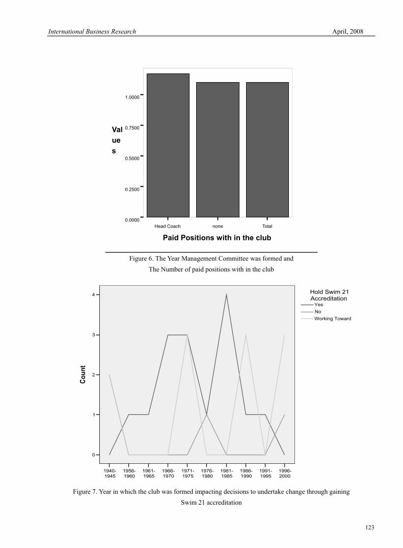
International Business Research April, 2008
123
Head Coach none Total
Paid Positions with in the club
0.0000
0.2500
0.5000
0.7500
1.0000
Val
ue
s
Figure 6. The Year Management Committee was formed and
The Number of paid positions with in the club
1996-2000
1991-1995
1986-1990
1981-1985
1976-1980
1971-1975
1966-1970
1961-1965
1956-1960
1940-1945
4
3
2
1
0
Co
un
t
Working Towards
No
Yes
Hold Swim 21Accreditation
Figure 7. Year in which the club was formed impacting decisions to undertake change through gaining
Swim 21 accreditation

Vol. 1, No. 2 International Business Research
124
The Analyze on Accounting Information
System of Third-party Logistics Enterprise
Su Yan
College of Economic and Trade, Shihezi University
Shihezi 832003, China
Tel: 86-993-259-5376 E-mail: [email protected]
Abstract
In the face of the fast developing of Information and technology and the appearance of the new management theory, the
author analyze the abuse of the conventional accounting system, and use the advance ideas on modern information and
technology (REA model and events drive) and the cooperation theory to redesign the frame of Accounting Information
System of Third party logistics enterprise, and point out the virtue of the new system.
Key words: logistics enterprise, Accounting Information System, REA, events drive
Since the sixties of the twenty century, the competition in market become more vehement, and the work divided become
more specific. In this backdrop, Information and Technology made a fast development and affect deeply other industries.
Third party logistics enterprise as a new industry is being influenced with it, and do change. Accounting is an
information system in enterprise, through the using of Information and Technology, Accounting not only enlarge own
scope, but also enhance the quality of service. But Accounting Information System in practice in our country now drop
terribly behind the practice demand and the development of its theory.
1. The analyze of conventional accounting system
The accounting information system in our country is on the foundation of Luca Pacioli’s accounting theory now, and it’s
core is accounting subjects. This system using original documents note the business activity occurred in enterprise and
the changed results of assets liabilities and equity caused by it, and depending on computer classify and compile this
notes, export to user in the form of the special report in the end. Though this system in that time was introduced with IT,
the basic framework of accounting information system was varied. As was said with professor Yun Gui Xue, now the
rule of the computerization information system is that modern technology suit to the regulation and it’s function
position, not but that, using the function offered with the modern technology reengineer the conversational accounting,
and the results are: 1 what the system stress on is the processing program of accounting and common absolute check
and calculation, and this system was close.2 the information the system collect process and use are after the event
absolutely, and don’t help the enterprise do management, control and decision-making.3 the system don’t settle for the
requirement of the supply-chain management.4 the system don’t settle for multi-user demand.(See Figure 1)
2. Rebuilding a new accounting Information System of Third party logistics enterprise
Followed the development of information technology, people’s ability of using information is getting stronger, and
information, as an important resource, in the operation and the decision-making process of enterprises play an important
role. Although third-party logistics enterprises is an emerging industry, but also the extent of competition is rather fierce,
in order to gain a firm place in the market and develop, every third-party logistics enterprises must use information
technology to reengineer it’s business processes and enhance it’s core competitiveness. Under the guidance of that
"supply chain is the third source of profit", the third-party logistics enterprises as parts of the chain was required in due
time and place to provide consumers with personality, specialization, and serialization of logistics services according to
the due price. At the same time, consumers also keep close relate to third-party logistics companies, so as to manage
and control the whole logistics process. According to Michael Porter's value chain management theory, we believe that,
in the value chain, the third-party logistics enterprise create the time and space value for the entire supply chain. The
essence of Accounting is the utilization of the means of value to reflect the enterprise's economic activity, and
ultimately meet the needs of accounting information. Third-party logistics enterprises through accounting methods
manage the economic business activities occurred in enterprises, but part of the economic business activities can not be
measured according to the monetary value, consequently bring the loss of business activities information. The
development of information technology has widened accounting measurement scales and changed the measurement

International Business Research April, 2008
125
scope of the third-party logistics enterprises accounting information system.
This paper mainly rebuilt the framework of third-party logistics enterprises accounting information systems by using
REA model, the revised E-R model and events driven approach. The so-called E-R model is a relationship data model
of classifying data information of entry system to by subject, respectively storing in a specific entity table, and
establishing the linkages between the corresponding form. REA model brought forward by the American scholar
William E. McCarthy's, and its main idea is to model the resource, the events and the agents of enterprise and the
relationship among them. Combining the two, the economic business activities in third-party logistics enterprises are
involved in the nature, the participants and the change of the enterprises’ resource. According to the principle of E-R
model, and all the enterprise objects can divided into three entities: events entities, resources entities and agent entities.
Each entity also can be divided into more specific entities, such as agent entities including employees, suppliers,
customers and other entities.
Following let’s example the warehousing activities of third-party logistics enterprises, and demonstrate the process of
designing model. (See Table 1)
"event-driven" is an idea in computer science, which is that most of the programs stored in database are events waiting
for the completion of some activities, users according to their own needs, implement the corresponding events, the
computer system respond to the events users make and transfer the particular procedure automatically to complete the
user's requirements. When the idea is applied to the accounting information systems, it is that when economic business
activities occurring, accounting information systems record the real situation of the activities, and don’t to do any
modification. Then, user-oriented event-driven procedures dealt with certain related economic business activities,
ultimately the information needed was extracted by the accounting information system. We call these event-driven
programs as unit events, which including not only accounting matters, but non-accounting matters. In short, it can be
said that it is matter oriented all user information needs.
Based on the above ideas, and the author implement value approaches and matters approaches, combining with modern
internal control technology, and rebuilt the framework of third-party logistics enterprise accounting information system,
the specific architecture as shown below (See Figure 2)
From a logical perspective, the system including four major parts: business process, entity record, event-driven and
usage of information.
(1) Business process. When business activities were at the time of the forthcoming, the enterprise's operational
departments requested to the accounting department's budget and Standard Management Centre, and reported the
business impropriating or spending resources, management control centre based on past experience and standards
budget decide whether the business occur, and timely inform the operational departments.
(2) Entity record. Operational departments based on good pre-recorded format do a real record on the economic
business of activities, and store it into entity DB. During this process, the accounting departments cooperate with the
operation departments; do a good job of canonical operating record.
(3) Event-driven. Users through the interface of man-pc, based on their own information needs, drive some program
stored in the Unite DB, the program will automatically transfer the data stored in entity DB and process, finally make
feedback to the users with the gained information.
(4) Usage of information. On one hand, accountant use the information make standard-setting, confirm the budget and
provide various accounting statements; on the other hand non-accountant refer to the information and other tools to do
decision-making and maximize their own interests.
Clearly, such a accounting information system is a decision-making-oriented, organic and open system with having an
effective internal control mechanism.
3. The advantages of the accounting information system
3.1 A good cooperation
Any thing is always linked to certain environment, exists and develops, third-party logistics enterprises in the supply
chain linking play a role of a bridge. Although the third-party logistics business as a separate entity exist in the market,
it and other enterprises still have to maintain a close relationship. This is because the consumers in order to ensure
normal operation of their production, they must understand and control the flow and the keeping of materials timely,
which calls that third-party logistics enterprises accounting information systems cooperate with up-downstream
enterprises, together control and manage the value-added activities occurred in the whole supply chain, and achieve
really supply chain competition. In addition, in the traditional enterprise organization mode, the enterprise's business
activities are divided in accordance with the functions and implement, so the lack of co-ordination between departments
the "islands of information" inevitably come into being. The new system really record and reflect the economic business
activities, do not require accountants note into the system according to the pre-format, consequently avoid duplication

Vol. 1, No. 2 International Business Research
126
of information collection and shortcomings; and accountant no longer were limited to the accounting departments, but
to participate in the enterprises operational activities to coordinate other departments do well accounting information
records and analytical work. In addition, other companies could line on a third party logistics enterprises accounting
information system through the Internet, timely query and know the flow situation of logistics, do well their production
plans.
3.2 To meet the needs of multi-users
With the change of the environment, the use objects of accounting information become expansion, including all levels
of enterprise management, all investment bodies outside, government agencies, intermediary organizations, and so on,
among them there are accountant and non-accountant. Traditional accounting information system can only generate
financial statements afforded to financial executive and fewer accounting information, which make the use objects
become narrow. But in the new system entity DB record all resources and economic business activities, users through
event-driven buttons on interactive interface can get the information they want. According to the value chain
management, any of the activities should be the value-added process, and account is a measure means of the value of
economic activity, therefore, any economic activity through the accounting information system can be measured and
reflected. However, as part of the current business activities can not be measured by money, and we are currently
unable to find suitable means of measuring the value, which caused some economic activities not reflected through
accounting information system.
3.3 To control afterwards, and control in advance and in concurrent
Account has the functions of supervision and control of the economic activities of the enterprise. And the traditional
manual account and of the computer accounting system for "accounting" can only do inspection afterwards, the
mistakes could not be avoided. New accounting information system integrate of real-time processing, the standard cost,
authorized the approval process control, budget management, and so on, so that employees based on the standard
budget, change from passive to active to manage their own activities, do Real-time check, control, and timely identify
problems, correct deviations and do truly Control afterwards, in advance and in concurrent.
Reference
Colanoni. C. S. R. P. Manes, and A. B. Winston(1971). “A Unified Approach to the Theory of Accounting and
Information Systems”. The Accounting Review. January,1971
Michael E. Porter Strategy and the Internet.(2001).Harvard Business Review, March
Ron Weber(1999), Information Systems Control and Audit. prentice-Hall, Inc., 1999
William E. McCarthy(1982).“The REA Accounting Model: A Generalized Framework for Accounting Systems in a
Shared Data Environment”,[J]. The Accounting Review, July 1982
Table 1. Simple warehousing activities and E—R entity table
E—R entity table economic
activities
Business
events events resources agents
warehousing
entry
safekeeping
leave
Entry requisition
Entry checker
Checked entry
checker
leave requisition
checked leave
inventory
storage
warehouseman
transport-team
stevedore
porter

International Business Research April, 2008
127
Figure 2 the framework of the accounting information system
Figure 1 the flow chart of the conventional accounting system

Vol. 1, No. 2 International Business Research
128
Intranet Redesign and Change Management: Perspectives on Usability
Des Flanagana
Thomas Acton (corresponding author)a
Michael Campiona
Seamus Hilla
Murray Scotta
aJ.E. Cairnes Graduate School of Business & Public Policy, National University of Ireland, Galway, Ireland
E-mail: [email protected] Tel: 353-91-493-806 Fax: 353-91-750-565
Abstract
As intranet implementations of enabling structures for internal electronic business communication increases, research is
needed to provide an insight into the factors affecting a successful intranet design (Tang 2000). Using a case study
involving a large multinational IT organisation, this paper studies changes made to the user interface design of a large
multinational organisation’s intranet and examines how that intranet’s usability has been affected by these changes from
both the managerial and employee end-user perspectives. The paper presents both a background on intranet design, its
links to the design of web-based systems, and intranet-focussed usability issues.
Keywords: Intranet, Usability, Redesign, Change Management
1. Introduction
To maximise their potential, Intranets must not be allowed to evolve in an ad-hoc manner. Often, Intranet projects have
been technology driven, being created for the sake of it (Tang 2000). An intra-organisational cross-departmental
approach to intranet design and evolution opens up data resources, corporate processes, and knowledge applications to a
wider base of users. As an organisation’s Intranet evolves with changing goals and usage patterns, it starts to focus on
knowledge creation as well as knowledge storage and access (Baker 2000). Behavioural and structural changes in
organisational work patterns are necessary if this potential is to be maximised. Motivation to create, use and share
information should be a primary, long-term critical success factor. Intranets are one mechanism enabling such
knowledge creation and sharing.
However, management motivation and commitment to mechanisms facilitating knowledge creation and
intra-organisational dissemination must be accompanied by employee ‘user’ buy-in. Intranet use should become part
of employee daily routines, and should not constitute ‘work’ (Tang 2000). Effective usage is dependent upon intranet
quality, strategic objectives and goals driving the usage, and alignment between the managerial aims and employee
needs. Users must be given access to well-integrated well-designed information sources that are timely, up-to-date,
maintainable and cost-effective. Intranets should provide fast and targeted access to relevant work- and
organisational-related information so employees can stay focused on the connection between their work patterns and
their company’s strategic objectives. This promotes co-ordinated thinking and actions among employees, as well as
maximising human resources (Denton 2003).
For an intranet to generate significant value-add, it must become the centrepiece of organisational strategy (Curry and
Stancich 2000). In order to use an intranet as a strategic tool, management must take a strategic approach to designing,
creating, maintaining and updating it. Companies aiming to gain competitive advantage from Intranet activities must
realise that technological solutions alone are not sufficient. Competitive advantage will stem from the management of
technology and effective use of resources (Gupta and Dale 1998).
This paper studies categorical changes made to the user interface design of a large multinational organisation’s intranet
and examine how that intranet’s usability has been affected by these changes from both the managerial perspective,
which focuses on the improvement of individual and workgroup performance, and employee ‘end-user’ perspectives.
It is hypothesised that individual and categorical design changes to the intranet will either positively or negatively affect
its usability. However, any such effects may be interpreted and regarded differently from management and end-user
perspectives. The paper begins by outlining the attributes central to the usability of an intranet. Following this the
research design is described in section 3. The findings are discussed in section 4 and finally the conclusion and
possible future work are outlined in section 5.

International Business Research April, 2008
129
2. From Intranets to Usability
Intranets are organisationally internal privately owned computing networks where access is only to authorised users.
Intranet applications differ in many ways including; users, tasks , types of information, amount of information available
(Nielsen 1997). Modern intranet design derives from implementations of Web-enabled technologies, encompassing and
facilitating multiple websites and web pages, and providing organisational resources such as e-mail, newsgroups, and
online meeting facilities (Baker 2000; Curry and Stancich 2000, Denton 2003). As intranet implementations of
enabling structures for internal electronic business communication increases, research is needed to provide an insight
into the factors affecting a successful intranet design (Tang 2000). However, as well as implementing a successful
intranet design it is also important to be aware that very effective intranets are often not the result of design alone, but
the continuous monitoring of user and business needs, and remaining aligned with current business strategies (Maurer
and Calabria 2004).
Whether an Intranet has been implemented as an operational tool or as a strategic/tactical-level vehicle, it must be
designed to be usable by employees. A number of attributes are central to the usability of an Intranet. The product
should be useful, easy to learn, easy to use and consistent (Gould and Lewis 1985; Palmer 2002). Authors such as
Lecerof and Paterno (1998) and Juristo et al. (2001) extend this list of attributes to also include memorability and
productivity. Whilst intranets are closed systems, they are derivations of web-based structures: usability has been
identified as a vitally important aspect of web-based systems (Juristo et al., 2001; Agarwal and Venkatesh, 2002;
Lecerof and Paterno, 1998).
Usability is in itself an umbrella term encompassing many subcomponents: as such usability cannot be measured in a
way that is consistent across studies examining the issue. However, usability is assessed through aggregated and
sometimes selective measurements of these subcomponents (Nielsen and Levy 1994). There are differences in opinion
regarding the particular components to use (Aladwani and Palvia 2002). Most authors include ease of use, ‘learnability’,
number of errors made during tasks, and satisfaction as measures of usability (Nielsen 2001; Carroll et al. 2002; Juristo
et al. 2001; Lecerof and Paterno 1998). Others extend this set to also include efficiency and emotion (Kim and Moon
1998; Agarwal and Venkatesh 2002; Lindgaard and Dudek 2002). Davis (1989) takes a different viewpoint,
maintaining that there has been widespread use of invalidated measures in terms of design, selection, implementation
and evaluation. Both Davis (1989) and Adams et al. (1992) regard successful usability including measures of perceived
usefulness and perceived ease of use.
Perceived usefulness is the extent, to which a system will help people do their jobs. Perceived ease of use refers to the
ease with which a user can use a system (Davis, 1989). Davis (1989) also shows that system usage is determined
primarily by its perceived usefulness, and secondarily by its ease of use, and advises not to put emphasis on ease of use
at the cost of functionality. Many authors comment that usability factors can be classified under subjective user
preferences and objective performance measures (Nielsen and Levy 1994; Agarwal and Venkatesh 2002; Kissel 1995).
In the past, focus has primarily been on objective measures, such as ‘learnability’, number of errors, and time needed to
complete tasks. Today, companies investing in online technologies need to see the benefits of their investments, and to
make this possible an appropriate tool for measuring the quality of their underlying systems must be identified
(Aladwani and Palvia 2002).
In terms of an ideal user interface, Shneiderman et al. (1998) states that an interface should be comprehensible,
predictable, and controllable. Colour should be applied both aesthetically and expressively, so it can be used as a
communication tool and add to the information being presented (Alben et al., 1994; MacDonald, 1999). Navigation
should be simplified through effective use of links, frames, text and buttons (Becker and Mottay, 2001). Agarwal and
Venkatesh (2002) state that content is a critical feature affecting usability, with Zhang and von Dran (2002) concluding
that customisation of content can increase the user experience. Catering for the diversity among end-users is a major
challenge for interface developers, who must know how certain users differ and what special needs they have
(Shneiderman and Hochheiser, 2001; Leventhal et al., 1994; Apple Computer Co., 1995; Huang, 2003).
3. Research Method
Using a case study involving a large multinational IT organisation, this research focuses on user interface changes made
to the design of that organisation’s worldwide intranet, analyses how that intranet’s usability has been affected by these
changes, and investigates the perceived effects of these changes on business processes and goals.
The 3-stage study involved a ‘top-down’ managerial-focussed qualitative method with a ‘bottom-up’ employee-based
quantitative approach. For this study, interviews and in particular telephone interviews were the chosen qualitative
methods for stages 1 and 2, while a quantitative web survey was adopted for stage 3 (see Table 1). The longitudinal
aspect allowed the impact of design changes on the organisations intranet to be assessed over a three month period.
The first two stages were qualitative, involving interviews with the five managers within the organisation who drove the
intranet design changes from the top-level. Prior to the implementation of any alterations to the existing intranet the

Vol. 1, No. 2 International Business Research
130
first set of interviews gathered data on why the intranet design changes were being sought. The second set of
interviews were conducted three months after the changes were introduced to explore whether the desired effects of the
changes had been realised from a managerial perspective. The third stage utilised a web survey to gather the
organisation’s employee ‘end-user’ opinions on the design changes and a frequency distribution of the results was
generated. This final stage occurred in parallel with stage 2. The purpose of each stage of the research is detailed
below.
3.1 Research Stage 1
Stage 1 involved a series of structured interviews with the sample population of managers championing the changes to
the Intranet in order to gain an understanding of the drivers for the intranet design changes and of this sample’s initial
satisfaction levels with the design changes. The central purpose of Stage 1 was to allow the researcher to gain an
understanding of the rationale behind the design changes to the intranet.
In addition, Stage 1 was intended to gather data on possible usability improvements arising from the design changes
from the point of view of those who drove the project.
3.2 Research Stage 2
Stage 2 was a similar series of structured interviews with the same sample of managers to determine each manager’s
evaluation of the design changes after a three month period had elapsed, and to compare this evaluation to the
expectations that each manager had for the design changes when the first set of interviews were carried out in Stage 1.
The central purpose of Stage 2 was to obtain data reflecting how the participants of Stage 1 perceived the intranet’s
design changes following a three month period for the organisation to become accustomed to the changes. The thoughts
of the participants at this stage of the research were then compared to their expectations when Stage 1 was carried out.
The primary objective of carrying out interviews for Stage 1 and, at a later date, for Stage 2 was to allow the managers
who were driving the Intranet changes to share their experiences on implementing the design changes and to give their
opinions on the success of the changes after an elapsed period. This qualitative and interpretivist approach allowed the
themes that arose from the interview questions in Stage 1 to form the basis for the interview questions for Stage 2.
3.4 Research Stage 3
Stage 3 consisted of a web-based survey, completed by over 30 employees who were end-users of the intranet. The
main purpose of stage 3 was to gather data from the end-users regarding their opinions on the usability of the intranet
following the design changes and to compare employee viewpoints (as end-users) to management intentions and views.
A survey was the research approach chosen as its focus is on extracting data which allowed the researcher to understand
the underlying principles driving the intranet changes. Past literature deems the survey approach suitable for gathering
data on specific topics under study (Adams, 1992; Caldwell and Uang, 1995; Chau and Hu, 2002; Kwahk and Han,
2002; Gelderman, 1998). Also, reliable survey instruments such as structured interviews were well suited for this
stage of research. The use of structured interviews for data collection helped address the primary and secondary
objectives outlined above and to ensure valid and reliable results are gathered from this study, all participants chosen for
the interview stages had adequate knowledge of the topics under study.
4. Findings
This research focuses on categorical changes made to the user interface design of the intranet of a large multinational
organisation, specifically:
Colour change of elements on the webpage;
Change in appearance of images;
Change in design of horizontal navigation.
The research also examines how that intranet’s usability has been affected by these changes both from the perspective of
management and that of employee ‘end-users’ It investigates improvements in information retrieval as well as the issue
of change management and the willingness of end-users to embrace the changes made to the intranet. The main
findings are outlined below.
4.1 Colour Usage
All interviewees acknowledged that the change in colour scheme of a number of elements on the intranet were driven
by the Global Branding Communications team within the organisation under study, to allow for consistency across not
only the portal, but everything that comes out of the marketing side of the organisation. This includes a move to align
and streamline the look and feel of the organisation. It also allows the organisation to communicate one brand to the
customer, both internally and externally.
With regard to the portal, the goal of having a new visual identity was to transition the organization’s brand elements

International Business Research April, 2008
131
from purely external-facing to internal-facing, thus uniting employees under one common identity. There was also
expectation that a new visual identity would drive cost improvements across the entire corporation as too many people
had been doing their own thing. This could be achieved by removing many of the inconsistencies about the intranet’s
look-and-feel, and everything that contributes to the brand identity.
An additional motive for changing the colour scheme was the Americans with Disabilities Act (A.D.A.) which details
the types of changes that should be made to a website to make it more user-friendly for users that have disabilities of
one sort or another, but typically visual impairment.
The colour change of a number of elements on the webpage was, to a large extent, a success in that the expectations
associated with this design change were met. Consistency was promoted on the intranet through the colour change of
both the background of the webpage and the horizontal navigation. This is consistent with findings from a study by
Becker and Mottay (2001) who outline that consistency should relate to both the colour of the background of the
webpage, and the colour of the links used throughout the website. The white background was found to tie-in well with
the black horizontal navigation which may be because, as MacDonald (1999) points out, maximising the contrast
between elements on the webpage improves look-and-feel and hence promotes consistency.
However, the colours used for the horizontal navigation were found to create confusion regarding what’s highlighted
and what’s not. This may be due to the fact that the colours used in the horizontal navigation do not stand out as well as
users would like. One possible solution may be to use colours which complement each other and hence minimise
confusion as outlined by Ling and van Schaik (2002) who state that the navigation area should be given special
attention, with attention-grabbing colour being placed here rather than the content area of the web page. A primary
motive for changing the background colour of the webpage was to promote usability. The white background was found
to provide the greatest readability to the user and to also care for people with visual impairment, which feels may be due
to a high level of contrast on the webpage improving performance, as found in a study by MacDonald (1999).
The change in colour scheme of the banner at the top of the webpage was viewed as a limited success by participants
who took part in this study. The decision to change the colour scheme from being one constant colour to rotating
through a palette of colours on a daily basis was driven by the Global Branding Communications team within the
organisation as the new company identity is tied in to an entire palette of colours and not just one in particular.
On the positive side, consistency across the intranet was improved as a result of the colour scheme changing on a daily
basis. This may be due to the fact that appropriate use of colour can improve the effectiveness of graphical displays, as
outlined by Ling and van Schaik (2002). This design change also influenced the usability of the intranet as the colour
scheme used for the top banner accentuated familiarity among end-users for the intranet. This appears to illustrate that
the consistent use of a complementary colour scheme, coupled with the use of quality graphic design, can help users to
become familiar with an interface, as found in studies by Rosen and Purinton (2002) and Ling Ngo et al. (2003).
However, a number of important problems arose with this design change to the banner. For example, the rotating colour
in the banner limits the range of colour that can be used elsewhere on the webpage, as there may be a clash with the
colour being used in the banner on any given day. One explanation for these negative side-effects may be provided by
Budgen (1995), who acknowledges the number of problems that may result from interface design changes, and
concludes that the design team can face tricky situations, as addressing one problem to improve usability may open up
other, more complicated problems.
4.2 Imagery
The change in the appearance of images used on the intranet, in terms of both image size and shape, was once again
driven by the Global Branding Communications and it helped to promote consistency throughout the portal. It was
also felt that the previous round-cornered images had been a design style of the organisation under study, and therefore
a new cleaner style was required and that the rounded corners should be discarded. For this reason a crisp
square-corner design was chosen. The image size was standardised to tie in with the overall new image design style.
Expectations regarding the change in image size and shape were met, with the square-shaped images of a standardised
size promoting a consistent look-and-feel. No impact on usability was expected, nor was realised. The changes in the
appearance of images may have had a positive effect on consistency because of the cleaner style with which the
square-shaped images promoted. Nielsen and Sano (1994) state that consistent design techniques applied to graphic
elements increases user satisfaction across an entire site.
4.3 Navigation
The primary motive in changing the navigation structure of the intranet from a drop-down menu to a two-level
horizontal menu was to increase usability and assist users better in determining their current and previous locations on
the intranet. This was only a minor success. Incorporating two horizontal levels of navigation reduced the number of
users getting lost while browsing through the intranet, and hence contributed to improving productivity. This may be

Vol. 1, No. 2 International Business Research
132
due to the improved efficiency experienced from deploying the new navigational system which, according to Palmer
(2002), can make information easier to find and more relevant to the user. In turn, this can improve employee
productivity, according to Nielsen (2001).
However, usability improvements emanating from the two-level horizontal navigation system were found to be
compromised by having the links on the vertical or left navigation listed in alphabetical order. Usability training has
shown that only long alphabetical lists are user-friendly. For short lists, like those used on the Intranet’s vertical
navigation, it’s extremely important to put them in order of importance, or some kind of grouping that puts similar
things together. This was found to hinder fast information retrieval which may be due to less important information
being displayed on the webpage than if the links were listed in order of importance. A study carried out by Shneiderman
and Chimera (1994) found that online browsing can be enhanced by interface designs that display appropriate
information in appropriate places.
4.4 Informational Retrieval
In carrying out the design changes with the aim of implementing a “breadcrumb trail”, the organisation under study had
hoped to achieve faster information retrieval for users of the intranet. However, findings from this research indicate that
this has not been a success. Although users have been provided with a visual clue of their navigational path, the visual
clue has been found to be just another way of finding information on the intranet. Therefore it is felt that, contrary to a
study carried out by Weinreich and Lamersdorf (2000), integrating the user’s history into the navigation trail is not
enough to improve information retrieval. What may be needed is a more consistent hierarchy across the intranet to
allow users have an improved logical understanding of their whereabouts in the navigation structure. Palmer (2002)
supports this, stating that navigation is influenced by the sequencing, layout, and arrangement of the website.
This research also found that accurate labelling of links facilitates faster information retrieval on an intranet. This may
signify that accurate labels minimise confusion among users who become more knowledgeable on which links to follow
and which to ignore. Weinreich and Lamersdorf (2000) and Kopetzky and Muhlhauser (1999) support this finding,
stating that there results a cognitive overhead from the extra effort needed to follow several navigation trails at the one
time. This dilemma has long been associated with users wondering whether they should follow a link or not, and could
be reduced by an improvement in link capabilities or by providing an overview of the hyperspace.
Incorporating customisable features into the interface design can also enhance information retrieval on an intranet, as
this research has found. When carrying out the design changes to the intranet under study, the personalisation of links
which had existed on the previous design was eliminated, and this was found to have had a detrimental effect on
information retrieval. The results from this research support Curry and Stancich (2000) in stating that this may be due
to the apathy among users for mass communication, when instead, according to Perrott (2001), information on an
intranet should be targeted at employees, and interactive features added.
4.5 Change Management
Change management was found to be a factor in limiting the success of the intranet design changes. Caused by the
dislike among employees for change, users had to grow to accept the change to the horizontal navigation, rather than
embrace it. This may have been due to inadequate communication from top management regarding the changes in
employee behaviour that were needed in order to make the two-level horizontal navigation structure a greater success.
This is consistent with findings from a study by Curry and Stancich (2000) who state that, when redesigning an Intranet,
behavioural and structural changes in the organisation’s work patterns will be needed in order to maximise its potential.
Top-down commitment, according to Tang (2000), must be accompanied by bottom-up employee buy-in.
5. Conclusions
This research studied the design changes made to an organization’s intranet, and analysed how the intranet’s usability
was subsequently affected. The colour change of a number of elements on the webpage was, to a large extent, a
success in that the expectations associated with this design change were met. Consistency was promoted on the intranet
through the colour change of both the background of the webpage and the horizontal navigation. However, the colours
used for the horizontal navigation were found to create confusion regarding what was highlighted. A primary motive
for changing the background colour of the webpage was to promote usability. The change in colour scheme of the
banner at the top of the webpage was viewed as a limited success by participants who took part in this study.
Expectations regarding the change in image size and shape were met, with the square-shaped images of a standardised
size promoting a consistent look-and-feel. No impact on usability was expected, nor was realised. The primary motive
in changing the navigation structure of the intranet from a drop-down menu to a two-level horizontal menu was to
increase usability. and was only a minor success. However, usability improvements emanating from the two-level
horizontal navigation system were found to be compromised by having the links on the vertical or left navigation listed
in alphabetical order. This was found to hinder fast information retrieval which may be due to less important
information being displayed on the webpage than if the links were listed in order of importance.

International Business Research April, 2008
133
Results also indicate that accurate labelling of links facilitates faster information retrieval on an intranet, and that
information retrieval on an intranet can also be enhanced by incorporating customizable features into the interface
design. When carrying out the design changes to the intranet under study, the personalisation of links which had existed
on the previous intranet design was eliminated, and this was found to have had a detrimental effect on information
retrieval. Finally, change management was found to be a factor in limiting the success of the intranet design changes.
Caused by the dislike among employees for change, users had to grow to accept the change to the horizontal navigation,
rather than embrace it. This may have been due to inadequate communication from top management regarding the
changes in employee behaviour that were needed in order to make the two-level horizontal navigation structure a
greater success.
The purpose of this research was to study categorical changes made to the user interface design of the intranet of a large
multinational organisation and examine how that intranet’s usability had been affected by these changes from both the
managerial and employee ‘end-user’ perspectives. The overall findings indicate that although the redesigning of the
user interface was largely successful, the degree of success was to a large extent based upon the management of the
changes which was found to be a factor in the successful implementation of the intranet redesign.
Future work extending from this research includes examining whether the difficulties encountered by users in deciding
whether to follow a link or not could be reduced by an improvement in link capabilities or by providing an overview of
the hyperspace; analysis of interface designs that display information in appropriate places to provide enhanced online
browsing; and further study on employee targeting of intranet information.
References
Adams, D. A., Nelson, R. R. and Todd, P. A. (1992) Perceived usefulness, ease of use, and usage of information
technology: A replication, MIS Quarterly, 16 (2), pp. 227-248.
Aladwani, A. M. and Palvia, P.C. (2002) Developing and Validating an Instrument for Measuring User-Perceived Web
Quality, Information and Management, 39, pp. 467-476.
Alben, L., Faris, J. and Saddler, H. (1994) Making it Macintosh: designing the message when the message is design,
Interactions, 1 (1), pp. 11-20.
Agarwal, R. and Venkatesh, V. (2002) Assessing a Firm's Web Presence: A Heuristic Evaluation Procedure for the
Measurement of Usability, Information Systems Research, 13 (2), pp. 168-187.
Apple Computer Co. (1995) Macintosh Human Interface Guidelines.
Baker, S. (2000) Getting the most from your Intranet and extranet strategies, Journal of Business Strategy, 21, p. 40.
Becker, S. A. and Mottay, F. E. (2001) A global perspective on website usability, IEEE Software, pp. 54-61.
Budgen, D. (1995) Design Models from Software Design Methods, Design Studies, 16, pp. 293-325.
Caldwell, B. S. and Uang, S. T. (1995) Technology Usability and Utility Issues in a State Government Voice Mail
Evaluation Survey, Human Factors, 37 (2), pp. 306-320.
Carroll, C., Marsden, P., Soden, P., Naylor, E., New, J. and Dornan, T. (2002) Involving users in the design and usability
evaluation of a clinical decision support system, Computer Methods and Programs in Biomedicine, 69 (2), pp. 123-135.
Chau, P. Y. K. and Hu, P. J. (2002) Examining a Model of Information Technology Acceptance by Individual
Professionals: An Exploratory Study, Journal of Management Information Systems, 18 (4), pp. 191-230.
Curry, A. and Stancich, L. (2000) The intranet - an intrinsic component of strategic information management,
International Journal of Information Management, 20, pp. 249.
Davis, F. D. (1989) Perceived Usefulness, Perceived Ease of Use, and User Acceptance of Information Technology, MIS
Quarterly, September, pp. 318-340.
Denton, D. K. (2003) Use an Intranet for Performance Measurement., Industrial Management, 45, p. 28.
Gelderman, M. (1998) The relation between user satisfaction, usage of information systems and performance,
Information & Management, 34 (1), pp. 11-18.
Gould, J. and Lewis, C. (1985) Designing for usability: Key principles and what Designers think, Communications of
the ACM, 28(4), pp. 300-311.
Gupta, A. S. and Dale O. (1998) Managing computing resources in intranets: an electronic commerce perspective.,
Decision Support Systems, 24, pp. 55.
Huang, A. H. (2003) An Empirical Study of Corporate Web Site Usability, Human Systems Management, 22, pp. 23-36.
Juristo, N., Windl, H. and Constantine, L. (2001) Introducing usability, IEEE Software, 18 (1), pp. 20-21.

Vol. 1, No. 2 International Business Research
134
Kim, J. and Moon, J.-Y. (1998) Designing towards emotional usability in customer interfaces-trustworthiness of
cyber-banking system interfaces, Interacting with Computers, 10 (1), pp. 1-29.
Kissel, G. V. (1995) The effect of computer experience on subjective and objective software usability measures,
Conference on Human Factors and Computing Systems, Denver, CO USA, May 7 - 11, pp. 284-285.
Kopetzky, T. and Muhlhauser, M. (1999) Visual preview for link traversal on the World Wide Web, Computer Networks,
31 (11-16), pp. 1525-1532.
Kwahk, J. and Han, S. H. (2002) A methodology for evaluating the usability of audiovisual consumer electronic
products, Applied Ergonomics, 33 (5), pp. 419-431.
Lecerof, A. and Paterno, F. (1998) Automatic support for usability evaluation, IEEE Transactions on Software
Engineering, 24 (10), pp. 863-888.
Leventhal, L., Teasley, B. and Stone, D. (1994) Designing for diverse users: will just a better interface do?, Proceedings
of the CHI '94 conference companion on Human factors in computing systems, Boston, USA, April 24 - 28, 1994,
Boston United States, pp. 191-192.
Lindgaard, G. and Dudek, C. (2002) What is this evasive beast we call user satisfaction?, Interacting with Computers,
15, pp. 429-452.
Ling, J. and van Schaik, P. (2002) The effect of text and background colour on visual search of Web pages, Displays, 23
(5), pp. 223-230.
Ling Ngo, D. C., Teo, L. S. and Byrne, J. G. (2003) Modelling interface aesthetics, Information Sciences, 152 25-46.
Maurer D. and Calabria T. (2004) 10 Ways to continuously improve your intranet, [Online],
http://www.steptwo.com.au/papers/kmc_continuousimprovement/pdf/KMC_ContinuousImprovement.pdf
MacDonald, L. W. (1999) Using color effectively in computer graphics, Computer Graphics and Applications, IEEE, 19
(4), pp. 20-35.
Nielson, J. (1997) The Difference Between Intranet and Internet Design, [Online], useit.com, available at
http://www.useit.com/alertbox/9709b.html
Nielsen, J. (2001) Novice vs. Expert Users, Vol. 2001, [Online], useit.com, available at
http://www.useit.com/alertbox/20000206.html
Nielsen, J. and Levy, J. (1994) Measuring usability: Preference vs. Performance, Communications of the ACM, 37 (4),
pp. 66-76.
Nielsen, J. and Sano, D. (1994) Design of SunWeb - Sun Microsystems' Intranet, [Online], useit.com
http://www.useit.com/papers/sunweb/
Palmer, J. W. (2002) Web Site Usability, Design, and Performance Metrics, Information Research, 13 (2), pp. 151-167.
Perrott, N. (2001) Intranets: Considering the User Experience, Strategic Communication Management, 5, pp. 32.
Rosen, D. E. and Purinton, E. (2002) Website Design: Viewing the Web as a Cognitive Landscape, Journal of Business
Research, pp. 1-8.
Shneiderman, B. and Hochheiser, H. (2001) Universal usability as a stimulus to advanced interface design, Behaviour &
Information Technology, 20, pp. 367-376.
Shneiderman, B., Byrd, D. and Croft, W. B. (1998) Sorting out searching: a user-interface framework for text searches,
Communications of the ACM, 41 (4), pp. 95 - 98.
Shneiderman, B. and Chimera, R. (1994) An exploratory evaluation of three interfaces for browsing large hierarchical
tables of contents, ACM Transactions on Information Systems, 12 (4), pp. 383-406.
Tang, S. M. (2000) An impact factor model of Intranet adoption: an exploratory and empirical research., Journal of
Systems & Software, 51, p. 157.
Weinreich, H. and Lamersdorf, W. (2000) Concepts for improved visualization of Web link attributes, Computer
Networks, 33 (1-6), pp. 403-416.
Zhang, P. and von Dran, G. M. (2002) User Expectations and Rankings of Quality Factors in Different Web Site
Domains, International Journal of Electronic Commerce, 6 (2), pp. 9-33.

International Business Research April, 2008
135
Table 1. Research Stages
Stage Research
Approach
Method Source Research Focus
1 Qualitative Individual
Interview
Managers Rationale for the intranet design changes;
potential usability improvements from
the proposed changes
2 Qualitative Individual
Interview
Managers Extent to which desired effects had been
realised
3 Quantitative Web-based
survey
Intranet
end-users
End-user opinions of the usability of the
Intranet after the design changes

Vol. 1, No. 2 International Business Research
136
Actuality Analysis and Development
Measures of China Enterprise Credit Rating
Haiqing Shao
College of Business Administration, Shandong University of Finance, Jinan 250014, China
Tel: 86-136-8531-1979 E-mail: [email protected]
Abstract
The enterprise credit rating in China is the new thing with continual advances of China economy and financial system
reform, and it still has many problems need to be researched and solved. This article firstly points out problems existing
in China enterprise credit rating, then analyzes reasons of these problems, and finally puts forward measures to develop
China enterprise credit rating.
Keywords: Enterprise credit rating, Credit, Risk
The enterprise credit rating in China is the new thing with continual advances of China economy and financial system
reform. After almost twenty years’ development, at present, China enterprise credit rating has had certain bases. But we
still should see that the developmental history of China enterprise credit rating is short after all, comparing with the
hundreds years’ history of international rating industry, it is still young, and many problems existing need to be further
researched and solved.
1. Main problems existing in China enterprise credit rating
1.1 The social effect of enterprise credit rating is not obvious
At present, China enterprise credit rating has not been recognized by all circles in the society, and the results of
enterprise credit rating are less utilized. However the result of international enterprise credit rating has acquired
effective utilization by all circles in the society, and governmental supervisory departments utilizes it to enhance the
supervisory efficiency, and enterprises utilize it to enhance its social reputation, and banks utilize it to reduce their credit
risks, and investors utilizes it to acquire investment incomes. But most results of China enterprise credit rating are only
used in the credit risk management of banks, and other domains still can not hear the voice of the enterprise credit rating,
which makes the function of credit rating suffer large limitation, and social effects can not be fully applied.
1.2 The result of enterprise credit rating is not just
The justice of rating result should be the most basic characteristic of credit rating. However, at present because of
various reasons, the result of China enterprise credit rating has not been ensured to be objective and just. Almost any
enterprise can acquire the good credit rate above “A” class, which doesn’t match with the actuality of credit losing in
China today and cannot but make people doubt the authenticity of the result, and also influences the social image of
enterprise credit rating to a certain extent.
1.3 The rating personnel is deficient and the personnel quality needs to be enhanced
The absence of professional personnel, especially the absence of rating experts has become the key problem to restrict
the development of enterprise credit rating. At the same time, most China rating personnel comes from various banks or
relative departments, who lack the practice experiences and theoretic bases of rating and have low professional qualities
at large. And at present, China has no the occupation qualification exam of enterprise credit rating, and lacks the
uniform standard to choose rating personnel, which makes the qualities of rating personnel different and can not adapt
the further development of rating operation.
1.4 The setup of rating index system needs to be further regulated
The setup of rating index system is the core problem to implement enterprise credit rating, which is directly associated
with the science of final rating result. At present, in China the setups of enterprise credit index is not uniform, and the
rating standard and principal are different, various rating institutions have large differences, which makes the rating
result jumbled.
2. Analysis of reasons of problems existing in China enterprise credit rating

International Business Research April, 2008
137
2.1 The market demand of Enterprise credit rating is seriously deficient
The market demand to the enterprise credit rating is its base to exist and develop. However, the present enterprise credit
rating in China has not be enough emphasized by the market, which is mainly embodied in two aspects. On the one
hand, those enterprises which are influenced by old concepts and habits in the period of the planned economy have low
enthusiasms to the credit rating. On the other hand, investors’ risk consciousness is weak and they don’t emphasize the
function of rating. That makes China enterprise credit rating run into the difficulty of “awaiting rice to cook”, and the
deficiency of market demand has become the most essential reason to limit its development.
2.2 The environment of credit data needs to be improved
Sufficient and true credit data is the premise to implement credit rating for enterprises, and the deficiency of enterprise
credit data and false credit information all will seriously influence the objectivity and justice of credit rating result.
However, in China, the opening degree of present credit data is very low, which makes the rating institutions hard to
acquire sufficient information needed by the rating through open channels. More seriously, false information of
enterprises prevail, which undoubtedly makes the authenticity of rating result suffer serious damage and blocks the
healthy development of credit rating.
2.3 The rating institution has large quantity, small scale and nonstandard operation
The credit rating industry is the industry which has obvious scale incomes, and in a matured market, its quality should
not be too much, or else it cannot but induce the unordered competition of various rating institutions and influence the
healthy development of the whole industry. As viewed from the international rating market, the setup of rating
institution basically accords with this industrial characteristic. Take US which has the most developed rating industry as
an example, the number of the rating institution which can broad develop operation in the market is about five. This
number in other countries is about two in substance. Though China credit rating operation has only short tens years’
developmental history, but the development of the rating institution is very quick, and the present quantity of the rating
institution are still tens after neatening. Under the situation that the present capital market is not developed and the
market demand is deficient in China, the quality of the rating institution is obvious overabundance. And most of these
rating institutions have small scale, which enrollment capital is in 1 million Yuan to 3 million Yuan and the number of
professional personnel doesn’t exceed 100. Up to now, China still lacks the recognized and authoritative rating
institution with a certain scale and broad influences, especially the rating institution with international influences.
Numerous rating institutions exist in a market which has deficient demand, and the malignant competition among them
is inevitable. To exist, some rating institutions cooperate with enterprises to add class and demand a low price without
credit standing. Drastic market competitions compel some rating institutions to adopt the method of non-market to
implement unfair competition, which seriously pollutes the rating environment and influences the healthy development
of the credit rating industry.
2.4 Collaboration and communication are deficient in industries
First, China still has not a uniform and authorized industrial management institution in the domain of enterprise credit
rating, and the rating operation lacks the guidance of the industry, and each rating institution does things in its own way,
and associations, collaboration and communication are lacked among various rating institutions. That blocks the further
improvement of the enterprise credit rating theory and actual operation level. Second, the rating institution has the
tradition of secrecy for the technology and methods in rating which generally can not be opened, which also weakens
the cooperation and communication among institutions to a certain extent and makes against the mutual advance and
development of this industry.
2.5 Professional education and training are deficient
The normal education in the present credit rating domain of China is almost blank, and there are no relative colleges to
open courses in this domain. Books and magazines about enterprise credit rating relative occupation trainings are
deficient, which makes the theoretic level of credit rating can not be enhanced, a large of eligible rating employees can
not be fostered, and this situation seriously restricts the healthy development of enterprise credit rating.
3. Development measures of China enterprise credit rating
Based on main problems and reasons existing in present enterprise credit rating of China, in order to make China
enterprise credit rating acquire further healthy development, we need perfect and improve it from many aspects.
3.1 Cultivating the market base making for the development of enterprise credit rating
The market base to make for the development of enterprise credit rating is to extend the demand of market to enterprise
credit rating, which is the key to clean the developmental obstacle of enterprise credit rating from the essential. The
developmental level of enterprise credit rating in the final analysis depends on the developmental situation of the market
economy of one country, especially the perfection degree of the capital market. So to foster the market environment
which makes for the development of China enterprise credit rating, we need fully develop and regulate the capital

Vol. 1, No. 2 International Business Research
138
market and let more enterprises financing through the mode issuing stock and bond to the society. Under this situation,
whether the enterprise can obtain capitals in the market depends on whether the credit of this enterprise is good. If the
credit of the enterprise is good, investors will invest and the enterprise will easily acquire more capitals, or else, the
enterprise cannot acquire enough capitals and its development will be blocked. Under the condition of interest rate
marketization, high credit rate always means low financing costs. Therefore, enterprises will actively utilize rating
institution and credit rating to introducing themselves in order to favorably implement financing. Facing numerous good
and evil financing enterprises mixed up, investors exact the rating result of professional rating institutions to know
issuers’ credits to reduce the investment risk. In order to maintain the stabilization and healthy development of capital
market, the government management departments need broadly referring the result of enterprise credit rating to
selectively supervise the capital market. To fully develop the capital market and cultivate the market base making for
the development of enterprise credit rating must offer growth fertile soil for the development of the enterprise credit
rating.
3.2 Actively constructing the credit environment making for the development of enterprise credit rating
To construct the credit environment making for the development of enterprise rating development, we first should fully
advocate the credit consciousness and form the social fashion of honest and faith, and make the concept of “glory for
keeping credit, shame for losing credit” go into people’s heart. Second, facing the actuality that the acquirement channel
of the credit data is not free and the quality of the credit data is low, we should expedite to establish good credit data
environment. To do that, one the one hand, relative laws should be instituted to expedite the opening of the credit data
and ensure the authenticity of the data. Except for coming down to national secrets and business secrets of enterprises
needed to be protected, it should force relative department of the government and relative social parties to publish other
various credit information through the mode of business or obligation and in different degree of opening in order to
make credit rating institutions can fully utilize opening enterprise credit information. At the same time, the authenticity
of information published by various relative departments should be ensured, and relative departments and principals
publish false information should be run law responsibilities to cleanse the credit information environment. On the other
hand, under the present condition that enterprise credit data is dispersive, the government should drive the united
collection and resource sharing of enterprise credit data among various departments and various regions, and establish
the complete, integrated and dynamic enterprise credit database covering the whole country, and offer necessary basic
establishment for the development of enterprise credit rating.
3.3 Strengthening the standard management to the credit rating industry
At present, the development of the credit rating industry is still in the elementary stage in China, and because
corresponding laws and regulations are deficient and there are no standard managements of guild, unordered situation
occurs in the development of the credit rating industry. As a aspect of the credit rating industry, the enterprise credit
rating system should strengthen the uniform management to the credit rating industry, regulate its operation behavior
and establish good work orders if it want to acquire healthy development. That can be started from following two
aspects.
3.3.1 Establishing and perfecting laws and regulations of the credit rating industry
In China, the resent legislation in the aspect about credit rating is seriously lagged, and there is no a complete and
specific law to regulate this industry, and only a few relative laws and regulations involve that, and most contents are
dispersive and abstract. This situation obviously can not adapt the developmental actuality of the credit rating industry.
Relative departments of China should expedite to establish and perfect laws and regulations of credit rating industry,
make specific and complete regulations to the admittance condition of the credit rating industry, rating objects, use
range of rating result, rating personnel’s occupation qualification, operation rules of the credit rating, and law
responsibilities of rating institutions to ensure the standard and healthy development of the credit rating industry.
3.3.2 Strengthening the industry self-discipline
Authoritative and standard industrial organization is propitious to advance the collaboration and communication among
credit rating institutions, enhance the whole level of the industry, and assist relative departments of the government to
manage the credit rating industry. The main functions of guild should include instituting industrial rules, supervising
and managing works of various credit rating institutions, calling in national credit rating meetings at fixed period,
strengthening associations, collaborations and information communication of various institutions, researching and
instituting uniform rating principles and standard and improving the rating technology to ensure the coherence of rating
results, strengthening the training of rating personnel and organizing the qualification exam of rating personnel, fronting
for national credit rating publication, advancing academic communication at every turn and publishing the rating results
of various rating institutions uniformly, strengthening association and communication with relative departments of the
government, and advancing the formation of national and uniform credit rating market system.
3.4 Strengthening the construction of rating personnel

International Business Research April, 2008
139
Because the activity of enterprise credit rating is a complex work with difficulties, so the requirement to rating
personnel’s comprehensive quality is very high. The rating personnel should not only possess diversifiable knowledge
structure, grasp professional knowledge such as economy, management, finance, financing, auditing and law, but also
have abundant experiences, strong analysis ability and good professional moral level. But any individual can not master
all knowledge and abilities needed, so a professional rating personnel group should be fostered, and the group includes
not only talents who master economic management, but talents who know well national laws and policies, includes not
only talents who are good at the macro environment, but talents who are good at analyzing the interior management of
the enterprise, includes talents who are good at qualitative analysis, but talents who fit for quantitative analysis.
Through reasonable selection and combination, professional rating personnel group with mutual compensation of
knowledge and ability structure can be gradually formed.
3.5 Establishing and strengthening scientific index system of enterprise credit rating
Though concrete rating indexes of various rating institutions differ in thousands ways, but scientific and standard rating
index system should include following factors keeping to principles such as integration, system, the combination of
universality and particularity, and the combination of international standard and Chinese situation.
3.5.1 The quality of the management layer
This mainly includes managers’ individual quality and ability, and the cohesion force and management level of the
whole management layer. Whether managers, especially the high-layer mangers, possess the moral characters of honest
and faith will decide whether enterprises possess the will to active pay loans and debts. And the management ability of
managers and management layer will decide whether enterprises can continually develop in the drastic competition, and
finally decide whether enterprises have enough cashes to pay loans and debts.
3.5.2 Financial status
It is the most basic factor to implement enterprise credit rating. Based on the analysis of B.S., profit sheet and cash flux
sheet of enterprises, the fluidity, security and profit of enterprise assets should be mainly reviewed, which concretely
include capital strength, profit ability, cashing ability and transportation ability and other factors.
3.5.3 Situations of management and market competition
The basic situation of enterprise itself should be mainly reviewed. The management and market competition situation
should be comprehensively evaluated from many aspects such as enterprise scale, employee quality, development
strategy, operation strategy, organization structure, management mode, market sharing rate of product, market
development ability and so on.
3.5.4 Environmental factors
Exterior environment and developmental tendency faced by enterprise should be mainly studied, which includes factors
such as competition situation, development tendency and periodicity of enterprises in the industry, and factors such as
economic environment, national policies, laws and regulations of enterprises in the country and region.
References
He, Shujie. (2000). Moody and Its Credit Rating System. Finance Forum. No.8.
Pang, Jianmin. (2006). Analysis and Thinking of Foreign and Domestic Enterprise Credit Rating. Shandong Social
Science. No.2.
Wu, Jingmei. (2001). Credit Evaluation. Beijing: China Auditing Press. Jan, 2001.
Yu, Chenxi. (2001). History and Development of Credit Rating. China Urban Finance. No.2.
Zhangwei, et al. (2007). Regulatory Models of Credit Rating Agencies: A Global Perspective. Studies of International
Finance. No.9.
Zhu, Shunquan. (2002). Innovation and Application of Enterprise Credit Rating Method. Chengdu: Southwestern
Finance and Economics University Press. Jan, 2002.

Vol. 1, No. 2 International Business Research
140
Efficiency of Rural Banks: The Case of India
Professor Dilip Khankhoje
National Institute of Bank Management, Pune, India
Dr Milind Sathye (Corresponding author)
School of Business and Government
University of Canberra
Bruce ACT 2617, Australia
Tel: 61-2-6201-5489 Fax: 61-2-6201-5238 E-mail: [email protected]
Abstract
The objective of this paper is to investigate whether the restructuring of regional rural banks in India –undertaken in
1993-94 - has helped improve their production efficiency. Several committees have emphasized the need to improve
the efficiency of these banks which are an important arm of the rural credit system in India. Improved production
efficiency in provision of services would mean lower cost and financially sustainable operations. Production efficiency
has been measured using a non-parametric technique of Data Envelopment Analysis (DEA). To measure efficiency
most directly, interest income and non-interest income were used as outputs and interest expenses and non-interest
expenses were used as inputs. Efficiency scores were calculated for the years 1990 to 2002. Thereafter these scores
were compared for before and after the restructuring year (1993-94). The study finds that efficiency of rural banks has
significantly improved after restructuring. It seems the policy of the Government of India to restructure these banks has
shown positive results and the study recommends its continuance.
JDE classification: E5, G2, N2, R3
Keywords: Rural Bank efficiency; DEA analysis, Indian banks
1. Introduction
The objective of this study is to measure the variation in the performance (in terms of productive efficiency) of
Regional Rural Banks (RRBs) in India and to assess if the efficiency of these institutions has increased
post-restructuring (in 1993-94). Studies during the later half of the 1990s indicated that ‘the reforms …… have done
little to increase the internal efficiency of the RRBs’ (see Gupta 1998, Reserve Bank of India (RBI) 1997 for example).
These were not academic studies and did not use rigorous framework and recent efficiency measurement techniques like
the Data Envelopment Analysis. The question therefore remains whether the programme of restructuring launched by
the Government of India resulted in efficiency improvements of these banks which are an important arm of the rural
credit system in India. We fill this gap in the literature.
A study of the efficiency of the rural banks is particularly important in the Indian context. ‘Efficiency linkages to
long-term viability are especially critical to rural banks since these banks play a vital role in influencing regional flows
of funds’ (Ellinger, 1994, p. 653). These banks are under public ownership and were created in 1975 exclusively to meet
the credit needs of the rural poor. There was a feeling that though commercial banks had branches in rural areas these
were used mainly to mobilise resources which were then deployed in urban areas. The idea behind setting up the RRBs
was that the resources mobilised in rural areas would be used for lending in rural areas. In so doing, however, these
banks were required to be run on commercial principles. ‘The working group ….recommended for setting up of State
sponsored region based rural oriented commercial banks (emphasis added), …….with the modernised outlook of
commercial banks (emphasis added). In a sense, it was an experiment to hybridise commercial banking culture with a
rural ethos’ (Loksabha, 2004). Their business operations are restricted to a particular geographical jurisdiction, that is,
one or two districts and were meant to be low cost institutions. There were also subsidies involved as the chief
executive/s was seconded by one of the nationalised banks sponsoring them which contributed to its capital along with
the Government of India (GOI), and State Government. The Board of the banks consists of representatives from all
these owners. The banks are subject to prudential supervision of the Reserve Bank of India. Their efficient operation
was crucial to achieve one of the major policy objectives of the Government of India, viz., to help in eradication of rural

International Business Research April, 2008
141
poverty. As the banks were operating under several restrictions, improving efficiency is an important strategy to
reduce costs and generate surplus – something that is necessary for their long-term sustainability. The Narsimhan
Committee (1998) emphasized that ‘While discharging their functions as purveyors of rural credit and mobilisers of
rural savings, RRBs should not ignore the importance of financial viability and operational efficiency. The productivity,
profitability and solvency of the RRBs must be maintained and sustained to enable them to function as an effective and
efficient institution of rural credit’ (RBI, 2004).
Interestingly, despite their importance in the Indian context, these banks have not been the subject of academic studies
though the commercial banks that coexist with them in rural credit markets have been studied by several researchers.
Efficiency study of rural banks would be helpful in locating sources of inefficiencies and enable all the stakeholders to
take a fresh look at their functioning and initiate suitable strategic measures given their importance in achieving national
objective of alleviation of rural poverty. There is growing interest in the Indian economy as the economy continues to
rapidly progress like China to become a major economic power as evidenced by the rise in number of foreign banks to
29 and their branches to 258 (2006). In the late 1990s, it was reported by the media that Morgan Stanley evinced
interest in acquiring the RRBs. Several foreign banks who are interested in expanding in rural credit market in India for
diversification of risk may find acquiring the RRBs as a possible option to consider and would be interested in knowing
their efficiency. The paper would also help those who are interested in assessing the efficiency of similar institutions
in other countries.
The paper is organized as follows. A brief review of the current state of the Indian rural banking sector is provided in
section 2. In section 3 data and methodology are discussed. Section 4 presents the results and section 5 concludes this
paper.
2. An overview of the Indian rural banking sector
The rural credit market in India consists of both formal and informal financial institutions and agencies that meet the
credit needs of the rural population. For the purpose of classification of bank branches, the Reserve Bank defines
rural area as a place with a population of less than 10,000. RRBs compete with the commercial banks in rural credit
market of India. RRBs give loans for agriculture and rural development while commercial banks also serve needs of
commerce and industry in rural areas.
Table 1 presents the rural credit delivery set up (branches of formal credit institutions) in India as of 30 June
As can be seen from the above Table, RRBs occupy an important position in the rural credit market of India. The
rationale for establishment of the RRB was to ‘combine the local feel and familiarity with rural problems, which the
cooperatives possess, and the degree of business organization, ability to mobilise deposits, access to central money
market and modernised outlook, which the commercial banks have’ (Narsimham Committee, 1975, p23). Though the
RRBs were intended to be low-cost institutions, a land mark court ruling in the year 1993 granted the staff of RRBs
equal pay and perquisites as were available to the staff of commercial banks. This ‘added to the bank’s already
escalating costs’ (Bhatt and Thorat, p13) and questions about improving their efficiency through restructuring began to
be asked. In 1993-94 the GOI introduced a program for restructuring of these banks to make them operationally
efficient and financially self sustainable. Several measures were initiated. To enhance financial viability of these banks,
a new set of prudential accounting norms of income recognition, asset classification, provisioning, and capital
adequacy were implemented. Banks were also required to make full provisioning for bulk of their non-performing
assets. Furthermore, they were permitted to lend to non-target group borrowers up to 60 per cent of new loans beginning
in 1993-94. Permission was also granted to introduce new services, such as loans for consumer durables. As such the
year 1993-94 marks a break and has been used as a cut off year for examining the efficiency of the rural banks.
In the following tables we present some important banking indicators of RRBs in India.
As against the total loans outstanding by the RRBs of Rs 261 billion in 2004, the commercial banks loans outstanding
were Rs 11.5 trillion. Data on loans outstanding of commercial banks in rural areas is not separately available to make
the comparison with the RRBs. The net non performing assets of RRBs as proportion of net advances in 2004 was 5.3%
as against 7.2% of all commercial banks. Since the early 1990s, the Government of India has implemented many
banking sector reforms. These include lowering of the cash reserve ratio from 15 per cent (1993-94) to 8.5 percent
(July 2000), lowering of the statutory liquidity ratio from 38.5 per cent (1992-93) to 28.2 per cent (1995-96), a
gradual deregulation of interest rates on deposits and lending, introduction of prudential norms in line with the
international standards and the like. A system of flexible exchange rates on current account has been adopted. The
Committee on the Financial System, appointed by the Government of India in 1991, identified directed investment and
credit programmes as the two main sources of declining efficiency, productivity and profitability among commercial
banks. Consequently, the percentage of priority sector advances has declined to 37 per cent (1998) and percentage of
rural branches network has come down to 42 per cent. The restriction on RRBs to confine their advances exclusively to
the weaker sections of rural society were removed. Certain limitations on the avenues open to them for making their

Vol. 1, No. 2 International Business Research
142
investments were also dispensed with. These and similar other policy initiatives indicate the desire to make Indian
banking more competitive by establishing a level playing field among the three groups of banks. As more than a decade
has now elapsed since the initiation of the banking sector reforms, it is appropriate to take stock of the production
efficiency of rural banks in India.
3. Literature on banking efficiency in India
It is usual to measure the performance of banks using financial ratios. Yeh (1996) notes that the major demerit of this
approach is its reliance on benchmark ratios. These benchmarks could be arbitrary and may mislead an analyst.
Further, Sherman and Gold (1985) note that financial ratios don’t capture the long-term performance, and aggregate
many aspects of performance such as operations, marketing and financing. In recent years, there is a trend towards
measuring bank performance using one of the frontier analysis methods. In frontier analysis, the institutions that
perform better relative to a particular standard are separated from those that perform poorly. Such separation is done
either by applying a non-parametric or parametric frontier analysis to firms within the financial services industry. The
parametric approach includes stochastic frontier analysis, the free disposal hull, thick frontier and the Distribution Free
Approaches (DFA), while the non-parametric approach is Data Envelopment Analysis (DEA) (Molyneux et al. 1996).
In this paper, the DEA approach has been used. This approach has been used since “recent research has suggested that
the kind of mathematical programming procedure used by DEA for efficient frontier estimation is comparatively
robust” (Seiford and Thrall, 1990). Furthermore, after Charnes, Cooper and Rhodes (1978) who coined the term DEA, a
‘large number of papers have extended and applied the DEA methodology’ (Coelli, 1996).
There are many studies that have measured the efficiency of banks the world over, however, very few studies have
evaluated the performance of Indian banks. Tyagarajan (1975), Rangarajan and Mampilly (1972), and Subramanyam
(1993) have examined various issues relating to the performance of Indian commercial banks, but none of these studies
have examined the efficiency of rural bank service provision in India. Some recent studies did measure the efficiency’
dimension in service provision of Indian commercial banks but they suffer from certain limitations as indicated in this
paper. Sathye (2003) studied the efficiency of Indian commercial banks for the year 1997-98. The results are shown in
Table 3.
The efficiency of rural banks is being studied for the first time to the author’s knowledge.
4. Methodology
The present study uses the latest available published data for the years 1990-2002 compiled from Financial Statement of
Regional Rural Banks and Statistics on Regional Rural Banks compiled by the National Bank for Agriculture and Rural
Development for the relevant years. As per this database, in the years 1990-2002, there were 196 regional rural banks
(RRBs) in India. We take 1993-94 as the cut off year to compare efficiency pre and post restructuring.
The first step in the analysis is the measurement of bank’s productive efficiency. Following Bhattacharya et al. (1997),
performance has been associated with technical efficiency (hereafter refereed to as ‘efficiency’). It is the ability to
transform multiple resources into multiple financial services. The efficiency has been calculated using variable returns
to scale (VRS) input oriented model of the DEA methodology. To measure efficiency as directly as possible, that is,
management’s success in controlling costs and generating revenues (that is, x-efficiencies), two input and two output
variables, namely, interest expenses, non-interest expenses (inputs) and net interest income and non-interest income
(outputs) have been used. These variables capture all the activities undertaken by the bank and have been used in prior
studies (see Avkiran, 1999 for example). Interest income captures the loan and investment activities undertaken by the
bank, non-interest income captures other activities (mainly fee based) of the bank. Interest expenses capture the
efficiency (low cost) in raising funds and non-interest expenses capture the operating
The choice of inputs and outputs in DEA is a matter of long standing debate among researchers. Two approaches exist.
One is called the production approach while the other an intermediation approach. The production approach uses
number of accounts of deposits or loans as inputs and outputs respectively. This approach assumes that banks produce
loans and other financial services. The intermediation approach on the other hand considers banks as financial
intermediaries and uses volume of deposits, loans and other variables as inputs and outputs. Most of the DEA studies
follow an intermediation approach. Within the intermediation approach, the exact set of inputs and outputs used
depends largely on data availability. As already stated DEA is sensitive to the choice of input-output variables. This is
strength of the technique, since it reveals which of the input-output variables need to be closely monitored by bank
management to improve efficiency.
Data Envelopment Analysis
DEA is a linear programming technique initially developed by Charnes, Cooper and Rhodes (1978) to evaluate the
efficiency of public sector non-profit organisations. Sherman and Gold (1985) were the first to apply DEA to banking.
DEA calculates the relative efficiency scores of various Decision-Making Units (DMUs) in the particular sample. The
DMUs could be banks or branches of banks. The DEA measure compares each of the banks/branches in that sample

International Business Research April, 2008
143
with the best practice in the sample. It tells the user which of the DMUs in the sample are efficient and which are not.
The ability of the DEA to identify possible peers or role models as well as simple efficiency scores gives it an edge over
other methods. As an efficient frontier technique, DEA identifies the inefficiency in a particular DMU by comparing it
to similar DMUs regarded as efficient, rather than trying to associate a DMU’s performance with statistical averages
that may not be applicable to that DMU.
Methodologically, the characteristics of DEA can be described through the original model developed by Charnes,
Cooper and Rhodes. Consider N units (each is called a Decision Making Unit, DMU) that convert I inputs into J
outputs, where I can be larger, equal or smaller than J. To measure efficiency of this converting process for a DMU,
Charnes et al. propose the use of the maximum of a ratio of weighted outputs to weighted inputs for that unit, subject
to the condition that the similar ratios for all other DMUs be less than or equal to one. That is,
0eMax =
=
=I
i
o
i
o
i
J
j
o
j
o
j
xv
yu
1
1 (1)
Subject to
;1
1
1 ≤
=
=I
i
n
i
o
i
J
j
n
j
o
j
xv
yu
n = 1,…..N,
;0, ≥o
j
o
i uv i= 1,….,I; j=1,…..J.
where n
j
n
j xy , are positive known outputs and inputs of the nth DMU and o
j
o
i uv , are the variable weights to be
determined by solving problem (1). The DMU being measured is indicated by the index 0, which is refereed to as the
base DMU. The maximum of the objective function oe given by problem (1) is the DEA efficiency score assigned to
DMU 0. Since every DMU can be DMU 0, this optimisation problem is well-defined for every DMU. If the
efficiency score oe =1, DMU 0, satisfies the necessary condition to be DEA efficient; otherwise it is DEA inefficient.
It is difficult to solve problem (1) as stated, because the objective function is non-linear and fractional. Charnes et al,
however, transformed the above nonlinear programming problem into a linear one as follows,
o
j
J
j
o
j
o yuhMax=
=1
(2)
Subject to
,11
==
o
i
I
i
o
i xv ;011
≤−==
n
i
I
i
o
i
n
j
j
j
o
j xvyu n = 1,……N,
,ε≥o
iv ε≥o
ju , i=1,….I, j=1,…..,J.
The variables defined in problem (2) are the same as those defined in problem (1). An arbitrarily small positive number,
ε is introduced in problem (2) to ensure that all of the known inputs and outputs have positive weight values and that
the optimal objective function of the dual problem to problem (2) is not affected by the values assigned to the dual slack
variables in computing the DEA efficiency score for each DMU. The condition ho =1 ensures that the base DMUo is
DEA efficient; otherwise it is DEA inefficient, with respect to all other DMUs in the test. A complete DEA model
involves the solution of N such problems, each for a base DMU, yielding N different (n
j
n
i uv , ) weight sets. In each
program, the constraints are held constant while the ratio to be maximized is changed.
DEA modelling allows the analyst to select inputs and outputs in accordance with a managerial focus. This is an
advantage of DEA since it opens the door to what-if analysis. Furthermore, the technique works with variables of
different units without the need for standardisation (e.g. dollars, number of transactions, or number of staff). Fried and
Lovell (1994) have given a list of questions that DEA can help to answer.
However, DEA has some limitations. Those DMUs indicated as efficient are only efficient in relation to others in the
sample. It may be possible for a unit outside the sample to achieve a higher efficiency than the best practice DMU in the

Vol. 1, No. 2 International Business Research
144
sample. Knowing which efficient banks are most comparable to the inefficient banks enables the analyst to develop an
understanding of the nature of inefficiencies and re-allocate scarce resources to improve productivity. This feature of
DEA is clearly a useful decision-making tool in benchmarking. As a matter of sound managerial practice, profitability
measures should be compared with DEA results and significant disagreements investigated. The DEA technique has
been used in efficiency analysis of banks (rather than branches); some recent examples are Yue (1992), Berg et al.
(1993), Favero and Papi (1995), Wheelock and Wilson (1995), Miller and Noulas (1996), Resti (1997) and Sathye
(2001).
5. Results
Tables 4 (a) and (b) present descriptive statistics of inputs and outputs used in the model:
Tables 4 (c) and (d) provide the descriptive statistics of RRB efficiency scores calculated for pre and post restructuring
years. The mean efficiency score of the RRBs shows an increase in post-restructuring years as Table 4 (a) and Table 4 (b)
demonstrate. The efficiency scores of each of the banks for each the years under study are also available on request
from authors (not reported here as the Table will be unwieldy). The mean efficiency scores of each of the RRBs for each
of the years under study are shown in Appendix 1.
Next we compare whether the post-restructuring efficiency is significantly different from the pre-restructuring
efficiency of these banks in order to test the hypothesis whether restructuring helped in efficiency improvement.
ANOVA test results are shown in Table 5.
The results from Tables 4 and 5 show that there is strong evidence that mean efficiency of the RRBs before introduction
of restructuring significantly differs from the mean efficiency of the RRBs post restructuring. Both the standard
ANOVA and the Welch adjusted ANOVA statistics are significant with probability values of zero.
We conclude that restructuring has in fact considerably improved efficiency of the RRBs and that the government may
like to continue with the policy.
The scores computed need some explanation. As already stated DEA is a flexible technique and produces efficiency
scores that are different when alternative sets of inputs and outputs are used. Though the comparison of efficiency
scores of RRBs with those of the commercial banks may not be appropriate since the latter have a presence nation wide
and also in metropolitan and urban areas and not necessarily in rural areas, these are quoted here as have been estimated
in other studies (see Table 3 above). However, these are available for only one year 1997-98. The mean efficiency of
196 RRBs in the year 1997-98 was 0.60. The RRBs were on average less efficient than commercial banks in the year
1997-98. This need not come as a surprise since these institutions suffer from many disadvantages as compared to
commercial banks as already indicated in this paper. The redeeming feature is that these institutions have shown
improved performance in recent years and restructuring measures seem to have a positive impact on the working in
these institutions - an important arm of the Indian rural credit delivery set up. The GOI may like to consider the
merger of these banks to bring about scale efficiency improvements. Bigger size banks would be able to afford new
technologies and would also be able to thereby improve technical efficiency. Sardesai Committee (2005) also supports
merger of these banks. The Sardesai committee held that ‘to improve the operational viability of RRBs and take
advantage of the economies of scale, the route of merger/amalgamation of RRBs may be considered taking into account
the views of the various stakeholders’ (Misra, 2006, p. 94).
6. Conclusion
Using published data, we calculated the production efficiency score of regional rural banks in India for the years 1990
to 2002. The scores were calculated using the non-parametric technique of Data Envelopment Analysis. As a major
restructuring of these banks occurred in the year 1993-94, the mean efficiency scores of pre-restructuring and post
restructuring years were compared using ANOVA to test whether restructuring has resulted in improving efficiency of
these banks. The study shows that the mean efficiency score of RRBs has shown a significant increase. This study
recommends that the existing policy of bringing down non-performing assets as well as curtailing the establishment
expenditure through voluntary retirement scheme for bank staff and rationalization of rural branches are steps in the
right direction that could help these banks improve efficiency further over a period of time. The findings may be of use
to rural banking institutions and policy makers in developing countries and to academics researchers in the area of
banking efficiency.
References
Aly, A. I., Seiford, L. M. 1993. The mathematical programming approach to efficiency analysis in: Fried, H. O., Lovell,
C. A. K., Schmidt, S. S., (Eds) The measurement of Productive Efficiency; Techniques and Applications, Oxford
University Press, U K, 120-159.
Avkiran, N. K. 1999. The evidence of efficiency gains: The role of mergers and the benefits to the public. Journal of
Banking and Finance 23, 991-1013.

International Business Research April, 2008
145
Banker, R. D., Charnes, A., Cooper, W. W., Swarts, J., Thomas, D. A. 1989. An introduction to Data Envelopment
Analysis with some of its models and their uses, in Chan, J. L., Patton J. M. (Eds.) Research in Governmental and Non
Profit Aaccounting, Vol. 5. Jai Press, Greenwich CN, 125-63.
Bauer, P. W. 1990. Recent developments in the econometric estimation of frontiers. Journal of Econometrics 46,
39-56.
Berg, S. A. Forsund, F. R., Hjalmarsson, L. and Souminen, M. 1993. “Banking efficiency in Nordic countries”, Journal
of Banking and Finance, Vol. 17, 371-88.
Berger, A. N., Humphrey, D.B. 1997. “Efficiency of financial institutions: International survey and directions for future
research”, European Journal of Operations Research (Special Issue) http://papers.ssrn.com/paper.taf?
ABSTRACT_ID=2140
Bery, S. 1996. “India: Commercial Bank Reform” in Financial Sector Reforms, Economic Growth and Stability:
Experiences in Selected Asian and Latin American Countries (Ed) Faruqi, Shakil. EDI Seminar Series, The World
Bank, Washington, D. C.
Bhattacharya, A., Lovell, C.A.K., and Sahay, P. 1997. “The impact of liberalization on the productive efficiency of
Indian commercial banks”, European Journal of Operational Research, 98, 332-345.
Bhatt, N and Y.S. P Thorat. 2001. India’s Rural Banks: The institutional dimension of reforms, Journal of Microfinance,
v3 (1).
Charnes, A., Cooper, W.W., Rhodes, E. 1978. Measuring efficiency of decision making units. European Journal of
Operations Research 2, 429-44.
Chatterjee, G. 1997. “ Scale Economies in Banking: Indian Experience in Deregulated Era”, RBI Occasional Papers,
Vol. 18 No. 1, 25-59.
Coelli, T. 1996. A Guide to DEAP Version 2.1, A Data Envelopment Analysis (Computer) Program. CEPA Working
Paper 96/08.
Ellinger, P. (1994) Potential Gains from Efficiency Analysis of Agricultural Banks
American Journal of Agricultural Economics, 76 (3) pp. 652-654.
Favero, C. A. and Papi, L. 1995. “Technical efficiency and scale efficiency in the Italian banking sector: a
non-parametric approach”m, Applied Economics, Vol. 27 No. 4, 385-95.
Fried, H. O., Lovell, C. A. K. 1994. Measuring efficiency and evaluating performance. quoted in Data Envelopment
Analysis: A technique for measuring the efficiency of government service delivery. Steering Committee for the
Review of Commonwealth/state Service Provision. 1997. AGPS, Canberra.
Government of India, Report of the Committee on Rural Banks, (Chairman - M Narsimham), New Delhi, 1975
Gupta, R. V. (1998). Report of the High-level Committee on Agricultural Credit Through Commercial Banks. Reserve
Bank of India. Mumbai.
IBA (Indian Banks’ Association). 1999. Performance Highlights of Banks, 1997-98, Indian Banks Association, Mumbai.
Khanna A. 1995. ‘South Asian Financial Sector Development’ in Financial Sector Development in Asia, (Ed.) S. N.
Zahid, Oxford University Press, Oxford.
[Loksabha] Parliament of India (2004) Motion for consideration of ‘The Regional Rural Banks (Amendment) Bill,
2004.
http://164.100.24.208/debate14/debtext.asp?slno=2312&ser=&smode=
Mester, L. J. 1996. “ A study of bank efficiency taking into account risk preferences”, Journal of Banking and Finance,
Vol.20 No. 6, 1025-45.
Misra, B. (2006) The Performance of Regional Rural Banks (RRBs) in India:Has Past
Anything to Suggest for Future? Reserve Bank of India Occasional Papers, 27 (1), Reserve Bank of India, Mumbai.
Miller, S. M. and Noulas, A. G. 1996. “The technical efficiency of large bank production”, Journal of Banking and
Finance, Vol. 20 No. 3, 495-509.
Molyneux, P., Altunbas, Y., Gardener, E. 1996. Efficiency in European Banking. John Wiley Chichester 198.
Rangarajan, C. 1995. ‘Inaugural address at the 18th Bank Economists’ conference’, Reserve Bank of India Bulletin,
December, XLIX (12), Reserve Bank of India, Mumbai.

Vol. 1, No. 2 International Business Research
146
Rangarajan, C., and Mampilly, P. 1972. “Economies of scale in Indian banking”, in: Technical Studies for Banking
Commission Report, Reserve bank of India, Mumbai, 244-268.
Reserve Bank of India. (1997). Report of the expert group on regional rural banks. Reserve Bank of India. New Delhi.
Reserve Bank of India. (2004) Major recommendations of various committees /working groups on Regional Rural
Banks.
Available at http://rbidocs.rbi.org.in/rdocs/content/PDFs/78971.pdf accessed on 8 Nov. 2007.
Resti, A. 1997. “Evaluating the cost-efficiency of the Italian banking system:what can be learned from the joint
application of parametric and non-parametric techniques’, Journal of Banking and Finance, Vol. 21 No. 2, 221-50.
Narasimhan Committee. 1991. Report of the Committee on the Financial System, Government of India.
RTPB, (Report on Trend and Progress of Banking in India 1995-96), Reserve Bank of India Bulletin, March 1997.
34-35.
Saha. A, and T. S. Ravishankar. 2000. Rating of Indian Commercial banks: A DEA approach, European Journal of
Operations Research, 124, 187-203.
Sathye, M. 1997. ‘Lending Costs, Margins and Financial Viability of Rural Lending Institutions in South Korea’
Spellbound Publications, Rohtak, India.
Sathye, M. 2001. “X-efficiency in Australian banking: an empirical investigation”, Journal of Banking and Finance, 25,
613-630.
Second Narasimhan Committee. 1997. Committee on Banking Sector Reform, Gazette of India-Extraordinary
Notification, Part II, Sec 3 (ii), Ministry of Finance, Government of India.
Seiford, L.M., Thrall, R. M. 1990. Recent developments in DEA. The mathematical programming approach to frontier
analysis. Journal of Econometrics 46, 7-38.
Sherman, H. D. and F. Gold. 1985. Bank Branch Operating Efficiency: Evaluation with Data Envelopment Analysis,
Journal of Banking and Finance, Vol. 9, #2, 297-315.
Subrahmanyam, G. 1993. “Productivity growth in India’s public sector banks: 1979-89”, Journal of Quantitative
Economics, 9, 209-223.
Thakur, S. 1990. Two Decades of Indian Banking: The Service Sector Scenario, Chanakya Publications, Delhi.
Tyagarajan, M. 1975. “Expansion of commercial banking. An assessment”, Economic and Political Weekly 10,
1819-1824.
Yeh, Q. 1996. “The Application of Data Envelopment Analysis in Conjunction with Financial Ratios for Bank
Performance Evaluation’, Journal of Operational Research Society, Vol. 47, 980-988.
Yue, P. 1992. Data Envelopment Analysis and Commercial bank performance with Applications to Missourie Banks,
Federal Reserve Bank of St Louis Economic Review, January/February, 31-45.
Wheelock, D. C. and Wilson, P. W. 1995. “ Evaluating the efficiency of commercial banks: does our view of what banks
do matter?” Review: Federal Reserve Bank of St Louis, July/August, 39-52.
Notes
Note 1. Readers interested in the details of the various frontier measurement techniques are encouraged to consult the
works of Banker, Charnes, Cooper, Swarts and Thomas (1989), Bauer (1990), and Seiford and Thrall (1990), Aly and
Seiford (1993) etc. There are a number of software options for running DEA. This study uses the software (DEAP)
developed by Coelli (1996) to calculate the efficiency scores.
International Business Research April, 2008
147
Attachment 1. Mean efficiency scores of Regional Rural Banks the years 1990-2002
CRS VRS Scale
1990 0734 0.753 0.976
1991 0.677 0.734 0.921
1992 0.724 0.737 0.984
1993 0.666 0.691 0.963
1994 0.604 0.662 0.914
1995 0.653 0.675 0.966
1996 0.587 0.612 0.955
1997 0.479 0.553 0.870
1998 0.604 0.635 0.948
1999 0.680 0.713 0.958
2000 0.632 0.678 0.938
2001 0.731 0.763 0.962
2002 0.726 0.755 0.963
Table 1. Number of Branches of Banks in rural India (As on June 30)
1990 1995 2000 2004
Commercial banks 20348 18495 18472 18002
District Central
Co-operative Banks
10585 11653 12407 12547*
Regional Rural banks 14443 14509 14301 14433
Source: Reserve Bank of India, Report on Trend and Progress of Banking in India, and Statistical Tables relating to
banks in India (various years) * for 2003.
Table 2. Key banking indicators of RRBs
Year Number Branches Deposits (Rs. Billion) Advances (Rs. Billion)
1990 196 14443 41.51 35.54
1995 196 14509 111.50 62.91
2000 196 14301 322.04 131.84
2003 196 14433 500.98 221.58
2004 196 14446 563.50 261.14
(Source: Table 2. National Bank for Agriculture and Rural Development, 2004, Regional Rural Banks Key Statistics,
National Bank for Agriculture and Rural Development. Mumbai. Table 2 (b) and (c): calculated by the authors).
Table 3. Efficiency scores of commercial banks 1997-98
N Mean
Public sector 27 0.89
Private sector 33 0.78
Foreign banks 34 0.84
All banks 94 0.83

Vol. 1, No. 2 International Business Research
148
Table 4 (a) . Descriptive Statistics of inputs and outputs used in the model: Pre-restructuring years
Int.
Income
Non-int
Income
Int.
expenses
Non-int
Exp
Mean 412.292 Mean 11.167 Mean 238.270 Mean 211.462
Median 230.4 Median 5.22 Median 166.33 Median 153.985
Mode 12.14 Mode 0.9 Mode 10.52 Mode 95.53
Standard
Deviation 959.404
Standard
Deviation 24.133
Standard
Deviation 238.638
Standard
Deviation 198.069
Kurtosis 474.427 Kurtosis 110.028 Kurtosis 9.325 Kurtosis 15.251
Skewness 19.516 Skewness 8.593 Skewness 2.469 Skewness 2.971
Range 24078.83 Range 419.36 Range 2100.99 Range 2016.56
Minimum 2.56 Minimum -21.56 Minimum 2.54 Minimum 4.49
Maximum 24081.39 Maximum 397.8 Maximum 2103.53 Maximum 2021.05
Count 784 Count 784 Count 784 Count 784
Table 4 (b) . Descriptive Statistics of inputs and outputs used in the model: Post-restructuring years
Int. Income
Non-int
Income
Int.
expenses
Non-int
Exp
Mean 1420.949 Mean 83.311 Mean 960.568 Mean 731.0356
Median 939.105 Median 38.875 Median 683.825 Median 454.67
Mode 414.18 Mode 46.08 Mode 103.04 Mode 584.7
Standard
Deviation
1507.261 Standard
Deviation
143.404 Standard
Deviation
921.232 Standard
Deviation
957.940
Kurtosis 8.638 Kurtosis 67.150 Kurtosis 6.586 Kurtosis 22.285
Skewness 2.470 Skewness 6.355 Skewness 2.208 Skewness 4.148
Range 12448.27 Range 2361.68 Range 6862.88 Range 9061.09
Minimum 17.64 Minimum 0.06 Minimum 15.06 Minimum -357.37
Maximum 12465.91 Maximum 2361.74 Maximum 6877.94 Maximum 8703.72
Count 1764 Count 1764 Count 1764 Count 1764
Table 4 (c) . Descriptive statistics of RRB efficiency: Pre-restructuring years
CRS VRS Scale
Mean 0.455 0.521 0.814
Median 0.499 0.5665 0.920
Maximum 1 1 1
Minimum 0.005 0.036 0.022
Std. Dev. 0.302 0.290 0.228
Skewness 0.104 0.007 -1.392
Kurtosis 1.628 1.661 4.152
Observations 784 784 784

International Business Research April, 2008
149
Table 4 (d) . Descriptive statistics of RRB efficiency: Post-restructuring years
CRS VRS Scale
Mean 0.632 0.671 0.941
Median 0.650 0.682 0.969
Maximum 1.000 1.000 1.000
Minimum 0.071 0.077 0.320
Std. Dev. 0.183 0.188 0.078
Skewness -0.275 -0.231 -2.902
Kurtosis 2.856 2.675 14.517
Observations 1764 1764 1764
Table 5. Test for Equality of Means Between Series
Method df Value Probability
Anova F-test (4, 12735) 7.07E+08 0.0000
Welch F-test* (4, 6067.89) 1.81E+08 0.0000
*Test allows for unequal cell variances
Analysis of Variance
Source of Variation df Sum of Sq. Mean Sq.
Between 4 8.12E+09 2.03E+09
Within 12735 36565.04 2.871224
Total 12739 8.12E+09 637048.7
Category Statistics
Std. Err.
Variable Count Mean Std. Dev. of Mean
CRS 2548 0.578377 0.241341 0.004781
VRS 2548 0.625437 0.235480 0.004665
SCALE 2548 0.902384 0.154357 0.003058

Vol. 1, No. 2 International Business Research
150
Unfair System: Allocate According to Employees’ Status
Liangqun Qian
Economic & Management School, Chongqing Normal University
Shapingba District, Chongqing 400047, China
Tel: 86-23-6501-2151 E-mail: [email protected]
Abstract
In marketplace, some enterprises allocate their employees according to their status. This unreasonable allocating system
has created human-made unequality among employees and influenced badly on enterprises’ development. This thesis
will describe the unreasonable phenomena of allocating according to status and analyze deeply on how it existed. Then
some practical reforming measures will be brought forward, so as to improve enterprise’ allocating system and promote
its healthy development.
Keywords: Allocating system, Employee’s status, Got-benefit employees, Lost-benefit employees
1. Background Introduction
In the environment of market economics, allocating according to contribution has been an essential basic for enterprises
to allocate revenue. But due to history reasons, the phenomena of allocating by different standards according to
employee’s status exists within some enterprises, especially in those that have processed institute-reform period. Why
this phenomena has been existed, what is the history background, how it will influence on enterprise’s management and
development in a long term, and how to fulfill this problem have been one important topic facing top management in
enterprises. This thesis will describe allocating cases according to employee’s status in some typical enterprises. Then
deep-level reasons for the phenomena will be analyzed. At last the practical resolve program will be brought forward to
promote healthy development of enterprises.
2. Phenomena Description
In Company A, one power industry company, whose employees are divided into two categories: One category is
formally-employed people, who have been employed for over-life period before transformation; The other category is
employed from outside according to requirement of business development for limited-time period. Because of different
status, the revenue and benefit of these two categories are different from each other. Take monthly salary of
management and technology for example. Even if the employees in same composition are taking same tasks, their
salaries are significantly different. The salary of formally-employed employees is about $ 800 per month, whereas the
salary of informally-employed employees is paid half of them, which is about $ 400 per month. As with house benefit,
formally-employed employees have gotten houses provided by company on very low price, whereas
informally-employed employees had to buy houses by themselves. As with other benefit, such as shuttles, uniforms, and
holiday’s gifts, there are no significant differences.
Company B is a medicine enterprise conducting sale business of medicine products, whose employees can be divided
two categories: one category is formerly country-owned employees named contracted employees, most of them occupy
more important positions such as management, technology, and marketing. The other category is employed for
short-time period, named jobbers. Most of them are in not-so-much-important positions such as retails, storage, and
transportation. As with salary, these two categories’ revenue can’t be compared according to the difference of works’
nature. But as with some company’s benefit, big differences exist among them. When experiencing reforming, all of the
contracted employees had got free stocks given by company, whereas none jobbers, including those working for many
years, hadn’t enjoyed this benefit. Secondly, as with daily incentives, the incentive of contracted employees is about $
120 per month, which is twice of that of jobbers about $ 60 per month. Thirdly, as with employment contract, there exist
obvious differences. Company can’t fire a contracted employee unless he offences the law and discipline seriously. But
the company can decide whether to continue employing a jobber according to the company’s financial status at any
moment. At last, the contracted employees can buy houses on half market price because the company has paid the other
half price, and jobbers can’t enjoy this preferential price.
Company C is an Internet media company, managed by higher-up department, whose employees are also divided into
two categories: One category is allocated from university, whose status is formal employee. The other category is
recruited from outside because of the requirement of business development, whose status is informal employee. The

International Business Research April, 2008
151
latter employees are excellent persons in Internet business field, so their monetary revenues are same as that of formal
employees when they conduct the same work. As with employment relationship and house allocation, differences exist.
The formal employees are employed for life-long period with various insurances, such as endowment and medicare
insurances. Whereas informal employees are hired for two-year period per times, company will decide whether to
continue to hire them. And they can’t get so many insurances as formal employees. As with house welfare, informal
employees can’t enjoy freely houses allocated by company as formal employees.
3. The causes for allocating according to status
To allocate fairly according to one’s work, in other words, to allocate according to the quality, quantity or skills
mastered by employees, is a basic allocating principle abided by managers in competition marketplace. Our country’s
enterprises have joined into market economics for more than twenty years, why the unfair allocating model are existing
now, that is, allocating according to employees’ status?
The reasons of allocating according to employees’ status can be divided into two categories: One is objective because of
country’s temporization, the other is subjective because of management viewpoints. All of the enterprises that allocate
according to employees’ status are born out of state-owned enterprises or strapped-down primary administration
departments. So, their allocating system inevitably uses the former system for reference, that is, allocating according to
employees’ status and their administration levels. But to newly-employ staff, the market-principle allocating system is
adopted. As with the latter reason, even after strapped-down some of top-managements have not rejiggered their
allocating concept and they are not accustomed to evaluate employees on the basic of their competence and actual
contribution. They just think “auld employees” have contributed to enterprises for a long time, so they should be treated
as formally-employed staff and should get better welfare. Whereas the newly-employed employees are unfairly treated,
they should not bargain with enterprises on compensation just because they are “new employees”. On the basic of
investigation and consult from the three former enterprises, Company A uses before- and after-transformation as a
borderline for determining employees’ status and allocates according to different criterions. Otherwise Company B and
Company C are also bringing out new unfair allocating system. As far as this year, if two employees joined Company B
and C from different channels, even though they conducted the same work and got the same performance, they would
get different rewards. If the first reason can be said the country’ temporization, then the latter is completely formed
because of outdated management concept.
4. The influence of allocating according to status
Then, if allocating according to different criterion in the same enterprise, how does it influence the feeling of employees
and what is the impact on enterprise’ management performance? This question is investigated from two categories. One
of which is the degree of employees’ attention about this phenomena, the other is the negative impact of this allocation
system on enterprises.
As with the different allocating criterion, employees within two categories are consulted respectively. The
formally-employed members who enjoin more benefit feel luckier and will think it is in the nature of things. They have
more superiority in work situation because of their formal status. They have more satisfaction and more loyalty, so most
of them will not leave enterprises. Members of this category can be named Got-benefit employees. Oppositely, all of
members who are employed from outside labor-market enjoin fewer benefit, and they feel inacceptable not only in
physical welfare but also in their personality. Consequently, in working process, they have lower satisfaction and lower
loyalty. They stay in the enterprise just because of strict management rules or their own responsibility. If finding out
other choices, they will leave here without any hesitate. Members of this category can be named Lost-benefit
employees.
It is obvious that the unfair allocation system impacts negatively on enterprises management, within which the most
negative influence is reflected in the loss of outstanding employees. Due to unfair welfare, many excellent staff
employed outside think their personality value can’t be respected in these enterprises and they even feel discrimination
in personality, so most of them will leave there after a short time. By statistic, the loss of excellent employees is more
serious in Company A and C. For example, 17 talents, which is about 92% of employed outside, leaved Company C in
2003, within which all of them are Lost-benefit employees. In addition, allocating according to status creates more
communication obstacles. Staffs among different status lack friendly communication atmosphere, hence they often
don’t support each other in work.
However, along the investigating process, there is a bewildering question, that is, no employees have protested and
appealed about the unfair allocating system to management, even if the Lost-benefit staff. The farther investigation
answers this question, that is, employees’ silence exists because of serious employment competition. They have to get
an occupation and then look for other choices. If protesting about the unfair allocating system, not only they can’t alter
it, but also they will offend Got-benefit employees and management, which will make against themselves. In any case
they will leave here sooner or later. They just opt for facial obey instead of direct protest.

Vol. 1, No. 2 International Business Research
152
5. How to settle this question of unfair allocation
The unfair system of allocating according to employees’ status has brought out many negative influences on enterprises,
and has hindered enterprise develop fast and healthy. How to break this ice has been urgency for enterprises’
management. It is not so easy to settle this question left behind country, because it involves a lot of deep-level factors.
But there are also some feasible measures for settling it.
Firstly, it should be begun with institutional framework, to clear up the question of ownership of enterprise. If the
institutional framework being scientific and enterprise ownership being cleared up, the specific owners will be
responsible for the long-term development of enterprise. They would like to manage human resources -the core factors
for enterprise’ development- more scientifically and rationally. They also would allocate according to employees’
capacities and contributions. The unfair allocation system will die out in the future.
Secondly, the management ideas must be changed. Although most of enterprises allocating according to employees’
status have transformed, they have enjoined advantages of country policies for a period. Otherwise they will participate
in domestic and global market competition sooner or later. If without scientific allocation system, excellent employees
can’t be motivated, then the development of enterprises is empty talk. As soon as realizing the hindering of allocating
according to employees’ status, it will be easier for management to reform it with an active will.
Thirdly, along the process of reforming allocation system, the benefit of Got-benefit employees will be touched, which
will bring forward austere challenge to management who want to carry out reformation. Hence, whether the
top-management has strategic foresight, enough courage and contribution spirit, has been the key to success or failure of
the reformation of allocating system. The top-management of involved enterprises has confronted with very high
requirement: To be failing also-ran or to be an outstanding and successful entrepreneur, will be a watershed.
At last, as with reality operating ideas, “shock therapeutics” may be introduced. It says that when enterprises begin to
reform their allocating system, the formally-employed staffs can get one-time solatium according to their work years
and other factors, by which to comfort their psychology feeling. As the new allocating system being brought out, each
and all will be allocated according to new and fair criterion. Whereas such a project is not so perfect and will pay a lot
of cost, it will resolve the unfair allocating system thoroughly forever. Thus, successfully transformed enterprises
involved can discharge of country burden to develop fast and healthy in the long run.
References
JiaKang, Reforming Actuality and Rational Thinking about State-Owned Enterprises, Economical Research References,
Jan 12, 2007
ChunGuang Wang, Benefit Gap and Social Conflict In the Fast-Reforming Period, Jiangsu Social Science, Feb 8, 2007
JinZhong Lin, Political and Economical Analysis on Revenue Differences In Reforming Background, Jiangsu Social
Science, Feb 8, 2007