lable at ScienceDirect

International Journal of Impact Engineering 37 (2010) 1207e1219

Contents lists avai

International Journal of Impact Engineering

journal homepage: www.elsevier .com/locate/ i j impeng

Constitutive model for thermoplastics with structural applications

Mario Polanco-Loria a,b,*, Arild H. Clausen b,c, Torodd Berstad a,b, Odd Sture Hopperstad b,c

a SINTEF Materials and Chemistry, NO-7465 Trondheim, Norwayb Structural Impact Laboratory (SIMLab), Centre for Research-based Innovation, Faculty of Engineering Science and Technology, NTNU, NO-7491 Trondheim, NorwaycDepartment of Structural Engineering, NTNU, NO-7491 Trondheim, Norway

a r t i c l e i n f o

Article history:Received 23 February 2009Received in revised form21 April 2010Accepted 24 June 2010Available online 13 August 2010

Keywords:ThermoplasticsConstitutive modellingHyperelasticityFinite strain viscoplasticityFinite element analysis

* Corresponding author. SINTEF Materials and CheNorway. Tel.: þ47 98230435.

E-mail address: mario.polanco@sintef.no (M. Polan

0734-743X/$ e see front matter � 2010 Elsevier Ltd.doi:10.1016/j.ijimpeng.2010.06.006

a b s t r a c t

A constitutive model for thermoplastics is described, which allows for hyperelastic-viscoplastic responsedue to intermolecular resistance and entropic hyperelastic response due to re-orientation of molecularchains. The Raghava yield function is introduced to capture the pressure-dependent behaviour, anda non-associative viscoplastic flow potential is assumed for volumetric plastic strain control. The strain-rate effects are formulated in a format suitable for structural applications. Assuming isothermal condi-tions, the material model requires 10 parameters which are easy to identify with uniaxial tensile andcompressive tests. The constitutive model developed herein captures important features observed inpolymers’ behaviour, e.g. pressure dependency, volumetric plastic strain and strain-rate sensitivity. Adetailed description of the constitutive model with numerical verification and parameter identificationprocedures is provided. Numerical simulations of three-point bending of beams and centrally loadedplates, all made of a polypropylene material, indicate that the constitutive model is able to predictreasonably well the load-carrying capacity observed in the tests.

� 2010 Elsevier Ltd. All rights reserved.

1. Introduction

Thermoplastics have several attractive properties [1,2]: they arelight, cheap, easy to form, ductile ande depending on environmentand additives e sustainable. Therefore, the interest of car manu-facturers for using such materials in structural and safety parts (e.g.bumpers, passenger protection and pedestrian impacts) has grownduring the last decades. In the engineering community of today,design of load-carrying components is mainly based on numericalsimulations, involving the finite element (FE) method. As a conse-quence, the need for reliable constitutivemodels for thermoplasticsin FE codes has increased [3].

Thermoplastics may have a very ductile behaviour involvinglarge elastic and plastic strains. The elasticity of polymers has twosources. Firstly, there is an energy-elastic contribution related tobond distance. The second elastic contribution is due to change inentropy, involving the whole assembly of molecules. The corre-sponding elastic strains may of course be rather large in thisdeformation mechanism. Turning the attention to the plasticresponse of polymers, inelastic deformation is related to relativemovement between the molecule chains. This is a thermally

mistry, NO-7465 Trondheim,

co-Loria).

All rights reserved.

activated process with viscous characteristics, and the mechanicalproperties are therefore strongly dependent on temperature andstrain rate [1,2,4].

Development of new material models involves experimentalefforts where material tests are required for calibration purposes.At present, the most common test used for material character-ization is the quasi-static uniaxial tension test. However, it isa challenge to obtain the true stressestrain curve for polymericmaterials in tension because of neck propagation and possibledevelopment of volumetric plastic strains during the deforma-tion process. Change of volume may also occur in compressiontests. Consequently, optical-based measuring systems should beused to establish the true stressestrain curve of thermoplasticmaterials.

Two optical methods seem to be in quite widespread use today.G’Sell et al. [5] proposed a system where seven markers areapplied at the surface of the tensile test coupon. Provided thata minor geometrical imperfection is machined in this area prior tothe test, the evolution of the initial neck will be captured bysuccessive photos of these markers. This technique has foundsome use in research and also in industry. Investigating the semi-crystalline thermoplastic POM and assuming transverse isotropy,Mohanraj et al. [6] found that there is a considerable plasticdilatation in tension, while the volume remains rather constant inshear and compression tests. They also confirmed the well-knownobservations on rate sensitivity and yield stress difference in

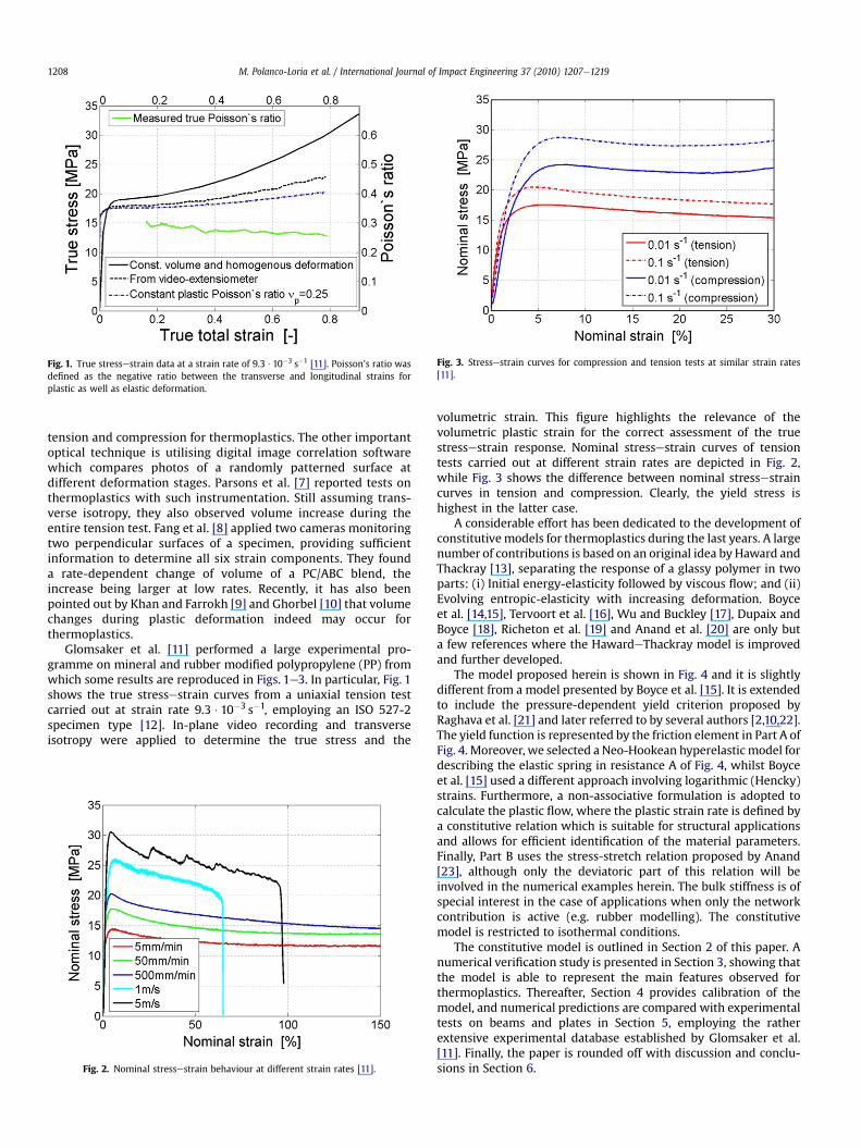
Fig. 1. True stressestrain data at a strain rate of 9.3 $10�3 s�1 [11]. Poisson’s ratio wasdefined as the negative ratio between the transverse and longitudinal strains forplastic as well as elastic deformation.

Fig. 3. Stressestrain curves for compression and tension tests at similar strain rates[11].

M. Polanco-Loria et al. / International Journal of Impact Engineering 37 (2010) 1207e12191208

tension and compression for thermoplastics. The other importantoptical technique is utilising digital image correlation softwarewhich compares photos of a randomly patterned surface atdifferent deformation stages. Parsons et al. [7] reported tests onthermoplastics with such instrumentation. Still assuming trans-verse isotropy, they also observed volume increase during theentire tension test. Fang et al. [8] applied two cameras monitoringtwo perpendicular surfaces of a specimen, providing sufficientinformation to determine all six strain components. They founda rate-dependent change of volume of a PC/ABC blend, theincrease being larger at low rates. Recently, it has also beenpointed out by Khan and Farrokh [9] and Ghorbel [10] that volumechanges during plastic deformation indeed may occur forthermoplastics.

Glomsaker et al. [11] performed a large experimental pro-gramme on mineral and rubber modified polypropylene (PP) fromwhich some results are reproduced in Figs. 1e3. In particular, Fig. 1shows the true stressestrain curves from a uniaxial tension testcarried out at strain rate 9.3 $10�3 s�1, employing an ISO 527-2specimen type [12]. In-plane video recording and transverseisotropy were applied to determine the true stress and the

Fig. 2. Nominal stressestrain behaviour at different strain rates [11].

volumetric strain. This figure highlights the relevance of thevolumetric plastic strain for the correct assessment of the truestressestrain response. Nominal stressestrain curves of tensiontests carried out at different strain rates are depicted in Fig. 2,while Fig. 3 shows the difference between nominal stressestraincurves in tension and compression. Clearly, the yield stress ishighest in the latter case.

A considerable effort has been dedicated to the development ofconstitutivemodels for thermoplastics during the last years. A largenumber of contributions is based on an original idea by Haward andThackray [13], separating the response of a glassy polymer in twoparts: (i) Initial energy-elasticity followed by viscous flow; and (ii)Evolving entropic-elasticity with increasing deformation. Boyceet al. [14,15], Tervoort et al. [16], Wu and Buckley [17], Dupaix andBoyce [18], Richeton et al. [19] and Anand et al. [20] are only buta few references where the HawardeThackray model is improvedand further developed.

The model proposed herein is shown in Fig. 4 and it is slightlydifferent from a model presented by Boyce et al. [15]. It is extendedto include the pressure-dependent yield criterion proposed byRaghava et al. [21] and later referred to by several authors [2,10,22].The yield function is represented by the friction element in Part A ofFig. 4. Moreover, we selected a Neo-Hookean hyperelastic model fordescribing the elastic spring in resistance A of Fig. 4, whilst Boyceet al. [15] used a different approach involving logarithmic (Hencky)strains. Furthermore, a non-associative formulation is adopted tocalculate the plastic flow, where the plastic strain rate is defined bya constitutive relation which is suitable for structural applicationsand allows for efficient identification of the material parameters.Finally, Part B uses the stress-stretch relation proposed by Anand[23], although only the deviatoric part of this relation will beinvolved in the numerical examples herein. The bulk stiffness is ofspecial interest in the case of applications when only the networkcontribution is active (e.g. rubber modelling). The constitutivemodel is restricted to isothermal conditions.

The constitutive model is outlined in Section 2 of this paper. Anumerical verification study is presented in Section 3, showing thatthe model is able to represent the main features observed forthermoplastics. Thereafter, Section 4 provides calibration of themodel, and numerical predictions are compared with experimentaltests on beams and plates in Section 5, employing the ratherextensive experimental database established by Glomsaker et al.[11]. Finally, the paper is rounded off with discussion and conclu-sions in Section 6.

Fig. 4. Proposed constitutive model with intermolecular (A) and network (B) contributions.

M. Polanco-Loria et al. / International Journal of Impact Engineering 37 (2010) 1207e1219 1209

2. Constitutive model for thermoplastics

2.1. Introduction

The material is assumed to have two basic resistances todeformation [15], see Fig. 4:

A. An intermolecular barrier to deformationB. An evolving entropic resistance due to molecular orientation

According to the rheological model of Fig. 4, the deformationgradient is the same for the two resistances:

F ¼ FA ¼ FB (1)

It follows that the volume change, given as the determinant ofthe deformation gradient, also is the same for both parts of themodel, i.e.

JA ¼ JB ¼ J ¼ detF (2)

The macroscopic Cauchy stress tensor for the material isobtained by summing the mesoscopic contributions from Parts Aand B, i.e.

s ¼ sA þ sB (3)

In order to facilitate the comprehension of the model,a conceptual illustration of the kinematics is given in Fig. 5.

0Ω

AΩ

Ω

pAF

eAF

A B= =F F F

Fig. 5. Illustration of the kinematics of the model, showing the reference configurationU0, the intermediate configuration UA and the current configuration U.

2.2. Part A e intermolecular resistance

The deformation gradient FA is decomposed into elastic andplastic parts [24]

FA ¼ FeA$FpA (4)

where it is assumed that the intermediate configurationUA definedby FpA is invariant to rigid body rotations of the current configura-tion [24,25]. Using Eq. (2), the Jacobian JA of Part A is decomposed as

JA ¼ detFA ¼ detFeAdetFpA ¼ JeA JpA ¼ J (5)

The velocity gradient in the current configuration UA is definedby

LA ¼ _FA$F�1A ¼ LeA þ LpA (6)

Using Eq. (4), the elastic and plastic velocity gradient tensors LeAand LpA are defined by

LeA ¼ DeA þWe

A ¼ _FeA$ðFeAÞ�1

LpA ¼ DpA þWp

A ¼ FeA$ _FpA$ðFpAÞ�1$ðFeAÞ�1 ¼ FeA$L

pA$ðFeAÞ�1 (7)

where

LpA ¼ _F

pA$ðFpAÞ�1 ¼ D

pA þW

pA (8)

Here LpA is the plastic velocity gradient on UA composed of the

symmetric plastic rate-of-deformation tensor DpA and the skew-

symmetricplastic spin tensorWpA. InEq. (7),D

eA andD

pA are thesymmetric

elastic and plastic rate-of-deformation tensors, whileWeA andWp

A are inturn the skew-symmetric elastic and plastic spin tensors with respect tothe current configurationUA.

The isotropic compressible Neo-Hookean material, whichrepresents an extension of Hooke’s law to large elastic deforma-tions, is chosen for the elastic part of the deformation. The Neo-Hookean stored energy function is defined according to Ogden [25].The elastic constitutive law in terms of the Kirchhoff stress sA on UA

is obtained as [26]:

sA ¼ l0 ln JeAIþ m0ðBeA � IÞ (9)

where l0 and m0 are the classical Lamé constants of the linearizedtheory, I is the second-order unit tensor, and Be

A ¼ FeA$ðFeAÞT is theelastic left Cauchy-Green deformation tensor. According to theclassical theory of elasticity, the Lamé coefficients may besubstituted by Young’s modulus E0 and Poisson’s ratio n0.

M. Polanco-Loria et al. / International Journal of Impact Engineering 37 (2010) 1207e12191210

The viscoplastic part of the model is formulated on the inter-mediate configuration UA, cf. Fig. 5. The following relationshipsexist between the Kirchhoff stress sA and the Cauchy stresssA onUA

and the Mandel stress SA on UA [26,27]:

sA ¼ JeAsA ¼ ðFeAÞ�T$SA$ðFeAÞT ; SA ¼ ðFeAÞT$sA$ðFeAÞ�T (10)

Hence, by appropriate transformation the isotropic elasticresponse is alternatively expressed in terms of SA on UA, viz.

SA ¼ l0 ln JeAIþ m0�CeA � I

�(11)

where CeA ¼ ðFeAÞT$FeA is the elastic right Cauchy-Green deformation

tensor. Note that while the Mandel stress tensor SA is not generallysymmetric, cf. Eq. (10), it becomes symmetric under the assump-tion of isotropic elasticity. Henceforth, we will take advantage ofthe symmetry property of the Mandel stress tensor SA in thedevelopment of the viscoplastic framework of the constitutivemodel.

Boyce et al. [15] applied a Maxwell type element (i.e. spring-dashpot in series) in Part A of their model, allowing for a certainstrain-rate effect even for very small stresses. In other words,material flow is observed as long as stresses are applied to thematter. Viscous effects in the linear and non-linear elastic domainare interesting for creep related problems, involving very smallstrain rates. However, the applications we intend to deal with arecrashworthiness and structural impact where high strain rates inthe large-strain domain are expected. Consequently, we choose toneglect the viscoelastic behaviour herein, and instead we adopt theclassical elastic-viscoplastic framework where the contribution ofthe dashpot occurs only if a certain yield condition is satisfied. Thiscorresponds with the introduction of a friction element in therheological model in Fig. 4. A possible extension of the model toinclude viscoelasticity as well might be considered in futureresearch.

The yield criterion fA¼ 0 is assumed in the form

fA ¼ sA � sT ¼ 0 (12)

where sT is the yield stress in uniaxial tension and the equivalentstress sA is defined according to Raghava et al. [21] to account forthe pressure-sensitive shear strength behaviour commonlyobserved in polymeric materials, viz.

sA ¼

�a� 1

�I1A þ

ffiffiffiffiffiffiffiffiffiffiffiffiffiffiffiffiffiffiffiffiffiffiffiffiffiffiffiffiffiffiffiffiffiffiffiffiffiffiffiffiffiffiffiffiða� 1Þ2I21A þ 12aJ2A

q2a

(13)

In Eq. (13), a ¼ sC=sT � 1 is amaterial parameter describing thepressure sensitivity, where sC is the uniaxial compressive yieldstrength of thematerial. The stress invariants I1A and J2A are definedby [27]

I1A ¼ tr sA ¼ tr SA; J2A ¼ 12sdevA : sdevA ¼ 1

2SdevA : S

devA (14)

where sdevA ¼ sA � ð1=3Þðtr sAÞI and SdevA ¼ SA � ð1=3Þðtr SAÞI are

the deviators of the Kirchhoff and Mandel stress tensors, respec-tively. Eq. (14) assumes the symmetry property of the Mandelstress. It should be noticed that the equivalent stress definition ofEq. (13) is the same in the intermediate and current configurations,according to Eq. (14).

The constitutive behaviour of the dashpot follows a non-asso-ciative flow rule where a plastic potential gA is introduced to derivethe plastic strain-rate tensor. This potential has a similar expressionto that used in Eq. (13), and reads

ðb� 1ÞI1A þffiffiffiffiffiffiffiffiffiffiffiffiffiffiffiffiffiffiffiffiffiffiffiffiffiffiffiffiffiffiffiffiffiffiffiffiffiffiffiffiffiffiffiffiðb� 1Þ2I21A þ 12bJ2A

q

gA ¼

2b� 0 (15)

where b� 1 is a material parameter introduced to control thevolumetric plastic strain. The plastic velocity gradient tensor L

pA on

UA is defined by the flow rule

LpA ¼ _3

pArA; rA ¼ vgA

vSA(16)

where _3pA is the viscoplastic multiplier and rA is the gradient of the

plastic potential on UA. Notice that because of the symmetryproperty of the Mandel stress tensor both rA and L

pA are symmetric

tensors. According to Eq. (8), we therefore have

LpA ¼ D

pA and W

pA ¼ 0 (17)

Next, the direction of the plastic flow rA on UA is obtained as

rA ¼ vgAvSA

¼ f1vI1AvSA

þ f2vJ2AvSA

¼ f1Iþ f2SdevA (18)

The functions f1 and f2 read

f1 ¼ vgAvI1A

¼ b� 12b

þ ðb� 1Þ2I1A2b

ffiffiffiffiffiffiffiffiffiffiffiffiffiffiffiffiffiffiffiffiffiffiffiffiffiffiffiffiffiffiffiffiffiffiffiffiffiffiffiffiffiffiffiffiðb� 1Þ2I21A þ 12bJ2A

q ;

f2 ¼ vgAvJ2A

¼ 3ffiffiffiffiffiffiffiffiffiffiffiffiffiffiffiffiffiffiffiffiffiffiffiffiffiffiffiffiffiffiffiffiffiffiffiffiffiffiffiffiffiffiffiffiðb� 1Þ2I21A þ 12bJ2A

q ð19Þ

The identification of the parameter b requires the measurementof the volumetric plastic strain. As a special case of the derived flowrule, an associated flow rule is obtained for b¼ a with the gradientdefined by Eq. (18). Further, an isochoric (volume preserving)plastic flow is obtained for a¼ b¼ 1 with the gradient defined by

vgAvSA

¼ vfAvSA

¼ 32

SdevAffiffiffiffiffiffiffiffiffi3J2A

p (20)

The plastic power per unit volumewith respect toUA is given by

_wpA ¼ SA : L

pA ¼ _3

pASA :

vgAvSA

¼ gA _3pA (21)

From Eqs. (15) and (21) it follows that _wpA � 0 for non-negative

_3pA, where the equality holds for elastic processes in which _3

pA ¼ 0.

Boyce et al. [15] assumed an incompressible plastic flow. Theychose the rate of flow to be a thermo-mechanically activatedprocess of Arrhenius type [28]:

_gpA ¼ _g0Aexp

�� DGð1� sA=sÞ

kq

�(22)

where _gpA is an equivalent plastic strain rate, _g0A is a pre-expo-

nential factor, DG is an energy barrier to flow, k is the Boltzmannconstant, and q is the absolute temperature. Further, sA is anequivalent stress (in terms of the deviatoric stress) and s is theshear resistance, which was assumed to be a fraction of the shearmodulus [14,15,29]. Eq. (22) is conveniently re-written as

_3pA ¼ _30Aexp

�1

CðqÞ�sAsT

� 1��

(23)

where _3pA is the equivalent plastic strain rate associated with the

Raghava yield criterion, and _30A is a reference strain rate withtypical value of the order of 10�4 to 10�3 s�1, corresponding to

Table 1Material parameters used for the numerical evaluation.

E0 (MPa) n0 sT (MPa) a b _30Aðs�1Þ C CR (MPa) lL

1200 0.4 25 1.3 1.2 1 $ 10�3 0.05 4.0 2.45

M. Polanco-Loria et al. / International Journal of Impact Engineering 37 (2010) 1207e1219 1211

quasi-static testing conditions. C(q) is a temperature-dependentstrain-rate sensitivity parameter representing the ratio kq/DG of Eq.(22), and hereafter denoted as C due to the assumption ofisothermal conditions. Finally, sA and sT are respectively theRaghava equivalent stress, see Eq. (13), and the uniaxial yield stressin tension. It is straightforward to re-write Eq. (23) into

sAsT

¼ 1þ C ln

_3pA

_30A

!(24)

The coefficient C is positive and usually small, i.e. of order 10�3

to 10�2, for metals. Most polymers exhibit significant strain-ratesensitivity, however, C is still not larger than about 0.1. In impactproblems and at other high-rate situations, _3

pA[_30A, thus, Eq. (24)

can be approximated as

sAsT

¼ 1þ C ln

1þ

_3pA � _30A_30A

!z1þ C ln

1þ

_3pA

_30A

!(25)

With this modification, the equivalent stress sA approaches thetensile yield strength sT when the strain rate approaches zero, andthe two coefficients of Eq. (25), i.e. C and _30A, are easy to identifyfrom strain-rate tests. The equivalent plastic strain rate (or visco-plastic multiplier) to be used in Eq. (16) can be found from

_3pA ¼

0 if fA � 0_30A

nexp

h1C

sAsT� 1

�i� 1

oif fA > 0 (26)

where fA is the yield function defined by Eq. (12). It is noted thatsA=sT > 1 when fA> 0, and thus _3

pA is zero for elastic processes and

positive for viscoplastic processes.

2.3. Part B e network resistance

The deformation gradient FB, see Eq. (1) and Fig. 4, representsthe network orientation and it is assumed that the network resis-tance is hyperelastic. The elastic stored energy function is definedaccording to Anand [23], and the elastic constitutive law in terms ofthe Kirchhoff stress sB¼ JBsB on U reads

sB ¼ CR3

lL

lL�1

�l

lL

�B*B � l2I

�þ kðln JÞI (27)

whereL�1 is the inverse function of the Langevin function definedasLðxÞ ¼ coth x� 1=x, and the Jacobian J ¼ detF ¼ detFB ¼ JB(see Eq. (2)). The effective distortional stretch l is calculated as

l ¼ffiffiffiffiffiffiffiffiffiffiffiffiffiffiffiffi13trðB*

BÞr

(28)

where B*B ¼ F*B$ðF*BÞT is the distortional left Cauchy-Green defor-

mation tensor, and F*B ¼ J�1=3B FB denotes the distortional part of FB.

There are three constitutive parameters describing the intra-molecular resistance, see Eq. (27): CR is the initial elastic modulus ofPart B; lL is the locking stretch, which is related to the maximumattainable deformation of the material; and k is a bulk modulus,which is used in applications where only the network contributionis active (e.g. rubber modelling). The coefficient k is not furtherapplied in this work.

3. Numerical verification

3.1. Introduction

The constitutive model presented in Section 2 is implementedas a user-defined model in the finite element code LS-DYNA [30],

working for brick elements. The semi-implicit stress updatealgorithm proposed by Moran et al. [31] (see also Ref. [26]) wasadopted. Since the constitutive model is developed for explicitfinite element analysis, it is assumed that the time steps are smalland that a semi-implicit algorithm is sufficiently accurate. Thissection presents some numerical tests performed to verify theimplementation and to study the sensitivity of some of the model’sparameters. A simple geometrical model consisting of one 8-nodebrick element with initial dimensions 10 mm� 10 mm� 10 mmwas employed.

Omitting the bulk modulus k of Eq. (27), the constitutive modelinvolves 9 parameters:

e Spring A: Two elastic coefficients E0 (Young’s modulus) and n0(Poisson’s ratio).

e Friction element A: Three plastic coefficients defined by theuniaxial tensile and compressive yield stress (related witha¼ sC/sT), and the parameter b controlling the plasticdilatation.

e Dashpot A: Two strain-rate sensitivity parameters _30A and C.e Spring B: Two coefficients CR (initial elastic modulus) and lL

(locking stretch)

The parameters given in Table 1 were selected as the baselineinput for the numerical verifications.

The numerical evaluations are organized in two forthcomingsections as follows. In Section 3.2, considering Part A only,sequences of tensile-compressive uniaxial, biaxial and hydrostaticstress states are applied for one loading cycle. Change of volumeduring plastic deformation and strain-rate effects are also investi-gated for a uniaxial tensile-compressive load cycle. Part B wasremoved from these simulations by setting CR¼ 0. In Section 3.3,involving both parts (Aþ B) of the model, the influence of theparameters CR and lL on the global response for monotonic andcyclic uniaxial stress situations is evaluated. Also, a series of ten-sionecompression cycles is investigated.

3.2. Evaluation of contribution from Part A

Fig. 6 illustrates the response of the model to uniaxial, biaxialand hydrostatic stress states up to a true strain level of �0.5, first intension and thereafter in compression. The response clearly indi-cates that both the uniaxial tensile (sT¼ 25 MPa) and compressive(sC¼ 32.5 MPa) yield stresses are recovered. The biaxial resultsindicate an expected reduction of the tensile strength and anincrease in the compressive strength. Further, the curveassociated with hydrostatic loading shows that the maximumpressure in tension, which in accordance with Eq. (13) isasT=3ða� 1Þ ¼ 36:11 MPa, is correctly predicted. The Raghavacriterion is open in hydrostatic compression, i.e. the yield stress isinfinite, hence the stressestrain curve does not approach any yieldplateau in this particular case, and experiences a monotonicincrease in stress as the strain decreases from 0.5 to �0.5.

An overview of the shear-pressure dependency predicted by theRaghava yield function, plotted in terms of the deviatoric invariantffiffiffiffiffiffiffi3J2

pand the hydrostatic invariant I1/3, is presented in Fig. 7. In

addition to the points already defined via the yield stresses in Fig. 6,the yield point for uniaxial strain in tension (UST) is included. The

-0.6 -0.4 -0.2 0 0.2 0.4 0.6

-50

-40

-30

-20

-10

0

10

20

30

40

50 σ (MPa)

ε

Hydrostatic

Uniaxial

Biaxial

Fig. 6. Response predicted by the model in a tensionecompression cycle for uniaxial,biaxial and hydrostatic stress states.

I1/3 (MPa)

BC

-60 -40 -20 0 20 40 60

10

20

30

40

50

f = 0

UC

UT

BT

USTHT

BC - Biaxial compressionUC - Uniaxial compressionUT - Uniaxial tensionBT - Biaxial tensionUST - Uniaxial strain in tensionHT - Hydrostatic tension

3J2 (MPa)

Fig. 7. Numerical prediction by the model of the Raghava yield surface.

Jp - 1 ( ≈ εvol )

0.6

0.8 pA

M. Polanco-Loria et al. / International Journal of Impact Engineering 37 (2010) 1207e12191212

non-linear shear-pressure dependency of the Raghava model is,thus, verified from a numerical point of view.

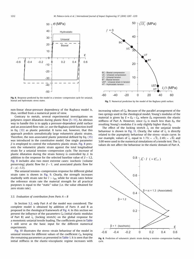
Contrary to metals, several experimental investigations onpolymers report dilatation during plastic flow [5e11]. An obviousway to handle this is to apply a pressure-dependent yield surfaceand an associated flow rule, i.e. use the Raghava yield function itselfin Eq. (13) as plastic potential. It turns out, however, that thisapproach predicts unrealistically large volumetric plastic strains.Therefore, the non-associated plastic potential defined by Eq. (15)was introduced in the constitutive model. One single parameterb is employed to control the volumetric plastic strain. Fig. 8 pres-ents the volumetric plastic strain against the total longitudinalstrain for a uniaxial tensionecompression cycle. The increase ofplastic dilatation during the strain history is controlled by b. Inaddition to the response for the selected baseline value of b¼ 1.2,Fig. 8 includes also two more extreme cases: isochoric (volumepreserving) plastic flow for b¼ 1; and associated plastic flow forb¼ a(¼1.3).

The uniaxial tensionecompression response for different globalstrain rates is shown in Fig. 9. Clearly, the strength increasesmarkedly with strain rate for _3 > _30A, while for strain rates belowthe reference strain rate the material strength for all practicalpurposes is equal to the “static” value (i.e. the value obtained forzero strain rate).

εβ = 1 (Isochoric)

-0.6 -0.4 -0.2 0 0.2 0.4 0.6

0.2

0.4

β = 1.2

β = α = 1.3 (Associated)

Fig. 8. Prediction of volumetric plastic strain during a tensionecompression loadingcycle.

3.3. Evaluation of contribution from Parts Aþ B

In Section 3.2, only Part A of the model was considered. Thecomplete model is obtained by addition of Parts A and B asproposed in the rheological framework of Fig. 4. In this section wepresent the influence of the parameters CR (initial elastic modulusof Part B) and lL (locking stretch) on the global response fora monotonic uniaxial tensile loading. The coefficients given in Table1 still serve as the basic input for the different numericalexperiments.

Fig. 10 illustrates the stressestrain behaviour of the model inuniaxial tension for different values of the coefficient CR, keepingthe remaining parameters as presented in Table 1. It is seen that theinitial stiffness in the elastic-viscoplastic regime increases with

increasing values of CR. Because of the parallel arrangement of thetwo springs used in the rheological model, Young’s modulus of thematerial is given by Ez E0þ CR, where E0 represents the elasticstiffness of Part A. However, since CR is much less than E0, theresulting Young’s modulus E is only slightly higher than E0.

The effect of the locking stretch lL on the uniaxial tensilebehaviour is shown in Fig. 11. Clearly, the value of lL is directlyrelated to the asymptotic behaviour of the stressestrain curve. Inour example, values of lL equal to 1:73ð¼

ffiffiffi3

pÞ, 2:45ð¼

ffiffiffi6

pÞ and

3.00 were used in the numerical simulations of a tensile test. The lLvalues do not affect the behaviour in the elastic domain of Part A.

-0.6 -0.4 -0.2 0 0.2 0.4 0.6

-50

-40

-30

-20

-10

0

10

20

30

40

50Strain rates

100 s1 s0.01 s0.0001 s

σ (MPa)

ε

Fig. 9. Strain-rate sensitivity predicted by the model in a tensionecompression cycle.

0.0 0.4 0.8 1.2 1.60

20

40

60

80

100

120

= 1.73= 2.45= 3.00

λL

σ (MPa)

ε

Fig. 11. Influence of the locking stretch lL on the uniaxial tensile behaviour.

M. Polanco-Loria et al. / International Journal of Impact Engineering 37 (2010) 1207e1219 1213

The stressestrain curves level out at a true stress close to110 MPa in both Figs. 10 and 11. This response is due to the inter-action between Parts A and B in the constitutive model, and isrelated to the maximummean stress that Part A can sustain. Firstly,we recall that the Cauchy stress is obtained as the sum of thecontributions in Parts A and B, viz. s¼sAþsB. Thus, for the specialcase of uniaxial loading with k¼ 0 and henceforth tr sB¼ 0,a matrix representation of the stress state in the model must read0@ s 0 0

0 0 00 0 0

1A ¼

0@ sA 0 0

0 sB=2 00 0 sB=2

1A

þ0@ sB 0 0

0 �sB=2 00 0 �sB=2

1A (29)

0.0 0.4 0.8 1.2 1.60

20

40

60

80

100

120

CR = 9 MPaCR = 6 MPaCR = 4 MPaCR = 2 MPa

CR

σ (MPa)

ε

Fig. 10. Influence of the modulus CR on the uniaxial tensile behaviour.

For small strains, the contribution from Part B is almost negli-gible, and the macroscopic response is dominated by Part A. Whenthe load increases, Part B becomes more important, and feeds moreand more of its triaxial state of stress into Part A. This increase oftriaxial stress state of Part A is limited by the Raghava yield crite-rion. According to Eq. (12), the critical mean stress associated withthe Raghava criterion is given by smean

A;cr ¼ ða=ð3ða� 1ÞÞÞsT . It is notpossible for the mean stress of Part A to exceed smean

A;cr , and themaximum attainable uniaxial tension in the model is therefore

0@smax 0 0

0 0 00 0 0

1A ¼

0B@

smeanA;cr 0 00 smean

A;cr 00 0 smean

A;cr

1CA

þ

0B@

2smeanA;cr 0 00 �smean

A;cr 00 0 �smean

A;cr

1CA (30)

Hence, we find that smax ¼ 3smeanA;cr ¼ ða=a� 1ÞsT , which for

the parameters given in Table 1 results in a numerical value ofsmax¼ 108.3 MPa. Clearly, this limiting stress is in good agreementwith the observations in Figs. 10 and 11.

Finally, the numerical response of the model for a series oftensionecompression cycles is analysed. The loading state includedthree tensionecompression cycles with a fourth cycle only intension, as illustrated in Fig. 12. The true strain levels attained withthis displacement history are symmetric in tension and compres-sion for the two first cycles (3 equal to�0.20 and�0.40), in the thirdcycle 3 is equal to 0.54 in tension and 0.68 in compression, and thefourth cycle corresponds to a strain of 1.25 in tension.

Fig. 13 shows the numerical behaviour of the model when it issubjected to the loading history involving the selected cycles oftensionecompression depicted in Fig. 12. For comparison purposesthe monotonic responses in tension and compression are alsoincluded in Fig. 13. During the first cycle the tensile behaviourfollows the same path as the monotonic response. However, thetensile pre-strain affects the subsequent compressive stressestrainbehaviour, and leads to a strain-induced anisotropy introduced viaPart B of the constitutive model. This effect gets stronger with

0 20 40 60 80 100

Time (s)-5

0

5

10

15

20

25

Uni

axia

ldis

plac

emen

t(m

m)

Fig. 12. Applied displacement history in the tensionecompression cycles.

-1.0 -0.5 0.0 0.5 1.0 1.5

-100

-80

-60

-40

-20

0

20

40

Cyclic loading (Fig. 12)Monotonic tensionMonotonic compression

σ (MPa)

ε

Shift

Shift

Fig. 13. Stressestrain behaviour under cyclic loading in uniaxial tension andcompression.

M. Polanco-Loria et al. / International Journal of Impact Engineering 37 (2010) 1207e12191214

increasing strain amplitudes. It follows that the stress induced bythe non-linear elastic spring of Part B acts as a backstress withrespect to Part A.

0 2 4 6 8 10 120.0

0.2

0.4

0.6

0.8

1.0

1.2

Test [11] − reference strain rateTest [11] − other strain ratesFit to model

C

(σ/σT – 1)–

ln(1+ε/ε0A). .

Fig. 14. Identification of strain-rate sensitivity parameters from test data shown inFig. 2.

4. Identification of material parameters

The model requires identification of 9 material parameters byusing simple uniaxial tests in tension and compression. We havechosen to use the experimental database which was obtained byGlomsaker et al. [11] for a polypropylene (PP) copolymer. In addi-tion to the material tests shown in Figs. 1e3, they performed three-point bending tests and plate impact tests under various loadingconditions. Their data are used to calibrate and evaluate the modelpresented herein.

Because we apply material data found in the literature, it turnedout that the test results were not perfectly suited for a direct cali-bration, even though a quite extensive database of material testswas provided [11]. Inverse modelling was applied to obtain anoptimal fit. Thus, the process adopted to identify the materialparameters in the model includes the following steps:

(a) From the uniaxial stressestrain curve in tension at the loweststrain rate, see Fig. 1, Young’s modulus Ez E0 is identified,capturing, in average, the non-linear behaviour of the initialelastic part of the stressestrain curve satisfactory. The slope ofthe stressestrain curve in the elastic domain is chosen as thesecant between stress levels of 20% and 60% of the yield stress,giving E0¼ 930 MPa. A Poisson’s ratio of n0¼ 0.4 was used inthe simulations [11].

(b) Using the nominal stressestrain curves at different strain ratesin tension, see Fig. 2, the rate sensitivity parameter C is iden-tified. The relative values of the maximum stresses are used asthe main input, and these are plotted in Fig. 14. The referencestrain rate _30A is taken as the lowest strain rate used in thetensile tests, and thus _30A ¼ 1$10�3 s�1. A slopewith a value ofC¼ 0.1 was found from the data shown in Fig. 14. Because thedata are reported in terms of the total strain rate, while Eq. (26)uses the effective plastic strain rate, the obtained value of C isused as an initial value in an iterative identification procedure.

(c) Using the true stressestrain curve shown in Fig. 1 as the maintarget, a numerical simulation with one element was per-formed to identify the parameters sT, CR and lL. The

experimentally obtained true stressestrain curve is comparedwith the numerical predictions from the one-element model inFig. 15.

(d) Using a FE model of the tensile specimen, see Fig. 16, applyingthe parameters identified so far, numerical calculations wereperformed using the forceedisplacement curves obtained attwo or more strain rates as target solutions. The parameter Cwas adjusted to approximate the target solutions as closely aspossible.

(e) Step (c) was repeated modifying only the yield stress, and thenstep (d) was repeated until the target solutions were reason-ably well predicted. With this procedure, the followingparameters were found: sT¼ 13.8 MPa, CR¼ 3.0 MPa, lL ¼ 3:0,

0.0 0.2 0.4 0.6 0.8 1.00

10

20

30

Experimental data [11]Inverse modeling

σ (MPa)

ε

Fig. 15. True stressestrain curve used for identification purposes.

0 5 10 15 20

Displacement (mm)

0

200

400

600

800

1000

1200

Forc

e(N

)

Tension testsExperimental data [11]Numerical prediction

1000 mm/s

8.33 mm/s

0.0833 mm/s

Fig. 17. Forceedeformation curves from tension tests at various strain rates used astarget solutions.

M. Polanco-Loria et al. / International Journal of Impact Engineering 37 (2010) 1207e1219 1215

C¼ 0.095 and _30A ¼ 1$10�3 s�1. The numerical and experi-mental forceedisplacement curves in uniaxial tension areshown in Fig. 17.

(f) The parameter b, which defines the plastic potential, wasidentified from experimental data on the evolution of thetransverse vs. longitudinal true strains in uniaxial tension, seeFig. 18. The numerical results presented in this figure areobtained with b¼ 1.35.

(g) Finally, theparametera,whichdefines thepressure sensitivityoftheyield stress,was obtained from tests in uniaxial compression.Based on the experimental data of Glomsaker et al. [11], a¼ 1.27was found.

The final set of parameters used in the experimental verificationis summarized in Table 2.

Fig. 16. Finite element model of tensile tes

5. Experimental verification

5.1. Three-point bending test on beams

Glomsaker et al. [11] reported three-point bending tests onsmall beams with length 80 mm and cross-section 4 mm� 10 mm.The beams were made of the PP material introduced in Figs. 1e3and applied in the calibration procedure described in Section 4.These tests were performed at velocities varying from 5 mm/min to4000 mm/s. Using a servohydraulic machine in the lower velocityregime, a constant deformation rate ranging from 5 to 500 mm/minin different tests was maintained during the experiment. At higherloading rates, a free-falling impactor with mass 3.15 kg was used. Afinite element model of the three-point bending test, involving3368 brick elements, is shown in Fig. 19. The PP beam was repre-sented with the model proposed herein and the coefficients of

t specimen with 80 mm gauge length.

0.0 0.2 0.4 0.6 0.80.20

0.25

0.30

0.35

0.40

Experimental data [11]Inverse modelling

−εt /ε

ε

Fig. 18. Identification of the parameter b.

Fig. 19. Finite element model of three-point bending test.

100

200

300

400

Forc

e(N

)

Three-point bendingExperimental data [11]

1000 mm/s

8.33 mm/s

M. Polanco-Loria et al. / International Journal of Impact Engineering 37 (2010) 1207e12191216

Table 2. Moreover, a friction coefficient of 0.15 and a rigid bodyimpactor were assumed in the simulations. In order to reduce thecomputational time, mass scaling was applied for the quasi-staticcase. It was checked that the kinetic energy was only a very smallfraction of the total energy involved in the numerical deformationprocess.

The global response from the experimental tests and numericalsimulations is shown as forceedisplacement curves in Fig. 20 fortwo different loading rates, one rather slow and one dynamic. Themodel provides a good representation of the behaviour observed inthe first part of the test. However, the FE model overestimates theload-carrying capacity of the beam by approximately 10% for thelower rate and 5% for the dynamic load case.

In problems related to for example pedestrian safety, the shapeof the forceedisplacement curve both during the loading andunloading phases is important. The unloading phase is funda-mental for calculating the internal energy recovered in the system.From Fig. 20 it is seen that the FE model is not able to capture thereduced stiffness during the last phase of unloading, and the reasonfor this is probably that viscoelastic effects are not included in theconstitutive model. It is believed that introducing viscoelasticityinto the constitutive model would improve its predictive capabil-ities, at the cost of increasing the complexity of the mathematicalformulation and the identification process.

It should also be recalled that a constant friction coefficient of0.15 was used in the simulations. It is likely that reduced frictionwill predict a larger maximum deformation before onset ofunloading in the dynamic test depicted in Fig. 20.

5.2. Plate impact tests

This example pays attention to circular injectionmoulded platesof 2 mm thickness and 55 mm diameter, still applying the same PPmaterial. The plates were centrally loaded at different velocities in

Table 2Material parameters identified for the PP copolymer.

E0 (MPa) n0 sT (MPa) a b _30Aðs�1Þ C CR (MPa) lL

930 0.4 13.8 1.266 1.35 1 $ 10�3 0.095 3.0 3.0

the experimental tests [11]. Similar to the three-point bending testspresented in Section 5.1, a free-falling impactor with mass 3.15 kgwas applied in dynamic tests at impact velocities between 1 and4 m/s. The plates were reported to be clamped by a pre-stressedsteel ring around the perimeter in the dynamic test set-up. Thefinite element model of the plate, employing 6500 brick elements,is shown in Fig. 21. Again, a friction coefficient of 0.15 and a rigidbody impactor were assumed in the simulations.

The forceedisplacement curves from the experimental tests andnumerical simulations are shown in Fig. 22 for two dynamic testswith impact velocities equal to 1 and 2 m/s. The FE model

0 2 4 6 8 10Displacement (mm)

0Numerical prediction

Fig. 20. Experimental and predicted forceedisplacement curves from three-pointbending test.

Fig. 21. Finite element model of plate impact test.

M. Polanco-Loria et al. / International Journal of Impact Engineering 37 (2010) 1207e1219 1217

overestimates the load-carrying capacity of the plate by about 15%.The shape of the forceedisplacement curve is fairly well captured,at least for moderate displacements up to 3 mm. Thereafter, thenumerical simulations predict too high force. The boundaryconditions are probably the reason for this discrepancy. Althoughthe plate was claimed to be clamped in the test, it is in practice verydifficult to obtain such a restriction, and the plate does usuallyexperience some in-plane displacements around the boundary ata sufficient high load. Thereby, the stiffness is slightly reducedcompared with the simulations, where the plate indeed wasmodelled as clamped.

It is further seen from Fig. 22 that the backstress induced by PartB of the constitutive model affects the unloading response. Theslope of the unloading branch is quite similar in experiments andsimulations. The curvature observed in the lower part of theunloading branch of the experimental forceedisplacement curveindicates a viscous effect, which is not included in the constitutivemodel. The simulations presented in Fig. 22 do not, however,capture the displacement at the onset of unloading. As discussed inthe Section 5.1, this may be linked to the value of the frictioncoefficient.

0 2 4 6 8 10 12Displacement (mm)

0

200

400

600

800

1000

1200

Forc

e(N

)

Plate impactExperimental data [11]Numerical prediction

2 m/s

1 m/s

Fig. 22. Experimental and predicted forceedisplacement curves from plate impacttest.

6. Discussion and concluding remarks

A hyperelastic-viscoplastic constitutive model for thermoplasticmaterials has been developed. Themodel is suitable for the analysisof thermoplastic structural components subjected to monotonic,quasi-static and impact loading conditions. The constitutive modelconsists of two fractions sharing the same deformation gradient,and accounting in turn for the intermolecular resistance by a pres-sure-dependent, non-associated hyperelastic-viscoplastic formu-lation, and the hyperelastic network resistance for compressiblerubber-like materials. A critical review with parameter identifica-tion and numerical verification is provided, and the model isevaluated through finite element analyses of quasi-static anddynamic three-point bending tests of beams and plate impact tests.

The parameters of the proposed constitutive model can bedetermined from uniaxial tension and compression tests atdifferent strain rates, provided that the strains (axial and lateral)are continuously measured during the deformation process. Sincesuch data were available only at the rate of 9.3 $10�3 s�1 for the PPmaterial under consideration, an alternative approach was taken.The calibration of the model parameters was based on the truestressestrain curve found in the uniaxial tension test withmeasurements of lateral strains, and forceedisplacement curves (orengineering stressestrain curves) at different strain rates. The lattercurves were used as target solutions in an iterative, inversemodelling approach to establish the final set of parameters. Thisprocedure seems to work reasonably well for the actual material,which exhibits cold drawing and a smooth decrease in the load-carrying capacity in all tensile tests subsequent to necking. Thesituationmight be different formaterials prone to localized neckingand thus abrupt softening, where the complete true stressetruestrain curves for various strain rates would be required in thecalibration procedure.

A more direct way to calibrate the material parameters, more orless avoiding inverse modelling, should be feasible if a complete setof relevant test data is available. As a general rule, more tests willimprove the accuracy of the calibrated coefficients. However, onlythree tests are required for a rough calibration: Quasi-static tests intension and compression, and one test in tension or compression atan elevated strain rate. Full-field deformation measurements mustbe performed in the quasi-static tests, preferably also in thedynamic test, to provide information on longitudinal as well astransverse strains. It is then straightforward to determine Young’smodulus E0, Poisson’s ratio n0, the yield stresses sT and sC (andsubsequently a), _30A and C. The transverse and longitudinal strainsafter the elastic regime can be used to find the ratio between thecomponents of the gradient to the flow potential in Eq. (18), andsubsequently estimate the parameter b governing plastic dilatation.Moreover, careful inspection of the stressestrain curve immedi-ately after yielding will reveal CR, being the initial elastic modulusof Part B, while the locking stretch lL is closely related to the strainwhere the stress approaches infinity.

The use of a Raghava yield function and the Raghava-like flowpotential makes it possible to account for pressure sensitivity of theyield stress and dilatation during plastic deformation, which bothare commonly observed for thermoplastics. In the current versionof the model, the yield function involves two coefficients sT and a,while the only extra material parameter required for the non-associated flow rule is b. According to Eq. (18), the amount ofvolumetric plastic strain is related to the gradient f1 ¼ vgA=vI1A ofthe potential function gA(I1A, J2A). Although this volumetriccomponent decreases with increasing value of the pressurep¼�I1A/3, the model will still predict evolution of some plasticvolume strain even for hydrostatic pressure. This does not neces-sarily fit all experimental observations, as some investigators have

M. Polanco-Loria et al. / International Journal of Impact Engineering 37 (2010) 1207e12191218

found that the plastic dilatation is large in tension, while it isinsignificant in compression and shear [6]. Introduction of a moreadvanced non-associated flow rule may therefore be necessary toprovide a better representation of various test data.

The physical source of the macroscopic dilatation seems to be animportant issue for constitutive modelling of thermoplastics. Oneobvious mechanism is damage, or void growth. On the other hand,Brusselle-Dupend and Cangémi [32] point out that increase ofvolume in semi-crystalline polymers also may be associated withdeformation of the crystalline part of the material. The moleculesare organized in a rather closely packed way in this part, and thespecific volume is therefore likely to increase when the crystallinelamellae break up.

A practical issue during the model development was how todeal with different types of thermoplastics (amorphous, semi-crystalline and particle-reinforced) while retaining a simplemodelling strategy. The choice was here to handle all types ofgrowth and nucleation of micro-defects, either related to porosity,crazes or debonding of particles, by observations of the plasticdilatation at the macroscale. Instead of introducing internaldamage variables to describe the degradation mechanisms, a clas-sical continuum approach was adopted, involving a non-associatedplastic potential, to represent the volumetric plastic strains. Geo-materials are often modelled in a similar way. The one-parameterRaghava flow potential should probably be enhanced to handleloading situations where tension is not the dominating mode.However, it seems reasonable to handle the plastic dilatation viathe separate parameter b.

With respect to the experimental verification of the constitutivemodel, the choice of flowpotential may explain the over-estimationof about 10% of the load-carrying capacity in the three-pointbending test, see Fig. 20. The parameter a, which defines thepressure-dependence of the yield stress, was calibrated fromobserved yield stresses in uniaxial tension and compression, whilethe parameter b, which governs plastic dilatation, was determinedfrom tensile data only. However, the test data indicate less plasticdilatation in compression than what is predicted by the model.

For the dynamic three-point bending test, we observe a betterprediction of the load-carrying capacity than in the quasi-staticcase, now with deviations of about 5% only. A closer analysis of thetests reported by Glomsaker et al. [11], see Fig. 3, indicatesa stronger strain-rate effect in compression than in tension. This isnot accounted for in the calibration procedure, where tension dataonly were used when determining the rate coefficient C. Thus, theover-prediction of the load-carrying capacity is reduced comparedwith the quasi-static case.

Considering the centrally loaded plate, the large deviations ofabout 15% in load-carrying capacity between simulations and testscan to some degree be explained in the samemanner as for the caseof three-point bending. In addition, they are believed to be partlycaused by the adopted boundary conditions. Fixed boundaries wereassumed in the simulations of the dynamic tests, while the pre-stressed steel ring fixture of the plate in the tests most likely willallow a minor movement. It is therefore reasonable to assume thatthe membrane forces induced in the plate during deformation arelarger in the simulation than in the test, hence the higher load-carrying capacity.

The Langevin rubbereelastic strain hardening contribution ofPart B has proven consistency from a phenomenological point ofview as shown in the results obtained by all the constitutive modelsderived from the original work of Haward and Thackray [13].Experimental arguments are, however, against this entropic natureof strain hardening. van Melick et al. [33] and Govaert and Tervoort[34] observed that the strain hardening intensity is much largerthan the expected values determined from the network density in

the melt. Interesting results are obtained in this direction byreplacing the classical Langevin function with a Neo-Hookeanspring model for the strain hardening behaviour of Part B [33e35].Wendlandt et al. [35] argued also that strain hardening is ratedependent which contradicts the purely elastic nature of Part B.This topic is out of the scope in this work, and further studies arerequired for a better understanding and modelling of strain hard-ening behaviour of thermoplastics.

It is believed that the proposed constitutive model should beapplicable in large-scale finite element analysis of polymericstructural components under impact loading conditions wherereliable assessments of load-carrying capacity are in focus.Improvements are clearly possible by considering more complexyield functions and flow potentials, but at the cost of addingadditional coefficients. In addition, introduction of viscosity in theelastic range and thermal effects are developments that are rele-vant. Finally, there is a yield plateau with constant stress in Part A ofthe model presented herein. A rather straightforward extension ofthe model is to allow hardening or softening during plasticdeformation.

Acknowledgements

The discussions with Professor A. Benallal at LMT-Cachan aregratefully appreciated.

References

[1] Ashby M, Jones DRH. Engineering materials 2: an introduction to micro-structures, processing and design. 2nd ed. Pergamon Press; 1992.

[2] Ehrenstein GW. Polymeric materials: structure, properties and applications.Carl-Hanser Verlag; 2001.

[3] Bois PAD, Kolling S, Koesters M, Frank T. Material behaviour of polymersunder impact loading. International Journal of Impact Engineering 2006;32(5):725e40.

[4] McCrum NG, Buckley CP, Bucknall CB. Principles of polymer engineering. 2nded. Oxford Science Publications; 2003.

[5] G’Sell C, Hiver JM, Dahoun A. Experimental characterization of deformationdamage in solid polymers under tension, and its interrelation with necking.International Journal of Solids and Structures 2002;39(13e14):3857e72.

[6] Mohanraj J, Barton DC, Ward IM, Dahoun A, Hiver JM, G’Sell C. Plastic defor-mation and damage of polyoxymethylene in the large strain range at elevatedtemperatures. Polymer 2006;47(16):5852e61.

[7] Parsons E, Boyce MC, Parks DM. An experimental investigation of the large-strain tensile behavior of neat and rubber-toughened polycarbonate. Polymer2004;45(8):2665e84.

[8] Fang Q-Z, Wang TJ, Beom HG, Zhao HP. Rate-dependent large deformationbehavior of PC/ABS. Polymer 2009;50(1):296e304.

[9] Khan AS, Farrokh B. Thermo-mechanical response of nylon 101 under uniaxialand multi-axial loadings: part I, experimental results over wide ranges oftemperatures and strain rates. International Journal of Plasticity 2006;22(8):1506e29.

[10] Ghorbel E. A viscoplastic constitutive model for polymeric materials. Inter-national Journal of Plasticity 2008;24(11):2032e58.

[11] Glomsaker T, Andreassen E, Polanco-Loria M, Lyngstad OV, Gaarder RH,Hinrichsen EL. Mechanical response of injection-moulded parts at high strainrates. In: Polymer Processing Society Europe/Africa regional meeting,PPS07EA; Proceedings on CD; Ghotenburg, Sweeden; 2007.

[12] (CEN), E.C.f.S. Plastics e determination of tensile properties. Part 2: testconditions for moulding and extrusion plastics. Brussels; 1996.

[13] Haward RN, Thackray G. The use of a mathematical model to describeisothermal stressestrain curves in glassy thermoplastics. Proceedings of theRoyal Society of London, Series A 1968;302(1471):453e72.

[14] Boyce MC, Parks DM, Argon AS. Large inelastic deformation of glassy poly-mers. Part I: rate dependent constitutive model. Mechanics of Materials1988;7(1):15e33.

[15] Boyce MC, Socrate S, Llana PG. Constitutive model for the finite deformationstressestrain behavior of poly(ethylene terephthalate) above the glass tran-sition. Polymer 2000;41(6):2183e201.

[16] Tervoort TA, Smit RJM, Brekelmans WAM, Govaert LE. A constitutive equationfor the elasto-viscoplastic deformation of glassy polymers. Mechanics ofTime-Dependent Materials 1997;1(3):269e91.

[17] Wu JJ, Buckley CP. Plastic deformation of glassy polystyrene: a unified modelof yield and the role of chain length. Journal of Polymer Science, Part B:Polymer Physics 2004;42(11):2027e40.

M. Polanco-Loria et al. / International Journal of Impact Engineering 37 (2010) 1207e1219 1219

[18] Dupaix RB, Boyce MC. Constitutive modeling of the finite strain behavior ofamorphous polymers in and above the glass transition. Mechanics ofMaterials 2007;39(1):39e52.

[19] Richeton J, Ahzi S, Vecchio KS, Jiang FC, Makradi A. Modeling and validation ofthe large deformation inelastic response of amorphous polymers over a widerange of temperatures and strain rates. International Journal of Solids andStructures 2007;44(24):7938e54.

[20] Anand L, Ames NM, Srivastava V, Chester SA. A thermo-mechanically coupledtheory for large deformations of amorphous polymers. Part I: formulation.International Journal of Plasticity 2009;25(8):1474e94.

[21] Raghava R, Caddell RM, Yeh GSY. The macroscopic yield behaviour ofpolymers. Journal of Materials Science 1973;8(2):225e32.

[22] Hiermaier S. Structures under crash and impact: Continuum mechanics, dis-cretization and experimental characterization. Springer; 2008.

[23] Anand L. A constitutive model for compressible elastomeric solids. Compu-tational Mechanics 1996;18(5):339e55.

[24] Lee EH. Elasto-plastic deformation at finite strains. Journal of AppliedMechanics 1969;36(1):1e6.

[25] Ogden RW. Non linear elastic deformations. Chichester: Ellis Horwood; 1984.[26] Belytschko T, Lin WK, Moran B. Nonlinear finite elements for continua and

structures. Wiley; 2000.

[27] Besseling JF, VanDerGiessenE.Mathematicalmodellingof inelastic deformation.Applied mathematics andmathematical computation. Chapman and Hall; 1994.

[28] Argon AS. A theory for the low-temperature plastic deformation of glassypolymers. Philosophical Magazine 1973;28(4):839e65.

[29] Boyce MC. Large inelastic deformation of glassy polymers. In: MechanicalEngineering. Boston: Massachusetts Institute of Technology; 1986.

[30] Livermore Software Technology Corporation (LSTC). LS-DYNA keyword user'smanual, version 971, vols. 1 and 2; 2007.

[31] Moran B, Ortiz M, Shih CF. Formulation of implicit finite element methods formultiplicative finite deformation plasticity. International Journal forNumerical Methods in Engineering 1990;29:483e514.

[32] Brusselle-Dupend N, Cangémi L. A two-phase model for the mechanicalbehaviour of semicrystalline polymers. Part I: large strains multiaxialvalidation on HDPE. Mechanics of Materials 2008;40(9):743e60.

[33] van Melick HGH, Govaert LE, Meijer HEH. On the origin of strain hardening inglassy polymers. Polymer 2003;44:2493e502.

[34] Govaert LE, Tervoort TA. Strain hardening of polycarbonate in the glassy state:influence of temperature and molecular weight. Journal of Polymer Science,Part B: Polymer Physics 2004;42(11):2041e9.

[35] Wendlandt M, Tervoort TA, Suter UW. Non-linear, rate-dependent strain-hardening behavior of polymer glasses. Polymer 2005;46(25):11786e97.