Applications - Keysight

Applications

MBP 2017

Applications 2

Notices

© Keysight Technologies Incorporated, 2002-2017

1400 Fountaingrove Pkwy., Santa Rosa, CA 95403-1738, United States

All rights reserved.

No part of this documentation may be reproduced in any form or by any means (including electronic storage

and retrieval or translation into a foreign language) without prior agreement and written consent from

Keysight Technologies, Inc. as governed by United States and international copyright laws.

Restricted Rights Legend

If software is for use in the performance of a U.S. Government prime contract or subcontract, Software is

delivered and licensed as "Commercial computer software" as defined in DFAR 252.227-7014 (June 1995),

or as a "commercial item" as defined in FAR 2.101(a) or as "Restricted computer software" as defined in

FAR 52.227-19 (June 1987) or any equivalent agency regulation or contract clause.

Use, duplication or disclosure of Software is subject to Keysight Technologies' standard commercial license

terms, and non-DOD Departments and Agencies of the U.S. Government will receive no greater than

Restricted Rights as defined in FAR 52.227-19(c)(1-2) (June 1987). U.S. Government users will receive no

greater than Limited Rights as defined in FAR 52.227-14 (June 1987) or DFAR 252.227-7015 (b)(2)

(November 1995), as applicable in any technical data.

Portions of this software are licensed by third parties including open source terms and conditions.

For detail information on third party licenses, see .Notice

http://edadocs.software.keysight.com/display/engdoc/Notice

Contents

Application Notes . . . . . . . . . . . . . . . . . . . . . . . . . . . . . . . . . . . . . . . . . . . . . . . . . . . . . 6Add Additional Instance Parameter . . . . . . . . . . . . . . . . . . . . . . . . . . . . . . . . . . . 6

Overview . . . . . . . . . . . . . . . . . . . . . . . . . . . . . . . . . . . . . . . . . . . . . . . . . . . . 6Steps . . . . . . . . . . . . . . . . . . . . . . . . . . . . . . . . . . . . . . . . . . . . . . . . . . . . . . 6

Advanced Graph Export . . . . . . . . . . . . . . . . . . . . . . . . . . . . . . . . . . . . . . . . . . . . . 8Overview . . . . . . . . . . . . . . . . . . . . . . . . . . . . . . . . . . . . . . . . . . . . . . . . . . . . 9Basic Concepts . . . . . . . . . . . . . . . . . . . . . . . . . . . . . . . . . . . . . . . . . . . . . . . 9Export Graphics . . . . . . . . . . . . . . . . . . . . . . . . . . . . . . . . . . . . . . . . . . . . . 10

Binned Model Generation and Tweaking . . . . . . . . . . . . . . . . . . . . . . . . . . . . . . 14Overview . . . . . . . . . . . . . . . . . . . . . . . . . . . . . . . . . . . . . . . . . . . . . . . . . . . 14Generate Binned Models . . . . . . . . . . . . . . . . . . . . . . . . . . . . . . . . . . . . . . 14Three Options Regarding Binned Model . . . . . . . . . . . . . . . . . . . . . . . . . . 15Tweak Binned Models . . . . . . . . . . . . . . . . . . . . . . . . . . . . . . . . . . . . . . . . 17

Call External Simulator . . . . . . . . . . . . . . . . . . . . . . . . . . . . . . . . . . . . . . . . . . . . 20Overview . . . . . . . . . . . . . . . . . . . . . . . . . . . . . . . . . . . . . . . . . . . . . . . . . . . 20Call Local HSPICE . . . . . . . . . . . . . . . . . . . . . . . . . . . . . . . . . . . . . . . . . . . 21Call Remote HSPICE . . . . . . . . . . . . . . . . . . . . . . . . . . . . . . . . . . . . . . . . . 21

DC/CV MDM Loader Configuration . . . . . . . . . . . . . . . . . . . . . . . . . . . . . . . . . . . 22Overview . . . . . . . . . . . . . . . . . . . . . . . . . . . . . . . . . . . . . . . . . . . . . . . . . . . 22Circuit Standard . . . . . . . . . . . . . . . . . . . . . . . . . . . . . . . . . . . . . . . . . . . . . 23List of Standard Node Names and Instance Names . . . . . . . . . . . . . . . . . 24Mapping . . . . . . . . . . . . . . . . . . . . . . . . . . . . . . . . . . . . . . . . . . . . . . . . . . . 26

Generate and Tweak Corner Model . . . . . . . . . . . . . . . . . . . . . . . . . . . . . . . . . . 28Overview . . . . . . . . . . . . . . . . . . . . . . . . . . . . . . . . . . . . . . . . . . . . . . . . . . . 28Generate Corner Models . . . . . . . . . . . . . . . . . . . . . . . . . . . . . . . . . . . . . . 28Tweaking Corner Models . . . . . . . . . . . . . . . . . . . . . . . . . . . . . . . . . . . . . . 31

Implementing Verilog-A Model . . . . . . . . . . . . . . . . . . . . . . . . . . . . . . . . . . . . . . 34Overview . . . . . . . . . . . . . . . . . . . . . . . . . . . . . . . . . . . . . . . . . . . . . . . . . . . 34Preparation . . . . . . . . . . . . . . . . . . . . . . . . . . . . . . . . . . . . . . . . . . . . . . . . . 35Sample Models . . . . . . . . . . . . . . . . . . . . . . . . . . . . . . . . . . . . . . . . . . . . . 35MBP Supported Functions and Keywords . . . . . . . . . . . . . . . . . . . . . . . . . 36

Implementing MOSRA Models . . . . . . . . . . . . . . . . . . . . . . . . . . . . . . . . . . . . . . 41Overview . . . . . . . . . . . . . . . . . . . . . . . . . . . . . . . . . . . . . . . . . . . . . . . . . . . 41Raw Data Format . . . . . . . . . . . . . . . . . . . . . . . . . . . . . . . . . . . . . . . . . . . . 42MOSRA Simulation and Parameter Extraction . . . . . . . . . . . . . . . . . . . . . 43

Load Multi-Die Data . . . . . . . . . . . . . . . . . . . . . . . . . . . . . . . . . . . . . . . . . . . . . . 47Overview . . . . . . . . . . . . . . . . . . . . . . . . . . . . . . . . . . . . . . . . . . . . . . . . . . . 47Script-based Environment Setup . . . . . . . . . . . . . . . . . . . . . . . . . . . . . . . 47Customization . . . . . . . . . . . . . . . . . . . . . . . . . . . . . . . . . . . . . . . . . . . . . . 49

Mismatch Modeling . . . . . . . . . . . . . . . . . . . . . . . . . . . . . . . . . . . . . . . . . . . . . . . 49Overview . . . . . . . . . . . . . . . . . . . . . . . . . . . . . . . . . . . . . . . . . . . . . . . . . . . 49Data, Plot and MC Simulation . . . . . . . . . . . . . . . . . . . . . . . . . . . . . . . . . . 50

Extraction Flow . . . . . . . . . . . . . . . . . . . . . . . . . . . . . . . . . . . . . . . . . . . . . 52Mismatch IMV . . . . . . . . . . . . . . . . . . . . . . . . . . . . . . . . . . . . . . . . . . . . . . 58

Multiple Simulations . . . . . . . . . . . . . . . . . . . . . . . . . . . . . . . . . . . . . . . . . . . . . . 60Overview . . . . . . . . . . . . . . . . . . . . . . . . . . . . . . . . . . . . . . . . . . . . . . . . . . . 61Double Simulation . . . . . . . . . . . . . . . . . . . . . . . . . . . . . . . . . . . . . . . . . . . 61Multiple Models Comparison . . . . . . . . . . . . . . . . . . . . . . . . . . . . . . . . . . . 63

Optimization Weight Setting . . . . . . . . . . . . . . . . . . . . . . . . . . . . . . . . . . . . . . . . 64Overview . . . . . . . . . . . . . . . . . . . . . . . . . . . . . . . . . . . . . . . . . . . . . . . . . . . 65Device Weight Setting . . . . . . . . . . . . . . . . . . . . . . . . . . . . . . . . . . . . . . . . 65Curve Weight Setting . . . . . . . . . . . . . . . . . . . . . . . . . . . . . . . . . . . . . . . . 68

Parameter Boundry . . . . . . . . . . . . . . . . . . . . . . . . . . . . . . . . . . . . . . . . . . . . . . . 70Overview . . . . . . . . . . . . . . . . . . . . . . . . . . . . . . . . . . . . . . . . . . . . . . . . . . . 70Double Simulation . . . . . . . . . . . . . . . . . . . . . . . . . . . . . . . . . . . . . . . . . . . 71

Statistical Modeling . . . . . . . . . . . . . . . . . . . . . . . . . . . . . . . . . . . . . . . . . . . . . . . 74Overview . . . . . . . . . . . . . . . . . . . . . . . . . . . . . . . . . . . . . . . . . . . . . . . . . . . 75Data, Plot and Simulation . . . . . . . . . . . . . . . . . . . . . . . . . . . . . . . . . . . . . 75BPV Extraction Flow . . . . . . . . . . . . . . . . . . . . . . . . . . . . . . . . . . . . . . . . . . 80Statistical IMV . . . . . . . . . . . . . . . . . . . . . . . . . . . . . . . . . . . . . . . . . . . . . . 86

Tmi Aging Model Application . . . . . . . . . . . . . . . . . . . . . . . . . . . . . . . . . . . . . . . 88TMI Aging Model Application . . . . . . . . . . . . . . . . . . . . . . . . . . . . . . . . . . 88Overview . . . . . . . . . . . . . . . . . . . . . . . . . . . . . . . . . . . . . . . . . . . . . . . . . . . 89Preparation . . . . . . . . . . . . . . . . . . . . . . . . . . . . . . . . . . . . . . . . . . . . . . . . . 89Simulation and Parameter Extraction . . . . . . . . . . . . . . . . . . . . . . . . . . . . 90

Transient Simulation . . . . . . . . . . . . . . . . . . . . . . . . . . . . . . . . . . . . . . . . . . . . . . 93Transient Simulation . . . . . . . . . . . . . . . . . . . . . . . . . . . . . . . . . . . . . . . . . 93

PCA Model Extraction . . . . . . . . . . . . . . . . . . . . . . . . . . . . . . . . . . . . . . . . . . . . . 95PCA Model Extraction . . . . . . . . . . . . . . . . . . . . . . . . . . . . . . . . . . . . . . . . 95

Statistical Model Extraction Module . . . . . . . . . . . . . . . . . . . . . . . . . . . . . . . . . 107Introduction . . . . . . . . . . . . . . . . . . . . . . . . . . . . . . . . . . . . . . . . . . . . . . . 107Start the statistical model extraction module . . . . . . . . . . . . . . . . . . . . . 108Setup the statistical model extraction progress . . . . . . . . . . . . . . . . . . . 109

SRAM Solution Operation Note . . . . . . . . . . . . . . . . . . . . . . . . . . . . . . . . . . . . . 121Statistical Model Extraction Module . . . . . . . . . . . . . . . . . . . . . . . . . . . . . . . . . 133

General Introduction . . . . . . . . . . . . . . . . . . . . . . . . . . . . . . . . . . . . . . . . 133Work Flow . . . . . . . . . . . . . . . . . . . . . . . . . . . . . . . . . . . . . . . . . . . . . . . . 135Demo Examples . . . . . . . . . . . . . . . . . . . . . . . . . . . . . . . . . . . . . . . . . . . . 158Q&A . . . . . . . . . . . . . . . . . . . . . . . . . . . . . . . . . . . . . . . . . . . . . . . . . . . . . 178

5 Applications

Application Notes

Applications 6

Application Notes

Add Additional Instance Parameter

Advanced Graph Export

Binned Model Generation and Tweaking

Call External Simulator

DCorCV MDM Loader Configuration

Generate and Tweak Corner Model

Implementing Verilog-A Model

Implementing MOSRA Models

Load Multi-Die Data

Mismatch Modeling

Multiple Simulations

Optimization Weight Setting

Parameter Boundry

Statistical Modeling

Tmi Aging Model Application

Transient Simulation

PCA Model Extraction

Statistical Model Extraction Module

SRAM Solution Operation Note

Statistical Solution Application

Add Additional Instance Parameter

This application note describes how to add additional instance parameters in Model Builder Program (MBP).

This document was originally released for MBP V2011.1.0 in August 2011.

Overview

MBP accepts user-defined instance parameters in both model file and measurement data. In this document, the steps required to add new instance parameters in MBP are covered. For more information go to http://www.keysight.

or contact your local Keysight office. The complete list is available com/find/eesofat http://www.keysight.com/main/contactInformation.jspx?

.tmprop=TM&cc=SG&lc=eng

Steps

http://www.keysight.com/find/eesof


http://www.keysight.com/main/contactInformation.jspx?tmprop=TM&cc=SG&lc=eng


7 Applications

Steps

You can follow the steps listed below to complete the process of adding additional instance parameters in MBP.

Model File

To begin, you must first edit the model file to which the new instance parameter will be added. For example, assume that you have specified an instance parameter

; (in this case, has no real physical meaning) in one subcircuit model as xxd xxdfollows:

.param +xvth0 = 1e5 . subckt macromodel d g s b w=1e-6 l=1e-6 xxd=1e-6 sa=1e-6 sb=1e-6 .param +dvth0 = _xxd*xvth0_ m1 d g s b nmos w=w l=l xxd=xxd sa=sa sb=sb .model nmos nmos *** Flag Parameter *** +level = 49 version = 3.2 binunit = 2 +vth0 = _0.7+dvth0_; ...... .ends

In this example, the new instance ; is added and declared in the model file. The xxdparameter is expressed as the product of and dvth0 xxd xvth0.

Instance Configuration File

Open the file under inst.ini. Append the , $MBP_HOME\etc\hspice\mosfet\bsim3v3\inst_core xxd

item to the file. Here, is the MBP installation path.$MBP_HOME

m1 d g s b nmos w=<1e-6,W,1e-6,0,um> ... ps=<0,PS,1,0,m> xxd=<1e-6,xxd,1,0,m>

Applications 8

The file claims the model name and instance parameter of the certain inst.inidevice. MBP creates a netlist according to this file. In this example, the instance named is added with the default value of a unit scale of an offset value of xxd 0, 1,

and the unit name 0, m.

Measurement File

Next, you must specify in the measurement file. For example:xxd

condition{mode=forward,type=nmos,modtype=DC} Page(name=Ids_Vgs_Vbs,x=Vgs,p=Vbs,y=Ids) { Vds=0.05,W=10.0,L=0.18,NF=1.0,SA=4.8E-7,SB=4.8E-7,T=25.0,xxd=1e-6}

In this example, the new instance ; is added with the value of ;xxd 1e-6

Simulation

Finally, load the modified model into MBP. Once the user tunes which is xvth0,correlated to , the change may be observed in the simulation curves, as shown xxdin the following figure.

Add the xxd instance parameter

Advanced Graph Export

This application note describes how to customize a report to be exported in Model Builder Program (MBP).

9 Applications

This document was originally released for MBP V2011.1.0 in July 2011.

Overview

In addition to the basic graph export functions like and All Pages Current View that MBP supports, the software also provides an advanced graph Screen In One

export function that allows you to customize reports according to their specific needs.This document introduces the options and steps for exporting graphs using this advanced mode. For more information go to or contact your www.keysight.comlocal Keysight office. The complete list is available at www.keysight.com

Basic Concepts

Before introducing MBP's advanced graph export function, a clear and solid understanding of the software's plot category methodology is necessary. To begin, the concepts of Device, Page and View in MBP are defined as follows

Device: Some measurement data and model simulation results are included under each device. Different devices are included in the device array at the top of the device navigator.

Page: Page means a set of curves under every device, like Id_Vg and Id_Vd. This information is shown in the page list at the bottom part of the device navigator.

View : Another plot sequence named is independent from the device viewarray and page list. View means that all of the plots are contained in the current screen. However, because of space limitations in the display area, MBP cannot display all of the plots at the same time. Instead, MBP displays some plots according to the layout configuration and hides the rest. You can loop the plots in View using the blue arrow buttons in the tool bar. As shown in the figure device list, you can add plots to the current view by clicking the

screen button beside the blue arrow. The math transform and the logAdd/linear scale will also be memorized in a View. Pay attention to the difference between View and Screen. A View is a kind of extension of Screen and may have more than one screen.

http://www.keysight.com/main/product.jspx?cc=SG&lc=eng&ckey=1475688&nid=-34360.0.00&id=1475688


Applications 10

Device list

Export Graphics

MBP's advanced export function is based on the Device, Page and View grouping categories. To export graphics, you must first click Export > Export Graph >

from the main menu. This pops up the window called Report Collector, Advancedas shown in the following figure:

11 Applications

Report Collector

Choose exported graphs

You must select the graphs to be exported. MBP provides two options in this regard: to export or You can choose either option.If is By view By device By viewchecked, there are two options you can choose from. One is to export the graphs in the current screen by checking . The other option is to export the Current screengraphs in all screens by checking .If is checked, you have All screens By devicemore options. First, you must specify the devices to be exported, either choosing all devices by checking or only the devices selected in device navigator by checking All

. Then, define the page to be exported for each device. Here, there are Selectedtwo options. exports all of the pages for the selected devices, while the All pages

option enables you to define a set of plots in a view and export the graphs As Viewof the selected devices according to the current view. If you check the Export error

option, the error monitor graph as shown in the figure below will also be monitorexported.

Applications 12

Error Monitor graph

By checking the option, the error tables as shown in the following Export error tablefigure will be added to the report.

Error table

Collector

The next step, is to click so that all of the graphs to be exported will be Importplaced in the section, as shown in the figure below. Here, you can adjust Collectorthe graph sequence by clicking the or icons. Then, click Move up Move down

icon to remove the selected graph from the . When a file is Remove Collectorselected in the , its corresponding graph will be plotted automatically in Collectorthe section.View Graph

13 Applications

1.

2.

Collector section

Choose the Exported File Format

MBP allows multiple formats to be exported, including GIF (.gif), PDF (.pdf), HTML (.html), PPT (.ppt or<br/>.pptx), EXCEL (.xls or .xlsx) and WORD (.doc or .docx). You may select any format desired in the section. If the exported file type is PPT, TypeExcel or Word, you will have more options to choose from in the MS Office Graph

section.Option

If the file type is PPT or Word, there are three options:

Choose in to export the graphs only in the Image Word, PPTgenerated PPT or Word file.

Choose in and in to export Excel Object Word, PPT Image Excelgraphs (plotted by MBP) with data in Excel format in the generated PPT or Word file.

Choose in and in to export graphs Excel Object Word, PPT Chart Excel(plotted by Excel) with data in Excel format in the generated PPT or Word file.

If the file type is Excel, there are two options:

Choose in to export the data and graphs (plotted by Image ExcelMBP) in the generated Excel file.

Choose in to export the data and graphs (plotted by Excel) Chart Excelin the generated Excel file.

Choose Exported File Format

Applications 14

Choose Exported File Format

After confirming the page layout (row x column), you can then click to Savegenerate the customized report.

Binned Model Generation and Tweaking

This application note describes how to generate and tweak binned models in Model Builder Program (MBP).


Overview

With process variation or when there is a requirement to fit a specific target, tweaking is generally used as a fast way to achieve the corresponding models. For a binned model, the modeling engineer should always pay attention to ensure continuity is kept from bin-to-bin. MBP features an integrated binning tweak capability to meet this need. In this document, we introduce the steps required to generate and tweak binned models. For more information go to www.keysight.com

or contact your local Keysight office. The complete list is available at /find/eesofwww.keysight.com/find/contactus

Generate Binned Models

First we introduce how to generate binned models from point models. After all the point models are ready, you can generate the corresponding binned model. To begin, choose from the main menu, and then click the Utilities > Binning Load Point

button to load the point models. As shown in the figure Load point model a Modeltotal of 16 point models are loaded.

Load point model



http://www.keysight.com/find/contactus

15 Applications

Binning region selection is done in a geometry plane. Click and the Select Bingraphical bin selection window will pop up. Press and hold , then use the cursor Ctrlto select the bin region. You can also click to generate the bins automatically. AutoIn the example, the 16 devices are divided into nine bins, as shown in the following figure:

Select bin

After the bin selection is done, click . The dialog window shown in the Generatefigure below will pop up where you must type in the bin model name. Then, you have an option to expand the bin boundary by checking the box Extend Boundaryand inputting the ratio value. For example, after checking and Extend Boundarysetting the ratio at 0.01, will become 1.01E-5 from 1E-5. also becomes LMax WMax1.01E-5 from 1E-5.

Generate binned model

Press the button to store the generated binned model.Save

Three Options Regarding Binned Model

Load the binned model just created. Right-click to open a new window as shown in the following figure:

Applications 16

1.

2.

3.

Three binned model options

There are three options:

Set bin boundaryFor a binned model, the user often extends the maximum channel width and length a little to verify that the simulation of the WMax/LMax device is correct. For example, given the setting shown below in the figure, the model is extracted from WMax/ LMax=10μm/10μm device. However, in the final binned model, the user will obtain a bin boundary of WMax/LMax =10.1μm/10.1μm. Set binning boundary

To point modeConvert the loaded bin models to point models. The newly generated point models are to the right of the original bin boundary points. After this operation, you can tune the bin boundary point models directly to meet the target. Finally, right-click and select Back to Binning Back to binning

17 Applications

3.

1.

Extend binIn the dialog window, shown in the figure extended bin, you can Extend Binre-scale the bin region or generate a binned model that incorporates all of the target devices, including the new insertion points, bin boundary point devices. Extend bin

Tweak Binned Models

Besides the method of re-extracting the point models and re-generating the binned model, MBP allows you to directly tweak binned models. With this method, you can tweak binned models much like they would tune global models.To implement this model in MBP choose . The window shown in the Extraction > Model Tweakingfollowing figure is displayed.

Model tweaking window

Applications 18

1.

2.

3.

4.

5.

6.

Click the tab in the window, as shown in figure target panel. Then:Target

Click to add a tweaking target.

Assign a name to this target, for example.vth

Choose one built-in algorithm (to achieve the above target) from the drop-down list. Here means to calculate the threshold voltage with the vth_gmmaximum transconductance method.

Input the bias conditions to perform the algorithm.

Click the button to confirm. Apply Target panel

Next, you can return to the tab. Click the icon to expand the hidden Tweaks panel. All of the original devices used to generate the binned Original Devices

model are listed in the panel. Choose the desired target devices by checking the box, and then click the to button. You can also Move Target Devices Upper Paneladd new target devices by clicking the Add device button.

Edit the values of instance parameters (W, L, T, etc.) and set the design targets (e.g., vth_Des), as shown in the following figure:

19 Applications

Binned model tweaking

Next, determine the bins to be tweaked. Obtain the geometry of the target devices (the devices selected to be optimized) and check which bins contain these devices. These bins are the ones that will be tweaked later. According to the target values and the bins to be tweaked, you can select the parameters with which to tweak the binned model. In the process of selecting tweaking parameters, you can add, remove and parametrize the non-binable parameters (e.g., tox), bin-core parameters (e.g., vth0) and L/W/P parameters (e.g., lvth0, pvth0 and pvth0).

Applications 20

Automated optimization

After selecting the parameters, checking the box and the items for optimize Selectthe target devices, you can perform automated optimization. Click the optimize

button in the window and MBP will invoke the internal optimizer Optimizationto proceed.

After optimization, you can check if the tweaking binned model meets their requirement. If you can save the newly generated model directly. If then, Yes Noyou can either manually tune the parameters or change the conditions and re-run the optimization.

Call External Simulator

This application note describes how to call an external simulator for simulation in Model Builder Program (MBP).

This document was originally released for MBP V2010.3.0.1 in May 2011.

Overview

MBP supports the ability to call external simulators, regardless of whether they are installed on a local computer or a remote host. From MBP v2007.2.6 on, all the configurations for calling external simulators can be set on the software's graphical user interface (GUI).

To avoid a long simulation time, it is recommended that the internal SPICE in MBP be used for simulation.

21 Applications

This section uses HSPICE as the example to introduce the steps required to call HSPICE in MBP. You can follow these steps to call HSPICE on a local computer or a remote host. For more information, go to or contact www.keysight.com/find/eesofyour local Keysight office. The complete list is available at www.keysight.com/find/contactus

Call Local HSPICE

To call HSPICE on a local computer, first open a cmd window. Type in the HSPICEcommand line to confirm that HSPICE can be run directly on the local computer. If HSPICE is properly installed, but cannot run directly, right-click and My Computeropen . Add System Properties > Advanced > Environment Variables

to the variable . Here, is the HSPICE $HSPICE_HOME\bin Path $HSPICE_HOME

installation path on the computer.

In the MBP main GUI, choose from the Simulation > Simulator > External Hspicemain menu to select the simulator.

When doing the simulation, the HSPICE window will flash in the background.

You may not see the HSPICE window when calling HSPICE on a remote host.

If the simulation results are not correct, choose from Simulation > External SPICEthe main menu and deselect the option in the popup window. Delete Netlist FilesRedo the simulation to see if the results are what is expected.

All netlist files can be found in the folder ( is $MBP_HOME\hspice $MBP_HOME

the MBP installation path on the computer). You can use these files when debugging.

Call Remote HSPICE

When calling HSPICE on a remote host, you must first confirm they have permission to do so. Telnet can be used to log in to the remote service to confirm the permission. In the MBP main GUI, choose Simulation > Simulator > External

from the main menu to select the simulator. Then, choose Hspice Simulation > from the main menu. The window will pop up as shown in the External SPICE

following figure.




Applications 22

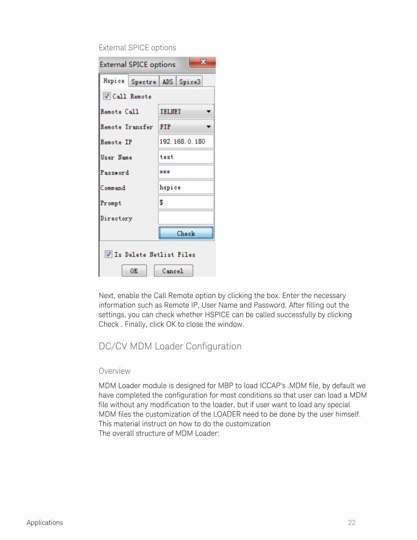
External SPICE options

Next, enable the option by clicking the box. Enter the necessary Call Remoteinformation such as Remote IP, User Name and Password. After filling out the settings, you can check whether HSPICE can be called successfully by clicking

. Finally, click to close the window.Check OK

DC/CV MDM Loader Configuration

Overview

MDM Loader module is designed for MBP to load ICCAP's .MDM file, by default we have completed the configuration for most conditions so that user can load a MDM file without any modification to the loader, but if user want to load any special MDM files the customization of the LOADER need to be done by the user himself. This material instruct on how to do the customization The overall structure of MDM Loader:

23 Applications

By configure the MDM loader user configure the Mapping to change the circuit in MDM file to a MBP standard circuit, then MBP can parser the file and simulation correctly.

Circuit Standard

Bias/Output Name Standard

Bias/Output Name is composed with , and .type node1 node2

Type

Type can be one of characters below:

Name Type

V Voltage

I Current

C Capacitance

G Conductance

Node

If node name contains '_', it is a composed node, for example:"d_s_b", this node is connected to 'd','s' and 'b'.

Bias/Output Name Format

Format 1<Type>_<Node1>#<Node2>

The first character is type, and followed by by node1, '#' and node2.

Applications 24

1.

2.

Example

Vd_s_b#g Voltage between d_s_b and g

Vg#d_s_b Voltage between g and d_s_b

Format 2<Type><Node1><Node2>

If each node contains no more than 1 character, '#' should be omitted.

Example

Vgs Voltage between g and s

Vbs Voltage between b and s

Format 3<Type>_<Node1>#

or<Type>_<Node1>

If the node2 is "ground", it should be omitted.

Example

Vd_s_b# Voltage between d_s_b and ground

Vg Voltage between g and ground

Vb Voltage between b and ground

Analysis Name Standard

Format<Output><Sweep1><Sweep2>@<Bias1>,<Bias2>

Analysis name is composed with output and bias names.

If there is '_' in output/bias name, it will be replaced with '~'

Example

Analysis Name Output Biases

Ids_vgs_vbs@vds,vs Ids Vgs,vbs,vds,vs

Cgc_vb_vdg_vds@vg Cgc Vb,vdg,vds,vg

Cg#d~s_vb_vdg_vds@vg Cg#d_s Vb,vdg,vds,vg

List of Standard Node Names and Instance Names

25 Applications

List of Standard Node Names and Instance Names

Model Nodes Instances

/bjt/gp c,b,e,s area,areab,areac,temp,l,w

/bjt/hicum c,b,e,s area,temp,l,w

/bjt/mextram c,b,e,s area,temp

/bjt/vbic c,b,e,s area,m,temp,l,w

/capacitor/mimcap

p,n w,l,temp

/capacitor/mosvar

g,bi,b w,l,temp,m,M_SEG,NGCON

/diode/diode p,n area,pj,temp,l,w,lm,wm,lp,wp,w

/diode/diode3 p,n area,pj,temp,l,w,lm,wm,lp,wp,w

/diode/juncap2 p,n area,pj,pgate,temp

/jfet/jfet d,g,s w,l,temp

/mosfet/mos2 d,g,s,b w,l,temp,nf,m,sa,sb,sd,sca,scb,scc,sc,ad,pd,as,ps,nrs,nrd

/mosfet/mos3 d,g,s,b

/mosfet/mos66 d,g,s,b

/mosfet/bsim3v3

d,g,s,b

/mosfet/bsim4 d,g,s,b w,l,temp,nf,m,sa,sb,sd,sca,scb,scc,sc,ad,pd,as,ps,nrs,nrd,rsc,rdc

/mosfet/bsim6 d,g,s,b l,w,nf,temp,nrs,nrd,m,rgatemod,rbodymod,geomod,rgeomod,sa,sb,sd,sca,scb,scc,sc

/mosfet/bsimcmg

d,g,s,b l,d,tfin,fpitch,nf,nfin,ngcon,temp,nrs,nrd,lrsd

/mosfet/bsimimg

d,g,s,b l,w,nf,temp,nrs,nrd

Applications 26

Model Nodes Instances

/mosfet/hisim2 d,g,s,b w,l,temp,nf,m,sa,sb,sd,ad,pd,as,ps,nrs,nrd,sca,scb,scc

/mosfet/hisim_hv

d,g,s,b w,l,temp,nf,m,sa,sb,sd,ad,pd,as,ps,nrs,nrd

/mosfet/LayoutConfig

d,g,s,b w,l,temp,nf,m,sa,sb,sd,sca,scb,scc,sc,ad,pd,as,ps

/mosfet/psp/102/local

d,g,s,b

/mosfet/psp/102/global

d,g,s,b

/mosfet/psp/103/local

d,g,s,b

/mosfet/psp/103/global

d,g,s,b w,l,temp,nf,m,sa,sb,sd,sca,scb,scc,sc,ad,pd,as,ps,nrs,nrd

/mosfet/RingOscillator

avin,roa,avdd,qvin,roq,qvdd,s

wp,lp,wn,ln,outtype

/resistor/poly-resistor

p,n w,l,temp

/resistor/r3 n1,nc,n2 m,l,w,temp,swnoise,sw_et,wd,a1,p1,a2,p2,c1,c2,sw_mman,nsmm_rsh,nsmm_w,nsmm_l

/resistor/resistor p,n w,l,temp

/soi/b3soi d,g,s,e,p w,l,temp,nrd,nrs,nf,m,sa,sb,sd,ad,pd,as,ps

/soi/b4soi d,g,s,e,p w,l,temp,nrd,nrs,nf,m,ad,as,pd,ps,sa,sb,sd

/tmi/bsim4/default

d,g,s,b w,l,temp,nf,m,sa,sb,sd,sca,scb,scc,sc,ad,pd,as,ps,nrs,nrd

Mapping

Click -> -> -> on MBP to start the configuration GUI.File Data Data Loader Config

27 Applications

1.

2.

There are 3 kinds of Mapping:

Instance Mapping(Change the instance name to standard name)

Var Source Var Name

Describe Name in mdm file Standard Name

Sample MAIN.SCA SCA

Node Mapping(Change the node to standard name)

Var Source Var Name

Describe node(nodeName) Standard Name

Sample node(d_s) c

Applications 28

2.

3.

This mapping is only for current, capacitor and conductance:For example:cg#d_s -> cgcFor voltage source, it doesn't care this mapping:For example:vg#d_s -> vgd, vds=0

Bias/Output Mapping(Change the bias/output to standard name for specified setup)

Var Source Var Name

Describe SetupName::VarName Standard Name

Sample Cap_S_G_Intrinisic::vg vgs

Generate and Tweak Corner Model

This application note describes how to generate and tweak corner models in Model Builder Program (MBP ).


Overview

Device model is relevant to the actual fabrication process. Even a well developed process may have some variations. And these variations are likely to affect the device characteristics and circuit behavior. To account for the variations in semiconductor process, based on an initial set of typical and comer device models, the process dependent model parameters needed to be tweaked. The smart model tweaking module integrated with MBP enables easy model retargeting, adjustment of global or binning models according to new specification. Both model cards and model libraries are well supported.

In this article, we will use global model as an example to introduce the steps to generate and tweak corner models, respectively.

Generate Corner Models

To generate corner models, choose from the main menu. Utilities > Corner ModelThe window shown in the following figure:

29 Applications

Corner model generation--Start

MBP currently supports two external simulators: HSPICE and Spectre. Choose either one as the SPICE simulator. You have an option to construct the corner model library from either tuned models or an existing library. In this document, we introduce the procedures to . The Construct corner model lib from tuned modesprocess of is almost the same, except Construct corner model lib from existing libthat it requires the additional step of importing a library.

Click .Next

Select to load the model card.Add Model

Click in the popup window.Add default Set Group

Select .OK

Check the box and click , as shown in following figure.Typical Next

Applications 30

Corner model generation-Step 1

In the popup window shown in following figure, choose the parameters (e.g., vth0, u0 and ags) and click .Next


The corresponding corner model structure will now be built, as shown in following figure. Click to save the library.Export

31 Applications


Tweaking Corner Models

Choose from the main menu. A warning message window will Utilities > Lib Parserpop up. Click to continue. In the tab, click to load the library Yes Lib Parser Loadjust created. The tree structure of the library and the model parameters to be tweaked are listed as shown in following figure.

Applications 32

1.

2.

3.

4.

5.

6.

Corner library and model parameters

Define Tweaking Target

To define the tweaking target choose from the main Extraction > Model Tweakingmenu and switch to the panel. The window shown in Target Figure: Target panelwill appear. In this window:

Click to add a tweaking target.

Assign a name to this target, for example .vth

Choose one built-in algorithm (to achieve the above target) from the drop-down list. Here, means to calculate the threshold voltage with the vth_gmmaximum transconductance method.

Input the bias conditions to perform the algorithm.

Click the button to confirm.Apply

Repeat steps 1 to 5 to add as another tweaking target.Idsat

33 Applications

Target panel

Define Target Devices

After defining the tweaking targets, switch to the Tweaks panel. Press the Add button to add target devices to the list. You can edit the instances such as device W

, and , in this case. Right-clicking on the table will pop up the instance L Tparameter list. MBP allows you to save or load device information, as shown in

.Figure: Tweaks panel

Following the instances, the design target (suffixed by , e.g., ), Des vth_Dessimulated value (suffixed by , e.g., ), and their differences (e.g., ) Sim vth_Sim Errorare listed. You can choose the as either or . Type in error format Absolute Relativethe value of the design target. The simulated value and will respond instantly Erroronce you tune the model parameters.

Model Tweaking

Select the proper parameters from the Optimization/Parameter_ window. You can then start tweaking the model. MBP provides both manual and automated tuning. For the latter, make sure that the design targets are set, parameters are selected, the items for tweaking target are checked, and the items for the optimize Selecttarget devices are checked ( ). Then, click the Figure: Automated optimization

button in the Optimization window. MBP will invoke its internal Optimizeoptimizer to proceed.

Applications 34

Tweaks panel

Automated optimization

If more than one target device is selected for automated tuning, you can differentiate the importance between devices by specifying different values. WeightThe device with the higher weight value normally generates higher accuracy.

Implementing Verilog-A Model

This application note describes how to implement Verilog-A models in Model Builder Program (MBP).


Overview

35 Applications

Overview

Verilog-A is an industry standard modeling language for analog circuits. MBP initiated support of Verilog-A models with MBP v2009.1.0.

This application note describes how to implement Verilog-A models in MBP. For more information, go to or contact your local www.keysight.com/find/eesofKeysight office. The complete list is available at: www.keysight.com/find/contactus

Preparation

To implement Verilog-A models, you must first ensure that MBP v2009.1.0 or a later version has been properly installed on the computer. Also, the Verilog-A license feature is needed.Windows users must add to the environment $MBP_HOME\win32\mingw\bin

variable . Here, stands for the directory where MBP is installed, Path $MBP_HOME

for example . Then, reboot the computer.C:\Keysight\modelbuilder

For Linux users, run and in the command line to make sure which gcc which g++both gcc and g++ have been installed properly on the machine. Otherwise, contact your IT administrator.

Sample Models

There must be a subcircuit model to define which Verilog-A model is to be called and which parameters are to be tweaked. MBP allows you to load this subcircuit model and tweak the parameters in the same way as any other model parameters in MBP.

Sample models are listed below for the HSPICE and SPECTRE simulators.

HSPICE

The following model, ekv.l, is an example of a model that is simulated by HSPICE:

hdl ekv.va // Define Verilog-A model to use: ekv.va.model verilog1 ekv // Define new model named verilog1. Use Verilog-A odel ekmv from ekv.va.+VTO=0.5 // Define model parameters to be tweaked in MBP.+GAMMA=1+PHI=0.5.subckt rf_nch d g s b W=10E-6 L=10E-6x3 d g s b verilog1 L=L W=W // The user could use the new model named verilog1,x2 d g s b ekv L=5E-6 W=10E-6 // or use the original model named ekv..ends

SPECTRE

The following model, , is an example of a model that is simulated by SPECTRE:ekv.l



Applications 36

simulator lang=spectreahdl_include ekv.va // Define Verilog-A model to use: ekv.va.model verilog1 ekv // Define new model named verilog1. Use Verilog-A model ekv from ekv.va.+VTO=0.5 // Define model parameters to be tweakedin BP. M+GAMMA=1+PHI=0.5subckt rf_nch (d g s b)parameters W=10E-6 L=10E-6x3 (d g s b) verilog1 l=l w=w // The user could use the new model named *verilog1*,x2 (d g s b) ekv l=5e-6 w=10e-6 // or use the original model named *ekv*.ends rf_nch

The element using Verilog-A must start with even in SPECTRE. Only the xparameters declared in , such as VTO, GAMMA and PHI, can be verilog1tweaked in MBP. The original Verilog-A model (e.g., ekv) can be called and simulated in the subcircuit. However, the parameters in ekv not declared in verilog1 cannot be tweaked in MBP.

MBP Supported Functions and Keywords

MBP supports most of the common functions and keywords defined in Verilog-A, including:

Basic operation: supports most of the basic operation in Verilog-A.

Syntax: supports if/else, for loop, while loop, etc. Does not support repeat.

Simulation system function: supports $stop, $temperature, $vt, $vt(temp), and strobe(express).

Function: supports user-defined function.

For additional details, refer to the following table:

Support Table

Category Type Item Example Support Status

Description

Basic Operator Mathematic / Supported Attention:res = 1/5;//The resulte of this integerdivision is zero,res = 0.

37 Applications


Description

Basic Operator Mathematic + Supported

Basic Operator Mathematic - Supported

Basic Operator Mathematic * Supported

Basic Operator Mathematic sqrt sqrt(x) Supported

Basic Operator Mathematic ln ln(x) Supported

Basic Operator Mathematic log log(x) Supported

Basic Operator Mathematic abs abs(x) Supported

Basic Operator Mathematic pow pow(x,y) Supported

Basic Operator Mathematic min min(x,y) Supported

Basic Operator Mathematic max max(x,y) Supported

Basic Operator Relational Operators

< a>b Supported


> a<b Supported


<= a<=b Supported


>= a>=b Supported

Basic Operator Logical operators != Supported

Basic Operator Logical operators == Supported

Basic Operator Logical operators && Supported

Basic Operator Logical operators || Supported

Basic Operator Conditional Operator

?: (a<b)?a:b Supported

Applications 38


Description

Basic Operator access I( ) I(branch)I(node1,node2)I(node1)

Supported Attention :I(node1) means the currentfrom the node1 to theground

Basic Operator access V( ) V(node1,node2)V(node1)

Supported

Basic Operator contribution I(a,b)<+V(c,d) Supported

Basic Operator contribution V(c,d)<+variable or constant

V(in,mid)<+0.5;V(in,mid)<+x;

Supported

Basic Operator contribution I(c,d)<+variable or constant

Supported

Basic Operator contribution V(c,d)<+I(a,b) Supported

Basic Operator contribution I(a,b)<+I(c,d) Not Supported

Basic Operator ddx Y=ddx(z,x); Supported

Basic Operator ddx Y=ddx(z,x); Supported Attention :Y= k*ddx(z,x); is

Basic Operator ddx Y=k* Y; unacceptable

Basic Operator ddx Y= ddx(func(x),x);

Fun(x) is the function of x.And fun is maybe

Supported

Basic Operator ddx Y=ddx(Y,x); Y is a var Not Supported

Attention :But z=ddx(Y ,x);Y=z;that is right

39 Applications


Description

Basic Operator ddx ddx(Userdefined function,x)

Supported

Basic Operator ddx I()<+ddx(y,x) Not Supported

Attention :But ,z=ddx(y,x)I()<+zIs right

Basic Operator ddx More than 2th derivate

ddx(ddx( a,b),b) Not Supported

Basic Operator idt Not Supported

Basic Operator assignment y=V(p,n); Supported

Basic Operator z=I(p,n); Not Supported

Syntax If else

Syntax Forloop Supported

Syntax case Supported

Syntax whileloop Supported

Syntax repeat Not Supported

Syntax Defining Macros `define Supported

Syntax Conditional Compilation

ìfdefèlseèndif

Supported

syntax including ìnclude ìnclude"disciplines.vams"

Supported

Simulation control $stop Supported

Applications 40


Description

Simulation System Function


Simulation control $finish Supported


Environment Parameter Functions

$realtime Current simulation time in seconds.

Not Supported



$temperature Ambient temperature in kelvin.

Supported



$vt Thermal voltage ( ). Supported



$vt(temp) Thermal voltage at given temperature

Supported



$abstime Returns the simulation time, in seconds

Not Supported


Input/output $fopen Not Supported


Input/output $fclose Not Supported


Input/output $fwrite Not Supported


Input/output $strobe(“express”)

Supported

41 Applications


Description

Function Userdefined Function

Not Supported

Analog Initial Step @(init_s) Not Supported

Events tep( ))

Final Step @(final_step( )) Not Supported

Cross cross() Not Supported

Timer timer() Not Supported

Hierarchical Basic_ hierarchical

Not Supported

Port_connect Not Supported

Reference: Accellera Verilog-AMS Language Reference Manual, Analog & Mixed-Signal Extensions to Verilog HDL, Version 2.3.1

Implementing MOSRA Models

This application note describes how to implement a MOSRA model in Model Builder Program (MBP).


Overview

Device models are relevant to the actual fabrication process. MBP offers an environment for MOS reliability analysis in general and MOSRA in particular. With this environment, you can measure device performance degradation over time and evaluate stress effects.

Applications 42

This section provides information on the raw data format and MOSRA simulation and parameter extraction. For more information go to www.keysight.com/find/eesofor contact your local Keysight office. The complete list is available at www.keysight.

.com/find/contactus

Raw Data Format

The data format for MOSRA analysis is similar to that of general measurement data in MBP. A sample of MOSRA data is as follows:

condition {corner = tt,date = oct_20_02,instrument= (hp4145, probe_station),mode=forward, datatype= mosra, version=1.0, type=nmos}Page (name=ids_vgs_vbs,x=vgs,p=vbs,y=ids) { vds=0.05, w=10.0, L=0.13, T=25.0}stress ( time=0.0, vds=2.0, vgs=1.0, vbs=0.0)curve { 0.0}0.0 5.000E-140.05 5.002E-140.1 5.010E-140.15 5.055E-140.2 5.315E-14

Here, the keyword should be specified as and datatype mosra version=1.0corresponds to the MOSRA level. The keyword defines the bias condition and stressthe duration of the aging test.

MBP also supports another kind of MOSRA data, which allows you to take the aging span as the variable. For example:

condition{corner = tt,date = oct_20_02,instrument=(hp4145, probe_station),mode=forward} Datatype{S_target} Version{2.1}type{nmos} Delimiter{,}Instance{L, W, T}Strss_Condtion{S_vgs=1, S_vds=2, S_vbs=0, S_time}Input{Vgg=2, Vdd=2, Vbb=-1,Vdlin=0.05}Data{ w, l, t, S_vgs, S_vds,S_vbs, S_time, vth_lin, vthsat, Idlin, Idsat, Ioff, gm }10, 2, 125, 1, 2, 0, 0, 0.728628, 0.697769, 7.348435E-5,8.848617E-4, 2.029162E-12,4.2957E-410, 2, 125, 1, 2, 0, 1e5, 0.728985, 0.698127, 7.343337E-5, 8.8407E-4, 2.028872E-12,4.2903E-4

Here, means the data type is DP data.Datatype{S_target}




43 Applications

All of the variables in this kind of MOSRA data need to start with S. For example, the gate-to-source voltage(vgs) during an aging test should be named as .S_vgs

All of the data, including instance parameters, bias conditions, timing nodes, and physical quantities, is stored in the session.Data

As shown in figure Pre-defined IMV pages for stress data, several IMV pages have been pre-defined in MBP to help you to better understand stress data trends.

Pre-defined IMV pages for stress data

MOSRA Simulation and Parameter Extraction

MBP invokes the external simulator (Synopsys HSPICE) for MOSRA model simulation.

Ensure that HSPICE has been installed properly before the simulation.

Choose Model Type

Choose from the main menu and select in the pop Model > Select Model Reliabilityup window. Then, select one core model in the upper section Core Model Selectionand MOSRA in the lower section.Reliability

Applications 44

Selecting MOSRA analysis

Model Parameters Panel

After setting up the model type, MBP merges the selected core model and MOSRA model. For example, as shown in the panel of following figure, the Parametersupper model ( ) is a MOSRA level 1 model and the lower one ( ) is mosra model nmosa BSIM3V3 core model. By clicking any model, the corresponding parameters will show on the right-side of the window.

Model viewer for MOSRA

Load Model

In the main menu, choose to load the model. A window named File > Model > Load Dialog is displayed.MOSRA Compose

45 Applications

MOSRA compose dialog window

A complete MOSRA model consists of two parts: the core model and the MOSRA model. You can deal with these two parts separately. Click to delete the Removeexisting models and click to load other models. After loading the models, click Load

to replace the current MOSRA model.Compose & Load

Then, choose from the main menu to load the data file. The File > Data > Loadwindow with the MOSRA model and data.

Load data

Now, you can select model parameters and adjust them to fit the measurement data.

MBP allows you to compare two MOSRA models. Simply, click to Compose & Addappend a MOSRA model for comparison. Select the two models and click the

icon to compare them.Compare

Applications 46

Compare two models

The result is shown in the following figure.

Comparison result

Run Task Tree

MBP also provides a built-in automatic extraction flow (task tree) for the MOSRA model. Task tree can be enabled by choosing from the main Extraction > Task Treemenu. After loading the task tree, you could run the flow automatically, or step by step. Task tree will select devices, region and parameters for optimization automatically. The task tree optimization window is shown in the following figure:

47 Applications

Task tree of a MOSRA model

Load Multi-Die Data

This application note describes how to set up the script-based environment so that MBP can load and utilize ET data.

This document was originally released for MBP V2011.1.0 and above in October 2011.

Overview

Besides the single sweep data (.mea) and single point data (.dp), there is also a multi-die data structure called ET data. This kind of multi-die data is important for retargeting the final SPICE model and monitoring final corner models.

MBP has the ability to deal with this type of ET data. In this document, we describe how to set up the script-based environment so that MBP can load ET data and use it to run simulation. For more information go to or www.keysight.com/find/eesofcontact your local Keysight office. The complete list is available at: www.keysight.

.com/find/contactus

Script-based Environment Setup

You can complete the script-based environment setup by following these steps:

Step 1. Un-Zip

The default.7z is actually the sample script code package for loading ET data. It can be un-zipped in any appropriate path. It contains the folders and files shown in the following figure.




Applications 48

Script code package

script_code.gif

Step 2. Start a New Project

Choose from the main menu. Doing so will start a new project.File > Project > New

Step 3. Load the Script Project File

You must choose from the main menu to pop up the Script > Script Project MBP window. Click the icon. Then, load the file in the folder where the Script Open jt.prj

the project is just un-zipped.

MBP Script window

script_window.jpg

Step 4. Run the Script Project

After loading, choose the item by clicking load_etdata Project > default > sys > gui .> menu > load_etdata

load_etdata

load_etdata.jpg

Step 5. Load ET Data

A new menu should now be added under from the main ERData > Load Scriptmenu. Choose to load the ET data (multi-die data), as shown in following figure.

Load ETData

load_ETData.gif

Step 6. Plot ET Data

Go to the IMV page and refresh the IMV tree. Here, you will find the Idsat_l_etexample, as shown in the following figure:

IMV tree

imv_tree.jpg

49 Applications

Click this IMV item. The multi-die plot will appear as shown in the following figure:

Multi-die plot

multidie_plot.jpg

Customization

You can also modify the source script to hide/show the mean (or median) value of the multi-die data. Let's use the above plot as an example. Choose Idsat_l_et Script

from the main menu to pop up the MBP Script window. In the > Script Project tab, click . Double click the Project default > imv >; imv > idsat > idsat_l_et

item to display the code window.idsat_l_et

Script for the Plot

script_plot.jpg

In the script, there are variables to show/hide the mean and median value: and . Set it to (or ) to show (or hide) the isshow_mean isshow_median true false

curve.

Mismatch Modeling

This application note introduces the basic components of Model Builder Program's (MBP's) mismatch module. The steps to run the built-in extraction flow and how to configure and plot an IMV graph in MBP are also demonstrated.

This document was originally released for MBP V2011.1.2 in December 2011.

Overview

Two devices in design that are the same (e.g., exactly the same property, geometry, etc.) may show different electrical behavior on the Silicon due to mismatch. The main reason for the difference is the local process variance across the wafer. Mismatch affects the yield and reliability of the final products. An accurate mismatch model is therefore, necessary to ensure the robust design of many analog and digital circuits.

MBP supports mismatch modeling and simulation for all major semiconductor devices such as MOSFETs, bipolar transistors, resistors, and capacitors. In this document, we first introduce the data format supported, plot configuration and Monte Carlo (MC) simulation in MBP. Examples of running the built-in extraction flow, and configuring and plotting an IMV graph are also demonstrated. For more information go to or contact your local Keysight www.keysight.com/find/eesofoffice. The complete list is available at: .www.keysight.com/find/contactus



Applications 50

Data, Plot and MC Simulation

Data Format

For mismatch, MBP supports two kinds of data formats. The first one is based on the actual measurement data, while the other allows you to input the mean and sigma value of the target.

Data Format I

Here is an example of the first data format supported in MBP:

miscondition {date=,type=NMOS}Page (name=vth_gm,target=vth_gm,scale=1.0,p=(L,W)){vds=0.1,Vgs=1,Vbs=0,icon=1E-7,T=25}{0.18,2.0}0.002604200182343308 0.015163779612074824 -0.00163863082047899230.0012339958926110839 0.008895426625025848 -0.0048731228537369775..........................{0.18,10.0}0.0011114374468496058 0.007055480752867993 -7.450025621094092E-44.969414898894353E-4 0.003966458228031433 -0.0024213892738844667..........................

The first line of the data file begins with the keyword and contains misconditioninformation like date and device type. The second line defines all page-related information. The information within the round bracket ( ) contains Page name, target, scale, and P variable. The information within the brace {} declares Page constants, including the bias/current condition and temperature.

The latter part is the data block information. Every curve block always begins with {L W} . All data information is then listed behind it. In this example, the data information is the threshold voltage difference (Δvth_gm) between two adjacent devices with the same geometry.

Data Format II

You can also choose the other format. As an example:

condition {corner = tt,date = oct_20_02} Datatype{mismatch}Version{1.0}type{nmos} Delimiter{,} Instance{L, W, T}Input{vds=0.05, Vgs=1, Vbs=-1,icon=1e-7} Targets{Ids}Data{ L, W, T, vds, vgs, vbs, ids}40, 5, 25, 0.05, 3, 0, 0, 6.448e-440, 2, 25, 0.05, 3, 0, 0, 9.836e-4

51 Applications

30, 2, 25, 0.05, 3, 0, 0, 9.6235e-420, 2, 25, 0.05, 3, 0, 0, 1.28e-320, 1, 25, 0.05, 3, 0, 0, 1.889e-320, 0.5, 25, 0.05, 3, 0, 0, 2.448e-36, 1, 25, 0.05, 3, 0, 0, 3.4727e-310, 0.5, 25, 0.05, 3, 0, 0, 3.503e-36, 0.5, 25, 0.05, 3, 0, 0, 4.1108e-3...............................

In this format, the first part of the data file contains general information such as corner type, date, data type, device type, instance, bias condition, and target. The second part of the data file includes the data block information. The first line begins with the keyword following the variables. All data is then listed from the Datasecond line. Note that the last two values in every line correspond to the mean and sigma of the target.

For example: means 40,5,25,0.05,3,0,0,6.448e-4 L=40um,W=5um, T=25C, Vds=0.05V, Vgs=3V,

.Vbs=0, ΔIds(mean) =0, ΔIds(sigma)=6.448e-4A

Plot

As shown in the following figure, the plot shows the value of σ (ΔVth_gm) versus *1/sqrt (W*L), and the trend slope lines. The simulation point and trend line are plotted in blue and the measurement data and trend line are plotted in purple.

Mismatch plot

By clicking on the legend you can disable/enable the geometries to be L, Wplotted. Right click on the plot and check the item from the Fit Line through Originpopup menu. MBP then forces the trend lines through the origin, as shown in the following figure:

Applications 52

Fit Line through Origin

MC Simulation

MBP's internal engine supports Monte Carlo analysis of mismatch models. You can right-click on the plot and select , as shown in the following Set Monte Countfigure. Then, set an appropriate number. A large number may lead to a more accurate result, but it can also cause a longer simulation time.

Set Monte Count

You have an option to execute a fast MC simulation by choosing Simulation > Fast- from the main menu.MC

Extraction Flow

We can use a demo to describe the steps required to run a mismatch model extraction through the built-in flow.

Demo Files

The demo folder is Here, is the $MBPHOME\demo\Mismatch\mosfet $MBPHOME

MBP installation path. There are a total of three files in the folder:

demo_model: the initial model card.

param.txt: the parameter list used in the extraction flow.

mis_data.mea: the demo data.

53 Applications

You can follow the steps below to complete the whole process.

Set Model Type

First, set the mode type. Choose from the main menu. In the Model > Select Modelpopup Model Type window, choose as the Project Type. Then choose Statistical

as the device type, as shown in .mosfet Figure: Model Type

Click the button to close the window.OK

Model type

Load Data and Model

Choose from the main menu and load the data file File > Data > Load mis_data.meaas shown in the following figure:

Applications 54

Data VS initial model

Then, choose from the main menu and load the model file File > Model > Load Here, MBP supports the ability to load the model with or without model_nmos.l.

mismatch information.

Extraction Flow

Choose from the main menu. The extraction panel is Extraction > Extraction Flowshown in the following figure:

Extraction Flow panel

Double-click the button to expand the flow, as shown in the Mismatch Extractionfollowing figure:

55 Applications

Global Extraction flow

There are three steps in the flow: select_mismatch_params, select_mismatch_targets and, mismatch_extraction. Click the icon to run the runmismatch extraction flow. The Select Parameters window pops up as shown in the following figure.

Select Parameters window

Click the button to load the parameter list file . The parameters used Load param.txtfor mismatch extraction are shown in the following figure.

Applications 56

Load Parameter list

Some comments on the column names in the figure above are as follows:

select: when it is checked, the parameter gets re-extracted. If it is unchecked, then the parameter depends on the sigma value. If the sigma value is given, the final value of the parameter is the sigma value. If sigma value is not given, the current value of the parameter remains as the final one.

name: mismatch parameter name. When is unchecked, the parameter selectname can be blank. At the same time, both must have random and sigmacorrect values.

random: random variable name. If in the current model file there is a random variable for the parameter, then put the name of the random variable here. If in the current model file there is no random variable for the parameter, you can either input a new name here, or keep it blank. For the latter case, a new name is created automatically. Note that the names of random variables cannot be repeated.

sigma: sigma of the mismatch parameter. You can input the value here. The extraction flow then bypasses this parameter and uses the predefined value instead.

step: the step for BPV calculation. It is used to calculate the sensitivity of the parameter to the target. Click the button to continue. The Select Targets OKwindow pops up as shown in the following figure.

57 Applications

Select targets - slope

In this window, you can select the data group for the following extraction and the corresponding weight. Click the tab in the window as shown in the following targetfigure.

Select targets - target

All the specific targets corresponding to the data group in as shown in Figure: are listed here. You can also change the weight values, which Select targets-slope

affects the final value of the slope.Close the window to continue. In the last step, the dialog window pops up. SaveInput a file name to save the extracted model file. Then, the following mismatch parameters that have been extracted are found:

.param+s_dtox_mis = 8.320052E-10 s_dvth_mis = 6.310913E-4 s_ddl_mis = 9.80127E-2

Applications 58

+s_ddw_mis = 6.175251E-3.param+random5 = agauss(0.0,1.0, 1)+random6 = agauss(0.0,1.0, 1)+random7 = agauss(0.0,1.0, 1)+random8 = agauss(0.0,1.0, 1).param+dtox_mis = â0.0+s_dtox_mis*random5'+dvth_mis = â0.0+s_dvth_mis*random6'+ddl_mis = â0.0+s_ddl_mis*random7'+ddw_mis = â0.0+s_ddw_mis*random8'

The fitting result is shown in following figure.

You can continue to fine tune the parameters manually. They can also modify some settings and rerun the flow until a satisfying result is obtained.

Fitting result

Mismatch IMV

Lastly, we use a demo case to illustrate how to customize mismatch IMV and plot it in MBP. After loading the data and model, choose from the Script > Script Projectmain menu to pop up the MBP Script interface.In the left tab window, click to expand the Project default > imv > imv > mismatchfolder, as shown in the following figure:

59 Applications

MBP script

Right-click the IMV and choose (see following figure).mis_sigma_ids New > Graph

Create new graph

Input as the code name. In the tab, choose as mis_sigma_ids_w_l GRAPH_PROP w, as and as as shown in the following figure.Axis[x] mis_sigma_ids Axis[x] l Axis[x]

Applications 60

Configure graph

Click the icon to save the current code. In the main menu of MBP, choose to open the IMV page. Click the icon to refresh. You Extraction > IMV > IMV Pages

can then view the customized IMV page (mis_sigma_ids_w_l) as shown in the following figure:

IMV pages

Multiple Simulations

This application note describes how to compare two or more different models in Model Builder Program (MBP).


61 Applications

Overview

MBP provides an option to plot two or more models (including binning models) on screen at the same time. This feature is specifically designed for modeling engineers tuning or comparing different models.This document introduces the steps and options to running a multiple simulation. For more information go to or contact your local www.keysight.com/find/eesofKeysight office. The complete list is available at: .www.keysight.com/find/contactus

Double Simulation

MBP features a double simulation function that can be used to compare two models— the models before and after tuning— by plotting their simulation results on screen at the same time.

Double simulation result

This function is enabled by clicking from the main menu Simulation > Double Simor pressing the and buttons on the keyboard at the same time. After that, Ctrl R

two new icons ( and ) are added to the optimization pane, as Cancel Confirmshown in the figure cancel and confirm icons. You can then easily compare the results of the two models.



Applications 62

Cancel and confirm icons

The old (original) model is represented by the solid line and cannot be modified. When one tunes a parameter, the new (current) model, which is represented by the dotted lines, becomes active and changes with the parameter.

On clicking the icon , the new model is kept. MBP then updates the old Confirmmodel using the parameters of the new model, as shown in the Figure: Confirm to

. On clicking the icon , MBP reverts back to the old use the new model Cancelmodel as the current model, as shown in Figure: Cancel to use the old model as the

.current

Confirm to use the new model

63 Applications

Cancel to use the old model as the current

When the double simulation functionality is in use and you want to save the model, only the new model gets saved. In case you quit the double simulation after some adjustment, MBP deletes the old model (solid one) and uses the new one (dotted one) as the current model.

Multiple Models Comparison

In addition to performing double simulation, MBP also allows you to compare multiple models. The model manager interface is located at the bottom-left corner of the main graphical user interface (GUI), as shown in figure Model manager interface. There are five icons at the top of this model manager. From left to right, they are: , , , ,and . A model list Add Model Remove Model Compare Save Version Hideis located under these icons. All models added to MBP can be found here. Model cards can be loaded into the model manager. In case you want to load a model library, it can be done by choosing from the main menu.Utilities > Lib ParserFigure 4. Model manager interface

Applications 64

The icon , as the name indicates, is used to minimize the model manager Hideinterface. The and icons are for loading/removing Add Model Remove Modelmodels into/from the model manager. The icon is used to compare Comparemodels in the model manager.

You can select multiple models (at least two) by clicking the models while pressing the button on the keyboard. Next, click the icon. The results can be Ctrl Compareviewed on the plot panel as shown in following figure.

Multiple models comparison

You can then observe the simulation results of three different models. The legend showing line symbols and the corresponding model names can be found at the bottom right corner of the screen.

During the comparison the icon becomes the Compare Drop

icon .Compare

Optimization Weight Setting

This application note describes how to set weight in Model Builder Program (MBP).


65 Applications

Overview

In MBP, weight can be separately assigned to device and curve. The weight setting takes effect when calculating root-mean-square (RMS) and thus, affects the final optimization result. When weight is set on one curve, all points on that curve inherit the weight value. In MBP, the default value of weight is always "1"; In this document, we introduce the steps to set weight for device and curve, respectively. For more information go to or contact your local www.keysight.com/find/eesofKeysight office. The complete list is available at: .www.keysight.com/find/contactus

Device Weight Setting

MBP allows you to set different weights for different devices when running the optimization. Here, means the part's weight in the whole integration. For weightexample, the default weight for every device in MBP is , so the RMS values of all 1devices are multiplied by 1 (e.g., they remain unchanged). Since the built-in optimizer implements optimization according to the RMS value, it treats all devices with the same importance. However, if you set the weight value of one device as , 2then the RMS value of this device will be multiplied by 2 and the optimizer will treat it with much more importance than ordinary devices with a weight of .1

To enable this feature, choose from the main menu. Extraction > Weight SettingThe weight setting dialog will pop up as shown in the following figure:

Weight setting for device



Applications 66

At the top of this dialog window there are two check boxes that allow you to apply the weight settings to either Task Tree or Manual Optimization. You can also check both options. In the panel, you can chose to apply the weight setting Multi-settingto the devices or devices. As for weight, you can either directly input Selected Allthe value or use the expression.

For example, as shown in figure Weight expression, weight is set as an expression given by W/L*T. After clicking the button, the values and expressions in the Applycolumn and will be updated. Device instance parameters Weight.Value Weight.Exp(such as W, L and T) may be employed in the expression.

Weight expression

MBP supported operator and functions are listed in Tables 1 and 2, respectively.

Support operator

Support Operator Symbol

Power ^

67 Applications

Support Operator Symbol

Boolean Not !

Unary Plus, Unary Minus +x, -x

Modulus %

Division /

Multiplication *

Addition, Subtraction +,-

Less or Equal, More or Equal <=, >=

Less Than, Greater Than <, >

Not Equal, Equal !=, ==

Boolean And &&

Boolean Or ||

Support function

Support Function Symbol

Sine sin()

Cosine cos()

Tangent tan()

Arc Sine asin()

Arc Cosine acos()

Arc Tangent atan()

Hyperbolic Sine sinh()

Hyperbolic Cosine cosh()

Applications 68

Support Function Symbol

Hyperbolic Tangent tanh()

Inverse Hyperbolic Sine asinh()

Inverse Hyperbolic Cosine acosh()

Inverse Hyperbolic Tangent atanh()

Natural Algorithm ln()

Algorithm base 10 log()

Angle angle()

Absolute Value / Magnitude abs()

Random number (between 0 and 1) rand()

Modulus mod()

Square Root sqrt()

Sum sum()

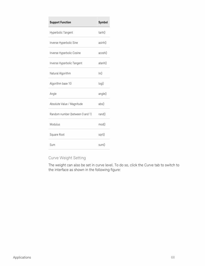
Curve Weight Setting

The weight can also be set in curve level. To do so, click the tab to switch to Curvethe interface as shown in the following figure:

69 Applications

Weight setting for curve

First, you need to define a plot. As shown in following figure, this is done by choosing one page from the drop-down list, for example, ids_vgs_vbs@vds=1.5

Set page

Applications 70

Next, select a math transform from the drop-down list as shown in figure Set Math. This is important because the user may be interested in or Id_Vg_Vb Gm_Vg_Vb(the derivative of Id_Vg) during the optimization. Choosing different math transformations can distinguish between these two plots.

Set math

The weight setting can also be accomplished by editing the value directly in the table. Note, however, that the final weight value of one curve needs to be multiplied by the weight of its device. So, the total weight of one curve is equal to

.device_weight*curve_weight

After all settings are done, click the button to save and close the window. All of OKthe selected settings will be immediately activated.

Parameter Boundry

This application note describes how to compare two or more different models in Model Builder Program (MBP).


Overview

MBP provides an option to plot two or more models (including binning models) on screen at the same time. This feature is specifically designed for modeling engineers tuning or comparing different models.

71 Applications

This document introduces the steps and options to running a multiple simulation. For more information go to or contact your http://www.keysight.com/find/eesoflocal Keysight office. The complete list is available at http://www.keysight.com/find

./contactus

Double Simulation

MBP features a double simulation function that can be used to compare two models' the models before and after tuning - by plotting their simulation results on screen at the same time (see following figure).

Double simulation result

This function is enabled by clicking from the main menu Simulation > Double Simor pressing the and buttons on the keyboard at the same time. After that, Ctrl R

two new icons ( and ) are added to the optimization pane, Cancel Confirmas shown in following figure. You can then easily compare the results of the two models.




Applications 72

Cancel and confirm icons

The old (original) model is represented by the solid line and cannot be modified. When one tunes a parameter, the new (current) model, which is represented by the dotted lines, becomes active and changes with the parameter.

On clicking the icon , the new model is kept. MBP then updates the old Confirmmodel using the parameters of the new model, as shown in Figure: Confirm to use

. On clicking the icon , MBP reverts back to the old the new model Cancelmodel as the current model, as shown in Figure: Cancel to use the old model as the

.current

Confirm to use the new model

73 Applications

Cancel to use the old model as the current

When the double simulation functionality is in use and you want to save the model, only the new model gets saved. In case you quit the double simulation after some adjustment, MBP deletes the old model (solid one) and uses the new one (dotted one) as the current model.

Multiple Models Comparison

In addition to performing double simulation, MBP also allows you to compare multiple models. The model manager interface is located at the bottom-left corner of the main graphical user interface (GUI), as shown in Figure 4. There are five icons at the top of this model manager. From left to right, they are: Add Model, Remove

, , , and . A model list is located under these icons. Model Compare Save Version HideAll models added to MBP can be found here. Model cards can be loaded into the model manager. In case you want to load a model library, it can be done by choosing from the main menu.Utilities > Lib Parser

Model manager interface

Applications 74

The icon , as the name indicates, is used to minimize the model manager Hide

interface. The and icons are for loadingAdd Model Remove Model

/removing models into/from the model manager. The icon is used to Comparecompare models in the model manager.

You can select multiple models (at least two) by clicking the models while pressing the button on the keyboard.Ctrl

Next, click the icon. The results can be viewed on the plot panel as shown Comparein .Figure: Multiple model comparison

During the comparison the icon becomes the Compare Drop

icon Compare

.

Multiple models comparison

From above figure, you can then observe the simulation results of three different models. The legend showing line symbols and the corresponding model names can be found at the bottom right corner of the screen.

Statistical Modeling

75 Applications

Overview

Incorporating process variability into models is critical for IC design. Moreover, statistical modeling is today playing an ever important role in ensuring high product yield in the design phase. MBP supports Monte Carlo simulation with statistical modeling. In this document, we first describe the data format supported, plot configuration and Monte Carlo simulation in MBP. Additionally, the built-in flow used to run statistical model extraction with the Backward Propagation of Variance (BPV) method is elaborated. Finally, we use a demo to introduce the steps to configure and plot statistical IMV. For more information go to http://www.

or contact your local Keysight office. The complete list is keysight.com/find/eesofavailable at: .http://www.keysight.com/find/contactus

Data, Plot and Simulation

Data Format

MBP supports two kinds of data formats for statistical modeling. The first is based on actual measurement data, while the second allows you to input the mean and sigma value of the target.

Data Format I

Below is an example of the first format (based on measurement data) supported in MBP:

staccondition{mode=forward,type=nmos} Page(name=Ids,target={Ids(vds=0.05,vgs=1.1)},p=vbs){w=0.18,L=0.15,T=25} curve{0.0} * site1 1.863622E-5* site2 1.859326E-5 * site3 1.826478E-5 * site4 1.79857E-5 * site5 1.857634E-5 * site6 1.89573E-5 * site7 1.831234E-5 * site8 1.895472E-5 * site9 1.901374E-5 * site10 1.882349E-5.........................

The first line of the data file begins with the keyword and staccondition

contains working mode and device type information. From this example, we know that its a NMOS device in forward working mode.




Applications 76

The second line defines all page related information. The information within the round bracket contains page name, target and P variable. The information within the brace declares the page constants, including geometry and temperature. For any assistance, mail to: [email protected]

The latter part is the data block information. For every curve block, it always begins with the keyword and the corresponding P value (vbs, in this example). All curvedata information is listed behind it. There are two values in every line: the site number and the target value ( Ids, in this example).

Data Format II

You can also choose the other format for the statistical data, allowing to input the mean and sigma value of the target. An example is as follows:

condition{corner = tt,date = oct_20_02} Datatype{statistical} Version{1.0} type{nmos} Delimiter{,} Instance\{L, W, T} Input{vds=0.05, Vgs=1, Vbs=-1,icon=1e-7} Targets{Vth_gm,Idsat} Data{L, W, T, vds, vgs,vbs, ids} 0.6, 0.27 , 25 , 5.5, 5.5 , 0, 1.94e-4, 2.44e-6 0.6, 10 , 25 , 5.5, 5.5 , 0, 1.94e-4, 2.44e-6 ............................................ Data{L, W, T, vds,vgs,vbs, vth_gm} 0.6, 0.27 , 25 , 5.5, 5.5 , 0, 0.83, 8.95e-3 0.6, 10 , 25 , 5.5, 5.5 , 0, 0.83, 8.95e-3 ............................................

In this format, the first part of the data file contains the general information such as corner type, time, data type, device type, instance, bias condition, and target. The latter part of the data file is the data block information. Every block begins with the keyword Data following the variables. All data is listed from the second line of each block. Note that the last two values in every line correspond to the mean and sigma of the target. In this example, line 0.6, 0.27,25, 5.5, 5.5, 0, 1.94e-4, 2.44e-6 means L=0.6um, W=0.27um, T=25C, Vds=5.5V, Vgs=5.5V, Vbs=0, Ids(mean)=1.94e-4A, Ids(sigma)=2.44e-6A.

77 Applications

Data Plot

Depending on the number of targets, there are two kinds of plots: histogram and scatter.

Histogram for Single Target

Using the target Ids_ as an example, the data plot(histogram) is shown in following figure.

Histogram with fill style

Two styles are available for the histogram: the fill style as shown in Figure 1 and the bias style as shown in following figure. For the Bias style, simply right-click the plot and in the popup menu choose > .Bar Styles Bias

Histogram with Bias style

Applications 78

You can also add a distribution line on the histogram. To do so, right-click on the plot and check the item Draw Distribution(Figure3).

Histogram with distribution line

Scatter Plot for a Pair of Targets

The scatter plot is used for a pair of targets. In this example, the pair of targets are defined as ids and vth_con. A scatter plot can be configured by the user on MBPs graphical user interface (GUI). Simply choose > > Tool GUI Options Statistical

from the main menu to open the Statistical Graph Configuration Graph Configwindow as shown in Statistical graph configuration. MBP automatically parses the targets (e.g., ids, vth_con, vth_gm, Ion, and Ioff, etc.). These targets can be freely chosen as X- or Y-axis values on the scatter pages. In this example, we choose ids as X scale and vth_con as Y scale. Next, click the button.Add Page

79 Applications

Statistical graph configuration

The contour of the scatter plot is also set in this window. Currently, MBP allows you to set the contour number up to 5 (corresponding to the case of five sigma). There are three contour styles available to choose from: fill, null and outline. The corresponding scatter plots are shown in following figure.

Scatter Plots: fill (left-most image), null(center) and outline(right-most image)

MC Simulation

MBPs internal engine is capable of performing Monte Carlo analysis. You may also call an external simulator for verification purposes.

Statistical Model

To enable Monte Carlo analysis in MBP, you need to first build a statistical model. The models key parameters must be set to Gaussian distribution as follows:

Applications 80

.param +p1=AGAUSS(0.37,0.01,1) .param +p2=GAUSS(1.21038E-1,0.03,1) ...... +vth0=p1 +u0=p2 ......

To begin, first load a compact model into the statistical module. Since no Monte Carlo analysis has yet been set, you will get only one point as a simulation output on each plot. MBP supports the ability to load the statistical model with a global or binning core model, or a macro model. It also allows the statistical model to be loaded directly from the model library using Lib Parser.

Set Monte Carlo Count

You can set the Monte Carlo simulation number by right-clicking on the plot and selecting Set Monte Count. You must set an appropriate number here. Note that a large number may lead to a more accurate result, but will also require a longer simulation time.

Fast MC Simulation

MBP provides an option to run fast MC simulation. To achieve this, choose > from the main menu. This method speeds up the simulation Simulation Fast-MC

using a unique methodology to deal with the statistical model.

BPV Extraction Flow

A demo case is used here to describe the steps required to run a statistical model extraction through the built-in flow.

Demo Files

The demo folder is . Here, $MBPHOME\demo\Statistical\mosfet $MBPHOME

is the installation path of MBP.There are a total of three files in this folder:

model_nmos.l, the initial model card;

param.txt, the parameter list used in the BPV extraction flow; and

sta_data.mea, the demo data.

You can follow the steps presented below to complete the extraction process.

81 Applications

Set Model Type

First, You must set the mode type. Choose > from the main Model Select Modelmenu. In the popup Model Type window, choose Statistical as the project type. Then choose mosfet_ as the device type, as shown in following figure.

Model type

Click the button to close the window.OK

Load Data and Model

To load the data, choose > > from the main menu. Load the model File Model Loadfile . Since there is no statistical information in the initial model, only model_nmoslone blue column indicating the simulation result is visible (see following figure).

Initial model versus measurement data

Applications 82

MBP also supports the ability to load a model with existing statistical information. You can use the flow to optimize the previously tuned model.

Run Extraction Flow

To run the extraction flow choose > from the main menu. Extraction Extraction FlowThe extraction panel shown in following figure.

Extraction flow panel

Double click the Global Extraction button to expand the flow as shown in following figure.

Global extraction flow

There are three steps in the flow:

select_global_params,

select_global_targets and global_extraction.

83 Applications

Click the run icon to automatically run the global extraction flow. The Select Parameters window will pop up as shown in Figure: Select Parameters window Select Parameters window

Click the Load button to load the parameter list file param.txt. The parameters are arranged as shown in Figure-Load parameter list. Load

parameter list

The parameter list window is now visible and can be used to select parameters for statistical calculation.Some comments on the column names are follows:

Select. When it is checked, the parameter will be re-extracted. If it is unchecked, the parameter will depend on the sigma value. If a sigma value is given, the final value of the parameter will be the sigma value; while if a sigma value is not given, the current value of the parameter will remain as the final one.

Name: parameter name. When select is unchecked, the parameter name may be blank. At the same time, both random and sigma must have correct values.

Applications 84

Random: random variable name. If there is a random variable for the parameter in the current model file, you must enter the name of the random variable here. If there is no random variable for the parameter in the current model file, you may either input a new name hereor keep it blank. In the latter case, a new name will be automatically created. Note that not all names of random variables can be repeated.

Sigma: sigma of the parameter. An example here is the dtox parameter. If you know the sigma of the TOX (normally the information can be obtained from fabrication), then the value can be input into it directly. The extraction flow then bypasses this parameter and uses the predefined value instead.

Step: the step for BPV calculation. The step is very important for the extraction flow and is used to calculate the sensitivity of the parameter to the target. You must input a suitable value; one that is not too big or too small. Here, you can carefully monitor the change in IdVd or IdVg plots while adjusting the step number.

Click the OK button to continue. The Select Targets window will pop up as shown in following figure. You must then select the targets for the BPV extraction. Normally, the user will select the targets that are important or you care most about it.

Select Targets

Select targets Next, you can set different weights for different targets. The default value is 1. Close the window to continue. In the last step, the Save dialog window will pop up. Here, the user inputs a name to save the model file. You will then find that the following statistical parameters have been extracted and added into the generated model file:

.param|| +s_dtox = 4.759276E-14 s_dxl = 2.757199E-13

85 Applications

s_dxw = 3.874035E-9 +s_dvth = 1.16912E-2 s_dlvth = 8.878411E-7 dwvth = 3.014865E-7 +s_dpvth = 3.740674E-9 s_du0 = 1.47506E-3 s_dpu0 = 2.144652E-8 +s_dvsat = 2.016329 .param +dtox = 0.0+s_dtox*random1* dxl = 0.0+s_dxl*random2* dxw = 0.0+s_dxw*random3* +dvth = 0.0+s_dvth*random4* dlvth = 0.0+s_dlvth*random5* dwvth = 0.0+s_dwvth*random6* +dpvth = 0.0+s_dpvth*random7* du0 = 0.0+s_du0*random8* dpu0 = 0.0+s_dpu0*random9* +dvsat = 0.0+s_dvsat*random10* .param +random1 = agauss(0.0,1.0, 1) +random2 = agauss(0.0,1.0, 1) +random3 = agauss(0.0,1.0, 1) +random4 = agauss(0.0,1.0, 1) +random5 = agauss(0.0,1.0, 1) +random6 = agauss(0.0,1.0, 1) +random7 = agauss(0.0,1.0, 1)

Applications 86

+random8 = agauss(0.0,1.0, 1) +random9 = agauss(0.0,1.0, 1) +random10 = agauss(0.0,1.0, 1)

The fitting result is shown in following figure.

Fitting result

You may continue to fine tune the parameters manually, or simply modify the step number as previously mentioned and rerun the flow until a satisfactory result is obtained.

Statistical IMV

Finally, we use a demo to illuminate how to customize statistical IMV and plot it in MBP. After loading the demo data, choose > from the main Script Script Projectmenu to pop up the MBP Script interface. In the left Project tab window, click default > imv > imv > statistical to expand the file structure, as shown in Figure MBP Script.

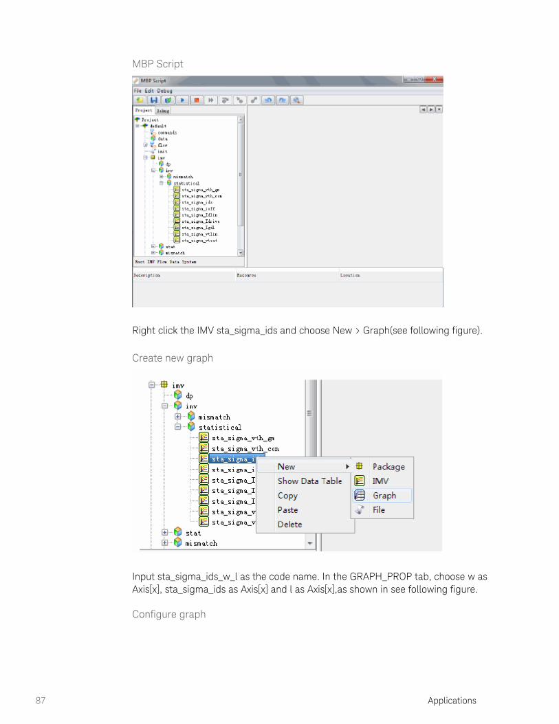
87 Applications

MBP Script

Right click the IMV and choose > (see following figure).sta_sigma_ids New Graph

Create new graph

Input as the code name. In the GRAPH_PROP tab, choose as sta_sigma_ids_w_l w, as and l as ,as shown in see following figure.Axis[x] sta_sigma_ids Axis[x] Axis[x]

Configure graph

Applications 88

Click the icon to save the current code. In the main menu of MBP, choose

> > to open the IMV page.Extraction IMV IMV Pages

Click the icon to refresh.

Then, you can view the customized IMV page (sta_sigma_ids_w_l) as shown in following

figure.

IMV pages

Tmi Aging Model Application

TMI Aging Model Application

This application note describes how to implement a TSMC Modeling Interface (TMI) aging model in Model Builder Program (MBP).


89 Applications

Overview

TMI or TSMC Modeling Interface is a C-based modeling application programming interface (API) developed to support extensions of standard compact models. TMI is an add-on to standard models. Therefore, the compatibility and robustness of standard models dictated by the Compact Model Council (CMC) is retained when applied to different simulators and platforms.

MBP V2011.1.0 offers an environment for TMI reliability aging model simulation. With it, you can measure the device performance degradation over time and evaluate the effects of stress.

This document provides information on how to run a TMI aging model simulation and optimization in MBP. For more information go to http://www.keysight.com/find

or contact your local Keysight office. The complete list is available at /eesof.http://www.keysight.com/find/contactus

Preparation

In preparation for using the TMI aging model application, all configuration files regarding TMI models must be placed under $MBP_HOME\etc\hspice\tmi

where is the MBP installation path. You need to specify one directory $MBP_HOME

as the TMI library path ( ) on the computer. Then, a subfolder under TMIPath

must be created to store the compiled, shared library file (TMIPath

_ ) according to different operating system (OS) platforms. For libTMImodel.dll

example, if the OS is a 32-bit version of Microsoft Windows , the library file should be placed under TMIPath/WIN/.

See following figure for more information on the directory structure for shared libraries of different platforms.

Directory structure for shared libraries of different platforms

In MBP, the data format for TMI aging analysis is the same as the MOS Reliability Analysis (MOSRA) data format. For more details, refer to the or MBP user guide The

.MOSRA Model Support in MBP Application Note




Applications 90

Simulation and Parameter Extraction

MBP invokes the external simulator (Synopsys HSPICE) for TMI aging model simulation. You must ensure HSPICE has been installed properly prior to the simulation. Then, the following steps must be followed.

Choose Model Type

Choose from the main menu and select in the Model > Select Model ReliabilityProject Type. Then, select one core model ( in this example) in the upper bsim4 Core

section and in the lower Reliability section, as shown in Model Selection tmi-defaultfollowing figure.

Choose model type

Set TMI library path

Choose from the main menu to set the TMI Extraction > Options > SPICE Optionslibrary path (& ) in the Spice Options window, as shown in following TMIPath

figure.

91 Applications

TMI path setting

In this example, we set as the ~\etc\hspice\tmi\bsim4\default\model_core\tmilib

Finally, click .TMIPath_ OK

Model Parameters Panel

As shown in following figure, the TMI aging parameters are sorted out in the TMI tab of the model card.Age

TMI aging parameters

Applications 92

Load Model and Data

In the main menu, choose to load the model file. Next, choose File > Model> Load from the main menu to load the data file. The window with the File > Data > Load

TMI aging model and data is shown in following figure.

Load model and data

You can now select model parameters and adjust them to fit the measurement data. MBP also allows to compare two different models. To do so, simply click the

icon to append another model for comparison. Select the two models by Add

pressing the button and clicking icon to compare them. The Ctrl Compareresulting window is shown in following figure.

Compare two models

Microsoft is a U.S. registered trademark of Microsoft Corporation. Windows and MS Windows are U.S. registered trademarks of Microsoft Corporation.

93 Applications

1.

2.



Overview

MBP Supports transient simulation for both internal engine and external simulator (hspice , spectre). And build the demo case for this application.

Ring oscillator demo case

MBP takes Ring oscillator as an example, which is a widely used test circuit.

Load the model for demo\DC\mosfet\RO

Load the script project.Select from > > script script project

Click the button, and load script project from Open demo\DC\mosfet\RO

Applications 94

2.

3.

4.

Load measurement data from demo\DC\mosfet\RO

Check the interesting targets and tweak the parameter

95 Applications

4.

1.

2.

1.



Overview

PCA (Principal Component Analysis), is a mathematical procedure that uses an orthogonal transformation to convert a set of observations of possibly correlated variables into a set of values of linearly uncorrelated variables called principal components. It uses major, independent components to describe the majority of variations of a larger number of characteristics and their correlation.In MBP, the PCA flow has two steps:

The first one extracts the point models from measurement data.

The second one generates the statistical model from the generated point models at last step.

Democase

Open the project from \demo\Statistical\PCAmosfet

Applications 96

1.

2. Load the task tree

97 Applications

2.

3.

There are two task trees, the left one is the first step of PCA flow. It will extract the point models. And the right one is the second step of PCA flow. It will generate the statistical model from the point models.

Initial SettingSelect the , and click button. An input table window will be InitPath runpopped.

Modeltype: pmos or nmos.

BaseModel: The path of base model, the base model is the initial model for the point models extraction.

MeaData: The path for measurement data.

Pointmodel: The path for the point model saving.

Logfile : The path for the log file saving.Close this window and the tree will run to next step(Parameter select).

Applications 98

Click the button, and select the Load demo\Statistical\PCAmosfet\ for nmos and opt_nparam.txt demo\Statistical\PCAmosfet\ opt_pparam.txt

for pmos (point models extraction). The point models will be automatically generated, and all the point models will be saved to the specified fold. We can repeat this flow for nmos if necessary.

99 Applications

1. Load Point ModelSelect from > , and add all the points models to model Local model managerthe table.

Applications 100

1.

2. Initial setting for statistical model settingSelect and click button, a input table window will be poped.InitPCA runPCAorder: The order-number for PCA algorithm.BaseModelPath: The path of base model, the base model is the initial model for the point models extraction.Savepath: The path for generated statistical model saving.

101 Applications

2.

3. Load the generated statistical modelA select window will be popped

Applications 102

3.

Select the model

Click the buttonadd

103 Applications

3.

Add a group

Add more model to the group

Applications 104

3.

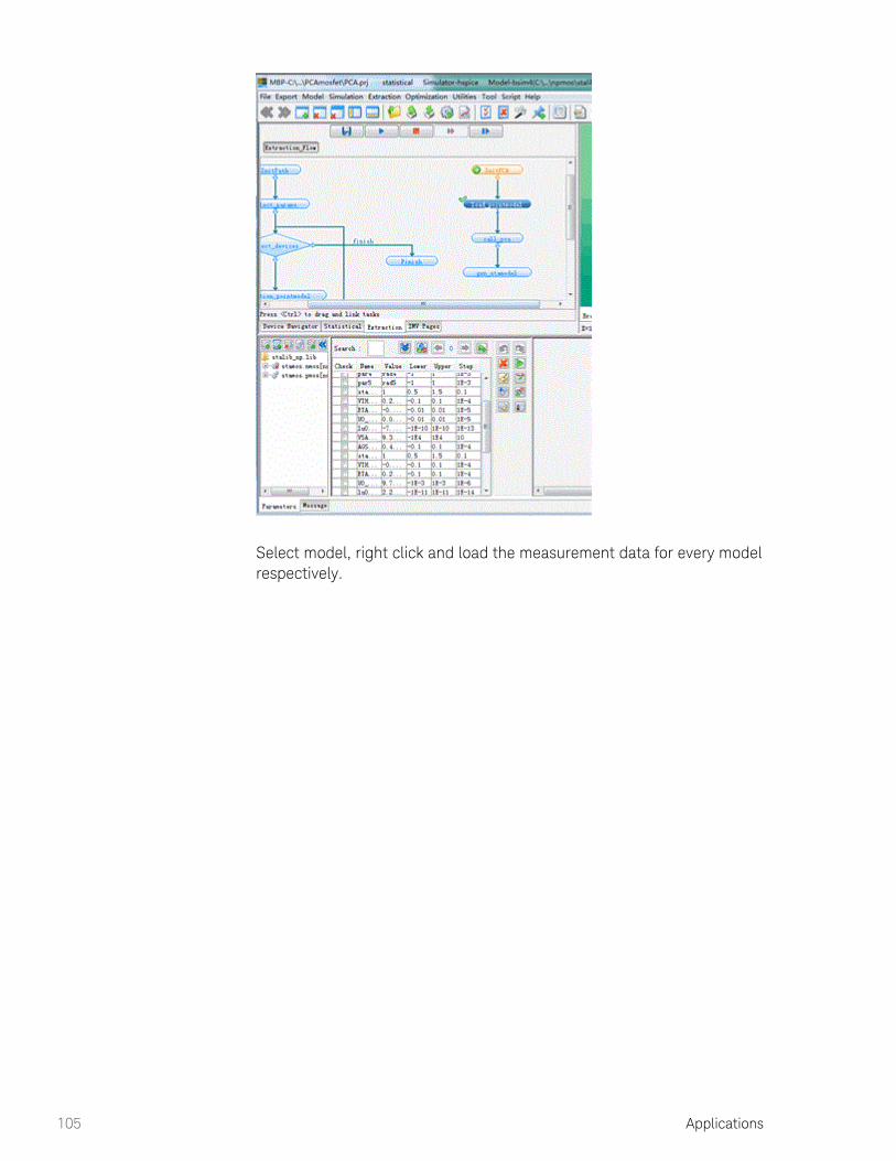
105 Applications

3.

Select model, right click and load the measurement data for every model respectively.

Applications 106

3.

107 Applications

3.

To see N,P correlation plot, go to > > Tool GUI Options Statistical Graph , user is able to choose targets for NMOS and PMOS, and then add the Config

page.


Introduction

MBP's statistical model extraction module is fully developed for generating SPICE model with Monte Carlo simulation capability, a capability of both local mismatch and global statistical.

Applications 108

1.

2.

3.

4.

The module is designed to satisfy any input model format: both a single model card and a model library can be the start point of a statistical model extraction process, and the whole extraction progress is fully automatic, customizable.It contains a comprehensive data dispose procedure which can separate the global variation from the total variation, and the re-centering feature allow user tweaking either the model or the data before go further into the statistical model extraction progress.Final fitting result is very good, take not only the variation itself but also the correlation between NMOS and PMOS into account.

Start the statistical model extraction module

Follow below four steps:

Switch to MOSFET statistical project model Select Model Statistical mosfet.

Load the statistical modeling package under: MBP_HOME\demo\Statistical\GUIBasedSolution\mosfet\demo_case_baseband

A drop-down menu named " " appears in the menu bar thenNavigator

Click the menu "Statistical Model Extraction Panel" in the drop-down menu to show/hide the Statistical Model Extraction Panel.

109 Applications

4.

Setup the statistical model extraction progress

There are five buttons in the panel: , , , Setup Data Analysis Re-targeting Local model, , Stand for the five main steps to complete a Statistical Model Global modelExtraction Progress.

Setup

User need setup the original data and model in follow four steps.

Set up Raw Data Path

Input Model Information

Applications 110

Select Simulation Method

Add Comments

Set up Raw Data Path

Two parts of this step:

Total Data (refer to statistical data)

Local Data (refer to mismatch data)

User may only fill in one of them, if you want to extract either global model or local model.User could also fill in NMOS or PMOS only.


MBP statistical module accept either model library or single model card.

111 Applications

1.

By using model library, please input library path, library name, NMOS model name, PMOS model name, , .stat flag Mis flag

Stat flag: the switch parameter in the model card, to switch on/offthe statistical function of the model.For example, we set as "staflag", if staflag=1, all statistical Stat flagparameters works; if staflag=0, all statistical parameters disabled.

Mis : the switch parameter in the model card, to switch the flag on/offmismatch capability of the model.For example we set as "misflag", if misflag=1, all mismatch Mis flagparameters works, if misflag=0, all mismatch parameters disabled.

By using baseband model, you need to fill in nmos model path or PMOS model path, or both of them.

The model must be a sub-ckt model and here must input the sub-ckt model name.

Select Simulation Method

MBP provides three simulation methods in its internal engine: method, method and Normal-MC simulation RSM simulation FMC simulation

method.

Applications 112

1.

2.

3.

Normal-MC: traditional Monte Carlo simulation method

RSM simulation: speed-up the mc-simulation with Response-Surface Method

FMC simulation: speed-up the mc-simulation with linear approximation

Add Comments

Any comments can be filled into the text box.Click "Update" after all the steps accomplished,.

Without completing " ", user cannot go to " ".Setup Data Analysis

Data Analysis

There are five steps in this section, four of them are optional.

Data Pruning

This option is to eliminate the data points beyond 3-sigma.

113 Applications

1.

2.

Data Sampling

This option is to minimize the data with "Group Size". For example, if "Group Size" is set to 10, MBP will select data every ten sites. If the entire data amount is too huge, user can sped up the progress by using this option.

Global Data Generation

This option is to generate global data from total and local data.

Mean Value Check

In case measurement total data's mean value is not equal to simulation total data's mean value, user could use this option to do data tweaking.Two methods for the tweaking:

Tweak model: Tweak the baseband model to fit the measurement, user need go to next step "Baseband Model" to select parameters for tweaking.

Tweak measurement total data: MBP will adjust measurement data to fit model simulation. The tweaked data will be used in following steps.

Create Mismatch Dummy Data

This step is to create mismatch dummy data:

The dummy data is a straight line, replace the original point data.

User can choose the straight line through origin point or not before the dummy data generation.

The dummy data line will be the optimization target during following steps; it can give better trend fitting result than original data points.

Click "Generate Data" button after all the steps to execute data dispose.If user are working on an existing project and want to reuse the data generated in the last data dispose operation, user can click the button "Use Last Data".

Re-centering

Must finished "Data Analysis" the can go to this step.Re-centering is used when " " is selected at " Tweak model Mean Value Check"steps, if user select " ", user could skip this step.Tweak data to fit model

The step is used to select parameters for model tweaking, as below.

Applications 114

Target Weight Setting

Click "Default", a weight table will appear. The left side of the table is device column, the upside of the table is target row, and all the default weights are set to 1.0.

User can set one value to the entire column or the entire row. By set the first column(or the first row)'s weight and then right-click on this column(or row) select "Set value to the whole column" or "Set value to the whole row".

User can load pre-defined configuration file by " ", also can save the Loadconfiguration file by " ".Save as

Model Parameter Setting

Fill in the parameters for model tweaking in this table, together with parameter's type ("nmos" or "pmos"), step, min/max value.Pre-defined configuration file can be loaded by " ". A new configuration file can Loadbe saved by " ".Save asClick " ", then the model will be tweaked automatically Baseband Model Generationto fit measurement data

Local Model

Note: Make sure you've finished "Data Dispose" before go to this step.

Local Model contains two parts:


115 Applications



You can load your pre-defined configuration file by clicking "Load". And you can save the

configuration file by clicking "Save as".


Two different table formats will appear depend on what format of model we start with: model library or single model card.

For model library, the table shows as below:

Applications 116

Fill in this table with user-defined mismatch model parameters and corresponding random parameters, the mean and sigma value of the parameter are "1" and "0" by default respectively.

If single model card is used, the table is as below:

The table is very similar to "Baseband Model".User need fill this table with parameters for tweaking, and specify parameters' polar type, polar type can be "NMOS" or "PMOS".

117 Applications

1.

2.

3.

User can also assign parameter's step, min value and max value.After setting up all the target weights and model parameters, click "Local Model

" button, then the mismatch model will be generated automatically.Generation

Please setup your model library as the MBP's demo example. Below are some useful trick in the model parameter setting:

Add ":" after parameter name, it means this parameter's input value will be the initial value for next step

Add "=" after parameter name, it means this parameter's value will always keep constant

If the input lib is complex, and the relation between the random and parameter is not very clear, please add "?" at first line and add the tuning parameters in the following lines.

Global Model

Before go to this step, make sure "Data Dispose" is done.

This section is used to generate global statistical model automatically.

Three steps to complete a "Global Model" table:

Applications 118


Correlation Weight Setting



User is suggested to use the default setting by click " " button.DefaultDifferent weight can be set to different target, MBP will put more effort on the target with high weightConfiguration file can be save and load by " " and " " button.Save as Load


If both NMOS and PMOS data is loaded within one extraction progress, user are enabled to set weight for NMOS and PMOS correlation.MBP put more effort to the correlation with higher weight, may have better fitting accuracy normally.

119 Applications


The table has two forms depending on the input model format.

Library model, the table is as below:

Applications 120

User need fill in this table with user-defined statistical model parameters and corresponding random parameters.Parameters' mean and sigma value are "1" and "0" by default respectively.User can also assign parameter's step, min/ max value.The configuration file can be save and load by " " and " " button.Save as Load


121 Applications

1.

User need fill in this table with parameters for tweaking, and specify parameters' corresponding polar type.User can also assign parameter's step, min/max value.The configuration file can be save and load by " and " " button."Save as LoadClick " " button after completed all setups, then the Global Model Generationglobal statistical model will be generated automatically.

SRAM Solution Operation Note

SRAM solution is an integrated solution in MBP for SRAM application. With this solution, the customer can check both SRAM and MOSFET device at the same time. All the details will be introduced in the following sections.

Load projectFrom the toolbar, click the button and then select File Project > Open…

Applications 122

1.

2.

Select a project from the pop-up window. A demo example has been included at :$MBP_home\demo\SRAM\sram.prj.

Load model

Click button.Load Model

Then load the model from the browser window:

123 Applications

2.

After model selection, a model mapping window will pop-up. Map the input model

with the Template Model categorization correctly.

Actually, in SRAM application, any customer input model can be categorized as

SRAM,pd, pg,pu (pull-down, pass-gate, and pull-up MOSFET), just like the

“Template Model” column list.

Applications 124

2.

3.

4.

In the example, “icrit” in the input model is the SRAM -kind model. With these mapping, it will ensure that MBP script draws and display the correct target plot.

Load dataClick the button.load data

Then the loading data window will pop-up.

Click the button to load data for every kind of model respectively, and it is ok Load

to select more than one data file at the one time. Click the button to empty Clear

the data you have selected. After these setting up, click the button to finish OK

loading data.

Parameter tuningClick model in the model navigator and select model parameters in the parameter navigator to tune like the following picture.

The selected model parameters will be displayed in the parameter panel, and different model’s parameter will be set with different colors.

125 Applications

4.

5.

Click the button on the top of parameter panel (pd, pg, pu in the following picture).

The selected model’s parameters will put into the front of the panel.

Double simulationDouble simulation is a power function to check parameter’s effect on the circuit or device performance.

Click from the menu.Double Simulation

Select some parameters from the parameter navigator and tweak them. And in the plot, square point line is the measurement data, other two curves are simulation result. The solid line represents the simulation result from original parameter value, and dot line is for updated parameters’ simulation result.

Applications 126

5.

6. Model Compare

Model Compare can be used to compare two models which have same Electrical Target and different model parameter.Firstly, click the button to add a new model into MBP.Add Model

127 Applications

6.

Select both models and click from the button.compare

Tweak some parameter to check plots.

Applications 128

6.

7.

a.

b.

c.

Appendix

6T SRAM circuit

Mosfet name

pu: means “pull up”mosfet

pd: means “pull down”mosfet

pg: means “pass gate”mosfet

129 Applications

7.

c. Plot definitionVch_Ibl: sweep voltage at node “ch”, and get the current value to node “bl”.

Vch_Ich: sweep voltage at node ch, and get the current value to node “ch”.

Vch_Vcl: sweep voltage at node ch, and get the voltage value at node “cl”.

Applications 130

7.

c.

d.

Vcl_Vch: sweep voltage at node cl, and get the voltage value at node “ch”.

Target introductionIcrit_RD[1]:SRAM work at read mode (Vbh=vdd, Vbl=vdd), get the maximum current value at Vch_Ich plot, the graph displays this point’s voltage and current value on Vch_Ich plot.

131 Applications

7.

d.

Icrit_WR[1]:

SRAM work at write mode (Vbh=0, Vbl=vdd), get the minimum current

value which Vch’svalue is between 0.3*vdd and vddatVch_Ich plot, the

graph displays this point’s voltage and current value on Vch_Ich plot.

Butterfly plot and SNM target:

Butterfly plot: The Graph overlays the two plots Vch_Vcl and Vcl_Vch to one plot to get butterfly plot.

SNM target: static noise margin, the graph displays SNM’s value on the butterfly plot.

Applications 132

7.

d.

1.

2.

Icell_Read[2]:

SRAM work at the read mode, get the maximum current value on Vch_Ibl plot, the graph displays this point’s voltage and current value on Vch_Ibl plot.

Reference:

Critical Current (ICR1T) Based SPICE Model Extraction for SRAM Cell

CMOS SRAM Circuit Design and Parametric Test in Nano-Scaled Technologies

133 Applications

1.

2.

1.

2.

3.


General Introduction

MBP's statistical model extraction module is fully developed for generating SPICE model with Monte Carlo simulation capability, a capability of both local mismatch and global statistical. The module provides GUI-Based Turn-Key solution and its work-flow chart is like following:3

Figure 1: General work-flow chart

In the Module, it supports the following input:

Inputs for this solution

Mismatch Input:

For mismatch model extrication, select one of these two kinds input.

Mismatch Measurement Data.

Mismatch Spec, dummy mismatch data will be generated from these specifications and replace the measurement data for mismatch model extraction.

Statistical Input:

For statistical model extrication, select one of these three kinds input.

Total Measurement Data;

Corner Spec, dummy statistical data will be generated from these corner spec and replace the measurement data for the statistical model extraction;

Corner Model, the statistical model could be generated directly from this corner model;

Applications 134

1.

2.

1.

2.

3.

1.

2.

3.

4.

5.

1.

2.

Model Input:

Baseband Model, no statistical-equation has been integrated into model card and our solution will generate equations automatically;

Library Model, it has pre-defined statistical-equation in model card and our solution will tweak the equation's coefficients to match targets;

Output from this solution

With our solution, it can get all kinds of output in the mismatch/statistical model extraction.

Mismatch Output:

Mismatch Model;

Generated dummy mismatch Data;

Mismatch Plot

Statistical Output:

Statistical Model;

Generated dummy statistical Data;

Histogram/Distribution Plot

Scatter/Contour Plot

Scatter/Corner Plot

Corner output:

Corner Spec;

Corner Model Template;

Typical Application Examples

With proper setup, this solution could be applied widely for various cases. Following table lists some typical application examples. These examples could be good references for quick start. And all the technical details will be presented in following section.

Tab 1. Typical Application Examples

Input Solution Output Comments

1. 1.Mismatch Measurement data;2.Statistical Measurement data;3.Baseband Model;

1.Data Analysis;2.Mismatch Model Extraction;3.Statistical Model Extraction

1.Mismatch Model;2.Statistical Model;

Don't need expertise on the statistical model extraction

135 Applications

Input Solution Output Comments

2. 1.Mismatch Measurement data;2.Statistical Measurement data;3.Liberary Model;

1.Data Analysis;2.Mismatch Model Extraction;3.Statistical Model Extraction

1.Mismatch Model;2.Statistical Model;

Flexible , and designed for specific applications

3. 1.Mismatch Spec;2.Baseband Model;

1.Dummy Data generation;2.Mismatch Model Extraction;

1.Dummy Mismatch Data2.Mismatch Model;

Mismatch model extraction without real measurement data

4. 1.Corner Spec;2.Baseband Model;

1.Dummy Data generation;2.Statistical Model Extraction;

1.Dummy Statistical Data2. Statistical Model;

Statistical model extraction without real measurement data

5. 1.Corner Model;2.Baseband Model;

1.Dummy Data generation;2.Statistical Model generation directly;

1.Dummy Statistical Data2. Statistical Model;

Generate statistical model from corner model directly

Work Flow

Load Project

Load Statistical Project from MBP's demo folder, Select Navigator > Statistical .Model Extraction Panel

Config

Applications 136

Config

In this window, user can configure the system parameters.

Switch between 3 simulation methodsSimulation:

Normal-MC: General Monte Carlo simulation, high accurate;

RSM Simulation: Response surface method simulation, fast speed;

FMC Simulation: Monte Carlo simulation with linear approximation, fast speed;

Parameter:

Corner/Statistical Scale:

It is a parameter to define ration scale between corner and statistical; please take table2.1 as reference;

PCA Number: It is order number in Principal Component Analysis;Just like following example.

Tab 2. corner/statistical scale

137 Applications

Corner/Statistical Scale=1

Debug Mode:

Debug Mode:

If Debug Mode is open, the extraction detail information will be printed to the log file for the trouble-shooting. Usually, the log file is saved to the project_path\ statistical\output\log\statdebug.txt

Local Optimization Parameters: optimization parameters' setting for local model extraction

Itermax: Max iteration times in optimization ;

Tol: Target tolerance for optimization convergence criterion;

Regress Iter: Iteration times for regression calculation;

Applications 138

Local Extraction Method:

Fast Mode: Use linear algorithm for mismatch model extraction, fast speed;

Normal Mode: Use general optimization for mismatch model extraction;

Global Optimization Parameters: optimization parameters' setting for global model extraction

Itermax: Max iteration times in optimization ;

Tol: Target tolerance for optimization convergence criterion;

Regress Iter: Iteration times for regression calculation;

Global Extraction Method:

Fast Mode: Use linear algorithm for statistical model extraction, fast speed;

Accurate Mode:

Use advanced optimization for statistical model extraction;

Advanced Mode:

Use advanced optimization for statistical model extraction, and user can set optimize-weight for nonlinear characters;

Corner Input Mode:

Input corner model and generate statistical model directly;

Mismatch/Statistical Target Define

Before model extraction, it should be make sure all mismatch and statistical targets have been defined in MBP correctly. MBP has defined some default targets and user also can define customized mismatch or statistical target with script.

Mismatch Target

Select from menu , MBP Script Windows will pop. Select Script > Script Projectimv in the left panel, right click and select to Default > > mismatch new > mismatch

define new mismatch targets.

139 Applications

Set the new target's name in the popped window, and it can be edit in the right panel.

How to edit target in MBP Script can reference MBP's help on IMV setting.

MBP supports both absolute and relative difference for mismatch targets.

Applications 140

Mismatch Expression: Absolute and Relative

Statistical target

Select from menu , MBP Script Windows will pop. Select Script > Script Project in the left panel, right click and select to define default > imv > stat new > Statistic

new statistical targets.

141 Applications

Set the new target's name in the popped window. It can be edit in the right panel. How to

edit target in MBP Script can reference MBP's help on IMV setting.

Setup

In "Setup" step, user will setup the input information. Three parts of this step:

Total Data (refer to statistical data)

Local Data (refer to mismatch data)

Input Model

Total Data

User can select one from these three options

Generate Data From Measurement

NMOS: Click the browse button to select measurement data for nmos;

PMOS: Click the browse button to select measurement data for pmos;

Generate Data From Corner Data

Generate dummy statistical data from input corner data. The Corner/Statistical parameter will be used in the dummy data generation.Scale

Applications 142

the corner data file contains corner spec information;Corner Data:

NMOS: Click the browse button to load corner nmos data file;

PMOS: Click the browse button to load corner pmos data file;

Corner Model: is not used for the model extraction, only for simulation result plot

With the default model as input:

If customer has no their own corner model, MBP's default corner model will be used in the following work;

Input Model: Click browse button to select corner model;

Corner Model Names: Corner models name for FF, SS, FS, SF, TT, and separated by comma;

NMOS Name: nmos model name

PMOS Name: pmos model name

Generate Data From Corner Model

143 Applications

Generate dummy statistical data from input corner model's simulation result. The "Corner/Statistical Scale" parameter will be used in the dummy data generation.

statistical target definitionTargets:

Polar: nmos or pmos;

Target: Targets Name;

Biases: bias condition for this target;

Applications 144

definition for devices instance parameters (w, l, temp, etc.)Devices:

Polar: nmos or pmos or n&pmos;

If select n&pmos, it means a pair of devices (both nmos and pmos) will be defined whose w=1 and l=2 as above picture.

the nmos and pmos which has the identical corindex value are a pair of devices, where w=1 and l=2 for nmos, w=0.6 and L=1.6 for pmos;

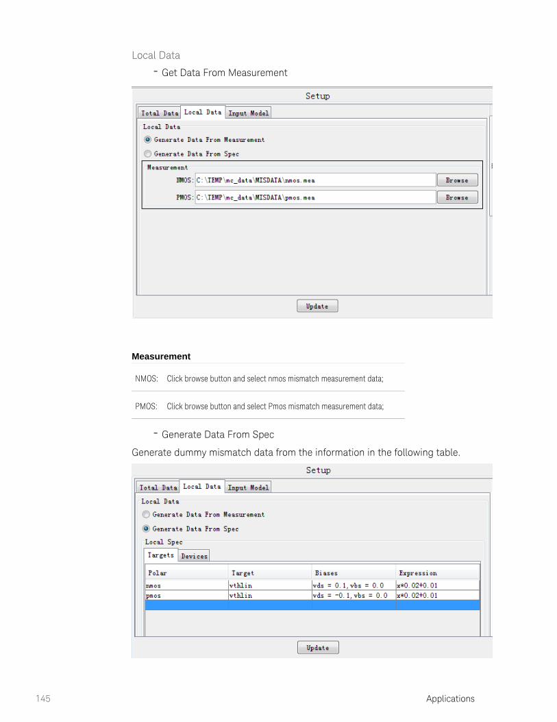
145 Applications

Local Data

Get Data From Measurement

Measurement

NMOS: Click browse button and select nmos mismatch measurement data;

PMOS: Click browse button and select Pmos mismatch measurement data;

Generate Data From Spec

Generate dummy mismatch data from the information in the following table.

Applications 146

mismatch target definitionTargets:

Polar: nmos or pmos;

Target: targets name;

Biases: bias condition for this target;

Expression: Target's sigma value= a*x + b;where, x=1/sqrt(w*l);a is slope coefficient;b is intercept value;we will use this express to calculate target value for every devices defined in "Devices" tab

147 Applications

definition for devices instance parameters (w, l, temp, etc.)Devices:

Polar: nmos or pmos or n&pmos;

If select n&pmos, it means a pair of devices (both nmos and pmos) will be defined whose w=1 and l=2 as above picture.

the nmos and pmos which has the identical corindex value are a pair of devices, where w=1 and l=2 for nmos, w=0.8 and L=1.6 for pmos;


MBP statistical module accepts either model library or single model card.

By using model library, please input library path, library name, NMOS model Lib File:

name, PMOS model name, stat flag, mis flag.

Lib Path:

Click browse button, and select the library model;

Lib Name:

Library's name;

Applications 148

NMOS Name:

nmos name;

PMOS Name:

Pmos name;

Stat flag:

The switch parameter in the model card, to switch the statistical function of the model.For on/offexample, we set as "staflag", if staflag=1, all statistical parameters works; if staflag=0, all Stat flagstatistical parameters disabled.

Mis flag:

The switch parameter in the model card, to switch the mismatch capability of the model.For on/offexample we set as "misflag", if misflag=1, all mismatch parameters works, if misflag=0, all Mis flagmismatch parameters disabled.

Model File: By using baseband model, please input nmos file, pmos file, nmos name, pmos name.

NMOS File: Click browse button, and select nmos baseband model;

PMOS File: Click browse button, and select pmos baseband model;

NMOS Name: Nmos model name;

PMOS Name: Pmos model name;

In the setup, all generated data can be found at "project_folder\statistical\data".

Data Analysis

There are five steps in this section, four of them are optional.

Data Pruning

This option is to eliminate the data points beyond 3-sigma.

Data Sampling

This option is to minimize the data with "Group Size". For example, if "Group Size" is set to 10, MBP will select data every ten sites. If the entire data amount is too huge, user can speed up the progress by using this option.

Global Data Generation

This option is to generate global data from total and local data.

Mean Value Check

In case measurement total data's mean value is not equal to simulation total data's mean value, user could use this option to do data tweaking.Two methods for the tweaking:

149 Applications

: Tweak the baseband model to fit the measurement, user need Tweak modelgo to next step "Baseband Model" to select parameters for tweaking.

: MBP will adjust measurement data to fit Tweak measurement total datamodel simulation. The tweaked data will be used in following steps.

Create Mismatch Dummy Data

This step is to create mismatch dummy data:

The dummy data is a straight line, replace the original point data.

User can choose the straight line through origin point or not before the dummy data generation.

The dummy data line will be the optimization target during following steps; it can give better trend fitting result than original data points.

Click "Generate Data" button after all the steps to execute data dispose.In the Data Analysis, all generated data can be found at "project_folder\statistical\data".

Re-centering

Re-centering is used when "Tweak model" is selected at "Mean Value Check" steps, if user select "Tweak data to fit model", user could skip this step. The step is used to select parameters for model tweaking, as below.


Click "Default", a weight table will appear. The left side of the table is device column, the upside of the table is target row, and all the default weights are set to 1.0.User can set one value to the entire column or the entire row. By set the first

Applications 150

column (or the first row)'s weight and then right-click on this column (or row) select "Set value to the whole column" or "Set value to the whole row".User can load pre-defined configuration file by "Load", also can save the configuration file by "Save as".


Fill in the parameters for model tweaking in this table, together with parameter's type ("nmos" or "pmos"), step, min/max value. Pre-defined configuration file can be loaded by " ". A new configuration file can be saved by " ". Click "Load Save as

", then the model will be tweaked automatically to fit Baseband Model Generationmeasurement dataIn the Re-Centering, the model can be found at "project_folder\statistical\output\baseband".

Local Model

contains two parts:Local Model




You can load your pre-defined configuration file by clicking "Load". And you can save the configuration file by clicking "Save as".

151 Applications


Two different table formats will appear depend on what format of model we start with: model library or single model card. For model library, the table shows as below:

Fill in this table with user-defined mismatch model parameters and corresponding

random parameters, the mean and sigma value of the parameter are "1" and "0" by

default respectively.

Setup your model library as the MBP's demo example. Below are some useful tricks in

the model parameter setting:

Add ":" after parameter name, it means this parameter's input value will be the initial value for next step

Add "=" after parameter name, it means this parameter's value will always keep constant

If the input lib is complex, and the relation between the random and parameter is not very clear, please add "?" at first line and add the tuning parameters in the following lines.


Applications 152

The table is very similar to "Baseband Model". User need fill this table with parameters for tweaking, and specify parameters' polar type; polar type can be "NMOS" or "PMOS". User can also assign parameter's step, min value and max value.After setting up all the target weights and model parameters, click "Local Model

" button, then the mismatch model will be generated automatically.Generation

Key points in the local model extraction

Firstly, selecting right parameters for the local model extraction is most important. Parameter selection depends on the mismatch targets and device's dimension. If simulation result is failed to converge, please reset parameter's min/max value and try again.Secondly, set weight matrix to tradeoff between different optimize targets.Finally, switch extraction methods or tweak optimization parameter to help optimization converge at better result.Moreover, open debug mode and read log file can help trouble-shooting.The extracted local model can be found at "project_folder\statistical\output\local".

Global Model

Before go to this step, make sure "Data Dispose" is done. This section is used to generate global statistical model automatically. Three steps to complete a "Global Model" table:





User is suggested to use the default setting by click " " button. Different Defaultweight can be set to different target, MBP will put more effort on the target with high weight Configuration file can be saved and load by " " and " " Save as Loadbutton.


If both NMOS and PMOS data is loaded within one extraction progress, user are enabled to set weight for NMOS and PMOS correlation.MBP put more effort to the correlation with higher weight, may have better fitting accuracy normally.

153 Applications

1. a.

1. a.

1. a.


The table has two forms depending on the input model format.Library model, the table is as below:

User need fill in this table with user-defined statistical model parameters and

corresponding random parameters. Parameters' mean and sigma value are "1" and "0"

by default respectively. User can also assign parameter's step, min/ max value. The

configuration file can be save and load by " " and " " button.Save as Load


User need to fill in this table with parameters for tweaking, and specify parameters' corresponding polar type. User can also assign parameter's step, min/max value.The configuration file can be saved and load by "Save as" and "Load" button.

Click " " button after completed all setups, then the Global Model Generationglobal statistical model will be generated automatically. There are some different algorithm will be used when the global model generation.

No device is selected in the target weight setting table

All devices will be taken into account in the statistical model extraction. And "global" statistical model will be extracted.

If only one device is selected in the target weight setting table

Only selected device will be taken into account in the statistical modeling extraction. And "point" statistical model will be extracted.

All devices are selected in the target weight setting table

All extracted "point" statistical model will be merged into a "global" statistical model

Applications 154

The extracted statistical model can be found at "project_folder\statistical\output\global".

Key points in global model extraction

Firstly, selecting right parameters for the global model extraction is most important. Parameter selection depends on the statistical targets and device's dimension. If simulation result is failed to converge, please reset parameter's min/max value and try again.Secondly, set weight matrix to tradeoff between different optimize targets.Finally, switch extraction methods or tweak optimization parameter to help optimization converge at better result. For example, user can select one device and extract point model one by one. It is a good way to find the cause for the problem.Moreover, open debug mode and read log file can help trouble-shooting.Ps: how to de-select the device? Please press "ctrl" button and right click mouse to de-select the specific devices.

Graph Configure

Statistical Graph Configure

Select from menu , and a setup Tool > GUI Options > Statistical Graph Configwindow is popped.

155 Applications

Applications 156

Scatter Pages:

X Scale: Target and polar selection for X-axial;

157 Applications

Y Scale: Target and polar selection for Y-axial;

Pages: Click Add Page, the plot defined by X Scale and Y Scale will be add into page;Select item in the Page List and click Del Page, the selected plot will be deleted from list.

Couple with corindex:

Nmos and Pmos device will be grouped by corindex;

Contour:

Contour Styles: Contour Curve Plot Styles;

Contour Numbers: Contour Curve number, default number is 5;

Color Contour Curve Plot Color;

Histogram:

Draw Distribution: Draw theoretical distribution curve or not

Bar Styles:

Bin Number: Bin Number in the histogram plot

Shift Mean to Zero:

Mismatch:

Mismatch X: Calculation expression for x axial in mismatch plot

MC Count:

MC Count: The random numbers in Monte Carlo Simulation

Scatter-Corner Graph Config

Select from menu , and a setup Tool > GUI Options > Scatter-Corner Graph Configwindow is popped.

Applications 158

X: Target and Polar for X-axial

Y: Target and Polar for Y-axial

Corner Analysis

Make corner analysis for the customer input to generate corner spec and corner model template.

Generate corner spec

Generate corner spec from global variation data;

Generate corner spec from total variation data;

Model parameter setting

Model parameter setting for corner model template generation.

Demo Examples

159 Applications

1. a.

1. a.

Demo Examples

Mismatch and Statistical model extraction from data – Baseband Model.

Open the project from "MBP_home\demo\Statistical\GUIBasedSolution\mosfet\demo_case_baseband"

Config

Setup

The measurement for this demo case can be found "project_path\MISDATA" and "project_path\STADATA"

Applications 160

1. a. Data Dispose

161 Applications

1. a.

Click the "Generate Data" for data dispose.

Local Model

Applications 162

1. a.

Set target weight table and parameter table, and click "Local Model Generation" button to

extract local model

Global Model

163 Applications

1. a.

Set target weight table, correlation weight table and parameter table, and click "Global

Model Generation" button to extract global model.

The generated dummy data and extracted model are saved in the

"project_path\mosfet_demo_2\statistical";

Mismatch and Statistical model extraction from data - Model Library.

Open the project from "MBP_home\demo\Statistical\GUIBasedSolution\mosfet\demo_case_library"

Configuration

Applications 164

1. a.

1. a.

Setup


Data Dispose

165 Applications

1. a.


Local Model

Applications 166

1. a.


extract local model

Global Model

167 Applications

1. a.

Set target weight table, correlation weight table and parameter table, and click "Global

Model Generation" button to extract global model.



Statistical model extraction from corner spec

Open the project from "MBP_home\demo\Statistical\GUIBasedSolution\mosfet\demo_case_cornerspec"

Config

Applications 168

1. a. Setup

The demo corner data for this example can be found at "mbp_folder\demo\Statistical\GUIBasedSolution\mosfet\demo_case_fromcornerspec\cornerdata".

Click setup button, dummy statistical will be generated. And the new generated dummy data can be checked from the plots. Switch to the "Statistical" tab,

Scatter, contour and corner plot checking

First, in the left table, select device whose polar type is blank. It means a pair of devices

(a nmos and a pmos with same instance value) will been selected. Second, select plot

from the pages' list. The scatter and corner plot can be plotted in the graph region.

169 Applications

1. a.

1. a.

Histogram plot checking

First, in the left table, select device whose polar type is 1 or 1 (1 for nmos and -1 for

pmos). Second, select plot from the pages' list. The Histogram plot can be plotted in the

graph region.

Data Dispose


Applications 170

1. a. Global Model Extraction

Click "Model Generation for Device" button for global model extraction. And extracted

model simulation result is plotted in the graph.

171 Applications

1. a.



Mismatch Model Extraction from spec

Open the project from "MBP_home\demo\Statistical\GUIBasedSolution\mosfet\demo_case_mismatchspec"

Config

Applications 172

1. a.

1. a.

Setup


Data Dispose

173 Applications

1. a.


Local Model

Applications 174

1. a.


extract local model

Statistical Model Extraction from Corner Model

Open the project from "MBP_home\demo\Statistical\GUIBasedSolution\mosfet\demo_case_cornermodel"

Configuration

175 Applications

1. a.

1. a.

Setup

Data Dispose

Applications 176

1. a. Global Model

The target weight table is similar as other examples. In the parameter table setting, please click the "create" button at first.

Then, select tuning parameters from the popped table.

177 Applications

Finally, click the "model generation" button to generate global model directly.

Applications 178

1.

2.

3.

4.

Q&A

What's relation between mismatch model/data, statistical model/data, local model/data, and global model/data?In our document, mismatch model/data equals to local model/data. And statistical model/data equals to global model/data

How to set Monte Carlo Number?Select menu "Tools->GUI Options->Statistical Graph Config->MC count".

How to find extracted result?Go to current project folder, and all result and setting configuration file can be found in the "statistical" folder.

How to import/export configuration files?Save, export, import

179 Applications

4.

5.

6.

7.

8.

How to set contour line's number?Select menu "Tools->GUI Options->Statistical Graph Config->Contour Number".

Usually, a pair of nmos and pmos which has identical dimension value can be checked with scatter plot and the correlation coefficient is calculated. If a nmos and pmos which has different dimension value also need scatter plot and correlation coefficient, how should we do?We can use "corindex" to define a pair of devices. The devices with same corindex will be paired. If you want to check scatter plot for this pair device defined by "corindex", please select "Tools->GUI Options->Statistical Graph Config->couple with corindex".

How to understand the debug log file?

How to customize the mismatch plot's x-axis?From Menu "Tool->GUI Options->Statistical GUI Options"Mismatch X-axis

Applications 180

8.

9.

10.

How to configure different type device?Script-> prog->defaultsetting

For mismatch spec, how to define x-axis?Default, we can define mismatch sigma by this way. Here, x=1/sqrt(w*l)

181 Applications

10.

Moreover, we can use instance in the expression for specific applications.

This information is subject to change without notice.

www.keysight.com

http://www.keysight.com

Applications - Keysight

Documents

Transcript of Applications - Keysight