
Conference Brno 2019 - MendelNet
710
MendelNet Conference Brno 2019 Editors: Radim Cerkal Natálie Březinová Belcredi Lenka Prokešová Aneta Pilátová Proceedings of 26 International PhD Students Conference 6-7 November 2019, Brno, Czech Republic th
-
Upload
khangminh22 -
Category
Documents
-
view
0 -
download
0
Transcript of Conference Brno 2019 - MendelNet

MendelNetConference Brno 2019
Editors:
Radim Cerkal
Natálie Březinová Belcredi
Lenka Prokešová
Aneta Pilátová
Proceedings of 26 International PhD Students Conference
6-7 November 2019, Brno, Czech Republic
th

Mendel University in Brno Faculty of AgriSciences
MendelNet 2019
Proceedings of 26th International PhD Students Conference 6–7 November 2019, Brno, Czech Republic
Editors: Radim Cerkal, Natálie Březinová Belcredi, Lenka Prokešová, Aneta Pilátová
©2019

The MendelNet 2019 conference would not have been possible without the generous support of The Special Fund for a Specific University Research according to the Act on the Support of Research, Experimental Development and Innovations and the support of:
Czech Academy of Agricultural Sciences
kontroluje.me
PELERO CZ o.s.
Profi Press s.r.o.
Research Institute of Brewing and Malting, Plc.
All contributions of the present volume were peer-reviewed by two independent reviewers. Acceptance was granted when both reviewers’ recommendations were positive.
ISBN 978-80-7509-688-3

6–7 2019, Brno, Czech Republic
Committee Members:
Section Plant Production
Prof. Ing. Radovan Pokorný, Ph.D. (Chairman)
Assoc. Prof. Ing. Stanislav Hejduk, Ph.D.
Assoc. Prof. Ing. Vladimír Smutný, Ph.D.
Ing. Tamara Dryšlová, Ph.D.
Section Animal Production
Prof. Ing. Gustav Chládek, CSc. (Chairman)
Prof. MVDr. Leoš Pavlata, Ph.D.
Ing. Zdeněk Hadaš, Ph.D.
Ing. Milan Večeřa, Ph.D.
Section Fisheries and Hydrobiology
Assoc. Prof. Ing. Radovan Kopp, Ph.D. (Chairman)
Ing. Jan Grmela, Ph.D.
MVDr. Ivana Papežíková, Ph.D.
RNDr. Michal Šorf, Ph.D.
Wildlife Research
Assoc. Prof. Ing. Josef Suchomel, Ph.D. (Chairman)
Prof. RNDr. Zdeněk Laštůvka, CSc.
Mgr. Jan Šipoš, Ph.D.
Section Agroecology and Rural Development
Prof. Ing. Dr. Milada Šťastná (Chairman)
Assoc. Prof. Ing. Dana Adamcová, Ph.D.
Assoc. Prof. Ing. Hana Středová, Ph.D.
Ing. Petra Oppeltová, Ph.D.
Section Food Technology
Assoc. Prof. Ing. Šárka Nedomová, Ph.D. (Chairman)
Assoc. Prof. Ing. Miroslav Jůzl, Ph.D.
Assoc. Prof. Ing. Libor Kalhotka, Ph.D.
3

6–7 2019, Brno, Czech Republic
Ing. Alena Saláková, Ph.D.
Section Plant Biology
Assoc. Prof. Ing. Pavel Hanáček, Ph.D. (Chairman)
Assoc. Prof. Ing. Tomáš Vyhnánek, Ph.D.
RNDr. Ludmila Holková, Ph.D.
Mgr. Jan Zouhar, Ph.D.
Section Animal Biology
Prof. MVDr. Zbyšek Sládek, Ph.D. (Chairman)
Prof. RNDr. Aleš Knoll, Ph.D.
Prof. Ing. Tomáš Urban, Ph.D.
Section Techniques and Technology
Assoc. Prof. Ing. Vojtěch Kumbár, Ph.D. (Chairman)
Assoc. Prof. Ing. Jiří Fryč, CSc.
Ing. et Ing. Petr Junga, Ph.D.
Ing. Adam Polcar, Ph.D.
Section Applied Chemistry and Biochemistry
Assoc. Prof. Mgr. Markéta Vaculovičová, Ph.D. (Chairman)
Assoc. Prof. RNDr. Jiří Urban, Ph.D.
Mgr. Tomáš Vaculovič, Ph.D.
Assoc. Prof. RNDr. Ondřej Zítka, Ph.D. (Chairman)
Ing. Simona Dostálová, Ph.D.
Mgr. Zbyněk Šplíchal, Ph.D.
4

6–7 2019, Brno, Czech Republic
PREFACE The 26th International PhD Students Conference for undergraduate and postgraduate students was hosted by the Faculty of AgriSciences, Mendel University in Brno, the Czech Republic, on November 6–7, 2019. It provided a relevant platform to discuss new trends in plant and animal production, fisheries and hydrobiology, wildlife research, agroecology and rural development, food technology, plant and animal biology, techniques and technology, applied chemistry and biochemistry, and beyond with participants arriving both from the Czech and European educational and research institutions.
The success of the event is reflected in the papers received, with participants coming from diverse backgrounds – stimulating a substantial international and multicultural exchange and mutual share of experience and ideas. The accepted papers are published in full in these proceedings after being admitted to Conference Proceedings Citation Index (Clarivate Analytics).
The conference of this calibre can succeed only as a team effort, so the editors express their thanks and gratitude to all committees and reviewers both for their outstanding work and invaluable comments and advice.
The Editors
5

6–7 2019, Brno, Czech Republic
TABLE OF CONTENTS
PLANT PRODUCTION
Susceptibility of boxwood species to Calonectria henricotiae BARTIKOVA M., SAFRANKOVA I., NOVAKOVA E. ........................................................... 18
The analysis of species composition of vegetation on the recultivated parts of municipal waste landfill
CERVENKOVA J., ULDRIJAN D., CERNY M., HANUSOVA H., VAVERKOVA M.D.,ADAMCOVA D., TROJAN V., WINKLER J. ........................................................................ 23
Quick determination of compounds contained in caraway (Carum carvi L.) by a method usable in agricultural practice
HORACKOVA L., PLUHACKOVA H., BRADACOVA M., KUDLACKOVA B. ......................... 29
Weeds infestation in selected forage species KADLCEK L., KOTLANOVA B., HORKY P., PLISKA R., WINKLER J. ................................. 34
Yield comparison of sorghum varieties depending on sowing date and soil conditions KOLACKOVA I., MRVOVA K., BAHOLET D., SMUTNY V., ELZNER P., PAVLATA L.,MRKVICOVA E., RIHACEK M. ......................................................................................... 38
The effect of seed treating in growth-promoting substances on malting barley root system size and formation of yield components
MACO R., HRIVNA L., NERADOVA V., DUFKOVA R., SOTTNIKOVA V., GREGOR T. ........ 42
Comparison of Sentinel–2 and ISARIA winter wheat mapping for variable rate application of nitrogen fertilizers
MEZERA J., LUKAS V., ELBL J., SMUTNY V. ................................................................... 48
Effects of stabilized nitrogen fertilizers in oilseed rape (Brassica napus L.) growing system
MIKUSOVA D., RYANT P. ................................................................................................ 54
Foliar application of zinc in pea (Pisum sativum) nutrition MIKUSOVA D., SKARPA P., HUSKA D., RANKIC I. ........................................................... 60
Monitoring of sorghum key pests under the field conditions of South Moravia in the vegetation season 2019
NECASOVA A., HRUDOVA E. ........................................................................................... 65
6

6–7 2019, Brno, Czech Republic
The first results of efficacy test of lambda cyhalothrin and thiaclopride on the Harmonia axyridis ladybug
NECASOVA A., HRUDOVA E., SEIDENGLANZ M. ............................................................. 70
Field phenotyping of root system for application in plant breeding NEMEC O., KLIMESOVA J., STREDA T. ............................................................................ 75
The formation of grains of coloured wheats after heading NERADOVA V., HRIVNA L., MACO R. ............................................................................. 81
The spectrum of fungal pathogens of Sorghum bicolor x Sorghum sudanense NOVAKOVA E., SAFRANKOVA I. ..................................................................................... 87
The influence of different types of waste on species composition of vegetation at the municipal waste landfill
PETRZELOVA L., CERVENKOVA J., HANUSOVA H., ULDRIJAN D.,VAVERKOVA M.D., ADAMCOVA D., TROJAN V., WINKLER J. ........................................ 93
Comparison of the effectiveness of different types of pheromone traps and lures on the plum fruit moth (Grapholita funebrana)
PRAZANOVA Z., SEFROVA H. .......................................................................................... 99
Insecticidal effect of silica dioxide nanoparticles against Tenebrio molitor larvae RANKIC I., JANOVA A., STURIKOVA H., HUSKA D. ....................................................... 104
Interactive effects of elevated CO2 concentration, drought and nitrogen nutrition on malting quality of spring barley
SIMOR J., KLEM K., PSOTA V. ....................................................................................... 108
Effect of nitrogen, sulphur and zinc application on sorghum biomass yield SKOLNIKOVA M., SKARPA P. ........................................................................................ 113
Appropriate use of specific types of perennial cover plants on vertical green wall VASTIK L., MASAN V., SOTOLAROVA O., VACHUN M. ................................................. 118
Evaluation of compost related to nutrient sources and grain composition ZATLOUKAL P., ZEMANEK P., CIZKOVA A., MASAN V. ................................................ 124
ANIMAL PRODUCTION
Effects of phenolic bioactive substances on reducing mortality of bees (Apis mellifera) intoxicated by thiacloprid
HYBL M., MRAZ P., SIPOS J., KOVAROVA D., PRIDAL A. .............................................. 131
Dogs jumping on people KORU E. ........................................................................................................................ 136
7

6–7 2019, Brno, Czech Republic
Facial bites caused by dogs KORU E. ........................................................................................................................ 139
Evaluting and comparing descendants from the Ladykiller and Cor de la Bryère lines in Czech Warmblood breeding according to basic body measurements
KUBIKOVA Z., JISKROVA I., KUBISTOVA B. .................................................................. 142
Effect of boars on reproductive parameters in sows, losses of piglets and birth weight of piglets
LUJKA J., NEVRKLA P., HADAS Z. ................................................................................. 148
Association of chosen environmental and animal factors with gestation length and lactation of dairy cows in two Slovak herds
MIKLAS S., ORAVCOVA M., MACUHOVA L., SLAMA P., TANCIN V. ............................. 153
Control of varroosis with oxalic acid trickling under conditions in the Czech Republic MUSILA J., PRIDAL A. ................................................................................................... 158
Effect of temperature-humidity index and sum of effective temperatures on the milk protein content and rennet coagulation time
NAVRATIL S., FALTA D., CHLADEK G. .......................................................................... 163
Rabbits performance and blood biochemical parameters with diet containing purple wheat flakes
NOVOTNY J., STASTNIK O., ROZTOCILOVA A., UMLASKOVA B.,MRKVICOVA E., PAVLATA L. ........................................................................................ 168
Length of pregnancy in inseminated Zwartbles sheep with previously synchronized oestrus cycle
PESAN V., HOSEK M., FILIPCIK R. ................................................................................ 174
Taurine addition into Duroc boar diet and its influence on ejaculate quality PRIBILOVA M., HORKY P., URBANKOVA L., SKLADANKA J. ......................................... 180
Assessment of susceptibility of poultry red mites (Dermanyssus gallinae) against commercial used acaricides
RADSETOULALOVA I., LICHOVNIKOVA M. .................................................................... 186
An occurrence of some chemical contaminants in ruminants milk during 2005–2017 in the Czech Republic
STRAKOVA K., HASONOVA L., SAMKOVA E. ................................................................ 191
The effect of parent stock age on embryo development at oviposition TESAROVA M., LICHOVNIKOVA M. ............................................................................... 196
8

6–7 2019, Brno, Czech Republic
Monitoring of the ketosis in the dairy cows in periparturient period with laboratory and stable methods
UMLASKOVA B., NOVOTNY J., STASTNIK O., ROZTOCILOVA A., PAVLATA L. .............. 200
The influence of different forms of selenium on vitality of laboratory rats URBANKOVA L., PRIBILOVA M., HORKY P. .................................................................. 206
FISHERIES AND HYDROBIOLOGY
Alteration in fatty acid profile in rainbow trout (Oncorhynchus mykiss) following the diet supplemented with clinoptilolite
BRUMOVSKA V., SORF M., MARES J. ............................................................................ 212
The effect of polycyclic musk compound on fish organism HODKOVICOVA N., BLAHOVA J., ENEVOVA V., PLHALOVA L., DOUBKOVA V.,MARSALEK P., FRANC A., FIORINO E., FAGGIO C., SVOBODOVA Z. .............................. 217
The ability of a bacterial-enzymatic preparation to break down the organic fraction of pond sediments
MUSILOVA B., KOPP R., RADOJICIC M. ......................................................................... 222
The effects of environmental factors on phytoplankton in Zámecký fishpond RADOJICIC M., MUSILOVA B., KOPP R. ......................................................................... 227
Occurrence of salmonids in northeastern Bohemia and their economic value ZAPLETAL T. ................................................................................................................. 231
Phytases in fish nutrition ZUGARKOVA I., MALY O., POSTULKOVA E., MARES J. ................................................. 236
WILDLIFE RESEARCH
Three species of sawflies (Symphyta: Pamphiliidae, Argidae, Tenthredinidae) new for the fauna of Slovakia
BALAZS A., HARIS A. ................................................................................................... 243
Influence of agroecosystems on nesting preferences of House Martin (Delichon urbicum) DVORAKOVA D., SIPOS J., SUCHOMEL J. ....................................................................... 248
First contribution to the faunistic research of true bugs (Insecta: Hemiptera: Heteroptera) in the Cerová vrchovina Upland
HEMALA V., BALAZS A. ............................................................................................... 253
9
6–7 2019, Brno, Czech Republic
Updated geographical distribution of species of the genus Nemorhaedus Hamilton Smith, 1827
HRABINA P. ................................................................................................................... 259
Microsatellite markers in genetic analysis of selected populations of greylag goose (Anser anser L.) in the Czech Republic and the Slovak Republic
HYJANEK J., MIFKOVA T., KNOLL A. ............................................................................ 265
A preliminary note to the bionomy of Colletes inexpectatus Noskiewicz, 1936 based on observation of a larger nesting site (Hymenoptera: Apiformes)
RIHA M., PRIDAL A. ...................................................................................................... 269
Environmental and overwintering conditions of Pellenes spp. (Araneae: Salticidae) STEMPAKOVA K., HULA V. ........................................................................................... 274
AGROECOLOGY AND RURAL DEVELOPMENT
Using of AHP method in assessment of selected directions of sewage sludge management BIESZCZAD A., SALAMON J. .......................................................................................... 281
Designing of crop management for reducing soil loss according to geographic location using STD-C factor tool
BRYCHTA J. ................................................................................................................... 287
Calculation of average annual soil loss in nongrowing period for South-Moravian region using USLE-GIS method
BRYCHTA J. ................................................................................................................... 293
Evaluation of water erosion in vineyards using rainfall simulator CIZKOVA A., MASAN V., BURG P., BURGOVA J. ........................................................... 299
Change of land cover and its impact on surface runoff and water retention capacity of the landscape
KULIHOVA M., SZTURC J. ............................................................................................. 305
Impact of using additives in composting food waste MAXIANOVA A., VAVERKOVA M.D., ADAMCOVA D. ................................................... 310
Degradation of fens and wet meadows of southeastern Bohemian-Moravian Highlands after 20 years
OULEHLA J., JIROUSEK M. ............................................................................................ 315
State of territorial systems of ecological stability in Hodonín municipality with extended power
POKORNA P. .................................................................................................................. 321
10

6–7 2019, Brno, Czech Republic
Life Cycle Assessment (LCA) of an e-waste device RELIGA A., DZIEWULSKA M., LUKASIEWICZ M., MALINOWSKI M. .............................. 326
Analysis of the phytotoxic effect of leachates from the landfill of municipal waste in Zdounky on higher plants
SINDELAR O., VAVERKOVA M.D., ADAMCOVA D. ....................................................... 332
Agro-phenological response to climate development in past and present STEHNOVA E., STREDOVA H., FUKALOVA P. ................................................................ 338
Effect of biochar application on physical and hydro-physical properties of soil ZACHOVALOVA M., JANDAK J. ..................................................................................... 344
Assessing the effect of irrigation with landfill-rainwater some higher plants ZLOCH J., VAVERKOVA M.D., ADAMCOVA D., NCHOUWET MEFIRE S.A. ..................... 350
FOOD TECHNOLOGY
The influence of temperature and yeasts on the main qualitative parameters and sensory properties of Welschriesling
CERVINKA L., BURG P., CIZKOVA A. ............................................................................ 357
Phthalic acid esters in the packaging of certain foods JANDLOVA M., JAROSOVA A. ........................................................................................ 362
Thermal stability of chicken skin gelatine gels in comparison with commercial gelatines MRAZEK P., MOKREJS P., GAL R., ORSAVOVA J., JANACOVA D. .................................. 368
The influence of fish oil addition on nutritional and quality parameters of frankfurters NERADOVA V., JUZL M., MATEJOVICOVA M., PIECHOWICZOVA M., KOMPRDA T.,NEDOMOVA S., POPELKOVA V., VYMAZALOVA P., MARES J. ....................................... 374
Effect of additives on the strength of hens egg albumen gels ONDRUSIKOVA S., NEDOMOVA S., DOSTALOVA M., HROZOVA T., KUMBAR V. ........... 380
Potential use of fish oil to partially replace pork back fat in Czech meat product "Špekáček"
PIECHOWICZOVA M., NERADOVA V., ONDRUSIKOVA S., MATEJOVICOVA M.,JUZL M., MARES J. ........................................................................................................ 386
Preparation of protein products from collagen-rich poultry tissues POLASTIKOVA A., GAL R., MOKREJS P., KREJCI O. ...................................................... 392
The effect of various storage conditions on changes in the colour of an alcoholic drink known as “tuzemák”
VANKOVA N., BARTUNKOVA S., SVAB M., HRIVNA L., SULCEROVA H. ....................... 398
11

6–7 2019, Brno, Czech Republic
PLANT BIOLOGY
Effect of UV light on plants with impaired UV-light signalling BLECHOVA V., KOUKALOVA V., MISHRA S. ................................................................. 405
Medium-term in vitro storage of vegetative propagated genotypes of Petunia hybrida and Calibrachoa in minimal amount of media
CERNA M., CERNY J., SALAS P. .................................................................................... 409
Towards nanoparticle mediated biomolecule delivery: effect of gold and PEI-capped gold nanoparticles on viability and growth in Chlamydomonas reinhardtii
CHALOUPSKY P., SEDLACKOVA E., DVORAK M., BARINKOVA M., HUSKA D. .............. 414
Negative effects of drought stress on the produced seeds composition, vigor and ageing DUFKOVA H., HLAVACKOVA M. ................................................................................... 419
Catalase: Bioinformatics analyses of one of the key enzymes in hydrogen peroxide metabolism.
KAMENIAROVA M., KOPECKA R. .................................................................................. 425
Protein pbHSP70 and its putative role in plants: bioinformatics analysis KOPECKA R., KAMENIAROVA M. .................................................................................. 431
The influence of the spectral composition of light for rooting cuttings KRALOVA O., BURGOVA J., SALAS P., AMBROZ M. ...................................................... 437
Regulation of cotyledonary bud outgrowth in pea (Pisum sativum L.) KUCSERA A., BALLA J., PROCHAZKA S. ........................................................................ 443
A role of plant circadian rhythms in plant development: omics analyses LUKLOVA M., KAMENIAROVA M., LIBERDOVA V., KOPECKA R. .................................. 447
Effect of abiotic stress on soil condition and plant development MISHRA S., BLECHOVA V. ............................................................................................ 453
ANIMAL BIOLOGY
Determining spatial distribution of interleukin-1β as an infection marker in pulmonary porcine tissues
JAROSOVA R., DO T., TESAROVA B., SMIDOVA V., GURAN R., ONDRACKOVA P.,FALDYNA M., SLADEK Z., ZITKA O. ............................................................................. 459
Introduction of a method for detection of pro-inflammatory mediators in APP-infected porcine lungs by using immunohistochemistry and immunofluorescence
JAROSOVA R., ONDRACKOVA P., SLADEK Z. ................................................................ 465
12

6–7 2019, Brno, Czech Republic
Morphological changes of monocytes during dendritic cells development KRATOCHVILOVA L., SLAMA P. .................................................................................... 470
Inhibitory effect of selected botanical compounds on the honey bee fungal pathogen Ascosphaera apis
MRAZ P., BOHATA A., HOSTICKOVA I., KOPECKY M., ZABKA M.,HYBL M., CURN V. ....................................................................................................... 474
Construction of a targeting vector for gene therapy RESSNEROVA A. ............................................................................................................ 480
Muramyl dipeptide can influence mammary gland lymphocytes ROZTOCILOVA A., KRATOCHVILOVA L., KHARKEVICH K., SLAMA P. .......................... 485
The search for single nucleotide polymorphisms in genes encoding non-collagenous proteins in bone tissue of laying hens
STEINEROVA M., HORECKY C., KNOLL A., NEDOMOVA S., PAVLIK A. ......................... 490
Expression of ZP3 glycoprotein in bovine oocytes before and after maturation and their interaction with acrosome-reacted spermatozoa
TRAVNICKOVA I., HULINSKA P., SLADEK Z., MACHATKOVA M. .................................. 494
TECHNIQUES AND TECHNOLOGY
The model of the tilt angle influence to the PV system energy production in the central European regions
BILCIK M., KISEV M., BOZIKOVA M., PAULOVIC S. ...................................................... 499
Tensile properties of degradable plastic bag materials BUKOVSKA P., BURG P., MASAN V., ZEMANEK P., DUSEK M. ...................................... 505
Chemical degradation of 3d printed polymers KASPAR V., ROZLIVKA J. .............................................................................................. 511
X-Ray spectroscopy as a method for evaluation of quality of raw material in biogas production
KOBZOVA E., VITEZ T. .................................................................................................. 516
The life cycle assessment (LCA) of selected TV models KWIECIEN K., KANIA G., MALINOWSKI M. ................................................................... 522
Use of inorganic corrosion coatings for heterogeneous weldments protection ROZLIVKA J., KASPAR V., SUSTR M. ............................................................................. 528
Comparison of online tribodiagnostics with conventional method TROST D., KUMBAR V., POLCAR A. .............................................................................. 534
Improvement of drawbar properties of small tractor with special spikes tires ZUBCAK T., KOLLAROVA K., MATEJKOVA E. ............................................................... 540
13

6–7 2019, Brno, Czech Republic
APPLIED CHEMISTRY AND BIOCHEMISTRY
Combination of molecularly imprinted polymers and capillary electrophoresis for analysis of nucleobases
BEZDEKOVA J., ZEMANKOVA K., VODOVA M., ZAHALKA M., VACULOVICOVA M. ..... 547
Differences in siRNA encapsulation between HsaHFt-RK ferritin and EcaLHFt CHAROUSOVA M., MOKRY M., PEKARIK V. ................................................................. 551
Tuning LC-MS/MS analysis for identification of peptide extracts from cryosections of porcine lung tissue affected by Actinobacillus pleuropneumoniae
DO T., JAROSOVA R., ILIEVA L., POSPISIL J., GURAN R., ONDRACKOVA P.,FALDYNA M., SLADEK Z., ZITKA O. ............................................................................. 557
LC-MS/MS identification of proteins from a porcine lung tissue affected by Actinobacillus pleuropneumoniae
DO T., JAROSOVA R., SEDLACKOVA E., GURAN R., ONDRACKOVA P.,FALDYNA M., SLADEK Z., ZITKA O. ............................................................................. 563
Biogenic amines modified carbon quantum dots as antibacterial agent GAGIC M., KOCIOVA S., RICHTERA L., SMERKOVA K., MILOSAVLJEVIC V. ................. 569
Transfer of mercury to mycelia of Armillaria cepistipes and Pleurotus ostreatus HRACHOVINOVA J., PELCOVA P., RIDOSKOVA A., GRMELA J., BADINOVA E. ............... 574
Hydroxyproline assay by HLPC-FLD applied for wound healing determination in rat model
KOCIOVA S., LACKOVA Z., CERNEI N., STERBOVA D., KOMPRDA T., ZITKA O. ........... 579
A non-enzymatic sensor for sensitive determination of H2O2 using biomimetic nanocomposite
MUKHERJEE A., ASHRAFI A., RICHTERA L., ADAM V. .................................................. 585
FRET as a powerful tool to study protein dimerization PAVELICOVA K., NEJDL L., VANICKOVA L.P., MACKA M., VACULOVICOVA M. .......... 591
The determination of deoxynivalenol and zearalenone in barley from Brazil and malted barley
PERNICA M., PIACENTINI K.C., BOSKO R., BELAKOVA S. ............................................. 596
An analysis of residue alkylphenols and bisphenol A using liquid chromatography-tandem mass spectrometry
PERNICA M., SIMEK Z. .................................................................................................. 601
Optimization of multiplex RT-PCR for selected isoforms of metallothionein genes and influence of cisplatin on prostatic cell lines
PETRLAK F., SMIDOVA V., SPLICHAL Z., MICHALEK P. ................................................ 606
14

6–7 2019, Brno, Czech Republic
Modification of Zinc Selenium nanoparticles with fish oil and their effect on bacteria POPELKOVA V., VYMAZALOVA P., BYTESNIKOVA Z., KOCIOVA S., SVEC P., NERADOVA V., PIECHOWICZOVA M., SMERKOVA K., KOMPRDA T. ............................. 612
UV-Induced fingerprint spectroscopy (UV-IFS) RYPAR T., VACULOVICOVA M., ADAM V., NEJDL L. .................................................... 617
A simple electrochemical biosensor for the detection of methylated DNA and for methyltransferase activity monitoring
SEDLACKOVA E., SMOLIKOVA V., BIRGUSOVA E., BYTESNIKOVA Z.,RICHTERA L., ADAM V. ................................................................................................ 621
Ferritin nanocages can deliver inhibitors of hyperactive protein kinases for a targeted treatment of breast cancer
SKUBALOVA Z., BYTESNIKOVA Z., PRIBYL J., WEERASEKERA A. ................................. 627
Developing chemoresistance to tyrosine kinase inhibitors SMIDOVA V., GOLIASOVA Z. ......................................................................................... 632
Determination of arsenic bioavailability in mineral springs in the Czech Republic SMOLIKOVA V., SEDLACKOVA E., PELCOVA P., RIDOSKOVA A., MUSILOVA B. ........... 636
Zinc oxide nanoparticles prepared from diverse coordination compounds provide distinct mode of action and hemocompatibility
STEPANKOVA H., SVEC P., KOPEL P., SWIATKOWSKI M., KRUSZYNSKI R. ................... 642
Effect of sarcosine dehydrogenase knockdown on sarcosine metabolism-related genes expression
SUBRTOVA H., SPLICHAL Z. .......................................................................................... 648
Novel Ruthenium coordinate compound combined with Schiff base and benzimidazole as a potent antibacterial agent against VRSA and MRSA
SUR V.P., MAZUMDAR A., KOPEL P., MOULICK A. ...................................................... 654
The effect of substituents on aromatic ring on antioxidant capacity of phenolic substances SVESTKOVA P., SOURAL I., BALIK J., BIENIASZ M. ....................................................... 659
Neutralization of lenvatinib charge hampers encapsulation into ferritin nanocages TAKACSOVA P., INDRA R., BARVIK I., HEGER Z., ADAM V., STIBOROVA M. ................ 665
Decreased immune response after PASylation of stealth ferritin nanocarriers TESAROVA B., POLANSKA H., SMIDOVA V., GOLIASOVA Z. ......................................... 671
Sensitive biosensor for detection oncogenic miRNA-21 VANOVA V., SEDLACKOVA E., HYNEK D., RICHTERA L., ADAM V. ............................. 676
15

6–7 2019, Brno, Czech Republic
LA-ICP-MS as a sensitive method for detection of nanoparticle-antibody conjugates in immunochemistry analysis
VLCNOVSKA M., TVRDONOVA M., STOSSOVA A., POLANSKA H.,VACULOVICOVA M., VACULOVIC T., MASARIK M. ...................................................... 682
UV-Fingerprinting as a tool for monitoring of pesticides VODOVA M., NEJDL L., VACULOVICOVA M. ................................................................ 687
Synthesis of zinc selenium-based nanoparticles modified by algal oil and their effect on bacterial growth
VYMAZALOVA P., POPELKOVA V., BYTESNIKOVA Z., KOCIOVA S., SVEC P.,NERADOVA V., BATIK A., SMERKOVA K., KOMPRDA T. ............................................... 690
Biomimetic peptides for active targeting of neuroblastoma cells ZIVOTSKA H. ................................................................................................................. 695
16

PLANT PRODUCTION

6–7 2019, Brno, Czech Republic
Susceptibility of boxwood species to Calonectria henricotiae
Marie Bartikova, Ivana Safrankova, Eliska Novakova
Department Crop Science, Breeding and Plant Medicine Mendel University in Brno Zemedelska 1, 613 00 Brno
CZECH REPUBLIC
Abstract: Boxwood blight, caused by Calonectria spp., is the most dangerous disease on Buxus worldwide. Since 2010 Calonectria is present in the Czech Republic and causes great loss, by infecting young boxwood plants in the production nurseries as well as grown plants in landscape, mainly historical gardens. To offer an alternative solution within the species, eight species and cultivars in total, commonly used in landscape architecture and propagated in the Czech Republic, were selected and their susceptibility to Calonectria henricotiae was tested on detached leaves. Species Buxus microphylla ‘Faulkner’ (4–67% spotted leaf area) and Buxus microphylla var. japonica (9–41%) appeared to be the most resistant, on the other hand, the most susceptible cultivar was B. sempervirens ‘Aurea’ (44–95%).
Key Words: Buxus, Cylindrocladium buxicola, boxwood blight, boxwood cultivars
INTRODUCTION Buxus spp. is frequently used plant in landscape architecture, with no equal substitute.
The strongest expansion of its use was in the baroque period. Since than it has remained as a cultural heritage in historical gardens and additionally it is often used in modern gardens for hedges, geometrical or topiary sculptures of various shapes (Hermans and van Trier 2005). Boxwood was considered for a long time as generally nonproblematic species (Henricot et al. 2008). Significant diseases described on Buxus spp. before occurrence of Calonectria spp. are Pseudonectria buxi (an. Volutella buxi), causing twig and leaf blight, Phytophthora sp., causing root rot and Puccinia buxi, causing rust (Strouts and Winter 2000). Boxwood blight caused by pathogens Calonectria pseudonaviculata (Crous, J.Z. Groenew. & C.F. Hill) Lombard et al. 2010 and Calonectria henricotiae Gehesquière, Heungens & J.A. Crouch 2015 (syn = Cylindrocladium buxicola Henricot and Culham 2002; Cy. pseudonaviculatum Crous, J.Z. Groenew. & C.F. Hill 2002) is relatively new disease. The first occurrence of Calonectria pseudonaviculata (Cps) was described in 1994 in the United Kingdom by Henricot and Culham (2002). Since than the occurrence of the disease was reported from New Zealand (Ridley 1998), other states of Europe, East Asia and North America. Šafránková et al. (2013) described the first occurrence of Cps in the Czech Republic (CZ) from isolates collected in 2010 in plant production nursery. Since than both pathogens Cps and Calonectria henricotiae (Che) have been detected in more plant nurseries and in historical gardens in CZ.
Pathogenicity of the Calonectria spp. is identical in the symptom expression. At first single brown spots on the leaves appear, that increase in amount and merge. Simultaneously thin linear lesions form on stems. When the whole leaf is infected premature leaf drop occurs. In suitable environment sporulation appears often on the abaxial side of the leaves but may be present also on adaxial side in the area of spots or on stems were the lesions are. LaMondia and Shishkoff (2017) report that no significant difference of their pathogenicity was found for the two species of Calonectria. Nevertheless, species and even cultivars of Buxus differ in the level of their susceptibility to the Calonectria species. It has been acknowledged by many authors, that genus Buxus consists of 95–100 species (Van Laere et al. 2019) and only B. sempervirens has more than 400 cultivars (Niemiera 2018). Species B. sempervirens primarily and B. microphylla and their cultivars are the most often used species in Europe (Van Laere et al. 2019). B. sempervirens (Common Box) and B. sempervirens ‘Suffruticosa’ (English Boxwood) are the most frequently occurred populations in established landscape plantings in CZ. B. sempervirens is evaluated as moderately susceptible, B. sempervirens ‘Suffruticosa’
18

6–7 2019, Brno, Czech Republic
as moderately to highly susceptible cultivar and B. microphylla species are considered as relatively resistant (Shiskoff et al. 2015, LaMondia 2015, Guo et al. 2015, Guo et al. 2016, LaMondia and Shishkoff 2017, Ganci et al. 2013).
The aim of the experiment was to evaluate susceptibility of species and cultivars commonly propagated in Czech nurseries to Che by detached leaves assay.
MATERIAL AND METHODS
Boxwood species and cultivars Eight species and cultivars of boxwood, Buxus sempervirens 'Aurea', B. sempervirens 'Gold Tip',
B. sempervirens 'Rosmarinifolia', B. sempervirens, B. sempervirens 'Suffruticosa', B. sempervirens 'Blauer Heinz', B. microphylla var. japonica and B. microphylla 'Faulkner', were acquired from Czech production nurseries, where they were propagated from cuttings. Four shoots of 15 leaves each were cut for the artificial inoculation in the laboratory. Each leaf served as a repetition of the variation, means 60 replicates were evaluated.
Fungal isolate and inoculation Pathogen was isolated from infected leaves and stems of Buxus sempervirens collected
from historical garden in Kroměříž and previously determined as Calonectria henricotiae. Samples were left for 5 days in humid chamber at room temperature in order to induce conidia sporulation. Conidia were harvested by metal spatula, suspended in distilled water and counted by hemocytometer (Meopta - optika, s.r.o – Přerov, CZ). Conidia suspension of Che pathogen (2.7 × 10⁷ spores per ml) was used for later inoculation. Shoots of tested species and cultivars were dipped into the suspension and left for 60 s of time. As a control, shoot of all eight species and cultivars were dipped and left for 60 s in distilled water only. Inoculated shoots as well as controls were left in humid chamber at room temperature and evaluated 2nd, 3rd and 4th day after the inoculation. Leaves were detached to be evaluated. Percentage of infected leaf surface of each leaf was expressed by a modified Horsfall-Barratt scale 1–5%, 6–20%, 21–35%, 35–50%, 51–70%, 71–90%, 91–100%.
Statistical analysis Results were evaluated by Kruskal-Wallis test with standard deviation (SD). The differences
among the boxwood species and cultivars were tested using Conover-Iman test at a 95% (P<0.05) level of significance using software RStudio version 1.1.456 (RStudio, Inc.).
RESULTS AND DISCUSSIOS Based on the survey, previously conducted by the authors, B. sempervirens and B. sempervirens
‘Suffruticosa’ are the most commonly planted populations in the Czech Republic, where they are highly valuated in chateau gardens. It has been proven, that B. sempervirens and B. sempervirens ‘Suffruticosa’ are highly susceptible (Shishkoff et al. 2015, LaMondia and Shishkoff 2017) and therefor boxwood plantings in historical gardens are exposed to the danger of being infected by pathogen Calonectria spp. This problem rises question, what alternative solution there is and what cultivars could be used as a replacement to lower the intensity of control management (LaMondia and Shishkoff 2017) and preserve historical value of the gardens. Therefore, it is important to have the knowledge of relative host resistance of species and cultivars grown in CZ to boxwood blight.
Boxwood susceptibility to boxwood blight disease has been tested by several methods, such as infecting whole plants under controlled conditions and in the fields, using cuttings, detached stems or leaves. The used method needs to be taken into consideration, when comparing the studies, as it can has an influence on the results (Guo et al. 2016, LaMondia and Shishkoff 2017, LeBlanc et al. 2019). In our trial cuttings of 15 leaves were dipped in relatively highly concentrated inoculum, in order to manifest the disease development in short time. Leaves were later detached for evaluations and to avoid them touching each other.
The result of Kruskal-Wallis test reject on the significance level of 0.05 the null hypothesis, that the samples originate from the same distribution. The least susceptible species were Buxus microphylla 'Faulkner' and Buxus microphylla var. japonica (Table 1). No difference between these two
19

6–7 2019, Brno, Czech Republic
species was proven by Conover-Iman test. The most susceptible of all tested species and cultivars was overall B. sempervirens ‘Aurea’. Possibly, the physiology of typically chlorotic leaves of this cultivar makes them less hardy and therefore more susceptible to the infection. Similar signs were visible also on the leaves of highly susceptible B. sempervirens ‘Gold Tip’, where the chlorotic parts were spotted first (Figure 1). Following highly susceptible cultivars were B. sempervirens ‘Suffruticosa’ and B. sempervirens ‘Blauer Heinz’. Due to the various species and different methods used by other authors, it makes it more difficult to compare the results. Nevertheless, the result that B. microphylla plants have significantly higher susceptibility to Che then B. sempervirens cultivars corresponds with the already published results of spotted area on detached leaves caused by Che and Cps (LaMondia and Shishkoff 2017) and by Cps only (Ganci et al. 2013, Shishkoff et al. 2015).
Lesions on the leaves under controlled disease-conducting environment expanded to cover the most area of the leaf surface already on fourth day of the evaluation on some of the evaluated species and cultivars. Sporulation appeared five to seven days after artificial inoculation on the abaxial surface of the leaves.
No symptoms of the boxwood blight were detected on control variants.
Table 1 Area of leaf spots in % caused by Calonectria henricotiae
Buxus species and cultivars
Leaf spots after 2 days ± SD (in %)
Leaf spots after 3 days ± SD (in %)
Leaf spots after 4 days ± SD (in %)
B. sempervirens 'Aurea' 43.55 ± 22.85 A 74.50 ± 21.02 A 95.17 ± 10.33 A B. sempervirens 'Gold Tip' 29.28 ± 29.27 B 62.92 ± 30.09 C 94.33 ± 15.66 A B. sempervirens 'Rosmarinifolia' 28.82 ± 25.84 B 65.00 ± 32.26 ABC 85.92 ± 29.45 AB B. sempervirens 23.78 ± 21.56 B 58.33 ± 26.11 C 92.50 ± 10.68 B B. sempervirens 'Suffruticosa' 22.77 ± 15.58 B 73.17 ± 18.82 AB 96.17 ± 8.46 A B. sempervirens 'Blauer Heinz' 22.05 ± 16.99 B 65.83 ± 23.38 ABC 95.67 ± 10.15 A B. microphylla var. japonica 9.09 ± 17.83 C 23.57 ± 28.44 D 41.07 ± 42.98 C B. microphylla 'Faulkner' 3.78 ± 6.21 C 17.58 ± 13.98 D 67.33 ± 31.80 C
Legend: No significant differences (P<0,05) are expressed by the same letters. Letters expressing differences between species and cultivars can be compared only within the parameter (column). SD – standard deviation
Figure 1 Leaf spots area of evaluated Buxus species and cultivars (2 days after the inoculation)
20

6–7 2019, Brno, Czech Republic
Legend: 2A – B. sempervirens ‘Aurea’; 2B – B. sempervirens ‘Gold Tip’; 2C – B. sempervirens ‘Rosmarinifolia’; 2D – B. sempervirens; 2E – B. sempervirens ‘Suffruticosa’; 2F – B. sempervirens ‘Blauer Heinz’; 2G – B. microphylla var. japonica; 2H – B. microphylla ‘Faulkner’.
21

6–7 2019, Brno, Czech Republic
CONCLUSION Susceptibility to Calonectria of species and cultivars of Buxus should be further tested in field.
Nevertheless, the lower susceptibility of Buxus microphylla species, especially B. micropphylla ‘Faulkner’, provides a hopeful alternative of existing cultivars. Slowly growing, but dense B. micropphylla ‘Faulkner’ could be considered as a possible replacement of highly susceptible B. sempervirens and B. sempervirens ‘Suffruticosa’.
REFERENCES Ganci, M. et al. 2013. Susceptibility of commercial boxwood cultivars to boxwood blight. June 2017. NCSU Cooperative Extension Online. Available at: https://plantpathology.ces.ncsu.edu/wp-content/uploads/2013/05/final-Cult-trials-summary-2013.pdf?fwd=no Guo, Y.H. et al. 2015. Effective bioassays for evaluating boxwood blight susceptibility using detached stem inoculations. HortScience, 50(2): 268–271. Guo, Y.H. et al. 2016. Use of mycelium and detached leaves in bioassays for assessing resistance to boxwood blight. Plant Disease, 100(8): 1622–1626. Henricot, B., Culham, A. 2002. Cylindrocladium buxicola, a new species affecting Buxus spp., and its phylogenetic status. Mycologia, 94(6): 980–997. Henricot, B. et al. 2008. Studies on the Control of Cylindrocladium buxicola Using Fungicides and Host Resistance. Plant Disease, 92 (9): 1273–1279. Hermans, D., van Trier, H. 2005. Buxus. 1st ed., Oostkamp: Stichting Kunstboek. LaMondia, J.A. 2015. Management of Calonectria pseudonaviculata in boxwood with fungicides and less susceptible host species and varieties. Plant Disease, 99(3): 363–369. LaMondia, J.A., Shishkoff, N. 2017. Susceptibility of Boxwood Accessions from the National Boxwood Collection to Boxwood Blight and Potential for Differences between Calonectria pseudonaviculata and C. henricotiae. HortScience, 52(6): 873–879. LeBlanc, N. et al. 2019. Limited genetic diversity across pathogen populations responsible for the global emergence of boxwood blight identified using SSRs. Plant Pathology, 68(5): 861–868. Niemiera, A.X. 2018. Selecting Landscape Plants: Boxwoods. Virginia Tech: Virginia Cooperative Extension. Available at: https://www.pubs.ext.vt.edu/426/426-603/426-603.html [2019-08-16]. Ridley, G. 1998. New plant fungus found in Auckland box hedges (Buxus). Forest Health News, 77: 1–2. Shishkoff, N. et al. 2015. Evaluating boxwood susceptibility to Calonectria pseudonaviculata using cuttings from the National Boxwood collection. Plant Health Progress, doi: 10.1094/PHP-RS-14-0033. Strouts, R.G., Winter, T.G. 2000. Diagnosis of ill-health in trees. Forestry Commission. Research for Amenity Trees No. 2. HMSO, London. Šafránková, I. et al. 2013. Leaf spot and dieback of Buxus caused by Cylindrocladium buxicola. Plant Protection Science, 49(4): 165–168. Van Laere, K. et al. 2019. Breeding and selection of Buxus for resistance to Calonectria pseudonaviculata. Journal od Phytopathology, 167(6): 363–370.
22

6–7 2019, Brno, Czech Republic
The analysis of species composition of vegetation on the recultivated parts of municipal waste landfill
Jana Cervenkova1, Dan Uldrijan1, Martin Cerny1, Helena Hanusova1, Magdalena Daria Vaverkova2, Dana Adamcova2, Vaclav Trojan1, Jan Winkler1
1Department of Plant Biology
2Department of Applied and Landscape Ecology Mendel University in Brno Zemedelska 1, 613 00 Brno
CZECH REPUBLIC
Abstract: The aim of this paper was to determine the species composition of plants that are able to sustain themselves in an active landfill (sites are located in Zlín Region, Czech Republic). Four different habitats on the recultiveted parts of municipal waste landfill were chosen for evaluation. Three habitats were selected on the land with the recultivated part of the landfill (recultivation between years 2010 and 2012). Fourth habitat is not maintained and is not use like landfill. Recultivation on fourth habitat was not carried out. The evaluation of the vegetation was carried out using the recording phytosociological methods. Altogether 90 plant species were found. It is clear from the results that the cultivated areas differ in the composition of plant species vegetation compared to the original vegetation. At the habitat with a younger recultivation, expansive species such as Calamagrostis epigejos, Arrhenatherum elatius or the nitrophilic species as Elytrigia repens, Galium album were more frequent. At the habitat with the oldest recultivation there were more frequent species,which were sown at the habitat and original plant species as Festulolium, Lathyrus pratensis. Recultivated landfills are an interesting ecosystem where succession takes place. However, species rich vegetation is not stable and the species composition changes.
Key Words: flora, phytosociological methods, Zlín Region, Calamagrostis epigejos
INTRODUCTION Recultivation of landfills is necessary to compensate for the disruption of the ecosystem.
Recultivation minimizes the adverse effects of the landfill on the environment and is necessary for its security and further use. (Lavagnolo et al. 2018). According to Paoli et al. (2012) should be in every process of assessing the environmental impacts of waste management included meaningful and periodical monitoring of the environment. The data obtained is used to evaluate the environmental impacts of the activities concerned and for environmental management.
Process of recultivation of landfill is linked with process of succession. The secondary succession takes place where the vegetation was already but part or whole vegetation was eliminated due to anthropogenic activities (Jehlík 1998). According to Bastl et al. (1997), the earlier succession stages are generally more prone to disruption than the later stages. The period for which dominant non-native species survive in specific habitats may be very long. In the case of extreme habitats with high temperature fluctuations, different soil moisture and thin cover, the successive stages are less affected. In the later successional stages, the involvement of communities invasive restricted competition has been growing herb or on wood floors.
Landfills or parts of landfills that are already closed (no further waste is brought) are recultivated. Their surface is covered with special foils followed by a layer of soil, and vegetation is then planted. The task of the vegetation is to create a continuous stand so as to prevent the erosion of the soil brought to the landfill. Furthermore, the roots of the vegetation must not grow into the body of the landfill itself and should form a limited amount of biomass so that it is not demanding in terms of maintenance. The aim of the thesis was to determine the species composition of plants that are able to sustain themselves in an active landfill.
23

6–7 2019, Brno, Czech Republic
MATERIAL AND METHODS
Characterization of locality of interest The work was conducted in the cadastral area Nětčice. It is a sanitary landfill incorporated
with multilayer composite bottom liner, leachate and landfill gas collection system, and a final cover system. In terms of maintenance, the landfill is classified in the S-category - other waste, sub-category S-OO3. The designed area of the landfill is 70 700 m2 in five stages with a total volume of 907 000 m3, i.e. ca. 1 000 000 103 kg of waste. Up to now, Stage I of 19 200 m2 has been constructed together with parts of Stage II (5 500 m2) and Stage III (7 500 m3). The facility receives waste (category of other waste) from a catchments area with the population of ca. 75 000 residents. The annually deposited amount of waste is ca. 40 000 103 kg of which 50% are from the communal sphere. The approved landfill sector for waste of sub-category S-OO1 has not been opened yet. The sector will be intended for the disposal of waste (category of other waste) with the low content of organic biologically degradable substances. A sector of the landfill will be intended largely for the disposal of asbestos-containing wastes, gypsum-based waste, stabilized waste, waste with the high sulphur content and waste with the increased content of metals. Waste with the substantial content of organic biologically degradable substances must not be stored in that sector (Vaverková et al. 2012).
The area belongs in the Kojetín bioregion (Culek 1996) situated in central Moravia and occupying the geomorphological subunit of Central Moravia Floodplain. The bioregion is formed by a broad alluvial plain with regulated rivers. Biota is of azonal character and dominated by agrocoenoses, preserved floodplain forests, remainders of meadows and ponds with abundant fauna. According to Quitt (1971), the entire region lies in the warm zone T2. Weather is warm with abundant precipitation.
Methodology for evaluating vegetation and processing statistics Three habitats that differ in terms of the time at which the recultivation was carried out were
selected on the land with the recultivated part of the landfill. The landfill was recultivated in 2012 at the site of the first habitat, in 2011 at the site of the second habitat and in 2010 at the site of the third habitat. It was also selected one habitat, which is in the landfill, but not yet used as a landfill and there is limited regulation of vegetation. The process of recultivation involves the overlapping of the waste with a rubber foil to prevent the contact of the waste and the recultivaton layers. Subsequently, approximately 1.5 m thick soil was transferred to the rubber foil. It was the original soil from the landfill that was taken from landfill before the landfill was established. Festulolium was planted on this soil, the area is regularly cut.
The evaluation of the vegetation was carried out using the phytosociological plots of size 20 m2. The coverage was estimated as a percentage. The monitoring took place in July 2017 and October 2017. Seven phytosociological images were recorded at each. The scientific names of each weed species were used according to Kubát et al. (2002). The evaluation of the coverage of the species found at the selected habitats with different waste was carried out by means of multidimensional analyses of ecological data. A Canonical Correspondence Analysis (CCA) was finally used.
RESULTS AND DISCUSSION Altogether 90 plant species were found. At the site of first biotop with latest recultivation (2012)
were found altogether 39 plant species. At the site of second biotop with recultivation in year 2011 were found 51 plant species. At the site of third biotop with recultivation in year 2010 were found 46 plant species. At the site of the non-recultiveted habitat were found 48 plant species. The average coverage of species found in the monitored habitats with different recultivation periods is specified in Table 1.
The results of the vegetation evaluation were first processed by DCA analysis. Based on this process the length of gradient was obtained, which is 3.92 and is decisive for further analysis. For this reason, canonical correspondence analysis was selected for subsequent data processing. (CCA). The results of the CCA analysis, which evaluated the relationship of the habitat to the different types of waste and plant species, are significant for first canonical axes at the significance level α = 0.011 and are therefore statistically conclusive. The ordination diagram (Figure 1) represents the graphical visualisation. Based on the results, the species can be divided into five groups.
24
6–7 2019, Brno, Czech Republic
The first group of species was more common in the first habitat, where recultivation (2012) is the most recent (Rec_1). Plant species Calamagrostis epigejos, Convolvulus arvensis, Elytrigia repens, Galium album, Lolium perenne and Vicia cracca had higher average. These are species that were sown at the habitat or weeds and expansive plant species inhabiting disturbed habitats.
The second group of species was more at the habitat with recultivation in 2011. Plant species Arrhenatherum elatius, Melilotus albus and Taraxacum sect Ruderalia had higher coverage. These are species, which were also sown at the habitat in purpose, or the plant species that seeds are spreading by wind.
The third group of species was more at the habitat with recultivation in 2010. Plant species Artemisia vulgaris, Cirsium arvense, Festuca pratensis, Festulolium, Lathyrus pratensis, Symphytum officinale and Tussilago farfara. Significant representation at this habitat has species that were sown and species with deep roots. It is precisely species with a deep root system that present a certain danger. Their root system can penetrate the landfill body and thus open the way for the substances released from the waste.
The fourth group of species was more at the non used habitat. Plant species Acer platanoides, Bromus sterilis, Cornus sanguinea, Crepis tectorum, Daucus carota, Medicago lupulina, Prunus avium and Sanguisorba officinalis had higher coverage. At this habitat are already trees or local native plant species. Because it is a little maintained area, significant presence of expansive plant species is here (for example Calamagrostis epigejos).
The fifth group was influence of another factor and was presence at the most habitat. Plant species Achillea millefolium, Hypericum perforatum, Rosa canina, Rubus sp. and Tanacetum vulgare had higher coverage and belong to typical species at the landfill. These species are able to apply in recultivation areas and also belong to flora sites. Table 1 Average coverage of plant species for habitats with different recultivation time
Species Abbreviations
Habitats (average coverage in %)
Recultivated landfill Not-used habitat
Recultivation 2012
(Rec_1)
Recultivation 2011
(Rec_2)
Recultivation 2010
(Rec_3)
Acer negundo Ace negu 0.1
Acer platanoides Ace plat 8.0
Achillea millefolium Ach mill 0.7 3.9 0.9 5.2
Allium oleraceum All oler 0.2
Arctium tomentosum Arc tome 0.1
Arrhenatherum elatius Arr elat 29.3 28.8 22.5 18.0
Artemisia vulgaris Art vulg 0.3 1.1 2.1 0.8
Astragalus glycyphyllos Ast glyc 0.3 0.5
Bromus arvensis Bro arve 1.0
Bromus sterilis Bro ster 4.5
Calamagrostis epigejos Cal epig 25.6 19.8 1.7 16.5
Campanula rapunculoides Cam rapu 0.1 0.1
Capsella bursa-pastoris Cap burs 0.9 0.1
Cardaria draba Car drab 2.0
Carduus acanthoides Car acan 0.2 0.4 0.1
Carduus crispus Car cris
Carlina vulgaris Car vulg 1.4
Centaurea scabiosa Cen scab 3.5
Cirsium arvense Cir arve 3.0 6.1 11.9 1.7
Convolvulus arvensis Con arve 1.4 0.9 0.3
Cornus sanguinea Cor sang 7.2
Crepis tectorum Cre tect 0.9 4.1
25

6–7 2019, Brno, Czech Republic
Table 1 Average coverage of plant species for habitats with different recultivation time (continue)
Species Abbreviations
Habitats (average coverage in %)
Recultiveted landfill Not-used habitat Recultivation
2012 Recultivation
2011 Recultivation
2010 Dactylis glomerata Dac glom 1.9 2.4 0.2
Daucus carota Dau caro 0.1 0.3 4.3
Dipsacus fullonum Dip full 0.1 0.4 1.5
Erigeron acris Eri acri 1.8
Elytrigia repens Ely repe 2.9 0.6 0.6
Erigeron annuus Eri annu 0.1
Euphorbia esula Eup esul 0.2 1.4 1.1
Euphorbia helioscopia Eup heli 0.1
Falcaria vulgaris Fal vulg 0.1
Festuca pratensis Fes prat 1.4 14.2 27.1
Festuca rubra Fes rubr 0.3
Festulolium Festuloli 6.8 12.7 27.8
Fraxinus excelsior Fra exce 3.5
Galium album Gal albu 18.8 11.8 3.4
Geum urbanum Geu urba 0.1
Glechoma hederacea Gle hede 2.8
Heracleum sphondylium Her spho 0.1
Hippocrepis comosa Hip como 0.1 0.5
Hypericum perforatum Hyp perf 0.1 2.3 1.4
Chenopodium album Che albu 0.1
Lathyrus pratensis Lat prat 3.7 6.4 12.8 0.1
Lathyrus tuberosus Lat tube 0.3 1.6
Leucanthemum ircutianum Leu ircu 0.3
Linaria vulgaris Lin vulg 0.1
Lolium perenne Lol pere 4.7 0.6 6.0
Medicago lupulina Med lupu 4.2
Melilotus albus Mel albu 2.9 6.6 3.6 3.0
Melilotus officinalis Mel offi 0.3 0.3 4.1
Pastinaca sativa Pas sati 0.9
Phleum pratense Phl prat 1.8 0.5
Phragmites australis Phr aust 0.4 0.3
Picris hieracioides Pic hier 0.3 0.2
Plantago lanceolata Pla lance 0.2 0.5
Plantago major Pla majo 0.6
Plantago media Pla medi 0.6
Poa pratensis Poa prat 5.0 1.3 0.1 3.0
Prunella vulgaris Pru vulg 0.2
Prunus avium Pru aviu 8.0
Ranunculus acris Ran acri 0.1
Ranunculus bulbosus Ran bulb 0.2
Reseda lutea Res lute 0.9
Rosa canina Ros cani 0.4 0.4 0.1 4.0
Rubus sp. Rub sp. 0.4 0.8 2.9 9.8
26

6–7 2019, Brno, Czech Republic
Table 1 Average coverage of plant species for habitats with different recultivation time (continue)
Species Abbreviations
Habitats (average coverage in %)
Recultiveted landfill Not-used habitat Recultivation
2012
Recultivation 2011
Recultivation 2010
Rumex crispus Rum cris 0.1
Salix caprea Sal capr 0.1
Sanguisorba officinalis San offi 0.3 0.3 3.3
Securigera varia Sec vari 0.8 4.8 7.8 0.6
Senecio jacobaea Sen jaco 0.4
Setaria pumila Set pumi 0.1
Sisymbrium officinale Sis offi 0.1
Symphytum officinale Sym offi 0.7 0.7 2.9
Tanacetum vulgare Tan vulg 0.1 0.4 0.4 3.0
Taraxacum sect. Ruderalia Tar Rude 0.5 1.0 0.9
Tragopogon orientalis Tra orie 0.5 0.6 0.4
Trifolium aureum Tri aure 0.7 1.2 0.1 0.1
Trifolium hybridum Tri hybr 0.1 0.3
Trifolium pratense Tri prat 0.1
Tripleurospermum inodorum Tri inod 0.1 0.1
Tussilago farfara Tus farf 0.3 6.3 1.9
Urtica dioica Urt dioi 0.2 0.3 0.1
Valeriana officinalis Val offi 0.1
Verbascum austriacum Ver aust 1.5
Verbascum densiforum Ver dens 0.1 0.3
Veronica hederifolia Ver hede 0.1
Veronica chamaedrys Ver cham 0.2
Veronica persica Ver pers 0.6 0.6
Vicia cracca Vic crac 0.4 0.2 0.1
Vicia tetrasperma Vic tetr 5.0 3.3 0.1
The results show that process of succession is running in recultivated habitats. According Bastl et al. (1997) the younger successive stages of vegetation are the most vulnerable to the occurrence of dominant species. This is also true of our finding that the highest proportion of undesirable plant species is on the youngest recultivation. Vegetation on a recultivated landfill can this become a source of neophyte plants spread.
It is the habitats affected by human activities, including reclultivated landfills, according to Wania et al. (2006) are characterized by settlement by non-native species (neophytes). By sowing a certain species limits the space for the invasive and expansive plant species. However, it is obvious that the representation of grass Festulolium did not prevent the occurence to some problematic plant species. The occurrence of the found plant species Arrhenatherum elatius, Bromus sterilis, Calamagrostis epigejos may be the source of spreading plants to the surrounding landscape. A number of found species can also be significant field weeds (f.e. Cirsium arvense, Taraxacum sect. Ruderalia).
As a result, it is necessary to focus more attention to the sown plant mixtures as well as their regular maintenance so as to prevent the spread of certain species to the environment and to encourage the occurrence of the original plant species.
CONCLUSION During the monitoring were found altogether 90 plant species. The results show that different
plant species composition on each recultivated habitat were found. It is therefore obvious that the influence of the year on the involvement of vegetation and successful recultivation
27

6–7 2019, Brno, Czech Republic
is considerable. Furthermore, the results show that the reclaimed areas differ in the species vegetative vegetation compared to the original vegetation. Some local species are directly undesirable on reclaimed landfills (trees, deep-rooting species). Areas with recultivated landfill of municipal waste is an interesting ecosystem. However, rich vegetation is not stable and there are changes. It is therefore necessary to monitor these changes in the species composition of plants and, if necessary, to influence them.
Figure 1 Ordination diagram expressing the relationship of the plant species found and recultivated habitats and non-used habitat
Legend: Rec_1 – recultivated landfill in 2012, Rec_2 – recultivated landfill in 2011, Rec_3 – recultivated landfill in 2010, Non-benA – non-used habitat, abbreviations of variants and plant species are explained in Table 1.
ACKNOWLEDGEMENTS This work was created with the financial support of project IGA no. TP 5/2017 of the Internal Grant Agency of the Faculty of AgriSciences at the Mendel University in Brno.
REFERENCES Bastl, M. et al. 1997. The effect of successional age and disturbance on the establishment of alien plants in man-made sites: an experimental approach. Plant Invasions: Studies from North America and Europe. 1st ed., Leiden: Backhuys Publishers. Culek, M. 1996. Biogeografické členění České republiky. 1. vyd., Praha: Enigma. Jehlík, V. 1998. Cizí expanzivní plevele České republiky a Slovenské republiky. 1. vyd., Praha: Academia. Kubát, K. et al. 2002. Klíč ke květeně České republiky. 1. vyd., Praha: Academia. Lavagnolo, M.C. et al. 2018. Innovative dual-step management of semi-aerobic landfill in a tropical climate. Waste Management, 74: 302–311. Paoli, L. et al. 2012. Long-term biological monitoring of environmental quality around a solid waste landfill assessed with lichens. Environmental Pollution, 161: 70–75 Quitt, E. 1971. Klimatické oblasti Československa. 1. vyd., Praha: Academia. Vaverková, M.D. et al. 2012. Research into the occurrence of some plant species as indicators of landfill impact on the environment. Polish Journal of Environmental Studies, 21(3): 755–762. Wania, A. et al. 2006. Plant richness patterns in agricultural and urban landscapes in Central Germany – spatial gradients of species richness. Landscape Urban Planning, 75(1–2): 97–110.
28

6–7 2019, Brno, Czech Republic
Quick determination of compounds contained in caraway (Carum carvi L.) by a method usable in agricultural practice
Lucie Horackova1, Helena Pluhackova1, Marta Bradacova1, Barbora Kudlackova21Department of Crop Science, Breeding and Plant Medicine
Mendel University in Brno Zemedelska 1, 613 00 Brno
2Institute of Analytical Chemisty of the Czech Academy of Sciences v.v.i. Veveri 967/97, 602 00 Brno
CZECH REPUBLIC
Abstract: Caraway is a very important agricultural commodity whose quality is determined by parameters such as dry matter, essential oil content and composition, especially the ratio of its two major components – carvone and limonene. Appropriate method for their analysis is given in the Český lékopis (2017); however, this method is rather time-consuming, costly and demands large quantity of sample. The use of a NIR spectrometer could be a viable alternative; it is much faster and cheaper, as can be clearly seen from the comparison of both methods in this paper. In the time aspect, it’s saving from many hours to a few minutes. Newly presented method could potentially be more accessible to agricultural companies who need quick quality verification of their product before taking it to the market from the viewpoint of final product quality – not just the quantity, which, in most cases, is nowadays a current state of practice.
Key Words: caraway, essential oil, carvone, limonene, quick method
INTRODUCTION Caraway (Carum carvi L.) is one of the most important commodities belonging to the MAP
group (medicinal plants, aromatic plants and spice) grown in the Czech Republic. It belongs to the Apiaceae family. Caraway grows as a wild plant in Europe and West Asia; cultivated cultivars can be found in autumn-sown or, more often, biennial form. According to history of cultivation caraway was one of the first plants cultivated in ancient times used both as spice and as a medicinal plant (Bailer et al. 2001). The achenes contain 1–6% of essential oil which gives it its characteristic aroma and taste. Essential oil contains up to 30 different components; however, major components – carvone and limonene – take about 95% of the total essential oil amount (Aćimović et al. 2015). Acetaldehyde, furfural, carveol, pinene, thujone, camphene, phelandrene and other compounds are also present on the essential oil. In addition to the essential oil the achenes contain also 13–21% oil, 25–35% crude protein, 13–19% fiber and 9–13% water (Azza et al. 2010).
As for the use, caraway is considered to be a very versatile plant. Caraway fruits, the achenes, are widely used in food, distillery and meat industries for their pleasant but intense taste and smell. They also found application in the production of spice mixtures, beverages, both alcoholic or non-alcoholic, various bakery products, ice cream, confectionery, pickles, meat, cheese etc. Its antibacterial and fungicidal effects are significant and often used in veterinary and human medicine, especially bioactive effects of certain components that work as anticancer, antioxidant, antimicrobial, antidiabetic, anti-ulcerogenic, antihyperglycemic and hypolipidemic agents (Azza et al. 2010, Aćimović et al. 2015, Sachan et al. 2016). In cattle breeding, caraway is considered to be a beneficial component of feed mixtures. It helps to increase milk production, increases the overall palatability of the feed mixture and, last but not least, it reduces flatulence. Caraway essential oil can be used in agriculture as an effective germination inhibitor for stored potatoes (Azza et al. 2010, Seidler-Łożykowska et al. 2013).
The determination of essential oil content in caraway achenes is subject to the Český lékopis (2017). The standard method, steam distillation, uses the volatility of essential oils that are extracted and removed from the sample by water vapour and after cooling condensed again as a liquid.
29

6–7 2019, Brno, Czech Republic
The mixture of volatile essential oil and steam is cooled and trapped in a pear-shaped flask in the distillation apparatus. The extract can be moved from there to calibrated capillary to directly measure the volume of distilled essential oil and stored in a vial for further analysis (Hay and Watermann 1993). However, even if the procedure is followed precisely, significant differences can occur for the same sample analysed by different laboratories. The differences can vary from a few hundredths of a percent up to tenths of a percent, which is no longer negligible. The procedures used in individual laboratories are not a problem, human factor is: there are differences in sample grinding (particle size), used instrumentation used and workers attitude and skills (Prugar et al. 2008). Similar results were obtained by Smallfield et al. (2001) who proved that just the use of two types of distillation apparatus gives almost identical results, while the quality of sample grinding and total distillation time had serious impact on the quantity and composition of the essential oils. Standard Czech Pharmacopoeia reference method is not advantageous for growers, especially economically. The use of spectroscopy would provide a rapid non-destructive method for both qualitative and quantitative determination of contained compounds to growers and plant breeders.
NIR is a physical, quick, non-destructive method that requires none or minimum sample preparation. It is widely used in the food and feed industry, human nutrition and also in textile, pharmaceutical and petrochemical industries to determine the material quality (Chen et al. 2008, Gaspardo et al. 2012). The method is used to determine qualitative and quantitative parameters from both chemical and physical viewpoint (Blažek et al. 2005). The advantage of this method is also the fact that several parameters can be measured at the same time. To be measurable, the sample must contain chemical bonds N-H, C-H, S-H and O-H, and the amount of measured component should be > 1 g/kg (Míka et al. 2008). NIR operates in the spectral range 700–2500 nm, i.e. between visible and medium infra-red radiation. Water, fat, carbohydrates and proteins are the basic components detected using the NT-NIR spectrometer in agricultural commodities. The method is based on correlation in the determination of the physico-chemical properties of known sample measured by reference method and on the reflectance or transmittance of light at different wavelengths in the NIR region. Thus, the principle is measuring the change and loss of radiation emitted by the instrument after contact with a given sample (Bradáčová et al. 2014).
MATERIAL AND METHODS The aim of the experiment was to compare two methods for the determination of quantitative
and qualitative parameters of caraway (Carum carvi L.) in terms of their time demands. Quantitative and qualitative parameters of interest were: dry matter, total content of the essential oil and representation of major components (carvone, limonene) in caraway essential oil. A quantity of four samples was selected to illustrate the time demand, as this is the number of samples that could be distilled in the laboratory at the same time in terms of space intensity.
The first method is the reference method for the analysis of caraway achenes given in the Český lékopis (2017). The analyses were carried out partly at the Department of Crop Science, Breeding and Plant Medicine, Faculty of AgriSciences, Mendel University in Brno (MENDELU) and partly at the Institute of Analytical Chemistry, Czech Academy of Sciences (IACH). The determination of dry matter and total content of the essential oil was performed at the Department of Crop Science, Breeding and Plant Medicine and subsequent evaluation of the representation of main components in caraway essential oil was done at the IACH. The first step of the method is sample grinding using a shredder mill. The sample thus prepared is weighed on analytical scales into pre-weighed dryers. The dryers with the sample go to pre-heated drying oven, they are dried at 130 °C for 2h and then put into a desiccator. Cool dryers are weighed and % dry matter is computed. The sample used for this determination is already destructed and must be discarded. Another part of the ground sample is used for steam distillation. The distillation can start during the drying process and be performed simultaneously. The sample can be ground together for both dry matter determination and steam distillation, if the initial sample weight is big enough. For steam distillation, 10g of ground sample is weighted, transferred quantitatively into the distillation flask, 200 ml of distilled water is added, as well as boiling chips to prevent secret boiling and the distillation apparatus is assembled. Steam distillation is carried out using hot plate for 90 minutes. After the given time the heating is turned off. When the boiling stops, the amount of condensed essential oil is determined from the apparatus scale,
30
6–7 2019, Brno, Czech Republic
the essential oil is transferred into pre-labelled vial and placed in the freezer. Now the sample is prepared for gas chromatography analysis. Assuming that there is enough sample, the distillation is performed in two replicates. The time required for this procedure is 145 minutes when determining the dry matter and the amount of essential oil at the same time.
After the steam distillation, gas chromatography analysis follows, performed at the IACH. Gas chromatograph Trace GC with flame ionization detector (ThermoFinnigan) was used for the analysis of major components of caraway essential oil: carvone and limonene. GC separation was carried out on a DB-5MS column (30 m × 0.25 mm i.d., 0.25 µm). 1 µl of ethanol-diluted extract was injected to the column in on-column mode at injection temperature 40 °C. The temperature program was set as following: T1 = 40 °C for 1 min, 20 °C/min to T2 = 280 °C for 5 min. The helium carrier gas flow rate was 1 ml/min, the detector temperature was 280 °C. Five calibration solutions of 2.5, 5, 10, 15 and 20 µl/ml, resp., of carvone and limonene were prepared for calibration. Each sample was analysed twice, so with 40 minutes per sample and one GC data acquisition, the total duration was 80 minutes (sample preparation and data processing included). The whole procedure is shown in Figure 1.
The other method is sample analysis using the FT-NIR Nicolet Antaris II DR instrument and evaluating given parameters by the means of the Omnic 8 programme. The procedure is as follows: turning on the computer and the instrument, opening the program, preparing the measurement: filling the cells with plant material. It takes about 3 minutes including the description input to the computer.
Figure 1 Graphical representation of the time consumption of the method of determining the quality of caraway seeds given by the Český lékopis 2017
RESULTS AND DISCUSSION As clearly seen from Material and Methods, where the whole procedure of analysis is described
in detail including the average time consumption, the reference method requires about 505 minutes (8 hours and 25 minutes) for the analysis of samples. NIR spectroscopy technology is much more favourable and convenient. Our results are in good accordance with findings of other authors.
PREPARATION (DRYING)
90 MIN + 25 MIN
20 MIN
120 MIN + 20 MIN
5 MIN
PREPARATION (DISTILLATION)
GAS CHROMATOGRAPHY
360 MIN
DATA PROCESSING
DISTILLATION
DATA PROCESSING
DRYING
31

6–7 2019, Brno, Czech Republic
For example, Teye et al. (2013) use NIR for identifying the origin or quality of cocoa beans and Gaspardo et al. (2012) uses it in his work on detection of fumonisins in corn meal.
The difference in time demand is enormous, even when only the “net time” is counted. Another important factor is the fact that the use of reference method in our case required the cooperation with another institution, the Institute of Analytical Chemistry, Czech Academy of Sciences. Financial demands of both procedures also need to be taken into account, as well as the material demands. FT-NIR not only takes less time, it is also less financially and materially demanding, because it is a non-destructive method. It finds a lot of use especially in plant breeding and related fields, where the amount of sample available for analysis can be relatively limited. It is also necessary to take into account that in the case of reference analytical methods carried out in the laboratory the work is not only a matter of “net time”. Preparatory work must be taken into account as well. This includes the washing of laboratory glass, cleaning the distillation apparatus, preparation of sample for the distillation (assembly of distillation apparatus, time from turning on the heat plate to the moment when the boiling starts), transport of the samples from the Department of Crop Science, Breeding and Plant Medicine to the IACH etc. Of course, the NIR spectroscopy method also includes preparatory work (time to turn on the computer, background measurements that are done every hour etc.), but these matters only take a few minutes.
This paper only deals with comparison of time consumption of the measurement itself. At the conclusion, it is of course necessary to emphasize the fact that in order to be able to perform such fast and undemanding analyses on the NIR spectrometer, it is necessary to create calibration models, according to which the samples are subsequently determined. From a financial point of view, it is worth highlighting the initial high investment to purchase the necessary instrumentation.
CONCLUSION From the viewpoint of the agricultural practice and public experts, the FT-NIR method has great
potential to be used for direct, rapid analyses, especially for the quality determination of the final product before it is sold, in a wide range of sectors and fields of interest in agriculture and food industry. Nowadays, caraway trade is done mainly on the frameworks of quantity, not quality, which is a very important parameter not only for this commodity. Given its low time, financial and material demands, the method would be available to almost any farmer who would be interested in knowing the quality of their products.
ACKNOWLEDGEMENTS The research was financially supported by the TA CR TE02000177 „Centre for innovative use and strengthening of competitiveness of Czech brewery raw materials and products “.
REFERENCES Aćimović, M. et al. 2015. The influence of environmental conditions on Carum carvi L. var, annum seed quality. Ratarstvo i povrtarstvo, 52(3): 91–96. Azza, A.E.E., et al. 2010. Enhancing growth, yield and essential oil of caraway plants by nitrogen and potassium fertilizers. International Journal of Academic Research, 2(3): 192–197. Bailer, J. et al. 2001. Essential oil content and composition in commercially available dill cultivars in comparison to caraway. Industrial Crops and Products, 14(3): 229–239. Blažek, J. et al. 2005. Prediction of wheat milling characteristics by near-infrared reflectance spectroscopy. Czech Journal of Food Sciences, 23(4): 145–151. Bradáčová, M. et al. 2014. Determination of mycotoxins in barley grain by FT–NIR spectroscopy. Kvasný Průmysl, 60(10): 254–257. Chen, Q. et al. 2008. Nondestructive identification of tea (Camellia sinensis L.) varieties using FT-NIR spectroscopy and pattern recognition. Czech Journal of Food Sciences, 26(5): 360–367. Český lékopis 2017. Pharmacopea Bohemica MMXVII (Ph.B. MMXVII), 2017: Part 4. Evropská část. 3965–3966.
32

6–7 2019, Brno, Czech Republic
Gaspardo, B. et al. 2012. A rapid method for detection of fumonisins B1 and B2 in corn mela using Fourier transform near infrared (FT-NIR) spectroscopy implemented with integrating sphere. Food Chemistry, 135: 1608–1612. Hay, R.K.M., Waterman, P.G. 1993. Volatile oil crops – their biology, biochemistry and production. Harlow: Longman Scientific & Technical. Míka, V. et al. 2008. Spektroskopie v blízké infračervené oblasti (NIR), Výběr praktických aplikací v zemědělství. Praha: Výzkumný ústav rostlinné výroby, v.v.i. Prugar, J. et al. 2008. Léčivé, aromatické a kořeninové rostliny. In Kvalita rostlinných produktů na prahu 3. tisícíletí. Praha: Výzkumný ústav pivovarský a sladařský, a.s., pp. 286–294. Sachan, A.K. et al. 2016. Carum carvi-an important medicinal plant. Journal of Chemical and Pharma-ceutical Research, 8(3): 529–533. Seidler-Łożykowska, K. et al. 2013. Microbial activity of caraway (Carum carvi L.) essential oil obtained from different origin. Acta Scientiarum. Agronomy, 35(4): 495–500. Smallfield, B.M. et al. 2001: Coriander spice: effects of fruit crushing and distillation time on yield and composition. Journal of Agricultural and Food Chemistry, 49(1): 118–123. Teye, E. et al. 2013. Rapid differentiation of Ghana cocoa beans by FT-NIR spectroscopy coupled with multivariate classification. Spectrochimica Acta Part A: Molecular and Biomolecular Spectroscopy, 114: 183–189.
33

6–7 2019, Brno, Czech Republic
Weeds infestation in selected forage species
Leos Kadlcek1, Barbora Kotlanova1, Pavel Horky2, Radim Pliska3, Jan Winkler11Department of Plant Biology
2Department of Animal Nutrition and Forage Production Mendel University in Brno Zemedelska 1, 613 00 Brno
CZECH REPUBLIC 3VOS zemedelcu a.s.
Dlouha 599, 679 63 Velke Opatovice CZECH REPUBLIC
Abstract: Drought stress is one of the most important limiting factor in agriculture. Growth and production of crops have led to a reduction of more than 50%. Climate change may influence the field crops but also survival and distribution of weeds. Weeds reduce forage yield by competing for water, sunlight, and nutrients. In addition to yield losses, weeds can also decrease the forage quality. The importance of weed control in forage production should not be overlooked. The weed species composition was assessed in three forage crops in the cadastral area of Velke Opatovice (district Blansko, South Moravian region, Czech Republic) within one land block. In total, we identified 25 weed species, the highest number, 19 species, in Medicago sativa, where also highest weed infestation, 355 individuals per 10 m2, was found. Observation over several years is necessary to draw more accurate conclusions.
Key Words: Medicago sativa, Setaria italica, Sorghum bicolor var. sudanense, vegetation, weed
INTRODUCTION Due to limited water resources in warm and dry areas, achieving maximum yield with
the minimum of water sources is one of the most important goals in the plant production. Foxtail millet (Setaria italica) is a quick growing species that can be grown in contour strips for erosion control. The stubble left after hay harvest provides an excellent winter soil cover and a protective seedbed for stubble seeding of the following crop. Foxtail millet provides valuable hay and silage (Nematpour et al. 2019). Climate change may influence the survival and distribution of field crop weeds. The other species of Setaria genus compose also one of the worst weed groups interfering with world agriculture and in other disturbed and managed habitats (Dekker 2003).
Narrowing the crop rows and increasing plant densities were found as effective in reducing the growth, biomass, and competitive ability of several weed species in sorghum (Sorghum bicolor var. sudanense). In addition, selection of competitive and allelopathic sorghum cultivars affect the weed seedling emergence by decreasing light interception. Weed infestations and costly weed management approaches increased sorghum production cost (Hoffman and Buhler 2002). In addition to other biotic and abiotic factors, weeds are considered to be a major constraint, causing 15–97% losses for sorghum growth and yield under different climatic conditions (Peerzada et al. 2017).
The importance of weed control in forage production should not be overlooked, especially when you consider the high investment associated with alfalfa (Medicago sativa) and other legume forages. Weeds reduce alfalfa yield by competing for water, sunlight, and nutrients (Green et al. 2006). In addition to yield losses, weeds can also lower forage quality, increase the incidence of disease and insect problems, cause premature stand loss, and create harvesting problems. Some weeds are unpalatable to livestock or, in some cases, may be poisonous. Alfalfa is the oldest forage crop grown solely for forage purposes, which made a tremendous contribution to world food production. While the weeds are not often a problem after the first harvesting of the crop growers should be prepared to address the potentially initial weed pressure with appropriate weed management tools (Massimi 2017).
34

6–7 2019, Brno, Czech Republic
The aim of this paper was to evaluate weed species composition in three different forage crops. Weeds with negative influence on fodder quality are discussed.
MATERIAL AND METHODS
Characterization of the growing locality The field assessed is located in the cadastral area Velke Opatovice (district Blansko, South
Moravia region, Czech Republic), land block 5601/6. The total land size is 90.95 ha. The area is situated in a flat area of an elevation of 350 m a.s.l. The plot is farmed by VOS zemědělců a.s.
Assessment of weed infestation The field assessment was made on 26 June 2019. The experiment was done on Medicago sativa
variety ´Zuzana´ seeds, Sorghum bicolor var. sudanense variety ´LATE´ seeds and on Setaria italica variety ´Ruberit´ seeds. The pre-crop was Secale cereale for all of the forage crops. There was no chemical protection on the plot. Urea fertilization of 200 kg/ha was used on the plot. The land was processed by minimization technology to a depth of 8 centimeters. In total, phytosociological data from 30 plots were sampled in three different variants, 10 plots in each of the crops. The area of each plot was 1 m2. Number of individuals was counted in each plot to characterise the weed abundance. The scientific names of each plant species were used according to (Kubát et al. 2002).
Multidimensional analyses of ecological data were used to determine the significance of presence of individual crops (Medicago sativa, Sorghum bicolor var. sudanense and Setaria italica) on the weed species. The selection of the optimum analysis (RDA in our case) was governed by the short length of the gradient (2.15 SDU), determined by Detrended Correspondence Analysis (DCA). Monte-Carlo test (999 permutations) in RDA was used for determination of the significance of the result. The data were processed using Canoco 5.0 computer software (Ter Braak and Šmilauer 2012).
RESULTS AND DISCUSSION In total, we identified 25 weed species, the highest number, 19 species, in Medicago sativa,
where also highest weed infestation, 355 individuals per 10 m2, was found. The least weeded crop was in Setaria italica, 223 individuals per 10 m2.
The results of the Monte-Carlo test (in RDA), which assessed the relationship of weed species particular crops, was found as significant at the significance level of α = 0.002 and are therefore statistically conclusive. The graphic outcome of the RDA analysis is presenting in an ordination diagram (Figure 1).
Based on the ordination diagram, the weed species can be divided into several groups. The first group of weed species (Anagallis arvensis, Stellaria media, Beta vulgaris) was found mainly in Sorghum bicolor var. sudanense.
The second group of weed species (Lamium amplexicaule, Persicaria lapathifolia, Chenopodium album and Brassica napus subsp. napus) occurred mainly in the stands with Medicago sativa and Sorghum bicolor var. sudanense.
The third group of species (Anagallis arvensis, Tripleurospermum inodorum, Lamium purpureum, Echinochloa crus-galli, Cirsium arvense, Veronica persica, Galium aparine, Aethusa cynapium, Polygonum aviculare, Viola arvensis) was found primarily in the crop formed by Medicago sativa.
The fourth group of species was found mainly in Medicago sativa and Setaria italica: (Persicaria maculosa and Fumaria officinalis).
The fifth group of species was found mainly in Setaria italica: (Tripleurospermum inodorum, Geranium pusillum, Solanum nigrum).
The sixth group of species was found mainly in Sorghum bicolor var. sudanense and Selaria italica: (Thlaspi arvense and Euphorbia helioscopia).
35

6–7 2019, Brno, Czech Republic
Forage crops are used mainly as the fodder for cattle, therefore higher attention must be on poisonous weeds. We found presence of poisonous weeds Solanum nigrum, Euporbia helioscopia, Aethusa cynapium and Anagalis arvensis in all assessed crops. With a high rate of presence in the fodder, these species might cause poisoning and health problems for cattle. In addition, we found plant species that reduce the digestibility of fodder. These are: Cirsium arvense, Brassica napus subsp. napus, Galium aparine and Fumaria officinalis (Green et al. 2006).
Figure 1 Ordination diagram illustrating the relationship of weed species identified and cover of forage crops
CONCLUSION A total of 25 weed species were identified in three forage crops of Medigago sativa, Selaria
italica and Sorghum bicolor var. sudanense. The results indicate that the forage crops are different in terms of weed infestation. The weed species included ones that reduce the digestibility of fodder, or even poisonous plants. Observation over more years is necessary for formulation of more accurate conclusions.
ACKNOWLEDGEMENTS The research was financially supported by the project AF-IGA-2018-tym001: Comparison of the impact of climate change on photosynthesis C3 and C4 plants cycles which are used in livestock feed.
36

6–7 2019, Brno, Czech Republic
REFERENCES Dekker, J. 2003. The evolutionary biology of the foxtail Setaria species group. In Inderjit, ed. Principles and Practices in Weed Management: Weed Biology and Management. The Netherlands. Green, J.D. et al. 2006. Weed management in grass pastures, hayfields, and other farmstead sites. AGR-172. Lexington, KY: University of Kentucky. Hoffman, M.L., Buhler, D.D. 2002. Utilizing Sorghum as a functional model of crop weed competition. I. Establishing a competitive hierarchy. Weed Science, 50(4): 466–472. Kubát, K. et al. 2002. Klíč ke květeně České republiky. 1st ed., Praha: Academia. Massimi, M. 2017. Importance of field extension training for farmers of alfalfa Medicago sativa L. to adopt weed control techniques. Asian Journal of Agricultural Extension, Economics & Sociology, 20: 1–7. Nematpour, A. et al. 2019. Drought tolerance mechanisms in foxtail millet Setaria italica and proso millet Panicum miliaceum under different nitrogen supply and sowing dates. Crop and Pasture Science, 70(5). 442–452. Peerzada, A. et al. 2017. Weed management in sorghum Sorghum bicolor L. Moench using crop competition: a review. Crop Protection 95: 74–80. Ter Braak, C.J.F., Šmilauer, P., 2012. Canoco reference manual and user’s guide: software for ordination (version 5.0). Microcomputer Power, Ithaca.
37

6–7 2019, Brno, Czech Republic
Yield comparison of sorghum varieties depending on sowing date and soil conditions
Ivana Kolackova1, Katerina Mrvova1, Daria Baholet1, Vladimir Smutny2, Petr Elzner3, Leos Pavlata1, Eva Mrkvicova1, Michal Rihacek1
1Department of Animal Nutrition and Forage Production
2Department of Agrosystems and Bioclimatology 3Department of Crop Science, Breeding and Plant Medicine
Mendel University in Brno Zemedelska 1, 613 00 Brno
CZECH REPUBLIC
Abstract: Six varieties were tested for silage use in the conditions of more humid location with higher nutrient content (location Obora) and poorer dry soil (location Písky) in the area of Žabčice, South Moravia. Highest fresh and dry matter yields were measured in the location Písky, which supports the economic relevance and low-maintenance character of sorghum. Expediency of two sowing dates was evaluated, higher overall yields were observed in sorghum sown in May. Most versatile in the followed year in terms of soil conditions is the variety KWS Titus, in terms of sowing date it is KWS Merlin. Based on fresh and mostly dry matter yields from our study, best properties were found in varieties such as KWS Titus or Pampa Centurion (sown in May) and KWS Merlin (sown in June) on fertile soil conditions. For areas with less fertile soil, best properties were found in KWS Titus, KWS Merlin and Triunfo BMR. Lowest yields were observed in Sweet Susana variety and therefore it was deemed not sufficiently yielding.
Key Words: sorghum, animal nutrition, South Moravia, silage, forage
INTRODUCTION Sorghum is grown all over the world, especially in countries with warm and dry climate.
However, experiments testing its suitability for Czech climate are sparse. It is a well-known annual C4 grain crop that originated in northeast Africa. Nowadays it is grown all around the world with uses ranging from green manure, building material and fuel to food, feed and forage production (Djian-Caporalino et al. 2019; Rooney and Serna Saldivar 2003).
Sorghum’s potential for high nutritional value is contingent on an understanding of good harvest and processing practices. Grain composition is comparable to that of wheat and maize (Are et al. 2019). However, quality of sorghum as feed depends on genotype, growing location and grain processing (He et al. 2019; Ronda et al. 2019).
Environmental requirements are quite low, minimal temperature for germination is 12–15 °C and annual temperature sum requirement is 2500–3000 °C. In case of grain varieties required temperatures are higher. Length of vegetation period without frosts required is 120–180 days. It is possible to grow sorghum without irrigation in areas with annual mean rainfall is 400–700 mm (Hermuth et al. 2012). Average dry matter yield of BMR varieties is 21.1 t/ha, of forage sorghum 24.4 t/ha (Marsalis et al. 2010).
Sorghum can reduce the agriculture’s impact on global warming as it is undemanding crop that releases less greenhouse gasses than other common cereals (Wang et al. 2018). However, practical information for farmers are often lacking. Hence, we felt the need to follow up on previous studies of sorghum performance in the area of Czech Republic and offer possible practical applications of this knowledge.
38

6–7 2019, Brno, Czech Republic
MATERIAL AND METHODS
Experimental location characteristics Two experimental locations Obora and Písky are situated in Žabčice field station (49°00'50.3"N,
16°36'03.6"E) in South Moravia region. This region of Czech Republic is characterized by average precipitation distributed unevenly during the year and frequent winds enhancing water evaporation of already arid environment in summer. The average annual precipitation is 480 mm. Average temperature of the area is 9.2 °C, the warmest month in the year is July (average daily temperature is 19.3 °C), the coldest month is January (average temperature is -2.0 °C). Average sunshine duration is 1800–2000 hours per year. Meteorological parameters were collected in dataloggers (Campbell, USA) of agroclimatologic station situated on the field station.
Obora is a location with higher soil moisture caused by high levels of ground water (up to 0.8–2.5 m deep below the soil surface). There is clay and loam fluvisol soil type present. On the other hand, soil in Písky is much lighter and sandier arenic cambisol, with less moisture overall. Differences between nutritional value and yields of sorghum grown on these two locations are observed in our study.
Sorghum hybrids and varieties Tested seeds were provided by companies KWS and SEED SERVICE. Six varieties were chosen
for the experiment. For the purpose of dry and fresh matter yield examination of different hybridizations of sorghum, these varieties were used: KWS Merlin (S. bicolor hybrid), KWS Sole (S. sudanense), KWS Titus (S. bicolor), Pampa Centurion (S. bicolor), Sweet Susana (S. bicolor) and Triunfo BMR (S. bicolor × S. sudanense). Varieties marked by “BMR” after the name describe those types of sorghum that have typical brown central (mid) rib on the leaves, reduced content of lignin (40–60%) and therefore higher digestibility (Hermuth et al. 2012).
Experimental design Sorghum varieties were sown in two dates, 29.5.2018 and 25.6.2018 to test sowing date’s effects
on green biomass and dry matter yields. Seeding rate was 278 000 seeds per hectare, preceding crop was barley. For the purposes of testing different soil conditions effects on chosen varieties, fertilization was applied only in Obora location, 120 kg of K2O, 90 kg of P2O5, 120 kg of N (in urea form) respectively.
Date of the first harvest was chosen depending on the dry matter content (28–38%) of most varieties at the time, which is used as a quality indicator in sorghum silage. Biomass was therefore harvested at different dates depending on the variety and weighted subsequently. Total yield from hectare was determined.
Statistical analyses For statistical evaluation of data from two locations, sowing dates and 6 varieties, STATISTICA
12.0 (TIBCO Software, CA, USA) software was used. Gathered values were tested for ANOVA and post-hoc Sheffé test, where p<0.05 was regarded as statistically significant difference.
RESULTS AND DISCUSSION Length of vegetation varied according to variety, sorghum growth lasted for 76–108 days until
the dry matter content was sufficient for the first harvest and 92–100 days until the second harvest. This is in accordance with Saini (2012), who recommends harvesting sorghum 100 days after sowing.
Average fresh biomass yield of sorghum grown in Žabčice was 36.67 t/ha, dry matter yield of tested sorghum was 10.99 t/ha. No statistically significant differences in fresh or dry matter yields were found between locations, however, there were noticeable differences among chosen varieties. This suggests that sorghum is capable of growing sufficiently in South Moravia despite less favorable soil conditions, when other requirements of these varieties are met. Many varieties have yielded lower dry matter content, however, this could be combated by wilting the fresh biomass before silage making.
Sowing date does, however, play a role in sorghum’s dry matter yield and significantly higher yield was found in May. Moreover, from previous study of Mrvova et al. (2018) it is apparent that late
39

6–7 2019, Brno, Czech Republic
sowing date is detrimental to sorghum feed quality. Statistically significant difference in fresh biomass yield was not found in the samples. Table 1 Average fresh and dry matter yields of sorghum depending on location and sowing date
Average values are statistically significant in p <0.05. These values are marked with a different letter in the upper index. Highest yields are marked in green, lowest in grey.
In case of fresh matter differences between Obora and Písky locations in different varieties, higher average fresh matter yield was measured in Písky. This is in agreement with study of Mrvova et al. (2018). KWS Titus was proven to be the most universal variety in terms of soil conditions, with highest fresh matter yields on both locations in the first sowing date (53.2 t/ha in Obora and 62.71 t/ha in Písky). Highest dry matter content was achieved in May sowing of KWS Titus in both Obora (12.51 t/ha) and Písky (18.70 t/ha). Later sown KWS Titus on the other hand, showed considerably lower dry matter yield in both locations, in Písky it was only 6.12 t/ha. Pampa Centurion also had high dry matter yield in May sowing in Obora (12.48 t/ha) and can be therefore considered good choice for silage preparation.
Highest fresh and dry matter yield on both locations was observed in aforementioned KWS Titus sown in May, and June sowing of KWS Merlin. KWS Merlin sown in June, however, yielded higher dry matter than KWS Titus (13.83 t/ha in Obora and 14.30 t/ha in Písky). Use of the two varieties resulted in higher-than-average dry matter yields.
In comparison to the last year’s yields recorded in Mrvova et al. (2018), higher fresh and dry matter yields were observed overall in their experiment, for example in Triunfo BMR, KWS Merlin or Sweet Susana varieties on both locations. Mrvova et al. (2018) stated 8.39–12.97 t/ha dry matter yield of Sweet Susana, with higher values observed in first sowing in Obora and second sowing in Písky. Very different data was obtained from Sweet Susana variety in our experiment, dry matter yield was 6.03–11.28 t/ha. In comparison with the observations of Povolný and Hampl (2015), were our yields noticeably lower in June sowing, with only up to 6.72 t/ha of dry matter. Povolný and Hampl stated more than 2-fold difference in yield (14.9 t/ha).
Sorghum is considered to have low resource requirements and high drought resistance due to its strong root system (Wang et al. 2018). Lighter soil types present in Písky may be therefore suitable for its production. However, higher water levels in sorghum production have been previously linked to higher yield of green biomass, even though overall forage quality was lower in this case (Kaplan et al. 2019). Data from our experiment supports this statement, higher yields of fresh and dry matter yields were observed in first sowing in drier and less fertile Písky. Management of sorghum production may be however still improved by irrigation scheduled 7 days before the harvest, as it increased dry matter, crude protein, crude fat and mineral matter significantly in the past (Saini 2012). This implies that minimal effort in sorghum growing is required for sufficient yields and quality.
CONCLUSION Sorghum is climate resilient cereal crop with broad geographical distribution. Use and relevance
in agriculture of South Moravian region in Czech Republic was supported through this experiment. For use in locations with fertile soil conditions it is recommended to sow varieties such as KWS Titus
Varieties
OBORA 1st sowing
OBORA 2nd sowing
PÍSKY 1st sowing
PÍSKY 2nd sowing
Yield [t/ha] Yield [t/ha] Yield [t/ha] Yield [t/ha] Fresh matter
Dry matter
Fresh matter
Dry matter
Fresh matter
Dry matter
Fresh matter
Dry matter
KWS Merlin 43.99 ab 12.35 48.12 a 13.83 a 52.25 bc 14.24 ac 47.93 c 14.30 b
KWS Sole 23.64 a 11.35 42.01 ab 11.78 ab 23.41 a 11.38 ab 43.05 bc 11.59 bc KWS Titus 53.20 b 12.51 35.32 ab 12.15 ab 62.71 c 18.70 c 20.80 a 6.12 a Pampa Centurion 33.50 ab 12.48 30.62 ab 7.41 ab 24.67 a 10.43 ab 43.81 bc 10.40 abc Sweet Susana 34.25 ab 11.28 23.75 b 6.72 b 27.82 ad 10.30 ab 22.22 a 6.03 a Triunfo BMR 36.60 ab 8.95 32.58 ab 7.91 ab 42.71 abcd 11.64 ab 48.92 c 12.70 b Average values 37.90 11.77 35.15 10.13 38.15 12.21 35.48 9.85
40

6–7 2019, Brno, Czech Republic
and Pampa Centurion because of their higher dry matter yields. In less fertile and drier locations KWS Titus and KWS Merlin varieties are highly yielding. However, main benefit of this C4 crop rests in sorghum’s ability to withstand and even thrive in poor soil conditions without much maintenance needed and therefore many of the varieties mentioned should be integrated into common agricultural crops.
ACKNOWLEDGEMENTS The research was financially supported by the AF-IGA-2018-tym001: Comparison of the impact of climate change on photosynthesis C3 and C4 plants cycles which are used in livestock feed.
REFERENCES Are, A.K. et al. 2019. Chapter 3 - Application of Plant Breeding and Genomics for Improved Sorghum and Pearl Millet Grain Nutritional Quality [Online]. In Sorghum and Millets. Second Edition, Sawston: Woodhead Publishing, pp. 51–68. Available at: https://doi.org/10.1016/B978-0-12-811527-5.00003-4. [2019-08-20]. Djian-Caporalino, C. et al. 2019. Evaluating sorghums as green manure against root-knot nematodes. Crop Protection [Online], 122: 142–150. Available at: https://doi.org/10.1016/j.cropro.2019.05.002. [2019-08-21]. He, J. et al. 2019. Genotypic impact on molecular structural, physicochemical, and nutritional characteristics of warm-season adapted sorghum kernels grown under warm climate conditions. Journal of Cereal Science [Online], 87: 334–339. Available at: https://doi.org/10.1016/j.jcs.2019.04.021. [2019-08-21]. Hermuth, J. et al. 2012. Čirok obecný Sorghum Bicolor (L.) Moench, možnosti využití v podmínkách České republiky: Metodika pro praxi [Online]. Praha-Ruzyně: Výzkumný ústav rostlinné výroby, v.v.i. Available at: https://www.vurv.cz/sites/File/Publications/ISBN978-80-7427-093-2.pdf. [2019-08-20]. Kaplan, M. et al. 2019. Water deficit and nitrogen affects yield and feed value of sorghum sudangrass silage. Agricultural Water Management [Online], 218: 30–36. Available at: https://doi.org/10.1016/j.agwat.2019.03.021. [2019-08-21]. Marsalis, M.A. et al. 2010. Dry matter yield and nutritive value of corn, forage sorghum, and BMR forage sorghum at different plant populations and nitrogen rates. Field Crops Research [Online], 116(1–2): 52–57. Available at: https://doi.org/10.1016/j.fcr.2009.11.009. [2019-10-29]. Mrvova, K. et al. 2018. Assessment of yields of 20 varieties of sorghum at two different locations. In Proceedings of International PhD Students Conference MendelNet 2018 [Online]. Brno, Czech Republic, 7–8 November, Brno: Mendel University in Brno, Faculty of AgriSciences, pp. 66–70. Available at: https://mnet.mendelu.cz/mendelnet2018/mnet_2018_full.pdf. [2019-09-09]. Povolný, M., Hampl, B. 2015. Výsledky zkoušek užitné hodnoty ze sklizně 2014: Čirok- registrované odrůdy + odrůdy ve zkouškách [Online]. Brno: Ústřední kontrolní a zkušební ústav zemědělský. Available at: http://eagri.cz/public/web/file/399243/ZUH_Cirok_2014.pdf. [2019-08-20]. Ronda, V. et al. 2019. Chapter 14 - Sorghum for Animal Feed [Online]. In Sorghum and Millets. Second Edition, Sawston: Woodhead Publishing, pp. 229–238. Available at: https://doi.org/10.1016/B978-0-08-101879-8.00014-0. [2019-08-21]. Rooney, L.W., Serna Saldivar, S.O. 2003. Sorghum. In Encyclopedia of Food Sciences and Nutrition [Online]. Second Edition, Oxford: Academic Press, pp. 5370–5375. Available at: https://doi.org/10.1016/B0-12-227055-X/01106-8. [2019-08-21]. Saini, A. 2012. Forage quality of sorghum (Sorghum bicolor) as influenced by irrigation, nitrogen levels and harvesting stage. Indian Journal of Scientific Research [Online], 3(2): 67–72. Available at: https://www.cabdirect.org/cabdirect/abstract/20193233828. [2019-08-21]. Wang, J. et al. 2018. Effect of Climate Change on the Yield of Cereal Crops: A Review. Climate [Online], 6(2): 41. Available at: https://doi.org/10.3390/cli6020041. [2019-08-21].
41

6–7 2019, Brno, Czech Republic
The effect of seed treating in growth-promoting substances on malting barley root system size and formation of yield
components
Roman Maco, Ludek Hrivna, Veronika Neradova, Renata Dufkova, Viera Sottnikova, Tomas Gregor
Department of Food Technology Mendel University in Brno Zemedelska 1, 613 00 Brno
CZECH REPUBLIC
Abstract: M-Sunagreen and Primseed products applied to seeds by treating were tested in 2018. The effect of these applications on the root system size, formation of yield components, grain yield and its quality was evaluated. Seed treating by M-Sunagreen increased the yield by approximately 200 kg/ha, while the Primseed stimulant application increased the specific weight of barley, thousand grain weight as well as the grain size above 2.5 mm usable for malting. The application of both products increased the plant root system size, number of spikes per m2, the number of grains per spike increased as well as the number of grains per plant.
Key Words: M-Sunagreen, Primseed, stress, grain quality, treated seed
INTRODUCTION The effect of abiotic stress factors on plants has been increasing in the last years. The effect
of high temperature and drought are one of the main factors that cause reduction of yield and quality of cultivated crops. Application of biologically active substances, mainly phytohormones, during vegetation, can partially eliminate the effect of the stresses on the plant (Mohammadi and Moradi 2013, Yang et al. 2016). Application of biologically active substances directly on seed can be beneficial as well. This application ensures even germination, increased germination energy, viability of seed and reduces infestation from various kinds of fungi and molds (Pekarskas and Sinkevičiene 2011). Ultimately, the effect of these substances may also result in increased yield, resistance to abiotic factors, and also affect grain quality parameters (Kunjammal and Sukumar 2019).
Auxins, which are classified as phytohormones, promote the formation and growth of roots, participate in cell division, increase drought resistance, and can also affect grain size (Yuan et al. 2019, Yang et al. 2003). Similar effects can also be expected from M-Sunagreen, which is presented as a plant growth and development stimulator intended for improving the intensity of the plant initial development during germination and increase in the root system weight (ChemapAgro 2019). It may significantly affect formation of productive tillers, and thereby indirectly limit grain quality. This presumption is based on the content of 2-aminobenzoic and 2-hydroxybenzoic acid auxins. Similar products, containing necessary nutritions as Primseed auxiliary plant preparation combined with present auxins and cytokinines, may contribute to an increase in the root system volume, more equal and fast coming up as well as to higher production quality (eAGRI 2019).
The application of cytokinines helps increase the number of cells in endosperm, thereby accelerating accumulation of starch and filling of grains, helping the plant ease the impacts of drought (Yang et al. 2016). Using the auxin precursor supports branching and growth of barley. When applied, the root weight increases by up to 30%. This helps improve plant resistance against stress factors and allows forming denser crops. A plant with a larger root system also forms more cytokinines which stimulate growing of tillers and suppress growing the main stem (Dundálková 2016). A larger root system has a positive effect on grain quality and grain yield in dry conditions. On the other hand, average or small size of root system during the drought leads to lower yields and quality independently on the variety (Chloupek et al. 2010).
42

6–7 2019, Brno, Czech Republic
MATERIAL AND METHODS The experiment which examined the mentioned products was founded in spring 2018 on a plot
belonging to the cadastral area of ZP Agrospol Velká Bystřice as a small-area plot. The plots are situated in moderately warm and moderately wet climatic region. The land is moderately heavy, the land type is brown earth.
A pre-crop was sugar beet, the post-harvest residues (sugar beet leaves) were worked in using the medium-deep ploughing in autumn 2017. Before sowing, N-fertilizers were applied at a dosage of 200 kg/ha of LAV 27, i.e. 54 kg/ha N (implemented on all area according to the agricultural plant fertilisation schedule). Sowing was carried out on 4 April 2018.
The Francin barley variety was sown. The sowing rate was 3.7 million germinative seeds per hectare. During vegetation weather conditions were continuously monitored as that year they were not favourable with regard to precipitation (Table 1).
Table 1 Weather conditions on experimental site
The experiment was arranged to 3 variants of fertilisation (Table 2).
Table 2 Variants of the experiment Variant Seed treatment Preparation - stimulant 1 Control, not treated - 2 Treated Sunagreen 3 Treated Primseed
Seed TGW (Thousand grain weight) = 44.8g, variant = 3 reps, the size of the land plot was 20.16 m2
During vegetation, standard agricultural interventions were carried out, in addition to the application of the tested products, i.e. the application of morphoregulators and fungicides. The root capacity was measured in 3 periods during vegetation. The root system size was measured indirectly by the determination of its electrical capacity which closely correlates with the length and surface of roots. Measurement of electrical capacity is determined in physical units - nanofarads (nF) (Středa and Klimešová 2016). For this determination, the singling of growth was carried out always on the second line of each repetition in the length of 1 m. The distance between plants themselves was 12 cm. The measurement of root capacity was carried out always for 6 plants from each repetition. After head emergence stage the number of spikes per m2 was determined. The grain number per spike and the grain number per plant were found out in singling of plants. The harvest of small-scale field experiment was carried out manually on 29.7.2018, subsequently the part of the land plot, including singling of growth, was removed by cutting and the size of the land plot (for harvesting) was adjusted to 13 m2 for all repetition. A small-scale combine harvester, Wintersteiger with automatic scales was used for land plot harvesting.
Basic technological parameters were determined in grain samples (Basařová et al. 1992). The results of vegetation observations and harvesting results were evaluated using the Microsoft Excel 2010 and Statistica 12 programs. A single and multiple factor analysis of variance followed by a post-hoc Tukey test with a significance level of 95% were carried out.
Month Average
temperature (°C)
The norm (°C)
Variation from the
norm (°C)
Precipitation (mm)
The norm (mm) Precipitation (%)
January 2.1 -2.0 4.1 28.5 22.0 129.5 February -2.2 -0.3 -1.9 20 18.0 111
March 2.2 3.9 -1.7 44.4 25.0 178 April 15.3 8.9 6.4 17.4 33.0 53 May 19.2 14.3 4.9 20.5 61.0 34 June 20.4 17.1 3.3 44.5 70.0 64 July 21.6 18.9 2.7 27 71.0 38
43
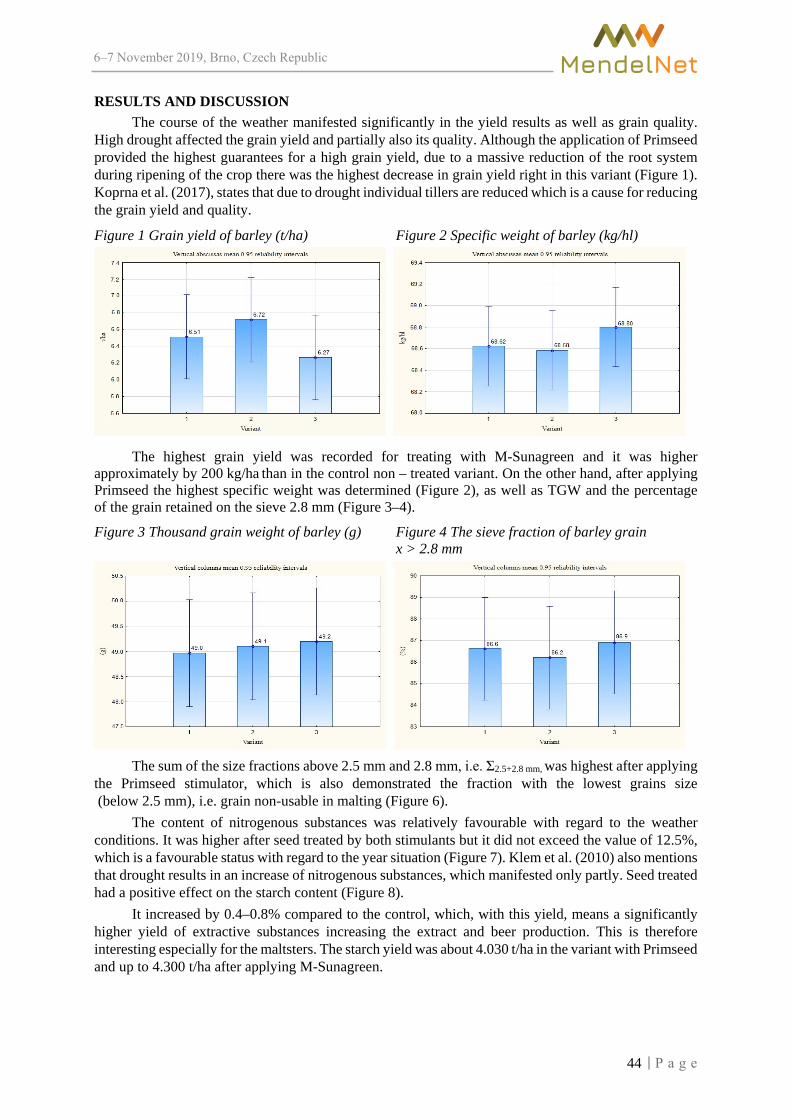
6–7 2019, Brno, Czech Republic
RESULTS AND DISCUSSION The course of the weather manifested significantly in the yield results as well as grain quality.
High drought affected the grain yield and partially also its quality. Although the application of Primseed provided the highest guarantees for a high grain yield, due to a massive reduction of the root system during ripening of the crop there was the highest decrease in grain yield right in this variant (Figure 1). Koprna et al. (2017), states that due to drought individual tillers are reduced which is a cause for reducing the grain yield and quality.
Figure 1 Grain yield of barley (t/ha) Figure 2 Specific weight of barley (kg/hl)
The highest grain yield was recorded for treating with M-Sunagreen and it was higher approximately by 200 kg/ha than in the control non – treated variant. On the other hand, after applying Primseed the highest specific weight was determined (Figure 2), as well as TGW and the percentage of the grain retained on the sieve 2.8 mm (Figure 3–4).
Figure 3 Thousand grain weight of barley (g) Figure 4 The sieve fraction of barley grain x > 2.8 mm
The sum of the size fractions above 2.5 mm and 2.8 mm, i.e. Ʃ2.5+2.8 mm, was highest after applying the Primseed stimulator, which is also demonstrated the fraction with the lowest grains size (below 2.5 mm), i.e. grain non-usable in malting (Figure 6).
The content of nitrogenous substances was relatively favourable with regard to the weather conditions. It was higher after seed treated by both stimulants but it did not exceed the value of 12.5%, which is a favourable status with regard to the year situation (Figure 7). Klem et al. (2010) also mentions that drought results in an increase of nitrogenous substances, which manifested only partly. Seed treated had a positive effect on the starch content (Figure 8).
It increased by 0.4–0.8% compared to the control, which, with this yield, means a significantly higher yield of extractive substances increasing the extract and beer production. This is therefore interesting especially for the maltsters. The starch yield was about 4.030 t/ha in the variant with Primseed and up to 4.300 t/ha after applying M-Sunagreen.
44

6–7 2019, Brno, Czech Republic
Figure 5 The sieve fraction of barley grain Figure 6 The sieve fraction of barley grain 2.5 mm < x < 2.8 mm x < 2.5 mm
Figure 7 Content of N-substances in barley grain Figure 8 Content of starch in barley grain (%) (%)
Results of measuring root capacity are presented in Figures 9–11. They clearly show that the root
capacity was gradually decreasing. During measurements there was a provable root capacity decrease (p ˃ 0.95) in 3 weeks. We can see differences after seed treated with Primseed, where the capacity was still increasing up to measurement 2 (Figure 11), while in the other variants it was already decreasing.
Figure 9 Root system size of barley Figure 10 Effect of seed treating on the barley root system size
We can evaluate positively especially that the root capacity was higher after treating
with M-Sunagreen as well as Primseed in average by 11–12.5%, but the root was reduced more significantly here than in the control variant. A significant effect of drought manifested in this case. Hajzler et al. (2010) measured root capacity under various humidity conditions. Their results show that a plant under stress terminates the activity of the root system prematurely, which was also shown in our case.
The favourable effect of both products was also manifested in the number of spikes per m2 (Figure 12). There was an increase by 25–27 spikes. The number of grains/spike also increased
45

6–7 2019, Brno, Czech Republic
(Figure 13) in average by 1.01–11.01% and the number of grains on the plant increased by 1.5–18.2% (Figure 14). Primseed provided higher benefits than M-Sunagreen.
Figure 11 Effect of seed treating on barley Figure 12 Effect of seed treating on the number root system size barley spikes per m2
Figure 13 Effect of seed treating on the number Figure 14 Effect of seed treating on the number of barley grains per spike barley grains per plant
CONCLUSION We can conclude that the application of M-Sunagreen and Primseed brought numerous positive
results and trends. A higher grain yield was observed after applying M-Sunagreen. Grain specific weight of barley, TGW as well as grain size above 2.5 mm (Ʃ2.5+2.8 mm) was determined to be higher after seed treating with Primseed. The content of N-substances after applying of both stimulants was higher, but it was not problematic and reached 12.5%. Seed treating contributed to higher starch content in the grain; the increment after applying Primseed reached 0.8%.
The application of M-Sunagreen and Primseed brought numerous positive results. The highest root capacity was recorded after applying Primseed and it too manifested in better values of yield components. However, in this variant there was the most significant root reduction during anthesis of the crop.
ACKNOWLEDGEMENT The research was financially supported by the Internal Grant Agency AF-IGA2019-IP053
REFERENCES Basařová, G. et al. 1992. Pivovarsko-sladařská analytika 1. 1st ed., Praha: Merkanta s.r.o. ChemapAgro ©2019. [Online]. Available at: https://www.chemapagro.cz/pripravky/stimulatory/sunagreen/. [2019–08–20]. Chloupek, O. et al. 2010. Drought tolerance of barley varieties in relation to their root system size. Plant Breeding, 129(6): 630–636.
46

6–7 2019, Brno, Czech Republic
Dundálková, L. 2016. Dlouhodobé výsledky aplikace systému stimulace a aktifolu mag v ječmeni jarním. In Proceedings of conference Dobrý začátek, jaký konec? Dobře zasít dobře sklidit: Kompendium 2016 [Online]. Velká Bystřice, Czech Republic, 25–28 January, Velká Bystřice: Sdružení pro ječmen a slad, pp. 33–35. Available at: http://konference.agrobiologie.cz/2016-01-25/thomson/2016_Kompendium.pdf. [2019–08–20]. eAGRI ©2009-2019 Ministerstvo zemědělství. [Online]. Available at: http://eagri.cz/public/app/rhpub/etikety/etiketa_39156.pdf?id=39156. [2019-08-20]. Hajzler, M. et al. 2010. Evaluation of root system characteristics by measurement of electrical capacity and image analysis. In Proceedings of International PhD Students Conference MendelNet 2010 [Online]. Brno, Czech Republic, 24 November, Brno: Mendel University in Brno, Faculty of Agronomy, pp. 48–55. Available at: http://web2.mendelu.cz/af_291_mendelnet/mendelnet2010/articles/15_hajzler_321.pdf. [2019–08–20]. Klem, K. et al. 2010. Faktory ovlivňující obsah dusíkatých látek v zrnu ječmene a možnosti ovlivnění. In Proceedings of conference Sladovnický ječmen – přiměřená ekonomika, vysoký výnos a kvalita zrna: Kompendium 2010 [Online]. Velká Bystřice, Czech Republic, 8–11 February, Velká Bystřice: Sdružení pro ječmen a slad, pp. 24–28. Available at: http://konference.agrobiologie.cz/2010-02-08/07-klem-klemova-misa_faktory_ovlivnujici_obsah_dusikatych_latek_v_zrnu_jecmene_a_moznosti_ ovlivneni.pdf. [2019–08–20]. Koprna, R. et al. 2017. Nové možnosti optimalizace počtu odnoží a zvýšení výnosové jistoty u obilnin. Agromanual [Online], 2(1): 71–75. Available at: https://www.agromanual.cz/cz/clanky/vyziva-a-stimulace/stimulace/nove-moznosti-optimalizace-poctu-odnozi-a-zvyseni-vynosove-jistoty-u-obilnin. [2019–08–20]. Kunjammal, P., Sukumar, J. 2019. Effect of different seed treatment on grain yield of maize (Zea mays l.) under drought stress conditions. Madras Agricultural Journal, 106(4–6): 384–387. Mohammadi, H., Moradi, F. 2013. Effects of plant growth regulators on endogenous hormones in two wheat cultivars differing in kernel size under control and water stress conditions. Agriculture & Forestry / Poljoprivreda i Sumarstvo, 59(4): 81–94. Pekarskas, J., Sinkevičienė, J. 2011. Influence of biological preparation on viability, germination power and fungal contamination of organic winter barley grain. In: Proceedings of the International Scientific Conference: Rural Development [Online]. Akademija, Lithuania, 24–25 November, Lithuania: Aleksandras Stulginskis University pp. 206–210. Available at: http://dspace.lzuu.lt/bitstream/1/2902/2/rural_development_2011_book2.pdf#page=207. [2019–08–20]. Středa, T., Klimešová, J. 2016. Hodnocení relativní velikosti kořenového systému rostlin v přirozeném prostředí: metodika pro praxi. 1st ed., Brno: Mendelova univerzita v Brně. Yang, D. et al. 2016. Exogenous cytokinins increase grain yield of winter wheat cultivars by improving stay green characteristics under heat stress. PLoS ONE, 11(5): 1–19. Yang, J. et al. 2003. Hormones in the grains in relation to sink strength and postanthesis development of spikelets in rice. Plant Growth Regulation, 41(3): 185–195. Yuan, W. et al. 2019. The barley miR393 has multiple roles in regulation of seedling growth, stomatal density, and drought stress tolerance. Plant Physiology and Biochemistry [Online], 142: 303–311. https://reader.elsevier.com/reader/sd/pii/S0981942819303006?token=4F2C970C359EBAE6292ACB75138007E97F9C76595DE4D613747AF36D0CC50856FF0941569996B27D63D8B3F5A0F5C46F. [2019–08–20].
47

6–7 2019, Brno, Czech Republic
Comparison of Sentinel–2 and ISARIA winter wheat mapping for variable rate application of nitrogen fertilizers
Jiri Mezera1, Vojtech Lukas1, Jakub Elbl1,2, Vladimir Smutny1 1Department of Agrosystems and Bioclimatology
Mendel University in Brno Zemedelska 1, 613 00 Brno
2Spearhead Czech s.r.o. Revolucni 130/30, 751 17 Horni Mostenice
CZECH REPUBLIC
Abstract: Correct application of nitrogen fertilizers in crop management on arable land has high importance both from economic and environmental point of view, mainly in the condition of higher spatial variability of farm fields. One of the solutions could be a variable rate application (VRA) of nitrogen fertilizers based on the spatial variability and identification of management zones, which addresses site specific crop changes, soil characteristics and crop requirements. The aim of the study was to compare proximal and remote sensing systems of winter wheat mapping for variable rate application of nitrogen fertilizers. The methodology of the work was based on the collection of spectral data from the ISARIA proximal crop sensor system, represented by the vegetation indices IRMI and IBI, and set of vegetation indices indices from Sentinel–2 satellite imagery, both on the trial fields. All experimental work was carried out at the farm company SALIX MORAVA a.s. (locality Zdounky, Kroměříž, Czech Republic) during the year 2018 on the selected fields with winter wheat and total area of 355 ha. Spatial data were processed and analyzed by using geographic information systems and then statistically evaluated the relationships between variables. The study has shown higher level of correlation between the ISARIA vegetation indices and all evaluated indices from Sentinel–2. Highest values of correlation with Sentinel–2 indices were achieved for the ISARIA’s IRMI index. The most sensitive Sentinel-2 vegetation indices were EVI, GNDVI and SRI indices, while the lowest correlation values were found for the NRERI, REIP, RENDVI and S2REP indices. Overall, the results of this study indicate high relationship between proximal and remote sensing, thus the use by farmers depends on the practical aspects of their in crop management practices.
Key Words: precision agriculture, crop sensing, Sentinel–2, vegetation indices
INTRODUCTION Precision agriculture is a production system that promotes variable management practices
within a field, according to site conditions. This system is based on new tools and sources of information provided by modern technologies. These include the global positioning system (GPS), geographic information systems (GIS), yield monitoring devices, soil, crop and pest sensors, remote sensing, and variable-rate technologies for applicators of inputs (Seelan et al. 2003). Precision agriculture generally involves better management of farm inputs such as fertilizers, herbicides, seed, fuel by doing the right management practice at the right place and the right time (Mulla 2013).
Remote sensing techniques are widely used in agriculture and agronomy. The use of remote sensing is necessary, as the monitoring of agricultural activities faces special problems not common to other economic sectors. Agricultural production follows strong seasonal patterns related to the biological lifecycle of crops. The production depends on the physical landscape (e.g., soil type), as well as climatic driving variables and agricultural management practices. All variables are highly variable in space and time. Moreover, as productivity can change within short time periods, due to unfavorable growing conditions, agricultural monitoring systems need to be timely. Remote sensing can significantly contribute to providing a timely and accurate picture of the agricultural sector, as it is very suitable for gathering information over large areas with high revisit frequency (Atzberger 2013).
48
6–7 2019, Brno, Czech Republic
The identification and mapping of crops are important for estimating potential harvest as well as for agricultural field management. Optical remote sensing is one of the most attractive options because it offers vegetation indices and some data have been distributed free of charge. Especially, Sentinel–2, which is equipped with a multispectral sensor (MSI) with blue, green, red, and near-infrared bands, offer some vegetation indices calculated to assess vegetation status and chlorophyll content in plants (Sonobe et al. 2018). In most of cases, spectral measurement of crop stands is utilized for estimation of crop N status by calculation of vegetation indices derived from proximal on-the-go (Heege et al. 2008) or remote sensing systems (Hansen and Schjoerring 2003). Knowledge on chlorophyll content is necessary assumption to prepare information background (i.e. map prescription) reflecting an actual situation of plants on the field. The background is used for targeted N application based on maps (Delegido et al. 2011).
For site specific crop management treatments, such as variable rate application of fertilizers or crop protection, main information about field variability is required. Main source of the information is based on the sensor mapping techniques, soil sampling, crop sensing or yield mapping. Recent studies shown that there are many factors influencing the spatial variability of crop yields, such as evapotranspiration (Johnen et al. 2014), topographic attributes (Kumhálová et al. 2014) or combined effects of soil fertility and weed control (Mallarino et al. 1999).
Crop sensors are mounted on the machinery and use information about the reflectance of visible and near-infrared spectrum, which is related to the crop parameters, such as LAI, chlorophyll content, aboveground crop biomass and other.
Aim of the study was to compare proximal and remote sensing systems of winter wheat mapping for variable rate application of nitrogen fertilizers.
MATERIAL AND METHODS
Study area Input data of winter wheat were acquired during the year 2018 by mapping of selected fields
with total area 355 ha at farm company SALIX MORAVA a.s. (part of Spearhead Czech s.r.o. holding). Zdounky area is located in the sugar beet production area in district Kroměříž (49.2978514N, 17.3931164E). According to Quitt climate classification is the climatic condition of the region slightly warm to warm and slightly damp (T3, MT2). The long-term average annual temperature during 1961–1990 is 8.1 °C and the average precipitation is 550–700 mm. The fields are located at an altitude of 205–320 m a.s.l. The soil types are Chernozem, Haplic Luvisol, Cambisol and Fluvisol with medium to deep soil depth. The humus content is moderately high, equal to 2–3%. Soil pH value ranges between 6.6–7.2. Fields are flat to moderately sloped.
Proximal sensing by Fritzmeier ISARIA Recorded data were obtained from proximal crop sensing system Fritzmeier ISARIA (Figure 1)
during second topdressing nitrogen application (N2). Nutrient status of plants is evaluated based on the spectral measurement of crops by active LED lighting in four spectral wavelenghts (660–780 nm). Two vegetation indices are calculated – Isaria Reflectance Measurement Index (IRMI), which is related to chlorophyll content, and Isaria Biomass Index (IBI) related to crop biomass.
Records of vegetation indices were downloaded from ISARIA board computer as the spatial point data in shapefile format. Files were merged based on the field identification, analysed and visualized in Geographic Information System ArcMap 10.6.1 (ESRI, Redlands, USA) in coordinate system WGS 1984. Statistical evaluation was carried out by Statistica 12 (Tibco, USA).
Remote sensing by satellite platform Sentinel–2 Sentinel–2 images were selected to be cloudless and taken near to the date of field mapping
by ISARIA system. The datasets were then downloaded from ESA open hub database as surface reflectance product L2A derived by sen2cor (Copernicus 2019) and filtered through a cloud mask derived with L2A scene classification dataset. Set of 11 vegetation indices was calculated from multispectral bands (see the list in Table 1) from selected four dates of images acquired during April 2018.
49

6–7 2019, Brno, Czech Republic
Figure 1 Nitrogen application by crop sensing system Fritzmeier Isaria on the field. Photo by J. Mezera
Table 1 Vegetation indices from Sentinel–2B (Sentinel Hub 2019, Klem et al. 2014)
EVI Enhanced Vegetation Index EVI2 Enhanced Vegetation Index 2 GNDVI Green Normalized Difference Vegetation Index NDMI Normalized Difference Moisture Index NDRE Normalized Difference Red Edge Index NDVI Normalized Difference Vegetation Index NRERI Normalized Red Edge Index REIP Red Edge Inflection Point RENDVI Red Edge NDVI S2REP Sentinel–2 Red-Edge Position SRI Simple Ratio Index
RESULTS AND DISCUSSION The results of crop mapping by ISARIA system in form of IRMI, IBI values and datasets
from Sentinel–2B were analysed by GIS. For each point of ISARIA dataset the value of Sentinel-2 pixels (as the value vegetation indices) was obtained by overlay analysis.
The data was then exported to Microsoft Excel (Microsoft Corporation, Redmond, USA) and subsequently to Statistica 12 (Tibco, USA) for correlation and regression analysis. In the box plot graph (Figure 2), there is a comparison between the correlation coefficients of IRMI and IBI depending on all vegetation indices for all evaluated Sentinel–2B satellite image terms. It is apparent that the IRMI index has less variance and the median is higher than the IBI index, but there is no statistically significant difference between them. The dependence between the ISARIA system indices and the Sentinel satellite indices was evaluated using the Spearman correlation coefficient (Table 2). All values are statistically significant at level of 95% due to the huge number of records.
In the Spearman correlation coefficient matrix, in most cases, a higher value for the IRMI index was reached, only on 11 April a higher coefficient for the IBI index was achieved. The value of the correlation coefficient also depends on the term of the Sentinel satellite image. The highest correlation was achieved for 21 April 2018. From evaluated indices, the maximum value of the coefficient was reached for the GNDVI index (Figure 3) and the highest overall values were for the EVI, NDMI and SRI. In contrast, the minimum correlation was found for the NRERI index and the lowest for NRERI, REIP, RENDVI and S2REP.
Results in study Vizzari et al. (2019) show that differences between treatments in crop vegetation index, grain yield, and protein content were negligible and generally not significant but study Batchelor et al. (2002) show implementation of crop models can lead to predict crop yield based on the weather data. The images from the Sentinel–2 satellite, respectively selected vegetation indices, can thus serve as useful information on the distribution of variability on the field and as a tool for creating prescription
50

6–7 2019, Brno, Czech Republic
maps for variable rate application. The disadvantage is that satellite images have lower resolution, but this is also sufficient for purposes of variable rate application of fertilizers.
Figure 2 Sentinel–2 GNDVI scene wioth the area of interest and box plot graph of Spearman correlation coefficient for observed fields
Figure 3 Map of vegetation index GNDVI from Sentinel–2 (background raster layer) and IRMI index from ISARIA system (point layer)
Table 2 Correlation matrix of Spearman correlation coefficient (r) Vegetation index Date 2018 EVI EVI2 GNDVI NDMI NDRE NDVI NRERI REIP RENDVI S2REP SRI
11 April
IRMI 0.79 0.82 0.80 0.77 0.75 0.79 0.51 0.23 0.42 0.23 0.79 IBI 0.85 0.79 0.84 0.76 0.83 0.85 0.53 0.31 0.44 0.31 0.85
18 April
IRMI 0.80 0.74 0.78 0.81 0.75 0.80 0.72 0.48 0.69 0.48 0.80 IBI 0.81 0.67 0.76 0.76 0.79 0.81 0.67 0.48 0.64 0.48 0.81
21 April
IRMI 0.85 0.84 0.86 0.83 0.81 0.85 0.79 0.64 0.76 0.64 0.85 IBI 0.84 0.81 0.83 0.79 0.82 0.84 0.73 0.60 0.70 0.60 0.84
28 April
IRMI 0.70 0.76 0.72 0.84 0.76 0.70 0.81 0.77 0.81 0.77 0.70 IBI 0.72 0.74 0.69 0.78 0.71 0.72 0.73 0.64 0.72 0.64 0.72
51

6–7 2019, Brno, Czech Republic
The ISARIA system is active sensor and independent of ambient light conditions. The availability and subsequent quality of the captured scenes of Sentinel is dependent on the presence of cloud cover and there is a risk that the image will not be available at the desired time due to cloud cover in the scene. Psomiadis et al. (2017) show capability and effectiveness are critical but complicated issues in the application of multi-sensor vegetation observations. Various factors such as the atmospheric conditions during acquisition, sensor and geometric characteristics, such as viewing angle, field of view, and sun elevation influence direct comparability of vegetation indicators among different sensors.
CONCLUSIONS Mapping using the proximal sensor system Fritzmeier ISARIA provides essential information
in precision agriculture about crop stands and the spatial variability within the fields. Based on these data it is possible to carry out variable rate application of fertilizers. Data about spatial variability of crop nitrogen status can also be obtained from the satellite images of the Sentinel by calculation of vegetation indices.
In this study were researched relationship between the Fritzmeier ISARIA vegetation indices (IRMI, IBI) and the Sentinel–2 indices on selected fields with winter wheat of the farm company SALIX MORAVA (Czech Republic) during second topdressing nitrogen application in April 2018. Significant correlations were found between both IRMI and IBI indices and all evaluated vegetation indices from the Sentinel–2 satellite. Overall, higher correlations with Sentinel–2 indices were achieved for the IRMI index. The highest correlation values were achieved for the EVI, GNDVI and SRI index, while the lowest correlation values were achieved by the NRERI, REIP, RENDVI and S2REP indices. The value of the correlation coefficient depends on the term of the Sentinel image. The best results were achieved for 21 April 2018. It is apparent that the online sensor for variable rate application may to some extent be replaced by Sentinel satellite images, but there is a high risk of unavailability of images at the desired time due to cloud cover in the scene.
Based on the results obtained, it can be stated that the precision farming system is able to provide sufficient information on the field heterogeneity with the potential to optimize input control in crop production. However, the economic effect is long-term and depends on the skills of the agronomists to implement precision farming technologies into crop management.
ACKNOWLEDGEMENTS This study was supported by Internal Grant Agency of Faculty of AgriSciences at Mendel University in Brno as the research project AF-IGA2019-IP017 “Evaluation of variable rate application of nitrogen fertilizers in precision agriculture”. Experimental data were obtained by cooperation with Spearhead Czech Ltd.
REFERENCES Atzberger, C. 2013. Advances in Remote Sensing of Agriculture: Context Description, Existing Operational Monitoring Systems and Major Information Needs. Remote Sensing, 5(2): 949–981. Batchelor, W.D. et al. 2002. Examples of strategies to analyze spatial and temporal yield variability using crop models. European Journal of Agronomy, 18(1–2): 141–158. Copernicus. 2019. Copernicus Open Access Hub [Online]. ESA. Available at: https://scihub.copernicus.eu/. [2019-08-25]. Delegido, J. et al. 2011. Evaluation of Sentinel–2 red-edge bands for empirical estimation of green LAI and chlorophyll content. Senzors, 11(7): 7063–7081. Heege, H.J. et al. 2008. Prospects and results for optical systems for site-specific on-the-go control of nitrogen-top-dressing in Germany. Precision Agriculture, 9(3): 115–131. Hansen, P.M., Schjoerring, J.K. 2003. Reflectance measurement of canopy biomass and nitrogen status in wheat crops using normalized difference vegetation indices and partial least squares regression. Remote Sensing of Environment, 86(4): 542–553.
52
6–7 2019, Brno, Czech Republic
Johnen, T. et al. 2014. An analysis of factors determining spatial variable grain yield of winter wheat. European Journal of Agronomy, 52(Part B): 297–306. Klem, K. et al. 2014. Využití měření spektrální odrazivosti a odvozených specializovaných vegetačních indexů v pěstební technologii jarního ječmene. Metodika pro zemědělskou praxi. Kroměříž, Brno, Havlíčkův Brod. Kumhálová, J. et al. 2014. Use of landsat images for yield evaluation within a small plot. Plant, Soil and Environment, 60(11): 501–506. Mallarino, A.P. et al. 1999. Interpreting Within-Field Relationships between Crop Yields and Soil and Plant Variables Using Factor Analysis. Precision Agriculture, 1(1): 15–25. Mulla, D.J. 2013. Twenty five years of remote sensing in precision agriculture: Key advances and remaining knowledge gaps. Biosystems Engineering, 114(4): 358–371. Psomiadis, E. et al. 2017. Evaluation and cross-comparison of vegetation indices for crop monitoring from Sentinel–2 and worldview-2 images. Conference: Remote Sensing for Agriculture, Ecosystems, and Hydrology. Seelan, S.K. et al. 2003. Remote sensing applications for precision agriculture: A learning community approach. Remote Sensing of Environment, 88(1–2): 157–169. Sentinel Hub. 2019. Sentinel 2 EO products [Online]. Ljubljana: Laboratory for geographical information systems, Ltd. Available at: https://www.sentinel-hub.com/develop/documentation/eo_products/Sentinel2EOproducts [2019-08-25]. Sonobe, R. et al. 2018. Crop classification from Sentinel–2-derived vegetation indices using ensemble learning. Journal of Applied Remote Sensing, 12(02): 026019 . Vizzari, M. et al. 2019. Sentinel 2-Based Nitrogen VRT Fertilization in Wheat: Comparison between Traditional and Simple Precision Practices. Agronomy-Basel, 9(6): 278.
53

6–7 2019, Brno, Czech Republic
Effects of stabilized nitrogen fertilizers in oilseed rape (Brassica napus L.) growing system
Dominika Mikusova, Pavel Ryant Department of Agrochemistry, Soil Science, Microbiology and Plant Nutrition
Mendel University in Brno Zemedelska 1, 613 00 Brno
CZECH REPUBLIC
Abstract: Oilseed rape (Brassica napus L.) is the most cultivated oilseed in the Czech Republic, where its cultivation occupies approximately 13% of arable land (395 thousand ha). In terms of nutrient con-sumption, oilseed rape ranks among very demanding crops and therefore the supply of nutrients (espe-cially N) in sufficient quantities plays an essential part of its cultivation. This study focused on two qualitative and quantitative parameters of oilseed rape - yield and oiliness. In the experiment, as basic fertilizers were used Urea and UAN. In the variants fertilized with urea-based fertilizers, Alzon 46 (Urea + NI) and Alzon neo-N (Urea + NI + UI) were used as nitrification (NI) and urease (UI) inhibitors. In variants fertilized with UAN, Piadin served as NI and StabilureN served as UI. The highest yields were recorded in variants fertilized with Alzon neo-N and UAN + NI. In the experiment, LOVOGRAN IN, LOVOGRAN B (Urea based variants) and LAS (UAN variants) fertilizers were used as source of sulfur, essential for the growth, development and synthesis of rapeseed oil. The differences in oil content between the individual varieties of oilseed rape did not show a significant positive or negative character.
Key Words: oilseed rape, yield, oil content, nitrification inhibitors, urease inhibitors
INTRODUCTION The presence of nitrogen in the soil determines the course of crop vegetation, their yield and seed
quality. Nitrogen can be directly absorbed by plant roots in inorganic (mineral) form in as NH4+
and NO3- - therefore, they are part of most mineral fertilizers (Spinelli et al. 2013). However, the use
of conventional mineral nitrogen fertilizers (due to emissions of NH3, NOx and NO3- leaching) results
in N losses from the soil - these losses pose not only a risk to hydrosphere, atmosphere and human health, but also reduce soil fertility (Cameron et al. 2013, Ju et al. 2006).
One way to reduce nitrogen losses and thus contribute to efficiency of fertilization, is to use sta-bilized nitrogen fertilizers containing nitrification and urease inhibitors. Nitrification is the process of oxidation of ammonium to nitrate by soil bacteria. Chemoautotrophic bacteria of the genera Nitro-somonas, Nitrosovibria, Nitrosospira and Nitrococus carry out the first degree of oxidation (NH4
+ ---NO2
-). The second degree of oxidation (NO2- --- NO3
-) is carried out by bacteria of the genera Nitrobac-ter and Nitrosolobus (Singh and Verma 2007). The main purpose of the nitrification inhibitors is to delay the first stage of bacterial oxidation of ammonium ion by attenuating the activity of soil bacteria of the genera Nitrosomonas, Nitrosovibria, Nitrosospira and Nitrococus for a period of time (4–10 weeks). The use of nitrification inhibitors is aimed at controlling nitrogen loss by maintaining nitrogen in ammoniacal form for an extended period of time, thereby increasing its usefulness (Edmeades 2004). Urease inhibitors partially suppress urease activity, thereby retarding the hydrolysis of urea to final ammonia (entering to nitrification process) and also reduce NH3 loss by volatilization (Trenkel 2010).
Sulfur is an important component of amino acids, proteins, vitamins and enzymes, which makes it essential for the synthesis of oil, proteins and for the growth and development of oilseed rape seeds (Ahmad et al. 2007, Parker 2009). Sulfur deficiency can lead to a reduction in the quality and quantity of oilseed rape seeds up to 40% (De Pascale et al. 2008, Abdallah et al. 2010).
54

6–7 2019, Brno, Czech Republic
The project was focused at evaluating the suitability of mixed nitrogen - sulfur fertilizer (based on urea and ammonium sulphate) and liquid nitrogen fertilizer (UAN) and their combinations with ni-trification inhibitors and urease inhibitors in the oilseed rape system.
MATERIALS AND METHODS The experiment was carried out in the form of precise small-plot experiments in the area
of the Field Trial Station Žabčice (W 49°1.37702', E 16°37.07360'). Oilseed rape (variety DK Excep-tion) was sown 23 August 2019 (3.5 kg/ha) on plots of 15 m2. The overview of selected fertilizer vari-ants, fertilizer rations and their applications is shown in Table 1.
Table 1 Overview of variants and selected types of fertilizers
Variant number Variant
Dose of N
[kg/ha]
Regenerative ferti-lization
Fertilization in phase of stem
elongation
Fertilization in phase
of butonization
Ure
a ba
sed
fert
ilize
rs
1 Urea
194
Urea
LOVOGRAN IN (78 kg/ha N)
Urea (58 kg/ha N)
Urea (58 kg/ha N)
2 Urea + NI 194
Alzon 46 LOVOGRAN IN
- -
3 Urea + NI
+ UI 194
Alzon neo-N
LOVOGRAN IN
- -
4
Urea + NI + UI + Boron
194
Alzon neo-N LOVOGRAN B
- -
UA
N f
ertil
izer
s
5
LAS + UAN
194
LAS (64 kg/ha N)
UAN
(130 kg/ha N) -
6
LAS + UAN + NI
194 LAS (64 kg/ha N)
UAN + NI (130 kg/ha N)
-
7
LAS + UAN + UI
194 LAS (64 kg/ha N)
UAN + UI (130 kg/ha N)
-
8
LAS + UAN + NI + UI
194 LAS (64 kg/ha N)
UAN + NI
+ UI (130 kg/ha N)
-
Legend: NI - nitrification inhibitor; UI - urease inhibitor; Alzon 46 - urea with NI; Alzone neo-N - urea with NI and UI; PIADIN: NI (1.5% methylpyrazole, 3% triazole); StabilureN: UI (NBPT).
Contents of nutrients in selected fertilizers: Urea (46% N), Alzon 46 (46% N), Alzon neo-N (46% N), UAN (30% N), LOVOGRAN IN (20% N and 20.5% S), LAS (24% N and 5.6% S) and LOVOGRAN B (20% N; 20.5% S and 0.2% B).
55

6–7 2019, Brno, Czech Republic
Regenerative fertilization with selected types of fertilizers was carried out on the plots in the area Trial Station Žabčice on 28 February 2019. Fertilization in phase of stem elongation with liquid nitrogen fertilizers and urea was carried out on 29 March 2019. Fertilization in phase of butonization was realized only in variant no.1 (see Table 1) on 8 April 2019. The harvest of oilseed rape was realized on 10 July 2019. Oil content of the seeds was evaluated by NIR method (near–infrared spectroscopy). The effect of the fertilization was evaluated by ANOVA analysis of variance followed by testing at a 95% (P <0.05) level of significance using Tukey's HSD test (Statistica CZ 12 programme).
RESULTS AND DISCUSSION
Urea fertilizers To compare the yield and oil content between varieties of oilseed rape fertilized with urea-based
fertilizers with additions of NI and UI, we used as a control the variant no.1. Based on the results of the Tukey's HSD test, we can conclude that within both the yield and oiliness of the seeds, there are no statistically significant differences between variations 1–4 (same letter a; P <0.05). The differences in yield and oil content are expressed by relative percentages in Table 2.
Table 2 Statistical evaluation of seed yield and oil content of urea-fertilized variants with the addition of nitrification and urease inhibitors
Vari-ant
num-ber
Variant Seed yield [t/ha]
± standard deviation
Relative percentage of
yield [%]
Seed oil con-tent [%] ±
standard devi-ation
Relative percentage
of oil content [%]
1 Urea 4.48 ± 0.68 100.0 40.1 ± 0.66 100.0 2 Urea + NI 4.87 ± 0.53 108.8 39.73 ± 0.96 99.1 3 Urea + NI + UI 5.04 ± 0.65 112.4 39.55 ± 1.51 98.6 4 Urea + NI + UI +
Boron 4.83 ± 0.42 107.7 39.63 ± 0.47 98.8
In comparison to the control variant, yield in variants fertilized with additions of NI and UI shows increased character. The highest yield of 5.04 t/ha was achieved in variant no.3 (additions of NI + UI). These findings correspond to the results of Šimka et al. (2012), which point to a positive effect of stabi-lized urea on the yield of oilseed rape. The differences in seed yield between variants 1–4 are shown in Figure 1.
The highest oil content of 40.1% was observed in control variant no.1. According to Ahmad et al. (2007) increased nitrogen doses may have a depressing effect on the oil content of oilseed rape seeds. Therefore, we can assume, that the highest oil content of the seeds in control variant in comparison to other variants might be affected by split application of urea used in its fertilization. The differences in oil content between variants of oilseed rape are shown in Figure 2.
Figure 1 Differences in yield between varieties of oilseed rape fertilized with urea fertilizers
Legend: The same letter (a) above the graph bars indicates that there are no statistically significant differences between the variants
56

6–7 2019, Brno, Czech Republic
Figure 2 Differences in oil content between varieties of oilseed rape fertilized with urea fertilizers
Legend: The same letter (a) above the graph bars indicates that there are no statistically significant differences between the variants
Liquid nitrogen fertilizers To compare the yield and oil content between varieties of oilseed rape fertilized with liquid nitro-
gen fertilizer with NI and UI additions, as a control the variant no.5.
Table 3 Statistical evaluation of the yield and oil content of seeds in variants fertilized with liquid nitro-gen fertilizer with the addition of nitrification and urease inhibitors
Variant number Variant
Seed yield [t/ha]
± standard deviation
Relative percent-
age of yield [%]
Seed oil content [%] ± standard deviation
Relative percentage
of oil content [%]
5 LAS + UAN 4.54 ± 0.43 100.0 39.98 ± 1.54 100.0 6 LAS + UAN + NI 4.64 ± 0.33 102.2 40.38 ± 1.33 101.0 7 LAS + UAN + UI 4.47 ± 0.26 98.6 40.60 ± 1.23 101.6 8 LAS + UAN + NI + UI 4.62 ±0.33 101.9 40.38 ± 0.72 101.0
Based on the results of the Tukey's HSD test, we can conclude that there are no statistically sig-nificant differences between the variants within the yield and oilseed rape seed (the same letter a; P<0.05). The differences in oilseed rape seed yield and oil content are expressed in relative percentages in Table 3.
Figure 3 Differences in seed yield between varieties of oilseed rape fertilized with liquid nitrogen ferti-lizer
Legend: The same letter (a) above the graph bars indicates that there are no statistically significant differences between the variants
57

6–7 2019, Brno, Czech Republic
The results presented in Table 3 show that the addition of NI and UI to the liquid nitrogen fertilizer UAN results in an increase in the yield of oilseed rape seeds. The highest yield of 4.64 t/ha was achieved in variant no.6, where NI was added to UAN. A reduced yield compared to the control variant was observed in variant no.7 fertilized with UAN with the addition of UI. This trend is also shown in the results from Grant et al. (2010). The differences in seed yield between variants are shown in Figure 3.
The results show a slightly increased oil content in variants with additions of NI and UI. Accord-ing to Ahmad et al. (2007) lower doses of N (in our case caused by the effects of NI and UI) may have a positive effect on oil content. The highest oil content of 40.6% was found in variant no.7, which was fertilized with liquid fertilizer UAN with the addition of UI. The differences in oil content between variants of oilseed rape are shown in Figure 4.
Figure 4 Differences in oil content between varieties of oilseed rape fertilized with liquid nitrogen fer-tilizers
Legend: The same letter (a) above the graph bars indicates that there are no statistically significant differences between the variants
CONCLUSION Presence of nitrogen in sufficient levels plays a crucial role in yield and oil content of rape seeds.
The use of stabilized nitrogen fertilizers in crop nutrition is one of the ways how to achieve a more efficient use of nitrogen by plants, but also to prevent its leaching and evaporation. According to the experiment, the use of nitrification and urease inhibitors in the oilseed rape system has shown a positive effect on seed yield, althought it was not statistically significant. The results of this experiment showed that the highest yield of 5.04 t/ha was achieved in the urea-fertilized variant with the addition of nitrification and urease inhibitors (variant no.3), which showed an increase of 12.4 relative yield percentage compared to the control variant. In comparison to the average yield of rape seeds in Czech Republic, this results might be considered as above average. Effect of stabilized fertilizers on oil content has shown in our case as statistically insignifficant.
ACKNOWLEDGEMENTS The research was supported by grant no. FA-IGA2019-IP037
REFERENCES Abdallah, M. et al. 2010. Effect of mineral sulphur availability on nitrogen and sulphur uptake and remobilization during the vegetative growth of Brassica napus L. Journal of Experimental Botany, 61(10): 2635–2646. Ahmad, G. et al. 2007. Influence of nitrogen and sulfur fertilization on quality of canola (Brassica napus L.) under rainfed conditions. Journal of Zhejiang University. Science. B, 8(10): 731–737.
58

6–7 2019, Brno, Czech Republic
Cameron, K.C. et al. 2013. Nitrogen losses from the soil/plant system: A review. Annals of Applied Biology, 162(2): 145–173. De Pascale, S. et al. 2008. Sulphur fertilisation affects yield and quality in friarielli (Brassica rapa L. subsp. Sylvestris L. Janch. var. esculenta Hort.) grown on a floating system. Journal of Horticultural Sciences and Biotechnology, 83(6): 743–748. Edmeades, D.C. 2004. Nitrification and urease inhibitors: A review of the national and international literature on their effects on nitrate leaching, greenhouse gas emissions and ammonia volatilisation from temperate legume – based pastoral systems. Environment Waikato Technical Report 2004/22. Grant, C.A. et al. 2010. Nitrogen fertilizer and urease inhibitor effects on canola emergence and yield in a one-pass seeding and fertilizing system. Agronomy Journal, 102(3): 875–884. Ju, X.T. et al. 2006. Nitrogen balance nad groundwater nitrate contamination: Comparison among three intensit cropping systems on the North China Plain. Environmental Pollution, 143(1): 117–125. Parker, P. 2009. Nutrition and soil fertility. In Canola best practice management quide for southeastern Australia. Kingston: GRDC, pp. 31–40. Singh, S.N., Verma, A. 2007. Environmental Review: The Potential of Nitrification Inhibitors to Man-age the Pollution Effect of Nitrogen Fertilizers in Agricultural and Other Soils: A Review. Journal: Enviromental Practice, 9(4): 266–279. Spinelli, D. et al. 2013. Environmental analysis of sunflower production with different forms of mineral nitrogen fertilizers. Journal of Environmental Management, 129: 302–308. Šimka J. et al. 2012. Využití stabilizovaných močovin ve výživě řepky olejné – 3-leté výsledky. In Proceedings of the Conference with International Participation Prosperous Oil Crops 2012 [Online]. Prague, Czech Republic, 6–7 December 2012. Prague: Czech University of Life Sciences Prague, pp. 43–48. Available at: http://konference.agrobiologie.cz/2012-12-06/thomson/2012_Olejniny.pdf. [2019-10-14]. Trenkel, M.E. 2010. Slow- and Controlled-Release and Stabilized Fertilizers: An Option for Enhancing Nutrient Efficiency in Agriculture. 2nd ed., Paris, France: IFA.
59

6–7 2019, Brno, Czech Republic
Foliar application of zinc in pea (Pisum sativum) nutrition
Dominika Mikusova1, Petr Skarpa1, Dalibor Huska2, Ivan Rankic2 1Department of Agrochemistry, Soil Science, Microbiology and Plant Nutrition
2Department of Chemistry and Biochemistry Mendel University in Brno Zemedelska 1, 613 00 Brno
CZECH REPUBLIC
Abstract: In areas suffering by deficient annual rainfall, drought stress is considered to be one of the main reasons for the decline in crop yields. Zinc, as a significant microelement, plays a key role in the resistance of plants to drought-induced stress. The aim of the experiment established in 2019 on the locality Žabčice was to determine the influence of foliar nutrition by selected forms of zinc: zinc oxide (ZnO), zinc sulphate (ZnSO4), zinc chelate (Zn-EDTA) and zinc oxide nanoparticles (ZnO-NPs) on yield of pea grain production (Pisum sativum). The effect of foliar application was significantly dependent on the form of zinc, where the effect of selected fertilizers was demonstrably dependent on the variety. Leaf application of zinc increased pea grain production in the range of 1.2 to 18.7%. Seed production was most affected by the application of zinc sulfate at a rate of 300 g/ha Zn. Based on the results of this study, zinc foliar application in pea vegetation can be presented as an intensifying factor increasing yield, especially in arid conditions.
Key Words: zinc, pea, drought-induced stress, leaf application, grain yield
INTRODUCTION Zinc is one of the essential microelements required for proper growth and reproduction of plants.
It is directly involved in many physiological functions, such as carbohydrate metabolism, photo-synthesis, phytohormone activity, protein metabolism, nucleic acid metabolism, and in protection against drought and oxidative stress (Marschner 1995). Drought is defined as a period of below-average precipitation, when the amounts of available water in the plant rhizosphere drop below the limits required for efficient growth and biomass production (Verslues et al. 2006, Deikman et al. 2012). It is major enviromental stressor, which directly compromises stomata function (leads to overproduction of reactive oxygen species and development of oxidative stress), increases loss of turgor, inhibits cell division and plant productivity, thus might upon prolonged exposure lead to the death of drought sensitive plants (Gill and Tuteja 2010, Kar 2011, Shao et al. 2009).
Pea (Pisum sativum) belongs to category of the most cultivated legumes in the world. Its seeds are characterized by hight content of proteins, carbohydrate, fiber, vitamins and mineral, which makes it an important commodity in human and animal nutrition, but also in industrial use (Vidal-Valverde et al. 2003). Peas are classified as less sensitive to Zn deficiency (Alloway 2008). However, Zn deficiency does occur in peas as Zn has many important roles in plantgrowth and a lack of Zn was linked to reduced seedformation (Bell and Dell 2008).
One pathway of direct micronutrient (Zn) application is foliar fertilization. This technique has increased during the last few years since it is more immediate, cheaper and more target oriented than soil fertilization (Fernandéz et al. 2013). Nanofertilizers have provided a new efficient alternative to regular fertilizers. The properties of nanotechnology in agriculture are high reactivity, enhanced bioavailability and bioactivity, adherence effects and surface effects of nanoparticles, which are increasing factors in absorption of fertilizers in plants (Gutierrez et al. 2011, Qureshi et al. 2018).
The aim of the experiment was to determine the influence of foliar nutrition of selected forms of zinc: zinc oxide (ZnO), zinc sulfate (ZnSO4), zinc chelate (Zn-EDTA) and zinc oxide nanoparticles (ZnO-NP) on pea grain yield (Pisum sativum).
60

6–7 2019, Brno, Czech Republic
MATERIAL AND METHODS The effect of zinc foliar application on pea (Pisum sativum) yield was observed in the precise
small-plot experiment at the Field Trial Station in Žabčice. This station is located in Southern Moravia in very warm and dry climatic region. For the purpose of this study were selected two varieties of pea: Protecta and Eso.
Protecta is classified as a mid-early variety of conventional leaf type. It is characterised by creating medium tall to tall plants with very good health of roots and high lodging resistance. Its yellow ovoid grains are characterised by very high protein content.
Eso is classified as a mid-late semi-leafless variety. It is characterised by creating medium tall to tall plants with very high health (strong Ascochyta pisi resistance) with very good lodging resistance. Its grains are characterised by medium protein content.
Pea was sown on 13 March 2019. The field experiment was carried out in randomized block design with 5 treatments (Table 1). The size of one parcel was 11 m2 and all variants were conducted in four repetitions. Application of zinc foliar fertilizers was realized by a backpack sprayer on 24 May 2019.
Table 1 Overview of small-plot experiment Treatment Dose of Zn (g/ha)
Zn0 Without Zn 0 Zn1 Zinc oxide (ZnO) 300 Zn2 Zinc sulphate (ZnSO4) 300 Zn3 Zinc chelate (Zn-EDTA) 300 Zn4 Zinc oxide nanoparticles (ZnO-NPs) 100
Yara Vita Zintrac 700 (700 g ZnO/liter of fertilizer, YARA Agri Czech Republic s.r.o.) was used as source of zinc oxide (Zn1). Zinc sulfate heptahydrate (purum p.a., 99.0–103.0%, Sigma-Aldrich) and Ethylenediaminetetraacetic acid disodium zinc salt tetrahydrate (Zn-EDTA purum p.a., for complexometry, ≥ 96.0% Sigma-Aldrich) was used (Zn2 and Zn3). The experiment used commercial ZnO-NPs (ZnO Nanoparticles Aqueous Dispersion, 20 wt%, 30–40 nm) from US Research Nanomaterials, Inc. (Zn4). The nanoparticles were dispersed in deionised water and sonicated for 10 minutes. The transmission electron microscopy (TEM) was performed due to its shapes and size characterization. The ZnO nanoparticles were weighed, then dried in the oven and then weighed again. The observed value was 33 wt%. We used this value to prepare the experimental part. We also investigated whether ZnO NPs are aggregated. Strong aggregation of nanoparticles was detected under detailed examination under the microscope. Therefore, we tried to sonicate nanoparticles at different settings: frequency: 37 kHz, power: 100%, time: 30 min, frequency: 80 kHz, power: 100%, time: 30 min, and frequency: 80 kHz, power: 100%, time: 60 min. However, neither combination had a significant improvement effect. We also tried to nanoparticles subjected to filtration and centri-fugation. However, neither of these adjustments had a sufficiently good result. Therefore, we proceeded to the treatment of nanoparticles using ultrasound. It was found that this treatment resulted to good quality of nanoparticles that could be further used for the experiment.
The harvest of pea grain was performed on 3 July 2019. The yield of pea grain was determined from the harvest of whole parcel. Moisture content of the grain was established in variety Protecta to value 13.6%, in variety Eso to value 12.7%. The effect of the zinc fertilization was evaluated by ANOVA analysis of variance followed by testing at a 95% (p < 0.05) level of significance using Fischer’s LSD test (Statistica CZ 12 programme).
RESULTS AND DISCUSSION According to our results, yield of pea was significantly influenced by the variety. Seed production
of Protecta was 5.5% higher than Eso, as it is shown in Figure 1. Protecta was identified as a more profitable variety compared to Eso, based on field trials by Škarpa et al. (2019).
61

6–7 2019, Brno, Czech Republic
The foliar application of selected forms of zinc had a significant effect on seed production, as shown in Table 2. Evaluation of the effect of zinc foliar application regardless of variety shows that the most pronounced seed production was influenced by the application of zinc contained in sulfate at 300 g/ha Zn. Seed yield in this variant increased by 14.5%. The lowest yield effect (5.2% above the control variant level) was demonstrated after fertilization of ZnO-NPs at a dose of 100 g/ha Zn.
Figure 1 Effect of variety on pea seed production
Legend: Variants with same letter are not significantly different at P < 0.05
Table 2 Effect of zinc application on pea yield (without varietal effect) Treatment Yield ± SE Rel % Fisher (LSD) test
Zn0 without Zn 3.06 ± 0.11 100.0 a Zn1 ZnO 3.38 ± 0.08 110.5 b Zn2 ZnSO4 3.50 ± 0.11 114.5 b Zn3 Zn-EDTA 3.31 ± 0.11 108.2 ab Zn4 ZnO-NPs 3.21 ± 0.09 105.2 ab
Legend: Values are expressed as means ± standard error (SE). Variants with same letter are not significantly different at P < 0.05
There are not many publications about the effects of Zn foliar fertilization on legumes. Ibrahim and Ramadan (2015) increased grain yield and Zn concentration in grain of beans (Phaseolus vulgaris L.) after foliar Zn application. Positive effect of zinc application to soil in peas was recorded at doses of 2 to 16 kg/ha Zn. Its supplementation led in the experiment Rafique et al. (2015) to increase the yield of 3 varieties in the range of 15–34%, while the maximum yield was achieved in doses between 3.2–5.3 kg/ha. On the other hand, the yield of pea grain was not significantly affected by zinc application in Poblaciones and Rengel (2016).
Figure 2 Influence of zinc application on pea yield in monitored varieties (Protecta and Eso)
Legend: Variants with same letter are not significantly different at P < 0.05
62
6–7 2019, Brno, Czech Republic
The evaluation of the effect of zinc application on selected varieties is presented in Figure 2. While in the case of the Protecta variety zinc applied in the form of zinc-oxide nanoparticles did not effect the yield, in the Eso variety its fertilization significantly increased the grain production by almost 17%. A study conducted by Rossi et al. (2018) showed that foliar application of ZnO-NPs positively influenced growth and physiology of coffee plants (Coffea arabica L.), even more than Zn (ZnSO4) salts application, due to greater leaf penetration. In both monitored pea varieties, the sulphate form of zinc was the most important for seed production (Figure 2).
CONCLUSION Increased interest in cultivation of pea as a traditional legume in Czech Republic in recent years
can be in particular expressed as a result of its cultivation in greening. In most of the Czech Republic, the weather in recent years is characterized by extremely above-average temperatures accompanied by low rainfall, therefore any effort to increase the drought resistance of the plants is most welcome. Zinc, which is one of the indispensable microbiogenic nutrients, plays a key role in the resistance of plants to drought-induced stress. The result of a one-year experiment clearly demonstrated the positive effect of zinc foliar application on pea yield.
ACKNOWLEDGEMENTS This study was supported by grant no. FA-IGA-2019-TP011.
REFERENCES Alloway, B. 2008. Areas of the World with Zinc Deficiency Problems. In Zinc in soils and crop nutrition. Brussels: IZA and IFA, pp. 93–110. Bell, R.W., Dell, B. 2008. Micronutrient for SustainableFood, Feed, Fibre and Bioenergy Production. 1st ed., Paris, France: IFA. Deikman, J. et al. 2012. Drought tolerance through biotechnology: Improving translation from the laboratory to farmer’s fields. Current Opinion in Biotechnology, 23(2): 243–250. Fernandéz, P. et al. 2013. Foliar Fertilization: Scientific Principles and Field Practices. 1st ed., Paris, France: IFA. Gill, S.S., Tuteja, N. 2010. Reactive oxygen species and antioxidant machinery in abiotic stress tolerance in crop plants. Plant Physiology and Biochemistry, 48(12): 909–930. Gutierrez, F.J. et al. 2011. Nanotechnology and Food Industry. In Scientific, Health and Social Aspects of the Food Industry. Croatia: In Tech, pp. 95–128 Ibrahim E.A., Ramadan W.A. 2015. Effect of zinc foliar spray alone and combined with humic acid or/and chitosan on growth, nutrient elements content and yield of dry bean (Phaseolus vulgaris L.) plants sown at different dates. Scientia Horticulturae, 184: 101–105. Kar, R.K. 2011.Plant responses to water stress: Role of reactive oxygen species. Plant Signaling and Behavior, 6(11): 1741–1745. Marschner, H. 1995. Mineral Nutrition of Higher Plants. 2nd ed., New York, NY: Academic Press. Poblaciones, M.J., Rengel, Z. 2016. Soil and foliar zinc biofortification in field pea (Pisum sativum L.): Grain accumulation and bioavailability in raw and cooked grains. Food Chemistry, 212: 427–433. Qureshi, A. et al. 2018. Nano-fertilizers: A Novel Way for Enhancing Nutrient Use Efficiency and Crop Productivity. International Journal of Current Microbiology and Applied Sciences, 7(2): 3325–3335. Rafique, E. et al. 2015. Zinc Application Affects Tissue Zinc Concentration and Seed Yield of Pea (Pisum sativum L.). Pedosphere, 25(2): 275–281. Rossi, L. et al. 2018. Effects of foliar application of zinc sulfate and zinc nanoparticles in coffee (Coffea arabica L.) plants. Plant Physiology and Biochemistry, 135: 160–166.
63

6–7 2019, Brno, Czech Republic
Shao, H.B. et al. 2009. Understanding water deficit stress-induced changes in the basic metabolism of higher plants-biotechnologically and sustainably improving agriculture and the ecoenvironment in arid regions of the globe. Critical Review in Biotechnology, 29(2): 131–151. Škarpa, P. et al. 2019. Vliv hnojení na výnos a obsah živinu hrachu a pelušky. Úroda, 3: 55–58. Verslues, P.E. et al. 2006. Methods and concepts in quantifying resistance to drought, salt and freezing, abiotic stresses that affect plant water status. The Plant Journal, 45(4): 523–539. Vidal-Valverde, C. et al. 2003. Assessment of nutritional compounds and anti nutritional factors in pea (Pisum sativum) seeds. Journal of the Science of Food and Agriculture, 83(4): 298–306.
64

6–7 2019, Brno, Czech Republic
Monitoring of sorghum key pests under the field conditions of South Moravia in the vegetation season 2019
Aneta Necasova, Eva Hrudova Department of Crop Science, Breeding and Plant Medicine
Mendel University in Brno Zemedelska 1, 613 00 Brno
CZECH REPUBLIC
Abstract: Sorghum (Sorghum vulgare var. sudanense) is a cultural thermophilic crop, its properties and appearance are most similar to maize. It is one of the world's longest-cultivated crops and has a wide range of uses, particularly as an alternative to maize. This contribution dealt with the monitoring of sorghum pests in the field conditions of South Moravia in the vegetation season 2019. Due to the weather, when the temperatures were high and the amount of precipitation was low, the occurrence of pests was very low and the plants were not significantly damaged. The presence of especially two key pests, namely the Western corn rootworm (Diabrotica virgifera) and the European corn borer (Ostrinia nubilalis), was observed. Western corn rootworm was recorded in the field, but only adults. The presence of European corn borer was monitored using a light trap, also only adults were recorded. However, the damage typical for these two pests has not been recorded.
Key Words: Sorghum vulgare var. sudanense, monitoring, pest, Ostrinia nubilalis, Diabrotica virgifera
INTRODUCTION The lack of precipitation has been a major problem for both the soil and the plants in recent years.
This results in reduced quality and production of agricultural crops. This is why crops that are capable of better adaptation to the stress cause by changes to climatic conditions are currently being looked for. At the same time, the goal is to keep the quality of plant products on the same level. Because high-quality fodder is the basis of correct nutrition for agricultural animals according to Zeman et al. (2006).
Sorghum (Sorghum vulgare var. sudanense) is the fifth most widely produced grain in the world. It is also one of the oldest agricultural crops. The areas used to grow sorghum have been steadily expanding in recent years. This crop is grown (not only in the Czech Republic) for use in bio-gas stations as an alternative to maize (Zea mays), because of its high yields of green silage material. Sorghum is grown in various forms, each of which has a wide range of uses, particularly in fodder production and for technical and power supply purposes (Venclová 2014). However, the more this crop is grown, the higher the risk of more frequent presence of pathogens and pests. But the advantage of this crop compared to maize is that young sorghum plants contain hydrogen cyanide. Thanks to this substance, they are less vulnerable to insect pests, birds and animals (Chobotová and Prokeš 2013).
Sorghum is a thermophilic crop (Venclová 2014), but it is capable of naturally adapting to various environmental conditions. Another reason why it is becoming increasingly important is its high heat and drought tolerance. This is particularly due to the structure of the root system. The roots penetrate to a depth of up to 150 cm and form a fine and dense network (Chobotová and Prokeš 2013). The leaves and stems are typically covered by a thin waxy layer (Sharma 1993). These properties are then used to breed it selectively for resistance to pathogens, pests and stress factors (Chobotová and Prokeš 2013).
The most frequent diseases of sorghum include anthracnose (Colletotrichum sublineolum; Ascochyta sorghi; Ramulispora sorghi; Cercospora sorghi, etc.) and smut (Sphacelotheca sorghi, Sphacelotheca cruenta). Sorghum may also suffer from mildew (Sclerospora sorghi) and rust (Puccinia purpurea) (Hýsek et al. 2010). Pests attacking sorghum are mainly insects and certain kinds of birds and animals. Young plants may be attacked by wireworms – the larvae of click beetles (Agriotes spp.), or the larvae of the Common cockchafer (Melolontha melolontha). Both these species damage the root system. Common pests in the Czech Republic are the European corn borer (Ostrinia nubilalis)
65

6–7 2019, Brno, Czech Republic
or the Western corn rootworm (Diabrotica virgifera). The symptoms of infestation in sorghum are the same as in maize (Hermuth 2012). Birds cause considerable local damage to inflorescence.
MATERIAL AND METHODS
Locality An experimental area in Žabčice was selected for a field experiment during which key pests
of Sorghum sudanense were monitored. This area is under the management of the School farm of Mendel University in Brno. Table 1 gives a brief description of this locality and Figure 1 shows the geographic location of the test area.
Table 1 Description of the location Žabčice (https://www.google.cz/maps, http://szp.mendelu.cz/o nas/26430 poloha)
Locality Žabčice Coordinates 49°1'18.658"N, 16°36'56.003"E
Altitude 185 m a. s. l. Average annual temperature 10.07 °C Average annual precipitation 550 mm
Figure 1 Geographical location of the sorghum experimental field (https://mapy.cz)
Sorghum pest monitoring under the field conditions The sorghum experimental area was sowed on 25 April 2019 at a rate of 254 thousand
specimens/ha. The selected variety was ‘KWS Tarzan’. The soil was prepared for sowing on the same day. Pre-sowing preparations and actual sowing was preceded by fertilisation that took place from 12 to 15 March 2019 at a rate of 100 t/ha. The vegetation was treated only once during growth, using the Gardoprim plus gold (herbicide) product at a rate of 4 l/ha. The field experiment was used to assess the different fertilization options as well as to monitor the presence of pests. There were 7 variants and they were always in 4 reps. The entire area sown with sorghum was monitored. The test parcels were harvested on 1 August 2019.
The presence of pests was regularly monitored during the 2019 growing season. Monitoring chiefly included assessment of the presence of the key pests mentioned above, the symptoms and intensity of infestation of the plants according to the scale given in Table 2. The presence of the European corn borer (Ostrinia nubilalis) was monitored using a light trap which was regularly checked and by visual inspections of the plants during which the presence of eggs laid on the leaves was
66

6–7 2019, Brno, Czech Republic
monitored. The symptoms of damage to the plants by the Western corn rootworm (Diabrotica virgifera) were also visually monitored.
Table 2 Scale for evaluation of plant damage Degree of damage Percentage of the destroyed leaf area
0 Without damage 1 5–20 2 21–40 3 41–60 4 61–80 5 80–100
RESULTS AND DISCUSSION The 2019 growing season was unfavourable for both the plants and the pests as far as precipitation
and drought are concerned. The fact that the intensity and distribution of precipitation and the average temperatures are changing means increasingly frequent weather extremes, which is confirmed by Pohanková et al. (2019). What is more, as Buntin (2012) states, sorghum itself is very resistant to attacks by pests. All these facts could be the cause of the low rate of the occurrence of pests during the last season.
Occurrence of European corn borer (Ostrinia nubilalis) The presence of adults European corn borer in the light trap was evaluated for the period
from 9 May until 29 July 2019 in the locality of Žabčice, as specified in Figure 2. The results indicate that the highest number of adults in the trap was registered at the turn of June and July. The presence of European corn borer eggs on leaves was also monitored during the aforementioned period. However, no eggs of this pest were registered during any period, despite the fact that eggs did appear in maize fields not far from the sorghum test area. As stated above, the fact that sorghum plants are not as attractive to insects (compared to maize) could be a reason for the absence of the eggs. Another reason for the lower insect infestation rate in the past season could be the weather, because, as Kher et al. (2012) state, changes in climate may result in changes to the distribution and number of insect pests.
Figure 2 Dates and numbers of specimens Ostrinia nubilalis in the light trap
67

6–7 2019, Brno, Czech Republic
Occurrence of Western corn rootworm (Diabrotica virgifera) The presence of Western corn rootworm in sorghum stand was monitored during the same period
as the presence of the European corn borer. The presence of this pest was monitored by visual inspections of the plants. However, only adults were found in the stand, in very small numbers. Neither larvae nor damage caused by this species were found. The fact that this plant is less attractive to the pests may again play a role here, although Bereś et al. (2019) state that sorghum may be a relatively good host plant for the Western corn rootworm. A higher rate of presence of this pest may also be expected due to drought and high temperatures, because these conditions are very favourable for this pest, as Radová (2019) mentioned. However, the change in climate may also play a role here, because the distribution and numbers of pests are changing, as is stated above.
Figure 3 Adults of Western corn rootworm (author)
CONCLUSION The health of sorghum vegetation was monitored during the 2019 growing season. The presence
of two key pests of this crop was monitored. Adults of both species were registered in the test area, but only in small numbers. No other stages or damage caused by these pests was registered. In our conditions, sorghum is a crop that is itself relatively resistant to pests. And the weather may also have contributed in some degree to such a low rate of infestation of the growth. The fact that the intensity and distribution of rainfall is gradually changing and the fact that the average temperature is slowly rising result in extreme weather. This may cause changes to the numbers and distribution of insect pest populations. However, all these trends need to be constantly monitored. Only then will it be possible to make accurate conclusions and forecasts of the presence of harmful factors.
ACKNOWLEDGEMENTS The research was financially supported by grant no. AF-IGA-2018-tym001.
REFERENCES Bereś, P.K. et al. 2019. Alternative host plants for Ostrinia nubilalis Hbn. and Diabrotica v. virgifera LeConte beetles in southern Poland. Progress in Plant Protection, 59(1): 69–75.
68

6–7 2019, Brno, Czech Republic
Buntin, G.D. 2012. Grain sorghum insect pests and their management. UGA Cooperative Extension Bulletin 1283 [Online]. Available at: http://extension.uga.edu/publications/detail.html?number=B1283&title=Sorghum%20Insect%20Pests%20and%20Their%20Management. [2019-08-30]. Chobotová, M., Prokeš, K. 2013. Čirok, plodina s budoucností. Farmář, 2: 24–26. Hermuth, J. 2012. Čirok obecný – Sorghum bicolor (L.) MOENCH: možnosti využití v podmínkách České republiky. Metodika pro praxi. Praha: Výzkumný ústav rostlinné výroby, v.v.i. Hýsek, J. et al. 2010. Choroby a škůdci čiroku pěstovaného v podmínkách České republiky. In Hodnotenie genetických zdrojov rastlín pre výživu a poľnohospodárstvo. 26.–27. máj, Piešťany. Piešťany, SK: Centrum výskumu rastlinnej výroby Piešťany, pp. 137–138. Kher, S. et al. 2012. Sustainable management of cereal leaf beetle. Top Crop Manager [Online]. Available at: https://www.topcropmanager.com/sustainable-management-of-cereal-leaf-beetle-10916/. [2019-08-25]. Pohanková, E. et al. 2019. Kde najít prognózy vývoje sucha, výnosů a možných dopadů klimatické změny pro území ČR. Agromanual.cz [Online]. Available at: https://www.agromanual.cz/cz/clanky/technologie/kde-najit-prognozy-vyvoje-sucha-vynosu-a-moznych-dopadu-klimaticke-zmeny-pro-uzemi-cr. [2019-08-30]. Radová, Š. 2019. Jak to bude v roce 2019 s bázlivcem kukuřičným? Agromanual.cz [Online]. Available at: https://www.agromanual.cz/cz/clanky/ochrana-rostlin a pestovani/skudci/jak-to-bude-v-roce-2019-s-bazlivcem-kukuricnym. [2019-08-30]. Sharma, H.C. 1993. Host-plant resistence to insects in sorghum and its role in integrated pest management. Crop Protection, 12(2): 11–34. Venclová, B. 2014. Má čirok budoucnost jako energetická plodina – ano, nebo ne? Úroda [Online], 11: 8. Available at: https://uroda.cz/ma-cirok-budoucnost-jako-energeticka-plodina-ano-nebo-ne/. [2019-08-27]. Zeman, L. et al. 2006. Výživa a krmení hospodářských zvířat. Praha: Profi Press s.r.o.
69

6–7 2019, Brno, Czech Republic
The first results of efficacy test of lambda-cyhalothrin and thiaclopride on the Harmonia axyridis ladybug
Aneta Necasova1, Eva Hrudova1, Marek Seidenglanz2 1Department of Crop Science, Breeding and Plant Medicine
Mendel University in Brno Zemedelska 1, 613 00 Brno
2AGRITEC, Research, Breeding & Services, Ltd. Zemedelska 16, 787 01, Sumperk
CZECH REPUBLIC
Abstract: The ladybug (Harmonia axyridis (Pallas 1773)) is considered not only in the Czech Republic to be an invasive species. Despite this fact, it is intentionally introduced in many countries for use in biological pest control. This contribution deals with the impact of selected insecticide active substances on the non-target species mentioned above. Resistance levels of the studied populations in the Czech Republic were evaluated. Laboratory tests were performed using adult-vial-test. A negative effect of the active substances of plant protection products (PPP) on non-target organisms has been demonstrated. Knowledge of the effect of PPP, respectively insecticides, used on the non-target species Harmonia axyridis is one of the prerequisites for finding out how to decrease the negative impact of plant protection on beneficial arthropods, in this case the ladybugs.
Key Words: Harmonia axyridis, resistance, natural enemy, active substance, insecticide
INTRODUCTION The harlequin ladybird beetle (Harmonia axyridis (Pallas 1773) is a predatory beetle
of the Coccinelidae family (Poutsma et al. 2008). This family is mainly considered to be important for two reasons. Firstly, from an economic viewpoint, when individuals are widely used in biological plant protection. Secondly, because of their diversity and ability to adapt to different habitats (Ali et al. 2018). The harlequin ladybird beetle originated from East Asia and is very variable in the colour of the elytra (Nedvěd 2014). Originally, this species was brought to North America in 1916 (Brown et al. 2008) to kill aphids and it was artificially released primarily into orchards as a biocontrol agent. In the Czech Republic, it was first introduced in 2003 for use in hop gardens (Nedvěd 2014). Its spread across the Czech Republic has been recorded gradually between 2006 and 2009 (Panigaj et al. 2014). At present, the harlequin ladybird beetle is used mainly in orchards as a natural predator of many aphid species. To a lesser extent, it is also used in field crops and greenhouses (Nedvěd 2014). In the case of overpopulation of the above-mentioned aphids, the beetle also occurs on cereals (Honěk et al. 2017). Due to their natural fondness of woody plants and human settlements, the most common habitat of this species are ornamental and park shrubs and trees (Nedvěd 2014). Osawa (2011) reports that certain environmental heterogeneity is an important factor in the coexistence of the harlequin ladybird beetle with other predator species.
Intensive crop production in monocultures increases the risk of appearance of pests. This fact is accompanied by a higher need for the use of plant protection products. At present, the insecticides that are used to protect plants are mainly of synthetic origin. Zimmer et al. (2014) state that the most commonly used group of insecticidal products are synthetic pyrethroids. Increasing the need for treatment with these products also leads to increased protection costs, as plant protection products are applied repeatedly, in some cases even incorrectly (Stará et al. 2009). The consequence is a negative impact on the quality of the environment as well as on the natural enemies of agricultural crop pests, which are also limited by these interventions.
Resistance is defined as the ability of organisms of a certain population to withstand adverse effects, or their ability to persist in adverse conditions (Buchtelová et al. 2001). One of the conditions for the development of resistance is the presence of resistance genes among individuals in a given
70

6–7 2019, Brno, Czech Republic
population and subsequent selection for resistance caused by the presence of a selection factor, e.g. an insecticide. According to the Insecticide Resistance Action Committee (IRAC) (2019), resistance may appear 2–20 years after the introduction or first use of the insecticide. Resistance selection results in insecticide inefficiency (Stará et al. 2009). Resistance should therefore be monitored, especially in the case of beneficial organisms. Therefore, we can determine the extent of the negative impact of the use of plant protection products on these organisms while effectively supporting their occurrence.
MATERIAL AND METHODS
Collecting of Harmonia axyridis imagoes During the 2019 vegetation season, three populations of harlequin ladybird beetle were collected
at selected localities (Table 1). The beating sheets method was chosen. The number of individuals was always determined so as to be sufficient for testing. After collection, the beetles were placed in a glass bottle in accordance with Nedvěd’s (2014) recommendations. A small number of aphid-infested plants were also placed in the bottle and served as food to prevent individuals from eating each other. There was also absorbent paper to absorb excess moisture inside the bottle. The prepared samples were transported to the laboratory where the beetles were tested immediately.
The substances that were chosen for the testing were lambda-cyhalothrin and thiacloprid. In the case of thiacloprid, the commercial formulation Biscaya 240 OD was used. The doses were derived from those registered in rapeseed stands. The reason for this choice was the fact that rapeseed is a crop that represents a large percentage of the crop rotation. Moreover, it is often treated with insecticides and these substances are among the most widely used.
Laboratory testing For laboratory testing, IRAC methods no. 011 for pyrethroids and no. 021 for neonicotinoids were
used, both using the adult-vial-test. One ml of the active ingredient solution was dispensed with a pipette to each of the glass vials.
Acetone was used as solvent. The active substances were applied in different concentrations, namely 0% (control dose, acetone only), 4% dose, 20% dose and 100% dose (registered field doses in the Czech Republic; 7.5 g/ha for lambda-cyhalothrin and 72 g/ha for thiacloprid). For thiacloprid, the commercial formulation Biscaya 240 OD was tested. There were three sets for each type of dose. Using the laboratory roller, the entire inner surface of the vials was then covered. The imagoes were inserted into the vials using soft entomological tweezers, 5 individuals per bottle. They were closed with perforated lids and then placed in a thermostat at 20 °C for 24 hours. The laboratory testing procedure is shown in Figure 1.
Figure 1 Use of adult-vial-test during testing by IRAC methods
RESULTS AND DISCUSSION The tested specimens were evaluated after 24 hours based on the efficacy of the active substance
used. The number of live individuals and the number of dead individuals or individuals in convulsions were evaluated. From these values, the mortality percentage for each substance and each set at 100% dose for lambda-cyhalothrin and thiacloprid (Biscaya 240 OD) were calculated. Furthermore, the results
71

6–7 2019, Brno, Czech Republic
were processed using a specialised POLO PLUS 2.0 programme, which calculates the lethal dose values – LD50, LD90 and LD95. All these data are listed in Table 1.
Table 1 Evaluation of the adult-vial-test for lambda-cyhalothrin and thiacloprid (Biscaya 240 OD)
Locality Active substances (preparation)
Registred dose (g/ha)
Mortality (%)
LD 50 (g/ha)
LD 90 (g/ha)
LD 95 (g/ha)
Žabčice – Sorghum Lambda–cyhalothrin 7.5 100 0.027 0.592 1.421
Žabčice – Corn 1 Lambda–cyhalothrin 7.5 100 0.334 1.722 2.743
Žabčice – Corn 2 Lambda–cyhalothrin 7.5 93.33 0.208 1.667 3.009
Žabčice – Sorghum
Thiacloprid (Biscaya 240OD) 72 73.33 12.423 92.269 162.901
Žabčice – Corn 1
Thiacloprid (Biscaya 240OD) 72 100 10.664 79.645 140.835
Žabčice – Corn 2
Thiacloprid (Biscaya 240OD) 72 86.66 17.035 57.252 80.730
Figures 2–5 show the increase in mortality (y) as a function of the increase in dosage (x).
Figure 2 Mortality growth (y) depending on the dose growth (x) for lambda-cyhalothrin in real quantities
Figure 3 Mortality growth (y) depending on the dose growth (x) for lambda-cyhalothrin in transformed (log = decimal logarithm) values
As the mortality and lethal dose calculations show, the observed harlequin ladybird beetle (Harmonia axyridis) populations are sensitive to lambda-cyhalotrin pyrethroid (Figures 2 and 3). On the other hand, Costa et al. (2018) tested field populations of the Eriopis connexa lady beetle for lambda-cyhalothrin and 50% of the samples tested showed resistance to this substance. Rodrigues et al. (2013) also monitored the response of Eriopis connexa populations to lambda-cyhalothrin, and their research confirmed that resistance is a genetically determined property. As given by these authors, resistance to this substance increased tenfold after 54.5 generations of selection.
The sensitivity to neonicotinoid thiacloprid in the tested Biscaya 240 OD was slightly reduced in our research (Figures 4 and 5). No data are available from another authors.
72

6–7 2019, Brno, Czech Republic
Our data are preliminar, the issue of natural predators’ resistance still isn’t explored thoroughly enough, in the Czech Republic or abroad. Figure 4 Mortality growth (y) depending on the dose growth (x) for thiacloprid (Biscaya 240 OD) in real quantities
Figure 5 Mortality growth (y) depending on the dose growth (x) for thiacloprid (Biscaya 240 OD) in transformed (log = decimal logarithm) values
CONCLUSION While in the case of plant pests the resistance to active substances in plant protection products
is clearly a negative phenomenon causing problems in practice, in the case of predators it is the other way round. The selection of resistant populations should ensure that individuals will always be present in the crop that will be able to control the surviving pests and thus slow their subsequent rapid multiplication.
Since these are just initial results and since only three populations were tested, it is difficult to generalise this phenomenon. It is necessary to continue to monitor natural predators’ resistance and to determine whether the hypothesis that they, like their prey, are subject to selective pressure due to the use of plant protection products (leading to the emergence of resistant populations) is generally valid.
ACKNOWLEDGEMENTS The research was financially supported by grant no. AF-IGA2019-IP061.
REFERENCES Ali, M. et al. 2018. An annotated checklist of Coccinellidae with four new records from Pakistan (Coleoptera, Coccinellidae). ZooKeys [Online], 803: 93–120. Available at: https://zookeys.pensoft.net/article/22543/. [2019-08-12]. Brown, P.M.J. et al. 2008. Harmonia axyridis in Europe: spread and distribution of a non-native coccinellid. In From biological control to invasion: the ladybird Harmonia axyridis as a model species. Dordrecht: Springer, pp. 5–21. Buchtelová, R. et al. 2001. Akademický slovník cizích slov A–Ž. 1. vyd, Praha: Nakladatelství Akademie Věd ČR. Costa, P. et al. 2018. Field-evolved resistance to λ-cyhalothrin in the lady beetle Eriopis connexa. Bulletin of Entomological Research, 108(3): 380–387. Honěk, A. et al. 2017. Mšice na obilninách: biologie, prognóza a regulace. Certifikovaná metodika. Praha: Výzkumný ústav rostlinné výroby, v.v.i. IRAC (Insecticide Resistance Action Committtee) Test Methods. 2019. [Online]. Available at: https://www.irac-online.org/. [2019-08-22].
73

6–7 2019, Brno, Czech Republic
Nedvěd, O. 2014. Slunéčko východní (Harmonia axyridis) – pomocník v biologické ochraně nebo ohrožení biodiverzity? Certifikovaná metodika pro praxi. 2., dopl. Vyd., České Budějovice: Jihočeská univerzita v Českých Budějovicích. Osawa, N. 2011. Ecology of Harmonia axyridis in natural habitats within its native range. BioControl, 56(4): 613–621. Panigaj, Ľ. et al. 2014. The invasion history, distribution and colour pattern forms of the harlequin ladybird beetle Harmonia axyridis (Pall.) (Coleoptera, Coccinellidae) in Slovakia, Central Europe. ZooKeys [Online], 412: 89–102. Available at: https://zookeys.pensoft.net/articles.php?id=3822. [2019-08-16]. Poutsma, J. et al. 2008. Predicting the potential geographical distribution of the harlequin ladybird, Harmonia axyridis, using the CLIMEX model. BioControl, 53(1): 103–125. Rodrigues, A.R.S. et al. 2013. Inheritance of lambda-cyhalothrin resistance in the predator lady beetle Eriopis connexa (Germar) (Colleoptera: Coccinellidae). Biological Control, 64(3): 217–224. Stará, J. et al. 2009. Metodika hodnocení rezistence blýskáčka řepkového k insekticidům. Metodika pro praxi. Praha: Výzkumný ústav rostlinné výroby, v.v.i. Zimmer, C. et al. 2014. Baseline susceptibility and insecticide resistance monitoring in European populations of Meligethes aeneus and Ceutorhynchus assimilis collected in winter oilseed rape. Entomologia Experimentalis et Applicata [Online], 150(3): 279–288. Available at: https://onlinelibrary.wiley.com/doi/epdf/10.1111/eea.12162. [2019-08-12].
74

6–7 2019, Brno, Czech Republic
Field phenotyping of root system for application in plant breeding
Ondrej Nemec, Jana Klimesova, Tomas Streda Department of Crop Science, Breeding and Plant Medicine
Mendel University in Brno Zemedelska 1, 613 00 Brno
CZECH REPUBLIC
Abstract: The increase of agricultural drought risk, as climate models predict, enhance the importance of the crop root system in the future. Moreover, quantitative features characterizing the root system such as length, area, weight, root density, depth of root penetration and root diameter are genotypically bound but also influenced by the environment. It is difficult to predict or model their behaviour. Adaptability allows the plant to optimize the costs expended to create and maintain the root system with access to water and nutrients. Selecting a suitable variety (based on the root system properties) into a specific area can be the key to a grower's success. The aim of this article is (i) to provide detailed description and thus standardization of promising procedures: for sampling of the plant root system using a direct soil-core method that allows for evaluation of the root system architecture, (ii) subsequent evaluation of root system parameters using digital image analysis, (iii) demonstrate practical experience using the direct method of sampling and evaluation of the plant root system for application in plant breeding. The described method of plant root system evaluation applicable in field conditions, usable for root phenotyping have been applied in research and practice many times. However, they have not been standardized in the Czech Republic and obligatory procedures have not yet been published.
Key Words: roots, RLD, drought tolerance, soil-core, phenotyping
INTRODUCTION Maximizing soil water uptake to sustain transpiration even during periods of intermittent drought
is the most important strategy for high yields in water limiting environments. Varieties with a deep root system and improved access to stored soil water could not only maintain opened stomata for assimilation. In addition, the cooling effect of transpiring leaves becomes more important with hot periods, another phenomenon considered to become more frequent in temperate and continental climates.
Information about the depth of roots and their distribution in soil profile allows to rationalize irrigation doses and reduce the unproductive loss of water through leakage outside of the root zone. More efficient (larger) root systems can contribute to reducing the use of mineral fertilizers and reducing the negative impacts of intensive crop production on the environment (e.g. water leakage and nitrate leaching from farmland to drinking water).
In order to limit the release of nutrients into the groundwater, the parameters of the root system are a point of interest at cover crops or catch crops. There are several publications that evaluate the interspecies or inter-variety differences in the production of above-ground biomass of those crops. But only a few authors assess underground biomass quantitatively and qualitatively in relation to the dynamics of nitrogen transformation in the soil. However, in species used as cover crops or catch crops, it is possible to assume not only interspecies, but also inter-variety differences in formation of root system, as well as in wheat or barley varieties. This could be used in breeding programs for the breeding of varieties with a greater ability to acquire and fix nutrients in biomass.
Experimental evaluation of root properties involves a wide range of methods (Smit et al. 2010). Each method has its advantages and disadvantages. When selecting a method, a wide range of factors and considerations must be respected (aim of monitoring, nature of examined features, environment – field versus laboratory, financial and technical difficulty, time and personnel capacities).
75
6–7 2019, Brno, Czech Republic
The soil-core method provides information about root properties – length, area, diameter, weight, depth and rooting density in different soil layers. The principle of the method consists of obtaining a soil sample using a probe, washing the sample and separating present roots. For quantitative and qualitative roots evaluation it is possible to use more follow-up methods (most often scanning of roots and digital image analysis using software). However, the results can be influenced by many human factors. Most work operations of the soil-core method are performed manually. Errors made by sampling, washing, and sample cleaning may invalidate results. Therefore, principles of sampling, methods of cleaning and conservation of roots, measurement of length and other root parameters, including use of digital image analysis, are defined below.
The soil sample contains only a small part of the total soil volume in which the plant's roots are located. For this reason, samples must be taken from more locations. With a decreasing diameter of the probe, it is necessary to increase the number of samples.
In terms of time and manually, the most demanding part of the direct method is the separation of roots by washing in water. Sample washing using a screen set can be manual or automatic (for example, Klimek-Kopyra and Rębilas 2018). With a decreasing screen mesh size, the amount of trapped mineral particles and plant residues rises, increasing the need for sample clean up.
To a certain extent, differentiation of dead and living roots may be problematic. Live roots are, however, mostly light and elastic. Especially the analysis of grass stand roots (perennial grasses) is problematic due to the large amount of organic residues and dead roots.
The subsequent phase is the analysis of root system morphological parameters. Recently, these characteristics, e.g. root length, root diameter, root area, RLD (root length density i.e. root length per unit of soil volume in cm/cm3), RSD (root surface density i.e. root area per unit of soil volume in cm2/cm3), SRL (specific root length i.e. root length per unit of root weight in m/g) etc., have been evaluated by digital image analysis. The world's most widely used root system evaluation software is WinRHIZO/MacRHIZO (Régent Instruments Inc., Quebec, Kanada).
MATERIAL AND METHODS
Direct ex situ method standardization – sampling and evaluating plant root system by the soil-core method, followed by evaluation by digital image analysis
Phase 1 – Sampling 1. At the University of Natural Resources and Life Sciences, Vienna, and Mendel University
in Brno a steel cylindrical probe with a length of 1 m, with an internal diameter of 63 mm, a wall thickness of 5 mm, and a hardened bevelled edge (crown) at the bottom (for easier penetration into the soil) is used. There are handles at the upper end of the probe that are used to pull the probe out of the soil. Prior to insertion of the probe into the soil, a steel head (prevents damaging of probe walls by a hammer) is fitted at the upper end. Using the hammer, the probe is rammed into the required depth. When removing the probe from the soil, a lever mechanism can be used. The sample is pressed up from the probe after removal from the soil using a stick with a diameter identical to the inner diameter of the probe.
2. The depth of sampling depends on the application of results, morphological characteristicsof a crop and soil conditions. Cereals should be evaluated at a minimum of 60 cm deep (in the field conditions). Soil samples with root biomass are segmented into 10 cm cylinders. It is thus possible to assess the vertical distribution of the root system and evaluate the quantitative and qualitative parameters at different depths of soil profile.
3. It is necessary to take samples from a representative part of the stand, which is located furtherfrom edges of lands or local terrain inequalities. Roots sensitively react to soil compaction (the effect of mechanization travel). The influence of local over-fertilization or uneven distribution of manure, straw and other post-harvest residues is possible. Plants indicate by habitat and colouring local adverse conditions. Pests and diseases can also have potential impact on roots.
4. In case of crops grown in rows, it is advisable to take samples in rows and between rows(density is different in upper layers). In deeper soil layers, the RLD is even. These differences in root
76

6–7 2019, Brno, Czech Republic
density must be taken into account at the beginning of vegetation, especially in the case of local application of fertilizers. For cereals, a sample plant is usually placed in the centre of probe. In the case of crops with woody massive roots, sampling is carried out between rows. It is necessary to follow a uniform methodology for all probes. Grasses and crops which are not grown in rows, demand a randomized selection of sampling points. This is the same for complex communities such as agroforest systems or natural vegetation. Gregory (2006) reports that when taking 15–20 samples of a diameter of 10 cm from one variant, on average, a 90% chance of detecting significant differences is reached.
5. The timing of sampling depends on the target of research. In the case of assessing the impact of crop management measures (e.g. different soil treatment systems) or assessing the effect of fertilizer localization, it is necessary to monitor the development of roots even at the beginning of growth. However, for most purposes, it is necessary to determine the size of roots at the time of the greatest development. In case of annual species, the total length of the roots and their depth increase in the vegetative phase of growth. At the time of seed formation the growth of roots ceases. The optimal term is at the end of vegetative growth, at the time of flowering and at the beginning of seed formation (BBCH 50–76). At this growth phase, the youngest roots are turgescent, mostly light, naked eye well distinguishable from the soil, organic residues and roots of fore crops.
6. Loss of weight (5–10%) occurs due to root respiration within 24 hours after sampling if the samples are not kept in cold (4 °C). Long-term storage of soil samples is optimal at -20 °C in polyethylene bags. This eliminates root degradation. According to the intended target of the analysis it is possible to store the separated roots even in a water-alcohol solution, or to dry them, or to store them at 15 °C in water for several days.
Phase 2 – Separation of roots 1. Before washing, frozen soil samples with roots must be thawed at laboratory temperature
or in a water bath. Before washing, it is advisable to leave the sample for several dozen minutes soaking in lukewarm water (thorough washing-off of soil aggregates).
2. During hand washing, the roots are washed out of the soil by running water. The water flow must be fine due to risk of loss and damage to root biomass. Based on previous experience, we recommend to use a system of sieves with a mesh size of 1.6 mm and 0.6 mm. This proved to be accurate enough for most field crops.
3. Roots are then manually separated from the sieves using tweezers and rinsed in water. Great care is needed when separating roots from other plant residues and roots of other plant species. This requires longer practice, experience and patience of the labourer. Dead (last year) roots are dark brown and break earlier during mechanical stress. To identify the finest roots on the sieve, it is necessary to use a laboratory lamp with a magnifying glass.
4. With regard to the purpose of analysis, roots for long-term storage may be (i) dried at 60–75 °C, or (ii) frozen in a plastic container with less water and chloramine (1–3%), or (iii) kept in formalin solution (5% concentration), or (iv) in alcohol solution. The amount of alcohol in the solution is inversely proportional to the storage temperature. Based on experience, it is recommended to store the samples in plastic tubes in a 1 : 2 ethanol/water solution.
Phase 3 – Evaluation of samples by digital image analysis and subsequent analyses 1. Root colouring allows you to get a sharp contrast between the roots and the background that is
required for image processing. The advantage of some pigments is that they only penetrate into the tissues of living roots. It is thus possible to separate dead roots. The colouring time lasts from several minutes to hours, depending on the used pigment. Commonly used pigments include methylene blue. The recommended length of methylene blue staining is 10 minutes.
2. Before placing on a scanner, it is necessary to rinse the pigment from the root surface. That is why roots are rinsed under running water after the colouring.
3. As part of the preparation for scanning, the roots are spread out into a shallow container of a known area that is filled with water up to a height of 2–3 mm. It is necessary to eliminate (i) air
77

6–7 2019, Brno, Czech Republic
bubbles that would devalue the scanned image, and (b) movement of the roots and their unwanted overlapping.
4. To evaluate the root system, it is necessary to use a scanner with top and bottom illuminationof the scanning area (to eliminate shadows). When using a scanner with this type of lighting, it is not necessary to colour the roots. The scanner's critical parameter is the resolution (at least 1200 x 2400 dpi).
5. This is followed by scanning and digital image analysis using software (e.g. WinRHIZO/MacRHIZO) with respect to the required outputs.
6. When the analysis is finished the root system samples may be dried to a constant weightand weighed for the analysis of root biomass.
Material and methods used in the case study Described principles have been fully applied in the experiment of using the direct method
of sampling and evaluation of the plant root system for application in plant breeding. The experiment was performed on one maize (Zea mays L.) genotype – drought stress tolerant
breeding line marked as “2087” (breeding material provided by CEZEA, Čejč, Czech Republic). Pot experiments were established under natural climate conditions with limited irrigation
and standard set of crop management measures (crop rotation, tillage, seeding time, fertilization). The plants were maintained under four different watering conditions beginning at phase BBCH 60. Based on the soil analysis, the field water capacity was 39% of water volume, and the wilting point was 21% of water volume. Condition A, the control, was 90% of available water holding capacity “AWHC”, condition B was mild stress at 50% AWHC, condition C was moderate stress at 25% AWHC, and condition D was high stress at 15% AWHC. The soil moisture content [%] was measured at 15-min intervals using VIRRIB automatic electromagnetic sensors (AMET Velké Bílovice, Czech Republic) with the accuracy of ± 1%. Containers of 200 dm3 volume and dimensions of 73 x 54 x 51 cm were planted with 6 maize plants each.
Data were statistically analysed, i.e. analysis of variance including mean comparison by Tukey’s HSD test, using STATISTICA 10 (StatSoft Inc., Tulsa, OK).
RESULTS AND DISCUSSION
Practical experience using the direct method of sampling and evaluation of the plant root system Most of the field crops produce up to 75% of their root biomass in the top layers of the soil down
to a depth of 30 cm (Manske and Vlek 2002). Jackson et al. (1996) collected a database of 250 studies of roots (length and biomass) and based on the database, they have defined a function describing root distribution. Generally, on average across the biomes and types of vegetation, 30% of the root mass is located within a depth of 10 cm, 50% up to 20 cm, and 75% is located at a depth of up to 40 cm. It was found that for most crops under normal conditions, root density in soil decreases exponentially or linearly with depth.
Deeply rooting varieties can be successful in dry years in deep soils with higher groundwater level or a sufficient supply of water in the soil from winter.
The length of root (expressed as RLD – root length density i.e. root length per unit of soil volume in cm/cm3) was analysed in each layer of the soil profile (0–10 cm, 10–20 cm, 20–30 cm), and the root length density was determined (Figure 1 and 2). The aim of this analysis was to evaluate the differences in root biomass production and the intensity of RLD in various soil profile layers in different soil moisture conditions. It is evident (Figure 1 and 2) that drier conditions encouraged a higher RLD (especially in 2013). This shows the adaptability of this genotype to dry environments. However, differences in RLD were not statistically significant at the same depth.
78
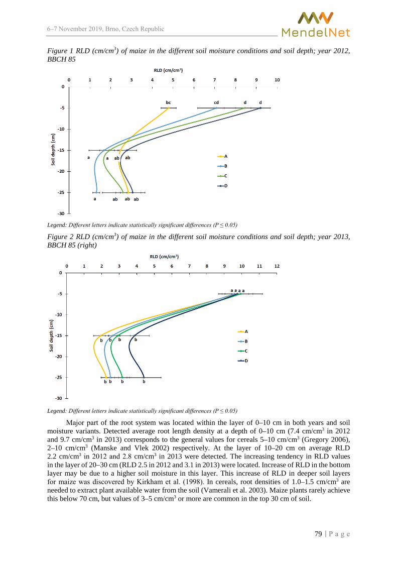
6–7 2019, Brno, Czech Republic
Figure 1 RLD (cm/cm3) of maize in the different soil moisture conditions and soil depth; year 2012, BBCH 85
Legend: Different letters indicate statistically significant differences (P ≤ 0.05)
Figure 2 RLD (cm/cm3) of maize in the different soil moisture conditions and soil depth; year 2013, BBCH 85 (right)
Legend: Different letters indicate statistically significant differences (P ≤ 0.05)
Major part of the root system was located within the layer of 0–10 cm in both years and soil moisture variants. Detected average root length density at a depth of 0–10 cm (7.4 cm/cm3 in 2012 and 9.7 cm/cm3 in 2013) corresponds to the general values for cereals 5–10 cm/cm3 (Gregory 2006), 2–10 cm/cm3 (Manske and Vlek 2002) respectively. At the layer of 10–20 cm on average RLD 2.2 cm/cm3 in 2012 and 2.8 cm/cm3 in 2013 were detected. The increasing tendency in RLD values in the layer of 20–30 cm (RLD 2.5 in 2012 and 3.1 in 2013) were located. Increase of RLD in the bottom layer may be due to a higher soil moisture in this layer. This increase of RLD in deeper soil layers for maize was discovered by Kirkham et al. (1998). In cereals, root densities of 1.0–1.5 cm/cm3 are needed to extract plant available water from the soil (Vamerali et al. 2003). Maize plants rarely achieve this below 70 cm, but values of 3–5 cm/cm3 or more are common in the top 30 cm of soil.
79

6–7 2019, Brno, Czech Republic
Value of the RLD is influenced mostly by the environment. Just precise targeting of the variety to a particular area of cultivation can be the basis for success and economic prosperity of farmers. Only a small amount of roots that were able to penetrate deeper layers prior to the onset of stress are involved in ensuring the supply of water and nutrients (Blum and Ritchie 1984).
Based on the variance analysis, we discovered: i) effects of environment on RLD (differences driven by soil moisture), and ii) differences in RLD driven by root’s depth (as a response on availability of sources – water and nutrients for drought stress tolerant breeding material of maize.
CONCLUSION Excavation methods are destructive (measurements on the same plant cannot be repeated), time
consuming and laborious. However, those direct methods of root system evaluation allowed to find out, for example, that with decreasing precipitation the ratio of root biomass to the above-ground biomass („root:shoot“ ratio) changes in favour of the roots in herbaceous species, but not in trees and shrubs. Or that the results of assessing the vertical distribution of roots in the soil can be generalized by statement that the root system is deeper in drier environments. The soil-core method is often used for sampling root system directly from the soil. This method is often considered as the reference method for evaluating quantitative and morphological parameters of the root system. The representativeness of the method is influenced by several criteria: sampling methodology with respect to land and vegetation heterogeneity, sample diameter, sample volume, sampling depth, number of replications, operator carefulness. The main disadvantages of the soil-core method include high labour demands and destruction of the plant (inability to repeat measurements during vegetation).
In the frame of international cooperation “The Czech Republic – Austria” at Mendel University in Brno and University of Natural Resources and Life Sciences, Vienna the improvement of direct method used to measure the features of a roots – the soil-core method (soil block method), was carried out. The method has been elaborated and then successfully used in agricultural research and breeding purposes.
ACKNOWLEDGEMENT The research was funded by projects No. QK1720285 (New methods for adjustment of altered crop water requirements in irrigation systems across Czechia as affected by soil and climate changes) and QK1920224 (Ways of soil erosion protection on the farm level after glyphosate ban) of the National Agency for Agricultural Research (NAZV).
REFERENCES Blum, A., Ritchie, J.T. 1984. Effect of soil surface water content on sorghum root distribution in the soil. Field Crops Research, 8(3): 169–176. Gregory, P. 2006. Plant roots, growth, activity and interaction with soils. Oxford, Blackwell Publishing. Jackson, R.B. et al. 1996. A global analysis of root distributions for terrestrial biomes. Oecologia, 108(3): 389–411. Kirkham, M.B. et al. 1998. Comparison of minirhizotrons and the soil-water-depletion method to determine maize and soybean root length and depth. European Journal of Agronomy, 8(1–2): 117–125. Klimek-Kopyra, A., Rębilas, K. 2018. Dependence of pea root mass distribution on weather conditions under varying levels of phosphorus application. International Agrophysics, 32(3): 365–372. Available at: http://www.international-agrophysics.org/pdf-104330-35397?filename=Dependence%20of%20pea% 20root.pdf. [2019-08-28]. Manske, G.B., Vlek, P.L.G. 2002. Root Architecture – Wheat as a Model Plant. In Plant roots: The hidden half. New York: Marcel Dekker Inc., pp. 249–260. Smit, A.L. et al. 2010. Root Methods: A Handbook. Berlin: Springer Science & Business Media. Vamerali, T. et al. 2003. Comparison of root characteristics in relation to nutrient and water stress in two maize hybrids. Plant and Soil, 255(1): 157–167.
80

6–7 2019, Brno, Czech Republic
The formation of grains of coloured wheats after heading
Veronika Neradova, Ludek Hrivna, Roman Maco Department of Food Technology
Mendel University in Brno Zemedelska 1, 613 00 Brno
CZECH REPUBLIC
Abstract: During the two-year monitoring, samples of spikes in the milk, soft dough and hard dough maturity stages were taken from coloured wheats of the PS Karkulka variety with a purple pericarp and the Skorpion variety with blue pigmentation in the aleurone layer. Each of the varieties was grown in 2 different levels of nitrogen fertilization: 150 kg/ha N and 210 kg/ha N. For each of the samples, the weight of the spikes, the weight and the number of grains in the spike and the grain yield were monitored. It was found out that the higher values of the yield-relevant parameters were reached by the Skorpion variety. The Skorpion variety was characterized by significantly higher growth in the grain weight during their formation. This was also reflected in the grain yield that was up to 20% higher than in the PS Karkulka variety. A higher nitrogen dose did not have any effects on the grain yield. The yield of both varieties was significantly influenced by weather conditions during the period of the grain formation.
Key Words: coloured wheats, PS Karkulka, Skorpion, grain formation, grain yield
INTRODUCTION Scientific research of wheat varieties with non-traditionally coloured caryopses is a relevant topic
at the moment. Red colouration of grains is typical for the commonly grown winter wheat varieties, the white colour can also be found in practise, although less frequently. It is also possible to obtain other colourations of grain by combination of the appropriate genes. Resources of uncommon grain colour have genes for yellow endosperm, purple pericarp and blue aleurone, which are determined by the presence of substances with antioxidant activity like carotenoids and anthocyanins, respectively (Martinek et al. 2014, Musilová et al. 2013). However, antioxidant activity of coloured wheat grains may depend on genotype, weather condition and cultivation system (Zrcková et al. 2018). According to Böhmdorfer et al. (2018) the anthocyanin content in grains can be increased by pyramidizing the different genes responsible for the accumulation of these pigments in the different grain layers.
These natural pigments substantially influence the quality of wheat products and they are considered to be physiologically active components and health promoters (Abdel–Aal and Hucl 2003). The increased content of natural pigments present in coloured wheat grains has anti-oxidation effects, and thus it can play an important role in prevention of cardiovascular diseases, some type of cancer, diabetes, inflamation, obesity, aging etc. (Garg et al. 2016). Therefore uncommon coloured wheat varieties can be used for production of specific bakery products, especially for the whole-grain products (Zrcková et al. 2018).
The relationship between pigmentation and the resistance of plants to biotic and abiotic stress has also been scientifically proven. Anthocyanins show a capability to absorb light with an excess of UV radiation or with gamma radiation and can prevent the development of photo-oxidative stress. They lower the risk of light damage of chlorophyll and contribute to the osmoregulation capabilities to protect the plant in extreme temperatures and against the effects of drought and salinization. They prevent the effects of phosphorus deficiency and thus contribute to the protection of the photosynthetic apparatus, they also create stable complexes with the heavy metal ions, prevent the lipid oxidation and thus the damage of plasma membrane. Coloured wheats are capable to produce and maintain significantly higher amounts of dry mass in stressful conditions compared to the varieties without these colour pigmentation (Martinek and Polišenská 2018, Mbarki et al. 2018).
81

6–7 2019, Brno, Czech Republic
According to Garg et al. (2016) the yields of coloured wheat varieties are lower in comparison with traditional wheat varieties at present. Hřivna et al. (2014) and Martinek and Vyhnánek et al. (2014) state that the newly-bred varieties of coloured wheat can be used in agriculture, food industry or feed industry only if they achieve yields and technological qualities of grain comparable to the common wheat varieties. The present work deals with the issues related to grain yields in coloured wheats varieties PS Karkulka and Skorpion.
MATERIAL AND METHODS In the years 2016–2018, a small-scale field experiment was carried out in locality belonging
to the company Agra Velký Týnec near Olomouc. The goal of the experiment was to assess the effects of nitrogen-based nutrition on the grain formation after the heading stage and on the yields of the PS Karkulka and Skorpion coloured wheat varieties. The locality is situated in a moderately hot and moderately wet climatic region. The soil is moderately heavy, the soil type is brown earth. The basic agro-chemical characteristics of the soil are given in Table 1, the weather conditions during the most significant months are given in Table 2. The previous crop in both years was winter oilseed rape. Sowing was carried out in the first half of October (8. 10. 2016 and 10. 10. 2017) and the sowing rate was 3.8 million of germinating seeds.
For each variety there were two levels of nitrogen fertilization (150 kg/ha N and 210 kg/ha N). The fertilization scheme is shown in Table 3. There were 3 repetitions for each variant. During the vegetation period, samples of spikes were taken from both varieties from each repetition at three sampling terms: the milk stage (1), the soft dough stage (2) and the hard dough stage (3). At each sampling term, the weight of 10 spikes, the grain weight per spike and the number of grains per spike were determined. Subsequently, the grains of all repetitions were harvested at full maturity with a small-scale combine harvester and the grain yield of each variety was determined.
Table 1 The agro-chemical characteristics of the soil Year pH Potassium Phosphorus Magnesium Sulfur Calcium CEC Humus
(mg/kg) (%) 2017 6.44 135 70.4 201 6.43 1890 – 3.452018 6.68 360 139 192 7.83 2390 144 –
Legend: Nutrient content determined by Mehlich III; CEC – Cation Exchange Capacity
Table 2 Weather conditions Year 2016–2017/2017–2018
Month Average
temperature (°C)
The norm (°C)
Variation from the norm (°C)
Precipitation (mm)
The norm (mm)
Precipitation (%)
September 17.9/13.9 13.8 4.1/0.1 25.5/120.0 47.0 53.2/255 October 8.8/10.1 8.7 0.1/1.4 41.2/79.2 36.0 114.4/220
November 4.0/4.5 3.1 0.9/1.4 47.3/58.0 36.0 131.4/161 December -0.9/1.4 -0.4 -0.5/1.8 15.3/35.0 26.0 58.8/135 January -5.7/2.1 -2.0 -3.7/4.1 19.7/28.5 22.0 89.5/129.5
February 1.4/-2.2 -0.3 1.7/-1.9 11.5/20.0 18.0 63.9/111 March 7.3/2.2 3.9 3.4/-1.7 30.8/44.4 25.0 123.2/178 April 8.8/15.3 8.9 -0.1/6.4 56.8/17.4 33.0 172.1/53 May 16.0/19.2 14.3 1.7/4.9 41.3/20.5 61.0 67.7/34 June 20.4/20.4 17.1 3.3/3.3 64.1/44.5 70.0 91.6/64 July 20.7/21.6 18.9 1.8/2.7 104.8/27.0 71.0 147.6/38
82

6–7 2019, Brno, Czech Republic
Table 3 Experiment design
Variant
Regenerative fertilization (kg/ha N)
Production fertilization (kg/ha N) Total fertilization
(kg/ha N) Code
A B A B 1 54 54 42 0 150 N1 2 54 54 42 60 210 N2
The measured data were statistically evaluated in Microsoft Excel 2010 and Statistica 12 programmes by one-way analysis of the variance ratio test, including Tukey’s post-hoc test (p < 0.05).
RESULTS AND DISCUSSION The aim of the experiment was to evaluate selected parameters which contribute to the yields
of the PS Karkulka and Skorpion varieties of coloured wheat. From the results of the analysis of the spikes it is clear that the environmental conditions have a crucial effect on the yield-relevant features of the grown variety. It can be observed that the weather conditions had a negative impact on the formation of spikes and grains in the second year. That year was characterized by a long and dry summer with minimum of precipitation compared to the previous year. In comparison of the two years, it is thus obvious that both varieties reached lower values of all monitored parameters in 2018 (Figures 1–4).
During the each sampling term, in both years, the increase of the weight of 10 spikes (Figure 1) and as well as the increase of the grain weight per spike (Figure 2) within the ripening period was monitored for both of the varieties. Higher values of these parameters were observed in the Skorpion variety. The Skorpion variety was also characterized by a higher dynamic of changes, which was often significant (p<0.05). While the Skorpion variety showed a significant increase of the weight of 10 spikes and the grain weight during the whole vegetation period of monitoring, the PS Karkulka variety showed significant changes especially between the first and the second sampling term. Significantly higher (p<0.05) values of the number of grains per spike were observed in Skorpion variety (Figure 3).The number of grains per spike varied between 37–39 grains in Skorpion variety and between 28–30 grains in PS Karkulka variety. According to Diviš et al. (2010), the theoretical spike productivity is up to 150 grains. However, the actual number of grains per spike is 15–40 grains during the harvest. According to Zhang et al. (2007), the lower number of grains per spike can be affected by an earlier sowing term. Rawson (1970) states that the yield of wheat is primarily affected by the length of the period of the differentiation of the spikes primordia, which determines the length of the spike and thus also the number of grains per spike. It can be said that the Skorpion variety is, in comparison with the PS Karkulka variety, a spike-focused variety, because shows a higher weight of spikes and a higher number of grains per spike on average. On the other hand, the PS Karkulka variety partially compensated the loss by the number of productive tillers, which is also confirmed by the mostly insignificant differences in the grain yields (Figure 4). PS Karkulka thus showed a higher capacity to form tillers and therefore the possibility to equalize the difference in the monitored parameters. However, the number of tillers also depends on the environmental conditions, such as nutrition, moisture, etc. (Diviš et al. 2010).
Coloured wheat varieties generally tend to have lower yields in comparison with the majority of other current varieties. A comparison of the grain yields of chosen varieties based on the effects of year, variety and nitrogen dose is shown in Figure 4. In our experiment, the Skorpion variety showed up to 20% higher yields than the PS Karkulka variety. Higher dose of nitrogen did not have an effect on the yields of the monitored varieties. In contrast, the unfavourable conditions of the year 2018 had a significant impact on the yield potential of the monitored varieties, particularly during the period of grain formation. Zimolka et al. (2005) states that the final yield and the plant arrangement are affected by a number of factors including the wheat variety, the sowing rate, the date of sowing, quality of seeds and the influence of the environment. Wheat breeders are currently attempting to develop new coloured wheat varieties with better quality and grain yield (Martinek et al. 2013).
83

6–7 2019, Brno, Czech Republic
Figure 1 Evaluating of the weight of 10 spikes at various maturity stages
Figure 2 Evaluating of the grain weight of 10 spikes at various maturity stages
Figure 3 The effect of the year and variety on the number of grains per spike
84

6–7 2019, Brno, Czech Republic
Figure 4 The effect of year, variety and nitrogen dose on the yields
CONCLUSION The grain yield and its quality have a crucial significance when choosing a variety. The grain
yield of a specific variety is determined genetically. However, it can also be significantly influenced by weather conditions in the locality, which was also shown in our experiment. It was found out that the Skorpion variety achieved the higher values of the yield-relevant parameters during the two years of monitoring. The Skorpion variety can be thus characterized as a spike-focused variety, whereas the PS Karkulka variety could be classified as a variety with a higher ability to create tillers. The successful application of coloured wheat varieties into practise depends on the grain yield and agronomic properties. The current donors of genes for purple and blue grain have lower grain yield in comparison with common wheat varieties. That is why wheat breeding programmes should focus on increasing this deficiency (Martinek et al. 2014). According to Zrcková et al. (2018) further research can lead to new opportunities for breeding and commercial production of coloured wheat rich in health-beneficial components.
ACKNOWLEDGEMENTS The research was financially supported by the Internal Grant Agency FA project No. IP 032/2019.
REFERENCES Abdel-Aal E.M., Hucl, P. 2003. Composition and stability of anthocyanins in Blue-Grained Wheat. Journal of Agricultural and Food Chemistry [Online], 51(8): 2174–2180. Böhmdorfer, S. et al. 2018. Profiling and quantification of grain anthocyanins in purple pericarp × blue aleurone wheat crosses by high‑performance thin‑layer chromatography and densitometry. Plant Methods [Online], 14: 29. Diviš, J. et al. 2010. Pěstování rostlin. 2nd ed., České Budějovice: Jihočeská univerzita v Českých Budějovicích, Zemědělská fakulta. Garg, M. et al. 2016. Transfer of grain colors to elite wheat cultivars and their characterization. Journal of Cereal Science, 71: 138–144. Hřivna, L. et al. 2014. Vliv mimokořenové výživy na kvalitu pšenic s barevným perikarpem. Úroda, 26(12): 525–528.
85
6–7 2019, Brno, Czech Republic
Martinek, P., Polišenská, I. 2018. Barevné látky mohou ovlivňovat adaptaci pšenice ke stresu. Obilnářské listy [Online], 26(3–4): 56–58. Available at: https://www.vukrom.cz/userfiles/files/obilnarske_listy/2018/2018_3_4/56-58.pdf. [2019-07-29]. Martinek, P., Vyhnánek, T. 2014. Barevné zrno pšenice jako zdroj antioxidantů. Úroda, 7:68–70. Martinek, P. et al. 2013. Development of the new winter wheat variety Skorpion with blue grain. Czech Journal of Genetics and Plant Breeding [Online], 49: 90–94. Available at: https://www.agriculturejournals.cz/web/cjgpb.htm?type=article&id=7_2013-CJGPB. [2019-10-17]. Martinek, P. et al. 2014. Use of wheat gene resources with different grain colour in breeding. In Proceeding of Tagungsband der 64. Jahrestagung der Vereinigung der Pflanzenzüchter und Saatgutkaufleute Österreichs [Online]. Raumberg-Gumpenstein, Austria, 25–26 November, Raumberg-Gumpenstein: Höhere Bundeslehr- und Forschungsanstalt für Landwirtschaft Raumberg-Gumpenstein, pp. 75–78. Available at: Mbarki, S. et al. 2018. Anthocyanins of coloured wheat genotypes in specific response to salstress. Molecules [Online], 23(7): 1518. Musilová, M. et al. 2013. Genetic variability for coloured caryopses in common wheat varieties determined by microsatellite markers. Czech Journal of Genetics and Plant Breeding [Online], 49(3): 116–122. Available at: https://www.agriculturejournals.cz/publicFiles/100533.pdf. [2019-10-16]. Rawson, H.M. 1970. Spikelet number, its control and relation to yield per ear in wheat. Australian Journal of Biological Sciences [Online], 23(1): 1–16. Zhang, L. et al. 2007. Factors in the reduction in grain number in winter wheat by early sowing in Yamaguchi. Plant Production Science [Online], 10(2): 189–198. Available at: https://www.tandfonline.com/doi/pdf/10.1626/pps.10.189. [2019-08-15]. Zimolka, J. et al. 2005. Pšenice – pěstování, hodnocení a užití zrna. Praha: Profi Press. Zrcková, M. et al. 2018. The effect of genotype, weather conditions and cropping system on antioxidant activity and content of selected antioxidant compounds in wheat with coloured grain. Plant, Soil and Environment [Online], 64(11): 530–538. Available at: https://www.agriculturejournals.cz/web/pse.htm?type=article&id=430_2018-PSE. [2019-10-16].
86

6–7 2019, Brno, Czech Republic
The spectrum of fungal pathogens of Sorghum bicolor x Sorghum sudanense
Eliska Novakova, Ivana Safrankova Department of Crop Science, Breeding and Plant Medicine
Mendel University in Brno Zemedelska 1, 613 00 Brno
CZECH REPUBLIC
Abstract: Sorghum belongs to the most cultivated cereals in the world. The biggest producers for food industry are Africa and Asia. In Europe it is mostly used as animal´s feed. The sorghum is a minority crop in the Czech Republic, it is cultivated mainly for silage as a forage crop for livestock production systems or for biogas production. Five evaluations were performed in 2019 (June–July) under the field condition on sorghum variety ´KWS Tarzan´. The occurrence of fungal pathogens on sorghum were observed and evaluated in the field experimental station in Žabčice. Leaves which were affected by fungal pathogens were photographed and collected for their determination. The fungal pathogens were identified according to morphological and microscopic characteristics which appeared on a leaves surface (spots, mycelium, and spores) on the field or after laboratory ´wet-cell´ cultivation. The sorghum plants were infected by pathogens from the group of leaves and stalks spots (Colletotrichum sublineola, Cercospora sorghi, Exserohilum turcicum, Bipolaris cookei) and sorghum rust (Puccinia sorghi).
Key Words: Colletotrichum sublineola, Cercospora sorghi, Exserohilum turcicum, field monitoring, Sudan grass
INTRODUCTION Due to the climatic changes crops with specific attributes have to be included into the rotation
in the Czech Republic. Such crops have to be able to provide good and high crop yields at high temperatures during the summer months and droughts.
The crop which meets the requirements is sorghum (Sorghum bicolor × Sorghum sudanense). It is also known as Sudan grass and is suitable for feed and biogas stations. The limiting factor for its cultivation is low temperatures during sowing and early emergence (Adamčík and Tomášek 2016). This problem can manifest as low coverage growth, high degree of weed infestation or lower resistance to harmful organisms. These factors can have negative influence on the quantity and quality of production (Das 2018).
Fungal pathogens of sorghum can be sorted into three groups according to parts of plants which are infected. There is an occurrence of inflorescence and seed pathogens (smuts and Fusarium spp.), foliar and stalk pathogens (leaves spot and rusts), and the root and root disc pathogens (Macrophomina phaseolina). Every pathogen which is mentioned above should make a lower biological value of feed → lower photosynthetic activities, lower digestibility for cattle as a consequence of lower content of saccharides and mycotoxin production (Nedělník et al. 2011).
The most important sorghum pathogens in Europe are Colletotrichum sublineola, (Baroncelli et al. 2014, Das 2018), Ascochyta sorghi (Schuh et al. 1986), Bipolaris cookei (Jonar et al. 2011, Das 2018), Cercospora sorghi, Ramulispora sorghicola, Exserohilum turcicum (Kuthan 2010), so the aim of this study was to determine, if they are present in the Czech Republic, nowadays.
MATERIAL AND METHODS The small-plot experiment was established at the field trial station in Žabčice 49°00'57.614" N,
16°5'92.1042 E" in Southern Moravia (Figure 1a–b). The average annual temperature is 9.5 °C, and average annual precipitation is 480 mm. The course of weather in the year 2019 is given
87

6–7 2019, Brno, Czech Republic
in Figure 2. The soil of experiment field is sandy. One plot area was 30 m2. Sorghum seeds were sown on 25. 4. 2019 (25 germinative seeds/m2), without pre-crop. The effect of nitrogen and sulphur fertilization was observed. The fertilizer with nitrogen (N) and sulphur (S) applied 7 days after plant emergence (27 May 2019), zinc foliar application (Zinkosol Forte) was made in 8–leaf growth stage (26 June 2019). The fertilizer with nitrogen (N) → ALZON neo-N (N = 115 kg/ha), fertilizer with nitrogen and sulphur (N+S) → ENSIN (N = 117 kg/ha, S = 58.5 kg/ha), fertilizer with nitrogen and zinc (N+Zn) → ALZON neo-N + ZINKOSOL forte (N = 115 kg/ha, Zn = 450 g/ha), fertilizer with nitrogen and sulphur and zinc → ENSIN + ZINKOSOL forte (N = 115 kg/ha, S = 58.5 kg/ha, Zn = 450 g/ha) were applied in particular variants. These plots were observed and evaluated separately from phytopathologic perspective.
Figure 1 Experimental field with Sorghum bicolor × Sorghum sudanense, (https://www.google.com/maps, 2019)
Figure 2 Climate diagram, Žabčice (Meteorological station in Žabčice, Department of Agrosystems and Bioclimatology, Mendel University in Brno, 2019)
Evaluation of the occurrence of pathogens during vegetation The total health condition of growth and occurrence of sorghum pathogens was evaluated
in June–July 2019 [10. 5., 20. 6., 10.7, 20. 7., and 31.7.; (Figure 3)]. Leaves which showed symptoms of the disease were photographed and collected to a paper bag and they were labelled according to a field number and fertilizer variant. These samples were used for microscopic identification of the pathogen according to morphological characteristic. The small-plot experiment was harvested by hands 1. 8. 2019.
88

6–7 2019, Brno, Czech Republic
Figure 3 Growth of Sorghum bicolor × Sorghum sudanense ´KWS Tarzan ́
Legend: 3a field of sorghum – Žabčice 20. 6. 2019; 3b fielf of sorghum – Žabčice 10. 7. 2019
Determination of sorghum pathogens in the lab conditions The infected leaves were cut to pieces and the surface was disinfected with 0.2% sodium
hypochloride followed by 3 minutes of soaking. Then the leaves were washed by distilled water for 3 minutes, dried in sterile conditions (flow-box, sterile filtration papers, 5 minutes) and placed on Petri dish (Ø 15 cm) with two-tier filtrate paper which was moisten by distilled water. The cultivation was conducted under standard laboratory conditions (temperature 20/25 °C, light mode 14/10 hour) for 7 days. Pathogens were identified under microscope (Olympus BX12, Olympus BX41) by their morphological characteristics (size of spots on the leaves, size of spores etc.).
If it was not possible to identify the pathogen directly from the leaves, cultivation of the pathogen had to be done in cultured dirt of Potato Dextrose Agar (PDA), Sabouraud agar (SA), Malt extract agar (MEA), cultivation lasted for 7–10 days, (23/20 °C, 14/10 hours light mode)
RESULTS AND DISCUSSION
Monitoring and detection of sorghum pathogens in field conditions The vegetation beginning was very slow, because in May the weather was cold and wet
(Figure 2), this not was suitable for sorghum growth. The sorghum stand was sparse and weedy. The first occurrence of fungal pathogens Colletotrichum sublineolum (Figure 4 a–b) and Cercospora sorghi on sorghum plants was noticed in the first half of July (Table 1). In the next observation (the second half of July) another three pathogens were determinated: Exserohilum turcicum, Bipolaris cookei (Figure 4g–h) and Puccinia sorghi (Figure 4e–f). Any differences in rate of infected plants between particular small-plot plots were not observed.
Anthracnose caused by Colletotrichum sublineolum was disease with the highest occurrence on the sorghum plants in the small-plot experiment. Typical anthracnose symptoms are circular-elliptical dark spots 2–6 cm diam., with a red pigmentation on leaves and stalks (Figure 4 a–b). The centre of mature lesions is straw-colored and contains numerous acervuli with black seta (Figure 4c–d). According to Thakur et al. (2007) grey/cream/salmon-colored spore masses are produced under humid conditions. In many instances leaves can be entirely blighted, and when the blight attacks the stalks it is known as 'stalk rot'. The optimal conditions for anthracnose occurrence are when dry and moisture period take turns.
Another fungal pathogen Cercospora sorghi causes very similar symptoms. The lesions are mostly isolated but can grow continuously to give long stripes. They are dark purple with a brown centre. Leaf spots which enlarge to become rectangular lesions (Odvody 1986, Cuevas 2016 et al.).
89
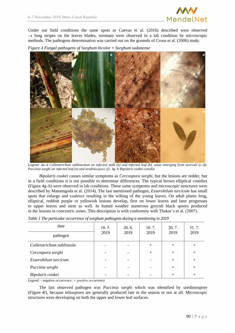
6–7 2019, Brno, Czech Republic
Under our field conditions the same spots as Cuevas et al. (2016) described were observed → long stripes on the leaves blades, stromata were observed in a lab condition by microscopic methods. The pathogens determination was carried out on the grounds of Crous et al. (2006) study.
Figure 4 Fungal pathogens of Sorghum bicolor × Sorghum sudanense
Legend: 4a–d Colletotrichum sublineolum on infected stalk (a) and infected leaf (b), setae emerging from acervuli (c–d); Puccinia sorghi on infected leaf (e) and urediniospore (f); 4g–h Bipolaris cookei conidia
Bipolaris cookei causes similar symptoms as Cercospora sorghi, but the lesions are redder, but in a field conditions it is not possible to determine differences. The typical brown elliptical conidies (Figure 4g–h) were observed in lab conditions. These same symptoms and microscopic structures were described by Manamgoda et al. (2014). The last mentioned pathogen, Exserohilum turcicum has small spots that enlarge and coalesce resulting in the wilting of the young leaves. On adult plants long, elliptical, reddish purple or yellowish lesions develop, first on lower leaves and later progresses to upper leaves and stem as well. In humid weather numerous greyish black spores produced in the lesions in concentric zones. This description is with conformity with Thakur´s et al. (2007).
Table 1 The particular occurrence of sorghum pathogens during a monitoring in 2019
date 10. 5. 2019
20. 6. 2019
10. 7. 2019
20. 7. 2019
31. 7. 2019 pathogen
Colletotrichum sublineola - - + + +
Cercospora sorghi - - + + +
Exserohilum turcicum - - - + +
Puccinia sorghi - - - + +
Bipolaris cookei - - - + + Legend: - negative occurrence; + positive occurrence
The last observed pathogen was Puccinia sorghi which was identified by urediniospore (Figure 4f), because teliospores are generally produced late in the season or not at all. Microscopic structures were developing on both the upper and lower leaf surfaces.
90

6–7 2019, Brno, Czech Republic
This year on locality Žabčice, pathogens had a more frequent rate of occurrence (Table 1), than in year 2018 when only two pathogens were observed: Colletotrichum sublineolum and Ramularia sorghi (Nováková and Šafránková 2018). This was probably due to unevenly distribution of precipitation during the vegetation. This fact had a negative effect on the development of fungal pathogens, probably.
According to Kuthan (2012), fungal pathogens that have been observed this year have a long history in our country, it can be assumed that the higher intensity cultivation of sorghum under south Moravian condition will lead to higher intensity of sorghum infestation by harmful organisms. As no pesticide product has been registered in the Czech Republic yet, it is necessary for farmers to choose varieties that show higher resistance to fungal organisms and buy only certified seed from verified distributors.
CONCLUSION Sorghum seems to be very suitable crop for semi-arid regions of dry land with unpredictable
rainfall. Sorghum can be used in these areas as a suitable replacement for maize, because it has higher resistance to drought and high temperature, which have positive influence on resistance of fungal pathogens, but with the risk of slowly growing on starting vegetation. The most of sorghum fungal pathogens are exotic in nature in our region and they do not have optimal conditions for this development in our geographical conditions, some pathogens expanded over several years, so it is necessary to address this issue. It is necessary to choose a suitable soil location and treatment for the implementation of this crop into crop rotation, more importantly to take into account the pre-crop and, last but not least, a suitable variety that is resistant to the most important pathogens. Multiple observations are necessary to determine the spectrum and importance of pathogens. However, it can be said that the above-mentioned species occur regularly in the Czech Republic conditions. These pathogens should have more influence on quality of cattle feed in following next years.
ACKNOWLEDGEMENTS The paper is an outcome of the project: AF-IGA-2018-tym001: Comparison of the impact of climate change on photosynthesis C3 and C4 plants cycles which are used in livestock feed.
REFERENCES Adamčík, J., Tomášek, J. 2016. Stimulace osiva čiroku pro praktické využití. Biom.cz [Online], Available at: https://biom.cz/cz/odborne-clanky/stimulace-osiva-ciroku-pro-prakticke-vyuziti. [2019-08-22]. Baroncelli, R. et al. 2014. Draft genome sequence of Colletotrichum sublineola, a destructive pathogen of cultivated sorghum. Genome Announcements, 2(3): e00540–14 Crous, P.W. et al. 2006. Species of Cercospora associated with grey leaf spot of maize. Studies in Mycology, 55: 189–197. Cuevas, H.E. et al. 2016. Assessment of sorghum germplasm from Burkina Faso and South Africa to identify new sources of resistance to grain mold and anthracnose. Crop Protection, 79: 43–50. Das, I.K. 2018. Advances in Sorghum Disease Resistance. In Breeding sorghum for diverse end uses. Netherlands: Elsevier Books, pp. 313–324. Jonar, I. et al. 2011. The Effect of seed-borne mycoflora from sorghum and foxtail millet seeds on germination and disease transmission. Mycobiology, 39(3): 206–218. Kuthan, A. 2010. Ochrana čiroku proti škodlivým činitelům: plevele choroby a ochrana. Kukuřičné listy. [Online]. Available at: http://www.crs-marketing.cz/files/crs-kukuricne-listy-c.4-2010-155.pdf. [2019-08-20]. Manamgoda, D.S. et al. 2014. The genus Bipolaris. Studies in Mycology, (79): 221–288. Nedělník, J. et. al. 2011. Výroba kukuřičné siláže z různých fyziologických typů hybridů kukuřice. Metodika 15/11. Zemědělský výzkum, spol. s r.o. Troubsko, Mendelova univerzita Brno, Výzkumný ústav pícninářský, spol. s r.o. Troubsko, pp. 36.
91

6–7 2019, Brno, Czech Republic
Nováková, E., Šafránková, I. 2018. The fungal pathogens of Sorghum vulgare and Lolium multiflorum with focus on feed quality. In Proceedings of International PhD Students Conference MendelNet 2018 [Online]. Brno, Czech Republic, 7–8 November, Brno: Mendel university in Brno, Faculty of AgriSciences, pp. 75–79. Available at: https://mnet.mendelu.cz/mendelnet2018/mnet_2018_full.pdf . [2019-08-15]. Odvody, G.N. 1986. Gray leaf spot. Compendium of Sorghum Diseases [Online], 1(1): 11–12. Available at: https://cropgenebank.sgrp.cgiar.org/index.php/management-mainmenu-433/stogs-mainmenu-238/sorghum/guidelines/fungi. [2019-08-15]. Schuh, W. et al. 1986. Analysis of spatial patterns in sorghum downy mildew with Morisita's index of dispersion. Phytopathology, 76(4): 446–450. Thakur, R.P. et al. 2007. Screening techniques for sorghum diseases. In Information Bulletin No. 76. Andhra Pradesh, India: International Crops Research Institute for the Semi Arid Tropics, pp. 92.
92

6–7 2019, Brno, Czech Republic
The influence of different types of waste on species composition of vegetation at the municipal waste landfill
Lenka Petrzelova1, Jana Cervenkova1, Helena Hanusova1, Dan Uldrijan1, Magdalena Daria Vaverkova2, Dana Adamcova2, Vaclav Trojan1, Jan Winkler1
1Department of Plant Biology
2Department of Applied and Landscape Ecology Mendel University in Brno Zemedelska 1, 613 00 Brno
CZECH REPUBLIC
Abstract: The aim of this paper is to determine the effect of a different type of waste on the plant species composition on the active part of landfill in Nětčice (Kroměříž District, Czech Republic). Three variants were selected for evaluation of the plant species composition within the actively used part of the landfill: biodegradable waste, inert waste and non-sorted municipal solid waste. A total of 124 plant species were found in all three variants together. Amaranthus powellii, Ballota nigra, Bromus sterilis, Echinochloa crus-galli, Elytrigia repens, Robinia pseudoacacia and Setaria pumila were found as characteristic species for a part of landfill with mixed municipal waste, whereas Atriplex patula, Atriplex sagittata, Cucurbita maxima, Hordeum murinum, Chenopodium album and Sisymbrium officinale as characteristic species for biodegradable waste and Arrhenatherum elatius, Cirsium arvense, Plantago major and Tussilago farfara for a part with inert waste. The landfill is a very specific environment for plants and the type of waste influences the species composition of vegetation.
Key Words: plant survey, ordination statistics, urbanization, biodegradable waste
INTRODUCTION Disturbances are considered to be the crucial factor affecting the succession of vegetation.
These disturbances are much more common in human-altered landscape contrary to the natural habitats. Frequency of disturbances by bulldozers and other machines on active landfills is extremely high, increased moreover by continual additions of new waste. Such a harsh environment excludes preservation of most of the plant species to survive. Simultaneously, suppression of competitively strong, mainly perennial, plant species can lead to the colonization of short-lived annual specialists successful in high seed production and dispersion to newly created patches. Unfortunately, it is a characteristic trait of invasion plant species, which can be expected to appear in the destabilizing environment of the landfill (Hobbs and Humphries 1995).
The increase urbanization in recent decades has led to the spread of ruderal flora in the landscape. Changes in the landscape are obvious and this is accompanied by a significant transformation of biodiversity in Central Europe. Research of ruderal vegetation is therefore important in terms of biodiversity prevention (Sukopp and Werner 1983). Sanitary landfilling is most widely used treatment for municipal solid waste deposition worldwide (Wong et al. 2015).
Presence of landfills in a landscape poses a number of environmental risks and raises the concerns regarding the negative effects on human health, air, soil and groundwater pollution, unpleasant odours, the risk of fires and explosions, or negative influence on current vegetation in the surrounding (Chrysikou et al. 2008, El-Fadel et al. 1997, Vrijheid 2000, Nannoni et al. 2015).
The municipal waste landfill is a very heterogeneous habitat with specific conditions for plants. The supply of new diasporas (fruits, seeds, vegetative propagation), sufficient nutrients and permanent disturbances creates specific conditions maintaining the occurrence of specific vegetation. The aim of the thesis is to determine the species composition of plants growing on three different parts of the landfill: biodegradable waste (organic waste decomposing through the action of bacteria
93

6–7 2019, Brno, Czech Republic
and fungi), inert waste (neither chemically nor biologically reactive waste, will not decompose) and non-sorted municipal solid waste.
MATERIAL AND METHODS
Characterization of research locality The fieldwork was conducted on the sanitary landfill in cadastral area of Zdounky-Nětčice
(Kroměříž District, Czech Republic). The landfill is surrounded by a thin line of trees and arable land behind it. According to Quitt (1971), the entire region lies in the warm zone T2. Weather is warm with abundant precipitation.
The bottom as well as all sides and the upper part of the landfill are protected by multi-layer composite liner. Leachate and landfill gas collection system is incorporated to catch the waste water and gases. In terms of maintenance, the landfill is classified in the S-category - other waste, sub-category S-OO3. The designed area of the landfill is 70 700 m2 in five stages with a total volume of 907 000 m3. The facility receives the waste from an area of ca. 75 000 residents. The annually deposited amount of waste is ca. 40 000 103 kg of which 50% are from the communal sphere. Three variants were distinguished within the actively used landfill: municipal waste, biodegradable waste and inert waste (consisting mainly of bricks, concrete and other construction waste).
Vegetation survey and analyses The evaluation of the vegetation was carried out using the phytosociological methods in all three
variants within the actively used landfill. Five phytosociological plots of an area 20 m2 were recorded at each of the variant. All plant species were recorded within the plot and coverage of all species was estimated in percentages. The monitoring of vegetation plots took place in July and October 2017. The scientific names of plant species were used according to Kubát et al. (2002).
The lists of all recorded species within the phytosociological plots are presenting in the paper, with mean values of coverages for five plots of each variant. Further, the species-samples matrices were processed by Canonical Analysis (CCA; in Canoco 5.0 software).
The evaluation of the species composition from phytosociological plots sampled in different variants of waste was carried out. CCA was chosen after the result in previously computed Detrended Correspondence Analysis, where the length of gradient was 3.492.
RESULTS AND DISCUSSION A total of 124 plant species were found in all three variants together. The highest number
of species was found on plots sampled on non-sorted municipal waste (85 species), fewer species were found on the variant with biodegradable waste (64 species) and least species on a variant with inert waste (53 species). The total list of species with the average coverage is shown in the Table 1.
We found, that the different types of waste significantly influenced the plant species composition (at a significance level α = 0.001). The ordination diagram (Figure 1) represents the graphical output of the result with the species affinities respectively to the analysed variants. Plant species with highest affinity to the cariant with municipal waste (violet colour; Figure 1) are especially common annual grasses (Bromus sterilis, Echinochloa crus-galli, Setaria pumila), common ruderal perennial species (Ballota nigra, Melilotus albus) and invasive species (Amaranthus powellii, Helianthus tuberosus, Robinia pseudacacia). High nutrient content from decomposing biodegradable waste was found as most suitable for nitrophilous weeds of Chenopodiaceae family (Atriplex patula, A. sagittata, Chenopodium album), nitrophilous crops, probably growing from the diaspores originating directly from the waste (Cucurbita maxima) and other common ruderal plants (Hordeum murinum, Lactuca serriola, Sisymbrium officinale; yellow colour; Figure 1). The inert waste (grey colour; Figure 1) was colonized mainly by common ruderal plants from Asteraceae family dispersed by wind (Cirsium arvense and Tussilago farfara), and other perennial plants resistant to disturbances (Arrhenatherum elatius and Plantago major). This habitat was found as less favourable for plants.
94

6–7 2019, Brno, Czech Republic
Table 1 The list and average coverage of species in the observed variants of waste
Species Abbreviations Variants (average coverage in %)
Municipal waste (Waste)
Biodegradable waste (Bio_waste)
Inert waste (Inert_wa)
Acer negundo Ace negu 0.30 Acer platanoides Ace plat 0.10 Achillea millefolium agg. Ach mill 1.20 Amaranthus albus Ama albu 0.10 Amaranthus powellii Ama powe 2.30 Amaranthus retroflexus Ama retr 1.55 4.30 1.90 Anagallis arvensis Ana arve 0.10 Anethum graveolens Ane grav 0.05 Apera spica-venti Ape spica 0.30 0.50 Arctium tomentosum Arc tome 0.50 Arrhenatherum elatius Arr elat 0.50 3.50 Artemisia vulgaris Art vulg 1.35 6.50 2.70 Atriplex hortensis Atr hort 0.10 Atriplex oblongifolia Atr oblo 2.05 0.40 0.10 Atriplex patula Atr patu 2.50 0.10 Atriplex sagittata Atr sagi 11.60 8.50 1.60 Avena fatua Ave fatu 0.90 Ballota nigra Bal nigr 0.05 1.10 Bromus japonicas Bro japo 1.20 Bromus sterilis Bro ster 1.40 6.30 Calamagrostis epigejos Cal epig 1.50 Calendula officinalis Cal offi 0.05 Cannabis ruderalis Can rude 0.05 Convolvulus arvensis Con arve 0.40 Conyza canadensis Con cana 0.75 2.10 Crepis tectorum Cre tect 0.60 Cucumis sativus Cuc sati 0.05 Cucurbita maxima Cuc maxi 1.25 Dactylis glomerata Dac glom 0.30 Datura stramonium Dat stra 0.15 0.10 Daucus carota Dau caro 0.20 0.80 1.10 Descurainia Sophia Des soph 0.70 0.80 Digitaria sanguinalis Dig sang 1.00 Dipsacus fullonum Dip full 0.10 Echinochloa crus-galli Ech crus 0.45 5.30 0.20 Elytrigia repens Ely repe 0.15 3.30 0.90 Erigeron annuus Eri annu 0.40 0.10 Erodium cicutarium Ero cicu 0.30 Erysimum cheiranthoides Ery chei 0.20 Euphorbia helioscopia Eup heli 0.40 0.40 Fallopia convolvulus Fal conv 0.10 Festuca rubra Fes rubr 0.50 Fumaria officinalis Fum offi 0.10 0.10 0.20 Galinsoga parviflora Gal parv 0.10 Galium album Gal albu 0.50 0.80 Galium aparine Gal apar 0.40 Geranium pusillum Ger pusi 0.15 0.20 Helianthus tuberosus Hel tube 0.05 2.50 0.80 Hordeum murinum Hor muri 1.35 0.80 Hordeum vulgare Hor vulg 0.10 Chelidonium majus Che maju 0.20 Chenopodium album Che albu 13.70 3.30 4.00 Chenopodium hybridum Che hybr 0.50 0.50
95

6–7 2019, Brno, Czech Republic
Table 1 The list and average coverage of species in the observed variants of waste – continue
Species Abbreviations Variants (average coverage in %)
Municipal waste (Waste)
Biodegradable waste (Bio_waste)
Inert waste (Inert_wa)
Chenopodium strictum Che stri 0.10 Chenopodium pedunculare Che pedu 0.10 Juglans regia Jug regi 0.05 Lactuca sativa Lac sati 0.10 Lactuca serriola Lac serr 1.45 1.90 Lamium purpureum Lam purp 0.05 0.10 Lepidium ruderale Lep rude 0.25 Ligustrum vulgare Lig vulg 1.00 Lolium perenne Lol pere 0.45 1.50 Malus domestica Mal dome 1.00 Malva neglecta Mal negl 0.35 0.20 Medicago lupulina Med lupu 0.10 0.40 Melilotus albus Mel albu 2.30 0.80 Melilotus officinalis Mel offi 0.10 Microrrhinum minus Mic minu 0.30 Papaver argemone Pap arge 0.30 Papaver rhoeas Pap rhoe 0.05 0.20 Papaver somniferum Pap somn 0.10 Persicaria lapathifolia Per lapa 0.20 0.10 Phragmites australis Phr aust 0.10 Picris hieracioides Pic hier 0.10 Pisum sativum Pis sati 0.15 Plantago lanceolate Pla lanc 0.25 0.50 0.40 Plantago major Pla majo 0.35 0.10 1.80 Poa annua Poa annu 0.80 0.50 Polygonum aviculare agg. Pol avic 2.15 5.30 3.30 Portulaca oleracea Por oler 0.50 Prunus avium Pru aviu 2.00 Potentilla reptans Pot rept 1.00 Reseda lutea Res lute 0.30 Robinia pseudacacia Rob pseu 2.00 Rorippa sylvestris Ror sylv 2.00 5.80 2.50 Rosa canina Ros cani 0.50 Rubus sp. Rub sp. 3.00 Rumex crispus Rum cris 0.05 0.10 Rumex obtusifolius Rum obtu 0.25 1.60 Senecio vulgaris Sen vulg 0.80 Setaria pumila Set pumi 0.25 2.90 0.30 Setaria viridis Set viri 0.20 Silene latifolia subsp. Alba Sil lati 0.10 Silene noctiflora Sil nocti 0.10 Sinapis arvensis Sin arve 0.30 0.10 Sisymbrium loeselii Sis loes 2.05 2.00 1.10 Sisymbrium officinale Sis offi 3.10 2.70 Solanum lycopersicum Sol lyco 0.35 0.80 Solanum nigrum Sol nigr 0.55 0.70 0.70 Solanum tuberosum Sol tube 0.60 0.10 Sonchus asper Son aspe 0.35 0.90 0.40 Sonchus oleraceus Son oler 0.05 Stellaria media agg. Ste medi 0.75 0.10 Symphytum officinale Sym offi 0.50 Tagetes patula Tag patu 0.35
96

6–7 2019, Brno, Czech Republic
Table 1 The list and average coverage of species in the observed variants of waste – continue
Species Abbreviations Variants (average coverage in %)
Municipal waste (Waste)
Biodegradable waste (Bio_waste)
Inert waste (Inert_wa)
Taraxacum sect. Ruderalia Tar offi 0.10 Tanacetum vulgare Tan vulg 0.50 Thlaspi arvense Thl arve 0.50 Trifolium hybridum Tri hybr 0.10 Trifolium repens Tri repe 0.10 Tripleurospermum inodorum Tri inod 2.70 4.60 2.40 Triticum aestivum Tri aest 0.25 0.10 Tussilago farfara Tus farf 1.60 Urtica dioica Urt dioi 0.10 1.10 Verbascum chaixii subsp. Austriacum Ver aust 0.10 Verbascum densiflorum Ver dens 0.50 Verbascum thapsus Ver thap 0.30 Veronica hederifolia Ver hede 0.20 Veronica persica Ver pers 0.05 0.20 0.10 Veronica polita Ver poli 0.40
Figure 1 Similarities of plant species composition on phytosociological plots with respect to analysed categorical factor (type of waste)
Legend: Waste – Municipal waste, Bio_waste – Biodegradable waste, Inert_wa – Inert waste, abbreviations of variants and plant species are explained in Table 1.
The rest of the species (black colour; central part of the diagram, Figure 1) was influenced by another unmeasured factor then the variant of waste. Common plant species on more types of waste substrates were Amaranthus retroflexus, Artemisia vulgaris, Polygonum aviculare agg. and Sisymbrium loeselii. These species can be consider as typical species growing in landfill.
Plants found in landfill are according to Chytrý et al. (2012), ranked among typical ruderal species. These species occur nutrient-rich habitats (N, P) as well as habitats disturbed by human activity. On the biowaste landfill there were found species that Winkler et al. (2017) ranks among the typical weeds of field fertilizers. The habitat with inert waste is poor in nitrogen and organic matter
97

6–7 2019, Brno, Czech Republic
and also has a higher pH, which is reflected in the low coverage of the found plant species and also in the lower number of species found.
CONCLUSION A total of 124 plant species were found during the phytosociological survey of three different
types of waste on the active part of the landfill. There were species with a wider ecological niche and occuring in all monitored variants (Amaranthus retroflexus, Artemisia vulgaris, Polygonum aviculare agg. or Sisymbrium loeselii). Different types of waste have an influence to the environmental conditions and we therefore found significant influence of the type of waste for species occurrences. These species with narrower ecological niche could be characterised as more specialized to grow rather on selected type of waste. These species changed according to their dispersion abilities, surviving through the disturbances, nutrient demands or origin of diaspores. Landfill is a suitable environment for the occurrence of invasive plant species and field weeds. Some plant species have the potential to spread to surrounding ecosystems.
ACKNOWLEDGEMENTS This work was created with the financial support of project IGA TP no. 5/2017 of the Internal Grant Agency of the Faculty of AgriSciences at the Mendel University in Brno.
REFERENCES Chrysikou, L. et al. 2008. Distribution of persistent organic pollutants, polycyclic aromatic hydro-carbons and trace elements in soil and vegetation following a large scale landfill fire in Northern Greece. Environment International [Online], 34: 210–225. Available at: https://www.sciencedirect.com/science/article/pii/S0160412007001481?via%3Dihub. [2019-08-08]. Chytrý, M. et. al. 2012. Vegetation of the Czech Republic: diversity, ecology, history and dynamics. Praha: Česká botanická společnost. El-Fadel, M. et al. 1997. Environmental impacts of solid waste landfilling. Journal of Environmental Management [Online], 50: 1–25. Available at: https://www.sciencedirect.com/science/article/pii/S0301479785701314. [2019-08-18]. Hobbs, R.J., Humphries, S.E. 1995. An integrated approach to the ecology and management of plant invasion. Conservation Biology, 9(4): 761–770. Kubát, K. et al. 2002. Klíč ke květeně České republiky. 1. vyd., Praha: Academia. Nannoni, F. et. al. 2015. Heavy element accumulation in Evernia prunastri lichen transplants around a municipal solid waste landfill in central. Waste Management [Online], 43: 353–362. Available at: https://www.sciencedirect.com/science/article/pii/S0956053X15004274?via%3Dihub. [2019-08-18]. Quitt, E. 1971. Klimatické oblasti Československa. 1. vyd., Praha: Academia. Sukopp, H., Werner, P. 1983. Urban environments and vegetation. In Man’s Impact on Vegetation. 1st ed., Netherlands: Springer. Vrijheid, M. 2000. Health effects of residence near hazardous waste landfill sites: a review of epidemiologic literature. Environmental Health Perspectives, 108: 101–112. Winkler, J. et. al. 2017 Vliv hnojení cukrovky chlévským hnojem na zaplevelení. Listy cukrovarnické a řepařské, 133(4), 130–136. Wong, J.T.F. et. al. 2015. Restoration of plant and animal communities in a sanitary landfill: a ten years case study in Hong Kong, Land Degrad.
98

6–7 2019, Brno, Czech Republic
Comparison of the effectiveness of different types of pheromone traps and lures on the plum fruit moth (Grapholita funebrana)
Zaneta Prazanova, Hana Sefrova Department of Crop Science, Breeding and Plant Medicine
Mendel University in Brno Zemedelska 1, 613 00 Brno
CZECH REPUBLIC
Abstract: In 2019 (May–July) the efficiency of two delta traps and pheromone lures from two manufacturers (Pherobank B.V. and Propher s.r.o.) for the plum fruit moth (Grapholita funebrana) were compared. The monitoring was carried out in 3 study areas, namely Kyjov, Starý Lískovec and Soběšice. In total, 6 traps from the manufacturer Pherobank and 6 traps from the manufacturer Propher were placed. Grapholita funebrana was found in all the study areas and 5,667 adults were caught in total. Most individuals were caught in Kyjov (3,083 in total). The green traps attracted 3,081 adults and the transparent traps 2,586 adults. A total of 3,581 adults were captured using the Pherobank pheromone lure, and 2,086 using the Propher lure. A total of 459 non-target species individuals were captured from the families Tortricidae, Noctuidae, and Autostichidae. The Pherobank pheromone lure attracted 201 less of the non-target species than the Propher pheromone lure. The largest number of non-target species were attracted in Kyjov (191 adults).
Key Words: delta pheromone trap, pheromone lure, Grapholita funebrana, monitoring
INTRODUCTION Monitoring and signalling are essential in integrated plant protection. The pheromone lure
is a very useful tool for monitoring a number of harmful insect species (Hrdý and Pultar 1998), allowing the course and intensity of flight activity of the pest to be determined (Kocourek 2012). In plant protection, pheromone lures are primarily used to monitor the occurrence of harmful moth species.
Tortrix moths (Tortricidae) belong to the most diverse family of moths (Hrdý et al. 1979, 1997, Hrudová 2003, 2005, Jakubíková et al. 2016, Stará and Kocourek 2004), with 11,365 species known worldwide (Gilligan et al. 2018), and 476 found in the Czech Republic (Laštůvka and Liška 2011). The caterpillars of these moths are significant pests in agriculture and forestry. They particularly attack the leaves, shoots and fruits of plants. About 28 species are harmful to ornamental plants, about 15 species to fruit trees, 12 species to coniferous trees, 6 species to field crops and vegetables, 3 species to other deciduous trees, and 1 species to hops and hemp (Šefrová 2014, 2015).
The plum fruit moth – Grapholita funebrana (Treitschke 1835) is a key fruit pest. It introduces maggots into fruit, attacking mainly plum trees, but can also harm peaches and apricots. It regularly impacts fruits and precautions must be taken against it almost every year (Šefrová 2003). The effectiveness of such regulatory intervention depends on its timing.
MATERIAL AND METHODS
Defining the study areas The monitoring took place from May to August 2019 in three study areas: gardens
in Kyjov, orchards in Starý Lískovec and in an old orchard near Soběšice – U Jezírka. The orchards in Kyjov and Soběšice are not chemically treated. The characteristics of the study areas are given in Table 1.
99
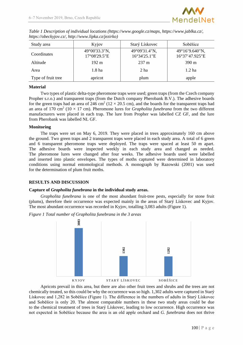
6–7 2019, Brno, Czech Republic
Table 1 Description of individual locations (https://www.google.cz/maps, https://www.jablka.cz/, https://obeckyjov.cz/, http://www.lipka.cz/jezirko)
Study area Kyjov Starý Lískovec Soběšice
Coordinates 49°00'33.3"N, 17°08'29.5"E
49°09'31.4"N, 16°34'25.1"E
49°16’9.640"N, 16°37’47.925"E
Altitude 192 m 237 m 390 m
Area 1.8 ha 2 ha 1.2 ha
Type of fruit tree apricot plum apple
Material Two types of plastic delta-type pheromone traps were used; green traps (from the Czech company
Propher s.r.o.) and transparent traps (from the Dutch company Pherobank B.V.). The adhesive boards for the green traps had an area of 246 cm2 (12 × 20.5 cm), and the boards for the transparent traps had an area of 170 cm2 (10 × 17 cm). Pheromone lures for Grapholita funebrana from the two different manufacturers were placed in each trap. The lure from Propher was labelled CZ GF, and the lure from Pherobank was labelled NL GF.
Monitoring The traps were set on May 6, 2019. They were placed in trees approximately 160 cm above
the ground. Two green traps and 2 transparent traps were placed in each study area. A total of 6 green and 6 transparent pheromone traps were deployed. The traps were spaced at least 50 m apart. The adhesive boards were inspected weekly in each study area and changed as needed. The pheromone lures were changed after four weeks. The adhesive boards used were labelled and inserted into plastic envelopes. The types of moths captured were determined in laboratory conditions using normal entomological methods. A monograph by Razowski (2001) was used for the determination of plum fruit moths.
RESULTS AND DISCUSSION
Capture of Grapholita funebrana in the individual study areas. Grapholita funebrana is one of the most abundant fruit-tree pests, especially for stone fruit
(plums), therefore their occurrence was expected mainly in the areas of Starý Lískovec and Kyjov. The most abundant occurrence was recorded in Kyjov, totalling 3,083 adults (Figure 1).
Figure 1 Total number of Grapholita funebrana in the 3 areas
Apricots prevail in this area, but there are also other fruit trees and shrubs and the trees are not chemically treated, so this could be why the occurrence was so high. 1,302 adults were captured in Starý Lískovec and 1,282 in Soběšice (Figure 1). The difference in the numbers of adults in Starý Lískovec and Soběšice is only 20. The almost comparable numbers in these two study areas could be due to the chemical treatment of trees in Starý Lískovec, leading to low occurrence. High occurrence was not expected in Soběšice because the area is an old apple orchard and G. funebrana does not thrive
3083
1302
1282
K Y J O V S T A R Ý L Í S K O V E C S O B Ě Š I C E
100

6–7 2019, Brno, Czech Republic
on apple trees. Hrnčířová (2009) also recorded G. funebrana in abundant numbers in apple orchards in Svinčany and Ostřešany. The results could be influenced by the location of the trap, the exposure of the land and the weather conditions.
Capture of Grapholita funebrana using different types of pheromone traps A total of 5,667 individuals of the species Grapholita funebrana were captured during
the study. 3,081 adults were captured using the green traps, 2,586 adults using the transparent ones (Figure 2). In the study areas in Kyjov and Starý Lískovec, more adults were always found in the green traps. Only in the study area in Soběšice were there more adults recorded in the transparent trap. In the green trap in Kyjov, 717 more adults were captured than in the transparent one, in Starý Lískovec 146 more, but in Soběšice there were 368 adults less in the green trap. The size of the adhesive board, which is larger in the green trap than in the transparent one, could play a role in the numbers of individuals caught.
Figure 2 Total numbers of Grapholita funebrana individuals in the pheromone traps
Capture of Grapholita funebrana using different types of pheromone
The Propher s.r.o. pheromone (CZ GF) caught 2,086 Grapholita funebrana adults and 330 non-target species adults; the Pherobank B.V. pheromone (NL GF) a total of 3,581 Grapholita funebrana adults and 129 non-target adults (Figure 3).
Figure 3 Total numbers of individuals of the Grapholita funebrana species caught using the different pheromones
The chemical structures of the two lures cannot be compared because Pherobank does not have
this information freely available. Similar results were found by Jakubíková et al. (2016) in the Czech-
1900
724
457
3081
1183
578 82
5
2586
K Y J O V S T A R Ý L Í S K O V E C S O B Ě Š I C E 3 S T U D Y A R E A S
green trap transparent trap
1155
530
401
2086
1928
772 88
1
3581
K Y J O V S T A R Ý L Í S K O V E C S O B Ě Š I C E 3 S T U D Y A R E A S
pheromone CZ GF pheromone NL GF
101

6–7 2019, Brno, Czech Republic
Moravian Highlands in 2014, when 1,509 individuals were found on the Pherobank pheromone but only 217 target-species individuals on two trapsfrom the Czech company. In addition, there were no non-target species on the pheromone lure from the Dutch company (Jakubíková et al. 2016). Jakubíková et al. had the same experience with the pheromone lures from these companies in areas in Moravia, when monitoring was carriedout in 2013. Jakubíková's (2016) results showed that although the Pherobank pheromone lure was not completely successful in selection by target, it did catch more target individuals than the Propher pheromone.
Non-target species A total of 459 non-target species adults from the families Tortricidae, Noctuidae, Autostichidae
were captured. A total of 330 non-target species adults were captured using the CZ GF pheromone and 129 adults using the NL GF pheromone (Figure 4). With the Pherobank pheromone, 201 less non-target species were recorded than with the Propher pheromone. Most non-target species individuals were recorded in the study area in Kyjov (191), followed by Soběšice (168) and Starý Lískovec (100). In Kyjov, 147 more non-target species individuals were lured to the CZ GF pheromone than the NL GF pheromone; and in the Soběšice study area, 74 more non-target species were also attracted to the CZ GF pheromone. However, the number of captured non-target adults was far lower than in the study areas in Kyjov and Starý Lískovec. A total of 249 non-target adults were captured with the green traps and 210 with the transparent ones. The colour of the trap did not play a big role for non-target species, with the difference being only 39 individuals, or 8.5% of the total number of non-target individuals.
Figure 4 Total numbers of non-target species with the different pheromones
CONCLUSION The occurrence of Grapholita funebrana was detected in all three study areas, and a total
of 5,667 adults were captured. The greatest abundance was in the study area in Kyjov (3,083 individuals), the least in the study area in Soběšice (1,282 individuals). The green traps caught 495 (8.7%) more adults than the transparent ones. The Pherobank pheromone (NL GF) proved more effective than the Propher pheromone (CZ GF) during our experiment. The Pherobank pheromone (NL GF) attracted 1,495 plum fruit moth (G. funebrana) individuals more than the Propher pheromone (CZ GF). The Pherobank pheromone’s efficiency is further evidenced by the additional finding that fewer non-target species were caught with this pheromone (201 non-target individuals less than with the Propher pheromone).
ACKNOWLEDGEMENTS The research was financially supported through grant No. AF-IGA2019-IP014.
169
87
74
330
22 13
94
129
K Y J O V S T A R Ý L Í S K O V E C S O B Ě Š I C E 3 S T U D Y A R E A S
pheromone CZ GF pheromone NL GF
102

6–7 2019, Brno, Czech Republic
REFERENCES Gilligan, T.M. et al. 2018. Online světový katalog Tortricidae (ver. 4.0) [Online]. Available at: http://www.tortricid.net/catalogue.asp. [2019-08-22]. Hrdý, I. et al. 1979. Sexual pheromone activity of 8-dodecenyl and 11-tetradecenyl acetates for males of several lepidopteran species in field trials. Acta Entomologica Bohemoslovaca, 76(2): 65–84. Hrdý, I. et al. 1997. Výskyt potenciálních škůdců sadů, obaleče slivoňového, Cydia lobarzewskii a obaleče trnkového, C. Janthinana (Lepidoptera: Tortricidae) v České republice a poznámky k dalším druhům podle úlovků do feromonových lapačů. Klapalekiana, 33: 155–172. Hrdý, I., Pultar, O. 1998. Feromonové lapáky – systémy pro monitorování hmyzích škůdců. Agro, 3(9): 19–21. Hrnčířová, Ž. 2009. Sezónní dynamika a význam obalečů škodících na ovocných stromech na Pardubicku. Diploma thesis, Mendel University in Brno. Hrudová, E. 2003. The presence of non-target lepidopteran species in pheromone traps for fruit tortricid moths. Plant Protection Science, 39(4): 126–131. Hrudová, E. 2005. Nontarget lepidoptera species found in the pheromone traps for selected tortricid species in 2002 and 2003. Acta Universitatis Agriculturae et Silviculturae Mendelianae Brunensis, 53(1): 35–44. Jakubíková, K. et al. 2016. Target and non-target moth species captured by pheromone traps for some fruit tortricid moths (Lepidoptera). Acta Universitatis Agriculturae et Silviculturae Mendelianae Brunensis, 64(5): 1561–1568. Kocourek, F. 2012. Uplatňování systému integrované ochrany rostlin v souvislosti se změnou legislativy (4.) Monitoring a systémy varování v ochraně rostlin. Agromanuál, 6(7): 42–45. Laštůvka, Z., Liška, J. 2011. Komentovaný seznam motýlů České republiky. Biocont Laboratory, Brno, pp. 148. Razowski, J. 2001. Die Tortriciden (Lepidoptera, Tortricidae) Mitteleuropas. Bestimmung – Verbreitung – Flugstandort – Lebensweise der Raupen. Bratislava: F. Slamka. Stará, J., Kocourek, F. 2004. Flight pattern of Archips podana (Lep.: Tortricidae) based on data from pheromone traps. Plant Protection Science, 40(3): 75–81. Šefrová, H. 2003. Změny ve škodlivosti druhů řádu Lepidoptera na polních, zahradních a okrasných rostlinách v průběhu 20. století. Acta Universitatis Agriculturae et Silviculturae Mendelianae Brunensis, 51(5): 7–18. Šefrová, H. 2014. Zavíječi (Pyraloidea) a obaleči (Tortricidae). Listy cukrovarnické a řepařské, 130(9–10): 304–308. Šefrová, H. 2015. Škůdci okrasných rostlin. Brno: Mendelova univerzita v Brně.
103

6–7 2019, Brno, Czech Republic
Insecticidal effect of silica dioxide nanoparticles against Tenebrio molitor larvae
Ivan Rankic1, 2, Anna Janova1, Helena Sturikova1, Dalibor Huska1, 2 1Department of Chemistry and Biochemistry
Mendel University in Brno Zemedelska 1, 613 00 Brno
2Central European Institute of Technology Brno University of Technology
Technicka 3058/10, 615 00 Brno CZECH REPUBLIC
Abstract: Bioassays were conducted to explore the effects of silicon dioxide nanoparticles (SiO2 NPs) against larvae of Tenebrio molitor. Silica nanoparticles were applied at the rates of 100, 200, 300, 400, 500 and 1000 ppm on larvae. Larvae were placed in Petri dishes and sprayed with SiO2 NPs two times in 72 hours. The mortality was counted after 24h, 48h and 72h of exposure. Silica nanoparticles have high toxicity on larvae T. molitor and mortality of larvae increased with increasing concentrations and exposure time. Obtained results showed that silica dioxide nanoparticles were efficient against T. molitor and can be used effectively in plant protection.
Key Words: nanotechnology, silica dioxide, nanoparticles, T. molitor
INTRODUCTION Agricultural production is very important. Insects and pathogens are among the main risks in plant
cultivation. Nanotechnology, as an area of research, holds the potential to help industry with new technological innovations and also opens up new possibilities for key improvements in the agricultural sector.
The nanotechnology is a multidisciplinary science, which combines different chemical and material processes, biotechnology and industrial processing technology. Nanotechnology is of great use in many fields, in agriculture, medicine, pharmacy, food industry (Kitherian 2017, de Francisco and García-Estepa 2018). Nanomaterials are materials usually 1–100 nm in size and possess specific properties, due to their unique size and structure. The possibilities offered by nanotechnology have been increasingly studied to develop new, effective methods for pest management (Rai and Ingle 2012). Nanomaterials can increase agricultural productivity because nanoparticles can be used as fertilizers, insecticides, fungicides. Nanoparticles (NPs) are used for water purification and bacteria treatment, because they have demonstrated antimicrobial properties against pathogens, and are probably non-toxic to humans (Elechiguerra et al. 2005, Yeo et al. 2003). Furthermore, NPs have been successfully applied against a wide range of harmful arthropods, covering both agricultural pests and vectors relevant to the public health and animal sciences (Rani et al. 2014).
Silicone is naturally found in soil, as an integral component of soil. Silicon dioxide nanoparticles are produced by various chemical methods. Their application in agriculture is very important because silica nanoparticles are very effective as insecticides, and they are not toxic to the plants. The use of silicon dioxide NPs in crops is very important because it provides a component of integrated crop protection against pests without leaving any harmful residues in the environment. It can be easily combined with other plant protection practices (Laing et al. 2006).
The aim of the experiment was to test silica dioxide nanoparticles (SiO2 NPs) on larvae T. molitor, as potential insecticides. T. molitor is an important pest in flour mills and which causes damage to commercial grain products, will be used as a model for our research.
104

6–7 2019, Brno, Czech Republic
MATERIAL AND METHODS
Preparation of Silica dioxide nanoparticle (SiO2 NPs) solution: Solutions of SiO2 NPs were prepared by mixing distilled water and stock solution
of the commercial SiO2 NPs (Sigma-Aldrich®) at six final concentrations (100, 200, 300, 400, 500, 1000 ppm). The size of the nanoparticles was 10–20 nm. The nanoparticle suspensions were sonicated 8 minutes before use.
Cultivation of larvae Tenebrio molitor: Larvae Tenebrio molitor were bought in an animal shop and were cultured under laboratory
conditions in Petri dishes. During the experiments, larvae were sprayed two times during 72 hours with the aforementioned concentration of nanoparticles.
Mortality of larvae T. molitor: Mortality was measured by Henderson-Tilton's formula (Henderson and Tilton 1955).
RESULTS AND DISCUSSION The effects of various SiO2 NPs concentrations were monitored in this study. During
the experiment, larvae were used, because of their easy availability in the animal shops. Larvae T. molitor were cultivated in Petri dishes in laboratory conditions for 72 hours. During 72h, larvae were sprayed two times in 72h with different concentrations of SiO2 NPs and mortality was monitored. Larval mortality was observed with the naked eye.
Figure 1 shows larval mortality during 3 control measurements as follows: 24h, 48h, 72h. Results show that larvae did not die in the control sample (water sprayed sample) within 72h. Water has no effect on larval mortality, which was expected. In SiO2 NPs sprayed samples, mortality increased with increasing concentration. Thus, in the sample treated with 100 ppm SiO2 NPs, only 10% of the larvae died within 48h of the treatment. Larvae treated with SiO2 NPs at 200 ppm concentration, in the first 48h exhibited 20% of the larval mortality. During the 48h, 10%–20% of larvae have died in samples treated with nanoparticles at a concentration between 300 ppm and 1000 ppm. The maximum mortality was observed within 72h in samples treated with SiO2 NPs at 300, 400, 500, 1000 ppm. Mortality ranged between 70%–80%.
Figure 1 Progress graph larval mortality of T. molitor over 72 hours
Figure 2 shows the total mortality of the T.molitor larvae during the experiment. The figure clearly shows that with increasing concentration, larval mortality also increases. Total mortality
0
20
40
60
80
100
Mortality 24 h Mortality 48 h Mortality 72 h
Perc
ento
fmor
talit
y
ControlSiO2 100 ppmSiO2 200 ppmSiO2 300 ppmSiO2 400 ppmSiO2 500 ppmSiO2 1000 ppm
105

6–7 2019, Brno, Czech Republic
in the samples treated by 100 ppm and 200 ppm SiO2 NPs were 10% or 20%. In the samples treated with SiO2 NPs with a concentration at 300, 400, 500, 1000 ppm the total mortality was 100%. Dead larvae had dark skin that looked dehydrated, resulting from the hypothesis that SiO2 NPs damage skin cells by their structure and lead to cell dehydration, causing larval death.
Figure 2 Total mortality of larvae T. molitor during 72 hours
Ziaee and Ganji in 2016 have reported – the insecticidal effect against Rhyzopertha dominica and Tribolium confusum of silica NPs at a concentration of 50–300 mg per kg of seed. Over the 7 days of the experiment, mortality ranged between 90–95% depending on the insect species (Ziaee and Ganji 2016). (El-Bendary and El-Helaly 2013) studied the effect of different concentrations of SiO2 NPs against the Spodoptera littoralis during 15 days. They used a concentration of 100–300 ppm and came to the conclusion that with increasing concentration, mortality increased. Thus, mortality in the 100 ppm concentration sample was 15.98%, while at the highest concentration of 350 ppm it was 98.24%. We have also confirmed their hypothesis of increasing mortality with increasing concentration. The influence of silver nanoparticles and silica nanoparticles at a concentration of 1 to 2.5 g per kilogram of seeds led to the death of adults (100%) and larvae (83%) of Callosobruchus maculatus (Rouhani et al. 2013). The concentration of 2 g SiO2 NPs per kilogram of rice seed over 14 days led to mortality of Sitophylus oryzae more than 90% (Debnath et al. 2011). Effect of various concentrations of silicon nanoparticles (0.125 mg, 0.25 mg, 0.5 mg) size 20 nm against Spodoptera litura during the experiment led to high insect mortality. The dead insects had a dehydrated body (Debnath et al. 2012). We also confirmed the hypothesis of dehydration of dead insect bodies.
CONCLUSION Nanotechnology, especially nanoparticles, have found wide application in the field of agricultural
production. So far, a large number of nanomaterials have been tested to protect plants against various pathogens. Silica nanoparticles are gaining increasing attention in plant protection because silicon is found as an integral component of soil. SiO2 NPs not only protect the plant from pests but also supply the deficient plant with the specified mineral. The large difference in larval mortality at 200 ppm (20%) and 300 ppm (100%) concentration has led us to a new experiment in which we will determine the actual
Control 0%
SiO2 100 ppm10%
SiO2 200 ppm20%
SiO2 300 ppm100%
SiO2 400 ppm100%
SiO2 500 ppm100%
SiO2 1000 ppm100%
106

6–7 2019, Brno, Czech Republic
lethal concentration, which will be of great importance. In addition to the determination of the lethal concentration of SiO2 nanoparticles, in future period insecticidal effects of different NPs which will be examined.
ACKNOWLEDGEMENTS The research was financially supported by the Internal Grand Agency of Mendel University in Brno AF-IGA2019-IP036, CEITEC (LQ 1601) and the Ministry of Education, Youth and Sports of the Czech Republic.
REFERENCES De Francisco, E.V., García-Estepa, R.M. 2018. Nanotechnology in the agrofood industry. Journal of Food Engineering, 238: 1–11. Debnath, N. et al. 2011. Entomotoxic effect of silica nanoparticles against Sitophilus oryzae (L.). Journal of Pest Science, 84(1): 99–105. Debnath, N. et al. 2012. Synthesis of surface functionalized silica nanoparticles and their use as entomotoxic nanocides. Powder Technology, 221: 252–256. El-Bendary, H., El-Helaly, A.A. 2013. First record nanotechnology in agricultural: Silica nano-particles a potential new insecticide for pest control. Applied Science Reports, 4(3): 241–246. Elechiguerra, J.L. et al. 2005. Interaction of silver nanoparticles with HIV-1. Journal of Nano-biotechnology, 3(1): 6. Henderson, C.F., Tilton, E.W. 1955. Tests with acaricides against the brown wheat mite. Journal of Economic Entomology, 48(2): 157–161. Kitherian, S. 2017. Nano and Bio-nanoparticles for insect control. Research Journal of Nanoscience and Nanotechnology, 7(1): 1–9. Laing, M. et al. 2006. Silicon use for pest control in agriculture: a review. In Proceedings of the South African Sugar Technologists’ Association. 80, pp. 278–286. Rai, M., Ingle, A. 2012. Role of nanotechnology in agriculture with special reference to management of insect pests. Applied Microbiology and Biotechnology, 94(2): 287–293. Rani, P.U. et al. 2014. Dynamic adsorption of α-pinene and linalool on silica nanoparticles for enhanced antifeedant activity against agricultural pests. Journal of Pest Science, 87(1): 191–200. Rouhani, M. et al. 2013. Insecticidal effect of silica and silver nanoparticles on the cowpea seed beetle, Callosobruchus maculatus F.(Col.: Bruchidae). Journal of Entomological Research, 4(4): 297–305. Yeo, S.Y. et al. 2003. Preparation of nanocomposite fibers for permanent antibacterial effect. Journal of Materials Science, 38(10): 2143–2147. Ziaee, M., Ganji, Z. 2016. Insecticidal efficacy of silica nanoparticles against Rhyzopertha dominica F. and Tribolium confusum Jacquelin du Val. Journal of Plant Protection Research, 56(3): 250–256.
107

6–7 2019, Brno, Czech Republic
Interactive effects of elevated CO2 concentration, drought and nitrogen nutrition on malting quality of spring barley
Jan Simor1, Karel Klem1,2, Vratislav Psota3 1Department of Agrosystems and Bioclimatology
Mendel University in Brno Zemedelska 1, 613 00 Brno
2CzechGlobe – Global Change Research Institute, CAS Belidla 986/4a, 603 00 Brno
3Research Institute of Brewing and Malting Mostecka 971/7, 614 00 Brno
CZECH REPUBLIC
Abstract: Elevated CO2 concentration [EC] generally leads to increased rates of photosynthesis, increased formation of assimilates and finally to storing them in the grain. Increased storage of starch in the grain, however, leads to an unbalanced proportion to the proteins, and their relative content decreases. This is particularly apparent in the conditions of nitrogen deficiency. The interactive effects of EC, nitrogen nutrition and reduced water availability are, however, not yet sufficiently understood. Within the manipulation experiment in open top chambers (Domanínek near Bystřice nad Pernštejnem) that allow simulation of EC (expected by the end of this century – 700 ppm) and drought, the effect of these interactions on protein content, and other quality parameters of spring barley grain was studied. EC reduced grain protein content, increased extract, Kolbach index and also summary Malting quality index. Such effect was more pronounced under higher nitrogen dose, which generally worsened malting quality parameters. Reduced water availability slightly enhanced all malting quality parameters and also showed slight synergistic effect to EC. No clear interactive effects on malting quality were found for nitrogen nutrition and water availability.
Key Words: malting barley, greenhouse gases, nitrogen fertilization, reduced water availability
INTRODUCTION Climate change, or global warming, is one of the world's greatest problems today. Although
we consider variability and instability to be characteristic features of the climate system, in the last two centuries human activity contribute to the negative enhancement of these properties. The beginning of a more significant anthropogenic impact on climate is dated back to the second half of the 18th century to the industrial revolution, which started many anthropogenic activities (deforestation, industrial development, intensive use of fossil fuel) negatively affecting climate change. These activities between the pre-industrial period and 2000 caused an increase in CO2 in the atmosphere by 90 ppm (House et al. 2002). The current state (May 2019) of CO2 concentration in the atmosphere is 411 ppm with an average increase of more than 2 ppm per year (NOAA 2019). Without any effort to mitigate of increasing the atmospheric CO2 it may reach the level of more than 1000 ppm by 2100 (Sokolov et al. 2009).
Spring barley is the most important spring cereal crop in the region of Central and Western Europe. It has an irreplaceable position in the malting industry, as well as a component in livestock feed. (Trnka et al. 2004). The impact of individual climate change factors, which represent beside EC also temperature rise, higher frequency of heat waves or drought period on barley yield and quality is different and often contradictory.
For this reason, understanding the interactions between the effect of EC and other factors associated with climate change is crucial for predicting future food security. In addition to crop yield, climate change is expected to affect also crop quality. However, a relatively small amount of work has been performed on the combined effect of climate change variables on crop quality. Crop quality is thought to be a complex subject involving crop growth, CO2 assimilation, biosynthesis
108
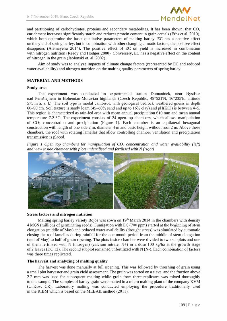
6–7 2019, Brno, Czech Republic
and partitioning of carbohydrates, proteins and secondary metabolites. It has been shown, that CO2 enrichment increases significantly starch and reduces protein content in grain cereals (Erbs et al. 2010), which both determine the basic qualitative parameters of malting barley. EC has a positive effect on the yield of spring barley, but in combination with other changing climatic factors, the positive effect disappears (Alemayehu 2014). The positive effect of EC on yield is increased in combination with nitrogen nutrition (Reedy and Hodges 2000). Conversely, EC has a negative effect on the content of nitrogen in the grain (Jablonski et. al. 2002).
Aim of study was to analyze impacts of climate change factors (represented by EC and reduced water availability) and nitrogen nutrition on the malting quality parameters of spring barley.
MATERIAL AND METHODS
Study area The experiment was conducted in experimental station Domanínek, near Bystřice
nad Pernštejnem in Bohemian-Moravian highlands (Czech Republic, 49°521'N, 16°235'E, altitude 575 m a. s. l.). The soil type is modal cambisol, with geological bedrock weathered gneiss in depth 60–90 cm. Soil texture is sandy loam (45–60% sand and up to 16% clay) and pH(KCl) is between 4–5. This region is characterized as rain-fed area with mean annual precipitation 610 mm and mean annual temperature 7.2 °C. The experiment consists of 24 open-top chambers, which allows manipulation of CO2 concentration and precipitation (Figure 1). Each chamber is an equilateral hexagonal construction with length of one side 2 m, diameter 4 m and basic height without roof 2 m. Above these chambers, the roof with rotating lamellas that allow controlling chamber ventilation and precipitation transmission is placed.
Figure 1 Open top chambers for manipulation of CO2 concentration and water availability (left) and view inside chamber with plots unfertilised and fertilised with N (right)
Stress factors and nitrogen nutrition
Malting spring barley variety Bojos was sown on 19th March 2014 in the chambers with density 4 MGS (millions of germinating seeds). Fumigation with EC (700 ppm) started at the beginning of stem elongation (middle of May) and reduced water availability (drought stress) was simulated by automatic closing the roof lamellas during rainfall for the one month period from the middle of stem elongation (end of May) to half of grain ripening. The plots inside chamber were divided to two subplots and one of them fertilized with N (nitrogen) (calcium nitrate, N+) in a dose 100 kg/ha at the growth stage of 2 leaves (DC 12). The second subplot remained unfertilized with N (N-). Each combination of factors was three times replicated.
The harvest and analyzing of malting quality The harvest was done manually at full ripening. This was followed by threshing of grain using
a small plot harvester and grain yield assessment. The grain was sorted on a sieve, and the fraction above 2.2 mm was used for subsequent malting while grain from three replicates was mixed thoroughly to one sample. The samples of barley grain were malted in a micro malting plant of the company KVM (Uničov, CR). Laboratory malting was conducted employing the procedure traditionally used in the RIBM which is based on the MEBAK method (2011).
109

6–7 2019, Brno, Czech Republic
RESULTS AND DISCUSSION Four main malting quality parameters were selected to demonstrate the effects of individual
factors and possible interactions - protein content in grain, extract of malt, Kolbach index and Malting quality index (MQI). Kolbach index is ratio of total soluble protein (measurable in wort) and the total protein (measurable in the malt). (MQI) summarizes the effect of eight malting quality parameters – N content in non-malted grain, malt extract, relative extract at 45 °C, Kolbach index, diastatic power, apparent final attenuation, friability and β–glucan content in wort.
Figure 2 Effect of elevated CO2 concentration (EC, 700 ppm) compared to ambient CO2 concentration (AC, 400 ppm) and interactions with N nutrition (N+, 100 kg/ha N; N-, 0 kg/ha N) or water availability (ambient precipitation and reduced water availability) on protein content in grain, extract, Kolbach index and malting quality index (MQI)
Protein content The protein content was generally reduced by EC and enhanced by the N fertilization (Figure 2).
Dominant effects on protein content had N nutrition. N fertilization increased the grain protein content, particularly under AC. The effect of EC on the decrease of protein content was thus more pronounced in N fertilized variants. These results correspond to results on the effect of EC on reduction of protein content in wheat grain (Wieser et al. 2008, Fernando et al. 2012) also soybean and other crops (Taub et al. 2008).
Extract of malt Variants fertilized by N during cultivation always showed a lower extract content in the malt.
However, grain from variants grown under EC exhibited a higher extract compare to AC counterparts, particularly in N-fertilized treatments. Effect of reduced water availability was manifested by a slight increase of the extract and the highest extract content in malt was found in the variant grown under reduced water availability and EC (Figure 2). Studies on the effect of EC on extract content in barley malt practically do not exist. The effect of EC on the reduction of viscosity of wort was documented only Erbs et al. (2010).
110

6–7 2019, Brno, Czech Republic
Kolbach index The values of Kolbach index indirectly express proteolytic enzymes activity, therefore were
always lower in N fertilized variants. EC, on the other side, increases the Kolbach index compared to AC. The increase of Kobach index under EC is higher in N–fertilized variants. The negative relationship between N nutrition and Kolbach index was described by Edney et al. (2012). Less is known about the effect of water availability on proteolytic enzyme activity. Verma et al. (2003) showed that water availability effect on Kolbach index varies between genotypes, but in general lower water availability is associated with reduced Kolbach index. Higher value of protein content in grains results in a lower value of Kolbach index and vice versa.
Malting quality index In the world we can find many various systems – malting quality indexes, created by international
organizations (Schildbach 1987) the aim of which is to transfer obtained data into clearer and more comprehensible form mainly for the basic orientation of malting experts, malting barley growers and breeders. In the Czech Republic was created system „Malting quality index“ (Psota and Kosař 2002) designed for evaluation of varieties in the registration procedure. This system was used for comparision of treated variants. After the registration procedure, the Bojos variety (Psota et al. 2005) was classified as a variety of very good malting quality suitable for the production of beer with the protected geographical indication "Czech beer" with a point evaluation of 6.7. Evaluation of the variants ranged from 2.7 (very low MQI) to values that were close to those reached in the registration procedure. The Malting quality index (MQI), which summarizes the effect of eight malting quality parameters (N content in non-malted grain, malt extract, relative extract at 45 °C, Kolbach index, diastatic power, apparent final attenuation, friability and β–glucan content in wort) was mainly affected by N fertilization (Figure 2). N nutrition reduced MQI by approximately 2.5 points. Lower effect of N on MQI was found only under reduced water availability and EC conditions. In this case was MQI reduced by 1.4 points only; EC enhanced MQI by less than 1 point. The higher effect of EC was again found for the combination of reduced water availability and N fertilized variant where EC increased MQI by 2.1 points. Generally lowest effect on MQI had water availability, and the worth mentioning effect of reduced water availability was found only for combination of EC conditions and N fertilized variant (increase by 1.4 points).
CONCLUSION I our experiment EC reduced protein content in barley grain and enhanced the main malting
quality parameters which resulted in higher Malting quality index (MQI). EC also reduced negative impact of N nutrition on malting quality parameters. The effect of reduced water availability on malting quality was rather small and improved slightly all malting quality parameters. Such positive effect of drought on malting quality is likely caused by application of drought in earlier stages. Drought in later growth stages is often reported to have negative impact on malting quality.
ACKNOWLEDGEMENTS This study was supported by research projects IGA – AF-IGA2019-IP043 (Climate change impact on crop structure and yield of spring barley).
REFERENCES Alemayehu, F.R. et al. 2014. Can barley (Hordeum vulgare L. s.l.) adapt to fast climate changes? A controlled selection experiment. Genetic Resources and Crop Evolution, 61(1): 151–161. Edney, M.J. et al. 2012. Effects of seeding rate, nitrogen rate and cultivar on barley malt quality. Journal of the Science of Food and Agriculture, 92(13): 2672–2678. Erbs, M. et al. 2010. Effects of free-air CO2 enrichment and nitrogen supply on grain quality parameters of wheat and barley grown in a crop rotation. Agriculture, Ecosystems & Environment, 136(1–2): 59–68.
111

6–7 2019, Brno, Czech Republic
Fernando, N. et al. 2012. Rising atmospheric CO2 concentration affects mineral nutrient and protein concentration of wheat grain. Food Chemistry, 133(4): 1307–1311. House, J.I. et al. 2002. Maximum impacts of future reforestation or deforestation on atmospheric CO2. Global Change Biology, 8(11): 1047–1052. Jablonski, L.M. et al. 2002. Plant Reproduction under Elevated CO2 Conditions: A Meta-Analysis of Reports on 79 Crop and Wild Species. New Phytologist [Online], 156(1): 9–26. Available at: http://dx.doi.org/10.1046/j.1469-8137.2002.00494.x. [2019-08-10]. MEBAK, 2011. Raw material. Mitteleuropäischen Brautechnischen Analysenkommission, Freising-Weihenstephan, Germany. NOAA (National and Oceanic Administration), 2019. Recent Global CO2 [Online], Available at: http://www.esrl.noaa.gov/gmd/ccgg/trends/global.html. [2019-08-11]. Psota,V., Kosař, K. 2002. Malting Quality Index, Kvasny Prumysl, 48(6): 142–148. Psota, V. et al. 2005. Barley varieties registered in the Czech Republic in 2005. Kvasny Prumysl, 51(6): 190–194. Reddy, K.R., Hodges, H.F. 2000. Climate Change and Global Crop Productivity. 1st ed., Wallingford, Oxon, UK: CABI Publishing. Schildbach, R. 1987. Report for the Barley and Malt Commitee. In Proceedings of 21st Congress of European Brewery Convention. Madrid, Spain, 10–14 May. Oxford: IRL Press, 701–705. Sokolov, A.P. et al. 2009. Probabilistic forecast for twenty-first-century climate based on uncertainties in emissions (without policy) and climate parameters. Journal of Climate, 23(8): 2230–2231. Taub, D.R. et al. 2008. Effects of elevated CO2 on the protein concentration of food crops: a meta‐analysis. Global Change Biology, 14(3): 565–575. Trnka, M. et al. 2004. Climate Change Impacts and Adaptation Strategies in Spring Barley Production in the Czech Republic. Climatic Change, 64(1–2): 227–255. Verma, R.P.S. et al. 2003. Influence of nitrogen and irrigation on malt and wort quality in barley. Cereal Research Communications, 31(3–4): 437–444. Wieser, H. et al. 2008. Effects of elevated atmospheric CO2 concentrations on the quantitative protein composition of wheat grain. Journal of Agricultural and Food Chemistry, 56(15): 6531–6535.
112

6–7 2019, Brno, Czech Republic
Effect of nitrogen, sulphur and zinc application on sorghum biomass yield
Marie Skolnikova, Petr Skarpa Department of Agrochemistry, Soil Science, Microbiology and Plant Nutrition
Mendel University in Brno Zemedelska 1, 613 00 Brno
CZECH REPUBLIC
[email protected] Abstract: Sorghum is known for its ability to grow in localities with limited water supply. Not only plant structure but also balanced nutrition is important for coming through shortage water stress. Especially zinc plays role in plant dealing with water stress and this microelement appears to be suitable for improving sorghum biomass yield. The aim of this study was describing the effect of foliar zinc application in combination with nitrogen and sulphur fertilizations on green forage and dry matter sorghum yield in condition of small-plot experiment in Žabčice. Fertilizer with nitrification and urease inhibitors ALZON neo-N (contains nitrogen), fertilizer with nitrification inhibitor ENSIN (contains nitrogen and sulphur) and ZINKOSOL forte with ZnSO4 form of zinc were used. Sulphur positive effect on sorghum yield did not prove but variants with zinc foliar application shown enhancing of sorghum biomass yield (but not significantly). The highest green forage yield (48.6 t/ha) and the highest dry matter yield (9 t/ha) was found in variant with application of ALZON neo-N and ZINKOSOL forte.
Key Words: sorghum, green forage yield, dry matter yield, foliar zinc application, nitrogen and sulphur fertilization
INTRODUCTION Drought is one of the most limiting factors which threaten agricultural production. The advantage
of sorghum cultivation is its tolerance to drought. Sorghum (Sorghum vulgare var. sudanense) has large root system which contributes to better access to water and it is cultivated mainly for silage or biogas production in the Czech Republic (Podrábský 2008). Not only function of root system but also the growth of whole plant is influenced by right nutrition.
Quality of sorghum forage is important for livestock production and it is involved mainly by nitrogen fertilization which enhances the content of protein and increases biomass yield (Hermuth et al. 2012). Zinc (Zn) plays role as functional, structural or regulatory cofactor of many enzymes (Marschner 2012), it also participates in chlorophyll synthesis and it is responsible for synthesis of proteins which are necessary for growth hormone auxin production (Havlin 2014). Carvalho (2008) states that sufficient content of zinc in plant is necessary to reduce drought stress by contributing to detoxification of reactive oxygen species. Zinc sulfate, which is part of some fertilizers, has important function in adjusting stomata and ionic balance in plant which decrease shortage water stress. Therefore, some authors (Karam et al. 2007, Babaeian et al. 2010) recommend using of zinc foliar application (especially of zinc sulfate fertilizers) in dry conditions. Ehdaie et al. (2008) reported that plants are not demanding to zinc but if it has not sufficient amount of zinc, various enzyme systems and metabolic functions related to zinc are inefficiency. According to Richards et al. (2002) the lack of zinc causes the major problems for producing crops, particularly in dry and semi-arid regions with water shortage. Erdem et al. (2006) claim that is crucial importance of zinc usage to enhance the growth and yield of plants in these areas.
This experiment should contribute to describe effect of zinc foliar application in combination with nitrogen and sulphur fertilization on sorghum green forage and dry matter yield.
MATERIAL AND METHODS Sorghum variety KWS Tarzan was used as a modal crop in precise small-plot experiment
which was established at the Field Trial Station in Žabčice in Southern Moravia (GPS 49°01′30.714″N,
113

6–7 2019, Brno, Czech Republic
16°58′18.883″E). Sorghum was seed on 25 April 2019. The size of one plot was 30 m2 and the soil of experiment field was light sand. Fertilizer with nitrogen (N) and sulphur (S) were applied in single doses 7 days after plant emergence (27 May 2019), zinc foliar application (ZINKOSOL Forte) was made in 8-leaf growth stage (26 June 2019) according to the scheme in Table 1. All variants were conducted in four repetitions.
Table 1 Scheme of small-plot experiment
Variant Fertilizer Dose of
N (kg/ha) S (kg/ha) Zn (g/ha) 1 (N) ALZON neo-N 115 0 0
2 (NS) ENSIN 117 58.5 0
3 (N + Zn) ALZON neo-N + ZINKOSOL forte 115 0 450
4 (NS + Zn) ENSIN + ZINKOSOL forte 117 58.5 450 Legend: ALZON neo-N – urea with nitrification and urease inhibitors, contains 46% N; ENSIN – ammonium sulphate nitrate with nitrification inhibitors, contains 26% N and 13% S, ZINKOSOL forte – contains ZnSO4 (11% Zn and 5% S).
The harvest of sorghum biomass was performed on 1 August 2019. The yield of sorghum green forage was determined from the harvest of whole plot. The content of dry matter was determined from sample of 10 plants which were crushed and dried to constant weight at the temperature of 105 °C. ANOVA analysis of variance and follow-up tests according to Fisher (LSD test) at 95% (P<0.05) level of significance in programme Statistica 12 CZ was used for statistical evaluation.
RESULTS AND DISCUSSION As shown climograph of experimental locality in Žabčice (Figure 1), the precipitation during
March and April 2019 was lower than normal precipitation for this locality. According to Venuto and Kindiger (2008) sorghum needs level of total precipitation at least 400 mm for right growth. Precipitation during next months was satisfying, but it was in combination with higher temperature than normal temperature of this locality.
Figure 1 Climograph of Žabčice
The highest yield was found in variant 3 (N + Zn), it was about 8% enhanced in comparison to the lowest yield from variant 2 (NS). Presented variants had range of dry matter content of biomass from 18.6% to 19.3% at harvest. Although the green forage yield of sorghum was not significantly
114

6–7 2019, Brno, Czech Republic
affected by fertilization, foliar application of zinc increased sorghum biomass yield in contrast to variants without zinc application (Figure 2). The green forage yield of variant 3 (N + Zn) was about 6.1% higher than variant 1 (N) without Zn, variant 4 (NS + Zn) had about 5.1% higher yield of green forage in contrast to variant 2 (NS). Similar positive effect of zinc on forage sorghum yield was found by Bhoya et al. (2014) who also observed increasing after zinc fertilization. Soleymani and Shahrajabian (2012) also mentioned increased level of biomass yield after foliar zinc treatment. Fertilizer ENSIN which contains nitrogen and sulphur was applied in variants 2 (NS) and 4 (NS + Zn) and in contrast to effect of zinc, positive effect of sulphur fertilization on yield was not found in this experiment.
Figure 2 The green forage yield of sorghum (t/ha). Means with same letter are not significantly different (P<0.05)
Jiang and Huang (2002) mentioned that zinc has positive impact on the amount of chlorophyll
which could contribute to increase of plant yield. The yield increasing after zinc application was obvious also on Figure 3, maximum dry matter yield was 9 t/ha and it was found in 3 (N + Zn) variant. The differences between the highest and lowest dry matter yield was not significant, but we found yield increasing about 7.1%. Variants 1 (N) and 4 (NS + Zn) had the same dry matter yield (Figure 3) which was slightly decreased in contrast to 3 (N + Zn). These results are in close conformity with Dambiwal et al. (2017) who also mentioned increasing of dry matter yield after foliar application of ZnSO4.
Figure 3 The dry matter yield of sorghum (t/ha). Means with same letter are not significantly different (P<0.05)
115

6–7 2019, Brno, Czech Republic
CONCLUSION Sorghum has potential to be cultivated in regions with high temperature in combination
with irregular rainfall. The sorghum yield depends not only on weather conditions but also on available nutrients. Nitrogen fertilization seems to be necessary for demanded biomass yield with good quality and micronutrient zinc plays important role in sorghum cultivation also. In our experiment, foliar application of zinc increased green forage yield and dry matter yield in compare with variants without zinc fertilization also. Variant with zinc application in combination with ALZON neo-N which contains nitrogen and nitrification and urease inhibitors had the highest green forage yield (48.6 t/ha) and dry matter yield (9 t/ha). The positive effect of sulphur fertilization did not show. Unfortunately, the results do not show statistically significant differences.
ACKNOWLEDGEMENTS The research was supported by grant no. AF-IGA-2018-tym001.
REFERENCES Babaeian, M. et al. 2010. Effect of water stress and foliar micronutrient application on physiological characterstics and nutrient uptake in sunflower (Helianthus annuus L.). Iranian Journal of Crop Sciences [Online], 12(4): 311–391. Available at: https://www.researchgate.net/publication/326122023_Effect_of_Foliar_Application_of_Zinc_on_Yield_of_Wheat_Grown_under_Water_Stress_Condition. [2019-08-30]. Bhoya, M. et al. 2014. Effect of nitrogen and zinc on growth and yield of fodder sorghum [Sorghum bicolor (L.) Moench] varieties. International Journal of Agricultural Sciences [Online], 10(1): 294–297. Available at: https://pdfs.semanticscholar.org/daad/a7ce02166508d9998e5a8f6fed90248a3fe4.pdf. [2019-08-30]. Carvalho, M.H.C.D. 2008. Drought stress and reactive oxygen species: production, scavenging and signaling. Plant Signaling [Online], 3(3): 156–165. Available at: https://www.researchgate.net/publication/26279543_Drought_stress_and_reactive_oxygen_species_Production_scavenging_and_signaling. [2019-08-28]. Dambiwal, D. et al. 2017. Effect of soil and foliar application of zinc on sorghum (Sorghum bicolor (L.) Moench) yield, agronomic efficiency and apparent recovery efficiency. International Journal of Chemical Studies [Online], 5(4): 435–438. Available at: https://www.researchgate.net/publication/331521413_Effect_of_soil_and_foliar_application_of_zinc_on_sorghum_Sorghum_bicolor_L_Moench_yield_agronomic_efficiency_and_apparent_recovery_efficiency. [2019-09-07]. Ehdaie, B. et al. 2008. Genotypic variation in linear rate of grain growth and contribution of stem reserves to grain yield in wheat. Field Crops Research [Online], 106(1): 34–43. Available at: https://www.researchgate.net/publication/223223152_Genotypic_variation_in_linear_rate_of_grain_growth_and_contribution_of_stem_reserves_to_grain_yield_in_wheat. [2019-08-29]. Erdem, T. et al. 2006. Water use characteristics of sunflower under deficit irrigation. Pakistan Journal of Biological Science [Online], 4(7): 766–769. Available at: https://scialert.net/abstract/?doi=pjbs.2001.766.769. [2019-08-30]. Havlin, J.L. et al. 2014. Soil Fertility and Fertilizers: An Introduction to Nutrient Management. Pearson Education. Hermuth, J. et al. 2012. Čirok obecný – Sorghum bicolor (L.) MOENCH: možnosti využití v podmínkách České republiky. Metodika pro praxi. Praha: Výzkumný ústav rostlinné výroby. Jiang, Y., Huang, B. 2002. Protein alterations in tall fescue in response to drought stress and abscisic acid. Crop Science [Online], 42: 202–207. Available at: https://www.researchgate.net/publication/318391516_Protein_Alterations_in_Tall_Fescue_in_Response_to_Drought_Stress_and_Abscisic_Acid. [2019-08-28].
116
6–7 2019, Brno, Czech Republic
Karam, F., Lahoud, R., Masaad, R. 2007. Evaporation, seed yield and water use efficiency of drip irrigated sun flower under full and deficit irrigation conditions. Agricultural Water Management [Online], 90(3): 213–235. Available at: https://www.researchgate.net/publication/222896762_Evapotranspiration_seed_yield_and_water_use_efficiency_of_drip_irrigated_sunflower_under_full_and_deficit_irrigation_conditions. [2019-08-30]. Marschner, P. 2012. Marschner's Mineral Nutrition of Higher Plants, 3rd Edn. New York, NY: Academic Press. Podrábský, M. 2008. Nový hybrid čiroku se súdánskou trávou. Agromanuál, 2: 66–67. Richards, R.A. et al. 2002. Breeding opportunities for increasing the efficiency of water use and crop yield in temperate cereals. Crop Science [Online], 42: 111–121. Available at: https://www.researchgate.net/publication/11601893_Breeding_Opportunities_for_Increasing_the_Efficiency_of_Water_Use_and_Crop_Yield_in_Temperate_Cereals. [2019-08-30]. Soleymani, A, Shahrajabian, M.H. 2012. The effects of Fe, Mn and Zn foliar application on yield, ash and protein percentage of forage sorghum in climatic condition of Esfahan. International Journal of Biology [Online], 4(3): 92–96. Available at: https://www.researchgate.net/publication/271318845_The_Effects_of_Fe_Mn_and_Zn_Foliar_Application_on_Yield_Ash_and_Protein_Percentage_of_Forage_Sorghum_in_Climatic_Condition_of_Esfahan. [2019-08-29]. Venuto, B., Kindiger, B. 2008. Forage and biomass feedstock production from hybrid forage sorghum and sorghum–sudangrass hybrids. Grassland Science [Online], 54(4): 189–196. Available at: https://onlinelibrary.wiley.com/doi/pdf/10.1111/j.1744-697X.2008.00123.x. [2019-08-29].
117

6–7 2019, Brno, Czech Republic
Appropriate use of specific types of perennial cover plants on vertical green wall
Lukas Vastik1, Vladimir Masan1, Oldriska Sotolarova2, Miroslav Vachun3 1Department of Horticultural Machinery
2Department of Vegetable Growing and Floriculture 3Mendeleum – Institute of Genetics and Plant Breeding
Mendel University in Brno Zemedelska 1, 613 00 Brno
CZECH REPUBLIC
Abstract: One research line into living wall system (LWS) focused now on use of suitable plants. It is very important to find the specific types of plants that are ideal for planting at the minimal costs. Vitality and prosper of each specific type is always based on climate, substrate, irrigation, fertigation, etc., therefore it is important to evaluate the plants for use in a specific LWS system and for specific site. In this experiment was used eight standards substrates to evaluate fifteen species and cultivars of plants suitable to be used on vertical green wall. At the beginning of vegetation was observed high conclusive differences between terms and side (exposure) were found. At the west side, there was a significantly reduced vitality compared to east side. During the season there were no significant increases or decreases in other terms. Between evaluation of individual species viability were found high conclusive differences. The highest adaptability had species Festuca glauca, together with the Sedum spectabile ´Stardust´. Another species with the higher adaptability and viability were Nepeta racemosa ´Walker´s Low´, Sempervivum arachnoideum, Sedum spectabile ´Matrona´. On the other hand, the worse adoption was at the species Heuchera, Carex comans and Festuca scoparia. Those species showed verifiable higher mortality than others.
Key Words: living wall, growth, vegetation, thrive, sustainability
INTRODUCTION The plants in urban areas have potential to help mitigate climate change, such as urban heat island
(UHI), air cleaning, increase water retention and biodiversity (Schettini et al. 2018, Mitterboeck and Korjenic 2017, Hoelscher 2015). Vertical planting is certainly an alternative to roof greenery in a city (Perini and Rosasco 2013, Heng et al. 2010). Many types of Vertical greenery systems (VGS) are known, for example, the most elementary one is Green Facade (GF) system with the climber plants, or more sophisticated system with hydroponics filled panel. The living wall system (LWS) is a complex technology that includes construction, waterproof layer, plants and containers for soil or hydroponic medium, irrigation, fertigation and drainage system as well as water computer (Lin et al. 2018).
Research into LWS focused now on thermal saving, different construction systems and use of suitable plants (Bustami et al. 2018). However, the limiting factors to LWS are installation and maintenance costs, mostly because of the plant renewal. This makes it the most expensive part of the maintenance (Huang et al. 2019). The real ability to apply above mentioned benefits is based mostly on the vitality and grow of plants. Therefore, it is very important to find the specific types of plants that are ideal for planting at the minimal costs.
In some studies, there have been evaluated perennial plants (Pérez-Urrestarazu et al. 2019, Mårtensson et al. 2016, Jorgensen et al. 2014), mediterranean aromatic plants (Devecchi et al. 2013) and mediterranean shrubs (Larcher et al. 2013). Vitality and prosper of each specific type is always based on climate, substrate, irrigation, fertigation, etc., therefore it is important to evaluate the plants for use in a specific LWS system and for specific site.
The aim of this study was to evaluate fifteen species and cultivars of plants suitable to be used on vertical green wall, by using eight different substrates.
118
6–7 2019, Brno, Czech Republic
MATERIAL AND METHODS
Plants The set of plant species and cultivars (taxa) in this experiment was selected on the basis of various
plant-ecological and habitat conditions. The demands on cultivation of each species is shown in Table 1.
Table 1 Climatic and soil demands on cultivation of selected plants species Species:
taxa and cultivar Light Soil Water Humidity pH of soil
Sempervivum arachnoideum L. full sun stony,
gravelly unassuming unassuming acidic
Phedimus spurius (M.Bieb.) t´Hart “Purple Winter”
full sun - semi-shade gravelly less
demanding unassuming neutral
Hylotelephium sp. “Matrona”
full sun - semi-shade
gravelly, humous
less demanding
unassuming - less
demanding
neutral - alkaline
Delosperma nubigensis (Schltr.)
L. Bolus full sun gravelly unassuming unassuming neutral -
alkaline
Ajuga reptans L. semi-shade - shade
loamy soil, humous
less demanding - demanding
unassuming - less
demanding
acidic - neutral
Nepeta racemosa Lam.
“Walker´s Low” full sun loamy soil,
humous less
demanding unassuming neutral - alkaline
Carex comans Berggr.
full sun - semi-shade
loamy soil, humous
unassuming-less
demanding
unassuming - less
demanding unassuming
Festuca glauca Vill. full sun gravelly unassuming unassuming neutral -
alkaline Festuca scoparia
Hook. f. full sun loamy soil, gravelly unassuming unassuming neutral -
alkaline
Hosta minor (Baker) Nakai
semi-shade - shade
loamy soil, humous
less demanding - demanding
less demanding - demanding
acidic - neutral
Dianthus gratianopolitanus Vill. “Babí Lom”
full sun - semi-shade
loamy soil, gravelly
unassuming- less
demanding unassuming neutral -
alkaline
Campanula carpatica Jacq. “Blue Clips”
full sun - semi-shade unassuming less
demanding
unassuming - less
demanding unassuming
Heuchera sp. semi-shade - shade
loamy soil, humous
less demanding- demanding
less demanding - demanding
acidic - neutral
Achillea millefolium L.
“Paprika” unassuming unassuming unassuming unassuming unassuming
Experimental place The experiment was being conducted from 1 May 2018 to 30 September 2018 at the Mendel
University in Lednice, Czech Republic (48.80N, 16.80E), where the altitude is 173 m a.s.l. This area is in a temperate climate zone, characterized by long summer and very warm and dry season.
119

6–7 2019, Brno, Czech Republic
In the experiment was used the mobile version of LWS characterized by a width of 2.00 m, a height of 2.00 m was composed of a metal structure, with a PVC panel installed on it, and three felt layers. From the felt layer is created a framework for substrate that allows the roots of the plants to propagate. Plants are in eight rows with 8 plants per row. The plants were irrigated with the drip method that allows to provide through each nozzle maximal 2.0 l/h of water. Each plant has one nozzle. The surplus of water drained off by the plants is collected on a 1.2 m3 catchment tank at the bottom of the structure. Water computer and humidity sensor managed irrigation.
The wall was divided into 8 sections, a different substrate was used in each section, with the same combination of plants in each section. Conventional horticultural substrates were used, special substrates for roof gardens in combination with additives such as hydrogel. The use of different composition of used substrates was intended to minimize the effect of a particular substrate on the resulting plant growth.
Evaluation of vitality During the season were the plants regularly evaluated using the adjusted scale presented
by Pejchal (2011): - vital plants; evaluation 1 - plants with markedly reduced vitality, yet acceptable properties; evaluation 2 - plants with very low vitality to dead, no longer acceptable properties; evaluation 3
Statistical analysis Analytical determinations were done in triplicate and data were reported as means ± standard
deviation. Tukey’s honestly significant difference (HSD) tests and hierarchical analysis of variance (ANOVA) were conducted to determine the differences among which means that the statistical significance was declared at p ≤ 0.05. The differences were analysed only within the specific sample not between the different samples. These statistical evaluation methods were applied using the computer software package “Statistica 12.0” (StatSoft Inc., USA).
RESULTS AND DISCUSSION During the season was observed variations between exposure and plant growth (Figure 1). High
conclusive differences between terms and side (exposure) were found. Between terms 2.7 and 16.7, there was a significant reduced vitality (mark 2) in both sides (exposures). This was due to the adaptation of the plants after transplanting, and such a reaction could be expected. At the west side, there was a significantly reduced vitality compared to east side (mark 1.5 and 1.8). During the season there were no significant increases or decreases in other terms, which corresponds to measurement of Devecchi et al. (2013). The exception was the comparison of the last measurement with condition after the winter, when east side showed a significant increase. On the other hand, there was an inconclusive decrease in west side. This is due to the dying of above-ground parts of plants as preparation for winter and their regeneration after winter, which is natural and was not evenly.
How shows Figure 2, high conclusive differences between evaluation of individual species viability were found. The highest adaptability had species Festuca glauca 1.02 together with the Sedum spectabile ´Stardust´ 1.09. Another species with the higher adaptability and viability were Nepeta racemosa ́ Walker´s Low´ (1.29), Sempervivum arachnoideum (1.3), Sedum spectabile ́ Matrona´(1.34). Klett and Wilson (2009) states minimal 30 species of plants that are low-growing and spread easily and are suitable for LWS, for example Nepeta, Festuca, Heuchera, Achillea. On the other hand, the worse adoption was at the species Heuchera (2.57), Carex comans (2.79) and Festuca scoparia (2.8).
During the vegetation, some species showed verifiable higher mortality than others (Figure 3). The highest mortality had species Dianthus ´Babí Lom´ (46.43%), Sedum spurium ´Purple Winter´ (33.93%) and Campanula carpatica ´Blue Clips´ (26.79%). The results are similar in comparison with others authors. Devecchi et al. (2013) states, that the mortality was 5% – 26% on east and west side, and maximum was on south side 46.3% (Cistus × purpurescens) and 38.6% (Teucrium × lucydris), and Jorgensen et al. (2014) for Campanula.
120

6–7 2019, Brno, Czech Republic
Figure 1 Evaluation of vitality during the experiment
Side East Side West
02.0
7.20
18
16.0
7.20
18
23.0
7.20
18
30.0
7.20
18
09.0
8.20
18
13.0
8.20
18
21.0
8.20
18
29.0
8.20
18
12.0
9.20
18
25.0
9.20
18
08.1
0.20
18
22.1
0.20
18
15.1
1.20
18
22.0
4.20
19
Date
0.8
1.0
1.2
1.4
1.6
1.8
2.0
2.2
2.4
2.6
Vita
lity
mar
k (-)
Legend: Vitality mark: 1 – vital plants; 2 – reduced vitality; 3 – low vitality to mortality
Figure 2 Evaluation of vitality by the species
Sem
perv
ivum
ara
chno
ideu
m
Car
ex c
oman
s
Ajug
a re
ptan
s
Nep
eta
r ace
mos
a ´W
alke
r´s L
ow´
Sedu
m s
puriu
m ´P
urpl
e W
inte
r´
Fest
uca
glau
ca
Hos
ta
Sedu
m s
pect
abile
´Mat
rona
´
Dia
nthu
s ´B
abí L
om´
Cam
panu
la c
arpa
tica
´Blu
e C
lips´
Fest
uca
scop
aria
Del
ospe
rma
nubi
gens
is
Achi
llea
mill
efol
ium
´Pap
rika´
Heu
cher
a
Sedu
m s
pect
abile
´Sta
rdus
t´
Species
0.81.01.21.41.61.82.02.22.42.62.83.03.2
Vita
lity
mar
k (-)
121

6–7 2019, Brno, Czech Republic
Figure 3 Evaluation of mortality during the experiment
Achi
llea
mille
foliu
m ´P
aprik
a´
Ajug
a re
ptan
s
Cam
panu
la c
arpa
tica
´Blu
e C
lips´
Car
ex c
oman
s
Del
ospe
rma
nubi
gens
is
Dia
nthu
s ´B
abí L
om´
Fest
uca
glau
ca
Fest
uca
scop
aria
Heu
cher
a
Hos
ta
Nep
eta
race
mos
a ´W
alke
r´s L
ow´
Sedu
m s
pect
abile
´Mat
rona
´
Sedu
m s
pect
abile
´Sta
rdus
t´
Sedu
m s
puriu
m ´P
urpl
e W
inte
r´
Sem
perv
ivum
ara
chno
ideu
m
Species
0%
10%
20%
30%
40%
50%
60%
70%
Mor
talit
y [%
]
CONCLUSION One research line into living wall system (LWS) focused now on use of suitable plants. It is very
important to evaluate the plants for use in a specific LWS system and for specific site, and found the specific types of plants that are ideal for planting at the minimal costs.
The results of the experiment can be summarized as follows. At the beginning of vegetation was observed high conclusive differences between terms and side (exposure) were found. At the west side, there was a significantly reduced vitality compared to east side. During the season there were no significant increases or decreases in other terms.
Between evaluation of individual species viability were found high conclusive differences. The highest adaptability had species Festuca glauca, together with the Sedum spectabile ´Stardust´. Another species with the higher adaptability and viability were Nepeta racemosa ´Walker´s Low´, Sempervivum arachnoideum, Sedum spectabile ´Matrona´. On the other hand, the worse adoption was at the species Heuchera, Carex comans and Festuca scoparia. Those species showed verifiable higher mortality than others.
ACKNOWLEDGEMENTS This paper was finalized and supported by the project IGA-ZF/2018-DP “Design and verification of mobile green walls” and by the project CZ.02.1.01/0.0/0.0/16_017/0002334 Research Infrastructure for Young Scientists, co-financed by Operational Programme Research, Development and Education.
REFERENCES Bustami, R. et al. 2018. Vertical greenery systems: A systematic review of research trends. Building and Environment [Online], 146: 226–237. Available at: https://doi.org/10.1016/j.buildenv.2018.09.045. [2019-08-06].
122

6–7 2019, Brno, Czech Republic
Devecchi, M. et al. 2013. The cultivation of mediterranean aromatic plants on green walls. Acta Horticulturae [Online], 999: 243–247. Available at: https://www.actahort.org/books/999/999_34.htm. [2019-07-29]. Heng, C.Y. et al. 2010. Thermal performance of a vegetated cladding system on facade walls. Building and Environment [Online], 45(8): 1779–1787. Available at: https://doi.org/10.1016/j.buildenv.2010.02.005. [2019-08-06]. Hoelscher, M.T. et al. 2015. Quantifying cooling effects of facade greening: shading. transpiration and insulation. Energy and Buildings, 114: 283–290. Huang, Z. et al. 2019. The true cost of “greening” a building: Life cycle cost analysis of vertical greenery systems (VGS) in tropical climate. Journal of Cleaner Production [Online], 228: 437–454. Available at: https://doi.org/10.1016/j.jclepro.2019.04.275. [2019-08-01]. Jorgensen, L. et al. 2014. Root growth of perennials in vertical growing media for use in green walls. Scientia Horticulturae [Online], 166: 31–41. Available at: https://doi.org/10.1016/j.scienta.2013.12.006. [2019-07-29]. Klett, J.E., Wilson, C.R. 2009. Xeriscaping: Ground Cover Plants. Colorado (USA): Colorado State University Extension Gardening Series: 7.230. Larcher, F. et al. 2013. The use of Mediterranean shrubs in green living walls. Agronomic evaluation of Myrtus communis L. Acta Horticulturae [Online], 990: 495–500. Available at: https://www.actahort.org/books/990/990_64.htm. [2019-08-08]. Lin, H. et al. 2018. Shading effect and heat reflection performance of green facade in hot humid climate area: measurements of a residential project in guangzhou. In Proceedings of IOP Conference Series: Earth and Environmental Science, China, 5. May. South China University of Technology, Department of Computer Science and Technology pp. 1–146. Mårtensson, L.M. et al. 2016. Exploring the use of edible and evergreen perennials in living wall systems in the Scandinavian climate. Urban Forestry and Urban Greening, 15: 84–88. Mitterboeck, M., Korjenic, A. 2017. Analysis for improving the passive cooling of building’s surroundings through the creation of green spaces in the urban built-up area. Energy and Buildings, 148: 166–181. Pejchal, M. 2011. Použití pnoucích rostlin v ZAKA. Studijní materiál pro předmět použití rostlin v ZAKA. Zahradnická fakulta, Lednice. Pérez-Urrestarazu, L. et al. 2019. Assessment of perlite, expanded clay and pumice as substrates for living walls. Scientia Horticulturae [Online], 254: 48–54. Available at: https://doi.org/10.1016/j.scienta.2019.04.078. [2019-07-15]. Perini, K., Rosasco, P. 2013. Cost–benefit analysis for green facades and living wall systems. Building and Environment [Online], 70: 110–121. Available at: https://doi.org/10.1016/j.buildenv.2013.08.012. [2019-08-06]. Schettini, E. et al. 2018. Green walls for building microclimate control. Acta Horticulturae [Online], 1215(13): 73–76. Available at: https://doi.org/10.17660/ActaHortic.2018.1215.13. [2019-08-01].
123

6–7 2019, Brno, Czech Republic
Evaluation of compost related to nutrient sources and grain composition
Patrik Zatloukal, Pavel Zemanek, Alice Cizkova, Vladimir Masan Department of Horticultural Machinery
Mendel University in Brno Zemedelska 1, 613 00 Brno
CZECH REPUBLIC
Abstract: The trend toward more efficient methods of compost production and handling requires a complete understanding of the process, the materials involved, and the physical parameters of the materials. This paper describes the evaluation of three compost bases recipes with different ratio/proportion of grape pomace grass and wooden chips. The results prove significant impact of input goods on nutrient content and grain composition of compost structure. The resulting values show that all variants of the proposed recipes meet the requirements of the standard ČSN 46 5735 “Industrial composts”. The highest content of macro elements was determined in the stock (Var.1) with predominance of marc and wood chips over other variants (K – 7150 mg/kg, Mg – 923.5 mg/kg, N – 1.96% and Cox – 13.4%). On the other hand, in terms of particle size distribution, the largest share of elements of produced compost in the size fraction was 0–10 mm (77.72%) in Var.3 with a smaller portion of structural raw materials in the input. When it comes to the grain composition of compost, the highest share of elements of produced compost was in the size of fraction at the Var. 3 with lower share of structured input goods at the beginning.
Key Words: compost, raw texture, horticulture waste, nutrients sources, particle size distribution
INTRODUCTION Composting in lines represents technologically most suitable and economically most optimal way
of processing the garden waste. Many research works had a goal to find out the potential value of different types of compost as horticultural substrates and nutrient sources (Spiers and Fietje 2000). The production and use of compost not only reduces the volume of waste but also offers a high potential substrate and permits reduced usage of peat in the market of growing substrates (Ribero et al. 2000, Zoes et al. 2001). The basis of successful composting is to set up the ideal ratio of input substrates which means not only the recipe of compost base but also setting and keeping some factors at the optimal level (temperature, moisture, aeration, pH, etc.) so the microorganisms itself are able to mature during the whole compost process. The ration of C:N as default mixture is important parameter for composting, the optimal ration of C:N is approximately 30–35. When the ration is higher than these numbers, it slows down the decomposition of the organic material. When this ration is lower than optima lit leads to excessive nitrogen losses. The optimal ration between carbon and nitrogen should be preserved, because microorganisms needs carbon for grow and nitrogen for synthesis of proteins. Low ratios cause loss of N as ammonia and cause odor problems, while higher ratios delay the composting process (Fraser and Lau 2000, Bertran et al. 2004). Ferrer et al. (2001) states that the optimization of feedstock proportions can affect not only the process of the composting itself, but also its overall length and the resulting grain size of the compost. Agnew and Leonard (2003) claims that the trend towards more efficient methods of compost production and handling requires a complete understanding of the process, the materials involved, and the physical parameters of the materials such as moisture content, bulk density, and various mechanical properties such as granularity.
The aim of the work is to design and verify the compost base recipes with the representation of selected types of horticultural waste with an emphasis on the evaluation of nutrient sources and grain composition.
124

6–7 2019, Brno, Czech Republic
MATERIALS AND METHODS
Experimental piles and site Experimental measurements were carried out at the Faculty of Horticultural Experimental
Composting in Lednice. The compost piles were founded in March 2019 and the composting process was completed in June 2019. For the purpose of experimental measurements, the raw material input was formed into strips of triangular profile with a base width of 1.0 m and height of 0.5 m. The length of each saw according to the evaluated variants was 2 m. Aeration of piles was performed 4 times in the monitored period depending on the temperature course of the composting process. The required hygiene temperature of 52–58 °C for at least 5 days as required by ČSN 46 5735 was achieved for all landfills. The Zetor Crystal 8011 tractor in combination with Euro Bagging 2.5 HP windrow turner was used for re-excavation.
Raw material composition of piles The pile formulas were designed in three variants with the representation of the main types
of garden waste (grape pomace, wood chips, grass matter). These variants were suitably supplemented with other components in different weight ratios in order to achieve the optimum ratio C:N = 35:1 as indicated in Table 1. The physical properties and content of the substances were determined in a laboratory.
Table 1 Raw material composition of piles
Raw material
Bulk density
of the raw material
Moisture Organic matter
N
Weight fraction of the raw material (kg)
kg/m3 % % of dry matter
% of dry matter Var.1 Var.2 Var.3
Grape pomace 490 40 92 1.6 500 400 350
Grass matter 150 70 90 1.0 300 450 500
Wood chips 220 38 97 0.3 100 50 50
Ratio C:N - - - - 35:1 35:1 35:1
Nutrient analysis Determination of the nutrient content was carried out according to the standard for industrial
and Testing in Agriculture of Czech Republic No. 475/2000 Coll (Central Institute for Supervising and Testing in Agriculture of Czech Republic). The actual analysis was due to the large number of organic substances carried out according to Morgan. To determine the nitrogen (N) content, a fresh 10 g compost sample was soaked with 30 ml of concentrated sulphuric acid. Then hydrogen peroxide was added and set on fire on the mineralizer to discolour the sample. It was then transferred to 250 ml volumetric flasks, supplemented with distilled water, and measured by Kjeldahl water vapour distillation on the Vapodest system. The determining of other nutrients, due to the large number of organic substances, was carried out according to Morgan. Analyses were carried out of mixed samples weighing 10 g in combination with Gohler's solution (sodium acetate and acetic acid) and activated carbon. After dilution, the solution was measured on an atomic absorption spectrometer (Mg, K) and a spectro-photometer (P). The following tools were used: vapodest 300 by Gerhardt GmbH & Co. KG, Germany; atomic absorption spectrometer Agilent 240 AA by Agilent Technologies, Inc., USA; spectro-photometer Genesys 10S UV-Vis by Thermo Fisher Scientific, Inc., USA.
Determination of pH To determine the pH, 10 g of the compost sample and 50 ml of 0.01 M CaCl2 was mixed together.
Then, the compound was mixed on a mechanical shaker for 60 minutes and the leachate was then measured with a pH meter. This method was used due to the working procedures common
125

6–7 2019, Brno, Czech Republic
for Agrochemical soil testing in the Czech Republic (Central Institute for Supervising and Testing in Agriculture of Czech Republic).
Determination of Cox and humus To determine the components, 10 ml of 0.4 M chromosulfuric mixture was added to a 150 ml
beaker 0.2 g of a ground compost. This content was mixed together with a slightly swirling motion so that the compost did not settle on the walls. The compost was crushed into 3 mm. The IKA MF 10 basic Microfine grinder drive by the IKA Works, Inc., USA was used. At the same time, 10 ml of 0.4 M chromosulfuric mixture was added into three beakers as blind samples. All four beakers were covered with hourglass slides and placed on a tray for 45 minutes in an oven at 125 °C. After being removed from the oven, the beakers were allowed to cool for about 10 minutes and the contents of each were subsequently diluted with distilled water to a volume of about 70 ml. The diluted sample and the blind samples were then titrated with a 0.1 M of Mohr salt solution to a grey colour.
Bulk density of compost This parameter was determined for each test variant as the ratio of weight of loose compost,
which was filled into a 50 litre vessel.
Granularity of compost Granularity of dried compost was determined by sieving it on 10, 20 and 30 mm sieves.
Each structural fraction was separately weighed and converted to percentages. In this way, the percentage of the individual particle size fractions of the compost was determined. The determination was carried out in triplicate for each of the compost pile variations.
Statistical analysis A statistical analysis was performed using the software package “Statistics 12.0” (StatSoft Inc.,
Tulsa, Oklahoma, USA). Analysis of variance was conducted, and the results were compared using Tukey's multiple range assay at a significance level α = 0.05.
RESULTS AND DISCUSSION Table 2 shows the resulting nutrient content values for compost, Cox, pH and bulk density,
respecting the proposed raw material composition.
Table 2 Lists the resultant values of the selected parameters and the content of main nutrients contained in the evaluated variants of the compost piles
Experimental variant
K Mg P Nc Cox Dry matter pH
mg/kg mg/kg mg/kg % % % -
1 7150.0 ± 4.24c
923.5 ± 4.95a
483 ± 4.24ab
1.96 ± 0.01c
13.06 ± 0.01a
69.25 ± 0.21a
7.15 ± 0.07c
2 6002.5 ± 3.54b
811.0 ± 1.41b
476.5 ± 4.95a
1.62 ± 0.02b
13.13 ± 0.02a
61.6 ± 0.14b
7.10 ± 0.14b
3 5654.5 ± 6.36a
922.5 ± 2.12a
499.5 ± 2.12b
1.44 ± 0.02a
7.43 ± 0.01b
69.1 ± 0.14a
7.70 ± 0.14a
Legend: Values are mean ± SD, n = 3; in each column, mean values of different letters are significantly different at P < 0.05
The resulting values show that all variants of the proposed formulas meet the requirements of the standard ČSN 46 5735 "Industrial composts" for minimum humidity (40–65%) and nitrogen content (min. 0.6%). Sager (2007) reports that high quality compost contains 6.8 g/kg K, 15.6 g/kg Mg and 5.3 g/kg P. Diaz (2002) reports for compost made out of grape pomace the values of nutrients at 27.9 g/kg K, 14.9 g/kg N and 4.11 g/kg P and pH 8.41. The pH value should be in the range of 6.0–8.5 for industrial composts according to ČSN 46 5735 norms. This requirement was also met for all evaluated variants, where the values ranged between 7.10–7.70.
126

6–7 2019, Brno, Czech Republic
Table 3 shows the bulk density values of the raw materials mixture at the time of setting the compost base and compost at the end of the process.
Table 3 Bulk density according to experimental variants
Experimental variant Bulk density at the beginning
of the process Bulk density at the end
of the process kg/m3 kg/m3
1 258 ± 1.41c 420 ± 0.71c
2 225 ± 2.12ab 389 ± 1.41b
3 215 ± 2.83a 362 ± 3.54a
Benito et al. (2006) reports the resulting bulk density values for compost pile of different composition in the range of 477–514 kg/m3. Larney et al. (2000) stated that the bulk density increases with composting time and is also determined by the initial ingredients and their preparation. Also, Diaz et al. (2002) states that the density of compost is often similar to that of soils; however, the bulk density values are generally much lower than those of soils due primarily to the larger amounts of air space.
Table 4 – Table 6 shows the results of compost grain evaluation, which were carried out at the end of each month (IV–VI). The results of the statistical evaluation show significant difference in the representation of particles of individual size categories between the evaluated variants. The largest proportion of particles up to 10 mm in size was determined for var. 3, which had a low content of wood chips and grape marc, on the other hand, a high proportion of mown grass matter. In relation to sampling and evaluation terms, the values show gradual decomposition of particles and their higher proportion in the categories 0–10 mm and 10–20 mm.
Table 4 Particle size composition in compost (IV/2019)
Experimental variant 0–10 mm 10–20 mm 20–30 mm >30 mm
% % % %
1 48.26 ± 0.20a 17.50 ± 0.14a 23.88 ± 0.04c 10.36 ± 0.01c
2 57.00 ± 0.14b 18.14 ± 0.04b 15.10 ± 0.02b 9.77 ± 0.12b
3 62.29 ± 0.08c 17.81 ± 0.02ab 13.90 ± 0.13a 6.02 ± 0.04a Legend: Values are mean ± SD; in each column, mean values of different letters are significantly different at P < 0.05.
Table 5 Composition of different sized fractions in compost (V/2019)
Experimental variant 0–10 mm 10–20 mm 20–30 mm >30 mm
% % % %
1 58.8 ± 0.11a 15.825 ± 0.06c 19.49 ± 0.21c 5.89 ± 0.03c
2 69.04 ± 0.23b 14.24 ± 0.06b 11.34 ± 0.35b 5.39 ± 0.19b
3 74.94 ± 0.02c 12.89 ± 0.04a 8.305 ± 0.05a 3.87 ± 0.07a Legend: Values are mean ± SD, in each column, mean values of different letters are significantly different at P < 0.05.
Table 6 Composition of different sized fractions in compost (VI/2019)
Experimental variant 0–10 mm 10–20 mm 20–30 mm >30 mm
% % % %
1 63.25 ± 0.04a 13.72 ± 0.04a 18.32 ± 0.04c 4.72 ± 0.04c
2 72.26 ± 0.03b 13.23 ± 0.03a 10.61 ± 0.04b 3.91 ± 0.02b
3 77.72 ± 0.28c 10.39 ± 0.3b 8.88 ± 0.01a 3.01 ± 0.00a Legend: Values are mean ± SD; in each column, mean values of different letters are significantly different at P < 0.05.
127

6–7 2019, Brno, Czech Republic
Particle size distribution and hence inter-particulate porosity affect the balance between water and air content for each moisture level (Raviv et al. 1998). Benito et al. (2006) states that for the application purposes to the soil profile, the best compost is the one with medium to coarse texture, equivalent to a particle size distribution between 0.25 and 2.5 mm, that allows retention of enough readily available water together with an adequate air content. Handreck (1983) studied grain structure of compost came to conclusion, that the fraction smaller than 0.5 mm, and in particular between 0.1 and 0.25 mm, has the highest influence on porosity and water retention.
Agnew and Leonard (2003) reports that mechanical properties encompass a wide variety of parameters including density and particle size distribution. Obviously, knowledge of these parameters is not a prerequisite for producing compost. However, some basic data could help improve the production efficiency and design of equipment and facilities used in the final treatment of compost by crushing and screening. In addition, the obtained data could lead to a better understanding of how compost can be used to ameliorate the relevant physical properties of soil.
CONCLUSIONS The physical properties of compost play an important role in all stages of compost production,
as well as in the handling and utilization of horticultural and other connected industries. The results of the carried-out experiment prove the impact of the structure of compost elements, which depends on the character of the input goods based on nutrient sources and grainy structure of produced compost. The results of the performed experiment show the influence of structure of compost bases in relation to the character of input materials on nutrient sources and grain composition of produced composts. The highest content of evaluated macro elements was determined in the filling (Var.1) with pre-dominance of marc and wood chips in comparison with other variants. On the other hand, in terms of particle size distribution, the largest proportion of compost produced particles in the size fraction was 0–10 mm (77.72%) for Var.3 with a smaller proportion of structural raw materials at the input.
ACKNOWLEDGEMENTS This paper was finalized and supported by the project IGA-ZF/2019–AP011 “Evaluation of the degree of particle decay during composting” and by the project CZ.02.1.01/0.0/0.0/16_017/0002334 Research Infrastructure for Young Scientists, co-financed by Operational Programme Research, Development and Education.
REFERENCES Agnew, J.M., Leonard, J.J. 2003. The Physical Properties of Compost. Compost Science and Utilization, 11(3): 238–264. Benito, M. et al. 2006. Chemical and physical properties of pruning waste compost and their seasonal variability. Bioresource Technology, 97(16): 2071–2076. Bertran, E. et al. 2004. Composting winery waste: sludges and grape stalks. Bioresource Technology, 95(2): 203–208. VN. 1991. Průmyslové komposty. ČSN 46 5735 (465735) A. Praha: Vydavatelství norem. Diaz, M.J. et al. 2002. Optimization of the rate vinasse/grape marc for co-composting proces. Process Biochemistry, 37(10): 1143–1150. Ferrer, J. et al. 2001. Agronomic use of biotechnologically processed grape wastes. Bioresource Technology, 76(1): 39–44. Fraser, B.S., Lau, A.K. 2000. The effects of process control strategies on composting rate and odor emission. Compost Science and Utilization, 8(4): 274–292. Handreck, K.A. 1983. Particle size and the physical properties of growing media for containers. Communications in Soil Science and Plant Analysis, 14(3): 209–222. Larney, F.J. et al. 2000. Physical changes during active and passive composting of beef feedlot manure in winter and summer. Bioresource Technology, 75(2): 139–148.
128

6–7 2019, Brno, Czech Republic
Raviv, R. et al. 1998. The use of compost as a peat substitute for organic vegetable transplants production. Compost Science and Utilization, 6(1): 46–52. Ribero, H.M. et al. 2000. Fertilisation of potted geranium with a municipal solid waste compost. Bioresource Technology, 73(3): 247–249. Spiers, T.M., Fietje, G., 2000. Green waste compost as a component in soilless growing media. Compost Science and Utilization, 8(1): 19–23. Zoes, V. et al. 2001. Growth substrates made from duck excreta enriched wood shavings and source-separated municipal solid waste compost and separates: physical and chemical characteristics. Bioresource Technology, 78(1): 21–30.
129

ANIMAL PRODUCTION

6–7 2019, Brno, Czech Republic
Effects of phenolic bioactive substances on reducing mortality of bees (Apis mellifera) intoxicated by thiacloprid
Marian Hybl1, Petr Mraz2, Jan Sipos1, Denisa Kovarova3, Antonin Pridal1 1Department of Zoology, Fisheries, Hydrobiology and Apiculture
Mendel University in Brno Zemedelska 1, 613 00 Brno
2Department of Plant Production University of South Bohemia in Ceske Budejovice
Studentska 1668, 370 05 Ceske Budejovice 3Department of Animal Nutrition and Forage Production
Mendel University in Brno Zemedelska 1, 613 00 Brno
CZECH REPUBLIC
Abstract: Nutrition is one of the major concerns related to the world decline in honey bee populations as malnutrition in the honeybee is associated with immune system impairment and increased pesticide susceptibility. The aim of this study was to test the effect of biologically active substances (mixture of phenolic acids and flavonoids) on mortality of worker bees intoxicated by thiacloprid. The tests were carried out in vitro on caged bees. Significantly lower mortality rate was observed in intoxicated bees treated by a mixture of phenolic compounds compared with the intoxicated and the untreated bees. It resulted probably from increased detoxification abilities of bees (due to increased phenol content and antioxidant activity in bee bodies). Therefore, the addition of phenolic substances to bee nutrition can probably lead to increased detoxifying capacity of bees which is often reduced by malnutrition caused by degradation of environment and common beekeeping management.
Key Words: Apis mellifera, cage experiment, flavonoids, mortality, phenolic acids
INTRODUCTION In recent years, a sudden large decline in the number of honeybees has been observed worldwide
(Naug 2009). Nutritional stress is considered to be one of the major causes of bee mortality (Pasquale et al. 2013). The development and survival of bee colonies is dependent on the availability of nutrients in the environment (Brodschneider and Crailsheim 2010). However, the availability and quality of food resources, as a result of the current intensification of agriculture and the associated landscape changes, are declining, reducing environmental sustainability, and consequently affecting bee populations (Naug 2009) by means of low species diversity of flowering plants resulting in reduced diversity of macro and micro elements in nutrition (Pasquale et al. 2013). The lack of nutrients is further underlined by the replenishment of winter supplies by beekeepers who do not provide bees with fully valuable nutrition (Van Engelsdorp 2008). Therefore, a direct consequence of the lack of nutrition is a reduction in the colony population (Pasquale et al. 2013).
Another important factor in reducing the honey bee population (A. mellifera) is the use of pesticides (Frazier et al. 2008). The toxicity of most pesticides varies depending on many factors, in addition to bee age, fitness colony, or subspecies (Nauen et al. 2001), it also depends on optimal nutrient intake (Wehling et al. 2009). Moreover, the bee genome is characterized by a low number of genes associated with detoxification. While the genome of most insect species contains 80 or more cytochrome P450 (major detoxifying enzyme) genes, A. mellifera has only 46 genes P450 (Claudianos et al. 2006). Overexpression of these genes is caused by phenolic and flavonoid substances, which are a common part of honey and pollen, but their amount and ratio differ significantly in food sources (Mao et al. 2013). Of these, p-coumaric acid and quercetin (Liao et al. 2017) are considered the most effective. However, the natural diet of bees always contains a mixture of phenolic acids, flavonoids,
131

6–7 2019, Brno, Czech Republic
and substances derived from them, and together they influence the detoxifying effect (Moniruzzaman et al. 2014, Liao et al. 2017).
Thus, the main aim of this study was to verify the effect of phenolic and flavonoid substances, in amounts that would correspond to the natural occurrence in honey, on the mortality of bees intoxicated by thiacloprid, one of the most abundantly applied neo-nicotinic insecticides in the landscape.
MATERIAL AND METHODS The experiment was carried out in the summer of 2019 in Brno (South Moravia, Czech Republic).
Bees Bees were provided by the university apiary of Mendel University in Brno. Bees from 4 different
honey bee colonies were used (1 frame with hatching bees per colony). The colonies were maintained according to standard beekeeping practices and the bees pertained to A. mellifera, stock Vigor®.
To minimize genetic variability, only bees from colonies derived from an inseminated queen were included in the experiment. As a result, that average coefficient of relatedness between workers from one colony was r = 0.5.
The frames with hatching bees (without adult bees) were placed into a thermostat (35°C and 65–80% RH for 12 hours). Then the bees were mixed together and afterwards split into 4 groups of 3 cages each. Every cage contained 34 bees. The cages with bees were thereafter placed into the thermostat (30 °C, 65–70% RH) and maintained for 2 weeks (Williams et al. 2013). The mortality was noted down daily and dead bee bodies were removed out of the cages.
Design of the experiment The bees were fed ad libitum with 2 top feeders per cage and the groups were established
in the following manner: 1. Treatment T – bees fed with sucrose solution and intoxicated by thiacloprid.2. Treatment FT – bees fed with sucrose solution enriched by a mixture of phenols
and intoxicated by thiacloprid.3. Treatment F – bees fed with sucrose solution enriched by a mixture of phenols.4. Treatment C – bees fed only with sucrose solution.
Chemicals and their concentrations Sucrose solution consisted of 50% (w/v) sucrose. Thiacloprid was added to a sucrose solution
in the concentration of 30 µg/g (= 30 ppm or 35 mg/L; thiacloprid) (Retschnig et al. 2014). The mixture of phenols contained 200 mg/kg of phenolic acids and 10 mg/kg of flavonoids in proportion based on Moniruzzaman et al. (2014), and the concentration of p-coumaric acid was increased according to Mao et al. (2013). The concentration of phenolic compounds was based on real concentrations in common honey.
Table 1 Composition of phenolic compounds used in treatments F and FT
Phenolic acids
caffeic acid 10.00% 20 mg/kg benzoic acid 20.00% 40 mg/kg gallic acid 7.50% 15 mg/kg ferulic acid 20.00% 40 mg/kg
p-coumaric acid 35.00% 70 mg/kg vanillic acid 7.50% 15 mg/kg
Flavonoids
rutin 25% 2.5 mg/kg quercetin 25% 2.5 mg/kg naringin 25% 2.5 mg/kg
hesperidin 25% 2.5 mg/kg
132
6–7 2019, Brno, Czech Republic
Data analysis The survival curves were fitted by the Kaplan-Meier method. Based on this method we estimated
survival probability for each group of bees from observed survivor times (Kaplan and Meier 1958). Significant difference between different survival curves was tested by log-rank test (Therneau and Grambsch 2000). This test compares observed number of events with the number of events what would be expected under null hypotheses (i.e. Identical survival curves). All data were analysed by using R statistical program.
RESULTS The interrelation between bee survival rate and applied treatment is shown in Table 2
and Figure 1. While the highest rate of mortality was observed in the group T, the lowest rate appeared in the group C. Differences detected between these two groups were statistically highly significant (p < 0.001). Analogically, the groups F and T differed from each other also with very high significance (p < 0.001) as well as groups FT and T (p < 0.001). Difference in mortality rates spotted in the groups C and FT was slighter yet still significant (p = 0.03). On the contrary, mortality in the groups F and FT turned out not to differ significantly (p = 0.17) and the weakest contrast could be seen between groups C and F who did not differ significantly either (p = 0.44).
Table 2 The results of log-rank test used for comparison of survival curves in the experimental groups Treatment Degrees of freedom Chi-square statistic p-value C/F 1 0.6 0.44
F/FT 1 1.8 0.17
C/ FT 1 4.6 0.03
FT/T 1 11.4 <0.001
F/ T 1 20.6 <0.001
C/T 1 28.31 <0.001 Legend: T – bees fed with sucrose solution and intoxicated by thiacloprid, FT– bees fed with sucrose solution enriched by a mixture of phenols and intoxicated by thiacloprid, F – bees fed with sucrose solution enriched by a mixture of phenols, C – bees fed only with sucrose solution.
DISCUSSION Thiacloprid toxicity, demonstrated by significantly higher mortality in group T compared to group
C, was proved as expected, which also correlates with the findings outlined by Retschnig et al. (2014). On the other hand, the conclusive difference between the bee groups T and F points towards a high level of thiacloprid toxicity compared to the mixture of tested bioactive substances represented by cohort F. Moreover, the harmlessness of the mixture of bioactive substances F is proved by the statistically insignificant difference in survival rate compared to group C. This is also in line with the findings reported by Liao et al. (2017). On the contrary, statistically significant drop in the mortality rate of the group FT in contrast to the group T possibly stemmed from increased detoxification capacity and antioxidant activity of the experimental bees as a result of the nutrition enriched by phenolic substances (Mao et al. 2013, Moniruzzaman et al. 2014, Liao et al. 2017). The significant difference between FT and C points towards limited detoxification abilities of the used bioactive substances where the mortality of thiacloprid-intoxicated bees decreased but not to the same level reached in the unintoxicated bees.
An interesting phenomenon appeared to be the insignificant differences in mortality rates that were observed in the groups FT and F compared to the significant difference between groups FT and C. This implies the probable existence of an increased metabolic burden caused by higher level of certain flavonoids (Mao et al. 2017).
As Wheeler and Robinson (2014) suggest, many components of high nutritional value and importance that occur naturally in honey are not present in artificial food sources widely used
133

6–7 2019, Brno, Czech Republic
in beekeeping. Apart from carbohydrates and proteins, bee diet also needs to contain certain elements (for example phenolic compounds) that have a significant effect on their detoxification capability (Mao et al. 2013, Liao et al. 2017). Based on these findings and the results of this study, we assumed that the addition of phenolic substances in bee nutrition can, to some extent, increase the detoxifying abilities of bees (Mao et al. 2013, Liao et al. 2017) which is reduced due to malnutrition caused by degradation of environment and common beekeeping management (Wheeler and Robinson 2014, Pasquale et al. 2013).
Figure 1 Survival rate in dependence on feeding (Kaplan Meier survival analyses)
CONCLUSION Compounds that occur naturally in the bee diet have been shown to have a compensatory effect
on bee health, reflecting the evolutionary relationships between bees and plants. The diversity of bee food sources in the landscape is decreasing, leading to their malnutrition
and also to lack of phenolic substances important for bee detoxification. By adding these substances to bee nutrition (e.g. when replenishing winter supplies), the risk
associated with malnutrition and bee intoxication can be reduced and conditions for successful overwintering colonies can be improved.
ACKNOWLEDGEMENTS The research was financially supported by: grant AF–IGA2019–IP007 and the donations by elitbau, Ltd. and Konica Minolta Business Solution Czech, Ltd.
REFERENCES Brodschneider, R., Crailsheim, K. 2010. Nutrition and health in honey bees. Apidologie, 41(3): 278–294. Claudianos, C. et al. 2006. A deficit of detoxification enzymes: pesticide sensitivity and environmental response in the honeybee. Insect Molecular Biology, 15(5): 615–636. Frazier, M. et al. 2008. What have pesticides got to do with it? American Bee Journal, 148(6): 521–523.
134

6–7 2019, Brno, Czech Republic
Kaplan, E.L. Meier, P. 1958. Nonparametric estimation from incomplete observations. Journal of the American Statistical Association, 53(282): 457–481. Liao, L-H. et al. 2017. Impacts of Dietary Phytochemicals in the Presence and Absence of Pesticides on Longevity of Honey Bees (Apis mellifera). Insects, 8(1): 22. Mao, W. et al. 2013. Honey constituents up-regulate detoxification and immunity genes in the western honey bee Apis mellifera. Proceedings of the National Academy of Sciences, 110(22): 8842–8846. Mao, W. et al. 2017. Disruption of quercetin metabolism by fungicide affects energy production in honey bees (Apis mellifera). Proceedings of the National Academy of Sciences, 114(10): 2538–2543. Moniruzzaman, M. et al. 2014. Identification of phenolic acids and flavonoids in monofloral honey from Bangladesh by high performance liquid chromatography: determination of antioxidant capacity. BioMed Research International, 1–11. Nauen, R. et al. 2001. Toxicity and nicotinic acetylcholine receptor interaction of imidacloprid and its metabolites in Apis mellifera (Hymenoptera: Apidae). Pest Management Science, 57: 577–586. Naug, D. 2009. Nutritional stress due to habitat loss may explain recent honeybee colony collapses. Biological Conservation, 142: 2369–2372. Pasquale, G.D. et al. 2013. Influence of pollen nutrition on honey bee health: do pollen quality and diversity matter. PLoS ONE, 8(8): e72016. Retschnig, G. et al. 2014. Thiacloprid–Nosema ceranae interactions in honey bees: Host survivorship but not parasite reproduction is dependent on pesticide dose. Journal of Invertebrate Pathology, 118: 18–19. Therneau, T.M., Grambsch, P.M. 2000. Modelling Survival Data: Extending the Cox Model. New York: Springer. Van Engelsdorp, D. et al. 2008. A survey of honey bee colony losses in the U.S., fall 2007 to spring 2008. PLOS ONE, 3(12): e4071. Wehling, M. et al. 2009. Colony losses-interactions of plant protection products and other factors. Julius Kuhn Arch, 423: 153–154. Wheeler, M.M., Robinson, G.E. 2014. Diet-dependent gene expression in honey bees: honey vs. sucrose or high fructose corn syrup. Scientific Reports, 4: 5726. Williams, G.R. et al. 2013. Standard methods for maintaining adult Apis mellifera in cages under in vitro laboratory conditions. Journal of Apicultural Research, 52(1): 1–36.
135

6–7 2019, Brno, Czech Republic
Dogs jumping on people
Eva Koru
Department of Animal Morphology, Physiology and Genetics Mendel University in Brno Zemedelska 1, 613 00 Brno
CZECH REPUBLIC [email protected]
Abstract: Dogs may sometimes perform unwanted behaviour. Among the most frequent problematic behaviour for owners is dogs jumping on people. A little is known about factors that may be associated with the dogs jumping on people. Therefore, the aim of the study was to assess whether the breed, dog size and living only with adults may affect dogs jumping on people. Two hundred and thirty jumping on people were examined. Terriers jumped on strangers on a walk and closely before feeding more often than other breeds (P < 0.05). Large dogs jumped on their household members closely before feeding less often than small dogs (P < 0.01). In conclusion, the dog’s breed and size may affect dogs jumping on people.
Key Words: dog, human, jumping
INTRODUCTION Walking activities may be an important component of weight management in people. Dog
walking can improve the health of humans (Epping 2011). However, dogs can sometimes exhibit behaviours that are not acceptable for their owners. One of the most common problems in dogs is jumping on people (Yin et al. 2008). There are many reasons why this behaviour is undesirable (Koru et al. 2018). More than one half of owners report that their dog jumps on people (Kobelt et al. 2003). The objective of the present study was to investigate factors affecting dog jumping on people in public places and closely before feeding.
MATERIAL AND METHODS
Data collection Dog owners were recruited via veterinary clinics in the Moravia. All the dogs were animals living
in households. The questionnaire was tested in a small pilot study with 12 dog owners. A total of 349 final questionnaires were given out, and 230 completed questionnaires were returned. Questions touched on breed (terriers, other breeds), dog size (small: less than 30 cm at the withers, medium sized: 30‒50 cm at the withers, large: more than 50 cm at the withers), and living only with adult people (yes, no). In addition, the questionnaire asked the owners whether in some period of their life the dogs jumped on their household members during walks (yes, no), on strangers during walks (yes, no), and on their household members closely before feeding (yes, no).
Statistical analysis Statistical evaluation of the data was performed using the SAS software (SAS Institute).
The effect of factors on dog jumping on people was analysed using the chi-square test. Results were considered significant for P < 0.05.
RESULTS AND DISCUSSION Fifty-five percent of the terriers and 51% of the other breeds jumped on their household members
during walks (Table 1). Fifty-four percent of the small dogs, 57% of the medium-sized dogs, and 46% of the large dogs jumped on their household members during walks. Forty-eight percent of the dogs that lived only with adult people jumped on their household members during walks. Jumping on people is one of the risky behaviours that may cause injuries namely in children (Koru et al. 2018). Results
136

6–7 2019, Brno, Czech Republic
showed that none of the tested factors had a significant effect on dogs jumping on their household members on walks.
Table 1 The effect of breed, dog size and living only with adult people on dogs jumping on their household members during walks (n = 230) as analysed by chi-square test
Characteristics Jumping, n (%) Not jumping, n (%) DF P value Breed
Terriers 22 (55) 18 (45) 1 P = 0.61 Other breeds 96 (51) 94 (49)
Dog size Small 44 (54) 38 (46) 2 P = 0.42
Medium-sized Large
29 (57) 45 (46)
22 (43) 52 (54)
Living only with adults Yes 83 (48) 89 (52) 1 P = 0.11 No 35 (60) 23 (40)
Forty-three percent of the terriers and 26% of the other breeds jumped on strangers during walks (Table 2). Twenty-eight percent of the small dogs, 37% of the medium-sized dogs, and 26% of the large dogs jumped on strangers during walks. Twenty-seven percent of the dogs that lived only with adult people jumped on strangers during walks. It is known that dogs jumping not only on their household members, but also on strangers (Rezac et al. 2017). Results showed that terriers jumped significantly more often on strangers than other breeds. However, the reason of this difference is not known.
Table 2 The effect of breed, dog size and living only with adult people on dogs jumping on strangers during walks (n = 230) as analysed by chi-square test
Characteristics Jumping, n (%) Not jumping, n (%) DF P value Breed
Terriers 17 (43) 23 (57) 1 P < 0.05 Other breeds 50 (26) 140 (74)
Dog size Small 23 (28) 59 (72) 2 P = 0.33
Medium-sized Large
19 (37) 25 (26)
32 (63) 72 (74)
Living only with adults Yes 47 (27) 125 (73) 1 P = 0.30 No 20 (34) 38 (66)
Table 3 The effect of breed, dog size and living only with adult people on dog jumping on their household members closely before feeding (n = 230) as analysed by chi-square test
Characteristics Jumping, n (%) Not jumping, n (%) DF P value Breed
Terriers 25 (63) 15 (37) 1 P < 0.01 Other breeds 71 (37) 119 (63)
Dog size Small 50 (61) 32 (39) 2 P < 0.01
Medium-sized Large
21 (41) 25(26)
30 (59) 72 (74)
Living only with adults Yes 67 (39) 105 (61) 1 P = 0.14 No 29 (50) 29 (50)
137

6–7 2019, Brno, Czech Republic
Sixty-three percent of the terriers and 37% of the other breeds jumped on their household members closely before feeding (Table 3). Sixty-one percent of the small dogs, 41% of the medium-sized dogs, and 26% of the large dogs jumped on their household members closely before feeding. Thirty-nine percent of the dogs living only with adult people jumped on their household members closely before feeding. Results showed that the breed and dog size had a significant effect on dogs jumping on their household members closely before feeding. Large dogs jumped on their household members closely before feeding less often than small dogs. Similarly, large dogs jumped on their household members entering the house less frequently than small dogs (Rezac et al. 2017). The reason may be that large standing dogs are closer to their head.
CONCLUSION Our results indicate that terriers jumped on strangers on a walk more often than other breeds.
Simultaneously, large dogs jumped on their household members closely before feeding less often than small dogs. The reason may be that large standing dogs are closer to the human head. Further research will be necessary to understand factors that may affect dog jumping on people.
ACKNOWLEDGEMENTS The research was financially supported by the IGA MENDELU IP 2017/49.
REFERENCES Epping, J.N. 2011. Dog ownership and dog walking to promote physical activity and health in patients. Current Sports Medicine Reports, 10(4): 224–227. Kobelt, A.J. et al. 2003. A survey of dog ownership in suburban Australia: conditions and behaviour problems. Applied Animal Behaviour Science, 82(2): 137–148. Koru, E. et al. 2018. Incidence of dogs jumping on household members upon entering their home in comparison with holding food. Applied Animal Behaviour Science, 209: 78–82. Rezac, P. et al. 2017. Factors affecting dog jumping on people. Applied Animal Behaviour Science, 197: 40–44. Yin, S. et al. 2008. Efficacy of a remote-controlled, positive-reinforcement, dog-training system for modifying problem behaviors exhibited when people arrive at the door. Applied Animal Behaviour Science, 113(1–3): 123–138.
138

6–7 2019, Brno, Czech Republic
Facial bites caused by dogs
Eva Koru
Department of Animal Morphology, Physiology and Genetics Mendel University in Brno Zemedelska 1, 613 00 Brno
CZECH REPUBLIC [email protected]
Abstract: Dogs may sometimes show problematic behaviours. Among the most undesirable for owners is dog bites to the face. Little is known about factors that may be associated with the human behaviour closely before face bites. Therefore, the goal of the present study was to examine whether the presence of the dog’s owner, familiarity and location may affect the victim’s behaviour before face bites. One hundred and thirty-two face bites were examined. Familiarity (P = 0.07), location (P = 0.06) and presence of the dog’s owner (P = 0.07) had a nearly significant effect on the incidence of face bites when the victim put his/her face close to the dog’s muzzle. In conclusion, familiarity, location and presence of owner may influence facial bites when the victim put his/her face close to the dog’s muzzle.
Key Words: dog bites, behaviour, factor
INTRODUCTION Dogs play an important role as human companions. However, their relationship may
be problematic because dogs can bite and cause injuries. The most stressful are wounds inflicted on the face (Brogan et al. 1995). These may be accompanied by lasting consequences and their treatment may be very costly (Tu et al. 2002). Also, the psychological consequences of shock from injuries in the face may significantly affect the quality of life (Peters et al. 2004).
Although literature on dog bites to humans is extensive (Mcheik et al. 2000, Morgan and Palmer 2007, Kaye et al. 2009), little research has been conducted concerning factors associated with the human behaviour closely before face bites (Rezac et al. 2015). Knowing what triggers biting people in the face is very important for all dog owners. Therefore, the goal of the study was to examine factors affecting human behaviour closely preceding a dog bite to the face.
MATERIAL AND METHODS
Data collection Participants were recruited via fliers that were posted in local veterinary practices and dog shows
in Moravia (Czech Republic). At the time of the dog bite consultation, all participants were asked to complete a questionnaire. The questionnaire was tested in a small pilot study with 10 participants. Included in the study were all cases in which dogs bit only the face. The completed questionnaire was assessed by an experienced researcher. Direct inquiries were made to the participants in case of missing data. Sixteen questionnaires were excluded because of incomplete data.
For each bite incident, familiarity between the victim and dog (familiar, unfamiliar), location of the incident (inside the victim’s dwelling, outside the victim’s dwelling) and the presence of the dog’s owner (yes, no) were examined. For each incident, the behaviour displayed by the victim immediately before being bitten to the face was noted.
Statistical analysis Statistical evaluation of the data was performed using the SAS software (SAS Institute). Complete
data on 132 face bite incidents were used for analysis. The effect of factors on human behaviour closely preceding a dog bite to the face was analysed using the chi-square test. Results were considered significant for P < 0.05.
139

6–7 2019, Brno, Czech Republic
RESULTS AND DISCUSSION Eleven percent of familiar dogs and fourteen percent of unfamiliar dogs bit in the face after mutual
gazing between the dog and victim (Table 1). Fourteen percent of dogs bit in the face in the presence of their owner after mutual gazing between the dog and victim. Ten percent of dogs bit in the face inside the victim’s dwelling and fifteen percent of dogs bit in the face outside the victim’s dwelling after mutual gazing between the dog and victim. Mutual gazing between the dog and human is one of the risky behaviours that may result in face bites (Rezac et al. 2015). Results showed that none of the tested factors had a significant effect on the incidence of face bites when the victim gazed in the dog’s eyes.
Table 1 The effect of familiarity, location and presence of dog’s owner on mutual gazing before dog bites to the face in 132 incidents as analysed by chi-square test
Characteristics Gazing, n (%) Not gazing, n (%) DF P value Familiarity
Familiar 11 (11) 93 (89) 1 P = 0.58 Unfamiliar 4 (14) 24 (86)
Presence of dog’s owner Yes 11 (14) 68 (86) 1 P = 0.26 No 4 (8) 49 (92)
Location Inside victim’s dwelling 11 (10) 94 (90) 1 P = 0.53
Outside victim’s dwelling 4 (15) 23 (85)
Seventy-one percent of familiar dogs and seventy-nine percent of unfamiliar dogs bit in the face after the victim bent over the dog (Table 2). Seventy-five percent of dogs bit in the face in the presence of their owner after the victim bent over the dog. Sixty-seven percent of dogs bit in the face inside the victim’s dwelling and seventy-six percent of dogs bit in the face outside the victim’s dwelling after the victim bent over the dog. Bending over the dog is another risky behaviour that may result in face bites (Reisner et al. 2011). Results showed that none of the tested factors had a significant effect on the incidence of face bites when the victim bent over the dog.
Table 2 The effect of familiarity, location and presence of dog’s owner on bending over the dog before dog bites to the face in 132 incidents as analysed by chi-square test
Characteristics Bending over, n (%) Not bending over, n (%) DF P value Familiarity
Familiar 74 (71) 30 (29) 1 P = 0.43 Unfamiliar 22 (79) 6 (21)
Presence of dog’s owner Yes 59 (75) 20 (25) 1 P = 0.54 No 37 (70) 16 (30)
Location Inside victim’s dwelling 35 (67) 17 (33) 1 P = 0.26
Outside victim’s dwelling 61 (76) 19 (24)
Twenty-two percent of familiar dogs and seven percent of unfamiliar dogs bit in the face after the victim put his/her face close to the dog’s muzzle (Table 3). Fourteen percent of dogs bit in the face in the presence of their owner after the victim put his/her face close to the dog’s muzzle. Twenty-seven percent of dogs bit in the face inside the victim’s dwelling and fourteen percent of dogs bit in the face outside the victim’s dwelling after the victim put his/her face close to the dog’s muzzle. It is known that dog bites to the face are almost always preceded by mutual gazing, bending over the dog or putting the victim’s head close to the dog’s muzzle (Rezac et al. 2015). Results in the present study showed that all tested factors had a nearly significant effect on the incidence of face bites
140

6–7 2019, Brno, Czech Republic
when the victim put his/her face close to the dog’s muzzle. This suggests that people behave differently in the presence of the dog’s owner. In other words, the dog’s owner may affect a person’s behaviour towards their dog.
Table 3 The effect of familiarity, location and presence of dog’s owner on putting one’s face close to the dog’s muzzle before dog bites to the face in 132 incidents as analysed by chi-square test
Characteristics Putting face close, n (%) Not putting face close, n (%) DF P value Familiarity
Familiar 23 (22) 81 (78) 1 P = 0.07 Unfamiliar 2 (7) 26 (93)
Presence of dog’s owner Yes 11 (14) 68 (86) 1 P = 0.07 No 14 (26) 39 (74)
Location Inside victim’s dwelling 14 (27) 38 (73) 1 P = 0.06
Outside victim’s dwelling 11 (14) 69 (86)
CONCLUSION Our results indicate that familiarity, location and owner’s presence had a nearly significant effect
on the incidence of face bites when the victim put his/her face close to the dog’s muzzle. Further research will be necessary to better understand factors that may affect face bites.
ACKNOWLEDGEMENTS The research was financially supported by the IGA MENDELU IP 2017/49.
REFERENCES Brogan, T.V. et al. 1995. Severe dog bites in children. Pediatrics, 96(5): 947–950. Kaye, A.E. et al. 2009. Pediatric dog bite injuries: A 5-year review of the experience at the Children’s Hospital of Philadelphia. Plastic and Reconstructive Surgery, 124(2): 551–558. Mcheik, J.N. et al. 2000. Treatment of facial dog bite injuries in children: a retrospective study. Journal of Pediatric Surgery, 35(4): 580–583. Morgan, M., Palmer, J. 2007. Dog bites. British Medical Journal, 334(7590): 413–417. Peters, V. et al. 2004. Posttraumatic stress disorder following dog bites in children. The Journal of Pediatrics, 144(1): 121–122. Reisner, I.R. et al. 2011. Behavioural characteristics associated with dog bites to children presenting to an urban trauma centre. Injury Prevention, 17(5): 348–353. Rezac, P. et al. 2015. Human behavior preceding dog bites to the face. The Veterinary Journal, 206(3): 284–288. Tu, A.H. et al. 2002. Facial fractures from dog bite injuries. Plastic and Reconstructive Surgery, 109(4): 1259–1265.
141

6–7 2019, Brno, Czech Republic
Evaluating and comparing descendants from the Ladykiller and Cor de la Bryère lines in Czech Warmblood breeding
according to basic body measurements
Zuzana Kubikova, Iva Jiskrova, Barbora Kubistova Department of Animal Breeding
Mendel University in Brno Zemedelska 1, 613 00 Brno
CZECH REPUBLIC
Abstract: The aim of this study was to evaluate the influence of the Ladykiller and Cor de la Bryère lines in Czech Warmblood breeding. Offspring by stud horses authorized to operate in Czech Warmblood breeding were used to evaluate the significance of these breeding lines. The observed attributes for evaluating the quality of the stud horses and lines were the values of the basic body measurements of their offspring (SHW – stick height at withers, THW – tape height at withers, ChC – chest circumference and CBC – cannon bone circumference). The descendants of a total of 24 breeding stallions were compared, of which 14 were Holsteiners, four were Hanoverians, four were Czech Warmbloods and two were Bavarian Warmbloods. The group for comparison consisted of 804 descendants from the Czech Warmblood breed by these sires. An underlying database was created on the basis of information published on the website of the Association of Czech Warmblood Breeders. The data were processed in the statistical programme Unistat 6.5 using a GLM linear model and the results obtained were subjected to multiple testing by the Tukey-B method. The influence of the line, the sire, the year of birth, the sire’s breed and sex on the basic body measurements of descendants were determined and compared. Evaluation by the GLM model revealed a high statistically conclusive influence of the sire on THW, ChC and CBC. The stud horses with the greatest influence on chest circumference were found to be the stallions Landino and Loutanos Orion. Cannon bone circumference is influenced most by the stud horse Caesar. Descendants from the 1994 year group have statistically highly conclusively greater cannon bone circumference, chest circumference and tape height at withers. The influence of the line was demonstrated in only one observed attribute: cannon bone circumference. Here the Cor de la Bryère line achieved statistically highly conclusively greater results than the Ladykiller line.
Key Words: stallion, offspring, line, Czech Warmblood
INTRODUCTION Pellarová et al. (2005) state that sport breeds of horses are used for showjumping competitions.
In almost every country we find a warmblood breed which is used in that location for equestrian sports. In the Czech Republic, the breed most frequently used is the Czech Warmblood. Creating the breed involves a careful selection of the most used breeds of sport horse which are near the top of the rankings. To improve marketability, function, soundness and performance in the show ring, breeders select complex traits like body size and skeletal conformation (Brooks et al. 2010).
According to Dušek (2011), the performance of horses can be described as the ability of an individual to achieve the greatest output per time unit by mobilizing the body’s energy reserves. Performance is thus the result achieved during high work effort but without damage to the organism. It is therefore crucial that sport horses have the optimal conformation.
The Horse Magazine (2016) writes that the stallion Ladykiller XX was the most important English Thoroughbred stud horse which influenced warmblood breeding in Germany in the 1960s and 70s. He played a key role in shaping the modern sport horse. He influenced most warmblood breeds in Germany, but his greatest influence can be seen in Holsteiner and Hanoverian horses.
142

6–7 2019, Brno, Czech Republic
Horse Sport Consulting (2017) states that the stallion Ladykiller XX was the founder of the L-line in Holsteiner warmblood breeding, with two of his sons becoming the main pillars of the showjumping area for this breed. Out of a total number of 35 sons, these were the stallions Langraf and Lord.
According to Štěrba (2015), in 1971 it was necessary to find a stud horse for the breeding of Holsteiner horses that would positively influence the rideability and jumping technique of its offspring as well as correct conformation, which had been adversely affected by the massive use of the Thoroughbred.
A stallion of the Selle Français breed, Cor de la Bryère, was thus selected for Holsteiner breeding. The great advantage he brought to sport horse breeding was the unprecedented jumping style and action of the forelegs. Every year he was able to produce top-class offspring with perfect conformation for all equestrian disciplines, which was a huge benefit to the breed (Müller 2018).
With regard to the breeding aims and breeding programmes of the Czech Warmblood, the Holsteiner and the Hanoverian horse, it is clear that the breeding requirements for individual breeds are very similar. For this reason, the Holsteiner horse, Hanoverian horse and Bavarian Warmblood appear to be the ideal choice for incorporation into the breeding process of the Czech Warmblood. The sporting prerequisites of all three breeds are demanded by breeders and riders as well as a number of individual stud books. That is why it is important to select individuals with specific sporting traits for breeding which have a proven record of performance and meet the breed standard for the Czech Warmblood (Kubíková and Jiskrová 2018).
MATERIAL AND METHODS The initial database was created on the basis of data obtained from the website of the Association
of Czech Warmblood Breeders. Here 24 stud horses from the Cor de la Bryère and Ladykiller line were selected and the monitored data on the stud horses and their offspring were collected. The database contains a total of 804 descendants, and the following data were recorded for each of them: name, year of birth, body measurements – stick height at withers (SHW), tape height at withers (THW), chest circumference (ChC), cannon bone circumference (CBC) – and information about the sire. Usually these measurments can be made by Lydtin’s stick and cattle string (Alagić et al. 2002).
The database of descendants was created in the programme Microsoft Office Excel 2010. The data were statistically processed using a general linear model (GLM) in the statistical programme UNISTAT 6.5. The effect of the sire, year of birth, sex, line and sire’s breed on the values of the basic body measurements was observed. Each stud horse was assigned an internal identification number from 1 to 21 solely for our purposes, with number 20 being used for the group Others, into which the stud horses 2836 Larcon, 2800 Carlos, 911 Leonardo, 950 Caprio, 2800 Carlos and 768 Corrado-T s.v. had to be amalgamated because of the low number of their descendants. The descendants’ years of birth were also numbered, and item number 21 (others) summarizes descendants born in the years 1993, 2014 and 2016, which had to be amalgamated because of their low number. The sex distribution has also been numbered, this time from 1 to 3. The groups of lines are labelled as follows: 1) Ladykiller and 2) Cor de la Bryère
Distribution of stud horses 1) 582 Caesar 2) 2772 Calanthano 3) 410 Carol 4) 2726 Cartouche 5) 814 Catango Z 6) 411 Comero 7) 2667 Chazar 8) 2840 Ladinos 9) 721 Lagran 10) 757 Lambadero 11) 900 Landino 12) 623 Landprinz 13) 584 Landruf – 18 14) 736 Lantaan 15) 535 Latinus 16) 2805 Le Patron 17) 521 Libertus 18) 2806 Ligoretto 19) 912 Loutanos Orion 20) Others
143
6–7 2019, Brno, Czech Republic
Descendants’ years of birth 1) 1994 2) 1995 3) 1996 4) 1997 5) 1998 6) 19997) 2000 8) 2001 9) 2002 10) 2003 11) 2004 12) 200513) 2006 14) 2007 15) 2008 16) 2009 17) 2010 18) 201119) 2012 20) 2013 21) OthersSex distribution
1) mare2) stallion3) gelding
Model equation: yijk = μ + pi + qj + rk + sl +eijk where: yijk is the observed effect (THW, SHW, ChC, CBC) μ is the total average of the set pi is the fixed effect of the i-th group of sires (i = 1,…, 20) qj is the fixed effect of the j-th year of birth (j = 1,…, 23) rk is the fixed effect of the k-th sex (k = 1,2,3) sl is the fixed effect of the s-th line (s = 1,2) eijk is the random effect Based on the results of the general linear model, the differences between values were established by subsequent testing according to Tukey-B. The test was conducted at a significance level of P ≤ 0.01.
RESULTS AND DISCUSSION Evaluation by the GLM model revealed statistical conclusiveness of the observed effects
for tape height at withers, cannon bone circumference and chest circumference. Only in the case of stick height at withers was no statistical conclusiveness of the observed effects recorded. This can be evaluated very positively, since the SHW value is subject to the breed standard for the Czech Warmblood and descendants in our observed set meet these values. The threshold is 161–167 cm for mares and 162–170 cm for stallions.
The effect of the year of birth emerged as statistically highly conclusive for the attributes THW, CBC and ChC. This result can be explained by the fact that in one of the year groups more descendants with above-average values for the observed measurements were born.
Cannon bone circumference is the other very important breed attribute subject to the standards for the Czech Warmblood. Descendants’ values for this attribute are very important because they also indicate the strength of the frame, which is highly desirable. At present it is particularly important that stud horses capable of passing on a heavy frame to their descendants are incorporated into breeding, as the influence of a wide range of different breeds in Czech Warmblood breeding has resulted in it becoming much lighter, which is undesirable for the breeding of sport and all-round horses. When sire, year of birth, sex and line were evaluated as part of CBC, a highly statistically conclusive effect was again recorded for the observed factors. It can therefore be stated that the importance of monitoring this attribute was confirmed and statistically proven. For the Czech Warmblood, the threshold given in the breed standard for cannon bone circumference is 19.5−22 for mares and 21−22.5 for stallions.
The sire and year of birth have a statistically highly conclusive effect on tape height at withers and chest circumference. This can be accounted for by the fact that more robust descendants of the breed in question were born in one of the year groups, while in another there were descendants with a weaker physical constitution.
The fact that in the case of the effect of the sire’s breed on individual body measurements no statistical differences were demonstrated is to be evaluated very positively. We can therefore assert
144
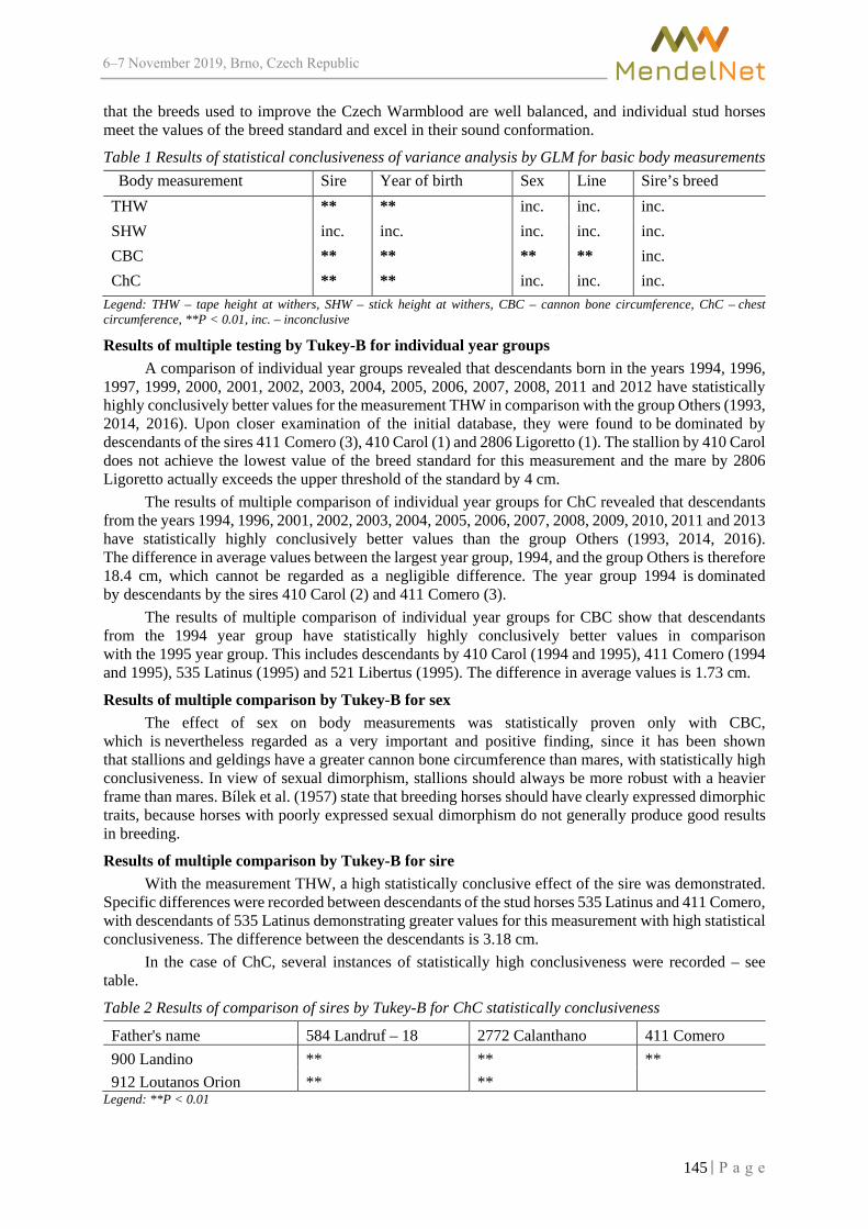
6–7 2019, Brno, Czech Republic
that the breeds used to improve the Czech Warmblood are well balanced, and individual stud horses meet the values of the breed standard and excel in their sound conformation.
Table 1 Results of statistical conclusiveness of variance analysis by GLM for basic body measurements Body measurement Sire Year of birth Sex Line Sire’s breed
THW ** ** inc. inc. inc. SHW inc. inc. inc. inc. inc. CBC ** ** ** ** inc. ChC ** ** inc. inc. inc.
Legend: THW – tape height at withers, SHW – stick height at withers, CBC – cannon bone circumference, ChC – chest circumference, **P < 0.01, inc. – inconclusive
Results of multiple testing by Tukey-B for individual year groups A comparison of individual year groups revealed that descendants born in the years 1994, 1996,
1997, 1999, 2000, 2001, 2002, 2003, 2004, 2005, 2006, 2007, 2008, 2011 and 2012 have statistically highly conclusively better values for the measurement THW in comparison with the group Others (1993, 2014, 2016). Upon closer examination of the initial database, they were found to be dominated by descendants of the sires 411 Comero (3), 410 Carol (1) and 2806 Ligoretto (1). The stallion by 410 Carol does not achieve the lowest value of the breed standard for this measurement and the mare by 2806 Ligoretto actually exceeds the upper threshold of the standard by 4 cm.
The results of multiple comparison of individual year groups for ChC revealed that descendants from the years 1994, 1996, 2001, 2002, 2003, 2004, 2005, 2006, 2007, 2008, 2009, 2010, 2011 and 2013 have statistically highly conclusively better values than the group Others (1993, 2014, 2016). The difference in average values between the largest year group, 1994, and the group Others is therefore 18.4 cm, which cannot be regarded as a negligible difference. The year group 1994 is dominated by descendants by the sires 410 Carol (2) and 411 Comero (3).
The results of multiple comparison of individual year groups for CBC show that descendants from the 1994 year group have statistically highly conclusively better values in comparison with the 1995 year group. This includes descendants by 410 Carol (1994 and 1995), 411 Comero (1994 and 1995), 535 Latinus (1995) and 521 Libertus (1995). The difference in average values is 1.73 cm.
Results of multiple comparison by Tukey-B for sex The effect of sex on body measurements was statistically proven only with CBC,
which is nevertheless regarded as a very important and positive finding, since it has been shown that stallions and geldings have a greater cannon bone circumference than mares, with statistically high conclusiveness. In view of sexual dimorphism, stallions should always be more robust with a heavier frame than mares. Bílek et al. (1957) state that breeding horses should have clearly expressed dimorphic traits, because horses with poorly expressed sexual dimorphism do not generally produce good results in breeding.
Results of multiple comparison by Tukey-B for sire With the measurement THW, a high statistically conclusive effect of the sire was demonstrated.
Specific differences were recorded between descendants of the stud horses 535 Latinus and 411 Comero, with descendants of 535 Latinus demonstrating greater values for this measurement with high statistical conclusiveness. The difference between the descendants is 3.18 cm.
In the case of ChC, several instances of statistically high conclusiveness were recorded – see table.
Table 2 Results of comparison of sires by Tukey-B for ChC statistically conclusiveness
Father's name 584 Landruf – 18 2772 Calanthano 411 Comero 900 Landino ** ** ** 912 Loutanos Orion ** **
Legend: **P < 0.01
145

6–7 2019, Brno, Czech Republic
The difference between descendants with the greatest average value by 912 Loutanos Orion and those with the smallest average value value by 584 Landruf – 18 is 10.1 cm. This clearly indicates that descendants of 912 Loutanos Orion excel in their robustness.
The evaluation of CBC revealed only one instance of statistically high conclusiveness between descendants by the sires 582 Caesar and 623 Landprinz. Here the difference between the average values is 0.7 cm and the initial database showed that all the descendants by 582 Caesar achieve the lower threshold of the breed standard, whereas three daughters of the stud horse 623 Landprinz do not.
Results of multiple comparison by Tukey-B for line A statistically highly conclusive effect of the line emerged only for the attribute CBC – see table.
Table 3 Results statistically conclusiveness of comparison of line by Tukey-B for CBC Group Number of descendants Average Ladykiller Cor de la Bryère Ladykiller 415 20.5477 ** Cor de la Bryère 389 20.7378 **
Legend: **P < 0.01
It can therefore be said that both lines are very well balanced and very beneficial for Czech Warmblood breeding. However, as far as cannon bone circumference is concerned, breeders should select stud horses from the “Corde” line. Kubikova et al. (2018) state that the influence of the English Thoroughbred on lightening the frame of Czech Warmblood dams is really quite considerable and has also manifested itself in the Cor de la Bryère line, specifically in the 1997 year group. At the same time, Štencl (1977) says that the imprudent choice of an unsuitable stud horse tends to introduce undesirable characteristics into the breeding of half-breds, particularly lightening of the frame. For that reason, breeders should take this into account, avoid the mistakes of past years and only breed from mares which meet the values of the breed standard. Even the Association of Czech Warmblood Breeders (2016) in its yearbook places emphasis on the conformation of the modern Czech Warmblood horse, which can only be achieved by a careful selection of breeding horses.
CONCLUSION The aim of this study was to evaluate the influence of the Ladykiller and Cor de la Bryère lines
in Czech Warmblood breeding. To evaluate the significance of these breeding lines, offspring by stud horses authorized to act in Czech Warmblood breeding were used. The monitored attributes for evaluating the quality of stud horses and lines were the values of the basic body measurements of their offspring. Five effects were monitored: sire, offspring’s year of birth, sex, line and sire’s breed. In the case of sire’s breed, no statistically conclusive effect on the values of offspring’s basic body measurements was established. With the measurement THW, a statistically high effect of the sire and year of birth was demonstrated. The sire and year of birth also have a statistically highly conclusive effect on ChC. In the case of SHW, no instances of statistical conclusive of the monitored effects were recorded. This is evaluated very positively, because this measurement is subject to the breed standard for the Czech Warmblood and descendants in the observed set meet these values on average. During evaluation of the sire, year of birth, sex and line as part of CBC, a highly statistically conclusive effect of the monitored factors was once again recorded. Due to the influence of sex on CBC, it was demonstrated that stallions and geldings have greater cannon bone circumference than mares, with statistically high conclusiveness. With regard to sexual dimorphism, this can be assessed very positively. From the results obtained, it can be stated that both of the evaluated lines have good results, but within individual year groups and stud horses there are descendants with inadequate values for the basic body measurements which do not even achieve the lower threshold of the breed standard. These descendants should not be incorporated into future breeding – and if they are, then only mares with a very prudent choice of stud horse who is capable of correcting the attribute in question. Nevertheless, the influence of both lines can be evaluated positively and it can be said that stud horses from both lines are beneficial for Czech Warmblood breeding. In the future, however, it is necessary to take into account the indisputable influence of dams on the body dimensions of descendants.
146

6–7 2019, Brno, Czech Republic
REFERENCES Alagić, D. et al. 2002. Body measures and indexes of the Holstein horses reared in Krizevci. [Online]. Acta Agraria Kaposváriensis, 6.2: 125–130. Available at: http://journal.ke.hu/index.php/aak/article/view/1653 [2019-08-20]. Association of Czech Warmblood Breeders. 2016. Ročenka 2016 [Online]. 1st ed., Písek: AP tiskárna. Available at: http://www.schct.cz/cz/uvod/rocenky-schct/rocenka-2016.html. [2019-08-20]. Bílek, F. et al. 1957. Speciální zootechnika chov koní. Vol. II. 1st ed., Prague: Státní zemědělské nakladatelství. Brooks, S. A. et al. 2010. Morphological variation in the horse: defining complex traits of body size and shape [Online]. Animal Genetics 41: 159–165. Available at: https://onlinelibrary.wiley.com/doi/full/10.1111/j.1365-2052.2010.02127.x. [2019-08-20]. Dušek, J. et al. 2011. Chov koní. 3rd ed., Prague: Nakladatelství Brázda. Horse Sport Consulting. 2017. Ladykiller. Horse sport consulting [Online]. Horse sport consulting. Available at: https://www.horsesportconsulting.com/ladykiller/. [2019-08-20]. Kubíková, Z., Jiskrová, I. 2018. Zhodnocení hřebců linie Ladykiller v chovu českého teplokrevníka podle skokové výkonnosti potomků. In Sborník z konference mladých vědeckých pracovníků Zootechnika 2018. České Budějovice, Czech Republic, 14 June, České Budějovice: Jihočeská univerzita v Českých Budějovicích. pp. 33–40. Kubikova, Z., Jiskrova, I., Kubistova, B. 2018. Evaluating the descendants of stallions from the Cor de la Bryère line in Czech Warmblood breeding. In Proceedings of International PhD Students Conference MendelNet 2018 [Online]. Brno, Czech Republic, 7 November, Brno: Mendel University in Brno, Faculty of AgriSciences, pp. 108–113. Available at: https://mnet.mendelu.cz/mendelnet2018/mnet_2018_full.pdf. [2019-08-20]. Müller, J. 2018. Corrado II. Equinní reprodukční centrum Pardubice-Mnětice [Online]. Available at: http://www.muller-equine.cz/reprodukce-koni-1/galerie-hrebcu/corrado-ii.htm. [2019-08-20]. Pellarová, A. et al. 2005. Přehled o sportovních koních ČR. VSCHK: Slatiňany. pp. 257. Štencl, F. et al. 1977. Vývoj chovu koní u nás. Vol. II. Pardubice: Ústav veterinární osvěty. (201) pp. 31–36. Štěrba, V. 2015. Nejznámější světové linie v původech sportovních koní - Cor de la Bryére. Česká společnost hipologická [Online]. Available at: https://cshipo.estranky.cz/clanky/pro-zacinajici-chovatele/chov-a-slechteni-koni/nejznamejsi-svetove-linie-v-puvodech-sportovnich-koni---cor-de-la-bryere.html. [2019-08-20]. The Horse Magazine. 2018. Ladykillerxx. The Horse Magazine [Online]. Thehorsemagazine [2019-08-20]. Available at: http://www.horsemagazine.com/thm/2010/08/ladykiller-xx/.
147

6–7 2019, Brno, Czech Republic
Effect of boars on reproductive parameters in sows, losses of piglets and birth weight of piglets
Jan Lujka, Pavel Nevrkla, Zdenek Hadas Department of Animal Breeding
Mendel University in Brno Zemedelska 1, 613 00 Brno
CZECH REPUBLIC
Abstract: The aim of this study was to evaluate effect of boars on reproductive performance in sows, birth weight of piglets and losses of piglets from birth to weaning. Effect of three different boars marked A (Large White - sire line x Pietrain), B (Large White - sire line x Duroc) and C (Duroc) was observed. No statistically significant differences were found between the evaluated boars and their effect on reproductive performance and losses of piglets. Evaluation of boars’ effect on birth weight of piglets revealed statistically significant differences (P ≤ 0.05) between mean birth weight of piglets from the boar A (1.33 kg) and mean birth weight of piglets from the boar B (1.28 kg) and between the birth weight of gilts from the boar A (1.39 kg) and the birth weight of gilts from the boar B (1.23 kg). Another statistically significant difference (P ≤ 0.05) was found between the birth weight of gilts from the boar B (1.23 kg) and the birth weight of gilts from the boar C (1.42 kg). The values of mean birth weight of piglets from the boar B (1.28 kg) and mean weight of piglets from the boar C (1.45 kg) were highly significantly different (P ≤ 0.01). Also the difference between the birth weight of gilts from the boar B (1.23 kg) and birth weight of boars from the boar C (1.48 kg) was highly statistically significant (P ≤ 0.01). The results document that the evaluated boars have a comparable effect on reproductive performance in sows and losses of piglets, on the contrary, the effect on birth weight of piglets was significantly different among the observed boars.
Key words: boar, sow, reproduction, birth weight
INTRODUCTION Pig breeding and production of pork meat are among the most important agricultural branches
in the Czech Republic, but also in the world. In our country, approximately 1,500,000 pigs are bred at present time, about 92,000 of them are sows. Production of pork meat does not cover our consumption by far, therefore more that 50% of pork meat is imported from abroad (Český statistický úřad 2018).
Pig breeding depends on many factors that influence its quality, efficiency and profitability (Pulkrábek 2005). An important parameter of breeding quality is reproductive performance in sows, mainly the number of live-born piglets and the number of reared piglets (Nevrkla et al. 2016). It is desirable for each sow to rear as many healthy and well-growing piglets per year as possible.
The level of reproductive performance in sows is among others influenced by the utilized boar (Lukač et al. 2014). Selection of a boar depends on breeding conditions, on required growth ability and meat conformation of fattening piglets and on slaughter weight of piglets. Commercial hybridization programmes try to ensure quality boars for each breeding conditions and reach the best possible level of the required characteristics in the fattening piglets (Stupka 2013).
The study compares three different boars commonly used for reproduction on Czech farms. The objective was to find out whether and eventually how much the effect of the observed boars on reproductive parameters of sows and losses of piglets from birth to weaning differs in stable conditions and what is the effect of the observed boars on birth weight of piglets.
MATERIAL AND METHODS The effect of boar on reproductive performance in sows was evaluated in 200 F1 sows (Large
White x Landrace). The sows were divided into three groups and each group was inseminated with one boar. All the sows were observed on their first parity.
148

6–7 2019, Brno, Czech Republic
Three types of boars. Breeding of the boar A (Large White - sire line x Pietrain) was focused on excellent productive characteristics of the final hybrid pigs. Fattening pigs should reach excellent meat conformation and great growth capacity. The fattening pigs from this boar are primarily determined for more favourable environmental conditions and their fattening is appropriate to the weight of 110 kg. Breeding of the boar B (Large White - sire line x Duroc) is aimed to excellent growth ability and fine meat quality of the final hybrids. Durability and vitality are emphasized characteristics. It is appropriate to fatten the pigs up to higher slaughter weights. Breeding of the boar C (Duroc) is goaled on highest possible lean meat content and high meat quality in the final hybrids and last but not least on excellent growth ability.
A total of 53 sows were inseminated by the boar A, 57 sows by the boar B and 90 sows by the boar C. After farrowing, effect of boars on the total number of piglets, number of live-born piglets and stillborn piglets, number of mummified foetuses, number of reared piglets per litter and losses of piglets were evaluated. The piglets were weaned at the age of 28 days.
A total of 396 piglets from 36 sows were included in the evaluation of boars’ effect on birth weight of piglets. Of those, 159 were from the boar A, 135 from the boar B and 102 from the boar C. The sows were inseminated in individual pens. Weighing was performed in the farrowing house, in the immediate vicinity to the farrowing pen, to prevent unnecessarily long manipulation with piglets and related inappropriate stress. The piglets were weighed on the day of birth with the KERBL DigiScale 50. The piglets were placed in a plastic bucket hanged on the scale and weight with the accuracy of 0.01 kg. The weight of piglets was evaluated according to the sex.
The sows and the piglets were fed with commercial complex feed mixtures for the given category. At the time of insemination, the sows were stabled individually for 30 days after the insemination. Subsequently, during pregnancy they were stabled in groups (dynamic method for 100 sows). One week before expected farrowing, the sows were transferred to the farrowing house (cage system).
Statistical analysis of the data was performed using the Statistica software, version 12. One-way ANOVA and multi-factor ANOVA were used. Differences of the results were tested using the Unequal N HSD test, where small letters a, b stand for statistically significant difference (P < 0.05) and capital letters such as A, B stand for highly statistically significant difference (P < 0.01). The evaluated parameters were express as selected statistical characteristics, mean, standard error of the mean (SE) and coefficient of variation (Vx).
RESULTS AND DISCUSSION The values in Tables 1, 2 and 3 show the results of monitoring the effect of boar on reproductive
parameters in sows.
Table 1 Basic statistical characteristics of selected reproductive parameters and losses of piglets per litter from the boar A
Parameter Inseminated sows (n) Mean SE Vx Total number of born piglets 53 14.19 0.34 17.21 Live-born piglets 53 13.08 0.30 16.49 Stillborn piglets 53 1.11 0.15 95.95 Mummified foetuses 53 0.13 0.05 298.37 Weaned piglets 53 11.79 0.21 12.81 Losses of piglets in pieces 53 1.28 0.24 136.18 Losses of piglets in percent 53 8.63 1.50 126.52
Legend: SE – standard error of the mean, Vx – coefficient of variation
No statistically significant differences were found between the evaluated boars and their effect on reproductive performance and losses of piglets.
Effect of a boar on reproductive parameters was studied also by Šprysl et al. (2010). In their experiment they compared the breeds Duroc (D), Hampshire (H) and hybrid combinations Duroc x
149

6–7 2019, Brno, Czech Republic
Belgian Landrace (BL) and Belgian Landrace x Hampshire. After insemination by the boar D, a total of 10.52 piglets were born of which 9.27 were born alive. Losses of piglets from birth to weaning reached 1.64 piece and 7.63 piglets were successfully reared. After insemination by the boar H, 10.58 piglets were born, 9.02 of them were born alive. A total of 1.07 piglets were lost and 7.95 piglets were reared on average. With the use of the hybrid combination DxBL, a total of 11.75 piglets were born of which 10.19 were born alive. Losses of piglets from birth to weaning counted 1.75 and 8.44 piglets were successfully reared. When the hybrid combination BLxH was used, the total number of piglets counted 10.24, the number of live-born piglets was 9.37. Losses of piglets reached number 1.50 and 7.87 piglets were reared. Šprysl et al. (2010) state that genetic factors have only limited effect on reproductive performance in the sphere of productive farms, on the contrary, the effect of environment dominates. Same as in our experiment, no statistically significant differences were found between the boars in this observation, which may be due to balanced level of reproductive traits in the observed breeds. It is possible that under the environmental conditions of the experiment conducted by these authors, the genotype potential was not fully expressed.
Table 2 Basic statistical characteristics of selected reproductive parameters and losses of piglets per litter from the boar B
Parameter Inseminated sows (n) Mean SE Vx Total number of born piglets 57 14.00 0.33 18.06
Live-born piglets 57 13.12 0.32 18.28
Stillborn piglets 57 0.88 0.17 144.63
Mummified foetuses 57 0.16 0.05 232.99
Weaned piglets 57 11.53 0.20 13.23
Losses of piglets in pieces 57 1.60 0.25 117.70
Losses of piglets in percent 57 10.72 1.51 106.47 Legend: SE – standard error of the mean, Vx – coefficient of variation
Table 3 Basic statistical characteristics of selected reproductive parameters and losses of piglets per litter from the boar C
Parameter Inseminated sows (n) Mean SE Vx
Total number of born piglets 90 14.31 0.23 14.95
Live-born piglets 90 13.39 0.18 12.75
Stillborn piglets 90 0.92 0.17 178.97
Mummified foetuses 90 0.26 0.11 400.26
Weaned piglets 90 12.13 0.13 10.35
Losses of piglets in pieces 90 1.26 0.17 127.23
Losses of piglets in percent 90 8.52 1.07 119.60 Legend: SE – standard error of the mean, Vx – coefficient of variation
Also Lukač et al. (2014) studied effect of father on reproductive performance in sows. In their experiment, they compared the breeds Yorkshire, Landrace, Pietrain, Duroc and Hampshire. With the use of the Yorkshire breed boar, the mean number of live-born piglets was 9.73 and 8.30 piglets were weaned. With the use of the Landrace breed boar, the mean number of live-born piglets was 10.00 and weaned piglets 8.27. The mean number of live-born piglets from the Pietrain boar was 10.55 with 8.92 weaned piglets. For the Duroc breed boar, 9.95 live-born piglets and 8.62 weaned piglets were recorded. For the Hampshire breed boar, the number of live-born piglets was 9.65 and 8.58 piglets were weaned on average. These authors confirmed in their experiments that the numbers of live-born and stillborn piglets are significantly influenced by the boar used.
Table 4 presents results of the evaluated effect of the boars on birth weight of piglets. Mean weight of all the tested piglets was 1.37 kg. The highest birth weight was reached by the piglets from the sow
150

6–7 2019, Brno, Czech Republic
inseminated by the boar C (1.45 kg), while the mean birth weight of boars was 1.48 kg, which is the highest value of all the tested piglets. The gilts from the boar C weighed 1.42 kg. The piglets from the boar A weighed 1.39 kg on average. The mean weight of boars from the boar A was 1.39 kg, the mean weight of gilts was 1.38 kg. The mean weight of piglets from the boar B was 1.28 kg. They were the only group that did not reach the total mean value. The difference between the boars and the gilts was the highest (0.10 kg), the boars weighed 1.33 kg and the gilts weighed 1.23 kg.
Table 4 Effect of the boar on birth weight of piglets
Parameter n Mean (kg) SE Vx All piglets 396 1.37 0.02 22.73 A total 159 1.39a 0.02 22.04 A gilts 91 1.39b 0.03 21.42 A boars 68 1.38 0.04 23.01 B total 135 1.28aA 0.03 23.24 B gilts 66 1.23 bBc 0.04 26.09 B boars 69 1.33 0.03 20.14 C total 102 1.45A 0.03 21.42 C gilts 55 1.42c 0.04 23.21 C boars 47 1.48B 0.04 19.29
Legend: SE – standard error of the mean, Vx – coefficient of variation; n – number of piglets; a:a–c:c – statistically significant differences (P ≤ 0.05); A:A, B:B – highly statistically significant difference (P ≤ 0.01)
The mean birth weight of the piglets from the boar A and the mean birth weight of piglets from the boar B were statistically significantly different (P ≤ 0.05). Statistically significant difference (P ≤ 0.05) was also between the birth weight of gilts from the boar A and the birth weight of gilts from the boar B. Also the birth weight of gilts from the boar B and the birth weight of gilts from the boar C were significantly different (P ≤ 0.05).
The values of mean birth weight of piglets from the boar B and mean birth weight of piglets from the boar C were highly significantly different (P ≤ 0.01). Also the difference between the mean birth weight of gilts from the boar B and the mean birth weight of boars from the boar C was statistically significant (P ≤ 0.01).
Wolter et al. (2002) state that birth weight is a result of intrauterine growth of piglets and is considered to be one of the most important factors affecting survival of pigs. Deen and Bilkei (2004) share the same opinion. Birth weight of all the tested piglets was more than 1 kg. According to Hájek (1992), the piglets below this limit are problematic, which was confirmed by Magnabosco et al. (2015), who described that piglets with birth weight below 1.1 kg are characterized with higher mortality and lower consumption of colostrum when compared to piglets with higher birth weight. Low birth weight can compromise not only the survival rate but also postnatal growth (Bee 2007, Václavková et al. 2012). Bazala (1999) state that optimum birth weight of piglets should be 1.2–1.5 kg. The birth weight of all the evaluated piglets was within this range.
CONCLUSION No statistically significant differences were found in the effect of boar on reproductive parameters
and losses of piglets. Results of the evaluated effect of boar on birth weight of piglets showed that the highest piglets were from the boar Duroc with the mean birth weight 1.45 kg. The mean birth weight of boars was 1.48 kg, the mean birth weight of gilts was 1.42 kg. The values of mean birth weight of piglets from the boar Large White - sire line x Pietrain and mean birth weight of piglets from the boar Large White - sire line x Duroc were statistically significantly different (P ≤ 0.05). Birth weights of the gilts from the boar Large White - sire line x Pietrain and of the gilts from the boar Large White - sire line x Duroc were significantly different (P ≤ 0.05). Also the difference between the birth weight
151

6–7 2019, Brno, Czech Republic
of gilts from the boar Large White - sire line x Duroc and the gilts from the boar Duroc was statistically significant (P ≤ 0.05).
The values of mean birth weight of piglets from the boar B and the mean birth weight of piglets from the boar Duroc were highly significantly different (P ≤ 0.01). Also the difference between birth weight of gilts from the boar Large White - sire line x Duroc and birth weight of boars from the boar Duroc was highly statistically significant (P ≤ 0.01).
Observations performed within the experiment confirmed that genotype of boar significantly affects birth weight of piglets. The results show that the birth weight of piglets from the Duroc boars are higher than the birth weight of piglets from the observed hybrid boars, which could be a prerequisite for better growth in later categories.
ACKNOWLEDGEMENTS This study was supported by the project of MENDELU internal grant agency, Faculty of AgriSciences No. TP 7/2017.
REFERENCES Bazala, E. 1999. Intenzita výroby selat. Náš Chov, 59(5): 27–29. Bee, G. 2007. Birth weight of litters as a source of variation in postnatal growth, and carcass and meat quality. Advances in pork production [Online], 18: 191–196. Available at: https://pdfs.semanticscholar.org/4660/35e33b63020a0e444f18b609031f1ee58e5b.pdf. [2019-01-19]. Český statistický úřad. Veřejná databáze, Výroba masa. [Online]. Available at: https://vdb.czso.cz/vdbvo2/faces/index.jsf?page=vystup-objekt&pvo=ZEM08&f=TABULKA&z=T&skupId=966&katalog=30840&pvo=ZEM08. [2019-02-03]. Deen, M.G.H., Bilkei, G. 2004. Cross fostering of low-birthweight piglets. Livestock Production Science [Online], 90(2–3): 279–284. Available at: https://www.sciencedirect.com/science/article/pii/S0301622604000673?via%3Dihub. [2018-12-14]. Hájek, J. 1992. Prasata v drobném chovu a na farmách. Jílové u Prahy: Apros. Lukač, D. et al. 2014. The effect of parental genotype and parity number on pigs litter size. Biotechnology in Animal Husbandry [Online], 30(3): 415–422. Available at: https://scindeks-clanci.ceon.rs/data/pdf/1450-9156/2014/1450-91561403415L.pdf. [2018-12-13]. Magnabosco, D. et al. 2015. Impact of the birth weight of Landrace × Large White dam line gilts on mortality, culling and growth performance until selection for breeding herd. Acta Scientiae Veterinariae, 43(1): 1–8. Nevrkla, P. et al. 2016. Analysis of Reproductive Parameters in Sows with Regard to Their Health Status. Acta Universitatis Agriculturae et Silviculturae Mendelianae Brunensis, 64(2): 481–486. Pulkrábek, J. 2005. Chov prasat. Praha: Profi Press, s.r.o. Stupka, R. 2013. Základy chovu prasat. Praha: Powerprint. Šprysl M., Čítek J., Stupka R. 2010. Monitoring of the reproduction performace in hybrid pigs by help of field tests. Research in Pig Breeding, 4(1): 37–40. Václavková, E., Daněk, P., Rozkot, M. 2012. The influence of piglet birth weight on growth performance. Research in Pig Breeding, 6(1): 59–61. Wolter, B.F. et al. 2002. The effect of birth weight and feeding of supplemental milk replacer to piglets during lactation on preweaning and postweaning growth performance and carcass characteristics. Journal of Animal Science, 80(2): 301–308.
152

6–7 2019, Brno, Czech Republic
Association of chosen environmental and animal factors with gestation length and lactation of dairy cows in two Slovak herds
Simon Miklas1, Marta Oravcova2, Lucia Macuhova2, Petr Slama3, Vladimir Tancin1,2 1Department of Veterinary Sciences
Slovak University of Agriculture in Nitra Tr. A. Hlinku 2, 949 76 Nitra
2NPPC – Research Institute for Animal Production Nitra Hlohovecka 2, 951 41 Luzianky
SLOVAK REPUBLIC 3Department of Animal Morphology, Physiology and Genetics
Mendel University in Brno Zemedelska 1, 613 00 Brno
CZECH REPUBLIC
Abstract: The aim of the study was to assess the effect of season of birth of females, their season of calving, as well as sex of calves and incidence of twins on the gestation length and milk yield during their first pregnancy and lactation. Data, 277 records, were collected from two farms located in northern and western Slovakia. The data in the herd “A” were collected in years 2006–2017, in the herd “B” in years 2014–2018. The herd “A” consisted of Slovak Spotted breed (127 records), the herd “B” consisted of black Holstein cows (150 records). Among observed environmental and animal factors were included: season of birth, season of calving, sex of the offspring and incidence of twins. Factor that reached at least to some degree statistical significance in relation to gestation length was season of calving in the both herds (P < 0.03; P < 0.06). 305-d milk yield tended to be influenced by season of calving (P < 0.09). Impact of season of calving on gestation length differed between studied herds. The herd “A” reached longest average gestation length at spring calving (286.66 ± 3.26 days), the herd “B” at autumn calving (278.49 ± 1.35 days). In the herd “A” calving season was associated with the highest milk production in summer (5876 ± 380 kg), however in the herd “B”, the most productive milk yield was reached in spring (9865 ± 269 kg). The physiological mechanisms of these changes are not clear, hence more research in larger scale is needed.
Key Words: dairy heifers, gestation length, milk yield, season
INTRODUCTION In order to reduce economic costs, it is important to study and identify factors affecting processes
on farm, animal production and well-being. For that reason, we have decided to focus on animal and environmental factors influencing gestation length and lactation. As understanding of gestation length, may help to improve the management of pregnant cows via more accurate prediction of parturition. And better knowledge of association between studied factors and milk yield may prove itself useful in enhancing economic benefits, via their optimization. Crucial factors for economy of dairy farms are milk production, milk composition, hygienic safety and technological qualities (Tančin et al. 2018).
Gestation length (GL) is the interval from conception to subsequent parturition. Gestation length is moderately heritable, and it is affected by many environmental factors (Norman et al. 2009). Older cows tend to have longer gestation (Andersen and Plum 1965), heifers tend to have shorter gestation (Tomášek et al. 2017). Dams carrying males tend to have longer gestation (Silva et al. 1992) and it is considerably shorter for twins, in comparison to singles (Tomášek et al. 2017). Gestation length is also associated with milk production, when lower producing cows have shorter gestation (Norman et al. 2009). Moreover, it is influenced by season of calving, season of conception (Tomášek et al. 2017), but also by temperature (Wright et al. 2014).
153

6–7 2019, Brno, Czech Republic
The milk production efficiency is influenced by numerous factors, where the most important is its quantity and quality (Tančin et al. 2018). Milk yield is influenced by genetic predisposition (Hanson et al. 2011). It can be also likely affected by calving season, via temperature changes and length of photoperiod (Barash et al. 1996), but also by seasonal changes in feeding (Froidmont et al. 2013). According to some authors milk yield can be also altered by season of birth (Van Eetvelde and Opsomer 2017), primarily by enhanced insulin sensitivity at birth, caused by warmer temperatures (Van Eetvelde et al. 2017). Thus it refers to hypothesis that seasonal changes are caused by temperature alterations and subsequent metabolic changes (Van Eetvelde et al. 2017). Though, publications concerning these changes show unclear results (Van Eetvelde et al. 2017).
The aim of the study was to assess the effect of season of birth of females, their season of calving, as well as sex of calves and incidence of twins on the gestation length and milk yield during their first lactation.
MATERIAL AND METHODS
Environment, animals and management The data were obtained from two commercial dairy farms in Slovakia (277 records), from which
farm “A” is located in northern Slovakia with average temperature 4–6 °C. The farm “B” is in western part of Slovakia with average temperatures 8–9 °C. Distance by air between these two farms is approximately 116 km.
The herd “A” consisted by more than 90% of Slovak Spotted breed, which was gradually improved with red Holstein cattle. The average 305-d milk yield in the herd “A” was 5528 ± 1213 kg. In the herd “B”, which consisted of black Holstein cows the average 305-d milk yield was 9402 ± 1097 kg. The herd “A” was referred as group located in colder area and the herd “B” as group located in warmer area. On the farm “A” were cows milked twice a day, on the farm “B” three times a day.
Data collection and statistical analysis The data from farm “A” (127 records) were collected over period of 12 years (2006–2017)
and the data from farm “B” (150 records) were collected over period of 5 years (2014–2018). All the recorded data were from the heifers and their first lactation. All cows with finished first lactation were enrolled into the study. From the database the following data were used: date of the birth of female calves and their further data throughout breeding period until the end of the first lactation: date of calving, milk yield during 305-d lactation, sex of calves, numbers of calves at calving.
Statistical analysis was performed using SAS (SAS Institute Inc., Cary, NC, USA). Investigated variables yij (length of gravidity, 305-d lactation milk yield) were analysed using linear statistical model (General Linear Model) with fixed factor of Ai (season of birth, season of calving, sex of the calves) and random error eij. According to season of birth and calving the following levels: winter (December to February), spring (March to May), summer (June to August), autumn (September to November) were considered; calve sex consisted of males, females and twins levels.
The model equation was as follows: yij = Aixij+ eij Statistical significance was declared at P <0.05 and tendency at 0.05<P <0.1. Due to different
breeds, analyses were done separately within each farm. Simple models with separate factors: (1) season at birth, (2) season at calving, (3), sex and number of calves (male, female, twins) were considered for investigated variables.
RESULTS AND DISCUSSION
Factors affecting gestation length Based on our statistical model, we found out that gestation length in the herd “A” was significantly
affected by season of calving (P < 0.03). Season of calving in the herd “B” also tended to influence gestation length (P < 0.06). Although we can assume that season of calving is affecting both herds, it’s effect in each herd was different (see Table 1). As in the herd “A” winter and spring calving were related to the longest gestation (285.96 ± 3.55 days; 281.03 ± 3.60 days), but in the herd “B” the longest gestations were connected with summer (278.92 ± 1.56 days) and autumn (279.63 ± 1.63 days).
154

6–7 2019, Brno, Czech Republic
That partially contradicts findings of Tomášek et al. (2017), that reported shorter gestation length of spring and summer calving and presumed effect of the natural calving season inherited from wild ancestors. Other authors attribute these changes to elevation of ambient temperatures (Wright et al. 2014), which may explain our findings in the herd “A”, but contradict them in the herd “B”.
Table 1 Dependence of gestation length (days) on seasons of calving during first lactation, separately
Factor Variable Herd “A” Herd “B”
N Estimate Std Err N Estimate Std Err
Season of calving
Spring 12 286.66 3.26 40 275.36 1.40 Summer 17 278.51 2.93 30 279.36 1.64 Autumn 57 279.17 2.28 48 278.49 1.35 Winter 41 285.72 1.91 32 276.74 1.35
The season of birth had no significant effect on gestation length in both herds (P < 0.46; P < 0.52), that was already investigated by Gianola and Tyler (1974), with the same conclusion. Average values for each season of birth are presented in Table 2.
Table 2 Dependence of gestation length (days) on seasons of birth during first lactation, separately
Factor Variable Herd “A” Herd “B”
N Estimate Std Err N Estimate Std Err
Season of birth
Spring 30 281.03 3.60 38 277.99 1.65 Summer 30 277.89 3.83 32 278.92 1.56 Autumn 28 280.77 3.86 41 279.63 1.63 Winter 39 285.96 3.55 39 277.91 1.47
Sex of the calf and incidence of twins were found insignificant in relation to gestation length (P < 0.94; P < 0.34). In these terms, our findings differ from previously conducted studies (Tomášek et al. 2017, Vieira-Neto et al. 2017). However, in consistence with aforementioned authors we found that development of males from conception to delivery was in both herds longer, in comparison to females (0.28 days; 0.91 days) (see Table 3). Although, reported gestation length difference between cows carrying males and females published by authors Tomášek et al. (2017), Vieira-Neto et al. (2017) was greater (from 1.2 to 1.4 days). We could not demonstrate the effect of twins compared to single born calves on length of gestation (gestation was approximately 1 day longer for twins) as other authors found out that twins shorten the gestation length (Norman et al. 2009, Echternkamp and Gregory 1999, Tomášek et al. 2017). In the herd “B” we have not investigated incidence of twins (Table 3).
Table 3 Dependence of gestation length (days) on sex of calves, herd “A” and herd “B” separately
Factor Variable Herd “A” Herd “B”
N Estimate Std Err N Estimate Std Err
Sex of the calf male 64 282.56 1.19 81 278.22 0.64
female 50 282.28 1.34 69 277.31 0.70 twins 7 283.57 3.59 - - -
Factors affecting 305-day milk yield 305-d milk yield in the herd “A” tended to correlate with calving season (P < 0.09). Heifers
that were calving in spring and winter had the lowest milk yield (4794 ± 423 kg; 5340 ± 247 kg) and heifers that calved in summer had the highest 305-d milk yield (5876 ± 380 kg) (Table 4). Comparable findings were published by Froidmont et al. (2013), that explained his findings by richer winter feed during period that is more representative of lactation and to a lesser extent by increasing photoperiod. In the herd “B” 305-d milk yield was not significantly affected by season of calving (P < 0.36). In this herd, the highest milk production was reached by heifers that were calving in spring (9865 ± 269 kg) and the lowest by those that were calving in summer (9122 ± 315 kg) (see Table 4).
155

6–7 2019, Brno, Czech Republic
Table 4 Dependence of 305-d milk yield (kg) among seasons of calving and 305-d milk yield (kg) during first lactation, separately
Factor Variable Herd “A” Herd “B”
N Estimate Std Err. N Estimate Std Dev
Season of calving
Spring 12 4794 423 40 9865 269 Summer 57 5876 380 30 9122 315 Autumn 17 5635 293 48 9598 259 Winter 41 5340 247 32 9651 259
Van Eetvelde and Opsomer (2017) suggested that in relation to milk yield, season of birth had greater influence than season of calving. However, in our study in both herds season of birth (P < 0.63; P < 0.88) did not reach statistical significance in relation to 305-d milk yield. There were only numerical differences (Table 5). Nevertheless, our findings in the herd “A”, on 305-d milk yield in relation to season of birth (see Table 5), corelate with work of Van Eetvelde et al. (2017), that found heifers born in warmer season were the ones with highest milk production at first lactation. As explanation the authors suggested effect of higher peripheral insulin sensitivity of offsprings born in warmer seasons (Van Eetvelde et al. 2017). However, in the herd “B” heifers born in spring had in average the highest milk yield (9409 ± 315 kg), and the animals born in summer had the lowest milk yields (9195 ± 297 kg), that contradicts findings of Van Eetvelde et al. (2017) (Table 5).
Table 5 Dependence of 305-d milk yield (kg) on seasons of birth during first lactation, separately
Factor Variable Herd “A” Herd “B”
N Estimate Std Err N Estimate Std Err
Season of birth
Spring 30 5847 463 38 9409 315 Summer 30 6078 489 32 9195 297 Autumn 28 5919 492 41 9257 311 Winter 39 4961 456 39 9358 279
In our study sex of the calf (P < 0.47; P < 0.91) did not affect 305-d milk yield significantly. Research data on sex of the calf and incidence of twins are shown in Table 6.
Table 6 Dependence of 305-d milk yield (kg) on sex of calves, herd “A” and herd “B” separately
Factor Variable Herd “A” Herd “B”
N Estimate Std Err N Estimate Std Err
Sex of the calf male 64 5510.13 147.43 81 9411.11 122.24
female 50 5685.00 167.72 69 9390.77 132.45 twins 7 5170.40 423.46 - - -
CONCLUSION Knowledge of environmental and animal factors may be useful in improving farm management
practices, sustaining high milk yields of dairy cows and enabling us to react promptly to changes of environment.
Several authors suggested number of environmental and animal factors, that can be taken into account to influence gestation length. In our study the length of gestation was influenced by the season of calving. However, in the studied herds season of calving affected gestation length differently.
Moreover, our findings in part confirmed influence of calving season on milk yield, with improved milk production in summer, in the herd “A”.
It is necessary to add, that we also at least partially proved that different herds, with different specifications, react to the same factors in different manner.
156

6–7 2019, Brno, Czech Republic
Although aforementioned observations partially confirm previous findings of other researchers, due to relatively small number of records in our study more research in this field is needed to asses closely our findings.
ACKNOWLEDGEMENTS The research was financially supported by the APVV-18-0121 “The effect of animal and environmental factors on milk production and udder health in dairy cows in Slovakia” and by the project KEGA 039SPU “Modernization of practical education of hygiene and prevention in animal production”.
REFERENCES Andersen, H., Plum, M. 1965. Gestation length and birth weight in cattle and buffaloes: a review. Journal of Dairy Science, 48(9): 1224–1235. Barash, H. et al. 1996. Effect of Season of Birth on Milk, Fat, and Protein Production of Israeli Holsteins. Journal of Dairy Science, 79(6): 1016–1020. Echternkamp, S.E., Gregory, K.E. 1999. Effects of Twinning on Gestation Length, Retained Placenta, and Dystocia. Journal of Animal Science, 77(1): 39–47. Froidmont, E. et al. 2013. Association between age at first calving, year and season of first calving and milk production in Holstein cows. Animal, 7(4): 665–672. Gianola, D., Tyler, W.J. 1974. Influences on Birth Weight and Gestation Period of Holstein-Friesian Cattle. Journal of Dairy Science, 57(2): 235–240. Hanson, M. et al. 2011. Developmental plasticity and developmental origins of non-communicable disease: theoretical considerations and epigenetic mechanisms. Progress in Biophysics and Molecular Biology, 106(1): 272–280. Norman, H.D. et al. 2009. Genetic and environmental factors that affect gestation length in dairy cattle. Journal of Dairy Science, 92(5): 2259–2269. Silva, H.M. et al. 1992. Factors affecting days open, gestation length, and calving interval in Florida dairy cattle. Journal of Dairy Science, 75(1): 288–293. Tančin, V. et al. 2018. Possible physiological and environmental factors affecting milk production and udder health of dairy cows: a review. Slovak Journal of Animal Science, 51(1): 32–40. Tomášek, R. et al. 2017. Environmental and animal factors associated with gestation length in Holstein cows and heifers in two herds in the Czech Republic. Theriogenology, 87(1): 100–107. Van Eetvelde, M., Opsomer, G. 2017. Innovative look at dairy heifer rearing: Effect of prenatal and postnatal environment on later performance. Reproduction in Domestic Animals, 52(3): 30–36. Van Eetvelde, M. et al. 2017. Season of birth is associated with first-lactation milk yield in Holstein Friesian cattle. Animal, 11(12): 2252–2259. Vieira-Neto, A. et al. 2017. Association among gestation length and health, production, and reproduction in Holstein cows and implications for their offspring. Journal of Dairy Science, 100(4): 3166–3181. Wright, E.C. et al. 2014. Effect of elevated ambient temperature at parturition on duration of gestation, ruminal temperature, and endocrine function of fall-calving beef cows. Journal of Animal Science, 92(10): 4449–4456.
157

6–7 2019, Brno, Czech Republic
Control of varroosis with oxalic acid trickling under conditions in the Czech Republic
Jan Musila, Antonin Pridal Department of Zoology, Fisheries, Hydrobiology and Apiculture
Mendel University in Brno Zemedelska 1, 613 00 Brno
CZECH REPUBLIC
Abstract: Oxalic acid is a powerful acaricide commonly used for the control of varroosis. The winter trickling of a bee colony constitutes an easy and effective treatment method leaving no harmful residues in bee products. Due to some scepticism in the Czech Republic about using oxalic acid for the winter treatment of a colony the object of the study was to verify this application under the Czech conditions and to test an alternative way of the oxalic acid application potentially reducing the winter disturbation of a colony. The results prove the high effectiveness (> 95%) of the trickling also under conditions in the Czech Republic including for newly proposed way of treatment not requiring a super unfolding. The results are discussed also in relation to the Czech beekeeping practice.
Key Words: oxalic acid, trickling, Apis mellifera, Varroa destructor, varroosis
INTRODUCTION Oxalic acid (OA) has been used as acaricide against mites (Varroa destructor) since late nineties
and showed several advantages compared to earlier used formic acid (Kunzler et al. 1979, Takeuchi and Harada 1983). Recently, oxalic acid is a commonly used medicament with positive results (Rademacher and Harz 2006). In the Czech Republic there have still been doubts about OA’s eligibility for the control of varroosis. Therefore, this form of treatment has not been spread in the Czech Republic.
The object of this contribution is to verify efficiency of OA trickling application under conditions in the Czech Republic with the possibility of reducing the colony disturbance.
MATERIAL AND METHODS The experiment was made in winter 2014/2015 at 3 apiaries. The apiaries were under the same
varroosis treatment during summer. All 66 experimental colonies genetically originated in Vigor®. All hives were protected against
ant access by Formistop® stand accessories (Klíma 2009). The therapeutic mite fall was monitored at the varroa diagnostic hive bottom (Přidal and Svoboda 2012a).
The treatment solution was prepared as a mixture of 42 g oxalic acid dihydrate, 600 g sucrose (sugar-beet sugar) and water up to one liter of the total volume. The solution contained 4.2% of OA dihydrate and 60% sucrose (all in w/v). The treatment solution was trickled in gaps among frames (“interframe gaps”) where the bee cluster was located. Five millilitres of OA solution per an interframe gap were applicated (Rademacher and Harz 2006).
Ways of OA trickling
A) Direct application – OA trickling only directly on the bee cluster, i.e. only in the occupiedinterframe gap where the position of a bee cluster was visible. The hives with the lower position of a bee cluster were unfolded for the direct OA application in the lower occupied super (apiaries: Černá Pole and Markvartice),
B) Indirect application – OA trickling only via the top super into every interframe gap regardlessthe horizontal or vertical position of the cluster (apiary: Příbram na Moravě).
158

6–7 2019, Brno, Czech Republic
Effectivity of the treatment by OA trickling To prove effectivity of the OA trickling the control treatment by Varidol FUM with active
substance amitraz was used for fumigation of colonies after the 1st experimental oxalic acid treatment in the control group. The therapeutic mite fall was monitored in the period between the first (November/December 2014) and the second (February 2015) treatment and then again 1 month after the second treatment.
The effectivity of trickling or fumigation was expressed as a percentage of the therapeutic mite fall related to the total mite fall.
Statistics Average values are presented with their standard errors (S.E.). The statistical significance
of differences of the mean values was analysed by t-test and the difference with p-value above 0.05 (p>0.05) was considered statistically insignificant.
RESULTS The therapeutic mite fall after the 1st OA application for each apiary and all apiaries together are
displayed in Table 1. The fall intensity differed in both groups but all differences were statistically insignificant (p>0.05). The total averages from all apiaries are different between groups by only three mites. The groups were infested equally.
Table 1 The first therapeutic mite fall after OA treatment
Apiary Date 1st therapeutic mite fall (only OA) p-value
Control group Experimental group
Černá Pole (n = 30) 20. 11. 2014 108 ± 43 110 ± 20 0.959
Markvartice (n = 16) 23. 11. 2014 410 ± 83 319 ± 79 0.472
Příbram na Moravě (n = 20)
6. 12. 2014 47 ± 13 115 ± 57 0.298
altogether (n = 66)
November/December 2014
161 ± 37 [3–746]
164 ± 32 [2–661] 0.951
Legend: n = number of colonies, [min–max]
In Table 2, the therapeutic fall after the February fumigation treatment and the 2nd OA trickling are displayed regarding each apiary alone and altogether. The mite fall differences are minimal and statistical insignificant (p>0.05).
Table 2 The second therapeutic mite fall after treatment by amitraz (A) and oxalic acid (OA)
Apiary Date 2nd therapeutic mite fall
p-value Control group
(amitraz) Experimental group
(OA) Černá Pole
(n = 16 and 14) 23. 2. 2015 3.4 ± 1.30 4.9 ± 1.25 0.432
Markvartice (n = 8 and 8) 21. 2. 2015 4.0 ± 1.72 3.9 ± 1.57 0.961
Příbram na Moravě
(n = 10 and 10) 21. 2. 2015 0.3 ± 0.28 0.9 ± 0.48 0.323
Altogether (n = 34 and 32) February 2015 2.6 ± 0.79
[0–22] 3.4 ± 0.76
[0–16] 0.495
Legend: n = number of colonies, [min–max]
159

6–7 2019, Brno, Czech Republic
The average effectivity achieved in the control bee colonies (amitraz treatment) at all the apiaries 96.4% effectivity and in the experimental colonies treated by OA for the 2nd time 94.9% effectivity. The difference is statistically insignificant (p = 0.483). The effectivity of OA at each apiary ranged from 92.1 to 99.0 (Table 3).
Table 3 Oxalic acid treatment effectivity
Apiary Effectivity of OA treatment
p-value Control group (A) Experimental
group (OA) Both groups
together
Černá Pole 92.9 ± 2.2% 91.2 ± 3.4% 92.1 ± 2.0% 0.697
Markvartice 99.2 ± 0.3% 98.9 ± 0.3% 99.0 ± 0 .2% 0.620
Příbram na Moravě 99.7 ± 0.3% 96.7 ± 2.0% 98.2 ± 1.1% 0.202
Altogether 96.4 ± 1.2% 94.9 ± 1.7% 95.6 ± 1.0% [76–100%] 0.483
Legend: [min–max]
The impact of the direct and the indirect application of OA was observed at apiary Příbram na Moravě (Table 4). The therapeutic mite fall was higher in the group of colonies with the lower bee cluster position and thus trickled with OA indirectly via the top hive super. However, the difference of the mite fall between the both ways of OA trickling was statistically insignificant (p = 0.251). The effectivity of the indirect treatment was lower about 3.1% in average in comparison with the direct treatment. The difference is statistically insignificant (Table 4).
Table 4 The impact of direct and indirect OA trickling on the winter bee cluster
Date of treatment
Therapeutic mite fall after:
p-value Indirect OA trickling
on a bee cluster via interframes gaps of the
top super (bee cluster in a lower super)
Direct OA trickling on a bee cluster
(bee cluster in the top super)
6. 12. 2014 (OA) 77 ± 26 41 ± 12 0.251
21. 2. 2015 (OA/A) 1 ± 0.48 0.1 ± 0.1% 0.113
Effectivity 96.8 ± 0.019% [80.8–100%]
99.9 ± 0.001% [99.1-100%] 0.146
Legend: [min–max]
DISCUSSION Varroa mites reduction effectiveness of the winter oxalic acid trickling into interframe gaps was
in average higher than 95% that is in accordance with previous studies (Nanetti et al. 2003, Bahreini 2003, Gregorc et al. 2004). Therefore, OA treatment is reliable and therefore should be highly recommended for routine usage also in the Czech Republic. The high effectivity of the OA trickling was fully comparable with the effectivity of the amitraz fumigation so far widely used in the Czech Republic. There were no apparent differences in the colony condition (colony strength, overwintering, brood area etc.) among bee colonies treated twice and only once by OA. It is necessary to use the modern approaches in the control of varroosis especially when the risk of use (Gregorc et al. 2004, Hatjina and Haristos 2005, Schneider et al. 2012, Staroň and Staroňová 2013) is difficult to track in practice
160

6–7 2019, Brno, Czech Republic
(Toomemaa et al. 2010) especially in the broodless period e.g. in winter (Higes et al. 1999). Hence, the winter OA treatment is recommended for the wide Czech beekeeping practice.
As the results confirmed if a bee cluster is not located at the top of the hive the top supers don’t have to be unfolded for the OA trickling application. Thus, the solution can be applicated also indirectly on a bee cluster via the top super interframe gaps. This way of the application reduces laboriousness, stress of a colony in the wintertime period and the risks of worker or even the queen damaging. Considering the extreme minimal value of 80.8% a certain worry about lower effectivity of the indirect trickling with OA can exists. Therefore, for more reliable results further tests of the indirect trickling are needed. The higher mite fall after the indirect OA trickling can be caused by the lower capturing of mites in the hive. The height of the unoccupied combs under the winter cluster is dependent on its position. Under the bee cluster with a lower position the area for the mite catching is shorter unlike the cluster located at the top of the hive as it was analogically argued by Přidal and Svoboda (2012b).
CONCLUSION OA trickling into interframe gaps as the treatment for the control of varroosis in the wintertime
was in average higher than 95%. It was not proved that OA trickling would have any lower effectivity compared to effectivity of the fumigation by amitraz. Hence, OA trickling is recommended as an effective treatment in the winter broodless period also under Czech conditions.
It was not proved that the indirect application of OA solution via the top hive super onto the bee cluster sitting in a lower super leads to any reduction in efficiency. Therefore, the method is highly recommended due to reducing of colony disturbation during wintertime. Regarding high effectiveness of OA treatment with minimal side effects, no harmful residues in bee products and easy application is desirable to keep recommending this effective treatment in the official Czech beekeeping practice.
ACKNOWLEDGEMENTS The research was financially supported from the donations by elitbau, Ltd.
REFERENCES Bahreini, R. 2003. A comparison of two methods of applying oxalic acid for control of Varroa. Journal of Apicultural Research, 42(4): 82–83. Gregorc, A. et al. 2004. Cell death in honeybee (Apis mellifera) larvae treated with oxalic or formic acid. Apidologie, 35(5): 453–460. Hatjina, F., Haristos, L. 2005. Indirect effects of oxalic acid administered by trickling method on honey bee brood. Journal of Apicultural Research, 44(4): 172–174. Higes M. et al. 1999. Negative long–term effects on bee colonies treated with oxalic acid against Varroa jacobsoni Oud. Apidologie, 30(4): 289–292. Klíma, Z. 2009. Řešení mravenčí otázky II. – Formistop – účinná ochrana úlového dna před mravenci. Moderní včelař, 6(5): 136. Kunzler, K. et al. 1979. Untersuchung über die Wirksamkeit der Ameisensäure bei der Bekämpfung der Bienenmilbe Varroa jacobsoni. Die Biene, 9: 372–373. Nanetti, A. et al. 2003. Oxalic acid treatments for Varroa control (review). Apiacta, 38: 81–87. Přidal, A., Svoboda, J. 2012a. Podletní spad a včasná diagnostika varroózy. (Late summer fall and early diagnostics of varroosis). Veterinářství, 62(12): 763–765. Přidal, A., Svoboda, J. 2012b. Otázky kolem zimní měli. Jak přesně výsledek vyšetření zimní měli odhaduje početnost přezimujících roztočů? Moderní včelař, 9(2): 42–43. Rademacher E., Harz M. 2006. Effectiveness of Oxalic Acid for Controlling the Varroa Mite. American Bee Journal, 146(7): 614–617. Schneider, S. et al. 2012. Sublethal effects of oxalic acid on Apis mellifera (Hymenoptera: Apidae): changes in behaviour and longevity. Apidologie, 43 (2): 218–225.
161

6–7 2019, Brno, Czech Republic
Staroň, M., Staroňová, D. 2013. Výskyt kalcium-oxalátových kryštálov v tele včiel po podaní komerčného prípravku na báze potencovaného roztoku kyseliny šťavelovej. Moderní včelař, 10 (4): 20–24. Takeuchi, K., Harada, K. 1983. Control of Varroa jacobsoni mites with oxalic acid spray. Honeybee Science, 4: 113–116. Toomemaa, K. et al. 2010. The effect of different concentrations of oxalic acid in aqueous and sucrose solution on Varroa mites and honey bees. Apidologie, 41(6): 643–653.
162

6–7 2019, Brno, Czech Republic
Effect of temperature-humidity index and sum of effective temperatures on the milk protein content and rennet coagulation
time
Stanislav Navratil, Daniel Falta, Gustav Chladek
Department of Animal Breeding Mendel University in Brno Zemedelska 1, 613 00 Brno
CZECH REPUBLIC
Abstract: This paper is aimed at the effect of THI (temperature-humidity index) and SET (sum of effective temperatures) on the milk protein content and RCT (rennet coagulation time). Both of these milk traits have a direct influence on milk sales and therefore are very important for farmers. The experiment for this work took place on Mendel University farm between July and August 2018. In total 532 Holstein were included to this experiment. Environmental data (temperature and humidity) were collected by data logger placed in the stable. Data about milk quality were analysed from samples in the lactologic laboratory of Department of Animal Breeding of Mendel University in Brno. SET, as a one way to evaluate heat stress, had a bigger relation to the both RCT and protein content (r=-0.455; -0.330 respectively). The THI had a lower relation to both RCT and protein content (r=-0.197; -0.302 respectively) throughout the whole experiment.
Key Words: THI, SET, cattle, heat stress, rennet coagulation time
INTRODUCTION Heat stress is one of the main problems in cattle milk production nowadays. The protentional
global warming can only worsen the issue (Nardone et al. 2010). Exposure to high temperatures can lower both milk quantity and quality significantly (Bernabucci et al. 2014). In USA alone, the economic losses $897 million is lost annually (St-Pierre et al. 2003). Where is the limit of temperature that induces cattle heat stress is a for a further debate. For example Berman et al. (2010) claim, that for Holstein cattle, the limit is 25 °C. With this temperature, cattle can maintain stable body temperature. Other authors claim, that in Central Europe, the limit temperature for Holstein cattle is 21 °C (Toušová et al. 2017).The decrease in quantity and quality of milk is mainly caused by the decrease of dry matter intake which is strongly influenced (r= - 0.65) (de Andrade Ferrazza et al. 2017).
Another problem with the temperature is, that it is not a single force that influences the limit and manifestation of heat stress. Therefore, a number of indexes that evaluates the stable environment from temperature and humidity point of view was made (Zejdová et al. 2014). THI (Temperature – humidity index) and is one of them. This index is taking into consideration not only temperature, but also a humidity of environment. The high environmental humidity can lead to the lower release of metabolic temperature to the environment. This of course works if body temperature is higher than the temperature of environment (Sugionoat et al. 2016).
THI itself is a number. The value of this number indicates thermal – humidity load of animal. When the value of THI is lower than 70, it is considered, that there is no heat stress. THI between 75 and 78 is considered stressful and if THI exceeds 78, it is considered for extreme suffering. With THI this high, animals are unable to maintain normal body temperature or thermoregulation mechanisms (Zejdová et al. 2014).
Other indexes can also be used for evaluation of cattle welfare. For these indexes, other branches of science can be searched. In entomology and pomology, the sum of effective temperatures (SET) is used. This is a sum of temperatures above certain level. It can be used to determine development of insect eggs, fruit ripening, and also for establishing development of seahorse eggs (Lin et al. 2007) .
163

6–7 2019, Brno, Czech Republic
Experiments with SET and yield were already done. Navrátil et al. (2017) concluded that decrease of milk production of high producing cows was related to the SET value (r=0.493)
In this paper, the SET was probed as a suitable index for evaluation of cattle heat stress. It was compared to the THI and its relations to the milk coagulation and protein content. (Navrátil et al. 2017)
MATERIAL AND METHODS The experiment for this article was executed at the farm of Mendel university in Brno for period
of three months (July, August, September) 2018. In total, the 532 cows of purebred Holstein (H100) were included to the experiment.
The temperature and humidity data were collected by HOBO (Onset) data – logger placed in height of animal’s withers. Temperature and humidity were recorded in 30 minutes interval. Data about the milk quantity were obtained from the milk recording system of milking parlour.
Data about milk quality were obtained from analysis in the lactology laboratory of Department of Animal Breeding, Faculty of AgriSciences, Mendel University in Brno. Here the Julie C5 automatic aperture by BioPro company was used to determine the protein content. RCT was evaluated by the nefelo – turbidimetric sensor for milk coagulation. This sensor works on the light absorbance transferred to electrical signal, which is later measured. During the coagulation, the amount of light transferred trough the curd is changing. For milk coagulation, the Laktochym rennet (1 : 5000) by MILCOM company was used. The 2 ml of 1:4 diluted rennet was used for 100 ml of milk (Skýpala and Chládek 2008).
Both variables were later correlated to the protein content and the RCT via Statistica 12 programme. All data were processed in MS Excel 2016.
RESULTS AND DISSCUSION Figures 1–4 describe the relationship between sum of effective temperatures (SET), temperature-
humidity index (THI), rennet coagulation time (RCT) and protein content (RCT). As it can be observed, the relationship of both SET and THI to RCT is quite low (r= -0.145; -0.101 respectively) in comparing to the relationship to protein content (r= -0.330; -0.302 respectively). The difference between SET and THI relationships to RCT and protein content is visible. The SET has closer relationship to RCT and protein content in both cases than THI.
Figure 1 Relationship between SET and RCT
164

6–7 2019, Brno, Czech Republic
Figure 2 The relationship between SET and protein content
Figure 3 Relationship between THI and RCT
A number of authors describe a significant decrease in the milk content when high THI is imminent (<72). This is caused by lower dry matter intake (DMI) and lower intake of energy (Bouraoui et al. 2002, Gantner et al. 2012).
165

6–7 2019, Brno, Czech Republic
Figure 4 Relationship between THI and protein content
CONCLUSION This article was targeted on the relationship of THI and SET on protein content and RCT
of Holstein cow milk. It is apparent that SET has bigger relation to the both RCT and protein content (r=-0.455; -0.3294 respectively). The THI on the other hand, has a lower relation to both RCT and protein content (r=-0.197; -0.3019 respectively). This could be caused by the fact, that humidity is not changing much throughout the course of summer period of year in central Europe. Findings of this work could be useful in in the welfare maintaining and farmer’s struggle to stay competitive and profitable through altered milk quality. It is apparent, that not only quantity, but also quality of milk could be changed due to heat stress induced by high temperature or/and humidity.
REFERENCES Berman, A. et al. 2010. Upper critical temperatures and forced ventilation effects for high-yielding dairy cows in a subtropical climate. Journal of Dairy Science, 68(6): 1488–1495. Bernabucci, U. et al. 2014. The effects of heat stress in Italian Holstein dairy cattle, Journal of Dairy Science, 97(1): 471–486. Bouraoui, R. et al. 2002. The relationship of temperature-humidity index with milk production of dairy cows in a Mediterranean climate. Animal Research, 51(6): 479–491. Ferrazza, R. de A. et al. 2017. Thermoregulatory responses of Holstein cows exposed to experimentally induced heat stress. Journal of Thermal Biology, 66: 68–80. Gantner, V. et al. 2012. Influence of temperature-humidity index (THI) on daily production of dairy cows in Mediterranean region in Croatia. EAAP Scientific Series, 131(1): 71–80. Lin, Q. et al. 2007. The effects of food and the sum of effective temperature on the embryonic development of the seahorse, Hippocampus kuda Bleeker. Aquaculture, 262(2–4): 481–492. Nardone, A. et al. 2010. Effects of climate changes on animal production and sustainability of livestock systems. Livestock Science, 130(1–3): 57–69. Navrátil, S. et al. 2017. Effect of temperature cumulation on milk yield of czech fleckvieh-simmental cattle. Acta Universitatis Agriculturae et Silviculturae Mendelianae Brunensis, 65(5): 1579–1584.
166

6–7 2019, Brno, Czech Republic
Skýpala, M., Chládek, G. 2008 The chemical composition and technological properties of milk obtained from the morning and evening milking, Acta Universitatis Agriculturae et Silviculturae Mendelianae Brunensis, 56(5): 187–198. St-Pierre, N.R. et al. 2010. Economic losses from heat stress by US livestock industries. Journal of Dairy Science, 86(Supplement): E52–E77. Sugiono, S. et al. 2016. Measuring thermal stress of dairy cattle based on temperature humidity index (THI) in tropical climate. MATEC Web of Conferences, 68: 06004. Toušová, R. et al. 2017. Influence of temperature-humidity relations during years on milk production and quality. Acta Universitatis Agriculturae et Silviculturae Mendelianae Brunensis, 65(1): 211–218. Zejdová, P. et al. 2014. Vliv stájového prostředí na chování a mléčnou užitkovost dojnic [Online]. Available at: https://web2.mendelu.cz/af_291_projekty/files/21/21-vliv_prostredi_na_skot_logolink.pdf. [2019-03-10].
167
6–7 2019, Brno, Czech Republic
Rabbits performance and blood biochemical parameters with diet containing purple wheat flakes
Jakub Novotny, Ondrej Stastnik, Andrea Roztocilova, Barbora Umlaskova, Eva Mrkvicova, Leos Pavlata
Department of Animal Nutrition and Forage Production
Mendel University in Brno Zemedelska 1, 613 00 Brno
CZECH REPUBLIC
Abstract: The effect of feed mixture with increased content of anthocyanins was studied during this study. The experimental feed mixture contained 10% of wheat variety PS Karkulka flakes with purple pericarp. The 10% of common wheat variety Vanessa flakes was used in the control group. Both of feed mixtures were made in non-pelleted form. The 18 female rabbits were divided into two groups: experimental (n = 9) and control (n = 9). The trial was performed at the age of 42 days to day 103 of the rabbits’ age. The performance parameters and biochemical blood parameters were analysed after the slaughter. No significant differences (P > 0.05) between the control and experimental group in all performance parameters as average weight gain, carcass weight, carcass yield, feed consumption, feed conversion ratio was observed. The same trend was found in biochemical blood parameters. Based on the results, we can conclude that the 10% of purple wheat PS Karkulka flakes in diet had no significant effect on performance parameters and biochemical blood parameters and their inclusion in rabbits’ nutrition is safe.
Key Words: rabbit nutrition, PS Karkulka, blood parameters, anthocyanins
INTRODUCTION Wheat has a lot of varieties with different colour of grain. Different colours of wheat grains are
caused by pigments with anthocyanins, flavonoids, carotenoids and more (Chalker-Scott 1999). Grains can be yellow, pink, red, purple blue or brown. It depends on amount of coloured substances, especially anthocyanins and carotenoids. The most common anthocyanin is cyanidin followed by delphinidin, pelargonidin, petunidin, peonidin and malvidin (Escribano-Bailón et al. 2007, Mazza 2007). In the purple grains the cyanidin 3-glucosid is the most represented (Hosseinian et al. 2008) followed by peonidin 3-glucosid. Purple wheat grains have the most of anthocyanins in pericarp (Knievel et al. 2009).
The anthocyanins protect plants against diseases, pests and stress (Lachman et al. 2003). It also protects plants against UV rays (Mazza and Miniati 1993) and have a lot of positive biological effects. That is the reason why they have a positive effect on health status of animals and humans. For example, they can improve a quality and nutritional values of animal products (Varga et al. 2013). They are also known for their anti-inflammatory, anti-bacterial, anticarcinogenic and antioxidation effects (Martinek and Vyhnánek 2014). The anthocyanins increase durability of hepatocytes against oxidation. They also decrease the concentration of glutathione in liver (Kowalczyk et al. 2003). They have a positive effect on cardiovascular system (Jerábková and Pšenáková 2004).
The aim of this study was to determine the effect of purple wheat PS Karkulka on performance and biochemical blood parameters of HYLA broiler rabbits.
MATERIAL AND METHODS
Animals and diets For the experiment the 18 HYLA broiler rabbits (females) were chosen. Rabbits were taken
from Mr. Kočár (Genetic centre of HYLA in Ratibořice, Czech Republic) at an age of 32 days.
168

6–7 2019, Brno, Czech Republic
The total of 18 rabbits were divided according their live weight into two equal groups, the experimental group (n = 9) and the control group (n = 9) with three replicates per treatment. There were three rabbits per replicate pen. The preparatory period before the trial lasted until 41 days of their age. It was made two different non-pelleted feed mixtures. The experimental diet contained 10% of purple wheat PS Karkulka flakes. In the control group was used 10% of common wheat variety Vanessa flakes. The main difference between these wheats is contain of anthocyanins. The total content of anthocyanins was measured by previous published methods Varga et al. (2013) and expressed as the cyanidine 3-glucoside content. The wheat PS Karkulka flakes contained 11.99 mg/kg cyanidine 3-glucoside and the Vanessa wheat flakes contained only 2.49 mg/kg.
The Table 1 shows composition of used diets and Table 2 shows chemical composition of used diets in dry matter.
Table 1 Composition of diets (g/kg)
Control group Experimental group Alfalfa meal 560 560 Wheat bran 150 150 PS Karkulka wheat 0 100 Vanessa wheat 100 0 Soybean meal 60 70 Rapeseed oil 40 40 Maize 40 30 Barley 10 10 Oat 30 30 Premix* 10 10
*Premix added to 1 kg of feed: calcium 0.48 g, phosphorus 5 mg, sodium 1.92 g, iron 47 mg, zinc 47 mg, manganese 43.5 mg, copper 13.5 mg, iodine 0.95 mg, cobalt 0.62 mg, selenium 0.15 mg, DL-methionine 1.25 g, methionine + cysteine 1.25 g, L-threonine 0.25 g, retinol 12,500 IU, calciferol 1,880 IU, tocopherol 50.5 mg, phylloquinone 2 mg, thiamine 2.5 mg, riboflavin 6 mg, pyridoxine 3.9 mg, cobalamine 20 mcg, pantothenic acid 15 mg, folic acid 2.4 mg, choline 157 mg, biotin 200 mcg, betain 0.15 g, butylhydroxytoluene 4 mg, butylhydroxyanisol 4 mg, etoxyquine 5 mg, adiCox AP 0.2 g.
The rations were calculated as isonitrogenous and isocaloric according to the nutrient requirements of rabbits (National Research Council 1977; Zeman et al. 2003). The chemical composition of nutrient content of diets were determined for dry matter, crude protein, ether extract, crude fibre, and ash according to Commission Regulation (EC) (Commission Regulation 152/2009). The trial lasted 9 weeks (from 42 days till 103 days of age). The average live weight at the start of the trial was 1.458 g. The Rabbits were fed ad libitum.
Table 2 Chemical composition of used diets in dry matter
Control group Experimental group
DE (MJ/kg) 10.75 10.77 Crude protein (%) 18.37 18.60 Crude fibre (%) 16.74 17.13 ADF (%) 19.03 20.16 NDF (%) 28.86 30.02 ADL (%) 4.0 4.45 Ether extract (%) 8.15 8.02 Ash (%) 8.07 8.34
Legend: DE – digestible energy (calculated value), ADF – acid detergent fibre, NDF – neutral detergent fibre, ADL – acidic detergent lignin
The rabbits were kept in metal balance cages (950 x 720 x 450 mm) in a room with air-condition regulation. Room temperature and humidity was controlled every day. The lighting system was set
169

6–7 2019, Brno, Czech Republic
to 16 hours of light and 8 hours of dark. Each cage had a wooden landing. Health status and feed consumption were daily checked per cage. Three death were recorded in the control group during the trial. The live weight was measured every week for each animal during the trial. The weight gain, carcass weight, carcass yield, feed consumption and feed conversion ratio (FCR) were evaluated. At 103 days of age, the rabbits were weighed and slaughtered by a captive bolt into the head. After the slaughter the rabbits’ blood was collected and evaluated.
Sample collection At the end of the trial rabbits’ blood was collected into heparinized tubes. It was centrifuged
for 15 minutes at 3,000 rpm till 2 hours after collection. The separated blood plasma was frozen (-20 °C) until biochemical examination. The following parameters were determined using standardized biochemical methods using Erba Lachema (Czech Republic) commercial sets on the Ellipse automatic biochemical analyzer (AMS Spa, Italy) in blood plasma samples: enzymes activity AST – aspartate aminotransferase (AST/GOT 500); GGT – gamma-glutamyltransferase (GGT 250); ALT – alanine aminotransferases (ALT/GPT 500); ALP – alkaline phosphatase (ALP AMP 500) a LD – lactate dehydrogenase (LDH-L 100). As other markers of hepatic metabolism, fat and nitrogen metabolism, as well as kidney activity, was determined concentrations of the total bilirubin – Bili (BIL T JG 350), TG – triglycerides (TG 250), cholesterol (CHOL 250), urea (Urea, no. UR 107; Randox, United Kingdom), creatine kinase (CK – 100, no. 10004494 Erba Lachema, Czech Republic), creatinine (kreat – CREA 500, no. 1010227 Erba Lachema, Czech Republic), TP – total protein (TP 500) and albumin(Alb 500). Consequently, the content of globulins (TP minus albumin) and albumins to globulins ratio were calculated.
Statistical analysis Data has been processed by Microsoft Excel (USA) and StatSoft Statistica (USA). It was used
one-way analysis (ANOVA). For evaluated differences between groups was used the Sheffe’s test. P ˂ 0.05 was a significance level determinate statistically significant difference.
RESULTS AND DISCUSSION The mean live weight of rabbits during the trial shows Table 3. There were no significant
differences between mean live weight of rabbits in the control and experimental group (P ˃ 0.05). It means both groups were balanced for the whole time of the trial. The differences in live weight at the end of trial between the control and the experimental group was 59.23 g.
Table 3 Mean live weight of rabbits during trial (g) Control group Experimental group
n 6 9 Week of trial
Age (days) Mean ± standard deviation
0 42 1454 ± 267.15 1460 ± 402.89 1 45 1503 ± 226.39 1520 ± 379.37 2 52 1762 ± 244.71 1811 ± 497.07 3 59 2073 ± 209.34 2013 ± 507.04 4 65 2318 ± 212.49 2242 ± 468.25 5 72 2569 ± 215.81 2519 ± 415.33 6 79 2787 ± 209.87 2732 ± 403.86 7 87 3032 ± 204.88 2963 ± 348.60 8 94 3185 ± 144.48 3139 ± 337.75 9 103 3276 ± 128.10 3336 ± 333.87
Legend: P ˃ 0.05, Control group – diet without PS Karkulka wheat flakes, Experimental group – diet with 10% PS Karkulka wheat flakes
170

6–7 2019, Brno, Czech Republic
The mean carcass weight and carcass yield of rabbits are presented in Table 4. The differences in carcass weight and carcass yield between the control and experimental group were 2.33 g and 1.11%, respectively. These differences were not statistically significant (P > 0.05). The results of experiment of Zita et al. (2011) indicated the carcass yield 57.62%. Zita’s experiment had lower carcass yield than our trial (about 3% difference).
Table 4 The mean carcass weight and carcass yield of rabbits
n Control group
6 Experimental group
9
Mean ± standard deviation
Carcass weight (g) 2002 ± 100.78 2004 ± 265.02
Carcass yield (%) 61.1 ± 1.66 60.0 ± 3.04
Legend: P ˃ 0.05, Control group – diet without PS Karkulka wheat flakes, Experimental group – diet with 10% PS Karkulka wheat flakes
The weight gain, feed consumption and feed conversion ratio (FCR) are shown in Table 5. The highest daily gain was recorded between 60 and 72 days of life. In both groups it was about 40 g/rabbit/day. The experimental group had a higher weight gain by 53 g than the control group. It had also higher feed consumption and FCR. Differences between control and experimental group in rabbits weight gain at the end of the trial was not significant (P > 0.05). The same trend was found in feed consumption and FCR. Mach et at. (2011) at experiment with HYLA rabbits found feed consumption 182 g/rabbit/day and feed conversation ratio 4.5. Our values were 146 g/rabbit/day (experiment) and 131 g/rabbit/day (control). The conversation ratio in our trial was higher in both groups than in Mach’s experiment. However, the length of experiments was different (103 days of live vs. 84 days of life).
Table 5 The average weight gain during trial, feed consumption and feed conversion ratio
n Control group
6 Experimental group
9
Mean ± standard deviation
Weight gain during trial (g) 1822 ± 203.76 1876 ± 374.85
Feed consumption (g/rabbit/trial)
8306 ± 334.70 9004 ± 369.67
Feed conversion
ratio 4.61 ± 0.45 4.97 ± 0.97
Legend: P ˃ 0.05, Control group – diet without PS Karkulka wheat flakes, Experimental group – diet with 10% PS Karkulka wheat flakes
The blood biochemical parameters are presented in Table 6. There were not found statistically significant differences (P > 0.05) between the control and experiment group. In comparison with reference range data in article by Wolford et al. (1986) the values are similar in most parameters. The biggest differences are between values of total bilirubin (3.90 and 3.50 in our experiment vs. 6.84 in the article) and creatinine (109.48 and 107.43 vs. 91.5).
171

6–7 2019, Brno, Czech Republic
Table 6 Rabbits blood biochemical parameters Control group Experimental group
n 6 6 Mean ± standard deviation
ALT (µkat/l) 0.79 ± 0.077 0.73 ± 0.16
AST (µkat/l) 0.46 ± 0.068 0.46 ± 0.20
GGT (µkat/l) 0.15 ± 0.05 0.15 ± 0.04
ALP (µkat/l) 2.34 ± 0.55 2.09 ± 0.48
LD (µkat/l) 4.78 ± 2.39 3.84 ± 1.41
CK (µkat/l) 30.02 ± 14.71 23.21 ± 11.80
TB (µmol/l) 3.90 ± 0.51 3.50 ± 0.35
Urea (mmol/l) 7.75 ± 0.72 6.93 ± 1.38
Creat (µmol/l) 109.48 ± 7.73 107.43 ± 15.41
TG (mmol/l) 1.01 ± 0.49 0.93 ± 0.53
Chol (mmol/l) 2.34 ± 0.45 2.17 ± 0.64
P (mmol/l) 1.93 ± 0.41 2.04 ± 0.25
Ca (mmol/l) 3.57 ± 0.11 3.29 ± 0.24
TP (g/l) 61.18 ± 4.24 58.28 ± 4.81
Alb (g/l) 39.21 ± 3.46 37.92 ± 3.67
Glb (g/l) 21.97 ± 5.35 20.36 ± 1.92
A/G 1.88 ± 0.51 1.87 ± 0.20 Legend: P > 0.05, Control group – diet without PS Karkulka wheat flakes, Experimental group – diet with 10% PS Karkulka wheat flakes; ALT – Alanine aminotransferase; AST – Aspartate aminotransferase; GGT – Gamma-glutamyltransferase; ALP – Alkaline phosphatase; LD – Lactate dehydrogenase; CK – Creatine kinase; TB – Total bilirubin; Creat – Creatinine;TG – Triglycerides; Chol – cholesterol; P – phosphorus; Ca – calcium; TP – Total protein; Alb – albumin; Alb (%) – Albumin; Glb – Globulin; A/G – Albumin/Globulin
CONCLUSION The addition of 10% purple wheat flakes did not affect performance neither biochemical
parameters of rabbits’ blood. This inclusion appears to be safe for using in rabbits feed mixtures.
ACKNOWLEDGEMENTS The research was financially supported by the project of the Technology Agency of Czech Republic TG2010074 (and its part GAMA TA91500218).
REFERENCES Chalker-Scott, L. 1999. Environmental Significance of Anthocyanins in Plant Stress Responses. Photochemistry and Photobiology, 70: 1–9. Escribano-Bailón, M.T. et al. 2004. Anthocyanins in Cereals. Journal of Chromatography A, 1054(1–2): 129–141.
172

6–7 2019, Brno, Czech Republic
Hosseinian, F.S. et al 2008. Measurement of Anthocyanins and Other Phytochemicals in Purple Wheat. Food Chemistry, 109(4): 916–924. Jerábková, Z., Pšenáková, L. 2005. Izolacia endofytických mikroorganizmov ako producentov antokyánov. Nova Biotechnologica, 4(1): 199–208. Knievel, D.C. et al. 2009. Grain Colour Development and the Inheritance of High Anthocyanin Blue Aleurone and Purple Pericarp in Spring Wheat (Triticum aestivum L.). Journal of Cereal Science, 50(1): 113–120. Kowalczyk, E. et al. 2003. Effect of Anthocyanins on Selected Biochemical Parameters in Rats Exposed to Cadmium. Acta Biochemica Polonica, 50(2): 543–548. Lachman, J. et al. 2003. Effect of Accelerated Ageing on the Content and Composition of Polyphenolic Complex of Wheat (Triticum aestivum L.) Grains. Plant, Soil and Environment, 49(1): 1–7. Mach, K., et al. 2011. Užitkovost finálních hybridů brojlerového králíka v závislosti na věku a živé hmotnosti při ukončení výkrmu. In Sborník referátů XI. celostátního semináře: Nové směry v intenzivních a zájmových chovech králíků. Praha, Czech Republic, 16 November, Praha: Czech University of Life Science Prague, VÚŽV v.v.i, pp. 76–79. Martinek, P., Vyhnálek, T. 2014. Barevné zrno pšenice jako zdroj antioxidantů. Úroda, 7: 68–70. Mazza, G. 2007. Anthocyanins and Heart Health. Annali dell´Instiuto Superiore di Sanita, 43: 369–374. Mazza, G., Miniati, E. 1993. Anthocyanins in Fruit, Vegetables and Grains. Florida (USA): Boca Raton. National Research Council. 1977. Nutrient Requirements of Rabbits. [Online] 2nd revised ed., Washington, DC (USA): The National Academies Press. Available at: https://doi.org/10.17226/35. [27-07-19]. Varga, M. et al. 2013. The Anthocyanin Content of Blue and Purple Coloured Wheat Cultivares and Their Hybrid Generations. Cereal Research Communication, 41(2): 284–292. Wolford, S.T. et al. 1986. Reference Range Data Base for Serum Chemistry and Hematology Values in Laboratory Animals. Journal of Toxicology and Environmental Health, 18(2): 161–188. Zeman, L. et al. 2003. Potřeba živin a tabulky výživné hodnoty krmiv pro králíky. 2nd ed., Brno, Czech Republic: Mendelova zemědělská a lesnická univerzita. Zita, L. et al. 2011. Porovnání užitkovosti brojlerových králíků hyla a hyplus. In Sborník referátů XI. celostátního semináře: Nové směry v intenzivních a zájmových chovech králíků. Praha, Czech Republic, 16 November, Praha: Czech University of Life Science Prague, VÚŽV v.v.i, pp. 70–75.
173

6–7 2019, Brno, Czech Republic
Length of pregnancy in inseminated Zwartbles sheep with previously synchronized oestrus cycle
Vojtech Pesan, Martin Hosek, Radek Filipcik Department of Animal Breeding
Mendel University in Brno Zemedelska 1, 613 00 Brno
CZECH REPUBLIC
Abstract: Easier breeding and shortening of the lambing period is mainly achieved with the use of insemination with the preceding oestrus cycle synchronization. With these biotechnical methods we are thus able to estimate the time span of lambing. However, another topic closely tied to this issue is the length of pregnancy, which can depend on the breed, the age of the individual animal, the number of foetuses, etc. Higher accuracy in the pregnancy length estimation might again lead to easier breeding and higher quality reproduction. In this research were observed thirty five Zwartbles ewes (from 2017 to 2019), first synchronized using tough intravaginal sponges (hormonal) Chronogest, Ovigest and CIDR (Controlled internal drug release). Afterwards, the ewes were inseminated with fresh, diluted and chilled semen taken from four ram lineages. Due to writing down the exact time of insemination and, subsequently, the exact time of lambing in each individual animal, it was possible to evaluate and compare the pregnancy lengths in individual animals. The total pregnancy rate after insemination was 50% in 2017 and 64.7% in 2018. The pregnancy length ranged between 142 and 148 days, and most of the animals lambed down between the 143rd and 146th day of pregnancy.
Key Words: lambing, length of pregnancy, reproduction, sheep
INTRODUCTION Similarly to cattle breeding, either natural breeding or artificial insemination is used in sheep
breeding (Louda and Hegedüšová 2009). Artificial insemination without synchronization of the oestrus cycle, with the synchronization, but also the natural breeding with preceding synchronization are all biotechnical methods used mainly to lower the demand on time and effort needed for breeding, to achieve easier and more precise record keeping of the animals, to achieve balance in the flock, as well as to shorten the lambing period (Čunát et al. 2013, Sándor et al. 2011).
Methods used for synchronization can be divided into natural (light regimen control, flushing and the ram effect) and artificial (additives in the feed, intravaginal sponges, subcutaneous implants) (Čunát et al. 2013, Horák et al. 2012, Louda et al. 2002). To reach better results, these individual methods can be combined (for example intravaginal sponges + flushing, intravaginal sponges + the ram effect, the ram effect + flushing, etc.) (Čunát et al. 2013, Kuchtík 2013, Říha 1999).
The insemination itself is performed mainly using fresh, chilled semen. Significantly less frequent is insemination with use of doses frozen and stored in liquid nitrogen over a longer period of time. These doses, however, show a significant lack of fertility after defrosting, thus being used mainly within the gene reserve program. Methods of insemination can be divided by the place of the semen insertion (the further away from the sexual apparatus of the ewe, the higher probability of pregnancy, but also the higher price and difficulty of the operation) into intravaginal (into the upper part of the vaginal fornix) and intrauterine (laparoscopically, into the uterus) (Čunát et al. 2013, Sándor et al. 2011).
After performing these reproduction methods, it is crucial to know the most exact data about the pregnancy length for the estimation of lambing. Such data then allows us to shorten the preparation period for lambing to an optimal length and, thanks to the provisional numbers of future lambs acquired through the pregnancy scanning, it leads to an optimal subsequent lamb care,
174

6–7 2019, Brno, Czech Republic
an optimal utilization of space, as well as lowering (or elimination) of possible complications, which are usually caused by unpreparedness and poor time arrangement of the lambing.
The pregnancy length in ewes varies. According to Vaněk and Štolc (2002) and Kuchtík (2013) and Kuchtík (2015), it can vary between 143 and 157 days, making 147–150 days the average pregnancy length. According to Gajdošík and Polách (1984), the upper limit is one day shorter (156 days). The average length of 147 days, with a difference of a few days, is introduced by Tzanidakis et al. (2014), Gootwine (2016).
The correct selection of biotechnical methods and their execution (semen extraction, the insemination doses creation, the insemination itself, or the synchronization of oestrus) is crucial for reproduction optimising. This research focuses on evaluation of the pregnancy lengths in individual ewes, and the subsequent optimising of the lambing process.
MATERIAL AND METHODS A total number of 54 Zwartbles ewes from two to eight years of age and with the average body
condition score (BCS) 3 was used for this research. These animals were observed at the Ing. Martin Hošek, Ph.D. family farm in Mohelno and the research itself took place from September 2017 to March 2019.
In the first year of research, the synchronization was performed at the end of September 2017. The subsequent insemination took place fourteen days later (9. 10. 2017). Pregnancy scanning was performed on the 46th and 89th day after insemination using OVI-SCAN (BCF technology, Scotland). The subsequent lambing took place from the end of February to the start of March 2018, in the span of six days.
At the end of September 2018, the second year of research, the ewes were again synchronized and then inseminated fourteen days later (13. 10. 2018). The pregnancy scanning took place on the 43rd and 83rd day after insemination, similarly to the scanning in 2017. The lambing took place in the first third of March in the span of six days.
The synchronization in both years was performed using an intravaginal device (term from literature e.g. Kesler 2002) CIDR (Controlled internal drug release) and intravaginal sponges Chronogest and Ovigest:
• CIDR: analogue progesterone – synthetic progestogen, 300 mg progesterone/insert, Pfizer• Chronogest: progestogen, 20 mg cronolone/sponge, Intervet• Ovigest: 60 mg medroxyprogesterone acetate/sponge, Laboratorios Hipra, Spain
These hormonal progesterone preparations or synthetic progestogens obstruct the oestrus cycle. The sponges (Chronogest and Ovigest) and CIDR were inserted into the vagina for 14 days using a specialized applicator. After removal of the sponges, each ewe was injected with a lyophilized serum gonadotropin PMSG (0,2 ml/ewe = Sergon 200 IU, Bioveta Ivanovice, CZ), which works similarly to the hormone-stimulating follicles (FSH) and the luteinizing hormone (LH). In 56–60 hours after this injection the ewes were inseminated.
Two rams from the Zbyšek (ZBS 6 years) and Zbyslav (ZBY 7 years) lineages were used for the ID (insemination dose) creation in 2017, while four rams from the Zbyslav (ZBY 2 years), Zbyšek (ZBS 3 years and 7 years) and Zoubek (ZOU 2 years) lineages were used in 2018. An ewe was fixed to a fixing pad and the semen was extracted into an artificial vagina (Minitübe, Germany) in one jump (two jumps in case of a lower amount of extracted semen) on the day of insemination.
The semen was then macroscopically and microscopically evaluated and the degree of dilution was determined due to the sperm concentration and motility. For the dilution, pasteurized cow milk with 3.5% fat content was used in a 1:1–2 (milk : semen) ratio. The diluted semen was then placed in plastic containers and cooled down to 3 °C in a cooling box, where it stayed until the insemination itself. The milk used for dilution was pasteurized (min. 95 °C for 10 minutes) to inactivate lactein, an antibacterial agent that would act as toxic towards the semen in its active state (Salamon and Maxwell 2000).
Both ewes and rams were fed with grass silage and hey ad libitum. Additionally, 400 g of grains and 200 g of fodder potatoes per animal was fed to the animals one month before and one and a half
175
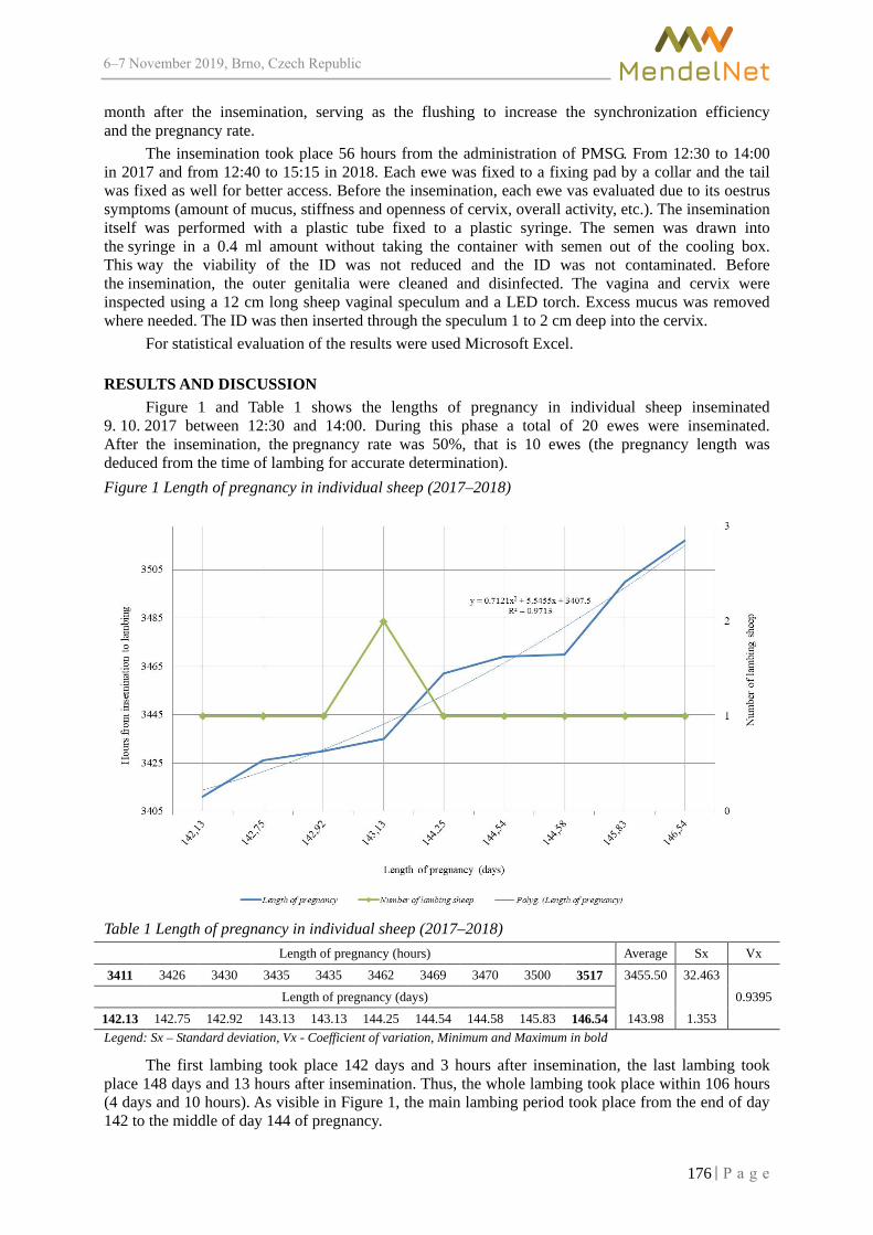
6–7 2019, Brno, Czech Republic
month after the insemination, serving as the flushing to increase the synchronization efficiency and the pregnancy rate.
The insemination took place 56 hours from the administration of PMSG. From 12:30 to 14:00 in 2017 and from 12:40 to 15:15 in 2018. Each ewe was fixed to a fixing pad by a collar and the tail was fixed as well for better access. Before the insemination, each ewe vas evaluated due to its oestrus symptoms (amount of mucus, stiffness and openness of cervix, overall activity, etc.). The insemination itself was performed with a plastic tube fixed to a plastic syringe. The semen was drawn into the syringe in a 0.4 ml amount without taking the container with semen out of the cooling box. This way the viability of the ID was not reduced and the ID was not contaminated. Before the insemination, the outer genitalia were cleaned and disinfected. The vagina and cervix were inspected using a 12 cm long sheep vaginal speculum and a LED torch. Excess mucus was removed where needed. The ID was then inserted through the speculum 1 to 2 cm deep into the cervix.
For statistical evaluation of the results were used Microsoft Excel.
RESULTS AND DISCUSSION Figure 1 and Table 1 shows the lengths of pregnancy in individual sheep inseminated
9. 10. 2017 between 12:30 and 14:00. During this phase a total of 20 ewes were inseminated. After the insemination, the pregnancy rate was 50%, that is 10 ewes (the pregnancy length was deduced from the time of lambing for accurate determination). Figure 1 Length of pregnancy in individual sheep (2017–2018)
Table 1 Length of pregnancy in individual sheep (2017–2018) Length of pregnancy (hours) Average Sx Vx
3411 3426 3430 3435 3435 3462 3469 3470 3500 3517 3455.50 32.463
0.9395 Length of pregnancy (days)
142.13 142.75 142.92 143.13 143.13 144.25 144.54 144.58 145.83 146.54 143.98 1.353 Legend: Sx – Standard deviation, Vx - Coefficient of variation, Minimum and Maximum in bold
The first lambing took place 142 days and 3 hours after insemination, the last lambing took place 148 days and 13 hours after insemination. Thus, the whole lambing took place within 106 hours (4 days and 10 hours). As visible in Figure 1, the main lambing period took place from the end of day 142 to the middle of day 144 of pregnancy.
176

6–7 2019, Brno, Czech Republic
Figure 2 Length of pregnancy in individual sheep (2018–2019)
Table 2 Length of pregnancy in individual sheep (2018–2019)
Length of pregnancy (hours) Averagea Sx Vx
3451 3459 3463 3469 3469 3475 3484 3489 3490 3494 3495 3507.82 35.689
1.0174
3515 3522 3522 3523 3524 3545 3545 3546 3559 3562 3571
Length of pregnancy (days)
143.79 144.13 144.29 144.54 144.54 144.79 145.17 145.38 145.42 145.58 145.63 146.16 1.487
146.46 146.75 146.75 146.79 146.83 147.71 147.71 147.75 148.29 148.42 148.79
Legend: Sx – Standard deviation, Vx - Coefficient of variation, Minimum and Maximum in bold
Figure 2 and Table 2 shows the lengths of pregnancy in individual sheep inseminated on 13. 10. 2018 between 12:40 and 15:15. In this phase a total of 34 ewes was inseminated. After the insemination the pregnancy rate reached 64.7%, that is 22 ewes (the pregnancy length was deduced from the time of lambing for accurate determination), which is an above–average outcome for a pregnancy rate after insemination. The average of pregnancy after insemination is 60% (Kuchtík et al. 2007).
The first lambing took place 143 days and 19 hours after the insemination, while the last one took place 148 days and 19 hours after the insemination. The whole lambing thus took place within 120 hours (5 days). Figure 2 shows that the main lambing period was split into two parts. The first peak occurred between the beginning of day 144 and the middle of day 145. After a 20-hour break, the second peak occurred in the middle of day 146 and ended in the middle of day 148 after the insemination.
Figure 3 shows the year-on-year difference in pregnancy lengths in ewes who became pregnant after insemination in both years 2017 and 2018. The pregnancy length varies significantly in the individual ewes. However, the year-on-year comparison shows that in half of the ewes, the year-on-year pregnancy length difference was quite low, 10 hours at highest. The other half of ewes however showed a striking year-on-year difference, up to 5 days.
The pregnancy length in ewes that were lambing in 2018/2019 (as seen in Figures 1 and 2) varied between 142 and 148 days. However, very little ewes go into lambing during the two threshold days, and the lambing is mainly an exception. In comparison with the average pregnancy lengths in sheep mentioned in the introduction (143–157 days), the average pregnancy length observed
177

6–7 2019, Brno, Czech Republic
in this research was approximately 145 days, which is two days less than stated by e.g. Ingoldby and Jackson (2016).
The difference in pregnancy lengths in 2018/2019 might be caused by differences in temperature, alternatively by a different numbers and genders of the foetuses in individual ewes.
Since the pregnancy length can be affected by a number of factors, from the feed composition to the microclimate, the amount of foetuses or the breed of sheep, it is necessary this research is replicated on a bigger number of animals with the subsequent evaluation of the impact of these factors on the pregnancy length itself.
Figure 3 Year-on-year differences in the length of pregnancy in sheep
CONCLUSIONThis research found that the pregnancy length in Zwartbles sheep varied between 142 and 148
days and the lambing took place between the 143rd and 146th day of pregnancy in majority of the ewes. These values are lower than the average pregnancy lengths usually stated for sheep without a breed specification.
Data acquired in this research will be used for its replication and extension, mainly to determine the lambing period more precisely and to achieve a better time arrangement during lambing.
REFERENCES Čunát, L. et al. 2013. Využití inseminace ovcí v chovatelské praxi, Praha: Česká zemědělská univerzita. Gajdošík, M., Polách, A. 1984. Chov oviec. 1. vyd., Bratislava: Príroda. Gootwine, W. 2016. Husbandry of Dairy Sciences: Sheep: Reproductive Management. Encyclopedia of Dairy Sciences [Online], 1(1): 887–892. Available at: https://www.researchgate.net/publication/310573090_Sheep_Reproductive_Management. [2019-08-02]. Horák, F. et al. 2012. Chováme ovce. Praha: Brázda. Ingoldby, L., Jackson, P. 2001. Induction od parturition in sheep. In Practice, 23: 228–231. Kesler, D.J. 2002. Review of estrous synchronization systems: CIDR inserts. The Applied Reproductive Strategies in Beef Cattle Workshop [Online]. Manhattan, Kansas, 5–6 September,
178

6–7 2019, Brno, Czech Republic
Manhattan: Kansas State University, pp. 47–59. Available at: https://beefrepro.unl.edu/proceedings/2002manhattan/05_ksu_cidr_kesler.pdf. [2019-10-12]. Kuchtík, J. et al. 2007. Chov ovcí. 1. Vyd., Brno: MZLU v Brně. Kuchtík, J. ©2013. Chov ovcí: Reprodukce ovcí [Online]. Available at: https://web2.mendelu.cz/af_291_projekty2/vseo/stranka.php?kod=1045. [2019-08-02]. Kuchtík, J. ©2015. Březost a porod ovcí [Online]. Available at: http://www.chovzvirat.cz/clanek/728-brezost-a-porod-ovci/. [2019-08-02]. Louda, F. Hegedüšová, Z. 2009. Inseminace ovcí – intenzifikační faktor šlechtitelské práce, Rapotín: Agrovýzkum Rapotín. Louda, F. et al. ©2002. Biotechnické metody v reprodukci ovcí a koz [online]. Available at: https://naschov.cz/biotechnicke-metody-v-reprodukci-ovci-a-koz/. [2019-01-17]. Říha, J. 1999. Biotechnologie v chovu a šlechtění hospodářských zvířat, Rapotín: Asociace chovatelů masných plemen. Sándor, K. et al. 2011. Artificial Insemination of Sheep–Possibilities, Realities and Technique at the Farm Level. Artificial Insemination in Farm Animals. Iran: IntechOpen, pp. 27–50. Salamon. S., Maxwell, W.M.C. 2000. Storage of ram semen. Animal Reproduction Science, 62(1–3): 77–111. Tzanigakis, N. et al. 2014. Dairy sheep breeding. LowInputBreeds Technical Note [Online], 1(1): 1–6. Available at: http://www.lowinputbreeds.org/publications/lib-technical-notes.html. [2019-08-02]. Vaněk, D., Štolc, L. 2002. Chov skotu a ovcí: (přednášky pro Bc). 1. vyd., Praha: Česká zemědělská univerzita, Agronomická fakulta.
179

6–7 2019, Brno, Czech Republic
Taurine addition into Duroc boar diet and its influence on ejaculate quality
Magdalena Pribilova, Pavel Horky, Lenka Urbankova, Jiri Skladanka Department of Animal Nutrition and Forage Production
Mendel University in Brno Zemedelska 1, 613 00 Brno
CZECH REPUBLIC
Abstract: Taurine is the main amino acid in sperm cells and seminal fluid. It plays role in antioxidant system, in capacitation of sperm, in membrane stabilization and improves sperm motility. Pigs have a very poorly developed thermoregulatory system. Boar thermoneutral zone renges form 12 to 20 °C. Temperatures above 23 °C are considered to thermal. In this study, Duroc boars where divided into two groups (n = 6). Control group was fed by basic diet (12.6 MJ/kg, 3.5 kg/day), experimental group was fed by basic diet with supplementation of 15 g taurine per boar per day. Monitored parameters of ejaculate were volume of ejaculate, concentration of sperm cells, total rate of sperm, motility of sperm and percentage of morphologically abnormal sperm. It has been found, that supplementation of 15 g taurine/boar/day had significant results in sperm motility. In comparison between groups, there can be observed statistically significant differences in motility in June by 0.47% (P<0.05) and July by 0.49% (P<0.05). However, supplementation of taurine into Duroc boar diet had no significant effect on quality and quantity of ejaculate.
Key Words: taurine, ejaculate, heat stress, boar
INTRODUCTION Taurine, the 2-aminoethansulfonic acid, is semi-esencial amino acid which is synthesized
in many organic tissues, such as central nervous system, liver, kidney, retina and mammary gland (Yang et al. 2010). Mayor synthesis of taurine in body is via the pathway that involves dioxygenation of cysteine into cysteine sulfinate by cysteine dioxygenase. Cystein sulfinate is then metabolized by decarboxylation to produce hypotaurine, which is further oxidized into taurine (Stipanuk 2004). Main functions of taurine are osmoregulation, calcium modulation, membrane stabilisation, antioxidation, radioprotection, energy storage, xenobiotic conjugation, isethionic acid and anion balance et al. (Huxtable 1992). In males it has been identified as the major free amino acid of sperm cells and seminal fluid (Holmes et al. 1992). It has detected in cytoplasm of Leydig cells, vascular endothelial cells and some other interstitial cells of testis and epithelial cells of efferent ducts (Lobo et al. 2000). In male reproduction system taurin is part of the antioxidant cell defense system (Green et al. 1991), participates in sperm capacitation, serves for membrane stabilization and affects sperm motility (Alvarez and Storey 1983, Meizel et al. 1980, Meizel 1985).
Free radicals, the most known reactive oxygen species, are highly reactive particles that immediately attack surrounding tissues, especially fatty acids, lipids and amino acids (Mourek et al. 2009, Štípek et al. 2000, Horký et al. 2016). Higher amount of free radicals can cause deterioration of boar reproduction and libido in summer period (Gadd, 2011). In susceptible boars, there is a higher incidence of abnormal sperm, decreased sperm motility, decreased ejaculate volume, reduced sex hormone production under thermal stress (Smital 2001, Horký et al. 2015). The thermoneutral zone of boars ranges from 12–20 °C (Pulkrábek et al. 2005). Hájek et al. (1992) claim that heat stress starts at border 25 °C. The onset of heat stress could be recorded according to the intensity of breathing. Under physiological conditions, normal breathing intensity is 15–20 breaths per minute. Thermal stress is then indicated if the intensity exceeds 40–50 breaths per minute (Smital 2001).
180

6–7 2019, Brno, Czech Republic
MATERIAL AND METHODS
Characterization of experiment Experiment has been done at insemination station in Velké Meziříčí during the summer months
(June–September) when we assumed potential heat stress. For the experiment have been chosen 12 Duroc boars divided into two equal groups (±275 kg, ±2.5 year). The control group (n = 6) was fed by basic diet (12.6 MJ/kg, 3.5 kg/boar/day). The taurine treated group (n = 6) was fed by basic diet with addition of 15 g taurine/boar/day. Temperature and relative humidity were measured hourly during the whole experiment. The average temperature was 22.3 °C, maximal temperature ranged 31.2 °C. The average humidity was 71%, maximal humidity ranged 85.5%.
Composition of feed mixture Table 1 shows the composition of feed mixture used at insemination station. The producer
is Agropodnik, a. s., Velké Meziříčí.
Table 1 Basic feed composition (values in 1 kg)
Composition: wheat, barley, soya extracted meal, dried blood, calcium carbonate, dicalcium phosphate, sodium chloride, soya oil
Analytical components % Additives Amount
Dry matter 88.0 Vitamin A 8000.0 IU
Crude protein 17.3 Ferrous sulfate monohydrate 37.5 mg
Crude fibre 3.7 Calcium iodate anhydrous 0.4 mg
Crude fat 2.3 Copper sulfate pentahydrate 7.2 mg
Crude ash 5.4 Copper chelate amino acid hydrate 9.8 mg
Lysine 0.9 Manganese oxide 22.7 mg
Methionine 0.3 Manganese chelate amino acid hydrate 19.5 mg
Calcium 0.8 Zinc oxide 86.9 mg
Phosphorus 0.7 Zinc chelate amino acid hydrate 48.0 mg
Sodium 0.2 Se (sodium selenite) 0.3 mg
Methodology of data processing Boars ejaculate was taken by hand-gloved technique once a week from all boars. Ejaculate,
if fulfilled the requirements, was used for commercial use. Analysis of ejaculate was performed by Lovercamp et al. (2013).
Volume of ejaculate was measured by weighing with 1 g to 1 ml conversion. Concentration of sperm was determined by using self-calibrating spectrophotometer Spekol 11
(SpermaCueTM, Minitube of America, Verona, WI) at wavelength 340–850 nm. The sample for spectrophotometer measuring was prepared by mixing 9 ml of 1M HCl and 0.25 ml of ejaculate.
Total sperm count was calculated by: volume of ejaculate × concentration of sperm. For sperm motility determination the ejaculate sample (500 μl) was diluted with 500 μl
of Androhep diluent and incubated in 37 °C for 30 min. After incubation the sample was monitored in contrast microscope with digital camera (Olympus microscope IX 71 S8F–3; Tokio, Japan) and Sperm Vision™ software (Minitube of America, Verona, WI).
For determination of morphologically abnormal sperm was 50 μl of each ejaculate fixed by 5 μl 10% buffered formalin, than 5 μl of this sample was dropped on slide incubated for 30 min (in 25 °C
181
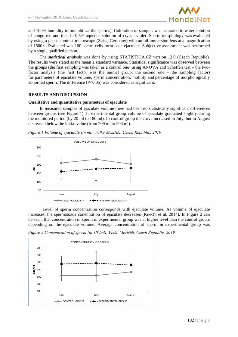
6–7 2019, Brno, Czech Republic
and 100% humidity to immobilize the sperms). Coloration of samples was saturated in water solution of congo-red and then in 0.5% aqueous solution of crystal violet. Sperm morphology was evaluated by using a phase contrast microscope (Zeiss, Germany) with an oil immersion lens at a magnification of 1500×. Evaluated was 100 sperm cells form each ejaculate. Subjective assessment was performed by a single qualified person.
The statistical analysis was done by using STATISTICA.CZ version 12.0 (Czech Republic). The results were stated as the mean ± standard variance. Statistical significance was observed between the groups (the first sampling was taken as a control one) using ANOVA and Scheffe's test – the two-factor analysis (the first factor was the animal group, the second one – the sampling factor) for parameters of ejaculate volume, sperm concentration, motility and percentage of morphologically abnormal sperm. The difference (P<0.05) was considered as significant.
RESULTS AND DISCUSSION
Qualitative and quantitative parameters of ejaculate In measured samples of ejaculate volume there had been no statistically significant differences
between groups (see Figure 1). In experimental group volume of ejaculate graduated slightly during the monitored period (by 20 ml to 180 ml). In control group the curve increased in July, but in August decreased below the initial value (from 209 ml to 203 ml).
Level of sperm concentration corresponds with ejaculate volume. As volume of ejaculate increases, the spermatozoa conentration of ejaculate decreases (Knecht et al. 2014). In Figure 2 can be seen, that concentration of sperm in experimental group was at higher level than the control group, depending on the ejaculate volume. Average concentration of sperm in experimental group was
Figure 1 Volume of ejaculate (in ml), Velké Meziříčí, Czech Republic, 2019
Figure 2 Concentration of sperm (in 106/ml), Velké Meziříčí, Czech Republic, 2019
182

6–7 2019, Brno, Czech Republic
477 × 106 and in control group was 335 × 106. Differences between groups were not statistically significant.
Values of total rate of sperm (see Figure 3) were determined by calculation: volume of ejaculate × concentration of sperm. As the results above, total sperm count has no significant differences. In control group was average sperm count 69 × 109 and in experimental group 76 × 109.
Figure 4 shows measured sperm motility results. As it can be seen form diagram, differences between groups were statistically significant in June by 0.47% (P<0.05) and July by 0.49% (P<0.05).
Figure 3 Total rate of sperm (in 109/ml), Velké Meziříčí, Czech Republic, 2019
Figure 4 Motility of sperm, (in %), Velké Meziříčí, Czech Republic, 2019
Figure 5 Morphologically abnormal sperm (in %), Velké Meziříčí, Czech Republic, 2019
183

6–7 2019, Brno, Czech Republic
But in both groups, curves decreased slightly during the whole experiment, so it could not be stated that taurine supplementation increases sperm motility.
Percentage of morphologically abnormal sperm increased in both groups inconclusive within each group and also differences between groups were not significant (see Figure 5). An increase in control group was from 10.2% to 12.6% ani in experimental group from 7.2% to 8.0%.
According to recent studies in rats, a statistically significant difference was found between the control group and the taurine-added group in motility and live sperm count (Yang et al. 2010). Taurine has also been shown to positively affect the in vitro motility and viability of cats, rams, stallions and donkeys (Baran et al. 2009, Ijaz and Ducharme, 1995, Yang et al. 2010, Dorado et al. 2014).
CONCLUSION From our results it can be stated, that supplementation of taurine into Duroc boar diet cannot
increase sperm motility or decrease percentage of morphologically abnormal sperm. That’s because the curves of both groups increased and decreased in the same trend over the course of the experiment regardless of taurine addition into the diet.
ACKNOWLEDGEMENTS The research was financially supported by the project IGA IP 039/2019: The effect of taurine on qualitative and quantitative parameters of ejaculate of Duroc boars is summer period.
REFERENCES Alvarez, J.G., Storey, B.T. 1983. Taurine, hypotaurine, epinefhrine and albimin inhibit lipid peroxidation in rabbit spermatoza and protect against loss of motility. Biology of Reproduction, 29(3): 549–555. Baran, A. et al. 2009. Short-term chilled storage of cat semen extended with and without taurine containing milk extenders. Journal of Animal and Veterinary Advances, 8(7): 1367–1371. Dorado, J. et al. 2014. Effect of extender and amino acid supplementation on sperm quality of cooled-preserved Andalusian donkey (Equus asinus) spermatozoa. Animal Reproduction Science, 146(2): 79–88. Gadd, J. 2011. Modern pig production technology: a practical guide to profit. New Edition. Nottingham: Nottingham University Press. Green, T.R. et al. 1991. Antioxidant role and subcellular location of hypotaurine and taurine in human neutrophilis. Biochimica et Biophysica Acta, 1073(1): 91–97. Hájek, J. et al. 1992. Prasata v drobném chovu a na farmách. Praha: Apros. Holmes, R.P. et al. 1992. The taurine and hypotaurine content of human semen. Journal of Andrology. 13(3):289–292. Horký, P. et al. 2015. Effect of Heat Stress on the Antioxidant Activity of Boar Ejaculate Revealed by Spectroscopic and Electrochemical Methods. International Journal of Electrochemical Science, 10(8): 6610–6626. Horký, P. et al. 2016. Effect of Selenium, Vitamins E and C on Antioxidant Potential and Quality of Boar Ejaculate. Journal of Animal and Feed Sciences, 25(1): 29–36. Huxtable, R.J. 1992. Physiological actions of taurine. Physiological Reviews, 72(1): 101–163. Ijaz, A., Ducharme, R. 1995. Effect of various extenders and taurine on survival of stallion sperm cooled to 5 C. Theriogenology, 44(7): 1039–1050. Knecht, D., Środoń, S., Duziński, K. 2014. The Influence of Boar Breed and Season on Semen Parameters. South African Journal of Animal Science, (44): 1–9. Lobo, M.V., Alonso, F.J., Del Rio, R.M. 2000. Immunohistochemical localization of taurine in the male reproductive organs of the rat. Journal of Histochemistry and Cytochemistry, 48: 313–320. Lovercamp, K.W. et al. 2013. Effect of dietary selenium on boar sperm quality. Animal Reproduction Science, 138(3–4): 268–275.
184

6–7 2019, Brno, Czech Republic
Meizel, S. 1985. Molecules that initiate or help stimlate the acrosome reaction by their interaction with the mammalian sperm srface. American Journal of Anatomy, 174(3): 285–302. Meizel, S. et al. 1980. Taurine and hypotaurine: their effects on motility, capacitation and the acrosome reaction of hamster sperm in vitro and their presence in sperm and reproductive tract fluids of several mammals. Deveplopment, Growth & Differentation, 22(3): 483–494. Mourek, J. et al. 2009. Mastné kyseliny omega-3: Zdraví a vývoj 2nd ed. Praha: Triton. Pulkrábek, J. et al. 2005. Chov prasat. 1st ed. Praha: ProfiPress. Smital, J. 2001. Chov a ošetřování pohlavně aktivních kanců. Náš chov, 61: 36–40. Stipanuk, M.H. 2004. Sulfur amino avid metabolism: pathways for production and removal of homocysteine and cysteine. Annual Review of Nutrition, 24: 539–577. Štípek, S. 2000. Antioxidanty a volné radikály ve zdraví a nemoci. Praha: Grada. Yang, J. et al. 2010. Effects of taurine on male reproduction in rats of different ages. Journal of Biomedical Science, 17(1): 9.
185

6–7 2019, Brno, Czech Republic
Assessment of susceptibility of poultry red mites (Dermanyssus gallinae) against commercial used acaricides
Iva Radsetoulalova, Martina Lichovnikova
Department of Animal Breeding
Mendel University in Brno Zemedelska 1, 613 00 Brno
CZECH REPUBLIC
Abstract: The main objective of the performed experiments was assessment of susceptibility and resistance poultry red mites (Dermanyssus gallinae), from two farms with cages system of egg-laying hens in the Czech Republic in 2019, against three commercially used acaricides (Milba STOP ultra, Elector, Poultry Shield) by Method No. 11 from IRAC (Insecticide Resistance Action Committee) Susceptibility Test Methods Series. This is in vitro direct contact method. According to the method concentrations of acaricides were used as follow: 0% (acetone only control); 4%; 20%; 100%; 500% of the recommended field application rates. All used commercial acaricides caused mortality of poultry red mites in all their stages of development. The assessment of susceptibility and resistance of PRM (Poultry Red Mites) against commercially used acaricides by Susceptibility rating scheme showed, that PRM were highly susceptible to acaricide Poultry Shield on the both farms, moderately resistant on the Farm 2 and highly resistant on the Farm 1 against acaricide Milba STOP ultra and highly resistant against acaricide Elector on both farms.
Key Words: pyrethroid, cypermethrin, spinosad, Milba STOP ultra, Elector, Poultry Shield
INTRODUCTION The poultry red mite (PRM, Dermanyssus gallinae) is an obligatory hematophagous ectoparasite
of birds, which feeds blood of its host, but it lives and develops out of host's body. All development stages feed blood except larva stage and adult males feed only sometimes (Sparagano et al. 2014).
Its abundance in poultry houses is a major source of disturbs of egg-laying hens, big health risks and one of an economic problem in egg production (Dohnal 2009). The cost expends on fight against PRM and production losses are calculated on 360 million EUR per year. PRM are found up to 95% flocks in Europe, USA, Japan and China (Teuling 2017). PRM may be a vector of a variety of poultry pathogens including zoonosis. Its faeces and small hairs on his cuticle are strong allergens for people, which caused eczema and dermatitis (Sparagano et al. 2014).
PRM has very fast life cycle (7–10 days) and some of them are becoming increasingly resistant against commercially used acaricides against these parasites (Sparagano et al. 2014). Selected commercially used acaricides are usually used for PRM elimination in poultry houses in the Czech Republic with the presence of egg-laying hens.
Among the most often used chemical substances to eliminate poultry red mite belongs pyrethroids, derivatives of fenols (DEET), carbamates, spinosin, organofosfates, amidine. Using products based on these substances is legislative constrained or absolutely prohibited in some countries. Among advantages of chemical acaricides belongs simple application and lower costs. On the beginning these acaricides are very effective, but their efficiency during repeating applications decrease depending on frequency of their usage. Disadvantages of chemical acaricides are nonavailability of new molecules, residues, toxicity, short-term effectiveness, necessary to repeat application until a week, resistance of PRM against chemical substance, some products may be used only in empty poultry house (without layers). Nevertheless, these products are still used for PRM elimination (Dohnal 2009, Sparagano et al. 2014).
The reasons of inherent resistance are fast reproductive cycle of PRM, inconsequence of zoo hygienic precautions, incorrect application and poorly chosen chemical products for PRM elimination.
186

6–7 2019, Brno, Czech Republic
The aim of this study was assessment of susceptibility of PRM to three commercially used acaricides (Milba STOP ultra, Elector, Poultry Shield).
MATERIAL AND METHODS The assessment of susceptibility of PRM to commercially used acaricides was examined using
in vitro direct contact method – Method No. 11 from IRAC (Insecticide Resistance Action Committee) Susceptibility Test Methods Series. This method is currently widely used in Western Europe for monitoring sensitivity of pollen beetle (Meligethes spp.) populations in oilseed rape to synthetic pyrethroids (IRAC 2009).
Used materials for this method was: plastic containers, cardboard, tested acaricides, acetone, pipettes, glass vials (10 ml volume) with lids, vial roller, box with water, entomological tweezer, fine pointed paintbrush, paper circles. There were used three acaricides: Milba STOP ultra, Elector, Poultry Shield. The active component in Milba STOP ultra is cypermethrin (pyrethroid), in Elector is Spinosad, in Poultry Shield are KAS - CAS 85409-23-0, EC 287-090-7 a CAS 68391-01-5, EC 269-919-4 (ÚSKVBL 2019).
Colonies of PRM used in these tests were collected from two farms with cages system for egg-laying hens in the Czech Republic in 2019. For trapping PRM were used plastic containers filled with rolled cardboard (see Figure 1) attached to the constructions in poultry houses. After 3–5 days the containers with PRM were closed by lids and transferred to the laboratory. PRM were tested within two days after collection (Sparagano et al. 2013).
The tested containers were glass vials with an internal surface area of 28.5 cm2 (see Figure 2). The surface area of the glass vials was determined by this formula: π r 2 + (2 π r) × h, where h is the height of the vial, r is the radius of the bottom (surface area = area of bottom + area of the side).
Figure 1 Plastic container with poultry red mites Figure 2 Glass vials
Figure 3 Vial roller
187
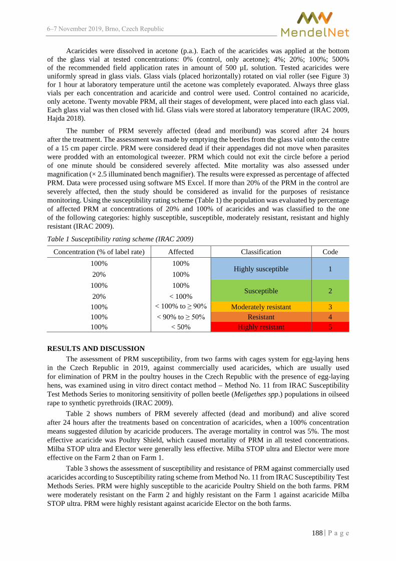
6–7 2019, Brno, Czech Republic
Acaricides were dissolved in acetone (p.a.). Each of the acaricides was applied at the bottom of the glass vial at tested concentrations: 0% (control, only acetone); 4%; 20%; 100%; 500% of the recommended field application rates in amount of 500 µL solution. Tested acaricides were uniformly spread in glass vials. Glass vials (placed horizontally) rotated on vial roller (see Figure 3) for 1 hour at laboratory temperature until the acetone was completely evaporated. Always three glass vials per each concentration and acaricide and control were used. Control contained no acaricide, only acetone. Twenty movable PRM, all their stages of development, were placed into each glass vial. Each glass vial was then closed with lid. Glass vials were stored at laboratory temperature (IRAC 2009, Hajda 2018).
The number of PRM severely affected (dead and moribund) was scored after 24 hours after the treatment. The assessment was made by emptying the beetles from the glass vial onto the centre of a 15 cm paper circle. PRM were considered dead if their appendages did not move when parasites were prodded with an entomological tweezer. PRM which could not exit the circle before a period of one minute should be considered severely affected. Mite mortality was also assessed under magnification (× 2.5 illuminated bench magnifier). The results were expressed as percentage of affected PRM. Data were processed using software MS Excel. If more than 20% of the PRM in the control are severely affected, then the study should be considered as invalid for the purposes of resistance monitoring. Using the susceptibility rating scheme (Table 1) the population was evaluated by percentage of affected PRM at concentrations of 20% and 100% of acaricides and was classified to the one of the following categories: highly susceptible, susceptible, moderately resistant, resistant and highly resistant (IRAC 2009).
Table 1 Susceptibility rating scheme (IRAC 2009)
Concentration (% of label rate) Affected Classification Code 100% 100%
Highly susceptible 1 20% 100%
100% 100% Susceptible 2
20% < 100% 100% < 100% to ≥ 90% Moderately resistant 3 100% < 90% to ≥ 50% Resistant 4 100% < 50% Highly resistant 5
RESULTS AND DISCUSSION The assessment of PRM susceptibility, from two farms with cages system for egg-laying hens
in the Czech Republic in 2019, against commercially used acaricides, which are usually used for elimination of PRM in the poultry houses in the Czech Republic with the presence of egg-laying hens, was examined using in vitro direct contact method – Method No. 11 from IRAC Susceptibility Test Methods Series to monitoring sensitivity of pollen beetle (Meligethes spp.) populations in oilseed rape to synthetic pyrethroids (IRAC 2009).
Table 2 shows numbers of PRM severely affected (dead and moribund) and alive scored after 24 hours after the treatments based on concentration of acaricides, when a 100% concentration means suggested dilution by acaricide producers. The average mortality in control was 5%. The most effective acaricide was Poultry Shield, which caused mortality of PRM in all tested concentrations. Milba STOP ultra and Elector were generally less effective. Milba STOP ultra and Elector were more effective on the Farm 2 than on Farm 1.
Table 3 shows the assessment of susceptibility and resistance of PRM against commercially used acaricides according to Susceptibility rating scheme from Method No. 11 from IRAC Susceptibility Test Methods Series. PRM were highly susceptible to the acaricide Poultry Shield on the both farms. PRM were moderately resistant on the Farm 2 and highly resistant on the Farm 1 against acaricide Milba STOP ultra. PRM were highly resistant against acaricide Elector on the both farms.
188
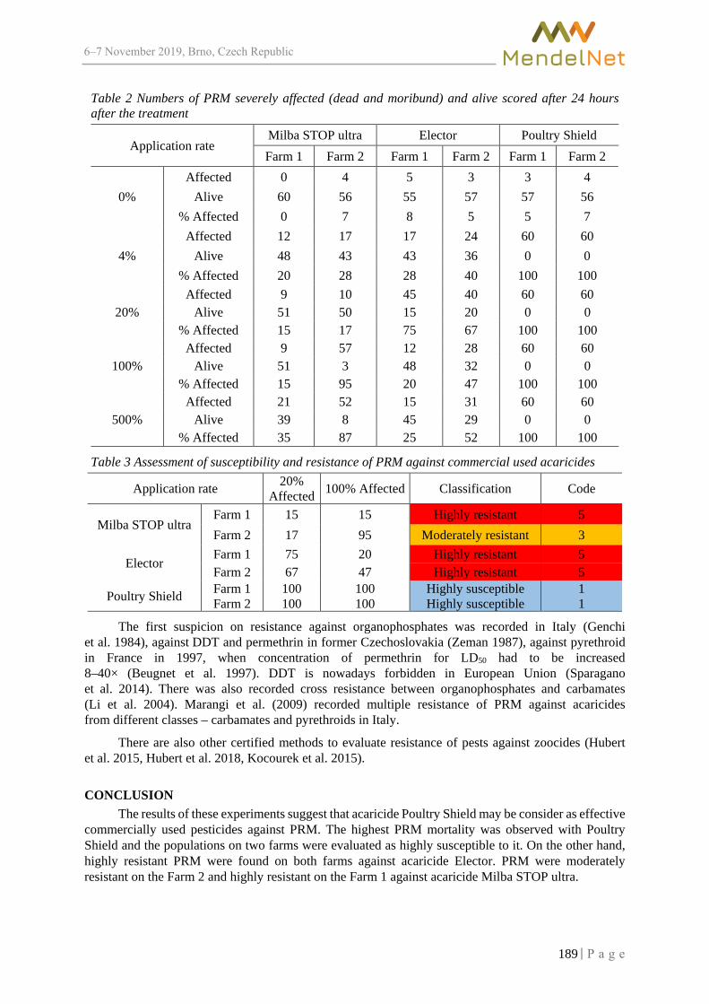
6–7 2019, Brno, Czech Republic
Table 2 Numbers of PRM severely affected (dead and moribund) and alive scored after 24 hours after the treatment
Application rate Milba STOP ultra Elector Poultry Shield Farm 1 Farm 2 Farm 1 Farm 2 Farm 1 Farm 2
0% Affected 0 4 5 3 3 4
Alive 60 56 55 57 57 56 % Affected 0 7 8 5 5 7
4% Affected 12 17 17 24 60 60
Alive 48 43 43 36 0 0 % Affected 20 28 28 40 100 100
20% Affected 9 10 45 40 60 60
Alive 51 50 15 20 0 0 % Affected 15 17 75 67 100 100
100% Affected 9 57 12 28 60 60
Alive 51 3 48 32 0 0 % Affected 15 95 20 47 100 100
500% Affected 21 52 15 31 60 60
Alive 39 8 45 29 0 0 % Affected 35 87 25 52 100 100
Table 3 Assessment of susceptibility and resistance of PRM against commercial used acaricides
Application rate 20% Affected 100% Affected Classification Code
Milba STOP ultra Farm 1 15 15 Highly resistant 5 Farm 2 17 95 Moderately resistant 3
Elector Farm 1 75 20 Highly resistant 5 Farm 2 67 47 Highly resistant 5
Poultry Shield Farm 1 100 100 Highly susceptible 1 Farm 2 100 100 Highly susceptible 1
The first suspicion on resistance against organophosphates was recorded in Italy (Genchi et al. 1984), against DDT and permethrin in former Czechoslovakia (Zeman 1987), against pyrethroid in France in 1997, when concentration of permethrin for LD50 had to be increased 8–40× (Beugnet et al. 1997). DDT is nowadays forbidden in European Union (Sparagano et al. 2014). There was also recorded cross resistance between organophosphates and carbamates (Li et al. 2004). Marangi et al. (2009) recorded multiple resistance of PRM against acaricides from different classes – carbamates and pyrethroids in Italy.
There are also other certified methods to evaluate resistance of pests against zoocides (Hubert et al. 2015, Hubert et al. 2018, Kocourek et al. 2015).
CONCLUSION The results of these experiments suggest that acaricide Poultry Shield may be consider as effective
commercially used pesticides against PRM. The highest PRM mortality was observed with Poultry Shield and the populations on two farms were evaluated as highly susceptible to it. On the other hand, highly resistant PRM were found on both farms against acaricide Elector. PRM were moderately resistant on the Farm 2 and highly resistant on the Farm 1 against acaricide Milba STOP ultra.
189

6–7 2019, Brno, Czech Republic
ACKNOWLEDGEMENTS The research was financially supported by the grant No. AF-IGA2019-IP028.
REFERENCES Beugnet, F., Chauve, C., Gauthey, M., Beert, L. 1997. Resistance of the red poultry mite to pyrethroids in France. Veterinary Record, 140(22): 577–579. Dohnal, K. 2009. Nezvaný host Dermanyssus gallinae alias čmelík kuří. Drůbežář, 9: 9–13. Genchi, C., Huber, H., Traldi, G. 1984. The efficacy of flumethrin (Bayticol Bayer) for the control of chicken mite Dermanyssus gallinae (De Geer, 1778) (Acarina, Dermanyssidae). Archivio Veterinario Italiano, 35(3): 125–128. Hajda, T. 2018. Rezistence škůdců řepky k vybraným účinným látkám insekticidů. Diplomová práce, Mendelova Univerzita v Brně. Hubert, J., Nesvorná, M., Stará, J. 2015. Certifikovaná metodika pro hodnocení účinnosti akaricidních látek na skladištní roztoče a pro identifikaci rezistence. Praha: Výzkumný ústav rostlinné výroby, v.v.i. Hubert, J., Nesvorná, M., Doskočil, I., Kamler, M., Stará, J. 2018. Certifikovaná metodika pro hodnocení rezistence roztoče Varroa destructor vůči tau-fluvalinátu. Praha: Výzkumný ústav rostlinné výroby, v.v.i. IRAC. 2009. IRAC Susceptibility Test Methods Series, Version: 3, Method No: 011. IRAC [Online]. Available at: www.irac-online.org. [2019-10-16]. Kocourek, F., Stará, J., Zichová, T., Hubert, J., Nesvorná, M. 2015. Metodika pro hodnocení rezistence škůdců k zoocidům pomocí biologických metod a antirezistentní strategie pro zabránění výskytu rezistence. Praha: Výzkumný ústav rostlinné výroby, v.v.i. Li, A.Y., Davey, R.B., Miller, R.J., George, J.E. 2004. Detection of amitraz resistance in the southern cattle tick, Boophilus microplus (Acari: Ixodidae). Journal of Medical Entomology, 41(2): 193–200. Marangi, M., Cafiero, M.A., Capelli, G., Camarda, A., Sparagano, O.A.E., Giangaspero, A. 2009. Evaluation of the poultry red mite Dermanyssus gallinae (Acari: Dermanyssidae) susceptibility to some acaricides in field populations from Italy. Experimental and Applied Acarology, 48(1–2): 11–18. Sparagano, O.A.E., Khallaayoune, K., Duvallet, G., Nayak, S., George, D.R. 2013. Comparing Terpenes from Plant Essential Oils as Pesticides for the Poultry Red Mite (Dermanyssus gallinae). Transboundary and Emerging Diseases, 60(2): 150–153. Sparagano, O.A.E., George, D.R., Harrington, D.W.J., Giangaspero, A. 2014. Significance and Control of the Poultry Red Mite, Dermanyssus gallinae. Annual Review of Entomology, 59(4): 447–66. Teuling, M. 2017. The battle against red mites. Poultry World [Online]. Available at: http://www.poultryworld.net. [2018-08-15]. ÚSKVBL. 2019. Ústav pro státní kontrolu veterinárních biopreparátů a léčiv. Registrace a schvalování – biocidy – Seznam DDD [Online]. Available at:http://www.uskvbl.cz/cs/registrace-a-schvalovani/biocidy/seznam-ddd?detail_info=998. [2019-08-30]. Zeman, P. 1987. Encounter the poultry red mite resistance to acaricides in Czechoslovak poultry-farming. Folia Parasitologica, 34(4): 369–373.
190

6–7 2019, Brno, Czech Republic
An occurrence of some chemical contaminants in milk of ruminants during 2005–2017 in the Czech Republic
Karolina Strakova, Lucie Hasonova, Eva Samkova
Department of Food Biotechnologies and Agricultural Products Quality
University of South Bohemia in Ceske Budejovice Studentska 1668, 370 05 Ceske Budejovice
CZECH REPUBLIC
Abstract: The presence of contaminants in milk may pose a great risk to consumer health. The aim of this work was to evaluate the presence of selected chemical contaminants (pesticides, polychlorinated biphenyls (PCBs), heavy metals, mycotoxins and dioxins) in raw milk samples of ruminant (n=12310). Results of monitoring data from the State Veterinary Administration of the Czech Republic from 2005–2017 were used. The highest percentage of positive samples was found in PCBs (25.1%) and in dioxins (22.7%). A low percentage of positive samples was found for aflatoxin M1 (0.5%) in cow's milk. Although banned substances (e.g. lindane) are still detected in milk, their amounts do not exceed the maximum residue level.
Key Words: raw milk, chemical contaminants, monitoring, maximum residue levels
INTRODUCTION The use of chemicals in agriculture and industry presents certain health risks for both
the animals and consumers. In addition to veterinary drugs, also other important contaminants such as pesticides,
polychlorinated biphenyls (PCBs), heavy metals, mycotoxins and dioxins are monitored in animal products including milk. Pesticides are mainly used to protect plants against weeds, pests and diseases and further to prevent storage losses. Organochlorine pesticides belong to the most frequently monitored pesticide group. These pesticides can persist for a long time in the environment and can be accumulated in fat tissue of animal and human bodies (Fromberg et al. 2011).
Organophosphate pesticides are the second important group of pesticides. Their consumption has increased as a result of industrial and household use. The organophosphate pesticides are of synthetic origin and most of them are poorly water soluble. In comparison with organochlorine pesticides, they are less toxic in mammalian organisms. These chemicals are potent neurotoxic agents, whose residues cause acute and chronic health problems in humans and animals (Fagnani et al. 2011).
Other monitored contaminants are PCBs, which are most commonly used in industry. PCBs are persistent organic pollutants with low water solubility. PCBs can have carcinogenic effects and can affect the immune, reproductive, nervous and endocrine systems (Loganathan and Masunaga 2015).
Heavy metals, particularly lead, arsenic, mercury and cadmium, enter the environment through wastewater irrigation, solid waste disposal and other industrial activities. This is the way how they get to the crops. Long-term exposure of toxic metals has an adverse effect on human health, which may occur even several years after the intake. Heavy metals can cause nervous system disorders, renal failure, genetic mutations, cancer, infertility etc. (Ziarati et al. 2018).
Mycotoxins are toxic substances produced as secondary metabolites of some fungal genera, particularly Aspergillus, Alternaria, Claviceps, Fusarium, Penicillium and Stachybotrys. Although many different mycotoxins are known, the monitoring in animal products is particularly focused on aflatoxins. Their main source is contaminated feed. Aflatoxins have mutagenic and carcinogenic effects and can cause chronic problems such as kidney, liver and immune system disorders (Ji et al. 2016).
Dioxins, a family of chlorinated compounds, including polychlorinated dibenzodioxins (PCDDs) and polychlorinated dibenzofurans (PCDFs), are highly toxic compounds often produced
191

6–7 2019, Brno, Czech Republic
unintentionally during combustion processes (Malisch and Kotz 2014). More than 90% of human exposure to dioxins is through the food supply, mainly meat and dairy products, fish and shellfish. Several adverse health effects have been associated with dioxins such as immune system damage, neurological effects, stomach cancer (Kulkarni et al. 2008).
Monitoring of contaminants in both plant and animal products is an important part of food chain control. From this reason, the aim of our work was to evaluate the occurrence of chemical contaminants in raw milk of ruminants during 2005–2017 in the Czech Republic.
MATERIAL AND METHODS Results of monitoring data from the State Veterinary Administration of the Czech Republic
from 2005–2017 (SVA CR 2019) were used (Table 1).
Table 1 Division of contaminants into groups, and number of analysed samples in ruminant milk during 2005–2017 in the Czech Republic (SVA CR 2019)
Groups Analytes Total (n)
Cow (%)
Sheep (%)
Goat (%)
Organochlorine pesticides
aldrin; aldrin + dieldrin (sum); chlordane; DDT (sum); 2,4'-DDT; 4,4'-DDD; 4,4'-DDE; 4,4'-DDT; dieldrin; endrin; endosulfan; hexachlorobenzene; heptachlor; alpha-HCH; beta-HCH; alpha-HCH + beta-HCH (sum); gamma-HCH (lindane)
6001 82 3 15
Organophosphate pesticides
chlorpyriphos; chlorpyriphos-methyl; diazinon; malathion; phorate; pirimiphos-methyl
901 59 6 35
Pyrethroids lambda-cyhalothrin; cyhalothrin; cypermethrin (sum of isomers); deltamethrin; permethrin (sum of isomers); cis-permethrin; trans-permethrin
955 84 5 11
Polychlorinated biphenyls (PCB)
PCB (sum of congeners); PCB 28; PCB 52; PCB 101; PCB 118; PCB 138; PCB 153; PCB 180
2294 82 3 15
Heavy metals arsenic; cadmium; mercury; lead 1152 70 6 24 Mycotoxins aflatoxin M1 730 87 3 10 Dioxins PCDD + PCDF (sum); 2,3,7,8-tetraCDD;
2,3,7,8-tetraCDF; 1,2,3,7,8-pentaCDD; 1,2,3,7,8-pentaCDF; 2,3,4,7,8-pentaCDF; 1,2,3,4,7,8-hexaCDD; 1,2,3,4,7,8-hexaCDF; 1,2,3,6,7,8-hexaCDD; 1,2,3,6,7,8-hexaCDF; 1,2,3,7,8,9-hexaCDD; 1,2,3,7,8,9-hexaCDF; 2,3,4,6,7,8-hexaCDF; 1,2,3,4,6,7,8-heptaCDD; 1,2,3,4,6,7,8-heptaCDF; 1,2,3,4,7,8,9-heptaCDF; 1,2,3,4,6,7,8,9-oktaCDD; 1,2,3,4,6,7,8,9-oktaCDF
277 93 7 0
Legend: DDT – dichlorodiphenyltrichloroethane, DDD – dichlorodiphenyldichloroethane, DDE – dichlorodiphenyldichloro-ethylene, HCH – hexachlorocyclohexane; PCDD – polychlorinated dibenzo-p-dioxins; PCDF – polychlorinated dibenzofurans
In the analysed samples, the number of “positive samples” (any presence of chemical contaminant) as well as a maximum value and maximum residue level (MRL) for each contaminant were observed. Hygienic limits are set according to the following regulations: Council Regulation (EEC) No. 315/1993 and Commission Regulation (EC) No. 1881/2006, which define maximum allowable
192

6–7 2019, Brno, Czech Republic
levels for contaminants in foodstuffs; and Regulation (EC) No. 396/2005, which defines the MRL of pesticides in foodstuffs and feed of plant and animal origin.
The percentages of positive samples were calculated from the total tested samples within each group of contaminants. Statistical tests of data were preformed using the program Statistica CZ 6.1 (Statsoft, Czech Republic).
RESULTS AND DISCUSSION The percentages of positive samples varied among each groups of contaminants from 2005
to 2017 (Table 2). The highest percentage of positive samples was found in PCBs (25.1%) and in dioxins (22.7%). These substances are immunotoxic, carcinogenic, and they can also negatively influence the development and reproduction of individuals (Loganathan and Masunaga 2015). PCBs and dioxins enter the milk through contaminated feed (Malisch and Kotz 2014). Authors reported, that this transfer depends on the congener and on the matrix. In total, there are 209 PCB congeners (Kulkarni et al. 2008); we focused only on seven of them in the work.
Aflatoxin M1 is a metabolite of aflatoxin B1, which is the most common aflatoxin in feed (Boudra et al. 2007). International Agency for Research on Cancer (IARC) classified aflatoxin M1 as human carcinogen belonging to Group 1. Some studies show different results for presence of aflatoxin M1, even in Europe. For example, in Kosovo, 38% of positive samples of aflatoxin M1 were detected, of which 5.7% exceeding the MRL for the European Union, i.e. 0.05 µg/l (Camaj et al. 2018). On the contrary, De Roma et al. (2017) found in Italy 12.3% of positive samples and Boudra et al. (2007) detected in France 3.41% of samples as positive. In the Czech Republic, a low percentage of positive samples for aflatoxin M1 (0.5%) in cow´s milk was found in the period 2005–2017. Favourable was also finding that no positive samples were found in milk of small ruminants.
Table 2 Number of positive samples in ruminant milk during 2005–2017 in the Czech Republic
Group Positive samples n %
Organochlorine pesticides 810 13.5 Organophosphate pesticides 0 0 Pyrethroids 0 0 Polychlorinated biphenyls 575 25.1 Heavy metals 142 12.3 Aflatoxin M1 4 0.5 Dioxins 63 22.7
More details about selected contaminants are given in Table 3. DDT was detected in 56.9% of milk samples in the period 2005–2017. A decreasing trend was observed during the reporting period, both in the number of positive samples and in the detected amount of this banned pesticide (data are not given in the table). Maximum value for DDT (0.418 mg/kg) was detected in 2006; however, in this year, the MRL for DDT was 1 mg/kg. Long term favourable development in DDT content in milk allowed the change of the MRL to current stricter value, i.e. 0.04 mg/kg. Kuba et al. (2015) detected DDT in all tested milk samples in Poland, but maximum value (0.002 mg/kg) was low. Although trend in DDT content in milk, and other animal products, is positive, the problem of DDT has not ceased. Therefore, the presence of this pesticide in milk should be monitored regularly.
A similar situation was observed for hexachlorobenzene. Maximum value (0.055 mg/kg) was reached in 2007, when the MRL was 0.25 mg/kg. Currently, the MRL is set to 0.005 mg/kg.
Strictly monitored pesticide is also banned lindane. This contaminant was found only in 3.5% of milk samples, and maximum value (0.006 mg/kg of fat) did not exceed the MRL. As reported Rusu et al. (2016), the values of lindane ranged from 0.004 to 0.268 mg/kg of fat in Romania.
193

6–7 2019, Brno, Czech Republic
Milk and dairy products may be also contaminated by some heavy metals, such as cadmium, mercury, arsenic and lead (Meshref et al. 2014). Heavy metals have a negative influence on quality and safety of food (Ziarati et al. 2018). In our study, positive samples were detected from 5.6% (for arsenic) to 26.0% (for mercury), no samples exceeded the MRL. The highest value was detected for lead (0.018 mg/kg); the MRL is 0.02 mg/kg. Other studies described above-MRL samples. For example, Meshref et al. (2014) found out lead content in range 0.0546–0.4086 mg/kg in Egypt.
WHO-PCDD/F-TEQ is the sum of the toxic equivalencies of the 17 most toxicologically significant dioxins and furans. The maximum value found in our study was 1.330 pg/g of fat, which not exceed the MRL (2.5 pg/g of fat). However, the presence of positive samples was very high (66.3%). In Poland, the concentrations of these contaminants in cow’s and goat’s milk samples were detected in the range of 0.34–1.50 pg/g of fat (Lizak et al. 2009).
Table 3 Number of positive samples and maximum value observed for selected contaminants in ruminant milk during 2005–20171 in the Czech Republic including current maximum residue level (MRL)
Contaminants Total (n) Positive samples Maximum value
MRL2 Unit
n % DDT (sum) 511 291 56.9 0.418 0.04 mg/kg Hexachlorbenzene 512 165 32.2 0.055 0.005 mg/kg Gama-HCH (lindane) 512 18 3.5 0.006 0.01 mg/kg of fat PCB (sum) 575 147 25.6 76.324 40 ng/g of fat Arsenic 288 16 5.6 0.016 0.05 mg/kg Cadmium 288 30 10.4 0.005 0.01 mg/kg Mercury 288 75 26.0 0.003 0.01 mg/kg Lead 288 21 7.3 0.018 0.02 mg/kg WHO-PCDD/F-TEQ 80 53 66.3 1.330 2.5 pg/g of fat Legend: DDT – dichlorodiphenyltrichloroethane, HCH – hexachlorocyclohexane, PCB – polychlorinated biphenyl, WHO-PCDD/F-TEQ – sum of dioxins 1SVA CR 2019; 2Commission Regulation (EC) No. 1881/2006
CONCLUSION In our work we focused on the occurrence of some chemical contaminants in raw milk
of ruminants during 2005–2017. The positive findings of our study were that most of selected chemical contaminants did not exceed their maximum residue level. On the other hand, the results show, that the problem of chemical contaminants has not ceased. For this reason, permanent monitoring of chemical contaminants should be an integral part of food safety.
ACKNOWLEDGEMENTS The research was financially supported by the project GAJU 028/2019/Z.
REFERENCES Boudra, H. et al. 2007. Aflatoxin M1 and ochratoxin A in raw bulk milk from French dairy herds. Journal of Dairy Science, 90(7): 3197–3201. Camaj, A. et al. 2018. Aflatoxin M1 contamination of raw cow´s milk in five regions of Kosovo during 2016. Mycotoxin Research, 34(3): 205–209. De Roma, A. et al. 2017. A survey on the aflatoxin M1 occurrence and seasonal variation in buffalo and cow milk from Southern Italy. Food Control, 81: 30–33. Fagnani, R. et al. 2011. Organophosphorus and carbamates residues in milk and feedstuff supplied to dairy cattle. Pesquisa Veterinária Brasileira, 31(7): 598–602.
194

6–7 2019, Brno, Czech Republic
Fromberg, A. et al. 2011. Estimation of dietary intake of PCB and organochlorine pesticides for children and adults. Food Chemistry, 125(4): 1179–1187. Ji, C. et al. 2016. Review on biological degradation of mycotoxins. Animal Nutrition, 2(3): 127–133. Kuba, J. et al. 2015. Comparison of DDT and its metabolites concentrations in cow milk from agricultural and industrial areas. Journal of Environmental Science and Health, part B - Pesticides Food Contaminants and Agricultural Wastes, 50(1):1–7. Kulkarni, P.S. et al. 2008. Dioxins sources and current remediation technologies – a review. Environment International, 34(1): 139–153. Lizak, R. et al. 2009. Occurrence and profiles of polychlorinated dibenzo-p-dioxins, dibenzofurans, and dioxin-like polychlorinated biphenyls in Polish farm milk. Bulletin of the Veterinary Institute in Pulawy, 53(4): 833–838. Loganathan, B.G., Masunaga, S. 2015. PCBs, dioxins and furans: Human exposure and health effects. In: Handbook of toxicology of chemical warfare agents. Boston: Elsevier/AP, Academic Press is an imprint of Elsevier, pp. 239–247. Malisch, R., Kotz, A. 2014. Dioxins and PCBs in feed and food – Review from European perspective. Science of the Total Environment, 491: 2–10. Meshref, A.M.S. et al. 2014. Heavy metals and trace elements levels in milk and milk products. Journal of Food Measurement and Characterization, 8(4): 381–388. Rusu, L. et al. 2016. Pesticide residues contamination of milk and dairy products. A case study: Bacau district area, Romania. Journal of Environmental Protection and Ecology, 17(3): 1229–1241. SVA CR – State Veterinary Administration of the Czech Republic. 2019. Food chain contamination [Online]. Available at: https://www.svscr.cz/category/dokumenty-a-publikace/prehled-podle-temat/kontaminace-potravnich-retezcu/. [2019-05-21]. Ziarati, P. et al. 2018. An overview of the heavy metal contamination in milk and dairy products. Acta Scientific Pharmaceutical Science, 2(7): 8–21.
195

6–7 2019, Brno, Czech Republic
The effect of parent stock age on embryo development at oviposition
Martina Tesarova, Martina Lichovnikova Department of Animal Breeding
Mendel University in Brno Zemedelska 1, 613 00 Brno
CZECH REPUBLIC
Abstract: This paper focuses on the stage of embryonic development determination after laying, based on the age of the parental flock of bearing type chicken. This study worked with a paternal flock of the Bovans Brown hybrid of 26 weeks of age. Fertilized eggs were extracted to determine the stage of embryonic development every two weeks from this age, until the parental flock reached the age of 52 weeks. Altogether, 780 fertilized eggs of Bovans Brown hybrid chickens were used in this study. After determination of the stage of embryonic development in given time frame, the study shows that during the 44th and 52nd week of age of the parental flock, there has been a statistically significant (P < 0.05) growth in the embryo from stage 10 to an average stage 10.8 and 10.4.
Key Words: embryonal development, embryonal stage, layer
INTRODUCTION To ensure a production that can cover the market demand, stabilizing and increasing profitability,
it is necessary to check and improve many aspects of poultry breeding. One of these aspects is the optimization of incubation.
Hamburger and Hamilton (1951) have described the embryo development from fertilization in the infundibulum all the way to the hatching. According to this scale, at the time of laying the embryos are in stage X (Eyal-Giladi and Kochav 1976), or less frequently in stage XI (Sellier et al. 2006), and are consists of 20 000 cells (Bachvarova et al. 1998).
The data gained from the embryonic stage determination can be used in various ways. It allows us to observe the early morphological development of the embryo and to find, observe and compare the occurrence of pathological embryo forms. The data can be used during the assessment of factors such as the age of the hen, the breed, the time of laying or the shell quality, based on the blastoderm development. Last but not least, it can be used for optimizing the pre-incubation methods and thus leading to an increase in hatchability.
Pre-incubation of fertilized eggs has the potential to positively affect the chicken egg hatchability, mainly before storing, which affects the hatchability negatively (Petek and Dikmen 2006). This method is based on the heat application and boosting the embryonic development into a stage that is more resistant towards the negative impact of storage (Fasenko et al. 2001).
However, to use this method, it is necessary to determine the stage of embryonic development based on the parental flock age (Bakst et al. 1997). The size of fertilized eggs increases with the age of the parental flock (Shanawany 1987), which increases the time of the creation of the egg, which is thus exposed to the hen’s body temperature, a temperature above the biological zero during which the embryo develops, for a longer time (Bakst 2018). This could be one of the causes for fertilized eggs laid with the embryo in the XI stage (Tesařová 2018). Another factor could be the breed and type (meat, laying) of the hybrid.
Determination of the embryonic development stage is absolutely fundamental for the pre-incubation application. If the temperature applied is too high or the time of pre-incubation is too long, the embryonic stage exceeds the XIII stage (Bakst 2018), a stage where a hypoblast is fully formed. In this stage, the base of primitive streak is forming and the hatchability decreases considerably (Tesařová 2018). This stage is defined as stage 3 according to Hamburger and Hamilton (1951).
196

6–7 2019, Brno, Czech Republic
MATERIAL AND METHODS Fertilized eggs of the laying type hybrid Bovans Brown of age of 26 weeks were used
in this study. Fertilized eggs were extracted to determine the stage of embryonic development every two weeks from this age until the parental flock reached the age of 52 weeks. The eggs were obtained from the INTEGRA a.s. company (Žabčice).
For each part of the experiment, 60 fertilized eggs were collected. The eggs were transported to the laboratory within 8 hours after laying. The eggs were always kept at a constant temperature of 15°C. Blastoderm extraction was performed within 48 hours after laying at constant temperature of 7°C. Altogether, 780 fertilized eggs were used in this study.
Embryo Isolation Embryonic development stage was determined using the method described by Eyal-Giladi
and Kochav (1976). Embryos were isolated at stages X and XI in this experiment. Stage X is defined as state when observation both from the upper and lower surfaces reveals that the formation of the area pellucida has been completed and there is a clearly demarcated border between it and the area opaca. Stage XI is indicated as observation of the upper surface of the blastoderm reveals a smooth thin layer through which deeper concentrations of cells may be seen. From the ventral side stage XI is defined by the formation Koller’s sickle (Eyal-Giladi and Kochav 1976).
Firstly, the egg was broken, and the egg yolk was separated from the egg white. Then, the blastoderm was found and the excess white in its vicinity on the ventral side was removed with cellulose swabs. A ring cut from a filter paper was placed around the cleaned blastoderm. The ring was then cut out and turned so that the blastoderm was in the middle of the aperture. The blastoderm prepared in such way was then placed into a Petri dish with physiological solution.
Cleaning and Determination of the stage of Embryo The blastoderm was cleaned in the physiological solution under a microscope using a hair loop
attached on a small stick. The excess yolk was slowly pushed away with the hair loop until the blastoderm was uncovered. After full cleaning, the blastoderm was released from the paper ring using a plastic pipette with more physiological solution. Picture of the embryo was taken with a Dino Capture camera and, subsequently, the stage of development was determined.
However, during each of the cycles, not all 60 samples were successfully isolated and evaluated. Altogether, 322 blastoderms were isolated and evaluated in this study. Because some of the eggs were unfertilized and due to the difficulty of embryos isolating it was impossible to achieve 100% success rate.
Statistical Methods Observed characteristics of the embryonic development stages based on the parental flock age
were described by an average, which was characterized by the standard error of the average. The variability in the document was characterized by a coefficient of variation.
Data were analysed by Kruskal-Wallis one-way analysis of variance using the Unistat 5.1 software package (Unistat Ltd., England).
RESULTS AND DISCUSION The results of the determination of stages of embryonic development are shown in Table 1.
At the parental flock age of 26 to 42 weeks and 46 to 50 weeks no statistically significant differences was observed. Almost all the fertile eggs were thus laid at the X stage. At the parental flock in age of 44 and 52 weeks, a statistically significant difference (P < 0.05) was observed. At the 44th week of the flock age half of the eggs were in the XI stage, where the average stage was 10.8. At the 50th week of the flock age, more than one third of the eggs were in the XI stage and the average stage was 10.4.
Sellier et al. (2006) compared the embryonic development stages in chicken, duck, turkey and quail, every six hours within the first 72 hours after laying in a temperature between 15 °C and 18 °C. Their study showed that the eggs are in the X stage immediately after laying, but in 12.5% of the tested eggs that were stored for 72 hours, the stage was boosted to XI. This shows that it is fundamental to determine the embryonic development stage immediately after laying.
197

6–7 2019, Brno, Czech Republic
Table 1 Determination of the stage of embryonic development based on the parental flock age Age of the parental
flock (weeks) Number of determined
embryos Stage of embryonic
development SE Vx
26 28 30 32 34 36 40 42 44 46 48 50 52
18 33 26 14 23 22 27 37 24 21 22 35 20
10.0a 10.0a 10.0a 10.0a 10.0a 10.0a 10.0a 10.0a 10.8c 10.0a 10.0a 10.1a 10.4b
0.00 0.00 0.00 0.00 0.05 0.00 0.03 0.00 0.20 0.04 0.00 0.07 0.08
0.00 0.00 0.00 0.00 0.02 0.00 0.02 0.00 0.08 0.02 0.00 0.03 0.05
Note: Different upper indexes (a, b, c) state the statistically provable variances (P < 0,05), Vx ‒ coefficient of variation, SE ‒ standard error
Similar data was concluded by Tesařová (2018), who determined the embryonic development stages in a meat type hybrid ROSS 308 of the parental flock age of 30, 45 and 58 weeks. Most of the fertilized eggs were in the X stage, but in all three groups eggs in the XI stage were observed.
Lukaszewicz et al. (2017) state that the development of the goose embryo at the time of laying is identical to that of the chicken. For an experiment was used fertilized eggs from White Koluda. The determination of the stage of embryos was made according to Eyal-Giladi's and Kochav's (1976) methodology. From 135 eggs it was determined that 35.6% was in stage X, 24.4% was in stage XI and 8.2% was in stage IX.
Lukaszewicz et al. (2019) supposed that age of parental flock has an influence on embryonic stage after laid. It has been found that geese have a much greater extent of embryonic development than chickens. The greater extent of embryonic development in geese was found from the stage VI according to Eyal-Giladi and Kochav (1976) to the 2. stage according to Hamburger and Hamilton (1951). Confirmed at the beginning of laying in the younger parent flock the embryos were in the stage VI‒XI. Eggs at the end of laying was observed more progress embryonic stage XI‒XIII. Some were even observed the beginning of formation primitive streak.
CONCLUSION The final data show that the age of the parental flock affects the embryonic development stages
after laying. The stages get higher with the rising age of the parental flock of a laying type hybrid. In an older parent flock, the egg weight increases, and thus the egg formation time, the embryo
is then exposed to a temperature above the biological zero in the laying hens body for a prolonged period, which may cause the embryo's developmental stage to shift from X to XI. If we applicated the same time of preincubation on fertilized eggs in an older parental flock, would be exceeded XIII developmental stage and preincubation would have a negative impact on hatchability.
ACKNOWLEDGEMENTS The research was financially supported by the grant no. AF-IGA2019-IP049.
REFERENCES Bachvarova, R.F. et al. 1998. Induction of primitive streak and Hensen’s node by the posterior marginal zone in the early chick embryo. Development, 125(17): 3521–3534.
198

6–7 2019, Brno, Czech Republic
Bakst, M.R. 2018. Let’s talk about isolating and staging embryos. In proceedings of Incubation and Fertility Research Group (IFRG/WPSA Working Group 6). Edinburgh, Scotland, 4–5 October. Edinburgh, Worlds Poultry Science Association, pp. 8. Bakst, M.R. et al. 1997. Comparative Development of the turkey and chicken embryo from cleavage through hypoblast formation. Poultry Science, 76(1): 83–90. Eyal-Giladi, H., Kochav, S. 1976. From cleavage to primitive streak formation: A complementary normal table and a new look at the first stages of the development of the chick. Developmental Biology, 49(2): 321–337. Fasenko, G.M. et al. 2001. Prestorage incubation of long-term stored broiler breeder eggs: 1. Effects on hatchability. Poultry Science, 80(10): 1406–1411. Hamburger, V., Hamilton, H.L. 1951. A series of normal stages in the development of the chick embryo. Journal of Morphology, 88(1): 49–92. Lukaszewicz, E. et al. 2017. Goose embryonic development from oviposition through 16 hours of incubation. Poultry Science, 96(6): 1934–1938. Lukaszewicz, E. et al. 2019. Stage of goose embryo development at oviposition depending on genotype, flock age, and period of laying. Poultry Science, 98(10): 5152–5156. Petek, M., Dikmen, S. 2006. The effect of prestorage incubation and length of storage of broiler breeder eggs on hatchability and subsequent growth performance of progeny. Czech Journal of Animal Science, 51(2): 73–77. Sellier, N. et al. 2006. Comparative staging of embryo development in chicken, turkey, duck, goose, guinea fowl, and japanese quail assessed from five hours after fertilization through seventy–two hours of Incubation. The Journal of Applied Poultry Research, 15(2): 219–228. Shanawany, M.M. 1987. Hatching weight in relation to egg weight in domestic birds. Word's Poultry Science Journal, 43(2): 107–115. Tesařová, M. 2018. Vliv preinkubace vajec během dlouhodobého skladování na líhnivost kuřat masného typu. Diplomová práce, Mendelova univerzita v Brně.
199

6–7 2019, Brno, Czech Republic
Monitoring of the ketosis in the dairy cows in periparturient period with laboratory and stable methods
Barbora Umlaskova, Jakub Novotny, Ondrej Stastnik, Andrea Roztocilova,Leos Pavlata
Department of Animal Nutrition and Forage Production Mendel University in Brno Zemedelska 1, 613 00 Brno
CZECH REPUBLIC
Abstract: Ketosis is a serious metabolic disease in high-producing dairy cows. It causes not only other health problems but also economic losses. The aims of the study were to monitor the ketosis (especially according to blood β-hydroxybutyrate concentration) and to draw a comparison between the hand-held device measuring with the laboratory methods. There were included 16 Holstein dairy cows in the trial. The animals were divided into two groups according to the Body Condition Score (BCS) – lower BCS group (BCS ≤ 3.5; n = 8) and higher BCS group (BCS ≥ 3.75; n = 8). Cows were observed once a week in almost 3 months. The first blood samples were collected by coccygeal venipuncture 2–3 weeks before the parturition (concentrations of triglycerides – TAG, non-esterified fatty acids – NEFA, β-hydroxybutyrate – BHB, total bilirubin – BILI, and activity of aspartate aminotransferase – AST and gamma-glutamyl transferase – GGT were determined). Another blood metabolic profile test was done at the end of the experiment that means 2 months after calving. In addition, the values of BHB and glucose (GLU) were measured by the FreeStyle Optium Neo hand-held device every week after calving till the end of the trial. According to the trial results, the higher concentrations of BHB were observed in the lower BCS group in the 2nd and 3rd week after parturition. Also, the low levels of glucose were observed in the lower BCS animals. The high correlation between laboratory and hand-held device measuring was calculated (r = 0.94, P < 0.01). The levels of most biochemical parameters were increased after parturition in both lower and higher BCS group. The incidence of ketosis was similar in both groups of cows.
Key Words: ketosis, dairy cows, β-hydroxybutyrate (BHB), blood parameters, hand-held device
INTRODUCTION Ketosis is the metabolic disease caused by the lack of energy and following development
of the negative energy balance. The prevalence of metabolic disease is typical in high-producing dairy cows during the periparturient period (Vanholder et al. 2015). Incidence of ketosis impacts cow´s health as well as financial implications on the farm. The study from 2017 calculated economical loss caused by the ketosis for $77 in primiparous cows and $181 for multiparous cows (Liang et al. 2017). The transition period is the most demanding time for the organism because it must adapt to the high metabolic demands of lactation (Drackley 1999). When the energy intake is lower than the energy expenditure, the organism gets into the negative energy balance. That causes an increased uncontrolled rate of body fat mobilization. The TAGs are disintegrated to glycerol and NEFA, which one enter to β-oxidation. Acetyl-CoA is the final product of β-oxidation and is metabolized in the Krebs cycle. Nevertheless, in case of lack of oxaloacetate, the ketogenesis goes instead. That is the reason why ketone bodies as BHB or acetoacetate can be identified in milk, blood and urine samples (Hofírek 2009, Murray et al. 2002). The negative energy balance (NEB) is characterized by increased levels of NEFA and BHB. Some degree of NEB is expected in dairy cows in postpartum period (Ospina et al. 2010). According to the extensive research done in the UK, the prevalence of subclinical ketosis in the first 20 days of lactation was 28.5%, 17.3% and 11.75% with the thresholds of 1.0, 1.2, 1.4 mmol/l respectively (Macrae et al. 2019). Development of subclinical ketosis influences the immune system and the higher incidence of milk fever, retained placenta, metritis, mastitis, pneumonia, and digestive disorders were recorded (Pin͂eiro et al. 2019).
200

6–7 2019, Brno, Czech Republic
MATERIAL AND METHODS
Animals The trial took place on the private dairy farm in South Moravia in the Czech Republic.
The experimental animals (n = 16) were Holstein dairy cows. The animals were kept on free-stall housing with no bedding. None of the animals showed any signs of the disease. Cows were fed with TMR (total mixture ration) fulfilling the different energy requirements according to the lactation and reproduction phase. The animals were divided into two groups according to their BCS, that is the lower BCS group (BCS ≤ 3.5; n = 8) and the higher BCS group (BCS ≥ 3.75; n = 8). The one animal of each group died or was culled because of the disease after calving, so at the end of the trial there was only 14 samples of the second sampling instead of 16 at first.
Clinical biochemistry The blood samples were collected 2–3 weeks before the parturition and 2 months after. The blood
was sampled to the non-heparinized tubes from the coccygeal vein. These samples at the beginning and at the end of the trial were centrifuged at 3000 rotation per minute for ten minutes the next day. That is the reason why the level of glucose was not defined with the laboratory analyser. The biochemical parameters evaluating the energy metabolism and liver function such as triglycerides (TAG), non-esterified fatty acids (NEFA), BHB, total bilirubin (BIL), aspartate aminotransferase (AST) and gamma-glutamyl transferase (GGT) were determined in the laboratory. Moreover, the glucose and BHB were measured from the drop of the blood sampled from the coccygeal vein. The values were measured immediately after the sampling in the stable with the FreeStyle Optium Neo hand-held device once a week after calving.
Statistical analysis Data has been processed by Microsoft Excel (USA) and Statistica version 12.0 (CZ). One-way
analysis (ANOVA) was used for data evaluation. To ensure evidential differences Scheffe’s test was applied and p < 0.05 was regarded as a statistically significant difference. The relationship between the set parameters was tested by correlation analysis. For the relationship of methods of measuring, the correlation coefficient (r) was calculated.
RESULTS AND DISCUSSION The results of the average values of blood BHB and glucose are shown in Table 1. One part
of the study focused on the comparison of hand-held devide and laboratory methods, therefore, Table 2 shows the results of BHB of two different measurements. Figure 1 shows the average values of the parameters characterizing the energy metabolism and liver function.
The increased values of BHB and NEFA are the markers of lipomobilisation and developing of the ketosis. On the other hand, the reduction in glucose concentration is observed. The threshold for BHB in lactating cows is 1.0 mmol/l (Doubek 2007, Macrae et al. 2019). The reference range in dry cows is the concentration of BHB above 0.8 mmol/l, including. Another source states the presence of subclinical ketosis in BHB concentration above 1.2 mmol/l, and clinical ketosis with the blood values above 2.6 mmol/l (Djokovic et al. 2019). In Table 1 there are shown the average values of blood BHB and glucose measured by the hand-held device FreeStyle Optium Neo. The BHB average values of any group, neither lower BCS nor higher BCS, were not above the reference range. Increased results were measured in the lower BCS group at the 2nd and 3rd week after the parturition, where the BHB concentrations were marginal. According to the information written above, increase of NEFA and BHB in the early postpartum period is predictable. The study comparing the blood parameters in different lactation period group confirms this thesis (Djokovic et al. 2019). Based on the results of this trial the hypothesis that the cows with BCS ≥ 4 are supposed to suffer from the ketosis was not confirmed. Moreover, the average blood BHB concentration was higher in the lower BCS group (BCS ≤ 3.5).
The glycaemia in ruminants is relatively constant. The reference range for glucose from 2.5 to 4.1 mmol/l was used (Doubek 2007). The other publication uses threshold glucose ≤ 3.0 mmol/l (Macrae et al. 2019). If the same reference range is used, the lower BCS group will be evaluated as being in hypoglycaemia for the whole time of the trial. According to another study, by progress in lactation 27% cows had had glucose concentration less than 2.5 mmol/l (Mohebbi-Fani
201

6–7 2019, Brno, Czech Republic
et al. 2019). The statistically significant difference was established between the lower BCS and the higher BCS group in the 2nd, 6th and 7th week after calving (1.87 ± 0.42 mmol/l and 2.59 ± 0.46 mmol/l, 2.66 ± 0.39 mmol/l and 3.36 ± 0.46 mmol/l, 2.67 ± 0.29 mmol/l and 3.41 ± 0.33 mmol/l respectively) as can be seen in Table 1. In all cases, the lower glucose concentrations were established in the lower BCS group.
Table 1 The values of BHB (β-hydroxybutyrate) and GLU (glucose) in periparturient period in dairy cows (L—lower BCS group, H—higher BCS group) every week after parturition (W1—W8). Blood sample before parturition (I) and two months after (II).
Legend: a, b—different letter in column means statistically significant difference between groups P < 0.05 A,B—different letter in column means statistically significant difference between groups P < 0.01
Table 2 compares two different methods of measuring the concentration of the BHB, immediately after the sampling directly in the stable with the hand-held device and the laboratory establishing from the serum centrifuged the next day. The highly significant correlation r = 0.94 was proved between the hand-held device and laboratory tests. In comparison to another study with the FreeStyle Precision device, where the correlation coefficient was 83%. The sensitivity and the specificity depend on the level of BHB and the device that is used. Based on a serum BHB laboratory concentration of 1.4 mmol/l the sensitivity is 100% and the specificity 92% for the FreeStyle Precision devise. When the BHB concentration of 1.2 mmol/l was used, the sensitivity was the same for this device, but the specificity was lower (76%) (Kanz et al. 2015).
The serum parameters like BHB, NEFA, TAG, BILI, AST, and GGT were determined. Using BHB, NEFA, and TAG can be assessed the level of the energy metabolism, the increased concentrations of BILI, AST, and GGT show the liver damage. The average serum BHB concentrations before parturition were not raised in any group (0.61 ± 0.07 mmol/l, 0.56 ± 0.15 mmol/l). The values sampled 2 months after parturition were not beyond the range, either. Those were higher but there was no statistically significant difference established (0.82 ± 0.48 mmol/l, 0.59 ± 0.20 mmol/l). On the other hand, the statistically significant difference was proved between the prepartum and postpartum samplings in the TAG concentration (C I: 0.21 ± 0.08 mmol/l, E I: 0.20 ± 0.05 mmol/l, C II: 0.11 ± 0.03 mmol/l, E II: 0.11 ± 0.03 mmol/l). But no average value was over the threshold (0.35 mmol/l). In non-esterified fatty acids, where the over reference range is the value up to 0.7 mmol/l, none of the average samples gets over it. As the significant difference was observed between the 1st and the 2nd sampling in the lower BCS and also in the higher BCS group. That can be seen in Figure 1. There is a strong increase in the NEFA level that conversely replicates the TAG curve. There was improved the negative correlation between TAG and NEFA. There are some studies that have shown that elevated NEFA is more objective parameter of negative downstream health and production outcomes than BHB. The incidence of subclinical ketosis according to the increased BHB values (over 1.0 mmol/l) was 28.5%. But 40.3% of animals had NEFA values equal or over 0.7 mmol/l (Macrae et al. 2019).
The concentration of the total bilirubin and levels of the liver enzyme are the parameters of the liver function. The thresholds of the liver enzymes (AST and GGT) are ≤ 1.5 µkat/land ≤ 0.5 µkat/l, respectively (Doubek 2007). As can be seen in Figure 1, there are the increased values
BHB [mmol/l] GLU [mmol/l] L H L H
I 0.53 ± 0.09 0.46 ± 0.16 I 2.33 ± 0.21 2.35 ± 0.17 W1 0.81 ± 0.28 0.59 ± 0.13 W1 2.37 ± 0.44 2.68 ± 0.65 W2 1.00 ± 0.42 0.59 ± 0.31 W2 1.87 ± 0.42 A 2.59 ± 0.46 B W3 1.02 ± 0.76 0.40 ± 0.10 W3 2.73 ± 0.45 3.05 ± 0.18 W4 0.62 ± 0.20 0.66 ± 0.37 W4 2.83 ± 0.37 3.06 ± 0.33 W5 0.66 ± 0.31 0.66 ± 0.38 W5 2.87 ± 0.31 3.01 ± 0.41 W6 0.86 ± 0.30 0.61 ± 0.26 W6 2.66 ± 0.39 A 3.36 ± 0.46 B W7 0.79 ± 0.19 0.66 ± 0.26 W7 2.67 ± 0.29 a 3.41 ± 0.33 b II (W8) 0.91 ± 0.51 0.64 ± 0.32 II (W8) 2.76 ± 0.62 3.24 ± 0.23
202

6–7 2019, Brno, Czech Republic
Figure 1 The average blood values of some biochemical parameters of the metabolic profile in lower BCS (C) and higher BCS (E) group before (I) and 2 months (II) after calving
Legend: 1 (C I), 2 (E I), 3 (C II), 4 (E II)
for both of the groups (lower BCS and higher BCS) after the calving, but no significant difference was proved. There was extended the strong positive correlation between the AST and GGT values. The bilirubin concentration was in the reference range for the whole trial period. There can be seen the higher values in the higher BCS group, but no significant difference was proved between the groups.
203

6–7 2019, Brno, Czech Republic
Table 2 The comparation of the BHB (β-hydroxybutyrate) values measured by the hand-held device in the stable (device) and defined in the laboratory (lab) in the dairy cows in periparturient period
BHB [mmol/l] %
BHB [mmol/l] %
lab device lab device
L I 0.88 0.8 91 H I 0.62 0.5 80 0.45 0.4 89 0.70 0.6 86 0.58 0.4 69 0.56 0.5 89 0.61 0.5 82 0.60 0.5 83 0.62 0.6 97 0.73 0.7 96 0.45 0.3 67 0.60 0.4 67 0.40 0.3 75 0.52 0.5 96 0.52 0.4 77 0.54 0.6 111
x ± sd 0.56 ± 0.14 0.46 ± 0.16 81 ± 10 x ± sd 0.61 ± 0.07 0.54 ± 0.09 89 ± 12 L II 0.82 1.3 159 H II 0.91 0.9 99
0.45 0.5 111 0.46 0.4 87 0.49 0.6 122 0.64 0.8 125 0.44 0.4 91 1.85 2.1 114 0.45 0.3 67 0.78 0.9 115 0.94 0.9 96 0.53 0.6 113 0.53 0.5 94 0.60 0.7 117
x ± sd 0.59 ± 0.19 0.64 ± 0.32 106 ± 27 x ± sd 0.82 ± 0.44 0.91 ± 0.51 110 ± 12
correlation 0.94 Legend: x – mean, sd – standard deviation, L – lower BCS group, H – higher BCS group; I – blood sample 2–3 week before parturition and II – 2 months after parturition, % – BHB (device)/BHB (lab) × 100
CONCLUSION The results of the study confirm the higher metabolic and liver burden in the postpartum period.
Nevertheless, no statistically significant difference was proved between the lower BCS and the higher BCS group. The measurement of the BHB with the hand-held device was established as sufficient methods for ketosis prevention.
ACKNOWLEDGEMENTS The research was financially supported by the IGA FA MENDELU (AF-IGA2019-IP079) and the authors would like to express the thanks for that.
REFERENCES Djokovic, R. et al. 2019. Estimation Metabolic Status in High Yielding Dairy Cows During Transition Period and Full Lactation. Acta Scientiae Veterinariae [Online], 47: 1667. Available at: https://www.researchgate.net/publication/334466518_Estimation_of_Metabolic_Status_in_High_Yielding_Dairy_Cows_During_Transition_Period_and_Full_Lactation. [2019-08-24].
Doubek, J. 2007. Interpretace základních biochemických a hematologických nálezů u zvířat. 1st ed., Brno: Noviko. Drackley, J.K. 1999. Biology of Dairy Cows During the Transition Period: the Final Frontier? Journal of Dairy Science [Online], 82(11): 2259–2273. Available at: https://www.mendeley.com/catalogue/biology-dairy-cows-during-transition-period-final-frontier/. [2019-08-19]. Hofírek, B. 2009. Poruchy metabolismu. In Nemoci skotu. Brno: Noviko, pp. 668—673.
204

6–7 2019, Brno, Czech Republic
Kanz, P. et al. 2015. Suitability of Capillary Blood Obtained by a Minimally Invasive Lancet Technique to Detect Subclinical Ketosis in Dairy Cows by Using 3 Different Electronic Hand-held Devices. Journal of Dairy Science [Online], 98(9): 6108–6118. Available at: https://www.sciencedirect.com/science/article/pii/S0022030215004403. [2019-08-29]. Liang, D. et al. 2017. Estimating US Dairy Clinical Disease Costs with a Stochastic Simulation Model. Journal of Dairy Science [Online], 100(2): 1472–1486. Available at: https://www.sciencedirect.com/science/article/pii/S0022030216308992. [2019-08-24]. Macrae, A.I. et al. 2019. Prevalence of Excessive Negative Energy Balance in Commercial United Kingdom Dairy Herds. The Veterinary Journal [Online], 248: 51–57. Available at: https://www.sciencedirect.com/science/article/pii/S1090023319300401. [2019-08-22]. Mohebbi-Fani, M. et al. 2019. A Field Study on Glucose, Non-esterified Fatty Acids, Beta-hydroxybutyrate and Thyroid Hormones in Dairy Cows During the Breeding Period in Fars Province, Iran. Iranian Journal of Veterinary Research [Online], 20(1): 55–59. Available at: https://www.researchgate.net/publication/332538708_A_field_study_on_glucose_non-esterified_fatty_acids_beta-_hydroxybutyrate_and_thyroid_hormones_in_dairy_cows_during_the_breeding_period_in_Fars_province_Iran. [2019-08-24].
Murray, R.K. et al. 2002. Harperova Biochemie. 4th ed., Jinočany: H & H. Ospina, P.A. et al. 2010. Evaluation of Nonesterified Fatty Acids and β-hydroxybutyrate in Transition Dairy Cattle in the Northeastern United States: Critical Thresholds for Prediction of Clinical Diseases. Journal of Dairy Science [Online], 93(2): 546–554. Available at: https://www.sciencedirect.com/science/article/pii/S0022030210714971. [2019-08-23]. Pine͂iro, J.M. et al. 2019. Associations of Pre- and Postpartum Lying Time with Metabolic, Inflammation, and Health Status of Lactating Dairy Cows. Journal of Dairy Science [Online], 102(4): 3348–3361. Available at: https://www.sciencedirect.com/science/article/pii/S0022030219301638. [2019-08-23]. Vanholder, T. et al. 2015. Risk Factors for Subclinical and Clinical Ketosis and Association with Production Parameters in Dairy Cows in the Netherlands. Journal of Dairy Science [Online], 98(2): 880–888. Available at: https://www.researchgate.net/publication/269711773_Risk_factors_for_subclinical_and_clinical_ketosis_and_association_with_production_parameters_in_dairy_cows_in_the_Netherlands. [2019-08-19].
205

6–7 2019, Brno, Czech Republic
The influence of different forms of selenium on vitality of laboratory rats
Lenka Urbankova, Magdalena Pribilova, Pavel HorkyDepartment of Animal Nutrition and Forage Production
Mendel University in Brno Zemedelska 1, 613 00 Brno
CZECH REPUBLIC
Abstract: The aim of the study was to compare the influence of two forms of selenium (sodium selenite, selenium nanoparticles) on the health status of animal organism. As model animals for this experiment males of the Wistar albino rat were selected and divided into 3 groups of 5 pieces. The first group (n = 5) served as control with no selenium (Se) addition. The second group was fed with mixture containing 1.2 mg/kg of diet of sodium selenite (Na2SeO3). The third group (n = 5) was fed with mixture containing selenium nanoparticles (SeNPs, 1.2 mg Se/kg of diet). The experiment lasted 28 days, during which rats were regularly weighed. At the end of experiment animal were euthanized and samples of liver and small intestine tissue were collected and subjected to histological analysis. Histological analysis showed liver damage in all experimental groups (treated and non-treated) of rats. Another measured parameter was total content of selenium in blood and liver tissue. Analysis showed that the addition of selenium to the feed dose has an effect on increasing amount of selenium in the liver and blood tissues. However, statistically significant difference was observed only in group Na2SeO3 in blood (by 97%). From the results of regular weighing of rats during the experiment, it is apparent that the addition of selenium nanoparticles has no significant effect on weight gain.
Key Words: selenium nanoparticles, rats, small intestine, liver tissue, sodium selenite
INTRODUCTION Selenium is an essential nutrient which participate in major biochemical pathways. It is part
of antioxidant defense system of the organism and protect body against harmful effect of free radicals (Adadi et al. 2019). Selenium is also cofactor of thyroid hormones, part of immune system and reproduction system (Brown and Arthur 2001, El-Demerdash and Nasr 2014, Hoffmann and Berry 2008). It is component of selenoenzymes and selenoproteins (Dogan et al. 2016). At higher doses, selenium may have toxic effects (Horky et al. 2014). Concentration of selenium in organism depends on its intake by food. In European Union the Se content in the soil is relatively low, therefore it is necessary to supplement it into the diet of farm animals but there is a very narrow range between the optimal dose and the toxic dose. (Horky 2014, Kursa et al. 2010).
Selenium nanoparticles (SeNPs) shows beneficial properties like lower toxicity, biocompatibility and chemical stability (Yazhiniprabha and Vaseeharan 2019). At presence, selenium nanoparticles are widely used as a nutritional supplement (Wang et al. 2007). It was found that SeNPs shows lower cytotoxicity compared to inorganic selenium compounds and have excellent anti-cancer and therapeutic properties (Anjum et al. 2016). In this study two forms of selenium (SeNPs, Na2SeO3) and their effect on tissue health status was compared. The aim was to show that SeNPs can serve as an alternative source of nutritional supplement for an animal organism.
MATERIAL AND METHODS
Animals The feeding experiment was carried out in the experimental facility of Department of Animal
Nutrition and Forage Production of Mendel University in Brno. Throughout the whole experiment, microclimatic conditions were observed and controlled at temperature of 23 ± 1 °C and constant
206

6–7 2019, Brno, Czech Republic
humidity of 60%. The photoperiod was maintained at 12 hours of light and 12 hours of darkness with a maximum illumination of 200 lx. As model animals for this experiment males of the Wistar albino rat were selected and divided into 3 groups of 5 pieces. All experimental groups of rats were regularly weighted in interval 0, 7th, 14th, 21st and 28th day. The initial weight of all groups was in the range 131.0-144.0 grams. The first group served as a control with no addition of selenium in their feed. The second group was supplemented with selenium in the form of Na2SeO3 at a dose of 1.2 mg/kg of diet. The third group (SeNPs) was fed with selenium in form of nanoparticles at a dose of 1.2 mg/kg of diet. All groups were fed with monodiet containing 0.03 mg Se/kg/diet. The experiment duration was 28 days. The animals had access to feed and drinking water ad libitum. At the end of the experiment, the animals were euthanized (in accordance with the act on the protection of animals against cruelty No. 246/1992 Coll.) and samples of liver and small intestine tissue were collected and subjected to histological analyses. Total content of selenium was measured by atomic absorption spectrometry (AAS).
Preparation of selenium nanoparticles modified by glucose and reduced by cysteine 250 mg of glucose was dissolved in Milli Q water (40 mL) with constant stirring. Subsequently,
5 mL of Na2SeO3 . 5H2O (0.263 g/50 mL) were added and the pH adjusted to 6.3 with 1 M HCl dropwise. Subsequently, 1 mL of cysteine (1.21 g/50 mL) was added. The mixture was decolorized to orange and the pH increased to 7.3.
Histopathology analysis Tissues were fixed individually in the 10% neutral buffered formaldehyde. Tissues sections were
cut at 3.0 μm and placed onto Superfrost Plus slides (Leica, UK) with the orientation core placed up on the slide. All sections were oriented the same way and the entire tissue block was cut with remaining sections dipped in wax and stored at the room temperature. The sections were stained with hematoxylin and eosin following standard procedures. Photographs were taken using an inverted Olympus microscope IX 71 S8F-3 (Tokyo, Japan).
Preparation of samples for AAS analysis Samples of liver weighting 0.3 g and samples of blood weighting 0.5 g were disintegrated by dry
method in a muffle furnace (LAC, Czech Rep.) and mineralized in 2.5 ml concentrated nitric acid Suprapure.
Statistics The data were processed statistically using STATISTICA.CZ, version 12.0 (the Czech Republic).
The results were expressed as mean ± standard deviation (SD). Statistical significance was determined using ANOVA and Scheffé’s test (one-way analysis).
RESULTS AND DISCUSSION
Total content of selenium in blood and liver tissue In the experiment the effect of two forms of selenium (Na2SeO3, SeNPs), included in the feed
ration for rats was monitoring. In blood and liver samples the total selenium level was determined. The level of selenium in liver was increased in both experimental groups compared with control
(Figure 1) but with no significant difference. In the blood samples statistically significant increasing amount of selenium was measured in the Na2SeO3 group (by 97%, P < 0.05). These results are in agreement with results of Horky et al. (2016) and show that the addition of selenium to the feed dose has an effect on increasing the amount of selenium in the liver and blood tissues.
Histology of liver and duodenum and rat growth All experimental groups of rats were regularly weighted in interval 0, 7th, 14th, 21st and 28th
day. The initial weight of all groups was in the range 131.0–144.0 grams. The weight results were almost comparable in all groups both at the beginning and at the end of the experiment with no significant differences (see Table 1).
207
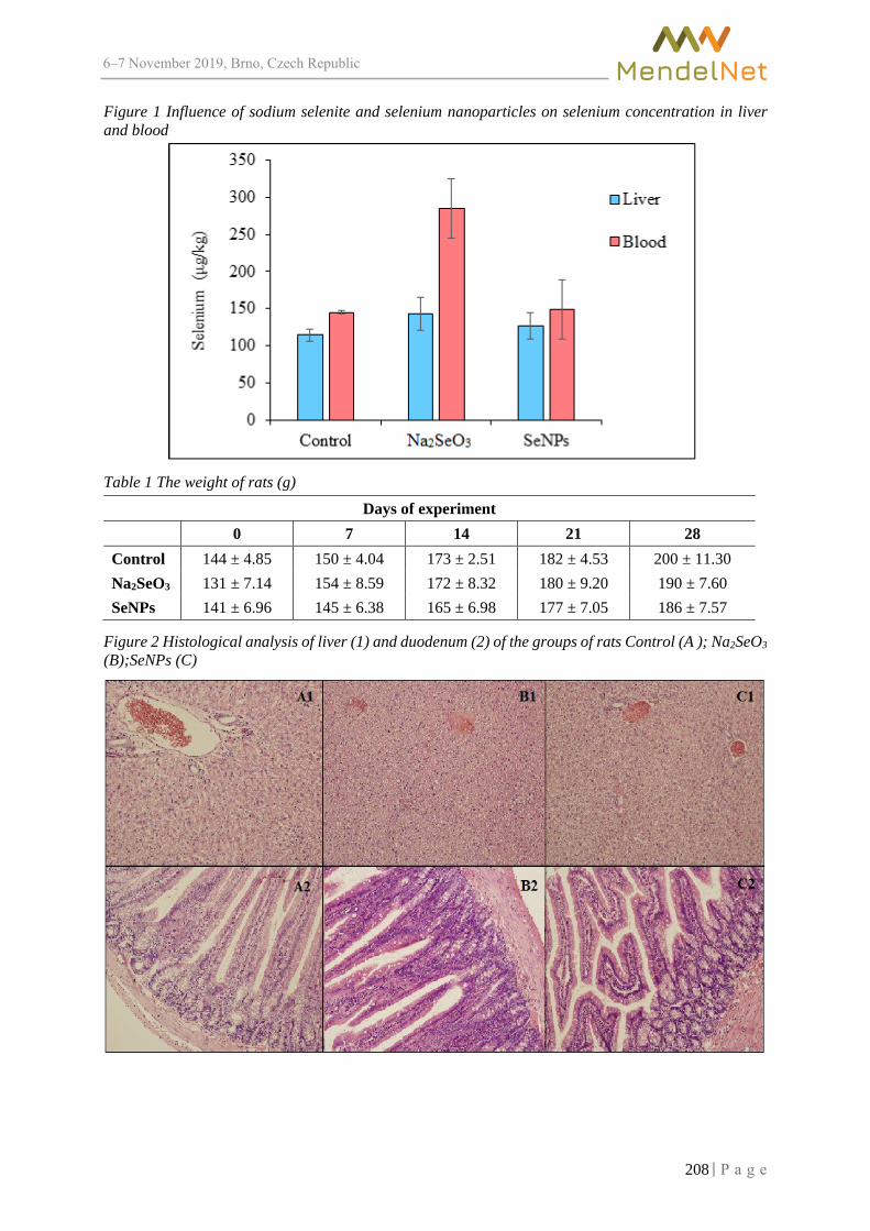
6–7 2019, Brno, Czech Republic
Figure 1 Influence of sodium selenite and selenium nanoparticles on selenium concentration in liver and blood
Table 1 The weight of rats (g)
Days of experiment 0 7 14 21 28
Control 144 ± 4.85 150 ± 4.04 173 ± 2.51 182 ± 4.53 200 ± 11.30 Na2SeO3 131 ± 7.14 154 ± 8.59 172 ± 8.32 180 ± 9.20 190 ± 7.60 SeNPs 141 ± 6.96 145 ± 6.38 165 ± 6.98 177 ± 7.05 186 ± 7.57
Figure 2 Histological analysis of liver (1) and duodenum (2) of the groups of rats Control (A ); Na2SeO3 (B);SeNPs (C)
208

6–7 2019, Brno, Czech Republic
The histological analysis of the liver and small intestine of rats were performed to assess possible effect of selenium nanoparticles on these organs. Results can be seen in Figure 2. Liver parenchyma of the control group of rats showed all-surface hepatodystrophy with significant portobiliary dilation (Figure 2 A1). Intestinal samples showed destruction of apical parts of the cartilage, mild autolytic lesion damage, numerous cup cells in crypts, sparse and lymphocytic cellulization in the stroma of the cartilage (Figure 2 A2). In the group of rats fed with Na2SeO3 all-surface hepatodystrophy with significant portobiliary dilation in liver samples was observed. In the liver tissue almost total absence of trabecular organization and foci of structural disintegration were found but without an apparent vital reaction (Figure 2 B1). In this group intestine samples showed usual segments of autolytic changes, frequent occurance of the cup cells and the inflammatory cellulization in the villi stroma (Figure 2 B2). In the SeNPs group, heavy hepatodystrophy with dilatation of portobilia was seen in the liver (Figure 2 C1). Intestinal samples in this group showed the usual state of autolytic damage. Also completely intact regions and numerous cup cells in crypts were found. Mild inflammatory cellulization in the villi stroma was present (Figure 2 C2). In a similar experiment, Keyhani et al. 2018 tested SeNPs in doses 2.5, 5, 10 and 20 mg/kg in mice and their effect of liver tissue without any significant effect. With dose of 30 mg/kg there was observed occasional focal mononuclear lymphocytic cellular infiltration around the portal and hepatocellular degeneration. However, this experiment lasted only two weeks.
CONCLUSION The concentration of selenium was increased in liver and also in blood compared with the control
group. The addition of selenium to the feed dose has an effect on increasing the amount of selenium in the liver and blood tissues. Histological analysis showed liver damage in all experimental groups (treated and non-treated) of rats. This can be likely caused by feeding with mono diet or stress. Intestinal tissue damage was most apparent in the group fed with Na2SeO3 but it cannot be argued that this was caused only by this compound. From the results of regular weighing of rats during the experiment, it is apparent that the addition of selenium nanoparticles has no significant effect on weight gain.
ACKNOWLEDGEMENTS The research was financially supported by the AF-IGA-2019-IP078.
REFERENCES Adadi, P. et al. 2019. Designing selenium functional foods and beverages: A review. Food Research International, 120: 708–725. Anjum N.A. et al. 2016. Transport phenomena of nanoparticles in plants and animals/humans. Environmental Research, 151: 233–243. Brown, K.M., Arthur, J.R. 2001. Selenium, selenoproteins and human health: a review. Public Health Nutrition, 4(2b): 593–599. Dogan H. et al. 2016. Determination of glutathione, selenium, and malondialdehyde in different edible mushroom species. Biological Trace Element Research, 174(2): 459–463. El-Demerdash, F.M., Nasr, H.M. 2014. Antioxidant effect of selenium on lipid peroxidation, hyperlipidemia and biochemical parameters in rats exposed to diazinon. Journal of Trace Elements in Medicine and Biology, 28(1): 89–93. Hoffmann, P.R., Berry, M.J. 2008. The influence of selenium on immune responses. Molecular Nutrition & Food Research, 52(11): 1273–1280. Horky, P. 2014. Influence of increased dietary selenium on glutathione peroxidase activity and glutathione concentration in erythrocytes of lactating sows. Annals of Animal Science, 14(4): 869–882. Horky, P. et al. 2016. Electrochemical Methods for Study of Influence of Selenium Nanoparticles on Antioxidant Status of Rats. International Journal of Electrochemical Science, 11(4): 2799–2824.
209

6–7 2019, Brno, Czech Republic
Keyhani, A. et al. 2018. Histopathological and Toxicological Study of Selenium Nanoparticles in BALB/C Mice. Entomology and Applied Science Letters 5(1): 31–35. Kursa J. et al. 2010. Iodine and selenium contents in skeletal muscles of red deer (Cervus elaphus), roe deer (Capreolus capreolus) and wild boar (Sus scrofa) in the Czech Republic. Acta Veterinaria Brno 79(3): 403–407. Wang H. et al. 2007. Elemental selenium at nano size possesses lower toxicity without compromising the fundamental effect on selenoenzymes: comparison with selenomethionine in mice. Free Radical Biology and Medicine 42(10): 1524–1533. Yazhiniprabha, M., Vaseeharan, B. 2019. In vitro and in vivo toxicity assessment of selenium nanoparticles with significant larvicidal and bacteriostatic properties. Materials Science and Engineering: C, 103: 109763.
210

FISHERIES AND HYDROBIOLOGY

6–7 2019, Brno, Czech Republic
Alteration in fatty acid profile in rainbow trout (Oncorhynchus mykiss) following the diet supplemented with clinoptilolite
Veronika Brumovska, Michal Sorf, Jan Mares Department of Zoology, Fisheries, Hydrobiology and Apiculture
Mendel University in Brno Zemedelska 1, 613 00 Brno
CZECH REPUBLIC
Abstract: The goal of this study was to investigate the effect of clinoptilolite as a feed supplement the fatty acid profile of rainbow trout muscle. A total of 180 rainbow trout were placed in twelve tanks of the volume of 160 l (15 fish in each). The duration of the experiment was 51 days. The industrially produced granular feed Biomar EFICO Enviro 920 Advance 4.5 mm was used as a base for the feed mixture. The clinoptilolite was mixed with commercial trout feed in five different rates (1%, 2%, 3%, 4% and 6%). The control group was without the addition of clinoptilolite. Lipids for determination of the fatty acid profile were extracted with methanol-chloroform solution according to Folch et al. (1957). The lipid analysis of muscle samples was performed individually from six fish in each group. We found significant differences in the fatty acid content of fish muscles, but no differences in the relative fatty acid content were confirmed. In general, the addition of 3% clinoptilolite was different from other treatments and controls. The lowest n-3/n-6 fatty acid ratio was found in the control, while the addition of clinoptilolite increased this ratio. For human nutrition, fish is indispensable as a valuable source of quality animal protein and fat. Fish fat is a rich in n-3 and n-6 fatty acids. The composition of the fatty acid groups depends on the diet, age or environmental conditions. The composition of fatty acid spectrum in fish can be adjusted by special diet with some additives such as clinoptilolite.
Key Words: fatty acid, clinoptilolite, rainbow trout, Oncorhynchus mykiss, feed additives
INTRODUCTION Zeolites are crystalline hydrated aluminosilicates of alkaline and alkaline earth metals (Mumpton
1999). Like all tectosilicates, zeolites have a three-dimensional bond of SiO4 and AlO4 tetrahedrons, which are interconnected by the sharing of peak oxygen. More than 60 types of zeolite present in nature have been discovered so far and more than 150 different types have been synthesised (Ghasemi et al. 2018). Natural zeolites arise where volcanic rocks and layers of ash react with alkaline groundwater. The most common mineral zeolites are analcite, chabazite, clinoptilolite, heulandite, mordenite, natrolite, phillipsite and stilbite. Since the discovery of these environmentally compatible materials, basic research of the properties of zeolite including ion exchange, adsorption and catalysis has been carried out in areas of high interest among researchers in various scientific disciplines including chemistry, construction, environmental engineering, jewellery, medicine, agriculture, aquaculture, soil remediation or wastewater treatment (Ghasemi et al. 2018).
Since the mid-sixties began zeolites often use in animal nutrition (Papaioannou et al. 2005). Zeolite supplements improve animal health, promote biomass production (Martin-Kleiner et al. 2001), reducing odour and associated pollution problems (Ghasemi et al. 2018). Numerous studies have shown that the addition of zeolite to feed leads to an improvement in the daily growth and feed conversion in pigs, calves, sheep (Pond and Mumpton 1984) and broilers (Feithiere et al. 1994).
Zeolites may be used in aquaculture in particular to capture ammonia and improve water quality on fish farms, hatcheries and transport tanks. Furthermore, due to its ion-exchange capability appears to be a promising alternative to biofiltration in freshwater fish farming systems (Ghasemi et al. 2018). Studies that have tested zeolites in fish farming have shown the possibility of their successful use as feed additives (Paritova et al. 2013). Danabas (2011) investigated the fatty acid profile of rainbow trout fed with clinoptilolite. He studied the lipid content and fatty acid composition of rainbow trout fed four
212

6–7 2019, Brno, Czech Republic
different ratios of clinoptilolite. The obtained results concluded that the composition of the fatty acid groups depends on the diet, age, environmental conditions and the effects of additives such as clinoptilolite.
For human nutrition, fish is indispensable as a valuable source of quality animal protein and fat. Fish proteins are a source of essential amino acids (methionine, cysteine, lysine, isoleucine, threonine and tryptophan) and their fat is a rich in omega-3 (C20:5n3, eicosapentaenoic acid and C22:6n3, docosahexaenoic acid) and omega-6 (C18:2n6, linoleic acid and C20:4n6, arachidonic acid) fatty acids (Danabas 2011). The composition of the spectrum of amino acids and fatty acids in fish can be adjusted by diet (Paritova et al. 2013).
The goal of this study was to investigate the effect of clinoptilolite as a feed supplement on the fatty acid profile of rainbow trout muscle.
MATERIAL AND METHODS Experimental conditions and materials
The research was carried out at the experimental facility of the Department of Fisheries and Hydrobiology of Mendel University in Brno. Recirculation system with its own biological filter Nexus 210 was used to perform the experiment (Figure 1), which ensured stable conditions throughout the experiment (water temperature 16.1 ± 1.4 °C, dissolved oxygen content 8.51 ± 1.01 mg/l and pH 7.86 ± 1.22). A total of 180 rainbow trout weighting 151.2 ± 2.6 g were used. The fish were placed in twelve tanks of the volume of 160 l. A total of 15 fish were placed in each aquarium. These fish were acclimatized for a period of three weeks before the beginning of the experiment. The duration of the experiment was 51 days.
Figure 1 Experimental equipment design and composition of feed mixtures
Description of the experimental diets The industrially produced granular feed Biomar EFICO Enviro 920 Advance 4.5 mm provided
by BioMar (Denmark) was used as a base for the feed mixture. Clinoptilolite produced by ZEOCEM, a.s. (Slovakia) was chosen as the zeolite addition to the fish diet. It consists of hydrated sodium-calcium aluminosilicate of sedimentary origin ≥ 80% and clay materials ≤ 20% (without fibers and quartz). The supplementary grain size is 0−50 μm. The clinoptilolite was mixed with commercial trout feed
Reserve tank
100% EFICO Enviro 920
100% EFICO Enviro 920
99% EFICO Enviro 920
98% EFICO Enviro 920
97% EFICO Enviro 920
96% EFICO Enviro 920
1st repetition
2nd repetition
94% EFICO Enviro 920
1% Clinoptilolite 2% Clinoptilolite 3% Clinoptilolite 4% Clinoptilolite 6% Clinoptilolite
Control 1% 2% 3% 4% 6%
98% EFICO Enviro 920
2% Clinoptilolite
6%4%3%2%
UV lighter
Biofilter Nexus 210
99% EFICO Enviro 920
1% Clinoptilolite
1% Control
97% EFICO Enviro 920
3% Clinoptilolite
96% EFICO Enviro 920
4% Clinoptilolite
94% EFICO Enviro 920
6% Clinoptilolite
213
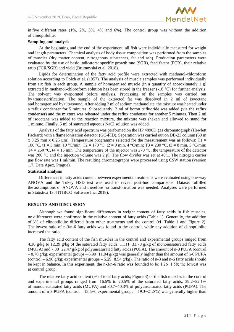
6–7 2019, Brno, Czech Republic
in five different rates (1%, 2%, 3%, 4% and 6%). The control group was without the addition of clinoptilolite. Sampling and analysis
At the beginning and the end of the experiment, all fish were individually measured for weight and length parameters. Chemical analysis of body tissue composition was performed from the samples of muscles (dry matter content, nitrogenous substances, fat and ash). Production parameters were evaluated by the use of basic indicators: specific growth rate (SGR), feed factor (FCR), their relative ratio (FCR/SGR) and yield (Brumovská et al. 2018).
Lipids for determination of the fatty acid profile were extracted with methanol-chloroform solution according to Folch et al. (1957). The analysis of muscle samples was performed individually from six fish in each group. A sample of homogenised muscle (in a quantity of approximately 1 g) extracted in methanol-chloroform solution has been stored in the freezer (-18 °C) for further analysis. The solvent was evaporated before analysis. Processing of the samples was carried out by transesterification. The sample of the extracted fat was dissolved in 2 ml of isooctane and homogenised by ultrasound. After adding 2 ml of sodium methanolate, the mixture was heated under a reflux condenser for 5 minutes. Subsequently, 2 ml of boron trifluoride was added (via the reflux condenser) and the mixture was reheated under the reflux condenser for another 5 minutes. Then 2 ml of isooctane was added to the reaction mixture, the mixture was shaken and allowed to stand for 1 minute. Finally, 5 ml of saturated aqueous NaCl solution was added.
Analysis of the fatty acid spectrum was performed on the HP 4890D gas chromatograph (Hewlett Packard) with a flame ionisation detector (GC-FID). Separation was carried out on DB-23 column (60 m x 0.25 mm x 0.25 µm). Temperature programme selected for the measurement was as follows: T1 = 100 °C, t1 = 3 min, 10 °C/min; T2 = 170 °C, t2 = 0 min, 4 °C/min; T3 = 230 °C, t3 = 8 min, 5 °C/min; T4 = 250 °C, t4 = 15 min. The temperature of the injector was 270 °C, the temperature of the detector was 280 °C and the injection volume was 2 µl. The flow divider was set at 40:1. The nitrogen carrier gas flow rate was 1 ml/min. The resulting chromatographs were processed using CSW station (version 1.7, Data Apex, Prague). Statistical analysis
Differences in fatty acids content between experimental treatments were evaluated using one-way ANOVA and the Tukey HSD test was used to reveal post-hoc comparisons. Dataset fulfilled the assumptions of ANOVA and therefore no transformation was needed. Analyses were performed in Statistica 13.4 (TIBCO Software Inc. 2018).
RESULTS AND DISCUSSION
Although we found significant differences in weight content of fatty acids in fish muscles, no differences were confirmed in the relative content of fatty acids (Table 1). Generally, the addition of 3% of clinoptilolite differed from other treatments and the control (cf. Table 1 and Figure 2). The lowest ratio of n-3/n-6 fatty acids was found in the control, while any addition of clinoptilolite increased the ratio.
The fatty acid content of the fish muscles in the control and experimental groups ranged from 4.36 g/kg to 12.29 g/kg of the saturated fatty acids, 11.11−33.70 g/kg of monounsaturated fatty acids (MUFA) and 7.88−22.47 g/kg of polyunsaturated fatty acids (PUFA). The amount of n-3 PUFA (control – 8.70 g/kg; experimental groups – 6.99−11.94 g/kg) was generally higher than the amount of n-6 PUFA(control – 6.96 g/kg; experimental groups – 5.29−8.54 g/kg). The ratio of n-3 and n-6 fatty acids should be kept in balance. In this experiment, the n-3/n-6 ratio was founded to be 1.26−1.58; the lowest was at control group.
The relative fatty acid content (% of total fatty acids; Figure 3) of the fish muscles in the control and experimental groups ranged from 16.5% to 20.5% of the saturated fatty acids, 39.2−52.1% of monounsaturated fatty acids (MUFA) and 30.7−40.3% of polyunsaturated fatty acids (PUFA). The amount of n-3 PUFA (control – 18.5%; experimental groups – 19.3−21.8%) was generally higher than
214
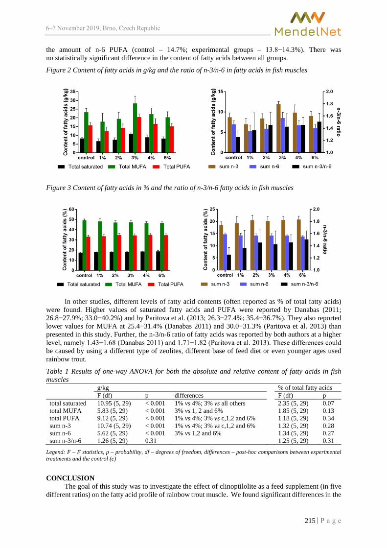
6–7 2019, Brno, Czech Republic
the amount of n-6 PUFA (control – 14.7%; experimental groups – 13.8−14.3%). There was no statistically significant difference in the content of fatty acids between all groups.
Figure 2 Content of fatty acids in g/kg and the ratio of n-3/n-6 in fatty acids in fish muscles
Figure 3 Content of fatty acids in % and the ratio of n-3/n-6 fatty acids in fish muscles
In other studies, different levels of fatty acid contents (often reported as % of total fatty acids)
were found. Higher values of saturated fatty acids and PUFA were reported by Danabas (2011; 26.8−27.9%; 33.0−40.2%) and by Paritova et al. (2013; 26.3−27.4%; 35.4−36.7%). They also reported lower values for MUFA at 25.4−31.4% (Danabas 2011) and 30.0−31.3% (Paritova et al. 2013) than presented in this study. Further, the n-3/n-6 ratio of fatty acids was reported by both authors at a higher level, namely 1.43−1.68 (Danabas 2011) and 1.71−1.82 (Paritova et al. 2013). These differences could be caused by using a different type of zeolites, different base of feed diet or even younger ages used rainbow trout.
Table 1 Results of one-way ANOVA for both the absolute and relative content of fatty acids in fish muscles
g/kg % of total fatty acids F (df) p differences F (df) p total saturated 10.95 (5, 29) < 0.001 1% vs 4%; 3% vs all others 2.35 (5, 29) 0.07 total MUFA 5.83 (5, 29) < 0.001 3% vs 1, 2 and 6% 1.85 (5, 29) 0.13 total PUFA 9.12 (5, 29) < 0.001 1% vs 4%; 3% vs c,1,2 and 6% 1.18 (5, 29) 0.34 sum n-3 10.74 (5, 29) < 0.001 1% vs 4%; 3% vs c,1,2 and 6% 1.32 (5, 29) 0.28 sum n-6 5.62 (5, 29) < 0.001 3% vs 1,2 and 6% 1.34 (5, 29) 0.27 sum n-3/n-6 1.26 (5, 29) 0.31 1.25 (5, 29) 0.31
Legend: F – F statistics, p – probability, df – degrees of freedom, differences – post-hoc comparisons between experimental treatments and the control (c)
CONCLUSION The goal of this study was to investigate the effect of clinoptilolite as a feed supplement (in five
different ratios) on the fatty acid profile of rainbow trout muscle. We found significant differences in the
215

6–7 2019, Brno, Czech Republic
fatty acid content of fish muscles, but no differences in the relative fatty acid content were confirmed. In general, the addition of 3% clinoptilolite was different from other treatments and controls. The lowest n-3/n-6 fatty acids ratio was found in the control, while the addition of clinoptilolite increased this ratio. A negative influence of clinoptilolite has not been determined.
According to the results of the experiment, the percentage content of monounsaturated fatty acids in rainbow trout muscles was higher than in the findings of Danabas (2011) and Paritova et al. (2013). Furthermore, the percentage content of saturated fatty acids, polyunsaturated fatty acids and the ratio of n-3/n-6 fatty acids were lower than for Danabas (2011) and Paritova et al. (2013). These differences in detected values may be different due to the age of the tested fish, different composition of feed diet or by using of different zeolite species.
ACKNOWLEDGEMENTS This study was financially supported by the grant no. AF-IGA-IP-2018/052. The results and outputs were processed using the equipment financed by the project OP VaVpI CZ.1.05/4.1.00/04.0135 Teaching and research capacities for biotechnology disciplines and infrastructure expansion. This study was supported by the project PROFISH CZ.02.1.01/0.0/0.0/16_019/0000869. The project is financed by European Regional Development Fund in the Operational Programme Research, Development and Education and The Czech Ministry of Education, Youth and Sports.
REFERENCES Brumovská, V. et al. 2018. Effect of the addition of zeolite to the rainbow trout diet. In Proceedings of International PhD Students Conference MendelNet 2018 [Online]. Brno, Czech Republic, 7 November, Brno: Mendel University in Brno, Faculty of AgriSciences, pp. 155−159. Available at: https://mnet.mendelu.cz/mendelnet2018/mnet_2018_full.pdf [2019-07-29]. Danabas, D. 2011. Fatty acids profiles of rainbow trout (Oncorhynchus mykiss Walbaum, 1792), fed with zeolite (clinoptilolite). Journal of Animal and Plant Sciences, 21(3): 561−565. Feithiere, R. et al. 1994. The utilization of sodium in sodium zeolite A by broilers. Poultry Science, 73(1): 118−121. Folch, J. et al. 1957. A simple method for the isolation and purification of total lipides from animal tissues. The Journal of Biological Chemistry, 226(1): 497−509. Ghasemi, Z. et al. 2018. Application of zeolites in aquaculture industry: a review. Reviews in Aquaculture, 10(1): 75−95. Martin-Kleiner, I. et al. 2001. The effect of the zeolite clinoptilolite on serum chemistry and haematopoiesis in mice. Food and Chemical Toxicology, 39(7): 717−727. Mumpton, F.A. 1999. La roca magica: Uses of natural zeolites in agriculture and industry. Proceedings of the National Academy of Sciences, 96(7): 3463−3470. Papaioannou, D. et al. 2005. The role of natural and synthetic zeolites as feed additives on the prevention and/or the treatment of certain farm animal diseases. A review. Microporous and Mesoporous Materials, 84(1−3): 161−170. Paritova, A. et al. 2013. The influence of chankanay zeolites as feed additives on the chemical, biochemical and histological profile of the rainbow trout (Oncorhynchus mykiss). Journal of Aquaculture Research and Development, 5(1): 205. Pond, W.G., Mumpton F.A. 1984. Zeo-agriculture: Use of natural zeolites in agriculture and aquaculture. 1st ed., Boulder, Colorado, USA: Westview Press Inc. TIBCO Software Inc. 2018. Statistica (data analysis software system), version 13. http://tibco.com.
216

6–7 2019, Brno, Czech Republic
The effect of polycyclic musk compound on fish organism
Nikola Hodkovicova1,2, Jana Blahova1, Vladimira Enevova1, Lucie Plhalova1, Veronika Doubkova1, Petr Marsalek1, Ales Franc3, Emma Fiorino4, Caterina Faggio4, Zdenka
Svobodova1 1Department of Animal Protection, Welfare and Behaviour University of Veterinary and Pharmaceutical Sciences Brno
Palackeho tr. 1946/1, 612 42 Brno 2Department of Immunology
Veterinary Research Institute, Brno Hudcova 296/70, 621 00 Brno 3Department of Pharmaceutics
University of Veterinary and Pharmaceutical Sciences Brno Palackeho tr. 1946/1, 612 42 Brno
CZECH REPUBLIC 4Department of Biological and Environmental Sciences
University of Messina Piazza Pugliatti 1, 981 22 Messina
ITALY
Abstract: The effect of tonalide, known as polycyclic musk compound, was studied on rainbow trout. Total of 65 individuals were acclimatized and consequently exposed to two tonalide concentrations – one environmentally-relevant (854 µg/kg); the second one 10× higher for evaluation of dose-dependent effect (8,699 µg/kg). The tonalide was incorporated into feed and fish were fed twice a day in amount 1% of their body weight. After six weeks of experimental phase, fish were sampled for gaining data for the biometrical, haematological, biochemical and oxidative stress analysis and for evaluation of endocrine disruption using plasma vitellogenin. In conclusion, the biochemical and oxidative stress parameters did not revealed any changes. In haematological profile, only the haematocrit was increased as reaction on both concentrations of tonalide. The endocrine disruption caused by tonalide was not observed in rainbow trout.
Key Words: tonalide, endocrine disruption, oxidative stress, Oncorhynchus mykiss
INTRODUCTION The musk compounds are synthetic substances, which are frequently used in perfumery
as an odour carrier in various anthropogenic industries (personal hygiene products, washing powders and household cleaners, candles etc.; Nakata et al. 2015). Due to their ubiquitous and worldwide usage, they have an ability to enter to the surface water and sediment, cause water pollution and have effects on non-target water organisms (Wong et al. 2019). Some of the musk compound are known to be weakly estrogenic (Luckenbach and Epel 2005) or, in contrast, anti-estrogenic (Schreurs et al. 2004), some are forbidden due to their bioaccumulation and persistence in the environment or various neurotoxic effects (Heberer 2002).
Tonalide (or AHTN) belongs to polycyclic musk compounds (PMC), which are one of the most used group nowadays (Vallecillos et al. 2015). The tonalide and galaxolide are the most produced PMC’s representatives: for example, the worldwide production of tonalide was 5,000 tons in 2004 (Lange et al. 2015). The toxicity of PMC’s is believed to be relatively low, however, the long exposure revealed to have an anti-estrogenic/estrogenic activity and cause endocrine disruption (Schreurs et al. 2004, Luckenbach and Epel 2005, Simmons et al. 2010). The environmental concentration of tonalide was found to be high in the waste water treatment (WWT) influent, where the concentration was measured between 49.9 and 64.6 µg/l (Chen et al. 2007, Vallecillos et al. 2015). The musk compounds
217

6–7 2019, Brno, Czech Republic
in water are not completely purified at WWT. The cleaning process is incomplete and depends on the technology; for tonalide was recorded not higher than 84.4% (Ren et al. 2013).
The aim of our study was to evaluate whether the tonalide oral exposure could affect the haematological and biochemical indices in fish. Moreover, the selected oxidative stress indices and vitellogenin (VTG) in plasma were measured.
MATERIAL AND METHODS In this experiment, the total of 65 individuals of rainbow trout (Oncorhynchus mykiss, Walbaum
1792) was implied. Fish (total length 32.2 ± 2.2 cm, weight 516.8 ± 102.9 g) were acclimatized for two weeks and fed with commercial pellets EFICO Enviro 920 Advance (BioMar, Denmark; crude protein 38–41%, crude lipid 32–35%, crude fiber 0.9–2.8%, carbohydrates 14–17%, ash 4–7%, total phosphorus 0.9%) twice a day in amount of 1% of their body weight. Tanks (volume = 1000 l) were connected to recirculation system and appropriate conditions of water were monitored daily, as follows: temperature 15.5 ± 0.8°C, pH 8.2 ± 0.2, dissolved oxygen 82.3 ± 8.2%, ammonia 0.24 ± 0.1 mg/l. After acclimatization, the experimental phase in duration six weeks followed. Fish were divided into three groups – control (n = 21), AHTN1 (n = 17) and AHTN2 (n = 20), while the tonalide was tested in two concentrations incorporated into feed – the first concentration was environmentally-relevant: 854 µg/kg (AHTN1); the second concentration was 8,699 µg/kg (AHTN2). Feed for the control group was prepared in the same way, however without the use of tonalide. The determination of tonalide concentration in feed granules was performed using gas chromatography tandem mass spectrometry.
After experimental phase, fish were sampled for various analysis. Firstly, every fish was bled from the caudal vein (blood stabilized with sodium heparin 50 IU/ml) and consequently stunned with the blow in the head, killed by spinal transection and dissected. Every fish was weighed and measured for gaining the biometrical data. For haematological analysis, the white (WBC) and red blood cell count (RBC), haemoglobin (Hb), haematocrit (PCV) and calculation of mean erythrocyte volume (MCV), mean erythrocyte haemoglobin (MCH) and mean corpuscular haemoglobin concentration (MCHC) was performed.
One half of every heparinized blood sample was centrifuged (800×g, 4 °C, 10 min) for gaining the plasma in whom the albumin (ALB), ammonia (NH3), total protein (TP), glucose (GLU), triglycerides (TG), cholesterol (CHOL), lactate (LACT), calcium (Ca), phosphorus (PHOS), alkaline phosphatase (ALP), alanine aminotransferase (ALT), aspartate aminotransferase (AST) and lactate dehydrogenase (LDH) were evaluated. The activity of ceruloplasmin (CP) and ferric reducing antioxidant power (FRAP) parameters were evaluated in plasma samples as representative of oxidative stress, moreover, the levels of VTG were detected for possible endocrine disruption. The biochemical analysis was performed using the commercial kit (BioVendor, Czechia) and biochemical analyser Konelab 20i (Thermo Fisher Scientific Inc., USA) following the manufacturer’s instructions. The CP was determined spectrophotometrically using the Varioskan Flash Spectral Scanning Multimode Reader (Thermo Scientific Inc., USA). All haematological and biochemical analysis were performed according to Svobodova et al. (2012) methodology for fish.
Statistical analysis was performed using the statistical software Unistat for Excel 5.6 (Unistat Ldt.). Data were tested for normality distribution using the Shapiro-Wilk. The ANOVA and Tukey-HSD test were implied in data with normal distribution. The Kruskal-Wallis nonparametric test was applied in results with non-normal distribution. For statistically significant difference (p<0.05 and p<0.01), the control, AHTN1 and AHTN2 group were compared. Data are expressed as mean ± standard deviation.
RESULT AND DISCUSSION No mortality of fish was observed during the experiment. An overview of the changes
in haematological profile after induction with both tonalide concentrations in compare to control group without tonalide exposure is given in Table 1. Significant change was found for PCV, where the lower and higher dose of tonalide caused increase of this parameter. Consequently, the MCV, MCH and MCHC significantly differ as well, because their calculation is based on the PCV result. The increase of PCV could be caused by stress reaction (Barton 2002).
218

6–7 2019, Brno, Czech Republic
Table 1 The results of haematological indices after oral tonalide exposure. Means in the same row lacking a common letter of superscript (a, b) differ significantly (<0.05, <0.01)
Parameter [unit] Control AHTN1 AHTN2 RBC [T /l] 1.37 ± 0.06a 1.54 ± 0.05a 1.46 ± 0.06a Hb [g/l] 83.87 ± 3.08a 80.72 ± 1.73a 78.21 ± 2.25a PCV [l/l] 0.38 ± 0.03b 0.45 ± 0.02a 0.44 ± 0.02ab MCV [fl] 262.07 ± 11.75b 295.90 ± 11.44ab 307.18 ± 11.44a MCH [pg] 60.97 ± 2.72a 52.92 ± 1.98b 54.45 ± 1.87ab MCHC [g/l] 0.24 ± 0.03a 0.18 ± 0.01b 0.18 ± 0.01ab WBC [G/l] 18.03 ± 1.43a 19.54 ± 2.17a 17.36 ± 1.45a
The results of biochemical indices are given in Table 2. There was not observed any significant change when compared to control group. The selected oxidative stress parameters, CP and FRAP, were not significantly differed from the control, also. The result of our previous experiment with tonalide on zebrafish (Danio rerio, Hamilton 1822) showed that 28-day long exposure can cause the alteration of enzymes known to be an oxidative stress markers (Blahova et al. 2018). However, submitted study did not confirmed these results.
Table 2 The results of biochemical indices after oral tonalide exposure. Means in the same row lacking a common letter of superscript (a,b) differ significantly (<0.05, <0.01)
Parameter [unit] Control AHTN1 AHTN2 ALB [g/l] 18.21 ± 0.86a 20.24 ± 0.60a 18.58 ± 0.69a NH3 [µmol/l] 240.30 ± 16.24a 245.17 ± 18.09a 262.13 ± 21.52a TP [g/l] 36.37 ± 1.32a 39.68 ± 0.96a 36.41 ± 1.06a GLU [mmol/l] 4.28 ± 0.17a 4.89 ± 0.20a 4.20 ± 0.09a TG [mmol/l] 2.54 ± 0.31a 4.29 ± 0.67a 3.62 ± 0.51a CHOL [mmol/l] 7.47 ± 0.38a 8.49 ± 0.26a 7.73 ± 0.37a LACT [mmol/l] 2.36 ± 0.27a 2.48 ± 0.32a 2.58 ± 0.26a Ca [mmol/l] 2.56 ± 0.04a 2.69 ± 0.05a 2.64 ± 0.05a PHOS [mmol/l] 3.93 ± 0.10a 3.98 ± 0.09a 4.07 ± 0.09a ALP [µkat/l] 1.06 ± 0.14a 1.52 ± 0.17a 1.08 ± 0.09a ALT [µkat/l] 0.29 ± 0.04a 0.23 ± 0.02a 0.23 ± 0.01a AST [µkat/l] 6.30 ± 0.76a 5.80 ± 0.44a 6.08 ± 0.28a LDH [µkat/l] 12.04 ± 1.03a 9.88 ± 0.78a 12.46 ± 1.76a CP [∆A/min×10 000] 113.3 ± 3.3a 120.1 ± 5.1a 114.1 ± 4.2a FRAP [µmol/l] 748.7 ± 42.6a 759.6 ± 22.0a 805.4 ± 22.7a
As a marker of possible endocrine disruption, the VTG was selected for our study. The VTG is a precursor protein of egg yolk and is synthetized only in female liver. The juveniles and males have the gene for VTG synthesis, nevertheless, the expression is not undertaken in physiological conditions. However, exposure to endocrine disruptors could start the VTG synthesis (Jobling et al. 1996). We examined the VTG in plasma of the males from control, AHTN1 and AHTN2 group. As our internal control, seven females were subjected to VTG analysis: the VTG concentration was detected between 41,200.2 and 5,741,303.6 ng/ml while the percentage of positive samples was 100%. Surprisingly, in control group composed of males, the level of positive samples was 19%. In lower tonalide concentration the positive samples were present in 29% cases, while in higher concentration only in 15% cases. The high percentage of positive samples in male control groups was probably caused by the fish origin. Fish for this experiment were taken from the Skalni Mlyn hatchery and it is obvious that even in natural water sources the endocrine disruptors are present. However, the VTG levels in male control group are low and not significantly different from the AHTN1 and AHTN2 groups. In conclusion, Yamauchi et al. (2008) reported that tonalide has a potential to cause endocrine disruption. However, in our study the percentage of positive samples was higher in male control than in the highest tested tonalide concentration, thus the endocrine disruption was not verified. The result of VTG analysis are reported in Table 3.
219

6–7 2019, Brno, Czech Republic
Table 3 Concentration of VTG in ng/ml in male fish plasma samples Group Percentage of positive samples VTG [ng/ml] Control 19 303.2–985.9 AHTN1 29 173.1–945.0 AHTN2 15 361.9–609.8
CONCLUSION In conclusion, the result of our experiment showed that the musk compound tonalide have
no effect on haematological and biochemical indices, except the PCV, which increased after exposure to both tested concentrations probably as stress marker. The oxidative stress plasma parameters, CP and FRAP, did not revealed any changes as well. The VTG results were positive not only after tonalide induction, but also for control male groups and the endocrine disruption was not confirmed.
ACKNOWLEDGEMENTS The research was financially supported by the Internal Grant Agency [IGA VFU 248/2015/FVHE] and by the ERDF/ESF "PROFISH" [CZ.02.1.01/0.0/0.0/16_019/0000869].
REFERENCES Barton, B.A. 2002. Stress in fishes: A diversity of responses with particular reference to changes in circulating corticosteroids. Integrative and Comparative Biology, 42(3): 517–525. Blahova, J., Divisova, L., Plhalova, L., Enevova, V., Hostovsky, M., Doubkova, V., Marsalek, P., Fictum, P., Svobodova, Z. 2018. Multibiomarker responses of juvenile stages of zebrafish (Danio rerio) to subchronic exposure to polycyclic muck tonalide. Archives of Environmental Contamination and Toxicology, 74(4): 568–576. Chen, D., Zeng, X., Sheng, Y., Bi, X., Gui, H., Sheng, G., Fu, J. 2007. The concentrations and distribution of polycyclic musks in a typical cosmetic plant. Chemosphere, 66(2): 252–258. Heberer, T. 2002. Occurrence, fate, and assessment of polycyclic musk residues in the aquatic environment of urban areas – a review. Acta Hydrochimica et Hydrobiologica, 30(5-6): 227–243. Jobling, S., Sheahan, D., Osborne, J.A., Matthiessen, P., Sumpter, J. P. 1996. Inhibition of testicular growth in rainbow trout (Oncorhynchus mykiss) exposed to estrogenic alkylphenolic chemicals. Environmental Toxicology and Chemistry, 15(2): 194–202. Lange, C., Kuch, B., Metzger, J.W. 2015. Occurrence and fate of synthetic musk fragrances in a small German river. Journal of Hazardous Materials, 282: 34–40. Luckenbach, T., Epel, D. 2005. Nitromusk and polycyclic musk compounds as long-term inhibitors of cellular xenobiotic defense systems mediated by multidrug transporters. Environmental Health Perspectives, 113(1): 17–24. Nakata, H., Hinosaka, M., Yanagimoto, H. 2015. Macrocyclic-, polycyclic-, and nitro musks in cosmetics, household commodities and indoor dusts collected from Japan: implications for their human exposure. Ecotoxicology and Environmental Safety, 111: 248–255. Ren, Y., Wei, K., Liu, H., Sui, G., Wang, J., Sun, Y., Zheng, X. 2013. Occurrence and removal of selected polycyclic musks in two sewage treatment plants in Xi'an, China. Frontiers of Environmental Science & Engineering, 7(2): 166–172. Schreurs, R.H.M.M., Legler, J., Artola-Garicano, E., Sinnige, T.L., Lanser, P.H., Seiner, W., van der Burg, B. 2004. In vitro and in vivo antiestrogenic effects of polycyclic musks in zebrafish. Environmental Science & Technology, 38(4): 997–1002. Simmons, D.B.D., Marlatt, V.L., Trudeau, V.L., Sherry, J.P., Metcalfe, C.D. 2010. Interaction of Galaxolide® with the human and trout estrogen receptor-α. Science of the Total Environment, 408(24): 6158–6164.
220

6–7 2019, Brno, Czech Republic
Svobodova, Z., Pravda, D., Modra, H. 2012. Methods of Haematological Examination of Fish. 1st ed. Czech Republic: University of South Bohemia in České Budějovice. (In Czech). Vallecillos, L., Borrull, F., Pocurull, E. 2015. Recent approaches for the determination of synthetic musk fragrances in environmental samples. TrAC Trends in Analytical Chemistry, 72: 80–92. Wong, F., Robson, M., Melymuk, L., Shunthirasingham, C., Alexandrou, N., Shoeib, M., Luk, E., Helm, P., Diamond, M., Hung, H. 2019. Urban sources of synthetic musk compounds to the environment. Environmental Science: Processes & Impacts, 21(1): 74–88. Yamauchi, R., Ishibashi, H., Hirano, M., Mori, T., Kim, J.W., Arizono, K. 2008. Effects of synthetic polycyclic musks on estrogen receptor, vitellogenin, pregnane X receptor, and cytochrome P450 3A gene expression in the liver of male medaka (Oryzias latipes). Aquatic Toxicology, 90(4): 261–268.
221

6–7 2019, Brno, Czech Republic
The ability of a bacterial-enzymatic preparation to break down the organic fraction of pond sediments
Barbora Musilova, Radovan Kopp, Marija RadojicicDepartment of Zoology, Fisheries, Hydrobiology and Apiculture
Mendel University in Brno Zemedelska 1, 613 00 Brno
CZECH REPUBLIC
Abstract: The high amount of sediments in ponds is a common problem in Czechia. In most cases, pond owners are not able to manage this problem neither financially, nor organizationally or professionally. An innovative solution could be a product that is able to decompose organic deposits directly on the bottom and in the water column using natural, unmodified microbial assemblages. The aim of the experiment was to evaluate the ability of a bacterial-enzymatic preparation to decompose pond sediments and to investigate the influence of this preparation on the quality and overall composition of sediments and water. According to our experiment the decomposition of pond sediments during the application of the preparation is not demonstrable. Our experiment did not confirm any significant effect of the product on the quality of the water in aquatic environment during the application of the products. However, the experiment was carried out under laboratory conditions, the results of this experiment do not fully correspond to the results that can be obtained in ponds under natural conditions.
Key Words: bacterial-enzymatic preparation, organic sediment, quality of pond water
INTRODUCTION The sediment reaches the ponds in various ways. In the case of flow-through ponds, this mainly
concerns the transport of soil particles through the feeding watercourse. Furthermore, it may reach the pond due to a bank abrasion or biomass breakdown directly in the pond water space (Mikšíková et al. 2012). The largest inflow of soil particles into the pond is caused by run-off from agricultural lands as a result of increased erosion in the basin, which is caused by inappropriate agricultural land management. Increased deposition of sediments at the bottom of ponds leads to their grounding, which limits the pond in the processes of removing pollution and the pond has subsequently a reduced ability to produce fish (Kubík 2011, Plaster 2014). The accumulation of organic matter in the pond is undesirable as it can accumulate to a level where the yield of fish can be adversely affected due to the release of toxic substances such as hydrogen sulfite and nitrite. High deposition of organic substances also results in high oxygen consumption, which can lead to depletion of oxygen mesocosmicand thus further reduce fish production (Boyd 1998, Muendo et al. 2014).
Pond sediments are mined and stored in piles; in many cases they are labelled as pond mud. Extracted sediments from ponds, reservoirs and watercourses are then regarded as waste, but the disposal of sediments in natural systems poses a threat to the environment in the form of wasting valuable nutrients (Havlíček et al. 1969, Muendo et al. 2014). Pond sediments contain high amounts of nutrients and organic substances, reported to be several times higher than in fertile ground. However, their use mesocosmicin agriculture is very low (Havlíček et al. 1969).
PTP Plus is a mixture of bacterial spores and enzymes that can be purchased from Baktoma Ltd. The product should decompose the organic content of sediments in ponds and reservoirs. It is a concentrate of spores and endospores of specially selected and targeted breeding strains of native soil bacteria that exhibit specific properties, such as the ability to increase production of the desired enzyme. According to the manufacturer, all strains of bacteria present in the mixture are non-pathogenic and naturally occurring, neither are they genetically altered or modified.
222
6–7 2019, Brno, Czech Republic
Shortly after the introduction of the product into the aquatic environment, spores and endospores should revive and feed the organic sediment. Regular use of PTP Plus should reproduce bacteria, resulting in continuous cleaning of ponds and lakes. The manufacturer of this preparation states that after a few weeks of use of the preparation, biological equilibrium will occur in the aquatic environment, thus reducing the amount of organic deposits and turbidity at the bottom and in the water column. Furthermore, the phosphorus and chlorophyll a content in the water column should be significantly reduced and the oxygen content of the water should be increased (BAKTOMA 2017).
MATERIAL AND METHODS Pond sediment from Pohořelický pond (Pohořelice nad Jihlavou, South Moravian region) was
used in the experiment. The pond is eutrophic and the sediment was taken after the spring fish harvest on April 3, 2019, namely from the fishing ground in the surface layer of 0–30 cm.
Sediment layers were deposited in nine tanks at a height of approx. 20 cm (approx. 115 kg of sediment per tank) and supplemented with aged drinking water. The tanks were placed in a room with unrestricted daylight and with a temperature ranging from 20.2 °C to 34.1 °C, the average temperature in April was 21.8 °C, in May 23.7 °C, in June 29.3 °C and 28.1 °C in July. On April 16, 2019 the bacterial-enzymatic preparation PTP Plus was applied to three tanks (tank No. 2, 5 and 8) with the sediment-water mixture prepared in the concentration according to the instructions recommended by the manufacturer. In three additional tanks (tanks number 3, 6 and 9) the preparation was applied at a concentration ten times higher. The remaining three tanks (tank number 1, 4 and 7) mesocosmicwith no PTP Plus addition served as a control. Here we added only pure zeolite. Zeolite serves as a carrier for the active ingredient of PTP Plus. The dosage of the product as recalculated mesocosmicto the water surface of the tanks was as follows:
Week 1 – application of 100 g Weeks 2 and 3 – application of 75 g per week Weeks 4 and 5 – application of 50 g per week Weeks 6 and 7 – application of 25 g per week To maintain the amount of water, the tanks were replenished every second week with 30 litres
mesocosmicof aged water. The basic physico-chemical parameters were measured five times a week mesocosmicin each tank. We measured the amount of dissolved oxygen, temperature, pH (Hach HQ40d) and conductivity (Hanna combo). A water sample was taken from each tank for chemical analysis mesocosmiceach week prior to application of the PTP Plus. Samples were taken into 0.5 l plastic bottles, about 20 cm below the tank surface. The following parameters were monitored: chemical oxygen consumption (CODCr), total nitrogen, phosphorus and iron, ammonium nitrogen, nitrites, nitrates, phosphates, chlorides, chlorophyll a concentration, acid neutralizing capacity and calcium content. Chemical parameters were determined by standard methods according to Horáková (2003). PTP Plus was first applied on 16/04/2019 according to the instructions above. After seven weeks (04/06/2019) from the first application, a part of the sediments was taken from the tanks and processed, the dry matter of the samples was determined and the soil extract was prepared using Aqua regia. The total phosphorus, calcium and iron content was determined from the extracts. The proportion of organic substances mesocosmicbefore and after application was also determined. Chemical parameters of extracts were determined by standard methods according to Horáková (2003) and Zbíral (2011). The results mesocosmicare expressed in dry weight units of the sediments.
RESULTS This chapter shows the results of the most important parameters, dissolved oxygen, total
phosphorus, organic substances and chlorophyll a. Figure 1 shows the dissolved oxygen content of all nine tanks. The measurements were taken five
times a week for the duration of application and one week after the application, i.e. 8 weeks, from which the weekly average was calculated. Oxygen was measured once a week before (11/04/2019) and once five weeks after the last dose (02/07/2019). The amount of dissolved oxygen was relatively balanced in all tanks for the first three weeks. Especially in the fifth and sixth week of application
223

6–7 2019, Brno, Czech Republic
of the preparation there was a significant decrease in the oxygen content, but again in all tanks. Significantly the lowest values of measured oxygen were recorded, with the exception of the ninth tank, on the last day of the measurement, i.e. five weeks after the last dose of the preparation. There was no significant effect of PTP Plus on the amount of oxygen in the water. Other measured physico-chemical parameters (temperature, pH, conductivity) were relatively balanced in all tanks before, during and after application.
Figure 1 Dissolved oxygen saturation in tanks with a mixture of sediment and water. Each point represents week average.
Figure 2 A) Total phosphorus concentration in water in tanks B) Total phosphorus concentration in sediments
In Figure 2 A, the total phosphorus concentration in water is recorded in all nine reservoirs during application and five weeks after the last dose of product. For the first six weeks, the phosphorus concentration in the water is low and balanced in all tanks except tank number 9. The tank No. 9, for unknown reasons, differed from the beginning of the experiment, and therefore the results from this tank cannot be used as a standard to evaluate the experiment. There is a slight increase in phosphorus concentration in all tanks in the 7th and 8th weeks of application, the highest values
224

6–7 2019, Brno, Czech Republic
are reached at the last measurement, five weeks after the application of the last dose of the product. The highest values of phosphorus in water were measured in tanks where a ten-fold dose of the preparation was used. Neither of these values can be attributed to the effect of PTP Plus on the amount of phosphorus in water.
The concentration of total phosphorus in the sediments was analysed twice, from the sediment taken prior to application (04/04/2019) and from the sediment taken from the tanks a week after the last dose of the product (04/06/2019). In tanks, where only zeolite was applied, the total phosphorus in the sediment was reduced. Conversely, in tanks where at the recommended and a ten-fold dose was applied, there was a slight increase in total phosphorus in sediments (Figure 2 B). With the application of the preparation, phosphorus concentration should decrease in the water column and increase in sediment. As with a preparation Phoslock ™, which has been tested for Lake Okareka in New Zealand (Hickey and Gibbs 2009). But it didn’t happen in our experiment.
Figure 3 Amount of organic substances in sediments
The content of organic substances in the sediments was also determined from the sediment taken
before the start of PTP Plus (04/04/2019) and from the sediment taken from the tanks a week after the last dose of the preparation (04/06/2019). In tanks, where only zeolite was applied, the amount of organic substances in the sediment increased. The amount of organic substances in the sediments at the tanks where PTP Plus was applied in the recommended and ten-fold dose slightly decreased (Figure 3).
Figure 4 Concentration of chlorophyll a in sediment-water tanks
Figure 4 shows the concentration of chlorophyll a in water during application and five weeks after the last application of PTP Plus. The highest values of chlorophyll a concentration were reached at the beginning of the experiment, during the first measurement. During the second week of application a significant decrease in chlorophyll a concentration occurred in all tanks. In the third week
225

6–7 2019, Brno, Czech Republic
of application, a higher increase of the concentration was observed, especially in the tanks where PTP Plus was applied at the recommended dose. In the following weeks, the concentration of chlorophyll a in all tanks decreased only in the seventh week of application of the product, in almost all tanks the concentration of chlorophyll a increased again. At the eighth week of application, the chlorophyll a concentration in the water decreased again and was increased again at the last measurement. The fluctuation of the chlorophyll a content mainly depended on the successive development of the tank, i.e. the alternation of maxima of development of primary producers (cyanobacteria and algae) with the development of zooplankton.
Calcium and total iron were also determined from sediment extracts, where no significant changes were observed before and after application. Neither do other results from chemical analysis of water show any significant influence of the product on water quality.
CONCLUSION The manufacturer of PTP Plus states that the application of the product in the aquatic environment
will reduce the amount of organic deposits, significantly reduce phosphorus and chlorophyll a in the water column, and increase the oxygen content in the water (BAKTOMA 2017). Based on the results of our experiment, we found no significant effect of PTP Plus on the monitored parameters of the aquatic environment or sediments. Neither the addition of the product to the tank at the recommended dose according to the manufacturer nor the 10-fold increased dose had any positive or negative effect on any of the monitored parameters compared to the control.
Although we tried to mimic the natural aquatic environment as much as possible, the experiment does not fully correspond to the natural conditions in ponds. Due to weather conditions and fish stock, water and sediments move in natural waters, which is not easily simulated in mesocosm experiments.
ACKNOWLEDGEMENTS This study was supported by the Internal Grant Agency project no. AF-IGA-IP-2017/030 and by the project PROFISH CZ.02.1.01/0.0/0.0/16_019/0000869. The project is financed by European Regional Development Fund in the Operational Programme Research, Development and Education and the Czech Ministry of Education, Youth and Sports.
REFERENCES BAKTOMA spol. s r.o. ©2017. Baktoma. [Online]. Available at: http://baktoma.eu/. [2017-08-21]. Boyd, C. E. 1998. Water Quality for pond aquaculture. Alabama Agricultural Experiment Station, Auburn University, USA, Alabama, 37 pp. Havlíček, L. et al. 1969. Rybniční bahno a rybniční okraje - vhodné materiály pro zúrodnění půd. In: Sborník přednášek z celostátní konference, konané ve dnech 21.–22. října 1969 v Českých Budějovicích. Dům techniky ČSVTS České Budějovice, pp. 213–223. Hickey, Ch. W., Gibbs, M. M. 2009. Lake sediment phosphorus release management – Decision support and risk assessment framework. New Zealand Journal of Marine and Freshwater Research, 43(3): 819–856. Horáková, M. 2003. Analytika vody. 2. vyd., Praha: Skriptum VŠCHT Praha. Kubík, L. 2011. Monitoring rybničních a říčních sedimentů. Brno: Odbor bezpečnosti krmiv a půdy, průběžná zpráva 1995–2010, ÚKZÚZ. Mikšíková, K. et al. 2012. Transport sedimentu a fosforu v malých vodních nádržích. Vodní hospodářství, 62(6): 203–208. Muendo, P. N. et al. 2014. Sediment Accumulation in Fish Ponds; Its Potential for Agricultural Use. International Journal of Fisheries and Aquatic Studies, 1(5): 228–241. Plaster, E. J. 2014. Soil science & management. 6th ed. Clifton Park: Delmar Cengage Learning. Zbíral, J. 2011. Analýza půd II: jednotné pracovní postupy. 3. vyd. Brno: ÚKZÚZ.
226

6–7 2019, Brno, Czech Republic
The effects of environmental factors on phytoplankton in Zámecký fishpond
Marija Radojicic, Barbora Musilova, Radovan Kopp
Department of Zoology, Fisheries, Hydrobiology and Apiculture Mendel University in Brno Zemedelska 1, 613 00 Brno
CZECH REPUBLIC
Abstract: The aim of the study was to determine the main factors influencing phytoplankton in Zámecký fishpond in Lednice (South Moravia, Czech Republic) during years 2016 and 2017. Taxa were classified in eight divisions and six morphologically based functional groups (MBFG II-VII). Redundancy analysis of taxonomic groups revealed a positive relation of total phosphorus (explaining 21.4% of total variability) with cyanobacteria and cryptophytes, and negative with diatoms and chlorophytes. The model including functional groups and selected environmental variables (explaining 53.5% of variability) showed a negative correlation of dissolved inorganic nitrogen to soluble reactive phosphorus ratio with groups MBFG III and VII, and positive correlation of the total nitrogen with the same functional groups. Results also showed that the most dominant taxonomic group – cyanobacteria – was affected by phosphorous concentrations.
Key Words: limiting nutrients, algae, cyanobacteria, water quality
INTRODUCTION Phytoplankton plays an important ecological role in aquatic ecosystems. Planktonic algae
and cyanobacteria are the primary producers and form the base of aquatic food webs that supports the zooplankton and fish (Graham et al. 2009).
As a result of anthropogenic activities, a lot of aquatic ecosystems encounter with the problem of eutrophication causing an excessive growth of phytoplankton (water bloom), especially cyanobacteria, which can have negative impacts on water quality and other aquatic organisms. The main consequences of cyanobacterial blooms include great fluctuation of oxygen levels and pH during the day and a decrease in water transparency. In addition, some of them are potential producers of toxins which can have negative impacts on zooplankton and fish.
Phytoplankton and water bloom development is influenced by different environmental factors, of which nutrient availability, water temperature and light intensity are the most important (Merel et al. 2013). It has long been known that phosphorus (P) and nitrogen (N) are both important limiting factors for the growth of phytoplankton (Kolzau et al. 2014, Paerl et al. 2001). Furthermore, some cyanobacteria are capable of converting atmospheric nitrogen to biologically available ammonia and thus gaining advantage over other algae in nitrogen deficient waters (Paerl et al. 2001).
Even though the relationship of nutrients and phytoplankton has been the subject of studies for decades, most of them focus mainly on stratified reservoirs for drinking water supply and recreational purposes, while smaller, shallow water bodies, including fishponds, are often neglected and not sufficiently studied (Céréghino et al. 2008). In this type of ecosystems that are often eutrophic (or even hypereutrophic) both the N and P concentrations are often very high, therefore not limiting factors at all (Paerl et al. 2001). However, in certain cases (secondary) nitrogen limitation can be caused by denitrification (Abrol et al. 2017).
The aim of the study was to determine environmental variables influencing the development of taxonomic or functional groups of phytoplankton in Zámecký fishpond.
227

6–7 2019, Brno, Czech Republic
MATERIAL AND METHODS
Phytoplankton analysis Phytoplankton and nutrients were studied at Zámecký fishpond, situated in municipality Lednice,
South Moravian Region, in years 2016 (April-September) and 2017 (April-October). Unfiltered samples collected with a 50 ml plastic container and preserved in Lugol’s solution were used for quantitative phytoplankton analysis. After concentrating the sample according to Marvan (1957), the cells were counted in Bürker chamber using light microscope Olympus BX51. Colonies of Microcystis were disintegrated by exposing approximately 25 ml of the sample to ultrasound SONOPULS HD 2070 for 3 minutes, with 20% strength. The abundance was presented as the number of cells per ml.
All determined species and genera were classified in 8 divisions: Cyanophyta, Cryptophyta, Chrysophyta, Xantophyta, Dinophyta, Bacillariophyta, Euglenophyta and Chlorophyta. The determined taxa were also classified in some of the six MBFG according to (Kruk et al. 2010): Group II: small flagellated organisms with siliceous exoskeletal structures (includes Chrysophyta), Group III: large filaments with aerotopes (trichal Cyanobacteria), Group IV: organisms of medium size lacking specialized traits (different divisions, but mainly Chlorophyta), Group V: unicellular flagellates of medium to large size (Cryptophyta, Dinophyta, Euglenophyta and some Chlorophyta), Group VI: non-flagellated organisms with siliceous exoskeletons (Bacillariophyta) and Group VII: large mucilaginous colonies (mainly colonial Cyanobacteria, in this study genus Microcystis).
Chemical analysis of water For chemical analysis, water samples were taken 20–30 cm below the water surface using 1 l
sample container. Dissolved inorganic nitrogen (DIN), which includes ammonium ions (N–NH4), nitrite nitrogen (N–NO2) and nitrate nitrogen (N–NO3); orthophosphate (P–PO4) also referred to as soluble reactive phosphorus (SRP), total nitrogen (TN) and total phosphorus (TP) were determined. All chemical analyses were conducted according to Horáková et al. (2007). Molar DIN:SRP ratio was calculated and used in analysis, as it represents available nutrients for utilization by phytoplankton. Water temperature was measured immediately in the field using mobile instrument Hach Lange. All the sampling was done at the outlet during the early morning.
Statistical data analysis Redundancy analysis (RDA) was used to reveal relationships between taxonomic
and morphological groups of phytoplankton and selected environmental variables. Those explanatory variables were as follows: the DIN:SRP ratio, TN, TP and temperature. The forward selection procedure was applied to select variables which significantly attributed to the final model. The permutation design of the Monte Carlo test (with 999 permutations) reflected time series within the dataset. RDA was done using Canoco 5.12 (Ter Braak and Šmilauer 2018).
RESULTS AND DISCUSSION Average water temperature was 21.13 ± 3.06 °C in 2016 and 19.1 ± 4.96 °C in 2017. Results
of chemical parameters, especially TN and TP, indicate that water in Zámecký fishpond was hypertrophic (Table 1).
Table 1 Average values and SD of analysed chemical parameters N-NH4 mg/l
N-NO2 mg/l
N-NO3 mg/l
TN mg/l
P-PO4 mg/l
TP mg/l
2016 0.04 ± 0.06 0.016 ± 0.024 0.37 ± 0.61 2.16 ± 1.92 0.021 ± 0.012 0.29 ± 0.16 2017 0.01 ± 0.01 0.007 ± 0.007 0.01 ± 0.02 ■3.89 ± 1.67 0.019 ± 0.011 0.62 ± 0.88
■Value from 7. 7. 2017 (>15.00 mg/l) is not included in this calculation
The RDA analysis of the taxonomic groups revealed the TP concentration as the only variable capable to explain 21.4% of the total variability (P = 0.04). While cyanobacteria and cryptophytes positively correlated with TP, negative relationship was found for chlorophytes and diatoms (Figure 1).
228

6–7 2019, Brno, Czech Republic
Figure 1 The RDA biplot of phytoplankton taxonomic groups and TP as the only one selected environmental variable
The RDA analysis of functional groups with the subsequent forward selection procedure revealed
two environmental factors explaining together 53.5% of the variability (Figure 2). The first selected factor, TN (explaining 29.9% of variability, P = 0.04), was negatively correlated with MBFG IV and VI, while the DIN:SRP ratio (explaining 23.6%, P = 0.03) was positively correlated with MBFG II and negatively with III and VII.
Figure 2 The RDA biplot of MBFG and selected environmental factors (TN and DIN:SRP)
There is a wealth of published data about the relationship between phytoplankton and nutrients.
Gorman et al. (2014) reported strong relationships between phytoplankton abundance and TP in shallow temperate lakes. Lee et al. (2015) found that the DIN:DIP ratio was inversely related to cyanobacteria biomass confirming our results. The study of Solis et al. (2016) aimed mostly at MBFG IV, has shown that chlorophyta are positively correlated with TN, while in our study the results are opposite (Figure 2). In the same study, a positive correlation of TP and cyanobacteria Planktothrix agardhii is also reported. Chen et al. (2017) reported a positive correlation of cyanobacteria, especially Microcystis to nutrients,
229

6–7 2019, Brno, Czech Republic
especially to TN, which was confirmed in this study (cf. MBFG VII at Figure 2). According to Jacoby et al. (2000) and this study, Microcystis blooms are also favored by the low DIN:DIP ratio (Figure 2).
CONCLUSION Results of chemical analyses confirmed the hypertrophic state of Zámecký fishpond. Analysis
of the taxonomic groups revealed that the TP was the best explanatory variable, while MBFGs were best explained by the TN and the DIN:SRP ratio. Cyanobacteria, which was the most dominant taxonomic group in this study was positively correlated with TP. Taking into consideration that MBFG III and VII in the studied samples consist almost exclusively of Cyanobacteria, it can be said that this group has a strong negative correlation with the ratio of DIN:SRP in Zámecký fishpond.
ACKNOWLEDGEMENTS This study was supported by the project PROFISH CZ.02.1.01/0.0/0.0/16_019/0000869. The project is financed by the European Regional Development Fund in the Operational Programme Research, Development and Education and The Czech Ministry of Education, Youth and Sports. The authors would like to acknowledge Michal Šorf for his help with the statistical analysis.
REFERENCES Abrol, Y.P. et al. 2017. The Indian Nitrogen Assessment: Sources of Reactive Nitrogen, Environmental and Climate Effects, Management Options and Policies. 1st ed: Elsevier. Céréghino, R.J. et al. 2008. The ecology of European ponds: Defining the characteristics of a neglected freshwater habitat. Hydrobiologia, 597: 1–6. Chen, K. et al. 2017. Community Structures of Phytoplankton with Emphasis on Toxic Cyanobacteria in an Ohio Inland Lake during Bloom Season. Journal of Water Resource and Protection, 9(11): 1–29. Gorman, M.W. et al. 2014. Relative importance of phosphorus, fish biomass, and watershed land use as drivers of phytoplankton abundance in shallow lakes. Science of the Total Environment, 466: 849–855. Graham, J.E. et al. 2009. Algae. 2nd ed., San Francisco: Pearson Education. Horáková, M. 2007. Analytika vody. Praha: Skriptum VŠCHT Praha. Jacoby, J.M. et al. 2000. Environmental Factors Associated with a Toxic Bloom of Microcystis Aeruginosa. Canadian Journal of Fisheries and Aquatic Sciences, 57(1): 231–240. Kolzau, S. et al. 2014. Seasonal Patterns of Nitrogen and Phosphorus Limitation in Four German Lakes and the Predictability of Limitation Status from Ambient Nutrient Concentrations. PLoS ONE 9(4): e96065. Kruk, C. et al. 2010. A morphological classification capturing functional variation in phytoplankton. Freshwater Biology, 55(3): 614–627. Lee, T.A. et al. 2015. The influence of water quality variables on cyanobacterial blooms and phytoplankton community composition in a shallow temperate lake. Environmental Monitoring and Assessment, 187(6): 315. Marvan, P. 1957. K metodice kvantitativního stanovení nanoplanktonu pomocí membránových filtrů. Preslia, 29: 76–83. Merel, S. et al. 2013. State of knowledge and concerns on cyanobacterial blooms and cyanotoxins. Environment International, 59: 303–327. Paerl, H. W. et al. 2001. Harmful Freshwater Algal Blooms, With an Emphasis on Cyanobacteria. Scientific World Journal, 1: 76–113. Solis, M.B. et al. 2016. Seasonal changes of phytoplankton and cyanobacteria/cyanotoxin risk in two shallow morphologically altered lakes: Effects of water level manipulation (Wieprz-Krzna Canal System, Eastern Poland). Ecological Indicators, 66: 103–112. Ter Braak, C.J.F., Šmilauer, P. 2018: Canoco reference manual and user's guide: software for ordination, version 5.10. Microcomputer Power, Ithaca, USA.
230
6–7 2019, Brno, Czech Republic
Occurrence of salmonids in northeastern Bohemia and their economic value
Tomas Zapletal
Department of Political Science University of Economics, Prague
W. Churchill sq. 1938/4, 130 67 Prague CZECH REPUBLIC
Abstract: Salmonid fishes are an important element of freshwater ecosystems in upper river basins, not least as they also play an important role in recreational fishing. In this study, I undertook an assessment of theoretical numbers and the economic value of salmonid stocks in northeastern fishing grounds. Summaries of angling catches served as a proxy for the first goal, while two methodologies were applied for assessing their monetary value. Angling catches strongly suggest a decline in the numbers of brown trout and grayling caught each year, while numbers of rainbow and brook trout have generally increased due to compensatory stocking. The theoretical monetary value salmonids was approximately 31 000 € according to the Czech Anglers Union’s methodology (food value only), and 55 000 € according to the Ministry of Agriculture of the Czech Republic’s methodology (food, breeding, genetic and trophy value), based on 6.2 tonnes caught in 2018. Anthropogenic factors, climatic change and increasing occurrence of fish predators all play an important role in this negative assessment and collaboration between stakeholders may be the only way to address this situation.
Key Words: trout, angling licences, fish stock, fishing grounds
INTRODUCTION Salmonids are an important element of freshwater ecosystems in upper river basins and play
an important role in ecosystem stability. Over the last twenty years, however, there has been some evidence of a dramatic decline in salmonid abundance in some rivers. In response, there has been an increase in the artificial stocking of allochthonous rainbow trout (Oncorhynchus mykiss) to compensate for losses of autochthonous brown trout (Salmo trutta morpha fario) (Stanković et al. 2015). Such losses in salmonid production are most likely due to a combination of both ecological and economic problems.
Angling for salmonids is an important recreational activity, though it sometimes causes conflicts with other stakeholders using such waters. Of these, some of the most important are owners of small hydropower plants, users of agriculture irrigation systems, members of the Czech Anglers Union (CAU) and ecological authorities and organisations promoting biodiversity protection. On the one hand, holders of angling licences demand maximum salmonid production capacity in such streams (Dalton et al. 2011) while others claim that production capacity should take account of trophic cascade quality, water discharge and, particularly, the occurrence of fish predators (Gilinski 1984). In addition, quantitative and qualitative changes in the global water cycle related to climate change are likely to be an important factor in the apparent decrease in occurrence of salmonid species in Czech rivers and streams (Chalupa et al. 2016).
This study has two main aims, I) to assess the theoretical occurrence of salmonids in northeastern Bohemian waters, and II) to assess their total monetary value. In doing so, I also discuss issues related to the methods used to calculate the results.
MATERIAL AND METHODS As a proxy for the quantity of salmonids in Czech rivers, and as an illustration of any changes
in abundance over the study period, I used summaries provided by the CAU for fish caught between 1998 and 2018 (Table 1).
231

6–7 2019, Brno, Czech Republic
The assessment of salmonid quantity in northeastern Bohemian waters was evaluated by hydrologic units, i.e. the water catchment areas (WCAs) covering defined groups of fishing grounds. Five WCAs were assessed, i.e. Labe, Metuje, Orlice, Úpa and Stěnava (Figure 1). These represent the most important WCAs in the Královehradecký region, containing 48 separate salmonid fishing grounds in total.
Figure 1 Map of the study area, illustrating the water catchment areas of the five most important salmonid rivers in northeastern Bohemia (Labe, Orlice, Metuje, Úpa, Stěnava)
The total monetary value (TMV) of salmonids in in each WCA was approximated using the formula: TMV = Ʃ Qi × Vi (1)
where Qi is the quantity of fish of the given species (catch in kg/year); Vi is the monetary value of the said species; and i = 1, 2, 3, where 1 = brown trout, 2 = rainbow trout and 3 = brook trout (Salvelinus fontinalis).
The unit values for Vi were adopted from two official Czech methodologies: A) The prize list of fish species published by the CAU. This methodology considers only the fish
meat value (for details see CAU 2018a). B) The tariff of fish stock damaged by poaching in fishing grounds, produced by the Ministry
of Agriculture of the Czech Republic (MACR 2018). This methodology goes beyond the previous CAU method by including breeding value, genetic value and trophy value of all important fish species in Czech waters, including salmonids.
Volumes for Qi were adopted from the summaries of fish caught for 2018 (CAU 2018b).
232

6–7 2019, Brno, Czech Republic
RESULTS AND DISCUSSION
Salmonid catch A simplified time series of the salmonid fish catch for the Czech Republic (as a proxy indicator
of abundance) shows a dramatic decline in autochthonous fish species (i.e. brown trout and grayling) while allochthonous species (rainbow trout and brook trout) show an increasing trend. This increase is primarily due to annual stocking efforts to increase the attractiveness of fishing grounds for anglers in the face of the previously mentioned declines (Table 1).
Table 1 Decreasing salmonid fish catch (kg/year) in the Czech Republic between 1998 and 2018, based on fish catch summaries provided by the Czech Anglers Union Species /Year 1998 2000 2005 2010 2015 2018 Brown trout 47 776 36 979 20 488 10 603 12 576 8 608 Rainbow trout 17 592 23 443 30 002 30 391 32 248 38 271 Brook trout 1 726 2 518 4 546 5 465 4 820 4 905 Grayling 7 990 9 730 4 890 1 999 1 087 151
Investigation into the composition of salmonids caught in the five WCAs in our study area indicated Rainbow trout and Brown trout as dominant in each WCA. Brook trout (Salvelinus fontinalis) is clearly recedent as regards sport angling, while the catch of European grayling (Thymallus thymallus) has decreased to around 2% over the last 20 years. For this reason, grayling were not evaluated further in this study.
A whole range of factors contribute to the final catch of salmonids, including their natural occurrence in each stream, levels of stocking, nativity, mortality, legal and illegal catching, feeding resources and any predatory pressure. In the Czech Republic, increasing angling pressure and heavy stocking of rainbow and brook trout are particularly important factors affecting the final numbers of salmonids caught and both could have a negative ecological impact on the rivers in question. Likewise, a range of factors could be contributing to the decrease in autochthonous salmonid species, including increasing droughts, high angling pressure, low water discharge (related to both climate change and the operation of water power plants), predator pressure and, as stated above, heavy stocking of allochtonic fish species.
Quantity of salmonids and their total value The total TMV of the three main salmonid species caught in the five WCAs in 2018
was approximately 31 000 €, using the CAU method, and 55 000 € using the MACR method, based on a total quantity of 6.2 tonnes caught (Table 2).
Table 2 Overview of salmonid monetary value for 2018, based on two different methodologies incorporating lesser (CAU) or greater (MACR) numbers of value factors River/ (WCA)
Brown trout (kg)
Rainbow trout (kg)
Brook trout (kg)
Total monetary value (€) (CAU)
Total monetary value (€) (MACR)
Labe 212 1095 5 6 000 10 000 Metuje 385 1585 61 9 000 16 000 Orlice 218 2905 78 13 000 22 000 Úpa 154 278 48 2 000 5 000 Stěnava 36 183 0 1 000 2 000 Total 1005 4952 192 31 000 55 000
It should be noted here that information gathered based on salmonids caught in fishing grounds is limited in its ability to predict actual salmonid population status. At the most basic level, it simply confirms the perennial occurrence of salmonids in the streams studied; however, it can also provide important information on the ‘quality’ of fishing grounds for angling as a recreational activity, e.g. by providing information on angler’s preference for particular fish species. Likewise, determination
233

6–7 2019, Brno, Czech Republic
of TMV using the two methods outlined above cannot express the full economic value of fish stocks. Indeed, the TMV would probably have been even higher if a more complex methodology had been used that included non-quantifiable services obtained by anglers, e.g. by taking account of the perceived value of salmonids as trophy fishes and the pleasure of angling in a beautiful environment. Further, such methodologies should include whether the angler practices catch and eat or catch and release. Likewise, the method used by MACR takes no account of the role of salmonids as bioindicators of ecosystem health. To address such factors, a number of recently proposed methodologies, such as the ‘travel cost method’ (Grilli et al. 2018), ‘contingent value method’ (Navrud 2001), ‘random utility maximization model’ (Melstrom et al. 2015) and the ‘choice experiment’ (Riepe et al. 2019) have attempted to take such ecosystem services into account in specific areas, while a number of other studies have attempted completely different approaches, including that of Bair et al. (2016) who addressed seasonality in economic assessments in a North American river, and Franquesa et al. (2015) who addressed economic values in Mediterranean rivers in anthropogenically modified landscapes.
CONCLUSION The decrease in salmonid occurrence over time (based on catch statistics), and thus their economic
value, is likely be the result of a range of factors, including trophic cascade quality, reduced water discharge and, to a certain extent, the return of fish predators such as the European otter (Lutra lutra), which “harvest” stocked salmonids, thereby reducing the numbers available to anglers.
Due to the complex nature of the problem, the success of future projects aiming to protect salmonid species/production in the Czech Republic will require cooperation and consensus between all stakeholders mentioned in the introduction. Any measures undertaken will need to be cost-effective, and yet aim to increase biodiversity (including acceptance of natural predators as part of a healthy ecosystem), decrease anthropogenic pressure (including potential control over angling access) and reduce municipal pollution outflow to salmonid rivers, e.g. through construction of new wastewater treatment plants at smaller WCA pollution sources (Šauer et al. 2016, 2017). The Czech Ministry of Agriculture should play a major role in coordinating such efforts.
ACKNOWLEDGEMENTS This research was financially supported through Project no. F/2/15/2019 - Economy and Politics
of Salmonid Angling from the Faculty of International Relations, University of Economics, Prague. I would like to thank Kevin Roche for English language correction.
REFERENCES Bair, L.S., Rogowski, D.L., Neher, C. 2016. Economic Value of Angling on the Colorado River at Lees Ferry: Using Secondary Data to Estimate the Influence of Seasonality. North American Journal of Fisheries Management, 36(6): 1229–1239. CAU 2018a. Prize list of fish species. Czech Anglers Union, Prague. CAU 2018b. Summaries of angling licenses for the year 2018. Czech Anglers Union, Prague (internal document; not published). Chalupa, P., Poštulková, E., Hadašová, L., Spurný, P. 2016. The Influence of Fisheries Management on the Brown Trout Population in Moravice River. Acta Universitas Agriculturae et Silviculturae Mendelianae Brunensis, 64(4): 1115–1123. Dalton, R.S., Bastian, C.T., Jacobs, J.J., Wesche, T.A. 2011. Estimating the Economic Value of Improved Trout Fishing on Wyoming Streams. North American Journal of Fisheries Management, 18(4): 786–797. Franquesa, R., Gordoa, A., Mina, T., Nuss, S., Borrego, J.R. 2015. The recreational fishing in the Central and Western European Mediterranean frame. Barcelona: Universidad Barcelona. Gilinski, E. 1984. The Role of Fish Predation and Spatial Heterogeneity in Determining Benthic Community Structure. Ecology, 65(2): 455–468.
234

6–7 2019, Brno, Czech Republic
Grilli, G., Landgraf, G., Curtis, J., Hynes, S. 2018. A travel cost evaluation of the benefits of two destination salmon river in Ireland. Journal of Outdoor Recreation and Tourism, 23(1): 1–7. MACR 2018. Tariff of fish stock damaged by poaching in fishing grounds and pond farming. Ministry of Agriculture of the Czech Republic, Prague. Melstrom, R.T., Lupi, F., Esselman, P.C., Stevenson, R.J. 2015. Valuing recreational fishing quality at rivers and streams. Water Resources Research, 51(1): 140–150. Navrud, E. 2001. Economic valuation of inland recreational fisheries: empirical studies and their policy use in Norway. Fisheries Management and Ecology, 8(4-5): 369–382. Riepe, C., Meyerhoff, J., Fujitani, M., Aas, O., Radinger, J., Kochalski, S., Arlinghaus, R. 2019. Managing River Fish Biodiversity Generates Substantial Economic Benefits in Four European Countries. Environmental Management, 63(6): 759–776. Stanković, D., Crivelli, A., Snoj, A. 2015. Rainbow trout in Europe: Introduction, Naturalization, and Impacts. Reviews in Fisheries Science & Aquaculture, 23(1): 39–71. Šauer, P., Dvořák, A., Fiala, P. 2016. Improvement to Green In-Country Tourism Conditions: a Case of the Czech Recreation Lake Pastviny. Journal of Environmental Protection and Ecology, 17(4): 1434–1442. Šauer, P., Fiala, P., Dvořák, A., Kolínský, O. 2017. Coalition Projects to Cut Back Costs of Cleaning Recreational Water Bodies: The Case of Lake Rozkoš. Polish Journal of Environmental Studies, 26(4): 1701–1714.
235

6–7 2019, Brno, Czech Republic
Phytases in fish nutrition
Iveta Zugarkova, Ondrej Maly, Eva Postulkova, Jan MaresDepartment of Zoology, Fishery and Hydrobiology and Apiculture
Mendel University in Brno Zemedelska 1, 613 00 Brno
CZECH REPUBLIC
Abstract: In the past, one of the basic components of fish feed was fish meal and other meals of animal origin. Thanks to a good amino acid profile, fish meal is one of the most advantageous sources of protein. Due to the reduced availability and relatively high price of fish meal and restrictions of the use of other feeds of animal origin, there have been efforts to replace these with alternative components of plant origin. However, plant components in fish feed carry limitations due to anti-nutrients. One of these is phytic acid, a phytate binding phosphorus. Phosphorus is essential for plants and animals. It is a component of nucleic acids and plays a role in the metabolism of lipids, saccharides and proteins. Phytate cannot be used by monogastric animals and fish because their digestive tracts lack the enzyme phytase needed to separate phosphorus from the phytic acid molecule. Undigested phosphorus excreted into water further contributes to the eutrophication. The ideal solution for increasing the digestibility of phosphorus from phytate is to add a phytase enzyme to compound feeds for fish. Phytases are commonly found in nature. Plants contain endogenous phytase which helps the plant grow during germination. Microbial phytases are generally more active than endogenous phytases. Phytase activity is affected by temperature and pH. Most phytases exhibit the greatest activity between a pH of 2.5–5.5. Fish without a stomach are not able to actively utilize phytase additives. A solution may be to acidify compound feeds with organic acids. Another limiting factor is the temperature in which phytases act. The maximum temperature at which industrially produced phytases are active is 46–60 °C. During the production of compound feeds by extrusion, this limit tends to be exceeded, resulting in denaturation of the enzyme. The addition of phytase and organic acids and the use of proper technological processes when manufacturing fish compound feeds may be a solution in the effort to increase the use of phytate phosphorus in feed and thus reduce water pollution.
Key Words: phytate, phytase, carp, cereals
INTRODUCTION Aquaculture is one of the fastest-growing food industries. Fish feed in intensive aquaculture
is widely based on fish meal (New and Wijkström 2002, Baruah et al. 2004). Thanks to a good amino acid profile, fish meal is the best source of protein rich in n-6 and n-3 fatty acids. However, limited supply, high price and the uncertain future availability of fish meal are reasons why fish meal is being replaced by cheaper and more available products. Another reason for restricting the use of fish meal is its high phosphorus content ranging from 24.6 to 32 g (Jirásek et al. 2005). Feed manufacturers are trying to incorporate plant products into compound feeds in various combinations that ensure a suitable balance of amino acids. The most commonly used plant component for fish feeds is soybean. Soybeans have a high nitrogen content, high production yields, and are available year-round (Kumar et al. 2011). Other cereal products are also used such as corn, rapeseed, peas and even lupine. However, plant components in feed carry limitations with respect to their utility for animals because they contain antinutrients. Antinutrients are natural or synthetic compounds that interfere with the absorption of nutrients. One of these is phytate, or phytic acid, which binds phosphorus (Papatryphon et al. 1999). Plant seeds stores 50–80% of all phosphorus in the form of phytate. Unfortunately, such phosphorus cannot be utilized by monogastric animals and fish which lack the enzyme phytase needed to separate phosphorus from phytate molecules. Undigested phosphorus is then excreted into the water environment, contributing to its eutrophication. A natural source of phosphorus that can be utilized by fish and monogastric animals comes from phosphate minerals.
236

6–7 2019, Brno, Czech Republic
However, this source is not renewable, which leads to the idea of using the phosphorus from plant products in a more efficient way (Kumar et al. 2011). Adding phytase enzymes to compound feeds is the ideal approach for increasing the digestibility of phosphorus from phytate. Phytases are commonly found in nature. Endogenous phytase is responsible for the growth of plants during germination. In ruminants, they are found in the rumen and intestinal microflora as microbial phytase. Microbial phytases are more active than endogenous phytases and hence produced and used as additives to compound feeds. Microbial phytases are already a common additive to feeds for pigs and poultry (Cao et al. 2007).
Phosphorus Phosphorus is important for plants and animals. It serves an important function by providing
energy for cells in the form of ADP and ATP. It is also a component of nucleic acids (Jelínek and Koudelka 2003) and plays a role in the metabolism of saccharides, lipids, proteins and amino acids in the body (Leeson and Summers 2001). It is also responsible for the mineralization of bones and teeth, and is also contained in the skin. The ideal amount of phosphorus in fish feed ranges from 0.3 to 0.9% depending on the species and breeding system (Halver and Hardy 2002).
Fish meal made of the bones and muscle tissue of fish is added to compound feeds for fish as a good source of organic phosphorus. Fish meal contains sources of quality saturated and unsaturated fatty acids and an ideal balance of amino acids. Due to limited availability and high price, fish meal is being replaced with plant components (Malý 2015). Lundová (2014) states that the digestibility of phosphorus from fish meal in laying hens is up to 100 %. In salmonids, the digestibility reaches 70–80%, however, in common carp (Cyprinus carpio L.) the digestibility is only 25% (Jirásek et al. 2005). Another possibility for adding phosphorus to feeds is monocalcium phosphate. This component achieves digestibility in carp of up to 94%, but the high price makes it uneconomical for fish compound feeds in aquaculture (Singh 2008).
By replacing fish meal with plant components, we can achieve quality levels of protein and amino acids in feed. Plant components are also another source of phosphorus in fish feeds. Some of the most commonly used plant components are cereals, pulses and extracted meals. Phosphorus is stored in plant products in the form of phytic acid, which provides a supply of phosphorus for plant growth during germination. Phytic acid is poorly digested by fish. Jirásek et al. (2005) report that the digestibility of phytate phosphorus in carp ranges from 8 to 35%, and in rainbow trout (Oncorhynchus mykiss) only 0–18%.
Phytic acid Phytate is created during the maturation of plant seeds and grains. It is an ester of a cyclic, six-
carbon hydrocarbon called myo-inositol to which six groups of phosphoric acid residues are attached (Fig. 1). Phytate is a storehouse of phosphorus in grains and seeds. In live animals, phytate has been described as an “anti-nutritional factor and indigestible nutrient” (Swick and Ivey 1992). The six phosphoric acid residues bound to myo-inositol can further bind to various types of cations such as calcium, magnesium, zinc, iron and potassium to form insoluble salts. These complicated complexes, also known as phytins, reduce the utilization of these indispensable minerals in feed (Papatryphon et al. 1999). Cao et al. (2007) report that phytate can also combine proteins and vitamins as insoluble complexes, which then reduces their use, activity and digestibility. Phytate and protein complexes tend to be less affected by proteolytic enzymes such as pepsin and amylase because they are inhibited by the phytate. Phytate also affects the intensity of growth and the feed conversion ratio in commonly farmed fish species such as common carp, tilapia or rainbow trout. It can be generally said that phytate is not an anti-nutrient factor only with respect to the digestibility of phosphorus, but it may also reduce the digestibility of many feed components such as minerals, proteins and even vitamins and enzymes.
Figure 1 Structural formula of phytic acid
237

6–7 2019, Brno, Czech Republic
The phytate concentration in plants differs significantly. In most cereals, oilseeds and grains phytate comprises 0.7–2% (Adeola and Sands 2003). The most poorly digestible phytate is found in the outer shells and bran, while the most easily digestible is found in the seed germ (Singh 2008). Table 1 shows selected plant components and their phytic acid content. One way how to make the phytate phosphorus available to fish is to add microbial phytases to compound feeds. Positive experience with the use of phytase additives in compound feeds for rainbow trout was reported as early as the 1990s (Halver and Hardy 2002).
Table 1 Content of phytic acid in grains (Schlemmer et al. 2009)
Cereals Phytic acid (g/100 g) Legumes Phytic acid
(g/100 g) Oilseeds Phytic acid (g/100 g)
Wheat 0.39–1.35 Kidney beans 0.61–2.38 Soybeans 1.0–2.22 Wheat bran 2.1–7.3 Peas 0.22–1.22 Soy concent. 10.7 Barley 0.38–1.16 Chickpeas 0.28–1.60 Linseed 2.15–3.69 Oat 0.42–1.16 Lentils 0.27–1.51 Rapeseed 1.44–5.36 Triticale 0.50–1.89 Rapeseed concent. 5.3–7.5 Maize 0.72–2.22 Sunflower meal 3.9–4.3
Phytases The chemical name of phytase is myo-inositol-(1,2,3,4,5,6)-hexaphosphate-phosphohydrolase.
This enzyme hydrolyses phytic acid into inositol and phosphate acid residues to form free inorganic phosphorus along with a chain of esters (Baruah et al. 2004). Phytase is contained in plant components as endogenous phytase or is created by microorganisms as the so-called microbial phytase. In monogastrics and fish, the presence of microorganisms in the intestinal mucosa is scarce, so they are not able to produce the enzyme. Industrially produced phytases are obtained from genetically modified microorganisms. These are primarily bacteria, yeasts and fungi. Phytase activity is reported in FTU units (Simons et al. 1990).
Phytases are divided into two categories depending on the place where hydrolysis of the phytate molecule begins. These two kinds of phytases are the 3-phytase (myo-inositol hexaphosphate 3-phosphohydrolase) and the 6-phytase (myo-inositol hexaphosphate 6-phosphohydrolase). In the 3-phytase group, hydrolysis begins at the third atom of carbon, and in the 6-phytase group, hydrolysis begins at the sixth carbon atom of the myo-inositol hexaphosphate ring (Cao et al. 2007). Most microbial phytases are classified in the 3-phytase group, while plant (endogenous) phytases are generally 6-phytases (Nayini and Markakis 1986). Phytases are further classified into acidic or alkaline phytases according to the optimal pH of the environment in which they are active. Most microbial phytases and industrially produced phytases belong to the acidic group and degrade phytate at a pH around 5. On the other hand, plant phytases are generally alkaline and exhibit the greatest activity at a pH around 8 (Kumar et al. 2011). Phytase activity depends on the temperature and pH of the environment.
Temperature Phytases are very sensitive to temperature. Most phytases exhibit the greatest activity
in a temperature range of 40 to 60°C (Table 3). During the manufacture of granulated and extruded feeds for fish, mixtures are often heated to over 100°C. In such cases, the enzyme protein is denatured, making the phytase enzyme unusable (Cao et al. 2007). For this reason, it is important to choose a suitable type of phytase that is more resistant to the effects of high temperature, and to choose a suitable manner of applying the enzyme to the feed. Cheng and Hardy (2003) report that during the production of feeds by extrusion there was a significant reduction in the availability of phosphorus and other minerals, possibly caused by the denaturing of the endogenous phytase protein of plant components of the mixture. Cao et al. (2007) report that one of the ways to reduce phytate in plant components is to treat them before using in compound feeds. Soaking or fermentation under suitable conditions (temperature and pH) can enhance the activity of endogenous phytase. Another way to avoid destruction of the enzyme by high temperatures is to pre-treat the feed with an enzyme application, so-called dephytinization. However, effects of this process are quite variable. The most suitable enzyme application in common carp (Schaefer and Koppe 1995) and in rainbow trout (Vielma
238

6–7 2019, Brno, Czech Republic
et al. 1998) was found to be the application of the enzyme on the surface of already manufactured pellets. The enzyme can be applied in both liquid and powdered form, where the medium is an inorganic salt. Another possibility is to use special types of enzymes, such as Phyzyme 10,000 TPT, the thermal stability of which exceeds 95% (Maly et al. 2017)
The most important factor is modification of the feed production process to avoid heating of the enzyme above the critical point.
pH value The optimal value for phytase activity is a pH of 2.5–5.5. Higher activity occurs at a pH of 5.5.
Salmonids, which have a digestive system with a stomach, meet these conditions. Carp, which do not have a stomach, have problems. The pH value of its digestive tract ranges from 6.5 to 8.4 (Ji 1999). Fish with stomachs, such as trout, have suitable conditions in their gastrointestinal tracts for phytate hydrolysis by microbial phytase. Increased utilization of phytase by fish without stomachs can be obtained by adding organic acids to compound feeds. Most commonly used acids are citric, fumaric, formic or lactic acid. Increasing the acidity of feed can increase phytase activity and thus increase the digestibility of phosphorus and minerals and improve the production parameters of farming (Baruah et al. 2005).
Plant phytases The greatest phytase activity is found in cereals (rye, barley, triticale and wheat)
and in secondary cereal products, while in pulses the activity is lower (Kumar et al. 2011). In dry seeds and grains phytase is inactive. It is activated during germination when phosphorus is released and becomes available for plant growth. However, this depends on the type and age of plant, humidity and seed storage conditions (Singh 2008). The optimum pH value for the action of endogenous phytases is 4–7.5 and the optimal temperature of the environment is 40–60 °C. It may generally be said that endogenous plant phytases are more sensitive to the effects of higher temperatures as well as to the pH values (Simons et al. 1990). Table 2 below gives an overview of certain plant components, the activity of their endogenous phytase and the proportion of phytate phosphorus to total phosphorus.
Table 2 Activity of endogenous phytase of plant components and share of phytate phosphorus (Kumar et al. 2011)
Ingredients Phytase activity (FTU/kg)
Phytate P / total P Ingredients Phytase activity
(FTU/kg) Phytate P /
total P Wheat 503 74.9 Wheat bran 2173 76.3 Barley 348 67.3 Soybean meal 42 68.4
Oat 38 86.4 Sunflower meal <10 82.8
Soybeans 40 55.5 Canola meal 5 76.4 Peas 58 48.4 Lupins <10 52
Table 3 Selected microorganisms that produce phytase and the characteristics of their phytases (Cao et al. 2007)
Source Phytase activity (FTU/g) pH optimum °C optimum
Aspergillus niger* 50–103 5.0–5.5 55–58 Aspergillus terreus* 142–196 5.0–5.5 70 Peniophora lycii* 1080 5.5 58 Escherichia coli** 811–1800 4.5 55–60 Citrobacter braakii** 3457 4 50 B. amyoliquefaciens** 20 7.0–8.0 70 Candida krusei*** 1210 4.6 40
Legend: * fungi, ** bacteria, *** yeasts
239

6–7 2019, Brno, Czech Republic
Microbial phytases The most commonly used industrially manufactured phytases are produced by filamentous fungi
(Aspergillus, Peniophora, Cladosporium), bacteria (Bacillus, Lactobacillus, Streptococcus) and yeasts (Hansenula, Scheanniomyces) (Malý 2013).
Phytases from filamentous fungi exhibit greater resistance to high temperatures but tend to be more active in the lower part of the pH spectrum. Phytases produced by bacteria, especially E. coli, are less resistant to environmental temperature than those from filamentous fungi. Considering the diverse pro-perties of phytases, Table 3 gives an overview of some species of microorganisms and the charac-teristics of the phytases they produce.
CONCLUSION Aquaculture is increasingly using plant components as a source of protein, especially
due to their low price and good availability. The availability of fish meal continues to decrease, making the use of plant components in fish farming inevitable. Plant components contain anti-nutrients, such as phytic acid, which decreases the availability of phosphorus stored in plants along with other minerals. Considering the environmental conditions of the digestive tract in fish, especially the pH, the temperatures during the production of compound feeds, and the great anatomical and physiological variability of individual fish species, the use of phytases in fish feeds is still in the research phase. Especially in the case of carp fish, which do not have favourable conditions in their digestive tract for phytase to function, phytase additives without further feed modification are ineffective. By adding organic acids to feed and using proper technological processes, it is possible to create a suitable environment for phytase activity, even when farming common carp. In livestock, phytases are already commonly used as a feed additive. In fish farming, phytases have great potential considering the ever-increasing pressure on fish producers. In particular, by improving farming from an ecological perspective, but also from an economic perspective. The use of phytases improves the feed conversion rate and thus reduces costs for fish production.
ACKNOWLEDGEMENTS The research was financially supported by the IGA grant, IP_12/2017 and the project PROFISH CZ.02.1.01/0.0/0.0/16_019/0000869.
REFERENCES Adeola, O., Sands, J. S. 2003. Does supplementary microbial phytase improve amino acid utilization? A perspective that it does not. Journal of Animal Science, 81(14): 78–85. Baruah, K., Pal, A.K., Sahu, N.P., Jain, K.K., Mukherjee, S.C., Debnath, D. 2005. Dietary protein level, microbial phytase, citric acid and their interactions on bone mineralization of Labeo rohita (Hamilton) juveniles. Aquaculture Research, 36(8): 803–812. Baruah, K., Sahu, N.P., Pal, A.K., Debnath, D. 2004. Dietary phytase: an ideal approach for a cost effective and low polluting aqua feed. NAGA World Fish centre Quarterly, 27(3-4): 15–19. Cao, L., Wang, W., Yang, C., Yang, Y., Diana, J., Yakupitiyage, A., Luo, Z., Li, D. 2007. Application of microbial phytase in fish feed. Enzyme and Microbial Technology, 40(4): 497–507. Cheng, Z.J., Hardy, R.W. 2003. Effects of extrusion and expelling processing, and microbial phytase supplementation on apparent digestibility coefficients of nutrients in full-fat soybeans for rainbow trout (Oncorhynchus mykiss). Aquaculture, 218(1):501–14. Halver, J.E., Hardy, R.W. 2002. Fish nutrition. 3rd ed., Academic Press, Elsevier Science. Jelínek, P., Koudelka, K. 2003. Fyziologie hospodářských zvířat, 1st ed., Brno: Mendelova zemědělská a lesnická univerzita v Brně. Ji, H. 1999: Anti-nutritional factors in plant based fish feed. Fish Reserv, 19(4): 22–24. Jirásek, J., Mareš, J., Zeman, L. 2005. Potřeba živin a tabulky výživné hodnoty krmiv pro ryby. 2nd ed., Brno: Mendelova zemědělská a lesnická univerzita v Brně.
240

6–7 2019, Brno, Czech Republic
Kumar, V., Sinha, A.K., Makkar, H.P.S., De Boeck, G., Becker, K. 2011. Phytate and phytase in fish nutrition, Journal of Animal Physiology and Animal Nutrition, 96(3) 335–364. Leeson, S., Summers, J.D. 2001. Nutrition of the chicken., 4th ed., Guelph: University Books. Lundová, Z. 2014. Vliv exogenní fytázy na stravitelnost fytátového fosforu u slepic. Diplomová práce, Mendelova univerzita v Brně. Malý, O. 2013. Využití fosforu krmiva v chovech ryb. Diploma thesis, Mendelova univerzita v Brně. Maly, O. 2015. Retence fosforu krmiva v chovech ryb. Diploma thesis, Mendelova univerzita v Brně. Maly, O., Mares, J., Zugarkova, I. 2017. Influencing the phosphorus digestibility from feed mixtures in carp breeding by using phytase enzymes and citric acid. In Proceedings of International PhD Students Conference MendelNet 2017 [Online]. Brno, Czech Republic, 8-9 November, Brno: Mendel University in Brno, Faculty of AgriSciences, pp. 319-324. Available at: https://mnet.mendelu.cz/mendelnet2017/mnet_2017_full.pdf. [2019-08-30] Nayini, N.R., Markakis, P. 1986. Phytases. In: E. Graf (ed), Phytic acid: Chemistry and Applications. Pilatus Press, Minneapolis, MN, pp. 101–118. New, M.B., Wijkström, U.N. 2002. Use of Fishmeal and Fishoil in Aquafeeds: Further Thoughts on the Fishmeal Trap, FAO Fish Circular No. 975. Food and Agriculture Organization of the United Nations (FAO), Rome, Italy. Papatryphon, E., Howell, R.A., Soares, J.H. Jr. 1999. Growth and mineral absorption by striped bass Morone saxatilis fed a plant feedstuff based diet supplemented with phytase. Journal of the World Aquaculture Society, 30(2): 161–173. Schaefer, A., Koppe, W.M. 1995. Effect of a microbial phytase on utilization of native phosphorus by carp in a diet based on soybean meal. Water Science and Technology, 31(1):149–55. Schlemmer, U., Frølich, W., Prieto, R. M., Grases, F. 2009. Phytate in foods and significance for humans: Food sources, intake, processing, bioavailability, protective role and analysis. Molecular Nutrition and Food Research, 5: 330–375. Simons, P.C., Versteegh, H.A., Jongbloed, A.W., Kemme, P.A., Slump, P., Bos, K.D., Wolters, M.G., Beudeker, R.F., Verschoor, G.J. 1990. Improvement of phosphorus availability by microbial phytase in broilers and pigs. British Journal of Nutrition, 64(2): 525–540. Singh, P.K. 2008. Significance of phytic acid and supplemental phytase in chicken nutrition: a review. World's Poultry Science Journal, 64(4): 553−580. Swick, R.A., Ivey, F.J. 1992. Phytase: the value of improving phosphorus retention. Feed Manage 43, 8–17. Vielma, J., Lall, S.P., Koskela, J. 1998. Effects of dietary phytase and cholecalciferol on phosphorus bioavailability in rainbow trout (Oncorhynchus mykiss). Aquaculture, 163(3): 309–323.
241

WILDLIFE RESEARCH

6–7 2019, Brno, Czech Republic
Three species of sawflies (Symphyta: Pamphiliidae, Argidae, Tenthredinidae) new for the fauna of Slovakia
Attila Balazs1, Attila Haris2 1Department of Zoology, Fisheries, Hydrobiology and Apiculture
Mendel University in Brno Zemedelska 1, 613 00 Brno
CZECH REPUBLIC 2H–1076, Garay street 19 2/20, Budapest
HUNGARY
Abstract: In 2019, we initiated a research focusing on sawflies in the south of Central Slovakia at the Upland called Cerová vrchovina. During this investigation we found three new species for Slovakia. Up to date, 654 species are recorded from this country. Euura calcicola (Benson, 1948) is for the first time reported from the Carpathian Basin. Furthermore, Aprosthema austriacum (Konow, 1892) and Pseudocephaleia praeteritorum (Semenov, 1934) are new findings for Slovakia.
Key Words: entomology, insects, faunistics, first records, Cerová vrchovina Upland
INTRODUCTION Roller and Haris (2008) published the 250 years' results of the sawlfy faunistics of the Carpathian
Basin listing 635 species from Slovakia. Since 2008 papers of Roller (2010), Roller and Olšovský (2012) and Roller and Macek (2017) extended our knowledge of the sawfly fauna of Slovakia. This year, the investigation of Cerová vrchovina Upland, conducted by the first author, resulted three new sawfly species for the fauna of the country. At first, Pseudocephaleia praeteritorum (Semenov, 1934) from the family Pamphiliidae and subfamily Pamphiliinae, the other species, Aprosthema austriacum (Konow, 1892) belongs to family Argidae and subfamily Sterictiphorinae and finally Euura calcicola (Benson, 1948) represents the family Tenthredinidae, subfamily Nematinae. Their chara-cteristic traits, distribution and further details are discussed in detail.
MATERIAL AND METHODS
Cerová vrchovina Upland The studied area takes place in the south of Central Slovakia along the state border with Hungary
in the historical counties of Nógrád and Gömör. It belongs to the Western Carpathians mountainous range in Slovakia and to the Matricum floristic region from the geobotanic point of view. The geomorphological unit contains the Cerová vrchovina Protected Landscape Area which was established in 1989 for the protection of unique geological relief with a natural landscape formations. Flora is exceptionally diversified with over 1300 species and subspecies which is promising for the next investigations on herbivorous hymenopterans. The most common associations are sessile oak-hornbeam forests, beech woods and pasture scrubs, whereas acidophilous oaks, slope- and rocky-mixed oak woods and rock scrubs are sparse or rare. Semi-dry hay meadows and pasturelands are common in the area, but tall-herbs, herb-rich vegetation of springs and slope steppes are rare. Robinia pseudoacacia and Pinus sp. cover sizeable area threatening autochthonous vegetation. Clime is warm, extremely dry with moderate winter, but can be also warm and moderately dry with cold winter. There is a little to say about the hydrologic values of the area since even the bigger streams tend to have low water heights or they drought out during summers.
Data collecting The specimens were obtained by sweeping net from the grass and shrubs. The specimens were pinned and deposited in the Rippl-Rónai Museum in Kaposvár in Hungary.
243

6–7 2019, Brno, Czech Republic
RESULTS AND DISCUSSION
Family: Pamphiliidae Subfamily: Pamphiliinae
Pseudocephaleia praeteritorum (Semenov, 1934) Dictyolyda praeteritorum Semenov, 1934: 64, 66. Cephalcia pseudoreticulata Zombori, 1967: 461–463. (synonymy by Benes, 1972) Pseudocephaleia brachycercus Zirngiebl, 1937: 339–340. (synonymy by Blank, 1996)
Material examined: 1 female, Jestice (Jeszte), Nagy-somos, 48°12′47.667″N, 20°2′37.664″E, 240 m a.s.l., 3.v.2019, collected by Jan Bezděk.
The species can be confused with dried and faded Caenolyda reticulata (Linnaeus, 1758). In living form, the bright red colour of C. reticulata clearly differentiates in both species. In dried specimens, the most reliable separating character is the upper branch of the subcostal vein. It is pretty long and close to the stigma in C. reticulata while in P. praeteritorum it is very short and hardly exceed the lover branch (see Figure 1). Furthermore, P. praeteritorum has long subapical tooth of claw, while this subapical tooth is missing in C. reticulata.
Pseudocephaleia praeteritorum (Semenov, 1934) is a Palaearctic species firstly recorded from Slovakia. The species is known from Albania (Zirngiebl 1937), Azerbaijan (Altai Mountains) (Semenov 1934), China (Xiao 2000), Croatia (Vitasaari 2002), Italy (Beneš 1972, Liston 1995, Taeger et al. 2006), Romania (Zombori 1967), Russia (Sundukov 2017) and Turkey (Kemal and Koçak 2013). Only two specimens are known from the Carpathian Basin so far, one female from Vászoly (North of Lake Balaton) collected on 23rd April 1984 (Shinohara and Zombori 1997, Roller and Haris 2008) and one female from Borosjenő (Ineu, West Transylvania) collected on 10th April 1921 (Zombori 1967, Roller and Haris 2008). Family: Argidae
Subfamily: Sterictiphorinae Euura calcicola (Benson, 1948)
Pachynematus calcicola Benson, 1948: 60–65. Material examined: 1 female, Tachty (Tajti), valley of Meleg-hegy Hill, 48°09′00.627″N 19°55′48.136″E, 290 m a.s.l., 1.v.2019, collected by Attila Balázs.
The taxonomic position of this species is complicated. Taeger and Blank (1998) synonymised this species with Pachynematus xanthocarpus (Hartig, 1840). Liston and Spath (2004) revised the species based on two distinguishing characters: 1) dark hairs of sawsheath, 2) relatively lighter colour. Lighter colour is definitely not a distinguishing mark, since Euura fallax (Serville, 1823) (formerly Pachynematus xanthocarpus (Hartig, 1840)) is variable in colour. The remaining character can be also infraspecific character as stated by Taeger and Blank (1998). This species needs further revision and genetic analysis. Now, the status of this species is valid and discussed as a valid species in the latest world catalogue of Symphyta (Taeger et al. 2010).
First record for Slovakia and even for the Carpathian Basin. West Palaearctic species, known from Austria (Schedl 1976), Czech Republic (Beneš 1989), France (Chevin 1984, Lacourt 1974), Germany (Liston and Späth 2004, Liston 1995, Taeger et al. 2006), The Netherlands (Mol 2019), Great Britain (Benson 1948), Ireland (Liston 1995) and Switzerland (Liston 1995). Three recorded males from Kerekegyháza: Kondor-tó, Dömsöd: Apaj-puszta and Ócsa published by Zombori from Hungary
Figure 1 Wing veins of two simbling species of Pseudocephaleia praeteritorum and P. reticulata (Achterberg and Artsen 1986)
244
6–7 2019, Brno, Czech Republic
(Zombori 1985) proved to be identical with Euura clitellata (Serville, 1823) (better known as Pachynematus clitellatus (Serville, 1823)) after genitalia studies (Haris 2001).
Family: Tenthredinidae Subfamily: Nematinae
Aprosthema austriacum (Konow, 1892) Schizocera austriaca Konow, 1892: 17, 21.
Material examined: 1 female, Čamovce (Csomatelke): Isten–hegy Hill, 48°14′19.758″N 19°53′23.016″E, 220 m a.s.l., 20.iv.2019, collected by Attila Balázs.
The newly recorded species is the most similar to Aprosthema melanurum (Klug, 1834) in the Slovak fauna. The two species is very closely related, the only reliable distiguishing mark between Aprosthema melanurum (Klug, 1834) and Aprosthema austriacum (Konow, 1892) is the black last tergite of A. melanurum which is entirely red in A. austriacum.
Aprosthema austriacum (Konow, 1892) is first record for Slovakia. West Palaearctic species, known from Austria (Franz 1982), Croatia, Finland, Germany, Greece, Hungary, Italy, Romania, Spain, Sweden and Ukraine (Taeger et al. 2006). In Hungary, this species sporadically occur, rather rare, known from Budapest: János-hegy and Hársbokorhegy, Mecsek, Simontornya, Szilvásvárad and Hetes (Móczár and Zombori 1973, Pillich 1918, Zombori 1996, Haris 2018, Roller and Haris 2008) In the Romanian Carpathian Mountains, it is known from Lepsa (Scobiola-Palade 1982) and we have indefinite records from Burgenland (Austria) (Schedl 1982) and Subcarpathia (Ukraine) (Ermolenko 1975) as well.
CONCLUSION The exceptional value of Cerová vrchovina Upland was confirmed. During several days spent in
the field during the late spring season showed three new species of sawflies for Slovakia mirroring the region’s remarkable vegetation diversity where these insects live on. In the future the research will focus also on new host plants to increase the studied area´s sawfly checklist.
ACKNOWLEDGEMENTS We would like to express our gratitude to Vladimír Hemala (Masaryk University, Brno) and to Jan Bezděk (Mendel University in Brno) for the help with the fieldwork.
REFERENCES Achterberg, C. van, Aartsen, B. van 1986. The European Pamphiliidae (Hymenoptera: Symphyta), with special reference to The Netherlands. Zoologische Verhandelingen, 234: 1–98. Beneš, K. 1972. Generic classification of the tribe Pamphiliini (Hymenoptera, Pamphiliidae). Acta Entomologica Bohemoslovaca, 69(6): 378–395. Beneš, K. 1989. Symphyta. In: Šedivý, J. (ed.): Enumeratio Insectorum Bohemoslovakiae. Checklist of Czechoslovak Insects III (Hymenoptera). Acta Faunistica Entomologica Musei Nationalis Pragae, 19: 13–25. Benson, R.B. 1948. British sawflies of the genus Pachynematus Konow (Hym. Tenthredinidae). The Entomologist's Monthly Magazine, Fourth Series, 84(9): 58–64. Blank, S.M. 1996. Revision of the sawflies described by Lothar Zirngiebl. (Preliminary studies for a catalogue of Symphyta, part 2.) (Insecta,Hymenoptera, Symphyta). Spixiana, 19(2): 195–219. Chevin, H. 1984. Note sur les Hyménoptères Tenthrédoides (X). 22. Quelques espèces rares ou nouvelles pour la France. Publications de la Société Linnéenne de Lyon, 53: 157–159. Ermolenko, V.M. 1975. Rogochvosty i piliľščiki, Tenthredoobraznye piliľščiki (Argidae, Diprionidae, Tenthredinidae: Selandrinae, Dolerinae). In: Fauna Ukrajiny. Tom. 10. Vip. 3. Naukova dumka, Kiev, 377 p. Franz, H. 1982. I. Unterordnung Symphyta (Tenthredinoidea). In: Die Hymenopteren des Nordostal-pengebietes und seines Vorlandes. Denkschriften der österreichischen Akademie der Wissenschaften, Mathematisch-naturwissenschaftliche Klasse, 124: 9–145.
245

6–7 2019, Brno, Czech Republic
Haris, A. 2001. Revisional list of the Hungarian Nematinae with the description of three new species (Hymenoptera: Tenthredinidae). Folia Entomologica Hungarica, 62: 95–114. Haris, A. 2018. Sawflies from Külső-Somogy, South-West Hungary (Hymenoptera: Symphyta). Natura Somogyiensis, 32: 147–164. Kemal, M., Koçak, A.Ö. 2013. Pseudocephaleia praeteritorum (Semenov) a new record for Turkey (Hymenoptera, Pamphiliidae). Centre for Entomological Studies Ankara, Cesa News, 90: 15–16. Konow, F.W. 1892. Analytische Übersicht der europäischen Arten der Tenthrediniden-Gattung Schizocera Latr. Wiener Entomologische Zeitung, 11(1): 11–22. Lacourt, J. 1974. Tenthrèdes rares ou nouvelles pour la France. L’Entomologiste, 30 (3):116–120. Liston, A.D. 1995. Compendium of European Sawflies. List of species, modern nomenclature, distribution, foodplants, identification literature. Chalastos Forestry, Gottfrieding, 190 pp. Liston, A.D., Späth, J. 2004. Bemerkenswerte Blattwespenfunde im Unteren Isartal (Niederbayern) (Hymenoptera, Tenthredinidae, Pamphiliidae). Nachrichtenblatt der Bayerischen Entomologen, 53: 51–57. Mol, A. 2019. Opmerkingen over bladwespen. Pp. 55–68. In: Peeters, T., Cramer, T., Eck, A. van (red.): Natuurstudie in De Kaaistoep. Verslag 2018, 24e onderzoeksjaar. TWM Gronden BV, Natuurmuseum Brabant and KNNV-afdeling Tilburg, 196 pp. Móczár, L., Zombori, L. 1973. Tenthredinoidea – Levéldarázs-alkatúak I. In: Fauna Hungariae, Akadémiai Kiadó, Budapest, 111, 11(2), 128 pp. Pillich, F. 1918. Simontornyai Hymenopterákról. Rovartani Lapok, 25: 44–53. Roller, L. 2010. Hrubopáse blanokrídlovce (Hymenoptera: Symphyta) PR Šúr. Pp. 215–235. In: Majzlan, O. and Vidlička, Ľ. (eds): Príroda rezervácie Šúr. Ústav zoológie SAV, Bratislava, 410 pp. Roller, L., Haris, A. 2008. Sawflies of the Carpathian Basin, History and Current Research. Natura Somogyiensis, 11: 1–261. Roller, L., Macek, J. 2017. Prvonálezy hrubopásych blanokrídlovcov (Hymenoptera, Symphyta) na Slovensku. Entomofauna Coarpathica, 29(1): 53–63. Roller, L., Olšovský, T. 2012. Prvonálezy hrubopásych blanokrídlovcov (Hymenoptera, Symphyta) v slatinných lesoch s tavoľníkom vŕbolistým (Spiraea salicifolia) v Borskej nížine. Entomofauna Carpathica, 24(1): 15–20. Schedl, W. 1976. Untersuchungen an Pflanzenwespen (Hymenoptera: Symphyta) in der subalpinen bis alpinen Stufe der zentralen Ötztaler Alpen (Tirol, Österreich). Veröffentlichungen der Universität Innsbruck: Alpin-Biologische Studien, 103(8): 1–85. Schedl, W. 1982. Unterordnung Symphyta II. In: Catalogus Faunae Austriae. Teil 16b. Österreichische Akademie der Wissenschaften, Wien, 20 pp. Scobiola-Palade, X. 1982. La liste espèces d’Argidae, de Cimbicidae et de Diprionidae (Sous-Ord. Symphyta) de Roumanie. Travaux du Museum d’Histoire Naturelle Grigore Antipa, 24: 125–133. Semenov, A. 1934. O novom rode podsemejstva Pamphiliinae (Hymenoptera, Pamphiliidae). [Über eine neue Gattung der Subfamilie Pamphiliinae (Hymenoptera, Pamphiliidae)]. Doklady Akademii Nauk SSSR, 3(1): 63–67. (In Russian, abstract in German and Latin) Shinohara, A., Zombori, L. 1997. New pamphiliid sawfly records in the Carpathian Basin (Hymenoptera: Symphyta). Folia Entomologia Hungarica, 58: 183–185. Sundukov, Y.N. 2017. Sawflies and Woodwasps. Pp. 20–118. In: Belokobylskij, S.A., Lelej, A.S. (eds.): Annotated Catalogue of the Hymenoptera of Russia. Volume I. Symphyta and Apocrita: Aculeata. Supplement 6. Saint Petersburg, 475 pp. Taeger, A., Blank, S.M. 1998. Beitrag zur Kenntnis einiger Nematinae (Hymenoptera: Tenthredinidae). Pp. 247–277. In: Taeger, A., Blank, S.M. (red.): Pflanzenwespen Deutschlands (Hymenoptera, Symphyta): Kommentierte Bestandsaufnahme. Goecke and Evers, Keltern, 368 pp. Taeger, A., Blank, S.M., Liston, A.D. 2006. European Sawflies (Hymenoptera: Symphyta). A Species Checklist for the Countries. Pp. 399−504. In: Blank, S.M., Schmidt, S., Taeger, A. (eds.): Recent Sawfly Research: Synthesis and Prospects. Goecke and Evers, Keltern, 704 pp + 16 pls.
246
6–7 2019, Brno, Czech Republic
Taeger, A., Blank, S.M., Liston, A.D. 2010. World Catalog of Symphyta (Hymenoptera). Zootaxa, 2580: 1–1064. Viitasaari, M. 2002. The Northern European taxa of Pamphiliidae (Hymenoptera). Pp. 235–358. In: Viitasaari, M. (ed.): Sawflies (Hymenoptera, Symphyta) I. A review of the suborder, the Western Palaearctic taxa of Xyeloidea and Pamphilioidea. Tremex, 1: 1–516. Xiao, G. 2000. A revisional list of the Chinese Pamphiliids (Hymenoptera: Pamphiliidae). (In Chinese, abstract in English). Forest Pests and Diseases, 6: 3–5. Zirngiebl, L. 1937. Neue oder wenig bekannte Tenthredinoiden (Hym.) aus dem Naturhistorischen Museum in Wien. Festschrift zum 60. Geburtstag von Professor Dr. Embrik Strand, 3: 335–350. Zombori, L. 1967. A new species of the genus Cephalcia Panzer, 1805 (Hymenoptera: Symphyta, Pamphiliidae). Acta Zoologica Academiae Scientiarum Hungaricae, 13: 459–464. Zombori, L. 1985. The Symphyta (Hymenoptera) fauna of the Kiskunság National Park. Pp. 357–363. In: Mahunka S. (ed.): The Fauna of the Kiskunság National Park: Volume I. Akadémiai Kiadó, Budapest, 491 pp. Zombori, L. 1996. Symphyta from the Bükk national park (Hymenoptera). Pp. 435–452. In: Mahunka, S. (ed.): The fauna of the Bükk National Park: Volume II. Hungarian Natural History Museum, Budapest, 655 pp.
247

6–7 2019, Brno, Czech Republic
Influence of agroecosystems on nesting preferences of House Martin (Delichon urbicum)
Denisa Dvorakova, Jan Sipos, Josef Suchomel Department of Zoology, Fisheries, Hydrobiology and Apiculture
Mendel University in Brno Zemedelska 1, 613 00 Brno
CZECH REPUBLIC
Abstract: The article evaluates the importance of agroecosystems (ie. fields and pastures) for nesting preferences of house martin. From the faunistic database Czech Society for Ornithology (CSO) were gathered 12 094 records concerning the nesting of house martin from 2009 to 2017 in the Czech Republic. The data about the occurrences was paired to data containing environmental condition. The boosted regression trees (BRT) and the generalized least squares method (GLS) were used for data analysis. The main result of this study showed that agroecosystems represent an important part of house martin living space. Our results also revealed that occurrence of house martin sharply increased with increasing percentages of pastures and after exceeding 30% the trend stabilized. In contrast, the occurrence of house martin rapidly increased after the area of the field reached 50% compared to other land uses. Based on the results we can conclude that a landscape suitable for survivor of house martin must consist from suitable combination of fields and pastures.
Key Words: common house martin, swallows (Hirundinidae), nesting preferences, mapping, occurrence of birds in agriculture
INTRODUCTION House Martin (Delichon urbicum Linnaeus, 1758) is a species from Hirundinidae family, that
breeds in the summer months and returns to the wintering in Africa or Asia in the autumn (Cepák et al. 2008). Availability of food, nesting areas, protection from predators and environmental conditions influence nesting success and habitat preference (Fretwell and Lucas 1969). Agroecosystems such as field crops and pastures significantly influence these factors which are important for the survivor of the individuals (Feledyn-Szewczyk et al. 2016).
Intensive agriculture has a generally negative impact on birds that use field ecosystems as their living space (Reif and Vermouzek 2018). Our results are in concordance with the works which state that agroecosystems serve as an optimal environment for the foraging (Robinson et al. 2001, Orłowski et al. 2014, Jones et al. 2005). Based on the results from other studies focused on the role of agroecosystems in Hirundinidae taxon surviving (Rajashekara and Venkatesha 2014) we assumed strong effect of the land uses associated with the agricultural practice. We thus tested: (i) how strong is the relationship between house martin occurrences and proportion of fields and pastures in landscape, and (ii) whether house martin occurrences show different trend along proportion of area of different land use types.
MATERIAL AND METHODS
Used data The main information about the nesting of house martin in the Czech Republic comes
from the public ornithological database (AVIF 2009–2017) operated by the Czech Society for Ornithology (CSO) and is freely available for non-commercial or study purposes in CSV format. Another important component was the data that originating from territorial analytical materials issued by the Czech Statistical Office (CZSO), (ÚAP 2017). Data on field ecosystems come from the Socioeconomic Data and Applications Center (SEDAC 2019). These are agricultural land
248
6–7 2019, Brno, Czech Republic
(fields) (Ramankutty et al. 2010a) and pastures (Ramankutty et al. 2010b). Environmental data which as much as possible coincided with the information about house martin occurrences were collected from the databases. Together we collected 12 094 records of house martin occurrences between 2009–2017.
Data processing The obtained information was processed into one CSV data file. Initially the CSO and CZSO
data were paired using unique CISOB (nomenclature of municipalities) codes. Subsequently, data from other sources (SEDAC) were connected using LAT and LON coordinates, in the geographical information system ArcMap by using special function for spatial analysis (Extract Multi Values to Points). This function extracts the data from individual cells that are specific by their coordinates and contain specified raster data in individual pixels of the image. The extracted data was added to the attribute table according to the desired point coordinates (ESRI ArcMap 2019).
The final data set was subsequently analyzed by two statistical methods. These methods were used to assess the degree of influence of individual explanatory variable on the house martin. The idea of using two methods is mainly to compare the results of different statistical approaches due to high heterogeneity of the explanatory variables.
Used statistical methods Two approaches were chosen to test the relationship between the presence of house martin
and two explanatory environmental factors (field and pasture area). The first approach was the non-parametric method “Boosted regression trees” (BRT), which is based on the interconnection of two statistical methods: decision trees (regression trees) and machine learning (boosting) (Elith et al. 2008). This approach was chosen due to diverse structure of the data (e.g. large amounts of unmeasured data, data recorded at different scales, outliers, correlated environmental factors). The second method of data processing was the regression model based on the generalized least squares method (GLS). The result of the BRT model was a list of all factors sorted by relative influence on the occurrence of house martin. The next step was to test the influence of individual environmental factors by using the GLS method. Among the most influential factors were selected those that had a high relative effect (calculated by BRT method) and at the same time significantly influenced the occurrence of house martin.
Partial dependence plots were used for graphical displaying dependence between environmental factors and the occurrence of house. The graphs show two curves one is fitted with the smallest deviation of the sum of squares, the other is fitted with the smoothing function. (Elith et al. 2008). Data were analyzed in R (R Core Team 2017).
RESULTS AND DISCUSSION The results of the analyzes show that fields and pastures significantly correlated
with the occurrence of house martin (Table 1, Table 2). The pattern in the occurrence of house martin along land use area was not the same for the fields and pastures (Figure 1a, b). This suggest that positive impact of agricultural land on house martin is not only given by the size of the fields, but also by their spatial structure. This is in concordance with works that highlight the positive impact of the landscape structure diversity on animals and plants (Lee and Martin 2017).
The scientific works dealing with the influence of agroecosystems on house martin mainly mention the positive impact of food sufficiency in these types of environment (Morris et al. 2001). Nowadays, studies show decreasing numbers of insect communities in the landscape. According to a study by Sánchez-Bayo and Wyckhuys (2019), the most negatively influenced insect taxon in the terrestrial ecosystem is Hymenoptera. This taxon is also one of the most dominant component of house martin diet (Boukhemza-Zemmouri et al. 2013). Turner and Rose (1989) also reported that Hymenoptera, Diptera, and Hemiptera are the main components of house martin diet. The study by Shortall et al. (2009) showed a decrease of Diptera abundance in time. It is therefore assumed that decreases of insect communities may have a negative impact on the occurrence of house martin in the future.
249

6–7 2019, Brno, Czech Republic
Spatial heterogeneity of land use is another factor influencing occurrence of farmland and non-farmland birds (Pedersen and Krøgli 2017). Most of the studies show negative effect of agricultural production and intensification on bird populations (Donald et al., 2001, Donald et al., 2006). Such negative relationship is explained by the reduction of landscape heterogeneity (Pickett and Siriwardena 2011). The results presented in this paper are in accordance with these published studies and showed that agroecosystem could be limiting factor for farmland birds (e.g. house martin). In our study we did not found linear relationship between size of agricultural land use types and occurrence of house martin this may indicate that different land use types must be in certain proportion (ie. high landscape spatial heterogeneity) to sustain high population of house martin (Figure 1a, b). On the other hand, positive relationship between the size of agricultural land and abundance of farmland birds could reflect the fact, that farmland birds are dependent of the habitats created by agriculture (Pedersen and Krøgli 2017).
Figure 1 Partial dependence plots showing the effect of: a) fields proportion and b) pastures proportion in the landscape on the occurrence of house martin. The blue curve was fitted by the smoothing function and the black curve was fitted by the generalized least squares method. On the y-axis are plotted predicted values fitted by the boosted regression tree method. Partial dependence plots examine dependence between explanatory and dependent variables after the effect of other explanatory variables have been removed.
Table 1 Results of the boosted regression trees (BRT) which compared relative impact of explanatory variables on the occurrence of house martin
Factor Relative impact
FIELDS 8.6461195
PASTURES 7.4764794
Table 2 Results of the Generalized Least Squares method (GLS) tested by the analysis of deviance
Factor Df X2 P(>|Chi|)
FIELDS 1 12.8891 < 0.001
PASTURES 1 6.5301 0.0106061
CONCLUSION Based on our results, we can say that the representation of pastures and fields in the landscape
positively influenced occurrence of house martin. We can conclude that for optimal functioning
250

6–7 2019, Brno, Czech Republic
of agroecosystem for the benefit of house martins the landscape must contain more than one type of land use. The agricultural landscape should at least contain the combination of crop fields with pastures.
ACKNOWLEDGEMENTS Many thanks to the Czech Society for Ornithology for kind permission to use the ornithological data.
REFERENCES AVIF. Faunistická databáze-vyhledávání-export. /Praha/Česká společnost ornitologická. 2009–2017. [Online]. Available at: http://birds.cz/avif/obs_new.php. [2018-05-06]. Birds. Faunistická databáze/Praha/Česká společnost ornitologická. 2019. [Online]. Available at: http://www.birds.cz/avif/web.php. [2019-01-21]. Boukhemza-Zemmouri, N., Farhi, Y., Mohamed Sahnoun, A., Boukhemza, M. 2013. Diet composition and prey choice by the House Martin Delichon urbica (Aves: Hirundinidae) during the breeding period in Kabylia, Algeria. Journal of Zoology [Online], 80(1): 117–124. Available at: https://doi.org/10.1080/11250003.2012.733138. [2018-10-17]. Cepák, J. et al. 2008. Atlas migrace ptáků České a Slovenské republiky. Praha: Aventinum. Donald, P.F., Green, R.E., Heath, M.F. 2001. Agricultural intensification and the collapse of Europe's farmland bird populations. Proceedings of the Royal Society [Online], Series B, 155: 39–43. Available at: https://doi.org/10.1098/rspb.2000.1325. [2019-08-25]. Donald, P.F., Sanderson, F.J., Burfield, I.J., van Bommel, F.P.J. 2006. Further evidence of continent-wide impacts of agricultural intensification on European farmland birds, 1990–2000. Agriculture, Ecosystems & Environment [Online], 116: 189–196. Available at: https://doi.org/10.1016/j.agee.2006.02.007. [2019-08-25]. Elith, J., Leathwick, J.R., Hastie, T. 2008. A working guide to boosted regression trees. Journal of Animal Ecology, [Online], 77(4): 802–813. Available at: https://doi.org/10.1111/j.1365-2656.2008.01390.x. [2019-08-27]. ESRI ArcMap, ArcGIS Desktop release 10.6.1. [Online]. Redlands. CA. Environmental Systems Research Institute. 2019. [2019-01-25]. Feledyn-Szewczyk, B., Kus, J., Stalenga, J., Berbeć, A.K., Radzikowski, P. 2016. The Role of Biological Diversity in Agroecosystems and Organic Farming [Online]. Available at: https://www.intechopen.com/books/organic-farming-a-promising-way-of-food-production/the-role-of-biological-diversity-in-agroecosystems-and-organic-farming. [2019-03-07]. Fretwell, D.S. 1969. On Territorial Behavior and Other Factors Influencing Habitat Distribution of Birds. Acta Biotheoretica, 19: 16–36. Jones, A.G., Sieving, K.E., Jacobson, S.K. 2005. Avian Diversity and Functional Insectivory on North-Central Florida Farmlands. Conservation Biology [Online], 19(4): 1234–1245. Available at: https://doi.org/10.1111/j.1523-1739.2005.00211.x. [2019-08-25]. Lee, M.B., Martin, J.A. 2017. Avian Species and Functional Diversity in Agricultural Landscapes: Does Landscape Heterogeneity Matter? PLos One [Online], 12(1): e0170540. Available at: https://doi.org/10.1371/journal.pone.0170540. [2019-08-25]. Morris, A.J., Whittingham, M.J., Bradbury, R.B., Wilson, J.D., Krykos, A., Buckingham, D.L.A Evans, A.D. 2001. Foraging habitat selection by yellowhammers (Emberiza citronella) nesting in agriculturally contrasting regions in lowland England. Biological Conservation [Online], 101: 197–210. Available at: https://doi.org/10.1016/S0006-3207(01)00067-2. [2018-09-18]. Orłowski, G., Karg J., Karg G. 2014. Functional invertebrate prey groups reflect dietary responses to phenology and farming activity and pest control services in three sympatric species of aerially foraging insectivorous birds. PLoS One [Online], 9(12): e114906. Available at: https://doi.org/10.1371/journal.pone.0114906. [2019-08-25].
251

6–7 2019, Brno, Czech Republic
Pedersen, CH., Krøgli S.O. 2017. The effect of land type diversity and spatial heterogeneity on farmland birds in Norway. Ecological Indicators [Online], 75: 155–163. Available at: https://doi.org/10.1016/j.ecolind.2016.12.030. [2019-08-25]. Pickett, R.A.S., Siriwardena, G.M. 2011. The relationship between multi-scale habitat heterogeneity and farmland bird abundance. Ecography [Online], 34: 955–969. Available at: https://doi.org/10.1111/j.1600-0587.2011.06608.x. [2019-08-25]. R Core Team, 2017. R: A language and environment for statistical computing. [Online]. R Foundation for Statistical Computing. Vienna. Austria. Available at: https://www.R-project.org/. [2019-02-27]. Rajashekara, S., Venkatesha, M.G. 2014. Insectivorous bird communities of diverse agro-ecosystems in the Bengaluru region, India. Journal of Entomology and Zoology Studies [Online], 142–155. Available at: http://www.entomoljournal.com/vol2Issue5/pdf/12.1.pdf. [2019-08-25]. Ramankutty, N., Evan, A.T., Monfreda, C., Foley, J.A. 2010a. Global Agricultural Lands: Croplands, [Online]. 2000. Palisades. NY. NASA Socioeconomic Data and Applications Center (SEDAC). Available at: http://sedac.ciesin.columbia.edu/data/set/aglands-croplands-2000. [2018-12-27]. Ramankutty, N., Evan, A.T., Monfreda, C., Foley, J.A. 2010b. Global Agricultural Lands: Pastures, [Online]. 2000. Palisades. NY. NASA Socioeconomic Data and Applications Center (SEDAC). Available at: http://sedac.ciesin.columbia.edu/data/set/aglands-pastures-2000. [2018-12-27]. Reif, J., Vermouzek, Z. 2018. Collapse of farmland bird populations in an Eastern European country following its EU accession. Conservation Letters [Online], 12(1): UNSP e12585. Available at: https://doi.org/10.1111/conl.12585. [2018-12-27]. Robinson, R.A., Wilson, J.D., Crick, H.Q.P. 2001. The importance of arable habitat for farmland birds in grassland landscapes. Journal of Applied Ecology [Online], 38: 1059–1069. Available at: https://doi.org/10.1046/j.1365-2664.2001.00654.x. [2018-09-18]. Sánchez-Bayo, F., Wyckhuys, K.A.G. 2019. Worldwide decline of the entomofauna: A review of its drivers. Biological Conservation [Online], 232: 8–27. Available at: https://doi.org/10.1016/j.biocon.2019.01.020. [2019-03-07]. SEDAC: About Us/US/NASA, 2019 [Online]. Available at: http://sedac.ciesin.columbia.edu/about. [2019-02-27]. Shortall, CH.R., Moore, A., Smith, E. Hall, M.J., Woiwod, I.P., Harrington, R. 2009. Long-term changes in the abundance of flying insects. Insect Conservation and Diversity [Online], 2(4): 251–260. Available at: https://doi.org/10.1111/j.1752-4598.2009.00062.x. [2019-03-07]. Turner, A., Rose, C. 1989. A Handbook to the Swallows and Martins of the World. London: Christopher Helm Publishers. ÚAP: ČSÚ a územně analytické podklady/Praha/Český stastistický úřad/ 2017 [Online]. Available at: https://www.czso.cz/csu/czso/csu_a_uzemne_analyticke_podklady. [2018-03-25].
252

6–7 2019, Brno, Czech Republic
First contribution to the faunistic research of true bugs (Insecta: Hemiptera: Heteroptera) in the Cerová vrchovina Upland
Vladimir Hemala1, Attila Balazs2 1Department of Botany and Zoology
Masaryk University Kotlarska 2, 611 37 Brno
2Department of Zoology, Fisheries, Hydrobiology and Apiculture Mendel University in Brno Zemedelska 1, 613 00 Brno
CZECH REPUBLIC
Abstract: True bugs (Hemiptera: Heteroptera) were intensively studied in the Cerová vrchovina Upland during the last two years (2018 and 2019). The species richness of the area is weakly known with only 116 published species. In our study, the records of 80 species are presented and 40 species of them are firstly reported from the area. The most interesting species of them are discussed.
Key Words: Heteroptera, Cerová vrchovina PLA, Carpathians, faunistics
INTRODUCTION The Cerová vrchovina Upland is situated at the southern part of the Central Slovakia near
the Hungarian state border in the Nógrád (= Novohrad) and Gömör (= Gemer) historical regions from times of the former Greater Hungary and one third of the upland’s area lies in the Cerová vrchovina Protected Landscape Area (abbreviation “PLA” in the following text) (Horváth and Gaálová 2010). The Heteropteran fauna of this upland is relatively poorly known. The oldest known records from the wide surroundings of the area came only as records for Gömör region (five species) (Bartholomaeides 1805–1808) and for Losonc (= Lučenec) surroundings (41 species) (Malesevics 1892) without any exact locality. The first reliable records were record of Eurygaster maura (L., 1758) (Scutelleridae) from Fülek (= Fiľakovo) on 15.vii.1910 and record of Odontoscelis (O.) fuliginosa (L., 1761) (Scutelleridae) from Serke (= Širkovce) on 26.vii.1917 (Halászfy 1955). They were followed by number of records from the near surroundings of 12 urban units (Belina, Chrámec, Fiľakovo, Gemerské Dechtáre, Gemerský Jablonec, Hajnáčka, Hostice, Petrovce, Šávoľ, Šíd, Šurice, Trebeľovce) in the following years (number of records in parentheses behind the year): before 1937 (1), in 1954 (3), 1966 (14), 1971 (1), 1987 (1), 1990–1991 (365), 1995 (1), 2000 (1), 2007 (1) and 2011 (1) (Balthasar 1937; Stehlík 1970; Stehlík 2002; Stehlík and Vavřínová 1991, 1993, 1994, 1995a,b, 1996, 1998a,b, 1999; Stehlík and Heiss 2001; Hoberlandt 1977; Franc 1997; Roháčová 1999; Kment et al. 2003, 2013). The most interesting species until now known from the area are Phyllomorpha laciniata (Villers, 1789) (Coreidae) (Franc 1997), Agramma (Agramma) atricapillum (Spinola, 1837) (Tingidae) (Kment et al. 2003, 2013), Aradus (Aradus) bimaculatus Reuter, 1872 (Aradidae) (Kment et al. 2013), Megalotomus junceus (Scopoli, 1763) (Alydidae) (Roháčová 1999; this paper) and Saldula xanthochila (Fieber, 1859) (Saldidae) (Hoberlandt 1977). Alltogether, 116 species of Heteroptera was published from the Cerová vrchovina Upland until now.
MATERIAL AND METHODS
Material The material was collected using several methods: sweep net, clap net, two-handed sifter, night
light and manual collecting. After killing, part of the material was mounted by gluing onto a card
253

6–7 2019, Brno, Czech Republic
and deposited in the private collection of the first author, and part of the material was stored in vials with 40% ethanol.
Abbreviations The following abbreviations are used through the following text: br – brachypterous specimen;
ma – macropterous specimen; L – larva; spec. – unsexed adult; lgt. (legit) – collected; observ. (observavit) – observed; E – eastern; SW – southwestern; W – western. The species firstly recorded from the Cerová vrchovina Upland are marked by asterisk (*).
List of localities 1) Belina (Béna), hill above the village, 48°14′43.23″N 19°51′18.08″E, 230–248 m a.s.l., meadow
on the xerothermic slopes above the cemetery; 2) Bottovo (Gernyő), Bottovo reservoir, 48°18′29.337″N 20°9′37.670″E, 177 m a.s.l., alongside the drainage channel; 3) Čamovce (Csomatelke), family house and garden in intravilan, 48°14′58.08″N 19°53′7.68″E, 210 m a.s.l.; 4) Čamovce (Csomatelke), Vidosza, 48°14′2.44″N 19°53′40.28″E, 240–268 m a.s.l., sweeping of trees and shrubs in the forest alongside the road; 5) Chrámec (Harmac), valley SW from the village, 48°15′56.90″N 20°8′52.13″E, 215–240 m a.s.l., meadows with juniper trees (Juniperus sp.) on xerothermic slopes; 6) Dubno (Dobfenek), Vadókás, 48°12′7.86″N 19°59′44.19″E, 248–260 m a.s.l., sand exposures and walls with sparse vegetation and nests of European bee-eater (Merops apiaster); 7) Fiľakovo (Fülek), town park, 48°16′14.23″N 19°49′37.03″E, 194 m a.s.l., on the grass; 8) Gemerské Dechtáre (Détér), Nagymal Bérc, 48°14′35.24″N 20°1′30.73″E, 215–327 m a.s.l., sand exposures and meadows with shrubs on xerothermic slopes; 9) Gemerské Dechtáre (Détér), Szénás, 48°14′2.87″N 20°1′42.52″E, 212–230 m a.s.l., sand exposures and meadow on slopes; 10) Hajnáčka (Ajnácskő), castle + intravilan, 48°13′3.99″N 19°57′19.86″E, 225–305 m a.s.l.; 11) Hajnáčka (Ajnácskő), Sás Bikk, 48°13′31.13″N 19°58′20.77″E, 307–380 m a.s.l., meadows with shrubs on xerothermic slopes; 12) Hajnáčka (Ajnácskő), meadows and forests towards Tillic Mt., 48°12′41.81″N 19°56′43.76″E, 235–340 m a.s.l.; 13) Jestice (Jeszte), under Holý vrch Mt., valley E from the village, 48°12′57.66″N 20°4′15.79″E, 220–270 m a.s.l., meadows with shrubs on slopes and terraces; 14) Jestice (Jeszte), valley W from the village, 48°12′44.94″N 20°2′44.56″E, 230–283 m a.s.l.; 15) Petrovce (Gömörpéterfalva), Fenek, 48°11′21.47″N 20°2′33.91″E, 216–240 m a.s.l., wet meadows, vegetation alongside the forest road and swamp in the forest; 16) Petrovce (Gömörpéterfalva), Kökényes, 48°11′2.178″N 20°3′54.448″E, 284 m a.s.l.; 17) Šiatorská Bukovinka (Sátorosbánya), park place and meadow under the Šomoška Castle,48°10′44.41″N 19°51′17.08″E, 375–380 m a.s.l.; 18) Šomoška Castle (Somoskői vár), on the stone, 48°10′17.22″N 19°51′26.22″E, 476 m a.s.l.; 19) Šurice (Sőreg), meadow near Bagoly-vár Castle, 48°13′34.54″N 19°54′49.50″E, 270 m a.s.l.; 20) Šurice (Sőreg), near the swamp, 48°14′8.06″N 19°55′24.39″E, 216–240 m a.s.l.; 21) Tachty (Tajti), xerothermic sand slopes SW from village, 48°9′1.74″N 19°55′46.45″E, 294 m a.s.l.
RESULTS AND DISCUSSION TINGIDAE: Catoplatus carthusianus (Goeze, 1778): 5 (1 ♀, 6.vii.2019, V. Hemala lgt.), 8 (1 ♂,
19.v.2018, sweeping of the grass under the hill, V. Hemala & A. Balázs lgt.), 12 (4 ♂♂ 5 ♀♀ 1 L, 20.v.2018, V. Hemala, A. Balázs & V. Franc lgt.); Oncochila scapularis (Fieber, 1844): 8 (1 ♀, 19.v.2018, V. Hemala & A. Balázs lgt.), 12 (1 ♀, 20.v.2018, V. Hemala, A. Balázs & V. Franc lgt.). MIRIDAE: Deraeocorinae: *Deraeocoris ruber (Linnaeus, 1758): 2 (1 spec., 16.vi.2018, A. Balázs observ. et photo); Mirinae: *Adelphocoris lineolatus (Goeze, 1778): 1 (1 ♂ 1 ♀, 7.vii.2019, V. Hemala lgt.), 5 (10 ♂♂, 5.vii.2019, V. Hemala lgt.), 14 (2 ♂♂, 7.vii.2019, night light, V. Hemala lgt.); *Adelphocoris seticornis (Fabricius, 1775): 1 (1 ♂, 7.vii.2019, V. Hemala lgt.), 5 (5 ♂♂, 5.vii.2019,V. Hemala lgt. / 1 ♂, 6.vii.2019, V. Hemala lgt.), 14 (5 ♂♂, 7.vii.2019, night light, V. Hemala lgt.); *Adelphocoris vandalicus (Rossi, 1790): 1 (3 ♂♂ 1 ♀, 7.vii.2019, V. Hemala lgt.), 5 (2 ♂ 1 ♀,5.vii.2019, V. Hemala lgt. / 1 ♂, 6.vii.2019, V. Hemala lgt.), 14 (3 ♂♂, 7.vii.2019, night light, V. Hemala lgt.); *Brachycoleus decolor Reuter, 1887: 5 (1 ♀, 5.vii.2019, V. Hemala lgt.); *Liocoris tripustulatus
254

6–7 2019, Brno, Czech Republic
(Fabricius, 1781): 11 (2 ♀♀, 26.v.2019, A. Balázs lgt.); *Mermitelocerus schmidtii (Fieber, 1836): 11 (1 ♀, 26.v.2019, A. Balázs lgt.); *Rhabdomiris striatellus striatellus (Fabricius, 1794): 8 (1 ♀, 30.iv.2018, A. Balázs lgt. / 1 ♂ 1 ♀, 2.v.2019, V. Hemala lgt.); *Stenotus binotatus (Fabricius, 1794): 5 (1 ♀, 5.vii.2019, V. Hemala lgt.); Orthotylinae: *Halticus apterus apterus (Linnaeus, 1758): 5 (1 ♀, 5.vii.2019, V. Hemala lgt. / 1 ♂, 6.vii.2019, V. Hemala lgt.); Phylinae: *Harpocera thoracica (Fallén, 1807): 8 (1 ♂ 2 ♀♀, 2.v.2019, A. Balázs & V. Hemala lgt.), 10 (1 ♀, 30.iv.2019, V. Hemala lgt.), 11 (5 ♂♂, 30.iv.2019, V. Hemala lgt.), 15 (1 ♂ 2 ♀♀, 30.iv.2019, A. Balázs lgt.). NABIDAE: *Himacerus (Himacerus) apterus (Fabricius, 1798): 15 (1 ♂, 6.vii.2019, V. Hemala lgt.); *Himacerus (Aptus) mirmicoides (O. Costa, 1834): 1 (1 L, 7.vii.2019, V. Hemala lgt.), 5 (1 ♂ 1 ♀, 9.iii.2019, V. Hemala lgt. / 2 L, 5.vii.2019, V. Hemala lgt.), 11 (1 ♂, 30.iv.2019, J. Bezděk lgt.), 13 (1 ♀, 1.–2.v.2019, night light, J. Bezděk lgt.), 14 (1 ♀, 3.v.2019, V. Hemala lgt.), 15 (1 L, 6.vii.2019, V. Hemala lgt.). REDUVIIDAE: *Peirates hybridus (Scopoli, 1763): 8 (1 ♂, 3.v.2019, night light, V. Hemala & J. Bezděk lgt.); Coranus (Coranus) subapterus (De Geer, 1773): 8 (1 ♂, 19.v.2018, V. Hemala lgt.); *Rhynocoris annulatus (Linnaeus, 1758): 11 (1 ♀, 2.v.2018, V. Hemala & A. Balázs lgt.), 17 (1 spec., 1.vi.2018, V. Hemala observ.); Phymata crassipes (Fabricius, 1775): 20 (1 ♂, 4.vi.2018, V. Hemala lgt.). ARADIDAE: *Aradus (Aradus) betulae (Linnaeus, 1758): Hostice (Gesztete), under the bark of the standing dead poplar (Populus sp.) with fungi, near the road ca. 1.2 km NE from the village, 48°14′55.80″N 20°4′34.84″E (1 ♀, 20.v.2018, V. Hemala, A. Balázs & V. Franc lgt.), 21 (3 ♀♀, 1.v.2019, J. Bezděk lgt.); *Aradus (Aradus) distinctus Fieber, 1860: 5 (1 ♂, 9.iii.2019, V. Hemala lgt.); *Aneurus (Aneurodes) avenius (Dufour, 1833): 12 (1 ♀, 20.v.2018, V. Hemala, A. Balázs & V. Franc lgt.). LYGAEIDAE: Ortholomus punctipennis (Herrich-Schaeffer, 1838): 1 (1 ♂, 7.vii.2019, V. Hemala lgt.); *Orsillus depressus (Mulsant & Rey, 1852): 5 (1 ♂ 2 ♀♀, 9.iii.2019, V. Hemala, V. Franc & A. Balázs lgt. / 1 ♂, 5.vii.2019, V. Hemala lgt.), 8 (2 ♂♂ 1 ♀, 19.v.2018, V. Hemala & A. Balázs lgt.). BLISSIDAE: Dimorphopterus spinolae (Signoret, 1857): 8 (1 ♀, 30.iv.2018, A. Balázs lgt.); *Ischnodemus sabuleti (Fallén, 1826): 11 (1 ♀, 30.iv.2019, J. Bezděk lgt.), 21 (1 ♀ ma, 1.v.2019, J. Bezděk lgt.). GEOCORIDAE: *Geocoris (Geocoris) ater (Fabricius, 1787): 9 (1 ♀, 2.v.2019, V. Hemala lgt.). OXYCARENIDAE: *Metopoplax origani (Kolenati, 1845): 11 (1 ♀, 2.v.2018, V. Hemala & A. Balázs lgt.), 13 (1 ♂, 1.–2.v.2019, night light, J. Bezděk lgt.); *Oxycarenus (Oxycarenus) lavaterae (Fabricius, 1787): 1 (1 ♂, 7.vii.2019, under the lime (Tilia sp.), V. Hemala lgt.), 5 (1 ♀, 5.vii.2019, V. Hemala lgt.); Oxycarenus (Euoxycarenus) pallens (Herrich-Schaeffer, 1850): 8 (1 ♂ 1 ♀, 2.v.2019, V. Hemala lgt.); *Tropidophlebia costalis (Herrich-Schaeffer, 1850): 21 (1 ♀, 1.v.2019, V. Hemala lgt.). HETEROGASTRIDAE: Heterogaster artemisiae Schilling, 1829: 5 (2 ♀♀, 6.vii.2019, V. Hemala lgt.), 21 (1 ♂, 1.v.2019, V. Hemala lgt. / 1 ♀, 1.v.2019, J. Bezděk lgt.). RHYPAROCHROMIDAE: Aellopus atratus (Goeze, 1778): 18 (1 ♀, 1.vi.2018, V. Hemala lgt.); *Beosus maritimus (Scopoli, 1763): 5 (1 ♂ 1 ♀, 9.iii.2019, V. Hemala lgt.); Raglius alboacuminatus alboacuminatus (Goeze, 1778): 9 (1 ♀, 19.v.2018, V. Hemala lgt.); *Raglius confusus (Reuter, 1886): 5 (1 ♀, 9.iii.2019, V. Hemala lgt.), 8 (1 ♀, 19.v.2018, sweeping of the grass under the hill, V. Hemala lgt.); Rhyparochromus pini (Linnaeus, 1758): 1 (1 ♂, 7.vii.2019, V. Hemala lgt.); Rhyparochromus vulgaris (Schilling, 1829): 5 (1 ♂, 9.iii.2019, V. Hemala lgt.); Xanthochilus quadratus (Fabricius, 1798): 8 (1 ♂, 19.v.2018, V. Hemala lgt. / 1 ♂, 2.v.2019, V. Hemala lgt.), 9 (1 ♂, 19.v.2018, V. Hemala lgt.), 21 (1 ♂, 2.v.2019, V. Hemala lgt.); *Eremocoris fenestratus (Herrich-Schaeffer, 1839): 5 (1 ♂ 3 ♀♀, 9.iii.2019, sifting of fallen leaves and detritus under willows (Salix sp.), V. Hemala, V. Franc & A. Balázs lgt.). BERYTIDAE: Neides tipularius (Linnaeus, 1758): 9 (1 ♀, 2.v.2019, V. Hemala lgt.). PYRRHOCORIDAE: *Pyrrhocoris apterus (Linnaeus, 1758): 5 (3 ♂♂ br, 1 ♂ ma, 1 ♀ ma, 9.iii.2019, V. Hemala lgt.), 7 (1 ♀ br, 15.vi.2019, V. Hemala lgt.), 15 (1 ♀, 6.vii.2019, V. Hemala lgt.), 21 (1 ♂ br, 1.v.2019, V. Hemala lgt.). STENOCEPHALIDAE: *Dicranocephalus agilis (Scopoli, 1763): 5 (1 ♀, 5.vii.2019, V. Hemala lgt.), 11 (1 ♀, 30.iv.2019, J. Bezděk lgt.). COREIDAE: Coreus marginatus marginatus (Linnaeus, 1758): 11 (1 ♂, 26.v.2019, A. Balázs lgt.), 13 (1 ♀, 1.v.2019, V. Hemala lgt.), 15 (1 ♂, 6.vii.2019, V. Hemala lgt.); Gonocerus juniperi Herrich-Schaeffer, 1839: 5 (1 ♀, 5.vii.2019, V. Hemala lgt.); *Bathysolen nubilus (Fallén, 1807): 5 (1 ♀, 6.vii.2019, V. Hemala lgt.); Ceraleptus gracilicornis (Herrich-Schaeffer, 1835): 5 (1 ♀, 6.vii.2019, V. Hemala lgt.), 8 (1 ♂,
255

6–7 2019, Brno, Czech Republic
2.v.2019, V. Hemala lgt.), 15 (1 ♂, 30.iv.2019, V. Hemala lgt.), 20 (1 ♂ 2 ♀♀, 21.v.2018, V. Hemala lgt.), 21 (1 ♂, 1.v.2019, J. Bezděk lgt.); *Ceraleptus lividus Stein, 1858: 8 (1 ♂, 2.v.2019, J. Bezděk lgt.); Coriomeris denticulatus (Scopoli, 1763): 5 (1 ♂, 6.vii.2019, V. Hemala lgt.), 13 (1 ♂, 1.–2.v.2019, night light, J. Bezděk lgt.), 20 (1 ♂, 21.v.2018, V. Hemala lgt.). ALYDIDAE: Alydus calcaratus (Linnaeus, 1758): 1 (1 ♂ 1 ♀ 3 L, 7.vii.2019, V. Hemala lgt.), 5 (1 ♂ 1 ♀ 1 L, 5.vii.2019, V. Hemala lgt.); Camptopus lateralis (Germar, 1817): 1 (1 ♀, 7.vii.2019, V. Hemala lgt.), 5 (1 L, 5.vii.2019, V. Hemala lgt.); Megalotomus junceus (Scopoli, 1763): 1 (1 ♂, 7.vii.2019, V. Hemala lgt.). RHOPALIDAE: Corizus hyoscyami hyoscyami (Linnaeus, 1758): 9 (1 ♀, 2.v.2019, V. Hemala lgt.); *Brachycarenus tigrinus Schilling, 1829: 1 (1 ♀, 7.vii.2019, V. Hemala lgt.); Rhopalus (Rhopalus)conspersus (Fieber, 1837): 8 (1 ♂, 2.v.2019, A. Balázs lgt.); Rhopalus (Rhopalus) parumpunctatus Schilling, 1829: 1 (1 ♀, 7.vii.2019, V. Hemala lgt.), 5 (1 ♀, 5.vii.2019, V. Hemala lgt.), 8 (1 ♀, 1.v.2018, A. Balázs lgt.), 11 (1 ♂, 2.v.2018, V. Hemala lgt. / 2 ♀♀, 30.iv.2019, J. Bezděk lgt.), 16 (1 ♂, 3.v.2018, A. Balázs lgt.), 21 (1 ♀, 1.v.2019, J. Bezděk lgt.); Rhopalus (Rhopalus) subrufus (Gmelin, 1790): 8 (1 ♂, 2.v.2019, V. Hemala lgt.), 5 (2 ♂♂, 5.vii.2019, V. Hemala lgt.), 11 (1 ♂, 2.v.2018, V. Hemala & A. Balázs lgt. / 1 ♂ 1 ♀, 30.iv.2019, J. Bezděk lgt.), 12 (1 ♀, 20.v.2018, V. Hemala, A. Balázs & V. Franc lgt.), 15 (1 ♀, 6.vii.2019, V. Hemala lgt.); Stictopleurus abutilon (Rossi, 1790): 1 (1 ♀, 7.vii.2019, V. Hemala lgt.), 5 (1 ♀, 5.vii.2019, V. Hemala lgt.), 8 (1 ♂, 2.v.2019, A. Balázs lgt.), 13 (1 ♀, 1.v.2019, V. Hemala lgt.), 15 (2 ♂♂ 1 ♀, 30.iv.2019, A. Balázs lgt.); Stictopleurus crassicornis (Linnaeus, 1758): 13 (1 ♂, 1.–2.v.2019, night light, J. Bezděk lgt.); Stictopleurus punctatonervosus (Goeze, 1778): 1 (1 ♀, 7.vii.2019, V. Hemala lgt.), 5 (1 ♂ 1 ♀, 6.vii.2019, V. Hemala lgt.), 15 (2 ♂♂ 2 ♀♀, 30.iv.2019, A. Balázs lgt.), 13 (2 ♂♂, 1.–2.v.2019, night light, J. Bezděk lgt.); Myrmus miriformis miriformis (Fallén, 1807): 1 (1 ♂ 1 ♀, 7.vii.2019, V. Hemala lgt.), 5 (1 ♂ br, 5.vii.2019, V. Hemala lgt.), 12 (2 ♂♂ 1 ♀, 20.v.2018, V. Hemala, A. Balázs & V. Franc lgt.), 20 (1 ♀, 4.vi.2018, V. Hemala lgt.). PLATASPIDAE: Coptosoma (Coptosoma) scutellatum (Geoffroy, 1785): 1 (3 ♂♂ 7 ♀♀, 7.vii.2019, V. Hemala lgt.), 5 (2 ♀♀, 5.vii.2019, V. Hemala lgt.). CYDNIDAE: *Ochetostethus opacus (Scholtz, 1847): 11 (1 ♀, 2.v.2018, V. Hemala & A. Balázs lgt.); Tritomegas bicolor (Linnaeus, 1758): 21 (1 ♀, 1.v.2019, J. Bezděk lgt.); Tritomegas sexmaculatus (Rambur, 1839): 11 (1 ♂ 1 ♀, 2.v.2018, V. Hemala & A. Balázs lgt. / 1 ♂, 30.iv.2019, V. Hemala lgt.), 15 (1 ♂, 30.iv.2019, A. Balázs lgt.). SCUTELLERIDAE: Odontoscelis (Odontoscelis) fuliginosa (Linnaeus, 1761): 14 (1 ♂ 2 ♀♀, 3.v.2019, V. Hemala lgt.), 21 (1 ♀ + 1 exuvium of L4, 1.v.2019, V. Hemala lgt. / 1 ♂, 1.v.2019, J. Bezděk lgt.). PENTATOMIDAE: Podopinae: Graphosoma (Graphosoma) lineatum (Linnaeus, 1758): 5 (1 ♂, 6.vii.2019, V. Hemala lgt.), 10 (1 spec., 1.v.2018, A. Balázs observ. / 1 spec., 2.v.2018, V. Hemala observ.), 15 (1 ♀, 6.vii.2019, V. Hemala lgt.), 17 (more specimens, 1.vi.2018, V. Hemala observ.); Vilpianus galii (Wolff, 1802): 11 (1 ♀, 2.v.2018, V. Hemala lgt.); Pentatominae: Aelia acuminata (Linnaeus, 1758): Petrovce (Gömörpéterfalva), meadow near the reservoir, 48°10′56.83″N 20°0′34.03″E (1 spec., 1.v.2018, A. Balázs observ.), 11 (1 ♂, 30.iv.2019, J. Bezděk lgt.), 12 (1 ♂, 20.v.2018, V. Hemala, A. Balázs & V. Franc lgt.), 15 (1 ♂, 30.iv.2019, A. Balázs lgt.), 19 (1 spec., 2.v.2018, V. Hemala observ.); Aelia rostrata Boheman, 1852: 8 (1 ♂, 2.v.2019, V. Hemala lgt. / 1 ♂, 3.–4.v.2019, J. Bezděk lgt.), 11 (1 ♂ 1 ♀, 2.v.2018, V. Hemala & A. Balázs lgt. / 1 ♂, 30.iv.2019, V. Hemala lgt. / 2 ♂♂ 3 ♀♀, 30.iv.2019, J. Bezděk lgt.), 12 (1 ♀, 20.v.2018, V. Hemala, A. Balázs & V. Franc lgt.), 15 (2 ♂♂ 2 ♀♀, 30.iv.2019, A. Balázs lgt.), 20 (1 ♂ 1 ♀, 21.v.2018, V. Hemala lgt.); *Eysarcoris ventralis (Westwood, 1837): 8 (1 ♀, 3.–4.v.2019, J. Bezděk lgt.), 14 (torso of specimen(metathorax, scutellum and abdominal ventrites, without genitalia), probably male, 3.v.2019, V. Hemala lgt.); Peribalus (Peribalus) strictus strictus (Fabricius, 1803): 14 (1 ♂, 3.v.2019, V. Hemala lgt.), 19 (1 spec., 2.v.2018, V. Hemala observ.); Carpocoris (Carpocoris) pudicus (Poda, 1761): 1 (1 ♂ 1 ♀, 7.vii.2019, V. Hemala lgt.), 5 (1 ♂ 7 ♀♀, 5.vii.2019, V. Hemala lgt.), 14 (1 ♀, 3.v.2019, V. Hemala lgt.); Carpocoris (Carpocoris) purpureipennis (De Geer, 1773): 5 (1 ♂, 6.vii.2019, V. Hemala lgt.), 8 (2 ♂♂ 1 ♀, 2.v.2019, V. Hemala lgt.), 11 (1 ♂, 30.iv.2019, V. Hemala lgt.), 17 (1 spec., 1.vi.2018, V. Hemala lgt.), 19 (1 spec., 2.v.2018, V. Hemala observ.); Dolycoris baccarum (Linnaeus, 1758): 5 (1 ♀, 5.vii.2019, V. Hemala lgt.), 10 (1 ♂, 30.iv.2019, V. Hemala lgt.), 19 (1 spec., 2.v.2018, V. Hemala observ.); Palomena prasina (Linnaeus, 1761): 14 (1 ♀, 3.v.2019, V. Hemala lgt.), 15 (1 ♂,
256
6–7 2019, Brno, Czech Republic
30.iv.2019, V. Hemala lgt.); Eurydema (Eurydema) oleracea (Linnaeus, 1758): 3 (1 spec., 28.iv.2018, A. Balázs observ. et photo), 4 (1 ♂, 11.ix.2018, A. Balázs lgt.), 8 (2 ♂♂ 1 ♀, 2.v.2019, A. Balázs & V. Hemala lgt.), 11 (1 ♂, 2.v.2018, V. Hemala & A. Balázs lgt.), 14 (1 ♀, 7.vii.2019, night light, V. Hemala lgt.), 21 (1 ♂ 1 ♀, 1.v.2019, J. Bezděk lgt.); Eurydema (Eurydema) ornata (Linnaeus, 1758): 11 (1 ♂, 30.iv.2019, J. Bezděk lgt.); *Eurydema (Rubrodorsalium) ventralis Kolenati, 1846: 1 (1 ♀, 7.vii.2019, V. Hemala lgt.), 8 (1 ♂, 30.iv.2018, A. Balázs lgt. / 2 ♀♀, 2.v.2019, A. Balázs lgt.); Piezodorus lituratus (Fabricius, 1794): 1 (2 ♂♂, 7.vii.2019, V. Hemala lgt.), 5 (1 ♂, 5.vii.2019, V. Hemala lgt.), 8 (1 ♀, 19.v.2018, V. Hemala lgt.), 11 (1 ♀, 2.v.2018, V. Hemala & A. Balázs lgt.); *Rhaphigaster nebulosa (Poda, 1761): 3 (3 ♂♂ 6 ♀♀, autumn 2018, A. Balázs lgt.), 10 (1 ♂, 30.iv.2019, V. Hemala lgt.); *Pentatoma (Pentatoma) rufipes (Linnaeus, 1758): 10 (1 spec., 1.vi.2018, A. Balázs observ. et photo), 15 (1 ♀, 6.vii.2019, V. Hemala lgt.); Asopinae: *Zicrona caerulea (Linnaeus, 1758): 5 (1 ♂, 5.vii.2019, V. Hemala lgt.). ACANTHOSOMATIDAE: *Elasmostethus interstinctus (Linnaeus, 1758): 11 (1 ♂, 30.iv.2019, V. Hemala lgt.); *Cyphostethus tristriatus (Fabricius, 1787): 5 (5 ♂♂ 1 ♀, 9.iii.2019, V. Hemala, A. Balázs & V. Franc lgt.), 8 (1 ♂ 1 ♀, 19.v.2018, V. Hemala & A. Balázs lgt.).
Notes to most interesting species Tropidophlebia costalis (Herrich-Schaeffer, 1850) (Oxycarenidae) is species known only
from ten localities in Slovakia (Stehlík and Vavřínová 1996). This record is interesting because it is first record of the species out of area of Záhorská nížina and Podunajská nížina Lowlands (where all until now known localities are situated) and also first record of species in Central Slovakia. The species lives on spores of lichens (especially Cladonia) and mosses, but it was found also on Artemisia, Calluna and Thymus.
Megalotomus junceus (Scopoli, 1763) (Alydidae) is known only from ten published localities in Slovakia. The species is relatively rare in the whole Carpathian range, but at least in its Slovak parts the number of records weakly increased in the last time (first author’s unpublished data). The nearest known localities are situated in Rimavská kotlina Basin, Slovak Karst and Štiavnické vrchy Mts. The species lives on plants from the family Fabaceae (Stehlík and Vavřínová 1995a).
Ochetostethus opacus (Scholtz, 1847) (Cydnidae) is known only from eight localities in Slovakia (Stehlík & Vavřínová 1993). The nearest known locality is Zádiel in Slovak Karst, all other localities lie in Záhorská nížina and Podunajská nížina Lowlands. First record of the species from Central Slovakia. The species is edaphic and polyphagous, with preference of xerothermophilous vegetation on sands.
Eysarcoris ventralis (Westwood, 1837) (Pentatomidae) was until recently considered to be rare, but its records have been increasing in the last years (unpublished data of the first author). The nearest known localities are situated in Krupinská planina Plateau and Slovak Karst. The species lives on plants especially from the families Poaceae (Poa bulbosa and Glyceria aquatica), but also on Brassicaceae, Fabaceae and others (Stehlík and Vavřínová 1994).
CONCLUSION The fauna of Heteroptera of the Cerová vrchovina Upland is weaker known with only
116 published species. In this paper, we presented locality records of 80 species, and 40 of them represent the first species reports from the area increasing the number of known species to 156. Further future faunistics surveys can bring more interesting results.
ACKNOWLEDGEMENTS We would like to thank Jan Bezděk (Mendel University in Brno) and Valerián Franc (Matej Bel University, Banská Bystrica) for help with data collecting. The work was supported by the project of Masaryk University No. MUNI/A/1436/2018.
257

6–7 2019, Brno, Czech Republic
REFERENCES Balthasar, V. 1937. Slovenské ploštice. Katalog a pokus o rozbor složek fauny slovenských Heteropter. Die Heteropteren der Slowakei. Ein Katalog und Analyse der faunistischen Komponenten der slowakischen Heteropteren. Bratislava, Časopis pro výzkum Slovenska a Podkarpatské Rusi, 11: 194–249. Bartholomaeides, L. 1805–1808. Caput III. Sectio I. de Productis naturae in terris Gömöriensibus obviis, juxta tria regna summarie recensitis. Pp. 311–338. In: Bartholomaeides, L. (ed.): Inclyti superioris Ungariae comitatus Gömöriensis notitia historico-geographico-statistica. Josephus Carolus Mayer, Leutschovia [= Levoča], viii + 782 pp + 1 tab. Franc, V. 1997. New records of Coreidae (Heteroptera) and Erotylidae (Coleoptera) from Slovakia. Biologia, Bratislava, 52(5): 662. Halászfy, É. 1955. Magyarország és a környező területek Scutellerida (Scutellerinae) fajainak ökológiája és elterjedése. Folia Entomologica Hungarica, 8(6): 73–94. Hoberlandt, L. 1977. Distributional data on Saldidae (Heteroptera) in Czechoslovakia with a taxonomic note on Salda sahlbergi Reuter and Salda henschi (Reuter). Acta Entomologica Musei Nationalis Pragae, 39: 139–158. Horváth, G., Gaálová, K. 2010. Geografická poloha CHKO Cerová vrchovina a CHKO Karancs-Medves. Pp. 9–10. In: Kiss, G., Baráz, Cs., Gaálová, K., Judik, B. (eds.): Chránená krajinná oblasť Karancs-Medves a Chránená krajinná oblasť Cerová vrchovina. Na hranici Novohradu a Gemera. Bükki Nemzeti Park Igazgatóság, Eger & Rimavská Sobota, 388 pp + map attachments A–D. Kment, P., Bryja, J., Jindra, Z., Hradil, K., Baňař, P. 2003. New and interesting records of true bugs (Heteroptera) from the Czech Republic and Slovakia II. Klapalekiana, 39: 257–306. Kment, P., Hradil, K., Baňař, P., Balvín, O., Cunev, J., Ditrich, T., Jindra, Z., Roháčová, M., Straka, M., Sychra, J. 2013. New and interesting records of true bugs (Hemiptera: Heteroptera) from the Czech Republic and Slovakia V. Pp. 495–541. In: Kment, P., Malenovský, I., Kolibáč, J. (eds): Studies in Hemiptera in honour of Pavel Lauterer and Jaroslav L. Stehlík. Acta Musei Moraviae, Scientiae Biologicae, 98(2): 1–543. Malesevics, E. 1892. Losoncz faunája vagyis az 1876. év őszétől, az 1891. év végeig talált és meghatározott állatfajok rendszeres felsorolása és a fauna jellemzése. Pp. 3–47. In: Miksa, G. (ed.): A Losonci Magyar Királyi Állami Főgymnasium értesítője. 1891–92. A Kármán-társulat könyvnyomdája, Losonc [= Lučenec]. Roháčová, M. 1999. Faunistic notes of some less frequent bug species (Heteroptera) in Slovakia. Entomofauna Carpathica, 11: 90–92. Stehlík, J.L. 1970. Contribution to the knowledge of Heteroptera of Moravia and Slovakia. Acta Musei Moraviae, Scientiae Naturales, 55: 209–232. Stehlík, J.L. 2002. Results of the investigations of Heteroptera in Slovakia made by the Moravian Museum (Tingidae). Acta Musei Moraviae, Scientiae Biologicae, 87: 151–200. Stehlík, J.L., Heiss, E. 2001. Results of the investigations of Heteroptera in Slovakia made by the Moravian museum (Aradidae, Pyrrhocoridae). Acta Musei Moraviae, Scientiae Naturales, 86: 177–194. Stehlík, J.L., Vavřínová, I. 1991, 1993, 1994, 1995a,b, 1996. Results of the investigations on Heteroptera in Slovakia made by the Moravian museum. Acta Musei Moraviae, Scientiae Naturales, 76: 185–223 (Introduction, Pentatomoidea I), 77 (1992): 157–208 (Pentatomoidea II), 78: 99–163 (Pentatomoidea III), 79 (1994): 97–147 (Stenocephalidae, Coreidae, Alydidae, Rhopalidae), 79 (1994): 149–168 (Piesmatidae, Berytidae), 80 (1995): 163–233 (Lygaeidae I). Stehlík, J.L., Vavřínová, I. 1998a, b, 1999. Results of the investigations on Heteroptera in Slovakia made by the Moravian museum. Acta Musei Moraviae, Scientiae Biologicae, 82 (1997): 109–126 (Reduviidae, Phymatidae, Nabidae: Prostemmatinae), 83: 71–97 (Lygaeidae II), 84: 153–201 (Lygaeidae III).
258

6–7 2019, Brno, Czech Republic
Updated geographical distribution of species of the genus Nemorhaedus Hamilton Smith, 1827
Petr Hrabina Department of Zoology, Fisheries, Hydrobiology and Apiculture
Mendel University in Brno Zemedelska 1, 613 00 Brno
CZECH REPUBLIC
Abstract: The paper listed distribution data of all species of the genus Nemorhaedus, combining 257 field observations supplemented by information from the labels on the museum specimens. The localities data are defined by GPS coordinates and altitude. The species determination was carried out on the basis of the pelage colour characters, which allows work directly in the field.
Key Words: Nemorhaedus, zoogeography, distribution, conservation
INTRODUCTION The native distribution of gorals ranges from Himalayan foothills of northern Pakistan and India,
further east across Nepal, Bhutan and Myanmar, northwestern Thailand, central and eastern China, the Korean Peninsula to coastal region of Russian Far East (Grubb 2005, Hrabina 2015). The delimitation of distribution range of individual goral species shows considerable variation depending on the taxonomic concept used by different authors (see e.g. Lydekker 1913, Adlerberg 1932, Groves and Grubb 2011, Hrabina 2015). This has led to inconsistencies both in the nomenclature and in the understanding of individual species' ranges.
The knowledgeability of goral distribution differs from country to country. Extensive research has been devoted to goral populations in Pakistan, western India, Thailand, South Korea and Russia (Cavallini 1992, Chen et al. 1999, Lee and Rhim 2002, Voloshina and Myslenkov 2010, Abbas et al. 2012), whereas for Nepal, eastern India, Bhutan, Myanmar, south-east China and North Korea we have no data available. Even from this reason the species boundaries are poorly understood (Hrabina 2015).
MATERIAL AND METHODS For all goral species were recorded localities of natural occurrence. The list was compiled
from field data (photographic records), as well as specimen labels. Each individual record was subsequently identified to the species level. Determination of particular taxa presented herein was based on pelage colour characters defined by Hrabina (2015) what allows easy diagnostic clues for species identification of field records.
I. Museum specimens The 111 specimens examined in this study are deposited in the following collections: American
Museum of Natural History, New York (AMNH), Academy of Natural Sciences of Drexel University, Philadelphia (ANSP), Natural History Museum, London (NHM), Bombay Natural History Society, Mumbai (BNHS), California Academy of Sciences, San Francisco (CAS), Field Museum of Natural History, Chicago (FMNH), Kunming Institute of Zoology, Kunming (KIZ), Louis Agassiz Museum of Comparative Zoology, Cambridge (Massachusetts) (MCZ), Muséum national d’histoire naturelle, Paris (MNHN), Naturhistorisches Museum, Vienna (NMW), Shaanxi Institute of Zoology, Xi’an (SIZ), Smithsonian Institution National Museum of Natural History, Washington, D.C. (USNM), Zoological Institute of the Russian Academy of Sciences, Saint Petersburg (ZIN), Museum für Naturkunde, Berlin (ZMB), Zoological Survey of India, Calcutta (ZSI). Principally skins as well as the skulls associated with skins were added in the work.
259

6–7 2019, Brno, Czech Republic
II. Field recordsMore than 257 photographed observations of animals are presented and localised by GPS
coordinates. The locations were defined directly by the authors of the photographs. GPS coordinates were either recorded directly by a digital camera with a built-in GPS module, or were subsequently taken in the field by some other portable equipment or deducted from a satellite map. In the subsequent step the data on the altitude were deducted in the Google Earth application. List of abbreviations of the protected areas used in the text: HR – Hunting Reserve, NFP – National Forest Park, NNR – National Nature Reserve, NP – National Park, NR – Nature Reserve, TR – Tiger Reserve, WS – Wildlife Sanctuary.
RESULTS AND DISCUSSION Nemorhaedus goral (Hardwicke, 1825) Studied material: skins – Pakistan: Nowshera BNHS 18055, Kathai Nullah NHM 27.2.7.7.; India: Jagatsukh NHM 24.6.22., Chamba NHM 8.8.22.5., Chamba NHM 8.8.22.6., Shimla NMW-ST-884, Barasu ZSI 13114, Bagaili NHM 33.2.4.10., Bagaili NHM 33.2.4.11., Ratighat BNHS 18053, W. Garhwal BNHS 18054, west India MNHM 1939-243; Nepal: Apoon BNHS 18048, Kathmandu BNHS 18052, Ramchu BNHS 18051; Ramchu NHM 21.5.1.45., Himalaya NMW-ST-704, “Tonkin” MNHN-ZM-MO-2011-899; skulls – Pakistan: Kathai Nullah NHM 27.2.7.7. India: Manali FMNH 91233, Barasu ZSI 13115 Localities: Pakistan: Soha (34°08'N, 72°58'E) 930 m, Margalla Hills NP (33°44'N, 73°00'E) 930 m, Sharan (34°40'N, 73°25'E) 2280 m, Machiara NP (34°30'N, 73°36'E) 1947 m, Neelum Valley (34°41'N, 73°58'E) 1651 m India: Jammu and Kashmir – Lachipora WS (34°12'N, 74°04'E) 2225 m, Limber WS (34°12'N, 74°09'E) 2692 m, Vaishno Devi (33°01'N, 74°55'E) 1619 m, Trikuta (33°05'N, 75°03'E) 1938 m, Ramban (33°16'N, 75°10'E) 1132 m, Himachal Pradesh – Kalatop (32°33'N, 76°01'E) 2360 m, Trakar Khartap (32°47'N, 76°20'E) 2896 m, Rewalsar (31°38'N, 76°50'E) 1370 m, Kasauli (30°54'N, 76°57'E) 1860 m, Majathal WS (31°15'N, 77°00'E) 1863 m, Water Catchment WS (31°05'N, 77°12'E) 1860 m, Kumarsain (31°19'N, 77°26'E) 1300 m, Chippini (31°36'N, 77°27'E) 1898 m, Majhan (31°47'N, 77°25'E) 2117 m, Rolla (31°40'N, 77°29'E) 2080 m, Shakti (31°47'N, 77°29'E) 2320 m, Great Himalayan NP (31°40'N, 77°31'E) 3020 m, Shilt (31°42'N, 77°37'E) 3020 m, Nigani (31°32'N, 78°01'E) 1582 m, Sangla (31°26'N, 78°14'E) 2495 m, Uttarakhand – Rajaji NP (30°05'N, 78°01'E) 580 m, Nawgaon (30°57'N, 78°05'E) 1930 m, Landour (30°27'N, 78°06'E) 2165 m, Chandi Devi (29°56'N, 78°10'E) 2900 m, Rajaji NP (29°58'N, 78°14'E) 450 m, Rajaji NP (29°56'N, 78°16'E) 385 m, Bukandi (30°00'N, 78°19'E) 520 m, Osla (31°06'N, 78°20'E) 2580 m, Shivpuri (30°07'N, 78°23'E) 382 m, Dhunar Gaon (30°07'N, 78°23'E) 385 m, New Tehri (30°22'N, 78°25'E) 1860 m, Khera (29°56'N, 78°32'E) 853 m, Lansdwone (29°45'N, 78°32'E) 383 m, Simlya (30°03'N, 78°36'E) 480 m, Lata (30°46'N, 78°37'E) 1620 m, Gumkhal (29°55'N, 78°38'E) 1649 m, Jim Corbett NP (29°30'N, 78°45'E) 420 m, Jim Corbett NP (29°32'N, 78°57'E) 430 m, Sonprayag (30°37'N, 78°59'E) 2134 m, Kola Talla (29°41'N, 79°03'E) 1146 m, Marchula (29°36'N, 79°05'E) 587 m, Kaakda (30°29'N, 79°05'E) 979 m, Kath Ki Naav (29°34'N, 79°08'E) 1349 m, Garjiya (29°28'N, 79°09'E ) 451 m, Chamkot Dhar (29°35'N, 79°18'E) 1370 m, Ghatgarh (29°19'N, 79°22'E) 1017 m, Vinayak (29°27'N, 79°23'E) 2228 m, Pangoot (29°25'N, 79°26'E) 2220 m, Naini Tal (29°22'N, 79°27'E) 1914 m, Naurakh (30°28'N, 79°28'E) 1430 m, Sattal (29°21'N, 79°31'E ) 1310 m, Sattal (29°21'N, 79°32'E) 1400 m, Auli (30°29'N, 79°34'E) 1146 m, Jilling Estate (29°22'N, 79°36'E) 1923 m, Binsar WS (29°42'N, 79°43'E) 1400 m, Binsar WS (29°40'N, 79°43'E) 1950 m, Nandhaur WS (29°10'N, 79°53'E) 655 m, Liti (30°00'N, 80°01'E) 2060 m, Khalia Top (30°03'N, 80°11'E) 3650 m, Munsiyari (30°03'N, 80°15'E) 2131 m, Himkhola (30°00'N, 80°38'E) 2687 m, Haryana – Panchkula (30°42'N, 76°58'E) 740 m, Bhoj Plasra (30°41'N, 77°02'E) 736 m, Bhoj Balag (30°39'N, 77°05'E) 840 m Nepal: Rapla (29°55'N, 80°44'E) 2578 m, Khaptad NP (29°23'N, 81°08'E) 3067 m, Bardiya NP (28°36'N, 81°19'E) 350 m, Mahabharad range (28°49'N, 81°46'E) 1500 m, Bhoor (28°39'N, 82°05'E) 1471 m, Karkibada (29°31'N, 82°08'E), Jajarkot District (29°01'N, 82°20'E), Mugu Nadi (29°35'N, 82°27'E) 2500 m, Lower Dolpo (28°54'N, 83°01'E) 3036 m, Dhorpatan HR (28°36'N, 83°02'E) 3704 m,
260

6–7 2019, Brno, Czech Republic
Chhapahile (28°42'N, 83°37'E) 2610 m, Larjung (28°42'N, 83°37'E) 2612 m, Ghasa (28°36'N, 83°38'E) 2210 m, Ghorepani Poon Hill (28°23'N, 83°44'E) 2965 m, Chomrong (28°25'N, 83°48'E) 2130 m, Ghandruk (28°22'N, 83°48'E) 1998 m, Rangkhola (28°05'N, 83°50'E) 910 m, Khumai Danda (28°23'N, 83°56'E) 3245 m, Pokhari (27°43'N, 84°05'E) 897 m, Thonche (28°34'N, 84°25'E) 2686 m, Ghap (28°31'N, 84°50'E) 2191 m, Ripchet (28°28'N, 84°58'E) 2328 m, Landslide (28°09'N, 85°22'E) 1810 m, Shivapuri Nagarjun NP (27°49'N, 85°24'E) 2570 m, Remche (28°09'N, 85°25'E) 2450 m China: Tibet – Qomolangma NNR (28°17'N, 85°22'E) 1849 m Overall distribution: Pakistan (Khyber Pakhtunkhwa, Punjab, Islamabad and Azad Kashmir), India (Jammu and Kashmir, Himachal Pradesh, Uttarakhand and northern Haryana), Nepal up to the Kathmandu Valley or along the Sun Kosi River and bordering areas of China. Nemorhaedus hodgsoni Pocock 1908 Studied material: skins – India: Namthang BNHS 18056, Lachen ZMB_Mam_91154, Deorali BNHS 18049, Gangtok ZMB_Mam_91159, Gangtok ZMB_Mam_91160, Chungthang ZMB_Mam_91150, Chungthang ZMB_Mam_91151, Chungthang ZMB_Mam_91152, Chungthang ZMB_Mam_91155, Lachung ZMB_Mam_91157, Lachung ZMB_Mam_91158; Sikkim NHM 91.10.7.169., skulls – India: Lachen ZMB_Mam_91154, Gangtok ZMB_Mam_91159, Gangtok ZMB_Mam_91160, Chungthang ZMB_Mam_91150, Chungthang ZMB_Mam_91151, Chungthang ZMB_Mam_91152, Chungthang ZMB_Mam_91155, Lachung ZMB_Mam_91157, Lachung ZMB_Mam_91158 Localities: Nepal: Singati (27°44'N, 86°10'E) 1031 m, Chadung (27°34'N, 86°35'E) 2600 m, Makalu-Barun NP (27°43'N, 87°22'E) 2240 m, Olanchungola (27°40'N, 87°47'E) 3189 m, Yamfudin (27°31'N, 87°56'E) 3290 m China: Tibet – Zhangmu (27°59'N, 85°58'E) 2219 m, Yadong (27°28'N, 88°54'E) 3032 m, Karchu Monastery (28°05'N, 91°07'E) 4021 m, Mama (27°50'N, 91°46'E) 2800 m India: Sikkim – Kanchenjunga NP (27°26'N, 88°12'E) 2800 m, Tashiding (27°18'N, 88°18'E) 1040 m, Tarey Bhir (27°06'N, 88°26'E) 840 m, Thambi (27°16'N, 88°47'E) 3480 m, Dhupidara (27°15'N, 88°47'E) 3603 m, Lungthu (27°15'N, 88°47'E) 3632 m, West Bengal – Siliguri (26°54'N, 88°24'E) 1100 m, Neora Valley NP (27°05'N, 88°39'E) 2371 m, Jawaharlal Nehru (27°22'N, 88°41'E) 2728 m, Buxa (26°45'N, 89°34'E) 645 m, Arunachal Pradesh – Shakti (27°31'N, 91°42'E) 2377 m, Zemithang (27°41'N, 91°44'E) 3153 m, Pangchen (27°40'N, 91°46'E), Nuranung Falls (27°35'N, 91°58'E) 2247 m, Sela (27°31'N, 92°04'E) 4090 m, Eaglenest WS (27°08'N, 92°27'E) 2696 m, Pakke TR (27°07'N, 92°51'E) 470 m Bhutan: Paro Taktsang (27°29'N, 89°21'E) 3300 m, Paro (27°19'N, 89°29'E) 2150 m, Chinakha (27°18'N, 89°32'E) 2100 m, Chagri Monastery (27°35'N, 89°37'E) 2670 m, Tango Monastery (27°35'N, 89°38'E) 2925 m, Chamgang (27°25'N, 89°42'E) 2967 m, Dochula (27°29'N, 89°44'E) 3145 m, Punakha (27°29'N, 89°52'E) 1506 m, Wangdu (27°28'N, 89°57'E) 1946 m, Wangdue Phodrang (27°14'N, 90°03'E) 633 m, Wangdue Phodrang (27°31'N, 90°12'E) 3611 m, Nangnang (27°13'N, 90°24'E) 2765 m, Bjeezam (27°31'N, 90°27'E) 1869 m, Zhemgang (27°15'N, 90°36'E) 1264 m, Riotala (27°13'N, 90°38'E) 914 m, Tingtinbi (27°08'N, 90°41'E) 550 m, Gonphu (27°05'N, 90°45'E) 508 m, Royal Manas NP (26°48'N, 90°57'E) 192 m, Nam-ling (27°19'N, 91°04'E) 2580 m, Yongkola (27°18'N, 91°09'E) 1699 m, Mongar (27°19'N, 91°08'E) 1857 m, Monka (27°23'N, 91°09'E) 1650 m, Lingmethang (27°15'N, 91°10'E) 986 m, Tashigang (27°16'N, 91°22'E) 1264 m, Trashigang Dzong (27°20'N, 91°33'E) 995 m, Jomotshangkha WS (26°59'N, 92°01'E) 847 m Overall distribution: Eastern Nepal, India (Sikkim, northern West Bengal and western Arunachal Pradesh). Bhutan and China (south eastern Tibet). Nemorhaedus baileyi Pocock, 1914 Studied material: skins – Myanmar: Adung Valley NHM 32.11.1.170.; China: Dre NHM 14.8.29.2., Bapo KIZ 005690; skulls – China: Dre NHM 14.8.29.2., Qiangtang NR SIZ 01144-1-1, Myanmar: Nam Tamai walley NHM 50.749.
261

6–7 2019, Brno, Czech Republic
Localities: India: Arunachal Pradesh – Gelemo (28°27'N, 93°27'E), Roing (28°14'N, 95°53'E) 2200 m, Mayodia Pass (28°14'N, 95°53'E) 2460 m, Acheso (28°56'N, 95°56'E), Angrim Valley (28°54'N, 95°56'E), Maliney (28°44'N, 96°11'E) 2075 m, Hayuliang (28°08'N, 96°52'E), Walong (28°08'N, 97°01'E) China: Tibet – Lago Qiao (28°59'N, 94°18'E) 4300 m, Bayu (30°20'N, 94°47'E) 3000 m, Yarlung Cangpo (29°46'N, 94°59'E) 3100 m, Medog (29°29'N, 95°26'E) 1090 m, Medog (29°28'N, 95°48'E) 2455 m Myanmar: Hponkan Razi WS (27°43'N, 97°04'E) 2780 m, Hkakaborazi NP (28°07'N, 97°37'E) 3720 m, Hkakaborazi NP (28°05'N, 97°37'E) 3360 m, Hkakaborazi NP (28°04'N, 97°40'E) 2900 m, Hkakaborazi NP (27°48'N, 97°55'E) 2950 m, Hkakaborazi NP (27°48'N, 97°56'E) 3000 m, Hkakaborazi NP (27°48'N, 97°57'E) 2820 m Overall distribution: China (Nyingchi prefecture), India (eastern Arunachal Pradesh), and Myanmar (Kachin state). Nemorhaedus evansi (Lydekker, 1905) Studied material: skins – Myanmar: Mt. Victoria NHM 5.7.21.1., Mt. Victoria NHM 5.7.21.2., Byingyi NHM 6.7.4.1., Dawna Range NHM 32.11.9.2, Raheng NHM 24.1.6.1., unlocalised BNHS-18061; China: Tengyueh (= Tengchong) MCZ-25358, Tengyueh MCZ-25360, Tsekou (= Yanmen) MNHM-ZM-MO-1897-90, Tsekou MNHM-ZM-MO-1900-608, Tsekou MNHM-ZM-MO-1900-609; Thailand: Doi Inthanon NHM 22.10.7.1.; skulls – Myanmar: Raheng NHM 24.1.6.1.; China: Tsekou MNHM-ZM-MO-1900-608, Tsekou MNHM-ZM-MO-1900-609 Localities: India: Mizoram – Chalkhawhkham (23°33'N, 92°55'E) 1400 m, Thlazuangkham (22°40'N, 93°02'E) 1850 m, Thlazuangkham (22°41'N, 93°02'E) 1510 m, Tualte (23°24'N, 93°12'E) 1315 m, Lengteng WS (23°48'N, 93°14'E) 1740 m, Lengteng WS (23°49'N, 93°15'E) 1800 m, Murlen NP (23°36'N, 93°16'E) 1570 m, Manipur: Kumbi (24°25'N, 93°47'E) 886 m Thailand: Doi Mhoe Ka Do (18°45'N, 98°07'E) 1690 m, Kew Mae Pan (18°33'N, 98°26'E) 2300 m, Doi Mon Jong (17°27'N, 98°31'E) 2000 m, Doi Mon Lium (19°14'N, 98°44'E) 1260 m, Amphoe Chiang Dao (19°22'N, 98°51'E) 2200 m China: Yunnan – Gaoligong (25°17'N, 98°48'E) 1510 m, Yericun (28°24'N, 99°08'E) 2750 m, Jinsha River (28°16'N, 99°16'E) 2025 m, Benzilan (28°14'N, 99°18'E) 2025 m, Tacheng (27°36'N, 99°24'E) 2 160 m, Deqen (27°53'N, 99°43'E), Lijiang (26°58'N, 100°04'E), Cangshan (25°43'N, 100°05'E) 2460 m, Guomenshan (22°14'N, 100°36'E) 1200 m, Jingfuxiang (24°20'N, 100°37'E) 1500 m, Jingdong (24°20'N, 100°41'E) 1760 m, Nanhua (24°30'N, 101°04'E) 2500 m, Chahe (24°07'N, 101°53'E) 1840 m, Dega (26°06'N, 102°37'E) 2730 m, Mohanxiang (27°49'N, 103°43'E) 1310 m Overall distribution: Eastern India (Manipur and Mizoram), southern Myanmar, Thailand (Mae Hong Son, Chiang Mai and Tak provinces), China (Yunnan). Nemorhaedus griseus Milne-Edwards, 1871 Studied material: skins – China: Batang ANSP 17424, Batang ANSP-17425, Hokow (= Yajiang) ANSP 17416, Hokow ANSP 17417, Hokow ANSP 17418, Hokow ANSP 17419, Hokow ANSP 17420, Hokow ANSP 17421, Tatsienlu (= Kangding) ANSP 17426, Chiulung ANSP 14908, Chiulung ANSP 14909, Chiulung ANSP 14910, Wasuko (= Wasigou) ANSP 17413, Wasuko ANSP 17414, Wasukon (=Wasigou) ZMB_Mam_48874, Gego CAS-MAM-7568, Lianghokou (= Lianghekou) ANSP 14906, Mai Tsaupo ANSP 14903, Mai Tsaupo ANSP 14904, Mai Tsaupo ANSP 14905, Tsao Po AMNH M-110485, Wenchwan (= Wenchuan) ANSP 14912, Scha-pei ANSP 14901, Scha-pei ANSP 14902, Leh ANSP 17427, Longxian SIZ 01121-3, Longxian SIZ 01121-6, Zhouzhi SIZ 01121-2, Zhouzhi SIZ 01121-37, Zhashui SIZ 01121-9, Luonan SIZ 01121-36, Pa-Tung Hsien (= Patungxian) MCZ 16493, Shennongjia NR SIZ 0049, Kwei-hwa-cheng USNM 199040, Beijing MNHM-ZM-MO-1865-354, Peking MNHN-ZM-MO-1864-582, Beijing MNHM-ZM-MO-1867-520, east Tibet MNHM-ZM-MO-1870-544, east China MNHM-ZM-MO-1870-546, unlocalised NMW-B-5755 1892-1893; skulls – China: Wenchuan USNM 259396, Pastou AMNH M-57292, Tschili (= Hebei) NMW-1566, Beijing MNHM-ZM-AC-1874-287, Beijing MNHM-ZM-AC-1874-288
262

6–7 2019, Brno, Czech Republic
Localities: China: Sichuan – Zhubalong NR (29°46'N, 99°01'E) 3020 m, Garze (30°03'N, 101°57'E) 2620 m, Labahe (30°09'N, 102°26'E) 1810 m, Labahe (30°10'N, 102°27'E) 2010 m, Gaodianzi (30°58'N, 102°51'E) 3580 m, Balangshan (30°54'N, 102°54'E) 4710 m, Balang Pass (30°52'N, 102°57'E) 3480 m, Dengsheng (30°53'N, 102°59'E) 2650 m, Wolong NNR (30°53'N, 103°00'E) 2600 m, Wolong NNR (30°59'N, 103°06'E) 2340 m, Baxi (33°36'N, 103°11'E) 3200 m, Anzihe NR (30°47'N, 103°12'E), Jiuding Shan NR (31°33'N, 103°50'E) 4770 m, Jiuzhai Valley NP (33°16'N, 103°54'E) 2020 m, Jiuzhai Valley NP (33°15'N, 103°56'E) 2120 m, Zharu (33°14'N, 103°57'E) 2310 m, Wanglang NR (33°00'N, 104°01'E) 3140 m, Wanglang NR (32°58'N, 104°03'E) 3010 m, Xuebaoding NR (32°21'N, 104°08'E), Tangjiahe NR (32°34'N, 104°45'E) 1440 m, Gansu – Lianhua Shan (34°56'N, 103°42'E), Baishui Jiang NR (32°46'N, 104°45'E), Xiaolong Shan NR (33°38'N, 106°20'E), Ningxia – Yuanzhou (36°00'N, 106°29'E), Hubei – Duheyuan NR (32°00'N, 110°04'E), Nanmuyuan (31°07'N, 110°18'E) 300 m, Shaanxi – Long Xian (34°53'N, 106°51'E), Qinling Liang (34°09', 107°18'E) 1870 m, Huangbaiyuan NR (33°46'N, 107°31'E) 1660 m, Changqing NR (33°42'N, 107°36'E) 2 520 m, Taibai Shan NR (33°57'N, 107°40'E) 2430 m, Foping NR (33°38'N, 107°47'E), Guanyin Shan NR (33°41'N, 107°51'E) 2280 m, Guanyin Shan NR (33°39'N, 107°54'E) 1670 m, Heihe NFP (33°53'N, 107°59'E) 995 m, Tongchagou (33°58'N, 108°46'E) 940 m, Niubeiliang NR (33°50'N, 108°52'E) 2200 m, Henan – Funiu Shan NR (33°42'N, 111°37'E) 1250 m, Shanxi – Xiaguan (39°07'N, 114°10'E) 870 m, Inner Mongolia – Saihan Ul NNR (44°13'N, 118°44'E) 1390 m, Saihan Ul NNR (44°12'N, 118°46'E) 1 275 m, Hebei – Xiaowutai NR (39°59'N, 115°02'E) 1980 m, Beijing – Song Shan NR (40°30'N, 115°48'E) 1000 m, Mentougou District (40°04'N, 115°49'E) 520 m, Baihe Canyon (40°42'N, 116°15'E) 645 m Overall distribution: Central and eastern China for more details, see Hrabina (2015). Nemorhaedus caudatus (Milne-Edwards, 1867) Studied material: skins – China: Imienpo USNM 199688, Imienpo USNM 199689; North Korea: Diamond Mts. (= Kumgangsan) CAS-MAM-23913, Diamond Mts. CAS-MAM-23914, Diamond Mts. CAS-MAM-9463, unlocalised ZMB_Mam_70001, unlocalised ZMB_Mam_70035; Russia: southern Sikhote-Alin MNW-1973/B-5632, unlocalised NMW-B-3632; skulls – Russia: Amur ZIN 603, Lagar river ZIN 603, Sidemi ZIN 1016, Sidemi ZIN 1017, Sudzukhe ZIN 18385, Tau-Khe River (north of Suchan) ZIN 15595, Tau-Khe River (north of Suchan) ZIN 15596, Vanin River ZIN 15758, southern Sikhote-Alin MNW-1973/B-5632 Localities: South Korea: Jonggok-ri (36°31'N, 127°45'E), Ojakgya (38°20'N, 127°47'E), 180 m amsl, Inje (38°17'N, 127°48'E) 290 m amsl, Hwacheon (38°15'N, 127°48'E) 240 m amsl, Yanggu (38°17'N, 127°58'E) 590 m amsl, Hwacheon (38°24'N, 128°16'E) 710 m amsl, DMZ (38°24'N, 128°19'E) 340 m amsl, Seoraksan NP (38°09'N, 128°19'E) 810 m amsl, Seoraksan NP (38°08'N, 128°21'E) 950 m amsl, Goseong (38°27'N, 128°23'E) 180 m amsl, Seoraksan NP (38°06'N, 128°27'E) 1070 m amsl, Seoraksan NP (38°05'N, 128°27'E) 1034 m amsl, Odaesan NP (37°47'N, 128°32'E), Uljin (36°59'N, 129°14'E) 715 m amsl Russia: Lazovsky Zapovednik (42°59'N, 134°07'E) 160 m amsl, Sikhote-Alinsky Zapovednik (44°54'N, 136°32'E) 30 m amsl, Sikhote-Alinsky Zapovednik (45°04'N, 136°43'E) 60 m amsl, Sikhote-Alinsky Zapovednik (45°04'N, 136°43'E) 370 m amsl, Sikhote-Alinsky Zapovednik (45°05'N, 136°45'E) 95 m amsl, Sikhote-Alinsky Zapovednik (45°08'N, 136°46'E) 120 m amsl Overall distribution: Mostly Russian and Korean coast of the Sea of Japan. Sporadically it occurs also in China (provinces of Heilongjiang and Jilin).
The paper presents 368 occurrence records of gorals from different regions based on localised photographs and museum specimens. As a result, in the present study the northeastern border of the distribution range of Nemorhaedus evansi is redefined with first direct record from Manipur. Several new field records of goral occurrence are listed.
CONCLUSION Gorals exhibit high fidelity to the territory therefore recognition of localities of theirs occurrence
has an essential role in their conservation. As populations of all goral species are decreasing all taxa are listed in the IUCN Red Book. The Himalayan taxa are classified as near threatened (NT), all the others are in the category of vulnerable (VU).
263

6–7 2019, Brno, Czech Republic
ACKNOWLEDGEMENTS The author would like to thank to authors of photos. For making available their collections, I would like to thank to Roberto Portela Miguez (Natural History Museum , London), Frank E. Zachos and Alexander Bibl (Naturhistorisches Museum, Vienna), Christiane Funk (Museum für Naturkunde, Berlin), Cécile Callou and Joséphine Lesur (Muséum national d’histoire naturelle, Paris), Gennady Baryshnikov and Olga Makarova (Zoological Institute of the Russian Academy of Sciences, Saint Petersburg). For submitting information about the museums’ materials and taking photos of specimens I would like to thank the curators of the mammalian collections and other employees of the museums, namely: Rahul Khot (Bombay Natural History Society, Mumbai), Ned Gilmore (Academy of Natural Sciences of Drexel University, Philadelphia), Paige Engelbrektsson (Smithsonian Institution National Museum of Natural History, Washington, D. C.), Mark Omura (Louis Agassiz Museum of Comparative Zoology, Cambridge), Laura Wilkinson and Maureen Flannery (California Academy of Sciences, San Francisco), Xuelong Jiang (Kunming Institute of Zoology, Kunming), , Gaurav Sharma (Zoological Survey of India, Calcutta, and also the Indian Museum, Calcutta) and Neil Duncan (American Museum of Natural History, New York). The project was supported by the Mendel University internal grant agency of the Faculty of AgriSciences (MENDELU AF-IGA-2018-tym004).
REFERENCES Abbas, F. et al. 2012. Distribution, population size, and structure of Himalayan grey goral Naemorhedus goral bedfordi (Cetartiodactyla: Bovidae) in Pakistan. Mammalia, 76(2): 143–147. Adlerberg, G. 1932. Critical review of the genera Nemorhaedus H. Smith and Capricornis Ogilby. Bulletin de l'Académie des sciences de l'URSS, Classe des sciences mathématiques et naturelles, (2): 259–285. Cavallini, P. 1992. Survey of the goral Nemorhaedus goral (Hardwicke) in Himachal Pradesh. Journal of Bombay Natural History Society, 89(3): 302–307. Chen, R.B. et al. 1999: Quantitative distribution of Naemorhedus goral in Daqingshan mountains. Acta Scientiarum Naturalium Universitatis Nei Monggol (Natural Science Edition), 30(2): 227–229. (in Chinese with English summary) Groves, C. P., Grubb, P. 2011. Ungulate Taxonomy. Baltimore, Maryland: Johns Hopkins University Press. Grubb, P. 2005. Order Artiodactyla. In Mammal Species of the World, 3rd edition. Baltimore, Maryland: Johns Hopkins University Press, pp. 637–722. Hrabina, P. 2015. A new insight into the taxonomy and zoogeography of recent species of goral (Nemorhaedus, Bovidae, Ruminantia). Gazella, 42: 32–91. Lee, W.S., Rhim, S.J. 2002. Changes in distribution of Amur goral (Nemorhaedus caudatus) in South Korea. Acta Theriologica Sinica, 22(3): 225–227. Lydekker, R. 1913. Artiodactyla, Family Bovidae, Subfamilies Bovinae to Ovibovinae (Cattle, Sheep, Goats, Chamois, Serows, Takin, Musk-Oxen, etc.). Vol. 1. of Catalogue of the ungulate mammals in the British Museum (Natural History). London: British Museum (Natural History). Voloshina, I.V., Myslenkov, A.I. 2010. Gis-based range and long-term monitoring of Amur goral in the Russian Far East. Galemys, 22 (nº especial): 359–374.
264

6–7 2019, Brno, Czech Republic
Microsatellite markers in genetic analysis of selected populations of greylag goose (Anser anser L.) in the Czech Republic
and the Slovak Republic
Jaroslav Hyjanek, Tamara Mifkova, Ales Knoll
Department of Animal Morphology, Physiology and Genetics CEITEC MENDELU
Mendel University in Brno Zemedelska 1, 613 00 Brno
CZECH REPUBLIC
Abstract: The greylag goose is a nesting bird species of the Czech Republic and the Slovak Republic makes few divided nesting populations. By the morphological differences, the greylag goose bird species has been divided into three subspecies. This pilot study aimed to determine the genetic structure of this species using variability in microsatellite loci, with the main focus on populations in the Czech Republic and the Slovak Republic with a future goal to determine how the geese populations mix. We used microsatellites from feathers of 27 bird individuals collected from 8 different nesting areas. The basic parameters of genetic variability were determined, the overall observed heterozygosity was 0.42 and polymorphic information content 0.52. The genotypic analysis revealed that an optimized panel of 6 microsatellites is suitable for studying diversity in this population.
Key Words: greylag goose, microsatellites, genetic structure, Czech, Slovak
INTRODUCTION
The greylag goose (Anser anser) is a Palaearctic bird species widespread throughout all of this geographical area. In 2017 in the Czech Republic the species for wintering occurred in 496 areas with 2 331 specimens (Musilová et al. 2017). The distribution of nesting population in the Czech Republic is shown in Figure 1. The number of nesting birds in the Czech Republic in 2003 was between 800–1 200 nesting couples (Šťastný et al. 2009). By personal talks with Michal Podhrázský (zoologist at ZOO Dvůr Králové, Štefánikova 1029, Dvůr Králové nad Labem) in 23. 7. 2019 the number of the nesting couples has risen over 1 200 currently. From the Slovak Republic we don´t have yet relevant data about the number of nesting couples.
The taxonomy of the graylag goose subspecies is not currently clear. By the morphological differences, the most research authors the greylag goose bird species divided into two subspecies. First subspecies A. a. anser is comprised of geese populations of the west and middle Europe; second subspecies A. a. rubrirostris involves populations of eastern Europe and Asia. Bird’s populations occurred at Northland, Scotland and Iceland have been describing as A. a. sylvestris, but this population has not been recognised as a subspecies (Šťastný et al. 2016).
Few studies have been published with subjects of genetic variability of genus Anser mainly by Ruokonen et al. (2000), Ruokonen et al. (2005), Johnsen et al. (2010). A research study focused on genetic variability of populations of the greylag goose species has been published only one by Pellegrino et al. (2015).
In the study above the author determines the genetic structure of north-western Europe populations and evaluates how goose populations mix. The study did not detect any geographically distinct cluster, and a high genetic admixture was recorded in all studied areas except one.
This paper summarized the results of the pilot study focused on genetic analyses of complete Czech Republic populations. For this part of the study we have chosen eight nesting areas to verify the method used by authors in theirs study of genetic differences of genus Anser.
265
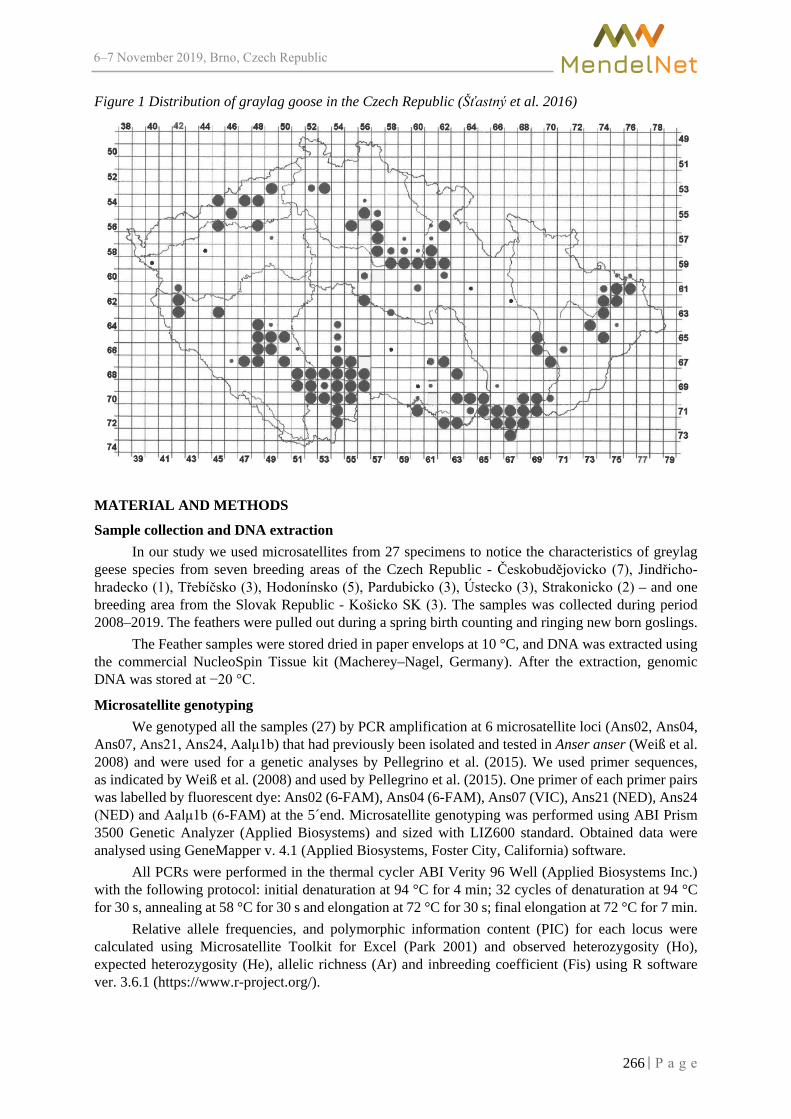
6–7 2019, Brno, Czech Republic
Figure 1 Distribution of graylag goose in the Czech Republic (Šťastný et al. 2016)
MATERIAL AND METHODS
Sample collection and DNA extraction In our study we used microsatellites from 27 specimens to notice the characteristics of greylag
geese species from seven breeding areas of the Czech Republic - Českobudějovicko (7), Jindřicho-hradecko (1), Třebíčsko (3), Hodonínsko (5), Pardubicko (3), Ústecko (3), Strakonicko (2) – and one breeding area from the Slovak Republic - Košicko SK (3). The samples was collected during period 2008–2019. The feathers were pulled out during a spring birth counting and ringing new born goslings.
The Feather samples were stored dried in paper envelops at 10 °C, and DNA was extracted using the commercial NucleoSpin Tissue kit (Macherey–Nagel, Germany). After the extraction, genomic DNA was stored at −20 °C.
Microsatellite genotyping We genotyped all the samples (27) by PCR amplification at 6 microsatellite loci (Ans02, Ans04,
Ans07, Ans21, Ans24, Aalμ1b) that had previously been isolated and tested in Anser anser (Weiß et al. 2008) and were used for a genetic analyses by Pellegrino et al. (2015). We used primer sequences, as indicated by Weiß et al. (2008) and used by Pellegrino et al. (2015). One primer of each primer pairs was labelled by fluorescent dye: Ans02 (6-FAM), Ans04 (6-FAM), Ans07 (VIC), Ans21 (NED), Ans24 (NED) and Aalμ1b (6-FAM) at the 5´end. Microsatellite genotyping was performed using ABI Prism 3500 Genetic Analyzer (Applied Biosystems) and sized with LIZ600 standard. Obtained data were analysed using GeneMapper v. 4.1 (Applied Biosystems, Foster City, California) software.
All PCRs were performed in the thermal cycler ABI Verity 96 Well (Applied Biosystems Inc.) with the following protocol: initial denaturation at 94 °C for 4 min; 32 cycles of denaturation at 94 °C for 30 s, annealing at 58 °C for 30 s and elongation at 72 °C for 30 s; final elongation at 72 °C for 7 min.
Relative allele frequencies, and polymorphic information content (PIC) for each locus were calculated using Microsatellite Toolkit for Excel (Park 2001) and observed heterozygosity (Ho), expected heterozygosity (He), allelic richness (Ar) and inbreeding coefficient (Fis) using R software ver. 3.6.1 (https://www.r-project.org/).
266

6–7 2019, Brno, Czech Republic
RESULTS AND DISCUSSION We have made an optimization of PCR multiplex to carry out the amplification
of all 6 microsatellite loci in one multiplex reaction. In the result of the PCR multiplex the microsatellite Ans07 had very weak amplification and microsatellite Ans04 at the most of the samples has not appeared but increasing the concentration of primers to twice that of the others was successful. The basic characteristics of the genetic diversity are presented in the Table 1. Frequencies of alleles are shown in the Table 2. The highest number of alleles found was at the Ans02 and Aalµ1b† loci. In these alleles we have found the highest heterozygosity and polymorphic informative content. On another side the allele Ans21 shows the lowest variability due to the occurrence only 2 alleles. Heterozygosity expected is in all cases higher than heterozygosity observed, which may be due to forces such as inbreeding. The inbreeding coefficient is quite high, but it could be caused by sampling error and relative low number of the samples, which were selected from different subpopulations. Similar values of heterozygosity (Ho = 0.45; He = 0.51) were obtained by Pellegrino el. al (2015) who used 14 microsatellite markers and 169 animals in their study. More animal samples and markers could provide a more accurate interpretation, which is a plan for further work.
Table 1 Basic genetic variation characteristics based on 6 microsatellite loci in the selected goose population Locus Na Ar Ho He PIC Fis Ans02 11 8.914 0.60 0.71 0.70 0.1583 Ans04 6 4.757 0.22 0.61 0.56 0.6336 Ans07 5 4.872 0.40 0.73 0.69 0.4493 Ans21 2 2.000 0.40 0.40 0.32 0.0079 Ans24 3 2.634 0.28 0.30 0.27 0.0716 Aalµ1b† 5 4.625 0.63 0.75 0.71 0.1676 overall 5.33 4.634 0.42 0.58 0.54 0.2480
Na – number of different alleles; Ar – allelic richness; Ho – heterozygosity observed; He – heterozygosity expected; PIC - polymorphic information content; Fis – inbreeding coefficient
Table 2 Allele and genotype frequencies of the analysed samples of the selected goose population Locus Allele Absolute frequency Relative frequency Ans02 206 3 0.0600
208 2 0.0400 210 7 0.1400 212 25 0.5000 214 2 0.0400 216 4 0.0800 218 1 0.0200 220 2 0.0400 226 2 0.0400 228 1 0.0200 232 1 0.0200
Ans04 158 1 0.0278 159 10 0.2778 161 2 0.0556 162 2 0.0556 163 20 0.5556 173 1 0.0278
Ans07 236 21 0.4200 237 240 243 247
11 8 7 3
0.2200 0.1600 0.1400 0.0600
Ans21
185 36 0.7200 188 14 0.2800
267

6–7 2019, Brno, Czech Republic
Locus Allele Absolute frequency Relative frequency Ans24 294 1 0.0200
298 8 0.1600 300 41 0.8200
Aalµ1b† 79 2 0.0417 81 13 0.2708 83 16 0.3333 85 9 0.1875 87 8 0.1667
CONCLUSION The greylag goose is a bird species widespread all around Palearctic and it deserves more interest
for the population management and population research. The functionality of the microsatellite panel was verified, and the methodology of sample testing
was optimized. The study of the pilot number of animals has approved that the variability of the studied microsatellites is sufficient for a subsequent research of Czech and Slovak greylag goose populations. Subsequently, testing and evaluation of a larger set of approximately 150 animals will be performed.
ACKNOWLEDGEMENTS This research work was supported by the Central European Institute of Technology (CEITEC) CZ.1.05/1.1.00/02.0068, and the Czech National Sustainability Programme NPU LQ1601. Our thanks go to all the collectors who provided the feather samples from the Czech and Slovak republic. Mainly thanks to Michal Podhrazský who organized the collecting and was helpful with all ethology details.
REFERENCES Johnsen, A. et al. 2010. DNA barcoding of Scandinavian birds reveals divergent lineages in trans-Atlantic species. Journal of Ornithology [Online], 151:565–578. Available at: https://link.springer.com/article/10.1007%2Fs10336-009-0490-3. [2019-08-04]. Musilová, Z. et al. 2017. Mezinárodní sčítání vodních ptáků v České republice v lednu 2017. Sborník Aythya [Online], 7: 6. Available at: http://www.waterbirdmonitoring.cz/sbornik-aythya/aythya-7/. [2019-09-01]. Park, S.D.E. 2001. The Excel microsatellite toolkit (version 3.1). Dublin: University College. Pellegrino, I. et al. 2015. Lack of genetic structure in greylag goose (Anser anser) populations along the European Atlantic flyway. PeerJ [Online], 3: e1161. Available at: https://doi.org/10.7717/peerj.1161. [2017-03-06]. Podhrázský, M. personal talks zoologist (ZOO Dvůr Králové, Štefánikova 1029, Dvůr Králové nad Labem) 23. 7. 2019. Ruokonen, M. et al. 2005. Colonization history of the high-arctic pink-footed goose Anser brachyrhynchus. Molecular Ecology [Online], 14:171–178. Available at: https://onlinelibrary.wiley.com/doi/abs/10.1111/j.1365-294X.2004.02380.x. [2019-08-04]. Ruokonen, M. et al. 2000. Close relatedness between mitochondrial DNA from seven Anser goose species. Journal of Evolutionary Biology [Online], 13:532–540. Available at: https://onlinelibrary.wiley.com/doi/full/10.1046/j.1420-9101.2000.00184.x. [2019-08-04]. Šťastný, K. et al. 2009. Atlas hnízdního rozšíření ptáků v České republice: 2001-2003. 2nd ed. Praha: Aventinum. Šťastný, K. et al. 2016. Ptáci = Aves. 3th ed, Praha: Academia. Weiß, B. et al. 2008. Isolation and characterization of microsatellite marker loci in the greylag goose (Anser anser). Molecular Ecology Resources [Online], 8:1411–1413. Available at: https://onlinelibrary.wiley.com/doi/abs/10.1111/j.1755-0998.2008.02339.x. [2018-06-15].
268

6–7 2019, Brno, Czech Republic
A preliminary note to the bionomy of Colletes inexpectatus Noskiewicz, 1936 based on observation of a larger nesting site
(Hymenoptera: Apiformes)
Martin Riha, Antonin Pridal
Department of Zoology, Fisheries, Hydrobiology and Apidology Mendel University in Brno Zemedelska 1, 613 00 Brno
CZECH REPUBLIC
Abstract: The new larger nest site of Colletes inexpectatus was discovered for the first in the Czech Republic. Obtained numerous material of this species was used for study of the species bionomy. It resulted that C. inexpectatus is not oligolectic on Fabaceae and its nest parasite is Epeolus variegatus. We proposed reclassification of the threat of C. inexpectatus in the Czech Republic and recommend the natural protection of the habitat.
Key Words: Colletes inexpectatus, faunistics, bionomy, parasite, Epeolus variegatus, foraging plant
INTRODUCTION Colletes inexpectatus was described by Noskiewicz (1936). He noticed that this bee was captured
on Trifolium and Medicago without remark to the parasite. Warncke (1978) regarded C. inexpectatus as conspecific with C. daviesanus Smith, 1846. This concept was not later followed with emphasizing on distinguishing characters in males (Přidal 1999, Kuhlmann 2000). The general distribution of the species is on the west from Central and Eastern Europe (Austria, Poland, Czech Republic), over the Central Asia (Kazakhstan, Kyrgyzstan, Tajikistan, Turkmenistan, Uzbekistan) up to the Far East (Mongolia). The records of this species are rather sparsely distributed and usually local with low density in whole region (Lukáš and Okáli 1998, Přidal 2001, Kuhlmann and Dorn 2002, Banaszak 2003, Ebmer 2003, Szczepko et al. 2002, Kuhlmann and Proshchalykin 2011, 2014, Proshchalykin and Kuhlmann 2012), e.g. in the Czech Republic are known only old records before 1966 (Přidal 1999). Therefore, the knowledge about the bionomy of this species are somewhat poor. Ebmer (2003) catched in Austria a female on Trifolium sp. This observation would confirmed Noskiewicz’s (1936) observation and an assumption about broad oligolecty for Fabaceae in C. inexpectatus. However, the study by Mueller and Kuhlmann (2008) palynologically confirmed the presence of pollen grains only from Asteroideae with conclusion “broadly oligolectic on Asteroideae”.
A larger nest site of C. inexpectatus was discovered in the Czech Republic for the first time, therefore, the object of this contribution is to identify: a) pollen grains on scopa and b) parasites flying in the nest site.
MATERIAL AND METHODS
Locality The larger nest site, as a loess wall approx. up to 6 m high and 50 m long, was discovered
at periphery of the town Oslavany (Moravia, Czech Republic). There was found area about 5 m2 very densely occupied by C. inexpectatus in the year 2017 (hundreds of nests). The last observation of the nest site was realised in 2019 (24th July and 1st August) when the female hatching just started. Sampling of bees
Bees (both host and parasite) were captured predominantly in close proximity of the nest entrances C. inexpectatus. Especially for pollen analysis, the just returning females entering in the nest
269

6–7 2019, Brno, Czech Republic
entrance were catched by the entomological net. Each captured female was inserted separately into the Eppendorf tube to prevent contamination by pollen from other females. Preparation
Bees were standardly prepared on entomological pin and dried. Male genitalia were prepared with glue on the card sheet or only as a pulled out from abdomen. Pollen grains from scopa were brushed with needle and tweezers, washed in ether to remove pollenkitt and overlaid by glycerine gelatine on a slide. The gelatine was pure or with dye (fuchsine). The pollen was studied from 17 females sampled on 1st August 2019. Identification
The bees were identified according to characters by Noskiewicz (1936), Přidal (1999), Kuhlmann and Proshchalykin (2014) and Bogusch and Hadrava (2018). The pollen grains were identified according to the pollen collection in the lab of apidology at Mendel University in Brno. Examined material
Colletes inexpectatus Noskiewicz, 1936. Moravia, Oslavany, 8.–13.vii.2010, 2 males, 2.viii.2017, 13 males, 120 females, M. Říha coll., 1 male, 1 female, A. Přidal coll., M. Říha lgt. et det., 24.vii.2019, 69 males, 39 females, A. Přidal lgt., det. et coll., 31 males, 2 females, M. Říha coll., 1 male, 1 female, coll. Moravian Museum Brno, M. Říha lgt. et det., 1.viii.2019, 17 females, A. Přidal lgt., det. et coll.
Epeolus variegatus (Linnaeus, 1758). Moravia, Oslavany, 2.viii.2017, 1 male, 29 females, M. Říha lgt. det. et coll., 24.vii.2019, 1 female, A. Přidal lgt., det. et coll., 1 male, M. Říha coll., 1 male, 1 female, Moravian Museum Brno coll., M. Říha lgt. et det., 1.viii.2019, 12 males, A. Přidal lgt., det. Et coll., 2 males, M. Říha lgt. det. et coll.
RESULTS AND DISCUSSION The loess wall and density of nests at the discovered nesting site in Oslavany are depicted
on Figure 1. So large nesting site C. inexpectatus without presence of the sibling species C. daviesanus was discovered for the first time. Both facts made it possible to collect easily identifiable males with unreliably and hardly identifiable females C. inexpectatus altogether (Kuhlmann and Proshchalykin 2014).
Figure 1 The nest site in Oslavany (A) loess wall (B) detail on the nest entrances (photo A. Přidal, 24. 7. 2019) A B
C. inexpectatus in CZ was considered as regionally extinct for a long time (Straka and Bogusch 2017). Thus, the current occurrence of the species in Oslavany changes its faunistic status after the last record in the Czech Republic from 1966 (Přidal, 1999). Moreover, really high density of the species on the site enabled to deposit the most numerous material in the authors’ collections in the Czech Republic for further studies.
270

6–7 2019, Brno, Czech Republic
We recorded a lot of nest parasites in immediate proximity of the nest entrances. The species (Figure 2) was identified as Epeolus variegatus (Linnaeus, 1758). C. inexpectatus as a host of this parasitic species is recorded for the first time. So far the parasite E. variegatus was known only at C. daviesanus, C. fodiens (Geoffroy, 1785), C. halophilus Verhoeff, 1943 and C. similis Schenck, 1853 (Gusenleitner et al. 2012, Bogusch and Hadrava 2018). These host species were not recorded on the site.
Figure 2 Epeolus variegatus on Tanacetum vulgare about 3–4 m from the nesting wall (photo A. Přidal, 1. 8. 2019)
The pollen grains brushed from scopa belong to Asteroideae; Achillea-type with colporus, echinate thick exine, width 24–26 µm and height 19–21 µm (Figure 3). This pollen grain was represented by 100 % of pollen spectrum in all studied pollen loads and females (Figure 4). Due to the females were visiting Tanacetum vulgare in immediate proximity 3–4 m from the nesting wall (Figure 5) we assume that it is pollen from this plant species. These results confirm the conclusions by Mueller and Kuhlmann (2008) about a broad oligolecty of C. inexpectatus on Asteroideae although we isolated from scopas of seventeen females likely only one plant species. This local monolecty was probably caused by the low plant diversity in vicinity of the nesting site. This confirmation increases reliability of previous results by Mueller and Kuhlmann (2008) about the food preferences in C. inexpectatus when the examined females were identified with higher reliability as it was argued above. The speciation process between daviesanus-inexpectatus was not probably influenced by differing food sources as it could been assumed according to data by Noskiewicz (1936) and Ebmer (2003) and it is known in related species group-succinctus: C. succinctus (Linnaeus, 1758), C. halophilus and C. hederae Schmidt & Westrich, 1993 (Kuhlmann et al. 2007).
Figure 3 Pollen grains from scopa C. inexpectatus: (A) equatorial/cross view (B) detail on exina (C) polar/longitudinal view (D) detail on colporus (photo A. Přidal) A) B) C) D)
271

6–7 2019, Brno, Czech Republic
Figure 4 Field of vision – spectrum of pollen grains (A) undyed (B) dyed (scale 20 µm; photo A. Přidal, 1. 8. 2019) A) B)
Figure 5 Female of Colletes inexpectatus on Tanacetum vulgare (photo A. Přidal, 1. 8. 2019)
CONCLUSION We conclude following notes to the bionomy of Colletes inexpectatus: 1. C. inexpectatus is currently confirmed for the Czech Republic (Moravian part) after 61 years.
The species was still missing and regionally extinct in the Czech Republic. We propose to classify the species threat as “critically endangered” (CR) for the Czech Republic due to the current occurrence at just one known locality.
2. E. variegatus can be newly considered as a nest parasite of C. inexpectatus due to its highoccurrence in the immediate proximity to the nest site of C. inexpectatus without presence other host species (C. daviesanus, C. fodiens, C. similis and C. halophilus).
3. The studied females of C. inexpectatus collected and brought in nests the pollenonly from Tanacetum vulgare. This finding is consistent with recent study confirming a broad oligolecty on Asteroideae and rejects the assumptions about oligolecty on Fabaceae.
The discovery of the nest site of C. inexpectatus, where the sibling species C. daviesanus is missing, is important for next research in the bionomy and morphology of C. inexpectatus. The nest site needs some legal habitat protection.
272

6–7 2019, Brno, Czech Republic
ACKNOWLEDGEMENTS The research was financially supported from the donations by elitbau, Ltd. and Konica Minolta Business Solution Czech, Ltd.
REFERENCES Banaszak, J. 2003. "Góry Pieprzowe" Hills in the vicinity of Sandomierz (SE Poland) as the European refuge of xerothermic bees (Hymenoptera: Apoidea). Polskie Pismo Entomologiczne, 72: 111–130. Bogusch, P., Hadrava, J. 2018. European bees of the genera Epeolus Latreille, 1802 and Triepeolus Robertson, 1901 (Hymenoptera: Apidae: Nomadinae: Epeolini): taxonomy, identification key, distribution, and ecology. Zootaxa, 4437(1): 1–60. Ebmer, A.W. 2003. Hymenopterologische Notizen aus Österreich – 16. (Insecta: Hymenoptera: Apoidea). Linzer biologische Beiträge, 35(1): 313–403. Gusenleitner, F., Schwarz, M., Mazzucco, K. 2012. Apidae (Insecta: Hymenoptera). Biosystematics and Ecology Series, 29: 9–129. Kuhlmann, M. 2000. Katalog der paläarktischen Arten der Bienengattung Colletes Latr., mit Lectotypenfestlegungen, neuer Synonymie und der Beschreibung von zwei neuen Arten (Hymenoptera: Apidae: Colletinae). Linzer Biologische Beiträge, 32(1): 155–193 Kuhlmann, M., Dorn, M. 2002. Die Bienengattung Colletes Latreille 1802 in der Mongolei sowie Beschreibungen neuer Arten aus Sibirien und den Gebirgen Zentralasiens (Hymenoptera, Apidae, Colletinae). Beiträge zur Entomologie, 52(1): 85–109. Kuhlmann, M., Proshchalykin, M.Y. 2011. Bees of the genus Colletes Latreille 1802 of the Asian part of Russia, with keys to species (Hymenoptera, Apoidea: Colletidae). Zootaxa, 3068: 1–48. Kuhlmann, M., Proshchalykin, M.Y. 2014. The bees of the genus Colletes Latreille 1802 of the European part of Russia, with keys to species (Hymenoptera: Apoidea: Colletidae). Zootaxa, 3878(3): 201–247. Kuhlmann, M. et al. 2007. Molecular, biogeographical and phenological evidence for the existence of three western European sibling species in the Colletes succinctus group (Hymenoptera: Apidae). Organisms, Diversity & Evolution, 7: 155–165. Lukáš, J., Okáli, I.1998. Včely (Hymenoptera, Apoidea) národnej prírodnej rezervácie Devínska Kobyla a Sandberg (juhozápadné Slovensko). (Bees of the national Nature Reserve Devínska Kobyla and Sandberg (southwestern Slovakia). Zborník Slovenského národného múzea, Prírodné Vedy, 44: 8–32 (in Slovak with English abstract). Mueller, A., Kuhlmann, M. 2008. Pollen hosts of western palaearctic bees of the genus Colletes (Hymenoptera: Colletidae): the Asteraceae paradox. Biological Journal of the Linnean Society, 95(4): 719–733. Noskiewicz, J. 1936. Die paläarktischen Colletes-Arten. Prace Naukowe Wydawnictwo Towarzystwa Naukowego we Lwowie, 3: 1–531. Proshchalykin, M.Y., Kuhlmann, M. 2012. The bees of the genus Colletes Latreille 1802 of the Ukraine, with a key to species (Hymenoptera: Apoidea: Colletidae). Zootaxa, 3488: 1–40. Přidal, A. 1999. Bee-species Colletes inexpectatus Noskiewicz, 1936 – species revocata (Hymenoptera: Colletidae). Acta Universitatis Agriculturae et Silviculturae Mendelianae Brunensis (Brno), 47(1): 55–60. Přidal, A. 2001. Annotated check-list of the bees from the Czech Republic and Slovakia – 1st. part (Hymenoptera: Apoidea, Colletidae). Sborník Přírodovědného klubu v Uherském Hradišti, 6: 139–163. Straka, J., Bogusch, P. 2017. Anthophila (včely). – In. Hejda et al. [eds.] Red List of threatened species of the Czech Republic. Invertebrates. Příroda, 36: 236–249. Szczepko, K. et al. 2002. Apoidea (Hymenoptera) in habitats of former agriculture area in a rena-turization stage of Kampinos National Park (Poland). Fragmenta Faunistica, 45: 115–122.
273

6–7 2019, Brno, Czech Republic
Environmental and overwintering conditions of Pellenes spp. (Araneae: Salticidae)
Kristina Stempakova, Vladimir Hula Department of Zoology, Fisheries, Hydrobiology and Apiculture
Mendel University in Brno Zemedelska 1, 613 00 Brno
CZECH REPUBLIC
Abstract: The research consisted of two parts. In the first part, the influence of the microclimate of hibernating hiding place (shade of shells) on the gregarious hibernation was solved and thus possible explanation of the formation of unusual social behaviour in these predatory species. In the second part, the presence/absence of spider species of interest – Pellenes tripunctatus (Walckenaer, 1802) and P. nigrociliatus (Simon, 1875) were observed at localities without calcareous bedrock, respectively without natural presence of gastropods by using scattered empty shells. The results showed that P. nigrociliatus also occurs at localities with acidic bedrock (27.59% occupancy of shells). It is interesting that individuals overwintered in larger shells of Caucasotachea vindobonensis (Férussac, 1821) despite the more frequent overwintering and affinity to the shell of Xerolenta obvia (Menke, 1828), what is mentioned in previous works. Up to 59.38% of individuals chose a larger shell. It has not been confirmed that the microclimate of shells affects group wintering. The white shells were the most inhabited (25.74%), but mainly by one individual, the brown shells were the least inhabited (17.61%). Regarding to gregarious hibernation, uncoloured shells were the most inhabited (20.65%). The highest number in the group of overwintering individuals was six individuals of P. tripunctatus.
Key Words: spiders, shells, environment, hibernation, behaviour
INTRODUCTION Pellenes tripunctatus (Walckenaer, 1802) and Pellenes nigrociliatus (Simon, 1875) of the family
Salticidae are typical thermophilic species with Eurasian distribution (Żabka 1997). In the Czech Republic, they belong to scarce species occurring at natural steppe and steppe-like habitats and secondary habitats such as various post-industrial sites. Despite a similar distribution area, environmental conditions such as vegetation cover density and stony substrate differ between these species. Spiders of species P. tripunctatus prefer more pronounced vegetation cover. In the southern parts of the country, it even inhabits meadows and pastures. Spiders of species P. nigrociliatus favour areas with low vegetation. It can be found on rocky steppes or sandbars (Kůrka et al. 2014). In addition, there was recorded a high abundance of these spider species on localities with empty shells of terrestrial gastropods (50–80% of occupancy in the shells). These are particularly steppe areas on calcareous bedrock, guaranteeing a high number of gastropods (Horn 1980, Bauchhenss 1995, Szinetár et al. 1998, Moreno-Rueda et al. 2008). Most of the life processes of these spiders are closely bound to the presence of the empty shells. These two spider species use empty shells not only for hibernation but also for mating, oviposition and taking care of offspring (Mikulska 1961, Horn 1980). In addition, preferred shells of certain species of gastropods have been detected. The most well-known is the affinity of P. nigrociliatus to the shell of Xerolenta obvia (Menke, 1828), which is described by Mikulska (1961) and Horn (1980). Species of P. tripunctatus prefers shells of the larger gastropod – Caucasotachea vindobonensis (Férussac, 1821), as described Niedobová et al. (2013) in their work. In this case, however, the affinity is not as pronounced and there are also records in shells of the genus Zebrina sp. and Xerolenta sp. (Bauchhenss 1995). At present, the abundance of these species is well known in the steppe landscape with calcareous bedrock. But are habitats on acidic bedrock (with similar natural
274

6–7 2019, Brno, Czech Republic
conditions) suitable habitats for the life of these species? To what extent does the abundance of these species relate to the abundance of empty shells in the habitat and the strong affinity to these shells?
In addition, there was found group hibernation in one shell in the case of P. tripunctatus and P. nigrociliatus. It is more significant in species of P. tripunctatus (Štempáková 2016 and personal observation). Most spiders are solitary and cannibalism is widespread among them, as is the case with the Salticidae family (Buskirsk 1981, Herberstein 2011). Despite this, in some cases certain groups are formed where natural aggressiveness is suppressed and mutual tolerance developed (Bilde and Lubin 2001). Before the formation of a certain aggregation, communication takes place, whether by means of chemical, sound or tactile signals. In addition, the Salticidae family use excellent eyesight (Krafft and Cookson 2012, Herberstein 2011). Also important in this case is the spider web, which plays a key role in spider sociality and explains the phenomena of group cohesion and cooperation (Krafft and Cookson 2012). For example, jumping spiders of Phidippus audax (Hentz, 1845) occasionally aggregate in dense cocoons below the bark. Temporary aggregations have also been reported for Paraphidippus marginatus (Hentz, 1845) or Marpissa undata (C. L. Koch, 1846). In the summer, cocoons were seen under the blades of grass in the case of Marpissa radiata (Grube, 1859) or Sitticus littoralis (Hahn, 1832), which also clustered with other species (Buskirsk 1981).
The shell of C. vindobonensis, which P. tripunctatus most often uses in our conditions, shows a distinct polymorphism. This is to some extent influenced by the habitat type and is shown externally by the tint of the shell, the tint of the band on the shell, the thickness of the bands, etc. Darker shells and shells with more marked bands absorb more heat from the sun (Ożgo and Komorowska 2009). Thus, the microclimate of shell could play an important role in spiders grouping within the gregarious wintering. Are darker shells inhabited more pronounced? And are they more often inhabited by a group of spiders or by the individual? So, is the microclimate inside the empty shell crucial to its selection and explains the group wintering?
MATERIAL AND METHODS The methodology describes two parts of the research. The first part is focused on an experiment
describing the effect of the microclimate inside the shell (shade of shells) on the spider hibernation. The second part describes the detection of the presence of spider species of interest in habitats with acidic bedrock.
Influence of shells microclimate on spider hibernation The research was carried out at two steppe habitats with calcareous bedrock. The location
of the habitats is shown in Figure 1. Empty shells of C. vindobonensis were scattered in number of 1050 shells in June 2017. At both localities, the rectangular areas (9 m x 3 m) were divided into three square sections. Specifically, at the locality of Malhotky, 8 areas were designed with 600 shells, and at the locality of Kamenný vrch, 6 areas were designed with 450 shells. Each square contained 25 shells in a different shade. For better results by emphasizing a more significant microclimate inside, the shells were painted in brown and white. The original shells that occurred on the localities were removed. In order to maximize the possibility of inhabit by spiders, the shells were left for two years at localities. Upon arrival, the shells were individually collected with locality designation, number of square and serial number. After collecting, the evaluation was based on the inhabitancy of the shells (in this case mainly P. tripunctatus), species diversity and which shells were preferred for gregarious hibernation.
Influence of natural conditions on the presence of species of interest and affinity to shells The research was carried out at five localities with natural conditions (low and sparse vegetation,
presence of stony substrate, moss, etc.) close to the species of interest (P. tripunctatus, P. nigrociliatus), but without the calcareous bedrock, respectively without the natural presence of gastropods – C. vindobonensis and X. obvia. The location of the habitats is shown in Figure 2. A total of 500 empty shells were scattered in July 2017. An area (10 m x 10 m) was designated at each locality. In number of 50 shells of C. vindobonensis and 50 shells of X. obvia were designed for each demarcated square. The shells were also collected after two years. The evaluation consisted in detection the presence/absence of the two spider species of interest and in confirming the strength of the affinity to the shells of the gastropods.
275

6–7 2019, Brno, Czech Republic
Figure 1 The location of the habitats – NR Kamenný vrch u Kurdějova (1) and NNM Malhotky (2)
Figure 2 The location of the habitats – NNM Miroslavské kopce (1), NNR Mohelenská hadcová step (2), NM Načeratický kopec (3), NM Skalky u Havraníků (4), NM Tasovické svahy (5)
RESULTS AND DISCUSSION
Influence of shells microclimate on spider hibernation (only P. tripunctatus) In the first part of the research, in winter 2019 altogether 672 shells (426 shells at Malhotky,
246 shells at Kamenný vrch) were collected. Thus, 64% of the 1050 shells were obtained. The smallest amount was represented by brown shells (159 shells), which were more difficult to identify in the country, especially on the experimental squares at the Kamenný vrch, where higher vegetation was left within the management (mosaic mowing). Regarding to spiders, 146 individuals of P. tripunctatus were obtained from these shells. The total occupancy (also in the case of group hibernation) is 21.73%. The numbers of collected shells and their occupancy are described in Table 1. The brown shells were inhabited the least. This low occupancy can be caused by the high temperature inside the shell absorbed by the dark surface. This can cause undesirable interruption of hibernation. Interestingly, the white shells were the most inhabited, mainly by individual occupancy (Total – 25.74%, Kamenný vrch – up to 31.04%). It was assumed that white shells would most often be inhabited by a larger number of individuals to provide a higher temperature inside the shell. In the case of group wintering in shells, this could be a sub sociality in which sub social species live in colonies only for a period of time benefiting from this coexistence (Yip and Rayor 2014, Herberstein 2011). Thus, one
276

6–7 2019, Brno, Czech Republic
advantage could be the higher number of aggregating individuals and the associated social thermoregulation, well known in social insects (Jones and Oldroyd 2006). Gregarious hibernation was most observed in uncoloured shells (see Table 2). Up to six hibernating individuals were found in one uncoloured shell at Malhotky. This is certainly interesting information when natural predators reaching the size of 5–7 mm can tolerate to each other and can hibernate together in relatively small shells with a diameter of about 20 mm (Kůrka et al. 2014, Welter-Schultes 2012). From the achieved results, however, it cannot be unambiguously determined that the microclimate of shells plays a role in its inhabitation. It is necessary to carry out several other experiments to confirm or refute the hypothesis. The formation of these groups is thus caused by another factor, which may be just communication, some form of agreement and the learning of socialization, which is mentioned in some of the few works of jumping spiders (Liedtke and Schneider 2017).
Table 1 The numbers of collected shells and their occupancy (red font - a case of group wintering in which shells were inhabited by more than one individual)
Table 2 Gregarious hibernation in species of P. tripunctatus
Influence of natural conditions on the presence of species of interest and affinity to shells
In the second part of the research, which also took place in the winter of 2019, the collection of shells was carried out at localities without calcareous bedrock and therefore without the natural presence of gastropods of interest. Unfortunately, only 116 shells were collected, representing 23.20%. No shells were recorded at Tasovické svahy. The reason was the passage of heavy mechanization, probably within certain management. The locality of Načeratický kopec brought a similar result.
A total of 56 shells of C. vindobonensis and 60 shells of X. obvia were collected. Of the total number, 32 were found inhabited by P. nigrociliatus. Spiders of P. tripunctatus were not found. In spite of the small amount of material obtained, new records of P. nigrociliatus species were identified, which complement the before discovered records mainly in southern Moravia and in the wider surroundings of Prague (Buchar and Růžička 2002). New information about the occurrence of the species is shown in Figure 3. An interesting discovery is the more frequent presence of this species in the shell of C. vindobonensis (up to 59.38%) despite the already mentioned strong affinity to the shell of the X. obvia (Mikulska 1961, Horn 1980). It was assumed that individuals would choose a smaller
Number of collected
shells
Number of occupied
shells
Number of spiders in
shells
Number of collected
shells
Number of occupied
shells
Number of spiders in
shells
Number of collected
shells
Number of occupied
shells
Number of spiders in
shells
Number of collected
shells
Number of occupied
shells
Number of spiders in
shells
Malhotky 102 12 13 150 31 34 174 26 39 426 69 86
Kamenný vrch 57 12 15 87 26 27 102 16 18 246 54 60
All shells
All spiders
672
146
159
28
237
61
276
57
Brown shells White shells Uncoloured shells
Locality
Total
Locality ShellNumber of individuals
Malhotky uncoloured 6
Malhotky uncoloured 4
Malhotky uncoloured 4
Malhotky white 3
Malhotky uncoloured 2
Malhotky uncoloured 2
Malhotky white 2
Malhotky brown 2
25
Kamenný vrch u K. brown 3
Kamenný vrch u K. uncoloured 3
Kamenný vrch u K. brown 2
Kamenný vrch u K. white 2
10
277

6–7 2019, Brno, Czech Republic
shell of X. obvia also in terms of a possibly more favourable size ratio. Consequently, there is no affinity to the shell in this case and the choice of shell kind is probably random.
Figure 3 The occurrence of species Pellenes nigrociliatus in the Czech republic. The black dots represent older records. The red dots show new records of P. nigrociliatus.
Other spider species found in the research Another nine species of spiders were found from both parts of the research. The Malhotky locality
with 6 species was the most interesting, of which 59.58% were Euryopis quinqueguttata (Thorell, 1875) classified as EN. Among others, five records of the species Attulus penicillatus (Simon, 1875), which is also in the EN category, can be mentioned. It was found at localities Malhotky and Miroslavské kopce. It is worth mentioning the species Haplodrassus kulczynskii (Lohmander, 1942) from the category VU (Řezáč et al. 2015) found on the locality Kamenný vrch.
CONCLUSION The results brought information regarding to new records of P. nigrociliatus also at localities
without calcareous bedrock and natural occurrence of empty gastropods, to which the living conditions of this species of spider are strongly linked. In addition, overwintering has been found to occur in a larger species of shell – C. vindobonensis rather than a predicted smaller species – X. obvia despite its availability. Thus, if both species of gastropods are present, P. nigrociliatus is likely to use both sources. In the group hibernation of P. tripunctatus species in one shell, the microclimate of the shell is probably not the cause of clustering of individuals and the associated social thermoregulation. White shells were mostly occupied by one spider. Group wintering was most common in uncoloured shells. Six individuals were the highest quantity found in one shell. Thus, the unusual gregarious hibernation in one shell of these otherwise predatory species causes a different factor than the shade of the shell providing a certain microclimate.
ACKNOWLEDGEMENTS The research was financially supported by IGA MENDELU grant no. AF-IGA-2018-tym004.
REFERENCES Bauchhenss, E. 1995. Überwinternde Spinnen aus Schneckenhäusern. Arachnologische Mitteilungen, 9: 57–60. Bilde, T., Lubin, Y. 2001. Kin recognition and cannibalism in a subsocial spiders. Journal of Evo-lutionary Biology, 14: 959–966. Buchar, J., Růžička, V. 2002. Catalogue of spiders of the Czech Republic. Praha: Peres Publisher, pp. 349. Buskirsk, R.E. 1981. Sociality in arachnida. In Social insect. Hermann, H., R. Georgia: Academic Press, pp. 506.
278

6–7 2019, Brno, Czech Republic
Herberstein, M.E. 2011. Spider behaviour: flexibility and versatility. New York: Cambridge University Press, pp. 391. Horn, H. 1980. Die Bedeutung leerer Schneckengehäuse für die Überwinterung und das Brutverhalten von Pellenes nigrociliatus L. Koch, 1874 in Steppenrasenformationen (Araneae: Salticidae). Beiträge zur naturkundlichen Forschung in Südwestdeutschland, 39: 167–175. Jones, J.C., Oldroyd, B.P. 2006. Nest thermoregulation in social insect. Advances in Insect Physiology, 33: 153–191. Krafft, B., Cookson, L.J. 2012. The role of silk in the behaviour and sociality of spiders. Psyche, 2012: 1–25. Kůrka, A., Řezáč, M., Macek, R., Dolanský, J. 2014. Pavouci České republiky. Praha: Academia, pp. 569. Liedtke, J., Schneider, J. M. 2017. Social makes smart: rearing conditions affect learning and social behaviour in jumping spiders. Animal Cognition, 20: 1093–1106. Mikulska, I. 1961. Parental care in a rare spiders Pellenes nigrociliatus (L. Koch) var. bilunulata Simon. Nature, 190 (4773): 365–366. Moreno-Rueda, G., Marfil-Daza, C., Ortiz-Sanchez, F.J., Melic, A. 2008. Weather and the use of empty gastropod shells by arthropods. Annales de la Société entomologique de France, 44(3): 373–377. Niedobová, J., Hula, V., Košulič, O. 2013. Prázdné ulity plžů a tajemství, která skrývají. Živa, 60 (1): 26–28. Ożgo, M., Komorowska, A. 2009. Shell banding polymorphism in Cepaea vindobonensis in relation to habitat in southeastern Poland. Malacologia, 51(1): 81−88. Řezáč, M., Kůrka, A., Růžička, V., Heneberg, P. 2015. Red list of Czech spiders: 3rd edition, adjusted according to evidence-based national conservation priorities. Biologia, 70(5): 645–666. Štempáková, K. 2016. Effect of environment and management to overwintering of spiders in shells of terrestrial molluscs. Diploma thesis, Mendel University in Brno, pp. 70. Szinetár, Cs., Gál, Zs., Eichardt, J. 1998. Spiders in snail shells in different Hungarian habitats. Miscellanea Zoologica Hungarica, 12: 67–75. Welter-Schultes, F. 2012. European non-marine molluscs, a guide for species identification. Göttingen: Planet Poster Edition. Yip, E. C., Rayor, L. S. 2014. Maternal care and subsocial behaviour in spiders. Biological Reviews, 89: 427–449. Żabka, M. 1997. Salticidae: Pająki skaczące (Arachnida: Araneae). Warszawa: Muzeum i Instytut Zoologii PAN, pp. 189.
279

AGROECOLOGY AND RURAL DEVELOPMENT
6–7 2019, Brno, Czech Republic
Using of AHP method in assessment of selected directions of sewage sludge management
Arkadiusz Bieszczad, Jacek Salamon Department of Bioprocess Engineering, Energetics and Automatization
University of Agriculture in Krakow Balicka 116b, 30–149 Krakow
POLAND
Abstract: The aim of the work was to evaluate selected directions od sewage sludge management such as composting, anaerobic stabilization and thermal conversion-combustion of sludge. The Hierarchy Process Analysis (AHP) method was used for assessment. The whole assessment was based on a multicriteria approach considering a number of characteristic parameters. The most important criteria for the assessment was the sterilization of sewage sludge and the reduction of waste mass. The remaining assessment criteria include the content of organic matter and the humidity of the process residue. As a result of the analysis, a compilation containing assessments for accepted development directions was created. This allowed to determine that the process of thermal treatment of sewage sludge best meets the accepted criteria of analysis.
Key Words: sewage sludge, waste, AHP
INTRODUCTION Measures taken in the field of sludge management should be applied in a hierarchy of waste
management methods. Based on the parameters and quality available, one should choose one of the following ways of development adequate to their form.
In the first place, it is necessary to prevent the formation of sewage sludge or take actions aimed at the loss of waste status. Second recycling of municipal sewage sludge in the process of organic reclamation of recyclable materials, such as composting with other wastes, in order to obtain a product fulfilling fertilizing functions. Next step is use methods of recovery of municipal sewage sludge directly on the surface of the earth, including recovery in composting plants, biogas plants or cementation, but also energy recirculation by burning deposits in or outside installations. The last one is neutralizing municipal sewage sludge by subjecting it to thermal transformation in an incineration or co-incineration plant without energy recovery.
The novelty of this study is an attempt to assess the directions of sewage sludge management taking into account the disproportions between the significance of the criteria for their management. Factors determining the requirements of process efficiency and the impact of sludge on human health are a direct impact on the way they are processed. In the AHP method, taking into account this differentiation allows for a more reliable presentation of the problem and for trying to determine the most appropriate direction for their development.
MATERIAL AND METHODS Before the evaluation, a number of criteria for the analyzed methods of sewage sludge
management were adopted. In them, we can distinguish criteria such as the content of organic material after the process, loss of mass in the process, decrease in the number of parasite eggs and the humidity of the residue after the process. All data and evaluation parameters are presented in Table 1.
In order to understand the subject, the problem was decomposed, resulting in a graphical model presented in Figure 1, showing the hierarchy of the analyzed criteria and parameters leading to the achievement of a specific goal. This allowed to specify such elements as the main objective for the discussed issue and the partial factors and available variants that lead to the achievement of the adopted objective.
281

6–7 2019, Brno, Czech Republic
Table 1 A summary of the data used in the calculations (Grabowski 2011, Dach et al. 2009, Malej 2000, Gałwa-Widera 2014, Kuklikowska and Bilicka 2009)
Analyzed criterion Unit Composting Anaerobic stabilization
Thermal transformation
Content of organic material after the process [% d.m.] 76.9 66.1 4
Loss of mass in the process [%] 23.1 39 88.59 Decrease in the number of parasite
eggs [%] 32.3 45 100
Humidity of the residue after the process [%] 50 80 0
Figure 1 The hierarchical structure of the task for the analyzed problem (Hachoł et al. 2017)
The following hierarchical model was adopted for the assessment of sewage sludge management methods, including such elements as:
• The main purpose: determining the efficiency of the sludge management process takinginto account changes in the structure of sewage sludge in the analyzed variants. It is a resultant of achieving goals by partial factors in individual processes,
• Partial factors: they determine the efficiency with which a given process takes place, takinginto account whether in the final effect a higher order is achieved that is higher in the hierarchy with the best possible effect. These are parameters expressed in the form of numerical data that make up the final process output,
• Analyzed variants: include specific technological processes such as composting, anaerobicstabilization and combustion, differing in the degree of fulfillment of the function leading to the achievement of the superior goal.
Evaluation of criteria by pair comparison The consequence of developing a hierarchical problem model in the AHP method is to compare
pairs of individual criteria in order to establish their mutual domination. Allowed ranges of domination are in the range from 1 to 9 where 1 means comparable decision options and 9 the extremely huge advantage of one variant over the second one (Saaty 2008).
Indicators of the relative importance of the factor-criterion Ki over Kj are expressed in the number aij, when:
𝑎𝑎𝑖𝑖𝑖𝑖 =𝑒𝑒𝑖𝑖𝑒𝑒𝑖𝑖
𝑖𝑖, 𝑗𝑗 = 1,2, … ,𝑛𝑛
282

6–7 2019, Brno, Czech Republic
where: 𝑒𝑒𝑖𝑖 − absolute rank of the Ki criterion 𝑒𝑒𝑖𝑖 − absolute rank of the Kj criterion 𝑎𝑎𝑖𝑖𝑖𝑖 ∈ {1,2,3, … ,9} The degrees of mutual dominance and factors aij and ei are presented in the form of a square matrix
A, taking into account that 𝑎𝑎𝑖𝑖𝑖𝑖 = 1𝑎𝑎𝑗𝑗𝑗𝑗
for i, j = 1,2,3, ... n. The matrix containing a summary of assessments
on the basis of which the final values for particular criteria were determined is presented in Table 3 (Downarowicz et al. 2000). The final values were obtained by summing up individual assessments contained in columns from KA to KD.
Table 3 Matrix comparisons of domination of the analyzed criteria
Criterion KA KB KC KD
KA 1 2 15
13
KB 12
1 12
4
KC 5 2 1 5
KD 3 14
15
1
Final values 9.5 5.22 1.9 10.3 Legend: KA - Content of organic material after the process, KB - Loss of mass in the process, KC - Decrease in the number of parasite eggs, KD - Humidity of the residue after the process
Determining the value of individual criteria
Table 4 Presentation of the participation of individual criteria assessments in the final evaluation and their unit value
Criterion KA KB KC KD Value
KA 0.105 0.381 0.105 0.032 0.156
KB 0.053 0.190 0.263 0.387 0.223
KC 0.526 0.381 0.526 0.484 0.479
KD 0.316 0.048 0.105 0.097 0.141
Sum 1 1 1 1 1
The determination of the unit weights for individual criteria presented in Table 4 was performed by calculating the arithmetic mean of all the results obtained for subsequent rows from KA to KD.
Examination of the consistency of the preference matrix according to the decision maker In order to verify the correctness of the performed calculations, it was necessary to determine
the λ max coefficient, which is the product of the sum of the final grades and the weight of the grades obtained for individual criteria analyzed. The λmax coefficient, which is a component of the conformity coefficient of the comparison matrix CI and the ratio of the ratio of conformity CR, allows to determine whether the principle of constancy of preferences has been violated. The value of Cl and CR should not exceed 0.1 (Downarowicz et al. 2000).
283

6–7 2019, Brno, Czech Republic
Table 5 Determination of the inconsistency ratio λmax for the analyzed criteria
Criterion Final values Value λmax
KA 9.5 0.156 1.481
KB 5.25 0.223 1.173
KC 1.9 0.479 0.911
KD 10.33 0.141 1.461
Sum 5.025
The obtained value of λ max = 5.025 was substituted to formula to determine the value of the CI comparison matrix index.
𝐶𝐶𝐶𝐶 =𝜆𝜆𝑚𝑚𝑎𝑎𝑚𝑚 − 𝑛𝑛𝑟𝑟(𝑛𝑛 − 1)
= 0.0057
where: 𝑛𝑛 − the value of the random index according to Saaty (n = 5) 𝑟𝑟 − expression of the matrix (r = 1.12) In the further part of the consistency matrix of the preference matrix, the second ratio of CR
consistency was calculated.
𝐶𝐶𝐶𝐶 =𝐶𝐶𝐶𝐶𝑟𝑟
= 0.0051
where: 𝐶𝐶𝐶𝐶 − 𝑖𝑖𝑛𝑛𝑖𝑖𝑒𝑒𝑚𝑚 𝑜𝑜𝑜𝑜 𝑐𝑐𝑜𝑜𝑚𝑚𝑐𝑐𝑎𝑎𝑟𝑟𝑖𝑖𝑐𝑐𝑜𝑜𝑛𝑛 𝑚𝑚𝑎𝑎𝑚𝑚𝑟𝑟𝑖𝑖𝑚𝑚 (𝐶𝐶𝐶𝐶 = 0.0057) 𝑟𝑟 − expression of the matrix (r = 1.12) The above calculations allowed to determine two coefficients Cl = 0.0057 and CR = 0.0051.
Both of them meet the condition Cl <0,1 and CR <0,1, which proves that in the case of the analyzed criteria there was no impairment of constancy of preferences. In the further part of the work in the same way as above all discussed variants of sewage sludge management were compared with pairs, taking into account the data contained in Table 1. This allowed to determine the value of individual variants with respect to the assessment criteria adopted at the beginning.
RESULTS AND DISCUSSION
The final result of the analysis made by the decision maker The results below shows that the best final score, taking into account the adopted data
and evaluation criteria, was given to the variant VC- thermal transformation, resulting in a final value of 0.737, rankings it in the first place. On the second and third place there are variants: VB - anaerobic stabilization, with the evaluation of 0.154 and VA - composting, with the result of 0.109.
Table 6 List of final results for the variants analyzed by decision maker
Variants
Value criterion (Table 4) The final result of the
analysis KA KB KC KD
0.156 0.223 0.479 0.141 VA 0.085 0.094 0.103 0.180 0.109 VB 0.148 0.168 0.174 0.071 0.154 VC 0.767 0.738 0.723 0.748 0.737
Legend: VA - composting, VB - anaerobic stabilization, VC - thermal transformation
284

6–7 2019, Brno, Czech Republic
The results obtained cannot be fully regarded as objective due to the lack of extensive experience of the decision maker, and therefore a similar evaluation process was carried out by expert familiar with the subject.
The final result of the analysis made by the expert’s As a result of the analysis based on the expert's assessment, the following results were obtained
the VC- thermal transformation variant is ranked first with a score of 0.740. The next option with the highest result is the VB - anaerobic stabilization with an evaluation of 0.167. The last place was attributed to the VA - composting and the rating value obtained by him equal to 0.092.
Table 7 List of final results for the variants analyzed by expert’s
Variants
Value criterion (Table 4) The final
result of the analysis
KA KB KC KD
0.096 0.560 0.269 0.075
VA 0.103 0.083 0.083 0.180 0.092 VB 0.178 0.193 0.137 0.071 0.167 VC 0.723 0.724 0.780 0.748 0.740
Legend: VA - composting, VB - anaerobic stabilization, VC - thermal transformation
CONCLUSION The application of the method of hierarchical analysis of the problem allowed for a multicriteria
evaluation of accepted variants of sludge management. As a result of the decision-making process, a strict ranking was obtained for the proposals in question. The obtained values of final decisions of the decision-maker coincide with the values received by the specialist. The duality of the inter-pretation of the criteria by various entities based on the subjectivity of the assessment additionally increases the reliability of the analysis. Among the three adopted methods of development, according to the decision of the decision-maker and specialist, the VC criteria was the highest classified, which determined the thermal transformation of sewage sludge by their combustion. This item has received ratings above 0.7 point significantly ahead of the other analyzed processes. In the further part of the comparison, the greater disproportions in the final assessments of the specialist and the decision maker are noticed. A person with greater experience for the analyzed issues assessed the VB option in a higher manner in relation to the result obtained by the decision-maker. However, the VA development method in the opinion of a specialist received a smaller weight percentage.
ACKNOWLEDGEMENTS This Research was financed by the Ministry of Science and Higher Education of the Republic of Poland.
REFERENCES Dach, J. et al. 2009. Influence of effective microorganisms addition (EM) on composting process and gaseous emission intensity. Journal of Research and Applications in Agricultural Engineering, 54(3): 49–51. Downarowicz, O. et al. 2000. Zastosowanie metody AHP do oceny i sterowania poziomem bezpieczeństwa złożonego obiektu technicznego. Politechnika Gdańska [Online], pp. 2–7. Available at: http://www.pg.gda.pl/~wst/arty/z4.pdf. [2019-07-15]. Gałwa-Widera, M. 2014. Unieszkodliwianie osadów ściekowych w procesie kompostowania z zastosowaniem różnych cykli napowietrzania. Inżynieria i Ochrona Środowiska, 17(4): 661–671. Grabowski, Z. 2011. Termiczne przekształcanie osadów ściekowych na przykładzie STUO w Krakowie. In Proceedings of IV Forum Gospodarki osadami ściekowymi [Online]. Warszawa, Polska, 29 Września: Politechnika Krakowska, pp. 12–21. Available at: http://odpady.nfosigw.gov.pl/gfx/odpady/userfiles/files/spotkanie_06/2_grabowski.pdf. [2019-07-15].
285

6–7 2019, Brno, Czech Republic
Hachoł, J. et al. 2017. Applying the Analytical Hierarchy Process into the effects assessment of river training works. Journal of Water and Land Development, 35(10-12): 65–66. Kuklikowska, D., Bilicka, K. 2009. Analysis of organic matter and nitrogen compounds transformations during sewage sludge composting. Technical Transactions, 3(11): 102–104. Malej, J. 2000. Właściwości osadów ściekowych oraz wybrane sposoby ich unieszkodliwiania i utylizacji. Rocznik Ochrona Środowiska [Online], pp. 2–6. Available at: http://ros.edu.pl/images/roczniki/archive/pp_2000_003.pdf. [2019-07-15]. Saaty, T.L. 2008. Decision making with the analytic hierarchy process. International Journal of Services Sciences, 1(1): 85–86.
286

6–7 2019, Brno, Czech Republic
Designing of crop management for reducing soil loss according to geographic location using STD-C factor tool
Jiri Brychta
Department of Geography J. E. Purkyne University
Ceske mladeze 8, 400 96 Usti nad Labem CZECH REPUBLIC
Abstract: Crop-management factor (C) is essential part of average annual soil loss calculation by USLE. Several methods were developed due to lack of optimal data required in original methodology. For designing optimal crop rotation expressed by C factor is presented methodology of calculation average annual soil loss over permissible limits for representative drainage subbasins of land parcel and C factor limits in combination with STD-C tool. This methodology brings a good opportunity for erosion control measures designing in land use planning with reflecting geographic location and local climate conditions and enables adequate allocation of financial expense for erosion control.
Key Words: USLE, C factor, P factor, STD-C factor, erosion control measures
INTRODUCTION The equations USLE (Wischmeier and Smith 1978) and RUSLE (Renard et al. 1997) are widely
used and accepted methods over the world for calculating average annual soil loss. Protective influence of vegetation cover and crop management are expressed by crop-management factor C. Many authors developed different methods of C factor estimation and calculation due to lack of optimal data defined in original methodology. Brychta et al. (2018) divided approaches for C calculation into these groups – based on: 1) long-term monitoring of runoff plots (Janeček et al. 2012, Wischmeier and Smith 1978), 2) defining subfactor values (Dissmeyer and Foster 1981, Renard et al. 1997, Wischmeier and Smith 1978), 3) simulated rainfalls (Garcia-Orenes et al. 2009, Janeček et al. 1995), 4) land cover classification method and average values (Panagos et al. 2015), 5) satellite multispectral data and vegetation indexes (Van der Knijff et al. 2000, De Jong 1994), 6) regression and correlation analyses with climate data (Toman and Kadlec 2003).
Groups 1–3 require time-consuming terrain measurements and are basic source of data for deriving any other methodology of C factor estimation. Group 4 leads to constant values for large areas, enables only low spatial and temporal resolution and does not reflect spatial and temporal variability. Often used are methods based on linear regressions with vegetation spectral properties expressed by normalized difference vegetations index NDVI (group 5) even according to De Jong (1994) this relationship exhibits quite low correlation. The most commonly used method in land used planning in the Czech Republic according to Toman and Kadlec (2003) is based on linear regression between C factor and climatic regions, determined by annual temperature and rainfall totals, sums of temperature over 10 ºC, probability of dry growing periods and moisture guarantee during growing period (group 6). This method is useful for average annual soil loss calculation but does not enable reflecting changes of soil loss by designing of optimal crop rotation or erosion control measures. For this purposes can be used quite time-consuming original methodology according Wischmeier and Smith (1978). Brychta et al. (2018) developed revised methodology were all steps of time- consuming C calculation were automated in GIS environment with innovative procedure of R factor weights determination for each agro-phase. This method respects original methodology based on division into 5 agro-phases and determination of weights of R factor distribution throughout the year (Wischmeier and Smith 1978) but using fully distributed monthly R factor maps (Brychta et al. 2018, Ballabio et al. 2017) which enable determination weights of R factor distribution throughout the year
287

6–7 2019, Brno, Czech Republic
according to land parcel geographic location and therefore local conditions are reflected (see Figure 1 and 2).
MATERIAL AND METHODS Average annual soil loss over permissible limits were calculated for cadastral area Kostomlaty
pod Milesovkou using USLE equation (Wischmeier and Smith 1978): GRISK =(R ∙ LS ∙ K ∙ C ∙ P) – GP, (1)
where: GRISK – average annual soil loss over GP (t/ha/yr), GP – permissible soil loss limit (t/ha/yr), R, L, S, K, C, P – USLE factors. For LS factor calculation was used DMR 5G (LiDAR data from CUZK) and resolution 10 m. Calculation were performed according to Renard et al. (1997) and McCool (1987) using equations: 𝐿𝐿 = � 𝑙𝑙𝑑𝑑
22.13�𝑚𝑚
, (2)
S = 10.8 sin(s1) + 0.03, (3) S = 16.8 sin(s2) – 0.5, (4)
where: LS – topographic factor, ld – horizontal projection of uninterrupted slope length, s1 – slope (rad) < 9%, s2 – slope (rad) ≥ 9%, 𝑚𝑚 – exponent determined by equation:
𝑚𝑚 = β(𝛽𝛽+1)
, where: 𝛽𝛽 =� sin 𝑠𝑠0.0896�
3(sin s)0.8+0.56 . (4)
The horizontal projections of uninterrupted slope lengths (ld) were calculated as unit contributing area raster (Moore and Wilson 1992) generated using flow accumulation raster derived from flow direction raster calculated using algorithm D∞ (Tarboton et al. 1997). Resulting LS values are shown on Figure 3. K factor values were determined according to Vopravil et al. (2007), C factor according to Toman and Kadlec (2003), R factor according to (Brychta and Janeček 2017, 2019) and permissible soil loss limits (Gp) according to Janeček at al. (2012). Resulting average annual soil loss for each pixel 10 x 10 m is shown on Figure 3. Using representative parts of land parcels derived according prevailing flow direction (Figure 4) were calculated GRISK values using zonal statistics (Figure 4). According to GP limits were created a raster with C factor limit values using equation (Wischmeier and Smith 1978, Novotný et al. 2014):
CLIMIT ∙ P = 𝐺𝐺𝑃𝑃
𝑅𝑅 ∙ 𝐿𝐿𝐿𝐿 ∙ 𝐾𝐾 , (5)
where: CLIMIT – C factor limit values, GP – soil loss limits (t/ha/yr), R, LS, K, P – USLE factors. Resulting CLIMIT values for each pixel were reclassified according Table 1. This map serves for framework recommendations for planning crop management and farming methods (Table 1, Figure 5). According these maps (Figure 4, 5) can be evaluated and designed several possibilities of crop-management or erosion control measures for each land parcel or its parts. For more detailed planning of crop rotation or agrotechnical management can be used STD-C factor model created by Brychta et al. (2018) and also erosion control measures expressed by P factor (Table 2). Model STD-C factor is based on revised methodology which respects original principles with accordance to Wishmeier and Smith (1978) based on division into 5 phases (Figure 1) and improved method of determination of weights of R factor distribution throughout the year.
Table 1 Recommendation for planning crop management according to C factor limit values CLIMIT values
Risk Recommendation Symbol
≤ 0.005 extreme Conversion to permanent grassland. PG 0.005–0.02 high Planting perennial fodder plant e.g. clover and alfalfa. PF
0.02–0.2 medium Exclusion of wide-row crops, narrow-row crops can be plantonly with the use of erosion control technology. NR
0.2–0.6 low Planting narrow-row crops without limitation, wide-row crops only with the use of erosion control technology. NRCM
> 0.6 no risk Planting without limitation. no limit
288

6–7 2019, Brno, Czech Republic
Table 2 Erosion control measures derived by P factor according to Wishmaier and Smith (1978)
Erosion control measures Slope (%) 2–7 7–12 12–18 18–24
maximal flow length for contour cultivation 120 m 60 m 40 m - 0.6 0.7 0.9 1
width and number of strips for strip cropping 40 m 30 m 20 m 20 m 6 strips 4 strips 4 strips 2 strips
– root crops and perennial forage 0.3 0.35 0.4 0.45 – root crops and winter cereals 0.5 0.6 0.75 0.9 contour furrow ploughing 0.25 0.3 0.4 0.45
Figure 1 The timeline of 5 agro-phases for C factor calculation
All steps of time-consuming C calculation were automated in GIS environment with innovative procedure of R factor weights determination for each agro-phase using fully distributed monthly R factor maps and land parcel geographic location and therefore local conditions are reflected. User interface of STD-C factor model and example of calculation are shown on Figure 2. The resultant weighted STD-C factor value is calculated according to following equations (6–8):
STD C = (∑ 𝐶𝐶𝐶𝐶𝑛𝑛=10𝑖𝑖=4 )/yr (6)
Ci = Ri × Cp (7) Ri = (Rd/Nm) × Np (8)
where: STD-C – spatial-temporal distributed C factor, i, n – sequential number of months where erosive rainfalls were detected (April–October), Ci – C factor values for each month that occurs in a given phase, yr – number of years, Cp – soil loss ratio between given vegetation conditions and black fallow (SLR) (Wischmeier and Smith 1978) for each agro-phase (according to Figure 1), Ri - R factor weights for each month that occurs in a given phase, Np – number of days that occurs in a given month and agro-phase, Rd – percentage distribution of R throughout the year (decimal number), Nm – number of days in a month (e.g. 31 for August, 30 for April etc.) A detailed example of generating Ri and Ci for August and geographic location of land parcel is described in Figure 2.
Figure 2 User interface of STD-C factor model and example of generating Ri and Ci for August according to geographic location (see details in Brychta et al. 2018)
289

6–7 2019, Brno, Czech Republic
RESULTS AND DISCUSSION According to above mentioned methodology were created rasters with values of each factors
of USLE equation. Resulting rasters with LS factor values and resulting average annual soil loss values for each pixel of size 10 x 10 m are shown on Figure 3.
Figure 3 Resulting raster with LS factor values (left) and G values (right) for pixel size 10 m
The USLE is not defined for calculation of soil loss for such small area represented by pixel and the soil loses have to be calculated for agricultural land parcel respectively from its representative parts. These representative drainage parts of land parcel were determined according prevailing flow direction (Figure 4 left). Using these representative parts of land parcels, derived similar as representative flow paths in original methodology (Wischmeier and Smith 1978), were calculated GRISK values (t/ha/yr) (Figure 4 right). According to Figure 4 (right) there are several land parcels where limits are exceeded by 0.1–9.8 t/ha/yr. According to GP limits were created a raster with CLIMIT values (Wischmeier and Smith 1978, Novotný et al. 2014). Raster with resulting CLIMITS values is shown on Figure 5 (left). Using classification by Novotný et al. (2014) in Table 1 were designed basic organisational erosion control measures (Figure 5 right). In the solved cadastral area Kostomlaty pod Milešovkou the soil loss values reached even 9.8 t/ha/yr over the soil loss limit 4 t/ha/yr. The basic recommendation by Table 1 and resulting Figure 5 right) should be respected. So that conversion to permanent grassland and planting perennial fodder plant e.g. clover and alfalfa were designed. Next places with exclusion of wide-row crops and narrow-row crops only with the use of erosion control technology were determined. Next these places have to be solved in more detail and crop rotation system should be designed with respecting CLIMITS respectively soil loss limits values (GP).
Figure 4 Representative drainage parts (left) and exceeded soil loses over permissible limits (right)
An example of C and P factors designed by STD-C factor model (Brychta et al. 2018) is shown on Figure 6. The most advantage of STD-C model is that user can quickly indentify the new C factor values and the rest percentage of soil loss reduction can be designed using P factor values according to Table 2 (Janeček et al. 2012, Wischmeier and Smith 1978). For the purposes of methodology demonstration was performed calculation for only one year (otherwise at least 5 year crop rotation
290

6–7 2019, Brno, Czech Republic
should be used) and only one endangered land parcel were selected. The resulting soil loss for selected land parcel were in range of 0.3–21.4 t/ha/yr (see Figure 6).
Figure 5 Raster with C factor limits values (left) and determined erosion control (right)
Figure 6 An example of evaluating soil loss according to designed C and P factor values
For part of the parcel where GRISK > 4 t/ha/yr was defined C = 0.17 (winter barley) by using STD-
C model. It reduced G by 83% for this part of parcel. For next reduction of G were designed contour cultivation with P = 0.6–0.9 according to slope which reduced G by 10–40%. For the rest of parcel were GRISK < 4 t/ha/yr were designed and calculated C = 0.23 (potatoes and perennial forage) and P = 1 and 0.3 (strip cropping). Resulting G after these reductions were in range of 0.3–11.4 t/ha/yr. So that this crop management and erosion control measures were not satisfactory. Other management was designed. For the part of parcel where CLIMIT = 0.02–0.2 was calculated by STD-C model C = 0.12 (winter wheat) which reduced G by 88%. For the rest of parcel where CLIMIT > 0.2 were calculated C = 0.22 (winter oilseed rape) which reduced G by 78% and P = 0.25–1 (contour furrow ploughing) according to slope which reduced G by 0–75%. These crop management expressed by C factor and erosion control measures expressed by P factor resulted in G in range of 0.3–4.3 t/ha/yr.
CONCLUSION Described methodology of calculation average annual soil loss over permissible limits
for representative drainage parts of land parcel (respectively hydrologically closed unit) and C factor limits in combination with STD-C tool brings a good opportunity for erosion control measures designing in land use planning with reflecting geographic location and local climate conditions. The reflectance
291

6–7 2019, Brno, Czech Republic
of local geography and climate conditions enables more accurate allocation of financial expense of erosion control measures.
ACKNOWLEDGEMENTS The research was financially supported by the Operational Programme Research, Development and Education of the Czech Republic for financing the project Smart City – Smart Region – Smart Community (grant number: CZ.02.1.01/0.0/0.0/17_048/0007435) that led to the present paper.
REFERENCES Ballabio, C. et al. 2017. Mapping monthly rainfall erosivity in Europe. Science of the Total Environment, 579: 1298–1315. Brychta, J., Janeček, M. 2017. Evaluation of discrepancies in spatial distribution of rainfall erosivity in the Czech Republic caused by different approaches using GIS and geostatistical tools. Soil and Water Research, 12(2): 117–127. Brychta, J., Janeček, M. 2019. Determination of erosion rainfall criteria based on natural rainfall measurement and its impact on spatial distribution of rainfall erosivity in the Czech Republic. Soil and Water Research, 14(3): 153−162. Brychta, J. et al. 2018. Crop-management factor calculation using weights of spatial-temporal distribution of rainfall erosivity. Soil and Water Research, 13: 150–160. De Jong, S.M. 1994. Derivation of vegetative variables from a Landsat TM image for modelling soil erosion. Earth Surface Processes and Landforms, 19(2): 165–178. Dissmeyer, G.E., Foster, G.R. 1981. Estimating the cover-management factor (C) in the Universal Soil Loss Equation for forest condition. Journal of Soil and Water Conservation, 36: 235–240. Garcia-Orenes, F. et al. 2009. Effects of agricultural management on surface soil properties and soil-water losses in eastern Spain. Soil and Tillage Research, 106(1): 117–123. Janeček, M. et al. 1995. Využití polního simulátoru deště při sledování půdoochranné účinnosti variant pěstování kukuřice. Rostlinná výroba, 41: 485–490. Janeček, M. et al. 2012. Ochrana zemědělské půdy před erozí. 1st ed. Prague: Czech University of Life Sciences. McCool, D.K. 1987. Revised slope steepness factor for the universal Soil Loss Equation. Transaction of ASAE, 30: 1387–1399. Moore, I.D., Wilson, J.P. 1992. Length-slope factors for the Revised Universal Soil Loss Equation: Simplified method of estimation. Journal of Soil and Water Conservation, 47(5): 423–428. Novotný, I. et al. 2014. Příručka ochrany proti vodní erozi. 2st ed. Prague: VUMOP. Panagos, P. et al. 2015. Estimating the soil erosion cover–management factor at the European scale. Science of the Total Environment, 48: 38–50. Renard, K.G. et al. 1997. Predicting soil erosion by water: A guide to conservation planning with the Revised universal soil loss equation (RUSLE). USDA Agriculture Handbook No. 703. USDA–ARS. Washington D.C. Tarboton, D.G. 1997. A new method for the determination of flow directions and upslope areas in grid digital elevation models. Water Resources and Research, 33(2): 309–319. Toman, F., Kadlec, M. 2003. Regionalization methods of agricultural land use expressed by C factor and number of runoff curves CN. Soil and Water, 2: 139–150. Van Der Knijff, J.M. et al. 2000. Soil Erosion Risk Assessment in Europe. European Soil Bureau, Joint Research Centre, Space Applications Institute. Vopravil, J. et al. 2007. Revised Soil Erodibility K-factor for Soils in the Czech Republic. Soil and Water Research. 2(1):1–9. Wischmeier, W.H., Smith, D.D. 1978. Predicting Rainfall Erosion Losses: A Guide to Conservation Planning. Agriculture Handbook no. 537. Washington: U.S. Government Printing Office.
292
6–7 2019, Brno, Czech Republic
Calculation of average annual soil loss in nongrowing period for South-Moravian region using USLE-GIS method
Jiri Brychta
Department of Applied and Landscape Ecology Mendel University in Brno Zemedelska 1, 613 00 Brno
CZECH REPUBLIC
Abstract: Content of suspended solids analysed in several Czech and Slovak rivers exhibit two peaks: in summer caused by heavy rainfall, in spring caused by snow melting. As a critical period were identified after harvest and snow melting period (August–April). Methodology of average annual soil loss (GNG) calculation in after harvest period (AH) is presented. Rainfall erosivity factor for AH represents 34.4% of average annual R factor, RAH = 15.4 MJ/ha x cm/h. Average snow melting erosivity value is RSM = 36.6 cm x mm/day. Results show that 49.7% of arable land exceeds the permissible limits (GP) by an average of 6.4 t/ha/yr. If fallow land condition is evaluated then 72.7% of arable land exceeds GP by an average of 15.7 t/ha/yr. It proved that GP values can be exceeded only in AH period and even only during snow melting in March or April.
Key Words: snow melting erosion, after harvest erosion, R factor, USLE, RUSLE
INTRODUCTION Soil erosion is serious problem in the Czech and Slovak Republic. According to Janeček
et al. (2012) more than 50% of arable land is threatened by water erosion. Analyses of flow of suspended solids in several Czech and Slovak rivers exhibits two peaks: in summer caused by heavy rainfall, in spring caused by snow melting. That is why snow melting erosion computation requires the similar attention as water erosion. Zachar (1982) performed analyses of 7 Slovak rivers: Dunaj, Morava, Nitra, Váh, Hron, Laborec, Uh and in all cases were the highest average monthly content of suspended solids in March or April. Similar analyses were performed by Kliment et al. (2007) for 4 Czech rivers: Blšanka, Lužická Nisa, Loučka, Olšava and usually two maxima in March and June were identified. These monitoring is summarized in Table 1.
Table 1 Overview of suspended solid content in several Czech and Slovak rivers
River Spring peak Summer peak
Content of suspended solids March–October November–April
Dunaj March July 56% 44% Morava April July 45% 55%
Nitra April July 20% 80% Váh April July 40% 60% Hron March not occurred 26% 74%
Laborec April June 20% 80% Uh April June 30% 70%
Blšanka March June 58% 42% Lužická Nisa March July 58% 42%
Loučka March, May June 50% 50% Olšava February, March June 54% 46%
We can see from these results that on average 58% of soil losses occurred in period from November to April and approximately 42% occurred in period from October to March. It is means that currently calculated values of average annual soil losses by USLE (Wischmeier and Smith 1978) can be underestimated in many cases. It is evident that permissible soil loss limits, set for CR at 4 t/ha/yr for soil depth > 30 cm and 0 t/ha/yr for soil depth < 30 cm (Janeček et al. 2012), can be exceeded even
293

6–7 2019, Brno, Czech Republic
only in part of year without occurrence of erosive rainfall. Wischmeier and Smith (1978) dealt with estimation of rainfall erosivity (R factor) values for thaw and snowmelt. They recommended adding Rs subfactor obtained by taking 1.5 times December-March precipitation for given localities where snow melting erosion occurs. McCool et al. (1982, 2002) calculated Rs subfactor as snow water equivalent (SWE) of average snow amount at 31th March. Zachar (1982) used for calculation among SWE also snow melting rate and soil freezing characteristics and runoff conditions. Středová and Toman (2002) calculated erosivity of snow cover according to Zachar (1982) for 50 meteo stations in CR and created map of erosion potential of snow cover for CR. Equation according to Zachar (1982) is based on USLE factors (Wischmeier and Smith 1978). Rainfall erosivity factor is replaced by so-called erosion potential of snow cover (Středová and Toman 2012). For practical application in land consolidation and erosion control measures designing is necessary to developed methodology for calculation of soil loss during the nongrowing period when the soil is not protected by vegetation cover especially after harvest period and period of the most intensive snow melt. For these purposes erosive potential of snow cover and also rainfall erosivity of this period have to be determined. Brychta and Janeček (2017, 2019) performed revised determination of erosive rainfall and R factor values computation. According to data of the Ministry of Agriculture (MZE) is usually 50% of arable land harvested in period from half of July to beginning of August. Brychta et al. (2018) created monthly R factor maps and calculated rainfall erosivity distribution throughout the year. According to Brychta et al. (2018) these period represents 34–49% of all occurred erosive rainfalls. Calculation of snow and rainfall erosivity values in this most endangered part of the year brings possibilities of appropriate G values calculation and allocation of financial expense for erosion control according to geographic location - local conditions respectively.
MATERIAL AND METHODS Analysis of average annual soil loss in nongrowing period was focused on Moravian region
and especially South-Moravian region. Using database of MZE were summarized weekly harvest data from period 2012–2019 (Table 2). According to these results was determined average harvest date when more than 50% of arable land of CR and separately of South-Moravian region was harvested. This date was used for definition of the beginning of critical period when more than 50% of arable land is not covered by vegetation.
Figure 1 Geographic location of used meteorological stations
Legend: SWE station – station with snow water equivalent measurement, RGCR – automatic rain gauge for continuous recording of rainfall.
For this critical period were calculated R factor values according to Brychta and Janeček (2019) using high resolution 1-min data from 17 rain gauges with continuous recording and 37 rain gauge stations of Czech Hydrometeorological Institute (CHMI) for 36 year period for Moravia. Resulted values were interpolated using Empirical Bayesian Kriging method (Figure 2 left). For creation of snow melting erosivity map were used snow water equivalent (SWE) and snow melting rate data from CHMI and resulted values of 22 stations by Středová and Toman (2012) for 30 year period. Resulted values were interpolated using Simple Cokriging method with covariates of altitude and climatic regions
294
6–7 2019, Brno, Czech Republic
(Figure 2 right). These maps can be used for USLE (Wischmeier and Smith 1978) and modified according to Zachar (1982) for snow melting erosion:
G = (RAH + RSM) · LS · K · C · P, (1) where: RAH – rainfall erosivity factor for nongrowing period, resp. after harvest of more than 50% of arable land (MJ/ha x cm/h), RSM – snow melting erosivity factor, calculated according to equation:
RSM = m · h · k, (2) where: m – snow melting rate (mm/day), h – amount of water created during snow-melting period, calculated using SWE value (cm), k – runoff coefficient determined as value 0.5 times to value between 1.5–3 according to freezing of soil profile. If data are not available, then middle value of soil freezing 2 can be used and then k = 1. LS, K, C, P – USLE factors.
Topographic factor values were calculated according to methodology by Renard et al. (1997) and McCool (1987) with respecting principles of so called hydrologically closed unit (HCU). For calculation were used morphological and spatial data of DIBAVOD, CUZK and ArcCR500 (hydrographic network, watershed of IV. level, DMR 4G, traffic network, forest area, urban area). Soil erodibility factor were determined according to Vopravil et al. (2007), cover-management factor according to climatic regions (Janeček et al. 2012) and support practice factor were set at 1 (without erosion control measures). Also variant with C = 1, respectively arable land was evaluated without any cover after harvest (protection of stubble, mulch or winter crops were not evaluated) which should simulate conditions close to fallow land. GP limits were determined according to soil depth using BPEJ map. Resulting values of average annual soil loss for each pixel of 10 m resolution for South-Moravian region were averaged using zonal statistics for each HCU and compared with GP limits and potential erosion risk areas were identified.
RESULTS AND DISCUSSION Analysis of average annual soil loss in nongrowing period was focused on Moravian region.
The definition of the beginning of nongrowing period was set at date when more than 50% of arable land is usually harvested. Harvest data of period 2012–2019 were analysed and results are summarized in Table 2. Average date when more than 50% of arable land is harvested is 4th August for CR and 27th July for the South-Moravian region. There for the beginning of the nongrowing season was set at the end of July and its end was estimated at 30th April. But in case of local analyses is necessary to take into account that already in the half of July can be more than 50% of arable land harvested in some regions. Rainfall erosivity factor R respectively RAH were calculated for all erosive rainfall occurred in this part of year from August to October for 36 years period. Resulting R factor values were in range of 6.6–24.5 with average of 15.2 MJ/ha x cm/h. If average annual R factor according to Brychta and Janeček (2019) is 44.8 MJ/ha x cm/h then RAH factor represents 34% of all erosive rainfalls during the year. Resulting RAH factor values were interpolated using Empirical Bayesian Kriging method. Resulting map is shown on Figure 2 (left). Erosivity of snow melting were expressed as RSM factor. RSM values were interpolated according to Středová and Toman (2002) using Simple Cokriging method with latitude derived from DMR 4G and climatic region as covariates (Figure 2 right).
Table 2 Summarization of harvest data from period 2012-2019
Year Harvest
day > 50% area
Harvested area (%) S-Moravian reg.
CR S-Moravian reg. Harvest day > 50% area
Harvested area (%)
2019 29.7. 50.1 74 29.7. 74 2018 23.7. 54.7 84.1 16.7. 62.6 2017 7.8. 60.5 93.8 24.7. 59.2 2016 8.8. 53.9 83.5 1.8. 61.6 2015 3.8. 55.1 85.4 27.7. 63.1 2014 4.8. 56.2 83.8 28.7. 67.2 2013 13.8. 59.7 89.1 6.8. 69.2 2012 7.8. 65.2 84 7.8. 84
Ø 4.8. 56.9 84.7 28.7. 67.6
295
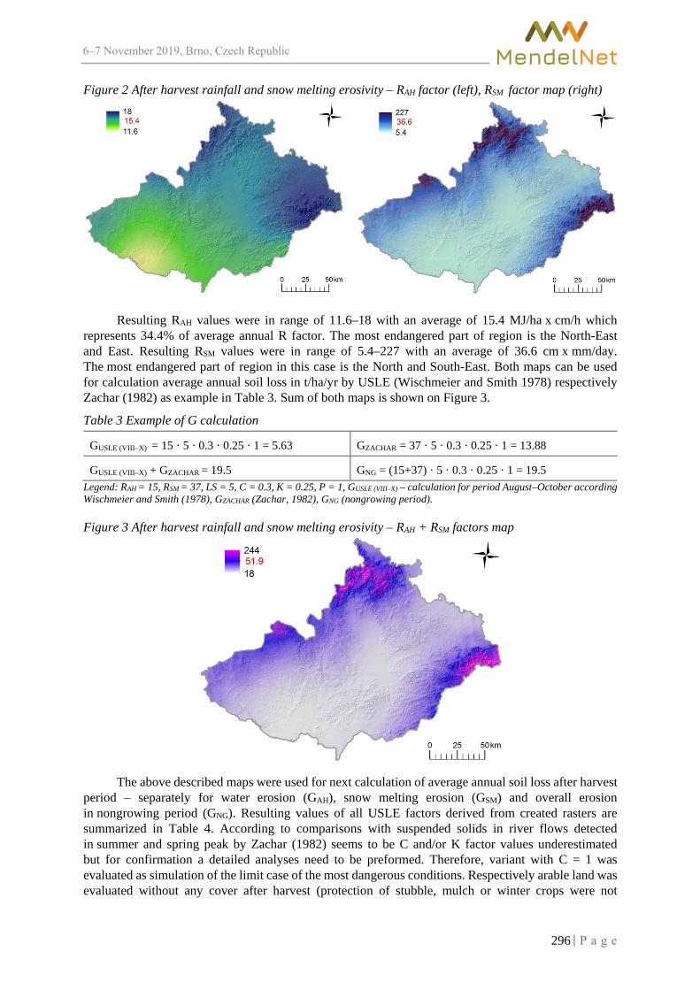
6–7 2019, Brno, Czech Republic
Figure 2 After harvest rainfall and snow melting erosivity – RAH factor (left), RSM factor map (right)
Resulting RAH values were in range of 11.6–18 with an average of 15.4 MJ/ha x cm/h which represents 34.4% of average annual R factor. The most endangered part of region is the North-East and East. Resulting RSM values were in range of 5.4–227 with an average of 36.6 cm x mm/day. The most endangered part of region in this case is the North and South-East. Both maps can be used for calculation average annual soil loss in t/ha/yr by USLE (Wischmeier and Smith 1978) respectively Zachar (1982) as example in Table 3. Sum of both maps is shown on Figure 3.
Table 3 Example of G calculation
GUSLE (VIII–X) = 15 · 5 · 0.3 · 0.25 · 1 = 5.63 GZACHAR = 37 · 5 · 0.3 · 0.25 · 1 = 13.88
GUSLE (VIII–X) + GZACHAR = 19.5 GNG = (15+37) · 5 · 0.3 · 0.25 · 1 = 19.5 Legend: RAH = 15, RSM = 37, LS = 5, C = 0.3, K = 0.25, P = 1, GUSLE (VIII–X) – calculation for period August–October according Wischmeier and Smith (1978), GZACHAR (Zachar, 1982), GNG (nongrowing period).
Figure 3 After harvest rainfall and snow melting erosivity – RAH + RSM factors map
The above described maps were used for next calculation of average annual soil loss after harvest period – separately for water erosion (GAH), snow melting erosion (GSM) and overall erosion in nongrowing period (GNG). Resulting values of all USLE factors derived from created rasters are summarized in Table 4. According to comparisons with suspended solids in river flows detected in summer and spring peak by Zachar (1982) seems to be C and/or K factor values underestimated but for confirmation a detailed analyses need to be preformed. Therefore, variant with C = 1 was evaluated as simulation of the limit case of the most dangerous conditions. Respectively arable land was evaluated without any cover after harvest (protection of stubble, mulch or winter crops were not
296

6–7 2019, Brno, Czech Republic
evaluated) which should simulate conditions close to fallow land. Resulting G values over GP limits values are shown on figure 4–5 and summarized in Table 5–6.
Table 4 Summarization of resulting USLE factors derived from created rasters USLE factor Range Ø SD
L 0–10.3 1.9 1.4 S 0.03–5.6 0.8 0.9 K 0.15–0.6 0.36 0.11 C 0.283–0.385 0.37 0.03
Legend: Ø – average, SD – standard deviation.
Figure 4 Average annual soil loss over GP in nongrowing period – separately GAH, GSM and GNG
Table 5 Summarization of G values for nongrowing period
Method Range (t/ha/yr)
Ø (t/ha/yr)
SD (t/ha/yr)
G > GP (%)
Ø (t/ha/yr)
GRISK > 4 (%)
GRISK > 8 (%)
GAH 0–17.5 2.3 2.8 32.5 2.8 5.4 1.5 GSM 0–23 1.8 3 24.8 6 6.2 2.9 GNG 0–32.8 4 5.2 49.7 6.4 20.36 9.59
Legend: Ø – average, SD – standard deviation, G > GP – soil loss exceeded permissible limit, GRISK > 4, 8 – soil loss exceeded GP by 4, by 8 t/ha/yr.
Figure 5 G over GP in nongrowing period – separately GAH, GSM and overall GNG for the case C = 1
Table 6 Summarization of G values for nongrowing period for the case C = 1
Method Range (t/ha/yr)
Ø (t/ha/yr)
SD (t/ha/yr)
G > GP (%)
Ø (t/ha/yr)
GRISK > 4 (%)
GRISK > 8 (%)
GAH (C=1) 0–41.9 6.3 7.2 70.3 8.3 32.7 19.7 GSM
(C=1) 0–56.6 5.2 10 51.9 8.4 25.1 24.3
GNG (C=1) 0–101.3 10.7 15.1 72.7 15.7 50.4 39 Legend: see Table 4.
297

6–7 2019, Brno, Czech Republic
CONCLUSION Methodology of average annual soil loss calculation in after harvest (AH) / nongrowing period
(GNG) is presented. Based on analyses of 8 year harvest data was defined critical risk period from August to April. Rainfall erosivity factor for this period were calculated for Moravia and represents 34.4% of average annual R factor of CR, average RAH = 15.4 MJ/ha x cm/h and is in range of 11.6–18 MJ/ha x cm/h. Average snow melting erosivity values for Moravia are in range of 5.4–227, with average RSM = 36.6 cm x mm/day. Results show that 49.7% of arable land exceeds the permissible limits (GP) by an average of 6.4 t/h/yr. Separate calculation of water and snow melting erosion of this period shows that 32.5% of arable land exceeds GP by an average of 2.8 t/ha/yr due to water erosion and 24.8% exceeds GP by an average of 6 t/ha/yr due to snow melting erosion. If fallow land condition (C = 1) were evaluated as simulation of the most dangerous conditions then 72.7% of arable land exceeds GP by an average of 15.7 t/ha/yr and separately 70.3% by 8.3 t/ha/yr due to water erosion and 51.9% by 8.4 t/ha/yr due to snow melting erosion. These results proved that GP values can be exceeded only in AH period and even only during snow melting in March or April without occurrence of erosive rainfall. Calculation of erosion in AH period and especially snow melting erosion have to be taken into account otherwise resulted average annual soil loss values can be significantly underestimated.
ACKNOWLEDGEMENTS The research was supported by the project TAČR TH04030363 Development of effective tools to evaluate and reduce the negative effects of rainfall-runoff processes in the nongrowing season in connection with the extremes of climate change.
REFERENCES Brychta, J., Janeček, M. 2017. Evaluation of discrepancies in spatial distribution of rainfall erosivity in the Czech Republic caused by different approaches using GIS and geostatistical tools. Soil and Water Research, 12(2): 117–127. Brychta, J. et al. 2018. Crop-management factor calculation using weights of spatial-temporal distribution of rainfall erosivity. Soil and Water Research, 13(3): 150–160. Brychta, J., Janeček, M. 2019. Determination of erosion rainfall criteria based on natural rainfall measurement and its impact on spatial distribution of rainfall erosivity in the Czech Republic. Soil and Water Research, 14(3): 153−162. Janeček, M. et al. 2012. Ochrana zemědělské půdy před erozí. 1st ed., Prague, CR: Czech University of Life Sciences. Kliment, Z. et al. 2007. Suspended sediment load and soil erosion processes in mesoscale catchment areas. In: Geomorphological Variations. Prague: P3K, pp. 221–252. McCool, D.K. 2002. Erosion, snowmelt. In: Encyclopedia of Soil Science. New York: Marcel Dekker, pp. 1476. McCool, D.K. et al. 1982. Adapting the Universal Soil Loss Equation to the Pacific Northwest. Transactions of the ASAE, 25(4): 928–934. Středová, H., Toman, F. 2012. Erosion potential of snow cover in the Czech Republic. Acta Universitatis Agriculturae et Silviculturae Mendelianae Brunensis, 60(1): 117–124. Vopravil, J. et al. 2007. Revised Soil Erodibility K-factor for Soils in the Czech Republic. Soil and Water Research, 2(1): 1–9. Wischmeier, W.H., Smith, D.D. 1978. Predicting Rainfall Erosion Losses: A Guide to Conservation Planning. Agriculture Handbook no. 537. Washington, USA: U.S. Government Printing Office. Zachar, D. 1982. Soil erosion. 1st ed. Amsterdam: Elsevier Scientific Publishing Company.
298

6–7 2019, Brno, Czech Republic
Evaluation of water erosion in vineyards using rainfall simulator
Alice Cizkova1, Vladimir Masan1, Patrik Burg1, Jana Burgova2 1Department of Horticultural Machinery
2Department of Breeding and Propagation of Horticultural Plants Mendel University in Brno Zemedelska 1, 613 00 Brno
CZECH REPUBLIC
Abstract: This paper discusses and evaluates the results of the impact of several types of cover materials on soil erosion in the vineyards in the Czech Republic. The experiment included a comparison of three variants for soil runoff and soil washdown in the rows of vineyards with a slope of 17.4%. In two variants, the cover materials used were crushed grain straw (var. A, 1200 g/m2) and compost (var. B, 2000 g/m2). The third control variant (var. C) consisted of cultivated interlayer without cover material. For the purposes of experimental measurements, a rainfall simulator was used, simulations were performed using a FullJet nozzle with a wide square spray, at a spray pressure of 0.8 bar and a selected intensity of 120 mm/h. Out of evaluated variants, the lowest cumulative surface runoff values were measured for variant A with a straw cover and corresponded to 8655.66 ml/m2, as well as soil washdown values of 8.84 ml/m2. The results of the statistical evaluation showed a significant difference between all evaluated variants. In the case of surface runoff, var. A decreases to 7.5% and var. B to 56.6% compared to control variant C. For soil washdown, it decreases to 4.6% for variant A and B at 55.0% compared to control var. C.
Key Words: vineyard, water erosion, rainfall simulator, water surface runoff, soil washdown
INTRODUCTION Extreme rainfall events, steep slopes, intensive soil tillage and soil surface characteristics have
been reported as the most relevant indicators to analyse and classify current soil erosion processes in European vineyards (Marques et al. 2007, Biddoccu et al. 2013). Soil erodibility and soil particle washdown in vineyards depend on soil properties of physical, chemical and mineralogical characters (Gabarrón-Galeote et al. 2013). The main process of water erosion is the separation of soil material due to the effect of rain drops and its transport by surface runoff, whereby the most fertile soil layer is lost (Assouline and Ben-Hur 2006).
The standardization of the arrangement, procedure, and evaluation of rainfall simulation experiments is one of the most important tasks for the rainfall simulation community in the next decade. This would be a valuable and necessary step for a reliable assessment of vulnerability, risk levels and control of soil erosion worldwide (Ries et al. 2013).
Currently, there are various methods of measuring water erosion, including rainfall simulation using a field rainfall simulator that generates artificial rain with selectable rainfall intensity and sprinkling time. This type of simulator works on the ground much like natural rainfall (Šindelář et al. 2007, Rodrigo Comino et al. 2016). Rainfall simulation with rainfall simulators is considered to be a useful tool for measuring interrelated soil erosion processes such as splash, initial rainfall-runoff processes and sediment losses (Ramos and Martínez-Casasnovas 2006, Rodrigo Comino et al. 2016). Marques et al. (2007) claims that the intensity and duration of simulated rainfall should be based on meteorological characteristics of the study area.
Several authors (Šindelář et al. 2007, Ries et al. 2013) dealt with the issue of reducing erosive effects on agricultural land. The results of previous work indicate that the positive effect is brought by the application of mulching materials or organic residues on surface runoff and soil washdown (Gabarrón-Galeote et al. 2013).
The aim of this work is to evaluate the effects of water erosion induced by rain simulations on soil runoff and soil wash in different ways of covering the soil surface in vineyards.
299

6–7 2019, Brno, Czech Republic
MATERIALS AND METHODS
Experiment area For experimental measurements, a test site was selected. This site is located in the “Velké
Pavlovice” wine-growing sub-region, in the area of village “Rakvice” and on the track called “Kozí Horky” (Latitude: 48°51′29″N, Longitude: 16°48′48″E). The sites are situated in a hot and dry region with an average annual temperature of 9–10 °C. The average rainfall is 500 mm. The soil type at this experimental site is black, mainly loamy soil with no soil skeleton. The slope of the land is up to 17.4%.
Character of mulching materials and experimental variants The experiment was based on 3 variants, for which 2 kinds of cover material were chosen
for the soil protection - crushed grain straw (variant A, consumption of covering material 1200 g/m2, volume weight 100 kg/m3) and compost made from grape pomace, grass, wood chips and vegetable waste (variant B, consumption of covering material 2000 g/m2, volume weight 560 kg/m3). The third control variant (C) consisted of a cultivated interlayer without covering material.
Collection and analysis of soil samples Sampling was performed from three layers of soil profile: a thin continuous layer - soil crust, was
taken from the soil surface, from a tillage at a depth of 0.0–0.10 m and a sub-tillage 0.10–0.30 m taken to Kopecky cylinders according to the methodology reported by Pospíšilová et al. (2016). Kopecky physical cylinders are made of stainless steel, usually of a volume of 100 cm3 and a maximum height of 5 cm. They are used to determine the physical properties of soils in their intact state (Pospíšilová et al. 2016), in particular current moisture, reduced bulk density and porosity. The soil structure was determined by sieving dry soil on sieves with average apertures of 0.25, 0.5, 1.0, 5.0, 10.0, 20.0 mm. Each structural fraction was separately weighed and converted to percentages. In this way, the percentage of individual dry fraction soil fractions was found. From the calculated values, a structural coefficient was determined, which indicates the ratio between agronomically valuable (i.e. aggregates with a diameter of 0.25–10.0 mm) and less valuable structural aggregates (Badalíková and Kňákal 2001).
Construction of rainfall simulator For the purposes of experimental measurements, we used a rainfall simulator type VÚZT
(Research Institute of Agricultural Engineering, p.r.i.), which consists of a spraying frame, stand and storage tank with manometer and pump. The simulations were performed using a FullJet wide square spray nozzle at a spray pressure of 0.8 bar. The intensity of the rain for the set spray pressure was determined from the weight of water (weighing to within ± 1 g) trapped in a 1.0 × 1.0 m square tub corresponding to the selected measurement area (1.0 m2) and was 120 mm/h. The nozzle meets the drop size (VDM = 2 mm) at the selected spray pressure. For each of the evaluated variants the measurement was performed in two replicates.
Surface runoff measurement From the beginning of each measurement, the time at which the surface runoff began,
and the constant time step of 3 minutes was recorded. The volume of the surface runoff (suspension) was recorded and collected at three-minute intervals into collection vessels. The total duration of the simulations was 30 minutes until the surface runoff got stabilized, the course of the whole experiment was recorded on the timeline - drains and washdowns. The resulting surface runoff volume, after subtracting the volume of dry matter washdown, was determined at individual intervals along with the cumulative surface runoff volume. The solid particles were obtained the next day after decanting, drying and subsequent weighing.
Soil washdown measurement The soil washdown value is obtained by sedimentation and subsequent drying of the soil taken
from the surface runoff at fixed time intervals. The dried samples are weighed, and the values obtained in grams are then converted into the soil volume and the cumulative soil volume by soil density.
300

6–7 2019, Brno, Czech Republic
Statistical analysis A statistical analysis was performed using the software package “Statistics 12.0” (StatSoft Inc.,
Tulsa, Oklahoma, USA). Analysis of variance was conducted, and the results were compared using Tukey's multiple range assay at a significance level α = 0.05.
RESULTS AND DISCUSSION Intact soil samples to evaluate their basic physical properties were taken immediately prior
to the measurement. The values of the basic physical properties of the soil corresponded to the site conditions as shown in Table 1.
Table 1 Physical character of soil
Depth (m)
Density (g/cm3)
Porosity (%)
Volume Maximum capillary capacity
Minimal air capacity Water Air
(% volume) (% volume) 0.0–0.1 1.11 ± 0.08 46.05 ± 3.85 23.02 ± 3.22 23.03 ± 6.55 32.36 ± 2.95 13.69 ± 6.10 0.1–0.2 1.23 ± 0.08 51.36 ± 3.10 26.98 ± 3.77 24.37 ± 4.29 35.54 ± 4.23 15.81 ± 5.28 0.2–0.3 1.32 ± 0.04 54.06 ± 0.83 25.10 ± 3.54 31.97 ± 3.99 36.31 ± 6.41 17.75 ± 6.02
The density values reduced at all depths were favourable and did not exceed the limit value of 1.45 g/cm3 reported by Šindelář et al. (2007). The porosity values also correspond to the limit values. E.g. Joel et al. (2002) states that the good condition has a porosity in the range of 46–54%, Kovaříček et al. (2013) reported the value of 47.08% for tillage. The values of maximum capillary capacity (critical value above 36%) and minimum air capacity values which were not below the limit of 10% vol. (Joel et al. 2002).
The soil structure, as measured by dry aggregation, is expressed by the structurality coefficient. The lower the coefficient, the worse the soil structure is and the increasing the coefficient improves the soil structure. The limit value structurality coefficient is given as 1 (Badalíková and Kňákal 2001). The results shown in Table 2 indicate favourable values of the structural coefficient at the depths studied.
Table 2 Representation of structural elements
Depth (m) Structural elements (% weight) Structurality
coefficient < 0.25 0.25–0.5 0.5–1.0 1.0–5.0 5.0–10.0 10.0–20.0 >20.0 0.0–0.15 7.73 9.36 9.89 38.88 14.76 12.64 6.75 2.69
0.15–0.30 6.91 9.63 9.96 39.07 16.32 12.59 5.51 3.00 Average 7.32 9.49 9.92 38.97 15.54 12.62 6.13 2.84
From the values shown in Figure 1, we can see that at the selected sprinkling rate (120 mm/h), the highest cumulative surface runoff over the monitored time was measured for control variants without covering material (115000.21 ml/m2), on the other hand, the lowest values were measured for variant A with a grain straw cover (8655.66 ml/m2). Joel et al. (2002) state that the intensity and magnitude of surface runoff on sloping soils is governed by precipitation intensity, hydraulic conductivity, microtopography, and soil surface treatment. Šindelář et al. (2007) claim that in order to monitor changes in soil hydraulic properties, it is appropriate to express the surface runoff not only in relation to a unit of area, but also to a unit of time. Prosdocimi et al. (2016) state that different types of plant residues and mulch materials can have a positive effect on soil conditions in small amounts at the same time as reducing erosion on sloping land.
Water erosion is a very complex phenomenon in which a number of factors are involved. In terms of quality, it can be characterized by a loss of soil mass, the so-called soil washdown on a surface unit of soil surface over a certain time period (Assouline and Ben-Hur 2006). The resulting soil washdown values and the cumulative soil washdown values, expressed in volume units, shown in Figure 2 show significantly higher values for control var. C (192.79 ml/m2), followed by variant B covered
301

6–7 2019, Brno, Czech Republic
with compost (107.82 ml/m2). The lowest values of soil washdown were measured in var. A covered with crushed grain straw (8.84 ml/m2). The maximum values of loss were recorded in the time interval 0.25–0.45 h from the start of sprinkling for each variant. Rodrigo Comino et al. (2016) states that a dense grain straw cover protects soil from direct impact of raindrops and contributes to increasing surface roughness, which in turn contributes to reducing surface runoff. García-Moreno et al. (2013) claim that grain straw is very efficient at reducing water losses under low frequency – high magnitude rainfall events and can be a key factor in reducing the amount of soil washdown.
Figure 1 Surface runoff
Figure 2 Washdown
The obtained cumulative values of surface runoff and dry matter loss were statistically evaluated by variance analysis and Tukey's multiple range test at a significance level α = 0.05, as shown in Table 3.
Table 3 The surface runoff and dry matter loss – evaluation of variants
Experiment variants Cumulative values of volume
Surface runoff (ml/m2)
Dry matter washdown (ml/m2)
Var. C (control) 115000.21 ± 101.4c 192.79 ± 0.59c Var. A (crushed grain straw) 8655.66 ± 35.60a 8.84 ± 0.10a Var. B (compost) 65110.18 ± 821.70b 107.82 ± 1.30b
Legend: Data are expressed as means ± standard deviation, different letters in the same columns represent significant difference (P < 0.05).
The values shown in Table 3 show a statistically significant difference in the values of cumulative surface runoff and soil washdown values between all evaluated variants. In the case of surface runoff, var. A decreased to 7.5% and var. B to 56.6% compared to control var. C. The soil washdown was reduced to 4.6% in var. A and 55.0% in var. B compared to control var. C. It follows from the mathematical model that these values represent, under real conditions in var. C loss is up to 7.8 × 10³ kg/ha/h, in var. B 4.4 × 10³ kg/ha/h and in var. A 0.4 × 10³ kg/ha/h.
The results obtained in the wine-growing conditions in the Czech Republic show, that particularly corn straw, together with other types of cover materials, has a positive effect on the surface of the interlayer in terms of erosion reduction.
302

6–7 2019, Brno, Czech Republic
CONCLUSIONS This experimental evaluation was focused on simultaneous measurement of surface runoff
and soil washdown in different ways of covering the soil surface in vineyards. The experiment was carried out in three variants using different types of cover materials - grain straw (1200 g/m2), and compost (dose 2000 g/m2). The third control variant consisted of a cultivated interlayer without cover material.
Resulting statistical analyses of measured data confirm the positive effect of cover materials in their counter-erosion protection. Out of evaluated variants, at the selected sprinkling rate (120 mm/h), the highest cumulative surface runoff over the monitored time was measured for control variant C without covering material (115000.21 ml/m2). For variant B, the surface runoff value (65110.18 ml/m2) and the lowest values were measured for variant A with a straw cover (8655.66 ml/m2).
The resulting soil washdown values and cumulative soil washdown values, expressed in volume units, show significantly higher values for control var. C (192.79 ml/m2), followed by variant B covered with compost (107.82 ml/m2). The lowest values of soil washdown were measured in var. A covered with cereal straw (8.84 ml/m2).
When using straw as a covering material, the surface runoff decreased to 7.5% and the soil washdown to 4.6% compared to the control variant. The use of cover materials can be considered as a promising way of protecting the soil from erosion and at the same time as a measure for increasing the soil moisture.
ACKNOWLEDGEMENTS This paper was finalized and supported by the project IGA-ZF/2019–DP001 “Evaluation of water surface runoff and water infiltration into the soil using rain simulation method” and by the project CZ.02.1.01/0.0/0.0/16_017/0002334 Research Infrastructure for Young Scientists, co-financed by Operational Programme Research, Development and Education.
REFERENCES Assouline, S., Ben-Hur, M. 2006. Effects of rainfall intensity and slope gradient on the dynamics of interill erosion during soil surface sealing. Catena, 66(3): 211–220. Badalíková, B, Kňákal, Z. 2001. Vliv zpracování půdy na půdní strukturu. Úroda [Online]. Available at: http://uroda.cz/vliv-zpracovani-pudy-na-pudni-strukturu. [2019-08-19]. Biddoccu, M. et al. 2013. Hillslope vineyard rainfall-runoff measurements in relation to soil infiltration and water content. Procedia Environmental Sciences, 19: 351–360. Gabarrón-Galeote, M.A. et al. 2013. Seasonal changes in the soil hydrological and erosive response depending on aspect, vegetation type and soil water repellency in different Mediterranean microenvironments. Solid Earth, 4(2): 497–509. García-Moreno, J. et al. 2013. Mulch application in fruit orchards increases the persistence of soil water repellency during a 15-years period. Soil Tillage Research, 130: 62–68. Joel A. et al. 2002. Measurement of surface water runoff from plots of two different sizes. Hydrological Processes, 16(7): 1467–1478. Kovaříček, P. et al. 2013. Vliv zapraveného kompostu na míru povrchového odtoku vody při simulovaném zadešťování. Komunální technika, 7(5), vědecká příloha. Marques, M.J. et al. 2007. Effect of vegetal cover on runoff and soil erosion under light intensity events. Rainfall simulation over USLE plots. Science of the Total Environment, 378(1–2): 161–165. Pospíšilová, L. et al. 2016. Standardní analytické metody a kritéria hodnocení fyzikálních, agrochemických, biologických a hygienických parametrů půd: původní vědecká práce. 1. vyd., Brno: Mendelova univerzita v Brně: Folia Universitatis Agriculturae et Silviculturae Mendelianae Brunensis. Prosdocimi, M. et al. 2016. The immediate effectiveness of barley straw mulch in reducing soil erodibility and surface runoff generation in Mediterranean vineyards. Science of The Total Environment [Online], 547: 323–330. Available at:
303

6–7 2019, Brno, Czech Republic
https://www.sciencedirect.com/science/article/pii/S016819230300203X. [2019-08-19]. Ramos, M.C., Martínez-Casasnovas, J.A. 2006. Impact of land levelling on soil moisture and runoff variability in vineyards under different rainfall distributions in a Mediterranean climate and its influence on crop productivity. Journal of Hydrology, 321(1–4): 131–146. Ries, J.B. et al. 2013. Rainfall simulations - constraints, needs and challenges for a future use in soil erosion research. Zeitschrift für Geomorphologie, Supplementary Issuses, 57: 1–10. Rodrigo Comino, J. et al. 2016. Quantitative comparison of initial soil erosion processes and runoff generation in Spanish and German vineyards. Science of the Total Environment, 565: 1165–1174. Šindelář, R. et al. 2007. Hodnocení povrchového odtoku vody metodou simulace deště. Agritech Science [Online], 2(5): 1–7. Available at: http://www.agritech.cz/clanky/2007-2-5.pdf. [2019-08-18].
304

6–7 2019, Brno, Czech Republic
Change of land cover and its impact on surface runoff and water retention capacity of the landscape
Martina Kulihova1, Jan Szturc2 1Institute of Water Landscape Management
Brno University of Technology Veveri 331/95, 602 00 Brno
2Department of Applied and Landscape Ecology Mendel University in Brno Zemedelska 1, 613 00 Brno
CZECH REPUBLIC
Abstract: The aim of this study is quantification and evaluation of surface runoff and water retention capacity of the landscape depending on land cover in Janovice u Frýdku-Místku in Moravia. For that selected catchment area were analyzed land cover, hydrological, geomorphological and hydropedological conditions using geographical information system (GIS) tools and database data. In the analysis were also identified 8 critical points in this area, where the concentrated surface runoff enters into the village. In the next step water retention capacity was evaluated in selected catchment area with current land cover as well as the volume of direct runoff in watersheds of determined critical points. In selected catchment area there were designed adaptation measures and the significance of land cover change was determined in relation to the water retention capacity of the landscape and direct runoff. Both the water retention capacity and the runoff were calculated using the CN curve number method and the hydrological model DesQ-MaxQ.
Key Words: water retention capacity, land cover, runoff, CN curve number, adaptation measures
INTRODUCTION Research on suitable approaches to increase water retention capacity and soil moisture is really
important these days because of the ongoing climate change and negative impact of hydrometeorological extremes such as drought or floods. Water retention capacity is important to reduce impacts such as soil erosion or soil degradation and to improve the quality of soil and water in our country. Many authors already dealt with the influence of landscape cover on water retention of soil. Much of the published information on this issue comes either from experimental studies or from long-term observations (Schwarze et al. 1994) and on the other hand from the results of using rainfall-runoff models (Tallaksen 1995).
The water retention capacity of the landscape came to the fore of public's interest due to the catastrophic floods in 1997 (Dumbrovský and Spitz 1997). The devastating floods in 2002 and in 2009 again strongly reminded the need to deal with erosion and flood protection and the need to increase water retention capacity in the landscape in the Czech Republic (Pavlík 2014).
The soil water retention relationship, characterized by soil water content and potential, are not unique and are affected by a number of environmental and soil factors. Temperature, irregular pore geometry and discontinuity, and variations in texture and mineralogy are the primary soil properties influencing soil water retention (Rawls et al. 1991). All of these variables can be also influenced by land use.
The arrangement of our country determines the water retention capacity of the landscape and its infiltration conditions. Land use and land cover significantly influence the basic characteristics of direct runoff. Intensive utilization of arable land areas, especially in dangerous erosion of crops, are inappropriate for direct runoff (Daňhelka 2007). Thanks to the water retention capacity of the landscape, the moisture mode on agriculturally cultivated lands and flood protection can be improved (Datel et al. 2015). Appropriately designed flood control and soil conservation measures can have a very positive
305

6–7 2019, Brno, Czech Republic
impact on drought protection and water retention. Adaptation measures on agricultural land such as organizational and agronotechnical measures are appropriate in all aspects. From the point of view of solving the problems of drought their effects on slowing down the surface runoff and increase infiltration are very important (Dzuráková et al. 2017).
MATERIAL AND METHODS
Characteristics of the area This research deals with quantification and evaluation of water retention capacity and surface
runoff depending on land cover. This study was conducted in the 39,4 km2 watershed area. The area of interest is the 4th order catchment areas in Janovice u Frýdku-Místku (number 2-03-01-028, 2-03-01-029, 2-03-01-030 and 2-03-01-032). Janovice is located in Moravian-Silesian region in Beskydy Mountains, 6 km southeast of Frýdek-Místek.
Figure 1 Overview map of the area of interest
The landscape in Janovice is due to its species diversity one of the most diverse natural areas in the region. The highest altitudes are around 470 meters above sea level and the lowest around 340 meters above sea level. Through Janovice flows the river Říčka with its numerous confluents. The area of interest belongs to the sea drainage area of Atlantic Ocean, the Baltic Sea and the Odra River Basin and its located in the 3th order catchment area number 2-03-01 Ostravice. The river network is an asymmetrical arrangement. Other significant flows are Baštice or Bystrý potok.
The whole area consists mainly of agricultural land with mainly crop and livestock production. Forests make up less than 20% of the area.
306
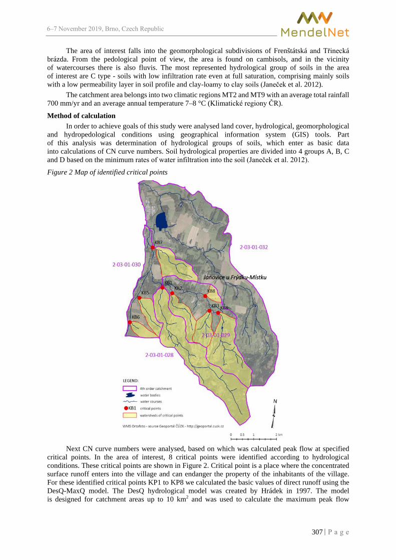
6–7 2019, Brno, Czech Republic
The area of interest falls into the geomorphological subdivisions of Frenštátská and Třinecká brázda. From the pedological point of view, the area is found on cambisols, and in the vicinity of watercourses there is also fluvis. The most represented hydrological group of soils in the area of interest are C type - soils with low infiltration rate even at full saturation, comprising mainly soils with a low permeability layer in soil profile and clay-loamy to clay soils (Janeček et al. 2012).
The catchment area belongs into two climatic regions MT2 and MT9 with an average total rainfall 700 mm/yr and an average annual temperature 7–8 °C (Klimatické regiony ČR).
Method of calculation In order to achieve goals of this study were analysed land cover, hydrological, geomorphological
and hydropedological conditions using geographical information system (GIS) tools. Part of this analysis was determination of hydrological groups of soils, which enter as basic data into calculations of CN curve numbers. Soil hydrological properties are divided into 4 groups A, B, C and D based on the minimum rates of water infiltration into the soil (Janeček et al. 2012).
Figure 2 Map of identified critical points
Next CN curve numbers were analysed, based on which was calculated peak flow at specified
critical points. In the area of interest, 8 critical points were identified according to hydrological conditions. These critical points are shown in Figure 2. Critical point is a place where the concentrated surface runoff enters into the village and can endanger the property of the inhabitants of the village. For these identified critical points KP1 to KP8 we calculated the basic values of direct runoff using the DesQ-MaxQ model. The DesQ hydrological model was created by Hrádek in 1997. The model is designed for catchment areas up to 10 km2 and was used to calculate the maximum peak flow
307

6–7 2019, Brno, Czech Republic
and the total amount of water flowing through a given profile (hydro.upol.cz). We also evaluated water retention capacity of the landscape to the current land cover in 4th order catchment areas.
After the analysis, adaptation measures were designed in two different variants. The first variant was the design of organizational and agronotechnical measures, such as rotation of crops, change of land use, grassing between fields, seeding into protective crop etc. In the second option we designed grassing of all agricultural land. Subsequently, the water retention capacity of the landscape in both variants was again evaluated, as well as the calculation of peak flow at critical points.
Finally, a comparison of values was performed and the evaluation of how the designed adaptation measures affect the water retention capacity of the landscape and the peak flow.
RESULTS AND DISCUSSION In the area of interest, the potential impact of land cover change on water retention capacity
of the landscape was evaluated. The results are presented in the form of two tables showing the effect of the designed adaptation measures. The results of our evaluation are given in Table 1 and Table 2. Table 1 contains critical points KP1–KP8 a three values of peak flows and flood wave volumes calculated in three variants – in the initial state and with two variants of adaptation measures. The initial state, against which the adaptation measures are compared, represents the worst state in the cultivation of wide-row crops in straight lines down the slope. The results in Table 1 shows that the change of land cover and the decrease on CN curve number have a positive impact to reduction the total amount of water flowing through identified profiles.
Table 1 Results of evaluation of peak flow and flood wave volumes in critical points
critical profile
watershed [km2]
CN curve number peak flow [m3.s-1] flood wave volume [10.m3]
initial state var. 1 var. 2 initial
state var. 1 var. 2 initial state var. 1 var. 2
KP1 6.47 70 68.9 68.1 28.6 26 24.2 209 198 190 KP2 1.065 75.1 73.3 72.4 8.92 7.71 7.3 43.4 40.1 38.5 KP3 0.954 72.8 72.5 72 5.25 5.18 4.98 35.1 34.6 33.9 KP4 3.187 68.1 68 67.9 10.4 10.3 10.2 93.4 92.9 92.5 KP5 0.821 83 78.2 77.5 9 6.48 6.21 46 38.2 37.1 KP6 0.467 85 78.2 77.2 6.24 3.88 3.64 28.2 21.7 20.8 KP7 1.523 69.9 68.1 67.5 6.93 5.94 5.65 48.9 44.6 43.3 KP8 0.288 84.3 79.7 78.7 3.56 2.66 2.45 16.9 14.2 13.7
Table 2 contains also three values of direct runoff and water retention capacity which were calculated in the area of 4th order catchments.
Table 2 Results of evaluation of water retention capacity
4th order catchment area area [km2]
direct runoff [mm/period] water retention [mm/period]
initial state var. 1 var. 2 initial state var. 1 var. 2
2-03-01-032 18.659 12.7 10.8 10.4 460 462 462 2-03-01-030 5.755 15.4 12.4 12 457 460 460 2-03-01-028 6.494 9.2 8.5 8 463 464 464 2-03-01-029 8.407 11.3 10.7 10.6 461 462 462
The results in Table 2 show that the effect of increased retention by the design adaptation measure is not very significant. Although the protection of adaptation measures, in addition to soil protection against degradation due to the negative effects of water erosion, are driven by efforts to significantly increase the retention and infiltration capacity of the territory.
308

6–7 2019, Brno, Czech Republic
In this study the most effective measure to increase retention is in the land use change grassland, which is also a very low cost measure compared to other. But when we compare water retention with water needs of plants, we found out that plants still do not have enough moisture because of the rainfall in the area of interest is too low, which means that we need different and more effective measures.
The optimal solution for the landscape as a whole is a comprehensive approach to deal with drought and a design a combination of suitably complementary types of measures (Dzuráková et al. 2017). Reduction of the volume of water flowing out from drainage system, irrigation systems or water reservoirs could be the solution (Mioduszewski 2014).
CONCLUSION The analysis of runoff conditions and water retention capacity of the landscape based
on the change of land cover showed that the design of adaptation measures has a positive effect on both factors. A change of land cover can increase the retained amount of water and reduce unwanted runoff from the landscape. But when we compare this retained water in soil with water needs of plants, it is still not enough.
Increasing the water retention capacity of the landscape cannot significantly increase the productivity of farming in the dry areas of the Czech Republic, as the water deficit is significantly bigger than the potential benefit of measures to increase retention (Trnka et al. 2014–2017).
ACKNOWLEDGEMENTS This study was supported by the National Agency for Agricultural Research of the Czech Republic no. QK1720303 called Retention capacity of the soil and landscape and possibilities of increasing in terms of climate change.
REFERENCES Daňhelka, J. 2007. Operativní hydrologie: hydrologické modely a nejistota předpovědí. Prague. Datel, J.V., Kašpárek, L., Vizina, A. 2015. Retence, ale jaká? Rozdílnost velikosti a funkce složek retence vody v krajině. Prague: T. G. Masaryk Water Research Institute, v.v.i. Dumbrovský, M., Spitz, P. 1997. Biotechnical Measures an Important Part of Watershed Projects in the Czech Republic. In Management of Landscapes Disturbed by Channel Incision. Oxford (USA): The University of Mississippi in Oxford. Dzuráková, M. et al. 2017. Potenciál aplikace přírodě blízkých opatření pro zadržení vody v krajině a zlepšení ekologického stavu vodních útvarů. Vodohospodářské technicko-ekonomické informace, 59(4): 25–32. Hydro.upol.cz. 2011. Vybrané kapitoly z hydrologie [Online]. Available at: http://hydro.upol.cz/. [2019-08-25]. Janeček, M. et al. 2012. Ochrana zemědělské půdy před erozí. Prague: Czech University of Life Sciences Prague. Klimatické regiony ČR (dle Quitt, 1971). 2018. [Online]. Available at: http://www.ovocnarska-unie.cz/sispo/?str=klima-mapa. [2019-08-05]. Mioduszewski, W. 2014. Small (natural) water retention in rural areas. Journal of Water and Land Development, 20: 19–29. Pavlík, F. 2014. Kvantifikace přirozené vodní retenční schopnosti krajiny ve vybraných povodích. Disertation thesis, Brno University of Technology, Institute of Water Landscape Management. Rawls, W.J., Gish, T.J., Brakensiek, D.L. 1991. Estimating Soil Water Retention from Soil Physical Properties and Characteristics. Advances in Soil Science, 16: 213–234. Schwarze, R., Herrmann, A., Mendel, O. 1994. Regionalization of runoff components for Central European basins. IAHS, 221: 493–502. Tallaksen L.M. 1995. A review of baseflow recession analysis. Journal of Hydrology, 165(1–4): 349–370. Trnka, M. et al. 2014–2017. Generel vodního hospodářství krajiny České republiky – stručný souhrn. Prague: SPÚ.
309

6–7 2019, Brno, Czech Republic
Impact of using additives in composting food waste
Alzbeta Maxianova, Magdalena Daria Vaverkova, Dana Adamcova Department of Applied Landscape and Ecology
Mendel University in Brno Zemedelska 1, 613 00 Brno
CZECH REPUBLIC
Abstract: This research was focused onto food waste composting with some additives. It studies the impact of additive on the process of food waste composting. Additives used were sawdust and biochar. Composting samples were cooked potatoes, cooked rice and vegetables. The objective of this study was to compare 6 composts of different compositions. A–100% food waste, B–10% sawdust and 90% food waste, C–10% sawdust from rat’s litter and 90% food waste, D–20% sawdust and 80% food waste, E–40% sawdust and 60% food waste and F–10% sawdust + 10% biochar and 80% food waste. The process of composting took 63 days and the composts were tested for physicochemical properties (temperature, pH, electrical conductivity) and biological properties (phytotoxicity test). The research results revealed that the concentration of 20% sawdust as additive was optimal for food waste compost because the compost exhibited the optimum pH and EC value, and the test of phytotoxicity proved the best results, too. The concentration of 20% sawdust was better than the concentration of 40% sawdust as the latter represented a large volume quantity.
Key Words: electric composter, indoors, sawdust, biochar
INTRODUCTION The Food and Agriculture Organisation (FAO) said that more than billion tonnes of food are
wasted each year. This number associated with food waste (FW), packaging and non-consumble material. The FW presented environmental risk mainly for the negative impact on the environment for the climate change (Morone et al. 2019). Many years ago, FW was disposed in incinerations or landfills. Nowadays, this situation has been changing in the world. Many countries decided for more sustainable methods (Cerda et al. 2018). The life cycle assessment studies showed that anaerobic digestion is the most environmental and economic method of waste disposal. The composting process is in second place before incineration or landfilling (Waqas et al. 2018). All of them comes from degradation biological wastes. The biogas is the final product of the anaerobic digestion. The biogas usually contains gases like methane, carbon dioxide and other gases (Cerda et al. 2018).
The composting process predominates anaerobic digestion for biological waste disposal. More than 90% of garden and FW is being changed into compost. The compost is part of circular economy because compost as a valuable fertilizer represents strategy between biological waste and sustainable agriculture (Razza et al. 2018). The quality of compost determines its application on the soil (Cerda et al. 2018). Compost properties depend on the source and composition of food. For the best properties, is necessary to comply with some criteria such as time, high temperature, pH value, CO2 and O2 (Cerda et al. 2018).
Food waste composting is a complicated process. Optimal method for utilizing food waste compost at the best is to use some additives (Kucbel et al. 2019, Maxianova et al. 2018). Possible additives are sawdust, biochar, zeolite, manure (Waqas et al. 2019, Sharma et al. 2018, Waqas et al. 2018). Sawdust is chosen for its ability to absorb moisture and reduce compost toxicity. The addition of sawdust minimizes nitrogen losses during the process and hence improved C/N ratio. Sawdust exhibits a great interaction with pH, total organic carbon and seed germination (Kebibeche et al. 2019). Biochar is produced from biomass by pyrolysis. The structure of biochar depends on biomass composition and temperature. Biomass converted into biochar can improve and optimize the composting of food waste (Waqas et al. 2018).
310

6–7 2019, Brno, Czech Republic
MATERIAL AND METHODS Study approach
This research is focused on food waste composting and follows the study of Maxianova et al. (2018). Therefore, we decided to use some additive that could improve the quality of the final compost. We chose sawdust and biochar because they can improve the Carbon/Nitrogen ratio and have a better effect on pH and seed germination (Kebibeche et al. 2019). Subsequently, we compared several concentrations of food waste composting processes by using the additive. Compost samples
For the compost samples we used representative leftovers from a local canteen. We chose cooked potatoes (different composition), cooked rice and vegetables (different types) at a ratio 2:2:1. The ingredients were used for every process to guarantee the same conditions.
We had 6 composts A, B, C, D, E and F. These composts were mutually compared. The composting process was prepared according to the publication by Maxianova et al. (2018); however, the additives were included at the beginning together with the food waste samples. A was without any additive, it was only food waste. The other composts were of the following composition: B (10% sawdust and 90% FW), C (10%sawdust from rat’s litter and 90% FW), D (20% sawdust and 80% FW), E (40% sawdust and 60% FW), F (10% sawdust + 10% biochar and 80% FW). The sawdust was bought at a pet shop because it is modified and treated to the same quality. The sawdust from rat’s litter was used because of improved activity of microbes. The biochar was produced from cereal husks and cellulose fibres heated to 600 °C.
The composting samples were mixed together and put into an electronic composter Green Good 02. This household composter of 27 kg in weight has 457 mm width, 457 mm length and 762 mm height. It was made for small consumers like homes, school canteens and offices. It can compost more than 4 kg of food waste per day and turn this waste into compost within 24 hours when the waste is reduced to 80–90%. This composter has power consumption 60–90 kWh/month (oklininternational.com). The electric composter is one of the composters which can compost food waste. The composting process of food waste is different than green composting because food waste can contain also animal products or products full of microbes, so it is necessary to kill these pathogens at higher temperatures. This composter is designed for heat up to almost 70 °C. This temperature is important in the process of hygienic treatment or thermophilic phase. This phase begins when the temperature reaches up to 55 °C. Then almost all pathogens are eliminated (Waqas et al. 2019).
The process of composting took 9 weeks, but the process was divided into two stages. The first stage included the first 4 weeks when the samples were in the composter (D0–D28). The manufacturer informs that food waste will be transformed into mature compost already after 24 hours in the composter. After those 4 weeks, the compost was taken out into a bucket where its maturation stage started, which took other 5 weeks (D28–D63). Testing method
The composts were tested for physicochemical (temperature, pH and electrical conductivity) and biological (phytotoxicity) properties. The temperature was measured according to Waqas (2018) every day by digital thermometer. The thermometer was put in the center of the composter. The pH value and electrical conductivity (EC) value were measured by using a pH/EC meter HQd portable Meter at 1:5 dilution (waste/distilled water) with standard deviation 0.1. Method was used from Unified work procedures by Central Institute for Supervising and testing in Agriculture. These values were measured every week during the composting process in the composter (D0, D7, D14, D21, and D28) and in the maturing phase (D35, D42, D49, D56, D63). The phytotoxicity test was conducted by using the Phytotoxkit made by MicroBio Tests. It was tested two times, after the composting process in composter was ended (D28) and after the maturing phase (D63). The phytotoxicity test was measured according to Maxianova et al. (2018).
RESULTS AND DISCUSSION Table 1 presents results of samples from physicochemical and biological properties.
From physicochemical properties was chosen pH and EC. The limit for pH was 5. Despite the optimal
311
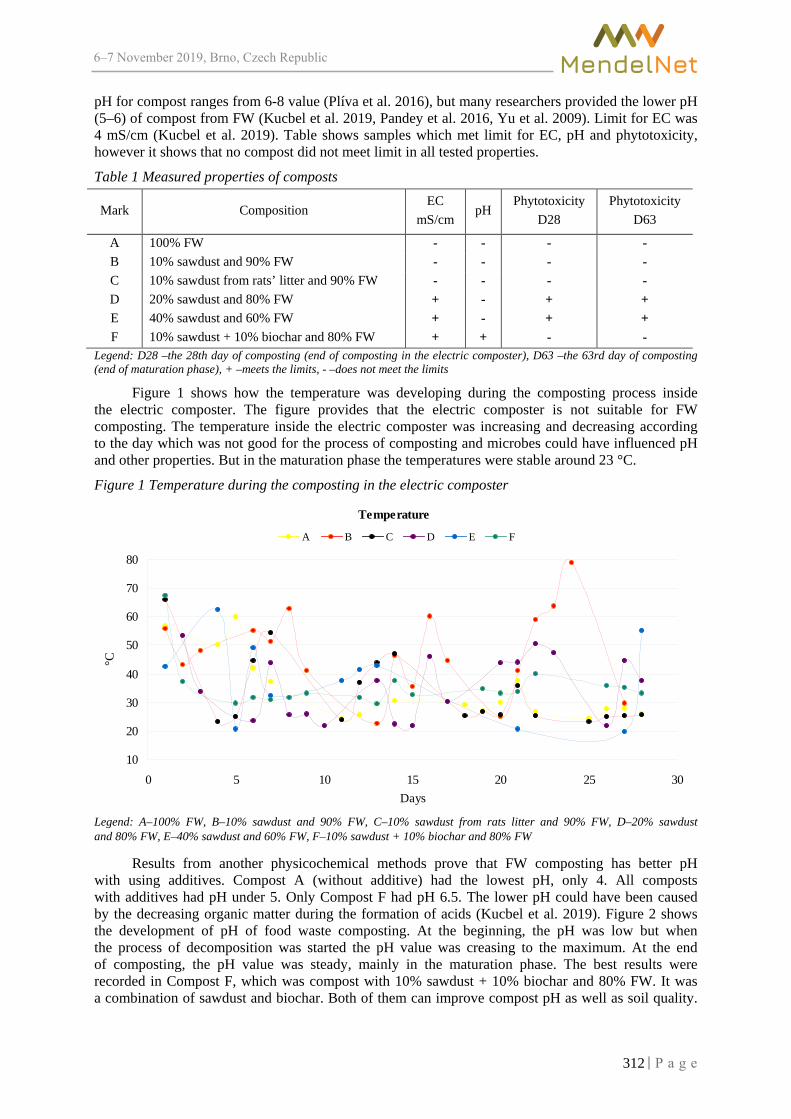
6–7 2019, Brno, Czech Republic
pH for compost ranges from 6-8 value (Plíva et al. 2016), but many researchers provided the lower pH (5–6) of compost from FW (Kucbel et al. 2019, Pandey et al. 2016, Yu et al. 2009). Limit for EC was 4 mS/cm (Kucbel et al. 2019). Table shows samples which met limit for EC, pH and phytotoxicity, however it shows that no compost did not meet limit in all tested properties.
Table 1 Measured properties of composts
Mark Composition EC
mS/cm pH
Phytotoxicity D28
Phytotoxicity D63
A 100% FW - - - - B 10% sawdust and 90% FW - - - - C 10% sawdust from rats’ litter and 90% FW - - - - D 20% sawdust and 80% FW + - + + E 40% sawdust and 60% FW + - + + F 10% sawdust + 10% biochar and 80% FW + + - -
Legend: D28 –the 28th day of composting (end of composting in the electric composter), D63 –the 63rd day of composting (end of maturation phase), + –meets the limits, - –does not meet the limits
Figure 1 shows how the temperature was developing during the composting process inside the electric composter. The figure provides that the electric composter is not suitable for FW composting. The temperature inside the electric composter was increasing and decreasing according to the day which was not good for the process of composting and microbes could have influenced pH and other properties. But in the maturation phase the temperatures were stable around 23 °C.
Figure 1 Temperature during the composting in the electric composter
Temperature
10
20
30
40
50
60
70
80
0 5 10 15 20 25 30Days
°C
A B C D E F
Legend: A–100% FW, B–10% sawdust and 90% FW, C–10% sawdust from rats litter and 90% FW, D–20% sawdust and 80% FW, E–40% sawdust and 60% FW, F–10% sawdust + 10% biochar and 80% FW
Results from another physicochemical methods prove that FW composting has better pH with using additives. Compost A (without additive) had the lowest pH, only 4. All composts with additives had pH under 5. Only Compost F had pH 6.5. The lower pH could have been caused by the decreasing organic matter during the formation of acids (Kucbel et al. 2019). Figure 2 shows the development of pH of food waste composting. At the beginning, the pH was low but when the process of decomposition was started the pH value was creasing to the maximum. At the end of composting, the pH value was steady, mainly in the maturation phase. The best results were recorded in Compost F, which was compost with 10% sawdust + 10% biochar and 80% FW. It was a combination of sawdust and biochar. Both of them can improve compost pH as well as soil quality.
312

6–7 2019, Brno, Czech Republic
However, the results show that sawdust as an additive can improve quality only at the beginning as seen in Figure 2.
Figure 2 The development of pH value of composts
pH
3
4
5
6
7
8
0 10 20 30 40 50 60 70Days
pH
A B C D E F
Legend: A–100% FW, B–10% sawdust and 90% FW, C–10% sawdust from rats litter and 90% FW, D–20% sawdust and 80% FW, E–40% sawdust and 60% FW, F–10% sawdust + 10% biochar and 80% FW, standard deviation of pH/EC meter is 0.1.
Results from EC also confirm that Compost A had the worst results. The EC value of Compost A was almost 9 mS/cm while limit is 4 mS/cm. The reason might have been a huge amount of salt contained in FW. This value might have been decreased due to the use of some additives. Results show us that Compost D, E and F had the lowest EC value and these composts meet the limit for EC value.
Results from biological method also proved that Compost A can not be apply to soil as fertilizer because it is toxic to plant. The phytotoxicity test proves that Compost D and Compost E stimulate seed germination. Compost F has the best results from all tested parameters but the test of phytotoxicity shows inhibition, i.e. no seed germination. Probably the biochar inhibited the process of plant growth which does not prove in other research works (Sun et al. 2017, Waqas et al. 2018).
CONCLUSION Food waste is a current environmental issue. This research shows that the composting of food
waste is difficult. It compares several composting processes with or without the use of additives. The additives used in our research included sawdust or biochar, or a combination of sawdust and biochar. The composts were tested for physicochemical and biological properties. The analysis of results proved that is necessary use some additive for food waste composting. Compost with additives had better results from tested methods than compost without additives. Additive can improve one of tested property but no other. The best results from physicochemical properties had compost with 10% sawdust + 10% biochar and 80% FW but the phytotoxicity test proved inhibiton. The biological method shows that sawdust as additive has good influence on seed germination. However, it is needed do more analysis.
313

6–7 2019, Brno, Czech Republic
ACKNOWLEDGEMENTS This research was financially supported from grant IGA no. TP 3/2018.
REFERENCES Central Institute for Supervising and Testing in Agriculture. 2016. Unified work procedures-Analysis of soils I. 30042.1. Brno: ÚKZÚZ. Cerda, A. et al. 2018. Composting of food wastes: Status and challenges. Bioresource Technology [Online], 248: 57–67. Available at: https://www.sciencedirect.com/science/article/pii/S0960852417310374. [2019–08–25]. Kebibeche, H. et al. 2019. Addition of wood sawdust during the co-composting of sewage sludge and wheat straw influences seeds germination. Ecotoxicology and Environmental Safety [Online], 168: 423–430. Available at: https://www.sciencedirect.com/science/article/pii/S0147651318310868. [2009–08–19]. Kucbel, M. et al. 2019. Properties of compost from household food waste produced in automatic composters [Online]. Journal of Environmental Management, 236: 657–666. Available at: https://www.sciencedirect.com/science/article/pii/S0301479719301598. [2019–08–09]. Maxianova, A. et al. 2018. Determination of phytotoxicity of compost from biodegradable waste from canteen. In Proceedings of International PhD Students Conference MendelNet 2018 [Online]. Brno, Czech Republic, 7–8 November. Brno: Mendel University in Brno, Faculty of AgriSciences, pp. 236–239. Available at: https://mnet.mendelu.cz/mendelnet2018/mnet_2018_full.pdf. [2019–08–15]. Morone, P. et al. 2019. Food waste: Challenges and opportunities for enhancing the emerging bio-economy. Journal of Cleaner Production [Online], 221: 10–16. Available at: https://www.sciencedirect.com/science/article/pii/S0959652619306638. [2019–08–25]. Oklin International Ltd. ©2019. Privacy Policy. [Online]. Available at: http://oklininternational.com/small-scale-composters/. [2019–08–19]. Pandey, P. et al. 2016. In-vessel composting system for converting food and green wastes into pathogen free soil amendment for sustainable agriculture. Journal of Cleaner Production [Online], 139: 407–415. Available at: https://www.sciencedirect.com/science/article/pii/S0959652616311593. [2019–10–14]. Plíva, P. et al. 2016. Kompostování a kompostárny. 1st ed., Praha: Profi Press s.r.o. Razza, F. et al. 2018. The Role of Compost in Bio-waste Management and Circular Economy. In Designing Sustainable Technologies, Products and Policies. New York: Springer Berlin Heidelberg, pp. 133–143. Sharma, D. et al. 2018. Role of sawdust and cow dung on compost maturity during rotary drum composting of flower waste. Bioresource Technology [Online], 264: 285–289. Available at: https://www.sciencedirect.com/science/article/pii/S0960852418307594. [2019–08–20]. Sun, J. et al. 2017. The molecular properties of biochar carbon released in dilute acidic solution and its effects on maize seed germination. Science of the Total Environment [Online], 576: 858–867. Available at: https://www.sciencedirect.com/science/article/pii/S0048969716322690. [2019–08–10]. Waqas, M. et al. 2018. Optimization of food waste compost with the use of biochar. Journal of Environmental Management [Online], 216: 70–81. Available at: https://www.sciencedirect.com/science/article/pii/S0301479717305960. [2019–08–19]. Waqas, M. et al. 2019. Untapped potential of zeolites in optimization of food waste composting. Journal of Environmental Management [Online], 241: 99–112. Available at: https://www.sciencedirect.com/science/article/pii/S0301479719304712. [2019–08–17]. Yu, H. et al. 2009. Effects of sodium acetate as a pH control amendment on the composting of food waste. Bioresource technology [Online], 100(6): 2005–2011. Available at: https://www.sciencedirect.com/science/article/pii/S0960852408008602. [2019–10–22].
314

6–7 2019, Brno, Czech Republic
Degradation of fens and wet meadows of southeastern Bohemian-Moravian Highlands after 20 years
Jan Oulehla1, Martin Jirousek2,3 1Department of Applied and Landscape Ecology
2Department of Plant Biology Mendel University in Brno Zemedelska 1, 613 00 Brno
3Department of Botany and Zoology Masaryk University
Kotlarska 2, 611 37 Brno
Abstract: Most fen and wet-meadow habitats in the Czech Republic have been transformed by drainage, fertilizers inputs and ploughing for agriculture purposes. At nowadays, despite regular management measures at many sites, we can see qualitative deterioration and gradual area loss of the low-productive wetland habitats. Using local historical vegetation data and current data, we demonstrate changes in studied natural habitats at 24 localities within southeastern Bohemian-Moravian Highlands after twenty years. The original habitats were found as same only at three localities, while the rest of localities changed somehow. Less than two-thirds of fens and wet meadows remained preserved up today, whereas a significant area changed into mesic meadows, reed beds, willow carrs, young alder forests or even ruderal vegetation, tree plantations or arable land. The main cause of degradation is mainly the abandonment of the traditional use, resulting in eutrophication and succession leading to above mentioned secondary habitats. Moreover, the deliberate destruction of the habitats for agriculture or forestry use was also documented.
Key Words: biodiversity, habitats, land use, landscape homogenisation, succession, vegetation change
INTRODUCTION Wetlands are among the most endangered habitats in Europe. Due to strong degradation,
especially fens are included in the European Red List of Habitats (Jansen 2016). The main causes are agricultural intensification and on the other hand also an abandonment of traditional land use (Wassen and Venterink 2006). In the Czech Republic, humans facilitate and accelerated changes in landscape in the last 70 years, which is associated with the succession of wetlands towards drier habitats (Szabó et al. 2017).
Fertilizers input from intensive agriculture is a major threat (Cussel 2014). Less than half of the total nitrogen input in fertilizers is used by plants, the rest is dispersed into the environment (Galloway et al. 2008). Wetland habitats are significantly affected by dewatering, which leads to a worsening of the effects of other stressors (Galbraith et al. 2005). It means that nutrient shifts are more concentrated in the case of drained wetlands. Long-term droughts have also had a similar effect to drainage in recent years. Due to this fact, degradation occurs even with well-chosen management. By lowering the water level, the upper layers are aerated. In aerobic conditions, decomposition of organic matter is approximately 50 times faster than in anaerobic condition (Mitsch and Gosselink 1993).
Most common fen vegetation Caricetum nigrae, developed on the site of the alder carrs and alluvial forests or the edges of pounds (Chytrý et al. 2011). Without mowing or removal trees this vegetation undergoes a successional change (Navrátilová 2017). Surface drainage or nutrient input may occur wet Cirsium meadows (Calthion palustris alliance) whereas permanent higher-water level leads to the vegetation of tall-sedges (Magno-Caricion elatae; Hájková and Hájek 2007), instead of original fens. Fen meadows provide ecosystem services such as water retention, drought prevention
315

6–7 2019, Brno, Czech Republic
and nutrient removal. Degraded fens still have the same ecosystem services but with lower effect (Klimkovska et al. 2010).
Wet meadows are more common than real fens within the study region. Several of them are still containing threatened fen organisms and have high importance for regional biodiversity. Threats of this habitat are fertilizing and drainage causes the overgrowth of tall-grass and ruderal species (Chytrý et al. 2010).
The landscape mosaic of diverse habitats is disappearing from the landscape and it is becoming homogenous (Navrátilová 2017).
Historical and present habitat occurrences were compared on the same 24 localities in this study. The main goal was to bring forward warning information of rapid deterioration of fens and wet meadows in the study area and the associated loss of biodiversity in the last 20 years.
MATERIAL AND METHODS
Study area The study area is located in the southeastern part of the Bohemian-Moravian Highlands (Czech
Republic) in the vicinity of the town Velké Meziříčí. Only three localities are protected by law as the small-scale protection areas where mowing management is set, whereas the other localities are used for different purposes or stay abandoned (Oulehla 2019). The hydrological regime has been greatly influenced after soil drainage. Altogether four localities are completely drained, two are partially drained and around nine others are drained neighbouring meadows or arable land. Drainage is missing only at nine localities.
List of study localities Loc.1. Nad Horníkem (coordinates: 49°25'49,580"N 16°01'27,430"E, area: 1.10 ha) Loc.2. Pod fotbalovým hřištěm (coordinates: 49°25'40,116"N 16°01'40.021"E, area: 0.15 ha) Loc.3. Nad Hodíškovským (coordinates: 49°30'51.344"N 16°02'11.055"E, area: 2.3 ha) Loc.4. Západně od Hodíškovského (coordinates: 49°30'38.178"N 16°02'00.936"E, area: 0.57 ha) Loc.5. Oudoly (coordinates: 49°22'38.284"N 16°09'19.760"E, area: 2.38 ha) Loc.6. Za Křižovníkem (coordinates: 49°21'48.850"N 16°06'51.812"E, area: 0.34 ha) Loc.7. Okolo studní (coordinates: 49°26'54.886"N 16°06'27.498"E, area: 0.88 ha) Loc.8. Nad studněmi (coordinates: 49°26'54.484"N 16°06'49.514"E, area: 0.03 ha) Loc.9. Pod Obecníkem (coordinates: 49°26'32.988"N 16°03'06.809"E, area: 1.47 ha) Loc.10. Šebeň (coordinates: 49°24'30.479"N 16°03'09.706"E, area: 0.02 ha) Loc.11. Pod Pařezným (coordinates: 49°28'33.781"N 15°51'14.953"E, area: 1.28 ha) Loc.12. Pod Ochozem (coordinates: 49°24'15.314"N 15°58'16.599"E, area: 2.51 ha) Loc.13. Pod Vrkočem (coordinates: 49°24'10.153"N 15°57'12.252"E, area: 1.42 ha) Loc.14. Obecní pastvina (coordinates: 49°25'26.494"N 16°03'55.137"E, area: 0.60 ha) Loc.15. U studní (coordinates: 49°26'20.600"N 16°03'58.690"E, area: 0.95 ha) Loc.16. Nad potokem (coordinates: 49°25'24.415"N 16°01'06.189"E, area: 0.59 ha) Loc.17. Lesní louka (coordinates: 49°27'39.326"N 15°50'10.296 "E, area: 0.58 ha) Loc.18. Západně od Čechova (coordinates: 49°26'44.741"N 16°04'50.803"E, area: 0.76 ha) Loc.19. U Znětíneckého (coordinates: 49°27'38.485"N 15°55'15.077"E, area: 1.07 ha) Loc.20. Pod Staropavlovským (coordinates: 49°27'29.522"N 15°55'06.869 "E, area: 0.61 ha) Loc.21. Pod Brejlovským (coordinates: 49°23'50.969"N 16°05'38.098"E, area: 0.59 ha) Loc.22. Pod Chlostůvkem (coordinates: 49°20'58.372"N 16°07'28.485"E, area: 0.50 ha) Loc.23. Za Mládkovem (coordinates: 49°20'51.515"N 15°51'29.398"E, area: 0.75 ha) Loc.24. Pod polem (coordinates: 49°24'50.990"N 16°04'19.391"E, area: 0.28 ha)
316

6–7 2019, Brno, Czech Republic
Data processing A total of 24 wetland localities were selected to compare the historical state of vegetation (Lysák
2000) and the current state of vegetation (Oulehla 2019) on the level of habitats (Chytrý et al. 2010). We focused only on localities with a dominance of low-productive non-forest wetland vegetation classified into fens and wet meadows (habitats R2.2, R2.3, T1.5 and T2.3 according to Chytrý et al. 2010, Filippov et al. 2008) described 20 years ago in the study area. Occurrences of the other habitats in the historical data formed only a marginal proportion concerning their natural character. Further, aerial maps from 2003 (closest available to the historical vegetation data) and 2017 (closest to the present), and analogously data from habitat mapping in 2001–2005 and mapping updates in 2010–2017 (Härtel et al. 2009) were used to verify the habitat classification and area proportion in certain cases.
Areas of the localities and habitats within them have been mapped and counted (ESRI ArcGIS Desktop). In one layer, historical data were drawn and in the second layer data updates after 20 years.
To demonstrate the trend of habitat change with respect to the localities, values were counted as follows: 1 (= 100%) was set for the presence of single habitat type on locality, where no mosaic with other minor habitat occurred. Lower values (between 0.05–1; habitats with a lower occurrence than 5% were not considered) have been assigned to the habitats in the case of presence of more habitats within the locality, where total sum had to be also 1 (100%).
RESULTS AND DISCUSSION Transitional mires were extremely rare in the area already in 2000 (two localities only), to this day
approximately half of the total area of transitional mires is preserved and occurs only as a part of one locality (Figures 1–2). One locality (Nad studněmi) with the transitional mire vegetation in the past passed into young alder forest as a whole.
Acidic moss-rich fens are a dominant type of mires in the study region. In last 20 years, about 60% of the original area stay preserved whereas due to degradation mechanisms and following succession, the rest of vegetation has been transformed into wet Cirsium meadows, submontane and montane Nardus grassland and ash-alder alluvial forests. By renewed drainage and intensive agricultural use at one locality, the fen changed into mesic Arrhenatherum meadow.
Figure 1 Comparison of areas of habitats in 2000 and present (2019)
The main recorded vegetation type at all in time 20 years ago were wet Cirsium meadows. Of the total area, 66% of the wet meadows have been preserved up to this day. Wet Cirsium meadows were found as most affected by human activities due to their economic availability (grass cutting, mulching, or even used as arable land). Expansion of tall-herb ruderal vegetation, reed bed vegetation, willows and alders was found as common. Paradoxically, also several of the meadows have been flooded and changed into tall-sedge beds.
317

6–7 2019, Brno, Czech Republic
The area of submontane and montane Nardus meadows has been preserved to 60% of the original area. Due to the fertilizers input, mesic Arrhenatherum meadows were created on intensively mown meadows.
Although the trend diagram (Figure 2) gives the impression that the landscape is more diversified contrary to the situation 20 years ago, the opposite is true. Note, that only relatively preserved localities with fen and wet meadow vegetation were chosen for comparisons with the present situation, whereas localities with strongly degraded vegetation as well as the vegetation types forming the landscape matrix already in time 20 years ago were excluded from the analysis. Compared to the historical state, the list of habitats in localities of non-natural character or strongly influenced by man appeared in the list of present habitats. The reason for this is spruce afforestation, creating the arable land in one case, or general end of mowing leading into habitats with competitively strong herb-sedge-grass vegetation and stands of early succession woody vegetation.
Figure 2 Trend diagram of habitat changes. The values indicate how many historical and present localities were covered by the vegetation of each habitat. The arrows indicate how the habitats on localities remained or changed to another habitats.
Although the same habitats still occur at individual sites, it should be noted that these are quantitative data, not qualitative data. Degradation of individual habitats, for example expanding of species like Calamagrostis canescens, is not considered in the study. If we would like to express a qualitative comparison of habitats in general, we would say that only 3 localities (Pod Vrkočem, Za Křižovníkem and Šebeň) have the same character as in the past. While wet Cirsium meadows, for example, consist of up to 70 species per locality of the studied region, the vegetation of degraded locality is often monodominant and have much lower biodiversity (Oulehla 2019). Primarily competitive weak plant species retreat or locally extinct in behalf of the stronger competitive ones, the better adapted to human-modified eutrophic agriculture landscape (Oulehla et al. 2018). Unfortunately, also despite
318

6–7 2019, Brno, Czech Republic
regular management measures at many sites, we can see qualitative deterioration and gradual area loss of the low-productive wetland habitats, hand to hand with plant species richness decreasing or even continual regional extinctions, as we found for example for Pedicularis palustris (Oulehla et al. 2018).
Figure 3 Photographs from the same place (Nad Hodíškovským) after 20 years with the typical young successional stage of alder forest creating after wet meadow abandonment. Photo: F. Lysák, 1999 (left), J. Oulehla, 2019 (right).
Already in 2000, many wetland habitats were degraded and therefore acidic moss-rich fens
in some localities were already substituted by wet meadows, and analogically wet meadows substituted by mesic meadows. Certainly, a longer period would be more appropriate for such comparisons and from the mid-nineteenth century continuously up to the recent we could find much more interesting results. However, there are only older floristic data, or data about historical land use, from which we are not able to determine the precise change on vegetation (habitat) level and get informative results for the whole study region. Nevertheless, comparisons after 20 years provide warning information on degradation and more attention to the management care should be given for further preservation of local threatened species (Bergamini et al. 2009) as well as fen and wet-meadow ecosystems (Klimkowska et al. 2010, Schrautzer et al. 2013).
CONCLUSION The changes in the habitats over the last 20 years shows us well the main phenomena
in the landscape use. General degradation occurs due to eutrophication, water regime changes and mainly abandonment of traditional land use. Whereas the drainage and following afforestation or agriculture were major threats for fen meadows in the 20th century, the main recent problem is the lack of management. Without regular care, vegetation shifts into the final successional stage concerning the local environment, the ash-alder alluvial forests. Moreover, eutrophication speeds up the succession processes. Localities affected by drainage changed into drier communities, despite regular care by mowing. Compared to the situation 20 years ago, valuable vegetation of acidic moss-rich and transitional fens, wet Cirsium meadows and wet Nardus meadows are now preserved at less than two-thirds of the former area. This is also associated with the loss of wetland flora bound to these specific habitats. For restoring fens we should raise water levels by closing drainage, remove nutrients from the system by mowing, pasturing or even topsoil removing in most affected patches. Preservation of selected habitats in the region for the next 20 years requires regular and well-organized care.
REFERENCES Bergamini, A. et al. 2009. Loss of habitat specialists despite conservation management in fen remnants 1995–2006. Perspectives in Plant Ecology, Evolution and Systematics, 11(1): 65–79. Chytrý, M. et al. 2010. Habitat Catalogue of the Czech Republic. 2nd ed., Praha: Agentura ochrany přírody a krajiny ČR. Chytrý, M. et al. 2011. Vegetation of the Czech Republic 3. Aquatic and Wetland Vegetation. Praha: Academia.
319

6–7 2019, Brno, Czech Republic
Cussel, C. et al. 2014. Nitrogen or phosphorus limitation in rich fens? - Edaphic differences explain contrasting results in vegetation development after fertilization. Plant and Soil, 384(1–2): 153–168. Fillipov, P. et al. 2008. Příručka hodnocení biotopů. Praha: Agentura ochrany přírody a krajiny ČR. Galbraith, H. et al. 2005. The effects of agricultural irrigation on wetland ecosystems in developing countries: A literature review. CA Discussion Paper 1 Colombo, Sri Lanka: Comprehensive Assessment Secretariat. Galloway, J.N. et al. 2008. Transformation of the Nitrogen Cycle: Recent Trends, Questions, and Potential Solutions. Science, 320: 889–892. Hájková, P., Hájek, M. 2007. Calthion palustris. In: Vegetation of the Czech Republic 1. Grassland and Heathland Vegetation. Praha: Academia, pp. 238–241. Härtel, H. et al. 2009. Mapování biotopů v České republice: východiska, výsledky, perspektivy. Praha: Agentura ochrany přírody a krajiny ČR. Jansen, F. 2016. Poor fen. European Red List of Habitats. Mires Group, EIONET. [Online]. Available at: https://forum.eionet.europa.eu/european-red-list-habitats/library/terrestrial-habitats/d.-mires-and-bogs/d2.2a-poor-fen. [2019-08-05]. Klimkovska, A. et al. 2010. Prospects for fen meadow restoration on severely degraded fens. Perspectives in Plant Ecology, Evolution and Systematics, 12(3): 245–255. Lysák, F. 2000. Ohrožená mokřadní květena Velkomeziříčska a její ochrana. Diplomová práce, Univerzita Palackého v Olomouci. Mitsch, W.J., Gosselink J.G. 1993. Wetlands. 2nd ed. New York: Van Nostrand Reinhold. Navrátilová, J. et al. 2017. Convergence and impoverishment of fen communities in a eutrophicated agricultural landscape of the Czech Republic. Applied Vegetation Science, 20(2): 225–235. Oulehla, J. et al. 2018. Local extinctions of threatened species of Pedicularis L. in agriculture landscape of southeastern Bohemian-Moravian Highlands. In Proceedings of International PhD Students Conference MendelNet 2018 [Online]. Brno, Czech Rebublic, 23 November, Brno: Mendel University in Brno, Faculty of AgriSciences, pp. 205–210. Available at: https://mnet.mendelu.cz/mendelnet2018/mnet_2018_full.pdf Oulehla, J. 2019. Degradace mokřadní vegetace na Velkomeziříčsku a možnosti její obnovy. Diplomová práce, Mendelova univerzita v Brně. Schrautzer, J. et al. 2013. Characterizing and evaluating successional pathways of fen degradation and restoration. Ecological Indicators, 25: 108–120. Szabó, P. et al. 2017. Trends and events through seven centuries: the history of a wetland landscape in the Czech Republic. Regional Environmental Change, 17(2): 501–514. Wassen, M.J., Olde Venterink, H. 2006. Comparison of nitrogen and phosphorus fluxes in some European fens and floodplains. Applied Vegetation Science, 9(2): 213–222.
320
6–7 2019, Brno, Czech Republic
State of territorial systems of ecological stability in Hodonín municipality with extended power
Pavla Pokorna
Department of Applied and Landscape Ecology Mendel University in Brno Zemedelska 1, 613 00 Brno
CZECH REPUBLIC
Abstract: This paper deals with the state of territorial systems of ecological stability in the territory of the municipality with extended competence, Hodonín, which manages 18 municipalities, each of which has one cadastral area. Specifically, this looks at five municipalities: Čejč, Čejkovice, Mutěnice, Starý Poddvorov, Nový Poddvorov. It analyses the situation at the time of planning and today, considering the state of implementation of the planned network. Orthophoto images and field survey were used for verification. The results were then displayed using ArcGIS. The results show that 76.7% of the proposed areas for TSES already exist, 6.9%, partly exist and 16.4% do not exist at all. In further analyses it is necessary to broaden the analysis to the verification of target communities and the correct proportions of individual elements according to the approved methodology.
Key Words: Territorial system of ecological stability, Hodonín
INTRODUCTION The territorial system of ecological stability (TSES) is, according to Act 114/1992 on Nature
and Landscape Protection, an interconnected set of natural and altered but naturally close ecosystems that maintain the natural balance. Often this term is confused with the term green network. Thanks to its being enshrined in Czech legislation, TSES is a building block of the green network in our country. In the Czech Republic, in addition to the TSES element, green areas include specially protected areas, important landscape features and defined habitats of specially protected species. The green network is thus a broader acceptance and TSES is a more concrete form with expert foundations (Pesout and Hosek 2012).
TSESs consist of biocentres, biocorridors and interaction elements. Territorial systems of ecological stability are divided into three levels according to their importance: supra-regional, regional and local. The local level is planned at the level of individual municipalities and is included in the zoning plan. The designation of individual areas in the zoning plan should be correctly based on the TSES plan or the TSES General plan. The TSES General Plan defines individual elements only schematically based on natural conditions. This document does not address ownership rights to land; therefore, it is necessary to refine the proposed areas precisely in the TSES plan (Binova et al. 2015)
Local TSES plans must always follow and include regional and supra-regional TSES levels. The responsibility for designing the system is always the local authority. The local TSES plan can be proposed by an authorised person with valid certification issued by the Ministry of the Environment. As part of the zoning plan approval process, the authorities, the surrounding municipalities and the public may comment on the newly proposed areas. A frequent problem in design is the inconsistency of the local TSES with regards to the borders of cadastres, which can be observed, for example, at the borders of Lužice and Mikulčice (Figure 1). This could be solved by the creation of local TSESs for municipalities with extended powers which would subsequently be the basis for territorial plans of individual municipalities. (Miklos et al. 2019).
This paper deals with the territory of Hodonín, a municipality with extended competence, which manages 18 municipalities, each of which has one cadastral territory. This area lies in the south of Moravia near the border with Slovakia, east of the village Břeclav. The White Carpathians Protected Landscape Area extends into part of the territory, and is the only large specially protected area
321

6–7 2019, Brno, Czech Republic
in the area. The Morava and Kyjovka rivers flow through the area and are important bodies of water. In the territory, all municipalities have a valid zoning plan. The municipality of Terezín has a plan last approved in 1998 and has not yet started to update it. Other municipalities with older plans have begun to propose new ones (see Table 1). All territorial plans contain the current state and design of territorial systems of ecological stability.
Figure 1 Disagreements on the border of the cadastres Lužice and Mikulčice
Table 1 Overview of fungicide treatments approved designed approved designed
Čejč 2002 Mutěnice 2016 Čejkovice 2014 Nový Poddvorov 1999 2017
Dolní Bojanovice 2013 Petrov 2005 2018 Dubňany 1999 2018 Prušánky 2000 2016 Hodonín 2012 Ratíškovice 2016 Josefov 2009 Rohatec 2018 Karlín 1998 2016 Starý Poddvorov 2013 Lužice 2015 Sudoměřice 2018
Mikulčice 2019 Terezín 1998
The issue of the implementation of TSES elements in professional circles is not much discussed by the authors. Some partial experiences are discussed at the cleaning seminars TSES - Green Spine of the Landscape, which is enjoyed every year in Brno. Hawkins and Selman (2002) deal with the issue of the implementation of ecological networks for the UK environment. In many cases, they do not clash with the reality of the Czech Republic. Above all, it concerns property relations, where in the UK they have less success than in our country. Jongman (2008) draws attention to the need for cooperation with stakeholders and the change in land issues. The evidence on specific examples boosts cooperation between government agencies and NGOs.
322

6–7 2019, Brno, Czech Republic
MATERIAL AND METHODS The maps of functional and proposed elements of territorial systems of ecological stability was
created by vectorisation in the ArcGIS program for above-ground plans of individual municipalities, which were provided by the Hodonín municipality with extended powers. These are also available on the website of the municipality. Subsequently, the data was verified according to the orthophotomap from 2018. Information from the ortophotomap verified in unclear places at field survey and then entered into the map. Using the images in the field verified the generic composition of elements of the TSES, the dimensions of elements and their existence. At present, five cadastral areas are verified in this way and gradually the data is being processed for the rest of the territory.
RESULTS AND DISCUSSION The comparison of plans with the actual progress of implementation clearly showed that the state
of local TSES corresponds to the time that the municipalities had to implement the plan. However, the situation in the village of Čejč, which has the oldest document among the selected municipalities, did not correspond to this pattern. The village of Nový Poddvorov has the smallest network of TSES elements, with the largest share of arable land. Generally, we can observe that municipalities propose most of the elements of the TSES while already established.
Figure 2 shows the current status of the proposed network of all levels of territorial systems of ecological stability. Green depicts functional elements, red shows those which have not yet been realised, and orange signifies those that have been partially implemented.
Figure 2 TSES and important landscape features in cadastres Čejč, Čejkovice, Mutěnice, Starý Poddvorov, Nový Poddvorov
The surveyed area of five municipalities covers a total of 7907.72 ha. After completion
of all TSES elements will occupy an area of 809.17 hectares which will be 10.23% of the territory. There is now 620.58 ha of TSES elements. See Figure 3 and Figure 4 for a detailed breakdown of each TSES type in the territory and its area.
323

6–7 2019, Brno, Czech Republic
Figure 3 Numerical representation of each TSES elements in the area
Legend: LBC – local biocentre, LBK – local biocorridor, NRBK – national biocorricor, RBC – regional bicentre, RBK – regional biocorridor¨
Figure 4 Area distribution of each TSES types in the area (total area of the area is 7907.72 ha)
The graphs show that regional biocentres occupy the largest area, although there are only two in the territory. These are the biocentres Kapánsko and Hájek-Ochozy. The highest number is local biocorridors, although they occupy only 13.6% of the total area of TSES elements in the territory. This result may be eligible for designers where biocorridors can be on existing features in the landscape. Therefore, it is possible to get local biocorridors which can be purchased or obtained in advance. The biggest realization problem is observed in the national biocorridor, where there are large areas, the biggest problems are property relations.
324

6–7 2019, Brno, Czech Republic
CONCLUSION The present results are only partial, on which further analyses will be carried out, in particular
the comparison of individual target communities with the actual form. Furthermore, the analysis of connectivity of individual elements, which is necessary to propose to complement the network of local TSES, especially the interaction elements, which is not too much problem with ownership relationships in building. Interaction elements also greatly help to increase biodiversity. In the landscape of Hodonín, where small tenancy is disappearing and large-scale excavations are spreading, individual trees or groups of shrubs will help.
ACKNOWLEDGEMENTS The research was financially supported by grant no. AF-IGA2019-IP030 „Analysis of local Territorial system of ecological stability of landscape and the Green infrastructures in the Hodonín municipality with extended powers “.
REFERENCES Binova, L. et al. 2015. Metodika vymezování územního systému ekologické stability. Praha: Ministry of the Environment of the Czech Republic. Czech Republic. 1992. Zákon č. 114/1992 Sb., o ochraně přírody a krajiny. In: Sbírka zákonů České republiky. 28: 666–692. Also available at: http://aplikace.mvcr.cz/sbirka-zakonu/SearchResult.aspx? q=1992&typeLaw=zakon&What=Rok&stranka=11. [2019-08-12]. Hawkins, V., Selman, P. 2002. Landscape scale planning: exploring alternative land use scenarios. Landsc. Urban Plan, 60: 211–222. Jongman, R. 2008. Ecological Networks are an Issue for All of US. Journal of Landscape Ecology, 1(1): 7–13. Miklos, L. et al. 2019. Ecological Networks and Territorial Systems of Ecological Stability. 1st ed., Berlin: Springer International Publishing. Pesout, P., Hosek M. 2012. Ekologická síť v podmínkách ČR. Ochrana přírody, 67(2012): 2–8.
325

6–7 2019, Brno, Czech Republic
Life Cycle Assessment (LCA) of an e-waste device
Arkadiusz Religa, Magdalena Dziewulska, Maria Łukasiewicz, Mateusz Malinowski Department of Bioprocesses Engineering, Energetics and Automatization
University of Agriculture in Krakow Balicka 116b, 30 – 149 Krakow
POLAND
Abstract: Life Cycle Assessment (LCA) is a method that allows a comprehensive assessment of the environmental impact of the process of extracting raw materials, manufacturing specific products from them, using and managing waste resulting from them. The increase in the mass of small household appliances introduced to the market raises the question of the environmental effects of their manufacture and use. In addition, it is essential from a cognitive point of view to know if recycling of certain components of the e-waste device can offset the negative effects on the environment. Three different iron models were subjected to the comprehensive LCA analysis. As a result of the analysis, it was found that the negative effect on the environment in the case of an iron was determined by the phase of its use in the household. Moreover, it was revealed that the design of irons allows recycling of very few of their components, which did not compensate for environmental damage resulting from the process of production and operation of these appliances. Key Words: Life Cycle Assessment (LCA), household appliances, an iron
INTRODUCTION All processes related to the production of products, their use and management have an impact
on the environment. The MBT method does not fully destroy the waste and landfilling is the most commonly used method of waste (MSW) disposal (Voberková et al. 2017, Vaverková et al. 2019). The production of electrical and electronic equipment is currently the fastest growing branch of industry. It is estimated that small household appliances currently account for around 10% of equipment placed on the market. In the years 2007–2015, an increase by over 22% in the mass of small household appliances introduced was noted. As Adamczyk (2004) reports, the phenomenon of widespread product life cycle shortening can be observed more and more often. This is due to the lack of spare parts and the production of devices with ever shorter durability. The shortening of the product life cycle is also caused by the increase in wealth and response to the market offer. This phenomenon also occurs as a result of introducing new (especially innovative) products.
Ecological Life Cycle Assessment (LCA) is a technique for assessing environmental aspects and a potential environmental impact, developed for product life cycle assessment, starting with the extraction of natural resources, their processing, through product manufacture, use, reuse, recycling to final waste disposal, i.e. "from cradle to grave" or "from cradle to cradle" (Grzesik 2006). This method can be described as the assessment of aspects affecting the environment throughout the product life cycle, i.e. from the acquisition of raw materials through production, use, end-of-life processing of various equipment components and final disposal (Grzesik and Terefeńko 2012). It is noteworthy that the LCA analysis is an iterative method, which means that the scope of research may be modified depending on the collected data and analysis of results (Generowicz et al. 2009). However, the most important aspect of the method is the fact that while having the ability to modify tests, the method takes into account the impact throughout the entire life cycle of the product (Grzesik and Terefeńko 2012, EN ISO 14040: 2006, LCA 2006). The first stage of the life cycle assessment, i.e. determining the purpose and scope, is a key stage of the analysis. The purpose of the LCA tests should clearly determine the intended applications of the test results, and the scope should define the system boundaries (Grzesik 2006). The scope of research is determined by characterizing the scope and type of collected data and system boundaries. At this point, it is determined which stages of the life cycle will be covered and the level of system advancement (Strykowski et al. 2006).
326

6–7 2019, Brno, Czech Republic
Life cycle analysis is conducted using specially developed models due to the need for very accurate databases, as well as methodologies modeling environmental mechanisms and effects caused by released emission (Grzesik and Malinowski 2016). According to Lewandowska (2006), the results obtained on the basis of LCA analyses allow to determine the most friendly product production system that is most beneficial for the environment.
The application of LCA in waste management is recommended in numerous official EU documents, including the Directive of the European Parliament and of the Council 2008/98/EC on waste (Directive 2008). It stipulates that it is necessary to tighten the regulations on waste prevention and introduce a requirement obliging Member States to develop waste prevention programs focusing on key elements of environmental impact and taking into account the entire life cycle of products and materials (Kowalski et al. 2007). Early analyzes performed using the LCA method provided different results from the current ones (Żelazna et al. 2014, Alsema 2000). Lesiuk et al. (2012) indicate that the scope of information analyzed by the LCA method and its availability is constantly increasing.
The article attempts to answer the question about the environmental effects of the production and use of the iron as an example of a small household appliance. The study also considers whether subjecting certain elements of the iron to the recycling process can balance the negative effects on the environment. It is also interesting from a cognitive point of view to compare the environmental impact of different models of commonly available irons.
MATERIAL AND METHODS The aim of the study was to conduct ecological life cycle assessment (LCA) of selected iron
models. The data for the analysis were obtained by dismantling previously selected irons. The masses of individual components of the devices were determined and the materials from which individual elements were made were identified. The energy consumption during operation was also estimated. Based on the information obtained, a comprehensive ecological life cycle analysis (LCA) was carried out applying SimaPro 8.1 software for the adopted system boundaries in order to compare with each other in terms of environmental impact the iron models analyzed. An iron weighing 1 kg was the functional unit. All of the analyzed models were used for 5 years. Figure 1 shows the boundaries of the analyzed system.
Figure 1 System boundaries
327

6–7 2019, Brno, Czech Republic
Sampling for analyses The irons used for the LCA analysis came from 3 different manufacturers. Table 1 presents
selected technical parameters of the analyzed devices.
Table 1 Selected parameters of the irons analyzed
No. Feature The iron model
A B C 1 Nominal weight (kg) 1.68 1.32 1.32 2 Power (W) 2400 2000 2400 3 Cable length (m) 3.0 2.0 2.4 4 Steam stream (g/min) 40 30 35
5 Iron soleplate Steam Glide Ceramic-steel coating Double-ceramic
Process conditions The first and key stage of the study was to define the boundaries of the system under review.
The system included extraction of raw materials, production of parts, assembly of the device, transport to Poland and distribution throughout the country, use (consumption of electricity during operation of the device), the recycling process and disposal of other elements.
It was assumed in the calculations that the A iron was transported by ship from China to Gdańsk, and from Gdańsk to Krakow by land using a 7.5 Mg truck complying with the European emission standard Euro 5. The other two irons were transported only within the country, from Warsaw to Krakow, by a 7.5 Mg truck, Euro 5 emission standard.
The next stage was to determine the electricity consumed during the operation of the device (the whole period of use). Electricity consumption was calculated in compliance with the literature (Adamczyk 2004). The service life of the iron was determined on the basis of the information obtained from users and covered a 5-year period.
Estimation the weight of individual irons, using a RADWAG laboratory scale was the next stage of the investigation. After weighing each iron, dismantling and isolation of components such as housing, a spray mechanism, a power cord, electronics and a soleplate began. The elements included in individual components were also weighed. The material of each element of the device was identified. The identification was based on the markings on the parts (e.g. PA - polyamides, PP - polypropylene, PE - polyethylene, PS - polystyrene, PVC - polyvinyl chloride, etc.). Elements of iron scrap were identified by means of a magnet.
SimaPro 8.1 was applied to estimate the potential environmental impact of e-waste equipment (irons). This software contains 17 methods that allow to determine the environmental impact of a given product or process. The most popular methods include ReCiPe, Eco-indicator 99, CML 2 baseline 2000, EPS 2000, EDPI / UMIP (Kowalski et al. 2007). SimaPro mainly uses the eco-indicator method. The damage assessment is carried out by estimating the loads assigned to individual categories of impacts.
The analysis employed the ReCiPe method, in which the impact of a given object on the environment was determined for three categories of damage: human health, ecosystem quality and resource depletion (Kowalski et al. 2007). Typical eco-indicators were determined for materials, production processes, transport processes, energy processes, waste management processes (Kamińska and Skarbek-Żabkin 2015). While carrying out calculations of the values of eco-indicators for individual processes, all their components were taken into account. For production processes, both emissions from processes themselves and energy-related emissions were included. The indicator referred to the unit of the product obtained as a result of the ongoing process, e.g. 1 m2 or 1 kg (Kamińska and Skarbek-Żabkin 2015). The results of the analyses can be presented in numeric form (single scores) and have the form of one ecopoint (Pt). Ecopoints (Pt) are defined as the ratio of the total annual environmental burden in Europe (consumption of raw materials, land use, emissions) to the number of inhabitants, and then multiplied by 1000. The indicator of 1000 Pt thus corresponds to the annual environmental burden caused by the average European citizen in all their life cycle. The higher the value
328

6–7 2019, Brno, Czech Republic
is, the greater the potential environmental impact of the analyzed process or product (Koneczna and Lelek 2011).
The analyzed irons were divided into the following components: electronics, a spray mechanism, a power cord, electronics and a soleplate. The components contained different materials and differed in mass.
RESULTS AND DISCUSSION System networks generated for the A iron revealed that its total environmental impact was
at the level of 139 Pt. The impact of the device itself was 1.85 Pt, and the largest impact from the separated components was characterized by the 0.72 Pt power cord and the 0.32 Pt iron soleplate. During the 5-year lifetime, the iron consumed 1095 kWh of electricity, equivalent to 137 Pt. As a result of recycling of selected elements, it was possible to offset the environmental impact by 0.07 Pt.
In the system network created for the B iron, the total environmental burden of the iron production and use amounted to 116 Pt. The environmental burden for the device itself was 1.45 Pt. As in the previous model, the influence of the power cord in relation to the entire device was the largest and amounted to 0.55 Pt. The impact of the iron soleplate, which was 0.41 Pt, was not much lower. During the 5-year lifetime, the iron, consuming 912 kWh of electricity, burdened the environment at the rate of 114 Pt. The recycled components of the device compensated for the environmental impact by only 0.01 Pt.
Based on the system network for the C iron it was found that the device had a total environmental impact of 139 Pt. The impact of the device itself was 1.72 Pt. In the case of this iron, electronics (0.63 Pt) had the greatest impact in relation to the entire device. This was due to the fact that this iron had an electronic display with a printed circuit board. The values of the influence of the power cord (0.38 Pt) and iron soleplate (0.23 Pt) were lower than in the other two models. During the 5-year lifetime, the iron consumed 1095 kWh of electricity, equivalent to 137 Pt. As a result of recycling selected elements, it was possible to offset the environmental impact by 0.04 Pt.
In all analyzed iron models, the greatest impact on the environment had the consumption of electricity during the operation of the iron. This occurs in terms of human toxicity, climate change in the context of human health, dust formation, climate change in the context of ecosystems, transformation of the natural environment and depletion of mineral deposits. In the remaining categories of the impact, the effect was negligible. Figure 2 illustrates the overall environmental impact of the iron models analyzed. The environmental impact of the A and C irons was at a similar level. This was mainly due to the fact that the power and service life of these devices were the same. The highest environmental impact of the device itself (not taking into account its operation) was characterized by the A iron (1.85 Pt), then the C iron (1.72 Pt) and the lowest by B the iron (1.45 Pt).
Figure 2 Total environmental impact of the iron models analyzed
329

6–7 2019, Brno, Czech Republic
The results obtained for individual damages coincide with those obtained by Grzesik and Terefeńko (2012).
CONCLUSION LCA is an environmental management technique that allows the assessment of environmental
hazards associated with a product from ‘cradle to cradle’, i.e. throughout its entire life cycle. All ecosystems and their components are considered in this technique. In addition, LCA identifies the transfer of environmental impacts, which allows a full assessment of environmental impact of the product.
The life cycle analysis (LCA) of selected iron models using the ReCiPe method showed that: a) In the case of small household appliances (i.e. iron), the most burdensome for the environment was
their operation (electricity consumption) than the very process of production and distribution of devices.
b) The environmental impact of models A and C was similar for the entire iron use process. The impactof the entire B iron cycle was lower. This was due to the technical parameters of the device and the use of less electricity during its operation.
c) Comparison of the devices themselves (without energy consumption) showed that the largestnegative impact on the environment was demonstrated by the A iron. In the case of separate components of the device, the power cord proved to be the most onerous; it resulted from the length of the cord adapted to the convenience and safety of the operation of the device and the presence of copper in it. The environmental impact in the case of the C iron model was slightly lower. Electronics had a significant impact on the environment in this iron. The printed circuit board placed in the C iron contained numerous hazardous metals such as mercury, cadmium, zinc and nickel. Once these compounds pass into the soil, water or air, they result in their contamination. The B iron had the lowest environmental impact. This model contained the fewest elements and its construction was the simplest.
d) The design of irons allowed recycling few of their components. A negligible recovery percentage didnot compensate for environmental damage resulting from the production and operation of the devices.
ACKNOWLEDGEMENTS This research was financed by the Ministry of Science and Higher Education of the Republic of Poland.
REFERENCES Adamczyk, W. 2004. Ekologia wyrobów: jakość, cykl życia, projektowanie. Warszawa, Polska: Polskie Wydawnictwo Ekonomiczne. Alsema, E.A. 2000. Energy Payback time and CO2 Emissions of PV Systems. Progress in Photovoltaics Research and Applications, 8(1): 17–25. Directive 2008/98/EC of the European Parliament and of the Council of 19 November 2008 on waste and repealing certain Directives (Text with EEA relevance). EN ISO 14040:2006. 2016. Environmental management – Life cycle assessment – principles and framework. CEN European Committee for Standardization. Generowicz, A. et al. 2009. Systemy zarządzania środowiskowego- ISO 14000/EMAS, Gospodarka odpadami komunalnymi, Analiza LCA, Ochrona środowiska Gruntowo-wodnego, Dokumentacja systemu zarządzania. Kraków, Polska: Politechnika Krakowska. Grzesik, K. 2006. Introduction to Life Cycle Assessment – new technique in the environmental protection. Environmental Engineering AGH Krakow. Grzesik K., Malinowski, M. 2016. Life cycle assessment of refuse-derived fuel production from mixed municipal waste. Energy Sources, Part A: Recovery, Utilization, and Environmental Effects, 38: 3150–3157.
330

6–7 2019, Brno, Czech Republic
Grzesik, K., Terefeńko, T. 2012. Life Cycle Assessment of an Inkjet Printer. Polish Journal of Environmental Studies. Hard Olsztyn, 5: 95–105. Kamińska, E., Skarbek-Żabkin, A. 2015. Analizy ekobilansowe w szacowaniu obciążeń środowiska. Transport Samochodowy, 1: 49–66. Koneczna, R., Lelek Ł. 2011. Ekologiczna ocean przedsiębiorstw sektora motoryzacyjnego – zastoso-wanie metody LCA. Wrocław, Polska: Wydawnictwo Uniwersytetu Ekonomicznego we Wrocławiu. Kowalski, Z. et al. 2007. Ekologiczna ocena cyklu życia procesów wytwórczych (LCA). Warszawa, Polska: Wydawnictwo Naukowe PWN. Lesiuk, A. et al. 2012. Zastosowanie technik LCA w ekologicznej ocenie produktów, technologii i gospodarce odpadami, Adsorbenty i katalizatory. Wybrane technologie a środowisko. Rzeszów: Uniwersytet Rzeszowski, pp. 453–466. Lewandowska, A. 2006. Środowiskowa Ocena Cyklu Życia Produktu na przykładzie wybranych typów pomp przemysłowych. Warszawa, Polska: Wydawnictwo Akademii Ekonomicznej. Life Cycle Assessment: Principles and Practice. 2006 U.S. Environmental Protection Agency (EPA). EPA/600/R- 06/060. Strykowski, W. et al. 2006. Środowiskowa ocena cyklu życia (LCA) wyrobów drzewnych. Poznań, Polska: Wydawnictwo Instytutu Technologii Drewna. Vaverková, M.D. et al. 2019. Municipal solid waste landfill – Vegetation succession in an area transformed by human impact. Ecological Engineering, 129: 109–114. Voberková, S. et al. 2017. Effect of inoculation with white-rot fungi and fungal consortium on the composting efficiency of municipal solid waste. Waste Management, 61: 157–164. Żelazna, A. et al. 2014. Porównanie wybranych paneli fotowoltaicznych na podstawie bilansu materiałowo-energetycznego w ich cyklu życia. Journal of Civil Engineering, Environment And Architecture, 61: 557–564.
331
6–7 2019, Brno, Czech Republic
Analysis of the phytotoxic effect of leachates from the landfill of municipal waste in Zdounky on higher plants
Ondrej Sindelar, Magdalena Daria Vaverkova, Dana Adamcova
Department of Applied and Landscape Ecology Mendel University in Brno Zemedelska 1, 613 00 Brno
CZECH REPUBLIC
Abstract: Municipal solid waste landfills represent sources of anthropogenic pollution of the environment. Waste degradation gives rise to leachates, which are source of pollutants. Landfill leachate are processed by using various methods. One of them being return of leachates into the landfill body, other methods include purification of leachates in the wastewater treatment plant, and there are also newly emerging trends of leachate processing by using the method of phytoremediation. Phytoremediation is a technology of gentle removal of pollutants from the environment by means of higher plants. Reasons for the development of this method lie mainly in achieving lower costs of decontamination. We performed a flowerpot test to demonstrate that ecotoxicity of leachates from the landfill can be reduced. In the test, we assessed the vitality of white mustard (Sinapis alba L.). Pollutants monitored in this research were primarily heavy metals. The dilution of added leachate were 20%, 50%, 75%, 90% and 100%. The goal of this work was to describe the response of white mustard (Sinapis alba L.) to the application of leachate during the simultaneously conducted targeted experiment focused on increasing the phytoremediation potential of white mustard (Sinapis alba L.) and on increasing affinity of heavy metals by the plant by using controlled LED illumination. Based on the research, the positive effect of LED lighting on the biomass growth of the white mustard (Sinapis alba L.) was apparent. The highest growth stimulation occurred at a dilution of 20% of added leachate. It is clear that LED lighting had a beneficial effect on biomass growth and plant vitality compared to the natural lighting experiment.
Key Words: municipal waste, leachate, heavy metals, Sinapis alba L.
INTRODUCTION World population shows an ever–increasing trend and it is expected to exceed the boundary
of nine billion people by 2050 (Buonocore et al. 2018). Proportional to the growing population is also the growing amount of municipal waste. One of the most common methods of municipal waste disposal is landfilling when the waste is continuously disposed according to its types on the landfill with a corresponding level of security to protect the environment. In 2017, municipal waste landfilled in the Czech Republic amounted to 3 642 958 Mg, this corresponding to the production of approximately 342 kg per capita and year (Český statistický úřad 2019).
Landfill of municipal waste is a threat for the environment. Its existence is inseparably accompanied with emergence of landfill gas but namely leachates, which represent one of possible sources of the contamination of soils, surface and ground waters.
Leachate is liquid waste of nearly black colour, which leaks from the landfill body if the sorption capacity of disposed material is exceeded. Landfill leachates represent a complex mixture of organic and inorganic substances. Their chemical composition depends on the type and composition of disposed waste but also on the age of landfill body. The amount and concentration of produced leachate depends primarily on the compaction of individual layers as well as on climatic conditions (Hendrych et al. 2019).
Nevertheless, the composition of most leachates is similar. Main components of leachates are dissolved organic matter, CH4 , volatile fatty acids and some refractory compounds such as fulvic acids and humic acids, macro–organic compounds (Ca2+ , Mg2+, Na+, K+, NH4
+, Cl-, SO42-, HCO3
-), heavy
332

6–7 2019, Brno, Czech Republic
metals (Zn, Ni, Pb, Cu, Cd) and xenobiotic organic compounds such as aromatic hydrocarbons, phenols and chlorinated aliphatic compounds (Tagliaferro et al. 2019).
The most problematic and even toxic pollutants occurring in leachates are trace elements. Typical concentrations of trace elements in leachates are: Cd (0.0001–0.13 mg/l), Cr (0.0005–1.6 mg/l), Fe (0.08–2 100 mg/l), Mn (0.01–65 mg/l), Ni (0.03–3.2 mg/l), Pb (0.0005–1.5 mg/l) and Zn (0.00005–120 mg/l). Concentrations of trace elements in the fresh (acetogenic) leachate are usually higher than in the older (methanogenic) leachate (Zloch et al. 2018).
Leachates are treated primarily in waste water treatment plants (WWTP). However, this method is rather costly. Leachate purification by using this method is accompanied by the production of sewage sludge, which is considered undesirable product due to the ever stricter legislation. There are also new strategies for leachate management that come to the fore such as the method of phytoremediation for detoxication of contaminants contained in the leachate or even their complete elimination by using higher plants as hyperaccumulators. Requirements imposed on hyperaccumulators include the capacity of absorbing a wide range and high levels of heavy metals and to concentrate the metals in the harvestable parts of plants with no impact on the plants themselves (Visioli et al. 2013). This method of removing pollutants ranks with cost–effective technologies, which are friendly to the environment and aesthetic in the landscape.
Phytoremediation is one of the most common techniques of bioremediation in situ in order to solve issues connected with high concentrations of for example heavy metals in the environment. The main problem in working with the pollution by heavy metals is the fact that they cannot be biologically degraded. Thus, their uncertain persistence in the environment (and their consequent accumulation in living organisms) can be combated only by appropriate removal/transformation (Alvarez–Vázquez et al. 2019). The process of phytoremediation can transform a wide range of pollutants such as inorganic chemicals including heavy metals and metalloids, many organic substances including persistent organic pollutants (POP) and radioactive elements. In the basic division, phytoremediation procedures can be classified into phyto–decontaminating and phyto–stabilizing technologies. Phyto–decontaminating procedures can be considered phytoextration, phytodegradation and phytovolatization. Pollutants can be removed by harvesting the biomass or degraded by the plant to less harmful or completely harmless forms of pollution, or transformed into more readily absorbable forms.
Phytoextraction is very often studied exactly in connection with the contaminating heavy metals when some plant species are used for their capacity to accumulate metals into relatively high concentrations with no detrimental effect on their growth. These plants are referred to as hyperaccumulators. Picking out plants suitable for phytoextraction, we usually assess their capacity to accumulate multiple metals, to sustain their relatively high concentrations in the earth and to produce a sufficient amount of biomass (Liang et al. 2009).
For the purposes of our research, we chose the method pf phytoextration. A higher plant (white mustard – Sinapis alba L.) was cultivated on the leachate–moistened medium. Pollutants, namely heavy metals, are extracted by the plant and accumulated in the upper part of stem and in the leaves. The produced biomass contains toxic substances and has to be harvested and disposed. The goal of the research is to demonstrate the increased phytoremediation potential of white mustard (Sinapis alba L.) at the controlled 16–hour lasting illumination supporting the growth of biomass and hence a higher degree of the accumulation of heavy metals contributing to the phytotoxicity of leachates from the landfill of municipal waste.
MATERIAL AND METHODS
Site location For the purposes of this research, we chose the municipal waste landfill in Zdounky-Kuchyňky
(49.2412514N, 17.3080472E), which is situated in the cadastral area of Zdounky-Nětčice, in the district of Kroměříž in the Zlín Region in the Czech Republic (Figure 1). Landfill operator is DEPOZ, spol. s.r.o. - Kuchyňky, the subject of whose business is landfilling and recycling of construction waste. The Company operates the landfill (waste category “other waste”), a recycling site for construction waste and a composting plant. Expected lifetime of the facility is ca up to year 2024.
333

6–7 2019, Brno, Czech Republic
Figure 1 Landfill site location
The Zdounky landfill of municipal waste belongs in the S-OO group (other waste) and in the S-OO3 subgroup (waste of the category of other waste including wastes with essential content of organic biologically degradable substances and wastes). It has separate sectors for wastes of S-OO1 subgroup, i.e. for wastes in the category of other waste with the low content of organic biologically degradable substances (where wastes containing essential part of organic biologically degradable substances must not be disposed), asbestos waste, gypsum–based waste, stabilized wastes (wastes, which are not further degraded in the landfill), wastes with a high content of sulphur and wastes with an increased content of metals. During the entire time of their storage, the contents of individual sectors must be neither mixed nor merged. The landfill is in permanent operation (Winkler et al. 2018).
Total area of the landfill is je 70 700 m2, which corresponds to the capacity of 907 252 m3 and 980 000 Mg of waste. The landfill is subject to the monitoring of landfill gas, groundwater and leachates (Adamcová and Vaverková 2016).
Collection of leachates is ensured by means of drainage pipes opening into the downpipe and subsequent discharge into the secured collection pit in the landfill site. Final removal of leachates takes place in WWTP. The leachates were samples in June 2018 into prepared samplers for the collection of leachates according to the Czech Standard ČSN 83 8033, on waste landfilling – Management of landfill leachates.
Test setup The phytoremediation potential increase in the higher plant to reduce phytotoxicity of leachates
was assessed in a flowerpot test (Figure 2) with the tested plant and at hyperaccumulator being white mustard (Sinapis alba L.).
Figure 2 Test setup, 2019
334

6–7 2019, Brno, Czech Republic
In the toxicity tests, white mustard (Sinapis alba L.) represents cultural crops and higher plants, belonging in the group of frequently used crops. It is characterized by high susceptibility to changes of environmental conditions to which it responds by leaf necroses or by retarded or ceased growth (Ruan et al. 2019).
The reference substrate consisted of the OECD soil, garden substrate and silicate sand at a ratio 1:1:1, which were thoroughly blended. OECD soil consists of 85% dried quartz sand, 10% kaolin clay, 5% peat and calcium carbonate. Garden substrate is produced of peat and active bark humus and is used to enrich the soil with humic acids and organic matter. It is also enriched with nutrients and trace elements to increase plant vitality.
The chosen concentrations of added leachates were 20%, 50%, 75%, 90% and 100%. The blind sample did not contain any leachate and served as a reference for the determination of growth inhibition in the seeds of white mustard (Sinapis alba L.). The test was performed in three repetitions.
In order to detect possible changes of phytoremediation properties of the plant while reducing leachate phytotoxicity, the test was repeated with the 16–hour cycle of controlled LED illumination. The light source was an indoor LED mini grow garden with the function of timer and brightness of 850 lm (Figure 3).
Figure 3 LED mini grow garden, 2019
The added leachate concentrations were labelled as follows: T-Zdounky without the controlled
illumination; S-test repeated with the controlled illumination; 0, 20, 50, 75, 90, 100-proportions of added leachate in %; I–III–repeat order. The labelling of flowerpots is summarized in Table 1.
Table 1 Labelling of pots in the flowerpot test Sample designation Amount of added leachate in % Repeat order
S/T 0 I, II, III S/T 20 I, II, III S/T 50 I, II, III S/T 75 I, II, III S/T 90 I, II, III S/T 100 I, II, III
Test of increased phytoremediation potential in white mustard (Sinapis alba L.) The earthenware flowerpot (h 10 cm, d 11 cm) was filled with 300 g reference substrate.
On the substrate surface, 100 of seeds of white mustard (Sinapis alba L.) were evenly spread, which were covered with a thin layer of quartz sand to prevent water evaporation. The amount of water added to the weight of the tested substrate was calculated by using the method of quick determination of water holding capacity (WHC). The plants were grown under controlled conditions, stable laboratory
335

6–7 2019, Brno, Czech Republic
temperature and humidity for 28 days. Evaporated water was regularly added as needed during the experiment.
After the specified period of growth, the plants were removed from the flowerpots, counted and results averaged. These data were used to evaluate the increased biomass of white mustard (Sinapis alba L.) as of a hyperaccumulator during the controlled LED illumination. The test was then photographically documented.
RESULTS AND DISCUSSION The below picture (Figure 4) illustrates differences in the growth of white mustard (Sinapis
alba L.) hyperaccumulator under the 16–hour LED illumination in the LED mini grow garden and under natural lighting.
Figure 4 Flowerpot test under natural and artificial lighting, 2019
In the case of natural lighting, the germination capacity of seeds was approximately comparable with that under controlled illumination. However, the biomass increment was considerably lower. At a concentration of 0% added leachate, which served as a test standard, the percentage of plants germinated from 100 sown white mustard (Sinapis alba L.) seeds amounted to 90.3%. The 20% and 50% concentrations of added leachate yielded 85.3% and 73.7% germinated seeds, respectively. The results show the apparent inhibitory effect of leachates from the landfill of municipal waste on the growth of white mustard (Sinapis alba L.). The concentrations of 75%, 90% and 100% added leachate exhibited significant growth inhibition resulting in the dieback of grown biomass. Under natural lighting, the plant had a lower amount of fine roots. The stem exhibited higher length but becauses its diameter was narrower, the whole above–ground part of the plant was bent. Leaves of white mustard (Sinapis alba L.) did not exhibit leaf area optimal for the efficient capture of light, which resulted in the impaired chlorophyll coloration, yellowing of leaves and finally in their death.
In the case of artificial lighting, the 0% concentration of added leachate yielded 76.3% germinated seeds. This concentration served as an etalon in the given test again. The 20% concentration of added leachate yielded 76.7% germinated seeds, which demonstrates the low stimulating effect of leachate on the growth of white mustard (Sinapis alba L.). The leachate concentration of 50% gave 32.3% germinated seeds. Leachate concentrations of 75%, 90% and 100% yielded 16%, 3.6% and only 4.3% germinated seed, respectively. In spite of the inhibitory effect of leachates on the vitality of white mustard (Sinapis alba L.), light radiation contributed to higher biomass increment. The root system of white mustard (Sinapis alba L.) exhibited widely spread fine roots and the stem –albeit reaching lower length–exhibited a greater circumference. Leaves showed an above–average leaf area and full colour thanks to chlorophyll, which contributes to higher vitality of the plant and to maximum biomass growth for contaminant absorption.
336

6–7 2019, Brno, Czech Republic
CONCLUSION Leachates arise during the biological degradation of waste; their essential part is atmospheric
precipitation. When the landfill body is compacted and loaded, they flow out from the landfill pores. Leachates contain a range of hazardous substances representing a potential risk to human health and the environment. Therefore, leachates are considered hazardous waste. In our research, we conducted a flowerpot experiment focused on the reduction of the phytotoxic effect of leachates from the Zdounky landfill of municipal waste on higher plants by using the LED light radiation. Results of our research confirmed the beneficial influence of LED illumination of LED´s mini grow garden on the growth of biomass in white mustard (Sinapis alba L.). The highest growth stimulation was recorded at a concentration of 20% leachate added from the landfill of municipal waste. In general, the favourable effect of illumination on the biomass growth and plant vitality was demonstrated as compared with the experimental variant with the natural lighting.
Our research opens new opportunities in managing leachates from municipal waste landfills and can be considered one of possible alternatives to various other methods of leachate management. The research will further continue.
ACKNOWLEDGEMENTS Research reported in this publication was supported by grant of the Czech Science Foundation no. TP 003/2018.
REFERENCES Adamcová, D., Vaverková, M. 2016. Does composting of biodegradable municipal solid waste on the landfill body make sense? Journal of Ecological Engineering [Online], 17(1): 30–37. Available at: http://www.jeeng.net/DOES-COMPOSTING-OF-BIODEGRADABLE-MUNICIPAL-SOLID-WASTE-ON-THE-LANDFILL-BODY-MAKE-SENSE-,61187,0,2.html. [2019-08-12]. Alvarez–Vázquez et al. 2019. Mathematical analysis and optimal control of heavy metals phyto-remediation techniques. Applied Mathematical Modelling, 73: 387–400. Buonocore, E. et al. 2018. Life cycle assessment indicators of urban wastewater and sewage sludge treatment. Ecological Indicators [Online], 94: 13–23. Available at: https://www.ncbi.nlm.nih.gov/pmc/articles/PMC6479948/. [2019-08-16]. Český statistický úřad [Online]. Available at: www.czso.cz. [2019-08-27]. Hendrych, J. et al. 2019. Stabilisation/solidification of landfill leachate concentrate and its residue obtained by partial evaporation. Waste Management [Online], 95: 560–568. Available at: http://www.sciencedirect.com/science/article/pii/S0956053X19304337. [2019-08-02]. Liang, H. et al. 2009. Model evaluation of the phytoextraction potential of heavy metal hyperaccumulators and non-hyperaccumulators. Environmental Pollution [Online], 157(6): 1945–1952. Available at: http://www.sciencedirect.com/science/article/pii/S0269749109000645. [2019-08-07]. Ruan, S. et al. 2019. Mechanisms of white mustard seed (Sinapis alba L.) volatile oils as transdermal penetration enhancers. Fitoterapia [Online], 104195. Available at: http://www.sciencedirect.com/science/article/pii/S0367326X19304824. [2019-08-09]. Tagliaferro, G.V. et al. 2019. Continuous cultivation of Chlorella minutissima 26a in landfill leachate–based medium using concentric tube airlift photobioreactor. Algal Research [Online], 41: 101549. Available at: http://www.sciencedirect.com/science/article/pii/S2211926418309652. [2019-07-28]. Visioli, G. et al. 2013. The proteomics of heavy metal hyperaccumulation by plants. Journal of Proteomics [Online], 79: 133–145. Available at: http://www.sciencedirect.com/science/article/pii/S1874391912007853. [2019-08-27]. Winkler, J. et al. 2018. Monitoring the vegetation of selected minicipal waste landfill. Česká bioklimatologická společnost z.s. [Online], Available at: http://www.cbks.cz/SbornikLednice18/Winkler_et_al.pdf. [2019-08-15]. Zloch, J. et al. 2018. Seasonal changes and toxic potency od landfill leachate for white mustard (Sinapis alba L.), Acta Universitatic Agriculturae et Silviculturae Mendelianae Brunensis [Online], 66: 235–242. Available at: https://acta.mendelu.cz/66/1/0235/. [2019-08-13].
337

6–7 2019, Brno, Czech Republic
Agro-phenological response to climate development in past and present
Eva Stehnova, Hana Stredova, Petra FukalovaDepartment of Applied and Landscape Ecology
Mendel University in Brno Zemedelska 1, 613 00 Brno
CZECH REPUBLIC
Abstract: This paper consists of two parts: i. analysis of phenological data ii. calculation of the protective effect value of vegetation. Crops with low ground cover were analysed i.e. maize, potato and sugar beet. Phenological data were obtained from direct phenological observations of the Czech Hydro-meteorological Institute. The period 1990–2012 was analysed at maize and potatoes. A shorter period was analysed at sugar beet namely the period 1992–2012. Outline of the possibilities of using phenological data from phenological observations in calculation of soil erosion is the aim of this paper. Phenology can be understood as a tool for detecting changes in the development of vegetation while recent global warming. It was found that phenological data in individual years show great variability. Primarily the influence of vintage has a significant influence on the onset of phenological phases and conducting agricultural operations. The length of growing period of the crop has a major influence on the resulting value of the protective effect of vegetation (C factor). The higher value of the C factor was found at the shorter growing season. The largest percentage difference between short a long growing season was found in sugar beet and to 17.60% (locality Kroměříž). If we are able to reduce the value of one element of the equation through crop management (in this case C factor), then the total erosion value is reduced by a given percentage.
Key Words: C factor, soil erosion, Keřkov, Kroměříž, Rymice, Central Europe, Czech Republic, field crops
INTRODUCTION Phenology deals with the development of vegetation. Uhlíř (1961) states that phenology
is a science about the life manifestations of plant and animal organisms that are related to weather and seasonal changes. IPCC (2014) state that phenology is one of the integration indicators of reactions of plants to environmental conditions. A number of studies have found that phenology is fundamentally influenced by climate change (Badeck et al. 2004, Peñuelas et al. 2009). The IPCC report (2014) indicates that changes have been observed in recent years with increasing night and day temperatures. These changes in meteorological elements are attributed to global climate change. Increasing air temperature can cause a change in the onset of phenological phases. Myneni et al. (1997) found that term of leaf unfolding and flowering are changed for example. Furthermore, climate change has been found to affect the length of the growing season. According to a number of studies, growing season prolonged (Wu et al. 2018). Šiška and Takač (2008) found that by 2020 the growing season could be extended by up to 21 days. The changes in phenology of field crops can also have a major impact on the intensity of erosion.
Soil erosion is a global phenomenon with significant economic and environmental consequences (Govers et al. 2014). Janeček (2012) said that in the Czech Republic more than 50% of arable land is at risk of water erosion and almost 10% by wind erosion. Soil erosion takes away the most fertile part of the soil (i.e. topsoil). Erosion of agricultural land affects the functioning of the soil (i.e. biochemical and hydrological cycle) and has an impact on crop production (Govers et al. 2014). Soils are the largest carbon store from all terrestrial ecosystems. Increased soil erosion and subsequent release of carbon into the atmosphere can affect the global climate (Zhou et al. 2019). One of the major factors affecting soil erosion is the protective effect of vegetation. This element is referred to as the C factor
338

6–7 2019, Brno, Czech Republic
in the Universal Soil Loss equation – USLE (Wischmeier and Smith 1978). The intensity of erosion depends on the vegetation cover but also on type and structure of vegetation (Zhongming et al. 2010).
MATERIAL AND METHODS Phenological data were analysed for the crops to susceptible to soil erosion so called as row crops:
(maize (Zea mays), potato (Solanum tuberosum), sugar beet (Beta vulgaris var. altissima) in the paper. Phenological data were obtained from long-term phenological observations of the Czech hydro-meteorological Institute (CHMI). Three phenological stations were analysed: Rymice, Keřkov a Kroměříž (Europe, Central Europe, Czech Republic). Detailed pieces of information about the stations, analysed crops and monitored phenological phases and operations are given in Table 1. The description of individual phenological phases and operations is given in the methodical regulation CHMI – Instructions for the operation of phenological stations (Valter 1982). Some phenological data missing in this analysis at sugar beet. The observer did not record these data during the observation.
Data on sowing and harvesting of a given agriculture crop were used to calculate the protective effect of vegetation from phenological observations of CHMI. The protective effect of vegetation was calculated in this paper also. The calculation was based on the equation on the %R × C where is:
• %R the percentage distribution of erosion hazardous rains, • C the protective influence of vegetation and the way of cultivation (Janeček 2012). Needed values of C factor and percentage distribution of erosion–hazardous rainfall are given
in the Methodology – Protection of Agricultural Land from Erosion (Janeček 2012). The protective effect of vegetation was calculated for the shortest and longest growing season (GS). GS is, in this case, understood as a period between sowing and harvest. Pieces of information from phenological observations were used for the calculation of the C factor (namely the sowing and harvest dates).
Table 1 Detailed information about the analysed data
Locality Altitude
[m a. s. l.] Analysed
crop Analysed
period Analysed phenological
phases
Basic climate characteristics*
(Average annual air temperature,
average annual precipitation total)
Rymice 210 Maize 1990
– 2012
Sowing (SO), Emergence (EM), Heading (HE), Milky wax ripeness
(MWR), Harvest (HA)
8–9 °C, 600–650 mm
Keřkov 490 Potato 1990
– 2012
Planting (SO), EM, Closing rows of the growth (CRG), Total closing of the growth
(TCG)
7–8 °C, 650–700 mm
Kroměříž 210 Sugar beet
1992 –
2012
SO, EM, beginning of decortications (BD), HA
8–9 °C, 500–550 mm
Legend: *Data were obtained from the publication of the Climate Atlas of Czechia. (Tolasz, 2007). This atlas worked with data for the period 1961–2000.
RESULTS AND DISCUSSION
Analysis of phenological data Phenological data for analysed crops show great variability in individual years. Primarily
the influence of vintage has a significant influence on the onset of phenological phases and conducting agricultural operations.
339

6–7 2019, Brno, Czech Republic
In the period 1990–2012, the onset of analysed phenological phases in maize were identified as follows: EM from the 114th day of the year to the 146th day of the year, HE from the 176th day of the year to the 208th day of the year and MWR from the 210th day of the year to the 253rd day of the year. Agricultural operations were carried out in these terms: SO from the 102nd day of the year to the 135th day of the year and HA from the 219th day of the year to the 307th day of the year (Figure 1).
Figure 1 Onset of phenological phases of maize
In the case of potatoes, phenological phases were found to occur in the following dates: EM from the 134th day of the year to the 160th day of the year, CRG from the 156th day of the year to the 180th day of the year and TCG from the 169th day of the year to the 196th day of the year. Sowing and harvest were carried out at the locality Keřkov as follow: SO from 96th day of the year to the 127th day of the year and HA from the 236th day of the year to the 276th day of the year (Figure 2).
Figure 2 Onset of phenological phases of potato
340

6–7 2019, Brno, Czech Republic
The onset of phenological phases of sugar beet was in locality Kroměříž as follows: EM from the 99th day of the year to the 131st day of the year and BD from the 127th day of the year to the 160th day of the year. Sowing and harvest were carried out as follow: SO from 87th day of the year to the 120th day of the year and HA from the 256th day of the year to the 323rd day of the year (Figure 3).
Figure 3 Onset of phenological phases of sugar beet
Protective effect of vegetation (C factor)
It was found that one of the major factors influencing the protective effect of vegetation is the length of the growing season. The higher value of the C factor was found at the shorter growing season while calculating the C factor. A higher value of the C factor means less erosion control (less cover and density of vegetation). The largest percentage difference between short a long GS was found in sugar beet and to 17.60% (Table 2). C factor is one of the elements of the equation for the calculation of water erosion. If we are able to reduce the value of one element of the equation through crop management (in this case C factor), then the total erosion value is reduced by a given percentages. This has been confirmed in other case studies (Stehnová and Středová 2016, Stehnová and Středová 2017).
Table 2 C factor of analysed crops
Locality Analysed crop
Growing season [number of day]
Date Value of C factor
Percentage difference [%] Sowing Harvest
Rymice Maize 107 1st May 16th August. 0.484
10.20 193 12th April 22nd October 0.434
Keřkov Potato 119 29th April 30th August 0.475
11.28 160 23rd April 30th September 0.422
Kroměříž Sugar beet 154 15th April 16th September 0.412
17.60 236 28th April 19th November 0.340
All analysed crops are ranked among crops susceptible to soil erosion. The value of C factor can be reduced about these row crops (potato, maize, sugar beet) through anti-erosion measures for example: sowing maize into stubble with crop residues, sowing maize into cereal straw, growing maize in autumn cover crop, planting potatoes into a ploughed clover and sowing sugar beet into mulch intercrops and other. Möller et al. (2017) and Panagos et al. (2014) report that vegetation cover (i.e. vegetation and post-harvest residues) together with precipitation erosivity are among the most dynamics factors that have a major impact on the resulting erosion. The European Union states in its strategy for soil
341

6–7 2019, Brno, Czech Republic
protection that water erosion is the most serious risk for European soils (Soil Thematic Strategy 2006). For this reason, we should try to implement already existing data (e.g. in this case phenological) into the refinement of the calculation of erosion shear. One of the options would be to use more phenological information and data on the development of vegetation (for example HE, CRG, TCG).
CONCLUSION Phenological data show great variability in individual years. The main factor affecting plant
phenology is impact of the vintage. It was found that the longer the growing of the crop on a given soil block, the lower the C factor value (the crop provides better erosion protection; in the concrete case of the locality Kroměříž even by 17.60%). Reducing one of the elements of the USLE equation results in an overall reduction in erosion by a given percentage. The development of vegetation and with connected phenological phases are one of the important factors that we should pay attention to.
ACKNOWLEDGEMENTS The study was processed with the support of projects No.: QK1920280 “Innovation of the Evaluated Soil–Ecological Units (BPEJ) for state administration needs” and QK1710197 “Optimization of methods for the assessment of vulnerability to wind erosion and proposals of protective measures in intensively exploited agricultural countryside.”
REFERENCES Badeck, F.W., Bondeau, A., Bottcher, K., Doktor, D., Lucht, W., Schaber, J. et al. 2004. Responses of spring phenology to climate change. The New Phytologist, 162(2): 295–309. Govers, G., Oost, K.V., Wang, Z. 2014. Scratching the critical zone: the global footprint of agricultural soil erosion. Procedia Earth and Planetary Science, 10: 313–318. IPCC. ©2014. Climate change 2014: impacts, adaptation, and vulnerability. [Online]. Available at: www.ipcc.ch/report/ar5/wg2. [2019-08-29]. Janeček, M. et al. 2012. Ochrana zemědělské půdy před erozí. Praha: Česká zemědělská univerzita. Möller, M., Gestmann, H., Gao, F., Dahms, T.Ch., Förster, M. 2017. Coupling of phenological information and simulated vegetation index time series: Limitations and potentials for the assessment and monitoring of soil erosion risk. Catena, 150: 192–205. Myneni, R. B., Keeling, C. D., Tucker, C. J., Asrar, G., Nemani, R. R. 1997. Increased plant growth in the northern high latitudes from 1981 to 1991. Nature, 386: 698–702. Pachauri, R. K., Meyer, L. A. 2014. Climate change 2014: Synthesis Report. Contribution of Working Groups I, II and III to the Fifth Assessment Report of the Intergovernmental Panel on Climate Change. Geneva: IPCC. Panagos, P., Karydas, C., Ballabio, C., Gitas, I. 2014. Seasonal monitoring of soil erosion at regional scale: an application of the G2 model in Crete focusing on agricultural land uses. International Journal of Applied Earth Observation and Geoinformation, 27: 147–155. Peñuelas, J., Rutishauser, T., Filella, I. 2009. Ecology, Phenology feedbacks on climate change. Science, 324: 887–888. Šiška, B., Takáč, J. 2008. Klimatická změna a polnohospodárstvo Slovenskej republiky: dôsledky, adaptačné opatreni a možné riešenia. Bratislava: Slovenská bioklimatologická společnosť. Soil Thematic Strategy. ©2006. Communication from the Commission to the Council, the European Parliament, the European Economic and Social Committee and the Committee of the Regions – Thematic Strategy for Soil Protection [SEC(2006)620] [SEC(2006)1165]. [Online]. Available at: https://www.eea.europa.eu/policy-documents/soil-thematic-strategy-com-2006-231. [2019-08-29]. Stehnova, E., Stredova, H. 2016. Fenologie řepy cukrové v kontextu rizika vodní eroze. Listy cukrovarnické a řepařské [Online], 132(12): 380–386. Available at: http://www.cukr-listy.cz/on_line/2016/PDF/380-386.pdf. [2019-08-23].
342

6–7 2019, Brno, Czech Republic
Stehnova, E., Stredova, H. 2017. Phenological phases and their possible influence on soil erosion at maize. In Proceedings of International PhD Students Conference MendelNet 2017 [Online]. Brno, Czech Republic, 8 November, Brno: Mendel University in Brno, Faculty of AgriSciences, pp. 483–488. Available at: https://mnet.mendelu.cz/mendelnet2017/mnet_2017_full.pdf. [2019-08-28]. Tolasz, R. 2007. Atlas podnebí Česka. Praha: Český hydrometeorologický ústav. Uhlíř, P. 1961. Meteorologie a klimatologie v zemědělství. Praha: Československá akademie zemědělských věd, Státní zemědělské nakladatelství. Valter, J. 1982. Metodický předpis č. 2 – Návod pro činnost fenologických stanic. Polní plodiny. Praha: Český hydrometeorologický ústav. Wischmeier, W.H., Smith, D.D. 1978. Predicting rainfall erosion losses – a guide book to conservation planning. Washington: U.S. Department of Agriculture. Wu, C., Wang, X., Wang, H., Ciais, P., Peñuelas, J., Myneni, R.B. et al. 2018. Contrasting responses of autumn-leaf senescence to daytime and night-time warming. Nature Climate Change, 8(12):1092–1096. Zhongming, W., Lees, B. G., Feng, J., Wanning, L., Haijing, S. 2010. Stratified vegetation cover index: A new way to assess vegetation impact on soil erosion. Catena, 2010, 83(1): 87–93. Zhou, Y., Hartemink, A.E., Shi, Z., Liang, Z., Lu, Y. 2019. Land use and climate change effects on soil organic carbon in North and Northeast China. Science of the Total Environment, 647: 1230–1238.
343

6–7 2019, Brno, Czech Republic
Effect of biochar application on physical and hydro-physical properties of soil
Marketa Zachovalova, Jiri Jandak
Department of Agrochemistry, Soil Science, Microbiology and Plant Nutrition
Mendel University in Brno Zemedelska 1, 613 00 Brno
CZECH REPUBLIC
Abstract: The field experiment assessing the effect of biochar application on physical and hydro-physical properties of soil was performed at the Research station Vatín. Observed variants of biochar on the experiment were: a) without application of biochar, b) the dose of biochar was 15 t/ha, 30 t/ha and 45 t/ha. Biochar is charcoal biomass, its composition and properties depend on the input material and the process of pyrolysis. The higher dose of biochar in soil significantly decreases bulk density but porosity increases. At the depth of 15 cm, a significant difference between the porosity in the control variant (51.40%) and in the variant 45 t/ha (54.39%) was determined. As far as the effect of biochar doses on field capacity is concerned, it was found out that at the depths of 5 and 15 cm, the highest average values of field capacity were after the biochar application of 30 t/ha. In the crop rotation without manure application and clover growing, the difference in field capacity among the control variant, 15 t/ha, 30 t/ha and 45 t/ha was significant at the depth of 15 cm. In the crop rotation with manure usage and clover growing, a noticeable difference was noted between field capacity in the control variant (27.02%) and in the variant 30 t/ha (31.39%). Key Words: biochar, bulk density, porosity, field capacity
INTRODUCTION Biochar is a product of pyrolysis of biomass under anoxic and hypoxic conditions
when complying with low temperature. It consists of more than 50% carbon. Apart from it, biochar also contains oxygen, nitrogen and other elements. Biochar decreases soil bulk density as well as soil acidity, raises softness of the soil and makes the soil terrain better (Tan et al. 2017, Are et al. 2017). Biochar is almost stable and remains in the soil for a long time. The ability of biochar is to reduce greenhouse gases and to increase agricultural production because of its effects as a soil amendment (Agegnehu et al. 2017, Are et al. 2017). Biochar is characterized by neutral to alkaline pH, but acidic biochar is also known. The pH of biochar is related to different aspects. The liming effect on acidic soils is caused by the alkaline pH of biochar. Biochar causes increased mobility of some toxic metals in soils (Ahmad et al. 2014). Studies have shown that composted and non-composted manures and biochar contributed to higher yields of maize and caused significantly higher grain yields (1.48–1.73 t/ha) compared to control treatments (0.87 t/ha) (Are et al. 2017).
Bulk density indicates the measurement of how tightly particular soil particles are pressed together. It affects soil properties and the growth of plants. The soil with bulk density higher than 1.6 Mg/cm3 can’t absorb so much water and plant roots are resistant to penetrate into the soil (Aslam et al. 2014). High bulk density leads to low ventilatory capacity and limits the roots growth, nutrients and absorption of water (Tan et al. 2017). Blanco-Canqui (2017) states that biochar cuts down soil bulk density by 3 to 31%. The concentration of biochar at 1–2% brings down the soil bulk density and improves soil porosity and infiltration rate by raising the total soil porosity (Aslam et al. 2014).
Tan et al. (2017) state that soil porosity can get better after straw usage on the field. Porosity is effective when applying biochar. It has been found out that porosity was higher thanks to biochar: 50.6% compared to 47.5%. That enhances soil environmental conditions and increases the growth of plants. When the biochar ratio to soil is 1:15, the soil weight is slightly reduced in comparison with the area without an application of biochar (control). If the ratio is higher than 1:15, soil density decreases. Biochar increases porosity by 14 to 64% (Blanco-Canqui 2017).
344

6–7 2019, Brno, Czech Republic
Drainage rate or flux, soil water content in the drained zone, drainage depth and drainage time from saturation belong to the major elements of field capacity (Reynolds 2018). Several research studies associated with the term field capacity have been published. In 2009, in Finland, it was found out that on the area with biochar the field capacity of the soil was higher compared to the area without an application of biochar (control). By adding biochar, the field capacity of the soil went up by 11% (Karhu et al. 2011).
MATERIAL AND METHODS The field trial was established on the area of Research grassland station Vatín – Faculty
of AgriSciences, Mendel University in Brno, the Czech Republic in 2016. This research station is situated in the Bohemian-Moravian Highlands, in a potato-growing area with an altitude of 560 metres above sea level. The village of Vatín is about 5 km far from the town of Žďár nad Sázavou.
The number of undisturbed (core) soil samples were 80 (2016), 80 (2017) and 96 (2018). The core and loose soil samples for determination of particle density were taken (16 samples in 2016, 16 ones in 2017 and 48 samples in 2018) after the end of vegetation in October from the depths of 5 cm (3–7 cm) and 15 cm (13–17 cm).
The first crop rotation involves primary production with livestock production (manure ploughing and clover incorporation) and the second crop rotation represents primary production without livestock one. A field trial was done in 2016 to find out the effect of biochar application on the changes in agro-ecological point of view.
The field experiment involved the following biochar variants: a) biochar was not applied and b) the dose of biochar was 15 t/ha, 30 t/ha and 45 t/ha in combination with manure (1x per cropping: corn, spring barley with clover, clover, winter wheat, winter oil seed; in the following years there is mineral fertilization – „livestock production“) or mineral fertilizer (annual application, cropping of corn, spring barley, corn, winter oil seed – „plant production“). Each variant of the field experiment is presented in three repetitions, the size of the plot was 12 m2.
The physical and hydro-physical properties of the soil were determined by the method of Basic analysis of undisturbed soil samples (Jandák et al. 2015).
The results were evaluated by single factor analysis of variants ANOVA programme (STATISTICA CZ 12). Then they were tested using the Tukey test at a 95% (P < 0.05) level of significance. The outcomes are expressed in the form of mean ± standard deviation (SD).
RESULTS AND DISCUSSION
Effect of biochar doses on bulk density When assessing the effect of biochar doses on bulk density (hereinafter referred to as BD) at both
sampling depths, after application of 15 t/ha doses and 30 t/ha doses almost the same values BD (1223 kg/m3 and 1231 kg/m3) as in the control variant (0 t/ha) 1233 kg/m3 were recorded. In the variant with the dose of 45 t/ha, a lower average value of BD 1195 kg/m3 was noted but the differences are inconclusive.
At the depth of 5 cm, the inconclusive effect of biochar on the BD was also determined, the average values are 1182 kg/m3 in the zero variant, 1211 kg/m3 in the variant 15 t/ha, 1193 kg/m3 in the variant 30 t/ha and 1182 kg/m3 in the variant 45 t/ha. In the crop rotation without manure application and clover growing, lower BD values 1120 kg/m3 and 1148 kg/m3 were established at this depth in the variants 30 t/ha and 45 t/ha than in the control variant and 1163 kg/m3 in the variant 15 t/ha and 1189 kg/m3 but all the differences are inconclusive. In the crop rotation with manure application and clover growing, average BD values 1233 kg/m3 and 1266 kg/m3 were identified higher at this depth in the variants 15 t/ha and 30 t/ha compared to the control variant (1201 kg/m3), in the variant 45 t/ha almost identical (1218 kg/m3). These differences are inconclusive.
At the depth of 15 cm, a significant difference (p = 0.022) was ascertained between BD in the control variant (1284 kg/m3) and in the variant 45 t/ha (1206 kg/m3).
345

6–7 2019, Brno, Czech Republic
While in the crop rotation without manure and clover growing, the difference in BD between these variants was highly significant (p = 0.009) at the depth of 15 cm, the BD in the zero variant was 1302 kg/m3 and in the variant 45 t/ha 1165 kg/m3 (see Figure 1). In the crop rotation with manure application and clover growing, inconclusive differences between average BD values were determined. These ones were in the zero variant 1265 kg/m3, in the variants 15 t/ha 1230 kg/m3, 30 t/ha 1282 kg/m3 and in the variant 45 t/ha 1247 kg/m3.
Figure 1 Effect of biochar doses on bulk density at 15 cm depth in the crop rotation without manure application and clover growing (2016, 2017, 2018)
Effect of biochar doses on porosity As far as the effect of biochar doses on porosity (hereinafter referred to as P) at both sampling
depths is concerned, after application of 15 t/ha doses and 30 t/ha doses almost the same P values (53.54% and 53.31%) as in the control variant (0 t/ha) 53.28% were found out. In the variant with the dose of 45 t/ha, a higher average P value 54.76% was noted but the differences are not conclusive.
At the depth of 5 cm, the inconclusive effect of biochar on the porosity was also determined, the average values are 55.15% in the zero variant, 54.06% in the variant 15 t/ha, 54.70% in the variant 30 t/ha and 55.19% in the variant 45 t/ha. In the crop rotation without manure application and clover growing, higher P values 57.44% and 56.37% were ascertained at this depth in the variants 30 t/ha and 45 t/ha than in the control variant and in the variant 15 t/ha (55.84% and 54.85%) but there was not statistically significant difference between them. In the crop rotation with manure application and clover growing, average P values 53.27% and 51.96% were identified lower at this depth in the variants 15 t/ha and 30 t/ha in comparison with the control variant (54.46%), 53.89% in the variant 45 t/ha which is almost identical with the variant 15 t/ha. But there was not statistically significant difference between them. At the depth of 15 cm, a statistically significant difference (p = 0.023) was determined between P values in the control variant (51.40%) and in the variant 45 t/ha (54.39%).
While in the crop rotation without manure and clover growing, the difference in P between these variants was significant (p = 0.010) at the depth of 15 cm, P value was 50.59% in the zero variant and 55.83% in the variant 45 t/ha (see Figure 2). In the variants 15 t/ha and 30 t/ha (52.67% and 52.46%) P values are almost identical. In the crop rotation with manure application and clover growing, inconclusive differences between average P values were recorded. These ones were 52.21% in the zero variant, 53.34% in the variants 15 t/ha, 51.37% for the variant 30 t/ha and 52.94% in the variant 45 t/ha.
346

6–7 2019, Brno, Czech Republic
Figure 2 Effect of biochar doses on porosity at 15 cm depth in the crop rotation without manure application and clover growing (2016, 2017, 2018)
Effect of biochar doses on field capacity When considering the effect of biochar doses on field capacity (hereinafter referred to as FC)
at both sampling depths, after the application of 15 t/ha doses and 45 t/ha doses almost the same values of FC (28.18% and 28.17%) were recorded but in the control variant (0 t/ha) this value is slightly higher (28.41%). In the variant with the dose of 30 t/ha, the highest average value of FC (29.82%) was noted but the differences are inconclusive.
At the depth of 5 cm, the inconclusive effect of biochar on the field capacity was also found out, the average values are 27.42% in the zero variant, 27.37% in the variant 15 t/ha, 29.23% in the variant 30 t/ha and 27.69 % in the variant 45 t/ha. In the crop rotation without manure application and clover growing, the highest FC value 28.17% was determined at the mentioned depth in the control variant and in the variants 15 t/ha and 30 t/ha these values are almost the same (27.78% and 27.29%) but the lowest (25.47%) is in the variant 45 t/ha. Differences are inconclusive. In the crop rotation with manure application and clover growing, average FC values were identified lower at this depth in the control variant and in the variant 15 t/ha (26.67% and 26.95%) compared to the variant 30 t/ha and 45 t/ha (31.17% and 29.77%). These differences are statistically significant in FC between these variants (p = 0.016 and 0.026).
At the depth of 15 cm, the effect of biochar on the field capacity was ascertained as inconclusive. In the zero variant the average value of field capacity is 29.39%. After the application of 15 t/ha doses and 45 t/ha doses almost similar FC values (28.99% and 28.72%) were identified whereas in the variant 30 t/ha, the highest average value of FC 30.41% was noted.
In the crop rotation without manure and clover growing, the difference in FC between these variants was significant (p = 0.032) at the depth of 15 cm. In the control variant, the highest average FC value (31.77%) was found out. The average values are 30.17% in the variant 15 t/ha and 29.43% in the variant 30 t/ha. The lowest average value of FC (27.21%) was established in the variant 45 t/ha (see Figure 3). In the crop rotation with manure application and clover growing, a significant difference (p = 0.014) was recorded between FC in the control variant (27.02%) and in the variant 30 t/ha (31.39%). In the variants with the dose of 15 t/ha and 45 t/ha average FC values 27.81% and 30.23% were determined.
Blanco-Canqui (2017) in his research study states that biochar generally reduces soil bulk density by 3 to 31%. The similar results have been evidenced by Chen et al. (2018) reporting that the higher
347

6–7 2019, Brno, Czech Republic
amount of biochar applied to the soil, the dose of biochar was 1.3 and 5% (w/w), has the consequence of lowering soil bulk density. The same outcomes were also confirmed in our study.
Figure 3 Effect of biochar doses on field capacity at 15 cm depth in the crop rotation without manure application and clover growing (2016, 2017, 2018)
Apart from soil bulk density, the application of biochar has the specific impact on the soil porosity. Omondi et al. (2016) claim that amendment of biochar led to the increase of soil porosity by 8.4%. The enhancement of soil porosity when applying biochar is also reported by other scientific literature (Gul et al. 2015, Busscher et al. 2010, Ibrahim et al. 2013). When compared to our study, the results correspond with the aforementioned articles presented.
According to the publication Chen et al. (2018) higher dose of biochar increased field capacity. In our work the highest average value of field capacity was mainly after the biochar application of 30 t/ha. High dosage (≥ 10 t/ha) of biochar can improve field capacity (Wang et al. 2019). Therefore, the association of higher biochar doses and the field capacity increase has been documented.
CONCLUSION In agricultural practice biochar has been widely studied for its ability to alter physical as well
as hydro-physical properties of soils. According to the conducted study, at both sampling depths (5 and 15 cm) after application of 15 t/ha doses and 30 t/ha doses of biochar almost the same values bulk density (1223 kg/m3 and 1231 kg/m3) as in the control variant (0 t/ha) (1233 kg/m3) were recorded. However, in the variant with the dose of biochar 45 t/ha, a lower average value of bulk density (1195 kg/m3) was noted but there was not statistically significant difference between them. When assessing the effect of biochar on soil porosity, at the depth of 5 cm the inconclusive effect of biochar on the porosity was also determined, the average values are 55.15% in the zero variant, 54.06% in the variant 15 t/ha, 54.70% in the variant 30 t/ha and 55.19% in the variant 45 t/ha. At the depth of 15 cm, a statistically significant difference was evidenced between porosity in the control variant (51.40%) and in the variant of 45 t/ha biochar (54.39%). In the study, attention was also paid to field capacity. In the crop rotation with manure usage and clover growing, average field capacity values were lower at the depth of 5 cm in the control variant and in the variant 15 t/ha (26.67% and 26.95%) compared to the variant 30 t/ha and 45 t/ha (31.17% and 29.77%). These differences are statistically significant in field capacity among these variants. In the crop rotation without manure
348

6–7 2019, Brno, Czech Republic
and clover growing, the difference in field capacity among aforementioned variants was significant at the depth of 15 cm.
REFERENCES Agegnehu, G. et al. 2017. The role of biochar and biochar-compost in improving soil quality and crop performance: A review. Applied Soil Ecology, 119: 156–170. Ahmad, M. et al. 2014. Biochar as a sorbent for contaminant management in soil and water: A review. Chemosphere, 99: 19–33. Are, K.S. et al. 2017. Improving physical properties of degraded soil: Potential of poultry manure and biochar. Agriculture and Natural Resources, 51(6): 454–462. Aslam, Z. et al. 2014. Impact of biochar on soil physical properties. Scholarly Journal of Agricultural Science, 4(5): 280–284. Blanco-Canqui, H. 2017. Biochar and Soil Physical Properties. Soil Science Society of America Journal, 81(4): 687–711. Busscher, W.J. et al. 2010. Influence of pecan biochar on physical properties of a Norfolk loamy sand. Soil Science, 175(1): 10–14. Chen, C. 2018. Effect of Biochar Application on Hydraulic Properties of Sandy Soil Under Dry and Wet Conditions. Vadose Zone Journal, 17(1): 1–8. Gul, S. et al. 2015. Physico-chemical properties and microbial responses in biochar-amended soils: Mechanisms and future directions. Agriculture, Ecosystems and Environment, 206: 46–59. Ibrahim, H.M. et al. 2013. Effect of Conocarpus biochar application on the hydraulic properties of a sandy loam soil. Soil Science, 178(4): 165–173. Jandák, J. et al. 2015. Cvičení z půdoznalství. Brno: Mendelova univerzita v Brně. Karhu, K. et al. 2011. Biochar addition to agricultural soil increased CH4 uptake and water holding capacity – Results from a short-term pilot field study. Agriculture, Ecosystems and Environment, 140(1–2): 309–313. Omondi, M.O. et al. 2016. Quantification of biochar effects on soil hydrological properties using meta-analysis of literature data. Geoderma, 274: 28–34. Reynolds, W.D. 2018. An analytic description of field capacity and its application in crop production. Geoderma, 326: 56–67. Tan, Z. et al. 2017. Returning biochar to fields: A review. Applied Soil Ecology, 116: 1–11. Wang, D. et al. 2019. Impact of biochar on water retention of two agricultural soils – A multi-scale analysis. Geoderma, 340: 185–191.
349

6–7 2019, Brno, Czech Republic
Assessing the effect of irrigation with landfill-rainwater some higher plants
Jan Zloch1, Magdalena Daria Vaverkova1, Dana Adamcova1, Sechout Arouna Nchouwet Mefire2
1Department of Applied and Landscape Ecology Mendel University in Brno Zemedelska 1, 613 00 Brno
CZECH REPUBLIC 2Department of Environmental Engineering and Protection
Poznan University of Life Sciences, Poznan Piątkowska 94a, Poznan
POLAND
Abstract: Landfilling of municipal solid waste (MSW) and waste handling in the landfill may be risk of pollution to the environment. Rainwater which does not fall into the open landfill body should not be contaminated with pollutants from waste and therefore, it is stored in a separate rainwater pond. There is however a risk that the precipitation water will come into contact with contaminants, which might occur on the landfill site (handling surfaces, access roads etc.). The pond is isolated from the surrounding environment by the HDPE foil. Because water from the rainwater pond can be used for watering e.g. the poplar plantation in the landfill site, it is necessary to evaluate its possible toxicity. This study focuses on the assessment of landfill rainwater effects on plant material. Phytotoxicity was assessed in modified semichronic tests with the seeds of hemp (Cannabis sativa L.) and white mustard (Sinapis alba L.) Vital seeds were cultivated on Petri dishes in laboratory conditions in the solution of landfill rainwater at various concentrations. Inhibition or stimulation of root growth was evaluated through calculation and comparison of seed root lengths from reference samples and tested samples. The tests demonstrated higher susceptibility of Sinapis alba L. to contamination as compared with Cannabis sativa L. The lowest value of mustard seed inhibition was recorded in March at a concentration of 20%. Values of inhibition were high in all tests with Sinapis alba L. (up to 89.5%). Inhibition in Cannabis sativa L. seeds from September, October and November was high. The tests with the use of Sinapis alba L. did not show any stimulation of root growth. In some cases, Cannabis sativa L. could resist the toxic influence of water samples and it was recorded growth stimulation of up to 33.2%. Results of the tests of landfill rainwater toxicity were fluctuating and pointing to the contamination of this water.
Key Words: toxicity, waste, inhibition, root length, Cannabis sativa L., Sinapis alba L.
INTRODUCTION In spite of the fact that waste landfilling should be refrained from by the year 2024, this method
of waste management is the most common nowadays. Landfills are in many cases built in agricultural areas, being surrounded with fields on which crops for the production of food products are grown. This is why all kinds of anthropogenic pollution should be given attention, including the risk of environment contamination, which may arise during landfill operation. Anthropogenic pollution can be connected with the capacity of bioaccumulation in some plants (mainly heavy metals). The issue of the bioaccumulation of harmful substances has become a challenge for crops in agricultural areas (Emamverdian et al. 2015).
The trend of landfilling is spread across the world. In industrial areas, thousands of tons of waste are landfilled per day (Singh 2019). Municipal waste is a material consisting of many waste types arisen in the municipality. It is a heterogeneous material, which may include biologically degradable components.
350

6–7 2019, Brno, Czech Republic
The landfill body is a place where many chemical, physical and biological metabolic processes take place, which is a source of pollutants. Therefore, the landfill is a potential source of water (surface and underground) and soil contamination. The contact of water with the waste inside the landfill body gives rise to landfill waste water – leachate. Leachates may have a negative impact on ecosystems as well as on the human health (Shu et al. 2018), including of possible negative influence of landfill rainwater. Leachates are mixtures of diverse organic and inorganic compounds dissolved or suspended in wastewater (Mendoza et al. 2017). In the past, many landfills were built without insulation layers and with the missing waste management strategy. Under controlled landfilling, landfill rainwater is stored in the rainwater pond directly in the landfill site. The pond is insulated from the surrounding environment by means of sealing HDPE foil to prevent leakage. Water in this reservoir is collected from the vicinity of landfill body and should not be therefore contaminated by harmful substances from the waste. Wastewater can be also recycled directly on the landfill (Sonawane et al. 2017).
In order to be able to select the most appropriate method of waste water treatment, it is necessary to understand their impact on the environment. The goal of this research was to assess a possible impact of rainwater from the landfill surroundings on the growth of germinating seeds of some plants. For the tests of phytotoxicity, it was chosen the seeds of white mustard (Sinapis alba L.) and hemp (Cannabis sativa L. varieta Monoica). White mustard (Sinapis alba L.) was selected for it susceptibility to contamination and hemp (Cannabis sativa L. varieta Monoica) for its capacity of bioaccumulation (phytoremediation potential). The study is part of a long-term research of Zdounky-Kuchyňky landfill operated by DEPOZ, Ltd.
MATERIALS AND METHODS
Natural conditions and site description The landfill is situated in an agricultural area and is surrounded with fields used for growing
crops. The landfill locality is in a morphological depression of a wide valley where elevation sometimes reaches up to 300 m above sea level. At the western border of Zdounky cadastral area, there is a surface stream of Olšinka. The stream is joined by Lipinka, which forms a hydrographical axis of the area. The Olšinka stream further opens into the Kotojedka brook. The watercourses are small, with no great importance for economy in the given locality. In terms of climate, the area belongs in the warm zone T2 with warm to mildly warm springs, long warm and dry summers, very short transitional periods of autumn, and mildly warm, dry to very dry winters with very short periods of snow cover (Vaverková et al. 2018).
The DEPOZ, Ltd. (Zdounky-Kuchyňky) landfill is situated in the Zlín Region (Figure 1) among the municipalities of Zdounky, Netčice and Zborovice (49.2419022N, 17.3051819E). The landfill is licenced for the disposal of municipal solid waste and has been in operation since 1996. It belongs in the subgroup of landfills where municipal waste with a high share of biologically degradable waste can be stored. In this region, elevations range from 240–396 m above sea level. The DEPOZ, Ltd. landfill site is situated at a point with a superelevation of nearly 30 m (altitude of 251–280 m a.s.l.) (Vaverková et al. 2018).
Figure 1 Location of the DEPOZ, Ltd. landfill
351

6–7 2019, Brno, Czech Republic
Basic characteristic of the landfill site Technical facility for waste disposal is called waste dump. Waste can be stored at a terrain level
or beneath. Technical specifications of waste dumps and landfills are included in Annex n. 23 to Decree no. 383/2001 Sb., on details of waste management. The landfill can receive waste from the category of other waste, including waste with a high share of organic biologically degradable matter, which cannot be assessed in respect of water extracts. The landfill is classified in the S-OO category, S-OO3 subcategory.
A part of the landfill is sealed by means of HDPE film and subjected to subsequent reclamation. Rainwater from this closed landfill part is conveyed by a collection drain into the rainwater pond. The landfill body is a place where landfill gas is generated – methane. The gas is collected and brought through the system of pipes into the cogeneration unit where it is burnt. Gas burning generates electricity which is used to operate the landfill. On the top of the landfill, a surface is created, which complies with legislative regulations imposed on the operation of composting plants. There the biologically degradable waste (public greenery) is accumulated and composted (Vaverková et al. 2018). Putting into operation of a new landfill part (Stage 5) was approved and is currently in progress.
Landfill rainwater sampling In January 2017, the water sampling was not possible due to technical reasons (very low
temperatures caused freezing of water surface in the rainwater pond), and this is why the landfill rainwater was sampled from February to December 2017. Methodology prescribed collection of samples once per month. The samples were collected into sterile and airtight plastic samplers (0.5L/sample). During the sampling, pH, electric conductivity and amount of dissolved oxygen were measured by using the Multi-Parameter Meter HQ30d Portable. Cold-stored samplers were brought to the laboratory at Mendel University for analyses. In the laboratory conditions, the samples were kept in the cold and dark environment to avoid changes of properties before the end of the analyses.
Phytotoxicity test For the assessment of phytotoxicity and impact of landfill rainwater on the higher plants was
chosen the hemp Cannabis sativa L. and the white mustard Sinapis alba L. Methodology of the test consists in the cultivation of vital plant seeds in Petri dishes with using the solution of sample and distilled water at concentrations of 20%, 50%, 75% and 100%. As reference sample was used only distilled water without rainwater. Each test series at the given concentration was performed in three repetitions in order to achieve conclusive results. The solution contained 5ml liquid in the given ratio. According to the methodology, this amount of liquid is optimal (a larger amount of the solution causes the seeds drifting and washed away while a lower amount of the solution causes precautious drying out of the samples and consequent plant death due to water absence). In each test, 15 vital seeds of Cannabis sativa L. and Sinapis alba L. of similar size (seeds were chosen from the certified seed material) were spread on the filter paper in the dish with the solution. All Petri dishes were covered with a lid to prevent contamination of samples and sample evaporation. The seeds of plants were cultivated in the Ecocell dryer for 72 h (in dark at a constant temperature of 24 °C and humidity of 80%). The test was ended after 3 days and the detected root lengths were recorded for further calculations. The below illustrates the performance of toxicity tests.
Data and Calculations Data from the measurement of root lengths in the tested seeds of higher plants were used
to calculate the root growth inhibition (RI). All samples were assessed three times and mean value was used to calculate RI according to the following formula (Eq. 1): RI = A - B/A × 100 (1) Where: A – root length in the control; B – root length in the test; RI – root growth inhibition
A positive calculation result means that toxicity was detected, i.e. negative influence of the sample on the plant as compared with the reference sample, i.e. root growth inhibition (the monitored sample exhibits retarded growth). On the other hand, a negative result of the test shows stimulation of the growth of roots, the measured length of which is higher as compared with the reference.
352
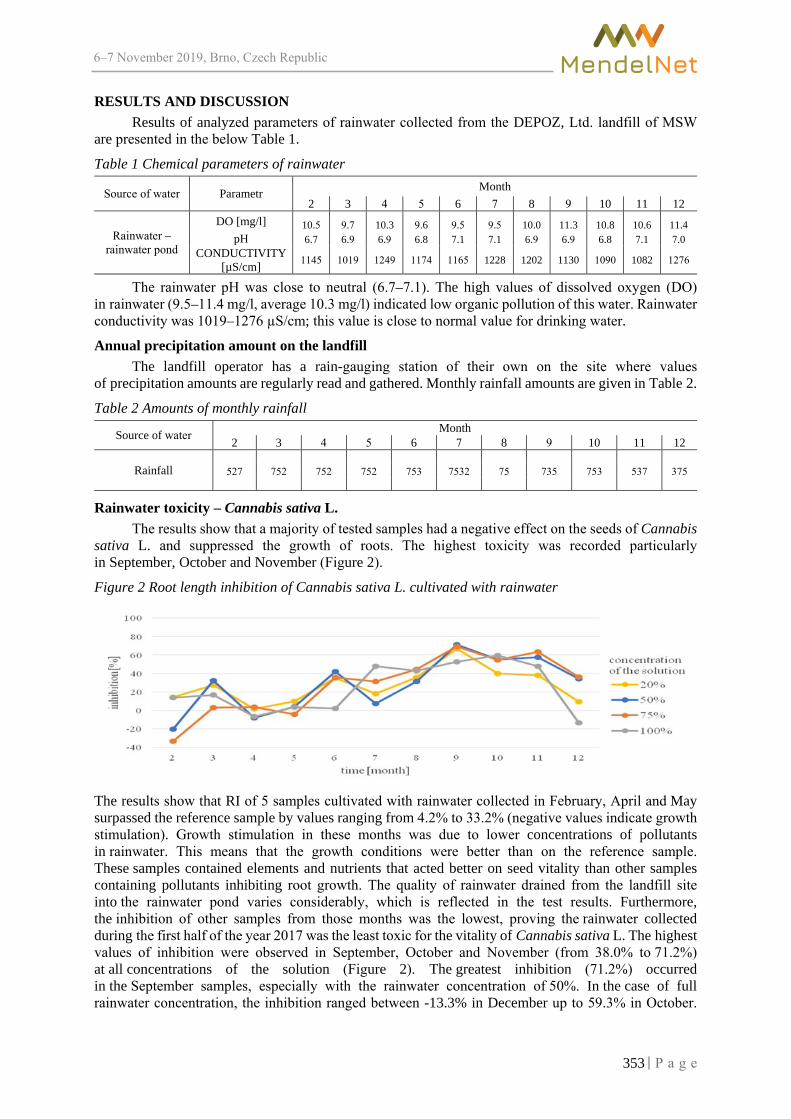
6–7 2019, Brno, Czech Republic
RESULTS AND DISCUSSION Results of analyzed parameters of rainwater collected from the DEPOZ, Ltd. landfill of MSW
are presented in the below Table 1.
Table 1 Chemical parameters of rainwater
Source of water Parametr Month 2 3 4 5 6 7 8 9 10 11 12
Rainwater – rainwater pond
DO [mg/l] 10.5 9.7 10.3 9.6 9.5 9.5 10.0 11.3 10.8 10.6 11.4 pH 6.7 6.9 6.9 6.8 7.1 7.1 6.9 6.9 6.8 7.1 7.0
CONDUCTIVITY [µS/cm] 1145 1019 1249 1174 1165 1228 1202 1130 1090 1082 1276
The rainwater pH was close to neutral (6.7–7.1). The high values of dissolved oxygen (DO) in rainwater (9.5–11.4 mg/l, average 10.3 mg/l) indicated low organic pollution of this water. Rainwater conductivity was 1019–1276 µS/cm; this value is close to normal value for drinking water.
Annual precipitation amount on the landfill The landfill operator has a rain-gauging station of their own on the site where values
of precipitation amounts are regularly read and gathered. Monthly rainfall amounts are given in Table 2.
Table 2 Amounts of monthly rainfall
Source of water Month 2 3 4 5 6 7 8 9 10 11 12
Rainfall
527 752 752 752 753 7532 75 735 753 537 375
Rainwater toxicity – Cannabis sativa L. The results show that a majority of tested samples had a negative effect on the seeds of Cannabis
sativa L. and suppressed the growth of roots. The highest toxicity was recorded particularly in September, October and November (Figure 2).
Figure 2 Root length inhibition of Cannabis sativa L. cultivated with rainwater
The results show that RI of 5 samples cultivated with rainwater collected in February, April and May surpassed the reference sample by values ranging from 4.2% to 33.2% (negative values indicate growth stimulation). Growth stimulation in these months was due to lower concentrations of pollutants in rainwater. This means that the growth conditions were better than on the reference sample. These samples contained elements and nutrients that acted better on seed vitality than other samples containing pollutants inhibiting root growth. The quality of rainwater drained from the landfill site into the rainwater pond varies considerably, which is reflected in the test results. Furthermore, the inhibition of other samples from those months was the lowest, proving the rainwater collected during the first half of the year 2017 was the least toxic for the vitality of Cannabis sativa L. The highest values of inhibition were observed in September, October and November (from 38.0% to 71.2%) at all concentrations of the solution (Figure 2). The greatest inhibition (71.2%) occurred in the September samples, especially with the rainwater concentration of 50%. In the case of full rainwater concentration, the inhibition ranged between -13.3% in December up to 59.3% in October.
353

6–7 2019, Brno, Czech Republic
In 6 samples cultivated with rainwater at concentrations of 50%, 75% and 100%, the root length surpassed the control test by 33.2% and 20.2% in February, by 13.3% in December, 8.3% and 6.8% in April and by 4.2% in May, respectively. The root length of Cannabis sativa L. was sometimes higher regardless of concentration.
Rainwater toxicity - Sinapis alba L. A similar test was conducted with using the seeds of of Sinapis alba L. Figure 3 shows root
lengths of seeds cultivated with the same landfill rainwater. In this test was not record any stimulation of root growth because Sinapis alba L. was more responsive and susceptible to toxic components found in the landfill rainwater samples.
Figure 3 Root length inhibition of Sinapis alba L. cultivated with rainwater
All samples with the 20%, 50%, 75% and 100% rainwater concentrations exhibited the inhibition higher than 60%. Only the sample with a rainwater concentration of 20% from March exhibited the inhibition of 59.5%. The lowest inhibition of Sinapis alba L. was recorded in samples collected in March and it ranged between 59.5% at the 20% concentration of the solution to 65.6% at the 100% concentration, as shown in Figure 3. Inhibition of samples from the remaining months varied between 65.4% and 89.5% with the highest values being recorded in September. No significant differences of inhibition values between the respective solution concentrations in the respective months were observed.
Influence of precipitation (rainfall) on inhibition Rain-gauging data recorded by the measuring instrument on the landfill were processed and fitted
into the diagram (Figure 4) illustrating the average value of inhibition to the growth of roots of Cannabis sativa L. and Sinapis alba L. The diagram presents one mean value of inhibition at concentrations of 20%, 50%, 75% and 100% for each plant.
Figure 4 Influence of precipitation on inhibition
As expected, the higher susceptibility of Sinapis alba L. was demonstrated and inhibition of root growth was high. In Cannabis sativa L., the rate of inhibition depended on the amount of rainfall, namely from June to November. Toxicity of these waters was higher in months with higher precipitation
354

6–7 2019, Brno, Czech Republic
amounts and it can be assumed that torrent rains may wash pollutants out from the landfill site. Quantity and quality of rainwater is influenced by local factors such as hydrogeological conditions, climate, and height and type of landfill (Khatri and Tyagi 2015). Landfill wastewater is subject of numerous studies (Webler et al. 2019, Pinjing et al. 2019). Waste stored in the landfill may contain many substances that are toxic to the environment. With respect to the risk, it is necessary to understand that also the precipitation water leaking from the landfill site and handling surfaces can contaminate the environment.
The results of this research showed Cannabis sativa L. to be resistant to contamination more than Sinapis alba L. and thus, Cannabis sativa L. brings a possibility of phytoremediation thanks to its remediation potential (Brett et al. 2019). This potential allows the plant to resist pollutants in the tested samples.
CONCLUSION The goal of this experiment was to characterize properties of rainwater from the landfill
and its influence on plants. Rainwater from landfills represents a mixture of various substances washed out from the landfill site, which is not always without the content of pollutants. The performed tests showed that the quality of these waters changes throughout the year. The tests of phytotoxicity confirmed a negative influence of this rainwater on the growth of roots of germinating seeds of higher plants. They also demonstrated higher resistance of Cannabis sativa L. as compared with Sinapis alba L. Taking into account the phytoremediation potential of hemp, the plant is recommended for decontamination of the environment. The remediation capacity of hemp has been subject of many studies and will definitely find applications in the future. Our results also showed that rainwater from the landfill site can represent a risk, too. Its quality fluctuates throughout the year and it is necessary to handle it with caution. The results of tests will help in landfill management and management of landfill waters. For landfill closure and subsequent site reclamation, the data from the long-term monitoring are important for understanding processes taking place in a closed landfill.
REFERENCES Brett, D.T. et al. 2019. Novel remediation of per- and polyfluoroalkyl substances (PFASs) from contaminated groundwater using Cannabis Sativa L. (hemp) protein powder. Chemosphere, 229: 22–31. Emamverdian, A. et al. 2015. Heavy metal stress and some mechanisms of plant defense response. Scientific World Journal, 2015(4): 1–18. Khatri, N., Tyagi, S. 2015. Influences of natural and anthropogenic factors on surface and groundwater quality in rural and urban areas. Frontiers in Life Science, 8(1): 23–39. Mendoza, M.B. et al. 2017. Groundwater and leachate quality assessment in balaoan sanitary landfill in la union, northern Philippines. Chemical Engineering Transaction, 56: 247–252. Pinjing, H. et al. 2019. Municipal solid waste (MSW) landfill: A source of microplastics? -Evidence of microplastics in landfill leachate. Water Research, 159: 38–45. Shu, S. et al. 2018. Leachate breakthrough mechanism and key pollutant indicator of municipal solid waste landfill barrier systems: Centrifuge and numerical modeling approach. Science of the Total Environment, 612: 1123–1131. Singh, A. 2019. Managing the uncertainty problems of municipal solid waste disposal. Journal of Environmental Management, 240: 259–265. Sonawane, J.M. et al. 2017. Landfill leachate: A promising substrate for microbial fuel cells. International Journal of Hydrogen Energy, 42(37): 23794–23798. Vaverková, M.D. et al. 2018. Assessment and evaluation of heavy metals removal from landfill leachate by Pleurotus ostreatus. Waste and Biomass Valorization, 9(3): 503–511. Webler, A.D. et al. 2019. Development of an integrated treatment strategy for a leather tannery landfill leachate. Waste Management, 89: 114–128.
355

FOOD TECHNOLOGY

6–7 2019, Brno, Czech Republic
The influence of temperature and yeasts on the main qualitative parameters and sensory properties of Welschriesling
Lukas Cervinka, Patrik Burg, Alice Cizkova Department of Horticultural Machinery
Mendel University in Brno Zemedelska 1, 613 00 Brno
CZECH REPUBLIC
Abstract: Instead of the quality raw material – grapes, the quality of wines can be fundamentally influenced by the technological conditions applied in the wine process. It is the fermentation of musts by using the autochthonous or active (selected) wine yeast, different length and temperature applied during maceration and temperature during fermentation process (below 15 ºC, up to 20 ºC) as well. The main aim of these measurements is to propose an optimal procedure of wine production and focus on their analytical parameters and aromatic character.
Key Words: yeast, fermentation, Welschriesling, sensory evaluation
INTRODUCTION The alcoholic fermentation with the emphasis on yeast is the main process during the wine
processing. It is a complex microbiological process (Fleet 2008). Fermentation can be divided into spontaneous and controlled. Spontaneous alcoholic fermentation starts by the propagation of non-saccharomycetous genera that naturally occur on the grapes. They are primarily Kloecker, Candida, Metschnikowia, Hansenula, Pichia, Torulaspora (Fugelsang and Edwards 2007, Ribéreau-Gayon et al. 2006).
At a level of approximately 5% alcohol, the yeasts of genus Saccharomyces cerevisiae start to work, because they tolerate higher concentrations of ethanol in the environment. Concentrated alcohol becomes toxic for them and it stops the fermentation process (Querol and Fleet 2006, Furdíková and Malík 2007). Compared to spontaneous fermentation, controlled fermentation is considerably safer. Genera Saccharomyces are used to starting fermentation, selected from a single strain or even from a particular clone. Active dry wine yeast are used at the most frequently in operation. (Farkáš 2002, Furdíková and Malík 2008). Active dry wine yeast is produced using the noble wine yeast Saccharomyces cerevisiae and Saccharomyces bayanus. Research of new suitable yeasts is still ongoing and this gives the possibility to discover other yeas strains with unique properties (Mingorance-Cazorla et al. 2003). Another important factor is a fermentation temperature. Temperature control can reduce the length and intensity of the fermentation process, but also the sensory character for the future wines (Balík and Stávek 2017). All these mentioned factors influence the final product quality and therefore the most premium wines are associated not only with a mature and healthy raw material, but also with an appropriately selected production process using modern wine technology and oenological products.
The aim of this study was to monitor the effect of commercial yeasts on qualitative parameters of wine Welschriesling.
MATERIALS AND METHODS
Must origin and treatments The Welschriesling (WR) grapes (Vinařství Červinka, Horní Věstonice, Pod Martinkou, Czech
Republic) were mechanized harvested on 10. 10. 2016 and 10. 10. 2017. The grapes were pressed and juice was prepared for fermentation. The sugar concentration in grape must was estimated with a normalised saccharometer and stated in °NM (says kg of total sugar in 100 l of juice). The result was 22.8 °NM (2016) and 23.2 °NM (2017). After the harvest, the temperature of juice was 19 °C; later
357

6–7 2019, Brno, Czech Republic
spontaneously decreased to 15 °C. The content of total acidity was 5.5 g/l (2016) and 5.7 g/l (2017). The following products were added to the must: 1.0 g/l tartaric acid, 40.0 mg/l sulfur dioxide, VitaFerm Ultra F3 (ERBSLÖH Geisenheim GmbH, Germany) and eventually yeast (more below). After 24 hours the must was racked and the sediment was filtrated with lees filter.
Fermentation procedure and Yeast strains The fermentation was carried out in 2000 l stainless tanks. For the experiments connected
with quality wines of the WR variety were selected the different yeast strains which were inoculated into the must according to the producers' instructions. At the same time, different fermentation temperature regimes were selected. The length of the process and its temperature course were monitored and continuously recorded during the all fermentation period (company cooling technology F-control). Differences in the duration of the fermentation process are considered to be a characteristic trait of individual yeast products as far as their capability to ferment the grape juice. The wines were racked and prepared for bottling. All fermentation batches of must were replicated two times.
Yeast strains (WR) Var.1WR: Fermivin VB 1 (Producer: Oenobrands SAS, France). VB1 is well adapted to ferment
very clear musts, is a strong fermenter and has a low nutrient demand. In case of very low turbidity an addition of nutrients. Yeast strain recommended for the production of qualitative Riesling wines. The range of recommended fermentation temperatures is 17–20 °C.
Var.2WR: Oenoferm Terra F3 (Producer: Erbslöh, Germany). The preparation Oenoferm Fredo is especially selected dry pure yeast strain LW317–30. That is used for inoculation of cold juices at temperatures above 8 °C as well as for the preservation of wine aroma under conditions of controlled fermentation at temperatures ranging between 17 and 20 °C. When using this yeast strain of S. cerevisiae var. bayanus, special attention was paid to reach a high degree of final fermentation even under conditions of low temperatures. This strain produces citrus and grapefruit tones as well as tones of apples, peaches and roses.
Var.3WR: Vintage white (Producer: Begerow, Germany). This strain of S. cerevisiae yeasts is suitable for cool fermentation and for aromatic varieties. It produces intensively aromatic, fresh, elegant and markedly spicy and fruity tones. In wines with residual sugar, these tones contribute to their increased complexity. This yeast strain is suitable not only for production of ice and straw wines but also for restarting of stuck fermentation. The range of recommended fermentation temperatures is 16–21 °C.
Var.4WR: Control. The native microflora that exists on the surface (skins) of berries, produce wine of a good quality the course of this type of fermentation and its results cannot be fully controlled.
Estimation of essential analytical parameters Determination of total acidity (OENO 52/2000) was estimated by the automatic titrator machine
TITROLINE EASY (manufacturer SI Analytics GmbH, Germany). Titrations were performed with standardized solution of NaOH (0.1 mol/l) as the titration reagent, using a SenTix 21 pH electrode. Sample (10.0 ml) was diluted with 10 ml of distilled water. Because of a subsequent formol titration, the sample was not titrated up to the usual pH value of 7.0 but up to the value of 8.1. At the end of the titration, consumption of NaOH solution in milliliters was read on the titrator’s display. The concentration of total acidity (in g/l) was calculated as equivalents of tartaric acid. Residual sugar, acetic acid and sugar free extract concentrations were estimated using Fourier-transform infrared (FTIR) spectrometer (ALPHA) with Attenuated Total Reflection (ATR) (Bruker Optik GmbH, Ettlingen, Germany). An ATR accessory operates by measuring the changes that occur in an internally reflected IR beam when the beam comes into contact with a sample. Before the first measurement, the spectrometer was thoroughly rinsed with deionised water and the background was determined using a deionized water. For analyses, 1 ml samples were taken after the fermentation with a syringe; of this sample, 0.5 ml was used for rinsing of the system while the remaining volume of 0.5 ml was analysed three times. Depending on the calibration used, the measured values were evaluated automatically using special software Opus Wine Wizard.
358

6–7 2019, Brno, Czech Republic
Sensory evaluation Altogether 7 experts participated in the sensory evaluation year 2016 and 2017. Wine samples
were evaluated using the UIOE (International Union of Oenologists) 100–point scale system. The evaluation was focused on the aromatic profile of wine sample and on the extract effect on the full taste and harmony of individual wine samples. The final result is average of 7 evaluations. In addition to the score, the tasters were able to comment on each wine and thereby extend the overall rating.
Statistical analysis A statistical analysis was performed using the software package “Statistics 12.0” (StatSoft Inc.,
Tulsa, Oklahoma, USA). Analysis of variance was conducted, and the results were compared using Tukey's multiple range assay at a significance level α = 0.05.
RESULTS AND DISCUSSION Figure 1 state an average values showing temperature and length of fermentation process
for variety WR, respecting the yeast culture which was used. In the case of temperature, it is very important to avoid the major decrease during the fermentation. Then the yeast suffers a thermal shock with impact on the slowing or ending the fermentation (Michlovský 2014). By Var.2WR in both years, the temperature was 15 °C in the both years during fermentation comparing to the other variants was 2 days longer in 2016. Other variants had temperature of fermentation 18.5 °C.
Figure 1 The course and length of the fermentation process for the WR variety
In the wine making process, the type of wine and amount of aroma depend on the following:
yeast, environmental factors (climate, soil), cultivar, fruit condition, vinification process, must pH, amount of sulphur dioxide, amino acids present in the must and malolactic fermentation (Romano et al. 2003). Low temperature enhanced the wine contents of some volatile compounds produced by the yeast during the alcoholic fermentation. For this reason, low temperature fermentation (15 °C) is of interest to winemakers to enhance the production of some volatile compounds and improve the wine aromatic profile (Ribéreau-Gayon et al. 2006). The resulting values of essential analytical parameters are shown in Table 1.
Molina et al. (2007) says that controlled fermentation contributes to differences in final ethanol and glycerol concentrations. At higher temperatures, the final ethanol concentration was lower than 15 °C, and the final glycerol concentration was higher. In both years, both spontaneous yeasts were used to determine increased alcohol content (max. 13.45 % for Var.4WR/18.5/2017), glycerol content (max. 10.22 g for Var.4WR/18.5/2017), but also acetic acid (max. 0.53 g / Var.4WR/18.5/2017). The results of the assay correspond to the statement that the spontaneous fermentation is characterized by increased contents of glycerol, higher alcohols, and volatile acids, as reported by Steidl (2002)
359
6–7 2019, Brno, Czech Republic
and Průšová et al. (2018). Also Michlovský (2014) reported that the formation of glycerol depends on the initial amount of sugars, the nature of the yeast and the fermentation conditions. Its average content ranges from 6 to 10 g/l. The pH values and all experimental variations are in the range of 3.21–3.28, which is stated by Štefecová and Čepička (2001) as a good prerequisite for the future chemical and biological stability of wines. From the point of view of titratable acids content values varied between 5.31 and 7.01 g/l. Ribéreau-Gayon et al. (2006) recommends titers. Acids in white wines in the range 5–7 g/l.
Table 1 Contents of essential analytical parameters in WR
Var./temp./ year
Alcohol Residual sugar pH Glycerol Density Titr.
acid Apple acid
Milk acid
Acetic acid
Wine acid
% g/l - g/l kg/m³ g/l g/l g/l g/l g/l Var.1WR/18.5
/2016 13.15ab 2.55a 3.25ab 7.48b 0.99a 5.78c 2.49b 0.67a 0.41cde 1.90d
Var.2WR/15/2016 13.35cd 2.12c 3.28a 7.73e 0.99a 5.68a 2.19d 0.73a 0.42de 2.15a
Var.3WR/18.5/2016 13.06a 2.48a 3.21b 7.35a 0.99a 5.62a 1.92a 0.71a 0.38bcd 2.44b
Var.4WR/18.5/2016 13.13d 2.30d 3.28a 7.60c 0.99a 5.31b 1.49c 1.14c 0.44e 2.18a
Var.1WR/18.5/2017 13.25bc 5.67e 3.23ab 7.87f 1.00a 7.01g 2.76e 0.93b 0.34ab 2.66c
Var.2WR/15/2017 12.77e 8.12g 3.25ab 7.66d 0.99a 6.11d 1.86a 1.27d 0.30a 2.26e
Var.3WR/18.5/2017 13.07a 6.13f 3.28a 8.65g 0.99a 6.82e 3.05f 1.13c 0.35abc 2.50b
Var.4WR/18.5/2017 13.45d 0.25b 3.23ab 10.22h 1.00a 6.92f 2.56b 0.95b 0.53f 2.60c
Legend: Data are expressed as means, different letters in the same columns represent significant difference (P < 0.05). var. - variant, temp. – temperature, y. - year
In Table 2 are results of sensory analysis, which was performed 6 months after the end of fermentation by using the UIOE 100-point scale system.
Table 2 Results of sensory evaluation in WR wines Variant/temperature
Year Var.1WR/18.5 Var.2WR/15 Var.3WR/18.5 Var.4WR/18.5 2016 82.7a 85.0b 82.3a 82.0a 2017 88.8b 80.4a 86.8a 85.6b
Legend: Data are expressed as means, different letters in the same columns represent significant difference (P < 0.05).
In the WR variety, the evaluated variants showed a vintage effect on the sensory properties of wines, except for the wines that were fermented with the yeast TERRA F3. In terms of final evaluation, tasters reported more intensity and fruity in the aroma of wines fermented by Var.1WR–Var.3WR. On the contrary, the aroma of spontaneous fermentation was evaluated as natural (varietal), but less intense.
CONCLUSIONS Wine is the product of many diverse interactions. These results demonstrate that the temperature
of fermentation in the presence of negative yeast strains can influencing the contents of essential analytical parameters produced wines. In most cases, the using of noble yeasts resulted in higher alcohol yield during fermentation, which it important during the processing of grapes with lower sugar content. By using active (selected) wine yeast, the winemaker can potentially increase the alcohol content, which is important for the final stability.
ACKNOWLEDGEMENTS This paper was supported by the project CZ.02.1.01/0.0/0.0/16_017/0002334 Research Infrastructure for Young Scientists, co-financed by Operational Programme Research, Development and Education.
360

6–7 2019, Brno, Czech Republic
REFERENCES Balík, J., Stávek, J. 2017. Vinařská technologie. Břeclav: TISK PÁLKA s.r.o. Farkáš, J. 2002. Všetko o víně. 2 vyd., Martin: Neografia, a.s. Fleet, H.G. 2008. Wine yeasts for the future. FEMS Yeast Research, 8(7): 979–995. Fugelsang, K.C., Edwards, CH.C. 2007. Wine microbiology: practical applications and procedures. 2nd ed., New York, NY: Springer. Furdíková, K., Malík, F. 2008. Autochtónne kvasinky a ich aplikácia do vinárskej praxe. Vinařský obzor, 101(5): 234–235. Furdíková, K., Malík, F. 2007. Kvasinky ve vinárstve. Vinařský obzor, 100(10): 488–489. Michlovský, M. 2014. Lexikon chemického složení vína. 1. vyd., Hradec Králové: Garamon s.r.o. Mingorance-Cazorla, L. et al. 2003. Contribution of different natural yeasts to the aroma of two alcoholic beverages. World Journal of Microbiology and Biotechnology, 19(3): 297–304. Molina, A.M. et al. 2007. Influence of wine fermentation temperature on the synthesis of yeast-derived volatile aroma compounds. Applied Microbiology and Biotechnology, 77(3): 675–687. Průšová, B. et al. 2018. Effect of Yeasts on the Aroma Profile of Sauvignon Blanc Varietal Wine. Acta Universitatis Agriculturae et Silviculturae Mendelianae Brunensis, 66(4): 889–896. Querol, A., Fleet, H.G. 2006. Yeasts in food and beverages. Springer–Verlag Berlin Heidelberg. Ribéreau-Gayon, P, et al. 2006. Handbook of Enology: Volume 1 The Microbiology of Wine and Vinifications. 2nd ed., Chichester West Sussex, England: John Wiley & Sons Ltd. Romano, P. et al. 2003. Function of yeast species and strains in wine flavour. International Journal of Food Microbiology, 86(1–2): 169–180. Steidl, R. 2002. Sklepní hospodářství. 1. vyd., Valtice: Národní salon vín. Štefecová, K., Čepička, J. 2001. Průběh změn hlavních organických kyselin v průběhu vinifikace. Kvasný průmysl, 47(9): 246–249.
361

6–7 2019, Brno, Czech Republic
Phthalic acid esters in the packaging of certain foods
Marcela Jandlova, Alzbeta JarosovaDepartment of Food Technology
Mendel University in Brno Zemedelska 1, 613 00 Brno
CZECH REPUBLIC
Abstract: Phthalic acid esters are used as plasticizers for plastics. These plastics can also be used as food packaging. Our aim was determined the concentrations of phthalic acid esters in food packagings purchased in the Czech Republic. Two phthalic acid esters, dibutyl phthalate (DBP) and di-(2-ethylhexyl) phthalate (DEHP) were detected on high-performance liquid chromatography. Foods from which the packages were analyzed were: potato croquettes, pommes frites, fish fillets in oil, two types of cheese, coffee cream, sunflower bread, puffed rice bread, spreadable vegetable fat, hazelnut spread, goulash soup, salt crackers, dried meat, olives, lentils with smoked meat, salted wafers, half dipped biscuits, beef broth, frozen puff pastry. The highest average DBP concentration was found in food packaging: soft transparent plastic without print (from puffed rice bread), type of material polypropylene, 335.03 µg/g of plastic. The lowest average DBP concentration was found in food packaging: lower hard plastic (from fish fillets), type of material unspecified, 0.72 µg/g of plastic. And the highest average concentration of DEHP was found in food packaging, outer plastic packaging with print (from lentils with smoked meat), type of material other plastic, 157.73 µg/g of plastic. And the lowest concentration of DEHP was found in the food packaging: white hard plastic bowl without print (from lentils with smoked meat), type of material polypropylene, 2.08 µg/g of plastic. In some cases, high concentrations of phthalic acid esters have been found, therefore we recommend replacing phthalic acid esters with a less toxic alternative.
Key Words: dibutyl phthalate, di-(2-ethylhexyl) phthalate, contaminant, packaging, printing
INTRODUCTION Phthalic acid esters are widely used as plasticizers, making them ubiquitous environmental
contaminants. Most of the phthalic acid esters are two: di-(2-ethylhexyl) phthalate and dibutyl phthalate. Phthalates have carcinogenic and teratogenic effects and negatively affect the reproductive system of the organism, acute toxicity is manifested by nausea, decreased blood pressure, sleepiness, visual disturbances (Velíšek and Hajšlová 2009). Plastics softened with phthalic acid esters can be found in toys, clothing, floor coverings, furniture, pipes, car interiors, paints, adhesives, but also in plastics for food use. Phthalates are not firmly bound in the polymers and can therefore be released from plastics (Brimer 2011).
Packaging of goods is very important nowadays, when the packaging has four main functions: protection function, control function, communication and for consumer comfort. Certain components of the package, especially additives (including plasticizers, antioxidants, etc.), oligomers and monomers may migrate, i.e., release from the packaging to the environment, as well as release and dissolve into the food with which the packaging is in contact. For this reason, regulations set migration limits of plastic components for plastics in contact with food (Robertson 2013).
The specific migration limits (SML) are also set for phthalic acid esters. SML indicates the maximum permitted amount of a given substance that can be released from the material into the food. This amount of the substance is one which does not pose a health risk to the consumer. For DBP, the specific migration limit is set at 0.3 mg/kg food and for DEHP, the specific migration limit is set at 1.5 mg/kg (EU 2011).
On individual packages may be marked the types of material. According to the Czech Packaging Act No. 477/2001 Coll. if the person placing the packaging on the market decides to indicate used material, the material must be to mark according to the Commission Decision 97/129/EC (Czech
362

6–7 2019, Brno, Czech Republic
Republic 2001). Commission Decision 97/129/EC (EU 1997) lists the numbers and abbreviations of materials used in the manufacture of packaging.
The aim of this work was to find what concentrations of the two most commonly used phthalic acid esters contain wrappers, which pack food on our market.
MATERIAL AND METHODS Foods, from which the wrappers were analyzed, were purchased in the Czech Republic. Foods,
and thus the analyzed wrappers were in two repetitions. The food was removed from the packaging, the packaging was washed from the food with lukewarm water and after with distilled water. Furthermore, the packages were allowed to dry at room temperature. Each wrapper was divided into parts: colored, colorless, soft or hard. Samples of known dimensions and weights were ground and placed in a solvent mixture of dichloromethane and hexane (1 : 1) for 72 hours. Subsequently, the samples were extracted on a shaker for 1 hour and 2 times for 0.5 hours. The extract was transferred through filter paper to an evaporation flask, and the content of the evaporation flask was evaporated on a vacuum rotary evaporator. The evaporation residue was taken up into vials in hexane. If the hexane solution was clear, it was transferred into smaller vials and analyzed in acetonitrile by high performance liquid chromatography (HPLC). If the hexane solution was turbid, only a clear part above the sludge was collected into small vials and determined in acetonitrile by HPLC. If the hexane solution was colored, it was purified by sulfuric acid and determined by HPLC in acetonitrile.
The used method was according to Gajdůšková et al. (1996). During analysis by HPLC were used acetonitrile as mobile phase, UV detection at 224 nm and Zorbax Eclipse C8 column. The evaluation was performed in Data Analysis (Agilent Technology). Further data processing was performed by Microsoft Excel.
RESULTS AND DISCUSSION Table 1 shows the determined average concentrations of DBP and DEHP in wrappers.
Table 1 Description of analyzed plastics and average DBP and DEHP concentrations with standard deviations [µg/g of wrapper and µg/dm2 of wrapper]
wrapped food description of wrapping type of
material
average DBP
[µg/g]
SD DBP
[µg/g]
average DBP
[μg/dm²]
SD DBP
[μg/dm²]
average DEHP [μg/g]
SD DEHP [μg/g]
average DEHP
[μg/dm²]
SD DEHP
[μg/dm²] fish fillets in
oil upper soft plastic U 2.53 0.64 1.77 0.46 12.88 1.18 9.04 0.87 lower hard plastic U 0.72 0.08 2.86 0.34 4.76 1.08 18.96 4.52
cheese slices, fat of 45%
upper soft plastic 7 8.11 3.65 5.48 2.55 5.10 0.06 3.42 0.02 lower hard plastic
with label 7 13.98 0.15 41.35 1.46 30.08 6.19 88.50 16.07 lower hard plastic
without label 7 21.92 5.56 36.72 8.70 6.43 0.39 10.84 0.85 sunflower
bread soft transparent plastic without
print PP 88.56 14.14 50.25 7.18 19.94 1.14 11.33 0.46 soft plastic with
print PP 4.27 1.63 6.50 2.54 15.00 7.36 22.84 11.39 spreadable
vegetable fat yellow hard plastic
tub with print U 8.15 0.34 33.30 0.71 4.65 0.01 19.04 0.43 yellow hard plastic
cap with print U 11.73 1.63 37.73 5.84 3.77 0.79 12.13 2.72 aluminum cap with
print ALU 75.30 6.18 76.84 7.97 9.32 0.07 9.49 0.28 toast cheese soft printed outer
plastic PP 32.15 10.17 19.81 3.39 21.41 7.07 13.16 2.45 inner transparent
soft plastic without print PA 172.67 14.59 28.72 1.80 35.14 1.43 5.86 0.37
hazelnut spread
brown hard plastic tub without print U 116.85 52.09 328.33 108.19 20.65 2.54 62.81 16.01
aluminum cap with print ALU 92.86 43.83 76.17 35.72 35.94 4.47 29.52 3.56
363

6–7 2019, Brno, Czech Republic
wrapped food description of wrapping type of
material
average DBP
[µg/g]
SD DBP
[µg/g]
average DBP
[μg/dm²]
SD DBP
[μg/dm²]
average DEHP [μg/g]
SD DEHP [μg/g]
average DEHP
[μg/dm²]
SD DEHP
[μg/dm²] puffed rice
bread soft colored plastic
with print PP 60.70 10.61 25.87 4.65 83.58 23.11 35.54 9.66 soft transparent plastic without
print PP 335.03 17.37 119.61 5.79 86.50 15.57 30.91 5.67 goulash soup plastic soft cap
with print U 51.93 12.77 42.34 10.99 43.73 1.33 35.51 0.57 yellow hard plastic
tub with print U 11.15 0.25 66.94 1.10 8.61 1.15 51.68 6.59 yellow hard plastic tub bottom without
print U 13.92 0.54 103.05 4.32 2.71 0.45 20.06 3.41 salt crackers soft yellow plastic
with print PP 85.61 10.37 37.17 4.73 62.43 6.84 27.10 3.14 coffee cream aluminum cap with
print ALU 72.35 7.02 58.69 0.62 20.55 0.57 16.85 1.92 hard white plastic small cup without
print PS 10.60 3.69 17.25 5.15 6.42 2.67 10.41 3.84 outer soft
transparent plastic cover with print PP 53.82 43.65 19.38 16.54 30.52 27.18 11.10 10.17
dried meat soft white plastic with print 7 11.53 2.65 17.17 0.43 6.72 0.38 10.47 2.09
olives semi-hard transparent plastic
without print U 79.14 10.04 86.78 11.87 18.51 4.39 20.32 5.01 semi-hard colored plastic with print U 33.06 8.10 48.27 12.23 60.05 28.09 87.84 41.70
lentils with smoked meat
white hard plastic bowl without print PP 7.79 5.05 90.75 58.39 2.08 1.27 24.56 15.16 aluminum cap with
print ALU 41.43 3.14 101.35 7.17 14.87 2.77 36.35 6.59 yellow hard plastic
cap 7 14.30 1.02 80.70 3.55 8.42 1.54 47.86 10.04 outer plastic
packaging with print 7 42.23 2.53 32.32 2.06 157.73 4.75 120.70 4.10
salted wafers outer soft transparent plastic
without print PP/PVC 263.37 43.47 95.63 13.64 99.20 43.16 35.79 14.90 outer soft colored plastic with print PP/PVC 46.18 5.03 19.35 2.29 87.89 11.98 36.74 4.67 inner semi-hard
transparent plastic PS 34.27 19.06 40.84 21.28 4.08 1.71 4.90 1.84 half dipped
biscuits soft colored plastic
with print PP 43.16 37.07 12.81 11.01 64.20 17.23 19.05 5.13 beef broth outer colored paper
box PAP 8.57 1.13 23.94 2.75 15.99 1.69 44.66 3.92 aluminum cap with
print ALU 45.29 1.37 41.49 1.43 25.07 11.64 22.92 10.56 transparent plastic
small cup 7 28.24 4.94 46.99 7.87 43.22 27.34 72.34 46.10 frozen puff
pastry soft colored plastic
with print U 29.97 5.77 23.88 4.22 9.62 2.13 7.67 1.58 potato
croquettes soft colored plastic
with print LDPE 48.93 0.17 24.62 0.34 26.07 0.36 13.11 0.04 pommes
frites soft colored plastic
with print LDPE 54.96 12.12 27.83 5.00 36.15 4.22 18.39 1.37
Legend: SD = standard deviation, U = unspecified, 7 = other plastic, PP = polypropylene, ALU = aluminium, PA = polyamide, PS = polystyrene, PP/PVC = polypropylene/polyvinyl chloride, PAP = paper, LDPE = low density polyethylene
Figures 1–4 show the average concentrations of phthalates for each specified type of wrapper. The average DBP concentrations ranged from 8.11 to 42.23 µg/g of plastic in wrappers marked 7
(other plastic) and the average DEHP concentrations ranged from 5.10 to 157.73 µg/g of plastic in wrappers marked 7 (other plastic). In polypropylene (PP) wrappers, the average DBP concentrations
364

6–7 2019, Brno, Czech Republic
ranged from 4.27 to 335.03 µg/g of plastic and the average DEHP concentrations ranged from 2.08 to 86.50 µg/g of plastic.
Figure 1 Average DBP and DEHP concentrations [µg/g of wrapper] in wrapper from material 7 (other plastic)
Legend: 1A = upper soft plastic (from cheese slices, 45% fat), 2A = lower hard plastic with label (from cheese slices, 45% fat), 3A = lower hard plastic without label (from cheese slices, 45% fat), 4A = soft white plastic with print (from dried meat), 5A = yellow hard plastic cap (from lentils with smoked meat), 6A = outer plastic packaging with print (from lentils with smoked meat), 7A = transparent plastic small cup (from beef broth)
Figure 2 Average DBP and DEHP concentrations [µg/g of wrapper] in wrapper from material PP (polypropylene)
Legend: 1B = soft transparent plastic without print (from sunflower bread), 2B = soft plastic with print (from sunflower bread), 3B = soft printed outer plastic (from toast cheese), 4B = soft colored plastic with print (from puffed rice bread), 5B = soft transparent plastic without print (from puffed rice bread), 6B = soft yellow plastic with print (from salt crackers), 7B = outer soft transparent plastic cover with print (from coffee cream), 8B = white hard plastic bowl without print (from lentils with smoked meat), 9B = soft colored plastic with print (from half dipped biscuits)
Figure 3 Average DBP and DEHP concentrations [µg/g of wrapper] in wrapper from material ALU (aluminium)
Legend: 1C = aluminum cap with print (from spreadable vegetable fat), 2C = aluminum cap with print (from hazelnut spread), 3C = aluminum cap with print (from coffee cream), 4C = aluminum cap with print (from lentils with smoked meat), 5C = aluminum cap with print (from beef broth)
The average DBP concentrations in aluminum (ALU) wrappers ranged from 41.43 to 92.86 µg/g of wrapper, the average DEHP concentrations from 9.32 to 35.94 µg/g of wrapper. The average DBP
365

6–7 2019, Brno, Czech Republic
concentrations in polystyrene (PS) plastic wrappers ranged from 10.60 to 34.27 µg/g of plastic and the average DEHP concentrations from 4.08 to 6.42 µg/g of plastic.
Figure 4 Average DBP and DEHP concentrations [µg/g of wrapper] in wrapper from material PS (polystyrene), PA (polyamide), PP/PVC (polypropylene/polyvinyl chloride), PAP (paper), LDPE (low density polyethylene)
Legend: 1D = hard white plastic small cup without print (from coffee cream) PS, 2D = inner semi-hard transparent plastic (from salted wafers) PS, 3D = inner transparent soft plastic without print (from toast cheese) PA, 4D = outer colored paper box (from beef broth) PAP, 5D = outer soft transparent plastic without print (from salted wafers) PP/PVC, 6D = outer soft colored plastic with print (from salted wafers) PP/PVC, 7D = soft colored plastic with print (from potato croquettes) LDPE, 8D = soft colored plastic with print (from pommes frites) LDPE
The average DBP concentrations in polypropylene/polyvinyl chloride (PP/PVC) wrappers ranged from 46.18 to 263.37 µg/g of plastic and for DEHP 87.89 to 99.20 µg/g of plastic. Brimer (2011) stated that PVC may contain up to 50% by weight of plasticizer. The average DBP concentrations in low density polyethylene (LDPE) wrappers ranged from 48.93 to 54.96 µg/g of plastic and for DEHP from 26.07 to 36.15 µg/g of plastic.
And the wrapper from the polyamide (PA) had the average DBP concentration 172.67 µg/g of plastic and DEHP 35.14 µg/g of plastic, and wrapper from the paper (PAP) had the average concentration for DBP 8.57 µg/g and for DEHP 15.99 µg/g.
The highest average DBP concentration was found in the type of polypropylene material, 335.03 µg/g of plastic. The lowest average DBP concentration was found in the unspecified material, 0.72 µg/g of plastic. And, the highest average concentration of DEHP was found in the type of material other plastic, 157.73 µg/g of plastic, this wrapper was without contact with the food as it was located on the outside of the dish. And the lowest average concentration of DEHP was found in the type of polypropylene material, 2.08 µg/g of plastic, this dish was intended for microwave heating of the food stored therein.
Bogdanovičová et al. (2014) examined the concentrations of DBP and DEHP in packaging films for meat products and found that the average concentrations of the sum of the two phthalates ranged from 1.89 µg/g to 139.93 µg/g, however, they were unused wrappers. In our study, we had higher concentrations, but we had used wrapper. Our higher concentrations could be due to contamination from the environment and possibly from food.
In the study, Shen (2005) identified 8 phthalic acid esters, including DBP and DEHP, in 25 types of plastic products intended for food use. He found that only one of the samples contained no phthalates. And the most common phthalate was DEHP. In our study we had no sample that did not contain phthalic acid esters, phthalic acid esters were detected in all analyzed samples, and higher average concentrations were found for DBP than for DEHP.
Pivnenko et al. (2016) mentioned the fact that plastic recycling can be a potential source of phthalates in recycled plastics.
Page and Lacroix (1992) investigated aluminum foil laminated paper used for packaging butter and margarine, they found that 76–88% of phthalates (DBP and DEHP) were present on the outer surface of the protective film in the unused foil. The food contact layer of foil contained 240–470 µg/dm2 DBP and 280–360 µg/dm2 DEHP, the inner layer being a paper layer. In our study, we had not a sample
366

6–7 2019, Brno, Czech Republic
of aluminum foil laminated paper, but in analyzed paper, we found lower concentrations, than in paper layer of mentioned study, the our average concentration for DBP in the paper was 23.94 µg/dm2 and for DEHP 44.66 µg/dm2.
CONCLUSION In our study, it was found that phthalic acid esters are still widely used in food packaging, average
DBP concentrations were found from 0.72 µg/g to 335.03 µg/g of plastic, and for DEHP from 2.08 µg/g to 157.73 µg/g of plastic. We therefore recommend: substituting phthalic acid esters with a less toxic alternative.
ACKNOWLEGEMENTS The research was financially supported by the grant IGA FA MENDELU No. IP_11/2017 Phthalates in packaged foods and used packaging.
REFERENCES Bogdanovičová, S. et al. 2014. Detection of phthalic acid esters in the packaging films of meat products. Acta Veterinaria Brno [Online], 83(10): S59–S64. Available at: https://actavet.vfu.cz/83/10/0059/. [2019-08-29]. Brimer, L. 2011. Chemical food safety. 1st ed., Oxfordshire, UK: CABI. Česká Republika. 2001. Zákon č. 477/2001 Sb., o obalech a o změně některých zákonů (zákon o obalech). In: Sbírka zákonů České republiky. 172: 9948–9969. Also available at: http://aplikace.mvcr.cz/sbirka-zakonu/ViewFile.aspx?type=c&id=3750. [2019-08-19]. EU. 2011. Commission Regulation (EU) No 10/2011, on plastic materials and articles intended to come into contact with food. In: Official Journal of the European Union. L 12: 1–89. Also available at: https://eur-lex.europa.eu/legal-content/EN/TXT/PDF/?uri=CELEX:32011R0010&qid=1567515129166&from=EN. [2019-08-20]. EU. 1997. Commission Decision of 28 January 1997 establishing the identification system for packaging materials pursuant to European Parliament and Council Directive 94/62/EC on packaging and packaging waste. In: Official Journal of the European Communities. L 50: 28–31. Also available at: https://eur-lex.europa.eu/legal-content/EN/TXT/PDF/?uri=CELEX:31997D0129&from=CS. [2019-08-21]. Gajdůšková, V. et al. 1996. Occurrence of phthalic acid esters in food packaging materials. Potravinářské Vědy, 14: 99–108. Page, B.D., Lacroix, G.M. 1992. Studies into the transfer and migration of phthalate esters from aluminium foil‐paper laminates to butter and margarine. Food Additives and Contaminants [Online], 9(3): 197–212. Available at: http://www.tandfonline.com/doi/abs/10.1080/02652039209374064. [2019-08-24]. Pivnenko, K. et al. 2016. Recycling of plastic waste: Presence of phthalates in plastics from households and industry. Waste Management [Online], 54: 44–52. Available at: https://linkinghub.elsevier.com/retrieve/pii/S0956053X1630246X. [2019-08-27]. Robertson, G.L. 2013. Food Packaging Principles and Practice. 3rd ed., Boca Raton: CRC Press. Shen, H. 2005. Simultaneous screening and determination eight phthalates in plastic products for food use by sonication-assisted extraction/GC–MS methods. Talanta [Online], 66(3): 734–739. Available at: https://linkinghub.elsevier.com/retrieve/pii/S0039914004007337. [2019-08-30]. Velíšek, J., Hajšlová, J. 2009. Chemie potravin II. 3rd ed., Tábor: OSSIS.
367

6–7 2019, Brno, Czech Republic
Thermal stability of chicken skin gelatine gels in comparison with commercial gelatines
Petr Mrazek1, Pavel Mokrejs1, Robert Gal2, Jana Orsavova3, Dagmar Janacova4 1Department of Polymer Engineering
2Department of Food Technology 3Language Centre
4Department of Automation and Control Engineering Tomas Bata University in Zlin Vavreckova 275, 760 01 Zlin
CZECH REPUBLIC
Abstract: Gelatine is a partial hydrolysate of collagen obtained from pre-treated raw material extracted in distilled water at higher temperatures. Its excellent functional properties predestine it for various applications not only in the food industry but also in further sectors. Technological conditions of the preparation process may influence gelatine structure and thus its quality. That is mainly assessed by gelatine gel strength and its thermal stability which was tested in this study. Chicken skin gelatines (CSG) were gained by enzymatic pre-treatment of the feedstock followed by extraction at five different temperatures. Series of CSG gels were prepared and their thermal stability was tested at three different temperatures (23, 29 and 35 °C). Changes in gelatine gel strength were monitored. What is more, results of CSG were compared with commercial beef and pork food-grade gelatines. The highest thermal stability was observed within CSG70 (CSG extracted at the temperature of 70 °C) at the temperature of 23 °C, within CSG50 at the temperature of 29 °C and CSG40 at the temperature of 35 °C. The lowest thermal stability was recorded in CSG80. These results have shown that thermal stability of CSG gels is comparable or even better than the one of commercial gelatines. Therefore, CSG provides a wide range of applications, particularly in the food industry, i.e. in confectionery.
Key Words: chicken skin, food gelatine, gel strength, thermal stability, poultry by-products, storage
INTRODUCTION Gelatine is a water soluble biopolymer and the only protein-based hydrocolloid widely used
as a part of food, pharmaceutical and biomedical products (Nelson and Cox 2005). Common commercial raw materials for the gelatine production are bovine and porcine skins, demineralized cattle bones, fish and recently insects (Abdelfadeel 2012). The extraction of gelatine from further sources has presently been a subject of a rising interest due to the issues concerning animal diseases, such as bovine spongiform encephalopathy (BSE) and foot and mouth disease (FMD). What is more, Judaism and Islam allow the use of pork gelatine in food products only if the animal has been slaughtered in accordance with the religious law (Badii and Howel 2006). That is why, alternative materials in the gelatine production attract an increasing attention as their utilization may also help reduce the amount of underutilized by-products and is significantly economic (Abedinia et al. 2017).
Generally, gelatine is widely used in the food industry. Depending on its specific application, different requirements for gelatine properties are demanded, such as viscosity, transparency, fat binding capacity, water holding capacity, emulsifying and foaming properties. One of the most important gelatine features is the ability to form a thermo-reversible gel with a low melting point, i.e. at the temperature of the human body (Zhou et al. 2006). Another significant attribute of gelatine is that its gel strength is usually higher than it is of most other gel-forming substances, such as starch, alginate, pectin, agar or carrageenan (Badii and Howel 2006). Gelatine is substantially desirable due to these various characteristics and is used as a foam stabilizer, thickener, adhesive, biodegradable film, clarifying, water binding and micro-encapsulation agent or emulsifier in a variety of food products, such as confections, desserts, jellies, milk and meat products, yoghurts, ice creams or canned food (Koli et al. 2012). The quality of gelatine is evaluated mainly by assessing the gelatine gel strength expressed
368

6–7 2019, Brno, Czech Republic
in Bloom. On the basis of this value, gelatine is classified as low (≤ 150 Bloom), medium (150–220 Bloom) or high (220–300 Bloom) gel strength gelatine (Johnston-Bank 1983). Generally, gelatine gel strength declines with an increasing temperature. At a particular temperature varying for different gelatine types, a phase transition from a solid (gel) to a liquid phase (solution) takes place. Gelatine gel strength is particularly important if the products containing gelatine gel are exposed to higher temperatures, i.e. in the summer or in the tropical and subtropical areas. Rheological and physical properties of gelatine also play an important role in food applications using gelatine as an additive (Gimenez et al. 2005).
Canpean et al. (2013) examined enhanced thermal stability of gelatine coated gold nanorods in water solution. Dranca and Vyazovkin (2009) investigated thermal stability of gelatine gels and effects of specific preparation conditions on the activation energy barrier to melting. Masutani et al. (2014) discussed an increased thermal stability of gelatine due to UV-induced cross-linking with glucose.
The aims of this work Chicken skin gelatines (CSG) were prepared according to the biochemical process of raw material
introduced in the previous paper (Mrázek et al. 2019). Present study continues with the investigation of CSG properties by examining the changes in gel strength during the storage at different temperatures and compares them with commercial food-grade gelatines. The scientific hypothesis tested: the gelatine gel strength decreases with time and temperature.
MATERIAL AND METHODS Chicken skin were purchased in Raciola Uherský Brod, Czech Republic and processed to CSG
according to the method described by Mrázek et al. (2019). Four types of commercial pork and beef gelatines were used as the comparison.
Appliances, tools and chemicals Lovibond thermostatic controlled incubator, Stevens LFRA texture analyser, P 98 meat mincer,
LT 43 shaker, Kern 770 analytical balance, A 10 labortechnik analytical mill, Memmert ULP 400 drying device and SLR heating board. Proteolytic enzyme Polarzyme 6.0 T (Novozymes, Denmark) – serine endoprotease with enzyme activity of 6 KPU/g. Commercial mammalian gelatines: types A pork gelatines 212 and 288 Bloom, types B beef gelatines 266 and 273 Bloom of the grain size of 2 mm.
Testing of prepared gelatine gels Gelatine gel strength (denoted as a Bloom value) was determined on texture analyser according
to the methods described at GMIA (2013). The analysis was repeated three times. Studies dealing with gelatine thermal stability focused mostly on determining rheological
properties of gelatine, thermal analysis (DSC) and activation energy required for the phase transition from gel to liquid. However, the influence of temperature on gelatine gel strength has not been examined yet. Therefore, the methodology has been proposed in this study: thermal stability of gelatine gels was tested at standard room temperature of 23.0 ± 0.1 and similarly at higher temperatures of 29.0 ± 0.1 and 35.0 ± 0.1 °C to model the behaviour in the storage conditions of products containing gelatine gel during a warm summer period or in the tropical and subtropical zones. After these tests, samples were maintained at the stable set temperatures in the incubator with a relative humidity of 47.0 ± 0.5%. Gelatine gel strength was measured every 15 minutes until the gel was converted into a solution or until the constant Bloom value was obtained.
Statistical analysis 1-sample and 2-sample t-tests on the significance level of p 0.05 were applied using Minitab 18
statistical software for Windows (Minitab 213 Inc. USA).
RESULTS AND DISCUSSION The initial values of gelatine gel strength of commercial and prepared gelatines are shown
in Table 1. The highest gel strength of 355 Bloom was registered in CSG40 and the lowest of 212 Bloom
369

6–7 2019, Brno, Czech Republic
in Pork212. It is evident that prepared gelatines showed comparable (CSG60) or significantly higher (CSG40 a CSG50) values of gel strength than commercial beef or pork gelatines. Aykin-Dincer et al. (2017) reported the value of broiler skin gelatine gel strength of 167 Bloom, which is significantly lower than those of chicken skin gelatines prepared in this study. This distinction may be explained by the different extraction procedure used, the age of animals or the presence of other hydrocolloids. Bichukale et al. (2018) reported at gelatines extracted from chicken skins (at temperatures of 40, 45, 50, 55 and 60 °C) gel strengths of 258, 274, 265, 263 and 260 Bloom respectively, which is slightly higher than the value of CSG60 in the present study. The difference could be due to different extraction time used. Tümerkan et al. (2019) studied chicken skin gelatine and published the bloom value of 352 Bloom, which is the same value as CSG50 in this study.
Table 1 Initial Bloom values of chicken skin, beef and pork gelatine gels Type of gelatine/Bloom value ± SD
Beef266 Beef273 Pork212 Pork288 CSG40 CSG50 CSG60 CSG70 CSG80 266 ± 3 273 ± 2 212 ± 2 288 ± 4 355 ± 2 352 ± 1 250 ± 4 312 ± 1 305 ± 2
Legend: CSG40, CSG50, CSG60, CSG70 and CSG80 denote chicken skin gelatine extracted at 40, 50, 60, 70 and 80 °C.
The results of thermal stability of chicken skin, beef and pork gelatine gels tested at 23, 29 and 35 °C are shown in Tables 2–4. The changes in gelatine gel strength are expressed as a Bloom index in %; the initial Bloom value at the beginning of the measurement is expressed as 100%.
Table 2 Thermal stability of chicken skin, beef and pork gelatines at 23 °C Temperature 23 °C Type of gelatine/Bloom index (%)
Time of measurement (min) Beef266 Beef273 Pork212 Pork288 0 100 100 100 100
15 88 73 77 76 30 76 64 65 61 45 52 47 46 45 60 46 41 40 40 75 37 34 30 32 90 32 28 24 26
105 120 195 420
27 25 21 16
24 22 16 13
20 18 13 10
23 20 15 12
Temperature 23 °C Type of gelatine/Bloom index (%) Time of measurement (min) CSG40 CSG50 CSG60 CSG70 CSG80
0 100 100 100 100 100 15 84 82 86 91 91 30 70 71 73 80 76 45 62 62 60 69 60 60 56 54 52 62 53 75 49 47 50 53 45 90 45 43 39 51 35
105 41 40 35 48 32 120 39 38 32 45 29 195 34 33 26 41 22 420 30 30 22 36 16
Table 2 demonstrates thermal stability of gelatine gels at the temperature of 23 °C. As expected, gel strength decreased with time. Considering commercial gelatines, the smallest decline in gel strength was monitored in Beef266 within all experiments. Reductions in other commercial gelatines were comparable or bigger than in Beef266. 48–55% decreases of gel strength were observed after 45 minutes in all commercial gelatines and approximately 90% drop of gel strength was registered in the last measurement. Regarding CSG, the smallest decrease of gel strength was determined in CSG70 and CSG80 recorded after 15 minutes while in other CSG declines were slightly larger. In the further
370

6–7 2019, Brno, Czech Republic
measurement, CSG70 showed the smallest drop whilst gel strength of CSG80 fell more. The values of other CSG dropped similarly or slightly more than in CSG80. Two following measurements showed the smallest decline in gel strength of CSG70 again whereas decrease of the values of other CSG were comparable or more significant. The smallest drop in the rest of measurements was recorded in CSG70 as well. The gelatine gel strength values of CSG40 and CSG50 showed slightly bigger falls, gel strength of CSG60 fell more and the most considerable decline in gel strength was recorded in CSG80. After 75 minutes, 50% decline of gel strength was monitored in all CSG. Decrease of gel strength in the range of 64–84% was registered during the final measurement after 420 minutes. These results have proven that CSG show less significant or comparable declines in gel strength if compared to commercial gelatines in all experiments.
Table 3 Thermal stability of chicken skin, beef and pork gelatines at 29 °C Temperature 29 °C Type of gelatine/Bloom index (%)
Time of measurement (min) Beef266 Beef273 Pork212 Pork288 0 100 100 100 100
15 94 96 89 91 30 54 57 52 56 45 34 34 25 32 60 17 18 11 17 75 11 11 7 10 90 7 7 4 6 105 120 195 420
5 4 3 2
5 4 3 2
3 2 0 0
4 3 1 1
Temperature 29 °C Type of gelatine/Bloom index (%) Time of measurement (min) CSG40 CSG50 CSG60 CSG70 CSG80
0 100 100 100 100 100 15 82 92 94 86 93 30 61 76 66 65 68 45 45 57 46 48 50 60 32 42 30 33 34 75 25 35 23 26 27 90 21 29 17 20 21
105 18 23 14 16 17 120 16 22 12 14 15 195 9 15 7 8 8 420 9 13 5 5 5
Thermal stability of gelatine gels at the temperature of 29 °C is shown in Table 3. Significantly deeper declines of gel strength were determined if compared with the values registered at the temperature of 23 °C. Concerning commercial gelatines, all beef gelatines showed the smallest falls in gel strength in all experiments. Pork288 demonstrated slightly deeper declines and the most significant decreases were established in Pork212. Approximately 55% reduction in gel strength was recorded after 30 minutes and around 90% after 75 minutes. During the last measurement Pork212 did not form a gel and declines in gel strength of the rest of commercial gelatines were almost 100%. Considering chicken skin gelatines, CSG60, CSG80 and CSG50 presented very similar and smallest declines after 15 minutes, CSG40 and CSG70 performed the deepest decrease. During the following measurements the smallest regression was monitored in CSG50 while the decrease of other CSG were similarly deeper. After 45 minutes, gel strength of CSG fell in the range of 43–55% and after 90 minutes in between 71 and 83%. During the final measurement after 420 minutes, decline of CSG gel strength was 87–95%. Reductions of CSG gel strength were significantly smaller or comparable with commercial gelatines as at the temperatures of 23 °C and 29 °C.
Table 4 displays thermal stability of gelatine gels at the temperature of 35 °C at which the fall of gelatine gel strength was the fastest and most considerable. Similar values of reduction of gel strength
371

6–7 2019, Brno, Czech Republic
were registered in both beef and pork gelatines. Beef gelatines showed slightly smaller declines in gel strength first; however, after 60 minutes, recorded values of these commercial gelatines were almost comparable. After 30 minutes, gel strength decreased by 55–62%, after 45 minutes by 83–87%. After 105 minutes, 100% reduction of gel strength of all commercial gelatines was registered. Concerning CSG, after 15 minutes, the smallest drop in gel strength was detected in CSG80, changes in the values in CSG40, CSG50 and CSG60 were more substantial than in CSG80 and the most significant drop was determined in CSG70. After 30 minutes, the decline of gel strength in the range of 44–61% was observed in all CSG. The smallest reduction in gel strength was in CSG40. It declined slightly more in CSG80 and CSG50 and significantly deeper in CSG60. The most considerable reduction in gel strength was established in CSG70 again. After 45 minutes, the smallest change in gel strength was determined in CSG40, slightly bigger in CSG50 and significantly greater in CSG80 and CSG50. The biggest reduction in gel strength was recorded in CSG70. After 105 minutes, 100% decline in gel strength was determined in CSG60, CSG70 and CSG80. It was 97% in CSG50 and only 93% in CSG40. During the final measurement, 98% reduction in gel strength was established in CSG50 and 94% in CSG40.
Table 4 Thermal stability of chicken skin, beef and pork gelatines at 35 °C Temperature 35 °C Type of gelatine/Bloom index (%)
Time of measurement (min) Beef266 Beef273 Pork212 Pork288 0 100 100 100 100
15 81 83 76 74 30 45 42 38 38 45 17 17 13 14 60 6 6 3 4 75 3 3 2 1 90 2 2 1 1
105 0 0 0 0 Temperature 35 °C Type of gelatine/Bloom index (%)
Time of measurement (min) CSG40 CSG50 CSG60 CSG70 CSG80 0 100 100 100 100 100
15 81 80 79 66 91 30 56 52 46 39 53 45 38 31 23 16 26 60 29 20 13 6 13 75 23 13 7 4 7 90 18 10 6 2 4
105 15 8 3 2 3 120 11 6 1 1 2 195 7 3 0 0 0 420 6 2 0 0 0
CONCLUSION Chicken skin gelatines (CSG) were obtained by the extraction at 5 different temperatures (40, 50,
60, 70 and 80 °C) and a constant time of 60 minutes. Gelatine gels were prepared from these CSG samples and their thermal stability was examined. Thermal stability was expressed as a percentage change of gelatine gel strength in time measured within 7 hours. Measurements were performed at three different temperatures of 23, 29 and 35 °C to reflect standard storage conditions and the storage in warm summer months or in the tropical and subtropical zones. In addition, thermal stability of prepared CSG gels with 4 types of commercial beef and pork gelatines were compared. The hypothesis that gelatine gel strength decreases with time and the reduction of gel strength is faster at higher temperatures has been proven. The results have shown that the stability of gelatine gels is lower at higher temperatures in both commercial gelatines and prepared CSG. Furthermore, CSG perform equal or higher thermal stability if compared with commercial gelatines. At the temperature of 23 °C, CSG70 showed the highest thermal stability and proved to be the most suitable for storage of gelatine products at room temperature.
372

6–7 2019, Brno, Czech Republic
The lowest thermal stability was detected in CSG80. At the temperature of 29 °C, the most significant thermal stability was determined in CSG50; at the temperature of 35 °C, the highest thermal stability was in CSG40, while the lowest in CSG60, CSG70 and CSG80. Therefore, CSG40 and CSG50 seem to be the most appropriate for the usage in higher storage temperatures. The results of the study have proved that prepared CSG are comparable with traditional pork and beef gelatines in terms of thermal stability of gelatine gels. They may become a part of food products stored at higher temperatures, such as confectionery (marshmallows, gummy bears, fruit gelatine candies).
ACKNOWLEDGEMENTS This research was financially supported by the Internal Grant Agency of the Faculty of Technology, Tomas Bata University in Zlín, ref. IGA/FT/2019/003.
REFERENCES Abdelfadeel, H.F.A. 2012. Extraction and characterization of gelatin from Melon bug (Aspongubus viduatus) and Sorghum bug (Agonoscelis pubescens) for application in to ice cream making. Msc. Thesis, Sudan University of Science and Technology. Abedinia, A. et al. 2017. Extraction and characterization of gelatin from the feet of Pekin duck (Anas platyrhynchos domestica) as affected by acid, alkaline, and enzyme pretreatment. International Journal of Biological Macromolecules, 98: 586–594. Aykin-Dincer, E. et al. 2017. Extraction and physicochemical characterization of broiler (Gallus gallus domesticus) skin gelatin compared to commercial bovine gelatine. Poultry Science, 96(11): 4124–4131. Badii, F., Howell, N.K. 2006. Fish gelatin: structure, gelling properties and interaction with egg albumen proteins. Food Hydrocolloids, 20(5): 630–640. Bichukale, A.D. et al. 2018. Functional properties of gelatin extracted from poultry skin and bone waste. International Journal of Pure & Applied Bioscience, 6(4): 87–101. Canpean, V. et al. 2013. Enhanced thermal stability of gelatine coated gold nanorods in water solution, colloids and surfaces a: physicochemical and engineering aspects. Elsevier, 433: 9–13. Dranca, I., Vyazovkin, S. 2009. Thermal stability of gelatine gels. Effect of preparation conditions on the activation energy barrier to melting. Polymer, 50(20): 4589–4867. Gimenez, B. et al. 2005. Storage of dried fish skins on quality characteristics of extracted gelatin. Food Hydrocolloids, 19: 958–963. GMIA Standard testing methods for edible gelatin. 2013. [Online]. Available at: http://www.gelatin-gmia.com/images/GMIA_Official_Methods_of_Gelatin_Revised_2013.pdf. [2018-05-03]. Johnston-Bank, F.A. 1983. From tannery to table: an account of gelatin production. Journal of the Society of Leather Technologists and Chemists, 68(5): 141–145. Koli, J.M. et al. 2012. Functional characteristics of gelatin extracted from skin and bone of Tiger-toothed croaker (Otolithes rubber) and Pink perch (Nemipterus japonicus). Food Bioproducts Processing, 90(3): 555–562. Masutani, E.M. et al. 2014. Increasing thermal stability of gelatine by UV-induced cross-linking with glucose. International Journal of Biomaterials, 2014: 979636. Mrázek, P. et al. 2019. Chicken skin gelatine as an alternative to pork and beef gelatines. Potravinarstvo Slovak Journal of Food Sciences, 13(1): 224–233. Nelson, D.L., Cox, M.M. 2005. Lehninger’s principles of biochemistry. 4th ed., New York, USA: WH Freeman and Co. Tümerkan, E.T.A. et al. 2019. Physiochemical and functional properties of gelatin obtained from tuna, frog and chicken skins. Food Chemistry, 287: 273–279. Zhou, P. et al. 2006. Properties of Alaska pollock skin gelatin: a comparison with tilapia and pork skin gelatins. Journal of Food Science, 71(6): C313–C321.
373

6–7 2019, Brno, Czech Republic
The influence of fish oil addition on nutritional and quality parameters of frankfurters
Veronika Neradova1, Miroslav Juzl1, Milena Matejovicova1, Marketa Piechowiczova1, Tomas Komprda1, Sarka Nedomova1, Vendula Popelkova1, Pavla Vymazalova1,
Jan Mares2 1Department of Food Technology
2Department of Zoology, Fisheries, Hydrobiology and Apiculture Mendel University in Brno Zemedelska 1, 613 00 Brno
CZECH REPUBLIC
Abstract: In this experiment, three groups of frankfurters with different recipe composition were produced. The pork backfat was partially replaced by fish oil to compare the differences among individual groups from the point of view better nutritional and quality parameters. Frankfurters included control group without and groups with 1.5% and 3.0% of fish oil. The addition of fish oil had a positive effect on fatty acid profile of products, especially on n-6 : n-3 ratio. The significant differences were also found in value of total colour difference (dE*ab) of frankfurters with fish oil addition to control, the change in the recipe has made higher lightness (L*) values. Despite that some of sensory parameters were negatively influenced by typical fishy odour of added oil, fish oil has a potential to successfully replace pork fat in some meat products.
Key Words: functional food, fat replacer, cod liver oil, colour, texture, sensory properties
INTRODUCTION A frankfurter-type sausage is non-fermented emulsified sausage with a fat content of 20–30%
(Ospina et al. 2012). The World Health Organization has proposed to limit the daily fat intake to less than 30% of the total calories and to reduce the saturated fatty acids (SFA) intake and cholesterol level, to increase proportion of monosaturated (MUFA) or polyunsaturated fatty acids (PUFA), especially PUFA n-3 serie and so better ratio of n-6/n-3 series. To follow this health recommendation, different recipe composition of frankfurters or replacing the animal fat, normally present in this product, with e. g. fat of marine origin, can be in line with health recommendation (Colmenero 2000). According to Kiliç and Özer (2019) animal fat can be replaced with vegetable oil partially or completely, but it has a negative effect on textural quality, appearance and oxidation stability of meat products. Animal fat directly affects the formation and stability of meat batters and quality characteristics of emulsified meat products. Therefore, the reduction or change of animal fat can cause technological and quality problems. To obtain functional and healthier frankfurters, direct addition of liquid oil, oil pre-emulsion and oil encapsulation in the product formulation can be done (Colmenero 2007). The aim of this experiment was to prepare frankfurter-type sausages with addition of fish oil as a pork fat-replacer to receive healthier frankfurters as functional food, as mentioned above.
MATERIAL AND METHODS
Frankfurters preparation The frankfurters were produced in two repetitions according to the common meat product quality
standard (beef H3, pork V4 and pork V5 according to Czech Meat Processors Association, from GEHA-Standard) in the pilot plant CZ 22067 (approved by the State Veterinary Administration, Czech Republic) of Mendel University in Brno. The basis of a common recipe was composition 20.1% H3, 13.4% V4 and 40.2% V5 meat. The frankfurters were spiced and made with usage of pepper, pepper extract, ginger, coriander, nutmeg, stabilizer E451, flavour enhancer E621, antioxidant E300 and colourant E120 (0.51%). Standard machines used in industrial production as cutter, filler and smoker
374
6–7 2019, Brno, Czech Republic
were used. Raw meat was kept in 2 °C and the second day it was coarsely grounded to obtain meat emulsion in cutter (Seydelmann, Germany) and filled (HTS 150, Germany) into ovine intestines (20/22) and treated (74 °C, 25 min) in smoker (Bastramat, Germany). A total of three groups of frankfurters were produced with different recipe composition in fat content (control, addition of 1.5% or addition of 3.0% of pharmaceutical cod liver oil – Jecoris aselli oleum). Control group was prepared only with pork back fat, the other two groups were prepared with a substitution of 1.5% and 3.0% of pork back fat by the cod liver oil. Samples of each variant were removed for subsequent analysis in three repetitions. For determination of quality parameters, methods of chemical and sensory analysis were used.
Basic chemical analysis The protein content (g/100 g), salt content (g/100 g), fat content (g/100 g) and dry matter (g/100 g)
were analysed after sample homogenization (250 g) in mixer in each group (AOAC 2005).
Fatty acids determination Samples of frankfurters were analysed according to the protocol described in the paper written
by Komprda et al. (2013). Methyl esters of fatty acids were identified with usage of gas chromatograph (Fisons GC 8000
series) with capillary column (DB–23, 60 m x 0.25 mm x 0.25 µm, Agilent Technologies, USA), flame ionization detector and autosampler (HT300A). Hydrogen gas was used as a carrier gas. The gas chromatograph setting is shown in Table 1.
Table 1 Gas chromatograph setting
Temperature parameters
Temperature program 140 °C/2 min. gradient 10 °C/min. to 175 °C/10 min. gradient 5 °C/min. to 240 °C/5 min.
Injector temperature 250 °C Detector temperature 260 °C
Separation conditions
Pressure 200 kPa Sample injection split ratio of 20 : 1
Flow rate 1 ml/min.
Instrumental colour measurement The CIE colour space was used for the instrumental colour measurement of the frankfurter
samples. Colour space L* (lightness), a* (redness) and b* (yellowness) was determined by CM 3500d spectrophotometer (Konica Minolta, Japan). The samples were measured (D 65, 6500 °K) on the surface and in cut with SCE (Specular Component Excluded) and 8 mm slot in triplicate (3 pairs, 2 batches). The CIE colour space allowed the calculation of the colour variation, determined as total colour difference dE*ab between the original and the sample according to Vik (1995). Sensory analysis
Sensory analysis was performed by 8–members trained panel of academic staffs (4 men, 4 women) in special sensory laboratory under ČSN ISO 6658 (560050) conditions at Department of Food Technology. For each frankfurter sample, assessors were asked to indicate their score on a 100 mm line scale ranging from 0 at the left to 100 at the right. Descriptors were expressed as the hedonic scores, where 0 is the sign minimum and 100 is maximum of pleasure. Following sensorial descriptors were evaluated: appearance, composition, colour, texture, juiciness, odour, saltiness and taste. Frankfurters were evaluated in the third day (product shelf life = 21 days) before (UT – untreated) and after heat treatment (HT – heat treated). A standard convection oven (Rational, Germany) and heating mode (80 °C, 100% humidity, 10 minutes) were used for heat treatment. Untreated frankfurters (UT) were analysed first, after a short interval (10 min) frankfurters under heat treatment (HT) were offer to the assessors. Water and non–salted bread were used as neutralizers. All samples were identified by a three–digit code. The sample groups were offered randomly to the assessors.
375

6–7 2019, Brno, Czech Republic
Texture analysis To determine the texture properties of the analyzed samples, an universal measuring instrument
for physical and mechanical properties TIRA test (type 27025, TIRA GmbH, Germany) was used. The strength F (N) of each sample was determined. A sample of cylinder size of 1 × 1 cm was punched out from individual samples (untreated and heat–treated samples) for a texture profile analysis (TPA) using a cork–borer.
Statistical analysis The measured data were statistically evaluated in Microsoft Excel 2010 and Statistica 12
programmes by one–way analysis of the variance ratio test (ANOVA), including Tukey’s post–hoc test (p < 0.05). Data were tested for normality by Shapiro–Wilk test.
RESULTS AND DISCUSSION The experiment was focused on the influence of fish oil addition on nutritional and quality
parameters. The effect of the partial pork fat replacement by fish oil on chemical composition, fatty acid profile, colour, sensory and texture parameters of frankfurters was researched. The results of basic chemical analysis are shown in Table 2. There were no significant differences in the individual groups in the monitored parameters. It could be related to the fact that the addition of fat, salt and water was the same in all recipe composition.
Table 2 Basic chemical composition (in g/100 g)
Group Parameter Protein Fat Salt Dry matter
Control 15.30 ± 0.04 18.31 ± 0.07 2.17 ± 0.04 36.43 ± 0.15 1.5% addition 15.25 ± 0.03 17.22 ± 0.25 2.34 ± 0.07 37.15 ± 0.02 3.0% addition 15.23 ± 0.04 18.96 ± 0.05 2.22 ± 0.00 37.39 ± 0.16
As expected, the fat replacement by fish oil significantly (p<0.05) modified the fatty acids profile of products (see Table 3). It is known that fish oil is a good source of long chain PUFA n-3 series like eicosapentaenoic acid (EPA, C20:5n-3) and docosahexaenoic acid (DHA, C22:6n-3). These fatty acids are regarded as essential constituents. High content of EPA and DHA was detected in selected fish oil and significantly (p<0.05) increased the amount of these fatty acids in modified products. Substitution of pork fat with fish oil affected the SFA and MUFA content in control and modified frankfurters. It was found out that PUFA composition of products correlates with fatty acids composition of added oil. High PUFA proportion should be balanced in relation to the n-6 : n-3 ratio. The addition of fish oil to frankfurters had a positive effect on increasing PUFA n-3 series in tested products. The highest value of the ratio of PUFA n-6 : n-3 was observed in the control group. Significant (p<0.05) reduction in the ratio of PUFA n-6 : n-3 in other groups enriched by fish oil was measured. According to Grofová (2010) the increased intake of food containing PUFA n-3 series and restriction of SFA, trans-fatty acids and consumption of PUFA n-6 series is a right way to health improvement. It was stated that PUFA n-6 : n-3 ratio should be optimally from 1 : 1 to 4 : 1 in human diet, but it is higher in fact (15–16.7 : 1) in economic developed countries (Kohout 2010, Simopoulos 2008). Therefore, the meat products enriched with fish oil could provide better nutritional value and balanced fatty acid profile.
According to Wang et al. (2018) the instrumental colour parameters of the sausages can be partially affected by the different fat sources. In this experiment the pork fat replacement by fish oil significantly (p˂0.05) affected colour parameters of frankfurters as well (see Table 4). Lightness (L*) values were significantly (p<0.05) influenced by fat content, the highest L* values were measured in group with 3% fish oil addition. The usage of 1.5% fish oil addition significantly (p<0.05) increased redness (a*) respect to the other groups. The highest yellowness (b*) values were observed in the frankfurters enriched with 3% of fish oil, which could be caused by yellow colour of used fish oil. In the case of colour variation of product surface, a clearly perceptible difference (p˂0.05) was noted between the control group and the groups enriched with fish oil (dE*ab = 2.98 and 2.77). When evaluating the colour of the product on the cut, a small difference (dE*ab = 0.96) was found in the group with lower addition of fish oil, while a clearly noticeable difference (dE*ab = 1.95) was
376

6–7 2019, Brno, Czech Republic
measured when adding 3% of fish oil to control (p˂0.05). Álvarez et al. (2011) found out that canola or olive oils used as a pork fat-replacers resulted in lighter, less red and more yellow frankfurters as well. Thus the pork fat replacement could result in the colour changes in emulsified meat products, where the a* value is decreased, but L* and b* values are enhanced (Wang et al. 2018).
Table 3 Fatty acids content in used fish oil and in frankfurters (in % of total fatty acids)
Fatty acid Fish oil Fat replacement in frankfurter
Control 1.5 % 3 % C14:0 7.41 ± 0.79 1.52 ± 0.22 1.68 ± 0.20 1.93 ± 0.11 C16:0 18.90 ± 2.00 24.93 ± 1.63 24.09 ± 1.56 23.05 ± 0.71 C16:1 12.74 ± 1.35 1.65 ± 0.13 a 2.22 ± 0.16 b 2.61 ± 0.08 c
C17:0 0.74 ± 0.08 0.32 ± 0.01 a 0.34 ± 0.03 ab 0.35 ± 0.01 b
C18:0 3.70 ± 0.46 13.94 ± 0.72 a 14.39 ± 0.49 ab 13.54 ± 0.26 b
C18:1n-9 13.23 ± 11.25 41.54 ± 0.82 a 40.12 ± 0.89 b 39.80 ± 0.20 b
C18:2n-6 2.63 ± 0.29 12.57 ± 0.26 a 11.86 ± 0.30 b 11.73 ± 0.08 b
C18:3n-6 0.29 ± 0.04 0.08 ± 0.02 0.08 ± 0.01 0.08 ± 0.01 C18:3n-3 1.41 ± 0.15 1.99 ± 0.11 1.88 ± 0.09 1.95 ± 0.06 C20:2n-6 0.55 ± 0.09 0.57 ± 0.13 0.61 ± 0.14 0.60 ± 0.08 C20:3n-6 0.14 ± 0.02 0.09 ± 0.03 0.13 ± 0.02 0.12 ± 0.02 C20:4n-6 0.80 ± 0.14 0.20 ± 0.02 a 0.28 ± 0.03 b 0.29 ± 0.01 b
C20:5n-3 15.39 ± 2.35 0.12 ± 0.06 a 0.85 ± 0.12 b 1.53 ± 0.10 c
C22:4n-6 0.17 ± 0.09 0.19 ± 0.08 0.19 ± 0.05 0.15 ± 0.04 C22:5n-3 2.07 ± 0.38 0.22 ± 0.06 a 0.38 ± 0.15 b 0.42 ± 0.04 b
C22:6n-3 19.82 ± 3.62 0.06 ± 0.02 a 0.91 ± 0.20 b 1.84 ± 0.26 c
SFA 30.75 ± 3.24 40.72 ± 1.18 a 40.50 ± 1.39 ab 38.88 ± 0.59 b
MUFA 25.98 ± 10.00 43.19 ± 0.70 42.34 ± 0.73 42.41 ± 0.15 PUFA 43.27 ± 7.10 16.10 ± 0.50 a 17.17 ± 0.74 b 18.71 ± 0.51 c
n-6 series 4.58 ± 0.64 13.70 ± 0.41 a 13.15 ± 0.38b 12.98 ± 0.15 b
n-3 series 38.70 ± 6.47 2.40 ± 0.16 a 4.02 ± 0.43 b 5.73 ± 0.40 c
n-6 : n-3 ratio - 5.73 ± 0.32 a 3.30 ± 0.31 b 2.27 ± 0.15 c
Legend:a-c means with different letters within a given trait differ at p < 0.05
Table 4 Colour parameters
Parameter Group Parameter L* a* b* dE*ab
Control 46.49 ± 2.97 ab 19.88 ± 1.12 a 28.73 ± 1.44 a 0 Surface 1.5% addition 44.39 ± 2.83 a 21.70 ± 1.35 b 29.78 ± 2.18 a 2.98
3.0% addition 48.87 ± 1.42 b 20.82 ± 0.68 ab 29.80 ± 1.09 a 2.77 Control 59.80 ± 0.92 a 13.29 ± 0.31 a 11.09 ± 0.22 a 0
Cut 1.5% addition 59.56 ± 1.16 a 13.92 ± 0.26 b 11.78 ± 0.33 b 0.96 3.0% addition 61.47 ± 1.34 b 13.40 ± 0.15 a 12.06 ± 0.28 b 1.95
Legend:a-c means with different letters within a given trait differ at p < 0.05
Not only nutritional parameters and colour, but also sensory evaluation and technological properties of frankfurters are affected by the type of used oil in recipe composition. In Table 5 the sensory analysis of frankfurters is presented. There were significant differences (p˂0.05) in parameters of appearance, odour and taste, negatively influenced by fish oil addition. Fat content in sausages is the key component for achieving final products with appropriate sensory properties, better texture, mouthfeel, flavour and juiciness (Mora–Gallego et al. 2013). Despite that fish oil is a good source of EPA and DHA fatty acids, the fishy odour can be problem. It could be overcome by the usage of either deodorized or encapsulated fish oil (Colmenero 2007).
377

6–7 2019, Brno, Czech Republic
Table 5 Sensory analysis of frankfurters
Treatment Descriptor Group Control 1.5% addition 3.0% addition
UT Appearance 85 ± 8.10 a 64 ± 24.43 b 63 ± 24.26 b
Composition 81 ± 13.93 76 ± 16.10 82 ± 13.26 Odour 85 ± 11.55 a 79 ± 13.60 ab 67 ± 24.67 b
HT Appearance 84 ± 10.48 81 ± 16.93 82 ± 19.00 Colour 86 ± 9.56 86 ± 9.85 87 ± 12.47 Texture 83 ± 14.12 81 ± 12.51 78 ± 15.31
Composition 83 ±10.34 75 ± 17.05 84 ± 14.64 Juiciness 86 ± 12.69 81 ± 14.90 79 ± 16.05 Odour 89 ± 9.09 83 ± 16.02 76 ± 23.51
Saltiness 82 ± 13.51 79 ± 14.56 76 ± 20.69 Taste 87 ± 14.17 a 77 ± 18.10 ab 62 ± 30.29 b
Legend:a-c means with different letters within a given trait differ at p < 0.05
The results of texture analysis of frankfurters are in Table 6. There were no significant differences for penetration method. The significant differences (p˂0.05) were obtain in texture profile analysis (TPA) in heat treated frankfurters with 3% fish oil addition, where high TPA initial compression force was detected. According to Wolfer et al. (2018) there are some studies where TPA initial compression force on finely–comminuted meat product is higher that replaced pork fat with vegetable oil. Other studies (Barbut et al. 2016, Youssef and Barbut 2009) contradict these studies that found frankfurters made with vegetable oils to be firmer than those made with animal fats. Oil-in-water emulsions used to replace animal fat in frankfurters have resulted in firmer frankfurters as well.
Table 6 Texture analysis of frankfurters (strength F expressed in Newtons)
Treatment Group Puncture F [N] TPA F1 [N] F2 [N]
Control 1.29 ± 0.25 a 28.95 ± 3.22 a 15.15 ± 3.47 a
UT 1.5% addition 1.31 ± 0.10 a 26.94 ± 4.01 a 16.43 ± 3.05 a
3.0% addition 1.34 ± 0.14 a 31.41 ± 6.48 a 18.74 ± 4.42 a
Control 0.86 ± 0.16 a 23.79 ± 3.25 a 16.21 ± 3.31 a
HT 1.5% addition 0.92 ± 0.17 a 26.68 ± 3.44 ab 17.79 ± 2.86 a
3.0% addition 0.91 ± 0.17 a 29.17 ± 5.48 b 15.49 ± 3.22 a
Legend:a-c means with different letters within a given trait differ at p < 0.05
CONCLUSION The aim of this study was to assess the influence of pork fat replacement by 1.5% and 3% of fish
oil on the nutritional and quality parameters, especially on chemical composition, instrumental colour, sensory analysis and texture properties. It was concluded that frankfurters enriched with fish oil could provide better nutritional value and balanced fatty acid profile in a line with dietary recommendations due to increased PUFA n-3 series in modified meat products. The addition of fish oil significantly (p˂0.05) affected colour parameters of frankfurters, high colour variations (dE*ab) were noted between the control group and the groups enriched with fish oil. There were also significant differences (p˂0.05) in sensory parameters of appearance, odour and taste influenced by fish oil addition. These parameters were negatively influenced by characteristic fishy odour. However, other experiments dealing with partial pork fat replacement by adding fish oil should continue for production better nutritional, sensory and textural properties.
ACKNOWLEDGEMENTS The research was financially supported by the Internal Grant Agency of the Mendel University in Brno (project No. TP 006/2019).
378

6–7 2019, Brno, Czech Republic
REFERENCES Álvarez, D. et al. 2011. Influence of canola-olive oils, rice bran and walnut on functionality and emulsion stability of frankfurters. LWT-Food Science and Technology [Online], 44(6): 1435–1442. Available at: http://europepmc.org/abstract/AGR/IND44615787. [2019-10-22]. AOAC 2005. Official method of analysis. 18th Edition, Association of Officiating Analytical Chemists, Washington DC. Barbut, S. et al. 2016. Potential use of organogels to replace animal fat in comminuted meat products. Meat Science [Online], 122: 155–162. Available at: https://www.ncbi.nlm.nih.gov/pubmed/27552678. [2019-10-22]. Colmenero, F.J. 2000. Relevant factors in strategies for fat reduction in meat products. Trends in Food Science and Technology [Online], 11(2): 56–66. Available at: https://www.sciencedirect.com/science/article/pii/S092422440000042X. [2019-08-27]. Colmenero, F.J. 2007. Healthier lipid formulation approaches in meat-based functional foods. Technological options for replacement of meat fats by non-meat fats. Trends in Food Science and Technology [Online], 18(11): 567–578. Available at: https://www.sciencedirect.com/science/article/pii/S0924224407001781. [2019-08-14]. Grofová, Z. 2010. Mastné kyseliny. Medicína pro praxi: časopis praktických lékařů [Online], 7(10): 388–390. Available at: https://www.medicinapropraxi.cz/artkey/med-201008-0010_Mastne_kyseliny.php. [2019-08-21]. Kiliç, B., Özer, C.O. 2019. Potential use of interesterified palm kernel oil to replace animal fat in frankfurters. Meat Science [Online], 148: 206–212. Available at: https://www.sciencedirect.com/science/article/pii/S0309174017315504. [2019-08-26]. Kohout, P. 2010. Možnosti ovlivnění imunitního systému nutraceutiky. Klinická farmakologie a farmacie [Online], 24(1): 47–50. Available at: https://www.klinickafarmakologie.cz/pdfs/far/2010/01/09.pdf. [2019-08-15]. Komprda, T. et al. 2013. The effect of dietary Salvia hispanica seed on the content of n-3 long-chain polyunsaturated fatty acids in tissues of selected animal species, including edible insects. Journal of Food Composition and Analysis, 32: 36–43. Mora–Gallego, H. et al. 2013. Effect of the type of fat on the physicochemical, instrumental and sensory characteristics of reduced fat non-acid fermented sausages. Meat Science [Online], 93(3): 668–674. Available at: https://www.sciencedirect.com/science/article/pii/S0309174012004032. [2019-08-14]. Ospina-E, J.C. et al. 2012. Substitution of saturated fat in processed meat products: A Review. Critical Reviews in Food Science and Nutrition [Online], 52(1–3): 113–122. Available at: https://www.tandfonline.com/doi/full/10.1080/10408398.2010.493978. [2019-08-23]. Simopoulos, A.P. 2008. The importance of the omega-6/omega-3 fatty acid ratio in cardiovascular disease and other chronic diseases. Experimental Biology and Medicine [Online], 233(6): 674–688. Available at: http://journals.sagepub.com/doi/abs/10.3181/0711-MR-311?url_ver=Z39.88-2003&rfr_id=ori%3Arid%3Acrossref.org&rfr_dat=cr_pub%3Dpubmed&. [2019-08-23]. Vik, M. 1995. Základy měření barevnosti. Liberec, Česká republika: Technická univerzita v Liberci. Wang, X. et al. 2018. Effects of partial replacement of pork back fat by a camellia oil gel on certain quality characteristics of a cooked style Harbin sausage. Meat Science [Online], 146: 154–159. Available at: https://www.ncbi.nlm.nih.gov/pubmed/30149279. [2019-10-22]. Wolfer, T.L. et al. 2018. Replacement of pork fat in frankfurter-type sausages by soybean oil oleogels structured with rice bran wax. Meat Science [Online], 145: 352–362. Available at: https://www.sciencedirect.com/science/article/pii/S0309174018305096. [2019-08-27]. Youssef, M.K., Barbut, S. 2009. Effects of protein level and fat/oil on emulsion stability, texture, microstructure and color of meat batters. Meat Science [Online], 82(2): 228–233. Available at: https://www.ncbi.nlm.nih.gov/pubmed/20416752. [2019-10-22].
379

6–7 2019, Brno, Czech Republic
Effect of additives on the strength of hens egg albumen gels
Sylvie Ondrusikova1, Sarka Nedomova1, Marie Dostalova1, Tereza Hrozova1, Vojtech Kumbar2
1Department of Food Technology 2Department of Technology and Automobile Transport
Mendel University in Brno Zemedelska 1, 613 00 Brno
CZECH REPUBLIC
Abstract: The aim of this study was to monitor the effect of additives on strength, color, water release and whiteness of egg albumen gels prepared from hen eggs. It was prepared albumen gels with additions of 3% sugar + 3% salt and 6% salt were selected. Albumen gels were prepared using temperatures of 80 and 90 °C in combination with a heat treatment time of 30 or 60 minutes. The highest strength of albumen gel (3.62 N) was obtained with a sample containing 3% sugar + 3% salt at 90 °C with a heat treatment time of 30 minutes, while the lowest strength (1.49 N) showed a sample with addition 6% salt/80 °C/60 min. The water release ranged from 0.0057 kg/m3 (without addition/30 min/90 °C) to 0.0353 kg/m3 (6% salt/30 min/80 °C and 6% salt/60 min/90 °C). The largest color difference being found in a sample containing 3% sugar + 3% salt/60 min/90 °C (4.58 slightly disturbing). The whiteness of the albumen gels of all samples ranged from 83.01 (without addition/60 min/90 °C) to 88.47 (3% sugar + 3% salt/30 min/90 °C).
Key Words: albumen gels, hen eggs, strength, additives, lightness, water release, color coordinates
INTRODUCTION The whole eggs or their individual components are key elements associated with sensory
properties, but also with excellent functional properties used in the food industry (Khemakhem et al. 2019). Egg albumen is known for its foam-forming, emulsifying and gel-forming properties (Mine 2002). Gel-forming abilities of egg white are mainly attributed to protein, where functionality is mainly attributed to ovalbumin (54%), which is the most abundant protein part, conalbumin (12%), ovomucoid (11%) and lysozyme (3.5%) (Van den Berg et al. 2015). The gel-forming ability, or coagulation of proteins, which occurs in our case by means of thermal heating, may vary depending on the pH, the presence of polysaccharides and salts (Ibanoglu and Erçelebi 2007). The interaction of proteins with polysaccharides may result in stable high molecular weight complexes that inhibit protein-protein aggregation (Kato et al. 1989) or may disrupt the overall structure of the protein, which may reduce its thermal stability (Khemakhem et al. 2019). The total protein content is also very important for the formation of protein gels. There are many types of gels that arise from protein denaturation, either chemically or by thermal heating. In China, such gels are commonly prepared using an alkali (Ai et al. 2019). Heat treatment is often necessary for microbial safety, yet for high temperatures treatment can have deleterious effects on the functional properties of hen egg albumen Heat-denatured globular proteins can form different types of aggregates and their size and type of the aggregates can be controlled by pH, type and quantity of salt, ionic strength, and protein concentration (Gharbi and Labbafi 2018). During storage many changes occur. Those alterations include the thinning of the albumen, an increase in albumen pH, loss of water and carbon dioxide, debilitating and extending of the vitelline membrane, as well as changes in protein conformation and these changes are likely to affect the albumen functional properties (Quan and Benjakul 2019). In traditional food applications, protein solutions are heated at relatively high temperatures to induce denaturation. Heating above a critical gelation concentration or percolation threshold results in the formation of gelled systems, whereas heating below this concentration thickens solutions but does not cause gelation (Weijers et al. 2006). Texture is a quality parameter and often caused by protein structures. Therefore, improving protein structures can provide answers to the constant requests for innovation (Weijers et al. 2006).
380

6–7 2019, Brno, Czech Republic
Albumen gel strength increases with temperature between 77.5 and 100 °C and firmness decreases as pH is lowered from 8.5 to 5 and dilution of total solids (Beveridge et al. 1980). The aim of this work is to investigate the gel-forming mechanisms of egg white as well as the mechanisms of its behaviour with using different additives, their concentrations and different temperatures during heat treatment.
MATERIAL AND METHODS For determination strength of albumen gels was used eggs hybrid Hisex Brown from cage farming
in South Moravia, Czech Republic. The laying hens were fed complete feed mixture and the eggs were collected on the laying day and stored at 4 °C with a relative humidity of 75%. Measurements were performed on eggs old 1 day from laying. Eggs, which were manually broken and the individual egg parts were separated. For the preparation of the protein gel, were used egg albumen, which were homogenized and fortified with additives in a given ratio. Food additives us salt (6%) and combination sugar and salt (3% sugar + 3% salt). The albumen gel samples prepared in this way were divided into 40 ml samples each time and was determinated the hydrogen exponent (pH) by used PORTAMESS 911 pH KNICK with injection electrodes. These mixtures were inserted placed in a water bath at 80 and 90 °C for 30 and 60 minutes. After cooling, the strength [N] of the albumen gels was determined using a universal TIRAtest physical and mechanical tester (type 27025, TIRA GmbH, Germany). A lat-plate pressure test with a crossbar speed of 100 mm/min was performed using this instrument. From each gel was cut 10 cylinders with a height and a diameter of 1 cm. Simultaneously with pressure compression, a water leakage test was performed by soaking on filter paper placed between the plate and the sample. The filter paper was always weighed before the measurement and then the compression test was carried out and the filter paper was weighed again. The released water was determination using the following equation:
𝑊𝑊𝑊𝑊 =(𝑃𝑃1 − 𝑃𝑃2)𝜋𝜋 × 𝑟𝑟2 × ℎ
where WR is water release [kg/m3], P1 is the weight of the filter paper before compression [g], P2 weight of filter paper after compression [g], π = 3.1416, r2 sample radius [cm] and h sample height [cm]. As another parameter, the height of the protein gels was determined using a caliper. The color determinations were performed using Konica Minolta CM-3500d (Japan). For measure was used mode reflectance. The parameters of measured: illuminant D 65, observer 10 °, SCE and size of slot 8 mm. The color coordinates L* (lightness), a* (red-green axis) and b* (yellow-blue axis) and ΔE* of the albumen gel samples were measured at 21 °C. The color coordinates were measured on the surface of the sample, each time 10 times from all sides of the albumen gel sample, ie from the perimeter, top and bottom of the protein gel. In addition, color coordinates of the central part were measured, when individual samples of the albumen gel were cut in half and color coordinates were also measured 10 times in this place. The whiteness of gel was calculated using the following equation:
𝑊𝑊ℎ𝑖𝑖𝑖𝑖𝑖𝑖𝑖𝑖𝑖𝑖𝑖𝑖𝑖𝑖 = 100 − �(100 − 𝐿𝐿∗)2 + 𝑎𝑎∗2 + 𝑏𝑏∗2
The ΔE* (color difference) was also calculated as follows equation:
𝛥𝛥𝐸𝐸 ∗ = �(𝛥𝛥𝐿𝐿∗)2 + (𝛥𝛥𝑎𝑎∗)2 + (𝛥𝛥𝑏𝑏∗)2 where ΔL*, Δa*, and Δb* are the difference between color parameter of the samples and the color parameter standard white at calibration. The measured results were statistically evaluated using Statistica12 (StatSoft, Czech Republic), one-factor ANOVA – Duncan test and further processed using Microsoft Excel version 2010 (Microsoft). The statistically inconclusive difference was considered to be a result whose probability value reached p < 0.05.
381

6–7 2019, Brno, Czech Republic
RESULTS AND DISCUSSION The highest strength were obtained at a sample prepared at 90 °C for 30 minutes (Table 1)
with the addition of 3% sugar and 3% salt, which reached 3.62 N. Raikos et al. (2007) reported the highest albumen gel strength achieved in a sample with the addition of 3% sugar and 3% salt depending on pH, which was 5 with a final albumen gel strength of 11.43 N. Furthermore, Raikos et al. (2007) reported that at a pH of 8, which is close to our egg albumens, the control had strength of 13.14 N and a sample with the addition of 3% sugar and 3% salt, 10.46 N, which is 6.84 N more. The lowest albumen gel strength was treated with a 6% salt addition for 60 minutes at 80 °C, which reached 1.49 N (Table 2). Khemakhem et al. 2019 at pH 8 reports the albumen gel strength of 4.59 N. Quan and Benjakul (2019) report the strength of albumen gels prepared from dried egg white, with the highest value being obtained from a albumen gel sample prepared from lyophilized egg albumen with a strength of 19.48 N and the lowest strength from a sample of gels prepared from dried egg albumen from spray drying without prior desugarization at 160 °C with a strength of 7.18 N.
Table 1 Result of albumen gels prepared at 90 °C Quantity and type of addition
Preparation time [min]
pH [-]
Gel height [mm]
Water release [kg/m3]
Strength [N]
Without addition 30
8.92c 21.49b 0.0057a 3.32a,b 3% sugar + 3% salt 8.71d 20.19a 0.0064d 3.62b 6% salt 8.58a 20.18a 0.0210b 3.17a Without addition
60 8.58a 20.71a,b 0.0287a 3.17a
3% sugar + 3% salt 8.66b 21.31b 0.0334b,c 3.16a 6% salt 8.92c 20.90a,b 0.0353c 2.54c Legend: a, b, c, d – different superscripts in a column indicate a statistically significant difference at p < 0.05.
When comparing the water release of the egg white gels during the heat treatment at 90 °C (Table 1) at 30 and 60 minutes, the results show that at 60 minutes the subsequent water release was higher than the results after the 30 minutes heat treatment, except for samples without addition. The lowest loss of water was found in protein gel without addition, in both heat treatment lengths, when at 30 minutes it was 0.0057 kg/m3 and at 60 minutes there was an increase in water release by 0.0230 kg/m3. Comparing the water release from the protein gels prepared at 80 °C (Table 2), the highest loss occurred in the sample with the addition of 6% salt prepared for 30 minutes (0.03533 kg/m3) and the lowest water release of the sample without addition, with a 30 minute heat treatment of 0.0111 kg/m3 and 60 minutes after 0.0102 kg/m3. When comparing the water release results of the protein gels prepared at 90 and 80 °C, it is evident that at lower temperatures higher water losses occur, especially for gels with 30 minute heat-up. Croguennec et al. (2002) reported that high NaCl concentrations increase water release and affect the microstructure of egg albumen gels, as demonstrated by our water release results too.
Table 2 Result of albumen gels prepared at 80 °C Quantity and type of addition
Preparation time [min]
pH [-]
Gel height [mm]
Water release [kg/m3]
Strength [N]
Without addition 30
8.92c 19.92a,b 0.0111b 1.81b 3% sugar + 3% salt 8.70a,b 19.80a,b 0.0318a,c 1.52a 6% salt 8.58a 19.08b 0.0353c 1.54a Without addition
60 8.89c 20.44a 0.0102b 2.40d
3% sugar + 3% salt 8.70b 20.75a 0.0293a 2.15c 6% salt 8.56a 20.39a 0.0293a 1.49a Legend: a, b, c, d – different superscripts in a column indicate a statistically significant difference at p < 0.05.
The height of the resulting albumen gels depends on the sample container used. At 90 °C the highest gel height was found in the sample without addition (21.49 mm) after 30 minutes of heat treatment. On the other hand, the lowest height of the albumen gel was in the sample
382

6–7 2019, Brno, Czech Republic
with the addition of 6% salt, when after 30 minutes of heating to 90 °C the height was 20.18 mm. When comparing the results of the height of the albumen gel prepared at 80 °C, a statistically significant difference was found. The height of the resulting albumen gels ranged from 20.39 mm (6% salt) to 20.75 mm (3% sugar + 3% salt).
The pH of the samples ranged from 8.58 (6% salt/30 min) to 8.92 (6% salt/60 min) at 90 °C (Table 1). For samples with heating temperature at 80 °C, the pH ranged from 8.56 (6% salt/60 minutes) to 8.92 (no addition/30 minutes). Ai et al. (2019) reports the pH values of egg white gels after addition of Ca(OH)2, where the pH ranged from 9.46 to 9.97. Chang et al. (1999) states that the pH of egg whites is influenced by the age of the eggs, which increases with the increasing storage time and values ranged from 7.5 to 8.5 for fresh eggs.
The resulting albumen gel surface color values are shown in Table 3. Chang et al. (1999) reported at pH 7.84 (without addition) L* 87.91, a* 9.54, b* 12.19. Lightness (L*) of albumen gel ranged from 86.99 (without addition/60 min) to 91.74 (3% sugar + 3% salt/30 min) for heat treated specimens at 90 °C and for heat treated specimens at 80 °C from 85.01 (without addition/30min) to 89.90 (6% salt/60 min). Chang et al. (1999) reports the lightness at various pH values of the albumen gel, indicating that as the pH increases, it becomes darker, i.e., decreases the lightness from 87.42 to 61.87. The a* values for samples prepared at 90 °C ranged from -4.70 (without addition/60 min) to -2.69 (6% salt/30 min), when a* for albumen gels without addition/30min and without addition/60 min indicates the position on the axis between green and red and for these samples it leans towards green. The b* values for samples prepared at 80 °C ranged from 4.93 (without addition/60 min) to 7.72 (6% salt/30 min). Quan and Benjakul (2019) reported b* values for albumen gels prepared from dried egg masses from -13.28 (prior desugarization and freeze drying) to 3.09 (without prior desugarization and spray drying at 180 °C) for duck egg albumen gels. The color difference (ΔE*) for the surface albumen gel samples at 90 °C ranged from 2.21 (not yet disturbing) to 4.58 (slightly disturbing) and at 80 °C from 0.65 (perceptible) to 4.48 (slightly disturbing). Chang et al. (1999) reported color difference values for albumen gels at pH 8.5 when ΔE* had 3.87 (slightly disturbing) and at pH 10 26.42 (disturbing).
Table 3 A surface color coordinates albumen gels at 90 and 80 °C Quantity and type of addition
Preparation time [min] L* a* b* ΔE*
Temperature [°C] 90 80 90 80 90 80 90 80
Without addition 30
87.95 85.01 -3.97 -4.12 7.10 6.23 2.21 4.48 3% sugar + 3% salt 91.74 89.89 -2.80 -3.13 8.11 7.24 3.52 2.67 6% salt 91.58 89.05 -2.69 -3.17 8.22 7.72 3.27 2.45
Without addition 60
86.99 88.62 -4.70 -4.34 9.72 4.93 3.16 0.65 3% sugar + 3% salt 90.43 88.90 -3.38 -3.32 10.02 7.66 4.58 2.14 6% salt 90.51 89.90 -3.02 -3.06 9.17 7.52 4.18 1.60
Legend: L* (lightness), a* (red-green axis) and b* (yellow-blue axis) and ΔE* (color difference)
The lightness (L*) of the albumen gels in the central position at 80 °C ranged from 87.06 (without addition/30 min) to 91.33 (6% salt/60 min). When comparing the lightness of the albumen gels at 80 °C and 90 °C, it can be seen that the albumen gels exhibited a lower lightness than the samples at 80 °C under higher heat treatment (Table 4). Quan and Benjakul (2019) reported a range of albumen gel lightness from 27.87 (without prior desugarization and spray drying at 180 °C) to 73.84 (prior desugarization and freeze drying) for duck egg albumen gels. The a* values for samples prepared at 80 °C ranged from -3.04 (6% salt/60 min) to -4.51 (without addition/60 min). Chang et al. (1999) reports the color of the albumen gel on the red-green axis (a*) from -5.82 (pH 8.5) to -10.24 (pH 10). The b* values for albumen gels at 90 °C ranged from 6.26 (without addition/60 min) to 7.92 (3% sugar + 3% salt/60 min), where b* indicates the color on the axis between yellow and blue and samples without addition/30 min, 6% salt/30 min and 6% salt/60 min incline to the shade of blue. The color difference (ΔE*) for surface albumen gel samples at 90 °C ranged from 0.26 (perceptible) to 3.22 (not yet disturbing) and at 80 °C from 0.41 (perceptible) to 3.56 (not disturbing).
383

6–7 2019, Brno, Czech Republic
Table 4 A central position color coordinates albumen gels at 90 and 80 °C Quantity and type of addition
Preparation time [min] L* a* b* ΔE*
Temperature [°C] 90 80 90 80 90 80 90 80
Without addition 30
89.46 87.06 -3.84 -4.23 6.63 7.32 0.26 3.56 3% sugar + 3% salt 91.91 89.90 -2.79 -3.42 7.73 8.40 2.52 2.41 6% salt 92.72 90.03 -2.63 -3.14 7.76 8.59 3.22 3.20
Without addition 60
89.19 89.24 -4.32 -4.51 6.26 5.64 0.41 0.41 3% sugar + 3% salt 91.60 90.89 -3.14 -3.11 7.92 7.41 2.40 1.77 6% salt 92.13 91.33 -2.86 -3.04 7.61 7.40 2.81 1.96
Legend: L* (lightness), a* (red-green axis) and b* (yellow-blue axis) and ΔE* (color difference)
The lightness (L*) of the albumen gels in the central position at 80 °C ranged from 87.06 (without addition/30 min) to 91.33 (6% salt/60 min). When comparing the lightness of the albumen gels at 80 °C and 90 °C, it can be seen that the albumen gels exhibited a lower lightness than the samples at 80 °C under higher heat treatment. Quan and Benjakul (2019) reported a range of albumen gel lightness from 27.87 (without prior desugarization and spray drying at 180 °C) to 73.84 (prior desugarization and freeze drying) for duck egg albumen gels. The a* values for samples prepared at 80 °C ranged from -3.04 (6% salt/60 min) to -4.51 (without addition/60 min). Chang et al. (1999) reports the color of the albumen gel on the red-green axis (a*) from -5.82 (pH 8.5) to -10.24 (pH 10). The b* values for albumen gels at 90 °C ranged from 6.26 (without addition/60 min) to 7.92 (3% sugar + 3% salt/60 min), where b* indicates the color on the axis between yellow and blue and samples without addition/30 min, 6% salt/30 min and 6% salt/60 min incline to the shade of blue. The color difference (ΔE*) for surface albumen gel samples at 90 °C ranged from 0.26 (perceptible) to 3.22 (not yet disturbing) and at 80 °C from 0.41 (perceptible) to 3.56 (not disturbing).
Table 5 A surface and central position whiteness of albumen gels at 90 and 80 °C Quantity and type of addition
Preparation time [min] Position Whiteness Position Whiteness
Temperature [°C] 90 80 90 80
Without addition 30
surface
85.46 83.26
central
86.97 86.86 3% sugar + 3% salt 88.09 87.18 88.47 86.11 6% salt 87.93 86.23 89.04 86.98
Without addition 60
83.01 84.54 86.78 87.08 3% sugar + 3% salt 85.74 86.42 88.04 87.86 6% salt 86.46 86.47 88.69 88.20
The whiteness of the albumen gels on the surface and in the central position with heat treatment at 90 and 80 °C is given in Table 5. The whiteness values for the albumen gels on the surface at 90 °C ranged from 83.01 (without addition/60 min) to 88.09 (3% sugar + 3% salt/30 min) and at 80 °C from 83.26 (without addition/30 min) to 87.18 (3% sugar + 3% salt/ 30 min). The whiteness values for central position albumen gels at 90 °C ranged from 86.78 (without addition/60 min) and at 80 °C from 86.11 (3% sugar + 3% salt/30 min) to 88.20 (6% salt/60 min). Quan and Benjakul (2019) reported whiteness ranging from 27.70 (without prior desugarization and spray drying at 180 °C) to 70.20 (prior desugarization and freeze drying).
CONCLUSION The practical importance of knowledge of the strength of egg albumen gels and influence
of addition, which can be used in setting up a production or packaging line, was outlined. As an addition, 3% sugar + 3% salt and 6% salt, were selected in combination with a heat treatment time of 30 or 60 min at 80 and 90 °C. All variants showed a statistically significant difference p < 0.05,
384

6–7 2019, Brno, Czech Republic
when in most samples the strength increased with the addition of 3% sugar + 3% salt. Furthermore, it has been found that the addition of salt to the albumen gels results in an increase in the water release from the albumen gel. Most of the color coordinates were influenced by the addition of additives, where on the green-red axis showed a color change from green (without addition) to red (3% sugar + 3% salt and 6% salt) and on the blue-yellow axis prevailed of yellow samples. Furthermore, it was found that the addition of these additives had a demonstrable effect on the whiteness of the albumen gels when there was an increase in whiteness.
ACKNOWLEDGEMENTS This research was supported by AF-IGA2019-IP042 "Qualitative parameters of protein gels based on hen eggs albumen" financed by Internal Grant Agency FA MENDELU. This research was carried out in Biotechnology Pavilion M, financed by the OP VaVpI CZ.1.05/4.1.00/04.0135 project at the Department of Food Technology at Mendel University.
REFERENCES Ai, M. et al. 2019. Effects of tea polyphenol and Ca(OH)2 on the intermolecular forces and mechanical, rheological, and microstructural characteristics of duck egg white gel. Food Hydrocolloids, 94: 11–19. Beveridge, T. et al. 1980. Firmness of heat induced albumen coagulum. Poultry Science, 59(6): 1229–1236. Chang, Y.I. et al. 1999. Rheological, surface and colorbvietric properties of egg albumen gel affected by pH. International Journal of Food Properties, 2(2): 101–111. Croguennec, T. et al. 2002. Influence of pH and salts on egg white gelation. Journal of Food Science, 67(2): 608–614. Gharbi, N., Labbafi, M. 2018. Effect of processing on aggregation mechanism of egg white proteins. Food Chemistry, 252: 126–133. Ibanoglu, E., Erçelebi, E.A. 2007. Thermal denaturation and functional properties of egg proteins in the presence of hydrocolloid gums. Food Chemistry, 101(2): 626–633. Kato, A. et al. 1989. New approach to improve the gelling and surface functional properties of dried egg white by heating in dry state. Journal of Agricultural and Food Chemistry, 37(2): 433–437. Khemakhem M. et al. 2019. The effect of pH, sucrose, salt and hydrocolloid gums on the gelling properties and water holding capacity of egg white gel. Food Hydrocolloids, 1(87): 11–19. Mine, Y. 2002. Recent advances in egg protein functionality in the food system. World’s Poultry Science Journal, 58(1): 31–39. Quan, T.H., Benjakul, S. 2019. Duck egg albumen: physicochemical and functional properties as affected by storage and processing. Journal of Food Science and Technology, 56(3): 1104–1115. Raikos, V. et al. 2007. Rheology and texture of hen's egg protein heat-set gels as affected by pH and the addition of sugar and/or salt. Food Hydrocolloids, 21(2): 237–244. Van den Berg, M. et al. 2015. Performance of egg white and hydroxypropylmethylcellulose mixtures on gelation and foaming. Food Hydrocolloids, 48: 282–291. Weijers, M. et al. 2006. Structure and rheological properties of acid-induced egg white protein gels. Food Hydrocolloids, 20(2–3): 146–159.
385

6–7 2019, Brno, Czech Republic
Potential use of fish oil to partially replace pork back fat in Czech meat product „Špekáček“
Marketa Piechowiczova1, Veronika Neradova1, Sylvie Ondrusikova1, Milena Matejovicova1, Miroslav Juzl1, Jan Mares2
1Department of Food Technology 2Department of Zoology, Fisheries, Hydrobiology and Apiculture
Mendel University in Brno Zemedelska 1, 613 00 Brno
CZECH REPUBLIC
Abstract: Traditional Czech sausage „Špekáček” was prepared with pharmaceutical cod liver oil as a replacement for pork back fat. Pharmaceutical cod liver oil acts as a source of EPA and DHA fatty acids. Fish oil was incorporated directly to meat emulsion in cutter in amount 1.5% and 3.0%. Basic chemical analysis was performed (the content of protein, fat, salt and dry matter). Fatty acid profile was also determined. The amount of EPA and DHA was gradually increased with the addition of fish oil (p < 0.05). Instrumental measurement of texture and colour was executed. Sausages with added oil in amount 3.0% had higher L* value than control (p < 0.05). Microbiological analysis was performed 21 days after processing, the microbial population was low and sausages were microbiologically acceptable. Hedonic test was used for sensory analysis. Heated sausages with fish oil (1.5%, 3.0%) were evaluated worse in taste against control (p < 0.05). Evaluators have responded positively to unheated sausages with fish oil (3.0%). This shows that meat products that are consumed unheated (bologna salami, fermented salami) have a greater potential in fat replacement with fish oil.
Key Words: meat products, Špekáček, fish oil, fatty acids, EPA, DHA, reformulation, fat replacement
INTRODUCTION Traditional Czech meat product „Špekáček” has been known in Czech Republic for over
a hundred years. The high quality of the product is given by the used ingredients (young rump beef, skinless pork, diced bacon). Since 2011 „Špekáček” has been included among the Traditional Specialties Guaranteed in Czech Republic (Regulation EU No. 1151/2012). „Špekáček” may contain at most 45% fat, according to decree No. 69/2016. In European countries the average fat intake (per person per day) is 30–47% of total energy intake, intake of SFA is about 9–26%, MUFA 11–18%, PUFA 4–8%, TFA 0.5–1.6% and intake of cholesterol is about 200–550 mg. The nutrient ratio in the diet should be 15% of protein, 30–35% of fat and 50% of carbohydrates of total energy per day (DGE 2015). According to FAO (2010), total intake of SFA should not exceed 10%E and TFA 1%E, recommended range for PUFA is 6–11%E and the rest of the total fat intake should be MUFA. PUFA are divided to groups by location of the first double bond (n-3, n-6, n-9). ALA, EPA and DHA are the most significant fatty acid of n-3 PUFA. Adequate Intake (AI) should be 0.25 g EPA plus DHA (FAO 2010). Due to the health benefits of these long-chain n-3 polyunsaturated fatty acid, such as reducing heart disease risk and more (Ruxton et al. 2004), enriched meat products are tested. There are enrichment trough animal feeding, direct addition or enrichment by PUFA emulsification or microencapsulation (Pérez-Palacios et al. 2019). Valencia et al. (2006), Cáceres et al. (2008), Marchetti et al. (2013) used refined fish oils, Delgado-Pando et al. (2010) tested combination of fish oil and vegetable oils, Domínguez et al. (2017) used microencapsulated fish oil.
MATERIAL AND METHODS
Material Sausage with name „Špekáček” is one of five meat products labelled Traditional Specialties
Guaranteed in Czech Republic (EC No.: TSG‐0007‐0055‐21.05.2007) pursuant Regulation (EU)
386

6–7 2019, Brno, Czech Republic
No. 1151/2012. Sausages were produced in two repetitions according to the TSG meat product quality standard (Czech Meat Processors Association) in the pilot plant CZ 22067 (approved by the State Veterinary Administration, Czech Republic). Recipe (C – control) contains beef with fat content up to 30% 38.5 kg, pork with fat content up to 50% 17.5 kg, pork back fat 27.0 kg, water (ice) 23.0 kg, potato starch 2.5 kg, nitrite salt mix 2.0 kg, sweet pepper ground (100 ASTA) 0.22 kg, black pepper ground 0.16 kg, garlic (concentrate) 0.09 kg, nutmeg ground 0.03 kg, polyphosphates (E 450 and E 451) 0,3 kg, ascorbic acid (E 300) 0,05 kg. Sausages were filled in beef intestines; portions were divided by the string. In the experimental variants the back fat was replaced by cod liver oil (Henri Lamotte oils, Brennen Island). Analysed fatty acid profile of this fish oil is shown in the table 1. In the variant labelled as “R 1.5%”, the addition of 1.5% (w/w) fish oil was added and the back fat was reduced to 25.5%. In the variant labelled as “R 3.0%”, 3.0% (w/w) of fish oil were added and the amount of lard was reduced to 24%. For making sausages were used cutter, filler and smoker. Raw meat was kept in 2 °C and on the second day was coarsely ground to obtain meat emulsion in cutter (Seydelmann, Germany) and filled (HTS 150, Germany) in beef intestine (40/43) and heated (70 °C, 10 min) in smoker (Bastramat, Germany). They weigh approx. 65 to 85 g.
Table 1 Analysed fatty acid profile of used cod liver oil
Fatty acid Content (wt %) Fatty acid Content (wt %) C14:0 7.41 ± 0.79 C20:4n-6 0.80 ± 0.14 C16:0 18.90 ± 2.00 C20:5n-3 15.39 ± 2.35 C16:1 12.74 ± 1.35 C22:4n-6 0.17 ± 0.09 C17:0 0.74 ± 0.08 C22:5n-3 2.07 ± 0.38 C18:0 3.70 ± 0.46 C22:6n-3 19.82 ± 3.62 C18:1n-9 13.23 ± 11.25 SFA 30.75 ± 3.24 C18:2n-6 2.63 ± 0.29 MUFA 25.98 ± 10.00 C18:3n-6 0.29 ± 0.04 PUFA 43.27 ± 7.10 C18:3n-3 1.41 ± 0.15 n-6 4.58 ± 0.64 C20:2n-6 0.55 ± 0.09 n-3 38.70 ± 6.47 C20:3n-6 0.14 ± 0.02
Chemical analysis The protein content (g/100 g), the fat content (g/100 g), the salt content (g/100 g) and the dry
matter content (g/100 g) were analysed. Samples (250 g) were homogenized in mixer and were analysed twice. For total amount of protein was used the Kjeldahl method, the total fat content was analysed by Soxhlet extraction, the salt content was determined by Mohr method and the dry matter content was analysed gravimetrically (AOAC 2005). Fatty acid profile for each group was analysed according to the methodology described in the article of Komprda et al. (2013). Each sample weighing 30 g was lyophilized (main drying: -45 °C/24 h, final drying: -50 °C/5 h, Christ Alpha 1-2 LD) in duplicate. Lyophilized samples were homogenized and the lipid extraction and derivatization were performed. FAMEs (fatty acid methyl esters) were separated and identified by gas chromatography (Fisons GC 8000 series) with hydrogen gas as a carrier gas. For separation was used capillary column DB-23, 60 m x 0.25 mm x 0.25 µm (Agilent Technologies, USA) and flame ionization detector was used for detection. Specified separation conditions were: pressure of 200 kPa, 1 ml/min for flow rate and split ratio of 20:1. The temperature program was set up at 140 °C/2 min, gradient 10 °C/ min. to 175 °C/10 min, gradient 5 °C/min. to 240 °C/5 min. Injector temperature was 250 °C and detector temperature was 260 °C.
Instrumental measurement Colour parameters L*, a* and b* were determined by CM 3500d spectrophotometer (Konica
Minolta, Japan). The samples were measured (D 65, 6500 °K) on the sausage surface and on the sausage cutting surface with SCE (Specular Component Exluded) and 8 mm slot. Each sample was measured in triplicate (3 pairs and in 2 batches).
387

6–7 2019, Brno, Czech Republic
Texture parameters were measured (each sample ten times) by universal physical measurement instrument TIRATEST 27025 (TIRA GmbH, Germany). Samples were measured before and after heat treatment (140 °C, 60% humidity, 5 minutes). Strength (N) of samples was determined by TPA test (Textural profile analysis), when were used samples of 1 x 1 cm cylinder size (cork borer was used). Strength (N) of the used intestine was determined by penetration using ball-end probe.
Microbiology analysis Samples for microbiological analysis were taken 21 days after processing (at the end of the shelf
life). Samples were homogenized and was prepared ten-fold dilution series. One ml of the original solution or a dilution of it was inoculated in a Petri dish. Appropriate substrate (total count of microorganisms and psychrotrophic microorganisms – PCA, coliform bacteria – VRBL, yeasts and moulds – Chloramphenicol Glucose Agar) was suffused to Petri dish and then was Petri dish incubated (total count of microorganisms 30 °C after 72 hours, psychrotrophic microorganisms – 6.5 °C after 10 days, coliform bacteria – 37 °C after 24 hours, yeasts and moulds – 25 °C after120 hours). Finally, the numbers of characteristic colonies were summed.
Sensory analysis Sensory analysis was assessed by an 8-member trained panel of academic staff (4 men, 4 women)
in special room (Department of Food Technology) under ČSN ISO 6658 (560050) condition. For sensory analysis was selected 100mm line scale with a description of outer points. Descriptors expressed as the hedonic scores, where 0 is the sign minimum and 100 is maximum of pleasure. First were analysed unheated sausages. Then were analysed heated sausages prepared in standard convection oven (Rational SCC WE 61, Germany) by 140 °C, 60% humidity, 5 minutes. Samples were identified by a four-digit code. The sample groups were offered randomly to the assessors.
Statistical analysis The measured data were statistically evaluated by analysis of variance (one-way ANOVA),
including Tukey´s test (p < 0.05) for multiple comparisons. STATISTICA 12 (StatSoft, USA) was used for statistical evaluation. The tables were created in Microsoft Excel 2013.
RESULTS AND DISCUSSION The production of sausages with fish oil was without complications like a traditional production.
It took more time to mix the meat batter, therefore oil was added in two doses for better dispersion in the meat. Meat emulsion was brighter and shinier than control group. Oil wasn´t separated from the meat emulsion. The intestines cracked less. There weren´t bruising after heat treatment.
Microbiological analysis was performed 21 days after processing, the microbial count was low, and sausages were microbiologically acceptable. The results of basic analysis are presented in table 2. The content of protein gradually decreases (p < 0.05), because the amount of pork back fat was reduced. A pork back fat contains about 3–4 g of protein. In the other contents wasn´t statistically significant difference (p > 0.05). The content of fat corresponds to requirements of the Decree No. 69/2016 and the content of salt corresponds to claims of the Regulation EU No. 1151/2012.
Table 2 Basic chemical analysis of sausage according to different oil content Content
(g/100 g) Group of samples
C (𝑥𝑥 ± SD) R 1.5% (𝑥𝑥 ± SD) R 3.0% (𝑥𝑥 ± SD) Proteins 12.63 ± 0.15 c 11.69 ± 0.14 b 11.38 ± 0.19 a
Fat 29.31 ± 0.52 29.89 ± 0.35 30.18 ± 0.05
NaCl 2.14 ± 0.04 2.11 ± 0.04 2.16 ± 0.00
Dry matter 46.19 ± 0.64 45.68 ± 0.13 45.97 ± 0.03 Legend: C – control group without cod liver oil, R 1.5% – group containing 1.5% of cod liver oil, R 3.0% – group containing 3.0% of cod liver oil; Values with different superscripts in the same rows means there are significant differences (p < 0.05).
The results of fatty acids analysis are presented in table 3. There was significant difference (p < 0.05) in content of C16:0 palmitic acid. The C16:0 content in the variant with fish oil (R 3.0%) was
388

6–7 2019, Brno, Czech Republic
lower than in the control. Content of C17:0 heptadecanoic acid gradually increased with the addition of fish oil (p < 0.05). Other SFA wasn´t conditioned. Content of C16:1 palmitoyl acid was affected. The amount of C16:1 was higher in the variant with fish oil (R 3.0%) than in the control. Content of PUFA was significantly influenced (p < 0.05). Content of C20:5n-3 EPA and C22:6n-3 DHA was gradually increased with the addition of fish oil as well as the total amount of n-3 fatty acids (p < 0.05). The total amount of n-6 fatty acids wasn´t changed. Valencia at el. (2006) produced fermented sausages with the addition of deodorized fish oil in amount of 3.3%, the SFA content wasn´t changed (p > 0.05), the MUFA (p < 0.05) and PUFA (p < 0.01) contents were higher than in the control. Cáceres et al. (2008) tested salami Bologna with the addition of fish oil in amount of 1–6%. The n-6/n-3 ratio and PUFA content was affected (p < 0.05). Marchetti et al. (2014) produced sausages with added fish oil, but without subsequent fatty acid profile analysis.
Table 3 Fatty acid profile of sausage according to different oil content Content (wt %)
Group of samples C (𝑥𝑥 ± SD) R 1.5% (𝑥𝑥 ± SD) R 3.0% (𝑥𝑥 ± SD)
C14:0 1.79 ± 0.30 1.69 ± 0.14 1.85 ± 0.07 C16:0 27.91 ± 2.18 b 26.12 ± 1.09 ab 25.41 ± 0.42 a
C16:1 2.77 ± 0.25 a 2.82 ± 0.12 ab 3.04 ± 0.07 b
C17:0 0.36 ± 0.01 a 0.39 ± 0.00 b 0.42 ± 0.00 c
C18:0 13.41 ± 0.81 14.18 ± 0.41 13.77 ± 0.09 C18:1n-9 39.75 ± 1.34 39.64 ± 0.73 39.50 ± 0.27 C18:2n-6 11.29 ± 0.34 ab 11.55 ± 0.24 b 11.11 ± 0.04 a
C18:3n-6 0.06 ± 0.03 0.09 ± 0.01 0.08 ± 0.04 C18:3n-3 1.13 ± 0.05 a 1.21 ± 0.06 ab 1.25 ± 0.06 b
C20:2n-6 0.50 ± 0.14 0.58 ± 0.07 0.60 ± 0.10 C20:3n-6 0.09 ± 0.01 a 0.11 ± 0.02 b 0.13 ± 0.01 b
C20:4n-6 0.22 ± 0.02 a 0.25 ± 0.02 b 0.28 ± 0.01 c
C20:5n-3 0.22 ± 0.08 a 0.48 ± 0.10 b 0.90 ± 0.12 c
C22:4n-6 0.18 ± 0.04 0.18 ± 0.03 0.21 ± 0.06 C22:5n-3 0.21 ± 0.10 a 0.25 ± 0.03 ab 0.34 ± 0.06 b
C22:6n-3 0.10 ± 0.05 a 0.47 ± 0.06 b 1.12 ± 0.21 c
SFA 43.47 ± 1.68 b 42.38 ± 1.03 ab 41.45 ± 0.40 a
MUFA 42.53 ± 1.10 42.46 ± 0.65 42.53 ± 0.20 PUFA 14.01 ± 0.59 a 15.16 ± 0.41 b 16.02 ± 0.25 c
n-6 12.33 ± 0.47 12.75 ± 0.27 12.41 ± 0.10 n-3 1.68 ± 0.23 a 2.40 ± 0.20 b 3.61 ± 0.20 c
n-6 : n-3 7.46 ± 0.95 c 5.33 ± 0.19 b 3.45 ± 0.19 a
Legend: C – control group without cod liver oil, R 1.5% – group containing 1.5% of cod liver oil, R 3.0% – group containing 3.0% of cod liver oil; Values with different superscripts in the same rows means there are significant differences (p < 0.05).
In the table 4 are results of instrumental measurement of sausage texture. In the unheated state, the control group was firmer than groups with addition of fish oil (p < 0.05). There wasn´t statistically significant difference in the warmed state (p > 0.05). „Špekáček” is a very specific product whose texture properties cannot be compared with fermented salami or Bologna salami.
In the table 5 are results of instrumental measurement of sausage colour. Sausages with addition of fish oil in the amount of 3% were brighter on the surface and on cross-section than control group. In the case of production of fermented salami with the addition of fish oil, the control group was brighter (Valencia at el. 2006). The results by Cáceres et al. (2008) are similar to our results, L* value was increased gradually with the addition of fish oil to salami Bologna. Marchetti et al. (2013) observed changes in colour when various binders were added to sausages with fish oil.
389

6–7 2019, Brno, Czech Republic
Table 4 Instrumental measurement of texture of unheated sausage according to different oil content
Texture parameter Group of samples
C (𝑥𝑥 ± SD) R 1.5% (𝑥𝑥 ± SD) R 3.0% (𝑥𝑥 ± SD)
Unheated Penetration F [N] 1.91 ± 0.30 ab 1.97 ± 0.31 b 1.61 ± 0.22 a
TPA F1 [N] 12.10 ± 2.41 10.97 ± 2.31 11.58 ± 2.19 F2 [N] 8.69 ± 2.28 b 6.37 ± 1.27 a 7.09 ± 1.37 a
Heated Penetration F [N] 1.47 ± 0.29 a 1.38 ± 0.27 a 1.82 ± 0.34 b
TPA F1 [N] 11.41 ± 1.84 11.68 ± 1.99 11.19 ± 1.81 F2 [N] 8.18 ± 1.75 8.42 ± 1.60 8.24 ± 1.24
Legend: C – control group without cod liver oil, R 1.5% – group containing 1.5% of cod liver oil, R 3.0% – group containing 3.0% of cod liver oil; Values with different superscripts in the same rows means there are significant differences (p < 0.05).
Table 5 Instrumental measurement of sausage colour according to different oil content
Colour parameter Group of samples
C (𝑥𝑥 ± SD) R 1.5% (𝑥𝑥 ± SD) R 3.0% (𝑥𝑥 ± SD) L* 43.88 ± 0.66 a 45.15 ± 1.10 ab 46.37 ± 1.86 b
Surface a* 21.80 ± 1.13 21.42 ± 0.78 21.59 ± 0.73 b* 27.55 ± 1.03 a 21.59 ± 0.73 a 30.30 ± 0.81 b L* 59.52 ± 1.86 a 61.66 ± 2.92 ab 62.03 ± 1.27 b
Cross-section a* 14.32 ± 1.37 13.01 ± 1.84 13.85 ± 0.96 b* 11.74 ± 0.99 12.19 ± 1.20 12.81 ± 0.65
Legend: C – control group without cod liver oil, R 1.5% – group containing 1.5% of cod liver oil, R 3.0% – group containing 3.0% of cod liver oil; Values with different superscripts in the same rows means there are significant differences (p < 0.05).
Unheated sausages with fish oil (3.0%) were evaluated better than control sausages in descriptors: appearance and composition. Both sausages with the addition of fish oil were better evaluated in the odour than control sausage. There was statistically significant difference (p < 0.05) in taste of the heated sausages, when control group was evaluated better than other groups. Some evaluators have noticed fish taste. Fermented salami (Valencia et al. 2006) and Bologna salami (Cáceres et al. 2008) with addition of fish oil were well rated in descriptor: general acceptability.
Table 6 Sensory analysis of sausage according to different oil content
Descriptor Group of samples
C (𝑥𝑥 ± SD) R 1.5% (𝑥𝑥 ± SD) R 3.0% (𝑥𝑥 ± SD)
Unheated Appearance 68.7 ± 23.2 a 75.3 ± 16.5 a 85.1 ± 8.5 b
Composition 68.6 ± 17.3 a 75.1 ± 17.4 a 86.2 ± 12.2 b
Odour 57.8 ± 21.1 a 73.1 ± 14.7 b 80.7 ± 12.4 b
Heated
Appearance 72.3 ± 18,0 81.5 ± 14.2 76.6 ±18.5 Colour 80.1 ± 12.2 81.2 ± 11.2 80.2 ± 15.3 Consistency 74.8 ± 12.3 77.3 ± 11.8 78.2 ± 13.1 Composition 74.1 ± 16.3 72.0 ± 18.2 75.9 ± 13.4 Juiciness 74.4 ± 17.2 78.3 ± 14.0 76.1 ± 19.5 Odour 76.0 ± 18.4 75.3 ± 16.0 74.4 ± 13.8 Saltiness 76.4 ± 15.8 71.7 ± 20.1 77.2 ± 14.6 Taste 81.8 ± 13.4 b 59.9 ± 28.5 a 61.1 ± 22.8 a
Legend: C – control group without cod liver oil, R 1.5% – group containing 1.5% of cod liver oil, R 3.0% – group containing 3.0% of cod liver oil; Values with different superscripts in the same rows means there are significant differences (p < 0.05).
390

6–7 2019, Brno, Czech Republic
CONCLUSIONS Technologically, there wasn´t problem with „Špekáček” produced with fish oil in amount 1.5%
and 3.0%. As expected, the amount of PUFA was gradually increased. The amount of EPA and DHA was also significantly (p < 0.05) affected. Microbiologically, sausages were safe 21 days after processing. Instrumental measurement of texture and colour shown differences between some groups, but sensory analysis did not correlate with these results. Heated sausages with fish oil (1.5%, 3.0%) were worse evaluated in taste against control (p < 0.05). Meat products that are consumed unheated (bologna salami, fermented salami) have probably a greater potential in fat replacement with fish oil. Alternatively, the encapsulation technique would be appropriate, but this method is more expensive. If we decide to continue with added fish oil to these types of sausages, we should analyse fatty acid profile after heating.
ACKNOWLEDGEMENTS The research was financially supported by the Internal Grant Agency of the Mendel University in Brno (project No. TP 006/2019).
REFERENCES Cáceres, E. et al. 2008. Effect of pre-emulsified fish oil – as source of PUFA n-3 – on microstructure and sensory properties of mortadella, a Spanish bologna-type sausage. Meat Science, 80(2): 183–193. ČSN 57 7115. 1978. Špekáček – Industry standard (In Czech). ČSN ISO 6658 (560050). 2010. Sensory Analysis – Methodology – General Condition. (In Czech). Decree No. 69/2016 Collection of Laws, (In Czech). Delgado-Pando, G. et al. 2010. Healthier lipid combination as functional ingredient influencing sensory and technological properties of low-fat frankfurters. European Journal of Lipid Science and Technology, 112(8): 859–870. DGE. 2015. D-A-CH Referenzwerte für die Nährstoffzufuhr. 2. Auflage. Neustadt: Neuer Umschau Buchverlag GmbH. Domínguez, R. et al. 2017. Effect of the partial replacement of pork backfat by microencapsulated fish oil or mixed fish and olive oil on the quality of frankfurter type sausage. Journal of Food Science and Technology, 54(1): 26–37. FAO. 2010. Fats and Fatty Acids in Human Nutrition. Reportof an Expert Consultation. FAO Food and nutrition paper. Horwitz, W., Latimer, G. 2005. Official methods of analysis of AOAC. International. Washington D.C., USA: Association of Official Analytical Chemists. Komprda, T. et al. 2013. The effect of dietary Salvia hispanica seed on the content of n-3 long-chain polyunsaturated fatty acids in tissues of selected animal species, including edible insects. Journal of Food Composition and Analysis, 32(1): 36–43. Marchetti, L. et al. 2013. Textural and thermal properties of low-lipid meat emulsions formulated with fish oil and different binders. Food Science and Technology, 51(2): 514–523. Marchetti, L. et al. 2014. Low-fat meat sausages with fish oil: Optimization of milk proteins and carrageenan contents using response surface methodology. Meat Science, 96(3): 1297–1303. Peréz-Palacios, T. et al. 2019_ Strategies for Enrichment in ω−3 Fatty Acids Aiming for Healthier Meat Products. Food Reviews International, 35(5): 485–503. Regulation (EU) No. 1151/2012 of the European Parliament and of the Council. Eur-lex. Ruxton, C.H.S. et al. 2004: The health benefits of omega-3 polyunsaturated fatty acids: a review of the evidence. Journal of Human Nutrition and Dietetics, 17(5): 449–459. Valencia, I. et al. 2006. Nutritional and sensory properties of dry fermented sausages enriched n-3 PUFAs. Meat Science, 72(4): 727–733.
391

6–7 2019, Brno, Czech Republic
Preparation of protein products from collagen-rich poultry tissues
Aneta Polastikova1, Robert Gal2, Pavel Mokrejs1, Ondrej Krejci1 1Department of Polymer Engineering
2Department of Food Technology Tomas Bata University in Zlin Vavreckova 275, 760 01 Zlin
CZECH REPUBLIC
Abstract: Chicken stomachs are by-products of the meat industry which are obtained when the poultry is processed in the slaughterhouse; they are animal tissue that contains fat, minerals and proteins (mainly collagen). Chicken stomachs can be used for the preparation of hydrolysates and gelatines of different molecular weight and subsequently applied mainly in the pharmaceutical-, cosmetic- and food industry. The aim of the study was to verify the possibility of extracting gelatines from chicken stomachs after pretreatment with proteolytic enzyme Protamex. Prior to extraction, accompanying non-collagenous proteins were removed from chicken stomachs using 0.2 M NaCl and 0.03 M NaOH. The mixture was then defatted with acetone and Lipolase. The purified collagen was then treated with a proteolytic enzyme and the gelatine was extracted with hot water. The influence of selected technological conditions, which mainly influenced gel strength and process yield, was studied. The extraction conditions were: amount of enzyme added (0.0–0.9%), extraction temperature (63–69 °C) and extraction time (1–3 hours). The process yield was 38.80 to 95.90% and the gel strength of hydrolysates/gelatines was 0 to 155 Bloom. The prepared gelatines (with a gel strength of 50–155 Bloom) would be suitable for application in the food industry for the manufacture of confectionery or in the pharmaceutical industry for the production of soft gelatine capsules.
Key Words: poultry, enzyme, extraction, hydrolysate, chicken stomachs, by-products, gelatine
INTRODUCTION The first production phase in the meat industry is the processing of the carcass. Animals are killed
prior to this stage. Meat is obtained as the main slaughter product, which is an irreplaceable part of the diet for the human organism, because the content of complete proteins is up to about 25% (Barbut 2015). In recent years, consumption of poultry meat has steadily increased. The Czech Statistical Office estimates the consumption of poultry meat for 2019 around 25 kg of meat per capita (Czech Statistical Office 2019). The meat supplies the body mainly with iron, phosphorus and vitamin B. As the meat consumption increases, so does the production of edible and inedible animal by-products (i.e. waste). Skin, viscera, blood, etc. are among the edible animal by-products (Alao et al. 2017). Furthermore, poultry processing produces inedible wastes up to 30% of the live weight of the animal. These are poultry feet, heads, intestines and feathers. These wastes must not be used in the meat industry for human consumption and must be processed in rendering plants. Inedible parts contain a relatively large amount of proteins (mainly collagen), on average around 35%. Therefore, these parts could serve as raw material for gelatine or hydrolysates production (Seong et al. 2015).
Collagen is the most widespread protein in the living system. It is part of bones, tendons, skins, cartilage, vascular walls and also cornea. Gelatine, which is a partial hydrolysate of collagen, is most commonly obtained from inedible animal by-products. Collagen gives specific mechanical properties to tissues and creates a protective and supportive function in the body due to its highly organized structure (Karsdal 2016, Schreiber and Gareis 2007). In practice, gelatine is prepared by converting collagen by acidic (gelatine type A) or alkaline (gelatine type B) method (Guoyuan et al. 2016). One of the most important properties of gelatine is that it is capable of forming a gel in an aqueous solution. Gel stiffness depends on pH value, temperature, but also on gelatine concentration, intrinsic strength of gelatine and the presence of various additives. The internal strength of the sample under study
392

6–7 2019, Brno, Czech Republic
depends on the molecular weight and structure. The higher the Bloom value, the better the quality of the gelatine gel prepared (Ahmed et al. 2016). Most suitable for the production of gelatine are pigskin and cowhide, bones and tendons, but also wastes containing significant amounts of collagen, such as chicken stomachs (Erge and Zorba 2018), may be a potential source of gelatine. The most widespread applications of gelatine are in the food and pharmaceutical industries (Banerjee and Bhattacharya 2012).
The aims of this work The aim of this work was to evaluate the possibilities of extraction of gelatines from chicken
stomachs after previous treatment of the starting material with protease and to monitor the influence of selected technological conditions during processing on extraction efficiency. The monitored factors were extraction temperature, extraction time and amount of enzyme added. Scientific hypothesis: gelatines with a medium gel strength (around 150 Bloom) can be extracted from chicken stomachs.
MATERIALS AND METHODS Raw chicken stomachs were provided by the firm Raciola s.r.o. Uhersky Brod. Stomachs were
ground, homogenized to 3 mm particles and stored at -18.0 ± 2.0 °C in a freezer. Before measurement, they were removed from the freezer and thawed slowly for 12 hours at 4.0 ± 2.0 °C in the refrigerator. Chicken stomach composition: dry matter content = 19.10 ± 0.05%; in dry matter: fat content = 21.70 ± 0.01%, total protein content = 75.6 ± 0.8% (collagen content = 99.6 ± 0.2%), mineral content = 3.900 ± 0.005%.
The methodology of the work was based on factor analysis, which denotes the method of experiments, in which several influences (factors) acting on the examined sample are monitored simultaneously. This is an optimization method that is more time-consuming and sensitive to measurement errors. The method provides extensive information. The influence of several factors on the sample is monitored. Factor analysis allows to evaluate one factor as well as complex analysis of factors affecting the studied sample. Factor plans 22 or 23 are most commonly used. Analysis is a matrix that creates a combination of input values. The number of attempts depends on the variables (Antony 2014). The factor plan 23 was used in this work, i.e. 2 levels and 3 quantities studied. The factors are: the amount of enzyme added (factor A); extraction temperature (factor B) and extraction time (factor C). For hydrolysate/gelatine analysis, the procedures of the Standard Testing Methods for Edible Gelatine were used.
Appliances, tools and chemicals Meat cutter BRAHER P22/82, Shaker LT2 from Kavalier, Kern 770 electronic analytical
laboratory scale, Kern 440–47 electronic laboratory scales, WTW 526 pH meter, LTHS 250 and 500 heating mantle, WTB Binder E–28–TB1 dryer, Memmert UPL 400 dryer, Schott Garate GMBH heating plate with magnetic stirrer, Stevens-LFRA gel strength analyzer, IKA Labortechnik PCT Basic magnetic stirrer with heating, Mora hot air oven, muffle furnace Labothem L9/11, gas burner, desiccator, centrifuge EBA 20 including rotor, vertical mixer ETA 0010 Nová Linie, Pulverisette Mill 19 and Samsung refrigerator.
Protamex enzyme (Bacillus protease complex developed for hydrolysis of food proteins; declared activity 1.5 AU/g), enzyme Lipolase (lipase with Thermomyces lanuginosus produced by submerged fermentation of genetically modified micro-organism Aspergillus oryzae; declared activity of 100 KLU/g), 0.03 M and 0.06 M NaOH, 0.2 M HCl, acetone, chloroform, ethanol.
Statistical analysis The results of the experiments were processed in software MiniTab 17.2.1 (Japan), which serves
for static processing of acquired data. The static significance of the investigated process factors within the observed limits was evaluated using P values for the 95% confidence level. Factors with a value less than α = 0.05 have an influence on the variables under evaluation with a probability of 95% and the lower the P value, the greater the influence of process factors on the sample under observation.
393

6–7 2019, Brno, Czech Republic
Figure 1 Processing of chicken stomachs into hydrolysates and gelatines
Processing of chicken stomachs into gelatine A flow chart of the processing of chicken stomachs into hydrolysates and gelatines is shown
in Figure 1. The preparation of pure collagen consisted of washing in cold water, during which the albumins are removed from the raw material. This was followed by treatment in 0.2 M NaCl in a ratio of 1:6 (removal of globulins). Further, the treatment was performed in 0.03 M NaOH in a ratio of 1:6 (removal of glutelins) from the raw material. As a final step, the defatting of the raw material was carried out in two stages, using enzyme and acetone. To defat the enzyme, the raw material was mixed with water in a ratio of 1:10 and the enzyme Lipolase was added in an amount of 5%. Thereafter, the tissue was spread on a baking sheet and the stomachs were dried at 35.0 ± 0.5 °C for 24 hours. This was followed by defatting of the raw material using acetone, where the dried tissue was mixed with acetone in a ratio of 1:9. Subsequently, the tissue was filtered through a metal sieve and spread on a baking sheet that was placed in a fume cupboard, and the tissue was let to lie still until the next day to evaporate the remaining solvent. This was followed by grinding pure collagen on a pulverisette shearing mill to 1 mm particles.
In the neutral treatment of the raw material with the enzyme, the ground pure collagen was mixed with distilled water in a ratio of 1:10. On a laboratory scale, this represented 20 g of pure collagen and 200 ml of distilled water. The system was shaken gently at laboratory temperature for 45 minutes and then the pH was adjusted to 6.5–7.0. Subsequently, Protamex was added to the tissue in an amount according to Factor A (0.3% or 0.6% or 0.9%), placed on a shaker and allowed to work for about 30 hours. The processing time was constant for all experiments, i.e. 30 hours. Then the filtration and washing of the treated raw material continued. The hydrolysate was boiled in a beaker for 5 minutes (enzyme inactivation). 200 ml of the hydrolysate was poured onto a 6 cm x 15 cm x 22 cm baking sheet in a 4mm thickness covered with a non-stick plastic film and the liquid was dried at 60.0 ± 0.5 °C for 48 hours.
Gelatine Extraction: The washed material was first placed in a beaker and mixed with distilled water in a ratio of 1:8. On a laboratory scale, this represented 20 g of treated product and 180 ml of distilled water. Subsequently, the system was heated (according to Factor B) to a temperature of 63 °C or 66 °C or 69 °C and after reaching the defined temperature the gelatine was extracted
Cleaned chicken stomach
Milling and homogenization (first size 20 to 30 mm; then
size 3 mm; 0–5 °C)
Wrapping and shock freezing (-20 °C)
Defrosting (5 °C, 12 h)
Separation non-collagen parts (0.2 M NaCl and 0.03 M NaOH, 22 °C)
Filtration and rinsing with water
Drying (35 °C, 48 h)
Defatting (Lipolase and
acetone, 22 °C)
Filtration and releasing
solvents
Milling (size 1 mm)
Neutral processing of feedstock with enzyme (adjusting pH 6.5–7.0; enzyme by factor A)
Distilled water (30 h)
Filtration
Solution of collagen
hydrolysate
Neutrally processed
starting material
Extraction of gelatine Distilled water (factor
B, factor C)
Filtration and drying (45 °C,
48 h)
Solution of chicken gelatine
Drying and milling Drying and
milling (size 1 mm)
394

6–7 2019, Brno, Czech Republic
(according to Factor C) for 1 hour or 2 hours or 3 hours (see the experiment schedule in Table 1). After extraction, the gelatine in the beaker was boiled and held at this temperature for 5 minutes (residual enzyme inactivation). Approximately 180 ml of gelatine was poured onto a 6 cm x 15 cm x 22 cm baking sheet in a 4mm thickness covered with a non-stick plastic filmd and the liquid was dried at 45.0 ± 0.5 °C for 48 hours.
Calculation of yield of gelatine Mass balance determination was performed in all experiments. The extraction efficiency
is calculated according to the following formulas: HY =
𝑚𝑚1
𝑚𝑚0 . 100 (1)
Y =
𝑚𝑚2
𝑚𝑚0 . 100 (2)
ƞ = HY + Y (3)
MBE = (𝑚𝑚1+𝑚𝑚2+𝑚𝑚3)−𝑚𝑚0
𝑚𝑚0 . 100 (4)
HY is the hydrolysate yield (%), m0 is the weight of the defatted raw material (g), m1 is the weight of the hydrolysate, GY is the gelatine yield (%), m2 is the weight of gelatine (g), m3 is the weight of the undissolved residue (g), ƞ is the total yield (%), and MBE is a mass balance error (%).
Measuring of gelatine gel strength The gel strength determination method is performed on a Stevens Texture Analyzer – LFRA.
Determination of gel strength is a physical method based on the principle of indentation of a 12.7 mm diameter roller under precisely defined conditions into a prepared gel with a concentration of 6.67%. A 6.67% gelatine solution is prepared by dissolving 7.5 g of extracted gelatine in 104.5 ± 0.2 g of distilled water.
RESULTS AND DISCUSSION A schedule of all experiments with technological conditions and characterization of prepared
products (hydrolysates and gelatines) according to Scheme 23 is given in Table 1.
Table 1 Schedule of experiments including technological conditions, process characterization and characterization of prepared hydrolysates / gelatines according to scheme 23
Factor A Addition of enzyme (%)
Factor B Extraction
temperature (°C)
Factor C Extraction time (h)
Yield of gelatine
(hydrolysate) ƞ (%)
Gelatine gel strength* F ± SD
(Bloom) 0.3 63 1 53.8 84 ± 8 0.3 63 3 68.8 67 ± 2 0.3 69 1 89.8 9 ± 1 0.3 69 3 90.4 0 ± 0 0.6 66 2 95.9 0 ± 0 0.6 66 2 94.2 0 ± 0 0.9 63 1 93.1 15 ± 0 0.9 63 3 93.7 0 ± 0 0.9 69 1 92.6 59 ± 2 0.9 69 3 85.9 155 ± 5 0.0 66 2 38.8 82 ± 7
*Zero Bloom value denotes hydrolysates
395

6–7 2019, Brno, Czech Republic
Yield of gelatine The gelatine extraction efficiency equation was: Ƞ = -67.9 + 26.1 A + 2.06 B + 1.18 C According to the p-factor, both the amount of enzyme added and the temperature and extraction
time were insignificant. The values were 0.118, 0.200 and 0.793. The effect of interactions of studied factors A, B and C on the overall extraction efficiency
is shown in Figure 2. The interaction of all factors has an influence on the extraction efficiency. The highest efficiency has always been achieved in a central experiment, i.e. with the addition of 0.6% enzyme, an extraction temperature of 66 °C and an extraction time of 2 hours. When factor A (the amount of enzyme) and factor B (the extraction temperature) interact, the temperature of 69 °C has almost no effect on the overall efficiency, but at 63 °C the overall efficiency of the extraction increases as the amount of enzyme added increases. With the interaction of factor A and factor C (extraction time), the overall extraction efficiency with the amount of enzyme added increased for both extraction for 1 hour and extraction for 3 hours. Thus, the yield of gelatine ranged from 54% to 96%. Due et al. processed chicken and turkey heads in acetic acid and reached gelatine weight ranging from 21% (chicken gelatine) to 38% (turkey gelatine). In both cases, a lower gelatine yield was achieved (Du et al. 2013).
Figure 2 Effect of studied factors Figure 3 Effect of studied factors on overall extraction efficiency on gelatine gel strength
Gelatine gel strength The gelatine gel strength equation was: 𝐹𝐹 = -148 + 28.9 A + 2.6 B + 6.9 C Again, according to the p-factor, both the amount of enzyme added and the temperature
and extraction time were insignificant. The values were 0.705, 0.756 and 0.762. Figure 3 shows the effects of the interaction of factors A, B and C on the strength of the gelatine
gel formed. In the central experiment, the extracted gelatine did not form a gel, it is a hydrolysate. Zero Bloom values were also measured at 0.3% enzyme and an extraction temperature of 69 °C as well as at an enzyme addition of 0.9% and an extraction temperature of 63 °C. The extraction time for both experiments was always 3 hours. Combination of Factor A and C with increasing amount of enzyme added and extraction time of 1 hour decreases gel strength. On the other hand, at the extraction time of 3 hours, the gel strength increases with increasing amount of enzyme added. The mutual combination of factor B and C points to the same dependence, that is, with increasing temperature the gel strength both increases (extraction time 3 hours) and decreases (extraction time 1 hour). Gel strength ranged from 9 Bloom to 155 Bloom. Due et al. treated gelatine from chicken and turkay heads after previous acetic acid treatment. They found gel strength of 367 Bloom for turkey gelatine and 248 Bloom for chicken gelatine. Thus, it can be said that they extracted gelatine with lower yield but higher quality (Du et al. 2013).
396

6–7 2019, Brno, Czech Republic
CONCLUSION With a suitable combination of extraction conditions, chicken stomachs can be processed
into medium-quality gelatines with gel strengths up to 155 Bloom with extraction efficiency of nearly 86%; the scientific hypothesis has been confirmed. Not only gelatines, but also collagen hydrolysates (with extraction efficiency up to 96%) were prepared. The monitored technological parameters (amount of enzyme added, extraction temperature and extraction time) influenced the degree of conversion and strength of gelatine gels. At lower extraction temperatures, hydrolysates or gelatines are prepared at a relatively low degree of conversion, about 55%; at increasing temperatures, a hydrolysate or gelatine with a higher degree of conversion is obtained. The method used is also energy-efficient; it is possible to prepare chicken stomach gelatines in about 20 hours, which is approximately 2 as low as in the production of type A gelatines and in the order of magnitude less than in the production of type B gelatines. The extracted products are suitable for application in the food, pharmaceutical and cosmetic industries. The hydrolysate is water-soluble and easily digestible and can be used as a food supplement or could be applied to cosmetic creams and gels. 150 Bloom gel strength gelatine could be applied in the pharmaceutical industry for the production of soft gelatine capsules or in the food industry for the manufacture of confectionery.
ACKNOWLEDGEMENTS This research was financially supported by the Internal Grant Agency of the Faculty of Technology, Tomas Bata University in Zlín, ref. IGA/UTB/FT/2019/003.
REFERENCES Ahmed, J. et al. 2016. Advances in Food Rheology and its Application. 1st edition, USA: Woodhead publishing. Alao, B.O. et al. 2017. The Potential of Animal by-products in Food Systems: Production, Prospect and Challenges. Sustainability, 9(7): 1089. Antony, J. 2014. Design of Experiments for Engineers and Scientists. 2nd edition, England: Elsevier books. Banerjee, S., Bhattacharya, S. 2012. Food Gels: Gelling Process and New Applications. Critical Reviews in Food Science and Nutrition, 52(4): 334–346. Barbut, S. 2015. The Science of Poultry and Meat Processing. 1st editon, Guelph: University of Guelph. Czech Statistical Office. 2019. Reports. Data Collection [Online]. Available at: https://www.czso.cz/csu/vykazy/vykazy_sber_dat. [2019–07–18]. Du, L. et al. 2013. Physicochemical and functional properties of gelatin extracted from turkey and chiceknd heads. Poultry Science, 92 (9): 1525–3171. Erge, A., Zorba, Ö. 2018. Optimization of Gelatine Extraction from Chicken Mechanically Deboned Meat Residue Using Alkaline Pre-treatment. Science Direct, 97: 205–212. Guoyuan, X. et al. 2016. Comparative Study of Extraction Efficiency and Composition of Protein Recovered from Chicken Liver by Acid-alkaline Treatment. Process Biochemistry, 51(10): 1629–1635. Karsdal, M. 2016. Biochemistry of Collagens Laminins and Elastin. 2nd edition, Elsevier books: Academic Press. Schrieber, R., Gareis, H. 2007. Gelatine Handbook – Theory and Industrial Practice. 1st edition, Wiley-VCH: Weinheim. Seong, P.N. et al. 2015. Characterization of Chicken By-products by Mean of Proximate and Nutritional Compositions. Korean Journal for Food Science of Animal Resources, 35(2): 179–188. Standard Testing Methods for Edible Gelatine. 2013. Gelatine Manufacturers Institute of America [Online]. Available at: http://www.gelatine_gmia.com/. [2019–07–02].
397

6–7 2019, Brno, Czech Republic
The effects of various storage conditions on changes in the colour of an alcoholic drink known as “tuzemák”
Nadezda Vankova, Sylva Bartunkova, Martin Svab, Ludek Hrivna, Hana Sulcerova Department of Food Technology
Mendel University in Brno Zemedelska 1, 613 00 Brno
CZECH REPUBLIC
Abstract: The present work examines the effects of storage conditions on the colour stability of Tuzemák, a typical Czech alcoholic drink. The measurements were carried out over a period of 24 months. Samples were stored in bottles made of dark and clear glass and were stored in two different temperature modes, 20 °C and 6 °C, with light allowed in, light not allowed in, and lighting with an LED bulb. During the storage period, the dynamics of the colour changes were determined using a Konica Minolta CM 3500d spectrophotometer. The measured value was lightness L*(D65). The results confirmed that storage conditions have a significant influence and effect on the stability and permanence of the colour of alcoholic drinks. In the samples, the parameter L*(D65) ranged between 83.32 and 92.22. Storage with no light (in the dark) at a low temperature (± 6 °C) and using a dark bottle as a container was found to be the best combination for ensuring maximum colour stability. The influence of light and temperature on storage was less pronounced in dark bottles than in the clear bottles where the lightening of the product was more obvious. Key Words: Tuzemák (an alcoholic drink), storage conditions, colour stability, lightness L * (D65)
INTRODUCTION Colour is the first sign by which people decide whether to buy a given food or drink or not
and its stability is a consumer requirement. It is as an important indicator of the quality of a product (Šottníková et al. 2014). Today, in order to appeal to customers, alcoholic drinks are distributed and sold in clear bottles. This imposes higher demands on their colour stability. Most colours are sensitive to being exposed to light, which contributes to the lightening of coloured alcoholic drinks and the products´ often limited the shelf life (Refsgaard et al. 1993). Colourants are added to food and drinks for the purpose of raising their attractiveness to the customer, renewing the original colour or enhancing the colourfulness if a partial loss of colour occurred during the processing.
Caramel is a natural colourant of dark brown to black colour and, globally, it is among the most widely available and most used colourants in the whole world. It is made by the caramelisation of sugars (sucrose, glucose) and from a legislative point of view, it is divided into four groups according to its use and the production methods (Socaciu 2008). Caramelisation is one of the reactions linked to sugar–containing foods turning brown. Reactions that turn food brown occur mainly during processing and storage. Two non-enzymatic reactions that belong in this group are ascorbic acid decomposition and Maillard’s reaction.
Non-enzymatic browning reactions are often responsible for important changes in quality which occur when storing food, which limits their shelf life (Koca et al. 2003). Tuzemák is one of the most popular alcoholic drinks in the Czech Republic, and its popularity continues to increase every year. It is also part of many hot and cold mixed drinks as well as of many confectionery and bakery products. It is distinguished by its distinct smell and taste, which are the product of a rum aroma with its main constituent, the ethyl acetate. Its content varies from about 38.5 to about 75 g/hl (Grégr and Uher 1974).
MATERIAL AND METHODS The samples for testing colour changes in Tuzemák during storage were provided
by the company AROMKA BRNO, Ltd. The original standard based on the Technical
398

6–7 2019, Brno, Czech Republic
and Commercial Standards from 1985 was used as a basis for its manufacturing (Hauser et al. 1985). The only alteration was the alcohol content, which was changed to 37.5% by volume in order to comply with the current legislation (Regulation 248/2018). The Tuzemák was manufactured from fine alcohol, softened water, rum and vanilla aromas, and an addition of caramel E150a. This alcoholic drink was manufactured using the cold method that is just by mixing the individual ingredients together. The caramel dosing was 0.5 g per 100 ml of the product. The caramel colourant was manufactured by the company AROMKA BRNO, Ltd., which manufactures and sells this colourant. For the purposes of this experiment, samplers made of clear and coloured glass with a volume of 200 ml were filled up to ¾ with Tuzemák. Different storage methods were then put in place (Table 1). These storage conditions were meant to simulate a variety of storage methods. The samples were stored under these conditions for 24 months. Table 1 Scheme of the experiment
Variant Colour of glass Temperature mode Lighting mode no.1 clear 20 °C daylight no.2 dark 20 °C daylight no.3 clear 20 °C darkness no.4 dark 20 °C darkness no.5 clear 20 °C LED light no.6 dark 20 °C LED light no.7 clear 6 °C darkness no.8 dark 6 °C darkness
Samples were taken before the containers were placed in the storage rooms and then every two months from each storage mode in order to monitor the changes of colour. For determining the colours and their changes during the storage of the samples, a Konica Minolta CM 3500d (KONICA, Japan) spectrophotometer was used in a transmittance mode at a wavelength of 380–780 nm, along with a CM-A98 glass cuvette (glass, 10 mm). The measurement parameters were: D65 and the value of L* (D65), was the measured indicator of lightness.
The results were evaluated by means of the Microsoft Excel 2010 and Statistica 12 programs using a multiple factor analysis of variance and further post-hoc Tukey test at a significance level of 95% (p < 0.05).
RESULTS AND DISCUSSION During the experiment, we concentrated on evaluating the effects of the storage temperature,
the lighting mode and the colour of the container on the dynamics of colour change during storage. The results confirmed that the colour of the spirits changed quite significantly during storage.
A gradual lightening of the product occurred, which was reflected in the increase of the value of L*(D65). The most important decrease and difference in the measurements occurred in the first stage, right at the start of the minimum shelf life. The other values did not show similar differences.
The effects of the lighting mode If we concentrate on the evaluation of the effect of lighting on the changes of colour during
storage (Figure 1), then we can safely say that the lighting conditions contribute to the reduction in colour intensity. Demonstrably smaller changes (p < 0.05) were recorded for products stored without any presence of light (L*(D65) = 88.69). On the other hand, the daylight mode and in particular the light bulb mode showed the most important changes of colour (L*(D65) = 91.65). In their study carried out on Amaretto liqueur, Castaneda-Olivares et al. (2010) also confirmed that the greatest colour stability occurred when storing in the absence of light. The sensitivity of spirits coloured by caramel to lighting conditions in storage was also confirmed by Refsgaard et al. (1993). In their study, which dealt with the stability of the caramel colour in alcohol, they concluded that the caramel colour is broken down in ethanol-based solutions due to the absorption of light. This corresponds with our results.
399

6–7 2019, Brno, Czech Republic
Figure 1 The effects of the lighting mode on L*(D65) Influence of Light Mode on L * (D65)
vertical columns represent 0.95 confidence intervals
darkness daylight LED
Lighting mode
88,0
88,5
89,0
89,5
90,0
90,5
91,0
91,5
92,0
L*(D
65)
88,69
90,94
91,65
The effects of the temperature mode Our results confirmed that storage at a low temperature contributes to better colourant stability
than storage at a room temperature (Figure 2). In an earlier study by Espejo and Armada (2014) it was found that higher temperatures (25–45 °C) negatively influenced colour, which is also confirmed by our results, where the level of change at lower storage temperatures was demonstrably lower (p < 0.05) than at higher temperatures. Hellström et al. (2013) came to a similar conclusion when they studied the stability of anthocyanins in fruit drinks and proved that a higher temperature (21 °C) accelerates the breakdown of anthocyanins. Laleh et al. (2006) also came to a similar conclusion when they found that the presence of light during storage leads to a faster breakdown of anthocyanins by up to 26% depending on type.
Figure 2 The effects of storage temperatures on the value of L*(D65) Influence of storage temperature on L * (D65)
vertical columns represent 0.95 confidence intervals
6 °C 20°C
temperature
86,6
86,8
87,0
87,2
87,4
87,6
87,8
88,0
88,2
88,4
88,6
88,8
89,0
L*(D
65)
86,91
88,69
The effects of the of the container colour Storage in dark bottles showed demonstrably (p < 0.05) better colour stability than storage
in clear bottles (Figure 3). The effect the colour of the glass is more pronounced at higher storage temperatures where the breakdown is faster. As we can see in Figure 4, the colour of the bottle plays a significant role when storing in daylight and under a LED bulb. While samples stored under a LED bulb in dark bottles showed values of L* (D65) = 90, for clear bottles it was demonstrably higher (p < 0.05) and had values of more than L* (D65) = 93. Maury et al. (2010) considered the colour
400

6–7 2019, Brno, Czech Republic
of glass as critical to the stability of the colour of the spirit. This is confirmed by the results obtained by Tamuno and Onyedikachi (2015), who found that samples stored in green or brown bottles had more stable colour than samples stored in clear glass bottles. For longer term storage it is more advantageous to store alcoholic drinks in darker bottles, or to prevent the entry of light by using other methods. This principle is applied to certain spirits that are bought as investments, where carton or wooden containers are used as packaging (https://www.whiskylover.cz).
Figure 3 The effects of the colour of the bottle on the value of L*(D65) Influence of bottle color on L * (D65)
Vertical columns represent 0.95 confidence intervals
dark glass clear glass
colour of glass
88,5
89,0
89,5
90,0
90,5
91,0
91,5
92,0
L*(D
65)
89,23
91,62
Figure 4 The effects of the colour of the bottle and the lighting mode on the value of L*(D65)
Influence of bottle colour and light mode on L * (D65)
vertical columns represent 0.95 confidence intervals
dark glass clear glass
colour of glass
87
88
89
90
91
92
93
94
L*(D
65)
Lighting mode darkness Lighting mode daylight Lighting mode LED light
The effects of the date of sampling (length of storage) In Figure 5, we can see that the demonstrably (p < 0.05) greatest differences in the measurement
of the value of L*(D65) were ascertained during the first measurements (in the first third of the minimum shelf life), where it increased from a value of L*(D65) = 83.32 to a value of L*(D65) = 89.02. Thus, a significant lightening of the product occurred right at the beginning of storage. The following samples and measurements did not show such significant differences. In Figure 6 we can see that the breakdown of colour over time (the length of storage) is significantly influenced by the storage temperature. The high temperature had a negative effect on the speed of the colour change.
401

6–7 2019, Brno, Czech Republic
Figure 5 The effects of the date of sampling on the value of L*(D65)
Influence the date of sampling on the value of L*(D65
vertical columns represent 0.95 confidence intervals
0 2 4 6 8 10 12 14 16 18 20 22 24
date of sampling
82
83
84
85
86
87
88
89
90L*
(D65
)
83,32
86,56
87,23 87,40
87,97 88,2187,64
88,5288,89 88,66 88,78
89,08 89,09
Figure 6 The effects of storage temperatures and the date of sampling Influence of storage temperature and date of sampling on L * (D65)
vertical columns represent 0.95 confidence intervals
temperature 6 °C temperature 20 °C
0 2 4 6 8 10 12 14 16 18 20 22 24
date of sampling
82
83
84
85
86
87
88
89
90
91
92
L*(D
65)
If we focus on the dynamics of change of the experiment´s individual variants, the most important changes occurred in variant no. 5, which is in the sample stored at a temperature of 20 °C under a LED bulb. On the other hand, the smallest colour changes were recorded when storing in dark bottles, without the presence of light and at a low temperature (6 °C) in variant no. 8.
CONCLUSION Storage is an essential step in preserving all of the required characteristics. The present work
shows that suitable storage conditions are essential for maintaining the appropriate product quality. The results show that the most important changes in colour occur when storing in a clear glass bottle under a LED bulb at room temperature. In contrast, when storing without the presence of light in dark bottles and at low temperatures, the changes are more gradual. Due to the fact that most manufacturers package their spirits into clear bottles in order to make their products more attractive for their customers, and considering that storage often occurs at room temperature, it is essential to at least list the basic storage conditions on the labels, or to use additional (secondary) packaging to prevent light from penetrating the product in order to ensure higher stability of its colour as well as its overall appearance.
402

6–7 2019, Brno, Czech Republic
REFERENCES Castaneda-Olivares, F. et al. 2010. Effect of light and sweeteners on colour in an Amaretto-type liqueur. Journal of Food Science, 75(9): C766–C773. Espejo, F., Armada, S. 2014. Colour changes in brandy spirits induced by light-emitting diode irradiation and different temperature levels. Food and Bioprocess Technology, 7(9): 2595–2609. Grégr, V., Uher, J. 1974. Výroba lihovin. Praha: SNTL. Hauser, P. et al. 1985. Technicko-hospodářské normy materiálové. V.díl chemické výrobky, líh, ocet, lihoviny. Oddíl konzumní lihoviny neslazené. Konzervárny a lihovary, koncern Praha. Hellström, J. et al. 2013. Stability of anthocyanins in berry juices stored at different temperatures. Journal of Food Composition and Analysis, 31(1): 12–19. Koca, N. et al. 2003. Kinetics of nonenzymatic browning reaction in citrus juice concentrates during storage. Turkish Journal of Agriculture and Forestry, 27: 353–360. Laleh, G.H. et al. 2006. The effect of light, temperature, pH and species on stability of anthocyanin pigments in four Berberis species. Pakistan Journal of Nutrition, 5(1): 90–92. Maury, C. 2010. Determination of the impact of bottle colour and phenolic concentration on pigment development in white wine stored under external conditions. Analytica Chimica Acta [Online], 660(1–2): 81–86. Available at: https://www.sciencedirect.com/science/article/pii/S0003267009015591 [2019-08-27]. Refsgaard, H.H.F. 1993. Light sensitivity of colorants used in alcoholic beverages. Zeitschrift fur Lebensmittel-Untersuchung und -Forschung, 197: 517–521. Socaciu, C. 2008: Food Colorants - Chemical and functional properties. CRC Press, Taylor &Francis Group. Šottníková, V. et al. 2014. The difference in colour and sensory organic quality wine and wine from conventional cultivation. Journal of Microbiology, Biotechnology and Food Sciences, 9(2): 285–288. Tamuno, E.N.J., Onyedikachi, E.C. 2015. Effect of packaging materials, storage time and temperature on the colour and sensory characteristics of cashew (Anacardium occidentale L.) Apple Juice. Journal of Food and Nutrition Research, 3(7): 410–414. Česká Republika. 2018. Vyhláška č. 248/2018 MZe o požadavcích na nápoje, kvasný ocet a droždí. In: Sbírka zákonů České Republiky. 125: 248–249. Also available at: https://www.mvcr.cz/sbirka/2018/ sb0125–2018–248–2018.pdf. [2019-08-27] Whisky lover. Jak správně skladovat whisky. [Online]. Available at: https://www.whiskylover.cz/skladovani. [2019-08-27].
403

PLANT BIOLOGY

6–7 2019, Brno, Czech Republic
Effect of UV light on plants with impaired UV–light signalling
Veronika Blechova, Vladena Koukalova, Shubhi Mishra
Department of Molecular Biology and Radiobiology
Mendel University in Brno Zemedelska 1, 613 00 Brno
CZECH REPUBLIC
[email protected] Abstract: UV–light as a ubiquitous part of solar radiation belongs to abiotic stress factors. It is a long time known that light within this spectrum could damage many parts of the cells. Here we have focused on the tolerance of the Arabidopsis mutant lines with impaired UV–light signalling to specific UV–light source. Two independent lines with a mutation in the UVR8 gene with particular wild type plants were used and cultivated under 2 lamps emitting in UV–B light spectrum. Our results show that UV–B light damage plantlets leave and reduce the rosette area. This effect was more pronounced in lines with impaired UV–B signalling showing the importance of the functional UVR8 signalling in process of the protection plants against UV–B light treatment.
Key Words: Arabidopsis, UV–B light, stress, growth, UVR8
INTRODUCTION Abiotic stress cause annually high crop losses. As a part of the solar radiation, some fraction
of the ultraviolet light (UV–light) penetrates through atmosphere and fall on the Earth surface. According to energy or wavelength, this light can be divided into UV–A, UV–B and UV–C region. UV–light generally and especially that region with higher energy could cause many damages to animals and also to plants (Gonzaga et al. 2009, Nawkar et al. 2013). This includes damage to the cell´s structures and molecules like proteins or DNA (Nawkar et al. 2013). It can induce blindness, cancer development in animals or damage plant structures (Gonzaga et al. 2009). Since plants are limited by the movement they have to cope with UV–light by some sophisticated mechanisms that would be induced by the presence of the UV–light. Such a mechanism has been already described and includes specific photoreceptor UV RESISTANCE LOCUS8 (UVR8) activated by the UV–B light spectrum (Brown et al. 2005). UV–B light induces its activation by disintegration photoreceptor homodimers to monomeric units which are transported from cytosol to nucleus and activate protective mechanisms like biosynthesis of protective flavonoids.
On the other hand, it was also found that UV–B light can work as photomorphogenic and thermomorphogenic signal and thus participates in the plant growth, development and response to other environmental stimuli like plant hormones (Nicky and Urwin 2012, Pavlů et al. 2018). Apart from the activation of the photoreceptor UVR8, UV–B signalling is dependent on the interaction between UVR8 monomers and CONSTITUTIVELY PHOTOMORPHOGENIC1 (COP1) protein. COP1 is well–known E3 ubiquitin–protein ligase that acts as a repressor of the photomorphogenesis (Lau and Deng 2012). As E3 ubiquitin ligase, it accepts ubiquitin and transfers it to target substrates like ELONGATED HYPOCOTYL5 (HY5), HY5 HOMOLOG (HYH) or LONG AFTER FAR-RED LIGHT1 LAF1 (Yi et al. 2005). By this process, UVR8 and COP1 modulate morphological changes.
Previously it was shown that UVR8 could drive response to very low fluence UV–B light and the effect on the expression of responding genes (Brown and Jenkins 2008). Before, different lamps and fluorescent tubes were used to test the plant tolerance to UV–light (Wade et al. 2002, Kliebenstein et al. 2002). Here we have tested the effect of the specific narrowband lamps emitting light within the range 305–315 nm (UV–B region) used usually for medical purposes to observe the effect of the light source on plant growth and tolerance to UV-light in lines with mutated UV-light receptor. Our data demonstrate that this light source inhibits plant growth and induce damage in similar manner as sources used before and thus is suitable for inducing UV-light stress in plants.
405

6–7 2019, Brno, Czech Republic
MATERIAL AND METHODS Cultivation of the plants
Seeds of the Arabidopsis thaliana (Ler) and mutant lines uvr8–1 and uvr8–2 (specified in Cloix et al. 2012 and kindly provided by Gareth Jenkins) were sown on the soil substrate. Based on the previous experiments, we have used soil substrate Potgrond H (Klasmann–Deilmann) with suitable soil properties (Mishra and Blechova 2019). Pots were kept in the dark and 4 °C after sowing for 1 day for stratification. After stratification, plants were grown in cultivation chamber AR36L (Percival Scientific) for 10 days at 50 μmol/m2/s1 (cool white fluorescent tubes TL–D 18W/33) under long daylight regime (16 h day / 8 h night). Ambient temperature was set to 20 °C. Later light source was supplemented with two lamps emitting in the UV–B region (TL 20W/01 RS UVB). The spectrum of the UV–B fluorescent tubes is represented in Figure 1. Plants were treated by these lamps for 4 days and then these additional lamps were removed and plants were grown under the same conditions as before the stress treatment to recover from stress.
Figure 1 Light spectrum of the TL 20W/01 RS UVB lamp (source lighting.philips.com)
Analysis of the morphometric parameters Plants were photographed 6 days after the stress treatment to analyze the effect of the UV–B light
on plant tolerance and growth parameters. Images were taken by iPhone 7 camera. The analysis of the rosette area was done manually in freeware ImageJ (https://imagej.nih.gov/ij/). Statistics
Each sample was prepared from at least 20 individual plants. Graphs represent arithmetic means and variability of the samples is visualized by error bars representing standard error. Differences among specific groups of plants were confirmed by ANOVA analysis followed by Dunkan post–hoc analysis (p < 0.05).
RESULTS AND DISCUSSION
UV–B light induce damage in plantlets
For the testing of the effect of the specific UV–B emitting lamps, Arabidopsis plantlets with well–described mutants in UVR8 gene were selected. The experiment was performed with independent mutant lines uvr8–1 and uvr8–2 (Cloix et al. 2012) and the wild type plants (accession Ler–0). Plants were cultivated in Potgrond H soil substrate 10 days under standard conditions without UV–B irradiation. Prepared plantlets were then exposed to 2 UV–B light–emitting tubes for 4 days. There was no visible difference among wild type plants and mutant lines cultivated in the absence of the UV–B light which indicates that photoreceptor UVR8 doesn´t play a crucial role in plant growth and development under standard conditions and correlates with previous works (Kliebenstein et al. 2002). After 4 days of UV–B light treatment, it was clearly visible that UV light has a harmful effect on the plants. Plants were left to recovery for 6 days and then photographed and analyzed. All lines treated by UV light were affected in their growth compared to plants without UV–B light
406
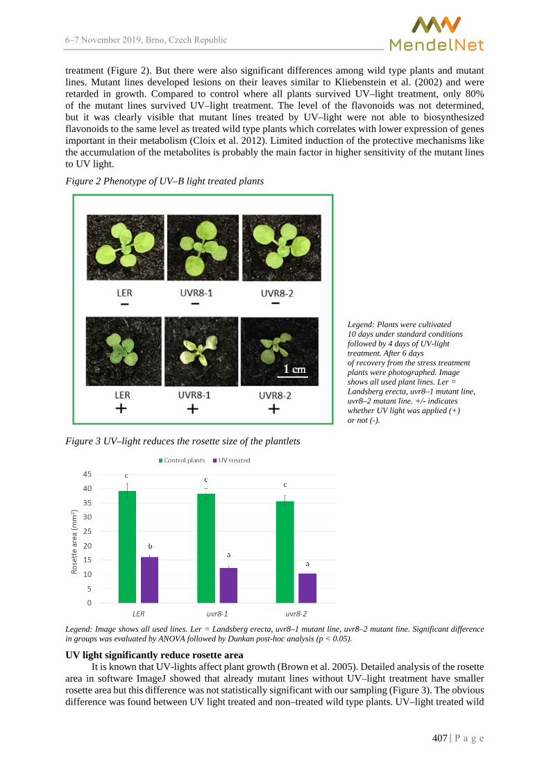
6–7 2019, Brno, Czech Republic
treatment (Figure 2). But there were also significant differences among wild type plants and mutant lines. Mutant lines developed lesions on their leaves similar to Kliebenstein et al. (2002) and were retarded in growth. Compared to control where all plants survived UV–light treatment, only 80% of the mutant lines survived UV–light treatment. The level of the flavonoids was not determined, but it was clearly visible that mutant lines treated by UV–light were not able to biosynthesized flavonoids to the same level as treated wild type plants which correlates with lower expression of genes important in their metabolism (Cloix et al. 2012). Limited induction of the protective mechanisms like the accumulation of the metabolites is probably the main factor in higher sensitivity of the mutant lines to UV light.
Figure 2 Phenotype of UV–B light treated plants
Legend: Plants were cultivated 10 days under standard conditions followed by 4 days of UV-light treatment. After 6 days of recovery from the stress treatment plants were photographed. Image shows all used plant lines. Ler = Landsberg erecta, uvr8–1 mutant line, uvr8–2 mutant line. +/- indicates whether UV light was applied (+) or not (-).
Figure 3 UV–light reduces the rosette size of the plantlets
Legend: Image shows all used lines. Ler = Landsberg erecta, uvr8–1 mutant line, uvr8–2 mutant line. Significant difference in groups was evaluated by ANOVA followed by Dunkan post-hoc analysis (p < 0.05).
UV light significantly reduce rosette area It is known that UV-lights affect plant growth (Brown et al. 2005). Detailed analysis of the rosette
area in software ImageJ showed that already mutant lines without UV–light treatment have smaller rosette area but this difference was not statistically significant with our sampling (Figure 3). The obvious difference was found between UV light treated and non–treated wild type plants. UV–light treated wild
407
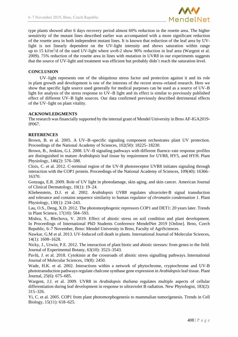
6–7 2019, Brno, Czech Republic
type plants showed after 6 days recovery period almost 60% reduction in the rosette area. The higher sensitivity of the mutant lines described earlier was accompanied with a more significant reduction of the rosette area in both independent mutant lines. It is known that reduction of the leaf area by UV-light is not linearly dependent on the UV-light intensity and shows saturation within range up to 15 kJ/m2/d of the used UV-light where uvr8-2 show 90% reduction in leaf area (Wargent et al. 2009). 75% reduction of the rosette area in lines with mutation in UVR8 in our experiments suggests that the source of UV-light and treatment was efficient but probably didn´t reach the saturation level.
CONCLUSION UV–light represents one of the ubiquitous stress factor and protection against it and its role
in plant growth and development is one of the interests of the recent stress–related research. Here we show that specific light source used generally for medical purposes can be used as a source of UV–B light for analysis of the stress response to UV–B light and its effect is similar to previously published effect of different UV–B light sources. Our data confirmed previously described detrimental effects of the UV–light on plant vitality.
ACKNOWLEDGMENTS The research was financially supported by the internal grant of Mendel University in Brno AF-IGA2019-IP067.
REFERENCES Brown, B. et al. 2005. A UV–B–specific signaling component orchestrates plant UV protection. Proceedings of the National Academy of Sciences, 102(50): 18225–18230. Brown, B., Jenkins, G.I. 2008. UV–B signaling pathways with different fluence–rate response profiles are distinguished in mature Arabidopsis leaf tissue by requirement for UVR8, HY5, and HYH. Plant Physiology, 146(2): 576–588. Cloix, C. et al. 2012. C-terminal region of the UV-B photoreceptor UVR8 initiates signaling through interaction with the COP1 protein. Proceedings of the National Academy of Sciences, 109(40): 16366–16370. Gonzaga, E.R. 2009. Role of UV light in photodamage, skin aging, and skin cancer. American Journal of Clinical Dermatology, 10(1): 19–24. Kliebenstein, D.J. et al. 2002. Arabidopsis UVR8 regulates ultraviolet-B signal transduction and tolerance and contains sequence similarity to human regulator of chromatin condensation 1. Plant Physiology, 130(1): 234–243. Lau, O.S., Deng, X.D. 2012. The photomorphogenic repressors COP1 and DET1: 20 years later. Trends in Plant Science, 17(10): 584–593. Mishra, S., Blechova, V. 2019. Effect of abiotic stress on soil condition and plant development. In Proceedings of International PhD Students Conference MendelNet 2019 [Online]. Brno, Czech Republic, 6–7 November, Brno: Mendel University in Brno, Faculty of AgriSciences. Nawkar, G.M et al. 2013. UV-Induced cell death in plants. International Journal of Molecular Sciences, 14(1): 1608–1628. Nicky, J., Urwin, P.E. 2012. The interaction of plant biotic and abiotic stresses: from genes to the field. Journal of Experimental Botany, 63(10): 3523–3543. Pavlů, J. et al. 2018. Cytokinin at the crossroads of abiotic stress signalling pathways. International Journal of Molecular Sciences, 19(8): 2450. Wade, H.K. et al. 2002. Interactions within a network of phytochrome, cryptochrome and UV-B phototransduction pathways regulate chalcone synthase gene expression in Arabidopsis leaf tissue. Plant Journal, 25(6): 675–685. Wargent, J.J. et al. 2009. UVR8 in Arabidopsis thaliana regulates multiple aspects of cellular differentiation during leaf development in response to ultraviolet B radiation. New Phytologist, 183(2): 315–326. Yi, C. et al. 2005. COP1 from plant photomorphogenesis to mammalian tumorigenesis. Trends in Cell Biology, 15(11): 618–625.
408
6–7 2019, Brno, Czech Republic
Medium-term in vitro storage of vegetative propagated genotypes of Petunia hybrida and Calibrachoa in minimal amount of media
Marketa Cerna, Josef Cerny, Petr Salas Department of Breeding and Propagation of Horticultural Plants
Mendel University in Brno Valticka 337, 691 44 Lednice
CZECH REPUBLIC
Abstract: In vitro storage of genetic materials is crucial for multiplication and breeding reasons. It prevents loosing valuable genotypes, which can happen due to biotic and abiotic effects while in vivo planting. Conventional in vitro storage of Petunia hybrida and Calibrachoa genotypes is labor and cost effective. Three explants are usually cultivated in one glass Erlenmeyer flask with MS Cultivation medium with 20 g/l saccharoses and 6 g/l agar added. Passaging needs to be done four times a year. The aim of this experiment was to determine a way how to store genotypes of vegetative propagated Petunia hybrida (diploid and tetraploid materials) and Calibrachoa in the conditions, so only one passaging will be needed. Stored material must regenerate fast, so it can be used promptly in breeding programs or experiments.
Key Words: Petunia hybrida, in vitro, storage
INTRODUCTION Storage and preserving of unique genetic material are crucial for multiplication of current varieties
and breeding new once, that will have better esthetic or growing values (Anderson 2007). Genotypes in in vivo conditions can be damaged by biotic and abiotic effects and lost. Due to this fact multiple national and private gene banks exist, conserving disease-free plant explants of different genotypes. These can be also subject of international material exchange (Suriyan and Chalermpol 2007).
Based on the researchers’ and producers’ needs, 3 main kinds of storage are used: short-, medium-and long-term. All of these are using techniques changing physical and chemical environment such as temperature, light intensity, osmotic pressure or medium content. This leads to slowing down the growth process and preserving the plant material for longer time (Engelmann 1998). Main advantages of in vitro storage are: low space requirements, all-year-round availability of material, health condition of the material and its control (McCown 2003).
Petunia hybrida and Calibrachoa are placed among the most popular annuals worldwide, so many companies are focusing on their production (generative as well as vegetative) and breeding. Majority of today’s assortment is vegetative propagated, thus securing this elite material is essential (Gerats and Strommer 2009). These cultures are cultivated in laboratories in glass Erlenmeyer flask with 20 ml MS Cultivation medium (Murashige and Skoog 1962) with 20 g/l sacharoses and 6 g/l agar added. Three explants are per one flask, pH is set to 5.8; higher pH causes chlorosis (Sink 1984). Petunia hybrida is facultative long-day plant, so photoperiod 8 hours long is necessary to prevent formation of flowers (Votruba 1999). Based on research (Sediva 2009), adding cytokinin benzyladenin increases number of shots but their quality (especially length) is not acceptable for further usage.
So cultivated explants need to be passaged four times a year, every three months. This represents financial and labor costs, especially when large collection of genotypes is preserved. To decrease the frequency of passaging, long term methods of conservation (cryopreservation) are used. Very efficient proved to be also medium term storage of meristems in minimal amount of media. The explants are planted in micro biotical test-tubes with diameter of 17 mm and length 120 mm, containing 5 ml of MS media.
409

6–7 2019, Brno, Czech Republic
MATERIAL AND METHODS
Characterization of experimental design and methods The aim of this research was to develop a protocol how to store vegetative propagated genotypes
of Petunia hybrida (diploid and tetraploid materials) and Calibrachoa so only one passaging per year is necessary. It is required for so stored material to regenerate fast, so it can be used in breeding or multiplication programs and experiments.
In the experiment were used three sources of genotype materials cultivated in the in vitro laboratory: (1) diploid vegetative propagated components of commercial Petunia hybrids, (2) tetraploid Petunia hybrida materials that originated from in vitro polyploidization and (3) commercial varieties of Calibrachoa. All Petunia hybrida materials were provided by Czech biotechnological company Černý-BioPro, Prague.
Experiment began in June 2018. Micro biological test-tubes with diameter of 17 mm and length 120 mm were filled with 5 ml of MS Cultivation media (Murashige and Skoog 1962) with 20 g/l saccharoses and 6 g/l agar. These tubes were autoclaved for duration of 21 minutes, temperature 121 °C to secure sterility of the growth medium. One explant (length 5–7 mm) per one test-tube was transplanted and placed to metal stand. Four test-tubes per one genotype were prepared. First 7 days of cultivation took place in cultivation room with set temperature of 18 °C. By this time, first roots were formed. After this first stage, test-tubes were placed in cultivation box with set temperature of 10 °C. Light regime was 8 hours, intensity 3 500 lux, fluorescent lamps were used as a light source.
After 12 months number of vital (green leaves, healthy roots; overall good condition for further transplantation) explants was evaluated for every genotype. If all 4 explants were vital it was considered 100%, 3 vital – 75%, 2 vital – 50%, 1 vital – 25% and none, 0%.
Important quality of stored explants is also their ability to regenerate fast, so they can be further used for breeding and multiplication purposes. To evaluate their ability to regenerate, 5 genotypes per diploid and tetraploid Petunia hybrida materials and 5 genotypes of Calibrachoa were examined. The content of 1 micro biological test-tube was transplanted to 3 glass Erlenmeyer flasks with 20 ml MS Cultivation medium (Murashige and Skoog 1962) with 20 g/l saccharoses and 6 g/l agar added. Flasks and medium were autoclaved before transplanting. This material was stored in cultivation room, temperature 18 °C, light regime 8 hours and intensity 3 500 lux. After a month was evaluated, if these explants regenerated and can be further used.
T-test was used to determine if there is a statistically significant difference among tested materials or the amount of vital explants after a yearlong storage in minimal amount of media is same for tetraploid and diploid materials of Petunia hybrida and Calibrachoa. Program STATISTICA 12 was used.
RESULTS AND DISCUSSION Average amount of vital plants after 12 months of storage in micro biological test-tubes
with minimal amount of media is listed in Table 1. Average vitality of Petunia hybrida tetraploid genotypes was 55%, vitality of diploid Petunia
hybrida materials was 57%. The highest vitality had Calibrachoa genotypes, on average 83%. Distribution of vitality of three tested groups of genotypes is represented in Figure 1.
Statistical significance of these experiment results was tested with t-test. Vitality of diploid and tetraploid Petunia hybrida proved to be equal (p=0.82), statistically different is vitality of Calibrachoa in comparison to both types of Petunia (p=0.00).
Second part of the experiment focused on ability of explants stored for 12 months in minimal amount of medium to regenerate fast in glass Erlenmeyer flasks. These are most commonly used in commercial laboratories for medium term in vitro storage of plant material. This was examined a month after transplantation. All 15 genotypes (5 per one type of plant material) regenerated successfully and new plants were formed. Same conclusion is also presented by Sediva 2009.
In this experiment were included in total 80 genotypes of Petunia hybrida (30 diploid and 30 tetraploid) and Calibrachoa (20 genotypes). The aim was to create and test protocol how to store this plant material so it is available, secured and easily multiplicable, but with low labour and material
410

6–7 2019, Brno, Czech Republic
costs Medium term storage in minimal amount of medium proved to be an efficient way. Results of this experiment are alligned with findings of Suriyan and Chalermpol 2007. The vitality of explants after 12 months is acceptable, even though average Petunia hybrida vitality was 56% since this material is easily replicable. In case of more critical components or components with proven worse vitality it would be beneficial to increase the amount of micro biological test-tubes to at least 6.
Table 1 Amount of vital plants after 12 months storage
Tetraploid Petunia hybrida
materials Diploid Petunia hybrida
materials Calibrachoa materials
Genotype Amount of test tubes
Amount of vital explants
Vitality Amount of test tubes
Amount of vital explants
Vitality Amount of test tubes
Amount of vital explants
Vitality
1 4 4 100% 4 2 50% 4 3 75% 2 4 2 50% 4 1 25% 4 4 100% 3 4 1 25% 4 3 75% 4 4 100% 4 4 1 25% 4 3 75% 4 3 75% 5 4 4 100% 4 1 25% 4 3 75% 6 4 3 75% 4 2 50% 4 4 100% 7 4 1 25% 4 3 75% 4 2 50% 8 4 1 25% 4 2 50% 4 3 75% 9 4 2 50% 4 3 75% 4 3 75%
10 4 0 0% 4 3 75% 4 4 100% 11 4 1 25% 4 2 50% 4 3 75% 12 4 3 75% 4 1 25% 4 3 75% 13 4 1 25% 4 3 75% 4 2 50% 14 4 0 0% 4 3 75% 4 4 100% 15 4 4 100% 4 1 25% 4 4 100% 16 4 1 25% 4 2 50% 4 3 75% 17 4 2 50% 4 3 75% 4 3 75% 18 4 3 75% 4 2 50% 4 4 100% 19 4 4 100% 4 1 25% 4 3 75% 20 4 4 100% 4 3 75% 4 4 100% 21 4 3 75% 4 2 50%
22 4 3 75% 4 3 75% 23 4 4 100% 4 2 50% 24 4 4 100% 4 3 75% 25 4 1 25% 4 3 75% 26 4 3 75% 4 2 50% 27 4 1 25% 4 2 50% 28 4 0 0% 4 3 75% 29 4 3 75% 4 3 75% 30 4 2 50% 4 1 25%
Average 2.20 55% 2.27 57% 3.30 83%
Explants were grown in micro biological test-tubes with only 5 ml of medium, that were stored in metal stand in cultivation box (Figure 2), this significantly reduces space needed for storage. Examples of genotypes after 12 months are presented in Figure 3.
411

6–7 2019, Brno, Czech Republic
Figure 1 Vitality of tested genotypes
Figure 2 Metal stand with micro biological test tubes
Figure 3 Genotypes stored in minimal amount of media after 12 months
Diploid Petunia hybrida V1
Diploid Petunia hybrida V3
Tetraploid Petunia hybrida X3
0
2
4
6
8
10
12
14
16
Petunia Tetraploid Petunia Diploid Calibrachoa
Am
ount
of g
enot
ypes
with
cer
tain
vi
talit
y
Material
0%
25%
50%
75%
100%
412

6–7 2019, Brno, Czech Republic
One of the biggest advantages of storage in minimal amount of media is significant reduction of costs of material and manual labour. Calculation is presented in Table 2. Cost of components of MS Cultivation medium was counted from VWR Price list 2019, cost of 1 hour of Laboratory Technician performing the passaging was set to 12 EUR. The costs of cultivation in the box (energy, amortization) were not counted. The savings is 91.31%.
Table 2 Comparison of yearly costs of storage of 1 genotype
Cost Erlenmeyer flasks (20 ml
medium) Micro biological test-tubes
(5 ml) Medium (cost of chemicals) 0.432 0.0432
Medium sterilization (autoclave) 0.04 0.01 Labour costs (Laboratory Technician) 0.96 0.32
Total Costs 1.432 0.3732 Amount of passaged flasks 3 4
Passaging per year 4 1 Yearly costs of storage of 1 genotype 17.184 1.4928
CONCLUSION Conservation of genetic material is crucial not only for research but also for commercial reasons.
Preserving large collections of genotypes is cost and labor intensive. Storage in minimal amount of media is effective way that enables to do so. The highest cost reduction is due to possibility to grow these explants for duration of one year without passaging. This represents more than 90% costs savings. The vitality of explants if acceptable and plants regenerate from this material easily.
ACKNOWLEDGEMENTS The research was financially supported by IGA Management uchovávání vegetativně množených genotypů petúnií v podmínkách in vitro (IGA - ZF/2019 - AP003).
REFERENCES Anderson, N.O. 2007. Flower Breeding and Genetics: Issues, Challenges and Opportunities for the 21st
Century. 1st ed., Dordrecht, Netherlands: Springer. Engelmann, F. 1998. In vitro conservation of horticultural genetic resources: review of the state of the art. World Conference on Horticultural Research [Online], 17–20 June 1998, ISHS, Rome, Italy. Available at: https://www.actahort.org/books/495/495_10.htm. [2019-09-10]. Gerats, T., Strommer, J. 2009. Petunia: Evolutionary, Developmental and Physiological Genetics. 1st ed. New York, USA: Springer. McCown, B.H. 2003. Biotechnology in Horticulture: 100 Years of Application. HortScience, 38(5): 1026–1030. Murashige, T., Skoog, F. 1962. A revised medium for rapid growth and bioassays with tobacco tissue cultures. Physiologia Plantarum, 15(1): 473–497. Sediva, J. 2009. Shrnutí poznatků při udržování kolekcí vybraných druhů květin s využitím in vitro technik. Acta Pruhoniciana, 93(1): 27–31. Sink, K.C. 1984. Petunia. 1st ed., Berlin, Germany: Springer-Verlag. Suriyan, C., Chalermpol, K. 2007. Minimal Growth in Vitro Culture for Preservation of Plant Species. Fruit, Vegetable and Cereal Science and Biotechnology, 1(1): 13–25. Votruba, R. 1999. Petunia. In Zahradnický slovník naučný IV. Praha: Ústav zemědělských a potra-vinářských informací, pp. 275–276.
413
6–7 2019, Brno, Czech Republic
Towards nanoparticle mediated biomolecule delivery: effect of gold and PEI-capped gold nanoparticles on viability
and growth in Chlamydomonas reinhardtii
Pavel Chaloupsky1, Eliska Sedlackova1, 3, Marek Dvorak1, Magda Barinkova1, Dalibor Huska1, 2, 3
1Department of Chemistry and Biochemistry 2CEITEC – Central European Institute of Technology
Mendel University in Brno Zemedelska 1, 613 00 Brno
3CEITEC – Central European Institute of Technology Brno University of Technology
Purkynova 656/123, 621 00 Brno CZECH REPUBLIC
Abstract: Unicellular algae are promising organisms potentially suitable for plethora of biotechnological applications. However, currently utilized methods of biomolecule delivery are limiting factor for broader utilization of the microalgae in genetic and metabolomic engineering. Currently utilized methods are often inefficient and result in cellular damage with accompanying difficulties with consequent regeneration. In order to overcome the barrier of the cell wall and membrane, nanomaterials can be employed in order to deliver molecular cargo. Within this study, we evaluated influence of different Au nanomaterials with and without surface modifications on viability and growth in order to select suitable material for delivery of genetic material into the unicellular alga Ch. reinhardtii.
Key Words: nanocariers, surface modifications, molecular cargo, toxicity
INTRODUCTION Due to the increase of global population, climatic changes, arable soils degradation
and pollution, plant biotechnologies play significant role in the frame of food and energetic security (Ray et al. 2013). Promising group in the field of plant biotechnology is the microalgal biotechnology. However, transport of biomolecules through cell wall and consequent regeneration of the cell remains as a significant barrier for the methods of genetic and metabolomic engineering (Neupert et al. 2012). Conventional methods utilized for the delivery of the biomolecules are often inefficient among wide range of species. Also cellular damage remains considerable issue lowering biomolecule delivery efficiency. Rapid development in the field of nanotechnologies may offer solution to the drawbacks of the currently utilized conventional methods. Despite the fact, that the nanotechnologies are widely utilized for molecular cargo delivery into the mammalian cells, application of nanoparticles for biomolecule delivery into the plant cells and plant systems was not extensively exploited. Agricultural nanotechnologies were primarily focusing on delivery of agrochemicals, impact on metabolism and accumulation of the particles in the cells (Zuverza-Mena et al. 2017). Both positive, such as increased growth or higher rate of chloroplast formation; and negative impacts, such as phytotoxicity and oxidative stress were observed (Tripathi et al. 2017). Processes involved in nanoparticle internalization into the plant cells and systems are, however, not yet fully elucidated and require further investigation (Cunningham et al. 2018). Despite the fact, that the structural-functional role of physicochemical parameters of nanoparticle-mediated biomolecule delivery into the plant cells is largely unknown, it is possible to utilize heuristic approach for the experimental design and assessment of nanoparticle suitability for biomolecule delivery. Limiting factor which has to be considered within the experimental design is size exclusion limit. Interaction between cell wall, its permeability and size of the nanocarriers play significant role in the molecular cargo transport capability (Eichert et al. 2008). Also charge of the nanoparticles plays important role in capability
414

6–7 2019, Brno, Czech Republic
to traverse the cell wall and ability to efficiently deliver the biomolecules is reported to be higher in positively charged particles due to cationic interaction with negatively charged cell wall (Schwab et al. 2016). Hence, biocompatibility of nanoparticles has to be studied for successful development of nanoparticle mediated molecular cargo delivery. Within this study, effect on viability and growth of the unicellular algae Chlamydomonas reinhardtii was studied to develop a basis for further development of flexible nanoparticle-aided biomolecule delivery system.
MATERIAL AND METHODS
Synthesis of the Au and Au-PEI nanoparticles Synthesis of the self assembled polyethylenimine-capped (PEI-capped) gold (Au) nanoparticles
carrying positive charge is described elsewhere and was applied here with some modifications (Kim et al. 2008). To obtain different sizes of the assembled nanoparticles variable ratio of PEI to HAuCl4
was employed within the separate reaction mixtures. In total, 3 different sizes of PEI-capped Au nanoparticles were obtained with average diameters of the Au core of 10, 20 and 40 nm. The 3 different sizes were further utilized for assessment of influence on growth rate in microalgal cultures and viability assays.
To synthesize citrate-stabilized Au nanoparticles without surface modifications kinetically controlled seeded growth synthesis was carried out (Bastús et al. 2011). Within this experiment, nanoparticles of 10 nm size were synthesized. The Au nanoparticles without surface modification were used as a control to compare influence of PEI modification in PEI-capped Au particles on microalgal cultures.
Nanoparticles were characterized by Malvern Zetasizer Nano ZS and by AFM microscopy to confirm the average size of the particles. Also CHNS elemental analysis was carried out to define nitrogen content in the polymeric coating of the particles.
Preparation of genetic material Plasmid utilized within this experiment to neutralize positive charge of PEI-capped
Au nanoparticles and for controls of the nanoparticles was pbr9-mcherry-cr (Rasala et al. 2013). The plasmid was prepared using alkaline lysis (He 2011) with some modifications. The plasmid was re-precipitated 2 times prior use and concentration of the obtained plasmid was measured spectrophotometrically. Quality of the isolated plasmid was evaluated using gel electrophoresis.
Treatment of algal cultures The microalgal cultures were cultivated on a fresh tris-acetate phosphate (TAP) medium solidified
with 1.5 % agar 3 days prior the experiment. Cell wall deficient mutant of Chlamydomonas reinhardtii (strain SAG 83.81) was used for the experiment. The algae were collected from the solidified medium into liquid TAP medium using inoculating loop. The resulting cell suspension was kept on a rotary shaker for 30 minutes to resuspend remaining cellular clumps. The suspension was consequently rested for 10 minutes and cells were collected from upper layer in order to avoid collecting unsuspended cells. Cells were consequently counted and for each treatment 1 × 10⁵ of the cells was used.
In the total 4 types of nanoparticles that did differ in size and surface modification were synthesized in order to evaluate the impact on viability and growth rate of the unicellular algae Chlamydomonas reinhardtii. List of the treatments is summarized in Table 1. The particles were further used in combination with pbr9-mcherry-cr plasmid to examine their toxicity after change of the positive charge carried by PEI. The experiment was carried out in 3 replicates.
Dispersions of nanoparticles were sonicated for 20 minutes in sonication bath prior use and were rested for 30 minutes prior treatments. Plasmid DNA was added dropwise into the nanoparticle dispersions and the solution was mixed by pipetting 10 times. The resulting solution was rested for 30 minutes.
Respective treatments were incubated for 60 minutes and the suspensions were consequently centrifuged at 1500 × g. The supernatant was carefully collected in order not to disturb the pellet and the cells were suspended in 500 μl liquid TAP medium. The cells were cultivated in tissue culture
415

6–7 2019, Brno, Czech Republic
plates on a rotary shaker at 150 rpm. The cultures were kept at 12 h light / 12 h dark photoperiod illuminated with 130 μmol·m-2·s-1. Temperature was constantly kept at at 21 ± 1 °C.
Table 1 Overview of the employed treatments listing nanoparticle size, nanoparticle content
Treatment Particle size [nm]
Nanoparticle amount [μg]
DNA amount [μg]
DNA-PEI-Au 10 20 20 DNA-PEI-Au 20 20 20 DNA-PEI-Au 40 20 20 DNA + Au 10 20 20 Free DNA - - 20 PEI-Au 10 - - PEI-Au 20 - - PEI-Au 40 - - Au 10 - - Control - - -
Evaluation of viability and growth rate Viability was evaluated by fluorescein-diacetate (FDA) assay after 48 h after treatment under
confocal microscope ZEISS LSM 700 (Hoppe and Bavister 1984). The FDA decomposition product – fluorescein was excited with 488 nm laser resulting in fluorescence of living cells. Total number of algal cells was obtained by excitation of chlorophyll A and B with 555 nm laser. In order to omit crosstalk between the fluorescein and chlorophyll, linear unmixing was carried out. Cells in which chlorophyll was present, but fluorescein was not detected were considered non-viable.
Growth rate was evaluated after 96 h after treatment by measurement of the optical density. Optical density was evaluated by measurement of absorbance at 750 nm using plate reader Tecan Infinite M200.
Data were evaluated by one way ANOVA with post-hoc Tukey HSD test at p<0.05.
RESULTS AND DISCUSSION Impact of Au nanoparticles on viability
Viability was evaluated after 48 h after treatment via FDA assay. Results of the FDA assay are visualized in Figure 1. Highest average viability excluding control was observed in cultures treated by non-surface modified 10 nm Au nanoparticles without addition of DNA, suggesting good biocompatibility with Ch. reinhardtii. Opposed to that, the lowest viability was observed in cultures treated by PEI capped 10 nm Au nanoparticles without addition of DNA. Significant difference between viability of cultures treated by PEI-capped 10 nm particles with and without addition of the plasmid DNA can be explained by change of charge on the particle surface. According to previous studies on mammalian cells proper P:N ratio is vital for efficient delivery of genetic material into the cells (Hu et al. 2010). The proper ratio has to be addressed in order to develop efficient protocol for transformation in unicellular algae. Influence of Au particles on growth
Growth rate was evaluated by measurement of the optical density. Results of the optical density measurements are summarized in Figure 2. Highest average growth rate was observed in cultures treated by gold nanoparticles without surface modifications, but there was no significant difference compared to control. Lowest optical density was observed in cultures containing PEI capped Au nanoparticles where no DNA was present on the surface of the particles. The average observed optical density was increasing with the size of the particles, however, no significant difference among the Au particles with polycationic modification was observed. The cationic nature of the PEI capped Au nanoparticles and interaction with the negatively charged surface of the cells causes a significant inhibitory effect in the C. reinhardtii cultures. In biological samples, nanoparticles are commonly forming a protein
416

6–7 2019, Brno, Czech Republic
corona which dynamically changes their properties. The protein corona may, in some cases, change charge of the nanoparticles. However, PEI capped Au nanoparticles had lethal effect despite the expected presence of the protein corona which would change the toxicological properties of the particles. This complies with previous report where preferential binding of positively charged nanoparticles is described (Forest and Pourchez 2017). Cultures in which PEI capped Au nanoparticles were incubated with plasmid DNA prior treatment had significantly higher growth rate compared to the particles without DNA. Negatively charged phosphate backbone of the DNA is able to neutralize the positive charge carried by surface modified nanoparticles thus reducing the lethal cationic interaction with the cellular membranes. Cultures treated with PEI capped particles with 10 nm Au core had significantly lower inhibitory effect on growth compared to the particles with 40 nm Au core. This is caused by insufficient change of the charge on the surface of the particles and different N:P ratio compared to the particles. Particles with 10 nm diameter of Au core contained 0.138 mg N per 1 mg nanoparticles, whereas particles with 40 nm diameter contained 0.127 mg N per 1 mg nanoparticles. In this respect, N:P ratio has to be adjusted accordingly to compensate different loading capacity of the different sizes of PEI capped Au particles.
Figure 1 Viability of cultures after different treatments after 48 hours (error bars are representing standard deviation)
Figure 2 Optical density of cultures after 96 hours after treatment (error bars are representing standard deviation)
417

6–7 2019, Brno, Czech Republic
CONCLUSION Within this work, we evaluated impact of different Au nanoparticles on viability and growth
of Ch. reinhardtii. Surface modification by high molecular weight PEI was proven to have inhibitory effect on growth and reduction of viability was observed. After neutralisation of the positive charge carried by PEI with plasmid DNA, the nanoparticle-DNA complexes had in most treatment significantly lower inhibitory effects on growth compared to the non-DNA counterparts. Higher viability was observed in cultures treated by nanoparticle complexes containing plasmid DNA. Further optimization of DNA loading to PEI-capped Au nanoparticles has to be carried out for efficient biomolecule internalisation. Presented work provides a basis for further experiments using nanocarriers for molecular cargo delivery into unicellular algae.
ACKNOWLEDGEMENTS The research was financially supported by the Internal Grant Agency of Mendel University in Brno AF-IGA2019-IP.
REFERENCES Bastús, N.G., Comenge, J., Puntes, V. 2011. Kinetically controlled seeded growth synthesis of citrate-stabilized gold nanoparticles of up to 200 nm: size focusing versus Ostwald ripening. Langmuir, 27: 11098–11105. Cunningham, F.J. et al. 2018. Nanoparticle-mediated delivery towards advancing plant genetic engineering. Trends in Biotechnology, 36(9): 882–897. Eichert, Thomas, et al. 2008. Size exclusion limits and lateral heterogeneity of the stomatal foliar uptake pathway for aqueous solutes and water‐suspended nanoparticles. Physiologia Plantarum, 151–160. Forest, V., Pourchez, J. 2017. Preferential binding of positive nanoparticles on cell membranes is due to electrostatic interactions: a too simplistic explanation that does not take into account the nanoparticle protein corona. Materials Science and Engineering, 70, 889–896. He, F. 2011. Plasmid DNA extraction from E. coli using alkaline lysis method. Biology Protocol, 30: 1–3. Hoppe, R.W., Bavister, B.D. 1984. Evaluation of the fluorescein diacetate (FDA) vital dye viability test with hamster and bovine embryos. Animal Reproduction Science, 323-335. Hu, C. et al. 2010. Low molecular weight polyethylenimine conjugated gold nanoparticles as efficient gene vectors. Bioconjugate chemistry, 836–843. Kim, K. et al. 2008. Self-assembly of poly (ethylenimine)-capped Au nanoparticles at a toluene− water interface for efficient surface-enhanced Raman scattering. Langmuir, 24–7183. Neupert, J. et al. 2012. Genetic transformation of the model green alga Chlamydomonas reinhardtii. Transgenic Plants, 35–47 Rasala, B.A. et al. 2013. Expanding the spectral palette of fluorescent proteins for the green microalga C hlamydomonas reinhardtii. The Plant Journal, 74(4): 545–556. Ray, Deepak K. et al. 2013. Yield trends are insufficient to double global crop production by 2050. PloS one: e66428. Schwab, F., et al. 2016. Barriers, pathways and processes for uptake, translocation and accumulation of nanomaterials in plants–Critical review. Nanotoxicology, 257–278. Tripathi, D.K. et al. 2017. An overview on manufactured nanoparticles in plants: uptake, translocation, accumulation and phytotoxicity. Plant Physiology and Biochemistry, 2–12. Zuverza-Mena, N. et al. 2017. "Exposure of engineered nanomaterials to plants: Insights into the physiological and biochemical responses-A review." Plant Physiology and Biochemistry 110, 236–264.
418

6–7 2019, Brno, Czech Republic
Negative effects of drought stress on the produced seeds composition, vigor and ageing
Hana Dufkova1, Barbora Hlavackova2 1Department of Molecular Biology and Radiobiology
Mendel University in Brno Zemedelska 1, 613 00 Brno
2Secondary Technical School of Chemistry in Brno
Vranovska 1364/65, 614 00 Brno CZECH REPUBLIC
Abstract: Seed germination is a crucial phase of plant's life, which may be affected by multiple factors. Most importantly, seed performance is defined by seed vitality, which is strongly affected by the seed maturation environment. Thus, unfavourable environmental conditions may be negatively projected in both maternal plant growth and next generation performance. Recently, drought is one of the most important sources of abiotic stress, causing significant yield losses. However, the effects of drought stress on the quality of produced seeds are understood poorly. In this work, we focused on the seed performance and proteome composition of Arabidopsis thaliana seeds produced under drought stress conditions. Our results suggest that the drought stress causes reduction in seed dormancy level, corresponding with faster seed germination of freshly harvested seeds and higher mortality of artificially aged seeds. The proteomic analysis revealed more than 50 canditate proteins. Among others, we found significant changes in proteins ensuring seed desiccation tolerance and protein folding, as well as abscisic acid and gibberellin responsive proteins.
Key Words: seed dormancy, abscisic acid, proteomic analysis
INTRODUCTION The plants ability to cope with unfavourable environmental conditions determines not only
survival of the plant itself, but also the seed performance and seedling establishment in the next generation. The seed germinability is mostly driven by the seed vitality, including the level of seed dormancy, seed coat robustness and accumulation of storage compounds. All these aspects of seed vitality are determined during the seed development. According to this, the parental environment during seed production has a major impact on the seed performance (Penfield and MacGregor 2016, Walck et al. 2011). It has been already proposed that the seed quality is strongly affected by temperature (MacGregor et al. 2015), light intensity and nitrate accessibility (He et al. 2016). Recently, the climate change causes extreme weather fluctuations, which may result in stress conditions. Out of these, drought represents one of the most harmful types of abiotic stress with an increasing relevance. It was reported that the drought stress imposed on parental plants results in significant yield losses, as well as the reduced seed quality. However, its impact is species-specific and the plant regeneration is determined by the seed type and genetical characters of the mother plant. For example, reduced seed vigor was reported in soybean, whereas no effect on standard seed germination was found in barley. Nevertheless, significantly lower barley seed vigor was proved after accelerated seed ageing test (Alqudah et al. 2011).
The decisive influence of seed vitality is determined by the level of seed dormancy. This phenomenon is defined as a state in which seeds are prevented from germinating, or do so under a narrow set of environmental conditions. The level of seed dormancy is regulated by two important classes of phytohormones: abscisic acid (ABA) and gibberellins (GAs). ABA deepens the seed dormancy and thus, inhibits premature seed germination. Fenner (1991) stated that the reduced vitality and longevity of seeds produced under drought stress conditions is probably caused by the disruption of ABA accumulation during the seed maturation. On the contrary, GAs promote seed germination by counteracting the effects of ABA.
419

6–7 2019, Brno, Czech Republic
The signalling of ABA is also essential for the seed development, maturation and desiccation tolerance, ensuring seed survival at the dry stage. Among others, ABA regulates the accumulation of protective molecules and storage compounds in seeds. A well-known group of protective molecules is represented by LEA (late embryogenesis abundant) proteins, which protect molecular structures from aggregation during seed desiccation (Amara et al. 2014). The chaperone-like function is also ensured by heat shock proteins (HSP), which maintain the correct protein conformations and which are also proposed to participitate in various signaling pathways in plants.
MATERIAL AND METHODS
Plant material and cultivation conditions Dry seeds of Arabidopsis thaliana (ecotype Columbia) were sown on wet soil substrate
and stratified for three days (7 °C). After stratification, imbibed seeds were placed into greenhouse, where germinated under long-day light regime (20 °C, 100 µmol/m2/s light intensity, 16 hours; 20 °C, no illumination, 8 hours). The soil relative humidity was maintained at 60% relative water content (RWC), until the flowering stem started emerging from the leaf rosette. At this point, plants were divided into two groups with at least 35 plants. The first group of plants was cultivated on 60% RWC, while the second one was cultivated under drought stress conditions (20% RWC). Finally, mature seeds were harvested and dried properly.
In vitro plate assay For plate assay, 40 seeds originating from plants cultivated under controlled conditions (C)
and drought stress (D) were sown on a half-strength Murashige & Skoog (Ducheva Biochemie) plant agar medium, containing (i) no additional chemicals (mock) and (ii) 80 mM sodium chloride (NaCl), and cultivated under long-day conditions (21 °C, 100 µmol/m2/s light intensity; 19 °C, no illumination). After seven days of cultivation, seedlings were photodocumented, and the cotyledon area was calculated using ImageJ program.
Accelerated seed ageing test The accelerated seed ageing test was performed according to Wang et al. (2012) with slight
modification. The seeds were incubated at 40 °C and 100% relative humidity for 48 hours. Next, one hundred of such treated seeds were placed on petri dish with filter paper (Whatman) and imbibed in 3.5 ml of water. The seeds were cultivated for 6 days under long-day light regime (21 °C, 100 µmol/m2/s light intensity; 19 °C, no illumination). After cultivation, the number of germinated seeds was calculated.
Seed proteome analysis For proteomic analysis, 20 mg of C and D seeds were collected in four biological replicates.
Samples were homogenized (RetschMill MM400) and total protein was extracted using TCA/acetone/phenol extraction as described previously (Cerna et al. 2017, Černý et al. 2019). Next, 100 µg aliquot of protein sample was digested with Trypsin Gold (Promega) overnight. The tryptic digests were desalted, using C18 SPE (Agilent). Samples were first eluted with 40 µl 50% acetonitrile (ACN) and 0.1 formic (FA). Second elution was done with 300 µl 100% ACN and then, samples were partially evaporated up to 10–20 µl of the final sample volume. The samples were analyzed by gel-free shotgun profiling, using nanoflow C18 reverse-phase liquid chromatography with a 15cm column (Zorbax, Agilent), a Dionex Ultimate 3000 RSLC nano-UPLC system (Thermo) and Orbitrap Fusion Lumos Tribrid Mass Spectrometer (Thermo). The instrument was operated with following parameters: positive-ionization mode, full MS scans over a mass range of m/z 375–1500, detection in the Orbitrap (resolution 60 000), auto gain control (AGC; 400 000) and the intensity threshold for the most intense ions was set to 50 000. Fragment ion spectra were acquired in the Orbitrap (MS2 detection, resolution 15 000) with an AGC of 50 000 and a maximum injection time of 30 ms. Resulting data files were searched against Arabidopsis (TAIR 10) protein database via Proteome Discoverer 2.3, using Sequest and Amanda searching algorithms. The relative quantification was done by Proteome Discoverer 2.3.
420

6–7 2019, Brno, Czech Republic
RESULTS AND DISCUSSION In this study, two complementary approaches were employed to investigate the negative effects
of drought stress on the produced seed quality. In the physiological part, we focused on the level of seed dormancy and germination ability of the seeds originating from drought-treated mother plants. Next, we employed LC-MS-based proteome profiling to evaluate the differences in the seed protein composition between drought-treated (D) and control (C) seeds.
Drought stress affects seed yield and quality It was widely reported that drought stress causes the yield reduction in many crop plants.
As we expected, limited water regime resulted in reduced Arabidopsis growth, lower number of siliques and thus, significantly lower seed yields (Figure 1). However, it was proposed that abiotic stress affects not only the vitality of mother plants but also the seed quality, including level of seed dormancy (Alqudah et al. 2011).
Figure 1 Drought stress negatively affects the amount of produced seeds
Legend: C – control (plants cultivated under optimal watering conditions), D – drought (plants cultivated under drought stress), * – significant difference compared to control (t-test, p < 0.05). The box plot shows data distribution, as well as the median (the band inside the box).
To investigate whether seed dormancy is affected by drought stress, two types of plate-assay experiments were designed. We hypothesized that the seeds produced under stress conditions will have reduced seed dormancy, which may result in faster germination of freshly harvested dry seeds. On the other hand, low level of seed dormancy, as well as stress-induced accumulation of harmful reactive oxygen species (ROS), could lead to faster loss of seed vitality during the seed ageing. Based on this hypothesis, we designed an in vitro plate assay focused on the seed germination ability of non-stratified C and D seeds. Further, since the D seed were produced by the long-term-stressed mother plants, we hypothesized that plants in the next generation may exhibit higher drought stress tolerance. Thus, the experiment was accompanied by 80 mM NaCl treatment. The results of two independent biological replicates supported our hypothesis (Figure 2a).
Second, we employed the test of accelerated seed ageing to elucidate whether the drought stress imposed on the mother plants causes loss of the seed vitality and longevity in the next generation. Briefly, seeds underwent an accelerated ageing treatment at 40 °C and 100% RH. After 48 hours of incubation, seeds were placed on a plate with filter paper and imbibed in water. We found that the seed germination is retarded in both seed samples, however, lower amount of seeds germinated in case of D sample (Figure 2b).
421

6–7 2019, Brno, Czech Republic
Proteomic analysis revealed multiple proteins to be potentially involved in drought-stress response in seeds
The effect of drought stress on the produced seeds was further studied, employing LC-MS proteome profiling. For the proteomic analysis, proteins were extracted from dry C and D seeds and analyzed by gel-free shotgun proteome profiling approach. The relative protein quantification of 531 proteins provided the list of 57 candidates with at least two-fold change in protein abundancy.
Based on the biological functions, the candidate proteins were mostly involved in lipid metabolism, protein folding and protection (molecular chaperones), and seed development regulation. Interestingly, 10 protein candidates were previously referred (online database Plaza 4.0) to be involved in response to either water deprivation or salt stress (which is known to share many similarities with drought stress responses). Out of these, three ABA-responsive proteins were significantly up-regulated in D samples, namely Non-specific lipid transfer protein 4 (LTP4, AT5G59310), Late embryogenesis abundant protein 18 (LEA18, AT2G35300) and Dehydrin Xero 2 (AT3G50970). Based on germination assays results, we hypothesized that the faster seed germination of D seeds is affected by impaired seed dormancy, which is caused by the decrease in ABA level. However, LEA proteins, dehydrins and LTP4 are well known to be upregulated by ABA. Simultaneously, two GA-regulated proteins (AT5G59845 and AT4G09610) showed decreased abundance in D seeds. Except the known involvement of these proteins in salt stress response, their function has not been resolved yet.
Figure 2 Seed germination and seedling growth ability is affected by drought stress. The drought-treated seeds showed fasted seed germination and higher salt stress tolerance, correlating with larger cotyledon area of the seedlings (a). The accelerated seed ageing test revealed that the control seeds dispose higher seed vitality and longevity (b).
Legend: C – control (plants cultivated under optimal watering conditions), D – drought (plants cultivated under drought stress), C48/D48 - seeds incubated in darkness and 100% relative humidity for 48 hours
Our results suggest that the drought stress imposed on mother plants affects the seed proteome composition. We proposed possible changes in the signalling of both ABA and GAs, the key phytohormones determining the level of seed dormancy and seed vitality. Simultaneously, we found increased abundancy of few important molecular chaperones involved in the protection of molecular structures during the seed maturation and desiccation. However, the molecular mechanisms regulating the drought stress responses in produced seeds, as well as the resulting seed vitality, remains unclear.
422

6–7 2019, Brno, Czech Republic
To understand it more deeply, the deciphering of higher seed proteome coverage is essential. Since the low abundant proteins are often involved in different signalling pathways, their detection and quantification may allow us to get a deeper insight into the complex mechanism regulating seed development and maturing. Thus, more efforts will be made on the technology of Arabidopsis seed proteome fractionation, resulting in higher proteome coverage.
CONCLUSION Drought represents one of the most harmful types of abiotic stress with an increasing relevance
in agriculture. It has been widely reported that the drought stress causes significant yield losses, however, it may also affect the seed performance and plant growth in the next generation. To get a deeper insight into the effect of the drought stress on the seed quality, we produced seeds of a model plant Arabidopsis thaliana under both optimal and limited water regime. The results of germination assays and accelerated seed ageing test indicate the effects of drought stress on seed dormancy level. Further, we identified almost 60 candidate proteins which are probably involved in drought stress response. Some of the candidates were previously referred as drought/salt stress responsive proteins or to be regulated by the signalling of abscisic acid or gibberellins, the key phytohormones determining the level of seed dormancy. These results contributed to the current knowledge of the environmental effects on the seed quality. However, the molecular mechanisms regulating seed development and maturation under drought stress conditions are not fully understood yet. Thus, more efforts will have to be made to get a deeper insight into this challenging topic.
ACKNOWLEDGEMENTS The research was financially supported by grant AF-IGA2019-IP035 (Internal Grant Agency of Faculty of AgriSciences, Mendel University in Brno). Hana Habánová – Brno Ph.D. Talent Scholarship Holder – Funded by the Brno City Municipality.
REFERENCES Alqudah, A.M. et al. 2011. Drought stress effect on crop pollination, seed set, yield and quality. In Alternative farming systems, biotechnology, drought stress and ecological fertilisation. Dordrecht: Springer, pp. 193–213. Amara, I. et al. 2014. Insights into late embryogenesis abundant (LEA) proteins in plants: from structure to the functions. American Journal of Plant Sciences, 5(22): 3440. Available at: https://doi.org/10.4236/ajps.2014.522360. [2019-08-19]. Cerna, H. et al. 2017. Proteomics offers insight to the mechanism behind Pisum sativum L. response to pea seed-borne mosaic virus (PSbMV). Journal of Proteomics, 153: 78–88. Available at: https://doi.org/10.1016/j.jprot.2016.05.018. [2019-08-23]. Černý, M. et al. 2019. Fractionation Techniques to Increase Plant Proteome Coverage: A Combined Parallel Separation on Protein and Peptide Level. In Functional Proteomics: Methods and Protocols. New York: Humana Press, pp. 80–94. Fenner, M. 1991. The effects of the parent environment on seed germinability. Seed Science Research, 1(2): 75–84. Available at: https://doi.org/10.1017/S0960258500000696. [2019-08-26]. He, H. et al. 2016. Effects of parental temperature and nitrate on seed performance are reflected by partly overlapping genetic and metabolic pathways. Plant and Cell Physiology, 57(3): 473–487. Available at: https://doi.org/10.1093/pcp/pcv207. [2019-08-25]. MacGregor, D.R. et al. 2015. Seed production temperature regulation of primary dormancy occurs through control of seed coat phenylpropanoid metabolism. New Phytologist, 205(2): 642–652. Available at: https://doi.org/10.1111/nph.13090. [2019-08-25]. Penfield, S., MacGregor, D.R. 2017. Effects of environmental variation during seed production on seed dormancy and germination. Journal of Experimental Botany, 68(4): 819–825. Available at: https://doi.org/10.1093/jxb/erw436. [2019-08-26].
423

6–7 2019, Brno, Czech Republic
Walck, J.L. et. al. 2011. Climate change and plant regeneration from seed. Global Change Biology, 17(6): 2145–2161. Available at: https://doi.org/10.1111/j.1365-2486.2010.02368.x. [2019-08-22]. Wang, F. et al. 2012. Quantitative dissection of lipid degradation in rice seeds during accelerated aging. Plant Growth Regulation, 66(1): 49–58. Available at: https://doi.org/10.1007/s10725-011-9628-4. [2019-08-23].
424

6–7 2019, Brno, Czech Republic
Catalase: Bioinformatics analyses of one of the key enzymes in hydrogen peroxide metabolism
Michaela Kameniarova, Romana Kopecka
Department of Molecular Biology and Radiobiology
Mendel University in Brno Zemedelska 1, 613 00 Brno
CZECH REPUBLIC
Abstract: Catalases (CAT) are family of important antioxidant enzymes present in different isoforms and responsible for scavenging of hydrogen peroxide in almost all aerobically living organisms. In plants, they were found both in unicellular and multicellular species. Here, we performed bioinformatics analysis and analysed catalase evolutionary relationship and expression patterns. By comparing expression profiles of CATs and expression profiles of genes related to abiotic stimuli we found that almost 50% of light signalling genes were co-expressed with CATs. Further, by datamining in available resources and structural modelling we pinpointed candidate amino acid residues responsible for CAT thermostability.
Key Words: catalase, H2O2, phylogenetics, abiotic stress, stability
INTRODUCTION Plants contain several types of enzymes involved in H2O2 metabolism. These include catalases,
ascorbate peroxidases, peroxiredoxins, glutathione/thioredoxin peroxidases, and glutathione S-transferases, but only catalases do not require additional cellular reductants (Mhamdi et al. 2010). Catalases are present almost in all aerobically respiring organisms. Within the cell environment, catalases are localized in all major sites of H2O2 production, mostly at peroxisomes, but they were detected in cytosol, mitochondria, and chloroplasts as well (Sharma and Ahmad 2014). Catalases (CAT, 1.11.1.6) are antioxidant enzymes that catalyse decomposition of hydrogen peroxide to water and molecular oxygen (2H2O2 → 2H2O + O2), an important process in defending cells against oxidative damage caused by reactive oxygen species (ROS; Alfonso-Prieto et al. 2009). The H2O2 affects a plant in the concentration-dependent manner. High amounts of H2O2 cause cell damage, potentially leading to cell death, whereas low concentrations can act as a signal regulating specific biological processes (Zámocký et al. 2012). For the survival and normal development of the plant it is necessary to maintain balance between H2O2 production and its decomposition.
Genes for catalases in plants usually create small gene family. Catalase gene family in model plant Arabidopsis consists of three genes encoding CAT1, CAT2 and CAT3. These CAT isoforms show different tissue localization. CAT1 is localized mostly in pollen and seeds, while CAT2 is expressed in photosynthetic tissues and in roots, and CAT3 in vascular tissues (Buzduga et al. 2018). Besides the different localization, they also have a different expression pattern, and the transcription levels depend on time, place and environmental stimuli. Expression studies of CAT2 and CAT3 revealed that they are regulated by circadian rhythm, with CAT2 expression peaking at the beginning of the light period and CAT3 in the dark (Mhamdi et al. 2012). Environmental stresses, such as drought, heat or cold, generally enhance the transcription of CATs, and thus increase catalases’ activity, maintaining redox balance in the cell. Mutation in CAT genes disturbs this redox state. In Arabidopsis, a loss-of-function mutant cat2 reduced catalase activity in leaves by 90% in comparison to Col-0 wild-type plants, but the deletion of CAT1 and CAT3 had only a mild effect on the total catalase activity (Mhamdi et al. 2010, Su et al. 2018).
425

6–7 2019, Brno, Czech Republic
MATERIAL AND METHODS
Selection of organisms and construction of phylogenetic tree The list of organisms and accession numbers of their CAT nucleotide sequences used
for phylogenetic reconstruction are summarized in Table 1. The sequences were obtained from ENA (European Nucleotide Archive) and GenBank databases. Multiple sequence alignment and phylogenetic analysis was constructed using the GenomeNet ETE 3 v3.0.0b32 (https://www.genome.jp/tools/ete/; Huerta-Cepas et al. 2016) with the following parameters: Aligner – mafft, Alignment cleaner – none, model tester – none, tree builder fasttree (Price et al. 2009). The constructed tree file was visualized using iTOL v3.0 (http://itol2.embl.de/index.shtml; Letunic and Bork 2006, Letunic and Bork 2011).
Table 1 Overview of model organisms and corresponding CATs used in the analysis Organism Accession numbers Arabidopsis thaliana NC_003070.9, NC_003070.9, NC_003075.7 Chlamydomonas reinhardtii NW_001843734.1 Malus domestica ENA|RXH96794|RXH96794.1, ENA|RXH96798|RXH96798.1 Marchantia polymorpha ENA|OAE35245|OAE35245.1, ENA|OAE31579|OAE31579.1
ENA|OAE35247|OAE35247.1 Medicago truncatula NW_013656164.1, NC_016409.2, ENA|KEH36313|KEH36313.1 Nicotiana benthamiana ENA|ACL27272|ACL27272.1, ENA|AFU48609|AFU48609.1 Oryza sativa NC_029257.1, NC_029258.1, NC_029261.1 Plasmodiophora brassicaceae ENA|CEO97147|CEO97147.1 Physcomitrella patens ENA|EDQ83048|EDQ83048.1 Populus trichocarpa ENA|PNT38671|PNT38671.1, NC_037289.1, NC_037286.1 Solanum tuberosum ENA|AAA80650|AAA80650.1, ENA|CAA85470|CAA85470.1 Zea mays ENA|CAA31056|CAA31056.1, ENA|CAA38588|CAA38588.1
ENA|AAC37357|AAC37357.1
Expression patterns of CAT genes To describe the correlation of CAT expression profiles with expression profiles of abiotic-stress
related genes, light signalling genes and phytohormones metabolism genes, we searched data from Černý et al. (2018) against the ThaleMine (https://www.araport.org/).
Searching for natural CAT mutants In order to obtain information about CAT polymorphism in different natural accessions
of Arabidopsis we used an online tool Polymorph 1001 https://tools.1001genomes.org/polymorph/.
Prediction of hotspot residues from CAT protein sequences Hotspots in CAT protein sequences of Zea mays were identified by automated multi-step
calculation using online tool HotSpot Wizard 3.0. (http://loschmidt.chemi.muni.cz/hotspotwizard). CATs protein sequences were obtained from UniProt and the tertiary structure of CATs was retrieved from repositories of homology models. We performed multiple alignment of selected CAT sequences, calculated hotspots with amino acid residues in which the CAT isoforms differ and modelled the mutation of CAT in these residues to determine its effect on the stability of the individual catalase isoforms. The data about temperature stability of CATs were obtained from enzyme database Brenda (https://www.brenda-enzymes.org/index.php).
RESULTS AND DISCUSSION
Evolutionary relationships of CATs in different plant species Catalases are produced by almost all aerobically living organisms ranging from unicellular
to multicellular species and their evolution relates to development of the aerobic biosphere on Earth. They are present in multiple molecular forms in plants, creating small gene families. In higher plants,
426

6–7 2019, Brno, Czech Republic
they usually consist of 3 members with varying levels of sequence similarity (Sharma and Ahmad 2014). Phylogenetic reconstruction using maximum likelihood method to the catalase sequences of 11 different organisms resulted in a rooted tree shown in Figure 1. Catalases of the same gene family are often clustered together, while CAT isoforms of some species (Oryza sativa, Zea mays, Populus trichocarpa) are situated on the distinct branches of the tree. CAT of single-cell Chlamydomonas reinhardtii shows the highest evolutionary distance from the rest of the sequences, creating a separated branch. The Arabidopsis genome encodes three CAT isoforms consisting of 492 amino acids (Mhamdi et al. 2010). They share high sequence similarity grouping Arabidopsis CATs together.
Figure 1 Rooted phylogenetic tree based on the nucleotide sequences of CAT genes
427

6–7 2019, Brno, Czech Republic
Relation of CATs expression patterns with expression patterns of abiotic stress-related genes and phytohormone metabolism genes
Catalase is a well-known enzyme involved in biotic and abiotic stress responses. Here, to underscore its role in a stress response, we employed a dataset containing previously reported marker genes in Arabidopsis and compared the expression patterns to that of catalase. The dataset contained genes related to nutrient stress (142 genes), temperature stress (43 genes), drought stress (13 genes), light signalling (27) and hormone metabolism genes (101). Surprisingly, we did not find a significant overlap between Arabidopsis CATs expression and the expression of temperature or drought-stress-related genes. However, we found that almost 50% of analysed light signalling genes and a significant portion of phytohormones metabolism genes were co-expressed with CATs. High level of similarity of CATs expression patterns and light signalling is likely the result of photosynthetic activity and ROS scavenging (Buzduga et al. 2018). In accordance, the light period plays role in regulation of transcript abundance in two of three catalases, CAT2 and CAT3. Their expression level is controlled by day-night rhythm, where the photorespiratory catalase CAT2 shows a peak early in the light period and the CAT3 in dark (Mhamdi et al. 2012).
Figure 2 Percentage of abiotic stress markers genes, light signalling genes and phytohormones metabolism genes co-expressed with CATs in Arabidopsis
Temperature stability of CATs and hotspots in CAT protein sequences of Zea mays Hotspot residues are important in the stability of protein-protein interactions, and they always
have some specific functions in protein. Thermostability of enzymes is critical for their applicability in biotechnologies. Because the data about temperature stability of CATs in Arabidopsis thaliana are not available, we analysed thermostability of CATs in important crop, Zea mays, wherein the names of catalases corresponds to catalases in Arabidopsis. The Brenda database showed that the most thermo stable isoform of CAT in Zea mays is CAT2, which is stable at 45 °C, while the half-life of CAT1 is 12.5 minutes and half-life of CAT3 is 18 minutes (Chandlee et al. 1983). By designing specific mutations, we identified amino acid residues that could be responsible for thermostability or thermolability of different CAT isoforms in Zea mays and they are shown in Figure 3. We found that mutation of CAT1 Met 185 to Thr, normally present in CAT3, leads to its destabilization, but on the concurrent mutation of Thr 343 to Cys has a positive effect on CAT3 stability. In CAT2, mutation of Val 288 to Thr and mutation of Thr 342 to Cys, normally present in CAT3 amino acid sequence, has a destabilizing effect on CAT3, and this could be a reason why CAT3 is not as thermo stable as CAT2.
Arabidopsis thaliana ecotypes with mutation in CAT Catalase is a well-optimized enzyme with one of the highest known turnover rates (Černý
et al. 2018). However, its mutation does not have to be lethal in optimal growth conditions. Here,
428

6–7 2019, Brno, Czech Republic
to investigate natural mutations rates, we employed the 1001 Arabidopsis genome database. Surprisingly, we found only four Arabidopsis thaliana accessions carrying a significant mutation in the CAT gene, and all these were mutants in CAT3. The further analysis showed that these mutants IP-Mdd-0, IP-Esn-2, IP-Moe-0 and IP-Tau-0 originated from the same area in Spain. This finding indicates that CAT2 and CAT1 are highly conserved and only CAT3 seems to be prone to mutation. This could correlate with the reports showing that knock-out of CAT3 does not have a significant impact on catalase activity and the plants can grow normally (Mhamdi et al. 2010).
Figure 3 Protein structure of Zea mays CAT isoforms. Amino acid residues potentially responsible for thermostability/thermolability of different CAT isoforms are visualised by yellow colour. The localization of their catalytic pockets is shown by orange colour.
CONCLUSION The main role of catalases in organisms is decomposition of H2O2, maintaining redox homeostasis
in cells. We found that catalases in plants share expression pattern with almost 50% of light signalling genes and with significant portion of phytohormones metabolism genes. In our study we also demonstrated evolutionary relationship of catalases in different plant species and we identified four ecotypes of Arabidopsis thaliana having unfunctional gene for CAT3. At the end we analysed amino acid residues responsible for temperature stability of Zea mays CAT isoforms, where we found that mutation of CAT2 Val 288 to Thr and mutation of Thr 342 to Cys, which are present in CAT3 amino acid sequences, cause destabilization of enzyme, what could be the reason for lower temperature stability of CAT3.
ACKNOWLEDGEMENTS The research was financially supported by AF-IGA-IP-2019/IP081 (Internal Grant Agency of Faculty of AgriSciences, Mendel University in Brno). The authors would like to express their thanks to Markéta Luklová and Martin Černý for support and constructive comments.
REFERENCES Alfonso-Prieto, M. et al. 2009. The Molecular Mechanism of the Catalase Reaction. Journal of the American Chemical Society, 131(33): 11751–11761. Buzduga, I.M. et al. 2018. Metabolic compensation in Arabidopsis thaliana catalase-deficient mutants. Cytology and Genetics, 52(1): 31–39. Černý, M. et al. 2018. Hydrogen Peroxide: Its Role in Plant Biology and Crosstalk with Signalling Networks. International Journal of Molecular Sciences, 19(9): 2812. Chandlee, J.M. et al. 1983. Purification and partial characterization of three genetically defined catalases of maize. Plant Science Letters, 29(2–3): 117–131. Huerta-Cepas, J. et al. 2016. ETE 3: Reconstruction, Analysis, and Visualization of Phylogenomic Data. Molecular Biology and Evolution, 33(6): 1635–1638.
429

6–7 2019, Brno, Czech Republic
Letunic, I., Bork, P. 2006. Interactive Tree of Life (iTOL): An online tool for phylogenetic tree display and annotation. Bioinformatics, 23(1): 127–128. Letunic, I., Bork, P. 2011. Interactive Tree of Life v2: Online annotation and display of phylogenetic trees made easy. Nucleic Acids Research, 39(Suppl). Mhamdi, A. et al. 2010. Catalase function in plants: A focus on Arabidopsis mutants as stress-mimic models. Journal of Experimental Botany, 61(15): 4197–4220. Mhamdi, A. et al. 2012. Plant catalases: Peroxisomal redox guardians. Archives of Biochemistry and Biophysics, 525(2): 181–194. Price, M.N. et al. 2009. FastTree: Computing Large Minimum Evolution Trees with Profiles instead of a Distance Matrix. Molecular Biology and Evolution, 26(7): 1641–1650. Sharma, I., Ahmad, P. 2014. Catalase. Oxidative Damage to Plants, 131–148. Su, T. et al. 2018. The Arabidopsis catalase triple mutant reveals important roles of catalases and peroxisome-derived signaling in plant development. Journal of Integrative Plant Biology, 60(7): 591–607. Zámocký, M. et al. 2012. Molecular evolution of hydrogen peroxide degrading enzymes. Archives of Biochemistry and Biophysics, 525(2): 131–144.
430

6–7 2019, Brno, Czech Republic
Protein pbHSP70 and its putative role in plants: bioinformatics analysis
Romana Kopecka, Michaela Kameniarova
Department of Molecular Biology and Radiobiology Mendel University in Brno Zemedelska 1, 613 00 Brno
CZECH REPUBLIC
[email protected] Abstract: Heat shock proteins are important proteins which have a complex role in organisms. Here, we performed bioinformatics analysis of a HSP70 family protein found in root pathogen Plasmodiophora brassicae. We aligned HSPs sequences from 13 organisms and determined approximate time of protein divergence for three of them. Further, a closer characterization of orthologues in Arabidopsis thaliana revealed a putative role of P. brassicae HSP70 in suppressing host’s defence mechanisms.
Key Words: heat shock protein, Plasmodiophora brassicae, Arabidopsis thaliana, bioinformatics analysis
INTRODUCTION Heat shock proteins (HSPs) are important proteins, which can be found in every organism
in the world (Li and Srivastava 2003). They are highly conserved (Lindquist 1986) and have been a significant point of interest ever since their discovery in 1962 (Rittosa 1962). HSPs are divided by molecular weight into six main families (HSP 100, HSP 90, HSP 70, HSP 60, HSP 40 and small HSPs) (Kim and Yenari 2017). HSPs were originally found in response to heat, but their role in the cell is much more complex. For instance, HSPs are essential in the protein folding and translocation processes or in the cell cycle regulation. Further, HSPs were also implicated in plant-pathogen interactions (Srivastava 2002, Nover and Miernyk 2001).
Here, we analysed in detail HSP70 family protein found in root pathogen Plasmodiophora brassicae (Malych and Berka 2018).
MATERIAL AND METHODS
Bioinformatics tool The Basic Local Alignment Search Tool (BLASTP) was used for orthologous sequences search
and the sequences with the highest similarity were aligned by CLUSTALW (https://www.genome.jp/ tools-bin/clustalw). Alignment and phylogenetic reconstructions were performed using the function "build" of ETE3 v3.0.0b32 (Huerta-Cepas et al. 2016) as implemented on the GenomeNet (https:// www.genome.jp/tools/ete/). Both phylogenetic trees were constructed by fasttree with slow NNI and MLACC=3 (to make the maximum-likelihood NNIs more exhaustive) (Price et al. 2009). Values at nodes are SH-like local support. Phylogenetic trees were displayed with the use of the Interactive tree of life (iTOL, http://itol2.embl.de/index.shtml). Motifs analyses were performed by MEME (Multiple Em for Motif Elicitation software, version 5.0.5.; http://meme-suite.org/tools/meme).
Divergence time calculation Plasmodiophora brassicae HSP70 and two orthologous sequences from Chlamydomonas
reindhartii and Arabidopsis thaliana were used for the divergence time calculation by KaKs Calculator 2.0. The divergence time was calculated according to T = Ks/2 λ (λ = 6.5 × 10⁻⁹). Arabidopsis thaliana orthologues analysis
The Basic Local Alignment Search Tool (BLASTP) was used to identify orthologous sequences to CEO96729.1, hereafter called pbHSP70, and the resulting sequence AT5G02500.1 was characterized in detail. Information about proteins were taken from protein database Uniprot, Arabidopsis information
431

6–7 2019, Brno, Czech Republic
portal ThaleMine and database of protein-protein interactions String (The UniProt Consortium 2019, Krishnakumar et al. 2017, Szklarczyk et al. 2019).
RESULTS AND DISCUSSION
Phylogenetic analysis In general, HSPs are highly conserved among the organisms but for example, HSPs and small
HSPs have a different evolutionary history. Here, two phylogenetic trees were constructed and analysed. The first compared closest pbHSP70 orthologues found in evolutionary diverse model organisms: Synechocystis sp., Plasmodiophora brassicae, Chlamydomonas reindhartii, Physcomitrella patens, Marchantia polymorpha, Arabidopsis thaliana, Medicago truncatula, Zea mays, Solanum lycopersicum, Oryza sativa, Populus trichocarpa, Populus euphratica and Malus domestica (Figure 1). Generally, if there is less than 50% similarity of amino acids, proteins are not considered to be highly conserved and there is possibility that they perform different functions (Waters1995). In this analysis, the lowest calculated identity score was 51.31% between Plasmodiophora brassicae and Synechocystis sp. This indicates that in theory, all these aligned sequences could have a similar function. Our analyses revealed that the closest pbHSP70 orthologue is P25840.2 (Chlamydomonas reinhardtii). Both these species are single-cell eukaryotes and it is thus likely that the 71.99% identity correlates with the evolutionary proximity. Besides pbHSP70, an intriguing clustering was observed for Physcomitrella patens HSP sequence and its orthologues found in higher plants. According to Nishiyama (2003), this is likely the result of land plants evolution, because the genes in flowering plants were recruited from the genes of the haploid ancestors. There is also a cluster of Poaceae family members Zea mays and Oryza sativa. The mosaic pattern in this group is probably a result of a similar and evolutionary conserved function found in these organisms.
Figure 1 Phylogenetic tree showing the closest pbHSP70 orthologues in selected organisms (iTOL, http://itol2.embl.de/index.shtml)
Next, we determined time of protein divergence by calculating the Ks value. The pbHSP70 Ks value was 4.56 and 2.11 for Chlamydomonas reindhartii (P25840.2) and Arabidopsis thaliana (AT3G12580), respectively. This indicates that divergence time was approximately 351 and 162 million years ago for P25840.2 and AT3G12580, respectively. According to Guo (2013), Arabidopsis thaliana genes could be traced back to 450 million years ago while members of supergroup Rhizaria
432

6–7 2019, Brno, Czech Republic
(that contains Plasmodiophora brassicae) have been present for at least 550 million years (Cavalier-Smith 2002). Identification of Arabidopsis thaliana orthologues
There are at least two expected roles for pbHSP70 in Plasmodiophora brassicae life cycle. It could be integral to its own development or play a role in the pathogen-host interaction by hijacking and interfering with host’s metabolism and/or signalling. The model plant Arabidopsis thaliana is the best characterized host of Plasmodiophora brassicae. Thus, to test the putative role of pbHSP70, we performed the second phylogenetic analysis comparing pbHSP70 sequence (CEO96729) to that of all Arabidopsis HSP70s (Figure 2A) and identified the closest orthologues. Phylogenetic analyses confirmed that HSPs are highly conserved and highlighted two subfamilies with the closest identity to pbHSP70.
Figure 2 Phylogenetic tree (A) and conserved motifs (B) of pbHSP70 and HSPs in Arabidopsis. Two sets of the closest pbHSP70 orthologues are highlighted (BiP proteins, blue; HSP70s, brown).
Next, we performed the alignment of conserved motifs. The analyses shown in Figure 2B revealed that pbHSP70 has a smaller number of detectable motifs compared to Arabidopsis HSPs. It also highlighted that of two sets of the closest pbHSP70s orthologues identified in the alignment, the set containing two proteins sequences (blue, AT5G28540 and AT5G42020) is more similar
A) Phylogenetic tree
B) Motifs analyses
433

6–7 2019, Brno, Czech Republic
in the protein domain structure. According to the ThaleMine portal, the BiP2 (AT5G42020.3) and BiP1 (AT5G28540.1) proteins are associated with protein folding (Cho et al. 2011), polar nucleus fusion (Maruyama et al. 2010) and a high expression is detectable in at least eight Arabidopsis developmental stages (mainly mature pollen stage and seedling growth) (Krishnakumar et al. 2017).The second set (brown) contains 5 protein sequences of the HSP70 family. Both these highlighted groups have high similarity with pbHSP70 (on average 68.65%) which could support the theory that pbHSP70 is replacing its Arabidopsis orthologues to undermine the integrity of the host organism.
Evaluation of pbHSP70 putative function by protein-protein interaction analysis To further elucidate the putative role of pbHSP70 in Arabidopsis, we performed a protein-protein
interaction analysis of its closest orthologues representing proteins from the subsets found in the sequence and shared-motifs alignments (Figure 3).
Figure 3 Representation of the protein-protein interactions of HSP70 and HSC70-1 (https://string-db.org/). Red colour represents proteins with known function in stress responses.
Our protein-protein analysis further confirmed the putative role of pbHSP70 in suppressing its host defense mechanisms by mimicking its own proteins. As highlighted in red, most of the known interactors of the pbHSP70 closest orthologues are involved in stress response and resistance, including HSP90.1 (AT5G52640.1: involved in R gene-mediated disease resistance), HSP81-3 (AT5G56010.1: which regulates cell death and defence responses), SGT1A and SGT1B (AT4G23570.3; AT4G11260.1: functionally redundant in the resistance to pathogens and J2 and J3(AT5G22060.1; AT3G44110.1: probably involved in plant development and the structural organization of compartments) (Pendle et al. 2005, Takahashi et al. 2003, Shen et al. 2011, Zhou et al. 2010).
CONCLUSION Our bioinformatics analyses revealed evolution relationships between HSP70 orthologues
in 13 plant species and calculated protein divergence time for pbHSP70 and its two orthologues in Chlamydomonas reindhartii and Arabidopsis thaliana. Based on our analysis of shared motifs
434

6–7 2019, Brno, Czech Republic
and orthologues protein-protein interactions in Arabidopsis, we postulate that pbHSP70 plays a role in suprression of the hosts defense mechanisms by mimicking and interfering with functions of HSP70 proteins of the host.
ACKNOWLEDGEMENTS The research was financially supported by the AF-IGA2019-IP081 (Internal Grant Agency of Faculty of AgriSciences, Mendel University in Brno). Authors thanks to Markéta Luklová and Martin Černý for their constructive criticism and comments that helped to improve this manuscript.
REFERENCES Cavalier-Smith, T. 2002. The phagotrophic origin of eukaryotes and phylogenetic classification of Protozoa. International Journal of Systematic and Evolutionary Microbiology, 52: 297–354. Cho, E.J.et al.2011. Protein disulfide isomerase-2 of Arabidopsis mediates protein folding and localizes to both the secretory pathway and nucleus, where it interacts with maternal effect embryo arrest factor. Molecules and Cells, 32(5): 459–475. Guo, Y-L. 2012. Gene family evolution in green plants with emphasis on the origination and evolution of Arabidopsis thaliana genes. The Plant Journal,73: 941–951. Huerta-Cepas, J. et al. 2016. ETE 3: reconstruction, analysis, and visualization of phylogenomic data. Molecular Biology and Evolution, 336: 1635–1638. Li, Z., Srivastava, P. 2003. Heat‐Shock Proteins. Current Protocols in Immunology, 58: A.1T.1-A.1T.6. Lindquist, S. 1986. The heat-shock response. Annual Review of Biochemistry, 55: 1151–1191. Kim, J. Y.,Yenari, M. 2017. Heat Shock Proteins and the Stress Response. Primer on Cerebrovascular Diseases: Second Edition, pp. 273–275. Krishnakumar, V. et al. 2017. ThaleMine: a warehouse for Arabidopsis data integration and discovery. Plant and Cell Physiology, 58(1): e4-e4. Malych, V., Berka, M. 2018. Plant-pathogen interactions: Plasmodiophora brassicae proteins in the root gall of Arabidopsis. In Proceedings of International PhD Students Conference MendelNet 2018 [Online]. Brno, Czech Republic, 23 November, Brno: Mendel University in Brno, Faculty of AgriSciences, pp. 65–70. Available at: https://mendelnet.cz/pdfs/mnt/2018/01/71.pdf. [2019-10-1]. Maruyama, D. et al. 2010. BiP-mediated polar nuclei fusion is essential for the regulation of endosperm nuclei proliferation in Arabidopsis thaliana. Proceedings of the National Academy of Sciences, 107(4): 1684–1689. Nishiyama, T. et al. 2003. Comparative genomics of Physcomitrella patens gametophytic transcriptome and Arabidopsis thaliana: implication for land plant evolution. Proceedings of the National Academy of Sciences of the United States of America, 100(13): 8007–8012. Nover, L., Miernyk, J. 2001. A genomics approach to the chaperone network of Arabidopsis thaliana. Cell stress &Chaperones, 6: 175–176. Pendle, A.F. et al. 2005. Proteomic analysis of the Arabidopsis nucleolus suggests novel nucleolar functions. Molecular Biology of the Cell, 16(1): 260–269. Price, M.N. et al. 2009. FastTree: computing large minimum evolution trees with profiles instead of a distance matrix. Molecular Biology and Evolution, 26(7):1641-1650. Ritossa, F. 1962. A new puffing pattern induced by temperature shock and DNP in drosophila. Experientia, 18: 571–577. Shen, L. et al. 2011. The J-domain protein J3 mediates the integration of flowering signals in Arabidopsis. Plant Cell, 23(2): 499–514. Srivastava, P.K. 2002. Roles of heat-shock proteins in innate and adaptive immunity. Nature Reviews Immunology, 2:185–194. Szklarczyk, D. et al. 2019. STRING v11: protein-protein association networks with increased coverage, supporting functional discovery in genome-wide experimental datasets. Nucleic Acids Research, 47: D607-613.
435

6–7 2019, Brno, Czech Republic
Takahashi, A. et al. 2003. HSP90 interacts with RAR1 and SGT1 and is essential for RPS2-mediated disease resistance in Arabidopsis. Proceedings of the National Academy of Sciences, 100(20): 11777–11782. The UniProt Consortium, 2019. UniProt: a worldwide hub of protein knowledge. Nucleic Acids Research, 47: D506–515 Waters, E. R. 1995. The molecular evolution of the small heat-shock proteins in plants. Genetics, 141(2): 785–795 Zhou, Ch. et al. 2010. Identification of Novel Proteins Involved in Plant Cell-Wall Synthesis Based on Protein-Protein Interaction Data. Journal of Proteome Research, 9: 5025–37.
436

6–7 2019, Brno, Czech Republic
The influence of the spectral composition of light for rooting cuttings
Olga Kralova, Jana Burgova, Petr Salas, Matej Ambroz Department of Breeding and Propagation of Horticultural Plants
Mendel University in Brno Zemedelska 1, 613 00 Brno
CZECH REPUBLIC
Abstract: To verify the effect of artificial LED lighting, especially the possibility of setting its spectral composition and intensity on rooting cuttings an experiment with three model plants was established. The effect on the chlorophyll content of the leaves during rooting as well as the formation of roots, their length and the overall rooting percentage of cuttings were studied. Based on the results it is not possible to clearly determine the positive effect of the investigated intensities and spectral composition of light on the rooting of cuttings. The model plants reacted differently to the experimental conditions. The best results were achieved with the model plant Forsythia intermedia 'Maluch', where plants placed in the variant Blue 75% achieved the highest percentage of rooting and the highest score of the number of roots.
Key Words: LED lights, light-emitting diode, adventinous rooting, cuttings, woody plants
INTRODUCTION Propagation of woody plants by cuttings is one of the widespread methods of vegetative tree
propagation. Formation of adventitious roots is a complex physiological process which affects many endogenous and environmental factors. The most important are the concentration of phytohormones, especially auxins, light, temperature and nutritional status of plants (Tombesi et al. 2015).
To ensure fast and uniform rooting of cuttings, it is necessary to maintain a balance between the parameters of the propagation environment, such as temperature of the propagation environment and the propagation substrate, humidity and light intensity (Runkle 2016).
When propagate woody plants by cuttings is illumination of propagation conditions in the early stages of rooting, uses very little. In practice, lighting is only started with rooted cuttings, for example to support their regrowth, especially in less overwintering species such as rhododendrons and azaleas. Plant cuttings in the first phase after cutting generally stop photosynthesis until rooting. In general, it is recommended to shading the propagation environment when rooting of woody plants cuttings, especially in spring and summer to reduce water loss and reduce leaf and ambient temperatures (Runkle 2016, Christiaens et al. 2016).
In the case of propagation of perennials and annual herbs by cuttings, it is recommended to regulate the intensity of illumination by gradually increasing it during the initiation of the formation of roots and their subsequent growth. Lighting is also recommended under unfavourable lighting conditions, especially during the winter months (Lopez and Runkle 2006).
The choice of supplementary lighting takes into account several aspects such as the intensity of the illumination, the spectral composition of the light, the size of the illuminable area, the power consumption and the purchase price. Currently, LED light sources come to the fore compared to the most commonly used high pressure sodium lamps (HPS) (Currey and Lopez 2013). Operating costs of HPS lights compared to LED lights are higher. Another disadvantage of high-pressure lamps is the excessive heating of the space compared to LED light sources, which in turn may increase the need for cooling and humidification of the environment so as to avoid overheating of the cuttings or excessive drying. The big advantage of some LED light sources is the possibility to set different light intensity for different needs of cultivated plants or their developmental stages (Kozai et al. 2016). Plants used for photosynthesis and photomorphogenesis (plant development and cell metabolism) photo-
437

6–7 2019, Brno, Czech Republic
synthetically active radiation (PAR), which is located in the range 400 to 700 nm. Plants are significantly affected by wavelengths just outside this range, and induce plant responses in their morphology and physiology (Randall and Lopez 2014).
The aim of this experiment was to observe the influence of different intensity and spectral composition of light on rooting of cuttings of model plants.
MATHERIAL AND METHODS
Characteristics of experimental site (propagation conditions) and test material The experiment took place in the summer months of 2019, when cuttings from three model plants
were taken at three propagation dates, namely Swida alba L., Forsythia intermiedia Zabel 'Maluch' and Hippophae rhamnoides L. The cuttings were further planted into propagation trays with a cell number of 54, which were filled with a propagating substrate composed of peat and perlite (Agro CS). The propagation trays were then placed in the experimental chamber, where there were 4 separate boxes with different lamps. During the experiment, the daylight mode day (16 hour) and night (8 hour) was set for the luminaire variants. The control variant was chosen without lighting, which was located in a foil house used for propagation of woody plants by cuttings (Faculty of Horticulture, MENDELU).
Characteristics of used lighting Four 100W HPL LED lamps (SVP Components Ltd.) containing red, blue and white LEDs were
used in the experiment. These lightning’s were further distinguished by the number of diodes, of which two luminaires count and composition fall within the red spectrum (Red – 660 nm) and two luminaires where the number and composition of LEDs fall within the blue spectrum (Blue – 470 nm). The lights intensity could be adjusted continuously. This was set during the experiment to the intensity of 25% and 75% of the maximum power consumption of the lights, the intensity of the illumination is shown in Table 1.
Evaluation of monitored parameters During the experiment, chlorophyll content in leaves was recorded in model plants of Swida alba,
Forsythia intermiedia 'Maluch' using a Chlorophyllmeter CCM 200 (Delta-T, UK). After a period of 6 weeks, the cuttings were removed from the propagation trays and the following parameters were evaluated: length of roots, number of roots, dry matter and the rooting percentage was calculated. The number of roots was evaluated on a five-point scale: 1 point – cuttings without callus and roots, 2 points – cuttings with callus without roots, 3 points – presence of 1 to 2 roots, 4 points – presence of 3 to 5 roots and 5 points with 6 or more roots. The results were subsequently tabulated and significant differences between variants were processed using the Statistica CZ version 12. The obtained results were evaluated by analysis of variance (ANOVA) using Tukey test for finding difference between variants at P < 0.05 level.
Table 1 Overview of light intensity treatments – measured by SunScan (Delta –T)
Treatment Photon flux
intensity (μmol/m2/s1)
Irradiation intensity (W/m2)
Control 60 59.4 Red 25% 64.0 14.4 Red 75% 257.9 45.6 Blue 25% Blue 75%
52.1 284.4
12.0 55.2
RESULTS AND DISCUSSION
Influence of light intensity on chlorophyll content in leaves During the experiment, the chlorophyll content index in leaves of two model plants was recorded,
namely Swida alba L. and Forsythia intermiedia 'Maluch'. In the model plant Hippophae rhamnoides,
438

6–7 2019, Brno, Czech Republic
this parameter could not be measured with the Chlorophyllmeter CCM 200 because of the leaf size and the size of the Chlorophyllmeter measuring cell are not compatible. In the remaining two model plants, the measured values of the chlorophyll content index indicate that neither of them showed a statistically significant difference between the experimental variants compared to the control variant. During rooting, however, the average value of the chlorophyll content index in the leaves increased during rooting for the Swida alba model plant, especially for cuttings that were placed in variants with lower intensity LED lighting (25%), but also in the blue spectrum variant with an intensity of 75% as shown in Figure 1.
Figure 1 Evaluation of the chlorophyll index in leaves – Swida alba L.
In the model plant Forsythia intermedia 'Maluch' the average values of chlorophyll content in the leaves were increased during rooting of all monitored variants with LED lighting. Mean values decreased slightly in the control variant. The highest increase in these values was recorded for the variant Blue 25% (see Figure 2). This results can be explained for example works by Wang et al. (2009), who state that the blue light increases the expression of various enzymes that regulate subsequently chlorophyll synthesis. Schroeter-Zakrzewska and Kleiber (2014) reached the opposite result, namely that the used LED lights reduced the chlorophyll content during illumination. This could be due, for example that these authors used almost by half lower quantum irradiance, in comparison with the variants in this experiment with lower light intensities. And it can also be influenced by the different model plants used and different period of lighting.
Effect of light intensity and spectral composition on rooting of cuttings After a period of six weeks, the cuttings were removed from the propagation trays and their root
system was cleaned of the propagating substrate for further evaluation. In the model plant Hippophae rhamnoides for six weeks, some cuttings produced callus. Presence of roots was found only in two variants, Red 75% and Blue 25%, where their average length reached 0.1 and 0.2 mm. The cuttings were not kept in experimental conditions for a long time due to the fall of their leaves and necrotization of the tissues of individual cuttings. The most cuttings of the model plant Swida alba rooted in the variant Blue 75%, when rooted 68% cuttings with the highest average score of the number of roots 2.65 points. Although the longest average values of root length were recorded in the variant Red 75%, where the roots averaged 20.70 mm in length. In the Red 25% variant, a significantly (P<0.05) lower root score was achieved compared to the control variant, although the roots were of a higher average length. Regarding the root length, there was a significant difference (P<0.05) between the control variant and variants illuminated by higher intensities, i.e. intensities of 75% (see Table 2). In the model plant Forsythia intermedia, the highest rooting percentage of all three experimental plants was achieved, ranging from 81 to 92%. Compared to the control variant, a statistically significantly lower number of roots was recorded for the variant Blue 25%, although almost identical root system
439

6–7 2019, Brno, Czech Republic
length values were recorded for this variant. The highest average rooting value as well as the number of roots was achieved in the variant Blue 75%. Significantly longest average length of roots in comparison with control variant had cuttings placed in variants with red light in 75% and 25% intensities (see Table 2).
Figure 2 Evaluation of the chlorophyll index in leaves – Forsythia intermedia ´Maluch´
Table 2 Evaluation of rooting, and root quality of model plants
Variant Model plant Length of roots (mm)
Number of roots (point) Dry matter (%) Rooting
(%)
Red 75%
Swida alba 20.70 ± 16.77b 2.25 ± 0.85a 22.4 ± 3.36a 40 Forsythia intermedia
´Maluch´ 80.85 ± 30.28a 3.76 ± 0.64a 19.60 ± 1.14a 81
Hippophae rhamnoides 0.10 ± 0.45a 1.25 ± 0.55a - 5
Red 25%
Swida alba 10.50 ± 13.94ab 1.55 ± 0.68b 23.6 ± 1.14a 10 Forsythia intermedia
´Maluch´ 70.65 ± 30.86a 4.12 ± 0.89a 21.4 ± 2.07ab 73
Hippophae rhamnoides 0.00 ± 0.00a 1.15 ± 0.36a - 0
Blue 75%
Swida alba 15 ± 16.70b 2.65 ± 0.74a 21.4 ± 3.78a 68 Forsythia intermedia
´Maluch´ 60.73 ± 20.35ab 4.70 ± 0.66a 22.4 ± 1.14ab 92
Hippophae rhamnoides 0.00 ± 0.44a 1.20 ± 0.41a - 0
Blue 25%
Swida alba 3.00 ± 9.23a 2.40 ± 0.59a 24.8 ± 1.48a 45 Forsythia intermedia
´Maluch´ 40.50 ± 10.85b 3.10 ± 0.31b 23.00 ± 1.22b 89
Hippophae rhamnoides 0.2 ± 0.89a 1.35 ± 0.00a - 5
Control
Swida alba 1.05 ± 1.57a 2.35 ± 0.87a 21.00 ± 2.73a 40 Forsythia intermedia
´Maluch´ 40.15 ± 10.75b 4.45 ± 0.83a 20.60 ± 1.67a 81
Hippophae rhamnoides 0.00 ± 0.00a 1.19 ± 0.44a - 0 Legend: results are expressed as a mean ± standard deviation (SD), different letters in the columns for individual model plants indicate significant (P<0.05) differences between variants
440

6–7 2019, Brno, Czech Republic
The results show that spectral composition can influence the formation and quality of roots when rooting cuttings. Wu and Lin (2012) report that the illumination of difficult propagate species with the help of LED lighting, especially with Red and Blue LEDs, positively influences the presence of substances that are associated with higher formation of adventitious roots. Schroeter-Zakrzewska and Kleiber (2014) achieved a higher number of rooted cuttings placed under blue LED lighting. In contrast Currey and Lopez (2013) not observed significant differences among LEDs varying in their spectral composition of red and blue light. Christiaens et al. (2015) investigated the use of spectral light quality and different light intensity to improve adventitious rooting of cuttings. Each of their test plants showed a higher percentage of spice at different intensities and spectral light composition
CONCLUSIONS In the conducted study it was found that with the model plant Hippophae rhamnoides was
observed no positive effect of different intensity and wavelength LED lighting for rooting cuttings. Cuttings of the model plant Swida alba, the use of LED lighting with blue lights positively influenced some of the monitored parameters, especially the rate of root formation and their length. In the model plant Forsythia intermedia 'Maluch', the LED illumination used also had a positive effect on some of the monitored parameters and the overall rooting percentage of cuttings. It was found that different model plants react differently to different intensities and spectral composition of LED lighting. Cuttings placed in the propagation environment for six weeks in variants with different intensities and spectral composition of light reacted mostly by increasing the average values of the leaf chlorophyll index. Cuttings placed in variants with LED lighting reached higher average values of root length. Further experiments will be needed to determine more precise conclusions.
ACKNOWLEDGEMENTS The research was financially supported by the project IGA – HF/2019 –AP005 – “Optimization of the intensity and spectral composition of artificial light to support the formation of roots”. The project CZ.02.1.01/0.0/0.0/16_017/0002334 Research Infrastructure for Young Scientists is co-financed from Operational Programme Research, Development and Education.
REFERENCES Currey, C., Lopez, R.G. 2013. Cuttings of Impatiens, Pelargonium, and Petunia Propagated under Light-emitting Diodes and High-pressure Sodium Lamps Have Comparable Growth, Morphology, Gas Exchange, and Post-transplant Performance. HortScience [Online], 48(4): 428–434. Available at: https://ag.purdue.edu/hla/Publication%20Library/Lopez/hortsci428.pdf. [2019-08-29]. Christiaens, A. et al. 2015. Rooting of ornamental cuttings affected by spectral light quality. Acta Horticulturae [Online], 1104: 219–224. Available at: https://www.ishs.org/ishs-article/1104_33. [2019-08-22]. Christiaens, A. et al. 2016. Light quality and adventitious rooting: a mini-review. Acta Horticulturae [Online], 1134: 385–394. Available at: https://www.ishs.org/ishs-article/1134_50. [2019-08-03]. Kozai, T. et al. 2016. LED Lighting for Urban Agriculture. 1st ed., Singapore: Springer. Lopez, R.G., Runkle, E.S. 2006. Daily light integral influences rooting and quality of petunia cuttings. Acta Horticulturae [Online], 711: 369–374. Available at: https://www.ishs.org/ishs-article/711_51. [2019-08-01]. Randall, W.C., Lopez, R.G. 2014. Comparison of Supplemental Lighting from High-pressure Sodium Lamps and Light-emitting Diodes during Bedding Plant Seedling Production. HortScience [Online], 49(5): 589–595. Available at: https://journals.ashs.org/hortsci/view/journals/hortsci/49/5/article-p589.xml. [2019-08-20]. Runkle, E.S. 2016. Managing Light to Improve Rooting of Cuttings. [Online]. Available at: https://gpnmag.com/article/managing-light-to-improve-rooting-of-cuttings/. [2019-08-03].
441

6–7 2019, Brno, Czech Republic
Schroeter-Zakrzewska, A., Kleiber, T. 2014. The effect of light colour and type of lamps on rooting and nutrient status in cuttings of Michaelmas daisy. Bulgarian Journal of Agricultural Science [Online], 20(6): 1426–1434. Available at: https://www.agrojournal.org/20/06-22.pdf. [2019-08-28]. Tombesi, S. et al. 2015. Influence of light and shoot development stage on leaf photosynthesis and carbohydrate status during the adventitious root formation in cuttings of Corylus avellana L. Frontiers in Plant Science [Online], 6(11): 1–13. Available at: https://www.frontiersin.org/articles/10.3389/fpls.2015.00973/full. [2019-08-20]. Wang, H. et al. 2009. Effects of light quality on CO2 assimilation, chlorophyll-fluorescence quenching, expression of Calvin cycle genes and carbohydrate accumulation in Cucumis sativus. Journal of Photochemistry and Photobiology B: Biology [Online], 96(1): 30–37. Available at: https://www.sciencedirect.com/science/article/pii/S1011134409000591?via%3Dihub. [2019-10-18]. Wu, H., Lin C. 2012. Red Light-emitting Diode Light Irradiation Improves Root and Leaf Formation in Difficult-to-propagate Protea cynaroides L. Plantlets In Vitro. HortScience [Online], 47(10): 1490–1494. Available at: https://journals.ashs.org/hortsci/view/journals/hortsci/47/10/article-p1490.xml. [2019-07-13].
442

6–7 2019, Brno, Czech Republic
Regulation of cotyledonary bud outgrowth in pea (Pisum sativum L.)
Attila Kucsera, Jozef Balla, Stanislav Prochazka CEITEC MENDELU
Mendel University in Brno Zemedelska 1, 613 00 Brno
CZECH REPUBLIC [email protected]
Abstract: Apical dominance in plants is a phenomenon enabling to accommodate to environmental factors and compete with other plant species for living space. The aim of this work was to obtain more details in regulatory system of cotyledonary bud outgrowth of pea plants (Pisum sativum L.). Plantlets were studied after decapitation of the shoot apex and removal of cotyledons and their subsequent substitution with agar gel containing different substances. Experiments were performed in light and dark conditions. The obtained results proved that auxin could regulate outgrowth of pea cotyledonary buds. Furthermore, cotyledons could regulate bud outgrowth depending on light or dark conditions.
Key Words: apical dominance, phytohormones, auxin, sucrose
INTRODUCTION Phytohormones are natural organic substances physiologically influencing plant organisms
in very low concentrations. They have impact on the growth, differentiation and development as well as in other processes, e.g. plant movements and opening-closing stomatas. They have also a role of endogenous signals between cells, tissues and plant organs. The overall growth and development of plants is controlled mainly by the main groups of phytohormones: auxins, cytokinins, gibberellins, abscisic acid, ethylene, brassinosteroids and jasmonates, whereas the most influencing for viability of plants are considered auxins and cytokinins (Davies 2010).
It is possible to define auxins as substances promoting elongation of plant cells, cell division in presence of cytokinins, lateral root initiation and adventitious root formation on separated leaves and stems. Furthermore, they stimulates seed and tuber maturation, enhances xylem and root formation, controls processes of vegetative growth, tropisms, photosynthesis, biosynthesis of wide range of metabolites and factors of stress resistance. The most well-known and physiologically most potent natural auxin is a free auxin, indole-3-acetic acid (IAA). Levels of auxin in different plant parts are very variable, there are auxin gradients that are crucial for its effect (Friml 2003).
Apical dominance is a growth phenomenon where the shoot apex (apical meristem) controls the growth of the lateral buds (lateral meristems) by their inhibition. Removing of the shoot apex initiates growth of the lateral buds, and the outgrowing buds form shoots that substitute the lost apex. The plant hormone auxin plays a key role in apical dominance (Cline 1991, Rameau 2015, Teichman and Muhr 2015). One of the possibilities how to explain the mode of action of auxin in this regulatory process is the competitive canalization model (Balla et al. 2011). It is also known that buds released from inhibition are able significantly enhance their auxin content and can become the new auxin sources (Balla et al. 2002).
MATERIAL AND METHODS For the experiments pea (Pisum sativum L.) seeds, variant Vladan (Semo a.s., Smržice, Czech
Republic) were used. Seeds were germinated in soaked perlite in dark. 7-Day-old proper plantlets (intact, not curved, with intact and fully developed cotyledons and roots) were selected for the experiments.
For every variant were used 60 plantlets. Plantlets were decapitated under the first primary scale. Depending on experimental variant one or both of the cotyledons were removed preserving only the cotyledonary stumps. Control variant was only decapitated. Next, to the cotyledonary stumps modified microtubes (original volume 200 μl) were mounted that contained agar and/or sucrose/IAA
443

6–7 2019, Brno, Czech Republic
depending on experimental variant. Plantlets were further cultivated in Richters’s solution in pots in dark at 20 °C or in light at 20 °C/ 18 °C under a 16 h day/8 h night photoperiod and light intensity 150 μmol/m2/s.
For the gel content of microtubes agar was used. Agar was mixed to the boiling water and before solidification was pipetted into microtubes. The original 200 μl microtubes were modified by cutting out of the upper part and lid for better fitting on cotyledonary stumps. For variants with sucrose the sucrose solution was added to agar for the concentration of 0.4 mol/l. For variants containing IAA first the agar was cooled to approx. 40-45 °C than IAA solved in DMSO was added for the concentration of 50 μmol/l, because of its thermal sensitivity. After solidification of the gel (agar or with other substances) the microtubes were mounted on cotyledonary stumps depending on experimental variant.
Table 1 The used experimental variants cultivated both in dark and light. The growth behaviour of each variant described in Results and Discussion is indicated by variant number. Variant number: Left side treatment Right side treatment 1 Intact cotyledon Intact cotyledon 2 Removed cotyledon Removed cotyledon 3 Removed cotyledon Intact cotyledon 4 Sucrose Sucrose 5 Sucrose + IAA Sucrose + IAA 6 Sucrose Sucrose + IAA 7 Sucrose IAA 8 Sucrose Removed cotyledon 9 Sucrose Agar 10 IAA IAA 11 IAA Agar 12 IAA Removed cotyledon 13 Agar Agar 14 Agar Removed cotyledon
RESULTS AND DISCUSSION Decapitation and removal of one cotyledon of pea seedlings cultivated in dark was followed
by outgrowth of cotyledonary bud in the vicinity of the removed cotyledon. If both cotyledons stayed intact both cotyledonary buds started to grow out. However, decapitation and one cotyledon removal of pea seedlings cultivated on light caused outgrowth and subsequent shoot formation from both cotyledonary buds (Dostál 1908). We tried to prove this behaviour also on pea cultivar Vladan, which is widely used for experimental purposes at CEITEC MENDELU. Results of the experiment were evaluated by determination of ratio of grown buds on the left or right side of the pea plantlets.
Decapitation of plantlets with intact cotyledons (1) and plantlets with removed both cotyledons (2) cultivated in dark was followed by outgrowth of one cotyledonary bud. Decapitation of plantlets with one removed cotyledon (3) caused cotyledonary bud outgrowth in 90% on the side, where cotyledons were removed, similarly as was observed by Dostál in 1908. Decapitation of plantlets with intact cotyledons (1) and with removed both cotyledons (2) cultivated on light showed same outgrowth pattern as their analogues cultivated in dark, i.e. one of the cotyledonary buds randomly grown out. In contrary to plants cultivated in dark, decapitation of plantlets with one removed cotyledon (3) cultivated on light caused random outgrowth of one cotyledonary buds, independently whether there was a cotyledon or not, same as in variants (1) and (2) on light or dark. Dostál (1908) explained the different bud outgrowth pattern in the vicinity of removed versus intact cotyledon by content of “inhibitory substances” in cotyledons that had strongest impact on bud outgrowth then the availability
444

6–7 2019, Brno, Czech Republic
of nutrients. Indeed, presence of auxin in cotyledonary buds was later demonstrated by DR5 expression visualised by GUS test (GUS) (DeMason and Polowick 2009).
Mason et al. (2014) based on their experimental setup demonstrated that not auxin but sucrose is a key regulator in apical dominance. Therefore, we tried to test the role of sucrose as a nutrient in our model system. If sucrose containing agar gel was mounted instead of both cotyledons (4), random outgrowth of one cotyledonary bud was observed, same in dark and light conditions. Combination of sucrose or sucrose and IAA instead of one cotyledon and sucrose and IAA or IAA instead of the second cotyledon (5, 6 and 7) showed that auxin had stronger effect on bud outgrowth then sucrose, because in all cases was able to completely inhibit bud outgrowth. Moreover, in other experimental variants sucrose showed slight inhibitory effect on cotyledonary bud outgrowth (8). Decapitated plantlets with sucrose instead of one cotyledon and agar instead of the second cotyledon (9) cultivated in light showed random outgrowth of one cotyledonary bud. However, the same plant variant (9) cultivated in dark showed outgrowth in 60% on the side where agar was applied. In variant sucrose and removed cotyledon (8) cultivated in light the outgrowth pattern was similar, the outgrowing bud was in 60% on the side with no sucrose application. Moreover, this variant (8) cultivated in dark showed same growth pattern in 70% of plantlets. There can be concluded that darkness in some manner enhances the inhibitory effect of sucrose on cotyledonary bud outgrowth. This finding that sucrose can have inhibitory effect on bud outgrowth was not expected and is in contrary with a theory of sucrose regulation of apical dominance (Mason et al. 2014). However, the observed inhibitory effect of sucrose on cotyledonary bud outgrowth is possible to explain by effect of sucrose on ZmYUCCA gene expression that is involved in auxin biosynthesis (LeClere et al. 2010). Sucrose in interaction with this gene can enhance auxin level that subsequently inhibits bud outgrowth. In the next experimental variants the IAA presence inhibited the cotyledonary bud outgrowth in all cases (10, 11 and 12). The variants with plane agar (13 and 14) did not affect the bud outgrowth pattern.
CONCLUSION The experimental model used in this work was inspired by the work of R. Dostál (1959). Pea
plants were cultivated in light and dark conditions. The obtained results proved that auxin is able to regulate outgrowth of cotyledonary buds of pea plantlets. Furthermore, there was observed that cotyledons are sources of auxin and light and dark influenced the ratio of outgrowing/inhibited cotyledonary buds and their way of outgrowth. From the obtained results was possible to conclude that auxin has dominant regulatory role in bud outgrowth process. It can over-compete the role of nutrients, in this case of sucrose. Moreover, there was observed that sucrose showed slight inhibitory effect on cotyledonary bud outgrowth. This inhibitory role was enhanced if plantlets were grown in dark.
This work provided valuable results, some aspects were revealed more, some only adumbrated. There is a further potential in this project to bring more details on role of auxin, sucrose and dark/light in bud outgrowth regulation.
ACKNOWLEDGEMENTS This research was carried out under the project CEITEC 2020 (LQ1601) from the Ministry of Education, Youth and Sports of the Czech Republic under the National Sustainability Programme II, and by the project “CEITEC – Central European Institute of Technology” (CZ.1.05/1.1.00/02.0068).
REFERENCES Balla, J. et al. 2002. Involvement of auxin and cytokinins in initiation of growth of isolated pea buds. Plant Growth Regulation, 38(2): 149–156. Balla, J. et al. 2011. Competitive canalization of PIN-dependent auxin flow from axillary buds controls pea bud outgrowth. Plant Journal, 65(4): 571–577. Cline, M.G. 1991. Apical dominance Botanical Review, 57(4): 318–358. Davies, P.J. 2010. “The plant hormones: their nature, occurrence, and functions” in Plant Hormones: Biosynthesis, Signal Transduction, Action! Dordrecht: Springer, pp. 1–15.
445

6–7 2019, Brno, Czech Republic
DeMason, D.A., Polowick, P.L. 2009. Patterns of DR5::GUS Expression in Organs of Pea (Pisum sativum). International Journal of Plant Sciences, 170 (1): 1–11. Dostál, R. 1908. Correlation relationships in germinating plants of Papilionaceae. Rozpravy České Akademie II, 17: 1–44. Dostál, R. 1959. O celistvosti rostliny. Praha: SZN. Friml, J. 2003. Auxin transport — shaping the plant. Current Opinion in Plant Biology, 6 (1): 7–12. LeClere, S. et al. 2010. Sugar levels regulate tryptophan-dependent auxin biosynthesis in developing maize kernels. Plant Physiology, 153: 306–318. Mason, M.G. et al. 2014. Sugar demand, not auxin, is the initial regulator of apical dominance. Proceedings of the National Academy of Sciences of the USA, 111(16): 6092–6097. Rameau, C. et al. 2015. Multiple pathways regulate shoot branching. Frontiers in Plant Science, 5: 741. Teichmann, T., Muhr, M. 2015. Shaping plant architecture. Frontiers in Plant Science, 6: 233.
446

6–7 2019, Brno, Czech Republic
A role of plant circadian rhythms in plant development: omics analyses
Marketa Luklova, Michaela Kameniarova, Vladena Liberdova, Romana Kopecka Department of Molecular Biology and Radiobiology
Mendel University in Brno Zemedelska 1, 613 00 Brno
CZECH REPUBLIC
Abstract: Circadian clock is the endogenous mechanism that allows organisms to time different processes during the day/night cycles. The presence of the system among the various domains of life proves its fundamental importance for organismal growth and survival. For plants, as sessile organisms, this system is even more important than in animals because they cannot easily escape from biotic and abiotic stimuli. Plant internal clock helps them to anticipate changes in their environment, but an unexpected change of environmental stimuli can result in damage or even can be lethal for them. Here, to further study the changes in diurnal rhythmicity in the line with disrupted light perception, we employed integrated LC-MS proteomic and GC-MS metabolomic profiling to comparatively analyze Arabidopsis thaliana mutant line phyB and its corresponding wild type. Results revealed 682 proteins with a significant change of protein abundance in the day/night phase, including a disrupted regulation of glyceraldehyde-3-phosphate dehydrogenase accumulation and possible induction of sugar metabolism.
Key Words: circadian rhythms, diurnal rhythms, LC-MS, GC-MS, proteomics, metabolomics, Arabidopsis thaliana
INTRODUCTION Plants are as a sessile organism constantly exposed to a myriad of environmental factors. Probably
the most crucial factor that influences plant development is a light. Light is not only the source of energy but also represents source information. Plants' responses to day-to-day and seasonal changes of the environment are regulated by intrinsic time-keeping mechanism circadian rhythm. This intrinsic time-keeping mechanism plays a central role in the plants´ regulatory system. However, experimental evidence indicates that these processes are also controlled by plant hormones, including plant hormone cytokinin. This phytohormone is known for its role as a regulator of cell cycle initiation. There is increasing evidence of direct interactions between cytokinin and light. Levels of the cytokinin pool vary diurnally, and mutants in the circadian system show altered cytokinin responses. Genomic studies have revealed that genes of circadian clock regulate up to 45% of genes that are found in response to cytokinin (Zheng et al. 2006, Cortleven et al. 2014). Moreover, the expression of cytokinin signaling pathway components exhibits an oscillation within the day/night cycle, including transcriptional factor Arabidospsis RESPONSIVE REGULATOR 5 (ARR5). The interplay between plant circadian rhythms and phytohormone cytokinin is mediated by the interaction of photoreceptor PhyB and ARR4 in a light-dependent manner (Zheng et al. 2006).
Here, we provide proteomic and metabolomic analyses of Arabidopsis thaliana phyB mutant line to further study possible changes in diurnal rhythmicity caused by the disruption of light perception.
MATERIAL AND METHODS
Material Seeds of Arabidopsis thaliana ecotype l (Ler-0) and mutant line phyB obtained from NASC
(Nottingham Arabidopsis stock center) were surface-sterilized by immersion in 75% (v/v) ethanol for 4 minutes and 96% ethanol (v/v) for 2 minutes. Sterile seeds were placed in Petri plates on a half-strength Murashige and Skoog medium (Ducheva) solidified with 1% agar (Ducheva) and stratified
447

6–7 2019, Brno, Czech Republic
at 4 °C for 5 days. Petri plates were transferred to growing chambers (Percival Scientific, Inc.) and cultivated at 21 °C/19 °C day/night temperatures with a 12 h photoperiod (100 µmol/m2/s light intensity) for 14 days. Seedlings were harvested exactly in the middle of the light or night period, flash-frozen in liquid nitrogen a homogenized in Retch Mill.
Proteomic and LC-MS analysis Total proteome was extracted by methanol/methyl/terc-butyl ether/water (1 : 3 : 1) extraction
as described previously (Cerna et al. 2017, Černý et al. 2019, Hloušková et el. 2019). Briefly, approximately 100 µg of extracted proteins were digested with Trypsin Gold solution (Promega) overnight at 29 °C. Digested peptides were desalted by C18 SPE, and partially dried on Speedvac (Thermo) and analyzed by nanoflow C18 reverse-phase liquid chromatography using 15 cm column (Zorbax, Agilent), Dionex Ultimate 3000 RSLC nano-UPLC system (Thermo) and Orbitrap Fusion Lumos mass spectrometer (Thermo). The mass spectrometer operated in positive ionization mode, full MS scan mode with range m/z 375-1500 with detection in Orbitrap (resolution 60 000) and with auto gain control (AGC) set to 40 000. The intensity threshold was set to 50 000. Ion collision energy was set to 30% (HCD) and fragment spectra were acquired at Orbitrap (Orbitrap MS2 detection resolution 15 000, AGC 50 000) and maximum injection time 30 ms. Spectra were recalibrated and searched against Arabidopsis protein database TAIR 10 (Lamesch et al. 2012) using ProteomeDiscoverer 2.3 (searching algorithm MS Amanda and MS Sequest) with following parameters: Enzyme - trypsin, max two missed cleavage sites; Mass tolerance - 5 ppm (MS) and 0.02 Da (MS/MS) and Sequest HT with the following parameters: Enzyme - trypsin, max two missed cleavage sites; Mass tolerance – 5 ppm (MS) and 0.1 Da (MS/MS); Dynamic modifications - Met oxidation, Asn/Gln deamidation; Static modification - Carbamidomethylation. Data were processed by ProteomeDiscoverer 2.3 (Thermo).
Metabolomic and GC-MS analysis Total metabolome content was extracted as described previously (Weckwerth et al. 2004). Briefly,
50 mg semipolar phase was concentrated on speedvac and derivatized by 20 µl methoximation solution (40 mg methoxiaminhydrochlorid in 1 ml Pyridine) and incubated for 90 minutes at 30 °C. After the incubation, 100 μl of silylation solution (N-methyl-N-trimethylsilyltrifluoroacetamid) was added to the mixture and the samples were incubated for 30 min at 37 °C with strong shaking. GC-MS measurements were carried out on Q Exactive GC Orbitrap GC-MS/MS (Thermo Fisher) using Trace 1300 Gas chromatograph (Thermo Fisher). Analytes were injected using split mode (1:10, total volume 1μl at 250 °C), with use of electron ionization mode. The mass spectrometer operated in full scan mode using a resolution 60 000 m/z, scan range 50-600 m/z. Data were analyzed by TraceFinder and CompoundDiscoverer and TraceFinder (Thermo Fisher) using the default workflow for GC-MS data. Data were validated in Skyline software (McLean et al. 2010).
Data analysis The principal component analyses were performed using InstantClue software (Nolte et al. 2018)
and OriginPro 2016 (OriginLab).
RESULTS AND DISCUSSION Previous studies have shown the importance of photoreceptors as mediators of plant's adaptive
responses to environmental stimuli. After light perception, photoreceptors trigger organism response on a molecular level resulting in a change such as stability of transcriptional factors or protein-protein interactions. Through these signaling mechanisms, light regulates the accumulation of metabolites and proteins changes resulting in day/night rhythmicity that allows plants to synchronize their growth and development (Inoue et al. 2017).
Protein identification To identify changes in protein rhythmicity we have employed Arabidopsis thaliana mutant line
phyB with disrupted light perception and its corresponding WT. The total protein extract was obtained as described in Material and Methods. Altogether, we have identified 1826 proteins. To reveal patterns within the diurnal rhythmicity, we normalized protein abundances and identified 402 and 405 proteins (Figure 1) with a significant change (p<0.05) in abundance in the night/day phase of the day in WT
448

6–7 2019, Brno, Czech Republic
or mutant line, respectively. Next, we have employed principal component analysis (PCA) on the normalized data sets of two biological replicates (Figure 2). The analysis clearly separated WT from the phyB mutant. The analysis also revealed three clusters of proteins. The first cluster was represented by 19 proteins with a significant difference in day/night accumulation in WT. This set included glycolic enzyme glyceraldehyde-3-phosphate dehydrogenase, an enzyme with a well-known diurnal oscillation (Shinohara et al. 1998). However, our analysis showed that this diurnal oscillation is disrupted in phyB mutant – its abundance was not significantly changed during the day/night phase.
Figure 1 The overlap of identified candidate light-responsive proteins in WT and mutant line phyB
Figure 2 PCA showing the separation of candidate proteins identified in WT and phyB mutant line and clustering of their candidate light-responsive proteins
Analysis of metabolomic content In total, the analysis of two independent biological replicates identified 171 putative metabolites.
To identify patterns of the effect of light disruption on diurnal rhythmicity we have performed a PCA. The PC1 represents 92.0% of the total variance in the dataset and clearly shows a separation of dark-regimes and light-regimes (Figure 3A). The multivariate analysis of relative night/day metabolite
449

6–7 2019, Brno, Czech Republic
abundances highlighted separation of eight metabolites (Figure 3B). Four of these metabolites were identified as members of the carbohydrate group. It has been previously demonstrated that circadian rhythms play a crucial role in higher plants, coordinating many metabolomic steps associated with carbon fixation and the allocation of starch metabolites in leaves (Kim et al. 2017).
Figure 3 Representation and clustering of identified metabolome content in WT and PhyB
A) PCA analyses of WT and phyB metabolome
B) Multivariate analyses of identified metabolites
450

6–7 2019, Brno, Czech Republic
For instance, sucrose is reportedly regulated by the circadian clock and is peaking in midday and midnight (Dalchau et al. 2011). Our analyses revealed a possible induction of sucrose synthesis or degradation of starch induced by light (Figure 4).
Figure 4 Relative abundance of sucrose is regulated by the circadian clock and reveals diurnal rhythmicity
CONCLUSION Our analysis identified over 1800 proteins in Arabidopsis thaliana phyB mutant line
and its corresponding WT line. However, only 400 of these proteins revealed regulation by the circadian clock. We have also identified proteins with putative disruption in diurnal rhythmicity in the phyB mutant line. Metabolomic analysis identified 8 metabolites significantly regulated by the circadian clock and revealed putative disruption of metabolites from primary carbohydrate metabolism in phyB mutant line.
ACKNOWLEDGEMENTS The research was financially supported by AF-IGA-IP-2018/014 (Internal Grant Agency of Faculty of AgriSciences, Mendel University in Brno) and Markéta Luklová – Brno Ph.D. Talent Scholarship Holder – Funded by Brno City Municipality.
REFERENCES Cerna, H. et al. 2017. Proteomics offers insight to the mechanism behind Pisum sativum L. response to Pea seed-borne mosaicvirus (PSbMV). Journal of Proteomics, 153: 78–88. Černý, M. et al. 2019. Fractionation Techniques to Increase Plant Proteome Coverage: A Combined Parallel Separation on Protein and Peptide Level. In Functional Proteomics: Methods and Protocols. New York: Humana Press, pp. 80–94. Cortleven, A. et al. 2014. A Novel Protective Function for Cytokinin in the Light Stress Response Is Mediated by the ARABIDOPSIS HISTIDINE KINASE2 and ARABIDOPSIS HISTIDINE KINASE3 Receptors. Plant Physiology, 164(3): 1470–1483. Dalchau, N. et al. 2011. The circadian oscillator gene GIGANTEA mediates a long-term response of the Arabidopsis thaliana circadian clock to sucrose. Proceedings of the National Academy of Sciences, 108 (12): 5104–5109. Hloušková, P. et al. 2019. Affinity chromatography revealed 14-3-3 interactome of tomato (Solanum lycopersicum L.) during blue light-induced de-etiolation. Journal of Proteomics, 193: 44–61. Inoue, K. et al. 2017. Oscillator networks with tissue-specific circadian clocks in plants. Seminars in Cell & Developmental Biology, 83: 78–85. Kim, J.A. et al. 2017. The Importance of the Circadian Clock in Regulating Plant Metabolism.
0
0,5
1
1,5
2
2,5
3
3,5
WT_Day WT_Night PhyB_Day PhyB_Night
Rela
tive
abun
danc
e
Sucrose, 8TMS derivative
aa
b
c
451

6–7 2019, Brno, Czech Republic
International Journal of Molecular Sciences, 18(12): 2680. Lamesch, P. et al. 2012. The Arabidopsis Information Resource (TAIR): improved gene annotation and new tools. Nucleic Acid Reseach, 40: D1202–D1210. McLean, B. et al. 2010. Skyline:an open source document editor for creating and analyzing targeted proteomics experiments. Bioinformatics, 26(7): 966–968. Nolte, H. et al. 2018. Instant Clue: A software suite for Interactive Data Visualization and Analysis. Scientific Reports [Online], 8: 12648. Available at: https://www.nature.com/articles/s41598-018-31154-6. [2019-10-13] Shinohara, M.L. et al. 1998. Glyceraldehyde-3-phosphate Dehydrogenase Is Regulated on a Daily Basis by the Circadian Clock. Journal of Biological Chemistry, 273(1): 446–452. Weckwerth, W. et al. 2004. Process for the integrated extraction, identification and quantification of metabolites, proteins and RNA to reveal their co-regulation in biochemical networks. Proteomics, 4(1): 78–83. Zheng, B. et al. 2006. Cytokinin affects circadian-clock oscillation in a phytochrome B- and Arabidopsis response regulator 4-dependent manner. Physiologia Plantarum, 127(2): 277–292.
452

6–7 2019, Brno, Czech Republic
Effect of abiotic stress on soil condition and plant development
Shubhi Mishra, Veronika Blechova Department of Molecular Biology and Radiobiology
Mendel University in Brno Zemedelska 1, 613 00 Brno
CZECH REPUBLIC
Abstract: Changing climatic conditions have placed a challenge for plants to survive in adverse growth conditions. These environmental conditions are affecting both soil and plant health. One of the main focus of this study was to observe the properties of different soil substrates as water retention and homogeneity of drying of different soil substrates. Steckmedium substrate was observed as a better candidate for growing plants in abiotic stress condition. Another aim of this study was to observe the effect of drought conditions on plant. It was found that unavailability of water resulted in retarded growth of plant however the negative effects of drought can be reverted back if water application is done before they cross their threshold level of survival from dehydration.
Key Words: drought, global climatic conditions, dehydration, soil health
INTRODUCTION Growth and productivity is a cumulative outcome of the genetic constituent of the plant as well
as the external environmental conditions. Abiotic stresses such as drought, high and low temperature are among the major threats over these with high impact on plant proteome (Johnová et al. 2016). Plant hormones are helpful for plants for coping up with these threats (Pavlů et al. 2018). Due to unavailability of water, plant roots are unable to uptake nutrients from the soil, even from the fertile soil (Xue et al. 2017). Temperature and moisture content of soil also gets disturbed due to less amount of water. It is harmful to microbial activities and nutrient mobility of soil for plants. Apart from this, plants also need water for germination, cellular activities, metabolic activities, synthesis of organic compound and growth development. Drought can affect the plants in multiple ways such as reducing of leaf area, short height, less quantitative and qualitative traits of plant products (da Silva et al. 2013).
As plants need sufficient amount of water and nutrient content throughout the life cycle for their proper growth, reduction in water availability is affecting the plants in a dual manner. Drought condition is a matter of concern for the current research era for the betterment of the agriculture sector. In the plant science, different kinds of plantation methods as well as different kind of soil substrates are used, depending upon their composition for growing plants in laboratory condition. An approach of comparison between these plantation techniques and substrates was applied in this study to observe the intensity and effect of drought on the soil as well as on plant. Under this investigation, different kinds of substrates are compared in terms of their homogeniousity in water retention capacity and moisture. Growth of plant is also observed between in vitro and in vivo conditions in relation to the drought intensity and time.
MATERIAL AND METHODS
Experimental material The comparison of soil substrate was done between Potgrond H (substrate G) and SteckMedium
substrate (substrate V) from Klasmann-Deilmann. Potgrond H is a mixture of frozen black sphagnum peat and fine white sphagnum peat added with some water-soluble fertilizer and trace elements whereas SteckMedium substrate is a mixture of very fine white sphagnum peat and 25% vol perlite.
Arabidopsis thaliana wild type line (Col-0) was selected for the observation of drought on plants. The treatment of drought stress was done both in in vitro and in vivo conditions.
453

6–7 2019, Brno, Czech Republic
Substrate comparison The comparison of soil substrate was done in terms of their water retention capacity and moisture
content. The amount of substrate G and substrate V, filled into 220 ml of plastic pot was 95 g and 42 g, respectively. The same amount of both fully water-saturated soil substrates was completely dried in the oven for 48 hours to define an percentage of the soil in the pot. Twenty-five pots for both variants of substrate were prepared and placed in controlled conditions (20 °C, 35% humidity, long-day regime). Weight of the pots and moisture of the soil were measured twice a day (morning and evening) for five days after complete saturation of soil by water. Their moisture content was measured with soil moisture kit (Delta T Devices Ltd. UK).
In vitro treatment with drought stress A. thaliana Col-0 seeds were grown in half-strength Murashige and Skoog medium. Four types
of media were prepared. One was control and the other three were supplemented with three different concentrations of mannitol (25 mM, 50 mM and 100 mM) as osmoticum. After inoculation, the seeds were incubated at 4 °C for three days and then incubated in controlled conditions for fourteen days. The plantlets were photographed after fourteen days of their incubation in controlled conditions and their root length was measured with ImageJ (http://rsb.info.niv.gov/ij/)
In vivo treatment with drought stress Seeds of Col-0 were initially put to stratification at 4 °C for two days and then sown on soil
substrate G (selected according to its homogenious property), fully saturated with water. Eighteen such pots were prepared with an equal amount of substrate and 3 seeds were sown in each pot. These pots were incubated in controlled conditions (20 °C, 35% humidity, long-day regime). The homogenization of their weight was done after ten days of their sowing and then devoided of water to treat them with drought stress condition. Their rosette leaves were photographed at a definite time interval and the area was analyzed with ImageJ (http://rsb.info.niv.gov/ij/). On their basis of visual observation, after 50% drying of the plants, half of the plants were watered to observe their recovery chances.
RESULT AND DISCUSSION This study is primarily focused on analyzing the properties of two types of soil substrates under
the stressed condition. In this study, the tendency of losing water from fully water-saturated soil in a dehydrating environment is observed. In the second part of this study, we observed the effect of in vitro and in vivo drought conditions on A. thaliana in terms of its root length and rosette leaf area, respectively.
Determination of the properties of soil substrate Amount of water can be an important factor affecting the growth rate of the plant
in droughtstressed condition. Here is the comparison of two substrates i.e. Potgrond H and SteckMedium substrate. As observed, the amount of Substrate G required to fill one 220 ml plastic pot was 95 g whereas only 42 g of substrate V was enough to fill the same. So it can be said that the density of former soil substrate was higher than the later one. Another observation that confirms differences in density of the soils was brought by analysis of the weight of the soil after complete drying. It was found that 16.2% of fully water-saturated substrate G was dry soil whereas the dry soil content of substrate V was only 12.7% (see Figure 1).
The weight and moisture content of the soil, fully saturated with water was measured continuously two times a day for five days. As both types of substrates were losing water in a gradual process and their water content was not being maintained by any external source, the weight of the pot and humidity of the substrate was decreasing gradually with the time. Scientific experiments and especially experiment with abiotic stress require as same environmental conditions for tested individuals as possible. For this reason, we have observed the similarity in drying state of different pots filled with the respective substrate. The drying of different pots filled with substrate V was better than substrate G as the former has 18% lower variability in drying than the later one (see Figure 1). Contrary to this, in terms of losing the moisture content, substrate G had 24% less variability than substrate V that signifies that substrate
454
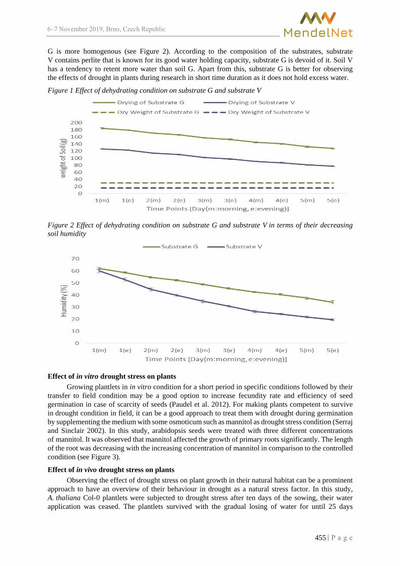
6–7 2019, Brno, Czech Republic
G is more homogenous (see Figure 2). According to the composition of the substrates, substrate V contains perlite that is known for its good water holding capacity, substrate G is devoid of it. Soil V has a tendency to retent more water than soil G. Apart from this, substrate G is better for observing the effects of drought in plants during research in short time duration as it does not hold excess water.
Figure 1 Effect of dehydrating condition on substrate G and substrate V
Figure 2 Effect of dehydrating condition on substrate G and substrate V in terms of their decreasing soil humidity
Effect of in vitro drought stress on plants
Growing plantlets in in vitro condition for a short period in specific conditions followed by their transfer to field condition may be a good option to increase fecundity rate and efficiency of seed germination in case of scarcity of seeds (Paudel et al. 2012). For making plants competent to survive in drought condition in field, it can be a good approach to treat them with drought during germination by supplementing the medium with some osmoticum such as mannitol as drought stress condition (Serraj and Sinclair 2002). In this study, arabidopsis seeds were treated with three different concentrations of mannitol. It was observed that mannitol affected the growth of primary roots significantly. The length of the root was decreasing with the increasing concentration of mannitol in comparison to the controlled condition (see Figure 3).
Effect of in vivo drought stress on plants Observing the effect of drought stress on plant growth in their natural habitat can be a prominent
approach to have an overview of their behaviour in drought as a natural stress factor. In this study, A. thaliana Col-0 plantlets were subjected to drought stress after ten days of the sowing, their water application was ceased. The plantlets survived with the gradual losing of water for until 25 days
455

6–7 2019, Brno, Czech Republic
of drought condition as there was a significant increase in the rosette leaf area until 35 days after sowing. After this, the wilting of the plants started and the plants almost died completely after approximately two months of their sowing. Hence, it can be said that nearly 43 days of drought treatment lead to the complete death of the Arabidopsis plant. Half of the plants were re-watered after 32 days of their drought treatment to, it was observed that all of them survived. (see Figure 4).
Figure 3 Effect of different concentration of mannitol on root length of A. thaliana in in vitro condition
Figure 4 Effect of drought condition on rosette leaf area of A. thaliana in soil condition and its recovery
CONCLUSION Drought is one of those major abiotic stresses, causing drastic loss to the agricultural era. It not
only affects the fertility of the soil but also retards the plant development. The response of abiotic stress conditions on plant is also being affected according to the properties of soil in which they are being grown. Different soil substrates have their different nutrient composition as well as water holding capacity. In this study, it was observed that Potgrond H can be chosen for observing the effect drought stress on plants in the research field as it has less water holding capacity. As stated from the results of the plants grown in in vitro in drought stress created with osmoticum, this technique can be used to select the plants that are better in tolerating the drought effect on planting them in field conditions. In the next experiment, it was observed that drought stress is affecting plant growth drastically in natural habitat.
456

6–7 2019, Brno, Czech Republic
ACKNOWLEDGEMENTS The research was financially supported by the internal grant of Mendel University in Brno AF-IGA2019-IP067.
REFERENCES da Silva, E.C. et al. 2013. Drought and Its Consequences to Plants From Individual to Ecosystem. In Responses of Organisms to Water Stress. IntechOpen. Johnová, P. et al. 2016. Plant Responses to Ambient Temperature Fluctuations and Water-Limiting Conditions: A Proteome-Wide Perspective. Biochimica et Biophysica Acta (BBA)-Proteins and Proteomics, 1864(8): 916–931. Paudel, M. et al. 2012. In Vitro Seed Germination and Seedling Development of Esmeralda clarkei Rchb. f. (Orchidaceae). Plant Tissue Culture and Biotechnology, 22(2): 107–111. Pavlů, J. et al. 2018. Cytokinin at the Crossroads of Abiotic Stress Signalling Pathways. International Journal of Molecular Sciences, 19(8): 2450. Serraj, R., Sinclair, T.R. 2002. Osmolyte Accumulation: Can It Really Help Increase Crop Yield under Drought Conditions? Plant, Cell & Environment, 25(2): 333–341. Xue, R. et al. 2017. Soil Water Content During and After Plant Growth Influence Nutrient Availability and Microbial Biomass. Journal of Soil Science and Plant Nutrition, 17(3): 702–715.
457

ANIMAL BIOLOGY

6–7 2019, Brno, Czech Republic
Determining spatial distribution of interleukin-1β as an infection marker in pulmonary porcine tissues
Rea Jarosova1, Tomas Do2, Barbora Tesarova2, Veronika Smidova2,4, Roman Guran2,4, Petra Ondrackova5, Martin Faldyna5, Zbysek Sladek1, Ondrej Zitka2,3,4
1Department of Morphology, Physiology and Animal Genetics
2Department of Chemistry and Biochemistry 3CEITEC – Central European Institute of Technology
Mendel University in Brno Zemedelska 1, 613 00 Brno
4Central European Institute of Technology Brno University of Technology Purkynova 123, 612 00 Brno 5Department of Immunology Veterinary Research Institute Hudcova 296/70, 621 00 Brno
CZECH REPUBLIC
Abstract: Interleukin-1β (IL-1β) belongs among proinflammatory cytokines that are produced by activated macrophages as an immune response of the organism. Therefore, IL-1β could serve as a possible biomarker of a bacterial infection caused by Actinobacillus pleuropneumonia. In this study, we applied matrix assisted laser desorption/ionization mass spectrometry imaging (MALDI MSI) together with immunohistochemical analyses (IHC) using primary antibody anti-IL-1β for IL-1β detection in cryo-sectioned pulmonary tissues. Using MALDI MSI, we detected and spatially visualized the tryptic fragment of IL-1β. This IL-1β tryptic fragment was more frequently detected in infected pulmonary tissues compared to healthy pulmonary tissue except one necrotic lung tissue where was not revealed the statistically significant difference. IHC confirmed the occurrence of IL-1β in necrotic pulmonary tissues. This knowledge could be useful for further clinical studying as a targeted therapy.
Key Words: immunohistochemistry, mass spectrometry imaging, infection, cytokine, interleukin, pig model, IL-1β
INTRODUCTION Among the common pulmonary porcine diseases belongs the porcine pleuropneumonia.
The disease agent of the porcine pleuropneumonia is a gram-negative bacterial pathogen Actinobacillus pleuropneumoniae (APP), originating from the family Pasteurellaceae. This pathogen causes the bacterial infection in pigs worldwide (Zimmerman et al. 2012). The clinical symptoms related with this infectious disease cause economic issues for breeders because affect the pig breeding itself (Park and Nakhyung 2019).
In presence of infection the organism reacts with immune response containing a local production of group of small signaling proteins called cytokines, and of tumor necrosis factor (TNF)-α. Among cytokines belong interleukins (IL)-1β, IL-6, IL-8 (Hsu et al. 2016, Ondrackova et al. 2010). IL-1β has ability to stimulate the expression of other cytokines, participate in a tissue repair and send signal to immune cells such as neutrophils and it is responsible for many local or systemic clinical signs, such as local swelling or increase of body temperature. Due to its abilities, IL-1β serve as a regulator of inflammatory responses on local or systematic level. The immune cells, such as monocytes, T lymphocytes and natural killer cells, belong among producer of IL-1β (Martin et al. 2019).
In our previous study we successfully confirmed that our optimized MALDI MSI method can serve as a tool for the determination of location of a several peaks representing biomarkers of immune cells in porcine cryo-sectioned pulmonary and lymphoid tissues (Do et al. 2018).
459
6–7 2019, Brno, Czech Republic
In the present study, we have focused on the detection and visualization of the location of IL-1β in the pulmonary porcine tissues and comparing the MALDI MSI method and immunohistochemistry (IHC) using antibodies for IL-1β.
MATERIAL AND METHODS
Materials All chemicals (HPLC grade), including 2,5-dihydroxybenzoic acid (DHB) used for MALDI MSI,
were purchased from Sigma-Aldrich (MO, USA) if not otherwise stated. Conductive indium-tin oxide (ITO) one-side coated glass slides and peptide/protein calibration standards were purchased from Bruker Daltonik GmbH (Bremen, Germany).
Collection of samples Pieces of pulmonary tissues were taken from infected pigs by APP that were bred at accredited
experimental stables of Veterinary Research Institute in Brno. The experiment was performed in compliance with the Act No. 246/1992 Coll. of the Czech National Council on the protection of animals against cruelty, and with the agreement of the Branch Commission for Animal Welfare of the Ministry of Agriculture of the Czech Republic (approval no. 31674/2018-MZE-17214).
The infection of pigs with the infectious dose of 2 × 10⁹ APP (field-origin strain, biotype 1, serotype 9, KL2-2000) was performed by administration of the infectious bacterium to the second third of each nasal cavity intranasally during inhalation as described previously (Ondrackova et al. 2013). After euthanasia of the animals, samples of affected pulmonary tissue (necrotic area) were taken for subsequent laboratory analyses.
For preservation open alveolar structure, the necrotic pulmonary samples were filled with mixture of cryoprotective embedding medium Tissue Tek (O.C.T. Compound, Sakura-Finetek, Japan) (OCT) with phosphate buffered saline (Bio Whittaker, Lonza) (PBS) in ratio 1:1, embedded in OCT and frozen by supercooled n-heptane placed on dry ice.
Cryo-sectioned samples of the pulmonary tissue were obtained according to the following protocol Preparing a cryostat section for MALDI imaging from FlexImaging 3.0 User Manual (Bruker Daltonik GmbH, Bremen, Germany). The frozen samples of lung were cut to a thickness of 10 μm by the cryostat (Leica Microsystems, CM 1900, GmbH, Wetzlar, Germany) at temperature -20 °C. Cryosections for MALDI MSI analysis were mounted onto ITO glass slides. Cryosections for Immunohistochemistry were placed onto glass slides and fixed in pre-cooled acetone for 5 minutes. All slides were stored at -80 °C.
Immunohistochemistry The endogenous peroxidase was blocked with Dual Endogenous Enzyme-Blocking Reagent
(DAKO, Glostrup, Denmark) for 10 min. After washing procedure of the slides, the Protein Block (DAKO, Glostrup, Denmark) was applied for 5 min. Then, primary antibody Rabbit anti-Porcine IL-1beta polyclonal antibody (Antibodies-online, Aachen, Germany) was added. The incubation was carried out at 37 °C for 60 min in the humid chamber. Prior the following incubation with the EnVision + system-HRP anti-Rabbit (DAKO, Glostrup, Denmark) at 37 °C for 30 min in the humid chamber, the slides were washed. In the next step, the slides were washed again and stained with DAB+ (Liquid, DAKO, Glostrup, Denmark) for approximately 30 sec. In the end, the slides were last washed with distilled water, lightly counterstained with Mayer hematoxylin and mounted in glycerol-gelatin.
The histological slides were evaluated in magnification 40 × and 200 × by using the light microscope (Olympus BH-2, Japan) and images were taken by camera (Canon EOS 1100D, Japan) using software (CellSens Standard, Netherlands).
Processing and trypsinization Pulmonary Tissues prior to MALDI MSI analysis The ITO glass slides were warmed by hand at room temperature to thaw-mount the cryosections
and desiccated under vacuum for 15 min at a Vacufuge Concentrator (Eppendorf, Czech Republic). Then, the slides were washed in a glass Coplin jar with 70% ethanol for 2 min twice and 100% ethanol for 2 min once. In the next steps prior the extraction of peptides, samples were desiccated under vacuum for 15 min, after that three guide marks using a white pencil corrector were marked for determining
460

6–7 2019, Brno, Czech Republic
positions of cryosections in FlexImaging 3.0 software (Bruker Daltonik GmbH, Bremen, Germany). Afterwards, images of the ITO glass slides at a resolution of 3200 DPI were taken by an Epson Perfection V500 Office scanner (Epson Europe B.V., Netherlands).
For extraction of peptides, on-tissue trypsinization was applied. Trypsin solution (0.075 μg/μl) was prepared by reconstituting trypsin powder (20 µg) with 40 μl of 50 mM acetic acid and adding 200 μl of 100 mM ammonium bicarbonate and 60 μl of acetonitrile in water. Trypsin solution was sprayed onto ITO glass slides using ImagePrepTM (Bruker Daltonik GmbH, Germany). The digestion was carried out at 37 °C for 18h. After the digest, the samples were dried under vacuum for 15 min.
Then, MALDI matrix was sprayed onto ITO glass slides using ImagePrepTM standard programs. As MALDI matrix was used DHB (Sigma-Aldrich, St. Louis, MO, USA) in concentration of 30 mg/ml in 50% methanol and 1% trifluoroacetic acid (TFA). The samples were ready for MALDI MSI analysis after drying.
MALDI MSI analysis MSI was performed on a MALDI-TOF mass spectrometer Bruker ultrafleXtreme (Bruker
Daltonik GmbH, Bremen, Germany) using optimized method from our previous study (Do et al. 2018) that was adjusted for measuring peptides. The total sample set containing four cryo-sectioned pulmonary tissues on two ITO glass slides mounted on the MTP Slide Adapter II was inserted into the mass spectrometer. The position of the MTP Slide Adapter II was adjusted in FlexImaging according the scanned images of ITO glass slides containing the three white guide marks. In FlexImaging were set the regions of measurement with 50 µm raster width. An external calibration was performed using a peptide calibration standard in an m/z range of 500–3500 Da. The intensity of each scan over the entire acquired mass range was mapped on the tissue section image to visualize the location of each m/z value detected. SCiLS Lab 2014b software (SCiLS–Bruker Daltonik GmbH, Bremen, Germany) was used for generating these images. The parameters of MALDI MSI method as reflection positive mode, m/z range of 500–3500 Da and the laser power to 85%, were set in FlexControl software (Bruker Daltonik GmbH, Bremen, Germany). A total of 500 spectra were summed for each spot using a random walk raster pattern, with no evaluation criteria.
Spectral processing and statistics The MSI data from FlexImaging were imported into the SCiLS Lab software. In the SCiLS Lab
software the MSI data were processed by using a pipeline segmentation and statistical analysis. The Anderson-Darling normality test revealed that the MSI data was not normally distributed. Therefore, the Kruskal-Wallis test and the Wilcoxon test were applied for statistical hypothesis testing. The statistical significance of differences in the peak intensities of IL-1β among individually pulmonary tissues were tested.
RESULTS AND DISCUSSION The necrotic pulmonary tissues from pigs infected by bacterium Actinobacillus pleuropneumonia
were analysed using MALDI-TOF MSI and IHC. The obtained MSI data were compared with data from the healthy pulmonary tissue (control) taken from the non-infected pig and analysed under the same conditions. This study also include comparison between MSI images and IHC images.
In our previous study (Do et al. 2018), we were able to develop a MALDI-TOF MSI method for visualization of molecular maps of biomarkers (e.g. interleukins) representing the presence of immune cells as lymphocytes, granulocytes and macrophages in APP infected pulmonary tissues. In the present study, we have focused on specific interleukin, namely IL-1β. After on-tissue trypsinization, in control and each necrotic pulmonary tissue was found the peak at m/z 3119.621 ± 0.100 Da that represents the IL-1β tryptic fragment NLYLSCVLKDDKPTLQLESVDPKNYPK. This tryptic fragment was determined in silico from IL-1β protein sequence using SequenceEditor (Bruker Daltonik GmbH, Bremen, Germany). The peak at m/z 3119.621 ± 0.100 Da was selected to export MSI images (Figure 1) and intensity box plots (Figure 2) to compare the differences among the necrotic pulmonary tissues and the healthy pulmonary tissue. An immunohistochemical detection was performed using antibody anti-IL-1β. The regions with higher presence of IL-1β were marked on MSI and IHC images (Figure 1). In the necrotic lung tissue 1,2 and 3 were localized the regions
461

6–7 2019, Brno, Czech Republic
with presence of IL-1β, but only in the necrotic lung tissue 1 and 2 the regions from IHC images correlated with regions from MSI images. The MSI image of necrotic lung tissue 3 does not display any specific regions of presence of IL-1β despite the results from IHC where three visible regions with higher occurrence of IL-1β were detected. In the control lung tissue the presence of IL-1β was not detected by using IHC.
Figure 1 IHC images of IL-1β and MALDI MSI images of selected m/z value 3119.621 Da representing the tryptic fragment of IL-1β in the necrotic pulmonary tissues and the healthy pulmonary tissue (control)
For comparing the differences in intensities of the peak at m/z 3119.621 ± 0.100 Da representing the IL-1β tryptic fragment among individual necrotic pulmonary tissues and the healthy pulmonary tissue the MALDI MSI data were submitted to SCiLS Lab where statistical analyses were performed and intensity box plots were generated (Figure 2). The Kruskal-Wallis test revealed the significant differences (p < 0.001) among pulmonary tissues.
According to the intensity box plots (Figure 2), the median of the intensity of the IL-1β tryptic fragment was the lowest in the control lung tissue. The highest median of intensity was found in the necrotic lung tissue 1. The median of the intensity was decreasing in a row necrotic lung tissue 1 > 3 > 2 > control. In each necrotic lung tissue was found the higher amount of the IL-1β tryptic fragment than in healthy lung tissue.
The statistically significant differences among individual pulmonary tissues were tested using the Wilcoxon test. The Wilcoxon test revealed the peak at m/z 3119.621 ± 0.100 Da representing the IL-1β varied significantly (p < 0.001) between necrotic lung tissues and the control lung tissue except necrotic lung tissue 2 (p ≥ 0.05). The significant differences (p < 0.001) were found among all individual necrotic lung tissues.
Our results demonstrate that the application of APP infection increased the occurrence of the IL-1β tryptic fragment in pulmonary porcine tissues in specific regions. Therefore, IL-1β could be used as the possible infection marker. Nevertheless, the results also revealed some issues that should be solved. In MSI image of necrotic lung tissue 3 the regions with presence of IL-1β did not correlate with results from IHC (Figure 1). The difference in intensities of the peak at m/z 3119.621 ± 0.100 Da representing the IL-1β tryptic fragment between a necrotic lung tissue 2 and the control lung tissue was
462

6–7 2019, Brno, Czech Republic
not statistically significant. To overcome these problems, it will be necessary to analyse and compare more pulmonary samples and focus on other tryptic fragments of IL-1β as well.
Nevertheless, our results shows the first use of MALDI-TOF MSI for the spatial determination of IL-1β in porcine lung tissue – according to the search performed on Web of Science and Google on 13th October 2019, using the words “mass spectrometry imaging AND interleukin AND porcine lung”, no study was found.
Figure 2 Intensity box plots of IL-1beta of the control pulmonary tissue and necrotic pulmonary tissues
CONCLUSION Based on the results from this study we can conclude, the specific interleukin, IL-1β, could serve
as the infection marker and the MALDI MSI and IHC methods are suitable for visualization the spatial distribution of IL-1β in healthy and necrotic pulmonary tissues from pigs.
In conclusion, our results contributed to the basic knowledge on IL-β distribution in necrotic pulmonary tissues and could be used in further clinical studying as a targeted therapy.
ACKNOWLEDGEMENTS The research team has been supported by grant no. AF-IGA-2018-tym005 and by the project CEITEC 2020 (LQ1601) with financial support from the Ministry of Education, Youth and Sports of the Czech Republic under the National Sustainability Programme II and by EFRR “Multidisciplinary research to increase an application potential of nanomaterials in agricultural” (No. CZ.02.1.01/0.0/0.0/ 16_025/0007314).
REFERENCES Do, T. et al. 2018. MALDI-TOF MSI method for determining spatial distribution of infection markers in pulmonary tissues of pigs. In Proceedings of International PhD Students Conference MendelNet 2018 [Online]. Brno, Czech Republic, 7–8 November, Brno: Mendel University in Brno, Faculty of AgriSciences, pp. 495–500. Available at: https://mnet.mendelu.cz/mendelnet2018/mnet_2018_full.pdf. [2019-08-27].
463

6–7 2019, Brno, Czech Republic
Hsu, C.W. et al. 2016. Involvement of NF-κB in regulation of Actinobacillus pleuropneumoniae exotoxin ApxI-induced proinflammatory cytokine production in porcine alveolar macrophages. Veterinary Microbiology, 195: 128–135. Martin, T.J., et al. 2019. Exposures to the environmental contaminants pentachlorophenol and dichloro-diphenyltrichloroethane increase production of the proinflammatory cytokine, interleukin‐1β, in human immune cells. Journal of Applied Toxicology, 39(8): 1132–1142. Ondrackova, P. et al. 2010. Porcine mononuclear phagocyte subpopulations in the lung, blood and bone marrow: dynamics during inflammation induced by Actinobacillus pleuropneumoniae. Veterinary Research, 41(5): 64. Ondrackova, P. et al. 2013. Distribution of porcine monocytes in different organs during experimental Actinobacillus pleuropneumoniae infection and the role of chemokines. Veterinary Research, 44(1): 98. Park, B.S., Nakhyung, L. 2019. A bivalent fusion vaccine composed of recombinant Apx proteins shows strong protection against Actinobacillus pleuroneumoniae serovar 1 and 2 in a mouse model. Pathogens and Disease, 77(2): ftz020. Zimmerman, J.J. et al. 2002. Diseases of Swine. 10th ed., Ames, Iowa: Wiley-Blackwell.
464

6–7 2019, Brno, Czech Republic
Introduction of a method for detection of pro-inflammatory mediators in APP-infected porcine lungs by using immunohistochemistry and immunofluorescence
Rea Jarosova1, Petra Ondrackova2, Zbysek Sladek1
1Department of Animal Morphology, Physiology and Genetics 2Department of Immunology Veterinary Research Institute Hudcova 296/70, 621 00 Brno
CZECH REPUBLIC
Abstract: To better understanding the pathogenesis of Actinobacillus pleuropneumoniae (APP) infection in pigs, expression of cytokines and chemokines at the protein level was detected by immune-histochemical method (IHC) and method of immunofluorescence (IF) in different parts of the lungs of infected pigs. Production of pro-inflammatory mediators in the lungs is an important feature of APP infection. In this work we focused on pro-inflammatory cytokines IL-1beta, IL-6, IL-8 and TNF-alpha and chemokines CCL2, CCL4 and CXCL14. Four pigs were inoculated intranasally with APP infection, pigs were sacrificed according to the development of clinical signs of infection. Significant increase in cytokine expression of IL-8, less IL-1beta was detected in frozen-sections of necrotic areas (NA) of infected lungs, however expression of IL-6 and TNF-alpha in NA of the lungs was not detected. In the areas bordering on necrotic areas – marginal zone (MZ) and visually unaffected areas (UA) the pro-inflammatory cytokine levels were not significantly increased. Very low expression levels of CCL4 and CXCL14 were detected in the NA, no expression of chemokines in MZ and UA was detected.
Key words: pulmonary tissue, porcine pneumonia, cytokines, chemokines, immunohistochemistry
INTRODUCTION Actinobacillus pleuropneumoniae (APP) is a gram-negative bacterium that causes swine
respiratory disease – porcine pneumonia. In recent years this disease has been the subject of intensive research because it causes great breeding losses (Zimmerman et al. 2002). Histological changes during APP infection are characterized by the presence of fibrino-hemorrhagic necrotizing bronchopneumonia (Chiers et al. 2010).
Various cytokines appear to play an important role in the pathological processes and development of lesions during APP infection. Inflammatory cytokines mobilize the immune system and increase the efficiency of an immune response (Lorenzo et al. 2006). The response of the organism to infection consists mainly in local production of pro-inflammatory cytokines - interleukin (IL) -1beta, IL-6, IL-8 or tumour necrosis factor-α (TNF-α) in porcine alveolar macrophages (PAMs) as response to bacterial lipopolysaccharide (LPS) (Chen et al. 2011, Hsu et al. 2016). IL-1β and TNF-α are classical proinflammatory cytokines which stimulate nearly all local and systemic inflammatory responses (Van Reeth et al. 2002). IL-1β is important cytokine in the development of the disease, participating in cell activation and inducing the production of other cytokines at the first stages of the disease (Dinarello 1992). TNF-α acts as an inducer of IL-8, which is a chemoattractant for neutrophil and basophil granulocytes and T-cells. IL-8 is produced by several cell types including neutrophils, monocytes and macrophages in response to inflammatory stimulation. Neutrophils are the predominant cell type expressing IL-8 in inflamed porcine tissue (Laursen et al. 2014), where infiltrate place of inflammation in the first wave of cell migration. They are able to eliminate bacteria through phagocytosis mechanisms and also contribute to destruction of the affected tissue. IL-1beta is principally expressed by macrophages and plays an important immunomodulatory role in the porcine immune response (Nechvatalova et al. 2005). IL-6 appears to be directly involved in the responses that occur
465

6–7 2019, Brno, Czech Republic
after infection and cellular injury, and it may prove to be important as IL-1 and TNF-α in regulating the acute phase response. IL-6 is produced by fibroblasts, activated T cells, activated monocytes or macrophages and endothelial cells. IL-6 has an important role function in the induction of the acute-phase response and acute-phase proteins, which may serve as a predictor of stress and disease (Baarsch et al. 1995).
The chemokine CCL2 is also referred to as monocyte chemoattractant protein 1 (MCP1) recruits monocytes, T cells, and dendritic cells to the sites of inflammation. CCL4, also known as macrophage inflammatory protein-1β (MIP-1β) is produced by neutrophils, monocytes, B cells, T cells, fibroblasts, endothelial cells, and epithelial cells. CCL4 may exhibit chemoattractive ability towards different cell types, including macrophages, natural killer cells, monocytes, immature dendritic cells. CXCL14 mainly contributes to the regulation of immune cell migration, also executes antimicrobial immunity (Jing et al. 2016).
The purpose of the study was identifying a presence of pro-inflammatory mediators in different part of infected porcine lungs by methods immunohistochemistry and immunofluorescence.
MATERIAL AND METHODS
Experimental material Four six-week-old healthy pigs (Landrace x Large White) from the herd without anomaly of APP
infection or vaccination were used in this experiment. The pigs were kept in the accredited barrier-type animal facilities of the Veterinary Research Institute (VRI). Authorization to use experimental animals, file no. 58809/2014-MZE-17214, valid until 21.8.2019. This accreditation also allows to experimentally infect animals under controlled conditions. The experiment was performed in compliance with the Act No. 246/1992 Coll. of the Czech National Council on the protection of animals against cruelty, and with the agreement of the Branch Commission for Animal Welfare of the Ministry of Agriculture of the Czech Republic (approval no. 31674/2018-MZE-17214).
Before performing the experimental infection, the pigs were allowed to acclimatize in the animal facilities for one week. The porcine experimental material was collected by trained staff from authorized and registered slaughterhouse at VRI.
Experimental infection The infection of A. pleuropneumoniae (biotype 1, serotype 9, strain KL2-2000) was performed
intranasally during inhalation, the infectious dose of 2,4 × 10⁸ CFU/mL was administered to the second third of each nasal cavity. Health status was monitored during the entire experiment and clinical signs of respiratory disorders were recorded (increased dyspnoea, coughing, anorexia, depression and lethargy).
Euthanasia was performed by exsanguination after combined anesthesia with a TKX (Telazol-Ketamin-Xylazin) mixture containing 12.5 mg/ml tiletamine and 12.5 mg/ml zolazepam (Telazol, Virbac, Carros, France), 12.5 mg/ml ketamine (Vetoquinol, Lure, France) and 12.5 mg/ml xylazine (Bioveta, Ivanovice na Hane, Czech Republic), administered intramuscularly in a final volume of 0.2 ml/kg body weight. Tissue sampling and processing
Immediately after euthanasia, samples of pulmonary tissue were acquired. Lung tissue was sampled from necrotic areas (NA), from visually unaffected areas (UA) and from areas bordering on necrotic areas – marginal zone (MZ). Samples of lungs were filled with mixture of cryoprotective embedding medium Tissue Tek (O.C.T. Compound, Sakura-Finetek, Japan) (OCT) with phosphate buffered saline (Bio Whittaker, Lonza) (PBS) in ratio 1 : 1 for preserved open alveolar structure, embedded in OCT and frozen by supercooled n-heptane placed on dry ice.
The tissue samples were cut to a thickness of 5–10 μm on the cryostat (Leica Microsystems, CM 1900, GmbH, Wetzlar, Germany) at temperature -20 °C. The cuts of tissues were placed on slides and fixed in pre-cooled acetone for 5 minutes and stored at -80 °C.
466

6–7 2019, Brno, Czech Republic
Immunohistochemistry The endogenous peroxidase was blocked with Dual Endogenous Enzyme-Blocking Reagent
(DAKO, Glostrup, Denmark) for 10 min. Slides were washed and the Protein Block (DAKO, Glostrup, Denmark) was applied for 5 min. Then, primary antibodies of cytokines anti-IL-8 (Bio-Rad, Hercules, USA), anti-IL-1beta (Antibodies-online, Aachen, Germany), anti-TNF-alpha (LifeSpan BioSciences, Seattle, USA), anti-IL-6 (GeneTex, Irvine, USA) and chemokines anti-CCL2 (OriGene Technologies, Rockville, USA), anti-CCL4 (LifeSpan BioSciences, Seattle, USA), anti-CXCL14 (Antibodies-online, Aachen, Germany) were applied and the slides were incubated for 60 min at 37 °C in a humid chamber. Then, the slides were washed and EnVision reagent HRP anti-Mouse or anti-Rabbit (DAKO, Glostrup, Denmark) was added. The slides were incubated for 30 min at 37 °C in a humid chamber. The slides were washed and stained with DAB + Liquid (DAKO, Glostrup, Denmark) for approx. 30 sec. Then, the slides were washed with distilled water, lightly counterstained with Mayer hematoxylin and mounted in glycerol-gelatin.
The histological slides were evaluated in magnification 40× and 200× by using the light microscope (Olympus BH-2, Japan) and images were taken by camera (Canon EOS 1100D, Japan) using software (CellSens Standard, Netherlands).
Immunofluorescence On the slides was applied Protein Block (DAKO, Glostrup, Denmark) for 30 min at 37 °C
in a humid chambre. Then, primary antibodies of cytokines anti-IL-8 (Bio-Rad, Hercules, USA), anti-IL-1beta (Antibodies-online, Aachen, Germany), anti-TNF-alpha (LifeSpan BioSciences, Seattle, USA), IL-6 (GeneTex, Irvine, USA) and chemokines anti-CCL2 (OriGene Technologies, Rockville, USA), anti-CCL4 (LifeSpan BioSciences, Seattle, USA), anti-CXCL14 (Antibodies-online, Aachen, Germany) were applied and the slides were incubated for 60 min at 37 °C in a humid chamber. The slides were washed and secondary antibodies Goat anti-mouse IgG1 Alexa Fluor 488 (Thermo Fisher Scientific, Massachusetts, USA) or Goat anti-rabbit IgG Alexa Fluor 488 (ThermoFisher Scientific, Massachusetts, USA) were added and incubated for 60 min at 37 °C in a humid chambre. Then, the slides were washed and Vectashield mounting medium with DAPI (Vector Laboratories, Burlingame, USA) was applied.
The histological slides were evaluated in magnification 40× and 200× by using the fluorescent microscope (Olympus IX51, Japan) with UV-lamp (Olympus u-RFL-T, Japan) and images were taken by camera (Canon EOS 1100D, Japan) using software (CellSens Standard, Netherlands).
RESULTS AND DISCUSSION An A. pleuropneumoniae infection model in swine was established to study expression
of inflammatory cytokines during acute respiratory disease. Immunohistochemical methods to detect cytokines in snap-frozen tissues from pigs is a valuable tool for studying the pathogenesis of swine diseases (Lorenzo et al. 2006). Detection of pro-inflammatory mediators by immunohistochemistry and immunofluorescence can help clarify the processes taking place in inflamed pulmonary tissues and contributing to an understanding of the pathogenesis of APP infection. We compared the expression of inflammatory proteins in different parts of infected lungs. Obtained results show that inflammatory cytokines and chemokines were expressed only in necrotic areas and pulmonary lesions. According to the authors (Baarsch et al. 1995) IL-1 and IL-8 were specifically detected in lung tissue at the sites of lesion. We achieved the same results and IL-1beta and IL-8 expression was detected in NA (Figure 1), very low or no expression of these cytokines was in MZ (Figure 2).
The highest expression was recorded for the cytokine IL-8. The high intensity of IL-8 expression in NA is caused by the production of this cytokine not only by neutrophils but also by other cell populations such as endothelial cells. Similar results indicate (Laursen et al. 2014) significant expression of IL-8 in inflamed porcine tissue. Using IL-8 immunohistochemistry were discovered that neutrophils were the predominant IL-8 positive cell population while epithelial cell types and endothelium of postcapillary venules could be positive when situated in close vicinity of an inflammatory lesion. Pro-inflammatory cytokines may be involved in lesion development during acute pleuropneumonia. Similarly to authors (Baarsch et al. 1995) inflammatory cytokines may contribute to the development and/or progression of porcine pleuropneumonia.
467

6–7 2019, Brno, Czech Republic
Unlike the authors (Lorenzo et al. 2006) all through the experiment, TNF-α levels significantly increased on infected tissues in relation to controls, our results show no expression of TNF-α in any part of infected lung tissues. In compared to the authors (Baarsch et al. 1995) elevated levels of TNF, IL-1, IL-8 were present in lung tissue from animals inoculated with APP bacteria, especially at the sites of lesion. These areas also contained numerous cells staining positive for TNF, IL-1, IL-8.
Immunoreaction to IL-6 was low in all animals of the trial being only during the first 2 wpi significantly increased in the alveolar septa of infected tissues (Lorenzo et al. 2006). These results contrast with the our findings, immunohistochemical analysis of the IL-6 molecule was negative in all part of infected lung.
Figure 1 Mayer hematoxylin stained frozen section of necrotic area of porcine lung infected by APP. Immunohistochemical analysis of the IL-8 molecule, IL-8 positive cells are stained by brown color.
Figure 2 Mayer hematoxylin stained frozen section of marginal zone of porcine lung infected by APP. Immunohistochemical analysis of the IL-1beta molecule, IL-1beta positive cells are stained by brown color.
Chemokines direct monocyte migration into inflamed tissue during infection, but our results of immunohistochemical analysis and immunofluorescence did not show any significant increase in the expression of CCL2, very low increase expression of CCL4 and CXCL14 chemokines in NA of the lungs. Similar results were obtained in the study (Ondrackova et al. 2013) in NA of the lungs, different chemokines were up-regulated. Probably, expression of chemokines cannot be detected at the protein level and it would be appropriate to measure chemokine levels by more sensitive methods.
In visually unaffected areas of the lungs and marginal zone of lesions we not recorded to any expression of inflammatory cytokines and chemokines. Similarly to authors (Baarsch et al. 1995) lung tissue from uninfected control animals and from regions of APP-inoculated animals which appeared normal histopathologically demonstrated very little or no TNF-α, IL-1, IL-8.
468
6–7 2019, Brno, Czech Republic
CONCLUSION Optimizing detection of the inflammatory mediators in the lungs of pigs infected by pneumonia
will lead to a better understanding the pathological process in the tissue. Identification of inflammatory processes in the lungs of infected animals and understanding the interaction of the immune system with pathogens can help to elucidate the pathogenesis of these diseases and improve the protection of pigs against these diseases.
ACKNOWLEDGEMENTS This research project AF-IGA-2018-tym005 was financially supported by the Internal Grant Agency of Mendel University in Brno.
REFERENCES Baarsch, M.J. et al. 1995. Inflammatory cytokine expression in swine experimentally infected with Actinobacillus pleuropneumoniae. Infection and Immunity, 63(9): 3587–3594. Dinarello, C.A. 1992. Role of interleukin-1 in infectious disease. Immunological Reviews, 127: 119–146. Chen, Z.W. et al. 2011. Mechanisms underlying Actinobacillus pleuropneumoniae exotoxin ApxI induced expression of IL-1beta, IL-8 and TNF-alpha in porcine alveolar macrophages. Veterinary Research, 42: 25. Chiers, K. et al. 2010. Virulence factors of Actinobacillus pleuropneumoniae involved in colonization, persistence and induction of lesions in its porcine host. Veterinary Research, 41(5): 65. Hsu, C.W. et al. 2016. Involvement of NF-κB in regulation of Actinobacillus pleuropneumoniae exotoxin ApxI-induced proinflammatory cytokine production in porcine alveolar macrophages. Veterinary Microbiology, 195: 128–135. Jing, L. et al. 2016. CXCL14 as an emerging immune and inflammatory modulator. Journal of Inflammation, 13: 1. Laursen, H. et al. 2014. Immunohistochemical detection of interleukin-8 in inflamed porcine tissues. Veterinary Immunology and Immunopathology, 159(1–2): 97–102. Lorenzo, H. et al. 2006. Cytokine expression in porcine lungs experimentally infected with Mycoplasma hyopneumoniae. Veterinary Immunology and Immunopathology 109(3–4): 199–207. Nechvatalova, K. et al. 2005. Significance of different types and levels of antigen specific immunity to Actinobacillus pleuropneumoniae infection in piglets. Veterinary Medicine, 50(2): 47–59. Ondrackova, P. et al. 2013. Distribution of porcine monocytes in different organs during experimental Actinobacillus pleuropneumoniae infection and the role of chemokines. Veterinary Research, 44(1): 98. Van Reeth et al. 2002. In vivo studies on cytokine involvement during acute viral respiratory disease of swine: troublesome but rewarding. Veterinary Immunology and Immunopathology, 87(3–4): 161–168. Zimmerman, J.J. et al. 2002. Diseases of Swine. 10th ed., Iowa: Willey-Blackwell.
469

6–7 2019, Brno, Czech Republic
Morphological changes of monocytes during dendritic cells development
Lucie Kratochvilova, Petr Slama
Department of Animal Morphology, Physiology and GeneticsMendel University in Brno Zemedelska 1, 613 00 Brno
CZECH REPUBLIC
Abstract: The aim of this work was the isolation of monocytes from bovine blood with the use of immunomagnetic beads coated with the monoclonal antibody, and magnetic separation and morphology determination of DCs generated from the monocytes. The experiment was performed on a group of healthy cows. Peripheral blood mononuclear cells were isolated from 100 ml of whole blood. Samples were incubated and centrifuged to achieve the desired concentration for the experiment. The isolated monocytes were cultured in the concentration of 1 x 10⁶ cells/mL in standard culture flasks in RPMI 1640 medium at 37 °C in a humidified 5% CO2 atmosphere in the presence of granulocyte-macrophage colony-stimulating factor (GM-CSF) and recombinant bovine interleukin-4 (IL-4). Cells were cultivated for 3 days. Cells transformed into DCs during this time. Morphology of DCs was observed in the light microscope. During 3 days of cultivation, there were found out morphological changes in the cell membrane of the cells. On the cell membrane, there were developed protrusions and during the time of incubation, there were developed typically elongated pseudopodia.
Key Words: monocytes, dendritic cells, light microscopy, immune system, cattle
INTRODUCTION Monocytes have nongranulated cytoplasm and are classified as agranulocytes (Abbas et al. 2017).
Monocytes are 10 to 15 µm in diameter, and they contain lysosomes, phagocytic vacuoles, and cytoskeletal filaments. Monocytes are heterogeneous and consist of different subsets distinguishable by cell surface markers and functions. In cattle, the most numerous monocytes produce abundant inflammatory mediators and are rapidly recruited to sites of infection or tissue injury (Haniffa et al. 2013).
DCs are antigen-presenting cells, which capture microbial antigens that enter from the external environment, transport these antigens to lymphoid organs, and present to naïve T lymphocytes to initiate immune responses. These cells were discovered in 1973 in mice. DCs are present in most tissues and are concentrated in lymphoid organs (Kratochvilova and Slama 2018). DCs behaviour is the focus of many laboratories due to their role as adjuvants for vaccines that prevent microbial infection (for instance mastitis). DCs can be divided into a few functionally distinct subsets. Freshly isolated DCs have poorly developed dendrites and typical morphology (Kratochvilova et al. 2019).
The morphologic organization of the cells and tissues of the immune system has a critical importance for the generation of effective innate and adaptive immune responses (Python et al. 2013). This organization permits the rapid delivery of innate immune cells, including monocytes and neutrophils, to sites of infection and permits a small number of lymphocytes specific for anyone antigen to locate and respond effectively to that antigen regardless of where in the body the antigen is introduced (Reid et al. 2011).
We would like to know how the monocytes are morphologically changed during development in a short time of cultivation. The hypothesis is that we assume that three days is enough for developing visible dendrites in CD14-positive cells.
470

6–7 2019, Brno, Czech Republic
MATERIAL AND METHODS
Isolation of monocytes Histopaque solution was used in this experiment along with the technique of separating cells using
magnetic microbeads (MicroBeads, Miltenyj Biotec, Germany). Blood was collected from vena jugularis externa in clinically healthy heifers. As anticoagulant was used ethylenediaminetetraacetic acid (EDTA). The blood was centrifuged, and the buffy coat was collected together with some of the surrounding erythrocytes and blood plasma. After, the Histopaque solution was used. Histopaque was placed into a test tube and softly layered over with blood, specifically the buffy coat + part of erythrocytes + part of blood plasma mixture. This test tube, with the contents as described, was centrifuged for 1 h (2100 rpm). The layer of mononuclear cells (monocytes and lymphocytes) was then acquired. This suspension of cells was further marked with microbeads (CD14 MicroBeads, human, Miltenyi Biotec, Germany). Antibodies with microbeads were attached to CD14-positive cells. Subsequently, the CD14-positive cells (i.e., monocytes) were acquired using a magnetic separator. The viability of cells was evaluated using trypan blue exclusion. The purity of monocytes was tested by marking the cells with the CD11c surface molecule, followed by analysis in a BriCyte E6 flow cytometer (Mindray, China). The acquired cells were stained using the Pappenheim method and then observed under a light microscope.
Monocyte culture The isolated monocytes were cultured at a concentration of 1 x 10⁶ cells/mL in standard culture
flasks in RPMI 1640 medium (containing glutamine, 10% of foetal calf serum (FCS) and antibiotics) at 37 °C and in a humidified 5% CO2 atmosphere in the presence of GM-CSF and IL-4 at in final concentration of 100 ng/mL. Cells were cultivated for 3 days. During that time, cells transformed into DCs.
DCs cytology After these days, the cultured cells were dislodged by gentle pipetting, washed, centrifuged onto
slides, and air-dried at room temperature. DCs were then stained with Giemsa´s stain and morphology of DCs observed in the light microscope.
RESULTS AND DISCUSSION Bovine blood contains about 1–4% monocytes. We can see the monocyte in Figure 1.
After isolation with the Histopaque solution, a mononuclear cell population with >99% purity was acquired. Using magnetic separation, a cell population with >90% monocytes was acquired. The purity of the monocyte population was verified using flow cytometry by marking cells on CD11c. The viability of cells evaluated by trypan blue exclusion was >99% for all samples.
Figure 1 Monocyte (original magnification was 1000 x, figure scaled and cropped)
471
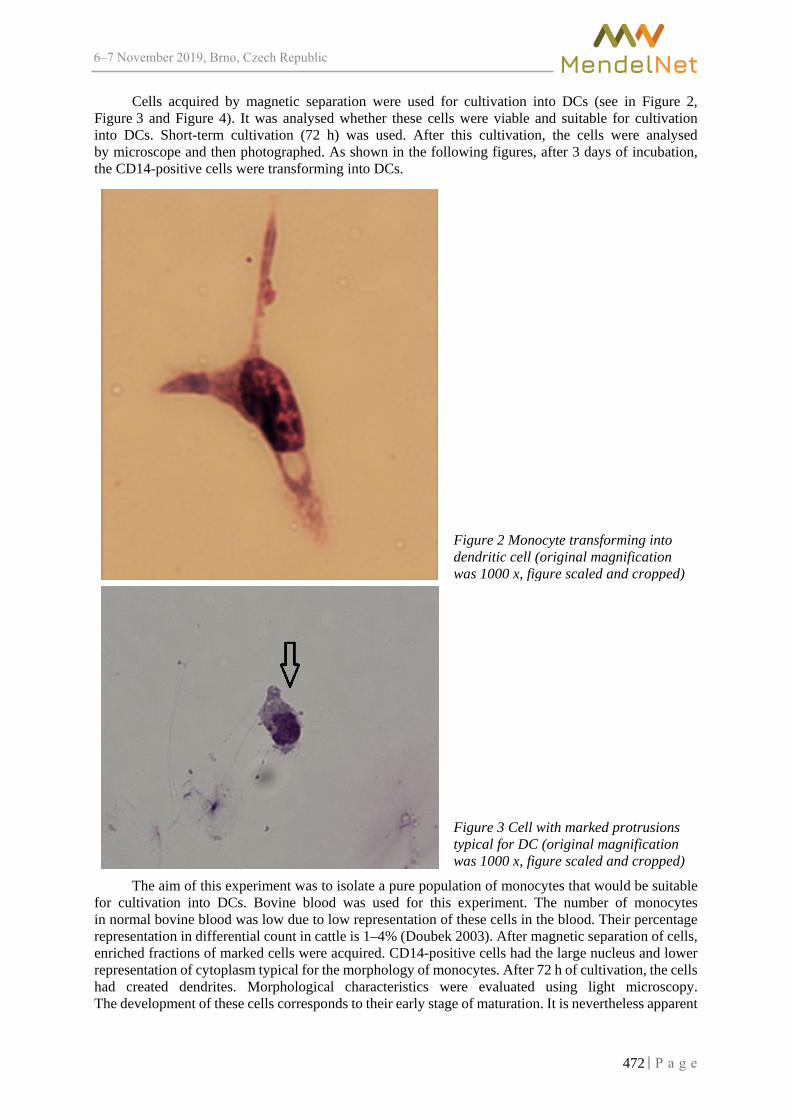
6–7 2019, Brno, Czech Republic
Cells acquired by magnetic separation were used for cultivation into DCs (see in Figure 2, Figure 3 and Figure 4). It was analysed whether these cells were viable and suitable for cultivation into DCs. Short-term cultivation (72 h) was used. After this cultivation, the cells were analysed by microscope and then photographed. As shown in the following figures, after 3 days of incubation, the CD14-positive cells were transforming into DCs.
Figure 2 Monocyte transforming into dendritic cell (original magnification was 1000 x, figure scaled and cropped)
Figure 3 Cell with marked protrusions typical for DC (original magnification was 1000 x, figure scaled and cropped)
The aim of this experiment was to isolate a pure population of monocytes that would be suitable for cultivation into DCs. Bovine blood was used for this experiment. The number of monocytes in normal bovine blood was low due to low representation of these cells in the blood. Their percentage representation in differential count in cattle is 1–4% (Doubek 2003). After magnetic separation of cells, enriched fractions of marked cells were acquired. CD14-positive cells had the large nucleus and lower representation of cytoplasm typical for the morphology of monocytes. After 72 h of cultivation, the cells had created dendrites. Morphological characteristics were evaluated using light microscopy. The development of these cells corresponds to their early stage of maturation. It is nevertheless apparent
472

6–7 2019, Brno, Czech Republic
that each cell develops individually, as the cells in the samples were in different stages of development, ranging from small signs of protrusions to typically elongated protrusions. In our opinion, the method used by Szczotka et al. (2009) is a promising one and could be used also for subsequent long-term cultivation into DCs.
Figure 4 Dendritic cell with developing pseudopodia (original magnification was 1000 x, figure scaled and cropped)
CONCLUSION In this article, we described populations of DCs and monocytes. We followed the same method
as Szczotka et al. (2009) using the Histopaque solution and magnetic separation. Cells acquired by magnetic separation were suitable for cultivation into DCs. Monocytes and dendritic cells have main functions in the immune system. In our next experiments, we would like to focus on the analysis of the possibility of DCs to recognize Streptococcus uberis adhesion molecule (SUAM) and present this information to lymphocytes during mammary gland inflammation caused by Streptococcus uberis. Knowledge of these cells is required to understand the immune systems of farm animals.
ACKNOWLEDGEMENTS The authors wish to express their thanks for financial support to the projects of IGA AF MENDELU No. AF-IGA-2018-tym002.
REFERENCES Abbas, K. et al. 2017. Cellular and Molecular Immunology, 9th ed., Philadelphia: Saunders/Elsevier. Doubek, J. 2003. Veterinární hematologie. Brno: Noviko. Haniffa, M. et al. 2013. Ontogeny and functional specialization of dendritic cells in human and mouse. Advanced Immunology, 120: 1–49. Kratochvilova, L., Slama, P. 2018. Overview of bovine dendritic cells. Acta Universitatis Agriculturae et Silviculturae Mendelianae Brunensis, 66(3): 815–821. Kratochvilova, L. et al. 2019. Isolation of monocytes from bovine blood for purposes of culture of dendritic cells. Journal of Microbiology, Biotechnology and Food Sciences. Accepted paper. Python, S. et al. 2013. Efficient Sensing of Infected Cells in Absence of Virus Particles by Blasmacytoid Dendritic Cells Is Blocked by the Viral Ribonuclease E-rns. PLOS Pathogens, 9(6): 100–134. Reid, E. et al. 2011. Bovine plasmacytoid dendritic cells are the major source of type I interferon in response to foot-and-mouth disease virus in vitro and in vivo. Journal of Virology, 85(9): 4297–4308. Szczotka, M. et. al. 2009. Bovine blood dendritic cells: isolation and morphology. Bulletin of the Veterinary Institute in Pulawy, 53: 687–691.
473

6–7 2019, Brno, Czech Republic
Inhibitory effect of selected botanical compounds on the honey bee fungal pathogen Ascosphaera apis
Petr Mraz1, Andrea Bohata1, Irena Hostickova1, Marek Kopecky2, Martin Zabka3, Marian Hybl4, Vladislav Curn1 1Department of Plant Production 2Department of Agroecosystems
University of South Bohemia in Ceske Budejovice Studentska 1668, 370 05 Ceske Budejovice
3Crop Research institute Drnovska, 507, 161 06 Praha
4Department of Zoology, Fisheries, Hydrobiology and Apidology Mendel University in Brno Zemedelska 1, 613 00 Brno
CZECH REPUBLIC
Abstract: Ascosphaera apis is a heterothallic fungus causing widespread honey bee disease called chalkbrood. In many countries, beekeepers use fungicides to control this pathogen. However, this approach results in residues in bee products as well as in resistance which are serious problems. For these reasons, in European Union countries is not allowed to use nor fungicides, neither antibiotic to control bee diseases. Therefore, there is an increasing need to find environmentally friendly methods to control honey bee pathogens. One of the most promising approaches seems to be using natural botanical compounds with antifungal effects. In this paper, 2 essential oils and 2 main components were tested for A. apis inhibition in in vitro conditions. Local strain of A. apis was cultivated on Sabouraud dextrose agar (SDA) with different concentrations of tested botanical compounds. Cultivation was carried out at 30 °C for 21 days. The greatest inhibitory effect reached thymol (MIC 500 µg/ml). Very promising seems to be also clove bud oil (MIC 2500 µg/ml) and eugenol (MIC 2500 µg/ml). Cedarwood oil did not stop the growth of A. apis even in the highest concentration (MIC >5000 µg/ml). This experiment confirmed that these plant substances are efficient as an antimicrobial agent against chalkbrood disease. Despite problems with unstable botanical compounds composition in the same plant species, application of essential oils and their main components could be gentle and safe way how to control a lot of bee diseases in the future.
Key Words: Essential oils, chalkbrood, cultivation media, cultivation, antifungal effect
INTRODUCTION More than three quarters of agricultural crops are dependent on pollination and approximately
one third of food production is influenced by pollinators (Klein et al. 2007). Therefore, reduction in abundance of insects and their extinction draw the attention to many scientists because it poses a significant threat. The same, if not worse situation affects also wild plants (Biesmeier et al. 2006). One of the most important pollinators is honey bee (Apis mellifera) which is currently affected by many diseases more frequently than before. It is the result of exposure of bees to pesticides applied to the fields and antibiotics to bee hives (Sandrock et al. 2014), decline of biodiversity and pollen mono diet, transfer of bee colonies for long distances, inadequate beekeeping practice and also anthropogenic modifications in habitats and climate changes (Biesmeier et al. 2006). One of the very common and worldwide spread diseases is chalkbrood. Its incidence is on the rise and may cause significant economic losses, especially in cold and damp weather conditions (Aronstein and Murray 2010). There are some reports from East Asia where beekeepers deal with this disease very often (Chantawannakul et al. 2005).
474

6–7 2019, Brno, Czech Republic
Chalkbrood is caused by heterothallic fungus Ascosphaera apis (Maassen ex Claussen) (Spiltoir 1955) which is closely specialized to honey bees and it can infect only bee larvae. Spores of this fungus can be consumed with food by honey bee larvae. In the suitable conditions in a gut, spores are activated by higher concentration of carbon dioxide and the mycelium starts grow. At the beginning of infection, the larvae cease food consumption and get swollen. During the time, mycelium grows throughout the larvae and causes its dead. After some time, the larvae are going to shrink and solidify and also form so-called chalkbrood mummy. The color of cadavers can be white, black/grey or mottled depend on the presence of ascospores being created on the surface. These ascospores, which can be produced only sexually, are placed into resistant cyst and stay viable for many years. The mummies resemble chalk, from that the name of the disease originated (Aronstein and Murray 2010).
In many countries, beekeepers still use fungicides to treat chalkbrood disease. It can, however, leave residues in bee products and also causes problem with pathogen resistance (Chaimanee et al. 2017). Therefore, in European Union countries, are these substances banned and there is no registered therapeutic agent against chalkbrood. A lot of chemotherapeutic compounds have been investigated as potential substances to treat chalkbrood. Although many of them have antifungal effect, they are not efficient to spores and, in addition, they have negative effect to bee vitality and longevity (Aronstein and Murray 2010). Moreover, there is also a worldwide increase prevalence of other fungal pathogen species on fields and warehouses which are associated with higher fungicide consumption (Zabka et al. 2014). Farmers and even consumers are exposed to long-term, low-dose unnatural substances due to fungicides residues in food supply and groundwater as well as many non-target organisms, especially in developing countries. These negative substances are linked to immune suppression, hormone disruption and cancer. Thus, there is an increasing effort to use alternative, more environmentally friendly methods. Recently, one of the most promising way how to control chalkbrood seems to be using of plant essential oils (EOs) or their main components (MCs) with fungicide effect (Gabriel et al. 2018). Their next substantial advantage is that they are allowed in human food chain included honey production because of GRAS status (Chantawannakul et al. 2005, Li et al. 2019).
A various plants had been used in medicine long time before microbes were discovered. Our ancestors empirically observed the healing potential of some plant species which is currently known as the antimicrobial effect. This effect is mainly caused by essential oils which are volatile substances of plants containing a various organic bioactive compounds. They are known for its very sharp aroma and taste and have a protective function in plants (Kuzyšinová et al. 2016). Even now, these plant substances are abundantly used in preventing and treating various digestive and respiratory diseases in the form of tea, spices and traditional remedies. They are still efficient because there is no resistance against these compounds. In recent time, there is an increasing effort to utilize these plant compounds because they are easily degradable and environmentally friendly and have minimum or no side effects (Li et al. 2019). In this paper, we demonstrated antifungal effect of some botanical compounds against the local strain of A. apis, which have a potential to be used as agents against honey bee pathogens.
MATERIAL AND METHODS
Fungal isolates and essential oils Ascosphaera apis isolates were obtained from mummified bee brood collected on apiary in South
Bohemia. The opposite mating types were separated on the PDA (Potato dextrose agar, Himedia) with addition of chloramphenicol by sub culturing until pure culture were established and stored as the maternal cultures on PDA at 30 °C. For antifungal effect, the male mating type was chosen due to its faster growth. For fungicide activity assay, two EOs (clove bud oil, cedarwood oil) and two MCs (thymol, eugenol) were chosen based on their antimicrobial activity. All of these substances were obtained from Sigma Aldrich and stored in dry, dark conditions at 22 °C. The DMSO (dimethyl sulfoxide, Himedia) served as a solvent. Four different concentrations of each tested substances were prepared by diluting 25, 50, 250 and 500 µl of EOs or MCs in 500 µl of DMSO for 100 ml media.
475

6–7 2019, Brno, Czech Republic
Testing of EOs and MCs For cultivation tests, SDA (Sabouraud dextrose agar, Himedia) medium was used
due to its suitability for A. apis growth and also for the medium uniformity. A volumes of 100 ml SDA media were autoclaved at 121 °C for 30 min in Erlenmeyer flask for each variant. Diluted substances of EO/MC were added to the autoclaved SDA cooled at 45 °C aseptically to ensure final concentrations (250, 500, 2500, 5000 µg/ml) and dispersed by circular movements. An amount of 20 ml were poured into Petri dishes (90 x 15 mm). After media solidification, the 8 mm cork bores of mycelium were cut from the edge of 7 days old culture and placed in the middle of each Petri dish. Five repetitions were prepared for each concentration of tested substances. A. apis was cultivated under the dark condition at 30 °C for 21 days. The growth of mycelium was measured by two perpendicular diameters daily for the first 10 days, then the 15th day and the 21st day. The inhibitions effect was calculated. Data from the 10th day of cultivation were statistically analysed with ANOVA (STATISTICA 12, StatSoft Inc.) and the mean values were compared using the Tukey HSD test (p < 0.05).
RESULTS AND DISCUSSION An antifungal effect of four plant substances was tested against A. apis. This fungus grew very
well on SDA medium as well as on the SDA controls including the DMSO. All the tested substances showed an antifungal effect (Figure 1). In each case, the higher concentration of tested botanical compounds caused higher growth inhibition. Thymol (F(5,54) = 32315.7, p < 0.05) has been detected as the most effective substances with the MIC < 500 µg/ml after 10 days of cultivation. However, during the first 7 days, there was no A. apis growth even at the lowest concentration (250 µg/ml). Calderone et al. (1994) determined its MIC as 1000 µg/ml after 7 days of cultivation. This variability may indicate different sensitivity of individual A. apis strains or different substances composition. Thymol is considered as a broad range inhibitor because it can suppress growth many fungal species as Alternaria alternate, Stachybotrys chartarum, Cladosporium cladosporioides and especially significant for beekeeping Aspergilus niger causing Stonebrood disease (Zabka et al. 2014) as well as Paenibacillus. larvae causing American foulbrood (Fuselli et al. 2006). This substance was tested against many different bacteria and yeast with very promising results (Wiese et al. 2018). Thyme, with its main component thymol, had very low MIC (300 µg/ml) also against the human pathogen as Staphylococcus aureus, Escherichia coli and Candida albicans (Hammer et al. 1999).
Great antifungal effect had also clove bud oil (F(5,54) = 47413.8, p < 0.05) with MIC < 2500 µg/ml measured after 10 days of cultivation. According to Chaimanee et al. (2017), clove bud EO had MIC very low (32 µg/ml) after 3 days of cultivation and as an efficient oil is also considered by Ansari et al. (2016) with MIC 400 µg/ml and by Calderone et al. (1994) with MIC 1000 µg/ml, both measured after 7 days of cultivation. In our study, the lowest concentration was relatively harmless and mycelium started to grow even on the second day of cultivation. However, the clove bud concentration of 500 µg/ml inhibited A. apis growth for the first 7 days (Figure 1). Clove bud oil is efficient also against Staphylococcus aureus, Escherichia coli and Candida albicans (MIC 1200 µg/ml) representing a group of common human pathogens (Hammer et al. 1999). Especially clove bud oil main component, eugenol, is known for its significant antifungal effect. In this study, eugenol inhibited 100% A. apis growth at 2500 µg/ml after 10 days of cultivation (F(5,54) = 11342, p < 0.05). Its particular efficiency was proved also by Larrán et al. (2001) who tested eugenol as a part of basil oil against A. apis and also by Gende et al. (2008) who tested eugenol as a main part of Cinnamomum zeylanicum against P. larvae.
Despite cedarwood essential oil (F(5,54) = 3876.25, p < 0.05) showed antimicrobial activity (Figure 1), it did not completely inhibit A. apis growth in any tested concentrations (MIC >5000 µg/ml). For this reason, its use can be suitable only assuming its synergic effect with other medical substances to treat chalkbrood disease. In cedarwood oil were recorded considerable diversity in its compositions, therefore the efficacy can differ. The same effect occurs in many plant oils (Paoli et al. 2011).
476

6–7 2019, Brno, Czech Republic
Figure 1 Inhibition effect of botanical compounds on the A. apis pathogen during 21 days, differences among the concentrations on the 10th day of fungus cultivation show small letters (HSD Tukey test)
0,0010,0020,0030,0040,0050,0060,0070,0080,0090,00
1 2 3 4 5 6 7 8 9 10 15 21
Rad
ial G
row
th (m
m)
Days Post-inoculation
Thymol
SDA DMSOTYM 250 TYM 500TYM 2500 TYM 5000
a a
bc c c
8,0018,0028,0038,0048,0058,0068,0078,0088,00
SDA DMSO TYM250
TYM500
TYM2500
TYM5000R
adia
l Gro
wth
on
the
10th
culti
vatio
n da
y (m
m)
Concentration (µg/ml)
Thymol
0,0010,0020,0030,0040,0050,0060,0070,0080,0090,00
1 2 3 4 5 6 7 8 9 10 15 21
Rad
ial G
row
th (m
m)
Days Post-inoculation
Clove Bud
SDA DMSOCB 250 CB 500CB 2500 CB 5000
a a a
b
c c8,00
18,00
28,00
38,00
48,00
58,00
68,00
78,00
88,00
SDA DMSO CB 250CB 500 CB2500
CB5000
Rad
ial G
row
th o
n th
e 10
thcu
ltiva
tion
day
(mm
)
Concentration (µg/ml)
Clove Bud
0,0010,0020,0030,0040,0050,0060,0070,0080,0090,00
1 2 3 4 5 6 7 8 9 10 15 21
Rad
ial G
row
th (m
m)
Days Post-inoculation
Eugenol
SDA DMSOEUG 250 EUG 500EUG 2500 EUG 5000
a a a
b
c c8,00
18,00
28,00
38,00
48,00
58,00
68,00
78,00
88,00
SDA DMSO EUG250
EUG500
EUG2500
EUG5000
Rad
ial G
row
th o
n th
e 10
thcu
ltiva
tion
day
(mm
)
Concentration (µg/ml)
Eugenol
477

6–7 2019, Brno, Czech Republic
CONCLUSIONS Plants contain a diverse composition of essential oils and their main components and a lot of them
have an antimicrobial effect. By these botanical compounds, plants can protect themselves against many pests and pathogens. Therefore, essential oils are used for plant protection in agriculture and it is considered as an environmentally friendly way with a minimum risk of acquisition of resistance. Moreover, there are no residues in agriculture products after their use because essential oils are easily degradable. In addition, they are convenient also for organic farming. For these reasons, botanical compounds have a large potential and represent a suitable alternative to prevent or treat different kind of bee diseases. Their antifungal effect was confirmed also by this study. There were tested four plant substances and especially thymol and clove bud essential oil had significant antimicrobial effect against A. apis. It is very likely, that some substances can cause a synergistic effect, which would increase antimicrobial activity and decrease costs for its practical use. However, the next studies are needed to confirm bee tolerance and also to find suitable methods for its application in bee hives.
ACKNOWLEDGEMENTS This study was supported by grants MZe ČR – RO0418, NAZV QK1910356 and GAJU 027/2019/Z.
REFERENCES Ansari, M.J. et al. 2016. In vitro evaluation of the effects of some plant essential oils on Paenibacillus larvae, the causative agent of American foulbrood. Biotechnology & Biotechnological Equipment, 30(1): 49–55. Aronstein, K.A., Murray, K.D. 2010. Chalkbrood disease in honey bees. Journal of Invertebrate Pathology, 103: 20–29. Biesmeijer, J.C. et al. 2006. Parallel declines in pollinators and insect pollinated plants in Britain and the Netherlands. Science, 313: 351–354. Calderone, N.W. et al. 1994. An in vitro evaluation of botanical compounds for the Honeybee pathogens Bacillus larvae and Ascosphaera apis, and the secondary invader B. alvei. Journal of Essential Oil Research, 6: 279–287. Chaimanee, V. et al. 2017. Antimicrobial activity of plant extracts against the honeybee pathogens, Paenibacillus larvae and Ascosphaera apis and their topical toxicity to Apis mellifera adults. Journal of Applied Microbiology, 123(5): 1160–1167. Chantawannakul, P. et al. 2005. Inhibitory effects of some medicinal plant extracts on the growth of Ascosphaera apis. Acta Horticulturae, 678: 183–189.
0,0010,0020,0030,0040,0050,0060,0070,0080,0090,00
1 2 3 4 5 6 7 8 9 10 15 21
Rad
ial G
row
th (m
m)
Days Post-inoculation
Cedarwood
SDA DMSOCED 250 CED 500CED 2500 CED 5000
a ab
c
d d
8,00
18,00
28,00
38,00
48,00
58,00
68,00
78,00
88,00
SDA DMSO CED250
CED500
CED2500
CED5000
Rad
ial G
row
th o
n th
e 10
thcu
ltiva
tion
day
(mm
)
Concentration (µg/ml)
Cedarwood
478

6–7 2019, Brno, Czech Republic
Fuselli, S.R. et al. 2006. Antimicrobial activity of some Argentinian wild plant essential oils against Paenibacillus larvae larvae, causal agent of American foulbrood (AFB). Journal of Apicultural Research, 45(1): 2–7. Gabriel, K.T. et al. 2018. Antimicrobial activity of essential oils against the fungal pathogen Ascosphaera apis and Pseudogymnoascus destructans. Mycopathologia, 183(6): 921–934. Gende, L.B. et al. 2008. Antimicrobial activity of cinnamon essential oil and its main components against Paenibacillus larvae from Argentine. Bulletin of Insectology, 61(1): 1–4. Hammer, K.A. et al. 1999. Antimicrobial activity of essential oils and other plant extracts. Journal of Applied Microbiology, 86: 985–990. Klein, A.M. et al. 2007. Importance of pollinators in changing landscapes for world crops. Proceedings of the Royal Society B: Biological Sciences, 274: 303–313. Kuzyšinová, K. et al. 2016. The use of probiotics, essential oils and fatty acids in the control of American foulbrood and other bee diseases. Journal of Apiculture Research, 55(5): 386–395. Larrán, S. et al. 2001. In vitro fungistatic effect of essential oils against Ascosphaera apis. Journal of Essential Oil Research, 13: 122–124. Li, X. et al. 2019. Review, Traditional uses, chemical constituents and biological activities of plants from the genus thymus. Chemistry & Biodiversity, 10.1002/cbdv.201900254. Paoli, M. et al. 2011. Chemical variability of the wood essential oil of Cedrus atlantica manetti from Corsica. Chemistry & Biodiversity, 8(2): 344–351. Sandrock, Ch. et al. 2014. Impact of chronic neonicotinoid exposure on honeybee colony performance and queen supersedure. PLOS ONE, 9(8): e103592. Spiltoir, C.F. et al. 1955. Life cycle of Ascosphaera apis (Pericystis apis). American Journal of Botany, 42(6): 501–508. Wiese, N. et al. 2018. The terpenes of leaves, pollen, and nectar of thyme (Thymus vulgaris) inhibit growth of bee disease-associated microbes. Scientific Reports, 8: 14634. Zabka, M. et al. 2014. Antifungal activity and chemical composition of twenty essential oils against significant indoor and outdoor toxigenic and aeroallergenic fungi. Chemosphere, 112: 443–448.
479

6–7 2019, Brno, Czech Republic
Construction of a targeting vector for gene therapy
Alzbeta Ressnerova
Max Delbrück Center for Molecular Medicine Robert-Rössle-Str. 10
13125 Berlin GERMANY
Abstract: Familial hemophagocytic lymphohistiocytosis (FHL) is a rare fatal autosomal recessive disease. It is caused by mutations in the perforin protein encoded by PRF1 gene that lead to disruption of cytotoxic activity of cytotoxic cells that cannot fight viral infections. When mutations in PRF1 are found in patients with FHL-type symptoms, it is not fully clear whether these mutations are indeed causing the disease. In this study, I constructed a targeting vector containing wild-type exon 3 of PRF1gene. This vector is suitable for CRISPR-Cas9 mediated knock-in with adeno-associated virus delivering the vector. This approach might be beneficial in studying adoptive T-cell therapy as a conditioning treatment of FHL patients. Moreover, I introduced mutations in the targeting vector. These mutations are described in the literature to be present in FHL patients. Targeting vectors carrying these mutations upon delivery to primary human T-cells might serve in a model of the disease.
Key Words: familial hemophagocytic lymphohistiocytosis, CRISPR-Cas9, perforin, gene therapy, targeting vector
INTRODUCTION Cytotoxic immunity is represented by many subtypes of cells with NK cells and CD8+ T cells
being the key players. CD8+ T cells differentiate into cytotoxic T-lymphocytes (CTLs) upon stimulation. CTLs can use various mechanisms to efficiently kill infected or transformed cells. Three major mechanisms leading to apoptosis of the target cell are known: 1) killing by perforin and granzymes; 2) by an interaction of Fas-FasL; 3) by a production of death-inducing cytokines (Waring and Mullbacher 1999). Cytolytic granules contain the proteins perforin, granzymes, and granulysin. Perforin, once released from granules, begins to polymerize and forms cylindrical pores in the target cell (Podack et al. 1985). The pores that perforin makes serve as a highway for granzymes and granulysin to get into the target cell and induce apoptosis.
Perforin-1 is a 67-kilodalton multidomain protein encoded by the PRF1 gene on chromosome 10. PRF1 has three exons but only exons 2 and 3 are protein-coding. Perforin consists of three domains, and perforin monomers oligomerize to form a pore. The amino-terminal membrane attack complex perforin-like (MACPF) domain is responsible for oligomerization of perforin monomers and pore formation (Baran et al. 2009). Perforin forms a key-shape (Figure 1) (Law et al. 2010).
Figure 1 Perforin structures
d- The structure of perforin protein. e- The key-shape structure of a mouse perforin. f- perforin pore reconstructed by cryo-electron microscopy. Adapted from (Voskoboinik et al. 2015).
480
6–7 2019, Brno, Czech Republic
Immunodeficiencies are characterized by the inability or lowered ability of the immune system to fight infections and malignant transformation. Primary or Familiar Hemophagocytic Lympho-histiocytosis (FHL) is a rare autosomal recessive disease with mutations affecting the cytotoxic activity of NK cells and T cells. The trigger for FHL can be most likely infection or previous malignancy but actually in most cases the trigger is not known. As the immune system tries to fight the contracted infection, it leads to a persistent activation of T cells and NK cells which are however unable to fight the infection due to their impaired cytotoxic activity. These cytotoxic cells secrete very potent cytokines, and this leads to a further activation of macrophages/histiocytes, which is followed by even more secretion of proinflammatory cytokines resulting in a cytokine storm and systemic hyperinflammation (Gholam et al. 2011).
There are various mutations in 4 genes that predispose to the development of FHL. These genes play key roles on many levels in the processes involved in the destruction of virus-infected cells by cytotoxicity. Disruption of these genes results in one of the 5 types of FHL. The first gene discovered to be associated with FHL was perforin (PRF1) (Dufourcq-Lagelouse et al. 1999). Mutations in this gene cause abnormally expressed and thus dysfunctional perforin protein being unable to form pores in the target cell. This form of FLH is referred to as FHL type 2. Mutations in PRF1 are the most common and occur in 20–50% of patients with FHL (Göransdotter Ericson et al. 2001). Proper treatment is crucial for the survival of patients with FLH. The probability that the patients survive for 3 years is less than 10% with a median survival of 1 to 2 months (Arico et al. 1996). Hematopoietic stem cell transplantation (HSCT) is the only curative treatment since the underlying cause is a genetic defect. Despite treatment, survival is not very high, ranging from 40 to 50% (Henter et al. 2002). Those patients who don’t survive die due to usual complications connected to HSCT (Gholam et al. 2011). The numbers of survival call for better strategies of treatment and gene therapy has always been a hope for familial immunodeficiencies such as FHL.
CRISPR was discovered as an adaptive immune system of bacteria and archaea (Mojica et al. 2005). Genomic targeting using CRISPR-Cas9 exploits this system and brings it to the bench. Guide RNAs designed to be used for genome targeting recognize a target sequence (Cong et al. 2013). Guide RNA associates with Cas9 and guides it to the target sequence. Once the target sequence is found, Cas9 needs to find a protospacer adjacent motif (PAM) on the target sequence in order to stop, hold and carry out the cut (Mojica et al. 2009).
Gene editing using CRISPR-Cas9 is based on the introduction of a double strand break (DSB). Since it is the most cytotoxic form of DNA damage, cells have repair mechanisms to maintain the genome integrity and survive. The same holds true for DSBs introduced by Cas9. Cells are using predominantly two major pathways to repair DSBs. Non-homologous end joining which leads to random deletions and insertions resulting in knock-out of the desired gene; and on the other hand, homology-directed repair (HDR) that can be used for sequence replacement or repair knock-in. A donor DNA template (targeting vector) must be provided and the cell repairs the cleaved DNA by homologous recombination. The delivery method of CRISPR-Cas9 to a cell depends on cell type and type of application. It ranges from using viral vectors to nucleofection of Cas9-guideRNA.
In this study I will be creating a targeting vector carrying a wild type exon 3 of PRF1 to be used for knock-in into perforin locus of primary human T-cells. This targeting vector will be subsequently modified with mutations described in FHL2 patients to potentially model the disease in primary human T-cells. If this approach is successful it might help to open a door to an adoptive T cell therapy of FHL patients by repairing the perforin gene in the patient’s peripheral T cells, and to make a model of FHL2 suitable for further research.
MATERIAL AND METHODS
Cloning of targeting vectors Targeting vectors that will be used for knock-in were cloned by classical restriction enzyme
cloning. Four targeting vectors were cloned. First, targeting vector carrying wild-type perforin was created and from this wildtype targeting vector three vectors each carrying a specific mutation were generated. Adeno-associated virus (AAV) backbone containing IRES and GFP has been used for cloning. Subsequently PAM sequences in 3’homology-arm was modified using oligonucleotides.
481

6–7 2019, Brno, Czech Republic
Mutations described in the literature were introduced into the wild type targeting vector to create three targeting vectors each with one mutation. For introduction of mutations whole first part of targeting vector was replaced creating chosen mutation in PRF1 exon 3. Each of the sequences carrying a mutation was then introduced into the AAV backbone. By this way first part of TV was replaced. All targeting vectors were sequenced for inserts.
RESULTS I screened the literature using Pubmed and Web of Science for articles and case reports focused
on genotypes of FHL type 2 patients. I chose three mutations to clone into three targeting vectors that might serve in modeling of the disease so to test whether they cause disruption of the cytotoxic activity of T cells and thus mimic the cytotoxic dysfunction of CTLs in FHL2 patients. All three chosen mutations are in exon 3, which is the second protein coding sequence of the perforin gene. This makes the knock-in efficiencies comparable since all three mutations are in the same region. 1122 G-A (W374X) mutation results in a trp374-to-stop substitution. It is located right at the end of the MACPF domain of perforin. 1122 G-A is the most common single mutation predominantly present in patients of Turkish origin and has been reported in more than 48 patients (Trizzino et al. 2008, Stepp et al. 1999, Göransdotter Ericson et al. 2001, zur Stadt et al. 2005). Diagnosis is being made in median at two months of age which is very early (Trizzino et al. 2008). 1090-91delCT (L364fsX) results in a L364 frameshift and after 456 amino acids is followed by a premature stop codon. 1090-91delCT is the typical mutation seen in Japanese patients with FHL type2 (Trizzino et al. 2008). 1091 T-G (L364R) is a novel mutation reported in 2014 in a two months old Korean female (Kim et al. 2014). It results in a Leu364-to-Arg substitution causing frameshift and affects the same amino acid as 1090-91delCT.
Four targeting vectors for knock-in into primary human T cells were designed and cloned. Targeting vectors were designed to include part of intron 2 (0.667 kb), that serves as a 5’ homology-arm, whole wild-type exon 3 (1.13 kb), IRES followed by GFP and 3’UTR (0.55 kb) that serves as a 3’ homology-arm (Figure 2). GFP serves as a tag for future Facs-sorting of repaired cells. Homology arms are necessary for HDR mediated repair. Two synthetic guide RNAs were designed using CrispRGold. First guide cuts in the intronic region. Second guide cuts in the 3’UTR which is partly included in the 3’homology-arm. Targeting vectors were cloned using restriction enzymes. PAM sequence was modified so the targeting vectors cannot be cut by Cas9. AAV 6 was planned to be used as a delivery tool for targeting vectors into PRF1 locus of primary human T cells and electroporation was planned to be used for the delivery of Cas9 and GuideRNAs. All targeting vectors were sequenced for inserts to ensure correctness of the cloning.
Figure 2 The design of targeting vector and the mechanism of CRISPC-Cas9 mediated knock-in
482

6–7 2019, Brno, Czech Republic
DISCUSSION FHL is a monogenic disease with high mortality and very limited options for successful therapy.
The only curative treatment for patients suffering from FHL is HSCT which comes with the burden of irradiation and possible transplant complications (Gholam et al. 2011). Minimally invasive approaches are needed to stabilize the patient either for later HSCT or for a gene therapy using hematopoietic stem cells. If not curative themselves, gene correction in peripheral T cells might serve as such a conditioning treatment. CRISPR-Cas9 opened a door for precise gene editing that holds a promise also for patients with FHL. The use of one wild type targeting vector would be a reasonable option for repair of a vast number of PRF1 mutations in Exon 3. That would make the therapy faster and elevate the chances of prompt delivery of conditioning therapy that could save lives. The use of targeting vector carrying mutations might serve in a further research to model the consequences of FHL2 on human T cells.
CONCLUSION In this study I have performed cloning of wild type targeting vector and targeting vectors carrying
mutations found in FHL2 patients. These targeting vectors might be further used for knock-in primary human T-cells to study the effects of FHL2 and to study potential gene therapy for FHL2 patients.
ACKNOWLEDGEMENTS This research was financially supported by Max Delbrück Center in Berlin, Germany.
REFERENCES Arico, M. et al. 1996. Hemophagocytic lymphohistiocytosis. Report of 122 children from the Inter-national Registry. FHL Study Group of the Histiocyte Society. Leukemia, 10: 197–203. Baran, K. et al. 2009. The molecular basis for perforin oligomerization and transmembrane pore assembly. Immunity, 30: 684–695. Cong, L. 2013. Multiplex Genome Engineering Using CRISPR/CasSystems. Science (New York, N.Y.), 339: 819–823. Dufourcq-Lagelouse, R. et al. 1999. Linkage offamilial hemophagocytic lymphohistiocytosis to 10q21-22 and evidence for heterogeneity. American Journal of Human Genetics, 64(1): 172–179. Gholam, C. 2011. Familial haemophagocytic lymphohistiocytosis: advances in the genetic basis, diagnosis and management. Clinical and Experimental Immunology, 163(3): 271–283. Göransdotter Ericson, K. 2001. Spectrum of Perforin Gene Mutations in Familial Hemophagocytic Lymphohistiocytosis. American Journal of Human Genetics, 68(3): 590–597. Henter, J.I. 2002. Treatment of hemophagocytic lymphohistiocytosis with HLH-94 immunochemo-therapy and bone marrow transplantation. Blood, 100(7): 2367–2373 Kim, J.Y. et al. 2014. A novel PRF1 gene mutation in a fatal neonate case with type 2 familial hemophagocytic lymphohistiocytosis. Korean Journal of Pediatrics, 57(1): 50–53. Law, R. H. 2010. The structural basis for membrane binding and pore formation by lymphocyte perforin. Nature, 468: 447–51. Mojica, F.J. et al. 2009. Short motif sequences determine the targets of the prokaryotic CRISPR defence system. Microbiology-SGM, 155: 733–740. Mojica, F.J. et al. 2005. Intervening sequences of regularly spaced prokaryotic repeats derive from foreign genetic elements. Journal of Molecular Evolution, 60: 174–82. Podack, E.R. 1985. Isolation and biochemical and functional characterization of perforin 1 from cytolytic T-cell granules. Proceedings of the National Academy of Sciences of the United States of America, 82(24): 8629–8633. Stepp, S.E. et al. 1999. Perforin gene defects in familial hemophagocytic lymphohistiocytosis. Science, 286: 1957–1959.
483

6–7 2019, Brno, Czech Republic
Trizzino, A. et al. 2008. Genotype-phenotype study of familial haemophagocytic lymphohistiocytosis due to perforin mutations. Journal of Medical Genetics, 45(1): 15–21. Voskoboinik, I. 2015. Perforin and granzymes: function, dysfunction and human pathology. Nature Reviews Immunology, 15: 388. Waring, P. Mullbacher, A. 1999. Cell death induced by the Fas/Fas ligand pathway and its role in pathology. Immunology and Cell Biology, 77(4): 312–317. Zur Stadt, U. et al. 2005. Linkage of familial hemophagocytic lymphohistiocytosis (FHL) type-4 to chromosome 6q24 and identification of mutations in syntaxin 11. Human Molecular Genetics, 14(6): 827–834.
484

6–7 2019, Brno, Czech Republic
Muramyl dipeptide can influence mammary gland lymphocytes
Andrea Roztocilova1, Lucie Kratochvilova2, Kristina Kharkevich2, Petr Slama2 1Department of Animal Nutrition and Forage Production
2Department of Animal Morphology, Physiology and Genetics Mendel University in Brno Zemedelska 1, 613 00 Brno
CZECH REPUBLIC
Abstract: Mammary gland is important organ for all calf. The mammary gland of the bovine is divided lengthwise into left and right halves and is further divided into anterior and posterior quarters. Inflammation of the mammary gland is one of the most serious production diseases of dairy cattle. Lukocytes play an important role during mammary gland inflammation. During inflammation, leukocytes move from the blood to the mammary gland. Programmed leukocyte cell death plays an important role in the inflammatory response of the mammary gland. The study was implemented on eight healthy heifers in age 16 to 18 months. Each mammary gland in each quarter of the udder was injected with 20 ml phosphate buffered saline (PBS) with 500 μg of muramyl dipeptide synthetic derivate. The lymphocytes obtained by lavages of mammary glands were analysed by flow cytometry and subsequently by software WinMDI 2.8. Proportion of apoptotic lymphocytes was enumerated by staining with Annexin-V and propidium iodide. The cytokine concentrations were determined using sandwich ELISA. Apoptosis of lymphocytes and concentration of TNF-α were peaked 48 hours following stimulation of the mammary glands by muramyl dipeptide. We have found high correlation in initial stage of mastitis between apoptosis of lymphocytes and TNF-α production especially in 48 hours after experimentally induced inflammation.
Key Words: mammary gland, TNF-alpha, mastitis, apoptosis, cytokines, lymphocytes
INTRODUCTION The mammary gland is a highly specialized gland providing nutrition to young mammals.
The udder is composed of two dairy pools in each half. The milk set consists of glandular body, ducts and teat (Miholova 1999).
Non-specific and specific immunity protects the mammary gland before infection. Immunity is a set of partially innate and acquired cellular and molecular mechanisms. These mechanisms provide protection of the organism against external pathogens (Kovac 2001). Pathogens are bacteria, viruses, fungi and other foreign elements of the external environment (Jelinek et al. 2003). The immune system also ensures the destruction of dysfunctional, fearful, dead, or foreign cell cells. The body's defense mechanisms specifically target cell death, or cell apoptosis, which affects many processes in the body (Slama and Kwak 2011). Immunity is divided into specific and non-specific. Inflammation may occur if pathogens enter the mammary gland. Inflammation of the mammary gland - mastitis is a frequently solved topic on dairy farms. One of the reasons is their economic burden for breeding. The increase in milk production is reason to an increase in more frequent cases of cattle mammary gland failure (Toman et al. 2000). The term mastitis comes from the Greek words mastos meaning breast and itis meaning inflammation (Slama et al. 2017). Mastitis is a polyfactor and polyethiological disease (Hofirek et al. 2009). We distinguish two main forms of mastitis, clinical and subclinical (Hofirek et al. 2004).
Mastitis-inducing microorganisms are found in a diverse environment. Mastitis is caused by microorganisms for example by Streptococcus agalactiae, Staphylococcus aureus, Streptococcus dysagalactiae, Streptococcus uberis and Escherichia Coli most often (Slama et al. 2017). Pathogenic microorganisms enter the mammary gland via the pathways: galactogenic, hematogenous, or non-lymphogenic (Hofirek et al. 2009). The manifestations of mastitis may vary as they depend on the degree of response of the affected udder tissue and the type of infection. The aim
485
6–7 2019, Brno, Czech Republic
of the inflammatory process is to eliminate penetrating microorganisms and help restore damaged udder tissue (Slama et al. 2017). The cattle have in the peripheral blood and lymphatic organs high proportion of the γδT lymphocytes. The lymphocytes predominate over neutrophil granulocytes and other leukocytes in peripheral blood. The specific cytokine is Interferon τ (Toman et al. 2000). In inflammation, circulating blood leukocytes flow to the gland of inflammation (Concha et al. 1986). Gram-negative and Gram-positive bacteria has peptidoglycan in the bacterial cell wall. Muramyl dipeptide is found in the walls of both bacteries but in cells of Gram-positive bacteria is higher content opposite to Gram-negative bacteria (Muhvic et al. 2001). Previously, Kabourkova et al. (2016) studied the effect of muramyl dipeptide on the production of cytokines. Cytokines are water-soluble regulatory peptides which are produced throughout inflammation. Peptidoglycan is able to induce inflammatory response (Trinchieri 1997). Muramyl dipeptide (MDP) is structural unit of peptidoglycan in Gram-positive bacteria and have important role in to induce inflammatory response (Sladek and Rysanek 2000). MDP binds to CD14 directly (Takeuchi et al. 2000). In some studies, there was found the different effect of muramyl dipeptide of Gram-positive bacteria and lipopolysaccharide of Gram-negative bacteria on the response of mammary gland leukocytes (Kabourkova et al. 2016).
The aim of this study was to evaluate if the MDP is able to modulate apoptosis of lymphocytes and if the cell death of lymphocytes is affected by inflammatory cytokines. We hypothesise that the apoptosis of lymphocytes could be influenced by TNF- α during inflammatory response.
New knowledge about these topic is important to develop better system of prevention, diagnosis and therapy of mastitis including decrease of antibiotic treatment.
MATERIALS AND METHODS We used eight clinically healthy virgin heifers (Holstein x Bohemian Red Pied crossbred) in age
16 to 18 months. All animals were free of infection of the mammary glands. For the experimental infection, there were used urethral catheter (AC5306CH06, Porges SA,
France) to insert into the teat canal after disinfection of the teat orifice (Sladek et al. 2005, Slama et al. 2009). Each mammary gland in each quarter of the udder was injected with 20 ml phosphate buffered saline (PBS) with 500 μg of muramyl dipeptide synthetic derivate. Before experimental infection, the mammary glands were used for preparation of control samples through treatment by PBS as previously described (Sladek et al. 2005).
The lymphocytes obtained by lavages of mammary glands were analysed by flow cytometry (FACS Calibur Apparatus, Becton Dickinson, CA, USA) and subsequently by software WinMDI 2.8 as in previous studies (Slama et al. 2006). Proportion of apoptotic lymphocytes was enumerated by staining with Annexin-V (FITC) and propidium iodide (PE) previously described by Vermes et al. (1995).
The cytokine concentrations were determined using sandwich ELISA. We used Bovine TNF-α Screening Set (Endogen, Rockford, Illinois, USA) and Sunrise reader (Tecan, Austria).
For statistical analysis, there were used statistical software STATISTICA 8.0 (StatSoft, Czech Republic). Arithmetic means and standard deviations were used to describe apoptosis of lymphocytes and TNF-α production. Statistically significant differences in the proportion of apoptotic lymphocytes and TNF-α were determined by paired t-test. Correlation between apoptosis of lymphocytes and production of TNF-α were analysed by correlation coefficient.
RESULTS AND DISCUSSION In our experiments, we have confirmed that MDP is able to induce inflammatory response
which was mentioned previously (Sladek and Rysanek 2000). This structural unit of peptidoglycan is also able to induce apoptosis of lymphocytes in early stage of mastitis. In the Figure 1, we are able to see that lymphocyte apoptosis was increased especially 48 hours following stimulation of experimental infection. Previously, Slama et al. (2009) described that S. aureus and S. uberis can delay apoptosis of lymphocytes in experimentally induced mastitis. Apoptosis of lymphocytes gradually increased during inflammation of mammary gland.
486

6–7 2019, Brno, Czech Republic
Figure 1 Apoptosis of lymphocytes (%) depending on time
Legend: h – hours; PBS – phosphate buffered saline; ** high statistically significant differences (p<0.01)
We have found high statistically significant differences between control samples and the cell population of stimulated mammary gland by MDP in 48 hours following the start of inflammation. We suggest that it is indirect effect of MDP because during initial stage of inflammation, there is a phenomenon which is called influx of leukocytes. The meaning is that leukocytes translocate from blood vessels to the site of inflammation (Sohn et al. 2007). The same was reported by Concha et al. (1986) in his article, that in inflammation, blood leukocytes flow into the gland of inflammation. In the start of inflammation, there is especially moving of neutrophils to the inflamed tissue. Those neutrophils are big source of cytokines as inflammation modulators. One of those cytokines is TNF-α (Sohn et al. 2007). This cytokine is able to induce apoptosis of cells. Therefore, we suggested that TNF-α, which was elevated in first 48 hours of inflammation, was able to induce apoptosis of lymphocytes. The elevated TNF-α values can be seen in Figure 2. We have found high correlation between TNF-α production and apoptosis of lymphocytes in 48 hours following the stimulation of inflammation which we can see in Table 1.
Figure 2 Concentration of TNF-α (pg/ml) depending on time
Legend: h – hours; PBS - phosphate buffered saline; ** high statistically significant differences (p<0.01)
MDP is a minimal structural unit of peptidoglycan. There were previously published that peptidoglycan induce production of TNF-α in the initial phase of inflammation (Kratochvilova
487

6–7 2019, Brno, Czech Republic
et al. 2018). We also previously published that TNF-α can induce lymphocyte apoptosis during experimentally induced mastitis caused by lipopolysaccharide (Slama et al. 2017).
Table 1 Correlation between TNF-α production and apoptosis of lymphocytes
Stimulator Time points
(hours) Correlation coefficient
Statistical
significance
muramyl dipeptide
(MDP)
24 0.617 P<0.05
48 0.890 P<0.01
72 0.389 -
168 - -
CONCLUSION MDP are able to modulate apoptosis of lymphocytes. We suggest that is due to indirect effect
of that agent because MDP induce influx of leukocytes from blood. In the initial stage of mastitis, it is especially influx of neutrophils. Then, neutrophils are the big source of TNF-α and this cytokine is able to induce apoptosis of cells.
ACKNOWLEDGEMENTS The research was financially supported by the project AF-IGA-2018-tym002.
REFERENCES Concha, C. et al. 1986. Cells found in non-infected and staphylococcus-infected bovine mammary quarters and their ability to phagocytose fluorescent microspheres. Journal of Veterinary Medicine, 33(1): 371–378. Hofirek, B. et al. 2004. Produkční a preventivní medicína v chovech mléčného skotu. 1st ed., Brno: Veterinární a farmaceutická univerzita. Hofirek, B. et al. 2009. Záněty mléčné žlázy. In Nemoci skotu. Brno: Noviko a.s., pp. 1149. Jelinek, P. et al. 2003. Fyziologie hospodářských zvířat. 1st ed., Brno: Mendelova zemědělská a lesnická univerzita v Brně. Kabourkova, E. et al. 2016. Production of cytocynes from bovine mammary gland leukocytes influenced by bacterial infection. In Procedings of 12th International Scientific Conference. Boretice, Czech Republic, 13–15 June, Boretice: Animal Physiology, pp. 93–98. Kovac, G. 2001. Choroby hovädzieho dobytka. 1st ed., Prešov: M&M vydavateľstvo. Kratochvilova, L. et al. 2018. Tnf-alpha and il-10 are produced by leukocytes during the experimental inflammatory response of bovine mammary gland induced by peptidoglycan. In Proceedings of the International PhD Students Conference MendelNet 2018 [Online]. Brno, Czech Republic, 7–8 November, Brno: Mendel University in Brno, Faculty of AgriSciences, pp. 376–379. Available at: https://mnet.mendelu.cz/mendelnet2018/articles/ 01_kratochvilova77.pdf. [2019-08-23]. Miholova, B. 1999. Anatomie a fyziologie hospodářských zvířat. Brno: Veterinární a farmaceutická univerzita Brno. Muhvic, D. et al. 2001. The involvement of cd14 in the activation of human monocytes by peptidoglycan monomers. Mediators in Inflammation, 10(3): 155–162. Sladek, Z., Rysanek, D. 2000. Apoposis of polymorphonuclear leukocytes of the juvenile bovine mammary glands during induced influx. Veterinary Research, 31: 553–563. Sladek, Z. et al. 2005. Neutrophil apoptosis during experimentally induced Staphylococcus aureus mastitis. Veterinary Research [Online], 36(4): 629–643. Available at: http://dx.doi.org/10.1051/vetres:2005023. [2019-08-24].
488

6–7 2019, Brno, Czech Republic
Slama, P., Kwak, J.Y. 2011. Bacterial pathogens and apoptosis of lymphocytes. In Cellular and Genetic Practices for Translational Medicine. Trivandrum-695 023, Kerla, India: Research Signpost, pp. 89–105. Slama, P. et al. 2006. Effect of isolation techniques on viability of bovine blood neutrophils. Acta Veterinaria Brno [Online], 75: 343–353. Available at: http://dx.doi.org/10.2754/avb200675030343. [2019-08-23]. Slama, P. et al. 2009. Effect of Staphylococcus aureus and Streptococcus uberis on apoptosis of bovine mammary gland lymphocytes. Research in Veterinary Sciences, 87(2): 233–238. Slama, P. et al. 2017. TNF-alpha can induce lymphocyte apoptosis during experimentally induced mastitis caused by lipopolysaccharide. Scandinavian Journal of Immunology, 86(4): 286–286. Sohn, E.J. et al. 2007. Bacterial lipopolysaccharide stimulates bovine neutrophil production of TNF-alpha, IL-1beta, IL-12 and IFN-gamma. Veterinary Research, 38(6): 809–818. Takeuchi, O. et al. 2000. Cutting edge: TLR2-deficient and MyD88-deficient mice are highly suspectible to Staphylococcus aureus infection. The Journal of Immunology, 165: 5392–5396. Trinchieri, G. 1997. Cytokines acting on or secreted by macrophages during intracellular infection (IL-10, IL-12, IFN-γ). Current Opinion in Immunology, 9(1): 17–23. Toman, M. et al. 2000. Veterinární imunologie. 1st ed., Praha: Grada Publishing, a. s. Vermes, I. et al. 1995. A novel assay for apoptosis. Flow cytometric detection of phosphatidylserine expression on early apoptotic cells using fluorescein labelled Annexin V. Journal of Immunological Methods, 184(1): 39–51.
489

6–7 2019, Brno, Czech Republic
The search for single nucleotide polymorphisms in genes encoding non-collagenous proteins in bone tissue of laying hens
Michala Steinerova1, Cenek Horecky1, Ales Knoll1, Sarka Nedomova2, Ales Pavlik11Department of Animal Morphology, Physiology and Genetics
2Department of Food Technology Mendel University in Brno Zemedelska 1, 613 00 Brno
CZECH REPUBLIC
Abstract: Osteoporosis in laying hens, which causes bone weakness, is a pathological condition that is associated with the progressive loss of structural bone throughout lay. This results in increased bone fragility and susceptibility to fracture. This work was focused on detection of single nucleotide polymorphisms in selected genes encodes non-collagenous proteins that could play a key role in osteoporosis in laying hens. In this study, polymorphisms of three genes (IBSP, SPP1 and SPARC) was studied in order to survey their relationship with parameters of bones in hens of ISA Brown hybrids (bone breaking strength, length, width, and bone mass). PCR and DNA sequencing were used to search for polymorphisms in nineteen samples for each marker. No polymorphisms were found in selected regions of the genes in the experimental group of animals.
Key Words: polymorphism, osteoporosis, laying hens, bone, non-collagenous proteins
INTRODUCTION Reduction in bone mineral density, a deterioration of the microstructure of bone tissue
and an increased risk of fracture. These symptoms are characteristic for the most common bone disease, osteoporosis (Osterhoff et al. 2016). Histologically, the disease has been described as a decrease in the volume of structural cancellous and cortical bone within the skeleton, defined as a local or systemic deficiency in the quantity of fully mineralized structural bone (Cransberg et al. 2001). In the case of laying hens, this is a condition that involves the loss of structural bone during laying period (Whitehead and Fleming 2010). Genetic variants may have correlation with the incidence and severity of osteoporosis, as elucidated many studies (El-Saeed et al. 2018), however, it is a complex disorder that is affected by a whole number of factors including nutrition, age, sex, exercising, disease and genetics (Guo et al. 2017).
An important aspect of laying hens breeding is skeletal health, since all skeletal problems, even those caused by osteoporosis, affect both the economic aspects of breeding and welfare. Many factors can affect osteoporosis. These include genetic composition. Therefore, an alternative to reducing the problem of osteoporosis could be research of polymorphisms for marker-assisted selection (MAS) (Fornari et al. 2012).
Integral components of bone’s organic matrix are non-collagenous proteins (NCPs). These proteins exhibit multifunctional roles in bones, which are critical for determination of bone quality and fracture resistance and by regulating the activity of osteoblasts and osteoclasts, they affect bone modeling and hence its geometry (Morgan et al. 2015).
Bone sialoprotein (IBSP) and osteopontin (secreted phosphoprotein-1, SPP1) are two members of the SIBLING (Small Integrin-Binding Ligand, N-linked Glycoprotein) family of genetically related proteins (Fisher et al. 2001). The major non-collagenous extracellular protein of mineralized tissues such as bone, dentin, cementum and calcified cartilage is bone sialoprotein produced by osteoblasts, osteoclasts, osteocytes and hypertrophic chondrocytes during bone morphogenesis (Kruger et al. 2013). The function of this protein is not fully understood but is believed to mediate adhesion between cellular surfaces and extracellular matrix components and further stimulates the formation of hydroxyapatite in vitro (Karmatschek et al. 1997). Osteopontin located within mineralized tissue is primarily involved
490

6–7 2019, Brno, Czech Republic
in bone metabolism and has multifaceted effects on morphogenesis and remodeling. SPP1 is associated with bone mineral density and bone turnover (De Fusco et al. 2017).
SPARC, also referred to as osteonectin, is a matricellular protein that plays a critical role in regulating bone remodeling, maintanance of bone quality, bone mass and is critical in the production and/or deposition of collagen (Rosset and Bradshaw 2016).
The selected genes are related to bone metabolism, therefore, possible polymorphisms of these genes encoding non-collagenous proteins may be significant in that they affect protein production and consequently bone formation. The aim of this study was to identify polymorphisms of selected genes, to determine whether the polymorphisms show associations with bone mechanical parameters.
MATERIAL AND METHODS Testing was carried out on ISA Brown hybrids, kept in enriched cage technology and slaughtered
at the average age of 26 weeks. Blood was taken immediately after slaughter by decapitation and subsequently stabilized with heparin. Specifically, isolated DNA samples were tested, where the isolation was performed with a commercially available DNA Lego kit (Top-Bio, Prague, Czech Republic). Nineteen samples of each gene were sequenced. The analyzed parameters were performed on the femur.
The PCR reactions were performed at volume 10 µl and own specific oligonucleotide primers were designed (Table 1) using the OLIGO software v4.0 (Molecular Biology Insights, Inc., Colorado Springs, CO, USA) according to sequences from GenBank database (Nucleotide sequence accession number for IBSP and SPP1: NC_006091.5; SPARC: NC_006100.5). Temperature profile of PCR reactions were 94 °C for 3 min, followed by 30 cycles of 94 °C for 1 min, 57 °C for 30 s; 72 °C for 1 min and 72 °C for 10 min. PCR amplifications were performed using a ABI Veriti 96-Well thermocycler (Life Technologies, Applied Biosystems, Foster City, CA, USA). Results from PCR reaction were tested by electrophoresis on 2.5% agarose gel stained with GoodView (Ecoli, ltd., Bratislava, Slovak Republic) at 120 V for 30 min using TBE buffer. Fragment size was compared with a weight marker 100 bp DNA Ladder (M100) (Thermo Fisher Scientific Inc., Waltham, USA). The PCR sequencing template was prepared, and conditions of cycle sequencing was 96 °C for 1 min followed by 25 cycles of 96 °C for 10 s, 50 °C for 5 s and 60 °C for 4 min. Samples was sequenced according to the producer’s protocol BigDye® Terminator v3.1 Cycle Sequencing Kit (Applied Biosystems, Foster City, CA, USA). The analysis was performed by an ABI PRISM 3500 DNA analyzer (Life Technologies, Applied Biosystems, Foster City, CA, USA). Sequence alignments were performed using SeqScape v2.7 (Life Technologies, Applied Biosystems, Foster City, CA, USA).
Table 1 IBSP, SPP1 and SPARC primers
Gene Primer sequence Product size (bp)
IBSP Forward: 5’-AGAGGAGCAGGATGTCAGTGT-3‘ 491 Reverse: 5’-CTTGTTGCTTTATTGCGTTTC-3‘
SPP1 Forward: 5‘-GCCCAACATCAGAGCGTA-3‘ 171 Reverse: 5‘-ATCTTCGGCATCCTCAGC-3‘
SPARC Forward: 5‘-TGGCACTGACAACAAGACCT-3‘ 795 Reverse: 5‘-ATCAATGGGGTGCTGGTC-3‘
RESULTS AND DISCUSSION Selected regions of genes that encode non-collagenous proteins were tested in nineteen samples
for each gene. The IBSP gene is in laying hens located on chromosome 4 and has 2 exons. We studied exon 2 where 84% of the testing sequence was in exon 2 and 16% of sequence was part of the 3′-untranslated region. The PCR product had a size of 491 bp. In the selected region microsatellite containing (GAG)n repeats was found. This prevented genotyping of polymorphism, so gene was excluded from further analysis.
The SPP1 gene has 7 exons, it is also found on chromosome 4 in laying hens, and exon 7 was examined. The PCR product had a size of 171 bp. No polymorphism was found in this region.
491
6–7 2019, Brno, Czech Republic
The SPARC gene in laying hens is located on chromosome 13, has 10 exons. Exon 6, 7 and 8 were tested. The PCR product had a size of 795 bp. This gene showed non-specific amplification and was excluded from the analysis.
There is no study focusing on testing polymorphisms of genes encoding non-collagenous proteins in laying hens and a limited number of studies that are focused on the study of polymorphisms related to osteoporosis in laying hens as confirmed by few studies (Fornari et al. 2012, Raymond et al. 2018). Guo et al. (2017) tested bone quality in a total of 1534 laying hens and discovered 9 single nucleotide polymorphisms (SNPs) that were associated with bone quality. Among them were three genes associated with human osteoporosis, namely the RANKL, ADAMTS and SOST genes.
Relatively more studies on this topic are within human medicine, candidate genes and SNPs were studied by number of researchers (Dastgheib et al. 2016, Liu et al. 2017).
CONCLUSION Problems concerning the skeleton of breeding hens are becoming more common and could
be aggravated if there is no reconsideration of the breeding of laying hens. It is clear, that genetic factors are the basis for the variability of bird's susceptibility to osteoporosis and bone fractures. Therefore, studies of polymorphisms that could affect bone parameters, with an emphasis on bone strength, can contribute to better economic aspects of breeding, but also to animal welfare.
The aim of this work was to determine the variability of selected regions of genes encoding non-collagenous proteins in laying hens. We searched for polymorphisms that could affect the bone indicators. No such polymorphism was found. Based on results, it would be appropriate to optimize the partial methods and extend the study to new genes, which play a crucial role in human osteoporosis.
ACKNOWLEDGEMENTS The research was financially supported by the Internal Grant Agency of the Faculty of AgriSciences, Mendel University in Brno (AF-IGA2019-IP 009).
REFERENCES Cransberg, P.H. et al. 2001. Sequential studies of skeletal calcium reserves and structural bone volume in a commercial layer flock. British Poultry Science, 42(2): 260–265. Dastgheib, S.A. et al. 2016. A Candidate Gene Association Study of Bone Mineral Density in an Iranian Population. Frontiers in Endocrinology, 7: 141. De Fusco, C. et al. 2017. Osteopontin: Relation between Adipose Tissue and Bone Homeostasis. Stem Cells International [Online], 2017: 4045238. Available at: https://www.ncbi.nlm.nih.gov/pmc/articles/PMC5282444/pdf/SCI2017-4045238.pdf. [2019-08-18]. El-Saeed, G.S.M. et al. 2018. Phenotype of vitamin D receptor gene polymorphisms, impact of feeding flaxseed oil, and osteoporosis in ovariectomised diabetic rats. Bulletin of the National Research Centre [Online], 42(11). Available at: https://bnrc.springeropen.com/track/pdf/10.1186/s42269-018-0003-8. [2019-08-18]. Fisher, L.W. et al. 2001. Flexible Structures of SIBLING Proteins, Bone Sialoprotein, and Osteopontin. Biochemical and Biophysical Research Communications, 280(2): 460–465. Fornari, M.B. et al. 2012. Association of the A211G polymorphism in the bone sialoprotein gene with skeletal structure in a paternal broiler line. Poultry Science Journal [Online], Supplement 1. Available at: https://pdfs.semanticscholar.org/109a/dd6f2fe28cde35f7821671ebe35b9307517e.pdf. [2019-08-18]. Guo, J. et al. 2017. Genetic architecture of bone quality variation in layer chickens revealed by a genome-wide association study. Scientific Reports, 7: 45317. Karmatschek, M. et al. 1997. Improved purification of human bone sialoprotein and development of a homologous radioimmunoassay. Clinical Chemistry, 43(11): 2076–2082. Kruger, T.E. et al. 2013. Bone Sialoprotein and Osteopontin in Bone Metastasis of Osteotropic Cancers. Critical Reviews in Oncology/Hematology [Online], 89(2): 330–341. Available at:
492

6–7 2019, Brno, Czech Republic
https://www.ncbi.nlm.nih.gov/pmc/articles/PMC3946954/pdf/nihms-527137.pdf. [2019-08-18]. Liu, K. et al. 2017. Functional relevance for associations between osteoporosis and genetic variants. Public Library of Science One, 12(4): E0174808. Morgan, S. et al. 2015. Do non-collagenous proteins affect skeletal mechanical properties. Calcified Tissue International, 97(3): 281–291. Osterhoff, G. et al. 2016. Bone mechanical properties and changes with osteoporosis. Injury [Online], 47(2): S11–S20. Available at: https://www.ncbi.nlm.nih.gov/pmc/articles/PMC4955555/pdf/nihms803093.pdf. [2019-08-18]. Raymond, B. et al. 2018. Genome-wide association study for bone strength in laying hens. Animal Science, 96(7): 2525–2535. Rosset, E.M., Bradshaw, A.D. 2016. SPARC/Osteonectin in Mineralized Tissue. Matrix Biology [Online], 52–54: 78–87. Available at: https://www.ncbi.nlm.nih.gov/pmc/articles/PMC5327628/pdf/nihms760740.pdf. [2019-08-18]. Whitehead, C.C., Fleming, R.H. 2000. Osteoporosis in Cage Layers. Poultry Science, 79(7): 1033–1041.
493

6–7 2019, Brno, Czech Republic
Expression of ZP3 glycoprotein in bovine oocytes before and after maturation and their interaction with acrosome-
reacted spermatozoa
Ivona Travnickova1,2, Pavlina Hulinska1, Zbysek Sladek2, Marie Machatkova1 1Department of Genetics and Reproduction
Veterinary Research Institute Hudcova 296/70, 621 00 Brno
2Department of Animal Morphology, Physiology and Genetics Mendel University in Brno Zemedelska 1, 613 00 Brno
CZECH REPUBLIC
Abstract: The aim of the present study was to characterize ZP3 protein expression in bovine oocytes before and after maturation and short-term interaction of mature oocytes with acrosome -reacted spermatozoa. It was confirmed that ZP3 glycoprotein is expressed in bovine oocytes before and after maturation. A band with molecular weight of about 47 kDa corresponding to molecular weight of ZP3 protein was detected by Western blot both in immature and mature oocytes. Unlike them, no expression of ZP3 protein was found in mature oocytes after their interaction with acrosome-reacted spermatozoa.
Key Words: bovine, oocytes, maturation, spermatozoa interaction, ZP3 glycoprotein
INTRODUCTION Mammalian oocytes are surrounded by the zona pellucida (ZP), a transparent envelope
that mediates several critical aspects of fertilization, including species-selective sperm recognition and blocking of polyspermy (Wassarman et al. 2001, Hoodbhoy and Dean 2004, Clark 2010, Clark 2014, Yonezawa 2014). The ZP consists of different glycoproteins that are species-dependent.
In bovine oocytes, ZP2, ZP3 and ZP4 glycoproteins have been described (Noguchi et al. 1994). Zona pellucida protein 3 (ZP3) plays a central role during fertilization, functioning as a specific receptor for sperm and as an inducer of the acrosome reaction. On the other hand, the zona pellucida protein 2 (ZP2) acts as a secondary receptor, binding to acrosome-reacted sperm (Hinsch et al. 2005).
In our preliminary study, we found specific differences in ZP2 protein between bovine oocytes with different meiotic competence (Travnickova et al. 2018).
The present study was designed to characterize ZP3 protein in bovine oocytes before and after maturation and short-term interaction of mature oocytes with acrosome-reacted spermatozoa.
MATERIAL AND METHODS
Donors Slaughtered Holstein dairy cows, aged 4 to 6 years, with a checked ovarian cycle stage were used
as ovary donors. Only those with ovaries in the stagnation and regression phases, assessed by follicle and corpus luteum (CL) morphology, were selected for oocyte collection.
Oocyte collection The oocytes were collected from 2 to 5 mm sized follicles by slicing of ovarian cortex.
Only healthy cumulus-oocyte complexes with a homogenous ooplasm, surrounded by compact multiple layers of cumulus cells, suitable for IVM and IVF were selected and used in experiments.
494

6–7 2019, Brno, Czech Republic
Oocyte maturation One half of the oocytes was matured in TCM-199 medium, supplemented with 20 mM sodium
pyruvate, 50 IU/ml penicillin, 50 μg/ml streptomycin (Sigma Chemicals, Prague, Czech Republic), 5% estrus cow serum (ECS, Sevapharma, Prague, Czech Republic) and gonadotropins (P.G. 600 15 IU/ml, Intervet, Boxmeer, Holland) in four-well plates (Nunclon Intermed, Roskilde, Denmark) for 24 h at 38.5 °C under 5% CO2 in air (Knitlova et al. 2017).
Spermatozoa capacitation Frozen-thawed semen from a bull tested in the IVF system was used. Motile spermatozoa were
isolated by the swim-up method. Briefly, semen (19 µl) was placed under a layer of SP-TALP medium (1000 µl) in each of five tubes and incubated in an atmosphere with 5% CO2 at 38.8 °C for 1 h. The upper fraction from each tube (850 µl) was collected and centrifuged twice (200 g, 10 min). The pellet was resuspended in modified Tyrode's medium (IVF-TALP). Capacitation was carried out in IVF-TALP medium containing 1 x 10⁶/ml spermatozoa and 10 µg/ml heparin at a spermatozoa/oocyte ratio of 10.000:1. The oocytes were co-cultured with the acrosome-reacted (AR) spermatozoa for 3 h and 5 h at 38.8 °C in a humidified atmosphere of 5% CO2 in air (Knitlova et. al. 2017).
Oocyte sample preparation The oocytes before (at the GV stage) and after maturation (at the MII stage) or after interaction
with acrosome-reacted spermatozoa were mechanically denuded of cumulus cells using hyaluronic acid and vortexing. The samples were frozen at –20 °C until examination.
SDS–PAGE analysis The buffer containing β-mercaptoethanol was added to samples before proteins were separated
by SDS-PAGE (Hoodbhoy et al. 2006). The SDS-PAGE analysis was carried out using a 12% resolving gel following the procedure described by Laemmli (1970). The electrophoresis procedures were performed for each sample, using the Mini Protean II Cell system (Bio-Rad, Prague, Czech Republic). The amount of proteins loaded was 20 μl per sample and molecular weight was estimated using Precision Plus Protein Dual Color Standards (Bio-Rad, Prague, Czech Republic).
Western blot analysis Proteins fractionated by SDS-PAGE were transferred to PVDF membranes. The membranes were
blocked overnight at 4 °C using Blotting Grade Blocker (Bio-Rad, Prague, Czech Republic) in a PBS solution. Blots were washed twice for 5 min with PBS-Tween 20 solution and incubated overnight at 4 °C with rabbit anti-ZP3 polyclonal antibody (Aviva Systems Biology, San Diego, California, USA) in dilution 1:100. The membranes were washed three times for 10 min with PBS-Tween 20, incubated at room temperature for 1 h with Anti-rabbit IgG, HRP – linked antibody (BioTech a.s., Prague, Czech Republic) in dilution 1:1500 - 2000 and washed four times for 10 min with PBS-Tween 20 and twice for 10 min only with PBS solution. Finally, developing and detection of bands were performed by chemiluminescence. Briefly, the membranes were incubated with enhanced chemiluminescence detection reagents (Thermo Fisher Scientific, Waltham, Massachusetts, USA) for 2 min, and exposed to Amersham Hyperfilm ECL (GE Healthcare, Chicago, Illinois, USA) for 1 min (Zaragoza et al. 2004).
RESULTS AND DISCUSSION The zona pellucida ZP3 glycoprotein was detected in bovine oocytes before and after maturation,
as is evident in Figure 1. Distinct bands at a molecular weight of about 47 kDa, corresponding to the molecular weight of ZP3 glycoprotein were found at the GV and MII stages of oocytes.
Unlike ZP2 glycoprotein (68 kDa) which was detected only in oocytes at the GV stage (Figure 2), the presence of ZP3 glycoprotein was confirmed in oocytes at both the GV and MII stages.
On the other hand, no visible band for ZP3 protein was demonstrated in mature bovine oocytes which were exposed for 3 and 5 hours to acrosome-reacted spermatozoa from the IVF-standard bull (Figure 3).
495

6–7 2019, Brno, Czech Republic
Figure 3 Detection of ZP3 protein after interaction of oocytes with AR-spermatozoa
Legend: M – molecular weight standards (kDa), lane 1 – oocytes at the GV stage (n=200), lane 2 –oocytes at the MII stage (n=200), lane 3 – oocytes and AR-spermatozoa for 3 h (n=100), lane 4 – oocytes and AR-spermatozoa for 5 h (n=100), lane 5 – control (without secondary antibody), lane 6 – control (without primary antibody)
CONCLUSIONS It was confirmed that ZP3 glycoprotein is expressed in bovine oocytes before and after
maturation. Specific differences in the expression pattern were found between ZP3 and ZP2 glycoproteins in oocytes. While ZP3 protein was detected both in immature and mature oocytes, the presence of ZP2 protein was confirmed only in immature bovine oocytes. Presence of ZP3 glycoprotein was not demonstrated in mature oocytes after their interaction with acrosome-reacted spermatozoa. Further studies are needed to characterize ZP glycoprotein expression during maturation and fertilization of bovine oocytes.
ACKNOWLEDGEMENTS The research was financially supported by Grant RO0519 of the Ministry of Agriculture of the Czech Republic.
REFERENCES Clark, G.F. 2010. The mammalian zona pellucida: A matrix that mediates both gamete binding and immune recognition? Systems Biology in Reproductive Medicine, 56(5): 349–364. Clark, G.F. 2014. A role for carbohydrate recognition in mammalian sperm-egg binding. Biochemical and Biophysical Research Communications, 450(3): 1195–1203. Hinsch, E. et al. 2005. A synthetic decapeptide from a conserved ZP3 protein domain induces the G protein-regulated acrosome reaction in bovine spermatozoa. Theriogenology, 63(6): 1682–1694. Hoodbhoy, T., Dean, J. 2004. Insights into the molecular basis of sperm-egg recognition in mammals. Reproduction, 127(4): 417–422. Hoodbhoy, T. et al. 2006. ZP2 and ZP3 traffic independently within oocytes prior to assembly into the extracellular zona pellucida. Molecular and Cellular Biology, 26(21): 7991–7998. Knitlova, D. et al. 2017. Supplementation of L-carnitine during in vitro maturation improves embryo development from less competent bovine oocytes. Theriogenology, 102: 16–22.
Figure 1 Detection of ZP3 glycoprotein in bovine oocytes before and after maturation
Figure 2 Detection of ZP2 glycoprotein in bovine oocytes before and after maturation
Legend: M – molecular weight standards (kDa), lane 1 – oocytes at the GV stage (n=100), lane 2 –oocytes at the MII stage (n=100), lane 3 – control (without secondary antibody), lane 4 – control (without primary antibody)
Legend: M – molecular weight standards (kDa), lane 1 – oocytes at the GV stage (n=200), lane 2 – oocytes at the MII stage (n=200), lane 3 – control (without secondary antibody), lane 4 – control (without primary antibody)
M 1 2 3 4 5 6 50
37
kDa
kDa kDa
496

6–7 2019, Brno, Czech Republic
Laemmli, U.K. 1970. Cleavage of structural proteins during the assembly of the head of bacteriophage T4. Nature, 227: 680–685. Noguchi, S. et al. 1994. Characterization of the zona pellucida glycoproteins from bovine ovarian and fertilized eggs. Biochimica and Biophysica Acta, 1201: 7–14. Travnickova, I. et al. 2018. Detection of ZP2 glycoprotein in bovine ovarian follicle cells and oocytes with different meiotic competence. In Proceedings of International PhD Students Conference MendelNet 2018 [Online]. Brno, Czech Republic, 7–8 November, Brno: Mendel University in Brno, Faculty of AgriSciences, pp. 392–394. Available at: https://mendelnet.cz/pdfs/mnt/2018/01/82.pdf. [2019-10-10]. Wassarman, P.M. et al. 2001. A profile of fertilization in mammals. Nature Cell Biology, 3(2): 59–64. Yonezawa, N. 2014. Posttranslational modifications of zona pellucida proteins. Advances in Experimental Medicine and Biology, 759: 111–140. Zaragoza, C. et al. 2004. Canine pyometra: a study of the urinary proteins by SDS–PAGE and Western blot. Theriogenology, 61(7–8): 1259–1272.
497

TECHNIQUES AND TECHNOLOGY

6–7 2019, Brno, Czech Republic
The model of the tilt angle influence to the PV system energy production in the central European regions
Matus Bilcik1, Marian Kisev2, Monika Bozikova1, Stanislav Paulovic2
1Department of Physics 2Department of Electrical Engineering, Automation and Informatics
Slovak University of Agriculture in Nitra Trieda Andreja Hlinku 609/2, 949 76 Nitra
SLOVAK REPUBLIC
Abstract: The article deals with the influence of photovoltaic module tilt angle on the photovoltaic system energy production. In central European region the optimal tilt angle of photovoltaic module is 35°, but it depends on the photovoltaic system location and on the azimuth angle orientation of photovoltaic module. In the text are presented dependencies which characterize relation between the tilt angle of photovoltaic module and electricity energy production for different month. Data from photovoltaic system were processed by editor Microsoft Excel and software Matlab version R2015b. The basic statistical characteristics were calculated. The results of research are presented as two-dimensional and three-dimensional graphical relations. For all dependencies were obtained regression equations with relatively high coefficients of determinations. On the three-dimensional relations was applied polynomial approximation of the second degree. Model mathematical dependencies allow simple prediction of the photovoltaic system energy production in the real operating conditions. It can be used for the design, dimensioning and the optimization of photovoltaic power plant operating conditions.
Key Words: month, external factor, relation, modelling, energy, mathematic description
INTRODUCTION Possibilities of using PV electricity production are presented in Slovak (Cviklovič and Olejár
2013, Olejár et al. 2015) and foreign literature (Milićević et al. 2012), but in most cases the literature gives only the general information, which should be modified according the solar energy conditions and location of PV system. It is known from the literature (Kafui et al. 2018) that the power, efficiency and quantity of electricity generated by PV system depend on many external and internal factors. Very important factor is the tilt angle of the PV panel. With influence of this factor deal many foreign authors such as (Shareef 2017, Mahdi 2010, Suman 2015, King et al. 2002, Osamede et al. 2012, Mehleri et al. 2010). The tilt angle is measured to horizontal plane. For the central Europe is considered the optimal tilt angle 35°. The operating conditions are different for every location, so that the optimum tilt angle can depend on the azimuth location and orientation of the PV modules. Considering the ideal azimuth orientation of PV panels to the south, in terms of the location of the PV system is important to observe the tilt angle of the PV module. For the mentioned reasons, the aim of the presented research was to point out the influence of the tilt angle change on the amount of electricity produced by the photovoltaic system in real operating conditions and quantify the influence of the tilt angle of the PV panels on the PV system energy production during the calendar year.
MATERIAL AND METHODS The model PV system was used for simulation of the PV plant operation throughout the year.
During the simulation, the tilt angle of the PV panels was changing in the range 0°–90°. Data for model system function were collected during the years 2014–2018. Large data files were processed with spreadsheet software Microsoft Excel, Matlab version R 2015b and using a special application running under Windows. To creating a mathematical model were performed data selection and processing of selected statistical characteristics (coefficient of determination, sum of squares,
499

6–7 2019, Brno, Czech Republic
standard error of arithmetic average) and then were created graphical dependencies: the energy produced by the PV system from the calendar month, average energy produced by the PV system from the calendar month and energy produced by the PV system from tilt angle of the PV module. These dependencies were suitably approximated. In software Matlab version R 2015b can be created three-dimensional dependencies, we can calculate relevant statistics coefficients and there is also possible to set up the graph visually. On three-dimensional dependencies can be applied approximations. In this case was chosen the polynomial approximation. The coefficients of the regression equation, the lower limit coefficient of the range, the upper limit coefficient of the range were calculated. For the three-dimensional dependences were also calculated the following statistical parameters: coefficient of determination, sum of squares, standard error of arithmetic average.
RESULTS AND DISCUSSION Within the results are presented modelled graphical dependencies. Figure 1 shows the course
of the generated electric energy amount for each calendar month and the individual tilt angles of PV module, from 0°, which representing the horizontal positioning of the PV modules, to angle 90°, which is the perpendicular positioning of the PV panels. The tilt angle was changing by 15°. At 0°, 15° and 30° the amount of energy produced by the PV system is very similar. The amount of energy produced by the PV system was decreasing from the tilt angle 45°.
Figure 1 Dependence of energy produced by the PV system in different calendar months for tilt angle range from 0° to 90°
Figure 2 shows the real course of the average amount of electricity produced in each calendar month. On this course was transferred the trend line, which can be described by the polynomial function of second degree with the regression equation shown in Figure 2 and the reliability coefficient R2 = 0.9363. In Figure 2 are plotted the standard error of arithmetic average for individual calendar months, which values are presented in Table 1.
In Figure 3 is shown more general evaluation the influence of the PV module tilt angle on the amount of produced electricity. This figure represents the dependence of the amount produced electricity by the PV system on the PV module tilt angle. Observed dependence is mathematically described by the regression Equation 1, which represents a polynomial of the second degree with the coefficient of determination R2 = 0.9999. 𝐸𝐸𝑚𝑚 = −0.9 𝛼𝛼2 + 61.929 𝛼𝛼 + 7514.3 (1)
where: Em is the energy produced by the PV system per month (kWh), α is the tilt angle (°).
0
2000
4000
6000
8000
10000
12000
14000
16000
1 2 3 4 5 6 7 8 9 10 11 12
Ene
rgy
prod
uced
byth
ePV
syst
em,k
Wh
Calendar month
0
15
30
45
60
75
90
500

6–7 2019, Brno, Czech Republic
Figure 2 Dependence of the average amount of energy produced by the PV system in different calendar months for the tilt angle 45°
Figure 3 Dependence of the electricity produced amount by the PV system for the different tilt angles of the PV module
For the each tilt angle were assigned positions (0° - position 1, 15°- position 2, 30°- position 3,
45° - position 4, 60° - position 5, 75° - position 6, 90° - position 7). The measured data were processed and the basic statistical characteristics for individual series of data were calculated. Especially, arithmetic average, deviations from arithmetic average, variance σ2, standard deviations σ, standard error of arithmetic average 𝛿𝛿̅(t) and the median were identified. The results show that the biggest amount of produced electricity is achieved within the evaluated locality at tilt angle from the interval (30–45°), while the maximum is achieved at tilt angle of 35° but for the evaluated locality Dubicko the maximum of energy production was obtained for the tilt angle 34.5°
The influence of the tilt angle on the amount of electricity produced by the PV system in individual calendar months of the year was also modelled in three-dimensional graphical dependence (Figure 4). On the presented three-dimensional dependence was applied polynomial approximation of second degree, which was used for the x-axis and the y-axis. The model functional dependence, which is presented in Figure 5 was obtained by the function approximation. Where the x-axis shows the time
Em = -340.89 t2 + 4256.7 t - 1533.9R² = 0.9363
0
2000
4000
6000
8000
10000
12000
14000
1 2 3 4 5 6 7 8 9 10 11 12
Ave
rage
ene
rgy
prod
uced
by
the
PV
syst
em, k
Wh
Calendar month
5000
6000
7000
8000
9000
0 10 20 30 40 50 60 70 80 90
Ene
rgy
prod
uced
by
the
PV sy
stem
, kW
h
Tilt angle, °
501

6–7 2019, Brno, Czech Republic
- represented by calendar months, the y-axis shows the individual positions corresponding to the tilt angles of the PV module, and the z-axis shows the average values of the electricity produced by the PV system. The final three-dimensional model dependency is shown in Figure 5 and it can be described by the characteristics which are presented in Table 2 and the mathematic description represents Equation 2. Presented functional relation represents the influence of the tilt angle variation of the PV panel duringthe time period on the amount of electricity produced by the PV system.
Table 1 Values of energy produced by PV system with different PV module tilt angle
Month Tilt angle of PV panel
0° position 1
15° position 2
30° position 3
45° position 4
60° position 5
75° position 6
90° position 7 Averagemonth σ 𝛿𝛿̅(t)
January
Ener
gy p
rodu
ced
by th
e PV
syst
em, k
Wh 1590 2060 2430 2650 2730 2670 2460 2370.00 380.64 155.36
February 3140 3910 4470 4790 4850 4660 4230 4292.85 561.04 228.99 March 7300 8600 9440 9790 9640 8980 7830 8797.14 874.93 357.11 April 11400 12500 12900 12800 12000 10600 8580 11540.00 1426.04 582.06 May 12700 13100 13000 12300 11100 9340 7050 11227.14 2104.31 858.90 June 13300 13500 13200 12300 10900 8930 6520 11235.71 2450.84 1000.34 July 13500 13900 13700 12800 11400 9470 6950 11674.29 2417.52 986.74
August 11800 12600 12900 12500 11600 10000 7900 11328.57 1659.36 677.29 September 8010 9160 9840 10000 9690 8860 7520 9011.42 878.02 358.38
October 4250 5170 5800 6130 6150 5840 5220 5508.57 629.54 256.95 November 2000 2600 3060 3340 3440 3360 3090 2984.28 479.40 195.67 December 1250 1710 2080 2330 2440 2420 2260 2070.00 407.99 166.52 Average 7520 8230 8560 8490 7990 7090 5800
σ2 22040667 21856024 20159081 17005502 13075875 8694258 4704474 Σ 4694.75 4675.04 4489.89 4123.77 3616.06 2948.60 2168.98
Median 7655 8880 9640 9895 9665 8895 6735
Table 2 Statistics data of three-dimensional dependency for Equation 2 Sum of squares 1,735 .108
Coefficient of determination 0,8723 Standard error of arithmetic average 1,491.103
Regression equation f (xy)= p00 + p10.x + p01.y + p20.x2 + p11.x.y + p02.y2 Coefficient Value Minimum of the range Maximum of the range
p00 -2486 -4610 -3161 p10 1250 425,5 2074 p01 4206 3754 4657 p20 -202,3 -295,9 -108,8 p11 12,76 -34,17 59,69 p02 -340,9 -371,6 -310,2
𝐸𝐸𝑚𝑚(𝑡𝑡,𝛼𝛼) = −2486 + 1250 𝑡𝑡 + 4206 𝛼𝛼 − 202.3 𝑡𝑡2 + 12.76 𝑡𝑡 𝛼𝛼 − 340.9 𝛼𝛼2 (2) where: Em is the energy produced by the PV system per month (kWh), α indicates the position 1–7 (-) and t is the time (month).
The presented results are in good agreement with the literature (Shareef 2017, Osamede et al. 2012, Mehleri et al. 2010).
Figure 4 Influence of PV module tilt angle on the amount of energy produced by the PV system
502

6–7 2019, Brno, Czech Republic
Figure 5 Influence of PV module tilt angle on the amount of energy produced by the PV system after polynomial approximation
CONCLUSION The authors Libra and Poulek (2009) in the publication presents, that any change in the tilt angle of the PV panel is the cause of electric energy production decreasing up to 10%. Measurements on the model PV module have shown a significant influence of the tilt angle, where the perpendicular placement of the PV module (90°) reduces the electricity production from 13200 kWh to 6520 kWh, which represents 49.39%. If the tilt angle of the PV module is from the range from 0° to 30°, in the months from April to August, so the difference of electric energy production by PV system is minimal. Especially, the energy range was from 12700 kWh to 13100 kWh, which means the difference 3.05%. However, if we compare the arithmetic average representing the amount of energy produced by the PV system in different months for different tilt angles, it is obvious that they differ from the total monthly average of 7668.571 kWh, especially in the range 5800–8560 kWh, which represents 24.37–11.62%. From the photovoltaic practise point of view, the average influence of the tilt angle on the energy production is approximately 18%. A considerable influence of the tilt angle is evident also from the graphical dependencies presented in Figure 1–5, where the most general mathematical description of the influence of the tilt angle is represented by Equation 2. This equation allows a simple calculation of electric energy production by the PV system after entering the time value and the position which corresponds to the tilt angle α of the PV panel. These parameters are easy to identify in practice. Based on the model equation, it is possible to determine the energy balance of a PV plant with an installed output of 100 kWp for any tilt angle and calendar month of the year in the central European region.
ACKNOWLEDGEMENTS This work was supported by project KEGA 017-SPU 4/2017 – Multimedia textbook of physics for engineers, Ministry of Education, Science, Research, and Sport of the Slovakia and was co-funded by European Community under project no 26220220180: Building Research Centre „AgroBioTech“.
REFERENCES Cviklovič, V., Olejár, M. 2013. Temperature dependence of photovoltaic cells efficiency. In Trends in agricultural engineering 2013. Prague, Czech Republic, 3–6 September. Czech University of Life Sciences Prague, pp. 128–131. Kafui, A.D. et al. 2018. Efficiency comparison of different photovoltaic modules. Acta Technologica Agriculturae, 22(1): 5–11. King, D.L. et al. 2002. Analysis of factors influencing the annual energy production of photovoltaic systems. In Proc. of the 29th IEEE Photovoltaic Specialists Conference. New Orleans, USA, 20–24 May. Piscataway, NJ: Institute of Electrical and Electronics Engineers, pp. 1356–1361. Libra, M., Poulek, V. 2009. Fotovoltaika: teorie i praxe využití solární energie. 1. vyd. Praha: Ilsa.
503
6–7 2019, Brno, Czech Republic
Mahdi, S.A. 2010. The Effect of Tilt Angle on the Solar Panel Output. Journal of Kerbala University, 8(4): 75–82. Mehleri, E.D. et al. 2010. Determination of the optimal tilt angle and orientation for solar photovoltaic arrays. Renewable Energy, 35(11): 2468–2475. Milićević, D. et al. 2012. Possibility of solar potential utilization in Republic of Serbia – practical example. Journal on Processing and Energy in Agriculture, 16(3): 109–112. Olejár, M. et al. 2015. Autonomous control of biaxial tracking photovoltaic system. Research in Agricultural Engineering, 61(1): 48–52. Osamede, A. et al. 2012. Optimum tilt angles for photovoltaic panels during winter months in the Vaal triangle. Smart Grid and Renewable Energy, 3(1): 119–125. Shareef, S.J.M. 2017. The Impact of Tilt Angle on Photovoltaic Panel Output. Journal of Pure and Applied Sciences, 29(5): 112–118. Suman, R.A.S.K. 2015. Effect of Tilt angle and Azimuth angle on Solar Output and Optimum Tilt and Azimuth angle for Chandigarh, India. International Journal of Advanced Research in Electrical, Electronics and Instrumentation Engineering, 4(6): 5105–5110.
504

6–7 2019, Brno, Czech Republic
Tensile properties of degradable plastic bag materials
Pavla Bukovska1, Patrik Burg2, Vladimir Masan2, Pavel Zemanek2, Martin Dusek2 1Institute of Metal and Timber Structures
Brno University of Technology Veveri 331/95, 602 00 Brno
2Department of Horticultural Machinery Mendel University in Brno
Valticka 337, 691 44 Lednice CZECH REPUBLIC
Abstract: Degradable plastic bags made from biopolymers present one of the alternatives to single-use plastic bags for food packaging in markets and supermarkets. Many works are focused on bags degradability and effects on quality of packaged food, however only little is known about tensile strength of these materials. Within the experimental part of our research, a tensile test of 6 variants of biopolymers was performed to verify their tensile strength, with both biodegradable and oxo - degradable biopolymers being represented. From the measured data, tensile strength, elongation and Young's modulus were calculated and the stress-strain curves were drawn. The obtained values are comparable with material characteristics of the polymers commonly used for the production of plastic bags – low-density polyethylene and high-density polyethylene.
Key Words: biopolymers, degradability, modulus of elasticity, plastic bag, tensile strength
INTRODUCTION The increasing use of plastics in all branches of human activity requires the search for ways
of either their further utilization or for gentle and effective removal. According to The Statistics Portal, plastics production in the world reached 335 million tons in 2016. The vast majority of synthetic polymeric materials are difficult to decompose and pose a serious environmental burden (Mohee and Unmar 2007). Efforts to effectively reduce the volume of polymer waste resulted in the development and progressive use of biodegradable polymers, often referred to as bioplastics. Bioplastics represent a wide range of thermoplastics that are obtained from biological and fossil sources or as a combination of both of them. These “new technologies” products allow the introduction of modified materials based on starch, cellulose, proteins and other water degradable substances (Mitrus et al. 2010).
Biodegradable polymers that have been designed the way to be easily degradable by micro- organisms in the environment, composters or landfill sites, receive broad public support as a suitable alternative to traditional petroleum-made plastics. In the current market, there is an increasing interest in their use in the form of packaging for consumer goods. Another example may be the bags produced for sorting and separate collection of bio-waste. Wide practical applications are increasingly being found in the form of small bags and plastic shopping bags. These biopolymeric products are promoted as environmentally friendly, especially if they are produced from renewable sources and can be removed in a natural way. The use of biodegradable materials in this area could help prevent potential environmental hazards that come with use of the plastic bags made of commonly used polymers (Sorrentino et al. 2007). Being non-biodegradable, plastic bags block water flow and make unfertile agricultural soil by inhibiting passage of nutrients in soil (Alam et al. 2018).
As stated by Lewis et al. (2010), the two most common degradable alternatives are biodegradable corn starch bags and oxo-degradable high-density polyethylene (i.e. plastic combined with a small amount of prodegradant additive). Currently, the plastic bags from the oxo-degradable polymers are very popular within the shopping chains and they are presented as environmentally friendly. However, the plastic bags made from these materials should not be taken as biologically degradable and they should be further analysed to stop spreading synthetic materials in the nature. The additive is not
505

6–7 2019, Brno, Czech Republic
sufficient to produce a complete mineralization of polyethylene (Finzi-Quintão et al. 2016, Musioł et al. 2017).
Biodegradable polymers can be compared to the oxo-degradable polymers used in fresh food packaging field (Siracusa et al. 2008). Biopolymers fulfil the environmental requirements but they have some limitations in terms of performance, like thermal resistance, barrier and mechanical properties. From the point of users, there are no significant data about the strength of materials or tensile strength of polymers available (Mensitieri et al. 2011, Galgano et al. 2015).
The aim of this paper is to provide the information about the strength features of biopolymers that are the alternative material for the small plastic bags as well as the shopping plastic bags and to help spread their use within this area. In this study, the bio-degradable as well as the oxo-degradable polymers are represented, that allows comparing the features of both groups of this polymers.
MATERIAL AND METHODS
Characteristic of tested biopolymers Six types of biopolymers with different material composition were selected for experimental
testing (Table 1). Degradable plastic bags made from these biopolymers are available in the Czech Republic nowadays. The material thickness is given by the actual thickness of the specific types of plastic bags. In order to compare materials of different thicknesses, the resulting load values are related to the cross-sectional area and the biopolymers are compared based on the maximum achieved stresses.
Table 1 Characteristic of the tested biopolymers
Variant Material composition Thickness of material
(µm)
Declared method of degradability
1 Starch, polylactic acid - PLA 15 biodegradable
2 A mixture of bioplastics, corn starch + additives 18 biodegradable
3 Starch, PCL - polycaprolactone, mater Bi 18 biodegradable
4 HDPE 2, PE granules + special additives d2w 40 oxo-degradable
5 HDPE 2, TDPA - completely degradable plastic additives 40 oxo-degradable
6 BIOflex 219 F (biodegradable plastic based on PLA and other biopolymers) 50 biodegradable
Variants 1 and 6 are mixtures of biopolymers that are only made from renewable sources and which are declared as biodegradable (compostable, environmentally friendly). Although biopolymers in variants 2 and 3 contain petroleum (additives, polycaprolactons), this material is also declared as biodegradable. Variants 4 and 5 contain the material used for the production of shopping bags commonly used in the stores. This is polyethylene with addition of d2w or TDPA. Decomposition of these plastics starts by chemical oxidation. Only then can biological mineralization occur. Therefore, these materials are referred as oxo-degradable.
Tensile test analysis Tensile test was made to determine the tensile strength (MPa), the percent elongation at yield (%),
the percent elongation at break (%) and the elastic modulus (MPa) of the food polymer packaging material. These values are important to get mechanical information of the biopolymer materials to be compared with the commercial non bio-degradable ones. For the evaluation of materials tensile strength, the tapes 230 mm long and 40 mm wide were prepared. The tensile test was carried out in a Wolpert tensile tester (Wolpert, Germany) in combination with Lukas S-22 T forcemeter (Lukas, Czech Republic), Megatron SPR18 - 25 mm potentiometric shift sensor (Megatron Elektronik, Germany), Peekel datalog digital exchanger with Autosoft software (Peekel Instruments, Germany),
506

6–7 2019, Brno, Czech Republic
which allows the sample to be deformed until it is destroyed. Three specimens for each variant were tested. During the test, each sample was subject to a uniaxial tensile loading at a constant velocity of 4 mm/min. During the loading, the force applied to the specimen and the elongation of the sample was measured until it was broken by the sample disruption. The test was performed at a temperature of 15 °C and a relative humidity of 65%.
The evaluation of the final results was carried out based on methodic stated in norm ČSN 64 5432. From the record about the tensile loading the maximum tensile force Fmax was deducted, elongation Δd and maximal elongation Δdmax, at which the specimen was broken. The maximal tensile strength σmax, relative elongation at maximal strength ɛ and relative elongation at break ɛmax were counted. These are described via Eqs (1), (2) and (3):
σ =𝐹𝐹
𝑏𝑏0 𝑡𝑡0 (1)
σ𝑚𝑚𝑚𝑚𝑚𝑚 =𝐹𝐹𝑚𝑚𝑚𝑚𝑚𝑚
𝑏𝑏0 𝑡𝑡0 (2)
ɛ =Δd𝑙𝑙0
x 100% (3)
where: σ – tensile strength (Pa), σmax – maximal tensile strength (Pa), F – tensile force (N), Fmax – maximum tensile force (N), b0, t0, l0 – width, thickness and length before deformation (m), Δd – elongation at maximum force (m), ɛ – relative elongation (%).
The behaviour of materials when loading is easily seen when stress-strain curve occurs. After the stress-strain curves are plotted for the different tested variants, the behaviour of biopolymers with different tensile strength composition can be compared. Depending on the shape of the stress-strain curve, it can be judged whether the material is brittle or tough, and in what area of deformation and stress the material behaves flexible. In an area where the linear dependence of strain on deformation is evident, the Hook law is applicable, and therefore the value of the modulus of tensile loading can be determined as the linear part of the tensile curve according to the formula (4).
σ = E x ɛ (4) where: σ – tensile strength (Pa), E – Young’s modulus of elasticity (Pa), ɛ – relative elongation (%).
The modulus of elasticity is the strength characteristic of the material, which expresses its stiffness. The higher the modulus of elastic is, the higher the stiffness is. Its value of polymeric materials is based on time, temperature and humidity.
Statistical analysis The results were reported as main values and standard deviations, and with analysis of variance
at the significance level of α = 0.05. As a follow-up method, the Tukey test was used at the level of α = 0.05. These statistical evaluation methods were applied using the computer software package “Statistica 12.0” (StatSoft Inc., USA).
RESULTS AND DISCUSSION The results of experimental verification of selected biopolymer variants behaviour in tensile
stressing is an overview of the average values of their maximum tensile strength, relative elongation at the maximum strength, relative elongation at break and Young's modulus (Table 2). The highest values of tensile strength and modulus of elasticity were found in variant 3. Variants 1, 2, 4, 5 and 6 have similar tensile strengths to LDPE (8–20 MPa according to Modi et al. 2011). It has been observed that variants 4 and 5, representing oxo-degradable polymers, have a lower tensile strength compared to biodegradable polymers. For biopolymer variants examined, the values of elongation at break are
507

6–7 2019, Brno, Czech Republic
significantly lower than the most common types of plastic, which confirms the results reported by Jost (2018).
Figure 1 presents the average values of tensile strength (σmax) and relative elongation at maximum strength (ε). Individual variants rank accordingly to their tensile strength. The highest strength has variant 3, which also has the lowest relative prolongation. For variants 2, 4, 5 and 6, the higher the tensile strength is, the higher the elongation of the material is.
Table 2 The results of tensile tests
Variant Maximal tensile strength (MPa)
Elongation at max strength
(%)
Elongation at break
1 24.96±1.27 7.19±0.35 7.80±0.68
2 13.00±0.19 4.89±0.26 7.30±1.02
3 42.35±0.15 3.00±0.02 6.44±0.75
4 7.23±0.19 4.60±0.54 8.16±1.98
5 14.91±0.17 5.20±0.02 9.94±0.25
6 19.41±0.01 10.24±0.06 10.24±0.06
Figure 1 The tensile strength and relative elongation for individual variants
In Figure 2, the stress-strain curves are pictured for the evaluated variants. The results show that the toughest material is variant 3. After reaching the maximum tensile strength, stretching and tearing of the tape occurs. Variants 1 and 6 are less rigid, initially behave flexibly, but then the curve goes into a nonlinear course (plastic behaviour). Higher stretching occurs before reaching maximum tensile strength, and when the strength limit is reached, the tape breaks. In variant 6, breakage was observed at the same time as elongation at maximum strength and elongation at break are equal. At variant 2, after reaching the strength of elongation, the tape breaks. At variants 4 and 5, a large elongation at a relatively small stress change is visible. After exceeding the ultimate strength of the material the tape extends longer without an increase in stress until breakage.
Table 3 presents the results of the Young's modulus and provides a comparison of the variants. Variant 3 has more than 100% higher modulus than other variants. Similarity is evident in the flexibility modulus of variants 1, 5 and 6. The lowest elastic modulus has variants 2 and 4. All biopolymer variants have a modulus of elasticity higher than 230 MPa, Young's modulus of low-density polyethylene
508

6–7 2019, Brno, Czech Republic
(Bleisch et al. 2014). The modulus of elasticity of variant 3 is higher than that of high-density polyethylene (1000 MPa according to Bleisch et al. 2014).
Figure 2 Relationships of tensile stress and relative elongation for variants 1–6
Table 3 Statistical analysis – the relationship between the Young's modulus Variant
Modulus of elasticity (MPa) - average value*
1 665.000±91.924bc 2 402.333±2.517a 3 1985.000±134.35d 4 430.000±42.426ac 5 890.000±98.995b 6 718.500±26.163b
*Values are average±SD, average values different letters are significantly different at P < 0.05.
The tensile test results show that biopolymers made from renewable sources (variant 1 and 6) have good tensile properties compared to biopolymers containing fossil origin (variant 2, 3, 4 and 5). The highest tensile strength (42.35 MPa) was found in the biopolymer variant 3, which also had the lowest elongation. From the point of user experience, it remains a question; which feature of the material is more user-friendly, whether it is a more rigid bag (variant 3) or the one that is stretched before the break and its break can be foreseen (variants 2, 5 and 6). With regards to the measurement results, it can be stated, that biopolymers which are declared as biodegradable, can, in terms of strength properties, substitute (in the production of the disposable plastic bags and plastic shopping bags) for both, oxo-degradable polymers as well as high-density and low-density polyethylene.
CONCLUSION For experimental measurements that aim to assess the tensile properties of disposable small plastic
bags and shopping plastic bags, six samples with different material composition were selected. These samples were subjected to tensile tests, the results of which allowed the determination of tensile strength, elongation, and Young's modulus of elasticity. The results were compared with the high-
509
6–7 2019, Brno, Czech Republic
density and low-density polyethylene tensile strength characteristics that are used for production of standard small bags and shopping bags. Based on the research we can draw the following conclusions:
1. From the tested biopolymer variants, the highest tensile strength has a material compositionthat corresponds to variant 3 (starch + polycaprolactone + Mater Bi). This strength was found to be 42.35 MPa, a tensile modulus of 1985 MPa and an elongation at break of 6.44%.
2. The lowest tensile strength of 7.23 MPa was found in Variant 4, which is an oxo-degradablebiopolymer commonly used for the production of shopping bags in many kind of shops.
3. Finding dependencies between the strength of the biopolymer and its composition, particularlythe percentage of starch in its composition, should be compared by subsequent studies.
4. As can be seen from the studies described in this work, biodegradable biopolymers (variants 1,2, 3 and 6) are a suitable alternative for the production of plastic bags and shopping bags, and can replace oxo-degradable polymers in this regard (variants 4 and 5) as well as PE-HD and PE-LD.
ACKNOWLEDGEMENTS The research was financially supported by the project CZ.02.1.01/0.0/0.0/16_017/0002334 ‘Research infrastructure for young scientists’.
REFERENCES Alam, O. et al. 2018. Characteristics of plastic bags and their potential environmental hazards. Resources, Conservation and Recycling, 132: 121–129. Bleisch, G. et al. 2014. Lexikon verpackungstechnik. 1st ed., Hamburg, Germany: Behr's Verlag. Finzi-Quintão, C.M. et al. 2016. Identification of Biodegradable and Oxo‐Biodegradable Plastic Bags Samples Composition. Macromolecular Symposia, 367(1): 9–17. Galgano, F. et al. 2015. Biodegradable packaging and edible coating for fresh-cut fruits and vegetables. Italian Journal of Food Science [Online], 27: 1. Available at: https://www.chiriottieditori.it/ojs/index.php/ijfs/article/view/70/8. [2019-08-30]. Jost, V. 2018. Packaging related properties of commercially available biopolymers – An overview of the status quo, eXPRESS Polymer Letters [Online], 12: 429–435. Available at: https://mediatum.ub.tum.de/doc/1489384/file.pdf [2019-08-30]. Lewis, H. et al. 2010. Evaluating the sustainability impacts of packaging: The plastic carry bag dilemma. Packaging Technology and Science [Online], 23(3): 145–160. Available at: https://onlinelibrary.wiley.com/doi/abs/10.1002/pts.886 [2019-08-30]. Mensitieri, G. et al. 2011. Processing and shelf life issues of selected food packaging materials and structures from renewable resources. Trends in Food Science & Technology, 22(2–3): 72–80. Mitrus, M. et al. 2010. Biodegradable Polymers and Their Practical Utility. In: Thermoplastic Starch: A Green Material for Various Industries. 1st ed., Weinheim, Germany: Wiley-VCH. Mohee, R., Unmar, G. 2007. Determining biodegradability of plastic materials under controlled and natural composting environments. Waste Management, 27(1): 1486–1493. Modi, S. et al. 2011. Assessment of PHB with varying hydroxyvalerate content for potential packaging applications. European Polymer Journal, 47(2): 179–186. Musioł, M. et al. 2017. Forensic engineering of advanced polymeric materials Part IV: Case study of oxo-biodegradable polyethylene commercial bag – Aging in biotic and abiotic environment. Waste Management, 64: 20–27. Siracusa, V. et al. 2008. Biodegradable polymers for food packaging: a review. Trends in Food Science & Technology, 19(12): 634–643. Sorrentino, A. et al. 2007. Potential perspectives of bio-nanocomposites for food packaging applications. Trends in Food Science & Technology, 18(2): 84–95. Statista. The Statistics Portal [Online]. Global plastic production. Available at: https://www.statista.com/statistics/282732/global-production-of-plastics-since-1950/. [2019-08-30]. ÚNM. 1977. Zkoušení lehčených hmot. Stanovení tahových vlastností tvrdých lehčených hmot. ČSN 64 5432. Praha: Úřad pro normalizaci a měření.
510

6–7 2019, Brno, Czech Republic
Chemical degradation of 3d printed polymers
Vaclav Kaspar, Jakub Rozlivka
Department of Technology and Automobile Transport
Mendel University in Brno Zemedelska 1, 613 00 Brno
CZECH REPUBLIC
Abstract: This template describes the features of the components created by additive technology called 3d printing. The material tested was PETG. This is a very popular print material. Normalized samples in the fish bone shape with a 20% grid fill were tested. The tested samples were subjected to chemical degradation in various types of environments and subsequently a tensile test was performed. The result of the research is the influence of the degradation factor on the mechanical properties of these samples and possible use in practice, specifically in agriculture.
Key Words: 3d printing, tensile test, chemical degradation, liquid fertilizer
INTRODUCTION Modern technology and especially technology driven by computer technology is currently
experiencing a great boom. Computers and fully automatic or robotized devices are becoming a common part of everyday life. One such technology is 3d printing. So-called 3d printers for hobby use are slowly but surely becoming part of an increasing number of households (Prusa and Prusa 2014). Not only hobby equipment but also professional machines are increasingly interfering with the development and production in industry. There are many advantages of 3d printing, an additive technology for modelling from polymers. When used in development, it significantly accelerates prototip formation and debugging. Its modification is very fast and responds dynamically to the designer's request. Also in mass production is beginning to enlighten, mainly because of the versatility of the use of the printing machine.
However, the components created by this additive technology will normally come into contact with different types of environments (Bellini and Guceri 2003). There is a high probability of exposure and stress in all sectors of use of the finished product. This is not only a matter of functional stress, but also of thermal, chemical and other types of radiation. These factors can fundamentally affect the functionality, reliability and, above all, the service life of the component.
It is therefore necessary to know the properties and behaviour of printouts in different types of degradation environment. The aim of the experiment was to compare the effect of chemical degradation on the mechanical properties of actual prints. It was chemical degradation in liquid environment. Liquid substances commonly used in agriculture as fertilizers were chosen as degrading agents. A practical example of stressed parts in practice is the full range of parts that are part of an agricultural plant sprayer.
MATERIAL AND METHODS The described experiment was performed on prints made on a 3d printer. These were fish bone
test specimens normalized for the tensile test. See Figure 1. The material for the production of these samples was chosen PETG. PETG is one of the most popular printing materials right after PLA. However, unlike PLA, it is not of biological origin and therefore is not biodegradable and is more stable in practice. Compared to PLA, the PETG material tested has very similar print properties. Especially very favourable printing temperatures, which even unprofessional printers achieve without problems, low shrinkage, the possibility of printing without chamber. Another advantage is the relatively strong adhesion to the printing pad, which very positively affects the printing of unstable models (Muller 2012).
511

6–7 2019, Brno, Czech Republic
Figure 1 Tested speciments according to ČSN EN ISO 527
Fluids commonly found in agricultural practice have been selected as degrading agents. More specifically, they are liquid forms of fertilizers. The first was a nitrogen fertilizer known as DAM. The second of these was urea.
The first selected degradation agent fertilizer DAM 390 is a solution of ammonium nitrate and urea with an average content of 30% by weight of nitrogen, of which 1/4 in the form of ammonium, 1/4 in the form of nitrate and 1/2 in the form of urea. Liquid nitrogen fertilizer DAM 390 with an optimal composition of 42.2% ammonium nitrate, 32.7% urea and 25.1% water contains 39kg of nitrogen in 100 liters of solution and has a density of 1300kg/m3 at 25 °C. for basic fertilization, as well as for fertilization during vegetation, to accelerate the decomposition of plowed straw (Agrocs 2019).
The second urea degradant selected is carbonic acid diamide - CO (NH2) 2. It is a neutral organic compound with a high nitrogen content (more than 45% N) in the anodic form. It is produced by synthesis from ammonia and carbon dioxide. The urea is white granules, slightly soluble in water. In the experiment, it was applied as a 30% solution. In practice it is mainly used for basic fertilization before sowing or before planting.
Sample preparation The tested samples were created on the popular printer of the Czech brand Origina Prusa, model
MK3. It is an affordable printer with only one type of material to print at the same time (Behalek 2016). Printing was carried out in an environment without a thermal insulation box. The printing temperatures for the extruder were set at 210 °C and for the substrate 60 °C. The print head speed was 40 mm/s. Printing was done using a standard nozzle with a diameter of 0.4mm. Material for printing PETG. The sample fill was set to a standard grid with + 45 ° and - 45 ° orientation. The fill density was set to the optimal 20%. The layout and density of the sample bed is shown in Figure 2. This 20% is a good compromise between print speed, material consumption and resulting properties.
Created sample groups were divided into three groups before testing. The first group without chemical exposure, the second for DAM 390 and the last for urea. The samples were exposed in these liquids for 24 hours, i.e. for one day. After this time, the samples were removed, dried and prepared for the tensile test immediately before the test (Nicolson 2006).
Testing of samples The individual sets of prepared specimens were inserted between the jaws of the ZDM-50
universal tearing machine. See Figure 3. The static tensile test was then run. The test was stopped after a sample failure (ÚNVMZ 2012) This stressing process was monitored and the load force values [F] were recorded. Tensile force values depended on displacement [s] was recorded by the computer.
512

6–7 2019, Brno, Czech Republic
The computer is connected to all sensors mounted on a universal tear device. An integral part of the computer is a special evaluation software. It can graphically represent the real-time loading of the material in real time and allows further processing of the obtained data.
The results of the measurements were plotted as graphs of dependence of loading force on sample elongation. In the conclusion, statistical processing of maximum load force data [F] was performed for the individual groups of degraded samples in the form of box graphs (see Figure 5).
Figure 2 Printing procedire of samples, detail of infill grind
Figure 3 Sample clamped between jaws of testing device
RESULTS AND DISCUSSION All recorded data describing the course of the load force versus elongation were processed
and graphs were created. A representative sample describing its tensile test behavior was selected from each group of samples. The resulting graph was created from graphs for representative samples of individual groups. This shows the difference between individual sample groups for a particular degradation environment. See Figure 4. Figure 4 Comparison of force curves of degradated samples
513

6–7 2019, Brno, Czech Republic
The graph shows the influence of individual degradation factors on the tensile test. The individual load forces are color-coded for sample groups. The orange curve describes a group that was not exposed to degradation. The gray color shows samples exposed to degradation in nitrogen fertilizer DAM390. The last yellow curve describes the third group of samples. They were immersed in a 30% urea solution.
The group of undegraded samples reached an average maximum breaking force of 1650N. The graph also shows the course of loading force in dependence on elongation. Obviously, in the zero-load range up to about 1200N, all samples behave according to Hook's law. Regarding degraded prints, the kit exposed to nitrogen fertilizer DAM achieved relatively good results. Here, an average maximum force of 1560N was reached. The last group most disturbed by degradation is the group degraded in urea solution. There was a decrease in power to 1430N. Compared to non-degraded samples, this represents a decrease of 13% on average.
Figure 5 Box graph of individual tested groups
The graphs also show the course of force. In the region around 1000N, there was a slight decrease in strength in all groups. This was most likely caused by uneven elongation and deformation of the specimen at the contact points of the grid filler with the specimen sidewall. This is evident from Figure 6. There was also a slight deformation of the curve in the area of the initial loading of the sample. This behavior is attributed to specimen slippage in the jaws of the tester. After the jaw was cut into the specimen, no further slip occurred.
Figure 6 Deformation of cracked sample after the test
514
6–7 2019, Brno, Czech Republic
CONCLUSION The present experiment describes testing of basic mechanical properties of polymeric material
used for 3d printing. This material was subjected to chemical degradation. The tested samples were made on a Prusa MK3 machine made of PETG printing material. The samples were degraded in nitrogen fertilizer DAM390 and in a 30% urea solution. The exposure time was 24h. Immediately after that, the tensile strength test was carried out. After processing the measured data, a conclusion was drawn describing the effect of degradation on the mechanical properties of printouts.
Urea has the greatest effect on tensile strength. Samples exposed to this environment achieved an average tensile strength of 13% lower than non-degraded prints. The group of prints exposed to DAM390 achieved better results. Here, the tensile strength decreased by an average of 5.4% compared to the non-degraded material. Degradation agents have no significant effect on the plasticity of the material. In principle, the individual load curves differ only in the maximum force attained for breaking.
The degradation agents described are commonly used in agricultural practice as plant fertilizers. These liquid fertilizers are applied to the soil or plants by spraying. This device transports the fertilizer from the tank through the pipe and valve system to the metering nozzles. Nozzle holders and fittings are very often exposed to impacts and contact with foreign objects. If they are destroyed, the part must be replaced immediately (Muller 2012). The idea is to manufacture these parts using 3d printing, which would speed up the delivery of the missing part in case of long waiting times for the original spare part. The results of the measurements show the influence of chemical substances on these printouts and the change of mechanical properties. Within 24 hours of degradation, there was no significant reduction in the breaking strength. Even in practice, the system is not exposed to prolonged exposure. After that, water is always flushed. Prints from PETG are therefore a suitable alternative (Prusa and Prusa 2014). However, changes in properties must be taken into account when designing and dimensioning parts.
ACKNOWLEDGEMENTS The research was financially supported by the project IP 018/2019: Use of inorganic corrosion coatings for heterogeneous weldments protection; financed by IGA FA MENDELU
REFERENCES Agrocs. 2019. Agroslužby, dusíkatá hnojiva [Online]. Available at: http://www.agrocs.cz/divize agrosluzby/produkty-a-sluzby/mineralni-hnojiva/dusikata-hnojiva/dam. [2019-06-04]. Behalek, L. 2016. Polymery. Verze knihy 17. [Online]. Available at: https://publi.cz/books/180/Cover.html. [2019-04-08]. Bellini, A., Guceri, S. 2003. Mechanical characterization of parts fabricated using fused deposition modeling. Rapid Prototyping Journal, 9(4): 252–264. Muller, B. 2012. Additive Manufacturing Technologies – Rapid Prototyping to Direct Digital Manufacturing. Assembly Automation, 32(2). Nicolson, J.W. 2006. The chemistry of polymers. 3rd ed., Cambridge, UK: RSC Pub. Prusa, J., Prusa, M. 2014. Základy 3d tisku [Online]. Available at: https://www.prusa3d.cz/kniha-zaklady-3d-tisku-josefa-prusi/. [2019-02-09]. ÚNVMZ. 2012. Plasty - Stanovení tahových vlastností - Část 1: Obecné principy. ČSN EN ISO 527-1. Úřad pro technickou normalizaci, metrologii a státní zkušebnictví, Praha.
515

6–7 2019, Brno, Czech Republic
X-ray spectroscopy as a method for evaluation of quality of raw material in biogas production
Eliska Kobzova, Tomas Vitez
Department of Agricultural, Food, and Environmental Technology Mendel University in Brno Zemedelska 1, 613 00 Brno
CZECH REPUBLIC
Abstract: Composition and quality of maize silage used as a raw material in biogas plants can influence production of biogas in positive or negative way. Decrease in biogas production can be caused for example by the presence of heavy metals as contaminants. Decreased biogas production has a negative effect on economic of biogas plant. Therefore, known elemental composition of input materials should be important for all biogas plant operators. This study is part of long-term research which is focused on finding easy, non-destructive and time-saving screening analysis of elemental composition of maize silage and other vegetal input material for biogas plants. Our samples of maize silage were obtained from 23 biogas plants in the Czech Republic. Samples were dried, ground and incinerated. After preparation, samples were measured by XRF spectrometer. A universal standardless method for a biological matrix was used for comparison. The presented step of long-term research, adds a correction factors, confirms the reduction of balance compounds after combustion and shows the presence of commonly occurring elements and no significant amount of heavy metals in analysed materials.
Key Words: XRF spectrometry, heavy metals, maize silage, elemental composition
INTRODUCTION Biogas plants belong to agricultural and industrial facilities which help to eliminate biodegradable
organic material. Moreover, the biogas is a possible source of natural renewable energy which contains methane, the final product of methanogenic metabolism (Wilkie 2008).
A natural process of anaerobic fermentation naturally occurs p.e. in swamps, wetlands or ruminant’s digestive tract (Le Mer and Roger 2001). Biogas can be produced from a wide range of substrates during anaerobic fermentation process. By the end of 2017, there were 17,783 biogas plants and 540 biomethane plants in operation in Europe. Most of that plants were based on agricultural substrates as energy crops (e.g. maize, sorghum), agricultural residues (e.g. manure, straw) and cover/ catch crops (EBA 2018).
In general, a lot of biomass can be used as a raw material for biogas plants, it depends mainly on nutritional value and mixing ratios. The most common used raw material is maize silage (Zea mays L.), which is made out of whole ensiled maize plants. It belongs to the most valuable forages for ruminant livestock and to the most worthwhile energy crops in temperate regions, but also in tropics. In the biogas plants, the ratio of energy crops used in fresh input materials ranges up to 86 (w/w %) (Yadvika et al. 2004). For evaluating the quality of the input material, the following parameters are important: primarily non-pathogenicity, composition and organic content, which are important also for high yields of biogas and methane.
Heavy metals in Zea mays, and generally in plants, are distributed through root tissues into plant shoots and after that to their cell walls (Nouri et al. 2009). A source of metal in input material could be from crop treatment or from modification of raw material during improving digestibility. There are several ways of its modifying such as disintegration (mechanical crushing and grinding), ionizing radiation, hydrolysis, microbial pre-treatment or ultrasound (Baier and Schmidheiny 1997, Mukherjee and Levine 1992). The digestibility of the cell wall in maize silage leads to large production
516

6–7 2019, Brno, Czech Republic
of biogas. (Bairoch 2000, Fontaine et al. 2003). On the other hand, higher level of metals can probably lead to the inhibition of correct function of microorganisms occuring in biogas station (Chen et al. 2014).
Different X-ray techniques offers their unique advantages (Bamford et al. 2004). X-ray fluorescence spectrometry (XRF) is non-destructive analysis with fast and accurate results, where is not necessary a lot of sample preparation. In comparison with other spectrometric techniques, there is a risk of contamination during sample preparation. The measurement range of this device with energy dispersed system is from sodium to uranium and from a few ppm to major elements, it can serve for determination of material thickness (Kalnicky and Singhvi 2001). With a standardless method it should be taken mainly as a screening method. Specialised standards are necessary for each type of matrix.
Connection of detector to helium system helps to eliminate an air absorption of low-energy radiation. Replacement of air with He means that all X-rays better reach the detector. On the other hand, helium does not affect the radiation from heavier elements.
This study is part of long-term research which is focused on finding easy, non-destructive and time-saving screening analysis of elemental composition of maize silage and other vegetal input material for biogas plants. This work is focused on the more accurate monitoring of presence of possible heavy metals in maize silage as a raw material using helium system. During the work, there were determined also major and minor compounds with a lower error level.
MATERIAL AND METHODS The 35 samples of raw material (maize silage) were collected from 23 biogas plant stations
in the Czech Republic. The collection was done before dosing into biogas reactors. Maize silage was chosen because of the highest rate among raw material. The samples were dried, ground, burned and the element composition was detected by XRF Analyser. A burned sample was used during XRF analysis for reduction of biogenic elements.
All samples were specified by the analysis of total solids (TS) and volatile solids (VS). To determine volatile solids (VS) and total solids (TS) content a muffle furnace (LMH 11/12, LAC Ltd., Czech Republic) was used. Samples were dried at 105 °C ± 5 °C to define total solids in accordance with a Czech Standard Method (CSN EN 15934). Volatile solids content was defined by the incineration of the samples at 550 °C ± 5 °C in accordance with CSN EN 15169.
A cutting mill Retch SM 100 (Retsch GmbH, Germany) equipped with square holes sieve was used for sample grinding. Mesh size was 2.0 mm. During the experiment, we count with the identical error due to a possibility of contamination of samples from cutting mill. Due to abrasion analysis, including comparison of the same sample ground by cutting mill and in porcelain bowl with pestle and then measurement by XRF spectrometer. It was not demonstrated an increase of metal content p.e. of Cr, that is used as one of alloying elements in tool steel. A muffle furnace was used for burning of samples. All 1) dried and ground and 2) burned samples were filled into cuvette with special thin film and prepared for measurement by XRF spectrometer NitonTM XL3t GOLDD+ (Thermo Fisher Scientific, Waltham, USA). XRF analyser was fitted in portable measurement stand and used with four filters including voltage from 6 to 50 kV by standardless analysis using reference samples. Each filter was used for 45 seconds, because an error is eliminated with longer time. Geometrically optimized large area drift detector was used without connection to helium bottle, but with more precision of background measurement and also a thickness of all samples was taken into account.
All measurements were performed in triplicates, done in standard laboratory conditions (t = 25 °C, p= 101 kPa), for statistical analysis was assumed normal data distribution and all measured values are expressed as arithmetic mean ± standard deviation. A laptop connected to XRF spectrometer was used for measuring device control and data processing. For analysis of variance, the Tukey test was used in application to MS Excel XLSTAT, Addinsoft SARL.
517

6–7 2019, Brno, Czech Republic
RESULTS AND DISCUSSION
Samples of raw materials, used for the XRF analysis, were specified by analysing of total solids, volatile solids and ash (Table 1). The obtained results of TS and VS were in match with results published before (Andrieu 1976, Han et al. 2014).
Table 1 Raw material characteristics
Raw material Total solids [%] Volatile solids [%] Ash [%] Maize silage 35.28 ± 4.90 95.31 ± 2.19 1.66 ± 0.76
Maize silage contains 35.28 ± 4.90 (w/w)% of dry matter, 1.66 ± 0.76 (w/w)% of ash. In comparison to other authors it is commonly occurring properties of maize silage, despite the fact that last year was not rich in rainfall.
Using the Tukey test from analysis of variance (ANOVA, P<0.05) shows no significant differences among total solids of all samples of maize silage.
The screening shows that after drying and grinding, sample contains higher amount of balance compounds (small organic compounds, without possibility to measure with XRF spectroscopy) than after incinerating, which means getting rid of these small organic compounds. On the other hand, we prefer the lowest possible modification of sample (Table 2).
Table 2 Share of Bal (balance compounds) without and with helium system
Dried and grounded Maize silage Incinerated Maize silage Balance compounds [%] 91.84 ± 0.03 15.23 ± 0.13
The percentage of balance compounds was lower with a more precise correction factor and lower after burning. Measurement with X-ray spectrometer could be affected by many factors, p.e. only with spot location on sample, a little bit of fine dust or different interaction of X-ray with matter. Production of characteristic fluorescent radiation is connected with classical model of an atom, where the innermost shell (or orbital) is called K, followed by L-shell. Example spectra shows distribution of energies and results measured by low range filter with energy below 19 keV (Figure 1).
The rest of structure of sample composition is very similar in both types. There are no differences in element content between maize silage used for feeding and for filling to the biogas station. Every time it is a corn (or its hybrid) and its processing like grinding, ripping or ensiling are the optimal combination, which leads to the compromise of good nutrition properties and accessibility of silage for microorganisms. After ballast compounds the rest of samples contains potassium, calcium, silicone, phosphorous and chlorine (Table 3, Figure 2). Because of using standardless and qualitative method, results show in Table 3 are a percentage ratio from 100% of whole element sample content. The element content is calculated from an intensity of spectral line. Spectral line is characteristic for every element.
Table 3 Share of analysed elements in dry matter and ash counted without ballast (n. d. – not detected, because of impossibility to differentiate from background signal and due to significant error)
Dried and ground Ash Amount ± error Amount ± error Unit
K 33.56 ± 0.36 42.90 ± 0.35 %
Si 29.05 ± 0.59 15.86± 0.16 %
Ca 13.59 ± 0.29 16.71 ± 0.31 %
Cl 7.33 ± 0.09 6.61 ± 0.05 %
P 6.58 ± 0.23 9.79 ± 0.10 %
518

6–7 2019, Brno, Czech Republic
Dried and ground Ash Amount ± error Amount ± error Unit
S 6.67 ± 0.16 3.01 ± 0.05 %
Mg n.d. 3.45 ± 0.84 %
Fe 1969.83 ± 117.20 5497.23 ± 122.83 ppm
Ti 310.98 ± 27.07 628.23 ± 73.80 ppm
W 2000.04 ± 250.08 543.66 ± 81.58 ppm
Mn n.d. 1322.69 ± 136.00 ppm
Cr 204.57 ± 68.52 42.74 ± 4.42 ppm
Sc 170.05 ± 15.55 121.70 ±16.63 ppm
Zn 490.70 ± 58.33 1521.87 ± 56.03 ppm
Cu 348.24 ± 48.64 350.67 ±32.13 ppm
Sr 156.18 ± 11.71 262.63 ± 8.09 ppm
Rb 60.21 ± 5.05 87.30 ± 3.84 ppm
Zr 125.92 ± 14.67 16.41 ± 3.41 ppm
Mo 146.33 ± 18.60 20.65 ± 3.20 ppm
If we look at the occurrence of the most represented elements, potassium is an element naturally occurred in plant stover and also grain in maize silage. Calcium metabolism is supported by a potassium level and increasing of calcium levels leads to stimulation and improvement of anaerobic fermentation results (Owens et al. 1969).
Figure 1 Example spectra of low range measurement
Significant amounts of silicon can be increased with the inflow of gravel by rainfall,
on the other hand it could cause problems during biogas combustion. But we are not able to define its exact way in biochemical transformation. Microorganism’s excretion is a possible source of phosphorous. (Ohbuchi et al. 2008).
There was no detection of cadmium and lead non-detection confirms a barrier role of the root system in plants (Sobotik et al. 1998). A presence of chromium depends on its oxidizing state, but toxicity reduction is made by addition of calcium, potassium and organic substances into the soil.
coun
ts/s
econ
ds
519

6–7 2019, Brno, Czech Republic
Figure 2 Share of element without ballast for maize silage in dry matter and in ash
In Figure 2 we can see a dominance of silicon, potassium and calcium in both types of samples. Metal elements represents a small amount of the whole composition.
At this time, there are no known composition regulations for raw material in biogas plants, only for using maize silage for feeding. It is possible to compare our results with Directive 2002/32/EC of European parliament.
CONCLUSION Chosen method established a screening and confirmation of 19 different elements in maize silage
(major compounds like K, Si, Ca, P and minor compounds like Cu, Mo, Zn, Fe, Cr). The raw material was consisted mainly of ballast for dried samples and of potassium in incinerated samples. In ash there was found ppm-s of manganese and magnesium. Using of ash leads to lower level of balance compounds, but it moves us away from non-destructive type of wanted method. Next time, using of helium-filled measurement means more precise results mainly for light elements.
The X-ray fluorescence spectroscopy can be used for easy, non-destructive and time-saving screening analysis. The analysis usually requires only a minimum of sample preparation depending on the type of state. It can be a good possibility to capture unwanted compounds during anaerobic fermentation, where no specific standards can be found, but also with a previous creation of well-described standards for this type of biological matrix. Our research continues with comparing of this method with other elementary analysis like Atomic absorption spectrometry (AAS) or Inductively Coupled Plasma-Mass Spectrometry (ICP-MS).We also continue with more precise validation and creation of calibration XRF standards for chosen elements in this type of matrix and with exact finding, which elements could be the worst for whole process of anaerobic fermentation.
ACKNOWLEDGEMENTS The research was financially supported by the Internal Grant Agency of the Faculty of AgriSciences, Mendel University in Brno, no. AF-IGA2019-IP047.
520

6–7 2019, Brno, Czech Republic
REFERENCES Andrieu, J. 1976. Factors Influencing the Composition and Nutritive Value of Ensiled Whole-Crop Maize. Animal Feed Science and Technology, 1(2–3): 381–92. Baier, U., Schmidheiny, P. 1997. Enhanced Anaerobic Degradation of Mechanically Disintegrated Sludge. Water Science and Technology, 36(11): 137–143. Bairoch, A. 2000. The ENZYME Database in 2000. Nucleic Acids Research, 28(1): 304–305. Bamford, S.A. et al. 2004. Application of X-Ray Fluorescence Techniques for the Determination of Hazardous and Essential Trace Elements in Environmental and Biological Materials. Nukleonika, 49(3): 87–95. Chen, J.L. et al. 2014. Toxicants Inhibiting Anaerobic Digestion: A Review. Biotechnology Advances, 32(8): 1523–1534. CZECH STANDARDS INSTITUTE. 2013. Sludge, treated biowaste, soil and waste – Calculation of dry matter fraction and determination of dry residue or water content. CSN EN 15934. Praha: Czech Standards Institute. CZECH STANDARDS INSTITUTE. 2007. Characterization of waste - Determination of loss on ignition in waste, sludge and sediments. CSN EN 15169. Praha: Czech Standards Institute. EBA. 2018. Annual Report 2018, Brussels. Fontaine, A.S. et al. 2003. Variation in Cell Wall Composition among Forage Maize (Zea Mays L.) Inbred Lines and Its Impact on Digestibility: Analysis of Neutral Detergent Fiber Composition by Pyrolysis-Gas Chromatography-Mass Spectrometry. Journal of Agricultural and Food Chemistry, 51(27): 8080–8087. Han, K.J. et al. 2014. Moisture Concentration Variation of Silages Produced on Commercial Farms in the South-Central USA. Asian-Australasian Journal of Animal Sciences, 27(10): 1436–1442 Kalnicky, D.J., Singhvi, R. 2001. Field Portable XRF Analysis of Environmental Samples. Journal of Hazardous Materials, 83(1–2): 93–122. Le Mer, J., Roger, P. 2001. Production, Oxidation, Emission and Consumption of Methane by Soils: A Review. European Journal of Soil Biology, 37(1): 25–50. Mukherjee, S.R., Levine, A.D. 1992. Chemical Solubilization of Particulate Organics as a Pretreatment Approach. Water Science and Technology, 26(9–11): 2289–2292. Nouri, J. et al. 2009. Accumulation of Heavy Metals in Soil and Uptake by Plant Species with Phytoremediation Potential. Environmental Earth Sciences, 59(2): 315–323. Ohbuchi, A. et al. 2008. X-Ray Fluorescence Analysis of Sludge Ash from Sewage Disposal Plant. X-Ray Spectrometry, 37(5): 544–550. Owens, F.N. et al. 1969. Effects of Calcium Sources and Urea on Corn Silage Fermentation. Journal of Dairy Science, 52(11): 1817–1822. Sobotik, I. et al. 1998. Barrier Role of Root System in Lead-Exposed Plants. Journal of Applied Botany-Angewandte Botanik, 72(3–4): 144–147. Yadvika, S. et al. 2004. Enhancement of biogas production from solid substrates using different technique. Bioresource Technology, 95: 1–10. Wilkie, A.C. 2008. Biomethane from Biomass, Biowaste and Biofuels. In Bioenergy. Washington, DC: ASM Press, pp. 195–205.
521

6–7 2019, Brno, Czech Republic
The life cycle assessment (LCA) of selected TV models
Klaudia Kwiecien, Gabriela Kania, Mateusz Malinowski Department of Bioprocesses Engineering, Energetics and Automatization
University of Agriculture in Krakow Balicka 116b, 30–149 Krakow
POLAND
Abstract: Television sets have become an integral part of human daily life all over the world. From the cognitive point of view, the assessment and comparison of various TV models in terms of the impact of their life cycle on the environment is thought-provoking. The aim of the study was to assess the life cycle (LCA) of selected TV sets: CRT (cathode-ray tube) and plasma (PDP – Plasma Display Panel) applying the ReCiPe and CML methods with the use of the SimaPro 8.1 software. As part of the realization of the main objective of the study, the system limitations were determined, the masses of individual elements and sub-assemblies of each TV set were identified, and the characteristics of materials from which they had been made were specified. One TV set of an average weight of 15 kg constituted the functional unit. Research results indicate that replacing cathode-ray tube TVs with newer, more economical plasma TVs was beneficial to the environment, as cathode-ray tube TVs had emitted far more harmful substances into the environment, primarily at the production (consumption of natural resources) and End of Life phase.
Key Words: Life Cycle Assessment (LCA), TV set
INTRODUCTION The history of television sets began in the nineteenth century, when Paul Nipkov constructed
a rotary disc with spirally arranged holes. This mechanism became the cornerstone for continuing research on the development of television. In the 20th century, the cathode-ray tube (CRT) created by Karl Ferdinand Braun and the teletroscope invented by Jan Szczepaniak enabled the generation of sound and image. All these solutions contributed to the construction of the television in the form known today. The 21st century is the time of change in video and audio transmission technology: from analog to digital. These changes affect the construction and assemblies of receivers (Kwiecien 2019). They have become a multimedia center integrated in one set. Television set is one of the most popular pieces of electrical and electronic equipment in our society (Song et al. 2012).
The prevalent share among European buyers of new television sets in Europe falls on the most populated countries, i.e. Germany, France, Italy and Great Britain, but the television sets manufactured in China accounted for more than 50% of the world production in 2010, and there are 136 TV sets per 100 urban households in 2009 in China (Song et al. 2012). The increase in the number of TV sets introduced to the market is associated with an increased demand for electricity and the consumption of raw materials for the production of radio and television equipment. The TV sets use consumes significant amount of electricity. In addition, waste from TV sets and their management can potentially have a serious impact on human health and the destruction of ecosystems. Numerous components of television sets contain hazardous materials such as brominated flame retardants, tin and lead, polychlorinated biphenyl in the transformer and mercury in switches (Qu et al. 2007, Deng et al. 2007).
The LCA (life cycle assessment) analysis is a technique that makes it possible to determine the mass of elements and raw materials (materials, fuels and energy) introduced into the ecosystem which were utilized for the production, use and processing of final generated waste – due to which designers of specific products can more easily upgrade their offer while limiting their harmfulness to people and the environment and enable their recycling (Grzesik and Malinowski 2017, LG 1997, Montejo et al. 2013). The LCA methodology is a standardized method of identifying and assessing the environmental impact of e.g. electronic products and is considered one of the most effective management tools (Wäger et al. 2011, Saner et al. 2012). Currently, most studies apply the LCA
522

6–7 2019, Brno, Czech Republic
methodology to assess the impact of PC products (Duan et al. 2009, Choi et al. 2006), or to other information and communication technologies such as mobile networks (Scharnhorst et al. 2006). However, very little research has been done into the environmental impact of television sets (Hischier and Baudin 2010, Song et al. 2012).
The purpose of the study was to conduct a comparative assessment of the life cycle of used TV sets differing primarily in their display. Television sets with various display structures, i.e. cathode-ray tubes (CRT) and plasma (PDP-Plasma Display Panel) were utilized for the research. The models selected for the analysis were the most common models on the television market in Poland. These models were selected for analysis because their production was banned. Life cycle analysis for the latest generation television sets (LCD) will be part of another publication, the results will be related to those presented below.
MATERIAL AND METHODS This study took into account the complete life cycle of the CRT and PDP TV-sets monitor, ranging
from manufacture (including all steps from material extraction up to final assembly of the device), through distribution (from the production site to the use site) and functional life span, up to and including end-of-life (EoL) treatment (recycling and disposal – incineration and landfilling). Analysed TV sets had a different weight. Authors decided, that 15kg will constitute the functional unit. The adoption of functional units is one of the basic elements of LCA.
The average lifespan of CRT TVs was: 20 years, whereas a plasma TVs: 6 years (established based on results of own questionaire research). According to the report by the National Broadcasting Council, the average Pole spends 6 hours a day watching television programs. By comparison, Yang et al. (2008) reports that the average Chinese resident spends 3-4 hours a day watching TV, and the average lifetime of the device is 10 years.
Considering the diagonal and the power of TV sets, the average power consumption of all TV sets was calculated and it was respectively: 70 W (CRT) and 150 W (PDP). They differed in production year (cathode-ray tubes were produced in the 1980s whereas PDPs at the beginning of the 21st century).
Each of the acquired TV sets was dismantled into pieces (Table 1), which were then subjected to detailed identification and then weighed. The next stage included entering data into the SimaPro 8.1 software, after which an analysis of the obtained results was carried out. The scope of the LCA analysis of TV sets was determined by the system limitations, which included: extraction of raw materials, production of parts, assembly of the model, transport of the device and distribution throughout the country as well as the use of the TV (energy consumption for watching television programs). The final stage of the analysis was the environmental impact assessment of the End of life (EoL) phase, including a scenario for the division of individual elements from which TV sets had been made in terms of their transfer to material recycling, landfilling and incineration.
Table 1 presents information on the material composition of these television sets and the assumptions of environmental assessment at individual stages of the life cycle.
Two popular environmental assessment methods were used in the LCA analysis: ReCiPe and CML, because both of these methods offer different possibilities of interpreting the results. In the ReCiPe method, the impact of a given object is assessed for three groups of so-called damage category (Kaminska and Skarbek-Zabkin 2015): Human Health, Ecosystem Quality and Depletion of Resources. Each of the damage categories has its quantitative indicators. The impact on human health is determined using the DALY (Disability Adjusted Life Years) unit that is the years affected by disability. The minimum value may equal 0 (no health effect) and the maximum value may amount to 10, which means death. The number of species disappearing in a given area during the year is a damage measure to the ecosystem. The impact on the consumption of natural resources is determined by the increase in costs associated with the extraction of these resources, expressed in dollars (Kaminska and Skarbek-Zabkin 2015). The final result (after weighing) is given in an aggregated PE unit, which allows comparing different life cycles of both products and processes. The ReCiPe method also allows comparing individual stages of the life cycle with each other.
523

6–7 2019, Brno, Czech Republic
Table 1 Elements of life cycle assessment of selected TV models
Life cycle stage Data source
Materials and assumptions for CRT
Materials and assumptions for plasma
Manufacturing
Extraction of resources
Processing of materials and final assembly
Production of electronic components
Final assembly
Ecoinvent data v3.0. (Global)
and
own study)
Housing
Acrylonitrile-butadiene-styrene copolymer (ABS),
Steel low-alloyed
Housing
ABS,
Steel low-alloyed,
Polyurethane, flexible foam
(PUR)
Screen
Polypropylene (PP) Copper, Glass,
Electronics Polycarbonate (PC) Polyvinylchloride (PVC), Steel low-
alloyed
Screen
PP, Cardboard, PDP, Steel low-
alloyed, PC, Polymethyl
methacrylate (PMMA),
Polychlorinated biphenyls (PCB), Polystyrene (PS),
Diode
Speakers
Synthetic rubber, Copper,
Steel unalloyed, Magnesium, PVC
Stand Steel low-alloyed, Synthetic rubber,
ABS
Printed circuit board
Capacitors Steel low-alloyed PC, Copper, Tin, PCB, Resistors, Electronics, PVC
Speakers
Synthetic rubber, Copper,
Steel unalloyed, Magnesium, PVC
Printed circuit board
Capacitors, Steel low-alloyed, PC, Copper, Tin
Cable Copper, PVC
Distribution Transportation between different steps Distances i Poland
Ecoinvent data v3.0
(Global and Poland)
Standard distances and means used
Use Consumption pattern Electricity consumption Electricity mixes
Ecoinvent data v3.0 (Poland)
100% Home use
6h / day (CRT – 20 years; PDP – 6 years)
93% Coal electricity, 7% Renewable Energy Sources
End of Life (EoL) Treatment process
Ecoinvent data v3.0 (Global)
All metals were transferred to the recycle material, plastics to incineration plant, and the remaining element to landfilling
524

6–7 2019, Brno, Czech Republic
For the sensitivity analysis of the overall results, the so-called CML method was applied. This Dutch method is an example of the so-called ‘‘problem-oriented’’ or ‘‘mid-point’’ approach. It is based on the publication of Guinee et al. (2001). Different impact assessment categories are grouped into three major types – obligatory impact categories (i.e. all those category indicators used in most LCA studies), additional impact categories (i.e. categories that have operational indicators, but are not often included in the LCA studies) and other impact categories (i.e. no operational indicators available; Song et al. 2012).
The analyzes were carried out in SimaPRO 8.1 software based on data obtained from measurements and the Ecoinvent 3.0 database. The environmental impact has been developed using mathematical models for specific impact categories. This methodology has been thoroughly described, among others, by: Saner et al. (2012) and Kwiecien (2019).
RESULTS AND DISCUSSION The lifecycle of the CRT TV calculated by the ReCiPe method in SimaPro 8.1 software showed
that its production (775 Pt) had a much greater impact on the environment than the production of a plasma TV (55 Pt). The significant difference was influenced by the cathode-ray tube screen and the multitude of electronics used in the CRT TV set. The process of transporting both televisions had a negligible impact on the condition of the environment. Comparing both receivers, it can be noticed that the amount of electricity they consumed is similar (CRT-350 Pt, PDP-370 Pt), despite such a significant difference in the years of use of the TV sets (Figure 1 and Figure 2). Taking into account the processes of storage and combustion, it can be concluded that the plasma TV has less impact on our natural ecosystem. Negative values appearing in Figures 1 and 2 indicate a positive impact on the environment and most often this situation relates to the process of material recycling of elements (separated from these devices) such as copper and iron. The analysis of the results obtained on the basis of the ReCiPe method shows that a CRT television had a greater negative impact on the environment. This is mainly due to the fact that the largest part of the TV mass was glass containing hazardous elements e.g. lead and strontium. The obtained analysis results for CRT type receivers are significantly higher than in the case of analyzes conducted by Song et al. (2012).
Figure 1 Results of the LCA analysis using the ReCiPe method for the cathode-ray tube TV
All the results presented below were calculated in SimaPro 8.1. Considering the first of the CML analysis categories, which is the depletion of abiotic resources, it can be stated that a greater share in the antimony emission concerned the cathode-ray tube TV (production stage) – approx. 2 kg Sb, and the process of subsequent combustion of a part of the cathode-ray tube: approx. 1.2 kg Sb. The subsequent element in the CML analysis is the carbon dioxide emission, directly linked to global warming. In this case, also the cathode-ray tube TV had the highest emission: over 3500 kg of CO2 during production and about 2000 kg of CO2 during its combustion process. Additional CO2 emission to the atmosphere also resulted from the process of electricity consumption (cathode-ray tube approx. 3500 kg; plasma approx. 3700 kg). The third category is the depletion of the ozone layer, which resulted from the emission of CFCs. The emission of this compound referred mainly to the cathode-ray tube TV
525

6–7 2019, Brno, Czech Republic
(0.00024 kg CFC-11) and its subsequent combustion process (0.00014 kg CFC-11). 1,4-DB eq (1,4-Dichlorobenzene), is a unit for determining the toxicity of many factors, the first of which is toxicity to humans, which is over 1,200 kg 1,4-DB emitted by the cathode-ray tube television and 700 kg by its subsequent combustion. The emission by electricity consumption was similar in both TV sets and was about 550 kg. In the category of toxicity to marine and ocean waters, the cathode-ray tube TV and energy consumed when using a plasma TV had again the largest share, emission from the use of the cathode-ray tube TV and the subsequent combustion of parts from the plasma TV were only marginally lower. As far as the soil ecotoxicity is concerned, the cathode-ray tube TV had the largest share in 1.4-DB eq emission - approx. 40 kg, followed by its combustion: approx. 20 kg. The processes of using both television sets had a similar share in pollution which were around 15 kg. The last category expressed in kg 1,4-DB eq is ecotoxicity for fresh waters, where the highest emission was obtained for the cathode-ray tube TV - approx. 145 kg, its subsequent combustion over 80 kg and storage over 40 kg. The eutrophication of water is primarily influenced by sulfur dioxide, the largest emission of which also came from the cathode-ray tube TV (approx. 28 kg), then from the electricity consumption of the plasma TV (approx. 25 kg) and the cathode-ray tube TV (approx. 22 kg). However, the subsequent combustion of the CRT parts emitted about 16 kg of SO2 into the environment. The effect on the formation of photochemical oxidants by the cathode-ray tube television emitted about 1.18 kg of C2H4. The energy consumed by the plasma and cathode-ray tube TV emitted about 0.9 kg of C2H4, and the subsequent combustion of the cathode-ray tube TV 0.65 kg of C2H4. The last category in the CML method is eutrophication expressed in kg of PO4 emission. It can be noted that the largest negative impact in this case had again the cathode-ray tube (25 kg PO4), its combustion (14 kg PO4) and storage (7 kg PO4).
Figure 2 Results of the LCA analysis using the ReCiPe method for the plasma TV
Comparing the results of the aforementioned analysis with the research of the Chinese CRT television sets (Song et al., 2012), where the greatest environmental impact also occurred at the stage of production and use, it can be stated that the replacement of CRT television sets with the flat ones and the ban on their sale was justified. Thanks to this, several times less carbon dioxide, sulfur dioxide, ethene and phosphates are emitted into the environment.
CONCLUSION The cathode-ray tube television had a much greater negative impact on the environment (twice
as high) than a plasma TV set. The impact on such a situation has a much higher impact on the environment in the case of extraction of raw materials, their processing and assembly into a whole CRT TV. The energy consumption and use of the television in different periods of their lives have given a similar negative impact on the environment in both cases. In both cases, a positive impact of emission is noticeable due to the recycling of metal parts from the components of the analyzed TV sets. It should be noted that in both methods and both televisions, the environmental impact of transport was negligible and close to zero.
526

6–7 2019, Brno, Czech Republic
ACKNOWLEDGEMENTS This Research was financed by the Ministry of Science and Higher Education of the Republic of Poland.
REFERENCES Choi, B. et al. 2006. Life cycle assessment of a personal computer and its effective recycling rate. The International Journal of Life Cycle Assessment, 11(2): 122–128. Deng, W. et al. 2007. Distribution of PBDEs in air particles from an electronic waste recycling site compared with Guangzhou and Hong Kong. Environment International, 33(8): 1063–1069. Duan, H. et al. 2007. Study on the reverse supply chain of e-products case in China. In: Proceeding of the second International Conference on waste Management and Technology, Beijing, China, July 18–19. Grzesik, K., Malinowski, M. 2017. Life cycle Assessment of the mechanical – biological treatment of mixed municipal waste in Miki Recycling, Krakow, Poland. Environmental Engineering Science, 34(3): 207–220. Guinee, J. et al. 2001. Life cycle assessment—an operational guide to the ISO standards. Centre of Environmental Sciences (CML), Leiden University. Hischier, R., Baudin, I. 2010. LCA study of a plasma television device. The International Journal of Life Cycle Assessment, 15(5): 428–438. Kaminska, E., Skarbek-Zabkin, A. 2015. Analizy ekobilansowe w szacowaniu obciążeń środowiska. Transport samochodowy, 1: 49–66. Kwiecien, K. 2019. Ekologiczna analiza cyklu życia wybranych modeli telewizorów. Diploma thesis. University of Agriculture in Krakow. LG (LCA Guide). 1997. A Guide to Approaches, Experiences and Information Source. Environmental Issue Series No. 6, European Environmental Agency. Montejo, C. et al. 2013. Mechanical–biological treatment: Performance and potentials. An LCA of 8 MBT plants including waste characterization. Journal of Environmental Management, 128: 661–673. Saner, D. et al. 2012. End-of-life and waste management in life cycle Assessment, Zurich, Switzerland. The International Journal of Life Cycle Assessment, 17(4): 504–510. Scharnhorst, W. et al. 2006. Life cycle assessment of second generation (2G) and third generation (3G) mobile phone networks. Environment International, 32(5): 656–675. Song, Q. et al. 2012. Life cycle assessment of TV sets in China: A case study of the impacts of CRT monitors, China. Waste Management, 32(10): 1926–1936. Qu, W. et al. 2007. Exposure to polybrominated diphenyl ethers among workers at an electronic, waste dismantling region in Guangdong, China. Environment International, 33(8): 1029–1034. Wäger, P.A. et al. 2011. Environmental impact of the Swiss collection and recovery systems for Waste Electrical and electronic Equipment (WEEE): a fallow-up. Science of the Total Environment, 409(10): 1746–1756. Yang, J. et al. 2008. WEEE flow and mitigating measures in China. Waste Management, 28(9): 1589–1597.
527

6–7 2019, Brno, Czech Republic
Use of inorganic corrosion coatings for heterogeneous weldments protection
Jakub Rozlivka, Vaclav Kaspar, Michal SustrDepartment of Technology and Automobile Transport
Mendel University in Brno Zemedelska 1, 613 00 Brno
CZECH REPUBLIC
Abstract: This paper deals with testing the inorganic corrosion coating for heterogeneous weldments protection. Metallic materials are the most commonly used construction materials that are electrically and thermally conductive due to the metal bond of atoms, solid, flexible, impermeable, etc. By constantly acting on their surfaces various environments such as atmosphere, water, soil, aqueous environments of acids, bases, salts, but also organic compounds, melts of metals, alloys and plastics, are degraded. Not only does their appearance change, but also their mechanical, electrical, etc. properties are therefore unusable for their purpose. Corrosion is a common cause of this degradation. Environmental protection of metal products can be achieved in a variety of ways, the most common of which are material selection, corrosion treatment and the use of protective coatings. In this case, the main method of material protection is based on the application of protective coatings, where 90% of inorganic coatings are predominantly in the form of paint systems that provide the desired properties such as weathering, abrasion resistance, high temperatures, insulation or surface conductivity chemical resistance, health and of course corrosion resistance and aesthetic appearance. Their application does not require complex and complicated devices and is not limited by the shape or size of the objects. This coating was applied to a set of CMT weldments (Cold Metal Transfer) which were subjected to a corrosion degradation test together with other CMT samples without a corrosion protective coating in a NaCl corrosion chamber under norm by EN ISO 9227:2006. Both sets of samples were then subjected to a tensile test in which measurements were performed using AE (acoustic emission).
Key Words: corrosion, tensile test, acoustic emission, deformation, maximum loading force
INTRODUCTION Atmospheric corrosion occurs to the greatest extent and causes up to 80% of all corrosion losses.
The corrosion process takes place under a very thin layer of water on the metal surface, saturated with soluble components of the atmosphere, such as sulfur dioxide, carbon monoxide, ammonia, hydrochloric acid, aerosols, etc. air and its formation and extent is therefore conditioned by climatic conditions, air pollution, sunlight, wind, surface film activity, etc. Climatic conditions mean humidity and air temperature. At supercritical relative humidity, a sufficiently thick electrolyte film on the metal surface (5–10 monolayers) is required to conduct corrosion reactions.
Such conditions are met if the relative humidity exceeds a critical value of 60–80%. If the metal surface is uneven (rough and covered with dust and dirt), a water film is formed even at a lower relative humidity of 60%. The temperature must be higher than 0 °C. At low temperatures, corrosion is stopped by freezing the electrolyte and, on the contrary, the corrosion rate increases with increasing temperature. An important parameter is also the wetting time – the time during which the humidity of the atmosphere is supercritical at temperatures when the surface electrolyte is liquid (Kreidl and Šmíd 2006).
Inorganic coatings are produced, depending on the type of substrate and the intended use, by the application of paints and their significant combinations forming paint systems. Inorganic coating is a chemical mixture, the main component of which is a film-forming substance which, when applied in a liquid, pasty or powder-like layer on a substrate, forms a solid, continuous and adhesive coating.
528
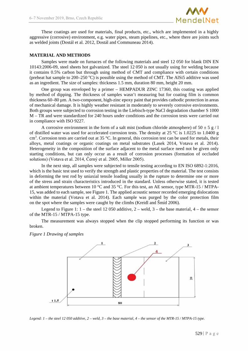
6–7 2019, Brno, Czech Republic
These coatings are used for materials, final products, etc., which are implemented in a highly aggressive (corrosive) environment, e.g. water pipes, steam pipelines, etc., where there are joints such as welded joints (Dostál et al. 2012, Dostál and Communeau 2014).
MATERIAL AND METHODS Samples were made on furnaces of the following materials and steel 12 050 for blank DIN EN
10143:2006-09, steel sheets hot galvanized. The steel 12 050 is not usually using for welding because it contains 0.5% carbon but through using method of CMT and compliance with certain conditions (preheat hat sample to 200–250 oC) is possible using the method of CMT. The AlSi5 additive was used as an ingredient. The size of samples: thickness 1.5 mm, duration 80 mm, height 20 mm.
One group was enveloped by a primer – HEMPADUR ZINC 17360, this coating was applied by method of dipping. The thickness of samples wasn’t measuring but for coating film is common thickness 60–80 µm. A two-component, high-zinc epoxy paint that provides cathodic protection in areas of mechanical damage. It is highly weather resistant in moderately to severely corrosive environments. Both groups were subjected to corrosion testing in the Liebisch-type NaCl degradation chamber S 1000 M – TR and were standardized for 240 hours under conditions and the corrosion tests were carried out in compliance with ISO 9227.
A corrosive environment in the form of a salt mist (sodium chloride atmosphere) of 50 ± 5 g / l of distilled water was used for accelerated corrosion tests. The density at 25 °C is 1.0225 to 1.0400 g cm3. Corrosion tests are carried out at 35 °C. In general, this corrosion test can be used for metals, their alloys, metal coatings or organic coatings on metal substrates (Lasek 2014, Votava et al. 2014). Heterogeneity in the composition of the surface adjacent to the metal surface need not be given only starting conditions, but can only occur as a result of corrosion processes (formation of occluded solutions) (Votava et al. 2014, Černý et al. 2005, Miller 2005).
In the next step, all samples were subjected to tensile testing according to EN ISO 6892-1:2016, which is the basic test used to verify the strength and plastic properties of the material. The test consists in deforming the test rod by uniaxial tensile loading usually in the rupture to determine one or more of the stress and strain characteristics introduced in the standard. Unless otherwise stated, it is tested at ambient temperatures between 10 °C and 35 °C. For this test, an AE sensor, type MTR-15 / MTPA-15, was added to each sample, see Figure 1. The applied acoustic sensor recorded emerging dislocations within the material (Votava et al. 2014). Each sample was purged by the color protection film on the spot where the samples were caught by the climbs (Kreidl and Šmíd 2006).
Legend to Figure 1: 1 – the steel 12 050 additive, 2 – weld, 3 – the base material, 4 – the sensor of the MTR-15 / MTPA-15 type.
The measurement was always stopped when the clip stopped performing its function or was broken.
Figure 1 Drawing of samples
Legend: 1 – the steel 12 050 additive, 2 – weld, 3 – the base material, 4 – the sensor of the MTR-15 / MTPA-15 type.
529

6–7 2019, Brno, Czech Republic
Figure 2 The sample during the tensil test, on the sample is fixing a sensor of AE
RESULTS AND DISCUSSION The data obtained from the measurements were processed and a graph representing the behaviour
of the samples exposed to the real load was created (Figure 3, Figure 4). The resulting graph shows the force acting on the samples, their extension and records of the acoustic emission. In the first phase, the force gradually increases to the first break – a slight decrease. There may be slippage between the jaws and the tool. Strength continued to grow steeply, with strong jaw strain on the samples tested. Based on the values obtained after testing all the samples on the universal test machine ZDM 5/51, a table was produced. This table contains the measured maximum force values obtained during the tensile test for the individual test specimens, see Table 1. Only in two cases were samples damaged in a weld, in the next six cases were samples damaged near a weld in the based material (heat–affected part).
Table 1 Overview of achieved maximum values during the tensile test Samples with protection film Samples Non-film
Sample Number
Rm
[MPA] Fmax [N] Sample Number
Rm
[MPA] Fmax [N]
1 4 840 14 521 1 4 305 12 917 2 4 445 13 336 2 4 412 13 236 3 4 998 14 995 3 4 530 13 590 4 4 992 14 977 4 4 676 14 028
Upon reaching the maximum force of 14 977N, a sharp drop in force occurred. Figure 3 is a diagram of working steel without significant yield strength. This representation is a typical tensile behavior of metallic materials. Hard and elastic materials showing tensile curves with high strength (high modulus) and low ductility. Their fracture is brittle, the materials are less resilient. All samples provided with an anti-corrosion protective film (film) achieved a significantly higher modulus of strength than samples without this protective film. When we would calculate some statistical relationship between the samples with protective film and samples without this protective film. The samples with protective film have higher tensile resistance by 6.92% than samples without this film.
530

6–7 2019, Brno, Czech Republic
Figure 3 Load force depending on extension
Figure 4 Records of acoustic emission
531

6–7 2019, Brno, Czech Republic
Figure 4 shows the acoustic emission recording. In the graph, the so-called Count is plotted on the y-axis, showing the amount of released energy at the beginning of dislocations or their propagation. The count is plotted following the chassis “t”, which is on the x-axis. The graph shows the origin and propagation of dislocations almost after the start of the measurement, when the crack is created and then spread, increasing as a result of loading during the measurement.
It can be seen from the measurements that samples which have not been provided with a protective coat after the degradation test do not have the same tensile limit as the samples provided with this protective coat. The highest record of acoustic emission and hence energy release occurred at sample number 8. This event is attributed to the moment when the total sample breakage occurred and, as a result, the subsequent large energy release that was reflected in the AE record.
CONCLUSION The results of the tensile test show a large difference between the properties of the steel materials
provided with the anticorrosive protective layer and the materials with no surface treatment. Metallic materials are used where there are high demands on strength, hardness, wear resistance, etc. Permanent deformation occurred in all samples tested. From the values and the following graphical representation it is evident that the samples coated with anticorrosive coating achieved higher tensile strength up to 7% compared to the samples without anticorrosive coating. They were also less sensitive to the emergence of dislocations and their subsequent spread through material.
As can be seen in the acoustic signal, samples without anticorrosive protection experienced dislocations, cracks and their growth and subsequent spread earlier. The first record of the exceeded counts at the "threshold" (setting the threshold for recording the AE signal) was recorded at 4 seconds and then grew and continued continuously for up to 45 seconds. The greatest AE activity was recorded between 15–35 seconds, at which point the largest dislocations and mechanical damage of samples occur. Conversely, samples treated with an anticorrosive coating proved to be more difficult for the formation of these dislocations and cracks, as well as for their growth and spread. These samples exceed the "threshold" at 14 seconds and continue intermittently until the 82th second except for samples 6 and 8. For samples 5–8 following the AE signal, the largest dislocations and mechanical damage of the samples occur between 25–67 seconds. Permanent mechanical damage occurs within this range. The signal is not as strong as for samples that do not have corrosion protection. These samples were not attacked by galvanic corrosion, which would reduce their mechanical properties and resistance, which was reflected in the AE signal recording. Samples 6 and 8 show a high incidence of AE signal at 120 seconds and 140 seconds due to total rupture. Finally, it is important to note that this paper clearly demonstrates that the anticorrosive coating has a significant impact and impact on the quality and durability of materials used in a highly corrosive active environment.
ACKNOWLEDGEMENTS The research was financially supported by the project IP 018/2019: Use of inorganic corrosion coatings for heterogeneous weldments protection; financed by IGA FA MENDELU.
REFERENCES Černý, M. et al. 2005. Zobrazení napětí a deformace s využitím AE. Acta Universitatis Agriculturae et Silviculturae Mendelianae Brunensis [Online], 53(2): 63–74. Available at: https://acta.mendelu.cz/media/pdf/actaun_2005053020063.pdf. [2019-08-18]. Dostál, P., Communeau, P. 2014. Visualisation of corrosion acoustic signals using quality tools. Acta Universitatis Agriculturae et Silviculturae Mendelianae Brunensis [Online], 62(1): 65–69. Available at: https://acta.mendelu.cz/media/pdf/actaun_2014062010065.pdf. [2019-08-28]. Dostál, P. et al. 2012. Accelerated corrosion and fatigue monitoring of aluminium alloy EN AW 7075. Jaunuju Mokslininku Darbai [Online], 38(5): 112–118. Available at: http://www.su.lt/bylos/mokslo_leidiniai/jmd/2012_5_38/dostal_kumbar_cerny_sabaliauskas.pdf. [2019-08-29].
532

6–7 2019, Brno, Czech Republic
Fajners. Porovnání označení hliníkových slitin podle EN – ČSN – DIN. DIN 1725. Available at: http://www.fajners.cz/pictures/pdf/Porovnani%20oznaceni%20normy.pdf. [2019-10-24]. Kreidl, M., Šmíd, R. 2006. Technická diagnostika – senzory, metody, analýza signálu – 4. díl edice Senzory neelektrických veličin. 1. vyd., Praha, CZ: BEN - technická literatura. Lasek, S. 2014. Základy degradačních procesů: studijní opora. 1. vyd., Ostrava, CZ: VŠB - Technická univerzita Ostrava. Miller, K.R. 2005. Nondestructive testing handbook: acoustic emission testing. 3rd ed., USA: American Society for Nondestructive Testing. Normaservis s.r.o. Technické normy DIN. DIN EN 10143:2006-09. Žďár nad Sázavou 460. Available at: https://eshop.normservis.cz/norma/dinen-10143-1.9.2006.html. [2019-10-24]. ÚNMZ. 2017. Kovové materiály – Zkoušení tahem-ČÁST 1: Zkušební metoda za pokojové teploty. EN ISO 6892-1:2016. Praha: Úřad pro technickou normalizaci, metrologii a státní zkušebnictví. Votava, J. et al. 2014. Degradation processes of Al–Zn welded joints. Acta Universitatis Agriculturae et Silviculturae Mendelianae Brunensis [Online], 62(3): 571‒578. Available at: https://acta.mendelu.cz/media/pdf/actaun_2014062030571.pdf. [2019-08-23]
533

6–7 2019, Brno, Czech Republic
Comparison of online tribodiagnostics with conventional method
Daniel Trost, Vojtech Kumbar, Adam Polcar Department of Technology and Automobile Transport
Mendel University in Brno Zemedelska 1, 613 00 Brno
CZECH REPUBLIC
Abstract: The paper deals with the use of tribodiagnostics in predictive maintenance in corporate practice. It is generally dealt with maintenance, then tribodiagnostics in the company Škoda Auto a.s. Used offline and online diagnostic tools are described. The experimental part is focused on detailed analysis of the comparison of measurement results offline and online diagnostics. The main aim of this experiment is verification and prove the high accuracy of tested online tool. There is also an economic evaluation of savings obtained by operation the online filter unit. In conclusion, the tribodiagnostics recommendations are given for Škoda Auto a.s. company.
Key Words: tribodiagnostics, predictive maintenance, offline and online diagnostics tools, hydraulic oil, hydraulic press
INTRODUCTION Tribodiagnostics is one of the methods of technical diagnostics using lubricants as a medium
for obtaining information about processes, mechanical changes and also degradation of lubricants in technical systems in which lubricants are applied (Vižintin et al. 2014). Tribodiagnostics is an effective objective tool for monitoring the process of mechanical wear and oil filling degradation. Its aim is to detect and warn in time of the possibility of machinery failure and thus prevent unplanned production interruptions. The lubricated friction nodes gradually wear out, the circulating oil entrains the trace metal particles and these remain in the oil as a suspension. Increased amount of impurities in the oil means not only increased wear of the lubricated parts, but can also cause breakdown of the lubrication system (Moffatt et al. 2012). By expert evaluation of the quantity, size and shape of these particles we get a picture of the kind of wear and technical condition of individual friction nods. Correct interpretation of the results allows early warning of the symptoms of a failure, and in many cases also helps to locate the site of the mechanical failure. By monitoring the oil quality changes of the lubricant itself we are able to determine the level of degradation and also predict oil duration. Tribodiagnostics can be done offline and online. Online tribodiagnostics is used especially for continuous monitoring of crucial equipment during their operation in order to ensure reliability and competent operation. This type of diagnostics is particularly suitable for large and decentralized manufacturing plants where it offers significant savings in maintenance time by the logistical transfers from the laboratory to the diagnosed equipment.
MATERIALS AND METHODS In experiment was used online filtration unit, which is able in real time to monitor and evaluate
amont of water and impurities in hydraulic oil during filtration process. The online filtration unit and the components are shown in Figure 1. The online filtration unit is able to evaluate actual values of quantities such as:
• the amount of water present in the oil [ppm],• amount of solids present in the oil [ISO 4406 code number],• hydraulic oil outlet pressure [Pa],• flow volume [l /min],• oil temperature [°C].
534
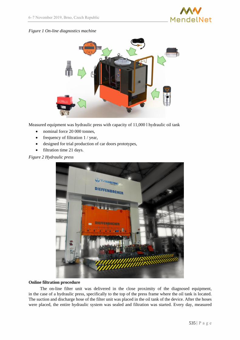
6–7 2019, Brno, Czech Republic
Figure 1 On-line diagnostics machine
Measured equipment was hydraulic press with capacity of 11,000 l hydraulic oil tank • nominal force 20 000 tonnes, • frequency of filtration 1 / year, • designed for trial production of car doors prototypes, • filtration time 21 days.
Figure 2 Hydraulic press
Online filtration procedure The on-line filter unit was delivered in the close proximity of the diagnosed equipment,
in the case of a hydraulic press, specifically to the top of the press frame where the oil tank is located. The suction and discharge hose of the filter unit was placed in the oil tank of the device. After the hoses were placed, the entire hydraulic system was sealed and filtration was started. Every day, measured
535
6–7 2019, Brno, Czech Republic
values were recorded from the on-line filter unit display. These values are shown in Table 1. Against in the Table 2 are shown values obtained by offline methods. Due to the principle of filtering, measuring and evaluating the required quantities on-line, it was not possible to measure the same oil sample multiple times. Specifically, the measured values were recorded at the same time as oil sample for offline diagnostics was taken. Both ways ones a day. Whole the experiment follows the standard ČSN EN ISO 3171 – Automatic sampling of pipelines for liquid petroleum products. Online values are shown in green in the tables and figures. The monitored quantities were the amount of water according to the standard ASTM D6304 and amount of impurities according to ISO 4406. The standard ISO 4406 describes method for coding the level of contamination by solid particles. Cleanliness levels are defined by three numbers divided by slashes. These numbers correspond to 4, 6 and 14 microns, in that order. Each number refers to an ISO Range Code, which is determined by the number of particles for that size and larger present in 1 ml of fluid. Each range of fluid is double the range below.
RESULTS AND DISCUSSION
In this chapter, the experimental results of the measurement will be commented on. First there are tables for online and offline results, then these tables are shown in graphs in Figure 3, Figure 4 and Figure 5. Images describing trends of online and offline diagnostics during oil filtration in hydraulic press. The filtration process is shown in the following tables:
Table 1 Initial Values of hydraulic oil parameters, hydraulic press, online
Day Amount of water [ppm]
ISO code number
[ISO 4406] Day
Amount of water [ppm]
ISO code number
[ISO 4406]
1 152 22/20/18 9 84 18/15/14 2 135 21/19/17 10 80 18/14/13 3 130 20/18/16 11 66 17/14/13 4 124 20/18 /15 12 63 17/14/11 5 119 20/18/15 13 62 16/13/12 6 100 20/17/15 14 60 16/12/11 7 96 18/16/14 15 58 15/13/10 8 92 19/15/14 16 58 15/11/10
Table 2 Initial Values of hydraulic oil parameters, hydraulic press, offline
Day Amount of water [ppm]
ISO code number
[ISO 4406] Day
Amount of water [ppm]
ISO code number
[ISO 4406]
1 158 23/21/17 9 79 17/13/11 2 142 22/20/16 10 74 16/12/11 3 130 21/20/15 11 64 16/12/10 4 123 20/19/14 12 62 15/12/10 5 116 19/18/13 13 60 15/11/10 6 96 18/16/13 14 58 15/11/9 7 89 17/15/13 15 57 15/11/9 8 85 17/14/12 16 55 14/11/9
a) Evaluation of impuritiesPurity code number in the form X / Y / Z was separated into 3 separate figures for better clarity
(Figure 3, Figure 4 and Figure 5). The graphs will be described sequentially in the order of X, Y and Z.
536

6–7 2019, Brno, Czech Republic
Figure 3 ISO Range Code X (≤ 4μm)
Figure 4 ISO Range Code Y (≤ 6μm)
Figure 5 ISO Range Code Z (≤ 14μm)
1 2 3 4 5 6 7 8 9 10 11 12 13 14 15 16off-line 17 16 15 14 13 13 13 12 11 11 10 10 10 9 9 9on-line 18 17 16 15 15 15 14 14 14 13 13 11 12 11 10 10
1716
15 1413 13 13
1211 11
10 10 109
9
1817
1615 15 15
14 14 1413 13
1112
1110 10
8
10
12
14
16
18
20
Clea
nlin
ess l
evel
s
Day
Comparison of solid particles quantity Z
1 2 3 4 5 6 7 8 9 10 11 12 13 14 15 16off-line 23 22 21 20 19 18 17 17 17 16 16 15 15 15 15 14on-line 22 21 20 20 20 20 18 19 18 18 17 17 16 16 15 15
2322
21 20
1918 17 17 17
16 16 15 15 15
15
14
22 2120
20 2018
1918 18
17 1716 16
15 15
13151719212325
Clea
nlin
ess l
evel
s
Day
Comparison of solid particles quantity X
1 2 3 4 5 6 7 8 9 10 11 12 13 14 15 16off-line 21 20 20 19 18 16 15 14 13 12 12 12 11 11 11 11on-line 20 19 18 18 18 17 16 15 15 14 14 14 13 12 13 11
2120 20
1918
1615
1413 12 12 12
11 11 11 11
2019
18 1817
1615 15
14 14 1413
1213
11
9
11
13
15
17
19
21
Clea
nlin
ess l
evel
s
Day
Comparison of solid particles quantity Y
537

6–7 2019, Brno, Czech Republic
b) Evaluating the amount of water
Figure 6 Water filtration, online and offline
The graphs show that the values of impurities (solid particles) measured by offline and on-line methods are very similar. The differences between online and offline measured values are the minimal because of measurement uncertainty reported by the equipment manufacturer ± 1 cleanliness level. When comparing the results of measuring the amount of water in the oil, the measured differences are also minimal. For all three graphs (Figure 3, Figure 4 and Figure 5), we can see a relatively exponential decrease in the amount of impurities X, Y, Z during the filtration process. The deviation of the values from the shape of the exponential curve is caused by the inaccuracy of the measurements, but also by the missing values of the measurements during the weekends.
In the experiment, the results of measuring water and impurities were achieved using Filtration Technology's mobile online filtration device, which is also able to diagnose the actual amount of water and impurities in the oil during oil filtration. The issue of introducing on-line devices is also described by Markova et al. (2010), however this paper deals with monitored the oil viscosity using on-line diagnostics. Authors Knowles and Baglee (2012) and Salgueiro et al. (2013) deal with a similar topic in their papers, but with slightly different methodologies and devices.
Economic evaluation Initial costs of diagnostics and filtration equipment.
Table 6 Initial costs of equipment Initial costs of equipment Costs [EUR]
Online equipment Online filter unit, Filtration Technology 16,000
Offline equipment
Determination of the water content, Karl Fischer Coulometer
44,000
Particle count, LaserNet 48,000 Offline filter unit, Filtration Technology 8,000
Financial savings using online unit . 84,000
CONCLUSION In this work, the results obtained by measuring online and offline instruments were compared.
The measured oil was HM 46 hydraulic oil from a hydraulic press used in the manufacture of automotive components. The results show that the online filter unit provides very similar results to the commonly
1 2 3 4 5 6 7 8 9 10 11 12 13 14 15 16on-line 152 135 130 124 119 100 96 92 84 80 66 63 62 60 58 58off-line 158 142 130 123 116 96 89 85 79 74 64 62 60 58 57 55
152135 130
124 119
100 96 9284 80
66 63 62 60 58 58
158142
130
123116
96 89 85 79 74 64 62
60 58 57 55
50
70
90
110
130
150
170
Amou
nt o
f wat
er [p
pm]
Day
Water quantity comparison
538

6–7 2019, Brno, Czech Republic
used offline laboratory equipment used for these purposes. The average deviation between online and offline unit is 5%. The advantage of the online filter unit is lower initial costs, because the used online filtration unit is able to replace 3 offline devices. Another advantage is saving time because of connectivity between user and device by on-line data transfer. Thus, the experiment shows that it is advisable to continue the automation of production and maintenance as well as with tribodiagnostics. The results obtained by this experiment are applicable in industrial practice.
ACKNOWLEDGEMENTS The research was financially supported by the OP PIK CZ.01.1.02/0.0/0.0/15_019/0004799 “ZETORS TRACTORS a.s. – The optimal aggregation of implement with a tractor”.
REFERENCES ČSN ISO 4406 (656206). Hydraulické kapaliny - Kapaliny - Metoda kódování úrovně znečištění pevnými částicemi. Praha: Český normalizační institut, 2006, 12 s. Třídící znak 65 6206. Knowles, M., Baglee, D. 2012. Condition management of marine lube oil and the role of intelligent sensor systems in diagnostics. Paper presented at the Journal of Physics: Conference Series, 364(1) doi:10.1088/1742-6596/364/1/012007. Markova, L.V. et al. 2010. On-line monitoring of the viscosity of lubricating oils. Journal of Friction and Wear, 31(6): 433–442. Moffatt, J. et al. 2012. Lubricant condition assessment system (LUCAS), an enabler for condition based maintenance best practice. Paper presented at the Annual Forum Proceedings – AHS International, 3: 1656–1662. Salgueiro, B.J. et al. 2013. On-line oil monitoring and diagnosis. Strojniski Vestnik/Journal of Mechanical Engineering, 59(10): 604–612. Vižintin, J. et al. 2014. System for automated online oil analysis. Paper presented at the 11th International Conference on Condition Monitoring and Machinery Failure Prevention Technologies, CM 2014 / MFPT 2014
539
6–7 2019, Brno, Czech Republic
Improvement of drawbar properties of small tractor with special spikes tires
Tomas Zubcak1, Katarina Kollarova2, Eva Matejkova3 1Department of Transport and Handling
2Information and Coordination Centre of Research 3Department of Statistics and Operations Research
Slovak University of Agriculture in Nitra Tr. A. Hlinku 2, 949 76 Nitra
SLOVAK REPUBLIC
Abstract: This article presents comparison of two versions of driving wheels of a small tractor. Special spikes tires were developed and compared with standard tires according to drawbar pull at 100% driving wheels slip. Spikes elements of the special spikes tires were placed into grooves made in tire-tread pattern of the standard tractor tires. When the spikes tires are in base position, the spikes elements don’t exceed the diameter of the standard tires. When the spikes tires are activated, the spikes elements change they position to improve drawbar properties of the tractor. The experiments were realised on a cultivated soil at soil moisture 30.98%. Percentage difference of drawbar pull 17.3% shows improvement of the drawbar properties of the tractor with the special spikes tires in comparison with the tractor with the standard tires.
Key Words: driving wheels, cultivated soil, tire-tread pattern
INTRODUCTION Technical innovations of the tractors are realized at a high speed to improve the tractor properties
and make the operation more effective. Besides the tractor effectivity, the innovation process affects also reduction of negative effects of agricultural machinery on the environment. Modern technologies used in today’s tractors allow to reduce soil damage and harmful emission in exhaust gases.
Modern agriculture brings with it a variety of new technologies and constructional innovations in terms of the appliances which enable productivity improvements as well as a reduction in energetic demands, reduction of the fuels consumption and its associated undesirable emission reduction in particular, together with their new existence in the market (Vykydal et al. 2012, Sedlák et al. 2004, Porteš et al. 2013).
To improve the drawbar properties, the tractors use various technique namely change of tire inflation pressure, additional ballast load, lug wheels, belts etc.
This paper deals with the properties of special spikes tires developed to improve the drawbar properties of tractors without the need above-mentioned conventional concepts.
MATERIAL AND METHODS
Design of special spikes tires The special spikes tires were designed at the Department of Transport and Handling of the Slovak
University of Agriculture in Nitra (Abrahám et al. 2015, Abrahám et al. 2018, Majdan et al. 2018). The main parts of the spikes tires (Figure 1) are four spikes elements (1), control (4) and carrier wire strands (3) and control mechanism rots (5). The control wire strand (4) protrudes the spikes from tire and also holds all parts in the same position. Each element is placed in tire groove (6) made in tire-tread pattern. Removing a screw (7) the rods of control mechanism (5) are released to allow protrusion (protruded position) of the spikes from the tire due to a wheel rotation. The spikes can be placed aback (base position) by the reason of the road transportation. The spikes elements were designed regarding
540

6–7 2019, Brno, Czech Republic
a space in tire-tread pattern because they can’t exceed a tire diameter in the base position. The design of spikes tires was developed according to theory presented by Majdan et al. (2016).
Figure 1 Spikes tires: a) assembly, b) spikes element placed in the tire groove, c) single spikes element, d) dimensions of the spikes element
Drawbar pull measurement
Drawbar pull at 100% wheels slip was used to compare the special spikes tires with standard tires. The test tractor was equipped with the standard tires TS-02 6.5/75-14 4PR TT type (Mitas a. s., Czech Republic). The drawbar pull measurements were realized in accordance with STN ISO 789-9 (Simikić et al. 2014).
Figure 2 Schematic diagram of drawbar pull measurement system HMG 2020
1
32
EMS150
PS 01 UANS+12V +24 V
PC
Legend: 1 – force sensor EMS 150 type, 2 – test tractor Mini 070 type, 3 – load tractor T4K10 type, HMG 2020 – data logger, UANS – universal battery source, PC – personal computer, PS 01 – junction box.
Main parts of a measurement system (Figure 2) are as follows: - The test tractor MT8-070 Mini type (Agrozet, Czech Republic) is characterised by gasoline
engine with volume capacity 400 ccm, ratted engine power 8 kW and ratted engine speed 3,600 min-1. The test tractor total weight is 310 kg. This tractor drew the load tractor to generate the drawbar pull. The special spikes tires were mounted to the test tractor to compare wheels properties with standard tires on the basis of the drawbar pull. The test tractor was operated in second gear.
- The load tractor 4K-14 type (Agrozet, Czech Republic) is characterized by diesel engine with volume capacity 661.6 ccm and maximal output power 13 kW. The load tractor total weight is 870 kg. This tractor loaded the test tractor during the measurement of the drawbar pull.
- The force sensor type EMS 150 (Emsyst s. r. o., Slovak Republic) with strain-gauge bridge in a steel housing (accuracy class: 0.2, rated capacity: 10 kN, rated output: 0–10 V). Drawbar pull measurement of tractor Mini 070 is implemented by means of strain tensometric force sensor marked as 150 EMS. Force sensor is connected between the load tractor and test tractor through the steel chain.
541

6–7 2019, Brno, Czech Republic
- The data logger type HMG 2020 (Hydac GmbH, Germany) is a high-performance portable measuring and data-logging device with accuracy ≤ ± 0.1. 1 kHz of a sampling frequency was set. Digital recording unit HMG 2020 was used to record electrical signals from force sensor.
- A power supply contains two accumulators (12 V) connected in series or parallel to supply the sensor and the data logger with a direct voltage (12 V or 24 V). The power supply was manufactured in our Department of Transport and Handling as a portable device (Cviklovič et al. 2012).
The measurements were performed on the field with a cultivated soil of the Slovak Agricultural Museum in Nitra (Slovak Republic) at soil moisture 30.98%. The Chernozem soil type (World Reference Base for Soil Resources) is typical for the area where the field tests were performed. The soil moisture was stated according to standard STN ISO 11465 after drying at temperature 105 °C as follows:
𝑤𝑤 = 𝑚𝑚1−𝑚𝑚3𝑚𝑚3−𝑚𝑚2
. 100 (1)
Where: m1 – weight of soil volume before drying and Kopecky roller, g m2 – weight of empty Kopecky roller, g m3 – weight of soil volume after drying and Kopecky roller, g
Drawbar pull calculation To calculate the drawbar pull of one measurement (Figure 3), a time interval from a start point 1
to a finish point 2 has to be stated. These points are intersection of two lines namely dotted line (minimum level) and solid line (measured course of drawbar pull). A data file contains variables from a minimum value (point 3) up to a maximum value (point 4). In such a way, the mean value of the drawbar pull for one measuring is obtained.
Using data from five drawbar pull measurements, the average drawbar pull X was calculated to evaluate the drawbar properties of the small tractor. Five measurement repetitions n minimize the measurement errors (Figure 3). The average drawbar pull is calculated according to equation (2) and used for comparison of the special spikes tires with the standard tires. The same methodology was published by Abrahám et al. (2019).
nx...xx
X n21 +++= (2)
Where: x1, x2 …, xn – values of drawbar pulls at 100% wheels slip, N X – average drawbar pull, N
n – drawbar pull measurement repetition.
Figure 3 Drawbar pull calculation
Dra
wba
r pu
ll, N
Drawbar pull (x1)
0Time, s
1th measurement 2nd measurement n- measurement
Drawbar pull (x2)Drawbar pull (xn)
Time interval
Minimum level
Maximum level
21
3
4
1
The special spikes tires and standard tires will be compared according to 95% confidence interval (CI). Kozelková et al. (2018) presents, that the 95% confidence interval is adequate for experiments in agricultural praxis. F-test of One-way Analysis of Variance (Anova) was used to test whether there are any significant differences amongst the means of drawbar pulls.
542

6–7 2019, Brno, Czech Republic
RESULTS AND DISCUSSION The results of drawbar pull measurements are shown in Figure 4 in case of the tractor
with the standard tires and Figure 5 in case of the tractor with the spikes tires.
Figure 4 Five measurements of drawbar pull in case of tractor with standard tires
Figure 5 Five measurements of drawbar pull in case of tractor with spikes tires
Table 1 Data of drawbar pulls of tractor with different tires
Tires type Drawbar pull X,
N σ, N
CI, N x1, N x2, N x3, N x4, N x5, N
Standard tires 3,941.6 3,726.1 3,988.7 3,747.6 3,717.6 3,859.1 328.91
4,020.6 3,697.6
Spikes tires 4,910.4 4,921.8 4,005.4 4,699.9 4,798.7 4,667.2 512.72
5,140.1 4,194.3
543

6–7 2019, Brno, Czech Republic
Regarding five measurements of drawbar pull of the tractor with two versions of driving wheels, Table 1 shows the drawbar pulls (x1 – x5), standard deviations (σ) and 95% confidence intervals (CI). Since the P-value (0.001576) is less than 0.01, there is a statistically significant difference (F-value 21.92). Figure 6 shows average drawbar pulls and 95% confidence intervals. Percentage difference 17.3% between drawbar pull of tractor with standard tires and special spikes tires was calculated from measured data listed in Table 1. The data variability is caused by the field character of experiments and the spikes which affects tire-soil interactions. The drawbar pull at 100% driving wheels slip taken relatively short time (only few seconds) because the wheels rapidly sank to the loose cultivated soil (Figure 4 and 5) when the tractor didn’t move.
Figure 6 Comparison of spikes and standard tires
Abrahám et al. (2014) presented the special wheels with auto-extensible blades. These lug wheels are mounted besides the tractor driving wheels to improve the tractor drawbar properties by means of steel blades. The spikes tires are simplifier construction and don’t change the tractor width in comparison with lug wheels mentioned above. The author presents increase in drawbar pull at 100% driving wheels slip 36.1% in comparison with the standard tires. In case of spikes tires, the increase reached lover value 17.3% due to significantly higher dimensions of steel lugs in comparison with spikes.
The special spikes wheels are universally applied to increase the tractor drawbar pull on the various grounds as well as cultivated soil similar to a sandy terrain. To increase the drawbar pull on the sandy terrain, Yang et al. (2014) compared actively actuated lugged wheels with fixed lugged wheels and smooth wheels. The actively actuated lugged wheels achieved the highest drawbar pull but their planetary gear doesn’t allow changing the lugged wheel to the smooth wheels in case of transportation on a hard landscaping. The spikes tires in base position don’t exceeds the standard tires diameter and allow a transport on roads.
CONCLUSIONS The paper presents the design and properties of the special spikes tires. It is advantageous
for tractor transportation on roads to use standard rubber tires. Therefore, the spikes of the special tires don’t touch a ground when they are in base position. The simple mechanical control system activates the special spikes wheels to improve the drawbar properties of the tractor. To innovate the special tire, the mechanical control system can be replaced by the automatic remote-control system.
Statistically significant difference 17.3% between drawbar pull of the tractor with standard and spikes tires shows the improvement of the tractor drawbar properties. This value is limited by the number and design of the spikes. In general terms, shape and dimensions of spikes also affect
544

6–7 2019, Brno, Czech Republic
the tire-soil interactions. Therefore, the next innovation can be based on the detection of the optimal inclination angle and shape of the spikes.
ACKNOWLEDGEMENTS The research was financially supported by the project VEGA No. 1/0724/19 of the Ministry of Education of the Slovak Republic “Research, Design and Application of Special Driving Wheels for Drawbar Properties Improvement and Elimination of Soil Damage under Operation of Cars and Tractors”.
REFERENCES Abrahám, R. et al. 2014. Increase in Tractor Drawbar Pull Using Special Wheels. Agronomy Research, 12(1): 7–16. Abrahám, R. et al. 2015.Výsuvné hrotové zariadenie na zlepšenie záberových vlastností kolies. 7347. PUV 11-2015. Available at: http://skpatents.com/6-u7347-vysuvne-hrotove-zariadenie-na-zlepsenie-zaberovych-vlastnosti-kolies.html. Abrahám, R. et al. 2018. Comparison of Consumption of Tractor at Three Different Driving Wheels on Grass Surface. Agronomy Research, 16(3): 621–633. Abrahám, R. et al. 2019. Special Tractor Driving Wheels with Two Modification of Spikes Inclination Angle. Agronomy Research, 17(2): 333–342. Cviklovič, V. et al. 2012. Methodology for Measuring the Efficiency of Sine Wave Inverters. Acta Technologica Agriculturae, 15(3): 60–63. Kozelková, D. et al. 2018. Eggs and Their Consumption Affected by the Different Factors of Purchase. Slovak Journal of Food Sciences, 12(1): 570–577. Majdan, R. et al. 2018. Drawbar Parameters of Tractor with Prototypes of Driving Wheels and Standard Tyres. Acta Technologica Agriculturae, 21(2): 63–68. Majdan, R. et al. 2016. Teória a konštrukcia traktorov: teoretické, výpočtové riešenie kolesových traktorov, pojazdové ústrojenstvo, motor, hydraulický systém a elektrické príslušenstvo. 1st ed., Nitra, Slovak Republic: Slovak University of Agriculture. Porteš, P. et al. 2013. Laboratory-Experimental Verification of Calculation of Force Effects in Tractor's Three-Point Hitch Acting on Driving Wheels. Soil and Tillage Research, 128: 81–90. Sedlák, P. et al. 2004. Factors Influencing Economic Aspects of Operation of Tractor Machines Aggregations. Acta Universitatis Agriculturae et Silviculturae Mendelianae Brunensis, 52(4): 83–90. Simikić, M. et al. 2014. Power Delivery Efficiency of a Wheeled Tractor at Oblique Drawbar Force. Soil and Tillage Research, 141: 32–43. STN ISO 11465: 2001. Soil Quality – Determination of Dry Matter and Water Content on a Mass Basis – Gravimetric Method. STN ISO 789-9: 1993. Agricultural Tractors. Test procedures. Part 9: Power Tests for Drawbar. Slovak Office of Standards, Metrology and Testing Vykydal, P. et al. 2012. The Influence of the Undercarriage and Tire Inflation Rating on Drawbar Characteristics of Tractors. Acta Universitatis Agriculturae et Silviculturae Mendelianae Brunensis, 60(5): 255–264. Yang, Y. et al. 2014. Drawbar Pull of a Wheel with an Actively Actuated Lug on Sandy Terrain. Journal of Terramechanics, 56: 17–24.
545

APPLIED CHEMISTRY AND BIOCHEMISTRY

6–7 2019, Brno, Czech Republic
Combination of molecularly imprinted polymers and capillary electrophoresis for analysis of nucleobases
Jaroslava Bezdekova, Kristyna Zemankova, Milada Vodova, Martin Zahalka, Marketa Vaculovicova
Department of Chemistry and Biochemistry Mendel University in Brno Zemedelska 1, 613 00 Brno
CZECH REPUBLIC
Abstract: Determination of DNA damage products in various samples including urine, plasma or cells is an important process enabling the evaluation of the overall body condition. Therefore, a powerful sensitive and selective analytical technique is needed. Here, the combined use of molecularly imprinted polymeric biorecognition extraction and capillary electrophoretic separation with UV/Vis detection is demonstrated. The tagged analytes are nucleobases and their biologically important derivatives. Capillary micellar electrokinetic chromatography using sodium dodecyl sulphate enabled the baseline separation of cytosine and methylcytosine and imprinted polydopamine polymeric surface allowed for selective extraction of a selected nucleobase.
Key Words: molecularly imprinted polymers, capillary electrophoresis, nucleobases
INTRODUCTION Nucleobases belong to the most important molecules in human body as they are responsible
for genetic coding. Moreover, DNA damage, manifested as an elevated content of nucleobases, nucleotides and/or nucleosides in cells as well as in body fluids can indicate not only serious diseases including cancer or neurodegeneration, but can be caused also by physical exercise, UV and ionising radiation or tobacco smoking (Weimann et al. 2002). Currently there is an interest in linking DNA alterations or amount of nucleobase lesions in biological fluids with carcinogenesis (Faure et al. 1996).
The average concentrations of most important ribonucleotides, are at the level of hundreds of µM and for deoxynucleosidestriphosphate, the concentrations are approximately in the range of tens of µM (except for dGTP – units of µM). The average concentration of bases and nucleosides extracellular fluids and in plasma is at the level of 0.4–6 µM; however intracellular concentrations these values are generally higher (Traut 1994).
From the analytical point of view, the optimal arrangement is a combination of a separation technique (e.g. chromatography or electrophoresis) with a specific detection such as mass spectrometry. However, to avoid sophisticated and costly instrumentation, the simple UV/Vis detection in combination with efficient sample pretreatment can be of an interest (Weimann et al. 2002).
In this work, a method combining the separation power of capillary electrophoresis with selective extraction abilities of molecularly imprinted polymers was developed. Moreover, the alternative of capillary zone electrophoresis using addition of detergents to increase the separation resolution – micellar electrokinetic chromatography enabled even the separation of methyl-derivative of cytosine, which will be further utilized for monitoring of epigenetic changes.
MATERIALS AND METHODS
Materials Dopamine hydrochloride, Trizma base and all nucleic bases were purchased from Sigma-Aldrich
(St. Louis, MO, USA) in ACS purity. Sodium tetraborate decahydrate were obtained from Thermo Fisher Scientific (Waltham, MA, USA).
547
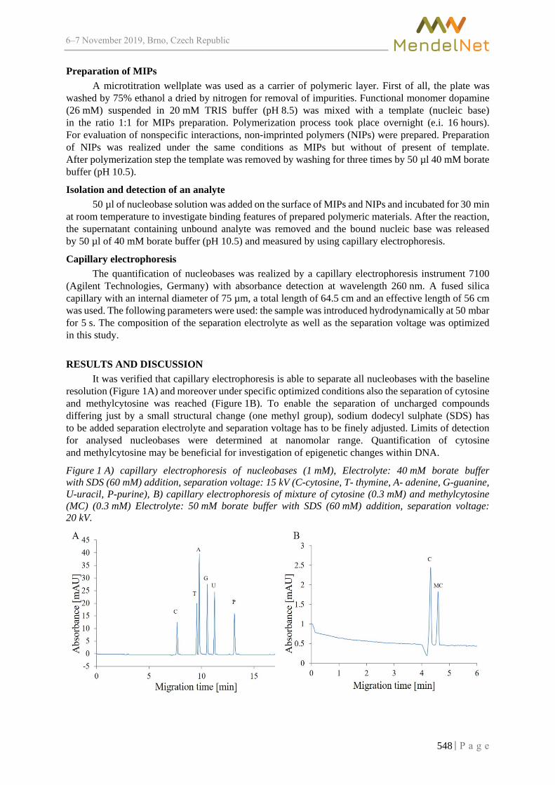
6–7 2019, Brno, Czech Republic
Preparation of MIPs A microtitration wellplate was used as a carrier of polymeric layer. First of all, the plate was
washed by 75% ethanol a dried by nitrogen for removal of impurities. Functional monomer dopamine (26 mM) suspended in 20 mM TRIS buffer (pH 8.5) was mixed with a template (nucleic base) in the ratio 1:1 for MIPs preparation. Polymerization process took place overnight (e.i. 16 hours). For evaluation of nonspecific interactions, non-imprinted polymers (NIPs) were prepared. Preparation of NIPs was realized under the same conditions as MIPs but without of present of template. After polymerization step the template was removed by washing for three times by 50 µl 40 mM borate buffer (pH 10.5).
Isolation and detection of an analyte 50 µl of nucleobase solution was added on the surface of MIPs and NIPs and incubated for 30 min
at room temperature to investigate binding features of prepared polymeric materials. After the reaction, the supernatant containing unbound analyte was removed and the bound nucleic base was released by 50 µl of 40 mM borate buffer (pH 10.5) and measured by using capillary electrophoresis.
Capillary electrophoresis The quantification of nucleobases was realized by a capillary electrophoresis instrument 7100
(Agilent Technologies, Germany) with absorbance detection at wavelength 260 nm. A fused silica capillary with an internal diameter of 75 µm, a total length of 64.5 cm and an effective length of 56 cm was used. The following parameters were used: the sample was introduced hydrodynamically at 50 mbar for 5 s. The composition of the separation electrolyte as well as the separation voltage was optimized in this study.
RESULTS AND DISCUSSION It was verified that capillary electrophoresis is able to separate all nucleobases with the baseline
resolution (Figure 1A) and moreover under specific optimized conditions also the separation of cytosine and methylcytosine was reached (Figure 1B). To enable the separation of uncharged compounds differing just by a small structural change (one methyl group), sodium dodecyl sulphate (SDS) has to be added separation electrolyte and separation voltage has to be finely adjusted. Limits of detection for analysed nucleobases were determined at nanomolar range. Quantification of cytosine and methylcytosine may be beneficial for investigation of epigenetic changes within DNA.
Figure 1 A) capillary electrophoresis of nucleobases (1 mM), Electrolyte: 40 mM borate buffer with SDS (60 mM) addition, separation voltage: 15 kV (C-cytosine, T- thymine, A- adenine, G-guanine, U-uracil, P-purine), B) capillary electrophoresis of mixture of cytosine (0.3 mM) and methylcytosine (MC) (0.3 mM) Electrolyte: 50 mM borate buffer with SDS (60 mM) addition, separation voltage: 20 kV.
548

6–7 2019, Brno, Czech Republic
Even though capillary electrophoresis is a powerful analytical method with high separation efficiency (˃ thousands of theoretical plates), extra small sample volume (nl), low times of analyses (˂ minutes), and it is possible to use wide variety of detection modalities, the complexity of biological samples (e.i. body fluids) makes the overall analysis significantly more difficult.
For this reason, an effective sample pretreatment technique has to be employed. And due to numerous benefits such as mainly flexibility and variability, molecularly imprinted polymers are the approach of choice. The principle of the method is schematically shown in Figure 2.
Figure 2 Scheme of the overall analytical process A) Preparation of the specific biorecognition surface, B) Sample pretreatment procedure
Selectivity of prepared MIPs
Polydopamine MIPs prepared under optimized conditions using uracil as a template were tested for their ability to distinguish between nucleic bases. The results are summarized in Figure 3. The negative selectivity values appeared in the situation when the amount of nucleic base bound by the NIPs layer was higher than the amount of nucleic bases bound by the MIPs layer. From data it is seen that created polymer has ability to selectively recognize, isolate, and extract the analyte/template (e.i. uracil). Other nucleic bases formed the nonselective interaction.
Figure 3 Selectivity characterization of prepared polymeric surface
-2
-1,5
-1
-0,5
0
0,5
1
1,5
2
2,5
U T C A GDiff
eren
ce b
etw
een
MIP
and
NIP
549
6–7 2019, Brno, Czech Republic
CONCLUSION In this work, capillary electrophoresis with UV/Vis detection was evaluated as a method capable
of separation and detection of nucleobases with high resolution and detection limits in nanomolar range. Even the methyl-derivative of cytosine was separated from cytosine with the base-line resolution using micellar electrokinetic chromatography. Finally, to enable the detection of nucleobases in complex real samples, the extraction and sample preparation method based on molecularly imprinted polydopamine was developed. The combination of these two powerful analytical approaches will enable the monitoring of not only nucleobases but also nucleotides and nucleosides as they are markers of cellular metabolism.
ACKNOWLEDGEMENTS The research was financially supported by AF-IGA2019-IP023.
REFERENCES Faure, H. et al. 1996. 5-hydroxymethyluracil excretion, plasma Tbars and plasma antioxidant vitamins in adriamycin-treated patients. Free Radical Biology and Medicine, 20(7): 979–983. Traut, T.W. 1994. Physiological concentrations of purines and pyrimidines. Molecular and Cellular Biochemistry, 140(1): 1–22. Weimann, A. et al. 2002. Quantification of 8-oxo-guanine and guanine as the nucleobase, nucleoside and deoxynucleoside forms in human urine by high-performance liquid chromatography-electrospray tandem mass spectrometry. Nucleic Acids Research, 30(2): e7.
550

6–7 2019, Brno, Czech Republic
Differences in siRNA encapsulation between HsaHFt-RK ferritin and EcaLHFt
Marketa Charousova1,2, Michal Mokry3, Vladimir Pekarik4 1Department of Chemistry and Biochemistry
Mendel University in Brno Zemedelska 1, 613 00 Brno
2Central European Institute of Technology (CEITEC) University of Technology
Purkynova 123 00, 612 00 Brno 3Department of Biomedical Engineering
University of Technology Technicka 10, 616 00 Brno 4Department of Physiology
Masaryk University Kamenice 5, 625 00 Brno
CZECH REPUBLIC
Abstract: Nanomedicine in cancer treatment has a great potential. With usage of proper nanocarrier we would be able to eliminate negative side effects and excessively high toxicity of chemotherapeutical drugs to normal cells. Ferritins in general are proteins which could do the trick. Their ability to change structure in low pH could be used for drug delivery. Ferritins are also ubiquitous so there is also very small chance of immune reaction in body. First and the most used and described ferritin is EcaLHFt (ferritin from horse spleen). Its ability to encapsulate various molecules is already known and used in research laboratories. Only molecules with negative charge are troublesome to encapsulate into EcaLHFt. For this reason, we created recombinant human ferritin – HsaHFt-RK, which is designed to encapsulate predominantly negatively charged molecules. We were able to confirm this hypothesis by comparing the encapsulation efficiency of FAM-siRNA inside EcaLHFt and HsaHFt-RK.
Keyword: nanomedicine, ferritin, gene therapy, siRNA, recombinant protein
INTRODUCTION Cancer never sleeps. More and more people are diagnosed with cancer every year. There is a need
for a novel cancer treatment, which would be gentler to patients. High hopes are given to immunotherapy (Bergman 2009) and nanomedicine (Wolfram and Ferrari 2019). However, the most used cancer treatment is still surgery with chemotherapy and radiotherapy.
Nanomedicine is based on nanotransporters which are able to encapsulate or bind at their surface active molecules and transfer it to cancer tissue without penetrating the normal cells and organs in patient body. For this purpose various types of molecules are used, most of them inorganic (Todd et al. 2013). Later, the use of proteins as nanotransporters started to be tested. Proteins are more biocompatible and less toxic than inorganic transporters. Interesting protein-based nanotransporter is ferritin. This ubiquitous protein with spherical structure is primarily used in body for iron storage and transportation. Its external diameter is about 12 nm with inside cavity of 8 nm (Uchida et al. 2006). Ferritin structure is robust and stable in physiological environment, in pH scale 2–10 and even in extreme biological temperatures up to 70 °C (Chen et al. 2008, Kang et al. 2008).
There is also one essential property which makes ferritin widely used in research labs, its ability to self-assemble. This ability was first found and described in horse spleen ferritin (EcaLHFt) in 1978. The protein cage can be disassociated in pH below 2 and fold back together if pH is returned back to neutral (Banyard et al. 1978, Domínguez-Vera and Colacio 2003). This property is used for encapsulation various types of molecules inside ferritin. By mixing ferritin with wanted drug,
551
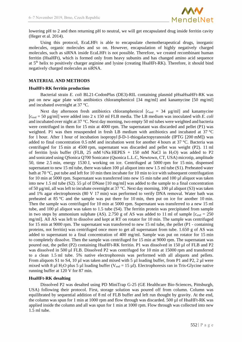
6–7 2019, Brno, Czech Republic
lowering pH to 2 and then returning pH to neutral, we will get encapsulated drug inside ferritin cavity (Heger et al. 2014).
Using this protocol, EcaLHFt is able to encapsulate chemotherapeutical drugs, inorganic molecules, organic molecules and so on. However, encapsulation of highly negatively charged molecules, such as siRNA inside EcaLHFt is not possible. Therefore, we created recombinant human ferritin (HsaHFt), which is formed only from heavy subunits and has changed amino acid sequence at 5th helix to positively charger arginine and lysine (creating HsaHFt-RK). Therefore, it should bind negatively charged molecules as siRNA.
MATERIAL AND METHODS
HsaHFt-RK ferritin production Bacterial strain E. coli BL21-CodonPlus (DE3)-RIL containing plasmid pHsaHsaHFt-RK was
put on new agar plate with antibiotics chloramphenicol [34 mg/ml] and kanamycine [50 mg/ml] and incubated overnight at 37 °C.
Next day afternoon fresh antibiotics chloramphenicol [cend = 34 µg/ml] and kanamycine [cend = 50 µg/ml] were added into 2 x 150 ml FLB media. The LB medium was inoculated with E. coli and incubated over night at 37 °C. Next day morning, two empty 50 ml tubes were weighted and bacteria were centrifuged in them for 15 min at 4000 rpm. The supernatant was discarded and pellet (P1) was weighted. P1 was then resuspended in fresh LB medium with antibiotics and incubated at 37 °C for 1 hour. After 1 hour of incubation isopropyl β-D-1-thiogalactopyranoside (IPTG [200 mM]) was added to final concentration 0.5 mM and incubation went for another 4 hours at 37 °C. Bacteria was centrifuged for 15 min at 4500 rpm, supernatant was discarded and pellet was weight (P2). 11 ml of ferritin lysis buffer (FLB, 25 mM ½Na HEPES + 150 mM NaCl in H2O) was added to P2 and sonicated using QSonica Q700 Sonicator (Qsonica L.L.C, Newtown, CT, USA) microtip, amplitude 50, time 2.5 min, energy 1530 J, working on ice. Centrifuged at 5000 rpm for 15 min, dispensed supernatant to new 15 ml tube, there was taken 100 µl aliquot into new 1.5 ml tube (S1). Preheated water bath at 70 °C, put tube and left for 10 min then incubate for 10 min to ice with subsequent centrifugation for 10 min at 5000 rpm. Supernatant was transferred into new 15 min tube and 100 µl aliquot was taken into new 1.5 ml tube (S2). 55 µl of DNase [10 mg/ml] was added to the sample to a final concentration of 50 µg/ml, all was left to incubate overnight at 37 °C. Next day morning, 100 µl aliquot (S3) was taken and 1% agar electrophoresis (80 V 17 min) was performed to verify DNA removal. Water bath was preheated at 85 °C and the sample was put there for 10 min, then put on ice for another 10 min. Then the sample was centrifuged for 10 min at 5000 rpm. Supernatant was transferred to a new 15 ml tube, and 100 µl aliquot was taken to 1.5 tube (S4). The ferritin protein was precipitated from sample in two steps by ammonium sulphate (AS). 2.750 g of AS was added to 11 ml of sample [cend = 250 mg/ml]. All AS was left to dissolve and kept at RT on rotator for 10 min. The sample was centrifuged for 15 min at 9000 rpm. The supernatant was transferred to new 15 ml tube, the pellet (P1 - containing proteins, not ferritin) was centrifuged once more to get all supernatant from tube. 1.650 g of AS was added to supernatant to a final concentration of 400 mg/ml. Sample was put on rotator for 15 min to completely dissolve. Then the sample was centrifuged for 15 min at 9000 rpm. The supernatant was poured out, the pellet (P2) containing HsaHFt-RK ferritin. P1 was dissolved in 150 µl of FLB and P2 was dissolved in 500 µl FLB. Dissolved P2 was centrifuged for 10 min at 15000 rpm and transferred to a clean 1.5 ml tube. 5% native electrophoresis was performed with all aliquots and pellets. From aliquots S1 to S4, 10 µl was taken and mixed with 5 µl loading buffer, from P1 and P2, 2 µl were mixed with 8 µl H2O plus 5 µl loading buffer (Vend = 15 µl). Electrophoresis ran in Tris-Glycine native running buffer at 120 V for 87 min.
HsaHFt-RK desalting Dissolved P2 was desalted using PD MiniTrap G-25 (GE Healthcare Bio-Sciences, Pittsburgh,
USA) following their protocol. First, storage solution was poured off from column. Column was equilibrated by sequential addition of 8 ml of FLB buffer and left run thought by gravity. At the end, the column was spun for 1 min at 1000 rpm and flow through was discarded. 500 µl of HsaHFt-RK was applied inside the column and all was spun for 1 min at 1000 rpm. Flow through was collected into new 1.5 ml tube.
552

6–7 2019, Brno, Czech Republic
Determination of protein concentration To determine the protein concentration of HsaHFt-RK, Bradford BioRad 500-0006 (BioRad,
California, USA) was used. BioRad dye reagent was diluted 1:5 with H2O. Standard samples of bovine serum albumin (BSA) were diluted to known concentration from 0.05 mg/ml to 0.6 mg/ml in seven-point linear curve plus blank sample. The HsaHFt-RK protein was diluted 10x and 100x. 10 µl of all samples were pipetted in 96 well-plate in triplicates. 200 µl diluted Bradford dye was added to the samples and left incubating for 5 min, then the absorbance was measured using Sunrise Basic Tecan (Tecan Group LtD., Männedorf, Switzerland) at 595 nm.
Encapsulation of FAM-siRNA EcaLHFt [50 mg/ml] and HsaHFt-RK [46.2 mg/ml] were diluted in a total volume of 100 µl
to final concentration 25 mg/ml. Fresh solutions of 1M HCl and 1M NaOH were prepared and one aliquot of FAM-siRNA [10µM] as let to defrost.
20 µl of EcaLHFt [25 mg/ml] and of HsaHFt-RK [25 mg/ml] was mixed with 50 µl H2O. Then, 10 µl NaOH [1M] was added, mixed well and left standing for 5 min. Then, 10 µl FAM-siRNA [10µM] was added, mixed well and incubated for 15 s, followed by addition of 10 µl HCl [1M]. Everything was mixed well and left standing for 5 min. The sample was split in half, first half was stored in fridge. To the second half, 0.5 µl RNase was added, mixed and incubated for 50 min at 37 °C. There were performed 1% agarose gel electrophoresis (80 V 20 min) and 6% native PAGE (120 V 85 min).
RESULTS AND DISCUSSION EcaLHFt as one of the most used ferritins in laboratory practice has a well known structure
(Figure 1). The structure is formed out of 2 heavy and 22 light subunits (Fukano et al. 2011). HsaHFt-RK ferritin is derived from human ferritin. It is formed out only by heavy subunits and amino acid sequence at C end of H5 helix was changed to arginine and lysine. Therefore, this ferritin is made to better and with higher efficiency bind negatively charged molecules.
Figure 1 Structure of EcaLHFt, modelled by our colleague Dr. Haddad
HsaHFt-RK isolation
HsaFtH-RK was produced in E. coli. As selective antibiotics kanamycine and chloramphenicol were used. Bacteria were incubated overnight. Next day first bacterial pellet (P1) was weighted. This pellet was incubated in fresh medium with added IPTG to induce plasmid translation and therefore production of our ferritin. After another incubation, the second bacterial pellet was weighted (P2, Table 1).
Second pellet was resuspended in FLB buffer and sonicated to disrupt bacteria cell wall and release ferritin to the solution. The solution was centrifuged to discard bacterial walls and organelles from protein lysate, and first aliquot (S1) was taken from supernatant. The protein lysate was heat denatured to discard unwanted proteins and molecules. Second aliquot (S2) was taken from supernatant after centrifugation.
553

6–7 2019, Brno, Czech Republic
Table 1 Weight of bacterial pellets
Sample Weight of empty tube (g) P1 (g) P2 (g)
HsaHFt-RK 1 13.46 13.71 14.16
13.37 13.81 14.09
Σ = 690 mg Σ = 1420 mg
HsaHFt-RK 2 13.36 13.58 13.95
13.36 13.70 14.09
Σ = 560 mg Σ = 1320 mg
Bacterial RNA was removed from solution by RNase. After incubation the third aliquot was taken (S3). Control agarose gel was performed from samples S2 and S3 to verify RNA and DNA removal (Figure 2).
Figure 2 Verification of DNA removal
Legend: 1 – S2 of HsaHFt-RK, 2 – S3 of HsaHFt-RK.
Second heat denaturation was done to remove another unwanted proteins. After centrifugation, the fourth aliquot was taken (S4). AS was used for a two-step salting out of proteins. The unwanted proteins were removed in the first step (P1). Higher concentration of AS lead to salting our HsaHFt-RK ferritin (P2). Both pellets were dissolved in FLB. After the last purification step, the supernatant with dissolved HsaHFt-RK was transferred to a sterile tube. Native PAGE was performed to verify protein isolation (Figure 3).
Figure 3 5% Native PAGE for verification ferritin isolation protocol
Legend: 1 – S1, 2 – S2, 3 – S3, 4 – S4, 6 – P1, 7 – P2 (ferritin HsaHFt-RK, desalted).
554
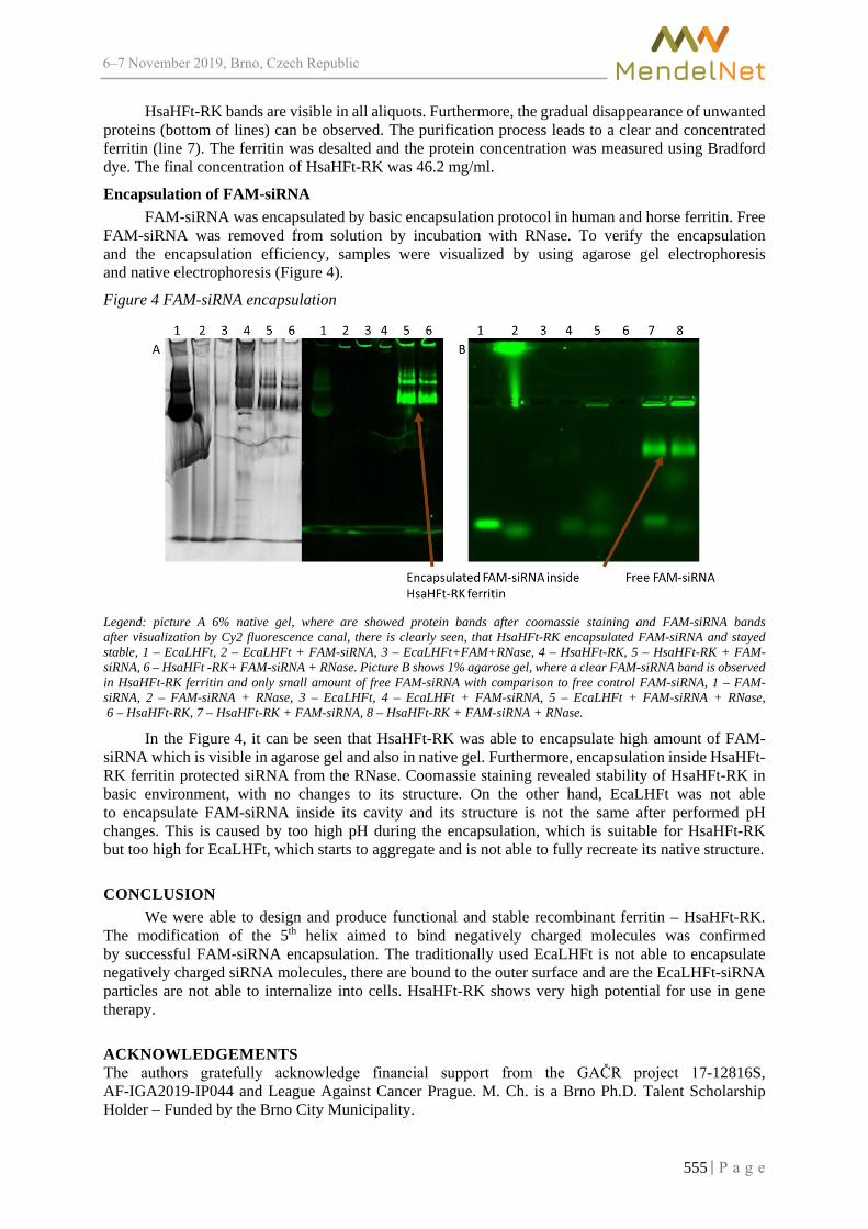
6–7 2019, Brno, Czech Republic
HsaHFt-RK bands are visible in all aliquots. Furthermore, the gradual disappearance of unwanted proteins (bottom of lines) can be observed. The purification process leads to a clear and concentrated ferritin (line 7). The ferritin was desalted and the protein concentration was measured using Bradford dye. The final concentration of HsaHFt-RK was 46.2 mg/ml.
Encapsulation of FAM-siRNA FAM-siRNA was encapsulated by basic encapsulation protocol in human and horse ferritin. Free
FAM-siRNA was removed from solution by incubation with RNase. To verify the encapsulation and the encapsulation efficiency, samples were visualized by using agarose gel electrophoresis and native electrophoresis (Figure 4).
Figure 4 FAM-siRNA encapsulation
Legend: picture A 6% native gel, where are showed protein bands after coomassie staining and FAM-siRNA bands after visualization by Cy2 fluorescence canal, there is clearly seen, that HsaHFt-RK encapsulated FAM-siRNA and stayed stable, 1 – EcaLHFt, 2 – EcaLHFt + FAM-siRNA, 3 – EcaLHFt+FAM+RNase, 4 – HsaHFt-RK, 5 – HsaHFt-RK + FAM-siRNA, 6 – HsaHFt -RK+ FAM-siRNA + RNase. Picture B shows 1% agarose gel, where a clear FAM-siRNA band is observed in HsaHFt-RK ferritin and only small amount of free FAM-siRNA with comparison to free control FAM-siRNA, 1 – FAM-siRNA, 2 – FAM-siRNA + RNase, 3 – EcaLHFt, 4 – EcaLHFt + FAM-siRNA, 5 – EcaLHFt + FAM-siRNA + RNase, 6 – HsaHFt-RK, 7 – HsaHFt-RK + FAM-siRNA, 8 – HsaHFt-RK + FAM-siRNA + RNase.
In the Figure 4, it can be seen that HsaHFt-RK was able to encapsulate high amount of FAM-siRNA which is visible in agarose gel and also in native gel. Furthermore, encapsulation inside HsaHFt-RK ferritin protected siRNA from the RNase. Coomassie staining revealed stability of HsaHFt-RK in basic environment, with no changes to its structure. On the other hand, EcaLHFt was not able to encapsulate FAM-siRNA inside its cavity and its structure is not the same after performed pH changes. This is caused by too high pH during the encapsulation, which is suitable for HsaHFt-RK but too high for EcaLHFt, which starts to aggregate and is not able to fully recreate its native structure.
CONCLUSION We were able to design and produce functional and stable recombinant ferritin – HsaHFt-RK.
The modification of the 5th helix aimed to bind negatively charged molecules was confirmed by successful FAM-siRNA encapsulation. The traditionally used EcaLHFt is not able to encapsulate negatively charged siRNA molecules, there are bound to the outer surface and are the EcaLHFt-siRNA particles are not able to internalize into cells. HsaHFt-RK shows very high potential for use in gene therapy.
ACKNOWLEDGEMENTS The authors gratefully acknowledge financial support from the GAČR project 17-12816S, AF-IGA2019-IP044 and League Against Cancer Prague. M. Ch. is a Brno Ph.D. Talent Scholarship Holder – Funded by the Brno City Municipality.
555

6–7 2019, Brno, Czech Republic
REFERENCES Banyard, S.H. et al. 1978. Electron density map of apoferritin at 2.8-Å resolution. Nature, 271(5642): 282. Bergman, P.J. 2009. Cancer immunotherapy. Topics in Companion Animal Medicine, 24(3): 130–136. Chen, G. et al. 2008. Apoferritin as a bionanomaterial to facilitate the electron transfer reactivity of hemoglobin and the catalytic activity towards hydrogen peroxide. Bioelectrochemistry, 72(1): 77–80. Domínguez-Vera, J.M., Colacio, E. 2003. Nanoparticles of Prussian blue ferritin: a new route for obtaining nanomaterials. Inorganic Chemistry, 42(22): 6983–6985. Fukano, H. et al. 2011. Synthesis of uniform and dispersive calcium carbonate nanoparticles in a protein cage through control of electrostatic potential. Inorganic Chemistry, 50(14): 6526–6532. Heger, Z. et al. 2014. Apoferritin applications in nanomedicine. Nanomedicine, 9(14): 2233–2245. Kang, S. et al. 2008. Controlled assembly of bifunctional chimeric protein cages and composition analysis using noncovalent mass spectrometry. Journal of the American Chemical Society, 130(49): 16527–16529. Todd, T.J. et al. 2013. Ferritin nanocages: great potential as clinically translatable drug delivery vehicles? Nanomedicine, 8(10): 1555–1557. Uchida, M. et al. 2006. Targeting of cancer cells with ferrimagnetic ferritin cage nanoparticles. Journal of the American Chemical Society, 128(51): 16626–16633. Wolfram, J., Ferrari, M. 2019. Clinical Cancer Nanomedicine. Nano Today, 25: 85–98.
556

6–7 2019, Brno, Czech Republic
Tuning LC-MS/MS analysis for identification of peptide extracts from cryosections of porcine lung tissue affected by Actinobacillus
pleuropneumoniae
Tomas Do1, Rea Jarosova2, Lada Ilieva1, Jiri Pospisil1, Roman Guran1,4, Petra Ondrackova5, Martin Faldyna5, Zbysek Sladek2, Ondrej Zitka1,3,4
1Department of Chemistry and Biochemistry 2Department of Morphology, Physiology and Animal Genetics
3CEITEC – Central European Institute of Technology Mendel University in Brno Zemedelska 1, 613 00 Brno
4Central European Institute of Technology Brno University of Technology Purkynova 123, 612 00 Brno 5Department of Immunology Veterinary Research Institute Hudcova 296/70, 621 00 Brno
CZECH REPUBLIC
Abstract: The porcine pleuropneumonia belongs to common pig bacterial infection caused by Actinobacillus pleuropneumoniae. This disease is affecting the economy of pig breeding. Therefore, it is important to better understand its effects and to find targeted therapy. To elucidate this infection different approaches can be used. One of them is to monitor the response of organism and detect changed expressions of proteins connected to immune reaction, especially cytokines subgroup called interleukins. Usually, these proteins are detected by enzyme-linked immunosorbent assay (ELISA), but other methods like label-free liquid chromatography connected with tandem mass spectrometry (LC-MS/MS) can be used. This study was aimed at adapting/developing a high-performance liquid chromatography-electrospray ionisation quadrupole time-of-flight mass spectrometry (HPLC-ESI-QqTOF MS) method for analysing these infection markers after on-tissue digestion and extraction from the surface of porcine lung tissue sections.
Key Words: liquid chromatography, electrospray-time of flight mass spectrometry, pulmonary infection, cytokine, pig
INTRODUCTION The lungs of pigs can be infected by various pathogens. One of the most important and serious
pulmonary diseases in pigs is porcine pleuropneumonia caused by a gram-negative bacterium Actinobacillus pleuropneumoniae (APP), originating from the family Pasteurellaceae. This bacterium is commonly found in all pigs worldwide. Porcine pleuropneumonia is described as a fibrinous, hemorrhagic, necrotizing and exudative pleuropneumonia (Zimmerman et al. 2012). Mainly the lung parenchymal tissue is affected by the APP. The clinical disease state depends largely on the animal’s immune status, on the serotype of infection and on the number of bacterial individuals in lungs. It can differ from peracute to chronic state. Among the symptoms of disease belong an increased respiratory rate, high fever, dyspnea, anorexia, coughing/sneezing, ataxia, vomiting, diarrhea, and severe respiratory distress with cyanosis. They have negative impact on breeding and therefore also on incomes of breeders (Bossé et al. 2002). The local expression of interleukins (IL)-1β, IL-6, IL-8, belonging to cytokines, and of tumor necrosis factor (TNF)-α in porcine lungs is the main immune response of organism (Hsu et al. 2016, Ondrackova et al. 2010).
557

6–7 2019, Brno, Czech Republic
One of the most suitable methods for quantification and identification of proteins/peptides in tissue extracts is the liquid chromatography connected with tandem mass spectrometry (LC-MS/MS). The best peptides separation performance for small volumes gives nanoLC (Emirbayer et al. 2017, Fanali 2017), but conventional HPLC columns can be used too (Gritti and Guiochon 2010). The cytokines were already analysed by LC-MS/MS in some previous works (Cobourne-Duval et al. 2018, Muqaku et al. 2015), but usually the sample preconcentration is crucial here because of very low concentrations of cytokines in tissues (Kupcova Skalnikova et al. 2017).
The focus of this work was the optimization of high performance liquid chromatography-electrospray ionisation quadrupole time-of-flight mass spectrometry (HPLC-ESI-QqTOF MS) method for the identification of proteins in the extracts of lung tissue slices.
MATERIAL AND METHODS
Chemicals All chemicals used for HPLC-ESI-QqTOF MS were purchased in LC-MS quality from VWR
International s.r.o. (Stribrna Skalice, Czech Republic). Other chemicals were purchased from Sigma Aldrich (St. Louis, MO, USA) in ACS quality, unless otherwise noted.
Animals and collection of samples Pieces of lymphatic and pulmonary tissues were taken from pigs infected by APP. A Pig breeding
was carried out at accredited experimental stables of Veterinary Research Institute in Brno. The experiment was performed in compliance with the Act No. 246/1992 Coll. of the Czech National Council on the protection of animals against cruelty, and with the agreement of the Branch Commission for Animal Welfare of the Ministry of Agriculture of the Czech Republic (approval no. 31674/2018-MZE-17214).
The infection with APP (field-origin strain, biotype 1, serotype 9, KL2-2000) was performed intranasally during an inhalation, and the infectious dose of 2 x 10⁹ bacteria was administered to the second third of each nasal cavity as described previously (Ondrackova et al. 2013). After euthanasia of the animals, samples of tracheobronchial lymph nodes and affected lung tissue were taken for subsequent laboratory analyses.
Preparation of samples and trypsinization The frozen lung tissue samples were cut to a thickness of 10 μm on the cryostat (Leica
Microsystems, CM 1900, GmbH, Wetzlar, Germany) at temperature -20 °C. The sections of tissue were placed on ITO (indium-tin oxide) glass slides (Bruker Daltonik GmbH, Bremen, Germany) and fixed in 70% ethanol for 90 s, then 100% ethanol for 90 s, ten times soaked in ultra-distilled water and again fixed in 70% ethanol for 90 s, then 100% ethanol for 90 s. Slides were stored at -80 °C before use.
An aqueous solution of bovine serum albumin (BSA) at concentration 20, 50 and 200 µg/ml was used as a standard sample which was deposited on a surface of lung tissue slices by pipetting 50 μl, each concentration was used per one lung tissue slice. Prior applying BSA solution, the ITO glass slides were warmed-up on a hand. After applying BSA solution, the ITO glass slides were put into vacuum desiccator for 15 min. Then, the ITO glass slides were put into ImagePrepTM (Bruker Daltonik GmbH, Bremen, Germany), where 300 μl of a trypsin solution (20 μg/ml in 40mM ammonium bicarbonate, 0.1 mM HCl and 9% acetonitrile) were sprayed onto ITO glass slides. The on-tissue trypsinization was performed in a small box with humid atmosphere, where the ITO glass slides were put, for 15 hours at 37 °C. After that, ITO glass slides were dried again in a vacuum desiccator for 15 min.
Then, the extraction of peptides was performed by applying 50 μl of 1% trifluoroacetic acid (aq) onto the same position of lung tissue slice as was applied the standard sample, waiting 1–2 min, and then carefully pipetting the solution into a glass vial (with 250 μl insert) without touching the surface of a tissue slice. Glass vials were then transferred into an autosampler. The scheme of preparation of samples and trypsinization is illustrated in Figure 1.
558
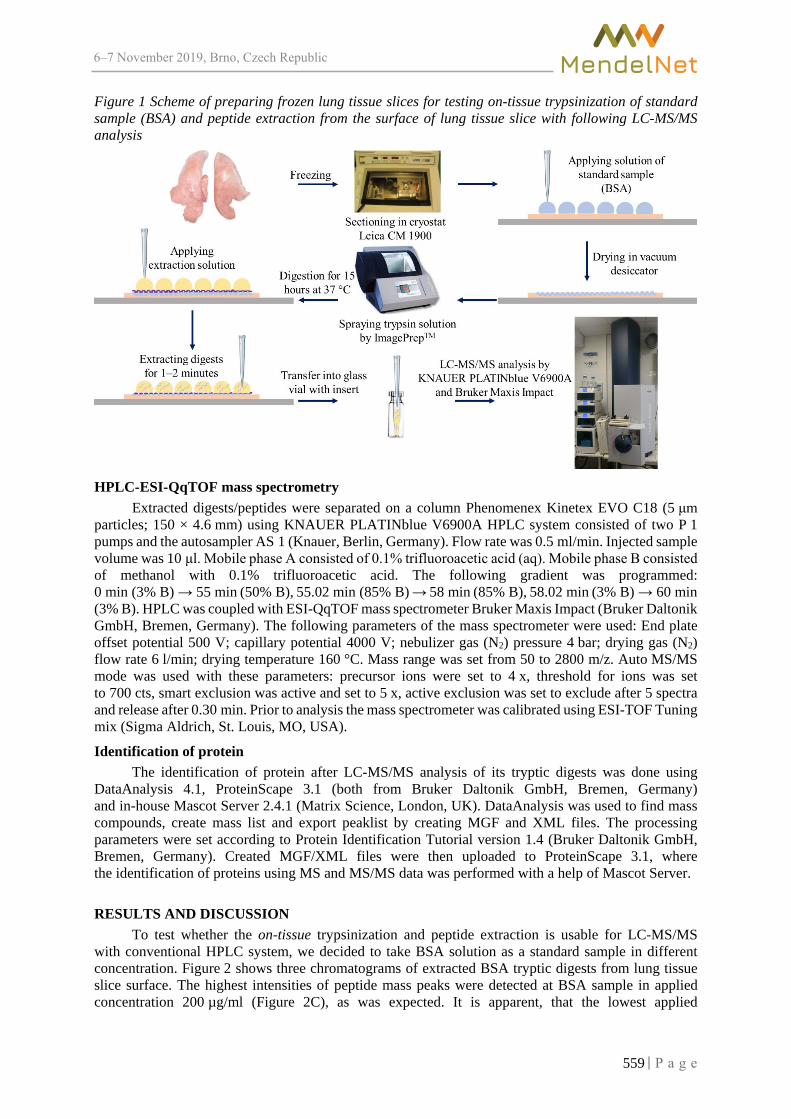
6–7 2019, Brno, Czech Republic
Figure 1 Scheme of preparing frozen lung tissue slices for testing on-tissue trypsinization of standard sample (BSA) and peptide extraction from the surface of lung tissue slice with following LC-MS/MS analysis
HPLC-ESI-QqTOF mass spectrometry
Extracted digests/peptides were separated on a column Phenomenex Kinetex EVO C18 (5 μm particles; 150 × 4.6 mm) using KNAUER PLATINblue V6900A HPLC system consisted of two P 1 pumps and the autosampler AS 1 (Knauer, Berlin, Germany). Flow rate was 0.5 ml/min. Injected sample volume was 10 μl. Mobile phase A consisted of 0.1% trifluoroacetic acid (aq). Mobile phase B consisted of methanol with 0.1% trifluoroacetic acid. The following gradient was programmed: 0 min (3% B) → 55 min (50% B), 55.02 min (85% B) → 58 min (85% B), 58.02 min (3% B) → 60 min (3% B). HPLC was coupled with ESI-QqTOF mass spectrometer Bruker Maxis Impact (Bruker Daltonik GmbH, Bremen, Germany). The following parameters of the mass spectrometer were used: End plate offset potential 500 V; capillary potential 4000 V; nebulizer gas (N2) pressure 4 bar; drying gas (N2) flow rate 6 l/min; drying temperature 160 °C. Mass range was set from 50 to 2800 m/z. Auto MS/MS mode was used with these parameters: precursor ions were set to 4 x, threshold for ions was set to 700 cts, smart exclusion was active and set to 5 x, active exclusion was set to exclude after 5 spectra and release after 0.30 min. Prior to analysis the mass spectrometer was calibrated using ESI-TOF Tuning mix (Sigma Aldrich, St. Louis, MO, USA).
Identification of protein The identification of protein after LC-MS/MS analysis of its tryptic digests was done using
DataAnalysis 4.1, ProteinScape 3.1 (both from Bruker Daltonik GmbH, Bremen, Germany) and in-house Mascot Server 2.4.1 (Matrix Science, London, UK). DataAnalysis was used to find mass compounds, create mass list and export peaklist by creating MGF and XML files. The processing parameters were set according to Protein Identification Tutorial version 1.4 (Bruker Daltonik GmbH, Bremen, Germany). Created MGF/XML files were then uploaded to ProteinScape 3.1, where the identification of proteins using MS and MS/MS data was performed with a help of Mascot Server.
RESULTS AND DISCUSSION To test whether the on-tissue trypsinization and peptide extraction is usable for LC-MS/MS
with conventional HPLC system, we decided to take BSA solution as a standard sample in different concentration. Figure 2 shows three chromatograms of extracted BSA tryptic digests from lung tissue slice surface. The highest intensities of peptide mass peaks were detected at BSA sample in applied concentration 200 µg/ml (Figure 2C), as was expected. It is apparent, that the lowest applied
559

6–7 2019, Brno, Czech Republic
concentration 20 µg/ml (Figure 2A) resulted in smaller intensities of peptide mass peaks and also caused loss of some peaks, probably because of too low concentration or ion suppression.
Figure 2 Comparison of HPLC-MS base peak chromatograms of digested bovine serum albumin in a concentration 20 (A), 50 (B) and 200 (C) µg/ml
After transferring measured LC-MS and LC-MS/MS data into ProteinScape, the identification results showed clearly, that there was a serum albumin. The highest number of identified peptides (Table 1) and the best Mascot score of identification (Table 2) showed LC-MS data from BSA sample at applied concentration 200 µg/ml.
Table 1 Peptides characterized by collision-induced dissociation (CID) together with identified protein. P stands for missed cleavages, z is a charge number.
Peptide m/z meas.
Mr calc. z Rt [min]
Score P Sequence Range Accession
1 571.8884 1141.7071 2 26.00 56.1 1 K.KQTALVELLK.H
548 - 557 gi|1351907
2 582.3453 1162.6234 2 25.20 48.7 0 K.LVNELTEFAK.T
66 - 75 gi|1351907
3 625.3362 1248.6139 2 18.80 41.2 1 R.FKDLGEEHFK.G
35 - 44 gi|1351907
4 653.3814 1304.7089 2 21.40 40.0 0 K.HLVDEPQNLIK.Q
402 - 412 gi|1351907
5 682.3647 2044.0207 3 31.10 35.7 1 R.RHPYFYAPELLYYA
NK.Y
168 - 183 gi|1351907
6 740.4139 1478.7882 2 28.90 61.5 0 K.LGEYGFQNALIVR.
Y
421 - 433 gi|1351907
7 756.4365 1510.8355 2 23.60 27.5 0 K.VPQVSTPTLVEVSR.
S
438 - 451 gi|1351907
8 784.3856 1566.7355 2 34.00 69.9 0 K.DAFLGSFLYEYSR.R
347 - 359 gi|1351907
9 789.4777 788.4644 1 16.20 31.0 0 K.LVTDLTK.V
257 - 263 gi|1351907
10 974.4573 973.4505 1 15.80 36.1 0 K.DLGEEHFK.G
37 - 44 gi|1351907
560

6–7 2019, Brno, Czech Republic
Table 2 Identified protein information. SC means sequence coverage.
Accession Protein MW [kDa] pI Database Score Number of
peptides SC [%]
gi|1351907 Serum albumin 69.2 5.8 NCBInr 101.4 10 17.1
Figure 3 illustrates the sequence coverage by identified peptides (highlighted by red color).
Figure 3 The sequence of identified serum albumin. Peptide sequences highlighted by red were detected and characterized by collision-induced dissociation (CID) by the mass spectrometer.
Our results showed, that it is possible to use on-tissue digestion and peptide extraction
from the surface of tissue slices. Nevertheless, we have not identified any other protein originating from lung tissue. It is probable, that concentration of BSA digests was much higher than the concentration of other peptides and that the extraction yields of these peptides were not as high as needed to be detected for further identification. To overcome these problems, it will be necessary to use some preconcentration techniques and optimize an extraction. In addition, the use of nanoLC separation system may improve the results as well. As another improvements, for example, in the recent study of Taverna and coworkers (Taverna et al. 2017), the polymeric hydrogel discs were used for localized digestion coupled with an isobaric mass tag strategy for peptide labeling and relative quantification.
CONCLUSION In this work we have optimized the HPLC-ESI-QqTOF method for identifying proteins
from frozen lung tissue slices after on-tissue trypsinization. It worked well with using BSA standard for a test, but for small concentration of proteins originating from pulmonary tissue an enhancement of this method by applying different extraction conditions and preconcentration techniques will be performed. We will also transfer this method to a micro- and nano-LC system and then we will optimize it on standards of interleukins.
ACKNOWLEDGEMENTS The research team has been supported by grant no. AF-IGA-2018-tym005 and by the project CEITEC 2020 (LQ1601) with financial support from the Ministry of Education, Youth and Sports of the Czech Republic under the National Sustainability Programme II and by EFRR “Multidisciplinary research to increase application potential of nanomaterials in agricultural” (No. CZ.02.1.01/0.0/0.0/16_025/ 0007314).
REFERENCES Bossé, J.T. et al. 2002. Actinobacillus pleuropneumoniae: pathobiology and pathogenesis of infection. Microbes and Infection, 4(2): 225–235. Cobourne-Duval, M.K. et al. 2018. Thymoquinone increases the expression of neuroprotective proteins while decreasing the expression of pro-inflammatory cytokines and the gene expression NF kappa B
561

6–7 2019, Brno, Czech Republic
pathway signaling targets in LPS/IFN gamma -activated BV-2 microglia cells. Journal of Neuro-immunology, 320: 87–97. Emirbayer, P.E. et al. 2017. Targeted label-free quantification of interleukin-8 in PMA-activated U937 cell secretome by nanoLC-ESI-MS/MS-sSRM. Proteomics, 17(9): 1600455. Fanali, S. 2017. An overview to nano-scale analytical techniques: Nano-liquid chromatography and capillary electrochromatography. Electrophoresis, 38(15): 1822–1829. Gritti, F., Guiochon, G. 2010. Performance of columns packed with the new shell Kinetex-C-18 particles in gradient elution chromatography. Journal of Chromatography A, 1217(10): 1604–1615. Hsu, C.-W. et al. 2016. Involvement of NF-κB in regulation of Actinobacillus pleuropneumoniae exotoxin ApxI-induced proinflammatory cytokine production in porcine alveolar macrophages. Veterinary Microbiology, 195: 128–135. Kupcova Skalnikova, H. et al. 2017. Advances in Proteomic Techniques for Cytokine Analysis: Focus on Melanoma Research. International Journal of Molecular Sciences, 18(12): 2697. Muqaku, B. et al. 2015. Quantification of cytokines secreted by primary human cells using multiple reaction monitoring: evaluation of analytical parameters. Analytical and Bioanalytical Chemistry, 407(21): 6525–6536. Ondrackova, P. et al. 2013. Distribution of porcine monocytes in different lymphoid tissues and the lungs during experimental Actinobacillus pleuropneumoniae infection and the role of chemokines. Veterinary Research, 44(1): 98. Ondrackova, P. et al. 2010. Porcine mononuclear phagocyte subpopulations in the lung, blood and bone marrow: dynamics during inflammation induced by Actinobacillus pleuropneumoniae. Veterinary Research, 41(5): 64. Taverna, D. et al. 2017. An optimized procedure for on-tissue localized protein digestion and quantification using hydrogel discs and isobaric mass tags: analysis of cardiac myxoma. Analytical and Bioanalytical Chemistry, 409(11): 2919–2930. Zimmerman, J.J. et al. 2012. Diseases of Swine, 10th Edition. John Wiley & Sons, Inc.
562

6–7 2019, Brno, Czech Republic
LC-MS/MS identification of proteins from a porcine lung tissue affected by Actinobacillus pleuropneumoniae
Tomas Do1, Rea Jarosova2, Eliska Sedlackova1,4, Roman Guran1,4, Petra Ondrackova5, Martin Faldyna5, Zbysek Sladek2, Ondrej Zitka1,3,4
1Department of Chemistry and Biochemistry 2Department of Morphology, Physiology and Animal Genetics
3CEITEC – Central European Institute of Technology Mendel University in Brno Zemedelska 1, 613 00 Brno
4Central European Institute of Technology Brno University of Technology Purkynova 123, 612 00 Brno 5Department of Immunology Veterinary Research Institute Hudcova 296/70, 621 00 Brno
CZECH REPUBLIC
Abstract: Targeted therapy of porcine pleuropneumonia, which is caused by the bacterium Actinobacillus pleuropneumoniae, would help pig breeders to lower their expenses related with solving this problem. In order to find potential receptors of a targeted therapy it is important to know the response of the organism on an infection and detect proteins connected to an immune reaction. Nowadays, a liquid chromatography connected with tandem mass spectrometry (LC-MS/MS) is one of the most used methods for this purpose. This study was aimed at detection and identification of proteins after homogenization and extraction from the porcine lung tissue cryosections by applying LC-MS/MS method using high-performance liquid chromatography-electrospray ionisation quadrupole-quadrupole time-of-flight mass spectrometry (HPLC-ESI-QqTOF MS).
Key Words: pig, liquid chromatography, tandem mass spectrometry, electrospray-time of flight mass spectrometry, pulmonary infection, proteins
INTRODUCTION The gram-negative bacterium Actinobacillus pleuropneumoniae (APP) can infect pigs worldwide,
causing severe pulmonary disease called the porcine pleuropneumonia. It is described as a necrotizing, hemorrhagic, fibrinous and exudative pleuropneumonia (Antenucci et al. 2017). APP infects mostly the lung parenchymal tissue. The clinical state of the organism can differ from peracute to chronic state, depending on the serotype of the infection, on the number of bacterial individuals and on the immune status. The main immune response of the organism is a local expression of interleukins and of a tumor necrosis factor (TNF)-α in porcine lungs (Ondrackova et al. 2010, Sassu et al. 2017, Xie et al. 2017).
For proteomics the best separation performance gives nanoLC (Emirbayer et al. 2017, Nassar et al. 2016). Conventional HPLC columns can be used too (Qi et al. 2019), but the sample preconcentration is usually needed, especially for detecting very low concentrations of cytokines in tissues (Cobourne-Duval et al. 2018, Kupcova Skalnikova et al. 2017, Muqaku et al. 2015).
We focused this work on the application of high-performance liquid chromatography-electrospray ionisation quadrupole-quadrupole time-of-flight mass spectrometry (HPLC-ESI-QqTOF MS) method for detection and identification of proteins from lung tissue cryosections extracts.
563

6–7 2019, Brno, Czech Republic
MATERIAL AND METHODS
Chemicals LC-MS quality chemicals were purchased from VWR International s.r.o. (Stribrna Skalice, Czech
Republic). Chemicals in ACS quality were purchased from Sigma Aldrich (St. Louis, MO, USA), unless otherwise noted.
Animals and collection of samples Pieces of lymphatic and pulmonary tissues were taken from pigs infected by APP. A pig breeding
was carried out at accredited experimental stables of Veterinary Research Institute in Brno. The experiment was performed in compliance with the Act No. 246/1992 Coll. of the Czech National Council on the protection of animals against cruelty, and with the agreement of the Branch Commission for Animal Welfare of the Ministry of Agriculture of the Czech Republic (approval no. 31674/2018-MZE-17214).
The infection with APP (field-origin strain, biotype 1, serotype 9, KL2-2000) was performed intranasally during inhalation, and the infectious dose of 2 x 10⁹ bacteria was administered to the second third of each nasal cavity as described previously (Ondrackova et al. 2013). After euthanasia of the animals, samples of tracheobronchial lymph nodes and the affected lung tissue were taken for subsequent laboratory analyses.
Preparation of samples and trypsinization The frozen lung tissue samples were cut to a thickness of 10 μm on the cryostat (Leica
Microsystems, CM 1900, GmbH, Wetzlar, Germany) at temperature -20 °C. The sections of tissue were placed on ITO (indium-tin oxide) glass slides (Bruker Daltonik GmbH, Bremen, Germany) and fixed in 70% ethanol for 90 s, then 100% ethanol for 90 s, ten times soaked in ultra-distilled water and again fixed in 70% ethanol for 90 s, then 100% ethanol for 90 s. Slides were stored at -80 °C before use.
ITO glass slides were warmed-up on a hand and the tissue sections were transferred into microvials with scalpel. Then, the homogenization, extraction and trypsinization protocol according to Sarah and coworkers (Sarah et al. 2016) was used and slightly changed: approximately 200 mg of tissue was homogenized in 1 ml of ice cold extraction buffer containing 7 M urea, 2 M thiourea, 50 mM dithiothreitol (DTT), 4% (w/v) 3-[(3-cholamidopropyl)dimethylammonio]-1-propanesulfonate (CHAPS), 0.4% (v/v) carrier ampholytes (pH 3–10; Bio-Rad, Hercules, CA) and 50 μl of protease inhibitor cocktail (Calbiochem; Merck Millipore), followed by centrifugation at 12,000 g for 10 min at 4 °C. The supernatant was collected and proteins were extracted by acetone precipitation. Briefly, 100 μl of protein were mixed with 4 volumes of cold acetone (400 μl, pre chilled at -20 °C for at least 1 h). The mixture was then vortexed and incubated at -20 °C overnight. The samples were then centrifuged at 12,000 g at 4 °C for 10 min. The resulting pellet was air-dried and re-solubilized in 1M urea extraction buffer (diluted in 100 mM ammonium bicarbonate). The total extractable protein concentration was then determined by Bradford assay.
Approximately 100 μg of extracted proteins were digested using trypsin. Briefly, samples were first reduced in 50 μl of 10 mM DTT/100 mM ammonium bicarbonate for 30 min at 60 °C. The mixture was then allowed to cool to room temperature before proceeding to the alkylation step: 50 μl of 55 mM IAA/100 mM ammonium bicarbonate for 20 min at room temperature (25 °C in the dark). In-solution tryptic digest was then performed with 1 μg of trypsin per 20 μg protein (in 25 mM ammonium bicarbonate, overnight at 37 °C). Tryptic peptides were then dried in a vacuum centrifuge Concentrator plus (Eppendorf Czech & Slovakia s.r.o., Ricany u Prahy, Czech Republic) and were acidified with 0.1% formic acid and subsequently subjected to a desalting procedure using ZipTip C18 (Millipore, Billerica, MA) before loading into LC-MS/MS.
LC-MS/MS Extracted digests/peptides were separated on a column Phenomenex Kinetex EVO C18 100Å
(1.7 µm particles; 100 × 2.1 mm) using KNAUER PLATINblue V6900A HPLC system consisted of two P 1 pumps and an autosampler AS 1 (Knauer, Berlin, Germany). Flow rate was 0.1 ml/min. Injected sample volume was 5 μl. Mobile phase A consisted of 0.1% trifluoroacetic acid (aq). Mobile phase B consisted of methanol with 0.1% trifluoroacetic acid. The following gradient was programmed:
564

6–7 2019, Brno, Czech Republic
0 min (3% B) → 60 min (50% B) → 80 min (85% B) → 100 min (85% B) → 100.02 min (3% B) → 120 min (3% B). HPLC was coupled with ESI-QqTOF mass spectrometer Bruker Maxis Impact (Bruker Daltonik GmbH, Bremen, Germany). The following parameters of the mass spectrometer were used: End plate offset potential 500 V; capillary potential 4000 V; nebulizer gas (N2) pressure 4 bar; drying gas (N2) flow rate 6 l/min; drying temperature 180 °C. Mass range was set from 50 to 2800 m/z. Auto MS/MS mode was used with these parameters: precursor ions were set to 20 x, threshold for ions was set to 2000 cts, smart exclusion was active and set to 5 x, active exclusion was set to exclude after 5 spectra and release after 0.30 min. Prior to analysis the mass spectrometer was calibrated using ESI-TOF Tuning mix (Sigma Aldrich, St. Louis, MO, USA).
Identification of protein The identification of proteins after LC-MS/MS analysis of tryptic digests was done using
DataAnalysis 4.1, ProteinScape 3.1 (both from Bruker Daltonik GmbH, Bremen, Germany) and in-house Mascot Server 2.4.1 (Matrix Science, London, UK). DataAnalysis was used to find mass compounds, create mass list and export peaklist by creating MGF and XML files. The processing parameters were set according to Protein Identification Tutorial version 1.4 (Bruker Daltonik GmbH, Bremen, Germany). Created MGF/XML files were then uploaded to ProteinScape 3.1, where the identification of proteins using MS and MS/MS data was performed with a help of Mascot Server. NCBIprot database was used. Carbamidomethylation of cysteine was chosen as fixed modification, oxidation of methionine was chosen as variable modification, one missed cleavage was allowed, MS/MS tolerance was set to ± 0.7 Da.
RESULTS AND DISCUSSION In Figure 1 is presented a 2D density plot of measured LC-MS/MS data, which was generated
in ProteinScape 3.1 after loading MGF/XML file exported from DataAnalysis 4.1.
Figure 1 Printscreen of 2D density plot of LC-MS/MS data from ProteinScape 3.1
Totally, 1375 compounds (peptides) were detected. From this, 55 proteins were identified based on 182 peptides. All of the identified proteins are listed in a Table 1. Most of the identified proteins are highly abundant in cells, therefore they are quite easily detected. No interleukins were identified, but some proteins from the list in Table 1, like Macrophage migration inhibitory factor, Peroxiredoxin-1 and Fructose-bisphosphate aldolase A can be connected with an immune response of the organism as was reported in previous studies (Al-Maleki et al. 2015, de Souza et al. 2019, Ding et al. 2017). Regarding the detection and identification of interleukins, it was probably below limits of used HPLC
565
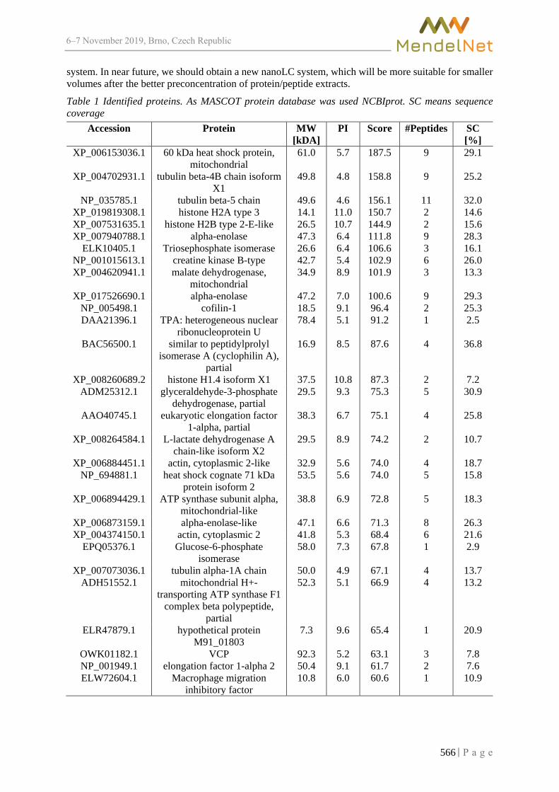
6–7 2019, Brno, Czech Republic
system. In near future, we should obtain a new nanoLC system, which will be more suitable for smaller volumes after the better preconcentration of protein/peptide extracts.
Table 1 Identified proteins. As MASCOT protein database was used NCBIprot. SC means sequence coverage
Accession Protein MW [kDA]
PI Score #Peptides SC [%]
XP_006153036.1 60 kDa heat shock protein, mitochondrial
61.0 5.7 187.5 9 29.1
XP_004702931.1 tubulin beta-4B chain isoform X1
49.8 4.8 158.8 9 25.2
NP_035785.1 tubulin beta-5 chain 49.6 4.6 156.1 11 32.0 XP_019819308.1 histone H2A type 3 14.1 11.0 150.7 2 14.6 XP_007531635.1 histone H2B type 2-E-like 26.5 10.7 144.9 2 15.6 XP_007940788.1 alpha-enolase 47.3 6.4 111.8 9 28.3
ELK10405.1 Triosephosphate isomerase 26.6 6.4 106.6 3 16.1 NP_001015613.1 creatine kinase B-type 42.7 5.4 102.9 6 26.0 XP_004620941.1 malate dehydrogenase,
mitochondrial 34.9 8.9 101.9 3 13.3
XP_017526690.1 alpha-enolase 47.2 7.0 100.6 9 29.3 NP_005498.1 cofilin-1 18.5 9.1 96.4 2 25.3 DAA21396.1 TPA: heterogeneous nuclear
ribonucleoprotein U 78.4 5.1 91.2 1 2.5
BAC56500.1 similar to peptidylprolyl isomerase A (cyclophilin A),
partial
16.9 8.5 87.6 4 36.8
XP_008260689.2 histone H1.4 isoform X1 37.5 10.8 87.3 2 7.2 ADM25312.1 glyceraldehyde-3-phosphate
dehydrogenase, partial 29.5 9.3 75.3 5 30.9
AAO40745.1 eukaryotic elongation factor 1-alpha, partial
38.3 6.7 75.1 4 25.8
XP_008264584.1 L-lactate dehydrogenase A chain-like isoform X2
29.5 8.9 74.2 2 10.7
XP_006884451.1 actin, cytoplasmic 2-like 32.9 5.6 74.0 4 18.7 NP_694881.1 heat shock cognate 71 kDa
protein isoform 2 53.5 5.6 74.0 5 15.8
XP_006894429.1 ATP synthase subunit alpha, mitochondrial-like
38.8 6.9 72.8 5 18.3
XP_006873159.1 alpha-enolase-like 47.1 6.6 71.3 8 26.3 XP_004374150.1 actin, cytoplasmic 2 41.8 5.3 68.4 6 21.6
EPQ05376.1 Glucose-6-phosphate isomerase
58.0 7.3 67.8 1 2.9
XP_007073036.1 tubulin alpha-1A chain 50.0 4.9 67.1 4 13.7 ADH51552.1 mitochondrial H+-
transporting ATP synthase F1 complex beta polypeptide,
partial
52.3 5.1 66.9 4 13.2
ELR47879.1 hypothetical protein M91_01803
7.3 9.6 65.4 1 20.9
OWK01182.1 VCP 92.3 5.2 63.1 3 7.8 NP_001949.1 elongation factor 1-alpha 2 50.4 9.1 61.7 2 7.6 ELW72604.1 Macrophage migration
inhibitory factor 10.8 6.0 60.6 1 10.9
566
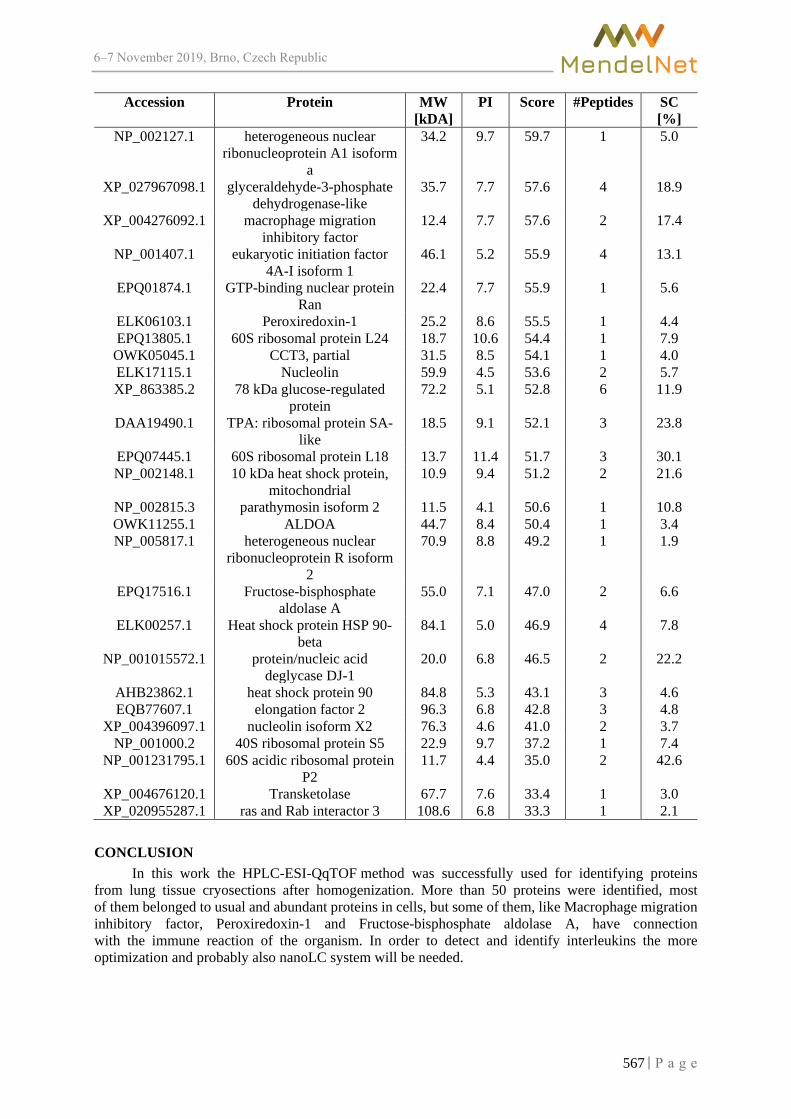
6–7 2019, Brno, Czech Republic
Accession Protein MW [kDA]
PI Score #Peptides SC [%]
NP_002127.1 heterogeneous nuclear ribonucleoprotein A1 isoform
a
34.2 9.7 59.7 1 5.0
XP_027967098.1 glyceraldehyde-3-phosphate dehydrogenase-like
35.7 7.7 57.6 4 18.9
XP_004276092.1 macrophage migration inhibitory factor
12.4 7.7 57.6 2 17.4
NP_001407.1 eukaryotic initiation factor 4A-I isoform 1
46.1 5.2 55.9 4 13.1
EPQ01874.1 GTP-binding nuclear protein Ran
22.4 7.7 55.9 1 5.6
ELK06103.1 Peroxiredoxin-1 25.2 8.6 55.5 1 4.4 EPQ13805.1 60S ribosomal protein L24 18.7 10.6 54.4 1 7.9
OWK05045.1 CCT3, partial 31.5 8.5 54.1 1 4.0 ELK17115.1 Nucleolin 59.9 4.5 53.6 2 5.7 XP_863385.2 78 kDa glucose-regulated
protein 72.2 5.1 52.8 6 11.9
DAA19490.1 TPA: ribosomal protein SA-like
18.5 9.1 52.1 3 23.8
EPQ07445.1 60S ribosomal protein L18 13.7 11.4 51.7 3 30.1 NP_002148.1 10 kDa heat shock protein,
mitochondrial 10.9 9.4 51.2 2 21.6
NP_002815.3 parathymosin isoform 2 11.5 4.1 50.6 1 10.8 OWK11255.1 ALDOA 44.7 8.4 50.4 1 3.4 NP_005817.1 heterogeneous nuclear
ribonucleoprotein R isoform 2
70.9 8.8 49.2 1 1.9
EPQ17516.1 Fructose-bisphosphate aldolase A
55.0 7.1 47.0 2 6.6
ELK00257.1 Heat shock protein HSP 90-beta
84.1 5.0 46.9 4 7.8
NP_001015572.1 protein/nucleic acid deglycase DJ-1
20.0 6.8 46.5 2 22.2
AHB23862.1 heat shock protein 90 84.8 5.3 43.1 3 4.6 EQB77607.1 elongation factor 2 96.3 6.8 42.8 3 4.8
XP_004396097.1 nucleolin isoform X2 76.3 4.6 41.0 2 3.7 NP_001000.2 40S ribosomal protein S5 22.9 9.7 37.2 1 7.4
NP_001231795.1 60S acidic ribosomal protein P2
11.7 4.4 35.0 2 42.6
XP_004676120.1 Transketolase 67.7 7.6 33.4 1 3.0 XP_020955287.1 ras and Rab interactor 3 108.6 6.8 33.3 1 2.1
CONCLUSION In this work the HPLC-ESI-QqTOF method was successfully used for identifying proteins
from lung tissue cryosections after homogenization. More than 50 proteins were identified, most of them belonged to usual and abundant proteins in cells, but some of them, like Macrophage migration inhibitory factor, Peroxiredoxin-1 and Fructose-bisphosphate aldolase A, have connection with the immune reaction of the organism. In order to detect and identify interleukins the more optimization and probably also nanoLC system will be needed.
567

6–7 2019, Brno, Czech Republic
ACKNOWLEDGEMENTS The research team has been supported by grant no. AF-IGA-2018-tym005 and by the project CEITEC 2020 (LQ1601) with financial support from the Ministry of Education, Youth and Sports of the Czech Republic under the National Sustainability Programme II and by EFRR “Multidisciplinary research to increase application potential of nanomaterials in agricultural” (No. CZ.02.1.01/0.0/0.0/ 16_025/0007314).
REFERENCES Al-Maleki, A.R. et al. 2015. Altered Proteome of Burkholderia pseudomallei Colony Variants Induced by Exposure to Human Lung Epithelial Cells. Plos One, 10(5): 31. Antenucci, F. et al. 2017. Identification and characterization of serovar-independent immunogens in Actinobacillus pleuropneumoniae. Veterinary Research, 48(1): 74. Cobourne-Duval, M.K. et al. 2018. Thymoquinone increases the expression of neuroprotective proteins while decreasing the expression of pro-inflammatory cytokines and the gene expression NF kappa B pathway signaling targets in LPS/IFN gamma -activated BV-2 microglia cells. Journal of Neuroimmunology, 320: 87–97. De Souza, G.F. et al. 2019. Macrophage migration inhibitory factor (MIF) controls cytokine release during respiratory syncytial virus infection in macrophages. Inflammation Research, 68(6): 481–491. Ding, C.B. et al. 2017. Peroxiredoxin 1-an antioxidant enzyme in cancer. Journal of Cellular and Molecular Medicine, 21(1): 193–202. Emirbayer, P.E. et al. 2017. Targeted label-free quantification of interleukin-8 in PMA-activated U937 cell secretome by nanoLC-ESI-MS/MS-sSRM. PROTEOMICS, 17(9): 1600455. Kupcova Skalnikova, H. et al. 2017. Advances in Proteomic Techniques for Cytokine Analysis: Focus on Melanoma Research. International Journal of Molecular Sciences, 18(12): 2697. Muqaku, B. et al. 2015. Quantification of cytokines secreted by primary human cells using multiple reaction monitoring: evaluation of analytical parameters. Analytical and Bioanalytical Chemistry, 407(21): 6525–6536. Nassar, A.F. et al. 2016. Rapid label-free profiling of oral cancer biomarker proteins using nano-UPLC-Q-TOF ion mobility mass spectrometry. Proteomics Clinical Applications, 10(3): 280–289. Ondrackova, P. et al. 2013. Distribution of porcine monocytes in different lymphoid tissues and the lungs during experimental Actinobacillus pleuropneumoniae infection and the role of chemokines. Veterinary Research, 44(1): 98–98. Ondrackova, P. et al. 2010. Porcine mononuclear phagocyte subpopulations in the lung, blood and bone marrow: dynamics during inflammation induced by Actinobacillus pleuropneumoniae. Veterinary Research, 41(5): 64. Qi, K.L. et al. 2019. A rapid immobilized trypsin digestion combined with liquid chromatography-Tandem mass spectrometry for the detection of milk allergens in baked food. Food Control, 102: 179–187. Sarah, S.A. et al. 2016. LC-QTOF-MS identification of porcine-specific peptide in heat treated pork identifies candidate markers for meat species determination. Food Chemistry, 199: 157–164. Sassu, E.L. et al. 2017. Frequency of Th17 cells correlates with the presence of lung lesions in pigs chronically infected with Actinobacillus pleuropneumoniae. Veterinary Research, 48(1): 4. Xie, F. et al. 2017. Attenuated Actinobacillus pleuropneumoniae double-deletion mutant S-8 Delta clpP/apxIIC confers protection against homologous or heterologous strain challenge. Bmc Veterinary Research, 13(1): 14.
568
6–7 2019, Brno, Czech Republic
Biogenic amines modified carbon quantum dots as antibacterial agent
Milica Gagic1,2, Silvia Kociova1,2, Lukas Richtera1,2, Kristyna Smerkova1,2, Vedran Milosavljevic1,2
1Department of Chemistry and Biochemistry Mendel University in Brno Zemedelska 1, 613 00 Brno
2Central European Institute of Technology Brno University of Technology Purkynova 123, 612 00 Brno
CZECH REPUBLIC [email protected]
Abstract: An alternative to conventional way is needed to treat multiple drug resistant bacteria. In this work, four different amine modified carbon quantum dots (CQDs) were obtained by microwave irradiation treatment. The four different biogenic amines (spermidine, putrescine, cadaverine, and histamine) as capping agent and citric acid as a carbon precursor were used. Prepared CQDs were evaluated for their antibacterial activity against three common pathogenic bacteria (Escherichia coli, Klebsiella pneumonia, Staphylococcus aureus), and the growth curves were modeled. The CQDs showed a strong broad-spectrum antibacterial activity. The bactericidal activity was linked to their specific surface chemistry and caused bacterial death, which was due to the electrostatic interactions between protonated CQDs and the lipids of the bacterial cell membrane. The biocompatibility of CQDs was tested in HBL100 and HEK293 cell lines and low or absence of toxicity was indicated.
Key Words: carbon quantum dots, antibacterial, biogenic amines, pathogenic bacteria, resistance
INTRODUCTION Due to the systematic massive use of antibiotics, bacteria have evolved sophisticated mechanisms
of drug resistance to avoid killing by antimicrobial molecules. Resistance is usually achieved through multiple biochemical pathways, and one bacterial cell may be capable of using a cadre of mechanisms of resistance to survive the effect of an antibiotic. It is estimated that bacteria resistant to antibiotics kill around 700,000 people per year. World Health Organization warns that there is an urgent need to invest in the research about resistant infections and way, how to treat them. The past decade has witnessed a substantial increase in the global use of nanoscale materials as innovative tools for combating these pathogens. Among the most recent discovered are carbon quantum dots (CQDs). CQDs are small carbon nanoparticles, generally exhibiting sizes smaller than 10 nm (Lim et al. 2015). They can be synthesized from any carbonaceous precursors, without being in general toxic, therefore they have been increasingly used in biological and biomedical applications (Zuo et al. 2016).
CQDs are reported by several studies as effective antibacterial agents. Although applied against both gram-positive and gram-negative bacteria, mode of action is not yet fully elucidated. Up to now, the antibacterial mechanism has been partially considered as the effect of disrupting the membrane integrity (Li et al. 2011). In 2016, Yang et al. reported CQDs with a minimum inhibitory concentration of 8 μg/mL for Staphylococcus aureus (Yang et al. 2016). The bactericidal activity was accomplished through electrostatic interaction between the anionic bacterial membrane and cationic residues on the CQDs surface (Liu et al. 2017). Similar electrostatically based inhibitory effect was described year after by Liu et al. against Porphyromonas gingivali (Liu et al. 2017). Depending on surface functionalization, CQDs may carry a negative, neutral or positive charge. To explore enhanced antibacterial effect based on electrostatic interaction between CQDs and bacteria, four biogenic amines (putrescine, spermidine, histamine, and cadaverine) were used as capping agents for CQDs (PCQDs, SCQDs, HCQDs and CCQDs). At physiologic pH these amines carry a net positive charge. It was demonstrated significant bactericidal activity of prepared CQDs toward three pathogenic bacteria.
569

6–7 2019, Brno, Czech Republic
The biocompatible CQDs were prepared through microwave irradiation of a mixture of citric acid and respective biogenic amine. The size and surface charge were characterized by dynamic light scattering.
MATERIAL AND METHODS
Chemicals The chemicals used in this work were purchased from Sigma Aldrich (St. Louis, MO, USA).
Deionized water was purified to produce 18.2 MΩ/cm MilliQ water using Millipore RG (Bedford, MA, USA).
Preparation of amine modified CQDs For the preparation of CQDs, citric acid was used as the carbon source. 5.0 g of citric acid
was mixed with 1.0 g of respective biogenic amine and diluted in 10 mL water. Then, 1.0 mL of the solution was aliquoted into the vials and heated at 110 °C and 300 W for 10 min (ramping time of 10 min) under microwave irradiation (Multiwave 3000; Anton-Paar GmbH, Graz, Austria). Finally, the products were purified by dialyzing (membrane with 1000 MWCO) against MiliQ, freeze dried and dissolved in water to obtain the concentration of 1.0 mg/mL.
Characterization of CQDs The zeta potential (ζ) and size of CQDs were determined by dynamic light scattering technique
(DLS) using the Zetasizer Nano ZS instrument (Malvern Instrument Ltd, UK). The parameters of particle size measurements were follows: refraction index of the dispersive phase of 3.00 and 1.333 for the dispersive environment, adsorption coefficient 10−3, temperature 25 °C, equilibration time 120 s, measurement angle of 173° backscatter. For measurement, disposable cuvettes type ZEN 0040 was used, containing 50 µL of sample. The ζ measurements were also performed at 25 ºC in polycarbonate folded capillary cells, incorporated with Au plated beryllium-copper electrodes (DTS1070) and deionized H2O was the dispersion medium. ζ were automatically obtained by the software using the Smoluchowski approximation.
In vitro bacterial testing The antibacterial effect of CQDs was analyzed by bacterial growth curves. Escherichia
coli NCTC 13216, Klebsiella pneumonia NCTC 8511, and Methicillin resistant S. aureus CCM 7110 (Czech Collection of Microorganisms, Brno, Czech Republic) were cultured on Muller-Hinton (MH) agar (Oxoid, Hampshire, UK) overnight at 37 °C.
Growth curve method One hundred μL of each bacterial suspension (1.0 × 10⁶ CFU/mL) was placed into a 100-well
microplate and mixed with CQDs (1.0 mg/mL), in the ratio 1:1. To monitor growth trends, Bioscreen C (Oy Growth Curves Ab Ltd, Helsinki, Finland) was used. The bacterial growth curves were achieved by measuring the optical density (OD) of the cultures and plotting it against time. OD reads at 600 nm were monitored at time zero, and then at 30 min intervals for 24 h at 37 °C.
Cell viability assay To assess effect of particles on the viability of HBL100 and HEK293 cell lines, MTT assay was
performed. The cells viability was tested by Infinite 200 PRO (Tecan, Maennedorf, Switzerland) using 96 well microtiter plates. Each microtiter plate well was filled with 50 μL of medium containing the suspension of 5.000 cells. The cell lines were treated with the samples in wide concentration range (from 0 to 500 μg/mL) and incubated for 24 h at 37 °C with 5% CO2.
RESULT AND DISCUSSION
Synthesis and Characterization of CDs In our experiment CQDs were synthesized by microwave irradiation. Firstly size and ζ potential
were monitored by DLS. The hydrodynamic diameter size of prepared CQDs is presented in the Figure 1, which reveals that prepared QDs have size of approximately 1.5 nm and are very close
570

6–7 2019, Brno, Czech Republic
to each other. The functional groups on the surface are expect to have an effect on the overall charge of our CQDs. The ζ potential values measured were 1.96 ± 0.27, 0.22 ± 0.16, 1.25 ± 0.51, 1.40 ± 0.34, for CCQDs, PCQDs, SCQDs and HCQDs (Figure 1A–D), respectively. Zeta potential in all cases is positive thus indicating the predominance of amine groups on the dots surfaces.
Figure 1 The hydrodynamic size distribution of: A) spremidine carbon quantum dots, SCQDs B) cadaverine carbon quantum dots, CCQDs, putrescine carbon quantum dots, PCQDs and D) histamine carbon quantum dots, HCQDs. The error bars are values expressed as mean ± standard deviation.
In vitro antibacterial activity Assuming that the OD at 600 nm reflects the number density of bacterial cells, its value was found
to increase in a sigmoid fashion in the absence of prepared quantum dots. In vitro antibacterial effect of prepared CQDs was verified by bacterial growth curves and the results are shown in Figure 2. Growth patterns of bacteria K. pneumonia, Methicillin resistant S. aureus and E.coli were obtained by plotting bacteria inhibition values against time. Growth patterns of all the selected bacteria were obtained in the presence of different CQDs concentration (0–4 mg/mL) in the bacterial growth media. Growth inhibition of each bacteria was observed suggesting significant antibacterial effect of all applied CQDs with 100% efficiency at different concentration.
Toxicity study in mammalian cells The biocompatibility and cytotoxic effect of the prepared nanomaterials on HBL-100 and HEK-
293 cells were metabolically quantified through MTT assay. The obtained results were plotted as percentage cell viability versus concentration of CQDs and are shown in Figure 3. As can be inferred from the Figure 3, among all the prepared samples, the minimum percentage cell viability observed was around 60% corresponding to the highest tested concentration (2.5 mg/mL) of HCQDs. More than 80% of the HBL100 cells (Figure 3A), were viable after the treatment with 1.25 mg/mL and less in all the prepared samples. Based on the obtained results, going by the definition of biocompatibility which requires minimum 80% of cells to be viable, we can easily say that all our tested samples are biocompatible. On exposure to HEK293 cells (Figure 3B), prepared CQDs didn’t show any decrease in cell viability at concentration from 2.5–0.03 mg/mL, thus indicating extraordinary biocompatibility.
571

6–7 2019, Brno, Czech Republic
Figure 2 The inhibition effect of prepared CQDs on (A) Staphylococcus aureus, (B) Escherichia coli and (C) Klebsiella pneumonia, respectively
Figure 3 Cytotoxicity of prepared CQDs in (A) HBL-100 and (B) HEK-293 cells
CONCLUSION In conclusion, we have demonstrated, through the growth curves analysis method that carbon
quantum dots, modified with biogenic amines obtained by a simple microwave irradiation approach, have a capability to act as bactericides against tested strains. We found that all four CQDs formulations inhibited bacterial growth in vitro of both, gram-negative and gram-positive bacteria. Probably, the bacterial cell death induced by CQDs involved electrostatic interactions between the protonated forms of the nitrogen functional groups and the negatively charged cell membrane.
ACKNOWLEDGEMENTS The research was financially supported by IGA grant no. AF-IGA2019-IP051.
REFERENCES Li, P. et al. 2011. A polycationic antimicrobial and biocompatible hydrogel with microbe membrane suctioning ability. Nature Materials, 10(2): 149–156.
572

6–7 2019, Brno, Czech Republic
Lim, S. Y. et al. 2015. Carbon quantum dots and their applications. Chemical Society Reviews, 44(1): 362–381. Liu, J. et al. 2017. One-step hydrothermal synthesis of photoluminescent carbon nanodots with selective antibacterial activity against Porphyromonas gingivalis. Nanoscale, 9(21): 7135–7142. Yang, J. et al. 2016. Carbon Dot-Based Platform for Simultaneous Bacterial Distinguishment and Antibacterial Applications. ACS Applied Materials & Interfaces, 8(47): 32170–32181. Zuo, P. et al. 2016. A review on syntheses, properties, characterization and bioanalytical applications of fluorescent carbon dots. Microchimica Acta [Online], 183(2): 519–542.
573

6–7 2019, Brno, Czech Republic
Transfer of mercury to mycelia of Armillaria cepistipes and Pleurotus ostreatus
Jana Hrachovinova1, Pavlina Pelcova1, Andrea Ridoskova1, Jan Grmela2, Ester Badinova1
1Department of Chemistry and Biochemistry 2 Department of Zoology, Fisheries, Hydrobiology and Apiculture
Mendel University in Brno Zemedelska 1, 613 00 Brno
CZECH REPUBLIC
Abstract: Fungi can bioaccumulate mercury from the substrate by mycelium and can be a health risk to their consumers. The transfer and bioavailability of mercury from contaminated forest soils to mycelia of Armillaria cepistipes and Pleurotus ostreatus was observed. The mercury concentration in mycelia increased linearly with increasing concentration of mercury in contaminated forest soils. The maximum mercury contents in mycelia were observed at 3–5 day after inoculation of mycelia on test soil. Statistically significantly higher mercury content was found in Pleurotus ostreatus mycelium, when mycelia were cultivated on highly contaminated soils. Bioconcentration factors were in the range 0.13–0.41 for Armillaria cepistipes, and between 0.16–0.56 for Pleurotus ostreatus.
Key Words: Jedová hora, bioaccumulation, atomic absorption spectrometry, soil, mycelium
INTRODUCTION Mercury pollution is global problem, because mercury has a high bioaccumulation capacity,
biotoxicity, mobility, and persists in the environment for a long time (Cozzolino et al. 2016). At present, the main source of mercury is industrial production, mining, metallurgy, and fossil
fuel combustion. Mercury compounds are released from anthropogenic and natural sources into all environmental compartments. From contaminated soil, mercury compounds can be bioaccumulated into fungi and may be a potential health risk for humans. Mycelium is generally considered to be the decisive organ of heavy metals uptake into a fungus (Kalac 2013).
The relationship between the bioavailability of mercury in soil and the accumulation of mercury by mycelium is very common, especially in the case of saprophytic fungi. However, this relationship is strongly dependent on the fungus species, body parts and size of fungus, mycelium age, soil characteristics, and composition, as well as the bioavailability of the mercury, mercury speciation and fractionation in soil (Zurera et al. 1986).
The aim of this work was to determine the bioavailability of mercury from mercury-contaminated soils into mycelia of Armillaria cepistipes and Pleurotus ostreatus. Tested species of wood-decaying fungi were cultivated on forest soil, because mercury naturally contaminated woody matter was not available.
MATERIAL AND METHODS
Sampling sites and treatment of soil samples The forest soils from surrounding of the Barbora mining adit located on Jedová hora (English
translation – Poison hill) were collected in May 2017. The soils were designated as 1S, 2S, and 5S. The GPS coordinates of sampling sites are listed in the Table 1. Jedová hora is forested hill locate about 4 km from the town Hořovice (Czech Republic). Jedová hora is one of the three Czech historical sites where cinnabar was mined from the 14th to 19th centuries. In addition to cinnabar, there was mainly mined iron ore (Velebit 2003).
574

6–7 2019, Brno, Czech Republic
The control forest soil was collected in the vicinity of Deblín and the GPS coordinates of sampling site are given in the Table 1. After removal of the plant material, the soil samples were collected at a depth of approximately 10–15 cm from the surface into plastic buckets. In the laboratory, foreign materials such as stones, roots, and branches were separated from the soil, and then the samples were dried under laboratory temperature (21 °C). The dried samples were screened to a mesh size of 2 mm. Approximately 1 kilogram of soil fraction remaining under the sieve was homogenized, stored in plastic screw boxes, and used for the experiment. The homogenized soils had a particle size of less than 250 µm.
Table 1 GPS coordinates of sampling sites Sampling site GPS coordinates Control 49° 18' 43.9''N, 16° 19' 19.1''E 1S 49° 47' 33.0''N, 13° 53' 07.9''E 2S 49° 47' 30.7''N, 13° 53' 14,8''E 5S 49° 47' 34.0''N, 13° 53' 21,4''E
Cultivation and treatment of mycelia The mycelium of the Armillaria cepistipes and Pleurotus ostreatus was used for the experiment.
The mycelia were obtained from the Department of Forest Protection and Wildlife Management (Faculty of Forestry and Wood Technology MENDELU Brno).
Prior to inoculation to the soil, mycelia were cultivated on agar (PDA = Potato Dextrose Agar) in Petri dishes. The agar was prepared by mixing 19.5 g of PDA (Sigma-Aldrich s.r.o., St. Louis, Missouri, USA) with 500 ml of Milli Q water (Millipore, Bedford, USA) and sterilized at 121 °C, pressure 0.1–0.15 MPa for 15 min (Autoclave 2840 EL-D, Tuttnauer, Hauppauge, New York, USA). Fungal plugs (0.4 mm in diameter) were placed at the center of Petri dishes into PDA culture media and were incubated at 28 °C for 7 days. After this period, the mycelium was inoculated onto sterilized control and contaminated soil (7.5 ± 0.2 g of soil). The soil was first moistened with 5 ml of PDB (Potato Dextrose Broth) solution (Sigma-Aldrich s.r.o., St. Louis, Missouri, USA). PDB was prepared by mixing 12 g of PDB with 500 ml of Milli Q and was autoclaved. The PDB provided suitable conditions for the growth and nutrition of mycelium. A sterilized plastic mesh-work was placed on the moist soil to facilitation remove the expanded mycelium from the soil. The mycelium was inoculated onto the soil with a plastic microbiological stick and mycelium was again moistened with 5 ml PDB. The Petri dishes were sealed with parafilm and incubated in a thermostat at 28 °C. Mycelium was collected every two days. The collected mycelium was rinsed by Milli Q water and lyophilized at -51 °C and 0.018 mBar for 25 h by lyophilizer FreeZone 2.5L (Labconco, Kansas City, Missouri, USA). The lyophilized samples were homogenized with a screw homogenizer (Schütt Homgenplus, Schuett-biotec, Göttingen, Germany) and were kept in a desiccator.
Mercury determination Determination of total mercury content in samples of soil and mycelium was performed using
atomic absorption spectrometry (Advanced Mercury Analyser, AMA 254, Altec, Praha Czech Republic). The soils (50 ± 1 mg), or mycelia (5 ± 1 mg) were inserted directly into atomic absorption spectrometry and analyzed under optimized conditions of drying (120 °C for 90 s) and decomposition (550 °C for 180 s), as described in Pelcová et al. (2014). Each sample was measured at least 4 times. The dilution of soils collected from Jedová hora was performed by purified sea sand (Penta, Chrudim, Česká republika). The sea sand was cleaned by annealing at 500 °C. The 1S, 2S and 5S soils were diluted 10x, 200x, and 10x, respectively.
The METRANAL 34 reference material was used to validate the method. METRANAL 34 is a clay soil with a total mercury content of 0.223 ± 0.016 mg/kg. The relative standard deviation (RSD) of determination was 2.85% (at Hg content 0.223 mg/kg, n = 10). The limit of detection of the method was 0.1 μg/kg (at a sample weight of 100 ± 0.1 mg).
575

6–7 2019, Brno, Czech Republic
Statistical analysis The results were processed by Excel software (Microsoft Office Professional Plus 2010). Values
are given as the mean of ± SD (n = 5–10). Statistical significance of differences between mercury concentrations was tested by analysis of variance (ANOVA) with significance level α = 0.05.
RESULTS AND DISCUSSION
Mercury content in soils The mercury content in the control forest soil was very low. The control soil contained
0.122 ± 0.011 mg/kg Hg. The mercury content in forest soils collected from Jedová hora was statistically significantly higher (p < 0.05) compared to control soil. The soil labelled 1S contained 22.428 ± 2.297 mg/kg Hg, soil 2S contained 105.893 ± 4.577 mg/kg Hg, and soil 5S contained 12.954 ± 0.912 mg/kg Hg. The differences in mercury content between soils were statistically significant (p < 0.05). The legislative limit for mercury in soil (0.3 mg/kg Hg) set by the Ministry of the Environment Decree No. 153/2016 was exceeded in three soil samples collected from locality Jedová hora.
Mercury accumulation into mycelia The maximum mercury contents were observed in mycelia at 3–5 day after inoculation of mycelia
on test soil (Figure 1). After this time period, the increase of mercury concentration in the mycelia was statistically insignificant. In addition, an increase of mycelium weight was observed only in the first three days of cultivation on contaminated soils. The stopping of mycelium growth was probably caused by a high concentration of mercury in soils. A significant increase of mycelium weight with the time of cultivation was observed when mycelia were cultivated on control forest soil. The weight of Armillaria cepistipes and Pleurotus ostreatus mycelium was increased 9.7 times and 17.7 times in 11 day after cultivation on control soil. Arica et al. (2003) reported that the greatest degree of biosorption from solution to mycelia Trametes versicolor and Pleurotus sajur-caju occurs during 60 min. Therefore, further experiments should be designed to monitoring the accumulation of mercury into mycelia in very short (hourly) periods.
Figure 1 Influence of accumulation time on mercury content in the mycelium
The mercury concentration in mycelia increased with increasing concentration of mercury in contaminated forest soils (Figure 2). The relationship between the mercury concentration in the soil and the mycelium was linear for the both tested mycelia with R2 = 0.995 for Armillaria cepistipes mycelium and R2 = 0.986 for Pleurotus ostreatus mycelium. A linear relationship between mercury concentration in substrate and mercury content in Amanita, Tricholoma, and Tylopilus fungal species was also reported by Falandysz et al. (2016).
When mycelia were cultivated on 5S and control soil, statistically insignificant difference (p > 0.068) was observed for the mercury accumulation by mycelium of Armillaria cepistipes and Pleurotus ostreatus. Statistically significantly higher mercury content was found in Pleurotus ostreatus mycelium, when mycelia were cultivated on contaminated 1S and 2S soils (Figure 3).
576

6–7 2019, Brno, Czech Republic
Figure 2 Transfer of mercury from contaminated soils to mycelia
Figure 3 Accumulation of mercury by mycelium
The bioconcentration factor was calculated to evaluate the transfer of mercury from soil
to mycelium. Bioconcentration factor (BCF) was expressed as the ratio of mercury concentration in mycelium to mercury concentration in soil (Kalina 2008, Ali et al. 2017). The BCF values were in the range 0.13–0.41 for Armillaria cepistipes, and between 0.16–0.56 for Pleurotus ostreatus.
CONCLUSION The mycelia of Armillaria cepistipes and Pleurotus ostreatus were classified as a medium
bioaccumulators of mercury. The accumulation of mercury into fungal mycelia proceeded relatively quickly. The maximum mercury contents were observed in mycelia at 3–5 day after inoculation. The mercury concentration in mycelia increased linearly with increasing concentration of mercury in soils.
ACKNOWLEDGEMENTS The research was financially supported by project Czech Science Foundation (19-11528S). We are grateful to the Institute Department of Forest Protection and Wildlife Management MENDELU Brno for providing mycelia.
577

6–7 2019, Brno, Czech Republic
REFERENCES Ali, A. et al. 2017. Mycoremediation of Potentially Toxic Trace Elements – a Biological Tool for Soil Cleanup: A Review. Pedosphere, 27(2): 205–222. Arica, M.Y. et al. 2003. Comparative biosorption of mercuric ions from aquatic systems by immobilized live and heat-inactivated Trametes versicolor and Pleurotus sajur-caju. Bioresource Technology, 89(2): 145–154. Česká republika. 2016. Vyhláška č. 153/2016 Sb., o stanovení podrobností ochrany kvality zemědělské půdy a o změně vyhlášky č. 13/1994 Sb., kterou se upravují některé podrobnosti ochrany zemědělského půdního fondu. Available at: https://www.zakonyprolidi.cz/cs/2016-153 Cozzolino, V. et al. 2016. Plant tolerance to mercury in a contaminated soil is enhanced by the combined effects of humic matter addition and inoculation with arbuscular mycorrhizal fungi. Environmental Science and Pollution Research, 23(11): 11312–11322. Falandysz, J. et al. 2016. Mercury in forest mushrooms and topsoil from the Yunnan highlands and the subalpine region of the Minya Konka summit in the Eastern Tibetan Plateau. Environmental Science and Pollution Research, 23(23): 23730–23741. Kalac, P. 2013. A review of chemical composition and nutritional value of wild-growing and cultivated mushrooms. Journal of the Science of Food and Agriculture, 93(2): 209–218. Kalina, J. 2008. Chemie životního prostředí II – definice pojmů [online]. Available at: http://jza.smerem.cz/Skola/C5250/definice.pdf. [2019-08-14]. Pelcová, P. et al. 2014. Development of the diffusive gradient in thin films technique for the measure-ment of labile mercury species in waters. Analytica Chimica Acta, 819: 42–48. Velebit, D. 2003. Jedová hora (Dědova hora) u Neřežína. Bulletin Mineralogie Petrologie [Online]: 86–99. Available at: http://www.velebil.net/clanky/jedova-hora/ [2019-08-14].Zurera, G. et al. 1986. Mercury content in mushroom species in the Cordova area. Bulletin of Environ-mental Contamination and Toxicology, 36(5): 662–667.
578

6–7 2019, Brno, Czech Republic
Hydroxyproline assay by HPLC-FLD applied for wound healing determination in rat model
Silvia Kociova1,2, Zuzana Lackova1,2, Natalia Cernei 1,2, Dagmar Sterbova1, Tomas Komprda3, Ondrej Zitka1,2,4
1Department of Chemistry and Biochemistry Mendel University in Brno
2Central European Institute of Technology Brno University of Technology Purkynova 123, 612 00 Brno
3Department of Food Technology 4CEITEC – Central European Institute of Technology
Mendel University in Brno Zemedelska 1, 613 00 Brno
CZECH REPUBLIC
Abstract: In this work, we focused on four types of oils and their response on wound healing of the skin of rats after dietary exposure. A set of samples consisted of 48 adult male rats of Wistar albino, which were divided into four groups according to the respective oil. The content of hydroxyproline in the skin tissue, used as a biomarker for wound healing, was determined by high-performance liquid chromatography with a fluorescence detector. There was found out, that the highest content of hydroxyproline was detected in the group of rats, which have been fed with the addition of palm oil (118.4 ± 1.9 µg/g). These results indicate that palm oil had the most positive effect on wound healing.
Key Words: high-performance liquid chromatography with fluorescence detector (HPLC-FLD), hydroxyproline, microwave hydrolysis, rat skin
INTRODUCTION
Hydroxyproline is a major part of the collagen of animals (Zhang and Duan 2017) and human (Sugioka et al. 2017) and it is responsible for collagen stability (Shoulders and Raines 2009). Furthermore, the presence of hydroxyproline and its concentration in biological fluids can be used as a marker of collagen catabolism and tissue degradation or bone resorption. Various changes in hydroxyproline metabolism play major role in the pathogenesis of different diseases (Srivastava et al. 2016). The higher level of hydroxyproline is observed in cases of depression and stress, or in cases of poor wound-healing (Srivastava et al. 2016, Dong et al. 2017). In the case of diagnosed fibrosis in hepatitis C, adiposity and cardiometabolic health, hydroxyproline may be used as potential oxidative biomarker. Nowadays, a high-performance liquid chromatography with fluorescence detection, the high-performance liquid chromatography with tandem mass spectrometric detection (LC-MS/MS), a capillary electrophoresis with in-capillary optical fiber light-emitting diode-induced fluorescence detection (Ji et al. 2018) and a hydrophilic interaction chromatography-quadrupole/electrostatic field orbitrap high resolution mass spectrometry (Liu et al. 2017) are used for determination of hydroxy-proline in tissues or body fluids.
This work was focused on determination of hydroxyproline in rat´s skin using a high-performance liquid chromatography with fluorescence detector. Figure 1 demonstrates the metabolism of hydroxy-proline in animals.
579

6–7 2019, Brno, Czech Republic
Figure 1 Scheme of metabolism of hydroxyproline in animals. This scheme was inspired by (Wu et al. 2011).
Legend: AA – amino acid, AGT – alanine-glyoxylate aminotransferase, Ala – alanine, Glu – glutamate, DAO D – amino acid oxidase, GO – glycolate oxidase, GOT – glutamate oxaloacetate transaminase, 4-Hyp – 4-hydroxy-proline, GR – glyoxylate reductase, 4-OH-2-KG – 4-hydroxy-2-ketoglutarate, 3-OH-P5C-Δ1-pyrro-line – 3-hydroxy-5-carboxylate, LDH – lactate dehydrogenase, OA – oxaloacetate, PDH – pyruvate dehydrogenase, Pyr – pyruvate
MATERIAL AND METHODS
Chemicals The chemicals were purchased from Sigma-Aldrich (St. Louis, MO, USA) in ACS purity, unless
noted otherwise.
Animals Adult male rats of Wistar albino (48 pieces) were used as a model animal for this experiment.
The average weight of rats was 200 g at the beginning of the experiment. The rats were housed in the plastic boxes in a room maintained at 23 ± 1 °C, humidity of 60% and 12/12 h of light/dark cycle (maximum intensity of 200 lx). The experiment was performed in compliance with the Czech National Council Act No. 246/1992 Coll. to protect animals against cruelty, the amended Act No. 162/1993 Coll., and was approved by the “Commission to protect animals against cruelty” of the Mendel University in Brno (Statement No. 16252-MZE-17214). The animals had the access to food and water ad libitum for the whole duration of the experiment. The rats were divided into four groups. Each group contained twelve rats. The rats were fed a base feed (pelleted complete chow for mice and rats, supplemented with 5% of palm oil, 5% of safflower oil, 5% of fish oil and 5% of oil extracted from the Schizochytrium microalga (marked as DHA; control). After 56 days of fattening, all animals were anesthetized, and sagittal excision was performed on their back. After an additional 18 days, the animals were sacrificed and immediately subjected to appropriate sampling analysis.
Preparation of the samples and the analysis using HPLC-FLD The 0.1–0.2 g aliquot of the granulated tissue was weighed (Analytical Weight EP 240A, Precisa,
Stare Mesto, Czech Republic) and mixed with 500 µl of 6 M HCl and the microwave hydrolysis (90 min, 120 °C, maximal pressure of 2.5 MPa) was performed (Anton Paar GmbH, Graz, Austria). Hydrolysate was centrifuged (Centrifuge Z326K, Herμe, Gosheim, Germany) 10 min by 24 000 g at 4 °C. After filtration (Mini-UniPrep - Whatman, Maidstone, Stone, UK) and concentrated by nitrogen evaporation (Sample Concentrator, Stuart, UK) at 60 °C the sample was mixed with 200 µl of 0.1 M HCl. Hydroxyproline was determined using a high-performance liquid chromatography HP 1100 Series (Agilent Technologies, California, USA) with a fluorescence detector (FLD; HP, Germany). The column effluent was monitored by a diode array detector (DAD; HP, Germany) at 338 nm and a FLD detector at 266ex/305em nm. For the separation of hydroxyproline, the column Zorbax Eclipse AAA (Agilent Technologies, California, USA) with dimensions of 150 x 4.6 mm and a particle
580

6–7 2019, Brno, Czech Republic
size of 3.5 µm was used. The column was equilibrated at 40 °C. The mobile phases A consisted of 40 mM sodium phosphate dibasic at pH 7.8 and mobile phase B acetonitrile/methanol/water (45:45:10 v/v/v). The flow rate of the mobile phase was 2 ml/min. The compounds were eluted with a linear upward gradient 0.0 min (0% B) → 1.9 min (0% B) → 18.1 min (57% B) → 18.6 min (100% B) → 22.3 min (100% B) → 23.2 min (0% B).
Statistical analyses The detection limits (3 signal/noise, S/N) were calculated according to Long and Winefordner
(Long and Winefordner 1983), whereas N was expressed as standard deviation of noise determined in the signal domain unless stated otherwise.
RESULTS AND DISCUSSION The determination of the presence and of the concentration of hydroxyproline in rat skin samples
was done by high-performance liquid chromatography with fluorescence detection (HPLC-FLD). The content of hydroxyproline in a rat skin was expressed as a mean ± standard deviation from three replicates. Calibration curve was prepared in the range 1–100 µg/ml for HPLC-FLD. For analysis of hydroxyproline, the limit of detection (LOD) was 0.33 ng/ml, whereas the limit of quantification (LOQ) was 1.00 ng/ml. The calibration curve showed a good linearity with correlation coefficient R2 = 0.9998 and R.S.D. = 1.5% (Figure 2 B, C). The figure 2A shows the HPLC-FLD chromatographic analysis record of real samples of rat skin.
Figure 2 (A) Chromatographic record of a real sample of rat skin, (B) chromatograms from calibration dependence of hydroxyproline determined by HPLC-FLD, (C) calibration curve measured within the range from 1 to 100 µg/ml under the experimental conditions.
Sample analysis was performed by calibrated high-performance liquid chromatography
with fluorescence detection (HPLC-FLD). As a control, an oil extracted from the Schizochytrium microalga (DHA) was taken up with a value of 90.2 ± 1.7 µg/g. In Figure 3 is obvious, that the highest
581

6–7 2019, Brno, Czech Republic
content of hydroxyproline was recorded in samples of rats, which have been fed with palm oil (118.4 ± 1.9 µg/g) compared to other oil supplements. The results indicate that the most positive effect on wound healing had a palm oil. Results of content of hydroxyproline for safflower oil (68.9 ± 1.3 µg/g) and fish oil (35.7 ± 0.9 µg/g) are lower than control results.
Only one third of hydroxyproline content in wound was determined against the control group after 18 days after excision of rats fed with fish oil (36 µg/g vs. 118 µg/g; Figure 3). This result agrees with the data of Gercek and co-workers (Gercek et al. 2007) who reported lower hydroxyproline content (99.3–99.8 µg/g) compared to control (saline; 152.9 µg/g) in wounds of rats treated five days after wounding with parenteral fish oil emulsion. Similarly, Rosa and co-workers (Rosa et al. 2014) found out lower hydroxyproline content (ca 0.25 µg/g) fourteen days post-excision in wounds of mice ingesting (by gavage) fish oil in comparison with both olive oil (ca 0.50 µg/g; high content of 18:1 n-9 oleic acid) and a control (water; ca 1 µg/g). Otranto and co-workers (Otranto et al. 2010) fed rats thirty days before cutaneous wounding with a diet supplemented with (among others) a fish oil and sunflower oil and found out two times higher hydroxyproline content in wounds fourteen days later in the fish oil group (about 2.2 µg/g) compared to the sunflower oil group (ca 1.1 µg/g).
Figure 3 Hydroxyproline content 18 days post-excision in wounded skin of rats fed with a diet supplemented with 5% of Schizochytrium microalga extract (control), 5% of palm oil, 5% of safflower oil and 5% of fish oil.
Legend: The values are expressed as the mean of twelve independent replicates (n=12). Vertical bars indicate standard error p<0.05.
All the above-mentioned experiments of (Gercek et al. 2007), (Rosa et al. 2014) and (Otranto et al. 2010), used a “basic” spectrophotometric determination according to (Woessner 1961), while HPLC method was applied in this work. Moreover, considering the fact that collagen fibrils begin to appear by the fifth day and collagen continues to accumulate within the second week (Hashimoto et al. 2002), the absolute amounts of hydroxyproline measured at different time intervals after the excision are practically incomparable. Only a relative comparison of dietary interventions is meaningful.
CONCLUSION The aim of this experiment was to determine the concentration of hydroxyproline in the rats’ skin
wound after supplementation with 5% of palm oil, 5% of safflower oil, 5% of fish oil and 5% of oil extracted from the Schizochytrium microalga (marked as DHA; control) in the feed. The results showed the highest concentration of hydroxyproline in samples of rats that have been fed with palm oil (118.4 ± 1.9 µg/g) compared to the others. The results suggest that the most positive effect on wound healing had palm oil. Content of hydroxyproline for safflower oil (68.9 ± 1.3 µg/g) and fish oil
582

6–7 2019, Brno, Czech Republic
(35.7 ± 0.9 µg/g) is lower than control (90.2 ± 1.7 µg/g). This data will serve as a pilot study for a larger experiment.
ACKNOWLEDGEMENTS This research was carried out under the project of the Internal Grant Agency of Mendel University in Brno (AF-IGA2019-TP006) and by the project CEITEC 2020 (LQ1601) with financial support from the Ministry of Education, Youth and Sports of the Czech Republic under the National Sustainability Programme II and by EFRR “Multidisciplinary research to increase application potential of nanomaterials in agricultural” (No. CZ.02.1.01/0.0/0.0/16_025/0007314).
REFERENCES Dong, W.W. et al. 2017. Protective Effects of Hydrogen-Rich Saline Against Lipopolysaccharide-Induced Alveolar Epithelial-to-Mesenchymal Transition and Pulmonary Fibrosis. Medical Science Monitor [Online], 23: 2357–2364. Available at: https://www.ncbi.nlm.nih.gov/pmc/articles/PMC5445901/. [2018-08-17]. Gercek, A. et al. 2007. Effects of parenteral fish-oil emulsion (Omegaven) on cutaneous wound healing in rats treated with dexamethasone. Journal of Parenteral and Enteral Nutrition [Online], 31(3): 161–166. Available at: https://onlinelibrary.wiley.com/doi/abs/10.1177/0148607107031003161. [2018-08-17]. Hashimoto, I. et al. 2002. Angiostatic effects of corticosteroid on wound healing of the rabbit ear. Journal of Medical Investigation [Online], 49(1-2): 61–66. Available at: https://www.ncbi.nlm.nih.gov/pubmed/11901762. [2018-08-17]. Ji, H.Y. et al. 2018. Sensitive determination of l-hydroxyproline in dairy products by capillary electrophoresis with in-capillary optical fiber light-emitting diode-induced fluorescence detection. Analytical Methods [Online], 10(19): 2211–2216. Available at: https://pubs.rsc.org/en/content/articlelanding/2017/ay/c7ay02356a/unauth#!divAbstract. [2018-08-17]. Liu, W. et al. 2017. Determination of hydroxyproline in liver tissue by hydrophilic interaction chromatography-quadrupole / electrostatic field orbitrap high resolution mass spectrometry. Chinese Journal of Chromatography [Online], 35(12): 1251–1256. Available at: https://www.ncbi.nlm.nih.gov/pubmed/29372775. [2018-08-17]. Long, G.L., Winefordner J.D. 1983. Limit of Detection A Closer Look at the IUPAC Definition. Analytical Chemistry [Online], 55(07): 712A–724A. Available at: https://pubs.acs.org/doi/pdf/10.1021/ac00258a724. [2018-08-17]. Otranto, M. et al. 2010. Effects of supplementation with different edible oils on cutaneous wound healing. Wound Repair and Regeneration [Online], 18(6): 629–636. Available at: https://onlinelibrary.wiley.com/doi/abs/10.1111/j.1524-475X.2010.00617.x. [2018-08-17]. Rosa, A.D.S. et al. 2014. Supplementation with olive oil, but not fish oil, improves cutaneous wound healing in stressed mice. Wound Repair and Regeneration [Online], 22(4): 537–547. Available at: https://onlinelibrary.wiley.com/doi/abs/10.1111/wrr.12191. [2018-08-17]. Shoulders, M.D., Raines R.T. 2009. Collagen Structure and Stability. Annual Review of Biochemistry. Palo Alto, Annual Reviews [Online], 78: 929–958. Available at: https://www.ncbi.nlm.nih.gov/pmc/articles/PMC2846778/. [2018-08-17]. Srivastava, A.K. et al. 2016. Hydroxyproline: A Potential Biochemical Marker and Its Role in the Patho-genesis of Different Diseases. Current Protein & Peptide Science [Online], 17(6): 596–602. Available at: http://www.eurekaselect.com/137423/article. [2018-08-17]. Sugioka, K. et al. 2017. Extracellular Collagen Promotes Interleukin-1 beta-Induced Urokinase-Type Plasminogen Activator Production by Human Corneal Fibroblasts. Investigative Ophthalmology & Visual Science [Online], 58(3): 1487–1498. Available at: https://iovs.arvojournals.org/article.aspx?articleid=2610161. [2018-08-17]. Woessner Jr, J.F. 1961. The determination of hydroxyproline in tissue and protein samples containing small proportions of this imino acid. Archives of Biochemistry and Biophysics [Online], 93(2): 440–447. Available at: https://www.sciencedirect.com/science/article/pii/0003986161902910. [2018-08-17].
583

6–7 2019, Brno, Czech Republic
Wu, G.Y. et al. 2011. Proline and hydroxyproline metabolism: implications for animal and human nutrition. Amino Acids [Online], 40(4): 1053–1063. Available at: https://www.ncbi.nlm.nih.gov/pmc/articles/PMC3773366/. [2018-08-17]. Zhang, J.J., Duan R. 2017. Characterisation of acid-soluble and pepsin-solubilised collagen from frog (Rana nigromaculata) skin. International Journal of Biological Macromolecules [Online], 101: 638–642. Available at: https://www.sciencedirect.com/science/article/pii/S0141813017304002?via%3Dihub. [2018-08-17].
584

6–7 2019, Brno, Czech Republic
A non-enzymatic sensor for sensitive determination of H2O2 using biomimetic nanocomposite
Atripan Mukherjee1,2, Amir Ashrafi1,2,3, Lukas Richtera1,2, Vojtech Adam1,2 1Department of Chemistry and Biochemistry
Mendel University in Brno Zemedelska 1, 613 00 Brno
2Central European Institute of Technology Brno University of Technology
Purkynova 656/123, 612 00 Brno 3Central European Institute of Technology
Mendel University in Brno Zemedelska 1, 613 00 Brno
CZECH REPUBLIC
Abstract: Hydrogen peroxide (H2O2), as a critical secondary messenger, is important for in vitro and in vivo study. In addition, it is of great significance in monitoring the biological condition under chemical oxidative stress. A non-enzymatic sensor was developed for the detection and monitoring of H2O2 using a nanocomposite (NC). The NC is prepared and modified by using multi-walled carbon nanotubes and tris(2,2’-bipyridyl) copper(II) dichloride complex acts as a mediator. The electrochemical techniques like cyclic voltammetry and chrono-amperometry were used to study the electrochemical behaviour of H2O2 at the developed electrode. The reduction peak of H2O2 shifts to less negative potential with increasing the reducing current at the developed electrode. The calibration curve of the proposed sensor was plotted using chrono-amperometry at −0.1 V as applied potential with stepwise addition of H2O2. The developed sensor has high stability and able to detect H2O2 with a high sensitivity and repeatability. The linear range was found to be 2.4–33.0 µg/ml. Furthermore, the limit of detection and the limit of quantification were 0.7 µg/ml and 2.4 µg/ml, respectively. The reproducibility of the prepared sensor was evaluated by calculating the RSD% = 7.2.
Key Words: non-enzymatic, nanocomposite, biomimetic, nanozymes, sensors
INTRODUCTION Various redox molecules like hydrogen peroxide (H2O2) are reactive oxygen species (ROS),
which are considered as environmental contaminants. The ROS are present in rain, groundwater and industrial wastes (Wang et al. 1998). They are essential mediators in the food industry. In addition, they act as cellular transduction in biology and medicine (Szatrowski and Nathan 1991, Giorgio et al. 2007). H2O2 is an indicator of oxidative stress, which is abnormally produced in the cellular organism due to either inflammation or physiological and pathological events like ageing, cancer, cardiovascular diseases and brain injury etc. (Szatrowski and Nathan 1991, Youdim and Joseph 2001, Zhang and Kaufman 2008). In recent years, real-time monitoring of H2O2 has become significant to study the physiological and pathological changes leading to investigate the chemical properties of oxidative stress in vivo. Previously, several methods were used for the detection, estimation and analysis of H2O2 through spectrophotometric and fluorimetric methods (Sunil and Narayana 2008, Abo et al. 2011, Gimeno et al. 2013). Most of these techniques use expensive chemical, require skilled technicians, extended time for the analysis and suffer from interferences. Electrochemical detection are selective, sensitive, simple, easy to use, accurate, cost-effective, and quick (Wang et al. 1998). Chrono-amperometric methods can be applied to measure accurate kinetic information in real-time to detect the continuous release of H2O2 (Wu et al. 2011). The detection and estimation of H2O2 by using chrono-amperometric techniques have attracted great attention for its application in biosensors and online monitoring.
585

6–7 2019, Brno, Czech Republic
Since the discovery of carbon nanomaterial, they have been frequently used for the preparation and development of sensors and biosensors. For the sensitive and selective recognition and analysis of the target analyte, the sensors are prepared with highly conductive nanocomposite (NC) material as the transducer. Carbon nanotubes including single-walled carbon nanotubes, multi-walled carbon nanotubes (MWCNT) and graphene oxide (GO) are able to promote and enhance the electron transfer reaction on the electrochemical biosensors (Feng et al. 2017, Yáñez Sedeño et al. 2016). Preparation of enzyme-based electrochemical biosensor is interesting for the detection of biologically complex analytes. However, enzyme-based biosensors possess serious challenges due to enzyme instability during immobilisation on the electrode surface resulting in leakage of enzyme into the solution which shorten the lifetime of the sensor. The last but not the least the enzymes are expensive which increase the final price of the enzyme-based biosensors (Zhang et al. 2013, Zhao et al. 2013). Therefore, the non-enzymatic sensors are considered as an alternative having more stability and possess a long lifetime. It must be taken into account that the successful analysis by chrono-amperometric methods is highly relied on the applied potential. The analysis at lower potential leads to a better selectivity of the developed sensor, as the redox reaction of the interferences presenting in the media is avoided.
The main aim of the present work is to construct a non-enzymatic sensor for H2O2 detection, which is cost-effect, able to perform at small potential magnitude with higher sensitivity, selectivity and stability. Hence, a copper containing complex tris(2,2’-bipyridyl)copper(II) dichloride was synthesized (Palmer and Piper 1966) and modified accordingly (Sotomayor et al. 2003) to be used as mediator (M) together with MWCNT to achieve a selective and sensitive analysis of H2O2 at less applied potential.
MATERIAL AND METHOD Multi-walled carbon nanotubes (MWCNT), Nafion (NF), Sodium chloride (NaCl), Potassium
chloride (KCl), Sodium phosphate dibasic (Na2HPO4), Potassium dihydrogen phosphate (KH2PO4), N,N-Dimethylformamide (DMF), Hydrogen peroxide (H2O2) were analytical grade and purchased from Sigma-Aldrich (St. Louis, MO, USA). The Milli-Q water (18.20 MΩ·cm) used for solution preparation was first double distilled by an Aqua Osmotic 02 (Aqua Osmotic, Tisnov, Czech Republic) and then deionized by using a Millipore RG (MilliQ water, Millipore Corp., Billerica, MA, USA).
0.01 M Phosphate buffer saline (PBS) was prepared with 0.132 M of NaCl, 0.0027 M KCl, 0.01 M of Na2HPO4 and 0.0018 M of KH2PO4 were mixed to prepare 1 l buffer solution. The pH was adjusted at 7.4 by 1.0 M NaOH. The entire study was conducted by using this buffer.
An Autolab electrochemical analyzer model “PGSTAT-101” operated via NOVA 2.1 software (Metrohm Autolab, Utrecht, The Netherland) was used for the voltammetry experiments. The conventional three-electrode configuration was used in which a platinum electrode used as a counter electrode, Ag/AgCl 1 M KCl as the reference electrode and a modified glassy carbon electrode (GCE) acts as working electrode.
Preparation of nanocomposite (NC) 2.0 mg of MWCNT mixed with 0.1 mg of copper mediator (M) were dispersed in 1.0 ml of DMF
and sonicated for 40 min to form MWCNT+M as NC
Preparation of modified electrode. The bare GCE was polished on a polishing pad by using diamond suspension in water (0.5 µm)
for 2 min followed by sonification in MilliQ water for 1 min and in ethanol for another 1 min. The cleaning procedure of the electrode was repeated while polishing with alumina slurry of (1.0 µm) and (0.3 µm) respectively. The polished electrode was modified by using NC.
The electrode was modified by drop casting 10.0 µl of the NC onto the bare GCE and left to be air-dried. 5.0 µl of 1.0% NF was drop casted on the electrode and left to be dried in room temperature (Figure 1). For the preparation of NF, 8.0% ammonium solution was used for the neutralization of NF. 0.1 M of H2O2 was freshly prepared as the stock solution.
586

6–7 2019, Brno, Czech Republic
Figure 1 Schematic diagram for electrode preparation
Electrochemical Measurements
Cyclic voltammetry The electrochemical behaviour of H2O2 at the developed electrode was studied by using cyclic
voltammetry (CV). The CV parameters were as follows: start potential 0.0 V, stop potential +0.4 V, scan rate 50 mV/s, upper vertex potential +0.5 V and lower vertex potential −1.0 V. The potential was scanned towards anodic direction.
Chrono-amperometry The chrono-amperometic study was carried out by applying the potential in a range of 0.0 V
to −0.4 V at the working electrode for 3000 s. The current directed between the working and counter electrode was sampled every 1 s.
RESULT AND DISCUSSION
Electrochemical study of NC using CV. The study for CV was conducted with the GCE and modified GCE in pure buffer and in presence
of 0.1 M H2O2 respectively. By addition of 0.1 M H2O2 in the PBS, GCE/MWCNT shows a reduction at −0.7 V. The H2O2 at the developed GCE/MWCNT+M/NF electrode started to undergo reduction from −0.1 V with current altitude of −15 µA to −0.36 V with a current altitude of −134 µA. Furthermore, compared to bare GCE and GCE/MWCNT the developed GCE/MWCNT+M/NF shows higher reduction current at less negative potential due to the electro-catalytic properties of the MWCNT along with mediating role of the copper complex (Figure 2).
Figure 2 Electrochemical behaviour of H2O2 by different modified GCE electrode using CV
As depicted in (Figure 3), the MWCNT+M is activated at the electrode surface after applying potential of −0.1 V. Then H2O2 was chemically reduced to water while the cupper in the complex is oxidized from Cu(I) to Cu(II) complex. The Cu(II) in the complex was subsequently reduced back to Cu(I) electrochemically at the electrode surface to Cu(I). The high surface area of the MWCNT
587

6–7 2019, Brno, Czech Republic
which results in its charge transfer catalytic effect, together with mediating effect of Cu-based complex enhance the sensitivity at such low negative potential.
Figure 3 Schematic mechanism of MWCNT+M as nanocomposite
Chrono-amperometry study: The quantification of H2O2 at a less negative potential by non-enzymatic biosensor was of great
importance. The sensitivity of the modified electrode GCE/MWCNT+M/NF was evaluated over the selected potential from 0.0 V to −0.4 V in (Table 1). The calibration curve was plotted at selected potential.
Table 1 Detail of sensitivity study Potential (V) 0.0 −0.1 −0.2 −0.3 −0.4
Sensitivity (µA·ml/µg) 0.024 0.843 0.570 0.977 1.083
Figure 4 Calibration curves of GCE/MWCNT+M/NF at selected potentials, with continuous injection of 20.0 µl of 0.1 M H2O2 in 0.01 M of PBS buffer
From the above calibration curves, the sensitivity of the electrode was found to be highest at −0.4 V. However, −0.1 V was selected as applied potential to achieve a good sensitivity (Figure 4). Subsequent addition of 20.0 µl of 0.1 M H2O2 was carried out to check the repeatability. All experiments were performed thrice to evaluate the stability and the sensitivity of the sensor.
588

6–7 2019, Brno, Czech Republic
Figure 5 Chrono-amperometry (5a) and calibration curve (5b) of GCE/MWCNT+M/NF at −0.1 V
The chrono-amperogram and the related calibration curve of the modified electrode
GCE/MWCNT+M/NF at −0.1 V are presented in (Figure 5a and Figure 5b.) It can be seen that the modified electrode shows a good linearity between the reduction current altitude and the concentration of the injected H2O2, into the measuring buffer solution. However, a very inconsistent chrono-amperometric response was obtained when GCE/MWCNT electrode was applied. The RSD% of the modified GCE/MWCNT+M/NF was calculated to be 7.2. The limit of detection (LOD) and the limit of quantification (LOQ) were 0.7 µg/ml and 2.4 µg/ml, respectively. The linear range of detection is 2.4–33.0 µg/ml.
CONCLUSION The study was carried out to develop a non-enzymatic sensor, capable of detecting of H2O2
with high sensitivity and at a small potential magnitude. Furthermore, the synergic effect of the MWCNT and the mediator increases the current altitude. The prepared sensor possesses enhanced sensitivity, higher repeatability with simple, cost-effective and easy to use. This preliminary study confirms the effectivity of the NC as a non-enzyme sensor for determination of H2O2. Furthermore, since H2O2 is produced as a product of some enzymatic reactions, the developed NC can be used as a transducer in element in the fabrication and development of enzyme-based biosensor in future. The integrity and stability of the enzyme will remain intact because of the developed NC enable the performing at a less negative potential.
ACKNOWLEDGEMENT This research was financially supported by the Central European Institute of Technology at Brno. The tris(2,2’-bipyridyl)copper(II) dichloride complex was kindly provided by Dr. Milan Sýs, Department of Analytical Chemistry, Faculty of Chemical Technology, University of Pardubice, Pardubice 532 10, Czech Republic.
REFERENCES Abo, M. et al. 2011. Development of a highly sensitive fluorescence probe for hydrogen peroxide. Journal of the American Chemical Society, 133(27): 10629–10637. Feng, T. et al. 2017. Recent Advances of Carbon Nanotubes based Electrochemical Immunosensors for the Detection of Protein Cancer Biomarkers. Electroanalysis, 29(3): 662–675. Gimeno, M.P. et al. 2013. A potentiometric titration for H2O2 determination in the presence of organic compounds. Analytical Methods, 5(6): 1510–1514. Giorgio, M. et al. 2007. Hydrogen peroxide: a metabolic by-product or a common mediator of ageing signals? Nature reviews Molecular Cell Biology, 8(9): 722.
5a
5b
589

6–7 2019, Brno, Czech Republic
Palmer, R.A., Piper, T.S. 1966. 2, 2'-Bipyridine Complexes. I. Polarized Crystal Spectra of Tris (2, 2'-bipyridine) copper (II),-nickel (II),-cobalt (II),-iron (II), and-ruthenium (II). Inorganic Chemistry, 5(5): 864–878. Sunil, K., Narayana, B. 2008. Spectrophotometric determination of hydrogen peroxide in water and cream samples. Bulletin of Environmental Contamination and Toxicology, 81(4): 422–426. Sotomayor, M.D.P.T. et al. 2003. Tris (2, 2’-bipyridil) copper(II) chloride complex: a biomimetic tyrosinase catalyst in the amperometric sensor construction. Electrochimica Acta, 48(7): 855–865. Szatrowski, T.P., Nathan, C.F. 1991. Production of large amounts of hydrogen peroxide by human tumor cells. Cancer research, 51(3): 794–798. Wang, Y. et al. 1998. Determination of Hydrogen Peroxide in Rainwater by Using a Polyaniline Film and Platinum Particles Co-Modified Carbon Fiber Microelectrode. Electroanalysis: An International Journal Devoted to Fundamental and Practical Aspects of Electroanalysis, 10(11): 776–778. Wu, P. et al. 2011. Enhancing the electrochemical reduction of hydrogen peroxide based on nitrogen-doped graphene for measurement of its releasing process from living cells. Chemical Communications, 47(40): 11327–11329. Yáñez Sedeño, P. et al. 2016. Uncommon carbon nanostructures for the preparation of electrochemical immunosensors. Electroanalysis, 28(8): 1679–1691. Youdim, K.A., Joseph, J.A. 2001. A possible emerging role of phytochemicals in improving age-related neurological dysfunctions: a multiplicity of effects. Free Radical Biology and Medicine, 30(6): 583–594. Zhang, K., Kaufman, R.J. 2008. From endoplasmic-reticulum stress to the inflammatory response. Nature, 454(7203): 455–462. Zhang, X. et al. 2013. Non-enzymatic hydrogen peroxide photoelectrochemical sensor based on WO3 decorated core–shell TiC/C nanofibers electrode. Electrochimica Acta, 108: 491–496. Zhao, B. et al. 2013. Construction of 3D electrochemically reduced graphene oxide–silver nanocomposite film and application as nonenzymatic hydrogen peroxide sensor. Electrochemistry Communications, 27: 1–4.
590
6–7 2019, Brno, Czech Republic
FRET as a powerful tool to study protein dimerization
Kristyna Pavelicova, Lukas Nejdl, Lucie P. Vanickova, Mirek Macka, Marketa Vaculovicova
Department of Chemistry and Biochemistry Mendel University in Brno Zemedelska 1, 613 00 Brno
CZECH REPUBLIC
Abstract: Herein, Förster resonance energy transfer (FRET) was used to investigate the oligomerization of mammalian metallothionein (MT) isoform MT-1. A FRET system was developed based on a highly fluorescent ZnCd quantum dot (QD) and cyanine 3 (Cy3) as a powerful tool to probe small distance changes between acceptor and donor fluorophores in nanometer range. In this study, the water-soluble 450-nm emitting ZnCd QDs as donor and 570-nm Cy3 as acceptor were covalently conjugated with MT-1. Metallothionein MT1 forms dimers (as well as higher oligomers) upon storing under aerobic conditions. These dimers/oligomers were investigated using capillary electrophoresis (CE) coupled with fluorescence detection.
Key Words: FRET, metallothioneins, oligomerization, capillary electrophoresis, quantum dots
INTRODUCTION Fluorescence resonance energy transfer (FRET) is a non-invasive powerful tool where
radiationless energy transfer occurs from an excited donor to an acceptor resulting from dipole-dipole interaction between the donor and the acceptor systems. Only in case the donor and the acceptor moieties are in a close proximity, efficient transfer of energy takes place (Jain 2012, Stanisavljevic et al. 2015). QDs and organic fluorophores such as cyanine dyes are widely exploited as FRET probes for numerous chemical and biological applications such as protein folding investigation or for sensing and imaging of macromolecular interactions. Moreover, it has been demonstrated to have a strong potential for optical data storage, biosensing, development of multicolour fluorescent probes, structural analysis, study of interactions between molecules, and in detection of genes (Saha et al. 2018, Buckhout-White et al. 2014, Li et al. 2010).
In the presented work, a FRET system was used for investigation of metallothionein dimerization. The process was monitored by capillary electrophoresis (CE) coupled with light-emitting diode-induced fluorescence detection.
Metallothioneins (MTs) are a group of small (6–7 kDa) non-enzymatic proteins with cysteine-rich (30%) structure and high affinity to metal ions (Sanz-Nebot et al. 2003, Zangger et al. 2001). Due to the disulphide bonds, MTs can create dimers (and/or higher oligomers), which can be formed either in oxidative (e.g. presence of NO or hydrogen peroxide) or non-oxidative conditions (addition of excess of Cd2+). Investigation of their structural arrangement can help understand the development of oxidative stress and mechanism of transport of toxic metals. Moreover, the oligomer formation (as well as their structures) may play an important role in a number of neurological disorders such as Alzheimer disease and amyotrophic lateral sclerosis (Zangger et al. 2001).
MATERIAL AND METHODS
Materials and reagents MT isoform (MT-1) from rabbit liver was obtained from Enzo Life Science, USA. Commercial
Cyanine 3 dye (Cy3) labelling kit, sodium borate, zinc acetate, cadmium acetate, sodium phosphate, mercaptosuccinic acid (MSA), isopropanol, N-Ethyl-N′-(3-dimethylaminopropyl)carbodiimide hydrochloride (EDC) and N-Hydroxysulfosuccinimide sodium salt (Sulfo-NHS) were purchased from Sigma-Aldrich in ACS quality. The stock solution of MT (1 mg/mL) was prepared in ultrapure
591
6–7 2019, Brno, Czech Republic
water and stored in the dark at -20 °C. Ultrapure water purified by Milli-Q system was used for preparation of all solutions.
Preparation of QDs Suspension of ZnCd QDs was prepared by mixing stock solutions of the 6 mM zinc acetate, 6 mM
cadmium acetate, 20 mM sodium phosphate buffer (PB) pH 7 and 16 mM mercaptosuccinic acid (MSA). The resulting mixture with the typical molar ratio of 1:4:4:6 (Cd2+:MSA:PB:Zn2+) was exposed to UV irradiation for 5 minutes. The ZnCd QDs were precipitated by isopropanol and then isolated by centrifugation. Finally, ZnCd QDs were suspended in sodium phosphate buffer (PB, pH 7.2) and subsequently, the solution was sonicated for 2 minutes before use.
QDs and Cy3 bioconjugation At first, conjugation of ZnCd QDs with 0.1 mM MT-1 was carried out by a method using coupling
agents EDC and Sulfo-NHS according to the protocol published elsewhere (Pereira and Lai 2008). Conjugation of Cy3 with MT-1 was carried out according to the manufacturer’s protocol.
MT dimerization Dimers (or higher oligomers) of MTs were obtained by storing QDsMT and Cy3MT mixture
(0.1 mM each mixed in 1:1 ratio) in 20 mM PB (pH 9.3) in presence of 0.5 mM Cd2+, at 8 °C under aerobic conditions for 1 week.
Fluorescence spectrometric analysis Conjugate solutions (Cy3MT, QDsMT and Cy3MTQDsMT) were pipetted (100 µL) into the well
plate (UV-transparent 96 well plate with flat bottom by CoStar (Corning, USA)) and emission spectra were recorded (λEx = 390 nm and λEm = 420–750 nm). Fluorescence signal was acquired by multifunctional microplate reader Tecan Infinite 200 M PRO (TECAN, Switzerland). Then excitation or emission spectra were recorded using 2-nm steps and gain 100.
CE analysis Monitoring of FRET signal between MT conjugates was performed using a Beckman Coulter CE
instrument (P/ACE 5500, USA) equipped with a light emitting diode (390 nm) as an excitation source and a band pass emission filter (607 ± 20 nm). Separations were performed in an uncoated fused-silica capillary (Polymicro Technologies, USA) with an internal diameter of 75 µm and external diameter of 375 µm. The total length of the capillary was 46.5 cm and the effective length to the detection window was 36 cm. The capillary was flushed with 0.1 M NaOH for 5 min and with background electrolyte (sodium borate buffer, pH 9.3) for 15 min prior to the first use. Before each run, the capillary was rinsed for 120 s with background electrolyte (BGE). Sample was injected hydrodynamically by pressure of 1 psi for 4 s. Separation voltage was 15 kV.
MALDI-TOF analysis MT-1 was analysed using MALDI-TOF-MS (ultrafleXtreme instrument, Bruker Daltonik GmbH,
Bremen Germany) equipped with a laser (operating at wavelength of 355 nm with an accelerating voltage of 25 kV, a maximum energy of 43.2 μJ, and a repetition rate of 2000 Hz) in linear positive ion mode. Organic matrix - namely 2,5-Dihydroxybenzoic acid (DHB) - was chosen. Matrix (1 µL) was applied on the prepared sample of MT-1 with Cd2+ (probably dimers or higher oligomers) and dried under atmospheric pressure and ambient temperature (25 °C). The laser frequency was set to 1000 Hz and laser energy was optimized prior to each measurement. External calibration using a protein standard mixture I and II (Bruker Daltonics, Bremen, Germany) was applied in the range of m/z 1–30 kDa. A total of 3000 spectra were summed for each spot using the Random Walk raster pattern, with no evaluation criteria and were analysed with the Flex Analysis software (Version 3.4).
RESULTS AND DISCUSSION Fluorescence-based detection offers the advantage of low-cost and high resolution and sensitivity.
Generally, fluorescence-based detection techniques are very sensitive as well as highly selective
592

6–7 2019, Brno, Czech Republic
with high potential for multiplexing. Moreover, Förster resonance energy transfer enables the measurements of distances at the molecular level. Therefore, this technique was selected for detection of protein dimerization. The selection of probes for the FRET pair is crucial. Therefore, at first, the selection of the FRET pair (donor and acceptor fluorophores) with optimal optical properties was optimized. The combination of organic dye (Cy3) and quantum dots was tested and the optimal combination providing the highest signal was selected. Mammalian metallothionein isoform MT-1 was used as a model biomolecule for protein dimerization (Figure 1).
Figure 1 Schematic representation of FRET analysis of non-oxidative dimerization of MTs (labelled by the Cy3 and QD) adapted from (Zangger et al. 2001)
Two aliquots of MT-1 protein were fluorescently labelled (each by one member of the FRET pair
– Cy3 and QD). In case of MTs oligomerization, the FRET will occur (ON state) due to the proximity of fluorophores. On the other hand, if oligomerization does not occur, the distance of the fluorophores is larger than required, the FRET signal is not observed (OFF state). QD nanoparticles developed in our laboratory will be tested as suitable donor fluorophore for the FRET pair. These QD nanoparticles are semiconductor nanocrystals prepared by UV irradiation. The emission wavelength can be easily tuned by duration of irradiation. The characterization of fluorescence properties of QDsMT, Cy3MT, and Cy3MTQDsMT conjugates was carried out by fluorescence spectrometry (Figure 2A) and then, the conjugates were studied by CE (Figure 2B).
As seen in Figure 2, the FRET signal was observed for Cy3MTQDsMT conjugate. Therefore, typical emission spectra were acquired (Figure 2A). Subsequently, Cy3MT, QDsMT and Cy3MTQDsMT were studied by capillary electrophoresis and their electropherograms are shown in Figure 2B. It can be seen clearly that Cy3MT provides no observable signal (pink trace), which is due to the excitation source 390 nm (Cy3 optimal excitation wavelength is 550 nm). In contrast, QDsMT provides a weak signal (blue trace), even though the instrumental setting (emission filter 607 bandpass) should disable the detection of the QDs fluorescence (emission maximum of QDs is 450 nm). This weak signal is caused by broad emission spectra of QDs and is considered as background signal. After interaction between the conjugates Cy3MT and QDsMT took place, a FRET signal occurred between Cy3 and QD and therefore, a FRET signal was obtained (grey trace).
593
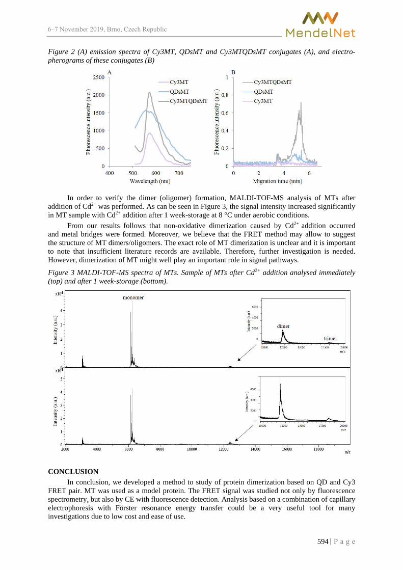
6–7 2019, Brno, Czech Republic
Figure 2 (A) emission spectra of Cy3MT, QDsMT and Cy3MTQDsMT conjugates (A), and electro-pherograms of these conjugates (B)
In order to verify the dimer (oligomer) formation, MALDI-TOF-MS analysis of MTs after addition of Cd2+ was performed. As can be seen in Figure 3, the signal intensity increased significantly in MT sample with Cd2+ addition after 1 week-storage at 8 °C under aerobic conditions.
From our results follows that non-oxidative dimerization caused by Cd2+ addition occurred and metal bridges were formed. Moreover, we believe that the FRET method may allow to suggest the structure of MT dimers/oligomers. The exact role of MT dimerization is unclear and it is important to note that insufficient literature records are available. Therefore, further investigation is needed. However, dimerization of MT might well play an important role in signal pathways.
Figure 3 MALDI-TOF-MS spectra of MTs. Sample of MTs after Cd2+ addition analysed immediately (top) and after 1 week-storage (bottom).
CONCLUSION In conclusion, we developed a method to study of protein dimerization based on QD and Cy3
FRET pair. MT was used as a model protein. The FRET signal was studied not only by fluorescence spectrometry, but also by CE with fluorescence detection. Analysis based on a combination of capillary electrophoresis with Förster resonance energy transfer could be a very useful tool for many investigations due to low cost and ease of use.
594

6–7 2019, Brno, Czech Republic
ACKNOWLEDGEMENTS The research was financially supported by IGA grant, no. IP_025/2019.
REFERENCES Buckhout-White, S. et al. 2014. Assembling programmable FRET-based photonic networks using designer DNA scaffolds. Nature Communications, 5: 5615. Jain, K.K. 2012. The handbook of nanomedicine. New York: Humana Press. Li, Y.Q. et al. 2010. High-sensitivity quantum dot-based fluorescence resonance energy transfer bioanalysis by capillary electrophoresis. Biosensors and Bioelectronics, 25(6): 1283–1289. Pereira, M., Lai, E.P.C. 2008. Capillary Electrophoresis for the Characterization of Quantum Dots After Non-Selective or Selective Bioconjugation with Antibodies for Immunoassay. Journal of Nanobiotechnology, 6: 10. Saha, S. et al. 2018. Evidence of homo-FRET in quantum dot–dye heterostructured assembly. Physical Chemistry Chemical Physics, 20(14): 9523–9535. Sanz-Nebot, V. et al. 2003. Characterization of metallothionein isoforms from rabbit liver by liquid chromatography coupled to electrospray mass spectrometry. Journal of Chromatography B, 796(2): 379–393. Stanisavljevic, M. et al. 2015. Quantum dots fluorescence resonance energy transfer-based nanosensors and their application. Biosensors and Bioelectronics, 74: 562–574. Zangger, K. et al. 2001. Oxidative dimerization in metallothionein is a result of intermolecular disulphide bonds between cysteines in the alpha-domain. Biochemical Journal, 359: 353–360.
595

6–7 2019, Brno, Czech Republic
The determination of deoxynivalenol and zearalenone in barley from Brazil and malted barley
Marek Pernica1, Karim C. Piacentini2, Rastislav Bosko1, 3, Sylvie Belakova1 1Research Institute of Brewing and Malting
Mostecka 7, 614 00 Brno CZECH REPUBLIC
2Department of Biotechnology University of Sao Paulo (USP)
Av. Professor Lineu Prestes, 03178-200, Sao Paulo BRAZIL
3Department of Crop Science, Breeding and Plant Medicine Mendel University in Brno Zemedelska 1, 613 00 Brno
CZECH REPUBLIC
Abstract: The present study describes the determination of mycotoxins deoxynivalenol (DON) and zearalenone (ZEA) in barley from Brazil and in malted barley. The quality of the raw materials involved in the malting process plays a decisive role in the creation of a safe beer product. Immunoaffinity columns for extraction and clean-up, and liquid chromatography coupled with mass spectrometry (LC-MS) are the most commonly used method for determining the presence of mycotoxins. A total of 24 samples were analysed for DON and ZEA. The average concentration of DON and ZEA was 2859.5 µg/kg and 727.9 µg/kg for barley and 1057.3 µg/kg and 275.1 µg/kg for malt, respectively. The content of mycotoxin decreases by about 63% during the malting process. The validation parameters of an analytical method such as linearity, limit of detection (LOD) and limit of quantification (LOQ), and recovery were tested. The calibration curves were linear at least in the range of 10–1000 ng/mL, LOD and LOQ ranging 2.8–3.5 µg/kg and 9.2–11.6 µg/kg, respectively. Recovery for DON and ZEA ranged 87.6%–92.9% with a RSD range of 2.9%–9.2% and 89.6%–105.7% with a RSD range of 0.4%–5.3%, respectively. Key Words: mycotoxins, barley, malt, liquid chromatography, malting process
INTRODUCTION Malted barley, together with water, hops and yeast, is one of the main raw materials for beer
production. The quality of the malted barley is proven to be reflected in the quality of beer. In context, the beer industry has several concerns about contamination in malting barley due to the loss of raw material, economic impact, and one of the most significant issues, loss of quality. One of the main contaminants in malted barley are mycotoxins (Bokulich and Bamforth 2013).
Mycotoxins are secondary metabolites of fungi. These toxins are produced by a few fungi that colonise crops in the field or after harvest, and are mainly of the genera Fusarium, Aspergillus and Penicillium. Two Fusarium mycotoxins that are considered hazardous to the beer industry and can be found throughout the entire malting and brewing processes are deoxynivalenol (DON) and zearalenone (ZEA) (Lulamba et al. 2019, Piacentini et al. 2019).
DON, also named vomitoxin, is a trichothecene B-type, an epoxy-sesquiterpenoid that elicits a complex spectrum of toxic effects. Chronic exposure can lead to anorexia, impaired weight gain, and immunotoxicity. Acute exposure can cause diarrhoea, vomiting, circulatory shock, and ultimately death (Pestka and Smolinski 2005). This mycotoxin occurs predominantly in grains such as wheat, barley, oats, rye, and corn, and less often in rice, sorghum and triticale. The occurrence of DON is associated primarily with Fusarium graminearum and Fusarium culmorum, which are important plant pathogens.
596

6–7 2019, Brno, Czech Republic
ZEA, also known as RAL (resorcylic acid lactone) and F-2 mycotoxin, is an endocrine disruptor because its structure is similar to the hormone estrogen and it competes with 17β-estradiol for binding the estrogen receptor, resulting in infertility and reproductive problems, abortion or other problems, especially in swine. This mycotoxin is heat-stable, is found worldwide in cereal crops and, is especially produced by Fusarium graminearum, Fusarium culmorum and other Fusarium and Gibberrella species (Metzler et al. 2010, Nesic el al. 2014).
Several techniques can be used for the determination of mycotoxins in brewing and malting, but the most common procedure steps are sampling, homogenization, extraction followed by a clean-up step to reduce or eliminate matrix effects, and finally the separation and detection, usually a chromatographic technique in combination with a variety of detectors. The most popular method for the determination of mycotoxins in foods and feeds is liquid chromatography with mass spectrometry for its very high sensitivity and specificity (as the issue of mycotoxins in brewing and malting is a residual issue; Rubert et al. 2012, Pernica et al. 2019).
Regulations have been established worldwide to fix the maximum levels allowed of mycotoxins in grains. In Europe, the levels for DON and ZEA in barley are set at 1250 µg/kg and 100 µg/kg, respectively. In Brazil, the regulations are being updated and in 2019 the DON levels for barley will be set at 1000 µg/kg for barley and 750 µg/kg for malt. Considering ZEA, the levels will be maintained at 100 µg/kg (Piacentini et al. 2019).
For the reasons stated above, the objective of the current study was to evaluate the content of mycotoxins such as deoxynivalenol and zearalenone in barley from Brazil and in malted barley as a raw material for beer preparation.
MATERIAL AND METHODS
Chemicals and Reagents Deoxynivalenol and zearalenone standards were purchased from Sigma Aldrich (Vienna,
Austria). The stock solutions standards were prepared in methanol/water (1:1, v/v). All reagents used in the following analyses were analytical and LC/MS-MS grade. Certified reference materials (CRM) (Trilogy, Washington) were used for quality assurance in the mycotoxin analyses. The concentrations for DON and ZEA were 700 ± 100 µg/kg and 454.2 ± 37.6 µg/kg, respectively.
Samples A total of 24 barley samples (Hordeum vulgare L.) with a weight of 500 g each were used
from a 2015 harvest and were supplied by the Brazilian agricultural research corporation (Embrapa). It is important to mention that the samples studied had natural mycotoxins levels acquired in the field without artificial interference. The samples were used for the process of malting and aliquot was taken for mycotoxin analysis.
Malting process The malting trial was carried out in the Research Institute of Malting and Brewing, Brno, Czech
Republic. The procedures used for malting were according to the methodology and amendments were approved by the barley and malt European Brewery Convention (EBC European Brewery Convention – Analytica EBC, 2008).
Extraction and clean-up of mycotoxins The immunoaffinity columns (DZT MS-PREP®, R-Biopharm, Glasgow, Scotland) were used
for extraction and clean-up. Briefly, 10 g of milled barley and malt were mixed with methanol 70% for 50 min, followed by 15 min of centrifugation at 4500 rpm. Then, 2 mL of the extract were added to 48 mL of PBS buffer (pH 7.4, adjusted with 2M NaOH). The elution was performed with 2 mL of 100% methanol. For injection, the extract was dried and then dissolved with 1 mL of 50% methanol in water.
597

6–7 2019, Brno, Czech Republic
Figure 1 Map of malting process
LC-MS/MS analysis The Finnigan Surveyor HPLC coupled to the ion trap LCQ Advantage mass spectrometer
(Thermo-Fisher, USA) with atmospheric pressure chemical ionization (APCI) was used for the identification and quantification of mycotoxins (DON and ZEA). Chromatographic separation was performed with Synergi Hydro RP 80Å column (3.0 × 150 mm, 4.0 µm particle size) equipped with a Security GuardTM cartridge C18 (4.0 × 3.0 mm, 4.0 µm) at 30 °C using gradient elution. The mobile phase was comprised of solvent A (water containing 10 mM amonium acetate) and solvent B (methanol). The gradient program was applied at a flow rate of 0.5 mL/min under the following conditions: 0.1 min 90% A; 2 min 50% A; 10 min 20% A; 15 min 20% A; 16 min 90%; 25 min 90% A. The APCI interface was operated at negative polarity and the following ionization conditions were used: Capillary temperature, 160 °C; source heater temperature of 450 °C; nitrogen sheath gas flow of 35 L/min; nitrogen auxiliary gas flow of 10 L/min; source voltage of 6.0 kV; collision gas was helium. For selectivity, the mass spectrometer was operated in MRM mode and two transitions per analyte were monitored (see Table 1).
RESULTS AND DISCUSSION
Method validation A seven-point calibration curve was constructed from the stock solution by gradual dilution.
The concentrations for each mycotoxin were as follows: 10, 20, 50, 100, 200, 500 and 1000 ng/ml. Quantification was carried out by external calibration. The limit of detection (LOD) and limit of quantification (LOQ) was determined as the concentration at which the signal to noise ratio equals to 3 and 10, respectively. Recovery was calculated using the barley sample spiked with the mycotoxins at three different levels with triplicate analyses conducted for each level. The spiking levels were chosen considering the contamination levels of examined samples (Piacentini et al. 2019). Recovery for DON and ZEA ranged 87.6%–92.9% with a RSD range of 2.9%–9.2% and 89.6%–105.7% with a RSD range of 0.4%–5.3%, respectively. The validation data are summarized in Table 1. Table 1 Validation and selected parameters of LC-MS/MS method for mycotoxin
Mycotoxin Retention
time (min)
Precursor ion (m/z) Product ion (m/z)
Normalized CE (%) Regression equation R2 LOD
(µg/kg) LOQ
(µg/kg)
DON 6.3 355 [M+CH3COO]- 295
34 y = 29586x + 29656 0.9994 3.5 11.6 265
ZEA 16.2 317 [M-H]- 273
64 y = 18282x + 84122 0.9992 2.8 9.2 299
55°C ± 2°C » 12 hours60°C ± 2°C » 1,5 hours65°C ± 2°C » 1,5 hours70°C ± 2°C » 1,5 hours75°C ± 2°C » 1,5 hours80°C ± 2°C » 4 hours
BARLEY
5 hours WET and 19 hours AIR STEEPING 1° DAY
4 hours WET and 20 hours AIR STEEPING 2° DAY
20 minutes WET and 23:40 hours STEEPING 3° DAY
45% moisture GERMINATION 1° DAY
GERMINATION 2° DAY14°C
GERMINATION 3° DAY
KILNING
MALT
598

6–7 2019, Brno, Czech Republic
Determination of mycotoxins in barley and malt The analytical method was used in our study for an analysis of the content of deoxynivalenol
and zearalenone in various barley from Brazil and malted barley. The results are shown graphically in Figure 2.
A total of 24 samples were analysed for DON and ZEA. 18 barley samples were above the regulation limit for both mycotoxins. For malted barley, 11 and 17 samples were above the regulatory limit, respectively. Mycotoxin contamination can by transferred into the malt during the process of malting. This can pose a risk to humans, taking into account the worldwide consumption of beer. The most important stages that have an inhibitory effect on mycotoxins are steeping and kilning. During these processes, mycotoxins can be removed with drainage water, spent grains, destroyed by heat treatment or absorbed on the surface (Pernica et al. 2019, Piacentini et al. 2019).
The average concentration of DON and ZEA was 2859.5 µg/kg and 727.9 µg/kg for barley and 1057.3 µg/kg and 275.1 µg/kg for malt, respectively. The maximum concentration of DON and ZEA was 5615.8 µg/kg and 3595.6 µg/kg for barley and 3789.8 µg/kg and 1386.3 µg/kg for malt, respectively. In Southern Brazil, where the samples were collected, the climatic conditions (temperature and high humidity) tend to increase the contamination by F. graminearum, F. culmorum and others. Consequently, this maximizes the production of mycotoxins. The analysis discussed is extremely important in the creation of a safe final product and because the high levels of mycotoxins pose a significant risk to consumers health.
Figure 2 Content of DON and ZEA in barley and malt
CONCLUSION The barley samples analysed showed a high concentration of DON and ZEA, averaging 2859.5
and 727.9 μg/kg, respectively. Due to the corresponding malt samples, mycotoxin content has been shown to decrease by about 63% during malting process, but mycotoxin contamination can still exceed the maximum regulatory limits. It should be noted that the mycotoxins play a decisive role in creating a safe end product as well as in the health of consumers.
ACKNOWLEDGEMENTS Supported by the Ministry of Agriculture of the Czech Republic, institutional support MZE-RO1918. The work was supported by the project TE02000177 „Centre for Innovative Use and Strengthening of Competitiveness of Czech Brewery Raw Materials and Products“ of the Technology Agency of the Czech Republic
REFERENCES Bokulich, N.A., Bamforth, C.W. 2013. The microbiology of malting and brewing. Microbiology and Molecular Biology Reviews, 77(2): 157–172. EBC Analysis Committee. 2008. Analytica-EBC. 7th ed., Nürnberg, Germany: Verlag, Hans Carl Getränke-Fachverlag.
0
1000
2000
3000
4000
5000
6000
A B C D E F G H I J K L M N O P Q R S T U V W X
µg/k
g
barley DON malt DON
0
500
1000
1500
2000
2500
3000
3500
4000
A B C D E F G H I J K L M N O P Q R S T U V W X
µg/k
g
barley ZEA malt ZEA
599

6–7 2019, Brno, Czech Republic
Lulamba, T.E., Stafford, R.A., Njobeh, P.B. 2019. A sub‐Saharan African perspective on mycotoxins in beer–a review. Journal of the Institute of Brewing, 125(2): 184–199. Metzler, M., Pfeiffer, E., Hildebrand, A. 2010. Zearalenone and its metabolites as endocrine disrupting chemicals. World Mycotoxin Journal, 3(4): 385–401. Nesic, K., Ivanovic, S., Nesic, V. 2014. Fusarial toxins: secondary metabolites of Fusarium fungi. Reviews of Environmental Contamination and Toxicology, 228: 101–120. Pernica, M., Piacentini, K. C., Benešová, K., Čáslavský, J., Běláková, S. 2019. Analytical techniques for determination of mycotoxins in barley, malt and beer: A review. Kvasný průmysl, 65(2): 46–57. Pestka, J.J., Smolinski, A.T. 2005. Deoxynivalenol: toxicology and potential effects on humans. Journal of Toxicology and Environmental Health, Part B, 8(1): 39–69. Piacentini, K.C., Benešová, K., Pernica, M., Savi, G.D., Rocha, L.O., Hartman, I., Běláková, S. 2019. Fusarium Mycotoxins Stability during the Malting and Brewing Processes. Toxins, 11(5): 257. Rubert, J., Dzuman, Z., Vaclavikova, M., Zachariasova, M., Soler, C., Hajslova, J. 2012. Analysis of mycotoxins in barley using ultra high liquid chromatography high resolution mass spectrometry: comparison of efficiency and efficacy of different extraction procedures. Talanta, 99: 712–719.
600

6–7 2019, Brno, Czech Republic
An analysis of residue alkylphenols and bisphenol A using liquid chromatography-tandem mass spectrometry
Marek Pernica1, 2, Zdenek Simek1 1Research Centre for Toxic Compounds in the Environment RECETOX
Masaryk University Kamenice 753/5, 625 00 Brno
2Research Institute of Brewing and Malting Mostecka 7, 614 00 Brno
CZECH REPUBLIC
Abstract: Bisphenol A (BPA) and alkylphenols (APs) such as 4-tert-octylphenol (4-t-OP) and mixture of nonylphenol isomers (iso-NP) are frequent contaminants of various environmental analyses. Analyse of various blanks is a serious problem in the residue analysis. Secondary contamination of analysed samples can come from laboratory air, septa vials, solvents and other chemicals used. Plastic tubes and connections could be another important source of sample contamination. This can be a problem especially in determination of alkylphenols and bisphenol A at low environmentally relevant concentrations. The analytical method for determination of residues of pollutants in water samples using solid phase extraction (SPE) followed by liquid chromatography-tandem mass spectrometry (LC-MS/MS) is presented here. In principle, alkylphenols can be analysed without derivatization. However, pre-column derivatization with 5-(dimethylamino) naphthalene-1-sulfonyl chloride (dansylchloride, DNSC) improves the sensitivity and selectivity of LC-MS/MS analysis. The instrumental blank for all compounds is under the limit of detection (LOD). The system contamination was maintained about 0.5 ng (reagent blank), and below 0.05 µg/L for the glass SPE columns and below 0.1 µg/L for the plastic columns (procedure blank).
Key Words: blank, blank contamination, LC-MS, alkylphenols, bisphenol A
INTRODUCTION Alkylphenols and bisphenol A as well known endocrine disrupting compounds (EDCs) are able
to mimic or antagonize the female estrogens 17 β-estradiol (Salgueiro-González et al. 2012b). Nonylphenols, which form a mixture of 211 branched nonyl-chain isomers, and 4-tert-octylphenol are the most important alkylphenols due to their toxicological properties. Bisphenol A has been used as a material for the production of epoxy resins, phenol resins, polycarbonates, polyesters, lacquer coatings on food cans, and also in flame retardants, adhesives, and as a component of electronic circuits (Salgueiro-González et al. 2012a). The concentrations of BPA, APs and their parent compounds have been measured worldwide in all compartments of the environment and even in food products for human consumption (Xie et al. 2006).
The primary purpose of analysis of blanks is to trace sources of artificially and or randomly introduced contamination of real samples. The diagram (see Figure 1) shows how comparison of different blank sample results can be used to identify and isolate the source of contamination introduced in the field or the laboratory. The source of contamination introduced in the field or laboratory can be deduced by comparing blank results. An equipment blank could potentially be contaminated in the field, during transport to the lab or in the lab. The method blank, on the other hand, could only be contaminated in the lab. Using all the blanks described in this fact sheet will facilitate the identification of contamination sources (EPA 2009).
Nonylphenols can also be present in laboratory air. For example, concentrations around 100 ng/m3 were found in the air of a typical laboratory and it has also been reported that an LC-MS vial with methanol left in the autosampler of the instrument can absorb NP from the laboratory air within weeks. Septa vials and solvent used as mobile phases can also cause blank contamination.
601

6–7 2019, Brno, Czech Republic
BPA contamination caused by the water purification system was observed in ultrapure water. Sampling, storage of samples, filtration and sample treatment are also important sources of blank contamination. APs and BPA from water samples are commonly extracted by liquid-liquid extraction (LLE) or solid-phase extraction (SPE). However, this procedure can also cause contamination due to the plastic materials of the SPE cartridges, the multiple steps involved and the use of relatively high volumes of solvent (Xie et al. 2006, Salgueiro-González et al. 2012a).
The terms such as ghost peaks, artifact (and artefact) peaks, system peaks, pseudo peaks, vacancy peaks, eigenpeaks, induced peaks and spurious peaks can be found in published papers. These terms are called peaks that are undesirable in the blank systems (Williams 2004).
It is important to fully characterise the analytical performance in order to understand their capability and limitations, and to ensure that they are “fit for purpose”. The terms such as LOB (limit of blank), LOD (limit of detection), and LOQ (limit of quantification) describe the smallest concentration of an analyte that can be reliably measured by an analytical procedure. LOB and LOD are important for tests used to distinguish between the presence or absence of an analyte and LOQ to reliably measure low levels of analyte and should be incorporated as part of any method evaluation (Armbruster and Pry 2008). • Blank equipment (equipment blank) includes the total field and laboratory contamination sources,which are determined by sputtering the blank over the decontaminated field sampling device before sampling the environment. The objective of the assessment is to assess the total contamination of the sampling. • Field blank includes overall ambient conditions during sampling and laboratory pollution sources.Blank determination is done as follows, a blank sample is transferred to the sampling container and then sent to a laboratory with a field sample. The aim is to assess contamination from field conditions during collection. • Trip blank includes shipping and laboratory contamination sources, only for volatile substances.The transport blind sample is a sample which is transported from the laboratory to the point of collection and transported back to the laboratory without being subjected to a sampling procedure. • The blank method (method blank) only shows laboratory sources of contamination. Blank methods areprepared and analyzed exactly in the same way as a field sample. The aim is to assess the contamination during sample preparation. • The instrumental blank (instrument blank) only shows instrumental source of contamination. The blankitself is parsed with the field sample and the goal is to assess the presence or absence of device contamination (EPA 2009). Figure 1 Comparison of different blank (EPA 2009)
The main purpose of our study was to compere individual types of blanks such as instrumental blank, reagent blank, method blank and also evaluated to effect use of glass and plastic SPE columns in residual analysis of alkylphenols and bisphenol A. Bisphenol A, 4-tert-octylphenol, 4-octylphenol, isomers of nonylphenol and 4-n-nonylphenol were selected for these purpose. The LC-ESI-MS/MS was used for intended study using pre-column derivatisation with dansyl chloride.
Equipment blank
Field blank
Trip blank
Method blank
Instrument blank
602

6–7 2019, Brno, Czech Republic
MATERIAL AND METHODS Instruments and chemicals
Chromatographic separations were performed using an Agilent 1200 Infinity Series (Agilent Technologies, Santa Clara, CA, USA) with chromatographic column ACE 5 C18, 150 mm × 4.6 mm i.d., 5μm particle size (ACE, Scotland, UK). The Agilent 6410 Triple Quadrupole (Agilent Technologies, Santa Clara, CA, USA) was used for MS/MS analysis. The glass and plastic SPE columns octadecyl C18, 500 mg (Supelco) was used for analysis. The analytical standards, derivatizing agent DNSC and water (ultrapure water for HPLC) were purchased from Sigma-Aldrich (Germany). Alkylphenols measurements
Alkylphenols and bisphenol A were measured in 3 levels blank samples such as instrumental blank, reagent blank and method blank. Sample of ultrapure water for HPLC was used for determination of instrumental source contamination (the instrumental blank) during analyses by LC-MS/MS method, as described by Pernica et al. (2015). Analyse of the reagent blank was used in this study to assess relationship between the instrumental blank and the method blank. The reagent blank was prepared in ultrapure water for HPLC with all of chemicals used for derivatization of alkylphenols by dansyl chloride (DNSC). The derivatization reaction was carried out in a 2 mL amber glass sample vial with 200 µL ultrapure water for HPLC. Fifty microliters of 100 mmol/L NaHCO3 (pH = 10.5) were added and the mixture was stirred (vortex) for 1 minute. Next 200 µL of DNSC in acetone (0.5 mg/mL) were added and stirred again. Subsequently the mixture was incubated for 60 minutes and 60 °C. The reaction mixtures were then cooled to the room temperature and evaporated to dryness under nitrogen atmosphere. The residue was redissolved in 1 mL of methanol and stirred (Pernica et al. 2015). The following procedure was used as the method blank for residue analyses of alkylphenols and bisphenols A. The glass and plastic SPE columns were conditioned with 2 mL of methanol and 2 mL of water (purity for LC/MS). 100 mL of ultrapure water for HPLC was passed through the SPE column using vacuum manifold flow rate 5 mL/min. After extraction, the columns were dried with air for 5 minutes. Elution was performed with 5 mL acetonitrile. The eluate was evaporated and converted into a mini-vial, derivatized with dansyl chloride and analysed by LC/ESI/MS/MS as described by Pernica et al. (2015). The method blank was measured 3 times for glass and plastic SPE columns.
RESULTS AND DISCUSSION The instrumental blank was under the limit of detection (LOD) for selected compounds, such
as bisphenol A (BPA), 4-tert-octylphenol (4-t-OP), mixture of nonylphenol isomers (iso-NP, technical mixture), 4-octylphenol (4-OP), and 4-n-nonylphenol (4-n-NP). Only BPA, 4-t-OP and iso-NP were detected and only 4-t-OP and iso-NP were quantified in the reagent blank. Three analytes were quantified in the method blank, which is about 10-times higher than the counts of chromatogram in the natural reagent blank. Repeatability of the reagent blank was measured once per day for a period of 20 days, when BPA was under of quantification (LOQ). The average concentration of 4-t-OP and iso-NP measured in the reagent blank was 42.6 pg/mL and 482.5 pg/mL, respectively. QC histograms for significant evaluation were used, the critical upper limit and lower limit was not exceeded in any way. Finally, a SPE glass column and SPE plastic column were compared in the method blank. The median concentration of BPA for the glass SPE column was 3.1 ng/L and 5.3 ng/L for the plastic SPE column. No significant differences were found in SPE columns for 4-t-OP. The median concentration of 4-t-OP was 2.45 ng/L for the glass SPE column and 2.42 ng/L for the plastic SPE column. The result of iso-NP was statistically significant with a concentration of 44.3 ng/L for the glass SPE column and 77.8 ng/L for the plastic SPE column (see Figure 2). The plastic SPE columns provided a higher method blank than the SPE glass columns. However, the SPE glass column had better repeatability than plastic materials. The SPE plastic columns provided relatively higher levels of alkylphenols and bisphenol A caused by common contamination of the prepared samples coming from laboratory air, septa vials, and solvents and chemicals used. These sources of contamination cannot be affected. The linear alkylphenols such as 4-OP and 4-n-NP were not present in any blank.
603

6–7 2019, Brno, Czech Republic
Figure 2 I. Chromatograms of blanks (A) instrumental blank (B) reagent blank (C) method blank. II. Intermittent repeatability (n = 20) of the reagent blank for selected alkylphenols and bisphenol A, include QC histograms for 4-t-OP and iso-NP. III. Comparison of SPE columns made of glass and plastic (n = 3).
CONCLUSIONS Significant blank contamination is a notorious problem in ultratrace analyses of alkylphenols
and bisphenol A, especially when we perform an analysis at concentrations close to the LOQ. A blank contamination may result in a significant increase in the detection limit. A systematic study and analysis of blanks together with analyses of a set of treated and analysed samples is necessary. In order to keep blank contamination as low as possible, the minimization of the number of potential contamination sources is required, such as plastic laboratory containers and plastic aids, water prepared in plastic devices etc., the work in a laboratory devoted solely to analyzes of alkylphenol is the strong requirement.
ACKNOWLEDGEMENTS The authors thank the Grant Agency of the Czech Republic for financial support (GA13-20357S). The RECETOX research infrastructure was supported by the projects of the Czech Ministry of Education (LO1214) and (LM2011028).
REFERENCES Armbruster, D. A., Pry, T. 2008. Limit of blank, limit of detection and limit of quantitation. The Clinical Biochemist Reviews, 29(Suppl 1): S49. EPA Government ©2009. Quality Control Tools: Blanks. [Online]. Available at: https://www.epa.gov/sites/production/files/2015-06/documents/blanks.pdf. [2019-09-19].
0
25
50
75
0 5 10 15 20 25 30 min
A
0
250
500
750
0 5 10 15 20 25 30
Coun
ts
min
B
0
2500
5000
7500
0 5 10 15 20 25 30 min
C
0 1 2 3 4 5 6 7 80
100200300400500600700800900
1000
2 4 6 8 10 12 14 16 18 20
90,089
482,50
874,90
0 2 4 6 8 1010
20
30
40
50
60
70
80
2 4 6 8 10 12 14 16 18 20
16,450
42,625
68,801
I.
III
II.
III.
604

6–7 2019, Brno, Czech Republic
Pernica, M., Poloucká, P., Seifertová, M., Šimek, Z. 2015. Determination of alkylphenols in water samples using liquid chromatography–tandem mass spectrometry after pre–column derivatization with dansyl chloride. Journal of Chromatography A, 1417: 49–56. Salgueiro-González, N., Concha-Graña, E., Turnes-Carou, I., Muniategui-Lorenzo, S., López-Mahía, P., Prada-Rodríguez, D. 2012a. Blank and sample handling troubleshooting in ultratrace analysis of alkylphenols and bisphenol A by liquid chromatography tandem mass spectrometry. Talanta, 101:413–419. Salgueiro-González, N., Turnes-Carou, I., Muniategui-Lorenzo, S., López-Mahía, P., Prada-Rodríguez, D. 2012b. Fast and selective pressurized liquid extraction with simultaneous in cell clean up for the analysis of alkylphenols and bisphenol A in bivalve molluscs. Journal of Chromatography A, 1270: 80–87. Williams, S. 2004. Ghost peaks in reversed-phase gradient HPLC: a review and update. Journal of Chromatography A, 1052(1–2): 1–11. Xie, Z., Selzer, J., Ebinghaus, R., Caba, A., Ruck, W. 2006. Development and validation of a method for the determination of trace alkylphenols and phthalates in the atmosphere. Analytica Chimica Acta, 565(2): 198–207.
605

6–7 2019, Brno, Czech Republic
Optimization of multiplex RT-PCR for selected isoforms of metallothionein genes and influence of cisplatin on prostatic cell
lines
Frantisek Petrlak1, Veronika Smidova1, Zbynek Splichal1,2, Petr Michalek1,2 1Department of Chemistry and Biochemistry
Mendel University in Brno Zemedelska 1, 613 00 Brno
2Central European Institute of Technology Brno University of Technology Purkynova 123, 621 00 Brno
CZECH REPUBLIC
Abstract: This study deals with the issue of metallothioneins as potential tumor markers using the multiplex reverse transcription polymerase chain reaction (RT-PCR) method, for which specific primers were designed, with the subsequent sequencing of their products. The following step involved a study of expression using the PCR method for selected MT1A, MT2A and MT3 genes after treating cell lines with cisplatin. Experiments were carried out on PNT1A, LNCaP and DU145 prostatic cell lines. Despite a very high similarity of the individual isoforms of metallothioneins, a triplex of three genes for two cell lines, PNT1A and DU145, was created. Upon a statistical evaluation of data obtained via the method of polymerase chain reaction in real time, it was found that, after the application of cisplatin, there was an increase in metallothionein expression.
Key Words: biomarkers, cisplatin, metallothioneins, PCR, prostatic cell lines
INTRODUCTION Metallothioneins (MT) are proteins rich in amino acid cysteine which increases their affinity
for metals. MT protects the cell from the toxic effects of heavy metals, DNA damage and oxidative stress. In addition, they play a role in cancer, preventing apoptosis and participating in tumor cell proliferation (Si and Lang 2018).
In humans, 16 localized genes on chromosomes have been identified that encode four isoforms of MT marked with numbers (MT1 to MT4). Proteins of MT2A, MT3 and MT4 are encoded by a single gene located on chromosome 16. MT1 contains many (sub)isoforms. The known active (sub)isoforms of MT1gene are MT1A, 1B, 1E, 1F, 1G, 1H, 1M and X.
In this study MT were studied in connection with prostate cell lines. Detecting changes in the expression of individual MT isoforms could contribute to early tumor diagnosis and targeted therapy. It is believed that future studies of MT will reveal not only their functions in the pathogenesis of cancer, but also provide new insights into diagnosis and therapy (Cherian et al. 2003).
MTs also play a critical role in the treatment of cytostatics. They can bind cisplatin compounds and remove them from cells, which can lead to resistance. Monitoring the expression of MTs in tumor cells may be useful in selecting a treatment method (Bizoń et al. 2017).
MATERIAL AND METHODS This study was divided into two experiments. The first experiment was based on designing
primers for isoforms and (sub)isoforms using the PCRTiler v1.42 web software, then these primers were used for RT-PCR multiplex and optimization. In the second experiment, the selected cell lines were treated with cisplatin and after an incubation time of 24 h the expression of different isoforms of MT (MT1A, MT2A and MT3) in selected cell lines (PNT1A, DU145 and LNCaP) was measured.
606

6–7 2019, Brno, Czech Republic
Cell lines and cultivation Prostate cell lines DU145, PNT1A and LNCaP were used for given experiments. Cultivation was
performed in RPMI 1640 medium with 10% fetal bovine serum and a mixture of the antibiotics penicillin and streptomycin (200 U/l penicillin and 0.2 mg/l streptomycin). Cell lines were cultured in an incubator at 37 °C, 5% CO2 and 70–90% humidity. Cells were maintained in an incubator Galaxy® 170 R (Eppendorf, Hamburg, Germany). Cells were counted using Countess II FL (Thermo Fisher Scientific, Waltham, MA, USA).
The first cell line used was PNT1A. It is a primary culture obtained from normal adult prostatic epithelial cells of a 35-year-old male post mortem. Immortalisation was established by transfection with a plasmid containing SV40 (simian virus 40). The second cell line was human hypotriploid prostate cancer DU145. These cells have moderate metastatic potential and they are positive at the androgen receptors. The last tested cell line was LNCaP which are androgen-sensitive human prostate adenocarcinoma cells derived from metastasis from a 50-year-old. They are adherent epithelial cells growing in aggregates and as single cells.
Isolation and transcription RNA isolation was performed according to the High Pure RNA Isolation Kit (Roche, Basel,
Switzerland) manufacturer's instructions. Synthesis of cDNA from all 4 cell lines was performed with a Transcriptor First Strand cDNA Kit (Roche, Basel, Switzerland) with a total yield of 2000 ng in a Mastercycler realplex4 thermocycler (Eppendorf, Hamburg, Germany).
Multiplex RT-PCR For better optimization, two PCR methods were combined, touchdown and multiplex.
This increased the annealing specificity of the primers. The RT-PCR multiplex reaction mixture consisted of a 10 µl Luna® Universal One-Step RT-qPCR Kit, (NEB, Massachusetts, USA), 0.5 µl of forward and reverse primer (Sigma-Aldrich, St. Louis, Missouri, USA) and template DNA with a final volume of 20 μl. The PCR procedure is described in Table 1.
Table 1 Multiplex RT-PCR reaction conditions Steps Temperature Time Cycles
Initial denaturation 95 °C 5 min 1 Denaturation 95 °C 25 s
23 Annealing, Extension X= 65 °C
X = X - 0.3 °C 35 s
Denaturation 95 °C 25 s 20
Annealing, Extension 58.1 °C 35 s Melting curve 60–95 °C 20 min 1
Cooling 4 °C ∞ ∞
Agarose gels All agarose gels were composed of 1 g of agarose dissolved in 1 × TAE buffer (40 mM Tris,
20 mM acetic acid and 1 mM EDTA). The separation time was 90 min at 80 V. Agarose gels were visualized and photographed under 365 nm UV radiation on the Azure c600 from Azure Biosystems (Dublin, California, USA).
MTT assay The viability was detected using the MTT (3-(4,5-dimethylthiazol-2-yl)-2,5-diphenyltetrazolium
bromide) assay. A 50% inhibitory concentration for cisplatin after 24 h was determined. Cisplatin was purchased from Sigma-Aldrich (St. Louis, Missouri, USA), diluted with 10% NaCl solution to a concentration of 1 mg/ml and dissolved at 80 °C for 5 min. After treatment, 10 µl of MTT (5 mg/ml in phosphate buffered saline) was added to the cells and incubated. After that, MTT containing medium was replaced by 100 µl of dimethyl sulfoxide and absorbance was determined at 570 nm using Infinite 200 PRO (Tecan, Männedorf, Switzerland).
607

6–7 2019, Brno, Czech Republic
Reverse transcription-quantitative polymerase chain reaction (RT-qPCR) Relative gene expression was calculated for MT1A, MT2A and MT3. GAPDH was used
as a housekeeping gene. Luna® Universal One-Step RT-qPCR Kit was used as a master mix for quantitative PCR analysis; the analysis was performed using the Mastercycler realplex4 (Eppendorf, Hamburg, Germany).
GraphPad Prism 8 Statistical analysis was performed using Student’s t-test and the difference between groups was
assessed as significant at p < 0.05. Statistics were performed from three biological replicates.
RESULTS AND DISCUSSION The aim of first experiment was to design complementary primers to cDNA of individual isoforms
and (sub)isoforms of MT. This was complicated by the high similarity between the sequences of the individual genes. Finally, primers were successfully designed. The products of primers were verified in agarose gel with following by optimization of the multiplex RT-PCR. Primers are shown in Table 2.
Table 2 Overview of primer design s for multiplex RT-PCR analysis
Optimization consisted of the correct annealing temperature and the amount of primers and cDNA. After testing all possible (sub)isoforms by multiplex RT-PCR, some duplexes were detected, but the most successful result is triplex in the last well of DU145 with MT1A, MT2A and MT3. The products and their semi-quantitative amounts can be identified in Figure 1. The best combination of amounts of primers and temperatures on Multiplex RT-PCR has opened new possibilities for further study of these genes.
The aim of the second experiment was to determine whether cisplatin affects the expression of genes in prostate cell lines. The dependence of cisplatin concentration on cell line vitality was measured using MTT assay. The result of this assay was the calculation of which concentration of cisplatin leads to 50% viability of cells (termed as IC50). For the PNT1A and LNCaP lines IC50 was found to be 15 µg/ml and for the DU145 line 62.5 µg/ml. At this concentration, the cells were treated with cisplatin and cultured for 24 h prior to the next part of the experiment. RT-qPCR was performed on selected MT1A, MT2A and MT3 genes after cisplatin treatment and subsequent comparison with control samples. The proposed multiplex primers were used to study this hypothesis. The results are shown in Figures 2–4.
As shown in Figure 2, the expression levels of MT1A in the non-tumor PNT1A line does not change significantly compared to the control. There is no statistically significant difference (p ≥ 0.05). For the MT1A gene in the LNCaP line, a big increase in expression is observed over the control, where
Name Forward primers 5‘–3‘ Reverse primers 5‘–3‘ Amplicon size (bp)
MT1A TCTGCAAAGGGGCATCAGAG TGGGTCAGGGTTGTATGGAA 122
MT1B GAACTCCAGGCTTGTCTTGG GATGAGCCTTTGCAGACACA 187
MT1E GCTTGTTCGTCTCACTGGTG TTGCAGGAGGTGCATTTG 136
MT1F GCTTCTCTCTTGGAAAGTCCAG TTGCAGGAGGTGCATTTG 128
MT1G CTAGTCTCGCCTCGGGTTGCA CAGGAGCAGCAGCTCTTCTTGC 128/131
MT1H CTGGGCTGTGCCAAGTGTG ATGAGTCGGAGTTGTAGAAA 153
MT1M AGCAGTCGCTCCATTTATCG AGGAGCAGCAGCTCTTCTTG 157
MT1X TCTCCTTGCCTCGAAATGGAC TTGCAGGAGGTGCATTTG 104
MT2A CTCGTCCCGGCTCTTTCTA GAGTCGGGACAGGTTGCAC 101
MT3 TCGACATGGACCCTGAGACC CACACTTCTCACACTCCGCA 141
MT4 ATGGACCCCAGGGAATGTGT CTGAGCCTCCTTTGCAGATG 166
608

6–7 2019, Brno, Czech Republic
there is a very statistically significant difference (*p ≤ 0.05). For the DU145 cell line (p ≥ 0.05), slightly increased level of MT1A is observed compared to control.
Figure 1 Multiplex PCR products after successful optimization
Legend: 2% agarose gel, staining by ethidium bromide (10 ng/ml), M means 100bp DNA Ladder
Figure 2 Effect of cisplatin on MT1A in prostate cell lines
Figure 3 Effect of cisplatin on MT2A in prostate cell lines
As shown in Figure 3, the change in MT2A gene expression was slightly divergent from the control in the PNT1A line. These results were not significantly different from the control (p ≥ 0.05). In the LNCaP cell line, an increase in MT2A expression was observed in the untreated line, which was assessed as significant (*p ≤ 0.05). These results are confirmed by a study describing an increase in MT2A expression associated with resistance to chemical drugs (Kondo et al. 1995). The DU145 line shows a similar trend in MT2A gene expression over control. Expression of this gene in the DU145 line is statistically without significant differences from the control (p ≥ 0.05).
609

6–7 2019, Brno, Czech Republic
Figure 4 Effect of cisplatin on MT3 in prostate cell lines
Figure 4 shows that the expression of the MT3 gene in the PNT1A line is increased compared to the control. In this case, there is also a highly statistically significant difference (*p ≤ 0.01) from the established control. Another result was determined in LNCaP cell line, where there is also a significant difference (*p ≤ 0.05) compared to the MT3 control, whose expression shows an increase over the untreated line. The last cell line to measure MT3 expression was DU145 where expression level was also increased over the control. This cell line also showed a statistically significant difference from the control (*p ≤ 0.05).
Dutta et al. (2002) also disclose MT3 overexpression enhancing chemotherapeutic drug resistance in PC3 prostate cancer cells. Overexpression of MT3 after cisplatin administration suggests that MT3 may play a similar role to MT1A and MT2A in metal homeostasis in prostate cells (Garrett et al. 1999).
The results show that MT expression is increased after cisplatin application. This phenomenon has also been observed in several other publications. Cisplatin causes oxidative stress leading to cell apoptosis. However, MT1A, MT2A and probably MT3 are also capable of capturing free radicals, even having the ability to bind cisplatin itself (Kelley et al. 1988, Brozovic et al. 2010).
CONCLUSION In this study the multiplex touchdown RT-PCR method using more than one set of primers
for various MT isoforms was successfully designed. As a result, MT1A, MT2A and MT3 gene triplex was established in two cell lines, PNT1A and DU145. The object of the design and optimization of multiplex RT-PCR was to find a suitable diagnostic method that would be less expensive and, its implementation would be faster and easier compared to other diagnostic methods with the elimination of errors.
In the second experiment, after MTT assay and cultivation of the cells with cisplatin for 24 h RNA isolation and transcription into cDNA by reverse transcriptase was performed. Expression was measured by RT-qPCR. Statistical evaluation of the obtained data confirmed increased expression of MT1A, MT2A and MT3 genes in cisplatin-treated cells. Increased expression was observed in the MT1A gene over the untreated control in the LNCaP line. This trend was also observed in the MT2A gene on the same cell line, which was a human prostate cancer cell derived from metastatic cells. LNCaP and DU145 tumor lines and non-tumor PNT1A lines have been shown to be overexpressed with MT3. Overexpression of MT3 following cisplatin administration suggests that MT3 may play a similar role to MT1A and MT2A in metal homeostasis in prostate cells. This overexpression may be due to the affinity of metallothionein to metals, or to the formation of a high concentration of oxidative stress caused by cisplatin in cell lines.
ACKNOWLEDGEMENTS The research was financially supported by the GAČR 19-13766J.
REFERENCE Bizoń, A. et al. 2017. The Role of Metallothionein in Oncogenesis and Cancer Treatment. Postepy Higieny i Medycyny Doswiadczalnej, 71: 98–109.
*
610

6–7 2019, Brno, Czech Republic
Brozovic, A. et al. 2010. The Relationship between Cisplatin-Induced Reactive Oxygen Species, Glutathione, and BCL-2 and Resistance to Cisplatin, Critical Reviews in Toxicology, 40(4): 347–359. Cherian, M.G. et al. 2003. Metallothioneins in Human Tumors and Potential Roles in Carcinogenesis. Mutation Research/Fundamental and Molecular Mechanisms of Mutagenesis, 533(1–2): 201–209. Dutta, R. et al. 2002. Metallothionein Isoform 3 Expression Inhibits Cell Growth and Increases Drug Resistance of PC‐3 Prostate Cancer Cells. The Prostate, 52(2): 89–97. Garrett, S. et al. 1999. Metallothionein Isoform 3 Expression in the Human Prostate and Cancer‐Derived Cell Lines. The Prostate, 41(3): 196–202. Kelley, S.L. et al. 1988. Overexpression of Metallothionein Confers Resistance to Anticancer Drugs. Science, 241(4874): 1813–1815. Kondo, Y. et al. 1995. Metallothionein Localization and Cisplatin Resistance in Human Hormone-Independent Prostatic Tumor Cell Lines. Cancer Research, 55(3): 474–477. Si, M., Lang, J. 2018. The Roles of Metallothioneins in Carcinogenesis. Journal of Hematology & Oncology, 11(1): 1–20.
611

6–7 2019, Brno, Czech Republic
Modification of Zinc Selenium nanoparticles with fish oil and their effect on bacteria
Vendula Popelkova1, Pavla Vymazalova1, Zuzana Bytesnikova2,3, Silvia Kociova2,3, Pavel Svec2,3, Veronika Neradova1, Marketa Piechowiczova1, Kristyna Smerkova2,3,
Tomas Komprda11Department of Food Technology
2Department of Chemistry and Biochemistry Mendel University in Brno Zemedelska 1, 613 00 Brno
3Central European Institute of Technology Brno University of Technology Purkynova 123, 612 00 Brno
CZECH REPUBLIC
Abstract: The aim of this study was develop suitable nanomaterial modified by fish oil using microwave-assisted synthesis. Dietary omega-6 and omega-3 polyunsaturated fatty acids can influence an inflammatory process, as well as they can modulate the inflammatory responses to stress situations. Thus, these fatty acids can be beneficial for wound healing. Also, the NPs are important components for many scientific fields, including nanomedicine and development of new and better wound dressing. This work deals with synthesis of ZnSe NPs with fish oil, and their subsequent in vitro testing on different bacterial strains. The synthesized nanomaterial was characterized by scanning electron microscopy, which showed the spherical NPs covered by fish oil. Staphylococcus aureus, methicillin resistant S. aureus, and Escherichia coli were used for the monitoring of NPs effect on bacteria. Wound care is inevitably important clinical challenge, which definitely requires fast growing.
Key Words: nanoparticles, zinc, selenium, microwave synthesis, fish oil
INTRODUCTION Nanotechnology is a part of technology, which manipulates with nanoscale matter (Rajendar
et al. 2018). Nanomaterials are significant for many scientific fields, because they have really important applications in a large variety of areas. For instance, they are utilized in many commercial products (sunscreens, cosmetics, pharmaceuticals, bandages for wound healing, etc.). Some nanoparticles (NPs) are characterized by their excellent biological properties, which make them applicable in medical field (Pivodova et al. 2015). For example, nanotechnology is used for novel drugs development, for better and effective drug delivery systems, or also for nanoelectronic biosensors or in vivo imaging (Rajendar et al. 2018). Nanotechnology is definitely prominent discipline of this millennium (Ovais et al. 2018).
Fish oil is rich mainly for omega-3 unsaturated fatty acids, such as docosahexaenoic (DHA) and eicosapentaenoic acid (EPA), naturally found in fish oil (Azizi et al. 2019). These unsaturated fatty acids are important for their well-known physiological functions or potential disease prevention abilities. They can help to reduce blood lipids, activate brain cells and enhance memory. They are important for regulation of physiological, biochemical reactions, and as well they help to increase anti-inflammatory abilities (Ding et al. 2019). Many studies have proved the fact that omega-3 unsaturated fatty acids have substantial effect on the disease prevention. Besides, it is assumed that, they have important role in cardiovascular disease prevention, treatment of inflammation, and autoimmune diseases (Ding et al. 2019).
Wound healing is a regulated sequence of a well-orchestrated cellular and biochemical processes, which restore the integrity of the skin (Hajialyani et al. 2018). It is sequential process, which exists in three related phases: inflammation, cell proliferation, and tissue remodeling (Komprda et al. 2018).
612

6–7 2019, Brno, Czech Republic
Omega-3 can generate bioactive lipid mediators, which reduce the inflammation. PUFA (poly- unsaturated fatty acids) change the proinflammatory cytokine production, however this is not clearly understood, yet (McDaniel et al. 2008). Limited evidences suggest that omega-3 PUFA can enhance the local inflammatory responses at wound healing (Kiecolt-Glaser et al. 2014).
MATERIAL AND METHODS
Microwave assisted synthesis of ZnSe NPs with fish oil The synthesis was inspired by Moulick et al. (2017). One milliliter of zinc acetate dehydrate
(52.51 mg/ml) was mixed with MilliQ water (85 ml) and 1 ml of mercaptosuccinic acid (60 mg/ml). The pH of solution was adjusted by 1 M ammonia to 7.5. Further it was added 1.5 ml of sodium selenite (5.26 mg/ml) and 10 ml fish oil (Fagron a.s.). Sodium borohydride (40 mg) was added as a reducing agent. The suspension was stirred for 2 hours (400 RPM). After 2 hours the suspension was filled up to 100 ml by MilliQ water. From this solution was taken two milliliters to small vessel and then it was heated under microwave irradiation (Multiwave3000, Anton-Paar, GmbH, Graz, Austria). The solution was heated at 80 °C, 90 °C, 100 °C or 110 °C for 10 minutes by 300 W (ramping time was 10 minutes) by using microwave oven. Prepared ZnSe NPs were finally stored at 4 °C in dark. Using these temperatures should be not a problem. Fournier et al. (2006) claims that temperature when the fish oil start degradation is 180 °C and higher.
Characterization of NPs by scanning electron microscopy Scanning electron microscopy (SEM; Tescan, Brno, Czech Republic) was used to determination
of the morphology of ZnSe NPs with fish oil. It was set to working distance 3 mm and 5 kV voltage. In this case, a MIRA 3 LMU for documentation of the nanomaterial morphology was utilized.
In vitro antibacterial testing of ZnSe NPs The effect of NPs on bacteria was detected by agar plating technique. For the measurements,
the bacterial cultures of Escherichia coli NCTC 13216, Staphylococcus aureus NCTC 8511 and methillicin-resistant S. aureus (MRSA) CCM 7110 were used. The bacterial strains were purchased from Czech Collection of Microorganisms (Brno, Czech Republic). The cultures were cultivated on MH (Muller-Hinton) agar (Oxoid, Hampshire, UK) at 37 °C. The colonies from overnight cultures were resuspended in MH broth and diluted to 0.1 optical density at 600 nm (∼1 × 10⁸ CFU/ml). Bacterial suspensions were then diluted hundred times more. Five hundred µ of bacterial cultures were mixed with 500 µl of ZnSe NPs. The control sample was prepared by mixing of 500 µl of bacteria suspension with 500 µl MiliQ water. After 2 hours of incubation at 37 °C, 100 µl from each inoculum was spread on MH agar. The rest of inoculum was incubated overnight at 37 °C and then applied on MH agar. After 24 hours cultivation at 37 °C the colonies were observed.
RESULTS AND DISCUSSION
Characterization of composites by SEM ZnSe NPs were successfully synthesized using the microwave irradiation and different
temperatures during synthesis. The SEM micrographs (Figure 1 and Figure 2) confirmed the formation of NPs with fish oil. From SEM pictures is obvious that higher treating temperature helps to create NPs. In all cases, NPs were correctly formed together with fish oil. Fish oil was bound to the surface of the NPs. The detection of NPs can be proved thanks to Figure 2 (B), where was used backscattered electrons, because on this figure can be seen NPs. The reason is that NPs are composed of heavier elements (Zn, Se) than fatty acids (C, H, O). There is a difference in comparison with picture from SEM. Therefore, it is assumed that the difference is made up of an envelope of NPs from fatty acids. All pictures that are included in Figure 1 and Figure 2 were selected in scale 2 µm.
613
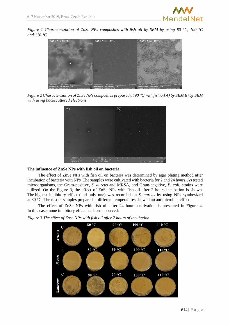
6–7 2019, Brno, Czech Republic
Figure 1 Characterization of ZnSe NPs composites with fish oil by SEM by using 80 °C, 100 °C and 110 °C
Figure 2 Characterization of ZnSe NPs composites prepared at 90 °C with fish oil A) by SEM B) by SEM with using backscattered electrons
The influence of ZnSe NPs with fish oil on bacteria The effect of ZnSe NPs with fish oil on bacteria was determined by agar plating method after
incubation of bacteria with NPs. The samples were cultivated with bacteria for 2 and 24 hours. As tested microorganisms, the Gram-positive, S. aureus and MRSA, and Gram-negative, E. coli, strains were utilized. On the Figure 3, the effect of ZnSe NPs with fish oil after 2 hours incubation is shown. The highest inhibitory effect (and only one) was recorded on S. aureus by using NPs synthesized at 80 °C. The rest of samples prepared at different temperatures showed no antimicrobial effect.
The effect of ZnSe NPs with fish oil after 24 hours cultivation is presented in Figure 4. In this case, none inhibitory effect has been observed.
Figure 3 The effect of Znse NPs with fish oil after 2 hours of incubation
614

6–7 2019, Brno, Czech Republic
Figure 4 The effect of ZnSe NPs with fish oil after 24 hour of incubation
CONCLUSION This study dealt with synthesis of ZnSe NPs with fish oil and determination their antimicrobial
activity potential. The results showed that the binding of NPs with fish oil by using different temperatures was successful (fish oil was bound to surface of nanocomposites). The antibacterial activity of these NPs with fish oils was observed only in one case (S. aureus by using 80 °C). The results of antibacterial activity could be influenced by the fish oil presence. It is possible to assume that the fish oil could block antibacterial effect of unmodified NPs. So, this testing is a subject of further exploring. Nanotechnology offers interesting and new strategies for regenerative medicine.
ACKNOWLEDGEMENTS The research was financially supported by the Internal Grant Agency of Mendel University in Brno, project No. TP 006/2019.
REFERENCES Azizi, M. et al. 2019. Study of the Physicochemical Properties of Fish Oil Solid Lipid Nanoparticle in the Presence of Palmitic Acid and Quercetin. Journal of Agricultural and Food Chemistry, 67(2): 671–679. Ding, M. et al. 2019. Effect of preparation factors and storage temperature on fish oil-loaded crosslinked gelatin nanoparticle pickering emulsions in liquid forms. Food Hydrocolloids, 95: 326–335. Fournier, V. et al. 2006. Thermal degradation of long‐chain polyunsaturated fatty acids during deodorization of fish oil. European Journal of Lipid Science and Technology, 108(1): 33–42. Hajialyani, M. et al. 2018. Natural product-based nanomedicines for wound healing purposes: therapeutic targets and drug delivery systems. International Journal of Nanomedicine, 13: 5023–5043. Kiecolt-Glaser, J.K. et al. 2014. Omega-3 Fatty Acids and Stress-Induced Immune Dysregulation: Implications for Wound Healing. Military Medicine, 179(11): 129–133. Komprda, T. et al. 2018. Effect of n-3 long-chain polyunsaturated fatty acids on wound healing using animal models–a review. Acta Veterinaria Brno, 87(4): 309–320. McDaniel, J.C. et al. 2008. Omega-3 fatty acids effect on wound healing. Wound Repair and Regeneration, 16(3): 337–345. Moulick, A. et al. 2017. Using CdTe/ZnSe core/shell quantum dots to detect DNA and damage to DNA. International Journal of Nanomedicine, 12, 1277. Ovais, M. et al. 2018. Wound healing applications of biogenic colloidal silver and gold nanoparticles: recent trends and future prospects. Applied Microbiology and Biotechnology, 102(10): 4305–4318.
615

6–7 2019, Brno, Czech Republic
Pivodova, V. et al. 2015. In vitro AuNPs' cytotoxicity and their effect on wound healing. Nanobiomedicine, 2: 7. Rajendar, N.K. et al. 2018. A review on nanoparticle based treatment for wound healing. Journal of Drug Delivery Science and Technology, 44: 421–430.
616

6–7 2019, Brno, Czech Republic
UV-Induced fingerprint spectroscopy (UV-IFS)
Tomas Rypar1,2, Marketa Vaculovicova1, Vojtech Adam1, Lukas Nejdl1
1Department of Chemistry and Biochemistry Mendel University in Brno Zemedelska 1, 613 00 Brno
2Department of Biochemistry Masaryk University in Brno
Kamenice 753/5, 625 00 Brno CZECH REPUBLIC
Abstract: This work is focused on a new, fast, simple, and robust method, based on physical-chemical changes caused in UV-irradiated sample. UV-IFS is an innovative approach for verification of authenticity and origin of drugs, pesticides, juices and beverages, but also useful tool for comparative analysis of clinical samples. UV-induced fingerprint spectroscopy is based on comparison of patterns (fingerprints), which are characteristic for a sample. There is no need for separation and the method is suitable for analysis of samples with complex matrixes within a short time.
Key Words: pattern recognition, UV-induced reactions, fluorescence spectrometry
INTRODUCTION The complexity of pharmacological agents, food, beverages/juices as well as clinical samples
(blood plasma, urine, histological sections etc.) is a fundamental problem complicating the identification of analytes or processes taking place in such samples within a short time (Lucci et al. 2017, Rosso et al. 2017). Moreover, most analyses must be preceded by an extraction/isolation or separation process appropriate to the target substance or type of the matrix (Goncalves et al. 2017, Tang et al. 2012). The entire process, though precise and effective, is time consuming and may be costly. In general, the methods used for such purposes include chromatographic, electrophoretic and/or spectroscopic techniques. Spectroscopic methods are less demanding for sample preparation compared to chromato-graphic of electrophoretic ones. For example, infrared (IR) spectroscopy enables to analyse the deformation vibrations where the bond lengths are constant, however the angles are changing. Such changes can be monitored in the region from 200 to 1200 1/cm. Such part of spectra is called a “fingerprint region” and based on the specific pattern in this region, the compound can be identified. So far, no such fingerprinting was described in fluorescence spectroscopy. Despite numerous advantages of IR spectroscopy (Porep et al. 2015), there are also several disadvantages including relatively costly instrumentation, difficult data interpretation and/or need for use of spectral databases. The calibration requires relatively high number of standard samples, which translates into the increased costs for creation of the calibration model (Mainali et al. 2014).
In recent years, an increasing interest in medical studies focusing on a top-down approach can be observed. This strategy is based on comparing patterns (fingerprints) of metabolites or other compounds changing as a response to various stimuli (e.g. disease progression, toxin exposure, environmental or genetic mutations, etc.) (Canese et al. 2016, Graca et al. 2017, Ma et al. 2013). The goal is not to identify each component separately, but to compare the patterns – the signatures of compounds that are changed as a response to the physiological/pathological states of the organism or changes occurring in surrounding environment. This approach can be used either for medical applications or for analyses of other various complex matrixes as a mixture of drugs, beverages (juices and wines) or natural products (vegetables, fruit and plants extracts) for profiling and identification purposes.
In this work, a new spectroscopic technique for fluorescence fingerprinting of different type of samples is introduced. This method uses natural fluorescence properties of samples in ultraviolet and visible region (230–600 nm) before and after UV-irradiation (λ = 254 nm). UV-exposure of a sample
617
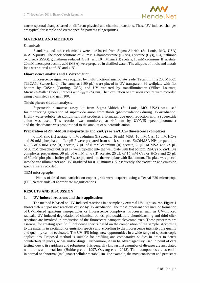
6–7 2019, Brno, Czech Republic
causes spectral changes based on different physical and chemical reactions. These UV-induced changes are typical for sample and create specific patterns (fingerprints).
MATERIAL AND METHODS
Chemicals Standards and other chemicals were purchased from Sigma-Aldrich (St. Louis, MO, USA)
in ACS purity. The stock solutions of 20 mM L-homocysteine (HCys), Cysteine (Cys), L-glutathione oxidized (GSSG), glutathione reduced (GSH), and 10 mM zinc (II) acetate, 10 mM cadmium (II) acetate, 20 mM mercaptosuccinic acid (MSA) were prepared in distilled water. The aliquots of thiols and metals ions were stored at −8 °C and 4 °C.
Fluorescence analysis and UV-irradiation Fluorescence signal was acquired by multifunctional microplate reader Tecan Infinite 200 M PRO
(TECAN, Switzerland). The samples (100 μL) were placed in UV-transparent 96 wellplate with flat bottom by CoStar (Corning, USA) and UV-irradiated by transilluminator (Vilber Lourmat, Marne-la-Vallee Cedex, France) with λem = 254 nm. Then excitation or emission spectra were recorded using 2-nm steps and gain 100.
Thiols photooxidation analysis Superoxide dismutase assay kit from Sigma-Aldrich (St. Louis, MO, USA) was used
for monitoring generation of superoxide anion from thiols (photooxidation) during UV-irradiation. Highly water-soluble tetrazolium salt that produces a formazan dye upon reduction with a superoxide anion was used. This reaction was monitored at 440 nm by UV/VIS spectrophotometer and the absorbance was proportional to the amount of superoxide anion.
Preparation of ZnCd/MSA nanoparticles and Zn/Cys or Zn/HCys fluorescence complexes 6 mM zinc (II) acetate, 6 mM cadmium (II) acetate, 16 mM MSA, 16 mM Cys, 16 mM HCys
and 80 mM phosphate buffer pH 7 were prepared from stock solutions. ZnCd/MSA NPs preparation: 43 μL of 6 mM zinc (II) acetate, 7 μL of 6 mM cadmium (II) acetate, 25 μL of MSA and 25 μL of 80 mM phosphate buffer pH 7 were pipetted into the well plate with flat bottom. Zn/Cys or Zn/HCys complexes preparation: 50 μL of 6 mM zinc (II) acetate, 25 μL of 16 mM Cys or HCys and 25 μL of 80 mM phosphate buffer pH 7 were pipetted into the well plate with flat bottom. The plate was placed into the transilluminator and UV-irradiated for 0–16 minutes. Subsequently, the excitation and emission spectra were recorded.
TEM micrographs Photos of dried nanoparticles on copper grids were acquired using a Tecnai F20 microscope
(FEI, Netherlands) at appropriate magnifications.
RESULTS AND DISCUSSION
1. UV-induced reactions and their applicationsThe method is based on UV-induced reactions in a sample by external UV-light source. Figure 1
shows different possible reactions caused by UV-irradiation. The most important ones include formation of UV-induced quantum nanoparticles or fluorescence complexes. Processes such as UV-induced radicals, UV-induced degradation of chemical bonds, photooxidation, photobleaching and thiol click reactions are involved in production of the fluorescent nanoparticles/complexes. These processes are essential for creating specific fluorescence spectra based on the composition of the sample. According to the patterns in excitation or emission spectra and according to the fluorescence intensity, the quality and quantity can be evaluated. The UV-IFS brings new opportunities in a wide range of spectroscopic applications. Proposed method is suitable for profiling and comparative studies in order to detect counterfeits in juices, wines and/or drugs. Furthermore, it can be advantageously used in point of care testing, due to its rapidness and robustness. It is generally known that a number of diseases are associated with thiols and metal ions (Hultberg et al. 1997, Ouyang et al. 2018). Thiol compounds are essential in normal or abnormal (malignant) cellular metabolism. For example, the most consistent and persistent
618

6–7 2019, Brno, Czech Republic
biochemical characteristic of prostate cancer is the significant decrease in zinc ions concentration in the malignant cells (Costello et al. 2004). Therefore, prostate cancer patients are obvious candidates for testing of here proposed method.
Figure 1 Chemical and physical changes in UV-irradiated sample and possible applications based on unique fluorescence patterns
2. UV-induced fluorescent quantum nanoparticles and complexes UV-irradiation causes various changes in a sample. We believe that the most important role play
thiols and metals. Reactions of different thiols and metals to UV-light irradiation lead to formation of fluorescent complexes or nanoparticles which results in specific fluorescence spectra.
Figure 2 A) UV/VIS absorption spectra in range 250–800 nm of 100 μM MSA, Cys, HCys, GSH and GSSG after 1 minute UV-irradiation with tetrazolium salt. The tetrazolium salt that produces a formazan dye upon reduction with a superoxide and can be monitored at λ = 440 nm and was proportionate to the amount of superoxide anion. These reactions together with metals ions form fluorescent nanoparticles and/or complexes. B) ZnCd/MSA nanoparticles tunable by prolongation of UV-irradiation (4–16 minutes) from (Zn: Cd: MSA in pH 7) precursors. C) Fluorescence excitation spectra of zinc and different thiols (Cys or HCys) mixtures before and after 20 minutes UV-treatment.
619
6–7 2019, Brno, Czech Republic
In Figure 2A, absorbance spectra of different thiols (Cys, HCys, MSA, GSH, GSSG) treated by UV-light (0 and 1 minute) are shown. Thiol group undergoes photooxidation and reducing environment with a superoxide anion is created. The generation of the superoxide anion was monitored by reaction with a tetrazolium salt producing a formazan dye. Reducing environment is essential for formation of fluorescent nanoparticles and complexes. It can be seen that all thiols except GSSG undergo photooxidation process and generate superoxide anion. The ions are represented by a peak in absorbance spectra at 440 nm. In Figure 2B and C, the fluorescence spectra of nanoparticles (Figure 2B) and complexes (Figure 2C), created by combination of thiols and metal ions after UV-treatment are shown. These nanoparticles are easily tuneable (emission wavelength) by a prolongation of UV-irradiation time (1–16 minutes) or composition of precursor’s mixture (Zn: Cd: MSA in pH 7). Also fluorescent complexes from mixture of Zn/Cys or Zn/HCys in pH 7 can be observed after 20 minutes of UV-irradiation with typical fluorescence spectra (patterns). In Figure 2D, micrographs of dried nanoparticles (composed of Zn: Cd: MSA) after 8 minutes of UV-irradiation are presented.
CONCLUSION In this work a new, simple, rapid and high-throughput spectroscopic method for sample
characterization was introduced. The method is suitable especially for origin discrimination through specific patterns recognition in different biological materials, but there are also other potential applications which have been intensively sought.
ACKNOWLEDGEMENTS The research was founded by Internal Grant Agency of Mendel University in Brno IGA MENDELU 2019_TP_009.
REFERENCES Canese, R. et al. 2016. In vivo Magnetic Resonance Metabolic and Morphofunctional Fingerprints in experimental Models of Human Ovarian Cancer. Frontiers in Oncology, 6: 164. Costello, L.C. et al. 2004. Role of zinc in the pathogenesis and treatment of prostate cancer: critical issues to resolve. Prostate Cancer and Prostatic Diseases, 7(2): 111–117. Goncalves, L.M. et al. 2017. Recent Advances in Membrane–Aided Extraction and Separation for Analytical Purposes. Separation and Purification Reviews, 46(3): 179–194. Graca, A. et al. 2017. Biological Predictors of Aging and Potential of FTIR to Study Age–related Diseases and Aging Metabolic Fingerprint. Current Metabolomics, 5(2): 119–137. Hultberg, B. et al. 1997. Copper ions differ from other thiol reactive metal ions in their effects on the concentration and redox status of thiols in HeLa cell cultures. Toxicology, 117(2–3): 89–97. Lucci, P. et al. 2017. Trends in LC–MS and LC–HRMS analysis and characterization of polyphenols in food. Trac–Trends in Analytical Chemistry, 88(1–24). Ma, D. et al. 2013. Magnetic resonance fingerprinting. Nature, 495(7440): 187–192. Mainali, D. et al. 2014. Development of a comprehensive near infrared spectroscopy calibration model for rapid measurements of moisture content in multiple pharmaceutical products. Journal of Pharmaceutical and Biomedical Analysis, 95(169–175). Ouyang, Y.F. et al. 2018. Modulation of thiol–dependent redox system by metal ions via thioredoxin and glutaredoxin systems. Metallomics, 10(2): 218–228. Porep, J.U. et al. 2015. On–line application of near infrared (NIR) spectroscopy in food production. Trends in Food Science & Technology, 46(2): 211–230. Rosso, G.L. et al. 2017. Seven years of workplace drug testing in Italy: A systematic review and meta–analysis. Drug Testing and Analysis, 9(6): 844–852. Tang, B. et al. 2012. Application of ionic liquid for extraction and separation of bioactive compounds from plants. Journal of Chromatography B–Analytical Technologies in the Biomedical and Life Sciences, 904(1–21).
620

6–7 2019, Brno, Czech Republic
A simple electrochemical biosensor for the detection of methylated DNA and for methyltransferase activity monitoring
Eliska Sedlackova1,2, Vendula Smolikova1,2, Eliska Birgusova1, Zuzana Bytesnikova1, Lukas Richtera1,2, Vojtech Adam1,2
1Department of Chemistry and Biochemistry
Mendel University in Brno Zemedelska 1, 613 00 Brno
2Central European Institute of Technology, Brno University of Technology,
Purkynova 656, 612 00 Brno CZECH REPUBLIC
Abstract: DNA methylation is one of the well-known epigenetic mechanism which plays a crucial role in the development of various diseases, such as cancer, cardiovascular diseases or diabetes. Electrochemical biosensors promise excellent results for clinical diagnostics, especially in term of their sensitivity, stability, selectivity, portability, they are cost-effective, easy-to-use and provides a fast response. In this study, simply, reliably and selective DNA based electrochemical biosensor for detection of methylated DNA was fabricated. The proposed biosensor was modified with the synthesised reduced graphene oxide combined with gold nanoparticles (rGO-AuNPs). This nanocomposite has shown a strong affinity to the DNA probe and demonstrated promising analytical characteristics. The electrochemical impedance spectroscopy (EIS) was used for the chara-cterization of interface properties of the gold electrode (GE). Additionally, the sensitivity of the developed biosensor was performed by differential pulse voltammetry (DPV) to investigate the activity of enzyme methyltransferase M.SssI (MTase). Fabricated biosensor offers quite a low detection limit (LOD), which was 3.2 U/ml and limit of quantification (LOQ) was 3.3 U/ml.
Key Words: electrochemical biosensor, methylated DNA, reduced graphene oxide, gold nanoparticles
INTRODUCTION Methylation of cytosines in DNA is one of the most studied epigenetic process regulating gene
expression and thus plays an important role in cell differentiation or proliferation. Among others, methylated DNA can be used as a new generation of biomarkers in modern diagnostic for detection of various diseases, prognosis or prediction of therapeutic response (Krejcova et al. 2017, Hossain et al. 2017). Methylated DNA can be detected quantitatively by many methods at the entire genome or specific gene loci in various samples of biological origin, such as urine, plasma and serum. The main advantage is that those samples can be obtained by non-invasive procedures (Gao et al. 2018, Li et al. 2012). Current conventional methods, such as polymerase chain reaction (PCR), colorimetric methods or high-performance liquid chromatography (HPLC) are effective, nevertheless, they have several disadvantages, such as expensive instrumentation and often involve complicated protocols or require skilled operators. On the other hand, electrochemistry provides sensitive, selective, cost-effective, reliable, fast and simple detection of MTase activity and methylated DNA assays (Wang et al. 2013, Chen et al. 2019).
This study was aimed to develop an efficient electrochemical DNA-based biosensor for the detection of DNA methylation. Furthermore, the rGO-AuNPs nanocomposite was used for quantification of methylated DNA to enhance the electrochemical signal and increase the sensitivity of the developed biosensor. The GE with a 1.6 mm diameter was used as a working electrode. As a recognition element was used thiolated single-stranded DNA (ssDNA) probe, because of strong sulphur affinity to gold (Au-S). Firstly, the ssDNA probe was immobilised on the GE surface via hybridization with ssDNA target, resulting in double-stranded DNA (dsDNA). The non-specific
621

6–7 2019, Brno, Czech Republic
binding sites were blocked by 6-mercapto-1-hexanol (MCH) and the characterization of the fabricated biosensor was carried out by EIS (Keighley et al. 2008). Afterwards, the dsDNA was methylated by enzyme M.SssI MTase. Then it was immersed in Methylene Blue solution (MB), which is used as an electrochemical indicator. Therefore, the sensitivity of the proposed biosensor was investigated by DPV. Then the methylated dsDNA was digested by the restriction endonuclease HpaII and then cleaved at a specific site sequence 5'-CCGG-3'. Obtained electrochemical signals of the reporter were decreased or disappeared (Bao et al. 2018).
MATERIAL AND METHODS
Reagents The synthetics oligonucleotides of specific sequence, such as probe: (ssDNA_1) HS-(CH2)6-5'-
CCT CGT GCG GGA TCA TTG TTA TTA GGCA-3'and target: (ssDNA_2) 3'-GGA GCA CGC CCT AGT AAC AAT AAT CCGT-5', chemicals for Piranha solution: nitric acid (HNO3), hydrogen peroxide (H2O2), MB, enzymes: CpG MTase M.SssI supplied with 10× NEBuffer 2, 200× S-adenosylmethionin (SAM, 32 mM) and restriction endonuclease HpaII with 10× CutSmart buffer (ThermoFisher), chemicals for buffers preparation: sodium chloride (NaCl), magnesium chloride (MgCl2), Trizma® base, hydrochloric acid HCl (37%), sodium hydroxide (NaOH), potassium sulfate (K2SO4), potassium hexacyanoferrate(III) (K3[Fe(CN)6]), potassium hexacyanoferrate(II) (K4[Fe(CN)6]), sodium dihydrogen phosphate (NaH2PO4) and sodium phosphate dibasic (Na2HPO4). Composition of used buffers is shown in Table 1. Reagents for the synthesis of GO and rGO-AuNPs: Tetrachloroauric acid (H[AuCl4]), 37% HCl, sodium citrate (Na3C6H5O7), potassium permanganate (KMnO4) and H2O2.
Chemicals used in this study, unless otherwise stated, were purchased from Sigma-Aldrich (St. Louis, MO, USA). The deionized water was prepared using reverse osmosis equipment Aqual 25 (Aqua Osmotic, Tisnov, Czech Republic). The deionized water was further purified by using the apparatus Milli-Q Direct QUV, equipped with the UV lamp (Aqua Osmotic, Tisnov, Czech Republic). The resistance was 18.2 MΩ·cm. The pH was measured using pH meter WTW InoLab (Weilheim, Germany).
Table 1 Buffer composition
Buffer Composition
Phosphate buffer 1.0 M at pH 7.0: 0.5 M NaH2PO4 + 0.5 M Na2HPO4
Immobilization buffer 0.8 M PB at pH 7 + 1.0 M NaCl + 5.0 mM
50 mM PB at pH 7 + MgCl2 + 1.0 mM EDTA
Hybridization buffer 0.1 M PB + 0.1 M K2SO4
Measuring buffer 50 mM PB at pH 7 + 5 mM K3[Fe(CN)6], K4[Fe(CN)6] + 0.1 M K2SO4
Synthesis of GO and rGO/ AuNPs GO was prepared by chemical oxidation of 5.0 g graphite flakes (100 mesh, ≥75% min)
in a mixture of concentrated H2SO4 (670 ml) and 30 g KMnO4 according to the simplified Hummer’s method (Hummers 1958) The reaction mixture was stirred vigorously. After 4 days, the oxidation of graphite was terminated by the addition of H2O2 solution (250 ml, 30 wt%). Formed GO was washed 3 times with 1.0 M HCl (37 wt%) and several times with Milli-Q water (total volume used 10 l) until constant pH value (3 – 4) was achieved. The amount of 3.75 mg of GO was added to 50 ml H[AuCl4] (0.24 mM) and the mixture was aged for 30 mins. Then, the mixture was heated at 80 °C and 940 µl of Na3C6H5O7 (0.085 M) was added dropwise. The mixture was maintained at 80 °C for 1 h (Goncalves et. al 2009).
622

6–7 2019, Brno, Czech Republic
Cleaning procedures of electrodes Prior to biosensor fabrication, the bare GE with a radius 1.6 mm (Basi, West Lafayette, USA) was
cleaned mechanically, chemically and electrochemically. The chemical cleaning of the bare GE was performed in Piranha solution (96% H2SO4 to 30% H2O2, ratio 3:1) for 15 mins with constant stirring and afterwards, the GEs were rinsed with Milli-Q and the procedure continued with mechanical polishing. The three bare GEs were first sonicated in ultrasonic cleaner Elmasonic P60H (Singen am Hohentwiel, Germany) for 15 mins in ethanol (EtOH) and then mechanically polished on a polishing pad (Buehler) with water-based Diamond suspension (0.5 μm). Followed by another sonication in EtOH and polished with and Alumina slurry (1.0 μm) and sonicated in EtOH for another 15 mins. Afterwards, the last polishing was carried out with 0.3 μm alumina slurry. As the last step were electrodes cleaned electrochemically in 0.5 M H2SO4 by 50 scans of CV by potential scanning between −0.05 V and +1.1 V. The GEs were rinsed with Milli-Q water and air dry out.
Biosensor fabrication For the biosensor construction (Figure 1), a 10 µl of rGO-AuNPs was dropped on bare GE
and let it dry in the oven at 70 °C for 1 h. The procedure continues with incubation of ssDNA_1 with 100 µM MCH diluted in immobilization buffer (50 µl in total) overnight (14 – 16 hours) at 4 °C. Then the GE was backfilled in 1.0 mM MCH for 1.5 h and followed with hybridization of ssDNA_2 for 1 h at 37 °C. After that, the 20 µl of enzyme M. SssI was dropped on electrode surface and let it incubated for 2 h at 37 °C. As the last step, the biosensor sensitivity via accumulation of MB on the electrode surface was investigated. The MB was accumulated by the immersing of GE containing various concentrations of M.SssI (c = 0; 50; 100; 150; 200; 300; 400 and 500 U/ml) in 20 mM Tris–HCl buffer (pH 7.0) containing 20 mM NaCl and 20 µM MB for 5 min. After incubation in the MB, was the GE rinsed with 0.1 M PB three times to remove the non-accumulated MB.
Figure 1 Illustration of the developed biosensor for the detection of methylated DNA and the M.SssI MTase activity
Electrochemical experiments
Electrochemical techniques, DPV and EIS were performed with an Autolab PGSTAT302N (Metrohm, Herisau, Switzerland). For the measurement was used a standard three-electrode connection in the electrochemical cell. As a reference electrode was used Ag/AgCl connected via a salt bridge (50 mM PB + 0.1 M K2SO4) and as auxiliary was set a platinum electrode. The parameters of EIS were the following: the frequency range from 100 kHz to 100 mHz, with a 10 mV a.c. voltage applied on a bias d.c. voltage of 0.2 V vs. reference electrode (corresponding to the formal potential of the redox couple). The sensitivity of biosensor was verified by DPV and the parameters were following: applied potential from 0.0 V to −0.6 V, amplitude 0.025 V and scan-rate 0.01 V/s.
623

6–7 2019, Brno, Czech Republic
RESULTS AND DISCUSSION
Synthesis of GO and rGO-AuNPs The SEM pictures (see Figure 2) confirmed the preservation of the fine structure of the large area
GO. This method also enabled determining the degree of exfoliation, which is crucial for nanomaterial. The SEM micrographs also allowed the rating of AuNPs adhesion to GO which acts as a carrier of AuNPs.
Figure 2 SEM pictures of A) GO and B) rGO-AuNPs
Optimization of self-assembled monolayer (SAM) For the modification of biosensor, the ssDNA_1 was mixed with 100 µM MCH for the creation
of the SAM layer. The MCH used as a spacer molecule which allows better control of the lateral density of the DNA structure as well as to both reduce the non-specific interactions and regulate the charge transfer (Rct) for EIS experiments. Additionally, MCH molecules help the ssDNA_1 structure to stand in the upright position enabling better capturing properties towards the target. To establish complete thiol coverage of the GE surface, the electrodes were backfilled with 1.0 mM MCH diluted in Milli-Q water. Therefore, the optimisation of the EIS sensor must be done compromising the surface conditions that provide the maximum target binding with a ratio of 1:20 of ssDNA_1 to 100µM MCH fraction as is seen in Figure 3. There were tested two concentration of the DNA probe, while the 100 nM showed a more significant change in the Rct. This ratio was used in the following electrochemical experiment as an optimal value.
Figure 3 The percentage increase of Rct for a ratio of DNA: MCH concentrations for the determination of ssDNA_1 (10 nM and 100 nM) in measuring buffer
Characterization of developed biosensor For investigation and characterisation of every single layer in the presence of the measuring buffer
(Table 1) was used EIS (Figure 4). The EIS method has been confirmed as an effective technique by evaluating of Rct. The effects of various modifications are presented by Nyquist plots in measuring buffer (Figure 3A). The bare GE has shown the lowest Rct (354 Ω) with a small semi-circle due to the free-electron transport process. After modification by rGO-AuNPs, the value of Rct (621 Ω) increased a little bit because of enhanced electron transport caused by the strong affinity between Au-S. When the ssDNA_1 was immobilised on a layer of rGO-AuNPs the value Rct (1.8 kΩ) increase.
624

6–7 2019, Brno, Czech Republic
And after hybridization with ssDNA_2, while the double structure of DNA (dsDNA) was formed and the Rct (5.5 kΩ) was more than three times higher. This increase is caused by electrostatic repulsion effect of [Fe(CN)6]3−/4− due to the negative charge of phosphate groups from DNA structure. The process continues with treatment by M.SssI MTase, which also led to increasing of Rct (13.7 kΩ), which indicates full methylation of dsDNA. As the last step, there was applied HpaII, which caused the decreasing of Rct (11.8 kΩ). The main reason is in blocking of the cleavage of a specific site by HpaII. This result indicates a successful biosensor fabrication.
Figure 4 EIS characteristic of different modifications in measuring buffer (Table 1). (a) The bare GE, (b) GE/rGO-AuNPs, (c) GE/rGO-AuNPs/probe DNA_S1, (d) GE/rGO-AuNPs/probe DNA_1/ target DNA_2, (e) GE/rGO-AuNPs/probe DNA_1/ target DNA_2/ M.SssI MTase (500 U/ml)/ HpaII (20 U/mL) and (f) GE/rGO-AuNPs/probe DNA_1/ target DNA_2/ M.SssI MTase (500U/ml)
Sensitivity of biosensor
In the term of biosensor sensitivity, the DPV technique was performed to investigate the level of M.SssI activity by increasing concentration of M.SssI, from 0 to 500 U/ml (Figure 5). As Figure 5A) shows, the signal grows with a higher concentration of M.SssI. It depends on the incorporation of MB into the grooves of the double helix structure, and therefore the more dsDNA, the more MB can be integrated and it enhances the signal. Nevertheless, it confirms a fact, that the highest concentration of M.SssI prevents HpaII to cleave the target specific sequence of dsDNA.
Figure 5B) presents the calibration curve with a linear signal increasing concentration of M.SssI from 0 to 500 U/ml. The values of linear equation are: I(µA) = −0.006c (U/ml) − 0.089; (R2 = 0.999). The LOD was estimated to 3.2 U/ml and the LOQ was 3.3 U/ml. The LOD was calculated from 3σ rule (S/N = 3) and error bars are presented as a standard deviation from measurement (n = 3).
Figure 5 A) DPV curves of modified electrode. The dsDNA was methylated by 0; 50; 100; 150; 200; 300; 400 and 500 U/ml M. SssI. B) Calibration curve corresponding to the accumulated MB in the groove of helix structure. Error bars were created in dependence on standard deviations from the measurement
625

6–7 2019, Brno, Czech Republic
CONCLUSION In summary, simple, reliable and selective DNA based electrochemical biosensor for the detection
of methylated DNA was fabricated. There were tested DNA methylation process via EIS and the level of methylation by DPV, which indicates good sensitivity as well. Compared with conventional methods, the proposed technique is simple, easy, without expensive instrumentation, PCR amplification and does not require multiple steps of the procedure. It has shown a great potential for detection on real samples which will be held in the future. Moreover, this biosensor promises to transfer to screen printed electrodes which enable mass and low-cost production of this biosensor which can be part of smart nanodevices for personal use.
ACKNOWLEDGEMENTS The research was financially supported by the IGA MENDELU AF-IGA2019-IP059 and was carried out under the project CEITEC 2020 (LQ1601) with financial support from the Ministry of Education, Youth and Sports of the Czech Republic under the National Sustainability Programme II.
REFERENCES Bao, J. et al. 2018. A simple and universal electrochemical assay for sensitive detection of DNA methylation, methyltransferase activity and screening of inhibitors. Journal of Electroanalytical Chemistry, 814: 144–152. Chen, X. et al. 2019. Electrochemical Biosensor for DNA Methylation Detection through Hybridization Chain-Amplified Reaction Coupled with a Tetrahedral DNA Nanostructure. ACS Applied Materials & Interfaces, 11(4): 3745–3752. Gao, F. et al. 2018. Highly efficient electrochemical sensing platform for sensitive detection DNA methylation, and methyltransferase activity based on Ag NPs decorated carbon nanocubes. Biosensors and Bioelectronics, 99: 201–208. Goncalves, G. et al. 2009. Surface Modification of Graphene Nanosheets with Gold Nanoparticles: The Role of Oxygen Moieties at Graphene Surface on Gold Nucleation and Growth. Chemistry of Materials, 21(20): 4796–4802. Hossain, T. et al. 2017. Electrochemical biosensing strategies for DNA methylation analysis. Biosensors and Bioelectronics, 94: 63–73. Hummers, W.S. 1958. Preparation of Graphitic Oxide. Journal of the American Chemical Society, 80(6): 1339–1339. Keighley, S.D. et al. 2008. Optimization of DNA immobilization on gold electrodes for label-free detection by electrochemical impedance spectroscopy. Biosensors and Bioelectronics, 23(8): 1291–1297. Krejcova, L. et al. 2017. Current trends in electrochemical sensing and biosensing of DNA methylation. Biosensors and Bioelectronics, 97: 384–399. Li, W. et al. 2012. Signal amplification of graphene oxide combining with restriction endonuclease for site-specific determination of DNA methylation and assay of methyltransferase activity. Analytical Chemistry, 84(17): 7583–7590. Wang, G.L. et al. 2013. Electrochemical strategy for sensing DNA methylation and DNA methyltransferase activity. Analytica Chimica Acta, 768: 76–81.
626

6–7 2019, Brno, Czech Republic
Ferritin nanocages can deliver inhibitors of hyperactive protein kinases for a targeted treatment of breast cancer
Zuzana Skubalova1, Zuzana Bytesnikova1,2, Jan Pribyl3, Akila Weerasekera4 1Department of Chemistry and Biochemistry
Mendel University in Brno Zemedelska 1,613 00 Brno
2Central European Institute of Technology Brno University of Technology Purkynova 123, 621 00 Brno
3Central European Institute of Technology Masaryk University
Kamenice 5, 625 00 Brno CZECH REPUBLIC
4Biomedical MRI unit/MoSAIC, Department of Imaging and Pathology Katholieke Universiteit Leuven Oude Markt 13, 3000 Leuven
BELGIUM
Abstract: This project was focused on targeted chemotherapy based on ferritin nanocarriers with encapsulated various types of tyrosine kinase inhibitors. Then this nanoconstruct is surface-modified by folic acid, with the aim to achieve specific targeting to folate receptor overexpressed in targeted breast cancer cell line.
Key Words: encapsulation, ferritin, folic acid, nanoconstructs, specifically targeted therapy
INTRODUCTION Targeted chemotherapy based on nanocarriers with entrapped drugs and surface-attached specific
ligands is a very promising area in current research. This research area includes efforts to avoid serious sides effects on healthy cells as effectively as possible, while at the same time retaining the ability to target and kill the cancer cells. The second aim of this new approach in chemotherapy is to increase survival time and the quality of patient’s life (Tolchilin et al. 2007).
By all means, development of nanocarriers with encapsulated active agents is very suitable for poorly water soluble pharmaceuticals. This is beneficial since large proportions of new potential drug candidates are water-insoluble. Also surface coating of prepared nanoconstructs by targeting ligands is a very useful manner how to target chemotherapeutics, because cancer cells often overexpress specific receptors (Brannon-Peppas et al. 2012).
This project is focused on successful encapsulation of water-insoluble drugs belonging to tyrosine kinase inhibitors family, namely lenvatinib and vandetanib. The main goal is to encapsulate them to the ferritin protein cage, which is a pH sensitive globular protein, and also provide effective targeting surface modification of prepared nanoconstructs. For purposes of this study, coating with folic acid was selected because the target cell line (T-47D) in our cell culture overexpressed appropriate receptor (folate receptor) compared to target normal cell lines (HBL-100, HEK) (Tesarova et al. 2019). Above all, because of the fact that endosomes have acidic pH, thanks to pH sensitive properties of ferritin, prepared nanoconstructs should release the incorporated drug after specific uptake via folate binding receptors in the target cancer cells (Kim et al. 2011, Chen et al. 2013). Then the active compounds are able to transduce endosome membrane via diffusion to cell cytoplasm.
In this study, we will compare two types of preparations of designed nanoconstructs. There are two ways how to entrap the drug into ferritin. The first is active encapsulation based on ferritin’s ability
627

6–7 2019, Brno, Czech Republic
to dissociate in acidic pH and subsequently reassociate in neutral pH. During this di/reassociation, molecules of active agents can be encapsulated. The second method is a passive encapsulation. This method requires molecules of the drug to spontaneously pass through pores in ferritin structure pores or bind on its surface (Figure 1).
Figure1 Scheme of two types of encapsulation process of tyrosine kinase inhibitors to ferritin protein cage
MATERIALS AND METHODS Cell lines used for analysis were: normal breast cell line (HBL-100), normal embryonic kidney
cell line (HEK-293), cancer mammary gland breast cell line (T-47D), cancer mammary gland breast cell line (MCF- 7).
Preparation and surface coating of designed nanoconstructs Designed nanoconstructs were prepared fresh for all tests and measurements. Nanoconstructs
were prepared following by optimised protocol. The first way of preparation was active encapsulation. The pH of ferritin solution in water was
decreased via 1M HCl to value around 4, and incubated for 15 min on rotator. After that, solution of lenvatinib/vandetanib in DMSO (1 mg/ml) was added together with solution of phosphate buffer pH 7.5. After further 15 min incubation, the prepared nanoconstructs were 3× washed via diafiltration (100K) with phosphate buffer pH 7.5.
The second way of preparation was passive encapsulation. Solution of ferritin in water with lenvatinib/vandetanib in DMSO (1 mg/ml) was incubated on rotator for 24 h at 25 °C. After incubation, the prepared nanoconstructs were 3× washed via diafiltration (100K) with phosphate buffer pH 7.5 or Milli-Q water.
Surface modification of nanocarriers was performed by utilizing 56 mM solution of folic acid in 1 M NaOH and 200 mM solution of zero-length liker N, N-dicyclohexylcarbodiimide (DCC) in DMSO with incubation at 23 °C and 600 rpm for 2 h. Unbound folic acid was washed away
628

6–7 2019, Brno, Czech Republic
via 3× diafiltration (100K). Washing environment depended on environment of prepared nanoconstructs (water or phosphate buffer pH 7.5).
Characterization of prepared nanoconstructs Yield of encapsulation was determined by measurement on UV-Vis spectrophotometer
before and after washing of prepared nanoconstructs. Tyrosine kinase inhibitors absorb light at the wavelength 320 nm, which is far enough to distinguish it from absorption wavelength of ferritin. Yield of encapsulation is dependent on the type of tyrosine kinase inhibitor, solution environment and pH during preparation. Usual percentage of encapsulation yield in this case was around 15–40 %.
Measurement of size and ζ-potential were performed via quasielastic dynamic light scattering (DLS). Measured samples were prepared fresh for each run, size was mainly influenced by solution environment and final pH of sample.
For imaging of shape and also verifying size and structure of ferritin after process of encapsulation, atomic force microscopy (AFM) was used. This technique can explore how the surface of nanocarrier looks and if the structure of ferritin is reassociated correctly. In addition, native polyacrylamide gel electrophoresis (PAGE) was used to uncover changes in ferritin’s structure after pH changes or addition of solvent or after other processes during encapsulation.
In vitro screening of effectivity of prepared nanoconstructs Colorimetric 3-[4, 5-dimethylthiazol-2-yl]-2, 5 diphenyl tetrazolium bromide (MTT) assay was
used as primary screening of effectivity of prepared nanoconstructs and for verifying a protective influence on normal cell lines. Also it was used to find acceptable effective concentration for both cancer and normal cell lines. Furthermore, to avoid interaction of MTT dye with prepared nanoconstructs independent on cell proliferation, an alternative viability test based on fluorescent dye CyQUANT was used. This allows an accurate measurement of cell number via binding to cellular nucleic acids.
Pulse-and-chase treatment mode was used to evaluate the influence of targeted nanoconstructs on further cell proliferation. For this purpose, we incubated cells in microplates for 6 h with the treatment, then we replaced it with fresh medium. The cell proliferation was evaluated after 6, 24, 48 and 72 h using MTT dye.
To evaluate the influence of the targeted treatment of clonogenicity of the cells, we performed an in vitro cell survival assay based on the ability of a single cell to grow into a colony.
RESULTS AND DISCUSSION Designed nanoconstructs have icosahedral shape because of ferritin structure. It was found
that the shape is changed just in case when ferritin is not properly reassocied after process of encapsulation. The incorrect reassociation has been proven to lead to formation of ferritin cages with two hole defects on the opposite poles a headset-shaped structure or even rod-like subunit oligomers (Kim et al. 2011). It was ascertained that the best way to reach correct reassociation is by using phosphate buffer pH 7.5 for increasing pH of final solution and also to avoid vortexing or hard mixing of prepared solution. Otherwise structure of ferritin is irreversibly dissociated, although based on native PAGE only, we cannot say which form, known from literature, the ferritin took.
Results performed via DLS measurements showed that the usual size is around 10–30 nm before and also after surface modification, regardless of type of preparation, used environment or used type of drug. This size is in agreement with the size of native ferritin, as published elsewhere (Tesarova et al. 2019), proving that the encapsulation has not lead to formation of large ferritin aggregates, as well as supporting the data obtained from native PAGE.
ζ-potential is a commonly used parameter for evaluating stability of colloidal an nanoparticle systems as in describes the electrostatic potential at the electrical double layer surrounding a nanoparticle in solution (Clogston and Patri 2011). For this reason, we measured the values of ζ-potential in our samples in the solutions used for their preparation. The results indicate stable samples in case of active encapsulation in phosphate buffer pH 7.5 and also in the case of passive encapsulation in water environment, equally after surface coating. On the one hand, passively encapsulated samples in phosphate buffer pH 7.5 with surface coating has decreased value of ζ-potential, which can refer
629

6–7 2019, Brno, Czech Republic
to less stable samples. But on the other hand, native PAGE with these samples uncovered properly reassembled nanoconstructs. Having said that, the surface-modified nanoconstructs prepared passively in water environment appeared to be unfolded on native PAGE or their electrophoretic mobility changed due to the surface modification (Figure 2). Moreover, according to the results from AFM, it can be concluded that all prepared nanoconstructs have oval shape without any signs of unfolding, comparing to positive control which was a directly unfolded structure of ferritin.
Regarding the in vitro cytotoxicological analyses, the passively prepared nanoconstructs performed better almost in every kind of assay, especially in the point of protective properties towards selected normal cell lines. This is the most focused-on parameter as the safety of nanomedical treatment compared to standard chemotherapy is of the most importance (Tesarova et al. 2019). In general, the most effective incubation time was 6 h. After longer incubation, the cells started to proliferate again or they became senescent.
All things considered, some of the designed targeted nanoconstructs seem to be quite effective and promising for targeted cancer therapy but it is still necessary to optimize and modify some of their features.
Figure 2 Native PAGE, prove of pH sensitive properties of ferritin and also prove of structure of nanoconstructs after encapsulation process. lenvatinib (L), vandetanib (V), ferritin (FRT), Buffer (phosphate buffer pH 7.5)
CONCLUSION We designed and prepared various types of targeted nanocarriers aiming to reduce cancer
proliferation and at the same time to protect normal cells from toxic effect of active compounds. One of the goal to accomplish was to compare effectivity among these prepared nanoconstructs. More or less, we had some successful results regarding the optimization of nanoconstructs properties, such as size, stability or final correct reassembly of ferritin. The performed in vitro viability screening tests lead us to determine the treatment mode and effective treatment concentration. The most promising of the prepared nanocarriers was chosen to perform further optimization and in vitro testing.
Overall, this research area is very promising and it is necessary to be focused on and try to find out another way how to prepare effective and specifically targeted drugs. In our study, we showed some of the promising results in this field of study. But it is still necessary to continue and improve the properties of designed nanoconstructs to obtain even better results.
630
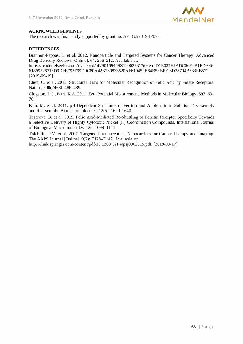
6–7 2019, Brno, Czech Republic
ACKNOWLEDGEMENTS The research was financially supported by grant no. AF-IGA2019-IP073.
REFERENCES Brannon-Peppas, L. et al. 2012. Nanoparticle and Targeted Systems for Cancer Therapy. Advanced Drug Delivery Reviews [Online], 64: 206–212. Available at: https://reader.elsevier.com/reader/sd/pii/S0169409X12002931?token=D1E037E9ADC56E4B1FDA4661899526318D9DFE793F99D9C80A42B260833820AF610459B64B53F49C3D28794B333EB522. [2019-09-19]. Chen, C. et al. 2013. Structural Basis for Molecular Recognition of Folic Acid by Folate Receptors. Nature, 500(7463): 486–489. Clogston, D.J., Patri, K.A. 2011. Zeta Potential Measurement. Methods in Molecular Biology, 697: 63–70. Kim, M. et al. 2011. pH-Dependent Structures of Ferritin and Apoferritin in Solution Disassembly and Reassembly. Biomacromolecules, 12(5): 1629–1640. Tesarova, B. et al. 2019. Folic Acid-Mediated Re-Shuttling of Ferritin Receptor Specificity Towards a Selective Delivery of Highly Cytotoxic Nickel (II) Coordination Compounds. International Journal of Biological Macromolecules, 126: 1099–1111. Tolchilin, P.V. et al. 2007. Targeted Pharmaceutical Nanocarriers for Cancer Therapy and Imaging. The AAPS Journal [Online], 9(2): E128–E147. Available at: https://link.springer.com/content/pdf/10.1208%2Faapsj0902015.pdf. [2019-09-17].
631

6–7 2019, Brno, Czech Republic
Developing chemoresistance to tyrosine kinase inhibitors
Veronika Smidova, Zita Goliasova
Department of Chemistry and Biochemistry Mendel University in Brno Zemedelska 1, 613 00 Brno
CZECH REPUBLIC
Abstract: Resistance to tyrosine kinase inhibitors (TKIs) is a major issue in cancer therapy, as almost every patient undergoing this treatment gains chemoresistance. In this project, we attempted to develop chemoresistant cell lines insensitive to three recently approved TKIs – vandetanib, lenvatinib and cabozantinib. Our goal was to obtain these cell lines by continuous growth in the presence of said inhibitors for further examination and research of chemoresistance mechanisms. Unfortunately, we came across some problems and the long-term character of our experiment forced us to take up a different approach. In the future, we plan to continue our project by inducing chemoresistance with transfection of an expression vector containing mutated sequence of receptor tyrosine kinase.
Key Words: drug resistance, cell line model, cabozantinib, lenvatinib, vandetanib
INTRODUCTION Tyrosine kinases (TKs) are molecules with pivotal role in signal transduction. Regulation of their
activity affects gene transcription and essentially controls cell cycle progression, proliferation, differentiation, motility and cell death (Prenzel et al. 2001, Slichenmyer et al. 2001). There are number of diseases and disorders caused by genetic changes or abnormalities in TKs that affect their activity, quantity, distribution in the cell and regulation. In malignant cells, mutations and aberrant activation of TK’s signal transduction pathways have been causally related to multiple types of cancer, diabetes, inflammation, severe bone disorders, arteriosclerosis or angiogenesis (Lemmon and Schlessinger 2010).
Chemoresistance is a major issue limiting the efficiency of chemotherapy and resulting in relapse and metastasis. There are two types of chemoresistance concerning its origin. Some tumours can be intrinsically resistant prior to therapy. However, most frequently, tumours are initially sensitive to therapy and obtain chemoresistance to the drug during the treatment. Moreover, in over 90% of metastatic cancer cases the resistance of either type is believed to be the cause of therapy failure (Longley and Johnston 2005). There are 35 TKIs that have been tested and approved for treatment of cancer by U. S. Food and Drug Administration. However, usually after 10 to 14 months of therapy, the patients incline to acquire resistance almost without exception. Therefore, it should be a priority in topical research to understand the mechanisms of resistance to TKIs and develop treatment strategies to surpass it (Chen and Fu 2011).
The key to studying chemoresistance mechanisms is developing chemoresistant cell line that can then be further examined and surveyed. Therefore, in this project, we set our goal to develop cell lines resistant to TKIs vandetanib, lenvatinib and cabozantinib.
MATERIAL AND METHODS
Chemicals Tyrosine kinase inhibitors vandetanib, lenvatinib and cabozantinib were purchased
from LC Laboratories (Woburn, MA, USA).
Cell viability assay Cells were seeded at a density of 5×10³ cells/well in 96-well plates. The next day, TKIs
(vandetanib, lenvatinib and cabozantinib) at starting concentration of 100 µM were added to cells and incubated further for 72 hours. Cell viability was spectrophotometrically measured on Tecan
632

6–7 2019, Brno, Czech Republic
Infinite 200 PRO using MTT assay with Thiazolyl Blue Tetrazolium Bromide (Sigma–Aldrich, St. Louis, MO, USA) at 570 nm.
Establishment of TKI chemoresistant cells Cell lines MDA-MB-468 and T-47D were cultured in RPMI-1640 (Sigma–Aldrich, St. Louis,
MO, USA). All media were supplemented with 10% fetal bovine serum (FBS). All cells were incubated at 37 °C in humidified air containing 5% CO2. Working solutions of drugs were dissolved in dimethyl sulfoxide (DMSO) and stored in -80 °C. Drugs were diluted in growth medium at appropriate concentrations immediately prior to use.
Cells were continually grown in the presence of each inhibitor. For each treatment, cells were grown in duplicate flasks. Two strategies were adapted. One starting with concentrations higher than IC50 and the other starting with concentrations ten times lower than the first concentration. Concentration of the inhibitors was raised after minimum of three passages according to cell growth and condition (see Table 1). Growth medium with treatment was changed every 2–3 days.
Cells were photographed after every concentration adjustment on EVOS FL Auto Imaging System (Life Technologies, Carlsbad, CA, USA).
Table 1 Overview of TKI concentration adjustments
Cell line Nr. of adjustment
Van. High [µM]
Van. Low [µM]
Len. High [µM]
Len. Low [µM]
Cab. High [µM]
Cab. Low [µM]
MDA-MB-468 0 7 0.7 15 1.5 10 1 1 7 0.9 20 2 12 1.2 2 7 1 20 3 10 1.5
T-47D 0 2 0.2 15 1.5 8 0.8 1 3 0.3 20 2 8 1 2 4 0.5 20 3 8 1.5
RESULTS AND DISCUSSION
Cell viability assay After 72 hours vandetanib IC50 value for MDA-MB-468 cell line was 4.65 µM and for T-47D
it was 1.3 µM. lenvatinib reached IC50 values of 20 µM and 3.5 µM, for MDA-MB-468 and T-47D respectively. IC50 values of cabozantinib were 8.7 µM for MDA-MB-468 and 4.7 µM for T-47D (Figure 1).
Cell imaging There were differences in morphology in some of the TKI treated cells. The change
in morphology first occurred in MDA-MB-468 treated with higher concentration of vandetanib. Cells were under great treatment pressure and didn’t grow as much as other cells. Therefore, for the entirety of the experiment, concentration of their treatment hadn’t been raised (Figure 2A, 2B). Cells treated with higher concentration of other inhibitors were visibly under treatment pressure, but their morphology wasn’t significantly changed (Figure 2C).
In T-47D cell line, the higher concentration of cabozantinib treatment had an effect on cell morphology after three months (Figure 2D, 2E), making the shape of the cells completely different from other treatments of the same cell line (Figure 2F). Overall, all cells showed signs of changes in the form of irregularity of the plasma membrane and microvesicular formation.
Assessment of cytotoxic effects of TKIs after 3 months of chemoresistance development As we were about to assess if and to what extent the chemoresistance has developed, problems
with contamination occurred. Unfortunately, with this type of long-term experiment there is a high risk of contamination of the cells due to frequent handling of flasks and using the growth media without antibiotics.
633

6–7 2019, Brno, Czech Republic
Figure 1 IC50 values of vandetanib, lenvatinib and cabozantinib
MDA-MB-468 T-47D0123456789
10111213141516171819202122232425
IC50
Cell line
Conc
entra
tion
(µM
)
Van Len Cab
Figure 2 Images of cells treated with TKIs
A) MDA-MB-468 after 1 monthof treatment with vandetanib (40x magnification)
B) MDA-MB-468 after 3months of treatment with vandetanib (20x magnification)
C) MDA-MB-468 after3 months of treatment with lenvatinib (20x magnification)
D) T-47D after 1 monthof treatment with cabozantinib (40x magnification)
E) T-47D after 3 monthsof treatment with cabozantinib (20x magnification)
F) T-47D after 3 monthsof treatment with lenvatinib (20x magnification)
CONCLUSION In this experiment we evaluated the cytotoxicity effects of three TKIs (vandetanib, lenvatinib
and cabozantinib) and began to develop chemoresistance to these three inhibitors in two different breast cancer cell lines (MDA-MB-468 and T-47D). In the middle of our experiment problems occurred and forced us to end it abruptly. We will further continue with different approach to achieve a similar
634

6–7 2019, Brno, Czech Republic
goal. We will use transfection of an expression vector with mutated receptor TKs as our means to induce chemoresistance in our cells, which we will then proceed to explore further.
ACKNOWLEDGEMENTS The research was financially supported by the grant AF-IGA2019-IP010.
REFERENCES Chen, Y., Fu, L. 2011. Mechanisms of acquired resistance to tyrosine kinase inhibitors. Acta Pharmacologica Sinica B, 1(4): 197–207. Lemmon, M.A., Schlessinger, J. 2010. Cell Signaling by Receptor Tyrosine Kinases. Cell, 141(7): 1117–34. Longley, D.B., Johnston, P.G. 2005. Molecular mechanisms of drug resistance. The Journal of Pathology, 205(2): 275–292. Prenzel, N. et al. 2001. The epidermal growth factor receptor family as a central element for cellular signal transduction and diversification. Endocrine-Related Cancer, 8(1): 11–31. Slichenmyer, W.J. et al. 2001. Signal Transduction in Cancer. Seminars in Oncology, 28(5): 67–79.
635

6–7 2019, Brno, Czech Republic
Determination of arsenic bioavailability in mineral springs in the Czech Republic
Vendula Smolikova1,3, Eliska Sedlackova1,3, Pavlina Pelcova1, Andrea Ridoskova1, Barbora Musilova2
1Department of Chemistry and Biochemistry 2Department of Zoology, Fisheries, Hydrobiology and Apiculture
Mendel University in Brno Zemedelska 1, 613 00 Brno
3Central European Institute of Technology Brno University of Technology Purkynova 123, 612 00 Brno
CZECH REPUBLIC
Abstract: Mineral springs Hronovka and Regnerka located in the northeast Bohemia, Czech Republic are characteristic for high content of arsenic. The diffusive gradient in thin films technique (DGT) was used for determination of arsenic bioavailable fraction in both mineral water samples. Despite the high concentration of iron in both mineral water, the arsenic content measured by DGT (cDGT) corresponded to the total arsenic concentration measured directly by ET-AAS in the grab sample of mineral water (cGRAB) with the final ratio cDGT/cGRAB 1.09 for Hronovka, and 1.06 for Regnerka. These results indicate that the composition of the mineral water prevents the complexation of arsenic and iron and so arsenic in tested spring waters is completely bioavailable.
Key Words: arsenic, bioavailability, DGT, mineral spring
INTRODUCTION In the Czech Republic, there are many natural mineral springs, some of which are traditionally
used for their healing effects in spa towns. In the area of northeast Bohemia, we can find arsenic-rich mineral springs. According to the former Czechoslovakian national standard (ÚNMZ 1966) the mineral spring can be considered as arsenic spring if the arsenic content exceeds the limit of 0.7 mg/l. The current classification of mineral waters does not take into account the arsenic content (Česká Republika 2001). Legislation of the Czech Republic sets the maximum hygienic level of arsenic in drinking water to 10 µg/l (Česká Republika 2014), which is also consistent with recommendations of World Health Organization (WHO 2011).
Generally, arsenic in natural water is present in arsenite AsO33− and arsenate AsO4
3− oxoanion forms (Smedley and Kinniburgh 2002). The composition of mineral spring is influenced by the geological and hydrogeological location of the spring (Fugedi et al. 2010). Mineral water generally contains a high concentration of sulfates, carbon dioxide, chlorides or iron, which can affect the speciation and bioavailability of arsenic. In the surface geothermal waters rich in sulfides, arsenic is rather than oxyanions present as thioanions with the predominance of thioarsenates (Guo et al. 2017). The presence of ferric compounds in the aquatic environment also has a significant influence on the mobility of arsenic (Farrell et al. 2013) and thus the bioavailable fraction of arsenic can be lower compared to the total arsenic concentration in mineral springs.
In this study, the diffusive gradient in thin films technique (DGT) was used for determination of arsenic bioavailable fraction in the samples of mineral springs. The principle of the DGT technique is based on the diffusion of metals through a diffusive gel and their subsequent accumulation on a resin gel containing functional groups for targeted analytes. In real ecosystems, primarily mobile and labile forms of the metal, such as free and hydrated ions and complexes with natural ligands smaller than the pore size of the diffusion gel are able to diffuse through the diffusion gel and subsequently are bound in the resin gel (Zhang and Davison 2000). Resin gels containing iron oxyhydroxide functional
636

6–7 2019, Brno, Czech Republic
groups were used for arsenic determination. Iron oxyhydroxide is able to adsorb arsenite as well as arsenate compounds by ion-exchange mechanism and is commonly used for arsenic removal from drinking water (Giles et al. 2011).
MATERIAL AND METHODS
Reagents All chemicals were of analytical grade or higher. Standard solution of AsIII (c = 1000 ± 4 mg/l
in 2% (v/v) HNO3 (Sigma-Aldrich, Germany)) was used for calibration. Palladium 10 g/l (Analytika, Czech Republic) was used as a matrix modifier for ET-AAS determination of arsenic, sodium tungsten dihydrate (Sigma-Aldrich, Germany) was used for graphite furnace surface coating. Test kit NANOCOLOR® Sulfate LR 200 (Macherey-Nagel, Germany) was used for photometric determination of sulfate. All solutions were prepared using Milli-Q water produced by Millipore Milli Q system (Millipore, Bedford, MA, USA), the 65% nitric acid (VWR, Czech Republic) was distilled by apparatus Type BSB-939IR (Berghof, Germany).
Acrylamide 40% (w/v) (Merck, Germany), ammonium persulfate (Honeywell Fluka, Germany), N,N,N′,N′-tetramethylethylenediamine (TEMED) (Sigma-Aldrich, Germany), DGT cross-linker (2%) (DGT Research Ltd., UK) and iron oxyhydroxide based resin (Lanxess, Germany) were used for DGT gel preparation. Sodium chloride and sodium hydroxide (Penta, Czech Republic) were used as elution agent for the release of arsenic from resin gels.
Instrumentation and DGT devices Measurement of arsenic was performed using atomic absorption spectrometer 280Z AA (Agilent
Technologies, USA) with a graphite furnace atomizer and Zeeman background correction. The resonance line of As was set at 193.7 nm with a spectral bandwidth of 0.5 nm and the arsenic lamp (Agilent Technologies, USA) as a light source operated with a current 10 mA.
DGT pistons with an exposure area of 3.14 cm2 (DGT Research Ltd., UK) and polyethersulfone membrane filters of 0.45 μm pore size and 0.013 cm thickness (Pall Corporation, USA) were used for experiments.
Diffusive and resin DGT gels Diffusive gels consist of 10 ml of gel solution (15% of acrylamide, 0.3% of cross-linker and Milli-
Q water), 70 µl of 10% (w/v) ammonium persulfate and 25 µl of TEMED and were produced according to the protocol stated in (Zhang and Davison 1999). Resin-containing gels were prepared in a similar manner with the addition of iron oxyhydroxide resin.
To elute the arsenic from DGT resin gel, the mixture of sodium hydroxide (10 g/l) and sodium chloride (10 g/l) in the combination with microwave-assisted extraction at 130 °C for 16 min was used.
Determination of arsenic The determination of As content in eluates of DGT resin gels was complicated by the loss
of arsenic content during the pyrolysis step and interferences caused by the matrix of elution agent (10 g/l NaOH + NaCl). Therefore, the optimized ET-AAS method combining the palladium modifier (1% (v/v)), cool-down step (130 °C) incorporated to temperature program and graphite tube coating by tungsten carbides was used. The parameters of ET-AAS method and procedure of arsenic determination are described in detail in Smolíková et al. The concentration of arsenic in the grab sample of mineral water was determined in the same way due to the high content of chlorides.
Samples Samples of mineral springs Hronovka and Regnerka were collected in July 2019 in the park
Jiráskovy sady, Hronov, Czech Republic. For direct determination of arsenic content, the samples were acidified to 1% (v/v) HNO3 concentration (VWR, Czech Republic). All samples were collected to acid-cleaned glass bottles and stored refrigerated until analysis.
637

6–7 2019, Brno, Czech Republic
Figure 1 Mineral springs Hronovka and Regnerka (A) and their location (B) (https://mapy.cz)
Determination of bioavailable arsenic in mineral spring water The DGT units (iron oxyhydroxide resin gel placed on the top of the plastic piston, covered
by diffusive gel and membrane filter, and capped by outer sleeve with an exposure window) were deployed to into 3 liters of the mineral water under constant stirring for 2, 4 and 6 h (5 replicates for each sampling time). After accumulation, the DGT units were removed from mineral water, disassembled and disks of resin gel were rinsed with Milli-Q water and eluted. The concentration of arsenic in the eluate represents the arsenic mass accumulated per resin gel disk (M, ng). This value was used for calculation of the arsenic concentration in mineral spring determined by DGT (cDGT, µg/l) using Equation (1), where ∆g is the thickness of diffusive layer (0.093 cm), D is the diffusion coefficient of the analyte, A is the exposed area (3.14 cm2) and t is the deployment time (e.g., 21,600 s). Since arsenic speciation analysis was not performed, the average diffusion coefficient (D = 6.41 × 10⁻⁶ cm2 s−1, determined in 0.01 M NaNO3 solution (pH 5.0)) of four arsenic species (AsIII, AsV, monomethylarsonic acid, and dimethylarsinic acid) which are available for iron oxyhydroxide resin gel was used for calculations.
𝑐𝑐𝐷𝐷𝐷𝐷𝐷𝐷 =𝑀𝑀 ∆𝑔𝑔𝐷𝐷 𝐴𝐴 𝑡𝑡
(1)
To evaluate the bioavailable fraction of arsenic in mineral spring water, the cDGT value was then compared to the arsenic concentration measured directly by ET-AAS in the grab sample of mineral water (cGRAB).
RESULTS AND DISCUSSION
Characterization of mineral water samples Samples of mineral springs Hronovka and Regnerka were characterized by determination of pH,
iron (determined by F-AAS Agilent Technologies, USA), sulfates, phosphates, chlorides, nitrates and nitrites (Horáková 2007) (Table 1).
Table 1 Characterization of mineral springs Hronovka and Regnerka Hronovka Regnerka
pH 6.45 6.13 Fe [mg/l] 8.61 14.22 SO4
2− [mg/l] 61.0 58.0 PO4
3− [mg/l] 0.07 0.05 Cl− [mg/l] 61.35 78.22 NH4
+ [mg/l] 0.39 0.29 NO3
− [mg/l] 0.13 < LOD NO2
− [mg/l] 0.13 0.09 Conductivity [µS/cm] 1570 1714
Legend: LOD – Limit of detection = 0.1 mg/l
638

6–7 2019, Brno, Czech Republic
The high concentration of iron in both samples could influence the availability of arsenic towards DGT. The previous laboratory experiments showed that the availability of arsenic towards iron oxyhydroxide resin gel is decreased by ~22% when 1mg/ l Fe3+ is added to the 0.01 mol/l NaNO3 solution (pH 5.0) which is used as a standard environment for determination of diffusion coefficients of DGT resin gels.
Time-dependence experiment Time-dependence experiment (Figure 2) was performed because the linearity of target analyte
accumulation over time is the fundamental assumption of the DGT use.
Figure 2 Time-dependence experiment
The results showed that the mass of arsenic accumulated per gel disk increased linearly
over the accumulation time, with a coefficient of determination R2 = 0.990–0.999 for Hronovka and Regnerka, respectively. The linear course of arsenic accumulation on DGT resin gels indicates the steady-state flux of analyte under perfect sink conditions was achieved and there was no factor adversely affecting the arsenic accumulation into DGT unit (e.g., competition, saturation, kinetic effects).
Determination of bioavailable arsenic In order to compare the concentration of arsenic measured by DGT (cDGT) to the concentration
measured directly by ET-AAS in the grab sample of mineral water (cGRAB), the ratio of both values was calculated (Table 2).
Table 2 The comparison of the arsenic concentration obtained by DGT and by direct ET-AAS measurement cDGT (µg/l) cGRAB (µg/l) cDGT/cGRAB Hronovka 192.54 ± 9.18 175.18 ± 10.51 1.09 Regnerka 120.81 ± 4.83 113.71 ± 9.32 1.06
Because speciation analysis of arsenic compounds was not performed, the average diffusion coefficient of four arsenic species was used for the calculations of cDGT. The use of this D value can only generate a maximum error of 11.6% compared to the result obtained when using the diffusion coefficient of particular arsenic species. Nevertheless, the obtained ratios close to 1.00 indicates that the bioavailable fraction of arsenic concentration determined by DGT corresponds to the total arsenic concentration analyzed in grab sample of mineral water. Although previous laboratory experiments with standard solutions containing only arsenic and iron led to the reduction of arsenic availability to DGT, in real samples of mineral spring water the arsenic was fully available to the DGT despite the naturally high concentration of iron in both samples of mineral spring water. It is assumed
639

6–7 2019, Brno, Czech Republic
that this phenomenon is caused by the presence of other components (e.g., sulfates, phosphates) in the samples. The effect of sulfates and phosphates on arsenic accumulation to ferric oxide has been described in the literature (Wilkie and Hering 1996, Youngran et al. 2007).
CONCLUSION Bioavailability of arsenic in two mineral springs Hronovka and Regnerka was evaluated using
diffusive gradient in thin films technique. The linear accumulation of arsenic on iron oxyhydroxide resin gel over time indicated that the DGT measurement had a quantitative character. Although it was expected that the bioavailability of arsenic in mineral water will be reduced by the high iron content, the obtained ratios of cDGT/cGRAB showed that the bioavailable fraction of arsenic determined by DGT corresponds to the total arsenic concentration in grab sample in mineral water. For this reason, it is assumed that the composition of the mineral water prevents the complexation of arsenic and iron, and so arsenic is completely available to DGT as well as to the biota.
ACKNOWLEDGEMENTS This research has been supported by grant no. AF-IGA2019-IP055 and by the Ministry of Education, Youth and Sports of the Czech Republic under the project CEITEC 2020 (LQ1601).
REFERENCES Česká Republika. 2001. Vyhláška Ministerstva zdravotnictví č. 423/2001 Sb., kterou se stanoví způsob a rozsah hodnocení přírodních léčivých zdrojů a zdrojů přírodních minerálních vod a další podrobnosti jejich využívání, požadavky na životní prostředí a vybavení přírodních léčebných lázní a náležitosti odborného posudku o využitelnosti přírodních léčivých zdrojů a klimatických podmínek k léčebným účelům, přírodní minerální vody k výrobě přírodních minerálních vod a o stavu životního prostředí přírodních léčebných lázní (vyhláška o zdrojích a lázních). In: Sbírka zákonů České republiky. Also available at: https://www.zakonyprolidi.cz/cs/2001-423. [2019-08-05]. Česká republika. 2014. Vyhláška, kterou se mění vyhláška č. 252/2004 Sb., kterou se stanoví hygienické požadavky na pitnou a teplou vodu a četnost a rozsah kontroly pitné vody, ve znění pozdějších předpisů. In: Sbírka zákonů České republiky. Also available at: https://www.zakonyprolidi.cz/cs/2014-8. [2019-08-05]. Farrel, J., Chaudhary, B.K. 2013. Understanding arsenate reaction kinetics with ferric hydroxides. Environmental Science, 47: 8342–8347. Fugedi, U. et al. 2010. Investigation of the hydrogeochemistry of some bottled mineral waters in Hungary. Journal of Geochemical Exploration, 107: 305–316. Giles, D.E. et al. 2011. Iron and aluminium based adsorption strategies for removing arsenic from water. Journal of Environmental Management, 92: 3011–3022. Guo, Q. et al. 2017. Arsenic and thioarsenic species in the hot springs of the Rehai magmatic geothermal system, Tengchong volcanic region, China. Chemical Geology, 453: 12–20. Horáková, M. 2007. Analytika vody. Praha: Skriptum VŠCHT. Smedley, P.L., Kinniburgh D. 2002. A review of the source, behaviour and distribution of arsenic in natural waters. Applied Geochemistry, 17(5): 517–568. Smolíková, V. et al. 2018. Modification of electrothermal atomic absorption spectrometry for determination of arsenic in high salinity samples. In Proceedings of International PhD Students Conference MendelNet 2018 [Online]. Brno, Czech Republic, 7 November, Brno: Mendel University in Brno, Faculty of AgriSciences, pp. 527–531. Available at: https://mendelnet.cz/pdfs/mnt/2018/01/112.pdf. [2019-07-25]. ÚNMZ. 1966. Přírodní léčivé vody a přírodní minerální vody stolní. Základní společná ustanovení. ČSN: 86 8000. Praha: Úřad pro technickou normalizaci, metrologii a státní zkušebnictví. Wilkie, J.A., Hering, J.G. 1996. Adsorption of arsenic onto hydrous ferric oxide: effects of adsorbate/adsorbent ratios and co-occurring solutes. Colloids and Surfaces, A: Physicochemical and Engineering Aspects, 107: 97–110.
640

6–7 2019, Brno, Czech Republic
WHO. 2011. Arsenic in drinking-water: Background document for development of WHO Guidelines for drinking-water quality. Youngran, J. et al. 2007. Effect of competing solutes on arsenic (V) adsorption using iron and aluminum oxides. Journal of Environmental Sciences, 19: 910–919. Zhang, H., Davison, W. 1999. Diffusional characteristics of hydrogels used in DGT and DET techniques. Analytica Chimica Acta, 398: 329–340. Zhang, H., Davison, W. 2000. Direct in situ measurements of labile inorganic and organically bound metal species in synthetic solutions and natural waters using diffusive gradients in thin films. Analytical Chemistry, 72: 4447–4457.
641

6–7 2019, Brno, Czech Republic
Zinc oxide nanoparticles prepared from diverse coordination compounds provide distinct mode of action
and hemocompatibility
Hana Stepankova1, Pavel Svec1, Pavel Kopel1, Marcin Swiatkowski2, Rafal Kruszynski2 1Department of Chemistry and Biochemistry
Mendel University in Brno Zemedelska 1, 613 00 Brno
CZECH REPUBLIC 2Institute of General and Ecological Chemistry
Lodz University of Technology Zeromskiego 116, 90−924 Lodz
POLAND
Abstract: Eight different forms of zinc oxide nanoparticles (ZnO−NPs, labelled A−H) were synthetized. Basic toxicity testing has undergone for possible use in nanomedicine. The ZnO−NPs (A−H) stability in three different solutions was studied by scanning electron microscopy (SEM) and nanoparticle size. In addition, the ability to intercalate into DNA as well as the ability to cleave plasmid DNA were tested to verify the mechanism of toxicity. Subsequently, the hemocompatibility of nanoparticles was also examined.
Key Words: nanomedicine, nanoparticles, nanotoxicology, zinc oxide
INTRODUCTION Due to its unique properties, inorganic and organic NPs are the focus of many years of research.
NPs are a wide class of materials at nanoscale level with at least one dimension less than 100 nm (Laurent et al. 2008). Size reduction to nanoscale can tune its chemical, electrical, mechanical, morphological, optical and structural features and thus NPs can be able to interact with cell molecules and easily transfer into intracellular structures (Rasmussen et al. 2010, Pal et al. 2007). It allows applications in many fields, such as bionanotechnology, biosensors and nanomedicine. Based on the above, NPs can be sorted into different groups. Among others, these are ceramic NPs, carbon NPs, polymeric NPs, protein−based NPs and metal NPs (Laurent et al. 2008).
Metal−containing nanoparticles can be formed by ZnO, generally known for its useful antibacterial features. Also its photo−oxidizing and photocatalytic effects on organisms can be highly desirable (Sirelkhatim et al. 2015, Buzea et al. 2007). Although they have similar basic properties, the content of these NPs can provide different effects. In this project, eight different ZnO−NPs (termed A−H) were prepared and subject to various analyses aimed to evaluate their potential for nanomedical application.
MATERIAL AND METHODS
Chemicals All chemicals of ACS purity were obtained from Sigma−Aldrich (St. Louis, MO, USA), unless
stated otherwise.
ZnO−NPs synthesis and characterization ZnO−NPs were synthesized using controlled thermal conversion of diverse coordination
compounds (serving as precursors). For ZnO−A and ZnO−B, zinc formate was used for formation of the coordination compounds. For ZnO−C and ZnO−D, zinc acetate was used. Zinc propionate was used for synthesis of ZnO−E, zinc butyrate for synthesis of ZnO−F, zinc isobutyrate for ZnO−G
642

6–7 2019, Brno, Czech Republic
and zinc valerate for ZnO−H. Precursors for ZnO−A, C, E, F, G and H were added into corundum crucibles in air atmosphere and heated with heating rate of 1 °C/min. Precursors for ZnO−B and ZnO−D were heated with a heating rate of 10 °C/min. Other details of the synthesis as well as detailed characterization of the resulting NPs are not the subject of this manuscript as they have already been published elsewhere by Kruszynski and Swiatkowski (Kruszynski and Swiatkowski 2018, Swiatkowski and Kruszynski 2019).
Intercalation of ZnO−NPs into DNA The stock dispersion of ZnO−NPs (A−H) with concentration of 1 mg/ml was prepared
by dispersing NPs in deionized water and keeping samples in a sonication bath for 2 h. Subsequently, 1 µg of plasmid MP px459 was preincubated at 20 °C for 10 min with 6 µM ethidium bromide (EtBr) in PBS containing 10 mM NaCl (total volume 25 µl). After incubation, various concentrations of ZnNPs (A−H), (100; 50; 25; 12.5 µg/ml) were added (total volume 25 µl) and incubated for 10 min at 20 °C. Resulting EtBr fluorescence intensity was measured at 360 nm (excitation) and 600 nm (emission) using Tecan Infinite 200 PRO (Männedorf, Switzerland). As a control, 1 µg of plasmid MP px459 with 6 µM EtBr and ZnNPs−free PBS with 10 mM NaCl were used.
Plasmid cleaving assay The stock dispersion of ZnO−NPs (A−H) was diluted to 500 µg/ml in 50 mM Tris−HCl buffer
with 50 mM NaCl (pH 7.2). After that, plasmid MP px330 (50 ng/µl) was treated with the samples in final volume of 10 µl, followed by incubation at 37 °C for 1 h. Subsequently, loading buffer was added to the samples and mixtures were loaded in 1% agarose gel containing 55 ml of 40 mM Tris−acetate buffer, 1 mM EDTA and 2.5 µl of EtBr (10 mg/ml). Then the samples were subjected to electrophoresis in a horizontal gel apparatus for 90 min, at 75 V and RT. The final results of possible plasmid cleavage were displayed by using Azure c600 Azure Biosystems (Dublin, CA, USA). As control sample, solution of 50 mM Tris−HCl buffer with 50 mM NaCl with plasmid (50 ng/µl) with a final volume of 10 µl was used. 2−Log DNA Ladder was used to display the size of the DNA components.
Hemocompatibility Fresh human red blood cells (RBCs) were used to determine the hemocompatibility of ZnO−NPs.
3 ml of blood was collected aseptically by antecubital venipuncture of healthy donor with signed informed consent. After the collection, RBCs were separated from plasma and leukocytes by centrifugation (5 min, 5,000 RPM, rotor ⌀ 16.8 cm, 20 °C). Collected suspension of RBCs was washed and centrifugated (5 min, 5,000 RPM, rotor ⌀ 16.8 cm, 4 °C) with 150 mM NaCl three to five times. Subsequently, concentrations 500; 250; 125; 62.5 µg/ml of ZnO−NPs (A−H) diluted in PBS (pH 7.4) were incubated with RBCs at 37 °C and 250 RPM for 1 h. As a negative control, RBCs with PBS were used. As a positive control, 0.1% Triton X−100 was used, causing complete lysis of RBCs. After incubation, the samples were centrifuged and the degree of hemolysis was determined by collecting supernatant, measuring the absorbance at 540 nm and calculating by the following equation: %hemolysis = [(At − Ac) /A100% − Ac)] × 100, where At is the absorbance of samples, Ac absorbance of negative control and A100% is the absorbance of positive control.
Physico−chemical characterization To evaluate the stability of ZnO−NPs, samples were monitored in Ringer's solution (6.5 g NaCl,
0.42 g KCl, 0.25 g CaCl2 and 0.2 g of sodium bicarbonate dissolved in 1 l of water) and medium RPMI 1640 containing 1 × Pen−Strep antibiotic (ATB) mixture (200 U/l penicillin, 0.2 mg/l streptomycin). The stock solutions (1 mg/ml) were dispersed in the mentioned solutions and sonicated in a sonication bath for 2 hours. Particle size was evaluated at different time points using particle size analyzer (Zetasizer Nano ZS90, Malvern instruments, Malvern, UK) and disposable cuvettes Zen 0040 (Brand GmbH, Wertheim, Germany), at a ratio of 1:200 of the stock sample with the solution (50 µl). During the experiment, the samples were kept at 37 °C. To monitor the morphological changes of ZnO−NPs in solution, they were dispersed in distilled water and imaged using a scanning electron microscope (SEM).
643
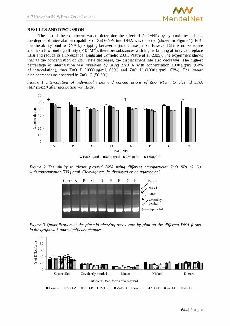
6–7 2019, Brno, Czech Republic
RESULTS AND DISCUSSION The aim of the experiment was to determine the effect of ZnO−NPs by cytotoxic tests. First,
the degree of intercalation capability of ZnO−NPs into DNA was detected (shown in Figure 1). EtBr has the ability bind to DNA by slipping between adjacent base pairs. However EtBr is not selective and has a low binding affinity (~105 M−1), therefore substances with higher binding affinity can replace EtBr and reduce its fluorescence (Bugs and Cornelio 2001, Pastre et al. 2005). The experiment shows that as the concentration of ZnO−NPs decreases, the displacement rate also decreases. The highest percentage of intercalation was observed by using ZnO−A with concentration 1000 µg/ml (64% of intercalation), then ZnO−E (1000 µg/ml, 63%) and ZnO−H (1000 µg/ml, 62%). The lowest displacement was observed in ZnO−C (50.2%).
Figure 1 Intercalation of individual types and concentrations of ZnO−NPs into plasmid DNA (MP px459) after incubation with EtBr.
Figure 2 The ability to cleave plasmid DNA using different nanoparticles ZnO−NPs (A−H) with concentration 500 µg/ml. Cleavage results displayed on an agarose gel.
Figure 3 Quantification of the plasmid cleaving assay rate by plotting the different DNA forms in the graph with non−significant changes.
0
10
20
30
40
50
60
70
A B C D E F G H
% in
terc
alat
ion
ZnO−NPs1000 µg/ml 500 µg/ml 250 µg/ml 125µg/ml
0
20
40
60
80
100
Supercoiled Covalently bonded Linear Nicked Dimers
% o
f DN
A fo
rms
Different DNA forms of a plasmid
Control ZnO-A ZnO-B ZnO-C ZnO-D ZnO-E ZnO-F ZnO-G ZnO-H
644

6–7 2019, Brno, Czech Republic
On the other hand, there were no significant changes in the plasmid structure during plasmid cleaving assay after adding ZnO−NPs (Figure 3). The first sample (Figure 2) displays a control without NPs where no plasmid cleavage can occur. Two clear and two thin bands show a common form of the used plasmid MP px459. Except for the highest bands with the presence of bifurcated structure next to the control, other plasmid−containing samples incubated with NPs show similar pattern of bands as the control sample. Therefore, although a slight cleaving of the DNA structure may occur by the effect of ZnO−NPs intercalation, most of the DNA remains intact.
Further, to determine the ability to lyse RBCs, NPs of various concentrations were tested for hemocompatibility. All samples showed a high rate of hemolysis at 0.5 mg/ml, with the highest level of hemolysis caused by ZnO−A (100%). Right behind were ZnO−G with 98% and ZnO−D (94% hemolysis). 90% was found in the ZnO−B sample. ZnO (C−F) caused hemolysis of ~80%. ZnO−H achieved the smallest percentage of hemolysis with 62%. Figure 4 shows the NPs with the highest hemolysis. However, the RBCs hemolysis was eliminated with lower concentrations of used ZnO−NPs.
Figure 4 Depicts the hemocompatibility results of ZnO−NPs. PBS represents negative control (100% hemocompatibility) and 0.1% Triton X−100 displays positive control (100% hemolysis). All displayed samples show at concentration 0.5mg/ml high hemolysis.
Another important parameter for nanomedical use is the NPs stability. For this purpose,
ZnO−NPs were incubated in various solutions. One set of samples (A−H) was kept in Ringer's solution (isotonic solution simulating an environment of blood plasma), at 37 °C and was measured for three days to detect the formation of possible large aggregates. Second set of samples (A−H) was measured in the culture medium for several weeks to determine the length of stability in the stock solutions. The aim was to determine the presence of any aggregates of several µm. It was found that neither the Ringer's solution nor the medium caused any formation of clusters. This leads us to the prediction that once NPs will be introduced in real blood plasma, they will not clump together and may retain existing properties. However, further analyses are still necessary to evaluate the biocompatibility and stability of these particles.
To monitor the morphological changes of ZnO−NPs in solution, SEM micrographs were taken (Figure 5). Although no changes were observed for most of the tested ZnO−NPs for up to 72 h, slight dissolving of ZnO−A, ZnO−B and ZnO−F was observed after prolonged stay in water.
0
10
20
30
40
50
60
70
80
90
100
110
Triton 0.1% 0.5mg/ml 0.25mg/ml 0.125mg/ml 0.0625mg/ml PBS
Hem
olys
is (%
)
Concentration
ZnO A ZnO B ZnO C ZnO DZnO E ZnO F ZnO G ZnO H
645

6–7 2019, Brno, Czech Republic
Figure 5 SEM micrographs of ZnO−NPs (B and G) in powder form and in Milli−Q after 24 h and 72 h. ZnO−B represents ZnO−NPs disolved in water after 72 h. ZnO−G represents ZnO−NPs stable in water for up to 72 h. The scale bar corresponds to 500 nm.
CONCLUSION The general behaviour of ZnO−NPs and their mutual differences caused by using different
precursors in the production process were studied by means of basic cytotoxicity tests. No nanoparticles showed significant ability to cleave plasmid DNA, while intercalation into DNA and hemolysis were demonstrated (ZnO A−H). ZnO−A, ZnO−B and ZnO−F showed higher solubility in water compared to others. ZnO−A appeared to be the most toxic, however, further testing is needed in the future for greater characterization.
ACKNOWLEDGEMENTS The work was supported from ERDF "Multidisciplinary research to increase application potential of nanomaterials in agricultural practice" (No. CZ.02.1.01/0.0/0.0/16_025/0007314).
REFERENCES Bugs, M.R., Cornelio, M.L. 2001. Analysis of the ethidium bromide bound to DNA by photoacoustic and FTIR spectroscopy. Photochemistry and Photobiology, 74(4): 512−20. Buzea, C. et al. 2007. Nanomaterials and nanoparticles: sources and toxicity. Biointerphases, 2(4): 17−71. Kruszynski, R., Swiatkowski, M. 2018. The structure of coordination precursors as an effective tool for governing of size and morphology of ZnS and ZnO nanoparticles. Journal of Saudi Chemical Society, 22(7): 816−825. Laurent, S. et al. 2008. Magnetic iron oxide nanoparticles: synthesis, stabilization, vectorization, physicochemical characterizations, and biological applications. Chemical Reviews, 108(6): 2064−110.
646

6–7 2019, Brno, Czech Republic
Pal, S. et al. 2007. Does the antibacterial activity of silver nanoparticles depend on the shape of the nanoparticle? A study of the Gram−negative bacterium Escherichia coli. Applied and Environmental Microbiology, 73(6): 1712−20. Pastre, D. et al. 2005. Study of the DNA/ethidium bromide interactions on mica surface by atomic force microscope: influence of the surface friction. Biopolymers, 77(1): 53−62. Rasmussen, J.W. et al. 2010. Zinc oxide nanoparticles for selective destruction of tumor cells and potential for drug delivery applications. Expert Opinion on Drug Delivery, 7(9): 1063−77. Sirelkhatim, A. et al. 2015. Review on Zinc Oxide Nanoparticles: Antibacterial Activity and Toxicity Mechanism. Nanomicro Letters, 7(3): 219−242. Swiatkowski, M., Kruszynski, R. 2019. Structurally diverse coordination compounds of zinc as effective precursors of zinc oxide nanoparticles with various morphologies. Applied Organometallic Chemistry, 33(4): 1−18.
647

6–7 2019, Brno, Czech Republic
Effect of sarcosine dehydrogenase knockdown on sarcosine metabolism-related genes expression
Hana Subrtova1, Zbynek Splichal1,2 1Department of Chemistry and Biochemistry
Mendel University in Brno Zemedelska 1, 613 00 Brno
2Central European Institute of Technology Brno University of Technology Purkynova 123, 616 00 Brno
CZECH REPUBLIC
Abstract: Sarcosine is extensively discussed as potential prostate cancer oncometabolite. Sarcosine dehydrogenase (SARDH) is one of the key enzymes involved in sarcosine metabolism that catalyses oxidative demethylation of sarcosine to glycine in mitochondrion. This study investigates the effects of small interfering RNA (siRNA) mediated SARDH knockdown on gene expression of sarcosine metabolism related enzymes: glycine N-methyltransferase (GNMT), peroxisomal sarcosine oxidase (PIPOX) and dimethylglycine dehydrogenase (DMGDH). The effect of SARDH knockdown was studied in three human prostate cell lines (PNT1A, DU-145, PC3) and gene expression was evaluated by quantitative real-time PCR (qPCR). Although the lowest SARDH knockdown was achieved in cancer DU-145 cell line, the highest changes in expression of other sarcosine metabolism genes were detected. In particular, the significant increase in DMGDH and PIPOX expression was observed. Our findings revealed potential stimulation effect of SARDH knockdown on DMGDH and PIPOX expression in prostate cancer cell line DU-145.
Key Words: knock-down, prostate cancer, sarcosine dehydrogenase, sarcosine metabolism
INTRODUCTION Prostate cancer is the second most commonly diagnosed cancer and fifth leading cause of death
in men worldwide (Bray et al. 2018). Early diagnosis of prostate cancer is essential step for subsequent successful treatment of this morbidity. In 2009, small non-proteinogenic amino acid sarcosine (N-methylglycine) was identified as a potential biomarker of prostate cancer (Sreekumar et al. 2009). Elevated sarcosine levels in urine have been associated with prostate cancer progression and metastatic processes (Sreekumar et al. 2009). In vitro experiments shown that elevated sarcosine levels induce proliferation, invasion and intravasation potential in human prostate cell lines (Khan et al. 2013).
Cancer cells are generally characterized by altered metabolism including biosynthetic and degradation pathways of amino acids (Ananieva 2015). The key enzymes involved in sarcosine metabolism are sarcosine dehydrogenase (SARDH; EC: 1.5.8.3), glycine N-methyltransferase (GNMT; EC: 2.1.1.20), peroxisomal sarcosine oxidase (PIPOX; EC: 1.5.3.1) and dimethylglycine dehydrogenase (DMGDH; EC: 1.5.8.4). Sarcosine can be formed in the cell either from glycine via the enzyme GNMT, which in cytosol catalyzes the transfer of the methyl group from S-adenosyl methionine (SAM) to glycine or from dimethylglycine via the mitochondrial enzyme DMGDH (Khan et al. 2013). On the other hand, degradation of sarcosine can be mediated by two enzymes, by PIPOX in peroxisomes or by mitochondrial SARDH that catalyze the oxidative demethylation of sarcosine to glycine. It was shown that up- or downregulation of sarcosine metabolism enzymes could affect prostate cancer progression, i.e. lowering the levels of GNMT or overexpression of SARDH reduced tumour growth in prostate cancer xenografts (Khan et al. 2013). Understanding the role of sarcosine metabolism related enzymes in prostate cancer metabolism may bring valuable information on tumorigenesis of prostate cancer.
648

6–7 2019, Brno, Czech Republic
The aim of this study was to investigate the effects of siRNA mediated SARDH knockdown on gene expression of sarcosine metabolism related enzymes in normal and prostate cancer cell lines.
MATERIAL AND METHODS
Chemicals All used chemicals were purchased from Sigma-Aldrich (St. Louis, Missouri, USA) unless
otherwise noted.
Cell lines Three different human prostatic cell lines were used. Firstly, PNT1A immortalized normal
prostatic epithelial cell purchased from HPA Culture Collections (Salisbury, Great Britain). Secondly, DU-145 prostate cancer cell line derived from brain metastasis purchased from ATCC (Manassas, Virginia, USA). Thirdly, PC3 prostate cancer cell line established from fourth grade of prostatic adenocarcinoma purchased from ATCC (Manassas, Virginia, USA).
Cell lines were cultured in RPMI-1640 medium with 10% fetal bovine serum and supplemented by two antibiotics penicillin (100 U/mL) and streptomycin (0.1 mg/mL). All cell lines were maintained in incubator Galaxy 170 R (Eppendorf, Hamburg, Germany) at 37 °C with 5% CO2. Transfection of siRNA (100 nM) was initiated after cells reached 50–60% confluence.
Transfection Lipid-based transfection reagent METAFECTENE® SI+ from Biontex (Munich, Germany)
was used for siRNA transfection. Transfection was performed according to the manufacturer's instructions. Transfection efficiency was verified using fluorescently labelled siRNA-siFAM (ABM, Richmond, Canada). The evaluation was performed using a fluorescence microscope EVOS FL Auto Imaging System from Thermo Fisher Scientific (Waltham, Massachusetts, USA).
RNA isolation Cells were harvested 48 hours after initiating transfection and were utilized in RNA isolation.
High Pure RNA Isolation Kit was purchased from Roche (Basel, Switzerland) for RNA isolation and the integrity of the isolated RNA was verified using a Bleach gel. Afterwards, the purity and concentration of the isolated RNA was spectrophotometrically verified by Infinite® M200 PRO from Tecan (Männedorf, Switzerland).
Reverse transcription The First Strand cDNA Synthesis Kit from Roche (Basel, Switzerland) was used for the reverse
transcription. 500 ng of isolated RNA was transcribed by application of random hexamers.
Gene expression analysis Quantification of gene expression was performed by Luna® Universal qPCR Master Mix (New
England Biolabs, Ipswich, Massachusetts, USA) and Mastercycler® ep Realplex real-time PCR instrument (Eppendorf, Hamburg, Germany). Each 20 μl qPCR mix contained 25 ng cDNA and set of primer with 250 nM final concentration. Threshold cycle (CT) was determined by noiseband with automatic baseline drift correction using Realplex software (Eppendorf, Hamburg, Germany). The relative expression levels of sarcosine metabolism (SARMET) genes were normalized to HPRT1 reference gene (ΔCT = CT HPRT1 - CT SARMET). ΔCT values are used for presentation of basal expression sarcosine metabolism genes. Relative gene expression between cells transfected with negative control siRNA (siNeg) and siRNA targeting SARDH (siSARDH) was calculated according to formula ΔΔCT = ΔCT SARMETsiSARDH – CT SARMET siNEG. Data are expressed as ΔΔCT mean±SD from tree biological replicates.
Descriptive statistics Statistically significant differences between individual results of gene expression were evaluated
by unpaired t-test. The threshold for significance was p < 0.05. Statistical evaluation was performed in GraphPad Prism (GraphPad Software, San Diego, California, USA).
649

6–7 2019, Brno, Czech Republic
RESULTS AND DISCUSSION
Verification of transfection efficiency Prior to the experiments with siSARDH, the efficacy of the selected transfection protocol had
to be verified. Transfection efficacy was verified by fluorescently labelled siRNA (siFAM) and analyzed by fluorescence microscopy. Figures 1 showed that >70% of the PC3 cells was transfected by siFAM molecules which confirmed efficacy of transfection protocol.
Figure 1 Transfection efficiency assay using fluorescently labelled siFAM analysed by fluorescence microscopy (PC3 cell line, magnification 40×, scale 100 µm)
Determination of basal gene expression First, the basal expression of sarcosine metabolism genes SARDH, DMGDH, PIPOX and GNMT
was determined. Figure 2 represents relative gene expression after 48 hours transfection with negative control siRNA. The lowest GNMT expression was observed in normal cell line PNT1A compared to both prostate cancer cell lines DU-145 and PC3. Simultaneously the normal cell line PNT1A has the highest SARDH expression from all tested cell lines. These results were in agreement with other publications (Khan et al. 2013, Song et al. 2011).
Figure 2 Basal expression of sarcosine metabolism genes (SARDH, DMGDH, PIPOX, GNMT)
Evaluation of knockdown efficiency Subsequently, SARDH knockdown efficiency was evaluated (Figure 3). The most significant
decrease in SARDH expression was achieved in the normal prostate cell line PNT1A where the average
650

6–7 2019, Brno, Czech Republic
ΔΔCT value was -1.07 corresponding to 52% knockdown efficiency. PC3 cell line also showed a statistically significant decrease in SARDH expression with a ΔΔCT value -0.78, which corresponds to 52% knockdown efficiency. The decrease in SARDH expression in DU-145 cell line was not statistically significant which could be probably caused by very low basal SARDH expression in this cell line.
Figure 3 SARDH expression 48 hours after transfection siSARDH (*p≤0.05)
Changes in expression of sarcosine metabolism genes Finally, DMGDH, PIPOX and GNMT gene expression after SARDH knockdown was evaluated
(Figure 4). The most pronounced and statistically significant changes in expression were observed in the cancer cell line DU-145 in which the expression of DMGDH and PIPOX genes increased after 48h SARDH knockdown. This is in contrary with Green et al. 2013 who described the inhibition effect of SARDH knockdown to DMGDH (Green et al. 2013). DMGDH is an enzyme that commonly catalyses the conversion of dimethylglycine to sarcosine, but it has been found that it can also convert sarcosine to glycine (Wittwer and Wagner 1981a, Wittwer and Wagner 1981b). This could explain the increase in DMGDH expression that probably substitutes the function of downregulated SARDH in mitochondrion. Similar effect was observed in case of PIPOX that also probably replaced the missing catalytic activity of SARDH in DU-145 cells. No significant changes were observed in the case of GNMT expression.
Figure 4 Change in expression of DMGDH 48 hours after siSARDH transfection (*p≤0.05)
651

6–7 2019, Brno, Czech Republic
Figure 5 Change in expression of PIPOX 48 hours after siSARDH transfection (*p≤0.05)
Figure 6 Change in expression of GNMT 48 hours after siSARDH transfection
CONCLUSION We found a significant increase in the expression of DMGDH and PIPOX genes after SARDH
knockdown in the DU-145 cell line, both of which are capable of converting sarcosine to glycine. These results provide new information on sarcosine metabolism that is potentially useful for further investigations regarding therapeutic agents.
ACKNOWLEDGEMENTS The research was financially supported by the by CEITEC 2020 (LQ1601).
REFERENCES Ananieva, E. 2015. Targeting amino acid metabolism in cancer growth and anti-tumor immune response. World Journal of Biological Chemistry, 6(4): 281–289. Bray, F. et al. 2018. Global cancer statistics 2018: GLOBOCAN estimates of incidence and mortality worldwide for 36 cancers in 185 countries. Ca-a Cancer Journal for Clinicians, 68(6): 394–424. Green, T. et al. 2013. TMEFF2 and SARDH cooperate to modulate one-carbon metabolism and invasion of prostate cancer cells. Prostate, 73(14): 1561–1575.
652

6–7 2019, Brno, Czech Republic
Khan, A.P. et al. 2013. The Role of Sarcosine Metabolism in Prostate Cancer Progression. Neoplasia, 15(5): 491–501. Song, Y.H. et al. 2011. The important role of glycine N-methyltransferase in the carcinogenesis and progression of prostate cancer. Modern Pathology, 24(9): 1272–1280. Sreekumar, A. et al. 2009. Metabolomic profiles delineate potential role for sarcosine in prostate cancer progression. Nature, 457(7231): 910–914. Wittwer, A.J., Wagner, C. 1981a. Identification of the folate-binding proteins of rat-liver mitochondria as dimethylglycine dehydrogenase and sarcosine dehydrogenase - flavoprotein nature and enzymatic-properties of the purified proteins. Journal of Biological Chemistry, 256(8): 4109–4115. Wittwer, A.J., Wagner, C. 1981b. Identification of the folate-binding proteins of rat-liver mitochondria as dimethylglycine dehydrogenase and sarcosine dehydrogenase - purification and folate-binding characteristics. Journal of Biological Chemistry, 256(8): 4102–4108.
653

6–7 2019, Brno, Czech Republic
Novel Ruthenium coordinate compound combined with Schiff base and benzimidazole as a potent antibacterial agent against
VRSA and MRSA
Vishma Pratap Sur1,2, Aninda Mazumdar1,2, Pavel Kopel1,2, Amitava Moulick1,2
1Department of Chemistry and Biochemistry Mendel University in Brno Zemedelska 1, 613 00 Brno
2Central European Institute of Technology Purkynova 123, 612 00 Brno
CZECH REPUBLIC
Abstract: The rise of antibiotic-resistant strains is an important public health problem and thus the development of an alternative to antibiotics is imminent. The Ruthenium–Schiff base with benzimidazole (RU–S2), a co-ordinate compound is novel and first of its kind to be synthesized in such combination. The aim of the experiment is based on the synthesis of RU–S2 and to study its antibacterial activity against the pathogenic resistant strains of Staphylococcus aureus like Vancomycin-resistant Staphylococcus aureus (VRSA) and Methicillin-resistant Staphylococcus aureus (MRSA). The antibacterial activity was studied using growth curve analysis based on turbidimetry which was confirmed by the fluorescence live/dead cell microscopic imaging of the bacteria after treatment with RU–S2. Lastly, the cytotoxicity test was performed by 3-(4,5-Dimethylthiazol-2-yl)-2,5-diphenyltetrazolium bromide (MTT) assay against human normal and cancer epithelial cell lines to understand the toxic effects of RU-S2 at 160 µg/ml concentration. The concentration 160 µg/ml of RU–S2 was very effective against those resistant strains and also nontoxic in this concentration. Thus RU-S2 can be used as an efficient alternative to antibiotics that have promising antibacterial efficacy against the pathogenic strains with no toxicity and biocompatibility towards human cells.
Key Words: antibiotic-resistant, coordinate compound, antibacterial activity, VRSA, MRSA
INTRODUCTION Worldwide multidrug-resistant bacterial infections are rapidly emerging, which endangered
the efficacy of the present antibiotics, modified medicines and even the definition of antibacterial drugs (Ventola 2015). The antibiotic resistance is majorly caused by abuse or incompletion of prescribed dosage and overuse of the antibiotics (Gould and Bal 2013). The infections caused by the resistant bacterial strains are significantly problematic as it has prolonged the admission time of patients in hospitals, increased the mortality rate, and caused a surge in medication cost (Wang and Ruan 2017). In hospitals, S. aureus and its resistant strains, such as Vancomycin-resistant Staphylococcus. aureus (VRSA) and Methicillin-resistant Staphylococcus. aureus (MRSA), are some of the major threats to treatment. Whereas patients with these infections sometimes are also exposed to nosocomial infections and become more vulnerable. To overcome these threatening antibiotic resistant bacterial infections, medical research and treatments need to find alternatives to conventional antibiotics (Sillankorva et al. 2019).
Transition metals like silver, nickel, and cobalt are already in use by researchers to synthesize various compounds with combinations of other chemicals to form antibacterial agents. But the limitation of these compounds is the toxicity and dosage amount. Recently, scientists are focusing on another transition metal to use as an antimicrobial agent which is ruthenium. This metal has the ability to effectively bind DNA, whereas toxicity against eukaryotic cells was significantly lower than other metals used in earlier studies (Liu et al. 2018, Brabec and Nováková 2006). Ruthenium is also used as an alternative treatment in cancer chemotherapy with some antibacterial efficacy (Brabec
654

6–7 2019, Brno, Czech Republic
and Nováková 2006, Liu et al. 2018). Further, the reports on benzimidazole have shown that it has some antibacterial and antifungal properties (Özkay et al. 2011). But to date, according to the best of our knowledge, no compound has been designed in combinations with ruthenium, schiff base and benzimidazole together to be used as an antibacterial agent.
Thus, a scope to develop an efficient solution to treat S. aureus and it’s resistant variants has led us to develop a novel ruthenium-schiff base with benzimidazole coordination compound (RU–S2), which is first of its type in such combination to be synthesized and used as antibacterial agents. The synthesized RU–S2 was tested against VRSA and MRSA to study its antibacterial activity. The activity of this compound was further confirmed by microscopic analysis using live/dead cell assay. Lastly, the cytotoxicity against the human normal and cancer prostate cells was observed using MTT assay.
MATERIALS & METHODOLOGIES
Chemicals, reagents, and Synthesis of RU–S2 For synthesis, all chemicals are graded according to the American Chemical Society purity were
purchased from Sigma-Aldrich (St. Louis, MO, USA), unless otherwise stated. Bacterial media and assay kits were obtained from HiMedia Laboratories (Pvt. Ltd., India).
1-(1-H-benzimidazole-2-yl)-N-(1H-benzimidazole-2-ylmethyl) methanamine (benzimidazole) and the schiff base was synthesized according to Kopel et al. (Kopel et al. 2014, Kopel et al. 2015). In a separate beaker, 0.252 g of Ruthenium chloride was dissolved in 40 ml of MeOH. Then 0.16 g benzimidazole was dissolved in 10 ml MeOH and added in stirring condition until a brown precipitate was formed. Thereafter, Schiff base 0.094 g was added followed by triethylamine. Brown solution with dark solid was heated under reflux for 24 hours (h). After cooling, dark solid was collected on a frit, washed with MeOH and dried at 40 °C. The yield was 0.30 g (Kopel et al. 2014).
Bacterial Culture In this research, two different bacterial strains were used. Resistant strains of Staphylococcus
aureus, named VRSA Czech Collection of Microorganism (CCM) 1767, and MRSA ST239:SCCmec III. All bacterial strains were cultured in Muller Hinton Broth for overnight in the incubator at 37 °C on shaking conditions.
Antibacterial effects of RU–S2 via growth curve analysis Antibacterial activity of the RU-S2 compound was studied by turbidimetry, measuring
the absorbance (A600) at 600 nm (van Sorge et al. 2013, Li et al. 1993) for 24 h against MRSA and VRSA. The activity of RU–S2 compound was measured by standard microdilution methods using different concentrations like 10 µg/ml, 20 µg/ml, 40 µg/ml, 80 µg/ml and 160 µg/ml. The different concentrations of the compound were added to bacterial cultures (0.5 McFarland and final dilution 1:100 with the MH medium) by multichannel pipet system in the 10x10 Honeycomb optical microplate well systems (Oy Growth Curves Ab Ltd Finland) in the microplate wells. The specially designed honeycomb plate was then incubated in growth curve analyzer, Bioscreen C MBR (Oy Growth Curves Ab Ltd Finland) for 24 h at 37 °C (Stasiak-Różańska et al. 2014, Hogenkamp et al. 2007). The viability percentage of the VRSA and MRSA was studied after treatment with RU–S2 for 24 h at 37 °C. The control was without treatment.
Live/dead assay and microscopic imaging of bacteria in the presence of RU–S2 Bacterial samples were treated with RU–S2 for microscopic live and dead cell visualization was
done by two different kinds of fluorescent dye. We have used SYTO 9 and propidium iodide for cell staining, the. 0.5 µl of SYTO9 and 2 µl propidium iodide were mixed with 10 µl respective bacterial samples and incubated for 1–2 minutes. For imaging, an inverted Olympus IX 71S8F3 fluorescence microscope (Olympus Corporation, Tokyo Japan) was used, which is equipped with Olympus UIS2 series objective LUC planFLN 40X (N.A. 0.6, WD 2.7-4 mm, F.N.22) and a mercury arc lamp X-cite 12(120 W; Lumen Dynamics, Mississauga, ON, Canada).
655

6–7 2019, Brno, Czech Republic
In vitro cytotoxicity testing assay The MTT assay was performed using PNT1A (normal prostate cancer cells) and Du–145
(prostate cancer cell line). The cells were cultured and maintained in RPMI-1640 medium with 10% fetal bovine serum, supplemented with penicillin (100 µg/ml) and streptomycin (0.1 mg/ml). In a microtiter plate, each well filled with 5000 cells supplemented with 50 µl medium and the plate was incubated for 24 h at 37 °C with 5% of CO2 aeration to ensure the cell growth. Once confluent in each well, cells were treated with RU–S2 in different concentrations and incubated for 24 h. The old medium was removed 24h post-treatment and 100 µl of fresh medium mixed with MTT (10 µl; 5 mg/ml in PBS) was added and incubated for 4 h at 37 °C with 5% CO2. Thereafter, MTT containing medium was replaced with 100 µl of 99.9% dimethyl sulphoxide (v/v) for dissolving the formazan crystals. The absorbance was taken 570 nm by Infinite m200 PRO reader (Tecan, Männedorf, Switzerland).
RESULT AND DISCUSSION Ruthenium, Schiff base and benzimidazole were used to synthesis the RU-S2 compound.
The synthesized compound was incubated with VRSA and MRSA to study the antibacterial efficacy. The antibacterial activity of RU–S2 has been determined by using growth curve and their viability percentage as shown in figure 1 and figure 2, which was further confirmed by live/dead cell imaging of VRSA and MRSA as shown in Figure 3. In vitro cytotoxicity was checked by MTT assay against human epithelial cells as shown in Figure 4.
Figure 1 Growth curves after application of different concentrations of RU-S2 on VRSA and MRSA (concentration of the compounds 10 µg/ml, 20 µg/ml, 40 µg/ml, 80 µg/ml, and 160 µg/ml)
Legend: growth curves of VRSA and MRSA: growth curve of VRSA in left (Figure 1A) denoting untreated VRSA as control and VRSA treated with different concentrations of RU-S2; where growth curve of MRSA in right (Figure 1B) denoting untreated MRSA as control and MRSA treated with different concentrations of RU-S2
Figure 2 Viability percentage of VRSA and MRSA treated by different concentrations of RU-S2
Legend: Viability percentage of VRSA and MRA: viability percentage of VRSA in left (Figure 2A) denoting untreated VRSA as control and VRSA treated with different concentrations of RU-S2; where viability percentage in the right (Figure 2B) denoting untreated MRSA as control and MRSA treated with different concentrations of RU-S2
656

6–7 2019, Brno, Czech Republic
Antibacterial effects of RU–S2 using growth curve analysis along with viability percentage The antibacterial activity of RU–S2 was investigated against VRSA and MRSA by growth curve
analysis. We incubated different concentrations of the compound, such as 10 µg/ml, 20 µg/ml, 30 µg/ml, 40 µg/ml, 80 µg/ml, and 160 µg/ml on the bacterial populations but the bacterial growth curve analysis showed that the highest activity of RU-S2 against MRSA and VRSA was obtained at 160 µg/ml (Figure 1). Whereas the viability percentage showed that the activity of the RU–S2 was highest at 160 µg/ml with viability percentage less than 1%, while treatment with other concentrations till 20 µg/ml showed less than 50% viability and concentration lower like 10 µg/ml showed almost no activity (Figure 2).
Live/dead cell imaging of bacteria treated with RU-S2 The antibacterial activity further confirmed by treatment of RU–S2 against VRSA and MRSA
and staining the samples with SYTO 9 and propidium Iodide followed by observation of the samples using an inverted fluorescence microscope. The images in figure 3 clearly reveal a high number of dead bacterial cells (red fluorescence) in treated samples compared to the control showing a high number of green fluorescence (live bacterial cells).
Figure 3 live/dead cell imaging treated with RU-S2 stained with SYTO9 (live cell) and Propidium Iodide (Dead cells)
Legend: (A)Merged image of untreated VRSA as control; (B) Merged image of VRSA treated with RU-S2; (C) Merged image of untreated MRSA as control; (D) Merged image of MRSA treated with RU-S2. Where green cells are denoting living cells and red cells are denoting dead cells. Scale bar is 5µm
In vitro cytotoxicity testing assay The cytotoxicity test was performed by using normal prostate epithelial cells (PNT1A)
and prostate cancer cells (Du–145) (Figure 4).
Figure 4 In vitro cytotoxicity testing
Legend: (A) PNT1A cells high viability percentage; (B) Du-145 cells with high viability percentage
The cells were treated with different concentrations of RU-S2 and the absorbance was measured after the MTT assay was performed. The results showed no reduction in viability which confirms
657
6–7 2019, Brno, Czech Republic
that the synthesized RU-S2 was completely non-toxic and biocompatible towards human cells (Figure 4).
CONCLUSION In the present study, RU–S2 was synthesized using ruthenium, schiff base and benzimidazole.
The antibacterial property of RU–S2 was studied against multidrug-resistant strains of S. aureus which are VRSA and MRSA by growth curve analysis and viability percentage which showed high antibacterial activity at 160 µg/ml. The antibacterial activity was further confirmed and supported against MRSA and VRSA by the presence of a significantly high number of dead cells with red fluorescence obtained after treatment with RU–S2 while almost no dead cells were seen in control samples without treatment. Lastly, the cytotoxicity of RU–S2 against human prostate cancer and normal epithelial cells using MTT assay showed no sign of toxicity in vitro. Thus hereby we report that RU–S2 compound can be a promising candidate for an alternative to the antibiotic with no toxicity at reported concentrations and biocompatibility towards human cells and requires further research.
ACKNOWLEDGMENTS The research was financially supported by the Internal Grant Agency of Mendel University in Brno (AF-IGA2019-IP063) and CEITEC 2020 (LQ1601).
REFERENCES Brabec, V., Nováková, O. 2006. DNA binding mode of ruthenium complexes and relationship to tumor cell toxicity. Drug Resistance Updates, 9(3): 111–122. Gould, I.M., Bal, A.M. 2013. New antibiotic agents in the pipeline and how they can help overcome microbial resistance. Virulence, 4(2): 185–191. Hogenkamp, A. et al. 2007. Effects of surfactant protein D on growth, adhesion and epithelial invasion of intestinal Gram-negative bacteria. Molecular Immunology, 44(14): 3517–3527. Kopel, P. et al. 2014. Trithiocyanurate complexes of iron, manganese and nickel and their anticholinesterase activity. Molecules, 19(4): 4338–4354. Kopel, P. et al. 2015. Biological activity and molecular structures of bis (benzimidazole) and trithiocyanurate complexes. Molecules, 20(6): 10360–10376. Li, R.C. et al. 1993. New turbidimetric assay for quantitation of viable bacterial densities. Antimicrobial Agents and Chemotherapy, 37(2): 371–374. Liu, X. et al. 2018. The antimicrobial activity of mononuclear ruthenium (II) complexes containing the dppz ligand. ChemPlusChem, 83(7): 643–650. Özkay, Y. et al. 2011. Antimicrobial activity of a new series of benzimidazole derivatives. Archives of Pharmacal Research, 34(9): 1427–1435. Sillankorva, S. et al. 2018. Antibiotic Alternatives and Combinational Therapies for Bacterial Infections. Frontiers in Microbiology, 9: 3359. Stasiak-Różańska, L. et al. 2014. Effect of glycerol and dihydroxyacetone concentrations in the culture medium on the growth of acetic acid bacteria Gluconobacter oxydans ATCC 621. European Food Research and Technology, 239(3): 453–461. Van Sorge, N.M. et al. 2013. Methicillin-resistant Staphylococcus aureus bacterial nitric-oxide synthase affects antibiotic sensitivity and skin abscess development. Journal of Biological Chemistry, 288(9): 6417–6426. Ventola, C.L. 2015. The antibiotic resistance crisis: part 1: causes and threats. Pharmacy and Therapeutics, 40(4): 277–283. Wang, L., Ruan, S. 2017. Modeling nosocomial infections of methicillin-resistant Staphylococcus aureus with environment contamination. Scientific Reports, 7(1): 580.
658

6–7 2019, Brno, Czech Republic
The effect of substituents on aromatic ring on antioxidant capacity of phenolic substances
Petra Svestkova1, Ivo Soural1, Josef Balik1, Monika Bieniasz2 1Department of Post-Harvest Technology of Horticultural Products
Mendel University in Brno, Valticka 337, 691 44 Lednice
CZECH REPUBLIC 2Faculty of Biotechnology and Horticulture
University of Agriculture in Krakow 29 Listopada 54, 31-425 Krakow
POLAND
Abstract: This study comprises thirteen selected phenolic antioxidants as follows: vanillin, acetosyringone, eugenol, isoeugenol, 4-ethylguaiacol, guaiacol and acids: gentisic, 4-hydroxybenzoic, protocatechuic, ferulic, syringic, coffee, chlorogenic. For each of the phenolic substances, total antioxidant capacity (TAC) was measured using the FRAP and DPPH method expressed as TEAC (Trolox Equivalent Antioxidant Capacity); antioxidants with the concentration of 20 mg/l were compared with each other as well as against Trolox. It was found based on the results of measurements that the presence and position of some substitution groups on fenolic ring significantly affect the antioxidant capacity of these substances. Larger antioxidant capacity was measured in multiple hydroxylated substances. An effect was also observed of the type of the functional group where substances possessing a hydroxyl group instead of the methoxyl group featured significant antioxidant capacity. Similar was seen for substances possessing a carboxyl group instead of acetyl group. An effect was also observed immediately between the ortho and para positions of hydroxyl groups in aromatic ring. Examples include gentisic and protocatechuic acid, where while either of the acids has the identical molecular formula, i.e., C7H6O4, for the hydroxyl group the antioxidant capacity is 1.2 to 1.7 times higher in case of the ortho position in gentisic acid than in the para position in protocatechuic acid.
Key Words: phenols, antioxidant capacity, functional group, FRAP, DPPH
INTRODUCTION Phenolic substances form a large group of antioxidants. The purpose of antioxidants is to bind
excess free radicals and thereby protect food products and substances that they contain. Foodstuffs are constantly subjected to tests for antioxidant potential. Determining the antioxidant activity is carried out in many different ways that feature different advantages (Bunaciu et al. 2016). Strong antioxidant activity was found for cherries, citrus fruit, plums, berry fruit and olives (Lobo et al. 2010). The chief sources of polyphenolic antioxidants include leguminous grains, fruit, vegetables and technologically prepared or produced foodstuffs such as red wine, chocolate, olive oil or green tea (Dolas and Gotmare 2015). Green/black tea is subjected to an extensive study because it contains up to 30% phenolic compounds in dry matter (Lobo et al. 2010). Contents of phenolic substances may also change during the period of storage (Snurkovic 2015). Phenolic antioxidants can have a synergetic effect (Sochor et al. 2010) and play an important role in the prevention and treatment of certain diseases caused by free radicals (Dacic and Gojak-Salimovic 2016), such as cancer, cardiovascular disease or neurodegenerative diseases (Parkinson/Alzheimer disease) (Costa et al. 2017). Individuals who regularly drink alcohol or are regularly exposed to tobacco smoke may find themselves to be short of antioxidants (Dolas and Gotmare 2015). The importance of phenolic substances thus plays an important role in the framework of nourishment and protection of the body. The background of the overall antioxidant capacity involves the influence of the individual substances, including phenolic compounds when individual phenols affect the total antioxidant capacity through varying degrees of intensity. Differences in terms of antioxidant capacity can also be very important between phenols, even in cases of similar
659

6–7 2019, Brno, Czech Republic
structures – substitution of a single functional group in the aromatic nucleus or even a changed position of the same group can make the difference. There are even multiple-fold differences appearing between such isomers of phenols.
MATERIALS AND METHODS Phenols used to measure the antioxidant capacity were as follows: vanillin, acetosyringone,
eugenol, isoeugenol, gentisic acid, 4-hydroxybenzoic acid, protocatechuic acid, 4-ethylguaiacol, guaiacol, ferulic acid, syringic acid, coffee acid, and chlorogenic acid (all with analytic purities ≥ 97%).
Other used substances were as follows: Methanol, Ethanol, Iron(III) chloride, Hydrochloric acid 35%, DPPH (2,2-diphenyl-1-picrylhydrazyl), buffer (Sodium acetate trihydrate & Acetic acid), Trolox (6-hydroxy-2,5,7,8-tetramethylchroman-2-carboxylic acid), TPTZ (2,4,6-tris(2-pyridyl)-s-triazine).
Sample pretreatment: For each of the analysed phenols, approximately 100 mg was weighed out on an analytical scale,
the precision being 0.1 mg. Each weighed phenol was quantitatively transferred into a 50 ml volumetric flask of 50 ml; 15 ml of ethanol was added into the flask and deionized water was supplemented to obtain a volume of 50 ml. The phenol solutions so mixed continued to be diluted with 0.1 ml solution and 9.9 ml distilled water to obtain a resulting concentration of solutions of 20 mg/l.
Total antioxidant capacity (TAC) TAC was measured using two methods: the ferring reducing antioxidant power (FRAP) method,
and the DPPH method. In both methods the quantitative determination (of the calibration curve) was making use of Trolox solutions of 0.1 to 0.5 mM.
For the FRAP method, the reaction mixture contained TPTZ (2,4,6-tris(2-pyridyl)-s-triazine) dissolved in HCl, FeCl3 and acetate buffer, the ratio being 1:1:10. The buffer solution (pH 3.6) was prepared by mixing 4 ml of concentrated CH3COOH with 0.775 g of CH3COONa.3H2O in a 250 ml volumetric flask and adding deionized water up to the punch mark. The solution of FeCl3 was prepared by weighing out and dissolving 0.081 g of FeCl3∙6H2O in a 25 ml volumetric flask adding deionized water up to the punch mark. The TPTZ complex in HCl was prepared from 0.078 g TPTZ dissolved in a 25 ml flask with water acidified with 0.088 ml of 35% HCl. To do the measurement, 2,000 µl of the reaction mixture was pipetted into the cuvette along with 25 µl of the sample diluted with deionized water. The filled up, 1.00 cm thick cuvette was shaken for 10 seconds using a mechanical shaker; the resulting solution was left in cuvettes for 10 minutes (reaction time). After this time the samples were analysed at a wavelength of 593 nm using a spectrometer, when absorbance of the sample was measured.
For the DPPH method 1,900 µl of the methanol solution of DPPH (the concentration of 0.1 mM) was pipetted into the cuvette along with 100 µl of the sample diluted with deionized water. The cuvette with the resulting solution was then shaken for 10 seconds on an orbital shaker. The mixed up solution was measured after 30 minutes using a spectrophotometer at the wavelength of 515 nm. The procedure was therefore the same as in our previous study (Hic et al. 2017).
RESULTS 13 phenolic substances were measured for antioxidant capacity using the FRAP and DPPH
methods. All of the results are expressed in the values of TEAC (Trolox Equivalent Antioxidant Capacity) when the values for each of the phenols obtained by measurement were converted to the exact concentration of 20.0 mg/l including the standard Trolox solution, which thus represented the TEAC value of 79.9 µmol/l for both FRAP and DPPH method. The solutions of the individual phenolic substances were subsequently matched against this value that represents 100%.
DPPH method TEAC values higher than Trolox were measured for 10 phenolic substances (the same as in the
case of the FRAP method, in Figure 1 and Table 1): gentisic acid 269.2 µmol/l (336.9%), protocatechuic acid 222.0 µmol/l (277.8%), syringic acid 193.1 µmol/l (241.6%), coffee acid 183.0 µmol/l (229.0%), 4-ethylguaiacol 177.3 µmol/l (221.9%), eugenol 165.0 µmol/l (206.5%), ferulic acid 125.7 µmol/l
660

6–7 2019, Brno, Czech Republic
(157.3%), guaiacol 120.8 µmol/l (151.2%), chlorogenic acid 119.2 µmol/l (149.2%) and Isoeugenol 100.3 µmol/l (125.5%). Conversely, TEAC values lower than the solution of Trolox alone, 79.91 µmol/l (100%), were found for: vanillin 58.3 µmol/l (73.0%), 4-hydroxybenzoic acid 57.9 µmol/l (72.5%) and acetosyringone 56.9 µmol/l (71.2%).
Table 1 Tukey’s honest significance test for phenols measured by DPPH in µmol/l. (One-way ANOVA: p < 0.05 (*); p < 0.01 (**); not significant p > 0.05 (n.s.), calculated from three measurements.
{1}
Prot
ocat
echu
ic
acid
{2}
4-et
hylg
uaia
col
{3}
4-hy
drox
yben
zoic
ac
id
{4}
Ace
tosy
ringo
ne
{5}
Cof
fee
acid
{6}
Euge
nol
{7}
Feru
lic a
cid
{8}
Gen
tisic
aci
d
{9}
Gua
iaco
l
{10}
C
hlor
ogen
ic a
cid
{11}
Is
oeug
enol
{12}
Sy
ringi
c ac
id
{13}
V
anill
in
{1} n.s. ** ** ** ** ** ** ** ** ** ** ** {2} 0.9914 ** ** ** ** ** ** ** ** ** ** ** {3} 0.0001 0.0001 n.s. ** ** ** ** ** ** ** ** n.s. {4} 0.0001 0.0001 1.0000 ** ** ** ** ** ** ** ** n.s. {5} 0.0002 0.0002 0.0001 0.0001 n.s. ** ** ** ** ** n.s. ** {6} 0.0067 0.0005 0.0001 0.0001 0.8256 ** ** ** ** ** n.s. ** {7} 0.0001 0.0001 0.0001 0.0001 0.0001 0.0001 ** ** n.s. n.s. ** ** {8} 0.0001 0.0002 0.0001 0.0001 0.0001 0.0001 0.0001 ** ** ** ** ** {9} 0.0001 0.0001 0.0001 0.0001 0.0039 0.0002 0.0011 0.0001 ** ** ** ** {10} 0.0001 0.0001 0.0001 0.0001 0.0001 0.0001 0.9774 0.0001 0.0002 n.s. ** ** {11} 0.0001 0.0001 0.0001 0.0001 0.0001 0.0001 1.0000 0.0001 0.0045 0.7758 ** ** {12} 0.0045 0.0003 0.0001 0.0001 0.8983 1.0000 0.0001 0.0001 0.0002 0.0001 0.0001 ** {13} 0.0001 0.0001 1.0000 1.0000 0.0001 0.0001 0.0001 0.0001 0.0001 0.0001 0.0001 0.0001
FRAP method TEAC values higher than Trolox were measured for 10 phenolic substances (in Figure 1
and Table 2): gentisic acid 257.7 µmol/l (322.5%), guaiacol 232.3 µmol/l (290.7%), 4-ethylguaiacol 214.8 µmol/l (268.8%), eugenol 220.6 µmol/l (276.1%), syringic acid 171.2 µmol/l (214.2%), protocatechuic acid 155.8 µmol/l (195.0%), coffee acid 149.6 µmol/l (187.2%), ferulic acid 137.3 µmol/l (171.8%), Isoeugenol 128.0 µmol/l (160.2%) and chlorogenic acid 89.2 µmol/l (104.9%). Conversely, TEAC values lower than the solution of Trolox alone, 79.91 µmol/l (100%), were recorded in three phenolic substances: acetosyringone 44.5 µmol/l (55.7%), vanillin 27.6 µmol/l (34.5%) and 4-hydroxybenzoic acid 26.3 µmol/l (32.9%).
Table 2 Tukey’s honest significance test for phenols measured by FRAP in µmol/l. One-way ANOVA: p < 0.05 (*); p < 0.01 (**); not significant p > 0.05 (n.s.), calculated from three measurements.
{1}
Prot
ocat
echu
ic
acid
{2}
4-et
hylg
uaia
col
{3}
4-hy
drox
yben
zoic
ac
id
{4}
Ace
tosy
ringo
ne
{5}
Cof
fee
acid
{6}
Euge
nol
{7}
Feru
lic a
cid
{8}
Gen
tisic
aci
d
{9}
Gua
iaco
l
{10}
C
hlor
ogen
ic a
cid
{11}
Is
oeug
enol
{12}
Sy
ringi
c ac
id
{13}
V
anill
in
{1} ** ** ** n.s. ** n.s. ** ** ** n.s. n.s. ** {2} 0.0002 ** ** ** n.s. ** n.s. * ** ** ** ** {3} 0.0002 0.0002 n.s. ** ** ** ** ** ** ** ** n.s. {4} 0.0002 0.0002 0.2731 ** ** ** ** ** ** ** ** n.s. {5} 1.0000 0.0002 0.0002 0.0002 ** n.s. ** ** ** n.s. n.s. ** {6} 0.0002 0.5179 0.0002 0.0002 0.0002 ** n.s. ** ** ** ** ** {7} 0.3514 0.0002 0.0002 0.0002 0.7657 0.0002 ** ** ** * ** ** {8} 0.0002 0.3296 0.0002 0.0002 0.0002 1.0000 0.0002 ** ** ** ** ** {9} 0.0002 0.0328 0.0002 0.0002 0.0002 0.0002 0.0002 0.0002 ** ** ** **
{10} 0.0002 0.0002 0.0002 0.0004 0.0002 0.0002 0.0002 0.0002 0.0002 ** ** ** {11} 0.9292 0.0002 0.0002 0.0002 0.5761 0.0002 0.0148 0.0002 0.0002 0.0002 n.s. ** {12} 0.4020 0.0002 0.0002 0.0002 0.1234 0.0002 0.0014 0.0002 0.0002 0.0002 0.9984 ** {13} 0.0002 0.0002 1.0000 0.3694 0.0002 0.0002 0.0002 0.0002 0.0002 0.0002 0.0002 0.0002
661

6–7 2019, Brno, Czech Republic
Figure 1 Antioxidant capacity of 20.0 mg/l
DISCUSSION The measurement showed that the antioxidant capacity is influenced by a number of hydroxyl
groups, their sites of binding in the aromatic ring, and also the number and position of other substituents bound to the aromatic ring. A similar argument is given in the 2016 article by Khan et al., where it is argued that methoxyl (-O-CH3) and hydroxyl (-OH) substitution groups in the aromatic nucleus may affect the antioxidant potential as well as the capacity of phenolic substances. The next similar opinion is given in the 2004 article by Leopoldini et al., where it is argued that antioxidant activity of phenolic compounds seems to be related to their molecular structure and number of hydroxyl groups, and to their conjugation and resonance effects.
In the event that the two substances are similar in terms of structure, but differ only in terms of the type of the bound functional group, larger antioxidant capacity was observed for substances possessing a hydroxyl group (-OH) than those featuring a methoxyl group (-O-CH3) (Svestkova 2018). In this case it involves coffee acid (TEAC: 149.6 µmol/l for FRAP and 183.0 µmol/l for DPPH) with a hydroxyl group that has larger capacity than ferulic acid (TEAC: 137.3 µmol/l for FRAP and 125.7 µmol/l for DPPH) with a methoxyl group; in the case of the FRAP method, however, no statistically significant difference was observed. The second example is protocatechuic acid (TEAC: 155.8 µmol/l for FRAP and 222.0 µmol/l for DPPH) with a hydroxyl group (-OH), which has larger capacity than vanillin (TEAC: 155.8 µmol/l for FRAP and 222.0 µmol/l for DPPH) with a methoxyl group (-O-CH3); here, while there is a difference between more substituents (carboxylic acid vs. carbaldehyde), the theory is supported coined by Dacic and Gojak-Salimovic (2016) who indicate in their article that the larger the hydroxylation, the larger the antioxidant activity of phenolic substances. The substances measured by us possessed one or two hydroxyl groups in their aromatic ring; all of the substances possessing two groups featured larger antioxidant capacity than Trolox; this included the weakest substance, chlorogenic acid (TEAC: 89.2 µmol/l for FRAP and 119.2 µmol/l for DPPH); this acid would increase the larger antioxidant activity at the same concentrations in µM than in mg/l. This is because of its molecular weight of 354.31 g/mol – one roughly twice compared with the other antioxidants.
Similarly to the hydroxyl group showing increased antioxidant capacity compared to the methoxyl group, the carboxyl group (-COOH) of syringic acid (TEAC: 171.2 µmol/l for FRAP and 193.1 µmol/l for DPPH) showed some increased levels than it was seen for the acetyl group (-CO-CH3) of acetosyringone (TEAC: 44.5 µmol/l for FRAP and 56.9 µmol/l for DPPH); between these two substances there were almost fourfold differences in either of the methods. In the case of the DPPH method, the ethyl group (-CH2-CH3) in the aromatic nucleus too increased the antioxidant capacity compared with simple hydrogen (-H) as was seen on the example of 4-ethylguaiacol (TEAC: 214.8 µmol/l for FRAP and 177.3 µmol/l for DPPH) with an ethyl group compared with guaiacol (TEAC: 232.3 µmol/l for FRAP and 120.8 µmol/l for DPPH) with a hydrogen atom, when values increased by about half; for the FRAP method, however, values were actually unchanged.
Dacic and Gojak-Salimovic (2016) also found that in phenolic acids the antioxidant activity is influenced by the position of hydroxyl groups (-OH) within the framework of the carboxyl functional
0
50
100
150
200
250
300A
ntio
xida
nt c
apac
ity µ
mol
/lDPPH FRAP
662

6–7 2019, Brno, Czech Republic
group (-COOH), providing the example of hydroxybenzoic acid with the OH group in the ortho or para position toward the carboxyl group as a substance that does not show any strong antioxidant activity unlike meta-hydroxybenzoic acid which does show the activity (Dacic and Gojak-Salimovic, 2016). In the case of gentisic acid and protocatechuic acid measured by us, the substances that possess the same molecular formulas (C7H64) and one hydroxyl group in the meta position, gentisic acid is the one that has larger antioxidant capacity (TEAC: 257.7 µmol/l for FRAP and 269.2 µmol/l for DPPH) than protocatechuic acid (TEAC: 155.8 µmol/l for FRAP and 222.0 µmol/l for DPPH). In these two acids, the second hydroxyl group is in the ortho position for gentisic acid, or, in the para position for protocatechuic acid. It follows from this that antioxidant capacity is influenced by not only the ortho vs. meta factor, i.e., different positions in terms of the reaction aspect (Gulcin 2012); differences are even seen between the ortho and para positions, i.e. those that are similar in terms of the standard reaction aspect. The same is argued also in the 2013 article by Bendary et al., where it was discovered that the ortho position was more active on ethen para and meta positions of compounds.
Kanski et al. (2002) found in his measurement that ferulic acid (with a larger conjugated system of double bonds) has much stronger antiradical properties against DPPH radicals than observed for vanillin acid. Through our measurements, similar results were achieved, i.e., that ferulic acid (TEAC: 137.3 µmol/l for FRAP and 125.7 µmol/l for DPPH) has much larger antioxidant capacity than vanillin – a derivative close to vanillic acid (TEAC: 27.6 µmol/l for FRAP and 58.3 µmol/l for DPPH) that featured similarly low TEAC values as did 4-hydroxybenzoic acid (TEAC: 26.3 µmol/l for FRAP and 57.9 µmol/l for DPPH). Results for coffee acid (TEAC: 149.6 µmol/l for FRAP and 183.0 µmol/l for DPPH) instead show, compared to those achieved for protocatechuic acid (TEAC: 155.8 µmol/l for FRAP and 222.0 µmol/l for DPPH) that while the lesser antioxidant conjugated system has slightly higher TEAC values, a statistically insignificant difference was observed in the case of the FRAP method. Zhang et al. (2017) who compared eugenol and isoeugenol using the DPPH and FRAP methods reports that isoeugenol with a larger conjugated system had a larger efficiency (activity) than eugenol. On the contrary, Bortolomeazzi et al. (2010) found in his measurements that eugenol exhibited larger capacity of capturing DPPH radicals than was true for isoeugenol. Ito et al. (2005), describing the capturing of the DPPH radical at various concentrations, came to the conclusion that there is a very little difference between eugenol and isoeugenol in terms of activity (while isoeugenol was a more efficient substance at a concentration of 50 µM, eugenol took its place from the concentration of 70 µM onwards). The solutions of the concentration of 20 mg/l that we measured correspond to 122 µM of eugenol (TEAC: 220.6 µmol/l for FRAP and 165.0 µmol/l for DPPH) and 122 µM of isoeugenol (TEAC: 128.0 µmol/l for FRAP and 100.3 µmol/l for DPPH), correlating with their antioxidant capacity levels with the observation performed by Ito et al. (2005) where eugenol showed larger antioxidant capacity than isoeugenol.
CONCLUSION The antioxidant capacity of the phenols, their concentration being 20 mg/l for each, was calculated
as a percentage of the effect compared with Trolox (which accounted for 100%) using the FRAP and DPPH method. The differences in measurements between the FRAP and DPPH methods were caused due to the various principles of the methods used. Antioxidants that had larger antioxidant capacity when measured by the FRAP method rather than by the DPPH technique were based on the structure of guaiacol and its derivatives in position 4: eugenol, isoeugenol, 4-ethylguaiacol and ferulic acid, except vanillin. Instead, most acids (gentisic acid, 4-hydroxybenzoic acid, protocatechuic acid, syringic acid, coffee acid and chlorogenic acid) had, along with acetosyringone and vanillin, a lower FRAP value than the DPPH value.
On average, the antioxidant capacity exhibited by substances with 2 hydroxyl groups (gentisic acid, protocatechuic acid, coffee acid and chlorogenic acid), with the average effect of 248% Trolox when using the DPPH method and 202% Trolox when using the FRAP method, was larger than that showed by substances possessing just one such group (vanillin, acetosyringone, eugenol, isoeugenol, 4-ethylguaiacol, guaiacol, ferulic acid, syringic acid and 4-hydroxybenzoic acid), with the average effect of 147% Trolox when using the DPPH method and 167% Trolox when using the FRAP method. Furthermore, a difference was observed between ortho and para positions of hydroxyl groups where gentisic acid with an ortho position was found to possess larger antioxidant capacity, whatever
663

6–7 2019, Brno, Czech Republic
of the two methods was used (323% or 337%), than protocatechuic acid with a para position (195% and 279% observed using both of the methods). Using the DPPH method, hydroxyl groups were observed to possess larger antioxidant capacity than methoxyl groups when coffee acid had a greater effect than Trolox (229%) with its hydroxyl group than ferulic acid with a methoxyl group (157%). A similar effect was also observed for a carboxyl group over an acetyl group using either of the two methods where syringic acid (214% and 242%) had roughly a fourfold effect than acetosyringone (56% and 71%) compared with Trolox. The effect of a larger conjugated system on the antioxidant capacity was not clear, as pointed out by the literature as well; for any comparison to be exhaustive, various concentrations would be necessary for measuring while our measurement was focused only on antioxidant solutions of 20 mg/l.
REFERENCE Bendary, E. et al. 2013. Antioxidant and structure–activity relationships (SARs) of some phenolic and anilines compounds. Annals of Agricultural Sciences, 58(2): 173-181. Bortolomeazzi, R. et al. 2010. Formation of dehydrodiisoeugenol and dehydrodieugenol from the reaction of isoeugenol and eugenol with DPPH radical and their role in the radical scavenging activity. Food Chemistry, 118(2): 256–265. Bunaciu, A.A. et al. 2016. Recent applications for in vitro antioxidant activity assay. Critical Reviews in Analytical Chemistry, 46(5): 389–399. Costa, C. et al. 2017. Current evidence on the effect of dietary polyphenols intake on chronic diseases. Food and Chemical Toxicology, 110: 286–299. Dacic, M., Gojak-Salimovic, S. 2016. The effect of chlorogenic acid on the Briggs-Rauscher oscillating reaction. Bulletin of the Chemists, 46: 51–54. Dolas Ashadevi, S., Gotmare, S.R. 2015. The health benefits and risks of antioxidants. Pharmacophore, 6(1): 25–30. Gulcin, I. 2012. Antioxidant activity of food constituents: an overview. Archives of Toxicology, 86(3): 345–391. Hic, P. et al. 2017. Antioxidant capacities of extracts in relation to toasting oak and acacia wood. Journal of Food and Nutrition Research, 56(2): 129–137. Ito, M. et al. 2005. Antioxidant action of eugenol compounds: role of metal ion in the inhibition of lipid peroxidation. Food and chemical toxicology, 43(3): 461–466. Kanski, J. et al. 2002. Ferulic acid antioxidant protection against hydroxyl and peroxyl radical oxidation in synaptosomal and neuronal cell culture systems in vitro: structure-activity studies. The Journal of nutritional biochemistry, 13(5): 273–281. Khan, F.A. et al. 2016. Inhibitory mechanism against oxidative stress of caffeic acid. Journal of Food and Drug Analysis, 24(4): 695–702. Leopoldini, M. et al. 2004. Antioxidant properties of phenolic compounds: H-atom versus electron transfer mechanism. The Journal of Physical Chemistry A, 108(22): 4916–4922. Lobo, V. et al. 2010. Free radicals, antioxidants and functional foods: Impact on human health. Pharmacognosy Reviews, 4(8): 110–126. Sochor, J. et al. 2010. Content of Phenolic Compounds and Antioxidant Capacity in Fruits of Apricot Genotypes. Molecules, 15:6285–6305. Svestkova, P. 2018. Antioxidacni aktivita fenolickych latek. Diploma thesis. Mendelova univerzita v Brne. Snurkovic, P. 2015. Evaluation of Changes in Antioxidant Compounds of Fruit during Their Ripening and Storage Using NIR Spectroscopy. Acta Horticulturae, 1079: 507–513. Zhang, L.L. et al. 2017. Comparison study on antioxidant, DNA damage protective and antibacterial activities of eugenol and isoeugenol against several foodborne 56 pathogens. Food & Nutrition Research, 61(1): 1353356.
664

6–7 2019, Brno, Czech Republic
Neutralization of lenvatinib charge hampers encapsulation into ferritin nanocages
Paulina Takacsova1, Radek Indra1, Ivan Barvik2, Zbynek Heger3, Vojtech Adam3, Marie Stiborova1
1Department of Biochemistry, Charles University Hlavova 8, 128 40 Prague
2Division of Biomolecular Physics, Charles University Ke Karlovu 5, 121 16 Prague
3Department of Chemistry and Biochemistry, Mendel University in Brno Zemedelska 1, 61300 Brno
CZECH REPUBLIC
Abstract: Lenvatinib is an oral multi-target tyrosine-kinase (TK) inhibitor. Ferritins are proteins naturally occurring in human body, where they are responsible for the iron storage, transport and harmful ferrous species detoxification. The ferric-ions-free apo-form of ferritins can be used for drug encapsulation and delivery to tumor cells. To avoid harmful side effects and increase the anticancer efficiency, we investigated to prepare lenvatinib-loaded apoferritin (ApoLen) nanoparticles. We tested various experimental conditions, i.e. different lenvatinib solvents and pH. Nevertheless, the construction of ApoLen nanoparticles was not successful. Therefore, lenvatinib interactions with the apoferritin cavity as well as lenvatinib encapsulation into the ApoLen nanoparticles were studied in silico using molecular dynamics (MD) simulations. In accordance with experimental results, theoretical models demonstrated that lenvatinib molecules are not suitable for preparation of ApoLen nanoparticles.
Key Words: apoferritin, tyrosine kinase inhibitor, lenvatinib, nanomedicine, molecular dynamics simulation
INTRODUCTION Lenvatinib is a multi-target tyrosine-kinase inhibitor (TKI) used for treatment of differentiated
thyroid cancer (Hussein et al. 2017). By inhibition of the activated receptor tyrosine kinases, TKIs hamper the tumor growth, proliferation, migration and activate cell apoptosis in tumor cells (Farsangi-Hojjat 2014). Although lenvatinib is used in cancer therapy, there are several harmful side effects caused by this drug, such as hypertension, heart problems, diarrhea, nausea, fatigue, vomiting and others (Eisai Inc. 2019).
The tumor tissue possesses specific features, which make it permeable for nanoparticles loaded with anticancer agents. To compare with healthy vessels, tumor vessels are poorly organized and branched. The openings in these leaky vessels allow specific entry of nanoparticles (Hashizume et al. 2000). In addition, impaired function of tumor lymphatic vessels causes the retention of macromolecules specifically in the tumor tissue (Iwai et al. 1984). Moreover, specific targeting to receptors on the tumor cells can be achieved using modifications of nanoparticles by antibodies, peptides, aptamers or small molecules (Heger et al. 2014).
Ferritin is a spherical hollow protein, which provides the iron storage, transport and detoxification of iron reactive species (Harrison et al. 1974, Ford et al. 1974). (Apo)ferritin is pH-sensitive. The intact spherical structure of apoferritin is well-preserved in the range of pH from 4 to 10.0 (Kim et al. 2011). Low pH allows disassembly of apoferritin subunits, while subsequent pH neutralization leads to reassembly. This disassembly-reassembly process enables encapsulation of drugs into the apoferritin nanoparticles. Besides the no toxicity, an excellent shelf-life was gained in previous study focused on doxorubicin- and ellipticine-loaded apoferritin nanoparticles (Dostalova et al. 2017, Indra et al. 2019).
665

6–7 2019, Brno, Czech Republic
Here, we focused on the preparation of lenvatinib-loaded apoferritin (ApoLen) nanoparticles to improve its anticancer properties and lower harmful side effects. In experimental approach, the construction of the ApoLen nanoparticles was investigated. Because of the poor lenvatinib solubility, many organic solvents were used for experimental preparation. Although various experimental conditions were tested, the construction of ApoLen nanoparticles was not successful.
Because of that, we used computer simulations to shed some light on interactions of ApoLen nanoparticles and lenvatinib. The distribution of lenvatinib molecules in the cavity of apoferritin together with the mechanism of encapsulation of lenvatinib into the apoferritin cavity were studied using molecular dynamics (MD) simulations.
MATERIAL AND METHODS
Lenvatinib-loaded apoferritin nanoparticles preparation 200 μl of water was added to 100 µl of 1 mg/ml lenvatinib dissolved in DMA and ethanol,
200 μl of ethanol was added to 100 µl of 1 mg/ml lenvatinib dissolved in ethylene glycol. After that, 20 µl of 50 mg/ml horse spleen apoferritin was added to all reaction mixtures. All samples were acidified with 1 M hydrochloric acid to pH 3 to disassemble the apoferritin nanoparticles and subsequently incubated 15 min at room temperature (RT) and shaking (at 450 RPM). After that, 1 M sodium hydroxide was added to increase pH in the range 8-10 for apoferritin reassembly and lenvatinib encapsulation. Then, all samples were incubated 15 min at 450 RPM at RT. After incubation, all samples were centrifuged 2.5 min at 7500xg to separate precipitated lenvatinib. Supernatants were rinsed twice with water using Amicon Ultra-0.5 mL 3 K for nanoparticles preparation. Concentration of encapsulated lenvatinib was then analyzed using HPLC. 25 μl of sample retained on filter (should contain ApoLen nanoparticles) was mixed with 25 μl of acetonitrile. HPLC conditions were as follows: Nucleosil®EC 100-5 C18 reverse phase column (150 × 4 mm, Macherey Nagel); the eluent was 30% 1.25 mM ammonium acetate in water containing 70% methanol with a flow rate of 0.6 ml/min. Column temperature was 37 ˚C and detection was at 254 nm. The elution time was 5 min.
Computer modelling The initial crystal structure of horse spleen apoferritin was gained from the Protein Data Bank
(PDB id 2W0O) (de Val et al. 2012). The initial structures of lenvatinib (in either protonated or neutral form) and dimethylacetamide (DMA - used as a solvent) were built using the Molefacture module in the VMD software package (Humphrey et al. 1996). All simulated systems were constructed using the VMD software package.
Distribution of lenvatinib in the apoferritin cavity To study the distribution of lenvatinib in the apoferritin cavity, protonated or neutral molecules
of lenvatinib were set inside the apoferritin structure. In this simulated system, the lenvatinib concentration was approximately 1.17 mM. The solvation box was composed of water:DMA molecules in a 2:1 ratio, to mimic experimental conditions (see Lenvatinib-loaded apoferritin nanoparticles preparation). The simulated systems (consisting of apoferritin loaded with lenvatinib molecules) were surrounded by water:DMA molecules which extended to the distance of ~10 Å from ferritin leading to ~200x200x200 Å box filled with ~735.000 number of atoms. The periodic boundary conditions (PBC) were applied. It means that ferritins in adjacent cells were separated by ~20 Å thick layer of water:DMA molecules.
The structure of horse spleen apoferritin was parameterized with the CHARMM force field. The geometry of lenvatinib and DMA molecules was optimized using the semi-empirical quantum-mechanical calculations and parameterized using the SwissParam server. Water molecules were represented by means of the TIP3P force field.
5-ns MD simulations were produced using the NAMD software package (Phillips et al. 2005) in supercomputing MetaCentre. The Langevin thermostat and Langevin-Hoover barostat were applied for temperature (310 K) and pressure control. VdW interactions were calculated to the distance of 12 Å. Long-range electrostatic interactions were calculated using the Particle-Mesh Ewald summation.
666

6–7 2019, Brno, Czech Republic
The electrostatic potential of apoferritin was visualized using the “PME Electrostatics” module of the VMD 1.9.3 software package.
Encapsulation of lenvatinib into the “holey” apoferritin structure Lenvatinib encapsulation was studied using an incomplete apoferritin assembly, where 1 of 24
subunits was missing. Initially, the protonated or neutral molecules of lenvatinib (~1.17 mM) surrounded the “holey” apoferritin structure. Solvation by water:DMA molecules in 2:1 ratio lead to ~196x196x196 Å box filled with ~715.000 atoms. PBC were applied again.
The “Generalized Amber Force Field” (GAFF) was used for lenvatinib and N,N-dimethylacetamide molecules. Partial atomic charges were calculated using the AM1BCC semi-empirical method. Initial files - *.inpcrd (coordinates) and *.prmtop (molecular topology, force field) - for the whole simulated systems were generated using the „tleap“ module of the AMBER 14 software package (Salomon-Ferrer et al. 2013).
Long 60-ns MD simulations representing the encapsulation of lenvatinib into the apoferritin cavity were produced using the AMBER software package. Initially, the total energy of simulated systems was minimized using the „pmemd“ module of AMBER 14. Long production MD runs were produced using the „pmemd.cuda.MPI“ module of AMBER 14. VdW interactions were calculated to the distance of 9 Å. Long-range electrostatic interactions were calculated using the Particle Mesh Ewald summation. The Langevin dynamics with the friction factor of 5 was used to ensure constant temperature (310 K) during MD runs. For constant pressure, the barostat based on the Monte Carlo method was used (new addition in AMBER 14). The length of covalent bonds with hydrogen atoms was fixed using the SHAKE algorithm. To fix water molecules, the SETTLE algorithm was used. „Hydrogen mass repartitioning“ scheme, which caused that the mass of heavy atoms is particularly transferred to bonded hydrogen atoms, while the total mass of simulated system is preserved, enabled to increase the time integration step from 2 to 4 fs.
RESULTS AND DISCUSSION Experimental approaches of our study were focused on the preparation of ApoLen
nanoparticles. Because of a poor solubility of lenvatinib in water, several organic solvents were tested. The suitable organic solvents, which dissolved lenvatinib and at the same time did not denature apoferritin, were DMA, ethanol, ethylene glycol and methanol. The best solubility of lenvatinib was obtained using the DMSO solvent but only with the addition of hydrochloric acid. During nanoparticle preparation, the solution alkalization occurs leading to lenvatinib precipitation. Here, the results from preparation of ApoLen nanoparticles using DMA as a lenvatinib solvent are shown. The results from experiments using other solvents were analogous to these results.
The experimental results are shown in Figure 1. In samples where all components were added into the reaction mixture (i.e. lenvatinib, apoferritin, HCl and NaOH), the low concentration of lenvatinib in fraction where ApoLen nanoparticles should be present („ApoLen fraction“) was found. In samples of negative controls, where NaOH was omitted (apoferritin nanoparticle closure was prevented), HCl was omitted (apoferritin nanoparticle disassembly was prevented) and apoferritin was omitted, the low concentration of lenvatinib in fraction, where ApoLen nanoparticles should be present, was also determined. Based on these results it can be assumed that „ApoLen“ fraction did not contain ApoLen nanoparticles, but the precipitated lenvatinib.
For better understanding the mechanism of ApoLen nanoparticles formation, MD simulations were carried out. Firstly, distribution of lenvatinib molecules in the apoferritin cavity was studied. The outer electrostatic potential of apoferritin is positive (shown in blue in Figure 2), while the electrostatic potential inside the cavity is negative (shown in red in Figure 2). As a result, noticeably different distribution of neutral and protonated lenvatinib molecules in the apoferritin cavity was observed. The protonated lenvatinib molecules are attracted to negatively charged amino acid residues covering the apoferritin cavity surface. At the end of a MD run, protonated lenvatinib molecules are optimally distributed over the apoferritin cavity surface (Figure 2A). On the contrary, neutral lenvatinib molecules are not attracted to the apoferritin cavity surface and precipitate (Figure 2B). Secondly, the encapsulation of lenvatinib was studied using the „holey“ apoferritin
667
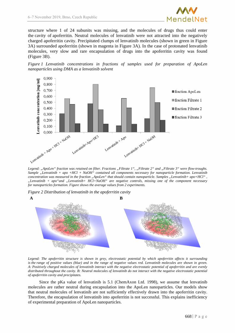
6–7 2019, Brno, Czech Republic
structure where 1 of 24 subunits was missing, and the molecules of drugs thus could enter the cavity of apoferritin. Neutral molecules of lenvatinib were not attracted into the negatively charged apoferritin cavity. Precipitated clumps of lenvatinib molecules (shown in green in Figure 3A) surrounded apoferritin (shown in magenta in Figure 3A). In the case of protonated lenvatinib molecules, very slow and rare encapsulation of drugs into the apoferritin cavity was found (Figure 3B). Figure 1 Lenvatinib concentrations in fractions of samples used for preparation of ApoLen nanoparticles using DMA as a lenvatinib solvent
Legend: „ApoLen“ fraction was retained on filter. Fractions „Filtrate 1“, „Filtrate 2“ and „Filtrate 3“ were flow-troughs. Sample „Lenvatinib + apo +HCl + NaOH“ contained all components necessary for nanoparticle formation. Lenvatinib concentration was measured in the fraction „ApoLen“ that should contain nanoparticle. Samples „Lenvatinib+ apo+HCl“ , „Lenvatinib + apo“and „Lenvatinib+ HCl+NaOH“ are negative controls, missing one of the component necessary for nanoparticles formation. Figure shows the average values from 2 experiments.
Figure 2 Distribution of lenvatinib in the apoferritin cavity A B
Legend: The apoferritin structure is shown in grey, electrostatic potential by which apoferritin affects it surrounding is the range of positive values (blue) and in the range of negative values red. Lenvatinib molecules are shown in green. A: Positively charged molecules of lenvatinib interact with the negative electrostatic potential of apoferritin and are evenly distributed throughout the cavity. B: Neutral molecules of lenvatinib do not interact with the negative electrostatic potential of apoferritin cavity and precipitates.
Since the pKa value of lenvatinib is 5.1 (ChemAxon Ltd. 1998), we assume that lenvatinib molecules are rather neutral during encapsulation into the ApoLen nanoparticles. Our models show that neutral molecules of lenvatinib are not sufficiently effectively drawn into the apoferritin cavity. Therefore, the encapsulation of lenvatinib into apoferritin is not successful. This explains inefficiency of experimental preparation of ApoLen nanoparticles.
668

6–7 2019, Brno, Czech Republic
Figure 3 Encapsulation of lenvatinib into the “holey” apoferritin structure A B
A B
Legend: The apoferritin structure is shown in magenta, lenvatinib molecules are shown in green. Figure shows the initial and the final image at the time of 60 ns. A: Successful encapsulation of positively charged molecules of lenvatinib into the „holey“ apoferritin structure. B: Unsuccessful encapsulation of neutral molecules of lenvatinib into „holey“ apoferritin structure. Precipitated molecules of lenvatinib surround the apoferritin structure
CONCLUSIONS Theoretical and experimental approaches show that lenvatinib, which is expected
to be in neutral form during re-assembly of apoferritin, is not suitable for preparation of ApoLen nanoparticles.
ACKNOWLEDGEMENTS The research was supported by the Grant Agency of Czech Republic (GACR 18-10251S).
REFFERENCES ChemAxon Ltd. ©1998–2019. Chemicalize Calculation [Online]. Available at: https://chemicalize.com/#/calculation. [2019-04-03]. de Val, N. et al. 2012. Structural Analysis of Haemin Demetallation by L-chain Apoferritins. Journal of Inorganic Biochemistry, 112: 77–84. Dostalova, S. et al. 2017. Apoferritin as an Ubiquitous Nanocarrier with Excellent Shelf Life. Journal of Nanomedicine, 12: 2265–2278. Eisai Inc. ©2019. Lenvima: Prescribing Information [Online]. Available at: http://www.lenvima.com/pdfs/prescribing-information.pdf. [2019-10-06].
669

6–7 2019, Brno, Czech Republic
Farsangi-Hojjat, M. 2014. Small-Molecule Inhibitor of Receptor Tyrosine Kinases: Promising Tools for Targeted Cancer Therapies. International Journal of Molecular Sciences, 15(8): 13768–13801. Ford, G.C. et al. 1984. Ferritin: Design and Formation of an Iron-storage Molecule. Philosophical Transactions of the Royal Society of London, 304(1121): 551–565. Harrison, P.M. et al. 1974. Ferritin Iron Uptake and Release – Structure, Function, Relationship. Biochemical Journal, 143(2): 445–451. Hashizume, H. et al. 2000. Openings between Defective Endothelial Cells Explain Tumor Vessel Leakiness. American Journal of Pathology, 156(4): 1363–1380. Heger, Z. et al. 2014. Apoferritin Aplications in Nanomedicine. Nanomedicine (Lond.), 9: 2233–2245. Humphrey, W. et al. 1996. VMD: Visual Molecular Dynamics. Journal of Molecular Graphics & Modelling, 14(1): 33–38. Hussein, Z. et al. 2017. Clinical Pharmacokinetic and Pharmacodynamic Profile of Lenvatinib, an Orally Active, Small-Molecule, Multitargeted Tyrosine Kinase Inhibitor. European Journal of Drug Metabolism and Pharmacokinetics, 42(6): 903–914. Indra, R. et al. 2019. Ellipticine-Loaded Apoferritin Nanocarrier Retains DNA Adduct-Based Cytochrome P450-Facilitated Toxicity in Neuroblastoma Cells. Toxicology, 419: 40–54. Iwai, K. et al. 1984. Use of Oily Contrast Medium for Selective Drug Targeting to Tumor: Enhanced Therapeutic Effect and X-Ray Image. Cancer Research, 44(5): 2115–2121. Kim, M. et al. 2011. pH-Dependent Structures of Ferritin and Apoferritin in Solution: Disassembly and Reassembly. Biomacromolecules, 12(5): 1629–1640. Phillips, J.C. et al. 2005. Scalable Molecular Dynamics with NAMD. Journal of Computational Chemistry, 26: 1781–1802. Salomon-Ferrer, R. et al. 2013. An Overview of the Amber Biomolecular Simulation Package. WIREs Computational Molecular Science, 3(2): 198–210.
670

6–7 2019, Brno, Czech Republic
Decreased immune response after PASylation of stealth ferritin nanocarriers
Barbora Tesarova1,2*, Hana Polanska3, Veronika Smidova1,2, Zita Goliasova1,2 1Department of Chemistry and Biochemistry
Mendel University in Brno Zemedelska 1, 613 00 Brno
2Central European Institute of Technology Brno University of Technology Purkynova 123, 612 00 Brno
3Department of Pathological Physiology and Department of Physiology Masaryk University
Kamenice 753/5, CZ-625 00 Brno CZECH REPUBLIC
Abstract: The effects on immunocompatibility after performed surface modifications (PEGylation and PASylation) of natural nanocarriers based on ferritin (FRT) were tested in this work. Potential cytostatic drug ellipticine (Elli) was encapsulated into FRT, leading to formation of FRTElli. The main goals of prepared PEG-FRTElli, PAS-10-FRTElli and PAS-20-FRTElli were to achieve decreased in vitro macrophage uptake and decreased in vivo complement activation. Macrophage uptake was studied via flow cytometry and complement activation via western blot. According to performed experiments PAS-10 modification was the only one that was sufficient to ensure both aspects.
Key Words: apoferritin, immune response, nanomedicine, PASylation
INTRODUCTION Even though there is a large number of drugs that can be used in cancer treatment, the goal
is to reach selective death of malignant cells while reducing toxicity to healthy cells. There are several biological barriers to provide effective drug delivery directly to malignant tissue such as renal, hepatic, or immune clearance. Herein, we focused on reducing the immune clearance. The fact is that only 5% of nanomaterial doses reach their intended target, which happens, among other reasons, due to non-specific recognition and uptake of nanoconstructs by macrophages (Bae and Park 2011). Macrophages are leukocytic cells involved in the detection, phagocytosis and destruction of bacteria and other harmful organisms (Gustafson et al. 2015). On the macrophages surface, receptors for complement proteins are located (van Lookeren Campagne et al. 2007). The system of complement proteins represent an important part of the innate immunity, acting as first-line defence against pathogenic infections (Noris and Remuzzi 2013). After intravenous administration, nanomaterials interact immediately with the immune system and activate the complement proteins (Halamoda-Kenzaoui and Bremer-Hoffmann 2018). Complement proteins can be activated via antibodies binding to antigen pathway, mannose binding to lectin pathway or by direct binding of the pathogen to the complement protein. All three pathways lead to the inflammatory process, macrophages accumulation in the liver and spleen or hypersensitivity reaction (Wang et al. 2017, van den Hoven et al. 2013).
Therefore, there is a huge need for ʺstealthʺ nanomaterials with a pronounced immuno-compatibility. Surface-related properties of nanomaterials are becoming more relevant than the category of a nanomaterial since they determine the protein corona composition and interaction with other plasma proteins and complement proteins (Moghimi and Simberg 2017). Surface modifications of nano-materials represent promising way to significantly improve the immunocompatibility of nanomaterial, e.g., decrease complement activation or reduce uptake by macrophages. PEGylation, as the first clinically approved modification of a drug, was shown to exhibit phenomenon called “accelerated blood
671

6–7 2019, Brno, Czech Republic
clearance” occurred due to production of specific anti-PEG IgM, followed by increased uptake of nanoparticles by the macrophages (Yang et al. 2013, Yang and Lai 2015). PASylation, a more biological alternative to PEGylation, is comprised of small residues of amino acids Proline (P), Alanine (A) and Serine (S) (Binder and Skerra 2017). Horse spleen FRT was chosen as a biocompatible organic nanocarrier. Its structure is strongly dependent on the pH value of the surrounding environment, thus it enables physical entrapment of cytostatic drug within the internal 8-nm cavity (Kim et al. 2011).
MATERIAL AND METHODS
Chemicals All chemicals of ACS purity were obtained from Sigma-Aldrich (St. Louis, MO, USA), unless
stated otherwise.
Encapsulation of Elli into FRT The stock solution of Elli with concentration of 1 mg/ml was prepared by dissolving Elli in 1 M
HCl and deionized water in ratio 1 : 80. For each sample, 200 µl of 1 mg/mL Elli was added to 100 µl of deionized water and 20 µl of 50 mg/ml horse spleen 22L/2H FRT and gently mixed for 15 min. FRT structure was reassembled by 0.66 µl of 1 M sodium hydroxide solution and the samples were mixed for further 15 min. To filter out non-encapsulated Elli, solution exchange was performed 3× (centrifugation at 6000 rcf and 4 °C for 15 min). The concentration of encapsulated Elli was evaluated via absorbance measurement at 420 nm using Tecan Infinite 200 PRO (Männedorf, Switzerland).
Surface modification with PAS sequences 25 µl of 1.3 nm gold nanoparticles were added to 321 µl FRTElli solution and the samples were
mixed for 14 h to allow adsorption of Au nanoparticles to the charged amino acid residues on the surface of FRTElli nanoparticles (leading to FRTElli-Au). Solution exchange was performed to remove unbound Au nanoparticles. 3 µl of 1.25 mg/ml PAS-10 (ASPAAPAPASC) or PAS-20 (ASPAAPAPASPAAPAPSAPAC) was added to FRTElli-Au and the samples were incubated for 1 h at 45 ºC to allow binding of cysteine to gold. Then, solution exchange was performed to remove unbound molecules of PAS peptides.
Surface modification with PEG 50 µl of 10 mM methoxy PEG maleimide in PBS (phosphate buffered saline, pH 7.4: 0.137 M
NaCl + 0.0027 M KCl + 0.0014 M KH2PO4 + 0.0043 M Na2HPO4) and 629 µl of PBS was added to FRTElli and mixed for 1 h. To remove unbound PEG, the sample was 5× diafiltrated using Amicon® Ultra 0-5 mL 50K Merck Millipore (Billerica, MA, USA) at 6000 rcf and 4 °C for 15 min.
Evaluation of macrophages uptake Macrophage uptake was performed with murine macrophage cell line derived from Abelson
murine leukemia virus-induced tumor RAW 264.7. A suspension of 300 000 RAW 264.7 cells was seeded into 12-well plate. After 24 h incubation, the cells were treated with 20 µM Elli in the form of free Elli, FRTElli, PEG-FRTElli, PAS-10-FRTElli, and PAS-20-FRTElli for 30 min. The cells were washed with phosphate buffered saline (PBS, pH 7.4), scraped and centrifuged at 1000 rcf for 10 min. Then, the cells were resuspended in 3% fetal bovine serum (FBS) in PBS solution. Macrophage uptake was analyzed via fluorescence using 488-nm laser and 533/30 filter on the BD Accuri C6 Plus flow cytometer (BD Biosciences, Franklin Lakes, NJ, USA). The flow rate was 35 µl/min and a minimum of 100 000 cells was analyzed in each group.
In vivo activation of complement (C3) Twelve female nude athymic BALB/c nu/nu mice were used for in vivo studies. The use
of the animals followed the European Community Guidelines as accepted principles for the use of experimental animals. The experiments were performed with the approval of the Ethics Commission at the Faculty of Medicine, Masaryk University, Brno, Czech Republic. The mice stayed in individually ventilated cages at 12/12 h light/dark cycle and provided ad libitum with standard diet and water.
672

6–7 2019, Brno, Czech Republic
The treatment of mice was carried out i.v. as two applications (100 μg dose of Elli for each mouse, either free or in the form of FRTElli or PAS-10-FRTElli). The control group received 100 μl of PBS. After 1 week, the mice were euthanized by intraperitoneal injection of 1% Narkamon + 2% Rometar, 5 μl/g of body weight, followed by intracardiac blood collection in ethylendiaminetetraacetic acid-treated tubes. Plasma was isolated after blood collection by centrifugation (1000 rcf, 20 ºC, 10 min)
Electrophoresis (200 V, 4 ºC, 35 min) of the plasma samples was done under non-reducing and non-denaturing conditions in 7.5% sodium dodecylsulphate gel. Proteins were electrotransferred onto the Immobilon®-FL transfer membrane (EMD Millipore Corporation, Burlington, MA, USA) and the non-specific binding was blocked with 5% (w/v) skimmed milk powder for 1 h at 20 ºC. Complement C3 monoclonal antibody (LF-MA0132, Thermo Fisher Scientific, USA, dilution 1:1 000) was used as primary antibody, incubation was performed at 20 ºC for 1 h. After washing, membrane was incubated with secondary antibody, which was labeled with horseradish peroxidase (p0260, Dako, Santa Clara, CA, USA, dilution 1:5 000) for 1 h at 20 ºC. Clarity Western ECL Blotting Substrate (Bio-Rad) was used in order to develop the signals and chemiluminescence was visualized via Azure c600 (Azure Biosystems).
RESULTS AND DISCUSSION Figure 1A showed cell distribution in each sample, population of live cells is shown in red circle.
The macrophage uptake (Figure 1B) was expressed as median fluorescence intensity of Elli. Obtained data (Figure 1B) showed that free Elli enters into macrophages. Importantly, the highest macrophages uptake was detected for PEG-FRTElli, which point out at possible immunogenicity of PEG (Ganson et al. 2006, Judge et al. 2006). On the other hand, the lowest activation of immune response was detected for PAS-10-FRTElli. Modification with PAS-10 sequences was the only one that caused the decrease of macrophage uptake compared to unmodified FRTElli.
Figure 1 Macrophage uptake via flow cytometry (A: forward scatter vs. side scatter, B: macrophage uptake)
673

6–7 2019, Brno, Czech Republic
The lowest in vivo activation of C3 complement protein (Figure 2) was achieved after treatment with PAS-10-modified FRTElli (81.9% ± 4.2% decrease of activation compared to FRTElli). Group treated with free Elli caused also lower activation than in unmodified FRTElli (74.8% ± 3.5% decrease of activation compared to FRTElli). Results were confirmed by three independent replicates. These findings correspond with in vitro macrophage uptake, that PAS sequences are able to decrease the immune response.
Figure 2 Western blot analysis of complement (C3) activation performed on Elli, FRTElli, PAS-10-FRTElli treated samples, including positive (serum) and negative (PBS) control
CONCLUSION Three types of FRTElli surface modifications were tested (modification with PAS-10, PAS-20
sequences and PEGylation) in order to decrease immune response after intravenous delivery. Modifications with PEG and PAS-20 sequences did not appear as suitable due to the increase in macrophage uptake. On the other hand, modification with PAS-10 sequences led to decrease macrophage uptake and also decreased in vivo complement activation. The in vitro and in vivo experiments presented in this work serve as suitable platform to carrying out additional preclinical studies of PAS-10-FRTElli.
ACKNOWLEDGEMENTS The research was financially supported by the Grant Agency of the Czech Republic (GACR 17-12816S), League Against Cancer Prague and Brno Ph.D. Talent.
REFERENCES Bae, Y.H., Park, K. 2011. Targeted drug delivery to tumors: myths, reality and possibility. Journal of Controlled Release, 153(3): 198–205.
674

6–7 2019, Brno, Czech Republic
Binder, U., Skerra, A. 2017. PASylation®: A versatile technology to extend drug delivery. Current Opinion in Colloid & Interface Science, 31: 10–17. Ganson, N.J. et al. 2006. Control of hyperuricemia in subjects with refractory gout, and induction of antibody against poly (ethylene glycol) (PEG), in a phase I trial of subcutaneous PEGylated urate oxidase. Arthritis Research & Therapy, 8(1): R12. Gustafson, H.H. et al. 2015. Nanoparticle Uptake: The Phagocyte Problem. Nano Today, 10(4): 487–510. Halamoda-Kenzaoui, B., Bremer-Hoffmann, S. 2018. Main trends of immune effects triggered by nano-medicines in preclinical studies. International Journal of Nanomedicine, 13: 5419–5431. Judge, A. et al. 2006. Hypersensitivity and loss of disease site targeting caused by antibody responses to PEGylated liposomes. Molecular Therapy, 13(2): 328–337. Kim, M. et al. 2011. pH-dependent structures of ferritin and apoferritin in solution: disassembly and reassembly. Biomacromolecules, 12(5): 1629–1640. Moghimi, S.M., Simberg, D. 2017. Complement activation turnover on surfaces of nanoparticles. Nano Today, 15: 8–10. Noris, M., Remuzzi, G. 2013. Overview of complement activation and regulation. Seminars in Nephrology, 33(6): 479–492. Van Den Hoven, J.M. et al. 2013. Complement activation by PEGylated liposomes containing prednisolone. European Journal of Pharmaceutical Sciences, 49(2): 265–271. Van Lookeren Campagne, M. et al. 2007. Macrophage complement receptors and pathogen clearance. Cellular Microbiology, 9(9): 2095–2102. Wang, G. et al. 2017. In Vitro and In Vivo Differences in Murine Third Complement Component (C3) Opsonization and Macrophage/Leukocyte Responses to Antibody-Functionalized Iron Oxide Nanoworms. Frontiers in Immunology, 8: 151. Yang, Q., Lai, S.K. 2015. Anti-PEG immunity: emergence, characteristics, and unaddressed questions. Wiley interdisciplinary reviews. Nanomedicine and Nanobiotechnology, 7: 655–677. Yang, Q. et al. 2013. Accelerated drug release and clearance of PEGylated epirubicin liposomes following repeated injections: a new challenge for sequential low-dose chemotherapy. International Journal of Nanomedicine, 8: 1257–1268.
675

6–7 2019, Brno, Czech Republic
Sensitive biosensor for detection oncogenic miRNA-21
Veronika Vanova1, Eliska Sedlackova1,2, David Hynek1,2, Lukas Richtera1,2, Vojtech Adam1,2
1Department of Chemistry and Biochemistry Mendel University in Brno Zemedelska 1, 613 00 Brno
2Central European Institute of Technology, Brno University of Technology,
Purkynova 123, 612 00 Brno CZECH REPUBLIC
Abstract: The aim of this study was to prepare a sensitive electrochemical biosensor for detection of oncogenic miRNA-21 as a potential biomarker for early detection of cancer. MicroRNAs (miRNAs) are small noncoding RNA, which play an important role in the regulation of gene expression. miRNAs are present in extracellular fluids like urine, serum, etc. in extremely low concentration. It is important for the biosensor to detect extremely low concentrations of specific miRNA as potential biomarkers. The aim of this experiment was designing, preparing and optimizing a sensitive and selective biosensor for the detection of miRNA-21. A biosensor was prepared to detect the lowest concentration of miRNA-21 in the sample. The linear concentration range for the calibration curve was 1 fM to 10 nM. LOD was 1 fM and obtained from the regression equation was 3.2 zM and LOQ was 10.8 zM. Subsequently, prepared biosensor was measured in artificial urine (AU) samples to verify the functioning of the sensor in induced real conditions. The results showed a minimal effect of the matrix for the determination of the target miRNA.
Key Words: nucleic acids, miRNA, electrochemical detection, biosensor
INTRODUCTION In the field of science, the possibility of biomarker detection as an indicator of biological
or pathological state of the organism could be a way to simplify, accelerate and refine the diagnosis of diseases. A particular possibility of such biomarkers is a miRNA molecule. It has been found that miRNA has an irreplaceable role in influencing the expression of large number of genes and also that the level of these molecules can be observed in various extracellular fluids such as e.g. urine or plasma (Krol et al. 2010).
Another interesting finding with these molecules is that the expression of some particular miRNAs varies considerably in oncological diseases (Rupaimoole and Slack 2017). Therefore, the level of these miRNAs varies significantly (increases / decreases), which can be detected non-invasively in these extracellular fluids. This knowledge has led scientists to wonder how these molecules could be detected in clinical practice as easily, as accurately, as quickly and as cheaply as possible (Cho 2010). Currently, the most commonly used methods are Northern blotting or RT-PCR (de Planell-Saguer and Rodicio 2013) but these methods are often laborious and costly. Therefore, new approaches are being sought to detect them in a simple, cost effective manner with higher selectivity and enhanced sensitivity (Tian et al. 2015). One such detection approach is to create a sensitive electrochemical biosensor for miRNA detection. An example of such biosensor is blood glucose meter which is already in practice for diabetes detection with high sensitivity and specificity. The advantage of such sensors is that they can detect the level of the substance in the body very quickly. A very small sample is sufficient and should be affordable when put into practice (Kilic et al. 2018, Hamidi-Asl et al. 2013).
676

6–7 2019, Brno, Czech Republic
MATERIALS AND METHODS
Chemicals and apparatuses We used 1.0 µm, 0.3 µm a 0.05 µm Alumina Slurry suspension and 0.5 µm Diamond suspension
(Electron Microscopy Sciences, Hatfield, United Kingdom) for electrode polishing, Ethanol absolute (VWR chemicals, Randor, Pennsylvánia, USA), Acetone (VWR chemicals, Randor, Pennsylvánia, USA), MiliQ water (18.20 MΩ/cm).
Phosphate buffered saline (PBS) (pH 7, 25 mM) was prepared by mixing 20.0 g sodium chloride (NaCl), 0.5 g Ptassium chloride (KCl), 3.6 g Sodium phosphate dibasic (Na2HPO4) and 0.6 g Potassium dihydrogen phosphate (KH2PO4) (Sigma-Aldrich, St. Louis, MO, USA) into 1000 ml of MiliQ water. 10 mM 1-amino-2-naftol-4-sulfonic acid (AN–SO3–) (Sigma-Aldrich, St. Louis, MO, USA) was diluted in PBS.
Other chemicals which we used: 40 mM, 16.7 mg Phosphorus pentachloride (PCl5) in acetone (2 ml), Tris-EDTA (TE buffer) pH 8 (Sigma-Aldrich, St. Louis, MO, USA).
All measurements were taken in 5 mM Potassium hexacyanoferrate (II) trihydrate K4[Fe(CN)6]/ 5 mM Potassium hexacyanoferrate(III) K3[Fe(CN)6] in 0.1 M KCl (Sigma-Aldrich, St. Louis, MO, USA).
Oligonucleotides were purchased also from Sigma-Aldrich: DNA probe (anti-miRNA-21): 5’-NH2-C6-TCAACATCAGTCTGATAAGCTA-3’ miRNA-21: 5’-UAGCUUAUCAGACUGAUGUUGA-3’.
Artificial urine was prepared into 250 ml MiliQ water by stirring 1.90 g KCl, 4.25 g NaCl, 12.25 g urea, 0.59 g Potassium dihydrogen phosphate (KH2PO4), 0.52 g Magnesium sulfate heptahydrate (MgSO4 . 7H2O), 0.52 g Citric acid, 0.17 g Ascorbic acid, 0.70 g Creatinine, 0.32 g Sodium hydroxide (NaOH), 0.24 g Sodium bicarbonate (NaHCO3), 0.14 ml Sulfuric acid (99%, H2SO4). Solution was diluted by MiliQ water into 500 ml.
Preparation and modification of electrode First of all, the glassy carbon electrode (GCE) was polished by using 1.0; 0.3; 0.05 μm Alumina
slurry and 0.5 μm Diamond suspension each for 90 s. Between each step, electrodes were sonicated in acetone, ethanol, and water for 90 s respectively. And finally, GCE was dried under the argon gas.
The second step of modification was electrodeposition of 1-amino-2-naphthol-4-sulfonic acid (AN–SO3–) (10 mM) in PBS buffer (25 mM, pH 7.0). It was done by cyclic voltammetry (CV) scanning between +1.5 V and –0.5 V with the scan rate 20 mVs-1 and 8 cycles. CV was performed by using a three-electrode system containing Ag/AgCl as a reference electrode, platinum wire as a counter electrode and GCE as a working electrode. In this step was obtained. AN–SO3– modified GCE (Wang et al. 2013).
Subsequently the electrode was immersed in a solution of PCl5 (40 mM) in acetone (absolute) for 30 min to transfer the sulfonic groups on the sulfonyl groups on the GCE modified with AN–SO3– (Chen et al. 2008).
DNA oligonucleotides with a sequence complementary to target miRNA were defrosted and diluted in TE buffer to 1 μM concentration and subsequently heated up to 80°C for 2 min. Then they were dropped on the surface of GCE in 10 μl volume (Smith et al. 2017). Oven was heated to 80 °C and the modified electrodes with oligonucleotides were placed inside for 90 min. After drying, electrode was slightly rinsed in TE buffer and then measured with CV and EIS. The hybridization was done at room temperature for 45 min by incubation in the exact concentration of target miRNA diluted in TE buffer and artificial urine (Figure 1).
Electrochemical measurement Electrochemical measurements were taken in every step of modification, before and after
the hybridization. We were using cyclic voltammetry (CV) method and electrical impedance spectroscopy method (EIS).
677

6–7 2019, Brno, Czech Republic
CV was running at a potential between +0.7 V and –0.3 V with scan rate 20 mVs-1 and 8 cycles. EIS was set at a DC potential of 0.23 V between frequencies of 0.01 Hz to 10 kHz with an AC of 5 mV (Wang et al. 2013).
Figure 1 a) bare GCE electrode b) electrodeposition of AN–SO3– on GCE c) sulfonylation d) DNA probe immobilization e) hybridization target miRNA-21
RESULTS AND DISCUSSION
Modification of the electrode
Electrodeposition of AN–SO3– on GCE In this part of the modification, we modified GCE by electrochemical immobilization of the AN–
SO3– (Nomura 1982) on the electrode surface. Deposition layer of the AN–SO3– were increased with the continuous growth of the CV cycles. As Figure 2 observe there are two reduction peaks at position −0.013 V (P3), −0.200 V (P4) and two oxidation peaks +0.600 V (P1) and +0.900 V (P2). This record shows us that the electrochemical deposition of AN–SO3– on the GCE surface is irreversible and with increasing cycles the peaks gradually decrease, which proofs the continuous growth of the AN–SO3– film. Successful electrodeposition was also displayed in the change of electrode colour from shiny silver to matt grey.
Figure 2 Electrodeposition of AN–SO3– on GCE
Step-by-step modification process of the electrode CV and EIS methods were done in each step of the electrode modification. Every step was
measured in 5 mM (K4[Fe(CN)6])/ 5 mM K3[Fe(CN)6] in 0.1 M KCl electrolyte. Cyclic voltammetry: by measuring the bare electrode we occurred pair of significant
oxidation-reduction peaks (Figure 3B a). However, after the electrodeposition of AN–SO3– on GCE
678

6–7 2019, Brno, Czech Republic
the peaks decreased dramatically in comparison with those of on bare GCE. AN–SO3– layer partially prevents electron transfer of electrolyte ions to the electrode surface as a result of electrostatic repulsion force (Figure 3B b). After incubation in a solution of PCl5, the redox peaks increased (Figure 3B c). Further, after application and incubation of the DNA probe on the modified electrode, the redox peaks decreased again (Figure 3B d). This is the affirmation that the immobilization of the probe was successful (Wang et al. 2013).
With EIS, we can monitor the changes of the diameter in Nyquists plots in different steps of the modification. The diameter of the semicircle reflect the resistance of electron transfer on the electrode surface. The lowest resistance was observed at bare GCE (Figure 3A a). The AN–SO3– electrodeposition leads to a significantly higher resistance (Figure 3A b). After reacting with PCl5, the resistance is again markedly increased (Figure 3A c). Finally, the resistance of the immobilized probe was decreased again (Figure 3A d) (Smith et al. 2017, Wang et al. 2013). Figure 3 A) Nynquist plots, B) CV voltammograms showing: a) unmodified electrode b) electro- deposition AN–SO3– c) modification with PC15 d) probe immobilization
miRNA hybridization with DNA probe in different concentrations
In this part of the experiment, the sensitivity of the designed biosensor was tested. For this part of the study we were using only EIS method for its better sensitivity. The aim of this study was to prepare as sensitive biosensor as possible. We measured different concentrations of miRNA-21 ranging from 10-8 M (10 nM) to 10-15 M (1 fM) dissolved in TE buffer (Figure 4). Irregular results were obtained at lower concentrations than 1 fM, therefore they were not included in the calibration curves. The values that were used in the calibration curve were calculated using NOVA 1.8 software as the value of the difference between the final point and the start point of the Nyquist semi-circle graph.
Figure 4 Nynquist plots from measurement of different concentrations of miRNA-21 in TE buffers by EIS method
Calibration curves
Calibration curves were generated according to data measured by EIS. Concentration values are reported in the calibration curves as log c (M) values to show their linear dependence. For better
679

6–7 2019, Brno, Czech Republic
accuracy of the regression coefficient (R2), the calibration data were divided into two calibration curves. The part with concentration values from 10 nM to 1 pM reached an accuracy of R2 = 0.9885 and the part with concentration values from 1 pM to 1 fM concentration had R2 = 0.9617 (Figure 5).
LOD and LOQ values were counting true the regression equation. LOD 3.2 zM and LOQ 10.8 zM (Table 1). However, these values were very low. Practically, we were able to measure the lowest 1 fM concentration, which is still low enough for measuring miRNA in real samples. According to Smith et al. (2017) the concentrations of miRNA-21 which were measured in real samples of urine were around 10-9 – 10-11 M. These values are fitting enough into the calibration range.
Table 1 Analytical table for LOD and LOQ calculation.
Sample Regression Equation Linear dynamic range log c (M) R2 LOD
(zM) LOQ (zM)
RSD (%)
miRNA-21 y = 0.8626x + 12.434 –8 to –12 0.9855 y = 0.1994x + 4.3858 –12 to –15 0.9617 3.2 10.8 2.5
Figure 5 Calibration curves: A) concentration values from 10–8 to 1–12 M B) concentration values from 1–12 to 1–15 M.
Measurement in artificial urine In the last section, we measured miRNA-21 oligonucleotides dissolved in AU. Concentration
levels which have been measured in AU samples have been selected according to the values corresponding to concentrations in real urine samples. The chosen values were 10–11, 10–10, 10–9 M. To check the measurements, the measured data from AU were fitted into the regression equation from the calibration curve A (Figure 5A) and calculated. We compared the measured data of AU and the calculated data in percentage. After the evaluating added concentrations and the calculated concentrations (recovery) (Tab.2), we achieved sufficient measurement accuracy, which suggests that the measurement was performed correctly and the artificial urine matrix does not affect the correct functionality and sensitivity of the prepared biosensor. Table 2 Values of real concentrations of miRNA-21 in AU compared to the values calculated from the regression equation and their percentage expression
Concentration (added) Calculated concentration Recovery (%) logc (M) (M) log c (M) % log c (M)
–11 1 × 10-11 –11.32 103 –10 1 × 10⁻¹⁰ –9.86 99 –9 1 × 10⁻⁹ –9.81 109
CONCLUSION To sum up we have designed, prepared and tested a stable concept of a biosensor for detection
of oncogenic miRNA-21. We also demonstrated the functionality of this biosensor to determine miRNA samples in an artificial urine matrix. For practical use in the future, it will be necessary to test the biosensor in real urine samples at clinical patients.
680

6–7 2019, Brno, Czech Republic
ACKNOWLEDGEMENTS This research was carried out under the project CEITEC 2020 (LQ1601) with financial support from the Ministry of Education, Youth and Sports of the Czech Republic under the National Sustainability Programme II. The research was financially supported by IGA MENDELU AF-IGA2019-IP059.
REFERENCES Chen, J.H. et al. 2008. Electrochemical Biosensor for Detection of BCR/ABL Fusion Gene Using Locked Nucleic Acids on 4-Aminobenzenesulfonic Acid-Modified Glassy Carbon Electrode. Analytical Chemistry, 80(21): 8028–8034. Cho, W.C.S. 2010. MicroRNAs: Potential biomarkers for cancer diagnosis, prognosis and targets for therapy. International Journal of Biochemistry & Cell Biology, 42(8): 1273–1281. de Planell-Saguer, M., Rodicio, M.C. 2013. Detection methods for microRNAs in clinic practice. Clinical Biochemistry, 46(10–11): 869–878. Hamidi-Asl, E. et al. 2013. A review on the electrochemical biosensors for determination of micro RNAs. Talanta, 115: 74–83. Kilic, T.A. et al. 2018. MicroRNA biosensors: Opportunities and challenges among conventional and commercially available techniques. Biosensors & Bioelectronics, 99: 525–546. Krol, J. et al. 2010. The widespread regulation of microRNA biogenesis, function and decay. Nature Reviews Genetics, 11(9): 597–610. Nomura, T. 1982. Alternating-Current Polarographic-Determination of Microgram Amounts of Iodide-Ion by Means of the Catalytic-Oxidation of 1-Amino-2-Naphthol-4-Sulfonic Acid. Journal of Electroanalytical Chemistry, 139(1): 97–104. Rupaimoole, R., Slack F.J. 2017. MicroRNA therapeutics: towards a new era for the management of cancer and other diseases. Nature Reviews Drug Discovery, 16(3): 203–221. Smith, D.A. et al. 2017. Electrochemical detection of urinary microRNAs via sulfonamide-bound antisense hybridisation. Sensors and Actuators B-Chemical, 253: 335–341. Tian, T. et al. 2015. A review: microRNA detection methods. Organic & Biomolecular Chemistry 13(8): 2226–2238. Wang, Q.X. et al. 2013. A sensitive DNA biosensor based on a facile sulfamide coupling reaction for capture probe immobilization. Analytica Chimica Acta, 788: 158–164.
681

6–7 2019, Brno, Czech Republic
LA-ICP-MS as a sensitive method for detection of nanoparticle-antibody conjugates in immunochemistry analysis
Marcela Vlcnovska1, 2, Michaela Tvrdonova3, Aneta Stossova3, Hana Polanska2, Marketa Vaculovicova1, 4, Tomas Vaculovic3, Michal Masarik2
1Department of Chemistry and BiochemistryMendel University in Brno Zemedelska 1, 613 00 Brno
2Department of Pathological Physiology 3Department of Chemistry
Masaryk University Kamenice 753/5, 625 00 Brno-Bohunice
4Central European Institute of Technology Brno University of Technology Purkynova 123, 612 00 Brno
CZECH REPUBLIC
Abstract: Laser ablation followed by inductively coupled plasma mass spectrometry is an analytical method suitable for low concentration measurement of elements in a sample. This can be used not only for detection of elemental distribution within a sample but also as a detection means for immunoanalytical techniques using nanoparticle-antibody conjugates as recognition elements. The aim of this work was to prepare a conjugate of 10nm gold nanoparticles with anti-p53 antibody, to verify the antigen binding ability, and to use this construct for identification of p53 in a real sample of cell lysate. It has been experimentally verified that it is possible to use nanoparticle-modified antibodies for immunochemical analysis coupled to LA-ICP-MS detection. However, the nonspecific sorption of nanoparticles on the sample surface needs to be minimized by optimization of the blocking step.
Key Words: gold nanoparticles, LA-ICP-MS, immunochemistry, dot-blot, protein detection, p53
INTRODUCTION Inductively coupled plasma mass spectrometry (ICP-MS) has become a routine technique
for determination of elemental (especially metal) composition of the sample (Pozebon et al. 2014). The interest in this method has grown considerably in the biological sciences. In combination
with laser ablation (LA-ICP-MS) this method provides information not only about composition but also about the spatial distribution of metals in solid samples. Most studies focus primarily on the measurement of endogenous elements in soft and hard tissues such as liver, kidney, brain, bones, teeth, etc. Increasingly, however, elementally labelled antibodies are used to visualize the distribution of important proteins (Seuma et al. 2008).
A wide variety of elemental labels can be conjugated to antibodies. Besides metal-containing chelates, the tags may include noble metal nanoparticles (e.g. gold and silver), quantum dots, iron or polymeric nanoparticles doped with lanthanides, and metal nanoclusters (Pozebon et al. 2017).
Current methods of immunochemistry make it possible to detect up to three different antibodies in parallel (Aljakna et al. 2018). Due to the great emphasis on the multiplex determination of proteins, the wide selection of elemental labels is advantageous. Multiplex determination of protein markers (e.g. in cancer diagnostics) together with distribution of endogenous elements (both natural and pathological) can lead to increased amount of information on molecular behaviour of diseased cells which translates in better diagnosis and thus contribute to the choice of appropriate treatment (Aljakna et al. 2018).
682

6–7 2019, Brno, Czech Republic
However, the absolute quantification of the biomolecules remains challenging. Therefore, this method allows relative comparisons of samples in research, which is sufficient for many biological applications (Clases et al. 2019).
MATERIAL AND METHODS
Materials As an antigen, standard of protein p53 was used Recombinant Human p53 protein ab43615
(Abcam, Cambridge, UK). And an anti-53 antibody DO-1 was delivered from Masaryk Memorial Cancer Institute in Brno.
For the preparation of conjugate the commercial kit of gold nanoparticles GOLD Conjugation Kit (10 nm, 20 OD) ab201808 (Abcam, Cambridge, UK) was used.
Composition of solutions 2x Blotting buffer: 25mM Trizma base, 150mM glycine, 10% (v/v) methanol 1x Blotting buffer: (50% (v/v) 2x blotting buffer with 40% (v/v) H2O and 10% (v/v) MetOH Blocking buffer: 1% BSA in PBS PBS: 2.7mM KCl, 1.8mM KaH2PO4, 137mM NaCl and 10mM Na2HPO4, pH 7.4 Antibody buffer: 0,1% BSA in PBS PBS-T: 0.05% (v/v) Tween-20 in PBS
Preparation of conjugates The conjugation protocol was based on the manufacturer's instructions. Briefly, 12 µl
of the diluted anti-p53 antibody DO-1 by antibody diluent were mixed with 45 µl of the reaction buffer and subsequently 45 µl from that were pipetting to lyophilized nanoparticles. 5 minutes later 5 µl of the Quencher were added.
Dot-blot At first, the PVDF membrane (Bio-Rad, USA) was activated by soaking in methanol
and in freshly prepared 1x blotting buffer, 30 s each. Subsequently, the membrane was placed on a filter-paper wetted by blotting buffer to prevent drying. Further, protein p53 and cell lysate samples (0.5 µl) were applied and dried for 20–30 minutes at 21 °C. The whole procedure was carried out at room temperature, 60 rpm using Multi RS-60 (Biosan, Latvia). The membrane was subsequently blocked by blocking buffer for 30 minutes. Subsequently, incubation with Ab-NPs conjugate in antibody buffer was carried out for 1 hour. Finally, three times repeated washing with PBS-T for 5 min was carried out and the membrane was analysed by LA-ICP-MS as described in (Tvrdonova et al. 2019).
RESULTS AND DISCUSSION
Preparation of conjugates The gold nanoparticles were delivered as a lyophilized mixture together with all necessary
solutions needed for conjugation (i.e. Antibody diluent, the Reactions buffer and the Quencher solution). A 10nm gold nanoparticle-antibody conjugate was prepared step by step according to the manufacturer's instructions. Immobilization of antibodies to the functional surface of nanoparticles was performed by covalent bonding through lysine residues containing primary amines. It causes their random spatial orientation on the surface of AuNPs (Richards et al. 2017).
Analysis of dot-blot membranes by LA-ICP-MS Prepared anti-p53 antibody conjugate with 10nm gold nanoparticles was used as a recognition
element in an immunochemical dot-blot analysis for identification of protein p53 in a sample. The measurement was performed by LA-ICP-MS.
683

6–7 2019, Brno, Czech Republic
Figure 1 Scheme of AuNPs-antibody conjugate according to Richards et al. (2017)
Figure 2 A An intensity of the Au signals depending on the amount of Recombinant Human p53 protein applied on the blotting membrane displayed in the colour-coded intensity scale (left); B Intensity of the Au signals shows nonspecific sorption of non-conjugated AuNPs (right)
The intensity of Au signals was measured, as a relation of Recombinant Human p53 protein applied to the blotting membrane in the range of 0.1–5 ng. Labelled anti-p53 antibody was applied in the total amount of 6.7 ng for each experiment.
The Figure 2 A shows that the ability of the antibody to bind the antigen was maintained and that the Au signal was proportionate to the amount of the antigen applied on the membrane.
Application of non-conjugated AuNPs on the membrane with standard of protein p53 showed a non-specific sorption of nanoparticles on the sample Figure 2 B. In this case, the intensity of Au signals was lower for about two orders of magnitude compared to AuNPs-antibody. These intensities can be subtracted during the data post-processing or the signals can be normalized as shown in Figure 3.
The figure 4 shows that the non-specific sorption of the non-conjugated AuNPs on the real sample of cell lysate is significant due to the sample complexity. The observed non-specific sorption can be eliminated by optimizing of the blocking steps such as blocking buffer composition (milk, BSA, casein) or time required for a thorough blocking. Another possibility is to suitably coat the surface of the particles. This is important in order to prevent the non-specific interactions of, for example, SH-rich proteins with the still active gold surface.
684

6–7 2019, Brno, Czech Republic
Figure 3 Normalization of Au signals to the same signal intensity
Figure 4 Intensity of the Au signals in a real sample of p53 positive MCF-7 cell lysate after immunochemical dot-blot analysis using AuNPs-antibody A and non-conjugated AuNPs as a negative control B
CONCLUSION Experimentally, it has been proven that anti-p53 antibody DO-1 does not lose its ability to bind
the antigen after conjugation with 10nm gold nanoparticle conjugation kit. The problem arises from the complexity of the biological sample containing high number
of proteins, lipids, nucleic acids, etc., with variable level of affinity to the nanoparticles. The following research will focus on the application of NPs-Ab immunochemical analysis
with LA-ICP-MS for the detection of biologically important molecules in samples. Subsequently,
685

6–7 2019, Brno, Czech Republic
the identification of multiple antigens in a single analysis will be carried out. Emphasis will also be placed on the elimination of frequently occurring nonspecific sorption of NPs to the sample.
ACKNOWLEDGEMENTS The research was financially supported by the Grant Agency of Czech Republic (GACR 17-12774S) and by the Grant Agency of Masaryk University (MUNI/C/0003/2019).
REFERENCES Aljakna, A. et al. 2018. Multiplex quantitative imaging of human myocardial infarction by mass spectrometry-immunohistochemistry. International Journal of Legal Medicine, 132(6): 1675–1684. Clases, D. et al. 2019. On-line reverse isotope dilution analysis for spatial quantification of elemental labels used in immunohistochemical assisted imaging mass spectrometry via LA-ICP-MS. Journal of Analytical Atomic Spectrometry, 34(2): 407–412. Pozebon, D. et al. 2014. Review of the applications of laser ablation inductively coupled plasma mass spectrometry (LA-ICP-MS) to the analysis of biological samples. Journal of Analytical Atomic Spectrometry, 29(12): 2204–2228. Pozebon, D. et al. 2017. Recent applications of laser ablation inductively coupled plasma mass spectrometry (LA-ICP-MS) for biological sample analysis: a follow-up review. Journal of Analytical Atomic Spectrometry, 32(5): 890–919. Richards, D.A. et al. 2017. Antibody fragments as nanoparticle targeting ligands: a step in the right direction. Chemical Science, 8(1): 63–77. Seuma, J. et al. 2008. Combination of immunohistochemistry and laser ablation ICP mass spectrometry for imaging of cancer biomarkers. Proteomics, 8(18): 3775–3784. Tvrdonova, M. et al. 2019. Gold nanoparticles as labels for immunochemical analysis using laser ablation inductively coupled plasma mass spectrometry. Analytical and Bioanalytical Chemistry, 411(3): 559–564.
686

6–7 2019, Brno, Czech Republic
UV-Fingerprinting as a tool for monitoring of pesticides
Milada Vodova, Lukas Nejdl, Marketa Vaculovicova
Department of Chemistry and Biochemistry Mendel University in Brno Zemedelska 1, 613 00 Brno
CZECH REPUBLIC
Abstract: UV-Fingerprinting is a new unique spectroscopic method based on the natural spectral (fluorescent) properties of the samples that change after irradiation with an external UV source (λem = 254 nm). In this work, it was demonstrated by samples of pesticides (Nurelle, Gallant super, ZATO 50 WP) that the resulting signals (excitation spectra) are typical and can be used for sample identification. The method is robust, time-effective and simple. This method can be used to monitor pesticides in the environment or to verify the authenticity of samples.
Key Words: pesticides, fluorescence spectroscopy, fingerprinting, UV irradiation
INTRODUCTION At the beginning of the 20th century, there was a growing interest in protecting the environment
due to concerns about the increasing use of chemicals (pesticides and fertilizers) in intensive agriculture. Exploitation of these chemicals entails various risks associated with disrupting the natural cycle of nutrients in nature (loss of soil fertility), disrupting ecosystems and ecosystem services. There are also risks of contamination of drinking water sources with a direct impact on human health (Li et al. 2014). The conventional agriculture is dependent on the use of pesticides to ensure a sufficient amount of crops (Abu-Qare and Duncan 2002). On 31 October 2011, the human population on Earth, according to the UN, reached 7 billion individuals and it is constantly increasing. This suggests that the volume of agricultural chemistry will continue to increase.
There are currently around 1,200 registered active substances (pesticides) in the world to control plant diseases, control weeds, animal pests and protect plants, stocks, technical products, houses, or even animals and humans. Worldwide, the number of deaths and chronic diseases due to pesticide poisoning are estimated at around 1 million cases per year (Aktar et al. 2009). For example, Grandjean et al. have shown that pesticides found in the environment have an impact on child neurodevelopment (Grandjean and Landrigan 2006, Grandjean and Landrigan 2014). Other pathological manifestations of these substances are related to attention and memory deficit, IQ decrease, learning disability, autism, hyperactivity or Attention Deficit Hyperactivity Disorder (ADHD) (Rauh and Margolis 2016). For example, organophosphates have been shown to have an effect on ADHD development and chromosome damage (Bolognesi et al. 2009).
Pesticides are predominantly analyzed using instrumental methods such as liquid chromatography with mass detection (LC–MS/MS) and/or coupling of gas chromatography with mass detection (GC–MS). In most cases, an extraction, isolation and/or separation process must be performed prior to analysis. The sample is subjected to instrumental analysis performed by a highly qualified person. The whole process is time-consuming and costly. For this reason, it is necessary to look for new methods that could quickly, easily and inexpensively substitute for classical bench top instrumentation.
For these reasons, a completely new UV-fingerprint method has been chosen for pesticide analysis. It is innovative, cost-effective, unpretentious and environmentally friendly.
UV-fingerprinting is based on the natural fluorescence properties of samples in the ultraviolet and visible range (230–600 nm) before and after irradiation with an external UV source (λem = 254 nm). This external UV radiation causes typical spectral changes of the sample based on photo-dissociation, photo-oxidation of molecules; furthermore it can be photo-fragmentation or photo-whitening. UV-induced changes are unique to the sample, creating a “UV-fingerprint” based on which the sample can be identified.
687

6–7 2019, Brno, Czech Republic
MATERIAL AND METHODS
Chemicals Dimethyl sulfoxide and cypermethrin standard were purchased from Sigma-Aldrich (St. Louis,
MO, USA) in ACS purity, Nurelle was purchased from AgroBio (Opava, Czech Republic) with the active ingredient chloropyriphos 500 g/l, Gallant super was purchased from DowAgroSciences, Indiana, USA) with the active ingredient haloxyfop-P, R-methyl ester 104 g/l, ZATO 50 WP was purchased from Bayer CropScience (Manheim, Germany) with the active ingredient trifloxystrobin 500 g/kg.
Fluorimetric analysis Fluorescence signal was acquired by multifunctional microplate reader Tecan Infinite 200 M PRO
(TECAN, Switzerland). The samples (100 μl) were placed in UV-transparent 96 wellplate with flat bottom by CoStar (Corning, USA) and 10 minutes irradiated by UV transilluminator (Vilber Lourmat, Marne-la-Vallee Cedex, France) with λem = 254 nm. Then excitation spectra in range 230–470 nm with λem = 500 were recorded using 2 nm steps and gain 100.
RESULTS AND DISCUSSION
Selected pesticides A total of 37 pesticides commonly available in the Czech Republic were tested. All investigated
samples showed significant change in excitation spectra after exposure to external UV (data not shown). This change enabled to identify the pesticide brand. This work is focused just to 3 of those tested pesticides. Three typical samples were selected in the categories insecticides (Nurelle), herbicides (Gallan Super) and Fungicides (ZATO 50WG). The structural formulas of the active ingredients are shown in Figure 2.
Figure 1 structural formulas A) chlorpyrifos (Nurelle), B) haloxyfop-methyl (Gallan Super) and C) trofloxystrobin (ZATO 50WG)
Sample preparation and experimental setup Stock solutions of pesticides were prepared in dimethyl sulfoxide (DMSO) at a concentration
of 1 mg/ml and subsequently diluted 10× by DMSO. From the prepared solutions 100 µl was pipetted into a microtitration plate. The plate was analyzed at time 0 (no UV irradiation) followed by a 10 minute UV irradiation in the transilluminator. Excitation spectra in range 230–480 nm at λem = 500 nm were monitored.
Figure 2 Schematic representation of the experiment
UV-fingerprint of selected pesticides (Nurelle, Gallant Super a ZATO 50WG) Figure 3 shows the fluorescence records (excitation spectra) of the three tested pesticides (Nurelle,
Gallant super, ZATO 50 WP). Based on visual assessment, it is evident that 10 minutes of UV irradiation caused significant changes in the spectra according to photo-dissociation and photo-fragmentation. The final structure of analytes (pesticides) after UV irradiation is unknown. These changes include not only an increase in fluorescence intensity, but also changes in the shape of the excitation spectrum. These changes are at first glance typical and can serve UV-fingerprint on the basis of which the pesticide
688

6–7 2019, Brno, Czech Republic
can be recognized. However, a statistical evaluation is needed for quantitative expression of the changes caused. The whole procedure (sample preparation, UV irradiation, analysis and evaluation) does not exceed 20 minutes. Since the sample is analyzed in the native state (only diluted with DMSO), the method is extremely robust and repeatable.
Figure 3 Excitation spectra in range 230–470 nm at λem = 500 nm of tested pesticides A) Nurelle, B) Gallant super and C) ZATO 50 WG before (blue) and after (red) 10 minutes UV irradiation
CONCLUSION The aim of this work was to assess the suitability of the method (UV-Fingerprinting)
for qualitative analysis of various pesticide brands. The results clearly showed that, based on the shape of the excitation spectra, it is possible to determine unambiguously the brand of pesticide. The advantage of the method is especially simplicity of analysis, robustness and short duration of analyzes.
ACKNOWLEDGEMENTS The research was founded by Internal Grant Agency of Mendel University in Brno IGA MENDELU 2019_TP_009.
REFERENCES Abu-Qare, A.W. et al. 2002. Herbicide safeners: uses, limitations, metabolism, and mechanisms of action. Chemosphere, 48(9): 965–974. Aktar, M.W. et al. 2009. Impact of pesticides use in agriculture: their benefits and hazards. Interdisciplinary Toxicology, 2(1): 1–12. Bolognesi, C. et al. 2009. Biomonitoring of Genotoxic Risk in Agricultural Workers from Five Colombian Regions: Association to Occupational Exposure to Glyphosate. Journal of Toxicology and Environmental Health-Part A-Current Issues, 72(15–16): 986–997. Grandjean, P., Landrigan, P.J. 2006. Developmental neurotoxicity of industrial chemicals. Lancet, 368(9553): 2167–2178. Grandjean, P., Landrigan, P.J. 2014. Neurobehavioural effects of developmental toxicity. Lancet Neurology, 13(3): 330–338. Li, Y.B. et al. 2014. Chiral fungicide triadimefon and triadimenol: Stereoselective transformation in greenhouse crops and soil, and toxicity to Daphnia magna. Journal of Hazardous Materials, 265: 115–123. Rauh, V.A., Margolis, A.E. 2016. Research Review: Environmental exposures, neurodevelopment, and child mental healthľ-new paradigms for the study of brain and behavioral effects. Journal of Child Psychology and Psychiatry, 57(7): 775–793.
689

6–7 2019, Brno, Czech Republic
Synthesis of zinc selenium-based nanoparticles modified by algal oil and their effect on bacterial growth
Pavla Vymazalova1, Vendula Popelkova1, Zuzana Bytesnikova2,3, Silvia Kociova2,3, Pavel Svec2,3, Veronika Neradova1, Andrej Batik4, Kristyna Smerkova2,3,
Tomas Komprda11Department of Food Technology
2Department of Chemistry and Biochemistry Mendel University in Brno Zemedelska 1, 613 00 Brno
3Central European Institute of Technology Brno University of Technology Purkynova 123, 612 00 Brno
4Department of Morphology, Physiology and Animal Genetics Mendel University in Brno Zemedelska 1, 613 00 Brno
CZECH REPUBLIC
Abstract: The aim of this study was to develop suitable zinc selenium-based nanoparticles modified by algal oil containing mainly polyunsaturated fatty acids. Dietary omega-6 and omega-3 polyunsaturated fatty acids can affect inflammation reaction of the human body. Polyunsaturated fatty acids include eicosapentaenoic fatty acid and docosahexaenoic fatty acid, which could favourably enhance the correct wound healing. The algal oil would be a great complementary element to accelerate wound healing in combination with nanoparticles. Nowadays, the nanomaterials are beneficial part in different branches, including medicine (e.g. development of new cover materials containing nanoparticles to accelerate the healing effect, targeted drug delivery), cosmetics, textiles, protective equipment, and agriculture. This study includes synthesis of ZnSe nanoparticles modified by algal oil and their characterization by scanning electron microscopy. For the determination of in vitro effect of these nanoparticles on microorganisms, Escherichia coli, Staphylococcus aureus, and methicillin-resistant S. aureus were employed. No antibacterial activity was found at these nanoparticles, therefore they could be used as nanocarrier for polyunsaturated fatty acids.
Key Words: nanomaterial, microwave synthesis, algal oil, scanning electron microscopy
INTRODUCTION Many recent studies have shown positive correlation between consumption of docosahexaenoic
unsaturated fatty acid (DHA) and various health benefits, such as protection against cardiovascular diseases, anxiety, depression, and inflammatory processes in the body (Waghmare et al. 2018, Bernstein et al. 2012). DHA is predominantly found in fatty fish, meat and eggs (Key et al. 2006). Another source of mentioned long chain polyunsaturated fatty acid may be microalgae. These microalgae use photosynthesis for the synthesis of sugar and producing of algal oil, which contains DHA. Algal oil is kind of vegetable oil. It has a similar chemical composition as vegetable oil with many unsaturated fatty acids content. The recommended daily dose of DHA is 300 mg per day (Simopoulos et al. 1999).
Nanotechnology has recently been a very frequent research topic. Nanotechnology deals with sub-microscopic particles with at least one dimension less than 100 nm (Khurana et al. 2019). At this size scale are differences in many material properties that are normally not seen at larger scales in the same materials. For example, differences in chemical, biochemical and physicochemical properties mainly due to their ratio of surface to volume (Khanna et al. 2019). It leads to differences in catalytic and biological activity, mechanical properties, optical absorption, thermal and electrical conductivity, and melting point (Shah et al. 2015). Nanoparticles (NPs) should work as a carrier
690

6–7 2019, Brno, Czech Republic
of some substances, too (El-Bayoumy and Sinha 2004). They are used in many fields, like medicine, cosmetics, agriculture. Nanomaterial plays a key role particularly in the formulation and delivery of drugs or other substances at pathological sites with increased success. They may therefore influence drug’s circulation, the half-life period, sustained release, and longer duration of action in the body. This could help heal faster in the patient’s postoperative condition (Pavitra et al. 2019).
The main purpose of this work was to find a suitable method for the synthesis of zinc and selenium-based nanoparticles modified by algal oil. Microwave synthesis at temperatures 80 °C, 90 °C, 100 °C, 110 °C was chosen. These nanoparticles were expected to have an antimicrobial effect which was further tested on three microbial strains in vitro - E.coli, methicillin-resistant Staphylococcus aureus and S. aureus.
MATERIAL AND METHODS
Chemicals Mercaptosuccinic acid (MSA), Ammonium salt, Sodium selenite, Sodium borohydride, and Zinc
acetate dihydrate, were obtained from Sigma–Aldrich (St Louis, MO, USA). Algal vegetable oil was obtained from DSM Nutritional Products (South Carolina, USA). Brain Heart Infusion Broth and Müeller-Hinton (MH) broth and agar were purchased from Oxoid (Hampshire, UK). The deionized water was prepared using reverse osmosis equipment Aqual 25 (Tišnov, Czech Republic). The deionized water was further purified by using the apparatus MilliQ Direct QUV, equipped with the UV lamp (Aqua osmotic, Tišnov, Czech Republic). The resistance was 18.2 MΩ. The pH was measured using pH meter WTW inoLab (Weilheim, Germany).
Microwave assisted synthesis of ZnSe-based NPs modified by algal oil Synthesis of ZnSe nanoparticles were performed by microwave irradiation inspired by Moulick
et. al. 2015. The solution was formed by 1 ml aqueous solution of zinc acetate dihydrate (52.51 mg/ml) and 1 ml of MSA (60 mg/ml) dissolved in 85 ml of Milli-Q water. The pH of the solution was adjusted to value 7.5 with solution of ammonia (1M). Then 1.5 ml of sodium selenite (5.26 mg/ml) and 10 ml of algal oil were added. Finally, 40 mg of sodium borohydride was added as a reducing agent. This final solution was stirred at 400 RPM on a magnetic stirrer for two hours at room temperature. Subsequently, the Milli-Q water was added to reach 100 ml and the solution was placed into microwave oven (Multiwave 3000, Anton-Paar, GmbH, Graz, Austria). The mixture was heated under microwave irradiation (300 W) with a different temperature treatment: 80 °C, 90 °C, 100 °C, and 110 °C for 10 minutes retention (10 minutes ramping time).
Determination of ZnSe NPs effect on bacterial cultures in vitro The effect of ZnSe NPs on microorganisms was tested on three bacteria cultures: Staphylococcus
aureus NCTC 8511, Escherichia coli NCTC 13216 and methicillin-resistant S. aureus (MRSA) CCM 7110 (Czech Collection of Microorganisms, Brno, Czech Republic). The mentioned cultures were cultivated on Müeller-Hinton agar (Oxoid, Hampshire, UK) at 37 °C overnight.
The cultures were resuspended in MH broth to achieve an approximate value of 1 × 10⁸ CFU/ml. The value was determined by optical density at 600 nm. This solution was subsequently diluted 1 : 100 with MH broth to a volume of 10 ml of suspension. Then, 0.5 ml of bacterial solution with 0.5 ml ZnSe NPs was mixed. As a control solution, 0.5 ml of bacteria suspension with 0.5 ml Milli-Q water was prepared.
All samples were shaken in incubator at 37 °C for 2 hours. After that, 100 µl of solution was applied onto MH agar and the remaining inoculum was cultivated at 37 °C for overnight. The bacterial growth on MH agar was evaluated after 24 h incubation at 37 °C.
Scanning electron microscopy (SEM) The structure of ZnSe NPs modified by algal oil, were observed by scanning electron microscopy
(Tescan, Brno, Czech Republic). It was used working distance (WD) 3 mm and voltage of 5 kV. MIRA 3 LMU was used for nanostructure documentation.
691

6–7 2019, Brno, Czech Republic
RESULTS AND DISCUSSION
ZnSe nanoparticles with algal oil characterization The experiment was focused on developing suitable NPs that contain zinc and selenium, because
these elements are assumed to have good antioxidant and anticarcinogenic effects (Abu-El-Zahab et al. 2019). The aim of this work was to bind algal oil to ZnSe NPs. Individual pictures of ZnSe NPs, modified by algal oil are shown in Figure 1. All pictures are on the same magnification (2 µm).
In the pictures, we can clearly see created NPs at 90 °C, 100 °C and 110 °C. It can be observed, that NPs has corona, which is made up of the mentioned algal oil. In mentioned temperatures we can see the bound algal oil directly on the nanoparticles.
At 80 °C are not visible precisely formed nanoparticles. The nanoparticles are partially recognizable, but arranged in clusters.
Figure 1 The influence of different temperatures on synthesis of ZnSe MPs modified by algal oil
Figure 2 The bacterial growth after 2 hours incubation with ZnSe NPs with algal oil
692

6–7 2019, Brno, Czech Republic
The effect of ZnSe NPs modified by algal oil on bacterial growth
For culture method, E. coli, S. aureus and MRSA, were used. ZnSe NPs were incubated with bacteria cultures for different time periods, 2 and 24 hours. The synthesized ZnSe NPs showed no influence on mentioned bacteria growth (Figure 2 and Figure 3). The incubation time had no effect on the microbial inhibition of bacteria cultures.
Figure 3 The bacterial growth after 24 hours incubation with ZnSe NPs with algal oil
CONCLUSION The formation of ZnSe NPs modified by algal oil differed in individual temperatures of synthesis.
The results showed that successful microwave synthesis was at temperatures 90 °C, 100 °C and 110 °C. On the contrary, synthesis of ZnSe NPs with algal oil at 80 °C was successful but ZnSe NPs are arranged in the clusters.
According to the results of our experiment, ZnSe NPs modified by algal oil showed no effect on bacterial growth. Therefore, ZnSe NPs could be considered as a suitable nanocarrier for polyunsaturated fatty acids, like DHA. The nanocomposite with the appropriate oil would have a beneficial effect on wound healing, mainly because fatty acids such as DHA and EPA have an anti-inflammatory effect and accelerate the healing process after topical application (Hidalgo-Lucas et al. 2014). The advantages of using a nanomaterial as a carrier for mentioned oil are, in particular, improved efficiency, protection against oil degradation and controlled oil release from the composite. As a result, algal oil can act on the wound for several days. This could help in the second phase of the healing process, where an inflammatory reaction occurs which could be alleviated by the oil and thus contribute to better healing of the wound. Not only the nanoparticles, but also fatty acids with anti-inflammatory effects would contribute to the healing process. These results could be subject to further investigation, especially in terms of cytotoxicity of ZnSe NPs to tissue cells, so that they can be safely applied to wound healing in postoperative conditions of the patient.
ACKNOWLEDGEMENTS The research was financially supported by the Internal Grant Agency of the Mendel University in Brno. Number of project is TP 006/2019.
REFERENCES Abu-El-Zahab, H.S.H. et al. 2019. Antioxidant, antiapoptotic, antigenotoxic, and hepatic ameliorative effects of L-carnitine and selenium on cadmium-induced hepatotoxicity and alterations in liver cell structure in male mice. Ecotoxicology and Environmental Safety, 173: 419–428.
693

6–7 2019, Brno, Czech Republic
Bernstein, A.M. et al. 2011. A meta-analysis shows that docosahexaenoic acid from algal oil reduces serum triglycerides and increases HDL-cholesterol and LDL-cholesterol in persons without coronary heart disease. Journal of Nutrition, 142(1): 99–104. El-Bayoumy, K., Sinha, R. 2004. Mechanisms of mammary cancer chemoprevention by organo-selenium compounds. Mutation Research/Fundamental and Molecular Mechanisms of Mutagenesis, 551(1): 181–197. Hidalgo-Lucas, S. et al. 2014. Oral and topical administration of ROQUETTE Schizochytrium sp. alleviate skin inflammation and improve wound healing in mice. Anti-Inflammatory & Anti-Allergy Agents in Medicinal Chemistry (Formerly Current Medicinal Chemistry-Anti-Inflammatory and Anti-Allergy Agents), 13(3): 154–164. Key, T.J. et al. 2006. Health effects of vegetarian and vegan diets. Proceedings of the Nutrition Society, 65(1): 35–41. Khanna, P. et al. 2019. Algae-based metallic nanoparticles: Synthesis, characterization and applications. Journal of Microbiological Methods, 163: 105–656. Khurana, A. et al. 2019. Therapeutic applications of selenium nanoparticles. Biomedicine & Pharmacotherapy, 111: 802–812. Moulick, A. et al. 2015. Application of CdTe/ZnSe quantum dots in in vitro imaging of chicken tissue and embryo. Photochemistry and Photobiology, 91(2): 417–423. Pavitra, E. et al. 2019. Engineered nanoparticles for imaging and drug delivery in colorectal cancer. In: Seminars in cancer biology. Academic Press (In press). Shah, M. et al. 2015. Green synthesis of metallic nanoparticles via biological entities. Materials, 8(11): 7278–7308. Simopoulos, A.O. et al. 1999. Workshop on the essentiality of and recommended dietary intakes for omega-6 and omega-3 fatty acids. Annals of Nutrition and Metabolism, 43(2): 127–130. Waghmare, A. et al. 2018. Comparative assessment of algal oil with other vegetable oils for deep frying. Algal Research, 31: 99–106.
694

6–7 2019, Brno, Czech Republic
Biomimetic peptides for active targeting of neuroblastoma cells
Hana Zivotska Department of Chemistry and Biochemistry
Mendel University in Brno Zemedelska 1, 613 00 Brno
CZECH REPUBLIC
Abstract: This work was focused on anticancer therapy through targeting ligands to raise the treatment efficacy of neuroblastoma, embryonal malignant tumor. Active targeting was attained by surface modifications of apoferritin (EcLHFRT) nanocarriers with encapsulated ellipticine, a potential chemotherapeutic drug. For the purpose of selective delivery of highly potent and highly cytotoxic ellipticine to neuroblastoma cells, surface modification of EcLHFRT nanocarrier was managed by targeting biomimetic peptide ligands, derived from neurotoxin of Conus marmoreus called conotoxin. These peptides exhibit a natural affinity towards human norepinephrine receptor, which is commonly overexpressed on membranes of neuroblastoma cells.
Key Words: conotoxin-derived peptide ligands, norepinephrine receptor, neuroblastoma
INTRODUCTION Targeted therapy is a promising medium for selective treatment of cancer (Allen 2002).
This benefits from an active targeting of cancer cells using specific ligands that can be antibodies, their fragments or peptides (Haddad et al. 2017). Peptides are attracting increasing attention because, with a booming research in nanotechnology, they have successfully been used in combination with nanocarriers to target a variety of tumors, including intracranial ones. Peptides also possess many advantages, such as small size, ease of modification and synthesis by chemical methods, good biocompatibility, potency and low toxicity. On the other hand, they have also certain disadvantages, such as a short half-life, poor stability and susceptibility to digestion by proteases. However, extensive research in the field of nanocarriers may overcome these disadvantages in the near future (Zhang et al. 2012). For this purpose, peptides derived from conotoxins with a natural affinity towards overexpressed human norepinephrine receptors on the neuroblastoma cells were designed (Lovelace et al. 2006). Their sequences were modulated by introducing more flexible amino acids (tyrosine, lysine, leucine, glycine and alanine) for easier recognition of the active sites on the target norepinephrine receptor.
As a mean for testing the active targeting of neuroblastoma cells via these peptides, a biocompatible organic nanocarrier from the spleen of horse called apoferritin (EcLHFRT) was chosen and conjugated with encapsulated cytotoxic drug (Dostalova et al. 2017). The most important attribute of ideal nanocarrier is its size. The nanocarriers must be small enough (below 100 nm in diameter) to exploit the enhanced permeability and retention effect and enter the tumor mass through irregularly dilated tumor blood vessels with relatively extensive pores, but on the other hand, they must be large enough (above 10 nm in diameter) that they are not removed from the human body by renal clearance (Mura et al. 2013). The advantage of EcLHFRT is that disassembly and reassembly of EcLHFRT is dependent on the pH of the surrounding environment (Dostalova et al. 2017). This ability was consequently used for encapsulation of ellipticine, which was chosen mainly because of its ability to inhibit growth of most types of cancer cells. However, ellipticine has toxic and possible mutagenic side effects and it also damages DNA (Stiborova and Frei 2001). For these reasons, our attention is also drawn towards the removal of the mentioned negative side effects through encapsulation in suitable nanocarriers while increasing the solubility, specificity, and biocompatibility of this drug.
It is known that the external surface of EcLHFRT can be modified by different substances, bound via hydrogen bonding or electrostatic interactions (Liu and Theil 2005). The modification of the surface of these nanocarriers by conotoxin-derived peptides enhances the selectivity of encapsulated ellipticine
695

6–7 2019, Brno, Czech Republic
for neuroblastoma cells. This reduces negative side effects on non-malignant cells and increases the efficiency of anti-cancer treatment (Muhamad et al. 2018).
Synthesized and surface-modified nanocarriers were characterized by spectrophotometry (ellipticine encapsulation efficiency), dynamic light scattering, Doppler microelectrophoresis (size and ζ-potential) and native PAGE (degree of reassembly). We proceeded with hemolytic assay (biocompatibility of the drug in targeted nanocarrier). The cellular uptake of prepared nanocarriers targeted via biomimetic peptides into target (UKF-NB-4) and off-target cells (HBL-100) was quantified using flow cytometry.
MATERIAL AND METHODS
Chemicals All chemicals of ACS purity were obtained from Sigma-Aldrich (St. Louis, MO, USA).
Encapsulation of ellipticine into EcLHFRT and surface modification with conotoxin-derived peptides
200 µl of ellipticine with concentration of 1 mg/ml (dissolved in 1 M HCl and Mili-Q water in ratio 1 : 85) was mixed with 100 µl of Mili-Q and 20 µl of 50 mg/ml horse spleen EcLHFRT and carefully mixed for 15 min at 600 rpm and 20 °C to disassemble EcLHFRT structure in pH 3.7. Next, 1.25 µl of 1 M NaOH was added to achieve the reassembly of EcLHFRT structure in pH 6.9 and all samples were mixed for 15 min at 600 rpm and 20 °C (creating EcLHFRT-ellipticine). To eliminate non-encapsulated ellipticine, buffer exchange was performed 3× (6000 g for 15 min at 4 °C). 25 µl of AuNPs (1.3 nm) was added to the solution and carefully mixed for 14 h at 600 rpm and 20 °C (creating EcLHFRT-ellipticine+Au). 2.8 µl of conotoxin-derived peptides [AYKL-4 (seq. AYKL AYKL AYKL AYKLC), YKL-4 (seq. YKL YKL YKL YKLC), YKL-6 (seq. YKL YKL YKL YKL YKL YKLC)] with concentration of 1.25 mg/ml were added to the samples. All samples were incubated at 450 rpm for 1 h and 45 °C. To filter out unbound conotoxin-derived peptides, buffer exchange was performed 1× at 6000 g for 15 min and 4 °C (creating EcLHFRT-ellipticine-peptide).
Basic characterization of prepared nanocarriers The ellipticine encapsulation efficiency in EcLHFRT-ellipticine-peptide was measured
by spectrophotometry using Tecan Infinite 200 PRO (Männedorf, Switzerland) via absorbance value at wavelength of 420 nm.
The average size of prepared nanocarriers was assayed using dynamic light scattering (Malvern Instruments Ltd., Worcestershire, UK). Individual samples were diluted with deionized water in ratio 1 : 200, pipetted into cuvettes ZEN0040 and measured in hexaplicates at 20 °C, with the refractive index of sample 1.45 and the refractive index of dispersive environment 1.333.
The ζ-potential of prepared nanocarriers was determined by Doppler microelectrophoresis (Malvern Instruments Ltd., Worcestershire, UK). Individual samples were diluted with deionized water in ratio 1 : 20, pipetted into cuvettes DTS1070 and measured in triplicates at 20 °C, with the refractive index of sample 1.45 and the refractive index of dispersive environment 1.333.
Toxicity of prepared nanocarriers Hemolytic assay was implemented to evaluate the biocompatibility of ellipticine,
EcLHFRT-ellipticine, EcLHFRT-ellipticine-peptide in fresh blood. At first, blood was centrifuged at 5000 rpm for 5 min in order to remove blood plasma. The remaining red blood cells (RBCs) were repeatedly washed by 150 mM NaCl and centrifuged at 5000 rpm for 5 min, until the supernatant was clear. Purified RBCs were diluted by PBS and 160 µl of this solution was added to 160 µl of different concentration of individual samples. PBS was chosen as a negative control and positive control was 0.2% Triton X-100. Next, samples were incubated in thermoblock at 400 rpm for 1 h and 37 °C and centrifuged at 5000 rpm for 5 min. Furthermore, absorbance of the sample supernatant was measured at wavelength of 540 nm and from these values percentages of hemolysis were calculated for different concentrations of individual samples.
696

6–7 2019, Brno, Czech Republic
Cellular uptake of targeted nanocarriers A suspension of 200 000 UKF-NB-4 and HBL-100 cells in the culture medium was seeded
to every well of 24-well plates and incubated overnight. The following day, 250 µl of samples containing 20 μM ellipticine (free ellipticine, EcLHFRT-ellipticine, EcLHFRT-ellipticine-peptide) diluted in medium was added to the cells and plates were incubated for another 12 h or 24 h at 37 °C. Treated UKF-NB-4 and HBL-100 cells were washed with PBS, then harvested using enzyme accutase and diluted by culture medium. After centrifugation, the pellets of cells were washed once with PBS. After second centrifugation, pellets were resuspended in 3% FBS with 1% sodium azide. The cellular uptake of individual nanocarriers was determined by flow cytometry (BD Accuri™ C6 Plus) with flow rate of 35 μl/min, based on fluorescence intensity of encapsulated ellipticine (a.u., excitation at 488 nm, emission at 533 nm) versus time (h).
RESULTS AND DISCUSSION The average size of EcLHFRT before encapsulation of ellipticine was 15 nm, process
of encapsulation increased it to 24.4 nm (EcLHFRT-ellipticine-AYKL-4) or to 32.7 nm (EcLHFRT-ellipticine, EcLHFRT-ellipticine-YKL-4, EcLHFRT-ellipticine-YKL-6). This fact could be caused by incomplete reassembly of the EcLHFRT structure, alternatively by molecules of ellipticine, AuNPs or peptides appended to the external surface of nanocarrier. For all prepared nanocarriers,very similar values of ζ-potential were determined (Table 1). The average encapsulation efficiency of ellipticine into EcLHFRT-ellipticine or EcLHFRT-ellipticine-peptide was 66%, which was established by absorbance measurement at a wavelength of 420 nm.
Table 1 Size and ζ-potential of prepared EcLHFRT nanocarriers
Native gel electrophoresis (Figure 1) was performed to evaluate the degree of reassembly of EcLHFRT. All EcLHFRT samples with modified or unmodified surface looked the same as the original EcLHFRT, that didn’t undergo the process of disassembly.
Figure 1 The size of empty, non-targeted and targeted nanocarrier
Legend: 1 – Marker, 2 − EcLHFRT, 3 − EcLHFRT-ellipticine, 4−8 −EcLHFRT-ellipticine-peptide
Sample Size (nm) ζ-potential (mV)
EcLHFRT EcLHFRT-ellipticine
EcLHFRT-ellipticine-AYKL-4 EcLHFRT-ellipticine-YKL-4 EcLHFRT-ellipticine-YKL-6
15.0 32.7 24.4 32.7 32.7
-23.2 -22.0 -24.1 -21.9 -19.9
697

6–7 2019, Brno, Czech Republic
Within hemolytic assay (Figure 2) it was determined that all nanocarriers with encapsulated ellipticine had no hemolytic effect on human blood, while free ellipticine caused hemolysis of 2.6% RBCs (at its highest concentration). This hemolytic property of ellipticine was completely avoided by its encapsulation into both the non-targeted and targeted nanocarrier.
Figure 2 Hemolytic assay of free ellipticine, EcLHFRT and EcLHFRT-ellipticine-YKL-6 nanocarriers
Legend: 1 − ellipticine, 2 − EcLHFRT-ellipticine, 3 − EcLHFRT-ellipticine-YKL-6
Figure 3 illustrates the uptake of ellipticine into the target (UKF-NB-4) and off-target (HBL-100) cells. All nanocarriers with surface modification induced increased uptake of ellipticine into target UKF-NB-4 cells. However, only nanocarrier EcLHFRT-ellipticine-YKL-6 increased uptake of ellipticine into target UKF-NB-4, while reducing its uptake into off-target HBL-100 cells, compared to the non-targeted nanocarrier EcLHFRT-ellipticine (Figure 4). The results of cellular uptake showed that surface modification of nanocarriers can enhance the selectivity of encapsulated cytotoxic drugs for cancer cells.
Figure 3 Cellular uptake of free or encapsulated ellipticine into target and off-target cells
Figure 4 Comparison of uptake of encapsulated ellipticine in targeted and untargeted EcLHFRT nanocarrier
698

6–7 2019, Brno, Czech Republic
CONCLUSION The main strategy of this project was to test potentially efficient biomimetic peptide-based
ligands, at first in vitro conditions, later also in vivo. All prepared nanocarriers were successfully optimized in terms of their size, reassembly, encapsulation efficiency of ellipticine and surface modification of EcLHFRT by biomimetic peptides. Encapsulation of ellipticine into EcLHFRT eliminated toxicity of ellipticine for red blood cells, as evaluated by hemolytic assay. In preliminary analyses, we found that EcLHFRT-ellipticine-YKL-6 nanocarrier increased the uptake of the cytotoxic drug ellipticine into neuroblastoma cells by using flow cytometry. This fact can bring novel insights into the use of biomimetics for the development of targeting ligands for neuroblastoma nanomedicine.
ACKNOWLEDGEMENTS The authors gratefully acknowledge financial support from the Grant Agency of the Czech Republic (GACR 17-12816S), by grant no. AF-IGA-IP-031/2019.
REFERENCES Allen, T.M. 2002. Ligand-targeted therapeutics in anticancer therapy. Nature Reviews Cancer, 2(10): 750–763. Dostalova, S., Vasickova, K., Hynek, D., Krizkova, S., Richtera, L., Vaculovicova, M., Eckschlager, T., Stiborova, M., Heger, Z., Adam, V. 2017. Apoferritin as an ubiquitous nanocarrier with excellent shelf life. International Journal of Nanomedicine, 12: 2265–2278. Haddad, Y., Heger, Z., Adam, V. 2017. Targeting Neuroblastoma Cell Surface Proteins: Recommendations for Homology Modeling of hNET, ALK, and TrkB. Frontiers in Molecular Neuroscience, 10(7): 1–7. Liu, X.F., Theil, E.C. 2005. Ferritins: Dynamic management of biological iron and oxygen chemistry. Accounts of Chemical Research, 38(3): 167–175. Lovelace, E.S., Armishaw, C.J., Colgrave, M.L., Wahlstrom, M.E., Alewood, P.F., Daly, N.L., Craik, D.J. 2006. Cyclic MrIA: a stable and potent cyclic conotoxin with a novel topological fold that targets the norepinephrine transporter. Journal of Medicinal Chemistry, 49(22): 6561–8. Muhamad, N., Plengsuriyakarn, T., Na-Bangchang, K. 2018. Application of active targeting nanoparticle delivery system for chemotherapeutic drugs and traditional/herbal medicines in cancer therapy: a systematic review. International Journal of Nanomedicine, 13: 3921–3935. Mura, S., Nicolas, J., Couvreur, P. 2013. Stimuli-responsive nanocarriers for drug delivery. Nature Materials, 12(11): 991–1003. Stiborova, M., Frei, E. 2001. Targeting of ellipticine drugs on tumor cells. Chemicke Listy, 95(9): 549–555. Zhang, X.X., Eden, H.S., Chen, X.Y. 2012. Peptides in cancer nanomedicine: Drug carriers, targeting ligands and protease substrates. Journal of Controlled Release, 159(1): 2–13.
699

6–7 2019, Brno, Czech Republic
AUTHORS INDEX
ADAM Vojtech .................................................... 585, 617, 621, 665, 676
ADAMCOVA Dana ............................................... 23, 93, 310, 332, 350
AMBROZ Matej .................................................... 437
ASHRAFI Amirmansoor ....................................... 585
BADINOVA Ester ................................................. 574
BAHOLET Daria ................................................... 38
BALAZS Attila ..................................................... 243, 253
BALIK Josef ......................................................... 659
BALLA Jozef ........................................................ 443
BARINKOVA Magda ............................................ 414
BARTIKOVA Marie .............................................. 18
BARTUNKOVA Sylva ........................................... 398
BARVIK Ivan ....................................................... 665
BATIK Andrej ...................................................... 690
BELAKOVA Sylvie ............................................... 596
BEZDEKOVA Jaroslava ........................................ 547
BIENIASZ Monika ................................................ 659
BIESZCZAD Arkadiusz ......................................... 281
BILCIK Matus ...................................................... 499
BIRGUSOVA Eliska .............................................. 621
BLAHOVA Jana .................................................... 217
BLECHOVA Veronika .......................................... 405, 453
BOHATA Andrea .................................................. 474
BOSKO Rastislav ................................................. 596
BOZIKOVA Monika .............................................. 499
BRADACOVA Marta ............................................. 29
BRUMOVSKA Veronika ....................................... 212
BRYCHTA Jiri ...................................................... 287, 293
BUKOVSKA Pavla ................................................ 505
BURG Patrik ........................................................ 299, 357, 505
BURGOVA Jana .................................................... 299, 437
BYTESNIKOVA Zuzana ........................................ 612, 621, 627, 690
CERNA Marketa ................................................... 409
CERNEI Natalia .................................................... 579
700

6–7 2019, Brno, Czech Republic
CERNY Josef ........................................................ 409
CERNY Martin ..................................................... 23
CERVENKOVA Jana ............................................. 23, 93
CERVINKA Lukas ................................................ 357
CHALOUPSKY Pavel ............................................ 414
CHAROUSOVA Marketa ....................................... 551
CHLADEK Gustav ................................................ 163
CIZKOVA Alice .................................................... 124, 299, 357
CURN Vladislav ................................................... 474
DO Tomas ........................................................... 459, 557, 563
DOSTALOVA Marie ............................................. 380
DOUBKOVA Veronika ......................................... 217
DUFKOVA Hana ................................................... 419
DUFKOVA Renata ................................................ 42
DUSEK Martin ..................................................... 505
DVORAK Marek ................................................... 414
DVORAKOVA Denisa ........................................... 248
DZIEWULSKA Magdalena .................................... 326
ELBL Jakub .......................................................... 48
ELZNER Petr ........................................................ 38
ENEVOVA Vladimira ........................................... 217
FAGGIO Caterina ................................................. 217
FALDYNA Martin ................................................. 459, 557, 563
FALTA Daniel ...................................................... 163
FILIPCIK Radek ................................................... 174
FIORINO Emma ................................................... 217
FRANC Ales ......................................................... 217
FUKALOVA Petra ................................................. 338
GAGIC Milica ...................................................... 569
GAL Robert ......................................................... 368, 392
GOLIASOVA Zita ................................................. 632, 671
GREGOR Tomas ................................................... 42
GRMELA Jan ........................................................ 574
GURAN Roman .................................................... 459, 557, 563
HADAS Zdenek .................................................... 148
HANUSOVA Helena ............................................. 23, 93
701

6–7 2019, Brno, Czech Republic
HARIS Attila ........................................................ 243
HASONOVA Lucie ................................................ 191
HEGER Zbynek .................................................... 665
HEMALA Vladimir ............................................... 253
HLAVACKOVA Martina ....................................... 419
HODKOVICOVA Nikola ........................................ 217
HORACKOVA Lucie ............................................. 29
HORECKY Cenek ................................................. 490
HORKY Pavel ...................................................... 34, 180, 206
HOSEK Martin ..................................................... 174
HOSTICKOVA Irena .............................................. 474
HRABINA Petr ...................................................... 259
HRACHOVINOVA Jana ......................................... 574
HRIVNA Ludek .................................................... 42, 81, 398
HROZOVA Tereza ................................................ 380
HRUDOVA Eva .................................................... 65, 70
HULA Vladimir ................................................... 274
HULINSKA Pavlina .............................................. 494
HUSKA Dalibor ................................................... 60, 104, 414
HYBL Marian....................................................... 131, 474
HYJANEK Jaroslav ............................................... 265
HYNEK David ...................................................... 676
ILIEVA Lada ........................................................ 557
INDRA Radek ....................................................... 665
JANACOVA Dagmar ............................................. 368
JANDAK Jiri ......................................................... 344
JANDLOVA Marcela ............................................. 362
JANOVA Anna ..................................................... 104
JAROSOVA Alzbeta .............................................. 362
JAROSOVA Rea .................................................... 459, 465, 557, 563
JIROUSEK Martin ................................................. 315
JISKROVA Iva ...................................................... 142
JUZL Miroslav ..................................................... 374, 386
KADLCEK Leos .................................................... 34
KAMENIAROVA Michaela ................................... 425, 431, 447
KANIA Gabriela ................................................... 522
702

6–7 2019, Brno, Czech Republic
KASPAR Vaclav ................................................... 511, 528
KHARKEVICH Kristina......................................... 485
KISEV Marian ...................................................... 499
KLEM Karel ......................................................... 108
KLIMESOVA Jana ................................................. 75
KNOLL Ales ......................................................... 265, 490
KOBZOVA Eliska ................................................. 516
KOCIOVA Silvia ................................................... 569, 579, 612, 690
KOLACKOVA Ivana ............................................. 38
KOLLAROVA Katarina ......................................... 540
KOMPRDA Tomas ................................................ 374, 579, 612, 690
KOPECKA Romana .............................................. 425, 431, 447
KOPECKY Marek ................................................. 474
KOPEL Pavel ........................................................ 642, 654
KOPP Radovan .................................................... 222, 227
KORU Eva ........................................................... 136, 139
KOTLANOVA Barbora .......................................... 34
KOUKALOVA Vladena ......................................... 405
KOVAROVA Denisa ............................................. 131
KRALOVA Olga ................................................... 437
KRATOCHVILOVA Lucie ...................................... 470, 485
KREJCI Ondrej ..................................................... 392
KRUSZYNSKI Rafal .............................................. 642
KUBIKOVA Zuzana .............................................. 142
KUBISTOVA Barbora ........................................... 142
KUCSERA Attila ................................................... 443
KUDLACKOVA Barbora ....................................... 29
KULIHOVA Martina ............................................. 305
KUMBAR Vojtech ................................................ 380, 534
KWIECIEN Klaudia .............................................. 522
LACKOVA Zuzana ............................................... 579
LIBERDOVA Vladena ........................................... 447
LICHOVNIKOVA Martina ..................................... 186, 196
LUJKA Jan ........................................................... 148
LUKAS Vojtech.................................................... 48
LUKASIEWICZ Maria ........................................... 326
703

6–7 2019, Brno, Czech Republic
LUKLOVA Marketa .............................................. 447
MACHATKOVA Marie .......................................... 494
MACKA Mirek ..................................................... 591
MACO Roman ..................................................... 42, 81
MACUHOVA Lucia............................................... 153
MALINOWSKI Mateusz ........................................ 326, 522
MALY Ondrej ...................................................... 236
MARES Jan .......................................................... 212, 236, 374, 386
MARSALEK Petr .................................................. 217
MASAN Vladimir ................................................. 118, 124, 299, 505
MASARIK Michal ................................................ 682
MATEJKOVA Eva ................................................. 540
MATEJOVICOVA Milena ...................................... 374, 386
MAXIANOVA Alzbeta .......................................... 310
MAZUMDAR Aninda ............................................ 654
MEZERA Jiri ........................................................ 48
MICHALEK Petr ................................................... 606
MIFKOVA Tamara ............................................... 265
MIKLAS Simon .................................................... 153
MIKUSOVA Dominika ......................................... 54, 60
MILOSAVLJEVIC Vedran ..................................... 569
MISHRA Shubhi ................................................... 405, 453
MOKREJS Pavel ................................................... 368, 392
MOKRY Michal ................................................... 551
MOULICK Amitava .............................................. 654
MRAZ Petr ........................................................... 131, 474
MRAZEK Petr ....................................................... 368
MRKVICOVA Eva ................................................ 38, 168
MRVOVA Katerina ............................................... 38
MUKHERJEE Atripan ........................................... 585
MUSILA Jan ......................................................... 158
MUSILOVA Barbora ............................................. 222, 227, 636
NAVRATIL Stanislav ............................................ 163
NCHOUWET MEFIRE Sechout Arouna .................. 350
NECASOVA Aneta ................................................ 65, 70
NEDOMOVA Sarka ............................................... 374, 380, 490
704

6–7 2019, Brno, Czech Republic
NEJDL Lukas ....................................................... 591, 617, 687
NEMEC Ondrej .................................................... 75
NERADOVA Veronika .......................................... 42, 81, 374, 386, 612, 690
NEVRKLA Pavel .................................................. 148
NOVAKOVA Eliska .............................................. 18, 87
NOVOTNY Jakub ................................................. 168, 200
ONDRACKOVA Petra ............................................ 459, 465, 557, 563
ONDRUSIKOVA Sylvie ......................................... 380, 386
ORAVCOVA Marta ............................................... 153
ORSAVOVA Jana .................................................. 368
OULEHLA Jan ...................................................... 315
PAULOVIC Stanislav ............................................ 499
PAVELICOVA Kristyna ........................................ 591
PAVLATA Leos .................................................... 38, 168, 200
PAVLIK Ales ........................................................ 490
PEKARIK Vladimir............................................... 551
PELCOVA Pavlina ................................................ 574, 636
PERNICA Marek ................................................... 596, 601
PESAN Vojtech .................................................... 174
PETRLAK Frantisek.............................................. 606
PETRZELOVA Lenka ............................................ 93
PIACENTINI Karim C. .......................................... 596
PIECHOWICZOVA Marketa ................................... 374, 386, 612
PLHALOVA Lucie ................................................ 217
PLISKA Radim ..................................................... 34
PLUHACKOVA Helena ......................................... 29
POKORNA Pavla .................................................. 321
POLANSKA Hana ................................................. 671, 682
POLASTIKOVA Aneta ........................................... 392
POLCAR Adam .................................................... 534
POPELKOVA Vendula .......................................... 374, 612, 690
POSPISIL Jiri ........................................................ 557
POSTULKOVA Eva ............................................... 236
PRAZANOVA Zaneta ............................................ 99
PRIBILOVA Magdalena ........................................ 180, 206
PRIBYL Jan .......................................................... 627
705

6–7 2019, Brno, Czech Republic
PRIDAL Antonin .................................................. 131, 158, 269
PROCHAZKA Stanislav ........................................ 443
PSOTA Vratislav .................................................. 108
RADOJICIC Marija ............................................... 222, 227
RADSETOULALOVA Iva ....................................... 186
RANKIC Ivan ....................................................... 60, 104
RELIGA Arkadiusz ............................................... 326
RESSNEROVA Alzbeta ......................................... 480
RICHTERA Lukas ................................................. 569, 585, 621, 676
RIDOSKOVA Andrea ............................................ 574, 636
RIHA Martin ........................................................ 269
RIHACEK Michal ................................................. 38
ROZLIVKA Jakub ................................................. 511, 528
ROZTOCILOVA Andrea ........................................ 168, 200, 485
RYANT Pavel ....................................................... 54
RYPAR Tomas ..................................................... 617
SAFRANKOVA Ivana ............................................ 18, 87
SALAMON Jacek .................................................. 281
SALAS Petr .......................................................... 409, 437
SAMKOVA Eva .................................................... 191
SEDLACKOVA Eliska ........................................... 414, 563, 621, 636, 676
SEFROVA Hana .................................................... 99
SEIDENGLANZ Marek .......................................... 70
SIMEK Zdenek ..................................................... 601
SIMOR Jan ........................................................... 108
SINDELAR Ondrej ................................................ 332
SIPOS Jan ............................................................. 131, 248
SKARPA Petr ........................................................ 60, 113
SKLADANKA Jiri .................................................. 180
SKOLNIKOVA Marie ............................................ 113
SKUBALOVA Zuzana ........................................... 627
SLADEK Zbysek .................................................. 459, 465, 494, 557, 563
SLAMA Petr ......................................................... 153, 470, 485
SMERKOVA Kristyna ........................................... 569, 612, 690
SMIDOVA Veronika ............................................. 459, 606, 632, 671
SMOLIKOVA Vendula .......................................... 621, 636
706
6–7 2019, Brno, Czech Republic
SMUTNY Vladimir ............................................... 38, 48
SORF Michal ........................................................ 212
SOTOLAROVA Oldriska ....................................... 118
SOTTNIKOVA Viera ............................................. 42
SOURAL Ivo ......................................................... 659
SPLICHAL Zbynek ............................................... 606, 648
STASTNIK Ondrej ................................................ 168, 200
STEHNOVA Eva ................................................... 338
STEINEROVA Michala ......................................... 490
STEMPAKOVA Kristina ........................................ 274
STEPANKOVA Hana ............................................. 642
STERBOVA Dagmar ............................................. 579
STIBOROVA Marie ............................................... 665
STOSSOVA Aneta ................................................. 682
STRAKOVA Karolina ........................................... 191
STREDA Tomas ................................................... 75
STREDOVA Hana ................................................. 338
STURIKOVA Helena ............................................. 104
SUBRTOVA Hana ................................................. 648
SUCHOMEL Josef ................................................. 248
SULCEROVA Hana ............................................... 398
SUR Vishma Pratap ............................................. 654
SUSTR Michal ...................................................... 528
SVAB Martin ....................................................... 398
SVEC Pavel .......................................................... 612, 642, 690
SVESTKOVA Petra ............................................... 659
SVOBODOVA Zdenka ........................................... 217
SWIATKOWSKI Marcin ........................................ 642
SZTURC Jan ......................................................... 305
TAKACSOVA Paulina ........................................... 665
TANCIN Vladimir ................................................ 153
TESAROVA Barbora ............................................. 459, 671
TESAROVA Martina ............................................. 196
TRAVNICKOVA Ivona .......................................... 494
TROJAN Vaclav ................................................... 23, 93
TROST Daniel ...................................................... 534
707

6–7 2019, Brno, Czech Republic
TVRDONOVA Michaela........................................ 682
ULDRIJAN Dan .................................................... 23, 93
UMLASKOVA Barbora ......................................... 168, 200
URBANKOVA Lenka ............................................ 180, 206
VACHUN Miroslav ............................................... 118
VACULOVIC Tomas ............................................. 682
VACULOVICOVA Marketa ................................... 547, 591, 617, 682, 687
VANICKOVA Lucie P. .......................................... 591
VANKOVA Nadezda ............................................ 398
VANOVA Veronika .............................................. 676
VASTIK Lukas ..................................................... 118
VAVERKOVA Magdalena Daria ........................... 23, 93, 310, 332, 350
VITEZ Tomas ....................................................... 516
VLCNOVSKA Marcela .......................................... 682
VODOVA Milada ................................................. 547, 687
VYMAZALOVA Pavla ........................................... 374, 612, 690
WEERASEKERA Akila .......................................... 627
WINKLER Jan ...................................................... 23, 34, 93
ZABKA Martin ..................................................... 474
ZACHOVALOVA Marketa ..................................... 344
ZAHALKA Martin ................................................ 547
ZAPLETAL Tomas ................................................ 231
ZATLOUKAL Patrik .............................................. 124
ZEMANEK Pavel .................................................. 124, 505
ZEMANKOVA Kristyna ........................................ 547
ZITKA Ondrej ...................................................... 459, 557, 563, 579
ZIVOTSKA Hana .................................................. 695
ZLOCH Jan ........................................................... 350
ZUBCAK Tomas ................................................... 540
ZUGARKOVA Iveta .............................................. 236
708

Contributions are published in original version, without any language correction.
Name of publication: MendelNet 2019 Proceedings of 26th International PhD Students Conference
Editors: Assoc. Prof. Ing. Radim Cerkal, Ph.D. Ing. Natálie Březinová Belcredi, Ph.D. Ing. Lenka Prokešová Mgr. Aneta Pilátová
Publisher: Mendel University in Brno Zemědělská 1665/1 613 00 Brno Czech Republic
Year of publication: 2019 Number of pages: 709 ISBN: 978-80-7509-688-3