NoDaLiDa 2019 22nd Nordic Conference on Computational ...

NoDaLiDa 2019

22nd Nordic Conference on Computational Linguistics(NoDaLiDa)

Proceedings of the Conference

September 30–October 2, 2019University of Turku

Turku, Finland

i

c©2019 Linköping University Electronic Press

Frontcover photo by Patrick Selin on Unsplash

Published byLinköping University Electronic Press, SwedenLinköping Electronic Conference Proceedings, No. 167NEALT Proceedings Series, No. 42Indexed in the ACL anthology

ISBN: 978-91-7929-995-8ISSN: 1650-3686eISSN: 1650-3740

Sponsors

iii

Introduction

Welcome to the 22nd Nordic Conference on Computational Linguistics (NoDaLiDa 2019) held at theUniversity of Turku in the beautiful city of Turku in Finland, on September 30-October 2, 2019. Theaim of NoDaLiDa is to bring together researchers in the Nordic countries interested in any aspect relatedto human language and speech technologies. It is a great honor for me to serve as the general chair ofNoDaLiDa 2019.

NoDaLiDa has a very long tradition. It stems from a working group initiative led by Sture Allèn, Kolb-jörn Heggstad, Baldur Jönsson, Viljo Kohonen and Bente Maegaard (as the preface of the oldest workshopproceedings in the ACL anthology reveals).1 They organized the first NoDaLiDa (“Nordiska datalingvis-tikdagar”) in Gothenburg on October 10-11, 1977. In 2006, NEALT, the Northern European Associationfor Language Technology was founded. We are very honored to bring this bi-annual conference after 42years to Turku this fall.

We solicited three different types of papers (long, short, demo papers) and received 78 valid submissions.In total, we accepted 49 papers, which will be presented as 34 oral presentations, 10 posters and 5 demopapers. A total of 4 submissions were withdrawn in the process. Each paper was reviewed by threeexperts. We are extremely grateful to the Programme Committee members for their detailed and helpfulreviews. Overall, there are 10 oral sessions with talks and one poster session organized into themes overthe two days, starting each day with a keynote talk.

We would like to thank our two keynote speakers for travel to Turku and sharing their work. Marie-Catherine de Marneffe from Ohio State University will talk about "Do you know that there’s still a chance?Identifying speaker commitment for natural language understanding". Grzegorz Chrupała from TilburgUniversity will talk about "Investigating neural representations of speech and language". We are also verygrateful to Fred Karlsson, who accepted to share his insights into the Finnish language in the traditionalNoDaLiDa language tutorial.

The conference is preceded by 5 workshops on a diverse set of topics: deep learning for natural languageprocessing, NLP for Computer-Assisted Language Learning, Constraint Grammar Methods, Tools andApplications, NLP and pseudonymisation and Financial Narrative Processing. This shows the breadth oftopics that can be found in language technology these days, and we are extremely happy and grateful tothe workshop organizers for complementing the main program this way.

There will be two social events. A reception which is sponsored by the City of Turku and held at the OldTown Hall in Turku. A conference dinner will be held in the Turku Castle in the King’s hall. Two fantasticevenings are awaiting.

I would like to thank the entire team that made NoDaLiDa 2019 possible in the first place. First of all,I would like to thank Beáta Megyesi for inviting me to take up this exciting (and admittedly at timesdemanding) role and all her valuable input regarding NEALT and previous editions of NoDaLiDa. JörgTiedemann, for the smooth transition from the previous NoDaLiDa edition and his input and work asprogram chair; the program chair committee Jurgita Kapociute-Dzikiene, Hrafn Loftsson, Patrizia Pag-gio, and Erik Velldal, for working hard on putting the program together. I am particularly grateful toJörg Tiedemann, Jurgita Kapociute-Dzikiene, Kairit Sirts and Patrizia Paggio for leading the reviewingprocess. Special thanks goes to the workshop chairs Richard Johansson and Kairit Sirts, who have donean invaluable job with leading the workshop selection and organization. A big thanks also to Miryam

1https://www.aclweb.org/anthology/events/ws-1977/

iv

https://www.aclweb.org/anthology/events/ws-1977/

de Lhoneux for her work as social media chair and Mareike Hartmann for leading the publication effortsthat led to this volume, as well as the coordination of the workshop proceedings. Thank you! Finally, myultimate thanks goes to the amazing local organization committee and team. Thank you, Filip Ginter andJenna Kanerva. With your infinite support and pro-active engagement in organizing NoDaLiDa you arethe ones that make NoDaLiDa possible and surely an unforgettable experience. Thanks also to the entirelocal team (with special thanks to Hans Moen for help with the program): Li-Hsin Chang, Rami Ilo,Suwisa Kaewphan, Kai Hakala, Roosa Kyllönen, Veronika Laippala, Akseli Leino, Juhani Luotolahti,Farrokh Mehryary, Hans Moen, Maria Pyykönen, Sampo Pyysalo, Samuel Rönnqvist, Antti Saloranta,Antti Virtanen, Sanna Volanen. NoDaLiDa 2019 has received financial support from our generous spon-sors, which we would also like to thank here.

This is the usual place for the greetings from the local organizers, but as we set out to write it, it turns outthat Barbara already said it all. So we really only need to add one thing: huge thanks to Barbara for all thehard work she put into NoDaLiDa. We can only wonder where you found the time for all this. We hopethe Turku edition of NoDaLiDa will be a success, at least we tried our best to make it so. In two weekswe will know. — Filip, Jenna, and the local team

Danke - kiitos!

We very much hope that you will have an enjoyable and inspiring time at NoDaLiDa 2019 in Turku.

Barbara Plank

København

September 2019

v

General Chair

Barbara Plank, IT University of Copenhagen, Denmark

Program Committee

Jurgita Kapociute-Dzikiene, Vytautas Magnus University, LithuaniaHrafn Loftsson, Reykjavík University, IcelandPatrizia Paggio, University of Copenhagen, DenmarkJörg Tiedemann, University of Helsinki, FinlandErik Velldal, University of Oslo, Norway

Organizing Committee

Publication Chair: Mareike Hartmann, University of Copenhagen, DenmarkSocial Media Chair: Miryam de Lhoneux, Uppsala University, SwedenWorkshop Chair: Richard Johansson, Chalmers Technical University and University of Gothenburg,SwedenWorkshop Chair: Kairit Sirts, University of Tartu, EstoniaLocal Chair: Filip Ginter, University of Turku, FinlandLocal Chair: Jenna Kanerva, University of Turku, Finland

Invited Speakers

Marie-Catherine de Marneffe, Ohio State UniversityGrzegorz Chrupała, Tilburg University

vi

Reviewers

Mostafa Abdou, University of CopenhagenYvonne Adesam, Department of Swedish, University of GothenburgLars Ahrenberg, Linköping UniversityLaura Aina, Pompeu Fabra UniversityEivind Alexander Bergem, UiOKrasimir Angelov, University of Gothenburg and Chalmers University of TechnologyMaria Barrett, University of CopenhagenValerio Basile, University of TurinJoachim Bingel, University of CopenhagenArianna Bisazza, University of AmsterdamKristín Bjarnadóttir, HI.isAnna Björk Nikulásdóttir, Grammatek ehfMarcel Bollmann, University of CopenhagenGerlof Bouma, University of GothenburgGosse Bouma, Rijksuniversiteit GroningenHande Celikkanat, University of HelsinkiLin Chen, UICJeremy Claude Barnes, University of OsloMathias Creutz, University of HelsinkiHercules Dalianis, DSV-Stockholm UniversityMiryam de Lhoneux, Uppsala UniversityKoenraad De Smedt, University of BergenRodolfo Delmonte, Universita’ Ca’ FoscariLeon Derczynski, ITU CopenhagenStefanie Dipper, Bochum UniversitySenka Drobac, University of HelsinkiJens Edlund, KTH Royal Institute of TechnologyRaquel Fernández, University of AmsterdamBjörn Gambäck, Norwegian University of Science and TechnologyFilip Ginter, University of TurkuJon Gudnason, Reykjavik UniversityMika Hämäläinen, University of HelsinkiDaniel Hardt, Copenhagen Business SchoolPetter Haugereid, Western Norway University of Applied SciencesDaniel Hershcovich, University of CopenhagenAngelina Ivanova, University of OsloTommi Jauhiainen, University of HelsinkiAnders Johannsen, Apple IncSofie Johansson, Institutionen för svenska språketJenna Kanerva, University of TurkuJussi Karlgren, Gavagai and KTH Royal Institute of TechnologyRoman Klinger, University of StuttgartMare Koit, University of TartuArtur Kulmizev, Uppsala University

vii

Andrey Kutuzov, University of OsloVeronika Laippala, University of TurkuKrister Lindén, University of HelsinkiNikola Ljubešic, Faculty of Humanities and Social SciencesJan Tore Loenning, University of OsloHrafn Loftsson, Reykjavik UniversityDiego Marcheggiani, AmazonBruno Martins, IST and INESC-ID - Instituto Superior Técnico, University of LisbonHans Moen, University of TurkuCostanza Navarretta, University of CopenhagenMattias Nilsson, Karolinska Institutet, Department of Clinical NeuroscienceJoakim Nivre, Uppsala UniversityFarhad Nooralahzadeh, UiOPierre Nugues, Lund University, Department of Computer Science Lund, SwedenEmily Öhman, University of HelsinkiRobert Östling, Department of Linguistics, Stockholm UniversityLilja Øvrelid, University of OsloViviana Patti, University of TorinoEva Pettersson, Uppsala UniversityIldikó Pilán, University of GothenburgTommi A Pirinen, University of HamburgAlessandro Raganato, University of HelsinkiTaraka Rama, University of OsloVinit Ravishankar, University of OsloMarek Rei, University of CambridgeNils Rethmeier, DFKI LT-LabCorentin Ribeyre, EtermindFabio Rinaldi, University of ZurichSamuel Rönnqvist, University of TurkuJack Rueter, University of HelsinkiRune Sætre, Dep. of Computer Science (IDI), Norwegian University of Science and Technology(NTNU) in TrondheimMagnus Sahlgren, RISE AIMarina Santini, SICS East ICTYves Scherrer, University of HelsinkiNatalie Schluter, IT University of CopenhagenRavi Shekhar, University of TrentoMiikka Silfverberg, University of Colorado BoulderRaivis Skadin, š, TildeAaron Smith, GoogleSteinþór Steingrímsson, The Árni Magnússon Institute for Icelandic StudiesTorbjørn Svendsen, Norwegian University of Science and TechnologyNina Tahmasebi, University of GothenburgAarne Talman, University of HelsinkiSamia Touileb, University of OsloFrancis M. Tyers, Indiana University Bloomington

viii

Martti Vainio, University of Helsinki, Institute of Behavioural SciencesRob van der Goot, RuGRaul Vazquez, University of HelsinkiErik Velldal, University of OsloSumithra Velupillai, TCS, School of Computer Science and Communication, KTH Royal Instituteof TechnologyMartin Volk, University of ZurichAtro Voutilainen, University of HelsinkiJürgen Wedekind, University of CopenhagenMats Wirén, Stockholm UniversityAnssi Yli-Jyrä, University of HelsinkiMarcos Zampieri, University of WolverhamptonHeike Zinsmeister, University of Hamburg

ix

Invited Talks

Marie-Catherine de Marneffe: Do you know that there’s still a chance? Identifying speaker com-mitment for natural language understanding.When we communicate, we infer a lot beyond the literal meaning of the words we hear or read. In par-ticular, our understanding of an utterance depends on assessing the extent to which the speaker standsby the event she describes. An unadorned declarative like "The cancer has spread" conveys firm speakercommitment of the cancer having spread, whereas "There are some indicators that the cancer has spread"imbues the claim with uncertainty. It is not only the absence vs. presence of embedding material thatdetermines whether or not a speaker is committed to the event described: from (1) we will infer that thespeaker is committed to there *being* war, whereas in (2) we will infer the speaker is committed to relo-cating species *not being* a panacea, even though the clauses that describe the events in (1) and (2) areboth embedded under “(s)he doesn’t believe”.

(1) The problem, I’m afraid, with my colleague here, he really doesn’t believe that it’s war.(2) Transplanting an ecosystem can be risky, as history shows. Hellmann doesn’t believe that

relocating species threatened by climate change is a panacea.In this talk, I will first illustrate how looking at pragmatic information of what speakers are committedto can improve NLP applications. Previous work has tried to predict the outcome of contests (such asthe Oscars or elections) from tweets. I will show that by distinguishing tweets that convey firm speakercommitment toward a given outcome (e.g., “Dunkirk will win Best Picture in 2018") from ones thatonly suggest the outcome (e.g., “Dunkirk might have a shot at the 2018 Oscars") or tweets that conveythe negation of the event (“Dunkirk is good but not academy level good for the Oscars”), we can out-perform previous methods. Second, I will evaluate current models of speaker commitment, using theCommitmentBank, a dataset of naturally occurring discourses developed to deepen our understanding ofthe factors at play in identifying speaker commitment. We found that a linguistically informed model out-performs a LSTM-based one, suggesting that linguistic knowledge is needed to achieve robust languageunderstanding. Both models however fail to generalize to the diverse linguistic constructions present innatural language, highlighting directions for improvement.

Grzegorz Chrupała: Investigating Neural Representations of Speech and LanguageLearning to communicate in natural language is one of the unique human abilities which are at the sametime extraordinarily important and extraordinarily difficult to reproduce in silico. Substantial progresshas been achieved in some specific data-rich and constrained cases such as automatic speech recognitionor machine translation. However the general problem of learning to use natural language with weak andnoisy supervision in a grounded setting is still open. In this talk, I will present recent work which addressesthis challenge using deep recurrent neural network models. I will then focus on analytical methods whichallow us to better understand the nature and localization of representations emerging in such architectures.

x

Table of Contents

Long Papers

Comparison between NMT and PBSMT Performance for Translating Noisy User-Generated Content 2José Carlos Rosales Nuñez, Djamé Seddah and Guillaume Wisniewski

Bootstrapping UD treebanks for Delexicalized Parsing . . . . . . . . . . . . . . . . . . . . . . . 15Prasanth Kolachina and Aarne Ranta

Lexical Resources for Low-Resource PoS Tagging in Neural Times . . . . . . . . . . . . . . . . 25Barbara Plank and Sigrid Klerke

Gender Bias in Pretrained Swedish Embeddings . . . . . . . . . . . . . . . . . . . . . . . . . . . 35Magnus Sahlgren and Fredrik Olsson

A larger-scale evaluation resource of terms and their shift direction for diachronic lexical semantics 44Astrid van Aggelen, Antske Fokkens, Laura Hollink and Jacco van Ossenbruggen

Some steps towards the generation of diachronic WordNets . . . . . . . . . . . . . . . . . . . . . 55Yuri Bizzoni, Marius Mosbach, Dietrich Klakow and Stefania Degaetano-Ortlieb

An evaluation of Czech word embeddings . . . . . . . . . . . . . . . . . . . . . . . . . . . . . . 65Karolína Horenovská

Language Modeling with Syntactic and Semantic Representation for Sentence Acceptability Pre-dictions . . . . . . . . . . . . . . . . . . . . . . . . . . . . . . . . . . . . . . . . . . . 76

Adam Ek, Jean-Philippe Bernardy and Shalom Lappin

Comparing linear and neural models for competitive MWE identification . . . . . . . . . . . . . 86Hazem Al Saied, Marie Candito and Mathieu Constant

Syntax-based identification of light-verb constructions . . . . . . . . . . . . . . . . . . . . . . . 97Silvio Ricardo Cordeiro and Marie Candito

Comparing the Performance of Feature Representations for the Categorization of the Easy-to-ReadVariety vs Standard Language . . . . . . . . . . . . . . . . . . . . . . . . . . . . . . . 105

Marina Santini, Benjamin Danielsson and Arne Jönsson

Unsupervised Inference of Object Affordance from Text Corpora . . . . . . . . . . . . . . . . . . 115Michele Persiani and Thomas Hellström

Annotating evaluative sentences for sentiment analysis: a dataset for Norwegian . . . . . . . . . . 121Petter Mæhlum, Jeremy Barnes, Lilja Øvrelid and Erik Velldal

An Unsupervised Query Rewriting Approach Using N-gram Co-occurrence Statistics to Find Sim-ilar Phrases in Large Text Corpora . . . . . . . . . . . . . . . . . . . . . . . . . . . . . 131

Hans Moen, Laura-Maria Peltonen, Henry Suhonen, Hanna-Maria Matinolli, Riitta Mieronkoski,Kirsi Telen, Kirsi Terho, Tapio Salakoski and Sanna Salanterä

Compiling and Filtering ParIce: An English-Icelandic Parallel Corpus . . . . . . . . . . . . . . . 140Starkaður Barkarson and Steinþór Steingrímsson

DIM: The Database of Icelandic Morphology . . . . . . . . . . . . . . . . . . . . . . . . . . . . 146

xi

Kristín Bjarnadóttir, Kristín Ingibjörg Hlynsdóttir and Steinþór Steingrímsson

Tools for supporting language learning for Sakha . . . . . . . . . . . . . . . . . . . . . . . . . . 155Sardana Ivanova, Anisia Katinskaia and Roman Yangarber

Inferring morphological rules from small examples using 0/1 linear programming . . . . . . . . . 164Ann Lillieström, Koen Claessen and Nicholas Smallbone

Lexicon information in neural sentiment analysis: a multi-task learning approach . . . . . . . . . 175Jeremy Barnes, Samia Touileb, Lilja Øvrelid and Erik Velldal

Aspect-Based Sentiment Analysis using BERT . . . . . . . . . . . . . . . . . . . . . . . . . . . 187Mickel Hoang, Oskar Alija Bihorac and Jacobo Rouces

Political Stance in Danish . . . . . . . . . . . . . . . . . . . . . . . . . . . . . . . . . . . . . . . 197Rasmus Lehmann and Leon Derczynski

Joint Rumour Stance and Veracity Prediction . . . . . . . . . . . . . . . . . . . . . . . . . . . . 208Anders Edelbo Lillie, Emil Refsgaard Middelboe and Leon Derczynski

Named-Entity Recognition for Norwegian . . . . . . . . . . . . . . . . . . . . . . . . . . . . . . 222Bjarte Johansen

Projecting named entity recognizers without annotated or parallel corpora . . . . . . . . . . . . . 232Jue Hou, Maximilian Koppatz, José María Hoya Quecedo and Roman Yangarber

Template-free Data-to-Text Generation of Finnish Sports News . . . . . . . . . . . . . . . . . . . 242Jenna Kanerva, Samuel Rönnqvist, Riina Kekki, Tapio Salakoski and Filip Ginter

Matching Keys and Encrypted Manuscripts . . . . . . . . . . . . . . . . . . . . . . . . . . . . . 253Eva Pettersson and Beata Megyesi

Perceptual and acoustic analysis of voice similarities between parents and young children . . . . . 262Evgeniia Rykova and Stefan Werner

Enhancing Natural Language Understanding through Cross-Modal Interaction: Meaning Recoveryfrom Acoustically Noisy Speech . . . . . . . . . . . . . . . . . . . . . . . . . . . . . . 272

Ozge Alacam

Predicting Prosodic Prominence from Text with Pre-trained Contextualized Word Representations 281Aarne Talman, Antti Suni, Hande Celikkanat, Sofoklis Kakouros, Jörg Tiedemann and Martti Vainio

Short Papers

Toward Multilingual Identification of Online Registers . . . . . . . . . . . . . . . . . . . . . . . 292Veronika Laippala, Roosa Kyllönen, Jesse Egbert, Douglas Biber and Sampo Pyysalo

A Wide-Coverage Symbolic Natural Language Inference System . . . . . . . . . . . . . . . . . . 298Stergios Chatzikyriakidis and Jean-Philippe Bernardy

Ensembles of Neural Morphological Inflection Models . . . . . . . . . . . . . . . . . . . . . . . 304Ilmari Kylliäinen and Miikka Silfverberg

Nefnir: A high accuracy lemmatizer for Icelandic . . . . . . . . . . . . . . . . . . . . . . . . . . 310Svanhvít Lilja Ingólfsdóttir, Hrafn Loftsson, Jón Friðrik Daðason and Kristín Bjarnadóttir

xii

Natural Language Processing in Policy Evaluation: Extracting Policy Conditions from IMF LoanAgreements . . . . . . . . . . . . . . . . . . . . . . . . . . . . . . . . . . . . . . . . . 316

Joakim Åkerström, Adel Daoud and Richard Johansson

Interconnecting lexical resources and word alignment: How do learners get on with particle verbs? 321David Alfter and Johannes Graën

May I Check Again? —A simple but efficient way to generate and use contextual dictionaries forNamed Entity Recognition. Application to French Legal Texts. . . . . . . . . . . . . . . 327

Valentin Barriere and Amaury Fouret

Predicates as Boxes in Bayesian Semantics for Natural Language . . . . . . . . . . . . . . . . . . 333Jean-Philippe Bernardy, Rasmus Blanck, Stergios Chatzikyriakidis, Shalom Lappin and Aleksandre

Maskharashvili

Bornholmsk Natural Language Processing: Resources and Tools . . . . . . . . . . . . . . . . . . 338Leon Derczynski and Alex Speed Kjeldsen

Morphosyntactic Disambiguation in an Endangered Language Setting . . . . . . . . . . . . . . . 345Jeff Ens, Mika Hämäläinen, Jack Rueter and Philippe Pasquier

Tagging a Norwegian Dialect Corpus . . . . . . . . . . . . . . . . . . . . . . . . . . . . . . . . . 350Andre Kåsen, Anders Nøklestad, Kristin Hagen and Joel Priestley

The Lacunae of Danish Natural Language Processing . . . . . . . . . . . . . . . . . . . . . . . . 356Andreas Kirkedal, Barbara Plank, Leon Derczynski and Natalie Schluter

Towards High Accuracy Named Entity Recognition for Icelandic . . . . . . . . . . . . . . . . . . 363Svanhvít Lilja Ingólfsdóttir, Sigurjón and Hrafn Loftsson

Neural Cross-Lingual Transfer and Limited Annotated Data for Named Entity Recognition in Danish370Barbara Plank

The Seemingly (Un)systematic Linking Element in Danish . . . . . . . . . . . . . . . . . . . . . 376Sidsel Boldsen and Manex Agirrezabal

Demo Papers

LEGATO: A flexible lexicographic annotation tool . . . . . . . . . . . . . . . . . . . . . . . . . 382David Alfter, Therese Lindström Tiedemann and Elena Volodina

The OPUS Resource Repository: An Open Package for Creating Parallel Corpora and MachineTranslation Services . . . . . . . . . . . . . . . . . . . . . . . . . . . . . . . . . . . . . 389

Mikko Aulamo and Jörg Tiedemann

Garnishing a phonetic dictionary for ASR intake . . . . . . . . . . . . . . . . . . . . . . . . . . 395Iben Nyholm Debess, Sandra Saxov Lamhauge and Peter Juel Henrichsen

Docria: Processing and Storing Linguistic Data with Wikipedia . . . . . . . . . . . . . . . . . . . 400Marcus Klang and Pierre Nugues

UniParse: A universal graph-based parsing toolkit . . . . . . . . . . . . . . . . . . . . . . . . . . 406Daniel Varab and Natalie Schluter

xiii

Conference Program

Monday, September 30, 2019 Workshops

08:00- Registration

09:00-17:00 The First NLPL Workshop on Deep Learning for Natural Language Pro-cessingLocation: PUB2

09:00-17:30 The 8th Workshop on Natural Language Processing for Computer-AssistedLanguage Learning (NLP4CALL)Location: PUB5

09:00-15:30 Constraint Grammar - Methods, Tools and ApplicationsLocation: PUB 209

14:00-17:00 The Workshop on NLP and PseudonymisationLocation: PUB4

09:00-15:30 The Second Financial Narrative Processing Workshop (FNP 2019)Location: PUB 126

10:00-10:30 Coffee break

12:00-14:00 Lunch breakLocation: Holiday Club Caribia


19:00 Welcome ReceptionLocation: Turku City Hall

xiv

Tuesday, October 1, 2019

09:00-09:15 OpeningLocation: PUB1

09:15-10:05 Keynote by Marie-Catherine de Marneffe: Do you know that there’s still achance? Identifying speaker commitment for natural language understand-ingChair: Joakim NivreLocation: PUB1


10:35-12:15 Parallel session A: Multilinguality and Machine TranslationChair: Jörg TiedemannLocation: PUB1

10:35-11:00 Comparison between NMT and PBSMT Performance for TranslatingNoisy User-Generated ContentJosé Carlos Rosales Nuñez, Djamé Seddah and Guillaume Wisniewski

11:00-11:25 Bootstrapping UD treebanks for Delexicalized ParsingPrasanth Kolachina and Aarne Ranta

11:25-11:50 Lexical Resources for Low-Resource PoS Tagging in Neural TimesBarbara Plank and Sigrid Klerke

11:50-12:15 Toward Multilingual Identification of Online RegistersVeronika Laippala, Roosa Kyllönen, Jesse Egbert, Douglas Biber andSampo Pyysalo

10:35-12:15 Parallel session B: Embeddings, Biases and Language ChangeChair: Richard JohanssonLocation: PUB3

10:35-11:00 Gender Bias in Pretrained Swedish EmbeddingsMagnus Sahlgren and Fredrik Olsson

11:00-11:25 A larger-scale evaluation resource of terms and their shift direction fordiachronic lexical semanticsAstrid van Aggelen, Antske Fokkens, Laura Hollink and Jacco van Ossen-bruggen

11:25-11:50 Some steps towards the generation of diachronic WordNetsYuri Bizzoni, Marius Mosbach, Dietrich Klakow and Stefania Degaetano-Ortlieb

xv

11:50-12:15 An evaluation of Czech word embeddingsKarolína Horenovská


13:45-15:00 Parallel session A: SemanticsChair: Marianna ApidianakiLocation: PUB1

13:45-14:10 Language Modeling with Syntactic and Semantic Representation for Sen-tence Acceptability PredictionsAdam Ek, Jean-Philippe Bernardy and Shalom Lappin

14:10-14:35 Comparing linear and neural models for competitive MWE identificationHazem Al Saied, Marie Candito and Mathieu Constant

14:35-15:00 A Wide-Coverage Symbolic Natural Language Inference SystemStergios Chatzikyriakidis and Jean-Philippe Bernardy

13:45-15:00 Parallel session B: Morphology and SyntaxChair: Kairit SirtsLocation: PUB3

13:45-14:10 Ensembles of Neural Morphological Inflection ModelsIlmari Kylliäinen and Miikka Silfverberg

14:10-14:35 Nefnir: A high accuracy lemmatizer for IcelandicSvanhvít Lilja Ingólfsdóttir, Hrafn Loftsson, Jón Friðrik Daðason andKristín Bjarnadóttir

14:35-15:00 Syntax-based identification of light-verb constructionsSilvio Ricardo Cordeiro and Marie Candito

15:00-15:30 Coffee Break

15:30-16:45 Parallel session A: Machine Learning Applications, Text ClassificationChair: Jenna KanervaLocation: PUB1

15:30-15:55 Natural Language Processing in Policy Evaluation: Extracting Policy Con-ditions from IMF Loan AgreementsJoakim Åkerström, Adel Daoud and Richard Johansson

15:55-16:20 Comparing the Performance of Feature Representations for the Catego-rization of the Easy-to-Read Variety vs Standard LanguageMarina Santini, Benjamin Danielsson and Arne Jönsson

xvi

16:20-16:45 Unsupervised Inference of Object Affordance from Text CorporaMichele Persiani and Thomas Hellström

15:30-16:45 Parallel session B: Language Resources and ApplicationsChair: Elena VolodinaLocation: PUB3

15:30-15:55 Annotating evaluative sentences for sentiment analysis: a dataset for Nor-wegianPetter Mæhlum, Jeremy Barnes, Lilja Øvrelid and Erik Velldal

15:55-16:20 Interconnecting lexical resources and word alignment: How do learnersget on with particle verbs?David Alfter and Johannes Graën

16:20-16:45 An Unsupervised Query Rewriting Approach Using N-gram Co-occurrence Statistics to Find Similar Phrases in Large Text CorporaHans Moen, Laura-Maria Peltonen, Henry Suhonen, Hanna-Maria Mati-nolli, Riitta Mieronkoski, Kirsi Telen, Kirsi Terho, Tapio Salakoski andSanna Salanterä

16:45-17:45 Poster and demo sessionLocation: Entrance hall

16:45-17:45 Posters:Compiling and Filtering ParIce: An English-Icelandic Parallel CorpusStarkaður Barkarson and Steinþór Steingrímsson

May I Check Again? —A simple but efficient way to generate and use con-textual dictionaries for Named Entity Recognition. Application to FrenchLegal Texts.Valentin Barriere and Amaury Fouret

Predicates as Boxes in Bayesian Semantics for Natural LanguageJean-Philippe Bernardy, Rasmus Blanck, Stergios Chatzikyriakidis,Shalom Lappin and Aleksandre Maskharashvili

DIM: The Database of Icelandic MorphologyKristín Bjarnadóttir, Kristín Ingibjörg Hlynsdóttir and Steinþór Stein-grímsson

Bornholmsk Natural Language Processing: Resources and ToolsLeon Derczynski and Alex Speed Kjeldsen

Morphosyntactic Disambiguation in an Endangered Language SettingJeff Ens, Mika Hämäläinen, Jack Rueter and Philippe Pasquier

Tagging a Norwegian Dialect CorpusAndre Kåsen, Anders Nøklestad, Kristin Hagen and Joel Priestley

xvii

The Lacunae of Danish Natural Language ProcessingAndreas Kirkedal, Barbara Plank, Leon Derczynski and Natalie Schluter

Tools for supporting language learning for SakhaSardana Ivanova, Anisia Katinskaia and Roman Yangarber

Inferring morphological rules from small examples using 0/1 linear pro-grammingAnn Lillieström, Koen Claessen and Nicholas Smallbone

16:45-17:45 Demos:LEGATO: A flexible lexicographic annotation toolDavid Alfter, Therese Lindström Tiedemann and Elena Volodina

The OPUS Resource Repository: An Open Package for Creating ParallelCorpora and Machine Translation ServicesMikko Aulamo and Jörg Tiedemann

Garnishing a phonetic dictionary for ASR intakeIben Nyholm Debess, Sandra Saxov Lamhauge and Peter Juel Henrichsen

Docria: Processing and Storing Linguistic Data with WikipediaMarcus Klang and Pierre Nugues

UniParse: A universal graph-based parsing toolkitDaniel Varab and Natalie Schluter

19:30-23:59 Conference DinnerLocation: Turku Castle

xviii

Wednesday, October 2, 2019

09:00-09:50 Keynote by Grzegorz Chrupała: Investigating Neural Representations ofSpeech and LanguageChair: Lilja ØvrelidLocation: PUB1


10:20-12:00 Parallel session A: Sentiment Analysis and StanceChair: Mathias CreutzLocation: PUB1

10:20-10:45 Lexicon information in neural sentiment analysis: a multi-task learningapproachJeremy Barnes, Samia Touileb, Lilja Øvrelid and Erik Velldal

10:45-11:10 Aspect-Based Sentiment Analysis using BERTMickel Hoang, Oskar Alija Bihorac and Jacobo Rouces

11:10-11:35 Political Stance Detection for DanishRasmus Lehmann and Leon Derczynski

11:35-12:00 Joint Rumour Stance and Veracity PredictionAnders Edelbo Lillie, Emil Refsgaard Middelboe and Leon Derczynski

10:20-12:00 Parallel session B: Named Entity RecognitionChair: Manex AgirrezabalLocation: PUB3

10:20-10:45 Towards High Accuracy Named Entity Recognition for IcelandicSvanhvít Lilja Ingólfsdóttir, Sigurjón Þorsteinsson and Hrafn Loftsson

10:45-11:10 Named-Entity Recognition for NorwegianBjarte Johansen

11:10-11:35 Neural Cross-Lingual Transfer and Limited Annotated Data for NamedEntity Recognition in DanishBarbara Plank

11:35-12:00 Projecting named entity recognizers without annotated or parallel corporaJue Hou, Maximilian Koppatz, José María Hoya Quecedo and Roman Yan-garber


xix

13:00-14:00 NEALT business meetingLocation: PUB1

14:00-15:15 Parallel session A: Text Generation and Language Model ApplicationsChair: Leon DerczynskiLocation: PUB1

14:00-14:25 Template-free Data-to-Text Generation of Finnish Sports NewsJenna Kanerva, Samuel Rönnqvist, Riina Kekki, Tapio Salakoski and FilipGinter

14:25-14:50 Matching Keys and Encrypted ManuscriptsEva Pettersson and Beata Megyesi

14:50-15:15 The Seemingly (Un)systematic Linking Element in DanishSidsel Boldsen and Manex Agirrezabal

14:00-15:15 Parallel session B: SpeechChair: Grzegorz ChrupałaLocation: PUB3

14:00-14:25 Perceptual and acoustic analysis of voice similarities between parents andyoung childrenEvgeniia Rykova and Stefan Werner

14:25-14:50 Enhancing Natural Language Understanding through Cross-Modal Inter-action: Meaning Recovery from Acoustically Noisy SpeechOzge Alacam

14:50-15:15 Predicting Prosodic Prominence from Text with Pre-trained Contextual-ized Word RepresentationsAarne Talman, Antti Suni, Hande Celikkanat, Sofoklis Kakouros, JörgTiedemann and Martti Vainio

15:15-15:45 Coffee Break

15:45-16:25 Tutorial on Finnish by Fred KarlssonChair: Filip GinterLocation: PUB1

16:25-16:35 ClosingLocation: PUB1

xx

Long Papers

A Comparison between NMT and PBSMT Performance for TranslatingNoisy User-Generated Content

José Carlos Rosales Núñez1,2,3 Djamé Seddah3 Guillaume Wisniewski1,21Université Paris Sud, LIMSI

2 Université Paris Saclay3 INRIA Paris

{jose.rosales,guillaume.wisniewski}@limsi.fr [email protected]

Abstract

This work compares the performancesachieved by Phrase-Based Statistical Ma-chine Translation systems (PBSMT) andattention-based Neural Machine Transla-tion systems (NMT) when translating UserGenerated Content (UGC), as encounteredin social medias, from French to English.We show that, contrary to what could be ex-pected, PBSMT outperforms NMT whentranslating non-canonical inputs. Our erroranalysis uncovers the specificities of UGCthat are problematic for sequential NMTarchitectures and suggests new avenue forimproving NMT models.

1 Introduction1

Neural Machine Translation (Kalchbrenner andBlunsom, 2013; Sutskever et al., 2014a; Cho et al.,2014) and, more specifically, attention-based mod-els (Bahdanau et al., 2015; Jean et al., 2015; Lu-ong et al., 2015; Mi et al., 2016) have recently be-come themethod of choice for machine translation:many works have shown that Neural MachineTranslation (NMT) outperforms classic Phrase-Based Statistical Machine Translation (PBSMT)approaches over a wide array of datasets (Ben-tivogli et al., 2016; Dowling et al., 2018; Koehnand Knowles, 2017). Indeed, NMT provides bet-ter generalization and accuracy capabilities (Bo-jar et al., 2016; Bentivogli et al., 2016; Castilhoet al., 2017) even if it has well-identified limitssuch as over-translating and dropping translations(Mi et al., 2016; Koehn and Knowles, 2017; Leet al., 2017).This work aims at studying how these interac-

tions impact machine translation of noisy texts1We thank our anonymous reviewers for their insightful

comments. This workwas funded by theANRParSiTi project(ANR-16-CE33-0021).

as generally found in social media and web fo-rums and often denoted as User Generated Content(UGC). Given the increasing importance of socialmedias, this type of texts has been extensively stud-ied over the years, e.g. (Foster, 2010; Seddah et al.,2012; Eisenstein, 2013).In this work we focus onUGC inwhich no gram-

matical, orthographic or coherence rules are re-spected, other than those considered by the writer.Such rule-free environment promotes a plethoraof vocabulary and grammar variations, which ac-count for the large increase of out-of-vocabularytokens (OOVs) in UGC corpora with respect tocanonical parallel training data.Translating UGC raises several challenges as

it corresponds to both a low-resource scenario —producing parallel UGC corpora is very costlyand often problematic due to inconsistencies be-tween translators — and a domain adaptation sce-nario— only canonical parallel corpora are widelyavailable to train MT systems and they must beadapted to the specificities of UGC. We there-fore believe that translating UGC provides a chal-lenging testbed to identify the limits of NMT ap-proaches and to better understand how they areworking.Our contributions are fourfold:• we compare the performance of PBSMT andNMT systems when translating either canon-ical or non-canonical corpora;

• we analyze both quantitatively and qualita-tively several cases in which PBSMT transla-tions outperform NMT on highly noisy UGCand we discuss the advantages, in terms of ro-bustness, that PBSMT offers over NMT ap-proaches;

• we explain how these findings highlight thelimits of seq2seq (Sutskever et al., 2014b)and Transformer (Vaswani et al., 2017) NMTarchitectures, by studying cases in which, asopposed to the PBSMT system, the attention

2

mechanism fails to provide a correct transla-tion;

• we introduce the Cr#pbank a new French-English parallel corpus made of UGC contentbuilt on the French Social Media Bank (Sed-dah et al., 2012). This corpus is much noisierthan existing UGC corpora.

All our data sets are available at https://gitlab.inria.fr/seddah/parsiti.

2 Related WorkThe comparison between NMT and PBSMT trans-lation quality has been documented and revisitedmany times in the literature. Several works, suchas (Bentivogli et al., 2016) and (Bojar et al., 2016),conclude that the former outperforms the latter asNMT translations require less post-editing to pro-duce a correct translation. For instance, Castilhoet al. (2017) present a detailed comparison of NMTand PBSMT and show that NMT outperforms PB-SMT in terms of both fluency and translation accu-racy, even if there is no improvement in terms ofpost-editing needs.However, other case studies, such as Koehn and

Knowles (2017), have defended the idea that NMTwas still outperformed by PBSMT in cross-domainand low-resource scenarios. For instance, Negriet al. (2017) showed that, when translating Englishto French, PBSMT outperforms NMT by a greatmargin in multi-domain data realistic conditions(heterogeneous training sets with different sizes).Dowling et al. (2018) also demonstrated a signifi-cant gap of performance in favor of their PBSMTsystem’s over an out-of-the-box NMT system ina low-resource setting (English-Irish). These con-clusions have recently been questioned by Sen-nrich and Zhang (2019) who showed NMT couldachieve good performance in low-resource sce-nario when all hyper-parameters (size of the byte-pair encoding (BPE) vocabulary, number of hid-den units, batch size, ...) are correctly tuned and aproper NMT architecture is selected.The situation for other NMT approaches, such

as character-based NMT, is also confusing: Wuet al. (2016) have shown that character-basedmeth-ods achieve state-of-the-art performance for dif-ferent language pairs; Belinkov et al. (2017) andDurrani et al. (2019) have demonstrated their sys-tems respective abilities to retrieve good amountof morphological information leveraging on sub-word level features. However, Belinkov and Bisk(2018) found that these approaches are not robust

to noise (both synthetic and natural) when trainedonly with clean corpora. On the other hand, Dur-rani et al. (2019) concluded that character-basedrepresentations were more robust to synthetic andnatural noise than word-based approaches. How-ever, they did not find a substantial improvementover BPE tokenization, their BPEMT system evenslightly outperforming the character-based one on3 out of 4 of their test sets, including the one withthe highest OOV rate.Similarly to all these works, we also aim at com-

paring the performance of PBSMT and NMT ap-proaches, hoping that the peculiarities of UGCwillhelp us to better understand the pros and cons ofthese two methods. Our approach shares severalsimilarity with the work of Anastasopoulos (2019)that described different experiments to determinehow source-side errors can impact the translationquality of NMT models.

3 Experimental SetupAs the goal of this work is to compare the output ofNMT and PBSMT when translating UGC corpora.Because of the lack of manually translated UGC,we consider a out-domain scenario in which oursystems are trained on the canonical corpora gen-erally used in MT evaluation campaigns and testedon UGC data. We will first describe the datasetsused in this work (§3.1), then the different systemswe have considered (§3.2) and finally the pre- andpost-processing applied (§3.3).

3.1 Data SetsParallel corpora We train our models on twodifferent corpora. We first consider the traditionalcorpus for training MT systems, namely the WMTdata made of the europarl (v7) corpus2 and thenewscommentaries (v10) corpus3. We use thenewsdiscussdev2015 corpus as a developmentset. This is exactly the setup used to train the sys-tem described in (Michel and Neubig, 2018) whichwill be used as a baseline throughout this work.We also consider, as a second training

set, the French-English parallel portion ofOpenSubtitles'18 (Lison et al., 2018), a collec-tion of crowd-sourced peer-reviewed subtitles formovies. We assume that, because it is made ofinformal dialogs, such as those found in popularsitcoms, sentences from OpenSubtitles will bemuch more similar to UGC data than WMT data,

2www.statmt.org/europarl/3www.statmt.org/wmt15/training-parallel-nc-v10.tgz

3

in part because most of it originates from socialmedia and consists in streams of conversation.It must however be noted that UGC differssignificantly from subtitles in many aspects:emotion denoted with repetitions, typographicaland spelling errors, emojis, etc.To enable a fair comparison between systems

trained on WMT and on OpenSubtitles, we con-sider a small version of the OpenSubtitles thathas nearly the same number of tokens as the WMTtraining set and a large version that contains allOpenSubtitles parallel data.To evaluate our system on in-domain data, we

use the newstest'14 as a test set as well as 11,000sentences extracted from OpenSubtitles.

Non-canonical UGC To evaluate our models,we consider two data sets of manually translatedUGC.The first one is a collection of French-English

parallel sentences manually translated from an ex-tension of the French Social Media Bank (Sed-dah et al., 2012) which contains texts collected onFacebook, Twitter, as well as from the forums ofJeuxVideos.com and Doctissimo.fr.4This corpus, called Cr#pbank, consists of 1,554

comments in French annotated with different kindof linguistic information: Part-of-Speech tags, sur-face syntactic representations, as well as a normal-ized form whenever necessary. Comments havebeen translated from French to English by a nativeFrench speaker and extremely fluent, near-native,English speaker. Typographic and grammatical er-ror were corrected in the gold translations but thelanguage register was kept. For instance, id-iomatic expressions were mapped directly to thecorresponding ones in English (e.g. “mdr” hasbeen translated to “lol” and letter repetitions werealso kept (e.g. “ouiii” has been translated to“yesss”). For our experiments, we have dividedthe Cr#pbank into a test set and a blind test setcontaining 777 comments each.We also consider in our experiments, the MTNT

corpus (Michel and Neubig, 2018), a dataset madeof French sentences that were collected on Redditand translated into English by professional transla-tors. We used their designated test set and added ablind test set of 599 sentences we sampled from theMTNT validation set. The Cr#pbank and MTNT cor-pora both differ in the domain they consider, their

4Popular French websites devoted respectively to video-games and health.

collection date, and in the way sentences were col-lected to ensure they are noisy enough. We willsee in Section 4 that the Cr#pbank contains muchmore variations and noise than the MTNT corpus.Table 3 presents examples of UGC sentences

and their translation found in these two corpora.As shown by these examples, UGC sentences con-tain many orthographic and grammatical errorsand differ from canonical language both in theircontent (i.e. the topic they address and/or the vo-cabulary they are using) and their structure. Sev-eral statistics of these two corpora are reported inTable 1. As expected, our two UGC test sets havea substantially higher token to type ratio than thecanonical test corpora, indicating a higher lexicaldiversity.

3.2 Machine Translation SystemsWe experiment with three MT models: a tradi-tional phrase-based approach and two neural mod-els.

3.2.1 Phrase-based Machine TranslationWe use the Moses (Koehn et al., 2007) toolkit asour phrase-based model, using the default featuresand parameters.The languagemodel is a 5-gram languagemodel

with Knesser-Ney smoothing on the target side ofthe parallel data. We decided to consider only theparallel data (and not any monolingual data) sothat the PBSMT and NMT systems use exactly thesame data.

3.2.2 seq2seq modelThe first neural model we consider is a seq2seqbi-LSTM architecture with global attention decod-ing. The seq2seq model was trained using theXNMT toolkit (Neubig et al., 2018).5 It consists ina 2-layered Bi-LSTM layers encoder and 2-layeredBi-LSTM decoder. It considers, as input, wordembeddings of 512 components and each LSTMunits has 1 024 components. A dropout probabil-ity of 0.3 was introduced (Srivastava et al., 2014).The model was trained using the ADAM optimizer(Kingma and Ba, 2015) with vanilla parameters(α = 0.02, β = 0.998). Other more specific set-tings include keeping unchanged the learning rate(LR) for the first two epochs, a LR decay methodbased on the improvement of the performance on

5We decided to use XNMT, instead of OpenNMT in ourexperiments in order to compare our results to the ones ofMichel and Neubig (2018).

4

Corpus #sentences #tokens ASL TTR

train setWMT 2.2M 64.2M 29.7 0.20Small 9.2M 57.7M 6.73 0.18Large 34M 1.19B 6.86 0.25

test setOpenSubTest 11,000 66,148 6.01 0.23WMT 3,003 68,155 22.70 0.23

Corpus #sentences #tokens ASL TTR

UGC test setCr#pbank 777 13,680 17.60 0.32MTNT 1,022 20,169 19.70 0.34

UGC blind test setCr#pbank 777 12,808 16.48 0.37MTNT 599 8,176 13.62 0.38

Table 1: Statistics on the French side of the corpora used in our experiments. TTR stands for Type-to-TokenRatio, ASL for average sentence length.

UGC Corpus Example

MTNT FR (src) Je sais mais au final c’est moi que le client va supplier pour son offre et comme Jsui un garscool, jfai au mieux.

EN(ref) I don’t know but in the end I am the one who will have to deal with the customer begging forhis offer and because I’m a cool guy, I do whatever I can to help him.

Cr#pbank FR (src) si vous me comprenez vivé la mm chose ou [vous] avez passé le cap je pren tou ce qui peum’aider.

EN (ref) if you understand me leave the same thing or have gotten over it I take everything that canhelp me.

.

Table 3: Excerpts of the UGC corpora considered. Common UGC idiosyncrasies are highlighted: non-canonical contractions, spelling errors, missing elements, colloquialism, etc. See (Foster, 2010; Seddahet al., 2012; Eisenstein, 2013) for more complete linguistic descriptions.

the development set and a 0.1 label smoothing(Pereyra et al., 2017).

3.2.3 Transformer architectureWeconsider a vanilla Transformermodel (Vaswaniet al., 2017) using the implementation proposed inthe OpenNMT framework (Klein et al., 2018). Itconsists of 6 layers with word embeddings of 512components, a feed-forward layers made of 2 048units and 8 self-attention heads. It was trained us-ing the ADAM optimizer with OpenNMT defaultparameters.

3.3 Data processing3.3.1 PreprocessingAll of our datasets were tokenized with byte-pair encoding (BPE) (Sennrich et al., 2016) usingsentencepiece (Kudo and Richardson, 2018).We use a BPE vocabulary size of 16K. As a pointof comparison we also train a system on LargeOpenSubswith 32KBPE operations. As usual, thetraining corpora were cleaned so each sentence has,at least, 1 token and, at most, 70 tokens.We did not perform any other pre-processing. In

particular, the original case of the sentences wasleft unchanged in order to help disambiguate sub-word BPE units (see example in Figure 1) espe-cially for Named Entities that are vastly present in

our two UGC corpora.

3.3.2 Post-processing : handling OOVs

Given the high number of OOVs in UGC, spe-cial care must be taken in choosing the strategyto handle them. The BPE pre-processing aims atencoding rare and unknown words as sequence ofsubword units reducing the number of tokens forwhich the model has no information. But, becauseof the many named-entities, contractions and un-usual character repetitions, this strategy is not ef-fective for UGC as it leads the input sentence tocontain many unknown BPE tokens (that are allmapped to the special symbol <UNK> before trans-lating).The most common strategy for handling OOVs

in machine translation systems is simply copyingthe unknown tokens from the source sentence tothe translation hypothesis. This is done in theMoses toolkit (using the alignments produced dur-ing translation) and in OpenNMT (that uses thesoft-alignments to copy the source token with thehighest attention weight at every decoding stepwhen necessary). At the time we conducted theMT experiments, the XNMT toolkit (Neubig et al.,2018) has no straightforward possibilities of re-

5

placing unknown tokens present in the test set.6For our seq2seq NMT predictions, we performedsuch replacement through aligning the translationhypothesis with the source sentences (both alreadytokenized with BPE) with fastalign (Dyer et al.,2013) and copying the source words aligned withthe <UNK> token.

4 Measuring noise levels as corpusdivergence

Several metrics have been proposed to quantifythe domain drift between two corpora. In partic-ular, the perplexity of a language model the KL-divergence between the character-level 3-gram dis-tribution of the train and test sets were two use-ful measurements capable of estimating the noise-level of UGC corpora as shown respectively byMartínez Alonso et al. (2016) and Seddah et al.(2012).We also propose a new metric to estimate

the noise level tailored to the BPE tokenization.The BPE stability, BPEstab, is an indicator ofhow many BPE-compounded words tend to formthroughout a test corpus. Formally BPEstab is de-fined as:

1

N·∑

v∈Vfreq(v) · n_unique_neighbors(v)

n_neighbors(v)(1)

where N is the number of tokens in the corpus, Vthe BPE vocabulary, freq(v) the frequency of thetoken v and n_unique_neighbors(v) the number ofunique tokens that surrounds the token v. Neigh-bors are counted only within the original word lim-its. Low average BPE stability refers to a morevariable BPE neighborhood, and thus, higher aver-age vocabulary complexity.Table 4 reports the noise-level of our test sets in-

troduced in Section 3.1 with respect to our largesttraining set, Large OpenSubtitles. These mea-sures all show how divergeent are our UGC cor-pora from our largest training set. As shown byits OOVs ratio and its KL-divergence score, ourCr#pbank corpus is much more noisier than theMTNT corpus, making it a more difficult target inour translation scenario.

6Note that the models described in (Michel and Neubig,2018) do not handle unknown words, its reported translationperformance (Table 8 in the Appendix) would be thus underes-timated if compared to our own results on the MTNT (Table 5).

5 Experimental Results

5.1 MT PerformanceTable 5 reports the BLEU scores7 achieved by thethree systems we consider on the different combi-nations of train/test sets. These results show that,while NMT systems achieve the best scores on in-domain settings, their performance drops when thetest set departs from the training data. On the con-trary, the phrase-based system performs far bet-ter in out-domain setting than in-domain settings.It even appears that the quality of the translationof phrase-based system increases with the noise-level (asmeasured by themetrics introduced in §4):when trained on OpenSubtitles, its score for theCr#pbank is surprisingly better than for in-domaindata. This is not the case for neural models. In thenext section we present a detailed error analysis toexplain this observation.Interestingly enough, we also notice that a MT

system trained on the OpenSub corpora performedmuch better on UGC test sets than the systemtrained on the WMT collection. To further investi-gate whether this observation results from a badlychosen number of BPE operations, we have alsotrained using the Large OpenSubtitles corpustokenized with a 32K operation BPE. We haveselected these numbers of BPE operations (16Kand 32K), beacause they are often used as main-tream values, but this BPE parameter has beenshown to have a significant impact on the MT sys-tem performance (Salesky et al., 2018; Ding et al.,2019). Thus, the number of merging BPE oper-ations should be carefully optimized in order togarantee the best performance. However, this mat-ter is out of the scope of our work.Comparing both Large OpenSubtitles with BPE

tokenization 16K and 32K, BLEU scores revealthat PBSMT has considerably lower performanceas the vocabulary size doubles. Regarding theseq2seq NMT and, specially, PBSMT, we can no-tice these systems underperform for such vocab-ulary size, whereas the Transformer architectureshows slightly better performances. However, theTransformer still does not outperforms our best PB-SMT benchmark on Cr#pbank. It is worth not-ing that performances of the in-domain test Open-SubsTest are kept almost invariable for PBSMTboth and NMT models.As expected, these perfor-mance gaps between PBSMT andNMTmodels are

7All BLEU scores evaluation are computed with Sacre-BLEU (Post, 2018).

6

↓Metric / Test set→ Cr#pbank † MTNT† Newstest OpenSubsTest

3-gram KL-Div 1.563 0.471 0.406 0.0060%OOV 12.63 6.78 3.81 0.76BPEstab 0.018 0.024 0.049 0.13PPL 599.48 318.24 288.83 62.06

Table 4: Domain-relatedmeasure on the source side (FR), between Test sets and Large OpenSubtitlestraining set. Dags indicate UGC corpora.

PBSMT seq2seq Transformer

Crap MTNT News Open Crap MTNT News Open Crap MTNT News Open

WMT 20.5 21.2 22.5† 13.3 17.1 24.0 29.1† 16.4 15.4 21.2 27.4† 16.3

Small 28.9 27.3 20.4 26.1† 26.1 28.5 24.5 28.2† 27.5 28.3 26.7 31.4†Large 30.0 28.6 22.3 27.4† 21.8 22.8 17.3 28.5† 26.9 28.3 26.6 31.5†

Large32K 22.7 22.1 16.1 27.4† 25.3 27.2 21.9 28.4† 27.8 28.5 27.1 31.9†

Table 5: BLEU score results for our three models for the different train-test combinations. All the MTpredictions have been treated to replace UNK tokens according to Section 3.3.2. The best result for eachtest set is marked in bold, best result for each system (row-wise) in blue color and score for in-domaintest sets with a dag. ‘Crap’, ‘MTNT’, ‘News’ and ‘Open’ stand, respectively, for the Cr#pbank, MTNT,newstest'14 and OpenSubtitlesTest test sets.

substantial to out-of-domain test corpora, whereasscores on the in-domain test sets remain almostinvariable regardless the chosen BPE vocabularysize.

5.2 Error AnalysisThe goal of this section is to analyze both quanti-tatively and qualitatively the output of NMT sys-tems to explain their poor performance in translat-ing UGC. Several works have already identifiedtwo main limits of NMT systems: translation drop-ping and excessive token generation, also knownas over-generation (Roturier and Bensadoun, 2011;Kaljahi et al., 2015; Kaljahi and Samad, 2015;Michel and Neubig, 2018). We will analyze in de-tail how these two problems impact our models inthe following subsections.It is also interesting to notice how performances

lowered on the LargeOpenSubtitles system to-kenized with 16K BPE operations for the seq2seqsystem. Specifically the newstest'14 translationresults, for which we noticed a drop of 7.2 BLEUpoints with respect to the SmallOpenSubtitlesconfiguration, despite having roughly 4 timesmore training data. This is due to a faulty be-haviour of the fastalignmethod, directly causedby a considerable presence of UNK on the seq2seqoutput. Concisely, there were 829 UNK tokenson the newtest’14 prediction for the Small model

and 3,717 of such tokens in the output of the Largesetup. As soon as we double the number of opera-tions on the further to train the Large 32K system,performances on all the out-of domain testsets sub-stantially increase, having 862 UNK tokens on thenewstest'14. This points to the fact that keep-ing the same size of BPE vocabulary while increas-ing the size of the trainig data several times causesto have too many UNK subword tokens on cross-domain corpora due to a small vocabulary giventhe size and the lexical variability of the trainingcorpus. This is also suggested by the fact that theLargeOpenSubtitles 16K system results for thein-domain test set are the only ones with no per-formance loss. On the othe hand, it is importantto note that the PBSMT and Transformer architec-ture did not showed a performance decrease for theLarge model either.

Additionally, the PBSMT results for the Large32K system are considerably lower than for any ofthe other 2 OpenSubtitles configurations. Thisshows that the PBSMT performs worse when wehave 32K vocabulary size keeping the same datasize, when compared to the Large system results.We hypothesize that this is caused by a loss of gen-eralization capability due to the fact that phrase-tables are less factorized when having bigger vo-cabularies of whole words, rather than relatively

7

few sub-word vocabulary elements.

5.2.1 Translation DroppingBy manually inspecting the systems outputs, wefound that NMT models tend to produce shorteroutputs than the translation hypotheses of ourphrase-based system, often avoiding to translatethe noisiest parts of the source sentence, such asin the example described in Figure 1. Sato et al.(2016) reports a similar observation.Analyzing the attention matrices shows that this

issue is often triggered by very unusual token se-quences (e.g. letter repetitions that are quite fre-quent in UGC corpora), or when the BPE tokeniza-tion results in a subword token that can generatea translation that has a high probability accordingto a corpus of canonical texts. For instance, inFigure 1, a rare BPE token, part of the NamedEntity “teen wolf” gets confused with the verycommon french token “te” (you). As a conse-quence, the seq2seq model suddenly stops trans-lating because the hypothesis “I want to lookat you” is a very common English sentence witha much lower perplexity than the (correct) UGCtranslation. Similar pattern can be observed withthe Transformer architecture in case of rare tokensequences on the source side, such as in the thirdexample of Table 9, causing the translation to stopabruptly.

Figure 1: Attention matrix for the source sentence‘Bon je veux regardé teen wolf moi mais ce soirnsm*’ predicted by a seq2seqmodel. *Ok, I do wantto watch Teen Wolf tonight motherf..r

Our phrase-based model does not suffer from

this problem as there is no entry in the phrase ta-ble that matches the sequence of BPE tokens ofthe source sentence. This illustrates how hardalignment tables can be more efficient than soft-alignment produced by attention mechanisms forhighly noisy cases, in particular when the BPE tok-enization generates ambiguous tokens, which con-fuses the NMT model.To quantify the translation dropping phe-

nomenon, we show, in Figure 2, the distributionof the ratio between the reference (ground truth)translation sentence length and the one producedby PBSMT and NMT for Cr#pbank. This figureshows that both the NMT and Transformersmodels have a consistent tendency of producingshorter sentences than expected, while PBSMTdoes not. This is a strong evidence that NMTsystems produce overall shorter translations,as has been noticed by several other authors.Moreover, there are a substantial percentage ofthe NMT predictions that are 60% shorter than thereferences, which demonstrates the presence oftranslations being dropped or shortened.

Figure 2: Distribution of Cr#pbank translationslength ratio w.r.t ground truth translations.

5.2.2 Over-translationA second well-known issue with NMT is that themodel sometimes repeatedly outputs tokens lack-ing any coherence, thus adding considerable artifi-cial noise to the output (Tu et al., 2016).When manually inspecting the output, we

noticed that this phenomenon occurred in UGCsentences that contain a rare, and often repetitive,sequence of tokens, such as those present insentences like “ne spooooooooilez pas teen

8

wolf non non non et non je dis non”(don’t spoooooil Teen wolf no and no I say no) inwhich the speaker emotion is expressed by repe-titions of words or letters. The attention matrixobtained when translating such sentences with aseq2seq model often shows that the attentionmechanism gets stalled due to the repetition ofsome BPE token (cf. the attention matrix inFigure 3 that corresponds to the example above).More generally, we noticed many cases in whichthe attention weights start focusing more and moreon the end-of-sentence token until the translationis terminated while ignoring the source sentencetokens thereafter.The transformer model exhibits similar prob-

lems (for instance it translates the previous exam-ple to “No no no no no no no no no no nono no no no no no no”). The PBSMT systemdoes not suffer for this problem and arguably pro-duces the best translation: “don't spoooooooztTeen Wolf, no, no, no, no, I say no”.

Figure 3: Attention matrix of a seq2seq modelthat exhibits the excessive token repetition prob-lem. The sharp symbol (#) indicates spaces be-tween words before the BPE tokenization.

To quantify the amount of noise artificiallyadded by each of our models, we report, in Table 6the Target-Source Noise Ratio (TSNR), recentlyintroduced by Anastasopoulos (2019). A TSNRvalue higher than 1 indicates that the MT systemadds more noise on top of the source-side noise,i.e. the rare and noisy tokens present in the sourcecreate even more noise on the output. This met-ric assumes that we have access to a corrected ver-sion of each source sentence. So in order to quan-

tify this noise, we manually corrected 200 sourcesentences of the Cr#pbank corpus. In Table 6, wecan observe that PBSMT has a better TSNR score,thus adding less artifacts (including dropped trans-lations) to the output. We notice that the gap be-tween PBSMT and NMT architectures (about 0.3)is much larger when training on WMT than whentraining in our OpenSubtitles (about 0.1).

PBSMT seq2seq Transformer

WMT 4.62 5.00 4.92Small 4.11 4.27 4.19Large 3.99 4.27 4.09

Table 6: Noise added by the MT system estimatedwith the TSNR metric for the Cr#pbank corpus,the lower the better.

5.2.3 Qualitative analysis

In Table 9, in the Appendix for space reasons,we present some more MT outputs to qualita-tively compare the PBSMT and NMT models.These predictions were produced using LargeOpenSubtitles, trained with 16K fixed size vo-cabulary. From Example 9.1, we can see bothNMT models exhibiting better grammatical coher-ence on the output. Specifically, the Transformerdisplays the most well-formatted and fluid trans-lation. From Example 9.2, the seq2seq modelproduces several potential translations to unknownexpressions (“Vous m’avez tellement soulé”) andtranslates “soulé” → “soiled”. Note that “flappy”is also often translated as “happy” throughout theCr#pbank translations. The Transformer modelproduces arguably the worst results for this exam-ple because of this unknown expression (“You’vegot me so flappy”). Example 9.3 shows one symp-tomatic example of the transformer producing ashorter translation than the source and a commontendency to the seq2seq and Transformer mod-els to basically “crash” when problematic casesare added (bad casing, rare word, incorrect syn-tax..). Finally, on Example 9.4, we can noticethat neither of the NMT systems can correctlytranslate the upper-cased source token “CE SOIR”→ “TONIGHT”, whereas PBSMT achieves to doso. It is interesting to note that the Transformermodel generated a non-existent word (“SOIRY”) inits attempt to translate the OOV.

9

6 Discussion

The results presented in the previous two sec-tions confirm the conclusions of Anastasopoulos(2019) that found a correlation between NMT per-formance and the level of noise in the source sen-tence. Note that, for computational reasons wehave considered a single NMT architecture in allour experiments. However, Sennrich and Zhang(2019) have recently shown that hyper-parameterssuch as batch size, size of BPE vocabulary, modeldepth, etc., can have a large impact on translationperformance especially in low-resource scenario,a conclusion that should be confirmed in cross-domain setting such as the one considered in thiswork.As shown by the differential of performance

in favor of the smaller training sets when usedwith the neural models, our results suggest thatthe specificities of UGC raise new challenges forNMT systems that cannot simply be solved byfeeding ours models more data. Nevertheless,Koehn and Knowles (2017) highlighted 6 chal-lenges faced by Neural Machine Translation, oneof them being the lack of data for resource poor-domain. This issue is strongly emphasized whenit comes to UGC which does not constitute a do-main on its own and which is subjected to a degreeof variability only seen in the processing historicaldocument over a large period of times (Bollmann,2019) or in emerging dialects which can greatlyvaries over geographic or socio-demographic fac-tors (transliterated Arabic dialects for example).This is why the availability of new UGC data setsis crucial and as such the release of the Cr#pbankis a welcome, small, stone in the edifice that willhelp evaluating machine translation architecturesin near-real conditions such as blind testing.In order to avoid common leaderboard pitfalls

in such settings, we did not use the Cr#pbank’sblind test set for any of our experiments, neitherdid we for the MTNT validation test. Neverthe-less, evaluating models on unseen data is neces-sary, the more being the better. Therefore, inthe absence of a MTNT blind test, we used a sam-ple of its validation set, approximately matchingthe same average sentence length than its refer-ence test set. In Table 7 are presented results ofour best systems, based on their performance onour UGC test sets. They confirm the tendencyexposed earlier: our PBSMT system is more ro-bust to noise than our transformer-based NMT

with respectively +4.4 and +11.4 BLEU points forthe MTNT and Cr#pbank blind tests. For com-pleteness, we run the seq2seq system of Micheland Neubig (2018), trained on their own data set(Europarl-v7, news-commentary-v10), with-out any domain-adaptation, on our blind tests. Re-sults are on the same range than the same seq2seqmodel we trained on our edited data set (WMT).It would be interesting to see how their domain-adaptation technique, fine-tuning on the target do-main data, which brought their system’s perfor-mance to BLEU 30.29 on the MTNT test set, wouldfare on unseen data. As UGC domain is a con-stantly moving, almost protean, target, addingmore data seems unsustainable on the long run. Ex-ploring unsupervised adaptive normalization couldprovide a solid alternative.

Blind Test SetsSystem MTNT Cr#pbank

Large 16K - PBSMT 29.3 30.5Large 32K - Transformer 24.9 19.1

N&G18 19.3 13.3N&G18 + our UNK 21.9 15.4

Table 7: BLEU score results comparison on theCr#pbank and MTNT blind test sets. N&G18 stands for(Michel and Neubig, 2018)'s baseline system

7 ConclusionsThis work evaluates the capacity of both phrase-based and NMT models to translate UGC. Our ex-periments show that phrase-base systems are morerobust to noise thanNMT systems andwe providedseveral explanations about thisrelatively surprisingfact, among which the discrepancy between BPEtokens as interpreted by the translation model atdecoding time and the addition of lexical noise fac-tors are among the most striking. We have alsoshown, by producing a new data set with more vari-ability, that using more training data was not nec-essarily the solution for coping with UGC idiosyn-crasies. The aim of this work is of course not todiscourage the NMT system deployment for UGC,but to better understand what in PBSMT methodscontribute to noise robustness.In our futurework, we plan to seewhether theses

conclusions still hold for other languages and evennoisier corpora. We also plan to see whether it ispossible to bypass the limitations of NMT systemswe have identified by pre-processing and normal-izing the input sentences.

10

ReferencesAntonios Anastasopoulos. 2019. An analysis of source-

side grammatical errors in NMT. In Proceedings ofthe 2019 ACL Workshop BlackboxNLP: Analyzingand Interpreting Neural Networks for NLP, pages213–223, Florence, Italy. Association for Computa-tional Linguistics.

Dzmitry Bahdanau, Kyunghyun Cho, and Yoshua Ben-gio. 2015. Neural machine translation by jointlylearning to align and translate. In Proceedings of the3rd International Conference on Learning Represen-tations, ICLR 2015, San Diego, CA, USA, May 7-9,2015, Conference Track Proceedings.

Yonatan Belinkov and Yonatan Bisk. 2018. Syntheticand natural noise both break neural machine transla-tion. In Proceedings of the 6th International Confer-ence on Learning Representations, ICLR 2018, Van-couver, BC, Canada, April 30 - May 3, 2018, Con-ference Track Proceedings.

Yonatan Belinkov, Nadir Durrani, Fahim Dalvi, Has-san Sajjad, and James R. Glass. 2017. What do neu-ral machine translation models learn about morphol-ogy? In Proceedings of the 55th Annual Meeting ofthe Association for Computational Linguistics, ACL2017, Vancouver, Canada, July 30 - August 4, Vol-ume 1: Long Papers, pages 861–872.

Luisa Bentivogli, Arianna Bisazza, Mauro Cettolo, andMarcello Federico. 2016. Neural versus phrase-based machine translation quality: a case study. InProceedings of the 2016 Conference on EmpiricalMethods in Natural Language Processing, EMNLP2016, Austin, Texas, USA, November 1-4, 2016,pages 257–267.

Ondrej Bojar, Rajen Chatterjee, Christian Federmann,Yvette Graham, Barry Haddow, Matthias Huck, An-tonio Jimeno-Yepes, Philipp Koehn, Varvara Lo-gacheva, Christof Monz, Matteo Negri, AurélieNévéol, Mariana L. Neves, Martin Popel, MattPost, Raphael Rubino, Carolina Scarton, Lucia Spe-cia, Marco Turchi, Karin M. Verspoor, and MarcosZampieri. 2016. Findings of the 2016 conference onmachine translation. InProceedings of the First Con-ference on Machine Translation, WMT 2016, colo-cated with ACL 2016, August 11-12, Berlin, Ger-many, pages 131–198.

Marcel Bollmann. 2019. A large-scale comparison ofhistorical text normalization systems. In Proceed-ings of the 2019 Conference of the North AmericanChapter of the Association for Computational Lin-guistics: Human Language Technologies, Volume 1(Long and Short Papers), pages 3885–3898, Min-neapolis, Minnesota. Association for ComputationalLinguistics.

Sheila Castilho, JossMoorkens, Federico Gaspari, RicoSennrich, Vilelmini Sosoni, Yota Georgakopoulou,Pintu Lohar, Andy Way, Antonio Valerio, Anto-nio ValerioMiceli Barone, andMaria Gialama. 2017.A comparative quality evaluation of pbsmt and nmt

using professional translators. In Proceedings of MTSummit XVI, vol.1: Research Track, Nagoya, Japan,September 18-22, 2017.

Kyunghyun Cho, Bart van Merrienboer, Dzmitry Bah-danau, and Yoshua Bengio. 2014. On the propertiesof neural machine translation: Encoder-decoder ap-proaches. In Proceedings of SSST@EMNLP 2014,EighthWorkshop on Syntax, Semantics and Structurein Statistical Translation, Doha, Qatar, 25 October2014, pages 103–111.

Shuoyang Ding, Adithya Renduchintala, and KevinDuh. 2019. A call for prudent choice of subwordmerge operations. CoRR, abs/1905.10453.

Meghan Dowling, Teresa Lynn, Alberto Poncelas, andAndy Way. 2018. SMT versus NMT: preliminarycomparisons for irish. In Proceedings of the Work-shop on Technologies for MT of Low Resource Lan-guages, LoResMT@AMTA 2018, Boston, MA, USA,March 21, 2018, pages 12–20.

Nadir Durrani, Fahim Dalvi, Hassan Sajjad, YonatanBelinkov, and Preslav Nakov. 2019. One size doesnot fit all: Comparing NMT representations of dif-ferent granularities. In Proceedings of the 2019 Con-ference of the North American Chapter of the Asso-ciation for Computational Linguistics: Human Lan-guage Technologies, NAACL-HLT 2019, Minneapo-lis, MN, USA, June 2-7, 2019, Volume 1 (Long andShort Papers), pages 1504–1516.

Chris Dyer, Victor Chahuneau, and Noah A. Smith.2013. A simple, fast, and effective reparame-terization of IBM model 2. In Proceedings ofthe Human Language Technologies: Conference ofthe North American Chapter of the Association ofComputational Linguistics, June 9-14, 2013, WestinPeachtree Plaza Hotel, Atlanta, Georgia, USA,pages 644–648.

Jacob Eisenstein. 2013. What to do about bad languageon the internet. In Proceedings of the 2013 confer-ence of the North American Chapter of the associa-tion for computational linguistics: Human languagetechnologies, pages 359–369.

Jennifer Foster. 2010. “cba to check the spelling”: In-vestigating parser performance on discussion forumposts. In Human Language Technologies: The 2010Annual Conference of the North American Chap-ter of the Association for Computational Linguistics,pages 381–384, Los Angeles, California. Associa-tion for Computational Linguistics.

Sébastien Jean, KyungHyun Cho, Roland Memisevic,and Yoshua Bengio. 2015. On using very large targetvocabulary for neural machine translation. In Pro-ceedings of the 53rd Annual Meeting of the Associ-ation for Computational Linguistics and the 7th In-ternational Joint Conference on Natural LanguageProcessing of the Asian Federation of Natural Lan-guage Processing, ACL 2015, July 26-31, 2015, Bei-jing, China, Volume 1: Long Papers, pages 1–10.

11

Nal Kalchbrenner and Phil Blunsom. 2013. Recurrentcontinuous translation models. In Proceedings ofthe 2013 Conference on Empirical Methods in Natu-ral Language Processing, EMNLP 2013, 18-21 Oc-tober 2013, Grand Hyatt Seattle, Seattle, Washing-ton, USA, A meeting of SIGDAT, a Special InterestGroup of the ACL, pages 1700–1709.

Rasoul Kaljahi, Jennifer Foster, Johann Roturier,Corentin Ribeyre, Teresa Lynn, and Joseph Le Roux.2015. Foreebank: Syntactic analysis of customersupport forums. In Proceedings of the 2015 Con-ference on Empirical Methods in Natural LanguageProcessing, pages 1341–1347.

Zadeh Kaljahi and Rasoul Samad. 2015. The roleof syntax and semantics in machine translationand quality estimation of machine-translated user-generated content. Ph.D. thesis, Dublin City Uni-versity.

Diederik P. Kingma and Jimmy Ba. 2015. Adam: Amethod for stochastic optimization. In Proceedingsof the 3rd International Conference on Learning Rep-resentations, ICLR 2015, San Diego, CA, USA, May7-9, 2015, Conference Track Proceedings.

Guillaume Klein, Yoon Kim, Yuntian Deng, VincentNguyen, Jean Senellart, and Alexander M. Rush.2018. Opennmt: Neural machine translation toolkit.InProceedings of the 13th Conference of the Associa-tion for Machine Translation in the Americas, AMTA2018, Boston, MA, USA, March 17-21, 2018 - Vol-ume 1: Research Papers, pages 177–184.

Philipp Koehn, Hieu Hoang, Alexandra Birch, ChrisCallison-Burch, Marcello Federico, Nicola Bertoldi,Brooke Cowan, Wade Shen, Christine Moran,Richard Zens, Chris Dyer, Ondrej Bojar, AlexandraConstantin, and Evan Herbst. 2007. Moses: Opensource toolkit for statistical machine translation. InACL 2007, Proceedings of the 45th Annual Meet-ing of the Association for Computational Linguistics,June 23-30, 2007, Prague, Czech Republic.

Philipp Koehn and Rebecca Knowles. 2017. Six chal-lenges for neural machine translation. In Proceed-ings of the First Workshop on Neural Machine Trans-lation, NMT@ACL 2017, Vancouver, Canada, Au-gust 4, 2017, pages 28–39.

Taku Kudo and John Richardson. 2018. Sentencepiece:A simple and language independent subword tok-enizer and detokenizer for neural text processing. InProceedings of the 2018 Conference on EmpiricalMethods in Natural Language Processing, EMNLP2018: System Demonstrations, Brussels, Belgium,October 31 - November 4, 2018, pages 66–71.

An Nguyen Le, Ander Martinez, Akifumi Yoshimoto,and Yuji Matsumoto. 2017. Improving sequence tosequence neural machine translation by utilizing syn-tactic dependency information. In Proceedings of

the Eighth International Joint Conference on Natu-ral Language Processing, IJCNLP 2017, Taipei, Tai-wan, November 27 - December 1, 2017 - Volume 1:Long Papers, pages 21–29.

Pierre Lison, Jörg Tiedemann, and Milen Kouylekov.2018. Opensubtitles2018: Statistical rescoring ofsentence alignments in large, noisy parallel corpora.In Proceedings of the Eleventh International Confer-ence on Language Resources and Evaluation, LREC2018, Miyazaki, Japan, May 7-12, 2018.

Thang Luong, Hieu Pham, and Christopher D. Man-ning. 2015. Effective approaches to attention-basedneural machine translation. In Proceedings of the2015 Conference on Empirical Methods in NaturalLanguage Processing, EMNLP 2015, Lisbon, Portu-gal, September 17-21, 2015, pages 1412–1421.

Héctor Martínez Alonso, Djamé Seddah, and BenoîtSagot. 2016. From noisy questions to Minecrafttexts: Annotation challenges in extreme syntax sce-nario. In Proceedings of the 2nd Workshop on NoisyUser-generated Text (WNUT), pages 13–23, Osaka,Japan. The COLING 2016 Organizing Committee.

Haitao Mi, Baskaran Sankaran, Zhiguo Wang, and AbeIttycheriah. 2016. Coverage embedding models forneural machine translation. In Proceedings of the2016 Conference on Empirical Methods in NaturalLanguage Processing, EMNLP 2016, Austin, Texas,USA, November 1-4, 2016, pages 955–960.

Paul Michel and Graham Neubig. 2018. MTNT: Atestbed for machine translation of noisy text. In Pro-ceedings of the 2018 Conference on Empirical Meth-ods in Natural Language Processing, Brussels, Bel-gium, October 31 - November 4, 2018, pages 543–553.

Matteo Negri, Marco Turchi, Marcello Federico,Nicola Bertoldi, and M. Amin Farajian. 2017. Neu-ral vs. phrase-based machine translation in a multi-domain scenario. In Proceedings of the 15th Con-ference of the European Chapter of the Associationfor Computational Linguistics, EACL 2017, Valen-cia, Spain, April 3-7, 2017, Volume 2: Short Papers,pages 280–284.

Graham Neubig, Matthias Sperber, Xinyi Wang,Matthieu Felix, Austin Matthews, Sarguna Padman-abhan, Ye Qi, Devendra Singh Sachan, Philip Arthur,Pierre Godard, John Hewitt, Rachid Riad, and Lim-ing Wang. 2018. XNMT: the extensible neural ma-chine translation toolkit. In Proceedings of the 13thConference of the Association for Machine Transla-tion in the Americas, AMTA 2018, Boston, MA, USA,March 17-21, 2018 - Volume 1: Research Papers,pages 185–192.

Gabriel Pereyra, George Tucker, Jan Chorowski,Lukasz Kaiser, and Geoffrey E. Hinton. 2017. Regu-larizing neural networks by penalizing confident out-put distributions. In 5th International Conferenceon Learning Representations, ICLR 2017, Toulon,

12

France, April 24-26, 2017, Workshop Track Proceed-ings.

Matt Post. 2018. A call for clarity in reporting BLEUscores. In Proceedings of the Third Conference onMachine Translation: Research Papers, WMT 2018,Belgium, Brussels, October 31 - November 1, 2018,pages 186–191.

Johann Roturier and Anthony Bensadoun. 2011. Eval-uation of mt systems to translate user generated con-tent. Proceedings of Machine Translation SummitXIII, Xiamen, China, pages 244–251.

Elizabeth Salesky, Andrew Runge, Alex Coda, JanNiehues, and Graham Neubig. 2018. Optimizingsegmentation granularity for neural machine transla-tion. CoRR, abs/1810.08641.

Takayuki Sato, Jun Harashima, and Mamoru Komachi.2016. Japanese-english machine translation ofrecipe texts. In Proceedings of the 3rd Workshopon Asian Translation, WAT@COLING 2016, Osaka,Japan, December 2016, pages 58–67.

Djamé Seddah, Benoît Sagot, Marie Candito, VirginieMouilleron, and Vanessa Combet. 2012. The frenchsocial media bank: a treebank of noisy user gener-ated content. In COLING 2012, 24th InternationalConference on Computational Linguistics, Proceed-ings of the Conference: Technical Papers, 8-15 De-cember 2012, Mumbai, India, pages 2441–2458.

Rico Sennrich, Barry Haddow, and Alexandra Birch.2016. Neural machine translation of rare words withsubword units. In Proceedings of the 54th AnnualMeeting of the Association for Computational Lin-guistics, ACL 2016, August 7-12, 2016, Berlin, Ger-many, Volume 1: Long Papers.

Rico Sennrich and Biao Zhang. 2019. Revisiting low-resource neural machine translation: A case study.In Proceedings of the 57th Conference of the As-sociation for Computational Linguistics, ACL 2019,Florence, Italy, July 28- August 2, 2019, Volume 1:Long Papers, pages 211–221.

Nitish Srivastava, Geoffrey E. Hinton, AlexKrizhevsky, Ilya Sutskever, and Ruslan Salakhutdi-nov. 2014. Dropout: a simple way to prevent neuralnetworks from overfitting. J. Mach. Learn. Res.,15(1):1929–1958.

Ilya Sutskever, Oriol Vinyals, and Quoc V. Le. 2014a.Sequence to sequence learning with neural networks.In Advances in Neural Information Processing Sys-tems 27: Annual Conference on Neural Informa-tion Processing Systems 2014, December 8-13 2014,Montreal, Quebec, Canada, pages 3104–3112.

Ilya Sutskever, Oriol Vinyals, and Quoc V. Le. 2014b.Sequence to sequence learning with neural networks.In Advances in Neural Information Processing Sys-tems 27: Annual Conference on Neural Informa-tion Processing Systems 2014, December 8-13 2014,Montreal, Quebec, Canada, pages 3104–3112.

Zhaopeng Tu, Zhengdong Lu, Yang Liu, Xiaohua Liu,and Hang Li. 2016. Modeling coverage for neuralmachine translation. In Proceedings of the 54th An-nual Meeting of the Association for ComputationalLinguistics (Volume 1: Long Papers), pages 76–85, Berlin, Germany. Association for ComputationalLinguistics.

Ashish Vaswani, Noam Shazeer, Niki Parmar, JakobUszkoreit, Llion Jones, Aidan N Gomez, Ł ukaszKaiser, and Illia Polosukhin. 2017. Attention is allyou need. In I. Guyon, U. V. Luxburg, S. Bengio,H. Wallach, R. Fergus, S. Vishwanathan, and R. Gar-nett, editors, Advances in Neural Information Pro-cessing Systems 30, pages 5998–6008. Curran Asso-ciates, Inc.

Yonghui Wu, Mike Schuster, Zhifeng Chen, Quoc V.Le, Mohammad Norouzi, Wolfgang Macherey,Maxim Krikun, Yuan Cao, Qin Gao, KlausMacherey, Jeff Klingner, Apurva Shah, MelvinJohnson, Xiaobing Liu, Lukasz Kaiser, StephanGouws, Yoshikiyo Kato, Taku Kudo, HidetoKazawa, Keith Stevens, George Kurian, NishantPatil, Wei Wang, Cliff Young, Jason Smith, JasonRiesa, Alex Rudnick, Oriol Vinyals, Greg Corrado,Macduff Hughes, and Jeffrey Dean. 2016. Google’sneural machine translation system: Bridging thegap between human and machine translation. CoRR,abs/1609.08144.

13

Appendix

↓ System / Test set→ Newstest’14 Discusstest’15 MTNT†

out-of-domain set-upWMT-seq2seq N&G18 28.93 30.76 23.27WMT-seq2seq (Ours) 28.70 30.00 23.00

domain adaptation set-upWMT-seq2seq N&G18+fine tuning - - 30.29

Table 8: BLEU score results comparison between our seq2seq system and thoses reported by Michel andNeubig (2018). None of the system outputs have been treated to replace UNK tokens. Dags indicate UGCcorpora. N&G18 stands for (Michel and Neubig, 2018)'s system.

À src Nen sans rire, j’ai bu hier soir mais ca faisait deux semaines.ref Yeah no kidding, I drank last night but it had been two weeks.PBSMT No, no, I’ve been drinking last night, but it’s been two weeks.seq2seq No laughing, I drank last night, but it’s been two weeks.Transformer No kidding, I drank last night, but it’s been two weeks.

Á src Vous m’avez tellement soulé avec votre flappy bird j’sais pas quoi. Mais je vais le télécharger.ref You annoyed me so much with your flappy bird whatever. But I’m going to download it.PBMST You’re so drunk with your flappy bird I don’t know. But I’m going to download.seq2seq You have soiled me happy bird I don’t know what, but I’m going to download it.Transformer You’ve got me so flappy I don’t know what, but I’m gonna download it.

Â src Vos gueul ac vos Zlatanref Shut the fck up with your Zlatan.PBMST Your scream in your Zlatanseq2seq Your shrouds with your ZlatanTransformer Zlatan!

Ã src CE SOIR Y A L’ÉPISODE DE #TeenWolf OMFGGGGref TONIGHT THERE’S THE #TeenWolf EPISODE OMFGGGGGPBMST Tonight’s It At The EPISODE OF #Teen Wolf OMFGGGGseq2seq Teenwolf OMFGGGGGGGGGGTransformer THIS SOIRY HAS THE #TeenWOL OMFGGGGGGGGGG

Table 9: Examples from our noisy UGC corpus.

Figure 4: Attention matrix for the source sentence ‘Ce soir Teen Wolf les gars.*’ showing a proper trans-lation thanks to correct casing of the named-entity BPE parts.*Tonight Teen Wolf guys.

14

Bootstrapping UD treebanks for Delexicalized Parsing

Prasanth KolachinaUniversity of Gothenburg

[email protected]

Aarne RantaUniversity of [email protected]

Abstract

Standard approaches to treebanking tradi-tionally employ a waterfall model (Som-merville, 2010), where annotation guide-lines guide the annotation process and in-sights from the annotation process in turnlead to subsequent changes in the anno-tation guidelines. This process remainsa very expensive step in creating linguis-tic resources for a target language, neces-sitates both linguistic expertise and man-ual effort to develop the annotations and issubject to inconsistencies in the annotationdue to human errors.

In this paper, we propose an alternative ap-proach to treebanking—one that requireswriting grammars. This approach is moti-vated specifically in the context of Univer-sal Dependencies, an effort to develop uni-form and cross-lingually consistent tree-banks across multiple languages. Weshow here that a bootstrapping approachto treebanking via interlingual grammarsis plausible and useful in a process wheregrammar engineering and treebanking arejointly pursued when creating resourcesfor the target language. We demonstratethe usefulness of synthetic treebanks in thetask of delexicalized parsing, a task of in-terest when working with languages withno linguistic resources and corpora. Ex-periments with three languages reveal thatsimple models for treebank generation arecheaper than human annotated treebanks,especially in the lower ends of the learningcurves for delexicalized parsing, which isrelevant in particular in the context of low-resource languages.

1 Introduction

Treebanking remains a vital step in the processof creating linguistic resources for a language –a practice that was established in the last 2-3decades (Marcus et al., 1994). The process of tree-banking involves training human annotators in or-der to obtain high-quality annotations. This is ahuman-intensive and costly process where multi-ple iterations are performed to refine the qualityof the linguistic resource. Grammar engineeringis a complementary approach to creating linguis-tic resources: one that requires a different kind ofexpertise. These two approaches have remainedorthogonal for obvious reasons: treebanks are pri-marily necessary to induce abstractions in NLU(Natural Language Understanding) models fromdata, while grammars are themselves abstractionsarising from linguistic knowledge. Abstractionsinduced from data have proven themselves to beuseful for robust NLU tasks, while grammars arebetter at precision tasks involving NLG (NaturalLanguage Generation).

Given the resources required for treebanking,synthetic treebanks have been proposed and usedas substitute in cross-lingual parsing for languageswhere treebanks do not exist. Such treebanks arecreated using parallel corpora where parse trees inone language are bootstrapped into a target lan-guage using alignment information through anno-tation projection (McDonald et al., 2011; Tiede-mann, 2014) or using machine translation systemsto bootstrap existing treebanks in one or moresource language(s) to the target language (Tiede-mann and Agic, 2016; Tyers et al., 2018). More re-cently, synthetic treebanks are generated for bothreal and artificial languages using multilingualtreebanks by learning feasible parameter combina-tions (Wang and Eisner, 2016) – Wang and Eisner(2018) show that such treebanks can be useful toselect the most similar language to train a parsing

15

model for an unknown language.

At the same time, grammar-based treebankingapproaches have been shown to work in monolin-gual setups—to derive rich linguistic representa-tions defined by explicit grammars (Oepen et al.,2004). These approaches are carried out by pars-ing raw corpora with a target grammar and usingan additional human disambiguation phase. Al-ternatively, existing treebanks are matched againstthe target grammar further reducing the human ef-fort in disambiguation: these approaches face achallenge of under-specification in the source tree-banks (Angelov, 2011). In the current paper, wepropose a hybrid of these two methods: we use ab-stract syntax grammars as core linguistic abstrac-tion to generate synthetic treebanks for a grammarthat can be translated to target representations withhigh precision.

The question of annotation costs and ways tominimize the dependence on such annotated cor-pora has been a recurring theme in the field forthe last two decades (Ngai and Yarowsky, 2000;Garrette and Baldridge, 2013). This question hasalso been extensively addressed in the contextof dependency treebanks. We revisit this ques-tion in context of Universal Dependencies and re-cent work on the interplay between interlinguagrammars and multilingual dependency trees inthis scheme (Kolachina and Ranta, 2016; Rantaand Kolachina, 2017; Ranta et al., 2017). Theuse of interlingua grammars to bootstrap depen-dency treebanks guarantees two types of consis-tencies: multilingual treebank consistency andintra-treebank consistency. We study the effi-cacy of these dependency treebanks using learn-ing curves of a transition-based parser in a delexi-calized parsing setup. The delexicalized parsingsetup allows for generation of parallel UD tree-banks in multiple languages with minimal pre-requisites on language-specific knowledge.

Another rationale behind the the current work inthe context of cross-lingual parsing is while syn-thetic treebanks offer a “cheap” alternative, thesignal for the target language is limited by thequality of the MT system. On the other hand, in-terlingua grammars provide a high-quality signalabout the target language. High quality using in-terlingual grammars refers to accurate generationof word-order and morphology – although lexicalselection in translation is still a problem. Therehave not been previous attempts in cross-lingual

parsing to our knowledge studying the effect ofthese.

This paper is structured as follows: Sec-tion 2 gives the relevant background on interlin-gua grammars and the algorithm used to generateUD trees given treebank derived from an interlin-gua grammar. Section 3 describes our algorithm tobootstrap treebanks for a given interlingua gram-mar and parallel UD treebanks from them alongwith an intrinsic evaluation of these bootstrappedUD treebanks. Section 4 shows the parsing setupwe use and Section 5 details the results of the pars-ing experiments.

2 Grammatical Framework

Grammatical Framework (GF) is a multilingualgrammar formalism using abstract syntax trees(ASTs) as primary descriptions (Ranta, 2011).Originating in compilers, AST is a tectogrammat-ical tree representation that can be shared betweenlanguages. A GF grammar consists of two parts –an abstract syntax shared between languages andconcrete syntax that is defined for each language.The abstract syntax defines a set of categories anda set of functions, as shown in Figure 1. Thefunctions defined in the abstract syntax specifythe result of putting subparts of two categories to-gether and the concrete syntax specifies how thesubparts are combined i.e. word-order preferencesand agreement constraints specific to the language.

A comprehensive implementation of a multilin-gual grammar in GF is the Resource GrammarLibrary, GF-RGL (Ranta, 2009), which currentlyhas concrete syntaxes for over 40 languages, rang-ing from Indo-European through Finno-Ugric andSemitic to East Asian languages. 1 This imple-mentation contains a full implementation of themorphology of the language, and a set of 284 syn-tactic constructors that correspond to the core syn-tax of the language. Also included is a small lex-icon of 500 lexical concepts from a set of 19 cat-egories, of which 10 correspond to different sub-categorization frames of verbs, 2 classes of nounsand adjectives. These grammars are reversible-i.e. they can be used for parsing and simultaneousmultilingual generation into multiple languages.The concrete syntaxes for all the languages de-fine the rules for these syntactic constructors and

1The current status of GF-RGL can be seen inhttp://www.grammaticalframework.org/lib/doc/synopsis.html which also gives access tothe source code.

16

Figure 1: Abstract syntax of a GF grammar and its specification for UD scheme. Also shown is anexample AST for the sentence the black cat sees us today. Any function with a definition written asf : C1 → C2 → ...Cn → C; can be rewritten as a context-free rule f. C ::= C1C2...Cn.

the lexical concepts. The expressivity of thesegrammars is equivalent to a PMCFG (Seki et al.,1991), which makes parsing complexity of thisformalism polynomial in sentence length. Poly-nomial parsing with high exponents can still betoo slow for many tasks, and is also brittle if thegrammars are designed to not over-generate. Butgeneration using GF grammars has been shown tobe both precise and fast, which suggests the ideaof combining data-driven parsing with grammar-driven generation. We refer the interested readerto Ljunglof (2004) for discussion on expressivityof this formalism and Angelov (2011); Angelovand Ljunglof (2014) for discussion on probabilis-tic parsing using GF grammars.

2.1 gf2ud

Kolachina and Ranta (2016) propose an algorithmto translate ASTs to dependency trees, that takesa specification of the abstract syntax of the GFgrammar (referred to as configurations, see Fig-ure 1) which describes the mapping between thegrammar and a target dependency scheme, in thiscase Universal Dependencies. These configura-tions can be interpreted as a synchronous grammarover the abstract syntax as source and dependencyscheme as target.

The first step in this transducer is a recursive an-notation that marks for each function in the AST,one of the arguments as head and specifies labelsfor the other arguments, as specified by the con-figuration. The algorithm to extract the resultingdependency tree from the annotated AST is sim-ple.

• for each leaf X (which corresponds to a lexi-cal item) in the AST

– trace the path up towards the root untilyou encounter a label L

– from the node immediately above L, fol-low the spine (the unlabeled branches)down to another leaf Y

– Y is the head of X with label L

At the end of these two steps, the resulting data-structure is an abstract dependency tree (ADTshown in Figure 2). It should be noted that theorder of nodes shown in the ADT does not re-flect the surface order that is specific to a language.The ADT combined with the concrete syntax of alanguage and concrete configurations (when nec-essary) results in the corresponding full UD tree.The concrete configurations are necessary to pro-vide appropriate labels to syncategorematic wordslike auxiliary verbs and negation particles. Addi-tionally, the category configuration on the abstract

17

see V2 cat N the Det black A we Pron today AdvV2 N Det A Pron Adv

root

nsubj det

amod

obj

mod

Figure 2: ADT for the sentence the black cat seesus today. The nodes in the ADT correspond to lex-ical functions defined in the grammar. Also shownis the UD part-of-speech tag sequence. Note thatthe order of nodes does not reflect the surface or-der in any particular language.

syntax can be augmented with a language-specificcategory configurations to generate the morpho-logical features in the dependency tree with a de-sired tag set.

Kolachina and Ranta (2016) show that theirmethod can be used to generate partially labeledUD trees for 30 languages when the correspond-ing concrete syntax is available. They also showthat using configurations defined on abstract syn-tax alone and depending on the availability of theconcrete syntax, a large fraction (around 75–85%of edges) of the dependency treebanks can be gen-erated automatically. This is done with small tree-banks of ASTs – a UD treebank of 104 ASTs and aGF treebank of 400 ASTs. Their results show thatparallel UD treebanks can be bootstrapped usingASTs and interlingua grammars, the usefulness ofsuch treebanks however is not addressed in thatwork. Full UD treebanks can be generated whenconcrete configurations (those addressing syncate-gorematic words) are additionally available for thelanguage.

3 Bootstrapping AST and UD treebanks

The abstract syntax component of a GF grammaris an algebraic datatype definition, which can alsobe seen as a context-free grammar (CFG). The dis-ambiguation model defined in GF uses a context-free probability distribution defined on the abstractsyntax. The advantage of defining the distributionon the abstract syntax is that it allows for trans-fer of distribution to languages for which GF tree-banks do not exist. The context-free distributiondecomposes the probability estimate of a tree asthe product of probabilities of the sub-trees and theprobability of the function applied to these sub-

(a) An AST of an existential clause bootstrapped using ourmodel.

there is nothing or nobody next Saturdaydet finns inget eller ingen nasta lordag

(b) Linearization of the AST in English and Swedish

nothing NP or Conj nobody NP saturday WeekdayPRON CCONJ PRON NOUN

root

cc

conj

obl

(c) ADT corresponding to the above example that has to bedelexicalized.

PRON VERB PRON CCONJ PRON ADJ NOUN

expl

root

nsubj cc

conj

amod

nmod

(d) The delexicalized UD tree in both English and Swedishshares the same part-of-speech tag sequence and dependencylabels

Figure 3: Example of a bootstrapped AST and UDtree and the intermediate ADT.

18

trees. The probabilistic abstract syntax grammarcan therefore be defined in terms analogous to aprobabilistic CFG (PCFG). The probability distri-bution over the set of categories in the grammar isalso included in the distribution corresponding tothe abstract syntax.

We use this formulation as a starting point andgenerate ASTs for a given grammar. The ASTsbootstrapped using the probability model definedabove are correct in terms of the grammar but donot follow the selectional preferences that encodesemantic preferences verbs have for their argu-ments typically found in language. For this reason,we refer to the bootstrapped treebanks as “syn-thetic” data.

Additionally, while the algorithm used to boot-strap ASTs does not change depending on whetherthe grammar includes a lexicon or not, it is signif-icantly faster depending the size of the grammar.Stacking gf2ud defined using abstract configu-rations on top of these bootstrapped ASTs resultsin a treebank of ADTs. Alternatively, the concretesyntax of a language can straightforwardly be usedto linearize a corpus of the target language. Theconcrete syntax and the concrete configurationswhen available are used to generate fully labelledUD treebanks for a target language. Figure 3shows an example of a synthetic AST and delexi-calized UD tree bootstrapped using the RGL.The bootstrapping algorithm uses a parameter cor-responding to the maximum depth of the trees d tobe generated. The generative story is as follows:• Pick a category C using the distribution over

categories defined in the probability model.• Select a function F with the definition C1 →C2 → ...→ Cn → C according to the condi-tional distribution P (F |C).• Recursively apply the same step to build sub-

trees of maximum depth d − 1, tC1 , tC2 ...tCn of categories C1, C2 ... Cn respectively.• Return (F tC1 tC2 .. tCn).

3.1 Differences against UDv2

The design of the RGL and corresponding config-urations do not contain all of the structures de-fined in the UD annotation scheme. The miss-ing structures fall into two major categories: la-bels that depend on the lexical realization in a spe-cific language, and structures that correspond tospecific linguistic constructions that are not partof the core RGL syntax. Examples of the first

Language H(PUD) H(PGF) Cross-entropyAfrikaans 39.59 58.34 63.12Arabic 40.00 42.13 51.38Basque 44.19 51.19 54.21Bulgarian 32.09 53.76 61.23Catalan 44.49 49.37 57.39Chinese 39.25 42.10 59.76Danish 44.85 55.28 63.39Dutch 48.99 49.67 61.27English 50.52 45.31 58.17Estonian 39.45 43.82 49.35Finnish 47.86 41.52 54.39French 43.41 49.43 53.47German 41.35 49.35 51.29Greek 29.48 41.13 49.17Hindi 32.99 43.18 54.27Italian 38.55 51.37 59.64Japanese 27.34 40.18 47.25Latin 42.07 43.47 49.89Latvian 49.75 49.91 59.26Norwegian (bokmal) 40.29 45.97 53.17Norwegian (nynorsk) 37.29 44.56 56.32Persian 33.07 47.29 47.16Polish 23.85 41.27 49.83Portuguese 40.84 48.73 53.60Romanian 47.31 52.31 57.12Russian 39.14 47.92 52.84Spanish 46.36 52.17 57.73Swedish 35.36 47.41 51.39Urdu 33.70 42.14 58.73Icelandic N/A 51.26 N/AThai N/A 41.23 N/A

Table 1: Entropy values of probability distri-butions P(label—(head-pos)) for different lan-guages estimated from real (PUD) and boot-strapped (PGF) treebanks. If a language has morethan one treebank in the UD distribution, we se-lect one treebank as the primary treebank and usethat to estimate the distribution and in the parsingexperiments. Languages for which a UD treebankdoes not exist but is included in GF-RGL are listedtowards the bottom of the table.

type include multi-word expressions and propernouns (labeled using fixed and flat label). Inthe second class, are ellipsis and paratactic con-structions in addition to labels that are used in ro-bust analysis of web text (orphan, goeswithand reparandum). Examples that cover theselabels can be generated by re-writing the gram-mar: however, we found very few instances ofthese in the treebanks. Finally, another varia-tion in the bootstrapped treebanks is in the caseof label subtypes that are optionally defined in alanguage-specific manner. While the configura-tions allow for accurate generation of certain la-bels (e.g. obl:agent in the case of passiveagents), recovering similar information in otherinstances is not possible without a significant re-design of the RGL (e.g. obl:tmod for tempo-ral modifiers). We address this issue by restrictinggf2ud to generate only the core labels in UD andignore subtype labels uniformly across languages.

Table 1 shows the entropies of the conditionalprobability distribution defined as probability of aUD label given the part-of-speech tag of the head.

19

The distributions are estimated on both the syn-thetic UD treebank and a human annotated UDtreebank 2 Also shown in the table are the cross-entropy values between the distribution estimatedfrom the synthetic and the original treebanks.

4 UD Parsing

The bootstrapped UD treebanks are used to traindelexicalized parsing models. We choose to workwith the delexicalized UD treebanks for two rea-sons: first, the context-free assumption in theprobabilistic model defined on the abstract syntaxmakes the tree generation decomposable, but se-lectional preferences are not encoded in the gener-ative model used for bootstrapping the ASTs. Sec-ondly, generating a full UD treebank assumes theavailability of an interlingua lexicon – which re-duces the portability of this approach to new lan-guages.3 For both these reasons, we restrict our-selves to strictly delexicalized UD treebanks in ourparsing experiments.

We are interested in the following three use-cases depending on the size of the training data(N) available for inducing parsing models.

• When N ≤ 1K sentences4 are available fora language. There are around 20 treebanksin the current UD distribution that matchthis criterion and almost all these treebankshave been manually annotated from scratch.This corresponds to the scenario of under-resourced languages, where either the mono-lingual corpus for treebank or annotatorsfor treebanking are scarce. This scenariostrongly corresponds to our proposed idea ofsimultaneous grammar engineering and tree-banking.

• When 1K ≤ N ≤ 5K sentences5 are avail-able for a language. There are around 18treebanks in the current UD distribution thatmatch this criterion. While one can arguethat these languages are not really under-resourced, this setup matches the typical caseof training domain-specific parsers either fora particular domain like bio-medical or legaltexts.

2The UD treebanks are taken from the v2.3 distribution.3 There is ongoing work on developing interlingual lexica

from linked data like WordNet (Virk et al., 2014; Angelovand Lobanov, 2016).

4This approximately corresponds to 20K tokens.5This approximately corresponds to 20K – 100K tokens.

• The case where treebanks are larger than ei-ther of the two previous scenarios N ≥ 5K.This setup is interesting to test the limit ofhow useful are bootstrapped ASTs and UDtreebanks to train parsing models.

For each of these use-cases, we train parsingmodels using data from both human annotatedUD treebanks and synthetic treebanks for differentsizes of training data. The resulting parsing mod-els are evaluated using labelled attachment scores,obtained by parsing the test set of the UD tree-bank for the language in question. We experimentwith an off-the-shelf transition-based dependencyparser that gives good results in the dependencyparsing task (Straka and Strakova, 2017). In theideal case the experiments need to be carried outusing multiple parsers from both the transition-based and graph-based paradigms. We leave thatfor future work.

5 Experiments

We ran experiments with 3 languages – English,Swedish and Finnish in this paper. In addition tothe availability of a concrete syntax for the lan-guage, our approach also requires concrete config-urations for the languages (Kolachina and Ranta,2016) in order to bootstrap full UD trees. Ta-ble 2 shows statistics about the concrete config-urations for the RGL grammar for the languages.The probability distribution defined on the RGLwas estimated using the GF-Penn treebank (Mar-cus et al., 1994; Angelov, 2011) of English. Thisraises another question – how well does the distri-bution defined on the abstract syntax of the RGLestimated from monolingual data transfer acrossother languages. The bootstrapping algorithm wasrestricted to generate 20K ASTs of depth less than10.6

We use UDPipe (Straka and Strakova, 2017) totrain parsing models, using comparable settingsto the baseline systems provided in the CoNLL18shared task (Zeman and Hajic, 2018). Gold tok-enization and part-of-speech tags are used in bothtraining and testing the parser. This was doneto control for differences in tagging performanceacross the synthetic and original UD treebanks.The models are trained using the primary tree-banks from Universal Dependencies v2.3 distri-bution.7 We plot the learning curves for parsing

6Trees of depth less than 4 were filtered out in the process.7 The notion of primary treebank for a language has been

20

(a) Learning curves for English (b) Learning curves for Finnish (c) Learning curves for Swedish

Figure 4: Learning curves for parsing models of trained on original UD and synthetic UD treebanks.

(a) Learning curves for English (b) Learning curves for Finnish (c) Learning curves for Swedish

Figure 5: Learning curves shown using bar plots for parsing models trained on less than 1000 sentencesfrom original UD and 2000 sentences from synthetic UD treebanks.

Language Abstract Concrete Morph-featuresEnglish 143 21 57Swedish 143 25 59Finnish 143 31 57

Table 2: Estimate of the effort required in gf2ud.The abstract configurations are the same forall languages, while the concrete functions andmorph-features are defined for each language. Thefirst column corresponds to configurations for syn-tactic constructors in the RGL, and second columncorresponds to constructors that use syncategore-matic words in the linearization.

models in Figure 4 trained on both the original andsynthetic treebank data for each use case outlinedin Section 4. The learning curves were plotted us-ing the LAS accuracies obtained on the test set forthe three languages using models trained on boththe original and the synthetic treebanks. It is seenfrom the learning curves that models trained on thesynthetic treebanks do not outperform the modelstrained using original UD treebanks.

However, the full learning curves shown in Fig-ure 4 do not tell the complete story. Figure 5shows the learning curves (visualized using barplots) for English, Finnish and Swedish in thesetup where less than 1K sentences from UD tree-

made obsolete in UD v2.3 distribution - with all treebanks be-ing assigned a code. So, we use the term primary in this paperto refer to EWT for English, TDT for Finnish and Talbankenfor Swedish.

banks are used. It is clear from the plots for allthe three languages that the synthetic treebanks aresub-optimal when directly compared against realtreebanks of the same size. However, what is in-teresting is that parsing models in this range (i.e.N ≤ 1K) with synthetic treebanks quickly reachcomparable accuracies to using real treebank data,with an approximate effective data coefficient of2.0. In other words comparable accuracies can beobtained using roughly twice the amount of syn-thetic data, generated for free by the abstract syn-tax grammar.

It is interesting to note that the learning curvesusing the synthetic data for the English parsingmodels become comparably flat in our setup withless than 5K sentences (shown in Figure 6a). De-spite the lower improvements with increasing tree-bank sizes, there is still a consistent improvementin parsing accuracies with the best accuracy of65.4 LAS using 10K synthetic samples (shownin Figure 6b). This pattern is consistent acrossSwedish and Finnish, which allows us to drawthe conclusion that while the effective data co-efficient is smaller, the synthetic treebanks are stilluseful to improve parsing accuracies.

6 Related Work

The current trend in dependency parsing is di-rected towards using synthetic treebanks in anattempt to cover unknown languages for which

21

(a) Learning curves for English with N between 1K and 5Ksamples

(b) Learning curves for English with N between 5K and 10Ksamples

Figure 6: Learning curves shown using bar plots for parsing models of English

resources are minimal or do not exist alto-gether. Such treebanks rely on various auxiliaryresources: parallel corpora (Tiedemann, 2014),multilingual word-embeddings (Xiao and Guo,2014), MT system for the target language (Tiede-mann and Agic, 2016; Tyers et al., 2018) ormore minimally, tagged corpora in the target lan-guage (Wang and Eisner, 2018).

Tiedemann and Agic (2016) propose a methodto generate synthetic treebanks for new lan-guages using machine translation systems to trans-fer cross-linguistic information from resource-richlanguage to under-resourced languages. This workbuilds on top of many previous approaches tocross-lingual parsing using parallel corpora andmultilingual word-embeddings. The synthetictreebanks generated in the current work are are dif-ferent in two ways:• we assume multilingual abstraction and the

concrete syntaxes are available, namely theGF-RGL to generate language-independentsamples in the form of ASTs.• we also assume that a distribution of the tar-

get language is not available and what isavailable is a distribution on the abstract syn-tax that generalizes to other languages.

Hence, the resulting treebank is licensed by agrammar, and high-precision cross-linguistic in-formation is specified, but the distribution over theresulting treebank is different from the distributionobtained using the real treebanks. An alternativeto the method of bootstrapping UD treebanks isto use ud2gf (Ranta and Kolachina, 2017) as away to translate existing UD treebanks to GF tree-banks, that are licensed by a grammar.

The current work also relates to more recent

work in data-augmentation for dependency pars-ing (Sahin and Steedman, 2018) and more gener-ally in NLP (Sennrich et al., 2016). The augmenta-tion methods are designed to address data scarcityby exploiting monolingual corpora or generat-ing synthetic samples in multilingual applications.However, the underlying abstractions used to gen-erate the synthetic data are induced from auxiliarycorpora.

Jonson (2006) show that synthetic corpora gen-erated using a GF grammar can be used to buildlanguage models for speech recognition. Ex-periments in their work show that synthetic in-domain examples generated using the grammarwhen combined with large out-of-domain data re-sult in significant reduction of word error rate ofthe speech recognizer. This work falls in line withsimilar approaches to combine corpus driven ap-proaches with rule-based systems (Bangalore andJohnston, 2004), as a way to combine the sta-tistical information available from corpora withgood coverage resulting from rule-based abstrac-tions especially when working with restricted do-mains. In this paper, we restrict ourselves to uti-lizing synthetic treebanks for parsing, and leavethe discussion on ways to combine synthetic tree-banks with real treebanks as future work. Thischoice is primarily motivated by our interest ingrammar-based development of dependency tree-banks as opposed to the traditional way of tree-banking – by training human annotators.

7 Conclusions

In the current paper, we propose an alternative ap-proach to cross-lingual treebanking — one thatrecommends grammar engineering. Multilingual

22

abstractions that facilitate bootstrapping of cross-lingual treebanks have been previously exploredin the setup of low precision high recall methods.These methods presume the availability of differ-ent resources in order to induce the cross-linguisticsignal – parallel or multilingual corpora, wordembeddings etc. Our approach explores the op-posite direction – multilingual grammars of highprecision are used to bootstrap parallel treebanks.While these multilingual grammars are not easyto develop, the question of how useful such gram-mars are is one that has been largely unexplored inthe context of cross-lingual syntactic parsing.

We use a context-free probability model to gen-erate ASTs that are used to bootstrap parallelUD treebanks in 3 languages. Experiments indelexicalized parsing show that these treebanksare useful in two scenarios – when data in thetarget language is minimal (<1K sentences) andsmall (<5K sentences). In the future, we intendto look at ways to generate synthetic treebanksfrom existing UD treebanks of languages usingud2gf (Ranta and Kolachina, 2017), that aims toaddress the lack of syntactic distributions in oursynthetic treebanks. We also did not pursue theobvious direction of combining the real and syn-thetic treebanks in the current work: we leave thisfor future work. Another direction that is of in-terest is to augment existing treebanks with syn-tactic variations to quantify the need for regularsyntactic variants in parser development, such asconverting declaratives to questions, varying tenseand polarity, adding and removing modifiers, andso on. String-based augmentation (as opposed toprecise grammar-based generation) in this direc-tion has already shown promising results (Sahinand Steedman, 2018).

Acknowledgements

We want to thank Joakim Nivre, Richard Jo-hansson, Filip Ginter, Lilja Øvrelid and MarcoKuhlmann for the discussion and the anonymousreviewers for helpful comments on this work. Theproject has been funded by the REMU project(Reliable Multilingual Digital Communication,Swedish Research Council 2012-5746).

ReferencesKrasimir Angelov. 2011. The Mechanics of the Gram-

matical Framework. Ph.D. thesis, Chalmers Univer-sity of Technology.

Krasimir Angelov and Peter Ljunglof. 2014. Fast Sta-tistical Parsing with Parallel Multiple Context-FreeGrammars. In Proceedings of the 14th Conferenceof the European Chapter of the Association for Com-putational Linguistics, pages 368–376, Gothenburg,Sweden. Association for Computational Linguistics.

Krasimir Angelov and Gleb Lobanov. 2016. Predict-ing Translation Equivalents in Linked WordNets. InProceedings of the Sixth Workshop on Hybrid Ap-proaches to Translation (HyTra6), pages 26–32, Os-aka, Japan. The COLING 2016 Organizing Commit-tee.

Srinivas Bangalore and Michael Johnston. 2004. Bal-ancing data-driven and rule-based approaches in thecontext of a Multimodal Conversational System. InHLT-NAACL 2004: Main Proceedings, pages 33–40, Boston, Massachusetts, USA. Association forComputational Linguistics.

Dan Garrette and Jason Baldridge. 2013. Learning aPart-of-Speech Tagger from Two Hours of Anno-tation. In Proceedings of the 2013 Conference ofthe North American Chapter of the Association forComputational Linguistics: Human Language Tech-nologies, pages 138–147, Atlanta, Georgia. Associ-ation for Computational Linguistics.

Rebecca Jonson. 2006. Generating Statistical Lan-guage Models from Interpretation Grammars in Dia-logue Systems. In 11th Conference of the EuropeanChapter of the Association for Computational Lin-guistics.

Prasanth Kolachina and Aarne Ranta. 2016. From Ab-stract Syntax to Universal Dependencies. LinguisticIssues in Language Technology, 13(3).

Peter Ljunglof. 2004. The Expressivity and Complexityof Grammatical Framework. Ph.D. thesis, Depart-ment of Computing Science, Chalmers University ofTechnology and University of Gothenburg.

Mitchell Marcus, Grace Kim, Mary AnnMarcinkiewicz, Robert MacIntyr, Ann Bies, MarkFerguson, Karen Katz, and Britta Schasberger.1994. The Penn Treebank: Annotating PredicateArgument Structure. In HUMAN LANGUAGETECHNOLOGY: Proceedings of a Workshop heldat Plainsboro, New Jersey, March 8-11, 1994, pages114–119.

Ryan McDonald, Slav Petrov, and Keith Hall. 2011.Multi-Source Transfer of Delexicalized DependencyParsers. In Proceedings of the 2011 Conference onEmpirical Methods in Natural Language Process-ing, pages 62–72, Edinburgh, Scotland, UK. Asso-ciation for Computational Linguistics.

Grace Ngai and David Yarowsky. 2000. Rule Writ-ing or Annotation: Cost-efficient Resource Usagefor Base Noun Phrase Chunking. In Proceedings ofthe 38th Annual Meeting of the Association for Com-putational Linguistics, pages 117–125, Hong Kong.Association for Computational Linguistics.

23

Stephan Oepen, Dan Flickinger, Kristina Toutanova,and Christopher D. Manning. 2004. LinGO Red-woods: A Rich and Dynamic Treebank for HPSG.Research on Language and Computation, 2(4):575–596.

Aarne Ranta. 2009. The GF Resource Grammar Li-brary. Linguistic Issues in Language Technology,2(2).

Aarne Ranta. 2011. Grammatical Framework: Pro-gramming with Multilingual Grammars. CSLI Pub-lications, Stanford.

Aarne Ranta and Prasanth Kolachina. 2017. FromUniversal Dependencies to Abstract Syntax. InProceedings of the NoDaLiDa 2017 Workshop onUniversal Dependencies (UDW 2017), pages 107–116, Gothenburg, Sweden. Association for Compu-tational Linguistics.

Aarne Ranta, Prasanth Kolachina, and Thomas Hall-gren. 2017. Cross-Lingual Syntax: Relating Gram-matical Framework with Universal Dependencies.In Proceedings of the 21st Nordic Conference onComputational Linguistics, pages 322–325, Gothen-burg, Sweden. Association for Computational Lin-guistics.

Gozde Gul Sahin and Mark Steedman. 2018. DataAugmentation via Dependency Tree Morphing forLow-Resource Languages. In Proceedings of the2018 Conference on Empirical Methods in Natu-ral Language Processing, pages 5004–5009, Brus-sels, Belgium. Association for Computational Lin-guistics.

Hiroyuki Seki, Takashi Matsumura, Mamoru Fujii,and Tadao Kasami. 1991. On multiple context-free grammars. Theoretical Computer Science,88(2):191–229.

Rico Sennrich, Barry Haddow, and Alexandra Birch.2016. Improving Neural Machine Translation Mod-els with Monolingual Data. In Proceedings of the54th Annual Meeting of the Association for Compu-tational Linguistics (Volume 1: Long Papers), pages86–96, Berlin, Germany. Association for Computa-tional Linguistics.

Ian Sommerville. 2010. Software Engineering, 9th edi-tion. Addison-Wesley Publishing Company, USA.

Milan Straka and Jana Strakova. 2017. Tokenizing,POS Tagging, Lemmatizing and Parsing UD 2.0with UDPipe. In Proceedings of the CoNLL 2017Shared Task: Multilingual Parsing from Raw Text toUniversal Dependencies, pages 88–99, Vancouver,Canada. Association for Computational Linguistics.

Jorg Tiedemann. 2014. Rediscovering Annotation Pro-jection for Cross-Lingual Parser Induction. In Pro-ceedings of COLING 2014, the 25th InternationalConference on Computational Linguistics: Tech-nical Papers, pages 1854–1864, Dublin, Ireland.Dublin City University and Association for Compu-tational Linguistics.

Jorg Tiedemann and Zeljko Agic. 2016. SyntheticTreebanking for Cross-Lingual Dependency Pars-ing. The Journal of Artificial Intelligence Research(JAIR), 55:209–248.

Francis Tyers, Mariya Sheyanova, Aleksandra Mar-tynova, Pavel Stepachev, and Konstantin Vinogorod-skiy. 2018. Multi-source synthetic treebank creationfor improved cross-lingual dependency parsing. InProceedings of the Second Workshop on UniversalDependencies (UDW 2018), pages 144–150, Brus-sels, Belgium. Association for Computational Lin-guistics.

Shafqat Mumtaz Virk, K.V.S Prasad, Aarne Ranta, andKrasimir Angelov. 2014. Developing an interlin-gual translation lexicon using WordNets and Gram-matical Framework. In Proceedings of the FifthWorkshop on South and Southeast Asian NaturalLanguage Processing, pages 55–64, Dublin, Ire-land. Association for Computational Linguistics andDublin City University.

Dingquan Wang and Jason Eisner. 2016. The Galac-tic Dependencies Treebanks: Getting More Data bySynthesizing New Languages. Transactions of theAssociation for Computational Linguistics, 4:491–505.

Dingquan Wang and Jason Eisner. 2018. SyntheticData Made to Order: The Case of Parsing. In Pro-ceedings of the 2018 Conference on Empirical Meth-ods in Natural Language Processing, pages 1325–1337, Brussels, Belgium. Association for Computa-tional Linguistics.

Min Xiao and Yuhong Guo. 2014. Distributed WordRepresentation Learning for Cross-Lingual Depen-dency Parsing. In Proceedings of the EighteenthConference on Computational Natural LanguageLearning, pages 119–129, Ann Arbor, Michigan.Association for Computational Linguistics.

Daniel Zeman and Jan Hajic. 2018. Proceedings ofthe CoNLL 2018 Shared Task: Multilingual Parsingfrom Raw Text to Universal Dependencies. Brus-sels, Belgium. Association for Computational Lin-guistics.

24

Lexical Resources for Low-Resource PoS Tagging in Neural Times

Barbara PlankDepartment of Computer ScienceITU, IT University of Copenhagen

[email protected]

Sigrid KlerkeDepartment of Computer ScienceITU, IT University of Copenhagen

[email protected]

AbstractMore and more evidence is appearing thatintegrating symbolic lexical knowledgeinto neural models aids learning. Thiscontrasts the widely-held belief that neuralnetworks largely learn their own featurerepresentations. For example, recent workhas shown benefits of integrating lexiconsto aid cross-lingual part-of-speech (PoS).However, little is known on how com-plementary such additional information is,and to what extent improvements dependon the coverage and quality of these exter-nal resources. This paper seeks to fill thisgap by providing a thorough analysis onthe contributions of lexical resources forcross-lingual PoS tagging in neural times.

1 Introduction

In natural language processing, the deep learningrevolution has shifted the focus from conventionalhand-crafted symbolic representations to dense in-puts, which are adequate representations learnedautomatically from corpora. However, particu-larly when working with low-resource languages,small amounts of symbolic lexical resources suchas user-generated lexicons are often available evenwhen gold-standard corpora are not. Recent workhas shown benefits of combining conventional lex-ical information into neural cross-lingual part-of-speech (PoS) tagging (Plank and Agic, 2018).However, little is known on how complementarysuch additional information is, and to what extentimprovements depend on the coverage and qualityof these external resources.

The contribution of this paper is in the analysisof the contributions of models’ components (tag-ger transfer through annotation projection vs. thecontribution of encoding lexical and morphosyn-tactic resources). We seek to understand un-der which conditions a low-resource neural tagger

benefits from external lexical knowledge. In par-ticular:

a) we evaluate the neural tagger across a totalof 20+ languages, proposing a novel baselinewhich uses retrofitting;

b) we investigate the reliance on dictionary sizeand properties;

c) we analyze model-internal representationsvia a probing task to investigate to what ex-tent model-internal representations capturemorphosyntactic information.

Our experiments confirm the synergetic effectbetween a neural tagger and symbolic linguisticknowledge. Moreover, our analysis shows that thecomposition of the dictionary plays a more impor-tant role than its coverage.

2 Methodology

Our base tagger is a bidirectional long short-termmemory network (bi-LSTM) (Graves and Schmid-huber, 2005; Hochreiter and Schmidhuber, 1997;Plank et al., 2016) with a rich word encodingmodel which consists of a character-based bi-LSTM representation ~cw paired with pre-trainedword embeddings ~w. Sub-word and especiallycharacter-level modeling is currently pervasive intop-performing neural sequence taggers, owingto its capacity to effectively capture morpholog-ical features that are useful in labeling out-of-vocabulary (OOV) items. Sub-word information isoften coupled with standard word embeddings tomitigate OOV issues. Specifically, i) word embed-dings are typically built from massive unlabeleddatasets and thus OOVs are less likely to be en-countered at test time, while ii) character embed-dings offer further linguistically plausible fallbackfor the remaining OOVs through modeling intra-word relations. Through these approaches, multi-lingual PoS tagging has seen tangible gains fromneural methods in the recent years.

25

2.1 Lexical resources

We use linguistic resources that are user-generatedand available for many languages. The first isWIKTIONARY, a word type dictionary that mapswords to one of the 12 Universal PoS tags (Liet al., 2012; Petrov et al., 2012). The second re-source is UNIMORPH, a morphological dictionarythat provides inflectional paradigms for 350 lan-guages (Kirov et al., 2016). For Wiktionary, weuse the freely available dictionaries from Li et al.(2012). UniMorph covers between 8-38 morpho-logical properties (for English and Finnish, re-spectively).1 The sizes of the dictionaries varyconsiderably, from a few thousand entries (e.g., forHindi and Bulgarian) to 2M entries (Finnish Uni-Morph). We study the impact of smaller dictionarysizes in Section 4.1.

The tagger we analyze in this paper is an exten-sion of the base tagger, called distant supervisionfrom disparate sources (DSDS) tagger (Plank andAgic, 2018). It is trained on projected data andfurther differs from the base tagger by the integra-tion of lexicon information. In particular, givena lexicon src, DSDS uses ~esrc to embed the lex-icon into an l-dimensional space, where ~esrc isthe concatenation of all embedded m properties oflength l (empirically set, see Section 2.2), and azero vector for words not in the lexicon. A prop-erty here is a possible PoS tag (for Wiktionary) ora morphological feature (for Unimorph). To inte-grate the type-level supervision, the lexicon em-beddings vector is created and concatenated to theword and character-level representations for everytoken: ~w ◦ ~cw ◦ ~e.

We compare DSDS to alternative ways ofusing lexical information. The first approachuses lexical information directly during decod-ing (Tackstrom et al., 2013). The second approachis more implicit and uses the lexicon to inducebetter word embeddings for tagger initialization.In particular, we use the dictionary for retrofittingoff-the-shelf embeddings (Faruqui et al., 2015) toinitialize the tagger with those. The latter is anovel approach which, to the best of our knowl-edge, has not yet been evaluated in the neural tag-ging literature. The idea is to bring the off-the-shelf embeddings closer to the PoS tagging taskby retrofitting the embeddings with syntactic clus-ters derived from the lexicon.

We take a deeper look at the quality of the lex-1More details: http://unimorph.org/

icons by comparing tag sets to the gold treebankdata, inspired by Li et al. (2012). In particular, letT be the dictionary derived from the gold treebank(development data), and W be the user-generateddictionary, i.e., the respective Wiktionary (as weare looking at PoS tags). For each word type, wecompare the tag sets in T and W and distinguishsix cases:

1. NONE: The word type is in the training databut not in the lexicon (out-of-lexicon).

2. EQUAL: W = T

3. DISJOINT: W ∩ T = ∅

4. OVERLAP: W ∩ T 6= ∅

5. SUBSET: W ⊂ T

6. SUPERSET: W ⊃ T

In an ideal setup, the dictionaries contain no dis-joint tag sets, and larger amounts of equal tag setsor superset of the treebank data. This is particu-larly desirable for approaches that take lexical in-formation as type-level supervision.

2.2 Experimental setupIn this section we describe the baselines, the dataand the tagger hyperparameters.

Data We use the 12 Universal PoS tags (Petrovet al., 2012). The set of languages is motivated byaccessibility to embeddings and dictionaries. Wehere focus on 21 dev sets of the Universal Depen-dencies 2.1 (Nivre and et al., 2017), test set resultsare reported by Plank and Agic (2018) showingthat DSDS provides a viable alternative.

Annotation projection To build the taggers fornew languages, we resort to annotation projec-tion following Plank and Agic (2018). In par-ticular, they employ the approach by Agic et al.(2016), where labels are projected from multi-ple sources to multiple targets and then decodedthrough weighted majority voting with word align-ment probabilities and source PoS tagger confi-dences. The wide-coverage Watchtower corpus(WTC) by Agic et al. (2016) is used, where 5kinstances are selected via data selection by align-ment coverage following Plank and Agic (2018).

Baselines We compare to the following alterna-tives: type-constraint Wiktionary supervision (Liet al., 2012) and retrofitting initialization.

26

DEV SETS (UD2.1)LANGUAGE 5k TCW RETRO DSDS

Bulgarian (bg) 89.8 89.9 87.1 91.0Croatian (hr) 84.7 85.2 83.0 85.9Czech (cs) 87.5 87.5 84.9 87.4Danish (da) 89.8 89.3 88.2 90.1Dutch (nl) 88.6 89.2 86.6 89.6English (en) 86.4 87.6 82.5 87.3Finnish (fi) 81.7 81.4 79.2 83.1French (fr) 91.5 90.0 89.8 91.3German (de) 85.8 87.1 84.7 87.5Greek (el) 80.9 86.1 79.3 79.2Hebrew (he) 75.8 75.9 71.7 76.8Hindi (hi) 63.8 63.9 63.0 66.2Hungarian (hu) 77.5 77.5 75.5 76.2Italian (it) 92.2 91.8 90.0 93.7Norwegian (no) 91.0 91.1 88.8 91.4Persian (fa) 43.6 43.8 44.1 43.6Polish (pl) 84.9 84.9 83.3 85.4Portuguese 92.4 92.2 88.6 93.1Romanian (ro) 84.2 84.2 80.2 86.0Spanish (es) 90.7 88.9 88.9 91.7Swedish (sv) 89.4 89.2 87.0 89.8

AVG(21) 83.4 83.6 81.3 84.1

GERMANIC (6) 88.5 88.9 86.3 89.3ROMANCE (5) 90.8 90.1 88.4 91.4SLAVIC (4) 86.7 86.8 84.6 87.4INDO-IRANIAN (2) 53.7 53.8 53.5 54.9URALIC (2) 79.6 79.4 79.2 79.6

Table 1: Replication of results on the dev sets. 5k:model trained on only projected data; TCW : typeconstraints; Retro: retrofitted initialization.

Hyperparameters We use the same setupas Plank and Agic (2018), i.e., 10 epochs, worddropout rate (p=.25) and l=40-dimensional lex-icon embeddings for DSDS, except for down-scaling the hidden dimensionality of the characterrepresentations from 100 to 32 dimensions. Thisensures that our probing tasks always get the sameinput dimensionality: 64 (2x32) dimensions for~cw, which is the same dimension as the off-the-

shelf word embeddings. Language-specific hy-perparameters could lead to optimized models foreach language. However, we use identical settingsfor each language which worked well and is lessexpensive, following Bohnet et al. (2018). For allexperiments, we average over 3 randomly seededruns, and provide mean accuracy.

We use the off-the-shelf Polyglot word embed-dings (Al-Rfou et al., 2013). Word embeddinginitialization provides a consistent and consider-able boost in this cross-lingual setup, up to 10%absolute improvements across 21 languages whenonly 500 projected training instances are avail-able (Plank and Agic, 2018). Note that we em-

Figure 1: Analysis of Wiktionary vs gold (dev set)tag sets. ‘None’: percentage of word types notcovered in the lexicon. ‘Disjoint’: the gold dataand Wiktionary do not agree on the tag sets. SeeSection 2.1 for details on other categories.

pirically find it to be best to not update the wordembeddings in this noisy training setup, as that re-sults in better performance, see Section 4.4.

3 Results

Table 1 presents our replication results, i.e., tag-ging accuracy for the 21 individual languages,with means over all languages and language fam-ilies (for which at least two languages are avail-able). There are several take-aways.

Inclusion of lexical information Combiningthe best of two worlds results in the overallbest tagging accuracy, confirming Plank and Agic(2018): Embedding lexical information into a neu-ral tagger improves tagging accuracy from 83.4 to84.1 (means over 21 languages). On 15 out of 21languages, DSDS is the best performing model.On two languages, type constraints work the best(English and Greek). Retrofitting performs bestonly on one language (Persian); this is the lan-guage with the overall lowest performance. Onthree languages, Czech, French and Hungarian,the baseline remains the best model, none of thelexicon-enriching approaches works. We proceedto inspect these results in more detail.

Analysis Overall, type-constraints improve thebaseline but only slightly (83.4 vs 83.6). Intu-itively, this more direct use of lexical informationrequires the resource to be high coverage and aclose fit to the evaluation data, to not introducetoo many pruning errors during decoding due tocontradictory tag sets. To analyze this, we look atthe tag set agreement in Figure 1. For languagesfor which the level of disjoint tag set informationis low, such as Greek, English, Croatian, Finnishand Dutch, type constraints are expected to help.This is in fact the case, but there are exceptions,

27

10 15 20 25 30 35 40 45 50num_properties

1

0

1

2de

lta

bg

csda

de

el

en es

fa

fi

fr

he

hi

hr

hu

it

nl

no plpt

ro

sv

SlavicGermanicGreekRomanceIndo-IranianUralicSemitic

(a) Absolute improvement (delta) vs number of dictionary properties (ρ=0.08). (b) Absolute improvement per OOV category(21 languages).

(c) Per language analysis: absolute improvements of DSDS over the baseline for words in the lexicon, in the training data, inboth or in neither (true OOVs).

Figure 2: Analysis of OOVs and dictionary properties.

such as Finnish. Coverage of the lexicon is alsoimportant, and for this morphologically rich lan-guage, the coverage is amongst the lowest (c.f.large amount of the ‘none’ category in Figure 1).

The more implicit use of lexical informationin DSDS helps on languages with relatively highdictionary coverage and low tag set disagreement,such as Danish, Dutch and Italian. Compared totype constraints, embedding the lexicon also helpson languages with low dictionary coverage, suchas Bulgarian, Hindi, Croatian and Finnish, whichis very encouraging and in sharp contrast to typeconstraints. The only outlier remains Greek.

Figure 2 (a) plots the absolute improvement intagging accuracy over the baseline versus the num-ber of properties in the dictionaries. Slavic andGermanic languages cluster nicely, with some out-liers (Croatian). However, there is only a weakpositive correlation (ρ=0.08). More properties do

not necessarily improve performance, and lead tosparsity. The inclusion of the lexicons results inhigher coverage, which might be part of the expla-nation for the improvement of DsDs. The ques-tion remains whether the tagger learns to rely onlyon this additional signal, or it generalizes beyondit. Therefore, we first turn to inspecting out-of-vocabulary (OOV) items. OOV items are the keychallenge in part-of-speech tagging, i.e., to cor-rectly tag tokens unseen in the training data.

In Figure 2 (b) and (c), we analyze accuracy im-provements on different groups of tokens: The inlex+train tokens that were seen both in the lexiconand the training data, the in train only tokens seenin the training data but not present in the lexicon,the in lex only tokens that were present in the lex-icon but not seen in the training data and the trueOOV tokens that were neither seen in training norpresent in the lexicon. Figure 2 (b) shows means

28

over the 21 languages, Figure 2 (c) provides de-tails per language. The first take-away is that inmany cases the tagger does learn to use informa-tion beyond the coverage of the lexicon. The em-bedded knowledge helps the tagger to improve ontokens which are in train only (and are thus notin the lexicon, green bars). For true OOVs (or-ange bars), this is the case for some languages aswell Figure 2 (c), i.e., improvements on true OOVscan be observed for Bulgarian, German, Greek,English, Finish, Croatian, Italian and Portuguese.Over all 21 languages there is a slight drop on trueOOVs: -0.08, but this is a mean over all languages,for which results vary, making it important to lookbeyond the aggregate level. Over all languages ex-cept for Hungarian, the tagger, unsurprisingly, im-proves over tokens which are both in the lexiconand in the training data (see further discussion inSection 4).

4 Discussion

Here we dig deeper into the effect of including lex-ical information by a) examining learning curveswith increasing dictionary sizes, b) relating tagset properties to performance, and finally c) hav-ing a closer look at model internal representations,by comparing them to the representations of thebase model that does not include lexical informa-tion. We hypothesize that when learning fromdictionary-level supervision, information is prop-agated through the representation layers so as togeneralize beyond simply relying on the respec-tive external resources.

4.1 Learning curves

The lexicons we use so far are of different sizes(shown in Table 1 of Plank and Agic (2018)),spanning from 1,000 entries to considerable dic-tionaries of several hundred thousands entries. Ina low-resource setup, large dictionaries might notbe available. It is thus interesting to examine howtagging accuracy is affected by dictionary size. Weexamine two cases: randomly sampling dictionaryentries and sampling by word frequency, over in-creasing dictionary sizes: 50, 100, 200, 400, 800,1600 word types. The latter is motivated by thefact that an informed dictionary creation (underlimited resources) might be more beneficial. Weestimate word frequency by using the UD trainingdata sets (which are otherwise not used).

Figure 3 (a) provides means over the 21 lan-

(a) Average effect over 21 languages of high-freq and randomdictionaries

(b) Effect for subset of language families of high-freq and ran-dom dictionaries

Figure 3: Learning curves over increased dictio-nary sizes.

guages (with confidence intervals of ±1 standarddeviation based on three runs). We note that sam-pling by frequency is overall more beneficial thanrandom sampling. The biggest effect of samplingby frequency is observed for the Romance lan-guage family, see Figure 3 (b). It is noteworthythat more dictionary data is not always necessarilybeneficial. Sometimes a small but high-frequencydictionary approximates the entire dictionary well.This is for instance the case for Danish, wheresampling by frequency approximates the entiredictionary well (‘all’ achieves 90.1, while using100 most frequent entries is close: 89.93). Fre-quency sampling also helps clearly for Italian, buthere having the entire dictionary results in theoverall highest performance.

For some languages, the inclusion of lexical in-formation does not help, not even at smaller dictio-nary sizes. This is the case for Hungarian, Frenchand Czech. For Hungarian using the entire dictio-nary drops performance below the baseline. ForCzech, this is less pronounced, as the performancestays around baseline. Relating these negative ef-

29

Figure 4: Proportion of tokens unseen in the train-ing data, in the lexicon or in both (true OOV’s).Lighter bars are proportion of correctly labeledportion, dark bars are proportion of errors.

fects to the results from the tag set agreement anal-ysis (Figure 1), we note that Hungarian is the lan-guage with the largest disjoint tag set. Albeit thecoverage for Hungarian is good (around .5), in-cluding too much contradictory tag informationhas a clear deteriorating effect. Consequently, nei-ther sampling strategy works. Czech, which hasless coverage, sees a negative effect as well: halfof the dictionary entries have disjoint tag sets. Ital-ian is the language with the highest dictionary cov-erage and the highest proportion of equal tag sets,thereby providing a large positive benefit.

We conclude that when dictionaries are notavailable, creating them by targeting high-frequency items is a pragmatic and valuable strat-egy. A small dictionary, which does not containtoo contradictory tag sets, can be beneficial.

4.2 Analysis of correct/incorrect predictions

In the following we analyze correctly and in-correctly labeled tokens. Because we are analyz-ing differences between languages as well as be-tween errors and successes we abstract away fromthe underlying sample size variation by comparingproportions.

The analysis inspects the differences in propor-tions on four subsections of the development set,as introduced above: the in lex+train tokens, thein train only tokens, the in lex only tokens and thetrue OOVs. The proportion of these four data sub-sets in the correctly and the incorrectly labeled to-kens are shown side by side in Figure 4 in lighterand darker shades, respectively. If the OOV-status of a word was unrelated to performance, thelighter and darker bars would be of identical size.This is not the case and we can observe that thetrue OOVs make up a significantly larger share ofthe errors than of successes (two-tailed paired Stu-dent’s t-test: p = 0.007). Similarly, seen across alllanguages the shift in the size of the proportion of

true OOVs is made up by more correct labelingof a larger proportion of in train only (two-tailedpaired Student’s t-test: p = 0.014) and in lex only(two-tailed paired Student’s t-test: p = 0.020),whereas the proportion of in lex+train does notsignificantly differ between the correctly and in-correctly labeled parts (two-tailed paired Student’st-test: p = 0.200).2

4.3 Probing word encodings

Probing tasks, or diagnostic classifiers, are sepa-rate classifiers which use representations extractedfrom any facet of a trained neural model as inputfor solving a separate task. Following the intuitionof Adi et al. (2017), if the target can be predicted,then the information must be encoded in the repre-sentation. However, the contrary does not neces-sarily hold: if the model fails it does not necessar-ily follow that the information is not encoded, asopposed to not being encoded in a useful way fora probing task classifier.

As the internal representations stored in neuralmodels are not immediately interpretable, probingtasks serve as a way of querying neural represen-tations for interpretable information. The prob-ing task objective and training data is designedto model the query of interest. The representa-tion layer we query in this work is the word-leveloutput from the character embedding sub-model.This part of the word-level representation startsout uninformative and thus without prior predic-tion power on the classifier objectives.

The pre-trained word embeddings stay fixedin our model (see Section 4.4). However, thecharacter-based word encodings get updated: Thisholds true both for the BASE system and the DSDS

tagger. As a target for assessing the flow of infor-mation in the neural tagger, we thus focus on thecharacter-based word encodings.

The word-level is relevant as it is the granular-ity at which the tagger is evaluated. The word em-beddings may already have encoded PoS-relevantinformation and the lexicon embeddings explic-itly encodes PoS-type-level information. By con-trast, the character-based word encodings are ini-tialized to be uninformative and any encoding ofPoS-related information is necessarily a result ofthe neural training feedback signal.

For these reasons we query the character-basedword representations of the tagger in order to com-

2Significance based on an α-level of 0.05

30

pare variation between the base tagger and theDSDS lexicon-enriched architecture.

Figure 5: Macro F1 scores for stand-alone clas-sifiers on the probing tasks of predicting whichwords are long and which are in the lexicon, re-spectively. The baseline (bl) is a simple majoritybaseline. The base- and DsDs-informed classifierswere trained on character-based word representa-tions from the neural taggers with and without ac-cess to lexical information, respectively.

We employ two binary probing tasks: predict-ing which words are long, i.e., contain more than7 characters3, and predicting which words are inthe lexicon. The word length task is includedas a task which can be learned independently ofwhether lexicon information is available to theneural model. Storing length-related informationmight help the model distinguish suffix patterns ofrelevance to PoS-tagging.

Following Shi et al. (2016) and Gulordava etal (2018), we use a logistic regression classifiersetup and a constant input dimensionality of 64across tasks (Conneau et al., 2018). The classi-fiers are trained using 10-fold cross-validation foreach of three trained runs of each neural modeland averaged. We include a majority baseline andreport macro F1-scores, as we are dealing withimbalanced classes. The training vocabulary ofboth probing tasks is restricted to the neural taggertraining vocabulary, that is, all word types in theprojected training data, as these are the represen-tations which have been subject to updates duringtraining of the neural model. Using the projecteddata has the advantage that the vocabulary is sim-ilar across languages as the data comes from thesame domain (Watchtower).

3Considering words of 7 characters or more to be long isbased on the threshold that was experimentally tuned in thedesign of the readability metric LIX (Bjornsson, 1983). Thisthreshold aligns well with the visual perceptual span withinwhich proficient readers from grade four and up can be ex-pected to automatically decode a word in a single fixation(Sperlich et al., 2015)

The results on the word length probing taskshown on the top half of Figure 5 confirm that in-formation relevant to distinguishing word lengthis being encoded in the neural representation,as expected. It is intriguing that the lexicon-informed DSDS representation encodes this infor-mation even at higher degree.

On the task of classifying which words are inthe lexicon, all neural representations beat themajority baseline, but we also see that this taskis harder, given the higher variance across lan-guages. With Spanish (es) and Croatian (hr) asthe only exceptions, the DsDs-based representa-tions are generally encoding more of the informa-tion relevant to distinguishing which words are inthe lexicon, confirming our intuitions that the in-ternal representations were altered. Note, how-ever, that even the base-tagger is able to solve thistask above chance level. This is potentially anartifact of how lexicons grow where it would belikely for several inflections of the same word tobe added collectively to the lexicon at once, andsince the character representations can be expectedto produce more similar representations of wordsderived from the same lemma the classifier willbe able to generalize and perform above chancelevel without the base-model representations hav-ing ever been exposed to the lexical resource.

4.4 Updating in light of noisy data?

When training a tagger with noisy training dataand pre-trained embeddings, the question ariseswhether it is more beneficial to freeze the wordembeddings or update them. We hypothesize thatfreezing embeddings is more beneficial in noisytraining cases, as it helps to stabilize the sig-nal from the pre-trained word embeddings whileavoiding updates from the noisy training data. Totest this hypothesis, we train the base tagger onhigh-quality gold training data (effectively, the UDtraining data sets), with and without freezing theword embeddings layer. We find that updatingthe word embedding layer is in fact beneficial inthe high-quality training data regime: on average+0.4% absolute improvement is obtained (meanover 21 languages). This is in sharp contrast tothe noisy training data regime, in which the base-line accuracy drops by as much as 1.2% accuracy.Therefore, we train the tagger with pre-trained em-beddings on projected WTC data and freeze theword embeddings lookup layer during training.

31

5 Related work

In recent years, natural language processing haswitnessed a move towards deep learning ap-proaches, in which automatic representation learn-ing has become the de facto standard methodol-ogy (Collobert et al., 2011; Manning, 2015).

One of the first works that combines neural rep-resentations with semantic symbolic lexicons isthe work on retrofitting (Faruqui et al., 2015). Themain idea is to use the relations defined in seman-tic lexicons to refine word embedding represen-tations, such that words linked in the lexical re-source are encouraged to be closer to each other inthe distributional space.

The majority of recent work on neural sequenceprediction follows the commonly perceived wis-dom that hand-crafted features are obsolete fordeep learning methods. They rely on end-to-endtraining without resorting to additional linguisticresources. Our study contributes to the increas-ing literature to show the utility of linguistic re-sources for deep learning models by providing adeep analysis of a recently proposed model (Plankand Agic, 2018). Most prior work in this directioncan be found on machine translation (Sennrich andHaddow, 2016; Chen et al., 2017; Li et al., 2017;Passban et al., 2018), work on named entity recog-nition (Wu et al., 2018) and PoS tagging (Sagotand Martınez Alonso, 2017) who use lexicons, butas n-hot features and without examining the cross-lingual aspect.

Somewhat complementary to evaluating theutility of linguistic resources empirically is the in-creasing body of work that uses linguistic insightsto try to understand what properties neural-basedrepresentations capture (Kadar et al., 2017; Adiet al., 2017; Belinkov et al., 2017; Conneau et al.,2018; Hupkes et al., 2018). Shi et al. (2016) andAdi et al. (2017) introduced the idea of prob-ing tasks (or ‘diagnostic classifiers’), see Belinkovand Glass for a recent survey (Belinkov and Glass,2019). Adi et al. (2017) evaluate several kinds ofsentence encoders and propose a range of probingtasks around isolated aspects of sentence structureat the surface level (sentence length, word contentand word order). This work has been greatly ex-panded by including both syntactic and semanticprobing tasks, careful sampling of probing tasktraining data, and extending the framework tomake it encoder agnostic (Conneau et al., 2018).A general observation here is that task-specific

knowledge is needed in order to design relevantdiagnostic tasks, which is not always straightfor-ward. For example, Gulordava (2018) investigatewhether RNNs trained using a language modelobjective capture hierarchical syntactic informa-tion. They create nonsensical construction so thatthe RNN cannot rely on lexical or semantic clues,showing that RNNs still capture syntactic proper-ties in sentence embeddings across the four testedlanguages while obfuscating lexical information.There is also more theoretical work on investigat-ing the capabilities of recurrent neural networks,e.g., Weiss et al. (2018) show that specific types ofRNNs (LSTMs) are able to use counting mecha-nisms to recognize specific formal languages.

Finally, linguistic resources can also serve asproxy for evaluation. As recently shown (Agicet al., 2017), type-level information from dictio-naries approximates PoS tagging accuracy in theabsence of gold data for cross-lingual tagger eval-uation. Their use of high-frequency word typesinspired parts of our analysis.

6 Conclusions

We analyze DSDS, a recently-proposed low-resource tagger that symbiotically leverages neu-ral representations and symbolic linguistic knowl-edge by integrating them in a soft manner. Wereplicated the results of Plank and Agic (2018),showing that the more implicit use of embeddinguser-generated dictionaries turns out to be morebeneficial than approaches that rely more explic-itly on symbolic knowledge, such a type con-straints or retrofitting. By analyzing the relianceof DSDS on the linguistic knowledge, we foundthat the composition of the lexicon is more impor-tant than its size. Moreover, the tagger benefitsfrom small dictionaries, as long as they do not con-tain tag set information contradictory to the eval-uation data. Our quantitative analysis also shedslight on the internal representations, showing thatthey get more sensitive to the task. Finally, wefound that freezing pre-trained word embeddingscomplement the learning signal well in this noisydata regime.

Acknowledgements

We kindly acknowledge the support of NVIDIACorporation for the donation of the GPUs andAmazon for an Amazon Research Award.

32

ReferencesYossi Adi, Einat Kermany, Yonatan Belinkov, Ofer

Lavi, and Yoav Goldberg. 2017. Fine-grained anal-ysis of sentence embeddings using auxiliary predic-tion tasks. In ICLR.

Zeljko Agic, Anders Johannsen, Barbara Plank,Hector Alonso Martınez, Natalie Schluter, and An-ders Søgaard. 2016. Multilingual projection forparsing truly low-resource languages. Transactionsof the Association for Computational Linguistics,4:301–312.

Zeljko Agic, Barbara Plank, and Anders Søgaard.2017. Cross-lingual tagger evaluation without testdata. In Proceedings of the 15th Conference of theEuropean Chapter of the Association for Computa-tional Linguistics: Volume 2, Short Papers. Associ-ation for Computational Linguistics.

Rami Al-Rfou, Bryan Perozzi, and Steven Skiena.2013. Polyglot: Distributed word represen-tations for multilingual nlp. arXiv preprintarXiv:1307.1662.

Yonatan Belinkov, Nadir Durrani, Fahim Dalvi, Has-san Sajjad, and James Glass. 2017. What do neu-ral machine translation models learn about morphol-ogy? In Proceedings of the 55th Annual Meeting ofthe Association for Computational Linguistics (Vol-ume 1: Long Papers), pages 861–872. Associationfor Computational Linguistics.

Yonatan Belinkov and James Glass. 2019. Analysismethods in neural language processing: A survey.Transactions of the Association for ComputationalLinguistics, 7.

C. H. Bjornsson. 1983. Readability of newspapersin 11 languages. Reading Research Quarterly,18(4):480–497.

Bernd Bohnet, Ryan McDonald, Goncalo Simoes,Daniel Andor, Emily Pitler, and Joshua Maynez.2018. Morphosyntactic tagging with a meta-bilstmmodel over context sensitive token encodings. arXivpreprint arXiv:1805.08237.

Huadong Chen, Shujian Huang, David Chiang, and Ji-ajun Chen. 2017. Improved neural machine trans-lation with a syntax-aware encoder and decoder. InProceedings of the 55th Annual Meeting of the As-sociation for Computational Linguistics (Volume 1:Long Papers), pages 1936–1945. Association forComputational Linguistics.

Ronan Collobert, Jason Weston, Leon Bottou, MichaelKarlen, Koray Kavukcuoglu, and Pavel Kuksa.2011. Natural language processing (almost) fromscratch. Journal of Machine Learning Research,12(Aug):2493–2537.

Alexis Conneau, German Kruszewski, GuillaumeLample, Loıc Barrault, and Marco Baroni. 2018.

What you can cram into a single .. vector: Prob-ing sentence embeddings for linguistic properties.In Proceedings of the 56th Annual Meeting of theAssociation for Computational Linguistics (Volume1: Long Papers), pages 2126–2136. Association forComputational Linguistics.

Manaal Faruqui, Jesse Dodge, Sujay Kumar Jauhar,Chris Dyer, Eduard Hovy, and Noah A. Smith. 2015.Retrofitting word vectors to semantic lexicons. InProceedings of the 2015 Conference of the NorthAmerican Chapter of the Association for Compu-tational Linguistics: Human Language Technolo-gies, pages 1606–1615. Association for Computa-tional Linguistics.

Alex Graves and Jurgen Schmidhuber. 2005. Frame-wise phoneme classification with bidirectional lstmand other neural network architectures. Neural Net-works, 18(5):602–610.

Kristina Gulordava, Piotr Bojanowski, Edouard Grave,Tal Linzen, and Marco Baroni. 2018. Colorlessgreen recurrent networks dream hierarchically. InProceedings of the 2018 Conference of the NorthAmerican Chapter of the Association for Computa-tional Linguistics: Human Language Technologies,Volume 1 (Long Papers), pages 1195–1205. Associ-ation for Computational Linguistics.

Sepp Hochreiter and Jurgen Schmidhuber. 1997.Long short-term memory. Neural computation,9(8):1735–1780.

Dieuwke Hupkes, Sara Veldhoen, and WillemZuidema. 2018. Visualisation and’diagnostic classi-fiers’ reveal how recurrent and recursive neural net-works process hierarchical structure. Journal of Ar-tificial Intelligence Research, 61:907–926.

Akos Kadar, Grzegorz Chrupała, and Afra Alishahi.2017. Representation of linguistic form and func-tion in recurrent neural networks. ComputationalLinguistics, 43(4):761–780.

Christo Kirov, John Sylak-Glassman, Roger Que, andDavid Yarowsky. 2016. Very-large scale pars-ing and normalization of wiktionary morphologicalparadigms. In Proceedings of the Tenth Interna-tional Conference on Language Resources and Eval-uation (LREC 2016). European Language ResourcesAssociation (ELRA).

Junhui Li, Deyi Xiong, Zhaopeng Tu, Muhua Zhu, MinZhang, and Guodong Zhou. 2017. Modeling sourcesyntax for neural machine translation. In Proceed-ings of the 55th Annual Meeting of the Associationfor Computational Linguistics (Volume 1: Long Pa-pers), pages 688–697, Vancouver, Canada. Associa-tion for Computational Linguistics.

Shen Li, Joao Graca, and Ben Taskar. 2012. Wiki-lysupervised part-of-speech tagging. In Proceedingsof the 2012 Joint Conference on Empirical Methodsin Natural Language Processing and Computational

33

Natural Language Learning, pages 1389–1398, JejuIsland, Korea. Association for Computational Lin-guistics.

Christopher D Manning. 2015. Computational linguis-tics and deep learning. Computational Linguistics,41(4):701–707.

Joakim Nivre and et al. 2017. Universal dependencies2.1.

Peyman Passban, Qun Liu, and Andy Way. 2018.Improving character-based decoding using target-side morphological information for neural machinetranslation. In Proceedings of the 2018 Conferenceof the North American Chapter of the Associationfor Computational Linguistics: Human LanguageTechnologies, Volume 1 (Long Papers), pages 58–68. Association for Computational Linguistics.

Slav Petrov, Dipanjan Das, and Ryan McDonald. 2012.A universal part-of-speech tagset. In Proceed-ings of the Eight International Conference on Lan-guage Resources and Evaluation (LREC’12), Istan-bul, Turkey. European Language Resources Associ-ation (ELRA).

Barbara Plank and Zeljko Agic. 2018. Distant super-vision from disparate sources for low-resource part-of-speech tagging. In Proceedings of the 2018 Con-ference on Empirical Methods in Natural LanguageProcessing, pages 614–620. Association for Com-putational Linguistics.

Barbara Plank, Anders Søgaard, and Yoav Goldberg.2016. Multilingual part-of-speech tagging withbidirectional long short-term memory models andauxiliary loss. In Proceedings of the 54th AnnualMeeting of the Association for Computational Lin-guistics (Volume 2: Short Papers), pages 412–418.Association for Computational Linguistics.

Benoıt Sagot and Hector Martınez Alonso. 2017. Im-proving neural tagging with lexical information. InProceedings of the 15th International Conference onParsing Technologies, pages 25–31, Pisa, Italy. As-sociation for Computational Linguistics.

Rico Sennrich and Barry Haddow. 2016. Linguisticinput features improve neural machine translation.In Proceedings of the First Conference on MachineTranslation, pages 83–91, Berlin, Germany. Associ-ation for Computational Linguistics.

Xing Shi, Inkit Padhi, and Kevin Knight. 2016. Doesstring-based neural mt learn source syntax? In Pro-ceedings of the 2016 Conference on Empirical Meth-ods in Natural Language Processing, pages 1526–1534. Association for Computational Linguistics.

Anja Sperlich, Daniel J. Schad, and Jochen Laubrock.2015. When preview information starts to matter:Development of the perceptual span in german be-ginning readers. Journal of Cognitive Psychology,27(5):511–530.

Oscar Tackstrom, Dipanjan Das, Slav Petrov, RyanMcDonald, and Joakim Nivre. 2013. Token and typeconstraints for cross-lingual part-of-speech tagging.Transactions of the Association for ComputationalLinguistics, 1:1–12.

Gail Weiss, Yoav Goldberg, and Eran Yahav. 2018. Onthe practical computational power of finite precisionrnns for language recognition. In Proceedings of the56th Annual Meeting of the Association for Compu-tational Linguistics (Volume 2: Short Papers), pages740–745. Association for Computational Linguis-tics.

Minghao Wu, Fei Liu, and Trevor Cohn. 2018. Evalu-ating the utility of hand-crafted features in sequencelabelling. In Proceedings of the 2018 Conferenceon Empirical Methods in Natural Language Pro-cessing, pages 2850–2856. Association for Compu-tational Linguistics.

34

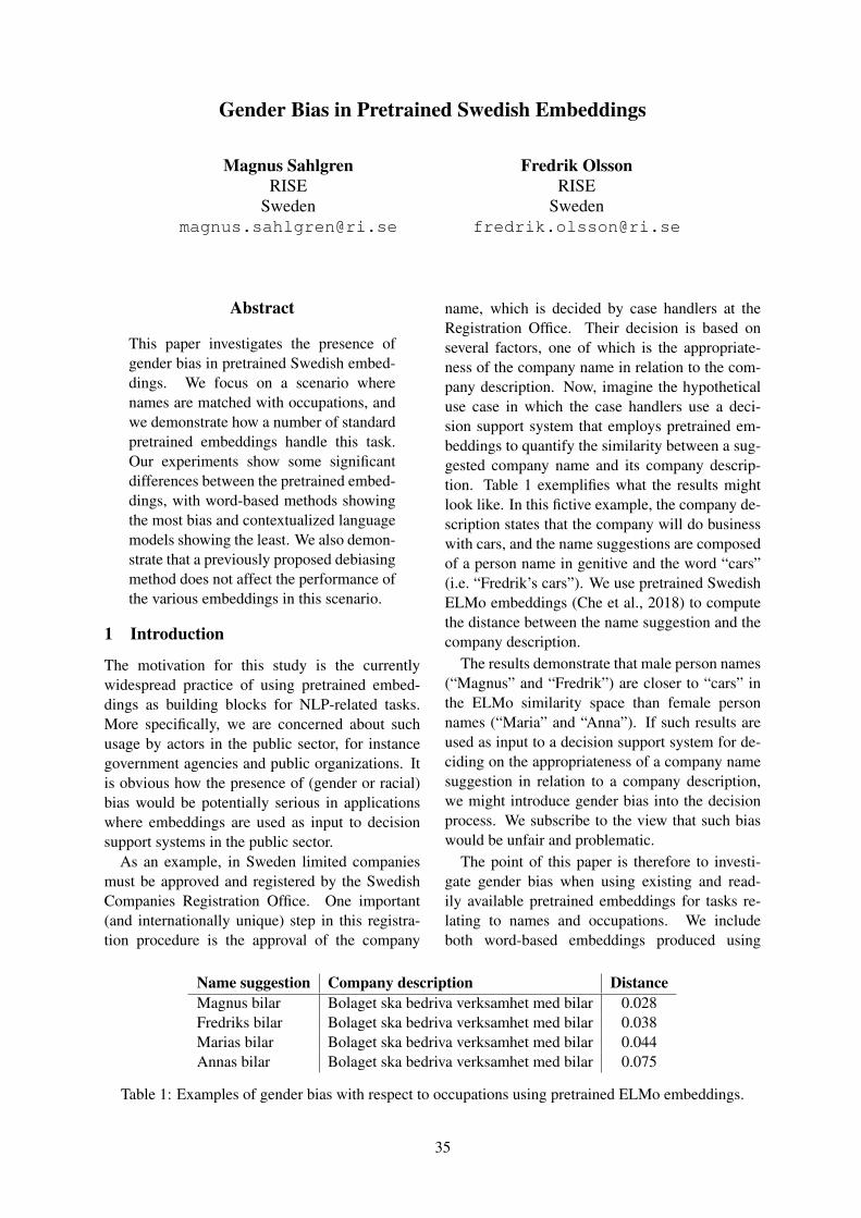
Gender Bias in Pretrained Swedish Embeddings

Magnus SahlgrenRISE

[email protected]

Fredrik OlssonRISE

[email protected]

Abstract

This paper investigates the presence ofgender bias in pretrained Swedish embed-dings. We focus on a scenario wherenames are matched with occupations, andwe demonstrate how a number of standardpretrained embeddings handle this task.Our experiments show some significantdifferences between the pretrained embed-dings, with word-based methods showingthe most bias and contextualized languagemodels showing the least. We also demon-strate that a previously proposed debiasingmethod does not affect the performance ofthe various embeddings in this scenario.

1 Introduction

The motivation for this study is the currentlywidespread practice of using pretrained embed-dings as building blocks for NLP-related tasks.More specifically, we are concerned about suchusage by actors in the public sector, for instancegovernment agencies and public organizations. Itis obvious how the presence of (gender or racial)bias would be potentially serious in applicationswhere embeddings are used as input to decisionsupport systems in the public sector.

As an example, in Sweden limited companiesmust be approved and registered by the SwedishCompanies Registration Office. One important(and internationally unique) step in this registra-tion procedure is the approval of the company

name, which is decided by case handlers at theRegistration Office. Their decision is based onseveral factors, one of which is the appropriate-ness of the company name in relation to the com-pany description. Now, imagine the hypotheticaluse case in which the case handlers use a deci-sion support system that employs pretrained em-beddings to quantify the similarity between a sug-gested company name and its company descrip-tion. Table 1 exemplifies what the results mightlook like. In this fictive example, the company de-scription states that the company will do businesswith cars, and the name suggestions are composedof a person name in genitive and the word “cars”(i.e. “Fredrik’s cars”). We use pretrained SwedishELMo embeddings (Che et al., 2018) to computethe distance between the name suggestion and thecompany description.

The results demonstrate that male person names(“Magnus” and “Fredrik”) are closer to “cars” inthe ELMo similarity space than female personnames (“Maria” and “Anna”). If such results areused as input to a decision support system for de-ciding on the appropriateness of a company namesuggestion in relation to a company description,we might introduce gender bias into the decisionprocess. We subscribe to the view that such biaswould be unfair and problematic.

The point of this paper is therefore to investi-gate gender bias when using existing and read-ily available pretrained embeddings for tasks re-lating to names and occupations. We includeboth word-based embeddings produced using

Name suggestion Company description DistanceMagnus bilar Bolaget ska bedriva verksamhet med bilar 0.028Fredriks bilar Bolaget ska bedriva verksamhet med bilar 0.038Marias bilar Bolaget ska bedriva verksamhet med bilar 0.044Annas bilar Bolaget ska bedriva verksamhet med bilar 0.075

Table 1: Examples of gender bias with respect to occupations using pretrained ELMo embeddings.

35

word2vec and fastText, as well as character-based (and WordPiece-based) contextualized em-beddings produced using ELMo and the multilin-gual BERT. The next section covers related work.We then discuss the various embeddings in Section3, before we then turn to some experimental evi-dence of bias in the embeddings, and we also showthat the previously proposed debiasing method isunable to handle gender bias in our scenario.

2 Related work

Research regarding bias and stereotypes ex-pressed in text and subsequently incorporated inlearned language models is currently a vivid field.Caliskan et al. (2017) show that learned embed-dings exhibit every linguistic bias documented inthe field of psychology (such as that flowers aremore pleasant than insects, musical instrumentsare preferred to weapons, and personal names areused to infer race). Garg et al. (2018) show thattemporal changes of the embeddings can be usedto quantify gender and ethnic stereotypes overtime, and Zhao et al. (2017) suggest that biasesmight in fact be amplified by embedding models.

Several researchers have also investigated waysto counter stereotypes and biases in learned lan-guage models. While the seminal work by Boluk-basi et al. (2016a, 2016b) concerns the identifi-cation and mitigation of gender bias in pretrainedword embeddings, Zhao et al. (2018) provide in-sights into the possibilities of learning embed-dings that are gender neutral. Bordia and Bowman(2019) outline a way of training a recurrent neuralnetwork for word-based language modelling suchthat the model is gender neutral. Park et al. (2018)discuss different ways of mitigating gender bias,in the context of abusive language detection, rang-ing from debiasing a model by using the hard de-biased word embeddings produced by Bolukbasiet al. (2016b), to manipulating the data prior totraining a model by swapping masculine and fem-inine mentions, and employing transfer learningfrom a model learned from less biased text.

Gonen and Goldberg (2019) contest the ap-proaches to debiasing word embeddings presentedby Bolukbasi et al. (2016b) and Zhao et al. (2018),arguing that while the bias is reduced when mea-sured according to its definition, i.e., dampeningthe impact of the general gender direction in thevector space, “the actual effect is mostly hiding thebias, not removing it”. Further, Gonen and Gold-

berg (2019) claim that a lot of the supposedly re-moved bias can be recovered due to the geometryof the vector representation of the gender neutral-ized words.

Our contribution consists of an investigation ofthe presence of gender bias in pretrained embed-dings for Swedish. We are less interested in bias asa theoretical construct, and more interested in theeffects of gender bias in actual applications wherepretrained embeddings are employed. Our experi-ments are therefore tightly tied to a real-world usecase where gender bias would have potentially se-rious ramifications. We also provide further evi-dence of the inability of the debiasing method pro-posed by Bolukbasi et al. (2016b) to handle thetype of bias we are concerned with.

3 Embeddings

We include four different standard embeddingsin these experiments: word2vec, fastText,ELMo and BERT. There are several pre-trainedmodels available in various web repositories. Weselect one representative instance per model, sum-marized in Table 2 (next page).

These models represent different types of em-beddings. word2vec (Mikolov et al., 2013)builds embeddings by training a shallow neuralnetwork to predict a set of context words based ona target word (this is the so-called skipgram archi-tecture; if we instead predict the target word basedon the context words the model is called contin-uous bag of words). The network learns two setsof vectors, one for the target terms (the embeddingvectors), and one for context terms. The objectiveof the network is to learn vectors such that their dotproduct correspond to the log likelihood of observ-ing word pairs in the training data. fastText(Bojanowski et al., 2017) uses the same neural net-work architecture, but incorporates character in-formation by using character n-grams instead ofwhole words in the prediction step.

It should be noted that most applications of theabove-mentioned vectors use only the embeddingsfor the target terms. In fact, many repositories withpretrained vectors do not even contain the contextembeddings. When the downstream task focuseson associative relations (which is the case in thepresent scenario with names and occupations), itwould be beneficial to be able to use both targetand context vectors, since using only one of thesewill result in more paradigmatic similarities.

36

Model Source Code Repository Training dataword2vec vectors.nlpl.eu CoNLL17 datafastText github.com/facebookresearch/fastText WikipediaELMo github.com/HIT-SCIR/ELMoForManyLangs CoNLL18 dataBERT github.com/google-research/bert Wikipedia

Table 2: The pre-trained embeddings and models included in these experiments were downloaded inApril 2019 from the following URLs. word2vec: vectors.nlpl.eu/repository/11/69.zip,fastText: dl.fbaipublicfiles.com/fasttext/vectors-crawl/cc.sv.300.bin.gz,ELMo: vectors.nlpl.eu/repository/11/173.zip, BERT: storage.googleapis.com/bert models/2018 11 23/multi cased L-12 H-768 A-12.zip

ELMo (Peters et al., 2018) is a deep character-based neural network that learns embeddings bypredicting the next token given an input sequence.The network architecture includes both convolu-tional and (bidirectional) LSTM layers, and pro-duces an embedding that that is sensitive to theparticular context of the input sequence. ELMo isthus different from word2vec and fastTextin the sense that it produces contextualized em-beddings, which has proven to be highly benefi-cial when using the embeddings as representationin downstream NLP tasks such as classification,entity recognition, and question answering.

BERT (Devlin et al., 2018) is similar to ELMo inthe sense that it uses a deep neural network archi-tecture and produces contextualized embeddings.However, it differs in the type of network used.BERT uses a (bidirectional) Transformer networkthat relies exclusively on attention, and the modelis trained using a masked language model task,similar to a cloze test. Contrary to ELMo, BERTis not character-based, but relies on WordPiece to-kenization of the input data. This has some poten-tially problematic effects when tokenizing propernames. As an example, the Swedish male name“Henrik” gets tokenized as [“hen”, “##rik”], with“rik” probably deriving from the Swedish word“rik” (eng. “rich”). It would have been desirable tonot use WordPiece tokenization for proper names.

In the following experiments, pre-trained ELMoand BERT are used to produce contextualized em-beddings both for individual words (such as namesor places) and for texts (such as company descrip-tions). Pre-trained word2vec and fastTextare used to look up individual words, and for textswe follow standard practice and average the vec-tors of the component words. Since proper namesin Swedish use uppercase for the initial letter, weretain the casing information for all models that

can handle such vocabulary, which in our case areall models except word2vec.

4 Data

In order to investigate whether our concerns aboutgender bias in pretrained Swedish embeddings arevalid, we collect lists of the 100 most commonSwedish female and male first names from Statis-tics Sweden (www.scb.se). We also collect listsof the most typical female and male occupationsfrom the same source, as shown in Tables 3 and 4(next page). These are the most common occupa-tions for women and men as compiled by StatisticsSweden, together with the percentage of womenand men in each occupation.

Since our interest in this paper is bias, we do notinclude occupations that have less than (or closeto) 50% occurrence of women or men (such casesare marked by ∗ in the tables). This leaves uswith 18 typically female occupations, and 15 typ-ically male occupations. Some of the remainingoccupations are very similar to each other, and wetherefore collapse them to one occupation (markedby numbers in the tables), resulting in 14 distinctfemale occupations and 14 distinct male occupa-tions. For each of these gendered occupations, wealso list a number of synonyms, collected fromwikipedia.se and framtid.se. Morpho-logical variants of each term are included.

5 Experiment 1: names and occupations

As a first experiment, we compute the similaritybetween the names and the occupations using thedifferent embeddings. We do this by computingthe similarity between each name and each occu-pation. Table 5 shows the percentage of femaleand male names that are on average more simi-lar to a female vs. male occupation. Numbers inparentheses are based on only the most similar oc-

37

Occupation (Swedish) Occupation (English) % women1Underskoterska Assistant nurse 92Barnskotare Nanny 89Grundskollarare Primary school teacher 75Forskollarare Preschool teacher 962Butikssaljare, fackhandel Shop sales 613Vardbitrade Care assistant 81Kontorsassistent och sekreterare Secretary 79Stadare Cleaner 75Personlig assistent Personal assistant 742Butikssaljare, dagligvaror Retail sales 673Vardare, boendestodjare Housing assistant 73Restaurang- och koksbitrade Restaurant assistant 65Planerare och utredare Planner 63Grundutbildad sjukskoterska Nurse 904Ekonomiassistent Accountant assistant 881Underskoterska, vard- och specialavdelning Nursing staff 91∗ Foretagssaljare Company sales 27∗ Kock och kallskanka Chef 524Redovisningsekonomer Accountant 79Socialsekreterare Social worker 86

Table 3: The 20 most common occupations for Swedish women in 2016 according to Statistics Sweden(www.scb.se).

Occupation (Swedish) Occupation (English) % menForetagssaljare Company sales 73Lager- och terminalpersonal Warehouse staff 79Mjukvaru- och systemutvecklare Software developer 80Lastbilsforare Truck driver 94Traarbetare, snickare Carpenter 99Maskinstallare och maskinoperatorer Machine operator 86∗ Butikssaljare, fackhandel Shop sales 39Fastighetsskotare Janitor 86Motorfordonsmekaniker och fordonsreparator Vehicle mechanic 97Installations- och serviceelektriker Electrician 98∗ Butikssaljare, dagligvaror Retail sales 33∗ Grundskollarare Primary school teacher 25Underhallsmekaniker och maskinreparator Maintenance mechanic 95∗ Planerare och utredare Planner 37∗ Restaurang- och koksbitrade Restaurant assistant 351Ingenjor och tekniker inom elektroteknik Electrical technician 871Civilingenjorsyrke inom elektroteknik Electrical engineer 84Verkstallande direktor CEO 84Buss- och sparvagnsforare Bus driver 86VVS-montor Plumber 99

Table 4: The 20 most common occupations for Swedish men in 2016 according to Statistics Sweden(www.scb.se).

38

Male names Male names Female names Female namesModel Male occupations Female occupations Male occupations Female occupations

word2vec 91 (86) 9 (14) 99 (98) 1 (2)fastText 4 (10) 96 (90) 100 (100) 0 (0)ELMo 96 (63) 4 (37) 49 (87) 51 (13)BERT 37 (54) 63 (46) 76 (55) 24 (45)

Table 5: Percentage of female and male names that are on average more similar to a female vs. maleoccupation. The similarities are calculated based on the original embeddings, before the application ofthe debiasing step described in Section 6. Numbers in parentheses only count the single most similaroccupation for each name.

cupation for each name. As an example, imaginewe only have two female and male occupations,and that the name “Anna” has the similarities 0.47and 0.78 to the female occupations, and the simi-larities 0.12 and 0.79 to the male occupations. Inthis example, “Anna” would be closer to the fe-male occupations when counting the average sim-ilarities (0.625 vs. 0.455), but closer to the maleoccupations when only considering the most sim-ilar examples (0.79 vs. 0.78).

There are several ways in which an embeddingcould show bias in this setting. The arguablymost detrimental effect would be if the embeddinggrouped male names with male occupations andfemale names with female occupations. Some-what less severe, but still problematic, would be ifthe embedding grouped all names with female ormale occupations. A completely unbiased modelwould not show any difference between the femaleand male names with respect to female and maleoccupations.

The numbers in Table 5 demonstrate some in-teresting differences between the different embed-dings. word2vec shows a clear tendency togroup both male and female names with male oc-cupations. fastText, on the other hand, showsa bias for female occupations for male names, andfor male occupations for female names. This is avery interesting difference, given that the only al-gorithmic difference between these models is theinclusion of character n-grams in the latter model.

The results for ELMo and BERT show some in-teresting differences too. ELMo groups the malenames with the male occupations, but is less bi-ased for the female names. When counting onlythe single most similar occupation, ELMo shows asimilar tendency as word2vec and groups bothmale and female names with male occupations.BERT, on the other hand, seems slightly more

balanced, with a tendency similar to fastTextwhen counting the average similarities. Whenonly counting the single most similar occupation,BERT is almost perfectly balanced between fe-male and male occupations.

6 Debiasing embeddings

We apply the debiasing methodology in (Boluk-basi et al., 2016b) to the pretrained embedddings.Debiasing a given vector space involves findingthe general direction in it that signifies genderusing a set of predefined definitional pairs, andthen removing the direction from all vectors ex-cept those corresponding to words that are natu-rally gender specific.

The definitional pairs are word pairs express-ing among themselves a natural distinction be-tween the genders, e.g., he – she, and mother –father. In our setting, there are 10 such pairs. Thegender specific words are words that also carry anatural gender dimension that should not be cor-rected during the debiasing phase of the vectorspace. We use the same methodology for growinga seed set of gender specific words into a largerset as described in (Bolukbasi et al., 2016b), andend up with 486 manually curated gender specificwords, including e.g., farfar (paternal grandfa-ther), tvillingsystrar (twin sisters), and matriark(matriarch).

The definitional pairs are used to find a genderdirection in the embedding space, which is doneby taking the difference vector of each of the def-initional pairs (i.e. w1 − w2), and then factorizingthe mean-centered difference vectors using PCA,retaining only the first principal component, whichwill act as the gender direction. The vector spaceis then hard debiased1 in the sense that the gen-

1The alternative is soft debiasing, in which one triesto strike a balance between keeping the pairwise distances

39



Table 6: Percentage of female and male names that are on average more similar to a female vs. maleoccupation. The similarities are calculated based on the debiased version of each model. Numbers inparentheses only count the single most similar occupation for each name.

der direction b is removed from the embeddings ofall non-gender specific words w using orthogonalprojection: w′ = w − b× w·b

b·b .The approach described by (Bolukbasi et al.,

2016b) includes an equalize step to make all gen-der neutral words equidistant to each of the mem-bers of a given equality set of word pairs. Theequality set is application specific, and since thecurrent investigation of Swedish language embed-dings does not naturally lend itself to include anequality set, the debiasing of the embeddings doesnot involve equalization in our case.

We apply the method described above to all pre-trained embeddings in Table 3, as well as to thetoken vectors generated by ELMo and BERT. Al-though it is not clear whether the proposed debias-ing method is applicable to embeddings producedby contextualized language models, we argue thatit is reasonable to treat the contextualized modelsas black boxes, and rely only on their output, giventhe proposed use case.

7 Experiment 2: names and occupations(revisited)

We repeat the experiment described in Section 5,but using the debiased embeddings. Table 6 sum-marizes the results. It is clear that the debiasingmethod does not have any impact on the results inthese experiments. The tendencies for the word-based embeddings word2vec and fastTextare more or less identical before and after debi-asing. The most striking differences between Ta-ble 5 and Table 6 are the results for ELMo andBERT, which become less balanced after apply-ing the debiasing method. ELMo actually showsa clearer gender distinction after debiasing, withmale names being more similar to male occupa-tions, and female names being more similar to fe-

among all vectors and decreasing the influence of the genderspecific direction.

male occupations. BERT also becomes less bal-anced after debiasing, grouping male names withfemale occupations, and female names with maleoccupations, when considering the average simi-larities. When counting only the most similar oc-cupation per name, BERT is still well balanced af-ter debiasing.

8 Experiment 3: company names andcompany descriptions

The experiments in the previous sections are ad-mittedly somewhat simplistic considering the sce-nario discussed in the Introduction: quantifyingthe similarity between a company name and acompany description. In particular the contex-tualized language models are not primarily de-signed for generating token embeddings, and it isneither clear what kind of quality we can expectfrom such un-contextualized token embeddings,nor whether they are susceptible to the debias-ing operation discussed in Section 6. In order toprovide a more realistic scenario, we also includeexperiments where we compute the similarity be-tween a set of actual company descriptions and aset of fictive company names generated from thelists of male and female names by adding the term“Aktiebolag” (in English limited company) aftereach name.2

The company descriptions are provided by theSwedish Companies Registration Office, and con-tain approximately 10 company descriptions foreach of the sectors construction work, vehicles andtransportation, information technologies, healthand health care, education, and economy. Basedon Tables 3 and 4, we consider the descriptionsfrom the first three sectors to be representative oftypically male occupations, and the descriptionsfrom the latter three sectors to be representative

2It is not uncommon for names of limited companies (inSweden) to feature a person name and the term “Aktiebolag”.

40



Table 7: Percentage of female and male names that are on average more similar to a female vs. maleoccupation. The similarities are calculated based on the original embeddings, using the names andoccupations in context. Numbers in parentheses only count the single most similar occupation for eachname.

of typically female occupations.We generate vectors for each of the descrip-

tions and for each fictive company name (i.e. amale or female name, followed by “Aktiebo-lag”). For the word-based models (word2vecand fastText), we take the average of the em-beddings of the words in the descriptions and thename. For the contextualized language models(ELMo and BERT), we generate vectors for eachdescription and each fictive name. In the case ofELMo we take the average over the three LSTMlayers, and for BERT we use the output embed-ding for the [CLS] token for each of the input se-quences.

The results are summarized in Table 7. It isclear that these results are significantly more bal-anced than the results using tokens only. Evenso, there are still some interesting differences be-tween the embeddings. Contrary to the results inTables 5 and 6, word2vec now shows a bias forfemale occupations, and fastText now shows abias for male occupations. ELMo and BERT seemmore balanced, with ELMo showing almost per-fectly balanced results, and BERT showing a slightbias for female occupations.

Even though the biases apparently are differentwhen considering tokens in comparison with con-sidering texts, there are still biases in all modelsin both cases. The only exception in our experi-ments is ELMo, when used for texts instead of to-kens. We hypothesize that the results for BERT arenegatively affected by artefacts of the WordPiecetokenization, as discussed in Section 3.

9 The effect of debiasing on embeddings

So far, we have shown that all Swedish pretrainedembeddings included in this study exhibit somedegree of gender bias when applied to a real-worldscenario. We now turn to investigate the effect

the hard debiasing operation has on the embed-ding spaces, using the intrinsic evaluation method-ology of Bolukbasi et al. (2016b). In this setting, anumber of analogy pairs are extracted for the orig-inal and debiased embeddings, and human evalu-ators are used to asses the number of appropriateand stereotypical pairs in the respective represen-tations. Bolukbasi et al. (2016b) used 10 crowd-workers to classify the analogy pairs as being ap-propriate or stereotypical. Their results indicatedthat 19% of the top 150 analogies generated usingthe original embedding model were deemed gen-der stereotypical, while the corresponding figurefor the hard debiased model was 6%.

We carry out a similar, but smaller, evalua-tion exercise using the analogy pairs generated bythe original Swedish word2vec and fastTextmodels, as well as their debiased counterparts.3

We use hon – han (she – he) as seed pair, and scoreall word pairs in the embeddings with respect tothe similarity of the word pair’s difference vectorto that of the the seed pair. The top 150 pairs aremanually categorized as either appropriate, gen-der stereotypical, or uncertain by the authors.

The results of the annotation are shown in Ta-ble 8 (next page). Due to the limited extent ofthe evaluation, we can only use these results forpainting the big picture. First of all, there is a rel-atively small overlap between the analogy pairsin the top 150 of the original models, and thetop lists of the debiased models: for word2vec,only 42 of the analogy pairs in the original list arealso in the list produced by the debiased model.The corresponding number for fastText is 31.This means that the debiasing operation changes

3It would have been preferable to also include ELMo andBERT in this experiment, but generating vectors for large vo-cabularies using these models takes a prohibitively long time,and it is neither clear whether the resulting token embeddingsmake sense, not whether the debiasing operation is applicableto the resulting embeddings.

41

Original Debiased Original DebiasedAnalogies quality word2vec word2vec fastText fastText

Appropriate 97 52 135 36Stereotypical 3 13 5 4

Uncertain 18 36 0 45

Table 8: The number of appropriate, stereotypical, and uncertain analogies in the top 150 pairs for theoriginal and debiased embeddings. The numbers are the analogy pairs for which the annotators agree onthe category.

the embedding space to a large extent. Second,there is a considerable amount of annotator uncer-tainty involved, either regarding the plausibility ofa given analogy pair, or regarding its appropriate-ness. This is manifested by an increase of the num-ber of uncertain analogy pairs that the annotatorsagree on between the original and debiased mod-els (both for word2vec and fastText). How-ever, the most interesting findings have to do withthe number of stereotypical analogy pairs. Thenumber of stereotypical analogy pairs output bythe Swedish models is small compared to the num-bers reported by Bolukbasi et al. (2016b). Further,the number of stereotypical pairs is larger in thedebiased word2vec model than in the originalmodel (we anticipated that it should be lower). Itthus seems as if the debiasing operation makes theword2vec embedding space more biased. ForfastText, the number of such pairs are slightlyfewer in the debiased model compared to its orig-inal counterpart.

10 Discussion

This paper has shown that pretrained Swedish em-beddings do exhibit gender bias to varying ex-tent, and that the debiasing operation suggestedby Bolukbasi et al. (2016a) does not have the de-sired effect, neither in the task of matching per-son names with occupations, nor in the case ofthe gender stereotypes being present among thetop ranked analogy pairs generated by the mod-els. Our experiments also indicate that word-basedembeddings are more susceptible to bias than con-textualized language models, and that there is anunexpectedly large difference in the biases shownby word2vec and fastText, something webelieve requires further study.

Although contextualized language models ap-pear to be more balanced with respect to genderbias in our experiments, there is still bias in thesemodels; in particular if they are used to generate

token embeddings, but also when they are used togenerate representations for texts – ELMo, whichproduces almost perfect scores in Table 7, maystill show bias in individual examples, such asthose in Table 1. We acknowledge the possibilitythat it may not be appropriate to use contextual-ized language models to generate embeddings forindividual tokens, but we also believe such usagesto occur in real-world applications, and we there-fore consider it relevant to include such examplesin these experiments.

The debiasing operation proposed by Bolukbasiet al. (2016a) does nothing to rectify the situa-tion in our setting. On the contrary, the debiasedmodels still show significant gender bias, and inthe case of ELMo and BERT, the bias actually be-comes more prevalent after debiasing. (However,we are aware that the debiasing operation mayneither be intended nor suitable for such repre-sentations.) Furthermore, our (admittedly small)analogy evaluation shows that debiasing actuallyintroduces more stereotypical word pairs in theword2vec model.

Why then does not debiasing the Swedish word-based embeddings produce results similar to thoseof Bolukbasi et al. (2016a)? One of the big differ-ences between the Swedish pretrained word2vecmodel and the one used by Bolukbasi et al. is thesize of the vocabulary. The Swedish model con-tains 3M+ word types, while Bolukbasi et al. con-strained their experiments to include only lower-cased words shorter than 20 characters, omittingdigits and words containing punctuation, from thetop 50,000 most frequent words in the model. Bydoing so, Bolukbasi et al. effectively removedmany person names from the model. A large por-tion of the word pairs in our analogy lists producedby the original model consist of person names(e.g., Anna – Jakob), which we consider to beappropriate, and their presence on the top 150list contribute to the comparatively low number of

42

stereotypical pairs. The debiasing operation of theword-based models remove many of the personsname pairs from the top list, giving way for po-tentially stereotypical pairs. Thus, the increase ofstereotypical pairs on the top list of analogy pairsgenerated by a debiased model is more likely to bedue to the debiasing operation effectively remov-ing many of the names from the top list, than themodel being more biased in the first place.

Since our experiments have focused on pre-trained embeddings readily available on the Inter-net, which have been trained on different types anddifferent sizes of data, we cannot speculate aboutthe extent to which a particular learning algorithmamplifies or distorts bias. We believe this is aninteresting direction for further research, and weaim to replicate this study using a variety of em-beddings trained on the same data.

ReferencesPiotr Bojanowski, Edouard Grave, Armand Joulin, and

Tomas Mikolov. 2017. Enriching word vectors withsubword information. Transactions of the Associa-tion for Computational Linguistics, 5.

Tolga Bolukbasi, Kai-Wei Chang, James Y. Zou,Venkatesh Saligrama, and Adam Kalai. 2016a. Manis to computer programmer as woman is to home-maker? debiasing word embeddings. arXiv preprintarXiv:1607.06520.

Tolga Bolukbasi, Kai-Wei Chang, James Y Zou,Venkatesh Saligrama, and Adam T Kalai. 2016b.Man is to computer programmer as woman is tohomemaker? debiasing word embeddings. In Ad-vances in neural information processing systems,pages 4349–4357.

Shikha Bordia and Samuel R. Bowman. 2019. Iden-tifying and reducing gender bias in word-level lan-guage models. In NAACL Student Research Work-shop.

Aylin Caliskan, Joanna J Bryson, and ArvindNarayanan. 2017. Semantics derived automaticallyfrom language corpora contain human-like biases.Science, 356(6334):183–186.

Wanxiang Che, Yijia Liu, Yuxuan Wang, Bo Zheng,and Ting Liu. 2018. Towards better UD parsing:Deep contextualized word embeddings, ensemble,and treebank concatenation. In Proceedings of theCoNLL 2018 Shared Task: Multilingual Parsingfrom Raw Text to Universal Dependencies, pages55–64, Brussels, Belgium. Association for Compu-tational Linguistics.

Jacob Devlin, Ming-Wei Chang, Kenton Lee, andKristina Toutanova. 2018. Bert: Pre-training of deep

bidirectional transformers for language understand-ing. arXiv preprint arXiv:1810.04805.

Nikhil Garg, Londa Schiebinger, Dan Jurafsky, andJames Zou. 2018. Word embeddings quantify100 years of gender and ethnic stereotypes. Pro-ceedings of the National Academy of Sciences,115(16):E3635–E3644.

Hila Gonen and Yoav Goldberg. 2019. Lipstick on apig: Debiasing methods cover up systematic gen-der biases in word embeddings but do not removethem. In Proceedings of the Annual Conference ofthe North American Chapter of the Association forComputational Linguistics (NAACL).

Tomas Mikolov, Ilya Sutskever, Kai Chen, Greg Cor-rado, and Jeffrey Dean. 2013. Distributed represen-tations of words and phrases and their composition-ality. In Proceedings of the 26th International Con-ference on Neural Information Processing Systems -Volume 2, NIPS’13, pages 3111–3119, USA. CurranAssociates Inc.

Ji Ho Park, Jamin Shin, and Pascale Fung. 2018. Re-ducing gender bias in abusive language detection.In Proceedings of the 2018 Conference on Empiri-cal Methods in Natural Language Processing, pages2799–2804.

Matthew Peters, Mark Neumann, Mohit Iyyer, MattGardner, Christopher Clark, Kenton Lee, and LukeZettlemoyer. 2018. Deep contextualized word rep-resentations. In Proceedings of the 2018 Confer-ence of the North American Chapter of the Associ-ation for Computational Linguistics: Human Lan-guage Technologies, Volume 1 (Long Papers), pages2227–2237.

Jieyu Zhao, Tianlu Wang, Mark Yatskar, Vicente Or-donez, and Kai-Wei Chang. 2017. Men also likeshopping: Reducing gender bias amplification us-ing corpus-level constraints. In Proceedings of the2017 Conference on Empirical Methods in NaturalLanguage Processing.

Jieyu Zhao, Yichao Zhou, Zeyu Li, Wei Wang, and Kai-Wei Chang. 2018. Learning gender-neutral wordembeddings. In Proceedings of the 2018 Confer-ence on Empirical Methods in Natural LanguageProcessing, pages 4847–4853, Brussels, Belgium.Association for Computational Linguistics.

43

A larger-scale evaluation resource of terms and their shift direction fordiachronic lexical semantics

Astrid van Aggelen♠ Antske Fokkens♦ Laura Hollink♠ Jacco van Ossenbruggen ♠♦♠ Centrum Wiskunde Informatica, Amsterdam, Netherlands

♦ Vrije Universiteit Amsterdam, [email protected], [email protected]

AbstractDetermining how words have changedtheir meaning is an important topic in Nat-ural Language Processing. However, eval-uations of methods to characterise suchchange have been limited to small, hand-crafted resources. We introduce an En-glish evaluation set which is larger, morevaried, and more realistic than seen todate, with terms derived from a historicalthesaurus. Moreover, the dataset is uniquein that it represents change as a shift fromthe term of interest to a WordNet synset.Using the synset lemmas, we can use thisset to evaluate (standard) methods that de-tect change between word pairs, as well as(adapted) methods that detect the changebetween a term and a sense overall. Weshow that performance on the new data setis much lower than earlier reported find-ings, setting a new standard.

1 Introduction

Determining how words have changed their mean-ing is an important topic in Natural LanguageProcessing (Tang, 2018; Kutuzov et al., 2018;Tahmasebi et al., 2018). Using large diachroniccorpora, computational linguistics has providedmethods that can detect or qualitatively explain se-mantic change automatically. In particular, sev-eral approaches have been introduced that use dis-tributional semantic models representing differenttime periods in diachronic corpora (Gulordava andBaroni, 2011; Mitra et al., 2014; Kulkarni et al.,2015, e.g.).

Researchers have illustrated through com-pelling examples that these methods can detect se-mantic shift, like cell obtaining the meaning of‘phone’ and gay shifting from ‘cheerful’ to ‘ho-mosexual’ (Mitra et al., 2014, e.g.) and have re-ported high accuracy on small evaluation sets of

selected examples. Hamilton et al. (2016) evenreport 100% accuracy in detecting known changeon 28 word pairs. As a result, these approacheshave been enthusiastically adopted (Wohlgenanntet al., 2019; Orlikowski et al., 2018; Kutuzov et al.,2016; Martinez-Ortiz et al., 2016, e.g.). However,it has been called into question how reliable thesemethods really are (Hellrich and Hahn, 2016a; Du-bossarsky et al., 2017).

These developments show that there is both awide interest in using distributional semantic mod-els to assess semantic change and an urgent needfor better insight into the possibilities and limita-tions of these methods. It is therefore unsurpris-ing that three recent survey papers on the topic alllist the lack of proper evaluation and, in particu-lar, the absence of large-scale evaluation sets, as akey challenge for this line of research (Tang, 2018;Kutuzov et al., 2018; Tahmasebi et al., 2018).

In this paper, we automatically derive HiT, thelargest English evaluation set to date, from a his-torical thesaurus. HiT consists of terms linked toWordNet (Fellbaum, 2012) entries that representsenses they gained or lost. We introduce senseshift assessment as a task, enabled by this dataset,that identifies whether a sense of a term of interestwas coming in our out of use, based on its changedrelationship with all lemmas of the sense. This isa variation of a task introduced by Hamilton et al.(2016) that assesses the relationship of the termsof interest with individual other terms. The senseshift assessment instead uncovers the conceptualchange that explains multiple observed trends be-tween word pairs. Cross-checking and summaris-ing individual observations also means drawingmore informed conclusions. Furthermore, the useof WordNet sense representations allows for thedataset entries to be automatically derived ratherthan manually (expert) collected, hence limitingthe effect of bias. We use HiT to answer two mainresearch questions. First, how well can current

44

methods detect sense shift on a larger and morevaried evaluation set? Second, how, by taking afull synset as a representation of meaning, does thetask of detecting sense shift compare to studyingword pairs in isolation? The main contributions ofthis paper are as follows. First, the new evalua-tion set, consisting of 756 target words and 3624word pairs. Second, we show that current meth-ods perform quite poorly on this more challengingset, thus confirming that this set introduces a newbenchmark. We also identify lexical factors thatcontribute to these differences.

2 Related Work

This section provides an overview of previouswork on detecting lexical semantic change throughdistributional semantic models.

Distributional models of meaning are motivatedby the hypothesis that words with similar mean-ings will occur in similar contexts (Harris, 1954;Firth, 1957). Tahmasebi et al. (2011) and Mitraet al. (2014) induce clusters of terms that tem-porally co-occur in particular syntactic patterns,and (qualitatively or quantitatively) trace their de-velopment. Their approach forms a bridge fromprevious document-based approaches (Blei andLafferty, 2006; Wang and McCallum, 2006, e.g.)to the window-based models that are currentlywidely used.

Gulordava and Baroni (2011) and Jatowt andDuh (2014) were among the first to use trends insimilarity between distributional representations.The former detect change within single terms bytracing their self-similarity. The latter, like wedo, interpret the change of a term by contrast-ing it with other terms. In recent work, the mostcommon type of distributional models used to as-sess semantic shift are known as prediction models(Kim et al., 2014; Kulkarni et al., 2015; Hamiltonet al., 2016, e.g). In this paper, we use embeddingsthat gave the best results in Hamilton et al. (2016)and are created through the skip-gram method in-cluded in word2vec (Mikolov et al., 2013).

Until recently, semantic shifts were determinedby comparing the distributional nearest neigh-bours of a term in one time period to its neighboursin another (see e.g. Tahmasebi et al. (2011)). How-ever, such an inspection is difficult to carry out atscale, is not suited for disappearing senses - dis-tant neighbours are hard to assess - and is prone tobias, especially when the aim is to confirm hypoth-

esized trends. Hamilton et al. (2016) use a prede-termined list of terms to which the target term gotmore and less related over time. This variation al-leviates the problem of bias and introduces ‘moredistant neighbours’ into the analysis, but with just28 term pairs it is still very small-scale.

Basile and McGillivray (2018) are, to ourknowledge, the first to exploit a large historicaldictionary as an evaluation source. The aim oftheir work is to detect changed terms and theirchange point, based on dips in the self-similarities,with the Oxford English Dictionary as the goldstandard. To verify whether the observed changepoint corresponds to a new dictionary sense, thetime-specific nearest neighbours of the term arecontrasted with the dictionary definition. Thiswork could have provided the evaluation set forthe task addressed in this paper. However, as faras we know, the authors have not enriched the datawith said nearest neighbours nor made them avail-able. Hence, the current work is still the first toprovide a large-scale evaluation set based on a dic-tionary.

3 A large-scale sense shift assessment set

This section describes a new evaluation set thatlinks terms of interest (target terms) to rich synsetrepresentations of their old and new senses. Thismeans that in an experimental setting (such as thatin Section 5), the target term can be contrasted to apredetermined, varied set of terms. We also adapttwo existing evaluation sets, HistWords (Hamiltonet al., 2016) and the Word Sense Change Testset1

(Tahmasebi and Risse, 2017), into datasets of thesame format.

3.1 Deriving a sense shift assessment set

The new dataset, which we call HiT, is derivedfrom The Historical Thesaurus of the Univer-sity of Glasgow (Kay et al., 2019). This thesauruslists (nearly all) English terms organised in a con-ceptual hierarchy of senses. It also documents thetime period in which a term was attested and as-sumed to be active in the given sense. For instance,one entry says that the verb bray was used in thesense of ‘Grind/pound’ (in turn a subconcept of‘Create/make/bring about’) for the period 1382 till1850. The thesaurus does not indicate how anylisted sense of a word relates to previous, concur-rent or future ones. Hence, it is unclear whether

1http://doi.org/10.5281/zenodo.495572

45

the term underwent a process of semantic narrow-ing or broadening, or whether it lost or gained asense altogether. The change that is consideredhere is a broad notion of rising or declining senses.

For HiT we use all terms in senses that came upbetween 1900 and 1959 and all terms in senses thatdisappeared - which were less numerous - between1850 and 1959. To enrich the thesaurus terms, weidentify their WordNet synsets and check if eachof these expresses the intended meaning. Thischeck is based on the overlap between the the-saurus definition and the synset terms. If any termfrom the synset (excluding the target term itself)overlaps with any of the terms from the thesaurusdefinition (in the example above, the terms are{create, make, bring about, grind, pound}), weassume that the synset in question provides the in-tended sense. The verb bray appears in WordNetunder two polylexical synsets: {bray, hee-haw},and {bray, grind, mash, crunch, comminute}. Dueto the overlapping term grind, the thesaurus en-try is matched with the latter, meaning ‘reduce tosmall pieces or particles by pounding or abrad-ing’, but not with the former (‘laugh loudly andharshly’).

Newly emerging senses from the thesaurus pro-vide gold standard instances that are supposed toattract the vector of the target term. Disappear-ing senses, on the other hand - such as ‘grind’ forbray after 1850 - are gold standard instances fromwhich the target term should move away. Table 1shows how the bray example translates to a HiTentry of a vanishing sense with the WordNet syn-onyms used as reference terms.

Only entries with at least one identified Word-Net synset are included. This results in a datasetof 756 target terms exhibiting 979 sense shifts.

target POS sense (WN synset) shift onsetterm b reference termbray v. grind.v.05 -1 1850

b grind, mash, crunch, comminute

Table 1: Example excerpt from an entry of HiT. Shift label-1 means a move away from the given meaning.

Validation To establish the accuracy of theWordNet matching method, two raters indepen-dently annotated a subset of 191 entries. Theagreement between the raters (i.e. the proportionof agreement above chance level) is assessed us-ing Cohen κ for two raters (Cohen, 1960). Also,we assessed how well the raters’ judgement corre-sponded to the output of the automated WordNet

matching, i.e., the supposed gold standard.Rater 1 verified whether the algorithm had se-

lected the correct synset or not. To counteract aneffect of bias from the gold standard, rater 2 didnot work with the gold standard, rather indicatingfor any given WordNet synset whether it repre-sented the given definition. These findings werethen translated to a judgement of the algorithmoutput in line with rater 1. The annotators agreedon the evaluation by 97.9 per cent; by Cohen’schance-normalised norm (κ = 0.789, z = 11,p < 0.001), this is generally thought of as ‘sub-stantial’ agreement. Except for 10 (rater 1) and9 (rater 2) instances out of 191, the raters’ judge-ments corresponded to that of the algorithm, an er-ror rate of approximately 5 per cent. We considerthis high enough to take the outcome of the synsetlinking method as the gold standard.

3.2 Transforming existing datasets

The thesaurus-derived dataset, HiT, qualitativelydiffers from existing evaluation sets in its auto-mated construction and in its representation ofsenses by a synset rather than selected terms.In order to compare this set to previously useddatasets, we adapt two standard evaluation setssemi-automatically to link the target words theycontain to synsets representing the given old ornew senses.

HistWords (Hamilton et al., 2016) (HW) con-tains 28 word pairs that saw their similarity in-crease or decrease over time, based on 9 targetterms. HistWords states the onset of the change -no end date - and the gold standard shift direction.For instance, since 1800, awful has moved towardsmess and disgusting and away from impressive.

The Word Sense Change Testset (WSCT)(Tahmasebi and Risse, 2017) lists terms that ac-quired a new sense and unchanged control words.It gives the type of change the term underwent (nochange, new, broader, or narrower sense), a shortexplanation of the change and the onset date of thechange. For instance, memory acquires a new re-lated sense ‘digital memory’ in 1960 whilst keep-ing its existing sense ‘human memory’.

From HW to HW+ and from WSCT toWSCT+. Every entry from WSCT and HW istreated as a separate change event, with an on-set date and a description; some target terms havemore than one change event. For each such event,the affected sense(s) are selected out of all can-

46

didate senses, i.e. all WordNet synsets that cor-respond to the target lemma (in the correct partof speech). This synset selection process hap-pened manually, by comparing the lexical infor-mation in WordNet against the change descriptionin the source data. More details about the anno-tation process are given below. The outcomes de-termine the change type listed for the combinationof target term and synset in the enriched datasetsWSCT+ and HW+. The target term is thought tomove towards any synset (and towards all terms ofthe synset) that captures an increasingly commonsense, and away from any synset that expresses anincreasingly uncommon sense. For any synset thatdoes not capture any described change, its relationto the target term is described as unchanged or un-known. See Table 2 for an example.

Annotation process and validation. The se-lection was carried out by the first author; thiswas then evaluated by two co-authors for HW+and one co-author for WSCT+. In the case ofthree raters, we used Fleiss’ extension of Cohen’smethod (Fleiss, 1971). The raters judged the shiftdirection of the target term with respect to allcandidate concepts (synsets): towards (+1), awayfrom (-1) one another, or no change (0). The eval-uation set of word-sense combinations was largerthan the final dataset (Table 3), as it includedsynsets with just the target term. The raters weregiven the following data: the change descriptionand the time of change, given in HW or WSCT; the(given or inferred) part of speech; the candidateWordNet concept that connects the two terms; andcorresponding WordNet data such as the definitionand the set of terms in the synset. For WSCT+(N=129 target-sense pairs), the two raters agreedby 88.4 per cent, which, chance-normalised (Co-hen’s κ = 0.63, z = 7.26, p < 0.01) is thoughtto be ‘substantial’. The raters then agreed on thefinal set of gold standard labels. On HW+ (N=70target-sense pairs), the three raters agreed almostperfectly (Fleiss’ κ = 0.83, z = 16, p < 0.01),and the ratings by the first author were taken asthe gold standard.

Resulting datasets The evaluation sets all pro-vide two types of pairings: target terms pairedwith reference terms and target terms with synsets.The gold standard for the individual word pairs -target word and synonym - corresponds to the goldstandard for the whole synset. After the inter-raterevaluation, synsets with just one term (the target

target POS sense (WN synset) t shiftterm b reference termmemory n. memory.n.03 1960 0

b retention, retentiveness, retentivitymemory n. memory.n.04 1960 1

b computer memory, storage, compu-ter storage, store, memory board

Table 2: Excerpts from two entries of WSCT+. Shift label 0means we have no evidence the word changed with respect tothe given sense. Label 1 means a shift towards the indicatedmeaning (and its associated terms).

term) were omitted, as the experiment requires ref-erence terms. Table 3 provides an overview ofthe resulting evaluation sets next to HistWords asa baseline. HiT does not show any overlap withthe other datasets except for a single target termlemma (verb call) in common with HW+, howeverwith the described change in a different meaning.

dataset HW HW+ WSCT+ HiTdataset type existing adapted adapted newtarget words (TWs) 9 9 23 756TW+term 28 117 213 3624converging 18 41 56 1173diverging 10 24 0 2451unchanged/-known 0 52 157 0TW+sense n.a. 42 93 979converging n.a. 10 23 282diverging n.a. 10 0 697unchanged/-known n.a. 22 70 0

Table 3: Contents of the evaluation sets, which come in twovariants: target terms paired with other terms and paired withWordNet senses (synsets). This allows the datasets to be usedfor the two types of evaluation used here.

4 Experiment

Two tasks are addressed in the experiment. Wordshift assessment (WordShiftAssess) (Hamiltonet al., 2016) is summarised as follows: givena target term, a reference term, and a time pe-riod, did the two terms become closer in mean-ing (gold standard label 1) or did their meaningsmove apart (label -1)? Sense shift assessment(SenseShiftAssess) goes as follows: given a tar-get term, a WordNet synset, and a time period, didthe target term in the given period move towardsor away from the given sense? To be comparableto previous findings, we evaluate the datasets onboth tasks. This section outlines the methods andthe experimental setup.

4.1 Change assessment for word-word pairs

Our method of determining shift direction wasproposed by Hamilton et al. (2016). It depends onthe availability of distributional representations forthe target term and reference terms, corresponding

47

to the synset lemmas, at regular intervals betweenthe start and the end of the period of interest. Thesuccessive cosine similarities of the embeddingsof the target and reference term are (Spearman)correlated with the time index (e.g. 1800, 1810,.., 1990). If the correlation is positive, the targetterm is taken to have moved towards the referenceterm; if it is negative, away from it. Given thebinary classification setting, the statistical signifi-cance of the correlation factor has no clear inter-pretation. However, we include it to comply withearlier reported findings and for readers to judgethe potential of the method for a three-way classi-fication with a null category.

4.2 Change assessment for word-sense pairsTo address SenseShiftAssess, we suggest twobroad approaches. The first starts from the methodoutlined in Section 4.1. That is, for any target-sense pair, we start from the given target wordpaired with all lemmas of the synset, and thetrend of the cosine similarities (Spearman ρ andp) for each of these word pairs. Then, we eithertake the most-observed sign of ρ as the outcome(majority vote), or we promote one word pair toexemplify the sense shift as a whole. Assumingthat an observed strong trend is likely to be cor-rect, argmax(corr) takes the sign of the highestabsolute ρ value of all word pairs in the synset asthe synset assessment. argmin(p(corr)) does thesame for the observation the correlation coefficientof which has the lowest p value.

The second approach we suggest, average vec.,operates on a lower level, as it aggregates the dis-tributional representations of the synset lemmasinto an average vector, for every time slice sep-arately. The target term and the averaged repre-sentation are then treated like a word pair (Section4.1).

4.3 Experimental setupWe apply word shift assessment on HW, HW+,WSCT+, and HiT. The reference terms of HW+,WSCT+ and HiT come from WordNet; those inHW are readily taken from the source. Figure 1 il-lustrates how the term awful from HW+ compareswith its individual WordNet synonyms over time.

Sense shift assessment is applied to WSCT+,HW+ and HiT, i.e. all sets that could be enrichedwith sense information. To continue with the ex-ample in Figure 1, sense shift assessment trans-lates the word-based observations into a single as-

Figure 1: WordShiftAssess with WordNet-based referenceterms: target term awful is individually contrasted with allterms from synset atrocious.s.02: abominable, atro-cious dreadful, painful, etc. The fitted lines illustrate the ob-served trend in cosine similarities, such as the growing simi-larity between awful and terrible.

sessment of the changed relation of awful with re-spect to the whole synset.

Distributional vectors. We use word embed-dings provided by Hamilton et al. (2016) of size300, trained through skip-gram with negative sam-pling (SGNS) for every decade separately on threecorpora: the Corpus of Historical American En-glish (Davies, 2015) (COHA), the complete En-glish Google N-Gram corpus (Michel et al., 2011),and the English Fiction corpus, a subset of theGoogle N-Gram corpus. The embeddings are not(part of speech) disambiguated, and can stand forseveral lemmas at once. We employ the embed-dings for every decade from the attested onset ofchange up to and including the last available em-bedding, trained on the 1990s subcorpus.

Handling of missing and infrequent data.Some terms appear infrequently in some slices ofthe corpus. The code that accompanies Hamiltonet al. (2016) deals with these cases by paddingthe cosine time series with a zero for the dimen-sion (i.e. time slice) in which either or both ofthe terms was insufficiently frequent (under 500times, except for COHA). However, this biases theoutcome, since zero is the smallest cosine sim-ilarity value. Given that low word frequenciesare more common in the corpora of the first fewdecades, this setting makes it more likely to find

48

cosine time series ρt1 ... t10 t11 t12 t13 t14 t150 ... 0 0.25 0.29 0.29 0.20 0.18 0.77NA ... NA 0.25 0.29 0.29 0.20 0.18 -0.7

Table 4: Similarity values based on infrequent data mustnot be padded with zero as this biases the correlation valuetowards a positive value. In the word pair delimit-define,padding the values for decades t1 (in fact, 1850) through tot11 (1940) with zeros would lead to a conclusion oppositeto the ground truth stating that these terms move away fromeach other; hence these observations are treated as missingdata (NA) instead.

a rising trend in cosine similarities. As this is anunwanted effect, we treated cosine values basedon low-frequency numbers as missing values. Ta-ble 4 illustrates the difference between the caveatexplained here and the approach taken. A furthercount filter ensures that all results (correlations)are based on at least five cosine values.

5 Results

Table 5 shows the proportion of word pair observa-tions (WordShiftAssess) displaying the expectedtrend in cosine similarities for every dataset andtraining corpus. The significance reported is theproportion of correct findings (i.e. with an upperlimit of 100%) with a Spearman ρ significant onthe 0.05 level. Whether the correlation coefficientis significant depends on its magnitude as well asthe number of cosine values considered. The latterin turn depends on the change onset - the longerthe time series, the more observations - minus ob-servations that were based on too little data andwere left out (see Section 4.3). N expresses howmany of the word pair entries from the datasets(Table 3) which displayed a real shift (unchangedwords were not used) resulted in a cosine time se-ries of at least five observations (see Section 4.3).This depends in part on the corpus, some of whichhave much greater coverage than other ones, par-ticularly the complete English corpus, eng-all. Forinstance, the results for HiT for eng-all are basedon 1461 word pairs as opposed to a mere 746 forCOHA and 772 for English fiction, out of a datasettotal of 3624 shifted terms. Moreover, eng-all re-sulted in more statistically significant correct out-comes than COHA and eng-fic. We therefore fo-cus on the results based on eng-all in particular.

HiT appears more challenging than WSCT+and HW+. On eng-all, just under 60 per cent ofall entries were correctly assessed, as opposed toaround 70 per cent for WSCT+ and 80 per cent

Figure 2: Proportions of correct word pairs (i.e. display-ing the expected similarity trend) within synsets for HiT (oneng-all). In just over half of the cases, the synset containedmore correct than incorrect observations (bottom half of thepie chart).

for HW+. The significance levels show a similarpattern, hence even the word pairs that showed thepredicted trend did so less clearly for HiT than forthe other datasets. The outcomes on COHA andeng-fic confirm the pattern for eng-all: HiT figuresconsistently lag behind WSCT+ and even furtherbehind HW+. While eng-all and eng-fic give simi-lar levels of accuracy, on COHA, the outcomes forHiT are below chance level.

HiT differs from WSCT+ and HW+ in thatthe target terms were not selected for the task athand. Unsurprisingly, the automatically selecteddictionary terms offer a more challenging evalua-tion set than the purposely selected terms in HW+and WSCT+. The difference observed betweenHW and HW+ reveals a similar trend concerninghand-picked reference terms compared to (semi)-automatically selected ones: the performance onHW+ is about 20 per cent lower than for HW. Insum, the selection of term pairs has great impact.

Table 6 shows the proportion of target-sense entries that were correctly assessed(SenseShiftAssess), based on several possibleaggregations of word pair level findings. Looking,firstly, at the different methods, argmin(p(corr))performed best. Hence, the word pair within asynset that shows the most statistically robustchange is the best indicator of the conceptualchange of the target term. For HiT this resulted in61.3% correct on eng-all and up to 64.0 % on eng-fic. The added performance over argmax(corr),whilst marginal (e.g. for HiT, 61.1 % on eng-alland 61.9% on eng-fic), suggests that balancing thecorrelation factor with the number of observationsleads to better judgements than looking at the

49

WordShiftAssess eng-all coha eng-ficHiT wsct+ HW+ HW HiT wsct+ HW+ HW HiT wsct+ HW+ HW

correct (%) 58.0 69.2 79.5 100.0 45.6 54.5 63.6 85.7 59.5 62.5 66.7 88.2sig (%) 38.4 66.7 60.0 88.9 29.1 33.3 19.0 66.7 24.0 40.0 30.0 46.7N 1461 13 44 27 746 11 33 21 772 8 30 17

Table 5: Results of determining the shift direction of a target word with respect to a reference word (WordShiftAssess).

SenseShiftAssesscorpus eng-all coha eng-ficdataset HiT wsct+ HW+ HW HiT wsct+ HW+ HW HiT wsct+ HW+ HWaverage vec. 57.8 100.0 88.9 - 44.1 50.0 57.1 - 58.9 100.0 66.7 -argmax(corr) 61.1 100.0 84.6 - 46.4 80.0 53.8 - 61.9 100.0 66.7 -majority vote 50.7 100.0 76.9 - 36.0 80.0 53.8 - 49.7 75.0 66.7 -argmin(p(corr)) 61.3 100.0 84.6 - 46.8 80.0 53.8 - 64.0 75.0 66.7 -N average vec. 374 2 9 - 204 2 7 - 214 1 6N other methods 450 5 13 - 278 5 13 - 286 4 12 -

Table 6: Results of determining the shift direction of a target word with respect to a reference word (SenseShiftAssess).

magnitude of the correlation alone. Averagingthe vectors of all reference terms (average vec.)was less reliable an aggregation overall thanpromoting one word pair to represent the synset.However, it still did better than the majority vote,which required more than half of the word pairsin a synset to display the expected shift pattern.For HiT, this did not surpass chance level onany of the corpora. Hence, within a synset, falseobservations can be as numerous as or outweightrue ones, and heuristics are needed to find thesignal in the noise.

SenseShiftAssess was expected to suffer lessfrom noisy results that occur on the word level(WordShiftAssess). However, the improvementobserved over the word pair results was marginal.For instance, for HiT on eng-all, the synset-levelapproach was correct in 61 per cent of cases atbest, as opposed to 58 per cent on the word pairlevel. HW+ and WSCT+ did benefit more fromthe synset aggregation, but the small sample sizemakes it hard to draw conclusions from this. Fig-ure 2 shows how much we can rely on the termswithin a synset to display the anticipated changein relation to the target term (for HiT and eng-all). The vast majority of synsets - all except 18per cent - contain at least one word pair that dis-plays the true shift. This means that SenseShift-Assess on HiT is feasible, at least in theory, andthe maximum accuracy attainable on eng-all is 82per cent. A third of all synsets (34%) have allword pairs displaying the predicted shift; hencethe lower limit is 34 per cent. There were moresynsets with mostly correct than mostly false ex-amples, and more synsets with just correct (33 per

cent) than just false (17 per cent) ones. Based onthe slightly higher odds of picking a correct thanan incorrect example, our selection methods areperhaps not informed by the most determining fac-tors. To know how we can find the signal in noisyword pair patterns, we must first understand whatcauses noise. This question is addressed next.

6 Follow-up analysis

We examine several lexical and corpus factors thatmay play a role in the outcomes. For every termin a word pair, we look at its polysemy, its fre-quency in the training corpus, and its typicality asa representation of the underlying concept. Ta-ble 7 breaks down the WordShiftEval results bythe combined lexical properties of target and ref-erence term. For every entry type we distinguish(e.g. a low-polysemous target term paired with ahigh-polysemous reference term), we examine theproportion of the result set it accounts for, and theobserved tendency for such word pairs to displaythe expected shift pattern. Due to its fewer out-comes, WSCT+ was left out of this analysis.

When a term is ambiguous, i.e. when it tends tooccur in various semantic and syntactic contexts,its distributional representation might be less suit-able to reflect any single one of these. Polysemyis difficult to define (Ravin and Leacock, 2000).Here, we define the polysemy of a term by its to-tal number of synsets divided by the number ofdifferent parts of speech it can occur in. We testeddifferent thresholds for considering a term polyse-mous, from two to six synsets per part of speech,which all revealed similar results. The results wereport are based on a minimum of three, four and

50

entry type (N.B.: ‘low’ can mean more or less challenging, depending on the property)low-low low-high high-low high-high

property threshold corpus accuracy proportion accuracy proportion accuracy proportion accuracy proportionpolysemy 3* HiT 63.8 17.8 60.9 18.2 62.8 18.4 52.7 45.6

3* HW 100 37 100 29.6 100 18.5 100 14.83* HW+ 70.6 38.6 71.4 31.8 100 20.5 100 9.1

polysemy 4* HiT 66.4 32.2 58.1 21.1 59.6 17.5 47.9 29.34* HW 100 51.9 100 25.9 100 11.1 100 11.14* HW+ 82.1 63.6 60 22.7 100 9.1 100 4.5

polysemy 5* HiT 64.8 45.3 58.7 19.7 53 14.9 45.9 20.15* HW 100 70.4 100 14.8 100 14.8 - 05* HW+ 81.8 75 40 11.4 100 11.4 100 2.3

frequency 100k HiT 65.7 33.9 61.4 17.2 58.6 17.1 47.6 31.8100k HW 100 18.5 100 11.1 100 22.2 100 48.1100k HW+ 80 34.1 66.7 13.6 81.2 36.4 85.7 15.9

frequency 10k HiT 65.1 7.5 74.5 14.8 63.5 12.9 52.4 64.810k HW - 0 - 0 100 11.1 100 88.910k HW+ - 0 - 0 76.9 29.5 80.6 70.5

frequency 5k HiT 52.5 2.7 74.3 9.9 68.8 9.7 54.8 77.85k HW - 0 - 0 100 7.4 100 92.65k HW - 0 - 0 66.7 13.6 81.6 86.4

centrality 1* HiT 56.4 75.8 62.4 10.2 66.9 9.7 56.5 4.21* HW - - - - - - - -1* HW+ 76 56.8 75 27.3 100 15.9 - 02* HiT 54.5 54.3 60.2 18.4 63.5 16.5 63.9 10.82* HW - - - - - - - -2* HW+ 66.7 34.1 81.8 25 100 9.1 85.7 31.8

*high polysemy means the term has min. [THRESHOLD] total synsets / total parts of speech*high centrality means the term has the intended concept as synset number [THRESHOLD] at most

Table 7: WordShiftEval results broken down by the frequency, centrality, and polysemy of the terms that make up the entries.

five senses per part of speech. Depending on thethreshold T , the most-observed type of word pairamongst the HiT results is that of two polysemousterms (45.6 % of the result set, T = 3), two rel-atively unpolysemous terms (45.3%, T = 5), orequal proportions of the two (T = 4).

The proportion of correctly classified term pairsis unequally distributed across polysemy classes,in particular for HiT. Word pairs with two non-polysemous (i.e. relatively unambiguous) termsare consistently more likely to see their shift di-rection assessed correctly (64-66% correct, de-pending on the polysemy threshold) than wordpairs with two polysemous terms (46-53% cor-rect), which have an almost equal chance of get-ting correctly or incorrectly classified. Entrieswith a single polysemous term consistently fallsomewhere between these two trends. Comparedto HiT, HW and HW+ have notably smaller pro-portions of polysemous term pairs, with as little as9.1% polysemous pairs (under T = 3) for HW and14.8% for HW+, as opposed to 45.6% for HiT.

A low corpus frequency was expected to neg-atively impact the results. With a small numberof occurrences used to collect (train) the vectorrepresentations, these risk being less stable andreliable. We take the frequencies underlying the

1990s eng-all vector corpus as a proxy for theoverall frequencies of the terms and use severalfrequency cut-offs (5k, 10k and 100k). HiT clearlydisplays more lower-frequent terms than HW andHW+. For instance, under a cutoff value of 100k,HiT has about the same proportion of low-frequent(33.9%) and high-frequent pairs (31.8%), whileHW has clearly more high-frequent (48.1%) thanlow-frequent pairs (18.5%). Also, HiT is the onlyset that contains entries made up of terms with fre-quencies under 5k and 10k.

Looking at the results on HiT when both termswere very sparse (under 5k) the assessment is justad random (52.5%), but with a higher threshold of10k the sparse pairs were more likely to be cor-rectly classified (65.1%). At the same time, high-frequent term pairs with target and reference termboth over 10k instances showed to be difficult toclassify (52.4%). Taken together, these findingssuggest that while higher-frequency terms are notalways more suitable, a minimum number of in-stances is indispensable for reliable results.

By centrality we mean how good a contem-porary example of the intended concept a termis. To this end we look at the synset that con-nects target and reference term. If the (targetor reference) term has this sense listed among

51

its top senses in WordNet, we assume it is ex-emplary. For the target term this is also an as-sessment of whether the change took place in(what is now) its primary, second, or in a moredistant sense. For instance, we assess the tar-get term shrewd in its currently most prevalentsense ‘marked by practical hardheaded intelli-gence’ (synset astute.s.01). While the ref-erence term astute is central to this concept, sharpis not, as it is only the sixth sense listed for thisterm. Hence shrewd-astute might be a better ex-ample of the shift than shrewd-sharp. HW wasexcluded from the analysis, as the terms in it arenot related through WordNet synsets.

We consider two cut-off points: one that ex-amines just the first sense and a less strict onethat includes the second listed sense. For the for-mer, the (rare) word pairs in HiT that were madeup of two strong terms (4.2%) surprisingly hadthe same proportion correct (56.5%) as the muchlarger group of word pairs (75.8%) with two weakterms (56.4% correct). This might be an artefactdue the small sample size, as the groups with a sin-gle strong term did show higher accuracies (62.4%and 66.9%) than those with none. Under the looserdefinition of centrality, the accuracy of the shift as-sessment on HiT increases with the centrality ofthe terms involved, from 54.5% on weak pairs upto 63.9% on strong pairs. HW+ displays the sametrend. However, with a much higher proportion ofweak term pairs and a lower proportion of strongpairs than HW+, the HiT results are more at riskof centrality effects.

7 Conclusion

This work offers the largest and most realisticdataset for assessing sense change to date, HiT,which provides 3624 English word pairs and 979word-synset pairs. HiT is made available alongwith this publication (click here or look for Sense-ShiftEval on GitHub) and can be automatically ex-tended with more entries. Our experiments havegiven a number of insights. Firstly, they show howbrittle the state-of-the-art method really is. Whenapplied to HiT rather than to small sets of hand-crafted examples, the state-of-the-art performancedrops dramatically. The error analysis shows inwhat way existing evaluation data are privileged, ifnot to say biased: they contain fewer polysemousterms, fewer terms that are less exemplary for theintended concept, and fewer terms modelled on

a low number of examples in the corpus. Allof these are factors inherent to natural language,which a robust model of sense change will need tohandle. The analysis showed that these factors in-deed hindered our ability to assess shift direction.For this reason, the two corpus-independent fac-tors, polysemy and centrality, will be incorporatedas features in the dataset, to be able to select moreor less challenging entries and to assess the effectof these factors on the outcomes.

Complementary to the findings above, severalstudies have demonstrated that noise is inherent todistributional approaches and stems from factorsboth computational - e.g. cross-temporal vectoralignment (Dubossarsky et al., 2017) - and fun-damental, by the mere variance found in naturaltext corpora (Hellrich and Hahn, 2016). Exper-imental validation was not the focus of this pa-per, but we would encourage follow-up work withmore rigid experimental checks, including controlconditions and non-aligned (e.g. see Dubossarskyet al. (2019)) or count-based vectors.

Given the presence of noise, it is crucial tocross-check findings. HiT is unique in that it catersfor this with multiple synonymous entries per tar-get term. We have presented a number of waysto derive holistic, sense-level insights. Some ag-gregations were more promising than others. Theterm pair with the largest and most significantcosine trend often displayed the predicted trend.However, averaging the vector representations ofall synonyms did not sufficiently cancel out noise.

A logical next step would be to exploit lexi-cal factors for sense-level evaluations, i.e., to se-lect the most representative term pair of a synsetbased on its centrality to the concept and its (lackof) ambiguity. A preliminary experiment on HiTshowed that selection by centrality outperformssome other evaluation techniques. This will be thetopic of follow-up work.

Acknowledgements

This work was supported in part by VRE4EIC un-der the Horizon 2020 research and innovation pro-gram, grant agreement No 676247, and by theNetherlands Organization of Scientific Research(Nederlandse Organisatie voor WetenschappelijkOnderzoek, NWO) as part of VENI grant 275-89-029 awarded to Antske Fokkens. We thank PiaSommerauer, Aysenur Bilgin, and the anonymousreviewers for their invaluable feedback.

52

ReferencesPierpaolo Basile and Barbara McGillivray. 2018. Ex-

ploiting the web for semantic change detection.In International Conference on Discovery Science,pages 194–208. Springer.

David M Blei and John D Lafferty. 2006. Dynamictopic models. In Proceedings of the 23rd interna-tional conference on Machine learning, pages 113–120. ACM.

Jacob Cohen. 1960. A coefficient of agreement fornominal scales. Educational and psychologicalmeasurement, 20(1):37–46.

Mark Davies. 2015. Corpus of Historical AmericanEnglish (COHA).

Haim Dubossarsky, Simon Hengchen, Nina Tah-masebi, and Dominik Schlechtweg. 2019. Time-out:Temporal referencing for robust modeling of lexicalsemantic change. arXiv preprint arXiv:1906.01688.

Haim Dubossarsky, Daphna Weinshall, and EitanGrossman. 2017. Outta control: Laws of semanticchange and inherent biases in word representationmodels. In Proceedings of the 2017 conference onempirical methods in natural language processing,pages 1136–1145.

Christiane Fellbaum. 2012. Wordnet. The Encyclope-dia of Applied Linguistics.

John Rupert Firth. 1957. A synopsis of linguistic the-ory, 1930-1955. Studies in linguistic analysis.

Joseph L Fleiss. 1971. Measuring nominal scale agree-ment among many raters. Psychological bulletin,76(5):378.

Kristina Gulordava and Marco Baroni. 2011. A distri-butional similarity approach to the detection of se-mantic change in the Google Books Ngram corpus.In Proceedings of the GEMS 2011 Workshop on Ge-ometrical Models of Natural Language Semantics,pages 67–71. Association for Computational Lin-guistics.

William L Hamilton, Jure Leskovec, and Dan Jurafsky.2016. Diachronic word embeddings reveal statisti-cal laws of semantic change. In Proceedings of the54th Annual Meeting of the Association for Compu-tational Linguistics (Volume 1: Long Papers), pages1489–1501.

Zellig S Harris. 1954. Distributional structure. Word,10(2-3):146–162.

Johannes Hellrich and Udo Hahn. 2016. Bad compa-nyneighborhoods in neural embedding spaces con-sidered harmful. In Proceedings of COLING 2016,the 26th International Conference on ComputationalLinguistics: Technical Papers, pages 2785–2796.

Johannes Hellrich and Udo Hahn. 2016a. Bad compa-nyneighborhoods in neural embedding spaces con-sidered harmful. In COLING (16), page 27852796.

Adam Jatowt and Kevin Duh. 2014. A framework foranalyzing semantic change of words across time. InProceedings of the 14th ACM/IEEE-CS Joint Con-ference on Digital Libraries, pages 229–238. IEEEPress.

Christian Kay, Jane Roberts, Michael Samuels, IrenWotherspoon, and Marc Alexander. 2019. The his-torical thesaurus of english.

Yoon Kim, Yi-I Chiu, Kentaro Hanaki, Darshan Hegde,and Slav Petrov. 2014. Temporal analysis of lan-guage through neural language models. ACL 2014,page 61.

Vivek Kulkarni, Rami Al-Rfou, Bryan Perozzi, andSteven Skiena. 2015. Statistically significant detec-tion of linguistic change. In Proceedings of the 24thInternational Conference on World Wide Web, pages625–635. ACM.

Andrey Kutuzov, Lilja Øvrelid, Terrence Szymanski,and Erik Velldal. 2018. Diachronic word embed-dings and semantic shifts: a survey. arXiv preprintarXiv:1806.03537.

Andrey Borisovich Kutuzov, Elizaveta Kuzmenko, andAnna Marakasova. 2016. Exploration of register-dependent lexical semantics using word embed-dings. In Proceedings of the Workshop on LanguageTechnology Resources and Tools for Digital Human-ities (LT4DH), pages 26–34.

Carlos Martinez-Ortiz, Tom Kenter, Melvin Wevers,Pim Huijnen, Jaap Verheul, and Joris Van Eijnatten.2016. Design and implementation of shico: Visual-ising shifting concepts over time. In HistoInformat-ics 2016, volume 1632, pages 11–19.

Jean-Baptiste Michel, Yuan Kui Shen, Aviva PresserAiden, Adrian Veres, Matthew K Gray, Joseph PPickett, Dale Hoiberg, Dan Clancy, Peter Norvig,Jon Orwant, et al. 2011. Quantitative analysis ofculture using millions of digitized books. science,331(6014):176–182.

Tomas Mikolov, Kai Chen, Greg Corrado, and Jef-frey Dean. 2013. Efficient estimation of wordrepresentations in vector space. arXiv preprintarXiv:1301.3781.

Sunny Mitra, Ritwik Mitra, Martin Riedl, Chris Bie-mann, Animesh Mukherjee, and Pawan Goyal.2014. Thats sick dude!: Automatic identification ofword sense change across different timescales. InProceedings of the 52nd Annual Meeting of the As-sociation for Computational Linguistics (Volume 1:Long Papers), pages 1020–1029.

Matthias Orlikowski, Matthias Hartung, and PhilippCimiano. 2018. Learning diachronic analogies to

53

analyze concept change. In Proceedings of the Sec-ond Joint SIGHUM Workshop on ComputationalLinguistics for Cultural Heritage, Social Sciences,Humanities and Literature, pages 1–11.

Yael Ravin and Claudia Leacock. 2000. Polysemy:an overview. Polysemy: Theoretical and computa-tional approaches, pages 1–29.

Nina Tahmasebi, Lars Borin, and Adam Jatowt.2018. Survey of computational approaches todiachronic conceptual change. arXiv preprintarXiv:1811.06278.

Nina Tahmasebi and Thomas Risse. 2017. Word sensechange testset. This work has been funded in partsby the project ”Towards a knowledge-based cultur-omics” supported by a framework grant from theSwedish Research Council (2012–2016; dnr 2012-5738). This work is also in parts funded by the Eu-ropean Research Council under Alexandria (ERC339233) and the European Community’s H2020Program under SoBigData (RIA 654024).

Nina Tahmasebi, Thomas Risse, and Stefan Dietze.2011. Towards automatic language evolution track-ing, a study on word sense tracking. In Joint Work-shop on Knowledge Evolution and Ontology Dy-namics.

Xuri Tang. 2018. A state-of-the-art of semanticchange computation. Natural Language Engineer-ing, 24(5):649–676.

Xuerui Wang and Andrew McCallum. 2006. Topicsover time: a non-markov continuous-time model oftopical trends. In Proceedings of the 12th ACMSIGKDD international conference on Knowledgediscovery and data mining, pages 424–433. ACM.

Gerhard Wohlgenannt, Ariadna Barinova, Dmitry Il-vovsky, and Ekaterina Chernyak. 2019. Creationand evaluation of datasets for distributional seman-tics tasks in the digital humanities domain. arXivpreprint arXiv:1903.02671.

54

Some steps towards the generation of diachronic WordNetsYuri Bizzoni

Saarland UniversitySaarbrucken, Germany

[email protected]

Marius MosbachSaarland University

Saarbrucken, [email protected]

Dietrich KlakowSaarland University


Stefania Degaetano-OrtliebSaarland University


Abstract

We apply hyperbolic embeddings to tracethe dynamics of change of conceptual-semantic relationships in a large di-achronic scientific corpus (200 years). Ourfocus is on emerging scientific fields andthe increasingly specialized terminologyestablishing around them. Reproducinghigh-quality hierarchical structures suchas WordNet on a diachronic scale is a verydifficult task. Hyperbolic embeddings canmap partial graphs into low dimensional,continuous hierarchical spaces, makingmore explicit the latent structure of the in-put. We show that starting from simplelists of word pairs (rather than a list of en-tities with directional links) it is possibleto build diachronic hierarchical semanticspaces which allow us to model a processtowards specialization for selected scien-tific fields.

1 Introduction

Knowledge of how conceptual structures changeover time and how the hierarchical relationsamong their components evolve is key to the com-prehension of language evolution. Recently, thedistributional modelling of relationships betweenconcepts has allowed the community to move abit further in understanding the true mechanismsof semantic organization (Baroni and Lenci, 2010;Kochmar and Briscoe, 2014; Marelli and Baroni,2015), as well as in better mapping languagechange in terms of shifts in continuous semanticvalues (Hamilton et al., 2016; Hellrich and Hahn,2017; Stewart and Eisenstein, 2017). In the pastdecades, extensive work has also gone into creat-ing databases of hierarchical conceptual-semanticrelationships, the most famous of these ontologiesprobably being WordNet (Miller, 1995). These

hand-made resources are tools of high quality andprecision, but they are difficult to reproduce on adiachronic scale (Bizzoni et al., 2014), due to wordform changes (De Melo, 2014) and shifts in mean-ing (Depuydt, 2016), which always make it hardto determine “when”, over a period of time, a newlexical hierarchy is in place (Kafe, 2017).

A recent attempt to integrate hierarchical struc-tures, typical of lexical ontologies, and the com-mutative nature of semantic spaces are hyperbolicembeddings (Nickel and Kiela, 2017). Hyper-bolic embeddings have shown to be able to learnhierarchically structured, continuous, and low-dimensional semantic spaces from ordered lists ofwords: it is easy to see how such technology canbe of interest for the construction of diachronic dy-namic ontologies. In contrast to hand-made re-sources, they can be built quickly from histori-cal corpora, while retaining a hierarchical struc-ture absent in traditional semantic spaces. In theirwork Nickel and Kiela (2017) have extensivelyevaluated hyperbolic embeddings on various tasks(taxonomies, link prediction in networks, lexicalentailment), evaluating in particular the ability ofthese embeddings to infer hierarchical relation-ships without supervision.

This paper is a first attempt in the direction ofusing hyperbolic semantic spaces to generate di-achronic lexical ontologies. While count-basedand neural word embeddings have often been ap-plied to historical data sets (Jatowt and Duh, 2014;Kutuzov et al., 2018), and the temporal dimen-sion has even solicited innovative kinds of distri-butional spaces (Dubossarsky et al., 2015; Bamlerand Mandt, 2017), this is to the best of our knowl-edge the first attempt to model a diachronic cor-pus through hierarchical, non-euclidean seman-tic spaces. The literature on hyperbolic embed-dings has until now mainly focused on reproduc-ing lexical and social networks from contemporarydata (Chamberlain et al., 2017; Nickel and Kiela,

55

2018).We demonstrate that these kinds of word em-

beddings, while far from perfect, can capture rel-evant changes in large scale lexico-semantic rela-tions. These relations are on the “vertical” axis,defining a super-subordinate structure latent in thedata. But we also show that meaningful rela-tions between words are preserved on the “hori-zontal” axis (similarity of meaning, common se-mantic belonging) as typically captured by distri-butional spaces and topic models.

While distributional semantic spaces can bebuilt from unconstrained texts, the main concep-tual limitation of hyperbolic embeddings proba-bly lies in the fact the user always needs to pre-compose (and so pre-interpret) their input in theform of a list of entities linked by a set of parent–children relations; we thus show a simple sys-tem to collect undirected relations between enti-ties that require less pre-interpretation of the textsat hand and a broader lexical coverage, givingmore value to the information provided by thespaces.

Our main contributions are thus two. First, weapply hyperbolic embeddings to a diachronic set-ting, for which hand-crafted hierarchical resourcesare extremely difficult to create. Second, we intro-duce a system to design training inputs that do notrely on directional lists of related word pairs as inprevious works. This is particularly advantageousas the system does not need a pre-interpretationnor a pre-formulation of the data in terms of ex-plicit hierarchy and it allows a wider terminologi-cal coverage than the previous systems.

2 Methodology

2.1 DataAs our data set, we use the Royal Society Cor-pus (RSC; version 4.0; Kermes et al. (2016))1,containing around 10.000 journal articles of theTransactions and Proceedings of the Royal Societyin London (approx. 32 million tokens). The timespan covered is from 1665 to 1869 and the cor-pus is split up into five main periods (1650: 1665-1699, 1700: 1700-1749, 1750: 1750-1799, 1800:1800-1849, 1850: 1850-1869).

As meta-data annotation, the RSC provides e.g.title, author, year, and journal of publication. Cru-cial for our investigation is the annotation of sci-

1We obtained the RSC from the CLARIN-D repository athttp://hdl.handle.net/21.11119/0000-0001-7E8B-6.

entific disciplines (18 in total), which has been ap-proximated by topic modeling (Blei et al., 2003)using Mallet (Fankhauser et al., 2016). Each doc-ument is annotated with primary topic and sec-ondary topic, each with confidence scores. Weselect two groups: (1) the primary topics Chem-istry and Physiology, which are subdivided intwo sub-groups (Chemistry I and II and Physiol-ogy I and II) and thus might indicate more pro-nounced specialization tendencies, (2) Botany andGalaxy, both forming only one topic each, andthus possibly reflecting less pronounced special-ization tendencies. Table 1 presents a detailedcorpus statistics on tokens, lemmas and sentencesacross decades.

decade tokens lemmas sentences1660-69 455,259 369,718 10,8601670-79 831,190 687,285 17,9571680-89 573,018 466,795 13,2301690-99 723,389 581,821 17,8861700-09 780,721 615,770 23,3381710-19 489,857 383,186 17,5101720-29 538,145 427,016 12,4991730-39 599,977 473,164 16,4441740-49 1,006,093 804,523 26,6731750-59 1,179,112 919,169 34,1621760-69 972,672 734,938 27,5061770-79 1,501,388 1,146,489 41,4121780-89 1,354,124 1,052,006 37,0821790-99 1,335,484 1,043,913 36,7271800-09 1,615,564 1,298,978 45,6661810-19 1,446,900 1,136,581 42,9981820-29 1,408,473 1,064,613 43,7011830-39 2,613,486 2,035,107 81,5001840-49 2,028,140 1,565,654 70,7451850-59 4,610,380 3,585,299 146,0851860-69 5,889,353 4,474,432 202,488

total 31,952,725 24,866,457 966,469

Table 1: Corpus statistics of the RSC per decade.

2.2 Approach

Our approach encompasses (1) extraction of re-lations from data to serve as training data (edgeextraction), (2) modeling hyperbolic embeddingson the obtained data, and (3) testing on selectedbenchmarks.

Edge extraction. In order to select relevant en-tities, we used the word clusters of a topic modeltrained on the whole RSC corpus (Fankhauseret al., 2016; Fischer et al., 2018), which gener-ated circa 50 meaningful clusters, mainly belong-ing to disciplines (such as Paleontology, Electro-magnetism) or objects of interest (such as SolarSystem or Terrestrial Magnetism).

56

topic label words in topicChemistry acid baro-selenite acid.-when hy-

droguretted salifiable diethacetonesubphosphate meta-furfurol chlori-onic causticity acidt acld pyrome-conate chloric acids pyroxylic di-ethyl acid* acid. iodic

Galaxy stars star to1 nebulosity milky-wayfacula rethe constellations nebulaelyrce nebula nebule presidenciespole-star st nebulhe sun-spots stars*nebulosities magnet.-

Table 2: The first 20 words from the Chemistryand the galactic Astronomy topic clusters.

For this study, we selected the topics of Chem-istry, Physiology, Botany, and galactic Astronomy.Chemistry and Physiology during the time spancovered by our corpus undergo a significant in-ner systematization, which is mirrored by the factthat they are both represented in to two distinctand cohesive topics in our topic model. Botanyand galactic Astronomy also underwent majorchanges during the covered years, but, despiteimportant systematization efforts, kept a moremulti-centered conceptual architecture: as a conse-quence, they represent less cohesive clusters, withmore noise and internal diversity. Since the mean-ingful clusters drawn from topic modeling wererelatively small, we populated them through co-sine similarity in euclidean semantic spaces builton the same corpus, so as to attain lists of circa 500elements, of the kind shown in Table 2. Notwith-standing the predictable amount of noise present inthese lists, they keep a relative topical cohesion2.

Based on this selection of words, for each ofthe five 50-years periods of the RSC, we extracta list of bigrams, i.e. pairs of words of entities ofinterest.

While usually the training input to model hy-perbolic word embeddings is based on directionallists of related word pairs (e.g. the Hearst patternsextracted via rule-based text queries (Roller et al.,2018; Le et al., 2019)), we decided to opt for amore “agnostic” method to create input lists forour model.

We consider two words as related if they occurin the same sentence, and we do not express any

2Stop words like adverbs, pronouns, determiners andprepositions are also rare in the lists.

hierarchical value or direction between the wordsconstituting the input lists: the input can be viewedas an undirected graph3.

On simple cases, this way of extracting undi-rected edges appears to work well. As an exam-ple, in Figure 1 we show the output space of theWikipedia article on Maslow’s Hierarchy of Needs(a very hierarchical topic). In this case, the key-words were selected manually and the text wassimple in its exposition of the theory. Accord-ing to the hierarchy exposed in the article, humanneeds are as follows: physiological needs (food,water, shelter, sleep), safety (health, financial,well-being), social needs (family, intimacy, friend-ships), self-esteem, self-actualization (parenting),transcendence. In the hyper-space resulting fromthis text, the word needs occupies the root of thehierarchy: it is the closest point to the origin ofthe axes and has, consequently, the smallest norm.The six categories of needs described in the in-put page directly follow as hyponyms: physiolog-ical, safety, social, self-esteem, self-actualization,transcendence. The specific kinds of needs mainlycluster as hyponyms of such categories: for exam-ple water, food, sleep, shelter are all very closein the space, higher in norm, and located as di-rect hyponyms of physiological (they are closer tophysiological than to the other categories).

The case we are going to deal with in this paperis much more complex: the lists of terms were se-lected automatically and the corpus is diachronic,technical in nature, and occasionally noisy.

On our corpus, we obtain through our systemof edge extraction lists of variable length, between500 and 5000 pairs depending on the topic and pe-riod. While this approach makes the input noisierand the model potentially more prone to errors, thesystem requires way less starting assumptions onthe nature of the data, guarantees a larger cover-age than the previous methods, and re-introducesthe principle of unstructured distributional profil-ing so effective in euclidean semantic spaces.

Poincare hierarchical embeddings. For train-ing hyperbolic semantic spaces, we rely on gen-sim’s implementation of Poincare word embed-dings. Here, we apply the Poincare hyperspacesemantic model recently described by Nickel andKiela (2017) on each 50-year period of the RSCcorpus. We train each model for 20 epochs, di-

3Basically, each word pair is twice in the list: (1) word Arelated to word B, and (2) word B related to word A.

57

Figure 1: The center of the disk (left) and the whole space (right) as extracted from a Wikipedia article onthe Hierarchy of Needs. The main needs cluster around the root of the hierarchy, while their hyponymscluster to the periphery, but tendentially closer to their hypernymic category than to the others. Note thatthe space organizes words along the hypernym-hyponym hierarchical line, and ignores other kinds ofhierarchy: physiological, albeit being treated as more “basic” in the input text, is not closer to needs thantranscendence.

rectly setting a bi-dimensional output. Since ourPoincare models generate 2d spaces, we can visu-alize them without losing any information.

Benchmarks. Since a gold standard to verify thequalities and pitfalls of diachronic hyperbolic se-mantic spaces is lacking, and it is of not obvi-ous generation, we use two different benchmarksto perform partial tests of the results. The firstbenchmark is the correlation between the numberof WordNet senses and words’ norm in the spaces.The other benchmark is the same topic model-ing described above: we use it to test whether thewords that happen to be in the same topic alsocluster together in our spaces.

3 Analysis and results

Having a look at the semantic spaces resultingfrom the four topics we selected, we can alreadysee that Chemistry and Physiology develop a par-ticularly centralized structure, with few elementsin the center and a large crown of peripheral ter-minology, while Botany and galactic Astronomyreturn less clear symptoms of their inner ordering.

Figure 2, for example, illustrates hyperbolicembeddings of the Chemistry field for each 50-year period (1650s-1850s). The closer to the cen-ter, the more abstract (and potentially ambiguous)the meaning of the words should be, while the

more distant from the center, the more we shouldfind specialized terminology. In an ideal semantichyper-space, the center should represent the realroot of the ontology, and its edges should repre-sent the most distant leaves.

In some disciplines (mainly Chemistry andPhysiology), we observe the emergence of aclearly centralized and hierarchical evolution,while in others (Biology and Astronomy) we seethe development a more multi-central, compli-cated sort of conceptual organization.

Comparing the evolution of Chemistry withgalactic Astronomy (see Figure 3), we can see thatthe development towards hierarchization does ap-ply to both, but is more pronounced in the Chem-istry space.

Figure 4, for clarity, shows only selected labelson the spaces of the 1650s and the 1850s: somewords pertaining to the empirical framework, suchas inquires and investigations, and technical termsat various degrees of specificity (still mostly ab-sent in the 1650s space). We see how simple formsof conceptual hierarchization appear in the latterspace: for example compound moves to the centerof the disk, close to a cluster including terms likesubstance and matter (and others not included forclarity, such as solution), all being more abstractin meaning. Actions becomes a hypernym of in-vestigations and inquiries. Instead, the more spe-

58

Figure 2: Evolution of the space with original edges for Chemistry.

Figure 3: Evolution of the spaces for Chemistry (top row) and galactic Astronomy (bottom row). Thehigh level of hierarchization in Chemistry appears evident. Galactic Astronomy maintains a more chaoticoutlook despite the increase of terminology; still, a cluster of terms can be seen growing in the center ofthe space, while the periphery of the spaces becomes more dense.

cialized terms tend to be located at the edge of thedisk, such as ammoniac vs. ammonium-salt, anhy-dride vs. carboneous vs. gas-carbon, or oxide vs.protoxide. See also Table 3 for some examples ofdeveloping hierarchization.

This tendency to cluster more clearly ab-stract/generic and specialized terms is visible inall four disciplines, and is mirrored in the evolu-tion of the structure of the spaces. Measuring thevariations in the overall norm of all words, and inthe average norm of the 30 elements with the high-est and lowest norm of the space for each of thefour fields taken into consideration (see Table 4),we record in all cases a tendency to an increas-ing hierarchization, with small clusters of wordsmoving towards the center and larger numbers ofwords clustering further away at the periphery ofthe hyper-disk (see Figure 5 for the highly cen-tralized space of Physiology in the last period ofour corpus). Even in Galaxy, the least cohesive ofthe topics, we notice a steady growth of the aver-

age norm (from 3.2 to 20.9), indicating an exten-sion of the periphery. Comparing the results witha “control group” (see again Table 4) formed bysentimental terms (happiness, misery), which arepresent throughout the corpus but are neither thetopic of the papers nor undergo systematic concep-tualizations, there is no hierarchization tendency.Moreover, on average the norm of the 30 mostperipheral words steadily increases through time.The tendency of words to increasingly populatemore peripheral areas of the disk can be seen as anindication of the increased formation of special-ized meanings within particular scientific fields(see Figure 6 for an example).

In Table 4, we show a compendium of these ob-servations for each topic, while in Figure 7 weshow the average norm of all words in the spacefor each discipline through time. It can be seenthat the control group does not show most of thetrends pictured by the other topics – centralizationof a group of words, average increase of the norm,

59

Epoch cluster plant flowers1650 clusters, triple, larger juice, stem, plants bud, roots, tree1700 dark-grey, situation, clusters species, seed, juice leaves, tree, trees1750 clusters, nebula, nebulae flowers, fruit, piece fruit, branches, plant1800 nebulosity, clusters, nebulae leaf-stalk, leaves, roots shurbs, stem, horse-chestnut1850 clusters, stellar, nebulae flowered, seeded, soil petals, stamina, pistilla

Table 3: Nearest descendants for cluster, plant and flowers in diachronic Poincare spaces for galacticAstronomy (in the first case) and Botany (second and third case). It is possible to observe the emergenceof stellar as a kind of cluster; of the division between flowered and seeded plants (an antithesis thatbecame meaningful towards the XIX century); and of specific elements of a flower’s anatomy, such asthe stamen, which were particularly relevant in the studies on flowers’ sexuality (mid XIX century).

Figure 4: Selected nodes (in violet) from 1850s Chemistry, as compared to the 1650s. In Compoundsjoins Substances and Matter to the top of the hierarchy, while Actions becomes a hypernym of Inquiresand Investigations. Raw chemical hierarchies can be seen forming at the edges of the hyperdisc.

extension of the peripheries – while a slight trendtowards the increase of the norm of the most pe-ripheral words can also be observed in this group.

WordNet comparison. Due to the practicaland theoretical difficulties of using contemporaryWordNet as a benchmark to validate historical on-tologies (should we expect an ideal algorithm toreturn us a close WordNet similarity on historicaldata?), we do not use WordNet to directly com-pare the structure of the spaces (as Nickel andKiela (2017) do for contemporary data sets), butto correlate the number of WordNet senses a wordhas with respect to its norm in each period. Wenotice that in all the considered disciplines, thecorrelation between the number of senses a wordhas and its vector’s norm is not null, and tends toincrease over time (see e.g. Table 5 for Physiol-

ogy). The words at the center of the hyper-disktend more and more to overlap with highly pol-ysemous words in contemporary English, whilethe words that cluster at the edges of the diskcorrelate more and more with highly specializedwords in contemporary English (words with oneor two senses at most). Table 5 shows the top30 words with the lowest norm (most abstract inmeaning) and the highest norm (most specialized)for Physiology through time. Both groups show atendency towards fewer senses over time, indicat-ing increased semantic specialization and decreas-ing polysemy. Also, in all epochs the first groupdisplays on average more senses than the secondgroup. Table 6 presents Pearson correlation be-tween WordNet senses and words’ norms per pe-riod across topics, showing an increasing correla-

60

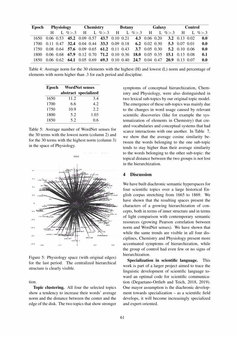
Epoch Physiology Chemistry Botany Galaxy ControlH L %>.3 H L %>.3 H L %>.3 H L %>.3 H L %>.3

1650 0.06 0.53 45.2 0.09 0.57 43.7 0.10 0.21 4.3 0.06 0.20 3.2 0.13 0.02 0.01700 0.11 0.47 32.4 0.04 0.44 33.3 0.09 0.18 6.2 0.02 0.30 5.3 0.07 0.01 0.01750 0.08 0.64 57.6 0.09 0.65 61.2 0.11 0.43 3.7 0.05 0.30 5.2 0.10 0.06 0.01800 0.06 0.68 67.9 0.12 0.70 71.2 0.10 0.36 18.0 0.05 0.35 15.1 0.13 0.08 0.11850 0.06 0.62 64.1 0.05 0.69 69.3 0.10 0.40 24.7 0.04 0.47 20.9 0.13 0.07 0.0

Table 4: Average norm for the 30 elements with the highest (H) and lowest (L) norm and percentage ofelements with norm higher than .3 for each period and discipline.

Epoch WordNet sensesabstract specialized

1650 11.2 3.41700 6.6 4.21750 10.9 2.21800 5.2 1.031850 5.2 0.6

Table 5: Average number of WordNet senses forthe 30 terms with the lowest norm (column 2) andfor the 30 terms with the highest norm (column 3)in the space of Physiology.

Figure 5: Physiology space (with original edges)for the last period. The centralized hierarchicalstructure is clearly visible.

tion.Topic clustering. All four the selected topics

show a tendency to increase their words’ averagenorm and the distance between the center and theedge of the disk. The two topics that show stronger

symptoms of conceptual hierarchization, Chem-istry and Physiology, were also distinguished intwo lexical sub-topics by our original topic model.The emergence of these sub-topics was mainly dueto the changes in word usage caused by relevantscientific discoveries (like for example the sys-tematization of elements in Chemistry) that cre-ated vocabularies and conceptual systems that hadscarce interactions with one another. In Table 7,we show that the average cosine similarity be-tween the words belonging to the one sub-topictends to stay higher than their average similarityto the words belonging to the other sub-topic: thetopical distance between the two groups is not lostin the hierarchization.

4 Discussion

We have built diachronic semantic hyperspaces forfour scientific topics over a large historical En-glish corpus stretching from 1665 to 1869. Wehave shown that the resulting spaces present thecharacters of a growing hierarchization of con-cepts, both in terms of inner structure and in termsof light comparison with contemporary semanticresources (growing Pearson correlation betweennorm and WordNet senses). We have shown thatwhile the same trends are visible in all four dis-ciplines, Chemistry and Physiology present moreaccentuated symptoms of hierarchization, whilethe group of control had even few or no signs ofhierarchization.

Specialization in scientific language. Thiswork is part of a larger project aimed to trace thelinguistic development of scientific language to-ward an optimal code for scientific communica-tion (Degaetano-Ortlieb and Teich, 2018, 2019).One mayor assumption is the diachronic develop-ment towards specialization – as a scientific fielddevelops, it will become increasingly specializedand expert-oriented.

61

Figure 6: Population of the same area of the hyper-disk for Physiology in the first and last epoch. Morespecialized and technical terms tend to populate the same level in the “hierarchy”.

Epoch Physiology I and II Chemistry I and II Galaxy Botany Control1650 -0.37 -0.42 -0.50 -0.09 -0.061700 -0.20 -0.44 -0.35 -0.05 0.671750 -0.40 -0.45 -0.43 -0.24 -0.341800 -0.42 -0.46 -0.16 -0.22 -0.171850 -0.41 -0.46 -0.37 -0.32 -0.16

Table 6: Pearson correlation between WordNet senses and word’s norm per period per topic.

Figure 7: For all four disciplines the averagewords’ norm increases through time. This isdue to the expansion of the hyperspace periphery:words become more specialized, hierarchies be-come deeper. The control group (sentiment terms)does not show this tendency.

Thus, as a field specializes, it develops moretechnical and differentiated vocabulary (Halliday,

Epoch P in P out C in C out1650 .58 .59 .54 .551700 .60 .60 .56 .561750 .53 .53 .50 .491800 .51 .50 .48 .471850 .50 .47 .47 .44

Table 7: Topic detectability. Average cosine simi-larity for elements pertaining to the same sub-topic(in) and elements pertaining to different sub-topics(out) in Physiology (P) and Chemistry (C) throughtime.

1988; Teich et al., 2016). For the disciplines in-vestigated here increased specialization over timeappears clearly in our hyperspaces showing a ten-dency towards the use of more peripheral wordsand deeper hierarchies.

Considerations on validity of our baselines.Finding valid, meaningful baselines to evaluatehierarchies based on a diachronic corpus is nota trivial task. Comparing them to the topic

62

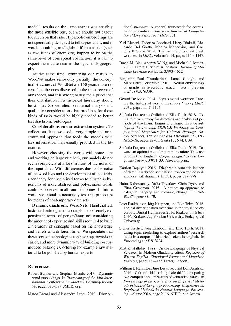
model’s results on the same corpus was possiblythe most sensible one, but we should not expecttoo much on that side: Hyperbolic embeddings arenot specifically designed to tell topics apart, and ifwords pertaining to slightly different topics (suchas two kinds of chemistry) happen to be on thesame level of conceptual abstraction, it is fair toexpect them quite near in the hyper-disk geogra-phy.

At the same time, comparing our results toWordNet makes sense only partially: the concep-tual structures of WordNet are 150 years more re-cent than the ones discussed in the most recent ofour spaces, and it is wrong to assume a priori thattheir distribution in a historical hierarchy shouldbe similar. So we relied on internal analysis andqualitative considerations, but baselines for thesekinds of tasks would be highly needed to bettertest diachronic ontologies.

Considerations on our extraction system. Tocollect our data, we used a very simple and non-committal approach that feeds the models withless information than usually provided in the lit-erature.

However, choosing the words with some careand working on large numbers, our models do notseem completely at a loss in front of the noise ofthe input data. With differences due to the noiseof the word lists and the development of the fields,a tendency for specialized terms to cluster as hy-ponyms of more abstract and polysemous wordscould be observed in all four disciplines. In futurework, we intend to accurately test this procedureby means of contemporary data sets.

Dynamic diachronic WordNets. Hand crafted,historical ontologies of concepts are extremely ex-pensive in terms of person/hour, not consideringthe amount of expertise and skills required to builda hierarchy of concepts based on the knowledgeand beliefs of a different time. We speculate thatthese sorts of technologies can be a step towards aneasier, and more dynamic way of building corpus-induced ontologies, offering for example raw ma-terial to be polished by human experts.

ReferencesRobert Bamler and Stephan Mandt. 2017. Dynamic

word embeddings. In Proceedings of the 34th Inter-national Conference on Machine Learning-Volume70, pages 380–389. JMLR. org.

Marco Baroni and Alessandro Lenci. 2010. Distribu-

tional memory: A general framework for corpus-based semantics. American Journal of Computa-tional Linguistics, 36(4):673–721.

Yuri Bizzoni, Federico Boschetti, Harry Diakoff, Ric-cardo Del Gratta, Monica Monachini, and Gre-gory R Crane. 2014. The making of ancient greekwordnet. In LREC, volume 2014, pages 1140–1147.

David M. Blei, Andrew W. Ng, and Michael I. Jordan.2003. Latent Dirichlet Allocation. Journal of Ma-chine Learning Research, 3:993–1022.

Benjamin Paul Chamberlain, James Clough, andMarc Peter Deisenroth. 2017. Neural embeddingsof graphs in hyperbolic space. arXiv preprintarXiv:1705.10359.

Gerard De Melo. 2014. Etymological wordnet: Trac-ing the history of words. In Proceedings of LREC2014, pages 1148–1154.

Stefania Degaetano-Ortlieb and Elke Teich. 2018. Us-ing relative entropy for detection and analysis of pe-riods of diachronic linguistic change. In Proceed-ings of the 2nd Joint SIGHUM Workshop on Com-putational Linguistics for Cultural Heritage, So-cial Sciences, Humanities and Literature at COL-ING2018, pages 22–33, Santa Fe, NM, USA.

Stefania Degaetano-Ortlieb and Elke Teich. 2019. To-ward an optimal code for communication: The caseof scientific English. Corpus Linguistics and Lin-guistic Theory, 0(0):1–33. Ahead of print.

Katrien Depuydt. 2016. Diachronic semantic lexiconof dutch (diachroon semantisch lexicon van de ned-erlandse taal; diamant). In DH, pages 777–778.

Haim Dubossarsky, Yulia Tsvetkov, Chris Dyer, andEitan Grossman. 2015. A bottom up approach tocategory mapping and meaning change. In Net-WordS, pages 66–70.

Peter Fankhauser, Jorg Knappen, and Elke Teich. 2016.Topical diversification over time in the royal societycorpus. Digital Humanities 2016, Krakow 1116 July2016, Krakow. Jagiellonian University; PedagogicalUniversity.

Stefan Fischer, Jorg Knappen, and Elke Teich. 2018.Using topic modelling to explore authors’ researchfields in a corpus of historical scientific english. InProceedings of DH 2018.

M.A.K. Halliday. 1988. On the Language of PhysicalScience. In Mohsen Ghadessy, editor, Registers ofWritten English: Situational Factors and LinguisticFeatures, pages 162–177. Pinter, London.

William L Hamilton, Jure Leskovec, and Dan Jurafsky.2016. Cultural shift or linguistic drift? comparingtwo computational measures of semantic change. InProceedings of the Conference on Empirical Meth-ods in Natural Language Processing. Conference onEmpirical Methods in Natural Language Process-ing, volume 2016, page 2116. NIH Public Access.

63

Johannes Hellrich and Udo Hahn. 2017. Explor-ing diachronic lexical semantics with JeSemE. InProceedings of ACL 2017, System Demonstrations,pages 31–36, Vancouver, Canada. Association forComputational Linguistics.

Adam Jatowt and Kevin Duh. 2014. A framework foranalyzing semantic change of words across time. InProceedings of the 14th ACM/IEEE-CS Joint Con-ference on Digital Libraries, pages 229–238. IEEEPress.

Eric Kafe. 2017. How stable are wordnet synsets? InLDK Workshops, pages 113–124.

Hannah Kermes, Stefania Degaetano-Ortlieb, AshrafKhamis, Jorg Knappen, and Elke Teich. 2016. TheRoyal Society Corpus: From Uncharted Data to Cor-pus. In Proceedings of the 10th LREC, Portoroz,Slovenia. ELRA.

Ekaterina Kochmar and Ted Briscoe. 2014. Detect-ing learner errors in the choice of content words us-ing compositional distributional semantics. In Pro-ceedings of COLING 2014, the 25th InternationalConference on Computational Linguistics: Techni-cal Papers, pages 1740–1751.

Andrey Kutuzov, Lilja Øvrelid, Terrence Szymanski,and Erik Velldal. 2018. Diachronic word embed-dings and semantic shifts: a survey. arXiv preprintarXiv:1806.03537.

Matt Le, Stephen Roller, Laetitia Papaxanthos, DouweKiela, and Maximilian Nickel. 2019. Inferring con-cept hierarchies from text corpora via hyperbolicembeddings. arXiv preprint arXiv:1902.00913.

Marco Marelli and Marco Baroni. 2015. Affixationin semantic space: Modeling morpheme meaningswith compositional distributional semantics. Psy-chological review, 122(3):485.

George A. Miller. 1995. Wordnet: A lexical databasefor english. Commun. ACM, 38(11):39–41.

Maximilian Nickel and Douwe Kiela. 2018. Learningcontinuous hierarchies in the lorentz model of hyper-bolic geometry. arXiv preprint arXiv:1806.03417.

Maximillian Nickel and Douwe Kiela. 2017. Poincareembeddings for learning hierarchical representa-tions. In Advances in neural information processingsystems, pages 6338–6347.

Stephen Roller, Douwe Kiela, and Maximilian Nickel.2018. Hearst patterns revisited: Automatic hy-pernym detection from large text corpora. arXivpreprint arXiv:1806.03191.

Ian Stewart and Jacob Eisenstein. 2017. Making”fetch” happen: The influence of social and linguis-tic context on nonstandard word growth and decline.arXiv preprint arXiv:1709.00345.

Elke Teich, Stefania Degaetano-Ortlieb, PeterFankhauser, Hannah Kermes, and EkaterinaLapshinova-Koltunski. 2016. The Linguistic Con-strual of Disciplinarity: A Data Mining ApproachUsing Register Features. Journal of the Associationfor Information Science and Technology (JASIST),67(7):1668–1678.

64

An evaluation of Czech word embeddings

Karolına HorenovskaCharles University, Faculty of Mathematics and Physics

Institute of Formal and Applied [email protected]

Abstract

We present an evaluation of Czech low-dimensional distributed word representa-tions, also known as word embeddings.We describe five different approaches totraining the models and three different cor-pora used in training. We evaluate the re-sulting models on five different datasets,report the results and provide their furtheranalysis.

1 Introduction

Distributed word representations, often referred toas word embeddings, have received a lot of atten-tion in recent years, and they have been used to im-prove results in many NLP tasks. The term itselfrefers to representing words as low-dimensionalreal-valued vectors (usually with dimensionalityof 50-1000), and is opposed to explicit sparserepresentations, i.e. representing words as high-dimensional vectors of 0s and 1s (usually with di-mensionality in the tens of thousands).

Many different models have been proposed (seesection 2). By their nature, these models arelanguage-independent (given the language can betokenized) but usually the reported results aremeasured using only English. This is encouragednot only by English being the standard scientificlanguage, but also by the availability of Englishtext corpora and, even more importantly, Englishdatasets to evaluate the models on.

We have decided to perform an intrinsic evalu-ation of embedding models on Czech. We haveidentified several successful models to evaluate,collected existing datasets to evaluate them on anddesigned two more datasets to extend the evalu-ation. We should note that we do not performdownstream-task evaluation, even though it mightnot correlate well with the intrinsic evaluation(Tsvetkov et al., 2015). We also use the models

with their default parameters and only try chang-ing the corpus they are trained on.

The rest of the paper is organized as follows:first, we describe related work (section 2). Wecontinue with a description of selected models(section 3), corpora used in training (section 4)and the datasets (section 5). Finally, we presentthe results (section 6).

2 Related work

Related work could be clustered into three groupsof papers.

First, we should mention papers performingevaluation of Czech word embeddings. Such eval-uation exists for Word2Vec and GloVe using anal-ogy corpus (Svoboda and Brychcın, 2016), how-ever we are not aware of any more recent evalua-tion (which would cover also more recent models).Still, some papers evaluate some word embed-dings in the context of a new dataset, as is the caseof Czech similarity-relatedness dataset (Konopiket al., 2017).

Second, there are intrinsic evaluations of em-beddings. These are usually part of new modelproposals but there are exceptions. A notable oneis a comparison by Baroni et al (2014), and alsothe work by Levy and Goldbert (2014), thoughthis paper proposes another objective to solvinganalogies. Tsvetkov (2015) should also be men-tioned for showing that intrinsic evaluation of em-beddings need not correlate with performance ondownstream tasks, and Nayak et al (2016) pro-posed a suite to test word embeddings.

Finally, there are model proposals. The most fa-mous one is probably Word2Vec (Mikolov et al.,2013a), which has later been extended to fastText(Bojanowski et al., 2017). Despite being so wellknown, Word2Vec is neither the older (cf. e.g. thework by Schutze (1993)) nor the only one. An-other famous models include GloVe (Penningtonet al., 2014), LexVec (Salle et al., 2016b), ELMo

65

(Peters et al., 2018) or a recent model BERT (De-vlin et al., 2018).

In addition to models themselves, there are pro-posals on altering the trained model so that it bet-ter fits a purpose, e.g. by transforming the vectorspace to get vectors of synonyms closer to eachother and increase the distance between antonymvectors (Faruqui et al., 2014; Mrksic et al., 2016).

3 Selected models

In this section, we outline each of the selectedmodels. We also report which implementation weuse in our experiments.

Following some literature, we characterize eachmodel as either predictive (trained by learning topredict a word) or counting (trained using co-occurences counts).

Unfortunately, it has not been feasible to trainsome model-corpus combinations.1 We were notable to train fastText on Czech National Corpususing forms and LexVec on Czech National Cor-pus using either forms or lemmata. We have alsonot trained BERT on our own, instead, we only usea pre-trained model.

3.1 Word2Vec

Word2Vec (Mikolov et al., 2013a,b) is proba-bly the most famous neural embedding model.The same name actually refers to two differentarchitectures – called continuous bag of words(CBOW) and skip-gram (SG).

Both architectures are basically feed-forwardnetworks. CBOW’s inputs are words (tokens)within another word’s context and its golden out-put is the surrounded word. Often, context win-dow of size 5 is used, i.e. five words precedingand five words following the predicted word formthe inputs. There’s one projection layeyr betweeninput and output layers. For skip-gram, it is theother way round, i.e. one word forms the inputand words surrounding it are predicted. In botharchitectures, all words share the projection layer,which reduces the number of parameters to train,and thus the training time.

When using Word2Vec without specifying ar-chitecture, skip-gram is usually the default as itperforms better in most evaluation. However,since Svoboda and Brychcın (2016) found outCBOW performed better in their experiments onCzech, we experiment with both architectures.

1We hope to overcome this limitation in our future works.

We use Word2Vec implementation provided inthe gensim library (Rehurek and Sojka, 2010).

An important concept introduced in the secondpaper (Mikolov et al., 2013b) is negative sam-pling: when training a word vector, other wordsare randomly sampled from the corpus and themodel is penalized for high similarity of their vec-tors.

3.2 FastText

FastText (Bojanowski et al., 2017) is an exten-sion of Word2Vec skip-gram which incorporatessubword information in resulting vectors. Wordsare prefixed and suffixed with boundary symbolsand vectors are then trained not only for all wordsbut also for all n-grams appearing in any of thewords. Boundary symbols are important to dis-tinguish short words from n-grams appearing in-side words. Using n-gram embeddings, even vec-tors for out-of-vocabulary words (i.e. words notpresent in training corpus) can be generated.

Please note that even though Bojanowski et al.(2017) describe the model as using skip-gram, itcan integrate with CBOW architecture. We havetried using both architectures.

We use the implementation provided in gensimlibrary (Rehurek and Sojka, 2010).

3.3 GloVe

GloVe (Pennington et al., 2014) is a countingmodel which utilizes co-occurence matrix, i.e.numbers of times a word occurs within the con-text of another word. The basic idea is that ifsome words are related to the same concept, theprobability of appearing in their context is muchhigher for these words than for any other word.This ratios need to be captured by the resultingmodel. The formulae to capture these similari-ties/ratios are further weighted so that rarely seenco-occurences contribute little to the resulting vec-tors (through loss function) and there’s a limit towhich frequent co-occurencies might contribute.

We use the original implementation provided byauthors.2

3.4 LexVec

LexVec (Salle et al., 2016b,a; Salle and Villavi-cencio, 2018) is, like GloVe, a counting model. Itagain utilizes co-occurence matrix and weights the

2https://github.com/stanfordnlp/GloVe

66

errors so that more frequent co-occurences con-tribute more. It however also employs the negativesampling (originally introduced as an extension toskip-gram Word2Vec (Mikolov et al., 2013b)) toforce scattering vectors of unrelated words.

Since the first paper, LexVec has been extendedwith positional context (i.e. it is not important onlywhether word a appeared in the context of word bbut also whether it was to the left or to the rightand how many words there were in between), theability to use external memory for storing the co-occurences (which allows to train on a huge cor-pus), and finally with subword information (whichallows deriving vectors even for out-of-vocabularywords).

We use the original implementation provided byauthors.3

3.5 BERT

BERT (Devlin et al., 2018), which stands forbidirectional encoder representations from trans-former, is a neural predictive model. It is trainedon sentences rather than on words themselves (ac-tually, its inputs are sentence pairs) but it doesproduce word embeddings. It’s training can beviewed as a two-step process, the model is firstpre-trained using specific tasks and then fine-tunedusing downstream tasks.

The two tasks used to pretrain the model arenext sentence prediction (i.e. deciding whetherthe second sentence really followed the first onein original text or if it was picked at random)and something the authors call masked languagemodel, which is very close to a cloze test (Taylor,1953). The idea is that some amount of randomlychosen words is masked (i.e. replaced with a spe-cial token), and the model has to correctly predictthem.

We do not train the model, we use the dis-tributed multilingual model 4 and our departmentwrapper around it.

Because of its different nature, we evaluate thismodel only on similarity datasets (those describedin subsections 5.2 and 5.3).

4 Corpora

In this section, we briefly describe the corpora weuse to train the models on.

3https://github.com/alexandres/lexvec4https://github.com/google-research/bert

Apart from using different models and corporato train on, we have also experimented with twomore settings: token form (i.e. training either onforms as they appear in the corpora, or on lem-mata) and keeping/substituting numbers. The sec-ond idea is rather a concept, though concretized innumbers – some words have similar function butcome in many different forms (and remain distinctwhen lemmatized) so their token counts are lowand they do not take big part in the training. How-ever, their similar function suggests that they couldstill be useful in defining contexts/concepts. Wetherefore tried also substituting all numbers (i.e.tokens tagged as C= by MorphoDiTa tool) with ameta-word.

For lemmatization of both corpora and datasets,we have used the MorphoDiTa tool (Strakovaet al., 2014).

4.1 Czech Wikipedia dump

As is common in natural language processing, weuse Wikipedia dump as a training corpus. Thiscorpus consists of short documents (hundreds tothousands words), the style is encyclopedic but notreally expert. No shuffling has to happen, all co-occurences are kept as they are. Unfortunately,Czech Wikipedia is rather small when comparedto the English version, thus we expect it to pro-duce worse results.

We have used the dump from 1st May 2019. Wehave processed the dump with wikiextractor5 andtokenized it using MorphoDiTa (Strakova et al.,2014) tool.

4.2 CzEng

CzEng (Bojar et al., 2016) is a parallel Czech-English corpus. The texts in it are of varied do-mains, including news, fiction, laws, movie sub-titles and tweets. It is shuffled at block level, i.e.only a few consecutive sentences are kept togethereach time. Each sentence is associated with its do-main but it is not possible to reconstruct the origi-nal documents.

We have used version 1.7 and only extracted theCzech part of CzEng, keeping the tokenization andlemmatization provided in CzEng. We have re-ordered the sentences so that all sentences whichshare the domain are grouped together.

5http://attardi.github.io/wikiextractor/

67

4.3 Czech National Corpus

Czech National Corpus (Kren et al., 2016) is alarge corpus of written Czech. Version SYN v4,which we have used, contains texts of varyingtypes, however news are by far the most common.(This version is not considered representative be-cause of the prevailing news, but it is much largerthan representative CNC subcorpora.) The cor-pus is again shuffled at block level, sentences arelinked with the exact document they come frombut their order cannot be reconstructed.

5 Datasets

We describe the existing (as well as no-longer-existing) datasets suitable for the evaluation ofCzech word embeddings.

5.1 RG-65 Czech (unavailable)

RG-65 Czech (Krcmar et al., 2011) is (or per-haps used to be) a Czech version of the fa-mous Rubenstein-Goodenough set (Rubensteinand Goodenough, 1965), a set on word related-ness.

In the original set, the data are triplets: twowords and a mean relatedness score as annotatedby human annotators, there are 65 word pairs.

The authors decided to translate the word pairs,using a reference on the original meanings. Pairrelatedness was annotated by 24 human annotatorsof varying age, gender and education. During thetranslation and annotation process, a total of 10pairs was omitted since one of the words could notbe easily translated (or it would be translated toexactly the same word as the other).

Unfortunately, this dataset seems not to beavailable any more. The URL provided in the pa-per does not work, neither does the first author’semail. We have tried contacting another author ofthe paper but they did not have the data.

We therefore do not evaluate on this dataset,however we think it should be listed when dis-cussing all relevant datasets.

5.2 WordSim353-CZ

WordSim353-CZ (Cinkova, 2016) is a Czech ver-sion of WordSim (Finkelstein et al., 2002), whichis another dataset on word relatedness. The dataare again triplets, word pair and a score (thoughtechnically the Czech dataset contains other infor-mation for each pair).

The author decided to create a dataset as similaras possible to the original, which especially meansshe encouraged the annotators to annotate related-ness, even though the name refers to similarity.

During the process of creating the dataset, fourcandidate translations were suggested for each ofthe original pairs, and 25 annotators annotated allreasonable pairs. The authors then selected thepairs so that the correlation between Czech andEnglish rankings is maximal.

A version with all annotated pairs is availablebut we stick to the selected subset in our experi-ments.

5.3 Czech similarity and relatedness

The dataset for Czech similarity and relatedness(Konopik et al., 2017) not only enables anotherevaluation of word similarity, it also addressesthe problem of scoring words which are closelyrelated but not really similar (those may be e.g.antonyms or pairs like beach and sand). Thisdataset contains 953 words.

The authors decided to build the dataset fromseveral different resources. They translated ran-dom pairs from several English datasets, RG-65(Rubenstein and Goodenough, 1965), WordSim(Finkelstein et al., 2002), MTurk (Radinsky et al.,2011), Rare words (Luong et al., 2013) and MEN(Bruni et al., 2014). They also mined translationaldata using Moses (Koehn et al., 2007) and CzEng(Bojar et al., 2016), language part of Czech gen-eral study tests SCIO, and they invented a fewpairs on their own.

Word pairs were annotated by 5 annotators andeach of them annotated both similarity and relat-edness, the annotators achieved Spearman corre-lation of 0.81.

The dataset itself does not contain only the wordpairs and their scores but also examples of their us-age, examples of ambiguities (sentences contain-ing the same word with different meaning) and ex-amples of the two words co-occuring; all exampleswere taken from the Czech National Corpus.

5.4 Czech analogy corpus

Czech analogy corpus was presented as a part ofembedding-related experiments by Svoboda andBrychcın (2016), and it mimics the Google anal-ogy test set.6

6http://download.tensorflow.org/data/questions-words.txt

68

It contains 11 relationship categories. Of those,4 are purely semantic (capital cities and threegroups of antonym relations, further divided basedon part-of-speech), 3 are purely syntactic (nounplural, verb past tense, adjective gradation), 3 arerather syntactic (gender variation of job names andof nationalities, grammatic number variation ofpronouns, including pairs like I and we) and 1 israther semantic (family relations, i.e. he-cousin toshe-cousin as father to mother). While family re-lations is in fact gender variation of family roles,feminime variants usually cannot be derived frommasculine ones.

There is also a phrase version which containssome additional categories but we use the versioncontaining single words only.

5.5 Extended semantic analogies

We have developed four additional analogy cat-egories and word pairs representing those cate-gories. These categories are: old or even ar-chaic words and more modern words with thesame / close enough meaning, e.g. biograf andkino ’cinema’; diminutives, e.g. mama ’mum’ andmaminka ’mummy’; more foreign-sounding (of-ten expert) words and their more Czech-soundingvariants, e.g. akceptovat and prijmout ’(to) ac-cept’; and synonyms.

While we understand and acknowledge the am-biguity of listed relations, we believe some ambi-guity accompanies also antonyms and family rela-tions, and we are curious about the model perfor-mance.

5.6 Synonym retrieval

We propose evaluating word embeddings also onsynonym retrieval. Using our department the-saurus, we have randomly selected 500 wordsknown to have at least 5 synonyms. (No two testedwords are synonyms of each other.)

For each tested word, we find 10 words havingthe most similar vectors and we evaluate the top-1, top-3 and top-5 precision. We do it both withrespect to the answer really given and with respectto an oracle which would move true synonyms totop positions whenever they would appear withinthe 10 candidates.

Please note that even though Leeuwenberg et al(2016) have shown that relative cosine similarityis a better approach to synonym extraction, it doesnot make a great difference in our case because we

do not need to set a similarity threshold betweensynonyms and non-synonyms.

6 Results

We evaluated all trained models on all availabledatasets, with the exception of BERT embed-dings which were only evaluated on WordSim353-CZ and Czech similarity and relatedness dataset.Please keep in mind that we were not able to trainfastText on Czech National Corpus using formsand LexVec on Czech National Corpus using ei-ther forms or lemmata.

When evaluating analogies, we have tried usingboth 3CosAdd suggested by Mikolov et al (2013b)and 3CosMul suggested by Levy and Goldbert(2014) as similarity objective. To evaluate simi-larity, we use cosine similarity in all tasks.

Since the number of trained and evaluated mod-els is high, we do not report results for each of themodels. Instead, we do the following:

• Divide the tasks into five groups: syntac-tic analogies, semantic analogies, extendedanalogies, similarity/relatedness assignmentand synonym retrieval. For each group, weidentify all models which achieve the best re-sult on any task within this group, and for allsuch models, we report results on all taskswithin this group. We also report the per-formace of BERT embeddings on the simi-larity/relatedness group.

• Report a basic approximation of parame-ter volatility, given by differences in perfor-mance when only the parameter in questionis changed.

• Discuss the patterns we have noticed duringour examination of all results.

Table 1 shows the results on syntactic analogies.Please note that the dominance of models trainedon forms is expected since models trained on lem-mata are not able to solve purely syntactic tasks(plural, past tense, pronouns, gradation). The non-zero accuracy of lemmatized models on plural isonly possible due to a dataset lemmatization error.

The achieved accuracies are pleasing, with a no-table exception of pronoun analogies. We suspectthis could be because the pronoun analogies in factmix several aspects, i.e. there are pairs like ja ’I’- my ’we’ but also meho ’my (sg., i.e. my thing)’- mych ’my (pl., i.e. my things)’, instead of meho

69

fastText Word2Vec Word2Vec LexVec fastTextWiki CNC CNC CzEng CNCforms forms forms forms lemmata

3CosMul 3CosAdd 3CosMul 3CosMul 3CosMulPlural 71.85 64.11 64.04 68.17 2.70Jobs 83.92 87.54 85.35 80.72 75.00

Past tense 89.02 66.58 67.84 87.79 0.00Pronouns 7.54 9.79 10.98 10.45 0.00Gradation 60.00 62.50 60.00 70.00 0.00Nations 43.18 25.19 28.03 40.15 67.52

Table 1: Results on syntactic analogies; numbers were always kept in place; both Word2Vec and fastTextwere trained using CBOW architecture

LexVec Word2Vec LexVec Word2Vec LexVecCzEng Wiki Wiki CNC CzEng

lemmata lemmata forms lemmata lemmatameta meta numbers meta numbers

3CosAdd 3CosAdd 3CosAdd 3CosAdd 3CosMulAnto-nouns 23.33 13.44 17.28 14.72 18.56

Anto-adj 20.96 31.71 3.54 23.17 20.15Anto-verbs 6.79 5.27 13.66 7.68 6.70City/state 5.35 41.62 3.03 54.72 5.08

Family 45.99 41.98 8.03 43.83 48.61

Table 2: Results on semantic analogies;

CNC CNC CNC CzEngnumbers meta meta numbers3CosMul 3CosAdd 3CosMul 3CosMul

Archaic 18.92 15.92 17.72 7.56Diminutives 25.97 27.66 27.66 13.97

Expert 23.09 19.63 23.48 14.19Synonyms 20.27 19.79 19.79 26.71

Total 22.80 21.32 23.17 14.83

Table 3: Results on extended analogies; all models were trained using Word2Vec with CBOW architec-ture, corpus was always lemmatized

’my’ - naseho ’our’. The possessive pronouns arealso given in genitive/accusative (same forms areused for both cases) while the personal pronounsare given in nominative.

Results on semantic analogies are reported in ta-ble 2, and results on extended analogies are givenin table 3.

Consistently with Svoboda and Brychcın(2016), we have found that CBOW outperformsskip-gram on Czech, which is not consistent withthe results observed on English (Mikolov et al.,2013b). We hypothesize this could be due to rel-atively free word order and strong inflection and

conjugation found in Czech. For example, whilethe two sentences Profesor pochvalil studenta andStudenta pochvalil profesor ’A professor praised astudent’, have a different meaning with respect totopic-focus articulation, they can be both utilizedin Czech to communicate roughly the same thing.In English, changing the word order would alsorequire transforming the verb. Therefore, a singleCzech word could be less predictive than a singleEnglish word, making skip-gram less effective.

The best result is not always achieved usingthe largest corpus available. Out of 15 anal-ogy classes, 4 are best solved when training on

70

Wikipedia dump. The difference is very subtlefor noun plural, rather subtle for past tense andverb antonyms (with LexVec trained on CzEng be-ing the second in all cases) but high for adjectiveantonyms (the best non-wiki model achieves ac-curacy of 25.67). While we are not able to trulyexplain, we suspect several factors could be re-sponsible: Wikipedia dump is probably more con-sistent in style than both other corpora (whichare compilations of various sources); many pagesoriginated as English Wikipedia translation andthus are likely to follow English stylistics, mak-ing the language more similar to English; its en-cyclopaedic nature could make the language moreregular in general. Perhaps these properties couldoutweight the corpus size.

However, CNC in general gives good resultson extended analogies. We suppose its size doesmake an advantage, though indirectly, by mak-ing the appearance of queried words in the cor-pus more likely and their contexts more recogniz-able (some words are unusual in Czech, especiallywords from archaic and expert analogies).

We notice that while syntactic analogies are bet-ter solved by models trained on forms (with theexception of gendered nationality analogies), mostsemantic analogies are better solved by modelstrained on lemmata. We suppose this is due tolarge numbers of word forms for each lemma (aprototypic Czech noun has 14 forms, adjectivesand verbs have even more), further strengthenedby lemmata having some basic sense disambigua-tion annotation.

The exception to lemmata performing better areverbal antonyms. The best lemma-based modelachieves accuracy of 10.18, which is notably lowerthan the best result. We are not sure about thecause. However, verbs have lots of forms (whichall get lemmatized to the same string) and manyverbal forms contain auxiliary words, often alsoverbal. The combination of that could make dis-tinguisting contexts more difficult.

Table 4 gives the results on similarity tasks. Toevaluate BERT on Czech similarity and related-ness dataset, we extracted all example sentences(which are given to demonstrate the use of theword with the desired meaning) and inferred theembeddings of all words in them. We then usedthe embeddings of the queried words to evaluatethe model.7

7Technically, we first associated the word with a unique

We were quite surprised to see the relativelylow results of BERT, compared to other models.We suspect the elimination of accented charac-ters could hurt BERT performance since accentsmay differentiate meaning in Czech and the re-moval of accented characters might produce thesame string (as turning both maly ’small (mascu-line)’ and mala ’small (feminime)’ into mal; mura’moth’ and mıra ’measure, rate’ to mra) or evento valid Czech words (as turning zed ’wall’ intoze ’from’). However, this should be rather rare,except for systematic occurences as with the mas-culine and feminime adjectives.

We find it more likely that BERT performanceis hurt by inferring embeddings of rather artificialsentences. For WordSim, the sentences had onlythe queried words. For the similarity and related-ness dataset, these were true sentences, but with-out further context.

The results on synonym retrieval are reportedin table 5. We again see that CBOW architectureoutperforms skip-gram, which might be becauseof relatively free word order in Czech. The effectcould be even stronger in context of synonym re-trieval, as the distinction e.g. between subject andobject could also be the distinction between (near-)synonym and (near-)antonym verb.

The corpus size might be a more important fac-tor than model selection for synonym retrieval.Even though moving from forms to lemmata helpsboth in general and specifically with this task,models trained on unlemmatized CNC often out-performed models trained on lemmatized CzEng.However, Word2Vec/CBOW trained on smallerlemmatized corpus still outperformed other mod-els trained on CNC. Unfortunately, we cannot besure about the performance of LexVec on CNCbut its performance on CzEng is 30%-70% ofword2vec/CBOW performance with the remain-ing parameters matching.

We have also noticed that while oracle precisionis good, the synonyms often do not come first. Theexact precisions differ but for all models, the realprecision is one third to one half of oracle preci-sion.

In all our experiments, GloVe did not perform

identifier, added the identifier and the inferred embedding to aspecial model using gensim, and finally evaluated this specialmodel against the translation of the dataset into the identifiers.The identifiers are needed since embeddings are contextual-ized, i.e. different for the same word in different contexts, butgensim only supports mapping one word to one embedding.

71

fastText LexVec BERTCNC CzEngmeta numbers

SimRel/Similarity 72.45 65.39 46.90SimRel/Relatedness 66.51 62.14 38.63

WordSim353-CZ 69.17 70.41 13.88

Table 4: Results (Spearman correlation coefficient) on similarity tasks; All models were trained onlemmatized corpus; fastText was trained using CBOW architecture

numbers meta-numbersTop-1 oracle 78.10 74.79Top-3 oracle 47.80 49.45Top-5 oracle 32.07 32.48

Top-1 precision 35.12 33.88Top-3 precision 26.86 26.45Top-5 precision 21.65 22.15

Table 5: Results on synonym retrieval; Modelswere trained using Word2Vec/CBOW on lemma-tized CNC

well. The rank of best performing GloVe modelwas usually around 30, therefore being worse thanabout a quarter of all other models. It is howeverpossible that GloVe would benefit from tweakingthe parameters more carefully. Altering a param-eter often has the opposite effect on GloVe thanon other modesl, which also encourages this as-sumption. Still, it should be noted that this resultagain is consistent with the findings of Svobodaand Brychcın (2016), who discovered GloVe per-formed worse than Word2Vec on Czech.

Despite all the research into incorporating sub-word information into embeddings (which is,among other, motivated by morphologically richlanguages), models trained on lemmata performbetter that their counterparts trained on forms.Tasks which require form distinguishing are a nat-ural exception to this. We suspect this gap is par-tially caused by some forms being quite differentfrom its lemma (and therefore hardly connectableon form/subword level), by lots of forms beingonly seemingly similar (sharing a long substringbut meaning a different thing), and also by someforms appearing in specific contexts only (mak-ing the model learn a relation more specific thanit should be).

However, we believe performing a strictly syn-tactic evaluation of embeddings which wouldfocus on deriving correctly inflected/conjugated

forms would be an interesting experiment to evalu-ate to benefits of subword information in morpho-logically rich languages.

As has been already mentioned, CBOW outper-forms skip-gram on Czech. The difference is big-ger on syntactic analogies; CBOW advantage isless clear in fastText models than Word2Vec mod-els and on similarity tasks (in which CBOW onlyoutperforms skip-gram if trained on lemmata).

Word2Vec with CBOW architecture generallyperforms well, though there are tasks (especiallysimilarity assignment) on which LexVec gives no-tably better results.

Number substitution with meta-words alters theresults only slightly. Though sometimes the bestresult is achieved by a model trained on text withthose meta-words, the substitution hurts more of-ten than it helps.

Similarly, the difference in analogy perfor-mance between different similarity objectives israther subtle, though it is notable that semanticanalogies are generally best solved with 3CosAddobjective while syntactic analogies are generallybest solved with 3CosMul. However, this pat-tern is not repeated in extended analogies whichare mostly semantic but best solved with 3CosMul(though the results on extended analogies are lowwhich might further reduce the effect of similarityobjective).

In general, training on CzEng instead of CNCresults in worse results, suggesting CNC is moreappropriate for training word embeddings. Thedifference of size is likely to play a role, but with-out further investigations we cannot eliminate thepossibility that the fact that CzEng is comprised ofmore different text types also worsens (or possiblyimproves) the results.

The comparison of training with CzEng andWikipedia dump is less one-sided. In most cases,moving from CzEng to Wikipedia dump has anegative impact, however it does improve the re-

72

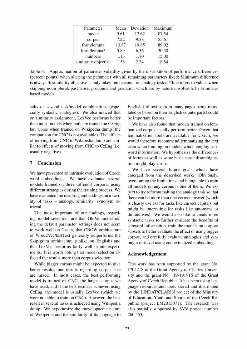
Parameter Mean Deviation Maximummodel 9.61 12.62 87.54corpus 7.22 9.38 55.61

form/lemma 13.87 19.85 89.02form/lemma* 5.89 6.36 30.30

numbers 1.13 1.70 15.00similarity objective 1.58 2.34 18.54

Table 6: Approximation of parameter volatility given by the distribution of performance differences(percent points) when altering the parameter with all remaining parameters fixed; Minimum differenceis always 0; similarity objective is only taken into account on analogy tasks; * line refers to values whenskipping noun plural, past tense, pronouns and gradation which are by nature unsolvable by lemmata-based models

sults on several task/model combinations (espe-cially syntactic analogies). We also noticed thaton similarity assignment, LexVec performs betterthan most models when both are trained on CzEngbut worse when trained on Wikipedia dump (thecomparison for CNC is not available). The effectsof moving from CNC to Wikipedia dump are sim-ilar to effects of moving from CNC to CzEng (i.e.usually negative).

7 Conclusion

We have presented an intrinsic evaluation of Czechword embeddings. We have evaluated severalmodels trained on three different corpora, usingdifferent strategies during the training process. Wehave evaluated the resulting embeddings on a vari-aty of tasks – analogy, similarity, synonym re-trieval.

The most important of our findings, regard-ing model selection, are that GloVe model us-ing the default parameter settings does not seemto work well on Czech, that CBOW architectureof Word2Vec/fastText generally outperforms theSkip-gram architecture (unlike on English) andthat LexVec performs fairly well in our experi-ments. It is worth noting that model selection af-fected the results more than corpus selection.

While bigger corpus might be expected to givebetter results, our results regarding corpus sizeare mixed. In most cases, the best performingmodel is trained on CNC, the largest corpus wehave used, and if the best result is achieved usingCzEng, the model is usually LexVec (which wewere not able to train on CNC). However, the bestresult in several tasks is achieved using Wikipediadump. We hypothesize the encyclopaedic natureof Wikipedia and the similarity of its language to

English (following from many pages being trans-lated or based on their English counterparts) couldbe important factors.

We have also found that models trained on lem-matized corpus usually perform better. Given thatlemmatization tools are available for Czech, wewould therefore recommend lemmatizing the texteven when training on models which employ sub-word information. We hypothesize the differencesof forms as well as some basic sense disambigua-tion might play a role.

We have several future goals which haveemerged from the described work. Obviously,overcoming the limitations and being able to trainall models on any corpus is one of them. We ex-pect to try reformumalting the analogy task so thatthere can be more than one correct answer (whichis clearly useless for tasks like currect capitals butmight be interesting for tasks like antonyms ordiminutives). We would also like to create moresyntactic tasks to further evaluate the benefits ofsubword information, train the models on corporasubsets to better evaluate the effect of using biggercorpus, and carefully evaluate analogies and syn-onym retrieval using contextualized embeddings.

Acknowledgement

This work has been supported by the grant No.1704218 of the Grant Agency of Charles Univer-sity and the grant No. 19-19191S of the GrantAgency of Czech Republic. It has been using lan-guage resources and tools stored and distributedby the LINDAT/CLARIN project of the Ministryof Education, Youth and Sports of the Czech Re-public (project LM2015071). The research wasalso partially supported by SVV project number260 453.

73

ReferencesMarco Baroni, Georgiana Dinu, and German

Kruszewski. 2014. Don’t count, predict! asystematic comparison of context-counting vs.context-predicting semantic vectors. In Proceedingsof the 52nd Annual Meeting of the Associationfor Computational Linguistics (Volume 1: LongPapers), volume 1, pages 238–247.

Piotr Bojanowski, Edouard Grave, Armand Joulin, andTomas Mikolov. 2017. Enriching word vectors withsubword information. Transactions of the Associa-tion for Computational Linguistics, 5:135–146.

Ondrej Bojar, Ondrej Dusek, Tom Kocmi, Jindrich Li-bovicky, Michal Novak, Martin Popel, Roman Su-darikov, and Dusan Varis. 2016. CzEng 1.6: En-larged Czech-English Parallel Corpus with Process-ing Tools Dockered. In Text, Speech, and Dialogue:19th International Conference, TSD 2016, number9924 in Lecture Notes in Computer Science, pages231–238, Cham / Heidelberg / New York / Dor-drecht / London. Masaryk University, Springer In-ternational Publishing.

Elia Bruni, Nam-Khanh Tran, and Marco Baroni. 2014.Multimodal distributional semantics. Journal of Ar-tificial Intelligence Research, 49:1–47.

Silvie Cinkova. 2016. Wordsim353 for czech. In Inter-national Conference on Text, Speech, and Dialogue,pages 190–197. Springer.

Jacob Devlin, Ming-Wei Chang, Kenton Lee, andKristina Toutanova. 2018. Bert: Pre-training of deepbidirectional transformers for language understand-ing. arXiv preprint arXiv:1810.04805.

Manaal Faruqui, Jesse Dodge, Sujay K Jauhar, ChrisDyer, Eduard Hovy, and Noah A Smith. 2014.Retrofitting word vectors to semantic lexicons.arXiv preprint arXiv:1411.4166.

Lev Finkelstein, Evgeniy Gabrilovich, Yossi Matias,Ehud Rivlin, Zach Solan, Gadi Wolfman, and Ey-tan Ruppin. 2002. Placing search in context: Theconcept revisited. ACM Transactions on informa-tion systems, 20(1):116–131.

Philipp Koehn, Hieu Hoang, Alexandra Birch, ChrisCallison-Burch, Marcello Federico, Nicola Bertoldi,Brooke Cowan, Wade Shen, Christine Moran,Richard Zens, et al. 2007. Moses: Open sourcetoolkit for statistical machine translation. In Pro-ceedings of the 45th annual meeting of the associ-ation for computational linguistics companion vol-ume proceedings of the demo and poster sessions,pages 177–180.

Miloslav Konopik, Ondrej Prazak, and David Stein-berger. 2017. Czech dataset for semantic similarityand relatedness. In Proceedings of the InternationalConference Recent Advances in Natural LanguageProcessing, RANLP 2017, pages 401–406.

Lubomır Krcmar, Miloslav Konopık, and Karel Jezek.2011. Exploration of semantic spaces obtained fromCzech corpora. In DATESO, pages 97–107.

Michal Kren, Vaclav Cvrcek, Tomas Capka, AnnaCermakova, Milena Hnatkova, Lucie Chlumska,Tomas Jelınek, Dominika Kovarıkova, VladimırPetkevic, Pavel Prochazka, Hana Skoumalova,Michal Skrabal, Petr Trunecek, Pavel Vondricka,and Adrian Zasina. 2016. SYN v4: large cor-pus of written czech. LINDAT/CLARIN digital li-brary at the Institute of Formal and Applied Linguis-tics (UFAL), Faculty of Mathematics and Physics,Charles University.

Artuur Leeuwenberg, Mihaela Vela, Jon Dehdari, andJosef van Genabith. 2016. A minimally supervisedapproach for synonym extraction with word embed-dings. The Prague Bulletin of Mathematical Lin-guistics, 105(1):111–142.

Omer Levy and Yoav Goldberg. 2014. Linguistic reg-ularities in sparse and explicit word representations.In Proceedings of the eighteenth conference on com-putational natural language learning, pages 171–180.

Thang Luong, Richard Socher, and Christopher Man-ning. 2013. Better word representations with recur-sive neural networks for morphology. In Proceed-ings of the Seventeenth Conference on Computa-tional Natural Language Learning, pages 104–113.

Tomas Mikolov, Kai Chen, Greg Corrado, and Jef-frey Dean. 2013a. Efficient estimation of wordrepresentations in vector space. arXiv preprintarXiv:1301.3781.

Tomas Mikolov, Ilya Sutskever, Kai Chen, Greg S Cor-rado, and Jeff Dean. 2013b. Distributed representa-tions of words and phrases and their compositional-ity. In Advances in neural information processingsystems, pages 3111–3119.

Nikola Mrksic, Diarmuid O Seaghdha, Blaise Thom-son, Milica Gasic, Lina Rojas-Barahona, Pei-Hao Su, David Vandyke, Tsung-Hsien Wen, andSteve Young. 2016. Counter-fitting word vec-tors to linguistic constraints. arXiv preprintarXiv:1603.00892.

Neha Nayak, Gabor Angeli, and Christopher D Man-ning. 2016. Evaluating word embeddings using arepresentative suite of practical tasks. In Proceed-ings of the 1st Workshop on Evaluating Vector-SpaceRepresentations for NLP, pages 19–23.

Jeffrey Pennington, Richard Socher, and ChristopherManning. 2014. Glove: Global vectors for wordrepresentation. In Proceedings of the 2014 confer-ence on empirical methods in natural language pro-cessing (EMNLP), pages 1532–1543.

Matthew E Peters, Mark Neumann, Mohit Iyyer, MattGardner, Christopher Clark, Kenton Lee, and Luke

74

Zettlemoyer. 2018. Deep contextualized word rep-resentations. arXiv preprint arXiv:1802.05365.

Kira Radinsky, Eugene Agichtein, EvgeniyGabrilovich, and Shaul Markovitch. 2011. Aword at a time: computing word relatedness usingtemporal semantic analysis. In Proceedings of the20th international conference on World wide web,pages 337–346. ACM.

Radim Rehurek and Petr Sojka. 2010. Software Frame-work for Topic Modelling with Large Corpora. InProceedings of the LREC 2010 Workshop on NewChallenges for NLP Frameworks, pages 45–50, Val-letta, Malta. ELRA. http://is.muni.cz/publication/884893/en.

Herbert Rubenstein and John B Goodenough. 1965.Contextual correlates of synonymy. Communica-tions of the ACM, 8(10):627–633.

Alexandre Salle, Marco Idiart, and Aline Villavicen-cio. 2016a. Enhancing the lexvec distributed wordrepresentation model using positional contexts andexternal memory. arXiv preprint arXiv:1606.01283.

Alexandre Salle and Aline Villavicencio. 2018. Incor-porating subword information into matrix factoriza-tion word embeddings. In Proceedings of the Sec-ond Workshop on Subword/Character LEvel Mod-els, pages 66–71.

Alexandre Salle, Aline Villavicencio, and Marco Idiart.2016b. Matrix factorization using window samplingand negative sampling for improved word represen-tations. In Proceedings of the 54th Annual Meet-ing of the Association for Computational Linguistics(Volume 2: Short Papers), volume 2, pages 419–424.

Hinrich Schutze. 1993. Word space. In Advances inneural information processing systems, pages 895–902.

Jana Strakova, Milan Straka, and Jan Hajic. 2014.Open-Source Tools for Morphology, Lemmatiza-tion, POS Tagging and Named Entity Recognition.In Proceedings of 52nd Annual Meeting of the As-sociation for Computational Linguistics: SystemDemonstrations, pages 13–18, Baltimore, Mary-land. Association for Computational Linguistics.

Lukas Svoboda and Tomas Brychcın. 2016. Newword analogy corpus for exploring embeddings ofCzech words. In International Conference on Intel-ligent Text Processing and Computational Linguis-tics, pages 103–114. Springer.

Wilson L Taylor. 1953. “Cloze procedure”: A newtool for measuring readability. Journalism Bulletin,30(4):415–433.

Yulia Tsvetkov, Manaal Faruqui, Wang Ling, Guil-laume Lample, and Chris Dyer. 2015. Evaluation ofword vector representations by subspace alignment.In Proceedings of the 2015 Conference on Empiri-cal Methods in Natural Language Processing, pages2049–2054.

75

Language Modeling with Syntactic and Semantic Representation forSentence Acceptability Predictions

Adam Ek Jean-Phillipe BernardyCentre for Linguistic Theory and Studies in Probability

Department of Philosophy, Linguistics and Theory of ScienceUniversity of Gothenburg

{adam.ek, jean-philippe.bernardy, shalom.lappin}@gu.se

Shalom Lappin

AbstractIn this paper, we investigate the effect ofenhancing lexical embeddings in LSTMlanguage models (LM) with syntactic andsemantic representations. We evaluate thelanguage models using perplexity, and weevaluate the performance of the modelson the task of predicting human sentenceacceptability judgments. We train LSTMlanguage models on sentences automat-ically annotated with universal syntacticdependency roles (Nivre et al., 2016), de-pendency tree depth features, and uni-versal semantic tags (Abzianidze et al.,2017) to predict sentence acceptabilityjudgments. Our experiments indicate thatsyntactic depth and tags lower the perplex-ity compared to a plain LSTM languagemodel, while semantic tags increase theperplexity. Our experiments also showthat neither syntactic nor semantic tags im-prove the performance of LSTM languagemodels on the task of predicting sentenceacceptability judgments.

1 Introduction

Lau et al. (2014) show that human acceptabilityjudgments are graded rather than binary. It is notentirely obvious what determines sentence accept-ability for speakers and listeners. However, syn-tactic structure and semantic content are clearlycentral to acceptability judgments. In fact, as Lauet al. (2015, 2017) show, it is possible to use a lan-guage model, augmented with a scoring function,to predict acceptability. Standard RNN languagemodels perform fairly well on the sentence accept-ability prediction task.

By experimenting with different sorts of enrich-ments of the training data, one can explore theireffect on both the perplexity and the predictive ac-curacy of the LM. For example, Bernardy et al.

(2018) report that including contextual informa-tion in training and testing improves the perfor-mance of an LSTM LM on the acceptability task,when contextual information is contributed by pre-ceding and following sentences in a document.

Here we report several experiments on the pos-sible contribution of symbolic representations ofsemantic and syntactic features to the accuracy ofLSTM LMs in predicting human sentence accept-ability judgments. 1

For semantic tags, we use the Universal Se-mantic Tagging scheme, which provides languageindependent and fine-grained semantic categoriesfor individual words (Abzianidze et al., 2017). Wetake our syntactic roles from the Universal Depen-dency Grammar scheme (Nivre et al., 2016). Thisallows us to assign to each word in a sentence asemantic and a syntactic role, respectively.

Our working hypothesis is that for a languagemodel the syntactic and semantic annotations willhighlight semantic and syntactic patterns observedin the data. Therefore sentences that exhibit thesepatterns should be more acceptable than sentenceswhich diverge from them. One would expect thatif we get lower perplexity for one of the taggingscheme LMs, then its performance would improveon the acceptability prediction task. Clearly, bet-ter performance on this task indicates that taggingsupplies useful information for predicting accept-ability.

2 Experimental Setup

First, we train a set of language models, some ofthem on tag annotated corpora, and some on plaintext. While we are interested in the effect of thetags on model perplexity, our main concern is tomeasure the influence of the tags on an LSTM

1Our training and test sets, and the code for generatingour LSTM LM models are available at https://github.com/GU-CLASP/predicting-acceptability.

76

LM’s predictive power in the sentence acceptabil-ity task.

We implement four variants of LSTM languagemodels. The first model is a plain LSTM that pre-dicts the next word based on the previous sequenceof words. The second, third and fourth models pre-dict the next word wi conditioned on the previoussequence of words and tags, for which we writePM (wi). For a model M that uses syntactic orsemantic information:

PM (wi) = P (wi|(wi−1, ti−1), ..., (wi−n, ti−n))(1)

We stress that the current tag (ti) is not given whenthe model predicts the current word (wi).

Using the main hyperparameters from a previ-ous similar experiment (Bernardy et al., 2018), alllanguage models use a unidirectional LSTM ofsize 600. We apply a drop-out of 0.4 after theLSTM layer. The models are trained on a vocab-ulary of 100,000 words. We randomly initialiseword embeddings of size 300 dimensions, and tagembeddings of size 30 dimensions. Each model istrained for 10 epochs.

Following the literature on acceptability (Lauet al., 2015, 2017; Bernardy et al., 2018), we pre-dict a judgment by applying a variant of the scor-ing function SLOR (Pauls and Klein, 2012) to amodel’s predictions.

2.1 SLOR

To estimate sentence acceptability, we use alength-normalized syntactic log-odds ratio (here-after simply referred to as SLOR). We use SLORrather than any other measurements since it wasshown to have the best results in a previous study(Lau et al., 2015). It is calculated by taking thelogarithm of the ratio to the probability of the sen-tence s predicted by a model M (PM ) with theprobability predicted by the unigram model (PU ),divided by the length of the sequence |s|.

SLORM (s) =log(PM (s))− log(PU (s))

|s| (2)

where PM (s) =∏|s|

i=1 PM (wi), and PU (s) =∏|s|i=1(PU (wi)). This formula discounts the effect

of both word frequency and sentence length on theacceptability score that it assigns to the sentence.SLOR has been found to be a robustly effectivescoring function for the acceptability predictiontask (Lau et al., 2015).

2.2 Model evaluation

We evaluate the model by calculating theWeighted Pearson correlation coefficient betweenthe SLOR score assigned by the model and thejudgments assigned by the annotators.

Even though we show only the mean judgmentin Figure 3, each data point comes also with a vari-ance (there is heteroscedasticity). Thus we havechosen to weight the data points with the inverseof the variance when computing the Pearson corre-lation, as is standard when computing least squareregression on heteroscedastic data.

We report the weighted correlation point wisebetween all models, and between each model andthe human judgments. Additionally, we performthree experiments where we shuffle the syntacticand semantic representations in the test sentences.This is done to determine if the tags provide usefulinformation for the task.

2.3 Language Model Training Data

For training the LMs we selected the English partof the CoNLL 2017 dataset (Nivre et al., 2017).The input sentences were taken from a subset ofthis corpus. We used only 1/10 of the total CoNNL2017 Wikipedia corpus, randomly selected. Wetook out all sentences whose dependency root isnot a verb, thus eliminating titles and other non-sentences. We also removed all sentences longerthan 30 words. After filtering, the training datacontained 87M tokens and 5.3M sentences.

3 Semantic Tags

We train a LSTM model for predicting semantictags. We use this model to tag both the trainingset extracted from the CoNLL 2017 corpus, andthe crowdsource annotated test set (described inSection 6).

The Universal semantic tagging scheme pro-vides fine-grained semantic tags for tokens. It in-cludes 80 different semantic labels. The seman-tic tags are similar to Part-of-Speech (POS) tags,but they are intended to generalise and to semanti-cally disambiguate POS tags. For many purposes,POS tags do not provide enough information forsemantic processing, and this is where semantictags come into play. A significant element of POSdisambiguation consists in assigning proper nounsto semantic classes (named entities). In this way,the scheme also provides a form of named entityrecognition. The scheme is designed to be lan-

77

guage independent. Annotations currently existfor English, German, Dutch and Italian, but weonly use the English labels in our model.

The corpus of semantically tagged sentencesthat we use comes from the Parallel Meaning Bank(PMB) (Abzianidze et al., 2017). It contains 1.4Mtagged tokens divided into 68,177 sentences2. Thedataset is extracted from a variety of sources:Tatoeba, News Commentary, Recognizing TextualEntailment (RTE), Sherlock Holmes stories, andthe Bible. The sentences are split into gold and sil-ver annotations, where the gold has been manuallyannotated, and the silver has been annotated by aparser with manual corrections. The silver anno-tations are mostly correct, but may contain someerrors.

Example (1) below is a semantically tagged sen-tence, taken from the PMB corpus. It includes twopronouns ’he’ and ’his’. Both of these instanti-

(1) He took his book .PRO EPS HAS CON NIL

ate the same POS, but their semantic classes aredistinct. The first is a simple third person pro-noun, while the second is a possessive pronoun.Semantic tags are able to handle this distinction,by assigning PRO (pronoun) to the third personpronoun, and HAS (possessive) to the possessivepronoun.

3.1 Semantic Tagging Model

To assign semantic tags to the CoNNL 2017 train-ing corpus and our training set we use a bidirec-tional LSTM of size 256, with a standard config-uration. The model is trained with a batch size of512 sentences. The word embeddings are of size256 and are randomly initialized. The model is im-plemented with keras (Chollet et al., 2015). Westress that this model is separate from the languagemodels used to predict sentence acceptability.

The semantic tagging model is trained for amaximum of 1024 epochs, with early stoppingif the validation loss does not improve after 32epochs. For each epoch, we feed the model 64batches of 512 randomly selected sentences. Themodel observes 32,768 sentences (e.g. roughlyhalf of the corpus) per epoch. To select the bestmodel we left out 1024 gold annotated sentences,

2Available for download at https://pmb.let.rug.nl/releases/sem-0.1.0.zip

randomly selected, and we used them for valida-tion.

Performance The model was validated on 1.5%of the sentences with gold annotations. The re-maining data were used for training. This split waschosen because the primary goal of this model isa downstream task, namely tagging data for lan-guage modeling. We wish to maximise the num-ber of sentences in the training data.

The model finished after 33 epochs, with a finalvalidation loss of 0.317 and a validation accuracyof 91.1%. The performance of our model is similarto that of (Bjerva et al., 2016).

4 Syntactic Tags

To introduce syntactic information into our modelin an explicit way, we provide it with UniversalDependency Grammar (UD) roles. The UD anno-tation scheme seeks to develop a unified syntac-tic annotation system that is language independent(Nivre et al., 2016). UD implements syntactic an-notation through labelled directed graphs, whereeach edge represents a dependency relation. Intotal, UD contains 40 different dependency rela-tions (or tags). For example, the sentence ’Thereis no known cure’ (taken from the CoNLL2017Wikipedia corpus) is annotated as the dependencygraph shown in Figure 1.

There is no known cure .

ROOT

expl

neg

amod

nsubj

punct

Figure 1: Dependency Graph

The model gives the label of the dependencyoriginating from each word, which we call the syn-tactic role of the word. This label is provided as anadditional feature for each word in the input to ourlanguage model. The model does not attempt topredict these roles. For the above sentence, the in-formation given to our syntactic tag trained mod-els would be:

There is no known cureexpl root neg amod nsubj

We use the Stanford Dependency Parser (Chenand Manning, 2014) to generate syntactic tags for

78

the training and test sets.

5 Syntactic Depth

In addition to using syntactic and semantic tags,we also experiment with syntactic depth. To as-sign a depth to word n, we compute the number ofcommon ancestors in the tree between word n andword n + 1. The last word is arbitrarily assigneddepth 0. This method was proposed by Gomez-Rodrıguez and Vilares (2018) for constituent trees,but the method works just as well for dependencytrees. An example tree is shown below:

There is no known cure .1 1 2 2 1 0

ROOT

expl

neg

amod

nsubj

punct

Figure 2: Linearized dependency graph

6 Test Set

The test set for evaluating our LMs comes fromthe work of Lau et al. (2015, 2017). 600 sentenceswere extracted from the BNC corpus (BNC Con-sortium, 2007) and filtered for length (8 < |s| <25). After this filtering 500 sentences remainedand were put through a round-trip machine trans-lation process, from English to Norwegian, Span-ish, Chinese or Japanese, and then back to English.In total, the test set contains 2500 sentences: 500original sentences, and 500 from each languageused for round-trip translation (i.e. Norwegian,Spanish, Chinese and Japanese). The purpose ofusing round-trip MT is to introduce a wide varietyof infelicities into some of the sentence in our testset. This insures variation in acceptability judge-ments across the examples of the set.

We used Amazon Mechanical Turk (AMT)crowdsourcing to obtain acceptability judgments.The annotators were asked to rate the sentencesbased on their naturalness (as opposed to the theo-retically committed notion of well-formedness) ona scale of 1 to 4. On average, each sentence had14 annotators after filtering (for a more detaileddescription see (Lau et al., 2017)).

The results are shown in Table 1. The originalsentences, and the sentences that were round-triptranslated through Norwegian and Spanish have a

higher mean rating than the sentences translatedthrough Japanese and Chinese. The standard devi-ation is slightly higher for all the sentences whichunderwent round-trip translation, which is to beexpected.

Table 1: Mean judgments and standard deviationfor the test set.

SENTENCES MEAN ST-DEV

en 3.51 0.46en-no-en 3.13 0.70en-es-en 3.12 0.69en-zh-en 2.42 0.72en-ja-en 2.14 0.74

7 Results

Below we denote the plain LSTM LM by LSTM,the LM with syntactic tags as +SYN, the LM withsemantic tags as +SEM, and the LM with syntactictree depth as +DEPTH. We denote the models withshuffled tags by using the star (*) as a modifier.

7.1 Language Model PerplexityWe report in Table 3 the training loss for the plain-LSTM language model, and for the LSTM lan-guage models enhanced with syntactic and seman-tic tags. At the end of the training, the languagemodel conditioned on syntactic tags shows thelowest loss. By definition loss is the logarithm ofthe perplexity. The semantic tag LM exhibits thehighest degree of loss. It seems that the syntac-tic tags reduce LM perplexity, while the semantictags increase it.

7.2 Acceptability PredictionsThe matrix in Table 2 gives the results for the sen-tence acceptability prediction task. Each entry rijindicates the weighted Pearson correlation r be-tween SLORi and SLORj . Scatter plots showingthe correlation between human and model predic-tions are given in Figure 3

The plain LSTM performs close to the level thatBernardy et al. (2018) report for the same type ofLM, trained and tested on English Wikipedia data.This indicates the robustness of this model for thesentence acceptability prediction task, given that,unlike the LSTM of Bernardy et al. (2018), it istrained on Wikipedia text, but tested on a BNC testset. Therefore, it sustains a relatively high level ofperformance on an out of domain test set.

79

Table 2: Weighted Pearson correlation between prediction from different models on the SMOG1 dataset.* indicates that the tags have been shuffled.

HUMAN LSTM +SYN +SYN* +SEM +SEM* +DEPTH +DEPTH*HUMAN 1.00LSTM 0.58 1.00+SYN 0.55 0.96 1.00+SYN* 0.39 0.76 0.75 1.00+SEM 0.54 0.81 0.78 0.61 1.00+SEM* 0.52 0.81 0.78 0.63 0.96 1.00+DEPTH 0.56 0.97 0.97 0.74 0.79 0.79 1.00+DEPTH* 0.46 0.87 0.85 0.73 0.72 0.72 0.86 1.00

Table 3: Training loss and accuracy for the lan-guage modeling task.

MODEL LOSS ACCURACY

LSTM 5.04 0.24+SYN 4.79 0.26+SEM 5.23 0.21+DEPTH 4.88 0.27

We also tested a model that combined depthmarkers and syntactic tags, which is, in effect, afull implicit labelled dependency tree model. In-terestingly, its Pearson correlation of 0.54 waslower than the ones achieved by the syntactic tagand depth LSTM LMs individually.

None of the enhanced language models in-creases correlation with human judgments com-pared to the plain LSTM. Neither does the addi-tional information significantly reduce correlation.

Shuffling the tags causes a drop of 0.16 in corre-lation for syntactic tags, and a drop of 0.1 for treedepth. Shuffling the semantic tags also lowers thecorrelation, but only by a small amount (−0.02).

8 Discussion

8.1 Semantic Tags

As can be observed in Table 3, the semantic tagsshow the highest loss during training. This indi-cates that semantic tags increase the perplexity ofthe model, and do not help to predict the next wordin a sentence. Despite this, +SEM correlates fairlywell with human judgments (r = 0.54).

The results obtained with shuffled semantic tags(+Sem*) are revealing. They yield a correlationfactor nearly as high as the non-shuffled tags (r =0.53). This suggests that the semantic tags do notprovide any useful information for the prediction

task. This hypothesis is further confirmed by thehigh correlation between the non-shuffled and theshuffled semantic tag LMs (r = 0.96).

The question of why semantic tags do not re-duce perplexity, or why randomly assigned seman-tic tags are almost as good as non-shuffled tagsat predicting acceptability requires further study.One possibility is that the tagging model does notperform as well on the ConLL 2017 Wikipediasubset, or the BNC test set, as it does on the PMBcorpus. It may be the case that since the domainsare somewhat different, the model is not able toaccurately predict tags for our training and testsets. Similarly, we do not know the accuracy ofthe Stanford Dependency Parser on the BNC testset.

8.2 Syntactic Tags

Providing syntactic tags improves the languagemodel, but not the correlation of its predictionswith mean human acceptability judgments. How-ever, shuffling the syntactic tags does lower thecorrelation substantially. This indicates that syn-tactic tags significantly influence the predictionsof the language model.

8.3 Tree Depth

The depth marker enriched LSTM performs bestof all the feature enhanced models. Shuffling themarkers significantly degrades accuracy, and thenon-shuffled depth model achieves a reduction inperplexity. However, it still performs below thesimple LSTM on the acceptability prediction task

It may be the case that the plain LSTM alreadyacquires a significant amount of latent syntactic in-formation, and adding explicit syntactic role label-ing does not augment this information in a waythat is accessible to LSTM learning. This con-

80

1 0 1 2 3 4 5Model score

1

2

3

4

Hum

an ju

dgm

ent

(a) Human - LSTM

1 0 1 2 3 4 5Model score

1

2

3

4

Hum

an ju

dgm

ent

(b) Human - Syn

0 1 2 3 4Model score

1

2

3

4

Hum

an ju

dgm

ent

(c) Human - Sem

0 1 2 3 4 5Model score

1

2

3

4

Hum

an ju

dgm

ent

(d) Human - Depth

Figure 3: Scatter plots showing the weighted Pearson correlation between human acceptability judgments(y-axis) and model predictions (x-axis).

clusion is supported by the work of Bernardy andLappin (2017) on syntactic agreement. They ob-serve that replacing a significant portion of the lex-icon of an LSTM with POS tags degrades its ca-pacity to predict agreement.

In general, our results do not show that syntac-tic and semantic information plays no role in theperformance of any LM for the acceptability pre-diction task. It seems clear that the simple LSTMmodel learns both semantic and syntactic relationsamong words and phrases, but represents these ina distributed way through the encoding of lexicalembeddings in vectors. In fact, there is a bodyof work which shows that such LSTMs recognisecomplex long-distance syntactic relations (Linzenet al., 2016; Bernardy and Lappin, 2017; Gulor-dava et al., 2018; Lakretz et al., 2019).

8.4 Error analysisWe analyse the models in two ways. First, we ex-plore how they score sentences in the test set ascategorised by the round-trip translation language

that the sentences went through. Second, we lookat two example sentences for which no model didparticularly well.

8.4.1 Model performance on test sentencesTo analyse the scores assigned by the model incomparison to the human judgments we first needto normalise the scores. We do this by dividingthe score assigned to each sentence by the maxi-mum score assigned. Thus, the relative score ofa sentence indicates how close it is to the highestacceptability judgment.

The mean relative score of the human judg-ments and model scores are presented in Table 4.We observe that the models generally appear to as-sign a lower relative score than humans. But allmodels also appear to follow the general trend ofhuman judgments and assign a lower score to theChinese and Japanese round-trip translated sen-tences compared to the Spanish, Norwegian andoriginal sentences. However, looking at the num-bers the difference in magnitude for Chinese and

81

Japanese sentences is rather large. The Chineseand Japanese sentences have a lower relative scoreof 0.27 and 0.35 respectively. But for models, thisdifference is only ≈ 0.07 and ≈ 0.12 respectively.This indicates that while the models are able to seesome acceptability differences between the sub-classes of test sentences, the models do not penal-ize these sentences as much as humans.

Table 4: Comparison of the average relative scoreassigned by the models and humans for the differ-ent sentences in the test set.

MODEL EN NO ES ZH JA

Human 0.88 0.78 0.78 0.61 0.53LSTM 0.41 0.40 0.40 0.34 0.29+SYN 0.46 0.44 0.45 0.39 0.35+SEM 0.39 0.36 0.37 0.30 0.28+DEPTH 0.45 0.43 0.44 0.38 0.34

We also note that the models consistentlyassign much lower relative scores than the humanannotators do to most of the sentences. This,biases their scores in favour of the Chinese andJapanese target sentences, since these are typically’worse’ than their original English sources, or theNorwegian and Spanish targets, according to thehuman judges (see Table 1).

We also compare the worst scoring sentencesbetween the models. This was done by splittingthe predictions into two sets: (a) model scoresabove the average3 and (b) model scores belowthe average. We sort these sets by their differenceto the humans and select the top 20 sentences foreach model. Table 5 shows the intersection of sen-tence sets for the different models.

Table 5: Shared erroneous sentences between themodels.

MODEL LSTM +SYN +SEM +DEPTH

LSTM 40+SYN 30 40+SEM 19 15 40+DEPTH 30 28 17 40

We observe that the syntactic tag and depthmodels share many sentences with each other, andwith the plain LSTM, but not as many with the

3We compare scores by dividing each score by it’s maxi-mum value, as described previously.

semantic model. This shows that the difficult sen-tences for the semantic model are different thanthose for the syntactic and plain models.

8.4.2 Model and human performanceWe use the relative scores from the previous sec-tion to select sentences for examination. We lookat two types of cases, one in which the model pre-dicts a higher score than the human judgments,and the other where the model predicts a lowerscore than human judgments. For both cases weselect a sentence at random.

We begin by considering an example to whichthe model assigns a higher score than humans do.The sentence went through Chinese:

(1) ’1.5% Hispanic or Latino of any race popula-tion.’

The sentence lacks a verb, and the modifier-noun construction ’race population’ is lexicallystrange. It is interesting to note that our syntacticmodels (+SYN and +DEPTH) both assign a highscore to this sentence, while the semantic and plainLM assign a lower score (which is closer to thehuman judgment). We would think that the modelusing syntactic tags would pick up on the missingverb, and so penalize the sentence. The scores forthe sentence (1) are shown in Table 6:

Table 6: Human judgments and model scores forsentence (1).

MODEL RELATIVE ABSOLUTE

HUMAN 0.40 1.62LSTM 0.77 3.74+SYN 0.90 4.47+SEM 0.71 3.29+DEPTH 0.85 4.17

For (1), the LM enhanced with semantic tagsgave the sentence the lowest score. The syntacticand depth model gave the sentence a high score(0.90 and 0.85 respectively). This indicates thatwhile still assigning the sentence a relatively highscore, the semantic and plain LM rate the sentencecloser to humans than the syntactical LM.

In the second case, (2), the sentence is one ofthe original English sentences:

(2) ’ACS makes a special ”FAT” heavy dutyBMX freewheel in 14T and 16T with 3/16”teeth compatible only with 3/16” chains.’

82

The human annotators gave it an appropriatelyhigh score, but the models did not, as indicated intable Table 7.

Table 7: Human judgments and model scores forsentence (2).

MODEL RELATIVE ABSOLUTE

HUMAN 0.80 3.23LSTM -0.007 -0.03+SYN 0.002 0.01+SEM 0.26 1.20+DEPTH 0.02 -0.01

Again, we can see that the LM enhanced withsemantic tags performed the best (i.e. assigned thesentence the highest score). The sentence has afew features which might make it difficult for thestandard LM and syntactically enhanced languagemodels. The sentence contains a high number ofquotations, acronyms (e.g. ACS) and specializedterms (e.g. 3/16). The dependency tags do nottreat these words in any special way. Because thewords are rare they are not likely candidates. Thesemantic tags will treat these words in a differentmanner, since it contains tags for named entitiesand quantities.

8.5 Pre-Trained Language ModelsRecently several large pre-trained language mod-els using transformation architecture, like BERT(Devlin et al., 2018), or bidirectional LSTM withattention, such as ELMo (Peters et al., 2018), haveachieved state of the art results across a varietyof NLP tasks. We opted not to experiment withany of these pre-trained language models for ourtask. The LSTM architecture of our LMs is farsimpler, which facilitates testing the contributionof explicit feature representation to correlation inthe acceptability prediction task, and perplexityfor the language modeling task.

9 Related Work

There has been a considerable amount of workshowing that encoding tree representations in deepneural networks, particularly LSTMs, improvestheir performance on semantic relatedness tasks.So, for example, Tai et al. (2015) show that Tree-LSTMs outperform simple LSTMs on SemEval2014 Task 1, and sentiment classification. Sim-ilarly, Gupta and Zhang (2018) argue that byadding progressive attention to a Tree-LSTM it is

possible to improve its performance on several se-mantic relatedness tasks.

Williams et al. (2018) describe a number of ex-periments with latent tree learning RNNs. Thesemodels learn tree structures implicitly, rather thanthrough training on a parse annotated corpus.They construct their own parses. Williams et al.(2018) state that they outperform Tree-LSTM andother DNN models on semantic relatedness appli-cations, and the Stanford Natural Language Infer-ence task. Interestingly, the parse trees that theyconstruct are not consistent across sentences, andthey do not resemble the structures posited in for-mal syntactic or semantic theories. This result isconsistent with our finding that LSTMs learn syn-tactic and semantic patterns in a way that is quitedistinct from the classifications posited in classicalgrammatical and semantic systems of representa-tion.

Finally, Warstadt and Bowman (2019) discussthe performance of several pre-trained transformermodels on classifying sentences in their Corpus ofLinguistic Acceptability (CoLA) as acceptable ornot. These models exhibit levels of accuracy thatvary widely relative to the types of syntactic andmorphological patterns that appear in CoLA.

It is important to recognise that CoLA is a verydifferent sort of test set from the one that we usein our experiments. It is drawn from linguists’examples intended to illustrate particular sorts ofsyntactic construction. It is annotated for binaryclassification according to linguists’ judgments.By contrast, our BNC test set consists of natu-rally occurring text, where a wide range of infe-licities are introduced into many of the sentencesthrough round trip machine translation. It is anno-tated through AMT crowd sourcing with gradientacceptability judgments. Given these significantdifferences in design and annotation between thetwo test sets, applying our models to CoLA wouldhave taken us beyond the scope of the sentenceacceptability task, as specified in (Lau et al., 2015,2017; Bernardy et al., 2018),

Moreover, our experiments are not focused onidentifying the best performing model as such. In-stead, we are interested in ascertaining whetherenriching the training and test data with explicitsyntactic and semantic classifier representationscontributes to LSTM learning for the sentence ac-ceptability prediction task.

83

10 Conclusions

We present experiments that explore the effectof enhancing language models with syntactic andsemantic tags, and dependency tree depth mark-ers, for the task of predicting human sentenceacceptability judgments. The experiments showthat neither syntactic nor semantic tags, nor treedepth indicators improve the correlation betweenan LSTM LM and human judgments. Our experi-ments also show that syntactic tags provide infor-mation that is useful for language modeling, whilesemantic tags do not. However, further experi-ments are needed to verify our results for semantictags. The model that we used for tagging, ratherthan the information in the tags themselves, maybe responsible for the observed result.

Surprisingly our initial hypothesis that lowertraining perplexity produces better acceptabilityprediction has been overturned. We have not ob-served any correlation between the perplexity ofan LM and its accuracy in acceptability prediction.The SLOR scoring function may mask an underly-ing connection between preplexity and predictionaccuracty.

Our tentative conclusion from these experi-ments is that simple LSTMs already learn syntac-tic and semantic properties of sentences throughlexical embeddings only, which they represent in adistributional manner. Introducing explicit seman-tic and syntactic role classifiers does not improvetheir capacity to predict the acceptability of sen-tences, although such information may be usefulin boosting the performance of deep neural net-works on other tasks.

In future work, we plan to test other sources ofinformation for the language models. One pos-sibility is to use constituency, rather than depen-dency tree depth. We also plan to experiment withdifferent combinations of tags for the languagemodels, such as models that use both semantic andsyntactic roles.

11 Acknowledgments

The research reported in this paper was supportedby grant 2014-39 from the Swedish ResearchCouncil, which funds the Centre for LinguisticTheory and Studies in Probability (CLASP) in theDepartment of Philosophy, Linguistics, and The-ory of Science at the University of Gothenburg.We are grateful to Stephen Clark for helpful ad-vice on encoding syntactic trees in lexical embed-

ding vectors for LSTMs. We would also like tothank our colleagues at CLASP for helpful discus-sion of some of the ideas presented here.

References

Lasha Abzianidze, Johannes Bjerva, Kilian Evang,Hessel Haagsma, Rik Van Noord, Pierre Ludmann,Duc-Duy Nguyen, and Johan Bos. 2017. The paral-lel meaning bank: Towards a multilingual corpus oftranslations annotated with compositional meaningrepresentations. arXiv preprint arXiv:1702.03964.

Jean-Philippe Bernardy and Shalom Lappin. 2017. Us-ing deep neural networks to learn syntactic agree-ment. Linguistic Issues In Language Technology,15(2):15.

Jean-Philippe Bernardy, Shalom Lappin, and Jay HanLau. 2018. The influence of context on sentence ac-ceptability judgements. In Proceedings of the 56thAnnual Meeting of the Association for Computa-tional Linguistics (Volume 2: Short Papers), pages456–461.

Johannes Bjerva, Barbara Plank, and Johan Bos.2016. Semantic tagging with deep residual net-works. arXiv preprint arXiv:1609.07053.

BNC Consortium. 2007. The british national corpus,version 3 (bnc xml edition). 2007. Distributed byOxford University Computing Services on behalf ofthe BNC Consortium.

Danqi Chen and Christopher Manning. 2014. A fastand accurate dependency parser using neural net-works. In Proceedings of the 2014 conference onempirical methods in natural language processing(EMNLP), pages 740–750.

Francois Chollet et al. 2015. Keras. https://keras.io.


Carlos Gomez-Rodrıguez and David Vilares. 2018.Constituent Parsing as Sequence Labeling.arXiv:1810.08994 [cs]. ArXiv: 1810.08994.

Kristina Gulordava, Piotr Bojanowski, Edouard Grave,Tal Linzen, and Marco Baroni. 2018. Colorlessgreen recurrent networks dream hierarchically. InProceedings of the 2018 Conference of the NorthAmerican Chapter of the Association for Computa-tional Linguistics: Human Language Technologies,Volume 1 (Long Papers), pages 1195–1205, NewOrleans, Louisiana. Association for ComputationalLinguistics.

84

Amulya Gupta and Zhu Zhang. 2018. To attend or notto attend: A case study on syntactic structures for se-mantic relatedness. In Proceedings of the 56th An-nual Meeting of the Association for ComputationalLinguistics (Volume 1: Long Papers), pages 2116–2125, Melbourne, Australia. Association for Com-putational Linguistics.

Yair Lakretz, German Kruszewski, Theo Desbordes,Dieuwke Hupkes, Stanislas Dehaene, and MarcoBaroni. 2019. The emergence of number and syn-tax units in lstm language models. arXiv preprintarXiv:1903.07435.

Jey Han Lau, Alexander Clark, and Shalom Lappin.2014. Measuring gradience in speakers grammat-icality judgements. In Proceedings of the AnnualMeeting of the Cognitive Science Society, 36.

Jey Han Lau, Alexander Clark, and Shalom Lappin.2015. Unsupervised Prediction of AcceptabilityJudgements. In Proceedings of the 53rd AnnualMeeting of the Association for Computational Lin-guistics and the 7th International Joint Conferenceon Natural Language Processing (Volume 1: LongPapers), pages 1618–1628, Beijing, China. Associ-ation for Computational Linguistics.

Jey Han Lau, Alexander Clark, and Shalom Lappin.2017. Grammaticality, Acceptability, and Probabil-ity: A Probabilistic View of Linguistic Knowledge.Cognitive Science, 41(5):1202–1241.

Tal Linzen, Emmanuel Dupoux, and Yoav Goldberg.2016. Assessing the ability of LSTMs to learnsyntax-sensitive dependencies. Transactions of theAssociation for Computational Linguistics, 4:521–535.

Joakim Nivre, Zeljko Agic, Lars Ahrenberg, andet al. 2017. Universal dependencies 2.0. LIN-DAT/CLARIN digital library at the Institute of For-mal and Applied Linguistics (UFAL), Faculty ofMathematics and Physics, Charles University.

Joakim Nivre, Marie-Catherine De Marneffe, FilipGinter, Yoav Goldberg, Jan Hajic, Christopher DManning, Ryan T McDonald, Slav Petrov, SampoPyysalo, Natalia Silveira, et al. 2016. Universal de-pendencies v1: A multilingual treebank collection.In LREC.

Adam Pauls and Dan Klein. 2012. Large-scale syntac-tic language modeling with treelets. In Proceedingsof the 50th Annual Meeting of the Association forComputational Linguistics: Long Papers-Volume 1,pages 959–968. Association for Computational Lin-guistics.

Matthew E. Peters, Mark Neumann, Mohit Iyyer, MattGardner, Christopher Clark, Kenton Lee, and LukeZettlemoyer. 2018. Deep contextualized word rep-resentations. In Proc. of NAACL.

Kai Sheng Tai, Richard Socher, and Christopher D.Manning. 2015. Improved semantic representationsfrom tree-structured long short-term memory net-works. In Proceedings of the 53rd Annual Meet-ing of the Association for Computational Linguisticsand the 7th International Joint Conference on Natu-ral Language Processing (Volume 1: Long Papers),pages 1556–1566, Beijing, China. Association forComputational Linguistics.

Alex Warstadt and Samuel R. Bowman. 2019.Grammatical analysis of pretrained sentence en-coders with acceptability judgments. CoRR,abs/1901.03438.

Adina Williams, Andrew Drozdov, and Samuel R Bow-man. 2018. Do latent tree learning models iden-tify meaningful structure in sentences? Transac-tions of the Association of Computational Linguis-tics, 6:253–267.

85

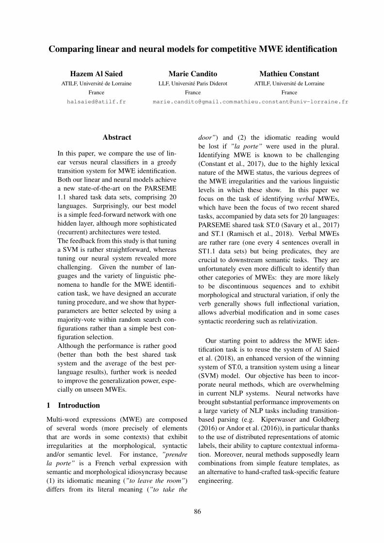
Comparing linear and neural models for competitive MWE identification

Hazem Al SaiedATILF, Universite de Lorraine

France

[email protected]

Marie CanditoLLF, Universite Paris Diderot

France

[email protected]

Mathieu ConstantATILF, Universite de Lorraine

France

[email protected]

Abstract

In this paper, we compare the use of lin-ear versus neural classifiers in a greedytransition system for MWE identification.Both our linear and neural models achievea new state-of-the-art on the PARSEME1.1 shared task data sets, comprising 20languages. Surprisingly, our best modelis a simple feed-forward network with onehidden layer, although more sophisticated(recurrent) architectures were tested.The feedback from this study is that tuninga SVM is rather straightforward, whereastuning our neural system revealed morechallenging. Given the number of lan-guages and the variety of linguistic phe-nomena to handle for the MWE identifi-cation task, we have designed an accuratetuning procedure, and we show that hyper-parameters are better selected by using amajority-vote within random search con-figurations rather than a simple best con-figuration selection.Although the performance is rather good(better than both the best shared tasksystem and the average of the best per-language results), further work is neededto improve the generalization power, espe-cially on unseen MWEs.

1 Introduction

Multi-word expressions (MWE) are composedof several words (more precisely of elementsthat are words in some contexts) that exhibitirregularities at the morphological, syntacticand/or semantic level. For instance, ”prendrela porte” is a French verbal expression withsemantic and morphological idiosyncrasy because(1) its idiomatic meaning (”to leave the room”)differs from its literal meaning (”to take the

door”) and (2) the idiomatic reading wouldbe lost if ”la porte” were used in the plural.Identifying MWE is known to be challenging(Constant et al., 2017), due to the highly lexicalnature of the MWE status, the various degrees ofthe MWE irregularities and the various linguisticlevels in which these show. In this paper wefocus on the task of identifying verbal MWEs,which have been the focus of two recent sharedtasks, accompanied by data sets for 20 languages:PARSEME shared task ST.0 (Savary et al., 2017)and ST.1 (Ramisch et al., 2018). Verbal MWEsare rather rare (one every 4 sentences overall inST1.1 data sets) but being predicates, they arecrucial to downstream semantic tasks. They areunfortunately even more difficult to identify thanother categories of MWEs: they are more likelyto be discontinuous sequences and to exhibitmorphological and structural variation, if only theverb generally shows full inflectional variation,allows adverbial modification and in some casessyntactic reordering such as relativization.

Our starting point to address the MWE iden-tification task is to reuse the system of Al Saiedet al. (2018), an enhanced version of the winningsystem of ST.0, a transition system using a linear(SVM) model. Our objective has been to incor-porate neural methods, which are overwhelmingin current NLP systems. Neural networks havebrought substantial performance improvements ona large variety of NLP tasks including transition-based parsing (e.g. Kiperwasser and Goldberg(2016) or Andor et al. (2016)), in particular thanksto the use of distributed representations of atomiclabels, their ability to capture contextual informa-tion. Moreover, neural methods supposedly learncombinations from simple feature templates, asan alternative to hand-crafted task-specific featureengineering.

86

Yet, using neural methods for our task ischallenging, the sizes of the available corpus arerelatively modest (no ST.1 language has morethan 5000 instances of training MWEs), albeitneural models generally have more parameters tolearn than linear models. Indeed, the best systemsat the shared tasks ST.0 and ST.1 (Al Saied et al.,2017; Waszczuk, 2018) (in closed track) are notneural and surpassed some neural approaches.

In this paper, we carefully describe and com-pare the development and tuning of linear versusneural classifiers, to use in the transition systemfor MWE identification proposed in Al Saied et al.(2018), which itself built on the joint syntactic/ MWE analyzer of Constant and Nivre (2016).We set ourselves the constraints (i) of buildingsystems that are robust across languages, henceusing the same hyperparameter configuration forall languages and (ii) of using lemma and POSinformation but not syntactic parses provided inthe PARSEME data sets, so that the resultingsystems require limited preprocessing. We reporta systematic work on designing and tuning linearand neural transition classifiers, including theuse of resampling, vocabulary generalization andseveral strategies for the selection of the besthyperparameter configuration. We address boththe open and closed tracks of the PARSEME ST.1,i.e with and without external resources (which inour case amount to pre-trained word embeddings).

The contributions of our work are:

• a new state-of-the art for the MWE identifica-tion task on the PARSEME ST1.1 data sets.Our neural model obtains about a four-pointerror reduction on an artificial score mixingthe best results for each language, and 4.5points compared to the best participating sys-tem (even though we do not use syntacticparses);

• a report on which hyperparameters provedcrucial to obtain good performance for theneural models, knowing that a basic feed-forward network without class balancingshowed high instability and achieves verypoorly (average F-score between 15% and30%);

• an alternative strategy for tuning the hyperpa-rameters, based on trends in random search

(Bergstra and Bengio, 2012);

• a fine-grained analysis of the results for vari-ous partitions of the MWE, shedding light onthe necessity to address unknown MWE (notseen in train);

• a negative result concerning the basic semi-supervised strategy of using pre-trained wordembeddings.

We discuss the related work in Section 2, datasets in Section 3 and the transition system in Sec-tion 4. Linear and neural models are describedin Sections 5 and 6, and the tuning methodologyin Section 7. We present experiments and discussresults in Sections 8 and 9, and conclude in Sec-tion 10.

2 Related work

Supervised MWE identification has made sig-nificant progress in the last years thanks to theavailability of new annotated resources (Schneideret al., 2016; Savary et al., 2017; Ramisch et al.,2018). Sequence tagging methods have beenlargely used for MWE identification. In particular,first studies experimented IOB or IOB-like anno-tated corpora to train conditional random fields(CRF) models (Blunsom and Baldwin, 2006;Constant and Sigogne, 2011; Vincze et al., 2011)or other linear models (Schneider et al., 2014).

Recently, Gharbieh et al. (2017) experimentedon the DiMSUM data set various IOB-basedMWE taggers relying on different deep learningmodels, namely multilayer perceptron, recurrentneural networks and convolutional networks.They showed that convolutional networks achievebetter results. On the other hand, Taslimipoor andRohanian (2018) used pre-trained non-modifiableword embeddings, POS tags and other technicalfeatures to feed two convolutional layers withwindow sizes 2 and 3 in order to detect n-grams.The concatenation of the two layers is then passedto a Bi-LSTM layer.Legrand and Collobert (2016) used a phraserepresentation concatenating word embeddings ina fixed-size window, combined with a linear layerin order to detect contiguous MWEs. They reachstate-of-the-art results on the French Treebank(Abeille et al., 2003; Seddah et al., 2013). Ro-hanian et al. (2019) integrate an attention-based

87

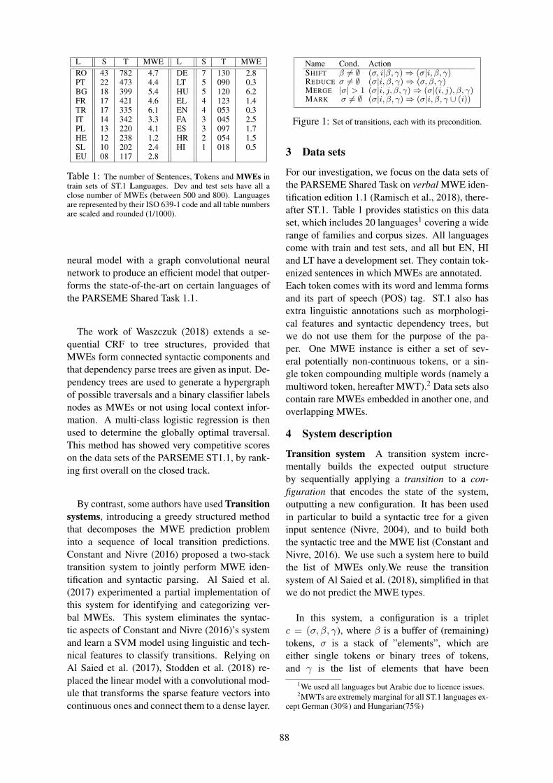
L S T MWE L S T MWERO 43 782 4.7 DE 7 130 2.8PT 22 473 4.4 LT 5 090 0.3BG 18 399 5.4 HU 5 120 6.2FR 17 421 4.6 EL 4 123 1.4TR 17 335 6.1 EN 4 053 0.3IT 14 342 3.3 FA 3 045 2.5PL 13 220 4.1 ES 3 097 1.7HE 12 238 1.2 HR 2 054 1.5SL 10 202 2.4 HI 1 018 0.5EU 08 117 2.8

Table 1: The number of Sentences, Tokens and MWEs intrain sets of ST.1 Languages. Dev and test sets have all aclose number of MWEs (between 500 and 800). Languagesare represented by their ISO 639-1 code and all table numbersare scaled and rounded (1/1000).

neural model with a graph convolutional neuralnetwork to produce an efficient model that outper-forms the state-of-the-art on certain languages ofthe PARSEME Shared Task 1.1.

The work of Waszczuk (2018) extends a se-quential CRF to tree structures, provided thatMWEs form connected syntactic components andthat dependency parse trees are given as input. De-pendency trees are used to generate a hypergraphof possible traversals and a binary classifier labelsnodes as MWEs or not using local context infor-mation. A multi-class logistic regression is thenused to determine the globally optimal traversal.This method has showed very competitive scoreson the data sets of the PARSEME ST1.1, by rank-ing first overall on the closed track.

By contrast, some authors have used Transitionsystems, introducing a greedy structured methodthat decomposes the MWE prediction probleminto a sequence of local transition predictions.Constant and Nivre (2016) proposed a two-stacktransition system to jointly perform MWE iden-tification and syntactic parsing. Al Saied et al.(2017) experimented a partial implementation ofthis system for identifying and categorizing ver-bal MWEs. This system eliminates the syntac-tic aspects of Constant and Nivre (2016)’s systemand learn a SVM model using linguistic and tech-nical features to classify transitions. Relying onAl Saied et al. (2017), Stodden et al. (2018) re-placed the linear model with a convolutional mod-ule that transforms the sparse feature vectors intocontinuous ones and connect them to a dense layer.

Name Cond. ActionSHIFT β 6= ∅ (σ, i|β, γ) ⇒ (σ|i, β, γ)REDUCE σ 6= ∅ (σ|i, β, γ) ⇒ (σ, β, γ)MERGE |σ| > 1 (σ|i, j, β, γ) ⇒ (σ|(i, j), β, γ)MARK σ 6= ∅ (σ|i, β, γ) ⇒ (σ|i, β, γ ∪ (i))

Figure 1: Set of transitions, each with its precondition.

3 Data sets

For our investigation, we focus on the data sets ofthe PARSEME Shared Task on verbal MWE iden-tification edition 1.1 (Ramisch et al., 2018), there-after ST.1. Table 1 provides statistics on this dataset, which includes 20 languages1 covering a widerange of families and corpus sizes. All languagescome with train and test sets, and all but EN, HIand LT have a development set. They contain tok-enized sentences in which MWEs are annotated.Each token comes with its word and lemma formsand its part of speech (POS) tag. ST.1 also hasextra linguistic annotations such as morphologi-cal features and syntactic dependency trees, butwe do not use them for the purpose of the pa-per. One MWE instance is either a set of sev-eral potentially non-continuous tokens, or a sin-gle token compounding multiple words (namely amultiword token, hereafter MWT).2 Data sets alsocontain rare MWEs embedded in another one, andoverlapping MWEs.

4 System description

Transition system A transition system incre-mentally builds the expected output structureby sequentially applying a transition to a con-figuration that encodes the state of the system,outputting a new configuration. It has been usedin particular to build a syntactic tree for a giveninput sentence (Nivre, 2004), and to build boththe syntactic tree and the MWE list (Constant andNivre, 2016). We use such a system here to buildthe list of MWEs only.We reuse the transitionsystem of Al Saied et al. (2018), simplified in thatwe do not predict the MWE types.

In this system, a configuration is a tripletc = (σ, β, γ), where β is a buffer of (remaining)tokens, σ is a stack of ”elements”, which areeither single tokens or binary trees of tokens,and γ is the list of elements that have been

1We used all languages but Arabic due to licence issues.2MWTs are extremely marginal for all ST.1 languages ex-

cept German (30%) and Hungarian(75%)

88

Trans Configuration = (σ, β, γ)Fi(s) ⇒ [ ], [Take, .., account], [ ]SHIFT ⇒ [Take], [the, .., account], [ ]SHIFT ⇒ [Take, the], [fact, .., account], [ ]REDUCE ⇒ [Take], [fact, .., account], [ ]SHIFT ⇒ [Take, fact], [that, .., account], [ ]...SHIFT ⇒ [Take, give], [up, into, account], [ ]SHIFT ⇒ [Take, give, up], [into, account], [ ]MERGE ⇒ [Take, (give, up)], [into, account], [ ]MARK ⇒ [Take, (give, up)], [into, account]

, [(give, up)]REDUCE ⇒ [Take], [into, account], [(give, up)]SHIFT ⇒ [Take, into], [account], [(give, up)]MERGE ⇒ [(Take, into)], [account], [(give, up)]SHIFT ⇒ [(Take, into), account], [ ], [(give, up)]MERGE ⇒ [((Take, into), account)], [ ], [(give, up)]MARK ⇒ [((Take, into), account)], [ ], (give, up),

((Take, into), account)]REDUCE ⇒ [ ], [ ], [(give, up), ((Take, into), account)]

Figure 2: Application of the oracle transition sequence forthe sentence Take the fact that I didn’t give up into account,containing two verbal MWEs: Take into account and give up.

identified as MWEs so far3. To build the list ofMWEs for a given input sentence w1, w2, ...wn,the system starts by the initial configuration(σ = [ ], β = [w1, ..., wn], γ = [ ]), and appliesa sequence of transitions until a terminal config-uration is reached, namely here when both thebuffer and stack are empty. The transition set,and their precondition is described in Figure 1.Note the MERGE transition creates complex stackelements, by merging the top 2 elements of thestack4.

The identification of a MWE made of m com-ponents t1, ..., tm necessitates m − 1 MERGEs,and one final MARK. The REDUCE transitionallows to manage discontinuities in MWEs. Notethat MARK identifies S0 as MWE, but doesnot remove it from the stack, hence enabling toidentify some cases of embedded MWEs (werefer to Al Saied et al. (2018) for the preciseexpressive power). At prediction time, we usea greedy algorithm in which the highest-scoringapplicable transition according to a classifier isapplied to the current configuration.

Learning algorithm and oracle To learn this3In all the following, we use σ|i to denote a stack with

top element i and remainder σ, and i|β for a buffer with firsttoken i followed by the elements in β. Si and Bi denote theith element of the stack and buffer respectively, starting at 0.

4Hence Si elements are either single tokens or binarytrees of tokens. In the latter case, their linguistic attributes(lemma, POS, word form) are obtained by simple concatena-tion over their components.

Tuning BoR TB Feature templatePrelim + + Unigrams S0, S1, B0

Prelim + + Bigrams S0S1, S0B0, S0B1, S1B0

Prelim + + Lemma ngrams and POS ngramsPrelim + + S0 in MWT dictionaryPrelim - - ResamplingRdm Sch - - word forms ngramsRdm Sch + - Unigram B1

Rdm Sch + - Bigram S0B2

Rdm Sch + - Trigram S1S0B0

Rdm Sch + + Distance between S0 and S1

Rdm Sch + + Distance between S0 and B0

Rdm Sch + - MWE component dictionaryRdm Sch - - Stack lengthRdm Sch + + Transition history (length 1)Rdm Sch - + Transition history (length 2)Rdm Sch + - Transition history (length 3)FG 62.5 60

Table 2: Linear model feature hyperparameters. First col-umn: prelim if the hyperparameter was fixed once and for allgiven preliminary tests vs. Rdm Sch for tuning via randomsearch (see Section 7). Best of random BoR column: whetherthe template is activated (+) or not (-) in the best performinghyperparameter set of the random search. Trend-based TB:same but for the trend-based hyperparameter set (cf. sec-tion 7). The last line provides the corresponding global F-scores on dev sets of the three pilot languages (BG, PT andTR).

transition classifier, we use the static deterministicoracle of Al Saied et al. (2018). For any inputsentence and list of gold MWEs, the oracledefines a unique sequence of transitions, pro-viding example pairs (config / next transition toapply). Transitions have a priority order (MARK

> MERGE > REDUCE > SHIFT), and the oraclegreedily applies the highest-priority transition thatis compatible with the gold analysis. MERGE

is gold-compatible whenever S0 and S1 are partof the same gold MWE.5 For REDUCE to begold-compatible, S0 must not be strictly includedin a gold MWE. Moreover, either S0 is not a goldMWE, or it is already marked as MWE.

Figure 2 shows the application of the ora-cle transition sequence for a sentence with twoMWEs.6

5 Linear model

In order to compare linear and neural modelsfor MWE identification, we reused the best

5Note that this order will lead to left-branching binarytrees for elements in the stack.

6The system is implemented in Python 2.7, usingKeras and Scikit-learn libraries. The code is availableat https://github.com/hazemalsaied/MWE.Identification/releases/tag/v.1 under MITlicence.

89

performing linear model of Al Saied et al. (2018),namely a SVM, in a one versus rest scheme withlinear kernel and squared hinge loss.

We used the feature templates of Al Saiedet al. (2018) minus the syntactic features, sincewe focus on MWE identification independentlyof syntactic parsing. Table 2 displays the list offeature templates. We detail the ”S0 in MWTdictionary” and ”MWE component dictionary”templates, the other features names being rathertransparent: ”S0 in MWT dictionary” feature fireswhen S0 lemma is a MWT at least once in train,and binary features fire when either S0, S1, B0,B1 or B2 belong to at least one train multi-tokenMWE.

We ran some preliminary experiments whichled us to set some hyperparameters once and for all(first four lines of Table 2). In particular, we endedup not using resampling to balance the class distri-bution, because it proved quite detrimental for thelinear model, contrary to the neural models. Wethen performed tuning for all the other features (cf.section 7).

6 MLP model

Though we investigated various neural archi-tectures7, the ”baseline” multi-layer perceptron(hereafter MLP) proved to be the best in theend. It is a plain feed-forward network, with anembedding layer concatenating the embeddingsfor the POS of S0, S1, B0 and B1 and for eithertheir word form or lemma (hyperparameter), fullyconnected to a dense layer with ReLU activation,in turn connected to the output layer with softmaxactivation.

Table 3 provides the exhaustive list of MLPhyperparameters, along with their possible valuesand their optimal values for the most performing

7We tried in particular (1) a MLP with several hidden lay-ers; (2) a MLP fed with a bidirectional recurrent layer to rep-resent the sequence of elements S0S1B0; (3) We also built amodel inspired by Kiperwasser and Goldberg (2016) in whichthe recurrent (LSTM) embeddings of certain focus elements(S0, S1, B0 and B1) are dynamically concatenated and fedinto a MLP, with back-propagation for a whole sentence in-stead of for each transition. The recurrent representations ofthe focus elements are supposed to encode the relevant con-textual information of these elements in the sentence. Thesemodels suffered from either a non-competitive performanceor a very unstable loss (36.7 for the bidirectional MLP and8.4 for kiperwasser on test data sets of ST1.1).

configurations. Lines 1 to 9 correspond to embed-ding and initialization hyperparameters: Lines (1,2) concern which elements to include as additionalinput (Use B2, Use B−1)8, (3) which form forinput tokens (Lemmatization), (4, 5) which sizefor token and POS tag embeddings (Token andPOS dimensions), (6) whether the embeddings areinitialized randomly or pre-trained (pre-trained),(7) whether the embeddings are Trainable ornot, and (8) how to generate embedding vectorsfor stack elements: as the average of tree tokenembeddings or as their sum (Averaging).

Vocabulary For the neural model, when Sior Bi are missing, a special dummy word is usedinstead. Moreover, we investigated an aggressivereduction of the known vocabulary. We compared2 strategies to define it: in exhaustive vocabularymode, hapaxes are replaced at training time by aUNK symbol, with probability 0.5. In compactvocabulary mode, any token (or complex element)whose lemma is never a component of a MWE inthe training set is replaced by UNK. Note that inboth modes, the used vocabulary contains the con-catenated symbols in case of complex Si elements.

Resampling Given that tokens are mostly notpart of a VMWE, the transitions for their identi-fication are very rare, leading to a very skewedclass distribution.9 Resampling techniques aimingat balancing class distribution are known to beefficient in such a case (Chawla, 2009). Moreover,preliminary experiments without resamplingshowed unstable loss and rather low performance.We thus used in subsequent experiments a hy-brid resampling method composed of (1) undersampling, that removes training sentences noncontaining any MWE, and (2) random over-sampling, that forces a uniform distribution ofthe classes by randomly duplicating minorityclass instances (all but SHIFT) (Chawla, 2009).Preliminary experiments showed that withoutthese strategies, the systems suffered from veryunstable loss and low performance, which led usto systematically use these two strategies in thesubsequent experiments.

8 B−1 is the last reduced element (its right-most token ifit is a complex stack element).

9For all ST.1 languages, the transitions in training sets areapproximately distributed as follows: 49% for SHIFT, 47%for REDUCE, 3% for MERGE and 1% for MARK.

90

Type Hyperparameter Range or set BoRc BoRo TB

Em

bedd

ing

and

initi

alis

atio

n Use B2 {True, False} True True TrueUse B−1 {True, False} True False TrueLemmatization {True, False} True True TrueToken dimension [100, 600] 157 300 300POS dimension [15, 150] 147 132 35Pre-trained {True, False} False True True | FalseTrainable {True, False} True True TrueAveraging {True, False} False True TrueVocabulary {Compact, Exhaustive} True False True

DenseUnit number [25, 600] 85 56 75Dropout {.1, .2,.. .6} 0.3 0.1 0.4

SamplingFocused / Frequency threshold {True, False} / {5, 10,.. 30} False / - False / - False / -Over loss / Loss coefficient {True, False} / [1, 40] False / 1 False / 1 False / 1

TrainLearning rate [.01, .2] 0.017 0.095 0.03Batch size {16, 32, 48, 64, 128} 128 16 48

FG on all languages (on dev sets if available or 20% of train) 61.2 57.8 63.5 | 64.3

Table 3: MLP hyperparameters and their possible values (”range or set” column). Best-of-random closed (BoRc) and Best-of-random open (BoRo) columns: hyperparameter values in best configurations according to random search on the three pilotlanguages, in closed and open tracks. Last column: Trend-based (TB) configuration (see text in section 7). Last line: globalF-scores for these configurations, calculated using the average precision and recall for all ST.1 languages. The models are fiton truncated training sets of the three pilot languages (BG, PT and TR) (cf. section 7).

Tuning explored two supplementary resamplingtechniques: ”focused” oversampling which aimsat mimicking a minimum number of occurrencesfor all MWEs. When set, training instances withMERGE and MARK transitions are duplicated foreach training MWE below a frequency threshold.”Over loss” hyperparameter penalizes the modelwhen it fails to predict MERGE and MARK, bymultiplying the loss by a coefficient (see Table 3).

7 Tuning methodology

The tuning phase served us to choose a hyperpa-rameter configuration for the linear model and theneural model, in closed and open track. In ourcase, we experimented open track for the neuralmodel only, by using pre-trained embeddingsinstead of random initialization. We thus considerthree cases: closed track linear, closed track MLPand open track MLP.

For each of these three cases, in order to enforcethe robustness across languages of the selected hy-perparameters, we aimed at selecting the same hy-perparameter configuration for all the languages.

Yet, to reduce the tuning time, we have chosento work on three pilot languages, from threedifferent language families. But because thevarious training sets have various sizes, we triedto neutralize this variation by using training setsof average size. This led us to choose threelanguages (Bulgarian, Portuguese and Turkish)among ST.1 languages having training sets bigger

than average and to tune the hyperparametersusing training sets truncated to that average size(270k tokens) and evaluating on dev sets.

Multilingual metric: the official metric for thePARSEME shared task is the macro average ofthe F-scores over all languages (hereafter FAV G).Yet we noted that although macro-averagingprecision and recall is appropriate because thenumber of dev and test MWEs is almost thesame for all languages, averaging the F-scoresof all languages sometimes substantially differs(e.g. by 2 points) from taking the F-score of themacro-averaged precision and the macro-averagedrecall (hereafter FG). We thus use FAV G forcomparability with the shared task results, butalso report the FG score, and use the latter duringtuning.

Random search: To tune the hyperparame-ters on the three pilot languages, we used randomsearch, which proved to be more efficient thangrid search when using the same computationalbudget, because it allows to search larger rangesof values (Bergstra and Bengio, 2012). We thusrun about 1000 trials for SVM, closed track MLPand open track MLP. For the SVM, random searchused a uniform distribution for the hyperparam-eters, which are all boolean. For the MLP, therandom hyperparameter values are generated fromeither a set of discrete values using a uniformdistribution or from a range of continuous values

91

using logarithmic distribution. For the MLP, eachresulting random hyperparameter configurationwas run on each pilot language twice, usingalways the same two seeds 0 and 110. We thenaveraged the precision and recall on the dev sets,for the three languages and the two seeds (i.e. usethe global F-score FG).

Selecting hyperparameter configurations:Random hyperparameter search for the three pilotlanguages led us to use two strategies to selectthe hyperparameter sets. The first one is simplyto select the best performing hyperparameter sets(shown in column BoR in Table 2 for the linearmodel, and in the BoRc and BoRo columns in Ta-ble 3). Yet, we noted that some hyperparametersvaried a lot among the top performing systems.We thus investigated to build a ”trend-based”configuration, by selecting each hyperparametervalue according to the observed trend among thetop k best configurations (with k=500/250 forMLP/SVM)11. This results in two sets for thelinear model (best-of-random and trend-based,in closed mode) and four configurations for theMLP: best-of-random or trend-based, in closed oropen mode.

We then trained these six configurations on thefull-size training sets for all ST.1.1 languages,using two seeds (0 and 1), and retaining the bestseed for each language. For the MLP case, theglobal F-scores on dev sets are provided in thelast row of Table 3. Interestingly, the trend-basedconfiguration largely beats the best-of-randomconfigurations, both in closed and open tracks12.This shows that choosing hyperparameter valuesindependently of each other is compensated bychoosing more robust values, by using the top kbest performing systems instead of one.

Note that for the linear case, the trend-basedconfiguration does not surpass the best perform-ing random search configuration (the last line of

10Preliminary experiments showed a relative stabilitywhen changing seeds, hence we used only two seeds in theend. Changing seeds was useless for the linear model whichis more stable.

11We chose the values using an approximate majority vote,using a graphical visualization of the hyperparameter valuesin the top k best performing systems.

12Moreover, the best-of-random open configurationshowed instability when switching from the three pilot lan-guages to all languages, leading to a null score for Hindi(hence the rather low global F-score of 57.8).

Language Closed track Open trackSVM MLPc ST.1 MLPo ST.1

BG 63.3 66.8 62.5 67.7 65.6HR 55.4 59.3 55.3 59.0 47.8LT 38.0 45.7 32.2 45.3 22.9PL 69.4 71.8 67.0 72.2 63.6SL 53.5 62.7 64.3 61.2 52.3DE 49.5 51.5 45.3 49.9 45.5EN 28.4 31.4 32.9 31.9 33.3ES 39.2 40.0 34.0 39.7 38.4FR 61.1 59.0 56.2 58.8 60.9IT 55.7 55.0 49.2 56.5 45.4PT 68.9 67.8 62.1 70.4 68.2RO 80.9 83.5 85.3 82.0 87.2HI 66.8 64.9 73.0 64.9 72.7FA 75.4 70.6 77.8 70.6 78.4EL 57.8 62.2 49.8 61.4 58.0EU 80.7 82.1 75.8 80.2 77.0HE 43.3 45.2 23.3 47.3 38.9HU 91.7 92.4 90.3 92.6 85.8TR 47.5 52.1 45.2 47.9 58.7

FAV G 59.3 61.3 56.9 61.0 57.9FG 60.8 62.6 57.8 62.3 58.7

FG best sys 54.0 58.1

Table 4: MWE-based F-scores for ST.1 languages on testsets using our tuned SVM and MLP models, fit on train anddev sets when available. ST.1 stands for the most perform-ing scores of the shared task for each language in closed andopen tracks. All ST.1 systems fit training and developmentsets except the system that produced the best score of BGon closed track. Languages are grouped according to theirlinguistic families (Slavic, Germanic, Romance, Indo-Iranianand other).) FAV G is the official metric (average F-scores).FG is the global F-score (see Section 7). In the FAV G andFG lines, the best ST.1 per-language scores are used, whereasthe last line concerns the FG score of the best ST.1 systems(Waszczuk, 2018; Taslimipoor and Rohanian, 2018).

Table 2). This asymmetry could mean that thenumber of random trials is sufficient for the lin-ear case, but not for the neural models, and that atrend-based strategy is advantageous within a lim-ited computational budget.

8 Experiments and results

Table 4 provides identification scores on test sets,for our tuned SVM and MLP models for eachST.1 language, along with the best score of ST.1for each language, in open and closed tracks. Italso displays overall scores using both the officialST.1 metrics (FAV G) and the more precise FG

score introduced in section 7. This FG score forthe ST.1 results is computed in two modes: in lineFG, the ST.1 columns correspond to artificiallyaveraging the best result of each language (inclosed / open tracks), whereas ”FG best sys” is thescore of the best system of ST.1. The differencesbetween SVM and MLPc results are significant13

13We used a MWE-based McNemar test.

92

for all languages except EU, HU, LT and PL.

For both FAV G and FG metrics, results showthat MLP models significantly outperforms allother systems both in the closed and open tracks.In the closed track, MLP surpasses SVM by 1.8points, the best ST.1 systems per language by4.8 points, and the best ST.1 system (Waszczuk,2018) by 8.6 points. In the open track, MLP beatsthe best ST.1 system (Taslimipoor and Rohanian,2018) by 4.2 points, and the best ST.1 systems perlanguage by 3.6 points14.

In the closed track, MLP ranks first for 11languages, while the SVM model and the bestST.1 systems per language reach the first positionrespectively for three and five languages. Inopen track, MLP achieves the highest scores for13 languages while ST.1 systems beat it for sixlanguages. These results tend to validate therobustness of our approach across languages.Regarding language families, MLP reportsremarkable gains for Slavic languages and lan-guages from the other family, but achieve lowerperformance on Indo-Iranian languages whencompared with best ST.1 results. For Romancelanguages, our models surpass the ST.1 bestresults (except for RO), and the SVM model isglobally better than the MLP.

Comparing the results of the open and theclosed track, we can observe that the use of pre-trained word embeddings has no significant im-pact on the MLP results. This might mean thatstatic embeddings are not well-suited for repre-senting tokens both when used literally and withinMWE. This tendency would deserve more investi-gation using other word embedding types, in par-ticular contextualized ones (Devlin et al., 2018).

9 Discussion

Performance analysis In order to better under-stand the strengths and weaknesses of the varioussystems, we provide in Table 5 an in-depthperformance analysis of our models, on dev sets,broken-down by various classifications of MWEs,

14It is worth noting that the model of Rohanian et al.(2019), published while writing this paper, outperforms ourscores for the languages they use for evaluating their model(EN:41.9, DE:59.3, FR:71.0, FA:80.0) on the ST.1 test sets.However, this model exploits syntactic information (See Sec-tion 2).

namely (1) whether a dev MWE was seen in train(and if so, more than 5 times or not) or unseen;(2) whether the MWE is continuous or has gaps;and (3) according to the MWE length. Thetable provides the proportions of each subclasswithin the gold dev set and within the predictionsof each model (% columns), in addition to theaverage precision and recall over all languages,and the global FG score, for each model. Overall,neural models (in closed and open tracks) tendsto get better recall than the SVM model (56and 57, versus 49) but lower precision (70 versus86), which is coherent with the use of embeddings.

Generalization power Without surprise, theglobal F-score on seen MWEs is high for all oursystems (> 80), and it is still above 75 for MWEswith frequency≤ 5. Yet this masks that the neuralmodels have comparable precision and recallon seen MWEs, whereas the SVM has betterprecision than recall. Now when turning to theunseen category, we can observe that all systemsget very low performance.

In comparison with MLP models, the mostimportant advantage of SVM is its (little) abilityto generalize (FG = 12 on unseen MWEs),whereas the MLPs have none at all. Note thatfrequency ≤ 5 is sufficient for the MLP modelsto surpass the linear model. For comparison, theaverage F-scores on test sets of the PARSEMEST.1 for unseen MWEs range from 0 to almost 20.This very low generalization of our MLP modelsis understandable since tuning led us to favorthe compact vocabulary mode, which agressivelyreduces the known vocabulary to seen MWEcomponents. Yet our best result on unseen MWEswith a MLP with exhaustive vocabulary modeonly achieves FG = 4 on unseen MWEs.

It appears that for all models, more than 90%of the unindentified MWEs (the silence) are eitherunseen or with frequency ≤ 5, which clearlyshows that the frequency of a MWE in train set isthe crucial trait for identification. Further analysisis needed to study the performance according tothe literal versus MWE ambiguity rate.

Continuous/discontinuous MWEs MLPmodels show better performances for discon-tinuous MWEs than SVM, whereas they reach

93

Type % SVM MLPo MLPc

% FG P R % FG P R % FG P RAll - - 63 86 49 - 62 70 56 - 63 70 57Seen 63 93 80 89 72 99 81 83 80 98 82 82 82- Freq > 5 26 37 80 84 77 37 82 81 82 36 81 81 82- Freq <= 5 38 56 75 86 67 62 77 79 76 61 78 79 77Unseen 37 7 12 44 7 1 0 7 0 2 2 10 1Contin. 67 77 69 88 57 75 69 84 59 74 70 83 60Discont. 33 23 45 78 31 25 50 77 37 26 50 75 37Length 1 (MWT) 6 7 84 93 77 7 82 89 77 7 84 91 78Length 2 78 84 64 86 51 85 65 82 54 85 66 81 56Length 3 13 8 40 66 29 7 40 69 28 7 40 66 29

Table 5: Performance of our tuned models, on all languages, with models fit on train and evaluated on dev sets if available,otherwise fit on 80% of train and evaluated on the rest (with seed 0 for MLP models). First line: performance on all languages.Subsequent lines: break-down according to various MWE classifications (first column). Second column: proportion of thesubclass in gold dev set. For each model (SVM, MLPo(open) and MLPc(losed)), we report for each subclass: the proportion ofthe subclass in the system prediction, the global F-score (FG), Precision (P) and Recall (R).

comparable scores for continuous MWEs. Inparticular, they display a 5-point gain in F-score,due to a 6-point gain in recall on discontinuousMWEs.

MWE length The three systems display com-parable scores regarding MWE length. Resultsvalidate the intuition that the shorter the MWE, theeasier it is to identify.

10 Conclusion

We described and compared the development oflinear versus neural classifiers to use in a transitionsystem for MWE identification (Al Saied et al.,2018). Surprisingly, our best neural architectureis a simple feed-forward network with one hiddenlayer, although more sophisticated architectureswere tested. We achieve a new state-of-the arton the PARSEME 1.1 shared task data sets,comprising 20 languages.Our neural and linear models surpass both thebest shared task system (Waszczuk, 2018) and theartificial average of the best per-language results.Given the number of languages and the varietyof linguistic phenomena to handle, we designed aprecise tuning methodology.Our feedback is that the development of the linear(SVM) system was pretty straightforward, withlow variance between the configurations. Forthe neural models on the contrary, preliminaryruns led to low and unstable performance. Classbalancing proved crucial, and our proposal toselect hyperparameter values using majority voteon the top k best performing systems in randomsearch also proved beneficial.

Although our systems are competitive, theirgeneralization power reveals disappointing: per-formance on unseen MWEs is very low for thelinear model (F-score=12) and almost zero for theneural models (whereas the shared task resultsrange from 0 to 20 for unseen MWEs). Basicsemi-supervised experiments, consisting in usingpre-trained word embeddings, did not bring anyimprovement. Static embeddings might not besuitable representations of MWE components, astheir behavior differs when used literally or withina MWE. This definitely calls for future work thatcan incorporate information on semantic irregular-ity.

Acknowledgement

This work was partially funded by the French Na-tional Research Agency (PARSEME-FR ANR-14-CERA-0001).

94

ReferencesAnne Abeille, Lionel Clement, and Francois Toussenel.

2003. Building a treebank for French. In AnneAbeille, editor, Treebanks. Kluwer, Dordrecht.

Hazem Al Saied, Marie Candito, and Matthieu Con-stant. 2017. The ATILF-LLF system for parsemeshared task: a transition-based verbal multiword ex-pression tagger. In Proceedings of the 13th Work-shop on Multiword Expressions (MWE 2017), pages127–132, Valencia, Spain. Association for Compu-tational Linguistics.

Hazem Al Saied, Marie Candito, and Matthieu Con-stant. 2018. A transition-based verbal multiwordexpression analyzer. In Multiword expressions atlength and in depth: Extended papers from the MWE2017 workshop, volume 2, page 209. Language Sci-ence Press.

Daniel Andor, Chris Alberti, David Weiss, AliakseiSeveryn, Alessandro Presta, Kuzman Ganchev, SlavPetrov, and Michael Collins. 2016. Globally nor-malized transition-based neural networks. arXivpreprint arXiv:1603.06042.

James Bergstra and Yoshua Bengio. 2012. Randomsearch for hyper-parameter optimization. Journal ofMachine Learning Research, 13(Feb):281–305.

Phil Blunsom and Timothy Baldwin. 2006. Multilin-gual deep lexical acquisition for hpsgs via supertag-ging. In Proceedings of the 2006 Conference onEmpirical Methods in Natural Language Process-ing, pages 164–171, Sydney, Australia. Associationfor Computational Linguistics.

Nitesh V Chawla. 2009. Data mining for imbalanceddatasets: An overview. In Data mining and knowl-edge discovery handbook, pages 875–886. Springer.

Mathieu Constant, Gulsen Eryigit, Johanna Monti,Lonneke Van Der Plas, Carlos Ramisch, MichaelRosner, and Amalia Todirascu. 2017. Multiword ex-pression processing: A survey. Computational Lin-guistics, 43(4):837–892.

Matthieu Constant and Joakim Nivre. 2016. Atransition-based system for joint lexical and syn-tactic analysis. In Proceedings of the 54th An-nual Meeting of the Association for ComputationalLinguistics (Volume 1: Long Papers), pages 161–171, Berlin, Germany. Association for Computa-tional Linguistics.

Matthieu Constant and Anthony Sigogne. 2011. Mwu-aware part-of-speech tagging with a crf model andlexical resources. In Proceedings of the Workshopon Multiword Expressions: from Parsing and Gen-eration to the Real World, pages 49–56. Associationfor Computational Linguistics.

Jacob Devlin, Ming-Wei Chang, Kenton Lee, andKristina Toutanova. 2018. BERT: pre-training ofdeep bidirectional transformers for language under-standing. CoRR, abs/1810.04805.

Waseem Gharbieh, Virendrakumar Bhavsar, and PaulCook. 2017. Deep learning models for multiwordexpression identification. In Proceedings of the6th Joint Conference on Lexical and ComputationalSemantics (*SEM 2017), pages 54–64, Vancouver,Canada. Association for Computational Linguistics.

Eliyahu Kiperwasser and Yoav Goldberg. 2016. Sim-ple and accurate dependency parsing using bidirec-tional lstm feature representations. arXiv preprintarXiv:1603.04351.

Joel Legrand and Ronan Collobert. 2016. Phrase rep-resentations for multiword expressions. In Proceed-ings of the 12th Workshop on Multiword Expres-sions, pages 67–71, Berlin, Germany. Associationfor Computational Linguistics.

Joakim Nivre. 2004. Incrementality in determinis-tic dependency parsing. In Proceedings of theACL Workshop Incremental Parsing: Bringing En-gineering and Cognition Together, pages 50–57,Barcelona, Spain. Association for ComputationalLinguistics.

Carlos Ramisch, Silvio Cordeiro, Agata Savary,Veronika Vincze, Verginica Mititelu, Archna Bhatia,Maja Buljan, Marie Candito, Polona Gantar, VoulaGiouli, et al. 2018. Edition 1.1 of the parsemeshared task on automatic identification of verbalmultiword expressions. In the Joint Workshop onLinguistic Annotation, Multiword Expressions andConstructions (LAW-MWE-CxG-2018), pages 222–240.

Omid Rohanian, Shiva Taslimipoor, SamanehKouchaki, Le An Ha, and Ruslan Mitkov. 2019.Bridging the gap: Attending to discontinuity inidentification of multiword expressions. arXivpreprint arXiv:1902.10667.

Agata Savary, Carlos Ramisch, Silvio Cordeiro, Fed-erico Sangati, Veronika Vincze, Behrang Qasem-iZadeh, Marie Candito, Fabienne Cap, Voula Giouli,and Ivelina Stoyanova. 2017. The parseme sharedtask on automatic identification of verbal multiwordexpressions.

Nathan Schneider, Emily Danchik, Chris Dyer, andNoah A. Smith. 2014. Discriminative lexical se-mantic segmentation with gaps: running the MWEgamut. TACL, 2:193–206.

Nathan Schneider, Dirk Hovy, Anders Johannsen, andMarine Carpuat. 2016. Semeval-2016 task 10: De-tecting minimal semantic units and their meanings(dimsum). In Proceedings of the 10th InternationalWorkshop on Semantic Evaluation (SemEval-2016),pages 546–559.

Djame Seddah, Reut Tsarfaty, Sandra Kubler, MarieCandito, Jinho D. Choi, Richard Farkas, Jen-nifer Foster, Iakes Goenaga, Koldo Gojenola Gal-letebeitia, Yoav Goldberg, Spence Green, NizarHabash, Marco Kuhlmann, Wolfgang Maier, Joakim

95

Nivre, Adam Przepiorkowski, Ryan Roth, WolfgangSeeker, Yannick Versley, Veronika Vincze, MarcinWolinski, Alina Wroblewska, and Eric Villemontede la Clergerie. 2013. Overview of the SPMRL 2013shared task: A cross-framework evaluation of pars-ing morphologically rich languages. In Proceed-ings of the Fourth Workshop on Statistical Parsing ofMorphologically-Rich Languages, pages 146–182,Seattle, Washington, USA. Association for Compu-tational Linguistics.

Regina Stodden, Behrang QasemiZadeh, and LauraKallmeyer. 2018. Trapacc and trapaccs at parsemeshared task 2018: Neural transition tagging of ver-bal multiword expressions. In Proceedings of theJoint Workshop on Linguistic Annotation, Multi-word Expressions and Constructions (LAW-MWE-CxG-2018), pages 268–274.

Shiva Taslimipoor and Omid Rohanian. 2018. Shomaat parseme shared task on automatic identifica-tion of vmwes: Neural multiword expression tag-ging with high generalisation. arXiv preprintarXiv:1809.03056.

Veronica Vincze, Istvan Nagy, and Gabor Berend.2011. Multiword expressions and named entities inthe Wiki50 corpus. In Proc. of RANLP 2011, pages289–295, Hissar.

Jakub Waszczuk. 2018. Traversal at parseme sharedtask 2018: Identification of verbal multiwordexpressions using a discriminative tree-structuredmodel. In Proceedings of the Joint Workshop onLinguistic Annotation, Multiword Expressions andConstructions (LAW-MWE-CxG-2018), pages 275–282.

96

Syntax-based identification of light-verb constructions

Silvio Ricardo CordeiroLLF, Université Paris Diderot

Paris, [email protected]

Marie CanditoLLF, Université Paris Diderot

Paris, [email protected]

Abstract

This paper analyzes results on light-verbconstruction identification, distinguishingbetween known cases that could be di-rectly learned from training data from un-known cases that require an extra level ofsemantic processing. We propose a simplebaseline that beats the best results of thePARSEME 1.1 shared task (Savary et al.,2018) for the known cases, and couple itwith another simple baseline to handle theunknown cases. We additionally presenttwo other classifiers based on a richer setof features, with results surpassing thesebest results by 7 percentage points.

1 Introduction

Light-verb constructions (LVCs), such as the ex-pression pay visit, are a linguistic phenomenoncoupling a verb and a stative or eventive noun,in which the verb itself is only needed for mor-phosyntactic purposes, its syntactic dependentsbeing semantically related to the noun. For in-stance in the sentence John paid me a visit, thesubject and object of paid play the roles of the vis-itor and the visited. The verb’s semantics is eitherbleached or redundant with that of the noun (as incommit crime) (Savary et al., 2018).This mismatch between syntax and semantics hasto be taken care of for semantically-oriented tasksto recover the full predicate-argument structure ofthe noun, since at least one of its semantic argu-ments of the noun is generally attached to the verbin plain syntactic treebanks.1 Moreover, the fact

1For instance, Nivre and Vincze (2015) report that for themajority of the 18 UD languages at that time, in a structurelike X takes a photo of Y in English, X is attached to theverb, but the Y argument is attached to the noun. In someannotation schemes, the Y would be attached to the verb too.Note though that some treebanks do annotate the LVC status(e.g. in Hungarian). Additional semantic annotation of LVCcan be found e.g. in propbank (Bonial and Palmer, 2016).

that the verb choice is conventionalized and se-mantically bleached makes LVC identification animportant requirement in semantic tasks such asmachine translation (Cap et al., 2015).

Because of their syntactico-semantic charac-teristics, LVCs are generally considered diffi-cult to circumscribe and annotate consistently(Bonial and Palmer, 2016). Yet recently, thePARSEME 2018 shared-task has brought forth acollection of corpora containing verbal multiwordexpression (VMWE) annotations across 19 lan-guages (Ramisch et al., 2018), including LVCs.The reported inter-annotator agreement is variableacross languages, but the macro-averaged chance-corrected kappa is overall 0.69, which is generallyconsidered to denote a good agreement. In the an-notated corpora, the category of LVCs2 accountedfor a third of all expressions (Savary et al., 2018).The annotation was performed in a separate layer,largely independent from the underlying syntacticframework, and relied on semantic properties ofthe verb (bleached or redundant in the given con-text) and both semantic and syntactic properties ofthe noun: it should be stative or eventive and takeat least one semantic argument, and it should bepossible to have all the syntactic arguments of theverb realized within a NP headed by the noun (forinstance out of John paid me a visit, one can createthe NP John’s visit to me).

A total of 13 systems participated in thePARSEME shared-task, predicting VMWEs oc-currence in the test corpora. Results for each sys-tem varied across different systems and target lan-guages, in which expressions that had been seenin the test corpus were predicted with variable ac-curacy. However, expressions that had never beenseen in the test corpus were hardly ever predictedby most systems (the best F-score on unseen-

2Unless otherwise stated, this paper refers to the 1.1edition of the PARSEME shared task, and to the categoryLVC.full (as opposed to LVC.cause).

97

in-train expressions in the closed track is below20%).

In this paper, we investigate the task of LVCidentification in running text. The main contribu-tions of this paper are: (1) we propose handlingthe task of LVC identification differently depend-ing on whether it was seen in the training corpus;(2) we present a simple baseline that surpasses allsystems for seen LVCs; (3) we propose and eval-uate different techniques for the prediction of un-seen LVCs, which we then compare to the state ofthe art.

The remainder of this paper is structured as fol-lows: Section 2 presents the related work; Sec-tion 3 describes the methodology that will be em-ployed; Section 4 describes the results; and finally,Section 5 presents our conclusions.

2 Related Work

LVC identification may follow one of two strate-gies: (a) LVC candidates are initially proposedbased on lexicosyntactic patterns, and are thenclassified as LVC or non-LVC based on other cri-teria; (b) a variant of the BIO scheme (Ramshawand Marcus, 1999) is employed so as to directlyclassify each token as belonging or not to an LVC.The former method allows the use of features thatencompass the LVC as a whole, while the lattercan be more easily implemented in the frameworkof some machine learning algorithms.

Most works in the literature concerning LVCidentification focus on annotations in a particu-lar language, often with a language-specific under-standing of LVCs. Vincze et al. (2013) adapt a de-pendency parser so as to identify Hungarian LVCcandidates as a byproduct of parsing, which theythen evaluate on the Szeged Dependency Treebankwith LVC annotations. Nagy T. et al. (2013) ex-tract English LVC candidates involving a verb anda dependent noun with a specific dependency la-bel. A J48 and an SVM classifier are then consid-ered, using lexical and morphosyntactic featuresfrom the corpus, as well as semantic features fromWordNet. The latter was found to contribute tobetter results when compared to earlier works thatrelied purely on morphosyntactic and statisticalfeatures (Tu and Roth, 2011). Chen et al. (2015)detect English LVCs in the BNC and OntoNotescorpora, using the PropBank layer to select LVCcandidates composed of an eventive noun linkedone of 6 known light verbs. The candidates are

then filtered based on semantic features, includingWordNet synsets and hypernym relations.

More recently, the PARSEME shared-task saw13 system submissions that tried to predict LVCsalong with other VMWEs for annotated corporain 19 languages (Ramisch et al., 2018). Over-all, the best F1 scores across all languages in theopen track were obtained by the SHOMA system,which employed a pipeline of CNNs, a Bi-LSTM,and and optional CRF layer (Taslimipoor and Ro-hanian, 2018). MWE prediction followed a variantof the BIO scheme that allowed multiple tags pertoken, with input features including a set of pre-trained embeddings (leading the system to com-pete in the open track category), POS tags, and aset of word-shape features.

In the closed track, the TRAVERSAL systemobtained the best overall results for MWEs in gen-eral as well as for LVCs. It uses a syntax-based ap-proach, in which each node in the syntax tree wasclassified as part of an MWE or not (Waszczuk,2018). The classifier resembles a second-orderCRF, but rather than considering the previous 2 to-kens at each point, it considers the parent and left-sibling. Features included the lemma, POS tag anddependency relation.

Rather than predicting each token as being partof an LVC or not, the varIDE system use a NaiveBayes classifier to tag LVC candidates (Pasqueret al., 2018). These were extracted based on allpossible token combinations whole multi-set oflemmas corresponded to an LVC that had beenseen in the training corpus (no attempts were madeat predicting unseen LVCs). Classifier features in-cluded POS tags and morphological information.

Graph convolutional neural networks have alsobeen used in the identification of VMWE can-didates for subsequent classification (Rohanianet al., 2019). In this work, the network is com-bined with an attention mechanism so as to im-prove the accuracy of long-range predictions, anda Bi-LSTM layer is used to classify these predic-tions and produce the final output. The systemuses contextualized embeddings (ELMo) and out-performs the state of the art for the four languagesfor which results are reported.

3 Methods and materials

Our LVC identification technique consists of twomain stages: (1) extraction of LVC candidatesbased on syntactic patterns; and (2) classification

98

of candidates based on a set of lexical, morpholog-ical, syntactic and semantic features, concerningboth the candidate as a whole and its components.

3.1 Extraction of candidates

The first step of LVC identification in a target cor-pus is to identify candidates. While LVCs arecommonly thought of as a combination of a verband noun acting as its direct object, other configu-rations can be attested in the PARSEME corpora.This may be due to morphosyntactic variations(e.g. passive voice), the presence of more com-plex noun phrases (instead of a single noun), non-standard analyses (e.g. verbs that are tagged as ad-jectives) or other language-specific idiosyncrasies.A robust candidate extraction method should han-dle this variation, and we do so by using the mor-phosyntactic patterns of the LVCs in the trainingcorpora, using the provided UD parses.

So we start by extracting language-specific mor-phosyntactic patterns from the training LVCs.More specifically, for each LVC annotated in atraining corpus, we retain a representation involv-ing the POS tag and the syntactic relation be-tween components (henceforth referred to as a“pattern”). If the LVC does not form a con-nected tree (e.g. to give a series of lectures),the pattern will additionally include the minimumnumber of nodes that makes the tree connected(if two nodes are only connected by the rootnode, we discard the occurrence instead). In theexample above, the extracted pattern would be:VERB1

obj−−→(NOUN2)nmod−−→NOUN3 (the components of

the LVC being those not within brackets).The number of extracted patterns ranges from

14 (Slovene) to 185 (Farsi), with an average of90 patterns per language. We then sort the pat-terns based on how many occurrences of LVCsled to each pattern. As expected, the patterns fol-low a Zipfian distribution. For example, for theFrench training data, the most common pattern isVERB1

obj−−→NOUN2 with 977 occurrences; the secondis NOUN1

acl−−→VERB2 with 150 occurrences (as in forinstance a picture taken yesterday); the third is

VERB1nsubj:pass−−−−−−→NOUN2 with 58 occurrences (as in

this picture was taken yesterday); and so on3.The most common patterns are then used to

identify LVC candidates in the train, development3Note that the majority of LVCs has two components only,

but some do contain additional components, such as preposi-tions when they are required to connect the verb and the noun.

and test data, using the Grew tool (Bonfante et al.,2018). Obviously, using unlexicalized patternsresults in getting a vast majority of candidatesthat are not LVCs, and this is even more true forrare patterns. We experimented with two pat-tern selecting stategies: topN, in which we takethe N most common patterns (we considered val-ues of N ∈ {1, 5, 10, 20, 50} ); and atleastNoc-curs, in which we take all patterns that originatedfrom at least N occurrences in the training cor-pus (we considered N ∈ {2, 5, 10, 50}). More-over, for each pattern p containing label−−−→NOUNi,we add a pattern p′ replacing this subpattern bylabel−−−→(NOUNj)

conj−−→NOUNi4.

Using the selected patterns, we identify LVCcandidates in the development and test corpora,but also in the training corpora, so as to obtain pos-itive and negative LVC candidates to train a binaryclassifier. For each identified candidate, we pro-duce a set of features which may be related eitherto the whole LVC, or to its components.5

3.2 Features

The PARSEME 1.1 data containstest/development and training data for 19languages. The training data contained an averageof 1171 LVCs per language (σ=948, rangingfrom 78 for English to 2952 for Turkish). Mostcorpora contain morphosyntactic information (inmost cases obtained by an external parser, and inmost cases representing data using the POS anddependency tagsets recommended by UD).

For a given candidate c, we first extract the verbcomponent v and predicative noun component n.This is in general trivial, but in order to cover allcases, v is taken to be the leftmost token that hasPOS tag VERB, or the leftmost AUX, or the leftmostADJ, or the leftmost token in c, while n is the left-most NOUN, leftmost PROPN, or leftmost token thatis not v. In all the features, we use the lemmas ofv and n. We then extract the following features:

• F1: One-hot representing the pattern used topredict the candidate (see Section 3.1).

• F2: Fraction of true LVCs among all candi-4This alternative pattern would cover the expression make

adjustment in make an effort and an adjustment, for whichtwo occurrences of LVCs would be annotated according thePARSEME guidelines.

5For the training data, we take the union of gold LVCs andLVC candidates identified through syntactic patterns, sincethe patterns do not cover all gold LVCs.

99

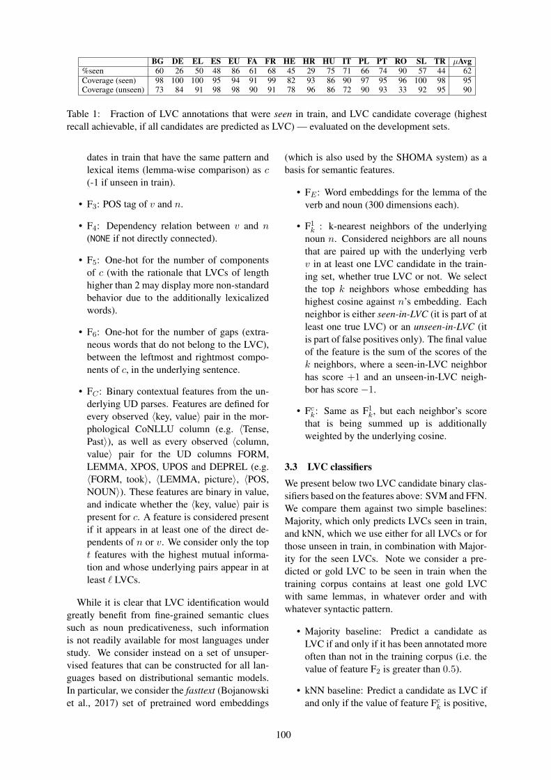
BG DE EL ES EU FA FR HE HR HU IT PL PT RO SL TR µAvg%seen 60 26 50 48 86 61 68 45 29 75 71 66 74 90 57 44 62Coverage (seen) 98 100 100 95 94 91 99 82 93 86 90 97 95 96 100 98 95Coverage (unseen) 73 84 91 98 98 90 91 78 96 86 72 90 93 33 92 95 90

Table 1: Fraction of LVC annotations that were seen in train, and LVC candidate coverage (highestrecall achievable, if all candidates are predicted as LVC) — evaluated on the development sets.

dates in train that have the same pattern andlexical items (lemma-wise comparison) as c(-1 if unseen in train).

• F3: POS tag of v and n.

• F4: Dependency relation between v and n(NONE if not directly connected).

• F5: One-hot for the number of componentsof c (with the rationale that LVCs of lengthhigher than 2 may display more non-standardbehavior due to the additionally lexicalizedwords).

• F6: One-hot for the number of gaps (extra-neous words that do not belong to the LVC),between the leftmost and rightmost compo-nents of c, in the underlying sentence.

• FC : Binary contextual features from the un-derlying UD parses. Features are defined forevery observed 〈key, value〉 pair in the mor-phological CoNLLU column (e.g. 〈Tense,Past〉), as well as every observed 〈column,value〉 pair for the UD columns FORM,LEMMA, XPOS, UPOS and DEPREL (e.g.〈FORM, took〉, 〈LEMMA, picture〉, 〈POS,NOUN〉). These features are binary in value,and indicate whether the 〈key, value〉 pair ispresent for c. A feature is considered presentif it appears in at least one of the direct de-pendents of n or v. We consider only the topt features with the highest mutual informa-tion and whose underlying pairs appear in atleast ` LVCs.

While it is clear that LVC identification wouldgreatly benefit from fine-grained semantic cluessuch as noun predicativeness, such informationis not readily available for most languages understudy. We consider instead on a set of unsuper-vised features that can be constructed for all lan-guages based on distributional semantic models.In particular, we consider the fasttext (Bojanowskiet al., 2017) set of pretrained word embeddings

(which is also used by the SHOMA system) as abasis for semantic features.

• FE : Word embeddings for the lemma of theverb and noun (300 dimensions each).

• F1k : k-nearest neighbors of the underlying

noun n. Considered neighbors are all nounsthat are paired up with the underlying verbv in at least one LVC candidate in the train-ing set, whether true LVC or not. We selectthe top k neighbors whose embedding hashighest cosine against n’s embedding. Eachneighbor is either seen-in-LVC (it is part of atleast one true LVC) or an unseen-in-LVC (itis part of false positives only). The final valueof the feature is the sum of the scores of thek neighbors, where a seen-in-LVC neighborhas score +1 and an unseen-in-LVC neigh-bor has score −1.

• Fck: Same as F1k, but each neighbor’s score

that is being summed up is additionallyweighted by the underlying cosine.

3.3 LVC classifiers

We present below two LVC candidate binary clas-sifiers based on the features above: SVM and FFN.We compare them against two simple baselines:Majority, which only predicts LVCs seen in train,and kNN, which we use either for all LVCs or forthose unseen in train, in combination with Major-ity for the seen LVCs. Note we consider a pre-dicted or gold LVC to be seen in train when thetraining corpus contains at least one gold LVCwith same lemmas, in whatever order and withwhatever syntactic pattern.

• Majority baseline: Predict a candidate asLVC if and only if it has been annotated moreoften than not in the training corpus (i.e. thevalue of feature F2 is greater than 0.5).

• kNN baseline: Predict a candidate as LVC ifand only if the value of feature Fck is positive,

100

Configuration BG DE EL ES EU FA FR HE HR HU IT PL PT RO SL TR µAvgMaj (seen) 72 84 76 89 81 83 93 68 91 91 87 92 86 90 70 38 81kNN (seen) 62 84 76 89 79 81 92 66 91 91 83 89 82 37 60 46 78FFN (seen) 74 78 82 94 87 87 94 67 92 92 86 90 88 87 68 71 85SVM (seen) 70 74 84 86 86 89 93 64 91 91 84 89 90 72 76 57 84kNN (unseen) 08 08 24 22 32 30 30 04 13 13 11 20 32 00 04 24 22FFN (unseen) 15 18 27 29 22 55 31 05 21 33 12 22 25 00 08 27 28SVM (unseen) 15 15 33 20 42 63 37 02 24 46 10 31 45 00 10 34 34

Table 2: F1 scores on Majority and kNN baselines (Fck with k = 2) , along with the best configurationfor the SVM and FFN classifiers — on the development sets.

meaning that within the k nominal neigh-bors of the noun n of the candidate, the totalcosine of seen-in-LVC surpasses that of theunseen-in-LVC neighbors.

• SVM: Support vector machine with RBF ker-nel. Positive and negative examples are bal-anced through compensating class weights.We use a 3-fold grid-search to select forthe best combination of classifier hyperpa-rameters for each language; we consider thevalues C ∈ {1, 10, 20, 50, 100} and γ ∈{0.5, 0.1, 0.05, 0.01}.

• FFN: Feed-forward network with a 100-neuron hidden layer, using tanh as an acti-vation function and 50% dropout. The net-work uses an SGD optimizer6 and negativelog-likelihood loss. Positive training exam-ples are duplicated as much as needed soas to be balanced against negative examples.The final list of examples is shuffled, andfed into the classifier in batches of size B ∈{1, 2, 4, 8, 16}. Training is performed for anumber e of epochs, such that epoch e+1would have had higher loss on the valida-tion set (10% of train). One-hot features areimplemented as a layer of trainable embed-dings instead (300 dimensions for lemmas; 5dimensions for dependency relations, for F5

and F6).

3.4 EvaluationWe explore hyperparameters on the 16 languagesthat contained a development set, and evaluate thefinal systems on the test set for all 19 languages(using both training and development set for train-ing). Evaluation of LVC predictions for each lan-guage uses the MWE-based F1 score from of thePARSEME shared task (Ramisch et al., 2018). Wemodified its evaluation script so as to output scores

6Basic tuning of the learning rate led us to use 0.01.

for seen and unseen LVCs: it first labels a LVC(whether gold or predicted) as "seen" if there ex-ists at least one gold LVC occurrence with thesame set of lemmas in the training set, and unseenotherwise. The two labels are then evaluated sep-arately.

We also present a micro-average score (µAvg),in which the F1 scores of all languages are av-eraged with a weight that is proportional to thenumber of LVCs in that languages test (or devel-opment) set.7 On test sets, we compare our resultswith SHOMA and TRAVERSAL, the two highest-scoring systems in the shared-task.8

4 Results

Table 1 presents the fraction of LVCs in the de-velopment set that can also be seen in the trainingset. In the lower end, German dev LVCs were onlyseen in train 26% of the time, mostly due to thesmall training set in this language. In the higherend, 90% of Romanian LVCs had a counterpart inthe training set, suggesting that a simple baselinefocusing on seen LVCs should already yield goodresults for this language.

The last two rows in Table 1 present the cov-erage (i.e. recall) in the initial step of LVC can-didate extraction, for the strategy atleastNoccurswith N = 2. This strategy was found to yield thebest results in both SVM and FFN settings dur-ing early experiments. It can be seen that, despitevariation across languages, mainly due to trainingcorpus size differences, the micro-averaged cover-age is 95% for dev LVCs seen in train, and slightly

7We chose to use micro-average, since the test sets acrosslanguages don’t have the same number of sentences, for rea-sons that are independent of the linguistic properties of each.

8We used the predicted test sets of all participat-ing systems (made available by the shared task organiz-ers at https://gitlab.com/parseme/sharedtask-data/tree/master/1.1/system-results), filtering them to con-sider LVCs only. The best systems in open and closed tracks(SHOMA and TRAVERSAL) are the same when consideringall verbal MWEs or LVCs only.

101

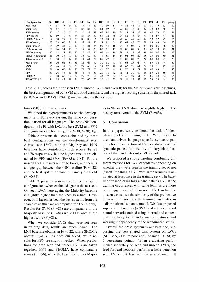
Configuration BG DE EL EN ES EU FA FR HE HI HR HU IT LT PL PT RO SL TR µAvgMaj (seen) 74 67 85 64 60 87 84 85 70 90 87 94 82 48 87 89 81 75 53 80kNN (seen) 71 67 78 64 61 83 84 87 64 89 89 92 80 47 88 87 38 62 58 78SVM (seen) 75 67 80 65 60 86 87 89 66 94 80 94 83 38 89 91 67 79 77 81FFN (seen) 82 69 79 67 64 87 86 89 69 92 85 94 82 48 88 93 74 69 87 83SHOMA (seen) 64 00 79 00 39 88 88 66 73 88 43 78 66 49 69 87 93 52 79 76TRAV (seen) 62 53 66 34 44 82 81 70 58 81 64 87 64 45 76 78 83 63 66 72kNN (unseen) 14 09 23 23 17 16 21 34 05 44 18 24 13 08 19 28 00 05 36 22SVM (unseen) 17 24 34 19 07 17 57 29 07 61 17 36 06 07 39 39 67 13 43 31FFN (unseen) 20 18 18 33 20 19 45 25 06 64 16 29 12 15 33 31 00 07 34 29SHOMA (unseen) 21 00 36 03 13 35 62 37 19 53 19 14 04 08 22 35 29 00 50 31TRAV (unseen) 08 00 18 14 10 11 41 31 05 42 21 23 00 01 20 24 00 00 23 20Maj + kNN 53 26 62 31 36 81 64 62 30 68 45 77 63 28 60 74 69 34 44 57kNN 56 26 59 32 37 77 65 64 29 67 46 76 62 28 61 72 28 31 49 57SVM 61 40 66 26 35 79 77 65 41 77 44 81 70 28 71 78 67 63 61 63FFN 53 26 43 40 36 74 74 51 21 78 42 75 44 30 60 68 57 26 56 56SHOMA 50 00 60 02 22 79 78 51 43 72 24 59 46 29 51 70 86 28 64 56TRAVERSAL 44 15 47 18 26 70 65 52 30 62 32 68 51 23 52 62 73 38 44 50

Table 3: F1 scores (split for seen LVCs, unseen LVCs and overall) for the Majority and kNN baselines,the best configuration of our SVM and FFN classifiers, and the highest-scoring systems in the shared-task(SHOMA and TRAV(ERSAL)) — evaluated on the test sets.

lower (90%) for unseen ones.We tuned the hyperparameters on the develop-

ment sets. For every system, the same configura-tion is used for all languages. The best kNN con-figuration is Fck with k=2; the best SVM and FFNconfigurations are both F1..6, FC (t=30, `=30), FE .

Table 2 presents the scores obtained by thesebest configurations on the development sets.Across seen LVCs, both the Majority and kNNbaselines have considerably high scores (F1=81and 78 respectively, but the highest results are ob-tained by FFN and SVM (F1=85 and 84). For theunseen LVCs, results are quite lower, and there isa bigger gap between the kNN baseline (F1=0.22)and the best system on unseen, namely the SVM(F1=0.34).

Table 3 presents system results for the sameconfigurations when evaluated against the test sets.On seen LVCs here again, the Majority baselineis slightly higher than the kNN baseline. How-ever, both baselines beat the best systems from theshared-task (that we recomputed for LVCs only).Results for SVM (F1=81) are comparable to theMajority baseline (F1=81) while FFN obtains thehighest score (F1=83).

When we consider LVCs that were not seenin training data, results are much lower. ThekNN baseline obtains an F1=0.22, while SHOMAobtains F1=0.31, as does our SVM, while re-sults for FFN are slightly weaker. When predic-tions for both seen and unseen LVCs are takentogether, FFN and SHOMA have comparablescores (F1=56), while the baselines (either Major-

ity+kNN or kNN alone) is slightly higher. Thebest system overall is the SVM (F1=63).

5 Conclusion

In this paper, we considered the task of iden-tifying LVCs in running text. We propose touse data-driven language-specific syntactic pat-terns for the extraction of LVC candidates out ofsyntactic parses, followed by a binary classifica-tion of the candidates into LVC or not.

We proposed a strong baseline combining dif-ferent methods for LVC candidates depending onwhether they were seen in the training set or not(“seen” meaning a LVC with same lemmas is an-notated at least once in the training set). The base-line for seen cases tags a candidate as LVC if thetraining occurrences with same lemmas are moreoften tagged as LVC than not. The baseline forunseen cases uses the similarity of the predicativenoun with the nouns of the training candidates, ina distributional semantic model. We also proposedsupervised classifiers (a SVM and a feed-forwardneural network) trained using internal and contex-tual morphosyntactic and semantic features, andworking independently of the seen/unseen status.

Overall the SVM system is our best one, sur-passing the best shared task system on LVCs(SHOMA, (Taslimipoor and Rohanian, 2018)) by7 percentage points. When evaluating perfor-mance separately on seen and unseen LVCs, thefeed-forward network performs a little better onseen LVCs, but less well on unseen ones. It

102

also appears that our results for seen LVCs sur-pass the best shared-task results even in the caseof the baseline, in spite of a much simpler tech-nique of supervised learning. For unseen LVCs,results are globally quite lower. The best perfor-mance is F1=31%, achieved both by the SHOMAsystem and our SVM. Our kNN-inspired baselineachieves F1=22% only, a performance that wouldrank second for unseen LVCs in the shared task.

Given the quality of predictions for seen LVCs,future works should focus on improving predic-tion for the unseen expressions. Such task couldbe achieved through an evaluation of differenttypes of neural network. Other semantically-motivated language-independent features shouldalso be considered, so as to estimate the candi-date noun’s abstractness and predicativeness, aswell as the level of semantic bleaching in the useof the verb. Finally, future works should investi-gate using a model for contextualized word em-beddings such as BERT (Devlin et al., 2018)), de-spite the difficulty of covering the 19 languages ofthe PARSEME datasets.

Acknowledgements

We would like to thank Bruno Guillaume for ad-vice in using Grew. This work was partiallyfunded by the French National Research Agency(PARSEME-FR ANR-14-CERA-0001).

ReferencesPiotr Bojanowski, Edouard Grave, Armand Joulin, and

Tomas Mikolov. 2017. Enriching word vectors withsubword information. Transactions of the Associa-tion for Computational Linguistics, 5:135–146.

Guillaume Bonfante, Bruno Guillaume, and Guy Per-rier. 2018. Application of Graph Rewriting to Natu-ral Language Processing. Wiley Online Library.

Claire Bonial and Martha Palmer. 2016. Comprehen-sive and consistent propbank light verb annotation.In LREC.

Fabienne Cap, Manju Nirmal, Marion Weller, andSabine Schulte im Walde. 2015. How to accountfor idiomatic German support verb constructions instatistical machine translation. In Proceedings ofthe 11th Workshop on Multiword Expressions, pages19–28, Denver, Colorado. Association for Computa-tional Linguistics.

Wei-Te Chen, Claire Bonial, and Martha Palmer. 2015.English light verb construction identification using

lexical knowledge. In Proceedings of the Twenty-Ninth AAAI Conference on Artificial Intelligence,AAAI’15, pages 2375–2381. AAAI Press.

Jacob Devlin, Ming-Wei Chang, Kenton Lee, andKristina Toutanova. 2018. BERT: pre-training ofdeep bidirectional transformers for language under-standing. CoRR, abs/1810.04805.

István Nagy T., Veronika Vincze, and Richárd Farkas.2013. Full-coverage identification of English lightverb constructions. In Proceedings of the Sixth In-ternational Joint Conference on Natural LanguageProcessing, pages 329–337, Nagoya, Japan. AsianFederation of Natural Language Processing.

Joakim Nivre and Veronika Vincze. 2015. Light verbconstructions in universal dependencies. In Posterat the 5th PARSEME meeting, Iasi, Romania.

Caroline Pasquer, Carlos Ramisch, Agata Savary, andJean-Yves Antoine. 2018. VarIDE at PARSEMEshared task 2018: Are variants really as alike as twopeas in a pod? In Proceedings of the Joint Workshopon Linguistic Annotation, Multiword Expressionsand Constructions (LAW-MWE-CxG-2018), SantaFe, New Mexico, USA. Association for Computa-tional Linguistics.

Carlos Ramisch, Silvio Ricardo Cordeiro, AgataSavary, Veronika Vincze, Verginica Barbu Mititelu,Archna Bhatia, Maja Buljan, Marie Candito, PolonaGantar, Voula Giouli, Tunga Güngör, AbdelatiHawwari, Uxoa Iñurrieta, Jolanta Kovalevskaite, Si-mon Krek, Timm Lichte, Chaya Liebeskind, Jo-hanna Monti, Carla Parra Escartín, Behrang Qasemi-Zadeh, Renata Ramisch, Nathan Schneider, IvelinaStoyanova, Ashwini Vaidya, and Abigail Walsh.2018. Edition 1.1 of the PARSEME shared task onautomatic identification of verbal multiword expres-sions. In Proceedings of the Joint Workshop on Lin-guistic Annotation, Multiword Expressions and Con-structions (LAW-MWE-CxG-2018), pages 222–240,Santa Fe, New Mexico, USA. Association for Com-putational Linguistics.

Lance A Ramshaw and Mitchell P Marcus. 1999. Textchunking using transformation-based learning. InNatural language processing using very large cor-pora, pages 157–176. Springer.

Omid Rohanian, Shiva Taslimipoor, SamanehKouchaki, Le An Ha, and Ruslan Mitkov. 2019.Bridging the gap: Attending to discontinuity inidentification of multiword expressions. In Pro-ceedings of the 2019 Conference of the NorthAmerican Chapter of the Association for Computa-tional Linguistics: Human Language Technologies,Volume 1 (Long and Short Papers), pages 2692–2698, Minneapolis, Minnesota. Association forComputational Linguistics.

Agata Savary, Marie Candito, Verginica Barbu Mi-titelu, Eduard Bejcek, Fabienne Cap, Slavomír

103

Céplö, Silvio Ricardo Cordeiro, Gülsen Ce-biroglu Eryigit, Voula Giouli, Maarten Van Gompel,Yaakov HaCohen-Kerner, Jolanta Kovalevskaite,Simon Krek, Chaya Liebeskind, Johanna Monti,Carla Parra Escartín, Lonneke Der, BehrangQasemi Zadeh, Carlos Ramisch, and VeronikaVincze. 2018. PARSEME multilingual corpus ofverbal multiword expressions. Berlin: LanguageScience Press.

Shiva Taslimipoor and Omid Rohanian. 2018.SHOMA at PARSEME Shared Task on automaticidentification of VMWEs: Neural multiword ex-pression tagging with high generalisation. arXivpreprint arXiv:1809.03056.

Yuancheng Tu and Dan Roth. 2011. Learning Englishlight verb constructions: contextual or statistical.In Proceedings of the Workshop on Multiword Ex-pressions: from Parsing and Generation to the RealWorld, pages 31–39. Association for ComputationalLinguistics.

Veronika Vincze, János Zsibrita, and István Nagy T.2013. Dependency parsing for identifying Hun-garian light verb constructions. In Proceedings ofthe Sixth International Joint Conference on Natu-ral Language Processing, pages 207–215, Nagoya,Japan. Asian Federation of Natural Language Pro-cessing.

Jakub Waszczuk. 2018. TRAVERSAL at PARSEMEShared Task 2018: Identification of verbal mul-tiword expressions using a discriminative tree-structured model. In Joint Workshop on LinguisticAnnotation, Multiword Expressions and Construc-tions (LAW-MWE-CxG-2018).

104

Comparing the Performance of Feature Representationsfor the Categorization of the Easy-to-Read Variety vs Standard Language

Marina SantiniRISE Research Institutes of Sweden

(Division ICT - RISE SICS East)Stockholm, Sweden

[email protected]

Benjamin DanielssonLinkoping University

(IDA)Linkoping, Sweden

[email protected]

Arne JonssonRISE Research Institutes of Sweden

& Linkoping University (IDA)Linkoping, [email protected]

AbstractWe explore the effectiveness of four fea-ture representations – bag-of-words, wordembeddings, principal components andautoencoders – for the binary categoriza-tion of the easy-to-read variety vs standardlanguage. “Standard language” refers tothe ordinary language variety used by apopulation as a whole or by a community,while the “easy-to-read” variety is a sim-pler (or a simplified) version of the stan-dard language. We test the efficiency ofthese feature representations on three cor-pora, which differ in size, class balance,unit of analysis, language and topic. Werely on supervised and unsupervised ma-chine learning algorithms. Results showthat bag-of-words is a robust and straight-forward feature representation for this taskand performs well in many experimen-tal settings. Its performance is equiva-lent or equal to the performance achievedwith principal components and autoen-corders, whose preprocessing is howevermore time-consuming. Word embeddingsare less accurate than the other feature rep-resentations for this classification task.

1 Introduction

Broadly speaking, a language variety is any spe-cific form of language variation, such as standardlanguage, dialects, registers or jargons. In this pa-per, we focus on two language varieties, namelythe standard language variety and the easy-to-readvariety. In this context, “standard language” refersto the official and ordinary language variety usedby a population as a whole, or to a variety that isnormally employed within a community. For ex-ample, “Standard English” is the form of the En-glish language widely accepted as the usual cor-rect form, while within the medical community it

is the specialized medical jargon that is consideredto be standard language. In contrast, the easy-to-read variety is a simpler version of a standard lan-guage. The need of an easy-to-read variety stemsfrom the difficulties that certain groups of peopleexperience with standard language, such as peoplewith dyslexia and other learning disabilities, theelderly, children, non-native speakers and so on.In order to meet the needs of a simpler languagethat makes information easy to read and under-stand for all, European Standards have been estab-lished1, and an important initiative like Wikipediahas created a special edition called Simple En-glish Wikipedia2. These are not isolated phenom-ena. For instance, in Sweden public authorities(sv: myndigheter) provide an easy-to-read version(a.k.a. simple Swedish or sv: lattlast) of their writ-ten documentation.

Both in the case of the Simple EnglishWikipedia and in the case of Swedish public au-thorities, the simplified documents are manuallywritten. Since the manual production of simplifiedtexts is time-consuming, the task called Text Sim-plification (TS) is very active in Natural LanguageProcessing (NLP) in the attempt to streamline thistype of text production. TS is a fast-growing re-search area that can bring about practical benefits,e.g. the automatic generation of simplified texts.There is, however, a TS subtask that is still un-derexplored: the categorization of the easy-to-readvariety vs standard language. The findings pre-sented in this paper contribute to start filling thisgap. The automatic separation of standard textsfrom easy-to-read texts could be particularly use-ful for other TS subtasks, such as the bootstrap-ping of monolingual corpora from the web or the

1https://easy-to-read.eu/wp-content/uploads/2014/12/EN_Information_for_all.pdf

2https://simple.wikipedia.org/wiki/Main_Page

105

extraction of simplified terminology. Other ar-eas that could benefit from it include informa-tion retrieval (e.g. for the retrieval of easy-to-reador patient-friendly medical information) and deeplearning-based dialogue systems (e.g. customizedchatbots for expert users or naive users).

The research question we would like to an-swer is: which is the most suitable feature rep-resentation for this categorization task? In or-der to answer this question, we compare four dif-ferent feature representations that can potentiallymake sense of the lexical makeup that differenti-ates easy-to-read from standard language, namelybag-of-words (BoWs), word embeddings, princi-pal components and autoencoders. It goes withoutsaying that these four feature representations arejust a few of the many possible feature representa-tions for this kind of task. We start our long-termexploration with these four feature representationsbecause they are straightforward and easy to ex-tract automatically from any corpora. We test theefficiency of the four feature representations withthree types of machine learning algorithms: tra-ditional supervised machine learning, deep learn-ing and clustering3. The experiments are basedon three corpora belonging to different domains.From these corpora, we extracted three datasetsof different sizes, different class balance, differentunits of analysis (sentence vs document), differentlanguages (Swedish and English).

The ultimate goal of the experiments presentedin this paper is to propose a first empirical baselinefor the categorization of the easy-to-read variety vsstandard language.

2 Previous Work

As mentioned above, the automatic separation ofstandard language from the easy-to-read variety isunderinvestigated, but it could be useful for sev-eral TS subtasks, such as the bootstrapping (Ba-roni and Bernardini, 2004) of monolingual paral-lel corpora (Caseli et al., 2009), of monolingualcomparable corpora (Barzilay and Elhadad, 2003)or the exploitation of regular corpora (Glavas andStajner, 2015). Extensive work exists in TS (Sag-gion, 2017). The most advanced work focuseson the implementation of neural text simplifica-tion systems that are able to simultaneously per-form lexical simplification and content reduction

3The umbrella term ‘categorization’ is used to cover thesethree machine learning approaches.

(Nisioi et al., 2017).In this paper, however, we do not focus on the

creation of TS systems, but rather on the sheerdownstream categorization task of separating stan-dard language from the easy-to-read variety. Toour knowledge, limited research exists in this area,which mostly focuses on the discrimination be-tween the specialized language used by domainexperts and the language used by non-experts(a.k.a. laypeople or the lay). This type of distinc-tion is required in some domains (e.g. medical andlegal domains), where the specialized jargon hin-ders the understanding of “ordinary” people, i.e.people without specialized education, who strug-gle to get a grip on professional sublanguages. Inthe experiments reported in Santini et al. (2019),it is shown that it is possible to successfully dis-criminate between medical web texts written forexperts and for laypeople in Swedish. Results areencouraging and we use one of their datasets in theexperiments presented here.

Other corpora are available that can be usedfor the automatic categorization of the easy-to-read variety vs standard language. For instance,the Simple English Wikipedia corpus4 (Kauchak,2013), and the DigInclude corpus5 in Swedish(Rennes and Jonsson, 2016). However, neitherSimple English Wikipedia nor DigInclude haveever been used for this text categorization task. Weuse them in this context for the first time.

3 Corpora and Datasets

In our experiments, we use three corpora, twoin Swedish and one in English. More precisely,we rely on 1) a subset of the eCare corpus (San-tini et al., 2019) in Swedish; 2) a subset of theDigInclude corpus (Rennes and Jonsson, 2016) inSwedish and 3) a subset of the Simple EnglishWikipedia corpus (Kauchak, 2013) in English.

The eCare corpus is a domain-specific web cor-pus. The domain of interest is the medical field ofchronic diseases. From the current version of thecorpus we re-use a labelled subset. The eCare sub-set contains 462 webpages without boilerplates.The webpages have been labelled as ‘lay’ or ‘spe-cialized’ by a lay native speaker. Lay sublanguageis an easy-to-read version of the standard lan-guage (the medical jargon) used by healthcare pro-

4http://www.cs.pomona.edu/˜dkauchak/simplification/

5https://www.ida.liu.se/˜arnjo82/diginclude/corpus.shtml

106

fessionals. The 462 webpages of the eCare dataset(amounting to 424,278 words) have been labelledin the following way: 388 specialized webpages(66%) and 154 lay webpages (33%). The datasetis unbalanced. The unit of analysis that we use inthese experiments is the document.

The DigInclude corpus is a collection of easy-to-read sentences aligned to standard languagesentences. The corpus has been crawled froma number of Swedish authorities’ websites. TheDigInclude datasets contains 17,502 sentences,3,827 simple sentences (22%) and 13,675 standardsentences (78%), amounting to 233,094 words.The dataset is heavily unbalanced. The unit ofanalysis is the sentence.

The Simple English Wikipedia (SEW) cor-pus was generated by aligning Simple EnglishWikipedia and standard English Wikipedia. Twodifferent versions of the corpus exist (V1 and V2).V2 has been packaged in sentences and in docu-ments. We used the subset of V2 divided into sen-tences. The SEW dataset contains 325,245 sen-tences, 159,713 easy-to-read sentences (49.1%)and 165,532 standard sentences (50.9%), amount-ing to 7,191,133 words. The dataset is fairly bal-anced. The unit of analysis is the sentence.

4 Features Representations and Filters

At the landing page of Simple English Wikipedia,it is stated: “We use Simple English words andgrammar here.” Essentially, this statement impliesthat the use of basic vocabulary and simple gram-mar makes a text easier to read. In these experi-ments we focus on the effectiveness of feature rep-resentations based on lexical items and leave theexploration of grammar-based tags for the future.

In this section, we describe the four featurerepresentations, as well as the filters that havebeen applied to create them. These filters and themethods described in Section 5 are included inthe Weka Data Mining workbench (Witten et al.,2016)6. All the experiments performed with theWeka workbench can be replicated in any otherworkbench, or programmatically in any program-ming language. We use Weka here for the sake offast reproducibility, since Weka is easy to use alsofor those who are not familiar with the practicali-ties of machine learning. Additionally, it is opensource, flexible and well-documented.

6Open source software freely available at https://www.cs.waikato.ac.nz/ml/weka/

In the experiments below several filters havebeen stacked together via the Multifilter metafil-ter, which gives the opportunity to apply severalfiltering schemes sequentially to the same dataset.

BoWs. BoWs is a representation of text that de-scribes the occurrence of single words within adocument. It involves two things: a vocabularyof known words and a weighing scheme to mea-sure the presence of known words. It is called a“bag” of words, because any information about theorder or structure of words in the document is dis-carded. The model is only concerned with whetherknown words occur in the document, not wherein the document, or with which other words theyco-occur. The advantage of BoWs is simplicity.BoWs models are simple to understand and im-plement and offer a lot of flexibility for customiza-tion. Preprocessing can include different levels ofrefinement, from stopword removal to stemmingor lemmatization, and a wide range of weighingschemes. Usually, lexical items in the form ofBoWs represent the topic(s) of a text and are nor-mally used for topical text classification. Severalrelated topics make up a domain, i.e. a subjectfield like Fashion or Medicine. Here we use BoWsfor a different purpose, which is to detect the dif-ferent level of lexical sophistication that existsbetween the easy-to-read variety and standard lan-guage. Intuitively, easy-to-read texts have a muchplainer and poorer vocabulary than texts written instandard language. The rationale of using BoWsin this context is then to capture the lexical diver-sification that characterizes easy-to-read and stan-dard language texts.

Starting from datasets in string format, we ap-plied StringToWordVector, which is an unsuper-vised filter that converts string attributes into a setof attributes representing frequencies of word oc-currence. For all the corpora, we selected the TFand IDF weighing schemes, normalization to low-ercase and normalization to the length of the doc-uments. Lemmatization, stemming and stopwordremoval were not applied. The number of wordsthat were kept varies according to the size of cor-pus. The complete settings of this and all the otherfilters described below are fully documented in thecompanion website.

Word embeddings. Word embeddings are oneof the most popular representations of documentvocabulary to date, since they have proved to be

107

effective in many tasks (e.g. sentiment analysis,text classification, etc.). The advantage of wordembeddings lies in their capability to capture thecontext of a word in a document, as well as se-mantic and syntactic similarity. The basic idea be-hind word embeddings is to “embed” a word vec-tor space into another. The big intuition is that thismapping could bring to light something new aboutthe data that was unknown before. More specifi-cally, word embeddings learn both the meaningsof the words and the relationships between wordsbecause they capture the implicit relations be-tween words by determining how often a word ap-pears with other words in the training text. Therationale of using word embeddings in this con-text is to account for both semantic and syntacticrepresentations, traits that can be beneficial for thecategorization of language varieties.

Word embeddings can be native or pretrained.Here we use the pretrained Polyglot Embed-dings (Al-Rfou et al., 2013) for Swedish (polyglot-sv) and for English (polyglot-en).

Principal Components. Principal ComponentAnalysis (PCA) involves the orthogonal transfor-mation of possibly correlated variables into a setof values of linearly uncorrelated variables calledprincipal components. This transformation is de-fined in such a way that the first principal com-ponent explains the largest possible variance, andeach succeeding component in turn explains thehighest variance possible under the constraint thatit is orthogonal to the preceding components. Theadvantage of PCA is to reduce the number of re-dundant features, which might be common but dis-turbing when using a BoWs approach, thus possi-bly improving text classification results. The ra-tionale of using PCA components in this contextis to ascertain whether feature reduction is benefi-cial for the categorization of language varieties.

To perform PCA and the transformation of thedata, we wrapped PrincipalComponents filter onthe top of the StringToWordVector filter, via theMultifilter metafilter. The PrincipalComponentsfilter is an unsupervised filter that chooses enoughprincipal components (a.k.a eigenvectors) to ac-count for 95% of the variance in the original data.

Autoencoders. Similar to PCA, the basic ideabehind autoencoders is dimensionality reduction.However, autoencoders are much more flexiblethan PCA since they can represent both linear and

non-linear transformation, while PCA can onlyperform linear transformation. Additionally, au-toencoders can be layered to form deep learningnetworks. They can also be more efficient in termsof model parameters since a single autoencodercan learn several layers rather than learning onehuge transformation as with PCA. The advantageof using autoencoders in this context is to trans-form inputs into outputs with the minimum possi-ble error (Hinton and Salakhutdinov, 2006). Therationale of their use here is to determine whetherthey provide a representation with enriched prop-erties that is neater than other reduced representa-tions.

In these experiments, autoencoders are gener-ated using the MLPAutoencoder filter stacked onthe top of the StringToWordVector filter, via theMultifilter metafilter. This MLPAutoencoder fil-ter gives the possibility of creating contractive au-toencoders, which are much more efficient thanstandard autoencoders (Rifai et al., 2011).

5 Methods, Baselines and Evaluation

In this section, we describe the categorizationschemes, the baselines and the evaluation metricsused for comparison.

Methods. We use three different learning meth-ods, namely an implementation of SVM, an imple-mentation of multilayer perceptron (MLP) and animplementation of K-Means for clustering. Therationale behind these choices is to compare thebehaviour of the four feature representations de-scribed above with learning schemes that have adifferent inductive biases, and to assess the differ-ence (if any) between the performance achievedwith labelled data (supervised algorithms) and un-labelled data (clustering). We calculate a randombaseline with the ZeroR classifier. All the catego-rization schemes are described below.

ZeroR: baseline classifier. The ZeroR is basedon the Zero Rule algorithm and predicts the classvalue that has the most observations in the train-ing dataset. It is more reliable than a completelyrandom baseline.

SVM: traditional supervised machine learning.SVM is a classic and powerful supervised machinelearning algorithm that performs extremely wellin text classification tasks with numerous features.Weka’s SVM implementation is called SMO andincludes John Platt’s sequential minimal optimiza-tion algorithm (Platt, 1998) for training a support

108

vector classifier (Joachims, 1998).Since two corpora are highly unbalanced, we

also combined SMO with filters that can cor-rect class unbalance. More specifically, we re-lied on ClassBalancer, which reweights the in-stances in the data so that each class has thesame total weight; Resample, which produces arandom subsample of a dataset using either sam-pling with replacement or without replacement;SMOTE, which resamples a dataset by applyingthe Synthetic Minority Oversampling TEchnique(SMOTE); and SpreadSubsample, which producesa random subsample of a dataset. All the modelsbuilt with SMO are based on Weka’s standard pa-rameters.

Multilayer Perceptron: Deep Learning. Wekaprovides several implementations of MLP. We re-lied on the WekaDeeplearning4j package that isdescribed in Lang et al. (2019). The main clas-sifier in this package is named DI4jMlpClassifierand is a wrapper for the DeepLearning4j library7

to train a multilayer perceptron. While fea-tures like BoWs, principal components and au-toencoders can be fed to any classifiers withinthe Weka workbench (if they are wrapped in fil-ters), word embeddings can be handled only bythe DI4jMlpClassifier (this explains N/A in Ta-ble 2). We used the standard configuration ofthe DI4jMlpClassifier (which includes only oneoutput layer) for BoWs, principal componentsand autoencoders. Conversely, the configura-tion used with word embeddings was cutomizedin the following way: word embeddings werepassed through four layers (two convulational lay-ers, a GlobalPoolingLayer and a OutputLayer);the number of epochs was set to 100; the in-stance iterator was set on CnnTextEmbeddingIn-stanceIterator; we used the polyglot embeddingsfor Swedish and English, as mentioned above.

K-Means: Clustering. We compare the perfor-mance of the supervised classification with clus-tering (fully unsupervised categorization). Weuse the traditional K-Means algorithm (Arthur andVassilvitskii, 2007) that in Weka is called Sim-pleKMeans. Since we know the number of classesin advance (i.e. two classes), we evaluate the qual-ity of the clusters against existing classes using theoption Classes to cluster evaluation, which firstignores the class attribute and generates the clus-

7https://deeplearning.cms.waikato.ac.nz/

ters, then during the test phase assigns classes tothe clusters, based on the majority value of theclass attribute within each cluster.

Evaluation metrics. We compare the perfor-mances on the Weighted Averaged F-Measure(AvgF), which is the sum of all the classes’ F-measures, each weighted according to the numberof instances with that particular class label.

In order to reliably assess the performancebased on AvgF, we also use k-statistic and the ROCarea value. K-statistic indicates the agreement ofprediction with true class; when the value is 0 theagreement is random. The quality of a classifiercan also be assessed with the help of the ROCarea value which indicates the area under the ROCcurve (AUC). It is used to measure how well aclassifier performs. The ROC area value lies be-tween about 0.500 to 1, where 0.500 (and below)denotes a bad classifier and 1 denotes an excellentclassifier.

ZeroR Baselines. Table 1 shows a breakdown ofthe baselines returned by the ZeroR classifier onthe three corpora. These baselines imply that thek-statistic is 0 and the ROC area value is below orequal to 0.500.

6 Results and Discussion

The main results are summarized in Table 2 andTable 3. As shown in in Table 2, by and large bothSMO and the DI4jMlpClassifier have equivalentor identical performance on all datasets in combi-nation with BoWs and principal components (weobserve however that the DI4jMlpClassifier is def-initely slower than SMO). Word embeddings havea slightly lower performance than BoWs and prin-cipal components on the eCare and SEW subsets.Autoencoders perform well (0.82) in combinationwith SMO on the eCare subset, less so (0.77) whenrunning with the DI4jMlpClassifier. The perfor-mance of clustering with BoWs on eCare gives anencouraging 0.59 (6 points above the ZeroR base-line of 0.53), while the performance with principalcomponents and autoencoders is below the ZeroRbaselines. In short, BoWs, which is the simplestand the most straightforward feature representa-tion in this set of experiments, has a performancethat is equivalent or identical to other more com-plex feature representations.

But what do the classifiers learn when theyare fed with BoWs? The classifiers learn the

109

Table 1: ZeroR baselines, breakdown

Class k Acc(%) Err(%) P R F ROC

eCare Subset (462 webpages)lay (154 webpages) 0.00 66.66 33.33 0.00 0.00 0.00 0.490specialized (308 webpages) 0.66 1.00 0.80 0.490AvgF 0.53

DigInclude Subset (17,502sentences)

simplified (3,827 sentences) 0.00 78.13 21.86 0.00 0.00 0.00 0.500specialized (13,675 sentences) 0.78 1.00 0.87 0.500AvgF 0.68

SEW Subset (325,235 sentences)simplified (159,708 sentences) 0.00 50.89 49.10 0.00 0.00 0.00 0.500specialized (165,527 sentences) 0.50 1.00 0.67 0.500AvgF 0.34

Table 2: Summary table (AvgF): easy-to-read variety vs standard language

Dataset Features SMO DI4jMlp K-Means

eCare Subset

BoW Features 0.80 0.80 0.59Word Embeddings N/A 0.75 N/APrincipal Components 0.80 0.81 0.44Autoencoders 0.82 0.77 0.50

DigInclude Subset

BoW 0.72 0.72 0.29Word Embeddings N/A 0.72 N/APrincipal Components 0.73 0.72 0.19Autoencoders 0.68 0.68 0.33

SEW Subset

BoW 0.58 0.56 0.43Word Embeddings N/A 0.55 N/APrincipal Components 0.55 0.56 0.49Autoencoders 0.52 0.51 0.49

Table 3: Summary table (AvgF): unbalanced datasets (BoWs + class balancing filters applied to SMO)

Dataset NoFilter ClassBalancer Resample SpreadSample SMOTEeCare Subset 0.80 0.81 0.81 0.80 0.81

DigInclude Subset 0.72 0.68 0.66 0.73 0.74

words that have been automatically selected by theStringToWordVector filter. Interestingly, since wedid not apply stopword removal, the lexical itemsselected by the filter are mostly function words andcommon lexical items. An example is shown inTable 4.

Table 4: 5 top frequent words and 5 bottom fre-quent words in one of the SEW models

Word Freqthe 237021of 159924in 149698

and 135958a 135867... ...... ...

usually 1517international 1503municipatlity 1449

show 1415island 1277

At first glance, it might appear counter-intuitivethat BoWs, which are very simple features that donot take syntax and word order into account, canperform well in this kind of task. However, we

surmize that this is the effect of the presence ofstopwords. As stopwords have not been removed(see settings reported earlier), the classifiers do notlearn ‘topics’ – since content words are pusheddown in the rank of the frequency list – but ratherthe distribution of function words, that are insteadtop-ranked and represent “structural” lexical itemsthat capture the syntax rather than the meaningof texts. Essentially, function words can be seenas a kind of subliminal syntactic features. Whatis more, in the corpora some words are domain-specific and difficult, while others are easy andcommon. Apparently, this difficult vs easy varia-tion in the vocabulary helps the classification task.The full list of the words extracted by the String-ToWordVectorFilter (utilized alone or as the basisof other filters) is available on the companion web-site.

The snap verdict of this set of experiments isthat BoWs are a valuable feature representationfor this kind of task. Their added value is that theyneed little preprocessing and no additional conver-sion schemes, as it is required by principal compo-nents and autoencoders. BoWs seem to be a robust

110

feature representation that accounts for both syn-tactic information and lexical sophistication.

As for word embeddings, it seems that their fullpotential remains unleashed in this context. The-oretically, word embeddings would be an idealfeature representation for this task because theycombine syntax and semantics and they couldcapture simplification devices both at lexical andmorpho-syntactic level. However, this does notfully happen here. As a matter of fact, it has al-ready been noticed elsewhere that word embed-dings might have an unstable behaviour (Wend-landt et al., 2018) that needs to be further inves-tigated.

Table 5: SMO, breakdown

SMO: eCare SubsetBOW k Acc(%) Err(%) P R F ROClay 0.56 80.92 19.04 0.72 0.68 0.70 0.779specialized 0.84 0.87 0.85 0.779AvgF 0.80PCA k Acc(%) Err(%) P R F ROClay 0.58 80.30 19.69 0.71 0.68 0.70 0.774specialized 0.84 0.86 0.85 0.774AvgF 0.80Autoenc k Acc(%) Err(%) P R F ROClay 0.60 82.16 17.83 0.72 0.75 0.73 0.804specialized 0.87 0.85 0.86 0.804AvgF 0.82

(a) eCare

SMO: DigInclude SubsetBOW k Acc(%) Err(%) P R F ROCsimplified 0.13 79.04 20.95 0.61 0.11 0.18 0.546standard 0.79 0.98 0.88 0.546AvgF 0.72PCA k Acc(%) Err(%) P R F ROCsimplified 0.14 78.80 21.19 0.56 0.14 0.22 0.555standard 0.80 0.97 0.77 0.555AvgF 0.73Autoenc k Acc(%) Err(%) P R F ROCsimplified 0.00 78.49 21.50 0.00 0.00 0.00 0.500standard 0.78 1.00 0.87 0.500AvgF 0.68

(b) DigInclude

SMO: SEW SubsetBOW k Acc(%) Err(%) P R F ROCsimplified 0.23 61.81 38.18 0.61 0.61 0.61 0.618standard 0.62 0.62 0.62 0.618AvgF 0.61PCA k Acc(%) Err(%) P R F ROCsimplified 0.13 57.08 42.91 0.57 0.45 0.51 0.569standard 0.56 0.67 0.61 0.569AvgF 0.56Autoenc k Acc(%) Err(%) P R F ROCsimplified 0.04 52.67 47.32 0.52 0.42 0.46 0.525standard 0.53 0.62 0.57 0.525AvgF 0.52

(c) SEW

We observe that the classification results arepromising on the eCare subset (see breakdown inTables 5a, 6a and 7a). Arguably, a factor hascontributed to achieve this performance: the unitof analysis. Certainly, classification at documentlevel is easier because the classifier has more textto learn from. Surprisingly, the unbalance of theeCare dataset seems to be somehow mitigated by

the unit of analysis, since the classifiers are not bi-ased towards the majority class and k-statistic andROC area values are quite robust (mostly above0.500 and above 0.800 respectively). Additonally,the dataset is small, and this might also facilitatethe learning. Clustering with BoWs is well abovethe ZeroR baseline, while with the other featurerepresentations the performance is below the base-line thresholds.

Table 6: DI4jMlpClassifier, breakdown

DI4jMlpClassifier: eCare SubsetBOW k Acc(%) Err(%) P R F ROClay 0.57 80.08 19.91 0.67 0.78 0.72 0.890specialized 0.88 0.80 0.84 0.890AvgF 0.80Embed k Acc(%) Err(%) P R F ROClay 0.45 75.79 24.20 0.63 0.65 0.64 0.807specialized 0.82 0.81 0.81 0.807AvgF 0.75PCA k Acc(%) Err(%) P R F ROClay 0.58 80.73 19.26 0.68 0.79 0.73 0.900specialized 0.88 0.81 0.84 0.900AvgF 0.81Autoenc k Acc(%) Err(%) P R F ROClay 0.52 77.07 22.92 0.61 0.84 0.71 0.872specialized 0.90 0.73 0.81 0.872AvgF 0.77

(a) eCare

DI4jMlpClassifier: DigInclude SubsetBOW k Acc(%) Err(%) P R F ROCsimplified 0.18 72.86 27.13 0.37 0.35 0.36 0.667standard 0.82 0.83 0.82 0.667AvgF 0.72Embed k Acc(%) Err(%) P R F ROCsimplified 0.10 77.24 22.75 0.41 0.13 0.20 0.587standard 0.80 0.94 0.86 0.587AvgF 0.72PCA k Acc(%) Err(%) P R F ROCsimplified 0.16 72.94 27.05 0.36 0.31 0.33 0.650standard 0.81 0.84 0.83 0.650AvgF 0.72Autoenc k Acc(%) Err(%) P R F ROCsimplified 0.00 78.49 21.50 0.00 0.00 0.00 0.500standard 0.78 1.00 0.87 0.500AvgF 0.68

(b) DigInclude

DI4jMlpClassifier: SEW SubsetBOW k Acc(%) Err(%) P R F ROCsimplified 0.13 56.50 43.49 0.55 0.57 0.56 0.594standard 0.57 0.55 0.56 0.594AvgF 0.56Embed k Acc(%) Err(%) P R F ROCsimplified 0.10 55.26 44.73 0.54 0.53 0.53 0.586standard 0.55 0.57 0.56 0.586AvgF 0.55PCA k Acc(%) Err(%) P R F ROCsimplified 0.10 55.21 44.78 0.54 0.55 0.55 0.577standard 0.56 0.54 0.55 0.577AvgF 0.55Autoenc k Acc(%) Err(%) P R F ROCsimplified 0.04 52.14 47.85 0.51 0.60 0.55 0.535standard 0.53 0.44 0.48 0.535AvgF 0.51

(c) SEW

The DigInclude subset (see breakdown in Ta-bles 5b, 6b, and 7b) is quite problematic from aclassification standpoint. It is highly unbalancedand the unit of analysis is the sentence. Theclassification models built with BoWs, word em-beddings and principal components in combina-

111

tion with SMO and the DI4jMlpClassifier are veryclose to random (see the value of k-statistic andthe ROC area value). Although the AvgF values inthe summary table (Table 2) seem to be decent fora binary classification problem, they are actuallymisleading, because the classifiers perform poorlyon the minority class, as revealed by the low valueof k-statistic and the ROC area value shown in thebreakdown tables (Tables 5b and 6b). Classifi-cation with autoencoders is perfectly random (k-statistic 0.00 and ROC area value 0.500). Cluster-ing results are very poor with all feature represen-tations. Arguably, with this dataset the learning ishindered by two factors: the high class unbalanceand the very short text that makes up a sentence.While in the case of the eCare subset, unbalance iscompensated by the longer text of webpages, withDigInclude the sentence does not allow any gen-eralizable learning. Given these results, a differ-ent approach must be taken for datasets like Dig-Include. Solutions to address these problems in-clude changing the unit of analysis from sentencesto documents (if possible) and/or applying a dif-ferent classification approach e.g. a cost-sensitiveclassifier of the kind used to predict rare events,e.g. Ali et al. (2015) or Krawczyk (2016). Algo-rithms used for fraud detection (Sundarkumar andRavi, 2015) could also be useful.

The SEW corpus (see Tables 5c, 6c and 7c) isbalanced and the unit of analysis is the sentence.The performance is promising because it is wellabove the ZeroR baseline (0.32). The best perfor-mance is with the combination of SMO and BoWsthat reaches an AvgF of 0.58 with only a limitednumber of features. Word embeddings performslightly worse than BoWs (but the running timeis much longer). Clustering is definitely encour-aging and much above the baseline level with allfeatures representations.

Since the eCare and DigInclude datasets areboth unbalanced, we applied class balance correc-tors. Table 8 shows the breakdown of SMO on theeCare subset in combination with four balancingfilters. The performance with filters is similar tothe performance without filters. This is true alsoif we look at the performance (P, R, AvgF) of theminority class (the lay class). K-statistic is sta-ble (greater than 0.50) as are the ROC area values(greater than 0.700). Essentially, this means thatthis dataset, although unbalanced, does not need aclass balancing filter. As pointed out earlier, we

Table 7: K-means, breakdown

K-means: eCareBOW Acc(%) Err(%) P R Flay 60.82 39.18 0.48 0.75 0.56specialized 0.81 0.53 0.64AvgF 0.59PCA Acc(%) Err(%) P R Flay 51.95 48.05 0.32 0.50 0.39specialized 0.65 0.47 0.54AvgF 0.44Autoenc Acc(%) Err(%) P R Flay 54.55 45.45 0.37 0.57 0.45specialized 0.71 0.53 0.61AvgF 0.50

(a) eCare

Simple K-means: DigIncludeBOW Acc(%) Err(%) P R Fsimplified 75.78 24.22 0.21 0.93 0.35standard 0.73 0.04 0.08AvgF 0.29PCA Acc(%) Err(%) P R Fsimplified 78.09 21.91 0.21 0 0standard 0.78 0.99 0.87AvgF 0.19Autoenc Acc(%) Err(%) P R Fsimplified 54.54 45.46 0.22 0.62 0.33standard 0.79 0.40 0.53AvgF 0.37

(b) DigInclude

K-means: SEWBOW Acc(%) Err(%) P R Fsimplified 50.27 49.73 0.46 0.17 0.25standard 0.50 0.80 0.62AvgF 0.43PCA Acc(%) Err(%) P R Fsimplified 50.37 49.63 0.48 0.49 0.48standard 0.50 0.50 0.50AvgF 0.49Autoenc Acc(%) Err(%) P R Fsimplified 50.46 49.55 0.48 0.54 0.51standard 0.50 0.45 0.47AvgF 0.49

(c) SEW

suppose that it is the unit of analysis used for theclassification (the webpage) that has a positive ef-fect on the results since the classifier learns morefrom an extended text (i.e. several sentences abouta coherent topic) than from a single sentence.

Conversely, on the DigInclude subset (see fullbreakdown in Table 9), two filters (ClassBalancerand Resample) out of four filters produce lowerAvgF values than the performance with no filters.A bit paradoxically, this might be good news if weare interested in the performance on the minorityclass (i.e. the simplified class). When we look atthe performance breakdown, we notice a big gapbetween P and R on the minority class. Withoutfilters, the P of the simplified class is decent (0.61),while the R is very low (0.11). When applying aClassBalancer and Resample, the P of the minor-ity class jumps down to about 0.30, but R soarsup to above 0.60. Thus, although the AvgF valueswith these two filters are lower than the SMO with-out any filter, the performance on the individualclasses is more balanced. The best performance

112

is, in our view, with SMOTE, which achieves anAvgF of 0.74 with a k-statistic of 0.24 and a ROCarea value of 0.624. The P and R of the minor-ity class are balanced (0.41 in both cases). Thisis indeed an encouraging result for this dataset. Itis to be acknowledged however that all the clas-sifiers based on the DigInclude subset shown inTable 9 are rather weak, since both k-statistic andROC area values are rather modest.

Table 8: eCare - Class balancing filters, break-down

eCare: SMO NoFilterBOW k Acc(%) Err(%) P R F ROClay 0.56 80.90 19.04 0.72 0.68 0.70 0.797specialized 0.84 0.87 0.85 0.779AvgF 0.80

eCare: SMO ClassBalancerBOW k Acc(%) Err(%) P R F ROClay 0.57 81.16 18.83 0.72 0.69 0.71 0.782specialized 0.85 0.87 0.86 0.782AvgF 0.81

eCare: SMO ResampleBOW k Acc(%) Err(%) P R F ROClay 0.58 81.81 18.18 0.74 0.70 0.72 0.789specialized 0.85 0.87 0.86 0.789AvgF 0.81

eCare: SMO SpreadsubsampleBOW k Acc(%) Err(%) P R F ROClay 0.56 80.95 19.04 0.72 0.68 0.70 0.779specialized 0.84 0.87 0.85 0.779AvgF 0.808

eCare: SMO SMOTEBOW k Acc(%) Err(%) P R F ROClay 0.57 81.16 18.83 0.73 0.68 0.70 0.781specialized 0.84 0.87 0.86 0.781AvgF 0.81

7 Conclusion and Future Work

In this paper, we explored the effectiveness offour feature representations – BoWs, word em-beddings, principal components and autoencoders– for the binary categorization of the easy-to-readvariety vs standard language. The automatic sep-aration of these two varieties would be helpfulin tasks where it is important to identify a sim-pler version of the standard language. We testedthe effectiveness of these four representations onthree datasets, which differ in size, class balance,unit of analysis, language and topic. Results showthat BoWs is a robust and straightforward fea-ture representation that performs well in this con-text. Its performance is equivalent or equal to theperformance of principal components and autoen-corders, but these two representations need addi-tional data conversion steps that do not pay offin terms of performance. Word embeddings areless accurate than the other feature representationsfor this classification task, although theoreticallythey should be able to achieve better results. Asmentioned in the Introduction, several other fea-

ture representations could be profitably tried outfor this task. We started off with the simplest ones,all based on individual lexical items. We proposethe findings presented in this paper as empiricalbaselines for future work.

We will continue to explore categorizationschemes in a number of additional experimentalsettings. First, we will try to pin down why wordembeddings are less robust than other feature rep-resentations in this context. Then, we will explorethe performance of other feature representationssuitable for the task, e.g. lexical and morphologi-cal n-grams as well as features based on syntacticcomplexity. We will also explore other classifica-tion paradigms, e.g. BERT (Devlin et al., 2018),and extend our investigation on the impact of theunit of analysis (e.g. by using the DigInclude andSEW versions that contain documents rather thansentences). Last but not least, we will try out ap-proaches specifically designed to address the prob-lem of unbalanced datasets.

Table 9: DigInclude - Class balancing filters,breakdown

DigInclude: SMO NoFilterBOW k Acc(%) Err(%) P R F ROCsimplified 0.13 79.04 20.95 0.61 0.11 0.18 0.546standard 0.79 0.98 0.88 0.546AvgF 0.72

DigInclude: SMO ClassBalancerBOW k Acc(%) Err(%) P R F ROCsimplified 0.22 65.24 34.57 0.34 0.62 0.44 0.645standard 0.86 0.66 0.74 0.645AvgF 0.68

eCare: SMO ResampleBOW k Acc(%) Err(%) P R F ROCsimplified 0.19 63.92 36.07 0.32 0.61 0.42 0.629standard 0.85 0.64 0.73 0.629AvgF 0.66

eCare: SMO SpreadsubsampleBOW k Acc(%) Err(%) P R F ROCsimplified 0.18 75.39 24.60 0.40 0.28 0.33 0.584standard 0.81 0.88 0.84 0.584AvgF 0.73

eCare: SMO SMOTEBOW k Acc(%) Err(%) P R F ROCsimplified 0.24 74.30 25.69 0.41 0.41 0.41 0.624standard 0.83 0.83 0.83 0.624AvgF 0.74

Companion Website & Acknowledgements

Companion website: http://www.santini.se/nodalida2019

This research was supported by E-care@home,a “SIDUS – Strong Distributed Research Environ-ment” project, funded by the Swedish KnowledgeFoundation [kk-stiftelsen, Diarienr: 20140217].Project website: http://ecareathome.se/

113

ReferencesRami Al-Rfou, Bryan Perozzi, and Steven Skiena.

2013. Polyglot: Distributed word representationsfor multilingual nlp. In Proceedings of the Seven-teenth Conference on Computational Natural Lan-guage Learning, pages 183–192, Sofia, Bulgaria.Association for Computational Linguistics.

Aida Ali, Siti Mariyam Shamsuddin, and Anca LRalescu. 2015. Classification with class imbalanceproblem: a review. Int. J. Advance Soft Compu.Appl, 7(3):176–204.

David Arthur and Sergei Vassilvitskii. 2007. k-means++: The advantages of careful seeding. InProceedings of the eighteenth annual ACM-SIAMsymposium on Discrete algorithms, pages 1027–1035.

Marco Baroni and Silvia Bernardini. 2004. Bootcat:Bootstrapping corpora and terms from the web. InLREC.

Regina Barzilay and Noemie Elhadad. 2003. Sentencealignment for monolingual comparable corpora. InProceedings of the 2003 conference on Empiricalmethods in natural language processing, pages 25–32. Association for Computational Linguistics.

Helena M Caseli, Tiago F Pereira, Lucia Specia, Thi-ago AS Pardo, Caroline Gasperin, and Sandra MariaAluısio. 2009. Building a brazilian portuguese par-allel corpus of original and simplified texts. Ad-vances in Computational Linguistics, Research inComputer Science, 41:59–70.


Goran Glavas and Sanja Stajner. 2015. Simplifyinglexical simplification: Do we need simplified cor-pora? In Proceedings of the 53rd Annual Meet-ing of the Association for Computational Linguisticsand the 7th International Joint Conference on Natu-ral Language Processing (Volume 2: Short Papers),volume 2, pages 63–68.

Geoffrey E Hinton and Ruslan R Salakhutdinov. 2006.Reducing the dimensionality of data with neural net-works. Science, 313(5786):504–507.

Thorsten Joachims. 1998. Text categorization withsupport vector machines: Learning with many rel-evant features. In European conference on machinelearning, pages 137–142. Springer.

David Kauchak. 2013. Improving text simplificationlanguage modeling using unsimplified text data. InProceedings of the 51st annual meeting of the as-sociation for computational linguistics (volume 1:Long papers), volume 1, pages 1537–1546.

Bartosz Krawczyk. 2016. Learning from imbal-anced data: open challenges and future directions.Progress in Artificial Intelligence, 5(4):221–232.

Steven Lang, Felipe Bravo-Marquez, ChristopherBeckham, Mark Hall, and Eibe Frank. 2019.Wekadeeplearning4j: A deep learning package forweka based on deeplearning4j. Knowledge-BasedSystems.

Sergiu Nisioi, Sanja Stajner, Simone Paolo Ponzetto,and Liviu P Dinu. 2017. Exploring neural text sim-plification models. In Proceedings of the 55th An-nual Meeting of the Association for ComputationalLinguistics (Volume 2: Short Papers), pages 85–91.

John C Platt. 1998. Sequential minimal optimization: afast algorithm for training support vector machines.MSRTR: Microsoft Research, 3(1):88–95.

Evelina Rennes and Arne Jonsson. 2016. Towards acorpus of easy to read authority web texts. In Pro-ceedings of the Sixth Swedish Language TechnologyConference (SLTC2016), Umea, Sweden.

Salah Rifai, Pascal Vincent, Xavier Muller, Xavier Glo-rot, and Yoshua Bengio. 2011. Contractive auto-encoders: Explicit invariance during feature extrac-tion. In Proceedings of the 28th International Con-ference on International Conference on MachineLearning, pages 833–840. Omnipress.

Horacio Saggion. 2017. Automatic text simplification.Synthesis Lectures on Human Language Technolo-gies, 10(1):1–137.

Marina Santini, Arne Jonsson, Wiktor Strandqvist,Gustav Cederblad, Mikael Nystrom, MarjanAlirezaie, Leili Lind, Eva Blomqvist, Maria Linden,and Annica Kristoffersson. 2019. Designing anextensible domain-specific web corpus for “lay-fication”: A case study in ecare at home. InCyber-Physical Systems for Social Applications,pages 98–155. IGI Global.

G Ganesh Sundarkumar and Vadlamani Ravi. 2015.A novel hybrid undersampling method for min-ing unbalanced datasets in banking and insurance.Engineering Applications of Artificial Intelligence,37:368–377.

Laura Wendlandt, Jonathan K Kummerfeld, and RadaMihalcea. 2018. Factors influencing the surpris-ing instability of word embeddings. arXiv preprintarXiv:1804.09692.

Ian H Witten, Eibe Frank, Mark A Hall, and Christo-pher J Pal. 2016. Data Mining: Practical machinelearning tools and techniques. Morgan Kaufmann.

114

Unsupervised Inference of Object Affordance from Text Corpora

Michele PersianiDepartment of Computing Science

Umea UniversityUmea, Sweden

[email protected]

Thomas HellstromDepartment of Computing Science

Umea UniversityUmea, Sweden

[email protected]

Abstract

Affordances denote actions that can be per-formed in the presence of different objects,or possibility of action in an environment.In robotic systems, affordances and actionsmay suffer from poor semantic generaliza-tion capabilities due to the high amount of re-quired hand-crafted specifications. To allevi-ate this issue, we propose a method to mine forobject-action pairs in free text corpora, succes-sively training and evaluating different predic-tion models of affordance based on word em-beddings.

Affordance; Natural Language Processing;Robotics; Intention Recognition; Conditional Varia-tional Autoencoder;

1 Introduction

The term “affordance” was introduced by the Amer-ican psychologist Gibson (Greeno, 1994) to describewhat an animal can do in a given environment. Ithas since then been extensively utilized, interpreted,and re-defined (see (Cakmak Mehmet R. Dogar et al.,2007) for an overview) in fields such as robotics (Zechet al., 2017), human-computer-interaction (Schneiderand Valacich, 2011) or human-robot-interaction (HRI)(E. Horton et al., 2012). Several interpretations for af-fordance exist in the literature, we use the term in aloose way to denote actions that can be performed withobjects. As a simplified first approach we assume aone-to-many mapping G: Objects→ Affordances. Theobject “door” may, for example, be used to perform theactions “open”, “close”, and “lock”.

This paper presents how G may be learned fromfree-text corpora. The results show how it is possi-ble to learn a generative model G that, given an objectname, generates affordances according to a probabilitydistribution that matches the used training data. Quali-tatively results also indicate that the model manages togeneralize, both to previously unseen objects and ac-tions.

The paper is organized as follows. In Section II andIII we give a brief literature review on affordances fromdifferent fields. The developed method is described

in Section IV, and results from the evaluation are pre-sented in Section V. The paper is finalized by conclu-sions in Section VI.

2 AffordancesWhen learned, the mapping G can be used in severalways in artificial systems, for example, by visuallyidentifying objects in the environment or in the ver-bal dialogue with the user, suitable actions can be in-ferred by applying G to the observed objects. The ob-jects and actions can then be used for shared planningor intent recognition (Bonchek-Dokow and Kaminka,2014), thus allowing closer cooperations with the user.

For example, the mapping G may be used in a robotto decide how it should act within a given context thataffords certain actions. In HRI, a service robot may forexample suggest its user to read a book after it beingvisually detected or mentioned. Affordances may alsobe useful for object disambiguation. When a robot istold to “pick it up!”, the robot only has to consider ob-jects that are “pickable” in the current scene (E. Hor-ton et al., 2012). Alternatively, affordances may beused to infer the human’s intention, which may guidethe robot’s behavior (Bonchek-Dokow and Kaminka,2014). If a user expresses will of talking to his children,a robot may infer that the user want to call them, andsuggest making a phone call. Inference of affordancesmay also be used to design robots that are understand-able by humans, since mutually perceived affordancesmay contribute to explaining a robot’s behavior (Hell-strom and Bensch, 2018), and thereby increase interac-tion quality (Bensch et al., 2017).

Classical planning require knowledge about the ac-tions that are possible in a certain situation, i.e. its af-forded actions. For simple scenarios, it could suffice toenumerate all objects in the current scene, to later scoretheir affordances and finally select the most promisingto activate.

Affordances can be organized in a hierarchy, thus ex-posing relations or subsumptions between actions (An-tanas et al., 2017; Zech et al., 2017). Assuming thata door affords the action open, it is clear that in orderto be opened, several actions must be performed in aprecise sequence (e.g. turn the handle, push the han-dle). Objects that offer the same grouped sequence ofactions could then be represented as similar in a latent

115

space.Antanas et al. (Antanas et al., 2017) relate affor-

dances to the symbol grounding problem. In the at-tempt of grounding the object door, we could say it isan object affording open, close, etc.: it is grounded overthose actions. Further stress is also put on describingaffordances as relations between objects and qualitiesof objects. A pear can be cut with a knife because it’ssoft, while a hard surface could instead be just scraped.The blade of the knife affords cut only if used in con-junction with soft enough objects. This relational hy-pothesis is supported by neuroscience studies showinghow motor cortices are activated faster if a tool is pre-sented together with another contextual object, ratherthan alone (Borghi et al., 2012).

Depending on the desired level of abstraction, af-fordances can be represented on different levels (Zechet al., 2017). We broadly distinct two categories,namely symbolic and sub-symbolic. In symbolic form,affordances are expressed through symbols, and ev-ery symbol enjoys certain relations with other sym-bols. This usually gives rise to the possibility of hav-ing a knowledge-base, containing entities such as af-fords(knife, cut, pear), and organizing them in a graph.Sub-symbolic encodings (such as through neural net-works) are instead useful to obtain percepts (Persianiet al., 2018). By clustering the perceptual/proceduralspace, we obtain entities (the centroids) that may ormay not be utilizable as symbols, depending on the na-ture of the input space and subsequent calculations.

Inference of affordances from images (Zech et al.,2017) is an example of sub-symbolic approach. Thisis related to object recognition/segmentation, and cor-responds to associating afforded actions to different vi-sual regions of the object. Recognized affordance re-gions can be used for object categorization (Dag et al.,2010). For example, in a kitchen environment objectshaving two graspable regions could be identified aspans or containers. This is especially useful for roboticmanipulation tasks (Yamanobe et al., 2017): a plannerfor a gripper must have knowledge about the geometricshape of the parts that can actually be grasped.

Ruggeri and Di Caro (Ruggeri and Caro, 2013) pro-pose methodologies on how to build ontologies of af-fordances, also linking them to mental models and lan-guage. If we think at the phrase “The squirrel climbsthe tree”, we can create a mental image for it, imaginghow it reaches the top. If an elephant climbs the tree in-stead, surely some semantic mismatch will soon arise.The mental model doesn’t fit because the tree doesn’tafford climbing to the elephant. The opposite mightinstead apply for scenarios like “Lifting a trunk”.

3 Related workUnsupervised extraction of object-action pairs fromfree text corpora has been a relevant point in recentNatural Language Processing (NLP) research. Differ-ently from the other methods, corpora can be mined by

different techniques with the goal of finding in an unsu-pervised manner relationships between objects, proper-ties of objects and actions. Chao et al. (Chao et al.,2015) show how in NLP objects and actions can beconnected through the introduction of a latent space.They argue that building such a space is equivalentto obtaining a co-occurrence table, referred to as the“affordance matrix”. In their approach every object-action word pair is scored through a similarity measurein the latent space, and only the pairs over a certainthreshold are retained as signaling the presence of af-fordance. The affordance matrix, together with otherautomatically extracted properties and relations (alto-gether referred to as commonsense knowledge), such asexpected location for objects, can be then used to buildPKS (Planning with Knowledge and Sensing (Petrickand Bacchus, 2002)) planners (Petrick and Bacchus,2002; Kaiser et al., 2014).

In (Chen et al., 2019), the authors map semanticframes to robot action frames using semantic role label-ing, showing how a language model can yield the likeli-hood of possible arguments. Their proposed Language-Model-based Commonsense Reasoning (LMCR) willgive as more probable an instruction such as ”Pour thewater in the glass.” rather than ”Pour the water in theplate.”. The LMCR is trained over semantic framesby using mined knowledge about semantic roles andcan be used to rank robot action frames by testing thedifferent combinations of the available objects. Whensearching for an object where to pour water, the LMCRis used to rank the available objects.

4 MethodWe trained a generative model for the one-to-manymapping G : Objects → Affordances using pairs ofthe type <object, action>. These pairs were gener-ated by semantic role labeling of sentences from a se-lected corpus. Objects and actions were represented bywordvectors throughout the process, as is illustrated inFig. 1. The model allows to rank the different affor-dances for a given object name, as names of actionsthat can per performed on it. By employing a neuralnetwork model rather than a tabular model we investi-gate whether wordvectors encoding allows for the gen-eralization the in mapping object-action.

CorpusSemantic

RoleLabeling

WordEmbeddings

GenerativeModel

(CVAE)

Figure 1: Steps taken to obtain the generative model.

4.1 CorpusAs data source we used the Yahoo! Answers MannerQuestions (YAMC) dataset1 containing 142,627 ques-

1Obtained at https://webscope.sandbox.yahoo.com/catalog.php?datatype=l.Accessed May 16, 2019.

116

tions and corresponding answers. The corpus is a dis-tillation of all questions gathered from the platform Ya-hoo! Answers during the year 2007. It is a small subsetof all questions, selected for their linguistic propertiessuch as good quality measured in terms of vocabularyand length.

This specific corpus was selected due to the natureof its content. Our hypothesis is that being a collectionof QA regarding daily living, the actions and objectsbeing mentioned are more closely related to affordancethan the ones in other corpora such as Wikipedia.

4.2 Semantic Role LabelingIn NLP, semantic roles denote the semantic func-tions that words have in a given phrase (Carreras andMarquez, 2004). For example, in the phrase “Johnlooks in the mirror”, the words “looks in” (denoted V )refer to the action being performed. “John” identifiesthe agent carrying out the action (denotedA0), and “themirror” is the object (denoted A1) being target of theaction.

Semantic role labeling (Gildea and Jurafsky, 2002) isthe task of assigning semantic roles to words or groupsof words in a sentence. A variety of tools exist for thistask, with different conventions for the associated roles.As an example, for (Sutherland et al., 2015), the SE-MAFOR parser (Das et al., 2010) was used to infer hu-man intention in verbal commands to a robot. In thecurrent paper we used the parser in SENNA (Collobertet al., 2011), which is a software tool distributed with anon-commercial license.

After parsing the corpus using SENNA, phrases withsemantic roles A1 and V of size one were selected.Each action V was lemmatized into the basic infini-tive form since we were not interested in discriminatingtemporal or other variants of the verbs.

Finally, all pairs (A1,V ) that appeared at leastseven times were used to create data samples <object,action>. This number was found to filter out spuriouspairs. A fictional example illustrating possible gener-ated sample pairs <object, action> is shown in Table4.2.

Phrase <object, action>Add flour. <flour, add>Crack the egg. <egg, crack>Set the mixer on two steps. <mixer, set>Whip using the mixer. <mixer, use>Open the oven. <oven, open>Enjoy the cake. <cake, enjoy>

Table 4.2 Examples of object-action pairs generatedfrom phrases in a recipe.

Objects and actions are further filtered based on aconcreteness value (Kaiser et al., 2014), that corre-spond to how close they are to being physical entitiesrather than abstract ones. To do so, for every sense ofevery object we navigate the WordNet entity hierarchy

and retain that sense only if it is a child node of physi-cal entity. Only objects with a ratio of physical sensesabove a certain threshold are kept. We apply the sameprocedure to actions but regarding them as physical ifthey are child of move, change, create, make.

4.3 DatasetThe words in each generated pair <object, action>were converted to wordvectors to provide numeric datato be used in the subsequent experiments. All data wasdivided into a training set comprising of 734,002 pairs,and a test set comprising 314,572 pairs. Special carewas taken to include different objects in training andtest data sets. This would allow us to test in a moreaggressive way the generalization capabilities of thetrained models. The data contained NO = 33,655 dis-tinct object names and NA = 11,923 distinct actionnames.

4.4 Word EmbeddingsWord embeddings (Collobert et al., 2011) model everyword x as a dense vector Wx. Words that co-occur of-ten in the corpus have similar associated vectors, andenjoy linear or non-linear properties reflecting seman-tic or syntactic relationships such as analogies(Drozdet al., 2016). Wking −Wman ≈ Wqueen −Wwoman

(semantic analogy), or Wlift − Wlifted ≈ Wdrop −Wdropped (syntactic analogy). Similarity of words isoften measured though cosine distance of the vectors.For a review on analogy tests see (Finley et al., 2017).

GloVe (Pennington et al., 2014) and Word2Vec(Mikolov et al., 2013) are common approaches to cre-ate word embeddings. We trained Word2Vec overYAMC to get embeddings for words that were mostspecific for our dataset. The selected dimensionalityfor the wordvectors was 100.

4.5 Generative ModelWe compare three different models in how good theyare in predicting P (A|O) provided the evidence in thedata. A Conditional Variational Autoencoder (CVAE)(Doersch, 2016) trained on off-the-shelf GloVe em-beddings with dimensionality 200, a CVAE trained onword2vec embeddings fitted on the YAMC dataset, aK-NN model.

4.5.1 Conditional Variational AutoencoderA CVAE is a trainable generative model that learnsa conditional probability distribution P (A|O) whilekeeping a stochastic latent code in its hidden lay-ers. They can be divided into two coupled layers:an encoder and a decoder. The encoder transformsthe input distribution into a certain latent distributionQφ(z|A,O), while the decoder reconstructs the orig-inal vectors from its latent representation z togetherwith the conditioning input o, with output distributionequal to Pϕ(A′|z, o).

The encoder’s latent layer is regularized to be closeto certain parametric prior Qϑ(z|O). The lower-bound

117

loss function for the CVAE is:

LCV AE = E[log Pϕ(A′|z, o)]−λDKL(Qφ(z|A,O)||qϑ(z|O))

(1)

The first term accounts for how good the autoen-coder reconstructs the input given its latent represen-tation. The second term regularizes the hidden latentspace to be close to a certain posterior distribution. Thefactor λ balances how regularization is applied duringlearning. Starting from zero it is linearly grown up toone as the learning epochs advance. This technique ad-dresses the vanishing latent variable problem and is re-ferred to as KL annealing (Bowman et al., 2016).ϕ, φ, ϑ denotes the three disjoint sets of parameters

of the components that are simultaneously involvedin learning. More specifically, they represent set ofweights for the three neural network composing theCVAE. The CVAE was trained using the training setgenerated as described above, and was implementedusing the Keras (Chollet et al., 2015) library for Python.

In order to search for a most direct relationship be-tween objects and actions in wordvectors space, wekeep the autoencoder with one hidden layer in both en-coder and decoder. Nevertheless, nonlinearity of theoutput function of the hidden units proved necessaryto yield a high accuracy. We set the dropout value forthe hidden layers of the autoencoder to 0 (no featuresare dropped during the training phase), as this settingproved better performance in all of the experiments.

4.5.2 Nearest NeighborFor a given input object o, the Nearest Neighbors modelpredicts P (A|o) as P (A|o′), where o′ is the closest ob-ject in training data. o′ is found by cosine similarityof the wordvectors o and o′. P (a′|o′) is computed asN(a′, o′)/N(o′), where N(.) is the counting of occur-rences in training data.

Input Outputdoor open, pull, put, loosen, grab, clean, leave,

get, slide, shutegg hatch, poach, implant, lay, crack, peel,

spin, whip, float, cookwine pour, add, mix, dry, rinse, melt, soak, get,

use, drinkbook read, get, write, purchase, find, use, sell,

print, buy, trycat declaw, deter, bathe, bath, spay, pet, scare,

feed, attackmoney loan, inherit, double, owe, withdraw, save,

waste, cost, earn, donateknife scrape, cut, brush, chop, use, roll, pull, re-

move, slide, rubbody trick, adapt, tone, adjust, recover, starve,

cleanse, respond, flush, exercise

Table 4.5.2 Examples of actions generated by theCVAE. For every input object the 10 most probable out-puts are sorted from high to low probability.

5 Evaluation

By sampling the model, we obtain names of possi-ble actions A. As described above, the sampling fol-lows the estimated conditional probabilities P (A|O).Hence, actions with high probability are generatedmore frequently than actions with low probability.Since the CVAE outputs actions in numeric wordvec-tor format, these actions are “rounded” to the closestaction word appearing in the dictionary. This is equiva-lent to a K-NN classification with K = 1. A few exam-ples of the most probable generated actions for CVAEare shown in Table 4.5.2.

Evaluation of generative models is in general seenas a difficult task (Theis et al., 2015; Hendrycks andBasart, 2017; Kumar et al., 2018), and one suggestionis that they should be evaluated directly with respect tothe intended usage (Theis et al., 2015). In that spirit weevaluated how often our models produced affordancesthat were correct in the sense that they exactly matchedtest data with unseen objects. For a model Pk(A|O) wedefine an accuracy measure as follows:

Algorithm 1 Accuracy computation of a modelPk(A|O)

1: procedure ACCURACY(Pk(A|O), l,m,test set)2: s← size(test set)3: x← 04: for (oi, ai) ∈ test set do5: Ao ← Pk(A|oi) . Output of the k-th

model, sampled m times, with m >> 16: SORT(Ao) . The list of actions is sorted in

descending order7: selil ← FIRST(Ao, l) . The most frequent

actions up to l are kept8: if ai ∈ selil then9: x← x+ 1 . x is increased when ai is

contained in selil10: end if11: end for12: accuracyk ← x

s13: end procedure

This measure tests how good a model replicates testdata, and is meant to be a quantitative evaluation. Twodifferent CVAEs are evaluated, the first with data en-coded with GloVe-200 embeddings, the second withword2vec embeddings obtained over YAMC. We eval-uated CVAE, K-NN and a baseline model by the de-scribed procedure. As baseline model we used a priorP (A|O) = P (A), that is the probability distribution ofactions over all objects. For every action a, P (a) =Na/Ntot, where Na is the number of times a appearedin the dataset. Accuracy computed on the test set forthe different models are presented in Figure 2.

118

Figure 2: Computed accuracy for the different models.The X axis shows different percentages of retained out-put actions, starting from the most probable ones (pa-rameter L). The Y axis shows the obtained accuracy.

The K-NN model fails to generalize the task: jump-ing to the closest object and outputting the empiricalprobability for it yield performances just above zero,also lower to the baseline.

We explain the K-NN performance as being this lowdue to the fact that similarity of objects (using cosinedistance) does not encode similarity of associated ac-tions. Supporting this hypothesis there is also the ne-cessity of having nonlinear layers in the autoencoder inorder to achieve high accuracy values. From this con-sideration we conclude that in word embedding spacethe mapping object-action is non-linear using the off-the-shelf embedding features.

The two CVAEs performance is higher, reaching ascore of 0.35 with the off-the-shelf wordvectors. Ad-ditionally, we observed that training word2vec embed-dings over the corpus lead to overfitting: performancecomputed over the test set comprising unseen objects islower than the performance obtained with general pur-pose wordvectors.

6 Conclusions

With the goal of mining knowledge about affordancefrom corpora, we presented an unsupervised methodthat extracts object-action pairs from text using Seman-tic Role Labeling. The extracted pairs were used totrain different models predicting P (A|O): two Condi-tional Variational Autoencoders and one K-NN model.The presented results show that, on unseen objects, aCVAE trained on off-the-shelf wordvectors performssignificantly better than the other tested models. Fur-thermore, we show how the K-NN model fails to gen-eralize on our specific benchmark task, having perfor-mance even lower than the baseline model.

Knowledge about affordance, even in simple formssuch as a object-action mapping, is relevant for appli-cations such as inference of intent or robot planning. Inrobotics, planning requires a high amount of specifica-

tions inserted in the domain description, usually result-ing in most of the decision rules being hand-crafted.With this paper, we present an algorithm allowing theleverage of knowledge about affordance present in cor-pora, thus allowing for a method of generating of atleast a part the domain automatically.

Future work related to this research will be about im-proving the method by which the object-action pairs aremined, followed by reasearch on how this knowledgecan be transformed to be used for robotic planning andintent recognition problems.

Acknowledgement

This work has received funding from the EuropeanUnion’s Horizon 2020 research and innovation pro-gram under the Marie Skłodowska-Curie grant agree-ment No 721619 for the SOCRATES project.

ReferencesLaura Antanas, Ozan Arkan Can, Jesse Davis, Luc De

Raedt, Amy Loutfi, A. Persson, Alessandro Saf-fiotti, Emre Unal, Deniz Yuret, and Pedro Zuid-berg dos Martires. 2017. Relational symbol ground-ing through affordance learning : An overview ofthe reground project. In International Workshop onGrounding Language Understanding (GLU). Stock-holm, Sweden: Satellite of INTERSPEECH.

Suna Bensch, Alexander Jevtic, and Thomas Hell-strom. 2017. On interaction quality in human-robotinteraction. In International Conference on Agentsand Artificial Intelligence (ICAART), pages 182–189.

Elisheva Bonchek-Dokow and Gal A Kaminka. 2014.Towards computational models of intention detec-tion and intention prediction. Cognitive Systems Re-search, 28:44–79.

Anna M Borghi, Andrea Flumini, Nikhilesh Natraj, andLewis A Wheaton. 2012. One hand, two objects:Emergence of affordance in contexts. Brain andcognition, 80(1):64–73.

Samuel R. Bowman, Luke Vilnis, Oriol Vinyals, An-drew M. Dai, Rafal Jozefowicz, and Samy Ben-gio. 2016. Generating sentences from a continuousspace. In Proceedings of the 20th SIGNLL Confer-ence on Computational Natural Language Learning,CoNLL 2016, Berlin, Germany, August 11-12, 2016,pages 10–21.

Xavier Carreras and Lluıs Marquez. 2004. Introduc-tion to the conll-2004 shared task: Semantic role la-beling.

Yu-Wei Chao, Zhan Wang, Rada Mihalcea, and JiaDeng. 2015. Mining semantic affordances of visualobject categories. In CVPR, pages 4259–4267. IEEEComputer Society.

119

Haonan Chen, Hao Tan, Alan Kuntz, Mohit Bansal,and Ron Alterovitz. 2019. Enabling robots to under-stand incomplete natural language instructions usingcommonsense reasoning. CoRR.

Francois Chollet et al. 2015. https://keras.io Keras.

Ronan Collobert, Jason Weston, Leon Bottou, MichaelKarlen, Koray Kavukcuoglu, and Pavel Kuksa. 2011.Natural language processing (almost) from scratch.J. Mach. Learn. Res., 12:2493–2537.

Nilgun Dag, Ilkay Atil, Sinan Kalkan, and Erol Sahin.2010. Learning affordances for categorizing objectsand their properties. In 2010 20th InternationalConference on Pattern Recognition, pages 3089–3092. IEEE.

Dipanjan Das, Nathan Schneider, Desai Chen, andNoah A. Smith. 2010. Probabilistic frame-semanticparsing. In Human Language Technologies: The2010 Annual Conference of the North AmericanChapter of the Association for Computational Lin-guistics, HLT ’10, pages 948–956, Stroudsburg, PA,USA. Association for Computational Linguistics.

Carl Doersch. 2016. Tutorial on variational autoen-coders.

Aleksandr Drozd, Anna Gladkova, and Satoshi Mat-suoka. 2016. Word embeddings, analogies, and ma-chine learning: Beyond king-man+ woman= queen.In Proceedings of COLING 2016, the 26th Inter-national Conference on Computational Linguistics:Technical Papers, pages 3519–3530.

Thomas E. Horton, Arpan Chakraborty, and RobertSt. Amant. 2012. Affordances for robots: A briefsurvey. In Avant. Pismo Awangardy Filozoficzno-Naukowej, 2, volume 3, pages 70–84.

Gregory Finley, Stephanie Farmer, and Serguei Pakho-mov. 2017. What analogies reveal about word vec-tors and their compositionality. In Proceedings ofthe 6th Joint Conference on Lexical and Computa-tional Semantics (*SEM 2017), pages 1–11. Associ-ation for Computational Linguistics.

Daniel Gildea and Daniel Jurafsky. 2002. Auto-matic labeling of semantic roles. Comput. Linguist.,28(3):245–288.

James G Greeno. 1994. Gibson’s affordances. Psycho-logical Review, 101(2):336–342.

Thomas Hellstrom and Suna Bensch. 2018. Under-standable robots - what, why, and how. Paladyn,Journal of Behavioral Robotics, 9(1).

Dan Hendrycks and Steven Basart. 2017. A quantita-tive measure of generative adversarial network dis-tributions.

Peter Kaiser, Mike Lewis, Ronald PA Petrick, TamimAsfour, and Mark Steedman. 2014. Extracting com-mon sense knowledge from text for robot planning.In 2014 IEEE International Conference on Roboticsand Automation (ICRA), pages 3749–3756. IEEE.

Ashutosh Kumar, Arijit Biswas, and Subhajit Sanyal.2018. ecommercegan : A generative adver-sarial network for e-commerce. arXiv preprintarXiv:1801.03244.

Maya Cakmak Mehmet R. Dogar, Emre Uur, and ErolSahin. 2007. Affordances as a framework for robotcontrol. In Proceedings of the 7th international con-ference on epigenetic robotics, epirob07.

Tomas Mikolov, Kai Chen, Gregory S. Corrado, andJames A. Dean. 2013. Efficient estimation of wordrepresentations in vector space. CoRR.

Jeffrey Pennington, Richard Socher, and Christo-pher D. Manning. 2014. Glove: Global vectors forword representation. In In EMNLP.

Michele Persiani, Alessio Mauro Franchi, and Giusep-pina Gini. 2018. A working memory model im-proves cognitive control in agents and robots. Cog-nitive Systems Research, 51:1–13.

Ronald PA Petrick and Fahiem Bacchus. 2002. Aknowledge-based approach to planning with incom-plete information and sensing. In AIPS, volume 2,pages 212–222.

Alice Ruggeri and Luigi Di Caro. 2013. How af-fordances can rule the (computational) world. InAIC@AI*IA.

C. Schneider and J. Valacich. 2011. Enhancing theMotivational Affordance of Human–Computer Inter-faces in a Cross-Cultural Setting, pages 271–278.Physica-Verlag HD, Heidelberg.

Alexander Sutherland, Suna Bensch, and Thomas Hell-strom. 2015. Inferring robot actions from verbalcommands using shallow semantic parsing. In Pro-ceedings of the 17th International Conference on Ar-tificial Intelligence ICAI’15, pages 28–34.

Lucas Theis, Aaron van den Oord, and MatthiasBethge. 2015. A note on the evaluation of genera-tive models. CoRR.

Natsuki Yamanobe, Weiwei Wan, Ixchel G Ramirez-Alpizar, Damien Petit, Tokuo Tsuji, Shuichi Ak-izuki, Manabu Hashimoto, Kazuyuki Nagata, andKensuke Harada. 2017. A brief review of affor-dance in robotic manipulation research. AdvancedRobotics, 31(19-20):1086–1101.

Philipp Zech, Simon Haller, Safoura Rezapour Lakani,Barry Ridge, Emre Ugur, and Justus Piater. 2017.Computational models of affordance in robotics: ataxonomy and systematic classification. AdaptiveBehavior, 25(5):235–271.

120

Annotating evaluative sentences for sentiment analysis:a dataset for Norwegian

Petter Mæhlum, Jeremy Barnes, Lilja Øvrelid, and Erik VelldalUniversity of Oslo

Department of Informatics{pettemae,jeremycb,liljao,erikve}@ifi.uio.no

Abstract

This paper documents the creation of alarge-scale dataset of evaluative sentences– i.e. both subjective and objective sen-tences that are found to be sentiment-bearing – based on mixed-domain profes-sional reviews from various news-sources.We present both the annotation schemeand first results for classification experi-ments. The effort represents a step to-ward creating a Norwegian dataset forfine-grained sentiment analysis.

1 Introduction

Sentiment analysis is often approached by first lo-cating the relevant, sentiment-bearing sentences.Traditionally, one has distinguished between sub-jective and objective sentences, where only theformer were linked to sentiment (Wilson, 2008).Objective sentences typically present facts aboutthe world, whereas subjective sentences expresspersonal feelings, views, or beliefs. More recently,however, it has become widely recognized in theliterature that subjectivity should not be equatedwith opinion (Liu, 2015): On the one hand, thereare many subjective sentences that do not expresssentiment, e.g., I think that he went home, and onthe other hand there are many objective sentencesthat do, e.g., The earphone broke in two days, toquote some examples from Liu (2015). Addition-ally, sentences often contain several polarities in asingle sentence, which complicates the labeling ofa full sentence as positive or negative.

This paper documents both the annotation ef-fort and first experimental results for sentence-level evaluative labels added to a subset of thedata in the Norwegian Review Corpus (NoReC)(Velldal et al., 2018), a corpus of full-text reviewsfrom a range of different domains, collected fromseveral of the major Norwegian news sources.

The annotated subset, dubbed NoReCeval, coversroughly 8000 sentences across 300 reviews and 10different thematic categories (literature, products,restaurants, etc.).

Sentences are labeled to indicate whether theyare evaluative, i.e. where they are intended by theauthor (or some other opinion holder) to serve asan evaluation or judgment. They are not, however,annotated with respect to positive/negative polar-ity. The reason for this is that polarity is oftenmixed at the sentence-level. Hence, we defer an-notating polarity to a later round of phrase-levelannotation. Although most of the sentences la-beled as evaluative will be subjective and personal,they can also include objective sentences. More-over, our annotation scheme singles out a partic-ular category of evaluative sentences called fact-implied non-personal, following the terminologyof Liu (2015). Evaluative sentences are also fur-ther sub-categorized as to whether they are consid-ered on-topic with respect to the object being re-viewed, and whether they express the first-personview of the author.

The annotation scheme is described in furtherdetail in Sections 3 and 4. We start, however, bybriefly outlining relevant previous work and back-ground in Section 2. In Section 5 we describemore practical aspects of the annotation procedureand go on to analyze inter-annotator agreement inSection 6, before Section 7 summarizes the result-ing dataset. In Section 8, we analyze the corpusexperimentally and present a series of preliminaryclassification experiments using a wide range ofstate-of-the-art sentiment models including CNNs,BiLSTMs and self-attention networks, before wein Section 9 conclude and outline some remainingavenues for future work. The dataset and the an-notation guidelines are made available, along withcode for replicating the experiments.1

1https://github.com/ltgoslo/norec_eval

121

2 Background and related work

In this section we briefly review some of the pre-vious annotation efforts (for English) that are mostrelevant for our work.

Toprak et al. (2010) present a sentiment-annotated corpus of consumer reviews. In a firstpass, sentences are annotated with respect to rel-evancy to the overall topic and whether they ex-press an evaluation. In a second pass, sentencesthat were marked as relevant and evaluative arefurther annotated with respect to whether they areopinionated (i.e. express a subjective opinion) orpolar-facts (i.e. factual information that impliesevaluation). In addition to evaluations, they alsoidentify sources (opinion holders), targets (the en-tity or aspect that the sentiment is directed to-wards), modifiers, positive/negative polarity andstrength, and anaphoric expressions.

Also working with review data, Scheible andSchutze (2013) present a simplified annotationscheme which appears similar in spirit to thefirst pass of annotation described by Toprak et al.(2010). Scheible and Schutze (2013) annotate sen-tences with respect to what they call sentiment rel-evance, indicating whether they are informativefor determining the sentiment of a document. Sen-timent relevant sentences can be either subjectiveor objective, but must be on topic and convey someevaluation of the object under review.

Van de Kauter et al. (2015) present a fine-grained scheme for annotation of polar expres-sions at the sub-sentential level. They distinguishbetween two types of sentiment; explicit senti-ment on the one hand, corresponding to privatestates, and implicit sentiment on the other, cor-responding to factual information that implies apositive/negative evaluation (van de Kauter et al.,2015). The latter category corresponds to whatis refered to as polar-facts by Toprak et al.(2010) or objective polar utterances by Wilson(2008). The annotations of van de Kauter et al.(2015) also identify sources, targets, and modi-fiers. Acknowledging that the distinction betweenimplicit/explicit sentiment is not always clear cut,polar expressions are labeled with a graded numer-ical value indicating a continuum ranging from ob-jective to subjective.

Liu (2015) proposes various sub-categorizations of what he calls opinionatedexpressions along several dimensions. Amongthe most relevant for our work is the distinction

between subjective and fact-implied opinions. Thesubjective expressions are further sub-categorizedas either emotional or rational, and the fact-implied can be either personal or non-personal(Liu, 2015). In the order they are listed above,these sub-categorizations can perhaps be seen tocorrespond to four bins of the subjective–objectivecontinuum defined by van de Kauter et al. (2015).Liu (2015) also differentiates between first-personand non-first-person opinions, where non-first-person indicates that the opinion is held bysomeone other than the author of the sentence.

In the next section we describe the choice of la-bel categories used in our sentence-level annota-tion of NoReC reviews.

3 Annotation scheme

Our annotation approach corresponds to some de-gree to that of Scheible and Schutze (2013) orthe first step described by Toprak et al. (2010) –see discussion above – in that we assign labelsonly at the sentence-level and without markingpolarity (as this might be mixed at the sentence-level), and include both subjective and objectivesentences. However, our approach is slightly morefine-grained in that we also explicitly annotateevaluative sentences with respect to being on-topicor not, and with respect to expressing a first-personopinion of the author or not. Finally, we also sin-gle out one particular sub-class of evaluative sen-tences, namely those that in the terminology ofLiu (2015) are fact-implied non-personal. Thesesentences might require special treatment, whereproper identification might be more dependent ontaking the overall domain and discourse contextinto account (Liu, 2015). In this section we pro-vide more details and examples for the various la-bel types in our annotation scheme.

Evaluative Following Toprak et al. (2010), weuse the term evaluative to refer to any sentence thatexpresses or implies a positive or negative evalua-tion, regardless of its subjectivity. An example ofan evaluative sentence can be found in (1) belowwhich contains the positive evaluation signaled bythe adjective lekkert ‘tastefully’.

(1) DetThe

helewhole

varwas

ogsaalso

lekkerttastefully

presentert.presented.

‘Everything was tastefully presented.’

Our EVAL label roughly comprises the threeopinion categories described by Liu (2015) as

122

emotional, rational and fact-implied personal.Sentences including emotional responses (arousal)are very often evaluative and involve emotionterms like e.g. elske ‘love’, like ‘like’ or hate‘hate’. Sentences that lack the arousal we findin emotional sentences may also be evaluative, forinstance by indicating worth and utilitarian value,e.g. nyttig ‘useful’ or verdt (penger, tid) ‘worth(money, time)’.

Evaluative fact-implied non-personal Thereare actually two types of evaluative sentences inour scheme: simply evaluative (labeled EVAL) asin (1) above, or the special case of evaluative fact-implied non-personal (FACT-NP).

A sentence is labeled as FACT-NP when it isa fact or a descriptive sentence but evaluation isimplied, and the sentence does not involve anypersonal experiences or judgments. (In contrast,objective sentences expressing personal experi-ences – so-called fact-implied personal in the ter-minology of Liu (2015) – are not seen as ob-jective to the same degree, and are labeled asEVAL.) FACT-NP-labeled sentences are usuallyunderstood to be evaluative because we interpretthem based on common (societal, cultural) back-ground knowledge, and they are often highly con-text dependent. The example in (2) illustrates aFACT-NP-labeled sentence which simply statesfactual information, however, within the contextof a car review, it clearly expresses a positive eval-uation.

(2) 178178

hestekrefter.horsepowers.

‘178 horsepower.’

Note that the definition of FACT-NP departs fromwhat at first might appear like similar categoriesreported in the literature, like factual implicit sen-timent (van de Kauter et al., 2015), polar-facts(Toprak et al., 2010) or objective polar utter-ances (Wilson, 2008), in that it does not includeso-called personal fact-implied evaluations (Liu,2015). This latter class is in our scheme subsumedby EVAL. The reason for this is that we found themto have a more explicit and personal nature, sepa-rating them from the purely objective FACT-NPsentences described above.

Non-evaluative Sentences that do not fall intoeither of these two categories (EVAL andFACT-NP) are labeled non-evaluative (NONE). Anexample of this category can be found in (3),

which is taken from a restaurant review. Eventhough this sentence clearly describes a personalexperience, it is still a factual statement that doesnot express any sort of evaluation.

(3) JegI

harhave

aldrinever

spisteaten

denthe

oransjeorange

variantenvariant

avof

sorten,kind.the,

sasaid

Fredag.Fredag.

‘I have never tasted the orange kind, said Fredag’

On-topic or not Sentences that are identified asevaluative, in either the EVAL or FACT-NP sense,are furthermore labeled with respect to two otherproperties: (i) whether the author is the one ex-pressing the evaluation, and (ii) whether the eval-uation is on topic or not.

Sentences that are not-on-topic are labeled¬OT. For an example, see (4), where the review isabout a music album, but the sentence expresses anevaluation about the author upon whose book thealbum is based, and does not reflect the reviewer’sevaluation of the album itself.

(4) JegI

likerlike

AuneAune

Sand.Sand

‘I like Aune Sand [name of author].’

The class of sentiment-bearing sentences that arenot considered relevant or on-topic are typicallynot marked in other annotation efforts, e.g. byToprak et al. (2010) or Scheible and Schutze(2013). However, from a modeling perspective,we expect it will be difficult in practice to cor-rectly identify evaluative sentences that are on-topic while leaving out those that are not, at leastwithout going beyond the standard sentence-levelmodels typically applied in the field today andmove towards more discourse-oriented modeling.By explicitly labeling the not-on-topic cases weare able to quantify this effect, both with respectto human annotations and system predictions.

First person or not Sentences where the authoris not the holder of the evaluation, are labeled ¬FP(‘not-first-person’). An example is provided in (5)where the holder of the opinion is not the author ofthe review, but rather the subject noun phrase ekteastronauter ‘real astronauts’.

(5) Ektereal

astronauterastronauts

harhave

ogsaalso

settseen

filmenmovie.the

ogand

skryterboast

hemningsløstunrestrainedly

avof

densits

autentisitetauthenticity

123

‘Real astronauts have also seen the movie andboast highly of its authenticity’

Mixed class sentences A sentence may includeseveral types of evaluative expressions. In thesecases, we label a sentence as EVAL if it containsboth EVAL and FACT-NP, as in example (6) be-low.

(6) Dettethis

girgives

etan

gjennomsnittaverage

paon

27,327,3

MB/sekMB/sec

somwhich

eris

megetvery

bra.good

‘This gives us an average of 27,3 MB / sec,which is very good.’

Similarly, we refrain from labeling ¬OT and ¬FPif a sentence contains any sentiment expressionthat is first-person or on topic respectively.

4 Annotation challenges / special cases

Below, we provide some more details about partic-ular annotation decisions related to various specialcases, including some challenges.

Modality In our annotation guidelines, the treat-ment of modals depends on the specific modalverb in use. In particular, we found that somemodals like burde ’should’ are frequently used toindicate evaluation, as in the example (7) below.

(7) HunShe

burdeshould

hatthad

medwith

segherself

enan

opplevelseexperience

iin

tillegg.addition.

‘On top of this she should have brought with heran experience.’

Conditionals Conditional sentences also re-quire special attention. In particular, so-called ir-realis sentences, i.e., sentences that indicate hy-pothetical situations, have been excluded in someprevious sentence-level annotation efforts (Topraket al., 2010), but we wish to include them as longas they clearly indicate evaluation. A seeminglycommon use of irrealis is to indicate negative eval-uation by expressing a future condition, indicatingthat the current situation is less optimal, as in (8)below.

(8) BareOnly

ElvebreddenElvebredden

fargets

nokenough

arbeidskraftwork-power

[. . . ][. . . ]

glederlook-forward

RobinsonRobinson

&&

FredagFredag

segthemselves

tilto

aINF

kommecome

tilbakeback

‘If only Elvebredden had more waiters, Robinson& Fredag would gladly return’

Questions Questions often have a similar rolein expressing evaluations as the conditionals dis-cussed above. Often a sentence may questionsome aspect of the object in question, also indi-cating a negative evaluation of the current state ofthe object, as in (9) below, labeled EVAL.

(9) EtA

“mimrespill”memory-game

skalshould

velwell

stimulerestimulate

mermore

ennthan

korttidsminnet?shortterm.memory.the?

‘Shouldn’t a “memory game” stimulate morethan the short term memory?’

Cross-sentential evaluation An evaluative ex-pression may sometimes span across several sen-tences. Since our annotation is performed at thesentence-level, annotations may not span acrosssentences. We decided to label adjacent sentencesthat were strongly related identically. In examples(10) and (11) below, for instance, the first sen-tence contains a general comment about the actionscenes penned by a given book author, but this istied to the topic of the review (the author’s newbook Gjenferd ‘Ghost’) only in the sentence fol-lowing it. In our annotation, these two sentenceswere both annotated as EVAL.

(10) Minmy

størstebiggest

innvendingobjection

eris

atthat

actionsceneneaction.scenes.the

tilof

NesbøNesbø

harhas

ena

tendenstendency

tilto

aINF

faget

noesomething

tegneserieaktigcartoon.like

overdreventexaggerated

overover

seg.themselves

‘My biggest objection is that Nesbø’s actionscenes have a tendency to give an exaggeratedcartoon-like expression.’

(11) DetThat

gjelderapplies

ogsaalso

iin

”Gjenferd”.”Gjenferd”

‘That also applies in ”Gjenferd” [book title].’

Other examples of evaluative expressions span-ning sentences are lists of reasons following orpreceding a more clearly evaluative expression,and sentences where the target and polar expres-sion are split, as in a question–answer structure.

External objective evaluation Another chal-lenging type of sentence encountered during an-notation are sentences where the author refers toprizes or evaluations by people other than the au-thor, as in (12) below. These expressions aremarked as ¬FP, but evaluation-wise they can be

124

seen from two angles: Is the author using thephrase to express an explicit positive evaluation,in which case it would be marked as EVAL, oris the author reporting a fact, in which case itis marked as FACT-NP. The same problem ap-plies to words like populær ’popular’ or folkekjær’loved by the people’, although these words tendtowards EVAL, while nominations like in (12) tendtowards FACT-NP.

(12) [...][...]

erare

badeboth

EjioforEjiofor

ogand

FassbenderFassbender

Oscar-nominert.Oscar-nominated .‘[...]] both Ejiofor and Fassbender have beenOscar-nominated.’

In this case, the evaluation has been performed bya different group of people at an earlier stage andthe evaluation is also not of the object being re-viewed, and is therefore marked as ¬OT, ¬FP andFACT-NP.

Higher-level topic evaluation At times the an-notators also found sentences where the evaluationis at a higher ontological level than the object be-ing reviewed, as in sentence (13), where the re-view is about a specific edition of a series of gamescalled Buzz, but the evaluation is about the seriesas a whole.

(13) DaThen

trorthink

jegI

BuzzBuzz

kancan

fengecaptivate

iin

mangemany

aryears

tilmore

[...].[...]

‘Then I think Buzz [game] can captivate formany more years’

In these cases, it was decided that as long as theobject being reviewed is a close subclass of thetarget of the evaluation, it is reasonable to assumethat the author wrote this sentence in order to saysomething about the overall quality of the actualobject under review, and thus the sentence aboveis labeled EVAL.

5 Annotation procedure

Annotation was performed using the WebAnnotool (Eckart de Castilho et al., 2016), and anno-tators were able to see the whole review in orderto judge sentences in context. There were fiveannotators in total (students with background inlinguistics and language technology) and all sen-tences were doubly-annotated. In cases of dis-agreement, another of the annotators would con-sider the sentence a second time and resolve the

conflict. Problematic sentences would be dis-cussed at a meeting with all annotators present.

The annotation guidelines were fine-tuned inthree rounds using two sets of texts. The first setcontained 10 texts, representing each of the the-matic categories in NoReC, in order to providethe annotators with as much variation as possi-ble. These texts were annotated by two of the an-notators, and the results were discussed, formingthe basis of the guidelines. The same annotatorsthen annotated a second set of 8 texts, trying tostrictly adhere to the guidelines. After a secondfine-tuning, the remaining annotators would an-notate the first set, and the guidelines were againfine-tuned in accordance with the new disagree-ments. These texts are not included when calcu-lating the agreement scores reported below.

6 Inter-annotator agreement

Inter-annotator agreement scores for the mainthree categories EVAL, FACT-NP, and NONE arepresented in Table 1, calculated as F1-scores be-tween pairs of annotators on the complete set ofsentences. We find that agreement among the an-notators is high for the EVAL sentences and forthe overall score. Agreement is much lower for theFACT-NP label, however, likely reflecting the factthat these sentences have no clear sentiment ex-pression, with interpretation more heavily depend-ing on context and domain-specific knowledge.

We also computed annotator agreement for theattribute categories ¬OT and ¬FP, restricted tothe subset of sentences labeled EVAL,2 yieldingF1 of 0.59 and 0.56, respectively. In other words,we see that the agreement is somewhat lower forthese subcategories compared to the top-level la-bel EVAL. Possible reasons for this might be thatalthough problems with these attributes seem tobe resolved quickly in annotator meetings, theymight pose difficulties to the individual annotator,as sometimes these attributes can be context de-pendent to an extent that makes them difficult toinfer from the review text by itself.

Kenyon-Dean et al. (2018) problematizes apractice often seen in relation to sentiment anno-tation, namely that complicated cases – e.g. sen-tences were there is annotator disagreement – arediscarded from the final dataset. This makes the

2For the FACT-NP subset there were too few instancesof these attributes (prior to adjudication) for agreement to bemeaningfully quantified; 1 for ¬OT and 0 for ¬FP.

125

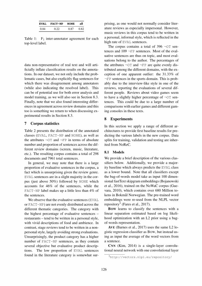
EVAL FACT-NP NONE all

0.84 0.22 0.87 0.82

Table 1: F1 inter-annotator agreement for eachtop-level label.

data non-representative of real text and will arti-ficially inflate classification results on the annota-tions. In our dataset, we not only include the prob-lematic cases, but also explicitly flag sentences forwhich there was disagreement among annotators(while also indicating the resolved label). Thiscan be of potential use for both error analysis andmodel training, as we will also see in Section 8.3.Finally, note that we also found interesting differ-ences in agreement across review domains and thistoo is something we return to when discussing ex-perimental results in Section 8.3.

7 Corpus statistics

Table 2 presents the distribution of the annotatedclasses (EVAL, FACT-NP and NONE), as well asthe attributes ¬OT and ¬FP in terms of absolutenumber and proportion of sentences across the dif-ferent review domains (screen, music, literature,etc.). The resulting corpus contains a total of 298documents and 7961 total sentences.

In general, we may note that there is a largeproportion of evaluative sentences in the corpus, afact which is unsurprising given the review genre.EVAL sentences are in a slight majority in the cor-pus (just above 50%) followed by NONE whichaccounts for 46% of the sentences, while theFACT-NP label makes up a little less than 4% ofthe sentences.

We observe that the evaluative sentences (EVALor FACT-NP) are not evenly distributed across thedifferent thematic categories. The category withthe highest percentage of evaluative sentences –restaurants – tend to be written in a personal style,with vivid descriptions of food and ambience. Incontrast, stage reviews tend to be written in a non-personal style, largely avoiding strong evaluations.Unsurprisingly, the product category has a highernumber of FACT-NP sentences, as they containseveral objective but evaluative product descrip-tions. The low proportion of EVAL sentencesfound in the literature category is somewhat sur-

prising, as one would not normally consider liter-ature reviews as especially impersonal. However,music reviews in this corpus tend to be written ina personal, informal style, which is reflected in thehigh rate of EVAL sentences.

The corpus contains a total of 396 ¬OT sen-tences and 109 ¬FP sentences. Most of the eval-uative sentences are thus on topic, and most eval-uations belong to the author. The percentages ofthe attributes ¬OT and ¬FP are quite evenly dis-tributed among the different domains, with the ex-ception of one apparent outlier: the 31.33% of¬FP sentences in the sports domain. This is prob-ably due to the interview-like style in one of thereviews, reporting the evaluations of several dif-ferent people. Reviews about video games seemto have a slightly higher percentage of ¬OT sen-tences. This could be due to a large number ofcomparisons with earlier games and different gam-ing consoles in these texts.

8 Experiments

In this section we apply a range of different ar-chitectures to provide first baseline results for pre-dicting the various labels in the new corpus. Datasplits for training, validation and testing are inher-ited from NoReC.

8.1 ModelsWe provide a brief description of the various clas-sifiers below. Additionally, we provide a major-ity baseline which always predicts the EVAL classas a lower bound. Note that all classifiers exceptthe bag-of-words model take as input 100 dimen-sional fastText skipgram embeddings (Bojanowskiet al., 2016), trained on the NoWaC corpus (Gue-vara, 2010), which contains over 680 Million to-kens in Bokmal Norwegian. The pre-trained wordembeddings were re-used from the NLPL vectorrepository3 (Fares et al., 2017).

BOW learns to classify the sentences with alinear separation estimated based on log likeli-hood optimization with an L2 prior using a bag-of-words representation.

AVE (Barnes et al., 2017) uses the same L2 lo-gistic regression classifier as BOW, but instead us-ing as input the average of the word vectors froma sentence.

CNN (Kim, 2014) is a single-layer convolu-tional neural network with one convolutional layer

3http://vectors.nlpl.eu/repository/

126

EVAL FACT-NP NONE ¬OT ¬FPDomain Docs Sents # % # % # % # % # %

Screen 110 2895 1359 46.94 50 1.73 1486 51.33 160 11.36 20 1.42Music 101 1743 1055 60.53 48 2.75 640 36.72 100 9.07 23 2.09Literature 35 930 327 35.16 31 3.33 572 61.51 50 13.97 18 5.03Products 22 1156 619 53.55 127 10.99 410 35.47 36 4.83 10 1.34Games 13 520 278 53.46 23 4.42 219 42.12 37 12.29 6 1.99Restaurants 6 268 167 62.31 10 3.73 91 33.96 4 2.26 6 3.39Stage 8 264 100 37.88 6 2.27 158 59.85 7 6.60 0 0.0Sports 2 149 78 52.35 5 3.36 66 44.3 2 2.41 26 31.33Misc 1 36 20 55.56 0 0.0 16 44.44 0 0.0 0 0.0

Total 298 7961 4003 50.28 300 3.77 3658 45.95 396 9.20 109 2.53

Table 2: Distribution of documents, sentences and labels across the thematic categories of reviews. Notethat the percentages for ¬OT and ¬FP are relative to evaluative (EVAL or FACT-NP) sentences.

on top of pre-trained embeddings. The embed-ding layer in convoluted with filters of size 2, 3,and 4 with 50 filters for each size and then 2-maxpooled. This representation is then passed to afully connected layer with ReLU activations andfinally to a softmax layer. Dropout is used afterthe max pooling layer and ReLU layer for regular-ization.

BILSTM is a one-layer bidirectional LongShort-Term Network (Graves et al., 2005) withword embeddings as input. The contextualizedrepresentation of each sentence is the concatena-tion of the final hidden states from the left-to-right and right-to-left LSTM. This representationis then passed to a softmax layer for classification.Dropout is used before the LSTM layers and soft-max layers for regularization.

SAN is a one-layer self-attention network(Vaswani et al., 2017) with relative position rep-resentations (Shaw et al., 2018) and a single setof attention heads, which was previously shownto perform well for sentiment analysis (Ambart-soumian and Popowich, 2018). The network usesa variant of the attention mechanism (Bahdanauet al., 2014) which creates contextualized repre-sentations of the original input sequence, such thatthe contextualized representations encode both in-formation about the original input, as well as howit relates to all other positions.

8.2 Experimental SetupWe apply the models to five experimental se-tups. The main task is to classify each sentenceas evaluative (EVAL), fact-implied non-personal(FACT-NP), or non-evaluative (NONE). In orderto provide a view of how difficult it is to modelthe secondary properties mentioned in Section 3,

Model EVAL FACT-NP NONE Overall

majority 66.2 0.0 0.0 49.5BOW 69.6 0.0 64.4 65.8AVE 75.4 0.0 70.4 71.6CNN 76.3 (0.7) 0.0 (0.0) 72.2 (0.7) 73.1 (0.3)

BILSTM 76.1 (0.1) 6.0 (4.8) 72.1 (0.1) 72.7 (0.1)

SAN 76.2 (0.1) 7.1 (3.1) 72.3 (0.3) 73.7 (0.1)

Table 3: Per class F1 score and overall micro F1

of baseline models on the main classification task.For the neural models mean micro F1 and standarddeviation across five runs are shown.

two additional binary classification tasks are per-formed; determining if the sentence is on topic(OT) and if the opinion expressed is from a first-person perspective (FP). Only the best performingmodel from the main experiment above is appliedfor these subtask, and the model is trained andtested separately on the two subsets of sentencesannotated as EVAL and FACT-NP, leading to fourbinary classification experiments in total.

For all models, we choose the optimal hyper-parameters by performing a random search on thedevelopment data. Given that neural models aresensitive to random initialization parameters, werun each neural experiment five times with differ-ent random seeds and report means for both per-class and micro F1 in addition to their standarddeviation.

8.3 ResultsTable 3 shows the results for all models on themain three-way classification task. All classifiersperform better than the majority baseline (at 49.5

127

F1 overall). Of the two logistic regression classi-fiers, the AVE model based on averaged embed-dings as input performs much better than the stan-dard discrete bag-of-words variant (65.8 vs. 71.6overall). While the AVE model proves to be astrong baseline, the three neural models have thestrongest performance. The CNN achieves the bestresults on the EVAL class (76.3) and improves 1.8ppt over AVE on NONE. While overall results arequite even, the strongest model is SAN – the self-attention network – which achieves an overall F1

of 73.7. This model also proves more stable in thesense of having slightly lower variance across themultiple runs, at least compared to the CNN.

The easiest class to predict is EVAL, followedclosely by NONE. The most striking result is thatis appears very difficult for all models to identifythe FACT-NP class. This is largely due to the fewexamples available for FACT-NP, as well as thefact that FACT-NP sentences do not contain clearlexical features that separate them from EVAL andNONE. This confirms the intuitions presented inSection 3. Only BILSTM and SAN manage tomake positive predictions for FACT-NP, but thescores are still very low (with 7.1 F1 being thebest) and we see that the variance across runs ishigh. An analysis of the strongest model (SAN)shows that the model tends to confuse FACT-NPnearly equally with EVAL (15 errors) and NONE(20 errors), while only correctly predicting thiscategory 6 times, suggesting this category is dif-ficult for the models to capture.

Performance per domain Table 4 breaks downthe F1 score of the SAN model across the differ-ent review domains. We observe that there arefairly large differences in performance, and fur-thermore that these can not simply be explainedjust by differences in the number of training exam-ples for each domain (cf. the class distributions inTable 2). We see that sentences from the literaturereviews appear difficult to classify, despite beingrelatively well represented in terms of training ex-amples, while the opposite effect can be seen forthe games category. The lowest performance isseen for the product reviews, which is unsurpris-ing given that – despite having a high number ofexamples – it is arguably the most heterogeneouscategory in the dataset, in addition to having a rel-atively high proportion of the difficult FACT-NPsentences.

Domain F1

Screen 77.5 (2.2)

Music 76.1 (1.3)

Literature 66.0 (1.3)

Products 65.0 (0.8)

Games 77.6 (2.2)

Restaurants 69.6 (1.5)

Stage 70.0 (2.2)

Table 4: Per domain micro F1 score of the SAN

model. Note that the test set does not contain sen-tences from the Sports or Misc domains.

Human agreement vs model performance Wealso computed the inter-annotator agreementscores per domain, again as pairwise micro F1,and found that while the agreement tends to varyless than model performance, the two scores yielda similar relative ranking of domains in terms ofdifficulty. For example, the two domains with thehighest prediction scores, Games and Screen (withF1 of 77.6 and 77.5, respectively), also have thehighest inter-annotator agreement (82.6 and 83.8).The two domains with lowest prediction F1, Prod-ucts and Restaurants (65.0 and 69.6, respectively),also have the lowest agreement (77.54 and 78.5).

As described in Section 3, while annotator dis-agreements have been resolved, we have chosen tomark them in the final dataset. An error analysisof the classifier predictions show there is a strongcorrelation between inter-annotator agreement anderrors that the classification models make (using aχ2 test, p � 0.01). This suggests that these ex-amples are inherently more difficult, and lead todisagreement for both human and machine learn-ing classifiers.

On-topic and first-person Table 5 shows theresults of applying the SAN architecture to thefour binary tasks. The sentences which are on-topic (OT) and first-person (FP) are the easiest toclassify (F1 ranging from 92.8 to 99.4), while thenot-on-topic (¬OT) and not-first-person (¬FP) arevery difficult (0.0 – 11.3 F1). None of the mod-els are able to correctly predict the ¬FP class. Inorder to distinguish this class, some kind of co-reference resolution likely needs to be included inthe model, as simple lexical information cannotdistinguish them from FP. Note, however, that theprediction scores for ¬FP need to be taken with a

128

Model Subset OT ¬OT Avg. FP ¬FP Avg.

SANEVAL 93.5 (0.1) 11.3 (4.3) 88.5 (1.0) 99.4 (0.0) 0.0 (0.0) 98.9 (0.0)

FACT-NP 97.2 8 (0.0) 0.0 (0.0) 94.6 (0.0) 92.8 (0.0) 0.0 (0.0) 86.5 (0.0)

Table 5: Per-class and micro F1 for the self-attention network trained to predict whether an example ison topic (OT) or not (¬OT) or whether the opinion is expressed by the first person (FP) or not (¬FP). Themodels are trained and tested on the subset of sentences annotated as evaluative (EVAL) and fact-implied(FACT-NP).

grain of salt as there are too few instances in thetest data to give reliable estimates; 5 in each of theEVAL and FACT-NP subsets. The same is trueof the ¬OT predictions for FACT-NP (8 test in-stances). We see that the network is able to predictto some degree (11.3) the ¬OT class for EVAL,but the absolute score is still low, which also re-flects the inter-annotator scores. Once informationabout aspect or target expressions is added to thedata in future annotation efforts, we hope that thismight be leveraged to more accurately predict ‘on-topicness’.

9 Summary and outlook

This paper has described an annotation effort fo-cusing on evaluative sentences in a subset ofthe mixed-domain Norwegian Review Corpus,dubbed NoReCeval. Both subjective and objectivesentences can be labeled as evaluative in our anno-tation scheme. One particular category of objec-tive sentences, conveying so-called fact-impliednon-personal sentiment, is given a distinct label,as this category might need special treatment whenmodeling. Evaluative sentences are also assignedlabels that indicate whether they are on topic andexpress a first-person point of view.

The paper also reports experimental results forpredicting the annotations, testing a suite of differ-ent linear and neural architectures. While the neu-ral models reach a micro F1 of nearly 74 on thethree-way task, none of them are able to success-fully predict the underrepresented minority-classFACT-NP, misclassifying it nearly equally as of-ten with EVAL as with NONE. Additional experi-ments show that it is difficult to classify sentencesas not-on-topic (¬OT) and not-first-person (¬FP),indicating that important of this in future researchon sentiment analysis. Moreover, our error anal-ysis also showed that the cases where annotatorsdisagree (flagged in the data) are also difficult forthe classifiers to predict correctly.

Note that, in our annotation scheme, we onlyannotate sentences as sentiment-bearing (i.e. eval-uative), not with positive/negative polarity val-ues, as labeling polarity on the sentence-level onlymakes sense for sentences that do not containmixed sentiment. Although such datasets are notuncommon, we argue that this is a rather idealizedclassification task not in line with the goal of thecurrent effort. In immediate follow-up work, how-ever, we will perform fine-grained sentiment an-notation where we label in-sentence sentiment ex-pressions and their polarity, in addition to sources(holders) and targets (aspect expressions). In lateriterations we plan to also analyze additional in-formation that can be compositionally relevant topolarity like negation, intensifiers, verbal valenceshifters, etc. The dataset and the annotation guide-lines are made available, along with code for repli-cating the experiments.4

Acknowledgements

This work has been carried out as part of theSANT project (Sentiment Analysis for NorwegianText), funded by the Research Council of Norway(grant number 270908). We also want to expressour gratitude to the annotators, who in additionto the first author includes Anders Næss Evensen,Carina Thanh-Tam Truong, Tita Enstad, and TrulzEnstad. Finally, we thank the anonymous review-ers for their valuable feedback.

ReferencesArtaches Ambartsoumian and Fred Popowich. 2018.

Self-attention: A better building block for sentimentanalysis neural network classifiers. In Proceedingsof the 9th Workshop on Computational Approachesto Subjectivity, Sentiment and Social Media Analy-sis, pages 130–139, Brussels, Belgium.

4https://github.com/ltgoslo/norec_eval

129

Dzmitry Bahdanau, Kyunghyun Cho, and Yoshua Ben-gio. 2014. Neural machine translation by jointlylearning to align and translate. arXiv e-prints,abs/1409.0473.

Jeremy Barnes, Roman Klinger, and Sabine Schulte imWalde. 2017. Assessing State-of-the-Art SentimentModels on State-of-the-Art Sentiment Datasets. InProceedings of the 8th Workshop on ComputationalApproaches to Subjectivity, Sentiment and SocialMedia Analysis, pages 2–12, Copenhagen, Den-mark.

Piotr Bojanowski, Edouard Grave, Armand Joulin,and Tomas Mikolov. 2016. Enriching word vec-tors with subword information. arXiv preprintarXiv:1607.04606.

Richard Eckart de Castilho, Eva Mujdricza-Maydt,Seid Muhie Yimam, Silvana Hartmann, IrynaGurevych, Anette Frank, and Chris Biemann. 2016.A Web-based Tool for the Integrated Annotationof Semantic and Syntactic Structures. In Pro-ceedings of the Workshop on Language Technol-ogy Resources and Tools for Digital Humanities,LT4DH@COLING, pages 76–84, Osaka, Japan.

Murhaf Fares, Andrey Kutuzov, Stephan Oepen, andErik Velldal. 2017. Word vectors, reuse, and replica-bility: Towards a community repository of large-textresources. In Proceedings of the 21st Nordic Con-ference of Computational Linguistics, pages 271–276, Gothenburg, Sweden.

Alex Graves, Santiago Fernandez, and Jurgen Schmid-huber. 2005. Bidirectional LSTM Networks for Im-proved Phoneme Classification and Recognition. InArtificial Neural Networks: Biological Inspirations -ICANN 2005, LNCS 3697, pages 799–804. Springer-Verlag Berlin Heidelberg.

Emiliano Raul Guevara. 2010. NoWaC: a large web-based corpus for Norwegian. In Proceedings of theNAACL HLT 2010 Sixth Web as Corpus Workshop,pages 1–7, NAACL-HLT, Los Angeles.

Marjam van de Kauter, Bart Desmet, and VeroniqueHoste. 2015. The good, the bad and the implicit: acomprehensive approach to annotating explicit andimplicit sentiment. Language Resources and Evalu-ation, 49:685–720.

Kian Kenyon-Dean, Eisha Ahmed, Scott Fujimoto,Jeremy Georges-Filteau, Christopher Glasz, BarleenKaur, Auguste Lalande, Shruti Bhanderi, RobertBelfer, Nirmal Kanagasabai, Roman Sarrazingen-dron, Rohit Verma, and Derek Ruths. 2018. Sen-timent analysis: It’s complicated! In Proceedings ofthe 2018 Conference of the North American Chap-ter of the Association for Computational Linguisticsand Human Language Technologies, pages 1886–1895, New Orleans, Louisiana.

Yoon Kim. 2014. Convolutional Neural Networks forSentence Classification. In Proceedings of the 2014Conference on Empirical Methods in Natural Lan-guage Processing, pages 1746–1751, Doha, Qatar.

Bing Liu. 2015. Sentiment analysis: Mining Opinions,Sentiments, and Emotions. Cambridge UniversityPress, Cambridge, United Kingdom.

Christian Scheible and Hinrich Schutze. 2013. Senti-ment relevance. In Proceedings of the 51st AnnualMeeting of the Association for Computational Lin-guistics, pages 954–963, Sofia, Bulgaria.

Peter Shaw, Jakob Uszkoreit, and Ashish Vaswani.2018. Self-attention with relative position represen-tations. In Proceedings of the 2018 Conference ofthe North American Chapter of the Association forComputational Linguistics: Human Language Tech-nologies, Volume 2 (Short Papers), pages 464–468,New Orleans, Louisiana.

Cigdem Toprak, Niklas Jakob, and Iryna Gurevych.2010. Sentence and expression level annotation ofopinions in user-generated discourse. In Proceed-ings of the 48th Annual Meeting of the Associationfor Computational Linguistics, pages 130–139, Up-psala, Sweden.

Ashish Vaswani, Noam Shazeer, Niki Parmar, JakobUszkoreit, Llion Jones, Aidan N Gomez, Ł ukaszKaiser, and Illia Polosukhin. 2017. Attention is allyou need. In I. Guyon, U. V. Luxburg, S. Bengio,H. Wallach, R. Fergus, S. Vishwanathan, and R. Gar-nett, editors, Advances in Neural Information Pro-cessing Systems 30, pages 5998–6008. Curran As-sociates, Inc.

Erik Velldal, Lilja Øvrelid, Cathrine Stadsnes EivindAlexander Bergem, Samia Touileb, and FredrikJørgensen. 2018. NoReC: The Norwegian ReviewCorpus. In Proceedings of the 11th edition of theLanguage Resources and Evaluation Conference,pages 4186–4191, Miyazaki, Japan.

Theresa Wilson. 2008. Annotating subjective con-tent in meetings. In Proceedings of the 6th editionof the Language Resources and Evaluation Confer-ence, pages 2738–2745, Marrakech, Morocco.

130

An Unsupervised Query Rewriting Approach Using N-gramCo-occurrence Statistics to Find Similar Phrases in Large Text Corpora

Hans Moen1, Laura-Maria Peltonen2, Henry Suhonen2,3, Hanna-Maria Matinolli2,Riitta Mieronkoski2, Kirsi Telen2, Kirsi Terho2,3, Tapio Salakoski1 and Sanna Salantera2,3

1Turku NLP Group, Department of Future Technologies, University of Turku, Finland2Department of Nursing Science, University of Turku, Finland

3Turku University Hospital, Finland{hanmoe,lmemur,hajsuh,hmkmat,

ritemi,kikrte,kmterh,sala,sansala}@utu.fi

Abstract

We present our work towards developing asystem that should find, in a large text cor-pus, contiguous phrases expressing sim-ilar meaning as a query phrase of arbi-trary length. Depending on the use case,this task can be seen as a form of (phrase-level) query rewriting. The suggested ap-proach works in a generative manner, isunsupervised and uses a combination ofa semantic word n-gram model, a statisti-cal language model and a document searchengine. A central component is a distri-butional semantic model containing wordn-grams vectors (or embeddings) whichmodels semantic similarities between n-grams of different order. As data we usea large corpus of PubMed abstracts. Thepresented experiment is based on man-ual evaluation of extracted phrases for ar-bitrary queries provided by a group ofevaluators. The results indicate that theproposed approach is promising and thatthe use of distributional semantic modelstrained with uni-, bi- and trigrams seemsto work better than a more traditional uni-gram model.

1 Introduction

When searching to see if some information isfound in a text corpus, it may be difficult to for-mulate search queries that precisely match all rel-evant formulations expressing the same informa-tion. This becomes particularly difficult when theinformation is expressed using multiple words, asa phrase, due to the expressibility and complex-ity of natural language. Single words may haveseveral synonyms, or near synonyms, which re-fer to the same or similar underlying concept (e.g.“school” vs “gymnasium”). When it comes to

multi-word phrases and expressions, possible vari-ations in word use, word count and word ordercomplicate things further (e.g. “consume food” vs“food and eating” or “DM II” vs “type 2 diabetesmellitus”).

An important task for a search engine is totry to bridge the gap between user queries andhow associated phrases of similar meaning (se-mantics) are written in the targeted text. In this pa-per we present our work towards enabling phrase-level query rewriting in an unsupervised manner.Here we explore a relatively simple generative ap-proach, implemented as a prototype (search) sys-tem. The task of the system is, given a queryphrase as input, generate and suggest as outputcontiguous candidate phrases from the targetedcorpus that each express similar meaning as thequery. These phrases, input and output, may beof any length (word count), and not necessarilyknown as such before the system is presented withthe query. Ideally, all unique phrases with similarmeaning as the query should be identified. For ex-ample, the query might be: “organizational char-acteristics of older people care”. This exact queryphrase may or may not occur in the target corpus.Regardless, a phrase candidate of related mean-ing that we want our system to identify in the tar-geted corpus could then be: “community care ofelderly”. In this example, the main challenges thatwe are faced with are: 1) how can we identifythese four words as a relevant phrase, and 2) de-cide that its meaning is similar to that of the query.Depending on the use case, the task can be seen asa form of query rewriting/substitution, paraphras-ing or a restricted type of query expansion. Rel-evant use cases include information retrieval, in-formation extraction, question–answering and textsummarization. We also aim to use this functional-ity to support manual annotation. For that purposethe system will be tasked with finding phrasesthat have similar meaning as exemplar phrases and

131

queries provided by the user, and/or as previouslyannotated text spans. An unsupervised approachlike we are aiming for would be particularly valu-able for corpora and in domains that lack relevantlabeled training data, e.g. in the form of searchhistory logs, needed for supervised paraphrasingand query rewriting approaches.

The presented system relies on a combinationof primarily three components: A distributionalsemantic model of word n-gram vectors (or em-beddings), containing unigrams, bigrams and tri-grams; A statistical language model; And a doc-ument search engine. Briefly explained, the waythe system works is by first generating a set ofplausible phrase (rewrite) candidates for a givenquery. This is done by first composing vector rep-resentation(s) of the query, and then searching forand retrieving n-grams that are close by in the se-mantic vector space. These n-grams are then con-catenated to form the phrase candidates. In thisprocess, the statistical language model helps toquickly discard phrases that are likely nonsensi-cal. Next the phrases are ranked according to theirsimilarity to the query, and finally the search en-gine checks which phrase candidates actually existin the targeted corpus, and where.

Similar to Zhao et al. (2017) and Gupta et al.(2019) we explore the inclusion of word n-grams of different sizes in the same semanticspace/model. One motivation for this is that theyboth found this to produce improved unigram rep-resentations compared to only training with uni-gram co-occurrence statistics. Another motivationis that we want to use the model to not only re-trieve unigrams that are semantically close to eachother, but also bigrams and trigrams.

2 Related Work

Unsupervised methods for capturing and modelingword-level semantics as vectors, or embeddings,have been popular since the introduction of La-tent Semantic Analysis (LSA) (Deerwester et al.,1990) around the beginning of the 1990s. Suchword vector representations, where the underlyingtraining heuristic is typically based on the distri-butional hypothesis (Harris, 1954), usually withsome form of dimension reduction, have shownto capture word similarity (synonymy and relat-edness) and analogy (see e.g. Agirre et al. (2009);Mikolov et al. (2013)). Methods and toolkits likeWord2Vec (Mikolov et al., 2013) and GloVe (Pen-

nington et al., 2014) are nowadays commonly usedto (pre-)train word embeddings for further usein various NLP tasks, including supervised textclassification with neural networks. However, re-cent methods such as ELMo (Peters et al., 2017)and BERT (Devlin et al., 2018) use deep neuralnetworks to represent context sensitive word em-beddings, which achieves state-of-the-art perfor-mance when used in supervised text classificationand similar.

Further, there are several relatively recent worksfocusing on using and/or representing n-gram in-formation as semantic vectors (see e.g. Bo-janowski et al. (2016); Zhao et al. (2017); Po-liak et al. (2017); Gupta et al. (2019)), possiblyto further represent clauses, sentences and/or doc-uments (see e.g. Le and Mikolov (2014); Pagliar-dini et al. (2018)) in semantic vector spaces.

A relatively straight forward approach to iden-tify and represent common phrases as vectors ina semantic space is to first use some type of col-location detection. Here the aim is to identify se-quences of words that co-occur more often thanwhat is expected by chance in a large corpus. Onecan then train a semantic model where identifiedphrases are treated as individual tokens, on thesame level as words, like it is done in Mikolovet al. (2013).

In the works mentioned so far, the focus is ondistributional semantics for representing and cal-culating semantic similarity and relatedness be-tween predefined lexical units and/or of predefinedlength (words/n-grams, collocations, clauses, sen-tences, etc.). Dinu and Baroni (2014) and Tur-ney (2014) take things a step further and approachthe more complex and challenging task of us-ing semantic models to enable phrase generation.Their aim is similar to ours: given an input query(phrase) consisting of k words, generate as outputt phrases consisting of l words that each expressesits meaning. Their approaches rely on applyinga set of separately trained vector composition anddecomposition functions able to compose a singlevector from a vector pair, or decompose a vectorback into estimates of its constituent vectors, pos-sibly in the semantic space of another domain orlanguage.

Dinu and Baroni (2014) also apply vector com-position and decomposition in a recursive man-ner for longer phrases (t ≤ 3). Their focus ison mapping between unigrams, bigrams and tri-

132

grams. As output their system produce one vec-tor per word which represent the (to be) generatedphrase. Here the evaluation primarily assumesthat t = 1, i.e. the nearest neighbouring wordin the semantic model, belonging to the expectedword class, is extracted per vector to form the out-put phrase. However, no solution is presented forwhen t > 1 other than independent ranked lists ofsemantically similar words to each vector.

Turney (2014) explores an approach targetingretrieval of multiple phrases for a single query (i.e.t > 1), evaluated on unigram to bigram and bi-gram to unigram extraction. Here he applies a su-pervised ranking algorithm to rank the generatedoutput candidates. For each input query, the eval-uation checks whether or not the correct/expectedoutput (phrase) is among the list of top hundredcandidates.

It is unclear how well these two latter ap-proaches potentially scale beyond bigrams or tri-grams. Further, they assume that the length of theinput/output phrases is known in advance. How-ever, the task that we are aiming for is to developa system that can take any query phrase of arbi-trary (sub-sentence) length as input. As output itshould suggest phrases that it identifies in a largedocument corpus which express the same or sim-ilar information/meaning. Here the idea is thatwe only apply upper and lower thresholds whenit comes to the length of the output phrase sugges-tions. In addition, we do not want to be concernedwith knowledge about word classes in the inputand output phrases. We are not aware of previouswork presenting a solution to this task.

In the next section, Section 3, we describe howour system works. In Section 4 we present a pre-liminary evaluation followed by discussion andplans for future work directions.

3 Methods

3.1 Semantic Model Training

In order to train a semantic n-gram model of un-igrams, bigrams and trigrams, we initially ex-plored two approaches. First using the Word2Vecf(Levy and Goldberg, 2014) variation of the origi-nal Word2Vec toolkit, where one can freely cus-tomize the word-to-context training instances asindividual rows in the training file – each row con-taining one source word and one target context topredict. We opted for a skip-gram representationof the training corpus, meaning, for each row in

the customized training file, we put the source n-gram and one of its neighboring n-grams as targetcontext. The size of the sliding window is decidedby how many neighboring (context) n-grams weinclude for each source n-gram. Overlap betweenthe source n-gram and target n-grams is allowed.

However, we found that Word2Vecf only allowstraining using negative sampling. As an alternativeapproach we simply used the original Word2Vectoolkit, with the skip-gram architecture, hierarchi-cal softmax optimization and a window size ofone, to train on the same word-to-context orga-nized training file intended for Word2Vecf. Thismeans that it sees and trains on only two n-grams(cf. word–context pair) at a time. Based on pre-liminary testing we found this latter approach toproduce semantic models that seemed to best cap-ture n-gram semantics for our use case.

The text used for training the semantic model isfirst stemmed using the Snowball stemmer. Thisis done to normalize inflected word forms, re-duce the number of unique n-grams and conse-quently the size of the model, as well as creat-ing more training examples for the remaining n-grams. Mapping back to full-form words andphrases is later done using a document search en-gine, as explained below.

3.2 Phrase-Level Query Rewriting SystemOur system works in a generative way when tryingto find phrases from a target corpus that are seman-tically similar to a query phrase. We describe thisas a five-step process/pipeline.

Step 1: As a first step we generate a set of queryvectors for each of the different n-gram ordersin the model – uni, bi and tri. We simply gen-erate these vectors by normalizing and summingthe associated n-gram vectors from the semanticmodel. In addition, if a word (or all words in an-grams when n > 1) is found in a stopword list1,we give these vectors half weight. As an example:given the query “this is a query”, we generate threequery vectors, # »q1-g, # »q2-g and # »q3-g as follows:

# »q1-g = sum(1

2

# »

this,1

2

#»

is,1

2#»a , # »query) (1)

# »q2-g = sum(1

2

# »

this is,1

2

# »

is a, # »a query) (2)

# »q3-g = sum(1

2

# »

this is a,# »

is a query) (3)

1We use the NLTK (Bird et al., 2009) stopword list forEnglish.

133

If, let’s say, the query only contains one word,we can not generate query bigram or trigram vec-tors. Also, not all n-grams might be found in thesemantic model. To compensate for this possibil-ity, we keep track of the coverage percentage ofeach composed vector. This is later used whencalculating similarity between the query and thegenerated phrase candidates (see step 4).

Step 2: Having composed the query vectors, thesecond step focuses on using the semantic modelto extract the most similar n-grams. For eachquery vector, # »q1-g, # »q2-g and # »q3-g, we extract se-mantically similar unigrams, bigrams and trigramsthat are near in the semantic space. As a distancemeasure we apply the commonly used cosine sim-ilarity measure (cos). We use a cut-off thresholdand a max count as parameters to limit the num-ber of retrieved n-grams and further the number ofgenerated phrase candidates in step 3.

Step 3: The third step focuses on generatingcandidate phrases from the extracted n-grams.This is primarily done by simply exploring all pos-sible permutations of the extracted n-grams. Herewe apply the statistical language model, trainedusing the KenLM toolkit (Heafield, 2011), to ef-ficiently and iteratively check if nonsensical can-didate phrases are being generated. For n-gramswhere n > 1 we also combine with overlappingwords – one overlapping word for bigrams andone or two overlapping words for trigrams. Asan example, from the bigrams: “a good” and“good cake”, we can construct the phrase “a goodcake” since “good” is overlapping.

The generation of a phrase will end if no ad-ditional n-grams can be added, or if the lengthreaches a maximum word count threshold rela-tive to the length of the query2. If, at this point,a phrase has a length that is below a minimumlength threshold3, it will be discarded. Finally, wealso conduct some simple rule-based trimming ofcandidates by mainly removing stopwords if theyoccur as the rightmost word(s).

Step 4: After having generated a set of candidatephrases, we now rank these by their similarity tothe query. For each phrase candidate we composephrase vectors ( # »pn-g) in the same way as we didfor the query. That said, we observed that the tri-gram coverage of the semantic model is relatively

2max length = query length + 2 if query length ≤ 2 else query length × 1.50

3min length = 1 if query length ≤ 2 else query length × 0.50

low compared to unigrams and bigrams. This is aresult of us using a minimum n-gram occurrencecount threshold of 20 when training the semanticmodel. Thus, for the presented experiment, we de-cided to exclude trigrams in the similarity scoringfunction.

As already mentioned, not all n-grams may befound in the semantic model. Thus, we also incor-porate what we refer to as coverage informationfor each # »qn-g – # »pn-g pair. The underlying intuitionis to let query vectors and phrase candidate vec-tors with low model coverage have a lower influ-ence on the overall similarity score. For example,if phrase p is “this is a phrase”, which consist ofthree bigrams, but the semantic model is missingthe bigram “a phrase”, the coverage of # »p2-g, i.e.cov( # »p2-g), becomes 2/3 = 0.66. The coverage ofa # »qn-g – # »pn-g pair is simply the product of theircoverage, i.e. cov( # »qn-g)× cov( # »pn-g).

The overall similarity function sim(q, p) for aquery q and a phrase candidate p is as follows:

sim(q, p) =1

covsum

2∑

n=1

2∑

m=1

(cos( # »qn-g, # »pm-g)

× cov( # »qn-g)× cov( # »pm-g))

(4)

Where cos is cosine similarity, cov( # »qn-g) andcov( # »pm-g) refer to their coverage in the semanticmodel, and covsum is:

(5)covsum =

2∑

n=1

2∑

m=1

(cov( # »qn-g)×cov( # »pm-g)

)

Finally, all candidate phrases generated from aquery are ranked in descending order.

Step 5: In the final step we filter out the can-didate phrases that are not found in the targetedtext corpus. To do this we have made the cor-pus searchable by indexing it with the Apache Solrsearch platform4. Since the candidate phrases areat this point stemmed, we use a text field ana-lyzer that allows matching of stemmed words andphrases with inflected versions found in the orig-inal text corpus. In this step we also gain infor-mation about how many times each phrase occurin the corpus, and where. By starting with themost similar candidate phrase, the search engineis used to filter out non-matching phrases until the

4http://lucene.apache.org/solr

134

desired number of existing phrases are found, oruntil there are no more candidates left.

In addition, the system checks to see if an ex-act match of the query exist in the corpus. If thisis the case, it removes any phrase candidate thatare either a subphrase of the query or contains theentire query as a subphrase. This is a rather strictrestriction, but for evaluation purposes it ensuresthat the system does not simply find and suggestentries of the original query phrase (with some ad-ditional words), or subphrases of it.

4 Experiment

Evaluating the performance of such a system ischallenging due to the complexity of the task andthe size of the text corpus. We are not aware ofevaluation data containing gold standards for thistask. Also, the complexity of the task makes it dif-ficult to apply suitable baseline methods to com-pare against.

We decided to conduct a relatively small ex-periment, relying on manual evaluation, with theaim of getting an insight into strengths and weak-nesses of the system. As text corpus we use acollection of PubMed abstracts consisting of ap-proximately 3.6B tokens. Since our approach isunsupervised, we use this same data set for bothtraining and testing. Six people (aka evaluators)with background as researchers and practitionersin the field of medicine were asked to provide 10phrases of arbitrarily length, relevant to their re-search interests. The requirements were that thephrases should be intended for PubMed, more orless grammatically correct, and preferably consistof two or more words. This resulted in 695 phrasesof different topics, length and complexity, with anaverage word count of 4.07. These serve as queryphrases, or simply queries, for the remainder ofthis experiment.

Next, we use three different versions of thesystem, Ngram, Unigram and Ngramrestr (de-scribed below) to separately generate and suggest20 candidate phrases for each query. The evalu-ators were then given the task of assessing/ratingif these phrases expressed the same information,similar information, topical relatedness or wereunrelated to the query. Each evaluator assessed thesuggestions for the query phrases they providedthemselves6. The five-class scale used for rating

5One person submitted 19 phrases.6No overlapping evaluation were conducted, so no inter-

Class Description1 Same information as the query.2 Same information as the query

and has additional information.3 Similar information as the query

but is missing some information.4 Different information than the query

but concerns the same topic.5 Not related to the query.

Table 1: Classes used by the evaluators when rat-ing phrases suggested by the system.

the phrase suggestions can be seen in Table 1. Intotal, 1380 phrases were assessed for each system(69 × 20).

System - Ngram: Here the system is employedas it is described in Section 3.2. We prepared thetraining data for the semantic n-gram model witha window size equivalent to 3. Minimum occur-rence count for inclusion was 207. A dimension-ality of 200 was used and otherwise default hyperparameters.

System - Unigram: Here we use a more tradi-tional semantic model containing only unigrams.We trained the model using Word2Vec with skip-gram architecture, a dimensionality of 200, win-dow size of 3, minimum inclusion threshold of20, and otherwise default hyper parameters. Thismodel was used to both extract relevant wordsand to calculate similarity between phrases andthe query. Comparing this to the Ngram vari-ant should provide some insight into the effectof training/using semantic models with word n-grams.

System - Ngramrestr: Here we add an addi-tional restriction to the default setup (Ngram) byremoving any generated phrase candidates con-taining one or more bigrams found in the query(based on their stemmed versions). The intentionis to see if the system is still able to find phrases ofrelated information to a query, despite not allowedto use any word pairs found in it.

In all system versions we use a statistical lan-guage model (KenLM (Heafield, 2011)) trainedon the mentioned text corpus with an order of 3.We set the phrase inclusion likelihood threshold to

rater agreement information is available.7Unique unigrams = 0.8M, bigrams = 6.5M, trigrams = 15.7M.

135

Class SystemNgram Unigram Ngramrestr

1 13.99% 9.78% 8.48%2 17.61% 12.54% 16.30%3 24.13% 23.04% 16.23%4 22.61% 25.14% 24.06%5 21.67% 29.49% 34.93%

1+2 31.59% 22.32% 24.78%1+2+3+4 78.33% 70.51% 65.07%

Table 2: Manual evaluation results.

−11.2. We strived to select parameters that madethe system variants produce, on average, approxi-mately the same number of phrase candidates (step2 and 3). The number of phrase candidates gener-ated in step 3 varied significantly depending on thequery and system, from some thousands to sometens of thousands.

5 Results, Discussion and Future Work

Table 2 shows how the evaluators rated the(rewrite) phrases extracted by the various systemsetups. With the Ngram variant, when allowed tosuggest 20 phrases, 31.59% of these contain thesame information as the query phrases – possi-bly with some additional information (rated class1+2). 78.33% of the suggested phrases concernsthe same topic as the query phrases, i.e. ratedclass 1+2+3+4. The latter indicate the percent-age of phrases that could be relevant to the userwhen it comes to query-based searching. Overallthe results show that the system is indeed capa-ble of generating, finding and suggesting (from thePubMed abstracts corpus) phrases that expressessimilar meaning as the query. Table 3 shows ex-amples of a few queries, rewrite suggestions bythe system and their ratings by the evaluators.

Using a semantic model trained on word n-grams of different orders simultaneously (Ngram)achieves better results than using a unigram model(Unigram). This supports the findings in Zhaoet al. (2017) and Gupta et al. (2019).

Naturally, the restricted Ngramrestr variantachieves lower scores than Ngram. However,the performance differences are not that greatwhen looking at the percentage of phrases ratedas class 2. This suggests that the system findsphrases containing some additional informationand/or phrases with words and expressions de-scribing other degrees of specificity. Further, de-

spite not allowed to suggest phrases containingbigrams found in the associated queries, it stillachieves a higher 1+2 score than Unigram.

For some expressions used in the queries, theremight not exist any good alternatives. Or, thesemight not exist in the PubMed abstracts cor-pus. For example, given the query “hand hy-giene in hospitals”. Since Ngramrestr is not al-lowed to suggest phrases containing the expres-sion “hand hygiene”, or even “hygiene in”, it hasinstead found and suggested some phrases con-taining somewhat related concepts such as “hand-washing” and “hand disinfection”. However, forother queries the system had an arguably easiertime. For example, for the query “digestive tractsurgery” it suggests phrases like “gastrointestinal( GI ) tract operations” (rated as class 1) and “gas-trointestinal tract reconstruction” (rated as class2). In other cases, the same meaning of a phraseis more or less retained when simply changing theword order (e.g. “nurses’ information needs” vs“information nurses need”).

We observed that step 5 typically took less timeto complete for Ngram compared to Unigram.This could indicate that Ngram – using the n-gram model – is better at producing phrases thatare likely to exist in the corpus. Another factorhere is the effect of using the n-gram model in theranking step (step 4), which retains some word or-der information from the queries.

A weakness of the conducted experiment is thatwe do not have a true gold standard reflecting ifthere actually exist any phrases in the corpus ofsimilar meaning to the queries, or how many therepotentially are. Still, the results show that theproposed system is indeed able to generate andsuggest phrases whose information expresses thesame or similar meaning as the provided queries,also when there are no exact matches of the queryin the corpus. A planned next step is to look intoother evaluation options. One option is to createa gold standard for a set of predefined queries us-ing a smaller corpus. However, it can be difficultto manually identify and decide which phrases arerelevant to a given query. Another option is touse the system to search for concepts and entitiesthat has a finite set of known textual variants – e.g.use one variant as query and see if it can find theothers. Alternatively, an extrinsic evaluation ap-proach would be to have people use the system inan interactive way for tasks related to phrase-level

136

Query phrase Rewrite suggestions by the system Ratinginfection prevention and control • prevent and control hospital infections 1in hospital • control and prevent nosocomial infection 2

• infection control and preventative care 4information system impact • information system influence 1

• impact of healthcare information systems 2• health information system : effects 2

attitude and hand hygiene • knowledge and attitude towards hand hygiene 2• Hand Hygiene : Knowledge and Attitudes 2• handwashing practices and attitudes 3

assessment of functional capacity • the functional assessment of elderly people 1of older people • functional capacity of the elderly 3

• the functional status of elderly individuals 4facial muscle electromyography • electromyography of facial muscles 1

• electromyography ( EMG ) of masticatory muscles 2• facial muscle recording 3

treatment of post-operative nausea • postoperative nausea and vomiting ( PONV ) treatment 1and vomiting • control of postoperative nausea and vomiting ( PONV ) 1

• treatment of emesis , nausea and vomiting 4fundamental care • fundamental nursing care 2

• palliative care is fundamental 2• holistic care , spiritual care 4

pain after cardiac surgery • postoperative pain after heart surgery 1• postoperative pain management after cardiac surgery 2• discomfort after cardiac surgery 4

Table 3: Examples of a few queries, rewrite suggestions by the system and their ratings by the evaluators.

searching and matching, and then collect qualita-tive and/or quantitative feedback regarding impacton task effectiveness.

So far, not much focus has been placed on sys-tem optimization. For example, no multithreadingwas used in the phrase generation steps. The av-erage time it took for the system to generate andfind 20 phrases in the PubMed abstracts corpus fora query was about 30 seconds. This varied quite abit depending on the number of n-grams extractedin step 2, the semantic model used and the lengthof the query. One bottleneck seems to be step 5which is dependent on the size and status of thedocument index. However, it is worth noting thatwe have observed this to take only a few secondsfor smaller corpora. For use in search scenarioswhere response time is critical, offline generationfor common queries is an option. Further, thiscould for example serve to produce training datafor supervised approaches.

As future work, system optimization will aimtowards having the system generate as few non-relevant phrase candidates as possible while avoid-

ing leaving out relevant ones. This includes mak-ing the search in the vector space (semantic model)to be as precise as possible (query vector com-position) with a wide enough search for semanti-cally similar n-grams (cos similarity cutoff thresh-old). Also, the similarity measure used to rank thephrase candidates relative to the query (sim(q, p))is important for the performance of the system. Asfuture work we also plan to look into the possibil-ity of incorporating ways to automatically excludenon-relevant phrase candidates, e.g. by using asimilarity cut-off threshold. Other text similaritymeasures and approaches could be tried, such assome of those shown to perform well in the Se-mEval STS shared tasks (Cer et al., 2017). In ourrelatively straight forward vector composition ap-proach, each word/n-gram are weighted equally(except for stopwords). Improvements may begained by incorporating some sort of statisticalword weighting, like TF-IDF (Salton and Buck-ley, 1988). Other vector composition approachescould also be considered. Further, we also plan toexplore other approaches to generating semantic

137

text representations, such as Sent2Vec (Pagliardiniet al., 2018). Also approaches like ELMo (Peterset al., 2017) and BERT (Devlin et al., 2018) couldbe applicable for this purpose. Additionally, onecould also explore the use of cross-lingual seman-tic models for tasks related to translation.

Some times the system had a hard time findingphrases reflecting all the information in some ofthe more lengthy and complex queries – possiblyreferring to multiple topics. For example, “meansto reduce the duration of surgical operations” and“a systematic approach to infection control”. Forsome of the queries one can assume that no con-tiguous (sub-sentence) phrases exist among thePubMed abstracts that expresses the same mean-ing. However, something that is missing from ourcurrent pipeline is some kind of query segmenta-tion step. We are now treating each query as asingle expression. As future work, especially inthe context of query-based free-text searching, weaim to incorporate some sort of query segmenta-tion which may split the query into smaller partsdependent on its complexity and the number oftopics it refers to. Here we also want to explorethe possibility of having wildcards in the query.

Overall we find these initial results to bepromising. Further exploration and evaluation ofthe presented approach and system is needed. Thisincludes looking into potential improvements andextensions, such as those mentioned above.

6 Conclusion

In this paper we have described a prototype sys-tem intended for the task of finding, in a large textcorpus, contiguous phrases with similar meaningas a query of arbitrary length. For each of the69 queries provided by a group of evaluators, wetested the system at finding 20 phrases expressingsimilar information. As corpus a large collectionof PubMed abstracts were used. The results indi-cate that using a semantic model trained on wordn-grams of different orders (1–3) simultaneouslyis beneficial compared to using a more traditionalword unigram model. Further, when restrictingthe system from suggesting phrases containing bi-grams from the corresponding queries, the resultsindicate that the system is still able to find and sug-gest relevant phrases.

Acknowledgments

This research was supported by the Academy ofFinland (315376). We would like to thank SuwisaKaewphan for helping out with the preprocessingof the PubMed abstracts data set.

ReferencesEneko Agirre, Enrique Alfonseca, Keith Hall, Jana

Kravalova, Marius Pasca, and Aitor Soroa. 2009. Astudy on similarity and relatedness using distribu-tional and wordnet-based approaches. In Proceed-ings of Human Language Technologies: NAACL2009, pages 19–27. Association for ComputationalLinguistics.

Steven Bird, Edward Loper, and Ewan Klein. 2009.Natural Language Processing with Python. OReillyMedia Inc., Sebastopol, California, USA.

Piotr Bojanowski, Edouard Grave, Armand Joulin, andTomas Mikolov. 2016. Enriching word vectors withsubword information. CoRR, abs/1607.04606.

Daniel Cer, Mona Diab, Eneko Agirre, Inigo Lopez-Gazpio, and Lucia Specia. 2017. SemEval-2017task 1: Semantic textual similarity multilingual andcrosslingual focused evaluation. In Proceedings ofthe 11th International Workshop on Semantic Eval-uation (SemEval-2017), Vancouver, Canada. Asso-ciation for Computational Linguistics.

Scott Deerwester, Susan T. Dumais, George W. Fur-nas, Thomas K. Landauer, and Richard A. Harsh-man. 1990. Indexing by latent semantic analysis.Journal of the American Society for Information Sci-ence, 41(6):391–407.


Georgiana Dinu and Marco Baroni. 2014. How tomake words with vectors: Phrase generation in dis-tributional semantics. In Proceedings of the 52ndAnnual Meeting of the Association for Computa-tional Linguistics (Volume 1: Long Papers), vol-ume 1, pages 624–633.

Prakhar Gupta, Matteo Pagliardini, and Martin Jaggi.2019. Better word embeddings by disentanglingcontextual n-gram information. arXiv preprintarXiv:1904.05033.

Zellig S. Harris. 1954. Distributional structure. Word,10:146–162.

Kenneth Heafield. 2011. KenLM: Faster and smallerlanguage model queries. In Proceedings of the SixthWorkshop on Statistical Machine Translation, WMT’11, pages 187–197, Stroudsburg, PA, USA. Associ-ation for Computational Linguistics.

138

Quoc Le and Tomas Mikolov. 2014. Distributed repre-sentations of sentences and documents. In Interna-tional conference on machine learning, pages 1188–1196.

Omer Levy and Yoav Goldberg. 2014. Dependency-based word embeddings. In Proceedings of the 52ndAnnual Meeting of the Association for Computa-tional Linguistics (Volume 2: Short Papers), vol-ume 2, pages 302–308.

Tomas Mikolov, Ilya Sutskever, Kai Chen, Greg S. Cor-rado, and Jeff Dean. 2013. Distributed representa-tions of words and phrases and their compositional-ity. In Advances in Neural Information ProcessingSystems 26, pages 3111–3119.

Matteo Pagliardini, Prakhar Gupta, and Martin Jaggi.2018. Unsupervised Learning of Sentence Embed-dings using Compositional n-Gram Features. InNAACL 2018 - Conference of the North AmericanChapter of the Association for Computational Lin-guistics, pages 528–540. Association for Computa-tional Linguistics.


Matthew Peters, Waleed Ammar, Chandra Bhagavat-ula, and Russell Power. 2017. Semi-supervised se-quence tagging with bidirectional language models.In Proceedings of the 55th Annual Meeting of theAssociation for Computational Linguistics (Volume1: Long Papers), pages 1756–1765.

Adam Poliak, Pushpendre Rastogi, M Patrick Martin,and Benjamin Van Durme. 2017. Efficient, com-positional, order-sensitive n-gram embeddings. InProceedings of the 15th Conference of the EuropeanChapter of the Association for Computational Lin-guistics: Volume 2, Short Papers, pages 503–508.

Gerard Salton and Christopher Buckley. 1988. Term-weighting approaches in automatic text retrieval.IPM, 24(5):513–523.

Peter D Turney. 2014. Semantic composition and de-composition: From recognition to generation. arXivpreprint arXiv:1405.7908.

Zhe Zhao, Tao Liu, Shen Li, Bofang Li, and XiaoyongDu. 2017. Ngram2vec: Learning improved wordrepresentations from ngram co-occurrence statistics.In Proceedings of the 2017 Conference on Empiri-cal Methods in Natural Language Processing, pages244–253.

139

Compiling and Filtering ParIce: An English-Icelandic Parallel Corpus

Starkaður BarkarsonThe Árni Magnússon Institute

for Icelandic Studiesstarkadur.barkarson@

arnastofnun.is

Steinþór SteingrímssonThe Árni Magnússon Institute

for Icelandic Studiessteinthor.steingrimsson@

arnastofnun.is

Abstract

We present ParIce, a new English-Icelandic parallel corpus. This is the firstparallel corpus built for the purposes oflanguage technology development and re-search for Icelandic, although some Ice-landic texts can be found in various othermultilingual parallel corpora. We mapwhich Icelandic texts are available forthese purposes, collect and filter aligneddata, align other bilingual texts we ac-quired and describe the alignment and fil-tering processes. After filtering, our cor-pus includes 39 million Icelandic wordsin 3.5 million segment pairs. We estimatethat our filtering process reduced the num-ber of faulty segments in the corpus bymore than 60% while only reducing thenumber of good alignments by approxi-mately 9%.

1 Introduction

In recent years machine translation (MT) systemshave achieved near human-level performance ina few languages. They rely heavily on largeamounts of parallel sentences. This can pose prob-lems for inflected languages like Icelandic, wherea substantial amount of data is necessary to covercommon word forms of frequent words. For train-ing statistical (SMT) and neural (NMT) machinetranslation systems, parallel data quality is im-portant and may weaken performance if inade-quate, especially for NMT (see e.g. Khayrallahand Koehn (2018)). A vital part of compiling goodparallel corpora is thus to assess how accurate thealignments are.

In addition to MT, parallel corpora have beenemployed for many tasks, including the creationof dictionaries and ontologies, multilingual andcross-lingual document classification and various

annotation projection across languages. See e.g.Steinberger et al. (2012) for a discussion on themany aspects of parallel corpora usage.

This paper introduces ParIce, the first parallelcorpus focusing only on the English-Icelandic lan-guage pair. There have been few available multi-lingual parallel corpora including Icelandic textsand those that exist vary in quality. Our primaryaim was to build a corpus large enough and ofgood enough quality for training useful MT sys-tems, while we also want it to be useful for otherpurposes, such as those listed above. The projectplan for a language technology program for Ice-landic, set to start in fall 2019, notes that for aquality MT system, a parallel corpus of 25-35million sentence pairs is preferable, although 2million may be sufficient for initial experimentswith state-of-the-art methods (Nikulásdóttir et al.,2017). This first version of ParIce includes 3.5million sentence pairs. That is quite far from theambitious aim set forward in the project plan, butis hopefully sufficient to get meaningful resultswhen used to train MT systems.

We started by mapping what parallel data wasavailable and assessed its quality. We then col-lected unaligned bilingual texts and aligned andfiltered them. In the filtering process we want toremove as many bad segment pairs as possible,while maximizing the number of good sentencepairs we hold on to. There is considerable liter-ature on filtering parallel texts. Taghipour et al.(2011) point out that a lack of properly labeledtraining data makes it hard to use discriminativemethods. They utilize unsupervised methods foroutlier detection. To reduce reliance on labeledexamples, Cui et al. (2013) conduct a PageRank-style random walk algorithm to iteratively com-pute the importance score of each sentence pair.The higher the score, the better the quality. Xuand Koehn (2017) tackle the problem of insuffi-cient labeled data by creating synthetic noisy data

140

to train a classifier that identifies known good sen-tence pairs from a noisy corpus.

In this paper we describe our semi-supervisedmethod of using an NMT system trained on part ofthe corpus, and a bootstrapped dictionary to itera-tively assess and score the sentence pairs. We thenshow how using the score to filter out low qualitydata results in a better quality corpus.

2 Available texts

The data mapping was twofold. First we lookedfor available parallel corpora with Icelandic andEnglish texts. Then we looked for texts availableto us in both languages that we could align and hadpermission to publish with open licenses.

2.1 Aligned data

We collected over 1.9 million English-Icelandicsentence pairs from other parallel corpora (see Ta-ble 1), mostly from the Opus project1 but alsofrom the Tilde MODEL corpus2, ELRC3 and amultilingual parallel bible corpus4.

Opus (Tiedemann, 2012) has a variety of differ-ent parallel corpora in multiple languages. In theEN-IS language pair there are film and tv subtitlescollected from OpenSubtitles5, texts from local-ization files for KDE4, Ubuntu and Gnome and acollection of translated sentences from Tatoeba6,an online collection of sentences and their transla-tions, created by volunteers.

ELRC (European Language Resource Coordi-nation) offers among others a parallel corpus thatwas derived from Icelandic and English texts fromthe Statistics Iceland (SI) website7.

From the Tilde MODEL corpus (Rozis andSkadins, 2017) we include the EN-IS languagepair from a corpus of texts from the EuropeanMedicines Agency document portal.

A parallel corpus of the bible in 100 lan-guages (Christodoulopoulos and Steedman, 2015)is available online. This includes the Icelandic

1http://opus.nlpl.eu2https://tilde-model.s3-eu-west-1.

amazonaws.com/Tilde_MODEL_Corpus.html3Available at the ELRC-SHARE repository4http://christos-c.com/bible/5http://www.opensubtitles.org6http://tatoeba.org7https://www.statice.is8Part of the Tilde MODEL corpus9Part of the OPUS corpus

10Created by ELRC

Sentence Bad align-Corpus pairs ments (%)The Bible4 31,085 0.5EMA8 420,297 3.3Gnome9 5,431 n/aKDE49 87,575 45.0OpenSubtitles9 1,368,170 8.3Statistics Iceland10 2,360 8.0Tatoeba9 8,139 0.0Ubuntu9 2,127 2.5TOTAL 1,923,060

Table 1: Pair count and ratio of bad alignments inthe parallel corpora available.

translation from 1981 and the King James versionof the English bible.

An examination of random sentences fromthese corpora revealed that the sentence pairs weresometimes faulty. This could be due to misalign-ment, mistranslation or other causes. Thus, incases where we could obtain the raw data that thecorpora were compiled from, we realigned themusing our methods. For the EMA corpus we onlyhad the raw data in pdf-files and decided againstharvesting the texts from these files for realign-ment. The raw data for the SI corpus was not avail-able on the ELRC-website, and we did not scrapethe SI website for this project. The Tatoeba datais collected in such a way that there is no reasonto align it again, and inspection of the data fromGNOME indicated that the alignments were of in-sufficient quality and that mending them wouldprove hard so we decided to exclude them fromour corpus.

2.2 Unaligned data

Regulations, directives and other documents trans-lated for the members of the European Eco-nomic Area (EEA) were obtained from the EFTA-website11, where they are available in both pdf andhtml format.

The Icelandic Sagas have been translated intonumerous languages. Some of these translationsare out of copyright and available in English onProject Gutenberg12. The Icelandic texts were ob-tained from the SAGA corpus (Rögnvaldsson andHelgadóttir, 2011). We also selected four booksfrom Project Gutenberg, which were available in

11https://www.efta.int12https://www.gutenberg.org

141

translation on Rafbókavefurinn13, a website witha collection of books in Icelandic in the public do-main. The purpose of this was to experiment withaligning literary translations.

3 Compiling ParIce

We employed a two-step process to pair the sen-tences. First the texts were aligned with LFAligner, except in cases where no alignment wasnecessary (see Section 3.1.2). Then the alignmentwas assessed and filtered.

3.1 Alignment

We used LF Aligner14, which relies on Hunalign(Varga et al., 2005) for automatic sentence pair-ing. It aligns sentences in two languages by usinga dictionary and information on sentence length.

3.1.1 DictionaryWe created a makeshift dictionary of over 12 thou-sand lemmas (D1) by scraping the Icelandic Wik-tionary. In the case of nouns, pronouns and ad-jectives all possible inflections are listed on Wik-tionary and were included in D1,

We ran LF Aligner, using D1, in the first passof the alignment process. Afterwards the data wassent through the filtering process described in Sec-tion 3.2. We then used bitextor-builddics (Esplà-Gomis, 2009), to create another dictionary (D2).Builddics takes as an input source language seg-ments in one file and target language segments inanother. It then compares corresponding lines andbuilds a bilingual dictionary. Finally, D2 was ex-panded by getting all possible word forms of everyIcelandic word in the dictionary from the Databaseof Modern Icelandic Inflection (DMII) (Bjar-nadóttir, 2005). For each Icelandic word in D2, allthe possible lemmas were found in DMII and ev-ery word form was retrieved for each lemma. D2contains approx. 31 thousand lemmas, not count-ing different word forms. We used this dictionaryfor a second run of alignment on all the corpora.

3.1.2 Texts not requiring alignmentTexts from localization files (KDE4 and Ubuntu)are aligned by design. Some lines also containstrings that are not proper words but placehold-ers. In order to have less noisy texts these were

13https://rafbokavefur.is14http://sourceforge.net/projects/

aligner

removed. The Tatoeba segments were also not re-aligned, as the segments are created by translation.

3.2 Assessment and filteringAside from the cases where there was no need forassessment due to the nature of the data (Tatoeba,Bible), or because the alignments had already beenfiltered (KDE4, Ubuntu), we start by assessing thequality of the alignment and filtering out all linesdeemed bad. A rough inspection of the alignedtexts reveals that bad alignments usually come inchunks. If an error occurs in one alignment it hasa tendency to affect the alignment of one or moresentences that follow since LF Aligner can takeseveral lines to find the right path again.

As part of the filtering process we translate theEnglish text of each sentence pair into Icelandicand then compare the translations to the Icelandicsentence and score each pair depending on thatcomparison. Every chunk of sentence pairs thathas unfavorable scoring is deleted, but the sen-tence pairs that are not deleted are used to expandthe dictionary (D2). These steps of translating,scoring, filtering and expanding the dictionary arerepeated several times.

Before describing the filtering pipeline in detailwe describe the scoring process.

3.3 ScoringAll English segments were translated into Ice-landic by employing these two methods:

i) All possible translations were obtained fromdictionary D2 for every word in the English sen-tence, thus creating a multiset for each word.

ii) We used OpenNMT (Klein et al., 2017) totrain an MT system, using a 1 million segmenttranslation memory provided by the TranslationCentre of the Ministry for Foreign Affairs, andparallel corpora obtained from Opus. The systemwas used to translate each English sentence intoIcelandic.

Since Icelandic is an inflected language it wasnecessary to take into account every word form.As described in Section 3.1.1, the D2 dictionaryincluded all possible word forms but for the trans-lated sentence obtained with OpenNMT all wordforms were obtained by using DMII and a multisetcreated for each word of the translated sentence.

The score for every sentence was calculated byfinding the average of score1 and score2. Score1 isthe ratio of words in the Icelandic sentence foundin any of the multisets created by either the first or

142

Accepted Bad Accepted Bad DeletedBefore Filtering Accepted Pairs Pairs (%) Pairs (%) Pairs (%)

The Bible 32,964 32,964 100.0 0.0 n/aBooks 16,976 12,416 73.1 3.5 38.0EEA 2,093,803 1,701,172 81.3 5.0 63.5EMA 420,297 404,333 96.2 1.3 45.0ESO 12,900 12,633 97.9 0.5 46.0KDE4 137,724 49,912 36.2 9.0 n/aOpenSubtitles 1,620,037 1,305,827 80.6 1.4 37.0Sagas 43,113 17,597 40.8 11.0 55.5Statistics Iceland 2,481 2,288 92.2 5.0 56.0Tatoeba 8,263 8,263 100.0 0.0 n/aUbuntu 11,025 10,572 95.9 2.0 n/aTOTAL 4,399,582 3,557,977 80.9

Table 2: Pair count before and after filtering as well as ratio of accepted pairs and deleted pairs that weredeemed bad during the assessment.

the second method of translation. Score2 was cal-culated by finding the ratio of multisets, createdwith dictionary D2, that contained a word formappearing in the Icelandic sentence, and the ratioof multisets, created with OpenNMT/DMII, thatcontained a word form appearing in the Icelandicsentence, and then selecting the higher ratio. Sen-tence pair (1) gets 1.0 as score1 since each word inthe Icelandic sentence would be found in the mul-tisets, and 0.38 as score2 since only three of eightmultisets would contain a word appearing in theIcelandic sentence. The score would thus be 0.69.

(1) a. Hann gekk inn. (e. He walked in)b. As he walked in he sang a song.

The score for each document is the averagescore for all sentence pairs.

3.3.1 FilteringWe set up a filtering pipeline, sending one subcor-pus through it at a time. Steps 4-8 in the pipeline,detailed below, were repeated several times withthe conditions for “good” sentence pairs strict atfirst but more lenient in later iterations. The con-ditions were controlled by thresholds and deletionrules described in step 7 below.

Our filtering pipeline is set up as follows:

1. Aligned sentences are cleaned of all out-of-vocabulary unicode symbols, as some sym-bols cause problems in parsing.

2. The aligned texts are divided into files, onefor each document in the text. The process

deletes faulty files, defining faulty to be onesthat contain either unusually few and largealigned segments or a very low ratio of Ice-landic letters (i.e. ð, þ, ö) in the Icelandic seg-ments, indicating that they might have beenobtained by inadequate OCR.

3. The English segments are automaticallytranslated to Icelandic with the OpenNMTsystem, as described in Section 3.3.

4. The English segments are translated usingdictionary D2, as described in Section 3.3.

5. Each sentence pair is scored.

6. Files receiving on average a score below agiven threshold for their segment pairs aredeleted. The assumption is that the Englishand Icelandic files being aligned are not com-patible or only compatible in minor parts.

7. Sentences are deleted according to one of tworules: i) If a certain number of pairs in a rowhave a score under a given threshold, theyare deleted. ii) If a certain number of pairsin a row have a score above a given thresh-old, they are not deleted but all other pairsare deleted. The second rule is more strictand is usually only used during the first iter-ation. For both rules, the number of pairs ina row and the threshold have different valuesselected for each iteration and subcorpus.

8. Two text files are created from the acceptedsentence pairs: English in one file and Ice-

143

landic in the other, with sentences matchingon line number. The files are used to create anew dictionary with bitextor-builddics whichis appended to dictionary D2.

In OpenSubtitles there often exist many ver-sions of both English and Icelandic subtitles forthe same film. Therefore we sometimes chose be-tween several files from the corpus. Working withthe Sagas, we sometimes had two translations ofthe same Saga. The files receiving the highestscore, after going through the pipe, were selected.

4 Resulting dataset

Before filtering the texts we had 4,399,582 sen-tence pairs in total, see Table 2. During the filter-ing process 841,605 pairs were deleted, 19.13%.The resulting dataset contains 3,557,977 pairs.

4.1 Quality assessment

We manually assessed the alignment quality of thenew corpus as well as the pre-existing corpora bychecking from 200 to 800 sentence pairs in eachsubcorpus, depending on its size. If the sentenceswere not in agreement, if a large chunk was erro-neous or if a sentence in one language containeda segment not found in the other language the pairwas classified as bad.

The quality of ParIce varies between subcor-pora, from containing no bad alignments to 11.0%.Approximately 3.5% of the alignments in the cor-pus are bad, while the ratio was 8% in the pre-existing corpora. See Table 1 for quality estimatesof the pre-existing corpora and Table 2 for qualityestimates of ParIce.

5 Filter assessment

We checked a random sample of 100 to 400 of thedeleted pairs in each subcorpus, depending on thenumber of deleted lines, and counted the amountof bad pairs. The results are shown in Table 2.When we compare this assessment to the assess-ment of the final version of ParIce, we can esti-mate the reduction of errors in the filtering pro-cess. If we exclude the alignments of KDE4 andUbuntu, which were not sent through the main fil-tering pipeline, then 753,340 of 4,250,833 align-ments, or 17.72%, were deleted during the filter-ing process. Of these 53.0% were bad, given thatthe ratio is the same as in our random samples, andthe filtering process reduced the number of faulty

segments in the corpus by 77.0% while it only re-duced the number of good ones by 9.5%.

6 Availability

ParIce can be downloaded from http://www.malfong.is. Available sentences have beenPoS-tagged with a BiLSTM tagger (Steingrímssonet al., 2019), lemmatized with Nefnir (Ingólfsdót-tir et al., 2019) and word aligned with GIZA++(Och and Ney, 2003).

The corpus is also searchable on http://malheildir.arnastofnun.is in a searchtool powered by Korp (Borin et al., 2012).

7 Conclusion and future work

From a fragmented collection of around 1.9 mil-lion sentence pairs of unknown quality, and otherdata, we have built the ParIce corpus of ap-prox. 3.5 million sentence pairs, assessed tobe of acceptable quality. This enables the Ice-landic language technology community, and oth-ers, to experiment with building MT systems forthe English-Icelandic language pair.

While increasing alignment quality, our methodfilters out many perfectly good sentence pairs. Itis necessary both to improve the filtering and thealignment processes. For better alignments a bet-ter dictionary is crucial. In the absence of a betterdictionary, multiple iterations of aligning and fil-tering, where the aligned data is used to grow thedictionary in every iteration, could be helpful.

For better filtering adding features to our scor-ing algorithm might be beneficial. Hangya andFraser (2018) follow Lample et al. (2018) and trainmonolingual word embeddings for two languagesand map them to a shared space without any bilin-gual signal. They use these bilingual word embed-dings for parallel corpus filtering. This approachcould prove useful for our purposes.

The web is our best prospect for growing thecorpus. We have yet to see how much the Para-Crawl project will collect of Icelandic paralleldata, but can expect filtering to be important forthat dataset (see e.g. Koehn et al. (2018)).

It would be useful to try to estimate how goodMT systems trained on this data can get, andwhether our filtering and realigning methods areuseful for that purposes. Training MT systems ondata from different stages and evaluating BLEUscores should thus be added as part of our pipeline,when working on future versions of ParIce.

144

ReferencesKristín Bjarnadóttir. 2005. Modern icelandic inflec-

tions. In H. Holmboe, editor, Nordisk Sprogte-knologi 2005. Museum Tusculanums Forlag, Copen-hagen, Denmark.

Lars Borin, Markus Forsberg, and Johan Roxendal.2012. Korp – the corpus infrastructure of språk-banken. In Proceedings of LREC 2012. Istanbul:ELRA, pages 474–478.

Christos Christodoulopoulos and Mark Steedman.2015. A massively parallel corpus: the bible in100 languages. Language Resources and Evalua-tion, 49(2):375–395.

Lei Cui, Dongdong Zhang, Shujie Liu, Mu Li, andMing Zhou. 2013. Bilingual data cleaning for SMTusing graph-based random walk. In Proceedingsof the 51st Annual Meeting of the Association forComputational Linguistics (Volume 2: Short Pa-pers), pages 340–345, Sofia, Bulgaria. Associationfor Computational Linguistics.

Miquel Esplà-Gomis. 2009. Bitextor: a Free/Open-source Software to Harvest Translation Memoriesfrom Multilingual Websites. In Proceedings of MTSummit XII, Ottawa, Canada. Association for Ma-chine Translation in the Americas.

Viktor Hangya and Alexander Fraser. 2018. An un-supervised system for parallel corpus filtering. InProceedings of the Third Conference on MachineTranslation: Shared Task Papers, pages 882–887,Belgium, Brussels. Association for ComputationalLinguistics.

Svanhvít Ingólfsdóttir, Hrafn Loftsson, Jón Daðason,and Kristín Bjarnadóttir. 2019. Nefnir: A high accu-racy lemmatizer for Icelandic. In Proceedings of the22nd Nordic Conference of Computational Linguis-tics, NODALIDA 2019, Turku, Finland.

Huda Khayrallah and Philipp Koehn. 2018. On theimpact of various types of noise on neural machinetranslation. In Proceedings of the 2nd Workshop onNeural Machine Translation and Generation, pages74–83, Melbourne, Australia. Association for Com-putational Linguistics.

Guillaume Klein, Yoon Kim, Yuntian Deng, JeanSenellart, and Alexander Rush. 2017. OpenNMT:Open-source toolkit for neural machine translation.In Proceedings of ACL 2017, System Demonstra-tions, pages 67–72, Vancouver, Canada. Associationfor Computational Linguistics.

Philipp Koehn, Huda Khayrallah, Kenneth Heafield,and Mikel L. Forcada. 2018. Findings of the WMT2018 shared task on parallel corpus filtering. In Pro-ceedings of the Third Conference on Machine Trans-lation: Shared Task Papers, pages 726–739, Bel-gium, Brussels. Association for Computational Lin-guistics.

Guillaume Lample, Alexis Conneau, Marc’AurelioRanzato, Ludovic Denoyer, and Hervé Jégou. 2018.Word translation without parallel data. In Interna-tional Conference on Learning Representations.

Anna Björk Nikulásdóttir, Jón Guðnason, and SteinþórSteingrímsson. 2017. Language Technology for Ice-landic 2018-2022: Project Plan. Mennta og men-ningarmálaráðuneytið, Reykjavík, Iceland.

Franz Josef Och and Hermann Ney. 2003. A systematiccomparison of various statistical alignment models.Computational Linguistics, 29(1):19–51.

Roberts Rozis and Raivis Skadins. 2017. TildeMODEL - multilingual open data for EU languages.In NODALIDA, pages 263–265. Association forComputational Linguistics.

Eiríkur Rögnvaldsson and Sigrún Helgadóttir. 2011.Morphosyntactic tagging of Old Icelandic texts andits use in studying syntactic variation and change.In C. Sporleder, A. van den Bosch, and K. Zer-vanou, editors, Language Technology for CulturalHeritage: Selected Papers from the LaTeCH Work-shop Series. Springer, Berlin.

Ralf Steinberger, Andreas Eisele, Szymon Klocek,Spyridon Pilos, and Patrick Schlüter. 2012. DGT-TM: A freely available translation memory in 22 lan-guages. In Proceedings of the Eighth InternationalConference on Language Resources and Evaluation(LREC-2012), pages 454–459, Istanbul, Turkey. Eu-ropean Language Resources Association (ELRA).

Steinþór Steingrímsson, Örvar Kárason, and HrafnLoftsson. 2019. Augmenting a BiLSTM tagger witha morphological lexicon and a lexical category iden-tification step. In Proceedings of RANLP 2019,Varna, Bulgaria.

Kaveh Taghipour, Shahram Khadivi, and Jia Xu. 2011.Parallel corpus refinement as an outlier detection al-gorithm. In MT Summit XIII. Machine TranslationSummit (MT-Summit-11), 13., September 19-23, Xi-amen, China. NA.

Jörg Tiedemann. 2012. Parallel data, tools and inter-faces in opus. In Proceedings of the 8th Interna-tional Conference on Language Resources and Eval-uation (LREC’2012).

Dániel Varga, László Németh, Péter Halácsy, AndrásKornai, and Viktor Nagy Viktor Trón. 2005. Parallelcorpora for medium density languages. In Proceed-ings of the RANLP 2005, pages 590–596.

Hainan Xu and Philipp Koehn. 2017. Zipporah: a fastand scalable data cleaning system for noisy web-crawled parallel corpora. In Proceedings of the 2017Conference on Empirical Methods in Natural Lan-guage Processing, pages 2945–2950, Copenhagen,Denmark. Association for Computational Linguis-tics.

145

DIM: The Database of Icelandic Morphology

Kristín Bjarnadóttir, Kristín Ingibjörg Hlynsdóttir, Steinþór SteingrímssonThe Árni Magnússon Institute for Icelandic Studies

University of [email protected], [email protected], [email protected]

AbstractThe topic of this paper is The Databaseof Icelandic Morphology (DIM), a mul-tipurpose linguistic resource, created foruse in language technology, as a referencefor the general public in Iceland, and foruse in research on the Icelandic language.DIM contains inflectional paradigms andanalysis of word formation, with a vocab-ulary of approx. 287,000 lemmas. DIMis based on The Database of Modern Ice-landic Inflection, which has been in usesince 2004. Whereas the older work wasdescriptive, the new version is partly pre-scriptive, making the data applicable in agreater range of projects than before.

1 Introduction

This paper describes The Database of IcelandicMorphology (DIM), containing the morphologi-cal analysis of approx. 287,000 Icelandic lemmas.The DIM is based on The Database of ModernIcelandic Inflection (DMII), a collection of inflec-tional paradigms first published in 2004, and orig-inally conceived as a resource for language tech-nology (LT) (Bjarnadóttir, 2012). The DMII hasbeen restructured and extended to include infor-mation on word formation, and the analysis hasbeen extended to include genre, style, domain,age, and various grammatical features. The orig-inal DMII was descriptive, but DIM is partly pre-scriptive, i.e., the “correctness” of both words andinflectional forms is marked in accordance withaccepted rules of usage. This greatly improvesthe scope of applications using the data, fromthe purely analytical possibilities of the old DMII(used for e.g. search engines, PoS tagging, namedentity recognition, etc.), to the productive possibil-ities of the DIM, such as correction and formula-tion of text. The additional analysis of morpholog-ical constituent structure also provides important

linkups between lexical items, as the morphologyof Icelandic is extremely productive. The nameDIM is here used inclusively for the new project,whereas DMII refers to the inflectional part only.1

DIM has five aspects:

• An LT data source for various uses (inclusiveof the original format available from 2007)

• A new enhanced and enlarged website for thegeneral public

• The prescriptive DMII Core which is a sub-set of the inflectional paradigms marked forcorrectness

• A morphological analysis (MorphIce) withbinary constituent structure and lemmatiza-tion of constituents

• A data source for linguistic research utilizingthe classifications in the database to the full.

The paper is structured as follows. Section 2contains a short description of Icelandic morphol-ogy, to pinpoint the features of analysis needed forvarious LT uses, with a discussion of the differ-ence of descriptive and prescriptive data. Section3 describes the DIM database and discusses de-tails of the classification system briefly. Section 4describes the five main parts of DIM listed above,one by one, drawing out the benefits of the newclassification system in each case, i.e., in the DIM

1The Icelandic name of the DMII is Beygingarlýsingíslensks nútímamáls, abbreviated BÍN. The abbreviation hasbecome a household name in Iceland, with the noun BÍN as-signed feminine gender, and the verb bína (with the object inthe accusative) used of the search. As the name is so wellknown, it is not easy to rename the project, and thus BÍNis still used inclusively in Icelandic for the whole project,both DMII and DIM, i.e., BÍN-vefurinn (DMII Web, for in-flection online), BÍN-máltæknigögn (DIM/DMII LT Data),BÍN-kjarninn (DMII Core), BÍN-orðföng (DIM Morpholog-ical Data, MorphIce)), and Rannsóknar-BÍN (DIM for Re-search).

146

Core, the DMII Web, MorphIce, the accessible LTdata, and a website for linguists doing research onIcelandic. Section 5 gives details on availabilityand licensing, and Section 6 contains the conclu-sion.

2 DIM and the Morphology of Icelandic

Work on the DMII was started in 2002, at the In-stitute of Lexicography in Reykjavík (cf. Bjarna-dóttir (2012) for a description of the project).2

The database (and the analysis) was very limitedin scope, due to considerations of finance andmanpower. The result was a set of inflectionalparadigms for Icelandic intended for LT use, anda website for the general public.3 The download-able LT data has been available in two formats,i.e., in a list of inflectional forms with grammati-cal tags, linked to a list of lemmas, and in a simplelist of inflectional forms without any analysis. Upto date, the data has most popularly been down-loaded as a CSV file, with the fields lemma; wordclass; domain; inflectional form; grammatical tag.The inflectional data for the genitive singular defi-nite form of the masculine noun köttur “cat” is asfollows, slightly simplified, with the grammaticaltag in English:

köttur;416784;masc;kattarins;GEN.SG.+DEF;

This simple data has been used extensively inIcelandic LT projects to date, but these projectshave shown the need for a more extensive analysisof Icelandic morphology, which is rich and full ofvariants and ambiguities, both in regard to inflec-tion and word formation. The reasons are shortlyaddressed in the following subsections, insofar asthey are reflected in the analysis used in DIM.

2.1 Inflection

The ratio of inflectional forms to paradigms inthe original DMII is quite high, i.e., 5.8 mil-lion inflected forms to 270,000 paradigms, withup to 16 inflectional forms to a noun, 120 to anadjective, and 107 to a verb, excluding variants(Bjarnadóttir, 2012).4 The inflectional categories

2In 2006, The Institute of Lexicography merged withother institutions under the name The Árni Magnússon In-stitute for Icelandic Studies.

3It should be noted that the DMII is a set of hardcodedparadigms and not a rule-based inflectional system. The rea-sons for this are given in Bjarnadóttir (2012).

4The figures are from Bjarnadóttir (2012), but the num-ber of inflectional forms of verbs quoted here is from the

for nouns are case (nom., acc., dat., gen.), num-ber (sg., pl.), and definiteness (-/+);5 for adjectivesgender (masc., fem., neut.), case (4), number (2),definiteness (2), and degree (pos., comp., superl.);for finite verbs voice (active, mediopassive), mood(indicative, subjunctive), tense (present, past),number (sg., pl.) and person (1st, 2nd, 3rd).6 Forother word classes, some adverbs inflect for de-gree; personal pronouns inflect for person, caseand number; other pronouns, the definite articleand the numbers from one to four inflect for gen-der, case and number, etc. All these features areused in the tag set for the DMII, which is corre-spondingly large, cf. footnote 4.

The number of inflectional forms is, per se,not problematic, but the number of variant formswith the same grammatical tag within the sameparadigm can be. A simple case in point is gen-itive forms taking different endings, as in the gen-itive singular of the masculine noun lestur “read-ing”: lestrar/lesturs. These two genitive formsare equally acceptable, but restrictions on the us-age of variants can, in other lexical items, be aquestion of context, style, and degree of accept-ability. A case in point is the feminine noun rödd“voice” where the otherwise obsolete dative sin-gular variant röddu is only used in contexts likehárri röddu “with a forceful voice” (i.e., “loudly,clearly”; this instrumental dative phrase construc-tion is quite common). The result of the numberof possible variants of inflectional endings (i.e.,exponents of a grammatical category) is a ratherlarge number of inflectional patterns or inflectionalclasses.7

The inflectional forms are highly ambiguous,and this can be demonstrated by the distributionof the inflectional endings. In the genitive plu-

original DMII. The new DIM includes additional cliticizedverb forms, and grammatical tags for impersonal construc-tions (i.e., verbs with oblique subjects), so the number ofpossible inflectional forms for a verb presently exceeds 300.That analysis is under review, and there are plans to reviewthe PoS tag set for Icelandic which at present contains morethan 670 possible morphosyntactic tags, of which 559 turn upin a corpus of 1.2 billion running words (Steingrímsson et al.,2018).

5Gender is a lexical category for nouns, not an inflectionalone.

6The categories for non-finite verbs are not listed here.7The paradigm of each word is run as a whole, i.e., all

the inflectional variants are produced by one bundle of rules,instead of specifying that a word can belong to more than oneinflectional class. There are at present (May 2019) 669 suchinflectional classes in the DIM; the number fluctuates easilywith new data.

147

ral, the universal ending for nouns is -a8 (as inanda, gen.pl. for both the feminine noun önd“duck” and the masculine noun andi “spirit”), butthe same ending is also one of the nom.sg. endingsin feminine nouns, the acc./dat./gen.sg. ending insome masculine nouns, the acc.pl. ending in somemasculine nouns, not to mention the function ofthe same ending in other word classes. The re-sult is that inflectional forms are hugely ambigu-ous, with only 32% of the inflectional forms in theoriginal DMII being unambiguous (Bjarnadóttir,2012). Disambiguation is therefore an importanttask in Icelandic LT, and because of the idiosyn-crasies of individual words in respect of variantinflectional forms this can only be achieved by re-ferring to a lexicon.

2.2 Word FormationIn Icelandic, the morphological head of a wordis the word-final base word or compound, de-pending on the binary structure of the word (cf.Bjarnadóttir (2017a) for a short reference). Com-pounds can be formed by joining any of the openword classes, but noun-noun compounds are byfar the most common. The rules of compoundformation are recursive, and there is no theoreti-cal limit to the number of constituents in a com-pound, although compounds with more than sixconstituents are rare. An added complication is thefact that the first part of compounds (i.e., the mod-ifier) can take a variety of combining forms. Nom-inal modifiers can appear as stems or inflectedforms, most often in the genitive, singular or plu-ral. The choice of forms is arbitrary, but not free,cf. examples in Table 1 where unacceptable com-pounds are marked by * (cf. also Bjarnadóttir(1995)).

Stem Gen.sg. Gen.pl. Meaningbóksala *bókarsala *bókasala “book store”*bókkápa bókarkápa bókakápa “book cover”*bókbúð *bókarbúð bókabúð “book store”

Table 1: Examples of combining forms in Ice-landic compounds.

The lemmatization of the modifiers is neededfor disambiguation, as inflectional forms arehighly ambiguous, as in the case of the genitiveplural anda in andagift “spiritual gift” (i.e., “in-spiration”), and andapollur “duck pond”, where

8Except for a subset of feminine nouns and a (very) fewneuter nouns where the generative plural ending is -na.

the lemma for anda in the first compound is themasculine noun andi “spirit, breath”, but the fem-inine noun önd “duck” in the second compound.

The ambiguity of the combining forms is a re-flection of the ambiguity of inflectional forms,and the most ambiguous of those in the DMIIat present is minni, which shows up as 30inflectional forms in four paradigms, i.e., inthe neuter noun minni “memory” (5 inflec-tional forms: nom./acc./dat. sg., nom./acc.pl.);in the verb minna “remember” (4 inflectionalforms, not counting impersonal ones: activevoice, 1.p.sg. pres. indicative & subjunctive;3.p.pl. pres. subjunctive); in the adjectivelítill “small, little” (20 inflectional forms, i.e.,comp., masc./fem. nom./acc./dat./gen.sg., andmasc./fem./neut. nom./acc./dat./gen.pl.); and inthe possessive pronoun minn “mine” (1 inflec-tional form, fem.dat.sg.). The ambiguity in com-bining forms is therefore linked to ambiguity else-where in the DIM.

2.3 Description vs. prescription

The DMII was originally created as a part of aneffort to start work on LT at the start of the millen-nium, financed by the Icelandic Ministry for Edu-cation and Culture. The first version of the DMIIwas a set of XML files with 173,389 paradigms,made available on CDs for use in LT in 2004. Thepurpose was quite simple, the data was to be usedin coping with the morphology in Icelandic texts,as well as in search engines and other tools requir-ing the information. The emphasis was being ableto cope with Icelandic texts “as is”, without re-gard to correct spelling, grammar, vocabulary, orstyle. In other words, the data was descriptive, asit had to function for analysis, but it was in no waysuited for production. For that prescriptive data isneeded, in order to conform with the establishedstandards for good Icelandic.

Icelandic standards appear in the “Rulesof spelling and punctuation” (Ritreglur (2016),Reglur um greinamerkjasetningu (2018)), pub-lished by the Ministry of Education and Culture,and in Stafsetningarorðabókin “The Dictionary ofSpelling” (Sigtryggsson, 2016), published by theÁrni Magnússon Institute for Icelandic Studies.9

Various handbooks and grammar books, used in

9These sources are available at the websiteof The Árni Magnússon Institute for IcelandicStudies, https://arnastofnun.is and athttps://malid.is.

148

the school system, also function as prescriptivesources.

In order to make the transition from descriptiveto prescriptive, the core vocabulary of the DMIIhas been checked against the standards mentionedabove, adding extensive cross-referencing of lessthan optimal instances of usage to the standardizedforms in the DMII. This applies both to spelling,inflectional forms, and to the vocabulary itself, as apart of good usage is considered to be in the choiceof native words instead of loan words.

The mark-up of the prescriptive data, with thelinks from the less optimal forms to the prescribedones, makes the data better suited for LT projectssuch as spell checkers, grammar checkers, and anykind of production of text, including teaching ma-terial such as grammatical exercises.

3 The structure of the DIM Database

The old DMII database has been restructured toachieve two main objectives. The first is to al-low for more detailed information and classifica-tion (cf. Subsection 3.1), and the other to allowfor configuring different aspects of the data fordifferent use (cf. Section 4). Some parts of thenew database have been designed from scratch andcontain new types of data, such as the analysis ofword formation which is linked to the other partsof DIM.

Examples of the detailed information added tothe database are features of usage restrictions (syn-tactic, semantic, stylistic, etc.), different ortho-graphic representations, and features of accept-ability, as described in Subsection 3.1. In ad-dition, a proposed part of the DIM, still only inthe preliminary stages, is a repository of writtenword forms not found elsewhere in the DIM data,including obsolete forms, errors of all kinds, andabbreviations. These will be classified, dated, at-tributed to source, and be linked to the list of lem-mas in the DIM proper. Extensive material of thistype is ready for import into the database, bothfrom lexicographic sources and from error anal-ysis. This data allows for new analytic possibil-ities, both for language technology and linguisticresearch. It also extends the time frame of the data,by creating a place for older inflectional variants,as the DMII was originally confined to ModernIcelandic, cf. the name: The Database of Mod-ern Icelandic Inflection. The inclusion of olderdata does not entail attempts at creating paradigms

for Icelandic through the centuries; the data is tooscarce for that. Experiments with using these pe-ripheral word forms in LT have been made, cf.footnote 14 below.

3.1 Classification

DIM uses a new sorting and grading system forwords and inflectional forms to differentiate be-tween prescriptive and descriptive use, or to giveresearchers access to vocabulary containing rele-vant grammatical features. Following is a briefdescription of the main sorting categories, witha handful of examples in footnotes. The systemis complex and a full exposition with examples isoutside the scope here.

• Grammatical features of words: Used tomark words with certain features or restrictedusage. Words can be marked for more thanone feature. These include: Idiom bound,gender variation, older word form, restrictedparadigm, loan word, spelling variants . . . 10

• Value of inflectional forms: Used for inflec-tional forms where two or more variants arepresented, to indicate their status in respect ofthe other variant(s), with values like: equal,dominant, yielding, uncertain.11

• Correctness Grade: Used to mark a word’sor variant’s correctness according to prescrip-tive grammar rules and standardized spelling.Grades range from 0 to 5. Most words havea grade of 1, and this is the default value andstands for “Correct”. Grades 2, 3 and 4 standfor “Used”, “Not good” and “Very bad”, de-pending on the level of “wrongness”, 4 beingthe lowest grade. Grade 5 exists for words orinflectional forms that have somehow made itinto the database but are so “wrong” that they

10Examples of “Grammatical features of words”: Idiombound: almannavitorð n.neut. “public knowledge”, onlyused in the dative singular in the idiom e-ð er á almanna-vitorði “sth is public knowledge”; Gender variation: engi-fer n.masc. or n.neut. “ginger”; Older word form: röddudat.sg. of rödd n.fem. “voice”, cf. Subsection 2.1; Restrictedparadigm: munu v. auxilary. The verb is finite only, activevoice only, and there is no past tense in the indicative; Loanword: engifer n.masc. or n.neut. “ginger” (Loanwords, es-pecially multisyllable ones, need marking as their inflectionvery often deviates from the inflection of the native vocabu-lary.); Spelling variants: pósitívur/pósitívur adj. “positive”.

11Examples of "Values of inflectional forms”: Equal:dugir/dugar, 3.p.sg.pres. active voice of duga v. “suffice”;Dominant: rödd, dat.sg. of rödd n.fem. “voice”; Yielding:röddu, dat.sg. (idiom bound) of rödd n.fem. “voice”.

149

could not possibly be part of the language ofan adult with a native speaker’s competencein Icelandic, and so they are only visible inadministrator mode. Words and inflectionalvariants classified by genre (cf. next para-graph) have the grade 0, standing for “Notapplicable, depends on style or genre”. Thisis because variants marked by genre are notincorrect, but they are not the most commoncorrect form either.12

• Genre: Used to sort words and inflectionalforms according to style or age. Values:Formal, informal, derogatory, obscene, rare,old-fashioned, obsolete, poetic language, re-gional. Genre is not a mandatory feature forwords or variants.

• Domain: A semantic classification, usedto classify named entities and domain spe-cific vocabulary. These include several dif-ferent kinds of names (e.g. Icelandic per-sonal names, place names, etc.), and tech-nical terms from different fields, etc. Mostwords are in the domain called Common lan-guage, which is the default value. All wordsbelong to one domain only.13 Domain spec-ification only applies to words, not to inflec-tional forms.

• Pronunciation: Features of pronunciationare marked on words with possible discrep-ancies between pronunciation and spelling.Still a work in progress, this is meant forlinguistic research, but it may be useful forspeech synthesizers or speech analysis, etc.

• Peripheral word forms: Older word forms,spelling errors and other forms that do not fitwithin a paradigm are kept in a separate listand connected to a lemma in the database.This can be used to connect errors or old

12Examples of “Correctness Grade”: 1 (Correct, defaultvalue): jafnvægi n.neut. “balance”. 2 (Used): ballansn.masc. “balance”. The compound jafnvægi is consideredbetter usage, it is also much more common.; 3 (Not good):pósitífur adj. “positive”. According to The Dictionary ofSpelling the correct form is pósitívur; 4 (Very bad): lítern.masc. “liter”. The correct form is lítri n.masc. 0 (Gradingis not applicable): blóðgagl “raven, vulture”, poetic language(blóð “blood” and gagl “goose; bird”).

13The result is that the common noun hrafn “raven”and the personal name Hrafn are shown in two differentparadigms, although the inflection is identical.

forms to the appropriate modern form.14

4 The Five Aspects of DIM

DIM has five aspects or conceptual units. All ofthem are part of one database; two of them aresolely focused on inflection, i.e., the DMII Core(Subsection 4.1) and the DMII Website (Subsec-tion 4.2), and one contains the word formationsanalysis, i.e., MorphIce (Subsection 4.3). The re-maining two aspects contain different modes ofaccess to the data, the LT Website for use in lan-guage technology (Subsection 4.4), and the Ling-Research for research on the language (Subsec-tion 4.5).

4.1 The DMII CoreThe DMII Core is designed to meet users’ de-mands for data from the DMII in a prescriptivecontext, and it is created to be used for third partypublication through an API, especially for lan-guage learners. The RESTful API is open foreveryone to use. It allows users to send sim-ple queries and receive full paradigms in JSON-format as a response. The data in the DMIICore only contains the core vocabulary of Ice-landic, only standardized spelling, and only themost common or correct inflectional forms. Thismakes the data suited for creating teaching mate-rial and for other prescriptive uses. As the datain the DMII Core is simplified and the vocabularylimited, the omission of a word or variant does notimply that it is wrong. However, if a word or vari-ant is found in the DMII Core, users should be ableto trust that it is safe to use, i.e., correct, in all (ormost) contexts.

The vocabulary of the DMII Core is based onthe list of headwords in The Modern IcelandicDictionary (Jónsdóttir and Úlfarsdóttir, 2016), andthe 50,000 most frequent words (lemmas) in theThe Icelandic Gigaword Corpus (Steingrímssonet al., 2018). The total number of paradigms inthe DMII Core now stands at 56,867 (end of May2019), as compared almost 287,000 in the wholeof DIM.

The new classification system (cf. Subsec-tion 3.1), is used to choose words and inflec-tional variants for the DMII Core. Only wordsand variants with a correctness grade of 1 (univer-sally acceptable) are included in the DMII Core,

14Cf. Daðason et al. (2014) for description of an LT toolfor transposing older Icelandic texts to modern spelling, usingdata from a pilot project of this kind.

150

and the categories of genre included are “formal,informal, derogatory, obscene”. (The excludedones are “rare, old-fashioned, obsolete, poetic lan-guage, regional”.) The only domain included inthe DMII Core is common language (i.e., the de-fault value), with a chosen selection of named enti-ties, i.e., common Icelandic personal names, a fewvery common place names, and the most commonnames of institutions.

The paradigms in the DMII Core have beensimplified as possible, without omitting equallyvalid variants, showing only the best forms, or thevariants not limited by specific usage restrictions.The correctness grade is also used for inflectionalforms, and only variants with correctness grade of1 are included.

4.2 The DMII website

Individual paradigms have been accessible on theDMII website from 2004.15 Extensively used bythe Icelandic public as a reference on inflection,the website has been popular from the start, andthe latest figures show that more than 200,000users viewed over 1.7 million pages in the yearstarting June 1, 2018. (The total population of Ice-land is approx. 360,000.) The figures are still ris-ing, with 9% growth over the previous year. Orig-inally, the data was set out to be purely descrip-tive, for use in analysing Icelandic text “as is”, notjust the “received” text adhering to the rather strictlanguage norms officially advocated. To make thewebsite more useful, notes on usage were placedwith individual inflectional paradigms, pointingthe way in the choice of variants, and containinginformation on restrictions on their use. Thesenotes are in Icelandic only, and they were origi-nally hand-crafted and not classified in any way.This makes the original website unsuited for anybut speakers with native or near native knowledgeof Icelandic, as the users themselves have to makethe final choice between variants, with the help ofthe notes. In this context, the multitude and ambi-guity of variant forms has to be stressed.

This mode of operation has not always been to-tally successful, as the descriptive nature of thedata causes problems, even for native speakers ofIcelandic. The expectation is that all word formsappearing on the site are “best usage”, all spellingvariants are “good”, and all words shown on thewebsite are acceptable, irrespective of genre, style,

15http://bin.arnastofnun.is

etc. The tolerance for substandard usage appear-ing on the website is at times very low, as the userswill let the editors know from time to time. Theconverse is also true, as some users expect all “ac-ceptable” Icelandic words to be found in the DMII,in spite of clear statements to the contrary on thewebsite, stating that the DMII is not exhaustiveand not an authority on acceptable Icelandic vo-cabulary. The original duality of purpose in theDMII, i.e., the need for the maximum number ofword forms found in texts for LT analysis vs. theneeds of ordinary users for prescriptive data, hastherefore caused some problems from the start.

The new version of the DMII website, to beopened in 2019, makes use of the work on clas-sification in the DMII Core described in Subsec-tion 3.1. Markings on variations in spelling andword formation, and any restrictions on use dis-covered in the work of adapting the standard, arecarried over into the paradigms on the DMII web-site, in the form of better notes on usage, withextensive cross-references. To give one exampleof two words commonly causing confusion be-cause of their spelling, the words híði “den” (asin “bear’s den”) and hýði “skin” (as in “bananaskin”) are pronounced in the same way. Each ofthese entries on the website gives both forms, ex-plaining the semantic difference. In case of sub-standard spelling (as in writing pósitífur insteadof pósitívur “positive”), a hyperlink to the appro-priate spelling rule is provided, as published on-line at The Árni Magnússon Institute’s portal forinformation on Icelandic usage.16 The guidelineson the DMII website still warn the users that theDMII is not a spelling dictionary, but there arenow referrals to the standard wherever possible.

4.3 MorphIce

The morphological analysis included in MorphIcegives full constituent structure, with lemmatizedconstituents. As compounding in Icelandic is ex-tremely productive, this is of importance in LTtasks, as the data can be used to minimize the ef-fect of out-of-vocabulary words. The data alsoserves for training of tools such as the com-pound splitter Kvistur (cf. Daðason and Bjarna-dóttir (2014)), which has been used to estimatethe probability of unknown compounds by the useof a preliminary version of the data in MorphIce.This data was originally analysed manually in the

16https://malid.is

151

nineties (Bjarnadóttir, 2006) and will now be in-corporated into the DIM. It is only with the cre-ation of MorphIce that this data can be made freelyavailable as a linguistic resource.

As stated in Subsection 2.2, compound forma-tion in Icelandic is complex. The compound anal-ysis in MorphIce assumes binary branching, andthe rules are recursive, resulting in quite complexbinary trees.

The data on each compound will give full de-tails on each component, with links to the mainindex in the DIM, with DMII ids. All informationon the inflection of each constituent word in thecompound will therefore be accessible.17 Boundconstituents (affixes and combining forms) form aseparate part of the data set, with information onthe structures into which they fit. The format ofthe output is still under construction, but a sampleof the analysis can be seen in the word orðabókar-maður “lexicographer” below, with the consituentparts orð “word”, bók “book”, and maður “man”.The analysis is binary, with each item in the ex-ample showing the result of one process or wordformation rule. These can be nested or not in theoutput, according to needs, but as stated above, thefinal format is still under construction. The num-bers are the ids of the words in the DMII.

• orðabókarmaður:[[orðabókar]<gen.sg.orðabók.n.fem.404616>[maður]<n.masc.5763>]<n.masc.88516>

• orðabók:[[orða]<gen.pl.orð.n.neut.2635>[bók]<n.fem.11100>]<n.fem.404616>

A coding system for the binary trees is included inthe data, with “0” for base words, “1” for a sin-gle join, “12” for a left-branching binary tree withthree constituents, as in [[[orða][bókar]][maður]]above, etc. The granularity of the compound anal-ysis can by adapted to the needs of each LT task,and the most detailed analysis will probably onlybe of interest to linguists.

The data in MorphIce will be linked to a datasetcontaining argument structure, presently found in

17The inflection of Icelandic compounds is notoriouslyunpredictable, especially when there is a choice of variantforms, as in útvegur “fishing industry”, gen.sg. útvegs (i.e.,út “out” adv., vegur “road, way”) vs. akvegur “road (forcars)”, gen.sg. akvegar (aka “drive” verb, vegur “road”).In recursive compounding, such genitives do appear as modi-fiers. In such cases, the data should be sufficient for analysis,but perhaps not unerring in predictions for new compounds.

a pilot version on the website of The Árni Magn-ússon Institute for Icelandic Studies (Bjarnadóttir,2017b). This data will be used to link multiwordconstructions, such as particle verbs and verbswith incorporated object, to their compound coun-terparts, as in greina að “separate” (i.e., “takeapart”, the compound verb aðgreina also ex-ists), the past participle/adjective aðgreindur, thepresent participle aðgreinandi, and the noun að-greining. Structures of this kind are very com-mon in Icelandic, and finding and analysing mul-tiword lexical entities and linking them to com-pounds helps in demarcating semantic units.

In the future, the plan is to make the binary treesthemselves accessible online, but as yet the for-mulation of that project is only in the preliminarystages.

4.4 The LT Website

Datasets from DIM, for use in language technol-ogy, are available from a separate website. Untilnow, two versions of the data have been availablefor download on the old DMII website along withdetailed descriptions of the datasets, in Icelandicand English. One version is the list of inflec-tional forms and lemmas, along with word classand grammatical tag, described in Section 2. Theother is a simple list of word forms, without anyclassification or linkups. The new DIM-LT web-site still makes the DIM data available for down-load in those formats, but more configurations areavailable, constructed in cooperation with a selectgroup of long-time users. The data available onthe DIM-LT website is updated daily. For repro-duction purposes, versioned datasets will be pub-lished periodically.

The dataset is published with an open licenseand is intended for use in the development of LTtools and methods, but it may also be suitable inother fields as well. The DIM-LT data is not in-tended for lookups. Users who build software thatneeds to do lookups in DIM at runtime will be en-couraged to use the API, described in Sections 4.1and 5, as that will allow them access at all times tothe most recently updated data.

As well as providing access to download-able data, the DIM-LT website has informa-tion on licensing, detailed information on all thegrammatical features appearing in the inflectionalparadigms, including lists of word classes, all in-flectional categories and grammatical terms, and

152

other relevant information, in Icelandic and En-glish. The tag set in the downloadable data is inIcelandic, but English translations are accessibleon the website.

4.5 DIM LingResearch

The DIM LingResearch is an adaptation of the edi-torial interface to the new database, to be made ac-cessible for linguistic research. All features of theclassification of words and inflectional forms willbe accessible for the extraction of data. Some fea-tures have been specially included in the databasewith linguistic research in mind, such as categoriesof irregular pronunciation. To name an example,the vowel a is diphthongized when preceding ng(as in the word bangsi “teddy bear”), except in afew loanwords, such as mangó and tangó. Thistype of data is interesting for linguists working onmorphophonemics, but it may also be useful forspeech systems, etc. There are at present 16 pro-nunciation sets of this kind in the data, along withsimilar sets for various other features of word for-mation, etc.

5 Access and licencing

As described in previous sections, DIM is avail-able in different configurations. The DMII Core ismade available through an API through a permis-sive license that allows third parties to publish thedata on the web. They are required not to mod-ify the data and to give appropriate credit. Allparadigms can be viewed individually on the newDMII website, as they have been on the old DMIIwebsite since 2004. Access is open to all andfree of charge, but scraping the data or copying enmasse is prohibited. For use in language technol-ogy or research on the language, the datasets areavailable for download with an open, permissivelicense, CC BY-SA. The same will apply to theMorphIce data. Finally, access to the DIM Ling-Research interface, intended for scholars, will begiven upon request.

6 Conclusion

The data from the old DMII has been used exten-sively from 2004, when it was first made avail-able. The initial dream was basically to createdata for rather simple tools, like a decent searchengine, etc. Very many of the projects using thedata have far surpassed these expectations. Two ofthese projects are mentioned above, i.e., the com-

pound splitter Kvistur (cf. Subsection 4.3), andthe spellchecker Skrambi, referred to in connec-tion with the use of peripheral word forms (cf.Subsection 3.1, footnote 14).18 Two very recentNLP-tools take advantage of DMII, the PoS Tag-ger ABLTagger (Steingrímsson et al., 2019) andthe lemmatizer Nefnir, which is described in thiscurrent version of NoDaLiDa (Ingólfsdóttir et al.,2019). A list of additional projects is accessible onthe DIM website.19

In fall 2019, the first projects will start in anational language technology programme, whichwill run for five years. The programme followsa plan set forward in 2017 (Nikulásdóttir et al.,2017), and aims to produce open systems for ma-chine translation, spell and grammar checking,speech synthesis and speech recognition.

Extensive linguistic resources are needed for thenew projects planned in the next five years. Thisis especially important for two reasons. First, theIcelandic language community is very small, andalthough Icelanders take pride in the productionof a great deal of text (as evidenced in a bloom-ing Icelandic literary scene, and the proliferationof Icelandic websites, etc.), the actual mass of textproduced is nowhere close to the scale accessi-ble in really large language communities. Even ifall Icelandic texts from all times were accessible,very many word forms would probably only oc-cur a few times, certainly not often enough to beuseful in statistical analysis.20 The other reasonis the complexity of Icelandic morphology, bothinflectional and morphological, with correspond-ing irregularities and ambiguities. It has thereforeproved to be necessary to produce and store themorphological data, instead of writing a rule sys-tem for analysing the morphology on the go.

We see the work in the immediate future asongoing excerption from the Gigaword Corpus(Steingrímsson et al., 2018), fine-tuning the analy-sis and classifications described in this paper, andongoing cooperation with the users of the data, asthey are the people who know what they need.

18Skrambi is available as an online spellchecker(http:skrambi.bin.arnastofnun.is), but itis also used in different versions for tasks such as correctingOCR texts, and to transpose older texts with unstandardizedspelling from different periods to Modern Icelandic.

19http:bin.arnastofnun.is20Some inflectional forms are not found at all, as is the case

for the dative singular of the name of Odin’s tree Yggdrasillwhich is not to be found in any of the Old Icelandic sources.

153

Acknowledgments

The restructuring of the DMII and the creationof DIM was made possible by a grant by theIcelandic Research Council in 2017. The au-thors wish to thank our co-workers in the project,without whom the project would not have takenshape: Samúel Þórisson, for the database, andTrausti Dagsson, for the creation of the newwebsites. Thanks are also due to our presentand former colleagues at The Árni MagnússonInstitute for Icelandic Studies and The Univer-sity of Iceland who have been generous withtheir time, advice and assistance: StarkaðurBarkarson, Jón Friðrik Daðason, Sigrún Helga-dóttir, Halldóra Jónsdóttir, Jón Hilmar Jóns-son, Ari Páll Kristinsson, Kristján Rúnarsson,Eiríkur Rögnvaldsson, Jóhannes B. Sigtryggsson,Einar Freyr Sigurðsson, Ásta Svavarsdóttir, ÞórdísÚlfarsdóttir, Ágústa Þorbergsdóttir, Gunnar ThorÖrnólfsson, and Katrín Axelsdóttir. Thanks arealso due to the company Já.is for their generoussupport through the years.

References

Kristín Bjarnadóttir. 1995. Lexicalization and theSelection of Compounds for a Bilingual IcelandicDictionary Base. Nordiske studier i leksikografi,(3):255–263.

Kristín Bjarnadóttir. 2006. Afleiðsla og samsetningí generatífri málfræði og greining á íslenskumgögnum. Orðabók Háskólans, Reykjavík, Iceland.

Kristín Bjarnadóttir. 2012. The Database of ModernIcelandic Inflection. In LREC 2012 Proceedings:Proceedings of “Language Technology for Normal-ization of Less-Resourced Languages”, SaLTMiL 8– AfLaT, pages 67–72.

Kristín Bjarnadóttir. 2017a. Phrasal compounds inModern Icelandic with reference to Icelandic wordformation in general. In Carola Trips and Jak-lin Kornfilt, editors, Further investigations into thenature of phrasal compounding. Language SciencePress, Berlin, Germany.

Kristín Bjarnadóttir. 2017b.https://notendur.hi.is/ kristinb/divs-2017.txt ÍSLEX-venslamálfræði. The Árni Magnússon Institute forIcelandic Studies, Reykjavík, Iceland.

Jón Friðrik Daðason and Kristín Bjarnadóttir. 2014.Utilizing constituent structure for compound anal-ysis. In Proceedings of LREC 2014. Reykjavik:ELRA, pages 1637–1641.

Jón Friðrik Daðason, Kristín Bjarnadóttir, and KristjánRúnarsson. 2014. The Journal Fjölnir for everyone:The post-processing of historical OCR texts. In Pro-ceedings of Language Resources and Technologiesfor Processing and Linking Historical Documentsand Archives - Deploying Linked Open Data in Cul-tural Heritage. Reykjavik: ELRA, pages 56–62.

Svanhvít Ingólfsdóttir, Hrafn Loftsson, Jón Daðason,and Kristín Bjarnadóttir. 2019. Nefnir: A high accu-racy lemmatizer for Icelandic. In Proceedings of the22nd Nordic Conference of Computational Linguis-tics, NODALIDA 2019, Turku, Finland.

Halldóra Jónsdóttir and Þórdís Úlfarsdóttir, editors.2016. http://islenskordabok.arnastofnun.is Íslensknútímamálsorðabók. The Árni Magnússon Institutefor Icelandic Studies.

Anna Björk Nikulásdóttir, Jón Guðna-son, and Steinþór Steingrímsson. 2017.https://notendur.hi.is/eirikur/mlt-en.pdf LanguageTechnology for Icelandic 2018-2022: Project Plan.Mennta- og menningarmálaráðuneytið, Reykjavík,Iceland.

Jóhannes B. Sigtryggsson, editor. 2016. http://malid.isStafsetningarorðabókin. The Árni Magnússon Insti-tute for Icelandic Studies.

Steinþór Steingrímsson, Sigrún Helgadóttir, EiríkurRögnvaldsson, Starkaður Barkarson, and JónGuðnason. 2018. Risamálheild: A Very Large Ice-landic Text Corpus. In Proceedings of the EleventhInternational Conference on Language Resourcesand Evaluation, LREC 2018, Miyazaki, Japan.

Steinþór Steingrímsson, Örvar Kárason, and HrafnLoftsson. 2019. Augmenting a BiLSTM tagger witha morphological lexicon and a lexical category iden-tification step. In Proceedings of RANLP 2019,Varna, Bulgaria.

154

Tools for supporting language learning for Sakha

Sardana Ivanova, Anisia Katinskaia, Roman YangarberUniversity of [email protected]

AbstractThis paper presents an overview of linguis-tic resources available for the Sakha lan-guage, and presents new tools for support-ing language learning for Sakha. The essen-tial resources include a morphological an-alyzer, digital dictionaries, and corpora ofSakha texts. We extended an earlier versionof the morphological analyzer/transducer,built on the Apertium finite-state platform.The analyzer currently has an adequate levelof coverage, between 86% and 89% on twoSakha corpora. Based on these resources,we implement a language-learning environ-ment for Sakha in the Revita computer-assisted language learning (CALL) plat-form. Revita is a freely available online lan-guage learning platform for learners beyondthe beginner level. We describe the tools forSakha currently integrated into the Revitaplatform. To our knowledge, at present thisis the first large-scale project undertaken tosupport intermediate-advanced learners ofa minority Siberian language.

1 IntroductionThe Sakha language, also known by its exonymYakut, is the language of an ethnic community, whomainly inhabit the Republic of Sakha in the FarEast of Siberia, Russian Federation. According tothe 2010 census, Sakha is the native language of450,140 people, and is considered vulnerable dueto its limited usage. Children do not use Sakha inall aspects of their life; they speak Sakha at homewith family, but do not use it in school and socially.Sakha belongs to the Northern group of the

Siberian branch of the Turkic language family, andis agglutinative, as are all Turkic languages, (Ubry-atova, 1982). It has complex, four-way vowel har-mony, and a basic Subject-Object-Verb word or-der. The lexicon of Sakha consists of native Turkic

words, has many borrowings from the surroundingMongolic and Tungusic languages, numerous loan-words from Russian, as well as words of unknownorigin. Sakhamakes extensive use of post-positions,which indicate syntactic relations and govern thegrammatical case of nominals, (Forsyth, 1994).In the digital sphere, Sakha can be considered a

low-resource language. We report on our projectto provide learning support for Sakha. Buildingon pre-existing digital resources, we aim to providea learning platform for students (including adults)who are interested in strengthening their linguisticcompetency in Sakha.The paper is structured as follows. Section 2 de-

scribes distinctive properties of the Sakha languageand motivates the need for language-learning sup-port by reviewing the social environment of the lan-guage. Section 3.1 presents an overview of previouswork Sakha; Section 3.2 describes the Revita plat-form for language learning. Section 4 describes theinstruments we integrate to support language learn-ing for Sakha. In Section 5 we discuss initial resultsobtained with the tools. Sections 6 concludes withpointers for future work.

2 Sakha language

Sakha is the national language of the Sakha people,which, along with Russian, is one of the official lan-guages of the Republic of Sakha (Yakutia), (Yart-seva, 1990). The Sakha language differs signifi-cantly from other Turkic languages by the presenceof a layer of vocabulary of unclear (possibly Paleo-Asiatic) origin, (Kharitonov, 1987). There are also alarge number of words ofMongolic origin related toancient borrowings, as well as late borrowings fromthe Russian language, (Tenishev, 1997).

2.1 Distinctive featuresVowels in Sakha follow complex vowel harmonyrules. The features of the vowels within a wordmustagree in a strictly defined fashion. First, palatal-

155

velar harmony of vowels is observed in Sakhastrictly sequentially and does not admit exceptions.If the first syllable contains a front vowel, then thevowels in all subsequent syllables in the word mustbe front. Otherwise, if the first syllable contains aback vowel, then the vowels in all subsequent syl-lables must be back. Second, labial vowel harmonyrequires that the sequence of vowels agree accordingto the degree of roundedness within adjacent sylla-bles, (Sleptsov, 2018). For example:

• back+unrounded: “аҕа / аҕалардыын”[aGa / aGalardIn]“father/with fathers”

• back+rounded: “оҕо / оҕолордуун”[oGo / oGolordun]“child / with children”

• front+unrounded: “эбэ / эбэлэрдиин”[ebe / ebelerdin]“grandmother / with grandmothers”

• front+rounded: “бөрө / бөрөлөрдүүн”[boro / borolord¯un]“wolf / with wolves”

Thus, the vowels in the suffixes “-лар-” [lar], in-dicating the plural, and “-дыын” [dIn], indicatingcomitative case, undergo 4-way mutation accordingto vowel harmony.In Sakha, the verb is the central part of

speech, (Dyachkovsky et al., 2018). Some verbs canhave multiple affixes (as in most Turkic languages),which can correspond to an entire clause or sentencein other languages, such as Russian. Sakha has noinfinitive form for verbs, therefore a predicate that(in other languages) would include an infinitive isconveyed by various indirect means, for example:

• “суруйан бүтэрдэ”: [surujan buterde]“he finished writing”(literally: “he wrote, finished”);

• “сатаан ыллыыр”: [satan IllIr]“he can sing”(literally: “he knows how, sings”);

• “бобуоххун син”: [bobuoXXun sin]“you can forbid”(literally: “you can, let’s forbid”).

Sakha is characterized by an exceptional varietyof verbal tenses. In particular, according to (Kork-ina, 1970), 8 past forms are distinguished:

• proximal-past:“үлэлээтим” [uleletim]“I worked (recently)”;

• remote-past:“үлэлээбитим” [ulelebitim]“I worked (long ago)”;

• past perfect:“үлэлээбиппин” [ulelebippin]“In fact, I worked”;

• episodic past:“үлэлээбиттээхпин” [ulelebitteXpin]“I used to work on occasion”;

• past imperfect:“үлэлиирим” [ulelirim]“I worked in the past for some time”;

• plusquamperfect:“үлэлээбит этим” [ulelebit etim]“I had worked prior to that”;

• episodic plusquamperfect:“үлэлээбиттээх этим” [ulelebitteX etim]“Long ago, I used to work”.

The total number of tense forms exceeds 20.One of the particularities of nouns is when paired

nouns are marked with possessiveness, both compo-nents of the compound noun change in parallel, asthe word is inflected:

• “баай-дуол” [baj duol] “wealth”:“баайа-дуола” [baja duola](3rd person possessive, nominative case),“баайын-дуолун” [bajIn duolun](3rd person singular possessive, accusative)

• “сурук-бичик” [suruk bicik] “writing”:“сурукта-бичиктэ” [surukta bicikte](partitive case),“суругу-бичиги” [surugu bicigi](accusative case)

2.2 Socio-linguistic environmentAccording to (Vasilieva et al., 2013), since 1990,the percentage of ethnic Sakha has grown, reach-ing 45% of the total population in the Republic ofSakha. Ethnic Sakha together with other indigenouspeoples of the North Siberia and the Far East com-prise over 50% of the total population.Vasilieva et al. (2013) has conducted surveys,

which show a direct dependence of the level of lin-guistic proficiency on the language of instruction atschool. A fluent level of proficiency is achieved by:

• respondents who had schooling in the Sakhalanguage (34.5%)

• respondents who had studied in schools, wheresubjects were taught in Russian and partly inSakha (27.4%).

156

Only 17.9% of respondents who had studied inRussian are fluent in Sakha. Respondents whospeak Sakha poorly, or do not speak at all, graduatedfrom Russian-speaking schools. Thus, as expected,linguistic skills and abilities in Sakha are poorer forthose who had studied in Russian.In work life, the Russian language is dominant

for all age groups. In the two youngest age groups(16–25 and 26–35 years old), the use of Russian isgrowing, approaching 50%. This is due to the re-quirements of formal communication, terminolog-ical dependence, ethnically mixed composition ofprofessional teams. On the other hand, after thecompletion of active professional life, the return toan increased usage of the original ethnic language iscommon, (Vasilieva et al., 2013).In Yakutsk—the capital and the largest city of

the Sakha Republic—one in three Sakha childrenlack the opportunity to study in their native lan-guage. This is a violation of the right to studyin one’s native language. The number of schoolswhich offer teaching in Sakha in Yakutsk in 2002–2003 was 16, and dropped to 15 by 2003–2004.The number of schools where Sakha is studied asa subject decreased from 22 (in 2002–2003) to 16(in 2003–2004). The number of Sakha languagelearners decreased from 6,377 to 2,902, (Vasilievaet al., 2013). According to the statistical reportof the Ministry of Education of the Republic ofSakha in 2006–2007, the cities of the Republic had147 schools with Russian language of instruction(61,055 children), 4 educational institutions withnon-Russian languages of instruction (1014 chil-dren), 29 institutions with amix of Russian and non-Russian languages of instruction (18,094 children).In 11 schools (serving 1,262 students) non-Russianlanguages are offered as optional subjects of study.Vasilieva et al. (2013) indicate that this situa-

tion concerning the language of instruction of eth-nic Sakha pupils has a direct correlation with otherserious problems in terms of linguistic competencyin Sakha and vitality of Sakha—acculturation andassimilation of urban youth, which will leads to lin-guistic conformism due to the lack of sufficient so-cial opportunities for using the language.

3 Prior work

3.1 Sakha language resourcesDespite the current advances in digitization, digitalresources for the Sakha language are severely lack-ing. The creation of digital tools would strengthen

the language in a number of ways, and severalprojects are being undertaken to support Sakha. Webriefly mention some of them here.The digital bilingual dictionary SakhaTyla.Ru1

currently offers over 20,000 items from Sakha toRussian, over 35,000 items from Russian to Sakha,about 2,000 items from Sakha to English, and about1,000 items from English to Sakha. In addition totranslations, this dictionary also contains examplesof usage, including idiomatic usage, for every item,which constitutes a base of lexical data, and canbe highly useful for language learning and teaching.The base of examples from this dictionary is cur-rently not utilized in our learning platform.Leontiev (2015) has compiled a newspaper cor-

pus of Sakha containing over 12 million tokens.The SakhaWikipedia contains over 12,000 articles,which makes up a corpus of over 2 million tokens.2A Sakha course on the educational platform

Memrise offers a vocabulary of about 3100 words.3Audio materials: Common Voice is a platform

for crowdsourcing open-source audio datasets.4 Atpresent, it offers just under 2.5 hours validatedvoice recordings in Sakha. By comparison, Englishhas almost 850 hours of audio content on the plat-form, and Russian has 50 hours.In summary, few linguistic resources exists for

Sakha.

3.2 Revita language learning platform

Revita is an e-learning platform, which usesmethods from computer-assisted language learn-ing (CALL) and intelligent tutoring systems (ITS).5The platform provides a language-independentfoundation for language learning, which can beadapted to support new languages, by addinglanguage-specific resources, without modifying thecore system. The platform is used for languageteaching and learning at several universities in Eu-rope and Asia.The goal of the system is to provide tools for

language learning, (Katinskaia et al., 2018), andto support endangered languages, (Katinskaia andYangarber, 2018; Yangarber, 2018). The systemfocuses on stimulating the student to actively pro-duce language, rather than passively absorb exam-

1www.sakhatyla.ru2sah.wikipedia.org3www.memrise.com/course/153579/sakha-tylyn-

leksikata-sakha-tyla-iakutskii/4voice.mozilla.org/en/about5revita.cs.helsinki.fi

157

ples of language use or grammatical rules. The sys-tem achieves this by helping students learn languagefrom stories. The story can be any text, which thestudents can choose themselves. The platform takesan arbitrary text chosen by the user and uses it aspractice material; it creates exercises for the stu-dent based on the text: the exercises are new everytime the student practices with the text—to keep thepractice sessions interesting and to reduce boredom.The computational engines in the platform analyzethe text, and try to determine which concepts arebest suited for the student to learn next.The platform has been customized for sev-

eral less-resourced Finno-Ugric languages: Erzya,Komi-Zyrian, Meadow Mari, North Saami, Ud-murt; it has also been customized for Kazakh (alsoa Turkic language), and several others. Revita alsooffers a number of languages with larger resources:currently, the most developed are Finnish, Russian,and German, and initial support exists for Swedish,Spanish, Catalan, and French.

4 System for supporting Sakha

In this section we describe our work on adding theSakha language to the Revita platform for languagelearning. The system is built on several lower-levellinguistic tools and components.

4.1 Morphological analyzerThe morphological analyzer, part of the packagecalled apertium-sah, was developed in the con-text of the Apertium platform, (Forcada et al.,2011). The analyzer is developed using the HelsinkiFinite-State Toolkit (HFST), (Lindén et al., 2011).The lexicon and morphotactics are written in thelexc formalism, and the morphophonology is de-veloped using the twol formalism, based on theTwo-Level Morphology framework, (Koskenniemi,1983). The transducers are compiled into a mor-phological analyzer and a generator. The transduceris two-directional: on one hand, it can map a surfaceform to all of its possible lexical forms; on the otherhand, it can take a lexical form and generate all ofits corresponding surface forms. That is, the trans-ducer can be used both for analysis and for genera-tion of surface forms.For example, the surface form “атын” receives

two analyses—lexical forms:

• ат [at] <n> <px3sg> <acc>Horse.Noun.Possessive-3sg.Accusative“his horse” (accusative)

• атын [atIn] <adj>“other” Adjective (indeclinable)

We extended the initial, baseline version of theApertium Sakha analyzer by adding lemmas to thelexicon based on their frequencies, which we com-puted from the Wikipedia corpus. Initially the ana-lyzer had 4,303 stems. Table 1 gives the number oflexical items for each of the major parts of speech(POSs) in inital and extended analyzer versions.

Part of speech Original ImprovedNoun 2,582 4,240Proper noun 815 2,155Adjective 464 1,362Verb 278 1,038Adverb 62 338Numeral 58 89Pronoun 15 17Postposition 12 42Conjunction 7 16Determiner 10 16Total: 4,303 9,313

Table 1: Number of stems per part of speech

The morphological tagset consists of 92 tags: 16tags indicate parts of speech—noun, adjective, verb,postposition, etc.—and 76 tags indicate values formorphological subcategories, e.g., for case, number,person, possession, transitivity, tense, aspect, mood,etc. We consultedUbryatova (1982) as the principalsource of grammatical information.

4.2 Language learning platformThe platform offers the learner several exercisemodes based on input stories: reading mode, prac-tice mode, flashcards, crossword mode, etc.In the reading mode learner can read a story, and

request translations of unfamiliar words.In the practice mode the system generates exer-

cises based on the story, which user has uploadedto the system. The story undergoes several stagesof analysis. At the lowest level the system usesthe Sakha morphological analyzer, (Ivanova et al.,(To appear). The story is presented in “snippets”—small pieces of text, about 50 tokens each, approx-imately one paragraph or 2–3 sentences in length.The system selects some of the tokens in the snip-pet to generate quizzes. Each quiz may be of severaltypes: “cloze” (i.e., fill-in-the-blank quiz), multiple-choice, or a listening exercise (where the learnermust type in the words s/he hears).

158

Figure 1: Practice mode

The system creates cloze quizzes from inflectedparts of speech, i.e., nouns, verbs, etc. For example,the first sentence in the snippet in Figure 1 is

“Туйаара уонна Айаал оонньуулларынсөбүлүүллэр .”

[tujara uonna ajal onnjullarIn sobul¯uller]

“Tuyaara and Ayaal like to play.”The current snippet of the story appears over agrey background, and contains cloze and multiple-choice exercises. The system created a cloze exer-cise, showing to the user only the base form (lemma)“сөбүлээ” [sobule] (“to like”) of the surface form“сөбүлүүллэр” [sobul¯uller] (“they like”):

“Туйаара уонна Айаал оонньуулларынсөбүлээ ...”

[tujara uonna ajal onnjullarIn sobule]

From the verb lemma the learner should guesswhich form of the hidden word fits the context best.Multiple-choice quizzes are constructed also

from non-inflected parts of speech (adverbs, post-positions, etc.) Tokens of similar part of speech arepresented to the learner as “distractors”—incorrectanswer options. Figure 1 shows a multiple-choicequiz for the token “куруук” [kuruk] (“always”) withother adverbs serving as distractors.Listening exercises (optional) are generated from

tokens in the story—the words are spoken by aspeech synthesizer and the learner must enter theword that was pronounced. Currently, listening ex-ercises are not available for Sakha; we plan to in-corporate them into the system when text-to-speech(TTS) synthesis for Sakha becomes available.

The previous snippets—above the currentsnippet—show correctly answered questions—coloured in green—and incorrectly answeredquestions in blue.The choice of candidates for exercises depends

on the user model—based on the history of theuser’s previous answers. The system computesprobabilities (weights) for potential candidates inthe snippet. Exercises receive a lower probabilityif the student had mostly answered them correctlyor mostly incorrectly in earlier sessions—since itmeans that they are too easy or too difficult for thelearner at present.In the crossword mode, a crossword is built based

on the text. Exercises for the crossword are selectedrandomly, and according to the same principles asin practice mode.The user can receive the translation of an unfa-

miliar word by clicking on it. The box on the left inFigure 1 shows a dictionary entry for a token clickedby the user—”дьиэ” [Zie] (“house”). The learnercan request a translation of an unfamiliar word inall practice modes. Translations are looked up inthe SakhaTyla.Ru digital dictionary. The systemrecords the words for which translations were re-quested into the user’s own set of flashcards. In theflashcardmode the user can practice vocabulary, us-ing timed repetition algorithms.Stories for learning can be found on newspaper

websites, such as edersaas.ru, kyym.ru, etc., or fromthe Sakha Wikisource.6

6https://sah.wikisource.org/

159

Figure 2: Example of a chunk

4.3 Chunking for exercisesRevita allows the language expert to customize thesystem for a new language by explicitly specify-ing rules for syntactic government and agreement.The system performs shallow parsing (“chunking”)based on these rules, and uses the chunks when cre-ating exercises, discussed in the previous section.Next we discuss how these rules can work for Sakha.A government rule, Rg, may state:(сылтаан, PostP)→ [Ablative]

which means that the post-position lemmaсылтаан, [sIltan], (meaning “because-of”),governs the ablative case of its preceding noun (ornoun phrase).A simple but quite general agreement rule, Ra,

may state:[ {pos: Noun, case: $X }+ {pos: PostP, gov_case: $X } ]

RuleRa consists of two elements/tokens, and de-scribes case agreement. If a token with noun POSis followed by a token with postposition POS, theywill form a unit (phrase) if the free variable $X, in-dicating the value of the case feature of the nounand the case that the postposition governs, has thesame value for both tokens.Using these two rules, the systems will match all

corresponding constructions in text. For example:

“... ардахтан сылтаан ... ”[ardaXtan sIltan]

Rain.Noun.ABL because_of.Post-position“... because of rain ...”

The Revita language learning system uses thesechunk rules to construct exercises. For example, theexercise based on the second sentence in Figure 2:

“Ол гын баран бэҕэһээ ардахт сылтаанолус тымныы этэ!”[ol gIn baran beGehe ardaX sIltan olus

tImnI ete]

“But it was very cold yesterday because of therain!”

Corpus Tokens % CoverageOriginal analyzer:Wikipedia 2015 1,020,000 73.02Kyym (newspaper) 1,040,000 71.36Improved analyzer:Wikipedia 2019 2,195,565 89.28Newspapers 16,436,999 86.41

Table 2: Coverage of the morphological analyzer

The boxes contain the cloze quizzes—exercises forthe user. The system provides hints for each cloze.First, inside the box it shows the lemma of theword. Further, each phrase circled in red forms achunk/unit—based on the government and agree-ment rules, such as Rg and Ra, above. Thus,the post-position “сылтаан” [sIltan] (“because of”),which governs the ablative case, links it to its pre-ceding noun “ардах” [ardaX] (“rain”) to hint to theuser that the noun’s surface form should be in theablative.

5 Discussion

5.1 Analyzer coverageTable 2 shows the coverage of the improved mor-phological analyzer, as compared to the originalone. Coverage of the original analyzer was mea-sured on the Wikipedia corpus (dump from 2015)and the “Kyym” Sakha newspaper.The improved analyzer was tested on aWikipedia

dump from 2019, and the large newspaper corpuscompiled by Leontiev (2015). Currently, the cov-erage on Wikipedia is about nine out of ten tokens,which is higher, as expected, since the analyzer wasdeveloped based on a frequency list from this cor-pus.

5.2 Learner engagementWe have presented the language learning platformto language experts and lecturers at the Departmentof the Sakha language, at the North-Eastern Fed-

160

eral University in Yakutsk, Russian Federation. Theexperts confirm that the language learning systemcan be a promising tool for enhancing instructionin Sakha. We also plan to introduce the learningsystem to Sakha learners in cooperation with Yaku-tia.Team, the organization for promoting Sakha lan-guage and culture.7Releasing the system for use by language learners

will yield mutual benefits for the learners as well asfor the researchers. The learners receive a trainingplatform which helps them improve their linguisticcompetency. From the interaction of the learnerswith the platform, the researchers receive valuableeducational data, for modeling the process of learn-ing Sakha, the patterns of mistakes that the learnersmake over time, and insights into how the learningsystem can be improved on the basis of the collecteddata.

5.3 Multiple admissibilityMultiple Admissibility (MA) in language learningoccurs when more than one surface form of a givenlemma fits syntactically and semantically within agiven context. MA implies that multiple alternativeanswers are “correct” for the given context, not onlythe word that the author chose to use in the story.From the perspective of CALL and ITS (intelligenttutoring systems), MA forms a complex challenge,discussed in current research, (Katinskaia et al.,2019).The Sakha language presents a particularly rich

source of scenarios for multiple-admissible an-swers. Due to the agglutinative morphology ofSakha, the learner can add affixes to a word,which carry additional information or connotationsto slightly alter the meaning of the word. We brieflydiscuss several such scenarios.The category of possessiveness—possessive af-

fixes on nominals—is one of the fundamental cate-gories of Sakha grammar. Possessive forms are verycommon, and the scope of their usage is far widerthan merely indicating possession in the strict sense;possessive affixes express a wide range of logical re-lations and connections between objects, which areoften not related directly to the strict notion of pos-session, (Ubryatova, 1982). For example:

• “сылдьыбатах сирим”[sIlZIbataX sirim]“a place where I have not been”(literally: “my place, where ...”)

7https://www.yakutia.team

• “билбэт киһитэ”[bilbet kihite]“man whom s/he doesn’t know”(literally: “her man, whom ...”).

We often find examples of using an impersonalform of a noun in place of a possessive form of anoun and vice versa, as in the following examples:

• Example of using an impersonal noun insteadof a possessive noun:1a. Form which was used in a story:

“ сааны ылан сүгэр”[sanI Ilan suger](“he hung a gun on his shoulder”)

1b. The learner’s input:“ саатын ылан сүгэр”[satIn Ilan suger](“he hung his gun on his shoulder”)

• Example of using a possessive form instead ofan impersonal form:2a. Form which was used in a story:

“моонньун уһатан уутун көрөр”[monnjun uhatan utun koror](“craning his neck, he looks at (his) wa-ter”)

2b. The learner’s input:“моонньун уһатан ууну көрөр”[monnjun uhatan unu koror](“craning his neck, he looks at the water”)

Secondly, Sakha has a highly developed systemof verbal aspects. Aspect in Sakha can be expressedby various affixes or analytically. Aspect is one ofthe most commonly used grammatical categories inSakha, which allows statements in the language tobe expressive and precise, (Ubryatova, 1982). Eightforms are used to designate actions that have oc-curred prior to the present time.As a result of this choice, it may be quite difficult

to decide which form best fits the context, given onlythe base form of the word. For instance, it can bedifficult to distinguish the “first past” perfect tenseand recent past tense, because the results of bothactions are connected with a present moment.The verb form which was used in a story: first

past perfect tense, indicative mood, third person,singular:

“Эһэм сиргэ сылдьан өрүү түргэнхаамыылаах, оттон бу сырыыга өссөчэпчэкитик үктэнэргэ дылы буолбут .”

161

[ehem sirge sIlZan or¯u turgen XamIlaX,otton bu sIrIga osso cepcekitik uktenergedIlI buolbut ]

“Grandfather usually walks fast in the field, butthis time he also seems to step lighter” (meaning,the action is inferred from its result).

The learner’s input was a verb form in the recentpast tense, indicative mood, third person, singular:

“Эһэм сиргэ сылдьан өрүү түргэнхаамыылаах, оттон бу сырыыга өссөчэпчэкитик үктэнэргэ дылы буолла .”[ehem sirge sIlZan or¯u turgen XamIlaX,otton bu sIrIga osso cepcekitik uktenergedIlI buolla ]“Grandfather usually walks fast in the field,but this time he also steps lighter” (meaning,the action is observed by the speaker).

These and many other examples show that thetask of generating exercises automatically for Sakhais far from trivial and requires much research due toextensive multiple admissibility.

6 Conclusion and future work

This paper offers an overview of the resources avail-able for Sakha, and describes our work on creatingtools to support language learning for Sakha. Oursurveys of available resources demonstrate that theyare severely lacking.We present the following tools and resources,

which we combine to create a system to support lan-guage learning for Sakha:

• morphological analyzer, built on the Apertiumplatform,

• language learning system, built on the Revitaplatform,

• bilingual Sakha dictionaries,• several Sakha corpora.The morphological analyzer is an essential com-

ponent in any natural language processing (NLP)system, without which little can be done to providecomputational tools for the language.The functionality of the language learning sys-

tem is under development. For larger languagesmany more linguistic resources and tools are avail-able than for Sakha. For example, currently, theSakha system has only noun–postposition govern-ment rules. We plan to implement additionalshallow-parsing rules to provide intelligent errorfeedback to the learners. For example, verb–complement government:

“ангинанан ыалдьыбыт”[anginanan IalZIbIt]

tonsillitis.Noun.INS contract.Verb.2SG.PAST(“s|he contracted tonsillitis”).

The verb “ыарый” [IarIj] (“to contract”) gov-erns the instrumental case of the noun “ангина”[angina] (“tonsillitis”).Currently, the system employs chunking (shallow

parsing) to track instances of syntactic government.The system can track more complex and longer-range government with the help of deep parsing.Once a parser for Sakha becomes available, it willenable Revita to provide richer feedback to thelearner.The Sakha analyzer needs further improvement

to reach higher coverage. The main work to bedone is extending the lexicon. While a good level ofcoverage has been achieved with only 9,313 stems,production-level morphological analyzers have atleast tens of thousands of stems—more typically,hundreds of thousands. Once good coverage hasbeen achieved for the morphological analyzer, thenext step is to build models for morphological andsyntactic disambiguation.As more advanced tools for Sakha become avail-

able, they will be incorporated into Revita, to pro-vide richer functionality:

• Parsers, e.g., dependency parsers, such asbased on the constraint-grammar formalism(commonly used in Apertium), or statistical orneural-network based parsers.

• Difficulty models—to predict the difficulty ofa story for the user, and to assess the learner’slevel of competency—based on how well alearner handles easy vs. difficult stories.

• Disambiguationmodels—to disambiguate am-biguous tokens in text.

• Text-to-speech—to provide listening exercisesbased on text.

• Speech-to-text—to provide speaking exercises(not yet available).

Acknowledgements

This research was supported in part by the “Fin-UgRevita” Project, Academy of Finland, Grant267097, and EDUFI Fellowship TM-18-10846.We are very grateful to Javad Nouri, Kim Salmi,

Max Koppatz, José María Hoya Quecedo, and JueHou for their contributions.

162

ReferencesKatja Bang. 2015. Language situation in the republicof Sakha (Yakutia). Master’s thesis, University ofTurku, School of Languages and Translation Studies.

Nikolay Dyachkovsky, Petr Sleptsov, K Fedorov, andM Cherosov. 2018. Поговорим по-якутски. Само-учитель языка саха (Let’s speak Sakha. Sakha lan-guage tutorial). Yakutsk: Bichik.

Mikel L Forcada, Mireia Ginestí-Rosell, Jacob Nord-falk, Jim O’Regan, Sergio Ortiz-Rojas, Juan An-tonio Pérez-Ortiz, Felipe Sánchez-Martínez, GemaRamírez-Sánchez, and Francis M Tyers. 2011. Aper-tium: a free, open-source platform for rule-based ma-chine translation. J. Machine Translation, 25(2).

James Forsyth. 1994. A history of the peoples of Siberia:Russia’s North Asian colony 1581-1990. CambridgeUniversity Press.

Sardana Ivanova, Francis Tyers, and Jonathan Washing-ton. (To appear). The Apertium implementation offinite-state morphological analysis for the Sakha lan-guage.

Anisia Katinskaia, Sardana Ivanova, and Roman Yangar-ber. 2019. Multiple admissibility: Judging grammat-icality using unlabeled data in language learning. InProceedings of the 7th Workshop on Balto-Slavic Nat-ural Language Processing, pages 12–22.

Anisia Katinskaia, Javad Nouri, and Roman Yangarber.2018. Revita: a language-learning platform at the in-tersection of ITS andCALL. In Proceedings of LREC:11th International Conference on Language Resourcesand Evaluation, Miyazaki, Japan.

Anisia Katinskaia and Roman Yangarber. 2018. Digi-tal cultural heritage and revitalization of endangeredFinno-Ugric languages. In Proceedings of the 3rdConference on Digital Humanities in the Nordic Coun-tries, Helsinki, Finland.

Leonid Kharitonov. 1987. Самоучитель якутскогоязыка (Yakut language tutorial). Yakutsk Publishing.

Evdokia Korkina. 1970. Наклонения глагола в якут-ском языке. Moscow, Nauka.

Kimmo Koskenniemi. 1983. Two-level morphology: Ageneral computational model for word-form recogni-tion and production. Ph.D. thesis, Helsinki, Finland.

Nyurgun Leontiev. 2015. The newspaper corpus of theYakut language. TurkLang-2015, page 233.

Krister Lindén, Erik Axelson, Sam Hardwick, Tommi APirinen, and Miikka Silfverberg. 2011. HFST—framework for compiling and applying morphologies.In International Workshop on Systems and Frame-works for Computational Morphology, pages 67–85.Springer.

Petr Sleptsov. 2018. Саха тылын быһаарыылаахулахан тылдьыта: Большой толковый словарьякутского языка. (Large explanatory dictionary ofthe Yakut language: in 15 volumes). Novosibirsk,Nauka.

Edhem Tenishev. 1997. Языки мира: Тюркские языки(Languages of the World: Turkic languages), vol-ume 2. Moscow: Indrik.

Elizaveta Ubryatova. 1982. Грамматика современ-ного якутского литературного языка (Grammarof the modern Yakut literary language: Phonetics andmorphology). Moscow, Nauka.

Rimma Vasilieva, M Degtyareva, N Ivanova, and L Se-menova. 2013. Современная этноязыковая си-туация в Республике Саха (Якутия): социопси-холингвистический аспект (Modern ethno-linguisticsituation in the Republic of Sakha (Yakutia): sociopsy-cholinguistic aspect). Novosibirsk, Nauka.

Roman Yangarber. 2018. Support for endangered andlow-resource languages via e-learning, translation andcrowd-sourcing. In FEL XXII: Proceedings of the22nd Annual Conference of the Foundation for En-dangered Languages, pages 90–97. London: FEL &EL Publishing.

Viktoria Yartseva. 1990. Лингвистический энцикло-педический словарь (Linguistic encyclopedic dictio-nary). Moscow, Sovetskaya entsiklopediya.

163

Inferring morphological rules from small examplesusing 0/1 linear programming

Ann Lilliestrom, Koen Claessen, Nicholas SmallboneChalmers University of Technology

Gothenburg, Sweden{annl,koen,nicsma}@chalmers.se

AbstractWe show how to express the problem offinding an optimal morpheme segmentationfrom a set of labelled words as a 0/1 linearprogramming problem, and how to buildon this to analyse a language’s morphology.The approach works even when there isvery little training data available.

1 Introduction

Many recent tools for morphological analysis usestatistical approaches such as neural networks (Cot-terell et al., 2018). These approaches can profitablyuse huge amounts of training data, which makesthem ideal for high-resource languages. But if thereis little training data available, statistical methodscan struggle to learn an accurate model. And whenthey learn the wrong model, it is difficult to diag-nose the error, because the model is a black box.

This paper presents a new approach tomorphological analysis that produces human-understandable models and works even if only afew training words are given. The user gives a listof inflected words together with each word’s mor-phosyntactic features and standard form (lemma):

standard inflected featureswoman women Pl;Nombaby babies’ Pl;Gendog dogs’ Pl;Gencat cat’s Sg;Genlorry lorries Pl;Nom

Our tool then proposes, for each feature, the affixesand morphological rules which mark that feature.For the example above it suggests the following:

feature context morphemeGen Sg +’s∗Gen Pl +’∗Pl Gen +s∗Pl Nom +a+→ +e+Pl +y∗ → +ies∗Sg +y∗, +a+, ∅

Here, +’s∗ represents the suffix ’s, and +a+ repre-sents an infix a.1 The table shows that both ’s andan apostrophe can mark the genitive case; the sec-ond column means that the genitive was markedby ’s only in singular nouns, and by an apostropheonly in plural nouns. An s suffix marks plural, andbecause of the tiny input data it was only seen ingenitive nouns. Plural can be marked by an innervowel change from a to e (indicated by the arrow),or by changing a final y to ies, in which case thesingular form is marked by a or y.

The tool also segments the input words into mor-phemes consistent with the table of rules (the in-ferred stem is marked in bold):

standard inflectedwom|a

Sg|n| ∅

Nomwom|e

Pl|n| ∅

Nombab|y

Sg| ∅Nom

bab|iesPl| ’Gen

dog| ∅Sg,Nom

dog|sPl| ’Gen

cat| ∅Sg,Nom

cat| ’sGen|∅

Sglorr|y

Sg| ∅Nom

lorr|iesPl| ∅Nom

Our key idea is a novel morphological segmen-tation algorithm used to produce the segmentationabove (section 3). Once we have a segmentation,we use it to compute the rules on the left (section 4).

In this example, the rules inferred by our tool pre-cisely capture the morphology of the input words,and the segmentation shows which rules are mostcommon. We claim that, together, they can beused to perform high-quality morphological analy-sis. We validate this claim in section 5 by showinghow to build on our tool to do reinflection.

2 Related Work

Morphological segmentation is a well-studied prob-lem in NLP, with applications including machinetranslation (Green and DeNero, 2012), speech

1The tool also supports prefixes such as ∗un+, and cir-cumfixes such as ∗ge+t∗ in the German gerannt (run; pastparticiple). We explain the meaning of ∗ and + in section 3.3.

164

recognition (Rajagopal Narasimhan et al., 2014)and information retrieval (Turunen and Kurimo,2008); for a more detailed overview we referthe reader to Ruokolainen et al. (2016) or Ham-marstrom and Borin (2011). Unsupervised learning(Harris, 1955; Creutz and Lagus, 2007; Goldsmith,2001; Johnson, 2008; Poon et al., 2009) relies onunannotated text, and is perhaps the most popularapproach, because of the large amount of unanno-tated text available for many languages, but it cansuffer from low accuracy (Hammarstrom and Borin,2011). One way to improve accuracy is to exploitsemantic information (Sakakini et al., 2017; Vulicet al., 2017; Schone and Jurafsky, 2000; Soricut andOch, 2015). Another is minimally-supervised learn-ing (Monson et al., 2007; Kohonen et al., 2010;Ruokolainen et al., 2013; Gronroos et al., 2014;Sirts and Goldwater, 2013; Ahlberg et al., 2014),which combines a large amount of unannotatedtext with a small amount of annotated text, andpotentially provides high accuracy at a low cost.

Silfverberg and Hulden (2017) observe that inthe Universal Dependencies project (Nivre et al.,2017), each word is annotated with its lemma andfeatures, but not segmented. They study the prob-lem of finding a segmentation for these words. Oursegmentation algorithm solves the same problem,and can be used in their setting. We improve ontheir solution by using a constraint solver to achievehigh accuracy even with limited data, and using aprecise language for expressing affixes and rules,which allows us to use the resulting model to pre-cisely analyse new words.

Luo et al. (2017) use Integer Linear Program-ming for unsupervised modelling of morphologicalfamilies. They use ILP as a component of a largertraining algorithm, so unlike our work they do notattempt to find a globally optimal solution. ILPhas been used in other NLP applications outsideof morphology (Berant et al., 2011; Roth and Yih,2005; Clarke and Lapata, 2008).

3 Morphological segmentation

The input to our tool is a list of words, each anno-tated with its lemma and morphosyntactic features.From now on, we model the lemma as simply an-other feature; for example, the word “women” hasthe features Nom, Pl and woman.

The goal of this section is to divide each wordinto segments, and assign each feature of the wordto one of those segments. A segment may consist

of multiple discontinuous pieces, or be empty. Inthe segmentation on page 1, for example, the wordwomen is segmented by assigning Pl the segmente, Nom the null segment, and woman the discon-tinuous segment wom*n. In general, the segmentassigned to the lemma feature represents the stemof the word.

We say a segmentation is valid if for each word:

• Every letter is in exactly one segment.

• Each feature labels exactly one segment.

• Each segment is labelled with exactly one fea-ture.2

There are many valid segmentations, some good,some bad. We consider a segmentation good if it isparsimonious: each morpheme should be markedby as few features as possible. Note that differentforms of a word may be assigned different stems(e.g. go and went), but parsimony dictates that weshare stems wherever reasonable. Perhaps surpris-ingly, finding the most parsimonious segmentationis an NP-hard problem, by reduction from set cover.

3.1 Segmentation as a constraint problem

We solve the segmentation problem using zero-onelinear programming (0/1 LP). A 0/1 LP problemconsists of a set of variables (e.g. x, y, z, . . .) anda set of linear inequalities over those variables (e.g.2x + 3y ≥ z and x ≤ 2y + 3). Given such aproblem, a 0/1 LP solver finds an assignment ofvalues to the variables that makes all the inequali-ties hold, and where all variables have the value 0or 1. A 0/1 LP problem also specifies a linear termwhose value should be minimised (e.g. 4x+y−z),called the objective function. A 0/1 LP solver isguaranteed to find the solution that minimises theobjective function, if a solution exists. The solverthat we use is CPLEX (ILOG, 2009).

In this section we assume that we are given, inaddition to the labelled words, a (possibly large)set of allowable segments for each feature, whichwe call candidate morphemes. How candidate mor-phemes are automatically generated is explained insection 3.2.

Our encoding uses the following variables. If mis a candidate morpheme of feature f , the variable

2This is an unrealistic assumption, but also fairly harmless:when a morpheme marks (e.g.) genitive plural, it will beassigned one of those features, but the inferred rules will showthat it only occurs together with the other feature.

165

Sf,m should be 1 if m is used to mark f , and 0otherwise. If f is a feature with a candidate mor-pheme m that occurs in word w, and P is the setof positions in w occupied by m, then the vari-able Mw,P,f,m should be 1 if this occurrence of mmarks feature f , and 0 otherwise.

Example Suppose that we are given the prob-lem of segmenting the Swedish word hastarna (thehorses). For simplicity, suppose that we know thatthe stem of hastarna is hast, and that the possibleaffixes are ar and na. (For now, we ignore the factthat these should be suffixes; we deal with this insection 3.3.) This results in the following candidatemorphemes:

feature candidate morphemesPl ar, naDef ar, nahast hast

The string ar appears at positions 5–6in hastarna, and na appears at positions7–8. Therefore, the encoding introducesthe following variables: SPl,ar, SPl,na, SDef,ar,SDef,na, Shast,hast, Mhast,5–6,Pl,ar, Mhast,5–6,Def,ar,Mhast,7–8,Pl,na, Mhast,7–8,Def,na, Mhast,1–4,hast,hast.

We then generate the following constraints:

• If a morpheme is used to mark a feature in agiven word, it must be a genuine morphemeof that feature. For each M -variable, if theM -variable is 1 then the corresponding S-variable must also be 1:

Sf,m ≥Mw,P,f,m

• Each position of each word must be in ex-actly one segment. For each position in eachword, there must be exactly one M -variablethat contains that position and whose value is1. Thus for each position p of each word wwe generate the following constraint:

∑

f∈features of wm∈candidate morphemes of f

P∈occurrences of m in w where p∈P

Mw,P,f,m = 1.

• In each word, each feature must be mapped toexactly one morpheme. For each feature f ofeach word w and feature f of w, exactly oneM -variable must be 1:

∑

m∈candidate morphemes of fP∈occurrences of m in w

Mw,P,f,m = 1.

Example For the above example, the first rulegenerates the following constraints, which force anS-variable to 1 when one of its M -variables is 1:

Shast,hast ≥Mhast,1–4,hast,hast

SPl,ar ≥Mhast,5–6,Pl,ar

SPl,na ≥Mhast,7–8,Pl,na

SDef,ar ≥Mhast,5–6,Def,ar

SDef,na ≥Mhast,7–8,Def,na

The second rule generates the following con-straints, since letters 1 to 4 can only be covered byhast, letters 5 to 6 by ar (either as Pl or Def), andletters 7 to 8 by na:

Mhast,1–4,hast,hast = 1

Mhast,5–6,Pl,ar +Mhast,5–6,Def,ar = 1

Mhast,7–8,Pl,na +Mhast,7–8,Def,na = 1

The third rule generates the following con-straints, stating that hast, Pl and Def must bemarked by exactly one morpheme each:

Mhast,5–6,Pl,ar +Mhast,7–8,Pl,na = 1

Mhast,5–6,Def,ar +Mhast,7–8,Def,na = 1

Mhast,1–4,hast,hast = 1

This set of constraints has two solutions:

1. One where Pl is assigned to ar and Def tona. In this solution, the following variablesare 1 and the rest are 0: Shast,hast, SPl,ar, SDef,na,Mhast,1–4,hast,hast, Mhast,5–6,Pl,ar, Mhast,7–8,Def,na.

2. One where Def is assigned to ar and Pl to na.

In general, any valid segmentation of the inputwords is a solution to the constraint problem. Tomake the constraint solver find the best segmen-tation, we also supply an objective function to beminimised. In our case, we choose to minimise thetotal number of morpheme-feature pairs used. Toachieve this, we supply the objective function

∑

f∈featuresm∈candidates of f

Sf,m.

Example Suppose that we add to our earlier ex-ample the word hundars (dogs’). Its stem is hundand its other features are Gen and Pl. We also adds to the candidate morphemes for Pl, Def and Gen.

The constraint solver finds the solution that min-imises the value of the objective function, which

166

in this case means assigning ar to Pl, s to Gen andna to Def. The objective function’s value is then 3(SPl,ar + SGen,s + SDef,na). This is the correct seg-mentation; the wrong segmentations are rejectedbecause they have more feature-morpheme pairsand thus make the objective function larger.

3.2 Choosing the candidate morphemes: thenaive approach

The constraint solver requires as input a set of can-didate morphemes for each feature. Since the prob-lem formulation requires that a morpheme or stemof a word in the dictionary must be a subsequenceof that word, one option is to simply let the candi-date morphemes of a feature f include all subse-quences of all words that are annotated with fea-ture f . This guarantees the optimal solution withrespect to the given constraints. We have foundtwo main problems with this approach.

1. While it works very well for small inputs(around 20 words), the constraint problemquickly becomes infeasible with larger sets ofdata, especially if many features are involved.

2. It does not consider the position of the mor-pheme in the word: the suffix -s is a pluralmarker in English, but the infix -s- is not.

We solve Problem 1 with an algorithm thatguesses an approximate stem and then refines theguess. The algorithm is described in section 3.4.

To solve Problem 2, we now introduce mor-pheme patterns, which restrict the way in whichmorphemes can be applied: in this case, a mor-pheme that has been observed only as a suffix inthe data should only occur to the right of the stem.

3.3 Morpheme patternsIf we do not distinguish prefixes, suffixes and in-fixes, we can not know whether the word seashellsshould be segmented as seashell|s or s|eashells oreven sea|s|hells. Morpheme patterns allow us tomake this distinction. A typical morpheme patternis +s∗, which represents the suffix s.

Morpheme patterns act as jigsaw pieces thatmake sure each morpheme is placed in its appropri-ate position in relation to the stem. By using mor-pheme patterns, we restrict the way morphemes canbe combined and obtain a more precise segmenta-tion. The purpose of this section is to formalisewhat + and ∗ in patterns mean, and to extend thesegmentation algorithm to respect the meaning of

the patterns. Both stems and affixes are describedusing morpheme patterns, but their semantics areslightly different.

Stem Patterns For stems, a ∗ symbol marks aposition where an affix can (but does not have tobe) inserted. For example, m∗n∗ is the stem of man,where an a can be inserted in the infix position tomake it singular, or an e to make it plural. In thesuffix position, we can have the null morpheme,or add an affix such as ’s. To accommodate wordforms with multiple tokens, such as the Germanword fangt an (begins), with standard form anfan-gen, stems are represented by a set of patterns. Thepatterns of this set can be combined in any order,with or without a space. {f∗ng∗, an} is thus a stemof both word forms.

Affix Patterns Affix patterns include two specialsymbols, + and ∗. For an affix pattern to matcha word, you must be able to obtain the word byreplacing each + and ∗ with an appropriate string.For example, +s∗ matches dogs’ by replacing +with dog and ∗ by an apostrophe. But there are twoimportant restrictions:

• Each + must be replaced by a string that con-tains some part of the stem.

• Each ∗ must be replaced by a string that doesnot contain any part of the stem.

In effect, the + symbol determines where thestem must be placed in relation to the affix, whilethe ∗ symbol allows other affixes to be attached inits place. For example, the plural morpheme +s∗in English must be placed after (but not necessarilydirectly after) a stem. Likewise, the genitive mor-pheme +’∗ must have the stem entirely on its leftside. The two morphemes can be combined into+s’∗, and be placed after the stem horse∗, to pro-duce the word horses’. The morpheme +ea+ mustbe placed where it has the stem on both sides, thusmaking it an infix. Together with the stem patternbr∗k∗, it produces the word break. Similarly, themorpheme +o+en∗ together with br∗k∗ producesthe word broken. An affix pattern can in theoryhave any number of +-symbols.

Extra constraints In order to make the con-straint solver follow the semantics of stem pat-terns and affix patterns, we must for each wordadd extra constraints for the stems and patternsthat are incompatible. An affix and stem can both

167

be chosen for a word only if the affix is in an ap-propriate position in relation to the stem. Thus,for all words w, and all pairs of M -variablesMw,P1,f1,m1 ,Mw,P2,f2,m2 , we check if m1 is astem pattern, m2 is an affix pattern and their posi-tions P1 and P2 are incompatible. If so, we add aconstraint that only one of them can be chosen:

Mw,P1,f1,m1 +Mw,P2,f2,m2 ≤ 1

For example, supposing we have +e+ as a candi-date morpheme for plural, +s’ as a candidate mor-pheme of genitive, and bus∗ as a candidate stem ofbuses’, the constraint will not accept bus|e|s’ as asegmentation, since +e+ is required to be an infixof the stem.

3.4 The AlgorithmConsidering all possible subsequences of all wordsyields an unmanageable number of variables forthe constraint solver. We therefore need to identifythe relevant subsequences, which is done in severalsteps.

1. As a first step, we approximate the stem as thelongest common subsequence of the inflectedword and the standard form:

standard inflected featureswoman women Pl;Nombaby babies’ Pl;Gendog dogs’ Pl;Genlorry lorry Sg;Nom

2. By removing the approximated stems, we sim-plify the problem to segmenting the non-stempart of each word. The resulting problem in-cludes many duplicates, as well as havingshorter strings to segment, making it feasi-ble to naively consider every subsequence asa candidate for each feature listed with theword. The result is as follows.

women e → ePl|

Nom

woman a → aSg|

Nom

babies’ ies’ → iesPl| ’

Gen

baby y → ySg|

Nom

dogs’ s’ → sPl| ’

Gen

dog →Sg|

Nom

lorry →Sg|

Nom

We simplify the problem further, by automat-ically giving the null morpheme to featuresthat are shared between the inflected form andthe standard form. Since we do not allow anysegment to be explained by multiple features,we can assume that the word difference is un-related to the features that are shared betweenthe two word forms. As an optimisation, whena word is annotated with a single non-sharedfeature, that feature is automatically pairedwith the entire non-stem part, and no subse-quences are generated.

The approximated stem together with the seg-mentation of the remainder of the word makesa first approximation of a segmentation of theentire word. However, choosing the longestcommon subsequence as the stem does notalways result in the best segmentation. In ourexample above, the -y is dropped in the stemof baby, but is included in the stem of lorry. Amore consistent choice would be to drop it forlorry too, which we achieve in the next step.

3. Taking the morphemes chosen by the con-straint solver in step 2, we generate additionalstem candidates by removing from each wordeach possible choice of morpheme for theword’s features. For example, in the segmenta-tion to the left, we got +y∗ as a morpheme ofthe Sg feature. Therefore, for any word withthe Sg feature that ends in y, we generate acandidate stem where the -y suffix is dropped.

For lorry, we get the candidate stem lorr∗ inaddition to the approximated stem lorry fromstep 1. For baby, in addition to the suffix +y,we also consider the infix +a+ from wom∗nin step 2 as a possibility for the singular mor-pheme. The candidate stems thus becomebab∗ and b∗by.

4. Using the morphemes computed in step 1 andthe stem candidates of step 3, we re-run theconstraint solver and let it find the optimalchoice of stems and morphemes. The cho-sen stems and morphemes are decoded fromthe 1-valued S-variables, while the segmen-tation can be decoded from the 1-valued M -variables.

4 Finding morphological rules

We have now discovered which morphemes markeach features. This section shows how to find in-

168

flections that change one morpheme to another, andmorphemes that mark a combination of features.

4.1 Function features

In order to detect inflection rules that involve re-placing one morpheme with another, such as thechange of the suffix +y∗ into +ie∗ in English plu-ral, we introduce the concept of function features.Without function features, we might find all of +s∗,+es∗ and +ies∗ as English plural morphemes. Byadding function features, we can specify that +s∗is generally used as the pluralisation morpheme,and when +ies∗ and +es∗ are used instead.

Function features are a special synthetic featureautomatically added to some input words. They areadded once we have segmented the input, and onlyfor words where the standard and inflected formhave the same stem. Let us take as an example theword babies, its standard form baby, and its stembab∗. We first remove the stem from the standardform to get +y∗. Our idea is that, since +y∗ is asuffix, we will add the feature From Suffix y to theset of features of babies. We process the wholeinput this way, and then re-run the segmentation.Assuming there are several words in the input thatshare the same paradigm, the constraint solver willmap +s∗ to Plural (because the pair (+s∗, Plural)is commonly occurring and shared by other words),and +ie∗ to the From Suffix y feature. This seg-mentation captures the fact that words ending in yoften change to ie in plural. We can picture thisprocess as: bab(y→ ie) |s

Pl.

In the same way, the word-lemma pairs men- man, wives - wife and mice - mouse result inthe stem changes +a+→ +e+, +f+→ +v+ and+ous+→ +ic+, after we synthesise the respectivefunction features From Infix a, From Infix f andFrom Infix ous.

An inflection rule may also be specific to a partof the stem, such as the doubling of the letter g inbig - bigger. To cover cases involving the last orfirst letter of the stem, we synthesise the featureAddTo Suffix x, where x is the last letter of the stem,and AddTo Prefix x, where x is the first letter of thestem. As an example, bigger, with the stem big∗,is given the additional feature AddTo Suffix g. Themorpheme +er∗ is likely to be mapped to the com-parative feature (due to its commonness in wordsin comparative form), while the remaining +g∗ ismapped to the AddTo Suffix g feature:

bi(g→ gg) | erComp

We also capture the phenomenon where extraletters are inserted when adding an affix, such asthe insertion of an extra g between the past tensemarker ge and a stem beginning with the letter ein German. To do so, we identify the first and lastletters of the stem and add them as synthesisedfeatures. In this case, this results in the extra fea-ture AddTo Prefix e, the segmentation of gegessen(eaten) becomes ge

Past|(e→ ge)ss|en

Past.

This algorithm is not language-specific: it worksfor any language where the concepts of prefix, infix,suffix, first and final letter affect inflection.

4.2 Morphemes with multiple features

Sometimes, a morpheme can be linked to morethan one feature. For example, +na∗ in Swedishis a morpheme of definite form, but it occurs onlyin plural. To find such links we post-process theresult returned by the constraint solver. For eachmorpheme m of each feature f, we collect all wordswhose segmentation uses morpheme m for featuref. The intersection of all features of all such wordentries reveals what features always occur togetherwith the combination of m and f .

5 Experimental Results

We evaluated our tool on four different problems:English nouns, Swedish nouns, Dutch verbs, andthe SIGMORPHON 2018 shared task of morpho-logical reinflection (Cotterell et al., 2018).

English nouns We tested our tool on 400 ran-domly selected English nouns from the GF resourcegrammar library (Ranta, 2009). The tool took 3.9sto run. Fig. 1 shows the morphemes chosen beforeand after the addition of function features.

From the test results, we randomly select 20words to demonstrate their segmentations. The firstsegmentation, based on approximated stems (step3 of the algorithm) is presented in Fig. 2.

Step 4 of the algorithm changes just one entry:the suffix y has been dropped from the stem of sky.None of the 20 word entries involves a functionfeature that was assigned to a non-null morpheme.

Combined morphemes Fig. 3 lists the mor-phemes with multiple features, as described in sec-tion 4.2. The list of combined features nicely showsmany of the inflection rules appearing in the data.

Reducing the test data We repeat the experi-ment after reducing the test data to include only

169

First approximation of morphemesfeature morphemesGen ∗ +’s∗ +’∗ +e+’s∗

+v+’∗Nom ∗Pl ∗ +s∗ +ies∗ +es∗ +e+

+ren∗ +v+s∗ +ic+Sg ∗ +y∗ +a+ +f∗ +f+

+oo+ +ous+Morphemes, including function featuresfeature morphemesGen ∗ +s’ +’sNom ∗ +ous+Pl ∗ +s∗Sg ∗ +a+ +oo+ +y∗

+f∗ +f+Infix a ∗ +e+Infix f ∗ +v+Infix oo ∗ +ee+ +oo+Infix ous ∗ +ic+Suffix f ∗ +ve∗ +f*Suffix y ∗ +ie∗ +y*AddToSuffix d ∗ +ren∗AddToSuffix h ∗ +e∗

Figure 1: Chosen morphemes after each step

the 20 randomly selected words. After step 2, thesegmentation based on 20 words is identical to thesegmentation based on 400 words, with just oneexception; the stem of country includes the suf-fix y. After step 3 and step 4, the segmentation isidentical to the one based on 400 words.

Swedish nouns and Dutch verbs We also testedour method on a set of Swedish nouns and Dutchverbs. For Swedish nouns, our method works verywell. The precision is 100% based on a set of 50words, and 94% based on a set of 250 words. Theerroneous results on the bigger data were becausethe algorithm noticed a vowel change in certainwords and applied it universally, causing for exam-ple the stem of grad (degree) to wrongly becomegr∗d∗ instead of grad∗, because of other words inwhich a becomes a in the plural. For Dutch verbs,the precision was 80%, based on 50 words, and74% based on 250 words. The errors made weresimilar to those on the Swedish test data.

Comparison with earlier work We comparedour results on Swedish with those of Silfverbergand Hulden (2017), although they do not use the

word stem morphemes1 rivers’ river +s’/Gen,Pl2 breasts breast +s/Pl /Nom3 river’s river +’s/Gen /Sg4 windows’ window +s’/Gen,Pl5 television’s television +’s/Gen /Sg6 country countr+ +y/Sg /Nom7 languages’ language +s’/Gen,Pl8 fire fire /Sg,Nom9 number number /Sg,Nom10 ceiling ceiling /Sg,Nom11 question’s question +’s/Gen /Sg12 song song /Sg,Nom13 airplane’s airplane +’s/Gen /Sg14 doors’ door +s’/Gen,Pl15 fires fire +s/Pl /Nom16 water water /Sg,Nom17 arts’ art +s’/Gen,Pl18 flowers’ flower +s’/Gen,Pl19 sky’s sky +’s/Gen /Sg20 ear ear /Sg,Nom

Figure 2: The segmentation of the 20 test words,based on the test data of 400 words

feature morpheme combines with+a+ → +e+ Pl(policeman→ policemen and 1 other(s) )+f+ → +v+ Pl(wife→ wives)+oo+ → +ee+ Pl,Gen(foot→ feet’s)+ous+ → +ic+ Pl,Nom(louse→ lice)Pl +s’∗ Gen(doctor→ doctors’ and 91 other(s) )+d → +d∗ren Pl(child→ children)+h → +h∗e Pl(church→ churches and 1 other(s) )+f → +ve∗ Pl,Gen(leaf→ leaves’)+y → +ie∗ Pl(country→ countries and 7 other(s) )

Figure 3: The combined features, where the featureof column 1 and morpheme of column 2 occur onlyin combination with the features of column 3

same dataset (in particular, ours only includesnouns). Our precision of 94% far exceeds their

170

precision of 62%.3 To find out why, we lookedinto what sort of errors both tools made. As men-tioned above, our tool made one class of errors,inferring a vowel change where none was needed,but produced a plausible segmentation.

Their tool found many implausible segmenta-tions; for example, inkomst (income) was some-times segmented into i|nkomst, and pension intop|ension. Furthermore, it segmented words incon-sistently: some occurrences of inkomst were (cor-rectly) left as one segment. This means that the toolhas not found the simplest explanation of the in-put data: its explanation requires more morphemesthan necessary, such as i, p and nkomst. We avoidthis problem since the constraint solver guaranteesto find the globally minimal solution to the inputconstraints.

Secondly, their tool does not restrict where ina word a morpheme can occur. For example, theletter a can mark common nouns, such as flicka(girl). It only occurs as a suffix, but their tool usesit as a prefix to segment arbetsinkomst (incomefrom work) into a|rbetsinkomst. By distinguishingdifferent kinds of affixes, we avoid this problem.

Morphological Reinflection We use an adaptedversion of our tool to solve the SIGMORPHON2018 shared task of morphological (type level) re-inflection (Cotterell et al., 2018). Given a lemmaand set of morphological features, the task is to gen-erate a target inflected form. For example, given thesource form release and target features PTCP andPRS, the task is to predict the target form releasing.

Our approach requires a set of labelled trainingdata, which we segment to obtain a list of affixesand their associated features. To predict the targetinflected form of a word, we: 1) find the stem ofthe word, 2) find a word in the training data whosefeatures match the target features, and 3) replacethe stem of that word with that of the input word.

In more detail, in step 1, we check if the wordcontains any affixes that are associated with a fea-ture belonging to the lemma. We remove any suchaffix from the word. There may be a choice ofaffixes for each feature so this results in a set ofcandidate stems. When considering a candidatestem, we also add the appropriate function featuresto the target feature list; for example, if the stemdrops a suffix suff from the source form, we add

362% is the figure for unlabelled morphemes. The figuresgiven in the paper for labelled morphemes are unfortunatelyerroneous.

the feature From Suffix suff. In step 2, for eachcandidate stem, we collect the entries of the train-ing data that match the target features (includingthe function features collected in step 1). Out ofthose, we pick the word whose stem best matchesthe source form. In step 3, we take this word, andreplace its stem with the stem of the input word.

Language Our system Mean BestArabic 25.6 14.77 45.2

(2.95) (6.63) (1.77)Galician 49.0 31.93 61.1

(1.42) (2.4) (0.72)Greek 27.9 15.76 32.3

(3.02) (4.89) (1.83)Karelian 32.0 47.93 94.0

(1.4) (1.53) (0.1)Russian 43.8 26.86 53.5

(1.41) (3.64) (1.07)Sanskrit 43.9 25.76 58.0

(1.55) (2.99) (0.93)Slovene 35.9 24.80 58.0

(1.15) (2.7) (0.73)Tatar 64.0 48.89 90.0

(0.44) (2.15) (0.14)Telugu 66.0 67.41 96.0

(0.98) (1.29) (0.06)West Frisian 43.0 32.52 56.0

(1.86) (1.85) (1.01)

Figure 4: Results of reinflection. The first line givesthe average accuracy and the second line the aver-age Levenshtein distance from the right answer.

We evaluate our system on the low training data,the smallest of the three available sizes, which con-sists of 100 words for each of the 103 languages.The data includes a mixture of nouns, adjectivesand verbs. 17 of the languages were excluded fromthe evaluation, because they involved a large num-ber of features, resulting in a too long executiontime. On the remaining 86 languages, our approachperforms, with a few exceptions, in the better half,and often in the better third of the 27 submittedsystems. For English, Czech, Greek, Livonian andRomanian, the accuracy is within 5% of the accu-racy of the system with the highest score. Figure4 shows the accuracy and Levenshtein distance ofour system on a sample of languages, and the meanand best values of the systems that took part inthe shared task. Our reinflection algorithm is verysimple, but still competes with state-of-the-art sys-

171

tems, indicating that the underlying morphologicalanalysis provided by our tool is of good quality.

6 Conclusion and Future Work

We have presented a method for morphological seg-mentation based on constraint solving. Our eval-uation shows that it works well even given littletraining data, producing almost the same segmen-tation from 20 English words as it does from 400words. It produces a morphological analysis pre-cise enough that a simple reinflection algorithmbuilt on it can compete with state-of-the-art sys-tems. The reasons for this good precision are (a)the pattern semantics, which allows the solver tomake precise distinctions between different kindsof morphemes, such as infix and suffix; (b) the useof function features to express replacement rules.

The paper also demonstrates that constraint solv-ing is a useful alternative to machine learning forsegmentation, particularly for low-resource lan-guages where one must make the most of a smallset of data. We hope that our paper spurs furtherresearch in this direction.There are many possiblerefinements to our technique and some of our ideasfor future work are listed below.

More refined semantics for morphemes Witha more refined semantics of morphemes, we canguide the constraint solver to pick a segmenta-tion that follows the observed data in a more pre-cise way. This can be done by restricting howa morpheme can be placed in relation to othermorphemes. For example, the definite morpheme+na∗ in Swedish always follows a plural morpheme(+er∗, +or∗ or +ar∗), and never occurs directlyafter a stem. The morpheme semantics could beimproved to allow these kind of restrictions, andthe algorithm refined to automatically infer themfrom the data.

Improved function features Currently, we con-sider only the first and last letter of the stem forstem additions, as described in section 4. We arecurrently investigating generalising this idea byusing the constraint solver to find the relevant seg-ment of the stem. This would allow us to detect awider range of morphological changes.

As an example, suppose we would like to findout which kinds of English words form their pluralwith +es. We could take all such words that occurin the input, and give the following segmentationproblem to the constraint solver:

standard featuresbus bus; Suffix esdress dress; Suffix esbox box; Suffix essuffix suffix; Suffix es

The solution returned indicates which letter pat-terns are associated with the plural form +es:

bu| sSuffix es

dres| sSuffix es

bo| xSuffix es

suffi| xSuffix es

We could then introduce new features Ad-dTo Suffix s and AddTo Suffix x to the originalproblem, whereupon the algorithm of Section 4would find the correct function features. Thismethod would be able to invent function featuresfrom an arbitrary substring of the given words.

Tweaking the objective function The objectivefunction can be weighted to give higher or lowercost to stems or morphemes related to specifickinds of features. For example, by multiplyingeach term Sf,m in the objective function by thelength of m, we would recover the Minimum De-scription Length principle. It is left as future workto investigate how the choice of cost function af-fects the result in different settings.

Distinguishing between rules and exceptionsOnce a morpheme is used in a segmentation, thealgorithm is sometimes too eager to use the samemorpheme elsewhere. This means that adding moredata sometimes leads to worse results, and errorsin the input can cause unrelated words to be seg-mented wrongly. We plan to investigate using sta-tistical methods to distinguish between morpholog-ical rules and exceptions; exceptions should not beapplied everywhere, but rules should.

Scalability For most languages our tool workscomfortably up to a thousand words or more, butfor languages with many morphosyntactic features(such as Basque) it can struggle to deal with a hun-dred words. We would like to see if, by tacklingfeatures in smaller groups, it is possible to scalethe approach to large inputs.

ReferencesMalin Ahlberg, Markus Forsberg, and Mans Hulden.

2014. Semi-supervised learning of morphologicalparadigms and lexicons. In Proceedings of the 14th

172

Conference of the European Chapter of the Asso-ciation for Computational Linguistics, Gothenburg,Sweden 26–30 April 2014, pages 569–578.

Jonathan Berant, Ido Dagan, and Jacob Goldberger.2011. Global learning of typed entailment rules. InProceedings of the 49th Annual Meeting of the Asso-ciation for Computational Linguistics: Human Lan-guage Technologies, pages 610–619, Portland, Ore-gon, USA. Association for Computational Linguis-tics.

James Clarke and Mirella Lapata. 2008. Global infer-ence for sentence compression: An integer linearprogramming approach. Journal of Artificial Intel-ligence Research, 31:399–429.

Ryan Cotterell, Christo Kirov, John Sylak-Glassman,Geraldine Walther, Ekaterina Vylomova, Arya DMcCarthy, Katharina Kann, Sebastian Mielke, Gar-rett Nicolai, Miikka Silfverberg, et al. 2018.The conll–sigmorphon 2018 shared task: Univer-sal morphological reinflection. arXiv preprintarXiv:1810.07125.

Mathias Creutz and Krista Lagus. 2007. Unsupervisedmodels for morpheme segmentation and morphol-ogy learning. ACM Trans. Speech Lang. Process.,4(1):3:1–3:34.

John Goldsmith. 2001. Unsupervised learning of themorphology of a natural language. Comput. Lin-guist., 27(2):153–198.

Spence Green and John DeNero. 2012. A class-basedagreement model for generating accurately inflectedtranslations. In Proceedings of the 50th AnnualMeeting of the Association for Computational Lin-guistics: Long Papers - Volume 1, ACL ’12, pages146–155, Stroudsburg, PA, USA. Association forComputational Linguistics.

Stig-Arne Gronroos, Sami Virpioja, Peter Smit, andMikko Kurimo. 2014. Morfessor flatcat: An hmm-based method for unsupervised and semi-supervisedlearning of morphology. In Proceedings of COLING2014, the 25th International Conference on Compu-tational Linguistics: Technical Papers, pages 1177–1185, Dublin, Ireland. Dublin City University andAssociation for Computational Linguistics.

Harald Hammarstrom and Lars Borin. 2011. Unsuper-vised learning of morphology. Computational Lin-guistics, 37(2):309–350.

Zellig S. Harris. 1955. From phoneme to morpheme.Language, 31(2):190–222.

IBM ILOG. 2009. IBM ILOG CPLEX V12.1: User’smanual for CPLEX.

Mark Johnson. 2008. Using adaptor grammars to iden-tify synergies in the unsupervised acquisition of lin-guistic structure. In Proceedings of ACL-08: HLT,pages 398–406, Columbus, Ohio. Association forComputational Linguistics.

Oskar Kohonen, Sami Virpioja, and Krista Lagus. 2010.Semi-supervised learning of concatenative morphol-ogy. In Proceedings of the 11th Meeting of the ACLSpecial Interest Group on Computational Morphol-ogy and Phonology, SIGMORPHON ’10, pages 78–86, Stroudsburg, PA, USA. Association for Compu-tational Linguistics.

Jiaming Luo, Karthik Narasimhan, and Regina Barzi-lay. 2017. Unsupervised learning of morphologicalforests. Transactions of the Association for Compu-tational Linguistics, 5:353–364.

Christian Monson, Jaime Carbonell, Alon Lavie, andLori Levin. 2007. Paramor: Minimally supervisedinduction of paradigm structure and morphologicalanalysis. In Proceedings of Ninth Meeting of theACL Special Interest Group in Computational Mor-phology and Phonology, pages 117–125, Prague,Czech Republic. Association for Computational Lin-guistics.

Joakim Nivre, Zeljko Agic, Lars Ahrenberg, Maria Je-sus Aranzabe, Masayuki Asahara, and Aitziber et al.Atutxa. 2017. Universal dependencies 2.0. LIN-DAT/CLARIN digital library at the Institute of For-mal and Applied Linguistics (UFAL), Faculty ofMathematics and Physics, Charles University.

Hoifung Poon, Colin Cherry, and Kristina Toutanova.2009. Unsupervised morphological segmentationwith log-linear models. In Proceedings of HumanLanguage Technologies: The 2009 Annual Confer-ence of the North American Chapter of the Associ-ation for Computational Linguistics, NAACL ’09,pages 209–217, Stroudsburg, PA, USA. Associationfor Computational Linguistics.

Karthik Rajagopal Narasimhan, Damianos Karakos,Richard Schwartz, Stavros Tsakalidis, and ReginaBarzilay. 2014. Morphological segmentation forkeyword spotting.

Aarne Ranta. 2009. The gf resource grammar library.

Dan Roth and Wen-tau Yih. 2005. Integer linear pro-gramming inference for conditional random fields.In Proceedings of the 22Nd International Confer-ence on Machine Learning, ICML ’05, pages 736–743, New York, NY, USA. ACM.

Teemu Ruokolainen, Oskar Kohonen, Kairit Sirts, Stig-Arne Gronroos, Mikko Kurimo, and Sami Virpioja.2016. A comparative study of minimally super-vised morphological segmentation. Comput. Lin-guist., 42(1):91–120.

Teemu Ruokolainen, Oskar Kohonen, Sami Virpioja,and Mikko Kurimo. 2013. Supervised morpholog-ical segmentation in a low-resource learning settingusing conditional random fields. In Proceedings ofthe Seventeenth Conference on Computational Nat-ural Language Learning, pages 29–37, Sofia, Bul-garia. Association for Computational Linguistics.

173

Tarek Sakakini, Suma Bhat, and Pramod Viswanath.2017. Morse: Semantic-ally drive-n morphemesegment-er. In Proceedings of the 55th Annual Meet-ing of the Association for Computational Linguistics(Volume 1: Long Papers), pages 552–561, Vancou-ver, Canada. Association for Computational Linguis-tics.

Patrick Schone and Daniel Jurafsky. 2000. Knowledge-free induction of morphology using latent semanticanalysis. In Fourth Conference on ComputationalNatural Language Learning and the Second Learn-ing Language in Logic Workshop.

Miikka Silfverberg and Mans Hulden. 2017. Auto-matic morpheme segmentation and labeling in uni-versal dependencies resources. In Proceedings ofthe NoDaLiDa Workshop on Universal Dependen-cies, UDW@NoDaLiDa 2017, Gothenburg, Sweden,May 22, 2017, pages 140–145. Association for Com-putational Linguistics.

Kairit Sirts and Sharon Goldwater. 2013. Minimally-supervised morphological segmentation using adap-tor grammars. Transactions of the Association forComputational Linguistics, 1:255–266.

Radu Soricut and Franz Och. 2015. Unsupervised mor-phology induction using word embeddings. In Pro-ceedings of the 2015 Conference of the North Amer-ican Chapter of the Association for ComputationalLinguistics: Human Language Technologies, pages1627–1637, Denver, Colorado. Association for Com-putational Linguistics.

Ville T. Turunen and Mikko Kurimo. 2008. Speech re-trieval from unsegmented finnish audio using statis-tical morpheme-like units for segmentation, recogni-tion, and retrieval. ACM Trans. Speech Lang. Pro-cess., 8(1):1:1–1:25.

Ivan Vulic, Nikola Mrksic, Roi Reichart, DiarmuidO Seaghdha, Steve Young, and Anna Korhonen.2017. Morph-fitting: Fine-tuning word vectorspaces with simple language-specific rules. In Pro-ceedings of the 55th Annual Meeting of the Associa-tion for Computational Linguistics (Volume 1: LongPapers), pages 56–68, Vancouver, Canada. Associa-tion for Computational Linguistics.

174

Lexicon information in neural sentiment analysis:a multi-task learning approach

Jeremy Barnes, Samia Touileb, Lilja Øvrelid, and Erik VelldalUniversity of Oslo

Department of Informatics{jeremycb,samiat,liljao,erikve}@ifi.uio.no

AbstractThis paper explores the use of multi-tasklearning (MTL) for incorporating externalknowledge in neural models. Specifically,we show how MTL can enable a BiLSTMsentiment classifier to incorporate infor-mation from sentiment lexicons. OurMTL set-up is shown to improve modelperformance (compared to a single-taskset-up) on both English and Norwegiansentence-level sentiment datasets. The pa-per also introduces a new sentiment lexi-con for Norwegian.

1 Introduction

Current state-of-the-art neural approaches to sen-timent analysis tend not to incorporate availablesources of external knowledge, such as polaritylexicons (Hu and Liu, 2004; Taboada et al., 2006;Mohammad and Turney, 2013), explicit negationannotated data (Morante and Daelemans, 2012;Konstantinova et al., 2012), or labels represent-ing inter-annotator agreement (Plank et al., 2014).One reason for this is that neural models canalready achieve good performance, even if theyonly use word embeddings given as input, as theyare able to learn task-specific information (whichwords convey sentiment, how to resolve negation,how to resolve intensification) in a data-drivenmanner (Socher et al., 2013; Irsoy and Cardie,2014). Another often overlooked reason is thatit is not always entirely straightforward how wecan efficiently incorporate this available externalknowledge in the model.

Despite achieving strong results, neural mod-els are known to be difficult to interpret, as wellas highly dependent on the training data. Re-sources like sentiment lexicons, on the other hand,have the benefit of being completely transparent,as well as being easy to adapt or update. Addition-ally, lexicons are often less sensitive to domain and

frequency effects and can provide high coverageand precision even for rare words. We hypothesizethat these two views of sentiment are complimen-tary and that even competitive neural models canbenefit from incorporating lexicon information.

In the current work, we demonstrate that multi-task learning (Caruana, 1993; Collobert et al.,2011) is a viable framework to incorporate lexi-con information in a sentence-level sentiment clas-sifier. Our proposed multi-task model shares thelower layers in a multi-layer neural network, whileallowing the higher layers to adapt to either themain or auxiliary task. Specifically, the sharedlower layers are a feed-forward network whichuses a sentiment lexicon auxiliary task to learnto predict token-level sentiment. The higher lay-ers use these learned representations as input for aBiLSTM sentiment model, which is trained on themain task of sentence-level classification. The in-tuition is that the representations learned from theauxiliary task give the model an advantage on themain task.

Compared to previous methods, our model hastwo advantages: 1) it requires only a single senti-ment lexicon, and 2) the lexicon prediction modelis able to generalize to words that are not foundin the lexicon, increasing the overall performance.Experimental results are reported for both Englishand Norwegian, with the code1 made available.While we rely on an existing sentiment lexicon forEnglish, we introduce and make available a newlexicon for Norwegian.2

In the following, we first consider relevant re-lated work (§ 2), and describe the sentiment lex-icons (§ 3) and datasets (§ 4) that we use for ourexperiments. In § 5 we detail our proposed multi-task model, while § 6 presents the experimentalresults and error analysis. Finally, we summarizeand point to future directions in § 7.

1https://github.com/ltgoslo/mtl_lex2https://github.com/ltgoslo/norsentlex

175

2 Related work

In this section we briefly review previous relevantwork related to (i) sentiment lexicons, (ii) lexicon-based approaches to sentiment analysis (SA), (iii)use of lexicon information in neural models, andfinally (iv) multi-task learning in NLP.

Sentiment lexicons Sentiment lexicons providea valuable source of information about the prioraffective orientation of words, oftentimes drivenby theoretical approaches to emotion (Stone et al.,1962; Bradley et al., 1999). There are severalfreely available sentiment lexicons for English.One widely used lexicon is that of Hu and Liu(2004),3 which was created using a bootstrappingapproach from WordNet and a corpus of productreviews. This is the lexicon that forms the basis ofthe experiments in the current paper and we returnto it in § 3.1. Other available lexicons include theMPQA subjectivity lexicon (Wilson et al., 2005)which contains words and expressions manuallyannotated as positive, negative, both, or neutral.SentiWordnet (Esuli and Sebastiani, 2006) con-tains each synset of the English WordNet anno-tated with scores representing the sentiment orien-tation as being positive, negative, or objective. TheSo-Cal (Taboada et al., 2011) English sentimentlexicon contains separate lexicons of verbs, nouns,adjectives, and adverbs. The words were manuallylabeled on a scale from extremely positive (+5) toextremely negative (−5), and all words labeled asneutral (0) were excluded from the lexicons.

While no high-quality sentiment lexicons forNorwegian are currently publicly available, therehave been some previous attempts at generatinglexicons for Norwegian. Hammer et al. (2014)used a set of 51 positive and 57 negative man-ually selected seed words to crawl three Norwe-gian thesauri in three iterations, to extract syn-onyms and antonyms at each iteration. These werethereafter used to build an undirected graph withwords as nodes, and synonymy and antonymy re-lations as edges. A label propagation algorithmwas applied to create a lexicon by identifying thestrength and polarity of the non-seed words andcalculating the weighted average of the connectednodes. They used the Norwegian full-form lexi-con SCARRIE4 to retrieve all forms of each word

3Available at https://www.cs.uic.edu/˜liub/FBS/sentiment-analysis.html

4https://www.nb.no/sprakbanken/show?serial=sbr-9

in the lexicon. As a benchmark, they have also cre-ated two other lexicons: a machine translated ver-sion of the AFINN lexicon (Nielsen, 2011), anda manually corrected version of this translation.The generated lexicons were evaluated against re-views containing ratings (dice values) by summingthe scores of each sentiment word present in a re-view, averaging these scores over the total num-ber of words in the review, and assigning a finalscore based on threshold intervals. The authorsalso took into account the use of the sentimentshifter ikke (not) if it appeared two words beforea word from the lexicons. Their results show thatthe translated lexicons outperformed, by mean ab-solute error with standard deviation, all of theirautomatically generated lexicons. Unfortunately,none of the lexicons are made available.

Bai et al. (2014) used a corpus of newspaperarticles and discussion forums with a modifiedversion of Pointwise Mutual Information (PMI)to compute the semantic orientation of candidatewords against a list of seed words. They manu-ally selected 7 positive and 7 negative words asseed words, and instead of using the entire cor-pus as candidate words they used a selection ofthe top 10,000 most frequent words in the corpusand a list of adjectives generated from their cor-pus using SCARRIE. Their results showed that thetranslated lexicons outperformed all of their gen-erated lexicons, but unfortunately only the latterwere made publicly available.

Lexicon-based approaches to SA Early ap-proaches to sentiment analysis classified docu-ments based on the sum of semantic orienta-tion scores of adjectives in a document. Often,researchers used existing lexicons (Stone et al.,1962), or extended these resources in a semi-supervised fashion, using WordNet (Hu and Liu,2004; Kim and Hovy, 2004; Esuli and Sebastiani,2006). Alternatively, an adjective’s semantic ori-entation could be determined as the strength of as-sociation with positive words (excellent) or nega-tive words (poor) as measured by Pointwise Mu-tual Information (Turney and Littman, 2003).

Researchers quickly discovered, however, thatvarious linguistic phenomena, e.g. negation, inten-sifying adverbs, downtoners, etc, must be takeninto account to correctly assign a sentiment score.Taboada et al. (2011) proposed an approach todetermine the semantic orientation of documentswhich incorporates sentiment lexicons for adjec-

176

tives, nouns, verbs, and adverbs. Additionally,they included compositional rules for intensifica-tion, negation, and irrealis blocking. They showedthat smaller, manually built lexicons outperformsemi-supervised lexicon approaches and that theirmodel is more robust to domain shifts than ma-chine learning models.

Lexicons in neural approaches The generaltendency in NLP when using neural approaches isto perform end-to-end learning without using ex-ternal knowledge sources, relying instead solelyon what can be inferred from (often pre-trained)word embeddings and the training corpus itself.This is also the case for neural sentiment model-ing. However, there have been some attempts toinclude external knowledge like lexicon featuresinto such models (Teng et al., 2016; Zou et al.,2018; Lei et al., 2018a; Bao et al., 2019a).

One notable example is the work of Shin et al.(2017) where several approaches are tested forhow to incorporate lexicon information into aCNN for sentiment classification on the SemEval2016 Task 4 dataset and the Stanford SentimentTreebank (SST). Shin et al. (2017) create featurevectors that encode the positive or negative po-larity values of words across a broad selection ofdifferent sentiment lexicons available for English.These word-level sentiment-score vectors are thencombined with standard word embeddings in dif-ferent ways in the CNN: through simple concate-nation, using multiple channels, or performingseparate convolutions. While all three approachesyield improvements for the SemEval data, perfor-mance deteriorates or remain unchanged for SST.The model used by Shin et al. (2017) requiresinformation from six different lexicons, which isoverly restrictive for most languages besides En-glish, where one will typically not have the luxuryof several publicly available sentiment lexicons.

Lei et al. (2018b) propose a different approachbased on what they dub a ‘Multi-sentiment-resource Enhanced Attention Network’, wherelexicon information is used for guiding an atten-tion mechanism when learning sentiment-specificsentence representations. The approach showspromising results on both SST and the Movie Re-view data of Pang and Lee (2005), although themodel also incorporates other types of lexicons,like negation cues and intensifiers.

In a similar spirit, Margatina et al. (2019) in-clude features from a range of sentiment-related

lexicons for guiding the self-attention mechanismin an LSTM. Bao et al. (2019b) generate featuresfrom several different lexicons that are added to anattention-based LSTM for aspect-based sentimentanalysis.

In the current paper we will instead explorewhether lexicon information can be incorporatedinto neural models using the framework of multi-task learning. This has two main advantages: 1)we require only a single sentiment lexicon, unlikemuch previous work, and 2) our model is able togeneralize to sentiment words not seen in the lex-icon as it only uses word embeddings as features.Below we review some relevant background onmulti-task learning for NLP.

Multi-task learning Multi-task learning (MTL)(Caruana, 1993; Collobert et al., 2011), whereby asingle machine learning model is simultaneouslytrained to perform two or more tasks, can allowa model to incorporate a useful inductive bias byrestricting the search space of possible represen-tations to those that are predictive for both tasks.MTL assumes that features that are useful for acertain task should also be predictive for similartasks, and in this sense effectively acts as a reg-ularizer, as it prevents the weights from adaptingtoo much to a single task.

The simplest approach to MTL, hard parame-ter sharing (Caruana, 1993), assumes that all lay-ers are shared between tasks except for the fi-nal predictive layer. This approach tends to im-prove performance when the auxiliary task is care-fully chosen (Plank, 2016; Peng and Dredze, 2017;Martınez Alonso and Plank, 2017; Fares et al.,2018; Augenstein et al., 2018). What charac-teristics determine a useful auxiliary task, how-ever, is still not completely clear (Bingel andSøgaard, 2017; Augenstein and Søgaard, 2017;Martınez Alonso and Plank, 2017; Bjerva, 2017).

Søgaard and Goldberg (2016) propose an im-provement over hard parameter sharing that usesthe lower layers of a multi-layer recurrent neuralnetwork to make predictions for low-level auxil-iary tasks, while allowing higher layers to focus onthe main task. In this work, we adopt a similar ap-proach to incorporate sentiment lexicon informa-tion as an auxiliary task to improve sentence-levelsentiment and evaluative-language classification.

177

3 Sentiment lexicons

We here describe the sentiment lexicons used inthe experiments reported in § 5.

3.1 English sentiment lexiconFor English we use the sentiment lexicon com-piled by Hu and Liu (2004), containing 4,783 neg-ative words and 2,006 positive words. The sen-timent lexicon was a bi-product of their task forpredicting which reviews were positive and nega-tive from a corpus of customer reviews of a rangeof products. Hu and Liu (2004) first PoS-taggedthe review corpus to identify all the adjectives itcontained, and then manually defined a list of 30seed adjectives and their labels (positive or nega-tive). The synsets and antonyms of the adjectivesin the seed list were searched for in WordNet, andthe positive and negative labels were automaticallyassigned based on the synonymy or antonymy re-lation of each word to the corresponding adjectivefrom the seed list, iteratively growing the set ofwords in the lexicon. This has also enabled the in-clusion of words that were not adjectives, whichmade the lexicon a mix of word classes and inflec-tions.

3.2 Norwegian sentiment lexiconWe automatically translated (from English to Nor-wegian) the positive and negative words in the sen-timent lexicon compiled by Hu and Liu (2004)described above. Thereafter, all the translationswere manually inspected and corrected when nec-essary. If an English word had several sensesthat could be translated into different Norwegianwords, these were manually added to the trans-lations during the manual inspection. For exam-ple the English word outstandingly has been trans-lated to the five following Norwegian words be-merkelsesverdig, fortreffelig, fremstaende, utmer-ket, and utsøkt.

We have also decided to omit all multi-word expressions, and only keep single-wordtranslations. For example the translations ofthe negative-labeled expressions die-hard, layoff-happy, ultra-hardline, muscle-flexing, martyrdom-seeking, anti-israeli; and positive-labeled expres-sions like counter-attacks, well-positioned, andwell-backlit were not included.

Some other words were not translated becausewe either believed that they did not fit into thepositive or negative categories, or because we

Negative Positive

Tran

slat

ed

All 3,917 1,601Adjectives 1,728 844Verbs 1,575 541Nouns 1,371 461Participle adjectives 146 97

Ful

l-fo

rms All 14,839 6,103

Adjectives 6,392 3,030Verbs 5,769 2,269Nouns 4,565 1,559Participle adjectives 938 368

Lem

mas

All 4,939 2,004Adjectives 2,085 958Verb 942 371Noun 1,186 415Participle adjectives 934 366

Table 1: Overview of the Norwegian sentimentlexicon, showing counts for the manually in-spected translations, the full-forms of the ex-panded version, and finally the lemmas found afterexpansion.

could not find an appropriate Norwegian transla-tion. Examples of some of the originally negative-labeled words that fell into these categories are:drones, vibration, miscellaneous, frost, funny, flirt,sober, and rhetorical. Examples of positive-labeled words that were excluded are work, hot-cakes, rapport, dawn, illuminati, electrify, ftw, andinstrumental. We also removed all words thatwere present in both the positive and the nega-tive lists. This process resulted in a Norwegiansentiment lexicon containing a collection of 3,917negative and 1,601 positive words. Table 1 givesan overview of the word classes present in thetranslated Norwegian lexicon (Translated). Sev-eral words can overlap between word classes, forexample 60 positive nouns and 123 negative nounsare also adjectives.

Similarly to the English lexicon, the resultingNorwegian lexicon contains a mix of word classesand inflected forms. In order to produce a moregeneral version of the lexicon containing all pos-sible word-forms (Full-forms), we have used thepreviously mentioned Norwegian full-form lexi-con SCARRIE to expand the entries to includeall inflected forms. This resulted in a lexicon of14,839 negative words and 6,103 positive words.Table 1 gives a detailed overview of the contentof the Norwegian lexicon, both with regards to the

178

number of word-forms and lemmas, where partici-ple adjectives are all words that can be both adjec-tives and participles.

Our preliminary experiments showed that us-ing the Norwegian lexicon as directly translatedyields similar results to using the expanded lexi-con. In what follows we therefore only report re-sults of using the translated and manually curated(but non-expanded) Norwegian lexicon. However,we make both versions of the lexicon publiclyavailable.5

Additionally, we set aside 20 percent of eachlexicon (1,357 words for English, 1,122 for Nor-wegian) as a development set to monitor the per-formance of the models on the auxiliary task.

4 Sentiment datasets

In the following we present the datasets used totrain and evaluate our sentence-level classifiers.

4.1 EnglishThe Stanford Sentiment Treebank (SST) (Socheret al., 2013) contains 11,855 sentences taken fromEnglish-language movie reviews. It was annotatedfor fine-grained sentiments (strong negative, neg-ative, neutral, positive, strong positive) based oncrowdsourcing. We perform experiments usingthe pre-defined train, development and test splits(of 8,455 / 1,101 / 2,210 sentences, respectively).

4.2 NorwegianThe Norwegian dataset used in this work formspart of the Norwegian Review Corpus NoReC(Velldal et al., 2018), consisting of full-text re-views from a range of different domains, such asrestaurants, literature, and music, collected fromseveral of the major Norwegian news sources. Theparticular subset used in the current work, dubbedNoReCeval, comprises 7961 sentences across 298documents that have been manually annotated ac-cording to whether or not each sentence con-tains an evaluation, as described by Mæhlumet al. (2019). Two types of evaluative sen-tence categories are distinguished (in addition tonon-evaluative sentences): simple evaluative anda special case of evaluative fact-implied non-personal. The latter follows the terminology ofLiu (2015), denoting factual, objective sentenceswhich are used with an evaluative intent but with-out reference to personal experience. Example

5https://github.com/ltgoslo/norsentlex

(1) shows an evaluative sentence, labeled EVAL,which contains the positive evaluation signaledby the adjectives sterk ‘strong/powerful’ and flott‘great’.

(1) SterkStrong

ogand

flottgreat

filmmovie

omabout

hevntankerrevenge

A powerful and great movie about revenge

Example (2) shows a fact-implied non-personalsentence, labeled FACT-NP, where a factual, ob-jective statement is interpreted as expressing anevaluation given the context of a car review.

(2) FirehjulsdriftenFourwheeldrive

kancan

koblesswitched

innin

ogand

utout

etterafter

behov.need

The four wheel drive can be switched on and offas required

Unlike the English dataset discussed above, theannotation does not specify the polarity of the sen-tence. The rationale for this is that a sentence maycontain more than one sentiment expression andhave a mixed polarity, hence this type of annota-tion is better performed sub-sententially followingan initial annotation of evaluative or sentiment-relevant sentences (Toprak et al., 2010; Scheibleand Schutze, 2013).

We use the training, development and test splitsas defined by Mæhlum et al. (2019), see the sum-mary of corpus statistics in Table 2.

5 Multi-task learning of lexiconinformation in neural models

This section details our multi-task neural architec-ture for incorporating sentiment lexicon informa-tion into neural networks, as shown in Figure 1.Our multi-task model shares the lower layers (anembedding and fully connected layer), while al-lowing the higher layers to further adapt to themain and auxiliary tasks. Specifically, we use asentiment prediction auxiliary task, where the goalis to correctly predict whether a single word ispositive or negative, to improve the main task ofsentence-level classification. Although the units ofclassification for the two tasks are different (word-level in the auxiliary task and sentence-level in themain), the auxiliary task can be assumed to behighly predictive for the main task, as sentimentbearing words are the main feature for identifyingevaluative sentences and their polarity.

179

Input Sentence

Embedding Layer

Fully Connected Layer

BiLSTM

Max Pooling

Softmax

Lexicon Prediction

Sentiment Classification

Fully Connected Layer

Softmax

Sentiment Infused Projection

Figure 1: Our proposed multi-task model to incorporate lexicon information into a neural classifier.

Train Dev Test

Documents 230 33 35Sentences 5,915 1,151 895Tokens 104,350 20,755 16,292

Table 2: Corpus counts for the Norwegian dataset.

Lexicon prediction model: We propose a lex-icon prediction model, which given a word froma sentiment lexicon, predicts whether the word ispositive or negative. We implement a multi-layerfeed-forward network which uses word embed-dings as input, ReLU non-linearities, and a soft-max layer for classification. This model has pre-viously shown promise for predicting abstractness(Koper and Schulte im Walde, 2017) and emotionratings (Koper et al., 2017). We additionally usedropout (0.3) after the embedding layer for regu-larization.

Sentence-level prediction model: For senti-ment classification, we use a bidirectional LongShort-Term Memory network to create contextual-ized representations of each token after being pro-jected to the sentiment infused space. The finalcontextualized vectors at each time step are con-catenated and then passed to a max pooling layerand finally to a softmax layer for classification.This single-task model trained without the lexicon

prediction task (STL) is also used as a baseline tomeasure the relative improvement.

Multi-task model: During training, the multi-task learning model (MTL) alternates betweentraining one epoch on the main task and oneepoch on the auxiliary task. Preliminary ex-periments showed that more complicated train-ing strategies (alternating training between eachbatch or uniformly sampling batches from the twotasks) did not lead to improvements. For Englishwe use 300 dimensional pre-trained embeddingsfrom GoogleNews,6 while for Norwegian we use100 dimensional skip-gram fastText embeddings(Bojanowski et al., 2016) trained on the NoWaCcorpus (Guevara, 2010). The pre-trained embed-dings were re-used from the NLPL vector reposi-tory7 (Fares et al., 2017). We train the model for10 epochs using Adam (Kingma and Ba, 2014),performing early stopping determined by the im-provement on the development set of the maintask. Given that neural models are sensitive tothe random initialization of their parameters, weperform five runs with different random seeds andshow the mean and standard deviation as the fi-nal result for each model. We use the same fiverandom seeds for all experiments to ensure a faircomparison between models.

6Available at https://code.google.com/archive/p/word2vec/.

7http://vectors.nlpl.eu/repository

180

Model SST NoReCeval

LEXICON 14.7 37.2BOW 37.4 45.0BOW+LEXICON 38.9 45.8LEX-EMB 34.7 (1.1) 48.9 (0.1)

STL 37.8 (3.1) 51.2 (2.6)MTL 42.4 (3.2) 52.8 (2.9)

Table 3: Macro F1 of models on the SST andNoReCeval sentence-level datasets. Neural modelsreport mean and standard deviation of the scoresover five runs.

Lexicon embedding Model: We also includean additional model (LEX-EMB), which usesthe feed-forward network previously described tolearn to predict word-level polarity and the sameBiLSTM architectures for sentiment classification.Instead of jointly learning the two tasks, we firsttrain the feed-forward model on the lexicon taskand update the original embeddings. We then con-catenate these learned sentiment embeddings tothe original embeddings to create a sentiment in-formed representation of each word before passingthem to the BiLSTM. All other parts of the modelsare the same as the STL model.

Baselines: We also include three non-neural baseline models: LEXICON, BOW,BOW+LEXICON. The LEXICON baseline uses thesentiment lexicon to create features for a LinearSVM. The inputs to the SVM were presented assequences of labels representing the sentencesof the datasets, such that each word present inthe lexicons was labeled as either +1 or −1 forpositive or negative words respectively, and therest were labeled as 0. This was done to incor-porate lexicon information, and predict classesbased on the distribution of positive and negativewords within sentences. The BOW baseline usesa bag-of-words representation of the data to traina Linear SVM. Finally, the BOW+LEXICON

adds two additional features to the BOW model:the total number of tokens which are found inthe positive and negative lists in the sentimentlexicons. We choose the optimal c value for eachclassifier on the development split.

6 Model results

Table 3 shows the Macro F1 scores for all mod-els on the SST and NoReCeval test sets. Note thatprevious work often uses accuracy as a metric onthe SST dataset, but as we hypothesize that lexi-con information may help the minority classes, wethought it important to give these equal weight.(A macro F1 of 40.1 in our case corresponds to46.7 accuracy). The BOW model performs quitewell on SST, only 0.4 percentage points (ppt)worse than STL. On NoReCeval, however, it per-forms much worse, which can be attributed to thethe difficulty of determining if a sentence is non-evaluative or fact-implied using only unigram in-formation, as these sentence types do not differlargely lexically.

BOW+LEXICON performs better than BOW onboth datasets, although the difference is larger onSST (1.5 ppt vs. 0.8 ppt). This is likely due to sen-timent lexicon features being more predictive forthe sentiment task. Additionally, it outperformsthe STL model by 1.1 ppt on SST, confirming thatit is a strong baseline (Mohammad et al., 2013).

LEX-EMB is the weakest model on the SSTdataset with 34.7 F1 but performs better than thenon-neural baselines on NoReCeval (48.9). STL

performs better than LEXICON, BOW, and LEX-EMB on both tasks, as well as BOW+LEXICON onNoReCeval. Finally, MTL is the best performingmodel on both tasks, with a difference of 3.5 pptbetween MTL and the next best performing modelon SST, and 1.6 ppt on NoReCeval.

6.1 Error analysisWe perform an error analysis by comparing howthe MTL model changes predictions when com-pared to the STL model. We create a confusionmatrix of the predictions of each model on the SSTand NoReCeval tasks over all five runs and showthe relative differences in Figures 2 and 3. Posi-tive numbers (dark purple) indicate that the MTL

model made more predictions in this square, whilenegative numbers (white) indicate it made fewerpredictions.

Counter-intuitively, the MTL model improvesmainly on the neutral, strong positive, andstrong negative classes, while performing rela-tively worse on the positive and negative classes.In general, the MTL makes fewer negative andpositive predictions than the STL model. On theNoReCeval task, the MTL model leads to fewer ab-

181

Sentence Gold STL MTL

Light, cute and forgettable. neutral negative neutralDespite some gulps the film is a fuzzy huggy. positive negative positiveThis is art paying homage to art. positive positive neutralUndercover Brother doesn’t go far enough. negative negative neutral

Table 4: Examples where MTL performs better and worse than STL. A red box indicates negativepolarity (blue box indicates positive) according to the sentiment lexicon used to in the auxiliary trainingtask.

Stron

gNeg Neg

Neutra

lPo

s

Stron

gPos

Predicted label

StrongNeg

Neg

Neutral

Pos

StrongPos

True

labe

l

36 -110 101 -33 6

3 -318 440 -154 29

8 -256 370 -156 34

-3 -120 244 -280 159

2 -33 65 -235 201

Figure 2: A relative confusion matrix on the SSTtask, where positive numbers (dark purple) indi-cate that the MTL model made more predictionsthan STL in the square and negative (white) indi-cate that it made fewer.

Evalu

ative

Fact-im

plied

Non-ev

aluati

ve

Predicted label

Evaluative

Fact-implied

Non-evaluative

True

labe

l

-2 1 1

-5 5 0

-9 4 5

Figure 3: A relative confusion matrix on theNoReCeval task, where positive numbers (darkpurple) indicate that the MTL model made morepredictions than STL in the square and negative(white) indicate that it made fewer.

Model English Norwegian

LEX-EMB 87.1 (0.2) 87.5 (0.2)MTL 86.7 (0.2) 72.4 (3.9)

Table 5: Mean accuracy and standard deviation ofthe MTL and LEX-EMB models over five runs onthe Hu and Liu lexicon for English and the trans-lated lexicon for Norwegian.

solute changes, but importantly reduces the num-ber of non-evaluative sentences predicted as eval-uative. Again, the MTL model has a tendency toreduce predictions for the majority class and in-crease them for the minority classes (fact-impliedand non-evaluative). This seems to point to theregularizing effect of multi-task learning (Augen-stein et al., 2018; Bingel and Søgaard, 2017). Ta-ble 4 additionally shows examples where MTL isbetter and worse than STL.

6.2 Lexicon prediction resultsIn this section, we evaluate the performance ofthe MTL and LEX-EMB models on the auxiliarylexicon prediction task. Table 5 shows that theLEX-EMB model outperform the MTL model onboth English and Norwegian. For English the dif-ference between models is small (0.4 ppt), whilemuch larger for Norwegian (15.1 ppt). Rather thanbeing attributed to differences in language, we hy-pothesize that the difference is due to task similar-ity. For English, the auxiliary task is much morepredictive of the main task (sentence-level senti-ment), while for Norwegian the main task of pre-dicting evaluative, fact implied and non-evaluativedoes not depend as much on word-level sentiment.The MTL classifier in Norwegian therefore reliesless on the auxiliary module.

182

Model Lexicon # tokens SST

STL – – 37.8 (3.1)

MTL

SOCAL 4,539 41.3 (3.1)SOCAL GOOGLE 1,691 37.9 (0.3)NRC EMOTION 4,460 41.5 (3.1)HU AND LIU 5,432 42.4 (3.2)

Table 6: Macro F1 of models on the SST sentence-level datasets. We compare the MTL model onSST using different lexicons.

6.3 Other lexiconsIn this section, we experiment with using differ-ent English lexicons as an auxiliary task for theMTL model. Specifically, we compare the follow-ing sentiment lexicons:

• SOCAL: a sentiment lexicon compiled man-ually with words taken from several reviewdomains (Taboada et al., 2011).

• SOCAL GOOGLE: a semi-supervised lexi-con created from a small set of seed words(Taboada et al., 2006) using a PMI-basedtechnique and search engine queries (Turneyand Littman, 2003).

• NRC EMOTION: a crowd-sourced emotionlexicon which also contains polarity annota-tions (Mohammad and Turney, 2013).

• HU AND LIU: the sentiment lexicon de-scribed in § 2.

While the NRC EMOTION lexicon already con-tains binary annotations, tokens in SOCAL andSOCAL GOOGLE are annotated on a scale from−5 to 5. We make these annotations binary byassigning positive polarity to tokens with a rating> 0 and negative for those < 0. Any neutral to-kens are discarded. Table 6 shows that the MTL

model is robust to different sources of sentimentinformation. The size of the dataset appears tobe more important than the specific content, as alllexicons over 4,000 words achieve similar scores.

7 Conclusion

This paper proposes a method to incorporate exter-nal knowledge, in this case about word polarity inthe form of sentiment lexicons, into a neural clas-sifier through multi-task learning. We have per-formed experiments on sentence-level sentiment

tasks for English and Norwegian, demonstratingthat our multi-task model improves over a single-task approach in both languages. We provide a de-tailed analysis of the results, concluding that themulti-task objective tends to help the neutral andminority classes, indicating a regularizing effect.

We have also introduced a Norwegian senti-ment lexicon, created by first machine-translatingan English lexicon and manually curating the re-sults. This lexicon, and its expansion to a full-formlexicon, are made freely available to the commu-nity. While our current model ignores subword in-formation, e.g. unimpressive, and multiword ex-pressions, e.g. not my cup of tea, including thisinformation could further improve the results.

Although we have limited the scope of our aux-iliary task to binary classification, using a regres-sion task with sentiment and emotion labels mayprovide more fine-grained signal to the classifier.We also plan to experiment with a similar setup fortargeted or aspect-level classification tasks.

Finally, it is important to note that the MTL ap-proach outlined in this paper could also be appliedto incorporate other types of external knowledgeinto neural classifiers for other types of tasks be-sides sentiment analysis.

Acknowledgements

This work has been carried out as part of theSANT project (Sentiment Analysis for NorwegianText), funded by the Research Council of Norway(grant number 270908).

ReferencesIsabelle Augenstein, Sebastian Ruder, and Anders

Søgaard. 2018. Multi-task learning of pairwisesequence classification tasks over disparate labelspaces. In Proceedings of the 2018 Conferenceof the North American Chapter of the Associationfor Computational Linguistics: Human LanguageTechnologies, Volume 1 (Long Papers), pages 1896–1906, New Orleans, Louisiana.

Isabelle Augenstein and Anders Søgaard. 2017. Multi-Task Learning of Keyphrase Boundary Classifica-tion. In Proceedings of the 55th Annual Meeting ofthe Association for Computational Linguistics (Vol-ume 2: Short Papers), pages 341–346, Vancouver,Canada.

183

Aleksander Bai, Hugo Hammer, Anis Yazidi, and PaalEngelstad. 2014. Constructing sentiment lexiconsin Norwegian from a large text corpus. In Pro-ceedings of the 17th IEEE International Conferenceon Computational Science and Engineering, pages231–237, Chengdu, China.

Lingxian Bao, Patrik Lambert, and Toni Badia. 2019a.Attention and lexicon regularized LSTM for aspect-based sentiment analysis. In Proceedings of the57th Annual Meeting of the Association for Com-putational Linguistics: Student Research Workshop,pages 253–259, Florence, Italy. Association forComputational Linguistics.

Lingxian Bao, Patrik Lambert, and Toni Badia. 2019b.Attention and lexicon regularized LSTM for aspect-based sentiment analysis. In Proceedings of the57th Annual Meeting of the Association for Com-putational Linguistics: Student Research Workshop,pages 253–259, Florence, Italy.

Joachim Bingel and Anders Søgaard. 2017. Identify-ing beneficial task relations for multi-task learningin deep neural networks. In Proceedings of the 15thConference of the European Chapter of the Associa-tion for Computational Linguistics: Volume 2, ShortPapers, pages 164–169, Valencia, Spain.

Johannes Bjerva. 2017. Will my auxiliary taggingtask help? Estimating Auxiliary Tasks Effectivityin Multi-Task Learning. In Proceedings of the 21stNordic Conference on Computational Linguistics,pages 216–220, Gothenburg, Sweden.

Piotr Bojanowski, Edouard Grave, Armand Joulin,and Tomas Mikolov. 2016. Enriching word vec-tors with subword information. arXiv preprintarXiv:1607.04606.

Margaret M. Bradley, Peter J. Lang, Margaret M.Bradley, and Peter J. Lang. 1999. Affective normsfor English Words (ANEW): Instruction manual andaffective ratings.

Richard Caruana. 1993. Multitask learning: Aknowledge-based source of inductive bias. In Pro-ceedings of the Tenth International Conference onMachine Learning, pages 41–48. Morgan Kauf-mann.

Ronan Collobert, Jason Weston, Leon Bottou, MichaelKarlen, Koray Kavukcuoglu, and Pavel Kuksa.2011. Natural language processing (almost) fromscratch. Journal of Machine Learning Research,12:2493–2537.

Andrea Esuli and Fabrizio Sebastiani. 2006. Sen-tiwordnet: A publicly available lexical resourcefor opinion mining. In In Proceedings of the 5thConference on Language Resources and Evaluation(LREC06), volume 6, pages 417–422, Genova, Italy.

Murhaf Fares, Andrey Kutuzov, Stephan Oepen, andErik Velldal. 2017. Word vectors, reuse, and replica-bility: Towards a community repository of large-textresources. In Proceedings of the 21st Nordic Con-ference of Computational Linguistics, pages 271–276, Gothenburg, Sweden.

Murhaf Fares, Stephan Oepen, and Erik Velldal. 2018.Transfer and multi-task learning for nounnoun com-pound interpretation. In Proceedings of the 2018Conference on Empirical Methods in Natural Lan-guage Processing, pages 1488–1498, Brussels, Bel-gium.

Emiliano Raul Guevara. 2010. NoWaC: a large web-based corpus for Norwegian. In Proceedings of theNAACL HLT 2010 Sixth Web as Corpus Workshop,pages 1–7, NAACL-HLT, Los Angeles.

Hugo Hammer, Aleksander Bai, Anis Yazidi, and PaalEngelstad. 2014. Building sentiment lexicons ap-plying graph theory on information from three Nor-wegian thesauruses. In Norsk Informatikkonferanse(NIK), Fredrikstad, Norway.

Minqing Hu and Bing Liu. 2004. Mining and summa-rizing customer reviews. In Proceedings of the 10thACM SIGKDD International Conference on Knowl-edge Discovery and Data Mining, pages 168–177,Seattle, USA.

Ozan Irsoy and Claire Cardie. 2014. Deep RecursiveNeural Networks for Compositionality in Language.In Z. Ghahramani, M. Welling, C. Cortes, N. D.Lawrence, and K. Q. Weinberger, editors, Advancesin Neural Information Processing Systems 27, pages2096–2104. Curran Associates, Inc.

Soo-Min Kim and Eduard Hovy. 2004. Determin-ing the sentiment of opinions. In Proceedings ofthe 20th International Conference on ComputationalLinguistics, Geneva, Switzerland.

Diederik Kingma and Jimmy Ba. 2014. Adam: Amethod for stochastic optimization. Proceedings ofthe 3rd International Conference on Learning Rep-resentations.

Natalia Konstantinova, Sheila C.M. de Sousa, Noa P.Cruz, Manuel J. Mana, Maite Taboada, and RuslanMitkov. 2012. A review corpus annotated for nega-tion, speculation and their scope. In Proceedingsof the Eighth International Conference on LanguageResources and Evaluation, pages 3190–3195, Istan-bul, Turkey.

Maximilian Koper, Evgeny Kim, and Roman Klinger.2017. IMS at EmoInt-2017: Emotion Intensity Pre-diction with Affective Norms, Automatically Ex-tended Resources and Deep Learning. In Proceed-ings of the 8th Workshop on Computational Ap-proaches to Subjectivity, Sentiment and Social Me-dia Analysis, pages 50–57, Copenhagen, Denmark.

184

Maximilian Koper and Sabine Schulte im Walde. 2017.Improving verb metaphor detection by propagatingabstractness to words, phrases and individual senses.In Proceedings of the 1st Workshop on Sense, Con-cept and Entity Representations and their Applica-tions, pages 24–30, Valencia, Spain.

Zeyang Lei, Yujiu Yang, and Min Yang. 2018a. Senti-ment lexicon enhanced attention-based lstm for sen-timent classification. In AAAI-2018-short paper,page 81058106.

Zeyang Lei, Yujiu Yang, Min Yang, and Yi Liu. 2018b.A multi-sentiment-resource enhanced attention net-work for sentiment classification. In Proceedings ofthe 56th Annual Meeting of the Association for Com-putational Linguistics, pages 758–763, Melbourne,Australia.

Bing Liu. 2015. Sentiment analysis: Mining Opinions,Sentiments, and Emotions. Cambridge UniversityPress, Cambridge, United Kingdom.

Petter Mæhlum, Jeremy Claude Barnes, Lilja Øvrelid,and Erik Velldal. 2019. Annotating evaluative sen-tences for sentiment analysis: a dataset for Norwe-gian. In Proceedings of the 22nd Nordic Conferenceon Computational Linguistics (NoDaLiDa), Turku,Finland.

Katerina Margatina, Christos Baziotis, and Alexan-dros Potamianos. 2019. Attention-based condition-ing methods for external knowledge integration. InProceedings of the 57th Annual Meeting of the Asso-ciation for Computational Linguistics, pages 3944–3951, Florence, Italy.

Hector Martınez Alonso and Barbara Plank. 2017.When is multitask learning effective? Semantic se-quence prediction under varying data conditions. InProceedings of the 15th Conference of the EuropeanChapter of the Association for Computational Lin-guistics: Volume 1, Long Papers, pages 44–53, Va-lencia, Spain.

Saif Mohammad, Svetlana Kiritchenko, and XiaodanZhu. 2013. NRC-canada: Building the state-of-the-art in sentiment analysis of tweets. In SecondJoint Conference on Lexical and Computational Se-mantics (*SEM), Volume 2: Proceedings of the Sev-enth International Workshop on Semantic Evalua-tion (SemEval 2013), pages 321–327, Atlanta, USA.

Saif M. Mohammad and Peter D. Turney. 2013.Crowdsourcing a Word-Emotion Association Lexi-con. Computational Intelligence, 29(3):436–465.

Roser Morante and Walter Daelemans. 2012.ConanDoyle-neg: Annotation of negation cuesand their scope in Conan Doyle stories. In Pro-ceedings of the Eight International Conferenceon Language Resources and Evaluation, Istanbul,Turkey.

Finn Arup Nielsen. 2011. A new ANEW: Evaluationof a word list for sentiment analysis in microblogs.In Proceedings of the ESWC2011 Workshop on Mak-ing Sense of Microposts: Big things come in smallpackages, pages 93–98, Heraklion, Crete.

Bo Pang and Lillian Lee. 2005. Seeing stars: Exploit-ing class relationships for sentiment categorizationwith respect to rating scales. In Proceedings of the43rd Annual Meeting of the Association for Com-putational Linguistics, pages 115–124, Ann Arbor,Michigan.

Nanyun Peng and Mark Dredze. 2017. Multi-task do-main adaptation for sequence tagging. In Proceed-ings of the 2nd Workshop on Representation Learn-ing for NLP, pages 91–100, Vancouver, Canada.

Barbara Plank. 2016. Keystroke dynamics as signal forshallow syntactic parsing. In Proceedings of COL-ING 2016, the 26th International Conference onComputational Linguistics: Technical Papers, pages609–619, Osaka, Japan.

Barbara Plank, Dirk Hovy, and Anders Søgaard. 2014.Learning part-of-speech taggers with inter-annotatoragreement loss. In Proceedings of the 14th Confer-ence of the European Chapter of the Association forComputational Linguistics, pages 742–751, Gothen-burg, Sweden.

Christian Scheible and Hinrich Schutze. 2013. Senti-ment relevance. In Proceedings of the 51st AnnualMeeting of the Association for Computational Lin-guistics, pages 954–963, Sofia, Bulgaria.

Bonggun Shin, Timothy Lee, and Jinho D. Choi. 2017.Lexicon integrated CNN models with attention forsentiment analysis. In Proceedings of the 8th Work-shop on Computational Approaches to Subjectivity,Sentiment and Social Media Analysis, pages 149–158, Copenhagen, Denmark.

Richard Socher, Alex Perelygin, Jean Wu, JasonChuang, Christopher D. Manning, Andrew Ng, andChristopher Potts. 2013. Recursive Deep Models forSemantic Compositionality Over a Sentiment Tree-bank. In Proceedings of the 2013 Conference onEmpirical Methods in Natural Language Process-ing, pages 1631–1642, Seattle, Washington, USA.

Anders Søgaard and Yoav Goldberg. 2016. Deepmulti-task learning with low level tasks supervisedat lower layers. In Proceedings of the 54th AnnualMeeting of the Association for Computational Lin-guistics, pages 231–235, Berlin, Germany.

Philip J. Stone, Robert F. Bales, J. Zvi Namenwirth,and Daniel M. Ogilvie. 1962. The general inquirer:A computer system for content analysis and retrievalbased on the sentence as a unit of information. Be-havioral Science, 7(4):484–498.

185

Maite Taboada, Caroline Anthony, and Kimberly Voll.2006. Methods for Creating Semantic OrientationDictionaries. In Proceedings of the Fifth Inter-national Conference on Language Resources andEvaluation (LREC’06), Genoa, Italy. European Lan-guage Resources Association (ELRA).

Maite Taboada, Julian Brooke, Milan Tofiloski, Kim-berly Voll, and Manfred Stede. 2011. Lexicon-basedmethods for sentiment analysis. Computational lin-guistics, 37(2):267–307.

Zhiyang Teng, Duy-Tin Vo, and Yue Zhang. 2016.Context-sensitive lexicon features for neural senti-ment analysis. In Proceedings of the 2016 Con-ference on Empirical Methods in Natural LanguageProcessing, pages 1629–1638, Austin, Texas. Asso-ciation for Computational Linguistics.

Cigdem Toprak, Niklas Jakob, and Iryna Gurevych.2010. Sentence and expression level annotation ofopinions in user-generated discourse. In Proceed-ings of the 48th Annual Meeting of the Associationfor Computational Linguistics, pages 130–139, Up-psala, Sweden.

Peter Turney and Michael Littman. 2003. Measuringpraise and criticism: Inference of semantic orienta-tion from association. ACM Transactions on Infor-mation Systems, 21(4):315–346.

Erik Velldal, Lilja Øvrelid, Cathrine Stadsnes EivindAlexander Bergem, Samia Touileb, and Fredrik Jr-gensen. 2018. NoReC: The Norwegian Review Cor-pus. In Proceedings of the 11th edition of the Lan-guage Resources and Evaluation Conference, pages4186–4191, Miyazaki, Japan.

Theresa Wilson, Janyce Wiebe, and Paul Hoffmann.2005. Recognizing Contextual Polarity in Phrase-Level Sentiment Analysis. In Proceedings of Hu-man Language Technology Conference and Confer-ence on Empirical Methods in Natural LanguageProcessing, pages 347–354, Vancouver, BritishColumbia, Canada.

Yicheng Zou, Tao Gui, Qi Zhang, and Xuanjing Huang.2018. A lexicon-based supervised attention modelfor neural sentiment analysis. In Proceedings ofthe 27th International Conference on ComputationalLinguistics, pages 868–877, Santa Fe, New Mexico,USA. Association for Computational Linguistics.

186

Aspect-Based Sentiment Analysis Using BERT

Mickel HoangChalmers University of Technology

[email protected]

Oskar Alija BihoracChalmers University of Technology

[email protected]

Jacobo RoucesSprakbanken, University of Gothenburg

[email protected]

Abstract

Sentiment analysis has become very popu-lar in both research and business due to thevast amount of opinionated text currentlyproduced by Internet users. Standard sen-timent analysis deals with classifying theoverall sentiment of a text, but this doesn’tinclude other important information suchas towards which entity, topic or aspectwithin the text the sentiment is directed.Aspect-based sentiment analysis (ABSA)is a more complex task that consists inidentifying both sentiments and aspects.This paper shows the potential of usingthe contextual word representations fromthe pre-trained language model BERT, to-gether with a fine-tuning method with ad-ditional generated text, in order to solveout-of-domain ABSA and outperform pre-vious state-of-the-art results on SemEval-2015 (task 12, subtask 2) and SemEval-2016 (task 5). To the best of our knowl-edge, no other existing work has beendone on out-of-domain ABSA for aspectclassification.

1 Introduction

Sentiment analysis, also known as opinion mining,is a field within natural language processing (NLP)that consists in automatically identifying the sen-timent of a text, often in categories like negative,neutral and positive. It has become a very popu-lar field in both research and industry due to thelarge and increasing amount of opinionated user-generated text in the Internet, for instance socialmedia and product reviews. Knowing how users

feel or think about a certain brand, product, ideaor topic is a valuable source of information forcompanies, organizations and researchers, but itcan be a challenging task. Natural language of-ten contains ambiguity and figurative expressionsthat make the automated extraction of informationin general very complex.

Traditional sentiment analysis focuses on clas-sifying the overall sentiment expressed in a textwithout specifying what the sentiment is about.This may not be enough if the text is simultane-ously referring to different topics or entities (alsoknown as aspects), possibly expressing differentsentiments towards different aspects. Identifyingsentiments associated to specific aspects in a text isa more complex task known as aspect-based senti-ment analysis (ABSA).

ABSA as a research topic gained special trac-tion during SemEval-2014 (Pontiki et al., 2014)workshop, where it was first introduced as Task 4and reappeared in the SemEval-2015 (Pontikiet al., 2015) and SemEval-2016 (Pontiki et al.,2016) workshops.

In parallel, within NLP, there have been numer-ous developments in the field of pre-trained lan-guage models, for example ELMo (Peters et al.,2018) and BERT (Devlin et al., 2019). These lan-guage models are pre-trained on large amounts ofunannotated text, and their use has shown to al-low better performance with a reduced require-ment for labeled data and also much faster train-ing. At SemEval-2016, there were no submissionsthat used such pre-trained language model as abase for the ABSA tasks. For this paper we willuse BERT as the base model to improve ABSAmodels for the unconstrained evaluation, whichpermits using additional resources such as exter-

187

nal training data, due to the pre-training of the baselanguage model. More precisely, the contributionsof this paper are as follows:

• It proposes the new ABSA task for out-of-domain classification at both sentence andtext levels.

• To solve this task, a general classifier modelis proposed, which uses the pre-trained lan-guage model BERT as the base for the con-textual word representations. It makes use ofthe sentence pair classification model (Devlinet al., 2019) to find semantic similarities be-tween a text and an aspect. This method out-performs all of the previous submissions, ex-cept for one in SemEval-2016.

• It proposes a combined model, which usesonly one sentence pair classifier model fromBERT to solve both aspect classification andsentiment classification simultaneously.

2 State-of-the-art

This chapter provides an overview of the tech-niques and models used throughout the rest of thepaper, as well as existing state-of-the-art results.

Section 2.1 will cover the pre-trained modelused in this paper, which has achieved state-of-the-art results in several NLP tasks, together withthe architecture of the model and its key features.Thereafter, Section 2.2 will explain the ABSAtask from SemEval-2016. Previous work with andwithout a pre-trained model will be briefly de-scribed in Section 2.3 and Section 2.4.

2.1 BERT

Pre-trained language models are providing a con-text to words, that have previously been learningthe occurrence and representations of words fromunannotated training data.

Bidirectional encoder representations fromtransformers (BERT) is a pre-trained languagemodel that is designed to consider the context ofa word from both left and right side simultane-ously (Devlin et al., 2019). While the concept issimple, it improves results at several NLP taskssuch as sentiment analysis and question and an-swering systems. BERT can extract more con-text features from a sequence compared to train-ing left and right separately, as other models suchas ELMo do (Peters et al., 2018).

The left and right pre-training of BERT isachieved using modified language model masks,called masked language model (MLM). The pur-pose of MLM is to mask a random word in a sen-tence with a small probability. When the modelmasks a word it replaces the word with a to-ken [MASK]. The model later tries to predict themasked word by using the context from both leftand right of the masked word with the help oftransformers. In addition to left and right contextextraction using MLM, BERT has an additionalkey objective which differs from previous works,namely next-sentence prediction.

Previous work

BERT is the first deeply bidirectional and un-supervised language representation model devel-oped. There have been several other pre-trainedlanguage models before BERT that also use bidi-rectional unsupervised learning. One of them isELMo (Peters et al., 2018), which also focuseson contextualized word representations. The wordembeddings ELMo generates are produced by us-ing a Recurrent Neural Network (RNN) namedLong Short-Term Memory (LSTM) (Sak et al.,2014) to train left-to-right and right-to-left inde-pendently and later concatenate both word repre-sentations (Peters et al., 2018). BERT does notutilize LSTM to get the word context features, butinstead uses transformers (Vaswani et al., 2017),which are attention-based mechanisms that are notbased on recurrence.

Input Representaion

The text input for the the BERT model is firstprocessed through a method called wordpiece to-kenization (Wu et al., 2016). This produces setof tokens, where each represent a word. Thereare also two specialized tokens that get added tothe set of tokens: classifier token [CLS], whichis added to the beginning of the set; and separa-tion token [SEP], which marks the end of a sen-tence. If BERT is used to compare two sets ofsentences, these sentences will be separated with a[SEP] token. This set of tokens is later processedthrough three different embedding layers with thesame dimensions that are later summed togetherand passed to the encoder layer: Token Embed-ding Layer, Segment Embedding Layer and Posi-tion Embedding Layer.

188

TransformersPrevious work in sequence modeling usedthe common framework sequence-to-sequence(seq2seq) (Sutskever et al., 2014), with tech-niques such as recurrent neural networks(RNNs) (Graves, 2013) and long short-termmemory (LSTM) (Hochreiter and Schmidhuber,1997).

The architecture of transformers is not based onRNNs but on attention mechanics (Vaswani et al.,2017), which decides what sequences are impor-tant in each computational step. The encoder doesnot only map the input to a higher dimensionalspace vector, but also uses the important keywordsas additional input to the decoder. This in turn im-proves the decoder because it has additional infor-mation such which sequences are important andwhich keywords give context to the sentence.

Sentence Pair Classifier TaskOriginally, BERT pre-trained the model to obtainword embeddings to make it easier to fine-tune themodel for a specific task without having to make amajor change in the model and parameters. Usu-ally, only one additional output layer on top of themodel was required to make the model more task-specific.

The Sentence Pair Classifier task deals with de-termining the semantic relations between two sen-tences. The model takes two texts as input, as de-scribed in Section 2.1, and outputs a label repre-senting the type of relation between the sentences.This kind of task evaluates how good a model is oncomprehensive understanding of natural languageand the ability to do further inference on full sen-tences (Conneau et al., 2017). There is a bench-mark that evaluates natural language understand-ing on models named general language under-standing evaluation (GLUE) (Wang et al., 2018),which consists of several tasks such as multi-genrenatural language inference (MNLI) (Williamset al., 2018), the semantic textual similarity bench-mark (STS-B) (Cer et al., 2017) and Microsoftresearch paraphrase corpus (MRPC) (Dolan andBrockett, 2005).

Pre-training tasksSupervised machine learning tasks are solvedtraining a model from scratch with training data.NLP is a diversified field that contains many dis-tinct tasks for which only small sets of human-labeled training data may be available. It has been

proven that a large amount of training data in-creases the performance of deep learning models,for instance in the computer vision field with Im-ageNet (Deng et al., 2009). The same concept canbe applied to deep language models. The devel-opment of a general purpose language model useslarge amount of unannotated text, which is calledpre-training, and the general purpose for the lan-guage model is to learn the contextual representa-tion of words.

Language Models are key components in solv-ing NLP problems and learn word occurrence andword prediction patterns based on unannotatedtext data. A language model learns the context byusing techniques such as word embeddings whichuse vectors to represent the words in a vector space(Mikolov et al., 2013). With the large amount oftraining data, the language model learns that rep-resentations of words, depending on the context,allows similar words to have a similar representa-tion.

Masked Language Model BERT uses a masktoken [MASK] to pre-train deep bidirectional rep-resentations for the language model. But as op-posed to conditional language models that trainleft-to-right or right-to-left to predict words, wherethe predicted word is positioned at the end or at thestart of the text sequence, BERT masks a randomword in the sequence. The other reason for using amask token to pre-train is that the standard condi-tional language models are only able to explicitlytrain left-to-right or right-to-left because the wordscan indirectly “see itself” in a multi-layered con-text.

Next Sentence Prediction is used to under-stand the relationship between two text sentences.BERT has been pre-trained to predict whether ornot there exists a relation between two sentences.Each of these sentences, sentence A and sentenceB, has its own embedding dimensions.

Sentence A : [CLS] The man went to the store . [SEP]

Sentence B : He bought a gallon of milk . [SEP]

Label : IsNextSentence

During training, half of the time sentence B isthe follow-up of sentence A in half and the Is-NextSentence label is used. The other half of thetime, a random sentence is chosen for sentence Band the IsNotNextSentence label is used.

189

2.2 Aspect-Based Sentiment Analysis

ABSA is a more complex task than traditionaltext-level sentiment analysis. It focuses on iden-tifying the attributes or aspects of an entity men-tioned in a text, together with the sentiment ex-pressed towards each aspect.

ABSA was first introduced in SemEval-2014(Pontiki et al., 2014), which provided a datasetwith annotated reviews about restaurants and lap-tops. The ABSA task in SemEval-2014 did notcontain full reviews until SemEval-2015 (Pontikiet al., 2015) and the dataset for SemEval-2016 didnot change from 2015 except for additional testdata.

The goal of the SemEval-2016 ABSA task isto identify opinions expressed towards specific as-pect for a topic within customer reviews. Specif-ically, given a text review about a certain topic,from the dataset (e.g. laptop, restaurant), the ob-jective for SemEval-2016, the goal is to addressthe following tasks:

Aspect category classification aims to identifythe topic and aspect pair, which an opinion is ex-pressed in the text. The topic and aspect should bechosen from an already defined set of topic types(e.g. LAPTOP, RESTAURANT, FOOD) and as-pects (e.g. PRICE, QUALITY) per domain.

Opinion target expression (OTE) is the task ofextracting the linguistic expression used in the textinput that refers to the reviewed entity, for eachentity-aspect pair. The OTE is defined with onestarting and ending offsets in the sequence. If noentity is explicitly mentioned, the value returnedis ”NULL”.

Sentiment polarity classification has the ob-jective of predicting the sentiment polarity foreach identified topic and aspect pair. The senti-ment polarity is a value within the set {positive,negative, neutral, conflict}.

Subtask 1: Sentence Level. The input consistsof one sentence, usually obtained from the fullytext level text.

Subtask 2: Text Level. The input is a full re-view, where several aspects can be mentioned si-multaneously and also different opinions on thesame aspect can be given.

2.3 ABSA without BERT

The submissions that performed best at theSemEval-2016 ABSA challenges used mostly ma-chine learning techniques such as support vec-

tor machines (SVM) (Joachims, 1998; Hsu et al.,2003) or conditional random field classifiers (Laf-ferty et al., 2001). Even though deep learningmodels have shown to perform well in sentimentanalysis (Kim, 2014), the submissions employingdeep learning techniques performed poorly thatyear.

The features used with the SVM were usuallycontextualized word representations extracted us-ing GloVe (Pennington et al., 2014) or word lists,which were generated by extracting the nouns andadjectives from the datasets.

2.4 ABSA with BERT

BERT has shown to produce good results on NLPtasks (Wang et al., 2018) due to the large amountsof text it has been trained on. For tasks such asABSA, performance has shown to improve withthe help of an additional training on Review text,called Post-Training (Xu et al., 2019). To solve anABSA task, the Post-Training paper constructedABSA as a question answering problem, togetherwith a machine reading comprehension techniquefor reviews called “review reading comprehen-sion”.

Solving ABSA as a sentence-pair classifica-tion task using BERT by constructing auxiliarysentence has been seen to improve the results,compared to the previous state-of-the-art modelsthat used single-sentence classification (Sun et al.,2019).

3 Experiments

The models implemented in this paper are three:an aspect classification model, a sentiment polar-ity classification model, and a combined model forboth aspect and sentiment classification. The as-pect classification model, described in Section 3.4,uses sentence pair classification from BERT (De-vlin et al., 2019). As it only predicts whether anaspect is related to a text or not, this model hasthe possibility to be used for out-of-scope aspects.The sentiment polarity classifier, described in Sec-tion 3.3, is a classification model that is trained todetermine the sentiment labels (positive, negative,neutral, conflict) for a given aspect and text input.Finally, Section 3.5 explains the last model, whichis a combination of both the sentiment and aspectclassification models. It outputs a sentiment if theaspect is related, and otherwise it returns the unre-lated label.

190

Sentence Level Text LevelRestaurant Laptop Both Restaurant Laptop Both

Texts 2000 2500 4500 334 395 729Unique Aspects 12 81 93 12 81 93

Aspects with Sentiment 2507 2908 5415 1435 2082 3517Aspects without Sentiment 21493 199592 413085 2573 29913 64280

Total Aspects 24000 202500 418500 4008 31995 67797

Table 1: Distribution of data in each training dataset.

3.1 Pre-processing entity and aspect pairs forBERT

The format of the pairs in the SemEval-2016dataset is originally structured in the form of ”EN-TITY#ASPECT”. In order to fit better the BERTmodel when training and to be able have the pre-trained data in BERT to be applicable, we for-matted it to have a sentence-like structure, so thepair ”FOOD#STYLE OPTIONS” gets parsed into”food, style options”. This text is what we use asaspect.

3.2 Data generation

The dataset used in our experiments is reused fromSemEval-2016 - Task 5 (Pontiki et al., 2016). Eachsample in the dataset contains text that has beenannotated with a list of aspects and sentiment po-larity which consists of ’positive’, ’neutral’, ’neg-ative’ or ’conflict’. The annotations to be gener-ated are those which have an aspect that are notrelated to the subject, for example, the text “Thefood tasted great!” and the aspect ’restaurant, am-bience’ do not have any relations.

As the dataset has a fixed amount of aspects(e.g. the Restaurant dataset has 12 different uniqueaspects), we can assume that each aspect that hasnot been annotated for a specific text is unrelatedto said text. The aspects, which are not related tothe text will be added to the list of aspects for thetext with an ’unrelated’ label instead of a senti-ment label. Table 1 and Table 6 show the distribu-tion of the original data and our generated data inthe training and test dataset respectively.

Unbalanced dataThe dataset from SemEval-2016 is originally veryunbalanced, it becomes even more so when the un-related data is generated, as seen in aspects with-out sentiment compared to aspects with sentimentin Table 1.

To compensate for the imbalance, we weight

each label depending on how frequently they showup in the training set. The higher the frequency ofa label, the lower the weight of the given label.

3.3 Sentiment ClassifierThis is a model for predicting sentiment on a text,given a specific aspect. It is implemented usingthe architecture of the Sentence Pair classificationmodel explained in Section 2.1, where the first in-put is the text to be evaluated, and the second in-put is the aspect that the text will be evaluated on.The output of this model will be one of the la-bels ‘positive’, ‘negative’, ‘neutral’ and ‘conflict’,where ‘conflict’ means that there are parts of thetext where the aspect is judged positively and otherparts where the aspect judged negatively.

3.4 Aspect Category ClassifierThis is a model for aspect classification, with thestructure of a Sentence Pair classifier described inSection 2.1, with the text and the aspect as input.This model is used to predict whether or not theaspect is related to the text or not, using labels ’re-lated’ and ’unrelated’. With the aspect as input,it is possible to handle out-of-domain aspects, i.e.outside the set of aspects the model was trainedon.

3.5 Combined modelThis model is structured as a multi-class classifierfor predicting both the aspect and the sentimentusing the structure of a Sentence Pair classifica-tion, described in Section 2.1. The model alsotakes the text and the aspect as input and returnsa sentiment label if the aspect is related to the text,and the unrelated label otherwise.

The model can be used as an entire ABSA struc-ture. It has the possibility to behave as either anaspect category model by mapping the polarity la-bels to ’related’ or it can behave like a sentimentmodel by ignoring the value of the ’unrelated’ la-bel or it can behave as both at the same time.

191

4 Evaluation

The evaluation is based on the SemEval-2016 Task5, more specifically the subtasks: aspect catego-rization in subtask 1 & 2, slot 1 and sentiment po-larity in subtask 1 & 2, slot 3. The results for eachmodel implemented are presented in the tables inTable 2a to Table 5c, with the previous state-of-the-art models as baseline.

The Aspect Category Classifier, the SentimentClassifier, and the Combined Classifier, have allbeen trained on each dataset described in Ta-ble 1. This results in 18 models, where each ofthese models have been tested on every dataset de-scribed in Table 6. However, the text-level Ho-tel dataset was generated by concatenating all thesentence-level input to a full text and labelling thetext with all the aspects corresponding to the sen-tences, because the Hotel dataset only consisted ofthe sentence level.

For the results in the tables of this section, weonly show the best performing model for modeltype, in-domain, out-of-domain, text-level andsentence-level model. The dataset in which thesemodels has been tested on can be found in the de-scription of the tables.

4.1 Aspect Category Models

In this section, we evaluate how well the aspectcategorization works with our models, which aredescribed in Section 3.4 and Section 3.5. Eachis trained in all the different domains and levelsdescribed in Table 1. As the performance of as-pect category classifiers is only measured with F1-score in SemEval-2016, all the result tables in thissection are ordered by F1 score in descending or-der.

In the tables within this section, the ’Model’column represents which model type it is. Thecombined model is defined as ’COM’ and ’ASP’is the Aspect Category Classifier. The other twocolumns, Domain and Level, denote which do-main and text type it was trained on.

For aspect classification, the text-level datasetsin Table 3 produce better results than the sentence-level datasets in Table 2. In both of these ta-bles, the aspect classifiers always outperform thecombined classifiers. In out-of-scope evaluations,aspect classification performs better with classi-fiers that have been trained on datasets with moreunique aspects.

Model Domain Level F1 PRE REC ACCASP REST SENL 79.9 80.2 79.5 96.3COM REST SENL 77.4 75.9 79.0 95.8ASP REST TEXL 55.5 41.0 85.9 87.4COM LAPT SENL 35.7 30.0 44.1 85.5Baseline: BERT-PT 78.0 - - -Baseline: NLANGP 73.0 - - -

(a) Results of Aspect models on dataset: Restau-rant, Sentence-Level. BERT-PT (Xu et al., 2019) andNLANGP (Toh and Su, 2016) as baselines

Model Domain Level F1 PRE REC ACCASP BOTH SENL 51.7 40.7 70.6 98.4ASP BOTH TEXL 39.0 27.5 66.7 97.5COM BOTH SENL 38.7 25.5 80.7 96.9ASP REST SENL 5.7 3.0 67.3 73.5Baseline: NLANGP 51.9 - - -

(b) Results of Aspect models on dataset: Laptop, SentenceLevel. With NLANGP (Toh and Su, 2016) as baseline.

Model Domain Level F1 PRE REC ACCASP BOTH SENL 34.4 23.3 65.9 89.1COM REST SENL 34.1 22.9 67.5 88.7ASP LAPT TEXL 33.8 28.2 42.1 92.8

(c) Performance of Aspect models on the dataset: Hotel,Sentence-Level.

Table 2: Best performance of aspect category clas-sifiers in sentence-level datasets

Model Domain Level F1 PRE REC ACCASP REST TEXL 85.0 84.2 85.9 88.7COM BOTH TEXL 82.4 78.2 87.1 86.1ASP BOTH SENL 78.8 81.9 76.0 84.7COM LAPT TEXL 68.0 66.4 69.6 75.5Baseline: GTI 84.0 - - -

(a) Results of Aspect models on dataset: Restaurant, Text-Level. Baseline: GTI (Alvarez-Lopez et al., 2016).

Model Domain Level F1 PRE REC ACCASP BOTH TEXL 64.3 60.9 68.1 92.3COM BOTH TEXL 63.9 57.4 72.1 91.7ASP LAPT SENL 61.0 58.7 64.6 91.6COM REST SENL 21.6 12.3 87.4 37.0Baseline: UWB 60.5 - - -

(b) Performance of Aspect models on the dataset: Laptop,Text-Level. UWB (Hercig et al., 2016) as baseline.

Model Domain Level F1 PRE REC ACCASP BOTH TEXL 60.8 48.3 82.0 62.8COM LAPT TEXL 59.4 53.7 66.4 68.0COM BOTH SENL 58.8 45.2 84.0 58.5ASP REST SENL 56.7 45.0 76.7 58.8

(c) Results of aspect category classifiers on the dataset: Ho-tel, Text-Level

Table 3: Best performance of aspect category clas-sifiers in text-level datasets

192

4.2 Sentiment Models

In this section, we evaluate how well the sentimentclassification performs with our models, which aredescribed in Section 3.3 and Section 3.5. Eachmodel trained on all the different domains and lev-els are described in Table 1. The F1 score mea-sured on the tables in this section is a weightedaverage of the F1 on each label. As the perfor-mance of sentiment classifiers are only measuredwith accuracy in SemEval-2016, all the tables inthis section is ordered by accuracy in descendingorder.

In the tables within this section, the ’Model’column represents which model type it is, ’COM’is the combined model, ’SEN’ is the SentimentClassifier. The other two columns, Domain andLevel, is which domain and text type it was trainedon.

For sentiment classification, in both Table 4 andTable 5, the combined classifiers always outper-formed the sentiment classifiers. In out-of-scopescenarios, the classifiers which have been trainedon sentence-level datasets outperform the classi-fiers which have been trained on the text-leveldatasets.

Model Domain Level F1 PRE REC ACCCOM BOTH SENL 89.5 89.5 89.8 89.8SEN BOTH SENL 89.2 89.6 89.5 89.5COM BOTH TEXL 83.3 84.0 84.0 84.0SEN LAPT SENL 81.6 84.0 81.2 81.2Baseline: XRCE - - - 88.1

(a) Performance of Sentiment models on the dataset:Restaurant, Sentence-Level. XRCE (Brun et al., 2016) asbaseline.

Model Domain Level F1 PRE REC ACCCOM BOTH SENL 83.2 83.6 82.8 82.8SEN LAPT SENL 82.7 83.0 82.6 82.6COM REST SENL 77.0 75.7 79.0 79.0COM BOTH TEXL 76.2 76.1 76.7 76.7Baseline: IIT-T - - - 82.8

(b) Performance of Sentiment models on the dataset: Lap-top, Sentence-Level. IIT-T (Kumar et al., 2016) as baseline.

Model Domain Level F1 PRE REC ACCCOM BOTH SENL 90.0 91.0 89.5 89.5SEN BOTH SENL 89.0 89.4 88.9 88.9SEN REST SENL 87.0 86.9 87.3 87.3COM LAPT SENL 86.2 86.0 87.0 87.0COM BOTH TEXL 84.2 84.2 84.2 84.2Baseline: lsislif - - - 85.8

(c) Performance of Sentiment models on the dataset: Hotel,Sentence-Level. Lsislif (Hamdan et al., 2015) as baseline.

Table 4: Best performance of sentiment classifiersin sentence-level datasets

Model Domain Level F1 PRE REC ACCCOM BOTH SENL 86.3 86.2 87.5 87.5COM BOTH TEXL 84.7 84.1 86.6 86.6SEN REST SENL 83.4 81.0 86.3 86.3COM LAPT SENL 80.4 79.9 82.4 82.4Baseline: UWB - - - 81.9

(a) Results of aspect category classifiers on dataset: Restau-rant, Text-Level. Baseline: GTI (Alvarez-Lopez et al.,2016).

Model Domain Level F1 PRE REC ACCCOM BOTH SENL 79.4 80.8 78.7 78.7COM REST SENL 75.6 73.4 78.2 78.2SEN BOTH SENL 77.1 76.7 77.8 77.8COM LAPT TEXL 75.1 74.4 76.7 76.7Baseline: ECNU - - - 75.0

(b) Performance of Sentiment models on the dataset: Lap-top, Text-Level. ECNU (Jiang et al., 2016) as baseline.

Model Domain Level F1 PRE REC ACCCOM BOTH SENL 86.9 86.5 87.3 87.3COM REST SENL 85.5 84.1 87.3 87.3COM BOTH TEXL 85.4 84.9 86.4 86.4SEN BOTH SENL 82.5 81.6 83.8 83.8COM LAPT SENL 82.3 81.1 83.5 83.5

(c) Performance of Sentiment models on the dataset: Hotel,Text-Level

Table 5: Best performance of sentiment classifiersin text-level datasets

5 Discussion

Our proposed out-of-domain implementation per-formed well in the out-of-domain evaluation. Inaspect category for hotels in Table 3c, which ouraspect models have not been introduced to before,the model achieved a higher F1 score than the in-domain baseline for laptop F1 score in Table 3b.This shows the potential of using semantic simi-larities to find features for relations between aspectand a text input. However, to compare these mod-els more in depth, a better measurement would beto look at both precision and recall, as the laptopdomain has much more unique aspects, which inturn makes it more likely to predict more false pos-itives which causes a lower precision.

For all the experiments and evaluation, wetrained the models on each specific dataset andtried for the others. Our expectation was thatthe model would be able to improve the per-formance by using the combined dataset (restau-rant & laptop) because it offers more features touse for the aspect classification task. This wasnot always the case, and we assume it has to

193

Sentence Level Text LevelRestaurant Laptop Hotel Restaurant Laptop Hotel

Texts 676 782 226 90 80 30Unique Aspects 12 81 28 12 81 28

Aspects with Sentiment 859 777 339 404 545 215Aspects without Sentiment 7253 62565 5989 676 5935 625

Total Aspects 8112 63342 6328 1080 6480 840

Table 6: Data distribution in test datasets.

do with the difference between the amount ofunique aspects in the domains. The aspect clas-sifiers seem not to work well on the sentence-level test dataset. We suspect that the reasonfor this is that each sentence does not necessar-ily have enough information to validate whetheran aspect is relevant for a text. A sentence-level text input example is “It wakes up super fastand is always ready to go”, which is categorizedas “LAPTOP#OPERATION PERFORMANCE”.In the out-of-domain and generalized model, thissentence does not provide the necessary informa-tion to make clear that the aspect is related to thesentence and instead can be applied to a lot ofother aspects from other domains.

The combined model performs consistently bet-ter than the sentiment model in all domains. Webelieve that the reason for this is that the combinedmodel is trained on a vast volume of “unrelated”data compared to the sentiment model, which al-lows it to learn to ignore redundant features whenpredicting the sentiment. However, the combinedmodel performs worse than the aspect model inclassifying relevant aspects. We conclude that thereason for this is that the combined model hasto find what is relevant, which for this model isdefined by the 4 sentiment polarity labels. Thisincreases the complexity compared to the aspectmodel that was trained specifically on whether ornot the aspect is relevant to the text.

A possible reason for why our model improvesupon previous state-of-the-art models may be thatit uses BERT for the word representation and canthen employ the semantic similarities in the dif-ferent word embeddings for the word, which cap-tures the context, to find sentiments for an aspectin a text. Compared to the previous best modelsthat generate one vector for each word, BERT usespositional word embeddings to generate differentword embeddings for each word, depending on itsposition in the text. Another possible reason is the

use of sentence-pair classification to compare thesimilarities of an aspect to a text instead of the pre-vious best models that used single-sentence classi-fication to determine what aspect is found in a text.

6 Conclusion

In this paper, we proposed an ABSA model thatcan predict the aspect related to a text for in-domain and out-of-domain. We achieve thisby using the pre-trained language model BERTand fine-tuning it to a sentence pair classificationmodel for the ABSA task. Moreover, we train theaspect classifier model with data that we generate,which consist of ’related’ and ’unrelated’ labels.

We further experimented with this approach forthe sentiment classifier, by fine-tuning the modelto find a relation between an aspect and a text andto make the model learn when the contextual rep-resentation showed a sentiment context. Further-more, we proposed a combined model that canclassify both aspect and sentiment using only onesentence pair classification model. Experimentalresults show that the combined model outperformsprevious state-of-the-art results for aspect basedsentiment classification.

ReferencesTamara Alvarez-Lopez, Jonathan Juncal-Martınez,

Milagros Fernandez Gavilanes, Enrique Costa-Montenegro, and Francisco Javier Gonzalez-Castano. 2016. Gti at semeval-2016 task 5:Svm and crf for aspect detection and unsu-pervised aspect-based sentiment analysis. InSemEval@NAACL-HLT.

Caroline Brun, Julien Perez, and Claude Roux. 2016.XRCE at SemEval-2016 task 5: Feedbacked ensem-ble modeling on syntactico-semantic knowledge foraspect based sentiment analysis. In Proceedings ofthe 10th International Workshop on Semantic Eval-uation (SemEval-2016), pages 277–281, San Diego,California. Association for Computational Linguis-tics.

194

Daniel Cer, Mona Diab, Eneko Agirre, Inigo Lopez-Gazpio, and Lucia Specia. 2017. SemEval-2017task 1: Semantic textual similarity multilingual andcrosslingual focused evaluation. In Proceedingsof the 11th International Workshop on SemanticEvaluation (SemEval-2017), pages 1–14, Vancou-ver, Canada. Association for Computational Lin-guistics.

Alexis Conneau, Douwe Kiela, Holger Schwenk, LoıcBarrault, and Antoine Bordes. 2017. Supervisedlearning of universal sentence representations fromnatural language inference data. In Proceedings ofthe 2017 Conference on Empirical Methods in Nat-ural Language Processing, pages 670–680, Copen-hagen, Denmark. Association for ComputationalLinguistics.

J. Deng, W. Dong, R. Socher, L. Li, Kai Li, and LiFei-Fei. 2009. Imagenet: A large-scale hierarchicalimage database. In 2009 IEEE Conference on Com-puter Vision and Pattern Recognition, pages 248–255.

Jacob Devlin, Ming-Wei Chang, Kenton Lee, andKristina Toutanova. 2019. BERT: Pre-training ofdeep bidirectional transformers for language under-standing. In Proceedings of the 2019 Conferenceof the North American Chapter of the Associationfor Computational Linguistics: Human LanguageTechnologies, Volume 1 (Long and Short Papers),pages 4171–4186, Minneapolis, Minnesota. Associ-ation for Computational Linguistics.

William B. Dolan and Chris Brockett. 2005. Automati-cally constructing a corpus of sentential paraphrases.In Proceedings of the Third International Workshopon Paraphrasing (IWP2005).

Alex Graves. 2013. Generating sequences with recur-rent neural networks. CoRR, abs/1308.0850.

Hussam Hamdan, Patrice Bellot, and Frederic Bechet.2015. Lsislif: CRF and logistic regression for opin-ion target extraction and sentiment polarity analysis.In Proceedings of the 9th International Workshop onSemantic Evaluation (SemEval 2015), pages 753–758, Denver, Colorado. Association for Computa-tional Linguistics.

Tomas Hercig, Tomas Brychcın, Lukas Svoboda, andMichal Konkol. 2016. UWB at SemEval-2016 task5: Aspect based sentiment analysis. In Proceed-ings of the 10th International Workshop on Seman-tic Evaluation (SemEval-2016), pages 342–349, SanDiego, California. Association for ComputationalLinguistics.

Sepp Hochreiter and Jurgen Schmidhuber. 1997. Longshort-term memory. Neural Comput., 9(8):1735–1780.

Chih-Wei Hsu, Chih-Chung Chang, and Chih-Jen Lin.2003. A practical guide to support vector classifi-cation. Technical report, Department of ComputerScience, National Taiwan University.

Mengxiao Jiang, Zhihua Zhang, and Man Lan. 2016.ECNU at SemEval-2016 task 5: Extracting effec-tive features from relevant fragments in sentence foraspect-based sentiment analysis in reviews. In Pro-ceedings of the 10th International Workshop on Se-mantic Evaluation (SemEval-2016), pages 361–366,San Diego, California. Association for Computa-tional Linguistics.

Thorsten Joachims. 1998. Text categorization withsupport vector machines: Learning with many rel-evant features. In Proceedings of the 10th EuropeanConference on Machine Learning, ECML’98, pages137–142, Berlin, Heidelberg. Springer-Verlag.

Yoon Kim. 2014. Convolutional neural networksfor sentence classification. In Proceedings of the2014 Conference on Empirical Methods in NaturalLanguage Processing (EMNLP), pages 1746–1751,Doha, Qatar. Association for Computational Lin-guistics.

Ayush Kumar, Sarah Kohail, Amit Kumar, Asif Ekbal,and Chris Biemann. 2016. IIT-TUDA at SemEval-2016 task 5: Beyond sentiment lexicon: Combin-ing domain dependency and distributional seman-tics features for aspect based sentiment analysis. InProceedings of the 10th International Workshop onSemantic Evaluation (SemEval-2016), pages 1129–1135, San Diego, California. Association for Com-putational Linguistics.

John D. Lafferty, Andrew McCallum, and FernandoC. N. Pereira. 2001. Conditional random fields:Probabilistic models for segmenting and labeling se-quence data. In Proceedings of the Eighteenth Inter-national Conference on Machine Learning, ICML’01, pages 282–289, San Francisco, CA, USA. Mor-gan Kaufmann Publishers Inc.

Tomas Mikolov, Kai Chen, Greg Corrado, and JeffreyDean. 2013. Efficient estimation of word represen-tations in vector space.

Jeffrey Pennington, Richard Socher, and ChristopherManning. 2014. Glove: Global vectors for wordrepresentation. In Proceedings of the 2014 Con-ference on Empirical Methods in Natural LanguageProcessing (EMNLP), pages 1532–1543, Doha,Qatar. Association for Computational Linguistics.

Matthew Peters, Mark Neumann, Mohit Iyyer, MattGardner, Christopher Clark, Kenton Lee, and LukeZettlemoyer. 2018. Deep contextualized word rep-resentations. In Proceedings of the 2018 Confer-ence of the North American Chapter of the Associ-ation for Computational Linguistics: Human Lan-guage Technologies, Volume 1 (Long Papers), pages2227–2237, New Orleans, Louisiana. Associationfor Computational Linguistics.

Maria Pontiki, Dimitrios Galanis, John Pavlopou-los, Harris Papageorgiou, Ion Androutsopoulos, andSuresh Manandhar. 2014. Semeval-2014 task 4: As-pect based sentiment analysis. Proceedings of the

195

8th international workshop on semantic evaluation(SemEval 2014), pages 27–35.

Maria Pontiki, Dimitris Galanis, Haris Papageor-giou, Ion Androutsopoulos, Suresh Manandhar, Mo-hammed AL-Smadi, Mahmoud Al-Ayyoub, YanyanZhao, Bing Qin, Orphee De Clercq, VeroniqueHoste, Marianna Apidianaki, Xavier Tannier, Na-talia Loukachevitch, Evgeniy Kotelnikov, Nuria Bel,Salud Maria Jimenez-Zafra, and Gulsen Eryigit.2016. Semeval-2016 task 5 : aspect based senti-ment analysis. In Proceedings of the 10th Interna-tional Workshop on Semantic Evaluation (SemEval-2016), pages 19–30. Association for ComputationalLinguistics.

Maria Pontiki, Dimitris Galanis, Haris Papageorgiou,Suresh Manandhar, and Ion Androutsopoulos. 2015.SemEval-2015 task 12: Aspect based sentimentanalysis. In Proceedings of the 9th InternationalWorkshop on Semantic Evaluation (SemEval 2015),pages 486–495, Denver, Colorado. Association forComputational Linguistics.

Hasim Sak, Andrew W. Senior, and Franoise Beaufays.2014. Long short-term memory recurrent neuralnetwork architectures for large scale acoustic mod-eling. In INTERSPEECH, pages 338–342.

Chi Sun, Luyao Huang, and Xipeng Qiu. 2019. Uti-lizing BERT for aspect-based sentiment analysis viaconstructing auxiliary sentence. In Proceedings ofthe 2019 Conference of the North American Chap-ter of the Association for Computational Linguistics:Human Language Technologies, Volume 1 (Longand Short Papers), pages 380–385, Minneapolis,Minnesota. Association for Computational Linguis-tics.

Ilya Sutskever, Oriol Vinyals, and Quoc V. Le. 2014.Sequence to sequence learning with neural net-works. In Proceedings of the 27th InternationalConference on Neural Information Processing Sys-tems - Volume 2, NIPS’14, pages 3104–3112, Cam-bridge, MA, USA. MIT Press.

Zhiqiang Toh and Jian Su. 2016. NLANGP atSemEval-2016 task 5: Improving aspect based sen-timent analysis using neural network features. InProceedings of the 10th International Workshop onSemantic Evaluation (SemEval-2016), pages 282–288, San Diego, California. Association for Com-putational Linguistics.

Ashish Vaswani, Noam Shazeer, Niki Parmar, JakobUszkoreit, Llion Jones, Aidan N. Gomez, LukaszKaiser, and Illia Polosukhin. 2017. Attention is allyou need.

Alex Wang, Amanpreet Singh, Julian Michael, Fe-lix Hill, Omer Levy, and Samuel Bowman. 2018.GLUE: A multi-task benchmark and analysis plat-form for natural language understanding. In Pro-ceedings of the 2018 EMNLP Workshop Black-boxNLP: Analyzing and Interpreting Neural Net-

works for NLP, pages 353–355, Brussels, Belgium.Association for Computational Linguistics.

Adina Williams, Nikita Nangia, and Samuel Bowman.2018. A broad-coverage challenge corpus for sen-tence understanding through inference. In Proceed-ings of the 2018 Conference of the North AmericanChapter of the Association for Computational Lin-guistics: Human Language Technologies, Volume1 (Long Papers), pages 1112–1122, New Orleans,Louisiana. Association for Computational Linguis-tics.

Yonghui Wu, Mike Schuster, Zhifeng Chen, Quoc V.Le, Mohammad Norouzi, Wolfgang Macherey,Maxim Krikun, Yuan Cao, Qin Gao, KlausMacherey, Jeff Klingner, Apurva Shah, MelvinJohnson, Xiaobing Liu, ukasz Kaiser, StephanGouws, Yoshikiyo Kato, Taku Kudo, HidetoKazawa, Keith Stevens, George Kurian, NishantPatil, Wei Wang, Cliff Young, Jason Smith, JasonRiesa, Alex Rudnick, Oriol Vinyals, Greg Corrado,Macduff Hughes, and Jeffrey Dean. 2016. Google’sneural machine translation system: Bridging the gapbetween human and machine translation.

Hu Xu, Bing Liu, Lei Shu, and Philip S. Yu. 2019. Bertpost-training for review reading comprehension andaspect-based sentiment analysis.

196

Political Stance Detection for Danish

Rasmus LehmannITU Copenhagen

Denmarkrasmus [email protected]

Leon DerczynskiITU Copenhagen

[email protected]

Abstract

The task of stance detection consists ofclassifying the opinion expressed withina text towards some target. This paperpresents a dataset of quotes from Dan-ish politicians, labelled for stance, andalso stance detection results in this con-text. Two deep learning-based models aredesigned, implemented and optimized forpolitical stance detection. The simplestmodel design, applying no conditional-ity, and word embeddings averaged acrossquotes, yields the strongest results. Fur-thermore, it was found that inclusion ofthe quote’s utterer and the party affiliationof the quoted politician, greatly improvedperformance of the strongest model.

Dansk abstrakt: I indeværende artikelpræsenteres et annoteret datasæt over ci-tater fra danske politikere, samt to DeepLearning-baserede modeller til brug vedidentifikation af holdninger i de an-noterede citater. Det konkluderes at densimpleste af de to modeller opnar de bed-ste resultater, samt at brug af informationvedrørende citaternes kontekst forbedrermodellernes resultater.

1 Introduction

As a result of digitalization, the availability of in-formation regarding the state of politics has neverbeen greater, interviews, debates, party programsand articles all readily available online. This canbe seen as a democratic benefit, contributing tothe enlightenment of the population, giving indi-viduals a basis on which to form their opinionsand place their votes. However, the large amountof information available means the time requiredfor keeping up to date on the state of politics be-comes increasingly higher. A partial solution to

this problem is to convert textual data into quanti-tative data, representing a large amount of text in amore compact fashion. This can be achieved usingNatural Language Processing (NLP), the field con-cerned with the automatic parsing, analysis andunderstanding of text. Within this field is thetask of stance detection, concerned with discern-ing the stance in a text towards some target. Build-ing a model which can accurately solve the taskof stance detection can help generate quantitativedata regarding the state of Danish politics.

The objective of this work is two-fold; creat-ing a dataset of quotes from politicians labelledfor stance, allowing statistical analysis of opinionswithin parties and for each politician, and buildinga machine learning-based stance detection model,able to determine the stances within quotes in thegenerated dataset.

The task of collecting data for the dataset is de-fined as the extraction of quotes from news arti-cles for all political parties within the Danish par-liament. Here, considerations are made regardingthe objectivity of the collected data, both takinginto account the subjectivity of journalists, mediaoutlets and the researcher.

The task of data labelling will be performed us-ing the labels for, against and neutral. For thistask, the subjectivity of the researcher is the pri-mary concern, in regards to the objectivity andgeneral applicability of the dataset.

The task of stance detection is defined as the au-tomatic detection of a stance within a given quotetowards some target, using the stance classes forand against the target, or as neither for nor againstthe target, which we call neutral. The goal of thiswork is to create a model which can perform thistask, both to be used as a tool for political anal-ysis and to expand the generated dataset by auto-matic labelling of quotes, as well as to be used asa benchmark for further research within the fieldof NLP in Danish.

197

2 Related Work

Stance detection has been addressed through anumber of different model approaches, includingprobabilistic classifiers (Qazvinian et al., 2011),kernel-based classifiers (Mohammad et al., 2017;Enayet and El-Beltagy, 2017; Collins and Duffy,2001) and ensemble learners (Zeng et al., 2016;Tutek et al., 2016). Recently, deep learning ap-proaches have shown promise at this task. Thetwo top performing teams of SemEval 2016 Task 6both applied deep learning models (Zarrella andMarsh, 2016; Wei et al., 2016) as did those in Ru-mourEval 2019 (Gorrell et al., 2019).

The task of stance detection has been appliedwidely within political analysis, both analyzingthe stance of politicians towards a given topic (Laiet al., 2016; Skeppstedt et al., 2017), as is thetask within this paper, and also to identify thestance of individuals towards some politician orpolicy (Aker et al., 2017; Augenstein et al., 2016;Mohammad et al., 2016; Johnson and Goldwasser,2016; Iyyer et al., 2014). For several of thesecases, the stance target has been mentioned explic-itly in the data. This is not necessarily the case forthe dataset generated for this paper, increasing thedifficulty of the task significantly. Furthermore, allof these examples perform stance detection for En-glish, whereas the dataset generated for this data isin Danish. This further increases the difficulty ofthe task, as fewer resources are available.

Enevoldsen and Hansen (2017) perform senti-ment analysis in Danish using newspaper articles,using the AFINN dictionary over sentiment ofDanish words (Arup Nielsen, 2011), performingternary classification of articles using for, againstand neutral labels. However, no research hasbeen done within political stance detection in Dan-ish (Kirkedal et al., 2019), and only very recentlyhas any work been done for stance in Danish inthe first place – just Lillie et al. (2019), publishedat the same time as this paper.

3 Data

We assembled a dataset of quotes from Danishpoliticians, extracted from articles from the Dan-ish media outlet Ritzau. Considerations weremade regarding the objectivity of the collecteddata, and seeing as Ritzau is owned by a conglom-erate of media outlets from all areas of the politi-cal spectrum (Ritzau, 2019), it is assumed that ar-ticles from the media outlet will not contain bias

towards any given party. A data statement (Ben-der and Friedman, 2018) is in the appendix.

A shortlist of possible topics to include in thedataset was attained based on an opinion poll exe-cuted by Kvalvik (2017), seeking to identify thetopics most important to the Danish population,when voting in the next election. Here, the fivemost important topics were identified as healthpolicy, social policy, immigration policy, crimeand justice policy and finally environment and cli-mate policy. Immigration policy was chosen asthe topic to be included in the dataset, due to al-ternative topics being defined too broadly to easilyallow a clear definition of annotation guidelines.

3.1 Choice of Politicians

To accurately represent the full spectrum of Dan-ish legislative politics, politicians from all politi-cal parties with seats in parliament are included inthe dataset. From each party, ten politicians havebeen chosen for inclusion in the dataset. Politi-cians with seats in parliament have been priori-tized over those without seats. For the parties withmore than ten politicians in parliament, prioritiza-tion has been made as follows:

1. Ministers2. Party heads3. Speakers

(a) Speakers within the five top topics of in-terest to the Danish population as pre-sented by (Kvalvik, 2017)

(b) Speakers not within the five top topics

4. Non-speaker Members of parliament

Considerations were made regarding the gen-der representativity within the dataset. The met-rics just described yields the gender distributionpresented in Table 1. It can be observed that theapproach creates a skewed gender distribution ofincluded politicians, but the skewness is judged tobe within a reasonable margin, with 58% male and42% female politicians.

3.2 Data Labelling

The choice of labelling convention is based on thatapplied by Mohammad et al. (2016) in organizingSemEval-2016 Task 6, which is concerned withthe detection of stance within tweets, and the cre-ation of a dataset for this task. Three classes aredefined along which quotes are labelled, the firstcalled for, declaring support of a given topic, the

198

Males FemalesParty Count % Count %Alternativet 7 70 3 30Dansk Folkeparti 5 50 5 50Det Konservative Folkeparti 6 60 4 40Enhedslisten 7 70 3 30Liberal Alliance 6 60 4 40Radikale Venstre 5 50 5 50Socialdemokratiet 7 70 3 30Socialistisk Folkeparti 3 30 7 70Venstre 6 60 4 40Total 52 58 38 42

Table 1: Gender distribution of dataset per party

second called against, declaring opposition to agiven topic, and a third, called neutral, containsboth quotes that are deemed to be neutral towardsthe topic, as well as quotes for which a specificstance can not be determined. During the initiallabelling efforts, it was observed that not all gath-ered quotes could be categorized along the sameaxis, and it was therefore decided to divide thedataset into sub-topics.

3.2.1 Defining Sub-topicsA clear division of the dataset was found alongwhether the quote concerned immigration issuesin the context of within the borders of Denmark, orin a more global context. The sub-topic Nationalimmigration policy (national policy for short) wasdefined as policy and topics that concern mat-ters within Danish borders, such as the numberof asylum seekers the country takes in, how theseare housed, and what requirements should be setfor them in regards to taking Danish educationand employment. An example of a quote withinthis subtopic can be found below, which concernsthe government’s initiative to combat communitiesthat they define as ghettos.

Det er godt, at der lægges op til højerestraffe og en styrket politiindsats i ghettoer. Menregeringen skal passe pa ikke at oversælge sit ud-spil. Det kan ikke løse alle problemer.

It is good that harsher penalties and an in-creased police effort in ghettos is encouraged.But the government should be careful not to over-sell its proposal. It can not solve all problems.Martin Henriksen, (Ritzau, 2018b)

Centralized immigration policy (centralizationfor short) is defined as policy and topics that con-cern immigration on a European or internationallevel, for example distribution of asylum seekersamong the member countries of EU, deterring im-migrants at EU’s boarders or the sending of im-

migrant from Denmark to refugee camps in othercountries. An example of such a quote is:

Den danske regering bør i stedet sige til denitalienske regering, at Danmark og Italien i fæl-lesskab kan transportere asylansøgerne tilbagetil Afrika, sa de kan blive sat af pa kyste.

The Danish government should instead tellthe Italian government that Denmark and Italycan transport the asylum seekers back to Africatogether, where they can be set ashore on thecoast.Martin Henriksen, (Ritzau, 2018f)

Some quotes fit both subtopics. In these cases,a duplicate quote is created, and one is labelledwith each subtopic. An example of this is foundbelow, where first half of the quote is concerningthe free mobility of labour within EU, and immi-gration stemming from this, and the second half isconcerned with the effect on immigration legisla-tion changes on a Danish level.

Det er oplagt at se pa, hvordan vi kanunderstøtte en højere grad af mobilitet i Europa,sa danske virksomheder, der har brug forarbejdskraft, kan fa den, uden det betyderden indvandring, som vil følge af at sættebeløbsgrænsen ned.

It would be natural to look at, how wecan support a higher level of mobility in Eu-rope, so Danish companies that need laborerscan get them, without it resulting in the immi-gration, which would result from lowering thethreshold.Mette Frederiksen, (Ritzau, 2018d)

3.2.2 Annotation GuidelinesThe subtopic national policy is defined as tighten-ing the policy within the borders of Denmark onthe legislative fields of immigration, integrationand asylum. Therefore, a quote would be classi-fied as for this topic, if it exhibits one or more ofthe following traits.

• support for higher restrictions on immigrantsor asylum seekers entering the country

• support for lowering public benefits to immi-grants or asylum seekers

• a wish to get immigrants or asylum seekersto leave Denmark, after they have entered thecountry

• making demands specifically of immigrantsor asylum seekers, for instance regarding tak-ing language courses or job search

199

• seeking to make immigrants or asylum seek-ers change their culture or behaviour

• communicating explicitly or implicitly thatimmigration is a burden to Danish society

• wishing to implement changes in behaviourthough negative incentives such as decreasedpublic benefits

Quotes classified as against the national policysubtopic, on the other hand, will exhibit one ormore of the following traits.

• support for lower restrictions on immigrantsor asylum seekers entering the country

• support for higher public benefits to immi-grants or asylum seekers

• immigrants or asylum seekers are free to stay,after having entered the country

• seeking to making fewer demands of, andgive more freedom to, immigrants or asylumseekers

• not seeking to make immigrants or asylumseekers change their culture or behaviour

• communicating explicitly or implicitly thatimmigration is an asset to Danish society

• wishing to implement changes in behaviourthough positive incentives such as increasedpublic benefits

The subtopic centralization is defined as yield-ing decision power to EU, and/or solving moreimmigration issues on a European or internationallevel, rather than on a national level, and for andagainst labels are thus more clearly defined forthis subtopic. A for quote would support yieldingpower, an example of which is found below.

Europa har en fælles udfordring medflygtninge og migranter. Vi ma have et fællesasylsystem.

Europe has a mutual challenge withrefugees and immigrants. We must have a com-mon asylum system.Rasmus Nordqvist, (Ritzau, 2018a)

On the other hand, an against quote would beopposed to yielding power, an example of whichis found below.

Der er for mange spørgsmal, som starubesvaret hen, og derfor mener vi, at man fradansk side skal suspendere det samarbejde,indtil der er fuldstændig klarhed over, hvad

regeringen har forpligtet sig til pa Danmarksvegne.

There are too many questions left unan-swered, and therefore we believe that Denmarkshould suspend the collaborative efforts, untilthere is complete clarity regarding what the gov-ernment has committed itself to on behalf of Den-mark.Martin Henriksen, (Ritzau, 2018g)

3.2.3 Resolving Grey AreasNot all quotes contain explicit communication ofa stance or even clear indicators, like the ones justdescribed. To solve this issue, inspiration is takenfrom Mohammad et al. (2016), and the questionsgiven to annotators. In line with Mohammad et al.(2016), when labelling quotes, stance is inferredfrom how the quotee refers to things and peoplealigned with or opposed to the topic. An exam-ple of this would be a politician indicating supporttowards a ban on the use of burkas, which fallswithin the subtopic of national policy. Seeing asthe ban on burkas is a restriction of behaviour, thequote would be labelled as for, as the stance ofthe quote can be induced by proxy. Furthermore,when no clear stance is communicated, and nostance can be determined by proxy, the tone of thequote is analyzed, looking at the use of weightedwords, for instance describing immigrants as re-sources, nuisances or in neutral terms.

4 Annotated Dataset

Looking at the quote count for the dataset as pre-sented in Table 2, it is clear that the dataset is sig-nificantly skewed towards the for label, contain-ing 57.2% of the quotes, with 23.4% labeled asagainst and 19.3% as neutral when observing thefull dataset, and the skewness remains if lookingat the two subsets in isolation. Such skewness hasshown to be an issue for stance detection mod-els in earlier research, an example of this beingthe SemEval-2017 competition Task 8, where thedataset contained a majority label with 66% of thedata points in the train set and 74% of data pointsin the test set (Derczynski et al., 2017).

Another potential issue for the stance detectiontask is the size of the dataset, as a size of 898instances might not be sufficient to learn the lan-guage patterns within the quotes.

4.1 Assessing Representativity in the DatasetOut of the 90 politicians chosen to be included inthe dataset, relevant quotes were only found in the

200

Party Topic # QuotesF A N Total

Alternativet NP 7 2 9C 2 2Total 2 7 2 11

Dansk Folkeparti NP 187 5 25 217C 5 18 7 30Total 192 23 32 247

Det Konservative NP 18 1 5 24Folkeparti C 2 2

Total 20 1 5 26Enhedslisten NP 3 26 5 34

C 4 1 5Total 3 30 6 39

Liberal Alliance NP 6 6 6 18C 0Total 6 6 6 18

Radikale Venstre NP 7 68 18 93C 6 1 7Total 13 68 19 100

Socialdemokratiet NP 92 20 42 154C 7 1 1 9Total 99 21 43 163

Socialistisk NP 5 26 2 33Folkeparti C 2 2

Total 7 26 2 35Venstre NP 144 14 54 212

C 38 1 8 47Total 182 15 62 259

All parties NP 462 173 159 794C 62 24 18 104Total 524 197 177 898

Table 2: Quote count overview for dataset, NP de-noting national policy, C denoting centralization,F denoting For, A denoting Against and N denot-ing Neutral.

Ritzau database for 63 politicians. This might con-stitute an issue in terms of representativity, if a cer-tain gender, party or political orientation is morelikely to be quoted by news outlets.

Dividing parties based on their placement on thepolitical axis, defining Alternativet, Enhedslisten,Radikale Venstre, Socialdemokratiet and Social-istisk Folkeparti as left-wing parties and DanskFolkeparti, Det Konservative Folkeparti, LiberalAlliance and Venstre as right-wing parties, a skew-ness towards the right-wing parties within thedataset can be observed, as seen in Table 3. Weobserve an over-representation of right-wing par-ties with 61% of the quotes.

Quote #Left-wing Right-wing Total

For 400 124 479Neutral 105 72 177Against 45 152 197Total 550 348 898

Table 3: Quote count divided by political axis

Figure 1: Quote distribution for the subtopic na-tional policy between the labels for, against andneutral, for each party, in percentage, totals calcu-lated as sums of quotes

Similarly, a skewness towards the male gendercan be observed in the data, shown in Table 4. Thisis, however, likely to be a reflection of the skew-ness in the number of male and female politiciansincluded in the party, observed in Table 1.

GenderMale Female

For 316 208Against 124 72Neutral 98 80Total 538 360% 60 40

Table 4: Quote count divided by gender

The skewness of data, as presented within thissection, is likely to constitute a weakness in anyclassifier built on the dataset, as the classifier willlikely be better at recognizing quotes from right-wing than from left-wing parties, and from malesthan from females.

4.2 Quote Distribution within Parties

Figure 1 shows the distribution of policy quoteson one topic, over parties. Alternativet is theonly party univocally against implementing tighterimmigration policy. Enhedslisten, Radikale Ven-stre and Socialistisk Folkeparti are largely against,with approximately 80% of quotes within thisclass. It is worth noting that the quote distribu-tions of both Socialdemokratiet and Liberal Al-liance differ significantly from the rest of the par-ties within their half of the political spectrum,and to a higher degree resembles that of theirpolitical opponents. With a for distribution of60%, Socialdemokratiet resides more closely tothe right-wing total of 75% than the 32% of the

201

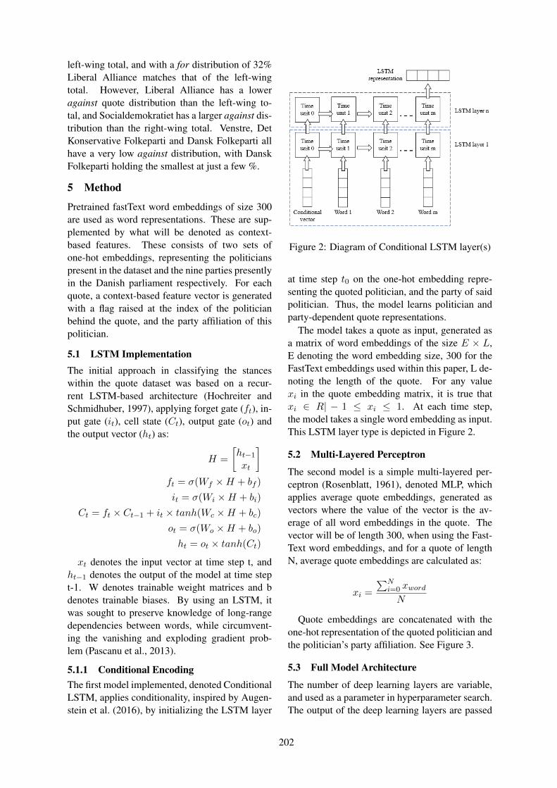
left-wing total, and with a for distribution of 32%Liberal Alliance matches that of the left-wingtotal. However, Liberal Alliance has a loweragainst quote distribution than the left-wing to-tal, and Socialdemokratiet has a larger against dis-tribution than the right-wing total. Venstre, DetKonservative Folkeparti and Dansk Folkeparti allhave a very low against distribution, with DanskFolkeparti holding the smallest at just a few %.

5 Method

Pretrained fastText word embeddings of size 300are used as word representations. These are sup-plemented by what will be denoted as context-based features. These consists of two sets ofone-hot embeddings, representing the politicianspresent in the dataset and the nine parties presentlyin the Danish parliament respectively. For eachquote, a context-based feature vector is generatedwith a flag raised at the index of the politicianbehind the quote, and the party affiliation of thispolitician.

5.1 LSTM ImplementationThe initial approach in classifying the stanceswithin the quote dataset was based on a recur-rent LSTM-based architecture (Hochreiter andSchmidhuber, 1997), applying forget gate (ft), in-put gate (it), cell state (Ct), output gate (ot) andthe output vector (ht) as:

H =

[ht−1

xt

]

ft = σ(Wf ×H + bf )

it = σ(Wi ×H + bi)

Ct = ft × Ct−1 + it × tanh(Wc ×H + bc)

ot = σ(Wo ×H + bo)

ht = ot × tanh(Ct)

xt denotes the input vector at time step t, andht−1 denotes the output of the model at time stept-1. W denotes trainable weight matrices and bdenotes trainable biases. By using an LSTM, itwas sought to preserve knowledge of long-rangedependencies between words, while circumvent-ing the vanishing and exploding gradient prob-lem (Pascanu et al., 2013).

5.1.1 Conditional EncodingThe first model implemented, denoted ConditionalLSTM, applies conditionality, inspired by Augen-stein et al. (2016), by initializing the LSTM layer

Figure 2: Diagram of Conditional LSTM layer(s)

at time step t0 on the one-hot embedding repre-senting the quoted politician, and the party of saidpolitician. Thus, the model learns politician andparty-dependent quote representations.

The model takes a quote as input, generated asa matrix of word embeddings of the size E × L,E denoting the word embedding size, 300 for theFastText embeddings used within this paper, L de-noting the length of the quote. For any valuexi in the quote embedding matrix, it is true thatxi ∈ R| − 1 ≤ xi ≤ 1. At each time step,the model takes a single word embedding as input.This LSTM layer type is depicted in Figure 2.

5.2 Multi-Layered Perceptron

The second model is a simple multi-layered per-ceptron (Rosenblatt, 1961), denoted MLP, whichapplies average quote embeddings, generated asvectors where the value of the vector is the av-erage of all word embeddings in the quote. Thevector will be of length 300, when using the Fast-Text word embeddings, and for a quote of lengthN, average quote embeddings are calculated as:

xi =

∑Ni=0 xword

N

Quote embeddings are concatenated with theone-hot representation of the quoted politician andthe politician’s party affiliation. See Figure 3.

5.3 Full Model Architecture

The number of deep learning layers are variable,and used as a parameter in hyperparameter search.The output of the deep learning layers are passed

202

Figure 3: Diagram of Multi-layered perceptronlayer(s)

to a number of linear layers containing ReLU acti-vation functions (Richard H. R. Hahnloser and Se-ung, 2000), the number of which are likewise usedas a parameter in hyperparameter search, followedby a softmax layer allowing for classification andoptimization using categoric cross entropy loss.Both models had the number of deep learning lay-ers and units, number of ReLU layers and unitsand L2 optimized, using a grid-wise search of thehyperparameter space. A learning rate of 0.001and dropout of 0.5 is applied to both models.

6 Results and Analysis

The overall evaluation of the three models wasperformed with the full dataset, as well as withthe national policy subset, using the optimal hy-perparameters. No experiments were made us-ing only the centralization dataset, as this wasdeemed too small at a quote count of just 104.The models were compared on both F1micro andF1macro. However, due to the skewed label dis-tribution within the dataset, as pointed out in Sec-tion 4, F1macro is the primary metric for modelevaluation.

Seeing as the dataset was generated specifi-cally for this piece of research, there exists noprior benchmarks with which to compare the mod-els. For this reason, two benchmark models are

Full DatasetGNB RF Cond. MLP

F1macro 0.266 0.387 0.375 0.575F1micro 0.306 0.461 0.400 0.717Facc 0.442 0.267 0.580 0.826Aacc 0.6 0.2 0.244 0.120Nacc 0.029 0.797 0.440 0.797

National Policy datasetGNB RF Cond. MLP

F1macro 0.254 0.435 0.358 0.585F1micro 0.283 0.560 0.372 0.774Facc 0.337 0.525 0.256 0.963Aacc 0.696 0.435 0.480 0.043Nacc 0.036 0.821 0.478 0.804

Table 5: Performance comparison of all models,including benchmark models, using optimized hy-perparameters, GNB referring to Gaussian NaıveBayes, RF referring to Random Forest

built, namely a Gaussian Naive Bayes classifierand Random Forest classifier, both out-of-the-boximplementations from the scikit-learn Python li-brary (Pedregosa et al., 2011).

There are three majority-based baselines. Thefirst majority baseline-based model uses the over-all majority class of the full dataset to classifyquotes. The second applies the majority class foreach politician to classify quotes from that politi-cian, and the third model does the same, insteadusing the majority class for each party.

6.1 Model Comparison

From Table 5 it can be observed that the MLPoutperforms all four other models in terms ofF1macro on both the full and national policydatasets. The MLP also performs best in regards toF1micro on both the full dataset and the nationalpolicy dataset.

Table 6 show that the MLP model out-performsboth majority baseline models in terms of F1macro.However, the politician-level baseline outperformsthe MLP in terms of F1micro.

F1macro F1microMLP 0.575 0.717Majority 0.253 0.611Majoritypol 0.299 0.835Majorityparty 0.270 0.696

Table 6: Comparison of majority baseline perfor-mance to MLP performance

203

Policy dataset Full datasetF A N F A N

F 77 0 3 F 22 52 1A 8 15 2 A 5 16 2N 10 57 2 N 2 52 2

Table 7: Confusion matrices for Multi-layeredperceptron, using optimized hyperparameters

6.2 Misclassification AnalysisTable 7 shows the confusion matrix for the MLP,run with optimal hyperparameters on both the fulland national policy dataset, can be found. Forboth datasets, the strength of the MLP is its abilityto correctly classify for and neutral quotes. As afunction of this, the model more or less ignores theagainst class, in pursuit of correctly classifying thetwo larger classes instead. A tendency can be ob-served towards classifying against-quotes as for,and to some extend also misclassifying some neu-tral quotes as for. This is not surprising, for beingthe majority class. Both the against-quotes andneutral-quotes classified as for are generally foundto contain a large number of negative words target-ing some other topic than immigration. Generally,the quotes within the for label apply a large num-ber of negative words, suggesting that the classi-fiers mis-interpret the target of the negative words.An example of a neutral-quote labeled as for is:

Det er ingen hemmelighed, at vi i DanskFolkeparti opfatter Dansk Industri som megetmanipulerende og utroværdig i diskussionen omudenlandsk arbejdskraft.

It is no secret that we in Dansk Folkepartiperceive Dansk Industri as being very manipu-lative and untrustworthy in the debate regardingforeign labor.Martin Henriksen, (Ritzau, 2018c)

And an example of an against quote:Det er bestemt ikke problemfrit at inte-

grere flygtninge. Men løsningen er da ikkeat eksportere problemerne til for eksempelNordafrika, hvor man i forvejen star med enkæmpemæssig opgave.

Integrating refugees is definitely not withoutits challenges. But the solution is not to exportthe problem to, for instance, North Africa, wherethe region is already faced with a huge task.Johanne Schmidt Nielsen, (Ritzau, 2018e)

6.3 Post-hoc Exploratory ExperimentsAdditional experiments were performed using theMLP trained on the full dataset, to gain additionalinsight into the model’s performance.

6.3.1 The Effect of Context-based FeaturesComparing Table 8 and Table 5, it can be observedthat removal of either party or politician from thecontext-based features significantly reduces theMLP’s results. A model applying a feature vectorcomposed only of the two context-based featuresout-performs models applying combinations of thetext-based features and one of the two context-based features, but is in turn out-performed bythe model applying all three features. This showsthat the inclusion of context-based features signifi-cantly improves the model’s performance, but thatthe model still relies on text-based features for op-timal performance.

Feature F1macro F1microFastText 0.138 0.261FastText, Vectorpol 0.405 0.522FastText, Vectorparty 0.441 0.594Vectorpol, Vectorparty 0.439 0.583FastText, Vectorpol, Vectorparty 0.575 0.717

Table 8: Results of experiments on MLP with re-duced contextual features

6.3.2 Size of the DatasetIt is assumed that the small size of the quotedataset is a significant factor in preventing themodels from achieving better performance, see-ing as a smaller dataset size makes generalizationto unobserved data points more difficult. To testthis hypothesis, experiments were performed onthe MLP using the optimal model hyperparame-ters, but a reduced training set sizes, in the rangeof 10 - 100% of the total quote dataset, the resultsof which can be found in Table 9. From this table,it is clear that decreasing the training set size re-duces the performance of the model. It is assumedthat the opposite is also true, and that a dataset oflarger size would thus increase performance of thegenerated models.

6.3.3 Choice of OptimizerThe models were implemented using a simplestochastic gradient descent optimizer from Py-Torch (Paszke et al., 2017). This decision wasmade early in the development process, prior tothe search of hyperparameter spaces for models.Thus, little testing was performed for the alter-native, more advanced, optimizers. To gain in-sight into whether the use of alternative optimizerswould have improved performance, a comparativeexperiment was performed, the results of whichare presented in Table 10.

204

Quotes Optimal epoch F1micro F1macro10% 72 Any 0.383 0.18520% 144 Any 0.383 0.18530% 216 Any 0.383 0.18540% 288 200 0.5 0.3350% 360 300 0.478 0.3360% 432 200 0.567 0.42570% 504 200 0.583 0.42880% 576 200 0.656 0.48890% 648 300 0.727 0.52100% 720 300 0.717 0.575

Table 9: Dataset size impact on MLP performance

Adagrad Adadelta Adamrate ε 0.001 0.01 0.001 0.01 0.001 0.01Epoch Any 200 300 30 30 AnyF1micro 0.383 0.633 0.722 0.622 0.661 0.383F1macro 0.185 0.490 0.518 0.536 0.547 0.185

Table 10: Performance of the Adagrad, Adadeltaand Adam optimizers in the MLP

From this table it can be seen, that the Adam op-timizer reaches an F1macro score of 0.547, com-parable to the best score of the basic SGD opti-mizer which was 0.575, despite hyperparametersbeing trained using the basic SGD optimizer. It isworth noting that this result is achieved after only30 epochs, whereas the basic SGD optimizer re-quired 300 epochs. This indicates that using anadaptive optimizer would not necessarily lead tohigher performance than stochastic gradient de-scent, for this task, but can be a more efficientchoice of optimizer.

6.3.4 Alternative Learning RatesAs can be seen in Table 11, a higher learningrate decreases the convergence time on high F1-scores significantly, however reducing the perfor-mance of models for higher numbers of epochs.The fact that the models applying a higher learn-ing rate can not achieve as strong a performanceas that using a learning rate of 0.001 is likely tobe due to the models skipping some maxima. Onesolution would be a variable learning rate, reduc-ing the learning rate once the model shows per-epoch diminishing loss reduction, thus achievingboth quick convergence and precision.

7 Conclusion

This work created both a dataset and approach forpolitical stance detection in Danish. A datasetof quotes from Danish politicians, including thequoted politician and the quoted politician’s party,annotated for use in stance detection was gener-

Learning Rate Epoch F1macro F1micro0.001 30 0.185 0.383

50 0.185 0.38370 0.185 0.383100 0.348 0.506200 0.525 0.733300 0.575 0.717

0.01 30 0.526 0.73350 0.410 0.60670 0.396 0.594100 0.454 0.578200 0.478 0.633300 0.410 0.500

0.1 30 0.423 0.58950 0.504 0.70670 0.442 0.617100 0.437 0.639200 0.397 0.572300 0.497 0.667

Table 11: Results of Learning Rate experimentson Quote LSTM using optimal hyperparameters

ated, and annotation guidelines for this datasetwere defined. Two deep learning-based classi-fiers were designed, implemented and optimizedfor the task. The simple MLP model that tookan averaged quote embedding as input far outper-formed the more advanced LSTM model, whichtook a single word at each time step. The gen-erated dataset is applicable for use in future re-search within the field of stance detection in Dan-ish, and the created models can be used as bench-marks when testing stance detection classifiers onthis dataset.

Labeled quote data and code for this project isavailable on GitHub (link).

Acknowledgements

We thank the reviewers, whose suggestions provedhighly useful, and Victor Petren Bach Hansenand Jakob Bang Helvind, whose sparring andfeedback was invaluable during both the researchbehind this paper, and the writing of the pa-per itself. This research was conducted underthe NeIC/NordForsk sponsored Nordic LanguageProcessing Laboratory (NLPL) project.

205

ReferencesAhmet Aker, Leon Derczynski, and Kalina Bontcheva.

2017. Simple open stance classification for rumouranalysis. In Proc. RANLP.

Isabelle Augenstein, Tim Rocktaschel, Andreas Vla-chos, and Kalina Bontcheva. 2016. Stance Detectionwith Bidirectional Conditional Encoding. In Pro-ceedings of the 2016 Conference on Empirical Meth-ods in Natural Language Processing, pages 876–885.

Emily M. Bender and Batya Friedman. 2018. Datastatements for natural language processing: Towardmitigating system bias and enabling better science.Transactions of the Association for ComputationalLinguistics, 6:587–604.

Michael Collins and Nigel Duffy. 2001. ConvolutionalKernels for Natural Language. In Proceedings of the14th International Conference on Neural Informa-tion Processing Systems, pages 625–632, Vancou-ver, Canada.

Leon Derczynski, Kalina Bontcheva, Maria Liakata,Rob Procter, Geraldine Wong Sak Hoi, and ArkaitzZubiaga. 2017. SemEval-2017 Task 8: Ru-mourEval: Determining rumour veracity and sup-port for rumours. In Proceedings of the 11thInternational Workshop on Semantic Evaluations(SemEval-2017), page 69–76, Vancouver, Canada.

Omar Enayet and Samhaa R. El-Beltagy. 2017. Deter-mining Rumour and Veracity Support for Rumourson Twitter. In Proceedings of the 11th InternationalWorkshop on Semantic Evaluations (SemEval-2017), pages 470–474, Vancouver, Canada.

Kenneth C. Enevoldsen and Lasse Hansen. 2017.Analysing political biases in danish newspapers us-ing sentiment analysis. Journal of Language Works,2(2).

Genevieve Gorrell, Elena Kochkina, Maria Liakata,Ahmet Aker, Arkaitz Zubiaga, Kalina Bontcheva,and Leon Derczynski. 2019. SemEval-2019 task 7:RumourEval, determining rumour veracity and sup-port for rumours. In Proceedings of the 13th Inter-national Workshop on Semantic Evaluation, pages845–854, Minneapolis, Minnesota, USA. Associa-tion for Computational Linguistics.

Sepp Hochreiter and Jurgen Schmidhuber. 1997.Long short-term memory. Neural Computation,9(8):1735–1780.

Mohit Iyyer, Peter Enns, Jordan Boyd-Graber, andPhilip Resnik. 2014. Political Ideology DetectionUsing Recursive Neural Networks. In Proceedingsof the 52nd Annual Meeting of the Association forComputational Linguistics, pages 1113–1122, Bal-timore, Maryland, USA.

Kristen Johnson and Dan Goldwasser. 2016. “AllI know about politics is what I read in Twitter”:

Weakly Supervised Models for Extracting Politi-cians’ Stances From Twitter. In Proceedings ofCOLING 2016, the 26th International Conferenceon Computational Linguistics: Technical Papers,pages 2966–2977, Osaka, Japan.

Andreas Kirkedal, Barbara Plank, Leon Derczynski,and Natalie Schluter. 2019. The Lacunae of Dan-ish Natural Language Processing. In Proceedings ofthe Nordic Conference on Computational Linguis-tics (NODALIDA).

Kristoffer Kvalvik. 2017. Køn, indkomst og ge-ografi: Her er vælgernes vigtigste dagsordener.https://www.altinget.dk/artikel/163051-koen-indkomst-og-geografi-her-er-vaelgernes-vigtigste-dagsordener.

Mirko Lai, Delia Irazu Hernandez Farias, Vivian Patti,and Paolo Rosso. 2016. Friends and Enemies ofClinton and Trump: Using Context for DetectingStance in Political Tweets. In Advances in Com-putational Intelligence: 15th Mexican InternationalConference on Artificial Intelligence, MICAI 2016,pages 155–168, Cancun, Mexico.

Anders Edelbo Lillie, Emil Refsgaard Middelboe, andLeon Derczynski. 2019. Joint rumour stance and ve-racity. In Proceedings of the Nordic Conference onComputational Linguistics.

Saif M. Mohammad, Svetlana Kiritchenko, ParinazSobhani, Xiodan Zhu, and Colin Cherry. 2016. ADataset for Detecting Stance in Tweets. In LREC,Portoroz, Slovenia.

Saif M. Mohammad, Parinaz Sobhani, and SvetlanaKiritchenko. 2017. Stance and sentiment in tweets.ACM Transactions on Internet Technology (TOIT) -Special Issue on Argumentation in Social Media andRegular Papers.

Finn Arup Nielsen. 2011. A new ANEW: evaluation ofa word list for sentiment analysis in microblogs. InProceedings of the ESWC2011 Workshop on ’Mak-ing Sense of Microposts’: Big things come in smallpackages, pages 93–98.

Razvan Pascanu, Tomas Mikolov, and Yoshua Bengio.2013. On the difficulty of training recurrent neu-ral networks. In Proceedings of the 30th Interna-tional Conference on International Conference onMachine Learning, pages 1310–1318.

Adam Paszke, Sam Gross, Soumith Chintala, Gre-gory Chanan, Edward Yang, Zachary DeVito, Zem-ing Lin, Alban Desmaison, Luca Antiga, and AdamLerer. 2017. Automatic differentiation in PyTorch.In NIPS-W.

F. Pedregosa, G. Varoquaux, A. Gramfort, V. Michel,B. Thirion, O. Grisel, M. Blondel, P. Pretten-hofer, R. Weiss, V. Dubourg, J. Vanderplas, A. Pas-sos, D. Cournapeau, M. Brucher, M. Perrot, andE. Duchesnay. 2011. Scikit-learn: Machine learningin Python. Journal of Machine Learning Research,12:2825–2830.

206

Vahed Qazvinian, Emily Rosengren, Dragomir R.Radev, and Qiaozhu Mei. 2011. Rumor has it: iden-tifying misinformation in microblogs. In Proceed-ings of the Conference on Empirical Methods in Nat-ural Language Processing, pages 1589–1599, Edin-burgh, United Kingdom.

Misha A. Mahowald Rodney J. Douglas Richard H.R. Hahnloser, Rahul Sarpeshkar and H. SebastianSeung. 2000. Digital selection and analogue ampli-fication coexist in a cortex-inspired silicon circuit.Nature, 405:947–951.

Ritzau. 2018a. Alternativet vil i EU med fyret græskfinansminister. Ritzau.

Ritzau. 2018b. DF siger nej til S-plan om jobcentre iSydeuropa. Ritzau.

Ritzau. 2018c. OVERBLIK: Det siger politikerne omghettoplanen. Ritzau.

Ritzau. 2018d. S vil skabe fem danske jobcentre isydeuropa. Ritzau.

Ritzau. 2018e. Socialdemokratisk asyludspil deler rødblok. Ritzau.

Ritzau. 2018f. Støjberg vil have migranter fra danskskib i land i Italien. Ritzau.

Ritzau. 2018g. Tyrkiske kulturformænds sympati forrabiat bevægelse alarmerer politikere. Ritzau.

Ritzau. 2019. Ejerskab, bestyrelse og arsregnskab.https://ritzau.com/ejerskab-bestyrelse-og-aarsregnskab/.

Frank Rosenblatt. 1961. Principles of neurodynam-ics: Perceptrons and the theory of brain mecha-nisms. Cornell Aeronautical Laboratory, Buffallo,New York, USA.

Maria Skeppstedt, Vasiliki Simaki, Carita Paradis, andAndreas Kerren. 2017. Detection of stance and sen-timent modifiers in political blogs. In Proceedingsof the International Conference on Speech and Com-puter, SPECOM, pages 1589–1599, Hatfield, UnitedKingdom.

Martin Tutek, Ivan Sekulic, Paula Gombar, Ivan Pal-jak, Filip Culinovic, Filip Boltuzic, Mladen Karan,Domagoj Alagic, and Jan Snajder. 2016. Take-Lab at SemEval-2016 Task 6: Stance Classificationin Tweets Using a Genetic Algorithm Based En-semble. In Proceedings of the 10th InternationalWorkshop on Semantic Evaluation (SemEval-2016),pages 464–468.

Wan Wei, Xiao Zhang, Xuqin Liu, Wei Chen, andTengijao Wang. 2016. pkudblab at SemEval-2016Task 6 : A Specific Convolutional Neural NetworkSystem for Effective Stance Detection. In Proceed-ings of the 10th International Workshop on SemanticEvaluation (SemEval-2016), pages 384–388.

Guido Zarrella and Amy Marsh. 2016. MITRE atSemEval-2016 Task 6: Transfer Learning for StanceDetection. In Proceedings of the 10th InternationalWorkshop on Semantic Evaluation (SemEval-2016),pages 458–463.

Li Zeng, Kate Starbird, and Emma S. Spiro. 2016.Unconfirmed: Classifying Rumor Stance in Crisis-Related Social Media Messages. In Proceedingsof the Tenth International AAAI Conference onWeb and Social Media (ICWSM), pages 747–750,Cologne, Germany.

Appendix 1: Data Statement

Curation rationale Quotes from Danish politi-cians published by the Ritzau news agency.

Language variety BCP-47: da-DK

Speaker demographic• Danish politicians.

• Age: approx. 25-70.

• Gender: mixed; see Section 3.1.

• Race/ethnicity: mostly white with Scandina-vian background.

• Native language: Danish.

• Socioeconomic status: minimum 56494.17DKK per month ($8470 USD).

• Different speakers represented: 63.

• Presence of disordered speech: Quotes aremostly curated, so not prevalent.

Annotator demographic• Age: 20-30.

• Gender: male.

• Race/ethnicity: white northern European.


• Socioeconomic status: higher education stu-dent.

Speech situation Quotes given by politicians inparliament during debate or discussion, duringverbal interviews or in writing, transcribed andthen published in edited newswire.

Text characteristics Danish Newswire.

Provenance Originally taken from Ritzau.

207

Joint Rumour Stance and Veracity

Anders Edelbo Lillie∗ITU Copenhagen

[email protected]

Emil Refsgaard Middelboe∗ITU Copenhagen

[email protected]


[email protected]

Abstract

The net is rife with rumours that spreadthrough microblogs and social media. Notall the claims in these can be verified.However, recent work has shown that thestances alone that commenters take towardclaims can be sufficiently good indicatorsof claim veracity, using e.g. an HMMthat takes conversational stance sequencesas the only input. Existing results aremonolingual (English) and mono-platform(Twitter). This paper introduces a stance-annotated Reddit dataset for the Danishlanguage, and describes various imple-mentations of stance classification mod-els. Of these, a Linear SVM provides pre-dicts stance best, with 0.76 accuracy / 0.42macro F1. Stance labels are then usedto predict veracity across platforms andalso across languages, training on conver-sations held in one language and using themodel on conversations held in another.In our experiments, monolinugal scoresreach stance-based veracity accuracy of0.83 (F1 0.68); applying the model acrosslanguages predicts veracity of claims withan accuracy of 0.82 (F1 0.67). Thisdemonstrates the surprising and powerfulviability of transferring stance-based ve-racity prediction across languages.

1 Introduction

Social media has come to play a big role in our ev-eryday lives as we use it to connect with our socialnetwork, but also to connect with the world. It iscommon to catch up on news through Facebook,or to be alerted with emerging events through

∗: These authors contributed to the paper equally.

Twitter. However these phenomena create a plat-form for the spread of rumours, that is, stories withunverified claims, which may or may not be true(Huang et al., 2015). This has lead to the con-cept of fake news, or misinformation, where thespreading of a misleading rumour is intentional(Shu et al., 2017). Can we somehow automati-cally predict the veracity of rumours? Researchhas tried to tackle this problem (Qazvinian et al.,2011), but automated rumour veracity predictionis still maturing (Gorrell et al., 2019).

This project investigates stance classification asa step for automatically determining the veracityof a rumour. Previous research has shown that thestance of a crowd is a strong indicator for verac-ity (Dungs et al., 2018), but that it is a difficulttask to build a reliable classifier (Derczynski et al.,2017). Moreover a study has shown that carefulfeature engineering can have substantial influenceon the accuracy of a classifier (Aker et al., 2017).A system able to verify or refute rumours is typ-ically made up of four components: rumour de-tection, rumour tracking, stance classification, andveracity classification (Zubiaga et al., 2018). Thisproject will mainly be concerned with stance clas-sification and rumour veracity classification.

Current research is mostly concerned with theEnglish language, and in particular data fromTwitter is used as data source because of itsavailability and relevant news content (Derczynskiet al., 2017; Gorrell et al., 2019). To our knowl-edge no research within this area has been carriedout in a Danish context. To perform automated ru-mour veracity prediction for the Danish languagefollowing the components in Zubiaga et al. (2018),a number of problems must be solved. (1) to facil-itate Danish stance classification a Danish datasetmust be generated and annotated for stance. (2)developing a good stance classifier is difficult, es-pecially given the unknown domain of the Dan-ish language. Therefore experiments must be per-

208

formed to investigate what approach to apply toDanish stance classification. (3) given rumourousdata, and aided by stance classification, a rumourveracity prediction component should be able todetermine whether it is true or false.

2 Background

The attitude that people express towards claimscan be used to predict veracity of those claims, andthese attitudes can be modelled by stance classi-fiers. This section will cover some state-of-the-artresearch for stance classification and rumour ve-racity resolution. While the introduced classifica-tion tasks are related to the work carried out in thisproject, they differ in a number of ways: (1) thisproject performs stance classification for the Dan-ish language, (2) the generated dataset is from theReddit platform, and (3) this project seeks to joinstance classification and veracity prediction with-out external fact verification.

Stance classification: Long-Short Term Mem-ory (LSTM) neural network models are popular, asthey have proven to be efficient for working withdata within NLP. In particular (Kochkina et al.,2017) introduced a stance classifier based on a“Branch-LSTM” architecture: instead of consid-ering a single tweet in isolation, whole branchesare used as input to the classifier, capturing struc-tural information of the conversation. The modelis configured with several dense ReLU layers, a50% dropout layer, and a softmax output layer,scoring a 0.78 in accuracy and 0.43 macro F1

score. They are however unable to predict theunder-represented “denying” class.

Another LSTM approach deals with the prob-lem introduced in the SemEval 2016 task 6 (Mo-hammad et al., 2016). The LSTM implements abidirectional conditional structure, which classi-fies stance towards a target with the labels “posi-tive”, “negative”, and “neutral” (Augenstein et al.,2016). The approach is unsupervised, i.e. datais not labelled for the test targets in the trainingset. In this case the system achieves state-of-the-art performance with a macro F1 score of 0.49,and further 0.58 when applying weak supervision.

A different approach is based on having well-engineered features for stance classification exper-iments using non-neural networks classifiers in-stead of Deep Learning (DL) methods (Aker et al.,2017). Common features such as CBOW and POStagging are implemented, but are extended with

problem-specific features, which are designed tocapture how users react to tweets and express con-fidence in them. A Random Forest classifier per-formed best, with an accuracy of 0.79.

The lack of labelled data is a major chal-lenge for stance classification. One study showsthat classification can be improved by transferringknowledge from other datasets (Xu et al., 2019).In particular, a model is implemented with adver-sarial domain adaptation to train on the FEVERdataset (Thorne et al., 2018) and test on the FakeNews Challenge dataset.1 By augmenting the tra-ditional approach for stance classification with adomain adaption component, the model learns topredict which domain features originate from.

RumourEval 2019 is a very recent SemEval taskwhich deals with stance classification and veracityprediction (Gorrell et al., 2019), and a first look atthe scoreboard indicates very promising results.2

With the Branch-LSTM approach as a baselineon the RumourEval 2019 dataset, scoring 0.4930macro F1, the “BERT” system scores a macro F1

of 0.6167 (Fajcik et al., 2019). The implemen-tation employs transfer learning on large Englishcorpora, then an encoding scheme concatenatesthe embeddings of the source, previous and tar-get post. Finally the output is fed through twodense layers to provide class probabilities. TheseBERT models are used in several different ensem-ble methods where the average class distributionis used as the final prediction.

Rumour veracity prediction: Rumour veracityclassification is considered a challenging task asone must typically predict a truth value from a sin-gle text, being the one that initiates the rumour.The best performing team for that task in Ru-mourEval 2017 (Derczynski et al., 2017) imple-ments a Linear Support Vector Machine (SVM)with only few (useful) features (Enayet and El-Beltagy, 2017). They experiment with severalcommon features such as hashtag existence, URLexistence, and sentiment, but also incorporates aninteresting feature of capturing whether a text is aquestion or not. Furthermore the percentage of re-plying tweets classified as supporting, denying, orquerying from stance classification is applied. It isconcluded that content and Twitter features werethe most useful for the veracity classification task

1http://www.fakenewschallenge.org2https://competitions.codalab.org/

competitions/19938 26-05-2019

209

and the system scores an accuracy of 0.53.While the system described above engages in

the task of resolving veracity given a single ru-mour text, another interesting approach is basedon the use of crowd/collective stance, which is theset of stances over a conversation (Dungs et al.,2018). This system predicts the veracity of a ru-mour, based solely on crowd stance as well astweet times. A Hidden Markov Model (HMM) isimplemented, which is utilised such that individ-ual stances over a rumour’s lifetime is regarded asan ordered sequence of observations. This is thenused to compare sequence occurrence probabili-ties for true and false rumours respectively. Thebest scoring model, which include both stance la-bels and tweet times, scores an F1 of 0.804, whilethe HMM with only stance labels scores 0.756F1. The use of automatic stance labels from (Akeret al., 2017) is also applied, which does not changeperformance much, proving the method to havepractical applications. It is also shown that usingthe model for rumour veracity prediction is stilluseful when limiting the number of tweets to e.g.5 and 10 tweets respectively.

Danish: While Danish is not a privileged lan-guage in terms of resources (Kirkedal et al., 2019),there is stance classification work on politicalquotes (Lehmann and Derczynski, 2019). How-ever, this is over a different text genre, and doesnot focus on veracity prediction as its final goal.

Comprehensive reviews of automatic veracityand rumour analysis from an NLP perspectiveinclude Zubiaga et al. (2018), Atanasova et al.(2019), and Lillie and Middelboe (2019b).

3 Dataset

Because of various limitations on big social mediaplatforms including Facebook and Twitter, Red-dit is used as platform for the dataset.3 This is anovel approach; prior research has typically reliedon Twitter (Mohammad et al., 2016; Derczynskiet al., 2017; Gorrell et al., 2019).

Data sampling: The data gathering process con-sists of two approaches: to manually identify inter-esting submissions on Reddit, and; to issue queriesto the Reddit API4 on specific topics. An ex-ample of a topic could be “Peter Madsen” refer-

3In particular the Danish Subreddit at www.reddit.com/r/Denmark/

4www.reddit.com/dev/api/

ring to the submarine murder case, starting fromAugust 2017.5 A query would as such be con-structed of the topic “Peter Madsen” as search text,a time window and a minimum amount of Red-dit upvotes. A minimum-upvotes filter is appliedto limit the amount of data returned by the query.Moreover the temporal filters are to ensure a cer-tain amount of relevance to the case, specificallywhen the event initially unfolded. Several submis-sions prior or subsequent to the given case maymatch a search term such as “ubad” (submarine).

Four Danish Subreddits were browsed, includ-ing “Denmark, denmark2, DKpol, and Gammel-Dansk”,6 although all relevant data turned outto be from the “Denmark” Subreddit. The sub-mission IDs found manually and returned by thequeries are used to download all posts from eachsubmission using the praw7 and psaw8 Pythonlibraries. The submission data is subsequentlystored in a JSON format, one JSON file per sub-mission, consisting of submission data and a listof comment data. These files include submis-sion post text and comment text, as well as meta-information about the following: submission post,submitter user, Subreddit, comments, and com-menting users.

Annotation: One widely used annotationscheme for stance on Twitter is the SDQCapproach from Zubiaga et al. (2016). Twitterdiffers from Reddit in the way conversations arestructured. Each tweet spawns a conversationwhich can have nested replies, and as suchcreates branches. Reddit implements the samemechanism, but a set of conversations are tiedto a specific submission, which is initiated by asubmission post. The Reddit structure is depictedin Figure 1, illustrating a conversation (in green)and two respective branches (in respectively redand purple). Note that branches share at leastone comment. Thus, a way to annotate datafrom the Reddit platform with the annotationscheme from Zubiaga et al. (2016) is by regardinga submission post as a source, instead of eachtop-level comment for the conversations.

The stance of the source/submission post istaken into account when annotating the stance for

5www.dr.dk/nyheder/tema/ubaadssagen6www.reddit.com/r/Denmark/wiki/

danish-subreddits7praw.readthedocs.io/en/latest/ v. 6.0.0.8github.com/dmarx/psaw v. 0.0.7.

210

Figure 1: The structure of a Reddit submission

replying posts of top-level posts. As stance anno-tations are relative to some target, each post doesnot have one single stance annotation: each post isannotated for the stance targeted towards the sub-mission and the stance targeted towards the directparent of the post. The double-annotation shouldfacilitate a way to infer the stance for individualposts. For instance, if the source post supports arumour, and a nested reply supports its parent post,which in turn denies the source, then the nested re-ply is implicitly denying the rumour.

Further, a majority of submissions have no text,but a title and a link to an article, image or an-other website, with content related to the title ofthe submission. If this is the case and the title ofthe submission bears no significant stance, it is as-sumed that the author of the submission takes thesame stance as the content which is attached to thesubmission.

Annotation tool: A custom web-based annota-tion tool was built to facilitate the annotation pro-cess of the data. C# and MySQL technologieswere used to build the tool in order to support rapiddevelopment. The tool enables annotators to par-tition datasets into events and upload submissionsin the JSON form from the gathering Reddit datato each event. Further the tool allows for a branchview of each submission in the event and facili-tates annotation following the SDQC scheme, aswell as certainty and evidentiality as presented byZubiaga et al. (2016). Any annotation conflicts arehighlighted by the tool, which will cause the an-notators to discuss and re-annotate the post with aconflict. A screenshot of the annotation page for

Figure 2: Screenshot of the annotation tool

the annotation tool is presented in Figure 2.During annotation of the first ∼ 500 posts, an-

notators disagreed upon labels for around 40-50%of posts. However after the initial annotation workthis rate dropped to around 25%. Annotation con-flicts were handled in collaboration between theannotators after annotation of every ∼ 100 posts.

DAST: The result of the data sampling and anno-tation process is the Danish stance-annotated Red-dit dataset (DAST). The dataset consists of a totalof 11 events with 3,007 stance-annotated Redditposts across 33 submissions with a total of 1,161branches. Information on DAST is presented in Ta-ble 1 including event names, SDQC distributionand total post counts.

EventLabel S D Q C Total

5G 26 47 7 193 273Donald Trump 39 17 5 185 246HPV vaccine 24 4 8 219 255ISIS 3 40 8 118 169“Kost” 50 56 4 447 557MeToo 1 8 3 48 60“Overvagning” 41 20 13 278 352Peter Madsen 15 45 19 302 381“Politik” 43 46 7 227 323“Togstrejke” 8 6 3 84 101“Ulve i DK” 23 11 4 252 290Total 273 300 81 2,353 3,007% 9.1 10 2.7 78.2 100

Table 1: SDQC stance labels per event

The “querying” label is rare with a total of 81annotations out of the 3,007 posts. The “support-ing” and “denying” labels are almost equally dis-tributed with a total of respectively 273 “support-ing” and “300” denying posts. The “commenting”class is the absolute dominant one, with a total of2,353 annotations.

Table 2 illustrates the relative SDQC distribu-tion for the whole dataset for both response types,being targeted towards respectively submission

211

TargetLabel S D Q C

Submission post 273 300 81 2,353Parent comment 261 632 304 1,810Submission post % 9.1 10 2.7 78.2Parent comment % 8.7 21 10.1 60.2

Table 2: SDQC stance label distribution in DAST

(source) and parent posts, i.e. the posts repliedto. The distribution is quite skewed towards the“commenting” class label, with a total distributionof S(0.091), D(0.1), Q(0.027) and C(0.782).

Rumour data: The dataset contains 16 ru-mourous submissions, 3 of which are true, 3are false and the remaining 10 are unverified.They make up 220 Reddit conversations, or 596branches, with a total of 1,489 posts, equal toabout half of the dataset. The posts are distributedacross the nine events as follows: 5G (233), Don-ald Trump (140), ISIS (169), “Kost” (324), MeToo(60), Peter Madsen (381), “Politik” (49), “Togstre-jke” (73), and “Ulve i DK” (56). Thus ISIS,MeToo, and Peter Madsen are the only eventswhich only contain rumourous conversations.

Although rumours with known truth valuewould be optimal for veracity classification, thismight reflect reality as the truth value of rumoursmay stay unverified. The amount of unverified ru-mours does however warrant more investigationin order to use all of the rumourous submissionsfor rumour veracity classification. Further detailsabout the approach to unverified rumours are cov-ered in Section 4.

In total the dataset contains 3,007 Reddit postsdistributed across 33 submissions respectivelygrouped into 16 events.

The tools9 and annotated corpora (Lillie andMiddelboe, 2019a) are openly released with thispaper in GDPR-compliant, non-identifying for-mat. See appendix for data statement (Bender andFriedman, 2018).

4 Method

Our veracity prediction approach depends on twocomponents: a stance classifier and a veracityclassification component (Zubiaga et al., 2018).

4.1 Stance ClassificationFor stance classification two different approacheshave been used, one being an LSTM classifier in-

9github.com/danish-stance-detectors

spired by (Kochkina et al., 2017) and the otheremploying a number of classic machine learningmodels with a focus on feature engineering as pre-sented in Aker et al. (2017).

LSTM classifier: The LSTM model is widelyused for tasks where the sequence of data and ear-lier elements in sequences are important (Gold-berg, 2016). The temporal sequence of tweets wasone of the motivations for Kochkina et al. (2017)to use the LSTM model for branches of tweets, aswell as for the bidirectional conditional LSTM forAugenstein et al. (2016).

While the results from both the Bi-LSTM inAugenstein et al. (2016) and Branch-LSTM inKochkina et al. (2017) achieve state-of-the-art per-formance, they both note that their deep learningapproaches suffer from the lack of a larger trainingdataset. This is not uncommon in this task (Tauleet al., 2017; Zubiaga et al., 2016; Gorrell et al.,2019). We suspect that we would observe the sametendency for the DAST dataset, which is relativelysmall with its 3,007 Reddit posts. However, as theLSTM approach still manages to achieve state-of-the-art performance, we opted to include an LSTMimplementation for the stance classification task.

Specifically, the LSTM classifier used for stanceclassification here is implemented with PyTorch10

and consists of a number of LSTM layers and anumber of ReLU layers, followed by a dropoutlayer and a softmax layer to perform classifica-tions. The model is trained with stochastic gra-dient descent (SGD) and a negative log likeli-hood loss function. The configurations consideredand overall approach is inspired by the Branch-LSTM classifier in (Kochkina et al., 2017), exceptthat we do not input data grouped sequentially bybranches, but one by one.

Non-neural network classifiers: It is the inten-tion to use non-neural network models in contrastto the LSTM deep learning approach above, as re-search shows that this approach can do very well(Derczynski et al., 2017), and particularly Deci-sion Tree and Random Forest classifiers (Akeret al., 2017). Furthermore Support Vector Ma-chine (SVM) and Logistic Regression have provento be efficient (Enayet and El-Beltagy, 2017; Der-czynski et al., 2017). The models are listed below,prefixed with a label, which we will use to denotethem throughout the paper:

10https://pytorch.org/

212

logit Logistic Regression classifier

tree Decision Tree classifier

svm Support Vector Machine (linear kernel)

rf Random Forest classifier

Baselines: A simple majority voter (MV) aswell as a stratified classifier (SC) were imple-mented. The former predicts only the most fre-quent class, and the latter generates predictions byrespecting the training set’s class distribution.

The non-neural networks models and baselinemodels described above are all implemented withthe Scikit Learn (Pedregosa et al., 2011) frame-work, which provides a wide variety of machinelearning implementations.

Preprocessing: As a preprocessing step, all posttexts are lower-cased and then tokenised with theNLTK library (Bird et al., 2009), and finally allpunctuation is removed, not including cases suchas commas and periods in numbers, as well as pe-riods in abbreviations. Furthermore URLs are re-placed with the tag “urlurlurl” and quotes with thetag “refrefref”.

Features: In order to represent the features ofthe preprocessed data numerically we employeight feature categories, which are grouped byhow they relate: text, lexicon, sentiment, Red-dit, most frequent words, BoW, POS, and wordembeddings. Note that only the Reddit specificfeatures are domain-dependent, while the othersshould apply for the general case. The choices offeatures are a compilation of select features fromvarious state-of-the-art systems (Aker et al., 2017;Kochkina et al., 2017; Enayet and El-Beltagy,2017), except for the Reddit specific ones. Mostof the features are binary, taking either a 0 or a 1as value, and those that are not are min-max nor-malised (Han et al., 2011, p. 114), except for theword embeddings.

Table 3 presents an overview of the total fea-ture vector, including the feature categories andtheir number of individual features. Note that theword embeddings are actually 300 long, but theextra 3 features are the cosine similarities betweendifferent word embeddings with regards to parent,source, and branch word tokens.

Sentiment analysis is performed with the Afinnlibrary (Arup Nielsen, 2011), and POS tagging isperformed with the Danish Polyglot library (Al-Rfou et al., 2013). Text features include binary

Category LengthText 13Lexicon 4Sentiment 1Reddit 10Most frequent words 132BOW 13,663POS 17Word embeddings 303Total 14,143

Table 3: Feature vector overview

features for presence of: ‘.’, ‘!’, ‘?’, ’hv’-words,‘...’, as well as text length, URL count, maximumlength of capital character sequence, and count of:‘...’, ‘?’, ‘!’, and words. Finally the text featuresinclude ratio of capital letters to non-capital lettersand average word length.

Lexicon features are extracted by looking upoccurrences of items in four predefined lexi-con/dictionaries: negation words, swear words,positive smileys, and negative smileys. Nega-tion words are translated from the English listused in Kochkina et al. (2017), as no list couldbe found for this purpose elsewhere. Beyondourselves, swear words are taken from varioussources: youswear.com, livsstil.tv2.dk, dansk-og-svensk.dk, and dagens.dk. Smiley lists werecompiled from Wikipedia using the western styleemoticons.11

Reddit-specific features include karma, goldstatus, Reddit employment status (if any), veri-fied e-mail, reply count, upvotes, and whether theuser is the submission submitter. Further, based onReddit commenting syntax, the following featuresare included: sarcasm (‘/s’), edited (‘edit:’), andquote count (‘>’).

Finally, word embeddings are generated withword2vec (Mikolov et al., 2013) using the Gensimframework (Rehurek and Sojka, 2010). The wordvectors are trained on a Danish text corpus ac-quired from “Det Danske Sprog- og Litteratursel-skab” (DSL),12 consisting of 45 million tokens ofwritten LGP (Language for General Purposes),13

as well as the preprocessed Reddit text.

4.2 Rumour Veracity PredictionThe rumour veracity classification implemented isinspired by the approach presented in Dungs et al.(2018). This approach is especially interesting

11en.wikipedia.org/wiki/List_of_emoticons

12https://dsl.dk/13https://korpus.dsl.dk/resources.html

213

as it relinquishes language specific features suchas word embeddings and relies on sequences ofstance labels and temporal features of the posts.This possibly enables the use of data across lan-guages and platforms. One implemented HMM,λ is alike the model presented in Dungs et al.(2018) receiving sequences of stance labels or-dered by their posting time as input. For eachlabel presented in the data, a model is trainedwith training data for that label. For examplein a label space containing the labels “True” and“False”, two HMM models λfalse and λtrue aretrained. The predicted label of the model λ will bewhichever labelled model presents a higher prob-ability score for the given sequence.

Further a model ω is built, which differs from λby also containing normalised timestamps for eachpost. This was done as inclusion of temporal fea-tures boosted performance in (Dungs et al., 2018).Note that ω is not the same model as the variably-spaced λ′ of Dungs et al. (2018).

As a baseline throughout the experiments, asimple stratified baseline will be used, denotedVB. The baseline notes the average distributionof stance labels as a four-tuple for respectivelytrue and false (and unverified where relevant) ru-mours. When predicting rumour veracity, VB cal-culates the distribution of stance labels in a givensequence in the testing data and chooses the truthvalue with the most similar class label distribution.

The data used for experiments across languagesand platforms include the PHEME dataset (Zubi-aga et al., 2016; Derczynski et al., 2015). First, ex-periments are performed isolated on DAST. Then,the PHEME dataset is used as training data whileDAST is used as test set. Further, unverified ru-mours are approached in two ways: (1) three-wayclassification is performed on true, false and un-verified rumours, and (2) two-way classificationis performed with unverified rumours treated asTrue. The results are presented in Section 5.2.

The data from DAST is used in three differentways, given the expected discrepancies betweenthe English Twitter data and the Danish Redditdata. The Reddit conversation structure in Figure1 differs slightly from the Twitter structure. Thesubmission post is the actual source of conversa-tion, while conversation top level comments arethe source for Twitter conversations. Three differ-ent representations are tested for DAST:

BAS each branch in a conversation is regarded as a

rumour (branch-as-source). This causes par-tial duplication of comments, as branches canshare parent comments.

TCAS top level comments are regarded as the sourceof a rumour and the conversation tree theyspawn are the sequences of labels (top-levelcomment-as-source).

SAS the entire submission is regarded as a rumour(submission-as-source). The SAS approachmeans that only 16 instances are available.

4.3 Evaluation MeasuresMost of the related work report results with ac-curacy as scoring metric (Derczynski et al., 2017;Aker et al., 2017), which expresses the ratio ofnumber of correct predictions to the total num-ber of input samples. However, this becomesquite uninteresting if the input samples have im-balanced class distributions, which is the case forour dataset. What is interesting to measure is howwell the models are at predicting the correct classlabels. As such, in addition to reporting accuracywe will also use the F1 scoring metric. In particu-lar we will use an unweighted macro-averaged F1

score for the case of multi-class classification.

5 Results and Analysis

This section reports performance at stance classi-fication and rumour veracity prediction.

5.1 Stance Classification ResultsFirst, an ablation study of the feature groups re-vealed that the Reddit specific features as well aslexicon features contributed negatively to perfor-mance for stance classification. Further, it turnedout that the Most Frequent Words (MFW) featurecategory resembled BOW with low variance fea-tures removed. Finally the generated MFW listcontained stopwords very specific to DAST, suchas “B12”, “CO2”, and “5G”. As such all clas-sifiers has the feature categories Reddit, lexicon,and MFW removed.

Second, parameter search was performedthrough grid-search for three classifiers, beingLSTM, Logistic Regression (logit), and SupportVector Machine (svm). Decision Tree and Ran-dom Forest were omitted due to poor performance.Full details of the parameters searched are givenin Middelboe and Lillie (2019).

Classifier results are given in Table 4, under 5-fold (stratified) cross validation. Top-level com-

214

Model Macro-F1 σ Accuracy σMV 0.2195 (+/- 0.00) 0.7825 (+/- 0.00)SC 0.2544 (+/- 0.04) 0.6255 (+/- 0.01)logit 0.3778 (+/- 0.06) 0.7812 (+/- 0.02)svm 0.3982 (+/- 0.04) 0.7496 (+/- 0.02)logit’ 0.4112 (+/- 0.07) 0.7549 (+/- 0.04)svm’ 0.4212 (+/- 0.06) 0.7572 (+/- 0.02)LSTM 0.2802 (+/- 0.04) 0.7605 (+/- 0.03)LSTM’ 0.3060 (+/- 0.05) 0.7163 (+/- 0.16)

Table 4: Stance cross validation results for logit,svm, LSTM, and baselines with macro F1 and ac-curacy, including standard deviation (σ).

ments are not shared across splits. The base-lines MV and SC and the default models for Lo-gistic Regression (logit) and Support Vector Ma-chine (svm) are included. logit’ and svm’ de-note parameter-tuned models without Reddit, lex-icon, and MFW features. Finally LSTM is theparameter-tuned model with all features; LSTM’is without Reddit, lexicon, or MFW features.

We see that svm’ is the best performing model,achieving a macro F1 score of 0.42, an improve-ment of 0.02 over the default model. Note thatthe accuracy is worse than the MV baseline, andlogit’ has even decreased its accuracy. The rea-son for this could be that the models have beentuned specifically for macro F1. As expected wesee that MV only predicts “commenting” classesand that SC follows the class label distribution ofthe dataset, while logit’ and svm’ are able to pre-dict the under-represented classes. Because of thelow-volume of data in DAST we did not expect theLSTM to perform very well, which was reflectedin its best macro F1 score of 0.3060.

5.2 Rumour Veracity Prediction Results

The results for the rumour veracity experimentsare presented in this section. For size limitationreasons only the result tables for “Unverified” ru-mours interpreted as “False” are included, as theseare superior. When interpreting “Unverified” as“True” the overall results for the experiments areworse. This indicates that the stance sequences in“Unverified” and “False” rumours are more alikethan those in “True” rumours. When performing3-fold cross validation on DAST, the best resultsare observed with the ω model on the BAS struc-ture with an accuracy of 0.83 and an F1 of 0.68.

We hypothesise that stance structures leadingto veracity predictions may be similar across lan-guages. To investigate this, we trained HMMs us-ing the PHEME data (mostly English and German)

Structure Model Acc. F1

SASλ 0.81 0.45ω 0.81 0.45

VB 0.39 0.36

TCASλ 0.73 0.63ω 0.79 0.61

VB 0.35 0.35

BASλ 0.78 0.66ω 0.83 0.68

VB 0.43 0.42

Table 5: Stance-only veracity prediction, cross-validated over the Danish-language DAST corpus.

and evaluated performance of these models overDAST. Results are in Table 6.


SASλ 0.88 0.71ω 0.75 0.67

VB 0.81 0.45

TCASλ 0.77 0.66ω 0.81 0.59

VB 0.80 0.62

BASλ 0.82 0.67ω 0.67 0.57

VB 0.77 0.53

Table 6: Veracity prediction from stance only,training on English/German PHEME rumour dis-cussions and testing on Danish-language DAST.

The best performance is under the SAS struc-ture. Note that the results when transferring ve-racity prediction across languages not only matchthe in-language training, but in fact exceed it. Thisindicates that cross-lingual stance transfer is pos-sible with advantages, suggesting extra-lingual be-haviours present in conversations about true andfalse claims. The increase in performance is at-tributed to the larger amount of training size avail-able in the PHEME dataset compared to perform-ing cross-validation within DAST.

There is also an interesting note about the effectof post times. λ performs better than ω when train-ing on PHEME data, but ω performs better whensolely training and testing on DAST. This suggestsdifferences in the posting time tendencies, whichmay be caused by either the platform or languagedifferences between the datasets.

5.3 Joining Stance and Veracity Prediction

To investigate the use of the system on new unseendata, the SVM stance classifier is used to classifystance labels for each of the rumour submissions.This is done by training on all of DAST except theone rumour to classify stance for (“hold one out”).

215


SASλ 0.81 0.64ω 0.75 0.67

VB 0.81 0.45

TCASλ 0.79 0.56ω 0.68 0.55

VB 0.76 0.43

BASλ 0.82 0.58ω 0.76 0.56

VB 0.76 0.48

Table 7: Training on the PHEME dataset and test-ing on automatic stance labels generated for DAST

with “Unverified” rumours treated as “False”.

This use of predicted instead of gold stance labelsevaluates the system’s extrinsic performance.

The best results were seen with “Unverified” la-bels as false, with the λ model on the BAS struc-ture, which is reported in Table 7. A generaltendency compared to the gold label results is amarginal drop in F1, but little to no effect in theveracity prediction performance of the system.

5.4 Unverified as TrueIn the following experiments the unverified ru-mours have been interpreted as true rumours.Comparisons between these results and the ‘Un-verified as false’ experiments above, might revealinteresting properties about the data. Switchingbetween interpreting unverified as true or as falseshould approximately afford either higher rumourdetection precision or higher recall, respectively.


SASλ 0.74 (+/- 0.21) 0.49 (+/- 0.13)ω 0.74 (+/- 0.21) 0.53 (+/- 0.33)

VB 0.19 (+/- 0.03) 0.16 (+/- 0.02)

TCASλ 0.67 (+/- 0.09) 0.55 (+/- 0.08)ω 0.65 (+/- 0.16) 0.49 (+/- 0.16)

VB 0.34 (+/- 0.02) 0.34 (+/- 0.02)

BASλ 0.61 (+/- 0.05) 0.54 (+/- 0.07)ω 0.71 (+/- 0.06) 0.62 (+/- 0.05)

VB 0.59 (+/- 0.10) 0.54 (+/- 0.03)

Table 8: Danish veracity results on 3-fold crossvalidation for unverified being true.

Results are given in Table 8. This framinggenerally saw lower scores than comparable priorresults (i.e. Table 5), with the highest accuracyat 0.74 achieved with the ω and λ models on theSAS structure. The highest F1 score is achievedby ω on BAS, at 0.62.

To check if this result was specific to Danish, werepeated the experiment, over the English and Ger-man conversations in the larger PHEME dataset,


SASλ 0.75 0.59ω 0.81 0.45

VB 0.69 0.54

TCASλ 0.72 0.54ω 0.76 0.52

VB 0.70 0.56

BASλ 0.62 0.56ω 0.60 0.51

VB 0.61 0.58

Table 9: Training and testing on PHEME data, with“Unverified” rumours treated as “True”.

again using its gold stance labels. Results are inTable 9. The performance level held in this non-Danish setting. The highest accuracy achieved is0.81 reached by the ω model on the SAS structure.The highest F1 score is 0.59, achieved on the SASstructure as well by the λ model.

5.5 Usage ImplicationsThe consequences of declaring a claim to be trueor false can be serious. As in Derczynski et al.(2019), we intend this technology to be used solelyas part of a “human-in-the-loop” system; althoughstories may be flagged automatically as false (ortrue), these should be presented to humans as un-reliable results for analysis. On the other hand,technology offers potential to assist in the vitaltask of finding candidate misinformation amongvast amounts of web data.

6 Conclusion

Social media has created a platform for the spreadof rumours, which are stories with unverifiedclaims. We investigated how to automatically pre-dict the veracity of rumours spread on Danish so-cial media by analysing the stance of conversationparticipants. Through experiments a Linear SVMgave SDQC stance classification with an accuracyof 0.76 and a macro F1 of 0.42. An HMM thenpredicted rumour veracity automatically-labelledstance with up to 81% accuracy.

Interestingly, we find that veracity predictionmodels that use only stance labels from conversa-tions in one language can be transferred effectivelyto predict veracity in conversations held in anotherlanguage, based again on stance. This indicatesthe presence and utility of cross-lingual conversa-tional behaviours around true and false claims.

Further and extensive experimentation and re-sults can be found in the thesis that led to thiswork (Middelboe and Lillie, 2019).

216

ReferencesAhmet Aker, Leon Derczynski, and Kalina Bontcheva.

2017. Simple Open Stance Classification for Ru-mour Analysis. In Proceedings of Recent Ad-vances in Natural Language Processing, pages 31–39, Varna, Bulgaria.

Rami Al-Rfou, Bryan Perozzi, and Steven Skiena.2013. Polyglot: Distributed word representationsfor multilingual nlp. In Proceedings of the Seven-teenth Conference on Computational Natural Lan-guage Learning, pages 183–192, Sofia, Bulgaria.Association for Computational Linguistics.

Pepa Atanasova, Preslav Nakov, Lluıs Marquez, Al-berto Barron-Cedeno, Georgi Karadzhov, Tsve-tomila Mihaylova, Mitra Mohtarami, and JamesGlass. 2019. Automatic fact-checking using contextand discourse information. Journal of Data and In-formation Quality, 11(3):12.

Isabelle Augenstein, Tim Rocktaschel, Andreas Vla-chos, and Kalina Bontcheva. 2016. Stance Detectionwith Bidirectional Conditional Encoding. In Pro-ceedings of the 2016 Conference on Empirical Meth-ods in Natural Language Processing, pages 876–885, Austin, Texas.


Steven Bird, Edward Loper, and Ewan Klein. 2009.Natural language processing with python.

Leon Derczynski, Torben Oskar Albert-Lindqvist,Marius Venø Bendsen, Nanna Inie, Viktor Due Ped-ersen, and Jens Egholm Pedersen. 2019. Misinfor-mation on twitter during the danish national election.In Proceedings of the conference for Truth and TrustOnline.

Leon Derczynski, Kalina Bontcheva, Maria Liakata,Rob Procter, Geraldine Wong Sak Hoi, and ArkaitzZubiaga. 2017. SemEval-2017 Task 8: Ru-mourEval: Determining rumour veracity and sup-port for rumours. In Proceedings of the 11thInternational Workshop on Semantic Evaluations(SemEval-2017), pages 69–76, Vancouver, Canada.

Leon Derczynski, Kalina Bontcheva, Michal Lukasik,Thierry Declerck, Arno Scharl, Georgi Georgiev,Petya Osenova, Toms Pariente Lobo, Anna Kolli-akou, Robert Stewart, et al. 2015. PHEME: Com-puting Veracity—the Fourth Challenge of Big SocialData. In Proceedings of the Extended Semantic WebConference EU Project Networking session.

Sebastian Dungs, Ahmet Aker, Norbert Fuhr, andKalina Bontcheva. 2018. Can Rumour Stance AlonePredict Veracity? In Proceedings of the 27th Inter-national Conference on Computational Linguistics,page 3360–3370, Santa Fe, New Mexico, USA.

Omar Enayet and Samhaa R. El-Beltagy. 2017.NileTMRG at SemEval-2017 Task 8: DeterminingRumour and Veracity Support for Rumours on Twit-ter. In Proceedings of the 11th International Work-shop on Semantic Evaluations (SemEval-2017),pages 470–474, Vancouver, Canada.

Martin Fajcik, Pavel Smrz, and Lukas Burget. 2019.BUT-FIT at SemEval-2019 Task 7: Determining theRumour Stance with Pre-Trained Deep BidirectionalTransformers. In Proceedings of the 13th Interna-tional Workshop on Semantic Evaluation.

Yoav Goldberg. 2016. A primer on neural networkmodels for natural language processing. Journal ofArtificial Intelligence Research 57, pages 345–420.Chapters 10-11.

Genevieve Gorrell, Elena Kochkina, Maria Liakata,Ahmet Aker, Arkaitz Zubiaga, Kalina Bontcheva,and Leon Derczynski. 2019. SemEval-2019 task 7:RumourEval, determining rumour veracity and sup-port for rumours. In Proceedings of the 13th Inter-national Workshop on Semantic Evaluation, pages845–854. Association for Computational Linguis-tics.

Jiawei Han, Micheline Kamber, and Jian Pei. 2011.Data Mining, Concepts and Techniques, 3 edition.Morgan Kaufmann Publishers Inc.

Y. Linlin Huang, Kate Starbird, Mania Orand,Stephanie A. Stanek, and Heather T. Pedersen. 2015.Connected through crisis: Emotional proximity andthe spread of misinformation online. In CSCW ’15Proceedings of the 18th ACM Conference on Com-puter Supported Cooperative Work & Social Com-puting, pages 969–980, Vancouver, BC, Canada. As-sociation for Computing Machinery.

Andreas Kirkedal, Barbara Plank, Leon Derczynski,and Natalie Schluter. 2019. The Lacunae of Dan-ish Natural Language Processing. In Proceedings ofthe Nordic Conference on Computational Linguis-tics (NODALIDA). Northern European Associationfor Language Technology.

Elena Kochkina, Maria Liakata, and Isabelle Augen-stein. 2017. Turing at SemEval-2017 Task 8: Se-quential Approach to Rumour Stance Classifica-tion with Branch-LSTM. In Proceedings of the11th International Workshop on Semantic Evalua-tions (SemEval-2017), pages 475–480, Vancouver,Canada.

Rasmus Lehmann and Leon Derczynski. 2019. Politi-cal Stance in Danish. In Proceedings of the NordicConference on Computational Linguistics (NODAL-IDA). Northern European Association for LanguageTechnology.

Anders Edelbo Lillie and Emil Refsgaard Middelboe.2019a. Danish stance-annotated Reddit dataset. doi:10.6084/m9.figshare.8217137.v1.

217

Anders Edelbo Lillie and Emil Refsgaard Middelboe.2019b. Fake news detection using stance classifica-tion: A survey. arXiv preprint arXiv:1907.00181.

Emil Refsgaard Middelboe and Anders Edelbo Lillie.2019. Danish Stance Classification and RumourResolution. Master’s thesis, ITU Copenhagen.

Tomas Mikolov, G.s Corrado, Kai Chen, and Jef-frey Dean. 2013. Efficient estimation of word rep-resentations in vector space. In Proceedings ofthe International Conference on Learning Repre-sentations (ICLR 2013), pages 1–12. arXiv preprintarXiv:1301.3781.

Saif M. Mohammad, Svetlana Kiritchenko, ParinazSobhani, Xiaodan Zhu, and Colin Cherry. 2016.SemEval-2016 Task 6: Detecting Stance in Tweets.In Proceedings of SemEval-2016, pages 31–41, SanDiego, California.

Finn Arup Nielsen. 2011. A new ANEW: evaluation ofa word list for sentiment analysis in microblogs. InProceedings of the ESWC2011 Workshop on ’Mak-ing Sense of Microposts’: Big things come in smallpackages. Volume 718 in CEUR Workshop Proceed-ings, pages 93–98.

F. Pedregosa, G. Varoquaux, A. Gramfort, V. Michel,B. Thirion, O. Grisel, M. Blondel, P. Pretten-hofer, R. Weiss, V. Dubourg, J. Vanderplas, A. Pas-sos, D. Cournapeau, M. Brucher, M. Perrot, andE. Duchesnay. 2011. Scikit-learn: Machine learningin Python. Journal of Machine Learning Research,12:2825–2830.

Vahed Qazvinian, Emily Rosengren, Dragomir R.Radev, and Qiaozhu Mei. 2011. Rumor has it: Iden-tifying Misinformation in Microblogs. In Proceed-ings of the 2011 Conference on Empirical Methodsin Natural Language Processing, pages 1589–1599,Edinburgh, Scotland.

Radim Rehurek and Petr Sojka. 2010. Software Frame-work for Topic Modelling with Large Corpora. InProceedings of the LREC 2010 Workshop on NewChallenges for NLP Frameworks, pages 45–50, Val-letta, Malta. ELRA. http://is.muni.cz/publication/884893/en.

Kai Shu, Amy Sliva, Suhang Wang, Jiliang Tang, andHuan Liu. 2017. Fake news detection on social me-dia: A data mining perspective. ACM SIGKDD Ex-plorations Newsletter, 19(1):22–36.

Mariona Taule, M. Antonia Martı, Francisco Rangel,Paolo Rosso, Cristina Bosco, and Viviana Patti.2017. Overview of the Task on Stance and Gen-der Detection in Tweets on Catalan Independence atIberEval 2017. In Proceedings of the Second Work-shop on Evaluation of Human Language Technolo-gies for Iberian Languages (IberEval 2017), pages157–177.

James Thorne, Andreas Vlachos, Oana Cocarascu,Christos Christodoulopoulos, and Arpit Mittal.2018. The Fact Extraction and VERification(FEVER) shared task. In Proceedings of the FirstWorkshop on Fact Extraction and VERification.

Brian Xu, Mitra Mohtarami, and James Glass. 2019.Adversarial domain adaptation for stance detection.In Proceedings of the Conference on Neural Infor-mation Processing Systems, Montreal, Canada.

Arkaitz Zubiaga, Ahmet Aker, Kalina Bontcheva,Maria Liakata, and Rob Procter. 2018. Detectionand Resolution of Rumours in Social Media: A Sur-vey. ACM Computing Surveys, Vol. 51, No. 2, Arti-cle 32.

Arkeitz Zubiaga, Maria Liakata, Rob Procter, Geral-dine Wong Sak Hoi, and Peter Tolmie. 2016.Analysing How People Orient to and Spread Ru-mours in Social Media by Looking at ConversationalThreads. PLoS ONE. 11(3).

218

A Rumour sources

Event Submission title Rumour status

5G5G-teknologien er en miljøtrussel, som bør stoppes UnverifiedDet er ikke alle, som glæder sig til 5G. UnverifiedUffe Elbæk er bekymret over de “sundhedsmæssigekonsekvenser” af 5G-netværket

Unverified

Donald Trump Hvorfor ma DR skrive sadan noget abenlyst falsk pro-paganda?

Unverified

16-arig blev anholdt for at rabe ‘fuck Trump’ til lovligdemonstration mod Trump

Unverified

ISIS 23-arig dansk pige har en dusør pa $1 million pa hendeshovede efter at have dræbt mange ISIS militanter

Unverified

Danish student ‘who killed 100 ISIS militants has$1million bounty on her head but is treated as terrorist’(The Mirror)

Unverified

Kost Bjørn Lomborg: Du kan være vegetar af mange godegrunde - men klimaet er ikke en af dem

Unverified

Professor: Vegansk kost kan skade smabørns vækst FalseMeToo Bjorks FB post om Lars Von Trier (#MeToo) Unverified

Peter MadsenSavnet ubad er fundet i Køge Bugt: Alle er i god behold FalseUndersøgelser bekræfter: Ubad blev angiveligt sunketbevidst

True

Peter Madsen: Kim Wall døde i en ulykke pa ubaden FalsePolitik KORRUPT TrueTogstrejke De ansatte i DSB melder om arbejdsnedlæggelse 1.

april.True

Ulve i DK Den vedholdende konspirationsteori: Har nogen udsatulve i Nordjylland?

Unverified

Table 10: Overview of the rumour submissionsand their veracity.

219

B Veracity results


SASλ 0.53 (+/- 0.09) 0.53 (+/- 0.10)ω 0.55 (+/- 0.09) 0.55 (+/- 0.10)

VB 0.37 (+/- 0.03) 0.31 (+/- 0.07)

TCASλ 0.60 (+/- 0.07) 0.58 (+/- 0.08)ω 0.64 (+/- 0.05) 0.61 (+/- 0.05)

VB 0.53 (+/- 0.04) 0.38 (+/- 0.03)

BASλ 0.60 (+/- 0.05) 0.58 (+/- 0.05)ω 0.67 (+/- 0.03) 0.62 (+/- 0.04)

VB 0.49 (+/- 0.10) 0.40 (+/- 0.01)

Noneλ 0.55 (+/- 0.05) 0.54 (+/- 0.07)ω 0.57 (+/- 0.08) 0.55 (+/- 0.10)

VB 0.43 (+/- 0.03) 0.33 (+/- 0.08)

Table 11: Training and testing on mix of PHEMEdata and different DAST structures for unverifiedfalse

220

C Data statement

Curation rationale Comments around ru-mourous claims.

Language variety BCP-47: da-DK

Speaker demographic

• Reddit users

• Age: Unknown – mixed.

• Gender: Unknown – mixed.

• Race/ethnicity: Unknown – mixed.

• Native language: Unknown; Danish speak-ers.

• Socioeconomic status: Unknown – mixed.

• Different speakers represented: Unknown;upper bound is the number of posts.

• Presence of disordered speech: Rare.

Annotator demographic

• Age: 20-30.

• Gender: male.



• Socioeconomic status: higher education stu-dent.

Speech situation Discussions held in public onthe Reddit platform.

Text characteristics Danish colloquial webspeech.

Provenance Originally taken from Reddit,2018.

221

Named-Entity Recognition for Norwegian

Bjarte JohansenDigital Centre of Excellence

Equinor ASA{[email protected]}

Abstract

NER is the task of recognizing and de-marcating the segments of a documentthat are part of a name and which typeof name it is. We use 4 different cate-gories of names: Locations (LOC), miscel-laneous (MISC), organizations (ORG), andpersons (PER). Even though we employstate of the art methods—including sub-word embeddings—that work well for En-glish, we are unable to reproduce the samesuccess for the Norwegian written forms.However, our model performs better thanany previous research on Norwegian text.The study also presents the first NER forNynorsk. Lastly, we find that by combin-ing Nynorsk and Bokmål into one trainingcorpus we improve the performance of ourmodel on both languages.

1 Introduction

NER is the task of recognizing and demarcating thesegments of a document that are part of a name andwhich type of name it is. We use 4 different cate-gories of names: Locations (LOC), miscellaneous(MISC), organizations (ORG), and persons (PER).Even though we employ state of the art methods—including sub-word embeddings—that work wellfor English, we are unable to reproduce the samesuccess for the Norwegian written forms. How-ever, our model performs better than any previousresearch on Norwegian text.

We also find that when we train on a combinedcorpus of Nynorsk and Bokmål, which we callHelnorsk, we get significantly better results (+5percentage points) than if we train the models sepa-rately. We believe that this shows us, together withevidence provided by Velldal et al. (2017) that itis possible to use the similarities in the two writ-ten forms to produce better models than we would

otherwise be able to when the models are trainedseparately. We discuss this further in section 7 and8.

Previous research on NER for Norwegian haschosen a more granular approach to the categoriesof names and have included the categories "works"and "events". The reason we chose to excludethese two categories was firstly that internationalresearch on English and other languages mainlyfocus on the same categories as us—that meansthat it is easier for us to compare our research towhat has been done for other languages.

Secondly, previous research on Norwegian NERdoes not implement the same type of model thatwe and international researchers have implemented.They focus solely on the task of recognizing whattype of name an already segmented name is cate-gorized as. Our research also includes the segmen-tation of the names as well. This makes it difficultto compare our research directly with theirs.

Using their tools would also prevent us fromusing the NER directly on new documents if wewanted to build new research on top of such a NERmodel. We would have to first segment the textthrough Named-Entity Chunking (NEC) and thenrun the their recognizer on the result from the NEC.Johansen (2015) does provide a chunker that per-forms well (>95% Fβ=1 score) However, we wantto see how well a model that use state-of-the-artalgorithms developed for English will perform onNorwegian. These algorithms usually do chunkingas an implicit step of the NER process.

In our study we show that our model performsbetter than all previous attempts at a Bokmål NER(> +5 percentage points). There are no other NERmodels for Nynorsk that we are aware of. Weshow that by combining Nynorsk and Bokmål, intowhat we call Helnorsk in our study, we get betterresults than if we train separate models for the twowritten forms. "Helnorsk" translates to "The wholeof Norwegian", which is fitting as it combines both

222

of the official written forms.The steps we take to present our study are to

1. Present related research on NER in section 2.

2. Introduce a new corpus which is tagged withnamed entities and their types in section 3.

3. Develop a sub-word embedding model forNynorsk, Bokmål, and Helnorsk and imple-ment a deep learning system designed to traina NER model based on a state-of-the-art En-glish model in section 4.

4. Run experiments on Bokmål, Nynorsk, andHelnorsk to show how the model performs insection 5.

5. Discuss the results of the experiments in sec-tion 6.

6. Conclude on what we believe the experimentsshow us in section 7.

7. Present future research that we believe shouldbe explored to answer some of the questionsthat we found at the end of this study in section8.

2 Related research

Bick (2000) developed an early Danish NER baseon constraint grammar parsing. They report an er-ror rate of ∼5%. It is unclear how their measurerelates to the more standard way of reporting ac-curacy with F -scores. Bick (2004) improved thefirst model and achieved an Fβ=1 score of 93%. Itis however unclear how they arrive at this score asthey originally report on different error rates of themodel and then say that these numbers translateto the given F score. They do not tell us how theytranslated these numbers.

Derczynski et al. (2014) worked on a NLP toolkitfor danish based on the Stanford NER package thatincludes a NER part. They annotated the Copen-hagen Dependency Treebank for person, locationand organisation entities. However, they do notreport on the performance of their tool.

Jónsdóttir (2003) did some early work on chunk-ing and recognition for Norwegian Bokmål. Theyused a ruled-based approach through the use ofconstraint grammar rules. The approach did pro-vide good recall scores (>90%) for NER, but theprecision did not reach satisfactory results (<50%).

Jónsdóttir does not provide the corresponding num-bers for their NEC.

Nøklestad (2009) and Haaland (2008) alsoworked on named entities for Norwegian Bokmåltexts. Nøklestad uses a Memory-Based Learningapproach while Haaland uses Maximum EntropyModels. The main challenge with the approach im-plemented by Nøklestad and Haaland is that theyonly categorize names that are already chunkedfrom the text. That means that they are dependenton a named-entity chunker to tell the categories ofnames in running text. Haaland provide a Fβ=1

score of 81.36%, while Nøklestad achieve a scoreof 82.53%.

Husevåg (2016) explores the role of named enti-ties in automatic indexing based on text in subtitles.They show that the distribution of named entitiesare not the same for all types of text and that Nor-wegian text has a significantly lower name densitythan English for non-fiction text. They also ar-gue that NER is an important tool for indexing asnamed entities are a common search request.

Kokkinakis (2004) created a NER for Swedishand showed that they could get good results on atest corpus of 45962 tokens. They got a Fβ=1 scoreof 90.50%.

Dalianis and Åström (2001) use a rule-basedapproach to NER for Swedish and show a Fβ=1

score of 61%.Mickelin (2013) also worked on NER for

Swedish. They use SVM to train their model andachieve a Fβ=1 score of 20%.

Olsson (2008) developed a tool for annotatingNER data an showed that their tool decreases thenumber of documents an annotator needs to reviewand still get good results.

Kokkinakis et al. (2014) converted and adaptedthe NER described by Kokkinakis (2004) to theHelsinki Finite-State Transducer Technology plat-form (HFST). HFST is a pattern matching tool(Karttunen, 2011). Their NER tags 8 different cat-egories: Person, location, organization, artifact,work, event, measure, and temporal. They report aprecision of 79.02%, recall of 70.56%, and a Fβ=1

score of 74.55%.Kapocute-Dzikiene et al. (2013) use CRF to train

a NER model for Lithuanian. They achieve anFβ=1 score of 89.5%.

Chiu and Nichols (2015) implemented NER forEnglish using LSTM-BiRNNs, and is the researchthat we have tried to implement for Norwegian, ex-

223

cept that we are using sub-word embeddings, repre-sent the character and case information differently,and work with Norwegian text instead of English.We also combine two different written forms of thesame language to increase performance.

Rama et al. (2018) present a new corpus con-sisting of Norwegian clinical trials annotated withentities and relationships. The entities are cate-gorized into 10 different categories, while thereare 5 different categories for relationships. Theybuild two different models, one entity extractionmodel and one model for relationship extraction.The entity extraction model achieves a F1 scoreof 84.1%. The relation extraction model achievesa F1 score of 76.8%. They use SVMs for bothmodels. The entities that they describe are not allfully named entities. They are also interested infinding family members addressed as, for example,"bestefar" (translation: grandfather) and nouns thatrefer to the patient in question, such as "pasienten"(translation: the patient).

Stadsnes (2018) trained and evaluated differentword embeddings models for Norwegian and cameto the conclusion that while fastText skipgram em-beddings performed better when recognizing analo-gies, word2vec CBOW embeddings were better forsynonym extraction. In section 5 we show thatskipgrams work better for NER.

Peters et al. (2018) implemented NER for En-glish using a novel approach they call ELMo,which "is a deep contextualized word representa-tion that models both complex characteristics ofword use (e.g. syntax and semantics) and how theseuses vary across linguistic context (i.e. to modelpolysemy)." They achieve a Fβ=1 score of 92.22%on English text.

3 Corpus

We introduce a newly tagged corpus with namedentities for the task of NER of Norwegian text. It isa version of the Universal Dependency (UD) Tree-bank for both Bokmål and Nynorsk (UDN) wherewe tagged all proper nouns with their type accord-ing to our tagging scheme. UDN is a convertedversion of the Norwegian Dependency Treebankinto the UD scheme (Øvrelid and Hohle, 2016).

Table 1 shows the distribution of the differenttypes of text in the corpus. It consists of 82%newspaper texts, 7% government reports, 6% par-liament transcripts, and 5% blogs (Solberg et al.,2014). Table 2 shows the number of names for

Resource PercentageNewspaper texts 82Government reports 7Parliament transcripts 6Blogs 5

Table 1: Description of data set.

each of the categories that the corpus has beentagged with. We chose to tag it with the samecategories as the CONLL-2003 shared task forlanguage-independent NER (Tjong Kim Sang andBuchholz, 2000): Location (LOC), miscellaneous1 (MISC), organization (ORG), and person (PER).The corpus along with the source for the projectcan be found here: https://github.com/ljos/navnkjenner.

We chose this scheme despite previous researchon NER for Norwegian has chosen a more granularapproach (e.g. Haaland (2008); Jónsdóttir (2003);Nøklestad (2009)) This meant that we are to beable to more easily compare our NER tagger totaggers developed for English. Previous researchstudies on Norwegian text are also not solving theexact same problem as we are investigating for ourresearch. They focus solely on categorizing namedentities and do not also delineate them from thetext at the same time. Having fewer categories alsomeant that an annotator could perform the taggingfaster as there were fewer choices to make whenthey decided the category of a name.

There are however some constraints on our cor-pus. The corpus has only been tagged by one anno-tator in one pass. This means that there are prob-ably mistakes which will affect the performanceof the trained models. The type of deep learningmodel that is trained for this research can never bebetter than the input it receives. After some inves-tigation of the UDN data set, we also decided totrust that all named entities were tagged in the orig-inal UDN corpus with the PROPN (proper noun)tag. It is entirely possible that some of the enti-ties are tagged as nouns only, further degrading theperformance.

During the tagging we noted that—especially forthe Nynorsk part of the UDN corpus—not all partsof a name were always tagged as a proper noun.This is not necessarily wrong in a grammaticalsense, but it does mean that the two written forms

1By "michellaneous" we mean a catch-all category whereany named entity that does not belong in any of the othercategories goes into this category.

224

Bokmål Tokens Sentences LOC MISC ORG PER TotalTraining 243894 15686 3241 498 3082 4113 10934Development 36369 2410 409 113 476 617 1615Test 29966 1939 420 90 317 564 1391Total 310229 20035 4070 701 3875 5294 13940

Nynorsk Tokens Sentences LOC MISC ORG PER TotalTraining 245330 14174 3482 588 2601 3992 10663Development 31250 1890 340 67 268 421 1096Test 24773 1511 300 59 246 362 967Total 301353 17575 4122 714 3115 4775 12726

Helnorsk Tokens Sentences LOC MISC ORG PER TotalTraining 489224 34170 6723 1086 5683 8105 21597Development 67619 4300 749 180 744 1038 2711Test 54739 3450 720 149 563 926 2358Total 611582 41920 8192 1415 6990 10069 26666

Table 2: Number of names for each data set.

follow a slightly different grammatical UD taggingschema. Since the tagging of named entities wasquite time consuming, we did not have time toinvestigate further or try to figure out how to correctany mistakes that were made in our named-entitytags or the PoS tags of the UDN corpus.

4 Method

For the NER tagger we chose to use the BIOEStagging scheme as other researchers report thatthe BIOES tagging scheme performs (marginally)better on this type of task (Lample et al., 2016).The BIOES tagging scheme uses 5 different tags,instead of the 3 of the IOB2 scheme. The tags are

B A token at the beginning of a sequence.

I A token inside a sequence.

O A token outside a sequence.

E A token at the end of a sequence.

S A single token representing a full sequence.

We tagged each of the tokens in our corpus withone of these tags and the corresponding class ofthat token. There is an example in table 3.

We then trained a CBOW and a skipgram em-bedding model for each of the language forms:Nynorsk, Bokmål, and Helnorsk. The models weretrained on a cleaned and combined corpus consist-ing of texts from Wikipedia, the Norwegian News

Corpus (Andersen and Hofland, 2012), and theNorwegian Dependency Treebank (Solberg et al.,2014). We used fastText to train the sub-word em-beddings with a vectors size of 300 componentswith a minimum n-gram size of 2 and maximumof 5 for the sub-words (Bojanowski et al., 2017).

We created a gazetteer from the NER corpus byextracting all words that appear as part of a namein the corpus. The gazetteer is used as part of theinput to the model so the model can tell if a tokenhas been used as part of a given category of namesin the past.

The model that we use is a bidirectional Recur-rent Neural Network with a Long Short-Term Mem-ory unit (biLSTM) and it is trained on sentencesthat we treat as sequences of words. RecurrentNeural Networks "are a family of neural networksfor processing sequential data" (Goodfellow et al.,2016, Chap. 10).

For each word in the sequence, we create aninput vector that consists of the sub-word embed-ding of the word, membership in the gazetteer, thesequence of the characters of the word, and thepart-of-speech of the word.

A biLSTM is a recurrent neural network thatwalks the sequence in both the forward and back-wards directions. Long Short-Term Memory unitsintroduces "self-loops to produce paths where thegradient can flow for long durations" and therebycapturing long-term dependencies (Goodfellowet al., 2016, Chap. 10). Using biLSTMs allows

225

O O O O O B-PER I-PER E-PER OFolk er så opptatt av Karl Ove Knausgård .People are so occupied with Karl Ove Knausgård .

Table 3: Example of tagging a sequence that mentions a person.

us to capture information about each word fromboth the past and future words in the sentence.

We also train a character embedding as part ofthe model. The character embeddings for eachcharacter in a word is run through a 1-dimensionalConvolutional Neural Network layer (CNN), andthe output of the convolutional layer is pooled to-gether by selecting the maximum value for eachposition in the vector from the character embed-dings. By 1-dimensional we mean that the CNNoperates on a view of the neighbouring charactersin each word .

The convolutional layer is activated by a Recti-fied Linear Unit. It constrains the value its outputto be 0 or greater and is used in many types of tasksfrom image classification to machine translation(Ramachandran et al., 2018).

CNNs are "neural networks that use convolutionin place of general matrix multiplication" (Good-fellow et al., 2016) and are used in tasks such asimage classification. Using a dense network forthese types of tasks would require too many neu-rons to be possible to train in a reasonable amountof time. Instead of operating on every point ofthe image, each neuron in a CNN operates on an-dimensional view of the input.

We use the sub-word embeddings, the part-of-speech, gazetteer information, and the pooled char-acter embeddings as the input to the biLSTM layer.

The output of the biLSTM layer is then fedthrough a linearly-activated dense layer that re-duces the dimensionality of the output from thebiLSTM down to the number of tags in our vocab-ulary.

A dense layer is a neural network where everyinput to the layer is connected to every output ofthe layer (Mitchell, 1997). It still has a weight forevery connection, an activation function, and a biasfor every output in the network. Each node in theneural network calculates the affine transformationof the inputs where the inputs ~x are weighted by thekernel ~w and then summed together with a bias b.The bias makes it possible to improve the fit of theinput of the activation function to the prdiction byaltering the shape of the function. The bias is either

set to a specific number like 1, or trained as oneof the parameters of the network. The sum is thenput through an activation function. The activationfunction acts as a decision boundary for the node.

The output of the dense layer is fed to a Linear-chain Conditional Random Field (CRF), that weuse to calculate the log likelihoods of the predictedtags. We then use the CRF to calculate the mostlikely sequence given the evidence we have seen.The model can be found here: [redacted for re-view].

A CRF is used to classify sequences where thevariables can be dependent on any other part of thesequence (Lafferty et al., 2001) like in a sentence.A CRF needs a takes a parameter vector that it usesfor classification and is usually learned through anoptimization algorithm, but in our case it is the out-put of the dense layer that we use as the parametervector. In other words, the neural network decidesthe parameter vector for the CRF and then the CRFuses that to classify each token in the input.

Variable ValueBatch size 100Char. embed size 25Conv. kernel 3Pool size 53Depth 1Dropout 0.5RNN hidden size 256Learning rate 0.01

Table 4: Hyperparameter configuration of themodel training.

We trained the model using the Adam optimiz-ing algorithm on the cross entropy loss given thepredicted likelihood for each tag. The cross en-tropy loss then provides how many bits are neededto represent the difference between the two distri-butions. Therefore, the smaller the difference, themore similar the distributions are.

We manually tested the training parameters, butbecause of time constraints we ended up using thehyperparameter configuration in table 4 as thosewere giving us the best results for the values that

226

were tested.Adam is an algorithm for "first-order gradient-

based optimization of stochastic objective func-tions" (Kingma and Ba, 2014). It gets its namefrom the fact that it uses "adaptive moment estima-tion" to train the weights in the model based on thelocal moments, instead using the global momentsas the estimated error.

The way the algorithm works is by calculatingadaptive learning rates for different parameters byestimating the mean (the first moment) and theuncentred variance (the second moment).

In further detail, it first calculates the gradient forthe stochastic objective of our loss function. Thenit updates the first and second moment estimatesbased on the current timestep. It then uses the in-dividual moment estimates of each gradient to cal-culate the updated parameters for the loss function.To update the network, it uses back-propagationof the errors through the network to update all theweights of the network.

To avoid the problem of exploding gradients inbiLSTMs as described by Bengio et al. (1994), itis adviced to clip the gradients to the global norm,or to a max value, as suggested by Pascanu et al.(2013). The reason for this problem is that biL-STMs allow the network to keep information aboutthe past for an unspecified amount of time. This re-sults in "an explosion of the long term components,which can grow exponentially more than the shortterm ones" (Pascanu et al., 2013).

For each model we set a batch size of 100, acharacter embedding size of 25, the convolutionkernel was 3, the max pooling of the convolutionrun was set to 53 wide and the biLSTM depth–orhow many biLSTM layers there are—was 1. Thedropout between layers was 50% and the hiddensize of the RNN was 256 neurons. The learningrate for the ADAM optimizing algorithm was 0.01.

Dropout is a regularization technique that helpsto reduce overfitting by holding out a percentageof the input to a neural network at random (Hintonet al., 2012). This forces each neuron in the net-work to detect a specific feature that can help thenetwork give the correct prediction.

5 Results

The results from training the different models aredisplayed in table 5. We trained 4 different mod-els. One for Bokmål, Nynorsk, and Helnorsk usingthe CBOW embedding model. It shows that the

combined Helnorsk model performs better than ei-ther of the models trained on a single written formby ∼5 percentage points (p.p.) over both forms.We then trained a skipgram model for Helnorskwhich performs ∼5 p.p. above the CBOW Hel-norsk model.

In the end we end up with a Fβ=1 score of86.73%, with a precision of 87.22% and recallof 86.25% for the combined written form. Themodel performs slightly better on Bokmål with anFβ=1 score of 87.20%, precision of 87.93%, andrecall of 86.48%. The same model has an Fβ=1

score of 86.06% for Nynorsk, 86.20% precision,and 85.93% recall.

Written form Precision Recall Fβ=1

Bokmål, CBOW 80.03 73.47 76.61Nynorsk, CBOW 77.86 68.04 72.62Helnorsk, CBOW 84.42 76.33 80.17H/Bokmål, CBOW 87.06 77.42 81.96H/Nynorsk, CBOW 80.78 74.76 77.65Helnorsk, SG 87.22 86.25 86.73H/Bokmål, SG 87.93 86.48 87.20H/Nynorsk, SG 86.20 85.93 86.06Helnorsk, SG-g 86.69 85.96 86.32H/Bokmål, SG-g 87.74 86.48 87.11H/Nynorsk, SG-g 85.21 85.21 85.21

Table 5: Results of NER experiments. (CBOW =continous-bag-of-words, SG = skipgram, SG-g =skipgram with smaller gazetteer)

LOC Nynorsk Bokmål HelnorskPrecision 87.98 89.55 88.89Recall 90.33 89.76 90.00Fβ=1 89.14 89.65 89.44ORGPrecision 81.63 80.06 80.74Recall 81.30 82.33 81.88Fβ=1 81.46 81.18 81.31MISCPrecision 71.88 74.54 73.56Recall 38.98 45.56 42.95Fβ=1 50.54 56.55 54.23PERPrecision 88.91 92.58 91.11Recall 93.09 92.90 92.98Fβ=1 90.96 92.74 92.04

Table 6: Per name precision, recall, and F1 scorefor the best performing Helnorsk model.

227

In table 6 the pr. name category results are dis-played. There, it can be seen that it is especiallythe miscellaneous (MISC) category that through itsrecall score is driving the results down with a scoreof 42.95%. The precision is also low with a scoreof 73.56%.

The organisation (ORG) category also performsworse than the total score with an Fβ=1 score of81.31%. It is the location (LOC) category, with aFβ=1 score of 89.44%, and especially the person(PER) category with a Fβ=1 score of 92.04%, thatis pushing the over all score upwards.

During the writing of the paper we discovered amistake in the experimental setup: We had includedthe names from the full corpus (the training and testdata), instead of just the training data. This leaksinformation between the training and test steps andcould in turn lead to overfitting the model to the testdata. We were able to rerun the experiment withoutthe names from the test data for the Helnorsk model.The results of that are reported in table 5 with thelabel "SG-g". With this model, the results reduceslightly over most of the measures (<1 p.p), excepton the recall of Bokmål where it stays the same.

It is difficult to tell if the difference between theSG and SG-g experiments are because of some vari-ation in the random initialization of the weights,random dropout between the layers, or some othervariant. As we did not have time to control forthese variables we still report the results of themodel with the full gazetteer with the caveat thatit includes data from the whole corpus. It couldalso be that because we use dropout, the gazetteerbecomes an unreliable feature and is not used. Inthe future, we could test this through feature ab-lation testing—removing features from a modelto see which features contribute the most to theperformance of the model.

6 Discussion

When comparing the results from our research withthat of other research that has been done on the Nor-wegian written forms, it is evident that our modelperforms significantly better than what has beenshown before:

Haaland (2008) and Nøklestad (2009) shows aFβ=1 score of 81.36% and 82.53%, respectively,for Bokmål and we have a score of 87.20%; almost5 p.p improvement over their results. However, thecomparison is not completely fair. They only try tocategorize already segmented names. Our research

segments and categorizes the text as part of thesame process.

Jónsdóttir (2003) shows a Fβ=1 score of 60%.We cannot boast of the same precision that theyhave (90%) for Bokmål, but we are close with87.93%. They do not provide any results forNynorsk.

(Rama et al., 2018) developed an entity extrac-tion model based on SVMs and got a Fβ=1 score of84.1% on a corpus of clinical texts. They are inter-ested in finding nouns, and not only named entities,such as "bestefaren" (translation: the grandfather),and it is therefore difficult to compare our studywith theirs.

Chiu and Nichols (2015) achieves a Fβ=1 scoreof 91.62% on the CoNLL-2003 data set and 86.28%on the OntoNotes data set. Both are English datasets. The CoNLL-2003 data set is somewhat com-parable to our data set on the number of entitiesand tokens. Their corpus has 35089 entities over302811 tokens (Tjong Kim Sang and De Meulder,2003), while ours has 26666 entities over 611582tokens for the Helnorsk data set. The OntoNotesdata set is 104151 over 1388955 tokens and is muchlarger than the data set we have available for Nor-wegian. We see here that the ratio between tokensand entities in OntoNotes is ∼7%, and in CoNLL-2003 it is ∼12%, while for the Helnorsk data theratio is ∼4%.

Though the CoNLL-2003 data set uses BIO (orIOB2) tags and we use BIOES, this is not a problemas we are not comparing how well the model islabelling each word, but how well the model findsand categorizes named entities.

This supports the conclusion by Husevåg (2016)that Norwegian has a much lower density of namedentities compared to English. Since deep learningmodels require large amounts of data to general-ize effectively over the data set, it is possible thatthis is a problem for training a model for NER onNorwegian text.

We saw in table 6 that the worst performingname category is the miscellaneous category. Thisis also the category with the fewest named entities,showing us that lower amounts of data gives usworse performance. If one looks at how manynames there are for each category, in table 2, andcompare to the performance on each category, itshows that the score is higher if there are moreexamples of names.

Peters et al. (2018) is the latest state-of-the-art

228

NER for English, as of writing, and achieves aFβ=1 score of 92.22% on the CoNLL-2003 dataset. Though we are not able to reach the same score,we are only trailing by∼5 p.p. Right now, there aremany avenues to try out for research on Norwegiantext to reduce that gap. In section 8 we discuss theideas that we believe are the most promising andthe most immediate.

7 Conclusion

The results of this research show that it is possibleto train a deep learning model to learn how to findnamed entities in Norwegian text and reach closeto ( ∼5 p.p.) the results of state-of-the-art modelsfor English text. Our model achieves a Fβ=1 scoreof 86.73 on the combined Bokmål and Nynorskcorpus (called Helnorsk).

We also show that it is plausible that Norwe-gian is harder to train for NER because Norwegianhas a lower density of named entities compared toEnglish.

We also show that we can get better performingmodels for both the written forms, Bokmål andNynorsk, if we use (sub)word embeddings and trainon a combined data set instead of training a separatemodel for each written form of the language. Wedo not know if this way of combining Nynorsk andBokmål into one training set will transfer to othernatural language tasks.

We do see some challenges like a worse result forNynorsk compared to Bokmål, which we cannotimmediately explain. However, Velldal et al. (2017)has shown similar results as us when they traineda PoS tagger using a combined corpus instead oftreating the two written forms as distinct languages.

8 Future work

There are many possible avenues for improvingon this research in the future. The first thing wewould like to try would be to do a hyperparametersearch to see if there are other parameter settingsthat could improve the results further. We shouldalso perform ablation testing of the input featuresto see which of the features are the most importantto the network. This could give us informationabout where we should focus our work to improvethe model further.

The comparison between the Helnorsk data setand the Nynorsk/Bokmål data could also be im-proved. As of this paper, it is difficult to say if theimproved scores are caused by having a larger data

set that is good enough or if the combined data setis truly better. A way we could do this is to run thetraining on a selection of the Nynorsk and Bokmåldata that has the same size as those data sets.

Next, we should investigate if we can train anduse the ELMo embeddings presented by Peterset al. (2018) for Norwegian. They report a relativeincrease of 21% on NER for English using theirnew embedding model.

More time should be spent on analyzing andcleaning the corpus. For now, only 1 annotator hasgone through and annotated the data set with NERtags.

We would also like to investigate why the mis-cellaneous category is performing so much worsethan the other categories. This could be because wehave more mistakes there or that the category is toobroad; and it is difficult for the model to find a gooddelineation between the names in the category andthe rest of the corpus.

We would also like to further test the hypothesisthat a model trained on both written forms performsbetter than if we train two separate models. Is itjust because we have more training data, and de-spite introducing noise, it performs better; or isit the model that is able to generalize better overthe wider data set? Does the performance increasehold for other natural language processing tasks?Is it just Nynorsk and Bokmål that exhibits this be-havior, or can we include other similar languageslike Swedish and Danish? How close do the lan-guages have to be to show this type of performanceincrease?

References

Gisle Andersen and Knut Hofland. 2012. Building alarge corpus based on newspapers from the web. Ex-ploring Newspaper Language: Using the web to cre-ate and investigate a large corpus of modern Norwe-gian, 49:1.

Yoshua Bengio, Patrice Simard, and Paolo Frasconi.1994. Learning long-term dependencies with gradi-ent descent is difficult. IEEE transactions on neuralnetworks, 5(2):157–166.

Eckhard Bick. 2000. Named entity recognition for dan-ish. I: Årbog for Nordisk Sprogteknologisk Forskn-ingsprogram, 2004.

Eckhard Bick. 2004. A named entity recognizer for dan-ish. In Fourth International Conference on LanguageResources and Evaluation.

229


Jason P. C. Chiu and Eric Nichols. 2015. Named en-tity recognition with bidirectional lstm-cnns. arXivpreprint arXiv:1511.08308.

Hercules Dalianis and Erik Åström. 2001. Swenam—aswedish named entity recognizer. Technical Report,TRITANA-P0113, IPLab-189, KTH NADA.

Leon Derczynski, Camilla Vilhelmsen Field, and Ken-neth S Bøgh. 2014. Dkie: Open source informationextraction for danish. In Proceedings of the Demon-strations at the 14th Conference of the EuropeanChapter of the Association for Computational Lin-guistics, pages 61–64.

Ian Goodfellow, Yoshua Bengio, and Aaron Courville.2016. Deep Learning. MIT Press. http://www.deeplearningbook.org.

Åsne Haaland. 2008. A Maximum Entropy Approachto Proper Name Classification for Norwegian. Ph.D.thesis, University of Oslo.

Geoffrey E. Hinton, Nitish Srivastava, Alex Krizhevsky,Ilya Sutskever, and Ruslan R. Salakhutdinov. 2012.Improving neural networks by preventing co-adaptation of feature detectors. arXiv preprintarXiv:1207.0580.

Anne-Stine Ruud Husevåg. 2016. Named entities inindexing: A case study of tv subtitles and metadatarecords. In Networked Knowledge Organization Sys-tems Workshop, pages 48–58.

Bjarte Johansen. 2015. Named-entity chunking for nor-wegian text using support vector machines. NIK:Norsk Informatikkonferanse.

Andra Björk Jónsdóttir. 2003. ARNER, what kind ofname is that? - An automatic Rule-based NamedEntity Recognizer for Norwegian. Ph.D. thesis, Uni-versity of Oslo.

Jurgita Kapocute-Dzikiene, Anders Nøklestad,Janne Bondi Johannessen, and Algis Krupavicius.2013. Exploring features for named entity recog-nition in lithuanian text corpus. In Proceedingsof the 19th Nordic Conference of ComputationalLinguistics (NODALIDA 2013); May 22-24; 2013;Oslo University; Norway. NEALT Proceedings Series16, pages 73–88. Linköping University ElectronicPress.

Lauri Karttunen. 2011. Beyond morphology: Patternmatching with fst. In International Workshop onSystems and Frameworks for Computational Mor-phology, pages 1–13. Springer.

Diederik P. Kingma and Jimmy Ba. 2014. Adam: Amethod for stochastic optimization. arXiv preprintarXiv:1412.6980.

Dimitrios Kokkinakis. 2004. Reducing the effect ofname explosion. In Proceedings of the LREC Work-shop: Beyond Named Entity Recognition, SemanticLabelling for NLP tasks, pages 1–6.

Dimitrios Kokkinakis, Jyrki Niemi, Sam Hardwick,Krister Lindén, and Lars Borin. 2014. Hfst-swener– a new ner resource for swedish. In Proceedingsof the Ninth International Conference on LanguageResources and Evaluation (LREC’14).

John D. Lafferty, Andrew McCallum, and FernandoC. N. Pereira. 2001. Conditional random fields:Probabilistic models for segmenting and labeling se-quence data. In Proceedings of the Eighteenth In-ternational Conference on Machine Learning, pages282–289. Morgan Kaufmann Publishers Inc.

Guillaume Lample, Miguel Ballesteros, Sandeep Sub-ramanian, Kazuya Kawakami, and Chris Dyer. 2016.Neural architectures for named entity recognition.arXiv preprint arXiv:1603.01360.

Joel Mickelin. 2013. Named entity recognition with sup-port vector machines. Master’s thesis, KTH RoyalInstitute of Technology.

Tom M. Mitchell. 1997. Machine Learning. McGraw-Hill.

Anders Nøklestad. 2009. A machine learning approachto anaphora resolution including named entity recog-nition, pp attachment disambiguation, and animacydetection. Ph.D. thesis, University of Oslo.

Fredrik Olsson. 2008. Bootstrapping named entity an-notation by means of active machine learning: amethod for creating corpora. Ph.D. thesis, Univer-sity of Gothenburg.

Lilja Øvrelid and Petter Hohle. 2016. Universal de-pendencies for norwegian. Proceedings of the NinthInternational Conference on Language Resourcesand Evaluation.

Razvan Pascanu, Tomas Mikolov, and Yoshua Bengio.2013. On the difficulty of training recurrent neuralnetworks. In International Conference on MachineLearning, pages 1310–1318.

Matthew E. Peters, Mark Neumann, Mohit Iyyer, MattGardner, Christopher Clark, Kenton Lee, and LukeZettlemoyer. 2018. Deep contextualized word repre-sentations. In Proc. of NAACL.

Taraka Rama, Pål Brekke, Øystein Nytrø, and LiljaØvrelid. 2018. Iterative development of family his-tory annotation guidelines using a synthetic corpusof clinical text. In Proceedings of the Ninth Interna-tional Workshop on Health Text Mining and Informa-tion Analysis, pages 111–121.

Prajit Ramachandran, Barret Zoph, and Quoc V. Le.2018. Searching for activation functions.

230

Per Erik Solberg, Arne Skjærholt, Lilja Øvrelid, KristinHagen, and Janne Bondi Johannessen. 2014. The nor-wegian dependency treebank. In Ninth InternationalConference on Language Resources and Evaluation.

Cathrine Stadsnes. 2018. Evaluating semantic vectorsfor norwegian. Master’s thesis, University of Oslo.

Erik F. Tjong Kim Sang and Sabine Buchholz. 2000.Introduction to the conll-2000 shared task: Chunking.In Proceedings of the 2nd Workshop on LearningLanguage in Logic and the 4th Conference on Com-putational Natural Language Learning - Volume 7,ConLL ’00, pages 127–132. Association for Compu-tational Linguistics.

Erik F. Tjong Kim Sang and Fien De Meulder. 2003.Introduction to the conll-2003 shared task: Language-independent named entity recognition. In Proceed-ings of the seventh conference on Natural languagelearning at HLT-NAACL 2003-Volume 4, pages 142–147. Association for Computational Linguistics.

Erik Velldal, Lilja Øvrelid, and Petter Hohle. 2017.Joint ud parsing of norwegian bokmål and nynorsk.In Proceedings of the 21st Nordic Conference onComputational Linguistics, NoDaLiDa, 22-24 May2017, Gothenburg, Sweden, pages 1–10. LinköpingUniversity Electronic Press.

231

Projecting named entity recognizers without annotated or parallel corpora

Jue Hou, Maximilian W. Koppatz,José María Hoya Quecedo and Roman Yangarber

University of Helsinki, Department of Computer Science, [email protected]

AbstractNamed entity recognition (NER) is a taskextensively researched in the field of NLP.NER typically requires large annotated cor-pora for training usable models. This isa problem for languages which lack largeannotated corpora, such as Finnish. We pro-pose an approach to create a named entityrecognizer for Finnish by leveraging pre-existing strong NER models for English,with no manually annotated data and noparallel corpora. We automatically gathera large amount of chronologically matcheddata in the two languages, then projectnamed entity annotations from the Englishdocuments onto the Finnish ones, by resolv-ing the matches with simple linguistic rules.We use this “artificially” annotated datato train a BiLSTM-CRF NER model forFinnish. Our results show that this methodcan produce annotated instances with highprecision, and the resulting model achievesstate-of-the-art performance.

1 Introduction

The goal of Named Entity Recognition (NER) is torecognize names and classify them into pre-definedcategories, based on their context. The quality ofNER is crucial, since it is an important step in mod-ern NLP, e.g., information retrieval (IR) or informa-tion extraction (IE) systems. Various approacheshave been proposed to tackle the NER task, includ-ing (Finkel et al., 2005; Huang et al., 2015; Lampleet al., 2016; Ma and Hovy, 2016; Chiu and Nichols,2016; Reimers and Gurevych, 2017; Peters et al.,2018; Devlin et al., 2018). These approaches re-quire large annotated datasets to train models, andhave been shown to be effective for languages withabundant linguistic resources, such as English.

However, not all languages are as resource-richas English. There are significantly fewer resources

for languages such as Finnish. Further, very fewNER taggers or corpora are publicly available on-line. The FiNER tagger from the Language Bankof Finnish1 is one of the few, but we found nodocumentation of its performance.

Automatically annotating corpora for trainingNER models is one solution to this problem. Sev-eral approaches have been proposed for buildingsuch corpora for NER. Most of these rely on theWikipedia corpus, (Al-Rfou et al., 2015; Ghaddarand Langlais, 2017; Kim et al., 2012; Richman andSchone, 2008; Kazama and Torisawa, 2007; Toraland Munoz, 2006; Nothman et al., 2013). However,the amount of Wikipedia documents in Finnish isalso relatively small.

In this paper, we propose a novel approach forautomatically marking Finnish text with NE an-notations, for the purpose of training a statisticalNER model from these annotated data. This canbe viewed as a projection of a pre-existing NERmodel in one language to a NER model in anotherlanguage. The core idea of our annotation approachis to utilize strong NER available for English andto match automatically annotated English data withFinnish data by resolving the base form of names.Ehrmann et al. (2011) proposed an idea of modelprojection similar to the one in the this work. How-ever, rather than resolving the base form of namedentities in target language internally as we do, theyused machine translation as the basis for projec-tion. This allows them to project models betweendifferent languages, including in languages withdifferent writing systems, such as Russian and En-glish. However, this assumes the existence of ahigh-quality machine translation system, and tokenbinding between the languages, which determinethe quality of the NER training dataset.

Using the resulting annotated data, we train anBiLSTM-CRF model on the basis of (Ma and Hovy,

1www.kielipankki.fi

232

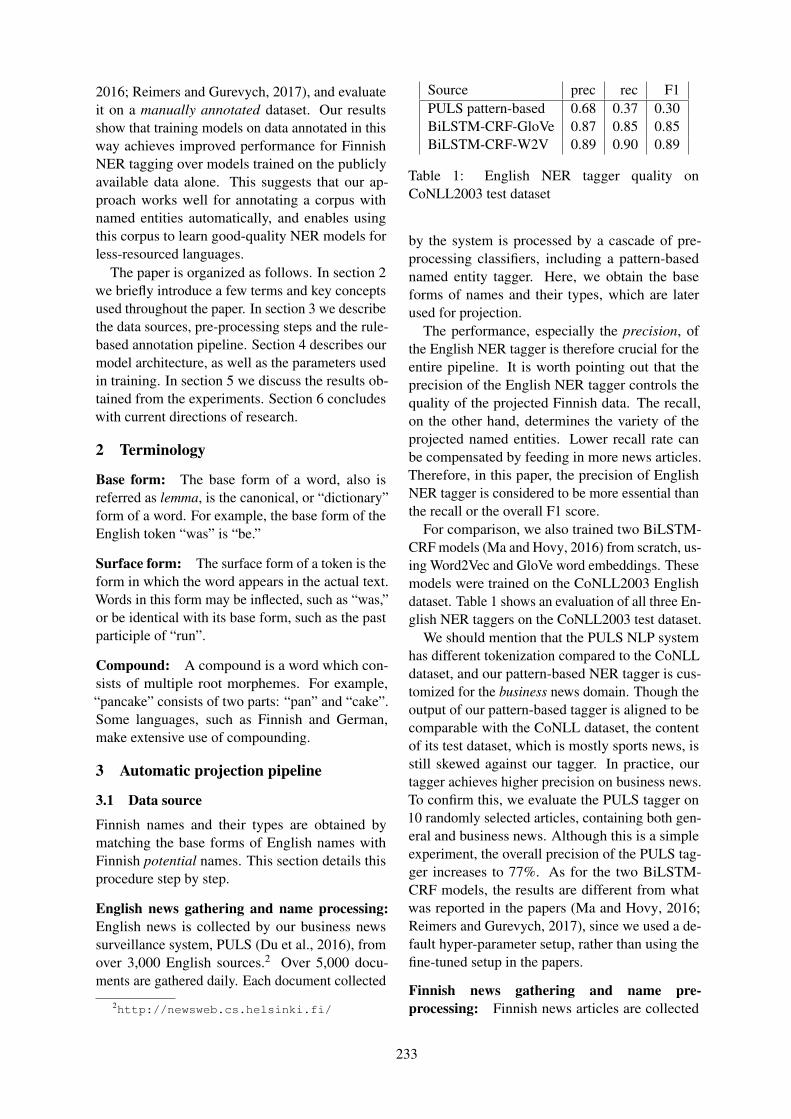
2016; Reimers and Gurevych, 2017), and evaluateit on a manually annotated dataset. Our resultsshow that training models on data annotated in thisway achieves improved performance for FinnishNER tagging over models trained on the publiclyavailable data alone. This suggests that our ap-proach works well for annotating a corpus withnamed entities automatically, and enables usingthis corpus to learn good-quality NER models forless-resourced languages.

The paper is organized as follows. In section 2we briefly introduce a few terms and key conceptsused throughout the paper. In section 3 we describethe data sources, pre-processing steps and the rule-based annotation pipeline. Section 4 describes ourmodel architecture, as well as the parameters usedin training. In section 5 we discuss the results ob-tained from the experiments. Section 6 concludeswith current directions of research.

2 Terminology

Base form: The base form of a word, also isreferred as lemma, is the canonical, or “dictionary”form of a word. For example, the base form of theEnglish token “was” is “be.”

Surface form: The surface form of a token is theform in which the word appears in the actual text.Words in this form may be inflected, such as “was,”or be identical with its base form, such as the pastparticiple of “run”.

Compound: A compound is a word which con-sists of multiple root morphemes. For example,“pancake” consists of two parts: “pan” and “cake”.Some languages, such as Finnish and German,make extensive use of compounding.

3 Automatic projection pipeline

3.1 Data source

Finnish names and their types are obtained bymatching the base forms of English names withFinnish potential names. This section details thisprocedure step by step.

English news gathering and name processing:English news is collected by our business newssurveillance system, PULS (Du et al., 2016), fromover 3,000 English sources.2 Over 5,000 docu-ments are gathered daily. Each document collected

2http://newsweb.cs.helsinki.fi/

Source prec rec F1PULS pattern-based 0.68 0.37 0.30BiLSTM-CRF-GloVe 0.87 0.85 0.85BiLSTM-CRF-W2V 0.89 0.90 0.89

Table 1: English NER tagger quality onCoNLL2003 test dataset

by the system is processed by a cascade of pre-processing classifiers, including a pattern-basednamed entity tagger. Here, we obtain the baseforms of names and their types, which are laterused for projection.

The performance, especially the precision, ofthe English NER tagger is therefore crucial for theentire pipeline. It is worth pointing out that theprecision of the English NER tagger controls thequality of the projected Finnish data. The recall,on the other hand, determines the variety of theprojected named entities. Lower recall rate canbe compensated by feeding in more news articles.Therefore, in this paper, the precision of EnglishNER tagger is considered to be more essential thanthe recall or the overall F1 score.

For comparison, we also trained two BiLSTM-CRF models (Ma and Hovy, 2016) from scratch, us-ing Word2Vec and GloVe word embeddings. Thesemodels were trained on the CoNLL2003 Englishdataset. Table 1 shows an evaluation of all three En-glish NER taggers on the CoNLL2003 test dataset.

We should mention that the PULS NLP systemhas different tokenization compared to the CoNLLdataset, and our pattern-based NER tagger is cus-tomized for the business news domain. Though theoutput of our pattern-based tagger is aligned to becomparable with the CoNLL dataset, the contentof its test dataset, which is mostly sports news, isstill skewed against our tagger. In practice, ourtagger achieves higher precision on business news.To confirm this, we evaluate the PULS tagger on10 randomly selected articles, containing both gen-eral and business news. Although this is a simpleexperiment, the overall precision of the PULS tag-ger increases to 77%. As for the two BiLSTM-CRF models, the results are different from whatwas reported in the papers (Ma and Hovy, 2016;Reimers and Gurevych, 2017), since we used a de-fault hyper-parameter setup, rather than using thefine-tuned setup in the papers.

Finnish news gathering and name pre-processing: Finnish news articles are collected

233

from two major Finnish online news agencies.Around 200 news articles are collected daily.The Turku dependency parser (Haverinen et al.,2014) has been applied for sentence splitting andtokenization. Three different problems need to besolved so that all potential names can be extractedin these steps: name identification, base formselection, and name merging.

Name identification: For identifying whethera token is a name or part of a name, we use therules based on the position of tokens as follows:

• Any capitalized token which appears in themiddle of a sentence is definitely a name orpart of the name.

• If token A is a name according to previousrule, and token B, having the same base formas token A, appears at the beginning of a sen-tence, we assume token B is the same name.

• If a token of a potential name appears in thedocument only at the beginning of sentences,it is not certain and therefore not assumed tobe a name.

Base form selection: To determine the baseform corresponding to a surface form found in text,we consider all base forms returned by our mor-phological analyzer, (Moshagen et al., 2013), anda simple rule-based stemmer, and look through theentire article. If there is an intersection between thepossible base forms of two name tokens, their truebase form can then be resolved. When the intersec-tion has only one base form, it can be confirmed tobe the base form of a name directly. Otherwise, allof them will be recorded as potential base form ofthe name. All potential base forms will be furtherfiltered when matching with English named entitiesduring projection.

Suppose the surface form “Trumpille” (in theallative case) and “Trump” (nominative) both ex-ist in an article. Without any external knowl-edge, the Finnish surface form “Trumpille” willbe assigned two potential lemmas by our stem-mer: “Trumpi” and “Trump” (both of these lem-mas have the same allative form). For the surfaceform “Trump”, only “Trump” will be returned as apotential lemma. Then, in this case, their intersec-tion, “Trump”, will be confirmed to be the lemmaof both “Trumpille” and “Trump”. However, ifinstead the article only contains the surface forms“Trumpille” and “Trumpin” (genitive). Then both

lemmas “Trumpi” and “Trump” will be recordedas potential lemmas.

We perform name identification and base formselection jointly, since they are connected, bysearching for the common base forms of tokens.

Name merging: We use a set of rules to mergenames that consist of more than one token. Poten-tial names can contain only the following kinds oftokens in positions other than the final position:

• Singular common noun or proper noun whichmust be in the nominative case, for example:“Spring Harbour”.3

• English function words: e.g., “the”, “and”,“new”, etc. For example: “The New YorkTimes”• Having no valid analyses returned by the

Finnish morphological analyzer, and its sur-face form can be confirmed to be its ownlemma during the base form selection processabove.One example is the token “Trump” in “TrumpTowerin” (genitive: “of the Trump Tower”).Our Finnish morphological analyzer will re-ject (not recognize) the input token “Trump”.We assume that “Trump” can be confirmedas a name or as part of a multi-token nameaccording to the rules. “Trump” can be con-firmed to be its own base form, which meansits base form happens to be the same as itssurface form. In this case, “Trump” will bemerged with the following token “Towerin”.

We should note that when several potential nametokens are strung together, the true partitioning ofnames is ambiguous. During name merging, alldifferent partitionings and potential forms of thebase forms of names are cached as candidates forthe following name resolution step.

Hyphenating between tokens are also a criterionfor merging names, such as the Indian surname“Ankalikar-Tikekar”.

3.2 Name projection

In the next stage, we annotate Finnish names byutilizing the potential names candidates producedby the previous three steps, namely name identifi-cation, base form selection, and name merging.

3Names such as “Helsingin Sanomat” (name of a majornewspaper in Finland), where the first token is in the genitivecase (of “Helsinki”) are currently not handled by these rules,and are handled separately by a list.

234

The fundamental assumption is that a namerefers to only one entity in a given article. We ex-pect this assumption to hold for well-edited newsarticles. This means that if only one instance (sur-face form) of a particular name has been annotatedin an article, the remaining occurrences of the samename in the article—possibly involving other sur-face forms—can be annotated as well.

We gather two sets of named entities fromFinnish document and English documents:

• For a Finnish document, published on day t,we use three steps mentioned above to obtaina set of potential Finnish named entity candi-dates, including both potential base forms andconfirmed base form of names.

• From English news in the time interval (t± 2days), using an English NER tagger, a setof English named entities and their corre-sponding tags are obtained. Each of them hasits base form resolved by the pre-processingpipeline in PULS.

Names can naturally be matched according to theirbase form. The type of the English named entitiescan therefore be projected to their Finnish coun-terparts. The remaining Finnish names candidates,for which no type annotation can be inferred, aredropped after this step.

The idea of a time window (t ± 2 days) is totake advantage of the fact that names overlap sig-nificantly in different articles due to continuouscoverage of important events, and therefore opti-mize our memory usage and time efficiency.

Again, take “Trump” as an example. Suppose wehave a named entity “Donald Trump” from the En-glish news articles and it is recognized as “Person”.We may have “Donald Trumpille” in a Finnish arti-cle; if the surface form “Trump” is not present inthe same Finnish article, as we mentioned already,we can only infer that the base form of “Trumpille”is “Trumpi” or “Trump”, using stemming rules.In addition, “Donald Trumpille” has two tokensbut we do not yet know whether they belong to-gether as one name. Therefore, “Donald”, “DonaldTrump”, “Donald Trumpi”, “Trump” and “Trumpi”are all Finnish name candidates. After matching,only “Donald Trump” will be kept and annotatedas Person, while other candidates, namely “Don-ald”, “Donald Trumpi”, “Trump” and “Trumpi”,are dropped.

In addition, for the Person type only, names willbe connected by their partial base form. Once“Donald Trump” gets annotated, all the other “Don-ald” and “Trump” tokens in the entire article willbe annotated as Person as well.

3.3 Special cases: rule-based projection

We use extra steps to handle special cases in thisprocess. In Finnish, geo-location names, such asthe names of countries, are often different fromtheir English names. For example, France is “Ran-ska” in Finnish, and the United States is “Yhdys-vallat” in Finnish. Some organizations also havethe same problem, as UN is “YK” in Finnish, etc.Therefore, we manually build a small database offrequent names, including Finnish geo-locations,and a few of the major and most frequently occur-ring international companies and organizations, toassure that they are annotated correctly. In addition,this covers some cases which the English taggerfails to catch. We also filter out names that canhave multiple types, such as MacLaren, since theseare ambiguous.

Additionally, we introduce a list of 1000 com-mon first names and assume that names beginningwith these tokens are of type Person. However,this practice requires more rules to constrain itsoutcome:

• A Person name should have at most 2 tokens.

• A Person name should not start with “The”.

• No token in a Person name should be fullyuppercase.

• We require that a Person name be mentionedusing the full name at least once in the article.

These rules are simple, naive and strict. Thepurpose of these rules is to remove any uncertaininstances and make the data as clean as possible.Even if only one name in an article can meet allthese rules, all other name instances related to thatname instance will be correctly annotated. Also,taking advantage of our enormous amount of data,we can afford to filter out uncertain data withoutworrying about the amount of remaining data.

Currently, the annotations may be wrong whenan article only mentions the last name of a person,which also happens to be the name of a location.For example, “Sipilä” is the last name of the currentPrime Minister of Finland, and may therefore be

235

mentioned many times in an article, without men-tioning the full name, “Juha Sipilä”. Coincidentally,“Sipilä” is a town in Finland. The situation whereboth the person and the location are mentioned inthe same article rarely occurs in practice and canbe tackled by filtering out such names.

4 NER model

Next we provide the details of the adaptedBiLSTM-CRF model for Finnish NER and the hy-perparameter setup for training this model. Thebasic network structure of the model is inspiredby (Ma and Hovy, 2016; Reimers and Gurevych,2017). The model is implemented in Keras withTensorFlow as its backend. The CRF layer is pro-vided by Keras-contrib.4 The training process wasrun on an Nvidia GeForce 1080 Ti GPU. It tookaround 3 hours to train the model using the setupin this section. The model is shown in Figure 1.

Tag-0 Tag-1 Tag-2

CRF CRF CRF

BiLSTM BiLSTM BiLSTM

Linear Linear Linear

|| ......

Word

Emb.Char

CNNCase

Emb.PoS

PoS-dense

Token-1

Figure 1: Adapted BiLSTM-CRF network struc-ture for Finnish NER

As seen in Figure 1, Part-of-Speech (PoS) is in-cluded as an additional feature, compared to themodel of Ma and Hovy (2016). This is because alemma may be assigned multiple PoS tags by ourmorphological analyzer (Moshagen et al., 2013).Word embeddings such as Word2Vec (Mikolovet al., 2013) may implicitly contain PoS informa-tion but will still be static regardless of context.Using PoS as input feature also compensates for

4www.github.com/keras-team/keras-contrib

out-of-vocabulary problem in embeddings. In thesecases, not even the implicit PoS information canbe detected by the network if PoS is not a part ofinput features.

4.1 Data encodingTokens are encoded into to several features: wordembedding, character embedding, case embeddingand Part of Speech (PoS). Except for PoS, mostof the features follow the setup in (Reimers andGurevych, 2017). Word embeddings are extendedwith a special mark for ambiguous tokens—tokens,for which our morphological analyzer fails returnsmore than one base forms and PoS. These tokensare replaced with a special token “AMBIGUOUS”.Additionally, we only use the embedding of thelast part of a compound word if this word is out-of-vocabulary. This is because the last part is theessential part of compounds in Finnish. Charac-ter embeddings are extended with a special valuefor “unrecognized” character. The PoS featureis encoded as an array of ones and zeros. Eachdimension corresponds to one PoS type, includ-ing PADDING and UNKNOWN. Integer “1” isassigned to the dimension corresponding to the to-ken’s PoS. If a token is a compound word, only thePoS of its last part is used for encoding. If a tokenhas multiple PoS analyses, more than one positionin the PoS array is assigned “1”. The values of PoSare as follows:

• PADDING• UNKNOWN• Noun• Verb• Adj• Adv

• Pron• Conj• Interj• Num• Punct• other

These four input features are concatenated be-fore feeding into BiLSTM.

4.2 Parameter initializationWord embeddings: We use a pre-trainedWord2Vec embedding matrix, which is trained by(Laippala and Ginter, 2014). It has been trained on4.5B words of text. As mentioned previously, weinclude vectors for “PADDING”, “UNKNOWN”and “AMBIGUOUS” tokens. Embeddings for thetokens “UNKNOWN” and “AMBIGUOUS” arerandomly initialized with uniform sampling from-0.25 to 0.25, while the “PADDING” embedding isa zero vector.

236

Layer Hyper-parameter Number

Char CNNNumber of filters 30Filter size 3

PoS-denseUnit size 30Activation Relu

BiLSTMNumber of layers 2State size 200Dropout rate 0.25

Table 2: Table of hyper-parameter for experiments

Character embeddings: Character embeddings,including “UNKNOWN” character embedding, arerandomly initialized with uniform samples from

−√

3dim to

√3

dim , where dim = 30.

Case embedding: Case embeddings are ran-domly initialized applying a uniform initializer.The dimensionality of the case embeddings is 10.

Weight Matrices and Bias Vectors: Most ofweights are initialized as a uniform sample from[−

√6

Ni+No,√

6Ni+No

], where Ni and No refer tothe number of input and output units in the weighttensor. Bias is initialized with zeros.

4.3 Optimization

Optimizer: We used the Adam optimizer, as rec-ommended in (Reimers and Gurevych, 2017). Thesetup for the Adam optimizer also followed theKeras default setting: lr = 0.001, β1 = 0.9, β2 =0.999. Although Ma and Hovy (2016) used gradi-ent norm clipping of 5.0, we did not.

Early stopping and learning rate decay: Weapplied early stopping following the categoricalaccuracy on the training dataset in case of over-fitting. On average, the training process stops after5 epochs. We have also explored reducing the learn-ing rate during the training process if the accuracystops improving. However, this made the trainingslower, and did not improve the final result on thevalidation dataset.

4.4 Hyper-parameter setup

Most of the hyper-parameter values, shown in Ta-ble 2, follow the recommendations in (Reimers andGurevych, 2017). The layer called “PoS-dense” inFigure 1 is a dense layer with a non-linear acti-vation function, rather than an embedding layer,due to the encoding method of the PoS features,as explained in Section 4.1. For the mini-batch

size, the authors recommend using the batch sizebetween 8 and 32, depending on the size of thetraining dataset. However, that is the result on theCoNLL-2003 dataset, which is an English dataset.We use 50 similarly to the German NER model in(Reimers and Gurevych, 2017).

We should mention that the CRF layer im-plemented by the Keras-contrib package offerstwo different modes for the training and testingprocesses: “Join” and “Marginal” for training,“Viterbi” and “Marginal” for testing. The “Join”training mode and “Viterbi” testing mode followsthe “vanilla” fitting algorithms for linear chain CRF.“Marginal” training is optimized via compositionlikelihood (product of marginal likelihood), whichis not optimal in this case. “Marginal” testing modewill decode the input sequence according to thetraining result and compute marginal probabilities.In this mode, it can therefore output a probabilityprediction of the classes for tokens. Accordingto the documentation, the “Join” training modecan outperform the other training mode, and the“Viterbi” testing mode can achieve better perfor-mance than “Marginal” testing mode, but reason-ably close. In this work, we evaluate using both“Join-Marginal” and “Join-Viterbi” modes.

5 Performance and evaluation

In this section, we report the performance for theautomatic projection pipeline and the NER model.F1-score is used as the evaluation metric. Theoverall F1-score is the weighted average F1-scoreof each category.

5.1 Automatic projection pipeline

We currently utilize data only from the beginningof 2017 to July of 2018 for development, modeltraining and validation. The total Finnish data con-sists of around 83,000 articles.

Our English data, on the other hand, date back6 years from 2018 to 2012. Only articles fromthe same time period as the Finnish data can beused for name matching. The amount of usableEnglish articles is around 4,486,000. We considerthe NER performance only on “person”, “location”and “organization” tags, to make the final outcomecomparable to the Polyglot Finnish NER tagger.

To evaluate the performance of the automaticprojection, we manually checked 1,000 randomlyselected sentences from March 2018 to April 2018.Since our three English NER taggers have different

237

Tag Prec Rec F1 SupportB-PER 0.97 0.99 0.98 823I-PER 0.97 0.97 0.97 668B-LOC 0.99 0.99 0.99 341I-LOC 1.00 0.67 0.80 3B-ORG 0.99 0.98 0.98 536I-ORG 1.00 0.82 0.90 78Avg / total 0.98 0.98 0.98 2449

Table 3: Quality of Finnish data projected fromPULS pattern-based NER: evaluated on 1,000 sen-tences, annotated manually.


Table 4: Quality of Finnish data projected fromBiLSTM-CRF-W2V model: evaluated on 1,000sentences, annotated manually.

performance, the manual evaluation is conductedseparately, as shown in Table 3, Table 4 and Ta-ble 5.

5.2 NER model

For training the NER models, we used data from2017-01 to 2017-12 (12 months). This periodcontains 50,009 Finnish documents, for which wefound 920,658 matching English documents. Wefiltered out projected sentences for which the En-glish tagger produced NER tags other than Per-son, Organization, or Location. This data pro-duced approximately 114,000 automatically pro-jected sentences after filtering. For validation, weused two months: 2018-04 to 2018-05. This periodcontained 11,452 Finnish documents, which had389,072 English matching documents. This dataproduced 23,277 automatically projected sentences,after filtering.

Instances are projected from 3 different En-glish NER taggers: the PULS pattern-based tagger,BiLSTM-CRF-GloVe tagger and BiLSTM-CRF-W2V tagger. Two train-test modes, “Join-Marginal”and “Join-Viterbi”, are also applied for comparison.Six different Finnish NER models are evaluated.


Table 5: Quality of Finnish data projected from theBiLSTM-CRF-GloVe model: evaluated on 1,000sentences, annotated manually.

Table 6 shows the model evaluation on this data.As expected, upon visual inspection, we noticed

instances with incorrect “ground truth” since pro-jection is not entirely clean. Despite its good over-all quality, the validation performance may stilldiffer from actual performance.

We conducted further model testing and inspec-tion to obtain better estimates of the true perfor-mance. We sampled another set of articles from2018-08 to 2018-10 (3 months), which is outsideour automatic projection time period. For furtherinspection and error analysis, in Section 5.3, werandomly sampled a total of 36 articles, evenlyfrom the following 6 sections of the newspaper:

• “Talous” (Economics)• “Politiikka” (Politics)• “Ulkomaat” (Foreign news)• “Kotimaa” (Domestic news)• “Koti” (Home)• “Kaupunki” (The City)

The first three of these categories are moreclosely related to the Business domain. Again, arti-cles are evaluated manually. The result is shownin Table 7. Polyglot is used as the performancebaseline. Two additional Finnish NER models aretrained with full FiNER-data (Ruokolainen et al.,2019), including the validation and test dataset, forbetter comparison.5

As shown in Table 7, Polyglot and the modeltrained with FiNER-data have better precision thanmost of our Finnish NER taggers, but have a worserecall rate. Overall, most of our Finnish NER tag-gers achieve better performance. Only one model,projected from BiLSTM-CRF-W2V in Join-Viterbimode, performs worse than the FiNER-data model

5www.github.com/mpsilfve/finer-data

238

Eng-NER Source Train-test mode Prec Rec F1 SupportPULS pattern-based Join-Viterbi 0.94 0.92 0.93 28858PULS pattern-based Join-Marginal 0.94 0.93 0.93 28858BiLSTM-CRF-GloVe Join-Viterbi 0.92 0.89 0.90 34526BiLSTM-CRF-GloVe Join-Marginal 0.93 0.91 0.92 34526BiLSTM-CRF-W2V Join-Viterbi 0.87 0.83 0.84 37219BiLSTM-CRF-W2V Join-Marginal 0.87 0.85 0.85 37219

Table 6: Validation scores on 2018-04 to 2018-05. “PULS pattern-based” and “BiLSTM-CRF-*” referto the Finnish NER models that are projected from our PULS pattern-based NER tagger and EnglishBiLSTM-CRF NER tagger respectively. “GloVe” and “W2V” indicates the embedding that English NERtaggers use.

NER Source Train-test mode Prec Rec F1 SupportPULS pattern-based Join-Viterbi 0.89 0.77 0.82 916PULS pattern-based Join-Marginal 0.80 0.83 0.81 916BiLSTM-CRF-GloVe Join-Viterbi 0.80 0.75 0.76 916BiLSTM-CRF-GloVe Join-Marginal 0.79 0.74 0.75 916BiLSTM-CRF-W2V Join-Viterbi 0.76 0.72 0.73 916BiLSTM-CRF-W2V Join-Marginal 0.78 0.79 0.78 916FiNER-data Join-Viterbi 0.83 0.72 0.75 916FiNER-data Join-Marginal 0.73 0.68 0.64 916Polyglot 0.82 0.55 0.64 916

Table 7: Test evaluation. “FiNER-data” refer to the Finnish NER model trained with data from FiNER-data.“Polyglot” entry illustrates the performance of their model on our test dataset

in Join-Viterbi mode. The Finnish NER tagger thatis projected from the PULS pattern-based EnglishNER tagger in Join-Viterbi mode achieves the over-all best performance. This result also suggests thatthe dataset produced by our automatic projectionpipeline is valid for model training, data of largesize and various topics, while FiNER-data onlycovers technology-related news.

5.3 Error analysis

Despite good overall performance on all automat-ically projected datasets, the average F1 score ofmodels with the different setups is still around 77%.More work is required to improve performance. Toguide future work, we did further visual inspectionsto examine the predictions in general.

One major problem is that the NER model getsdata from automatic projection with limited pat-tern diversity. During the training pipeline, in-cluding automatic projection, there are two reasonsthat may cause this problem.

Firstly, flaws still exist in the automatic projec-tion pipeline. One flaw that shows up often duringvisual inspection is that the projection currently

does not support named entities without any capitalletters. Named entities such as “Valkoinen talo”(the White House) cannot be fully recognized atthe beginning of the pipeline (because the secondtoken is lowercase). As a result, only the tokenwith a capitalized letter such as “Valkoinen” willbe predicted as a named entity by Finnish NERtagger.

Secondly, the English data source is biased infavor of foreign business topics. Within the timeperiod of the training data, our database containsmostly business news. As a consequence, morebusiness-related news and their named entities inFinnish news can be tagged. General news maybehave differently than business news, and maycontain more patterns for the task of NER. To ver-ify this conjecture, we inspect each category withthe model projected from the PULS pattern-basedtagger in Join-Viterbi mode. As shown in Table 8,the model can achieve better performance on av-erage on the topics which are related to foreignbusiness or politics news, compared to domestic orlocal news.

Another major problem is due to a flaw in

239

Category Prec Rec F1 SupportOverall 0.89 0.77 0.82 916Talous 0.91 0.90 0.90 123Politiikka 0.89 0.79 0.83 191Ulkomaat 0.92 0.75 0.83 227Kotimaa 0.90 0.70 0.78 100Koti 0.86 0.73 0.77 167Kaupunki 0.83 0.71 0.74 108

Table 8: Performance of the Finnish NER taggerfor each category. The tagger is projected from thepattern-based English NER tagger in Join-Viterbimode, first line in Table 7.

data encoding. As mentioned previously, out-of-vocabulary compound lemmas are decomposed andassigned the embedding of the last part of the com-pound lemma. Many ordinary tokens may bene-fit from this approach, while organization namedentities do not. During visual inspection, we no-ticed that the name of some Finnish national orlocal governmental departments can be a made-up word or a compound word. Such names willeither be assigned the “UNKNOWN” token em-bedding or the embedding of the last part of thecompound word, which is most likely a commonnoun. For example, “Verohallinto” (Tax Admin-istration) does not have an embedding as a whole.However, “hallinto” (“government”) is a commonnoun within the embedding vocabulary. As a result,these named entities are more likely to be tagged in-correctly. As illustrated in Table 9, the performanceof organizations (B-ORG) suffers from severelylow recall rates due to this problem, as well as thepreviously mentioned problem that Finnish domes-tic named entities are less likely to get projectionsin the pipeline.6

6 Conclusions and future work

In this paper, we propose the idea of building aFinnish NER dataset by leveraging the output ofan English NER tagger and projecting the type ofrecognized named entities from English to Finnish.The contributions of this paper are:

• Our work shows that the Finnish NER datasetproduced by only simple rule-based projec-tion can be used for NER model training. Noparallel bilingual documents are used, only

6Because they are unlikely to appear in English-languagenews.

Tag Prec Rec F1 SupportB-PER 0.88 0.70 0.78 20I-PER 0.83 1.00 0.91 10B-LOC 0.85 0.90 0.88 52I-LOC 0.00 0.00 0.00 5B-ORG 1.00 0.32 0.48 19I-ORG 0.00 0.00 0.00 2avg/total 0.83 0.71 0.74 108

Table 9: Detailed performance of Finnish NERtagger for category “Kaupunki” (“The City”) inTable 8.

projected named entities, obtained by severalmonolingual tools.

• We demonstrate the performance of our NERmodel, and set a new benchmark for FinnishNER.

For future work, we plan to first tackle the prob-lems that we mentioned in the error analysis sec-tion and conduct further inspection. Secondly, weplan to combine our pipeline with a disambiguationmodel, to improve both the pre-processing and thedata encoding steps. Thirdly, it would be interest-ing to experiment and generalize our approach withother languages with limited NER tools, such asEstonian, if corresponding news datasets are easilyaccessible.

Acknowledgements

This work was supported in part by TEKES, theFinnish Funding Agency for Technology and Inno-vation, Project “iMEDL—Digital Media Evolutionthrough Deep Learning”, number 5933/31/2017.

ReferencesRami Al-Rfou, Vivek Kulkarni, Bryan Perozzi, and

Steven Skiena. 2015. Polyglot-ner: Massive mul-tilingual named entity recognition. In Proceedingsof the 2015 SIAM International Conference on DataMining. SIAM, pages 586–594.

Jason P.C. Chiu and Eric Nichols. 2016. Named entityrecognition with bidirectional LSTM-CNNs. Trans-actions of the Association for Computational Lin-guistics 4:357–370.

Jacob Devlin, Ming-Wei Chang, Kenton Lee, andKristina Toutanova. 2018. BERT: pre-training ofdeep bidirectional transformers for language under-standing. CoRR abs/1810.04805.

240

Mian Du, Lidia Pivovarova, and Roman Yangarber.2016. PULS: natural language processing for busi-ness intelligence. In Proceedings of the 2016 Work-shop on Human Language Technology.

Maud Ehrmann, Marco Turchi, and Ralf Steinberger.2011. Building a multilingual named entity-annotated corpus using annotation projection. InProceedings of the International Conference RecentAdvances in Natural Language Processing 2011.pages 118–124.

Jenny Rose Finkel, Trond Grenager, and ChristopherManning. 2005. Incorporating non-local informa-tion into information extraction systems by Gibbssampling. In Proceedings of the 43rd Annual Meet-ing on Association for Computational Linguistics.Association for Computational Linguistics, Strouds-burg, PA, USA, ACL ’05, pages 363–370.

Abbas Ghaddar and Phillippe Langlais. 2017. Winer:A Wikipedia annotated corpus for named entityrecognition. In Proceedings of the Eighth Interna-tional Joint Conference on Natural Language Pro-cessing (Volume 1: Long Papers). pages 413–422.

Katri Haverinen, Jenna Nyblom, Timo Viljanen,Veronika Laippala, Samuel Kohonen, Anna Missilä,Stina Ojala, Tapio Salakoski, and Filip Ginter. 2014.Building the essential resources for Finnish: theTurku Dependency Treebank. Language Resourcesand Evaluation 48(3):493–531.

Zhiheng Huang, Wei Xu, and Kai Yu. 2015. Bidi-rectional LSTM-CRF models for sequence tagging.CoRR abs/1508.01991.

Jun’ichi Kazama and Kentaro Torisawa. 2007. Exploit-ing Wikipedia as external knowledge for named en-tity recognition. In Proceedings of the 2007 JointConference on Empirical Methods in Natural Lan-guage Processing and Computational Natural Lan-guage Learning (EMNLP-CoNLL).

Sungchul Kim, Kristina Toutanova, and Hwanjo Yu.2012. Multilingual named entity recognition usingparallel data and metadata from Wikipedia. In Pro-ceedings of the 50th Annual Meeting of the Associ-ation for Computational Linguistics: Long Papers-Volume 1. Association for Computational Linguis-tics, pages 694–702.

Veronika Laippala and Filip Ginter. 2014. SyntacticN-gram collection from a large-scale corpus of inter-net Finnish. In Human Language Technologies-TheBaltic Perspective: Proceedings of the Sixth Interna-tional Conference Baltic HLT 2014. IOS Press, vol-ume 268, page 184.

Guillaume Lample, Miguel Ballesteros, Sandeep Sub-ramanian, Kazuya Kawakami, and Chris Dyer. 2016.Neural architectures for named entity recognition.In Proceedings of the 2016 Conference of the NorthAmerican Chapter of the Association for Compu-tational Linguistics: Human Language Technolo-gies. Association for Computational Linguistics,San Diego, California, pages 260–270.

Xuezhe Ma and Eduard H. Hovy. 2016. End-to-endsequence labeling via bi-directional LSTM-CNNs-CRF. CoRR abs/1603.01354.

Tomas Mikolov, Kai Chen, Greg S Corrado, and JeffreyDean. 2013. Efficient estimation of word represen-tations in vector space. In NIPS.

Sjur N Moshagen, Tommi Pirinen, and TrondTrosterud. 2013. Building an open-source de-velopment infrastructure for language technologyprojects. In Proceedings of NODALIDA 2013: the19th Nordic Conference of Computational Linguis-tics. Oslo, Norway.

Joel Nothman, Nicky Ringland, Will Radford, TaraMurphy, and James R Curran. 2013. Learning mul-tilingual named entity recognition from Wikipedia.Artificial Intelligence 194:151–175.

Matthew E. Peters, Mark Neumann, Mohit Iyyer, MattGardner, Christopher Clark, Kenton Lee, and LukeZettlemoyer. 2018. Deep contextualized word repre-sentations. In Proc. of NAACL.

Nils Reimers and Iryna Gurevych. 2017. Optimal hy-perparameters for deep lstm-networks for sequencelabeling tasks. CoRR abs/1707.06799.

Alexander E Richman and Patrick Schone. 2008. Min-ing wiki resources for multilingual named entityrecognition. In Proceedings of ACL-08: HLT . pages1–9.

Teemu Ruokolainen, Pekka Kauppinen, Miikka Silfver-berg, and Krister Lindén. 2019. A finnish newscorpus for named entity recognition. Language Re-sources and Evaluation pages 1–26.

Antonio Toral and Rafael Munoz. 2006. A proposalto automatically build and maintain gazetteers forNamed Entity Recognition by using Wikipedia. InProceedings of the Workshop on NEW TEXT Wikisand blogs and other dynamic text sources.

241

Template-free Data-to-Text Generation of Finnish Sports News

Jenna Kanerva, Samuel Ronnqvist, Riina Kekki, Tapio Salakoski and Filip GinterTurkuNLP

Department of Future TechnologiesUniversity of Turku, Finland

{jmnybl,saanro,rieeke,sala,figint}@utu.fi

Abstract

News articles such as sports game reportsare often thought to closely follow the un-derlying game statistics, but in practicethey contain a notable amount of back-ground knowledge, interpretation, insightinto the game, and quotes that are notpresent in the official statistics. Thisposes a challenge for automated data-to-text news generation with real-world newscorpora as training data. We report onthe development of a corpus of Finnishice hockey news, edited to be suitablefor training of end-to-end news generationmethods, as well as demonstrate genera-tion of text, which was judged by journal-ists to be relatively close to a viable prod-uct. The new dataset and system sourcecode are available for research purposes.1

1 Introduction

Automated, or robotic, journalism aims at newsgeneration from structured data sources, either asthe final product or as a draft for subsequent post-editing. At present, automated journalism typi-cally focuses on domains such as sports, financeand similar statistics-based reporting, where thereis a commercial product potential due to the highvolume of news, combined with the expectation ofa relatively straightforward task.

News generation systems—especially those de-ployed in practice—tend to be based on intricatetemplate filling, aiming to give the users the fullcontrol of the generated facts, while maintaininga reasonable variability of the resulting text. Thiscomes at the price of having to develop the tem-plates and specify their control logic, neither ofwhich are tasks naturally fitting journalists’ work.

1https://github.com/scoopmatic/finnish-hockey-news-generation-paper

Further, this development needs to be repeated forevery domain, as the templates are not easily trans-ferred across domains. Examples of the template-based news generation systems for Finnish areVoitto2 by the Finnish Public Service Broadcast-ing Company (YLE) used for sports news genera-tion, as well as Vaalibotti (Leppanen et al., 2017),a hybrid machine learning and template-based sys-tem used for election news.

Wiseman et al. (2018) suggested a neural tem-plate generation, which jointly models latent tem-plates and text generation. Such a system in-creases interpretability and controllability of thegeneration, however, recent sequence-to-sequencesystems represent the state-of-the-art in data-to-text generation. (Dusek et al., 2018)

In this paper, we report on the developmentof a news generation system for the Finnishice hockey news domain, based on sequence-to-sequence methods. In order to train such a system,we compile a corpus of news based on over 2000game reports from the Finnish News Agency STT.While developing this corpus into a form suitablefor training of end-to-end systems naturally re-quires manual effort, we argue that compiling andrefining a set of text examples is a more naturalway for journalists to interact with the system, inorder for them to codify their knowledge and toadapt it for new domains.

Our aim is to generate reports that give anoverview of a game based on information in-ferrable from the statistics. Such reports can beused either as a basis for further post-editing bya journalist imprinting own insights and back-ground information, or even used directly as anews stream labelled as machine-generated.

In the following, we will introduce the newsdataset and the process of its creation, introduce anend-to-end model for news generation, and eval-

2https://github.com/Yleisradio/avoin-voitto

242

uate its output respective to the abovementionedobjectives.

2 Ice Hockey News Dataset

An ice hockey game is recorded into statistics interms of different events occurring during play,such as goals and penalties. In order to train amodel to generate game reports, we need accessto these events, as well as example news articlesabout the game. Only recently have game statis-tics become available to the public through a webinterface or API, whereas the information has tra-ditionally been recorded as structured text files.

The news corpus from the Finnish NewsAgency STT3 includes, among all other news, ar-ticles covering ice hockey games in the Finnishleagues during the years 1994–2018. In additionto news articles, the corpus also includes the orig-inal game statistics text files. This creates an op-portunity to align the game statistics with the cor-responding news articles, producing a dataset ofover 20 years of ice hockey data with referencenews articles for the games. When automaticallypairing the game statistics with news articles us-ing date and team names as a heuristic, we obtaina total of 3,454 games with existing statistics andat least one corresponding news article.

Utilizing real journalistic material poses a chal-lenge in that the articles mix information thatcan be found directly in the game statistics (e.g.,scores and names) with information inferable fromthe statistics (e.g., statements such as shortly af-ter), information based on background knowledge(e.g., a team’s home city or player’s position),game insight and judgement based on viewing thegame (e.g., expressions such as slapshot or tippingthe puck describing the character of a shot), andeven player interviews.

Therefore, directly using the limited amount ofactual news articles for end-to-end system trainingbecomes problematic. In our initial experimentsthe generation model learns to “hallucinate” facts,as easily occurs when the target text is too looselyrelated to the conditioning input.4 In order to en-sure that the generation model is able to learn togenerate accurate descriptions from game statis-tics, we clean the news corpus by manually align-

3A version of the corpus is available at http://urn.fi/urn:nbn:fi:lb-2019041501 for academic use.

4This observation is also supported by Wiseman et al.(2017) mentioning that their generation model occasionally“hallucinates factual statements” that are plausible but false.

ing corresponding text spans with game events de-tailed in the statistics.

For the sake of comparison, let us considerthe Rotowire corpus (Wiseman et al., 2017) con-taining basketball game summaries and statistics,which was recently released and has become apopular data set for training data-to-text genera-tion systems (cf., e.g., Nie et al. (2018); Wise-man et al. (2018); Puduppully et al. (2019)). TheRotowire game summaries are straightforward intheir style of reporting, focusing on the game athand and tend for the most part to reference factsin the statistics. By contrast, our news corpus ismore heterogeneous, including both articles focus-ing on the particular game and articles that take abroader perspective (e.g., describing a player’s ca-reer). The STT news articles tend to read in thejournalist’s voice, putting substantial emphasis onthe character of the game, often in colorful lan-guage, as well as quoting players and coaches.

An example of the events available in the gamestatistics, the actual news article on the game, andhow these align, is shown in Figure 1. Text spanshighlighted with blue color are based on informa-tion available in the statistics, all other being ex-ternal information. It illustrates the typical portionof a raw article that is not inferrable from the data.English translations are available for a comparableexample in Figure 4.

2.1 Extraction of Game Events

For each event occurring in a game and recordedin statistics, we identify its type and associatedfeatures. There are four event types: end result,goal, penalty and save. As a general rule, for eachgame the end result entry specifies total scores,participating teams and additional circumstancesof the game such as overtime or shootout. Thegoal event is the most frequent and includes fea-tures such as goal scorer, assists, team, resultingscore, time and the current state of the game (e.g.,power play, penalty shot). We also derive specialfeatures that in many cases require considerationof other events in the context, but pertain to oneparticular event, e.g., is the goal deciding or final.The penalty event specifies player, team, time inthe game and penalty time. The save event sum-marises the number of saves of a goaltender/team.

We perform information extraction with regularexpressions on the statistics in order to structurethe game into a chronological sequence of events,

243

Game events:

E1 Lopputulos Blues–HPK 4–0 (1–0, 2–0, 1–0)E2 Jäähy Jaakko Turtiainen, HPK 2min 11.57E3 Maali 1–0 Arttu Luttinen, Blues (Jari Sailio) 14.56E4 Jäähy Petri Lammassaari, Blues 2min 16.31E5 Jäähy Mathias Porseland, HPK 2min 20.47E6 Jäähy Janne Kolehmainen, HPK 2min 21.20E7 Maali 2–0 yv Toni Kähkönen, Blues (Camilo Miettinen) 22.26E8 Maali 3–0 yv Jere Karalahti, Blues (Stephane Veilleux, Stefan Öhman) 23.01E9 Jäähy Roope Ranta, Blues 2min 25.57E10 Jäähy Jere Sallinen, Blues 2min 29.04E11 Jäähy Oskari Korpikari, Blues 2min 32.41E12 Maali 4–0 J Sallinen, Blues (Valtteri Virkkunen) 42.11E13 Jäähy Turtiainen, HPK 2min 44.58E14 Jäähy Teemu Lassila, HPK 2min 48.47E15 Jäähy Virkkunen, Blues 2+2min 50.29E16 Jäähy Jukka Laamanen, HPK 2min 51.30E17 Jäähy Laamanen, HPK 2min 57.46E18 Torjunnat Iiro Tarkki, Blues 30 torjuntaaE19 Torjunnat Teemu Lassila, HPK 34 torjuntaa

Original game report (with alignments):

Espoon Blues kukisti HPK:n jääkiekon SM-liigassa 4–0-numeroin.[E1]Kotijoukkue Blues hankkiutui avauserässä 1–0-johtoon Arttu Luttisenmaalilla [E3], mutta ottelun ratkaisut nähtiin toisessa erässä. Blues iskierän alussa vajaassa minuutissa kaksi osumaa [E7,8], ja HPK:n pelihalutkarisivat.– Oikea joukkue voitti. Monessa pelissä olemme onnistuneet kirimään,tänään emme. Ekassa erässä olimme hyvin mukana, mutta selkeätratkaisut tulivat meidän alivoimissa, joissa emme onnistuneet, HPK-käskijä Harri Rindell harmitteli.Ensin osui Toni Kähkönen ajassa 22.26. kahden miehen ylivoimalla.[E7]Alle minuutin päästä Jere Karalahti lisäsi kotijoukkueen johdon jo 3–0:aan.[E8] Kokenut puolustaja nousi kulmalta maalille, laukoi ja iskioman paluukiekon ohi HPK-vahti Teemu Lassilan. Osumaan nappasisyöttöpisteen pirteästi pelannut Stephane Veilleux[E8], jolle peli oliensimmäinen SM-liigassa. Jere Sallinen kaunisteli vielä päätöserässälukemat 4–0:aan.[E12]– Pelimme oli kurinalaista, ei kauhean nättiä, mutta pisteet ratkaisevat.Oltiin, hyviä, tehokkaita ja suht tylyjä, Blues-valmentaja PetriMatikainen ynnäsi.

Figure 1: A representative example of events extracted from game statistics and the corresponding reportin the news corpus. Events that are mentioned in the article are boldfaced (left) and the aligned text spansare highlighted in blue (right). Event references are indicated at the end of each alignment (e.g., [E1]).

which can then be aligned with the correspondingtext spans from the news article, as well as used asinput in the text generation. An initial sequence ofevents after information extraction is shown on theleft side in Figure 1. Before text generation, theseevents are yet enhanced with additional informa-tion derived from the event itself, or the game.

2.2 Manual Alignment

The manual alignment of game events and the ar-ticle text is carried out by a single annotator inapproximately 6 weeks as an integral part of thesystem development work. The annotator receivesa sequence of extracted events and aligns thesewith the corresponding news article, typically butnot necessarily a single sentence for every ex-pressed event. All ungrounded parts within thetext are removed and if necessary, the text is mod-ified for fluency. We cannot align full sentenceswith events as, for instance, Barzilay and Lapata(2005) do, as often information not grounded inthe statistics is expressed together with statistics-based facts within the same sentences and clauses.

The alignment process therefore frequently re-quires rephrasing the text, for instance, in order tomake it more neutral and avoid generating arbi-trary subjective judgements. We find that the newsarticle commonly includes description that is notevident from the data (e.g., subjective characteris-tics of the player or the shot), and often may re-flect the reporter’s viewpoint. For instance, the re-porter may evaluate an event negatively by writing

Player A did not manage to score more than onegoal, reflecting expectation of the player’s perfor-mance, which we would change into a more objec-tive form such as Player A scored one goal. Sim-ilarly, word choices based on viewing the game(e.g., slapshot) are changed to more neutral coun-terparts.

After removing the uninferable parts of a sen-tence, the remainder is often relatively short, inwhich case we sometimes opt to replace the infor-mation that was removed with references to otherappropriate information from the game statistics,such as the time of the event or the state of thegame. This serves to maintain a similar sentenceand clause structure as that of the original corpus.

In the majority of our aligned data one text spanrefers to one game event. However, in some casesthe same indivisible span can describe multipleevents, most commonly of the same type (e.g.,Player A scored two goals, or Team A received atotal of eight penalties). In such cases, we producemulti-event alignments, where all related eventsare aligned with a single text span.5 Multi-eventalignments support the development of more ad-vanced generation, which stands to produce morenatural-sounding reports in terms of less repetitionand more flexible structuring.

5Cf. Figure 1, alignments of E7 and E8: The events areexpressed differently depending on type of alignment, wherethe 2-to-1 aligned text says that the team scored two goals.

244

Games 2,134Events 36,097Aligned events 12,251

End result 2,092Goal 6,651Penalty 2,163Save 1,345

Aligned spans 8,831Aligned sentences 9,266Aligned tokens 84,997

Table 1: Event alignment statistics.

Original Corpus AlignedSentences 49,496 9,266Tokens 601,990 84,997Unique tokens 54,624 7,393Unique lemmas 24,105 4,724STTR (words) 0.641 0.525STTR (lemmas) 0.501 0.424

Table 2: Comparison of the original hockey newsand the aligned sentences, including analysis oflexical diversity.

2.3 Corpus Statistics

In Table 1, we summarize the overall size statis-tics of the final ice hockey corpus after the statis-tics and news articles have been automaticallypaired, and events have been manually alignedwith the text. In total, 2,307 games were manuallychecked (66.8% of the paired corpus), of which2,134 games were correctly paired with the arti-cle describing the game. In these games, 12,251out of 36,097 events (33.9%) were referenced inthe text and successfully aligned. End result oc-curs in nearly all news articles as the first event,whereas the goal event is by far the most frequentone, each game mentioning on average 3.1 goals.The number of aligned events is greater than thenumber of aligned text spans due to multi-eventalignments. While 82.1% of text spans align witha single event, there is a long tail of multi-eventalignments, with 11.2% aligning to two events,3.4% to three, 1.4% to four, etc.

In Table 2 we measure the lexical diversityof original ice hockey news articles, as well asthe resulting dataset after manual alignment, bycomputing the Standardized Type–Token Ratio(STTR). The measure is defined as the numberof unique tokens or lemmas divided by the totalnumber of tokens, calculated on every segment of

1,000 tokens separately and averaged across thecorpus. STTR is more meaningful than the stan-dard type–token ratio when comparing corporaof substantially different sizes. Both corpora aretokenized and lemmatized using the Turku Neu-ral Parser pipeline (Kanerva et al., 2018, 2019).STTR of the aligned corpus is lower than in theoriginal hockey news on both word and lemmalevel, indicating a somewhat—but not substan-tially so—more restricted vocabulary use in ouraligned subset.

3 Event Selection Model

As illustrated previously, any given news articledescribes only a subset of most noteworthy eventsof a game. We observe that most reports are con-cise, referencing on average 5.7 events. The distri-bution of events/report is: 1st quantile at 3 events(20.9% of events in game), 2nd at 5 (22.2%), 3rd at7 (38.5%), 4th at 36 (100%).

Our alignment serves as a gold standard reflect-ing which events the journalists have chosen tomention for each game. In our generation task,we are presented with the problem of selecting ap-propriate events from the full game statistics. Weuse the gold standard selection during training andvalidation of the text generation model, as well asthe automatic evaluation. As we deploy our textgeneration model for manual evaluation, we use aConditional Random Field (CRF) model to predictwhich events to mention.

Casting the event selection problem as a se-quence labeling task, the CRF model takes as in-put the full sequence of events in one game to-gether with associated features for each event,and predicts a binary label for each event.6 Weachieve an overall F-score of 67.1% on the testset, which broken down by event type is: end re-sult (98.0%), goal (70.2%), penalty (20.1%), save(47.7%). Penalties are the most difficult to pre-dict, being reported only 7.8% of the time in real-ity, e.g., compared to 54.1% for goals.

4 Text Generation

Next, we present the model architecture used intext generation, and evaluate the model on a pop-

6We use label weighting to account for the imbalanceddistribution, which we optimize against the validation set to0.85:1 for the positive class (other optimal hyperparametersare C1=35.0, C2=0.5, as well as defaults). We use CRFsuite(Okazaki, 2007) with label weighting by Sampo Pyysalo:https://github.com/spyysalo/crfsuite

245

ular baseline dataset. After that, we describe thetraining of the generation model on our ice hockeycorpus and use automatic evaluation metrics tocompare against existing references.

4.1 Model ArchitectureWe use a pointer-generation network (Vinyalset al., 2015; Gu et al., 2016; See et al., 2017),where the neural attention mechanism in theencoder-decoder model is adapted to jointly modela probability distribution over words from theknown vocabulary, a distribution over words fromthe input sequence to copy and a probability thatcontrols the copying mechanism. A separate cov-erage attention vector, a sum of past attention dis-tributions, is maintained to inform the model of itspast attention decisions. Such a coverage model isshown to prevent text repetition in generated out-put (Tu et al., 2016; See et al., 2017).

The model is implemented using theOpenNMT-py library (Klein et al., 2017). Theencoder has two bidirectional LSTM layers with500 hidden units, together with 500-dimensionalword embeddings. The decoder has two unidi-rectional LSTM layers with 500 hidden units.Both encoder and decoder apply a dropout of 0.3between LSTM layers.

4.2 Baseline Experiments on the E2E DatasetTo demonstrate the performance of our generationmodel architecture, we report results on a knowndataset with published baselines, namely the E2ENLG Challenge (Dusek et al., 2018) on end-to-endnatural language generation in spoken dialoguesystems. The task is to produce a natural lan-guage description of a restaurant based on a givenmeaning representation (MR)—an unordered setof attributes and their values. The attributes in-cluded, among others, the restaurant name, area,food type and rating. We represent the given MRas a sequence of tokens where each attribute valueis embedded into XML-style beginning and endattribute markers, and the order of attributes is keptfixed across the whole dataset. The target output isa sequence of tokens. We do not apply any explicitdelexicalization steps.

In Table 3 we measure BLEU (Papineni et al.,2002), NIST (Doddington, 2002), METEOR(Lavie and Agarwal, 2007), ROUGE-L (Lin,2004) and CIDEr (Vedantam et al., 2015) met-rics on the 2018 E2E NLG Challenge test datausing the evaluation script provided by the orga-

nizers7. Our generation system is compared to theofficial shared task baseline system, TGen (Dusekand Jurcıcek, 2016), as well as to the top perform-ing participant system on each score (ST top). Oursystem outperforms the TGen baseline on 3 outof 5 metrics (BLEU, METEOR and ROUGE-L),which is on par with the official shared task results,where not a single one participant system was ableto surpass the baseline on all five metrics. On twometrics, BLEU and METEOR, our system outper-forms the best shared task participants.

E2E NLG Challenge evaluation is based on hav-ing multiple references for each MR, on averageeach unique MR in the corpus having 8 referencedescriptions. In the evaluation, the output for eachunique MR is compared against all references andthe maximum score is used, naturally leading tohigher scores. To have more comparable num-bers to our ice hockey corpus, where we have onlyone reference for each input event, we also includescores obtained by comparing each MR to each ofits reference descriptions separately as if they wereindividual data points (Ours single ref.).

4.3 Hockey Data Representation

Currently, we concentrate on training the modelonly with text spans aligning with single events,excluding the less frequent multi-event align-ments. Furthermore, we are considering eachevent as a separate training example, independentof other events in the game.

Given a single event described as a sequenceof features and their values, our text generationmodel is trained to produce the text span alignedwith it. Following the data representation used inE2E NLG Challenge experiments, the input eventsare represented as a linearized sequence of tokens,where XML-style beginning and end tags are usedto separate the different features (see Figure 2).This allows the model to directly copy some of theinput tokens to the output when necessary. Theability to copy tokens is especially important withplayer names and exact times, where the vocab-ulary is sparse, and many of these can even bepreviously unseen, unknown tokens. In addition,we also include features that are meant to informgeneration without being copied themselves, forexample, the type of the event. The target of gen-eration is a tokenized sequence of words, where

7https://github.com/tuetschek/e2e-metrics

246

BLEU NIST METEOR ROUGE-L CIDErOurs 0.6758 8.5588 0.4536 0.6990 2.2007TGen 0.6593 8.6094 0.4483 0.6850 2.2338ST top 0.6619* 8.6130* 0.4529** 0.7083† 2.2721‡

Ours single ref. 0.3190 5.1995 0.3574 0.4969 1.7922

Table 3: Performance of our generation model on the E2E test set compared to the shared task baseline(TGen) and winners on each metric (*Juraska et al. (2018), **Puzikov and Gurevych (2018), †Zhanget al. (2018), ‡Gong (2018)), as well as our model in an adapted evaluation setup (Ours single ref.).

also dashes inside scores are separated, allowingthe model to swap scores when necessary. The ref-erence text sometimes flips the order of the teams,requiring the score to be inverted as well (TeamA–Team B 0–1 into Team B won Team A 1–0).

One particular challenge in our corpus is thatthe decision of which aspects to focus on, i.e.,which particular features from the source eventto verbalize, is relatively arbitrary. For exam-ple, sometimes a journalist mentions the player orplayers assisting a goal, but in many cases it is leftout. Both options are equally correct, but overlap-based metrics such as BLEU penalize such cre-ative variation. By contrast, in other text gener-ation datasets such as the E2E NLG Challenge,the output text in general describes all input fea-tures. To account for this variation, we include alength feature to act as a minimal supervision sig-nal for the model to rely on. We divide output textlengths into three evenly sized categories (short,medium and long) to provide a hint to the modelduring training of how long and detailed output itis expected to generate for each training example.At test time, we then have the possibility to con-trol the desired approximate length of the gener-ated text. In the experiments throughout this pa-per, we generate all three length variants for eachevent and pick the one with the highest averageconfidence of the generation model.

4.4 Training and Optimization

The model is trained using the Adam optimizerwith learning rate of 0.0005 and batch size of 32.The model is trained for a maximum of 8000 steps(ca. 40 epochs), and the final model is chosenbased on validation set performance. We use 80%of the aligned games for training, 10% for valida-tion and 10% for testing.

In our initial experiments, we used the RBFOptlibrary (Costa and Nannicini, 2014) for hyperpa-rameter tuning, maximizing validation set BLEU

score. However, when manually inspecting gen-eration results on the validation set, we noticedthat models with a higher BLEU score result inmore fluent text but generate more factual mis-takes. This observation is supported by Wisemanet al. (2017), who note that BLEU score tends toreward fluent text rather than other aspects desir-able in generation of sports summaries from data.For this reason, we ultimately decided to use hy-perparameters manually tuned on the validationset to give a good perceived balance between flu-ent and factually correct text.

4.5 Automatic Evaluation of HockeyGeneration

In Table 4, we provide evaluation results using thefive aforementioned metrics. We evaluate on eventlevel using gold standard event selection, whereeach generated event description is compared toits existing reference text. As the model is trainedto produce a tokenized sequence, we apply a deto-kenizer to be able to compare against the origi-nal untokenized reference text. On the test set,the model achieves a BLEU score of 19.67. Tothe extent that different datasets allow comparison,the best reported score on the Rotowire basketballnews corpus is 16.50 (Puduppully et al., 2019).Compared to our earlier E2E baseline experiment,we score lower than our closest comparable ref-erence of 31.90 (with single references), which isunderstandable due to the much smaller train setsize for the hockey corpus (about 13% in size).

In Figure 3, we plot the learning curve with in-creasing sizes of training data in order to illustratehow generation performance benefits from moredata. The learning curve is still steadily increas-ing when using 100% of the training data currentlyavailable, which indicates that more data wouldmost likely further improve the performance.

247

INPUT: <length>long</length> <type>result</type> <home> Assat </home> <guest> Blues </guest><score> 0 - 4 </score> <periods> ( 0 - 3 , 0 - 0 , 0 - 1 ) </periods>

OUTPUT: Blues vei voiton Assista maalein 4 - 0 ( 3 - 0 , 0 - 0 , 1 - 0 ) .

Figure 2: An example input–output pair for the text generation model, derived from manual alignment.The original, untokenized output sentence is Blues vei voiton Assista maalein 4–0 (3–0, 0–0, 1–0).(Literal English translation: Blues took a win from Assat with goals 4–0 (3–0, 0–0, 1–0).)

BLEU 0.1967NIST 4.4144METEOR 0.2297ROUGE-L 0.4159CIDEr 1.8658

Table 4: Automatic evaluation metrics on hockeycorpus test set.

●

●

●

●

●

20 40 60 80 100

05

1015

20

Training data size (%)

BLE

U 11.09

15.5816.32

18.0619.67

Figure 3: Learning curve demonstrating the effectof training data size on generation performance.

5 Human evaluation

As our objective is practically usable news gen-eration, we carry out a manual evaluation of itsoutput on 59 randomly selected games from thetest set, focusing in particular on the correctionsthat would be necessary to obtain acceptable out-put. Example corrections are shown in Figure 4.These full game reports are generated by first ap-plying the selection model described in Section 3to select the events to be included in the report,and then using the text generation model to ver-balize each selected event. The generated texts ofthe events are then detokenized and concatenatedin chronological order into a full game report.

5.1 Minimum Edit EvaluationIn the minimum edit evaluation, carried out bythe annotator who created the news corpus, onlyfactual mistakes and grammatical errors are cor-rected, resulting in text which may remain awk-ward or unfluent. The word error rate (WER)

Error type CountTeam or player name 25Type or score of goal 24Time reference 14Total score 6Penalty 5Assist 2Power play 2

Table 5: Types of factual errors in the generatedoutput for 59 games.

of the generated text compared to its correctedvariant as a reference is 5.6% (6.2% disregard-ing punctuation). The WER measure is defined asthe number of insertions, substitutions, and dele-tions divided by the total length of the reference,in terms of tokens. The measure is the edit dis-tance of the generated text and its corrected vari-ant, directly reflecting the amount of effort neededto correct the generated output.

5.1.1 Factual CorrectnessThe factual errors and their types are summarizedin Table 5. From the total of 510 game events gen-erated by the system, 78 of these contained a fac-tual error, i.e. 84.7% were generated without fac-tual errors.

The most notable errors involved player or teamnames. The input for a single game event maycontain more than one name (e.g. the goal scorerand up to two assisting players). In these cases, themodel occasionally paired first name and surnameincorrectly. Less frequent errors include wrongteam pairings when referring to the end result ofthe game, e.g., Team A lost to Team A.

In sentences where the exact time of a gameevent is generated as a number (at time 39.54) themodel copied the time reliably, but when the ap-proximate time of an event is verbalized (at theend of the second period) there were occasionalerrors. Another notable error category is types ofgoals or their scores (e.g. 3–0, deciding goal, tyinggoal). In this category, the error similarly occurredin cases when the reference is verbal (third goal),

248

but occasionally also in numerical representation(3–0 instead of 0–3). The other, less common cat-egories relate to game total scores, power play, as-sists and penalties.

5.1.2 FluencyOverall, the generated text is highly grammati-cal. The most frequent grammatical error in theoutput is unconjugated player names; commonlynames in their Finnish nominative case that shouldbe in genitive. In a few cases, the model makesgrammatical errors when it copies an incompati-ble word from the input, e.g., a name instead of atime reference.

Both error types commonly occur when themodel copies from the input. As it operates on thetoken rather than sub-word level, it is challengingto map between word forms and inflect infrequentwords such as player names. The latter error likelyoccurs when the copy attention is indecisive andfails to recognize the type for infrequent tokens.

Most fluency issues relate to the overall flowand structure of the report. Addressing these is-sues would require the model to take into accountmultiple events in a game, and combine the infor-mation more flexibly to avoid repetition. For in-stance, the output may repeatedly mention the pe-riod number for all goals in the same period. Like-wise, this setup sometimes results in unnatural, yetgrammatical, repetition of words across consecu-tive sentences. Even though the model has learneda selection of verbs meaning to score a goal, it isunable to ensure their varied use. While not suc-cessful in our initial experiments, generating textbased on the multi-event alignments or at docu-ment level may eventually overcome these issues.

5.2 Product-Readiness Evaluation

The second human evaluation aimed at judgingthe acceptability of the output for production usein a news agency. The output is evaluated interms of its usability for a news channel labelledas being machine-generated, i.e. not aiming at thelevel of a human journalist equipped with sub-stantial background information. The evaluationwas carried out by two journalists from the STTagency, who split the 59 games among themselvesapproximately evenly. The first journalist editedthe games to a form corresponding to a draft forsubsequent minor post-editing by a human, simu-lating the use of the generated output as a prod-uct where the final customer is expected to do

own post-editing before publication. The secondjournalist directly edited the news to a state readyfor direct publication in a news stream labeled asmachine-generated news. In addition to correctingfactual errors, the journalists removed excessiverepetition, improved text fluency, as well as occa-sionally included important facts which the systemleft ungenerated. The WER measured against theoutput considered ready for post-editing, is 9.9%(11.2% disregarding punctuation), only slightlyworse than the evaluation with only the factual andgrammatical errors corrected. The WER measuredagainst the output considered ready for direct re-lease, was 22.0% (24.4% disregarding punctua-tion). In other words, 75–90% of the generatedtext can be directly used, depending on the ex-pected post-editing effort.

Figure 4 shows two example games alongwith the generated reports and manual correctionsmade by the journalist in order to prepare it forpublication. Literal translations from the gener-ated, uncorrected Finnish into English are pro-vided for reference.

6 Conclusions and Future Work

We developed and evaluated an end-to-end sys-tem for news generation from structured data, us-ing a corpus of news and game statistics in theice hockey domain. In terms of the data, our pri-mary finding was the level to which professionallyproduced news contain information that cannot beinferred from the game statistics. This leads tothe model learning to ”hallucinate” facts and ne-cessitates a manual alignment and editing of thetraining data. Once we created a suitable train-ing dataset, we were able to generate highly gram-matical text which, in terms of word error rate(edit distance), was relatively close to what wasjudged as a viable product by domain journalists.We found that most factual errors in the gener-ated output fall into a small number of categories,mostly related to copying names from the input,types of events, and time references. Addressingthese errors is a matter of future work and can beapproached using data augmentation techniques aswell as introducing sub-word units which wouldallow the model to deal with inflections.

Currently, we only generate the news as inde-pendent events, with roughly one sentence corre-sponding to one event. As this leads to a some-what unnatural text, we have attempted in prelim-

249

Events (game 1):

E1 Lopputulos Blues–Ilves 3–2 ja (0–1, 1–0, 1–1, 1–0)E2 Maali 0–1 Linda Välimäki, Ilves (None) 2.07E3 Jäähy Salla Korhonen, Blues 2min 3.22E4 Jäähy Annina Rajahuhta, Ilves 2min 6.08E5 Jäähy Johanna Koivula, Ilves 2min 15.37E6 Maali 1–1 Essi Hallvar, Blues (None) 27.03E7 Jäähy Ninni Taskinen, Blues 2min 27.13E8 Jäähy Anna Kinnunen, Blues 2min 32.43E9 Jäähy Jenni Hiirikoski, Ilves 2min 37.53E10 Maali 2–1 Marjo Voutilainen, Blues (Oona Parviainen, Terhi Mertanen) 43.55E11 Maali 2–2 Annina Rajahuhta, Ilves (Linda Välimäki, Satu Niinimäki) 47.49E12 Jäähy Ninni Taskinen, Blues 2min 54.03E13 Jäähy Satu Niinimäki, Ilves 2min 56.04E14 Jäähy Tea Villilä, Blues 2min 66.55E15 Jäähy Tiia Reima, Blues 2min 69.07E16 Jäähy Annina Rajahuhta, Ilves 2min 70.55E17 Jäähy Linda Välimäki, Ilves 2min 71.16E18 Maali 3–2 yv Oona Parviainen, Blues (Emma Laaksonen, Terhi Mertanen) 72.34E19 Torjunnat Anna Vanhatalo, Blues 45 torjuntaaE20 Torjunnat Linda Selkee, Ilves 30 torjuntaa

Generated game report with manual corrections:Ilves voitti IlvesBluesin jatkoajalla 3–2 (0–1, 1–0, 1–1, 1-0). Linda Välimäki vei Ilveksen johtoon 1-0 avauserässä. Bluesin ainokaisentasoituksen teki Essi Hallvar toisessa erässä. Kolmannessa erässä Marjo Voutilainen vei Bluesin 2–1 -johtoon. Ilveksen Linda Rajahuhta viimeisteli 2–2 -tasoituksen. Oona Ottelun ratkaisun teki Oona Parviainen jatkoajalla.Bluesin maalivahti Anna Vanhatalo torjui 45 laukausta. Ilveksen maalivahti Linda Selkee torjui 30 laukausta.

Literal English translation of generated report:Ilves won Ilves on overtime 3–2 (0–1, 1–0, 1–1). Linda Välimäki took Ilves to a 1-0 lead. Blues’ only goal was made by Essi Hallvar. In the third period Marjo Voutilainen took to a 2–1 lead. Linda Rajahuhta finished off with a 2–2 tying goal. Oona the deciding goal was made by Oona Parviainen. Blues’ goalkeeper Anna Vanhatalo saved 45 shots. Ilves’ goalkeeper Linda Selkee saved 30 shots.

Events (game 2):

E1 Lopputulos HIFK–Jokerit 2–4 (1–1, 1–2, 0–1)E2 Jäähy Jere Karalahti, Jokerit 2min 3.20E3 Maali 0–1 Antti Tyrväinen, Jokerit (Nichlas Hardt, Teuvo Teräväinen) 6.12E4 Maali 1–1 Juuso Puustinen, HIFK (Ville Peltonen, Corey Elkins) 7.12E5 Jäähy Hardt, Jokerit 2min 17.47E6 Maali 1–2 Steve Moses, Jokerit (Ossi Väänänen, Teräväinen) 23.36E7 Maali 1–3 Mikko Kousa, Jokerit (Teräväinen, Hardt) 26.28E8 Jäähy Braden Birch, HIFK 2min 28.56E9 Jäähy Trevor Gillies, HIFK 5+20min 32.16E10 Maali 2–3 av Iiro Pakarinen, HIFK (Eero Somervuori, Peltonen) 34.11E11 Jäähy Elkins, HIFK 2min 36.02E12 Jäähy Kousa, Jokerit 2min 37.58E13 Jäähy Janos Hari, HIFK 2min 39.22E14 Jäähy Dehner, Jokerit 2min 46.24E15 Jäähy Toni Söderholm, HIFK 2min 47.21E16 Jäähy Karalahti, Jokerit 2min 51.53E17 Jäähy Birch, HIFK 2min 57.40E18 Jäähy jr, Jokerit 2min 59.21E19 Jäähy Tomi Mäki, Jokerit 2min 59.33E20 Maali 2–4 av, tm Jeremy Dehner, Jokerit (None) 59.55E21 Torjunnat Brad Thiessen, HIFK 27 torjuntaaE22 Torjunnat Leland Irving, Jokerit 22 torjuntaa

Generated game report with manual corrections:Jokerit löi HIFK:n 4–2 (1–1, 2–1, 1–0). Jokerit meni avauserässä 1–0 -johtoon Antti Tyrväinensen osumalla. HIFK:n Juuso Puustinen iski 1–1 -tasoituksen ajassa 7.12. Toisessa erässä Jokerien Steve Moses iski 2–1 -johdon. Toisessa erässä Jokerit meni 3–1 -johtoon. HIFK:n Trevor Gillies joutui suihkuun.HIFK:n Iiro Pakarinen kavensi 2–3:een ajassa 34.11 alivoimalla.2-4 -osuman iski Jokerien Jeremy Dehner Dehner. HIFK:n maalivahti Brad Thiessen torjui 27 kiekkoa.Jokerien maalivahti Leland Irving torjui 22 kiekkoa.

Literal English translation of generated report:Jokerit beat HIFK 4–2 (1–1, 2–1, 1–0).Jokerit went in the opening period to a 1–0 lead due to Antti Tyväinen goal score.HIFK’s Juuso Puustinen scored a 1–1 tie at 7.12.In the second period Jokerit’s Steve Moses scored a 2–1 lead.In the second period Jokerit went to a 3–1 lead.HIFK’s Trevor Gillies was sent to the shower.Iiro Pakarinen narrowed to 2–3 at 34.11.The 2-4 goal was scored by Jokerit’s Dehner Dehner.HIFK’s goalkeeper Brad Thiessen saved 27 pucks.Jokerit’s goalkeeper Leland Irving saved 22 pucks.

Figure 4: Generated reports with manual corrections for two example games. Insertions in manualcorrections are marked in green and deletions in red and struck through. English translations are based onoriginal, uncorrected generation output. English translations for input events: Lopputulos (End result),Maali (Goal), Jaahy (Penalty), Torjunnat (Saves), ja (overtime), yv (power play), av (short-handed), tm(empty net).

inary experiments to generate whole news textsat once, as well as sentences combining severalevents, nevertheless with results far from useful.This is likely due to the relatively small numberof training examples where a single sentence ac-counts for several distinct events. We will focuson this problem in our future work, investigatingmethods which would allow pre-training the gen-eration model so as to be able to successfully ac-cept several events on its input.

The new dataset, the original news corpus andthe source code of the model are available for re-search use. 8

8https://github.com/scoopmatic/finnish-hockey-news-generation-paper

Acknowledgments

We gratefully acknowledge the collaborationof Maija Paikkala, Salla Salmela and PihlaLehmusjoki of the Finnish News Agency STT, aswell as the support of the Google Digital NewsInnovation Fund, Academy of Finland, CSC – ITCenter for Science, and the NVIDIA CorporationGPU Grant Program.

ReferencesRegina Barzilay and Mirella Lapata. 2005.

https://www.aclweb.org/anthology/H05-1042Collective content selection for concept-to-textgeneration. In Proceedings of Human LanguageTechnology Conference and Conference on Empiri-cal Methods in Natural Language Processing, pages

250

331–338, Vancouver, British Columbia, Canada.Association for Computational Linguistics.

Alberto Costa and Giacomo Nannicini. 2014. RBFOpt:an open-source library for black-box optimizationwith costly function evaluations. Optimization On-line, 4538.

George Doddington. 2002.http://dl.acm.org/citation.cfm?id=1289189.1289273Automatic evaluation of machine translation qualityusing n-gram co-occurrence statistics. In Pro-ceedings of the Second International Conferenceon Human Language Technology Research, pages138–145. Morgan Kaufmann Publishers Inc.

Ondrej Dusek and Filip Jurcıcek. 2016.https://doi.org/10.18653/v1/P16-2008 Sequence-to-sequence generation for spoken dialogue viadeep syntax trees and strings. In Proceedingsof the 54th Annual Meeting of the Associationfor Computational Linguistics (Volume 2: ShortPapers), pages 45–51, Berlin, Germany. Associationfor Computational Linguistics.

Ondrej Dusek, Jekaterina Novikova, and Verena Rieser.2018. https://www.aclweb.org/anthology/W18-6539 Findings of the E2E NLG challenge. In Pro-ceedings of the 11th International Conference onNatural Language Generation, pages 322–328. As-sociation for Computational Linguistics.

Heng Gong. 2018. Technical report for e2e nlg chal-lenge. In Proceedings of the E2E NLG ChallengeSystem Descriptions.

Jiatao Gu, Zhengdong Lu, Hang Li, and Victor OKLi. 2016. Incorporating copying mechanism insequence-to-sequence learning. In Proceedings ofthe 54th Annual Meeting of the Association for Com-putational Linguistics (ACL 2016).

Juraj Juraska, Panagiotis Karagiannis, KevinBowden, and Marilyn Walker. 2018.https://doi.org/10.18653/v1/N18-1014 A deepensemble model with slot alignment for sequence-to-sequence natural language generation. InProceedings of the 2018 Conference of the NorthAmerican Chapter of the Association for Computa-tional Linguistics: Human Language Technologies,Volume 1 (Long Papers), pages 152–162. Associa-tion for Computational Linguistics.

Jenna Kanerva, Filip Ginter, Niko Miekka,Akseli Leino, and Tapio Salakoski. 2018.http://www.aclweb.org/anthology/K18-2013 Turkuneural parser pipeline: An end-to-end systemfor the conll 2018 shared task. In Proceedingsof the CoNLL 2018 Shared Task: MultilingualParsing from Raw Text to Universal Dependencies.Association for Computational Linguistics.

Jenna Kanerva, Filip Ginter, and Tapio Salakoski.2019. Universal lemmatizer: A sequence to se-quence model for lemmatizing universal dependen-cies treebanks. arXiv preprint arXiv:1902.00972.

Guillaume Klein, Yoon Kim, Yuntian Deng,Jean Senellart, and Alexander M. Rush. 2017.https://doi.org/10.18653/v1/P17-4012 OpenNMT:Open-source toolkit for neural machine translation.In Proc. ACL.

Alon Lavie and Abhaya Agarwal. 2007.https://www.aclweb.org/anthology/W07-0734METEOR: An automatic metric for MT evaluationwith high levels of correlation with human judg-ments. In Proceedings of the Second Workshop onStatistical Machine Translation, pages 228–231.Association for Computational Linguistics.

Leo Leppanen, Myriam Munezero, MarkGranroth-Wilding, and Hannu Toivonen. 2017.https://doi.org/10.18653/v1/W17-3528 Data-drivennews generation for automated journalism. InProceedings of the 10th International Conferenceon Natural Language Generation, pages 188–197.Association for Computational Linguistics.

Chin-Yew Lin. 2004.https://www.aclweb.org/anthology/W04-1013ROUGE: A package for automatic evaluation ofsummaries. In Text Summarization Branches Out:Proceedings of the ACL-04 Workshop, pages 74–81.Association for Computational Linguistics.

Feng Nie, Jinpeng Wang, Jin-Ge Yao,Rong Pan, and Chin-Yew Lin. 2018.https://www.aclweb.org/anthology/D18-1422Operation-guided neural networks for high fi-delity data-to-text generation. In Proceedings ofthe 2018 Conference on Empirical Methods inNatural Language Processing, pages 3879–3889,Brussels, Belgium. Association for ComputationalLinguistics.

Naoaki Okazaki. 2007.http://www.chokkan.org/software/crfsuite/ Crf-suite: a fast implementation of conditional randomfields (crfs).

Kishore Papineni, Salim Roukos, ToddWard, and Wei-Jing Zhu. 2002.https://doi.org/10.3115/1073083.1073135 Bleu:A method for automatic evaluation of machinetranslation. In Proceedings of the 40th AnnualMeeting on Association for Computational Linguis-tics, pages 311–318. Association for ComputationalLinguistics.

Ratish Puduppully, Li Dong, and Mirella Lapata.2019. Data-to-text generation with content selec-tion and planning. In Proceedings of the of the 33rdAAAI Conference on Artificial Intelligence, Hon-olulu, Hawaii. AAAI.

Yevgeniy Puzikov and Iryna Gurevych. 2018.https://www.aclweb.org/anthology/W18-6557 E2ENLG challenge: Neural models vs. templates. InProceedings of the 11th International Conferenceon Natural Language Generation, pages 463–471,Tilburg University, The Netherlands. Associationfor Computational Linguistics.

251

Abigail See, Peter J. Liu, and Christopher D. Manning.2017. https://doi.org/10.18653/v1/P17-1099 Get tothe point: Summarization with pointer-generatornetworks. In Proceedings of the 55th Annual Meet-ing of the Association for Computational Linguis-tics (ACL 2017), pages 1073–1083. Association forComputational Linguistics.

Zhaopeng Tu, Zhengdong Lu, Yang Liu, Xiaohua Liu,and Hang Li. 2016. Modeling coverage for neuralmachine translation. In Proceedings of the 54th An-nual Meeting of the Association for ComputationalLinguistics (ACL 2016).

Ramakrishna Vedantam, C. Lawrence Zitnick, andDevi Parikh. 2015. Cider: Consensus-based imagedescription evaluation. In Proceedings of the 2015IEEE Conference on Computer Vision and PatternRecognition (CVPR), pages 4566–4575.

Oriol Vinyals, Meire Fortunato, and Navdeep Jaitly.2015. Pointer networks. In Advances in Neural In-formation Processing Systems, pages 2692–2700.

Sam Wiseman, Stuart Shieber, and Alexander Rush.2017. https://doi.org/10.18653/v1/D17-1239 Chal-lenges in data-to-document generation. In Proceed-ings of the 2017 Conference on Empirical Methodsin Natural Language Processing, pages 2253–2263,Copenhagen, Denmark. Association for Computa-tional Linguistics.

Sam Wiseman, Stuart Shieber, and Alexander Rush.2018. https://www.aclweb.org/anthology/D18-1356Learning neural templates for text generation. InProceedings of the 2018 Conference on EmpiricalMethods in Natural Language Processing, pages3174–3187, Brussels, Belgium. Association forComputational Linguistics.

Biao Zhang, Jing Yang, Qian Lin, and Jinsong Su.2018. Attention regularized sequence-to-sequencelearning for e2e nlg challenge. In Proceedings ofthe E2E NLG Challenge System Descriptions.

252

Matching Keys and Encrypted Manuscripts

Eva Pettersson and Beáta MegyesiDepartment of Linguistics and Philology

Uppsala [email protected]

AbstractHistorical cryptology is the study of his-torical encrypted messages aiming at theirdecryption by analyzing the mathematical,linguistic and other coding patterns andtheir historical context. In libraries andarchives we can find quite a lot of ciphers,as well as keys describing the method usedto transform the plaintext message into aciphertext. In this paper, we present workon automatically mapping keys to ciphersto reconstruct the original plaintext mes-sage, and use language models generatedfrom historical texts to guess the underly-ing plaintext language.

1 Introduction

Hand-written historical records constitute an im-portant source, without which an understanding ofour society and culture would be severely limited.A special type of hand-written historical recordsare encrypted manuscripts, so called ciphers, cre-ated with the intention to keep the content of themessage hidden from others than the intended re-ceiver(s). Examples of such materials are political,diplomatic or military correspondence and intel-ligence reports, scientific writings, private lettersand diaries, as well as manuscripts related to se-cret societies.

According to some historians’ estimates, onepercent of the material in archives and libraries areencrypted sources, either encrypted manuscriptscalled ciphertexts, decrypted or original plain-text, and/or keys describing how the encryp-tion/decryption is performed. The manuscripts areusually not indexed as encrypted sources (Láng,2018), which makes it difficult to find them un-less you are lucky to know a librarian with exten-sive knowledge about the selection of the partic-ular library you are digging in. In addition, re-lated ciphertexts, plaintexts and keys are usually

not stored together, as information about how theencrypted sources are related to each other is lost.If the key has not been destroyed over time – unin-tentionally, or intentionally for security reasons –it is probably kept in a different place than the cor-responding ciphertext or plaintext given that thesewere probably produced in different places by dif-ferent persons, and eventually ended up in differ-ent archives. Information about the origin of theciphertext and key, such as dating, place, senderand/or receiver, or any cleartext in the manuscript,might give some important clues to the probabilitythat a key and a ciphertext originate from the sametime, and persons. However, information aboutmetadata is far from enough to link the related en-crypted sources to each other. It is a cumbersome,if not impossible, process for a historian to try tomap a bunch of keys to a pile of ciphertexts scat-tered in the archive in order to try to decrypt theseon the basis of the corresponding key. Further, thecryptanalyst might reconstruct a key given a ci-phertext, and the reconstructed key might be ap-plicable to other ciphertexts as well thereby pro-viding more decrypted source material.

In this paper, we present work on automaticallymapping ciphertext sequences to keys to returnthe plaintext from the ciphertext based on sim-ple and homophonic substitution from Early Mod-ern times. We measure the output of the map-ping by historical language models developed for14 European languages to make educated guessesabout the correct decryption of ciphertexts. Themethod is implemented in a publicly available on-line user interface where users can upload a tran-scribed key and a ciphertext and the tool returnsthe plaintext output along with a probability mea-sure of how well the decrypted plaintext matcheshistorical language models for these European lan-guages.

In Section 2, we give a brief introduction tohistorical cryptology with the main focus on en-

253

crypted sources and keys. Section 3 describes themethod for mapping ciphers to their correspond-ing keys. The experimental results are presentedin Section 4 and discussed in Section 5. Finally,we conclude the paper in Section 6.

2 Historical Cryptology

Ciphers use a secret method of writing, based onan encryption algorithm to generate a ciphertext,which in turn can be used to decrypt the messageto retrieve the intended, underlying information,called the plaintext. A cipher is usually operatedon the basis of a key. The key contains informationabout what output the cipher shall produce giventhe plaintext characters in some specific language.

Historical cryptology is the study of encodedor encrypted messages from our history aiming atthe decryption by analyzing the mathematical, lin-guistic and other coding patterns and their histo-ries. One of the main and glorious goals is to de-velop algorithms for decryption of various types ofhistorical ciphers, i.e. to reconstruct the key in or-der to retrieve the corresponding plaintext from aciphertext. The main focus for cryptanalysts hasbeen on specific ciphers, see e.g. (Bauer, 2017;Singh, 2000) for nice summaries, while systematicdecryption of various cipher types on a larger scalehas been paid less attention to (see e.g. Knightet al. (2006); Nuhn and Knight (2014); Ravi andKnight (2008)). Historians, on the other hand, aresearching for ciphertexts and keys in libraries toreveal new, important and hitherto hidden infor-mation to find new facts and interpretations aboutour history. Another, less observed goal withinhistorical cryptology is therefore to map the en-crypted sources, the original keys and correspond-ing ciphertexts.

There are many different types of ciphersused throughout our history (Kahn, 1996). Inearly modern times, when encryption became fre-quently used in Europe, ciphers were typicallybased on transposition, where the plaintext charac-ters are reordered in a systematic way, or substitu-tion of plaintext characters to transform each char-acter in the plaintext to another symbol from exist-ing alphabets, digits, special symbols, or a mixtureof these (Bauer, 2007). More advanced substi-tution ciphers include homophonic, polygraphic,and polyalphabetic substitution. In Figure 1, weshow a homophonic substitution cipher with a key,a short ciphertext and the corresponding plaintext

generated by the key. Each plaintext character,written in capital letter, has one or several corre-sponding symbol(s) by which the plaintext char-acters are substituted to encrypt the message. Tomake decryption difficult, the most frequently oc-curring plaintext characters are usually substitutedwith one of several possible symbols.

Figure 1: Ciphertext, key, and the correspondingplaintext for a homophonic substitution cipher.

Ciphertexts contain symbol sequences withspaces, or without any space to hide word bound-aries. Similar to historical text, punctuation marksare not frequent, sentence boundaries are typicallynot marked, and capitalized initial characters inthe beginning of the sentence are usually missing.We can also find nulls in ciphertexts, i.e. symbolswithout any corresponding plaintext characters toconfuse the cryptanalyst to make decryption evenharder.

Keys might contain substitution of not onlycharacters in the plaintext alphabet, but alsonomenclatures where bigrams, trigrams, syllables,morphemes, common words, and/or named enti-ties, typically referring to persons, geographic ar-eas, or dates, are substituted with certain sym-bol(s). Diacritics and double letters are usuallynot encoded. Each type of entity to be encryptedmight be encoded by one symbol only (unigragh),two symbols (digraph), three symbols (trigraph),and so on. For example, the plaintext alphabetcharacters might be encrypted with codes usingtwo-digit numbers, the nomenclatures with three-digit numbers, space with one-digit numbers, andthe nulls with two-digit numbers, etc. Figure 2illustrates a key based on homophonic substitu-tion with nomenclature from the second half ofthe 17th century. Each letter in the alphabet hasat least one corresponding ciphertext symbol, rep-resented as a two-digit number (digraph), and thevowels and double consonants have one additional

254

graphical sign (unigraph). The key also containsencoded syllables with digraphs consisting of nu-merals or Latin characters, followed by a nomen-clature in the form of a list of Spanish words en-coded with three-digit numbers letters or graphicalsigns.

Figure 2: A key from the second half of the 17thcentury (Algemeen Rijksarchief, 1647-1698) fromthe DECODE database (Megyesi et al., 2019).

One of the first steps, apart from digitization ofthe encrypted source, is the transcription of keysand ciphertext images, before cryptanalysis can beapplied, aiming at the decryption of the ciphertextto recover the key. However, there are other chal-lenges that also need attention depending on whatdocument types that are available and what docu-ments that need to be recovered. These are:

1. generate ciphertext given a plaintext and akey (i.e. encryption)

2. reconstruct plaintext from a ciphertext anda key (less trivial due to unknown plaintextlanguage and ambiguous code sequences andnulls)

3. map key and ciphertexts

Next, we will describe our experiments on re-trieving plaintext from keys given a ciphertextwith the goal to be able to automatically find ci-phertexts that belong to a particular key.

3 Mapping Ciphers to Keys

3.1 DataFor our experiments on automatically mapping ci-phertext sequences to key-value pairs, we need ac-cess to four kinds of input files:

1. a transcribed ciphertext

2. its corresponding key

3. its corresponding plaintext (for evaluationpurposes)

4. a set of language models (for language detec-tion)

A collection of several hundreds of ciphers andkeys from Early Modern times can be found in therecently developed DECODE database (Megyesiet al., 2019).1 The database allows anyone tosearch in the collection, whereas upload of newencrypted manuscripts may be done by registeredusers only. The collected ciphertexts and keysare annotated with metadata including informa-tion about the provenance and location of themanuscript, transcription, possible decryption(s)and translation(s) of the ciphertext, images, andany additional material of relevance to the partic-ular manuscript.

Currently, most of the ciphertexts in the DE-CODE database are still unsolved. Even thoughthe overall aim of the cipher-key mapping algo-rithm (CKM) is to automatically try to match theseunsolved ciphertexts to existing keys, we need pre-viously solved ciphertexts, connected to a key anda plaintext file, to conduct our experiments. In ourexperiments, we thus make use of three previouslybroken keys and their corresponding ciphertexts,written originally during Early Modern times. Forall three manuscripts, the transcribed ciphertext aswell as the key and a plaintext version of the con-tents are available through the DECODE database.We also add a fourth decrypted file, the Copialecipher (Knight et al., 2011),2 for which both theciphertext and the plaintext are accessible throughthe DECODE database. This cipher will only beused for evaluation of the language detection partof the algorithm. The data collection used for theexperiments is summarized in Table 1, where eachmanuscript is described with regard to its ciphertype and plaintext language.

In our experiments, we will use the Barb ci-pher for initial tests during the development of theCKM algorithm, hence-forth the training set. Thiscipher is based on homophonic substitution with

1https://cl.lingfil.uu.se/decode/2https://cl.lingfil.uu.se/~bea/

copiale/

255

Name Cipher type Plaintext UseBarb.lat.6956 homophonic, nulls, nomenclature Italian trainingFrancia-64 homophonic, nulls, nomenclature Italian evaluationBorg.lat.898 simple substitution Latin evaluationCopiale homophonic German evaluation (lang. detection)

Table 1: Datasets used for training and evaluation of the CKM algorithm.

nomenclatures, and consists of codes with num-bers. The codes are 2-digit numbers representingplaintext characters, syllables and some functionwords, and three-digit codes for place and personnames and common words. The cipher also con-tains two one-digit codes denoting word bound-aries. The evaluation set on the other hand, con-sists of two ciphers:

1. the Francia cipher, which has the same ciphertype (homophonic substitution with nulls andnomenclature) and underlying plaintext lan-guage (Italian) as the Barb cipher used duringtraining

2. the more divergent Borg cipher, which is in-stead a simple substitution cipher with Latinas the underlying plaintext language

The transcription of the ciphertexts was also re-trieved from the DECODE database. Each tran-scription file of a particular cipher (which mayconsist of one or multiple images) starts withcomment lines (marked by "#") with informationabout the name of the file, the image name, thetranscriber’s id, the date of the transcription, etc.The transcription is carried out symbol by sym-bol and row by row keeping line breaks, spaces,punctuation marks, dots, underlined symbols, andcleartext words, phrases, sentences, paragraphs, asshown in the original image. In case cleartext isembedded in the ciphertext, the cleartext sequenceis clearly marked as such with a language id. Fora detailed description of the transcription, we referto Megyesi et al. (2019).

Original and reconstructed keys also follow acommon format, starting with metadata about thekey followed by a description of the code groups.Each code is described in a separate line followedby the plaintext entity (character, syllable, word,etc), delimited by at least one space character.

Figure 3 shows a few lines from the key file be-longing to the Barb cipher, with codes 1 and 8 de-noting a word boundary, codes 00 and 02 denotingthe letter a, code 03 denoting the letter o, code 04

#Key#homophonic with nomenclature#null = space (word boundary)1 <null>8 <null>00 a02 a03 o04 u/v...232 ambasciatore di Spagna

Figure 3: Example format for a transcribed key filein the Decode database.

denoting either the letter u or the letter v (sincethere was often no distinction between these twoletters in historical texts), and code 232 denotingthe whole phrase ambasciatore di Spagna (ambas-sador of Spain).

3.2 Storing code-value pairs

In the first step of the CKM algorithm, the key fileis processed and the code-value pairs, as well asthe length of the longest code, are stored for fu-ture reference. The key file is required to be inplain text format, and with one code-value pairon each line. Furthermore, the code and its valueshould be separated by at least one white spacecharacter. If the key file contains values denot-ing word delimiters, the script will recognise theseas such if they are written as "null" (in any com-bination of upper-case and lower-case characters,so for example "Null" and "NULL" will also berecognised as word delimiters). Any lines initial-ized with a hashtag sign ("#") will be ignored, ascontaining comments, in accordance with the for-mat illustrated in Figure 3.

3.3 Mapping ciphertexts to code-value pairs

In the second step, the transcribed ciphertext isprocessed, and its contents matched against thecode-value pairs stored in the previous step, to re-

256

#002r.jpg<IT De Inenunchi? 14 Maggio 1628.>6239675017378233236502343051822004623?

Figure 4: Example of a ciphertext segment in theDecode database.

veal the underlying plaintext message. In this pro-cess, three types of input are ignored:

1. text within angle brackets (presumed to con-tain cleartext segments)

2. lines starting with a hashtag (presumed to becomments)

3. question marks (presumed to denote the an-notator’s uncertainty about the transcription)

The first lines from a transcribed ciphertextfile in the Decode database is shown in Figure4, where the name of the image from which thetranscription has been made is given as a com-ment (preceded by a hashtag), cleartext is givenwithin angle brackets, and the annotator’s uncer-tainty about transcribing the last character on theline as the digit "3" is signalled by a questionmark.

If the transcribed ciphertext contains wordboundaries in the form of space characters, or ifthe code-value pairs stored in the previous stepcontain codes for denoting word boundaries, theciphertext is split into words based on this infor-mation, and the remaining mapping process is per-formed word by word. If no such information ex-ists, the whole ciphertext is treated as a single seg-ment, to be processed character by character.

If word boundaries have been detected, for ev-ery word that is shorter than, or equal in lengthto, the longest code in the key file, we check ifthe whole word can be matched towards a code.If so, we replace the ciphertext sequence with thevalue connected to that code. If not, or if the wordis longer than the longest code in the key file, weiterate over the sequence, character by character,and try to match each character against the keyfile. If not successful, we merge the current char-acter(s) with the succeeding character, and try tomatch the longer sequence against the key file,until we reach a sequence equal in length to thelongest code in the key file. If nothing can bematched in the key file for the maximum lengthsequence, we replace this sequence by a questionmark instead, and move on to the next character.

If sequence equals a code:Replace sequence by matched value

Else:While characters in sequence:

If char(s) equals a code:Replace char(s) by matched value

Else if char length equalslongest code length:

Replace char(s) by ? andmove on to next character

Else:Merge char with next charand try again

Figure 5: Algorithm for mapping ciphertext se-quences to code-value pairs.

This non-greedy search-and-replace mechanism isapplied for the whole word, except for the end ofthe word. Since we know that the key in the train-ing file contains code-value pairs for representingsuffixes, the script checks, in each iteration, if theremaining part of the word is equal in length to thelongest code in the key file. If so, we try to matchthe whole sequence, and only if this fails, we fallback to the character-by-character mapping. Thewhole algorithm for the matching procedure is il-lustrated in Figure 5.

3.4 Language identification

When the plaintext has been recovered, the nexttask is to guess what language the decrypted text iswritten in, and present hypotheses to the user. Thisis done based on language models for historicaltext, derived from the HistCorp collection of his-torical corpora and tools (Pettersson and Megyesi,2018).3 We use word-based language models cre-ated using the IRSTLM package (Federico et al.,2008), for the 14 languages currently availablefrom the HistCorp webpage: Czech, Dutch, En-glish, French, German, Greek, Hungarian, Ice-landic, Italian, Latin, Portuguese, Slovene, Span-ish and Swedish. For this particular task, we onlymake use of the unigram models, i.e. the sin-gle words in the historical texts. The plaintextwords generated in the previous steps, by match-ing character sequences in the ciphertext againstcode-value pairs in the key file, are compared tothe words present in the language model for eachof these 14 languages. As output, the script pro-duces a ranked list of these languages, presentingthe percentage of words in the plaintext file thatare also found in the word-based language model

3https://cl.lingfil.uu.se/histcorp/

257

for the language in question. The idea is that ifa large percentage of the words in the decryptedfile are also present in a language model, there is ahigh chance that the key tested against the cipher-text is actually an appropriate key for this particu-lar text.

3.5 Evaluation

We evaluate our method for cipher-key mappingbased on the percentage of words in the evalua-tion corpus that are identical in the automaticallydeciphered text and in the manually decipheredgold standard version (taking the position of theword into consideration). Casing is not consideredin the comparison, since lower-case and upper-case words are usually not represented by differ-ent codes in the key files used in our experiments.Furthermore, some codes may refer to several (re-lated) values, such as in the example given in Fig-ure 3 (see further Section 3.2), where the code 04could correspond either to the letter u or to theletter v. This also holds for different inflectionalforms of the same lemma, such as the Italian wordfor ’this’, that could be questo, questa or questi,depending on the gender and number of the headword that it is connected to, and therefore wouldtypically be represented by the same code. In thesecases, we consider the automatic decipherment tobe correct, if any of the alternative mappings cor-responds to the form chosen in the gold standard.

The language identification task is evaluated byinvestigating at what place in the ranked list of14 potential languages the target language is pre-sented.

4 Results

4.1 Cipher-Key mapping

In the first experiment, we tested the CKM algo-rithm on the Francia cipher (see further Section3.1); a cipher of the same type as the cipher usedas a role model during the development of themethod. This cipher shares several characteristicswith the training text: (i) it is written during thesame time period, (ii) it is collected from the Vat-ican Secret Archives, (iii) it is a numerical cipherwith homophonic substitution and nomenclatures,and (iv) word delimiters are represented in the key.

When comparing the automatically decryptedwords to the words in the manually decipheredgold standard, approximately 79% of the wordsare identical. The cases where the words differ

could be categorized into four different types:

1. Incomplete key: Diacritics(36 instances)The key only contains plain letters, withoutdiacritics. The human transcriber has how-ever added diacritics in the manually deci-phered text, where applicable. For example,the code 9318340841099344 has been inter-preted by the script as the word temerita. Thehuman transcriber has added a diacritic tothe last letter a, resulting in the word temer-itá (’boldness’), even though the key statesa (without accent) as the value for the code"44".

2. Character not repeated(27 instances)In cases where a character should be repeatedin order for a word to be spelled correctly (atleast according to present-day spelling con-ventions), the human transcriber has in manycases chosen to repeat the character, eventhough this is not stated in the key.

3. Human reinterpretation(2 instances)In a few cases where the text contains unex-pected inflectional forms, such as a singularending where a plural ending would be ex-pected, the human transcriber has chosen thegrammatically correct form, even though thecode in the ciphertext actually is different.

4. Wrong interpretation by the script(16 instances)Due to the non-greedy nature of the algo-rithm, it will sometimes fail to match longercodes in the key file, when it finds a match fora shorter code. This could be seen for exam-ple for prefixes such as buon- in buonissima(’very good’), and qual- in qualche (’some’).

In a second experiment, we tested the scriptagainst a cipher of another type, the Borg cipher,4

based on simple substitution with a small nomen-clature, encoded by 34 graphical signs with wordboundaries marked by space. Since this cipher isbased on simple substitution, rather than homo-phonic substitution, and with word boundaries al-ready marked, it is less ambiguous than the Fran-cia cipher. Accordingly, approximately 97% of the

4https://cl.lingfil.uu.se/~bea/borg/

258

words in the output from the cipher-key mappingscript are identical to the words in the gold stan-dard. The mismatches are mainly due to someword-initial upper-case letters in the ciphertext be-ing written as the plaintext letter, instead of beingencoded. As an example, the Latin word nucem(inflectional form of the word ’nut’) would nor-mally be enciphered as ’9diw1’ in the Borg cipher,but in one case it occurs instead as ’Ndiw1’. Thereare several similar cases for other words through-out the cipher.

4.2 Language identification

For the language identification task, we can seefrom Table 2 that both the Barb cipher and theFrancia cipher are correctly identified as writtenin Italian by the CKM algorithm, and the Copialecipher is correctly identified as written in German.These guesses are based on the fact that 79.17%of the tokens in the automatically recovered ver-sion of the Barb plaintext, and 80.05% of the to-kens in the Francia text, could also be found in theItalian language model, whereas 86.55% of the to-kens in the Copiale cipher could be matched in theGerman language model. As could be expected,the second best guess produced by the algorithmfor the Italian manuscripts is for the closely re-lated languages Spanish and Portuguese respec-tively. More surprisingly, the third best guessfor both these texts is German, with a substantialamount of the tokens found in the German lan-guage model as well. A closer look at the Germanlanguage model used in our experiments revealsa possible explanation to this. The German lan-guage model is based on data from the time period1050–1914, where the oldest texts contain a sub-stantial amount of citations and text blocks actu-ally written in Latin, a language closely related toItalian. This might also explain why the Borg text,written in Latin, is identified by the script as writ-ten in German. The third guess for the Borg textis Swedish, for which the language model is alsobased on very old text (from 1350 and onwards),with blocks of Latin text in it. The Latin languagemodel on the other hand is rather small, contain-ing only about 79,000 tokens extracted from theAncient Greek and Latin Dependency Treebank.5

Due to the small size of this language model ascompared to the language models for the other lan-

5https://perseusdl.github.io/treebank_data/

guages in this study, in combination with the factthat Latin words occur in older texts for many lan-guages, it is hard for the script to correctly identifyLatin as the source language.

For the German Copiale cipher, the second bestguess is for Slovene, and the third best guess is forSwedish. This could be due to the fact that bothSlovene and Swedish were strongly influenced bythe German language in historical times, meaningthat many German and German-like words wouldappear in historical Slovene and Swedish texts.

4.2.1 Present-day language models

So far, we have presumed that language modelsbased on historical text would be best suited forthe task of language identification in the context ofhistorical cryptology. This is based on the assump-tion that spelling and vocabulary were differentin historical times than in present-day text, mean-ing that some words and their particular spellingvariants would only occur in historical text. Itcould however be argued that it is easier to findlarge amounts of present-day text to build lan-guage models from. As a small test to indicatewhether or not present-day text would be usefulin this context, we downloaded the Spacy lan-guage models for present day Italian6 and Ger-man,7 trained on Wikipedia text, and compared thecoverage in these language models to the coveragein the historical language models, when appliedto the plaintexts of the Barb, Francia and Copialemanuscripts.

As seen from Table 3, the percentage of wordforms found in the language models based onpresent-day data is considerably lower than forthe historical language models, even though thepresent-day data sets are larger. The preliminaryconclusion is that language models based on his-torical text is better suited for the task at hand,but present-day language models could also beuseful, in particular in cases where it is hard tofind suitable historical data to train a languagemodel. More thorough experiments would how-ever be needed to confirm this.

6https://github.com/explosion/spacy-models/releases//tag/it_core_news_sm-2.1.0

7https://github.com/explosion/spacy-models/releases//tag/de_core_news_md-2.1.0

259

Name Top 3 language models Gold languageBarb-6956 Italian 79.17% Italian

Spanish 66.77%German 65.73%

Francia-64 Italian 80.05% ItalianPortuguese 72.40%German 70.22%

Borg.lat.898 German 56.73% LatinSpanish 55.01%Swedish 51.50%

Copiale German 86.55% GermanSlovene 69.95%Swedish 57.76%

Table 2: Language identification results.

Name Historical LM Present-day LMBarb-6956 79.17% 64.11%Francia-64 80.05% 66.23%Copiale 86.55% 81.44%

Table 3: Language identification results, comparing language models based on historical text to languagemodels based on present-day text.

5 Discussion

From our experiments, we can conclude that theimplemented algorithm makes it possible to re-store the hidden plaintext from ciphertexts andtheir corresponding key. For one of the ci-phers evaluated, 79% of the words were correctlymapped to the gold standard plaintext words, andthe mismatches were mainly due to diacritics andrepeated characters not being part of the key. Thisknowledge could easily be taken into consider-ation in further development of the algorithm,where the script could test to add diacritics instrategic positions and to repeat certain charac-ters in cases where a specific word could not befound in a language model (provided that we al-ready have an educated guess on what languagethe underlying plaintext is written in). For theother cipher evaluated, being an out-of-domainmanuscript of a different cipher type and anotherunderlying language than the manuscript used dur-ing training, we got very encouraging results with97% of the words in the manuscript being cor-rectly matched, and the mismatches in the remain-ing words mainly being due to plaintext charactersoccurring as part of ciphertext words.

For the language identification task, the resultsare mixed. The German and Italian manuscripts

are correctly identified as being written in Germanand Italian respectively, whereas the algorithm as-sumes the Latin text to be written in German. Thisindicates that we need to be careful about whattexts to put into the language models. In the cur-rent experiments, we have simply used the lan-guage models at hand for historical texts for dif-ferent languages, without taking into account dif-ferences in time periods and genres covered, northe size of the text material used as a basis for thelanguage model. Thus, the language models usedin the experiments are very different in size, wherethe Latin language model contains about 79,000tokens, as compared to approximately 124 milliontokens in the German language model. Further-more, since the language in very old texts is typi-cally quite different from the language in youngertexts, language models only containing texts fromthe time period in which the cipher is assumed tohave been created would better suit our purposes.In addition, many old texts contain blocks of Latinwords, since this was the Lingua Franca in largeparts of the world in historical times. This re-sults in many Latin words being found in languagemodels for other languages as well.

The language detection evaluation also showsthat using language models based on historical texthas a clear advantage over using state-of-the-art

260

language models based on present-day language.

6 Conclusion

In this paper, we have presented a study within thefield of historical cryptology, an area strongly re-lated to digital humanities in general, and digitalphilology in particular. More specifically, we haveintroduced an algorithm for automatically map-ping encrypted ciphertext sequences to their cor-responding key, in order to reconstruct the plain-text describing the underlying message of the ci-pher. Since ciphertexts and their correspondingkeys are often stored in separate archives aroundthe world, without knowledge about which key be-longs to which ciphertext, such an algorithm couldhelp in connecting ciphertexts to their correspond-ing keys, revealing the enciphered information tohistorians and other researchers with an interest inhistorical sources.

Acknowledgments

This work has been supported by the Swedish Re-search Council, grant 2018-06074: DECRYPT -Decryption of historical manuscripts.

ReferencesBelgium Algemeen Rijksarchief, Brussels. 1647-1698.

cl.lingfil.uu.se/decode/database/record/960 [link].

Craig Bauer. 2017. Unsolved! The History and Mys-tery of the World’s Greatest Ciphers from AncientEgypt to Online Secret Societies. Princeton Univer-sity Press, Princeton, USA.

Friedrich Bauer. 2007. Decrypted Secrets — Methodsand Maxims of Cryptology. 4th edition. Springer.

Marcello Federico, Nicola Bertoldi, and Mauro Cet-tolo. 2008. IRSTLM: an open source toolkit for han-dling large scale language models. In Proceedingsof Interspeech 2008, pages 1618–1621.

David Kahn. 1996. The Codebreakers: The Compre-hensive History of Secret Communication from An-cient Times to the Internet. New York.

Kevin Knight, Beáta Megyesi, and Christiane Schae-fer. 2011. The copiale cipher. In Invited talk at ACLWorkshop on Building and Using Comparable Cor-pora (BUCC). Association for Computational Lin-guistics.

Kevin Knight, Anish Nair, NishitRathod, and Kenji Yamada. 2006.https://www.aclweb.org/anthology/P06-2065Unsupervised analysis for decipherment prob-lems. In Proceedings of the COLING/ACL 2006

Main Conference Poster Sessions, pages 499–506,Sydney, Australia. Association for ComputationalLinguistics.

Benedek Láng. 2018. Real Life Cryptology: Ciphersand Secrets in Early Modern Hungary. AtlantisPress, Amsterdam University Press.

Beáta Megyesi, Nils Blomqvist, and Eva Pettersson.2019. The DECODE Database: Collection of Ci-phers and Keys. In Proceedings of the 2nd Inter-national Conference on Historical Cryptology, His-toCrypt19, Mons, Belgium.

Malte Nuhn and Kevin Knight. 2014. Cipher type de-tection. In Proceedings of the 2014 Conference onEmpirical Methods in Natural Language Processing(EMNLP), pages 1769–1773. Association for Com-putational Linguistics.

Eva Pettersson and Beáta Megyesi. 2018. The Hist-Corp Collection of Historical Corpora and Re-sources. In Proceedings of the Digital Humanitiesin the Nordic Countries 3rd Conference, Helsinki,Finland.

Sujith Ravi and Kevin Knight. 2008. Attacking de-cipherment problems optimally with low-order n-gram models. In Proceedings of the 2008 Confer-ence on Empirical Methods in Natural LanguageProcessing, pages 812–819. Association for Com-putational Linguistics.

Simon Singh. 2000. The Code Book: The Science ofSecrecy from Ancient Egypt to Quantum Cryptogra-phy. Anchor Books.

261

Perceptual and acoustic analysis of voice similarities between parents

and young children

Evgeniia Rykova

Université Toulouse Paul Sabatier

[email protected]

Stefan Werner

University of Eastern Finland

[email protected]

Abstract

Human voice provides the means for verbal

communication and forms a part of personal

identity. Due to genetic and environmental

factors, a voice of a child should resemble the

voice of her parent(s), but voice similarities

between parents and young children are

underresearched. Read-aloud speech of

Finnish-speaking and Russian-speaking

parent-child pairs was subject to perceptual

and multi-step instrumental and statistical

analysis. Finnish-speaking listeners could not

discriminate family pairs auditorily in an

XAB paradigm, but the Russian-speaking

listeners’ mean accuracy of answers reached

72.5%. On average, in both language groups

family-internal f0 similarities were stronger

than family-external, with parents showing

greater family-internal similarities than

children. Auditory similarities did not reflect

acoustic similarities in a straightforward way.

1 Introduction

The current paper is based on the research made

as a master thesis. An overall inspiration comes

from encountering online the company VocaliD

Inc., whose aim is to create unique personalized

voices for text to speech devices (VocaliD, Inc.).

The author asked herself, “How would a

(hypothetical) voice of a child, who never had an

ability to speak, most likely sound?” Intuitively,

it should somehow resemble the voice of the

parent(s). However, the up-to-date research does

not give a direct answer to the question. In the

present paper, the similarity between parents and

their young children is also researched from the cross-linguistic perspective, comparing two

prosodically different patterns.

2 Background

2.1 Human voice similarities

Human voice, a sound produced by a

combination of human organs called vocal

apparatus, is used by humans to generate speech

and other forms of vocalizations. Each voice is

unique due to the physiological factors (e.g., age,

body size or hormones) and the manner in which

the sounds are articulated (consciously or

unconsciously). Due to the same factors, the

voice of an individual is subject not only to

major changes throughout the lifespan (Decoster

and Debruyne, 2000; Stathopolous et al., 2011),

but also in everyday communication. Thus, it is a

source of biological, psychological and social

(Bogdanova, 2001; Bolinger, 1989) information

about the speaker. Both related and unrelated

people can sound alike. In the blood members of

the same family, the reasons for such similarities

are both biological (genetic) and environmental.

The former are reflected not only in the body

parts but also in structural brain organization

(Peper et al., 2007; Thompson et al., 2001). The

latter include socialization and learning by

imitation (Zuo and Mok, 2015; see also

Hirvonen, 1970; Bolinger, 1989). Interestingly,

the prosody of the native language is acquired

earlier than the segmental phonology (Iivonen,

1977) and around two years of age, children are

able to produce adult-like intonational contrasts

(Bolinger, 1986).

Juslin and Scherer (2008) divide the cues for

voice description into four broad groups, as

related to 1) fundamental frequency (f0); 2)

intensity; 3) temporal aspects; 4) voice quality.

Acknowledging the importance of all the voice

cues in building voice identity of an individual,

for the purposes of the current research, f0 (or its

contour, a sequence of f0 values across an

262

utterance) will be the principal feature in focus.

F0 analysis is a robust acoustic method of

speaker identification (Labutin et al., 2007; Rose,

1999) and the source for prosody generation in

speech synthesis. Linguistically, f0 encodes

suprasegmental categories of tone, stress and

intonation (Rose, 1999). F0 contour is the most

important physical correlate of intonation

(Iivonen, 2005).

Primarily mean f0 shows significantly high

intra-twin correlation in monozygotic twins,

(Debruyne et al., 2002; Decoster et al., 2001;

Fuchs et al., 2000; Przybyla et al., 1992; Van

Lierde et al., 2005). Dizygotic twins show

greater discrepancies in f0 than monozygotic

twins (Debruyne et al., 2002; Przybyla et al.,

1992), but the same f0 variation, which is thus

considered to correspond to learnt language

behavior (Debruyne et al., 2002). A variety of

studies on perceptual similarity also show that

twins, followed by same-sex siblings, are the

most difficult to differentiate both for human

listeners and an automatic system (Decoster et al,

2001; Feiser and Kleber, 2012; Kushner and

Bickley, 1995; Nolan et al., 2011; Rose and

Duncan, 1995; Rose, 1999; San Segundo and

Kunzel, 2015; Sebastian et al., 2013; Weirich

and Lancia, 2011). Listeners are also able to

identify twin and sibling pairs in different tasks,

and in general rate voices of related speakers

with higher similarity scores than those of

unrelated speakers. In most of the experiments,

longer utterances seem to be more suitable

stimuli. Albeit one word is enough to distinguish

unrelated speakers in the study by Weirich and

Lancia (2011); when the voices are knowingly

similar-sounding, the task becomes more

difficult even for familiar listeners (Rose and

Duncan, 1995; Rose, 1999). F0 seems to be one

of the most important factors that contribute to

detect similarity between speakers, on one hand,

and to determine dissimilarity, on the other.

2.2 Finnish and Russian prosody/intonation

A detailed comparison of phonetics, phonology

and phonotactics is far beyond the scope of the

current paper. In brief, Finnish is a mora-timed

language with primary stress is fixed to the initial

syllable of the word. Russian is stress-timed with

movable word stress. Unlike Finnish, Russian

has vowel reduction and no phonological

durational contrasts (see, e.g., Suomi et al., 2008

and Zvukovaya forma, 2001-2002, respectively).

A typical property of Finnish is falling or rising-

falling intonation, steadily and smoothly

declining, so that Finnish is often called

prosodically monotone (Suomi et al., 2006;

2008). Russian language, on the opposite,

presents a variety of f0 falling and rising

contrasts with floating intonation center

(Bryzgunova, 1977; Nikolaeva, 1970; Volskaya,

2009; see also Ullakonoja et al., 2007 for a

comparison). Intonation in Russian plays a

distinctive role in structures, where in Finnish,

grammatical means are sufficient to express the

difference and the difference can be

characterized as mostly pragmatical (de Silva

and Ullakonoja, 2009).

3 Method

3.1 Audio-data collection

The current paper presents the analysis of data

collected from three mother-child pairs, whose

native language is Finnish (parents of mean age

43.67 y/o, SD=4.93; two girls of 10 and 12 y/o

and one nine-year-old boy), and four pairs,

whose native language is Russian (parents of

mean age 41.5 y/o, SD=2.65 and 12-year-old

girls). The participants had no history of

neurological, language or speech deficits, had

normal or corrected-to-normal vision and were

right-handed. They were monolingual, with some

knowledge of foreign languages, but the native

language being the only one spoken at home.

The young age of the boy allows to include his

voice/f0 into analysis together with the girls.

Mutation, or significant f0 lowering ,shows the

first signs on average at the age of 10-11 (Hacki

and Heitmüller, 1999). Additionally, boys before

puberty might speak at a higher f0 with mothers

that with fathers (Bolinger, 1989).

The recording of audio-data consisted of

reading a text and five short dialogues (20

sentences of different types in total) and

producing quasi-spontaneous speech in a picture

description task, but only the read-aloud speech

was further analyzed acoustically.

The members of the same family were

recorded together. The text was first read by the

child, then read by the parent in order to promote

her own way of reading it and decrease the

imitation effect. The dialogues were read in

pairs. The recordings were made at 44100 Hz

sampling frequency, and 16-bit bit depth. The

263

files were saved in wav-format1 and later

segmented into separate sentences. The Finnish

families are coded with letters H, L and P, and

the Russian families are coded with letter

combinations AL, MA, OO and VN.

3.2 Perceptual experiments

Young (from 20 to 30 y/o, M=26.08, SD=2.68)

native speakers of Finnish and Russian (twelve

and fifteen, respectively, gender-balanced) were

asked to judge the perceptual similarities in the

families. They had no history of neurological,

language, speech or hearing deficits, and had

normal or corrected-to-normal vision.

The perceptual experiments in both languages

consisted of two parts. In the first part, a

participant first heard an item, pronounced by a

child, followed by a beep-signal, and then the

same item, pronounced by two adults, one of

which was the child’s parent (target) and the

other served as a distractor. The task was to

choose the adult, whose voice sounded more

likely to be that of the child’s parent. In the

second part, the task was the opposite: to choose

the child, whose voice sounded more likely to be

that of the adult’s offspring. There were training

trials in each part, and the test trials (36 as 3

families x 6 items x 2 in Finnish, and 40 as 4

families x 10 items in Russian) were randomized

and could be repeated three times each. Scoring

was binary. The audio was presented binaurally,

the experiments were conducted in a quiet

environment.

3.3 Instrumental and statistical analysis

First, all the segmented sentences were compared

pairwise in the same family in order to find

auditory and gross f0 curve similarities. The

corresponding recordings were annotated in

TextGrid files. All the selected sentences in

Finnish resulted to follow a falling pattern (see

Iivonen, 1978; Anttila, 2009) and therefore were

annotated at syllable and word level only,

without distinguishing between sentence types.

Annotation of the Russian data included the

following: (1) section: (prepeak) – peak – (tail);

1 Recording, segmentation, instrumental analysis

and perceptual experiment were carried out via Praat

(Boersma and Weenink, 2017).

(2) movement: rise/fall/rise-fall; (3) position:

non-final/focus (the part containing IC of the

sentence)/final; (4) group: subject or predicate;

(5) orthographic word; (6) sentence type.

Segmenting sentences into positions adapts the

principle of additional syntagmatic segmentation

(Bryzgunova, 1977). Segmenting into sections

adapts the principle of a tone unit structure (see

Brazil et al., 1980; Crystal, 2003): a prepeak

corresponds to the pre-head and head, and a peak

corresponds to the nucleus. After comparing the

f0 contours inside each word for the Finnish

data, and inside each position for the Russian

data, the most similar pairs of sentences were

chosen for the following analysis.

The f0 contours of the sentences were

described through the following values:

maximum f0 of the first syllables, min f0 of the

other syllables for the Finnish data; maximum f0

of the peaks, mean and minimum f0 of the

prepeaks and tails for the Russian data.

Since the selected Finnish sentences had

different number of words and the words had

different number of syllables, an equal

framework of five three-syllable words was

created. Thus, each word was represented by

three data points, hereinafter referred to as

syllables (1-3), unless otherwise specified. The

syllables represent raw initially extracted values

or means of the adjacent values that were close

to each other. The same principle of “adjacent

similarities” was applied to make five-word

sentences out of six-word sentences. Missing

values of the syllables were added manually

following the dependencies shown between the

similarly positioned syllables in the speech of the

speaker. Such manipulations were applied within

identical patterns in family pairs.

Statistical analysis was performed in R (R

Core Team, 2017). For the purposes of the

current study, analysis of variance (ANOVA)

and a posthoc Tukey's Honest Significant

Difference (THSD) tests were used. All the tests

were carried out at 95% confidence. The graphs

were created via ggplot function (Wickham,

2009).

As shown by ANOVA tests, in the Finnish

data word position had a statistically significant

effect (p-values (p) less than 0.05) on the raw f0

values, while the interaction word*sentence did

not (p’s greater than 0.1). Therefore, the words

from different sentences were compared to each

264

other in accordance with their position (1-5). In

the Russian data, the position*sentence

interaction was similarly non-significant (p’s

greater than 0.1), but the effect of the position

was significant (p’s less than 0.05) for six out of

eight speakers. The comparison of the same

positions from different sentences was

nevertheless applied to all the analyzed data.

The f0 features were scanned for similarities

within each family (general speech rhythm

comparison). However, each child within a

language group was not only compared to their

parent, but to all the parents in question (and vice

versa) by means of ratios, calculated dividing the

f0 values of each word/position from the selected

sentences pronounced by an adult by the f0

values of the same words/positions from every

selected sentence produced by children, data

point by data point. The ratios were selected for

the further analysis on the grounds of their

homogeneity (0.1 as the maximum difference

between the values) within a word/position and,

additionally, visual similarity between f0 curves.

The exception was made for some individual

high peaks in the Russian data. The ratios were

considered acceptable if the peak value was more

than two standard deviations higher than the

adjacent segments in the data from both speakers

in question.

Finally, the selected ratios were reviewed

word by word or position by position, focusing

on the statistical differences in each pair of

speakers. The ratios without significant

differences were clustered together. The clusters

were characterized with a coefficient, which was

the mean of the clustered ratios, and strength,

which was the number of clustered ratios. The

latter was interpreted as the strength of similarity

between the speakers. The strongest clusters

from each pair of speakers were further

compared to each other and used for creation of

the “sentence maps”, examples of which are

presented in the following section.

4 Results

4.1 Perceptual experiments

In the Finnish data, none of the explanatory

variables or their interactions show significant

effect on the results (p’s greater than 0.1 in a

series of ANOVA tests). In the parent-matching

task, mean accuracy per target ranges from 50%

to 61.8%, M=56%, SD=5.9%; and the accuracy

of answers per participant ranges from 44.4% to

63.9%, M=56%, SD=6.5%. In the child-

matching task, mean accuracy per target ranges

from 51.4% to 57.6%, M=53.5%, SD=3.6%; and

the accuracy of answers per participant ranges

from 33% to 72%, M=53.5%, SD=1.7%.

In the Russian data, the accuracy of answers

per participant ranges from 50% to 77.5%,

M=65%, SD=8.9% in the parent-matching task;

from 50% to 80%, M=66.8%, SD=7% in the

child matching task. The ANOVA tests show a

significant effect of the target on the answer

accuracy in both tasks (p’s less than 0.01). In the

parent-matching task, mean accuracy of answers

for target AL (42%) is significantly lower than

for the other targets (range from 68% to 78.7%,

M=72%, SD=5.8%). In the child-matching task,

mean accuracy of answers for target MA (49.3%)

is significantly lower than for the other targets

(range from 71.3% to 76.7%, M=73%,

SD=2.9%). In the child-matching task, there is

also a significant effect of the distractor: mean

accuracy of answers with VN distractor is higher

than with AL-distractor, adjusted p=0.04. Item

and item*target interaction have statistically

significant effect in both parts of the experiment:

F=3.392, p=0.005, Df=5 and F=9.972, p =2.63e-

14, Df=4, respectively, in the parent-matching-

task; F=5.082, p=4.96e-04, Df=4 and F=7.448,

p=2.44e-10, Df=9, respectively, in the child-

matching task. THSD test shows that for every

target the distribution of mean accuracy among

the items is different. In other words, the same

item corresponds to different mean accuracy for

different targets.

The effect of language on the results of the

perceptual experiment is obvious (F=26.73,

p=2.57e-07, Df=1 in the ANOVA test). Task (F

value=0.074; p=0.785) and interaction

task*language (F=1.549; p=0.213, Df=1) do not

show a significant effect on the results

4.2 Family-internal f0 similarities

For each Finnish speaker, ANOVA test shows a

significant effect of the syllable and word, but

not of their interaction on the f0. The adjacent

similarities between the words and syllables

inside the words are based on the difference

between mean f0 values.

265

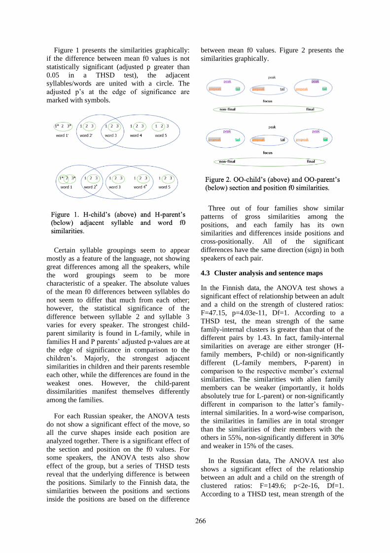
Figure 1 presents the similarities graphically:

if the difference between mean f0 values is not

statistically significant (adjusted p greater than

0.05 in a THSD test), the adjacent

syllables/words are united with a circle. The

adjusted p’s at the edge of significance are

marked with symbols.

Certain syllable groupings seem to appear

mostly as a feature of the language, not showing

great differences among all the speakers, while

the word groupings seem to be more

characteristic of a speaker. The absolute values

of the mean f0 differences between syllables do

not seem to differ that much from each other;

however, the statistical significance of the

difference between syllable 2 and syllable 3

varies for every speaker. The strongest child-

parent similarity is found in L-family, while in

families H and P parents’ adjusted p-values are at

the edge of significance in comparison to the

children’s. Majorly, the strongest adjacent

similarities in children and their parents resemble

each other, while the differences are found in the

weakest ones. However, the child-parent

dissimilarities manifest themselves differently

among the families.

For each Russian speaker, the ANOVA tests

do not show a significant effect of the move, so

all the curve shapes inside each position are

analyzed together. There is a significant effect of

the section and position on the f0 values. For

some speakers, the ANOVA tests also show

effect of the group, but a series of THSD tests

reveal that the underlying difference is between

the positions. Similarly to the Finnish data, the

similarities between the positions and sections

inside the positions are based on the difference

between mean f0 values. Figure 2 presents the

similarities graphically.

Three out of four families show similar

patterns of gross similarities among the

positions, and each family has its own

similarities and differences inside positions and

cross-positionally. All of the significant

differences have the same direction (sign) in both

speakers of each pair.

4.3 Cluster analysis and sentence maps

In the Finnish data, the ANOVA test shows a

significant effect of relationship between an adult

and a child on the strength of clustered ratios:

F=47.15, p=4.03e-11, Df=1. According to a

THSD test, the mean strength of the same

family-internal clusters is greater than that of the

different pairs by 1.43. In fact, family-internal

similarities on average are either stronger (H-

family members, P-child) or non-significantly

different (L-family members, P-parent) in

comparison to the respective member’s external

similarities. The similarities with alien family

members can be weaker (importantly, it holds

absolutely true for L-parent) or non-significantly

different in comparison to the latter’s family-

internal similarities. In a word-wise comparison,

the similarities in families are in total stronger

than the similarities of their members with the

others in 55%, non-significantly different in 30%

and weaker in 15% of the cases.

In the Russian data, The ANOVA test also

shows a significant effect of the relationship

between an adult and a child on the strength of

clustered ratios: F=149.6; p<2e-16, Df=1.

According to a THSD test, mean strength of the

266

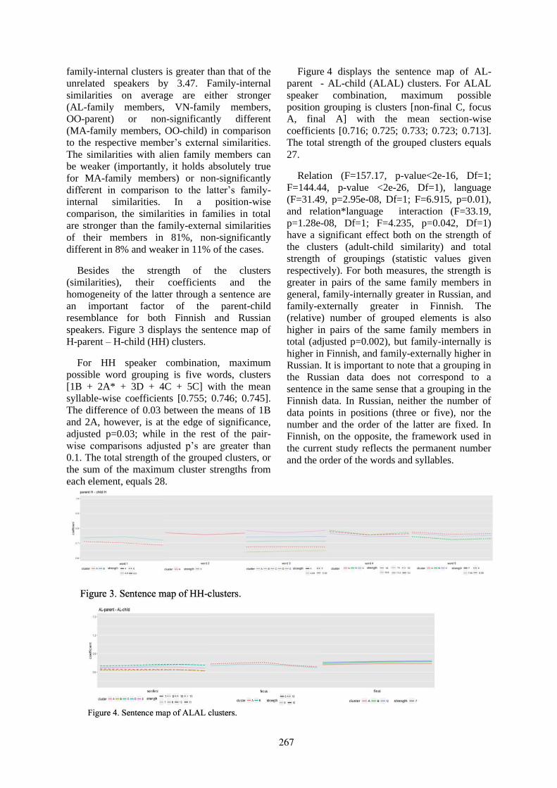
family-internal clusters is greater than that of the

unrelated speakers by 3.47. Family-internal

similarities on average are either stronger

(AL-family members, VN-family members,

OO-parent) or non-significantly different

(MA-family members, OO-child) in comparison

to the respective member’s external similarities.

The similarities with alien family members can

be weaker (importantly, it holds absolutely true

for MA-family members) or non-significantly

different in comparison to the latter’s family-

internal similarities. In a position-wise

comparison, the similarities in families in total

are stronger than the family-external similarities

of their members in 81%, non-significantly

different in 8% and weaker in 11% of the cases.

Besides the strength of the clusters

(similarities), their coefficients and the

homogeneity of the latter through a sentence are

an important factor of the parent-child

resemblance for both Finnish and Russian

speakers. Figure 3 displays the sentence map of

H-parent – H-child (HH) clusters.

For HH speaker combination, maximum

possible word grouping is five words, clusters

[1B + 2A* + 3D + 4C + 5C] with the mean

syllable-wise coefficients [0.755; 0.746; 0.745].

The difference of 0.03 between the means of 1B

and 2A, however, is at the edge of significance,

adjusted p=0.03; while in the rest of the pair-

wise comparisons adjusted p’s are greater than

0.1. The total strength of the grouped clusters, or

the sum of the maximum cluster strengths from

each element, equals 28.

Figure 4 displays the sentence map of AL-

parent - AL-child (ALAL) clusters. For ALAL

speaker combination, maximum possible

position grouping is clusters [non-final C, focus

A, final A] with the mean section-wise

coefficients [0.716; 0.725; 0.733; 0.723; 0.713].

The total strength of the grouped clusters equals

27.

Relation (F=157.17, p-value<2e-16, Df=1;

F=144.44, p-value <2e-26, Df=1), language

(F=31.49, p=2.95e-08, Df=1; F=6.915, p=0.01),

and relation*language interaction (F=33.19,

p=1.28e-08, Df=1; F=4.235, p=0.042, Df=1)

have a significant effect both on the strength of

the clusters (adult-child similarity) and total

strength of groupings (statistic values given

respectively). For both measures, the strength is

greater in pairs of the same family members in

general, family-internally greater in Russian, and

family-externally greater in Finnish. The

(relative) number of grouped elements is also

higher in pairs of the same family members in

total (adjusted p=0.002), but family-internally is

higher in Finnish, and family-externally higher in

Russian. It is important to note that a grouping in

the Russian data does not correspond to a

sentence in the same sense that a grouping in the

Finnish data. In Russian, neither the number of

data points in positions (three or five), nor the

number and the order of the latter are fixed. In

Finnish, on the opposite, the framework used in

the current study reflects the permanent number

and the order of the words and syllables.

267

4.4 Relationship between the perceptual

experiments and instrumental analysis

ANOVA tests, run with the binary result of the

perceptual test as a dependent variable, and the

total strength of groupings divided into two

explanatory variables, similarity (family-internal)

and distracting power (family-external), show the

only significant effect of the similarity on the

accuracy results in the child-matching task in

Russian (F=13.3, p=3.00e-04, Df=1), which

reflects that significantly lower accuracy for

target MA is associated with its low similarity

coefficient.

The only significant correlation found between

the total strength of family-internal groupings

and mean accuracy in perceptional experiment

for the corresponding target is in the subset of

the child-matching task in Finnish: r=0.87,

rs=0.87.

5 Discussion

In the current study, the possibility to

perceptually distinguish between the members of

the same family and unrelated adult-child pairs

in an XAB paradigm appears to be language

dependent. Finnish naïve unfamiliar listeners do

not attribute adults or children to a particular

alien family more than to their own one, but

rather they cannot draw any conclusions on

perceptual (dis)similarity.

In Russian, the accuracy of answers depends

on the target family. Interestingly, the families

with the chance-level results are different in the

two tasks. For the rest of the targets,

respectively, the accuracy is above chance

(M=72.5%), and comparable to the results of

perceptual identification of twin- and same-

gender sibling pairs in voice trios (Decoster et

al., 2010; Feiser and Kleber, 2012). The same

item can correspond to different mean accuracy

for different target families. Thus, rephrasing

Rose and Duncan’s (1995) conclusion, some

voices and some tokens of the same utterance

may differ in the identification of the adult-child

relationship.

In total, despite some strong family-external

similarities, family-internal f0 contour

similarities are consistently significantly stronger

than family-external in both language groups

separately and together. The numerical

coefficients of family similarity are not

language-specific. However, due to the

language-conditioned differences in applied

frameworks, it might not be reasonable to

compare the strengths of pair similarities

between language groups.

In Finnish, both the syllable position in a word

and the word position in a sentence have a

significant effect on f0 in the proposed five-word

three-syllable sentence framework. Unlike the

adjacent similarities between syllables, which

look rather as a language property, adjacent word

similarity represents a gross picture of f0 falling

in the sentence and therefore to a certain extent

reflects the individual’s speech rhythm. Two out

of three participating families (H and P)

demonstrate strong parent-child resemblance in

adjacent word similarities and consistently strong

internal similarity in the final coefficient

groupings. However, the similarity in the final

coefficient groupings of the third family (L) also

shows a tendency to be stronger or more

consistent than its members’ external similarities

(especially those of L-parent). Whether the

reason of this distinction lies in L-child’s older

age, smaller parent-child age difference, L-

parent’s hearing disadvantage (self-reported

tinnitus) or other, remains unclear.

In Russian, both position and section have a

significant effect on f0 in the proposed three-

position three-section framework (changeable

number and order of positions in a sentence).

The similarities of the sections inside and across

positions, as well as of the positions among

themselves are believed to reflect the

individual’s speech rhythm. Parent-child

resemblance range from nearly identical in two

families (OO and VN), slightly less similar in

one family (AL) and showing the greatest

dissimilarity in the other (MA). The latter family

is also characterized by the weakest internal

similarity in the final coefficient groupings,

which are, however, in five out of six cases

stronger than the family-external similarities of

its members.

Interestingly, the parents’ family-internal

similarities are always stronger or/and more

consistent than their similarities to alien children,

which is not always the case the other way

around. Hence, the individual characteristics of

adult’s f0 contours pervasively appear in the

speech of their children, but children can

noticeably demonstrate features that are found in

268

other adult speakers of the same language, which

is most probably reflecting the classic extremes,

biology and socialization (Bolinger, 1989) in

parent-child intonation similarities.

The accuracy of the Finnish-speaking

listeners’ performance in the perceptual

experiment shows no dependency on the target,

nor on the distractor in a trio of voices, albeit

family-internal and external similarities vary.

The correlation (r=0.87, rs=0.87) found between

the similarity strength and mean accuracy of

answers in the child-matching (always second)

task might signal that the participants get used to

the material and are attempting to base the

decision, which child sounds more like the

adult’s offspring, on family-internal f0

similarities. However, it seems that either the

similarities, as proposed by the current

framework, are not prominent enough or the

listeners rely on other voice cues.

The results of the perceptual experiment on

Russian seem to interestingly reflect the

specificity of an XAB discrimination paradigm.

Selecting the answer between A and B, listeners

in fact make a decision about X. In the parent-

matching task, listeners do not choose the parent

(A or B) but attribute the child (X) to one of the

adults. Albeit AL-family demonstrates high

internal similarity in acoustic analysis, AL-

parent’s external similarities are also strong.

Thus, a listener cannot “learn” within the task to

map the features exclusively of AL-child to AL-

parent and gives more incorrect answers for

target AL. The low internal similarity of MA-

family does not bring the accuracy for MA-target

down because MA-parent’s external similarities

are weaker. In the child-matching task, on the

opposite, a listener cannot “learn” within the task

to map the features exclusively of MA-parent to

MA-child due to a combination of low internal

similarity strength per se and the differences

between it and the average external similarity of

MA-child. It is also important to note that

proposed explanation concerns only the average

results of the perceptual experiment. Not all the

sentences from the perceptual experiment were

acoustically analyzed, which means that they

reflect less f0 contour similarities than the

selected ones. Half of the non-selected sentences

correspond to quite high accuracy results

(median 68.9%). Hence, although the f0 contour

similarities between Russian-speaking parents

and children contribute to identification of family

pairs in a trio of voices by non-familiar listeners,

the relationship is not linear, may have certain

thresholds and involve other voice cues.

6 Conclusion

The current paper presents an attempt to find f0

contour similarities between parents and their

young children.

The authors fully acknowledge the limitations

of the present study. Analyzed data are limited in

their amount, on the one hand, and to read-aloud

speech, on the other. The recording scripts do not

necessarily reflect naturally occurring utterances

in terms of pragmatic, which plays an especially

important role in Finnish. The f0 contours are

analyzed mostly in their static parameters, nor

are other voice cues analyzed as possible

contributors to perceptual similarity.

However, the presented findings can be used

for the further research on perceptual and

acoustic voice similarities between parents and

young children or, broader, family members of

different age (and gender).

269

References

Hanna Anttila. 2009. Interrogative intonation in

spontaneous Finnish. In V. de Silva and

R. Ullakonoja (Eds.) Phonetics of Russian and

Finnish, general description of phonetic systems,

experimental studies on spontaneous and read-

aloud speech, pages 167-176. Frankfurt am Main:

Peter Lang.

Paul Boersma and David Weenink. 2017. Praat:

doing phonetics by computer [Computer program].

Version 6.0.33, retrieved 29 September 2017 from

http://www.praat.org/

Natalya V. Bogdanova. 2001. Zhivye foneticheskie

protsessy russkoi rechi. Posobie po spetskursu

[Live phonetical processes in Russian speech.

Course manual]. Saint Petersburg: Philological

Faculty of Saint Petersburg State University.

Dwight Bolinger. 1986. Intonation and its parts:

Melody in spoken English. London: Edward

Arnold.

Dwight Bolinger. 1989. Intonation and its uses:

Melody in Grammar and Discourse. Stanford,

California: Stanford University Press.

David Brazil, Malcolm Coulthard, and Catherine

Johns. 1980. Discourse intonation and language

teaching. London: Longman.

Elena A. Bryzgunova. 1977. Zvuki i intonatsiya

russkoy rechi [Sounds and intonation of Russian

speech] (3rd ed.). Moscow: Russkiy yazyk.

David Crystal. 2003. A dictionary of Linguistics and

phonetics (5th ed.). Blackwell Publishing.

Viola de Silva, and Riikka Ullakonoja. 2009.

Introduction: Russian and Finnish in Contact. In

V. de Silva, and R. Ullakonoja (Eds.), Phonetics of

Russian and Finnish. General Description of

Phonetic Systems. Experimental Studies on

Spontaneous and Read-aloud Speech, pages 15-20.

Frankfurt am Main: Peter Lang.

Frans Debruyne, Wivine Decoster, Annemie Van

Gijsel, Julie Vercammen. 2002. Speaking

fundamental frequency in monozygotic and

dizygotic twins. Journal of Voice, 16(4):466-471.

Wivine Decoster and Frans Debruyne. 2000.

Longitudinal voice changes: Facts and

interpretation. Journal of Voice, 14(2):184-193.

Wivine Decoster, Annemie Van Gijsel, Julie

Vercammen, and Frans Debruyne. 2001. Voice

similarity in identical twins. Acta

Otorhinolaryngologica Belgica, 55(1):49-55.

Hanna S. Feiser and Felicitas Kleber. 2012. Voice

similarity among brothers: evidence from a

perception experiment. In Proceedings of the 21st

Annual Conference of the International

Association for Forensic Phonetics and Acoustics

(IAFPA). Santander, Spain.

Michael Fuchs, Jens Oeken, Thomas Hotopp, Roland

Täschner, Bettins Hentschel, and Wolf Behrendt.

2000. Similarity of monozygotic twins regarding

vocal performance and acoustic markers and

possible clinical significance [Abstract]. HNO,

48(6):462-469.

Tamas Hacki and S. Heitmüller. 1999. Development

of the child’s voice. International Journal of

Pediatric Otorhinolaryngology, 49(1): 141-144.

Pekka Hirvonen. 1970. Finnish and English

communication intonation. Turku: Publications of

the Phonetics Department of the University of

Turku 8.

Antti Iivonen. 1977. Lausefonetiikan tutkimuksesta

[About the research on phonetics in clauses]. In

K. Suomi (Ed.), Selected papers of the VII

Phonetics Symposium Fonetiikan päivät – Turku

1977, pages 1-14. Turku University, Finland.

Antti Iivonen. 1978. Is there interrogative intonation

in Finnish? In E. Gårding, G. Bruce, and

R. Bannert (Eds.), Nordic Prosody: Papers from a

Symposium, pages 43-53. Department of

Linguistics, Lund University, Sweden.

Antti Iivonen. 2005. Intonaation käsitteen

täsmennystä [Specification of the concept of

intonation]. In A. Iivonen (Ed.), Puheen

salaisuudet: Fonetiikan uusia suuntia [Speech

secrets: New directions in phonetics], pages 93-

128. Helsinki: Guadeamus.

Patrik N. Juslin and Klaus R. Scherer. 2008. Vocal

expression of affect. In J. Harrigan, R. Rosenthal,

and K. Scherer (Eds.) The New Handbook of

Methods in Nonverbal Behavior Research, pages

65-136. Oxford University Press.

Rachel E. Kushner and Corine A. Bickley. 1995.

Analysis and perception of voice similarities

among family members. Journal of the Acoustical

Society of America 98: 2936.

Pavel Labutin, Sergey Koval, and Andrey Raev. 2007.

Speaker identification based on the statistical

analysis of f0. In Proceedings of IAFPA. The

College of St Mark and St John, Plymouth, UK.

Tatiana M. Nikolaeva. 1970. Frazovaya intonatsiya

slavyansih yazykov [Phrasal intonation of Slavic

languages]. Moscow.

Francis Nolan, Kirsty McDougall, and Toby Hudson.

2011. Some acoustic correlates of perceived

(dis)similarity between same-accent voices. In

Proceedings of the 17th ICPhS, pages 1506-1509.

Hong Kong.

270

Jiska S. Peper, Rachel M. Brouwer, Dorret I.

Boomsma, René S. Kahn, and Hilleke E. Hulshoff

Pol. 2007. Genetic influences on human brain

structure: A review of brain imaging studies in

twins. Human Brain Mapping, 28:464-473.

Beata D. Przybyla, Horii Yoshiyuki, and Michael H.

Crawford. 1992. Vocal fundamental frequency in a

twin sample: Looking for a genetic effect. Journal

of Voice, 6(3):261-266.

Phil Rose and Sally Duncan. 1995. Naive auditory

identification and discrimination of similar voices

by familiar listeners. Forensic Linguistics, 2/1:1-

17.

Phil Rose. 1999. Differences and distinguishability in

the acoustic characteristics of hello in voices of

similar-sounding speakers: A forensic phonetic

investigation. Australian Review of Applied

Linguistics, 22(1):1-42.

R Core Team. 2017. R: A language and environment

for Statistical Computing. R Foundation for

Statistical Computing, Vienna, Austria. Retrieved

from ttps://www.R-project.org

Eugenia San Segundo and Hermann Künzel. 2015.

Automatic speaker recognition of Spanish siblings:

(monozygotic and dizygotic) twins and non-twin

brothers. Loquens, 2(2), e021.

Swapna Sebastian, Anto Suresh Benadict, Geethu K.

Sunny, and Achamma Balraj. 2013. An

investigation into the voice of identical twins.

Otolaryngology online journal, 3(2):1-7.

Elaine T. Stathopoulos, Jessica E. Huber, and Joan E.

Sussman. 2011. Changes in acoustic characteristics

of the voice across the life span: Measures from

individuals 4–93 years of age. Journal of Speech,

Language, and Hearing Research, 54:1011-1021.

Kari Suomi, Juhani Toivanen, and Riikka Ylitalo.

2006. Fonetiikan ja suomen äänneopin perusteet

[The basics of phonetics and Finnish phonology].

Helsinki: Guadeamus.

Kari Suomi, Juhani Toivanen, and Riikka Ylitalo.

2008. Finnish sound structure: Phonetics,

phonology, phonotactics and prosody. Oulu: Oulu

University Press.

Paul M. Thompson, Tyrone D. Cannon, Narr, K.L.,

Theo G.M. van Erp, Veli-Pekka Poutanen, Matti

Huttunen, Jouko Lönnqvist, Carl-Gustav

Standertskjöld-Nordenstam, Jaakko Kaprio,

Mohammad Khaledy, Rajneesh Dail, Chris I.

Zoumalan, and Arthur W. Toga. 2001. Genetic

influences on brain structure. Nature Neuroscience,

4(12):1253-1258.

Riikka Ullakonoja, Hanna Kärkkäinen, and Viola de

Silva. 2007. Havaintoja venäjän kielen

lukupuhunnan sävelkulun ja spontaanin puheen

jaksottelun oppimisesta [On learning to perceive

pitch in read-aloud speech and spontaneous speech

segmenting of Russian]. In O.-P. Salo, T. Nikula,

and P. Kalaja (Eds.), Language in Learning –

AFinLA Yearbook, 37(65), pages 215-231.

Jyväskylä: Suomen soveltavan kielitieteen yhdistys

AfinLA.

Kristiane M. van Lierde, Bart Vinck, Sofia De Ley,

Gregory Clement, and Paul Van Cauwenberge.

2005. Genetics of vocal quality characteristics in

monozygotic twins: A multiparameter approach.

Journal of Voice, 19(4):511-518.

VocaliD, Inc. (2015-2017). https://www.vocalid.co

Natalya B. Volskaya. Aspects of Russian Intonation.

In V. de Silva and R. Ullakonoja (Eds.), Phonetics

of Russian and Finnish, general description of

phonetic systems, experimental studies on

spontaneous and read-aloud speech, pages 37-46.

Frankfurt am Main: Peter Lang.

Melanie Weirich and Leonardo Lancia. 2011.

Perceived auditory similarity and its acoustic

correlates in twins and unrelated speakers. In The

17th International Congress of Phonetic Sciences

(ICPhS XVII): Congress Proceedings, pages 2118-

2121.

Hadley Wickham. 2009. ggplot2: Elegant graphics

for data analysis. New York: Springer-Verlag.

Donghui Zuo and Peggy Mok. 2015. Formant

dynamics of bilingual identical twins. Journal of

Phonetics, 52, 1-12.

Zvukovaya forma russkoy rechi. Uchebnik po fonetike

russkogo yazyka [Sound form of Russian speech.

Russian phonetics manual]. 2001-2002. Saint

Petersburg: Saint Petersburg State University,

Philological Faculty, Department of Phonetics and

Experimental Phonetics Lab. Retrieved from

www.speech.nw.ru/Manual

271

Enhancing Natural Language Understandingthrough Cross-Modal Interaction:

Meaning Recovery from Acoustically Noisy Speech

Ozge AlacamDepartment of Informatics

University of Hamburg, Hamburg, [email protected]

Abstract

Cross-modality between vision and lan-guage is a key component for effectiveand efficient communication, and humanlanguage processing mechanism success-fully integrates information from variousmodalities to extract the intended mean-ing. However, incomplete linguistic in-put, i.e. due to a noisy environment, isone of the challenges for a successful com-munication. In that case, incompletenessin one channel can be compensated byinformation from another one (if avail-able). In this paper, by employing a visual-world paradigm experiment, we investi-gated the dynamics between syntacticallypossible gap fillers for incomplete Germansentences and the visual arrangements andtheir effect on overall sentence interpreta-tion.

1 Introduction

In recent years, a growing body of literature hasinvestigated how and to what extent cross-modalinteraction contributes to natural language under-standing. Human language processing system in-tegrates information from various modalities toextract the meaning of the linguistic input ac-curately, but the contribution of cross-modalityto a successful communication goes beyond it.It facilitates early reference resolution while thesentence unfolds and allows disambiguation evenwithout realizing that another (linguistic) interpre-tation would be possible, e.g. see (Altmann andMirkovic, 2009; Knoeferle et al., 2005; Tanen-haus et al., 1995). Furthermore, it also preparesthe grounds for the re-construction of the mean-ing from noisy/missing input. When the environ-ment is noisy, or the communication partner suf-fers from a motor or cognitive impairment, text

completion/prediction becomes a crucial elementof a communication. Instead of waiting for orrequesting spoken input, combining the uncertaininformation from the linguistic channel with in-formation from the visual one increases the flu-ency and the effectiveness of the communication(Garay-Vitoria and Abascal, 2004).

In this study, by conducting an experiment withhuman-subjects, we address the problem of com-pensating the incompleteness of the verbal chan-nel by additional information from visual modal-ity. Investigating how humans reconstruct themeaning from a noisy data provides insights abouthow to incorporate human-like processing intocommunication systems. The psycholinguistic ex-periments help us to understand baseline prefer-ences and the underlying mechanism of gap con-struction processes for meaning extraction. Thiscapability for multi-modal integration can be avery specific yet crucial feature in resolving ref-erences and/or performing commands for i.e. ahelper robot that aids people in their daily activ-ities.

2 Meaning Recovery

The task of extracting meaning from a noisy in-put has been widely addressed by uni-modal ap-proaches. In a uni-modal way, re-construction canbe guided by e.g. morphological, syntactic, andsemantic properties. In that case, a probability ofa syntactic category in a certain context can be ob-tained from a language model (Asnani et al., 2015;Bickel et al., 2005). For example, using N-gramsis a popular method for this task since they pro-vide very robust predictions for local dependen-cies. However, their power is less when it comesto dealing with long-range dependencies. On theother hand, as several studies (Mirowski and Vla-chos, 2015; Gubbins and Vlachos, 2013) show, alanguage model employing the syntactic depen-dencies of a sentence brings the relevant contexts

272

closer. Using the Microsoft Research SentenceCompletion Challenge (Zweig and Burges, 2012),Gubbins and Vlachos (2013) have showed that in-corporating syntactic information leads to gram-matically better options for a semantic text com-pletion task. Semantic classification (e.g. ontolo-gies) and clustering can also be used to derive pre-dictions on the semantic level for meaning recov-ery. However, when it comes to the descriptionof daily activities, contextual information comingfrom another modality would be more beneficial,since linguistic distributions alone could hardlyprovide enough clues to distinguish the action ofbringing a pan from bringing a mug, which is acrucial difference for e.g. helper robots.

Cross-modal integration of two modalities canbe addressed by various methods in a range fromsimply putting all features from both modali-ties together and then train a model to learnthe associations, to more complex structures,e.g. relating uni-modal features from sev-eral modalities on a conceptual level by usingcommon representations. Considering that thetask of meaning extraction may benefit fromnot only low-level but also high-level knowl-edge representations, one meaningful methodwould be to utilize a triplet notation, consistingof (argument, relation type, predicate) whererelation type is one of a predefined set of ac-cepted relations, such as AGENT or THEME whilePredicate and Argument are tokens of the in-put sentence. Within this framework, the re-construction of content words can be formalizedas recovering/predicting the predicates or argu-ments of a sentence. To put it simply, a sentencelike “the woman carries ....” can be formulatedinto two triplets; (womani,AGENT, carry) and(unknowni, THEME, carry). Here the task is todetermine the unknown entity which has directlyrelated to the carry action and indirectly to theagent woman. In case the contextual informationprovided by the visual environment contains ad-ditional information (e.g. a scene that depicts awoman with a grocery bag), the missing part canbe successfully filled.

Salama et al. (2018) address the problem of in-complete linguistic input referring to daily envi-ronment context by utilizing a context-integratingdependency parser. Their focus was to recovercontent words like nouns, adjectives and verbsgiven the contextual features (e.g. object prop-

erties, spatial relations among the objects or the-matic roles). The results indicate that giving astrong influence to contextual information helps tofill a majority of gaps correctly.

While re-construction of content words ismostly about finding out either the argument or thepredicate based on the relation between each other,re-construction of grammatical words is to deter-mine the relation between argument and predi-cate. Furthermore, re-construction of grammaticalwords could be more challenging since they tendto occur with higher frequencies than the contentwords, yielding a very small type/token ratio (i.e.weaker a collocational relationship) that makes thereconstruction of them based on only linguisticinformation more difficult. Although this is be-yond the scope of the current paper, it should benoted that a full-fledged cross-modal meaning re-covery system is dependent on a success of visualrelation extraction component as well. The state-of-art computer vision systems can be consideredmore effective to extract spatial relations amongobject and object properties compared to relationsbetween the actors and their actions.

3 Situated Language Comprehension ina Noisy Setting

The noise in communication could be originatedfrom various channels and sources. First of all,it can be a linguistic noise (e.g. spelling mis-takes, complex attachments), or visual ambiguities(e.g. clutter of the environment, occlusions) or anacoustic noise.

The issues of how to comprehend noisy lin-guistic input and reconstruct the intended meaninghave been addressed by both psycholinguistic andcomputational line of research (e.g. (Levy, 2011,2008)).

According to a noisy-channel account, thatmainly focus on linguistic noise, the sentencecomprehension mechanism integrates all the in-formation (at the syntactic, semantic and dis-course level) from the existing words and use thislinguistic evidence to predict the missing partsand infer the possible meaning (Gibson et al.,2013). Several studies have shown that in caseof higher degrees of syntactic complexity, hu-mans tend to choose an interpretation which isin line with the concurrent visual information orgeneral world knowledge, even though this inter-pretation requires to accept grammatically unac-

273

ceptable syntactic structures (Johnson and Char-niak, 2004; Christianson et al., 2001; MacWhin-ney et al., 1984). Cunnings (2017)’s study on lan-guage learners also indicated when the perceiverprocesses (syntactically) noisy linguistic input, theother linguistic and non-linguistic constraints areprioritized compared to syntactic ones.

Based on noisy-channel framework, Levy(2008) proposes a probabilistic model of languageunderstanding regarding situations where there areuncertainty about word-level representations. Headdresses the problem in two different levels; aglobal inference that can be reached after process-ing the entire input, and incremental inference thatis formed (usually) word-by-word the sentenceunfolds. The main contribution of the proposedmethod is that it takes into account the prior andposterior probabilities calculated based on bothlinguistic and non-linguistic evidence, includinge.g. the expectations about speaker’s grammaticalcompetence or about the environmental conditionthat can hinder the speech signals.

Gibson et al. (2013) describes language under-standing as rational integration of noisy evidenceand semantic expectations. In their study, theytest their predictions by conducting reading ex-periments, in which mostly the prepositions inthe sentences were altered (by deletion or inser-tion) keeping content-word same across condi-tions. For example, an ungrammatical sentence“The mother gave the candle the daughter” canbe easily treated as plausible by inserting to be-fore “the daughter”. The higher prior probabilityof the latter version of the sentence compared tothat of the former one pulls the sentence meaningtowards itself.

4 Negation Processing

One interesting question regarding the task ofmeaning recovery is how to recover a meaningcommunicated with a sentence that involves un-clear negated statement.

Since negation is considered as a higher orderabstract concept, it has its own uniqueness as agrammatical category. Identifying the scope andfocus of negation is one of the challenging issuesthat gets particular attention from the NLP com-munity (e.g. SEM 2012 shared task, Morante andBlanco (2012)). From a psycholinguistic perspec-tive, the core discussion lies around whether bothnegated and actual situation of content is simu-

lated or only the actual one. However, regardlessof how this process happens, the literature agreeson that sentences containing negation are harder tointerpret than affirmative sentences (Orenes et al.,2014; Khemlani et al., 2012; Kaup et al., 2006;Ludtke and Kaup, 2006; Carpenter and Just, 1975;Clark and Chase, 1972).

It has been conclusively shown that a negativesentence is processed by first simulating the pos-itive argument. For example, after reading a neg-ative sentence “The bird was not in the air”, aresponse to image that depicts a flying bird wasfaster than to a image of a bird at rest, (Zwaan,2012). In addition to an overall processing diffi-culties that negation entails, it has been also shownthat it is only integrated into the sentence meaningat a later point (Ludtke et al., 2008).

On the other hand, there are also some evi-dence that indicates that when negation is sup-ported by right contextual support, the positive ar-guments is no longer need to be represented, yield-ing faster verification compared to no-context sit-uations (Tian et al., 2016; Dale and Duran, 2011;Nieuwland and Kuperberg, 2008).

5 Experiment

This study focuses on humans’ preferences for thereconstruction of unclear sentence parts (in Ger-man) by using visual-world paradigm. Moreover,the effect of contextual information on situatedreference resolution and on gap re-constructionhas been also manipulated by restricting the affor-dances of the locative object in one of the visualarrangements.

Gibson et al. (2013) list four different criteriaof language processing system that have an im-pact on meaning recovery; (i) how close the literalsentence is to the plausible alternative, (ii) whatkind of change is involved (insertion or deletion),(iii) the expectations about the corruption (noise-rate), and (iv) the plausibility of implausible sen-tences based on context or speaker-based. Basi-cally by keeping all the criteria described by Gib-son et al. (2013) constant, we focus, in this ex-periment, on obtaining prior probabilities of threetypes of grammatical words; two common prepo-sition of location (on and next to) and negation par-ticle (not). All sentences are syntactically plau-sible regardless from which focus-of-interest gapfiller is used and their semantic plausibility isdependent on the information coming from the

274

visual-world. Here in this current paper, we fo-cus more on how meaning recovery is affected bynegation, instead of detailed discussion into nega-tion processing. Thus we kept the focus of nega-tion constant among conditions, and the scene hasbeen designed to have low referential competition(i.e. there are two tables in the scene, makingthe decision a binary task instead of a multinomialone).

The task is simply, hearing a sentence that com-municates the intended meaning and process it andextract the meaning as close as possible to the in-tended one (Shannon, 1948). The goals that needto determined are;

• the re-construction of the gap-word

• full-sentence interpretation (“which objectneeds to be moved, and where to”)

5.1 Participants20 students (native speakers of German) partici-pated in the experiment (Mean age = 23.8, SD =3.1). They were paid or given a course credit toparticipate. The entire experiment took approxi-mately 45 minutes for each participant includingthe familiarization and instruction sessions.

5.2 MaterialLinguistic Material. In their complete form with-out a gap, all sentences have the same structureexcept the negation/preposition part (NEG/PP) asgiven below. The sentences start with a verb inan imperative form preceding an object (NP) anda prepositional phrase that specifies the goal loca-tion (PP). Then the sentence continues with a dis-fluency (umm) and a repair/complement part con-sisting of a negation or one of the two prepositionof location. Our focus-of-interest gap fillers are(nicht (not), auf(on), neben (next to). These arechosen since they can fill the same position inter-changeably.

• Stell den Becher auf den Tisch, umm[auf/nicht/neben] den blauen.put the mug on the table, umm [on/not/nextto] the blue one.

The choice of filler-word given the visual in-formation determines which object that the re-pair/complement part is attached to. In this set-ting, the repair/complement may have three differ-ent syntactic roles; referring back to the OBJECT

which is the mug (with not), referring back to theADVERBIAL which is the table (with both onand not) or providing new complementary AD-VERBIAL which is an another mug (with nextto). Due to filling different roles, all possible lin-guistic interpretations require different parsing re-sults. In all cases, the object referred to in therepair/complement part shares either the property(e.g. blue) or the object class (e.g. mug) with thetarget object or location.

Pre-prossessing of the spoken material. Thesentences were recorded by a male native speakerof German at a normal speech rate. Intona-tional differences between different linguistic en-tities have been found to have a significant effecton reference resolution (Coco and Keller, 2015;Snedeker and Trueswell, 2003). Therefore, weavoided unequal intonational breaks that may biasthe interpretation. The breaks separating phraseswere equalized.

A constant background noise (a sound record-ing from a restaurant) was added to an entire spo-ken sentence with the Audacity software 1. In or-der to mask the target word completely, the vol-ume of the NEG/PP part starting from the inter-jection (umm) was gradually decreased till the endof the gap-word. Concurrently, the volume of thebackground noise was increased during this seg-ment.

Scenes. In order to accommodate the intendedinterpretation(s) and to eliminate others, the ob-ject properties and their spatial relations amongeach other have been systematically manipulatedfor each scene. Although, other many more differ-ent visual arrangements could be possible, for thesake of systematicity, we have narrowed our visualconditions down to five scene arrangements, seeFigure 1. Scene-1 conveys all possible interpreta-tions for all the focus-of-interest fillers. Scene-2Aand Scene-2B allows only on and not. However,the availability of the location signaled by on isoccupied by another object in Scene-2B. The lasttwo visual arrangements allows only one interpre-tation; signaled by not in Scene-3A and by next toin Scene-3B. The number of objects in the sceneswas limited to eight and one additional object hasbeen used in Scene-2B. For each visual condition,six different visual scene were designed resulting30 main-trial scene. The 2D visual scenes were

1http://www.audacityteam.org/ - retrieved on 21.11.2018

275

created with the SketchUp Make Software 2.To prevent participants’ associating the focus-

of-interest gap fillers with a particular visual ar-rangement, additional slightly changed sentencesand scenes were introduced as filler items.

5.3 Procedure

Using the visual-world paradigm, we presentedparticipants visual scenes with accompanying spo-ken sentences. We employed a simple “look-and-listen” experiment following clicking tasks to getuser’s preferences. The experiment started withfilling out the written consent and demographicdata form. Afterwards, the instructions were givenin written format, preceding the 3 familiarizationtrials.

The participants were instructed that multi-modal stimuli always contain some backgroundnoise, and at one point, one word will be impossi-ble to hear. Then they are expected to choose thegap-filler word and click on the target object andlocation communicated in the sentence. It was toldthat target object is always located on the middlestand and needs to be moved to one of the whitetrays on the scene located on various places. Inorder to be able to separate the task of identifyingobject from identifying location, target objects andlocations are presented in a specific layout.

The stimuli were displayed on an SR Eyelink1000 Plus eye tracker integrated into a 17 mon-itor with a resolution of 1280 x 1024 pixels. Weutilized a total of 53 visual displays with accompa-nying spoken utterances (3 familiarization, 30 testtrials and 20 fillers). Each trial began with a a driftcorrection and the presentation of a simple fixa-tion cross for 2 sec, located at the middle-bottomof the screen. Afterwards, a 5 sec of visual pre-view before the onset of the spoken sentence wasgiven. The preview gives a comprehender time toencode the visual information in advance of thelinguistic information being presented. So, visualattention is intended to be free of recognizing theobjects of the visual context during language pro-cessing. Then, the spoken sentence was presentedaccompanying the visual stimulus. A trial ended2 sec after the offset of the sentence. Participantswere asked to examine the scene carefully and at-tend the information given in the audio. The orderof stimuli was randomized for each participant.

After the sentence is completed, the scene dis-

2http://www.sketchup.com/ - retrieved on 06.05.2018

appears and the participants are asked to click theirpreference for the gap position among five op-tions. They were also informed about that the gapcould be accurately filled by more than one op-tion. These options are “nicht (not)”, “neben (nextto)”, “auf (on)”, “mit (with)”, and “den/das/die(the)3”. Whereas the focus-of interest gap-fillersare syntactically acceptable for the gap posi-tion, two other grammatical words were providedamong the options as distractors; mit (with) andden/das/die (the). In German, the preposition mit(with) requires a dative object, therefore the gen-der of the following article should be differentthan the nominative or accusative forms of the ar-ticle in the repair/complement part. Furthermore,den/das/die (the) can be understood in two ways,either as a repetition of the definite article or as arelative pronoun. In the former case, as a gap filler,it does not provide any additional information. Onthe other hand, the lack of relative clause verbmakes the second interpretation unacceptable.

After the preference has been explicitly made,the scene appears again so that the participant canclick on the scene to answer two questions respec-tively; which object is the target? and where is thetarget location?.

Although a time-course analysis of fixateditems and locations when the sentence unfoldsis very relevant in understanding the underlyingmechanisms of language processing, in this paper,we narrow down our scope into participants’explicitly made choices after each multi-modalstimulus.

Our hypothesizes are listed as

- Syntactically all gap positions require oneinsertion to correctly accommodate the in-tended meaning, however unlike prepositionof locations, negation operation is consideredas a high-level (abstract) concept. Therefore,the sentences with on and next to should bemore easier to disambiguate, therefore morepreferred compared to ones with not.

- Conceptual information, i.e. target location’sbeing not available as illustrated in Figure 1emay force to change the interpretation, ac-cordingly the preference, from on to not.

3The respective article/relative pronoun was shownamong options in accordance with the grammatical genderof the noun it modifies

276

(a) Scene-1: on, next to, not

.(b) Scene-2A: on, not (c) Scene-2B: not, on

(d) Scene-3A: only not (e) Scene-3B:only next to

Figure 1: Sample scenes that illustrate five different visual manipulations

6 Results

In this section, the gap-filler preferences and theglobal sentence interpretation by analyzing accu-rately chosen object given their preference havebeen reported. Figure 2 shows the distribution ofthe preferences for each visual condition. In total,participant preferences for 600 trials (20 partici-pant * 30 scene) were taken into account.

Gap Construction Preferences. The visualcondition Scene-1 was designed to analyze user’sgeneral tendency among three focus-of interestgap fillers, since all are equally plausible w.r.t. thevisual context. In this condition, next to was pre-ferred more in 43.9% of the trials compared to on

(30.8%) and not (20.6%). The other distractor op-tions were preferred only in 3.7% of trials. The re-sults of a Friedmans ANOVA indicated that prefer-ence rates for the three focus-of interest gap fillerssignificantly differs (χ2(2) = 8.95, p < .001).Wilcoxon tests were used to follow up this find-ing. It seems that this difference among groups isoriginated by the difference between not and nextto (z − score = −2.23, p < .0167), with a Bon-ferroni correction).

The analysis on whether the participant couldchoose the object and the location in line withtheir explicitly made preference also demonstratedthat all target objects are correctly identified. Thisresult is highly expected, considering that the

277

PP/NEG part does not carry relevant informationfor the target identification in this visual setting.On the other hand, regarding the location, while100% of the participants, who chose next to, cor-rectly determine the target location, which is inline with their preference, this accuracy score is90.9% for on and it drops drastically to 71.4% fornot.

Figure 2: Preference distributions regarding eachvisual condition

The Effect of Contextual Cues. Whether theavailability of a location signaled by one of thepossible gap fillers has an effect on the preferenceshas been investigated by a mixed-design ANOVAcomparing the number of preferred option acrosstwo visual arrangements; Scene-2A and Scene-2B. In these conditions, on and not are the twoonly semantically plausible gap fillers. The pro-portion results indicated that when the two lo-cations are equally available (Scene-2A), partici-pants prefer more on as a gap filler (57.5%), andthe option not was chosen in only almost 13.3%of the trials. On the other hand, while the tar-geted location referred by the sentence with on re-pair is occupied (Scene 2B), then the participants’tendency to prefer not increases considerably by21%. The preference of next to stays almost thesame across the conditions.

The results of the ANOVA indicated no maineffect of the visual condition (p > .05). How-ever, the main effect of Preference was signifi-cant (F (2, 38) = 8.642, p = .001). In gen-eral, on has been preferred more compared to notand neben; (F (1, 19) = 10.92, p = .004) and(F (1, 19) = 11.61, p = .003) respectively. Re-garding our research question, the interaction ef-fect between the visual condition and the prefer-ence is the relevant one, and it displays a signif-icant interaction (F (2, 38) = 7.79, p = .001).

This indicates that the preference tendencies sig-nificantly differed in Scene-2A and Scene-2B. Tobreak down this interaction, contrasts were per-formed comparing each level of focus-of-interestpreferences across two scene types. These re-vealed significant interactions when comparing onand not, (F (2, 38) = 18.98, p < .001). Look-ing at the interaction graph in Figure 3, this sug-gests that when the target location signaled byon is occupied, participants looks for alternativesand ending up with only other available interpre-tation in line with not. Moreover, the contrastbetween not and next to was significant as well,(F (2, 38) = 5.30, p < .05).

Figure 3: Mean number of preferred focus-of-interest fillers across Scene-2A and Scene-2B

Preferences under Restricted Conditions.The last comparison focuses on the cases, in whichthe visual arrangements and the properties of theobjects only allow one interpretation. Scene-3Afavors only the interpretation which is in line withthe use of not as a gap filler. Yet, only in 53.3%of the trials correct option has been chosen as gapfiller. Despite their conflict with the visual world,other gap fillers have been chosen in a consider-able amount; next to (16.7%), on (10.8%), with(5.8%) and the/that (11.7%). On the other hand,Scene-3A syntactically allows only next-to. Theresults showed that in 72.5% of the trials, par-ticipants preferred next to. The comparison be-tween the number of correct preferences acrosstwo visual condition revealed that on average, par-ticipants make more correct choices when theysee Scene-3B (M = 4.35, SE = 1.72) comparedto Scene-3A (M = 3.20, SE = .41), (t(19) =−2.31, p < .05).

278

7 Conclusion

In this study, by systematic manipulation of visualscene, we have obtained prior expectations regard-ing two locative prepositions and negation parti-cle and we have also demonstrated how contextualcues pull an interpretation towards one side.

In order to accommodate different interpreta-tions, five different visual arrangements have beenutilized. Although our investigations into this areaare still ongoing, the results could be a usefulaid for developing models of situated natural lan-guage understanding that aims to account noisydata comprehension and meaning recovery. In thisstudy, we particularly tried to put some spotlightinto the special case “negation” as well.

The results indicate that when the visual worldsupports all interpretations, people have tendencyto choose next to as a gap filler, that entails therepair/complement part referring to another ob-ject, which is not mentioned in the sentence be-fore. Their second preference is to attach therepair part to the prepositional phrase (ADVER-BIAL) by choosing on as gap filler. This selec-tion also inherently assumes that the repair partis an affirmative statement. On the other hand,even in the cases where not is the only semanti-cally plausible option as gap filler, the participantsshowed hesitance to choose it. This results are alsoin line with noisy-channel framework. A sentencewith a gap is more harder to process compared toa complete sentence, since it requires at least twosub-tasks to be performed; predicting the gap-fillergiven the context and then confirming the inferredmeaning. While the spatial relations like next toand on are easily graspable from an image, a neg-ative statement requires additional operation to ac-count for actual situation, that’s why the listen-ers may prefer to override contextual expectationsand stick to more easy-to-process one even it se-mantically, and sometimes syntactically creates aconflict (Ferreira, 2003). However, this preference(choosing on over not) still seems to be affected bythe contextual cues like the availability of a targetlocation.

It should nonetheless be acknowledged that thesystematicity that we had to follow to single outall other effects becomes a limitation for general-ization, thus further research is needed to betterunderstand first the dynamics between the prefer-ence and the visual arrangements and second thedynamics between negation in detail and contex-

tual cues. Moreover, none of the visual manipula-tions in this study was designed to address to ex-plain the difference between choosing next to andon. Another set of experiments with reversed or-der; the first PP with a next to and the complementpart with on would help us to gain some insightson this issue.

Acknowledgments

This research was funded by the German Re-search Foundation (DFG) in the project Cross-modal Learning, TRR-169.

ReferencesGerry TM Altmann and Jelena Mirkovic. 2009. Incre-

mentality and prediction in human sentence process-ing. Cognitive science, 33(4):583–609.

Kavita Asnani, Douglas Vaz, Tanay PrabhuDesai,Surabhi Borgikar, Megha Bisht, Sharvari Bhosale,and Nikhil Balaji. 2015. Sentence completion us-ing text prediction systems. In Proceedings of the3rd International Conference on Frontiers of Intelli-gent Computing: Theory and Applications (FICTA)2014, pages 397–404. Springer.

Steffen Bickel, Peter Haider, and Tobias Scheffer.2005. Learning to complete sentences. In EuropeanConference on Machine Learning, pages 497–504.Springer.

Patricia A Carpenter and Marcel A Just. 1975. Sen-tence comprehension: a psycholinguistic process-ing model of verification. Psychological review,82(1):45.

Kiel Christianson, Andrew Hollingworth, John F Hal-liwell, and Fernanda Ferreira. 2001. Thematic rolesassigned along the garden path linger. Cognitivepsychology, 42(4):368–407.

Herbert H Clark and William G Chase. 1972. Onthe process of comparing sentences against pictures.Cognitive psychology, 3(3):472–517.

Moreno I Coco and Frank Keller. 2015. The interac-tion of visual and linguistic saliency during syntac-tic ambiguity resolution. The Quarterly Journal ofExperimental Psychology, 68(1):46–74.

Ian Cunnings. 2017. Interference in native and non-native sentence processing. Bilingualism: Lan-guage and Cognition, 20(4):712–721.

Rick Dale and Nicholas D Duran. 2011. The cognitivedynamics of negated sentence verification. Cogni-tive science, 35(5):983–996.

Fernanda Ferreira. 2003. The misinterpretation ofnoncanonical sentences. Cognitive psychology,47(2):164–203.

279

Nestor Garay-Vitoria and Julio Abascal. 2004. A com-parison of prediction techniques to enhance the com-munication rate. In ERCIM Workshop on User In-terfaces for All, pages 400–417. Springer.

Edward Gibson, Leon Bergen, and Steven T Pianta-dosi. 2013. Rational integration of noisy evidenceand prior semantic expectations in sentence interpre-tation. Proceedings of the National Academy of Sci-ences, 110(20):8051–8056.

Joseph Gubbins and Andreas Vlachos. 2013. Depen-dency language models for sentence completion. InProceedings of the 2013 Conference on EmpiricalMethods in Natural Language Processing, pages1405–1410.

Mark Johnson and Eugene Charniak. 2004. A tag-based noisy channel model of speech repairs. InProceedings of the 42Nd Annual Meeting on As-sociation for Computational Linguistics, ACL ’04,Stroudsburg, PA, USA. Association for Computa-tional Linguistics.

Barbara Kaup, Jana Ludtke, and Rolf A Zwaan. 2006.Processing negated sentences with contradictorypredicates: Is a door that is not open mentallyclosed? Journal of Pragmatics, 38(7):1033–1050.

Sangeet Khemlani, Isabel Orenes, and Philip NJohnson-Laird. 2012. Negation: A theory of itsmeaning, representation, and use. Journal of Cog-nitive Psychology, 24(5):541–559.

Pia Knoeferle, Matthew W Crocker, Christoph Scheep-ers, and Martin J Pickering. 2005. The influ-ence of the immediate visual context on incre-mental thematic role-assignment: Evidence fromeye-movements in depicted events. Cognition,95(1):95–127.

Roger Levy. 2008. A noisy-channel model of rationalhuman sentence comprehension under uncertain in-put. In Proceedings of the Conference on EmpiricalMethods in Natural Language Processing, EMNLP’08, pages 234–243, Stroudsburg, PA, USA. Associ-ation for Computational Linguistics.

Roger Levy. 2011. Integrating surprisal and uncertain-input models in online sentence comprehension: for-mal techniques and empirical results. In Proceed-ings of the 49th Annual Meeting of the Associationfor Computational Linguistics: Human LanguageTechnologies-Volume 1, pages 1055–1065. Associ-ation for Computational Linguistics.

Jana Ludtke, Claudia K Friedrich, Monica De Filippis,and Barbara Kaup. 2008. Event-related potentialcorrelates of negation in a sentence–picture verifi-cation paradigm. Journal of cognitive neuroscience,20(8):1355–1370.

Jana Ludtke and Barbara Kaup. 2006. Context effectswhen reading negative and affirmative sentences. InProceedings of the 28th annual conference of thecognitive science society, volume 27, pages 1735–1740. Lawrence Erlbaum Associates Mahwah, NJ.

Brian MacWhinney, Elizabeth Bates, and ReinholdKliegl. 1984. Cue validity and sentence interpreta-tion in English, German, and Italian. Journal of ver-bal learning and verbal behavior, 23(2):127–150.

Piotr Mirowski and Andreas Vlachos. 2015. Depen-dency recurrent neural language models for sentencecompletion. arXiv preprint arXiv:1507.01193.

Roser Morante and Eduardo Blanco. 2012. * sem 2012shared task: Resolving the scope and focus of nega-tion. In * SEM 2012: The First Joint Conferenceon Lexical and Computational Semantics–Volume 1:Proceedings of the main conference and the sharedtask, and Volume 2: Proceedings of the Sixth In-ternational Workshop on Semantic Evaluation (Se-mEval 2012), volume 1, pages 265–274.

Mante S Nieuwland and Gina R Kuperberg. 2008.When the truth is not too hard to handle: An event-related potential study on the pragmatics of nega-tion. Psychological Science, 19(12):1213–1218.

Isabel Orenes, David Beltran, and Carlos Santamarıa.2014. How negation is understood: Evidence fromthe visual world paradigm. Journal of Memory andLanguage, 74:36–45.

Amr Rekaby Salama, Ozge Alacam, and WolfgangMenzel. 2018. Text completion using context-integrated dependency parsing. In Proceedings ofThe Third Workshop on Representation Learning forNLP, pages 41–49.

Claude Elwood Shannon. 1948. A mathematical the-ory of communication. Bell system technical jour-nal, 27(3):379–423.

Jesse Snedeker and John Trueswell. 2003. Usingprosody to avoid ambiguity: Effects of speakerawareness and referential context. Journal of Mem-ory and language, 48(1):103–130.

Michael K Tanenhaus, Michael J Spivey-Knowlton,Kathleen M Eberhard, and Julie C Sedivy. 1995.Integration of visual and linguistic informationin spoken language comprehension. Science,268(5217):1632–1634.

Ye Tian, Heather Ferguson, and Richard Breheny.2016. Processing negation without context–whyand when we represent the positive argument. Lan-guage, Cognition and Neuroscience, 31(5):683–698.

Rolf A Zwaan. 2012. The experiential view oflanguage comprehension: How is negation rep-resented? Higher level language processes inthe brain: Inference and comprehension processes,page 255.

Geoffrey Zweig and Chris JC Burges. 2012. A chal-lenge set for advancing language modeling. In Pro-ceedings of the NAACL-HLT 2012 Workshop: WillWe Ever Really Replace the N-gram Model? On theFuture of Language Modeling for HLT, pages 29–36. Association for Computational Linguistics.

280

Predicting Prosodic Prominence from Text with Pre-trainedContextualized Word Representations

Aarne Talman,∗ † Antti Suni,∗ Hande Celikkanat,∗ Sofoklis Kakouros,∗Jorg Tiedemann∗ and Martti Vainio∗

∗Department of Digital Humanities, University of Helsinki, Finland†Basement AI, Finland

{name.surname}@helsinki.fi

AbstractIn this paper we introduce a new natu-ral language processing dataset and bench-mark for predicting prosodic prominencefrom written text. To our knowledgethis will be the largest publicly avail-able dataset with prosodic labels. We de-scribe the dataset construction and the re-sulting benchmark dataset in detail andtrain a number of different models rang-ing from feature-based classifiers to neuralnetwork systems for the prediction of dis-cretized prosodic prominence. We showthat pre-trained contextualized word rep-resentations from BERT outperform theother models even with less than 10% ofthe training data. Finally we discuss thedataset in light of the results and point tofuture research and plans for further im-proving both the dataset and methods ofpredicting prosodic prominence from text.The dataset and the code for the modelsare publicly available.

1 Introduction

Prosodic prominence, i.e., the amount of empha-sis that a speaker gives to a word, has been widelystudied in phonetics and speech processing. How-ever, the research on text-based natural languageprocessing (NLP) methods for predicting prosodicprominence is somewhat limited. Even in thetext-to-speech synthesis domain, with many re-cent methodological advances, work on symbolicprosody prediction has lagged behind. We be-lieve that this is mainly due to the lack of suit-able datasets. Existing, publicly available anno-tated speech corpora, are very small by currentstandards.

In this paper we introduce a new NLP datasetand benchmark for predicting prosodic promi-nence from text which is based on the recently

published LibriTTS corpus (Zen et al., 2019), con-taining automatically generated prosodic promi-nence labels for over 260 hours or 2.8 millionwords of English audio books, read by 1230 dif-ferent speakers. To our knowledge this will be thelargest publicly available dataset with prosodic an-notations. We first give some background aboutprosodic prominence and related research in Sec-tion 2. We then describe the dataset constructionand annotation method in Section 3.

Prosody prediction can be turned into a se-quence labeling task by giving each word in a texta discrete prominence value based on the amountof emphasis the speaker gives to the word whenreading the text. In Section 4 we explain the exper-iments and the experimental results using a num-ber of different sequence labeling approaches andshow that pre-trained contextualized word repre-sentations from BERT (Devlin et al., 2019) outper-form our other baselines even with less than 10%of the training data. Although BERT has been pre-viously applied in various sequence labeling tasks,like named entity recognition (Devlin et al., 2019),to the best of our knowledge, this is the first appli-cation of BERT in the task of predicting prosodicprominence. We analyse the results in Section5, comparing BERT to a bidirectional long short-term memory (BiLSTM) model and looking at thetypes of errors made by these selected models. Wefind that BERT outperforms the BiLSTM modelacross all the labels.

Finally in Section 6 we discuss the methodsin light of the experimental results and high-light areas that are known to negatively impactthe results. We also discuss the relevance ofpre-training for the task of predicting prosodicprominence. We conclude by pointing to fu-ture research both in developing better methodsfor predicting prosodic prominence but also tofurther improve the quality of the dataset. Thedataset and the PyTorch code for the models are

281

available on GitHub: https://github.com/Helsinki-NLP/prosody.

2 Background

2.1 Prosodic Prominence

Every word and utterance in speech encompassesphonetic and phonological properties that are notresulting from the choice of the underlying lex-ical items and that encode meaning in additionto that of the individual lexemes. These prop-erties are referred to as prosody and they de-pend on a variety of factors such as the seman-tic and syntactic relations between these items,and their rhythmic grouping (Wagner and Wat-son, 2010). Prosodic variation in speech con-tributes to a large extend to the perception of nat-ural sounding speech. Prosodic prominence repre-sents one type of prosodic phenomenon that mani-fests through the subjective impression of empha-sis in speech where certain words are interpretedas more salient within their lexical surroundingcontext (Wagner and Watson, 2010; Terken andHermes, 2000).

Due to the inherent difficulty in determiningprominence — even for human subjects, see, e.g.,(Yoon et al., 2004) — the development of auto-matic tools for the annotation of prominent unitshas been a difficult task. This is exemplifiedfrom the large degree of discrepancy observedbetween human annotators when labeling promi-nence where the inter-transcriber agreement canvary substantially based on a multitude of fac-tors such as the choice of annotators or annotationmethod (Mo et al., 2008; Yoon et al., 2004; Kak-ouros and Rasanen, 2016). Similarly, in promi-nence production, certain degree of freedom inprominence placement and large variability be-tween styles and speakers (Yuan et al., 2005), ren-ders the task of prominence prediction from textvery difficult compared to most NLP tasks involv-ing text only.

2.2 Generating Prominence Annotations

Throughout the literature a number of methodshave been proposed for the labeling of prosodicprominence. These methods can be roughly cate-gorized on the basis of the need for training data(manual prosodic annotations) into supervised andunsupervised, but crucially, on the basis of the in-formation they utilize from speech and languageto generate their predictions (prominence labels).

As prominence perception has been found to cor-relate with acoustic-phonetic features (Lieberman,1960), with the constituent syntactic structure ofan utterance (Gregory and Altun, 2004; Wagnerand Watson, 2010; Bresnan, 1973), with the fre-quency of occurrence of individual lexical items(Nenkova et al., 2007; Jurafsky et al., 2001), andwith the probabilities of contiguous lexical se-quences (Jurafsky, 1996), automatic methods havebeen developed utilizing these features either incombination or independently (Nenkova et al.,2007; Kakouros et al., 2016; Ostendorf et al.,1995; Levow, 2008).

Overall, these features can be largely dividedinto two categories: (i) acoustic (derived fromthe sound pressure waveform of the speech sig-nal) and (ii) language (extracted by studying theform of the language; for instance, semantic orsyntactic factors in the language). Both acous-tic and language-based features have been shownto provide good overall performance in detect-ing prominence (in both supervised and unsuper-vised cases), where, however, the methods utiliz-ing acoustic features seem to provide better per-formance for the unsupervised detection of promi-nences in speech (Suni et al., 2017; Wang andNarayanan, 2007; Kakouros and Rasanen, 2016),with state-of-the-art results reaching high level ofaccuracy, close to that of the inter-annotator agree-ment for the data. While the top-down linguis-tic information is known to correlate with percep-tual prominence, in this paper we want to make aclear distinction between data labelling and text-based prediction. Thus, in this work, we uti-lize purely acoustic prominence annotations of thespeech data using the method developed by Suniet al. (2017) as the prosodic reference.

2.3 Predicting Prosodic Prominence fromText

To what extent prosodic prominence can be pre-dicted from textual input only has been a topic ofinquiry in linguistics for a long time. In traditionalgenerative phonology (Chomsky and Halle, 1968),accent placement was considered to be fully deter-mined by linguistic structure, whereas a seminalwork by Bolinger (1972) emphasized the impor-tance and relevance of the lexical semantic contextas well as the speakers’ intention, positing that,in general, a mind reading ability may be neces-sary to determine prominent words in a sentence.

282

Figure 1: Continuous Wavelet Transform Annotation method.

non-prominent prominentsets (clean) speakers sentences words 0 1 2

train-100 247 33,041 570,592 274,184 155,849 140,559train-360 904 116,262 2,076,289 1,003,454 569,769 503,066

dev 40 5,726 99,200 47,535 27,454 24,211test 39 4,821 90,063 43,234 24,543 22,286

total: 1230 159,850 2,836,144 1,368,407 777,615 690,122

Table 1: Dataset statistics

As longstanding inquiries hold, the goal of reli-ably predicting the placement of prominent enti-ties from information automatically derived fromtextual resources is still ongoing.

Several efforts have been made towards this di-rection, especially in text-to-speech (TTS) syn-thesis research, where generation of appropriateprosody would increase both intelligibility andquality of synthetic speech. Before the deeplearning paradigm shift in NLP, several linguis-tic features were examined for prominence pre-diction, including function-content word distinc-tion, part-of-speech class, and information status(Hirschberg, 1993). Statistical features like uni-grams, bigrams, and TF-IDF have also been fre-quently used (Marsi et al., 2003). Later, the ac-cent ratio, or simply the average accent status ofa word type in the given corpus, was found to bea stronger predictor than linguistic features in theaccent prediction task (Nenkova et al., 2007), sug-gesting that lexical information may be more rel-evant than linguistic structure for the prominenceprediction task.

Recently, continuous representations of wordshave become commonplace in prosody predic-

tion for TTS, though the symbolic level is of-ten omitted and pitch and duration are predicteddirectly using lexical embeddings (Watts, 2012).Yet, closely related to the proposed method, (Ren-del et al., 2016) experimented with various lex-ical embeddings as an input to a Bi-directionalLSTM model, predicting binary prominence la-bels. Training on a proprietary, manually an-notated single speaker corpus of 3730 sentences,they achieved an F-score of 0.71 with Word2Vec(Mikolov et al., 2013) embeddings, with a clearimprovement over traditional linguistic features.

3 Dataset

We introduce, automatically generated, high qual-ity prosodic annotations for the recently publishedLibriTTS corpus (Zen et al., 2019). The LibriTTScorpus is a cleaned subset of LibriSpeech corpus(Panayotov et al., 2015), derived from English au-diobooks of the LibriVox project.1 We selected the‘clean’ subsets of LibriTTS for annotation, com-prising of 262.5 hours of read speech from 1230speakers. The transcribed sentences were aligned

1https://librivox.org

283

Token Tell me you rascal , where is the pig ?Discrete label 2 0 0 0 NA 2 0 0 1 NAReal-valued label 1.473 0.333 0.003 0.167 NA 2.160 0.006 0.037 0.719 NA

Table 2: Example sentence with the annotation from the dataset. Discrete prominence values were usedin the experiments of this paper. The real-valued labels are used for generation of the discrete labels,however, they could also be used directly for prominence prediction.

with the Montreal forced aligner (McAuliffe et al.,2017), using a pronunciation lexicon and acous-tic models trained on the LibriSpeech dataset.The aligned sentences were then prosodically an-notated with word-level acoustic prominence la-bels. For the annotation, we used the WaveletProsody Analyzer toolkit2, which implements themethod described in (Suni et al., 2017). Briefly,the method consists of 1) the extraction of pitchand energy signals from the speech data and du-ration from the word level alignments, 2) fillingthe unvoiced gaps in extracted signals by inter-polation followed by smoothing and normalizing,3) combining the normalized signals by summingor multiplication, and 4) performing a continuouswavelet transform (CWT) on the composite signaland extracting continuous prominence values aslines of maximum amplitude across wavelet scales(see Figure 1). Essentially, the method assumesthat the louder, the longer, and the higher, the moreprominent. On top of this, the wavelet transformprovides multi-resolution contextual information;the more the word stands out from its environ-ment in various time scales, the more prominentthe word is perceived.

For the current study, continuous prominencevalues were discretized to two (non-prominent,prominent) or three (non prominent, somewhatprominent, very prominent) classes. The binarycase is closely related to the pitch accent de-tection task, aiming for results comparable withthe majority of the literature on the topic. Theweights in constructing the composite signal anddiscretization thresholds were adjusted based onThe Boston University radio news corpus (Os-tendorf et al., 1995), containing manually anno-tated pitch accent labels. This corpus is oftenused in the evaluation of pitch accent annotationand prediction quality, with the current annotationmethod yielding state-of-the-art accuracy in wordlevel acoustic-based accent detection, 85.3%, us-

2https://github.com/asuni/wavelet_prosody_toolkit

ing weights 1.0, 0.5 and 1.0 for F0, energy andduration respectively, and using multiplication ofthese features in signal composition. For three-way discretization, the non-prominent / promi-nent cut-off was maintained and the prominentclass was split to two classes of roughly equalsize. Statistics of the resulting dataset are de-scribed in table 1. The full dataset is availablefor download here: https://github.com/Helsinki-NLP/prosody. Although not dis-cussed in this paper, the described acoustic annota-tion and text-based prediction methods can be ap-plied to prosodic boundaries too, and the bound-ary labels will be included in the dataset at a laterstage.

4 Experiments

In this section we describe the experimental setupand the results from our experiments in predictingdiscrete prosodic prominence labels from text us-ing the corpus described above.

4.1 Experimental Setup

We performed experiments with the followingmodels:• BERT-base uncased (Devlin et al., 2019)• 3-layer 600D Bidirectional Long Short-Term

Memory (BiLSTM) (Hochreiter and Schmid-huber, 1997)• Minitagger (SVM) (Stratos and Collins,

2015) + GloVe (Pennington et al., 2014)• MarMoT (CRF) (Mueller et al., 2013)• Majority class per wordThe models were selected so that they cover

a wide variety of different architectures fromfeature-based statistical approaches to neural net-works and pre-trained language models. The mod-els are described in more detail below.

We use the Huggingface PyTorch im-plementation of BERT available in thepytorch transformers library,3 which

3https://github.com/huggingface/

284

we further fine-tune during training. We takethe last hidden layer of BERT and train a singlefully-connected classifier layer on top of it,mapping the representation of each word to thelabels. For our experiments we use the smallerBERT-base model using the uncased alternative.We use a batch size of 32 and fine-tune the modelfor 2 epochs.

For BiLSTM we use pre-trained 300D GloVe840B word embeddings (Pennington et al., 2014).The initial word embeddings are fine-tuned dur-ing training. As with BERT, we add one fully-connected classifier layer on top of the BiLSTM,mapping the representation of each word to the la-bels. We use a dropout of 0.2 between the layers ofthe BiLSTM. We use a batch size of 64 and trainthe model for 5 epochs.

For the SVM we use Minitagger4 implemen-tation by Stratos and Collins (2015) using eachdimension of the pre-trained 300D GloVe 840Bword embeddings as features, with context-size 1,i.e. including the previous and the next word in thecontext.

For the conditional random field (CRF) modelwe use MarMot5 by Mueller et al. (2013) withthe default configuration. The model applies stan-dard feature templates that are used for part-of-speech tagging such as surrounding words as wellas suffix and prefix features. We did not opti-mize the feature model nor any of the other hyper-parameters.

All systems except the Minitagger and CRF areour implementations using PyTorch and are madeavailable on GitHub: https://github.com/Helsinki-NLP/prosody.

For the experiments we used the larger train-360training set. We report both 2-way and 3-way clas-sification results. In the 2-way classification taskwe take the three prominence labels and merge la-bels 1 and 2 into a single prominent class.

4.2 Results

All models reach over 80% in the 2-way classi-fication task while 3-way classification accuracystays below 70% for all of them. The BERT-based model gets the highest accuracy of 83.2%and 68.6% in the 2-way and 3-way classificationtasks, respectively, demonstrating the value of a

pytorch-transformers4https://github.com/karlstratos/

minitagger5http://cistern.cis.lmu.de/marmot/

pre-trained language model in this task. The 3-layer BiLSTM achieves 82.1% in the 2-way classi-fication and 66.4% in the 3-way classification task.

The traditional feature-based classifiers performslightly below the neural network models, withthe CRF obtaining 81.8% and 66.4% for the twoclassification tasks, respectively. The MinitaggerSVM model’s test accuracies are slightly lowerthan the CRF’s with 80.8% and 65.4% test accu-racies. Finally taking a simple majority class perword gives 80.2% for the 2-way classification taskand 62.4% for the 3-way classification task. Theresults are listed in Table 3. The fairly low resultsacross the board highlight the difficulty of the taskof predicting prosodic prominence from text.

To better understand how much training data isneeded in the two classification tasks, we trainedselected models with different size subsets of thetrain-360 training data. The selected subsets were:1%, 5%, 10%, 50% and 100% of the training ex-amples (token-label pairs). Figures 2 and 3 containthe learning curves for the 2-way and 3-way clas-sification tasks, for all the models except for themajority and random baselines.

For all models and for both of the classifica-tion tasks we notice that they achieve quite hightest accuracy already with a very small numberof training examples. For most of the models thebiggest improvement in performance is achievedwhen moving from 1% of the training examplesto 5%. All models have reached close to theirfull predictive capacity with only 10% of the train-ing examples. For example, BERT achieves 2-wayclassification test accuracy of 82.6% with 10% ofthe training data, which is only -0.6% points lowerthan the accuracy with the full training set. In the3-way classification task 10% of the training datagives 67.1% for BERT, which is -1.7% points be-low the accuracy with the full training set.

Interestingly, in the 2-way classification task theBiLSTM model shows a slightly different learningcurve, having already quite a high performancewith just 1% of the training data, but then mak-ing no improvement between 1% and 5%. How-ever, between 5% and 100% the BiLSTM modelimprovement is almost linear.

As the proposed dataset has been automaticallygenerated as described in Section 3, we also testedthe best two models, BERT and BiLSTM, with amanually annotated test set from The Boston Uni-versity radio news corpus (Ostendorf et al., 1995).

285

Model Test accuracy (2-way) Test accuracy (3-way)BERT-base 83.2% 68.6%3-layer BiLSTM 82.1% 66.4%CRF 81.8% 66.4%SVM+GloVe 80.8% 65.4%Majority class per word 80.2% 62.4%Majority class 52.0% 48.0%Random 49.0% 39.5%

Table 3: Experimental results (%) for the 2 and 3-way classification tasks.

For this experiment we trained the models usingthe train-360 training set (as above) replacing onlythe test set. The results of this experiment areshown in Table 4. The good results6 from this ex-periment provide further support for the quality ofthe new dataset. Notice also that the differencebetween BERT and BiLSTM is much bigger withthis test set (+3.9% compared to +1.1%). This dif-ference could be due to the genre difference be-tween the two test sets, with the Boston Univer-sity news corpus being more contemporary com-pared to the source for our proposed dataset (pre-1923 books). This point will be further discussedin Section 6.

Model vs expert vs acousticBERT-base 82.9% 82.1%3-layer BiLSTM 79.0% 79.3%

Table 4: Test accuracies (%) for the Boston Uni-versity radio news corpus (2-way classification).expert = expert annotated perceptual prominencelabels, acoustic = our acoustic prominence labels

5 Analysis

The experimental results show that although pre-dicting prosodic prominence is a fairly difficulttask, pre-trained contextualized word representa-tions clearly help, as can be seen from the resultsfor BERT. The difference between BERT and theother models is clear if we compare the other mod-els with BERT fine-tuned with a small fraction ofthe training data. In fact, BERT already outper-forms the other models with just 5% of the trainingexamples in the 2-way classification case and with10% of the training data in the 3-way classification

6Better results have been reported on Boston dataset us-ing lexical features, but there are methodological concernsrelated to cross-validation training and speakers reading thesame text, see discussion on (Rosenberg, 2009).

1·1

0−

2

5·1

0−

2

0.1

0.5 1

0.79

0.8

0.81

0.82

0.83

Fraction of training data

Acc

urac

yBERT

BiLSTMSVM+Glove

CRF

Figure 2: Test accuracy with different size sub-sets of the training data for the 2-way classificationtask.

1·1

0−

2

5·1

0−

2

0.1

0.5 1

0.62

0.64

0.66

0.68

Fraction of training data

Acc

urac

y

BERTBiLSTM

SVM+GloveCRF

Figure 3: Test accuracy with different size sub-sets of the training data for the 3-way classificationtask.

286

case. This can be seen as an indication that BERThas acquired implicit semantic or syntactic infor-mation during pre-training that is useful in the taskof predicting prosodic prominence.

To gain a better understanding of the types ofpredictive errors BERT makes, we look at the con-fusion matrices for the two classification tasks andcompare those with the confusion matrices for theBiLSTM.

The 3-way classification confusion matrices aremore informative as they allow comparison of thetwo models with respect to the predicted label incases of error. Figure 4 contains the 3-way classi-fication confusion matrix for BERT and Figure 5for the BiLSTM model.

Figure 4: 3-way classification task confusion ma-trix for BERT.

Figure 5: 3-way classification task confusion ma-trix for BiLSTM.

In the 3-way classification task, when the goldlabel is 0 (non prominent) BERT makes moreerrors with prediction being 2 (very prominent)compared to the BiLSTM model. However, whenthe gold label is 2 (very prominent) BiLSTMmakes more predictions with 0 (non prominent)compared to BERT. In general for 0 labels BERTseems to have higher precision and BiLSTM betterrecall, whereas for label 2 BERT has clearly higherrecall and precision. Both models have low preci-sion and recall for the less distinctive prominence(label 1). It seems that the clearest difference be-tween the two models is in their ability to predicthigh prominence (label 2).

We also provide the confusion matrices for the2-way classification task for the two models. Fig-ure 6 contains the 2-way classification confusionmatrix for BERT and Figure 7 for the BiLSTMmodel. Here BERT has slightly higher precisionand recall across both of the labels.

Figure 6: 2-way classification task confusion ma-trix for BERT.

Figure 7: 2-way classification task confusion ma-trix for BiLSTM.

6 Discussion

We have shown above that prosodic prominencecan reasonably well be predicted from text us-ing different sequence-labelling approaches andmodels. However, the reported performance isstill quite low, even for state-of-the-art systemsbased on large pre-trained language models suchas BERT. We list a number of reasons for theseshortcomings below and discuss their impact andpotential mitigation.

Although the annotation method has beenshown to be quite robust, errors in automatic align-ment, signal processing, and quantization intro-duce noise to the labels. This noise might not bedetrimental to the training due to dataset size, butthe test results are affected. To measure the size ofthis effect, manual correction of a part of the testset could be beneficial.

It is well known that different speakers havedifferent accents, varying reading proficiency, andreading tempo, which all impact the consistency ofthe labeling as the source speech data contains intotal samples from over 1200 different speakers.

287

REF: One way led to the left and the other to the right straight up the mountain .BERT: One way led to the left and the other to the right straight up the mountain .

REF: In the next moment he was concealed by the leaves .BERT: In the next moment he was concealed by the leaves .

REF: I had to read it over carefully , as the text must be absolutely correct .BERT: I had to read it over carefully , as the text must be absolutely correct .

REF: Where were you when you began to feel bad ?BERT: Where were you when you began to feel bad ?

REF: He is taller than the Indian , not so tall as Gilchrist .BERT: He is taller than the Indian , not so tall as Gilchrist .

Table 5: Typical 3-way prominence predictions of BERT compared to reference labels.

Given that inter-speaker agreement on pitch ac-cent placement is somewhere between 80 and 90%(Yuan et al., 2005), we cannot expect large im-provements without speaker-specific modelling.

The source speech data contains multitude ofgenres ranging from non-fiction to metric poemswith fixed prominence patterns and children’s sto-ries with high proportion of words emphasized.The difference in genres could impact the testresults. Moreover, the books included in thesource speech data are all from pre-1923, whereasBERT and GloVe are pre-trained with contem-porary texts. We expect that the difference be-tween BERT and other models would be higherwith a dataset drawn from a more contemporarysource. As noted in Section 3, the difference be-tween BERT and BiLSTM is much bigger withthe The Boston University radio news corpus testset (+3.9% compared to +1.1% with our test set).This could be due to the genre, with The BostonUniversity radio news corpus being derived froma more contemporary source.

Overall, our results for BERT highlight the im-portance of pre-training of the word representa-tions. As we noticed, already with as little as 10%of the training data, BERT outperforms the othermodels when they are trained on the entire train-ing set. This suggests that BERT has implicitlylearned syntactic or semantic information relevantfor the prosody prediction task. Our results arein line with the earlier results by Stehwien et al.(2018) and Rendel et al. (2016) who showed thatpre-trained word embeddings improve model per-formance in the prominence prediction task. Ta-ble 5 lists five randomly selected examples fromthe test set and shows the prominence predictions

by BERT compared to the reference annotation.These examples indicate that even if the overallaccuracy of the model is not high, the predictionsstill look plausible in isolation.

Finally, the classifiers in this paper are trainedon single sentences, losing any discourse-level in-formation and relations to surrounding context.Increasing the context to contain, e.g., also pre-vious sentences could improve the results.

7 Conclusion

In this paper we have introduced a new NLPdataset and benchmark for predicting prosodicprominence from text, which to our knowledge isthe largest publicly available dataset with prosodiclabels. We described the dataset creation and theresulting benchmark and showed that various se-quence labeling methods can be applied to thetask of predicting prosodic prominence using thedataset.

Our experimental results show that BERT out-performs the other models with just up to 10% ofthe training data, highlighting the effectiveness ofpre-training for the task. It also highlights thatthe implicit syntactic or semantic features BERThas learned during pre-training are relevant for thespecific task of predicting prosodic prominence.

We also discussed a number of limitations ofthe automatic annotation system, as well as ourcurrent models. Based on this discussion, andmore broadly, on the findings of this paper, wewant to focus our future research activities intwo fronts. Firstly, we will further develop thedataset annotation pipeline, improving the qual-ity of prominence annotation and adding prosodicboundary labels. Secondly, we will further de-

288

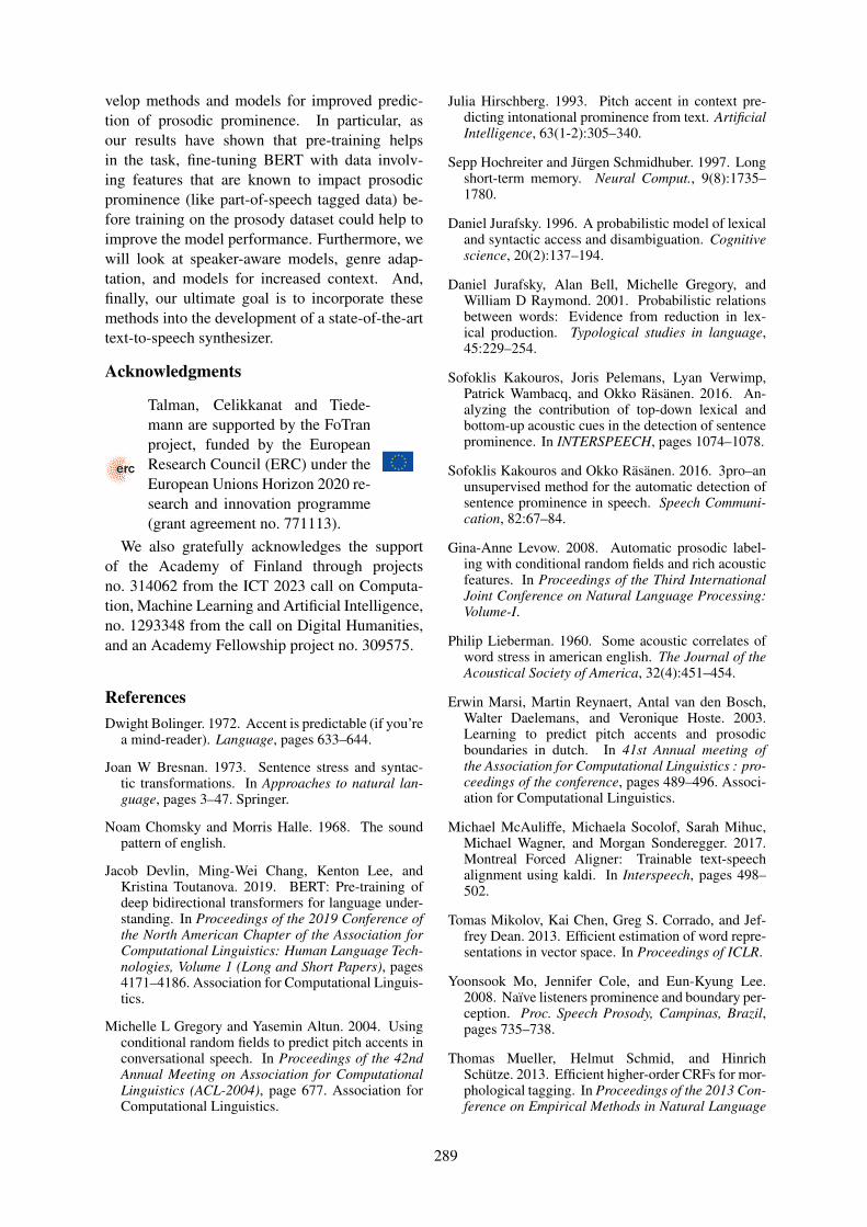
velop methods and models for improved predic-tion of prosodic prominence. In particular, asour results have shown that pre-training helpsin the task, fine-tuning BERT with data involv-ing features that are known to impact prosodicprominence (like part-of-speech tagged data) be-fore training on the prosody dataset could help toimprove the model performance. Furthermore, wewill look at speaker-aware models, genre adap-tation, and models for increased context. And,finally, our ultimate goal is to incorporate thesemethods into the development of a state-of-the-arttext-to-speech synthesizer.

Acknowledgments

Talman, Celikkanat and Tiede-mann are supported by the FoTranproject, funded by the EuropeanResearch Council (ERC) under theEuropean Unions Horizon 2020 re-search and innovation programme(grant agreement no. 771113).

We also gratefully acknowledges the supportof the Academy of Finland through projectsno. 314062 from the ICT 2023 call on Computa-tion, Machine Learning and Artificial Intelligence,no. 1293348 from the call on Digital Humanities,and an Academy Fellowship project no. 309575.

ReferencesDwight Bolinger. 1972. Accent is predictable (if you’re

a mind-reader). Language, pages 633–644.

Joan W Bresnan. 1973. Sentence stress and syntac-tic transformations. In Approaches to natural lan-guage, pages 3–47. Springer.

Noam Chomsky and Morris Halle. 1968. The soundpattern of english.

Jacob Devlin, Ming-Wei Chang, Kenton Lee, andKristina Toutanova. 2019. BERT: Pre-training ofdeep bidirectional transformers for language under-standing. In Proceedings of the 2019 Conference ofthe North American Chapter of the Association forComputational Linguistics: Human Language Tech-nologies, Volume 1 (Long and Short Papers), pages4171–4186. Association for Computational Linguis-tics.

Michelle L Gregory and Yasemin Altun. 2004. Usingconditional random fields to predict pitch accents inconversational speech. In Proceedings of the 42ndAnnual Meeting on Association for ComputationalLinguistics (ACL-2004), page 677. Association forComputational Linguistics.

Julia Hirschberg. 1993. Pitch accent in context pre-dicting intonational prominence from text. ArtificialIntelligence, 63(1-2):305–340.

Sepp Hochreiter and Jurgen Schmidhuber. 1997. Longshort-term memory. Neural Comput., 9(8):1735–1780.

Daniel Jurafsky. 1996. A probabilistic model of lexicaland syntactic access and disambiguation. Cognitivescience, 20(2):137–194.

Daniel Jurafsky, Alan Bell, Michelle Gregory, andWilliam D Raymond. 2001. Probabilistic relationsbetween words: Evidence from reduction in lex-ical production. Typological studies in language,45:229–254.

Sofoklis Kakouros, Joris Pelemans, Lyan Verwimp,Patrick Wambacq, and Okko Rasanen. 2016. An-alyzing the contribution of top-down lexical andbottom-up acoustic cues in the detection of sentenceprominence. In INTERSPEECH, pages 1074–1078.

Sofoklis Kakouros and Okko Rasanen. 2016. 3pro–anunsupervised method for the automatic detection ofsentence prominence in speech. Speech Communi-cation, 82:67–84.

Gina-Anne Levow. 2008. Automatic prosodic label-ing with conditional random fields and rich acousticfeatures. In Proceedings of the Third InternationalJoint Conference on Natural Language Processing:Volume-I.

Philip Lieberman. 1960. Some acoustic correlates ofword stress in american english. The Journal of theAcoustical Society of America, 32(4):451–454.

Erwin Marsi, Martin Reynaert, Antal van den Bosch,Walter Daelemans, and Veronique Hoste. 2003.Learning to predict pitch accents and prosodicboundaries in dutch. In 41st Annual meeting ofthe Association for Computational Linguistics : pro-ceedings of the conference, pages 489–496. Associ-ation for Computational Linguistics.

Michael McAuliffe, Michaela Socolof, Sarah Mihuc,Michael Wagner, and Morgan Sonderegger. 2017.Montreal Forced Aligner: Trainable text-speechalignment using kaldi. In Interspeech, pages 498–502.

Tomas Mikolov, Kai Chen, Greg S. Corrado, and Jef-frey Dean. 2013. Efficient estimation of word repre-sentations in vector space. In Proceedings of ICLR.

Yoonsook Mo, Jennifer Cole, and Eun-Kyung Lee.2008. Naıve listeners prominence and boundary per-ception. Proc. Speech Prosody, Campinas, Brazil,pages 735–738.

Thomas Mueller, Helmut Schmid, and HinrichSchutze. 2013. Efficient higher-order CRFs for mor-phological tagging. In Proceedings of the 2013 Con-ference on Empirical Methods in Natural Language

289

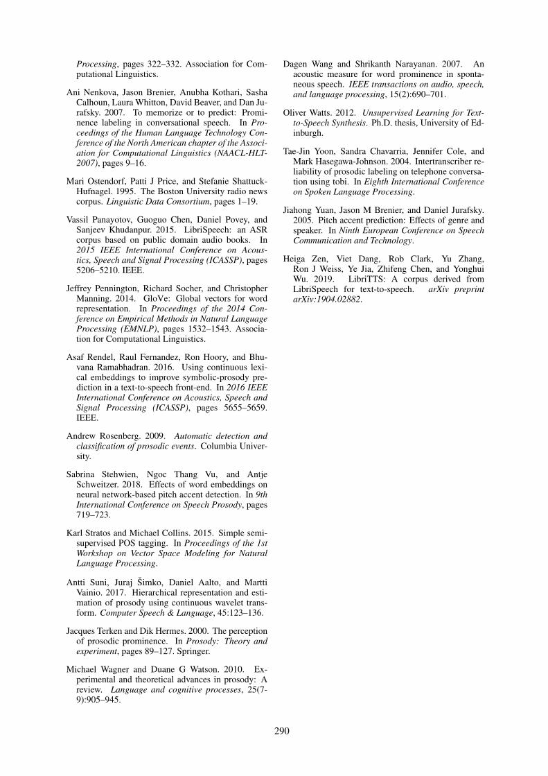
Processing, pages 322–332. Association for Com-putational Linguistics.

Ani Nenkova, Jason Brenier, Anubha Kothari, SashaCalhoun, Laura Whitton, David Beaver, and Dan Ju-rafsky. 2007. To memorize or to predict: Promi-nence labeling in conversational speech. In Pro-ceedings of the Human Language Technology Con-ference of the North American chapter of the Associ-ation for Computational Linguistics (NAACL-HLT-2007), pages 9–16.

Mari Ostendorf, Patti J Price, and Stefanie Shattuck-Hufnagel. 1995. The Boston University radio newscorpus. Linguistic Data Consortium, pages 1–19.

Vassil Panayotov, Guoguo Chen, Daniel Povey, andSanjeev Khudanpur. 2015. LibriSpeech: an ASRcorpus based on public domain audio books. In2015 IEEE International Conference on Acous-tics, Speech and Signal Processing (ICASSP), pages5206–5210. IEEE.

Jeffrey Pennington, Richard Socher, and ChristopherManning. 2014. GloVe: Global vectors for wordrepresentation. In Proceedings of the 2014 Con-ference on Empirical Methods in Natural LanguageProcessing (EMNLP), pages 1532–1543. Associa-tion for Computational Linguistics.

Asaf Rendel, Raul Fernandez, Ron Hoory, and Bhu-vana Ramabhadran. 2016. Using continuous lexi-cal embeddings to improve symbolic-prosody pre-diction in a text-to-speech front-end. In 2016 IEEEInternational Conference on Acoustics, Speech andSignal Processing (ICASSP), pages 5655–5659.IEEE.

Andrew Rosenberg. 2009. Automatic detection andclassification of prosodic events. Columbia Univer-sity.

Sabrina Stehwien, Ngoc Thang Vu, and AntjeSchweitzer. 2018. Effects of word embeddings onneural network-based pitch accent detection. In 9thInternational Conference on Speech Prosody, pages719–723.

Karl Stratos and Michael Collins. 2015. Simple semi-supervised POS tagging. In Proceedings of the 1stWorkshop on Vector Space Modeling for NaturalLanguage Processing.

Antti Suni, Juraj Simko, Daniel Aalto, and MarttiVainio. 2017. Hierarchical representation and esti-mation of prosody using continuous wavelet trans-form. Computer Speech & Language, 45:123–136.

Jacques Terken and Dik Hermes. 2000. The perceptionof prosodic prominence. In Prosody: Theory andexperiment, pages 89–127. Springer.

Michael Wagner and Duane G Watson. 2010. Ex-perimental and theoretical advances in prosody: Areview. Language and cognitive processes, 25(7-9):905–945.

Dagen Wang and Shrikanth Narayanan. 2007. Anacoustic measure for word prominence in sponta-neous speech. IEEE transactions on audio, speech,and language processing, 15(2):690–701.

Oliver Watts. 2012. Unsupervised Learning for Text-to-Speech Synthesis. Ph.D. thesis, University of Ed-inburgh.

Tae-Jin Yoon, Sandra Chavarria, Jennifer Cole, andMark Hasegawa-Johnson. 2004. Intertranscriber re-liability of prosodic labeling on telephone conversa-tion using tobi. In Eighth International Conferenceon Spoken Language Processing.

Jiahong Yuan, Jason M Brenier, and Daniel Jurafsky.2005. Pitch accent prediction: Effects of genre andspeaker. In Ninth European Conference on SpeechCommunication and Technology.

Heiga Zen, Viet Dang, Rob Clark, Yu Zhang,Ron J Weiss, Ye Jia, Zhifeng Chen, and YonghuiWu. 2019. LibriTTS: A corpus derived fromLibriSpeech for text-to-speech. arXiv preprintarXiv:1904.02882.

290

Short Papers

Toward Multilingual Identification of Online Registers

Veronika Laippala1, Roosa Kyllonen1, Jesse Egbert2, Douglas Biber2, Sampo Pyysalo3

1 School of Languages and Translation Studies, University of Turku2 Applied Linguistics, Northern Arizona University

3 Department of Future Technologies, University of Turku1,3 [email protected], 2 [email protected]

AbstractWe consider cross- and multilingual textclassification approaches to the identifica-tion of online registers (genres), i.e. textvarieties with specific situational charac-teristics. Register is arguably the mostimportant predictor of linguistic variation,and register information could improve thepotential of online data for many appli-cations. We introduce the Finnish Cor-pus of Online REgisters (FinCORE), thefirst manually annotated non-English cor-pus of online registers featuring the fullrange of linguistic variation found online.The data set consists of 2,237 Finnishdocuments and follows the register taxon-omy developed for the Corpus of OnlineRegisters of English (CORE), the largestmanually annotated language collection ofonline registers. Using CORE and Fin-CORE data, we demonstrate the feasibil-ity of cross-lingual register identificationusing a simple approach based on convo-lutional neural networks and multilingualword embeddings. We further find thatregister identification results can be im-proved through multilingual training evenwhen a substantial number of annotationsis available in the target language.

1 Introduction

The massive amount of text available online indozens of languages has created great opportuni-ties for Natural Language Processing (NLP). Forinstance, methods such as machine translation, au-tomatic syntactic analysis and text generation havebenefited from the large-scale data available on-line (Tiedemann et al., 2016; Zeman et al., 2018;Devlin et al., 2018).

However, the diversity of online data is alsoa challenge to its use. Documents have little or

no information on their communicative purposeor, specifically, on their register (genre) (Biber,1988). Register – whether a document is a blog,how-to-page or advertisement – is one of the mostimportant predictors of linguistic variation and af-fects how we interpret the text (Biber, 2012). Au-tomatic identification of registers could thus im-prove the potential of online data, in particularfor linguistically oriented research (Webber, 2009;Giesbrecht and Evert, 2009).

However, the automatic identification of regis-ters has proven to be difficult. Studies of WebGenre Identification (WGI) have been limited bysmall and scattered data sets which have resultedin lack of robustness and generalization of themodels (Sharoff et al., 2010; Petrenz and Web-ber, 2011; Pritsos and Stamatatos, 2018; Asheghiet al., 2014). Furthermore, although online datais available in many languages and NLP systemsare increasingly focused on multilingual settings(e.g., Zeman et al. (2018)), WGI studies have fo-cused nearly exclusively on English texts. Theonly large-scale data set representing the full rangeof online registers is CORE — the Corpus of On-line Registers of English — which is based onan unrestricted sample of English documents fromthe searchable web (Egbert et al., 2015).

In this paper, we extend the scope of modelingonline registers to cross- and multilingual settings.We 1) present the first non-English data set of on-line registers with manual annotations, 2) showthat it is possible to identify online registers ina cross-lingual setting, training only on Englishdata while predicting registers also in Finnish,and 3) demonstrate that multilingual training canimprove register identification performance evenwhen a substantial number of target language an-notations are available. Our approach is based onconvolutional neural networks (Kim, 2014) andmultilingual word embeddings (Conneau et al.,2018).

292

2 Previous Work

In WGI, reported performance is often very highdue to small and skewed corpora. With six widelyused online register corpora composed of 7-70classes, the best accuracy achieved by Sharoffet al. (2010) was 97% with character n-grams.Similarly, Pritsos and Stamatatos (2018) achievedan F1-score of 79% using two of the same cor-pora. However, the authors noted that their classi-fier models identified specific corpus topics ratherthan generalizable register features. This wasfurther confirmed by Petrenz and Webber (2011)who showed that the applied system performancesdropped drastically when the topic distribution ofthe target data was changed after training.

Using the larger Leeds Web Genre (LWG) cor-pus (Asheghi et al., 2016) of 3,964 documents,Asheghi et al. (2014) showed that online regis-ters can be identified in a representative collec-tion. Their best accuracy was 78.9% on 15 classesbased on plain texts and 90.1% based on a semi-supervised graph-based method. However, as theLWG corpus represents only registers exclusiveto the web and is compiled by manually select-ing the texts, it does not feature the full range oflinguistic variation online. By contrast to LWG,CORE (Egbert et al., 2015) is based on an un-restricted sample of the web. Biber and Egbert(2016) evaluated automatic CORE register detec-tion performance with stepwise discriminant anal-ysis, achieving 34% precision and 40% recall.

In previous studies, crosslingual models havebeen developed using various methods. Andradeet al. (2015), Shi et al. (2010) and Lambert (2015)applied bilingual dictionaries and machine trans-lation to generate target language models in cross-lingual topic detection and sentiment analysis.Many recent neural approaches use multilingualembeddings to build the document representa-tions. Approaches such as that of Klementievet al. (2012) are based on either the combination ofmultilingual word embeddings or directly learnedsentence embeddings. Schwenk and Li (2018)compared their performance in genre classifica-tion of a multilingual Reuters corpus, using wordembeddings generated by Ammar et al. (2016)and combined to document representations usinga one-layer convolutional network and an LSTM-based system as proposed by Schwenk and Douze(2017), finding out that the system based on wordembeddings achieved the best performance.

Register English FinnishNarrative 12,541 (50%) 778 (35%)Opinion 3,960 (16%) 339 (15%)D-Informational 3,195 (13%) 379 (17%)Discussion 2,697 (11%) 140 (6%)How-to 955 (4%) 144 (7%)Info-Persuasion 684 (3%) 446 (20%)Lyrical 576 (2%) 0 (0%)Spoken 304 (1%) 11 (0%)Total 24,912 2,237

Table 1: The sizes of the register classes in the twodata sets. The proportions of the classes are givenin parentheses.

3 Data

The data for our study come from two sources.The English CORE consists of 48,571 documentscoded by four annotators, who used a taxonomydeveloped in a data-driven manner to cover thefull range of linguistic variation found in the In-ternet. The taxonomy is hierarchical and con-sists of eight main registers divided into 33 sub-registers. The Narrative main register includessub-registers such as News, Short stories and Per-sonal blogs. The Opinion main register con-sists of texts expressing opinions, such as Opinionblogs and Reviews. Informational description (D-Informational) covers informational registers suchas Descriptions of a thing and Research articles.The Discussion class includes various discussionssuch as Discussion forums and Question / answerforums. The How-to / Instructional main reg-ister consists of sub-registers providing differentkinds of instructions, such as actual How-to pages,Recipes and Technical support pages. The Infor-mational persuasion (Info-Persuasion) main regis-ter covers texts that use facts to persuade, such asEditorials and Descriptions with intent to sell. Fi-nally, the Lyrical main register includes, e.g., Songlyrics and Poems, and the Spoken main register,e.g., Interviews and Video transcripts. For a de-tailed description of the CORE annotation processand corpus quality, we refer to Egbert et al. (2015).

The Finnish data is based on a sample ofthe Finnish Internet Parsebank (Luotolahti et al.,2015), a web-crawled corpus that currently con-sists of nearly 4 billion words. The annotationswere done jointly by a supervisor and a dedicatedannotator. The Finnish annotations aim to followthe CORE annotation guidelines as closely as pos-

293

Figure 1: Illustration of text classification approach. Tokens are prefixed with language tags to differ-entiate e.g. the English word on from the Finnish word on ‘is’. Multilingual word vectors are used andthe same network applied regardless of language to allow cross-lingual and multilingual training andclassification. (Following in part Kim (2014))

sible. The process advances through a decisiontree, where the annotator 1) evaluates the mode ofthe text (spoken or written), 2) determines whetherthe text is interactive (multiple authors) or non-interactive (one author) and 3) identifies the gen-eral register of the text. Finally, the most accuratesub-register is selected if applicable. If the textappears to have more than one appropriate regis-ter, the annotator may choose up to three registers.Texts with several registers are called hybrid texts.

In this paper, we focus on the main registerlevel because of the small size of the Finnish dataset. Furthermore, to simplify the task setting, weuse only the CORE documents for which at leastthree out of four annotators agreed on the register,thus excluding English hybrid texts, and similarlyexclude the Finnish documents that were identi-fied as hybrids. Finally, as the numbers of an-notated Finnish texts in the main registers Spokenand Lyrical were too low for meaningful evalua-tion (11 and 0, respectively), these registers wereexcluded from the experiments.

The distribution of documents in the data usedin our experiments is shown in Table 1. We notethat the classes are very unevenly distributed, andthe distributions are quite different in the two lan-guages. In English, Narrative represents half ofthe data, with Opinion being the second most fre-quent with 16%. For Finnish, Narrative coversonly 35%, and the second most frequent registeris Informational persuasion, at 20%. For English,this is one of the least frequent classes, with only3% of the data.

Both data sets were split into training, develop-ment and test sets using a stratified 70%/10%/20%split. The test data was held out during method de-velopment and parameter selection and only usedfor the final experiments.

4 Methods

Our approach is based on a simple convolutionalneural network (CNN) architecture following Kim(2014) and illustrated in Figure 1. Documentsare first tokenized using the Turku Neural Parser(Kanerva et al., 2018) trained on language-specificUniversal Dependencies (Nivre et al., 2016) re-sources. The input is represented as a word vec-tor sequence to a convolution layer with ReLUactivation, followed by max-pooling and a fully-connected output layer. Similarly to Schwenk andLi (2018), we use pretrained multilingual wordembeddings for multi- and cross-lingual classifi-cation; to differentiate between the same wordforms in different languages, we simply prefix alanguage tag to each token and modify word vec-tor indexing analogously. We use English andFinnish word vectors from the Multilingual Un-supervised and Supervised Embeddings (MUSE)library1 (Conneau et al., 2018) in all experiments.As MUSE word vectors are uncased, we lowercasetext following tokenization.

Based on initial experiments on the develop-ment set, we set the maximum number of wordvectors to 100000, the number of CNN filters to

1https://github.com/facebookresearch/MUSE

294

Setting Monolingual Cross-/MultilingualMethod fastText CNN CNN

Training data Finnish English Finnish English English En + FiTest data Finnish English Finnish English Finnish Finnish

D-Informational 67.1% 93.9% 75.4% 94.1% 69.0% 75.4%Discussion 86.5% 93.3% 83.1% 96.5% 80.1% 86.5%

How-to 84.6% 94.9% 88.3% 94.8% 82.9% 89.7%Info-Persuasion 84.5% 93.2% 84.7% 95.2% 74.0% 85.5%

Narrative 76.3% 91.9% 85.2% 92.7% 79.8% 86.3%Opinion 78.2% 86.6% 86.2% 88.2% 85.8% 88.3%Average 79.5% 92.3% 83.8% 93.6% 78.6% 85.3%

Table 2: Evaluation results (AUC scores) in mono-, cross-, and multilingual training settings.

128, the filter size to one word, and froze theword vector weights. Wider filters and word vec-tor fine-tuning appeared to give modest benefit inmonolingual settings, and reduced performance incross-lingual settings. The latter results were ex-pected given that wider filters capture aspects ofword order that are not consistent cross-lingually,and fine-tuned word vectors may no longer alignacross languages. Input texts are padded or trun-cated to 1000 tokens. We train the CNN for 10epochs using Adam with the default settings sug-gested by Kingma and Ba (2014). We refer to Kim(2014) and Conneau et al. (2018) for further infor-mation on the model and word vectors, and ouropen-source release2 for implementation details.

For reference, we also report results using fast-Text (Joulin et al., 2016), a popular text classifi-cation method based on word vector averages thatemphasizes computational efficiency. We initial-ize fastText with the same word vectors and trainfor the same number of epochs as the CNN, and re-tain its parameters otherwise at their defaults. AsfastText does not support cross-lingual classifica-tion, we only use it in the monolingual setting.

The class disbalance and the different class dis-tributions in the two languages represent chal-lenges for cross-lingual generalization and evalu-ation. We opted to focus on ranking and evalu-ate performance for each register in a one-versus-rest setting using the distribution-independent areaunder the receiver operating characteristic curve(AUC) measure. Additionally, to account for ran-dom variation from classifier initialization, we re-peat each experiment ten times and report averagesover these runs.

2https://github.com/TurkuNLP/multiling-cnn

5 Results

The primary results are summarized in Table 2.First, we briefly note that in a monolingual setting,the CNN and fastText results are broadly com-parable, with the CNN achieving slightly higherperformance for both English and Finnish overallas well as for most individual classes. This con-firms that the somewhat restricted nature of theCNN (e.g. frozen word vector weights) does notcritically limit its performance at the task. As ex-pected, performance is notably higher for English,which has more than 10 times the number of an-notated examples for Finnish.

In the cross-lingual setting, we find that whentrained on English data and tested on Finnish,the CNN clearly outperforms the random base-line (50%) for all classes, confirming the basicfeasibility of the approach to cross-lingual regis-ter identification. As expected, performance is be-low the comparable monolingual results (Finnish-Finnish), but the differences are encouraginglysmall; in particular, the cross-lingual CNN perfor-mance is very close to the monolingual fastTextbaseline.

The best results for Finnish are achieved whentraining on the combination of English and Finnishdata, both overall as well as for most individualclasses. Given the different languages and inde-pendent development histories of these two cor-pora, it is far from given that this corpus combi-nation would be successful, and this result is verypositive in indicating both the basic compatibilityof these specific resources as well as the broaderability to generalize the CORE register classifica-tion and annotation strategy to new languages.

To gain further insight into the effectiveness ofmultilingual training, we evaluated Finnish regis-

295

Figure 2: Average AUC for Finnish register pre-diction when training with varying proportionsof Finnish training data, contrasting performancewith and without additional English training data.

ter classification performance using subsets (10%,20%, . . . ) of the Finnish training data both in themonolingual (Finnish only) and multilingual (En-glish and Finnish) training settings. All of the En-glish training data was used in the latter setting.The results, summarized in Figure 2, show thatwith these corpora, multilingual training is bene-ficial regardless of the size of available target lan-guage data, and that zero-shot cross-lingual clas-sification (no target language data) outperformsmonolingual classification with up to 900 exam-ples of target language data.

6 Discussion and future work

In this paper, we explored the identification of reg-isters in Internet texts in cross- and multilingualsettings. We introduced FinCORE, the first non-English corpus annotated following the guidelinesof the CORE corpus, the largest online registercorpus representing the full range of linguisticvariation found online. Evaluation using a sim-ple CNN with multilingual word vectors indicatedthat cross-lingual register classification is feasible,and that combination of the large CORE corpusdata with smaller target language data further ben-efits classification performance. This positive re-sult also confirmed the compatibility of the En-glish and Finnish corpus annotations.

While our study has only considered a singlelanguage pair, we note that the general approachis immediately applicable to any language forwhich a tokenizer and multilingual word vectorsare available, including 30 languages in MUSE atthe time of this writing. As the approach avoids

many language-specific features (e.g. word order)and is demonstrated on a pair of languages that arenot closely related, we are optimistic regarding itsability to generalize to other languages.

This is an early study in a relatively new areaand leaves open several avenues to explore. Forexample, our approach is based on a straightfor-ward application of convolutional neural networksfor text classification, and it is likely possible toimprove performance through further model de-velopment and parameter optimization. Futurework should also consider the effectiveness ofmore advanced deep learning methods, such asmultilingual transformer architectures. In currentand planned future work, we are building on theseinitial results to address additional languages aswell as the full CORE register hierarchy.

All of the data and methods newly in-troduced in this work are available underopen licenses from https://github.com/TurkuNLP/FinCORE.

Acknowledgements

We thank Fulbright Finland, Kone foundation andEmil Aaltonen Foundation for financial support.

ReferencesWaleed Ammar, George Mulcaire, Yulia Tsvetkov,

Guillaume Lample, Chris Dyer, and Noah A Smith.2016. Massively multilingual word embeddings.arXiv preprint arXiv:1602.01925.

Daniel Andrade, Kunihiko Sadamasa, Akihiro Tamura,and Masaaki Tsuchida. 2015. Cross-lingual textclassification using topic-dependent word probabili-ties. In Proceedings of HLT-NAACL.

Noushin Asheghi, Serge Sharoff, and Katja Markert.2016. Crowdsourcing for web genre annotation.Language Resources and Evaluation, 50(3):603–641.

Rezapour Noushin Asheghi, Katja Markert, and SergeSharoff. 2014. Semi-supervised graph-based genreclassification for web pages. In Proceedings ofTextGraphs-9, pages 39–47.

Douglas Biber. 1988. Variation across Speech andWriting. Cambridge University Press.

Douglas Biber. 2012. Register as a predictor of lin-guistic variation. Corpus linguistics and linguistictheory.

Douglas Biber and Jesse Egbert. 2016. Using gram-matical features for automatic register identificationin an unrestricted corpus of documents from the

296

open web. Journal of Research Design and Statisticsin Linguistics and Communication Science, 2:3–36.

Alexis Conneau, Guillaume Lample, Marc’AurelioRanzato, Ludovic Denoyer, and Herve Jegou. 2018.Word translation without parallel data. CoRR,abs/1710.04087.

Jacob Devlin, Ming-Wei Chang, Kenton Lee, andKristina Toutanova. 2018. BERT: Pre-training ofdeep bidirectional transformers for language under-standing. arXiv preprint arXiv:1810.04805.

Jesse Egbert, Douglas Biber, and Mark Davies. 2015.Developing a bottomup, userbased method of webregister classification. Journal of the Associationfor Information Science and Technology, 66:1817–1831.

Eugenie Giesbrecht and Stefan Evert. 2009. Is part-of-speech tagging a solved task? an evaluation of postaggers for the german web as corpus. In Web asCorpus Workshop (WAC5), pages 27–36.

Armand Joulin, Edouard Grave, Piotr Bojanowski, andTomas Mikolov. 2016. Bag of tricks for efficient textclassification. arXiv preprint arXiv:1607.01759.

Jenna Kanerva, Filip Ginter, Niko Miekka, AkseliLeino, and Tapio Salakoski. 2018. Turku neu-ral parser pipeline: An end-to-end system for theCoNLL 2018 shared task. In Proceedings of CoNLL2018 Shared Task.

Yoon Kim. 2014. Convolutional neural networks forsentence classification. Proceedings of EMNLP.

Diederik P Kingma and Jimmy Ba. 2014. Adam: Amethod for stochastic optimization. arXiv preprintarXiv:1412.6980.

Alexandre Klementiev, Ivan Titov, and Binod Bhat-tarai. 2012. Inducing crosslingual distributed rep-resentations of words. In Proceedings of COLING.

Patrik Lambert. 2015. Aspect-level cross-lingual sen-timent classification with constrained SMT. In Pro-ceedings of ACL.

Juhani Luotolahti, Jenna Kanerva, Veronika Laip-pala, Sampo Pyysalo, and Filip Ginter. 2015. To-wards universal web parsebanks. In Proceedings ofDepling’15, pages 211–220.

Joakim Nivre, Marie-Catherine De Marneffe, FilipGinter, Yoav Goldberg, Jan Hajic, Christopher DManning, Ryan McDonald, Slav Petrov, SampoPyysalo, Natalia Silveira, et al. 2016. Universal de-pendencies v1: A multilingual treebank collection.In Proceedings of LREC 2016, pages 1659–1666.

Philipp Petrenz and Bonnie Webber. 2011. Stable clas-sification of text genres. Computational Linguistics,37(2):385–393.

Dimitrios Pritsos and Efstathios Stamatatos. 2018.Open set evaluation of web genre identification.Language Resources and Evaluation.

Holger Schwenk and Matthijs Douze. 2017. Learn-ing joint multilingual sentence representations withneural machine translation. Proceedings of the 2ndWorkshop on Representation Learning for NLP.

Holger Schwenk and Xian Li. 2018. A corpus for mul-tilingual document classification in eight languages.In Proceedings of the 11th Language Resources andEvaluation Conference.

Serge Sharoff, Zhili Wu, and Katja Markert. 2010. Theweb library of babel: evaluating genre collections.In Proceedings of LREC).

Lei Shi, Rada Mihalcea, and Mingjun Tian. 2010.Cross language text classification by model transla-tion and semi-supervised learning. In EMNLP.

Jorg Tiedemann, Fabienne Cap, Jenna Kanerva, FilipGinter, Sara Stymne, Robert Ostling, and MarionWeller-Di Marco. 2016. Phrase-based SMT forfinnish with more data, better models and alterna-tive alignment and translation tools. In Proceedingsof the First Conference on Machine Translation, vol-ume 2, pages 391–398.

Bonnie Webber. 2009. Genre distinctions for dis-course in the Penn treebank. In Proceedings of ACL-IJCNLP, pages 674–682.

Daniel Zeman, Jan Hajic, Martin Popel, Martin Pot-thast, Milan Straka, Filip Ginter, Joakim Nivre, andSlav Petrov. 2018. Conll 2018 shared task: Multi-lingual parsing from raw text to universal dependen-cies. In Proceedings of CoNLL 2018 Shared Task,pages 1–21.

297

A Wide-Coverage Symbolic Natural Language Inference System

Jean-Philippe BernardyDepartment of Philosophy, Linguistics

and Theory of ScienceUniversity of Gothenburg

[email protected]

Stergios ChatzikyriakidisDepartment of Philosophy, Linguistics

and Theory of ScienceUniversity of Gothenburg

[email protected]

Abstract

We present a system for Natural LanguageInference which uses a dynamic semanticsconverter from abstract syntax trees to Coqtypes. It combines the fine-grainedness ofa dynamic semantics system with the pow-erfulness of a state-of-the-art proof assis-tant. We evaluate the system on all sec-tions of the FraCaS test suite, excludingsection 6. This is the first system that doesa complete run on the anaphora and ellip-sis sections of the FraCaS. It has a betteroverall accuracy than any previous system.

1 Introduction

Natural Language Inference (NLI) is the task ofdetermining of whether an NL hypothesis H fol-lows from an NL premise(s) P. NLI has received alot of attention in the Computational Semantics lit-erature and has been approached using a variety oftechniques, ranging from logical approaches (Bos,2008; Mineshima et al., 2015; Abzianidze, 2015;Bernardy and Chatzikyriakidis, 2017), all the wayto the recent Deep Learning (DL) models for NLI.The latter approaches, following a general trendin NLP, have been dominating NLI and a num-ber of impressive results have been produced (Kimet al., 2018; Radford et al., 2018; Liu et al., 2019).1

State-of-the-art DL systems achieve an accuracyof around 0.9 when tested on suitable datasets.However, the datasets that are used are assuminga definition of inference that can be thought to be‘looser’ or less precise compared to the definitionassumed in platforms based in logical approaches(Bernardy and Chatzikyriakidis, 2019). For ex-ample, consider the following example from theSNLI dataset, predominatly used to test DL ap-proaches:

1These are the three systems with the best results on SNLIin increasing order at the time of writing.

(1) P A man selling donuts to a customer duringa world exhibition event held in the city ofAngeles.H A woman drinks her coffee in a small cafe.Label: Contradiction [SNLI]

In (1), a number of non-trivial assumptions haveto be made in order to arrive at a contradiction:a) the two situations described have to be taken torefer to the same situation in order to judge thatthe latter contradicts the former, b) the indefinitearticle in the premise has to be identified with theindefinite article in the hypothesis. (Additionallyconsidering that a person cannot be a man sell-ing donuts and a woman drinking coffee at thesame time.) While this can be part of the reason-ing humans perform, it is not the only possibility.More precise, logical reasoning is also a possibil-ity, and will render the above label as unknown.Furthermore, reasoning can get very fine-grainedas the Contained Deletion ellipsis example (2) be-low shows:

(2) P1 Bill spoke to everyone that John did [el-liptic V2].P2 John spoke to Mary.Q Did Bill speak to Mary?H Bill spoke to Mary.Label: Yes [FraCas 173]

For this reason, and despite the dominance ofDL approaches in pretty much all NLP tasks, logi-cal approaches continue to be developed and eval-uated on datasets like the FraCaS test suite andthe SICK dataset (Marelli et al., 2014). Bernardyand Chatzikyriakidis (2017) define a correspon-dence between abstract syntax parse trees of theFraCas examples, parsed using the GrammaticalFramework (GF, Ranta (2011)), and modern type-theoretic semantics that are output in the Coqproof assistant (the FraCoq system). The accu-racy is 0.85 for 5 sections of the FraCaS test suite.

298

The LANGPRO system presented by Abzianidze(2015) is based on a Natural Logic tableau theo-rem prover. It achieves an accuracy of .82 on theSICK dataset.

In this paper, we concentrate on this sort offine-grained, logical reasoning. In particular, wepresent a logic-based system that deals with manylinguistic phenomena at the same time. It is thefirst system covering the sections on ellipsis andanaphora in the FraCaS test suite and has the bestcoverage and accuracy on the overall test suite.

2 Background

GF In GF, abstract syntax is comprised of: a) anumber of syntactic categories, and b) a numberof syntactic construction functions. The latter pro-vide the means to compose basic syntactic cate-gories into more complex ones. For example, con-sider the constructor: AdjCN : AP → CN →CN . This expresses that one can append an ad-jectival phrase to a common noun and obtain anew common noun. Furthermore, GF is equippedwith a library of mappings from abstract syntax tothe concrete syntax of various natural languages.These mappings can be inverted by GF, thus offer-ing parsing from natural text into abstract syntax.However, in this project we skip the parsing phaseand use the parse trees constructed by Ljunglofand Siverbo (2011), thereby avoiding any syntac-tic ambiguity.

Coq Coq is an interactive theorem prover (proofassistant) based on the calculus of inductive con-structions (CiC), i.e. a lambda calculus with de-pendent types. Coq is a very powerful reasoningengine that makes it fit for the task of NLI, whenthe latter is formalized as a theorem proving task.It supports notably dependent typing and subtyp-ing, which are instrumental in expressing NL se-mantics.

Dynamic Monadic Semantics DynamicMonadic Semantics have been proven to bean effective way of dealing with anaphora andellipsis. There are a number of approaches usingmonads or other equivalent constructions (e.g.continuations as in the work of de Groote (2006))for anaphora and ellipsis Shan (2002); Unger(2011); Barker and chieh Shan (2004); Qian et al.(2016); Charlow (2017). In this paper, we followthe approach described in Bernardy et al.. Moredetails are given in the next section.

3 Overview of the system

Our system consists of two main parts.

1. A converter from syntax trees to types. Thesyntax trees follow the GF formalism, and thetypes follow the Coq formalism. The con-verter itself is a Haskell Program, which im-plements a dynamic semantics and comprisesthe bulk of our system.

2. A number of type-theoretical combinators,that encode semantical aspects which have noinfluence on the dynamic part. Such aspectsinclude the treatment of adjectives (intersec-tive, subsective, etc.) and adverbs (veridicalor not).

The architecture is represented schematically inFigure 1.

All the underlying systems (GF, Haskell, Coq)are based on lambda calculi with types. We takeadvantage of typing, ensuring that each translationpreserve typing, locally:

1. Every GF syntactic category C is mapped toa type noted JCK.

2. GF Functional types are mapped composi-tionally : JA→ BK = JAK→ JBK

3. Every GF syntactic construction function (f :X) is mapped to a function JfK such thatJfK : JXK.

4. GF function applications are mapped compo-sitionally: Jt(u)K = JtK(JuK).

Because all systems embed the simply-typedlambda calculus, ensuring type-preservation lo-cally means that types are preserved globally.Therefore, we are certain that every GF syntax treecan be mapped to Haskell, and eventually Coq,without error.

The dynamic semantics follows a monadicstructure, as pioneered by Shan (2002). There aretwo kinds of effects carried by the monad. Thefirst one comprises a series of updates and queriesof stateful elements. There is one piece of up-dateable state for every element which can be re-ferred to by anaphoric expressions. These can bethe usual ones (like NPs), but also less usual ones(like 2-place verbs, or a quantity — which we il-lustrate below). The other kind of effects is non-determinism. We use non-determinism to modelthe property that linguistic expressions can haveseveral interpretations. The monadic structure al-lows to locally express that a given expression has

299

text AST Probabilistic program result in (0, 1)GF

Haskell inter-preter Coq

SyntaxDynamic Semantics

Additional Semantics∗

Figure 1: Phases in our system. (∗) At the level of Coq, we handle the details of the adverbial (veridi-cality properties) and adjectival semantics (division into subsective, extentional, non-committal, etc.categories.)

several meanings; the monadic bind ensures thatall combinations of meanings are considered at thetop-level, combinatorially. This dynamic seman-tics allows us to model many phenomena in a pre-cise way.

Anaphora Thanks to the above system, we canhandle many anaphoric cases, including E-Typeand Donkey anaphora. Indeed, even objects whichhave no syntactic representation can be added tothe environment. We follow here the generalmonadic semantics approach as outlined by Unger(2011). However, we use a more general scope-extension mechanism, which allows us to supportexamples like the following:

(3) P1 Every committee has a chairman.P2 He is appointed its members.H Every committee has a chairman appointedby members of the committee.Label: YES [FraCaS 122]

In the above example, the pronoun “he” is allowedto refer to the object quantified over by “every”,whose scope is extended accordingly. We describethe anaphora resolution system in every detail in amanuscript (Bernardy et al.).

Ellipsis Ellipsis is handled in essentially thesame way as anaphora. This method is made es-pecially straightforward thanks to using GF syntaxtrees, which require an explicit argument for eachpredicate. Thus, ellipsis are made explicit by theparsing phase. Such ellptic expressions are han-dled in the same way as anaphora. For example,in (2) repeated below as (4), the argument of “did”is explicitly marked as an elliptic V2, which weresolve to “speak” in that context:

(4) P1 Bill spoke to everyone that John did [el-liptic V2].P2 John spoke to Mary.Q Did Bill speak to Mary?H Bill spoke to Mary.Label: Yes [FraCas 173]

Definites A naive way to handle definites is us-ing an existential type. However, if the semanticsdoes not feature a dynamic element, then the ex-istential quantification is introduced locally. Thismeans that the quantifier can be introduced in thewrong Context. Consider the phrase “everyonepets the dog”. The structure of the interpretationwould be ∀x.person(x)→ ∃y.dog(y)∧pet(x, y).Instead, our take is that definites should be treatedas an anaphoric expression with an implicit refer-rent. That is, if the referent is not found in thediscourse, then it will be forcibly introduced, us-ing an existential type, at the top-level of the ex-pression. To be able to do this, we record all def-inites without referent, using another portion ofthe environment (using a monadic effect). For theabove example, we obtain the desired interpreta-tion: ∃y.dog(y) ∧ (∀x.person(x)→ pet(x, y)).

Phrasal comparatives Previous attempts totackle the section of the FraCaS test suite devotedto comparatives showed that handling them is noteasy. Our strategy here is to leverage our dynamicsemantics, revealing an anaphoric element of com-paratives. Indeed, consider the hypothesis of (Fra-CaS 239): “ITEL won more orders than APCOMlost.” We postulate that this sentence is equivalentto the following two separate parts: “APCOM lostzero or more orders. ITEL won more orders [thansome elliptic quantity].” A quantity is introducedevery time we talk about some quantity (indexedby a CN, in this case “orders”), and it can be re-ferred to by a comparative, later in the discourse.Using this idea, we can go one level deeper in theinterpretation of our example: “APCOM lost θ or-ders. θ ≥ 0. ITEL won at least θ+1 orders.”. Wesee here how the quantities are introduced. Theyare added to the environment so that, they can bereferred to as elliptic quantity expressions.2 Fi-

2The degree parameter assumption is not new in theformal semantics literature (Cresswell, 1976; Heim, 2000;Kennedy, 2007; Chatzikyriakidis and Luo, 2017) amongmany others. The specific details and computational imple-

300

nally, “more” is systematically intepreted as “atleast ¡elliptic quantity¿+1”. This treatment, whichwe illustrated here on an example, is systematic inour implementation.

Adjectives We interpret gradable adjectives us-ing a pair of a measure m : objects → Z anda threshold τ : Z, where Z is treated as an ab-stract ordered ring by Coq. (This structure hasno dynamic aspect in our model, and thus is en-tirely handled within Coq.) For subsective adjec-tives, τ will additionally depend on the class of theobject in question. This structure has the benefitthat opposite adjectives can be easily represented(measures are opposites ∀x.m1x = ¬m2x andthresholds do not overlap τ1 + τ2 > 0). Formal-ization aside, this idea is reminiscent of degree-based approaches to gradable adjectives of Cress-well (1976); Kennedy (2007). Additionally adjec-tival predicates, as present in the FraCaS suite, areinterpreted as linear inequations inZ. Solving sys-tems of such inequations is decidable. Indeed, thetactic that Coq offers for this purpose can solve allsuch problems in the FraCaS suite, automatically.

Adverbs Another point, of minor theoretical im-portance but major practical one, is our handlingof adverbial phrases. We interpret adverbs (andin general all adverbial and prepositional phrases)as VP-modifiers: Adv = V P → V P , whereV P = object → Prop. However, applying ad-verbs to verb-phrases heavily complicates the Coqproofs, because such phrases can contain quanti-fiers. Therefore, we instead move the adverbs, sothat they apply to (atomic) verbs only. Proofs canthen be simplify accordingly.

4 Results and evaluation

We evaluated FraCoq against 8 sections of the Fra-CaS test suite, for a total of 259 cases. We ex-cluded only section 7, “temporal reference”. Thereason for doing so is that, in our view, it containstoo many examples which require ad-hoc treat-ment, and thus makes little sense to include with-out complementing it with a more thorough suitewhich captures a more complete landscape of thephenomena that section 7 touches.

FraCaS classifies each problem as either entail-ment (YES), entailment of the opposite (NO) or noentailment (UNK). In this work, we have amendedthe FraCaS suite to correct a few problems. First,

mentation, however, are.

test case new class comment005 UNK missing hypothesis: there are

italian tenors056 Yes Already identified as such by

MacCartney069 Unk Mary could have used some-

one else’s workstation119 Unk ibid.181 Yes for the same reason as 180226 Yes

Table 1: Overruled FraCaS cases

certain test case are not formed correctly. Thosewere already identified by MacCartney and Man-ning (2007) as such (using an “undef” labelling),and we removed those. Second, a few test casesoccur twice in the suite, but with two differentlabellings (one YES and one UNK), with an an-notation that those labellings correspond to differ-ent readings. However, elsewhere in the suite, ifa problem has several readings but only one hasentailment, it occurs only once and is marked asYES. To make the test suite consistent, if one read-ing yields entailment we have always consideredit as YES. We have also removed case 199 (whichappears to be vacuous). Finally we changed thelabelling of 6 cases which appeared to have beenmisclassified. We note that the majority of themistaken classifications occur in sections 3 and4, which have not been previously attempted andthus, we propose, have not been properly scruti-nized. In terms of comparison, this only has a mi-nor effect, since our system is the first system torun sections 3 and 4.

Our system classifies a case as YES if a proofcan be constructed from the premises to the hy-pothesis, NO if a proof of the negated hypothesiscan be constructed and UNK otherwise. Becausewe work with a non-decidable logic, one cannot ingeneral conclude decisively that no proof exists.Thus, we consider here that no proof exists if itcannot be constructed with reasonable effort. Inparticular, we test at the minimum that the auto-matic proof search built in Coq does not succeedbefore classifying a problem as UNK.3

Table 2 shows a considerable improvement overearlier approaches in terms of coverage, with threemore sections covered over previous approaches.We thus cover 259 out of 337 cases (77%), com-pared to at most 174 cases (52%) in previous work.Additionally, our system performs generally the

3The other way this can be done is by introducing a time-out as Mineshima et al. (2015) have done.

301

Section #cases Ours FC MINE Nut LangproQuantifiers 75 .96 .96 .77 .53 .93

74 44

Plurals 33 .82 .76 .67 .52 .7324

Anaphora 28 .86 - - - -Ellipsis 52 .87 - - - -Adjectives 22 .95 .95 .68 .32 .73

20 12

Comparatives 31 .87 .56 .48 .45 -Temporal 75 - - - - -Verbs 8 .75 - - - -Attitudes 13 .92 .85 .77 .46 .92

9

Total 337 .89 .83 .69 .50 .85259 174 174 174 89

Table 2: Accuracy of our system compared to oth-ers. “Ours” refers to the approach presented in thispaper. When a system does not handle the nomi-nal number of test cases (shown in the second col-umn), the actual number of test cases attemptedis shown below the accuracy figure, in smallerfont. “FraCoq” refers to the work of Bernardyand Chatzikyriakidis (2017). “MINE” refers to theapproach of Mineshima et al. (2015), “NUT” tothe CCG system that utilizes the first-order auto-mated theorem prover nutcracker (Bos, 2008), and“Langpro” to the system presented by Abzianidze(2015). A dash indicates that no attempt was madefor the section.

best in terms of accuracy. In particular, section 6largely improves in accuracy, which we attribute toour dynamic semantics analysis of comparatives.

error analysis Our system fails to correctlyclassify 28 cases out of 259. We give here a sum-mary of the missing features which are responsi-ble for the failures. The biggest source of error isincomplete handling of group readings. (FraCaS013, 014, 046, 084, 111, 124, 126, 127, 137, 171,172, 191, 193, 195, 243, 250, 333, 346). These arecases where a syntactic conjunction of individualsis treated as a semantic group, or where precisecounting of the members of a group is necessary.Other problematic cases include definite pluralswith no universal readings (091, 094, 095). Ad-ditionally, neither measure phrases (242) nor at-tributive comparatives (244, 245) are handled.

5 Conclusions and Future Work

We presented a system converting GF trees to Coqtypes using dynamic semantics. The system out-performs the state of the art in logical approacheswhen tested on the FraCaS and is the only sys-

tem to date to perform a run on the FraCaS el-lipsis/anaphora section. The system is preciseenough to form the start of a precise NL reasonerfor controlled domains. In the future, we plan toextend the system to cover the remaining sectionof the FraCaS (tense/aspect), and also develop amore applied version to perform reasoning on con-trolled NL domains.

ReferencesLasha Abzianidze. 2015. A tableau prover for natural

logic and language. In Proceedings of EMNLP15.

Chris Barker and Chung chieh Shan. 2004. Continua-tions in natural language. In in Proceedings of thefourth ACM SIGPLAN workshop on continuations,Hayo Thielecke, pages 55–64.

Jean-Philippe Bernardy and Stergios Chatzikyriakidis.2017. A type-theoretical system for the fracas testsuite: Grammatical framework meets coq. In IWCS2017-12th International Conference on Computa-tional Semantics-Long papers.

Jean-Philippe Bernardy and Stergios Chatzikyriakidis.2019. What kind of natural language inference arenlp systems learning: Is this enough? In Proceed-ings of ICAART.

Jean-Philippe Bernardy, Stergios Chatzikyriakidis, andAleksandre Maskharashvili. A computational treat-ment of anaphora and its algorithmic implementa-tion. Manuscript available online https://bit.ly/2xQ4G2M.

Johan Bos. 2008. Wide-coverage semantic analysiswith boxer. In Proceedings of the 2008 Conferenceon Semantics in Text Processing, pages 277–286.Association for Computational Linguistics.

Simon Charlow. 2017. A modular theory of pronounsand binding. In Logic and Engineering of NaturalLanguage Semantics (LENLS) 14. Springer.

Stergios Chatzikyriakidis and Zhaohui Luo. 2017. Ad-jectival and adverbial modification: The view frommodern type theories. Journal of Logic, Languageand Information, 26(1):45–88.

Max J Cresswell. 1976. The semantics of degree. InMontague grammar, pages 261–292. Elsevier.

Philippe de Groote. 2006. Towards a montagovianaccount of dynamics. In Semantics and LinguisticTheory, volume 16, pages 1–16.

I. Heim. 2000. Degree operators and scope. In Pro-ceedings of SALT, volume 10, pages 40–64.

Christopher Kennedy. 2007. Vagueness and grammar:The semantics of relative and absolute gradable ad-jectives. Linguistics and philosophy, 30(1):1–45.

302

Seonhoon Kim, Jin-Hyuk Hong, Inho Kang, and No-jun Kwak. 2018. Semantic sentence matching withdensely-connected recurrent and co-attentive infor-mation. arXiv preprint arXiv:1805.11360.

Xiaodong Liu, Pengcheng He, Weizhu Chen, and Jian-feng Gao. 2019. Multi-task deep neural networksfor natural language understanding. arXiv preprintarXiv:1901.11504.

P. Ljunglof and M. Siverbo. 2011. A bilingual treebankfor the FraCas test suite. Clt project report, Univer-sity of Gothenburg.

Bill MacCartney and Christopher D Manning. 2007.Natural logic for textual inference. In Proceedingsof the ACL-PASCAL Workshop on Textual Entail-ment and Paraphrasing, pages 193–200. Associa-tion for Computational Linguistics.

Marco Marelli, Luisa Bentivogli, Marco Baroni, Raf-faella Bernardi, Stefano Menini, and Roberto Zam-parelli. 2014. Semeval-2014 task 1: Evaluation ofcompositional distributional semantic models on fullsentences through semantic relatedness and textualentailment. In Proceedings of the 8th internationalworkshop on semantic evaluation (SemEval 2014),pages 1–8.

Koji Mineshima, Yusuke Miyao, and Daisuke Bekki.2015. Higher-order logical inference with composi-tional semantics. In Proceedings of EMNLP.

Sai Qian, Philippe de Groote, and Maxime Amblard.2016. Modal subordination in type theoretic dy-namic logic. LiLT (Linguistic Issues in LanguageTechnology), 14.

Alec Radford, Karthik Narasimhan, Tim Salimans, andIlya Sutskever. 2018. Improving language under-standing by generative pre-training. URL https://s3-us-west-2. amazonaws. com/openai-assets/research-covers/languageunsupervised/language under-standing paper. pdf.

Aarne Ranta. 2011. Grammatical framework: Pro-gramming with multilingual grammars. CSLI Pub-lications.

Chung-chieh Shan. 2002. Monads for natural languagesemantics. CoRR, cs.CL/0205026.

Christina Unger. 2011. Dynamic semantics as monadiccomputation. In JSAI International Symposium onArtificial Intelligence, pages 68–81. Springer.

303

Ensembles of Neural Morphological Inflection Models

Ilmari Kylliainen and Miikka SilfverbergDepartment of Digital Humanities, University of Helsinki, Finland

{ilmari.kylliainen,miikka.silfverberg}@helsinki.fi

AbstractWe investigate different ensemble learn-ing techniques for neural morphologi-cal inflection using bidirectional LSTMencoder-decoder models with attention.We experiment with weighted and un-weighted majority voting and bagging. Wefind that all investigated ensemble meth-ods lead to improved accuracy over a base-line of a single model. However, contraryto expectation based on earlier work byNajafi et al. (2018) and Silfverberg et al.(2017), weighting does not deliver clearbenefits. Bagging was found to underper-form plain voting ensembles in general.

1 Introduction

Natural language processing (NLP) systems forlanguages which exhibit rich inflectional morphol-ogy often suffer from data sparsity. The rootcause of this sparsity is a prohibitively high type-token ratio which is typical for morphologicallycomplex languages. A common way to allevi-ate the problem is to incorporate modeling of in-flectional morphology instead of building purelyword-based NLP systems—by representing wordforms as combinations of a lemma and mor-phosyntactic description, data sparsity is reducedboth in analysis and generation tasks.

Morphology-aware language generation sys-tems usually require a component which gen-erates inflected word forms from lemmas andmorphosyntactic descriptions. Such a compo-nent is called a morphological inflection (MI)1

model. For example, given the Italian verb man-giare ’to eat’ and the morphosyntactic descriptionV;IND;FUT;1;SG, an MI system should gener-ate the 1st person singular future indicative formmangero as output.

1Sometimes also called morphological reinflection (Cot-terell et al., 2016)

Traditionally, rule-based methods have been ap-plied in morphological inflection and analysis. Re-cently, machine learning methods have also gainedground in this task. Especially deep learningmethods have delivered strong results in MI (Cot-terell et al., 2017, 2018). Starting with the workby Kann and Schutze (2016), the predominantapproach has been to use a bidirectional RNNencoder-decoder system with attention. Whileneural encoder-decoder systems have been suc-cessfully applied to the MI task and many pa-pers have investigated simple model ensembles us-ing unweighted majority voting, few studies havefully investigated ensembles of neural systems.Weighted model ensembles for MI are proposedby Najafi et al. (2018) and Silfverberg et al. (2017)but neither provides a detailed analysis of modelensembles. This paper compares the performanceof different model ensembles for MI.

We explore methods which use unweighted andweighted voting strategies to combine outputs ofdifferent models. We also investigate differentways of training the component models in the en-semble using both random initialization of modelparameters and varying the training data usingbootstrap aggregation commonly known as bag-ging (Breiman, 1996). Bagging is a popular en-semble method where new training sets are createdby resampling from an existing training set. Bothbagging and majority voting are known to reducethe variance of the model. This makes them suit-able for neural models which are known to obtainhigh variance (Denkowski and Neubig, 2017).

Due to practicality concerns, we limit the scopeof the paper to methods which can combine exist-ing models without changes to model architecture.Therefore, we do not explore merging model pre-dictions during beam search in decoding or aver-aging model parameters.

We perform experiments on a selection of tenlanguages: Arabic, Finnish, Georgian, German,

304

Hindi, Italian, Khaling, Navajo, Russian, andTurkish. Our experiments on this morphologi-cally and areally diverse set of languages showthat model ensembles tend to deliver the best re-sults confirming results presented in earlier work.However, our findings for weighted ensembles andbagging are largely negative. Contrary to expecta-tion based on the work by Najafi et al. (2018) andSilfverberg et al. (2017) weighting did not deliverclear benefits over unweighted model ensembles.Bagging, in general, does deliver improvements inmodel accuracy compared to a baseline of a sin-gle model but does not outperform plain majorityvoting.

2 Related Work

Following Kann and Schutze (2016) and manyothers, we explore learning of MI systems in thecontext of bidirectional LSTM encoder-decodermodels with attention. Several papers have em-ployed straightforward majority voting for the taskof MI (Kann and Schutze, 2016; Kann et al., 2018;Makarov and Clematide, 2018; Kementchedjhievaet al., 2018; Sharma et al., 2018). However, workon more advanced ensembling methods is scarcefor the MI task.

Najafi et al. (2018) and Silfverberg et al. (2017)explored weighted variants of majority voting.Both of these approaches are based on weightingmodels according to their performance on a held-out development set. Silfverberg et al. (2017) usesampling-based methods for finding good weight-ing coefficients for the component models in anensemble. Najafi et al. (2018) instead simplyweight models according to their accuracy on thedevelopment set. We opt for using the latterweighing scheme in our experiments because Sil-fverberg et al. (2017) report that the sampling-based method can sometimes overfit the develop-ment set which leads to poor performance on thetest set. Najafi et al. (2018) combined differenttypes of models, both neural and non-neural, intheir ensemble but we apply their technique in apurely neural setting.

Ensemble learning has received more atten-tion in the field of neural machine translation.A common approach is to combine predictionsof several models in beam search during decod-ing (Denkowski and Neubig, 2017). Another ap-proach is to train several models and then distillthem into a single model (Denkowski and Neu-

big, 2017). The simplest approach to distillation isto average the parameters of the different models.While these techniques could be applied in MI, thefocus of this paper is to explore ensemble methodswhich do not require any changes to the underly-ing model architecture. Therefore, such methodsfall outside of the scope of our work.

3 Task and Methods

We formulate the MI task as a sequence-to-sequence translation task. The input to our modelconsists of the characters in the lemma of a wordand the grammatical tags in its morphosyntacticdescription. The output form is the inflected wordform represented as a sequence of characters. Forexample:

Input: m, a, n, g, i, a, r, e, +V, +IND, +FUT, +1, +SGOutput: m, a, n, g, e, r, o

The remainder of this section describes the neu-ral encoder-decoder models used in our experi-ments, the ensemble learning methods and ourapproach to weighting the component models ofmodel ensembles.

3.1 Encoder-Decoder Architecture

We use a standard bidirectional LSTM encoder-decoder with attention. The character embed-dings for input and output characters are 100-dimensional. The embeddings are processed by a1-layer bidirectional LSTM encoder (BRNN) withhidden state size 300. The encoder representationsare then fed into a 1-layer LSTM attention decoderwith hidden state size 300.

3.2 Ensembles

An ensemble consists of a set of individuallytrained models whose predictions are combinedwhen classifying novel instances or generating se-quences. The aim is to combine the models in away which delivers better performance than anyof the models individually.

Majority Voting Our first ensemble learningtechnique is majority voting. We train N modelson the entire training data with different randominitializations of model parameters. During testtime, we apply each of the models on a given testinput form and then perform voting among modeloutputs. In case of a tie, the final output is chosenrandomly among the most frequent predictions.

305

ARA FIN GEO GER HIN ITA KHA NAV RUS TURBest baseline model 93.40 94.00 99.10 91.60 100.00 98.00 99.90 91.30 91.50 98.00Baseline mean 92.74 93.45 98.69 90.78 100.00 97.27 99.44 89.63 90.60 97.43MV 10.NMV *94.60 *95.40 *99.40 *92.70 100.00 *98.00 *99.80 *94.00 *92.60 *98.40MV 10.WMV *94.80 *94.90 *99.40 *92.80 100.00 *98.00 *99.80 *94.20 *92.80 *98.40

High Bagging 10.NMV 93.90 95.30 99.10 92.10 100.00 97.60 99.70 91.10 92.10 98.00Bagging 10.WMV 94.00 95.20 99.10 92.50 100.00 97.80 99.60 91.40 91.90 98.00Bagging 100.NMV 94.50 95.30 98.90 92.80 100.00 97.70 99.50 92.50 92.40 98.00Bagging 100.WMV 94.50 95.40 98.90 92.90 100.00 97.70 99.50 92.50 92.40 98.20Best baseline model 76.80 75.60 92.50 78.60 98.10 92.10 90.00 47.30 78.00 86.90Baseline mean 74.13 71.89 92.14 75.80 96.91 90.21 88.95 43.68 76.60 84.95MV 10.NMV *80.80 *80.70 *93.50 *80.30 *98.50 *93.10 *91.70 *52.50 *83.00 *88.70MV 10.WMV *80.80 *80.80 *93.40 *80.70 *98.60 *93.00 *91.50 *52.70 *82.90 *88.60

Medium Bagging 10.NMV 74.40 72.90 93.50 77.70 97.80 91.50 84.00 46.50 76.50 86.80Bagging 10.WMV 75.60 74.00 93.40 78.00 97.80 92.00 84.10 47.30 76.60 87.10Bagging 100.NMV 78.90 74.50 93.20 79.00 97.70 91.50 85.20 51.80 78.50 88.40Bagging 100.WMV 79.10 74.50 93.20 79.10 97.70 91.40 85.50 52.10 78.50 88.40Best baseline model 0.40 1.30 40.26 21.38 21.78 13.29 6.59 1.70 8.29 7.29Baseline mean 0.23 0.80 33.18 15.92 15.81 8.72 3.16 1.39 5.93 2.77MV 10.NMV 0.20 *1.40 *49.80 *25.67 *22.58 *15.00 *4.30 *1.80 10.30 *5.20MV 10.WMV 0.20 *1.50 *49.50 *26.07 *22.98 *17.38 *5.59 *1.80 *11.30 *7.39

Low Bagging 10.NMV 0.09 0.00 9.79 1.30 8.49 0.30 0.80 0.70 0.80 0.00Bagging 10.WMV 0.01 0.00 13.89 2.50 8.99 1.10 0.30 0.80 0.90 0.20Bagging 100.NMV 0.00 0.00 17.18 2.30 10.59 0.80 1.10 0.60 2.60 0.20Bagging 100.WMV 0.00 0.00 19.20 4.00 12.29 1.40 1.30 0.80 2.90 0.60

Table 1: Accuracies (%) of bagging and majority voting ensembles and best baseline models, and baseline model means forArabic (ARA), Finnish (FIN), Georgian (GEO), German (GER), Hindi (HIN), Italian (ITA), Khaling (KHA), Navajo (NAV),Russian (RUS) and Turkish (TUR). Ensemble size (10 or 100) and majority voting type (NMV or WMV) are marked after theensemble type (Majority voting (MV) or Bagging). Significant improvements over the baseline mean at the 95% confidencelevel as measured by a two-sided t-test are indicated by asterisk (*).

Bagging Our second ensemble learning tech-nique is bagging. Here we resample N new train-ing sets from our existing training set and usethose to train N models. The aim is to createa more diverse collection of models than can beaccomplished simply by varying model initializa-tion. After training the N models, we then applymajority voting on their output during test time.

A standard way to create a bagging ensemble isto generate each of the new training sets by draw-ing |D| samples with replacement from the origi-nal training set D. It can be shown that this giveson average 0.63|D| different examples in each ofthe new data sets (Efron and Tibshirani, 1993).

Weighting Models We compare straightforwardmajority voting and bagging to weighted voting.The key difference here is that models now get afractional vote in the interval [0, 1] based on themodel weight. The model weight is determinedby the accuracy of the model on a held-out set.For example, if a model’s accuracy is 87%, itsweight in voting is 0.87. Regular majority vot-ing corresponds to assigning the weight 1 to eachmodel. We denote the two different voting strate-gies by NMV for naive majority voting and WMVfor weighted majority voting.

4 Experiments

4.1 DataWe use data for 10 different languages fromCoNLL-SIGMORPHON 2017 Task 1 dataset(Cotterell et al., 2017) to train and evaluate mod-els. The languages are Arabic (ARA), Finnish(FIN), Georgian (GEO), German (GER), Hindi(HIN), Italian (ITA), Khaling (KHA), Navajo(NAV), Russian (RUS) and Turkish (TUR). Thelanguage set is diverse in terms of morphologicalstructure and encompasses diverse morphologicalproperties and inflection processes.

The shared task data sets are tab separated fileswith three columns: lemma, inflected form, andmorphosyntactic description. For example,

uberbewerten uberbewerteten V;IND;PST;3;PL

The data sets are sparse in the sense that they in-clude only a few inflected forms for each lemmainstead of complete inflectional paradigms.

For all languages, we perform experiments us-ing the official shared task data splits. We trainfor the high training data setting (10,000 trainingexamples), medium setting (1,000 training exam-ples) and low setting (100 training examples). Ad-ditionally, we use the official shared task develop-

306

ment set to tune models and the test sets for finalevaluation.

4.2 Experimental Setup

Baseline For baseline experiments, 10 inflectionmodels were trained for each language with dif-ferent random initial values for the model param-eters. We trained models both for the high andmedium training data settings. Model parameterswere optimized using the Adam optimization al-gorithm (Kingma and Ba, 2014) and we used mini-batches of 64 examples during training.

According to preliminary experiments, the de-velopment accuracy and perplexity for each lan-guage converged around 6,000-10,000 trainingsteps for each dataset, where one training step cor-responds to updating on model parameters for asingle minibatch (64 items). To ensure conver-gence for all languages, we therefore trained allmodels for 12,500 training steps. We do not em-ploy character dropout. All our models are im-plemented using the OpenNMT neural machinetranslation toolkit (Klein et al., 2017).

Ensembles The 10 baseline models of each lan-guage and training data setting were used to formvoting ensembles. We applied both naive majorityvoting and weighted majority voting.

For bagging, two experiments are conducted onthe high, medium and low training data setting. Inthe first experiment, we form 10 training sets byresampling from the original training sets. In thesecond one, we form 100 new training sets by re-sampling. Each of the sampled training sets hasthe same size as the original training set for thehigh, medium and low setting, respectively. Sub-sequently, we train models on each of the newlyformed training sets. In addition to using differentdata for training, diversity between the ensemblemembers is ensured by different random initial-ization of model parameters. In each experiment,both naive majority voting and weighted major-ity voting are applied to outputs of each model toform two ensembles for each language.

4.3 Results

Table 1 shows results for all experiments. On thewhole, ensembles delivered improvements withregard to the baseline of a single model. Thisholds true both when comparing to the mean ac-curacy of the 10 individual baseline models andwhen comparing to the best individual baseline

model. In general, the best accuracies were ob-tained by naive and weighted majority voting en-sembles. For the high, medium and low settings,we obtain small improvements by weighting bothmajority voting and bagging ensembles. However,in most cases these improvements are not statisti-cally significant at the 95% confidence level.

In most cases, the results of the bagging ex-periments were worse than results for both naiveand weighted majority voting ensembles. For thehigh training data setting, accuracies delivered bybagging ensembles were similar or slightly worsethan results for plain naive and weighted majorityvoting ensembles. However, in the medium datasetting, differences in accuracy between majorityvoting and bagging ensembles are larger. For ex-ample, the difference between the best baggingmodel and best plain voting model is greater than2%-points for three languages (KHA, NAV, RUS).For the medium data setting, bagging did not de-liver consistent improvements over the baseline ofa single model although we do get an improve-ment for 5 languages (ARA, GEO, GER, NAV,RUS and TUR). For the low training data set-ting, the bagging ensembles clearly underperformweighted and unweighted majority voting and thebaselines for all languages. In general, baggingensembles consisting of 100 models did deliverimprovements upon ensembles consisting of 10models.

5 Discussion and Conclusions

Our results demonstrate that an ensemble of mod-els trained in parallel nearly always outperformsa single model. Contrary to earlier findings byNajafi et al. (2018) and Silfverberg et al. (2017),we do not see clear improvements from weight-ing models in ensembles. One reason for this dis-crepancy may be that Najafi et al. (2018) traineda diverse ensemble of both non-neural and neuralmodels, whereas, all of our models have the sameunderlying architecture.

Bagging does not deliver clear improvementsover majority voting in the high and medium train-ing data setting. Instead it often underperformsthe baseline of a single model on medium trainingsets of 1,000 training examples. For larger trainingsets of 10,000 examples, bagging typically out-performs the baseline models but its performancestill lags behind weighted and unweighted major-ity voting ensembles. This can partly be explained

307

by the fact that each individual model in a baggingensemble is trained on a subset containing approx-imately 60% of all training examples. Therefore,individual models in the ensemble are likely to beweaker than models trained on the entire trainingset because even our largest training set of 10,000examples is still relatively small.

In the low training data setting of 100 trainingexamples, bagging substantially underperformsthe baselines. Here overfitting becomes a severeproblem. Each of the component models in the en-semble, therefore, delivers very poor performancecompared to the baselines resulting in poor perfor-mance for the entire ensemble.

We observe moderate improvements when thenumber of models in the bagging ensemble wasincreased from 10 to 100. Therefore, we believethat bagging could eventually outperform major-ity voting in the high and medium data settingwhen the number of models in the ensemble is in-creased. However, the moderate gains suggest thatthe number of models that is required may be quitelarge.

ReferencesLeo Breiman. 1996. Bagging Predictors. Machine

Learning, 24(2):123–140.

Ryan Cotterell, Christo Kirov, John Sylak-Glassman,Geraldine Walther, Ekaterina Vylomova, Arya D.McCarthy, Katharina Kann, Sebastian J. Mielke,Garrett Nicolai, Miikka Silfverberg, DavidYarowsky, Jason Eisner, and Mans Hulden.2018. The CoNLL-SIGMORPHON 2018 SharedTask: Universal Morphological Reinflection. CoRR,abs/1810.07125.

Ryan Cotterell, Christo Kirov, John Sylak-Glassman,Geraldine Walther, Ekaterina Vylomova, PatrickXia, Manaal Faruqui, Sandra Kubler, DavidYarowsky, Jason Eisner, and Mans Hulden. 2017.CoNLL-SIGMORPHON 2017 Shared Task: Uni-versal Morphological Reinflection in 52 Languages.In Proceedings of the CoNLL SIGMORPHON 2017Shared Task: Universal Morphological Reinflection,pages 1–30. Association for Computational Linguis-tics.

Ryan Cotterell, Christo Kirov, John Sylak-Glassman,David Yarowsky, Jason Eisner, and Mans Hulden.2016. The SIGMORPHON 2016 Shared Task—Morphological Reinflection. In Proceedings of the2016 Meeting of SIGMORPHON, Berlin, Germany.Association for Computational Linguistics.

Michael Denkowski and Graham Neubig. 2017.Stronger baselines for trustable results in neural ma-

chine translation. In Proceedings of the First Work-shop on Neural Machine Translation, pages 18–27,Vancouver. Association for Computational Linguis-tics.

Bradley Efron and Robert J. Tibshirani. 1993. An In-troduction to the Bootstrap. Number 57 in Mono-graphs on Statistics and Applied Probability. Chap-man & Hall/CRC, Boca Raton, Florida, USA.

Katharina Kann, Stanislas Lauly, and KyunghyunCho. 2018. The NYU system for the CoNLL–SIGMORPHON 2018 shared task on universal mor-phological reinflection. In Proceedings of theCoNLL–SIGMORPHON 2018 Shared Task: Univer-sal Morphological Reinflection, pages 58–63, Brus-sels. Association for Computational Linguistics.

Katharina Kann and Hinrich Schutze. 2016. MED: TheLMU System for the SIGMORPHON 2016 SharedTask on Morphological Reinflection. In Proceed-ings of the 14th SIGMORPHON Workshop on Com-putational Research in Phonetics, Phonology, andMorphology, pages 62–70. Association for Compu-tational Linguistics.

Yova Kementchedjhieva, Johannes Bjerva, and Is-abelle Augenstein. 2018. Copenhagen at CoNLL–SIGMORPHON 2018: Multilingual inflection incontext with explicit morphosyntactic decoding. InProceedings of the CoNLL–SIGMORPHON 2018Shared Task: Universal Morphological Reinflection,pages 93–98, Brussels. Association for Computa-tional Linguistics.

Diederik P. Kingma and Jimmy Ba. 2014. Adam:A Method for Stochastic Optimization. CoRR,abs/1412.6980.

Guillaume Klein, Yoon Kim, Yuntian Deng, JeanSenellart, and Alexander M. Rush. 2017. Open-NMT: Open-Source Toolkit for Neural MachineTranslation. In Proc. ACL.

Peter Makarov and Simon Clematide. 2018. UZH atCoNLL–SIGMORPHON 2018 shared task on uni-versal morphological reinflection. In Proceedingsof the CoNLL–SIGMORPHON 2018 Shared Task:Universal Morphological Reinflection, pages 69–75,Brussels. Association for Computational Linguis-tics.

Saeed Najafi, Bradley Hauer, Rashed Rubby Riyadh,Leyuan Yu, and Grzegorz Kondrak. 2018. Combin-ing neural and non-neural methods for low-resourcemorphological reinflection. In Proceedings of theCoNLL–SIGMORPHON 2018 Shared Task: Uni-versal Morphological Reinflection, pages 116–120,Brussels. Association for Computational Linguis-tics.

Abhishek Sharma, Ganesh Katrapati, and Dipti MisraSharma. 2018. IIT(BHU)–IIITH at CoNLL–SIGMORPHON 2018 shared task on universal mor-phological reinflection. In Proceedings of the

308

CoNLL–SIGMORPHON 2018 Shared Task: Uni-versal Morphological Reinflection, pages 105–111,Brussels. Association for Computational Linguis-tics.

Miikka Silfverberg, Adam Wiemerslage, Ling Liu, andLingshuang Jack Mao. 2017. Data augmentationfor morphological reinflection. Proceedings of theCoNLL SIGMORPHON 2017 Shared Task: Univer-sal Morphological Reinflection, pages 90–99.

309

Nefnir: A high accuracy lemmatizer for Icelandic

Svanhvít Ingólfsdóttir, Hrafn LoftssonDepartment of Computer Science

Reykjavik University{svanhviti16, hrafn}@ru.is

Jón Daðason, Kristín BjarnadóttirThe Árni Magnússon Institute

for Icelandic StudiesUniversity of Iceland

{jfd1, kristinb}@hi.is

AbstractLemmatization, finding the basic morpho-logical form of a word in a corpus, isan important step in many natural lan-guage processing tasks when working withmorphologically rich languages. We de-scribe and evaluate Nefnir, a new opensource lemmatizer for Icelandic. Nefniruses suffix substitution rules, derived froma large morphological database, to lem-matize tagged text. Evaluation shows thatfor correctly tagged text, Nefnir obtains anaccuracy of 99.55%, and for text taggedwith a PoS tagger, the accuracy obtainedis 96.88%.

1 Introduction

In text mining and Natural Language Processing(NLP), a lemmatizer is a tool used to determinethe basic form of a word (lemma). Lemmatizationdiffers from stemming in the way this base form isdetermined. While stemmers chop off word end-ings to reach the common stem of words, lem-matizers take into account the morphology of thewords in order to produce the common morpho-logical base form, i.e., the form of the word foundin a dictionary. This type of text normalizationis an important step in pre-processing morpholog-ically complex languages, like Icelandic, beforeconducting various tasks, such as machine trans-lation, text mining and information retrieval.

To give an example from the Icelandic lan-guage, lemmatization helps find all instances ofthe personal pronoun ég “I” in a text corpus, takinginto account all inflectional forms (ég, mig, mér,mín, við, okkur, and okkar). These variations ofeach word can be up to 16 for nouns and over ahundred for adjectives and verbs. The value of be-ing able to reduce the number of different surfaceforms that appear for each word is therefore evi-dent, as otherwise it is hard or even impossible to

correctly determine word frequency in a corpus, orto look up all instances of a particular term.

In this paper, we describe and evaluate Nefnir(Daðason, 2018), a new open source lemmatizerfor Icelandic. Nefnir uses suffix substitution rulesderived (learned) from the Database of ModernIcelandic Inflection (DMII) (Bjarnadóttir, 2012),which contains over 5.8 million inflectional forms.

This new lemmatizer was used for large-scalelemmatization of the Icelandic Gigaword Corpus(Steingrímsson et al., 2018) with promising re-sults, but a formal evaluation had not been car-ried out. Our evaluation of Nefnir indicates that,compared to previously published results, it ob-tains the highest lemmatization accuracy of Ice-landic, with 99.55% accuracy given correct part-of-speech (PoS) tags, and 96.88% accuracy giventext tagged with a PoS tagger.

2 Related work

The most basic approach to lemmatization is asimple look-up in a lexicon. This method has theobvious drawback that words that are not in thelexicon cannot be processed. To solve this, wordtransformation rules have been used to analyze thesurface form of the word (the token) in order toproduce the base form. These rules can either behand-crafted or learned automatically using ma-chine learning.

When hand-crafting the rules that are used todetermine the lemmas, a thorough knowledge ofthe morphological features of the language isneeded. This is a time-consuming task, furthercomplicated in Icelandic by the extensive inflec-tional system (Bjarnadóttir, 2012). An exampleof a hand-crafted lemmatizer is the morphologi-cal analyzer that is part of the Czech DependencyTreebank (Hajic et al., 2018).

Machine learning methods emerged to make therule-learning process more effective, and variousalgorithms have been developed. These methods

310

rely on training data, which can be a corpus ofwords and their lemmas or a large morphologicallexicon (Jongejan and Dalianis, 2009). By ana-lyzing the training data, transformation rules areformed, which can subsequently be used to findlemmas in new texts, given the word forms.

In addition, maching learning lemmatizersbased on deep neural networks (DNNs) have re-cently emerged (see for example finnlem (Myr-berg, 2017) for Finnish and LemmaTag (Kon-dratyuk et al., 2018) for German, Czech and Ara-bic). Along with the best rule-derived machinelearning methods, these are now the state-of-the-art approaches to lemmatizers for morphologicallycomplex languages.

The biggest problem in lemmatization is the is-sue of unknown words, i.e. words not found inthe training corpus or the underlying lexicon ofthe lemmatizer. This has been handled in variousways, such as by only looking at the suffix of aword to determine the lemma, thereby lemmatiz-ing unseen words that (hopefully) share the samemorphological rules as a known word (Dalianisand Jongejan, 2006). DNN-based lemmatizersmay prove useful in solving this issue, as theyhave their own inherent ways of handling theseout-of-vocabulary (OOV) words, such as by us-ing character-level context (Bergmanis and Gold-water, 2018).

Previous to Nefnir, two lemmatization toolshad been developed for Icelandic. We will nowbriefly mention these lemmatizers, before describ-ing Nefnir further.

2.1 CST Lemmatizer

The CST Lemmatizer (Jongejan and Dalianis,2009) is a rule-based lemmatizer that has beentrained for Icelandic on the Icelandic FrequencyDictionary (IFD) corpus, consisting of about590,000 tokens (Pind et al., 1991). This is alanguage-independent lemmatizer that only looksat the suffix of the word as a way of lemmatizingOOV words, and can be used on both tagged anduntagged input.

The authors of Lemmald (see Section 2.2)trained and evaluated the CST Lemmatizer on theIFD and observed a 98.99% accuracy on correctlytagged text and 93.15% accuracy on untagged text,in a 10-fold cross-validation, where each test setcontained about 60,000 tokens. Another evalu-ation of this lemmatizer for Icelandic (Cassata,

2007) reports around 90% accuracy on a randomsample of 600 words from the IFD, when the in-put has been PoS tagged automatically (with a tag-ging accuracy of 91.5%). The PoS tagger usedwas IceTagger (Loftsson, 2008), which is part ofthe IceNLP natural language processing toolkit(Loftsson and Rögnvaldsson, 2007). These resultsindicate that the accuracy of this lemmatizer isvery dependent upon the tags it is given. To ourknowledge, the Icelandic CST Lemmatizer modelis not openly available.

2.2 Lemmald

The second tool is Lemmald (Ingason et al., 2008),which is part of the IceNLP toolkit. It uses amixed method of data-driven machine learning(using the IFD as a training corpus) and linguis-tic rules, as well as providing the option of look-ing up word forms in the DMII. Given correct PoStagging of the input, Lemmald’s accuracy mea-sures at 98.54%, in a 10-fold cross-validation. Theauthors note that the CST Lemmatizer performsbetter than Lemmald when trained on the samedata, without the added DMII lookup. The DMIIlookup for Lemmald delivers a statistically sig-nificant improvement on the accuracy (99.55%),but it is not provided with the IceNLP distribu-tion, so this enhancement is not available for pub-lic use. When used for lemmatization of the Ice-landic Tagged Corpus (MÍM) (Helgadóttir et al.,2012), the lemmatization accuracy of Lemmaldwas roughly estimated at around 90%.1

3 System Description

The main difference between Nefnir and the twopreviously described lemmatizers for Icelandic,CST Lemmatizer and Lemmald, is that Nefnir de-rives its rules from a morphological database, theDMII, whereas the other two are trained on a cor-pus, the IFD. Note that the IFD only consists ofabout 590,000 tokens, while the DMII containsover 5.8 million inflectional forms.

Nefnir uses suffix substitution rules, derivedfrom the DMII to lemmatize tagged text. An ex-ample of such a rule is (ngar, nkfn, ar→ur), whichcan be applied to any word form with the suffixngar that has the PoS tag nkfn (a masculine plu-ral noun in the nominative case), transforming thesuffix from ar to ur. This rule could, for example,

1See https://www.malfong.is/index.php?lang=en&pg=mim

311

be applied to the word form kettlingar “kittens”to obtain the corresponding lemma, kettlingur.Words are lemmatized using the rule with thelongest shared suffix and the same tag.

Each inflectional form in the DMII is annotatedwith a grammatical tag and lemma. As the DMIIis limited to inflected words, the training data issupplemented with a hand-curated list of approxi-mately 4,500 uninflected words (such as adverbs,conjunctions and prepositions) and abbreviations.

To account for subtle differences between thetagsets used in the DMII and by the Icelandic PoStaggers, Nefnir translates all tags to an intermedi-ate tagset which is a subset of both.

Rules are successively generated and applied tothe training set, with each new rule minimizing thenumber of remaining errors. Rules continue to begenerated until the number of errors cannot be re-duced. The process is as follows:

1. Initially, assume that each word form is iden-tical to its lemma.

2. Generate a list of rules for all remaining er-rors.

3. Choose the rule which minimizes the num-ber of remaining errors and apply it to thetraining set, or stop if no improvement canbe made.

4. Repeat from step 2.Rules are only generated if they can correctly

lemmatize at least two examples in the training set.A dictionary is created for words which are incor-rectly lemmatized by the rules, for example be-cause they require a unique transformation, suchas from við “we” to ég “I”. Once trained, Nefnirlemmatizes words using the dictionary if they arepresent, or else with the most specific applicablerule.

A rule is generated for every suffix in a wordform, with some restrictions. For base words,Nefnir considers all suffixes, from the empty stringto the full word. For skó “shoes”, an inflectedform of the word skór “shoe”, rules are gener-ated for the suffixes ε, ó, kó and skó. However,Nefnir does not create rules for suffixes that areshorter than the transformation required to lemma-tize the word. For example, for bækur “books”,which requires the transformation ækur→ók (thelemma for bækur is bók), only the suffixes ækurand bækur are considered.

Compounding is highly productive in Icelandicand compound words comprise a very large por-

tion of the vocabulary. This is reflected in theDMII, where over 88% of all words are com-pounds (Bjarnadóttir, 2017). Any of the openword classes can be combined to form a com-pound, and there is no theoretical limit to howmany words they can consist of. Due to the abun-dance of compounds in the training data, and thefreedom with which they can be formed, Nefnirplaces additional restrictions on which suffixes toconsider when generating rules for them. Suffixesfor the final part of a compound are generated inthe same manner as for base words, growing partby part thereafter. For example, the compoundword fjall+göngu+skó “hiking boots” would yieldrules for the suffixes ε, ó, kó, skó, gönguskó andfjallgönguskó. Allowing suffixes to grow freelypast the final part of the compound may result inoverfitting as the rules adapt to incidental patternsin the training data.

4 Evaluation

We have evaluated the output of Nefnir against areference corpus of 21,093 tokens and their correctlemmas.

Samples for the reference corpus were extractedfrom two larger corpora, in order to obtain a di-verse vocabulary:• The IFD corpus mostly contains literary texts

(Pind et al., 1991). It was first published inbook form and is now available online. Thiscorpus has been manually PoS tagged andlemmatized.• The Icelandic Gold Standard (GOLD) is a

PoS tagged and manually corrected corpusof around 1,000,000 tokens, containing a bal-anced sample of contemporary texts from 13sources, including news texts, laws and adju-cations, as well as various web content suchas blog texts (Loftsson et al., 2010).

Samples were extracted at random from thesetwo corpora, roughly 10,000 tokens from each,and the lemmas manually reviewed, following thecriteria laid out in the preface of the IFD (Pindet al., 1991).

The incentive when performing the evaluationwas to create a diverse corpus of text samplescontaining foreign words, misspellings and otherOOV words. Such words are likely to appear inreal-world NLP tasks, and pose special problemsfor lemmatizers. In the proofread and literature-heavy IFD corpus, which was used for training and

312

Gold tags IceTagger tagsAccuracy (%) Errors Accuracy (%) Errors

99.55 94 96.88 658

Table 1: Results of the evaluation, with the accu-racy and the total number of errors found.

evaluating the previous two lemmatizers, theseOOV words are less prevalent. Consequently, thetest corpus used here is not directly comparablewith the corpus used to evaluate Lemmald andthe CST Lemmatizer for Icelandic. On the otherhand, it is more diverse and offers more challeng-ing problems for the lemmatizer.

One of the motivations of this work was to de-termine how well Nefnir performs when lemma-tizing text which has been PoS tagged automati-cally, without any manual review, as such manuallabour is usually not feasible in large-scale NLPtasks. For this purpose, we created two versions ofthe test corpus, one with the correct PoS tags, andanother tagged using IceTagger (Loftsson, 2008).The accuracy of IceTagger is further enhanced us-ing data from the DMII. Measured against the cor-rect PoS tags, the accuracy of the PoS tags in thereference corpus is 95.47%.

Accuracy of the lemmatizaton was measured bycomparing the reference corpus lemmas with theobtained lemmas from Nefnir. This was done forboth the correctly tagged corpus (gold tags) andthe automatically tagged one (IceTagger tags). Asseen in Table 1, the accuracy for the test file withthe correct PoS tags is 99.55%, with 94 errors in21,093 tokens. For the text tagged automaticallywith IceTagger, the accuracy is 96.88%, with 658errors.

These results indicate that given correct PoStags, Nefnir obtains high accuracy, with under ahundred errors in the whole corpus sample. Thisis comparable to the score reported for Lemmald,when DMII lookup has been added (99.55%). Infact, it can be argued that a higher score is hardto come by, as natural language always containssome unforeseen issues that are hard to accommo-date for, such as OOV words, misspellings, col-loquialisms, etc. When Nefnir bases its lemmason the automatically PoS tagged text, the accu-racy decreases, from 99.55% to 96.88%, resultingin six times as many errors.

We can classify the errors made by Nefnir intothe following main categories:

1. Foreign words2. Proper names3. Two valid lemmas for word form4. Typos5. Incorrect capitalization, abbreviations, hy-

phenation, etc.6. Unknown Icelandic words7. Wrong PoS tag leads to wrong lemma

The most prevalent error categories when thePoS tags are correct are foreign words and propernames, such as foreign names of people, productsand companies. A special issue that often came upis the cliticized definite article in Icelandic propernames. This is quite common in organizationnames (Síminn, Samfylkingin), titles of works ofart (Svanurinn), names of ships (Vonin), buildings(Kringlan), etc. Ultimately, it depends on the aimof the lemmatization how these should be handled,but in this evaluation we assume as a general rulethat they should be lemmatized with the definitearticle (Síminn, and not sími or Sími). The sameapplies to the plural, in names such as Hjálmar“helmets” (band) and Katlar (place name).

In the automatically tagged data, tagging errorsare the most common source of lemmatization er-rors, such as when læknum (referring to the plu-ral dative of the masculine noun læknir “doctor”)is tagged as being in the singular, which leads toit being incorrectly lemmatized as lækur “brook”.This was to be expected, as the rules learned fromthe DMII rely on the correct tagging of the input.However, as the authors of Lemmald comment, aslong as the word class is correct, the lemmatizercan usually still find the correct lemma (Ingasonet al., 2008).

The main reason for the high accuracy in ourview lies in the richness of the DMII data. Nolexicon can ever include all words of a particularlanguage, as new words appear every day, but mostoften, new words in Icelandic are compounds, cre-ated from words already present in the DMII. Thisexplains how rare or unknown words such as theadjective fuglglaður “bird-happy”, which appearsin the corpus data, can be correctly lemmatized us-ing the suffix rule for glaður “happy”.

As mentioned above, Nefnir, the CST Lemma-tizer for Icelandic, and Lemmald have not beenevaluated using the same reference corpus. Theaccuracy of the three lemmatizers are, therefore,not directly comparable, but our results indicatethat Nefnir obtains the highest accuracy.

313

5 Conclusion

We described and evaluated Nefnir, a new opensource lemmatizer for Icelandic. It uses suffix sub-stitution rules, derived from a large morphologi-cal database, to lemmatize tagged text. Evaluationshows that Nefnir obtains high accuracy for bothcorrectly and automatically PoS-tagged input.

As taggers for Icelandic gradually get better, wecan expect to see the lemmatization accuracy goup as well. Expanding the morphological databasewith more proper names may also help to achieveeven higher accuracy.

ReferencesToms Bergmanis and Sharon Goldwater. 2018. Con-

text sensitive neural lemmatization with Lematus.In Proceedings of the 2018 Conference of the NorthAmerican Chapter of the Association for Computa-tional Linguistics: Human Language Technologies,Volume 1 (Long Papers), New Orleans, Louisiana.

Kristín Bjarnadóttir. 2012. The Database of Mod-ern Icelandic Inflection. In Proceedings of theWorkshop on Language Technology for Normalisa-tion of Less-Resourced Languages (SaLTMiL 8 –AfLaT2012), LREC 2012, Istanbul, Turkey.

Kristín Bjarnadóttir. 2017. Phrasal compounds inModern Icelandic with reference to Icelandic wordformation in general. In Carola Trips and Jaklin Ko-rnfilt, editors, Further investigations into the natureof phrasal compounding. Language Science Press,Berlin, Germany.

Frank Cassata. 2007. Automatic thesaurus extractionfor Icelandic. BSc Final Project, Department ofComputer Science, Reykjavik University.

Hercules Dalianis and Bart Jongejan. 2006. Hand-crafted versus Machine-learned Inflectional Rules:The Euroling-SiteSeeker Stemmer and CST’s Lem-matiser. In Proceedings of the 5th InternationalConference on Language Resources and Evaluation,LREC 2006, Genoa, Italy.

Jón F. Daðason. 2018. Nefnir. https://github.com/jonfd/nefnir.

Jan Hajic, Eduard Bejcek, Alevtina Bémová, EvaBuránová, Eva Hajicová, Jirí Havelka, Petr Ho-mola, Jirí Kárník, Václava Kettnerová, Na-talia Klyueva, Veronika Kolárová, Lucie Kucová,Markéta Lopatková, Marie Mikulová, Jirí Mírovský,Anna Nedoluzhko, Petr Pajas, Jarmila Panevová,Lucie Poláková, Magdaléna Rysová, Petr Sgall, Jo-hanka Spoustová, Pavel Stranák, Pavlína Synková,Magda Ševcíková, Jan Štepánek, Zdenka Ure-šová, Barbora Vidová Hladká, Daniel Zeman, ŠárkaZikánová, and Zdenek Žabokrtský. 2018. Prague

dependency treebank 3.5. LINDAT/CLARIN dig-ital library at the Institute of Formal and AppliedLinguistics (ÚFAL), Faculty of Mathematics andPhysics, Charles University.

Sigrún Helgadóttir, Ásta Svavarsdóttir, Eiríkur Rögn-valdsson, Kristín Bjarnadóttir, and Hrafn Loftsson.2012. The Tagged Icelandic Corpus (MÍM). InProceedings of the Workshop on Language Technol-ogy for Normalisation of Less-Resourced Languages(SaLTMiL 8 – AfLaT2012), LREC 2012, Istanbul,Turkey.

Anton Karl Ingason, Sigrún Helgadóttir, Hrafn Lofts-son, and Eiríkur Rögnvaldsson. 2008. A MixedMethod Lemmatization Algorithm Using a Hierar-chy of Linguistic Identities (HOLI). In Advancesin Natural Language Processing, 6th InternationalConference on NLP, GoTAL 2008, Proceedings,Gothenburg, Sweden.

Bart Jongejan and Hercules Dalianis. 2009. AutomaticTraining of Lemmatization Rules That Handle Mor-phological Changes in Pre-, In- and Suffixes Alike.In Proceedings of the Joint Conference of the 47thAnnual Meeting of the ACL and the 4th InternationalJoint Conference on Natural Language Processingof the AFNLP, ACL ’09, Suntec, Singapore.

Daniel Kondratyuk, Tomáš Gavenciak, Milan Straka,and Jan Hajic. 2018. LemmaTag: Jointly taggingand lemmatizing for morphologically rich languageswith BRNNs. In Proceedings of the 2018 Confer-ence on Empirical Methods in Natural LanguageProcessing, Brussels, Belgium.

Hrafn Loftsson. 2008. Tagging Icelandic text: A lin-guistic rule-based approach. Nordic Journal of Lin-guistics, 31(1):47–72.

Hrafn Loftsson and Eiríkur Rögnvaldsson. 2007.IceNLP: A Natural Language Processing Toolkit ForIcelandic. In Proceedings of InterSpeech 2007, Spe-cial session: Speech and language technology forless-resourced languages, Antwerp, Belgium.

Hrafn Loftsson, Jökull H. Yngvason, Sigrún Helga-dóttir, and Eiríkur Rögnvaldsson. 2010. Developinga PoS-tagged corpus using existing tools. In Pro-ceedings of 7th SaLTMiL Workshop on Creation andUse of Basic Lexical Resources for Less-ResourcedLanguages, LREC 2010, Valetta, Malta.

Jesse Myrberg. 2017. finnlem. https://github.com/jmyrberg/finnlem.

Jörgen Pind, Friðrik Magnússon, and Stefán Briem.1991. Íslensk orðtíðnibók [The Icelandic FrequencyDictionary]. The Institute of Lexicography, Univer-sity of Iceland, Reykjavik, Iceland.

Steinþór Steingrímsson, Sigrún Helgadóttir, EiríkurRögnvaldsson, Starkaður Barkarson, and Jon Gud-nason. 2018. Risamálheild: A Very Large Icelandic

314

Text Corpus. In Proceedings of the Eleventh In-ternational Conference on Language Resources andEvaluation, LREC 2018, Miyazaki, Japan.

315

Natural Language Processing in Policy Evaluation:Extracting Policy Conditions from IMF Loan Agreements

Joakim Åkerström1 Adel Daoud2,3,4 Richard Johansson1

1Department of Computer Science and Engineering, University of Gothenburg, Sweden2Centre for Business Research, Cambridge Judge Business School, University of Cambridge, UK

3Harvard Center for Population and Development Studies, Harvard University, USA4The Alan Turing Institute, London, UK

[email protected], [email protected],[email protected]

Abstract

Social science researchers often use text asthe raw data in investigations: for instance,when investigating the effects of IMF poli-cies on the development of countries un-der IMF programs, researchers typicallyencode structured descriptions of the pro-grams using a time-consuming manual ef-fort. Making this process automatic mayopen up new opportunities in scaling upsuch investigations.

As a first step towards automatizing thiscoding process, we describe an experimentwhere we apply a sentence classifier thatautomatically detects mentions of policyconditions in IMF loan agreements writtenin English and divides them into differenttypes. The results show that the classifieris generally able to detect the policy con-ditions, although some types are hard todistinguish.

1 Introduction

In the social sciences, evaluating policies often re-lies on text. What is the effect of a high-rankingpolitician’s tweet on Wall Street? What is the im-pact of a new economic treaty on trade betweennations? What part of the treaty or the tweet in-duced the relevant effect? These types of policyevaluation questions often require that researchersidentify the relevant text passages in large corpora.

Currently, many researchers in these fields de-vote considerable amounts of resources to hand-coding the relevant passages of the entire corpusof interest (King et al., 2017). For example, so-cial scientists have recently devoted much atten-tion to identifying the impact of macroeconomicpolicies. These policies affect a population’s liv-ing conditions both in the short and the long term.

The International Monetary Fund (IMF) has sincethe 1980s been involved in setting the macroeco-nomic policy space for many countries. IMF’sprograms contain many different policies, wheresome might be considered more effective than oth-ers. Researchers have therefore sought to com-pile structured databases identifying what policieseach IMF program contains. However, this re-quires that researches sift all these IMF policiesby going through the documents of about 880 pro-grams, between 1980 and 2014, that have beenimplemented in about 130 countries, and qualita-tively hand-coding them (Daoud et al., 2019; Ken-tikelenis et al., 2016; Vreeland, 2007).

Accordingly, combining qualitative coding toguide a machine-learning powered natural lan-guage processing (NLP) tool to operate on largetextual data will likely produce large benefits forthe social science community. In this paper, wecarry out an experiment that investigates the fea-sibility of developing such a system. We use theIMF research domain as a case study to evaluatethe efficacy of our method.

2 Background and Related Work

Textual datasets are often used in investigations inthe social sciences, but such investigations typi-cally rely on manual qualitative coding, which isnot only labor-intensive but also has the risk of in-troducing a methodological bias. The principlesof grounded-theory has spurred ethnographic andother qualitative research. These principles aimto guide in building social science explanationsfrom the meaning of a corpus (Strauss and Corbin,1998). Often, this approach does not aim to buildsystematic coding procedures that are meant to beused in quantitative research. A spin-off of thisqualitative methodology, however, called contentanalysis, addresses this gap (Evans and Aceves,

316

2016). A variety of content analysis has been usedto produce databases. Two or more researchers areset to the task of implementing a coding schemainterpreting the text and coding it up by hand. Us-ing multiple coders help in estimating inter-coderreliability metrics for qualitative validation. Be-cause it is labor-intensive, content analysis suitssmaller-sized corpora.

However, with the rise of larger corpora, theneed for automatic content analysis has emerged.This has led to a number of methodological inno-vations in the overlap between computer scienceand social science. For example, unsupervisedmachine learning methods such as topic model-ing are often used for various social science prob-lems (Daoud and Kohl, 2016; DiMaggio et al.,2013; Meeks and Weingart, 2012). These unsu-pervised methods help reduce the dimensionalityof the data, but they are unsuitable when thereis a clear outcome target – policy text – the re-searchers desire to code. For these task a num-ber of supervised machine learning methods havebeen proposed (Grimmer and Stewart, 2013; Kinget al., 2017). Yet, although a combination of NLPand machine learning are on the rise in computerscience, they have yet to fully reach their poten-tial within a social science audience. One way ofdemonstrating the potential of applying NLP tech-niques in the social sciences is to evaluate thesemethods in a real application: extracting policyconditions from IMF reports.

So far, we are aware of no previous workwhere automated NLP methods have been ap-plied to compile IMF policies from program doc-uments. Most of the research uses qualitative con-tent analysis (Kentikelenis et al., 2016). Recentapproaches have been based on a combination ofcontent analysis and a dictionary method to iden-tify IMF food and agricultural policies (Daoudet al., 2019). Some unsupervised methods, mainlydifferent types of topic models, have been appliedto the sister organization of the IMF, namely toWorld Bank, to identify overarching topic changesover time (Moretti and Pestre, 2015).

3 Data and Implementation

3.1 IMF reports

The corpus used in this investigation consists ofloan agreements between countries and the IMF,all written in English. These agreements formthe policy foundation for the IMF and the recip-

ient government. These agreements outline themacroeconomic problems that the country is fac-ing as well as what the IMF expects from the recip-ient government. These expectations are definedas a set of policy conditions. The conditions aretypically outlined at the end of the loan document.

3.2 AnnotationA team of researchers have coded the policy con-ditions qualitatively using content analysis princi-ples (Kentikelenis et al., 2016). Two researcherscoded all of these policy documents resulting inover 54,000 individual conditions in about 880programs over the 1978–2016 period. When theyassigned conflicting codes, these issues were dis-cussed and resolved by consensus. After all thepolices were coded, the next step was to cate-gorize all these individual conditions into overar-ching policy categories. The categories we con-sider here are policy area, such as finance or en-vironment, and policy type, such as benchmarks,performance criteria, etc. This qualitative hand-annotated data provides the input to our supervisedtraining.

3.3 PreprocessingThe IMF documents are stored as PDF documents,some of which required scanning and OCR. Thedocuments go back to the late 1970s, and the qual-ity of the OCR’d text is slightly lower in the earlierdocuments. Finally, all the documents were con-verted into plain text using the pdftotext tool.

The documents were then scanned to extract thetext pieces that matched exactly with the hand-annotated instances. When a text piece consistedof two or more sentences, it was split up to createmultiple examples of exactly one sentence each.We did not consider text pieces below the sentencelevel. Furthermore, all tokens were lowercasedand all numeric and punctuation symbols were re-moved. Stop words were not removed.

3.4 Building the ClassifiersWe formalized the extraction of policy conditionsas a classification problem on sentences. In thesimplest case, the classifier just spots the men-tions of policy conditions among a document’ssentences. We also extended this basic approach totwo different multiclass scenarios, where the pol-icy conditions are subdivided in different ways.

We implemented the classifiers using the scikit-learn library (Pedregosa et al., 2011). The clas-

317

sifiers use a tfidf-weighted feature representationbased on n-grams of size one and two, without anyfeature selection. The classifier is a linear supportvector machine with L2 regularization and a regu-larization term of 1.0. A one-versus-rest approachwas used for multiclass classification. Preliminaryexperiments using a classifier based on BERT (De-vlin et al., 2019) were less successful.

4 Experiments

We carried out a number of experiments to seehow well the classifier retrieves policy conditionsfrom the IMF loan agreements, and how well dif-ferent types of policy areas and policy types canbe distinguished.

4.1 Finding Policy Conditions

In the first experiment, we investigated themodel’s capability of finding mentions of the pol-icy conditions in the documents. This task wasframed as a binary classification task where an-notated text pieces were treated as a positive setwhile non-annotated pieces constituted a negativeset. The negative examples were subsampled in arandom fashion to create a balance of 20% positiveexamples.

We partitioned the data into training sets andtest sets in two different ways. In the first case,we wanted to see how well the classifier gener-alizes between different countries. We assignedthe documents corresponding to 80% of the coun-tries into the training set while the remaining doc-uments were placed in the test set. In the secondcase, we instead considered the question how wellthe classifier generalizes to newer documents; inthis case, we used the oldest 80% of the documentsas the training set.

The classifiers were evaluated using precision–recall curves and average precision scores (AP) tosee how well they perform for different classifica-tion thresholds. Figure 1 shows the curves and APscores obtained for the country-based and time-based partition schemes, respectively. It is read-ily apparent that in both cases the model outper-forms a random-guess baseline, which would givean AP score of about 0.20. Furthermore, while theclassifier is slightly less accurate when the test setconsists of the newer documents, the difference inperformance appears to be quite small as indicatedby the similar AP scores.

4.2 Classifying the Policy AreaNext, we considered how well the model can clas-sify a text piece as one of several policy areas.The data sampling scheme employed in this exper-iment was similar to the one described in 5.1, withthe main difference that the policy area for eachexample was treated as a target attribute to createa multiclass classification task. Furthermore, thepartitioning of the data into training and test setswas performed in a random fashion.

Table 1 shows the precision and recall scoresobtained for each individual policy area. The pre-cision scores are consistently higher than the cor-responding recall scores. One probable cause forthis tendency is the imbalance between positiveand negative examples in the training set. Table 1also shows that the results obtained for some pol-icy areas are remarkably low, with redistributivepolicies being the most obvious example. Themost likely explanation for this phenomenon is theimbalance in the number of training instances perclass. Figure 2 compares the F1 scores for the dif-ferent policy areas to the number of training ex-amples. While the curve is not perfectly smooth,it is clearly visible that the F1 score increases quiterapidly with the number of training examples, es-pecially in the lower range of the domain.

Policy area Precision RecallDebt 1.000 0.280Environment 0.750 0.353External 0.875 0.491Finance 0.824 0.618Fiscal 0.880 0.523Institutional 0.958 0.354Labor 0.864 0.520Redistributive 0.000 0.000Privatization 0.745 0.522Revenues 0.863 0.548SOE 0.918 0.421Social 0.833 0.469Other 1.000 0.158

Table 1: Policy area classification scores.

4.3 Classifying the Type of ConditionIn the final experiment, we evaluated how well themodel distinguishes policy conditions by the pol-icy type: indicative benchmark (IB), prior action(PA), quantitative performance criterion (QPC),structural benchmark (SB), or structural perfor-

318

0.0 0.2 0.4 0.6 0.8 1.0Recall

0.0

0.2

0.4

0.6

0.8

1.0Pr

ecisi

on2-class Precision-Recall curve: AP=0.86

(a) Training/test split by country.

0.0 0.2 0.4 0.6 0.8 1.0Recall

0.0

0.2

0.4

0.6

0.8

1.0

Prec

ision

2-class Precision-Recall curve: AP=0.82

(b) Training/test split by date.

Figure 1: Precision–recall curves for detecting policy conditions.

0 200 400 600 800 1000Training examples

0.0

0.1

0.2

0.3

0.4

0.5

0.6

0.7

F1 sc

ore

Figure 2: Classification F1 scores for policy areasas a function of the number of training examples.

mance criterion (SPC). The partitioning of the datawas done in a similar way as in §4.2, with the onlydifference that policy type was designated as thetarget attribute. Table 2 shows the precision andrecall scores obtained for each individual policytype. As in the experiment on classifying exam-ples according to policy area, the precision scoresare consistently higher than the corresponding re-call scores and we propose the same explanationfor this phenomenon as in §4.2.

5 Conclusions

We have evaluated a sentence classification ap-proach as a supporting technology in a social sci-ence research scenario. Our results are promisingand show that a straightforward sentence classifieris quite successful in detecting mentions of policy

Policy type Precision RecallIB 0.955 0.963PA 0.762 0.535QPC 0.833 0.269SB 0.720 0.420SPC 0.913 0.583

Table 2: Policy type classification scores.

conditions in IMF loan agreements, as well as dis-tinguishing different policy areas and policy types,although the rarer classes are more difficult for oursystem. This work can be seen as a preparatoryeffort for the main goal of automatizing coding-based methods in social science, and a more am-bitious goal will be to actually apply the classifierin a research scenario and see how the conclusionsare affected by the use of an automatic system.

Our use case is just one of many where textprocessing methods open up new opportunitiesfor changing the way social scientists work withtext as research data. Another example is toidentify what policies exist around the world:UCLA’s WORLD Policy Analysis Center continu-ously sifts through all the legislation of the world’sgovernments to identify the variation of social, en-vironmental, and economic policies. This includesidentifying policies concerning the level of mini-mum wage, anti-poverty policies, gender inequal-ity, and maternal and child health. These codingprocedures require a considerably large team andtraining to conduct, and this is another scenariowhere NLP techniques could probably facilitatetext-based research in social science.

319

Acknowledgments

Richard Johansson was supported by the SwedishResearch Council under grant 2013–4944.

ReferencesAdel Daoud and Sebastian Kohl. 2016. How much

do sociologists write about economic topics? Us-ing big-data to test some conventional views in eco-nomic sociology, 1890 to 2014. Technical report,Max Planck Institute for the Study of Societies. Dis-cussion Paper.

Adel Daoud, Bernhard Reinsberg, Alexander E. Ken-tikelenis, Thomas H. Stubbs, and Lawrence P. King.2019. The international monetary fund’s interven-tions in food and agriculture: An analysis of loansand conditions. Food Policy.

Jacob Devlin, Ming-Wei Chang, Kenton Lee, andKristina Toutanova. 2019. BERT: Pre-training ofdeep bidirectional transformers for language under-standing. In Proceedings of the 2019 Annual Con-ference of the North American Chapter of the Asso-ciation for Computational Linguistics (NAACL).

Paul DiMaggio, Manish Nag, and David Blei. 2013.Exploiting affinities between topic modeling and thesociological perspective on culture: Application tonewspaper coverage of u.s. government arts funding.Poetics, 41(6):570–606.

James A. Evans and Pedro Aceves. 2016. Machinetranslation: Mining text for social theory. AnnualReview of Sociology, 42(1):21–50.

Justin Grimmer and Brandon Stewart. 2013. Text asdata: The promise and pitfalls of automatic contentanalysis methods for political texts. Political Analy-sis, 21(3):267–297.

Alexander E. Kentikelenis, Thomas H. Stubbs, andLawrence P. King. 2016. Imf conditionality and de-velopment policy space, 1985-2014. Review of In-ternational Political Economy, (Online first).

Gary King, Patrick Lam, and Margaret E. Roberts.2017. Computer-assisted keyword and document setdiscovery from unstructured text. American Journalof Political Science.

Elijah Meeks and Scott Weingart. 2012. The digitalhumanities contribution to topic modeling. Journalof Digital Humanities, 2(1).

Franco Moretti and Dominique Pestre. 2015.Bankspeak. New Left Review, (92):75–99.

Fabian Pedregosa, Gaël Varoquaux, Alexandre Gram-fort, Vincent Michel, Bertrand Thirion, OlivierGrisel, Mathieu Blondel, Peter Prettenhofer, RonWeiss, Vincent Dubourg, Jake VanderPlas, Alexan-dre Passos, David Cournapeau, Matthieu Brucher,

Matthieu Perrot, and Edouard Duchesnay. 2011.Scikit-learn: Machine learning in Python. Journalof Machine Learning Research, 12:2825–2830.

Anselm L. Strauss and Juliet M. Corbin. 1998. Ba-sics of qualitative research: techniques and proce-dures for developing grounded theory, 2nd edition.SAGE, London and New Delhi.

James Raymond Vreeland. 2007. The InternationalMonetary Fund: politics of conditional lending.Routledge, Taylor & Francis Group, New York, NY.

320

Interconnecting lexical resources and word alignment:How do learners get on with particle verbs?

David Alfter1 & Johannes Graën1,2

1Språkbanken, Department of Swedish, University of Gothenburg2Grael, Department of Translation and Language Sciences, Pompeu Fabra University

AbstractIn this paper, we present a prototype foran online exercise aimed at learners of En-glish and Swedish that serves multiple pur-poses. The exercise allows learners ofthese languages to train their knowledgeof particle verbs receiving clues from theexercise application. At the same time,we collect information which will help usjudge the accuracy of our graded wordlists. As resources, we use lists with an-notated levels from the proficiency scaledefined by the Common European Frame-work of Reference (CEFR) and a multi-lingual corpus with syntactic dependencyrelations and word alignments for all lan-guage pairs. From the latter resource, weextract translation equivalents for particleverb constructions together with a list ofparallel corpus examples that are used asclues in the exercise.

1 Introduction

Combinations of verbs and particles have beenstudied extensively in various aspects, e.g. parti-cle placement with regard to cognitive processes(Gries, 2003), the relation between syntactical andsemantic structure (Roßdeutscher, 2011) and theircompositionality with respect to syntactic argu-ment structure (Bott and Schulte im Walde, 2015).In the field of language learning, verb-particlecombinations have been investigated in matters oftheir use of language learners of English (EFL)(Gilquin, 2015; Liao and Fukuya, 2004), also incomparison to native language speakers (Schnei-der and Gilquin, 2016) and with regard to ped-agogical suggestions for language learning andteaching (Gardner and Davies, 2007).

The term ‘phrasal verb’ is used in most publi-cations to refer to an English verb-particle combi-nation that "behaves as a semantic unit" (Gilquin,

2015), while for other (mostly Germanic) lan-guages term such as ‘verb-particle constructions’,‘verb-particle expressions’ (Toivonen, 2002) orsimply ‘particle verbs’ prevail (Zeller, 2001).Dehé (2015) compares particle verbs in Germaniclanguages and regards these terms as synonyms.We will thus refer to construction of verb and par-ticle as particle verbs.

Particle verbs are especially difficult for learn-ers since they present no discernible pattern inthe selection of the particle. Gardner and Davies(2007) observe that “many nonnative Englishspeakers actually avoid using phrasal verbs alto-gether, especially those learners at the beginningand intermediate levels of proficiency.” Not allverbs and particles are equally likely to take partin particle verbs. In English, “a number of lexicalverbs such as take, get, come, put and go are par-ticularly productive and frequent when they com-bine with adverbial particles” (Deshors, 2016).Gardner and Davies (2007) recommend learnersto memorize those verbs and particles that occurfrequently in verb-particle combinations.

Recently, so-called Games With A Purpose(GWAPs) (Lafourcade et al., 2015) have been usedto collect information from players while offeringa ludic interface that promotes participation. Forexample, JeuxDeMots (Lafourcade and Joubert,2008; Lafourcade, 2007) has been used to findlexico-semantic relations between words, Zom-biLingo (Fort et al., 2014) for the annotation ofdependency syntax in French corpora, RigorMor-tis (Fort et al., 2018) for the identification of multi-word expression by (untrained) learners, relyingon their subjective opinion.

With the six reference levels of the Com-mon European Framework of Reference (CEFR)(Council of Europe, 2001), henceforth CEFR lev-els, we can classify learners according to theirlevel of proficiency. In Section 2.1, we introducetwo resources that we build upon, which provide

321

lists of vocabulary units together with their es-timated distribution over CEFR levels. In Sec-tion 2.2, we explain how we look up translationequivalents in several languages in a word-alignedmultiparallel corpus, followed by a manual re-assessment step described in Section 2.4.

In continuation, we present an application thatimplements a gamified exercise based on parti-cle verbs in English and Swedish, their translationequivalents and corpus examples that demonstratetheir use in authentic translations (Section 3).Learners playing the game try to not lose whilethe game automatically adapts to their current pre-dicted knowledge level. The application keepstrack of decisions taken by the user during thecourse of the game to provide them with feedbackregarding their language skills, and points to po-tential weaknesses and (language-specific) factorsfor confusions. At the same time, we expect that asufficiently large collection of decisions will helpus assess the CEFR levels of our lexical resourcesand provide insights for future extensions.

2 Data Preparation

We extract particle verbs for CEFR levels fromA1 to C1 from two lexical resources, one for En-glish and one for Swedish.1 For each particle verbthat we find in these resources, we look up po-tential translation variants for several other lan-guages, from a large multilingual word-alignedcorpus. Since word alignment is less reliable whenit comes to function words, we need to review thelists of translation variants and adjust word orderand missing function words in multiword variantsmanually.

2.1 Lexical Resources

The CEFRLex project2 offers lists of expressionsextracted from graded textbook corpora for differ-ent languages. The languages currently availableare French, Swedish and English. For this project,we use the Swedish list SVALex (François et al.,2016) and the English list EFLLex (Dürlich andFrançois, 2018) from the CEFRLex project. Eachresource lists single-word and multi-word expres-sions, as recognized by a syntactic parser, and theirfrequency in textbooks of different CEFR levels.Table 1 shows examples from the EFLLex list.

1No particle verb has been classified as C2.2http://cental.uclouvain.be/cefrlex/

We extract particle verbs from both lists. ForEFLLex, we use regular expressions to match alltwo-word expressions that are tagged as verbs.Manual inspection of the results shows that mostexpressions extracted this way are indeed particleverbs; we only had to exclude four expressions.3

For SVALex, we consider the subset of expres-sions tagged as verbal multi-word expressions.Since not all verbal multi-word expressions areparticle verbs, we cross-check for the existenceof each expression in the upcoming version ofSaldo,4 which includes particle verbs. Upon man-ual inspection of the resulting list we removed tworeflexive particle verbs.5 In total, we extracted 221English and 362 Swedish particle verbs. As weare, among other things, interested in seeing howCEFR levels correlate with self-proclaimed pro-ficiency, we assign each particle verb the CEFRlevel at which it first occurs in the respective re-source, as has been previously done in variousother experiments (Gala et al., 2013, 2014; Alfteret al., 2016; Alfter and Volodina, 2018).

2.2 Translation Equivalents from ParallelCorpus Data

The exercise is based on finding the correct parti-cle for a particle verb in the target language basedon translations in the source language. In otherwords, it means that, for example, learners ofSwedish (target language) with knowledge of En-glish (source language) will have to guess Swedishparticle verbs based on English translations. Foridentifying translation equivalents in multiple lan-guages, we use the Sparcling corpus (Graën, 2018;Graën et al., 2019), which, in addition to stan-dard annotation such as part-of-speech tagging,features dependency relations from syntactic pars-ing in a number of languages (including Englishand Swedish) and bilingual word alignment forall language pairs. We use dependency relationsto identify pairs of particles and their head verbmatching the list that we extracted from EFLLexand SVALex.

For each occurrence of those pairs in the corpus,we look up aligned tokens in all other languagesavailable to spot corresponding translation equiva-lents. We then filter the aligned tokens for content

3Those are ‘finger count’, ‘deep fry’, ‘go lame’ and ‘tapdance’, which use other part of speech than particles.

4https://spraakbanken.gu.se/eng/resource/saldo

5To wit ‘ge sig ut’ ‘go out’ and ‘klamra sig fast’ ‘cling to’.

322

Expression PoS A1 A2 B1 B2 C1 C2

video noun 65.19 0 67.87 81.76 111.06 90.93write verb 758.66 1421.51 1064.47 682.26 1104.72 1053.96empty adjective 0 28.83 28.65 102.29 37.84 61.88shopping center noun 0 45.12 9.80 0 15.50 11.45dream up verb 0 0 0 0 0.82 0.24

Table 1: Example entries from EFLLex.

words, that is, in terms of universal part-of-speechtags (Petrov et al., 2012), verbs, nouns, adjectivesor adverbs. Functional parts of multi-word ex-pressions are notoriously misaligned if the syntac-tic patterns of the corresponding expressions dif-fer. For instance, English ‘to cry out (for sth.)’can be expressed in Spanish with the fixed expres-sion ‘pedir (algo) a gritos’. In this case, we oftensee ‘cry’ aligned with ‘pedir’ and ‘gritos’, and theparticle ‘out’ with the preposition ‘a’. A similarexpression is ‘llevar (algo) a cabo’ ‘get through(sth.)’, where ‘carry’ is aligned with ‘llevar’ and‘out’ with ‘cabo’; the preposition ‘a’ often remainsunaligned in this case.

By filtering out function words, we systemat-ically miss any preposition, determiner or parti-cle that forms part of the equivalent expression.Not filtering them out, on the other hand, leadsto considerably noisier lists. The missing func-tional parts need to be added back later and theset of lemmas needs be put in the preferred lex-ical order (see Section 2.4). We retrieve lemmasof the aligned tokens as a set, disregarding theirrelative position in the text, and calculate frequen-cies for each translation equivalent. Translationequivalents are most frequently single verbs. TheSwedish particle verb ‘ha kvar’ (literally ‘haveleft’), for instance, is aligned to the English verbs‘retain’ 49 times, to ‘maintain’ 31 times and to ‘re-main’ 26 times.

2.3 Example Sentence SelectionAlongside other options (see Section 3), we wantto provide learners with authentic examples wherethe given particle verb is used as translation ofa particular expression in another language. Wetypically find several example sentences per trans-lation correspondence in the Sparcling corpus.The question now is how to select the most ad-equate one for the respective learner. In previ-ous works, we have used the length of the candi-date sentence pair as ranking criterion, downgrad-

ing those pairs that showed a substantial deviationin length (Schneider and Graën, 2018; Clematideet al., 2016).

While there is a substantial amount of previouswork on finding good example sentences for use indictionaries (e.g. GDEX (Kilgarriff et al., 2008))or for language learners (e.g. HitEx (Pilán et al.,2017)), most of the features they use are language-specific, such as blacklists, ‘difficult’ vocabulary,or recognizing and excluding anaphoric expres-sions without referent in the same sentence.

For the purpose of this study, we have thusopted for a simple heuristics which works wellacross a number of different languages. We usesentence length and a weighted measure for lex-ical proficiency required to understand the targetlanguage sentence (since we do not have gradingsfor most of the source languages).

2.4 Manual RevisionManual correction involves the removal of irrele-vant translations, the re-ordering of words, in casea particle verb has been aligned to multiple otherwords, and the insertion of missing words into thetranslation variants (as in ‘llevar a cabo’). In ad-dition, we judge example sentences with regard toadequacy.

While the translation candidate extraction couldbe restricted to allow only verbal translations forparticle verbs, this is a constraint that we do notwant to impose. Indeed, certain languages tendtowards more nominal ways of expression whileother languages tend towards more verbal ways ofexpression (Azpiazu Torres, 2006). Thus, impos-ing such a constraint could possibly induce non-idiomatic or unnatural translation candidates.

Having multiple part-of-speech possibilities fortranslation variants also allows us to potentiallycontrol the difficulty of the exercise by only giv-ing verbal translation variants to beginners while,as the learner progresses and improves, other part-of-speech variants could be included.

323

3 Crowdsourcing and Gamification

We use our gamified system to assess knowl-edge of language learners in their L2 (Englishor Swedish), and to judge the accuracy of theautomatically assigned CEFR labels. The gamepresents one base verb each round, together witha list of particles to choose from and one initialclue in form of a translation variant for the parti-cle verb that the player is supposed to guess. Theplayer can gain points by choosing the right par-ticle and loose points by choosing a wrong one.Additional clues can be traded off against points.These clues can also be example sentences in thetarget language or the elimination of several of thenon-fitting particles.

The learner assessment is achieved by monitor-ing how players of certain self-proclaimed profi-ciency levels deal with expressions that they aresupposed to master, according to the automaticCEFR level assignment method. If learners sys-tematically struggle with expressions of their self-chosen proficiency level, we assume that theyovervalued their level and provide feedback ac-cordingly. If they show little or no difficultiesin dealing with expressions deemed of their cur-rent self-proclaimed proficiency level, we assumethat their actual proficiency is higher, and gradu-ally increase the challenge by using particle verbsof higher levels and more difficult clues (e.g. lessfrequent translation variants).

The accuracy of the automatically assignedCEFR labels is measured by aggregating resultsover all players. We also take into account re-sponse times for individual exercises. Signifi-cantly large deviance from the average answer-ing time or the average number of points used for‘trading’ clues for particle verbs of the supposedlysame proficiency level suggests that the particleverb in question could belong to a different level.

Before the actual game starts, learners have tochoose the language that they want to train. Theyare also asked to indicate their mother tongueand any other languages they know, including aself-assessment of their proficiency in the respec-tive languages (beginner, intermediate, advanced).This rough scale is translated to the levels A1 andA2, B1 and B2 and C1 respectively.

Having finished the self assessment, the learnergets a predefined amount of points, as a virtual cur-rency. More points can be gained each round byfinding the right particle for the given verb with as

few clues as possible. A wrong answer is worth anequally negative amount of points that could havebeen gained by choosing the right answer. We em-ploy a function to calculate the reward based onhints used and difficulty of the hints in terms oflanguage knowledge, i.e. a clue in a lower-ratedlanguage will cost the learner less points than, forinstance, in his mother tongue. The game endswhen the player is out of points or the game is outof particle verbs. The final score is used to createan entry on a leaderboard.

4 Discussion and Future Work

With the development of new CEFR graded multi-word expression lists, including a wider range ofexpressions, the exercise can be extended to othertypes of expressions. With the advent of CEFRgraded multi-word lists in other languages, the ex-ercise can also be extended to encompass a morediverse set of languages.

One aspect that is not specifically addressedin this study is the issue of polysemy. Indeed,a particle verb can have multiple meanings, andthus multiple different translations. This aspectwill prove problematic when the particle verbs areshown in context, as one has to ensure that boththe original as well as the translation pertain to thesame sense of the expression.

Another question concerns the accuracy of theautomatic assignment of CEFR levels based on themethod used. While we surmise that we can gaininsights about the accuracy of the assigned levelsthrough the proposed prototype, a separate inves-tigation should be carried out. One could possiblycompare the automatically assigned levels fromEFLLex to the levels given in English VocabularyProfile.6

Acknowledgements

The authors would like to express their gratitudetowards Lars Borin for making available the up-coming version of the Saldo lexical resource. Thisresearch is partly supported by the Swiss NationalScience Foundation under grant P2ZHP1_184212through the project “From parallel corpora to mul-tilingual exercises – Making use of large text col-lections and crowdsourcing techniques for innova-tive autonomous language learning applications”.

6http://www.englishprofile.org

324

References

David Alfter, Yuri Bizzoni, Anders Agebjörn, ElenaVolodina, and Ildikó Pilán. 2016. From Distribu-tions to Labels: A Lexical Proficiency Analysis us-ing Learner Corpora. In Proceedings of the jointworkshop on NLP for Computer Assisted LanguageLearning and NLP for Language Acquisition, 130,pages 1–7. Linköping University Electronic Press.

David Alfter and Elena Volodina. 2018. Towards Sin-gle Word Lexical Complexity Prediction. In Pro-ceedings of the 13th Workshop on Innovative Use ofNLP for Building Educational Applications (BEA).

Susana Azpiazu Torres. 2006. Stylistic-contrastiveanalysis of nominality and verbality in languages. InStudies in Contrastive Linguistics: Proceedings ofthe 4th International Contrastive Linguistics Con-ference, 170, pages 69–77. Universidade de Santi-ago de Compostela.

Stefan Bott and Sabine Schulte im Walde. 2015. Ex-ploiting Fine-grained Syntactic Transfer Featuresto Predict the Compositionality of German ParticleVerbs. In Proceedings of the 11th InternationalConference on Computational Semantics (IWCS),pages 34–39.

Simon Clematide, Johannes Graën, and Martin Volk.2016. Multilingwis – A Multilingual Search Toolfor Multi-Word Units in Multiparallel Corpora. InGloria Corpas Pastor, editor, Computerised andCorpus-based Approaches to Phraseology: Mono-lingual and Multilingual Perspectives – Fraseolo-gia computacional y basada en corpus: perspectivasmonolingües y multilingües, pages 447–455. Trad-ulex.

Council of Europe. 2001. Common European Frame-work of Reference for Languages: Learning, Teach-ing, Assessment. Press Syndicate of the Universityof Cambridge.

Nicole Dehé. 2015. Particle verbs in Germanic. InPeter O. Müller, Ingeborg Ohnheiser, Susan Olsen,and Franz Rainer, editors, Word-formation: an in-ternational handbook of the languages of Europe,40 edition, volume 1 of Handbücher zur Sprach-und Kommunikationswissenschaft, chapter 35, pages611–626. De Gruyter Mouton.

Sandra C. Deshors. 2016. Inside phrasal verb con-structions: A co-varying collexeme analysis of verb-particle combinations in EFL and their semantic as-sociations. International Journal of Learner CorpusResearch, 2(1):1–30.

Luise Dürlich and Thomas François. 2018. EFLLex:A Graded Lexical Resource for Learners of En-glish as a Foreign Language. In 11th InternationalConference on Language Resources and Evaluation(LREC).

Karën Fort, Bruno Guillaume, and Hadrien Chastant.2014. Creating Zombilingo, a Game With A Pur-pose for dependency syntax annotation. In Gami-fication for Information Retrieval Workshop (Gami-fIR).

Karën Fort, Bruno Guillaume, Mathieu Constant,Nicolas Lefebvre, and Yann-Alan Pilatte. 2018.“Fingers in the Nose”: Evaluating Speakers’ Identi-fication of Multi-Word Expressions Using a SlightlyGamified Crowdsourcing Platform. In Joint Work-shop on Linguistic Annotation, Multiword Expres-sions and Constructions, pages 207–213.

Thomas François, Elena Volodina, Ildikó Pilán, andAnaïs Tack. 2016. SVALex: a CEFR-graded Lex-ical Resource for Swedish Foreign and Second Lan-guage Learners. In 10th International Conferenceon Language Resources and Evaluation (LREC).

Núria Gala, Thomas François, Delphine Bernhard, andCédrick Fairon. 2014. Un modèle pour prédire lacomplexité lexicale et graduer les mots. In 21èmeTraitement Automatique des Langues Naturelles,pages 91–102.

Núria Gala, Thomas François, and Cédrick Fairon.2013. Towards a French lexicon with difficulty mea-sures: NLP helping to bridge the gap between tra-ditional dictionaries and specialized lexicons. E-lexicography in the 21st century: thinking outsidethe paper.

Dee Gardner and Mark Davies. 2007. Pointing OutFrequent Phrasal Verbs: A Corpus-Based Analysis.TESOL quarterly, 41(2):339–359.

Gaëtanelle Gilquin. 2015. The use of phrasal verbsby French-speaking EFL learners. A constructionaland collostructional corpus-based approach. CorpusLinguistics and Linguistic Theory, 11(1):51–88.

Johannes Graën. 2018. Exploiting Alignment in Mul-tiparallel Corpora for Applications in Linguisticsand Language Learning. Ph.D. thesis, Universityof Zurich.

Johannes Graën, Tannon Kew, Anastassia Shaitarova,and Martin Volk. 2019. Modelling large parallel cor-pora:the zurich parallel corpus collection. In Pro-ceedings of the 7th Workshop on Challenges in theManagement of Large Corpora (CMLC).

Stefan Thomas Gries. 2003. Multifactorial analysis incorpus linguistics: A study of particle placement.Open Linguistics. A&C Black.

Adam Kilgarriff, Milos Husák, Katy McAdam,Michael Rundell, and Pavel Rychly. 2008. GDEX:Automatically finding good dictionary examples ina corpus. In Proceedings of the XIII EURALEX In-ternational Congress.

Mathieu Lafourcade. 2007. Making people play forLexical Acquisition with the JeuxDeMots prototype.In 7th International Symposium on Natural Lan-guage Processing (snlp), page 7.

325

Mathieu Lafourcade and Alain Joubert. 2008. JeuxDe-Mots: un prototype ludique pour l’émergencede relations entre termes. In Journées in-ternationales d’Analyse statistiques des DonnéesTextuelles (JADT), pages 657–666.

Mathieu Lafourcade, Alain Joubert, and NathalieLe Brun. 2015. Games with a Purpose (GWAPS).John Wiley & Sons.

Yan Liao and Yoshinori J. Fukuya. 2004. Avoidanceof phrasal verbs: The case of Chinese learners ofenglish. Language learning, 54(2):193–226.

Slav Petrov, Dipanjan Das, and Ryan McDonald. 2012.A universal part-of-speech tagset. In Proceedingsof the 8th International Conference on LanguageResources and Evaluation (LREC). European Lan-guage Resources Association (ELRA).

Ildikó Pilán, Elena Volodina, and Lars Borin. 2017.Candidate sentence selection for language learningexercises: from a comprehensive framework to anempirical evaluation. TAL, 57(3/2016):67–91.

Antje Roßdeutscher. 2011. Particle Verbs and PrefixVerbs in German: Linking Theory versus Word-syntax. Leuvense Bijdragen, 97:1–53.

Gerold Schneider and Gaëtanelle Gilquin. 2016. De-tecting innovations in a parsed corpus of learner En-glish. International Journal of Learner Corpus Re-search, 2(2):177–204.

Gerold Schneider and Johannes Graën. 2018. NLPCorpus Observatory – Looking for Constellationsin Parallel Corpora to Improve Learners’ Colloca-tional Skills. In Proceedings of the 7th workshopon NLP for Computer Assisted Language Learning(NLP4CALL), pages 69–78. Linköping ElectronicConference Proceedings.

Ida Toivonen. 2002. Verbal particles and results inswedish and english. In Proceedings of the WestCoast Conference in Formal Linguistics, volume 21,pages 457–470.

Jochen Zeller. 2001. Particle verbs and local domains,volume 41. John Benjamins Publishing.

326

May I Check Again? — A simple but efficient way to generate and usecontextual dictionaries for Named Entity Recognition. Application to

French Legal Texts.Valentin BarriereCour de CassationPalais de Justice

5 quai de l’horloge75001 PARIS

[email protected]

Amaury FouretCour de CassationPalais de Justice

5 quai de l’horloge75001 PARIS

[email protected]

AbstractIn this paper we present a new methodto learn a model robust to typos for aNamed Entity Recognition task. Our im-provement over existing methods helps themodel to take into account the context ofthe sentence inside a court decision in or-der to recognize an entity with a typo.We used state-of-the-art models and en-riched the last layer of the neural networkwith high-level information linked withthe potential of the word to be a certaintype of entity. More precisely, we utilizedthe similarities between the word and thepotential entity candidates in the taggedsentence context. The experiments on adataset of French court decisions show areduction of the relative F1-score error of32%, upgrading the score obtained withthe most competitive fine-tuned state-of-the-art system from 94.85% to 96.52%.

1 Introduction

Automatic Named Entity Recognition (NER) is atask that has been tackled and tackled over theyears, because of the multitude of possible appli-cations that flow from it. It can be useful for en-tity information extraction (Ferre et al., 2018), forthe creation of Knowledge Bases like DBPedia orfor purposes of pseudonymisation (identificationand replacement) in sensitive documents from themedical or the legal domain (Neamatullah et al.,2008).

In our application, the French Courts of Justicerelease 3800k court decisions each year. The sizeof this number makes the manual de-identificationof each court decision helpless. Hence it is manda-tory to use natural language processing NER toolsto automatize the operation.

The domain of NER has considerably evolvedin the last several years. The NER models can be

rule-based systems using expert knowledge (Nea-matullah et al., 2008), hybrid models using lin-guistics and domain specific cues as features ofa learning method (Sutton and McCallum, 2011;Bodnari et al., 2013) or end-to-end deep learningmodels using distributed learned representationsof words and characters (Peters et al., 2018; Lam-ple et al., 2016).

Each method has its own advantages and draw-backs. The rule-based ones allow high precisionbut are nonetheless domain-specific, nor robust tonoisy data and costly to design. Hybrid meth-ods combine the robustness and the high accuracyof Machine Learning algorithms with the fine-grained information of external dictionaries or lin-guistic rules (Cohen and Sarawagi, 2004; Barriere,2017). The deep learning approaches that achievehigh performances relying on a big amount oftraining data are the most efficient nowadays (De-vlin et al., 2018).

Nevertheless, even the most efficient systemsstruggle to manage with some kind of noise: thetypos and misspelling (Kukich, 1992) are com-mon in real-world tasks, up to 15% of the searchqueries (Cucerzan and Brill, 2004), and lowerthe performances of the NER systems (Lai et al.,2015).

In this paper, we propose a new method calledMICA (May I Check Again) that improves the per-formances of a state-of-the-art NER model usingcontextual information by automatically generat-ing contextual dictionaries of entities. We use atwo-learning-step method that: learns a first NERneural network model, then uses the first networkto create a list of potential entities that will be usedto create new features for each word in the lastlayer of the second NER neural network model.We chose last layer since those new features con-tain high-level information regarding our task andthe level of complexity increases with the depthof neural network (Sanh et al., 2019). Neverthe-

327

less, this method can also be used with a simpleNER system like Conditional Random Fields, andit shows interesting results although not state-of-the-art.

The use of language-specific knowledge-source, dictionaries or gazetteers is very commonfor this type of task. Neelakantan and Collins(2015) also proposed to learn dictionaries of en-tities for NER and we distinguish our work fromtheirs by several points. Our method does not aimto create a dictionary of entities but instead use theentities detected in the context of each sentence inorder to enhance the NER model.

Finally, we also worked on the language modelembeddings in order to adapt the language modelsand embeddings from general domain to the legaldomain. For that, we refined the BiLM Flair em-beddings (Akbik et al., 2018) and trained the Fas-text embeddings (Grave et al., 2018) on a datasetof 660,000 court decisions in order to adapt thelanguage models and embeddings from generaldomain to the legal domain.

2 Sequence Labeling models

The method we are presenting :

1. Learn a Vanilla model for NER

2. For each sentence, create a list of potentialentities using a context window

3. Create a vector of similarity values for eachword between the word and each type of en-tities

4. Use this vector as a new feature in the lastlayer of the new NER neural network

As Vanilla sequence tagger model, we chose touse the work of Akbik et al. (2018) which obtainedstate-of-the-art results for NER, part-of-speech-tagging and chunking. This method is not spe-cific to the use of deep learning, though addinghigh-level information on the last layer is perfectlyadapted to our problem, but can apply to any se-quence tagger model.

In order to verify this hypothesis, we also usedMICA with a basic NER model composed ofa Conditional Random Fields using hand-craftedfeatures as input (Peng and Koborov, 2014).

2.1 Vanilla ModelThe Vanilla model consists of a BidirectionalLong Short Term Memory coupled with a Condi-tional Random Field output layer (BLSTM-CRF)

(Huang et al., 2015) at the word level. The inputof the BLSTM-CRF is a global vector composedof the concatenation of three different embeddingvectors (see Equation 1).

Vector Stacking This global vector counts acontextualized word embedding vector obtainedwith a Bidirectional character-level LanguageModel and a word embedding vector learned inde-pendently of the NER task, and a character-levelword embeddings learned jointly with the NERtask, as shown below:

wi =

wFastTexti

wCharBiLMi

wChari

(1)

where wCharBiLMi is the precomputed Bidirec-

tional character-level Language Model from Ak-bik et al. (2018), wFastText

i is the precomputedFastText from Grave et al. (2018) and wChar

i thecharacter-level word embedding learned duringthe task (Ma and Hovy, 2016).

BLSTM-CRF For each word, we’ll obtain asoutput of the BLSTM a vector ri (see Equation2 where rfi and rbi are respectively the forward andbackward output states).

ri =[

rfirbi

](2)

The sequence of ri vectors is used as observa-tions for the CRF (Lafferty et al., 2001).

More details on the model can be found in (Ak-bik et al., 2018).

2.2 MICA

Vanilla model Once the training of the VanillaNER model over, we create a new model with thesame architecture and initialize its weights withthe ones of the trained Vanilla except for the CRFlast layer.

Similarity Vector For every sentence sent thenew model sees, the Vanilla model sees a bunch ofsentences from its neighborhood and create a dic-tionary of local entity candidates Dsent (see Equa-tion 3).

328

Dsent =

PER : [c1PER, ..., cLPERPER ]

PRO : [c1PRO, ..., cLPROPRO ]

LOC : [c1LOC, ..., cLLOCLOC ]

DATE : [c1DATE, ..., cLDATEDATE ]

(3)

We can create for each word wi ∈ sent a vec-tor si containing the potentiality of a word beingan entity of each type, computing similarity withthe Damerau-Levenshtein distance dL (Damerau,1964; Levenshtein, 1966), and the longest com-mon string LCS. The Damerau-Levenshtein dis-tance is a derivative of the Levenshtein one knownto be useful for misspellings detection. For eachentity type, we compute the Damerau-Levenshteinsimilarity between the word wi and the entity can-didates, and take the maximum value. We alsoused a similarity based on the longest commonstring between the word and the most similar en-tity candidate c∗ENT.

si =

maxl

(Lev(wi, clPER)) + LCS(wi, c

∗PER)

maxl

(Lev(wi, clPRO)) + LCS(wi, c

∗PRO)

maxl

(Lev(wi, clLOC)) + LCS(wi, c

∗LOC)

maxl

(Lev(wi, clDATE)) + LCS(wi, c

∗DATE)

(4)

Enriched CRF Then we stack the vector si tothe previous ri vector which is the input of theCRF (see Equation 5).

renhancedi =

rfirbisi

(5)

2.3 Simple CRF

The MICA method does not necessarily need tobe used with a neural network although it is ap-propriate, so we also experimented MICA with asimple NER model. We tested it using a simplebaseline model: a Conditional Random Fields us-ing classical hand-crafted features as input. Weused all the features of the CONLL 2002 NER Tu-torial of Peng and Koborov (2014) except the partsof speech that are not given in our dataset.

The configuration stays the same, with thehandcrafted features vector ri concatenated withthe similarity vector si as input of the CRF.

3 ExperimentsWe tested three kind of models, that were allbuild upon a state-of-the-art performing systemfor Named Entity Recognition (Akbik et al., 2018)that we call Vanilla for reasons of simplicity. TheVanilla model is a BiLSTM-CRF taking as inputdifferent kinds of embeddings learned on generaltext data. We compared the Vanilla model with amodel using embeddings that were fine-tuned orlearned on legal text from the same domain thatthe text in our NER dataset. Eventually, we com-pare those baseline models to our models with theCRF layer enhanced with high-level similarity in-formation.

All the models were compared on the samedataset, with the same split between the train, val-idation and test datasets. Each set constitutes re-spectively approximately 80%, 10% and 10% ofthe full dataset.

All the models have been implemented usingPytorch (Paszke et al., 2017) and based on theFlair toolbox (Akbik et al., 2018). The sim-ple CRF had been implemented using pycrfsuite(Peng and Koborov, 2014).

3.1 Dataset

Our dataset is composed of 94 of real court deci-sions for a total of 11,209 sentences and 276,705tokens. It has been manually annotated by aunique law expert regarding the following 4 typesof entities:

1. PER: first and last name of the individuals,

2. PRO: first and last name of the court mem-bers and attorneys,

3. LOC: addresses concerning birthplaces andresidences,

4. DATE: dates of birth.

Following the protocol of CONLL-2003 (Tjonget al., 2003), the dataset has been annotated withthe BIO scheme (Ramshaw and Marcus, 1995) andseparated into a train, a development and a testdataset. The statistics of the subdivided sets areshown in Table 1.

Examples of decision after anonymization ofthe PER, LOC and DATE classes can be found onthe Internet website of Legifrance.

Due to the facts that a second annotation passwould be costly and that the court decisions followa writing protocol familiar to the annotator (expert

329

Dataset Train Dev Test Total# of cases 57 20 17 94# of sentences 6,989 1,963 2,257 11,209# of tokens 173,448 42,964 60,293 276,705

Ent

PER 1799 447 629 2875LOC 468 115 139 722PRO 750 215 243 1208

DATE 57 9 18 84

Table 1: Description of the dataset of French courtdecisions with the associated entities

in law), there is no validation of the expert’s anno-tations with an inter-agreement score.

Finally, it is important to note that it is a clas-sical NER problem with four classes, neverthelessonly the PER, LOC and DATE classes are usefulfor the de-identification problem.

3.2 Results

Regarding the metrics, we use the ratio of the truepositives over the sums of the: true positives andfalse positives (precision), true positives and falsenegatives (recall), true positives and false positivesand negatives (accuracy). The F1 is the weightedharmonic mean of the precision and the recall.

Table 2 reports the models’ performances. Firstof all, our MICA enhanced CRF models obtainthe best performances compared to their respec-tive baselines.

Regarding the CRF-Baseline, the results are stillfar from a state-of-the-art system like the Vanillamodel of (Akbik et al., 2018). Nevertheless wecan see that the MICA method is improving theresults, even when applied on a CRF-Baseline.We can note that for both the CRF-Baseline andthe BLSTM-CRF, when the context window is toowide, the precision of the system is dropping. Fora window wider than 128, the gain in recall is notsufficient anymore to counter drop of precision inorder to keep a high F1.

The Vanilla model of (Akbik et al., 2018) ob-tains the poorest performances, but we can noticethat using embeddings learned on legal domainrather than general domain helps significantly thesystem.

Regarding our proposed models, we can noticedifference of performances regarding the size ofthe context used to create the dictionary of entitycandidates (see Equation 3). The best model isobtained with a context size of 128.

High Recall In the case of de-identification, weneed our systems to reach a high recall in orderto remove any sensible information. As a matterof fact, our best model allows a reduction of therelative recall error of 40,90% compared with thefine-tuned Vanilla model.

3.3 AnalysisWhen analyzing our models, we witnessed severalcases in which the systems we proposed improvedthe results over classical methods. To be more pre-cise, we present in the subsequent few predictiondivergences between the model using a context ofsize 0 and our best model.Typos Obviously, our system allows to detectthe entities with typos, as shown by the resultshighlighted in Table 2. We noticed some relevantexamples of missing spaces like the one belowthat were not detected by the model using nocontext:

Whereas [MS.LAVERGNE]PER does not justifyher situation ...

Register We noticed that when the registerchanges, the system can make mistakes. Espe-cially when it happens that the entities to detect arechildren, they just use the first name to describethem, which is pretty uncommon for this kind offormal text. Our system can detect the name whenit is presented for the first time in the text sincethere is the formality helping the system to detectthe entity (Example 1), but struggle to detect theentity when it is in a long sentence without con-text (Example 2) :

(1) [Jeremy]PER , born on February 19th, 1990.

(2) She states that [Jeremy]PER and [Leo]PER

have expressed the will to ....

One drawback of this method is that if the firstmodel is predicting a false positive, it is likely thatthe new model will also predict that false positive.Nevertheless, the results do not show that behav-ior and the rate of false positive is stable. An-other drawback of our system is its inefficiencyagainst the same words that were detected by thefirst models as different types of entities.

4 Conclusion and Future Works

In this paper, we introduced a new model forNamed Entity Recognition. When tagging a sen-

330

Model Context Rec Prec F1 AccCRF-Baseline (Peng and Koborov, 2014) 0 79.06 92.77 85.37 74.47

MICA + CRF-Baseline 8 80.31 94.28 86.74 76.58MICA + CRF-Baseline 128 86.30 93.83 89.91 81.67MICA + CRF-Baseline 512 87.39 92.30 89.78 81.45

Vanilla (Akbik et al., 2018) 0 92.18 96.52 94.30 89.21Vanilla + LMfinetuned 0 93.62 96.11 94.85 90.20MICA + LMfinetuned 0 93.68 97.03 95.33 91.07MICA + LMfinetuned 1 93.87 97.04 95.43 91.26MICA + LMfinetuned 8 94.36 96.95 95.64 91.64MICA + LMfinetuned 32 95.94 96.90 96.42 93.08MICA + LMfinetuned 128 96.23 96.81 96.52 93.28MICA + LMfinetuned 256-512 96.34 96.62 96.48 93.20

Table 2: Results with the different models on the test dataset. The Context is in number of sentences.

tence, It uses context elements in order to createa dictionary of entity candidates. This dictionaryallows to compute a value corresponding to thepotentiality of a word to be an entity of a certaintype using the Damerau-Levenshtein distance andthe longest common string distance to calculatea similarity coefficient. We tested our model ona dataset of French court decisions. Our resultsshow a diminution of the relative recall error ofmore than 40% compared to a fine-tuned state-of-the-art system while also slightly augmenting theprecision.

We have in mind several improvements of oursystem, regarding the creation of the entities dic-tionary, the similarity function and the embed-dings used.

A possible improvement of our system to ob-tain a more accurate dictionary of entity candi-dates could be to use the full document instead of adocument-blind context window to create the dic-tionary of the entity candidates. We can see thata window size larger than 128 reduces the perfor-mance.

Regarding the similarity function, it could be in-teresting to use the word embeddings generated bythe character embeddings neural network with acosine similarity. This would be an improvementover using only string-based similarities and takeadvantage of the robustness to noise of the charac-ter embeddings.

Recently, (Edizel et al., 2019) proposed a newmethod to upgrade the Fastext embeddings in or-der to make them robust to misspelled words. Itcould be interesting to improve our system by re-placing the classical Fastext embeddings into the

vector of stacked embeddings with the ones of(Edizel et al., 2019). We leave this improvementfor future work.

Finally, since our system is domain-agnosticand language-agnostic we strongly want to com-pare it on other classical open-domain NERdatasets with different languages (Tjong et al.,2003).

Acknowledgments

We would like to thank Pavel Soriano and CedricMalherbe for the insighful discussions and help-ful comments. The authors of this work have beenfunded by the EIG program of the State in the con-text of the OpenJustice project.

ReferencesAlan Akbik, Duncan Blythe, and Roland Vollgraf.

2018. Contextual String Embeddings for SequenceLabeling.

Valentin Barriere. 2017. Hybrid Models for OpinionAnalysis in Speech Interactions. In ICMI, pages647–651.

Andreea Bodnari, Louise Deleger, Thomas Lavergne,Aurelie Neveol, and Pierre Zweigenbaum. 2013. Asupervised named-entity extraction system for med-ical text. CEUR Workshop Proceedings, 1179:1–8.

William W. Cohen and Sunita Sarawagi. 2004. Ex-ploiting dictionaries in named entity extraction.page 89.

Silviu Cucerzan and Eric Brill. 2004. Spelling correc-tion as an iterative process that exploits the collec-tive knowledge of web users. In Proceedings of the2004 Conference on Empirical Methods in NaturalLanguage Processing.

331

Fred J. Damerau. 1964. A technique for computer de-tection and correction of spelling errors. Communi-cations of the ACM, 7(3):171–176.

Jacob Devlin, Ming-wei Chang, Kenton Lee, andKristina Toutanova. 2018. BERT: Pre-training ofDeep Bidirectional Transformers for Language Un-derstanding.

Bora Edizel, Aleksandra Piktus, Piotr Bojanowski,Rui Ferreira, Edouard Grave, and Fabrizio Silvestri.2019. Misspelling Oblivious Word Embeddings.

Arnaud Ferre, Louise Deleger, Pierre Zweigenbaum,and Claire Nedellec. 2018. Combining rule-basedand embedding-based approaches to normalize tex-tual entities with an ontology. 11th edition ofLanguage Resources and Evaluation Conference,LREC’18, pages 3443–3447.

Edouard Grave, Piotr Bojanowski, Prakhar Gupta, Ar-mand Joulin, and Tomas Mikolov. 2018. LearningWord Vectors for 157 Languages. pages 1–5.

Zhiheng Huang, Wei Xu, and Kai Yu. 2015. Bidirec-tional LSTM-CRF Models for Sequence Tagging.

Karen Kukich. 1992. Technique for automatically cor-recting words in text. ACM Computing Surveys,24(4):377–439.

John D Lafferty, Andrew McCallum, and FernandoC N Pereira. 2001. Conditional Random Fields:Probabilistic Models for Segmenting and LabelingSequence Data. Proceedings of the Eighteenth In-ternational Conference on Machine Learning, pages282–289.

Kenneth Lai, Maxim Topaz, Foster Goss, and Li Zhou.2015. Automated misspelling detection and correc-tion in clinical free-text records. Journal of Biomed-ical Informatics.

Guillaume Lample, Miguel Ballesteros, Sandeep Sub-ramanian, Kazuya Kawakami, and Chris Dyer. 2016.Neural Architectures for Named Entity Recognition.

Vladimir I. Levenshtein. 1966. Binary codes capableof correcting deletions, insertions, and reversals. So-viet Physics Doklady.

Xuezhe Ma and Eduard Hovy. 2016. End-to-end Se-quence Labeling via Bi-directional LSTM-CNNs-CRF. In ACL.

Ishna Neamatullah, Margaret M. Douglass, Li Wei H.Lehman, Andrew Reisner, Mauricio Villarroel,William J. Long, Peter Szolovits, George B. Moody,Roger G. Mark, and Gari D. Clifford. 2008. Auto-mated de-identification of free-text medical records.BMC Medical Informatics and Decision Making,8(September 2014).

Arvind Neelakantan and Michael Collins. 2015.Learning Dictionaries for Named Entity Recogni-tion using Minimal Supervision. In EACL, pages452–461.

Adam Paszke, Sam Gross, Soumith Chintala, andG Chanan. 2017. Pytorch: Tensors and dynamicneural networks in python with strong gpu accelera-tion.

Terry Peng and Mikhail Koborov. 2014. Pycrfsuite.

Matthew E. Peters, Mark Neumann, Luke Zettlemoyer,and Wen-tau Yih. 2018. Dissecting ContextualWord Embeddings: Architecture and Representa-tion. pages 1499–1509.

Lance Ramshaw and Mitchell Marcus. 1995. TextChunking Using Transformation-Based Learning.In ACL Workshop on Very Large Corpora.

Victor Sanh, Thomas Wolf, and Sebastian Ruder. 2019.A Hierarchical Multi-task Approach for LearningEmbeddings from Semantic Tasks. In AAAI Con-ference on Artificial Intelligence (AAAI-19).

Charles Sutton and Andrew McCallum. 2011. An In-troduction to Conditional Random Fields. MachineLearning, 4(4):267–373.

Erik F. Tjong, Kim Sang, and Fien De Meulder.2003. Introduction to the CoNLL-2003 SharedTask: Language-Independent Named Entity Recog-nition. In CoNLL.

332

Predicates as Boxes in Bayesian Semantics for Natural Language

Jean-Philippe Bernardy, Rasmus Blanck, Stergios Chatzikyriakidis, Shalom Lappin,and Aleksandre Maskharashvili

Gothenburg University, Department of philosophy,linguistics and theory of science,

Centre for linguistics and studies in probability

[email protected]

AbstractIn this paper, we present a Bayesian ap-proach to natural language semantics. Ourmain focus is on the inference task inan environment where judgments requireprobabilistic reasoning. We treat nouns,verbs, adjectives, etc. as unary predicates,and we model them as boxes in a boundeddomain. We apply Bayesian learning tosatisfy constraints expressed as premises.In this way we construct a model, by spec-ifying boxes for the predicates. The prob-ability of the hypothesis (the conclusion)is evaluated against the model that incor-porates the premises as constraints.

1 Introduction

Goodman et al. (2008) interpret natural languageexpressions as probabilistic programs, which areevaluated through Markov chain Monte Carlo(MCMC) methods. This technique assigns mean-ings to various phenomena, including graded ad-jectives (Lassiter and Goodman, 2017). Bernardyet al. (2019, 2018) combine this approach with theidea (present in much recent computational lin-guistic literature (Mikolov et al., 2013, 2018; Pen-nington et al., 2014) (but which can be traced backto Gardenfors (1990)) that individuals are encodedas points in a multidimensional space. Using thisapproach they construct Bayesian models of in-ference for natural language. While these modelswork well for many cases, they generate seriouscomplexity problems for others.

In this paper we propose a simplified geomet-ric model that allows us to reduce the need forsampling, and the complexity that it can create.In certain cases we eliminate sampling altogether.We model properties as (unions of) boxes, andwe identify individuals as points. To estimate theprobability of a predication being true, we deter-mine the likelihood that an individual, a set of

individuals, or another property is contained in abox corresponding to a predicate. This frameworkgives us a more tractable procedure for evaluatingthe probability of sentences exhibiting the samesyntactic and semantic constructions that the ap-proaches proposed by Bernardy et al. (2019, 2018)cover, but it extends to all representations of pred-icates in a probabilistic language.

The alternative system for evaluating argumentsthat we propose brings us closer to the prospect ofa wide coverage probabilistic natural language in-ference system. Such a system will be useful forthe Recognising Textual Entailment task (Daganet al., 2009), which encompasses non-logical ar-guments based on real world knowledge and lexi-cal semantics. It can also be applied in other NLPtasks that rely on probabilistic assessment of infer-ence.

2 Interpretation of predicates as boxes

An underlying assumption of a Bayesian inter-pretation of natural language is that one has an(immanent) space of all (relevant) individuals,and predicates are represented as measurable sub-spaces of this space.

We treat every linguistic predicate as a box in ann-dimensional euclidean space. (A scaled n-cubewhose faces are orthogonal to the axes.) To sim-plify computing the volume of a box, we also takethe underlying space of individuals itself to be abox of a uniform density. Without loss of general-ity, we can assume that this box is of dimension 1in all directions, and it is centred at the origin. Wedenote this unit box by U .

Formally, with each predicate P we associatetwo vectors of dimension n, P c and P d, whereP c is the centre of the box and P d

i is the (posi-tive) width of the box in dimension i. Hence, thesubspace associated with P is the subspace S(P )

333

given by

P (x) = ∀i.||xi − P ci || < P d

i

Note that S(P ) itself never extends past the com-plete space:

S(P ) = U ∩{x∣∣∣∀i.||xi − P c

i || < P di

}

(A box could isomorphically be defined usinglower and higher bounds P l and P h with P c =0.5(P h + P l) and P d = 0.5(P h − P l)).

Typically, P c and P d will be themselves sam-pled. In our experiments, P c

i is taken in the uni-form distribution on [0, 1], while 1/P d

i is taken ina beta distribution with parameters a = 2, b = 8.

2.1 Relative clausesBoxes are closed under intersections. Thus if weuse the expression P ∧Q to denote the intersectionof the predicates P and Q, we have (P ∧ Q)li =max(P l

i , Qli) and (P ∧Q)hi = min(P h

i , Qhi ). The

centre and the width of the box ((P ∧Q)c and (P ∧Q)d respectively) are recovered using the habitualformula.

2.2 QuantifiersWith this in place, we can interpret quantifiers. Inclassical formal semantics the phrase “every P isQ” is interpreted by

∀x.P (x)→ Q(x)

A naive translation of this formula yields:

∀x.(∀i.||xi − P ci || < P d

i )→ (∀i.||xi −Qci || < Qd

i )

Enforcing this condition as such in a proba-bilistic programming language is expensive. It re-quires:

1. Sampling an individual x.

2. Verifying if x satisfies the hypothesis (P (x)).If not, go back to point 1.

3. Check if x satisfies the conclusion (Q(x)). Ifnot, stop, otherwise loop back to point 1.

Typically this loop is iterated thousands of times,in order to ensure that we do not miss (too many)points x where P holds but Q does not. Eventhough optimisations are possible in the generalcase, the above algorithm is inefficient. The con-dition that it tests is really intended to check the

inclusion of S(Q) in S(P ). Because both spacesare boxes, this test can be done without samplingby checking the following geometric constraint:

∀i.P li ≤ Ql

i ∧ P hi ≤ Qh

i

where P l = P c − P d and P h = P c + P d.

2.3 Generalised quantifiersGeneralised quantifiers can also be efficiently im-plemented with box models. Consider the phrase“most P are Q.” Following Bernardy et al. (2019,2018), “most P are Q” can be interpreted as

V (P ∧Q) ≥ θV (P )

for a suitable proportion θ matching the semanticsof “most” in the context. Here, V (P ) stands forthe measure of S(P ) in the space of individuals.In general, this measure is given by

V (P ) =

∫1(P (x))PDFInd(x) dx

with 1(c) being 1 if the condition c is true and 0otherwise. Considering that individuals are ele-ments in a high-dimensional space, if either thedensity of individuals PDFInd or P (x) is non-trivial, the above integral is often non-computablesymbolically. (This is the case, for example, ifPDFInd is a Gaussian distribution). Instead itmust be approximated numerically, often using aMonte Carlo method.

By contrast, if S(P ) is a box in a uniform space,then we have

V (P ) =∏

i

(P ∧ U)di

Thus, “most P are Q” is interpreted as follows:∏

i

(P ∧Q)di ≥ θ∏

i

P di

2.4 Graded predicatesWe want our models to support predicates that cor-respond to comparative degree properties. To ac-commodate these properties we associate a degreefunction with predicates.

The degree to which an individual x satisfies aproperty P is

s(P, x) = 1−max

{ ||xi − P ci ||

P di

∣∣∣∣i ∈ [1..n]

}

334

This definition entails that the subspace corre-sponding to a predicate coincides with the spacewhere its degree of satisfaction is positive. For-mally:

x ∈ S(P ) iff. s(P, x) > 0

Additionally, the maximal degree of satisfaction is1.

The phrase “x is taller then y” is interpreted asx satisfying the Tall predicate to a larger degreethan y:

s(Tall, x) > s(Tall, y).

Predicates formed from positive comparativesare also boxes. For example, the predicate P (x) =J“x is taller than k”K for some constant individualk is a box centered at Tallc and whose widths isgiven by

Talld = (1− s(Q, y))P d

2.5 Negation and unionBoxes are closed under intersection, but not un-der negation nor union. Thus, in general, a pred-icate is represented by a union of disjoint boxes.If a predicate can be represented by a single box,we call it a box-predicate. Measuring the volumeand checking intersection of general predicates isa straightforward combinatorial extension of thecorresponding box-predicate algorithms.

However, general predicates cannot be associ-ated with a degree, in the sense of the previoussection – only box-predicates can. This limitationis in fact a welcome result. It correctly rules outphrases like “John is more not-tall than Mary” or“John is more tall or happy than Mary” as infe-licitous, but sustains “John is shorter than Mary”.Traditional formal semantic approaches to grad-able predicates (e.g. Klein, 1980; Kennedy, 2007)have a problem excluding cases like “John is morenot-tall than Mary.”

3 Comparison with bisected multivariateGaussian model

We highlight a few important differences betweenthe present box model and the bisected multivari-ate Gaussian model proposed by Bernardy et al.(2018).

In the Gaussian model, individuals are repre-sented as vectors, sampled in a multivariate Gaus-sian distribution of dimension k, with a zero meanand a unit covariance matrix. A (unary) linguis-tic predicate is represented as a pair of a bias b

and a vector d: d is obtained by normalising a vec-tor sampled in the same distribution as individuals,while b is sampled in a standard normal distribu-tion. The interpretation of a predicate can be un-derstood as a hyperplane orthogonal to dwith b be-ing the shortest distance from the origin to the hy-perplane. An individual satisfies a predicate P if itlies on the far side of the hyperplane, as measuredfrom the origin. Hence, every predicate partitionsthe vector space into two parts: one of individu-als satisfying P , and one of individuals satisfyingnot-P .1

In the box model, a linguistic predicate is rep-resented as a box, and individuals satisfy the pred-icate if they lie inside the boundary of the box.Here, individuals are sampled in a uniform distri-bution. For gradable predicates, we see here animportant difference: in the Gaussian model, anindividual has a higher degree of P if and onlyif it lies further from the origin, while in the boxmodel, having a higher degree of P means lyingcloser to the center of the box.

Priors differ between the Gaussian model andthe box model. In the Gaussian model, an arbitraryindividual has a 0.5 chance of satisfying an arbi-trary predicate when no additional information isgiven. In contrast, in the box model, the same sit-uation has a 0.15 chance of holding. While thesepriors are somewhat arbitrarily chosen, they re-flect the different geometric structures of the twomodels. If, in the box model, an arbitrary predi-cate corresponded to a box covering half the space,any additional predicate would force intuitivelyvery non-probable configurations of the space. Inparticular, each additional predicate would have alower probability of holding for an arbitrary indi-vidual.

The Gaussian model evaluates the size ofa predicate by estimating the volume of thespace beyond the corresponding hyperplane us-ing MCMC sampling. Similarly, degrees of predi-cate inclusion (used for the interpretation of gener-alised quantifiers) are calculated by estimating thevolume of the overlapping space. Approximationof the volumes by sampling is required since thedensity of individuals in the space is non-trivial.By contrast, in the box model, the volume of apredicate extension can be calculated by symbolic

1In a recent work, Bernardy et al. (2019) propose a Gaus-sian model in which a predicate divides the space into threedisjoint sections, but we set aside a detailed comparison withthat model.

335

means, since every such extension is a box, thesurrounding space is bounded, and individuals aredistributed uniformly in this space.

The evaluation of inclusion differs between thetwo models. In the Gaussian model, a predicateP is fully contained in a predicate Q if and onlyif the corresponding hyperplanes are parallel andthe distance of P from the origin is greater thanthe distance of Q from the origin. This configura-tion is stochastically impossible to obtain, mean-ing that the system would fail to evaluate any ar-gument with “every P is Q” among its premises.This condition can be relaxed in several ways tomake it satisfiable. Bernardy et al. (2019, 2018)sample elements from P and check if all satisfyQ. The issue with this approach is that if the pred-icate P is far from the origin, then the density ofindividuals is so low that sampling does not con-verge in a reasonable time. Another possibility isto check that the angle between the planes defin-ing P and Q is less than a certain threshold α. Butthis raises another issue: implication is no longertransitive (even if the angle between P and Q isless α and the angle between Q and R is also, itdoes not follow that P andR are also separated byan angle less than α.)

By contrast, the box model interprets inclusionof P in Q by placing the box for P strictly insidethe boundaries of Q. This is easier to obtain, bysampling the dimensions for the box P within theboxQ. As a consequence, any predicate containedin another predicate has a strictly lower chance ofholding for an arbitrary individual than any arbi-trary predicate has.

We did a preliminary evaluation of our modelusing the testsuite for probabilistic inference de-veloped by Bernardy et al. (2019). While thereis no gold standard to evaluate against, the resultsobtained by our model are more stable than theones obtained from the Gaussian model. This islikely to depend on the indeterminacy introducedby sampling in the Gaussian model: increasing thenumber of samples would improve stability, butalso lead to longer computation times.

4 Related Work

Boxes in Euclidean spaces are simple objects, andas such they have already been considered as ge-ometric representations of predicates. Vilnis et al.(2018) use boxes to encode WordNet lexical en-tries (unary predicates) in order to predict hyper-

nyms. Like us, they take the distribution in thevector space to be uniform, and the probability ofa predicate is defined as the volume of the corre-sponding box. In our work, we use a Bayesianmodel. It is best suited to represent a small numberof predicates, and to fully model the uncertainty ofthe boundary for each box. Vilnis et al. (2018) optfor a neural network to learn a large number of boxpositions. This is appropriate, given that their dataset is the complete WordNet hypernym hierarchy.Their model converges on a single mapping ofpredicates to precise box boundaries, rather thanto a distribution of such mappings.

We have not yet tested the box representation ofwords by Vilnis et al. (2018) for our task, but weplan to do so in future work. As our approach ap-plies Bayesian sampling, we will need to modifythe sizes of certain boxes to deal with a data set ofthis kind. It is important to recall that because theirrepresentations are learned for the purpose of de-tecting the WordNet hypernymy, they do not needto contain any additional lexical information notrequired for this task.

5 Future Work and Conclusion

We present an approach to natural language in-ference based on Bayesian probabilistic semanticsfor natural language. It differs from the work ofBernardy et al. (2019, 2018) in several respects.The main distinction is that we model predicatesas boxes contained in a unit box, while they use(infinite) subsets of a vector space equipped witha Gaussian density. The density of the distributionin the current approach is uniform, which allowsus to construct a more computationally efficientsystem for estimating the probability of the con-clusion of an argument, given its premises. Oursystem is more stable than the one described byBernardy et al. (2019) when tested against theirtest suite.

We have been relying on expert subjects forjudgments on the strength of probabilistic infer-ences. In future work, we plan to collect crowd-sourced data to ground these estimates or tryto crowd source existing categorically annotateddatasets like the FraCas test suite (Cooper et al.,1996), and use the mean judgments that we obtainas the target values for our system. Another wayof testing our system would be to evaluate againstthe categorically annotated datasets, e.g. the Fra-CaS test suite. Success in this case would con-

336

sist in assigning high probability to yes cases, lowprobability to no cases, and intermediate values tounknown instances.

Instead of boxes, one could use arbitrary convexpolytopes. This would give a more precise, butmore computationally expensive model. We leavefurther evaluation of this trade-off to future work.

Acknowledgements

The research reported in this paper was supportedby grant 2014-39 from the Swedish ResearchCouncil, which funds the Centre for LinguisticTheory and Studies in Probability (CLASP) in theDepartment of Philosophy, Linguistics, and The-ory of Science at the University of Gothenburg.We are grateful to our colleagues in CLASP forhelpful discussion of some of the ideas presentedhere. We also thank three anonymous reviewersfor their useful comments on an earlier draft of thepaper.

ReferencesJean-Philippe Bernardy, Rasmus Blanck, Stergios

Chatzikyriakidis, and Shalom Lappin. 2018. A com-positional Bayesian semantics for natural language.In Proceedings of the International Workshop onLanguage, Cognition and Computational Models,COLING 2018, Santa Fe, New Mexico, pages 1–11.

Jean-Philippe Bernardy, Rasmus Blanck, StergiosChatzikyriakidis, Shalom Lappin, and AleksandreMaskharashvili. 2019. Bayesian inference seman-tics: A modelling system and a test suite. In Pro-ceedings of the Eighth Joint Conference on Lexicaland Computational Semantics (*SEM), Minneapo-lis, pages 263–272. Association for ComputationalLinguistics.

R. Cooper, D. Crouch, J. van Eijck, C. Fox, J. van Gen-abith, J. Jaspars, H. Kamp, D. Milward, M. Pinkal,M. Poesio, and S. Pulman. 1996. Using the frame-work. Technical report LRE 62-051r, The FraCaSconsortium. ftp://ftp.cogsci.ed.ac.uk/pub/FRACAS/del16.ps.gz.

Ido Dagan, Bill Dolan, Bernado Magnini, and DanRoth. 2009. Recognizing textual entailment: Ratio-nal, evaluation and approaches. Natural LanguageEngineering, 15:1–17.

Peter Gardenfors. 1990. Induction, conceptual spacesand AI. Philosophy of Science, 57(1):78–95.

N. Goodman, V. K. Mansinghka, D. Roy, K. Bonawitz,and J. Tenenbaum. 2008. Church: a language forgenerative models. In Proceedings of the 24th Con-ference Uncertainty in Artificial Intelligence (UAI),pages 220–229.

Christopher Kennedy. 2007. Vagueness and grammar:The semantics of relative and absolute gradable ad-jectives. Linguistics and philosophy, 30(1):1–45.

Ewan Klein. 1980. A semantics for positive and com-parative adjectives. Linguistics and Philosophy,4(1):1–45.

Daniel Lassiter and Noah Goodman. 2017. Adjecti-val vagueness in a Bayesian model of interpretation.Synthese, 194:3801–3836.

Tomas Mikolov, Edouard Grave, Piotr Bojanowski,Christian Puhrsch, and Armand Joulin. 2018. Ad-vances in pre-training distributed word representa-tions. In Proceedings of the International Confer-ence on Language Resources and Evaluation (LREC2018).

Tomas Mikolov, Ilya Sutskever, Kai Chen, Greg Cor-rado, and Jeffrey Dean. 2013. Distributed represen-tations of words and phrases and their composition-ality. In Proceedings of the 26th International Con-ference on Neural Information Processing Systems -Volume 2, NIPS’13, pages 3111–3119.

Jeffrey Pennington, Richard Socher, and Christopher DManning. 2014. Glove: Global vectors for wordrepresentation. In EMNLP, volume 14, pages 1532–1543.

Luke Vilnis, Xiang Li, Shikhar Murty, and An-drew McCallum. 2018. Probabilistic embedding ofknowledge graphs with box lattice measures. InProceedings of the 56th Annual Meeting of the As-sociation for Computational Linguistics (Volume 1:Long Papers), pages 263–272. Association for Com-putational Linguistics.

337

Bornholmsk Natural Language Processing: Resources and Tools

Leon Strømberg DerczynskiITU Copenhagen

[email protected]

Alex Speed KjeldsenUniversity of Copenhagen

[email protected]

Abstract

This paper introduces language processingresources and tools for Bornholmsk, a lan-guage spoken on the island of Bornholm,with roots in Danish and closely relatedto Scanian. This presents an overview ofthe language and available data, and thefirst NLP models for this living, minorityNordic language.

Sammenfattnijng pa borrijnholmst:Dæjnna artikkelijn introduserer natur-spragsresurser a varktoi for borrijnholmst,ed sprag a dær snakkes pa on Borrijnholmme rødder i danst a i nær familia meskanst. Artikkelijn gjer ed auersyn auerspraged a di datan som fijnnes, a di fossteNLP modællarna for dætta læwenesnordiska minnretalsspraged.

1 Introduction

Bornholmsk is a language spoken on Bornholm,an island in the Baltic Sea, the easternmost landmass of Denmark.1 Bornholmsk is an endan-gered language. Inhabitants of Bornholm havebeen changing to using standard Danish over thepast century – a development that has escalatedwithin the last 20 years or so; cf. Larsen (2019).In total the island has around 40.000 residents,though there is notable migration to and from theother Danish islands and the mainland, leading toa Bornholmer diaspora.

Given the endangered status of the language, itis important to capture knowledge about it now.One way of doing this is to create tools for work-ing with the language. In particular, we attempt to

1Following the most common usage on Bornholm we re-fer to Bornholmsk as a separate language and not a variantof Danish. Although Bornholmsk is normally described asa Danish dialect (the language code for Bornholmsk underIETF BCP-47 is da-bornholm), this shouldn’t pose anyproblems in the context of this paper.

(1) FarijnFaren

kjorekørte

tetil

bojnbyen

aog

fikkjfik

auogsa

ejnen

fæzeliautrolig

nætterpæn

kjaulkjole

kjefterkøbt

tetil

’nahende

‘The father drove to town and got her a really beautifuldress’

(2) HorranaDrengene

hahar

løvvedløbet

ætteefter

dæjnden

piblijnpige

helahele

dajndagen‘The boys have run after that girl the entire day’

Figure 1: Sentences in Bornholmsk

build machine translation support for Bornholmsk,to not only assist with understanding the language,but also to enable users of it to stick with Born-holmsk instead of being forced to switch to stan-dard Danish – a factor in language erosion – whilehelping open access to Bornholmsk to those whouse standard Danish. Additionally the develop-ment of such tools could give higher linguistic sta-tus to Bornholmsk among its potential users.

Code switching between Danish and Born-holmsk remains common and has been for sometime (Baumann-Larsen, 1973).

Historically Bornholmsk is categorised as EastDanish (along with the language spoken in Skane,Halland and (part of) Blekinge) of which it is theonly representative in present-day Denmark. Ex-amples of distinctive linguistic features are: 1) theexistence of three grammatical genders (the gen-der inflection is not limited to the definite article,but is also manifested in adjectives, past partici-ples and possessive pronouns). 2) An enclitic formof the third person personal pronoun, namely mas-culine -(i)jn “him” and feminine -na “her”. 3) Theoccurrence of a in unstressed syllables along withe (as well as i and u in certain contexts). 4) So-called “double definiteness” like in Norwegian and

338

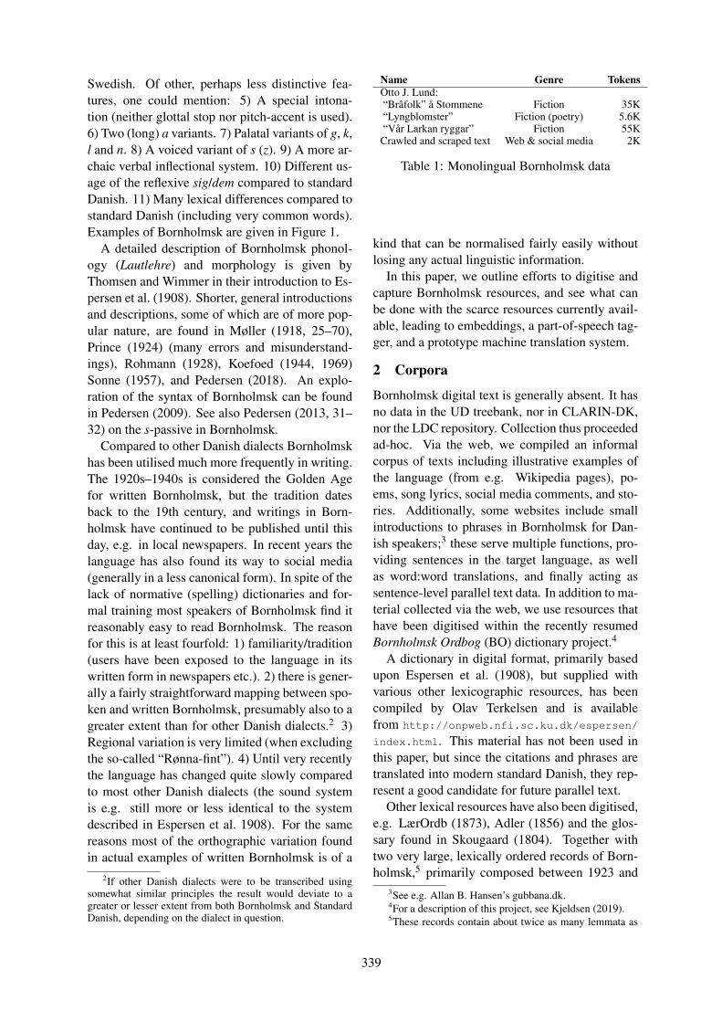
Swedish. Of other, perhaps less distinctive fea-tures, one could mention: 5) A special intona-tion (neither glottal stop nor pitch-accent is used).6) Two (long) a variants. 7) Palatal variants of g, k,l and n. 8) A voiced variant of s (z). 9) A more ar-chaic verbal inflectional system. 10) Different us-age of the reflexive sig/dem compared to standardDanish. 11) Many lexical differences compared tostandard Danish (including very common words).Examples of Bornholmsk are given in Figure 1.

A detailed description of Bornholmsk phonol-ogy (Lautlehre) and morphology is given byThomsen and Wimmer in their introduction to Es-persen et al. (1908). Shorter, general introductionsand descriptions, some of which are of more pop-ular nature, are found in Møller (1918, 25–70),Prince (1924) (many errors and misunderstand-ings), Rohmann (1928), Koefoed (1944, 1969)Sonne (1957), and Pedersen (2018). An explo-ration of the syntax of Bornholmsk can be foundin Pedersen (2009). See also Pedersen (2013, 31–32) on the s-passive in Bornholmsk.

Compared to other Danish dialects Bornholmskhas been utilised much more frequently in writing.The 1920s–1940s is considered the Golden Agefor written Bornholmsk, but the tradition datesback to the 19th century, and writings in Born-holmsk have continued to be published until thisday, e.g. in local newspapers. In recent years thelanguage has also found its way to social media(generally in a less canonical form). In spite of thelack of normative (spelling) dictionaries and for-mal training most speakers of Bornholmsk find itreasonably easy to read Bornholmsk. The reasonfor this is at least fourfold: 1) familiarity/tradition(users have been exposed to the language in itswritten form in newspapers etc.). 2) there is gener-ally a fairly straightforward mapping between spo-ken and written Bornholmsk, presumably also to agreater extent than for other Danish dialects.2 3)Regional variation is very limited (when excludingthe so-called “Rønna-fint”). 4) Until very recentlythe language has changed quite slowly comparedto most other Danish dialects (the sound systemis e.g. still more or less identical to the systemdescribed in Espersen et al. 1908). For the samereasons most of the orthographic variation foundin actual examples of written Bornholmsk is of a

2If other Danish dialects were to be transcribed usingsomewhat similar principles the result would deviate to agreater or lesser extent from both Bornholmsk and StandardDanish, depending on the dialect in question.

Name Genre TokensOtto J. Lund:“Brafolk” a Stommene Fiction 35K“Lyngblomster” Fiction (poetry) 5.6K“Var Larkan ryggar” Fiction 55K

Crawled and scraped text Web & social media 2K

Table 1: Monolingual Bornholmsk data

kind that can be normalised fairly easily withoutlosing any actual linguistic information.

In this paper, we outline efforts to digitise andcapture Bornholmsk resources, and see what canbe done with the scarce resources currently avail-able, leading to embeddings, a part-of-speech tag-ger, and a prototype machine translation system.

2 Corpora

Bornholmsk digital text is generally absent. It hasno data in the UD treebank, nor in CLARIN-DK,nor the LDC repository. Collection thus proceededad-hoc. Via the web, we compiled an informalcorpus of texts including illustrative examples ofthe language (from e.g. Wikipedia pages), po-ems, song lyrics, social media comments, and sto-ries. Additionally, some websites include smallintroductions to phrases in Bornholmsk for Dan-ish speakers;3 these serve multiple functions, pro-viding sentences in the target language, as wellas word:word translations, and finally acting assentence-level parallel text data. In addition to ma-terial collected via the web, we use resources thathave been digitised within the recently resumedBornholmsk Ordbog (BO) dictionary project.4

A dictionary in digital format, primarily basedupon Espersen et al. (1908), but supplied withvarious other lexicographic resources, has beencompiled by Olav Terkelsen and is availablefrom http://onpweb.nfi.sc.ku.dk/espersen/

index.html. This material has not been used inthis paper, but since the citations and phrases aretranslated into modern standard Danish, they rep-resent a good candidate for future parallel text.

Other lexical resources have also been digitised,e.g. LærOrdb (1873), Adler (1856) and the glos-sary found in Skougaard (1804). Together withtwo very large, lexically ordered records of Born-holmsk,5 primarily composed between 1923 and

3See e.g. Allan B. Hansen’s gubbana.dk.4For a description of this project, see Kjeldsen (2019).5These records contain about twice as many lemmata as

339

1931 by the three original editors of BO, and thepart of BO which was edited before work on theproject came to a halt in the 1940s, these resourceswill be published as a fully searchable meta dictio-nary in August 2020. For this reason, apart froma smaller part of the edited part of BO which isused for training of the MT models (about 3000sentence pairs), these sources have not been usedin the present project.

Some prose and poems have been digitised,namely three longer prose texts written by OttoJ. Lund (Magarsfolken, Lund 1935b, Enj Gal-nerojs, Lund 1935a, and Brafolk a Stommene,Lund 1941), a number of poems by the same au-thor, Lyngblomster (Lund, 1930), as well as a col-lection of folk stories published by J. P. Kuhre in1938 under the title Borrinjholmska Sansager hasbeen used. The latter text collection is of specialvalue: it is in many respects the best written rep-resentative of canonical Bornholmsk, the orthog-raphy used is unusually consistent and each storyis translated to (somewhat old fashioned) standardDanish, more or less sentence by sentence. Al-though not identical, the orthographic principlesused by Kuhre are very similar to those used in theBO dictionary project.

A data statement (Bender and Friedman, 2018)for these resources is given in the appendices.The data used in and produced by the dictionaryproject will be published under CC BY-SA.

3 Embeddings and Alignment

Given some text in Bornholmsk, we attempted toinduce distributional word embeddings. For this,we chose FastText (Bojanowski et al., 2017). AsBornholmsk is a low-resource language, it is im-portant to be able to connect it to other languageseasily. Standard FastText embeddings are avail-able for many languages. FastText supports sub-word embeddings, which are likely to be usefulin a language like Bornholmsk that has a rela-tively small alphabet, and also have some chanceof compensating for the high data sparsity.

Embeddings are induced with 300 dimensions,in order to be compatible with the public Com-mon Crawl-based FastText embeddings. Hav-ing induced these embeddings for Bornholmskebornholmsk, they are then aligned into the embed-ded space of Danish from FastText edanish. We trythree alignment methods: (1) unsupervised align-

Espersen’s dictionary.

da-bo bo-da da-bo bo-da‘hvid’ ‘vid’ ‘morgen’ ‘marn’

vid hvid marn morgenvidd sort Imarn aftenvid- rød marnmal eftermiddagvidt gul marnijn majmorgenvida hvidfarvet marna formiddag

Table 2: Closest words after supervised alignment

ment, where matching surface forms are used asanchor points for the two embedded spaces; (2)alignment augmented with the 1:1 word dictio-naries captured earlier, where these translationsare used as anchor points; (3) a mixed alignment,using both unsupervised and supervised points.Dictionary words missing from just one languageare inserted into the dictionary using the embed-ding of anchor point in the other language, post-alignment. We choose Danish (edanish) as the tar-get space for Bornholmsk as the two languages arelikely to have some lexical overlap, and there isvastly more data for Danish.

To align vectors, a transformation is built fromthe singular value decomposition of the product ofthe target space and the transpose of the sourcespace (Smith et al., 2017). This orthogonal trans-formation aligns the source language to the tar-get, thus mapping Bornholmsk embeddings intoedanish. A test set of 10 % of the bilingual map-pings was held out for evaluation. In this case,the mean similarity was 0.3469 for unsupervised(i.e. lexical match) anchoring, 0.4238 for super-vised anchoring over translated word pairs, and0.3959 for the union of unsupervised and super-vised anchor pairs. We can see that while the un-supervised alignment is helpful, when supervisedpairs are available, it detracts from performance.Table 2 shows closest pairs for sample words.

4 Part-of-speech Tagging

Because there is no part-of-speech (PoS)-taggeddata, we must look to resources from other lan-guages. Using aligned embeddings, it is possi-ble to train a PoS tagger for one language lsourcewhere the words are represented in embeddingsspace e. By mapping words in sentences in a tar-get language ltarget into e, these sentences canbe posed to the tagger as if they were in lsource.This requires that embeddings for both languages,esource and etarget, are aligned to the general em-

340

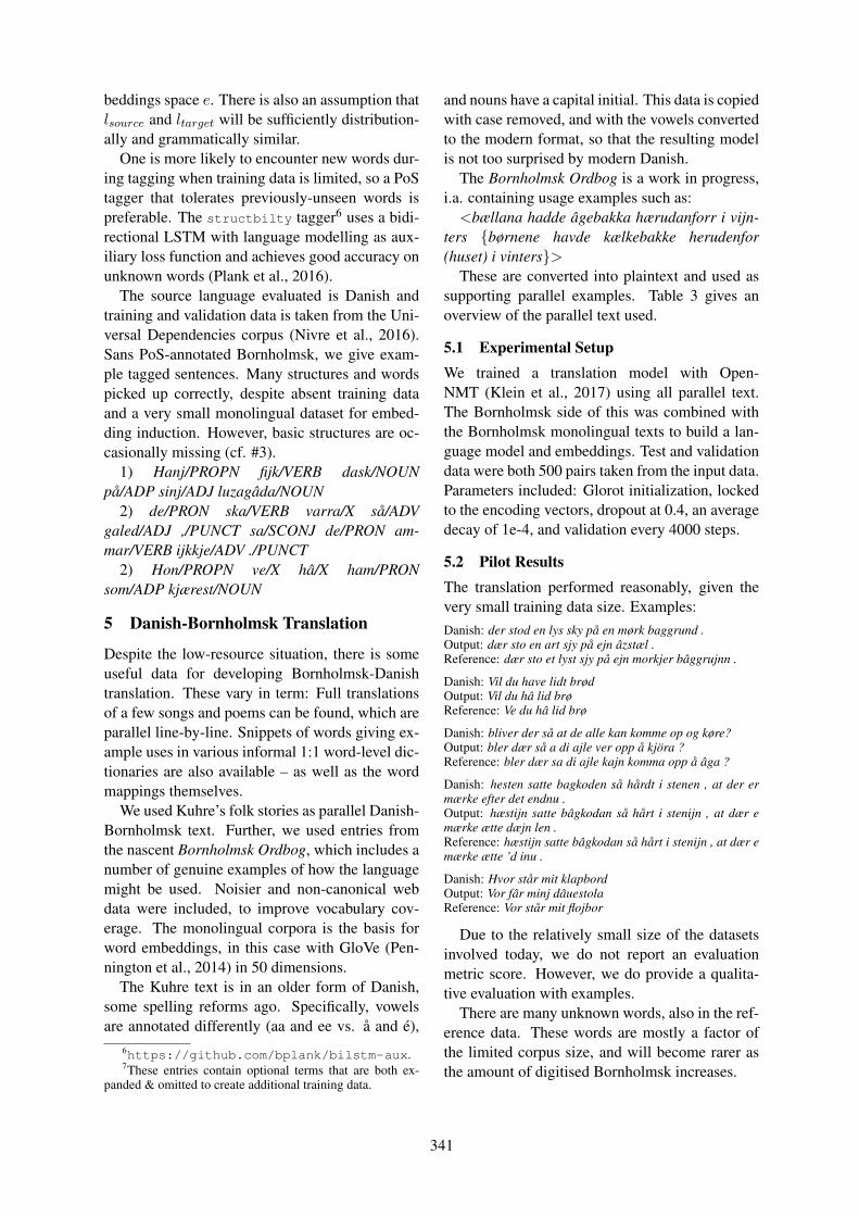
beddings space e. There is also an assumption thatlsource and ltarget will be sufficiently distribution-ally and grammatically similar.

One is more likely to encounter new words dur-ing tagging when training data is limited, so a PoStagger that tolerates previously-unseen words ispreferable. The structbilty tagger6 uses a bidi-rectional LSTM with language modelling as aux-iliary loss function and achieves good accuracy onunknown words (Plank et al., 2016).

The source language evaluated is Danish andtraining and validation data is taken from the Uni-versal Dependencies corpus (Nivre et al., 2016).Sans PoS-annotated Bornholmsk, we give exam-ple tagged sentences. Many structures and wordspicked up correctly, despite absent training dataand a very small monolingual dataset for embed-ding induction. However, basic structures are oc-casionally missing (cf. #3).

1) Hanj/PROPN fijk/VERB dask/NOUNpa/ADP sinj/ADJ luzagada/NOUN

2) de/PRON ska/VERB varra/X sa/ADVgaled/ADJ ,/PUNCT sa/SCONJ de/PRON am-mar/VERB ijkkje/ADV ./PUNCT

2) Hon/PROPN ve/X ha/X ham/PRONsom/ADP kjærest/NOUN

5 Danish-Bornholmsk Translation

Despite the low-resource situation, there is someuseful data for developing Bornholmsk-Danishtranslation. These vary in term: Full translationsof a few songs and poems can be found, which areparallel line-by-line. Snippets of words giving ex-ample uses in various informal 1:1 word-level dic-tionaries are also available – as well as the wordmappings themselves.

We used Kuhre’s folk stories as parallel Danish-Bornholmsk text. Further, we used entries fromthe nascent Bornholmsk Ordbog, which includes anumber of genuine examples of how the languagemight be used. Noisier and non-canonical webdata were included, to improve vocabulary cov-erage. The monolingual corpora is the basis forword embeddings, in this case with GloVe (Pen-nington et al., 2014) in 50 dimensions.

The Kuhre text is in an older form of Danish,some spelling reforms ago. Specifically, vowelsare annotated differently (aa and ee vs. a and e),

6https://github.com/bplank/bilstm-aux.7These entries contain optional terms that are both ex-

panded & omitted to create additional training data.

and nouns have a capital initial. This data is copiedwith case removed, and with the vowels convertedto the modern format, so that the resulting modelis not too surprised by modern Danish.

The Bornholmsk Ordbog is a work in progress,i.a. containing usage examples such as:<bællana hadde agebakka hærudanforr i vijn-

ters {børnene havde kælkebakke herudenfor(huset) i vinters}>

These are converted into plaintext and used assupporting parallel examples. Table 3 gives anoverview of the parallel text used.

5.1 Experimental SetupWe trained a translation model with Open-NMT (Klein et al., 2017) using all parallel text.The Bornholmsk side of this was combined withthe Bornholmsk monolingual texts to build a lan-guage model and embeddings. Test and validationdata were both 500 pairs taken from the input data.Parameters included: Glorot initialization, lockedto the encoding vectors, dropout at 0.4, an averagedecay of 1e-4, and validation every 4000 steps.

5.2 Pilot ResultsThe translation performed reasonably, given thevery small training data size. Examples:Danish: der stod en lys sky pa en mørk baggrund .Output: dær sto en art sjy pa ejn azstæl .Reference: dær sto et lyst sjy pa ejn morkjer baggrujnn .

Danish: Vil du have lidt brødOutput: Vil du ha lid brøReference: Ve du ha lid brø

Danish: bliver der sa at de alle kan komme op og køre?Output: bler dær sa a di ajle ver opp a kjora ?Reference: bler dær sa di ajle kajn komma opp a aga ?

Danish: hesten satte bagkoden sa hardt i stenen , at der ermærke efter det endnu .Output: hæstijn satte bagkodan sa hart i stenijn , at dær emærke ætte dæjn len .Reference: hæstijn satte bagkodan sa hart i stenijn , at dær emærke ætte ’d inu .

Danish: Hvor star mit klapbordOutput: Vor far minj dauestolaReference: Vor star mit flojbor

Due to the relatively small size of the datasetsinvolved today, we do not report an evaluationmetric score. However, we do provide a qualita-tive evaluation with examples.

There are many unknown words, also in the ref-erence data. These words are mostly a factor ofthe limited corpus size, and will become rarer asthe amount of digitised Bornholmsk increases.

341

Name Genre Sentence pairs Tokens (da) Tokens (da-bornholm)Borrinjholmska Sansager (Kuhre) Fiction 1K 29.1K 30.2KBornholmsk Ordbog: citations Dictionary 3.6K7 41.9K 34.2KGubbana.dk Web data 1.4K 8.3K 8.0KWeb scrape Web data <1K <1K <1K

Table 3: Parallel corpora for Bornholmsk-Danish

Another result of the low volume of trainingdata is that there are few points in the embeddings.This means that the nearest neighbour may actu-ally have a quite different meaning to the target.Thus, qualitatively, when the model gets thingswrong, it will tend to get them really wrong.

Despite its small size and different traininggenre, the model was also capable of produc-ing tolerable output given colloquial modern Dan-ish. Some Danish spellings creep through and thephrasing is imprecise, but nevertheless, a roughmapping is available between the two languages:Danish: Hej , hvad hedder du ?Model output: Te , va heder du ?Correct Bornholmsk: Hai , va heder du ?

Danish: Det er Mads og han er en god dreng.Model output: Ded e slæføre a hajn e en go majn.Correct Bornholmsk: De(d) e Mads a hajn e ejn goer horra.

Danish: København er en af de større byer – faktisk denstørste .Model output: København e en majed raganat !Correct Bornholmsk: Kjøvvenhawn e ejn a di storre byana –fakta dæjn storsta .

6 Related Work

There is no former work that we are aware of onNLP for Bornholmsk. The closest resource is anopenly-available toolkit for Danish, DKIE (Der-czynski et al., 2014), which is designed for theGATE platform (Cunningham et al., 2012), thougheven for Danish work is scarce (Kirkedal et al.,2019). Written Bornholmsk corpora are also rare;these exist almost entirely in smaller collections,some of which have been built with great care.

Two other Scandinavian tongues as small asBornholmsk have had quite different stories.Faroese (ISO639: fao; BCP-47: fo-FO) is spo-ken by about 72000 people, many of whom livein the Faroes; it has a fairly long written tradi-tion and is actively published in. It has some NLPvisibility, being present in the Universal Depen-dencies treebanks, and a steady if slow stream ofNLP research includes the language (e.g. Richteret al. (2018)). In contrast, Scandoromani (ISO639:rmg/rmu) has many fewer speakers than Born-holmsk; its original grammar has been overtaken

by that of the dominant languages in the regionswhere it is spoken and is thus lost. There are nev-ertheless efforts to document the remnants of thistongue (Carling et al., 2014).

No machine translation is available for Scan-doromani or Faroese. The Faroes built an inno-vative solution to this where phrases to be trans-lated are distributed to citizens, who film them-selves saying the translation, making essentially atranslation memory (Kay, 1997) for Faroese.8

7 Conclusion

This work introduced resources and tools for do-ing natural language processing for Bornholmsk,an endangered Nordic language. Contributions in-cluded corpus creation, corpus collection, basicNLP resources, and a pilot translation model. Thecorpora are licensed separately; the NLP embed-dings and models are available openly via ITUCopenhagen’s NLP group page, https://nlp.

itu.dk/resources/, and the public domain textsare available from this paper’s authors. Futurework should focus on digitising more text (incl.lexicographic resources); on making the best usepossible out of the available corpora; on tuningmodels to perform better on the existing data;on increasing awareness around Bornholmsk; onhelping learn Bornholmsk; and on making it pos-sible for Bornholmsk-speakers to work digitally inBornholmsk instead of Danish.

Acknowledgments

This research was carried out with support fromthe Bornholmsk Ordbog project sponsored bySparekassen Bornholms Fond, Brødrene E., S. &A. Larsens Legat, Kunst- og Kulturhistorisk Radunder Bornholms Regionskommune and Born-holms Brandforsikring, and with thanks to theNEIC/NordForsk NLPL project. Titan X GPUsused in this research were donated by the NVIDIACorporation. We are grateful to those who havegathered and published resources on Bornholmsk.Thanks to Emily M. Bender for helpful feedback.

8See https://www.faroeislandstranslate.com/ .

342

ReferencesA. P. Adler. 1856. Prove paa et bornholmsk Dialekt-

Lexikon, 1. og 2. Samling. C. A. Reitzels Bo ogArvinger, København.

M. Baumann-Larsen. 1973. The function of dialectsin the religious life of the bornholm inhabitants. InZur Theorie der Religion/Sociological Theories ofReligion, pages 236–242. Springer.



Gerd Carling, Lenny Lindell, and Gilbert Ambrazaitis.2014. Scandoromani: Remnants of a mixed lan-guage. Brill.

Hamish Cunningham, Diana Maynard, KalinaBontcheva, Valentin Tablan, Niraj Aswani, IanRoberts, Genevieve Gorrell, Adam Funk, AngusRoberts, Danica Damljanovic, Thomas Heitz,Mark A. Greenwood, Horacio Saggion, JohannPetrak, Yaoyong Li, Wim Peters, Leon Derczynski,et al. 2012. Developing Language ProcessingComponents with GATE Version 8 (a User Guide).University of Sheffield.

Leon Derczynski, C. Vilhelmsen, and Kenneth S Bøgh.2014. DKIE: Open source information extractionfor Danish. In Proceedings of the Demonstrationsat the 14th Conference of the European Chapterof the Association for Computational Linguistics,pages 61–64.

Johan Christian Subcleff Espersen, Vilhelm Thom-sen, Ludvig Frands Adalbert Wimmer, and ViggoHolm. 1908. Bornholmsk Ordbog. Bianco LunosBogtrykkeri.

Martin Kay. 1997. The proper place of men and ma-chines in language translation. machine translation,12(1-2):3–23.

Andreas Kirkedal, Barbara Plank, Leon Derczynski,and Natalie Schluter. 2019. The Lacunae of Dan-ish Natural Language Processing. In Proceedings ofthe Nordic Conference on Computational Linguis-tics (NODALIDA). Northern European Associationfor Language Technology.

Alex Speed Kjeldsen. 2019. Bornholmsk Ordbog, ver-sion 2.0, forthcoming. Mal og Mæle, 40. argang:22–31. [expected medio 2019].

Guillaume Klein, Yoon Kim, Yuntian Deng, JeanSenellart, and Alexander M. Rush. 2017. Open-NMT: Open-source toolkit for neural machine trans-lation. In Proc. ACL.

H. A. Koefoed. 1944. Sproget – Bornholmsk. In HansHjorth, editor, Bornholmernes Land, volume 2,pages 267–282. Bornholms Tidendes Forlag, Rønne.

H. A. Koefoed. 1969. Folkemal. In Bent Rying, editor,Gyldendals egnsbeskrivelser. Bornholm, pages 99–109. Gyldendal, København.

J. P. Kuhre. 1938. Borrinjholmska Sansager. Born-holmske folkeæventyr og dyrefabler, volume 45 ofDanmarks Folkeminder. Schønberg, København.

LærOrdb. 1873. Bornholmsk Ordbog. Udgivet afLærere. Colbergs Boghandel, Rønne.

Anne Larsen. 2019. Dialekt pa tværs afsteder og generationer. Available online athttps://dialekt.ku.dk/maanedens emne/dialekt-i-periferien/.

Otto J. Lund. 1930. Lyngblomster. BorrinjholmskaDækt. Henry Andersen, Aakirkeby.

Otto J. Lund. 1935a. Enj Galnerojs. In Var Larkanryggar. To borrinjholmska Fortællinjer, pages 69–139. Eget Forlag, Aakirkeby.

Otto J. Lund. 1935b. Magarsfolken. In Var Larkanryggar. To borrinjholmska Fortællinjer, pages 5–68.Eget Forlag, Aakirkeby.

Otto J. Lund. 1941. Brafolk a Stommene, Fortælling.Eget Forlag, Aakirkeby.

Peter Møller. 1918. Det bornholmske Sprog. FritzSørensens Boghandels Forlag, Rønne.

Joakim Nivre, Marie-Catherine De Marneffe, FilipGinter, Yoav Goldberg, Jan Hajic, Christopher DManning, Ryan McDonald, Slav Petrov, SampoPyysalo, Natalia Silveira, et al. 2016. Universaldependencies v1: A multilingual treebank collec-tion. In Proceedings of the Tenth InternationalConference on Language Resources and Evaluation(LREC), pages 1659–1666.

Karen Margrethe Pedersen. 2009. Bornholmsk dialekt-syntaks. In I mund og bog, pages 249–262. MuseumTusculanum Press.

Karen Margrethe Pedersen. 2013. Refleksivt sig/dem –varianter gennem 800 ar. Danske talesprog, 17:1–37.

Karen Margrethe Pedersen. 2018. Bornholmsk dialekt– i historisk og geografisk belysning. Mal og Mæle,39. argang:12–17.


Barbara Plank, Anders Søgaard, and Yoav Goldberg.2016. Multilingual Part-of-Speech Tagging withBidirectional Long Short-Term Memory Models andAuxiliary Loss. In Proc. ACL.

343

John Prince. 1924. The Danish Dialect of Bornholm.Proceedings of the American Philosophical Society,63:190–207.

Caitlin Richter, Matthew Wickes, Deniz Beser, andMitch Marcus. 2018. Low-resource post processingof noisy OCR output for historical corpus digitisa-tion. In Proceedings of the Eleventh InternationalConference on Language Resources and Evaluation(LREC), Miyazaki, Japan. European Languages Re-sources Association (ELRA).

Aage Rohmann. 1928. Det bornholmske sprog. Born-holmske Samlinger, 1. Række, 19:153–166.

Peder Nikolai Skougaard. 1804. Beskrivelse overBornholm, 1. Del. København.

Samuel L. Smith, David H. P. Turban, Steven Hamblin,and Nils Y. Hammerla. 2017. Offline bilingual wordvectors, orthogonal transformations and the invertedsoftmax. In Proc. ICLR (conference track).

H. P. Sonne. 1957. Sproget. In R. Nielsen and Th.Sørensen, editors, Bogen om Bornholm, pages 520–544. Danskernes Forlag, Aabenraa.

Appendix 1: Data Statement

Curation rationale Collection of Bornholmskdocuments and parallel texts from speakers whohave had Bornholmsk as their (dominant) L1.

Language variety BCP-47: da-DK-bornholm

Speaker demographic

• Speakers of Bornholmsk

• Age: mostly 60+

• Gender: male and female.

• Race/ethnicity: mostly of Scandinavian de-scent.

• Native language: Danish (Bornholmsk).

• Socioeconomic status: various.

• Different speakers represented: unknown.

• Presence of disordered speech: Generally notprevalent.

Annotator demographic

• Age: 30+

• Gender: male and female.


• Native language: Danish (Bornholmsk).

• Socioeconomic status: unknown.

Speech situation Literary works, with some ad-hoc collections and samples of the language.

Text characteristics Mostly literary works.

Provenance Original authors are credited in thiswork.

344

Morphosyntactic Disambiguation in an Endangered Language Setting

Jeff Ens♠ Mika Hamalainen♦ Jack Rueter♦ Philippe Pasquier♠♠ School of Interactive Arts & Technology, Simon Fraser University

♦ Department of Digital Humanities, University of [email protected], [email protected],

[email protected], [email protected]

AbstractEndangered Uralic languages present ahigh variety of inflectional forms in theirmorphology. This results in a high num-ber of homonyms in inflections, which in-troduces a lot of morphological ambigu-ity in sentences. Previous research hasemployed constraint grammars to addressthis problem, however CGs are often un-able to fully disambiguate a sentence, andtheir development is labour intensive. Wepresent an LSTM based model for auto-matically ranking morphological readingsof sentences based on their quality. Thisranking can be used to evaluate the exist-ing CG disambiguators or to directly mor-phologically disambiguate sentences. Ourapproach works on a morphological ab-straction and it can be trained with a verysmall dataset.

1 Introduction

Most of the languages in the Uralic language fam-ily are endangered. The low number of speak-ers, limited linguistic resources and the vast com-plexity in morphology typical to these languagesmakes their computational processing quite a chal-lenge. Over the past years, a great deal of workrelated to language technology for endangeredUralic languages has been released openly onthe Giellatekno infrastructure (Moshagen et al.,2014). This includes lexicographic resources, FST(finite-state transducer) based morphological ana-lyzers and CG (constraint grammar) disambigua-tors.

Despite being a great resource, the Giellateknoinfrastructure has tools and data originating fromdifferent sources by different authors. Recent re-search conducted with the resources for Komi-Zyrian, Skolt Sami, Erzya and Moksha has identi-fied a need for proper evaluation of the resources

available in the infrastructure, as they are not freeof errors (Hamalainen et al., 2018; Hamalainen,2018).

This paper presents a method to learn the mor-phosyntax of a language on an abstract level bylearning patterns of possible morphologies withinsentences. The resulting models can be usedto evaluate the existing rule-based disambigua-tors, as well as to directly disambiguate sentences.Our work focuses on the languages belonging tothe Finno-Permic language family: Finnish (fin),Northern Sami (sme), Erzya (myv) and Komi-Zyrian (kpv). The vitality classification of thethree latter languages is definitely endangered(Moseley, 2010).

2 Motivation

There are two main factors motivating this re-search. First of all, data is often very scarce whendealing with endangered Uralic langauges. Apartfrom Northern Sami, other endangered Uralic lan-guages may have a very small set of annotatedsamples at best, and no gold standard data at worst.As a result, evaluating disambiguated sentencescan often only be conducted by consulting nativespeakers of the language or by relying on the re-searcher’s own linguistic intuition.

Secondly, canonical approaches involving Part-of-Speech (POS) tagging will not suffice in thiscontext due to the rich morphology of Uralic lan-guages. For example the Finnish word form voitacan be lemmatized as voi (the singular partitive ofbutter), vuo (the plural partitive of fjord), voittaa(the imperative of win) or voitaa1 (the connegativeform of spread butter).

The approach described in this paper, addressesthese two issues, as we use a generalized sen-tence representation based on morphological tagsto capture morphological patterns. Moreover, our

1A non-standard form produced by the Finnish analyzer

345

models can be trained on low resource langauges,and models that have been trained on high re-source languages can be applied to low or no re-source languages with reasonable success.

3 Related Work

The problem of morphological tagging in thecontext of low-resource languages has been ap-proached using parallel text (Buys and Botha,2016). From the aligned parallel sentences, theirWsabie-based model can learn to tag the low-resource language based on the morphologicaltags of the high-resource language sentences inthe training data. A limitation of this approach isthe morphological relatedness of the high-resourceand low-resource languages.

A method for POS tagging of low-resourcelanguages has been proposed by Andrews et al.(2017). They use a bi-lingual dictionary betweena low and high-resource language together withmonolingual data to build cross-lingual word em-beddings. The POS tagger is trained on an LSTMneural network, and their approach performs con-sistently better than the other benchmarks they re-port.

Lim et al. (2018) present work conducted onsyntactically parsing Komi-Zyrian and NorthernSami using multilingual word-embeddings. Theyuse pretrained word-embeddings for Finnish andRussian, and train word-embeddings for the low-resource languages from small corpora. These in-dividual word-embeddings are then projected intoa single space by using bilingual dictionaries. Theparser was implemented as an LSTM model and itperformed better in a POS tagging task than in pre-dicting syntactic relations. The key finding for ourpurposes is that including a related high-resourcelanguage (Finnish in this case) improved the accu-racy.

DsDs (Plank and Agic, 2018) is a neural net-work based POS tagger for low-resource lan-guages. The idea is to use a bi-LSTM model toproject POS tags from one language to anotherwith the help of word-embeddings and lexical in-formation. In a low-resource setting, they find thatadding word-embeddings boosts the model, butlexical information can also help to a smaller de-gree.

Much of the related work deals with POS tag-ging. However, as the Uralic languages are mor-phologically rich, a full morphological disam-

biguation is needed in order to improve the per-formance of higher-level NLP tools. In addition,we do not want to assume bi-lingual parallel dataor access to word embeddings as we want our ap-proach to be applicable for truly endangered lan-guages with extremely limited resources.

4 The Rule-based Tools and Data

We use the morphological FST analyzers in theGieallatekno infrastructure to produce morpholog-ical readings with UralicNLP (Hamalainen, 2019).They operate on a word level. This means thatfor an input word form, they produce all the pos-sible lemmas together with their parts-of-speechand morphological readings, without any weightsto indicate which reading is the most probable one.

The existing CG disambiguators get the mor-phological readings produced by the FST for eachword in a sentence and apply their rules to re-move the non-possible readings. In some cases,a CG disambiguator might produce a fully disam-biguated sentence, however these models are oftenunable to resolve all morphological ambiguity.

In this paper, we use the UD Treebanks for ourlanguages of interest. For Finnish, we use TurkuDependency Treebank (Haverinen et al., 2014)with 202K tokens (14K sentences). The NorthernSami Treebank (Sheyanova and Tyers, 2017) is thelargest one for the endangered languages with 26Ktokens (3K sentences). For Komi-Zyrian, we usethe Komi-Zyrian Lattice Treebank (Partanen et al.,2018) of 2K tokens (189 sentences) representingthe standard written Komi. The Erzya Treebank(Rueter and Tyers, 2018) is the second largest en-dangered language one we use in our research with15k tokens (1,500 sentences).

5 Sentence Representation

We represent each word as a non-empty set ofmorphological tags. This representation does notcontain the word form itself nor its lemma, aswe aim for a more abstract level morphologi-cal representation. This representation is meantto capture the possible morphologies followingeach other in a sentence to learn morphosyntacticinter-dependencies such as agreement rules. Thislevel of abstraction makes it possible to apply thelearned structures for other morphosyntacticallysimilar languages.

As we are looking into morphosyntax, we trainour model only with the morphosyntactically rele-

346

vant morphological tags. These are case, number,voice, mood, person, tense, connegative and verbform. This means that morphological tags such asclitics and derivational morphology are not takeninto account. We are also ignoring the dependencyinformation in the UD Treebanks as dependenciesare not available for text and languages outside ofthe Treebanks due to the fact that there are no ro-bust dependency parsers available for many of theendangered Uralic language.

Each sentence is simply a sequence of mor-phological tag sets, represented as a sequenceof integers with a special token SP demar-cating spaces between words. For exam-ple the sentence ”Nyt on lungisti ottamisenaika.” (now it is time to relax), is encodedas [150,SP, 121, 138, 168, 178, 205, 214, 221,SP150,SP, 25, 138, 158,SP, 31, 138, 158,SP, 165].

Equation 1 is used to measure the distance be-tween two sentences containing nwords, where xidenotes set of morphological tags associated withthe ith word in x, || · || denotes the number ofelements in a set, and 4 denotes the symmetricdifference of two sets. This distance measure isused to approximate the quality of different read-ings, based on the assumption that the quality ofa reading decreases as its distance from the goldstandard sentence increases.

distance(a, b) =n∑

i=1

||ai4bi|| (1)

6 Model

We implement our models using Keras (Cholletet al., 2015), which are trained to rank two sen-tences encoded as described in Section 5. Themodel is comprised of a Long Short Term Mem-ory (LSTM) (Hochreiter and Schmidhuber, 1997)layer π and a feed-forward layer φ. Given two sen-tences a and b, the LSTM layer is used to pro-duce the n-dimensional vectors π(a) and π(b),which are concatenated and passed through thefeed-forward layer to produce a single scalar valueφ(π(a), π(b)) indicating the preferred sentence.We train each model with early stopping basedon the validation accuracy with a patience of 10epochs. We use the Adam optimizer (Kingma andBa, 2014), train the model with batches of size 32,and set n = 128.

1 2 3 4 5 6 7 8 9 10 11 12 13 14 15 16 17 18 19 20K

0.5

0.6

0.7

0.8

0.9

1.0

Gold

Sta

ndar

d Se

nten

ce in

Top

-K F

requ

ency

kpv sme fin myv

Figure 1: The frequency with which the gold stan-dard sentence is ranked in the top-k with 1000 tri-als per model averaged over 10 data splits.

7 Evaluation

We produce all the morphological readings foreach word in a gold standard sentence (GSS) usingFST analyzers, and construct incorrect sentences(INS) of varying quality by randomly selectinga reading for each word. In order to provide adetailed evaluation, we categorize each sentencebased on their distance from the GSS using theranges [[0, 1), [1, 10), [10, 20), [20,+∞)], whichwe will refer to as categories G,1,2, and 3. By con-struction, category G only contains GSS. Theseranges were chosen so that each bin contains ap-proximately the same number of sentences. Wemeasure the accuracy of the model for each of the(42

)= 6 possible types of comparisons between

sentence categories. To create training, validationand testing data, the set of GSS are randomly splitbefore generating INS. In cases where two lan-guages are used to train the model, the trainingdata consists of an even number of comparisonsfrom each language to ensure that a larger lan-guage does not dominate a smaller language.

Since we are interested in exploring the viabil-ity of using high resource to disambiguate low re-source languages, we evaluate the models by train-ing on each language and each possible combina-tion of languages, resulting in 4+

(42

)= 10 distinct

models.

8 Results

In order to ensure that our results are not the arti-fact of a particular data split, we train each modelon 10 random splits of the data. The average ac-

347

kpv sme fin myvmodel Gv1 Gv2 Gv3 1v2 1v3 2v3 Gv1 Gv2 Gv3 1v2 1v3 2v3 Gv1 Gv2 Gv3 1v2 1v3 2v3 Gv1 Gv2 Gv3 1v2 1v3 2v3kpv .93 .97 .97 .79 .95 .77 .53 .62 .66 .56 .60 .54 .62 .65 .68 .59 .64 .58 .65 .72 .77 .64 .71 .62myv .59 .68 .68 .66 .76 .62 .18 .13 .10 .40 .32 .40 .66 .65 .68 .56 .61 .56 .95 .99 .99 .78 .92 .76sme .65 .70 .70 .55 .56 .52 .93 .98 .99 .73 .89 .71 .57 .59 .61 .56 .58 .56 .22 .14 .10 .39 .31 .40fin .49 .60 .66 .60 .70 .60 .44 .58 .68 .58 .67 .57 .88 .95 .98 .72 .85 .70 .70 .74 .74 .62 .67 .59

kpv+myv .92 .97 .99 .79 .96 .79 - - - - - - - - - - - - .92 .98 .99 .80 .93 .77kpv+fin .90 .95 .99 .77 .95 .78 - - - - - - .87 .94 .97 .72 .85 .69 - - - - - -

kpv+sme .91 .95 .97 .73 .89 .69 .91 .97 .99 .73 .86 .69 - - - - - - - - - - - -myv+fin - - - - - - - - - - - - .83 .90 .94 .69 .82 .69 .93 .98 .99 .79 .91 .75

myv+sme - - - - - - .89 .95 .97 .73 .86 .70 - - - - - - .86 .94 .96 .75 .87 .72sme+fin - - - - - - .90 .96 .98 .73 .88 .71 .86 .93 .97 .73 .85 .71 - - - - - -

Table 1: Model accuracy averaged over 10 data splits with 1000 trials per model.

curacy across data splits is shown in in Table 1,where the accuracy of a single model with respectto a single comparison type is calculated based on1000 comparisons. The mean standard error was0.008, and the maximum standard error was 0.054for these measurements. Figure 1 shows the per-centage of times the GSS is ranked in the top-ksentences, given a set of 20 sentences containing19 randomly selected INS. The

(202

)= 190 pair-

wise rankings are aggregated using iterative LuceSpectral Ranking algorithm (Maystre and Gross-glauser, 2015).

9 Discussion and Future Work

The results in Table 1 demonstrate that our mod-els are as effective for extremely low resource lan-guages like Komi-Zyrian (kpv) as they are for highresource languages like Finnish (fin). Further-more, there is evidence that training on a higherresource langauge that is genealogically related toa low resource langauge is a viable option. Forexample, the models trained on Finnish (fin) dataperformed relatively well when tested on the Erzya(myv) data. In cases where languages are not ge-nealogically close to each other, such as North-ern Sami (sme) and Erzya (myv), models performvery poorly when trained on one of these lan-gauges and tested on another.

According to the results, the most difficult com-parisons are 1v2 and 2v3. Since Equation 1 isonly a proxy for sentence quality, it is possiblethat for some number of comparisons category 1sentences are actually lower quality than category2 sentences. In contrast, Gv1, Gv2, and Gv3 arecomparisons against GSS, which are guaranteedto be correct. Consequently, it seems reasonableto conclude that this decrease in performance ispartially due to deficiencies in measuring sentencequality.

Figure 1 demonstrates that pairwise rankingscan be aggregated to reliably rank sentences basedon their quality, as the GSS was frequently in thetop-k sentences for small values of k. For exam-ple, the kpv, myv and sme models ranked the GSSin the top 3 roughly 86 percent of the time.

Future work may involve experiments with veryclosely related languages. For instance, out of 9Sami languages, North Sami is the only one witha UD Treebank. Testing the performance of oursystem on the other Sami languages while trainingon North Sami is one of our goals for the futureresearch. However, as due to the lack of gold an-notated data, we need to recruit nearly native ornative speakers with linguistic knowledge to eval-uate our system. This is a time consuming taskand it is outside of the scope of this paper.

10 Conclusion

Uralic languages exhibit a high degree of mor-phological ambiguity, and resources for these lan-guages are often limited, posing difficulties fortraditional methods that have been employed suc-cessfully on other languages. In order to mitigatethese issues, we proposed a representation basedon the morphological tags associated with eachword in a sentence.

Our experimental results demonstrate that anLSTM based model can accurately rank alter-nate readings of a single sentence, even when themodel is trained on an extremely low-resourcelanguage. This technique requires much less ef-fort than developing complex rule-based grammarmodels for an endangered languages, as our modelcan be trained on a small set of gold-standard ex-amples. Furthermore, a trained model can be usedto disambiguate morphological readings producedby an FST analyzer or to evaluate the output of aCG model.

348

ReferencesNicholas Andrews, Mark Dredze, Benjamin

Van Durme, and Jason Eisner. 2017.https://doi.org/10.18653/v1/P17-1095 Bayesianmodeling of lexical resources for low-resourcesettings. In Proceedings of the 55th Annual Meetingof the Association for Computational Linguistics(Volume 1: Long Papers), pages 1029–1039.Association for Computational Linguistics.

Jan Buys and Jan A. Botha. 2016.https://doi.org/10.18653/v1/P16-1184 Cross-lingualmorphological tagging for low-resource languages.In Proceedings of the 54th Annual Meeting of theAssociation for Computational Linguistics (Volume1: Long Papers), pages 1954–1964. Association forComputational Linguistics.

Francois Chollet et al. 2015. Keras. https://keras.io.

Mika Hamalainen. 2018. Extracting a SemanticDatabase with Syntactic Relations for Finnish toBoost Resources for Endangered Uralic Languages.In Proceedings of the Logic and Engineering of Nat-ural Language Semantics 15 (LENLS15).

Mika Hamalainen. 2019. UralicNLP: An NLP libraryfor Uralic languages. Journal of Open Source Soft-ware, 4(37):1345. 10.21105/joss.01345.

Mika Hamalainen, Liisa Lotta Tarvainen, and JackRueter. 2018. Combining Concepts and TheirTranslations from Structured Dictionaries of UralicMinority Languages. In Proceedings of the EleventhInternational Conference on Language Resourcesand Evaluation (LREC 2018). European LanguageResources Association (ELRA).

Katri Haverinen, Jenna Nyblom, Timo Viljanen,Veronika Laippala, Samuel Kohonen, Anna Mis-sila, Stina Ojala, Tapio Salakoski, and Filip Ginter.2014. https://doi.org/10.1007/s10579-013-9244-1Building the essential resources for finnish: theturku dependency treebank. Language Resourcesand Evaluation, 48(3):493–531.

Sepp Hochreiter and Jurgen Schmidhuber. 1997.https://doi.org/10.1162/neco.1997.9.8.1735 Longshort-term memory. Neural Comput., 9(8):1735–1780.

Diederik P Kingma and Jimmy Ba. 2014. Adam: Amethod for stochastic optimization. arXiv preprintarXiv:1412.6980.

KyungTae Lim, Niko Partanen, and Thierry Poibeau.2018. Multilingual dependency parsing for low-resource languages: Case studies on north saamiand komi-zyrian. In Proceedings of the Eleventh In-ternational Conference on Language Resources andEvaluation (LREC 2018).

Lucas Maystre and Matthias Grossglauser. 2015.http://dl.acm.org/citation.cfm?id=2969239.2969259

Fast and accurate inference of plackett-luce models.In Proceedings of the 28th International Conferenceon Neural Information Processing Systems - Volume1, NIPS’15, pages 172–180, Cambridge, MA, USA.MIT Press.

Christopher Moseley, editor. 2010. Atlas ofthe World′s Languages in Danger, 3rd edi-tion. UNESCO Publishing. Online version:http://www.unesco.org/languages-atlas/.

Sjur Moshagen, Jack Rueter, TommiPirinen, Trond Trosterud, and Fran-cis M. Tyers. 2014. http://www.lrec-conf.org/proceedings/lrec2014/workshops/LREC2014-Workshop-CCURL2014-Proceedings.pdf Open-Source Infrastructures for Collaborative Work onUnder-Resourced Languages. The LREC 2014Workshop “CCURL 2014 - Collaboration andComputing for Under-Resourced Languages in theLinked Open Data Era”.

Niko Partanen, Rogier Blokland, KyungTae Lim,Thierry Poibeau, and Michael Rießler. 2018. Thefirst komi-zyrian universal dependencies treebanks.In Proceedings of the Second Workshop on Univer-sal Dependencies (UDW 2018), pages 126–132.

Barbara Plank and Zeljko Agic. 2018.http://aclweb.org/anthology/D18-1061 Distantsupervision from disparate sources for low-resourcepart-of-speech tagging. In Proceedings of the2018 Conference on Empirical Methods in NaturalLanguage Processing, pages 614–620. Associationfor Computational Linguistics.

Jack Rueter and Francis Tyers. 2018. Towards anOpen-Source Universal-Dependency Treebank forErzya. In Proceedings of the Fourth InternationalWorkshop on Computatinal Linguistics of UralicLanguages, pages 106–118.

Mariya Sheyanova and Francis M. Tyers. 2017. An-notation schemes in north sami dependency parsing.In Proceedings of the 3rd International Workshopfor Computational Linguistics of Uralic Languages,pages 66–75.

349

Tagging a Norwegian Dialect Corpus

Andre KasenDepartment of Informatics

University of [email protected]

Kristin HagenThe Text LaboratoryUniversity of Oslo

Anders NøklestadThe Text LaboratoryUniversity of Oslo

{kristin.hagen, anders.noklestad, joel.priestley}@iln.uio.no

Joel PriestleyThe Text LaboratoryUniversity of Oslo

AbstractThis paper describes an evaluation offive data-driven Part-of-Speech (PoS) tag-gers for spoken Norwegian. The tag-gers all rely on different machine learn-ing mechanisms: decision trees, hiddenMarkov models (HMMs), conditional ran-dom fields (CRFs), long-short term mem-ory networks (LSTMs), and convolutionalneural networks (CNNs). We go into someof the challenges posed by the task of tag-ging spoken, as opposed to written, lan-guage, and in particular a wide range ofdialects as is found in the recordings of theLIA (Language Infrastructure made Ac-cessible) project. The results show thatthe taggers based on either conditionalrandom fields or neural networks performmuch better than the rest, with the LSTMtagger getting the highest score.

1 Introduction

The most commonly used PoS tagger for Norwe-gian is the the Oslo-Bergen tagger (OBT); a Con-straint Grammar tagger for Bokmal and Nynorsk(Johannessen et al., 2012), the two written stan-dards that exist for written Norwegian. For spo-ken language transcribed into Bokmal, the sta-tistical NoTa tagger was developed and trainedon Bokmal transcriptions from Oslo and the sur-rounding area (Nøklestad and Søfteland, 2007).A recent infrastructure project, LIA (LanguageInfrastructure made Accessible) has produced alarge number of dialect transcriptions in Nynorsk,the other written standard. This creates a need fora new tagger that works on this written standardand that can also handle a diverse data set contain-ing a wide range of dialects.

In this paper we will first describe the LIA di-alect transcriptions and then the manually anno-

tated training material for Nynorsk as well as somechallenges in annotating spoken language. After-wards we will describe a number of experimentswith five different open source taggers.

2 Dialect transcriptions

The audio files were recorded between 1950 and1990 in order to explore and survey the manydifferent dialects in Norway. Most of the infor-mants are older people and native speakers of theirdialect. Typically, the recordings are interviewsabout old trades such as agriculture, fishing, log-ging and life at the summer farm. Other topicsare weaving, knitting, baking or dialects. Some-times the research questions also concern personor place names. The recordings are semi-formalto informal and often take place in an informant’shome.

The original LIA transcriptions are semi-phonetically transcribed (Hagen et al., 2015). Ex-ample (1) below shows the semi-phonetic and nor-malized transcription. To make the transcriptionssearchable and suitable for automatic tagging, theyare semi-automatically transliterated to Nynorskby the Oslo Transliterator, which is trained onmore than 200 Norwegian dialects.

(1) hannhan

eer

flinngkeflink

tea

drivadrive

garengarden

‘He is good at running the farm.’

Øvrelid et al. (2018) note that the segmentationheuristic in this material is such that segments donot necessarily correspond to sentences, but ratherto (conversational) meaningful units.

3 The Training Corpus, Dialects andSpoken language PoS

The starting point was the annotation scheme ofthe Norwegian Dependency Treebank (NDT) de-scribed by Solberg et al. (2014). This is an ex-tension of the OBT scheme (which is based on

350

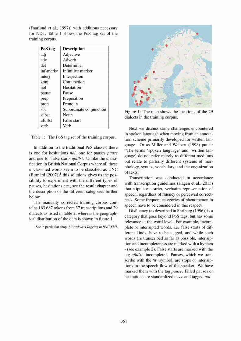
(Faarlund et al., 1997)) with additions necessaryfor NDT. Table 1 shows the PoS tag set of thetraining corpus.

PoS tag Descriptionadj Adjectiveadv Adverbdet Determinerinf-merke Infinitive markerinterj Interjectionkonj Conjunctionnol Hesitationpause Pauseprep Prepositionpron Pronounsbu Subordinate conjunctionsubst Nounufullst False startverb Verb

Table 1: The PoS tag set of the training corpus.

In addition to the traditional PoS classes, thereis one for hesitations nol, one for pauses pauseand one for false starts ufullst. Unlike the classi-fication in British National Corpus where all theseunclassified words seem to be classified as UNC(Burnard (2007))1 this solutions gives us the pos-sibility to experiment with the different types ofpauses, hesitations etc., see the result chapter andthe description of the different categories furtherbelow.

The manually corrected training corpus con-tains 163,687 tokens from 37 transcriptions and 29dialects as listed in table 2, whereas the geograph-ical distribution of the data is shown in figure 1.

1See in particular chap. 6 Wordclass Tagging in BNC XML

Figure 1: The map shows the locations of the 29dialects in the training corpus.

Next we discuss some challenges encounteredin spoken language when moving from an annota-tion scheme primarily developed for written lan-guage. Or as Miller and Weinert (1998) put it:“The terms ‘spoken language’ and ‘written lan-guage’ do not refer merely to different mediumsbut relate to partially different systems of mor-phology, syntax, vocabulary, and the organizationof texts.”

Transcription was conducted in accordancewith transcription guidelines (Hagen et al., 2015)that stipulate a strict, verbatim representation ofspeech, regardless of fluency or perceived correct-ness. Some frequent categories of phenomenon inspeech have to be considered in this respect:

Disfluency (as described in Shriberg (1996)) is acategory that goes beyond PoS tags, but has somerelevance at the word level. For example, incom-plete or interrupted words, i.e. false starts of dif-ferent kinds, have to be tagged, and while suchwords are transcribed as far as possible, interrup-tion and incompleteness are marked with a hyphen- (see example 2). False starts are marked with thetag ufullst ‘incomplete’. Pauses, which we tran-scribe with the ‘#’ symbol, are stops or interrup-tions in the speech flow of the speaker. We havemarked them with the tag pause. Filled pauses orhesitations are standardized as ee and tagged nol.

351

Dialect area # segments # tokensAustevoll 1193 11191Bardu 560 4205Bergen 993 10416Bolsøy 645 6669Brandbu 404 6112Eidsberg 679 5880Farsund 351 3707Flakstad 1201 11080Fla 149 2808Førde 332 3175Fredrikstad 554 7676Froland 378 6660Giske 874 10821Gjesdal 415 4101Gloppen 526 5724Gol 158 2414Hemsedal 244 4436Herad 214 2186Hjartdal 354 4032Høyanger 330 4357Kristiansand 259 3713Lierne 365 3867Skaun 482 4661Trondheim 216 3392Vardø 481 6055Al 542 8685Amli 212 3128Amot 423 5123Asnes 466 7413Total 14000 163687

Table 2: The manually corrected training corpuscontains tokens from 37 transcriptions and 29 di-alects.

(2) saso

detit

varwas

ganskevery

m-ufullst

#pause

eenol

mangemany

derthere

‘There were a lot of people there.’

Another challenge is frequent and form-identical words. For example, sentential connec-tives or conjunctions are a well delimited group ofwords in written Norwegian. In spoken Norwe-gian, however, the usage patterns of certain wordshave yet to be examined, and the difference be-tween certain conjunctions and pragmatic mark-

ers/particles is somewhat unclear.2. For instance,sa seems to take on multiple functions:

(3) saso

KariKari

løpran

fortfast.

‘so Kari ran fast.’

The next two examples illustrate another chal-lenge. Adverbs, interjections and particles are farmore common in spoken language than in writtentext. The pragmatic particle lell probably has afunction like the adverb heller (‘just as well’), orsome sort of particle. Then in example (5) we see asomewhat similar use pattern, but with a token thatis form-identical with the conjunction eller (‘or’).In both cases, we have chosen to tag the words asadverbs.

(4) menbut

huttetumy

egI

greiddecould

naPART

ikkjenot

aTO

sjasee

paon

detit

lellPART

‘oh my I couldn’t look at it.’

(5) eris

detit

langtlong

forfor

degyou

aTO

reisetravel

tilto

#pause

tilto

jobbenwork

dathen

eller?or?

‘do you have a long travel to work?’

Haberg (2010) describes and analyzes what isknown as the preproprial article, which is form-identical with the third person pronoun:

(6) saso

dæthen

skræivwrote

hushe

F1F1

ena

særappgavepaper

ommabout

dæyou

‘Then F1 wrote a paper about you.’

The analysis given by Haberg (2010) states thatthe function of the preproprial article is more akinto that of a determiner, and therefore constitutes anambiguity between the tags det and pron. In bothof the cases above a heuristic that only consideredform was employed, i.e. the preproprial article istagged pron. Note also that the preproprial articleis close to non-existent in written language.

Other problems that can be considered are vari-able word order in embedded structures (Rognes,2011) or form-identical subjunctions and preposi-tions (Huus, 2018). To draw an intermediate con-clusion, we can say that an investigation like thatof Hohle (2016) is called for with regard to spokenlanguage.

2Several case studies can be found in the special issueon pragmatic particles of The Norwegian Linguistic Journalhttp://ojs.novus.no/index.php/NLT/issue/view/196/showToc

352

4 Taggers

In order to find the most suitable tagger, an ar-ray of different taggers from different paradigmswere tested. In the following, we give a short de-scription of the systems in use in the present paper,along with references to them.

TreeTagger3 In order to keep some continu-ity with the aforementioned NoTa tagger, newmodels were induced for the TreeTagger. Tree-Tagger is based on the decision tree paradigm(Schmid, 1999), and was shown by (Nøklestad andSøfteland, 2007) to be the best performing systemfor the NoTa data set.

TnT4 is a second order HMM tagger (Brants,2000). It has been used on multiple occasions (seeHohle et al. (2017), Velldal et al. (2017)) to tagNorwegian. It is therefore natural to include itamong the systems in the present paper.

MarMoT5 is a generic CRF tagger (Mulleret al., 2013), and is widely used as a baseline tag-ger. It can with relative ease be extended to includemorphological tags as well which is a natural nextstep for the present work.

Bilstm-aux6 is a bidirectional LSTM taggerwith auxiliary loss that has been shown to workwell for Norwegian (Plank et al., 2016). Plank etal. (2016) report a tagging accuracy of 98.06% forthe Norwegian part of the Universal DependencyTreebanks v1.2 (Nivre et al., 2015). The Norwe-gian UD part is the NDT mentioned earlier, con-verted to the UD standard (see (Øvrelid and Hohle,2016; Øvrelid et al., 2018)).

Sclem2017-tagger7 is a general purpose taggerutilizing a CNN with a character compositioncomponent and a context encoder (Yu et al., 2017).Yu et. al (2017) report a accuracy of 97.65% forNorwegian UD.

5 Results

In the current work, we only tested the perfor-mance of the taggers on the entire corpus, not onindividual dialects, for several reasons:

3https://www.cis.uni-muenchen.de/ schmid/tools/TreeTagger/4http://www.coli.uni-saarland.de/ thorsten/tnt/5https://github.com/muelletm/cistern/tree/master/marmot6https://github.com/bplank/bilstm-aux7https://github.com/EggplantElf/sclem2017-tagger

First, there is considerable variation in theamount of material we have for the different di-alects, preventing a balanced comparison betweendialects. Furthermore, for many of the dialects thesize of the material is too small to yield a reliableevaluation. Finally, the transcription into standardorthography by necessity removes parts of whatdistinguishes the dialects, in particular with re-spect to morphological features, and the amount ofnormalization is highest for those dialects that dif-fer the most from standard written Nynorsk, againpreventing a fair comparison of dialects.

All systems were evaluated intrinsically using10-fold cross validation and reported with accu-racy. Care has been taken to ensure that each foldhas the relative equal distribution of dialects asthe whole data set to prevent skewed folds. Af-ter splitting the whole data set (80-10-10) evenlyw.r.t. dialects and distributing the 80% portion into10 folds each with a hold out portion, the data wasrandomized. Table 3 shows the calculated accu-racy for all the systems with the respective stan-dard deviation for the ten folds. As is evident,the top performing taggers have relatively similarscores, but according to McNemars test, Bilstm-aux performs significantly better than the next besttagger, MarMoT (p < 0.05), and it also shows asomewhat smaller standard deviation. For the bestsystem we also add a table for each PoS tags pre-cision and recall (Table 4).

System Accuracy (std.)TreeTagger 95.16 (0.0020)TnT 93.18 (0.18)MarMoT 97.25 (0.14)Sclem2017 97.16 (0.15)Bilstm-aux 97.33 (0.11)

Table 3: The PoS accuracy and standard deviationfor the 10-fold cross validation for each system.

Both Sclem2017 and Bilstm-aux are evaluatedwith their integrated test function, whereas Mar-Mot and TreeTagger are evaluated with an ad hocpython script. What sets these systems apart is thefact that the neural networks are given a develop-ment set at training time for early stopping pur-poses, while MarMot demands brown-like clustersinduced with Marlin 89

8https://github.com/muelletm/cistern/tree/master/marlin9Marlin was trained with the Nynorsk part of the Habit

corpus and the Norwegian Newspaper Corpus.

353

(Martin et al., 1998; Muller and Schutze, 2015).This is most likely one of the reasons it performsso well compared to the neural taggers, and callfor an investigation of neural taggers with pre-training as well, i.e. neither of the neural taggerswas trained with pre-trained word embeddings.

PoS tag Presicion Recalladj 89.45 90.87adv 96.64 94.90det 94.03 92.95inf-merke 97.07 98.17interj 99.32 99.08konj 96.42 97.95nol 100 100pause 100 100prep 97.77 98.11pron 98.53 98.65sbu 92.05 91.97subst 95.85 96.86ufullst 97.81 99.06verb 98.20 98.20

Table 4: The precision and recall (averagedacross all 10 folds) for the best performing system:Bilstm-aux (Plank et al., 2016)

5.1 Removal of pauses, hesitations andpauses+hesitations

In the style of Nøklestad and Søfteland (2007),evaluations where different speech specific tokenswere removed were also carried out. Nøklestadand Søfteland (2007) report that this in fact low-ered the performance of the systems they tested.The results that were obtained from the two bestperforming systems in the present paper are foundin Table 5.

System Accuracy (std.)MarMoThesitations 97.19 (0.001)Bilstm-auxhesitations 97.27 (0.1)MarMoTpauses 97.08 (0.001)Bilstm-auxpauses 97.17 (0.14)MarMoThesitations+pauses 97.03 (0.001)Bilstm-auxhesitations+pauses 97.07 (0.18)

Table 5: The PoS accuracy and standard devia-tion for the 10-fold cross validation with speechspecific tokens removed. The subscripts indicatewhat kinds of tokens are removed in each case.

The accuracy deteriorates as speech specific to-

kens are removed, and for both systems removalof pauses have a greater impact on the accuracythan hesitations. This supports the findings by(Strangert et al., 1993) that pauses tend to occurat important positions in an utterance, includingsyntactic boundaries, and hence may provide im-portant clues about the syntactic structure.

6 Conclusions and Further Work

The present paper has reported on new results forPoS tagging of Norwegian dialect data. It has alsoshown that, among the tagger technologies tested,the ones based on CRFs or neural networks showthe best performance on this task.

A subset of the training material in this paperconstitutes the LIA Treebank of Spoken Norwe-gian Dialects and it would be interesting to investi-gate whether removal of other phrasal disfluenciesthan the ones already tested would have an impacton the final accuracy score (see Dobrovoljc andMartinc (2018) and references therein). It wouldalso be worth the effort to see whether neural tag-gers respond better if the input is semi-phoneticrather than normalized. Finally, if we are able toproduce a considerable amount of material for aset of dialects, transcribed in a way that is morefaithful to the peculiarities of each dialect, it wouldbe interesting to test and compare the performanceof the taggers on individual dialects.

354

ReferencesThorsten Brants. 2000. Tnt: a statistical part-of-speech

tagger. In Proceedings of the sixth conference onApplied natural language processing, pages 224–231.

Lou Burnard. 2007. Reference guide for the british na-tional corpus. Technical report.

Kaja Dobrovoljc and Matej Martinc. 2018. Er ... well,it matters, right? on the role of data representationsin spoken language dependency parsing. In Pro-ceedings of the Second Workshop on Universal De-pendencies, pages 37–46.

Jan Terje Faarlund, Svein Lie, and Kjell Ivar Vannebo.1997. Norsk referansegrammatikk. Universitetsfor-laget.

Live Haberg. 2010. Den preproprielle artikkelen inorsk: ei undersøking av namneartiklar i kvæfjord,gausdal og voss. Master’s thesis.

Kristin Hagen, Live Haberg, Eirik Olsen, and AshildSøfteland. 2015. Transkripsjonsrettleiing for lia.Technical report.

Petter Hohle. 2016. Optimizing a pos tag set for nor-wegian dependency parsing. Master’s thesis.

Petter Hohle, Lilja Øvrelid, and Erik Velldal. 2017.Optimizing a pos tagset for norwegian dependencyparsing. In Proceedings of the 21st Nordic Confer-ence on Computational Linguistics, pages 142–151.

Andrea Myklebust Huus. 2018. Distribusjonen av tesom infinitivsmerke i norsk: En korpusbasert un-dersøkelse av utbredelsen av te som infinitivsmerkei norsk. Master’s thesis.

Janne Bondi Johannessen, Kristin Hagen, AndreLynum, and Anders Nøklestad. 2012. Obt+ stat. acombined rule-based and statistical tagger. In Ex-ploring Newspaper Language. Corpus compilationand research based on the Norwegian NewspaperCorpus.

Sven Martin, Jorg Liermann, and Hermann Ney. 1998.Algorithms for bigram and trigram word clustering.Speech communication.

James Edward Miller and Regina Weinert. 1998. Spon-taneous spoken language: Syntax and discourse.Oxford University Press.

Thomas Muller, Helmut Schmid, and Hinrich Schutze.2013. Efficient higher-order crfs for morphologicaltagging. In Proceedings of the 2013 Conference onEmpirical Methods in Natural Language Process-ing, pages 322–332.

Thomas Muller and Hinrich Schutze. 2015. Robustmorphological tagging with word representations.In Proceedings of the 2015 Conference of the NorthAmerican Chapter of the Association for Computa-tional Linguistics: Human Language Technologies,pages 526–536.

Joakim Nivre, Zeljko Agic, Maria Jesus Aranzabe,Masayuki Asahara, Aitziber Atutxa, Miguel Balles-teros, John Bauer, Kepa Bengoetxea, Riyaz AhmadBhat, Cristina Bosco, et al. 2015. Universal depen-dencies 1.2.

Anders Nøklestad and Ashild Søfteland. 2007. Tag-ging a norwegian speech corpus. In Proceedings ofthe 16th Nordic Conference of Computational Lin-guistics, pages 245–248.

Lilja Øvrelid and Petter Hohle. 2016. Universal depen-dencies for norwegian. In Proceedings of the TenthInternational Conference on Language Resourcesand Evaluation, pages 1579–1585.

Lilja Øvrelid, Andre Kasen, Kristin Hagen, AndersNøklestad, Per Erik Solberg, and Janne Bondi Jo-hannessen. 2018. The lia treebank of spoken nor-wegian dialects. In Proceedings of the Eleventh In-ternational Conference on Language Resources andEvaluation, pages 4482–4488.

Barbara Plank, Anders Søgaard, and Yoav Goldberg.2016. Multilingual Part-of-Speech Tagging withBidirectional Long Short-Term Memory Models andAuxiliary Loss. In Proceedings of the 54th AnnualMeeting of the Association for Computational Lin-guistics, pages 412–418.

Stig Rognes. 2011. V2, v3, v4 (and maybe even more):The syntax of questions in the rogaland dialects ofnorway. Master’s thesis.

Helmut Schmid. 1999. Improvements in part-of-speech tagging with an application to german. InNatural language processing using very large cor-pora, pages 13–25. Springer.

Elizabeth Shriberg. 1996. Disfluencies in switchboard.In Proceedings of International Conference on Spo-ken Language Processing, volume 96, pages 11–14.

Per Erik Solberg, Arne Skjærholt, Lilja Øvrelid, KristinHagen, and Janne Bondi Johannessen. 2014. Thenorwegian dependency treebank. In Proceedings ofthe Ninth International Conference on Language Re-sources and Evaluation, pages 789–795.

E. Strangert, E. Ejerhed, and D. Huber. 1993. Clausestructure and prosodic segmentation. In FONETIK-93 Papers from the 7th Swedish Phonetics Confer-ence.

Erik Velldal, Lilja Øvrelid, and Petter Hohle. 2017.Joint ud parsing of norwegian bokmal and nynorsk.In Proceedings of the 21st Nordic Conference onComputational Linguistics, pages 1–10.

Xiang Yu, Agnieszka Falenska, and Ngoc Thang Vu.2017. A general-purpose tagger with convolutionalneural networks. In Proceedings of the First Work-shop on Subword and Character Level Models inNLP, pages 124–129.

355

The Lacunae of Danish Natural Language ProcessingAndreas Kirkedal†

ITU Copenhagen & Interactions LLCDenmark

[email protected]

Barbara PlankITU Copenhagen

[email protected]


[email protected]

Natalie SchluterITU Copenhagen

[email protected]

Abstract

Danish is a North Germanic languagespoken principally in Denmark, a coun-try with a long tradition of technologi-cal and scientific innovation. However,the language has received relatively lit-tle attention from a technological perspec-tive. In this paper, we review Natural Lan-guage Processing (NLP) research, digitalresources and tools which have been de-veloped for Danish. We find that availabil-ity of models and tools is limited, whichcalls for work that lifts Danish NLP a stepcloser to the privileged languages.

Dansk abstrakt: Dansk er et nordger-mansk sprog, talt primært i kongerigetDanmark, et land med stærk tradition forteknologisk og videnskabelig innovation.Det danske sprog har imidlertid væretgenstand for relativt begrænset opmærk-somhed, teknologisk set. I denne artikelgennemgar vi sprogteknologi-forskning,-ressourcer og -værktøjer udviklet fordansk. Vi konkluderer at der eksistereret fatal af modeller og værktøjer, hvilketindbyder til forskning som løfter dansksprogteknologi i niveau med mere priv-iligerede sprog.

1 Introduction

Danish is the majority language of the King-dom of Denmark, a country of around six mil-lion people, with five written languages across itsmany islands (others including Færøysk, Kalaal-lisut, Tunumiit oraasiat, and Borrinjholmsk (Der-

†: Research Scientist at Interactions LLC.: These authors contributed to the paper equally.

czynski and Kjeldsen, 2019)). Despite its privi-leged place in the world, Denmark has not keptup pace with comparable countries in developinglanguage technology. Few systems are designedexplicitly for Danish; rather, general-purpose sys-tems might be run on Danish and results producedfor it as a by-product of larger studies. This sup-poses having adequate developed datasets. Asa result, language technology does not have asprominent a place in Denmark as it might in othercountries. This paper gives an overview of NLPmodels, tasks and datasets for Danish.

Traditionally, the country has created cor-pora, lexicographic resources, and other sym-bolic knowledge through government sponsor-ship. This has led to excellent research at theDansk Sprognævn (dsn.dk) and by CLARIN DK(clarin.dk), who have both consistently pro-duced volumes of quality Danish data within theirremit. This paper examines NLP from perhaps theopposite direction: our study is task-driven insteadof corpus-driven, meaning we pragmatically con-sider what NLP technology exists, how it is repre-sented in the scope of Danish, and, where appro-priate, what might help improve the situation.

While Denmark has multiple languages (asabove), Danish also has multiple language variants– for example ømalsdansk, which encompasses allfrom the absence of stød (Hansen, 1943; Basbøll,2005) in fynsk, to københavnsk, with its quirks,like the use of forrasten in place of standard Dan-ish forræsten (Institut for Dansk Dialektforskning,1992-). This study ignores these variants, focusingon standard Danish. We recognise that this choiceperpetuates the erosion of other tongues withinDenmark but, at the same time, we are aware ofhow the high prevalence of English in the countrysimilarly erodes access to good NLP for Danishusers – and addressing the lacunae of latter is theprimary concern for this paper.

356

We present an overview of the status of Dan-ish on a sample of NLP tasks drawn from the“NLP Progress” list,1 automatic speech recogni-tion and speech synthesis, organized thematically.This work considers speech to be natural languageand applications such as automatic speech recog-nition and speech synthesis as NLP tasks.

2 Syntactic Tasks

Starting at the most basic linguistic hierarchy is of-ten to identify the syntactic structure of a sentence.

2.1 Part-of-speech tagging

PoS tagging is the task of assigning abstract basicsyntactic categories to every token. PoS taggingis one of the cornerstone NLP tasks and typicallyone of the first to be addressed for a new language.Consequently, PoS tagging schemes and corporahave emerged for a variety of languages, includingDanish (Bilgram and Keson, 1998).

Typically, each annotation effort developedtheir own annotation guidelines. Early workon Danish included over 100 fine-grained PoStags (Bilgram and Keson, 1998). A recent ini-tiative, the Universal Dependencies (UD) (Nivreet al., 2016), initiated a new broadly-adoptedmodel to homogenize prior diverging efforts. Bysacrificing detail for standardisation, UD proposesa unified annotation scheme for syntactic annota-tion of dependency trees including PoS tags andmorphological features, which maximizes paral-lelism between languages while still allowing forlanguage-specific annotations. For PoS, the UDscheme consists of 17 universal PoS tags.2 Thelatest UD release (v2.4) covers 83 languages. UDhas been widely adopted in both academia and in-dustry (Nivre et al., 2016; Bohnet et al., 2018).

Two existing Danish-specific PoS taggers existunder restricted access (Asmussen, 2015). Theyinclude mostly rule-based systems accessible viaan online interface: the Brill PoS tagger developedby the Centre for Language Technology3 and atagger developed by GrammarSoft. In contrast,many general purpose tagging tools are widelyavailable as open-source taggers.4 The currentbest systems rely on deep learning implement-ing bidirectional LSTM architectures (Plank et al.,

1https://nlpprogress.com/

2universaldependencies.org/u/overview/morphology.html

3https://cst.dk/online/pos_tagger/

4https://github.com/bplank/bilstm-aux/

2016; Bohnet et al., 2018). They reach accura-cies in the high 90s for Danish, i.e 96% on UDDanish (Plank et al., 2016). Contrary to majorlanguages such as English, there is a lack of datafor PoS annotated data for non-canonical domainslike social media or specialized medical data.

2.2 Dependency Parsing

Dependency parsing is the task of identifying thesyntactic structure of a sentence. In dependencyparsing, the syntactic structure is expressed as a setof bilexical head-modifier relationships called de-pendencies, e.g., subj(Anna, sings). The set ofdependencies forms a tree structure, thereby yield-ing a structured prediction problem.

The first Danish treebank is the CopenhagenDependency Treebank (CDT) (Kromann et al.,2003). It consists of 100k tokens of syntactially-annotated data from the Parole corpus (Bilgramand Keson, 1998). The Danish UD treebank(Danish-DDT) is a conversion of the Copen-hagen Dependency Treebank to UD (Johannsenet al., 2015). In recent evaluations, labeling accu-racies of 86% were reported for Danish UD depen-dency parsing (Zeman et al., 2018), mainly overnews articles. Overall, Danish dependency pars-ing has received the most attention.

3 Semantic Tasks

The processing tasks that depend on the meaningsof a target text are gathered in this section. Whilea broad area of NLP, including meaning represen-tation, commonsense reasoning, automatic sum-marization, spatial and temporal information ex-traction, and linguistic inference, we focus areaswhere some work on Danish exists: recognisingname mentions and supersenses, handling clinicaltext, and sentiment extraction.

3.1 Named Entity Recognition and Senses

Picking up on specifically named items, likenames of people, places and organizations, canlead to useful analyses; this is called Named En-tity Recognition (NER). For some genres and lan-guages, NER has advanced to high accuracies (e.g.English Newswire). For others, the technology isless advanced. It is a more coarse-grained taskthan sense tagging which has received attention inDanish (Alonso et al., 2015; Pedersen et al., 2015).

Many NER results for Danish are outdated andbased on closed, systems. E.g., Bick (2004) offers

357

details of a system trained on 43K tokens but re-ports no F1. One has to pay for this tool and thedata is not open. Johannessen et al. (2005) men-tion efforts in Danish NER but the research liesbehind a paywall that the authors do not have ac-cess through, and we failed to find other artefactsof this research. More recently, Derczynski et al.(2014) describe a dataset used to train a recog-nizer that is openly available in GATE (Cunning-ham et al., 2012). Current efforts focus on address-ing the problem of data sparsity and on providingaccessible tools (Plank, 2019; Derczynski, 2019),including as part of the ITU Copenhagen open toolset for Danish NLP.5

In contrast, for English, F1 scores are inthe mid-90s (e.g., 94.03 from Chiu and Nichols(2016)). Researchers have since moved on tomore exotic challenges, such as nested entities,emerging entities, and clinical information extrac-tion (Katiyar and Cardie, 2018; Derczynski et al.,2017; Wang et al., 2018).

To improve Danish NER seems simple: weneed open tools and annotated data. Fortunately,the landscape for Danish NER is somewhat bar-ren, and so first movers have an advantage. Openlycontributing such a dataset to a shared resourcewould mean that Danish NER would be includedin multilingual NER exercises, thus enabling therest of the world to also work on improving entityrecognition for Danish.

3.2 Clinical IE

The language used in biomedical and clinical ap-plications has its own nuance. Technical termsabound, and dialects vary between specialisationsand even from institution to institution. Patientrecord notes have the potential for particularlybroad variations: they are uncurated, they are notdesigned for publication, and the target audiencetends to be quite similar to the target author, thuspermitting greater use of idiosyncratic language.These factors make text in this domain hard to dealwith for standard tools. They also make it difficultto use transfer approaches from other languages.For example, while one might reasonably be ableto use belles lettres in English to better processbelles lettres in Danish, the idiosyncracies in clin-ical notes mean that one language’s clinical notedata is unlikely to hugely help understanding clin-ical notes in other languages.

5See nlp.itu.dk/resources/ and github.com/ITUnlp

Danish clinical NLP lags behind that for otherlanguages, even when English is taken out ofthe picture, with for example four times as manyPubmed references to Swedish clinical processing,and twice as many to Finnish, than exist for Danishclinical NLP (Neveol et al., 2018). Work relies onolder technology, not exploiting the higher perfor-mance of deep learning (Eriksson et al., 2013). Ef-forts to improve on this situation are hampered bythe data being tightly closed to NLP researchers,compared to the situation in Sweden and Fin-land – this despite Denmark having an unusallyrich archive of clinical data, which is “gatheringdust” (Reiermann and Andersen, 2018).

There is limited Danish clinical data (Pantazoset al., 2011), but basic tasks such as entity recog-nition are not yet in place. Adverse drug reactionextraction tools have been built (Eriksson et al.,2013), achieving an F1 of 0.81 on psychiatric host-pial patient records, compared to an F1 of 0.87 forEnglish on the more difficult task of multi-genrerecords (Huynh et al., 2016). Clinical timeline ex-traction (Sun et al., 2013; Bethard et al., 2016) isabsent for Danish.

To improve the situation for people whose med-ical data is stored in Danish, both the institutionalaccess problem and the technology developmentproblems need to be addressed. Fortunately, re-search into clinical NLP for other languages isquite advanced, making it easier to catch up.

3.3 Sentiment Extraction

Sentiment analysis is a long-standing NLP task forpredicting the sentiment of an utterance, in generalor related to a target (Liu, 2012). It has been inves-tigated for non-formal text, which presents its ownhurdles (Balahur and Jacquet, 2015), leading to aseries of shared tasks (Rosenthal et al., 2015).

The afinn tool (Nielsen, 2011) performs sen-timent analysis using a lexicon consisting of 3552words, labelled with a value between -5 (very neg-ative) and 5 (very positive). This approach onlyconsiders the individual words in the input, andtherefore the context is lost.

Full-text annotations for sentiment in Danishhave appeared in previous multilingual work, in-cluding systems reaching F-scores of 0.924 onsame-domain Trustpilot reviews and 0.462 goingacross domains (Elming et al., 2014). Alexan-dra Institute offer a model6 based on Facebook’s

6See https://github.com/alexandrainst/danlp

358

LASER multilingual sentiment tool.7 This is totalof Danish sentiment text tools, and all are includedincidentally as part of multilingual efforts.

4 Machine Translation

Machine translation (MT) is the automatic trans-lation from one language to another. MT typicallythrives on sentence-aligned data, where sentencesin the source language are paired with their trans-lation in the target language. Tools specifically de-signed in Denmark for Danish are not open and of-ten only translate one way;8 this makes them im-possible to benchmark.

On the other hand, it is rare that translationtools include Danish in evaluations. Popular pairsare en-fr, en-de, en-zh and en-ja, which tendto be present in most large-scale research exer-cises (Johnson et al., 2017; Chen et al., 2018).When Danish does appear, it is typically in or-der to make a linguistic point, rather than im-prove MT for Danish-speakers (Vanmassenhoveet al., 2018). However, even given that, there isa relatively large amount of Danish parallel text(that MT relies on): Opus9 reports 63M sentencesfor English-Danish, 70M for English-Swedish,117M for English-German, and 242M for English-French. A large amount of the Danish data comesfrom colloquial, crowdsourced sites like Open-Subtitles.net and Tatoeba. Just as it’s incidentalthat Danish is included in these (i.e. their trans-lations is not purpose-created for Danish, whichis a signal of quality), there are also no dedicatedDanish parallel texts listed on CLARIN.eu.10 Theresult is thus that Danish MT is missing focusedtechnology, and focused corpora, specifically de-signed to give correct Danish translations.

5 Speech Technology

Automatic speech recognition (ASR) convertsspoken utterances to text. Converting text to spo-ken utterances is known as speech synthesis ortext-to-speech (TTS) systems.

5.1 Automatic speech recognitionDanish ASR has received limited attention froma research perspective. In terms of data, Dan-ish should be considered a medium-resource lan-guage largely due to the access to the open-domain

7See https://github.com/facebookresearch/LASER8See https://visl.sdu.dk/visl/da/tools/9See http://opus.nlpl.eu/

10See www.clarin.eu/resource-families /parallel-corpora

speech corpus known as Sprakbanken,11 whichcontains 300 hours of phonetically-balanced ASRtraining data and 50 hours of test data – as wellas data for telephony and dictation. The data isread-aloud speech which assures a good corre-spondence between text and speech. However, thisgenre does not contain examples of many issues inrealistic speech like dysfluencies, restarts, repairsand foreign accents. ELRA hosts the Speech-Dat/Aurora, EUROM1 and Collins data collec-tions behind a paywall, but these do not containa substantial amount of spontaneous speech; ac-cess to realistic spontaneous speech is extremelylimited for Danish languages. This is a barrier toresearch and development for Danish ASR. Creat-ing these resources from scratch is expensive andcannot be undertaken by start-ups, SMEs or singleresearch groups without substantial backing.

In terms of available software or systems, aspeech recogniser training recipe based on theKaldi toolkit (Povey et al., 2011) is available on-line.12 This is a hybrid DNN-HMM system thatrequires a phonetic transcription, but if we desireto train end-2-end ASR systems, phonetic tran-scription is not necessary and we can take anoff-the-shelf toolkit like OpenSeq2Seq (Kuchaievet al., 2018) and train an off-line system.13

Google, Nuance, IBM and Danish companies likeMIRSK, Dictus and Corti develop Danish ASR;Dictus and Mikroværkstedet also have TTS solu-tions. Dictus recently released Dictus Sun14 whichwill be used at the Danish parliament to draftspeech transcriptions.

ASR system performance depends on languagemodels. As speech genre is important for acousticmodel performance, so language models trainedon newswire, Wikipedia, Twitter data or similarwill not work as well as language models trainedon speech transcriptions. Dictus Sun has access to11 years of transcribed speeches and so may workwell for monologues in that domain, but we havenot been able to test the system and cannot knowits performance on spontaneous speech.

A lot of medium quality transcribed data is bet-ter than a little perfectly transcribed data and cre-ating more data rather than correcting existingtranscriptions provides better performance (Sper-ber et al., 2016; Novotney and Callison-Burch,

11See github.com/fnielsen/awesome-danish for links.12github.com/kaldi-asr/kaldi/tree/master/egs/sprakbanken.

13Offline means it cannot recognise speech in real-time.14https://www.dictus.dk

359

2010). This was used to create the Fisher cor-pus, a standard benchmark (Cieri et al., 2004). Werecommend this approach, coupled with release ofpublicly-owned parallel data (e.g. subtitles & au-dio from Danmarks Radio archives; Danish parlia-ment speeches with transcriptions).

5.2 Speech synthesis.The synthesisers available online are eSpeak andResponsive Voice.15 Sprakbanken contains a sec-tion of data that can be used to train a speechsynthesiser. Recently, toolkits to train DNN-based speech synthesisers have become availableonline16 because they can be trained on alignedspeech and text data like ASR systems, but weare not aware of any systems or recipes to trainDanish speech synthesisers. A first step wouldbe to develop a synthesiser on the TTS part ofSprakbanken and then the ASR part.

6 Discussion and Conclusion

This paper discussed a range of NLP tasks andavailable technologies. It is a not an exhaustivesurvey of Danish NLP tools: good resources andresource lists can be found out on the web. Rather,we focus on academic research and pressing tasks.

Danish language technology remains nascent.Corpora are somewhat available, but not guidedby modern technological advances. The argumentof a national report on language technology, par-allel to and independent of this paper, was thatmore data is needed (DSN, 2019). In the era ofdeep learning, which a major part of contemporaryNLP relies upon, we need huge datasets. These donot exist on the same scale as in privileged lan-guages. Danish language text needs to be anno-tated, but because in the Danish context annota-tion is very expensive and doesn’t scale (cf. e.g.annotation for the world’s second language, En-glish), one must be careful about where effort is al-located. The exact kinds of annotation must be ledby modern NLP research to have the most impact,listening to advances in the field. We recommenda top-down approach, basing choices for develop-ment on those where they are found to be lackingfor a certain specific applied goals. For example,modern and colloquial parallel corpora will serveto improve the standard of machine translationsthat Danish speakers experience daily; sentiment

15See https://responsivevoice.org/16For example github.com/NVIDIA/tacotron2, github.com/

r9y9/deepvoice3_pytorch, github.com/CSTR-Edinburgh/merlin.

and NER datasets and benchmarks for Danishwill enable the innovation and technology projectsthat often serve to spark local industrial interestin NLP; high-vocabulary-coverage contextual em-beddings for Danish will enhance performanceof contemporary machine learning approaches inboth research and in innovation; including Dan-ish in NLI datasets will drive forward progress onDanish as the NLP world works on multilingualreasoning and inference. A bottom-up approach,constructing a set of resources with the eventualgoal of assembling a large, complex system, risksfailing to match opportunities in Denmark and thebroader NLP community. We draw an analogy be-tween these approaches and the choice of beingmarket-led or product-led. Product-led organisa-tions specialise in producing one kind of productand do it very well. In contrast, market-led busi-nesses learn their market and provide what theirmarket wants. The bottom-up approach to struc-turing and funding NLP research is similar to be-ing product-led. The resources are good, but therecan be a disconnect with important parts of thecommunity, making it a risky strategy. The presentlacunae are a symptom of this strategy.

We propose that Danish language technologyis steered in directions that directly support andengage with the global frontier in NLP. Danishsyntactic tools, Danish semantic processing, andapplied Danish NLP comprise the core pillars ofsuch a strategy. As this paper shows, much ex-isting Danish NLP is included incidentally as partof multilingual efforts. This means that Denmarkhas lost ownership and control of important partsof Danish NLP, and Danish speakers risk experi-encing substandard technology as a result.

In the mean time, Danish NLP – intrinsicallyinterdisciplinary – remains absent from local re-search agendae and so continues to languish; it isreally this technology that we need if Danish usersare to enjoy the benefits that NLP can deliver.

Acknowledgments

This work was conducted under Carlsberg Infras-tructure Grant no. CF18-0996 on Danish Lan-guage Inclusion. This work was also conductedunder the NeIC/NordForsk NLPL project. Wegratefully acknowledge the support of NVIDIACorporation with the donation of Titan X GPUsused for this research. We thank the anonymousreviewers for their comments.

360

ReferencesHector Martınez Alonso, Anders Johannsen, Sussi

Olsen, Sanni Nimb, Nicolai Hartvig Sørensen, AnnaBraasch, Anders Søgaard, and Bolette SandfordPedersen. 2015. Supersense tagging for Danish. InProceedings of the Nordic Conference of Computa-tional Linguistics (NODALIDA), 109, pages 21–29.Northern European Association for Language Tech-nology.

Jørg Asmussen. 2015. Survey of POS taggers. Techni-cal report, DK-CLARIN WP 2.1 Technical Report,DSL.

Alexandra Balahur and Guillaume Jacquet. 2015. Sen-timent analysis meets social media–Challenges andsolutions of the field in view of the current infor-mation sharing context. Information Processing &Management, 51:428–432.

Hans Basbøll. 2005. The phonology of Danish. OxfordUniversity Press.

Steven Bethard, Guergana Savova, Wei-Te Chen, LeonDerczynski, James Pustejovsky, and Marc Verha-gen. 2016. SemEval-2016 task 12: Clinical Tem-pEval. In Proceedings of the 10th InternationalWorkshop on Semantic Evaluation (SemEval-2016),pages 1052–1062.

Eckhard Bick. 2004. A named entity recognizer forDanish. In Proc. LREC. European Language Re-sources Association.

Thomas Bilgram and Britt Keson. 1998. The construc-tion of a tagged Danish corpus. In Proceedings ofthe Nordic Conference on Computational Linguis-tics (NODALIDA), pages 129–139. Northern Euro-pean Association for Language Technology.

Bernd Bohnet, Ryan McDonald, Goncalo Simoes,Daniel Andor, Emily Pitler, and Joshua Maynez.2018. Morphosyntactic tagging with a meta-BiLSTM model over context sensitive token encod-ings. In Proc. EMNLP. Association for Computa-tional Linguistics.

Mia Xu Chen, Orhan Firat, Ankur Bapna, MelvinJohnson, Wolfgang Macherey, George Foster, LlionJones, Niki Parmar, Mike Schuster, Zhifeng Chen,et al. 2018. The best of both worlds: Combining re-cent advances in neural machine translation. arXivpreprint arXiv:1804.09849.

Jason PC Chiu and Eric Nichols. 2016. Named entityrecognition with bidirectional LSTM-CNNs. Trans-actions of the Association for Computational Lin-guistics, 4:357–370.

Christopher Cieri, David Miller, and Kevin Walker.2004. The Fisher Corpus: a resource for the nextgenerations of speech-to-text. In Proc. LREC, pages69–71. European Language Resources Association.

Hamish Cunningham, Diana Maynard, KalinaBontcheva, Valentin Tablan, Cristian Ursu, MarinDimitrov, Mike Dowman, Niraj Aswani, IanRoberts, Yaoyong Li, et al. 2012. DevelopingLanguage Processing Components with GATEVersion 8.0: A User Guide. University of Sheffield.

Leon Derczynski. 2019. Simple Natural Lan-guage Processing Tools for Danish. arXiv,abs/1906.11608.

Leon Derczynski and Alex Speed Kjeldsen. 2019.Bornholmsk Natural Language Processing: Re-sources and Tools. In Proceedings of the NordicConference on Computational Linguistics (NODAL-IDA). Northern European Association for LanguageTechnology.

Leon Derczynski, Eric Nichols, Marieke van Erp,and Nut Limsopatham. 2017. Results of theWNUT2017 shared task on novel and emerging en-tity recognition. In Proceedings of the 3rd Workshopon Noisy User-generated Text, pages 140–147.

Leon Derczynski, C. Vilhelmsen, and Kenneth S Bøgh.2014. DKIE: Open source information extractionfor Danish. In Proceedings of the Demonstrations atthe Conference of the European Chapter of the Asso-ciation for Computational Linguistics, pages 61–64.

DSN. 2019. Dansk sprogteknologi i verdensklasse.Technical report, Dansk Sprognævn.

Jakob Elming, Barbara Plank, and Dirk Hovy. 2014.Robust cross-domain sentiment analysis for low-resource languages. In Proceedings of the 5th Work-shop on Computational Approaches to Subjectivity,Sentiment and Social Media Analysis, pages 2–7.

Robert Eriksson, Peter Bjødstrup Jensen, SuneFrankild, Lars Juhl Jensen, and Søren Brunak. 2013.Dictionary construction and identification of possi-ble adverse drug events in Danish clinical narrativetext. Journal of the American Medical InformaticsAssociation, 20(5):947–953.

Aage Hansen. 1943. Stødet i dansk. Det Kon-gelige Danske Videnskabernes Selskab. Historisk-Filologiske Meddelelser, 29.

Trung Huynh, Yulan He, Alistair Willis, and StefanRuger. 2016. Adverse drug reaction classificationwith deep neural networks. In Proc. COLING.

Institut for Dansk Dialektforskning. 1992-.Ømalsordbogen. C. A. Reitzels Forlag.

Janne Bondi Johannessen, Kristin Hagen, Asne Haa-land, Andra Bjork Jonsdottir, Anders Nøklestad,Dimitris Kokkinakis, Paul Meurer, Eckhard Bick,and Dorte Haltrup. 2005. Named entity recognitionfor the mainland Scandinavian languages. Literaryand Linguistic Computing, 20(1):91–102.

361

Anders Johannsen, Hector Martınez Alonso, and Bar-bara Plank. 2015. Universal dependencies for Dan-ish. In Proc. International Workshop on Treebanksand Linguistic Theories (TLT), page 157.

Melvin Johnson, Mike Schuster, Quoc V Le, MaximKrikun, Yonghui Wu, Zhifeng Chen, Nikhil Thorat,Fernanda Viegas, Martin Wattenberg, Greg Corrado,et al. 2017. Google’s multilingual neural machinetranslation system: Enabling zero-shot translation.Transactions of the Association for ComputationalLinguistics, 5:339–351.

Arzoo Katiyar and Claire Cardie. 2018. Nested namedentity recognition revisited. In Proceedings of theConference of the North American Chapter of theAssociation for Computational Linguistics: HumanLanguage Technologies, Volume 1 (Long Papers),pages 861–871.

Matthias T Kromann, Line Mikkelsen, and Stine KernLynge. 2003. Danish dependency treebank. In Proc.International Workshop on Treebanks and LinguisticTheories (TLT), pages 217–220.

Oleksii Kuchaiev, Boris Ginsburg, Igor Gitman, Vi-taly Lavrukhin, Jason Li, Huyen Nguyen, Carl Case,and Paulius Micikevicius. 2018. Mixed-PrecisionTraining for NLP and Speech Recognition withOpenSeq2Seq. arXiv preprint arXiv:1805.10387.

Bing Liu. 2012. Sentiment analysis and opinion min-ing. Synthesis Lectures on Human Language Tech-nologies, 5(1):1–167.

Aurelie Neveol, Hercules Dalianis, Sumithra Velupil-lai, Guergana Savova, and Pierre Zweigenbaum.2018. Clinical natural language processing in lan-guages other than English: Opportunities and chal-lenges. Journal of Biomedical Semantics, 9(1):12.

Finn Arup Nielsen. 2011. A new ANEW: Evaluation ofa word list for sentiment analysis in microblogs. InProceedings of the ESWC2011 Workshop on ’Mak-ing Sense of Microposts’: Big things come in smallpackages, volume 718, pages 93–98. CEUR-WS.

Joakim Nivre, Marie-Catherine De Marneffe, FilipGinter, Yoav Goldberg, Jan Hajic, Christopher DManning, Ryan McDonald, Slav Petrov, SampoPyysalo, Natalia Silveira, et al. 2016. Universal de-pendencies v1: A multilingual treebank collection.In Proc. LREC, pages 1659–1666. European Lan-guage Resources Association.

Scott Novotney and Chris Callison-Burch. 2010.Cheap, fast and good enough: Automatic speechrecognition with non-expert transcription. InTheAnnual Conference of the North AmericanChapter of the Association for Computational Lin-guistics, pages 207–215. Association for Computa-tional Linguistics.

Kostas Pantazos, Søren Lauesen, and Søren Lippert.2011. De-identifying an EHR database-anonymity,correctness and readability of the medical record. InMIE, pages 862–866.

Bolette Sandford Pedersen, Sanni Nimb, and SussiOlsen. 2015. Eksperimenter med et skalerbartbetydningsinventar til semantisk opmærkning afdansk. In Rette Ord, pages 247–261. DanskSprognævns skrifter.

Barbara Plank. 2019. Cross-Lingual Transfer and VeryLittle Labeled Data for Named Entity Recognition inDanish. In Proceedings of the Nordic Conference onComputational Linguistics (NODALIDA). NorthernEuropean Association for Language Technology.

Barbara Plank, Anders Søgaard, and Yoav Goldberg.2016. Multilingual part-of-speech tagging withbidirectional long short-term memory models andauxiliary loss. In Proceedings of the 54th AnnualMeeting of the Association for Computational Lin-guistics (Volume 2: Short Papers), pages 412–418.Association for Computational Linguistics.

Daniel Povey, Arnab Ghoshal, Gilles Boulianne, LukasBurget, Ondrej Glembek, Nagendra Goel, MirkoHannemann, Petr Motlicek, Yanmin Qian, PetrSchwarz, et al. 2011. The Kaldi speech recognitiontoolkit. Technical report, IEEE Signal ProcessingSociety.

Jens Reiermann and Torben K. Andersen. 2018. Guld-grube af sundhedsdata samler støv. Mandag Mor-gen.

Sara Rosenthal, Preslav Nakov, Svetlana Kiritchenko,Saif Mohammad, Alan Ritter, and Veselin Stoyanov.2015. Semeval-2015 task 10: Sentiment analysisin twitter. In Proceedings of the 9th internationalworkshop on semantic evaluation (SemEval 2015),pages 451–463.

Matthias Sperber, Graham Neubig, Satoshi Nakamura,and Alex Waibel. 2016. Optimizing computer-assisted transcription quality with iterative user in-terfaces. In Proc. LREC, pages 1986–1992. Euro-pean Language Resources Association.

Weiyi Sun, Anna Rumshisky, and Ozlem Uzuner. 2013.Evaluating temporal relations in clinical text: 2012i2b2 Challenge. Journal of the American MedicalInformatics Association, 20(5):806–813.

Eva Vanmassenhove, Christian Hardmeier, and AndyWay. 2018. Getting gender right in neural machinetranslation. In Proceedings of the Conference onEmpirical Methods in Natural Language Process-ing, pages 3003–3008.

Xu Wang, Chen Yang, and Renchu Guan. 2018.A comparative study for biomedical named en-tity recognition. International Journal of MachineLearning and Cybernetics, 9(3):373–382.

Daniel Zeman, Jan Hajic, Martin Popel, Martin Pot-thast, Milan Straka, Filip Ginter, Joakim Nivre, andSlav Petrov. 2018. Conll 2018 shared task: Mul-tilingual parsing from raw text to universal depen-dencies. In Proceedings of the CoNLL 2018 SharedTask: Multilingual Parsing from Raw Text to Univer-sal Dependencies, pages 1–21.

362

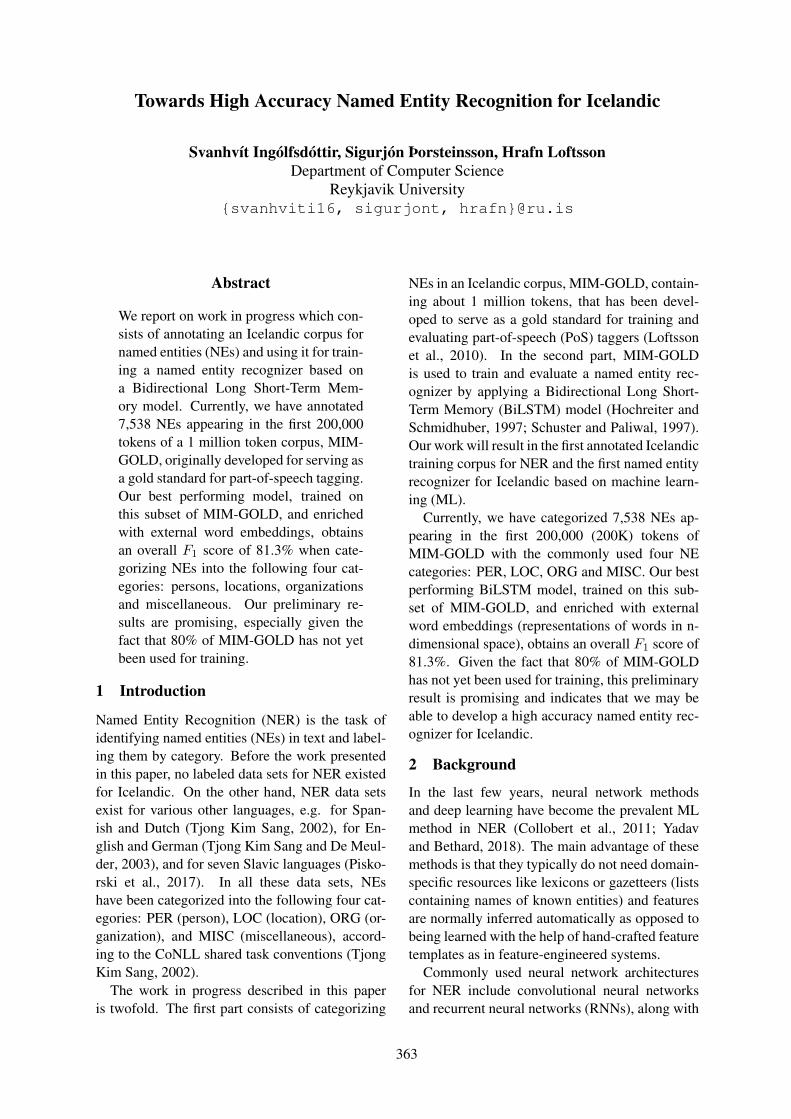
Towards High Accuracy Named Entity Recognition for Icelandic

Svanhvít Ingólfsdóttir, Sigurjón Þorsteinsson, Hrafn LoftssonDepartment of Computer Science

Reykjavik University{svanhviti16, sigurjont, hrafn}@ru.is

Abstract

We report on work in progress which con-sists of annotating an Icelandic corpus fornamed entities (NEs) and using it for train-ing a named entity recognizer based ona Bidirectional Long Short-Term Mem-ory model. Currently, we have annotated7,538 NEs appearing in the first 200,000tokens of a 1 million token corpus, MIM-GOLD, originally developed for serving asa gold standard for part-of-speech tagging.Our best performing model, trained onthis subset of MIM-GOLD, and enrichedwith external word embeddings, obtainsan overall F1 score of 81.3% when cate-gorizing NEs into the following four cat-egories: persons, locations, organizationsand miscellaneous. Our preliminary re-sults are promising, especially given thefact that 80% of MIM-GOLD has not yetbeen used for training.

1 Introduction

Named Entity Recognition (NER) is the task ofidentifying named entities (NEs) in text and label-ing them by category. Before the work presentedin this paper, no labeled data sets for NER existedfor Icelandic. On the other hand, NER data setsexist for various other languages, e.g. for Span-ish and Dutch (Tjong Kim Sang, 2002), for En-glish and German (Tjong Kim Sang and De Meul-der, 2003), and for seven Slavic languages (Pisko-rski et al., 2017). In all these data sets, NEshave been categorized into the following four cat-egories: PER (person), LOC (location), ORG (or-ganization), and MISC (miscellaneous), accord-ing to the CoNLL shared task conventions (TjongKim Sang, 2002).

The work in progress described in this paperis twofold. The first part consists of categorizing

NEs in an Icelandic corpus, MIM-GOLD, contain-ing about 1 million tokens, that has been devel-oped to serve as a gold standard for training andevaluating part-of-speech (PoS) taggers (Loftssonet al., 2010). In the second part, MIM-GOLDis used to train and evaluate a named entity rec-ognizer by applying a Bidirectional Long Short-Term Memory (BiLSTM) model (Hochreiter andSchmidhuber, 1997; Schuster and Paliwal, 1997).Our work will result in the first annotated Icelandictraining corpus for NER and the first named entityrecognizer for Icelandic based on machine learn-ing (ML).

Currently, we have categorized 7,538 NEs ap-pearing in the first 200,000 (200K) tokens ofMIM-GOLD with the commonly used four NEcategories: PER, LOC, ORG and MISC. Our bestperforming BiLSTM model, trained on this sub-set of MIM-GOLD, and enriched with externalword embeddings (representations of words in n-dimensional space), obtains an overall F1 score of81.3%. Given the fact that 80% of MIM-GOLDhas not yet been used for training, this preliminaryresult is promising and indicates that we may beable to develop a high accuracy named entity rec-ognizer for Icelandic.

2 Background

In the last few years, neural network methodsand deep learning have become the prevalent MLmethod in NER (Collobert et al., 2011; Yadavand Bethard, 2018). The main advantage of thesemethods is that they typically do not need domain-specific resources like lexicons or gazetteers (listscontaining names of known entities) and featuresare normally inferred automatically as opposed tobeing learned with the help of hand-crafted featuretemplates as in feature-engineered systems.

Commonly used neural network architecturesfor NER include convolutional neural networksand recurrent neural networks (RNNs), along with

363

other ML methods, such as conditional randomfields (Lafferty et al., 2001), which have been im-plemented as layers in neural network architec-tures (Lample et al., 2016) and used for NERtasks in under-resourced languages such as Persian(Poostchi et al., 2018).

Various studies show that pre-trained characterand word embeddings are beneficial for NER tasks(Demir and Özgür, 2014; Wu et al., 2015; Dernon-court et al., 2017). This is especially relevant formorphologically rich languages without large an-notated datasets, such as Icelandic, since they offera way to obtain subword information that cannotbe inferred from the training corpus alone (Laf-ferty et al., 2001). Word embeddings have alsobeen used to construct multilingual NER systemswith minimal human supervision (Al-Rfou et al.,2014).

2.1 NeuroNER

Neural networks can be complicated and challeng-ing to use, even for experts. NeuroNER (Dernon-court et al., 2017) is an easy-to-use tool for NERbased on a bidirectional RNN. An RNN is a neu-ral network that is specialized for processing a se-quence of values. A bidirectional RNN combinesan RNN that moves forward in a sequence withanother RNN that moves backward. The specifictype of a bidirectional RNN used in NeuroNERis a BiLSTM model, which is capable of learninglong-term dependencies.

The BiLSTM model in NeuroNER containsthree layers: 1) a character-enhanced word-embedding layer, 2) a label prediction layer, and3) a label sequence optimization layer (Dernon-court et al., 2016). The first layer maps each tokento a vector representation using two types of em-beddings: a word embedding and a character-leveltoken embedding. The resulting embeddings arethen fed into the second layer which outputs thesequence of vectors containing the probability ofeach label for each corresponding token. Finally,the last layer outputs the most likely sequence ofpredicted labels based on the output from the pre-vious label prediction layer.

Instead of implicitly learning the word embed-dings, NeuroNER allows users to provide theirown external (pre-trained) word embeddings (seeSection 4).

NeuroNER enables users to annotate a corpusfor NEs by interfacing with the web-based anno-

tation tool BRAT (Stenetorp et al., 2012), and usethe annotated corpus to train a named entity rec-ognizer.

2.2 NER for Icelandic

As mentioned in Section 1, no labeled Icelandicdata set for NER existed before our work started.Annotating a training corpus of a viable size forNER can be time-consuming task even if semi-automatic methods are used (Lample et al., 2016;Piskorski et al., 2017). Presumably, this is why noNER tools based on ML had been developed forIcelandic.

A rule-based named entity recognizer for Ice-landic, IceNER, is part of the IceNLP toolkit(Loftsson and Rögnvaldsson, 2007). It has beenreported to reach F1 score of 71.5% withoutquerying gazetteers, and 79.3% using a gazetteer(Tryggvason, 2009).

Greynir is an open-source NLP tool and web-site that parses sentences and extracts informa-tion from Icelandic news sites (Þorsteinsson et al.,2019). One of the features of Greynir is a rule-based named entity recognizer used to find and la-bel person names in the news texts. The accuracyof this named entity recognizer has not been eval-uated.

3 Developing the Training Corpus

The MIM-GOLD corpus is a balanced corpus of1 million tokens of Icelandic texts, written in2000-2010, from 13 different sources, includingnews texts, speeches from the Icelandic Parlia-ment, laws and adjucations, student essays, andvarious web content such as blogs and texts fromwebsites (Loftsson et al., 2010).1 The texts havebeen tokenized and automatically PoS-tagged us-ing the tagset developed for the Icelandic Fre-quency Dictionary corpus (Pind et al., 1991), withsubsequent manual corrections (Helgadóttir et al.,2014). Note that MIM-GOLD is tagged for propernouns, but does not contain any categorization ofthe proper nouns.

In order to reduce the work of categorizing Ice-landic proper nouns in MIM-GOLD, we gatheredofficial gazetteers of persons, organizations andplace names, and used them as input to an auto-matic pre-classification program. Thereafter, wemanually reviewed and corrected the results.

1Available for download from http://malfong.is

364

Category Count %

PER 3,045 40.4LOC 1,748 23.2ORG 1,768 23.4MISC 977 13.0Total 7,538 100.0

Table 1: Number of NEs in the 200K token train-ing corpus.

Foreign tokens in the MIM-GOLD are all as-signed the same tag with no further distinction,and since a large portion of them are NEs, theywere reviewed and classified manually.

To make the review and correction process moreefficient, we used the BRAT annotation tool (seeSection 2). We use the IOB (inside, outside, be-ginning) format as used in the CoNLL data sets(Tjong Kim Sang, 2002).

At the time of writing, we have categorized7,538 NEs appearing in the first 200K tokens ofMIM-GOLD with the commonly used four cate-gories: PER, LOC, ORG and MISC (see Table 1).

The annotated corpus was reviewed by a singlelinguist (first author), using the following defini-tions for each of the four categories:

• Persons: Names of humans and other beings,real or fictional, deities, pet names.

• Locations: Names of locations, real or fic-tional, i.e. buildings, street and place names,both real and fictional. All geographical andgeopolitical entities such as cities, countries,counties and regions, as well as planet namesand other outer space entities.

• Organizations: Icelandic and foreign com-panies and other organizations, public or pri-vate, real or fictional. Schools, churches,swimming pools, community centers, musi-cal groups, other affiliations.

• Miscellaneous: All other capitalized nounsand noun phrases, such as works of art, prod-ucts, events, printed materials, vessels andother named means of transportation, etc.

4 Training and Evaluation

The training corpus was arranged into two setsof different sizes, 100K and 200K tokens, eachsplit into training (80%), validation (10%) and test

W. embeddings Implicit ExternalCorpus size 100K 200K 100K 200K

PER 71.8 76.1 95.2 93.3LOC 61.8 65.6 81.8 85.6ORG 23.5 40.5 62.7 69.2MISC 3.2 28.3 14.8 41.5Overall 55.5 61.8 80.6 81.3

Table 2: F1 scores (%) of four different trainingconfigurations.

(10%) sets. Four different models were trainedand evaluated, for the two different training setsizes and for both implicitly and externally trainedword embeddings.

We pre-trained our own word embeddings of200 dimensions using about 543 million tokensfrom a large unlabelled corpus, the Icelandic Gi-gaword Corpus (Steingrímsson et al., 2018), usinga Word2Vec architecture (Mikolov et al., 2013).

All the parameters in NeuroNER’s configura-tion file, controlling the structure of the model,along with the hyperparameters directed towardsthe learning process, were left at their defaultvalues. The only exception to this is the to-ken_embedding_dimension parameter, controllingthe length of the word vectors. This value was in-creased from 100 to 200 for the external word em-beddings.

In the training, early stop was applied by defaultwhen no improvement had been seen on the vali-dation set for ten consecutive epochs. The modelused is based on the network weights taken fromthe epoch where the F1 score last peaked for thevalidation set.

Evaluation was done automatically by Neuro-NER according to CoNLL practices, which meansthat to score a true positive, both the NE categoryand the token boundaries need to be correct.

The F1 scores for the models of the four train-ing configurations, i.e. for the two training cor-pora sizes, with implicit and external word embed-dings, are shown in Table 2. The best performingmodel is the one trained on 200K tokens and usingexternal pre-trained word embeddings, achievingan overall F1 score of 81.3%.

5 Discussion

The results presented in Section 4 are promising,especially given the few NEs found in the 200Ktokens of the training corpus (see Table 1).

365

Table 2 shows that, using implicitly trainedword embeddings, the F1 score increases consid-erably when doubling the corpus size, i.e. from55.5% to 61.8%. This was to be expected, as thetraining set in the 100K token corpus only con-tains around 80K tokens, and has thus a very lim-ited number of NE examples to learn from. Whenfurther increasing the training corpus, we expectthis trend to continue.

However, a more effective approach to in-crease the accuracy proved to be incorporatingpre-trained word embeddings. In that case, theF1 score increases to 81.3% when using the 200Kcorpus. In what follows, we refer to this best per-forming model as 200K_External.

Most studies on the benefits of word embed-dings in NER tasks do not report more than a fewpercent points increase in F1 score by introduc-ing pre-trained word embeddings. Intuitively, wededuce that the main reason we are experiencingthis huge benefit of pre-trained word embeddingsis the small size of our training corpus. For a smalltraining set, the model will more often encounterunseen words in the test set. In our 200K cor-pus, 60% of the incorrectly labeled words had notbeen seen in the training set. When the large col-lection of word embeddings is added to the pool,the chances that a word is known increase substan-tially.

Another reason as to why word embeddingsfrom a large external corpus are so beneficial forour model may be the underlying language. Ice-landic, a morphologically rich language, presentsspecial challenges for various NLP tasks, suchas NER. Nouns, generally the building blocks ofNEs, have up to 16 unique inflectional forms, andverbs and adjectives can have over a hundred dif-ferent forms. This greatly increases the vocabu-lary size of a corpus, and causes a problem withdata sparsity, as pointed out by Demir and Özgür(2014), for the case of Turkish and Czech. The im-plication is that a NER system may not recognize aNE in the test set even if it has seen it in a differentform in the training set.2 We could try to lemma-tize the tokens in the training corpus and use thenormalized output for building the NER model,but then we would lose important contextual in-formation about the NEs and their neighbors. The

2For example, the Icelandic person name “Egill” (nom-inative) may be tagged as such in the training set and thenappear as “Egil” (accusative),“Agli” (dative), or “Egils” (gen-itive) in the test set.

pre-trained word embeddings contribute many ex-amples to the model of different word forms thatdo not appear in the training set, and the likelihoodof correctly labeling them increases as a result.

With a larger corpus, say by doubling it onceagain, we believe, from the trend, that the F1

score without external embeddings might end upbetween the earlier score (61.8%) and the one ob-tained by 200K_External (81.3%). On the otherhand, the results with pre-trained embeddings in-dicate a much slower increase in F1 score whenincreasing the size of the corpus (from 80.6% to81.3% when increasing the corpus size from 100Kto 200K). This might indicate that we are ap-proaching the upper limit with regard to the F1

score.NeuroNER has achieved 90.5% F1 score for

English on the CoNLL data set (Dernoncourtet al., 2017). This English data set contains 35,089NEs (Tjong Kim Sang and De Meulder, 2003)whereas our 200K Icelandic training corpus con-tains only 7,538 NEs. Therefore, we are optimisticthat increasing the training corpus size for Ice-landic will further increase the overall F1 score, al-beit we do not expect getting close to the score forEnglish, which is a morphologically simple lan-guage compared to Icelandic.

5.1 Accuracy for Different Categories

Table 2 shows a considerable difference in the ac-curacy of different categories. Especially promis-ing are the results for the PER category, with F1

score of 93.3% for 200K_External. The recallfor PER is high, 94.85%, which means that onlyabout 5% of the person names in the test set werenot identified. Several factors may explain the topperformance in this category. Most importantly,person names are by far the most frequent entitytype in the training corpus, almost double that ofthe LOC and ORG categories (see Table 1). Per-son names are often constructed in a similar man-ner, with Icelandic full names usually composed ofone or two given names and a surname ending in-son or -dóttir “daughter”. Furthermore, they arealmost always capitalized, and since they are notunique (many people can have the same name),each person name is bound to appear more oftenthan, for example, each organization name.

200K_External also performs quite well on theLOC category (85.6%). It is the nature of a corpussampled from any geographic area that some lo-

366

Predicted categoriesLOC MISC ORG PER O

LOC 161 3 11 8 5MISC 7 87 26 14 68ORG 19 6 174 4 21PER 0 3 1 568 16

O 1 46 33 12 19,245

Table 3: Confusion matrix for the classificationof the test set in 200K_External. True categoriesare shown vertically, predicted categories horizon-tally. The O category denotes “outside”, i.e. thatthe corresponding token is not a part of a NE.

cations appear more often than others, in this caseÍsland “Iceland” and Reykjavík, to name two of themost common. This means that during testing, thesystem is much more likely to label them correctly,because they are likely to have been found duringtraining. Another property of place names is thatthey tend to be single word entities, and are capi-talized, with a few exceptions. As a result, detect-ing word boundaries becomes less of a challenge.

The LOC and ORG categories are equally com-mon in the corpus, but the accuracy for ORG(69.2%) is significantly worse. In the ORG cat-egory, word boundaries are a problem, as orga-nizations are often composed of more than oneword, not necessarily capitalized, e.g. Sambandlífeyrisþega ríkis og bæja “Organization (of) pen-sioners (of) state and towns”. Furthermore, some-times it can be hard to decide whether an entityis an organization name or a product, which maycause overlap with the MISC category.

The MISC category was the most problematicone for 200K_External, with F1 score of only41.5%. Recall is particularly low (33.6%), mean-ing many MISC entities are not found, and preci-sion is not particularly high either (54.17%), thusmany entities are mislabeled.

The confusion matrix (see Table 3) from theclassification of the test set in 200K_Externalshows how many of the tokens in the test set werecorrectly labeled (the diagonal line running fromthe top left corner to the bottom right), and wheremislabeling occurs. The MISC category containsthe most outliers, with a total of 115 NEs misla-beled out of 202 in total. In the PER categoryonly 20 NEs out of 588 are mislabeled. Thereare only around 1000 MISC entities in the whole200K corpus, and a lot of variation in how they are

constructed, which makes detecting them harder,even for human annotators. Some are long book ormovie titles, some are complicated product nameswith numbers and hyphens, and there is no corre-lation within the category. This is the category thattends to score lowest in most NER models, but asubstantially larger corpus should lead to some im-provement.

6 Conclusion

We have described work in progress consisting ofannotating the MIM-GOLD corpus for NEs andusing it to train a named entity recognizer basedon a BiLSTM model. By only categorizing about20% of the NEs found in MIM-GOLD, the bestresulting model, enriched with external word em-beddings, achieves an overall F1 score of 81.3%.We are optimistic that we can further increase theF1 score for Icelandic by increasing the trainingcorpus size. Currently, the number of NEs foundin our training corpus (7,538) is only about 1/5of the training examples provided in the EnglishCoNLL data set.

In future work, we will continue categorizingNEs in MIM-GOLD, such that we will be ableto use 100% of the corpus to train NER mod-els for Icelandic. We are also working on addingcategories for numerical units, such as dates andprices. The annotated corpus will be publicly re-leased, in order to serve as a valuable asset for fur-ther research on NER for Icelandic. The resultingNER models will also be made available for publicuse.

In addition to further developing our BiLSTMmodel and testing different configurations, we in-tend to develop models based on other ML tech-niques, for the sake of comparison, as well as be-ing able to combine various different classifiers.

As mentioned in Section 2, different wordand character representations have shown promisewhen developing NER models. In this preliminarywork we used the Word2Vec architecture, whichresulted in a large improvement, but in the fu-ture we intend to measure how some of the otherword and character representation methods com-pare, e.g. contextual word embeddings such asELMo (Peters et al., 2018) and flair (Akbik et al.,2018).

367

ReferencesAlan Akbik, Duncan Blythe, and Roland Vollgraf.

2018. Contextual String Embeddings for SequenceLabeling. In Proceedings of the 27th InternationalConference on Computational Linguistics, COLING2018, Santa Fe, New Mexico, USA.

Rami Al-Rfou, Vivek Kulkarni, Bryan Perozzi, andSteven Skiena. 2014. POLYGLOT-NER: MassiveMultilingual Named Entity Recognition. CoRR,abs/1410.3791.

Ronan Collobert, Jason Weston, Léon Bottou, MichaelKarlen, Koray Kavukcuoglu, and Pavel Kuksa.2011. Natural language processing (almost) fromscratch. CoRR, abs/1103.0398.

Hakan Demir and Arzucan Özgür. 2014. Improv-ing Named Entity Recognition for MorphologicallyRich Languages Using Word Embeddings. In 13thInternational Conference on Machine Learning andApplications, Detroit, MI, USA.

Franck Dernoncourt, Ji Young Lee, and PeterSzolovits. 2017. NeuroNER: an easy-to-use pro-gram for named-entity recognition based on neuralnetworks. In Proceedings of the 2017 Conferenceon Empirical Methods in Natural Language Pro-cessing: System Demonstrations, Copenhagen, Den-mark.

Franck Dernoncourt, Ji Young Lee, Ozlem Uzuner,and Peter Szolovits. 2016. De-identification of pa-tient notes with recurrent neural networks. CoRR,abs/1606.03475.

Sigrún Helgadóttir, Hrafn Loftsson, and Eiríkur Rögn-valdsson. 2014. Correcting Errors in a New GoldStandard for Tagging Icelandic Text. In Proceedingsof the Ninth International Conference on LanguageResources and Evaluation, LREC 2014, Reykjavik,Iceland.

Sepp Hochreiter and Jürgen Schmidhuber. 1997.Long Short-Term Memory. Neural computation,9(8):1735–1780.

John D. Lafferty, Andrew McCallum, and FernandoC. N. Pereira. 2001. Conditional Random Fields:Probabilistic Models for Segmenting and Label-ing Sequence Data. In Proceedings of the Eigh-teenth International Conference on Machine Learn-ing, ICML 2001, Williamstown, MA, USA.

Guillaume Lample, Miguel Ballesteros, Sandeep Sub-ramanian, Kazuya Kawakami, and Chris Dyer. 2016.Neural Architectures for Named Entity Recognition.In Proceedings of the 2016 Conference of the NorthAmerican Chapter of the Association for Computa-tional Linguistics: Human Language Technologies,San Diego, California, USA.

Hrafn Loftsson and Eiríkur Rögnvaldsson. 2007.IceNLP: A Natural Language Processing Toolkit forIcelandic. In Proceedings of InterSpeech, Special

Session: Speech and language technology for less-resourced languages, Antwerp, Belgium.

Hrafn Loftsson, Jökull H. Yngvason, Sigrún Helgadót-tir, and Eiríkur Rögnvaldsson. 2010. Developing aPoS-tagged corpus using existing tools. In Proceed-ings of 7th SaLTMiL Workshop on Creation and Useof Basic Lexical Resources for Less-Resourced Lan-guages, LREC 2010, Valetta, Malta.

Tomas Mikolov, Kai Chen, Greg Corrado, and JeffreyDean. 2013. Efficient Estimation of Word Represen-tations in Vector Space. CoRR, abs/1301.3781.

Matthew E. Peters, Mark Neumann, Mohit Iyyer, MattGardner, Christopher Clark, Kenton Lee, and LukeZettlemoyer. 2018. Deep contextualized word rep-resentations. In Proceedings of the 2018 Confer-ence of the North American Chapter of the Associ-ation for Computational Linguistics: Human Lan-guage Technologies, Volume 1 (Long Papers), NewOrleans, Louisiana, USA.

Jörgen Pind, Friðrik Magnússon, and Stefán Briem.1991. Íslensk orðtíðnibók [The Icelandic FrequencyDictionary]. The Institute of Lexicography, Univer-sity of Iceland, Reykjavik, Iceland.

Jakub Piskorski, Lidia Pivovarova, Jan Šnajder, JosefSteinberger, and Roman Yangarber. 2017. The FirstCross-Lingual Challenge on Recognition, Normal-ization, and Matching of Named Entities in SlavicLanguages. In Proceedings of the 6th Workshop onBalto-Slavic Natural Language Processing, Valen-cia, Spain.

Hanieh Poostchi, Ehsan Zare Borzeshi, and MassimoPiccardi. 2018. BiLSTM-CRF for Persian Named-Entity Recognition ArmanPersoNERCorpus: theFirst Entity-Annotated Persian Dataset. In Proceed-ings of the Eleventh International Conference onLanguage Resources and Evaluation, LREC 2018,Miyazaki, Japan.

Mike Schuster and Kuldip. K. Paliwal. 1997. Bidirec-tional Recurrent Neural Networks. IEEE Transac-tions on Signal Processing, 45(11):2673–2681.

Steinþór Steingrímsson, Sigrún Helgadóttir, EiríkurRögnvaldsson, Starkaður Barkarson, and Jón Guð-nason. 2018. Risamálheild: A Very Large IcelandicText Corpus. In Proceedings of the Eleventh In-ternational Conference on Language Resources andEvaluation, LREC 2018, Miyazaki, Japan.

Pontus Stenetorp, Sampo Pyysalo, Goran Topic,Tomoko Ohta, Sophia Ananiadou, and Jun’ichi Tsu-jii. 2012. brat: a Web-based Tool for NLP-AssistedText Annotation. In Proceedings of the Demonstra-tions at the 13th Conference of the European Chap-ter of the Association for Computational Linguistics,Avignon, France.

Erik F. Tjong Kim Sang. 2002. Introduction to theCoNLL-2002 Shared Task: Language-Independent

368

Named Entity Recognition. In Proceedings ofCoNLL-2002, Taipei, Taiwan.

Erik F. Tjong Kim Sang and Fien De Meulder.2003. Introduction to the CoNLL-2003 SharedTask: Language-Independent Named Entity Recog-nition. In Proceedings of CoNLL-2003, Edmonton,Canada.

Aðalsteinn Tryggvason. 2009. Named Entity Recog-nition for Icelandic. Research report – ReykjavikUniversity.

Yonghui Wu, Jun Xu, Min Jiang, Yaoyun Zhang, andHua Xu. 2015. A Study of Neural Word Em-beddings for Named Entity Recognition in Clini-cal Text. AMIA Annual Symposium Proceedings,2015:1326–33.

Vikas Yadav and Steven Bethard. 2018. A Surveyon Recent Advances in Named Entity Recognitionfrom Deep Learning models. In Proceedings ofthe 27th International Conference on ComputationalLinguistics, COLING 2018, Santa Fe, New Mexico,USA.

Vilhjálmur Þorsteinsson, Hulda Óladóttir, and HrafnLoftsson. 2019. A Wide-Coverage Context-FreeGrammar for Icelandic and an Accompanying Pars-ing System. In Proceedings of Recent Advances inNatural Language Processing (to appear), RANLP2019, Varna, Bulgaria.

369

Neural Cross-Lingual Transfer and Limited Annotated Datafor Named Entity Recognition in Danish

Barbara PlankDepartment of Computer ScienceITU, IT University of Copenhagen

[email protected]

Abstract

Named Entity Recognition (NER) hasgreatly advanced by the introductionof deep neural architectures. How-ever, the success of these methodsdepends on large amounts of train-ing data. The scarcity of publicly-available human-labeled datasets hasresulted in limited evaluation of exist-ing NER systems, as is the case forDanish. This paper studies the effec-tiveness of cross-lingual transfer forDanish, evaluates its complementarityto limited gold data, and sheds light onperformance of Danish NER.

1 Introduction

Named entity recognition is a key step fornatural language understanding (NLU), andimportant for information extraction, relationextraction, question answering and even pri-vacy protection. However, the scarcity ofpublicly-available human annotated datasetshas resulted in a lack of evaluation for lan-guages beyond a selected set (e.g., those cov-ered in early shared tasks like Dutch, German,English, Spanish), despite the fact that NERtools exists or recently emerged for other lan-guages. One such case is Danish, for whichNER dates back as early as (Bick, 2004) andtools exist (Bick, 2004; Derczynski et al.,2014; Johannessen et al., 2005; Al-Rfou et al.,

2013) but lack empirical evaluation.Contemporarily, there exists a surge of in-

terest in porting NLU components quicklyand cheaply to new languages. This in-cludes cross-lingual transfer methods that ex-ploit resources from existing high-resourcelanguages for zero-shot or few-shot learning.This line of research is blooming, particularlysince the advent of neural NER, which holdsthe state of the art (Yadav and Bethard, 2018).However, neither neural tagging nor cross-lingual transfer has been explored for DanishNER, a gap we seek to fill in this paper.

Contributions We present a) publicly-available evaluation data to encourageresearch on Danish NER; b) an empiricalcomparison of two existing NER systems forDanish to a neural model; c) an empiricalevaluation of learning an effective NERtagger for Danish via cross-lingual transferpaired with very little labeled data.

2 Approach

We investigate the following questions: RQ1:To what extent can we transfer a NER taggerto Danish from existing English resources?RQ2: How does cross-lingual transfer com-pare to annotating a very small amount of in-language data (zero-shot vs few-shot learn-ing)? RQ3: How accurate are existing NERsystems for Danish?

370

2.1 NER annotation

To answer these questions, we need gold an-notated data. Access to existing resources islimited as they are not available online or be-hind a paywall. Therefore, we annotate NERson top of publicly available data.1

In line with limited budget for annotation(Garrette and Baldridge, 2013), we add an an-notation layer for Named Entities to the de-velopment and test sets of the Danish sec-tion of the Universal Dependencies (UD) tree-bank (Nivre et al., 2016; Johannsen et al.,2015). To answer RQ2, we further annotatea very small portion of the training data, i.e.,the first 5,000 and 10,000 tokens. Examplesare shown in Figure 1. Dataset statistics areprovided in Table 2.

The Danish UD treebank (Danish-DDT)is a conversion of the Copenhagen Depen-dency Treebank (CDT). CDT (Kromann et al.,2003) consists of 5,512 sentences and 100ktokens, originating from the PAROLE-DKproject (Bilgram and Keson, 1998). In con-trast to original CDT and the PAROLE to-kenization scheme, starting from the DanishUD has the advantage that it is closer to every-day language, as it splits tokens which wereoriginally joined (such as ‘i alt’).

We follow the CoNLL 2003 annotationguidelines (Tjong Kim Sang and De Meul-der, 2003) and annotate proper names of fourtypes: person (PER), location (LOC), orga-nization (ORG) and miscellaneous (MISC).MISC contains for example names of prod-ucts, drinks or film titles.

2.2 Cross-lingual transfer

We train a model on English (a medium andhigh resource setup, see details in Section 3)and transfer it to Danish, examining the fol-lowing setups.

1https://github.com/UniversalDependencies/UD_Danish-DDT

B-LOC O O O O O O ORom blev ikke bygget pa en dag .

O O O B-PER O O B-MISC I-MISCvinyl , som Elvis indspillede i Sun Records

Table 1: Example annotations.

Evaluation TrainingDEV TEST TINY SMALL

Sentences 564 565 272 604Tokens 10,332 10,023 4,669 10,069Types 3,640 3,424 1,918 3,525TTR 0.35 0.34 0.41 0.35Sent.w/ NE 220 226 96 206Sent.w/ NE% 39% 34% 35% 34%Entities 348 393 153 341

Table 2: Overview of the annotated DanishNER data. Around 35%-39% of the sentencescontain NEs. TTR: type-token ratio.

• Zero-shot: Direct transfer of the Englishmodel via aligned bilingual embeddings.• In-Language: Training the neural model

on very small amounts of in-languageDanish training data only. We test twosetups, training on the tiny data alone; orwith unsupervised transfer via word em-bedding initialization (+Poly).• Few-shot direct transfer: Training the

neural model on English and Danishjointly, including bilingual embeddings.• Few-shot fine-tuning: Training the neu-

ral model first on English, and fine-tuning it on Danish. This examineswhether fine-tuning is better than train-ing the model from scratch on both.

3 Experiments

As source data, we use the English CoNLL2003 NER dataset (Tjong Kim Sang andDe Meulder, 2003) with BIO tagging.

We study two setups for the source side:a MEDIUM and LARGE source data setup.For LARGE we use the entire CoNLL 2003

371

neural in-lang. neural transferTnT plain +Poly +MEDIUM src +LARGE src FINETUNE

zero-shot — — — 58.29 61.18 —

TINY 37.48 36.17 56.05 67.14 67.49 62.07SMALL 44.30 51.90 67.18 70.82 70.01 65.63

Table 3: F1 score on the development set for low-resource training setups (none, tiny 5k orsmall 10k labeled Danish sentences). Transfer via multilingual embeddings from MEDIUM

(3.2k sentences, 51k tokens) or LARGE English source data (14k sentences/203k tokens).

training data as starting point, which containsaround 14,000 sentences and 200,000 tokens.To emulate a lower-resource setup, we con-sider a MEDIUM setup, for which we employthe development data from CoNLL 2003 astraining data (3,250 sentences and 51,000 to-kens). The CoNLL data contains a high den-sity of entities (79-80% of the sentences) butis lexically less rich (TTR of 0.11-0.19), com-pared to our Danish annotated data (Table 2),which is orders of magnitudes smaller, lexicalricher but less dense on entities.

Model and Evaluation We train a bilstm-CRF similar to (Xie et al., 2018; Johnsonet al., 2019). As pre-trained word embed-dings we use the Polyglot embeddings (Al-Rfou et al., 2013). The word embeddingsdimensionality is 64. The remaining hyper-parameters were determined on the EnglishCoNLL data. The word LSTM size wasset to 50. Character embeddings are 50-dimensional. The character LSTM is 50 di-mensions. Dropout was set to 0.25. We useStochastic Gradient Descent with a learningrate of 0.1 and early stopping. We use theevaluation script from the CoNLL shared taskand report mean F1 score over three runs.

Cross-lingual mapping We map the exist-ing Danish Polyglot embeddings to the En-glish embedding space by using an unsu-pervised alignment method which does not

require parallel data. In particular, weuse character-identical words as seeds forthe Procrustes rotation method introduced inMUSE (Conneau et al., 2017).

4 Results

Table 3 presents the main results. There areseveral take-aways.

Cross-lingual transfer is powerful (RQ1).Zero-shot learning reaches an F1 score of 58%in the MEDIUM setup, which outperformstraining the neural tagger on very limited golddata (plain). Neural NER is better than tra-ditional HMM-based tagging (TnT) (Brants,2000) and greatly improves by unsupervisedword embedding initialization (+Poly). Itis noteworthy that zero-shot transfer benefitsonly to a limiting degree from more sourcedata (F1 increases by 3% when training on allEnglish CoNLL data).

To compare cross-lingual transfer to limitedgold data (RQ2), we observe that training theneural system on the small amount of data to-gether with Polyglot embeddings is close tothe tiny-shot transfer setup. Few-shot learninggreatly improves over zero-shot learning. Themost beneficial way is to add the target data tothe source, in comparison to fine-tuning. Thisshows that access to a tiny or small amount oftraining data is effective. Adding gold datawith cross-lingual transfer is the best setup.

372

DEV All PER LOC ORG MISC

Majority 44.8 61.8 0.0 0.0 —DKIE 55.4 65.7 58.5 20.3 —DKIE July 23 58.9 68.9 63.6 23.3Polyglot 64.5 73.7 73.4 36.8 —Ours 70.8 83.3 71.8 60.0 23.9

TEST All PER LOC ORG MISCPolyglot 61.6 78.4 69.7 24.7 —Ours 66.0 86.6 63.6 42.5 24.8

Table 4: F1 score on the Danish dev set.

In both MEDIUM and LARGE setups are fur-ther gains obtained by adding TINY or SMALL

amounts of Danish gold data. Interestingly, a)fine-tuning is less effective; b) it is better totransfer from a medium-sized setup than fromthe entire CoNLL source data.

Existing systems (RQ3) perform poorly(Table 4). Polyglot (Al-Rfou et al., 2013) isbetter than DKIE (Derczynski et al., 2014).Our best system is a cross-lingual transferNER from MEDIUM source data paired withSMALL amounts of gold data. Per-Entityevaluation shows that ours outperforms Poly-glot except for Location, which is consistentacross evaluation data (Table 4). Overall wefind that very little data paired with dense rep-resentations yields an effective NER quickly.

5 Related Work

Named Entity Recognition has a long historyin NLP research. While interest in NER origi-nally arose mostly from a question answeringperspective, it developed into an independenttask through the pioneering shared task orga-nized by the Message Understanding Confer-ence (MUC) (Grishman and Sundheim, 1996;Grishman, 1998). Since then, many sharedtask for NER have been organized, includ-ing CoNLL (Tjong Kim Sang and De Meul-der, 2003) for newswire and WNUT for so-cial media data (Baldwin et al., 2015). While

Danish NER tools and data exists (Bick, 2004;Derczynski et al., 2014; Johannessen et al.,2005; Al-Rfou et al., 2013), there was alack of reporting F1 scores. Supersense tag-ging, a task close to NER has received atten-tion (Martınez Alonso et al., 2015).

The range of methods that have been pro-posed for NER is broad. Early methodsfocused on hand-crated rule-based methodswith lexicons and orthographic features. Theywere followed by feature-engineering richstatistical approaches (Nadeau and Sekine,2007). Since the advent of deep learning andthe seminal work by (Collobert et al., 2011),state-of-the-art NER systems typically rely onfeature-inferring encoder-decoder models thatextract dense embeddings from word and sub-word embeddings, including affixes (Yadavand Bethard, 2018), often outperforming neu-ral architectures that include lexicon informa-tion such as gazetteers.

Recently, there has been a surge of interestin cross-lingual transfer of NER models (Xieet al., 2018). This includes work on trans-fer between distant languages (Rahimi et al.,2019) and work on projecting from multiplesource languages (Johnson et al., 2019).

6 Conclusions

We contribute to the transfer learning litera-ture by providing a first study on the effec-tiveness of exploiting English NER data toboost Danish NER performance.2 We pre-sented a publicly-available evaluation datasetand compare our neural cross-lingual Dan-ish NER tagger to existing systems. Our ex-periments show that a very small amount ofin-language NER data pushes cross-lingualtransfer, resulting in an effective Danish NERsystem.

2Available at: https://github.com/ITUnlp/transfer_ner

373

Acknowledgements

We kindly acknowledge the support ofNVIDIA Corporation for the donation of theGPUs and Amazon for an Amazon ResearchAward.

ReferencesRami Al-Rfou, Bryan Perozzi, and Steven Skiena.

2013. Polyglot: Distributed word representa-tions for multilingual NLP. In ACL.

Timothy Baldwin, Marie-Catherine de Marneffe,Bo Han, Young-Bum Kim, Alan Ritter, andWei Xu. 2015. Shared tasks of the 2015 work-shop on noisy user-generated text: Twitter lexi-cal normalization and named entity recognition.In Proceedings of the Workshop on Noisy User-generated Text, pages 126–135.

Eckhard Bick. 2004. A named entity recognizerfor danish. In LREC.

Thomas Bilgram and Britt Keson. 1998. The con-struction of a tagged danish corpus. In Proceed-ings of the 11th Nordic Conference of Compu-tational Linguistics (NODALIDA 1998), pages129–139.

Thorsten Brants. 2000. Tnt: a statistical part-of-speech tagger. In Proceedings of the sixth con-ference on Applied natural language process-ing, pages 224–231. Association for Computa-tional Linguistics.

Ronan Collobert, Jason Weston, Leon Bottou,Michael Karlen, Koray Kavukcuoglu, and PavelKuksa. 2011. Natural language processing (al-most) from scratch. Journal of machine learn-ing research, 12(Aug):2493–2537.

Alexis Conneau, Guillaume Lample,Marc’Aurelio Ranzato, Ludovic Denoyer, andHerve Jegou. 2017. Word translation withoutparallel data. arXiv preprint arXiv:1710.04087.

Leon Derczynski, Camilla Vilhelmsen Field, andKenneth S Bøgh. 2014. Dkie: Open source in-formation extraction for danish. In Proceedingsof the Demonstrations at the 14th Conferenceof the European Chapter of the Association forComputational Linguistics, pages 61–64.

Dan Garrette and Jason Baldridge. 2013. Learn-ing a part-of-speech tagger from two hours ofannotation. In Proceedings of the 2013 Con-ference of the North American Chapter of theAssociation for Computational Linguistics: Hu-man Language Technologies, pages 138–147.

Ralph Grishman. 1998. Research in informationextraction: 1996-98. In Proceedings of theTIPSTER Text Program: Phase III, pages 57–60, Baltimore, Maryland, USA. Association forComputational Linguistics.

Ralph Grishman and Beth Sundheim. 1996. Mes-sage understanding conference- 6: A brief his-tory. In COLING 1996 Volume 1: The 16th In-ternational Conference on Computational Lin-guistics.

Janne Bondi Johannessen, Kristin Hagen, AsneHaaland, Andra Bjork Jonsdottir, AndersNøklestad, Dimitris Kokkinakis, Paul Meurer,Eckhard Bick, and Dorte Haltrup. 2005.Named entity recognition for the mainlandscandinavian languages. Literary and Linguis-tic Computing, 20(1):91–102.

Anders Johannsen, Hector Martınez Alonso, andBarbara Plank. 2015. Universal dependenciesfor danish. In International Workshop on Tree-banks and Linguistic Theories (TLT14), page157.

Andrew Johnson, Penny Karanasou, JudithGaspers, and Dietrich Klakow. 2019. Cross-lingual transfer learning for Japanese named en-tity recognition. In Proceedings of the 2019Conference of the North American Chapter ofthe Association for Computational Linguistics:Human Language Technologies, Volume 2 (In-dustry Papers), Minneapolis - Minnesota. As-sociation for Computational Linguistics.

Matthias T Kromann, Line Mikkelsen, andStine Kern Lynge. 2003. Danish dependencytreebank. In Proc. TLT, pages 217–220. Cite-seer.

Hector Martınez Alonso, Anders Johannsen, SussiOlsen, Sanni Nimb, Nicolai Hartvig Sørensen,Anna Braasch, Anders Søgaard, and BoletteSandford Pedersen. 2015. Supersense tag-ging for Danish. In Proceedings of the 20thNordic Conference of Computational Linguis-tics (NODALIDA 2015), Vilnius, Lithuania.

374

Linkoping University Electronic Press, Swe-den.

David Nadeau and Satoshi Sekine. 2007. A surveyof named entity recognition and classification.Lingvisticae Investigationes, 30(1):3–26.

Joakim Nivre, Marie-Catherine De Marneffe, FilipGinter, Yoav Goldberg, Jan Hajic, Christo-pher D Manning, Ryan McDonald, Slav Petrov,Sampo Pyysalo, Natalia Silveira, et al. 2016.Universal dependencies v1: A multilingualtreebank collection. In Proceedings of theTenth International Conference on LanguageResources and Evaluation (LREC 2016), pages1659–1666.

Afshin Rahimi, Yuan Li, and Trevor Cohn. 2019.Multilingual ner transfer for low-resource lan-guages. In Proceedings of the 2019 Conferenceof the Chapter of the Association for Computa-tional Linguistics.

Erik F Tjong Kim Sang and Fien De Meul-der. 2003. Introduction to the conll-2003shared task: Language-independent named en-tity recognition. arXiv preprint cs/0306050.

Jiateng Xie, Zhilin Yang, Graham Neubig,Noah A Smith, and Jaime Carbonell. 2018.Neural cross-lingual named entity recogni-tion with minimal resources. arXiv preprintarXiv:1808.09861.

Vikas Yadav and Steven Bethard. 2018. A surveyon recent advances in named entity recognitionfrom deep learning models. In Proceedings ofthe 27th International Conference on Computa-tional Linguistics, pages 2145–2158.

375

The Seemingly (Un)systematic Linking Element in Danish

Sidsel Boldsen and Manex AgirrezabalCentre for Language Technology

University of Copenhagen{sbol,manex.aguirrezabal}@hum.ku.dk

Abstract

The use of a linking element betweencompound members is a common phe-nomenon in Germanic languages. Still,the exact use and conditioning of suchelements is a disputed topic in linguis-tics. In this paper we address the issueof predicting the use of linking elementsin Danish. Following previous researchthat shows how the choice of linking el-ement might be conditioned by phonol-ogy, we frame the problem as a languagemodeling task: Considering the linking el-ements -s/-∅ the problem becomes pre-dicting what is most probable to encounternext, a syllable boundary or the joining el-ement, s. We show that training a lan-guage model on this task reaches an ac-curacy of 94 %, and in the case of anunsupervised model, the accuracy reaches80 %.

1 Introduction

In Danish, Norwegian and Swedish, as well asin other Germanic languages, a common way offorming new words is by compounding. Here,novel words can be formed by combining alreadyknown words with an addition of a linking ele-ment between the components. Within linguis-tic research this linking element is somewhat ofa puzzle: First of all, several languages withinthe Germanic family seem to share similar link-ing elements (Fuhrhop and Kurschner, 2014). Theorigin of these elements are however disputed(Nubling and Szczepaniak, 2013). Even if we as-sume a common origin, the use and distributionof single elements have changed among daugh-ter languages, and we often find contradicting ex-amples e.g., when comparing Ge. Volk-s-musikand Da. folk-e-musik ’folk music’ (Fuhrhop and

Kurschner, 2014). Secondly, even though thechoice of a linking element may be clear to theindividual speaker, linguists still struggle to es-tablish rules for when the individual elements oc-cur. In Danish, the linking element is decidedfrom the first member of a compound. But whenlooking for rules that systematize what wordstake which element, only few guidelines are given(Hansen and Heltoft, 2011). Interestingly, recentstudies on linking elements in German suggestthat the choice of linking element is at least par-tially phonological, determined by features suchas stress (Nubling and Szczepaniak, 2013).

Compounding has received attention in lan-guage technology as well, since it is the essenceof one of the main challenges within this field:that language is productive. Within the area of sta-tistical machine translation, segmentation of com-pounds into units is an important task, e.g., whentranslating compound words from German to En-glish where compounding is not productive (Saget al., 2002). Similarly, when translating En-glish multiword expressions (MWE) into German,methods for synthesis or generation of compoundsare called for (Stymne et al., 2013). Here thechoice of a correct linking element becomes anissue. In the work by Cap and Fraser (2014)they rely on a rule-based morphological analyzerfor German to generate the correct compoundingform. Here they report that on a reference set of283 correctly identified compounds 44 had an in-correct linking element. Recent work by Matthewset al. (2016) proposes a translation model from En-glish MWE to German compounds that allows formodeling linking elements. In their work, theyreport a high recall score when generating novelcompounds. Their error analysis show that theirmodel has issues when choosing linking elements(e.g., when generating Kirchenturme instead of thecorrect Kirchturme ’church towers’), but they donot further provide any metrics on this subtask.

376

In this paper we wish to see how well a sim-ple character-based language model is able to pre-dict the usage of linking elements in Danish. Morespecifically we will look at the case of predictingoccurrence of two elements -s and -∅ (tradition-ally referred to as a nulfuge ’zero link’) in Danishnoun-noun compounds.

2 The linking element in Danish

In Danish, a compound is formed by attaching alinking element to the stem of its first member.Table 1 shows a list of the most common link-ing elements. The choice of linking element ina compound is determined by the first member.While most nouns only have one possible link-ing element, we do find alternation: First of all,a noun may have more competing elements thatare used in connection with certain second mem-bers. An example is the noun bad ’boat’ to whichdifferent elements can be attached depending onthe compound (bad-skat ’boat tax’, but bad-e-byggeri ’boat building’). Secondly, some nounshave alternating linking elements that can be usedinterchangeably as in aluminium(s)rør ’aluminumtube’.

Hansen & Heltoft (2011) present rules only forcases where the linking element -s is used: Usu-ally an -s occurs when the first member is a com-pound, but many exceptions can be added to thisrule. Moreover, words derived with the suffixes-(n)ing, -ion, and -tek always get an -s.

LE Example-s idræt idrætsdag ’sports day’-∅ ankel ankelled ’ancle joint’-e mælk mælkepulver ’milk powder’-er student studenterhue ’graduation hat’-n rose rosenbed ’rose bed’

Table 1: Linking elements (LE) in Danish. Theelements above the separator are considered pro-ductive while the elements below are only foundin isolated forms (Hansen and Heltoft, 2011).

In some dialects the use of -s is preferred in-stead of the unmarked -∅ in some cases. Thiscould suggest that phonology does play a role inthe choice of linking element as was also proposedby Nubling and Szczepaniak (2013) in the case ofGerman. Following this suggestion, we focus onthe two linking elements -s and -∅ in order to ex-plore how well the choice between these elements

can be predicted using a character-based languagemodel.

3 The task

We formulate the problem of determining the cor-rect linking element of a noun as a language mod-eling task over the characters of a word: Given aword as a sequence of characters, what is the mostprobable element to come next, assuming that theword continues? Thus, when trying to determinewhether a noun should take -s or -∅, the problembecomes to estimate what would be most probableto observe next: an s or a syllable boundary?

The intuition behind this approach is, assumingthat some underlying phonological process gov-erns the choice of linking elements, then, learningthe distribution over the sounds or characters ofa word (including the two linking elements—thesound s and a syllable boundary), will help us topredict what element will occur as the linking ele-ment of the first member of a compound.Data The dataset that we use for the task isRetskrivningsordbogen (RO) (Jervelund, 2012),which is the main source for official orthographyin Danish with over 61, 000 entries in total. In RO,all words are marked with syllable boundaries (in-dicated by a + in the text string) and informationon what linking element(s) the word takes as a firstmember of a compound. From RO we extract thesyllabified forms of nouns with linking element -s/-∅ (excluding nouns with alternate linking ele-ments), providing us with a dataset of 6,880 in-stances of nouns and linking elements.

4 Experiments

We introduce two models to approach the problemand two baselines from which we make our con-clusions. First, we investigated whether character-based language models would be able to estimatethe correct linking element of a word. To this end,we trained a language model on syllabified wordstogether with their linking element (s/+). Sec-ond, we approached the problem in an unsuper-vised manner, training a general language modelon syllabified words, without providing any spe-cific information on linking elements.

In both experiments the models are evaluatedas a prediction task on how well they are ableto predict the correct linking element of a wordby weighing the estimated probabilities of observ-ing an s or a syllable boundary (+) in the end of

377

Training objective Input Training signal Prediction task Correct answerLanguage model, unsupervised î+dræt P (s) > P (+)? TrueLanguage model, unsupervised ân+kel P (s) > P (+)? FalseLanguage model, supervised î+dræt$ s P (s) > P (+)? TrueLanguage model, supervised ân+kel$ + P (s) > P (+)? False

Table 2: Examples of input, training signals and prediction task for the supervised and unsupervisedapproaches. Adapted from (Linzen et al., 2016).

a word. In order to validate the performance ofour models, we employ 5-Fold Cross-Validationon the set of -s/-∅ nouns from RO. For each it-eration, we train a model with four folds and wedivide the remaining fold equally for developmentand test.

4.1 Experiment 1: Supervised approach

In the first experiment, we train a character-basedRecurrent Neural Network (RNN) language modelon the entire set of -s/-∅ nouns from RO, includingthe linking element at the end of each instance.

We use a two-layer RNN with LSTM that re-ceives an embedded representation of the charac-ters with 128 dimensions, which are learned whiletraining. Each LSTM layer has 64 dimensions andpredictions are made using a softmax over the vo-cabulary of characters. We train the model usingStochastic Gradient Descent with cyclical learn-ing rate (Smith, 2015) using the DyNet framework(Neubig et al., 2017).

As Table 2 shows, besides a beginning-of-wordsymbol (ˆ), we also add an end-of-word symbol(EOW) ($) to the input. We expect that this ad-dition will improve the performance of the model,as it helps to supervise the training signal moreclearly by restricting the distribution of s and +as compounding elements to occur only after theEOW symbol. However, this approach also addsnoise to the signal as the original sequence of char-acters is altered.

4.2 Experiment 2: Unsupervised approach

In the second experiment, we train an RNN iden-tical to that in the first experiment, but withoutincluding any specific information on linking el-ements. Thus, at test time, this model has not beentrained on nouns and linking elements, but wouldestimate the probabilities, P (s) and P (+), fromthe distribution of s and + word-internally. Themodel is trained on the words from RO that arenot included within the set of -s/-∅ nouns. The

difference between the two models is summarizedin Table 2.

4.3 Baseline

For each of the experiments we create two base-lines. The first baseline common to both experi-ments chooses the most frequent linking elementfrom the dataset. In the supervised approach, thismeans choosing the most frequent label from thetraining set. In the unsupervised case, this corre-sponds to the most frequent character (as it doesnot have access to labeled examples). In the sec-ond baseline we create an iterative back-off modelthat attempts to match the input word with alreadyobserved sequences of syllables from the trainingset.

For the supervised model, the reason that wecreate this baseline is because we know the rimeof a word may be predictive for the choice of link-ing element. Thus, the back-off model starts bytrying to retrieve the whole word in order to testif this was observed during training. If not, it willtry to match iteratively shorter sequences of sylla-bles until a matching rime is found. If a match isfound the most frequent case of linking element ispredicted. If no match is encountered, the modelwill back-off to the most frequent strategy.

The back-off model in the unsupervised case issimilar. Here, the only difference is that we do notlook for rimes, but all of the possible continuoussubsequences of syllables. This is done in order totest how well a model performs in determining thejoining element by remembering exact sequencesof possible syllables word internally.

5 Results

The results from the two experiments are pre-sented in Table 3. Starting with the results fromExperiment 1 using the supervised approach, wesee that the supervised LM reaches 0.94 for bothaccuracy and f1, which is higher than both ofthe baselines we provided. Looking more closely

378

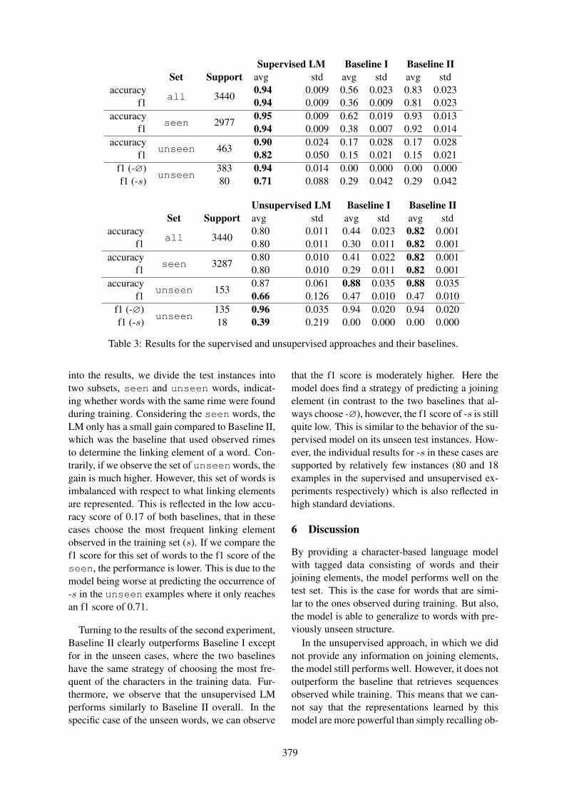
Set SupportSupervised LM Baseline I Baseline II

avg std avg std avg stdaccuracy

all 34400.94 0.009 0.56 0.023 0.83 0.023

f1 0.94 0.009 0.36 0.009 0.81 0.023accuracy

seen 29770.95 0.009 0.62 0.019 0.93 0.013

f1 0.94 0.009 0.38 0.007 0.92 0.014accuracy

unseen 4630.90 0.024 0.17 0.028 0.17 0.028

f1 0.82 0.050 0.15 0.021 0.15 0.021f1 (-∅)

unseen383 0.94 0.014 0.00 0.000 0.00 0.000

f1 (-s) 80 0.71 0.088 0.29 0.042 0.29 0.042

Set SupportUnsupervised LM Baseline I Baseline IIavg std avg std avg std

accuracyall 3440

0.80 0.011 0.44 0.023 0.82 0.001f1 0.80 0.011 0.30 0.011 0.82 0.001

accuracyseen 3287

0.80 0.010 0.41 0.022 0.82 0.001f1 0.80 0.010 0.29 0.011 0.82 0.001

accuracyunseen 153

0.87 0.061 0.88 0.035 0.88 0.035f1 0.66 0.126 0.47 0.010 0.47 0.010

f1 (-∅)unseen

135 0.96 0.035 0.94 0.020 0.94 0.020f1 (-s) 18 0.39 0.219 0.00 0.000 0.00 0.000

Table 3: Results for the supervised and unsupervised approaches and their baselines.

into the results, we divide the test instances intotwo subsets, seen and unseen words, indicat-ing whether words with the same rime were foundduring training. Considering the seen words, theLM only has a small gain compared to Baseline II,which was the baseline that used observed rimesto determine the linking element of a word. Con-trarily, if we observe the set of unseenwords, thegain is much higher. However, this set of words isimbalanced with respect to what linking elementsare represented. This is reflected in the low accu-racy score of 0.17 of both baselines, that in thesecases choose the most frequent linking elementobserved in the training set (s). If we compare thef1 score for this set of words to the f1 score of theseen, the performance is lower. This is due to themodel being worse at predicting the occurrence of-s in the unseen examples where it only reachesan f1 score of 0.71.

Turning to the results of the second experiment,Baseline II clearly outperforms Baseline I exceptfor in the unseen cases, where the two baselineshave the same strategy of choosing the most fre-quent of the characters in the training data. Fur-thermore, we observe that the unsupervised LMperforms similarly to Baseline II overall. In thespecific case of the unseen words, we can observe

that the f1 score is moderately higher. Here themodel does find a strategy of predicting a joiningelement (in contrast to the two baselines that al-ways choose -∅), however, the f1 score of -s is stillquite low. This is similar to the behavior of the su-pervised model on its unseen test instances. How-ever, the individual results for -s in these cases aresupported by relatively few instances (80 and 18examples in the supervised and unsupervised ex-periments respectively) which is also reflected inhigh standard deviations.

6 Discussion

By providing a character-based language modelwith tagged data consisting of words and theirjoining elements, the model performs well on thetest set. This is the case for words that are simi-lar to the ones observed during training. But also,the model is able to generalize to words with pre-viously unseen structure.

In the unsupervised approach, in which we didnot provide any information on joining elements,the model still performs well. However, it does notoutperform the baseline that retrieves sequencesobserved while training. This means that we can-not say that the representations learned by thismodel are more powerful than simply recalling ob-

379

served sequences. Nevertheless, the model is ableto predict the joining element in some cases of un-seen rimes.

7 Conclusion & future work

In this paper we approached the issue of predictingthe linking element of Danish -s/-∅ compoundsusing a character-based language model. Whenusing a language model trained of examples ofwords and linking elements, we reach an accuracyof 94 %. Using a language model that has neverseen tagged examples reaches an accuracy of 80 %on the same task. These are promising results, butwe need further error analysis to better understandthe examples in which language modeling is strug-gling to identify the correct elements.

To pursue the approach of language model-ing further, one future line of work would be toadd more information to the training signal. Asmentioned in the introduction, features such asstress may be an important factor in the phonolog-ical processes determining what linking elementis chosen. Such information is not immediatelyapparent using the orthographic representation ofa word as was used in this experiment. In thisrespect, it would be interesting to see how themodels perform using phonetic transcriptions in-stead. Since such transcription is expensive, onecould try to construct this level using grapheme-to-phoneme conversion software. As an alterna-tive one could also attempt to reproduce the ex-periment using speech data.

In this paper we used a dictionary of words astraining corpus. An alternative would be to use acollection of text in which information about wordfrequency would be included. This, in turn, mightresult in a different model that would be interest-ing to compare to the one presented above.

Furthermore, it would be interesting to see howwell this approach is able to predict other linkingelements in Danish, as well as in other languages.

Acknowledgments

The first author is supported by the project Scriptand Text in Time and Space, a core group projectsupported by the Velux Foundations. We are grate-ful to Patrizia Paggio for her support and com-ments regarding this paper. We would also liketo acknowledge the anonymous reviewers for theirsuggestions and comments.

ReferencesFabienne Cap, Alexander Fraser, Marion Weller, and

Aoife Cahill. 2014. How to produce unseen teddybears: Improved morphological processing of com-pounds in SMT. In Proceedings of the 14th Confer-ence of the European Chapter of the Association forComputational Linguistics, pages 579–587, Gothen-burg, Sweden. Association for Computational Lin-guistics.

Nanna Fuhrhop and Sebastian Kurschner. 2014. Link-ing elements in Germanic. In Susan OlsenFranz Rainer Peter O. Muller, Ingeborg Ohnheiser,editor, Word formation. An international hand-book of the languages of Europe, HSK 40/1, page568–582. de Gruyter Mouton, Berlin/New York.

Erik Hansen and Lars Heltoft. 2011. Grammatik overdet Danske Sprog, 1 edition, volume 1-3. SyddanskUniversitetsforlag.

Anita Agerup Jervelund. 2012. Retskrivningsordbo-gen, 4. udg. edition. Alinea, København.

Tal Linzen, Emmanuel Dupoux, and Yoav Goldberg.2016. Assessing the ability of LSTMs to learnsyntax-sensitive dependencies. Transactions of theAssociation for Computational Linguistics, 4:521–535.

Austin Matthews, Eva Schlinger, Alon Lavie, and ChrisDyer. 2016. Synthesizing compound words for ma-chine translation. In Proceedings of the 54th An-nual Meeting of the Association for ComputationalLinguistics (Volume 1: Long Papers), pages 1085–1094, Berlin, Germany. Association for Computa-tional Linguistics.

Graham Neubig, Chris Dyer, Yoav Goldberg, AustinMatthews, Waleed Ammar, Antonios Anastasopou-los, Miguel Ballesteros, David Chiang, DanielClothiaux, Trevor Cohn, et al. 2017. Dynet: Thedynamic neural network toolkit. arXiv preprintarXiv:1701.03980.

Damaris Nubling and Renata Szczepaniak. 2013.Linking elements in german origin, change, func-tionalization. Morphology, 23(1):67–89.

Ivan A. Sag, Timothy Baldwin, Francis Bond, AnnCopestake, and Dan Flickinger. 2002. Multiwordexpressions: A pain in the neck for nlp. In Com-putational Linguistics and Intelligent Text Process-ing, pages 1–15, Berlin, Heidelberg. Springer BerlinHeidelberg.

Leslie N Smith. 2015. ’cyclical learning rates fortraining neural networks’, cite. arXiv preprintarxiv:1506.01186.

Sara Stymne, Nicola Cancedda, and Lars Ahrenberg.2013. Generation of compound words in statisticalmachine translation into compounding languages.Computational Linguistics, 39(4):1067–1108.

380

Demo Papers

LEGATO: A flexible lexicographic annotation tool

David AlfterSpråkbanken

Department of SwedishUniversity of Gothenburg

[email protected]

Therese Lindström TiedemannDepartment of Finnish, Finno-Ugrian

and Scandinavian StudiesUniversity of Helsinki

Finland

[email protected]

Elena VolodinaSpråkbanken

Department of SwedishUniversity of Gothenburg

[email protected]

Abstract

This article reports an ongoing projectaimed at analyzing lexical and grammat-ical competences of Swedish as a Secondlanguage (L2). To facilitate lexical anal-ysis, we need access to linguistic infor-mation about relevant vocabulary that L2learners can use and understand. The fo-cus of the current article is on the lexicalannotation of the vocabulary scope for arange of lexicographical aspects, such asmorphological analysis, valency, types ofmulti-word units, etc. We perform parts ofthe analysis automatically, and other partsmanually. The rationale behind this is thatwhere there is no possibility to add infor-mation automatically, manual effort needsto be added. To facilitate the latter, atool LEGATO has been designed, imple-mented and currently put to active testing.

1 Introduction

Lexical competence has been acknowledged asone of the most important aspects of languagelearning (e.g. Singleton, 1995; Milton, 2013;Laufer and Sim, 1985). Some claim that weneed to understand 95–98% of the words in atext to manage reading comprehension tasks (cf.Laufer and Ravenhorst-Kalovski, 2010; Nation,2006; Hsueh-Chao and Nation, 2000). It has alsobeen observed that vocabulary is actively taughtat all levels of L2 proficiency courses with a ten-dency to be dominating at more advanced levelsin comparison to other linguistic skills, see for ex-ample findings from a course book corpus COC-TAILL (Volodina et al., 2014, p.140). Lexical fea-tures have also been found to be one of the bestpredictors in text classification studies (e.g. Pilánand Volodina, 2018; Xia et al., 2016; Vajjala andMeurers, 2012) with important implications to the

area of educational NLP. Deciding on which vo-cabulary to use and include is thus an importantpart of teaching a foreign language, in designingcourse materials and tests. In theoretical descrip-tions of L2 acquisition, lexical knowledge waspreviously "side-lined" according to Milton, butwithin academic circles its place has been "signifi-cantly revised" and received an increasing amountof interest over recent decades (Milton, 2013).

There are multiple characteristics of vocabu-lary that are interesting from the point of viewof both theoretical analyses, as well as for peda-gogical and NLP-based applications. Such char-acteristics include, among others, vocabulary size& breadth (e.g. Nation and Meara, 2010; Milton,2013), corpus frequency (Dürlich and François,2018; François et al., 2016), word family relations(Bauer and Nation, 1993), syllable structure, mor-phological characteristics, semantic relations, top-ical domain categorization (Alfter and Volodina,2018), and many others (e.g. Capel, 2010, 2012).

While frequency information comes from cor-pora, most linguistic characteristics are non-trivialto acquire by automatic methods and require ei-ther manual effort or access to manually preparedresources – lexicons being the most extensive andreliable sources for that. However, dictionariesand lexicons are often proprietary resources (e.g.Sköldberg et al., 2019), which complicates auto-matic lexicon enrichment. Among freely avail-able lexicons for Swedish, we can name Saldo(Borin et al., 2013), Swesaurus (Borin and Fors-berg, 2014), Lexin (Hult et al., 2010) and a fewother resources provided through Språkbanken’sinfrastructure Karp (Borin et al., 2012), although,even there many aspects of vocabulary are not doc-umented, e.g. the transitivity of verbs, the mor-phological structure of the words (root, prefix, suf-fix) or the topical domain of the words.

To circumvent the problem of access to the in-formation that may prove crucial in the context

382

of the current project for the three outlined ar-eas of application (theoretical studies, pedagogicalstudies/applied linguistics and educational NLP),we have initiated semi-automatic annotation oflearner-relevant vocabulary interlinking availableresources with manual controls of those, andadding missing aspects manually. The work is on-going, and below we present the reasoning aroundthis annotation process and the main componentsof the system that facilitate that.

2 Second language profiles project

In the current project, Development of lexical andgrammatical competences in immigrant Swedishfunded by Riksbankens Jubileumsfond, the mainaim is to provide an extensive description of thelexical and grammatical competence learners ofL2 Swedish possess at each CEFR1 level, and toexplore the relation between the receptive and pro-ductive scopes. The exploration of the grammat-ical and lexical aspects of L2 proficiency is per-formed based on two corpora, COCTAILL (Volo-dina et al., 2014), a corpus of course books used inteaching L2 Swedish and the SweLL-pilot (Volo-dina et al., 2016a), a corpus of L2 Swedish es-says. The corpora are automatically processed us-ing the SPARV pipeline (Borin et al., 2016), andinclude, e.g., tokenization, lemmatization, POS-tagging, dependency parsing, and word sense dis-ambiguation.

3 LEGATO tool

LEGATO2 - LExicoGraphic Annotation TOol -is a web-based graphical user interface that al-lows for manual annotation of different lexico-graphic levels, e.g. morphological structure (root,affix etc), topic, transitivity, type of verb (e.g. aux-iliary, motion verb), etc. The interface shows alemgram for a given word sense, the part of speechand the CEFR level, as well as the Saldo sense andthe primary and secondary sense descriptors usedin Saldo (Borin et al., 2013), and up to three ex-ample sentences taken from the COCTAILL cor-pus. If there are fewer than three sentences avail-able at the target CEFR level, the maximum num-ber of sentences found is shown. It also featuressearch, filter and skip functionalities as well as ex-

1CEFR = Common European Framework of Reference(Council of Europe, 2001)

2https://spraakbanken.gu.se/larkalabb/legato; user "test" for testing purposes

ternal links to other information sources such asKarp (Ahlberg et al., 2016); SAOL, SO & SAOBvia svenska.se (Malmgren, 2014; Petzell, 2017);and the Swedish Academy’s Grammar (SAG, themain grammar of the Swedish language) (Telemanet al., 1999). Figure 1 shows the user interface forthe annotation of nominal type category.

3.1 Data for lexicographic annotation

For lexical analysis, we generate word lists(SenSVALex and SenSweLLex) based on sensesfrom the two linguistically annotated corpora, bothlists being successors of the lemgram-based onesfrom the same corpora (François et al., 2016; Volo-dina et al., 2016b). The lists contain accompany-ing frequency information per CEFR level accord-ing to the level assigned to the texts/essays wherethey first appear. In practical terms, the task ofpreparing a resource for lexical studies involves:1. labeling all items for their "target" level of pro-ficiency – that is, the level at which the item is ex-pected to be understood (receptive list) or activelyused (productive list). The CEFR level of eachitem is approximated as the first level at which theitem appears, i.e. the level would be B2 for entryX if it was first observed at level B2 (cf. Gala et al.,2013, 2014; Alfter and Volodina, 2018).2. interlinking items with other resources for en-richment, e.g. adding information on adjective de-clension3. manually controlling the previous step for asubset of items to estimate the quality4. setting up an annotation environment for addingmissing information.

While (1) above has been partially addressedby Alfter et al. (2016) and Alfter and Volodina(2018), steps (2–4) are described shortly in thesections below.

3.2 Automatic enrichment

An overview of linguistic aspects annotated usingLEGATO is provided in Table 1. All aspects arekept as close as possible to the terminology and thedescription of Swedish grammar in SAG (Telemanet al., 1999). A subset of those aspects, marked asA or A-M in Table 1 (column "Mode") are anno-tated automatically using a range of available re-sources mentioned in the column "Resources forauto-enrichment". Other aspects are added manu-ally (M) following guidelines3 explaining choices

3https://urlzs.com/PZoRm

383

Aspect Explanation / choices Mode Resources forauto-enrichment

1 Adj/adv structure comparisons: periphr.: (mer/mest) en-tusiastisk; morph.: vacker-vackrare-vackrast; irreg.: god-bra-bäst

A-M2 Saldo-Morphology

2 Adj declension decl. 1 & 2, irregular, indeclinable A-M Saldo-Morphology

3 Morphology 1 word analysis for morphemes: M3

oändlig: prefix:o-; root:-änd-; suffix:-lig

4 Morphology 2 word-building: root, compound, deriva-tion, suppletion, lexicalized, MWE1

M

5 MWE type taxonomy under development M

6 Nom declension decl. 1-6, extra A4 Saldo-Morphology

7 Nom gender common, neuter, both, N/A A Saldo-Morphology

8 Nom type abstract–concrete, (un)countable,(non)collective, (in)animate, propername, unit of measurement

M

9 Register neutral, formal, informal, sensitive M

10 Synonyms free input, same word class A-M Swesaurus

11 Topics/domains general + 40 CEFR-related topics5 A-M Lexin, COCTAILL

12 Transitivity (in-, di-)transitive, N/A A-M SAOL (under negotiation)

13 Verb category lexical, modal, auxiliary, copula, recip-rocal, deponent

M

14 Verb conjugation conjugations 1-4, irregular, N/A A Saldo-Morphology

15 Verb action type motion, state, punctual, process6 M

Table 1: Linguistic aspects added to SenSVALex and SenSweLLex items1MWE = Multi-Word Entity; 2Manual based on automatically enriched input; 3Manual; 4Automatic;5Topics come from the CEFR document (Council of Europe, 2001), COCTAILL corpus (Volodina et al.,2014), and some other resources; 6Incl. limited and unlimited process verbs

and argumentation based on SAG and other workon the Swedish language and linguistic descriptionin general.

To augment SenSVALex & SenSweLLex, weuse different resources. Besides the informationalready present in these lists (word senses, Saldodescriptors, automatically derived CEFR level,part-of-speech), we use Saldo / Saldo morphology(Borin et al., 2013), Swesaurus (Borin and Fors-berg, 2014), Lexin (Hult et al., 2010) and poten-tially SAOL (Malmgren, 2014) to enrich the lists.

Saldo morphology is used to add nominal gen-der, nominal declension and verbal conjugation.

Adjectival declension and adjectival (and adver-bial) structure are derived from the comparativeand superlative forms given in Saldo morphologyand checked manually. Synonyms are added usingSwesaurus. Other named resources are plannedfor enriching topics and transitivity patterns. Theremaining categories are left to be manually anno-tated.

3.3 Tool functionalityLEGATO offers a range of useful functionali-ties. It allows moving forward as well as back-wards through the list; to search through the listof word senses to be annotated and to filter by

384

certain criteria; to skip words you are uncertainabout. Items that are skipped are added to a ded-icated ‘skip list’ which makes it is easy to comeback to these items. It also keeps track of yourprogress, allowing the annotator to close the inter-face, come back at a later time and continue wherethey left. Finally, it includes (automatically gen-erated) links to different external resources suchas Saldo (through Karp), Wiktionary, svenska.se,Lexin, synonymer.se, Korp and SAG.

For user friendliness, we keep guidelines, issue-reporting and lookup/reference materials linked tothe front page of the tool. It is possible to leavecomments, start issues/discussion threads, as wellas see an overview of all completed tasks and tasksthat are remaining.

3.4 Piloting the toolTo test LEGATO’s functionality as well as to con-trol that the automatic linking of items is suffi-ciently reliable, we carried out an experiment with100 SenSVALex items, divided equally betweennouns, verbs, adjectives and adverbs. The se-lected words represent all the CEFR levels avail-able in the COCTAILL corpus, various morpho-logical paradigms and other types of linguisticallyrelevant patterns as shown in Table 1.

In order to test the tool, two of the authors vol-unteered as annotators. After gathering data fromthe intial test phase, we calculated inter-annotatoragreement (IAA) between the automatic analysisand annotator one (IAA 1), as well as the inter-annotator agreement between annotator one andannotator two (IAA 2). Table 2 shows Cohen’sκ4 for the various categories. For IAA 1, onlycategories where annotator one had completed alltasks, and where automatic enrichment was used,were taken into account. For IAA 2, only cate-gories where both of the annotators had completedall tasks were taken into account. This explainswhy some of the values are missing in the Table.

As can be gathered from Table 2, categorieswith closed answers, e.g. only one possible answervalue, lead to higher agreement (nominal declen-sion, nominal gender, verbal conjugation), whilecategories that allow multiple answers or free-textinput show less agreement (nominal type, adjec-tival adverbial structure, morphology 1). For ex-ample, for nominal type, if one annotator selects

4While values between 0.40 and 0.60 are generally con-sidered borderline, values of 0.75 and above are seen as goodto excellent.

Category IAA 1 IAA 2

nominal declension (6) 0.85 0.80nominal gender (7) 0.82 0.73nominal type (5) 0.20verbal conjugation (14) 0.82 0.94adjectival declension (2) 0.49adjectival adverbial structure (1) 0.39morphology 1 (3) 0.48

Overall κ 0.73 0.60

Table 2: Inter-annotator agreement. Numbers inbrackets (Column 1) refer to the numbering of cat-egories in Table 1

“abstract, countable, inanimate" and another anno-tator select “concrete, countable, inanimate", thiswould be counted as disagreement. In order to ad-dress such problems, one would have to calculatepartial agreement. One notable exception is adjec-tival declension, which only allows one value, buthas low agreement between the automatic analysisand annotator one. This discrepancy could stemfrom the fact that all forms in Saldo morphologyare automatically expanded, according to regularmorphology, thus potentially producing forms thatare incorrect.

As a result of the IAA calculations, a subsetof categories has been deemed reliable enough tobe added automatically (categories 6, 7, 14 in Ta-ble 1), and another subset will be offered in a semi-automatic way, where a manual control check willbe performed (categories 1, 2, 10, 11, 12 in Ta-ble 1).

The experiment with the 100 items has alsohelped us set up and refine guidelines for more ex-tensive annotation by project assistants, as well asimprove the functionality of the tool.

3.5 Technical details

LEGATO is a module integrated with the Lärka-Labb5 platform. Like its parent platform, theLEGATO front-end is written in TypeScript andHTML using the Angular (previously called An-gular 2) framework6. The back-end is written inPython 2. Data is stored in MySQL format.

Data preparation (i.e. automatic enrichment, seeSection 3.2) is done outside of the LEGATO plat-form using a set of dedicated scripts. In a multi-

5https://spraakbanken.gu.se/larkalabb6https://angular.io

385

Figure 1: LEGATO graphical user interface

step process, these scripts (1) create the sense-based word list, (2) add Saldo primary and sec-ondary descriptors, (3) add further informationsuch as synonyms and nominal gender by link-ing lexical resources based on lemgram, senseand part-of-speech tuples and (4) add examplesentences. The resulting data is played into thedatabases on the server side to reduce the num-ber of API calls and reduce runtime. As some ofthese scripts have a rather long runtime (the aver-age time per entry for example selection is 0.66seconds on an Intel Core i5-5200U processor, re-sulting in about 3 hours total for the whole list),they are not distributed as an integrated part ofLEGATO and we do not consider advisable to in-tegrate them into the LEGATO platform. How-ever, the code for running interlinking can be madeavailable for reuse.

4 Concluding remarks

We are currently exploring a possibility of usingLexin (Hult et al., 2010) and COCTAILL (Volo-dina et al., 2014) to automatically derive topicaldomains for vocabulary items. Furthermore, fruit-ful negotiations are ongoing on a potential access

to parts of the SAOL database (Malmgren, 2014)for semi-automatic support of annotation of tran-sitivity patterns.

A full-scale annotation of the two lists isplanned for the near future, with the results (i.e. afull resource) expected by the end of 2019. Oncethe resources are richly annotated, we expect toperform both quantitative and qualitative analysisof L2 lexical competence. The LEGATO tool willhave a thorough testing during that time and wehope this will lead to further improvements of thetool.

Since Legato is a module in a highly intricateand interlinked system Lärka, we do not deemit reasonable to release the code for this moduleonly. However, in the future, we would like tomake the platform available to other users by al-lowing them to upload their own data and definewhat they want to annotate.

5 Acknowledgements

This work has been supported by a grant fromthe Swedish Riksbankens Jubileumsfond (Devel-opment of lexical and grammatical competencesin immigrant Swedish, project P17-0716:1).

386

ReferencesMalin Ahlberg, Lars Borin, Markus Forsberg, Olof

Olsson, Anne Schumacher, and Jonatan Uppström.2016. Språkbanken’s open lexical infrastructure.SLTC 2016.

David Alfter, Yuri Bizzoni, Anders Agebjórn, ElenaVolodina, and Ildikó Pilán. 2016. From distribu-tions to labels: A lexical proficiency analysis us-ing learner corpora. In Proceedings of the jointworkshop on NLP for Computer Assisted LanguageLearning and NLP for Language Acquisition atSLTC, Umeå, 16th November 2016, 130, pages 1–7. Linköping University Electronic Press.

David Alfter and Elena Volodina. 2018. Towards Sin-gle Word Lexical Complexity Prediction. In Pro-ceedings of the 13th Workshop on Innovative Use ofNLP for Building Educational Applications.

Laurie Bauer and Paul Nation. 1993. Word families.International journal of Lexicography, 6(4):253–279.

Lars Borin and Markus Forsberg. 2014. Swesaurus; or,The Frankenstein approach to Wordnet construction.In Proceedings of the Seventh Global Wordnet Con-ference, pages 215–223.

Lars Borin, Markus Forsberg, Martin Hammarstedt,Dan Rosén, Roland Schäfer, and Anne Schumacher.2016. Sparv: Språkbanken’s corpus annotationpipeline infrastructure. In The Sixth Swedish Lan-guage Technology Conference (SLTC), Umeå Uni-versity, pages 17–18.

Lars Borin, Markus Forsberg, and Lennart Lönngren.2013. SALDO: a touch of yin to WordNet’s yang.Language resources and evaluation, 47(4):1191–1211.

Lars Borin, Markus Forsberg, Leif-Jöran Olsson, andJonatan Uppström. 2012. The open lexical infras-tructure of Spräkbanken. In LREC, pages 3598–3602.

Annette Capel. 2010. A1–B2 vocabulary: insightsand issues arising from the English Profile Wordlistsproject. English Profile Journal, 1.

Annette Capel. 2012. Completing the English vocabu-lary profile: C1 and C2 vocabulary. English ProfileJournal, 3.

Council of Europe. 2001. Common European Frame-work of Reference for Languages: Learning, Teach-ing, Assessment. Press Syndicate of the Universityof Cambridge.

Luise Dürlich and Thomas François. 2018. EFLLex: AGraded Lexical Resource for Learners of English asa Foreign Language. In Proceedings of the EleventhInternational Conference on Language Resourcesand Evaluation (LREC-2018).

Thomas François, Elena Volodina, Ildikó Pilán, andAnaïs Tack. 2016. SVALex: a CEFR-graded Lex-ical Resource for Swedish Foreign and Second Lan-guage Learners. In LREC.

Núria Gala, Thomas François, Delphine Bernhard, andCédrick Fairon. 2014. Un modèle pour prédire lacomplexité lexicale et graduer les mots. In TALN2014, pages 91–102.

Núria Gala, Thomas François, and Cédrick Fairon.2013. Towards a French lexicon with difficulty mea-sures: NLP helping to bridge the gap between tra-ditional dictionaries and specialized lexicons. E-lexicography in the 21st century: thinking outsidethe paper., Tallin, Estonia.

Marcella Hu Hsueh-Chao and Paul Nation. 2000. Un-known vocabulary density and reading comprehen-sion. Reading in a foreign language, 13(1):403–30.

Ann-Kristin Hult, Sven-Göran Malmgren, and EmmaSköldberg. 2010. Lexin-a report from a recy-cling lexicographic project in the North. In Pro-ceedings of the XIV Euralex International Congress(Leeuwarden, 6-10 July 2010).

Batia Laufer and Geke C Ravenhorst-Kalovski. 2010.Lexical threshold revisited: Lexical text coverage,learners’ vocabulary size and reading comprehen-sion. Reading in a foreign language, 22(1):15–30.

Batia Laufer and Donald D Sim. 1985. Measuring andexplaining the reading threshold needed for englishfor academic purposes texts. Foreign language an-nals, 18(5):405–411.

Sven-Göran Malmgren. 2014. Svenska akademiens or-dlista genom 140 år: mot fjortonde upplagan. Lexi-coNordica, (21).

James Milton. 2013. Measuring the contribution of vo-cabulary knowledge to proficiency in the four skills.In Camilla Bardel, Lindqvist Christina, and BatiaLaufer, editors, L2 vocabulary acquisition, knowl-edge and use. New perspectives on assessment andcorpus analysis, pages 57–78. EuroSLA monographseries 2.

I Nation. 2006. How large a vocabulary is needed forreading and listening? Canadian modern languagereview, 63(1):59–82.

Paul Nation and Paul Meara. 2010. Vocabulary. Anintroduction to applied linguistics, pages 34–52.

Erik M Petzell. 2017. Svenska akademiens ordbok pånätet. LexicoNordica, (24).

Ildikó Pilán and Elena Volodina. 2018. Investigat-ing the importance of linguistic complexity featuresacross different datasets related to language learn-ing. In Proceedings of the Workshop on Linguis-tic Complexity and Natural Language Processing,pages 49–58.

387

David Singleton. 1995. Introduction: A critical lookat the critical period hypothesis in second languageacquisition research. The age factor in second lan-guage acquisition, pages 1–29.

Emma Sköldberg, Louise Holmer, Elena Volodina, andIldikó Pilán. 2019. State-of-the-art on monolinguallexicography for Sweden. Slovenšcina 2.0: empiri-cal, applied and interdisciplinary research, 7(1):13–24.

Ulf Teleman, Staffan Hellberg, and Erik Andersson.1999. Svenska akademiens grammatik. Svenskaakademien.

Sowmya Vajjala and Detmar Meurers. 2012. On im-proving the accuracy of readability classification us-ing insights from second language acquisition. InProceedings of the seventh workshop on building ed-ucational applications using NLP, pages 163–173.Association for Computational Linguistics.

Elena Volodina, Ildikó Pilán, Stian Rødven Eide,and Hannes Heidarsson. 2014. You get whatyou annotate: a pedagogically annotated corpus ofcoursebooks for Swedish as a Second Language.In Proceedings of the third workshop on NLPfor computer-assisted language learning at SLTC2014, Uppsala University, 107. Linköping Univer-sity Electronic Press.

Elena Volodina, Ildikó Pilán, Ingegerd Enström,Lorena Llozhi, Peter Lundkvist, Gunlög Sundberg,and Monica Sandell. 2016a. Swell on the rise:Swedish learner language corpus for European ref-erence level studies. LREC 2016.

Elena Volodina, Ildikó Pilán, Lorena Llozhi, BaptisteDegryse, and Thomas François. 2016b. SweLLex:second language learners’ productive vocabulary. InProceedings of the joint workshop on NLP for Com-puter Assisted Language Learning and NLP for Lan-guage Acquisition at SLTC, Umeå, 16th November2016, 130, pages 76–84. Linköping University Elec-tronic Press.

Menglin Xia, Ekaterina Kochmar, and Ted Briscoe.2016. Text readability assessment for second lan-guage learners. In Proceedings of the 11th Work-shop on Innovative Use of NLP for Building Educa-tional Applications, pages 12–22.

388

The OPUS Resource Repository: An Open Package for Creating ParallelCorpora and Machine Translation Services

Mikko Aulamo, Jorg TiedemannDepartment of Digital Humanities / HELDIG

University of Helsinki, Finland{name.surname}@helsinki.fi

AbstractThis paper presents a flexible and pow-erful system for creating parallel corporaand for running neural machine translationservices. Our package provides a scalabledata repository backend that offers trans-parent data pre-processing pipelines andautomatic alignment procedures that fa-cilitate the compilation of extensive par-allel data sets from a variety of sources.Moreover, we develop a web-based inter-face that constitutes an intuitive frontendfor end-users of the platform. The wholesystem can easily be distributed over vir-tual machines and implements a sophisti-cated permission system with secure con-nections and a flexible database for stor-ing arbitrary metadata. Furthermore, wealso provide an interface for neural ma-chine translation that can run as a serviceon virtual machines, which also incorpo-rates a connection to the data repositorysoftware.

1 Introduction

Parallel corpora are tremendously useful for a va-riety of tasks. Their natural home is the devel-opment of machine translation (MT) where data-driven approaches such as neural MT are data-hungry and still most language pairs and tex-tual domains are under-resourced. Besides MT,there is also plenty of other work that exploitsparallel corpora for, e.g., annotation projection(Tiedemann and Agic, 2016), representation learn-ing (Artetxe and Schwenk, 2018), word sensedisambiguation (Lefever, 2012), discovery of id-iomatic expressions (Villada Moiron and Tiede-mann, 2006) and automatic paraphrase detection(Sjoblom et al., 2018). Finally, we should notforget translation studies (Doval and Sanchez Ni-eto, 2019) and computer-aided language learning

(Frankenberg-Garcia, 2005) as additional applica-tion areas.

We have a long tradition in collecting and pro-viding parallel corpora for the public use. OPUS1

has become the major hub for such data sets andwe are now in the process of developing softwarethat makes it easier for external collaborators tocontribute to the collection. For this purpose, wehave created the OPUS resource repository toolkitthat we introduce in this paper. The purpose ofthis software package is to implement a scalabledata processing pipeline that can be accessed viaintuitive interfaces and powerful and secure APIs.

Figure 1 illustrates the overall architecture ofthe repository software. The package is dividedinto a distributed backend that combines stor-age servers, metadata databases, a cluster of pre-processing nodes, and a frontend that provides theinterface to the backend via secure HTTPS con-nections. More details about both parts will begiven further down.

Finally, we also implement a translation toolthat connects to the repository software. The mainpurpose of that tool is to serve translation enginesthat can be trained on parallel data from the repos-itory or other sources via a clean web-interfacewith options for donating data to the project. Moredetails are given in section 3.2.

The software itself is available as open sourcefrom github2 and we provide a public instanceof the toolkit from http://opus-repository.

ling.helsinki.fi/. The implementation of theonline translator is also available3 and currentlywe run an instance for the translation betweenScandinavian languages (Swedish, Danish, Nor-wegian) and Finnish.4

1http://opus.nlpl.eu2https://github.com/Helsinki-NLP/OPUS-repository3https://github.com/Helsinki-NLP/OPUS-translator4https://translate.ling.helsinki.fi

389

BackendFrontend

Web interface

(flask)

Backend serverREST API

SLURM server

Backend serverREST APIBackend server

REST APIStorage servers

gitgitgit

Backend serverREST APIBackend server

REST APIBackend clients

(SLURM nodes)

Meta DB

API calls

HTTPS

UH gitlab server

Figure 1: Overall architecture of the OPUS resource repository software.

2 Resource Repository Backend

The backend of the resource repository is basedon software development for LetsMT! (Vasiljevset al., 2012), a project within the ICT PolicySupport Programme of the European Commis-sion.5 The basic architecture of the OPUS re-source repository is the same as in the package de-veloped in that project but the software has beenupdated and extended in various ways:

• The job scheduler now uses SLURM6 forworkload management and the distribution ofjobs over connected nodes in the cluster.

• The storage servers rely on git as their defaultdata repository backend. Other backends arealso still supported such as SVN repositoriesand plain file systems without revision con-trol. We also support the connection to a re-mote git server for automatic replication andbackups of the data.

• The software has been updated to run onUbuntu servers with the current versionsof software libraries and tools. This up-date included numerous bug fixes and per-formance optimizations to reduce bottlenecksand memory leaks in the backend.

• The data processing pipeline has been im-proved in various ways, e.g. integrating mod-ern language identifiers (langid.py (Lui and

5http://project.letsmt.eu6https://slurm.schedmd.com

Baldwin, 2012) and CLD27) and robust doc-ument conversion tools such as ApacheTika8

running in server mode.

• The APIs have been extended with manyadditional functionalities. This includeschanges to the job control API, metadatasearch and the storage API. We now alsosupport the creation of translation mem-ories for better interoperability. Moredetails can be found in the online docu-mentation of the repository software athttps://github.com/Helsinki-NLP/

OPUS-repository/tree/master/doc

• New sentence alignment modes have beenadded, word alignment using eflomal9

(Ostling and Tiedemann, 2016) has been in-tegrated and an experimental call for settingup interactive sentence alignment has beenadded.

An important feature for the backend is scala-bility. The system has been designed in a mod-ular way to ensure that additional servers can beconnected to the network to adjust for increasingworkloads. Figure 1 shows the overall picture ofthe backend architecture. The main server pro-vides the REST API that can be accessed fromthe outside for the different actions and requests

7https://github.com/CLD2Owners/cld28https://tika.apache.org9https://github.com/robertostling/eflomal

390

to be send to the system. It also serves the meta-data DB that stores the essential information forall data records, users and permissions. The ac-tual data sets can be distributed over several stor-age servers. In the basic setup, they will also beplaced on the main backend server with local gitrepository on mounted file systems. Communica-tion between all nodes in the backend and from thefrontend to the backend is done via secure HTTPSconnections with signed certificates and privatekeys. The main bottleneck for the repository isdata pre-processing and alignment. For scalabilityand robustness we, therefore, implement a work-load manager based on SLURM that can distributedata processing tasks to various worker clients inthe backend cluster. Those workers communicatewith the SLURM server and with the storage andmetadata servers via the repository API.

The metadata DB is based on a flexible key-value store using TokyoTyrant and TokyoCabi-net10. It enables fast access and complex queriesabout data records and configurations. It scaleswell to large numbers of data records and pro-vides the essential functionality that we require ina system, which will be further enhanced in the fu-ture and that requires extensive meta-information,which is not pre-defined and strictly categorical.The key-value store allows arbitrary data recordsto be connected with any data record in the repos-itory. It is also used to control jobs and processconfigurations.

Each backend client includes the software nec-essary for converting and processing data includ-ing language identification, data validation, textextraction, sentence boundary detection, tokeniza-tion and sentence alignment. The result of thisconversion process is a unified format for paral-lel corpora based on XCES Align for the standoffsentence alignment and a standalone XML formatfor encoding the textual documents. With this, wefollow the structure of OPUS to be immediatelycompatible with that data source.

The repository software and pre-processingpipelines received substantial improvements. Thesystem now runs ApacheTika servers for ro-bust document conversion, another server for lan-guage identification based on langid.py and CLD2and the system supports pre-processing with UD-compatible models using UDpipe (Straka andStrakova, 2017) with pre-trained models from

10https://fallabs.com/tokyotyrant/

the universaldependencies project.11 In the basicsetup, this includes sentence boundary detectionand tokenisation but even full parsing is supported.Alternative pre-processing tools are also availablesuch as the Moses tokenizers (Koehn et al., 2007)and OpenNLP pre-processing modules.12 Addi-tional tools may be added later on.

A final feature is the automatic word alignerbased on eflomal and pre-trained models from theOPUS project. The system can use model priorsderived from existing OPUS data to reliably aligneven the smallest document pair that arrives in therepository. This is, however, an experimental fea-ture and not enabled by default.

The backend provides a number of complexAPIs that control the system. Those APIs are onlyaccessible via verified connections. The frontendimplements the public interface that allows exter-nal users to communicate with the system. Thisinterface supports the essential functionality of thesystem. Details will be given in the following sec-tion.

3 Interfaces

The project includes open source online inter-faces for the resource repository backend13 andfor a translation system.14 Both of the interfacesare written in Python using the Flask web frame-work15 and our running instances are accessiblevia any common web browser. Users can regis-ter on either website and the same account maybe used to login to both of these services. Usingthe translator is possible without a user account,but gaining access to the repository requires beinglogged in as a registered user.

3.1 Online repositoryThe online repository website is a graphical userinterface for the resource repository API. With theAPI, one can upload documents, that are transla-tions of each other, and the backend aligns themon the sentence level. The interface enables theuse of the API without certification and commandline operations. In practice, whenever a user takesan action on the repository website, a commandline request is sent to the API. The API sends a re-sponse, which is parsed and displayed on the web-

11https://universaldependencies.org12https://opennlp.apache.org13https://github.com/Helsinki-NLP/OPUS-interface14https://github.com/Helsinki-NLP/OPUS-translator15http://flask.pocoo.org/

391

Figure 2: A screenshot of the OPUS resource repository interface.

site in an appropriate way depending on the typeof request. Anytime a web page or a part of a webpage is generated, all the data, that is presented, isreceived from the API, e.g. lists of corpora, docu-ments, jobs or users.

In order to use the interface, one must first reg-ister to the website and login. Once logged in,users may create new corpora with metadata andsettings, which can be edited later. User groupscan also be created, and a corpus may be set tobe accessible to only a specific group. Users canupload translated documents to a corpus, whichare then aligned in the backend. Currently, theallowed document formats are PDF, DOC, TXT,XML, HTML and EPUB. Multiple files may beuploaded at once using TAR, TAR.GZ, or ZIParchives. All uploaded documents and the result-ing alignment files are browsable using the tree filesystem on the interface. Figure 2 shows an exam-ple. The website also has a function to search forpublic corpora and to clone them for further use.

3.2 Online translator

The current translation application runs two mul-tilingual translation models: Finnish to Dan-ish/Norwegian/Swedish (fi-da/no/sv) and Dan-ish/Norwegian/Swedish to Finnish (da/no/sv-fi).The models are trained using the Marian Neu-ral Machine Translation framework (Junczys-Dowmunt et al., 2018) and they run usingthe framework’s web-socket server feature. Totranslate a text, a source language is first se-lected from two options: Finnish or Dan-ish/Norwegian/Swedish. The source language can

also be automatically detected. Language detec-tion is performed using pycld2 Python bindings16

for Google Chromium’s Compact Language De-tector 2.17 The target language is chosen fromFinnish, Danish, Norwegian, or Swedish. Oncethe source and target languages are selected andan input text is entered, the text can be trans-lated. If the source language is Finnish and thetarget language is either Danish, Norwegian orSwedish, the source sentence is translated with fi-da/no/sv model. If the source language is Dan-ish/Norwegian/Swedish and the target language isFinnish, da/no/sv-fi model is used. The result-ing translation is represented on the web page. Ascreenshot of the interface is shown in Figure 3.

The online translator includes a feature to do-nate more training data. There are three differentoptions to upload data. The first option is to uploadtranslation memories, which can be either TMX orXLIFF files. The second option is to upload doc-uments that are translations of each other and thefiles must be in XML, HTML, TXT, PDF, DOC,SRT, RTF or EPUB format. In the third option,the user enters two URLs, which point to two webpages that are translations of each other. When up-loading translated files or entering translated webpages, the user has an option to receive a TMX filecreated from their contributed data.

4 Conclusions

This paper presents a new public resource repos-itory for creating and managing parallel corpora

16https://pypi.org/project/pycld2/17https://github.com/CLD2Owners/cld2

392

translate

detect input languagemultilingual model select outputlanguage

uploadtraining data

send atranslationmemory

Figure 3: A screenshot of the translator interface.

with a scalable backend and intuitive interfaces. Atranslation demonstrator is also provided and thesoftware is released as open source.

Acknowledgments

The work was supported by the Swedish CultureFoundation and we are grateful for the resourcesprovided by the Finnish IT Center for Science,CSC.

References

Mikel Artetxe and Holger Schwenk. 2018.http://arxiv.org/abs/1812.10464 Massively mul-tilingual sentence embeddings for zero-shotcross-lingual transfer and beyond. CoRR,abs/1812.10464.

Irene Doval and M. Teresa Sanchez Nieto. 2019.https://doi.org/https://doi.org/10.1075/scl.90 Paral-lel Corpora for Contrastive and Translation Studies– New resources and applications. John Benjamins.

Ana Frankenberg-Garcia. 2005. Pedagogical uses ofmonolingual and parallel concordances. ELT jour-nal, 59(3):189–198.

Marcin Junczys-Dowmunt, Roman Grundkiewicz,Tomasz Dwojak, Hieu Hoang, Kenneth Heafield,Tom Neckermann, Frank Seide, Ulrich Ger-mann, Alham Fikri Aji, Nikolay Bogoychev,Andre F. T. Martins, and Alexandra Birch.2018. http://www.aclweb.org/anthology/P18-4020Marian: Fast neural machine translation in C++. InProceedings of ACL 2018, System Demonstrations,pages 116–121, Melbourne, Australia. Associationfor Computational Linguistics.

Philipp Koehn, Hieu Hoang, Alexandra Birch,Chris Callison-Burch, Marcello Federico, NicolaBertoldi, Brooke Cowan, Wade Shen, ChristineMoran, Richard Zens, Chris Dyer, Ondrej Bojar,Alexandra Constantin, and Evan Herbst. 2007.http://dl.acm.org/citation.cfm?id=1557769.1557821Moses: Open source toolkit for statistical ma-chine translation. In Proceedings of the 45thAnnual Meeting of the ACL on Interactive Posterand Demonstration Sessions, ACL ’07, pages177–180, Stroudsburg, PA, USA. Association forComputational Linguistics.

Els Lefever. 2012. ParaSense: parallel corpora forword sense disambiguation. Ph.D. thesis, GhentUniversity.

Marco Lui and Timothy Baldwin. 2012.https://www.aclweb.org/anthology/P12-3005langid.py: An off-the-shelf language identification

393

tool. In Proceedings of the ACL 2012 SystemDemonstrations, pages 25–30, Jeju Island, Korea.Association for Computational Linguistics.

Eetu Sjoblom, Mathias Creutz, and Mikko Aulamo.2018. http://arxiv.org/abs/1809.07978 Paraphrasedetection on noisy subtitles in six languages. CoRR,abs/1809.07978.

Milan Straka and Jana Strakova. 2017.http://www.aclweb.org/anthology/K/K17/K17-3009.pdf Tokenizing, pos tagging, lemmatizingand parsing ud 2.0 with udpipe. In Proceedingsof the CoNLL 2017 Shared Task: MultilingualParsing from Raw Text to Universal Dependencies,pages 88–99, Vancouver, Canada. Association forComputational Linguistics.

Jorg Tiedemann and Zeljko Agic. 2016.https://doi.org/doi:10.1613/jair.4785 Synthetictreebanking for cross-lingual dependency pars-ing. Journal of Artificial Intelligence Research,55:209–248.

Andrejs Vasiljevs, Raivis Skadins,and Jorg Tiedemann. 2012.http://www.aclweb.org/anthology/P12-3008LetsMT!: Cloud-based platform for do-it-yourselfmachine translation. In Proceedings of the ACL2012 System Demonstrations, pages 43–48, JejuIsland, Korea. Association for ComputationalLinguistics.

Begona Villada Moiron and Jorg Tiedemann.2006. http://aclweb.org/anthology//W/W06/W06-2405.pdf Identifying idiomatic expressions usingautomatic word-alignment. In Proceedings of theEACL 2006 Workshop on Multiword Expressions ina Multilingual Context, Trento, Italy.

Robert Ostling and Jorg Tiedemann. 2016.http://ufal.mff.cuni.cz/pbml/106/art-ostling-tiedemann.pdf Efficient word alignment withmarkov chain monte carlo. The Prague Bulletin ofMathematical Linguistics (PBML), (106):125—-146.

394

Garnishing a phonetic dictionary for ASR intake

Iben Nyholm Debess

Sandra Saxov Lamhauge

Grunnurin Føroysk Teldutala

[email protected]

[email protected]

Peter Juel Henrichsen

Danish Language Council

[email protected]

Abstract

We present a new method for preparing a

lexical-phonetic database as a resource for

acoustic model training. The research is an

offshoot of the ongoing Project Ravnur

(Speech Recognition for Faroese), but the

method is language-independent. At

NODALIDA 2019 we demonstrate the

method (called SHARP) online, showing how

a traditional lexical-phonetic dictionary (with

a very rich phone inventory) is transformed

into an ASR-friendly database (with reduced

phonetics, preventing data sparseness). The

mapping procedure is informed by a corpus

of speech transcripts. We conclude with a

discussion on the benefits of a well-thought-

out BLARK design (Basic Language

Resource Kit), making tools like SHARP

possible.

1 Introduction

We introduce a new method for pre-processing

phonetic databases for use in ASR development.

Our research, to be presented at NODALIDA

2019, is an offshoot of the ongoing Faroese ASR

project (automatic speech recognition) called

Ravnur. After giving some background on the

project proper, we turn to the main focus of the

present paper: the algorithm SHARP.

We first introduce the Ravnur components

and the principles behind them (section 2), and

then go into details with SHARP (section 3). In

conclusion we offer some remarks on the

challenges and advantages of developing an

‘eco-system’ of inter-dependent language

technology resources.

Project Ravnur was initiated in January 2019

with the purpose of creating all the necessary

constituents for developing high quality ASR for

Faroese. One of the challenges of ASR for small

languages is the sparsity of language resources,

making the development of such resources a vital

part of the project (Nikulasdóttir et al., 2018).

Existing speech and language materials for Faroese have been developed for other purposes

(Helgason et al., 2005; Johannesen et al., 2009;

Hansen, 2014; Bugge, 2018; Debess, 2019), but

these alone are insufficient in size, quality and/or

availability. Beginning almost from scratch

allowed us the advantage of establishing rational

and explicit principles for all aspects of data

collection, annotation, and processing.

2 The Faroese BLARK

A BLARK (Basic Language Resource Kit) is

defined as the minimal set of language resources

necessary for developing language technology

for a particular language (Krauwer, 2003;

Maegaard et al., 2006). Although the BLARK is

not the main theme of this paper, it is detailed

below as a prerequisite to the following section

on SHARP.

2.1 Inter-dependent language resources

Only non-proprietary file formats are used (txt,

csv, html, rtf, textGrid, wav, flac).

• SAMPA: the phonetic inventory is inspired

by the SAMPA initiative providing

computer-readable phonetic alphabets 1 . Following the tradition within Faroese

phonetic research and description, our

SAMPA includes the most common, salient, and distinctive phones and diacritics

(Rischel, 1964; Helgason, 2003; Árnason,

2011; Thráinsson et al., 2012; Knooihuizen,

2014; Petersen and Adams, 2014; Weyhe,

1 According to John Wells, the founding father of the

international SAMPA initiative, the project is long closed,

the website no longer maintained. As recommended by

Wells (p.c.), we hereby put our suggestion for a Faroese

SAMPA definition forward, inviting future projects to use it

as a reference. The phone table (and documentation) is

available at https://lab.homunculus.dk/Ravnshornid

395

2014). Our work is closely coordinated with

the (now completed) Faroese TTS project

(Helgason and Gullbein, 2002; Helgason et

al., 2005).

• PoS: the tagset for Faroese complies with the

Pan-European PAROLE meta-tagset

(Bilgram and Keson, 1998).

• Dictionary: the dictionary encompasses

largely all function words and irregular

content words, and a substantial part of

highly frequent content words. Each entry

includes pronunciation, PoS, and frequency

information. The dictionary is versatile by

design and can be used for many purposes

including traditional lexicographic editions,

teaching materials (e.g. CALL and CAPT),

TTS development, interactive voice-response

systems, and more. The dictionary currently

holds about 3,000 entries, aiming at 25,000

by January 2021.

• Speaker sessions: transcripts of speech

recordings documenting the phonetic and

prosodic variation of modern Faroese.

Reading materials comprise a word list, a

closed vocabulary reading (numerals 1-100,

calculator commands), a phrase list (eliciting

prosodic variation, intonation patterns, etc.),

and a few samples of connected text (2-5

minutes each). Each session produces

roughly 20 min. of speech. The speech

corpus currently holds 8 hours of speech (26

speakers), aiming at 200 hours by January

2021 (project end). All acknowledged

contemporary dialects of Faroese

(Thráinsson et al., 2012) are covered.

• Transcript Corpus: the recordings are

transcribed manually by multiple transcribers

(orthography and SAMPA) and time coded

according to the Ravnur conventions

(https://lab.homunculus.dk/Ravnshornid).

Phonetic transcription of speech production

is carried out by trained phoneticians.

• Background Text Corpus: at present, the

background corpus holds 13M words (formal

and informal styles). Some of the material is

collected in collaboration with Sjúrður

Gullbein from the TTS project and Hjalmar

P. Petersen from the University of the Faroe

Islands.

• Background Speech Corpus: the background

speech corpus consists of audiobooks and

material from UiO (Johannesen, 2009;

Johannesen et al., 2009) and elsewhere.

• Tools: the text and speech tools developed in

Project Ravnur can be accessed at

(https://lab.homunculus.dk/Ravnshornid).

2.2 Consistency Principle

All BLARK components relate to and depend on

each other: each word appearing in a transcript

must correspond to a lexical entry. Each

manuscript (for recording sessions) must

represent all SAMPA phones, and so forth. The

Consistency Principle allows the BLARK to

develop like an eco-system where the individual

components feed off and grow from each other in

an iterative process.

3 Garnishing the dictionary

We are now in a position to discuss the SHARP

algorithm for optimizing lexical-phonetic

information prior to the training of ASR acoustic

models.

3.1 Phone inventories

When phoneticians need to represent

pronunciation phenomena in symbolic form, they

largely follow one of two strategies, either

abstracting over speakers and contexts (the

lexical approach) or sampling actual speech

productions (the descriptive approach). ASR

projects typically apply the lexical strategy only,

shying away from the burden of phonetic

transcription. Since classical phonetic

dictionaries (complying with structuralist

minimal-pair tests) are usually considered too

rich for ASR purposes, lexical-phonetic forms

are reduced prior to acoustic training, deleting

certain phone types and collapsing others. To the

best of our knowledge, the concrete reduction

procedure is most often based on technological

considerations or gut feeling rather than

linguistic principle.

By way of an example, most popular

commercial ASR applications for Danish allow

users to supply phonetics for new lexical

insertions, but in impoverished form without

symbols for stød, accent, prolongations,

assimilations, and only a subset (not a very

rational one) of the Danish vowel inventory.

Such linguistically unwarranted restrictions limit

the general usability of the users’ accumulated

lexical contribution, in effect tying it to a

particular ASR product.

Thus, in keeping with the Consistency Principle, we needed to devise a principle-based

procedure allowing us to maintain the versatility

396

of the dictionary and yet provide the reduced

phonetic forms required for acoustic training.

Our solution, called SHARP, utilizes the

transcript corpus for deriving a reduced SAMPA

in a non-destructive way.

Lex Trsc

X → X opposed phones MATCH

X Y → Y X adjacent phones ‘swapped’

X Y → Y 1 phone skipped

X Y Z → Z 2 phones skipped

X Y Z → W Z 2+1 phones skipped

X Y V Z → Z 3 phones skipped

X Y V Z → W Z 3+1 phones skipped

X → Y two opposed phones skipped

X → _ fallback rule: IGNORE

Table 1. Transduction rules. Lex = lexical-phonetic tier, Trsc = transcript tier. Rules also

apply in mirrored versions (e.g. Y → X Y).

Transduction of identical strings uses the

MATCH rule only. The IGNORE rule ensures

completion (_ is the empty string). The term

‘skipped’ is used for symbols only occurring in

one tier.

3.2 The phonetic mapping

As mentioned above, each word appearing in the

Transcript Corpus is also represented in the

Dictionary. We can therefore align the phonetic

representation of any phrase appearing in a

transcript with its corresponding lexical

projection. For alignment of phone strings, we

employ a finite state transducer (FST) with

limited look-ahead. Pairs of phone strings are

traversed left-to-right applying the transduction

rules in table 1.

Consider the alignment of two phonetic

renderings of “vónandi er hann ikki koyrdur útav”

hopefully he hasn’t driven off (the road), one

lexical and one descriptive.

Lex: [vOWnandIerhanIHdZIkOrdur0WdEAv]

Trsc: [vOWnandIer anIS kORDIRU dEAv]

Observe that this alignment corresponds to the

FST transitions (h→_), (H→S), (dZI→_), (r→R),

(d→D), (u→I), (r→R), and (0W→U).

Repeating the alignment procedure for all

phrases in the Transcription Corpus, a list of rule

instances develops. A sample from the rule list

(excluding instances of the MATCH rule) is shown below, with the number of instances.

128 (j → _)

96 (I → _)

80 (U → I) *

68 (r → _)

58 (I → 3)

58 (r → R)

43 (U → _) *

36 (U → 3) *

32 (d → _)

32 (i → I)

25 (d → D)

22 (E A → a)

21 (E A d → a)

Consider the three starred rules, all concerning

the lexical phone [U], in 80 cases pronounced as

[I], in 36 cases as [3], and in 43 cases not

pronounced at all. There are several (less

frequent) (U→X) rules for (X≠U). In comparison,

the MATCH rule (U→U) has only 63 occurrences,

contributing to the general impression that [U] is

an unstable phone exposed to pronunciation

variation.2

Several other phones are shown to be

unstable in this sense, evident in rules such as

(‘→_), (5→_), (j→_), (4→E), (w→_), (u→o). Such

rules we shall call skewed. Formally, skewed

rules are determined by

count(X→X) < ∑count(X→Y) for all (Y≠X).

3.3 Generations

Skewed rules are interpreted in SHARP as

transformation rules and are applied everywhere

in the Dictionary and Transcription Corpus (in

size-order), creating new tiers of phonetic forms.

In some cases, phone symbols are cut out of the

SAMPA renderings (like (5→_)), in other cases

two phones are collapsed into one (e.g. (u→o)),

effectively reducing the cardinality of the phone inventory. We call this new lexical tier of

transformed phonetic forms the Generation-1 tier

(or simply G1).

The transduction procedure is repeated using

G1 as lexical forms, producing a G2 tier, and so

forth. With each new generation, the cardinality

of the phone table decreases (often by 1-3 items)

while the average inhabitation (number of

exemplars) in the remaining types increases.

2 Observe that rule types (X→_) outnumber the mirror

form (_→X), as a sign of a general fact: phonetic

dictionaries aim at a high degree of articulatory explicitness

while speech production show exactly the opposite

tendency.

397

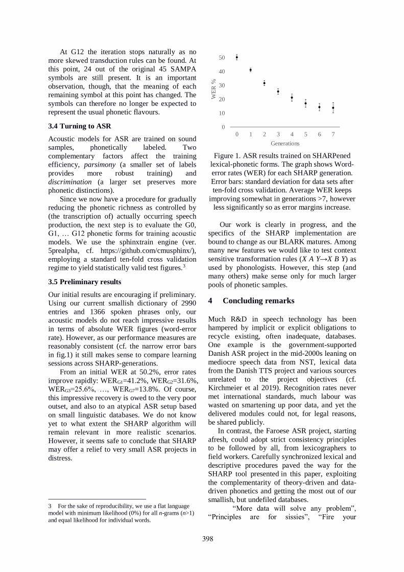
At G12 the iteration stops naturally as no

more skewed transduction rules can be found. At

this point, 24 out of the original 45 SAMPA

symbols are still present. It is an important

observation, though, that the meaning of each

remaining symbol at this point has changed. The

symbols can therefore no longer be expected to

represent the usual phonetic flavours.

3.4 Turning to ASR

Acoustic models for ASR are trained on sound

samples, phonetically labeled. Two

complementary factors affect the training

efficiency, parsimony (a smaller set of labels

provides more robust training) and

discrimination (a larger set preserves more

phonetic distinctions).

Since we now have a procedure for gradually

reducing the phonetic richness as controlled by

(the transcription of) actually occurring speech

production, the next step is to evaluate the G0,

G1, … G12 phonetic forms for training acoustic

models. We use the sphinxtrain engine (ver.

5prealpha, cf. https://github.com/cmusphinx/),

employing a standard ten-fold cross validation

regime to yield statistically valid test figures.3

3.5 Preliminary results

Our initial results are encouraging if preliminary.

Using our current smallish dictionary of 2990

entries and 1366 spoken phrases only, our

acoustic models do not reach impressive results

in terms of absolute WER figures (word-error

rate). However, as our performance measures are

reasonably consistent (cf. the narrow error bars

in fig.1) it still makes sense to compare learning

sessions across SHARP-generations.

From an initial WER at 50.2%, error rates

improve rapidly: WERG1=41.2%, WERG2=31.6%,

WERG3=25.6%, …, WERG7=13.8%. Of course,

this impressive recovery is owed to the very poor outset, and also to an atypical ASR setup based

on small linguistic databases. We do not know

yet to what extent the SHARP algorithm will

remain relevant in more realistic scenarios.

However, it seems safe to conclude that SHARP

may offer a relief to very small ASR projects in

distress.

3 For the sake of reproducibility, we use a flat language

model with minimum likelihood (0%) for all n-grams (n>1)

and equal likelihood for individual words.

Figure 1. ASR results trained on SHARPened

lexical-phonetic forms. The graph shows Word-

error rates (WER) for each SHARP generation.

Error bars: standard deviation for data sets after

ten-fold cross validation. Average WER keeps

improving somewhat in generations >7, however

less significantly so as error margins increase.

Our work is clearly in progress, and the

specifics of the SHARP implementation are

bound to change as our BLARK matures. Among

many new features we would like to test context

sensitive transformation rules (X A Y→X B Y) as

used by phonologists. However, this step (and

many others) make sense only for much larger

pools of phonetic samples.


Much R&D in speech technology has been

hampered by implicit or explicit obligations to

recycle existing, often inadequate, databases.

One example is the government-supported

Danish ASR project in the mid-2000s leaning on

mediocre speech data from NST, lexical data

from the Danish TTS project and various sources

unrelated to the project objectives (cf.

Kirchmeier et al 2019). Recognition rates never

met international standards, much labour was

wasted on smartening up poor data, and yet the

delivered modules could not, for legal reasons,

be shared publicly.

In contrast, the Faroese ASR project, starting

afresh, could adopt strict consistency principles

to be followed by all, from lexicographers to

field workers. Carefully synchronized lexical and

descriptive procedures paved the way for the

SHARP tool presented in this paper, exploiting

the complementarity of theory-driven and data-

driven phonetics and getting the most out of our

smallish, but undefiled databases.

“More data will solve any problem”,

“Principles are for sissies”, “Fire your

0

10

20

30

40

50

0 1 2 3 4 5 6 7

WE

R %

Generations

398

linguists!”. Such fresh attitudes are currently

shared by many developers. We invite the

serious ASR manufacturer to rediscover the

power of linguistic precision.

Acknowledgments

Project Ravnur wishes to personally thank Karin

Kass for her never-failing entrepreneurship and

diligence. We also wish to thank a number of

investors from the Faroese society.

References

Anna Björk Nikulasdóttir, Inga Rún Helgadóttir,

Matthías Pétursson and Jón Guðnason. 2018. Open

ASR for Icelandic: Resources and a Baseline

System. In Proceedings of the 11th International

Conference on Language Resources and

Evaluation, pages 3137-3142.

Bente Maegaard, Steven Krauwer, Khalid Choukri

and Lise Damsgaard Jørgensen. 2006. The

BLARK concept and BLARK for Arabic. In

Proceedings of the 5th International Conference on

Language Resources and Evaluation, pages 773-

778.

Edit Bugge. 2018. Attitudes to variation in spoken

Faroese. Journal of Sociolinguistics 22(3):312-330.

Eivind Weyhe. 2014. Variatión av i og u í

herðingarveikari støðu í føroyskum. Fróðskaparrit,

61:116-136. Fróðskapur, Tórshavn, Faroe Islands.

Höskuldur Thráinsson, Hjalmar P. Petersen, Jógvan í

Lon Jacobsen and Zakaris Hansen. 2012. Faroese,

an overview and reference grammar, 2nd edition.

Fróðskapur, Tórshavn, Faroe Islands, and

Linguistic Institute, University of Iceland,

Reykjavík, Iceland.

Iben Nyholm Debess. 2019. FADAC Hamburg 1.0.

Guide to the Faroese Danish Corpus Hamburg.

Kieler Arbeiten zur skandinavistischen Linguistik

6. Institut für Skandinavistik, Frisistik und

Allgemeine Sprachwissenschaft (ISFAS), FID

Northern Europe https://macau.uni-

kiel.de/receive/macau_publ_00002318

Janne Bondi Johannesen. 2009. A corpus of spoken

Faroese. Nordlyd, 36(2):25-35.

Janne Bondi Johannesen, Joel Priestly, Kristin Hagen,

Tor Anders Åfarli and Øystein Alexander

Vangsnes. 2009. The Nordic Dialect Corpus - an

Advanced Research Tool. In Kristiina Jokinen and

Eckhard Bick (eds.). 2009. NEALT Proceedings

Series, 4:73-80.

Jonathan Adams and Hjalmar P. Petersen. 2014. A

Language Course for Beginners, 3rd edition. Stiðin,

Tórshavn, Faroe Islands.

Jørgen Rischel. 1964. Toward the Phonetic

description of Faroese vowels. Fróðskaparrit,

13:99-113.

Kirsti Dee Hansen. 2004. FTS - Føroyskt

TekstaSavn/færøsk talekorpus. In Henrik Holmboe

(ed.). 2005. Nordisk sprogteknologi 2004 - Årbog

for Nordisk Sprogteknologisk Forskningsprogram

2000-2004, pages 47-50.

Kristján Árnason. 2011. The Phonology of Icelandic

and Faroese. Oxford University Press, Oxford, UK.

Pétur Helgason. 2003. Faroese Preaspiration. In

Proceedings of the 15th International Congress of

Phonetic Sciences, pages 2517-2520. Universidad

Autònoma de Barcelona, Barcelona, Spain.

Pétur Helgason and Sjúrður Gullbein. 2002.

Phonological norms in Faroese speesch synthesis.

In Proceedings of the International Conference on

Spoken Language Processing, pages 2269-2272,

Denver, Colorado.

Pétur Helgason, Sjúrður Gullbein and Karin Kass.

2005. Færøsk talesyntese: Rapport marts 2005. In

Henrik Holmboe (ed.). 2005. Nordisk

sprogteknologi 2005 - Årbog for Nordisk

Sprogteknologisk Forskningsprogram 2000-2004,

pages 51-58.

Remco Knooihuizen. 2014. Variation in Faroese and

the development of a spoken standard: In search of

corpus evidence. Nordic Journal of Linguistics,

37(1):87-105.

Sabine Kirchmeier, Peter Juel Henrichsen, Philip

Diderichsen and Nanna Bøgebjerg Hansen. 2019.

Dansk Sprogteknologi i Verdensklasse.

Steven Krauwer. 2003. The Basic Language Resource

Kit (BLARK) as the First Milestone for the

Language Resources Roadmap. In Proceedings of

the International Workshop “Speech and

Computer”, SPECOM 2003, Moscow, Russia.

Thomas Bilgram and Britt Keson. 1998. The

Construction of a Tagged Danish Corpus.

Proceedings of the 11th Nordic Conference of

Computational Linguistics, NODALIDA 1998,

pages 129-139.

399

Docria: Processing and Storing Linguistic Data with Wikipedia

Marcus [email protected]

Lund UniversityDepartment of Computer Science

S-221 00 Lund, Sweden

Pierre [email protected]

Lund UniversityDepartment of Computer Science

S-221 00 Lund, Sweden

Abstract

The availability of user-generated con-tent has increased significantly over time.Wikipedia is one example of a cor-pus, which spans a huge range of top-ics and is freely available. Storing andprocessing such corpora requires flexi-ble document models as they may con-tain malicious or incorrect data. Docriais a library which attempts to addressthis issue with a model using typedproperty hypergraphs. Docria can beused with small to large corpora, fromlaptops using Python interactively in aJupyter notebook to clusters running map-reduce frameworks with optimized com-piled code. Docria is available as open-source code at https://github.com/marcusklang/docria.

1 Introduction

The availability of user-generated content has in-creased significantly over time. Wikipedia is oneexample of a corpus, which spans a huge rangeof topics and is freely available. User-generatedcontent tests the robustness of most tools as itmay contain malicious or incorrect data. In ad-dition, data often comes with valuable metadata,which might be semi-structured and/or incom-plete. These kinds of resources require a flexibleand robust data model capable of representing adiverse set of generic and domain-specific linguis-tic structures.

In this paper, we describe a document modelwhich tries to fill the gap between fully structuredand verifiable data models and domain-specificdata structures. This model, called Docria, aims atfinding a tradeoff between the rigidity of the for-mer and the specificity of the latter. To show itsmerits, we contrast the application of fully struc-

tured data models to practical noisy datasets withthe simplicity of Docria.

2 Related Work

Linguistically annotated data have been stored inmany different formats, often developed to solvepractical problems. We can group prior work intothree categories:

Formats – the technical formats which are usedto serialize the data;

Document models – conceptual descriptions ofhow the data is connected, often mapped toconcrete software implementations;

Applications and tooling – user-facing applica-tions for annotation, search, etc.

in this section, we will focus on the low-levelformats and libraries to parse and access the datacontained within.

Pustylnikov et al. (2008), in their work on uni-fying 11 treebanks, made a summary of formatstypically used, which shows a dominance of XMLvariants and CoNLL-like formats. We examinesome of them here.

Tabular annotation. The tabular annotation inplain text is one of the simplest formats: One to-ken per line and white space separation for the datafields connected to the token followed by a dou-ble line separation to mark a sentence. This kindof format was used first in the CoNLL99 task onchunking (Osborne, 1999) and then on subsequenttasks. Its main merits are the ease of use with re-gards to writing parsers and its readability withoutdocumentation.

Universal Dependencies (Nivre et al., 2019) isan example of a recent project for multilingual cor-pora using this format. It defines a variant calledCoNLL-U, an adaption of the format used inCoNLL-X shared task on multilingual dependency

400

parsing (Buchholz and Marsi, 2006). CoNLL-Uincludes field descriptions at the start of a docu-ment using hashtag (#) comments, adds subwordsupport, and a field, if used, would allow for unto-kenization by including information about spacingbetween tokens.

CoNLL-* formats are tightly connected to dataused in the shared tasks. Variations of these plain-text formats in the wild have no real standard andare mostly ad-hoc development. The field separa-tion is a practical aspect, which may vary: spacesor tabulations. Depending on the corpus, theseare not interchangeable as the token field mightinclude ordinary spaces as part of the data field.

Semi-structured formats. Semi-structured for-mats specify stricter rules and a frequent choiceis to follow the XML syntax to implement them(Bray et al., 2008). XML is hierarchical and cansupport higher-order structures such as sections,paragraphs, etc. XML has been used successfullyin the development of the TIGER Corpus (TIGERXML) (Brants et al., 2002) and the Prague Depen-dency Treebank (PML) (Hajic et al., 2018).

The XML annotation relies on a schema defin-ing its content on which programs and users mustagree. Aside from TIGER XML and PML, theText Encoding Initiative (TEI) and FoLiA XML(van Gompel and Reynaert, 2013) are general pur-pose XML schema definitions focused on linguis-tic and text annotation. TEI and FoLiA provide ex-tensive documentation and guidelines on how datashould be represented in XML.

Graph formats. From primarily hierarchicalformats, the NLP Interchange Format (NIF) pro-vides a graph-oriented way of connecting infor-mation which builds on existing standards such asLAF/GrAF, RFC 5147, and RDF. The main inno-vation in NIF is a standardized way of referring totext with offsets also known as a stand-off anno-tation. NIF is similar to WIKIPARQ (Klang andNugues, 2016).

3 Docria

Docria is a document model based on typed prop-erty hypergraphs. We designed it to solve scala-bility and tooling problems we faced with the au-tomatic processing and annotation of Wikipedia.This corresponds notably to:

• The lack of document models and storage so-lutions that could fit small and large corpora

and that could be compatible with researchpractices;

• The impossibility to use the same documentmodel with potentially costly large-scale ex-traction algorithms on a cluster with a map-reduce computing framework such as ApacheSpark.

Motivation. These aspects were dominant in theconstruction of Docria, for which we set a list ofrequirements:

Openness – release the library as open source1;share processed corpora such as Wikipedia informats used by this library; invite others touse the library for various tasks;

Scalability – from small corpora using a few linesof code to show a concept on a laptop tolarge-scale information extraction running onmultiple computers in a cluster with opti-mized code;

Low barrier – progressive learning curve, sensi-ble defaults, no major installations of servicesor configurations. Specifically, we wanted toreduce barriers when we shared larger cor-pora with students for use in project courses;

Flexibility – capable of representing a diverse setof linguistic structures, adding informationand structures progressively, changing struc-ture as needed;

Storage – reducing disk-space and bandwidth re-quirements when distributing larger corpora.

Design. To meet these goals, we implementedDocria in both Python and Java with a shared con-ceptual model and storage format. One of the usergroups we had in mind in the design step wasstudents in computer science carrying a courseproject. As our students have programming skills,we elected a programmer-first approach with a fo-cus on common tasks and algorithms and a toolingthrough an API.

Python with Jupyter notebooks provides an in-teractive Read-Evaluate-Print-Loop (REPL) withrich presentation possibilities. We created exten-sions for it to reduce the need for external tool-ing and so that with a few lines of code, a pro-grammer can inspect the contents of any Docria

1https://www.github.com/marcusklang/docria

401

20 24 40 48

Offsets

LundSpan

Deprel

Sentence

NE

Token Lund

LOC

T

Relation

. . .

AnnotationLayers

Lund is a city.Text

Property

connection

Figure 1: Docria data model

document. Through a matching implementationin Java, Docria provides a path to scale up whenneeded, as specific tasks can be orders of magni-tudes faster than with a CPython implementation.

Docria documents consist of text collectionsand layers, shown in Figure 1. Text collectionsallow for multiple representations of a single text.A layer is a collection of nodes. These nodes canhave fields which refer to the text collections. Oneparticular restriction we impose is that a user mustdefine a schema per layer. This is essential for in-trospection and verification of the data containedin documents. The schema defines the availablefields and their data type with support for meta-data.

Datatypes. The datatypes include basic typessuch as Boolean, integer, float, and string. Ad-vanced types include text spans, node spans, nodereferences, and node array references, which en-able a programmer to represent graph structures.Field types, which are node references, must spec-ify a target layer. In addition, this restriction re-sults in well-defined dependencies between layers,which can be used in the future for partial docu-ment reconstruction when reading.

Using a relational database analogy, layers cor-respond to tables; they contain nodes which areequivalent to rows with fields, which are typedcolumns with specialized support for references toother nodes in other layers.

Stand-off references. Docria uses stand-off ref-erences in which we separate text from linguisticlayers. These layers refer to ranges in the origi-nal text. To simplify the implementation and re-

duce sources of common bugs, the text string issplit into pieces according to the offsets and storestext as a list of substrings, which is reconstructedwithout a loss by a join. Offsets, when serialized,only refer to spans of substrings. Software imple-mentations can reconstruct offsets by computingthe actual substring length and creating a lookuptable. This will generate correct offsets even ifthe in-memory representation of a string differs,which is the case with standard strings in Java andPython 3.

Binary format. For the binary format, weselected MessagePack. MessagePack is self-describing, has an open well-defined specification,and has multiple open-source implementations ina diverse set of programming languages. The bi-nary format can be used on a per document ba-sis or in an included collection container, whichwrites multiple binary documents in sequence.This binary format was also designed to allow fora quicker content listing by separating content intocompartments which can be read independently:document properties, schema, text, and layer data.

The Wikipedia corpus. We used the officialREST API provided by Wikimedia and a pagelisting from the official dump page to collect theWikipedia corpus. We downloaded all the pagesin HTML format from this page listing in Octo-ber 2018. This HTML format was processed andconverted into a DOM using JSoup. Using recur-sive rules, we transformed the DOM into a flattext representation with structural layers referringto ranges such as section, paragraph, and anchors.Furthermore, we linked anchors to Wikidata bytranslating page targets to Q-numbers where avail-able. We also retained formatting, such as boldand italics. We stored all this information usingDocria.

In this dump, there are 5,405,075 pages exclud-ing redirections.

4 Evaluation

We applied the spaCy library2 to annotate all theEnglish Wikipedia pages with parts of speech, en-tities, and dependency graphs, and we made theresult available at http://fileadmin.cs.lth.se/papers/nodalida2019/. On av-erage, each page of the corpus, after annotation,

2https://spacy.io/

402

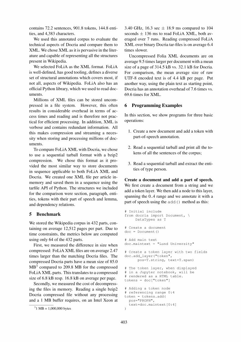
contains 72.2 sentences, 901.8 tokens, 144.8 enti-ties, and 4,383 characters.

We used this annotated corpus to evaluate thetechnical aspects of Docria and compare them toXML. We chose XML as it is pervasive in the liter-ature and capable of representing all the structurespresent in Wikipedia.

We selected FoLiA as the XML format. FoLiAis well-defined, has good tooling, defines a diverseset of structural annotations which covers most, ifnot all, aspects of Wikipedia. FoLiA also has anofficial Python library, which we used to read doc-uments.

Millions of XML files can be stored uncom-pressed in a file system. However, this oftenresults in considerable overhead in terms of ac-cess times and reading and is therefore not prac-tical for efficient processing. In addition, XML isverbose and contains redundant information. Allthis makes compression and streaming a neces-sity when storing and processing millions of doc-uments.

To compare FoLiA XML with Docria, we choseto use a sequential tarball format with a bzip2compression. We chose this format as it pro-vided the most similar way to store documentsin sequence applicable to both FoLiA XML andDocria. We created one XML file per article in-memory and saved them in a sequence using thetarfile API of Python. The structures we includedfor the comparison were section, paragraph, enti-ties, tokens with their part of speech and lemma,and dependency relations.

5 Benchmark

We stored the Wikipedia corpus in 432 parts, con-taining on average 12,512 pages per part. Due totime constraints, the metrics below are computedusing only 64 of the 432 parts.

First, we measured the difference in size whencompressed: FoLiA XML files are on average 2.47times larger than the matching Docria files. Thecompressed Docria parts have a mean size of 85.0MB3 compared to 209.8 MB for the compressedFoLiA XML parts. This translates to a compressedsize of 6.8 kB resp. 16.8 kB on average per page.

Secondly, we measured the cost of decompress-ing the files in memory. Reading a single bzip2Docria compressed file without any processingand a 1 MB buffer requires, on an Intel Xeon at

31 MB = 1,000,000 bytes

3.40 GHz, 16.3 sec ± 18.9 ms compared to 104seconds ± 136 ms to read FoLiA XML, both av-eraged over 7 runs. Reading compressed FoLiAXML over binary Docria tar-files is on average 6.4times slower.

Uncompressed Folia XML documents are onaverage 9.5 times larger per document with a meansize of a page of 314.5 kB vs. 32.1 kB for Docria.For comparison, the mean average size of rawUTF-8 encoded text is of 4.4 kB per page. Putanother way, using the plain text as starting point,Docria has an annotation overhead of 7.6 times vs.69.6 times for XML.

6 Programming Examples

In this section, we show programs for three basicoperations:

1. Create a new document and add a token withpart-of-speech annotation.

2. Read a sequential tarball and print all the to-kens of all the sentences of the corpus;

3. Read a sequential tarball and extract the enti-ties of type person.

Create a document and add a part of speech.We first create a document from a string and weadd a token layer. We then add a node to this layer,spanning the 0..4 range and we annotate it with apart of speech using the add() method as this:

# Initial includefrom docria import Document, \

DataTypes as T

# Create a documentdoc = Document()

# Add main textdoc.maintext = "Lund University"

# Create a token layer with two fieldsdoc.add_layer("token",

pos=T.string, text=T.span)

# The token layer, when displayed# in a Jupyter notebook, will be# rendered as a HTML table.tokens = doc["token"]

# Adding a token node# referencing range 0:4token = tokens.add(pos="PROPN",text=doc.maintext[0:4]

)

403

Print the tokens. We assume we have a tarballof documents segmented into sentences and to-kens, and annotated with the parts of speech. Weread the tarball with TarMsgpackReader andwe access and print the sentences, tokens, andparts of speech using the Python dictionary syn-tax.

from docria.storage \import TarMsgpackReader

with TarMsgpackReader("enwiki00001.tar.bz2",mode="r|bz2") as reader:

for rawdoc in reader:# Materialize documentdoc = rawdoc.document()

# Lists all layers with field# types and metadatadoc.printschema()

# Print the original text# Equivalent to doc.text["main"]print(doc.maintext)

for sentence in doc["sentence"]:# Print the full sentenceprint(sentence["tokens"].text())

for tok in sent["tokens"]:# Form <TAB> part-of-speechprint("%s\t%s" %

(tok["text"], tok["pos"])

Extract entities of a certain type. We assumehere that the tarball is annotated with entitiesstored in an ENTITY layer. We read the tarballand access the entities. We then extract all the en-tities of category PERSON:

with TarMsgpackReader("enwiki00001.tar.bz2",mode="r|bz2") as reader:

for rawdoc in reader:# Materialize documentdoc = rawdoc.document()

# Get the entity layerentities = doc["entity"]

# Filter out PERSON in entity# layer having field label# equal to PERSONquery = (entities["label"]

== "PERSON")

for person in entities[query]:# Tokens represents potentially# many tokens, text()# transforming it to a string# from the leftmost# to the rightmost token.print(person["tokens"].text())

7 Discussion

When converting the Wikipedia corpora to fit theFoLiA XML format, we had issues identifying asuitable span annotation for the Wikipedia anchorlink. We decided to associate it with the FoLiAXML entity type.

In addition, when using stand-off annotations,some documents did not pass validation with off-set errors, possibly due to normalization issuescommon to Wikipedia text. This gives an argu-ment that these kinds of formats do not work re-liably with noisy datasets. We instead includedthe sentences as text and used the nospace attributeto allow untokenization, which does increase ver-bosity slightly.

Initially, we used the official foliapy library, butwe were unable to get a decent performance withit, potentially addressed in the future. We resortedto using the LXML DOM matching example doc-uments with Folia. To ensure correctness, we ver-ified samples of our XMLs using foliavalidator.

Acknowledgments

This research was supported by Vetenskapsradet,the Swedish research council, under the Det digi-taliserade samhallet program, grant number 340-2012-5738.

ReferencesSabine Brants, Stefanie Dipper, Silvia Hansen, Wolf-

gang Lezius, and George Smith. 2002. The tigertreebank. In Proceedings of the workshop on tree-banks and linguistic theories, volume 168.

Tim Bray, Eve Maler, Francois Yergeau, MichaelSperberg-McQueen, and Jean Paoli. 2008.Extensible markup language (XML) 1.0(fifth edition). W3C recommendation, W3C.Http://www.w3.org/TR/2008/REC-xml-20081126/.

Sabine Buchholz and Erwin Marsi. 2006. Conll-xshared task on multilingual dependency parsing. InProceedings of the Tenth Conference on Computa-tional Natural Language Learning, CoNLL-X ’06,pages 149–164, Stroudsburg, PA, USA. Associationfor Computational Linguistics.

Maarten van Gompel and Martin Reynaert. 2013. Fo-lia: A practical xml format for linguistic annotation— a descriptive and comparative study. Computa-tional Linguistics in the Netherlands Journal, 3:63–81.

Jan Hajic, Eduard Bejcek, Alevtina Bemova, EvaBuranova, Eva Hajicova, Jirı Havelka, Petr Ho-

404

mola, Jirı Karnık, Vaclava Kettnerova, Na-talia Klyueva, Veronika Kolarova, Lucie Kucova,Marketa Lopatkova, Marie Mikulova, Jirı Mırovsky,Anna Nedoluzhko, Petr Pajas, Jarmila Panevova,Lucie Polakova, Magdalena Rysova, Petr Sgall, Jo-hanka Spoustova, Pavel Stranak, Pavlına Synkova,Magda Sevcıkova, Jan Stepanek, Zdenka Uresova,Barbora Vidova Hladka, Daniel Zeman, SarkaZikanova, and Zdenek Zabokrtsky. 2018. Praguedependency treebank 3.5. LINDAT/CLARIN dig-ital library at the Institute of Formal and AppliedLinguistics (UFAL), Faculty of Mathematics andPhysics, Charles University.

Marcus Klang and Pierre Nugues. 2016. WIKIPARQ:A tabulated Wikipedia resource using the Parquetformat. In Proceedings of the Ninth InternationalConference on Language Resources and Evaluation(LREC 2016), pages 4141–4148, Portoroz, Slovenia.

Joakim Nivre, Mitchell Abrams, Zeljko Agic, LarsAhrenberg, Gabriele Aleksandraviciute, et al. 2019.Universal dependencies 2.4. LINDAT/CLARINdigital library at the Institute of Formal and Ap-plied Linguistics (UFAL), Faculty of Mathematicsand Physics, Charles University.

M. Osborne. 1999. CoNLL-99. Computational Nat-ural Language Learning. Proceedings of a Work-shop Sponsored by The Association for Computa-tional Linguistics. Association for ComputationalLinguistics (ACL).

Olga Pustylnikov, Alexander Mehler, and RudigerGleim. 2008. A unified database of dependencytreebanks: Integrating, quantifying & evaluating de-pendency data. In LREC 2008.

405

UniParse: A universal graph-based parsing toolkit

Daniel VarabIT University

Copenhagen, [email protected]

Natalie SchluterIT University

Copenhagen, [email protected]

Abstract

This paper describes the design and useof the graph-based parsing framework andtoolkit UniParse, released as an open-source python software package devel-oped at the IT University, CopenhagenDenmark. UniParse as a frameworknovelly streamlines research prototyping,development and evaluation of graph-based dependency parsing architectures.The system does this by enabling highlyefficient, sufficiently independent, read-able, and easily extensible implementa-tions for all dependency parser compo-nents. We distribute the toolkit with ready-made pre-configured re-implementationsof recent state-of-the-art first-order graph-based parsers, including highly efficientCython implementations of feature en-coders and decoding algorithms, as well asoff-the-shelf functions for computing lossfrom graph scores.

1 Introduction

Motivation. While graph-based dependencyparsers are theoretically simple models, extensi-ble and modular implementations for sustainableparser research and development have to date beenseverely lacking in the research community. Con-tributions to parsing research generally centresaround particular components of parsers in isola-tion, such as novel decoding algorithms, novel arcencodings, or novel learning architectures. How-ever, due to perceived gains in performance ordue to the lack of foresight in writing sustainablecode, these components are rarely implementedmodularly or with extensibility in mind. Thisapplies to prior sparse-feature dependency parsers(McDonald and Pereira (2006)’s MST parser),as well as recent state-of-the-art neural parsers

(Kiperwasser and Goldberg, 2016; Dozat andManning, 2017). Implementations of parsercomponents are generally tightly coupled to oneanother which heavily hinders their usefulness infuture research.

With UniParse, we provide a flexible, highlyexpressive, scientific framework for easy, low-barrier of entry, highly modular, efficient devel-opment and fair benchmarking of graph-baseddependency parsing architectures. With theframework we distribute pre-configured state-of-the-art first-order sparse and neural graph-basedparser implementations to provide strong base-lines for future research on graph based depen-dency parsers.

Novel contributions

• We align sparse feature and neural researchin graph-based dependency parsing to a com-mon terminology. With this shared termi-nology we develop a unified framework forthe UniParse toolkit to rapidly prototype newparsers and easily compare performance toprevious work.• Prototyping is now rapid due to modular-

ity: parser components may now be devel-oped in isolation, with no resulting loss inefficiency. Measuring the empirical perfor-mance of a new decoder no longer requireimplementing an encoder, and investigatingthe synergy between a learning strategy anda decoder no longer requires more than a flagor calling a library function.• Preprocessing is now made explicit within

its own component and is thereby adequatelyisolated and portable.• The evaluation module is now easy to read

and fully specified. We specify the subtledifferences in computing unlabeled and la-beled arc scores (UAS, LAS) from previous

406

literature and have implemented these in Uni-Parse in an explicit manner.• To the best of our knowledge, UniParse is

the first attempt at unifying existing de-pendency parsers to the same code base.Moreover, UniParse is to our knowledgethe first attempt to enable first-order sparse-feature dependency parsing in a sharedpython codebase.

We make the parser freely available under a GNUGeneral Public License1.

2 Terminology of a unified dependencyparser

Traditionally, a graph-based dependency parserconsists of three components. An encoder Γ, a setof parameters λ, and a decoder h. The possibledependency relations between all words of asentence S are modeled as a complete directedgraph GS where words are nodes and arcs are therelations. An arc in GS is called a factor which Γassociates with a d-dimensional feature vector, itsencoding. The set of parameters λ are then usedto produce scores from the constructed featurevectors according to some learning procedure.These parameters are optimized over treebanks.Lastly a decoder h is some maximum spanningtree algorithm with input GS and scores forfactors of GS given by λ; it outputs a well-formeddependency tree, which is the raw output of adependency model.

Recent work on neural dependency parserslearns factor embeddings discriminatively along-side the parameters used for scoring. The result isthat Γ and λ of dependency parsers fuse togetherinto a union of parameters. Thus, in this workwe fold the notion of encoding into the parameterspace. Now, for the neural models, all parametersare trainable, whereas for sparse-feature models,the encodings of sub-sets of arcs are non-trainable.So the unified terminology addresses only param-eters λ and a decoder h.

3 API and the joint model architecture

We provide two levels of abstraction for imple-menting graph-based dependency parsers. First,our descriptive high-level approach focuses on ex-pressiveness, enabling models to be described in

1github.com/danielvarab/uniparse

just a few lines of code by providing an interfacewhere the required code is minimal, only a meansto configure design choices. Second, as an alter-native to the high-level abstraction we emphasisethat parser definition is nothing more than a com-position of pre-configured low-level modular im-plementations. With this we invite cherry pickingof the included implementations of optimised de-coders, data preprocessors, evaluation module andmore. We now briefly overview the basic use ofthe joint API and list the central low-level mod-ule implementations included with the UniParsetoolkit.

Elementary usage (high level). For ease of usewe provide a high-level class to encapsulate neu-ral training. Its use results in a significant reduc-tion in the amount of code required to implementa parser and counters unwanted boilerplate code.It provides default configurations for all includedcomponents, while enabling custom implementa-tion whenever needed. Custom implementationsare only required to be callable and adheres tothe framework’s function definition. The mini-mum requirement with the use of this interface is aparameter configuration, loss function, optimizer,and batch strategy. In Listing 1 we show an exam-ple implementation of Kiperwasser and Goldberg(2016)’s neural parser in only a few lines. The fulllist of possible arguments along with their inter-faces can be found in the toolkit documentation.

Vocabulary. This class facilitates preprocessingof CoNLL-U formatted files with support for out-of-vocabulary management and alignment withpre-trained word embeddings. Text preprocessingstrategies have significant impact on NLP modelperformance. Despite this, little effort has putinto describing such techniques in recent litera-ture. Without these details preprocessing becomesyet another hyper-parameter of a model, and ob-fuscates research contribution. In the UniParsetoolkit, we include a simple implementation forrecently employed techniques in parsing for tokencleaning and mapping.

Batching. UniParse provides functionality to or-ganise tokens into batches for efficient compu-tation and learning. We provide several con-figurable implementations for different batchingstrategies. This includes 1. batching by sentencelength (bucketing), 2. fixed-length batching withpadding, and 3. clustered-length batching as seen

407

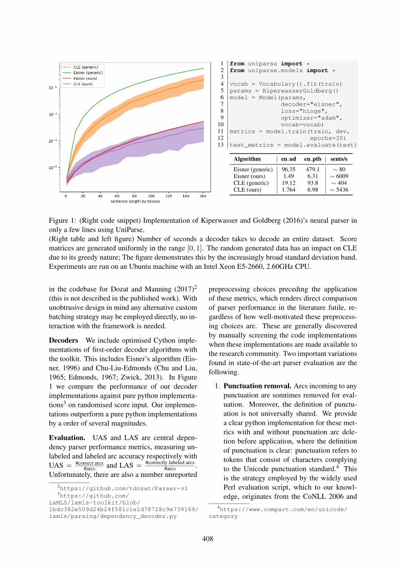
1 from uniparse import *2 from uniparse.models import *34 vocab = Vocabulary().fit(train)5 params = KiperwasserGoldberg()6 model = Model(params,7 decoder="eisner",8 loss="hinge",9 optimizer="adam",

10 vocab=vocab)11 metrics = model.train(train, dev,12 epochs=30)13 test_metrics = model.evaluate(test)

Algorithm en ud en ptb sents/s

Eisner (generic) 96.35 479.1 ∼ 80Eisner (ours) 1.49 6.31 ∼ 6009CLE (generic) 19.12 93.8 ∼ 404CLE (ours) 1.764 6.98 ∼ 5436

Figure 1: (Right code snippet) Implementation of Kiperwasser and Goldberg (2016)’s neural parser inonly a few lines using UniParse.(Right table and left figure) Number of seconds a decoder takes to decode an entire dataset. Scorematrices are generated uniformly in the range [0, 1]. The random generated data has an impact on CLEdue to its greedy nature; The figure demonstrates this by the increasingly broad standard deviation band.Experiments are run on an Ubuntu machine with an Intel Xeon E5-2660, 2.60GHz CPU.

in the codebase for Dozat and Manning (2017)2

(this is not described in the published work). Withunobtrusive design in mind any alternative custombatching strategy may be employed directly, no in-teraction with the framework is needed.

Decoders We include optimised Cython imple-mentations of first-order decoder algorithms withthe toolkit. This includes Eisner’s algorithm (Eis-ner, 1996) and Chu-Liu-Edmonds (Chu and Liu,1965; Edmonds, 1967; Zwick, 2013). In Figure1 we compare the performance of our decoderimplementations against pure python implementa-tions3 on randomised score input. Our implemen-tations outperform a pure python implementationsby a order of several magnitudes.

Evaluation. UAS and LAS are central depen-dency parser performance metrics, measuring un-labeled and labeled arc accuracy respectively withUAS = #correct arcs

#arcs and LAS = #correctly labeled arcs#arcs .

Unfortunately, there are also a number unreported2https://github.com/tdozat/Parser-v13https://github.com/

LxMLS/lxmls-toolkit/blob/1bdc382e509d24b24f581c1e1d78728c9e739169/lxmls/parsing/dependency_decoder.py

preprocessing choices preceding the applicationof these metrics, which renders direct comparisonof parser performance in the literature futile, re-gardless of how well-motivated these preprocess-ing choices are. These are generally discoveredby manually screening the code implementationswhen these implementations are made available tothe research community. Two important variationsfound in state-of-the-art parser evaluation are thefollowing.

1. Punctuation removal. Arcs incoming to anypunctuation are somtimes removed for eval-uation. Moreover, the definition of punctu-ation is not universally shared. We providea clear python implementation for these met-rics with and without punctuation arc dele-tion before application, where the definitionof punctuation is clear: punctuation refers totokens that consist of characters complyingto the Unicode punctuation standard.4 Thisis the strategy employed by the widely usedPerl evaluation script, which to our knowl-edge, originates from the CoNLL 2006 and

4https://www.compart.com/en/unicode/category

408

Parser configurations Dataset UAS wo.p..original

LAS wo.p.original

UASwo.p.

LASwo.p.

UASw.p.

LASw.p.

Kiperwasser and Goldberg en ud — — 87.71 84.83 86.80 85.12(2016) en ptb 93.32 91.2 93.14 91.57 92.56 91.17

da — — 83.72 79.49 83.24 79.62Dozat and Manning en ud — — 91.47 89.38 90.74 89.01

(2017) en ptb 95.74 95.74 95.43 94.06 94.91 93.70da — — 87.84 84.99 87.42 84.98

MSTparser en ud — — 75.55 66.25 73.47 65.20(2006) + extensions en ptb — — 76.07 64.67 74.00 63.60

da — — 68.80 55.30 67.17 55.52

Table 1: UAS/LAS for included parser configurations. We provide results with (w.p.) and without (wo.p.)punctuation. For the English universal dependencies (UD) dataset we exclude the github repository suffixEWT. Regarding (Dozat and Manning, 2017), despite having access to the published TensorFlow codeof we never observed scores exceed 95.58.

2007 shared tasks.5 We infer this from refer-ences in (Buchholz and Marsi, 2006).

2. Label prefixing. Some arc labels are “com-posite”, their components separated by acolon. An example from the English Uni-versal Dependencies data set is the labelobl:tmod. The official CoNLL 2017shared-task evaluation script6 allows partialmatching of labels based on prefix matchesfor components, for example matching toobl of obl:tmod giving full points. We in-clude this variant in the distributed UniParseevaluation module.

Loss Functions. Common loss functions applyto scalar values, or predictions vectors represent-ing either real values or probabilities. Howeverloss functions for dependency parsers are unortho-dox in that they operate on graphs, which hasbeen dealt with in various creative ways over theyears. We include a set of functions that apply tofirst-order parser graphs which are represented assquare matrices. In the future we hope to expandthis set for first-order, as well as explore higher-order structures.

Callbacks. While we have done our uttermostto design UniParse in a unobtrusive manner, fewlimitations may occur when developing, and es-pecially during exploration of model configura-tions when using the high-level model class. Thiscould be the likes of manual updating of optimis-ers learning rates during training, or logging gran-

5https://depparse.uvt.nl/SoftwarePage.html#eval07.pl

6https://universaldependencies.org/conll17/baseline.html

ulated loss and accuracy. To accommodate this weinclude callback functionality which hooks intothe training procedure enabling users to do the lastfew things perhaps inhibited by the framework.We include a number of useful pre-implementedcallback utilities, such as a Tensorboard logger7,model saver, and a patience mechanism for earlystopping.

Included parsers. We include three state-of-the-art first-order dependency parser implementa-tions as example configurations of UniParse: Mc-Donald and Pereira (2006)’s MST sparse-featureparser 8, Kiperwasser and Goldberg (2016) andDozat and Manning (2017)’s graph-based neu-ral parsers. Experiments are carried out on En-glish and Danish: the Penn Treebank (Marcuset al., 1994) (en ptb, training on sections 2-21, de-velopment on section 22 and testing on section23), converted to dependency format followingthe default configuration of the Stanford Depen-dency Converter (version≥ 3.5.2), and the English(en ud), and Danish (da) datasets from Version 2.1of the Universal Dependencies project (Nivre etal., 2017). Table 1 shows how our parser con-figurations perform compared with the originallyreported parser performance.

7github.com/tensorflow/tensorboard8Note that this MST parser implementation consists of a

restricted feature set and is only a first-order parser, as proofof concept.

409


In this paper, we have described the design andusage of UniParse, a high-level un-opinionatedframework and toolkit that supports both feature-based models with on-line learning techniques,as well as recent neural architectures trainedthrough backpropagation. We have presented theframework as answer to a long-standing need forhighly efficient, easily extensible, and, most ofall, directly comparable graph-based dependencyparsing research.

The goal of UniParse is to ease developmentand evaluation of graph-based syntatic parsers.Future work includes extending UniParse to a gen-eral parsing pipeline from raw text.

ReferencesSabine Buchholz and Erwin Marsi. 2006. Conll-x

shared task on multilingual dependency parsing. InIn Proceedings of CoNLL, pages 149–164. Associa-tion for Computational Linguistics.

Y.J. Chu and T.H. Liu. 1965. On the shortest arbores-cence of a directed graph. Sci. Sinica, 14:13961400.

Timothy Dozat and Christopher M. Manning. 2017.Deep biaffine attention for neural dependency pars-ing. In Proceedings of ICLR.

J. Edmonds. 1967. Optimum branchings. J. Res. Nat.Bur. Standards, 71B:233240.

Jason M. Eisner. 1996.https://doi.org/10.3115/992628.992688 Threenew probabilistic models for dependency parsing:An exploration. In Proceedings of the 16th Con-ference on Computational Linguistics - Volume 1,COLING ’96, pages 340–345, Stroudsburg, PA,USA. Association for Computational Linguistics.

Eliyahu Kiperwasser and Yoav Goldberg. 2016. Sim-ple and accurate dependency parsing using bidirec-tional lstm feature representations. Transactions ofthe ACL, 4:313–327.

Mitchell Marcus, Grace Kim, Mary AnnMarcinkiewicz, Robert MacIntyre, Ann Bies,Mark Ferguson, Karen Katz, and Britta Schas-berger. 1994. The penn treebank: Annotatingpredicate argument structure. In Proceedings ofthe Workshop on Human Language Technology,HLT ’94, pages 114–119, Stroudsburg, PA, USA.Association for Computational Linguistics.

Ryan McDonald and Fernando Pereira. 2006. Onlinelearning of approximate dependency parsing algo-rithms. In Proceedings of EACL. Association forComputational Linguistics.

Joakim Nivre et al. 2017.http://hdl.handle.net/11234/1-2515 Universaldependencies 2.1. LINDAT/CLARIN digital libraryat the Institute of Formal and Applied Linguistics(UFAL), Faculty of Mathematics and Physics,Charles University.

Uri Zwick. 2013. http://www.cs.tau.ac.il/ zwick/grad-algo-13/directed-mst.pdf Lecture notes on “analysisof algorithms”: Directed minimum spanning trees.

410

NoDaLiDa 2019 22nd Nordic Conference on Computational ...

Documents

Transcript of NoDaLiDa 2019 22nd Nordic Conference on Computational ...