Concrete Buildings - Adelaide Research & Scholarship
267
q.- 2- -q.T Procedures for Diagnosis and Assessment of Concrete Buildings \Men-Gang Hua B.Sc. (8"s.) (P.R. China) Thesis Submitted For The Degree of Doctor of Philosophy In The Faculty of Engineering (Civil) The University of Adelaide Australia t ^i ,-.1 ì ' , .
-
Upload
khangminh22 -
Category
Documents
-
view
0 -
download
0
Transcript of Concrete Buildings - Adelaide Research & Scholarship

q.- 2- -q.T
Procedures for
Diagnosis and Assessment of
Concrete Buildings
\Men-Gang Hua
B.Sc. (8"s.) (P.R. China)
Thesis Submitted For The Degree of
Doctor of Philosophy
In
The Faculty of Engineering (Civil)
The University of AdelaideAustralia
t ^i ,-.1 ì ' , .

TO MY MOTHER

Contents
List of Figures
List of Tables
Summary
Statement of OriginalitY
Acknowledgements
Principal Notations
1 Introduction
1.1 Background
t.2 Dealing With Defective Concrete Structures - An Overview 5
t.2.t General Procedure
L.2.2 Condition Survey of Existing Concrete Structures 7
lx
xll
xlll
xv
xvl
xvlt
1
1
5
I
Contents ll
81.2.3 Diagnosis of Defective Concrete Buildings
I.2.4 Condition Evaluation of Existing Concrete Structures 12
L.2.5 Decision-making and Repair Techniques L7
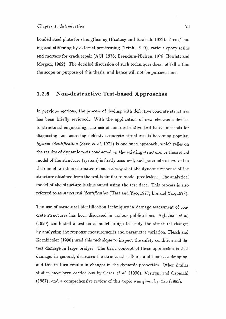
1.2.6 Non-destructive Test-based Approaches
L.2.7 Summary and Conclusions
1.3 The Overall Process for Dealing With Defective Concrete Build-
ings
1.4 Objectives and Scope of Thesis
1.5 GeneralTerminology
1.6 Layout and Contents of Thesis .
2 Diagnosis of Defective Concrete Buildings
2.I Introduction .
2.2 Diagnostic Methods In Other Fields
2.2.1 The Overall Process of Diagnosis
2.2.2 Probabilistic Reasoning for Diagnosis
2.2.3 Diagnosis Using Ftzzy Reasoning
2.2.4 Other Approaches for Diagnostic Reasoning
20
2L
23
26
26
27
29
29
30
30
32
42
44
482.3 Summary and Conclusions

Contents
2.4 A Method for Diagnosing Defective Concrete Buildings
2.4.I Introduction
2.4.2 The Representation of Diagnostic Data
2.4.3 The Candidate Set of Hypotheses
2.4.4 Formation of Hypotheses
2.4.5 Diagnostic Reasoning
2.4.6 The Bayesian Interpretation of Diagnostic Reasoning
2.4.7 SequentialDiagnosis
2.4.8 Stopping Rule and Test Selection
2.5 Summary of This Chapter
3 Condition Evaluation of Existing Concrete Buildings
3.1 Introduction
3.2 Structural Reliability Analysis
3.2.L Classical Reliability Method
3.2.2 Monte-Carlo Simulation Technique
3.2.3 First Order Second Moment Method
3.2.4 Advanced First Order Second Moment Method
lll
50
50
51
oð
57
59
64
64
68
70
72
72
74
74
76
78
81
843.2.5 Brief Summary of Structural Reliability Theory
Contents
3.3 Reliability Analysis Relevant to the Evaluation of Existing Struc-
tures
3.3.1 Safety Revision Using Bayesian Updating .
3.3.2 other Approaches for the Revision of structural Reliability 92
3.3.3 Brief Summary on Reliability Updating 96
3.4 Structural Safety Evaluation Using Ftvzy Sets
3.5 Summary on Fuzzy-Based Safety Evaluation
iv
85
86
r02
. r02
97
3.6 Summary and Conclusions on This Review
3.7 Safety Study of Existing Concrete Buildings 104
3.7.1 Reliability-Based Safety Evaluation ...105
3.7.2 Assessment for Safety Conditiòns Using B Values tL4
3.7.3 Experience-Based Safety Assessment . . .1r7
3.8 Assessment for Serviceability Conditions . 119
3.9 Assessment for Durability Conditions r2l
3.10 Prognosis Procedure r22
3.11 Summary of This Chapter . r23
4 A Method of Decision-making for Dealing With Existing Con-
crete Buildings L24
4.I Introduction . r24

Contents
4.2 A Brief Review of Statistical Decision Theory 126
4.2.L Basic Steps in Simple Decision Analysis ..126
4.2.2 Concepts of Preference and Utility
4.2.3 The Estimation of Utilities . 131
4.2.4 Decision-making With Incomplete Knowledge
4.2.5 Multi-stage Decision-making . r37
4.2.6 Different Decision Rules . I4I
4.3 Decision Analysis in Relevant Engineering Problems ' .144
4.4 Summary on This Review r46
4.5 A Method of Decision-making for Dealing With Structural Defects146
4.5.L Introduction .
4.5.2 Identification of Objectives and Their Associated At-
tributes
4.5.3 The Consequence Space
4.5.4 Assessment of Utility Values .
4.5.5 Creating Courses of Action.
4.5.6 Single-stage Decision-making
4.5.7 Multi-stage Decision-making
v
L29
135
t46
t47
150
L52
156
158
160
1654.5.8 Risk Control for Making a Terminal Decision
Contents
4.5.9 A Special Case 168
4.6 Some Comments on the Proposed Method . . . . 170
4.7 Summary of Tliis Chapter . . . . .771
5 The Detailed Process for Dealing With Defective Concrete
Buildings 173
5.1 Introduction . 173
6.2 The Detailed Process for Dealing \Mith Existing Defective Build-
ings
5.3 Taking Urgent Action
vl
. t74
5.4 Summary of This Chapter
6 Examples
6.1 Example 1
6.1.1 Identification of Anomalies .
6.1.2 Available Information .
6.1.3 Identification of Possible Explanations
6.1.4 Creating the Hypothesis Set H
180
182
183
183
184
184
185
186
6.1.5 Assessment of Subjective Probabilities for Each HypothesislST
6.1.6 Need for an Urgent Action ?
6.1.7 Conducting More Tests ?
188
.190
6.1.8 The Second Cycle of Diagnosis . 191
Contents
6.1.9 The Final Decision
6.2 Example 2
7 Summary and Future 'Work
7.L Summary
7.1.1 The Method of Diagnosis
7.1.2 The Method of Condition Evaluation
7.1.3 The Method of Decision-making .
7.I.4 The Complete Process
7.2 Concluding Remarks and Future Work
Appendix
A Statistical Data on Basic Variables
4.1 Introduction
A.2 Statistical Properties on Concrete Strength
4.3 Statistical Properties on Dimensrons
4.4 Statistical Properties on Reinforcement
B Probabilistic Models for Building Live Loads
vlt
..193
193
196
196
r97
197
198
198
199
200
200
200
20L
202
203
205
2058.1 Introduction

Contents
8.2 Probabilistic Models for Sustained Live Load .
B.3 Probabilistic Models for Extraodinary Live Load
8.4 The Combined Maximum Live Load
Bibliography
207
vlll
.2L0
.zIL
2L3
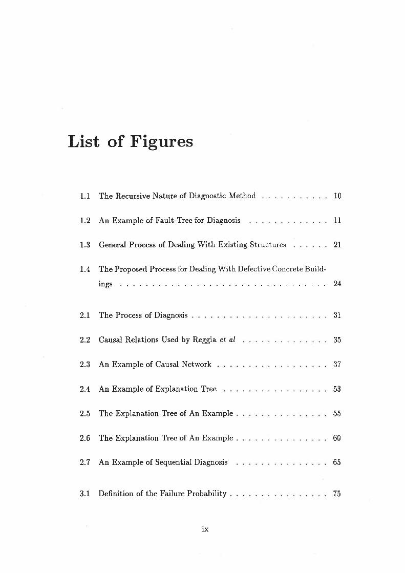
List of Figures
1.1 The Recursive Nature of Diagnostic Method
I.2 An Example of Fault-Tree for Diagnosis
1.3 General Process of Dealing With Existing Structures
I.4 The Proposed Process for Dealing With Defective Concrete Build-
ings
2.1 The Process of Diagnosis
2.2 Causal Relations Used by Reggia et aI
2.3 An Example of Causal Network
2.4 An Example of Explanation Tree
2.5 The Explanation Tree of An Example
2.6 The Explanation Tree of An Example
2.7 An Example of Sequential Diagnosis
3.1 Definition of the Failure Probability
10
. 11
.21
24
31
35
37
53
55
60
65
/Ð
lx
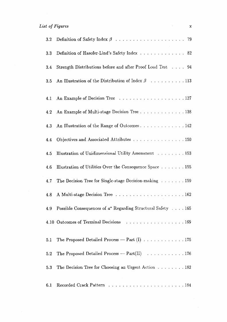
List of Figures
3.2 Definition of Safety Index P
3.3 Definition of Hasofer-Lind's Safety Index
3.4 Strength Distributions before and after Proof Load Test
3.5 An Illustration of the Distribution of Index B
4.1 An Example of Decision Tree
An Example of Multi-stage Decision Tree
An Illustration of the Range of Outcomes
Objectives and Associated Attributes
Illustration of Unidimensional Utility Assessment
Illustration of Utilities Over the Consequence Space
The Decision Tree for Single-stage Decision-making
A Multi-stage Decision Tree
Possible Consequences of ø* Regarding Structural Safety
5.1 The Proposed Detailed Process - Part (I)
5.2 The Proposed Detailed Process - Part(II)
5.3 The Decision Tree for Choosing an Urgent Action
x
79
113
. r27
. 138
.142
82
94
4.2
4.3
4.4
4.5
4.6
4.7
4.8
4.9
150
153
155
159
162
165
169
175
176
4.10 Outcomes of Terminal Decisions
. .182
6.1 Recorded Crack Pattern 184

List of Figures
6.2 Explanation Tree of Example I ...186
6.3 The Modified Process for Dealing With Concrete Bridges . . . . 195
8.1 The Time History of Live Loads
xl
206
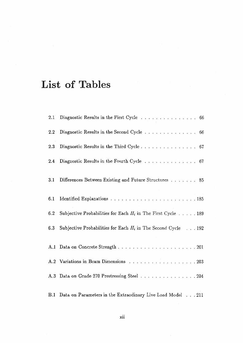
List of Tables
2.I Diagnostic Results in the First Cycle
2.2 Diagnostic Results in the Second Cycle
2.3 Diagnostic Results in the Third Cycle
2.4 Diagnostic Results in the Fourth Cycle
3.1 Differences Between Existing and Future Structures
6.1 Identified Explanations
6.2 Subjective Probabilities for Each I/¡ in The First Cycle . . 189
6.3 Subjective Probabilities for Each fl¡ in The Second Cycle . . .192
4.1 Data on Concrete Strength . 201
4.2 Variations in Beam Dimensions
4.3 Data on Grade 270 Prestressing Steel .
8.1 Data on Parameters in the Extraodinary Live Load Model
66
66
67
67
85
185
.203
.204
,2IT
xll
xlll
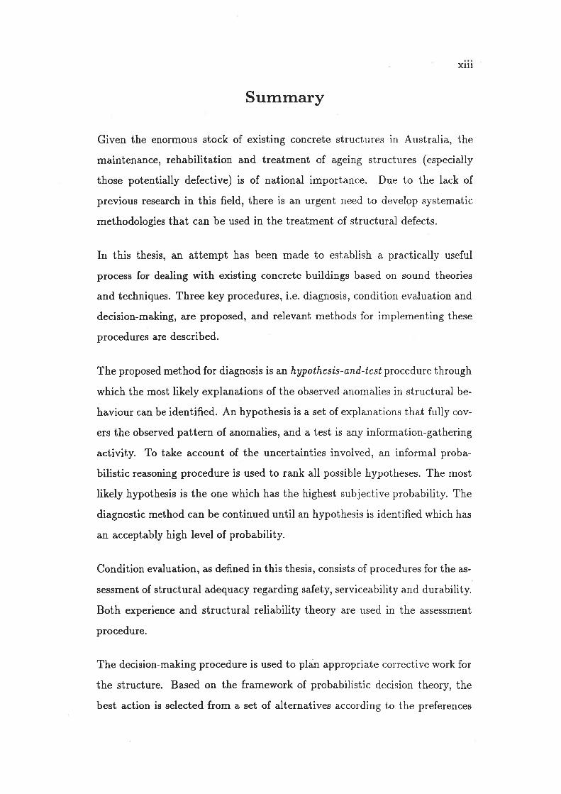
Surnmary
Given the enormous stock of existing concrete structures in Australia, the
maintenance, rehabilitation and treatment of ageing structures (especially
those potentially defective) is of national importance. Due to the lack of
previous research in this field, there is an urgent need to develop systematic
methodologies that can be used in the treatment of structural defects.
In this thesis, an attempt has been made to establish a practically useful
process for dealing with existing concrete buildings based on sound theories
and techniques. Three key procedures, i.e. diagnosis, condition evaluation and
decision-making, are proposed, and relevant methods for implementing these
procedures are described.
The proposed method for diagnosis is an hypothesis-and-tesú procedure through
which the most likely explanations of the observed anomalies in structural be-
haviour can be identified. An hypothesis is a set of explanations that fully cov-
ers the observed pattern of anomalies, and a test is any information-gathering
activity. To take account of the uncertainties involved, an informal proba-
bilistic reasoning procedure is used to rank all possible hypotheses. The most
likely hypothesis is the one which has the highest subjective probability. The
diagnostic method can be continued until an hypothesis is identified which has
an acceptably high level of probability.
Condition evaluation, as defined in this thesis, consists of procedures for the as-
sessment of structural adequacy regarding safety, serviceability and durabiliiy.
Both experience and structural reliability theory are used in the assessment
procedure.
The decision-making procedure is used to plan appropriate corrective work for
the structure. Based on the framework of probabilistic decision theory, the
best action is selected from a set of alternatives according to the preferences

xlv
of the olvner of the structure, in regard to factors such as structural safety,
serviceability, durability and incurred costs. The proposed method forms a
multi-stage process in which the engineer can also decide on whether to gather
more data or to take action at any stage, using the results obtained from
diagnosis and condition evaluation.
By integrating systematically the iterative procedures of diagnosis, assessment
and decision-making, a comprehensive process is developed for dealing with
existing concrete structures, which allows the engineer to decide rationally on
what to do about a given structure in a well-structured manner, Two examples
are used to show how the proposed process is practically useful.

XI/
STATEMENT OF ORIGINALITY
This work contains no material which has been accepted for the award of any
other degree or diploma in any university or other tertiary institution and, to
the best of my knowledge and belief, contains no material previously published
or written by another person, except where due reference has been made in
the text.
I give consent to this copy of my thesis, when deposited in the University
Library, being available for loan and photocopying.
Signed (Wen-Gang Hua) Date

xvl
Á.CKNO\vLEDGEMENTS
Grateful acknowledgement is made to my supervisor Prof. R. F. Warner for
his excellent guidance, constant encouragement and invaluable suggestions
throughout the preparation of this thesis. I feel deeply indebted to him for all
what he has done for the supervision during my candidature.
I also gratefully acknowledge the helpful advice of my associate supervisor Dr
M. C. Griffith, and his review of this thesis.
I wish to thank the academic staff, technical and administrative officers in
the Department of Civil and Environmental Engineering for their help and
cooperation. I would also like to thank Dr D. J. Oehlers for reading part of
the thesis.
I am indebted to my friends, Mr Y. Xu, Ms A. Lo and their family members,
as well as my elder brother, for their moral support. Finally, I wish to express
my deepest gratitude to my mother for her love and encouragement.

xvll
ai
Aar
Principal Notations
: irÀ course of action in a candidate set
: a set of courses of action available
: the best course of action in A at iúh stage of the multi-stage
decision-making
: selected urgent action to be taken
- j'h attribute of anomaly s¡
: i'ä causal factor of an explanation
: the maximum amount of money the owner is willing to spend on
the improvement of the structure's safety condition
: confidence factor of (.)
: ir[ explanation of an anomaly
: distribution function of random variable X: cumulative distribution function of random variable X: limit state function in reliability analysis
: hypothesis set
: candidate set of hypotheses
: i¿â hypothesis in H
- the highest ranked hypothesis in H
: itf, possible outcome of a test
- probability of (.)
- prior probability of ('): posterior probability of (.)
: risk of action o* regarding the safety attribute
- acceptable probability value in diagnosis
- ir[ anomaly
: set of tests to be considered
øi¡
b;i
ci
Co+
C F(.)ei
f x@)Fx(*)G(X)H
HcH;
H*
o;P(.)
P'(.)P" (.)
P*oHt n"?t
si
T
Principal Notations
t' : selected test to be conducted at it[ stage of the multi-stage
decision-making
t¡ : dr[ test in ?U(.) - utility of (')
U(') : exPected utilitY of (')
Xc : attribute of the objective - to mi'nimize cost
Xo : attribute of the objective - to proaiile adequate durability
Xr : attribute of the objective - to prouide adequate safety
Xs - attribute of the objective - to prouide adequate seruiceability
X"¡ : consequences of course of action ø;
p : reliability index
þln(H¡): reliability index conditional on hypothesis fI¡
0¡ : j'h outcome of a course of action
LI - newly obtained information
e : prior knowledge
ltx : mean value of random variable Xp¡(t) : membership function of f',nzy set Ã
ox : standard deviation of random variable X
xvlll

Chapter 1-
fntroduction
L.L Background
Since the end of the Second World War there has been an enormous increase
in the construction of bridges, buildings, dams, roads, railways and the like, in
most countries around the world. Today, the existing infrastructure represents
an immense investment of our society.
Although these structures have been designed to last for a long time, they are
hardly maintenance-free. One obvious reason is that any system decays withtime, and materials used in the structure deteriorate. The functionality of a
structure thus inevitably decreases as the structure ages, and maintenance is
necessary to keep the structurets functions above the level of acceptance. In
addition to st¡uctural deterioration, original inadequacies in design and con-
struction occasionally occur in structures, and these "inherent deficiencies"
together with various damage to the structure due to factors such as improper
1

Chapter 1: Introd,uction
use, fire, overloading and earthquake, can cause structural inadequacy and
safety problems with serious consequences. Again, appropriate actions are
required in such cases to improve the condition of those structures to an ac-
ceptable level. Furthermore, it is usually an economic proposition to undertake
a regular maintenance program to extend the service life of a structure. With-
out investment in relevant maintenance, the huge resource represented by the
existing infrastructure will be depleted. It is therefore not surprising to see the
increased attention now being paid to problems in existing structures, both by
engineers and managers.
The scale of the problem of maintaining existing structures is already remark-
ably large in many countries, and is increasing because ever more structures
are being erected. It is reported (Ahlskog, 1990) that about 40 per cent of
the 578 000 highway bridges in the U S are classified as deficient by the Fed-
eral Highway Administration. In the U K, 3 per cent of houses needed major
repairs in 1971; in 1976 it was 4.3 per cent and it was over 5 per cent in
1981 (Blakey, 1989). Although comprehensive data are not available in Aus-
tralia, published information on the requirement of structural maintenance is
not optimistic. An article appearing in The Australian (Stewart, 1992) says
that uAustralia's basic infrastructure is in serious decay, with an estimated $8
billion in extra spending required each year for the next decade to restore our
crumbling roads, sewers, railways, schools and hospitals".
The task of maintaining such a huge stock of structures provides both owners
and engineers with financial and technical challenges. On the one hand, owners
of public structures, such as relevant authorities and government agencies, are
faced with questions which relate to the managerial aspect of structural main-
tenance. "Which structures need to be repaired, which need to be demolished
and which require minimum maintenance ?"1 "How much money should be
spent on maintenance-related work ?"; "How can the available funding be best
used for maintenance ?" Such questions have to be answered. To this end, a
2
Chapter 1: Introd.uction
comprehensive management system is needed to assist high level policy makers
in allocating resources for maintenance, and for providing managers with rel-
evant guidelines for developing detailed maintenance plans. Obviously such a
system needs to consider the technical, social and economic factors involved, as
well as the general condition of the stock of existing structures. However, the
current situation is far from being ideal or even adequate. Many political lead-
ers and top level decision makers do not recognize the importance and urgency
of taking care of existing infrastructure, and hence available financial resources
are always short. Although more and more researchers are now involved in the
study of infrastructure management, and computerized management systems
for bridge maintenance have been developed in several countries (Andersen,
1990; Sinha, et a\,1990), further research is needed to enhance the capability
of these systems. It is also desirable to establish network-linked data bases
with information on the condition of all existing structures, so that efficient
management of the entire stock of any particular owner can be achieved. Fur-
thermore, relevant legislation and standards for structural repair work are also
needed.
In addition to the managerial aspect of the problem, structural engineers are
responsible for solving the problems arising from an individual structure which
is defective, deteriorated or damaged. Tasks to be fulfilled can be summarized
briefly as: to ileciile what to do about a giuen structure and how to do it ef-
ficiently. Superficially, such decisions can be easily made'on the basis of the
condition of the structure and its ability to satisfy various structural and func-
tional requirements. If the structure is considered inadequate to satisfy the
structural requirements, appropriate action such as major repair can be un-
dertaken. Otherwise, actions such as preventive maintenance may be enough.
Unfortunately, it is not an easy task to evaluate accurately the condition of a
structure, especially when safety is a problem. Firstly, the assessment of an
existing structure usually suffers from the limited data available and imprecise
3

Chøpter 1: Introiluction
theoretical models. Secondly, any experiment or test on an existing structure
needs to be non-destructive. Thirdly, while the causes of defects usually need
to be considered in assessing the structure and also in deciding on an appro-
priate repair method, determining the true causes is rarely a straightforward
task. Due to these difficulties, two types of error can occur in evaluating an
existing structure (Warner, 1981):
o A type I error occurs when the structure is assessed, incorrectly, as being
inadequate, thereby incurring unnecessarily the costs of corrective work;
o A type II error is made if the structure is assessed as adequate when itis not, so that property, and possibly life, are endangered.
Since the possibility of committing such errors always exists due to various
uncertainties, the best possible option is to have a systematic approach which
can be used to,,raiioo.fi],...ess'the condition of an existing structure using the
information available, and to make relevant decisions on what to do about the
structure in such a way that the risk of making type I or type II errors and the
cost incurred by assessment/repair are balanced-. However, such an approach
has not been available partially due to the fact that dealing with the problems
of existing structures has not to date attracted wide attention of researchers.
The treatment of structural defects in practice is in many cases carried out
on the basis of experience, without rigorous prior condition assessment. Atthe same time, engineers are now faced with ever more structures in need of
maintenance, and more complex situations. It is time to study maintenance-
related problems in the research, and to develop needed methodologies which
can aid engineers in treating a concrete structure with symptoms of deficiency
or inadequacy.
There is thus a need for research into two different areas regarding maintenance-
related problems of existing structures, i.e. the establishment of effective man-
4

Chapter 1: Introd,uctíon
agement programs for building stock, and the development of systematic meth-
ods for dealing with individual defective structures. This thesis attempts to
tackle the second problem. Problems related to the managerial aspect of struc-
tural maintenance will not be considered in this study.
Before defining the detailed scope of the work to be carried out, a brief overview
will be given in the next section on relevant past work. This review provides a
framework and context for the work described in later chapters of this thesis.
L.2 Dealing With Defective Concrete Struc-
tures - An Overview
This review is primarily concerned with the overall process of treating defec-
tive concrete structures and with the different steps and methods involved in
this process. More detailed reviews of specific methocls and techniques are
presented in subsequent relevant chapters.
L.2.L General Procedure
The remedial treatment of a defective concrete structure has not yet become
a unified process, and different engineers tend to have developed their own
individual strategies based on personal experience. Nevertheless, the general
procedures adopted by many researchers and practical engineers all contain a
number of similar steps. Firstly, a condition survey of the structure is carried
out, which usually includes a preliminary inspection, detailed site inspection of
the structure, examination of relevant documents, such as the original design
calculations and drawings, construction records (if available). During the con-
dition survey, any anomalies in structural behaviour such as excessive cracking
5
Chapter 1: Introduction
or rusting of steel bars is marked and recorded with attention paid to features
such as location and seueri,úy. Based on the results of the condition survey, the
second step of the process is to identify the likely contributing factors or causes
of the recorded anomalies in structural behaviour using a diagnostic method,
and for convenience this may be called diagnosis. The third step, referred to
as condition evaluation is to assess the real physical state of the structure
with regard to relevant structural requirements such as safety, serviceability
and remaining service life using the information gained up to date. Finally a
decision has to be made on what course of action is appropriate for the given
structure according to the result obtained from the first three steps. The last
step mentioned above is decision-making. If the information available is not
sufÊcient for making an appropriate decision, further activities such as site and
laboratory testing, structural analysis, have to be performed, and the process
goes back to the second step. Obviously this process of dealing with existing
defective structures is iterative, and stops when a terminal decision is made.
There are actually a number of researchers, such as Warner (1981), Rewerts
(1985), Yao (1985), and Chung (1991), who have discussed general procedures
similar to the one outlined above.
There are also a number of reported case studies which clearly demonstrate
these steps, such as in the treatment of building floor cracking by Majid et al
(1989), the rehabilitation of a long bridge by Beard eú ø/ (1988), the remedy
of a corbel support failure by Aboobucker eú al (1989).
In the context of the overall procedure summarized above, the review presented
in the following sections will consider in turn the steps of condition survey,
diagnosis, condition evaluation and decision-making.
6

Chapter 1: Introduction
L.2.2 Condition Survey of Existing Concrete Struc-
tures
The purpose of the condition survey is to gather relevant information about
the structure for use in subsequent steps such as diagnosis and assessment.
Rewerts (1985) summarized various approaches available and proposed that
the following key items should be considered in the investigation of an existing
structure:
o description of the structure;
¡ visual inspection and measurements;
o loading environment;
o construction details;
¡ environmental conditions;
o materials of construction.
For this purpose, appropriate procedures and tools can be employed. Visual
inspection plays a very important role in identifying noticeable deflections,
cracks, deterioration, etc. (Whittington et ø/., 1988). Photography is also use-
ful (Shroff, 1986), and can provide quick, accurate records of anomalies in
structural behaviour, appearance and surface conditions. Relevant measure-
ments are necessary in determining the dimensions of the structure, as well as
the presence, location, width and depth of cracking, and corrosion (Domon et
al, 1989). To obtain detailed information, some in-situ or laboratory testing
may be needed for evaluating variables such as concrete strength, ca¡bonation
depth, chloride content (Tassios et al, 1990). Furthermore, new modern tech-
nologies have resulted in non-destructive tests which now make it possible to
7
Chapter 1: Intrciluction
detect deterioration and damage inside the concrete, and obtain needed infor-
mation without damaging the existing structure. Wiberg (1989) used ultra-
sonic testing to detect cracks and deterioration in concrete. Hillemeier (1989)
applied radar technology to locate prestressing tendons in concrete structures.
An active microwave imaging system was designed and used to determine the
number, position, and diameter of the different steel bars in concrete (Pichot
et al, 1990). New techniques from other fields have been reviewed by Nowak
(1990) with regard to their application in structural engineering.
From the condition survey a list of anomalies in structural behaviour can be
assembled, which is indicative of possible defects. This list, together with other
information obtained, provides the starting point for the diagnosis.
L.2.3 Diagnosis of Defective Concrete Buildings
The terminology relating to diagnosis is in itself the cause of some confu-
sion, because researchers have used similar terms in different contexts. Hartog
(1989) used a tetm builili,ng iliagnosúfcs, and quoted a definition for it given
by the U S National Academy of Science as " all actiuities inuolued in judg-
ing how well a build,ing performs its function through an understanding of the
buildíng's purpose, present use, enuironrnent and historu. " Nowak (1990) de-
fined the diagnostic procedure as to "identifu the critical parts or elements of
the structure, identity the cause of distress, monitor structural performance,
warn agøinst failure, and proaide statisti,cal d,ata for the deuelopment of design
and eualuation criteriø." However, CIB Working Commission 86 - Building
Pathology, considers that the diagnostic procedure has the purpose of finding
out the causes of defects (van den Beukel, 1991). In this chapter, the word
iliagnosis temporarily refers to finding out the causes of anomalies in structural
behaviour as observed in the condition survey. A rigorous definition will be
given in Chapter 2.
8
Chapter 1: Introduction
In the practice oftreating defective concrete structures, diagnosis relies heavily
on the experience of the investigator (Majid et aI, L989; Beard and Tung 1988),
and the detailed diagnostic reasoning procedure which can single out the true
causes of a defect from a set of candidates, using the information available,
is lacking. Several publications have discussed diagnosis from the scientific
researcher's point of view, and emphasised the need for a well-structured diag-
nostic procedure. Hartog (1989) stated: " I haue emphasised the irnportance of
scíentific method, of a structured approach to the investigation of building fail-
utes,n and that "SkiII in problem-soluing is often ascribedto an inaestigator's
'experience', 'insight', 'juilgement' or euen 'intuition', but building diagnostics
is neither an o,rcane art nor a mysterious process. Many con'Ln'Lon problem-
soluing techniques are used, euery tlay by the buililing diagnostician, though he
might not recognize them by nam,e." The importance and need for a system-
atic approach to building diagnosis is also well recognized by the CIB Working
Commission W86 (van den Beukel, 1991)'
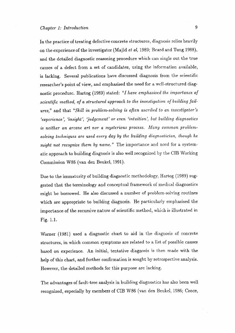
Due to the immaturity of building diagnostic methodology, Hartog (1989) sug-
gested that the terminology and conceptual framework of medical diagnostics
might be borrowed. He also discussed a number of problem-solving routines
which are appropriate to building diagnosis. He particularly emphasised the
importance of the recursive nature of scientific method, which is illustrated in
Fig. 1.1.
Warner (1981) used a diagnostic chart to aid in the diagnosis of concrete
structures, in which common symptoms are related to a list of possible causes
based on experience. An initial, tentative diagnosis is then made with the
help of this chart, and further confirmation is sought by retrospective analysis.
However, the detailed methods for this purPose are lacking.
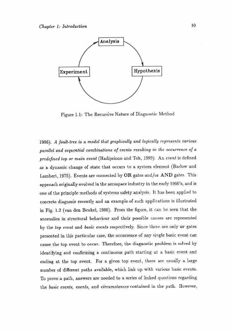
The advantages of fault-tree analysis in building diagnostics has also been well
recognized, especially by members of CIB W86 (van den Beukel, 1986; Croce,
9
Analysis
HypothesisExperiment
Chopter 1: Introiluction 10
Figure 1.1: The Recursive Nature of Diagnostic Method
1986). A fault-tree is a moilel that graphically and logically represents uarious
pørallel ønd sequentíal combinations of eoents resulting in the occurrence of a
predefinedtop or rnain event (Hadipriono and Toh, 1989). An euent is defined
as a dynamic change of state that occurs to a system element (Barlow and
Lambert, 1975). Events are connected by OR gates and/or AND gates' This
approach originally evolved in the aerospace industry in the early 1960's, and is
one of the principle methods of systems safety analysis. It has been applied to
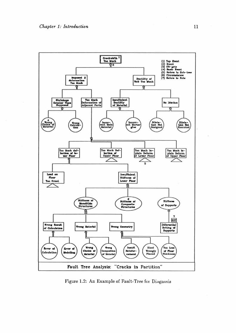
concrete diagnosis recently and an example of such applications is illustrated
in Fig. 1.2 (van den Beukel, 1986). From the figure, it can be seen that the
anomalies in structural behaviour and their possible causes are represented
by the top eoent and. basic euents respectively. Since there are only or gates
presented in this particular case, the occurrence of any single basic event can
cause the top event to occur. Therefore, the diagnostic problem is solved by
identifying and confirming a continuous path starting at a basic event and
ending at the top event. For a given top event, there are usually a large
number of different paths available, which link up with various basic events.
To prove a path, answers are needed to a series of linked questions regarding
lhe basic euents, euents, arrd circurnstances contained in the path. However,
Chøpter 1: Introduction 11
toprd 2d¡lmtlolbo Iæù
Ducüllty ofIrll lbo lr¡ch
Sh¡lD&.f.GrctLr lÌ¡rSuppcd
lbo l¡cl lnruftlchDtDr¡cUlltt
oú Lfrñ¡l llo ltllrtto
IlL¡tâ-llôt¡ Nol
Dlbr.-üon llôt
lh¡c
Ir¡oh dcl-lcclloo oa lÈrr Floor
Iuch D.l-hctlo ol
nærllr¡h ln-
IÞfor¡rrlorcr
1æ ll¡rch b>
l¡d o¡noa
lo GruL
Il¡ufflolc¡tSUfln¿¡¡ oflon¡ Tloor
Ior¡lfll¡o St¡flncrol Supportr
$lñhär ofConpclbgl¡lctuna
Iron¡ RrarltC¡lou¡¡l¡o. lroD¡ Lf.r¡l lrru¡ G.odrl+t Dlflc¡cnthl
SctUn¡ dSupDor{¡
È¡E ofoú 71ff
frÛlìfCboþ. olI¡Lrl¡l
lEutf.DclnloecanFDt
Erro" .fIodclü¡t
ÍÐa
Iffi (r)
{3(.)(õ)(0)Ø
lop EraalEvcalOR-¡rtrB.dc Èt¡tR.f.E to Sub-l¡..ClrrotDrl¡r¡caR¡lcn lo l{ot¡
Fault lÏee ^Analysis: "Cracks in Partition"
Figure 1.2: An Example of Fault-Tree for Diagnosis

Chapter 1: Introiluction L2
these answers usually can not be obtained with certainty in practice, and
hence it is difficult to obtain a conclusive diagnostic result based on the fault-
tree if information available is incomplete. Applications of this approach to
concrete diagnosis in the literature are still very limited, and detailed methods
for reaching diagnostic conclusions are needed'
As can be seen from the above review, although the importance of having a sys-
tematic method for concrete diagnosis has been well recognized, and a number
of publications regarding diagnosis have appeared, including the application of
techniques in other fields, detailed methods for diagnostic reasoning specifically
for concrete structures are still lacking.
After an existing structure has already undergone condition survey and diagno-
sis, in which all indications of structural deficiencies and defects are identified,
and the true causes or most likely causes have been determined, condition eval-
uation is carried out next to determine the structure's capability of satisfying
various requirements for its future use. This is also referred t'o as structural
eualuation, structural assessment, conilition assessn'tent or condition eualua-
tion in the literature, and relevant work on this subject is reviewed in the next
section.
L.2.4 Condition Evaluation of Existing Concrete Struc-
tures
Depending on the characteristics and severity of identified anomalies in struc-
tural behaviour, an assessment is usually needed to evaluate the structural
condition regarding various requirements such as durability, serviceability and,
in particular, safety.
Chopter 1: Introduction 13
Durability Assessment
Unlike safety and serviceability requirements, durabilill_i: a vague concept.
Strictly speaking, durability assessment can not be.-9_learfVieparatelfrom ser-
viceability and safety related problems. However, the difference is that the
study of durability problems has to include effects of time, while serviceability
and safety requirements are usually evaluated at a specific time.
In the design of a new structure, durability requirements are achieved by obey-
ing relevant specifications in adopted codes on factors such as materials, mix
properties and workmanship. For an existing concrete structure, however,
there is no code to apply, and the ¿ì,ssessment of durability usually requires a
study of factors such as deterioration, corrosion, and chemical attack. For this
purpose, research into the individual deterioration mechanisms of construc-
tion materials exposed to various environmental conditions has been extensive
(Tonini and Dean, 1976; Rostasy and Bunte, 1989; Gulikers, 1989; Hilsdorf,
1989; Page et ø1., 1990). However, the effect of the degrz'dation of materials on
the analysis of structural behaviour requires further study. In practice, quali-
tative and descriptive approaches based on personal experience are widely used
in durability assessment. For example, Sakai et aI (1990) evaluated a concrete
structure subjected to chemical attack. The steel bars inside the concrete were
assessed on the basis of the carbonation depth of concrete, and the corrosion
of the reinforcement was classified as grade I, II, III, or IV. Concrete proper-
ties such as chloride content were also measured, and the structural members
were finally judged as being in deteriorøtion degree 1 or degree 2 according to
the severity of deterioration of steel bars and concrete. In a similar approach
proposed by Chung (1991), the damage intensity of reinforced concrete due
to corrosion is assessed from the condition of the concrete and steel in the
member. The condition of concrete is classified as "satisfactory", "poor", "se-
rioust', or "very serious" according to the carbonation of the concrete cover
Chapter 1: Introd,uction74
and chloride content. Relevant repair techniques are then recommended forthe concrete according to the deterioration level. These methods are obviouslyonly concerned with the properties of the component materials regarding in-dividual deterioration mechanisms, and are very much experience-based. Aunified condition measure for a structural member or a structure concern-ing all aspects of deterioration based on a quantitative approach is obviouslyneeded. For this purpose, Roper et at, (rgg5) developed a set of useful equa_tions for assessing the durability of concrete members. upon the study of 50deterioration phenomena commonly present in defective concrete structures,three descriptors, called Measurement, Intensity, and Distribution, are definedfor each of the phenomena. These descriptors are in turn calculated quanti-tatively by three unified eqations, and the durability condition of a structuralmember is then represented by these three values.
From the above brief review on durability assessment, existing approaches tendto evaluate only the seve¡ity of individual deterio¡ation phenomena. Conse-quently the remedial recommendations are often determined from experience.Due to the lack of knowledge about the relationship between a deteriorationphenomenon and the material's property change with time, quantitative mea_sures of structural durability such as service life in terms of years based onaccurate calculation seems impractical for the time being, and those existingexperience-based methods are relatively useful from a practical point of view.However, a unique measure is obviously needed to describe the durability con-dition of a structure for various deterioration phenomena. Although linguisticwords such as ugood" and "satisfactory" are used in methods reviewed previ-ously, they can not be compared on the same basis.
Chapter 1: Introiluction 15
Serviceability Assessment
Serviceability problems in existing structures are in many cases noticeable on
inspection, md the necessity of corrective work is relatively easy to decide
based on the comparison of the intensity of observecl anomalies in structural
behaviour, such a^s excessive cracking, with various requirements in terms of
relevant limits, such as limit on crack width specified by codes. Potential
serviceability deficiency may be identified according to the causes of anomalies
occurred. For these rea,s¡ons, attention should be focused on diagnosis, and a
rigorous assessment regarding the relevant serviceability requirements is not
as important as in safety and deterioration problems.
There are few methods mentioned in the literature purely for assessing ade-
quacy with regard to serviceability for existing structures. Instead, assessment
of the general condition of the structure is carried out by considering both dura-
bility and serviceability. For example, in a rating system developed by Sabnis
et aI, (1990), structural members are placed in one of the following states:
*good condition', *minor deteriorationn, *major deteriorationtt, *hazatdous"
according to the severity of cracking, corrosion and humidity. The general
condition of the structure can then be determined by the member conditions.
These experience-based approaches have also been formulated using finzy set
theory so that the non-numerical subjective data obtained in linguistic form
can be processed systematically. Tee eú al(1988) developed afnzzy mathemat-
ical approach for bridge condition evaluation, in which the subcomponents of
the bridge structure are first inspected, and their conditions and importance
are then rated according to the physical states and related functions in the
structure. The results for each component are represented in linguistic terms
such as ugoodn, upoor", and described by fuzzy sets. The overall condition of

Chapter 1: Introiluction
the bridge is represented by the weighted average, and obtained by:
Dw;en
16
(1.1)
Dw,
where jí¡ and lfl¡ repretent the rated condition and importance of the irr
structural member respectively.
It is important to note that serviceability and durability problems should not
be mixed up. Time plays an important role in durability assessment, while
time-dependent deterioration of materials is usually not considered in the eval-
uation of serviceability.
Safety Assessment
For safety assessment of a possibly defective concrete structure, there is a trend
to use simple approaches in conjunction with experience-based judgement in
practice, in order to avoid complicated structural analysis, especially when
methods for such analysis are not well established. In a reported case study
by de Brito eú øl (1989), tests were made to explore the strength of the con-
crete, and although the structure had deteriorated, the fact that the measured
concrete strength was higher than the original design value led to the conclu-
sion that the structure was safe. Generally, though, evaluation of materials is
not a sufficient basis for structural adequacy.
Even if structural analysis is carried out, the code-specified design methods
are usually adopted (Shroff, 1986; Majið, et aI, 1989). However, due to dif-
ferences in the physical state of the structure between the design phase and
the stage of assessment, the use of design methods for the safety evaluation
of an existing structure may sometimes lead to incorrect results. Code de-
sign methods deal necessarily with the uncertainties of creating a structure at
Chapter 1: Introduction L7
some time in the future. In an existing building, many of these uncertainties
can be eliminated in the assessment process. Therefore, use of the partial
safety factors of a design method may lead to over-conservative results. On
the contrary, when a structure shows signs of being defective, the causes of the
defects may play an important part in evaluating the safety of the structure.
However, the design codes do not consider the influences of all specific causes,
and assume that the design and construction of the structure are under some
standard quality control scheme which results in an acceptably low probability
of committing errors in the design and construction phase. If it happens that
the true causes are not confirmed with certainty in the diagnosis (this is very
likely in practice), and/or the efects of causes on the safety evaluation have to
be accounted for by specifically modifying the model or relevant equations of
structural analysis, code-based safety assessment may lead to unconservative
results, and this is highly undesirable. For these reasons, particular care is
needed if a code-based deterministic approach has to bè used. More realis-
tic methods for safety evaluation of existing defective structures are required,
which can handle uncertainties rationally, and have a sound theoretical ba-
sis. For this purpose, probabilistic methods and fuzzy set-based approaches
are well developed for structural safety evaluation (Thoft-Christensen, 1982;
Melchers, 1987; Blockley, 1975; Brown, 1979). Related rvork in these areas will
be reviewed in some detail in Section 3.2 and Section 3.4 of Chapter 3, and
will not be discussed further in this overview.
L.2.5 Decision-making and Repair Techniques
After the completion of diagnosis and condition evaluation of a given struc-
ture, it is necessary to decide what action, if any, needs to be taken. Although
different courses of action can be identified for specific problems, depending
on the severity of defects and the ownerts resources, as indicated by several re-

Chapter 1: Introduction 18
searchers (Warner and Kay, 1983; Chung, 1991), the following broad categories
are usually a subset of those to be considered in treating defective concrete
structures:
r do nothing, on the judgement that the structure will be able to satisfy
all relevant performance requirements;
¡ monitor the structure in service, in order to check more carefully on
performance and deterioration;
r undertake repair or corrective work in order to bring the structure into
an acceptable condition;
¡ undertake repair or corrective work after taking the structure temporarily
out of service;
r take the structure out of service with the possibility of demolition and
reconstruction;
o Other options in particular cases.
Choosing the most appropriate action for any particular problem is not an
easy task. The decision usually needs to take account of both the technical
and financial aspects of the problem. Technically, both the necessity and con-
sequences of taking a particular course of action have to be considered with
regard to durability, serviceability and safety conditions of the structure be-
fore and after the action is executed. Financially, it is desirable to choose the
action which is the cheapest and also capable of producing a durable, service-
able and safe structure. However, due to the lack of systematic approaches
for this purpose, courses of action regarding the remedy of defective structures
are usually determined on an ail hoc basis in practice. Frequently, the deci-
sion to strengthen a structure is determined conservatively from experience
(Beard et aI, 1988; Mahamond eú a/, 1989; Pakvor et aI, Ig89; Tassios aú ø/,
Chapter 1: Introduction 19
1990) without a rational evaluation of necessity and efficiency. In many cases,
corrective work is planned solely according to the causes of defects (Majid,
1989). When difficulties arise from diagnosing the true causes, actions are oc-
casionally taken arbitrarily. Warner and Kay (1983) tried to apply statistical
decision theory (Raiffa, 1970) to the establishment of a rational approach in se-
lecting relevant repair strategies for dealing with defective concrete structures.
In the method, possible consequences of each course of action and the risk of
failure are considered, and the final action is chosen in such a \¡/ay that the
expected cost is minimized. Although the approach has presented a framework
for applying decision theory to the planning of appropriate actions in treating
defective structures, detailed methods for estimating relevant probabilities and
evaluating consequences were not discussed.
Basically the majority of the existing methods for making a decision in regard
to a repair strategy are based on the engineer's personal experience. Some well
developed approaches (Chung, 1991) are domain-dependent, and only appli-
cable to very narrowly defined fields. Importantly, the risk of making a wrong
decision and the related consequences such as structural failure are not ,¿ti*nally treated.in most of those experience-based methods. Although Warner
and Kay's approach seems promising, many detailed procedures involved are
yet to be developed. For these reasons, a well structured and universal ap-
proach is needed, which can be used to find the most appropriate course of
action for general problems using the information available.
If there is such an approach, a set of relevant courses of action with regard
to repair have to be designed so that a choice can be made. For this pur-
pose, depending upon the specific problem, various detailed repair techniques
are available (O'Donnell, 1989). Generally speaking, repair of concrete struc-
tures is carried out to improve durability, strength, function and appearance.
For these purposes, there exist a variety of different methods, techniques and
materials which can be adopted in specific cases, for example, the use of epoxy-
Chapter 1: Introd,uction 20
bonded steel plate for strengthening (Rostasy and Ranisch, 1982), strengthen-
ing and stiffening by external prestressing (Trinh, 1990), various epoxy resins
and mortars for crack repair (ACI, 1978; Brøndum-Nielsen, 1978; Hewlett and
Morgan, 1982). The detailed discussion of such techniques does not fall within
the scope or purpose of this thesis, and hence will not be pursued here.
L.2.6 Non-destructive Test-based Approaches
In previous sections, the process of dealing with defective concrete structures
has been briefly reviewed. With the application of new electronic devices
to structural engineering, the use of non-destructive test-based methods for
diagnosing and assessing defective concrete structures is becoming popular.
System identificøtioz (Sage et aI, 1971) is one such approach, which relies on
the results of dynamic tests conducted on the existing structure. A theoretical
model of the structure (system) is firstly assumed, and parameters involved in
the model are then estimated in such a way that the dynamic response of the
structure obtained from the test is similar to model predictions. The analytical
model of the structure is thus tuned using the test data. This process is also
referred to as súrzctural identification (Hart and Yao, 1977; Liu and Yao, 1978).
The use of structural identification techniques in damage assessment of con-
crete structures has been discussed in various publications. Agbabian eú a/,
(1990) conducted a test on a model bridge to study the structural changes
by analyzing the response measurements and parameter variation. Flesch and
Kernbichler (1990) used this technique to inspect the safety condition and de-
tect damage in large bridges. The basic concept of these approaches is that
damage, in general, decreases the structural stiffness and increases damping,
and this in turn results in changes in the dynamic properties. Other similar
studies have been carried out by Casas et aI, (Igg0), Vestroni and Capecchi
(1987), and a comprehensive review of this topic was given by Yao (1985).
Chøpter 1: Introduction 2L
Structural identification is a ne\ry technique in the evaluation of existing con-
crete structures. Several technical problems, however, are still to be solved.
For example, the structural response from a dynamic test is recorded by sen-
sors which always contain a certain amount of noise. The presence of such
noise can influence the accuracy and reliability of various system identification
algorithms. On the other hand, as a result of limited dynamic load applied on
the tested structure, the measured responses may be insensitive to changes in
some structural parameters of interest. Also, the method does not give ¡eliable
information on the strength of structural members. Due to these shortcomings,
the application of this technique is still very limited in practice.
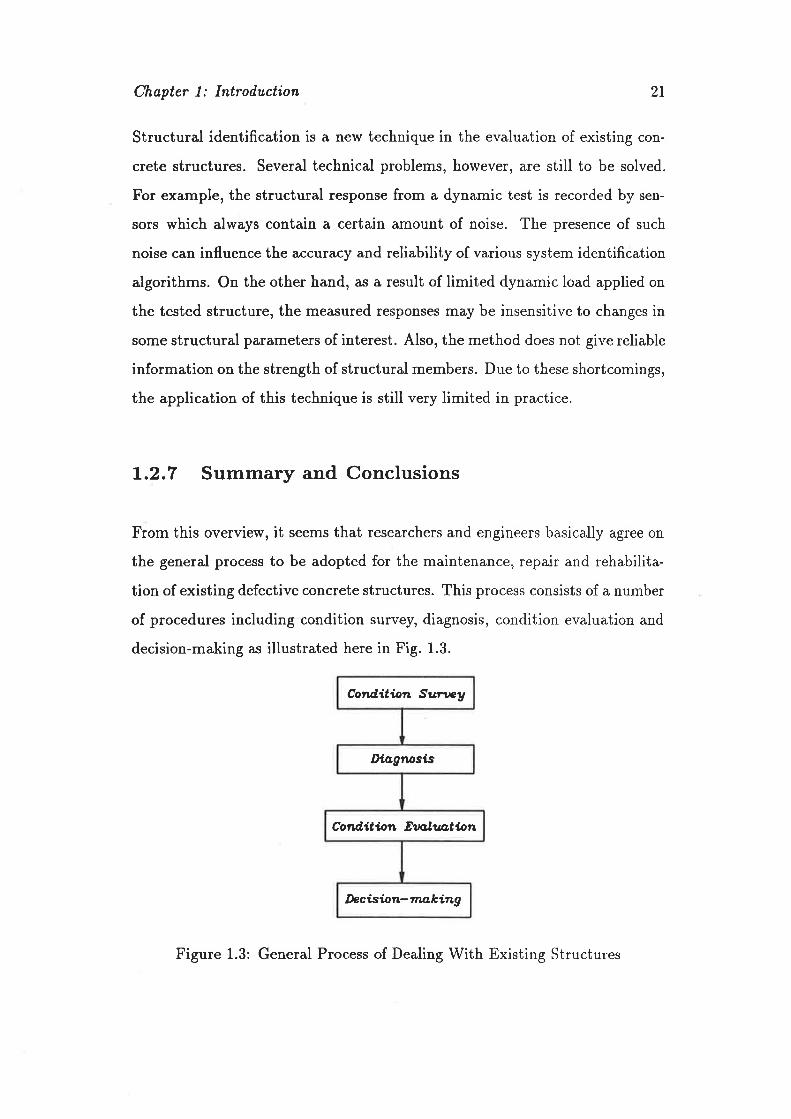
L.2.7 Summary and Conclusions
From this overview, it seems that researchers and engineers basically agree on
the general process to be adopted for the maintenance, repair and rehabilita-
tion of existing defective concrete structures. This process consists of a number
of procedures including condition survey, diagnosis, condition evaluation and
decision-making as illustrated here in Fig. 1.3.
Cottd,ildøta Szney
.Dtogzrosis
Cotd,itiar¿ E\to,Iua,tion
Deci.sbn-nu,kíng
Figure 1.3: General Process of Dealing With Existing Structures

Chopter 1: Introiluction 22
However, detailed methodologies for diagnosis, condition evaluation and decision-
making have not been well established, and relevant literatu¡e available on
these subjects is very limited. For these re¿Éons, the task of dealing with an
existing defective concrete structure in practice is usually carried out in an ad
l¿oc manner. Although experienced engineers have implicit abitity to assess
a structure and make relevant decisions based on their own judgements, the
decision of this type is too often made without the aid of formal models con-
sidering the balance between the imposed cost and the possible consequences
(or outcomes). It is reasonable to argue that such a decision-making process
may not always be suitable for dealing with existing concrete structures. This
is particularly the case when new and difficult problems are encountered.
On the other hand, the existing process of dealing with defective structures
itself needs to be further developed. Firstly, procedures involved in this pro-
cess are highly inter-related, and the output of one procedure is the input
of the next. Unfortunately outcomes of these procedures usually contain un-
certainties due to the incompleteness of information available, and hence a
practically useful process has to logically integrate these procedures in order
to make decision under uncertainty. The simple process illustrated in Fig. 1.3
is not suitable for this purpose. Furthermore, the individual procedures in-
volved can not be undertaken in the simple sequence as in Fig. 1.3 due to
practical reasons. For example, if a structure shows signs of defects, after the
inspection, an immediate decision has to be made as whether to take urgent
action to protect the property and human life. In this case, the engineer can
not afford to wait for detailed information to go through the intermediate steps
of thorough diagnosis and assessment.
Based on the above discussion, it can be concluded that detailed methodologies
for diagnosis, condition evaluation and decision-making need to be developed,
but also that a comprehensive process of integrating these procedures in amethodical way is essential for the treatment of existing defective concrete
Chapter 1: Introduction 23
structures. This thesis attempts to fulfill these tasks
For this purpose, an overall process of treating existing structures is firstly
proposed in the next section, and relevant details needed in the process are
then developed in later chapters of this thesis.
1,.3 The Overall Process for Dealing \Mith De-
fective Concrete Buildings
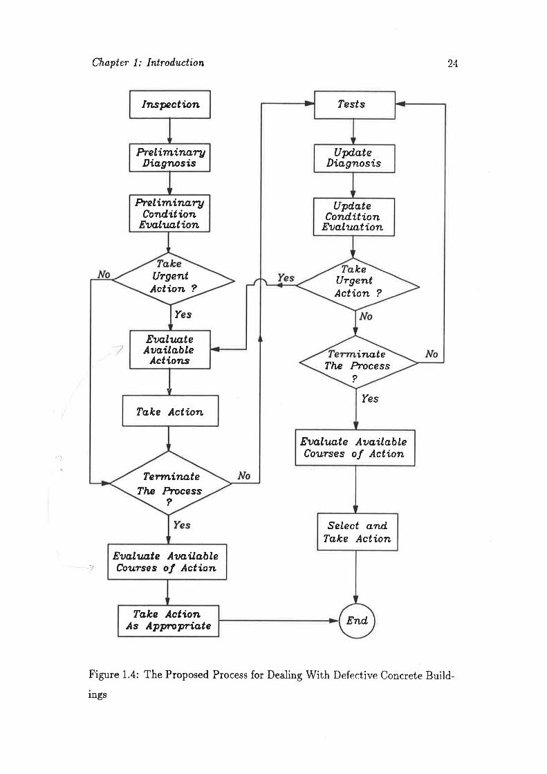
An overall process for dealing with existing defective concrete structures, par-
ticularly for buildings, is proposed in Fig. 1.4. Although there are a lot of
details lacking at this stage, an overall picture of the work to be carried out in
this thesis can be seen from the flow-chart.
The process starts with the inspection of the structure, and a set of anomalies
in structural behaviour can be obtained. U/ith the information gained through
various actions such as an interview with the owner or occupants and study of
available documents, preliminary diagnosis is undertaken to identify possible
causes of the obtained anomalies. Preliminary condition evaluation is carried
out next to determine the real physical state of the structure with regard to
structural requirements of safety, serviceability and durability. Based on these
results, a decision is immediately to be made as to whether urgent action
is necessary or not, using the available information. If the structure is in
danger of immediate collapse, appropriate action is taken to protect human
life and property. After the selected action is executed or if such an action is
unnecessary, an immediate decision needs to be made as whether to continue
the process of assessment. If the information available up to date is sufficient
to make a terminal decision or if the process has to stop for whatever reasons,
feasible courses of actions are then evaluated, and a final decision is made as
Chapter 1: Introd,uction
Yes
Yes
24
a
Inspctdon lests
heliminnryDiøgrwsis
UpdøteDiagnosis
helimínaryCottl,ition
Euo,lua,tion
UpdøteCondition
Eualuntion
UrgentAction ?
UrgentAction ?
ke
Euq,IunteAuøiløble
Actíons The hocessinøte
?
Tøke Action
Eualu,ate AuøilableCourses of Action
Tenníno.teTlæ hpcess
?
Select and.Take Action
Eaa.luøte AuaíløbleCourses of Action
Toke ActionAs Apptoyríote End
Ll
Figure 1.4: The Proposed Process for Dealing With Defective Concrete Build-
lngs

Chapter 1: Introiluction
appropriate. Otherwise, the process advances to the step of gathering more
information by means of tests. Using the new information obtained from the
tests, the diagnosis and condition evaluation can be updated. Based on the new
results from the updated diagnosis and condition evaluation, it is necessary to
decide again on the necessity of taking urgent action.
After all this, an appropriate course of action needs to be determined fo¡ the
given structure. For example, if the structure is evaluated as having inad-
equate safety, a remedy for strengthening the structure would be required.
However, due to the incomplete information available, outcomes of diagnosis
and condition assessment are usually presented with some uncertainty. This
can only be reduced at the expense of acquiring more information. Therefore,
a decision has to be made at this stage on whether to continue the process by
obtaining new data to improve the precision of diagnosis and assessment, or
to take the chosen course of action based on the current information. If the
latter is the case, the process ends when the action is executed. Otherwise, the
process goes back to the information gathering step, and more tests have to be
conducted. The term test here should be interpretated in a broad sense, i.e.
it includes not only experimental work but also any other information gather-
ing activities such as analysis or even study of relevant documents. Using the
new knowledge obtained, diagnosis and condition evaluation are updated, and
a new decision is made. The process thus works iteratively until a terminal
decision is made.
The overall process of dealing with existing concrete structures has been pro-
posed above. The objective of the rest of this thesis is to develop relevant
methods for the steps in the process, and hence to further elaborate the flow-
chart in Fig. 1.4 with details. Of particular importance are the decision-making
steps, represented by diamonds in the flow-chart. The specific objectives and
scope of the thesis are outlined next.
25
Chapter 1: Introduction 26
L.4 Objectives and Scope of Thesis
The general objective of this study is to develop a detailed, systematic process
for dealing with defective concrete buildings based on sound theories. Specific
objectives are:
1. development of a diagnostic procedure which can be used to find out
the most likely causes of anomalies in structural behaviour observed
in a concrete building;
2. development of a method to assess the condition of existing concrete
buildings, in particular those which are damaged or defective;
3. development of a decision model which is able to decide "what to
don about a given concrete building using the results from diagnosis
and condition evaluation, with incomplete information;
4. development of a detailed, comprehensive process for dealing with
existing defective concrete buildings by integrating these three steps
together.
The study is primarily concerned with problems related to existing concrete
buildings which are damaged or become defective as the result of "ordinary"
causes. The term orilinary is used to exclude other extreme causal events like
fire or earthquake which are special problem areas. The fatigue phenomenon
is also ignored because it rarely controls in building design.
1.5 General Terminology
Before specific procedures are described, it is necessary to define the terminol-
ogy to be used throughout this thesis. Additional terms which are used for a
specific method will be introduced in appropriate chapters.
Chapter 1: Introd,uction 27
To be consistent with concepts in structural design, some terminologies of di-
agnosis, condition evaluation and related decision-making in this thesis are
defined in accordance with the philosophy of limit state design which specifies
various structural requirements through relevant limit states. For example,
the serviceability limit states define the requirements for structural per-
formance when the structure is subjected to service loads and normal envi-
ronmental conditions, while ultimate limit states define the requirements
when extreme conditions of overload and environment are considered. In ad-
dition, a structure usually has to satisfy various non-structural requirements
for functional purposes.
Based on this philosophy, a concrete building or one of its structural members
will be said to be defective if it does not satisfy one or more of the limit state
design requirements. Specifically, a structural defect is the non-satisfaction
of a structural requirement, either serviceability or strength. In addition, a
functional defect occurs when a functional requirement is violated.
Usually defects in a structure are initially indicated by various anomalies. An
anomaly is an unusual or undesirable pattern of structural behaviour which
is observed during the operation or inspection of the structure.
L.6 Layout and Contents of Thesis
In Chapter 2,, a literature review on diagnostic techniques in other fields such
as medical science is carried out. A diagnostic method for concrete buildings is
then proposed, in which the most likely explanations of the observed anoma-
lies can be identified through a hypothesis-a,nd-test process using information
available.
Chapter 3 describes the development of methods for condition evaluation of ex-

Chøpter 1: Introd,uction 28
isting concrete buildings, following a literature review on structural reliability
theory and other techniques such as fuzzy-based safety assessment.
Statistical decision theory is briefly reviewed in the early part of Chapter 4,
and a procedure for deciding on the course of action to be taken for a defective
concrete building is developed from this theory using the results of diagnosis
and condition evaluation described in Chapter 2 and Chapter 3.
In Chapter 5, an extensive overall process of dealing with existing defective
concrete buildings is established by assembling logically the procedures already
developed.
Chapter 6 gives two examples of solving real problems using the process pro-
posed in Chapter 5.
Chapter 7 contains a brief summary, and recommendations for future research
work.
Finally, the appendices list some statistical information on basic variables,
which may be needed in carrying out some of the procedures proposed. This
information has been taken from existing literature.

Chapter 2
Diagnosis of Defective Concrete
Buildings
2.L Introduction
The identification of explanations for the observed anomalies is a crucial step
in the whole process of dealing with potentially defective concrete buildings.
Other procedures such as condition evaluation and clecision-making with re-
gard to the corrective work all rely on the output of the clia,gnosis. In this chap-
ter, a method is developed with the aim of providing a sysf's1na,tic approach
for engineers to diagnose existing buildings in a well-strncturecl manner.
Although diagnosis has not yet been extensively stucliecl fbr existing concrete
structures in current research, various diagnostic techniques have been well-
established in other fields such as medical science, ancl it is berreficial to use
this experience of diagnostic research as a reference in the clevelopment of our
29

Chapter 2: Diagnosis
own method for concrete diagnosis. For this reason, literature on research into
diagnostics in related fields iq brieflv ,reviewed,''I
in the next section
2.2 Diagnostic Methods In Other Fields
Extensive research has been conducted in medical diagnosis and mechanical
and electrical trouble shooting in the last few decades. A major emphasis of
this research has been placed on developing computer-aiclecl automatic diagnos-
tic systems. In these systems, diagnostic reasoning mechanisrns ancl r-elevant
expertise used by human experts are acquired and explicitly stolecl in comput-
ers so that the user of the system can diagnose like an expert. While relevant
publications on diagnostic methods developed in these fields ale -briefly,re-
viewed here, there is no intention to deal with the design ancl architecture of
these systems. Instead, the primary emphasis is on the techniques fbr diag-
nostic reasoning used in these systems.
2.2.L The Overall Process of Diagnosis
Although different approaches may be employed for cliagnosis in va,rious areas,
existing methods seem to follow a common process (Weiss et al, Ig78; Peng
and Reggia, 1987a; de Kleer and Williams, 1987). This process is usually
triggered by a set of anomalous patterns of behauiour observecl in the system
to be diagnosed. The anomalous behaviour has genelally been relèrred to in
the literature as symptoms, signs or manifestations. The task of diagnosis
is to identify a set of causes which are responsible 1'or the identified symp-
toms. These causes are usually diseases in medical cliagnosis, a,ncl faults inmechanical and electrical trouble shooting.
For this purpose, a hypothesis-and-test procedure is usualh, acloptecl whereby
Chapter 2: Diagnosis 31
the hypothesis is a set of diseases or faults that can explain the obser-ved symp-
toms, while the test is an experimental action that can confirm a hypothesis
or provide additional relevant information. This proceclnle is schema,tically
illustrated in Fig. 2.1.
Yes
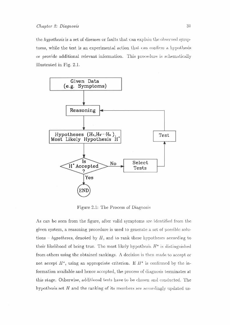
Figure 2.1: The Process of Diagnosìs
As can be seen from the figure, after valid symptoms are identifiecl frorn the
given system, a reasoning procedure is used to generate a, set of possible solu-
tions - hypotheses, denoted by H, and to rank these hvpotheses a,ccorcling to
their likelihood of being true. The most likely hypothesis f[* is clistinguished
from others using the obtained rankings. A decision is then ma,de to accept or
not accept f1*, using an appropriate criterion. If 11* is confir'rned bv the in-
formation available and hence accepted, the process of diagnosis terminates at
this stage. Otherwise, additional tests have to be chosen antl conclucted. The
hypothesis set -FI and the ranking of its members are accolclingly updated us-
Given Data(..g. Symptoms)
Reasoning
TestHypotheses (Hr,H."'H" ), -Most Likely Hypothesis H-
SelectTeststedpAc
Isceq
H.
END
Chapter 2: Diagnosts 32
ing the new information resulting from the testing, ancl the cliagnostic pr-ocess
continues.
In the hypothesis-and-test process discussed above, a majol task of the reason-
ing procedure is to rank all possible hypotheses using techniques available such
as probability or ftzzy set theory. Criteria for accepting the most likely hy-
pothesis l/* and selecting a test are usually dependent on the ranking method
adopted. Obviously the reasoning mechanism is the nost important part in
the diagnosis, and therefore wili be the focus of this litera,ture review.
2.2.2 Probabilistic Reasoning for Diagnosrs
Many existing systems for medical diagnosis (Ben-Bassat, 1980a,; Reggia el ø/,
1985a, 1985b; Lauritzen and Spiegelhalter, 1988) and electrical or mechanical
trouble shooting (de Kleer and Williams, 1987) have been cleveloped using
probabilistic reasoning. Although various detailed proceclures can be adopted
for this purpose, the reasoning mechanism used in all these zr.pproaches is more
or less Bayesian in style. Specifically, possible symptoms of huma,n patients or
mechanical systems are related to a set of diseases or faults, with the strength of
these relations defined in terms of relevant conditional plobabilities. With the
evidence such as identified symptoms, diagnostic reasoning is usecl to evaluate
the updated posterior probabilities of those diseases or fa,ults fiom their prior
probabilities. Diseases or faults are hence ranked bv their probabilities, and
the most likely disease or fault is the one which has the highest probability.
For this purpose, assuming that there are rn possible ca,uses ç : Crt Cr, . . . , C^
to be considered for an observed pattern of symptoms, the prior probabil-
ity of C¿ is assessed and denoted by P'(C;). After the set of symptoms
,S : (sr ¡s2¡...,srr) are observed from the given system (patient or rnachine),

Chapter 2: Diagnosis
the posterior probability of the irä cause C¿ is given bv
P(C; I s1, s2,' ' ' , s",) : P' (Cn). P(tt ,¡ s2¡' ' ' , "* I C¡) (2,r)
\e'(c,) . P("r,s2,.. .,s,, I c¡)i=l
where P("t, s2,t...,""1C¿) is the joint probability of s1, szt' ,s, conditional
on C¿. However, this formula is only suitable for diagnostic problems in which
only one cause can be true. Although a multi-cause problem, in principle, can
be transformed into a single-cause problem by defining a new set of possible
causes which consists of all the 2- possible intersections of Ct,Cr,,'" ,,C,n, e.E.
(Ct,Cr,CtCz,/) for rn:2, where / is an empty set, the exponentia,l increase
in the number of causes makes this approach impractical a,s n¿ irLcrea,ses.
For this reason, Ben-Bassat (1980a) assumed that all carlses in C a,re mutually
independenú, i.e. the probability of C¿ being true does not a,ffect the probability
that C* is true given a pattern of symptoms observed. It has to be mentioned
that if C: (CtrCzr..'rC^) are mutually exclusive ancl exha,r-tstirre, tnentbets
in C aie then mutually dependent, since the existence of a,ny one cause will
exclude the occurrence of all others. Under this inclepenclence assumption,
Ben-Bassat applied Eq. 2.1 to determine the probabilitv of each cause C¿ in
the following manner: Let C¡ denote the event that the c¿ùuse C¿ is responsible
for the observed symptoms, and C; denote the complementary event that the
cause C; is not responsible for the occurrence of identifred syrnptoms. C¿ and
C¿ thus constitute a mutually exclusive and exhaustive set, ancl hence the
posterior probability lhat C¿ is the cause of an observecl syrnptom pattern
,S : (sr ,s2r- .. , sr,) is given by:
P(C;1sl,s2,"',s,,) :P' (Cn)' P(tr, s2t' ' , s* I C;)
33
(2.2)P'(Cn).P("t, s2¡.' ,s*lC¿) + (1 - P'(Co)).P(tt, s2¡" ,s^l C¿)
In this way, by applying trq. 2.2 for every element of C, the probabilitv of
each cause P(C,) can be obtained, and these P(C¿)'s constitute the solution of
the problem. Alternatively, since C1, Czr. . . ,Cn are mutua,lly inclependent, the

Chapter 2: Diagnosr,s
probability of any multi-cause set can also be evaluatecl as the product of the
corresponding probabilities of the relevant causes involved. This method has
been applied to real problem- solving (Ben-Bassat, 1980b) ancl clemonstrated
its usefulness in certain domains.
Obviously due to the difficulty of handling too many members in a multi-cause
set, Ben-Bassat's approach transformed the multi-cause cliagnostic problem
into a single-cause problem based on the independence assumption. Actually
the multi-cause diagnostic problem has been tacklecl by ma,rry resea,rche-r''s in
different \4/ays. Reggia et al (1985a, 1985b) proposed a so-callecl generalised set
couering model which deals with the multi-cause problem in a very rneaningful
manner. To demonstrate this method, an example is given in Fig. 2.2 Á which
there are two symptoms ,9 : lsr, s2] and three diseases p : @t,d2,tfu1. Causal
relationships between diseases and symptoms are denotecl in the figure by
appropriate lines, e.B.sr can be caused by d, and/or rI2, ancl s2 câil. be caused
by dt and/or d3. From the assumed relations, the hypothetical solution th.e
hypothesis can be found using the concept of set covering. For this purpose,
a hypothesis is firstly defined as a set of diseases whiclt cun !u,ll'y erpla'in, or
coler, all of the presented symptoms. Under this definition, hvpotheses for-
the examplein Fig. 2.2wiII include Ht : (dr), H, - (d2,d"), H": (û,dz),
Ha - (ù,d2,ú).
It has to be mentioned that there are only four valid h1'potheses in this pa'-tic-
ular example, but for a complicated problem in whicir the nutrber of possible
diseases is large, the hypothesis set fI generated in this wa,y coulcl become
too big to handle. To overcome this difficulty, Reggia, et al rsecl a mini-
mal cardinality principle to restrict the valid number- of h¡,potheses, i.e. in
the hypothesis set H, only those members which contair¿ the mi,r¿i,nt1r"rrL n'urn-
ber of diseases will be considered at the nert stage of itrur:stigatiort,. In fact,
this is another application of Occam's Razor, which reflects the iclea of
the simplest solution being the best among all possible solu,t'ior¿s. IJsing this
34
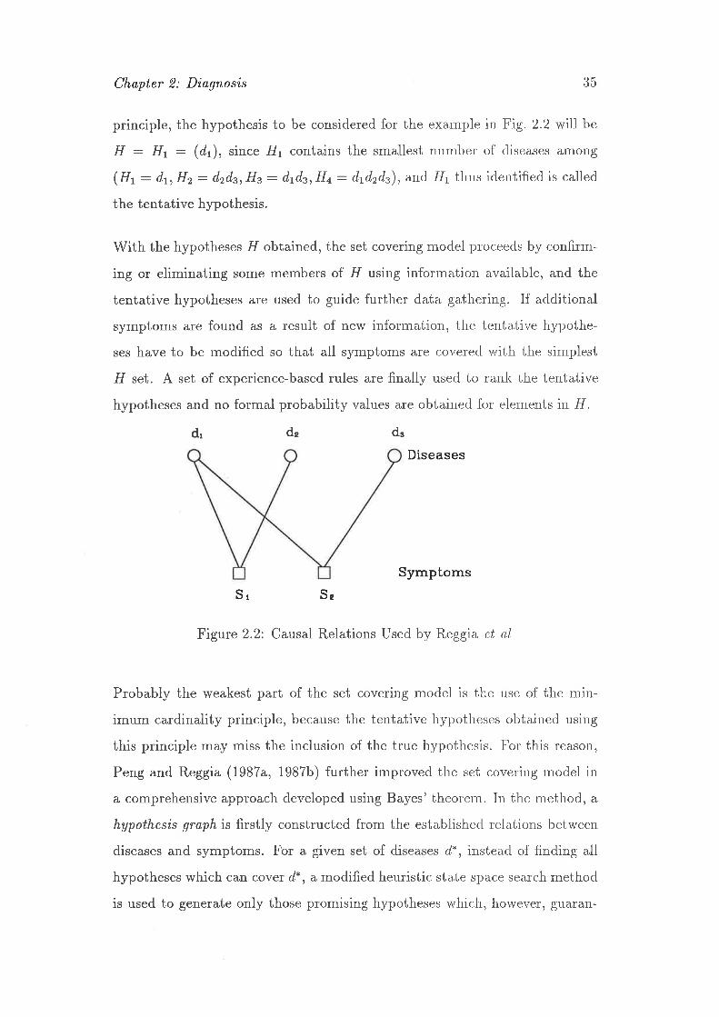
Chapter 2: Diagnosis 35
principle, the hypothesis to be considered for the example in Fig. 2.2 will be
H : Ht : (dt), since ffi contains the smallest number of diseases among
(Ht : dr, H" : d,zds, Hz : d'1d4, Ha : d'i'zdz), and flr thus identified is called
the tentative hypothesis.
With the hypotheses -FI obtained, the set covering moclel p,.-oceecls by confirm-
ing or eliminating some members of fI using information available, and the
tentative hypotheses are used to guide further data gathering. If aclditional
symptoms are found as a result of new information, the tentative hypothe-
ses have to be modified so that all symptoms are coverecl with the simplest
fI set. A set of experience-based rules are finally usecl to rank the tentative
hypotheses and no formal probability values are obtainecl 1'or elements in 11.
dr dz ds
Diseases
SymptomsSr Se
Figure 2.2: Carsal Relations Used by Reggia, el ø/
Probably the weakest part of the set covering model is the use of the min-
imum cardinality principle, because the tentative hypotheses obtained using
this principle may miss the inclusion of the true hypothesis. For this reason,
Peng and Reggia (1987a, 1987b) further improved the set coveling model in
a comprehensive approach developed using Bayes' theolem. In the rnethod, a
hypothesis graph is firstly constructed from the establishecl relations between
diseases and symptoms. For a given set of diseases d*, insteacl of finding all
hypotheses which can cover d*, a modified heuristic state space seat-ch method
is used to generate only those promising hypotheses which, horvever, guaran-
Chapter 2: Diagnosts 36
tee that the most probable hypotheses are included. The cliagnosis is then
focused on evaluating the probability of each member in the hypotheses thus
generated.
For this purpose, given a symptom s¡ and a disease d;,L'he ca'usation euent
s¡: d"¡ is defined as the euent that d¿ actually c&uses sj. In other words, the
event s¡ : d,¿ is true if and only if both d; and s¡ occur and s¡ is actually
caused by d;. The probability P(s¡ : d; I d¿) is then callecl the con'ditional
causal probability of s¡ giaen d¿, which represents the strength of the relation
between s¡ and d;. Also, the prior probability of each clisea,se, P(r1¿), is assumed
to be known. Thus for a diagnostic problem with observed symptoms s* :(rr,"r, '..s,,) and a set of hypotheses fI : (Ht,Hr,"' ,H^), the probabiiity
of each hypothesis in fI can be evaluated through Bayes' theolem:
P(Hnl ,*) : P(s. l-Ht)P(Ht) Q3)P(".)where the prior probability P(Ho) is to be calculated fïom the prior probabil-
ity of each disease d,¿, and the conditional probability P(-s* I f1,) ttu"" to be
calculated from P(s¡ : d¡ | d¿); P(".) is a constant for a pa,rticular diagnostic
problem. However, since the hypothesis set 11 is not completely generated, the
constant P(".) can not be obtained, and hence only the lelative likelihood of
each H¡ is obtained in this approach.
Peng and Reggia's method provides a good framework for clea,ling with multi-
cause diagnosis using formal probabilistic manipulation. Howet'er, due to the
large amount of computational work required, the approach is suitable for
building a computer-based automatic diagnostic system, but not par-ticularly
useful as a practical procedure to be used by a diagnostician.
In diagnostic reasoning previously reviewed, probabilistic relations ar-e defined
between only causes and symptoms. In real cases, however, a, cause or fault
may be attributed to further causes, and symptoms can a,lso ha,ve correlated
sub-symptoms. These further co,uses and sub-symyttoms constitute a very im-

Chapter 2: Diagnosis 37
portant part of information other than the previous deflnecl causes and symp-
toms. To include this knowiedge in the probabilistic reasoning,, Pearl (1986),
and Kim and Pearl (1987) used a tree structure called a causal network or a
belief networlc to represent the relationship between various pieces of informa-
tion. The strength of these relations are also expressed in terms of conditional
probabilities. Two examples of the network are shown in Fig. 2.3, in which
Figure 2.3: An Example of Causal Network
each node represents a variable or proposition, e.g. symptom, clisease, or- sub-
symptom. The root node (node A in the figure) usually stancls fbr the original
cause, e.g. disease or fault, and nodes on the tips of the clilected graph (nodes
8,, D, E) arc data nodes which represent various manifestecl sJ¡mptoms. Those
nodes which are needed to tie together the root node ancl the clata nocle are
called interuening nodes. All nodes are not necessarily bina,ry variables, and
hence each node can have many possible values. Directed arcs a e used to
represent causal relations between two nodes, and the strength of this relation
is quantified by a conditional probability, e.g. P(c I a) clenoting ihe probability
of node C, given the occurrence of node A.
After the prior probabilities of those root nodes and leleva,nt conclitional prob-
abilities have been assessed for an established netwolk, the plobability fl of
each node is evaluated and updated using new information a,vailable, while
ba
Chapter 2: Diagnosis 38
the conditional probabilities are kept unchanged. Since P¿ thus clynamically
changes, the probability of any node, say node B, is representeil by the ovelall
belief in B based on the data D available up to date, and clenoted by BEL(B),
i.e. BEL(B): P(B I D). BEL(B) can be obtained by:
BEL(B): aÀ(B)r(B) (2 4)
where a is a constant; À(B) : P(DA I B),, r(B) : P(B I DÐ in which D;represents the data contained in those nodes of a sub-network rooted at node
B, and Df stands for the data contained in nodes of the rest of the whole
network. Obviously F,q.2.4 is also derived from Bayes' theorem, where r"(B)
represents the causal support attributed to B by the ancestors of B, and À(B)
represents the diagnostic support B receives from descencla,nts of B.
Using Eq. 2.4, the probability of each node can be obtainecl ancl stored. Ifnew information is gathered on a node i, the effect of this cla,ta, on the belief
of any node in the network can be evaluated, and the nocle-probabilitv is then
updated through a propagation procedure.
Exploring new information to reduce the uncertainty of a particular node is
called node erpansion, and which node to be further expa,nclecl is clecided by
the benefit of this expansion. For this purpose, the benefit of a node 1/ inresolving the uncertainty of node 7 is defined as:
BEFIT(T,l/) : IMP(7,¡/) ¿(¡/) (2.5)
where IMP(T,,nú) is called "important factor" determinecl by the strength of
dependency between 7 and lú; and E(¡f) is the uncertaint)/ of the node /y'
which is measured by its entropy:
E(¡/) : -t P("0) 'losP(n¿) (2 6)
Kim and Peari's work provides a good tool for solving cliagnostic problems
in a well-structured way under the context of proba,bilitv theory. However,

Chapter 2: Diagnoszs 39
the network used in this method is restricted to a specia,l kincl of sirt,gLy con-
nected causal networlc (SCCN). A SCCN is defined as the network in which
one (undirected) path, at most, eri,sts between any two rt'odes (Pearl, 1986). For
example, the network in part ø of Fig. 2.3 is a SCCN, while the one in part ó
of Fig. 2.3 is not. The latter is usually referred to as a network with "loops".
This restriction certainly limits the applicability of the approach, since many
real problems can not be represented by a simple SCCN.
Probabilistic reasoning using a more general causal netwolk ha,s been proposed
by Lauritzen and Spiegelhalter (1988) in which loops a,re permittecl. For a given
causal network with known conditional probabilities betrveen linlçecl nodes and
prior probabilities of root nodes, the ideal representation of oul belief within
the network is the construction of a joint probability clistribution over all those
nodes involved in the network. Relevant marginal proba,bilities on interested
nodes can then be obtained for the purpose of diagnosis. However, the cornpu-
tation for this purpose is usually a formidable task when the number of nodes
is large. To overcome this difficulty, Lauritzen and Spiegelhalter cleveloped a
method which is capable of calculating the marginal plobabilities on individ-
ual nodes efficiently without obtaining the joint probabilitv clistribution. For
this purpose, some topological changes are made to the original network, and
the resulting new network consists of a number of. cl'iqttes whìch a,re clefinecl as
sets of nodes that are all joined directly in the networ-lc. With this change, the
marginal probabilities on these cliques are evaluated, ancl the malginai proba-
bility on a single node can be easily calculated from the ma,rginal probabilities
of relevant cliques.
By using this algorithm of efficient probability manipulation rvitirin the net-
work, one can determine the marginal probabilities of interestecl nocles that
are considered as causes of observed symptoms. This can be carriecl out for
any state of available information. If new data are gatherecl, the a,pproa,ch is
capable of absorbing the knowledge through the network ancl hence rqrclating
Chapter 2: Diagnosis 40
the node probabilities. The use of strict probabilistic methocls also ensures
that the effect of multiple pieces of evidence does not clepencl on their order of
arrival.
When deciding what test is to be conducted next for gathering more informa-
tion on a particularly interesting node, say node -4., "mtttual information" is
used to determine how valuable another node is to nocle A. For exa,rnple, the
mutual information between node A and B, M(B,A), is <lefinecl as:
M(B,A) : Df r"s14g !,'U )P(B t A)P(A) (2.7)B A P(B) 't- \" t'
This approach provides probably the most comprehensive methocl for rigorous
probability calculation within a causal network, and is very suita,ble for con-
structing computer-based diagnostic systems. The applica,tion of it in meclical
diagnosis can be found in the work by Andreaseen et al (1987).
In addition to the above formal probability-based diagnostic reersoning, a large
number of computer-aided diagnositic systems have also em¡rloyecl the sub-
jective Bayesian inference (Lesmoet et a\,1982) using some mles in the form
of:
I f E then H with probability p, i.e. E ---+ H
where E can be evidence such as symptoms, and 11 is an hypothesis, e.B. a
disease. The probabilistic nature of this kind of rule ha,s been summarized
by Duda et al (1976). Speciflcally, if the prior probabilitv of H, P(11), and
the conditional probability P(E I ,É1) are assessed, the posteliol probability
of .FI after the evidence E is observed can be easily eva,lua,tecl through Bayes'
theorem, i.e. :
p(H I B¡: P(H)'P@ | n) (2.8)P(E)

Chapter 2: Diagnosis 4T
in which P(E) : P(H)'P(E I H)+P(H)'P(E I fI), ancl ll is the complement
of H . However, sometimes the eviden ce E rnay not be identifieci with certainty.
For example, the conclusion "I am 70 percent certain lhat E is true" from a
diagnostician only indicates that P(E I releuant obseruations) : 0.7. If .E' is
used to denote the relevant observations, we can denote P(E I E'):0.7. The
probability of fI given E' is obtained as:
P(H I E'): P(H,E I E') + P(H,E I E',) (2 e)
: P(H I E,E,). P(E I E,) + P(H I E,E') P(E I E') (2.10)
where ,E is the complement of B. If ii is assumed that when -E is known with
certainty, the observations E' relevant to E provide no further infbrmation
about H, E,q. 2.10 becomes
p(H I E'): p(H IE).p(EIE')+p(H IE).p@ | E) (2.rr)
where P(H l.E) and P(H I E) can be obtained from trq. 2.8. Thus the poste-
rior probability of f1 given the vague evidence -E' is r-epresentecl by Eq. 2.11.
If there are several rules of the form -81 - Hr'..,8r, --+ H all concerning
the same hypothesis H , the diagnostic problem becornes to eva,luate the prob-
ability P(H I Et,.'.,8,). For this purpose) based on the assumption that
those pieces of information are conditionally independent, i.e. P(8t,. . . , En) :firp, I f1) and P(Er,'.',Enl fr) : firçn, | 11), an a,na,logous solutioni=I i=7can be obtained from Eq. 2.8.
Although probability-based diagnostic reasoning as reviewed a,bove has been
very popul ar, fizzy set theory is also widely applied in rna,n1, existing clia,gnostic
systems, and this is briefly reviewed in the next section.
Chapter 2: Diagnosis 42
2.2.3 Diagnosis Using Euzzy Reasoning
Frzzy set theory (Zadeh,,1965, 1973; Dubois and Pra,cle, 1980) has been suc-
cessfully used in treating unclearly defined linguistic variables, ancl proves to
be a good tool for handling uncertainties. The application of Írzzy set theory
in diagnosis can be 'frequent$ found in the literature (Gupta and Sanchez,
1e82).
A, fuzzy sel is a collection of objects, in which there is a clegree of membership
related to each object. For illustration purpose, the iinguistic term "integers
close to 10" can not be described by an ordinary set, but can be easily repre-
sented lsy a fuzzy set à with its membership function in the fbrm: I p¡(:r) | r,e.g.:
Á,:0.1l7+0.5 l8+0.8 le+1110+0.8 111 +0.5 l12+ 0.1 113 (2.t2)
where r € X; X is the ordinary set representing all integers, a,ncl is referredto
as the reference set; ¡"t¿(r) denotes the degree of memberslrip of z in the luzzy
set Ã. For example, 0.8 | 9 means: "integer 9 belongs to Á with the clegree of
membership of 0.8".
In diagnosis, many variables such as symptoms can be clescribed by fuzzy sets.
For example, a symptom ,9¿ can be defined as a Trzzy subset .í¿ of a, reference
set X : (Xt,". ,,Xn), characterized by a membership functiotT l11¿(:r). Set Xcontains all possible values which can be taken by,5,. The rnembelship function
pS,@) defines the strength of ø being i" ^9,. In this context, iT fitzzy sets ^l
and Õ represent symptoms and causes respectively in a, clitr,gnostic problern,
the causal relation lf Õ then S can be described by a, fiuzy opela,tion called
fuzzy relation denoted by R (Zadeh,1965; 1975a):
R:ÕxS (2.18)
in which the membership function of R can be obtainecl 1ìom that of Õ onl S
using relevant finzy calculations. With the observed symptom pa,ttern defined
Chapter 2: Diagnosis 43
by afrzzy set ,S*, the causes responsible for the occurrence of S*, also described
by a htzzy set Õ*, is obtained through another fizzy operation, called fuzzy
compos'ition:
Õ*:^9*oR (2.r4)
where the membership function of. Õ* can be easily evaluatecl from that of ,9*
and R.
Many fuzzy diagnostic reasoning techniques in existing a,pproaches are based
on the fuzzy relation and fuzzy composition described al:rove (Zacleh, 1975b;
Sanchez, 1979a, 1979b; Soula et al, 1980; Baldwin, 1981; Zadeh, 1983), al-
though various forms of relations may be defined for specific p-,-oblerns.
For example, Adlassnig and KoIarz (1982b) used fuzzy lelation to build a
medical diagnostic system in which symptoms and cliseases of a, particular
kind are collected and represented by two ordinary sets S: (5r,5r,...,5*),D : (Dt,Dr,---,D^). Each ,S¿ and D¡ are in turn clefinecl a,s fuzzy subsets
of relevant reference sets, and denoted bV ^9n and b¿ respectivelv. Svmptom-
disease relationships are described in terms of two depenclencies. The first
dependency is the occurrence of a symptom ,S¿ in case of a clisease D¡, which
represents the knowledge about the possibility of the presence of ,5; given D¡.
This "occurrence relation" is further represented by a fizzy relation R9 de-
fined on the reference set S x D. The second dependency is the confirrnabilityrelation which indicates the power of an observecl symptorn 5i to confirm a
certain disease D¡. The confirmability is also deflned by a ftzzy relation Rçon S x D. If. the fitzzy set ^í* describes the observed syrnptoms on a particular
patient, fotlr fiizzy indications can be calculated by means oÍhzzy composition
(Eq.2.1a):
1. S;, D¡ occurrence indication: -r?1 - -R* o RCI;
2. S;,, D¡ confirmability indication: ñ - ñ* o R6;
3. ^9i, D¡ rort-occurrence indicationr 3 : ,?- o (f - RO);

Chapter 2: Diagnosr,s
4. S;,, D¡ non-slmptom indication: És, - (1 - A.) o Roi
The final decision regarding the diagnostic result is to be determined based on
these four indications.
A similar approach using fiizzy relations is also usecl by Johnston (1985) in
diagnosing faults of the wastewater treatment process, in which a clifferent
algorithm for fis,zzy composition is adopted.
Although there are many other applications of fitzzy set th.eory to diagnostic
reasoning, methods reviewed in this section represent the most popular ap-
proaches in this domain, and demonstrate the relevant concepts clearly. More
literature on existingfizzy-based diagnostic systems can be f'ouncl elsewhere
such as Gupta, Saridis and Gaines (1977), Esogbue ancl Elcler (1980), Gupta
and Sanchez (1982), Adlassnig (1982a), and will not be fìrrther leviewecl here.
Techniques using probability and fiizzy set theory thus reviewecl constitute
the majority of existing methods for diagnostic reasoning. In aclclition, some
other approaches are also frequently used in medical cliagnosis a,ncl mechanicai
trouble shooting, and are briefly discussed next.
2.2.4 Other Approaches for Diagnostic Reasoning
In either probability or fiizzy reasoning discussed in previous sec.tions, symp-
toms are related to relevant diseases or faults in terrns of conclitional prob-
abilities or fivzy relations assessed ftorn erperience or rttalitatiue analysis of
the physical system to be diagnosed. In troubleshooting mecha,nical devices
or electrical circuits, however, some other approaches employ cliagnostic rea-
soning based on the actual physical model of the devices o.-. cìr'cuits, in which
the relationship between symptoms and faults is established accorcling to the
measured behaviour of the model.
44

Chapter 2: Di,agnosi,s 45
De Kleer and Williams (1987) proposed a domain-incleperrclent rnethocl f'or di-
agnosing multiple faults. For a device to be diagnosed, if its behaviour can be
predicted without uncertainty from an established model which is a descrip-
tion of the physical structure of the device, a symptom can then be defined
as ûnA difference between a predicted and obseraed behauiour. From relevant
measurements and records of the model behaviour, a set of such symptoms
can be identified. These symptoms are further related to one or mor-e "candi-
dates" which are defined as a set of components of the deuice wh,ich are possibly
faulted.
Under these definitions, a set of possible candidates a,re cr-eatecl through a
candidate generating procedure which is basically similar to Peng ancl Reggia's
set covering model described on page 34. The diffelence is that in this pro-
cedure every possible cover is considered in generating the ca,ncliclates, while
Peng and Reggia's approach considers only the hypotheses ha,r,ing minimal el-
ements. The task of diagnosis is to confirm a particular cancliclate or to reduce
the number of elements in the candidate set until only the true candidates are
left. For this purpose, testing or measurements have to be callied out so that
the candidate set can be re-generated using the new inf'ormation obtained.
However, the concept of probability is again employecl to cletelmine the most
valuable parameter to be measured in the next testing. Suppose thele are a
set of parameters t : tt¡t2¡..'tr¿ to be measured in the testing. To choose
one from u, each member of the "candidate set" C : (Ct,Cr,. . . ,C^) obtained
above has to be ranked by its probability p¿, which is subjectively estimated
using the knowledge currently available. The entropy EH is in turn defined
EH : -Dp logpo (2.r5)z:l
If a test is conducted to measure variable r¿, which has possible values uirt' ' . ,ui^,the expected entropy for measuring r¿ is evaluated by
TH-(r¡) : ip(r¡ : u¡¡r)EH(r¿ - uik) (2.16)fr=1
Chapter 2: Diagnosis 46
where p(r¿ : u¿¡) is the probability that the variable r¿ equa,l u¿¡, ancl E H (r¿ :u;¡) can be computed from Eq. 2.15 conditioned on r¿ - uik. According to the
calculated expected entropy, the best choice is to measrte :I:j1if ø¡ has the
minimum expected entropy among all variables to be mea,sured. However, the
approach did not specify how the probability pi was estimatecl.
Methods using well-established models are also found in meclica,l cliagnosis. For
example, Weiss et al (1978) constructed a computerized diagnostic system in
which a detailed model is established to represent various pathophysiological
states in the form of a network. The causal relation between two states is
defined for all possible states with the deep understancling of a particular
kind of diseases. For instance, if n¿ and n¡ are two pa,thophvsiological states,
the mappilg n¿"j n¡ indicates that state n¡ is causecl by st¿ite n¿ with the
numerical strength a¿¡. The belief in the truth of each state can be represented
by a confidence factor CF(n¡).
The diagnostic procedure is carried out in sequences, a,ncl new informatlon
about the pathophysiological states is obtained through experirrents. The
confidence factor of each state can be updated accolclingly. If a, symptom or
a piece of evidence is observed from a test f¿, a confiderce mea,sule is used to
indicate the degree of belief in the presence of specific states. For instance,
t¿9J n¡ means that the ith test or evidence supports the pr.esence of state n¡
with confidence Q¿¡.
To select a test to be conducted, relevant weights are definecl for- va,r'ious states
presented in the causal network. For this purpose, a pa,thrva,1, can be iclentified
between any two states in the network. A. "forward ueigh.t"of entering a state
n¡ frorn a single pathway starting at state n¿ is definecl as:
j-ruF(j I i) : ll clk,te¡7 (2.17)
,b=1
where úk,k+L is the causation strength between two adjacent states n¡,, n¡¡1ir'the pathway as defined above. The total forward weight ,ur(j) of state n¡ is
Chapter 2: Diagnosis 47
the sum of all weights -r(j I i) for those pathways entering node n¡ starting
at the nearest confirmed state n¿ in the network. With a set of interested
states identified, the weight of these states can be evaluated from Eq. 2.17,
and the state with the highest weight should be focussed in the next stage of
information gathering. To do this, a set of tests can be ctesignecl, ancl the best
choice is the one which is cheaper than all others.
After a test is conducted, confidence factors of relevant states are updated. For
each state n¡, if. its confidence factor CF(n¡) is greater than a, certa,in value,
the state n¡ is considered true. If several confirmed states l'orrn a continuous
path in the causal network, a particular pattern of pa,thophysiological states
can be identified and prove to exist. This pattern of sta,tes is then related
to a specific disease by a set of pre-defined rules derivecl fïom experience and
other relevant knowledge. Finally, the disease which has the highest confidence
factor is considered true, and the relevant treatment suggestecl accorclingly.
The methods reviewed in this section either require a well-established model
to represent the physical structure of the system to be cliagnosed, or need
a deep understanding of the system so that accurate precliction of relevant
behaviour is possible. These conditions are usually clifficult to meet iu dealing
with existing concrete buildings, and hence it is probably not convenient to
directly apply these methods for our purpose. Nevertheless, the strategies used
for test selection as well as the reasoning mechanisms a,re domain independent,
and could be useful in diagnosing defective concrete structures clepending on
particular problems at hand. Many more similar approa,ches can be f'ound in
the literature (Szolovits and Panker, 1978; Davis, 1984; de Kleer, 1986; R,eiter,
1987), but will not be further discussed.
Chapter 2: Diagnosis 48
2.3 Surnmary and Conclusions
It can be seen from the above discussion that an iterative process of hypothesis-
and-test has been widely adopted in most of the computer.izecl cliagnostic sys-
tems. This procedure works in cycles using the mechanism of abductive rea-
soning, i.e. it begins with a set of observed symptoms, and tr-ies to find out
the best hypothesis which can fully explain the given pattern of symptoms
through a relevant process of information gathering, such as testing. Although
diagnostic problems are very diverse, the hypothesis-and-test pr-ocedure seems
to be suitable for a wide variety of diagnostic tasks. For this rea,son, the
hypothesis-and-test procedure will be adopted in the clevelopment of a, method
for diagnosing defective concrete buildings.
In most existing approaches for diagnostic reasoning, relations between symp-
toms and causes are defined and measured by using either probabilitt, or fizzy
sets. Probabilistic reasoning proves to be a very meaningful and practical tool
to deal with uncertainties in diagnosis, especially by the nse of Ba,J,esian sub-
jective probability, while fiizzy reasoning is more capa,ble of tleatirrg variables
or symptoms which are vaguely defined or in linguistic f'orrns. In this work,
probabilistic reasoning will be used.
However, available approaches for probabilistic reasoning are generallv devel-
oped and used for the construction of computerised dia,gnostic systems. These
methods are not suitable for direct application to the cliagrLosis of concr-ete
buildings due to the following reasons. Firstly, a computerisecl a,utonla,tic di-
agnostic system has a large data base created by collecting a,ll possible causes
(diseases/faults) and symptoms for a specific kind of problem. In orcler to
carry out probabilistic reasoning, relations between the ca,uses and symptoms
of the entire set have to be pre-defined in terms of conclitiona,l probabilities.
In the diagnosis of existing buildings, it is very difficult l'or the engineer to
create a complete set of diagnostic knowledge for a specific lcincl of problem.
Chapter 2: Diagnosis 49
Secondly, as a result of using the large data base, complicated computation
procedures are usually needed to reach a diagnostic conclusion from the given
evidence. This is a big disadvantage for the engineer in diagnosing concrete
buildings, where simple calculations are obviously preferred. Therefore, the
method of diagnostic reasoning adopted for concrete structures will have to
overcome this difficulty.
For this purpose, consider the fact that unlike computers which need a com-
plete set of pre-defined rules to proceed diagnostic reasoning, engineers can
intelligently carry out relevant reasoning quickly in their mind using only the
information currently available. Then an attractive way is to have a simple but
well-structured procedure which can aid the engineer to process consistently
the knowledge obtained, and to update his belief when new data become avail-
able. This procedure has to be less rigorous mathematically than that used in
the computerised diagnostic systems, and easier to be carried out. Obviously,
an informal probabilistic approach based on Bayes'theorem would be ideal for
this purpose. If so, a complete, yet simple and practical method for diagnosing
concrete buildings can be obtained by integrating this informal probabilistic
reasoning into the hypothesis-and-test process. It is for this purpose that such
a method is developed in the next section, for use in solving real problems in
practice.
Finally, terms like diseases, føults are frequently used and are clearly defined
in medical diagnosis and mechanical trouble shooting. However, similar termi-
nologies are not well defined for concrete diagnostics. For this reason, pertinent
terminology to be used will be defined whenever it becomes necessary.
Chapter 2: Diagnosis
2.4 A Method for Diagnosing Defective Concrete
Buildings
2.4.L Introduction
For a defective concrete building, diagnosis is usually tliggered by a set of
observed anomalies. They are defined as the unusual orundesired aspects
of structural behauiour. Depending on the purpose of diagnosis, there can
be different goals to be achieved by carrying out the clia,gnosis. If liability-
related legal issues or insurance assessment a,.-e involvecl, the cliagnosis is to
find out who is responsible for the occurrence of the obselvecl anomalies and
any ensuing repair. On the other hand, if the purpose of diagnosis is to iclentify
causes of the anomalies so that an appropriate course of action can be chosen
to eliminate the causes and to rehabilitate the structure, then it is sufÊcient
for the diagnosis to search for a set of explanations which c¿r,n fïlly sapl¿in the
occurrence of the anomalies within the context of concrete technologv. The
latter is the case in this work.
However, although the term c&use was already used by sorne resea chers in con-
crete diagnostics (Warner, 1981; ven den Beukel, 1991), it has not been clearly
defined. Existing evidence indicates that the cause of an a,nornaly such as er-
cessiue cracking can in general be the consequence of some prececling causes,
e.g. ' . . .'. human error-)improper curing--+shrinkage--cracking, and
therefore it is almost impossible to go back to the origina,l cause. Fortunately,
the identification of the original cause is rarely necessary in structural assess-
ment. For example, in the case of the cracking mentionecl above, rT shrinkage
can be confirmed as responsible for the occurrence of cracking, the decision
on the remedy of the cracking can be confldently made, ¿rncl fïrrther- ìnvesti-
gation on why the shrinkage has occurred becomes Lrnrlecessa,r)r. In this case,
50
Chapter 2: Diagnosis 51
the cause shrinkage suff.ces for the purpose of structural evaluation and repair
planning. This kind of cause will be called an explanation in the rest of this
thesis to distinguish it from other causes. In general, a satisfactory explanation
can always be identified from a given chain of causes for an anomaly.
Based on this definition, the term diagnosis in dealing with potentially de-
fective buildings is defined here as the process of determining a set of technical
explanøtíons for the occurrence of the obseraed, anomalies. To identify expla-
nations, relevant diagnostic data first have to be gathered and assembled.
2.4.2 The Representation of Diagnostic Data
At the beginning of diagnosis, the pattern of anomalies can be obtained from
the condition survey. For each anomaly, a set of causes can be identified
drawing on the engineer's experience together with some common sense and
relevant knowledge of concrete structures. These causes are most likely toform a set of causal chains. From each chain, an explanation can be ob-
tained according to the definition described above. For example, given an
anomaly "excessive cracking on the bottom surface of a concrete beam", two
possible cause-chains are as ". . .design error-rinadequate reinforcement+cracking', *...construction error+ early over-loading +cracking".Obviously the explanations in these cases are t'inadequate reinforcement" andttearly over-loading".
Although there is probably no text book from which one can draw possible
explanations for given structural anomalies, the following general approach
may be helpful. Explanations of an anomaly can usually be categorised, and
more specific explanations can always be figured out by dividing each category
into further sub-categories. For example, the explanation of "cracking" may
be worked out as:

PHYSICAL
Chapter 2: Diagnosis 52
Plostí¿ ctuckìngh-aíng shrirakogeFneze r/3ltz,ttt o.cti.ott
Oaerload, duringconslntntion
Sttlpltlo,te o,tto'chOuerlood. d,uring
ín-senice priodFovnù,tìnn mouemenl
Oae¡loo.d,
Læk ol súi/JhzssInadequt te reínþreemzntBad,lg locøted, ninþæem,entlput cott¡wte stængtltDetøiling problem-s
In fact, for most common structural anomalies in concrete builclings, related
explanations can usually be deduced from the three broacl categolies listed in
the above example, i.e. ttphysical", (¿chemical" and "structura,l". This can be
used as a general guide in the identiflcation of explanations 1'or nost structural
anomalies.
The observed anomalies and their related explanations can be represented by
a tree structure. An example of such a tree is shown in Fig. 2.4 in which an
anomaly such as "excessive crack f 1" is represented by a, circle rtode, ancl rele-
vant explanations are included in various recto,ngles; the clirectecl lines inclicate
the causal direction between different nodes. For each a,norna,ly, there usually
exist a set of attributes which lepresent the chalacteristic.s of the anoma,ly.
For example, attributes for "cracking" may include ((the tirne of appea,r'ance)',
"crack orientation", "crack width and length", etc. These a,ttributes, when
their values are known, can prove to be valuable information in cliagnostic rea-
soning, and are representedby ellipse nodes in the tree. Also, accolding to our
previous definition, an explanation is only one representative ca,use in a chain
of causes of an anomaly. Therefore, an explanation in the tree can usua,lly be
further explained by other causal factors which are leplesentecl in the tlee by
Cottpsion ol nìnþæemznlAl køIi- og grz gøte teøctionCHEMICAL
STRUCTURAL

Chapter 2: Diagnosis 53
- Causes
Explanations
<- Anomaly
- Attributes
\
ConstrucIionerror
currng
Incorrect placementof reinforcementToo heavy live load
Shrlnkage Early over-loading InadequabereinforcemenL
Excessivecraek fl
Orien[af,ion lYidth & lengthoccurrence
of
Figure 2.4: An Example of Explanation Tree
Chapter 2: Diagnosis 54
polygons. In diagnostic reasoning, confirming the existence or non-existence
of these causal factors will be in general very helpful for the identification of
the true explanations. The true explanations are those which really caused
the occurrence of the observed anomalies. The tree structure thus described
can be used to represent available diagnostic information in a well-organised
manner, and will be called an explanation tree throughout this thesis. For
a given pattern of anomalies, the task of diagnosis is to find out a set of true
explanations witl-r the help of the explanation tree.
It has to be pointed out that although there is only one anomaly presented in
the explanation tree shown in Fig. 2.4, no restriction is placed on the number
of anomalies in such a tree. In fact, many diagnostic problems have more than
one anomaly presented, and all observed anomalies have to be included in the
explanation tree. For each anomaly node, the related explanation nodes have
to be as complete as possible in order to avoid missing the true explanations.
At different stages of the diagnostic process, the explanation tree can be modi-
fied according to new information available. For example, the causes in polygon
nodes do not necessarily need to be exhaustive, and new causal nodes may be
added any time when new causal factors are identified. Explanation nodes can
also be modified if necessary. For instance, at the early stage of diagnosis, ex-
planations like "inadequate amount of reinforcement" and t'wrong location of
reinforcement", denoted by ct,, ê2 respectivel¡ can be represented by a single
explanation uwrong reinforcementtt to reduce the total number of explanation
nodes. At a later stage, however, when structural evaluation such as safety
assessment has to be carried out using the diagnostic results, the explanation*wrong reinforcement" may need to be replaced by e1 and e2. Obviousl¡ the
identification of explanation nodes at any stage of the diagnostic process has
to relate to the purpose of the diagnosis.
In practice, the explanation tree can be constructed by an engineer who has an

Chapter 2: Diagnosis 55
understanding of structural behaviour and some previous experience in con-
crete diagnostics. Of course, the people without such experience, but who are
familiar with basic structural analysis can also build the tree, but diagnostic
experience would certainly be helpful in creating a complete explanation tree
without missing any important explanation nodes. For example, existing ex-
perience strongly suggests the possible explanation for diagonal cracking on a
wall - d,ifferenti,al foundation settlement.
With the explanation tree thus constructed for a given pattern of anomalies, itis possible to create a set of hypotheses, and this is described in the following
sections.
2.4.3 The Candidate Set of Hypotheses
An hypothesis is defined here as a set of explanatíons which can fully account
for the obseraed' pattern of anomal¿es. The generation of an hypothesis from
given anomalies can be easily made using an explanation tree. This is demon-
strated by an example with the related explanation tree shown in Fig. 2.5. St
ç
Figure 2.5: The Explanation Tree of An Example

Chapter 2: Dí.øgnosi,s 56
and ^92 are two observed anomalies which can possibly be caused by explana-
tions e1, e2 and e3 with relevant causal relations denoted by directed lines;
the three explanations can in turn be caused by other factors/events denoted
by CtrCzr...; some common attributes of .91 and ^92 are also listed in the tree
and denoted by ó¡. From the explanation tree, it can be seen that the single
explanatiorr ê2 cã,rr be responsible for both the two observed anomalies, and
hence e2 is obviously an hypothesis. In addition, multi-explanations such as
ê1ê2, eles are also feasible hypotheses. Based on the definition of hypothe-
sis given above, all possible hypotheses for Sr and .92 can be obtained from
Fig. 2.5 æ H.: (ez, e1ê2, €,1ês, e2e, e1e2e).
The set f/" thus generated is exclusive and exhaustive. However, most real
problems will have explanation trees much larger than the one in this example,
and consequently a complete set f/" may be very large. This can produce
difficulties for diagnostic reasoning, since the engineer is usually not very good
at handling hundreds of hypotheses at one time. Fortunately, some members inH" can usually be eliminated when information on relevant attributes and/orcausal factors of explanations are available. For example, in Fig. 2.5,, if. e2 :"over-loading during construction", and sl : "excessive cracking" with itsattribute órr : "the time of appearance", e2 is certainly a valid hypothesis
before the value of fu1 is known. However, if new information reveals that s1
appeared 5 years after the structure wa^s erected, and there \ryas no cracking
observed right after the construction was completed, e2 can then be eliminated
from.[/o.
Therefore, the hypotheses in H. can be updated at each stage of the diagnostic
process using new information available. Even at the beginning of diagnosis,
information together with relevant experience are usually enough to eliminate
some members from I/", and hence to only consider a limited numer of hy-
potheses in the diagnostic reasoning. For this reason, the set fI" obtained
above is called the candiilate set of hypotheses. The vaLid hypothesis set at any
Chapter 2: Diøgnosis Ðl
stage is a subset of H., and only contains those elements which are realistic
possibilities. The hypothesis set is thus dynamic, and can be obtained from
.I/" depending on the information available.
2.4.4 Formation of Hypotheses
The valid hypotheses are obtained from the candidate set H.Iry making intel-
ligent use of all available information. However, if the data available are not
sufficient to eliminate enough elements from 11", the hypothesis set, if denoted
by H,, could still be too large to be practically handled. More importantl¡ at
the beginning of the diagnosis, if no particular useful knowledge is gathered,
the hypothesis set I1 would be theoretically equivalent to H". In these cases,
it is necessary to limit the number of hypotheses to be considered in fI, as
long as the potential true hypothesis is included in fI.
For this purpose, some useful principles and existing experience can be jointly
applied. For example, one widely used rule for forming hypotheses in many
computer-based diagnostic systems is the so called Occam's Razor mentioned
on page 34, i.e. a simple solution is better than a complicated one. Consider-
ing the example shown in Fig. 2.5 in which the candidate set of hypotheses is
H. - (HtrHrrHsrH$Hu) : (e2, e1e2, ê1ê3, ê2Ês, e1e2es). The application of
Occam's Razor would result in H : (f/r) : (e2), since f/r has the minimum
numer of explanations to cover the anomalies ,S1, ,52, and hence is simpler
than any others. However, this seems too arbitrary, and could lead to over-
simplification. In order to avoid missing the true hypothesis in obtaining fIfrom .[/o, the following rule can be used as a guide: the hypothesis containing
rnore explanations is less likely to be true than the one høaing fewer expla-
nations, unless eaisting information suggests otherwise. However, in applying
this rule, the hypotheses to be eliminated ftorra Hç have to be determined
by careful evaluation of all existing evidence so that the promising members
Chapter 2: Diagnosis 58
remain in H. Experience can also play an important role for this purpose. For
instance, Hs - ê1a2es may be eliminated in the above example, because past
experience indicates it is rare that all possible explanations are true simulta-
neously.
However, the hypothesis set Il thus obtained is not complete, and there is a risk
of missing the true hypothesis. To guarantee the true hypothesis is included
in fI, a pseud,o hypothesis Ho : others is added to H,, which represent all
those hypotheses being ignored. In other words, if. HL,Hzr.",fI¡ are valid
hypotheses obtained from the candidate set f/., the hypothesis set f1 will be
formed as -Él : (HtrUzr...,Ht,Ho). At a later stage of diagnosis, if any
revealed evidence tends to eliminate members in .[fi, Hzr. . . , Hr, but support
some elements in I/o, the set ff then has to be revised, and relevant hypotheses
previously ignored have to be included. The hypothesis set -t1 created in this
way is complete, and can be consiilered exclusive and exhaustive.
As the process of diagnosis proceeds, and more information is gathered through
experiments and other means, the hypothesis set -iÊI is usually reduced in size.
With the hypothesis set fI thus generated from the given pattern of anoma-
lies, diagnosis must identify the true hypothesis fI* from .fl. However, until
complete information is available, the confirmation of 11* is difficult. It is al-
ternatively useful to rank the members of H in a rational way so that the most
likely hypothesis can be obtained under uncertainty. This can be achieved
through a procedure of diagnostic reasoning to be described next.

Chapter 2: Di,agnosis 59
2.4.5 Diagnostic Reasoning
Prior Confidence Factor
To rank the elements in a hypothesis set H : (Ht, Hz,,- . . , H,) obtained using
the procedure described in the last section, before any pertinent information
is gathered, the engineer has to estimate his/her degree of belief in how often
l/¡ is true in practice from past experience and existing knowledge. It is con-
venient to represent this degree of belief by a numerical scale called the priorconfidence factor denoted by C F(H¿). A real number between 0 and 10 can
be assigned to CF(H;) for each hypothesis of I/ using a scaler shown below:
lmposslök vry tøa selùtn otlernccrtøínly lnn
uery otlen Jbr cll cøses
t0I6I20
where CF(H;):0 indicates that the hypothesis fI¡ is impossible in practice;
a value of 10 represents that I/¡ is true for all cases; and all other possibilities
fall between 0 and 10.
For a single-element hypothesis, the assessment of the confidence factor C F(H;)can be easily made. However, for a multi-explanation hypothesis, such as
H; - eiei+t...ej1¡6t the assessment of CF(H;) *uy not be so straightfor-
ward. For this reason, in addition to relevant experience, the principle used
in the hypothesis formation can be applied, i.e. "a hypothesis which contains
more explanations is usually less likely to occur in practice than the one which
has fewer explanations.' For example, for two hypotheses Ilr : (e1e3ea) and
Hz: ("u), CF(Hr) would usually be smaller than CF(H2).

Chapter 2: Diagnosis 60
After C F(Ht) is thus assessed, it can be normalized over all membels of Jy' as:
P'(Hi) : c F(Ht)(2.18)
lc F(H)n
i=l
where \f'çnn¡:1. Since the hypothesis set 11 is consiclered exclusivei=I
and exhaustive according to its definition, the normalized va,lue P'(H¡) can
be loosely interpreted as the subjective probability of H¡. For convenience,
P'(Ho) is called the prior probability of H¿.
Figure 2.6: The Explanation Tree of An Exa,rnple
The numerical ranking of H¿ in terms of the prior subjective probability thus
obtained only reflects our degree of belief in H¿ bel'ore using any specific in-
formation about the observed anomaiies and associatecl attributes. Therefore,
it is not suficient to decide on the truth of H¿ purely from CF(11,). When
new knowledge, denoted by 41, is gathered through releva,nt means such as
detailed site inspection or testing, our belief in each /1¿ accorcling to both the
prior information and A1 has to be re-assessed. This can be clone using the
procedure described below.
Chapter 2: Diagnosis 61
Partial Confidence Factors
First of all, the general principle for confirming or rejecting an hypothesis used
in this thesis is that (L) øn hypothesis H¡, consisting of erplanationu er.. .êi+kt
is true if and only if there is sufi,cient eaidence auailable to support the oc-
currence oÍ e;r- -. te¡+*i and e¡ .. - ei+k can completely explain the attri.butes
o,nd, other properties of the obseraed, anomaly pattern; (2) H¿ is false if there is
eai,d,ence which cøn rejectthe existence. of any erplanation contained in H¡; orH¡ can not fully explain the obseraed anomalies and associated properties.
The above principle can be clearly demonstrated with the assistance of the
explanation tree shown in Fig. 2.6 on Page 60, in which, for simplicity, only two
possible explanations e1 and €2 â,rE considered for the two observed anomalies
sr, s2 with associated attributes denoted by órr,ô21 and b22. The hypothesis
set is H : (Ht, Hz) : (eye1e2). Thus if the information available can confirm
the existence of a factor or event C1 which surely causes the occurrence of e1,
and if €1 côn completely explain s1,s2 and b¡¡rbztrb22,,the hypothesis H1 can
be considered true. On the contrary, if c1 contradicts the existence of e1, orany revealed attribute tends to reject e1, then I11 is false.
In the above example, apparently two types of information are used separately
in two difierent ways, i.e. (1) the information about C1 is used to confirm the
existence of. Cu and this in turn confirms the occurrence of explanation e1;
(2) the information on anomalies .91, ,92 and their attributes b:n,, bzt and b22
is used to explore how well e1 explains the observed anomalies. The totalinformation available A.f can thus be divided into two parts: A1+ and LI-.A1+ represents the information on the explanation nodes and their parent-
nodes in the explanation tree, and A1- denotes the evidence regarding the
anomaly nodes and attribute nodes. For example, in the explanation tree
shown in Fig. 2.6, ô.I+ will represent the knowledge relevant to e1, e2 and
their further causes such as cttc2¡ while A1- denotes the information regarding

Chapter 2: Diagnosis 62
31,s2 and b11rb21rb22
To assess the impact of the nervly obtained information AI on the belief in a
hypothesis H¿, two partial confidence factors C F(LI+ ,11,) ancl C F(LI- , Hi)
are introduced. C F(LI+,f4) describes how likely explanations contained in
fI¿ really exist according to the information A1+. CF(LI+,11') it assumed
to be a real number between 0 and 100. Similarly, CF(LI-,ä') is also real
number of [0,100], and reflects how well f4 explains the eviclence revealed by
A1-. These two partial confidence factors can be assessecl with the a,ssistance
of the numerical scaler shown below:
Re ject Negetiue Supprt Ineleuønt Positiue Confínn
O îO 20 30 40 50 60 70 80 90 100
in which values of 0 and 100 indicate the rejection a,ncl confirtnation of the
explanations in fI¿ respectively. If the information available is ir.relevant to H¡,
the confidence factor is then 50. The values of C F(LI+, H) ancl CF(A t-, Ho)
increase in the range of (50,100) with the increasing of tlie strength of positive
support to H¿ by A1+ and A1- respectively. On the contrary, CF(LI+,H¡)and CF(A I-, H¿) decrease in the range of (0,50) with tlie incleasing of the
strength of negative support from A1+ and A1- respectively.
Total Confidence Factor
The total strength between fI¿ and L,I : A/+ + A1- is tiren lepresented by
a total confidence factor denoted by C F(LI,l1,) which is clefinecl as:
C F(LI, ¡70) : C F^(LI+, Hi) . C F"(LI- , H¡) (2 1e)
in which C F"(LI+, f4) and C F^(LI-, H¿) arc obtained by nolrna,lizingC F(LI+, H¿)
and CF(A I-, H;) over all elements in the hypothesis set 11 : (Ht, H",''', H^)

Chapter 2: Diagnosis 63
respectively
Finally, the obtained total confidence factor CF(LL,II,) is also normalized
and denoted by P(A,1, H¿):
c F(LI, Hi)(2.20)H¿IAP (
lc rçu, n¡n
i=l
With prior subjective probabilities P' (H;) and the normalizecl total confidence
factor P(LI,f4) thus defined for each hypothesis H¿, the ranking of H¡ € H
is represented by the product of these two values , i.e. P' (ø,) x P(LL,//,) Aloosely defined total subjective probability of. H; can then be evaluated by:
P'(Ho) x P(LI, H¿) (2.2r)H¿P ( ) n
I r' (Ho) x P(Lr , Hi)i=1
The obtained P(H¿) represents the degree of truth ol H; based on both the
prior information and newly obtained information A/ : A1+ * A1-. In
this way, any element in the hypothesis set H : (Hr,Hr,"',H,) can be
ranked by its subjective probability P(H;). In other worcls, the higher the
subjective probability of a hypothesis 11¿ is, the more lihell, f1¿ is going to be
true. The hypothesis fI. which has the highest probability is ca,llecl the most
likely hypothesis.
The procedure of obtaining these subjective probabilities is callecl tentative
diagnosis. Although the true hypothesis is yet to be figulecl ont, the tenta-
tive diagnosis results in the "best explanation" for the observecl anomalies at
this stage of the diagnostic process using the informa,tion cu,..-rently a,vailable.
Further information may also be gathered, and the obtainecl ra,nking can be
updated using the same procedure. The procedure of this updating may be
called sequential diagnosis, and is discussed later in Section 2.4.7.
Chapter 2: Diagnosis 64
2.4.6 The Bayesian Interpretation of Diagnostic Rea-
soning
The method of ranking hypotheses described in the last section is in fact a loose
application of Bayes'theorem. For a hypothesis set fi : (Hr,Hr,"',H*), H
is exclusive and exhaustive. The normalized confldence factors P'(f1,) and
P(N, H¡) are analogous with the prior probability P'(Hn) a,ncl conclitional
probability P(LI I f/u) t".pectively. At the beginning of diagnosis, if there
is no specific information available, the ranking of a h5rpothesis can be rep-
resented by P' (f1¿). After the new information A1 is obtainecl, the posterior
probability of. H; can be evaluated by Bayesian theorem as:
P'(Hn) P(Lr I Hò(2.22)IAH¿P ( n
D p'Gtn) . P(Lr I H;)i=l
As can be seen, if P(A/,14) substitutes for the term P(LI I Ho), the right
hand side of Eq. 2.22 eqt:,als to that of Eq. 2.21 in the last section. The
subjective probability P(H;) obtained in the last section is thus equivalent of
P(Hn I A1) in Eq. 2.22.
2.4.7 Sequential Diagnosis
Using the method described in Section 2.4.5, the tentatirre clia,gnosis for a
given pattern of anomalies can be represented by a set of hvpotheses fI whose
members are ranked in terms of subjective probabilities, P(Ho), fbr every fI¿ €
fI. However, this ranking is obtained using only the inf'ormation available at
the time. When more knowledge is gathered, the sr-rb.jective ploba,bilities of
hypotheses can be updated. In this way, the whole plocess of cliagnosis works
iteratively through sequential diagnosis. The updatecl P(11,) can be calculated
using the same method as in the tentative diagnosis, ancl is clemonstratecl here
by an example.

Chapter 2: Diagnosis 65
Figure 2.7: An Example of Sequential Diagnosis
The explanation tree of the example is shown in Fig. 2.7, where s1 and s2
are two observed anomalies with their associated attributes clenotecl by b;¡;
there are three possible explanations denoted by "r,€,2,('4
rvhich can cause
the occurrence of s1, s2. An explanation e¿ can also be attributed to fur-
ther causes such ãs c1,c2. At the beginning of diagnosis, tlie va,lues of at-
tributes bt,bzs are known, and the two callses ct¡ c2 a,r'e not levealed until
some later stage of the diagnosis. The candidate set of hvpotheses is obtained
as H.: ("2, €1o2, €1€3, e2e3, eye2e3). From past experience ancl the judge-
ment of the engineer, €1€2€3 is not considered likely to be true, a,ncl hence is
ignored temporarily. The hypothesis set is then /1 : (Hr, Hr, H,t, Ha, Ho) :(e2, e1e2, €1€3, €2€3, others) at this stage.
Relevant confidence factors and probabilities for the rrembels in H in the
first cycle of the diagnostic reasoning are listed in Table 2.1. The prior confr-
dence factor CF(Ht) for each hypothesìs before further analysis is assessed as
6, 5, 5, 4, 2 respectively based on how often these hypotheses h.appen in prac-
tice. Since there is no evidence yet available regarding the ca,usa,l factors Ct,C,

Chapter 2: Diagnosis 66
at this stage, i.e. A.I+ - /, where / is an empty set, the value of CF(L'I+,H¿)
is assessed as 50 for all hypotheses. Suppose the known attributes l,tt,br"
favour explanatiors €1 and e2, and the confi.dence factors CF(LI-',H¡) ate
estimated as 80, 65, 55, 55 and 45 for Hr, Hz, H", Hn ancl 'F/o respectively' The
subjective probabilities of fI are finally evaluated and givel in the la,st column
of Table 2.1. This is the first cycle of the iterative diagnostic pr-ocess.
Table 2.1: Diagnostic Results in the First Cvcle
Hypothesis c F(Hi) C F(A,I+, H¡) C F(LI- , Hi) P(^'I, Hi) P(H;)
Ht -- ez 6 50 80 0.267 0.346
Hz: €Lez 5 50 65 0.2r7 0.234
Hs - eles 5 50 55 0.183 0.197
H¿: ez€s 4 50 55 0.183 0.158
Ho : others 2 50 45 0.150 0.065
Table 2.2: Diagnostic Results in the Seconcl Cycle
Hypothesis P'(H¿) C F(LI+ , Hi) C F(LI- , Hi) P(LI, Hi) P(H¿)
Ht: ez 0.346 50 70 0.298 0.443
Hz = etez 0.234 50 70 0.298 0.300
Hs: etes 0.197 50 35 0.149 0.126
H4 - e2e3 0.158 50 35 0.149 0.101
Ho : others 0.065 50 25 0.106 0.030
After the first cycle of reasoning, further information A1 rerreals other unlçnown
attributes of Sr,,92, and results of updated reasoning using A1 a,re girzen in
Table 2.2. Firstly, the subjective probability P(H;) obta,irted in the first cycle
is used here as the prior probability P'(Hn). Other-corrfi.clence fa,ctors are
then re-assessed according to 41. Suppose the revealecl attributes favour the
explanation e2, but tend to negatively support the expla,nation e3. The re-
assessed confidence factors of Hs : €r€z and Hq : €'2€J a,re thus lower than

Chapter 2: Diagnosrs b/
50. The updated values of P(H¿) are listed in the sixth column of Table 2.2
This is the second cycle of the diagnostic process.
Further investigation confirms the existence of c1 which slightlv fa,vour the
explanation e1, but is irrelevant to e2 arrd es. Basecl on this inf'or-mation,
relevant subjective probabilities are updated and listecl in Table 2.3.
Table 2.3: Diagnostic Results in the Tliird Cycle
Hypothesis P'(H¿) C F(LI+ , Hi) C F(LI-, Hi) P(LI, H;) P(H;)
Ht- ez 0.443 50 50 0.185 0.408
Hz: etez 0.300 60 50 0.222 0.332
Hs -- eles 0.t26 60 50 0.222 0.139
H¿: €zez 0.101 50 50 0.185 0.093
Ho : others 0.030 50 50 0.185 0.028
In the fourth round of diagnosis, the information availa,ble confirms the ex-
istence of c2 which strongly supports e2 but tends to nega,tiveh, sntrpot, "t.Therefore, newly assessed values for CF(AI+,H;) a,re 80, 20,20,50 ancl 20
respectively. The updated probabilities are listed in Table 2.4.
At this stage, it is obvious that the hypothesis ffi : e.z is rnuch more likely
Table 2.4: D\agnostic Results in the Fourth Cy6,]¡1
Hypothesis P'(H¡) C F(LI+, Hi) c F(LI- , H¿) P(LI, Hi) P(H¡)
Ht=ez 0.408 85 50 0.436 0.704
H2 -- e1e2 0.332 20 50 0.102 0.134
H3 - e1e3 0.139 20 50 0.102 0.056
H4 - e2e3 0.093 50 50 0.256 0.094
Ho = others 0.028 20 50 0. 102 0.011
Chapter 2: Diagnosis 68
to be true than others using the information available. However, the engineer
still has the choice of conducting more tests or taking e2 as the acceptable
explanation. Actually, the diagnostician has to ma,ke a, similal clecision at
each round of diagnosis before the true hypothesis is conflrrnecl. Some issues
regarding this will be further discussed in the next section.
2.4.8 Stopping Rule and Test Selection
Based on our approach, the process of diagnostic rea,soning can continue fïom
stage to stage until eventually a true hypothesis is iclentifiecl. A practical
question is then when to stop gathering more information ancl to make a final
conclusion so that the iterative diagnostic procedure can ter-rnina,te. Obviously,
if this decision is made too early, risks of making errors are high, because
diagnostic results are usually not very reliable in the eally stages clue to the
limited knowledge available. On the other hand, if the clecision is made too
late, financial resources may be wasted since it is usua,ll1, expensive to gather
ever more information. Therefore) any stopping rule has to consicler both of
these two factors.
However, the risk of making errors in the diagnosis has to be evaluatecl with
regard to the impact of accepting a wrong hypothesis on selecting a, course of
action for the structure and related consequences, because the clia,gnostic re-
sults are to be used in procedures of condition evalua,tion a,ncl decision-making
for remedy planning. Therefore, the rule for stopping fïrrthel infbrmation-
gathering for the purpose of diagnosis has to consider the lesults of condition
evaluation and possible consequences of relevant actions taken. For these rea-
sons, such a rule simply can not be determined at this stage. Instead, it will
be developed and integrated into a comprehensive decision-making procedure
to be described in Chapter 4.
Chapter 2: Diagnosis 69
On the other hand, the diagnostic procedure can be simply stoppecl irr a special
case where the true hypothesis is found. Mathematically, this means that there
is a hypothesis whose probability reaches unity. From a, rrror-e realistic and
practical point of view, if the probability of the most likely hypothesis 11* is
high enough, the engineer would take 11* as the acceptable set of explanations
for the observed anomalies. For this purpose, if there is an acceptable value of
probability P!"r, avallable, the diagnostic procedure can be stoppecl when the
probability of H* is not less than Pl"rr.
The use of Pf;"o, to stop the diagnostic procedure rnea,ns that the engineer will
accept the risk of 1 - Pf"et, regardless of what woulcl ha,ppen if H* is false.
Therefore, the value of Pf;.,, should be reasonably conservative. Pfu, can be
determined by the engineer for specific problems b5r fi¿]çittg into a,ccount of
factors such as the importance of the structure. The va,lue a,rouncl 0.90 may be
suggested here from the experience of using the method of cliagnostic reasoning
described in this chapter.
Since the summation of probabilities of all members in the hvpothesis set
H : (Ht,H2,.",,H,) has to be unity, the use of afixecl value of Pflr, usually
leads to the fact that it is very difficult for a fI* e. H lo sa,tisf'y the conclition
of P(H.) ) Pf"pt, if n is large. This is reasonable and conserr.a,tive. According
to our diagnostic reasoning, the number of valid hypotheses is closely related
to the amount of information available. Limited inforrn¿r,tiol u'oulcl result in a
large number of hypotheses, and certainly is not suffrcient to stop the sequential
diagnosis.
The criteria for terminating the iterative diagnostic proceclure have been dis-
cussed. In short, if the probability of the highest rankecl h1'pothesis 11* rea,ches
the acceptable value Pf.et, H* can be considered true. Othelwise) a, more so-
phisticated criterion has to be used to decide whether it is necessa,rt/ to c.ortinue
the diagnosis by gathering more data or not. Such a, criterion is elaborated
Chapter 2: Diagnosts 70
through a decision-making procedure to be described in Cha,pter 4.
If doing more tests is adopted, it is necessary to determine rvhich test is to be
conducted next. In most of those existing diagnostic systems reviewed in the
early part of this chapter , test selection is usually determinecl by the incurred
cost and the probability changes of interested hypotheses before ancl after the
test. However, the purpose of testing here is to reduce the uncer-tainty and
hence to decrease the risk of making errors in the selection of the repai..' method.
Therefore, the most appropriate test has to be determinecl ivith regarcl to both
the financial cost and the consequence of taking a coruse of action. For this
reason, as for the stopping rule, the choice of a test is also to l-re a,clclressecl in
the decision-making procedure described in Chapter 4.
It can be seen from the above discussion that different proceclures of cliagnosis,
condition evaluation and decision-making involved in the plocess of treating
existing structures are highly inter-related, and the clia,gnosis is usua,llJ, carriecl
out before the others. A final decision regarding what to clo about the structure
has to be made based on the results obtained from all these procedures. The
inter-relationship among the involved procedures will be clesclibecl fïrrther in
the overall process later in Chapter 5.
2.5 Surnrnary of This Chapter
A method for diagnosing potentially defective concrete builclings has been
developed using the procedure of hypothesis-and-test. A set of hypotheses H :(Hr,Ht,-..,H^) is firstly created for a given pattern of obserrtecl anomalies
with the heip of an erplanation tree, and each hypothesis 11¿ is then ranked
by its subjective probability assessed using the informa,tiol a,r'a,ilable. The
approach allows for the use of the engineer's personal experience as rvell as the
pertinent data on the given problem. The procedure works itela,tively with the

Chapter 2: Diagnosis 7r
subjective probabilities in each cycle updated according to the new knowledge
obtained from relevant testing. The process becomes complete when a simple
stopping rule is satisfied, or alternatively when a terminal decision is made
regarding the remedy of the structure. The diagnostic results obtained in this
chapter will be part of the input to the procedure for condition evaluation
described in the next chapter.
Chapter 3
Condition Evaluation ofExisting Concrete Bu dingsil
3.1. Introduction
Condition evaluation is the process of determining the structural adequacy
of an existing building or component for its intended use. Depending on the
relevant structural and functional requirements, this process usually includes
the assessment for safet¡ serviceability, durability, and other matters such as
appearance.
In the design of a new building, structural requirements are fulfilled by com-
plying with specifications in relevant codes. Since the real structure is never
exactly the same as its original design, the condition evaluation of an exist-
ing buitding has to be carried out for its present physical state, and design
codes are not necessarily sufficient for this purpose. Although some standards
72

Chøpter 3: Cond,ition Eualuotíon 73
such as Guideline for Structural Conilition Assessment of Eristing Buildings(ASCE' 1991) have been published in response to the increasing need to dealwith existing defective concrete structures, rigorous assessment codes are stillunavailable and current practice in condition evaluation is very much based onthe individual's experience and expertise. Occasionally, different interpreta-tions of the assessment results can be obtained somewhat arbitrarily by differ-ent engineers, and it makes the situation even \¡¡orse when these inconsistentinterpretations are influenced by factors such as financial costs and politicalpressure. It is the purpose of this chapter to develop a systematic approach forevaluating existing concrete buildings using not only the engineer's experiencebut also available theories and sound methodologies. The results from such anapproach .r" tã be suitable for use in relevant decision-making techniques, andthe methods adopted are to be as simple and realistic as possible, yet able tomake use of all sorts of information available, as well as the diagnostic resultobtained from Chapter 2.
For this purpose, procedures for assessing safety, serviceability and durabil-ity of existing buildings will be described in separate sections with particu-lar emphasis on the safety issue, simply because safety is likely to dominatedecision-making in regard to maintenance and repair. To study the problem ofstructural safety, sound theories are available, and a vast amount of referencescan be found in the literature. Therefore, before the procedures for conditionevaluation are proposed, a brief literature review will be carried out on thetheory of structural safety and its relevant application. On the other hand,literature available on the serviceability and durability assessment of existingstructures, which is very limited, was already briefly reviewed in Chapter 1,
and will not be discussed in this chapter,
For the analysis of structural safet¡ reliability theory has been one of the mostpopular methods, and is accepted by more and more people in the engineeringprofession. Ftzzy set approaches have also been introduced into engineering
Chapter 9: Condition Eaaluotion 74
in recent years, and could be a potentially useful tool. The following literature
review therefore focuses on these two theories.
9.2 Structural Reliability Analysis
In the conventional design procedure, the requirement of structural safety is
achieved by assuring that the "maximum" Ioad effect is less than the "mini-
mumt' resistance: in this way, the structure is considered to be safe. However,
absolute limits on the ttlargest" load and the "weakest" strength do not ex-
ist because of the large uncertainties involved. It has been widely recognized
that random variations in structural resistance and load effects are important
sources of uncertainties and need to be treated in a rational way in designing
a structure. For this reason, structural reliability theory (ASCE, 1972; Thoft-
Christensen, 1982; Melchers, 1987) based on the concept of probability has
been well developed over the past few decades, and structural safety can now
be quantified in terms of probability. This theory not only allows checks to be
made of the safety of structures; it also provides a basis for rational probabilis-
tic design. In this section, the theory of structural reliability is firstly reviewed,
and the application of this method to the assessment of existing structures is
then discussed.
3.2.L Classical Reliability Method
The classical method for structural reliability analysis is largely derived from
the work of Freudenthal (1956; 1966) and Borges (1971). For a structural
member or a system drawn from a defined population, the resistance -R and
load effect ,9 a¡e considered to be random variables to account for the variations
in .R and ^S. Failure occurs when ,S exceeds .R, and the probability of failure,
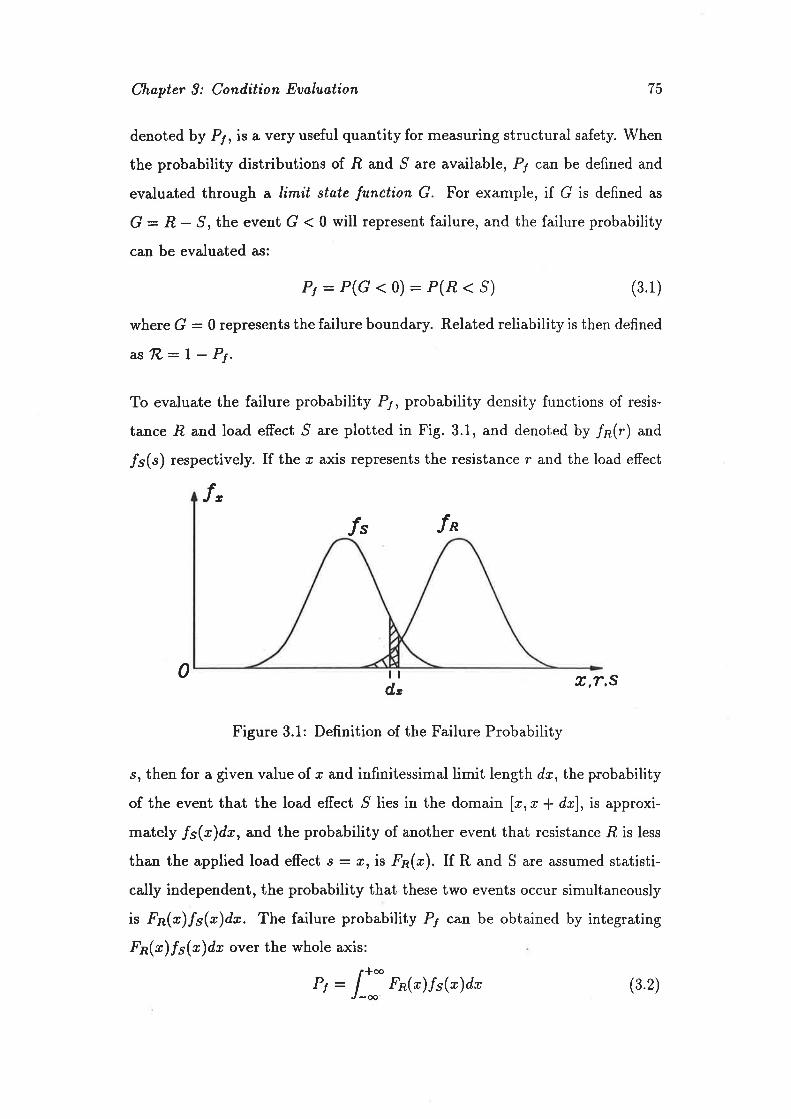
Chapter 9: Cond,ition Eualuatíon 75
denoted by P¡, is a very useful quantity for measuring structural safety. When
the probability distributions of .R and ,S are available, P¡ can be defined and
evaluated through a limít state function G. For example, if G is defined as
G : R - ^9, the event G < 0 will represent failure, and the failure probability
can be evaluated as:
P¡ - P(G < o) - P(Æ < S) (3.1)
where G : 0 represents the failure boundary. Related reliability is then defined
as'l?-: | - P¡.
To evaluate the failure probability P1, probability density functions of resis-
tance .R and load effect ^9 are plotted in Fig. 3.1, and denoted by /p(r) and
/s(") respectively. If the ø axis represents the resistance r and the load effect
t,It 1*
0 tt l,T"s
Figure 3.1: Definition of the Failure Probability
s, then for a given value of ø and infinitessimal limit length dr, the probability
of the event that the load effect ^9 lies in the domain lr,r* dø], is approxi-
mately fu(æ)dx, and the probability of another event that resistance -R is less
than the applied load effect s: t,t is ^Fp(c). If R and S are assumed statisti-
cally independent, the probability that these two events occur simultaneously
is .Fp(ø)/5(x)dæ. The failure probability P¡ can be obtained by integrating
Fp(æ)fs(x)dr over the whole axis:
r*ooP, : J__ Fp(x)fs(r)dx (3.2)
d.,

Chopter 3: Condition Eualuøtion 76
In practice, however, the limit state function G can not always be expressed
in terms of only .R and ,S. In f.act, G is usually a function of a set of variables,
denoted by X : (Xr, Xz,...rXn), where Xtr...,Xn are fundamental and
onally ndepend.ent uøriables that may be used in the structural ilesign ..''u
process, such as material properties, dimensions and applied loads. These
variables are so-called basic aariables. For a particular limit state with nbasic variables involved, the function G can be defined in such a way that
G(Xt,Xr,... ,Xn) ( 0 represents the failu¡e. The probability of failure is
then evaluated by:p, : [ -., fx(z)dr (3.s)' Jclx'¡<o " -^ ' '
where Íx(r) is the joint probability distribution function of the basic variables
X : (Xt,..-rXn). To clearly understand Eq. 3.3, it is helpful to point out
that the random variables X form an n-dimensional space, and the failure
equation C(X) - 0 which defines a failure surface divides the whole space into
a'safe region" and a "failure region". P¡ obtained by Eq. 3.3 thus represents
the weighted volume of the failure region.
Although classical reliability theory is clear in concept, the evaluation of Eq. 3.3
needs multiple integrations and a closed-form solution does not exist in most
ca{¡es. For this reason, numerical methods are usually used to evaluate the fail-
ure probability, and Monte-Carlo simulation is widely adopted for this purpose
in practice.
3.2.2 Monte-Carlo Simulation Technique
This technique was probably first used to study structural safety by Warner )and Kabaila (1968), and its main idea is as follows. If the failure criterion is
saÍe
boundary
f ailure
the failure probability P! : P(G < 0) can be evaluated by carrying out the
following steps:
Chøpter 9: Conilition Evaluatíon 77
defined by the limit state function G(X) as:
1. Generating a set of values randomly for the basic variables (Xr, ' ' ' , X^)
according to appropriate probability density functions;
2. Evaluating function G(X) using the values of X obtained in step 1;
3. Repeating steps 1 and 2 many times until a sufficiently large sample
size is achieved;
4. Estimating the probability of failure Py:
,, : *å r'",o, x,,..., x.)f (3.4)
where N is the number of cycles; IIG(X¡,X2,...,X")] it a function
which takes 1 for G ( 0 and 0 for G ) 0.
The above procedure is called the conventional Monte-Carlo technique, and is
widely used in structural reliability analysis. For example, Allen (1970) used
the method to study the ultimate strength and ductility ratio of reinforced
concrete beams. Grant et al. (L978) conducted a comprehensive study of the
strength of concrete columns using the Monte-Carlo technique. Other similar
works are such as those by Ramsay et al. (1979) and by Monnier and Schmalz
(1e81).
Although the conventional Monte-Carlo technique proves very useful in many
cases, the method is usually time consuming in order to evaluate a reliable P¡.
It is reported (Melchers, 1988) that the error involved in P¡ from the procedure
is proportional to N-å, where N is the number of samples. Most structures

Chapter 3: Condition Eualuatíon 78
are designed with a very low failure probability, say less than 10-4, so that ifthe error is controlled to be less than 10-5, at least 1010 repetitions a¡e needed.
This is too time consuming even for a high speed computer, especially when
the structural analysis procedure is itself complicated and time consuming.
To overcome this difficult¡ a more efficient algorithm can be adopted (Warner
and Kabaila; 1968), and a recently developed smart Monte-Carlo technique has
been suggested by Melchers (1988) in which the required number of repetitions
is greatly reduced, while the accuracy of P¡ remains.
Although the classical method of structural reliability discussed above is con-
ceptually important, the computations required for obtaining P1 make the
method too complicated for practical purposes. Also, the joint probability
distribution function lx(r) in Eq. 3.3 is usually not available in practice. In
recognition of this difficult¡ the so-called First Order Second Mornent method
has been developed as a means of using probabilistic methods in dealing with
structural safety, while remaining simple in application. This approach is re-
viewed next.
3.2.3 First Order Second Moment Method
For the random resistance .R and load effect ^9 with means þn¡ lts and standard
deviations oR,¡ as respectively, failure occurs when the function G : r? - ^9 is
less than zero. If. we consider G itself as a random variable, its distribution can
be obtained via -R and ^9 as illustrated in Fig. 3.2. In the absence of information
on distributions of .R and .5, it is difÊcult to evaluate the probability of failure
P1. However, the quantity
p ltn-s pR - l.ts (3.5)oR-s
1f "þ+ "'g
defined by only the mean and deviation of G : R-,9 is a very useful measure
of the degree of safety or reliability of a structure, and is called the safety
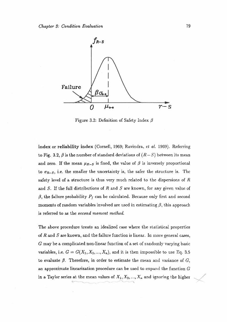
Chøpter 3: Conilition Eualuation 79
-cJn-s
Failure
0 ltrn'. r-sFigure 3.2: Definition of Safety Index B
index or reliability index (Cornell, 1969; Ravindra, et al. Ig69). Referring
to Fig. 3.2, P is the number of standard deviations of (,R - ,S) between its mean
and zero. If the mean þn-s is fixed, the value of B is inversely proportional
to ø¡-s, i.e. the smaller the uncertainty is, the safer the structure is. The
safety level of a structure is thus very much related to the dispersions of -R
and ,S. If the full distributions of ,R and ,9 are known, for any given value of
Brthe failure probability P¡ can be calculated. Because only first and second
moments of random variables involved are used in estimating þ, this approach
is referred to as the second, moment method.
The above procedure treats an idealized case where the statistical properties
of -R and ,5 are known, and the failure function is linear. In more general cases,
G may be a complicated non-linear function of a set of randomly varying basic
variables, i.e. G: G(Xt,X2,...,X"), and it is then impossible to use Eq.3.5
to evaluate B. Therefore, in order to estimate the mean and variance of G,
an approximate linearization procedure can be used to expand the function G
in a Taylor series at the mean values of Xr, X2,...,X, and ignoring the higher
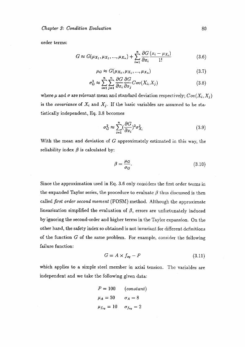
G æ G(¡t2¡r,t.x1,...,t'x^)- å #@+Ð (s.6)
ltc æ G(p*rr ltxt,,...,ltx^) (3.7)
""=äF^#,#3ou(x;'x¡) (3'8)
where p, ard a are relevant mean and standard deviation respectively; Cou(X¡, X¡)is the coaariance of Xi and X¡. If the basic variables are assumed to be sta-
tistically independent, Eq. 3.8 becomes
Chapter 9: Condítion Eaøluøtion 80
order terms:
o2c x )'oT, (3.e)
With the mean and deviation of G approximately estimated in this way the
reliability index B is calculated by:
p Itc(3. 1o)oc
Since the approximation used in Eq. 3.6 only considers the first order terms inthe expanded Taylor series, the procedure to evaluate B thus discussed is then
called first oriler second moment (FOSM) method. Although the approximate
Iinearization simplified the evaluation of B, errors are unfortunately induced
by ignoring the second-order and higher terms in the Taylor expansion. On the
other hand, the safety index so obtained is not invariant for diferent definitions
of the function G of the same problèm. For example, consider the following
failure function:
G:Axf,y-P (9.11)
which applies to a simple steel member in axial tension. The variables are
independent and we take the following given data:
Ëi=l
AG0t(
P: 100
lt¿, :50FÍ"n: L0
(constønt)
oA:8oî"u :2
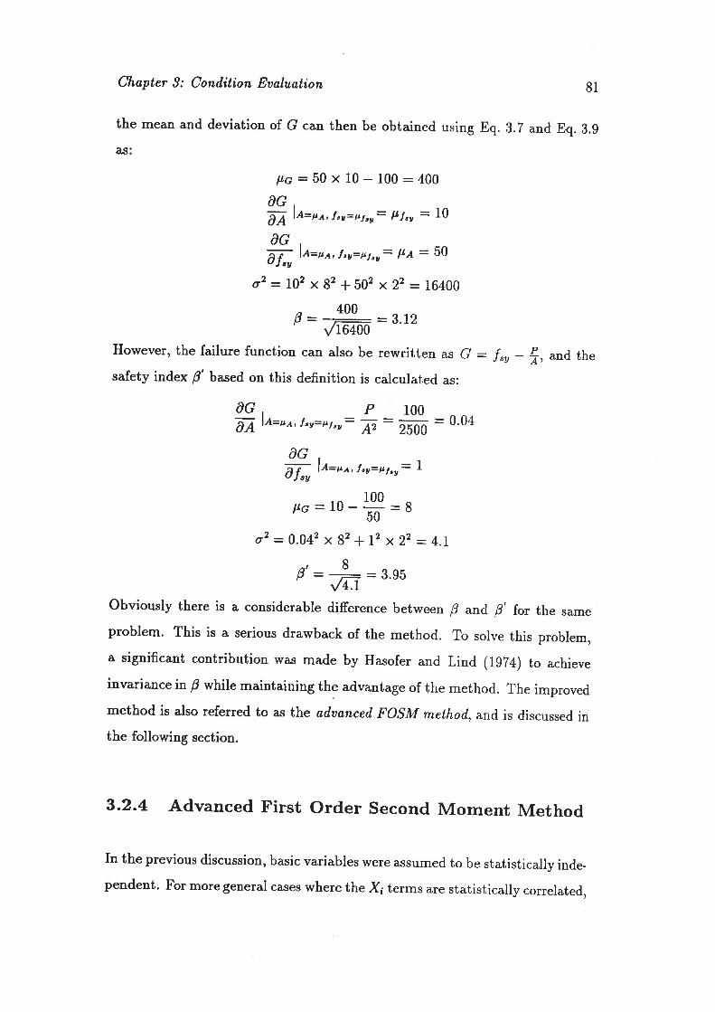
Chapter 3: Condition Eaaluation 81
the mean and deviation of G can then be obtained using Eq. 3.2 and Eq. 3.9
pc:50 x 10 - 100 :400aG.{¡ le=r^, Ícy=tt¡"r: F!", : I0
AG
ffi le='^' fts=F¡sv: ltl': 5o
o2 = L02 x 82 + 502 x 22 :16400
ß:L:J.12y'l6400However, the failure function can also be rewritten as G : l"y - f,, u.nd thesafety index B' based on this definition is calculated as:
aG, P 100fu lA=un, Íry=tt¡"u: A, - tñ : 0.04
AG
-
I -10f"u '^=u^r
IcY=F¡"u- L
þG=ro-*-S50
o2 = 0.042 x 82 * L2 x22 : 4.L
o' : L:3.95,/4.IObviously there is a considerable difference between B and, B' fot the sameproblem. This is a serious drawback of the method. To solve this problem,a significant contribution was made by Hasofer and Lind (1924) to achieve
invariance in B while maintaining the advantage of the method. The improvedmethod is also referred to as the ad,aanced, FOSM method, and is discussed inthe following section.
3-2-4 Advanced First order second Moment Method
In the previous discussion, basic variables were assumed to be statistically inde-pendent. For more general cases where the X; terms are statistically correlated,
as

Chapter 3: Condition Eualuation 82
an orthogonal transformation (Hasofer and Lind, 1974) can be carried out so
that the variables X are replaced by a new set of variables, y : (Yr,"',Yr),which are uncorrelated. In addition, the new basic variables are further trans-
formed so that they are comparable in the same coordinate system, i.e.
zr:Y - ttu (3.12)oy
where py. and, oyi are the mean and standard deviation of }{ respectively.
As mentioned previously, for a limit state function G(X1 ,"' ,Xn), the failure
surface, defined by G : 0, will divide the n-dimensional space of basic variables
into a safe region and a failure region. Thus under these transformations,
Hasofer and Lind (1974) showed that the shortest distance from the origin
to the failure surface in the transformed coordinate system of 21,"'rZn is
equivalent to the reliability index p defined in the FOSM method, i... þ -tL-
min(f Zïà, if the function G is linear. If the failure boundary is non-linear,d=1
a linearization similar to the Taylor expansion used in the FOSM method can
be made. The two dimensional case is illustrated in Fig. 3.3, where ("i,ti)is the so.called d,esign pointor checking point (Paloheimo and Hannus, 1974),
which is located ¿t the point where the failure is most likely to occur, and
G("T, zi) : 0.
Z.
Failure surface
Design pointFailure region
Safe region ,ztù
0Zt
Figure 3.3: Definition of Hasofer-Lind's Safety Index
It should be noted that the Taylor expansion of G(X) is made here at the
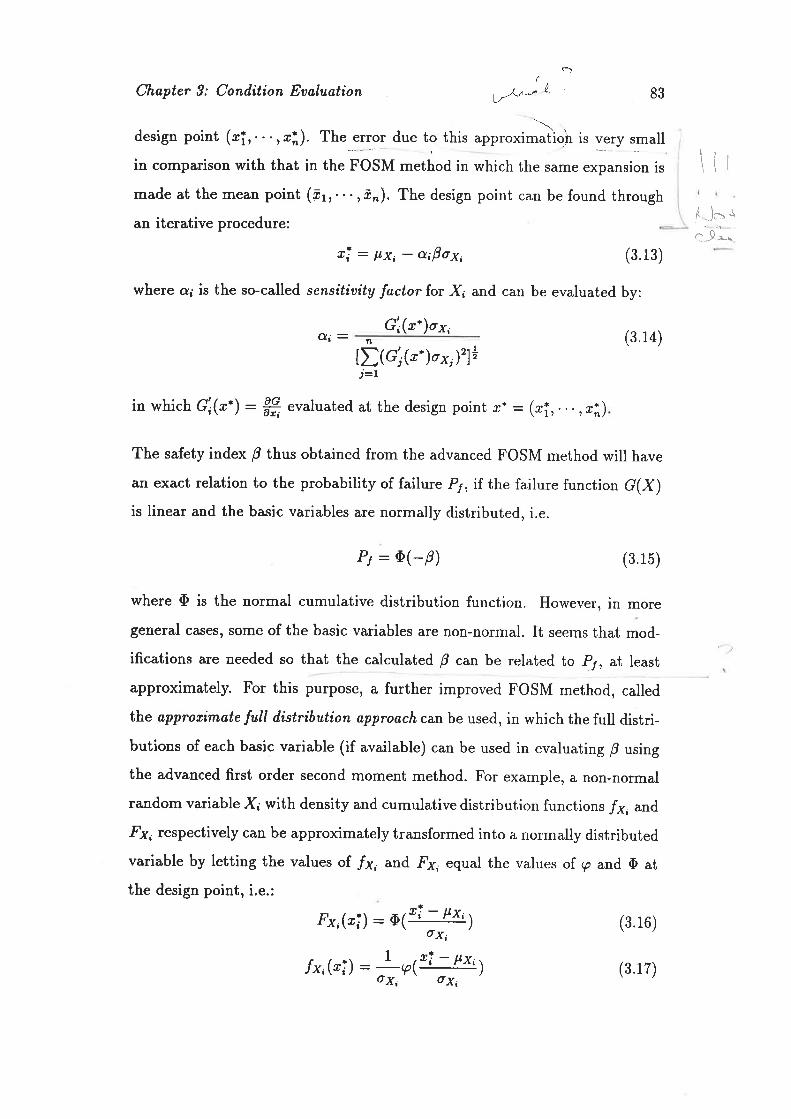
rÐChapter 9: Conilition Euoluation lz-Ln- L 83
design point (rT,. . . ,ri). The-eÏ9J due to this appro*irrrìùoir is very small
in comparison with that in the FOSM metiod in which the same expansion is
made at the mean point (¡rr.--,õn).The design point can be found through
an iterative procedure:
xI : px, - a;þox, (3.13)
where a¡ is the so'called sensitiuity factor for X¡ and can be evaluated by:
Od: nG'r(r')o*, (3.14)
IDG¡@-)o*,)']tj=L
in which G'¡(r*) : # evaluated at the design point r* : (xî,. . . ,r:^)
The safety index B thus obtained from the advanced FOSM method will have
an exact relation to the probability of failure P¡, il the failure function G(X)is linear and the basic variables are normally distributed, i.e.
P¡ : aGþ) (3.15)
where tÞ is the normal cumulative distribution function. However, in more
general cases, some of the basic variables are non-normal. It seems that mod-
ifications are needed so that the calculated B can be related to P¡, at least
approximately. For this purpose, a further improved FOSM method, called
the approtimøte full d,istribution approachcan be used, in which the full distri-
butions of each basic variable (if available) can be used in evaluating B using
the advanced first order second moment method. For example, a non-normal
random variable X¡ with density and cumulative distribution functions /¡, and
-F¡, respectively can be approximately transformed into a normally distributedvariable by letting the values o1 lx¡ and F¡, equal the values of g and O at
the design point, i.e.:
Fx,(rî) :61ri - ttx; ) ql.ro¡\dX¡,
rx,@î): !rf\tt) (s.rz)ox; ox¡
\{lIt ì.rrC-9--
Chapter 9: Cond,ition Euo,luation 84
where Õ and I ûe the cumulative and density functions of a unit normaldistribution respectively; cj is the ordinate of the design point; Fx¡ and oy.are the mean and standard deviation of the new normal variable, and are tobe evaluated. From Eq. 3.16 and Eq. 3.12, we can get:
oY. = P{o-1 F*,("T)lÌ(3.18)Íx,(ri
þx¡ : øi - ¡,-t [Fy,þ!))oy, (3.19)
After þx, and ox. are obtained, the same procedure as in the advanced FOSMmethod can be used to calculate B value.
3.2.5 Brief summary of structural Reliability Theory
By treating parameters in structural design as random variables, the conceptof structural safety is changed from the traditional "absolute" approach to themodern statistical approach whereby uncertainties encountered are considered
in a rational way. With the approximate FOSM method available, st¡ucturalreliability now serves not only as the theoretical foundation for safety analysis,but also as a tool for probabilistic desirn,(Ang, et al. 1gZ4; Ravindra, et al.
,]
r974) and reliability-based code implementation (CIRIA, lgZZ; Ellingwood, eú
ø1. 1980; Leicester, eú ol. 1986).
As a useful tool to study structural safety, reliability theory has also been
applied to evaluate existing structures. This witl be reviewed in the nextsection.
'i
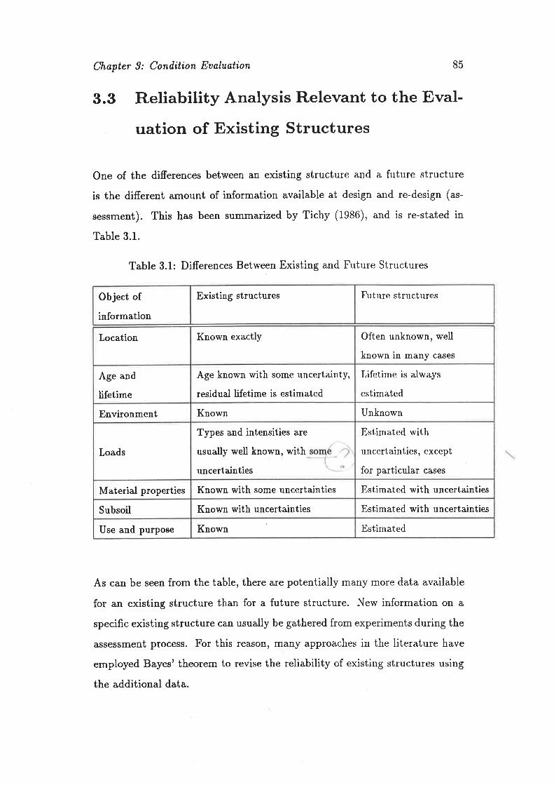
Chapter 9: Conilition Eualuøtion 85
3.3 Reliabitity Analysis Relevant to the Eval-
uation of Existing Structures
One of the differences between an existing structure and a future structure
is the different amount of information available at design and re-design (as-
sessment). This ha^s been summarized by Tichy (1986), and is re-stated in
Table 3.1.
Table 3.1: Differences Between Existing and Future Structures
As can be seen from the table, the¡e are potentially many more data available
for an existing structure than for a future structure. New information on a
specific existing structure can usually be gathered from experiments during the
assessment process. For this reason, many approaches in the literature have
employed Bayes' theorem to revise the reliability of existing structures using
the additional data.
Object of
information
Existing structures Future structures
Location Known exactly Often unknown, well
known in many cases
Age and
lifetime
Age known with some uncertainty,
residual lifetime is estimated
Lifetime is always
estimated
Environment Known Unknown
Loads
Types and intensities are
usually well known, with
uncertainties
Estimated with
uncertainties, except
for particular cases
Material properties Known with some uncertainties Estimated with uncertainties
Subsoil Known with uncertainties Estimated with uncertainties
Use and purpose Known Estimated
Chapter 3: Conditíon Eaaluation 86
3.3.1 Safety Revision Using Bayesian Updating
For a future structure, the intended nominal safety of the original design can be
evaluated using any standard method of reliability analysis. For this purpose,
properties of relevant basic variables and limit state function are usually esti-
mated using both subjective judgement and test data available on the whole
population of a specific kind of structure. The re-evaluation of the reliabilityof an existing structure at the time of ¿ìssessment can be made by updatingthe probability distributions of those basic random variables in the limit statefunction G(xr,"',Xn), and/or by improving the function G itself, consider-
ing the real physical state of the structure using new information acquired inthe process of investigation.
The updating of the distributions of X can be made in two ways (CIRIA,rgTT;Bosshard, 1979). For a random variable X¡, its true mean þx, and standarddeviation oxj are usually unknown. However, if testing is conducted on asample, the sample mean and standard deviation can be evaluated by:
1 i.,,j=L(3.20)Ii
n
ols2x,: ù l(tt¡ - ¡,)' (3.21)' j=l
where n is the sample size. If n is sufficiently large, a convenient way is thento let
Fx;: t; and 6x;: sx: (3.22)
However, this is usually not the case, and the sample size may be very limited,especially for existing structures, where any test is supposed not to damage
the structure itself.
Another way to update the distribution of. X; is by means of Bayes' theorem.
In this method, it is assumed that the mean and deviation of X¡ ca\ never be
known exactly, and. p,1çr, ø¡, themselves are random variables. When more and
Chapter 3: Condition Eaøluation 87
more data are available, the distributions of Fx, and o¡, will closely approach
their true values. Generally, assuming that d is a parameter in the distribution
function of the basic variable X¡, such as ¡.r¡,, the distribution of 0 after the
test can be updated by:
l" (0) : kL(0)Í'(0) (3.23)
where /'(0) and Í" (0) are the prior and posterior distributions of d respectively;
L(0) is the so-called likelihood function, i.e. the probability of obtaining the
specific data observed for a given value of 0, namely P(d,ata I 0); k is a constant.
The predictor distribution of X is obtained by:
fx, = t:: f x,(r¡ | o)f" (o)do (3.24)
After the distributions of basic variables are thus updated, safety revision of.j
an existing structure can be easily)carried out by calculating the reliability
index B using the First Order Second Moment method (Diamantidis, 1987).
For this purpose, it is well known that for a limit state function G(X), there is
a design point X* : (ri,.' ' ,r;) at which failure is most likely to occur. The
design value øi for each random variable X¡ with distribution function Fy, can
be defined by the following equation:
4 : Fx:lo(-orÉ)l (3.25)
where iÞ is the standard normal distribution function, and o; is a so-called
sensitiuity or importance føctor. If the distribution of the basic variable X, is
updated from .F¡,(ci) to f! (ci), a new design value i;* caî be defined such
that:
P*,@'Ð - Fx,("i) (3.26)
The reliability change, denoted by L0;, due to the change of statistical prop-
erties of Xi can be evaluated by:
Lþ, = orlo-1(4, ("1')) - 6-t (4,("î))1, (3.27)
Chopter 3: Conilition Eualuation 88
which represents the increase or decrease in safety compared to the original
reliability index p, provided that the importance factor ai remains the same.
With the above procedure available for evaluating the relative change in the
reliability index B of a , Diamantidis (1987) suggested a number of
steps to be adopted in the assessment of existing structures:
(1) quantification of the additional information based on the inspection results;
(2) identification of the major risk items;
(3) definition of risk scenarios;
(4) formulation of limit states;
(5) assessment of the relative change in reliability compared to the
originally accepted safety goals;
(6) evaluation of the cost-effectiveness of possible courses of action;
In addition to the revision of statistical properties of basic variables, in some
cases, the reliability of an existing structure can also be updated by the use
of the recorded structural performance using Bayes' theorem. For this pur-
pose, the parameter d discussed in Eq. 3.23 can be generalized to denote a
parameter in any mechanistic model, and its statistical properties can be up-
dated from observations of the model. For example, Tang (1981) used this
approach to refine the analysis of the settlement of a gravity platform from
the recorded platform performances. The equation for predicting the amount
of settlement was expressed by p(t,d), in which ú represents time, and á is
a random variable. According to the in-situ measured settlement in the his-
tory, the posterior distribution of d, denoted by f"(0), can be obtained from
Eq. 3.23. If the maximum permissible settlement is d, the updated probability
of satisfying the settlement requirement is then given by:
P"(p<-d): r P(p<dl0)f"@)d0 (3.28)
Chøpter 9: Condition Eualuation 89
Updating the reliability of existing structures using additional data on the
structural behaviour can also be achieved in a slightly different way. For ex-
ample, when a structure has resisted an external load Q, Andersen (1989)
used the following equation to update the failure probability of the structure
through Bayes' theorem:
Pt: P(L>,R l^R > o) - P(LZ !îR> Q) /^-e t P(R > af (3'2e)
where P¡ is the probability of failure; -t and -R are the load effect and resistance
of the structure respectivelV; Q is the external load resisted by the structure
in the history.
Some concepts of reliability-based evaluation of existing structures are explic-
itly illustrated by Schneider (1992) using an example. An assessment proce-
dure is also proposed based on the assumption that a correct application of the
respective codes or standards results in a safe structure. Thus if an existing
structure is correctly designed according to relevant standards, its reliability
index achieved in the design, 86, can be easily evaluated using the FOSM
method. The safety index related to the actual condition of the structure, B,
is secondly estimated using the current information available. fi B is not less
than Bo, the structure is assessed to be safe.
It should be noted that in all methods discussed above, the updated failure
probability PJ is not an inherent characteristic attached to the structure itself.
The quantity P¡ simply represents the expert's degree of belief in the safety
condition of the structure, and hence depends upon the state of knowledge
available to the expert. To clearly understand the safety index B, various
uncertainties involved have to be clarified.
Following Kiureghian (1989), the sources of uncertainty involved in engineering
structures can be classified broadly into four kinds: (1) inherent variability;
(2) estimation error; (3) model imperfection; and (4) human error. Inherent
variability reflects the random nature of the characteristics of the structure
Chøpter 3: Condition Eualuotion 90
and the loading environment such as material properties, load effects. Estima-
tion error arises from the incompleteness of statistical data and our inability
to accurately estimate the parameters of probability models that describe the
inherent variability. Model imperfection exists in both mathematical models,
such as the model for structural analysis, and probability models such as the
chosen probability distribution functions for random variables. Finally, human
error arises from mistakes made by various people during design, construction
and operation of the structure. It is interesting to note that there are differ-
ences among these uncertainties. Inherent va¡iability does not change with the
amount of information available, while the second and third uncertainties can
be reduced if more relevant data are obtained. Uncertainties due to human
error are influenced by quality control measures.
When complete information is available and uncertainties arise only from the
inherent variability, a strict measure of structural safety can be represented by
the probability of failure P¡ or the reliability index B with the relation:
þ: Q-r(t - P¡) (3.30)
where Õ is the standard normal distribution function; and B can be estimated
using any standard reliability method. In this case, P¡ and B are intrinsic
statistical properties of a structure and its environment, and only vary if the
structure and/or its environment are altered.
However, the exact value of the strict safety measure usually can not be eval-
uated in practice, since uncertainties other than inherent variabilities always
present. We can only reduce these uncertainties by acquiring more data, and
it is difficult to completely eliminate them. Assuming an imperfect state of
knowledge, Kiureghian (1989) proposed an approach using Bayes'theorem to
evaluate the possible values of the strict p. For this purpose, let the vector of
random variables X describe the irreducible uncertainties such as inherent vari-
ability, and @ represent the reducible uncertainties such as those arising from

Chopter 3: Condition Eaaluation 91
estimation errors. Specifically, @ includes the set of parameters that define the
probability models of X and that of the limit state function G(X). The prob-
ability distribution of X is expressed as a conditional distribution, /¡¡6(x,0),and the limit state function a^s G(X, @). When perfect information, i.e. com-
plete statistical data and perfect models, are available, @ is deterministically
known. Otherwise, the degree of incompleteness of the available knowledge
is characterized by the distribution of @, denoted bV /e(P). The predictor
distribution of X, combining the inherent variability of X and the uncertainty
in @ is given by:
/x(*):tf*e(x,0)fs(0)d,á (3.31)
where føQ) can be updated by the Bayesian rule if new information on @ is
obtained.
For a given @:0, the conditional failure probability can be evaluated as:
P¡p(o) : I.r*,"r.o.fxto(x, o)dx (3.32)
and the conditional reliability index is obtained bV þp(0): (Þ-1[1 - P¡¡o(d).
For uncertain @, the reliability index Éfo(@) is also uncertain, and its distri-
bution reflects the level of our knowledge available. If perfect data is gathered,
Éle(@) then coincides with the strict reliability index B.
One important advantage of this approach is that uncertainties from various
sources are considered separately so that the level of knowledge available can
be quantified through the distribution of B. Although this is a good idea, due
to limited data available, the application of this approach is usually restricted.
In addition to Bayesian safety updating, there are also other reliability-based
approaches available for existing structures which are discussed in the following
section.
Chøpter 9: Conìlition Eaaluation 92
3.3.2 Other Approaches for the Revision of StructuralReliability
Motivated by recent advances in structural code development using probabilis-
tic limit state design or load and resistance factor design, Shin eú ø1. (1988)
looked to the establishment of practical reliability-based bridge rating methods
or rating codes. A rating criterion in the form of a Load and Resistance Factor
Rating (LRFR) code is proposed which can take into consideration any data
obtained on actual bridge conditions such as the umeasured-to-calculated" load
effects and other test results. In the approach, failure is defined as:
R-So-S¿<0 (3.33)
where .B is a random variable representing the resistance; ,9¡ and ,5¿ are dead
and live load effects respectively, which are both random quantities. These
variables can be further modelled so that various uncertainties can be treated
rationally. For example, -R is represented by:
R: R"MFPD (3.34)
where -R, :nominal resistance of real section considering deterioration, damage etc. ;
M :random va¡iable representing uncertainties about materials;
F :random variable representing fabrication or construction uncertainties;
P :random variable representing model uncertainties;
D :random variable representing uncertainties involved in the
assessment of damages and/or deteriorations.
The mean value of -R can be expressed as: R -- R"M FPD : R*nn where 4n
is the mean-nominal ratio of resistance. From the data available in the litera-
ture and experience-based judgements on those uncertainties involved in .R,,S¿¡
and ,9¿, the mean-nominal ratio and variance of resistance, dead and live load
Chapter 3: Condition EuøIuation 93
effects can be evaluated. Also, from the field inspection and relevant measure-
ments, the nominal resistance in consideration of factors such as damage, and
nominal load effects in consideration of measured-to-calculated responses are
obtained by appropriate analysis. The reliability index B can then be evaluated
using these data and the First Order Second Moment method. If the obtained
p is larger than the target value, say þo - 3.0, the bridge is classified as being
safe. Otherwise, appropriate actions have to be undertaken for maintenance
or repair regarding structural safety.
Haú et al. (1981) also used the reliability-based method to evaluate the ex-
pected damage to existing structures resulting from the futu¡e occurrence of
natural hazards such as earthquakes. The reliability index or failure probabil-
ity of the structure concerned is firstly evaluated from data available. A set
of damage states such as mod,erate, seuere d,amage., pørtial collapse are defined
according to the cost of repairing the damage. These states are further related
to different values of the reliability index for one component, one failure mode,
or alternatively the average of a system of components. Therefore, the damage
state of a particular structure can be obtained from the calculated reliability
index of the structure. However, the relation between the damage states and
reliability values are obtained arbitrarily from experience and subjective judge-
ments, and there is no reasonable procedure available to establish this linkage
consistently.
If a proof load test has been conducted on an existing structure, the reliability
of the tested structure can also be updated using the test results. Early work
on this topic was carried out by Shinozuka (1969).
A proof load test is a test in which some pre-determined load is applied. The
strength of a structure which successfully passes the proof load test is clearly
higher than the test load. If the stiucture is chosen from a population with
strength distribution "fn(r), it is possible to obtain the strength distribution of
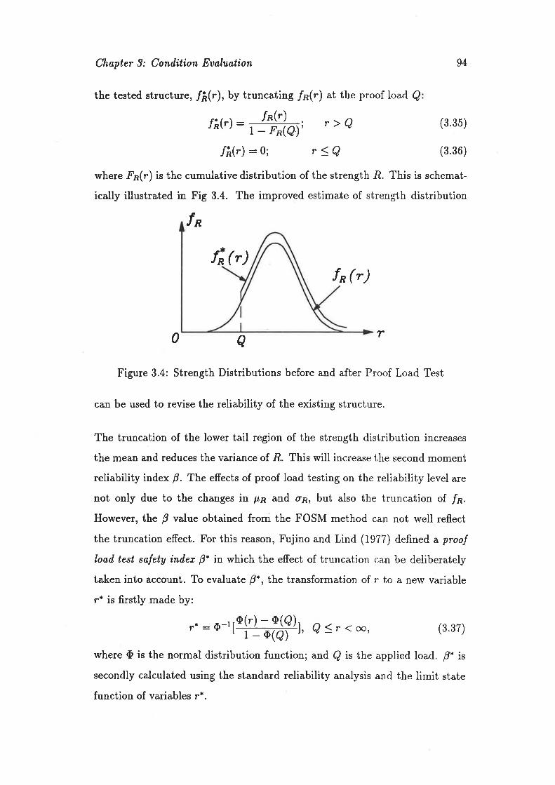
Chapter 3: Condition Eualuotion 94
the tested structure, fñþ), by truncating /¡(r) at the proof load Q
F¡ / \ fn(r\/å(r):;-a-1;*.,i r>Q (3.35)L _ rRlv)
/ñ(r)-0; r<Q (3.36)
where Fn(") is the cumulative distribution of the strength ,R. This is schemat-
ically illustrated in Fig 3.4. The improved estimate of strength distribution
1a
¡Ïþ)l^ (")
r
Figure 3.4: Strength Distributions before and after Proof Load Test
can be used to revise the reliability of the existing structure.
The truncation of the lower tail region of the strength distribution increases
the mean and reduces the variance of .R. This will increase the second moment
reliability index B. The effects of proof load testing on the reliability level are
not only due to the changes in ¡r¿ and ø¿, but also the truncation of /¡.However, the B value obtained from the FOSM method can not well reflect
the truncation effect. For this reason, Fujino and Lind (1977) defined a proof
loail test søfety inilex 0* io which the effect of truncation can be deliberately
taken into account. To evaluate p*, the transformation of r to a new variable
r* is firstly made by:
r*:iÞ-lf$f,¡øÌ, e<r(oo, (B.sz)
where iÞ is the normal distribution function; and Q is the applied load. B. is
secondly calculated using the standard reliability analysis and the limit state
function of variables r*.
a0
Chopter 3: Condition Eaaluation 95
These approaches for updating structural reliability based on proof load test-
ing, however, have used only the information of survival or failure of the struc-
ture under testing. Veneziano et al. (1978) further improved the reliability-based analysis of proof load testing by using additional data such as the
moment-curvature relation recorded during the test. In the approach, the pos-
terior strength distributio" f Åþ) after proof load testing is obtained through
the Bayes'theorem:
¡Å(r) x ¡"(r)t(r I e,C) (8.88)
where fh@ is the prior strength distribution, and Q is the largest value ofapplied load; C denotes the moment-curvature relation; /(r I Q,C) represents
the likelihood of the strength r, given Q and C. The failure probability of the
structure is evaluated as:
Pî : ll r;ç¡ar,ç"¡ (3.3e)
in which .F's(r) is the distribution function of load effect ^9
However, practical difficulties of using this method arise from the constructionof the likelihood function, because the value of Q is usually considerably smaller
than the value of strength in practice. In a given example, the author triedto obtain the ultimate strength from an idealized parabolic moment-curvature
curve. The accuracy of the procedure'was discussed, and is questionable.
It is important to realized that prior service load in the service history of the
structure can also be considered as a proof load, so that the reliability of an
existing structure may be revised without the expense of conducting a load
test. For an existing structure without severe wearout, Hall (1988) suggested
that the service load can be treated as proof load with uncertainty. In thiscase, the proof load ^9 is a random variable with distribution function Fs(").The posterior strength distribution /fi(r) in Eq. B.3b changes to:
f;(r): - r"(")/tt)-.r-"" ¡'s(")/å (r)d,r (3'40)

Chopter 3: Condition Eualuation 96
The improvement in the reliability thus assessed depends on service load data
collected. If the proof load has a high variance, then little improvement can be
achieved in updating the strength distribution and hence the safety evaluation.
Also, this approach can only be used when it is judged that the structural
condition is not seriously deteriorated. Otherwise, the approach may lead to
an unconservative result.
Retiability analysis relevant to the safety evaluation of existing concrete struc-
tures has been briefly discussed above. This review will be summarized in the
next section.
3.3.3 Brief Sumrnary on Reliability Updating
Generally, reliability analysis for future structures has to consider all possible
sources of uncertainty. For an existing structure, more specific details can be
obtained in the a^r¡sessment procedure, and hence part of the uncertainty can
be eliminated. However, there is no fundamental difference between reliability-
based methods for analysis of future structures and existing structures.
Most of the existing approaches for reliability evaluation of existing structures
are carried out by either updating the probability distributions of relevant
basic variables or updating the model which describes the limit state function.
The updating of basic variables usually uses the sample data available. Since
sample testing is in many cases restricted to concrete and has only limited
size due to practical difficulties in investigating existing structures, reliability
revision using only sample data on basic variables seems not very efficient.
As Yao (1980) pointed ort: followi,ng the contpletion of the construction pro-
cess, each structure ho,s its own characteristics, which can no longer be de-
scribeil with the same initial mathematical mod,els used in the d,esign phase,
the uncertainty involved in the structural analysis itself, or model error, will
Chøpter 3: Conilítion Eualuation 97
play an important role in the reliability re-evaluation. However, appropriate
methods for this purpose seem yet to be developed. Although proof load test-
ing is a good way to justify structural resistance, its effectiveness is usually
restricted due to the limited load Q applied. If Q is too large, the risk of
structural failure under testing has to be considered.
In addition to reliability-based assessmenl, finzy set theory is another mean-
ingful tool in dealing with uncertainties, and has proved useful in structural
safety evaluation. Approaches of this kind will be discussed next.
3.4 Structural Safety Evaluation Using Euzzy
Sets
The concept of. firzzy sets was already discussed on page 42. More details on
this theory can be found elsewhere (Zadeh, 1965; 1973; 1975a; I975b; Zim-
mermann, 1985). The use of fuzzy sets in structural safety evaluation was
triggered by the work of Pugsley (1973). He suggested that one way to study
the proneness to accidents of a given structure, or a class of structures, is to
look at a number of parameters that have been highlighted as relevant by ex-
perience in previous accidents. For this purpose, a set of parameters such as
erperience of design and, construction team, industrial climate, financial cli-
mate are distilled from structural failures experienced in the past. A group of
experienced engineers could then assess the accident proneness of a given struc-
ture in broad terms by grading these parameters. However, speciflc mistakes
made in design or construction can not be identified by using the procedure.
Instead, the method is only able to draw attention to some overall features of
the structural design-construction process, and hence to reduce the possibility
of structural failure.
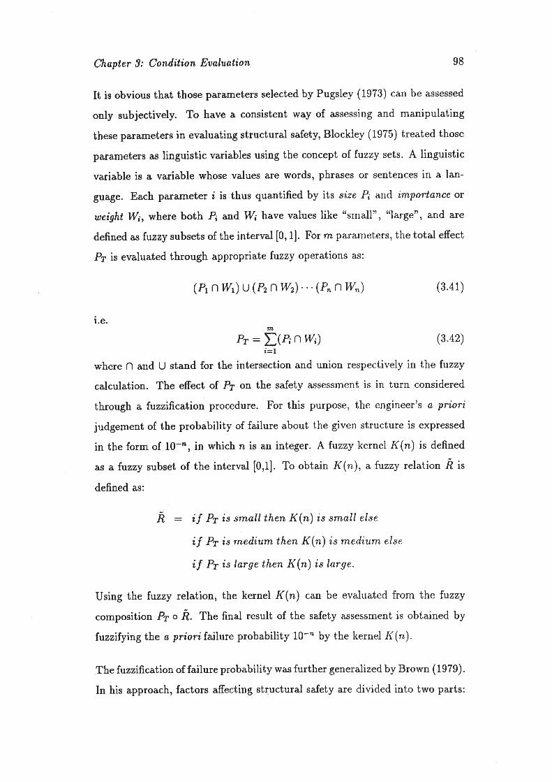
Chapter 9: Conilition Eaaluation 98
It is obvious that those parameters selected by Pugsley (1973) can be assessed
only subjectively. To have a consistent way of assessing and manipulating
these parameters in evaluating structural safety, Blockley (1975) treated those
parameters as linguistic variables using the concept of. fuzzy sets. A linguistic
variable is a variable whose values are words, phrases or sentences in a lan-
guage. Each parameter i is thus quantified by its size P; and importance ot
weíght IlØ¡, where both 4 an'ð,W; have values like "small", "large", and are
defined asluzzy subsets of the interval [0,1]. For rn parameters, the total effect
Pa is evaluated through appropriate fivzy operations as:
(a n wr)r (Prnwù...(P"ìW") (3.41)
l.e.,n
Pr - Dt¿ nw) (3.42)
where l'ì and U stand for the inr"r."liirn and union respectively in the fitzzy
calculation. The effect of. Pr on the safety assessment is in turn considered
through a firzzifrcation procedure. For this purpose, the engineer's ¿ priori
judgement of the probability of failure about the given structure is expressed
in the form of 10-", in which n is an integer. A htzzy kernel I{(n) is defined
as aÍuzzy subset of the interval [0,1]. To obtain K("), afitzzy relation à is
defined as:
if Pr is small then K(n) is small else
if Pr is med,ium then K(n) is rnedium else
if Pr is large then K(n) is large.
Using Ihe fuzzy relation, the kernel K(") can be evaluated from the fuzzy
composition P7 o,É. fn" final result of the safety assessment is obtained by
fuzzifying the ø príori failure probability 10-" by the kernel I{(n).
The fuzzification of failure probability was further generalized by Brown (1979).
In his approach, factors affecting structural safety are divided into two parts:
R

Chopter 3: Condition Euø'Iuation
the objective and subjective factors. It is considered that the failure proba-
bility P¡ in the form of 10-" obtained from structural reliability theory using
objective information is incomplete because the subjective part has not been
considered. With the presence of additional subjective information, the belief
in r¿ of 10-' wavers, and the attractions of n - | and n - 2 increase. For this
reason, the combination of both objective and subjective knowledge will result
in arange of beliefsinthe set n, n-1, n-2, ... I n-d, where dis an integer
and d ( n. Considering the failure set l7 : {n,n - l,' ' ' )Tt' - d}, the support
for the membership of n, n - Ir"')n - d, car- be represented by:
F=pol" * nl@-1) + ...,ttdl@-d) (3.43)
where ¡^r¡ is the membership function and p¡ € [0,1]. F can be obtained
by a fizzification procedure similar to that used by Blockley (1975). Under
this definition, it is clear the failure probability 10" obtained from ordinary
reliability analysis using only objective information has the support of 1 for n,
and no supports for others, i.e. Fo: I ln + 0 I ("- 1) + "', + 0 I (" - d).
Similar approaches using luzzy sets in structural engineering are also illustrated
by Yao (1980) in several examPles.
The safety measure obtained by previous approaches is a fitzzy quantity, and
hence there are difÊculties in interpreting the result and comparing it with
the failure probability P¡. With the concept of fuzzy probability, Shiraishi
and Furuta (1983) define failure as a htzzy event so that the resulting safety
mea{¡ure is still in terms of probability or reliability index as that in reliability
analysis, but is fuzzified according to the subjective information available. In
reliability analysis, the failure probability P¡ is defined as the probability of
the event .4 that the structural resistance .R is smaller than the load effect ,S,
i.e.:
99
P¡ - P(A): loaewhere A is expressed by the safety margin Z, e.E. Z : R - S < 0.
(3.44)
This
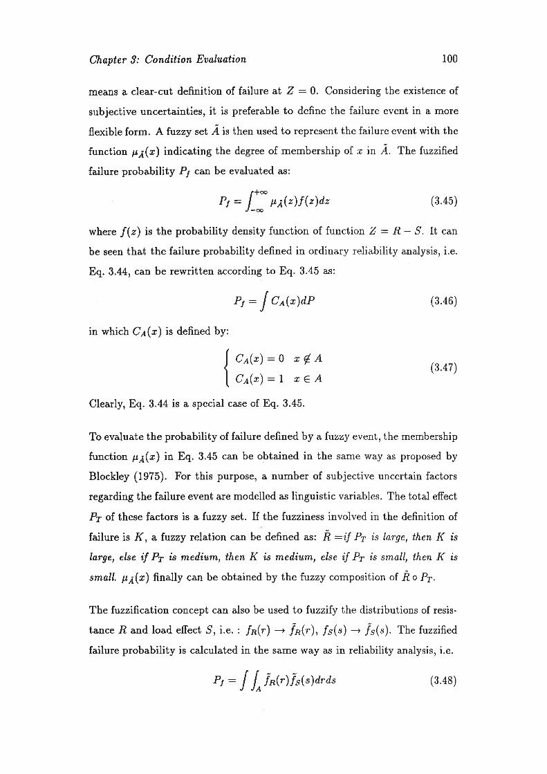
Chapter 3: Condition Eaaluation 100
means a clear-cut definition of failure at Z : 0. Considering the existence of
subjective uncertainties, it is preferable to define the failure event in a more
flexible form. A hnzy set Ã, is then used to represent the failure event with the
function p¡(c\ indicating the degree of membership of r in Ã. The fuzzified
failure probability P¡ can be evaluated as:
r*ooP, = J__ ¡r¡(z)f(z)dz (3.45)
where f(z) is the probability densityfunction of function Z : R -.9. It can
be seen that the failure probability defined in ordinary reliability analysis, i.e.
Eq. 3.44, can be rewritten according to Eq. 3.45 as:
P¡:JC¡(r)dP (3.46)
in which Ct(r) is defined by:
( colr¡:s ,øA{ "., r (J.42)
IC¡(r¡ :1 r€AClearly, Eq. 3.44 is a special case of Eq. 3.45.
To evaluate the probability of failure defined by a fitzzy event, the membership
function p¡(¡) in Eq. 3.45 can be obtained in the same way as proposed by
Blockley (1975). For this purpose, a number of subjective uncertain factors
regarding the failure event are modelled as linguistic variables. The total effect
Pr of. these factors is afuzzy set. If the fuzziness involved in the definition of
failure is K, a fuzzy relation can be defined utt -É :if Pr is large, then I( is
Iarge, else if Py is medium, then K is ¡neilium, else if Py is small, then K is
sma,Il. p¡(x) finally can be obtained by the fivzy composition of ñ o P7.
The fuzzification concept can also be used to ftzzily the distributions of resis-
tance.R and load effect.S, i.e. : ln(r) - in(r), /"(") ---l /s(t). The fuzzified
failure probability is calculated in the same way as in reliability analysis, i.e.
D-tîY¡ : J JnÍn(r)f s(s)drds (3.48)
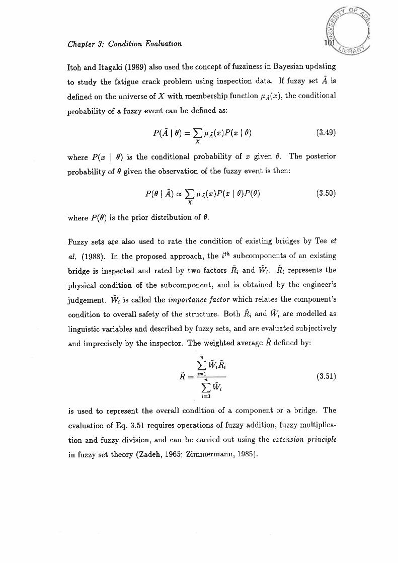
Chapter 9: Condition Evaluotion
Itoh and Itagaki (1989) also used the concept of.Iuzz\ness in Bayesian updating
to study the fatigue crack problem using inspection data. 11 fitzzy set i is
defined on the universe of X with membership function p¡(x), the conditional
probability of. afivzy event can be defined as:
1
P(Ãld): D p¡@)P(xlo) (3.4e)x
where P(" I 0) is the conditional probability of ø given d. The posterior
probability of d given the observation of the fuzzy event is then:
P(0 | A) o< ! ¡t,¡(x)P(n | 0)P(0) (3.50)x
where P(d) is the prior distribution of d.
Fuzzy sets are also used to rate the condition of existing bridges by Tee et
aI. (1988). In the proposed approach, the itå subcomponents of an existing
bridge is inspected and rated by two factors h and fu;. .fo ."pt"t"nts the
physical condition of the subcomponent, and is obtained by the engineer's
judgement. iV¡ is called Lhe importance factor which relates the component's
condition to overall safety of the structure. Both .R, anð, ft; are modelled as
linguistic variables and described by finzy sets, and are evaluated subjectively
and imprecisely by the inspector. The weighted average à defined by:
,t
DwtR"ñ d=1 (3.51)
D,W,,L
i=1
is used to represent the overall condition of a component or a bridge. The
evaluation of Eq. 3.51 requires operations of fiizzy addition, fitzzy multiplica-
tion and fitzzy division, and can be carried out using the ertension principle
infl:øzy set theory (Zadehr 1965; Zimmermann' 1985).
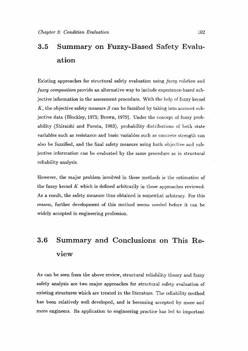
Chapter 3: Cond.ition Eualuation L02
3.5 Summary on F\rzzy-Based Safety Evalu-
ation
Existing approaches for structural safety evaluation using fuzzy relation and
fuzzy composití,on provide an alternative way to include experience-based sub-
jective information in the assessment procedure. With the help ol fiizzy kernel
K , lhe objective safety measure B can be fuzzified by taking into account sub-
jective data (Blockley, 1975; Brown, 1979). Under the concept of fizzy prob-
ability (Shiraishi and Furuta, 1983), probability distributions of both state
variables such as resistance and basic variables such as concrete strength can
also be fuzzifred, and the final safety me¿x¡ure using both objective and sub-
jective information can be evaluated by the same procedure as in structural
reliability analysis.
However, the major problem involved in these methods is the estimation of
the finzy kernel K which is defined arbitrarily in those approaches reviewed.
As a result, the safety meaf¡ure thus obtained is somewhat arbitrary. For this
reas¡on, further development of this method seems needed before it can be
widely accepted in engineering profession.
3.6 Summary and Conclusions on This Re-avtew
As can be seen from the above review, structural reliability theory and htzzy
safety analysis are two major approaches for structural safety evaluation of
existiqg structures which are treated in the literature. The reliability method
has been relatively well developed, and is becoming accepted by more and
more engineers. Its application to engineering practice has led to important
Chapter 3: Conilition Eoaluati,on 103
structural code implementation worldwide. However,, fizzy-based safety as-
sessment needs further resea¡ch before it can be widely applied in practice.
For this reason, the reliability method will be used in the development of
a rational procedure for the safety evaluation of existing defective concrete
buildings.
The reliability method proves to be very useful in dealing with statistical vari-
ations. It is not surprising to see that most of those existing methods mainly
employ the updating of probability distributions of basic variables using test
data in a^ssessing the existing structures. However, uncertainties arise not only
from random variations but also other sources such as unknown faults which
have occurred in the construction. Uncertainties of the second kind are in fact
particularly important in the evaluation of defective structures. A structure
is designed to behave properly within its planned service life under specified
conditions. If it manifests structural anomalies, there are good reasons to be-
lieve that various errors, faults or harmful factors may have occurred during
the process of design, construction and operation. Although the occurrence of
these anomalies may also be attributed to the "low-strength and high-load"
event due to random variations, the chance of this event is usually very small
because of conservative design. Therefore, a realistic method for reliability as-
sessment of existing structures has to be able to take into account these faults
and harmful factors explicitly.
Existing methods are generally inadequate for this purpose. Although the
study of effects of human errors on structural safety has attracted many re-
searchers (Ditlevsen, 1980; Melchers, 1984a, 1984b, 1984c; Arafah and Nowak,
1986; Hadipriono and Lin, 1986), current research is primarily concerned withthe effectiveness of quality a^ssurance in controlling human errors, and the
implementation of quality control in structural design, construction and use.
However, for a specific existing structure which shows signs of defects, its safety
ar¡sessment has to account for the particular faults and harmful factors which
Chapter 3: Condi,ti,on Eualuation 104
have occurred.
From the above discussion, it can be concluded that a realistic reliability-based
safety assessment of an existing structure has to consider uncertainties arising
from not only random variations but also various specific faults and harmful
factors which may have occurred to the structure itself. Such a method is
developed in the next section, in which possible faults/factors identified from
the diagnostic procedure and their effects on structural safety are explicitly
taken into account.
As mentioned at the beginning of this chapter, condition evaluation should
include the assessment not only for safety but also for other structural require-
ments such as serviceability and durability. Therefore, suitable assessment
procedures will also be developed for durability and serviceability in the fol-
lowing sections.
Finally, prognosis of structural behaviour regarding various requirements after
a course of action is taken, is briefly described in Section 3.10.
3.7 Safety Study of Existing Concrete Buitd-
Safety assessment is probably the most important part of condition evaluation
due to the possible serious consequences of structural failure. An accurate eval-
uation of safety regarding various structural requirements will help the decision
maker choose appropriate actions, and hence avoid the severe consequences of
failure. For this purpose, reliability-based approaches can be used. In practice,
however, experience usually also plays an important role in safety evaluation,
and experience-based safety assessment is a good alternative to be considered,
atngs

Chapter 3: Cond,ition Eaaluation 105
especially when existing information is insufficient to allow numerical analysrs
to be carried out, but a decision regarding the safety condition must never-
theless be made at the time. In usual cases, both of these two approaches are
likely to be employed together to produce satisfactory results. In the following
sections, detailed methods of assessing the safety of an existing defective con-
crete building, using both the engineer's experience and the reliability method
are described.
3.7.L Reliability-Based Safety Evaluation
Structural reliability analysis can be carried out for various purposes. For
example, in the reliability-based code implementation, a large population of
structures has to be considered, and the related reliability analysis is generíc.
In the assessment of an existing defective concrete building, the reliability
evaluation is specific, and involves only one particular structure or even a
single member.
Conceptual differences exist between generic and specific reliability evalua-
tions. In structural reliability analysis, the safety margin can usually be ex-
pressed bV Q - ¡l - ^9, in which r? and ,S are random variables representing
resistance and load effect respectively. In generic reliability analysis, .B repre-
sents the resistance of a large group of structural members of the same kind,
and hence its probability distribution, denoted by "fn(r), describes the fre-
quency of the occurrence of all possible values of .8. In this case, /¿(r) is
obtained from experimental data or numerical simulations.
In dealing with a specific defective structure, the reliability evaluation is unique
to the member and a particular limit state, and the related resistance .R is the-
oretically a deterministic variable. For example, if a concrete beam is loaded
to bending failure, there is only one ultimate load to be recorded. If this deter-
Chapter 3: Condition Eualuation 106
ministic value can be obtained, safety assessment would be much simplified.
Unfortunately, the resistance -R of a real structural element is never known
exactly in practice, because the failure test usually can not be conducted on
an existing structure which is still in service, and uncertainties unavoidably
exist in evaluating r? by whatever methods. The uncertain resistance .R of an
existing structure or member then has to be treated also as a random variable
for the purpose of analysis. However, the probability distributio" "fn(") in this
case should be interpreted in a Bayesian or subjectiue sense rather than in a
frequency sense. In other words, /a(") here only reflects our degree of belief
in the true value of the resisf,ance, and hence iis shape is closely dependent
upon the amount of information available. The more information available
on the given structure, the closer fnþ) will be to the true point value of ft.Reliability-based safety assessment of an existing structure is very much di-
rected to the evaluation of /¿(r) using specific information about the physical
state of the structure.
Since the resistance .B is usually a function of a set of basic variables such
as material properties, dimensions, and the function is dependent on the cho-
sen model of structural analysis, the estimation of the probability distribution
Ín(r) involves determining the distributions of those basic variables and to
assess the uncertainty involved in the model of structural analysis. In generic
reliability analysis, each of these basic variables is represented by a popula-
tion distribution obtained from available test data together with professional
judgements, with its mean and variance estimated with reference to the nom-
inal value of the variable a.ssumed in the original design. For example, the
compressive strength of concrete with "good workmanship" can be modelled
by a normal distribution with the mean value of 1.16fl and a coefficient of vari-
ation of 0.10, in which fl is the nominal concrete strength (Ellingwood, 197?).
Distributions of this kind for common basic variables are available in the ex-
isting literature, and are summarized in Appendix A. In the assessment of an
Chøpter 3: Condition Eualuation 107
existing structure, if sample data are not available, a good approximation is
to use these population distributions to represent the relevant basic variables,
provided that the structure is functioning properly and there is no serious de-
terioration. However, the real physical state of an existing concrete building
at the time of assessment may be considerably different from that in the orig-
inal design documents, mainly due to føctors such as errors or faults iluring
d,esi,gn, construction and, serai,ce periods, deterioration and d,amage. This is
particularly the case for potentially defective structures where the observed
anomalies strongly suggest the occurrence of these errors or harmful factors.
Therefore, the use of population distributions to represent the basic variables
for an existing structure is irrelevant in many cases. The effects of those factors
which cause the defects have to be taken into account. Procedures described
below are specifically developed for this purpose.
Updating the Distributions of Basic Variables
Two types of basic variables regarding structural resistance are usually en-
countered in evaluating the reliability of an existing structure regarding an
interested ultimate limit state. For those variables whose properties can be
obtained with certainty in the condition survey deterministic treatment is ad-
equate. For example, the dimension of a concrete beam at the mid-span may
be accurately measured during the investigation, and can be considered as
a deterministic variable in the reliability analysis regarding the bending ulti-mate limit state. Other ba^sic variables such as concrete strength, the amount
of reinforcement (which may not be directly measured) have to be treated as
random variables, and represented by their probability distributions.
Suppose there are rn basic variables involved, i.e. X : (Xt, Xz,. . . , X, ). To es-
timate the distribution f x¡(a¡), the effects on the structure of any errors and/or
harmful factors have to be taken into account. Since the observed anomalies

Chapter 3: Conilition Eaaluation 108
are the manifestations of possible defects, it is convenient here to use the hy-
potheses obtained in the diagnosis to represent the errors and harmful factors
when estimating Íx,(*;\. For this purpose, the distribution of each random
basic variable X¡ can be assessed conditional on a hypothesis .[/¡, and denoted
by Íx,w@r, H¡). Obviously each hypothesis H¡ e H : (Ht, Hr," ' , f1') con-
tains a set of explanations which are possibly responsible for the occurrence
of the identified anomalies, and thereforc f y,1¡¡(x,, H¡) represents the distribu-
tion of X¡ with regard to the joint effects of all explanations contained in 11¡.
Thus if the diagnosis is incomplete, X; has to be described by n conditional
distributions.
Before sufficient sample test data are available, these conditional distributions
have to be estimated using experience and judgement with reference to the
original design documents available. Actually the incorporation of subjective
information such as experts' opinion in engineering problem-solving is indis-
pensable, and the subjective assessment of /x,lr(rr,H¡) is practically possi-
ble. For example, in a case where cracks were found in concrete beams of
a newly erected structure, it is assumed, for simplicity, that there are only
three hypotheses to be considered ,, i.e. Hs:unull hypothesis" , Hr:"early over-
loadingn , Hz:"the wrong use of lower grade concrete". To evaluate the vari-
able ttcompressive concrete strength" X", it is necessary to estimate the three
conditional distributions f¡"¡¡¡(r.,Ho), fx"ln(r.,/{) and fx"¡n(r",fIz). The
concrete strength assumed in the original design documents is considered to
follow a normal distribution with mean and deviation of rn and ø respectively.
Since I/s and Ilt do not affect the properties of X", relevant distributions
conditional on I/o and llr can be approximately represented by the same pop-
ulation distributions as in the design, with their means and deviations being
f x"ln(r"rflo) : (*, o), f x"1n(*", Ht) : (*, o) respectively' The conditional
distribution lx"lg(x",H2) can be represented also by a normal distribution
with mean and standard deviation as (m - L,m,, o * Ao), in which Arn and
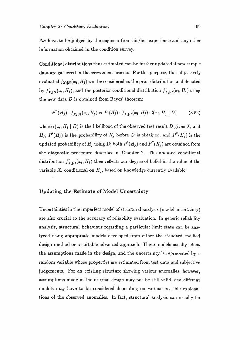
Chapter 3: Cond,ition Eualuation 109
Aø have to be judged by the engineer from his/her experience and any other
information obtained in the condition survey.
Conditional distributions thus estimated can be further updated if new sample
data are gathered in the assessment process. For this purpose, the subjectively
evaluated f x,lu(r¡rIlr') can be considered as the prior distribution and denoted
by f 1ç,1¡¡@;,Hj), and the posterior conditional distribution f |,py(x;,f!) using
the new data D is obtained from Bayes'theorem:
P" (H¡) ' fT¡r@,, H¡) o P'(H¡) ' f *¡r(*,, H¡) 'I(r;, H¡ I D) (3.52)
where I(x¡, H¡ | D) is the likelihood of the observed test result D given X¡ and
H¡; P'(H¡) is the probability oL H¡ before D is obtained, and P" (H¡) is the
updated probabitity of. H¡ using D; both P'(H¡) and P" (H¡) are obtained from
the diagnostic procedure described in Chapter 2. The updated conditional
distribution f y,¡¡¡(ri,I1r') then reflects our degree of belief in the value of the
variable X¡ conditional on l/¡, based on knowledge currently available.
Updating the Estimate of Model Uncertainty
Uncertainties in the imperfect model of structural analysis (model uncertainty)
are also crucial to the accuracy of reliability evaluation. In generic reliability
analysis, structural behaviour regarding a particular limit state can be ana-
Iyzed using appropriate models developed from either the standard codified
design method or a suitable advanced approach. These models usually adopt
the assumptions made in the design, and the uncertainty is represented by a
random variable whose properties are estimated from test data and subjective
judgements. For an existing structure showing various anomalies, however,
assumptions made in the original design may not be still valid, and different
models may have to be considered depending on various possible explana-
tions of the observed anomalies. In fact, structural analysis can usually be
Chapter 3: Condition Eualuation 110
improved at the time of assessment by applying a more specific and accurate
model. Generally, if the hypothesis f/¡ h* been confirmed f¡om the diagno-
sis, a mathematical model particularly suitable for the relevant limit state can
be determined by taking into account the effect of H¡, and denoted by G¡ø¡.
For the whole hypothesis set f/ : (Ht,Hz,.",Hn), there could be n models
selected in this way, i.e. Glr,Glr",... ,Gln^. Apparently GW¡ is valid only iffI¡ is true.
For conditional models thus obtained, the error involved in each G¡r, regarding
its own imperfection can be treated in the same way as that in the generic
reliability analysis mentioned above.
It has to be pointed out that for a hypothesis set f/ : (fIt,Hr,...,Hn),theoretically there would be n models to be considered. However, since one
model might well be suitable for a number of different hypotheses, the actual
number of models to be considered in practice is far less than n. Therefore, the
treatment of model uncertainties in this manner should not lead to a formidable
task of computation.
Building Floor Loads
The reliability of a structure or structural member is evaluated in terms of
the probability of not entering the ultimate limit state which is defined by
the structural resistance and load effects. Large uncertainties are usually also
present in the determination of applied loads, and hence appropriate proba-
bility models for various loads are crucial to the reliability analysis.
The important load component applied to a building is the floor load, which
consists of dead and live loads. The dead load is produced by the weight of el-
ements comprising the structure such as permanent equipment, partitions and
installations, roofing and floor coverings. In the assessment of existing struc-
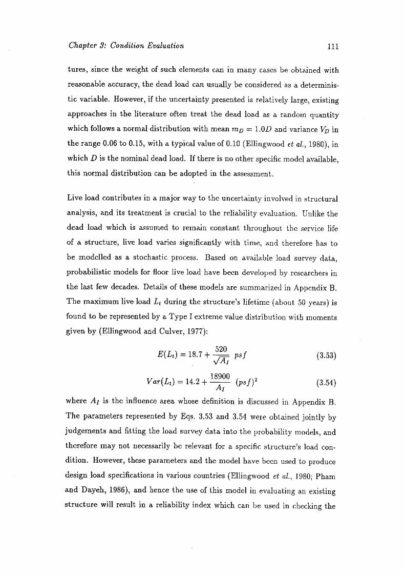
Chøpter 3: Condition Eaaluation 111
tures, since the weight of such elements can in many cases be obtained withreasonable accuracy, the dead load can usually be considered as a determinis-
tic variable. However, if the uncertainty presented is relatively large, existing
approaches in the literature often treat the dead load as a random quantity
which follows a normal distribution with mean rnp :1.0D and variance Vo inthe range 0.06 to 0.15, with a typical value of 0.10 (Ellingwood et aL,1980), inwhich D is the nominal dead load. If there is no other specific model available,
this normal distribution can be adopted in the assessment.
Live load contributes in a major way to the uncertainty involved in structural
analysis, and its treatment is crucial to the reliability evaluation. Unlike the
dead load which is assumed to remain constant throughout the service life
of a structure, live load varies significantly with time, and therefore has tobe modelled as a stochastic process. Based on available load survey data,
probabilistic models for floor live load have been developed by researchers inthe last few decades. Details of these models are summarized in Appendix B.
The maximum live load .[¿ during the structure's lifetime (about 50 years) is
found to be represented by a Typ" I extreme value distribution with moments
given by (Ellingwood and Culver, 1977):
E(1,)- 18.7 + ffi n'f (3.b8)
Var(L¿): r4.2- # @rÐ, (3.54)
where At is the influence area whose definition is discussed in Appendix B.
The parameters represented by Eqs. 3.53 and 3.54 were obtained jointly byjudgements and fitting the load survey data into the probability models, and
therefore may not necessarily be relevant for a specific structure's load con-
dition. However, these parameters and the model have been used to produce
design load specifications in various countries (Ellingwood et a1.,1g80; pham
and Dayeh, 1986), and hence the use of this model in evaluating an existing
structure will result in a ¡eliability index which can be used in checking the

Chapter 3: Condition EuøIuation II2
structure's safety level in comparison with that required in the appropriatedesign codes.
The Formulation of Reliability Analysis
Since probability distributions of the basic variables regarding structural re-sistance are assessed conditional on a hypothesis f/¡, the distribution of theresistance .R can also be represented by a conditional distribution denoted by
fnln(r,/1¡). using fng\,H¡) and the probability distribution of the appliedload /s(s) discussed in the last section, the failure probability conditional oneach hypothesis, P¡¡u(Hi), can be calculated and conceptually expressed by:
P¡¡n(H): l:FHn(,,H¡)-fs(x)d,x (3.55)
where Fnln(r,Il¡) is the cumulative probability distribution of resistance .R
conditional on a hypothesis H¡.In practice, it is more convenient to evaluatethe conditional reliability index þln(H¡) using the famous First Order SecondMoment method, and the relation between the failure probability and thesafety index can be approximately represented by
þtu(H¡) = (Þ-r lt - P¡q(H)J (8.56)
in which iÞ is the cumulative distribution function of the standard normaldistribution. The conditional reliability index þw@) thus defined representsthe engineer's belief in the safety condition of the structure if the hypothesis11¡ is true. For simplicity, it is assumed in the above formulation that the loadeffect is independent of 11¡.
Apparently there will be n conditional safety indices available for the hypoth-esis set H : (Ht,I{2,' ' ' , Hn). The probability that B¡¡y(H¡) is true is equal tothe probability of hypothesis H¡,i.e. Pl\W@)): p(H¡), in which p(/i¡) is asubjective probability, and obtained from the diagnostic procedure describedin Chapter 2. This is schematically illustrated in Fig. 3.5.
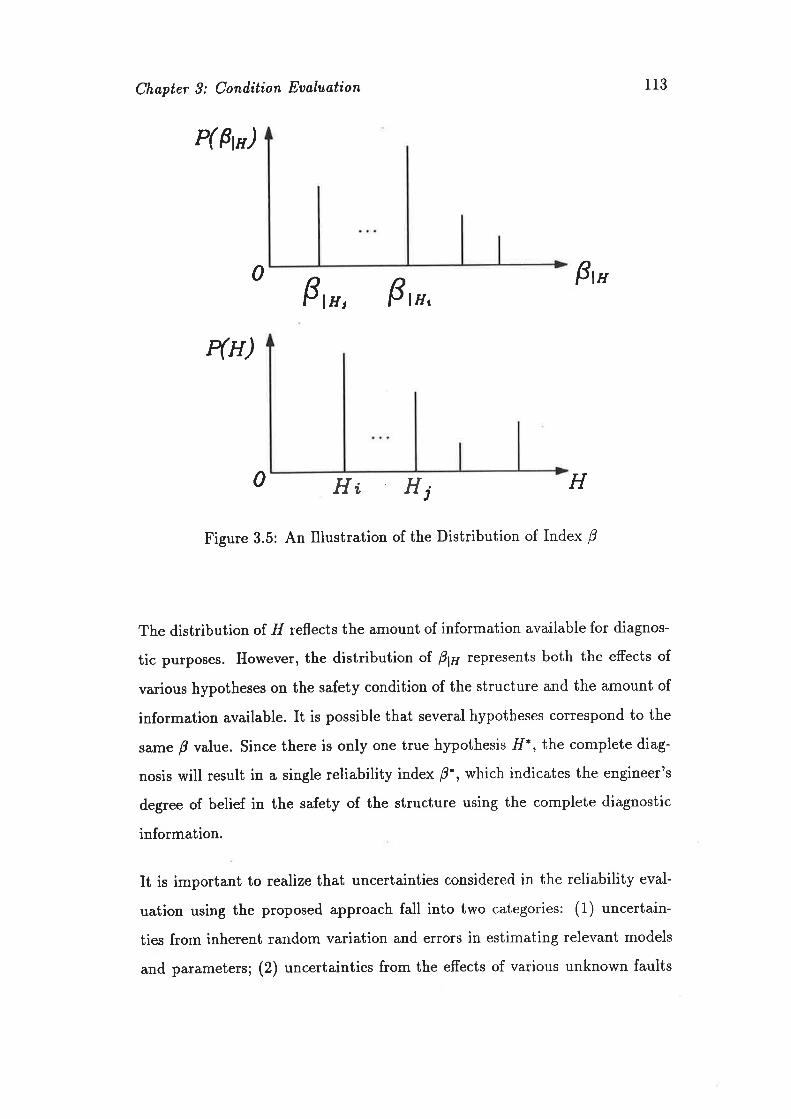
Chapter 9: Conilition Eoaluation
P( Ftn)
0
113
ßw
4n)F r*, ß,*,
HtH H0 iFigure 3.5: An Illustration of the Distribution of Index B
The distribution of I/ reflects the amount of information available for diagnos-
tic purposes. However, the distribution of þW represents both the effects of
various hypotheses on the safety condition of the structure and the amount of
information available. It is possible that several hypotheses correspond to the
same B value. Since there is only one true hypothesis .I/*, the complete diag-
nosis will result in a single reliability index B*, which indicates the engineer's
degree of belief in the safety of the structure using the complete diagnostic
information.
It is important to realize that uncertainties considered in the reliability eval-
uation using the proposed approach fall into two categories: (1) uncertain-
ties from inherent random variation and errors in estimating relevant models
and parameters; (2) uncertainties from the effects of various unknown faults

Chapter 3: Condition Eualuation LI4
or events which have caused the damage and deterioration of the structure.
Generic reliability analysis usually only considers the uncertainties of the firstcategory. With the uncertainties from the second category treated by evaluat-
ing the safety index conditional on a hypothesis, the resulting B¡¡¡, is at least
as accurate as that in generic reliability analysis. This makes it possible tocompare the safety condition of an existing defective structure with the legal
safety level required in the relevant codes, which have usually been obtained
using generic reliability analysis.
3.7.2 Assessment for safety conditions I-Isir'g p values
As is widely known, the reliability index usually does not correspond directlyto any true failure probability, but nevertheless reflects consistently the safety
condition of a structure. The accurate and practical interpretation of thevalues obtained for B¡¡¡ is very important to the assessment of existing defective
structures.
Although there is no absolute safety for engineering structures, it is frequentlydesirable to describe whether a structur e is safe or not sale under specified
conditions. Practically, a structure can be considered safe if its risk of failureis below the level which is widely accepted by the engineering profession and
community, i.e. if the calculated failure probability P¡ is not greater thanan acceptable target probability Po. Using the reliability index p in lieu ofprobability values, this P¡ < Po is then equivalent to 0 > þo,io which Bo:O-t(1 - Po), and tÞ is the function of standard normal distribution. Therefore,
if a target reliability index B0 is available, an existing structure can be assessed.
to be legally safe if its calculated B is not less than Bo.
However, difficulties exist in finding a suitable value of Po acceptable to allinterested parties. In the reliability-based code implementation of recent years,

Chopter 3: Condition Eaaluøtion 115
fhe þ value implied in current practice has been adopted as the target reliability
for deriving the load factors. For example, it was found that B values for most
flexural and compression concrete members tend to fall within the range of.2.5
to 3 for different load combinations in the United States, and hence the target
safety index po adopted for the combination of dead and live loads was 3.0
in The Build,ing Cod,e Requirements for Minimum Design Loads in Buildings
anil Other Structures (Ellingwood. et aL, 1980). For the purpose of assessing
the safety condition of an existing structure, one could naturally compare the
calculated B with the code-implied target reliability. Specifically,if P ) þo,
the structure can be considered safe. However, the fact that B values vary
with different kinds of structural members and load combinations makes this
approach a little clumsy in application.
In addition to the code-implied target reliability index Bo, based on the axiom
that ¿ comect applicatíon of the releaant codes or standards results in a safe
structure, Schneider (1992) suggested that an existing structure will be safe ifits re-evaluated B value at the time of assessment is not less than the value
Bd which is the safety index achieved in a correct design of the same structure
according to relevant codes. For any existing structure, if there is no error
in its original design according to relevant codes, Bd can be easily evaluated
using the design data of this structure. Otherwise, if there are design errors
involved, 9d hu to be calculated using the design data of the same structure
after the error has been corrected. The comparison between B and Bd thus
reflects the relative change of safety index of the same structure, and hence
is reliable and meaningful. In this work, it is suggested that þo b" used to
compare with the re-evaluated B for the the safety a,ssessment, i.e. if 0 > pd,
the structure is considered legally safe.
If P < B¿, the structure's safety condition is deteriorated or damaged, and
further examination is necessary. Generally, the higher the value of B, the
safer the structure will be. If the calculated B using the information currently
Chapter 3: Condition Eaaluotion 116
available is far smaller than Bd, the danger of structural failure is real, and
hence the safety condition of the structure is certainly unacceptable. Therefore,
the structure is useverely defectiven regarding the relevant ultimate limit state.
How much fhe p value is less than Bd has to be determined by the engineer
based on experience with reference to typical values of B accepted in the current
practice. For example, the typical value of 0d for flexible concrete members
subjected to gravity loads is around 3.0 in current practice. If the evaluated B
is less than 2.0, there is then little doubt that the structural safety condition
has to be improved in order to keep the structure in service.
However, difficulties usually exist when the re-evaluated B is less than, but
close to þn.lo this case, the assessment has to be made by evaluatingfactors
such as likelihood and possible consequences of structural failure, using relevant
judgements and information such as the diagnostic results. If it is judged that
the danger of structural failure is a real concern, the structure is classified to
be "severely defective"; if the structure is in a satisfactory condition, and no
structural repair is needed, the structure is then classified to have "negligibly
defectiven; otherwise, the structure's safety condition falls into the category of
being "moderately defective".
In summary, according to the reliability index B obtained, the safety condition
of an existing structure concerning a specific limit state can be represented by
the following four categories:
rr p>p2 søf e
(3.57)rr p < p2
in which the value of B is estimated conditional on a hypothesis H¡. h other
words, this assessment has to be carried out for each hypothesis H¡ e H.
Outlined above is the procedure for evaluating the safety of existing conc¡ete
Chapter 3: Cond,ition Eaaluation TT7
buildings based on structural reliability theory. It is certainly ideal to use
this method in practice to assess accurately the safety condition of structures.
However, the amount of data and knowledge needed in implementing the ap-
proach are not always available to the engineer in solving real problems. Ifthis is the case, the experience-based procedure described in the next section
can be adopted.
3.7.3 Experience-Based Safety Assessment
Safety a,ssessment based purely on the engineer's experience has been occasion-
ally criticized for its unreliability. Surely it is very difficult to judge whether
a building is safe or not only using experience without carefully carrying out
relevant calculations. However, by the use of diagnostic results obtained from
Chapter 2, it is possible to assess the safety of an existing structure with
reasonable accuracy.
In practice, ïve are usually only interested in a particular structural member or
substructure regarding one specific ultimate limit state in the safety evaluation.
Thus considering a potential safety problem triggered by a set of observed
anomalies which can be related to a set of. explanations defrned in Chaptet 2,
if the true explanation has been identified, an acceptable judgement on the
safety condition regarding the relevant limit state may be made by the engineer
from has/her experience and relevant knowledge of concrete structures. For
example, if it is confirmed tbat the explanation for the craclcing on the bottom
surface of a reinforced concrete slab is ttearly over loading during construction",
it can be concluded that the slab will be sale regarding its bending ultimate
limit state, provided that there are no other anomalies observed in the slab
and the design complies with relevant codes. Since there is no absolute safety
for engineering structures due to unavoidable uncertainties, in this kind of
assessment the conclusion usafe' should be interpreted as "the member is at

Chapter 3: Condition Eualuation 118
least as safe as the code requires", and hence can be considered as ,,legally safe,,
under the current code specification. For practical purposes, the experience-based procedure for safety assessment described in this section will use ,,safen,
"moderately defective' and useverely defective" to indicate the safety conditionof a structural member or substructure. The last two terms can be interpretedas "there is a potential danger' and "there is definitely a danger" respectively.
From the diagnostic procedure described in the last chapter, explanations forthe pattern of anomalies observed in a structure are generally represented by aset of hypotheses r/ : (Ht, Hr,. .., H,). For a given H¡, itis possible to assess
the safety condition of the structure according to explanations contained in I*together with any other relevant information available. If it can be concludedby the engineer confidently that the structure can fulfill its intended functionssatisfactorily, and that the risk of failure is acceptable, the safety condition isthen assessed sa/e. Otherwise, if repair action has to be carried out in orde¡to keep the structure in service, the structure is assessed to be mod,eratelyd,etectiae ot seuerely defectiae depending on factors such as urgency of repair,repair cost and possible consequences of failure. In this wa¡ safety assessmentis carried out conditionally on each hypothesis H; € H.
Obviously, if the diagnosis is incomplete, the result of safety assessment is notunique. For a hypothesis set having n elements, i.e. H : (Hr,Hz,...,Hn),with each member ranked by its probability p(Hr),the safety condition of thestructure, if denoted by xp, can be representedby xp1¡¡,, where i = L,2,... ,D.The probability P(xrl*) indicate how likery xrrn, is true, and p(xprø,) :P(H¡).
In some cases' the judgement of safety will not be so straightforward, even ifthe explanation of the anomaly has been identified, simply because the infor-mation contained in the explanation is not suficient to make such a judgement.For instance, if the explanation in the above example is ,,conc¡ete compres-

Chapter 3: Conilition Eualuation 119
sive strength is low", it is then insufficient to conclude that the slab will be
safe or unsafe. Under such circumstances, further information on the concrete
strength needs to be gathered through experiments, and used in an analysis toprovide new information for the assessment. The reliability-based safety as-
sessment procedure given in previous sections may be adopted as appropriate.
It should be pointed out that the safety evaluation discussed above is carriedout regarding the present physical state of the st¡ucture. Therefore, the ob-
tained results are valid only if there are no chronic factors involved. Uponthe examination of the outcomes of the condition survey and diagnosis, iftime-dependent factors play important roles in the safety conditions, then itis necessary to carry out a durability assessment. For example, if the observed
anomaly is ttcorrosion of the reinforcing steel", the safety evaluation regard-
ing any ultimate limit state of the structural member or substructure will be
carried out as part of the durability assessment, to be discussed in section 3.g.
3.8 Assessment for serviceability conditions
Since serviceability problems are usually manifested by various anomalies such
as excessive cracking and deflection, the extent of damage regarding a inter-ested serviceability limit state such as the crack width may be determined atthe time of assessment. If this is the case, by comparing the obtained measure-
ments with various limits on serviceability requirements specified in ¡elevantcodes, the engineer can decide whether the structure is satisfactory or inade-quøte regarding the relevant serviceability. Of course) owners of the structuremay have their preferred requirements on particular serviceability limit states,
and in this case the assessment has to allow for the owner's demand,
However, the assessment made in this way is valid only at the time of in-vestigation. Requirements regarding any serviceability limit state have to be

Chapter 3: Condítion Eaaluøtion r20
satisfied during the whole period of service life. For this reason, the structural
performance regarding the interested limit state in the future has to be pre-
dicted and assessed as to whether it will be satisfactory or inadequate. For this
purpose, numerical calculation using reliability method , if possible, is ideal.
Unfortunately, due to poor mathematical models available for predicting the
serviceability behaviour, relevant calculations for serviceability performance,
such as the estimation of crack width, usually prove only effective in determin-
ing the dimensions of structural members in the design phase, and usually are
not accurate enough for re-assessment. Therefore, serviceability assessment
using numerical calculations is not always meaningful.
On the contrary, experience-based approaches can be very useful. Since the
¿Nsessment of a serviceability limit state is usually triggered by the observed
anomalies, the future serviceability performance of the structure, in most cases,
can be well-predicted from experience, if explanations of the anomalies are
identified. Specifically, for a given limit state X5, the engineer can find out the
code-specified limit on the structural performance concerning X5, and is able
to judge whether the structure is going to satisfy the se¡viceability requirement
or not by assessing the effects of the identified explanations on the concerned
serviceability. Because the explanations of anomalies are represented by a set of
hypotheses in the diagnostic procedure, the result for serviceability assessment
can be represented by Xs¡¡¡, -satisfactory and XsV, :inadequaúe, where f{ is
the ith hypothesis. Thus for n, hypotheses available, i.e. H : (Hr, Hz,. . . , Hn),
an assessment for any serviceability limit state can be made conditional on 11,
and denote by Xs¡¡¡(fl¡). The probability distribution of Xs¡¡¡ can be easily
obtained from that of. H,i.e. P(Xs¡¡¡,) : P(H¡), where P(H') is obtained from
the diagnostic results.
Chapter 3: Condition Eualuation t2r
3.9 Assessment for Durability Conditions
Durability problems, in this work, refer to those chronically developing anoma-
lies which a¡e, or will, be indications of violation of ultimate and/or service-
ability limit states. Examples of this kind are corrosion of reinforcing steel and
carbonation of concrete cover.
Regarding the durability problem, repair becomes necessary when the anoma-
lies have developed to such an extent that the structural safety is threatened,
or the serviceability, functionality of the structure are impaired. Since the
problem is time-dependent in nature, the decision on when to carry out the
repair ideally should be made with an accurate relationship between the struc-
ture's performance and time represented by a curve. However, due to limited
knowledge available on the mechanism of development of common anomalies,
such a relationship can hardly be established. In practice, realistic solution
is usually to determine the necessity of repair according to factors such as
the owner's preferences and financial situation together with the structure's
condition judged by the engineer. Generally, when the problem is firstly iden-
tified in the condition survey, owners of the structure have different attitudes
to the repair strategy. Some would like to take a repair action only when
it is definitely needed, while others may prefer to have cheaper but regular
maintenance activities. No matter which situation it might be, the engineer
has to provide the owner with an approximate estimation of the structurets
remaining service life both with and without taking a course of action. The
period of this remaining service life may be called satisfactory period, during
which the structure is supposed to behave satisfactorily regarding the identi-
fied durability problem. Since the satisfactory period is a very important and
useful parameter in the practical approach of selecting the repair strategy, itwill be used here to represent the result of durability assessment. In other
words, an existing structure's durability condition can be assessed in terms of

Chøpter 9: Conilition Eualuation t22
its satisfactory period, denoted by Xp. Xp car- be measured in te¡ms of. years,
and for practical purposes is represented by the relevant ranges such as 5 years,
15 yeørs ar'd 20 yeørs. Of course different ranges can be used depending on
the specific problem at hand.
The satisfactory period of a particular problem has to be assessed using ex-
perience by taking into account the physical state of the structure and ambi-
ent conditions. Information and test data such as chloride content, corrosion
intensity are all valuable mate¡ials for this purpose. The causes or expla-
nations of the deterioration may also be important in determining X¿. Ifthis is the case, like the assessment for safety described in Section 3.7.2, Xpcan also be evaluated conditional on a hypothesis fl¡. For the hypothesis set
H¡ €. H : (HtrHzr..' ,Hn),, Xp can be represented by Xrlr(Hr).
Outlined above is the assessment of safety, serviceability and durability which
are usually compulsory. In addition, depending on the owner's preference,
other cosmetic concerns such as a,ppearance may also be non-trivial issues.
Therefore, the content of condition assessment has to be determined by the
engineer for specific problems.
3.10 Prognosis Procedure
Prognosis here refers to the process of predicting the structural adequacy of
an existing structure or component in the future after the corrective work is
executed. Methods for assessing structural safety, serviceability and durability
described in previous sections can be directly applied to the prognosis by taking
into account the effect of the chosen course of action.
Thus in experience-based safety prognosis, the engineer has to judge whether
the structure is going to be usafeu or not from his/her experience, with regard
Chapter 3: Cond,ition Eualuation t23
to a hypothesis and a chosen action ø¡. Il reliability-based prognosis has to be
carried out, the statistical properties of basic variables as well as the model
uncertainty have to be modified by taking into account the effect of ø¡. The
resulting conditional reliabitity index has to be denotedbV þiir,. Finally, the
result of the safety prognosis is represented by Xfi1¡.(H;), where H; € H.
Similarly, the results of a serviceability prognosis can be representedby XiiH@;)with two linguistic values: ttsatisfactory" and ttinadequate". Both the safety
and serviceability prognoses ha to be carried out for the entire period of the
planned service life of the structure.
Durability prognosis can be performed in exactly the same way as that indurability assessment except that the effect of a course of action ø¡ has to be
considered over time. For example, the result can be denoted by Xffrr@;)with three values: "5 years", "15 years" and "20 years."
3.1-1- Surnmary of This Chapter
A procedure for condition evaluation of existing concrete buildings has been
outlined, in which the structural conditions regarding safety, serviceability
and durability before and after a course of action is taken cán be assessed
using both experience and reliability analysis. The set of hypotheses obtained
from the diagnostic procedure described in Chapter 2 are deliberately used
in the proposed approach, and the result of this chapter forms the basis on
which relevant decisions with regard to maintenance and repair can be made
through a rational decision-making procedure which will be developed in the
next chapter.
Chapter 4
A Method of Decision-makitrg
for Dealittg With ExistingConcrete Buildings
4.L fntroduction
In previous chapters, our attention was focused on the development of suitable
procedures for identifying and explaining observed anomalies, and assessing
structural conditions regarding safety, serviceability and durability. However,
the final purpose of dealing with existing concrete structures is to determine
what course of action is appropriate for the structure. To do this, sound
decision-making techniques need to be employed which can cope with the in-
herent difficulties of the situation.
One major difficulty is how to deal with uncertainty in making a relevant
124

Chapter l: Decision-moking r25
decision. The main purpose of taking a course of action is to restore the struc-
ture's performance to an acceptable level regarding various requirements such
as structural safety, serviceability and durability at an acceptable cost. If the
structure can be assessed for these requirements with certainty, the selection
of a course of action from a set of candidates available can be simply made
by comparing consequences of each action according to the decision-maker's
preferences. However, as can be seen from the procedures of diagnosis and
condition assessment, uncertainties are always presented unless perfect infor-
mation is obtained." It is' ,rrrruúy practical only to predict possible outcomes
of a course of action. It is therefore difficult to make a decision using any
deterministic approach or experience alone. This is especially the case when
the consequence of making an inappropriate decision is very serious, such as
structural collapse. Under such circumstances, a well-structured procedure
combining suitable decision-making techniques together with practical con-
cerns is needed to help the engineer consistently make rational decisions under
risk and uncertainty, and hence reduce the chance of committing mistakes. Itis the aim of this chapter to develop such an approach using sound theories.
Depending on specific problems concerned, many techniques are available for
making decisions under risk and uncertainty. Probability-based modern deci-
sion theory is one of a number of reasonable approaches, and has been widely
applied in engineering and other fields. The outcomes of diagnosis and condi-
tion evaluation described in previous chapters have been presented in terms of
the concepts of probabilìty, and cai be easily incorporated with this theory.
For these reasons, statistical decision theory will be used in this chapter as the
framework for the development of a method of making rational decisions inthe treatment of existing defective concrete buildings. A preliminary review
of decision theory is therefore presented in Sections 4.2 and 4.3. Following
a short summary given in Section 4.4, the proposed method is described inSection 4.5.

Chapter /: Decision-rnaking 126
4.2 A Brief Review of statistical DecisionTheory
Decision-making is a matter of choosing a course of action from a set of alter-natives. This choice is made in decision theory by comparing different coursesof action using an appropriate criterion according to the decision maker,s pref-erences. Before going more deeply into this theory, some concepts and basicsteps involved are briefly summarized in the next section.
4.2.1 Basic Steps in Simple Decision Analysis
statistical decision analysis (pratt et al, rg65; Raiffa, 1g70; Robinson, 1gg1)is usually carried out through a number of steps which decompose a complexproblem into small subtasks and allow the decision analyst to solve them se-
quentially' Although the detailed steps are usually dependent upon the specificproblem, broadly speaking, there are four basic steps in decision analysis.
The first step is to structure the problern, i.e. to work out feasible coursesof action or alternative actions and their possible outcomes, to identify thenature of risk and uncertainties involved, and to identify the decision maker.The result of this step may be best represented by a tree structure called ad,ecision tree as shown in Fig. 4.1. The square node D is the decision node,and the branches emanating from it denoted by rr, a2t. ,4n represent thecourses of action which have been identified. Since the outcome of each o,i cannot be pre-determined with certainty at this stage, all possible outcomes of ø;are presented in the decision tree and denoted by á1, 02,. . ., d,,. The likelihoodof occurrence of each outcome 0¡ is measured by its probability p(0) whichis estimated by the decision analyst using the information available. Since thedecision maker may have dife¡ent preferences for the various outcomes of an
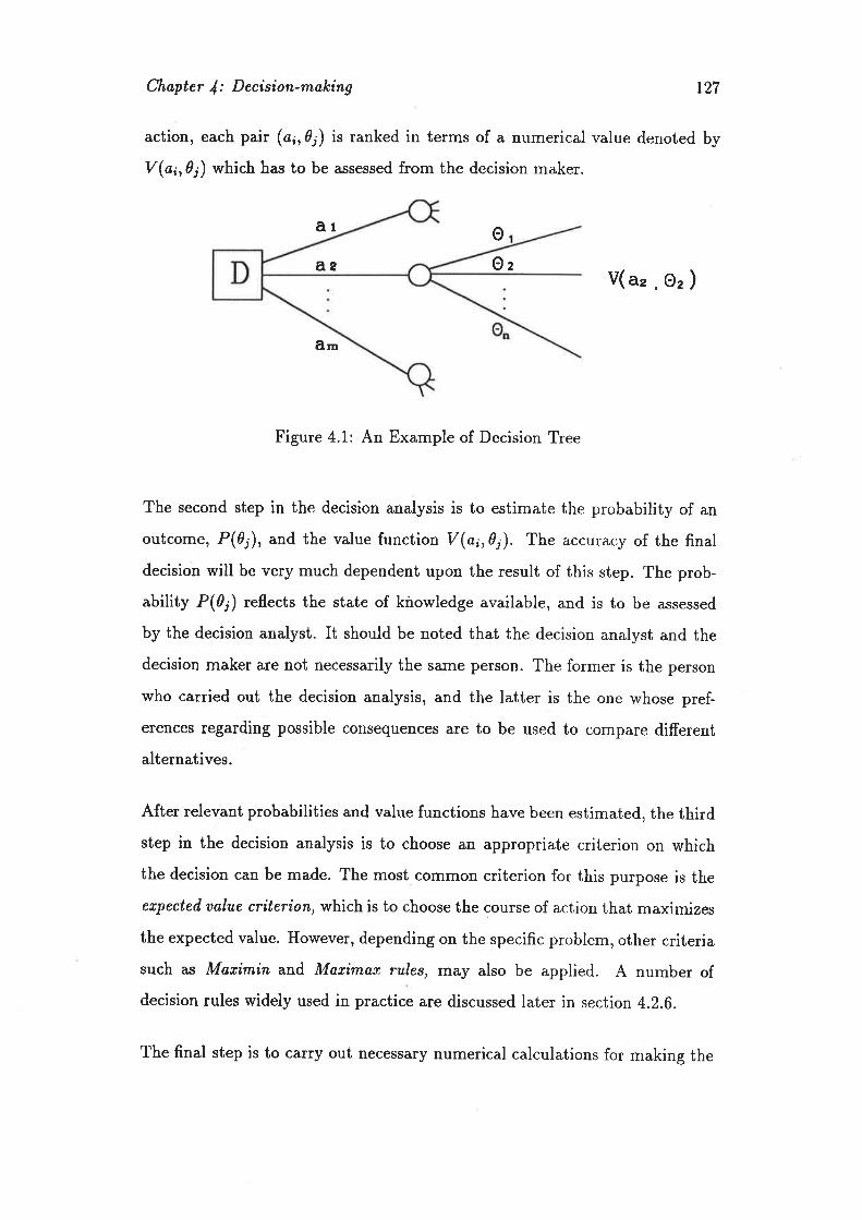
Chøpter l: Decísion-making 127
action, each pair (or,0¡) is ranked in terms of a numerical value denoted by
V(a¡,0¡) which has to be assessed from the decision maker.
ar 0a2 Oz
V(az , O, )
âm
Figure 4.1: An Example of Decision Tree
The second step in the decision analysis is to estimate the probability of an
outcome, P(0¡), and the value function V(a;,î¡). The accuracy of the final
decision will be very much dependent upon the result of this step. The prob-
ability P(0¡) reflects the state of knowledge available, and is to be assessed
by the decision analyst. It should be noted that the decision analyst and the
decision maker are not necessarily the same person. The former is the person
who carried out the decision analysis, and the latter is the one whose pref-
erences regarding possible consequences are to be used to compare different
alternatives.
After relevant probabilities and value functions have been estimated, the thirdstep in the decision analysis is to choose an appropriate criterion on which
the decision can be made. The most common criterion for this purpose is the
etpected ualue criterion, which is to choose the course of action that maximizes
the expected value. However, depending on the specific problem, other criteriasuch as Maai.min and Maximax rules, may also be applied. A number of
decision rules widely used in practice are discussed later in section 4.2.6.
The final step is to carry out necessary numerical calculations for making the

Chapter l: Decision-maleing 128
decision. As a simple example, the decision problem illustrated in Fig. 4.1 can
be solved by firstly evaluating the expected value for each course of action ø¡
as,l
E(",) - D P(0¡) x V(a¡,0 ¡),j=l
and choosing the action ¿' which has the maximum expected value, i.e.
E(o') -- Max{E(a), E(a2),. .. , E(o^)}
(4.1)
(4.2)
The process of decision analysis has been briefly summarized above, and good
references on decision theory can be found elsewhere (von Neumann, 1947;
Howard, 1968; North, 1968; Benjamin and Cornell, 1970; Raiffa, 1970; Bradley,
1e76).
As can be seen from the above discussion, uncertainties in decision analysis are
represented by probability distributions which are estimated from information
available. Therefore, the quality of a decision made at any time is closely
related to the amount of knowledge available at that time. It is also necessary
to realize that, unless uncertainties are completely eliminated, there is always
a risk of facing bad outcomes from a decision thus made. In other words,
a decision maker can make a good decision, but can not guarantee the best
results.
In order to compare different courses of action, appropriate values have to be
assigned to their outcomes. For this purpose, there exist a number of different
ways to assess the value function over possible consequences from the decision
maker's preferences, and some concepts regarding this are addressed in the
next section.
Chapter l: Decision-moking I29
4.2.2 Concepts of Preference and Utility
Generally, preferences are of two types, i.e. direct preference and the preference
reflecting attitude to risk. For instance, "I would prefer red to blaclë'is an
example of direct preference. An example of the second type is : "I would,
rather talee course of action A and, accept outcome As for certain, rather than
ad'opt course of øction B, giuing rne o, twenty percent chance of outcome 81
and, øn ei'ghty percent chance of outcome Bz". In practice, preferences appear
mostly as the combinations of these two types.
Various preferences may be simply scaled using monetary value, e.g. the cost
of an outcome of a course of action in terms of dollars. However, this approach
does not allow for decision-making in situations where non-monetary outcomes
are present. Also, existing evidence indicates that most decision makers are
averse to risk (Pratt, 1964; Benjamin and Cornell, 1970; Raiffa, 1g70; Dandyand Warner, 1989), and the phenomenon of risk aversion can not be accounted
for in the decision analysis if the monetary value is used to scale the preferences.
For example, given two options A and ^B with the following properties:
¡ A:win $ 100,000 for sure;
¡ B:win $ 1,000,000 with probability of 0.1 or $ 0 with probability of 0.g,
it is reasonable to expect that different people would have different choices
depending on factors such as their financial resources, and attitude to risk.However, based on the expected value criterion using monetary values, there
will be no diference between choosing A and B.
For these re¿ùsons, monetary value is not always appropriate for ranking con-
sequences in decision-making, and better quantities are certainly necessary
for scaling preferences when uncertainties are involved. According to Hull eú
aI. (1977), utility is probably the most satisfactory, and generally accepted,
Chopter l: Decision-mølcing 130
scale for preferences. Utility theory derives from von Neumann's four basic
assumptions (von Neumann, 1947). Briefly, these are:
l. outcomes resulting from a course of action can be compared. Inother words, preferences can be evaluated for outcomes or prizes,
and these preferences are transitive;
2. preferences can be assigned in the same way to lotteries involving
prizes as they are assigned to the prizes themselves;
3. there is no fun in gambling;
4. continuity holds for preferences.
If these assumptions are accepted, there is then a mathematical function U,
called a utility function, that assigns a real number to each prize or outcome
with the following properties:
o utility function U is defined on the set of possible outcomes;
¡ outcome d¿ is preferred to outcome d¡ if and only if U(0ò > U(?a);
. a course of action resulting in þossible outcomes 0t,,02,... ,0n with prob-
abilities pt,tpz,...,tp, is preferred to another one resulting in possible
outcomes tþt,rþ2r.. . ,rþ^ with probabilities et¡g2,.. . ,Q^ if and only if
DPtt U(0¡) tDq¡xUAþ¡)n
i=1
m
j--r(4.3)
where f,o, :1 and io, - 1. The utility function allows preferencesi=l j=l
to be consistently described by means of a real number scale.
One interesting property of the utility function which needs to be mentioned
is that its absolute magnitude is not important, since the preference scaled byits utility is unchanged if the numerical value of the utility is multiplied by a

Chapter l: Decision-malcing 131
positive constant or added to any constant, i.e. if U(",y) is a utility function,
then [/'(ø, U) = Iet!lc2U(x,y), where lc2 ] O,is also a utility function. In other
words, the utility function is invariant to positive linear transformations. This
indicates that with preferences, utilities of consequences are measured relative
to an arbitrary origin and unit of measure. This property greatly simplifies
the estimation of utility values in practice.
4.2.3 The Estimation of Utilities
Utility values over possible outcomes are usually extracted from the decision
maker by the decision analyst through an appropriate acquisition procedure
which varies with the type of utilities. In practice, there are broadly two kinds
of utility according to the number of dimensions in describing the consequences.
If outcomes of a course of action can be described by a single parameter, the
related utility is unidimensíonal. If more than one parameter are needed to
fully describe the outcome, the resultant utility is then multi-dimension,al, and.
is also referred to as a multi-attriózúe utility. Depending on the dimensionality,
different techniques are required to estimate various utility values.
Assessing Unidimensional Utility
The simplest approach to evaluate unidimensional utility is direct rating (Torg-
erson, 1958). This method involves assigning quantitative scales to discrete
outcomes according to the decision makerts judgement.
Perhaps the most widely used approach in assessing unidimensional utility isthe gamble method which was described by von Neumann (1942) and Raiffa
(1970). It involves establishing the certainty equivalents of a number of simple
gambles, and utility values can be easily obtained for discrete outcomes. The

Chapter l: Decision-making 132
method has been successfully applied to many practical decision problems
(Marguardt et ø1,1965; Ginsberg et ø1, 1968; Betaque and Gorry,1977).
However, if utility values are required for a wide range of outcomes in a decision
situation, the utility estimation using the above methods may become very
tedious. This difficulty triggered the development of some simplified methods
which usually reduce the utility evaluation from obtaining all points on a curve
to determining a few parameters in a functional form. The commonly used
function for this purpose is a quadratic one (Markowitz,7959). However, itseems that this approach was mostly developed and used in the context of the
utility of investors for money, and few applications are reported in other fields.
Assessing Multidimensional Utility
No fundamental differences exist between unidimensional and multi-dimensional
utilities, since both of them are a means of describing preferences and attitude
to risks over a set of outcomes involved in a decision problem. Theoretically,
multi-dimensional utilities can also be evaluated using the same methods as
for assessing unidimensional utilities. However, there exist practical dificulties
for this purpose. Since a complete multi-dimensional outcome space is formed
from the combination of different dimensions, if the involved dimensions are
continuous, the total number of outcomes will be too large to be handled in
the utility assessment. Therefore, various methods specifically suitable for
estimating multi-attribute utilities have been developed (Fishburn, 1966; Far-
quhar, L977), which can simplify the assessment procedure based on some
assumptions.
Of these methods, one simple approach (Hull, 1977) is to assume that the
utility is a linear function of values of different dimensions of the outcomes.
For this purpose, if each dimension X, can be measured by its own quantitative

Chapter l: Deci,sion-malcing 133
scale ø¡, and if it is assumed that there is a constant rate of trade-off between
one dimension and another, the utility over n-dimensional outcomes can be
represented by the following function:
nU(rr,r.2¡'" ,Ín) :Dotr. (4.4)
r=l
where U(*t,r.2¡. ,o,") is the multi-dimensional utility function; z¡ is the nu-
merical scale of iúå dimension and ø¡ is a constant representing the trade-off
between different dimensions. However, the application of this approach is
very limited because, in many cases, not all dimensions can be measured by
their own numerical scales.
Perhaps the most widely used method is to assume that multi-dimensional
utilities follow an additiae utility function (Adams, 1959; Fishburn, 1965; 1967;
Pollak, 1967), i.e.
(J(rr,r2¡. ,rn):iU,çrr¡ (4.5)i=1
where tl¡("¡) is the unidimensional utility function on the i'r dimension X;.
Fishburn (1965) has proven that the necessary and sufficient condition for using
an additive utility function is that the evaluation of a course of action under
risk depends only on the marginal distribution over each dimension, i.e. for an
outcome space X = (Xt,Xz,-'.,Xn), Eq. 4.5 holds only if "the individual is
indifferent between the two gambles in any pair of gambles that have the same
total probability for each x; e X;(i - 1,. -. ,n) that appears in either." He
also developed theorems which can be used to test for this condition. Pollak
(1967) also described this condition in terms of preferences.
The function t/¡(ø¡) in Eq. 4.5 can be evaluated using the same method as
used in estimating unidimensional utility functions, conditional on some fixed
element of outcomes. However, it is not sufficient to obtain U(q,,rzr...rrn)by simply summing U¡(r;) thus assessed. Because each U;(*;) is defined up to
a positive linear transformation, linear transformations of each U;(r¡) do not
Chapter J: Decísion-malcing 134
(4.6)
(4.7)
necessarily result in a linear transformation of iUr{rr).Different dimensions
have to be ranked by a set of scale factors "r. fLXr" factors reflect the decision
maker's trade-ofs between diferent dimensions. Methods for evaluating ci are
available in (Eckenrode, 1965; Keeney, Lg74), and Eq. 4.5 then becomes:
IJ (rt, c.2t. .', r,-) : I c¡U¡(x;)n
d=l
The major shortcoming of additive utility is the restrictiveness of its requisite
condition which is usually diffcult to justify. A less restrictive, but more
practical alternative was originated'in Keeney's work (Keeney, lg72) which
is referred to a"s quasi-ad,ditiae utility. The foundation of this method is the
concept of utility independence. Given a utility function U(r,y), one can say ø
is utility independent of y if the decision maker's preferences over any gambles
on ø, for a fixed yo in A,are the same regardless of the amount of y6. Then, ifo and y are mutually utility independent,U(r,y) can be evaluated as:
u (r, v) : u (a, uo) + u (xo, v) + ku (r, ao)tJ (rs, y)
where,t is a constant, and U(*,yo),U(ro,y) arc conditional utilityfunctions for
r and yrlot arbitrary /s and øe respectively. The same concept can be extended
to the n-dimensional case (Keeney,1972;1977; Keeney and Raiffa, 1g76). The
method has been illustrated by using a two dimensional example (Keeney,
t972), and it was shown that the approach has great practical importance.
Using relevant methods reviewed above, utility values over various outcomes
can be assessed. To make a decision under incomplete information, proba-
bilities of all possible outcomes have to be estimated, and depending on the
amount of knowledge available, making a decision can fall into a number of
different categories.

Chapter l: Decision-malei,ng 135
4.2.4 Decision-making \Mith Incomplete Knowledge
For a set of courses of action at)ø2,r... tant if perfect information has been
acquired, the outcome of each a; cãrr be pre-determined, and the decision can
be easily made by choosing the alternative which has the highest utility. This
is called decision-making und,er certainty. However, decisions usually have to
be made without knowing exactly the outcome of ø¡. Rather, the information
available allows us to assign probabilities to the possible consequences of each
alternative. Decision-making in this situation is referred to as decision-maleing
under risk. If there is no knowledge available at all about the occurrence of
outcomes, the decision is then to be made under uncertainty.
In addition to the above three categories, decisions may fall in between deci-
sion und,er uncertainty and, decision under risk, i.e. the information available is
able to rank the possibilities of outcomes, but is insufficient to obtain the spe-
cific probability values. Fishburn (1964) studied this problem and developed
an equation which can be used to make decisions under such circumstances.
Firstly, he assumed that each course of action has n possible outcomes, and
the decision maker has sufficient knowledge to rank the probabilities of these
n outcomesr e.B. & 2 Pz > ...of action a1, U(ar), is larger than or equal to that of alternative a2, U(a2), i.e.
U("r) > U(a2), iftlDu("1)>Du("1) (4.s)
t=l Ë=1
for all j : I,' ' ' ,n, where U(of) and U(af) are the utilities of the fr¿å outcomes
of ay ø2 respectively. In other words, given Pt ) Pz > . . . >
the probability of iÚä outcome, if Eq. 4.8 is satisfied, alternative ø1 is preferred
to a2.
However, a major disadvantage of this approach is that Eq. 4.8 is very difficultto satisfy in practice. To overcome this difficulty, Kmietowicz and Pearman
Chapter J: Decision-malcing 136
(1981) improved the above method by employing the linear programming tech-nique in which the maximum and minimum expected utility of each course ofaction can be obtained by only knowing that Pr > p2 > ... >course of action is the one whose maximum expected utility is larger than anyothers'.
Regarding the common decision situations discussed above, the problem treatedin this thesis falls into the second category, i.e. decisions under risk. There-fore, the assessment of probabilities for outcomes is an important taskProbabilities involved in many existing decis usu sub ec-
tively assessed. Subjective probability is the measure of a person's belief as
to the occurrence of an event. The evaluation of this probability is based onthe state of mind, rather than independent trial experiments, and reflects thestate of knowledge available. Many techniques for estimating subjective prob-abilities are available, and choosing'an appropriate one is dependent on thespecific decision problem. In this work, relevant probabilities of consequences
are evaluated from the results of diagnosis and condition evaluation, and no
separate probability assessment is necessary. Therefore, techniques of proba-bility assessment will not be discussed here in detail, as references are availableelsewhere (Winkler, 1970; Hampton eú al.r ISTJ; Tversky, lgl4).
With utilities and relevant probabilities obtained, the best course of action can
be easily chosen using the expected utility criterion, and a single-stage decision-
making is thus complete. However, it is usually possible and desirable toimprove the quality of decision-making by gathering new information throughvarious means such as experimental work, refined analysis. Therefore, differentdecisions can be made in sequence depending on the information available. Inthis way the decision-making becomes a multi-stage process. Since gatheringnew information is costly, and sometime can be very expensive, whether toacquire more data or to take a terminating action at any stage is a crucialdecision to be made. The most commonly used methods for this purpose will
Chapter J: Decision-making 137
be reviewed briefly in the next section
4.2.5 Multi-stage Decision-making
Multi-stage decision-making can be carried out in different situations. For
a physical system whose states change stochastically, a sequence of mainte'
nance/repair actions regarding its whole service period can be determined
through a multi-stage analysis which is usually modelled as a Markovian pro-
cess (Eckles, 1968; Satia et al, L973). In this case, each stage represents one
state of the system, and a course of action is usually chosen for each stage.
Alternatively, in the situation where time factor is ignored, the multi-stage
decision-making is to determine a sequence of information-gathering activities
such as experiments, and finally to choose a course of action using the infor-
mation available at each stage. In this case, various stages represent different
states of information available. Decision-making considered in this thesis falls
into the second category, and therefore the review here does not include the
literature on stochastic process models.
Generally, a decision at the first stage is made by choosing a course of action ¿*
which has the highest expected utility calculated using the prior information.
If there are a set of tests from which more data can be obtained, there is then
a choice to be made between taking ¿* or making the decision after a selected
test is conducted. The key point in this multi-stage process is obviously to
decide the necessity of transition from one stage to another. This is usually
determined based on the ualue of informøtion obtained from an experiment
e (Howard, 1966; Matheson, 1968). To illustrate this, a two-stage decision
tree is plotted in Fig. 4.2 where i and i + 1 denote the itå and (i 1 1)úÀ stage
respectively; e denotes the experiment to be conducted and C" is its cost; the
possible outcomes of e are represented by d1, dzr..'rd,¡; all other symbols have
the same meanings as in Fig. 4.1 except that [/ is now the utility function
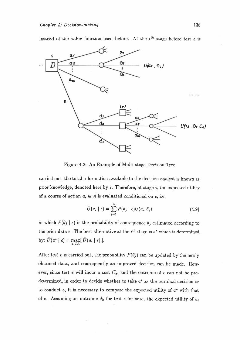
Chapter J: Decision-making 138
instead of the value function used before. At the itä stage before test e is
OrI Q,t
Uþz , Oz)
oñ
eí+l
ddz Uþ, . Az .C,)
Figure 4.2: An Example of Multi-stage Decision Tree
carried out, the total information available to the decision analyst is known as
prior knowledge, denoted here by e. Therefore, at stage i, the expected utilityof a course of action a¡ e A is evaluated conditional on e, i.e.
ú(o,1.) :Ë P(o¡le)tJ(a;,l¡) (4.e)j=l
in which P(0¡ I e) is the probability of consequence 0¡ estimated according to
the prior data e. The best alternative at the i¿å stage is ¿* which is determined
by: U(ø* | .) :.*åît U(a¡l e)).
After test e is carried out, the probability P(0¡) can be updated by the newly
obtained data, and consequently an improved decision can be made. How-
ever, since test e will incur a cost C", and the outcome of e can not be pre-
determined, in order to decide whether to take ¿* as the terminal decision or
to conduct e, it is necessary to compare the expected utility of a* with that
of e. Assuming an outcome d¡ for test e for sure, the expected utility of ø;
Chapter l: Decision-møking 139
changes to: úþ, r e,dt) - i rrro I e,d¡)U(a;,o j,c,) (4.10)
j=l
where P(0¡ I e, d¡) is the probability of consequence d¡ conditional on the newly
obtained data d¡. To evaluate P(0¡ l r,d*), it needs to estimate the probability
P(d* I d¡, e) subjectively from experience and other relevant knowledge. P(0¡ I
e, d¡) can then be obtained through Bayes' theorem:
P(d¡ I 0¡, e)P(0¡ | e)P(0¡le,d*)-ffi (4.11)
The expected utility of test e conditional on a single outcome d¡ can now be
evaluated as:
U(e I e,,d*) : m9¡lU(ø; I ,,d*)l (4.12)
Finally, since the test e has I possible outcomes dt,dz,...,dr, its expected
utility has to be calculated by:
U P(dr I e)U(e I ,, do)eeI
Dlt=1
(4.13)
in which P(dr I e) is the probability of outcome d¡, and evaluated by:
nP(d* l.) = D P(ù l0¡,,e)P(0¡ | e) (4.14)
j=L
Up to this point, the decision at the ith stage can be made by comparing
the expected utility of experiment e with that of the best course of action ¿*
determined without performing the test. That is, if U(e I .) > fl1o. ¡ r¡,test e is preferred to ø*, and the decision process continues. In this case, the
future decision at the (i + t)úå stage will be made according to the result of
experiment e. otherwise, if U(ele) 1U(ø* le), it is not worth conducting e
to gather more data, and the decisicin is to take ø*.
Instead of using the expected utility of an experiment, a different approach also
widely used in multi-stage decision-making is to compare the expected utility

Chapter l: Decision-making 140
of a piece of information with that of ¿*. For this purpose, given a decision
problem with courses of action A: [otr@2¡. , ø^], and possible consequences
O : [0r,02,...,dr,] for each ø;, the best action a* in A at the irÀ stage can
be firstly identified as the one which has the highest expected utility using
the information e, i.e. U("' I e) : mfflu(a¡ | e)1. Since the evaluation of
the consequences of an action usually involves a number of variables, it is
assumed here that each consequence 0r' is dependent upon a set of variables
X : (Xt,Xzr...,X^), among which those unknown are treated randomly
with the probability distribution denoted by {"t}. If there is a test e which
can reveal pertinent information on X;, the distribution of X; is updated, and
consequently an improved decision çan be made using the updated {c;}. To
do this, the question is then which variable among X is so valuable that the
expected utility of searching more data on it is higher than that of ¿*. For
this purpose, assuming that the true value o1 X; can be obtained from an
experiment e at the cost C",, the probability of the consequence á¡ is then
updated from P(d¡ | e) to P(0¡ I c;, e) where r¡ is the assumed true value of
X;. The expected utility of spending C,. to gather this information on X¡ is
evaluated by:
U(C,, | .) : l* Oþ- | z;, e){ø; I e} (4.15)
where U(o. | ø¡,e) is the expected utility of ø* using the prior knowledge e
together with ø¡, i.e. u(a* | rr,.) = iåî t(o¡ I ri,e); in which ù(o¡ I ø;, e) can
be evaluated in a routine manner:
t("¡ lø¡, €) : D U("t,Îk)P(0k l r;,r) (4.16)d* €O
With the expected utility of gathering information on X; thus evaluated, the
transition of the decision process from stage i, to i * 1 can be easily decided,
i.e. if U(C", I e) is larger than the expected utility of c*, we should design and
carry out an appropriate test program which can result in particular data on
X¡.

Chapter f : Decision-møking L4T
Actually by evaluatingU(C,, I e) for all i : L,2,...,m,the most valuable
variable x* in x can be found by u(c,, I .) : ,!1f,^[ú(c,, I .)]. However,
it is usually difficult to identify X* because of large amount of computation
required.
Theoretically this approach can also be used to determine whether it is worthgathering new information on more than one variables X; ' . . X* simultaneously
by considering the probability P(0¡ I ti. . . rk¡e) and the joint distribution
{t¡'' 't*}.
Approaches based on the ualue of informatior¿ as reviewed above are the basis
of multi-stage decision analysis. However, both of these two methods have thesame shortcoming: in order to find the optimal test, computations involving an
extremely large decision tree is needed. Therefore, application of the approach
to real problem-solving is limited.
In approaches discussed above, all decisions are made using the expected
value/utility criterion. In practice, there exist many other rules which can
be adopted depending upon the specific problem at hand. In the next section,
several commonly used decision rules as well as disadvantages of the expected
value/utility criterion are discussed.
4.2.6 Different Decision Rules
Expected value/utility criterion has been most widely used in decision analysis.
In the case of decision-making under risk, this is a very useful and meaningfulcriterion. However, its shortcomings are obvious. Since decisions made using
this rule can not guarantee a good result, in an important decision situation,the approach may lead to severe conseguences for the decision maker if theworst outcome of the selected action unfortunately occurs. On the other hand,the expected value/utility criterion only considers the mean value, and ignores

Chøpter l: Decision-making r42
the other properties of probability distributions such as deviation. This may
result in an irational decision. For example, in the decision problem illustrated
in Fig. 4.3, q and a2 are two courses of action available to the decision maker,
and each of them has three possible consequences denoted by r't(1), *",(2),
and ø"r(3) respectively. The utility of each consequence and related probability
are represented by the bar chart in the figure. The expected utilities of ø1 and
a2 ã¡ê E("r) : 61 and E("r) : 56 respectively. Using the expected utilitycriterion, apparently ø1 is preferred to ø2. However, it is reasonable to assume
that many decision makers would choose ø2 instead of ø1 if they are averse to
risk, because the consequences of ø2 have less deviation than that of ø1.
,"?z) E(ør) - 61
.50
artr (î)
o 25 so 76 ,OO Orúcomc(UtilílU)
E(o -58
o.2z (2)
ø2t (8)
cL2x (r)
o 25 50 75 ,OO Oúcone(Utility)
Figure 4.3: An Illustration of the Range of Outcomes
Due to the inadequacy of the expected utility criterion, a number of other
decision rules are also widely adopted in practice. One of these is the so-called
Maximin rule, which tends to select the course of action ø* whose possible min-
i*u* uutrr"l tn" greatest among all available courses of action, i.e. (according
25
25
¡ôdoof

Chøpter l: Decision-making 143
to Fig. 4.1 on page 127)
U(o'): m,ax{mrinlU(a;,0¡)l} (4.17)
This rule is usually used by conservative or pessimistic decision makers. For
example, it may be appropriate in structural assessment when the decision
maker wishes to avoid a catastrophe at all costs.
In contrast to the conservative decision maker, optimistic decision makers usu-
ally hope that the uncertain future develops favourably for them, and hence
try to select the course of action ¿* whose possible maximum value is larger
than that of any others, i.e. :
U (". ) : m-ax{mêxlU (ø;, 0 ¡)l}t1 (4.18)
and this is called Maximax rule
f'eThe disadvantage of both the Maximin and Maximax criteria is that theyu" ay''ti..-frely on extreme utilities or values, and this can lead to over conservative or
over risky. Nevertheless, these rules are still very useful in some situations,
especially when the decision is to be made under uncertainty.
For decision-making under uncertainty there exist another criterion which is toassign the most unbiased probabilities for all possible outcomes and change the
problem into decision-making under risk. Logically, the most unbiased judge-
ment without any information on the chance of occurrence of consequences
is that all outcomes have equal probability of occurrence (Jaynes, lg68), i.e.
P(0) : I ln, where d¡ denotes the ¡'tå outcome of n possible outcomes. The
expected utility principle can then be used to choose the alternative which has
the highest expected utility:
u(o-): *,u*{; Ð_rr",,rr, (4.1e)
These decision criteria represent most of those commonly used in practice
Chapter J: Decision-making L44
Statistical decision theory has thus been briefly reviewed. While decision the-
ory has been successfully applied in fields such as medical science (Ginsberg
et al. L968; Betaque and Gorry,L977), economics (Keeney and Raiffa, 1976),
its application in solving civil engineering problems can also be found in the
literature. In the next section, previous work relevant to decision-making instructural assessment is briefly discussed.
4.3 Decision Analysis in Relevant Engineer-ing Problems
There are a large number of applications of decision theory in engineering
problem-solving. Of these approaches, however, very limited work on dealing
with structural defects of existing concrete structures has been found in the
literature. For this reason, the review in this section contains only a few
applications which are more or less relevant to our problem.
Folayan, Ht "g and Benjamin (1970) employed decision theory to study theproblem of foundation settlement. The amount of settlement was considered
as a function of a set of deterministic quantities as well as a random variable
which represents the soil property. The probability distribution of this ran-
dom variable is firstly estimated by an experienced engineer, and then updated
through Bayes'theorem using sampling data obtained from further testing.The decision to be made is how many samples are needed to make a good
prediction of the settlement. For this purpose, a utility loss function was de-
fined as a quadratic curve of the prediction error €, which is the difference
between the calculated settlement and the true settlement. The optimal num-ber of samples is obtained by minimizing the expected loss through a simpleoptimization procedure.
Chøpter l: Decision-møking 145
In a similar study, decision tree analysis is employed by Wu (197a) to decide
whether sample testing is worth being conducted to explore soil properties for
improving the prediction of foundation settlement and slope stabilit¡ in which
a cost function was used in lieu of utility values.
In addition to the unidimensional decision analysis, in which the consequence
of an action is represented by a single parameter, Nessim and Jordaan (1989) I
applied multi-dimensional approach to study er-ror-control in structural design. :
For this purpose, probabilistic models are firstly developed for estimating the
error content in a structure after the application of a checking strategy with
given efficiency. The error content is then related to structural safety and ser-
viceability through relevant structural analysis. Consequences of a course of
action in structural design are represented by a set of attributes such as úoúøl
cost, number of d,eaths anil injuries in case of structural failure. The utility
function is assessed over these attributes. The expected utility given an ef-
ficiency of quality control are next evaluated, and the best level of efficiency
is obtained when the expected utility reaches the highest value. However, in
order to calculate the expected utility it is necessary to assess the joint prob-
ability distribution over those involved attributes, and this is usually difficult
in practice.
To study the maintenance and repair related problems of existing concrete
structures, Warner and Kay (1983) have made a pioneering attempt to apply
theory. However, as already mentioned in Chapter 1 on Page 19,
their approach lacks a great deal of details needed to implement the proposed
procedure.

Chapter l: Decision-making 146
4.4 Summary on This Review
Probabilistic decision theory provides a good framework for consistently mak-
ing choices from alternatives according to the decision maker's preferences,
even when the consequences of courses of action can not be predicted withcertainty. With the use of utility values, the decision maker's attitude to-
ward risks can be considered in the decision-making. Since risks regarding
the occurrence of various bad consequences are explicitly expressed in terms ofprobabilities, the decision maker can have a clear understanding of the risk sce-
narios to be faced. It is therefore potentially very helpful to use decision theory
in the treatment of existing concrete structures, especially when involved risks
of having severe consequences are high in choosing courses of action.
Although decision theory has been extensively applied to engineering as well
as other areas, a systematic approach particularly suitable for dealing withexisting concrete structures has not yet been available. Such a method is to
be developed in the next section, by use of which questions such as what tod'o about a giuen ilefectiae concrete buildi,ng can be answered rationally using
results of diagnosis and condition evaluation obtained from previous chapters.
4.5 A Method of Decision-making for Deal-
ing \Mith Structural Defects
4.5.L fntroduction
We shall be concerned with a decision-making situation in which the engi-
neer and the owner of the structure work together to decide on how to handle
problems in an existing concrete building. When a building shows noticeable
fi] ce^1,
ò (¡..t,t-."
¡--1\-._
Chapter f : Decision-maleing r47
anomalies, the engineer is usually called upon by the owner of the structure to
carry out an assessment and to advise on possible remedies. A final decision
on adopting a course of action is to be made based on the owner's require-
ments and financial resources with references to the condition of the structure.
Therefore, the owner of the structure will be considered here as the decision
maker, whose preferences on different choices are to be used in the decision-
making, and the engineer serves as the decision analyst who is responsible
for carrying out relevant analysis required for making such choice, and advising
the decision maker of technical options available, etc.
In dealing with potentially defective concrete buildings, decisions to be made
usually include a,nswers to questions such as "is any repair action needed ?",
"what is the best action to cure the problem ?" Although different people
have their own ways to find out satisfactory solutions, the primary principle
probably adopted by most decision makers is to minimize the incurred cost
while trying to satisfy uarious requirements for the structure. In other words,
when a number of courses of action have been identified by the engineer, the
problem is to choose one alternative which can best satisfy the abovementioned
principle. For this purpose, the principle to be adopted for a given problem is
usually defined in terms of a set of objectives which are to be achieved in the
decision-making. The identification of relevant objectives for our problem are
discussed in the next section.
4.5.2 Identification of Objectives and Their Associated
Attributes
It is usually up to the decision maker to specify a set of objectives. However, in
solving real problems, the decision analyst and the decision maker have to work
closely together so that the decision maker clearly understands the essential
features of the problem, and all important aspects are taken into account

Chapter y': Decision-malcing 14g
in determining the objectives. For dealing with existing concrete buildings,although objectives tend to vary with different concerns from the owner, thefollowing four objectives are suggested for most problems:
1. to provide adequate structural safety;
2. to provide adequate structural serviceability;
3. to provide adequate structural durability;
4. to minimize the cost of achieving the first three objectives.
Of course for specific problems, relevant objectives other than those listed canbe included if necessary. On the other handdropped off.
, some items in the list may be
To assess the degree to which a particular objective is satisfied by a course ofaction, each objective is associated with an attribute which has values. Anobjective can then be assessed using the value of its associated attribute. Forexample, the objectiue "to minimize the total cost,, can be assessed accordingto its attribute xvç interms of "dollars", \ilhere x7ç rcpresents the totar cost.obviousl¡ the value of. x76 in this case is a real number.
To define an apPropriate attribute for an objective, it is important to ensurethat the attribute is rneøsuraóre and comprchensiue (Keeney and Raifa, 19z6).An attribute is mea^surable if it is possible to obtain a joint probability distri-bution over its range of values. An attribute is comprehensive if, by knowing aparticular value of the attribute, the decision maker has a clear understandingof the extent to which the associated objective is achieved.
considering these two requirements, the objectiue ,,toprovide adequate safety,,will now be associated with an attribu te xp which is a discrete linguisticvariable with four possible values: ø¡(1)-,,safe,,, n¡(2):,,negligibly defective,,,s/(3):(moderately defective" and c¡(4):,,severely def'ective,,. For a given

Chapter J: Decision-møkíng 149
structure and a specific ultimate limit state, these fou¡ values can be obtained
from the safety assessment procedure described in Section 3.7.2 of Chapter 3,
and the interpretation is the same as before. Apparently any value of. Xpis a clear indicator of the safety condition of the structure either before or
after a course of action is taken. The probability distribution of. Xp can also
be estimated f¡om the result of condition evaluation. Therefore, X¡ is both
comprehensive and measurable.
The second objectiae "to provide adequate serviceability" can be treated in a
similar way. Using the results of serviceability assessment described in Sec-
tion 3.8, an attribute Xs is defined for this objective, which is a linguistic
variable with two values: z"(1):"s¿iisfactory" and r"(2):"inadequate".
The objectiue "to provide adequate durability" is measured in terms of an
attribute X¿ which takes the values of the satísfactory period defined in dura-
bility assessment in Section 3.9, i.e. ø¿(1):"5 years", r¿(2)-"I5 years", and
îd(3):.*20 years". For example, æ¿(1):"5 years" means that the structure willperform satisfactorily for at least 5 years regarding the concerned durability
problem.
The last objectiue "to minimizethetotal cost" can be measured by the attribute
Xc in "dollars", which represents all costs incurred in the process of structural
assessment, i.e. :
Xc = Ct * Cn* Ct (4.20)
in which C¡ and Cn denote the costs incurred by the investigation (e.g. di-
agnosis, experiments) and repair respectivel¡ Cn represents the cost which is
equivalent to the profit loss due to any inconvenience to normal business caused
by any action involved in the assessment and/or repair process. Obviously, Xcr
is a continuous real number.
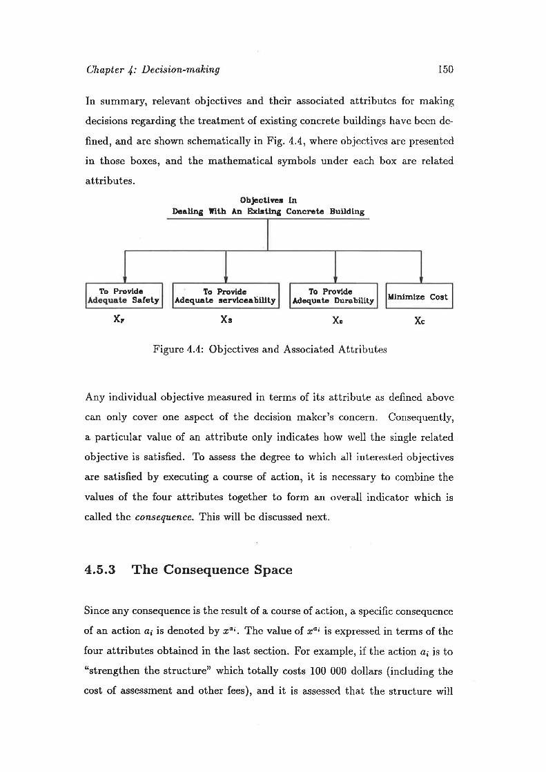
Chapter l: Decision-malci,ng 150
In summary, relevant objectives and their associated attributes for making
decisions regarding the treatment of existing concrete buildings have been de-
fined, and are shown schematically in Fig. 4.4, where objectives are presented
in those boxes, and the mathematical symbols under each box are related
attributes.
Obþctlws InIlealing fith An Exirting Concrctc Building
Xr Xs Xc
Figure 4.4: Objectives and Associated Attributes
Any individual objective measured in terms of its attribute as defined above
can only cover one aspect of the decision makerts concern. Consequently,
a particular value of an attribute only indicates how well the single related
objective is satisfied. To assess the degree to which all interested objectives
are satisfied by executing a course of action, it is necessary to combine the
values of the four attributes together to form an overall indicator which is
called the consequence. This will be discussed next.
4.5.3 The Consequence Space
Since any consequence is the result of a course of action, a specific consequence
of an action ø¡ is denoted by øoi. The value of roi is expressed in terms of the
four ¿ttributes obtained in the last section. For example, if the action ø; is to
"strengthen the structure" which totally costs 100 000 dollars (including the
cost of af¡sessment and other fees), and it is assessed that the structure will
Xo
To ProvidcSafety
To P¡ovidcAdequatc servlceabllity
To ProvldcAdequata Durability Mlnlmlze Cost

Chapter J: Decisi,on-rnaking 151
be t'safe", ttsatisfactory" regarding the safety and serviceability performance
respectively, and uwill satisfactorily la^st about 15 years" in regard to the iden-
tified durability problem, the consequence of o¡ is then represented by ror - I
"safe', "satisføctorA" r "l5 years", 100,000 ]. In this case, the value of each
attribute is known with certainty, and hence the consequence r"' is determined
as a single point in the consequence space.
However, when uncertainties are involved in evaluating the attributes, all pos-
sible consequences have to be considered. For this purpose, the consequence
spo,ce of a course of action ø¡, denoted by X"i, can be obtained by combin-
ing all possible values of the four attributes of ø;, i.e. Xo: - X"i x X"s' x
Xf x X!', where XF - [cir(l), "]'(2),"i'(3), "]'@)), X"r' : ["3,(1), *?,(2)),
Xf : ["i'(1), "i'(2),":'(3)] and r!. e Xi ç R, R is the set of real numbers.
In many cases, the number of dimensions of the consequence space can be
reduced, depending on the specifrc problem. For example, after the condition
survey and preliminary assessment of a concrete structure, if it can be judged
that there will be no durability problem for a long period of time, the attribute
Xp can then be eliminated from X, and the consequence space is reduced to
X:XrxXsxXc.
It has to be pointed out that consequences can be defined in many different
ways, depending on how the objectives and their attributes are specified. For
example, many objectives can usually be further broken down into a set of
more detailed sub-objectives, and the consequences are in turn represented
by the attributes of these sub-objectives. However, the number of dimensions
in the consequence space resulting from this specification will be very large,
and it is therefore very difficult to handle the large set of consequences in the
utility and probability ä¡sessment to be discussed later. For this reason, the
consequence space defined in this section aims at being as practical as possible
on the one hand, and as comprehensive as possible on the other.
Chapter J: Decision-making 752
In order to compare two courses of action in terms of their consequences,
it is convenient to rank or scale all possible consequences according to the
decision makerts preferences. If numerical values can be used for the ranking,
this comparison can be made with mathematical expressions. As discussed
previously in Section 4.2.2, utility is a very meaningful tool for this purpose,
which can represent not only the decision maker's preferences on different
consequences, but also the attitude toward risks, and hence will be adopted in
this work. In the next section, a method for assessing utility values over the
defined consequence space is described.
4.5.4 Assessment of Utility Values
Utility values of various consequences can be assessed by asking the decision
maker releva¡t questions in a well-designed procedure. For the problem con-
sidered in this thesis, utilities have to be assessed over the entire consequence
spaceX:XrXXsxXoxXc.
Utility values defined on a unidimensional consequence space can be easily
assessed using the standard lottery-based method (Raiffa, 1970). For this
purpose, if a lottery .[ yields consequenc€s Í1 ,t2,...,r,, with probabilities
pt,pz,... ,pn respectively, the certainty equivalent of L is defined as a con-
sequence c* such that the decision maker is indifferent between the lottery .L
and the certainty of. t*. Therefore, the utility of ø* equals the expected utilityof this lottery, i.e. :
U(r.) : U(L): É p;U(x;) (4.2r)r'=1
where U(rt) is the utility of the single consequence îi.
Based on the concept of certainty equivalent, unidimensional utilities can be
evaluatedin aroutine manner. To do this, let Y: (yr,Az,...,A^)be discrete
unidimensional consequences, and y1 ,u^ be the least preferred and the rnosú

Chøpter l: Decision-malcíng 153
preferrtd, consequences, respectively. Since utility values are relative, \rye can
arbitrarily assign utilities to y1 and U^¡ e.g. U(yr) : 0 and U(y^) : t. To
assess the utility of other consequences in Y, say y*, a lottery (y^,p,Ut),yielding a p chance for y^ and I - p chance for y1, is firstly designed. If we
can find a value between 0 and I for p such that y* is the certainty equivalent
of (U,n,pryr), i.e. we are indifferent between y* lor certain and the lottery(u^,p,yr), the utility of y* can be obtained as:
U(v-):pU(y^) +(1 - p)U(vr):p (4.22)
This is schematically illustrated in Fig. 4.5. By applying the same procedure,
utilities of all consequences in Y can be determined. If Y is continuous, the
assessed utility values can be approximately fitted to a curve or a function
denoted bV U(V). The above procedure may be called direct method.
u(a )
0At a^a
Figure 4.5: Illustration of Unidimensional Utility Assessment
However, to assess multi-dimensional utilities, the direct method is generally
not suitable, and more comprehensive approaches such as that proposed byKeeney based on the concept of utility independence may have to be employed
(Keeney, 1972; 1973; L974; Keeney and Raifa, 1976). Fortunately, due tothe feature of the consequence space defined in this thesis, the assessment ofthe multi-dimensional utilities on Xp x Xs x Xo x Xc can be simplified toa unidimensional utility estimation, and carried out using the direct methodjust described.
îP
u'
Chapter /: Decision-moking 154
For this purpose, let us consider the four attributes in the consequence space
X : Xp x Xs x Xo x Xc. The first three attributes are discrete variables
with very limited numbers of possible values; however, Xs is continuous and
represents the total cost in terms of dollars. 'Iherefore, the possible combina-
tions of Xp x Xs x X¿ will produce a limited number of elements, and can be
represented by a finite set denoted by Y. For example, in a decision problem,
if these three attributes - safety (Xe), serviceability (xs) and durability (X¿)
- a¡e all relevant, the maximum number of combinations from X¡ x Xs x Xpis 4 x 2 x 3 : 24. In many cases, if not all these three attributes have tobe considered, the dimension of Y can be reduced, and consequently the totalelements in Y could be much smaller than 24.
Having Xr x Xs x Xp represented by Y with a limited number of discrete
elements, the original four dimensional consequence space X : XrxXsxXpxXc is reduced to X : Y x Xc with two dimensions. Thus for a fixed value in y,sãY U', the utilities on y* xXc can be fully described by a unidimensional utilityfunction defined on the continuous variable xc conditional on y* , j.e.U(r",y*),
where x" € Xs. The utility over the whole space X can be represented by a set
of such conditional unidimensional utility functions as schematically illustratedin Fig. 4.6.
Obviously if there are n elements in Y, there will be n conditional utilityfunctions available, i.e. U(x.,Ur), U(x",Ur),... ,U(r",y"). An important pointis that these functions can be easily assessed using the direct method.
To do this, the possible maximum and minimum values of the attribute Xcr
have to be identified first, and denoted by tanos¡ øcmiu respectively. Utitityvalues on the consequences formed by Y x tc,nox and Y x tcmin¡ i.e. those pointsmarked by small circles and triangles in Fig. 4.6, are then assessed simply fromthe direct method. For a fixed value of. Y, say g*, the certainty equivalent ofany point between lrnninry.] and lr",norrg*], say lrï,y.l, can be found as the
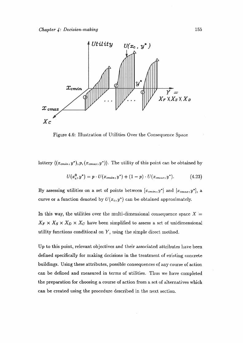
Chapter l: Decision-rnaleing
tctnin
Utility (I(r" , A* )
a
155
rt
tT_XrY,,XsY,Xo
I "root
Xc
Figure 4.6: Illustration of Utilities Over the Consequence Space
lottery ((*o,,rn,U*),p,(*.,no,,y.)). The utility of this point can be obtained by
U("Z,y*) : p.U(xon;ni y.) * (t - p) .(J(n.*o,,,U*). (4.23)
By a^ssessing utilities on a set of points between f*onrnry.] and f*" o,rA*1, a
curve or a function denoted by U(r"ry*) can be obtained approximately.
In this way, the utilities over the multi-dimensional consequence space X :Xp x Xs x Xo x Xc have been simplified to assess a set of unidimensional
utility functions conditional on Y, using the simple direct method.
Up to this point, relevant objectives and their associated attributes have been
defined specifically for making decisions in the treatment of existing concrete
buildings. Using these attributes, possible consequences of any course of action
can be defined and measured in terms of utilities. Thus we have completed
the preparation for choosing a course of action from a set of alternatives which
can be created using the procedure described in the next section.

Chapter l: Decision-making 156
4.5.5 Creating Courses of Action
Although specific courses of action for different problems are not necessarily
the same, the following broad categories cover most of those common courses
of action to be considered in practice (Warner and Kay, 198J):
o do nothing, on the judgement that the structure will be able to satisfyall relevant requirements;
o monitor the structu¡e in service, in order to check more carefully on
adequacy of performance and any deterioration;
o undertake repair or corrective work which maintain the structure in ser-
vrce;
o undertake repair or corrective work after taking it temporarily out ofservrce;
I take the structure out of service with the possibility of demolition and
reconstruction.
Superficially, by modifying and amplifying this list, a set of courses of action
for a particular problem can be identified. Since decision theory is basicallynothing but a tool to aid the decision maker to choose one alternative from a set
of candidates in a rational way, clearly, the set of candidates thus created has tobe complete so that all potential effective courses of action can be considered inmaking the choice. However, the creation of such a complete set of candidates
is not always practical. Each course of action itself is usually not necessarily
an independent entity, and may be divided further into smaller parts. Variouscombinations of these parts can in turn produce a large number of valid courses
of action which will make the decision tree extremely large. Consequently, thedecision analysis becomes too complicated for practical purpose. The set of
Chøpter j: Decisi,on-malcing
remalns.
L57
alternatives therefore has to be kept as small as possible, and at the same time
has to contain all potentially good actions. For convenience, such a set will be
called the effectiae set in this thesis. The procedure described below can be
used a^s a guide to create the effective set of actions in dealing with existing
concrete structures.
Considering an existing building with a set of anomalies identified, possible
methods for remedy are usually determined following the results of diagnosis
and condition evaluation. If the explanations of the observed anomalies are
confirmed, it must be possible to plan appropriate courses of action for the
defects, unless current technology is incapable of doing so. Since the diagnostic
result is represented by a set of hypotheses fI : (Ht,Hr,... ,H^), for each fI¡,the engineer can design a set of relevant courses of action A; which can cure
the defects explained bV f/¡. If we can identify a course of action a¿ from A¿
such that a¡ is the best in A¡ regarding factors such as costs, effectiveness,
availability of materials, ø; could be used as the effective alternative for 11¡.
Suppose we can identify such an effective option for each hypothesis in .[/, then
the effective set is obtained as A: (orror,...,an). Theoretically, there are
n elements in .4 thus created. In this wa¡ the total number of actions to be
considered in the decision analysis is greatly reduced, while the completeness
It has to be mentioned that sometimes an hypothesis may have more than one
effective alternatives. For example, if fli : "bad environmental conditions",
and the observed anomaly is "corrosion of reinforcement", there are two op-
tions available: o¡(l) : "repair immediately", a¡(2): "regular maintenance".
Since it is difficult to compare these two actions by subjective judgement with-
out detailed decision analysis, both ø¡(1) and ø¡(2) have to be considered as
effective options lor H;. Therefore, the creation of the effective set of options
.,4. is closely related to the explanations contained in the hypothesis set I/.

Chapter l: Decision-malei,ng 158
The effective set of alternatives created in this way is d,ynamic in the sense
that ,4 has to be re-generated at each stage of the multi-stage decision-making
process, because the hypothesis set I/ itself is updated regularly. The iterative
nature of the decision-making process will be shown later in section 4.5.7. The
dynamic property of A will improve the efficiency of decision-making, and help
to avoid missing any best course of action in making the final decision.
However, the effective set .4 only contains the kind of actions regarding re-
pair/maintenance activities. Actions of other kinds, such as conduct erper-
iment or wa,it ønd, see, also have to be considered in any rational decision-
making. Such actions can be added to the set A in the multi-stage decision-
making whenever it is necessary, since A is modified at each stage.
After courses of action have been created, it is now possible to choose an
alternative from A through a simple decision analysis.
4.5.6 Single-stage Decision-making
In order to choose an alternative from the effective set of actions A : (ot, azr. - - , an),,
it is necessary to compare the utilities of each course of action. Since utilities
are previously defined on the consequence space, the possible consequences of
every ø; e. A have to be specified first. For this purpose, a decision tree is shown
in Fig. 4.7 in which 11¡ is the iúh hypothesis in fI, and X : Xr x X5 x Xp x Xsrepresents the consequence space. As defined in Section 4.5.2, Xp, Xs, Xpand Xç are attributes regarding structural safety, serviceability, durability
and the total cost respectively. Xr has four possible values: üf 0) : saf e¡
tî(2) : negligibly d,ef ectiue, x¡(3) : modero.tely d,ef ectiue and x¡(4) :seuerely defectiue; Xs has two: ø"(1) - satisf actory, r,(2) : inadequate;
X¿ is measured in terms of the satisfactory period, and has been classified
into c¿(1) = 5 years, ûd(2) : 15 years and od(3) - 20 aears. Finally, Xc is
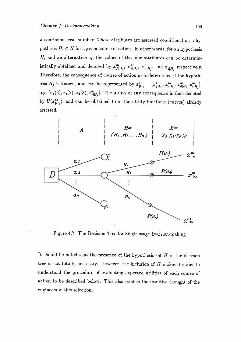
Chapter J: Decísion-making 159
a continuous real number. These attributes are assessed conditional on a hy-
pothesis H¡ € H for a given course of action. In other words, for an hypothesis
Il¡ and an alternative ø;, the values of the four attributes can be determin-
istically obtained and denoted by *ï]¡n,, ,iin,, räjn,, and rii, respectively.
Therefore, the consequence of course of action ø¡ is determined if the hypoth-
esis l/¡ is known, and can be represented by ,ih,: [ri\*,,riin,,r"aiø,,riin,J,e.g. [c¡(3),r"(2),r¿(3), "iir,]. The utility of any consequence is then denoted
Ay U@ih), and can be obtained from the utility functions (curves) already
assessed.
A H--(H,,Hr,...,H,)
XX¡'Xs'Xo'Xc
4nù nl|.a* lt,o.t
Ht@2 Hz 4n') TT-
^aa*ln
Figure 4.7: The Decision Tree for Single-stage Decision-making
It should be noted that the presence of the hypothesis set .FI in the decision
tree is not totally necessary. However, the inclusion of f1 makes it easier to
understand the procedure of evaluating expected utilities of each course ofaction to be described below. This also models the intuitive thought of the
engineers in this selection.
Ø¡ H.
4n.)

Chapter l: Decision-m,aleing 160
Using these notations and from Fig. 4.7, the expected utility of each course of
action can be evaluated easily by:
fau(")-Du({ù,).P(H¡) (4.24)f=1
where the bar "-' denotes the expectation, and P(II¡) is the subjective proba-
bility of the hypothesis I/¡, which can be obtained from the result of diagnosis
in advance. At this stage, the best decision is to choose the course of action
¿* which maximizes the expected utility over ,4., i.e.:
u (".) : iåit lt @,) l (4.25)
The decision thus made has used the expected, aalue criterion. This rule is
used because it is a very meaningful tool in decision-making under risk, and
has been widely accepted in practice. However, due to its shortcomings, some
practical modifications are made to this principle in making the final decision,
and this will be discussed in Sections 4.5.7 and 4.5.8.
It is also to note that the course of action ø* chosen from Eq. 4.25 is lhe best
among .4 only according to the information currently available. Therefore,
it does not necessarily mean that ¿* is the real best action and should be
executed without further consideration. In reality, information can be gathered
in sequence at different stages of the assessment process, and often a good
decision can be made using a multi-stage decision process. This is described
in the next section.
4.5.7 Multi-stage Decision-making
In dealing with existing structures, decision-making is a multi-stage process
in the sense that when new information is available, related diagnosis and
condition evaluation have to be updated, and consequently the choice of a
Chopter f: Decision-maki,ng 161
course of action needs to be reviewed. For this purpose, the procedure for
single-stage decision-making is perfectly suitable for making the choice within
one cycle. However, to decide whether the process should continue or not, a
number of tasks have to be fulfilled at the beginning of each stage.
Firstly, the effective set of alternatives A obtained in the previous stage need
to be updated using the new information available. Secondly, since the effec-
tive set contains the kind of actions only regarding repair and maintenance,
alternatives of other kinds such as "postpone the decision-making, and closely
monitor the structure", have to be added to A. Thirdly, a set of feasible tests
need to be worked out for information-gathering purposes.
With the updated courses of action A and feasible tests ?, a decision usually
ha.s to be made on whether to stop the process by choosing an alternative from
24, using the information currently available or to acquire more information
by conducting an experiment in 1. The problem can be represented by the
decision tree shown in Fig. 4.8 where tt,tz,"',t* are feasible candidates of
tests, and 01, Ozr...,O¡ are possible outcomes of úr. All other symbols have
the same meanings as in Fig. 4.7. Theoretically, the complete decision tree
should include all future stages, and therefore is usually very large as can be
seen from Fig. 4.8. At the itft stage, a best course of action ¿* can be firstly
chosen from A in such a way that the expected utility of ¿* is the largest
arnong all members in A using the information available up to date. If the
expected utility of each test in T : (hrtzr. - ., ú-) is now calculated, and if the
expected utility of the best test ú* is larger than that of c*, then the decision
is to take test ú*. After t* is carried out, a further decision will be made at
the (i + 1)'h stage using the new information resulting from the outcomes of
ú*, and the process continues. If this is the case, the decision made at the irä
stage is referred to as i,ntermeiliate deci,sion. Otherwise, if no such test ú* can
be found, which means ø* is preferred to any test in ?, the decision is to choose
ø', and the decision-making process terminates. Thus ø* is called a terminal

Chøpter /: Decisíon-making L62
decision.
Figure 4.8: A Multi-stage Decision Tree
However, evaluating the expected utility of every test in ? could be very te_dious' Since any combination of different elements in ? can also be valid testcandidates, the number of tests to be considered can be theoretically verylarge, and this makes the above approach impractical. For this ¡eason, in lieuof applying the routine decision-making procedure, a more practical approachis proposed here, in which the decision analyst, i.e. the engineer, subjectivelyselects the next test. Specificalty at the iúÀ stage, the decision analyst startswith calculating the expected utility of only a single test ú¡ which has beenselected from ? based on experience by considering factors such as ,,cost,,,
"usefulness of possible outcomes". If the calculated U(t¡) is greater than thatof a* ', this test is then taken as the intermediate decision without evaluatingexpected utilities of other candidate tests in ?, and the decision-making pro_cess moves to the next stage. Otherwise, it is necessary to select another testand evaluate its expected utility. If all tests in ? have been tried, and the con-dition Ù(t¡) > t(".) is not satisfied, a* may be taken as the terminal decision,
útv¡1
u4n
qàæ
t,
Chapter l: Decision-making 163
and the process stops. This procedure will be called the step-by-step approachin the rest of this thesis.
Since the multi-stage decision tree is usually very large, it is extremely tediousto calculate the expected utility of a test from the entire tree. In the eval-uation of expected utilities in the above step-by-step approach at any stage,
consequences of tests contained in the child-branches in the decision tree aretherefore ignored as a practical measure. For example, in Fig. 4.g, the evalua-tion of expected utilities of any test at the ith stage only considers the part ofthe decision tree ccintained in the dashed square.
Using the step-by-step approach, the best course of action a* at any stage canbe identified from the candidate set A using the information available at thetime, and the decision-making process advances to the next stage if a test ú*
is adopted by the decision maker. The ideal case is that this process continuesuntil sufficient information is gathered so that the true hypothesis fI* can beidentified. In reality however, the information-gathering process may stopmuch earlier if:
1. there is no such test ú* € T whose expected utility is larger thanthat of a* €. Aj or
2. it is impossible to continue the information-gathering process dueto reasons such as financial, political factors; or
3. the decision maker prefers to take a terminating course of actionright now.
If this is the case, the question is then "is it rational to take ¿* as the terminaldecision ?" To answer this question, the risk implied by a* has to be explicitlyestimated. In our problem, the risk involved in a decision is closely relatedto the diagnostic result. If the probability of the most likely hypothesis I/*reaches the acceptable probability value p{*, as defined in section 2.4.g or

Chapter J: Decision-malcing 164
Chapter 2,i.e. P(H.) ) P!"rt, H' can be considered acceptable. Under such
circumstance, other hypotheses in I/ can be ignored with acceptable risk, and
the decision can be made with regard to only I/'. Therefore, by carrying out
the prognosis regarding the structure's future behaviour conditional on .I/* and
ø*, the terminating decision can be determined in the following way:
o if various structural requirements can be satisfied by executing ø*, the
decision is to take ø*, and the multi-stage process terminates; Otherwise,
it is necessary to design a set of feasible courses of action A* which
are specifically suitable for curing problems caused by H*. Because the
situation in this case is decision-making under certainty, the final decision
is to choose action ø* from .,4.* such that ¿* is the cheapest among those
that can meet the relevant structural requirements.
However, if the information at this stage is insufficient to identify such an
acceptable hypothesis I1*, the consequences of o,* can not be obtained withcertainty, and have to be evaluated conditional on all elements in H . Therefore,
the choice of any action will lead to unavoidable risks of bad consequences.
Logically, ø* simply can not be taken as the terminal decision if the involved
risk of catastrophic consequence such as structural collapse is unacceptably
high. On the other hand, if the risk of structural failure is acceptable to the
decision maker, but not acceptable to the public community, a* cart not be
taken as the terminal decision either, because the disastrous consequence willbe faced not only by the o\ryner but also by the engineer and the community.
Therefore, the risk related to ø* regarding the severe consequences has to be
acceptable to all parties involved if ø* is taken as the terminal decision.
In choosing a course of action, consequences of having a dangerous structure
can be very severe, and hence related risk has to be limited. This risk implied
by course of action ø* will be explicitly evaluated and controlled through a
procedure to be proposed in the next section.

Chøpter l: Decisíon-making 165
4.5.8 Risk Control for Making a Terminal Decision
The risk of having a dangerous structure after ø* is taken can be evaluated
with the help of a partial decision-tree shown in Fig. 4.9 (a), in which f{ is the
irä valid hypothesis in I/ at the stage ¿* is obtained r"¡in is the value of safety
attribute X¡ evaluated conditional on H; for course of action ¿*. P(H¡) is
the subjective probability of the hypothesis f/r', obtained from the diagnostic
procedure.
drÍtr, Or
úrÍtrtz\
dlttrt os
(")
tad
(b)
Figure 4.9: Possible Consequences of ø* Regarding Structural Safety
As defined in section 4.5.2, ziþ has four possible values, i.". ,"¡iuQ)søf e, "]inQ) : negligibly def ectiue, x"¡in.(3) : moderately def ectiue and
""¡iuØ) : seuerely def ectiue, which can be assessed from either experi-
ence or the calculated reliability index,6iri,, r.ing the procedure described inSection 3.7.2 of Chapter 3. If we define here that consequences r;þ_(4) -seuerely ilef ectiue and øiþ(3) : moderately def ectiue imply that ,,the
structure is dangerous', these four values can be lumped into two, i.e. Or -""¡in,Ø) u øiix,(3) indicating potential føilure,and 05 : r"¡in,Q) u ïîiHQ)indicating non-failure. In this way, the possible consequences of the course ofaction ø* regarding the safety attribute can be fully represented by the two
outcomes denoted by Oe and Os. This is illustrated in Fig. 4.9 (ó), where p*
is the probability of the outcome Op after ø* is taken, and can be evaluated

Chapter /: Decísion-making 166
byft
P* :Dp@,). F(,]ix,) (4.26)r'=l
in which r@'jin) is a function which takes I when ,]ir, e op, and is 0 ifx"¡iu, e Os. This P' can then be interpreted as uthe subjective probabilitythat the structure will be dangerous according to the current practice,, and
hence represents the risk of a*. It has to be pointed out that P* obtained hereis different from the failure probability defined in structural reliability theory.
Due to the reasons discussed in the last section, this risk P* must be controlledif ø* is to be taken as the terminal decision. For this purpose, an acceptable
value of P* has to be determined. In the diagnosis, the engineer adopts a valueof P!*, to accept a hypothesis. This implies that a risk of \ - plptof makingwrong decisions is acceptable. If there is no other suitable value available, theprobability L - P{*, will be used as the acceptable risk level. In other words,the calculated risk P* has to be not higher than 1 - pf"r, for the terminaldecision.
With P* and r - P!*, thus determined, \rye can now continue the multi-stagedecision-making following the last section. At the stage where further testingis impractical, the risk P* of course of action ø* has to be evaluated first. IfP* < L - P!*r, a' can be taken as the terminal decision, and the decision-making process stops. Otherwise, if the safety requirement is not met by a*, itmeans that none of the actions in the candidate set A is satisfactory to boththe engineer and the owner simultaneously, because ¿* is determined usingthe owner's utilities, and 1 - Pl"pt is specified by the engineer. However, as
mentioned in Section 4.5.5, although set A is representative, it is incomplete.In other words, it is still possible that a course of action ø+ may exist outsideA, which can result in the acceptable risk level and has the expected utility notless than that of ¿*. In fact, in multi-attribute decision-making, it is usuallypossible to keep the utility unchanged by obtaining gains in one attribute andsacrificing in others. Therefore, such an action ø+ might be found by modifying
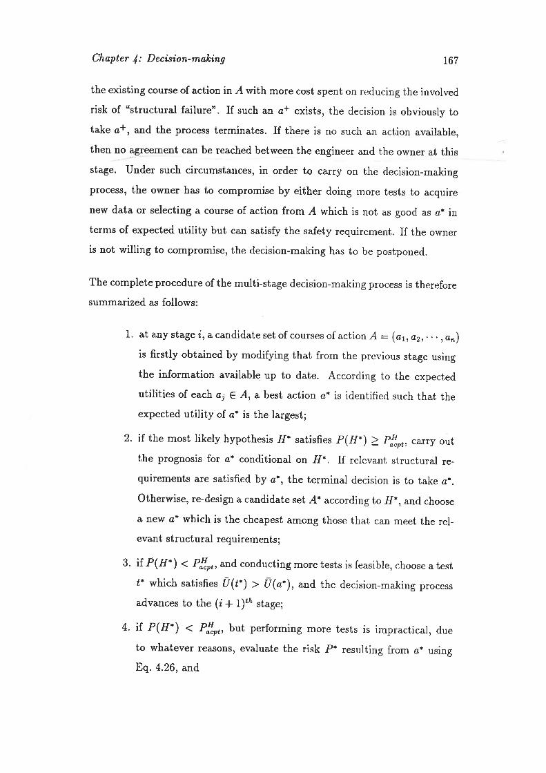
Chapter J: Decision-malcing r67
the existing course of action in A with more cost spent on reducing the involved
risk of ustructural failuren. If such an ø* exists, the decision is obviously totake ø+, and the process terminates. If there is no such an action available,
then no agreement can be reached between the engineer and the owner at thisstage. Under such circumstances, in order to carry on the decision-making
Process' the owner has to compromise by either doing more tests to acquire
new data or selecting a course of action from A which is not as good as ø* interms of expected utility but can satisfy the safety requirement. If the owner
is not willing to compromise, the decision-making has to be postponed.
The complete procedure of the multi-stage decision-making process is therefore
summarized as follows
1. at any stage i, acandidate set of courses of action A: (or,,az,... ,an)is firstly obtained by modifying that from the previous stage using
the information available up to date. According to the expected
utilities of each a¡ € A, a best action ¿* is identified such that theexpected utility of ¿* is the largest;
2. if the most likely hypothesis .Il' satisfies p(H.) Z p{"pt,carry out
the prognosis for ¿* conditional on fI*. If relevant structural re-
quirements are satisfied by ø*, the terminal decision is to take ¿*.
otherwise, re-design a candidate set .4.* according to H*, and choose
a new ø* which is the cheapest among those that can meet the rel-
evant structural requirements;
3. if P(rl.) 1 P{"rr, and conducting more tests is feasible, choose a testl. which satisfies t(t-) > u(o-), and the decision-making process
advances to the (i + 1)t,l stage;
4. if. P(H') < P!*r, but performing more tests is impractical, due
to whatever reasons, evaluate the risk P* resulting from ø* using
Eq. 4.26, and
-)

Chapter l: Decision-møleing 168
(a) if P* < | - P!*r, take ¿* as the terminal decision, and the
process stops;
(b) if P* > | - P!*r, creat a new candidate set A+ by designing
actions which obtain gains in the attribute of "structural safety"
but havelosses in other attributes such as financial cost. Ifthereexists an action a+ e A+ such that the risk implied by ø+ is
not larger than 1 - P!.pt, and U(ø+) > U(o-), the decision is
to take ¿+. If ai can not be found, the terminal decision can
not be made by satisfying both the decision maker's preferences
and the risk control policy. Three possibilities then exist: (i)persuade the owner to adopt a course of action which results in
a satisfactory risk level, at higher cost; (ii) persuade the owner
to conduct further testing, if feasible; (iii) if items i and ii can
not apply, the decision-making has to be postponed.
It can be seen from the procedure that the terminal decision is actually made
using both the expected utility criterion and the risk control policy. This
means that the final course of action is chosen by the o\ryner together with the
engineer, and both of them jointly represent the interests of the community.
4.5.9 A Special Case
In a special case when the consequence space X consists of only the attributes
X¡ (safety) and Xc' (cost), part (b) of step 4 of the multi-stage decision-making
process described in the last section can be further elaborated.
Suppose at stage i, a "best" course of action ¿* has been identified from Ausing the expected utility criterion, but the risk P* is higher than I - P!*r.In order to find out how much the decision maker is willing to sacrifice in the
cost attribute to gain in the safety attribute so that the safety requirement
(t
9.."'c t \
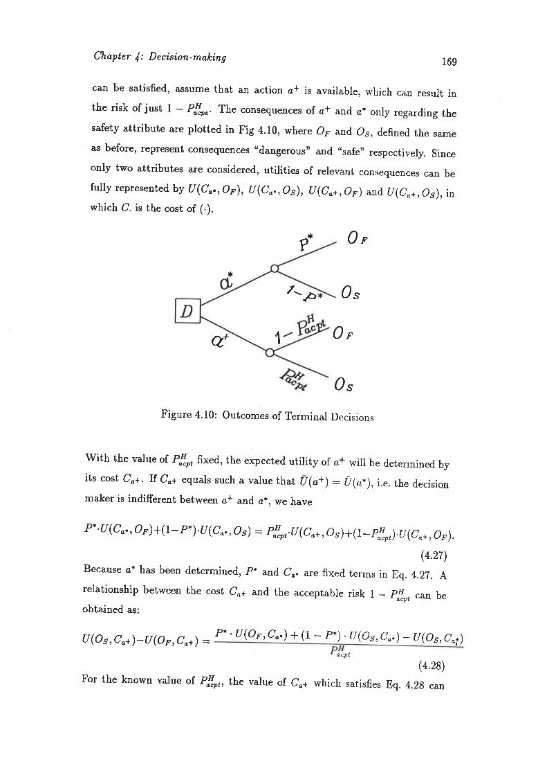
Chapter l: Decision-maleing 169
can be satisfied, assume that an action ø* is available, which can result inthe risk of just t - P!*". The consequences on a+ and ¿* only regarding thesafety attribute are plotted in Fig 4.10, where o¡ and 05, defined the sameas before, represent consequences "dangerous' and. ,,safe" respectively. sinceonly two attributes are considered, utilities of relevant consequences can befully represented by U(C".,Op), U(Co,,Os), U(C,r,Or) and, U(C,+, Os), inwhich C. is the cost of (.).
f 0e
7- Osþ
*
q- Oe1
0sFigure 4.10: Outcomes of Terminal Decisions
with the value of P!*, fixed, the expected utility of ¿+ will be determined byits cost co+. rr. co+ equals such a value that u(a+) : u(o.), i.e. the decisionmaker is indifferent between ø* and ø*, we have
P*' U (C "', O r) + (L - P* )' U (C "., O s) = Pf"pt. U (C "*, Os ) + ( 1 - pl"et).U (C "r, O r).(4.27)
Because ¿* has been determined, p* and c¿, ãî.. fixed te¡ms in Eq. 4.27. Arelationship between the cost Co+ and the acceptable risk I _ p!*, can beobtained as:
U(Os,C"+)-U(Or,Co+) =P- .U(Op,Co.) + (1 - .P. ) 'U(Os,C".) - U(Os,C"i)
acpt
(4.28)For the known value of. P!*r, the value of. Co+ which satisfies Eq. 4.2g can

Chapter l: Decision-making 170
be found according to relevant utility functions. C"+ thus obtained is a very
useful value. In fact, if there is an action ¿+ which can result in a risk not
higher than 1 - P!.p, and is less expensive than C.+, the decision is to take
¿+ without evaluating its expected utility. Therefore, part (b) of step 4 of the
complete procedure in the last section can be modified for this special case as:
. (b) if P. > I - Pf.pt, evaluate the value Co+ from Eq. 4.28. If there exist
a course action ¿* such that the P+ is smaller than 1 - Pl"pt, and the
cost of ¿* is lower than C,+, ø+ is then the terminal decision. Otherwise,
if ø+ is not available, options (i), (ii) and (iii) listed in the last section
apply.
4.6 Some Comments on the Proposed Method
It has to be mentioned that decisions thus made are not strictly optimal,
because the expected utility is evaluated using the information currently avail-
able, and it is impossible to predict the future with certainty. At the ith stage,
if an optimal decision is to be made using the expected utility criterion, the
complete multi-stage decision tree including all possible outcomes of futurestages have to be considered. This seems too tedious because the evaluation
of relevant expected utilities is a formidable task. Even if the calculations can
be made by a computer, it is likely that the errors involved in predicting alarger numbe¡ of probabilities of future outcomes will make the final result
very unreliable.
Alternatively, an optimal decision may be made through an optimization pro-
cedure. In fact, decision-making aims to balance the cost and the risk ofmaking wrong decisions. As illustrated in Fig. 4.11, the reduction of risk can
only be achieved with more financial cost denoted by C1, and the expected cost

Chapter l: Decision-maleing L7L
of accepting the risk, C2, is proportional to the magnitude of the risk itself.
The optimal decision can be made at the risk P,o¿ when the total cosl Ct * Cz
achieves its minimum value. Unfortunately, those relations in Fig 4.11 can not
be evaluated in practice, and hence the approach is only an idealized model
for the time being.
For these reasons, it seems that it is impractical to search for optimal decision
Instead, the practical procedure proposed previously is more useful.
Ct
0 Rísk (hrbøbitítg)Cz
0 Ri^slc (Prr,bo.bilitg)
Ct*Ç2
0 Pq Ri^sk (P,þbo;bility)
Figure 4.11: The Relation Between Cost and Risk
4.7 Summary of This Chapter
A multi-stage process for selecting a relevant course of action for an existing
concrete building has been developed from decision theory using the results

Chøpter f: Decision-malsing 772
of diagnosis and condition evaluation obtained from previous chapters. The
approach is purposefully developed in such a direction that it is practically
applicable, md therefore any probability and mathematics concepts involved
a¡e treated in a simple way.

Chapter 5
The Detailed Process forDealing \Mith DefectiveConcrete Buildings
S.L Introduction
In Chapter 1, an overall process of dealing with existing concrete buildings
ïvas proposed and represented by a flow-chart on page 24. In the chart, es-
sential components including methods for diagnosis, condition evaluation and
decision-making were not available at that time. These methods have been de-
veloped in Chapters 2,3 and 4, and it is the purpose of this chapter to establish
an integrated procedure incorporating the results of those chapters.
173

Chapter 5: The Detøileil Process L74
6.2 The Detailed Process for Dealing WithExisting Defective Buildings
The proposed process is shown in the flow-chart in Fig. 5.1 together with
Fig. 5.2. It is developed from the framework of Fig. 1.4 in Chapter 1, but
contains much more detail. In the chart, the rectangles in solid lines represent
various actions to be executed in the process, and relevant decisions or choices
to be made are included in rhombuses. For convenience, most components of
the chart are numbered.
The process starts with the identification of anomalies through appropriate
means such as site inspection. Information at this stage is then gathered
by means such as interviews with occupants, analysis of inspection results,
searching the design and construction documents.
With the anomalies and information thus obtained, a set of diagnostic hypothe-
ses fI : (HrrHrr..-,H^) can be created using the explanation tree approach
described in Chapter 2. The method for diagnostic reasoning developed in Sec-
tion 2.4.5 can be employed to rank the hypotheses in terms of their subjective
probabilities.
After this, the process goes to step 5 in Fig 5.1 and an immediate decision is
made as to whether urgent action such as eaacuøting the build,ing is needed to
protect the safety of occupants and contents. If the answer is yes, an urgent
action øi is selected, and the process moves to the next step. Otherwise,
the process advances directly to step 6 in Fig. 5.1. The detailed method for
deciding on the necessity of taking action øi is to be described in Section 5.3.
After the initial consideration of urgent action, decisions regarding the struc-
ture's long term future have to be made. For this purpose, the most likely
hypothesis fy'' is identified from the hypothesis set .F/, and its subjective prob-

Chapter 5: The Detailed Process
No
l.es
Yes
Go o"l::"
175
ltes
No
Identíty tÌrz set ol ønnma,IíesS--(Sr,Sr,
2Gøth¿¡ ínþnna,tíon o,tn il,øbtre
3Cnøt/ufi,øte ø set of hyptlwses:Ht.Hz,
4Assess/ufiete lhz pmbo;bítíty ol eonhHt: P(Ht)
trgent o,ctíoztæed,ed ?
Ezecuie eiu
Yes
t2Design ø set ofco¿rses of øctionla øccord,ítr,g to H'
7 't3I)esígnr/ufule cor¿rses ol o,ctínn A--(ø ,et,Idenrífo úlr¿ òesú octinn Oi ønd euølunte
..ø.)ø
Cørty otú,pmgnnsís
I't4select øtt øctiott ø'
fiotn ArÍu)ìe
IDesígn/tzfirrte possible ¿""¿5 7:(tt,tt, "' t¿)Identily f,' s'uch thøt t( t') > Ú( ø* )
Ezecu,teo.'
tt ezisl
,,END
icolly/s iú
Ezecule f,,'
Figure 5.1: The Proposed Detailed Process - PaLt (I)
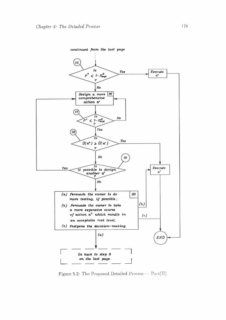
Chapter 5: The Detailed' Process
contitntzd finn tlæ lo,st p.ge
(")
Go bqßk to step 9on tlw lo,st p,ge.
176
Yes
_l
-Jrl_
Figure 5.2: The Proposed Detailed Process - PaLt(II)
Ereculeø'e' 4 t-n!r,
/s
?
t6Design q, rrunlecornVrclænsíae
ontìnn ø+
?u(ø') > t(a¿')
Yes Ezeculeø,*
topossiöleq*q,rwtlur
2
(")
(o) krnnde tlw outnp¡ to d.o
ntpæ testíng, ít pssíble;(b) kæuadz tlv oun¿r to toke
ú flurÍe etpnsiue cotæîseo! ortion ø+ uthi.ch results ìnøtt øcceptable risk leuel;
(c) Æ,stptts tlæ decìsìnn-mø,kíng,
g
ffo
Yes
Yes
END

Chapter 5: The Detailed Process r77
ability is P(fI.). As mentioned in Section 4.5.7,1f P(H-) reaches the value
pLr, H* canbe considered acceptable, and the decision-making can be simply
carried out according to fI*, where P!,o, is determined subjectìvely by the en-
gineer based on his/her experience. Therefore, at step 6, if an hypothesis 11*
is accepted, a set of actions A* cat be determined b1' specifically considering
the implications of H* in regard to the observed anomalies and future struc-
tural performance. To choose the best one from A*, prognosis is carried out to
predict the consequence of each member in A* defined on relevant attributes
such as safety and serviceability. Since only ,ä* is being consiclerecl, according
to our definition, the consequence of each action o,¡ € A* c.a,rt l-ie cleterrninisti-
cally assessed. The decision is then to be made uncler cer-ta,irrty, a,rrcl tlre best
alternative ¿* can be easiiy found in such a way that ø* is the cheapest among
those that can meet the specifled ,..equirements. Fina,lly, tlie process aclvances
to the next step - execution of ø*, and is then complete.
However, if the answer to question No. 6 is no, the choice of an appropriate
course of action has to be made under risk. For this purpose, possible courses of
action A: (atü2¡' ,ø¿) havefirst to be designed. An a,ctiorr r.¿* is identifred
as the one which has the highest expected utility U(".) in A. This means that
if a terminal decision has to be made at this stage, r¿* is the best cancliclate
to the decision-maker concerning all attributes in the consequence space based
on the information available at the time. If new infbrmation is gathered, an
improved decision can be made.
However, acquiring more data is not always feasible even if thele a,,-'e obviously
some promising tests available. Factors such as ytoliti,crr,l 'press'tlre to nt'ake a
terminal deci,sion right now, financi,al difficulties, tLr,e r,trurtr:r'ltrt:Jr:rertce to take
a terminal course of action all can prevent the engineer tÏom ga,thering more
information. Question No. 8 is mainly concerned with these factors. If itis feasible to carry out further testing, a set of candidate tests have to be
identified. These are denoted here by T : (tr,tr,"',ft). A test l* is then

Chapter 5: The Detailed Process 178
subjectively chosen by the engineer from 7 with regai-d to factols such as cost
and importance of the test. Using the routine procedure of clecision analysis,
the expected utility of f ,[J(t*), can be evaluated. If U(t.) > U(o.),1* is the
candidate test to be conducted. If there are no technica,l clifflculties, l* can be
executed, and the process goes back to step 3 in Fig. 5.1. Otherwise, if there
are difficulties which prevent the conduct of f*, a nelv f* has to be ideniified
from ?, and the process returns to step 9. If there is no such test f* € T with
fl(t.) > (1(a"), or if the answer to questions 8 is no, conclucting more tests is
impossible, and the possibility of taking a* as the ternrinal decision has to be
consider-ed. If this is the case, the process switches to the seconcl part of the
flow-chart shown in Fig. 5.2 on page 176.
The risk of ø* regarding the safety issue is now evaluatecl in telms of the
probability P* of having a dangerous structure following action ¿*. If P* is
not larger than the acceptable risk 1 - Pf"pt, the terminal decision is to take
a*, and the process is complete. Otherwise, if a* ca,n not rneet the safety
requirement, a new course of action ø* has to be designecl ì-t1r palzing mels
attention to the safety attribute with more cost. A prognosis is then carried
out, from which the risk of ø+, P+, is obtained. If the conclition P+ < I - Pf"r,
is satisfied, and the expected utility of a+ is greater than that ctT o,*, n* can be
taken as the terminal decision. Otherwise,if.U(a+) > (l(ct'.) is not met, the
re-design of another ¿* is necessary, and the process goes bac.k to step 16.
In a special case where the relevant attributes inclucle the "sa,fettr" (X¡) ancl
the ttcost" (Xç) only, the determination of a suitable r-¿* can l-re carried out
using the procedure described on page 170 in the last chapter'.
However, if there does not exist such an ¿* that satisfies both the safèty
requirement and the expected utility criterion, the process moves to step 20.
This means that although the engineer has tried er¡erything, a,n agreement on
the terminai decision has not been achieved with the clecision lllà,ker) using the

Chapter 5: The Detailed Process t79
information available up to date. In this case, three options ca,n be considered:
(i) if the engineer can persuade the o\Mner to gather more information and let
the terminal decision be made at a later stage, the process Boes l¡a,ck to step 9
in the flow-chart; (ii) if there is no promising test availaì.rle, or iT the decision
maker agrees to compromise by spending more money to ta,ke a satisfactory
action a+ which does not satisfy U(o*) > U(o*), but nevertheless has the
highest expected utility among those that satisfy the safety requirement, the
process terminates after o* is executed; (iii) if no agleenlent can be achieved,
the decision-making has to be postponed, and the process stops at this time.
Obviously the overall process works iteratively, and its lec.ursive nature lLas to
be emphasised. If test f* is selected as an intermediate decision at the itt' cycIe,
further analysis has to be carried out at the (i + 1)tn cvcle according to the
actual outcome of test ¿*. At each cycle, the hypothesis set ,I1 has to be updated
using the procedure given in Chapter 2, and the probabilitv of Ël is r-e-assessed
using the new information available. The courses of action A: (ut,az,"' ,at)and test candidates T: (h,tz,"',1¡) also need to be uptiatecl. The dvnamic
nature of A is an important and indeed essential charactelistic of the proposed
procedure.
Although the process thus described is well structured ancl complehensive, it
appears to be tedious, especially if it has to run through a, large numl:er of
cycles, especially when the number of hypotheses is a,lso large. However, the
intuitive thought processes of an engineer faced with this type of problem are
exceedingly complex, and at least as involved as the logical proceclure described
here. Also, the analysis of each step in the procedure can be simplifled as the
amount of information increases. At the first cycle of analysis the lcnowledge
available is very iimited, and the number of hypotheses ancl coutses of action
may be very large. As the assessment process proceeds, more information is
gathered, and many hypotheses will be eliminated frorn f1, thr-rs sinrplifying
future cycles.
Chapter 5: The Detailed Process 180
The complete process of dealing with existing defective concrete buildings has
now been outlined. In the next section, a procedure is suggested for arrswering
question No. 5 in Fig. 5.1, i.e. how to decide whether urgent action needs to
be taken.
5.3 Taking lJrgent Action
The objective of taking urgent action is to protect the safèt1r of huma,n life ancl
property in case the structure is in danger of immediate collapse. Whether to
adopt such an action or not has to be decided immediately afler the site inspec-
tion and preliminary assessment have been completed. Any relevant analysis
regarding this decision only needs to consider the structure's perlbrmance in
a very short term.
Although any urgent action will have to be ch.osen il rela,tion to the specific
problem, those commonly used in practice will fall into the f'ollorving categories:
. at : evacuate the structure;
. (r2 - restrict the applied load;
o as : provide temporary support or strengthening;
. a+ - provide monitoring and a warning system ìrut keep the building in
SCTVlCE
A relevant choice from a set of actions of this kind carr usually be made based
on the engineer's experience and expertise. For example, if ihe anomaly has
been present for some time and the structure has not rret failed, it may be
concluded from experience that the structure is not likelv to fail in the near

Chapter 5: The Detailed Process 181
future unless circumstances change markedly, and hence no ch'a,stic action is
needed. An experience-based approach is obviously applopliate'
However, if a decision can not be made in this way, ancl the danger of imme-
diate failure is a real concern, a well structured procedure, which can balance
the cost of taking action against the cost of serious consequences, is needed
in order to reduce the chances of making unnecessary mistakes. In the fol-
lowing, a simple approach using decision analysis sirnilal to tha,t in Chapter 4
is proposed. It is aimed at helping the decision makeÏ t,o icleltif¡, ratioilal
choices in complex situations. For this purpose, a ilecisiou tree is shown in
Fig. 5,3, in which ø; is an urgent action from the list on the pt.evious page;
¿o is the action of "doing nothing and keeping the br.rilcling in service"; H¿ is
the ith hypothesis obtained in the preliminary diagnosis, a,ncl P(') clenotes the
probability of (.). The possible consequence is deflnecl a,s a bina,r'y errent, i.e.
failure or non-failure denoT,ed by F and tr' respectivelv. Failur.e is 1ïlthet rep-
resented by ductile fai,lure D and non-ductile fail'ure D. It ltas to be pointed
out that the failure defined here is conceptually diffèr'ent fì'om that used in
Section 4.5.8 of Chapter 4 where failure only indicates an unacceptable risk
level. Failure defined in this section means real structural failure regarding a
particular ultimate limit state in a short term.
The probability P(D) is to be estimated subjectivel), conclitiona,l on F, and
P(Ð) is then I - P(D). The failure probability P(f ) shoulcl l.ie estirnated by
considering only the current loading condition. EitlLer Lrtilities or nonetary
cost can be used to scaie the three consequences denotetl by (ø¿, D), (a¿.,D)
and (a;, F).
With these notations, a routine decision analysis can be ca,'-riecl out to select an
action øi which has the highest expected utility (ol lorvest cost), t.e'. (l(o"i):rnaxu(a¿). I1 a" is chosen, it means no urgent action is neeclecl.
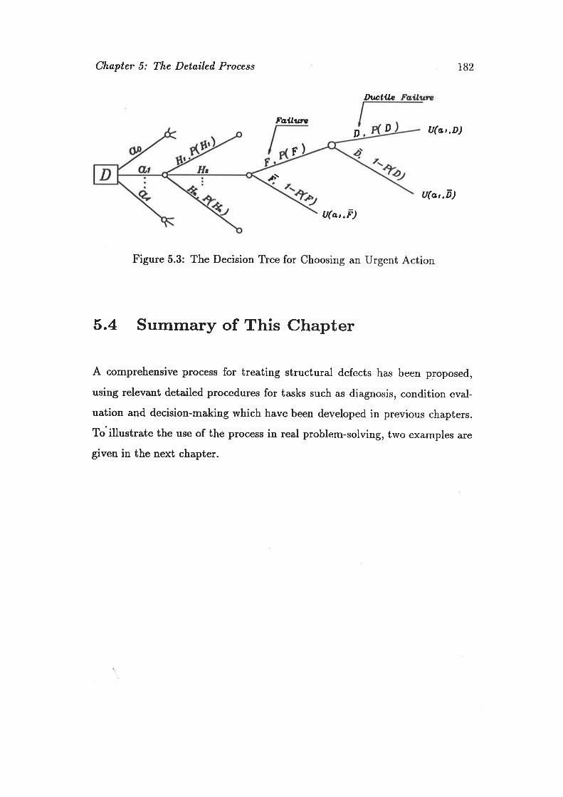
Chapter 5: The Detaileil Process 182
Dtrctil,e
Fqilutz
F
D D U(o,t,D)
â\tl(øt,D)
U(ør,F)
Figure 5.3: The Decision Tree for Choosing an Urgent Action
5.4 Summary of This Chapter
A comprehensive process for treating structural defects has been proposed,
using relevant detailed procedures for tasks such as diagnosis, condition eval-
uation and decision-making which have been developed in previous chapters.
To'illustrate the use of the process in real problem-solving, two examples are
given in the next chapter.
Chapter 6
Examples
6.1 Example 1
In a multi-story building, a permanent sag was found in the reinforced con-
crete slab floor at mid-panel of several panels. Extensive cracks were observed
on first inspection on the underneath surface in mid-panel, and also around
adjacent columns on the top surface. The olrr'ner of the structure was alerted
by concerned occupants, and wanted to know whether there IMas a structural
problem, and what, if any thing, needed to be done.
For this purpose, the procedure proposed in Chapter 5 is applied, and related
details are given in the following sections.
183

Chapter 6: Examples 184
6.1.1 Identification of Anomalies
The cracking pattern \4/as recorded during the site inspection, and is shown
schematically in Fig 6.1. According to our terminology, the observed cracks
and excessive deflection are considered to be anomalies. For convenience, the
cracking on the bottom surface of the slab in the mid-panel is called anomaly
No. l and denoted by ^S1, and the cracks on the top surface around adjacent
columns are referred to as anomaly No. 2, denoted by Sr, while 53 represents
anornaly No. 3 - the deflection. Attributes of 51 to be considered are bn :orientation, bn : time of occurrence,, b13 : appeürance and btn -- roidth.
The same attributes are also considered for ^92. Two attributes are considered
for 53: bzt: time of occurrence and bsz: endurãnce.
colutnn
Vieut Frorn Belout SZøb PLo,n Vieu.t
Figure 6.1: Recorded Crack Pattern
6.L.2 Available Information
From relevant sources, it was known that the building was 4 years old, and
the concrete floors were cast in-situ. According to the appearance of the ob-
Sr
rucfts
conctete süøb
Ct.o,cks
Sz
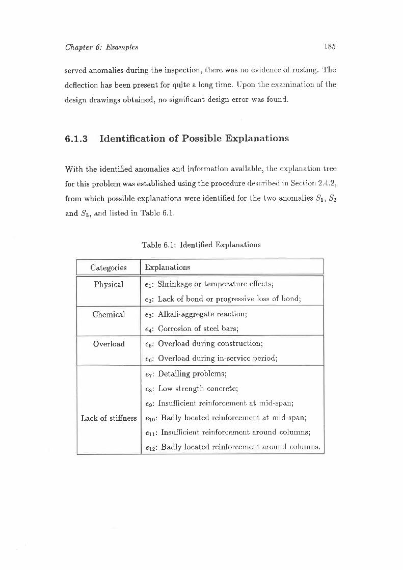
Chapter 6: Examples 185
served anomalies during the inspection, there was no evidence of rusting. The
deflection has been present for quite a long time. Upon the examination of the
design drawings obtained, no significant design error \¡¡as found.
6.1.3 Identification of Possible Explanations
\Mith the identified anomalies and information available, the explanation tree
for this problem was established using the procedure described in Section2.4.2,
from which possible explanations were identified for the two anomalies ,51, ,52
and 53, and listed in Table 6.1.
Table 6.1: Identified Explanations
Categories Explanations
Physical er: Shrinkage or temperature effects;
e2: Lack of bond or progressive loss of bond;
Chemical es: Alkali-aggregate reaction;
e4: Corrosion of steel bars;
Overload e5: Overload during construction;
e6: Overload during in-service period;
Lack of stiffness
e7: Detailing problems;
es: Low strength concrete;
ee: InsufÊcient reinforcement at micl-span;
e1s: Badly located reinforcement at mid-span;
e11: Insufficient reinforcement around columns;
e12: Badly located reinforcement around columns

Chapter 6: Eramples 186
6.L.4 Creating the Hypothesis Set H
The explanation tree is shown in Fig. 6.2, in which ei represents the ith ex-
planation, ,S; denotes the i¿h anomaly, and ó¿¡ is the jrh attribute of the ità
anomaly; and the directed lines indicate the causal relations between explana-
tions and relevant anomalies. From the information obtained so far, attributes
bn,bzt (orientatiot), br¡, ó23 (appearance), and ó32 (deflection endurance) are
known, and represented by shaded ellipses.
\/\/ \/
Figure 6.2: Explanation Tree of Example 1
It is obvious that the candidate set Hc ofhypotheses consists of single-explanation
elements flrc = êt¡ Hî : €2,¡ Hl : "", Hl : €4¡ H? : €s,¡ Hg
.c, Hl : €8r two-explanation elements such as H3 : e7es, H$ : €T€to¡ "'and multi-explanation elements like €1€2€s, €s€6€7,"'. It is too tedious to
list the complete set of f16r because of its large number of possible elements.
However, as mentioned in Section2.4.4, the hypothesis set H e Hc only com-
prises those promising members, and temporarily excludes the elements which
are not very likely to be true, according to the information currently avail-
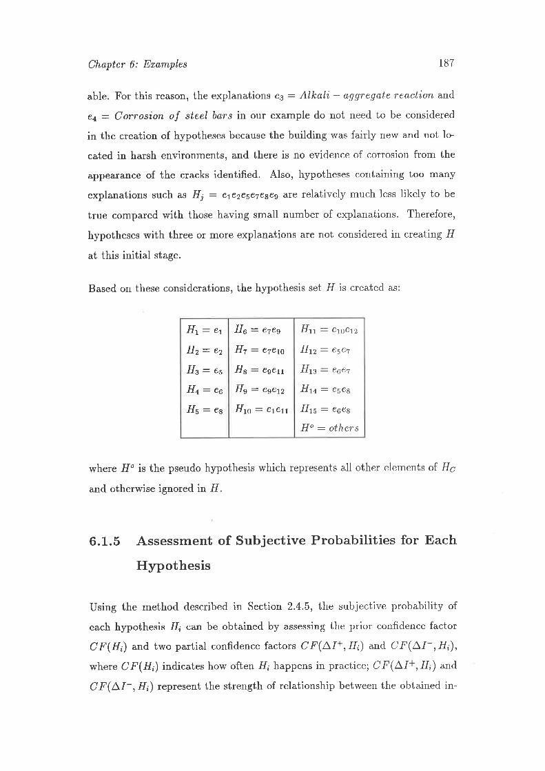
Chapter 6: Eramples 187
able. For this reason, the explanations ee: Alleali - aggregate reaction and
e+ : C orrosion of steel ó¿rs in our example do not need to be considered
in the creation of hypotheses because the building was fairly new and not Io-
cated in harsh environments, and there is no evidence of corrosion from the
appearance of the cracks identified. Also, hypotheses containing too many
explanations such as H¡ : ere2esel€s€e ilre relatively much less likely to be
true compared with those having small number of explanations. Therefore,
hypotheses with three or more explanations are not considered in creating fIat this initial stage.
Based on these considerations, the hypothesis set ff is created as
Ht- et
Hz- ez
Hz- es
Hq: ea
Hs- ee
Ha: ezes
H7: e7e1s
Ha: €s€tt
Hg: egetz
Hro: €t€rt
Ht - €to€tz
H12: eseT
Hts: eaez
Hta: ese¿
Hts: eaes
Ho : others
where f/' is the pseudo hypothesis which represents all other elements of. Hc
and otherwise ignored in H.
6.L.5 Assessment of Subjective Probabilities for Each
Hypothesis
Using the method described in Section 2.4.5, the subjective probabìlity of
each hypothesis H¿ can be obtained by assessing the prior confldence factor
CF(H¿) and two partial confidence factors CF(LI+,,fI;) and CF(A'I-,H;),,
where C F(H) indicates how often fI¿ happens in practice; C F(LI+,14) .nd
C F(LI-,f1,;) represent the strength of relationship between the obtained in-
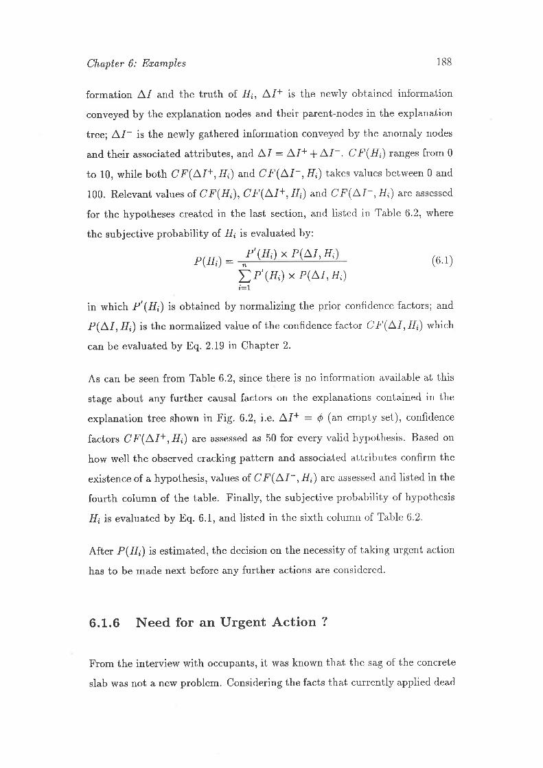
Chapter 6: Eramples 188
formation A.I and the truth of H;, A.I+ is the newly obtained information
conveyed by the explanation nodes and their parent-nodes in the explanation
tree; A.I- is the ne\^/ly gathered information conveyed by the anomaly nodes
and their associated attributes, and A1 : A1+ + A1-' C F(Ht) ranges from 0
to 10, while both C-F( LI+, Hi) and CF(A I- , H¿) takes values between 0 and
100. Relevant values of. C F(H¿), C F(LI+, fl) and C F(LI-,11,;) ar" assessed
for the hypotheses created in the last section, and listed in Table 6,2, where
the subjective probability of H¿ is evaluated by:
P(Hi): P'(H¿) x P(LI, Hi(6.1)
I n' (ø,) x P(LI, Hi),i=1
in which P'(Hr) is obtained by normalizing the prior confidence factors; and
P(LI,f4) is the normalized value of the confidence factor C F(LI,11') which
can be evaluated by Eq. 2.19 in Chapter 2.
As can be seen from Table6.2, since there is no information available at this
stage about any further causal factors on the explanations contained in the
explanation tree shown in Fig. 6.2, i.e. A1+ - d (ut empty set), confidence
factors C F(LI+, H¿) are assessed as 50 for every valid hypothesis. Based on
how well the observed cracking pattern and associated attributes confirm the
existence of a hypothesis, values of. C F(L,I- , H¿) are assessed and listed in the
fourth column of the table. Finally, the subjective probability of hypothesis
ll¿ is evaluated by Eq. 6.1, and listed in the sixth column of Table 6.2.
After P(H;) is estimated, the decision on the necessity of taking urgent actron
has to be made next before any further actions are consiclered,
6.L.6 Need for an Urgent Action ?
From the interview with occupants, it was known that the sag of the concrete
slab was not a new problem. Considering the facts that currently applied dead
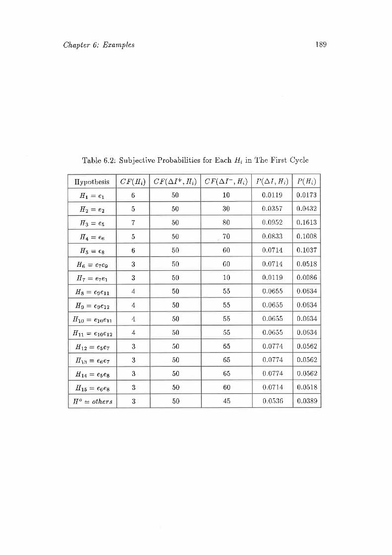
Chapter 6: Eramples
Table 6.2: Subjective Probabilities for Each H¡ in The First Cycle
189
Hypothesis c F(tti) C F(A,I+, H¿) c F(a,I- , H;) P(LI, H¿) P(H;)
Ht- et 6 50 10 0.0119 0.0173
Hz=e2 5 50 30 0.0357 0.0432
Hz- es 7 50 80 0,0952 0.1613
Ha Qa .5 50 70 0.0833 0.1008
Hs=eB 6 50 60 0.07L4 0.1037
He = ezÊs 3 50 60 0.0714 0.0518
Hz : ezet 3 50 10 0.0119 0.0086
Hs - ese11 4 50 ÐÐ 0.0655 0.0634
Hg = ege12 4 50 55 0.0655 0.0634
Hto = €roêtt 4 50 55 0.0655 0.0634
Htt: etoet2 4 50 55 0.0655 0.0634
Htz = esez 3 50 65 0.0774 0.0562
Htz = eaez 3 50 65 0.0774 0.0562
H14: e5eg 3 50 65 0.077 4 0.0562
Htí = €6ea 3 50 60 0.0714 0.0518
Ho = others 3 50 45 0.0536 0.0389
Chapter 6: Eramples 190
and live loads were not large in comparison with the design load, and the sag
was not getting worse, it was suggested that no urgent action was needed,
but the applied load must be kept no higher than the current level. This
decision was also supported by the fact that, in the hypotheses obtained above,
the three top ranked hypotheses -it13 : Ouerloading during construction,,
Ha - Ouerloading during in seruice period and fls : Lou strength concrete
were not likely to result in catastrophic consequences in the short term if there
is no sudden increase of applied loads.
6.L.7 Conducting More Tests ?
At this stage, since the highest ranked hypothesis ä¡ has only the probability
of 0.161, which is far lower than a reasonable acceptable value (say 0.85), it is
too early to make a final diagnostic conclusion. Therefore, a decision has to be
made on whether to do more tests or to take an appropriate course of action
regarding the hypotheses. For this purpose, if following the proposed process
described in Chapter 5, a set of actions A : (otr&2¡', ør,) have to be decided
on, and the best action ¿* chosen from A using the expected uiility criterion.
Any test ú to be conducted has to satisfy the condition of U(t) > U(o.), where
[/ denotes the expected utility. Among the following feasible tests:
o 11: search for information on loading during construction and in service
period;
. t2 caruy out relevant structural analysis to calculate the deflection;
o ú3: detect locations and quantities of steel bars using appropriate devices;
. ¿4: remove small regions of concrete to observe the steel reinforcement;
o f5: take core samples of concrete to test for compressive strength;
Please note: sections 6.1.7, 6.r.g and 6.1.9 are superseded by relevant sectionsspecified in the Amendment at the back of this thesis.

Chapter 6: Eramples 191
o f6: conduct non-destructive tests to estimate compressive strength of
concrete,
tests f1 and ú6 should cost only a very limited amount of money, and therefore
is almost certain to have expected utility larger than [/(ø*), provided it can be
done within a reasonable short period of time, and hence the cost of delay can
be ignored. For this reason, ú1 and f6 can be executed at this stage without
identifying ø* and evaluating the expected utility U(".).
After these tests are carried out, the process goes back to the procedure of
diagnosis.
6.1.8 The Second Cycle of Diagnosis
During the information search, it was confirmed by interview and knowledge
from other sources that the cracking had already appeared when the construc-
tion was completed, and no excessive live loads were experienced during the
4-year service period. Also, from the construction documents, it was found
that excessive loading r¡/as very likely applied mistakenly cluring the construc-
tion before the concrete reached its designed strength. Also, from the non-
destructive test, it was found that the concrete was in good condition, and the
compressive strength was acceptable.
Using this information, the probabilities of hypotheses fI obtained in the first
cycle of diagnosis can now be updated. According to the reasoning procedure,
the time of fi,rst o,ppe&rance of cracking is the value of the attributes b12,b22 of
the anomalies ^9r and ^92 respectively, and hence constitutes A1-. The result
of non-destructive test belongs to A1+. All other information is about the
causal factors of explanation nodes, (refer Fig. 6.2) and should be denoted by
A1+. Confidence factors C F(LI- ,, Ht), C F(LI+, Hn) are accordingly assessed,
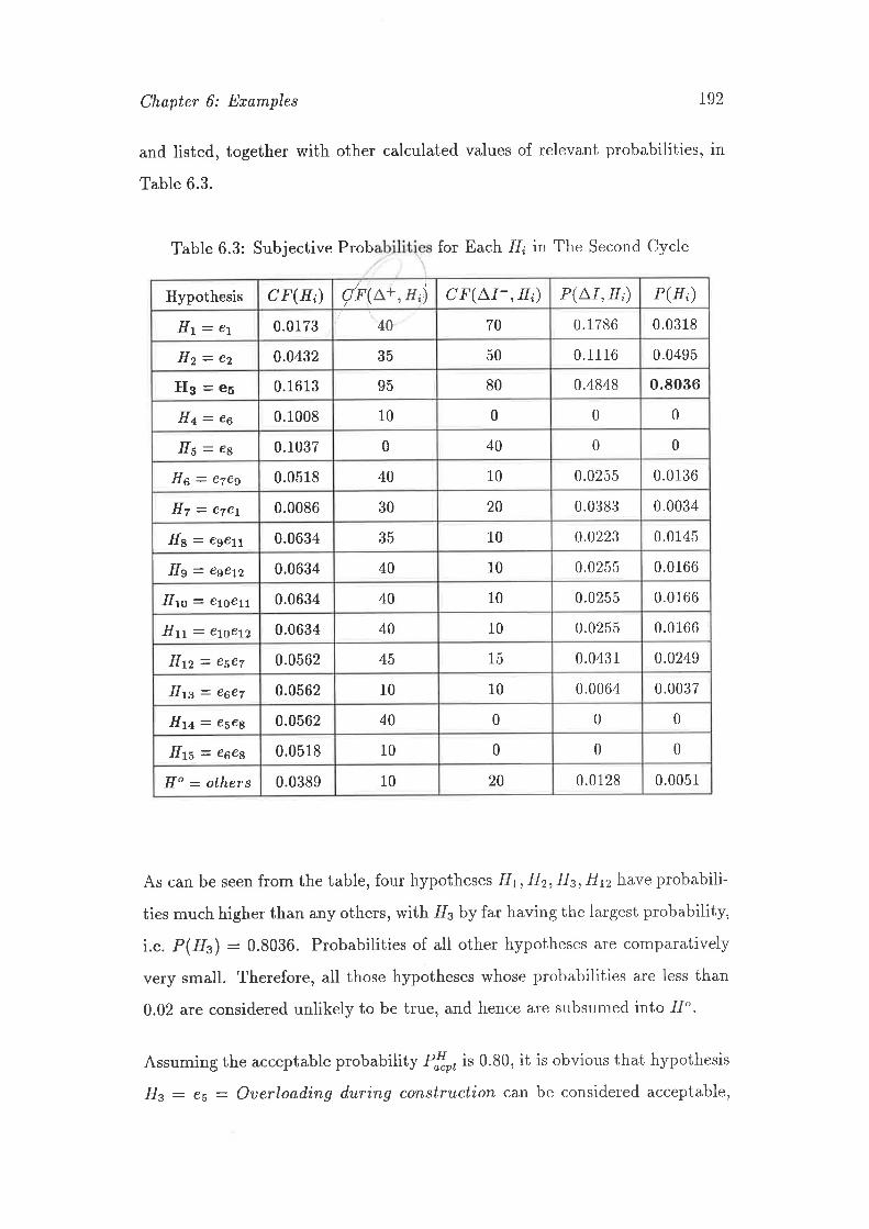
Chapter 6: Examples r92
and listed, together with other calculated values of relevant probabilities, in
Table 6.3.
Table 6.3: Subjective Prob for Each H¡ rn The Second Cycle
As can be seen from the table, four hypotheses Ht, Hz, Hs, Hn have probabili-
ties much higher than any others, with fI¡ by far having the largest probability,
i.e. P(ff3) - 0.8036. Probabilities of all other hypotheses are comparatively
very small. Therefore, all those hypotheses whose probabilities are less than
0.02 are considered unlikely to be true, and hence are subsumed into 11'.
Assuming the acceptable probability P!"rris 0.80, it is obvious that hypothesis
Hs - es : Ouerloading during construction carr be considered acceptable,
cF(LI-,H;) P(LI, Hi) P(H¿)c F(Hi) q'rrO*,Hr)Hypothesis
70 0.1786 0.03180.0173 40Ht: et
0.1116 0.04950.0432 35 50H2=ez0.4848 0.80360.1613 95 80Hg=es
0 00.1008 10 0H¿- ea
40 0 0H6: ea 0.1037 0
0.013640 10 0.0255He -- ezes 0.0518
0.003430 20 0.0383H7 = ezet 0.0086
10 0.0223 0.01450.0634 35He = egett
0.016610 0.0255Hg = eseLz 0.0634 40
0.016640 10 0.0255Hn -- etoêt¡ 0.0634
10 0.0255 0.01660.0634 40Hr.: etoeLz
0.024945 15 0.0431Htz = esez 0.0562
0.003710 10 0.0064Htz: eseT 0.0562
0 0 00.0562 40Hta: ese|
10 0 0 0Hts = esee 0.0518
0.005110 20 0.0128Ho : others 0.0389
Chøpter 6: Exømples 193
and the diagnosis is completed. According to the flow-chart shown in Fig. 5.1
of Chapter 5, the process of treating structural defects can then advance from
step 6 directly to step L2, i.e. the design of a relevant course of action with
regard to explanations contained in fls.
6.1.9 The Final Decision
Three courses of action are considered in this case:
o d,1:ds nothing;
. a2:tepair the cracks using relevant epoxy resin;
o d3:i¡1ç¡ease the stiffness by ep.oxy-bonded steel plate.
Since there are no safety and durability problems, the choice among the avail-
able actions is quite simple and mainly dependent upon the owner's demand for
serviceability behaviour ¿ùs well as financial situation. tl1 w&s finally adopted
as the terminal decision.
6.2 Example 2
A State Government Department is responsible for the management of its stock
of highway bridges. Inclined cracking has been identified in 16 T-beam concrete
bridges since October 1990. In fear of structural failure without warning, two
of these bridges have already been replaced. Due to the limited funding, a value
management study has been carried out in order to determine a cost-effectivé
strategy for the management of the existing bridges. The proposed process
described in Chapter 5 was employed for the assessment of the conditions of

Chapter 6: Eramples 194
individual bridges and for the repair procedures (Hua, McGee and Warner,
1ee3).
In order to be applicable to this particular bridge problem, the flow-chart of
Fig. 1.4 on page 24 was modified to the one shown below in Fig. 6.3. Although
the approach has been developed in this thesis for concrete buildings, the
application to bridges shows that the procedures are very useful and practical
and, potentiall¡ applicable to a wide range of problems.
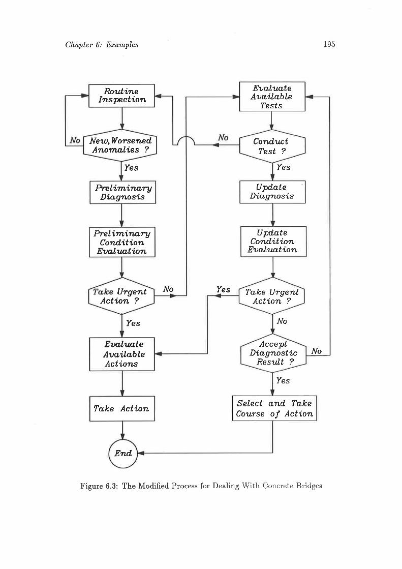
Chapter 6: Enamples
Yes
195
Rotú,ineInspection
EuøLtto,teAuailøbIe
lnesf s
Neut,lïorsenedAtwmnlies ?
ConduntTest ?
UpdøteDiøgnosis
helinilzo.ryDiøgrtosis
Updø.teCondition
EaaIuø.tion
helirnirldryCond.ition
EaøIuntion
)zes
NoUrgentAction ?
Talce UrgentAction ?
)zes
Yes
Yes
No
.À/oEaq,lltÃ,teAuo,iløbIeActions
DiagnosticResul.t ?
Accept
Select ønd TøkeCourse oJ ActionTølce Action
Erld
Figure 6.3: The Modified Process for Dealing With Concrete Bridges

Chapter 7
Summary and Fbture Work
7.L Summary
In this thesis, an attempt has been made to establish a practically useful
approach for dealing with existing concrete buildings from the academic re-
search ,"tçøóhpoint of view. For this purpose, a number of methodologies are,'-developed for diagnosis, condition evaluation and decision-making which are
essential to the treatment of structural defects. By integrating systematically
the metho ds f9øet{er, a detailed process has been proposed, which is capa-
ble of solving real problems in a well organized manner, and can be adopted
by engineers a͡ a guide in practice. The usefulness of the process has been
demonstrated by examples.
196

Chapter 7: Summary and, Future Worle 197
7.L.L The Method of Diagnosis
The proposed method for diagnosis is an hypothesis-and,-tesúprocedure through
which the most likety explanations of observed anomalies can be identified. An
hypothesis is the set of explanations that can fully cover the observed pattern
of anomalies. Relevant hypotheses are firstly generated from an explanation
tree constructed using observed anomalies and their associated attributes as
well ¿s other information obtained in the condition survey. An informal prob-
abilistic reasoning procedure is then employed to rank the hypotheses in terms
of subjective probabilities. If the probability of the most likely hypothesis 11.
reaches a pre-defined value P{"et, l/* is considered acceptable, and the diag-
nosis stops. Otherwise, gathering more information through testing has to
be considered. Since the diagnostic results are used by other procedures to
evaluate the structural condition and eventually to choose a course of action,
the necessity of conducting more tests and the strategy of test selection are
determined in a comprehensive decision-making procedure. Thus the diagno-
sis is closely related to other procedures in the whole process of dealing with
structural defects.
7.L.2 The Method of Condition Evaluation
Condition evaluation of existing concrete buildings defined in this thesis con-
sists of procedures for the assessment of structural adequacy regarding safety,
serviceability and durability. For a specific hypothesis obtained from the diag-
nosis, the safety index B of. an interested ultimate limit state concerning the real
physical state of the structure at the time of aɡsessment can be evaluated us-
ing structural reliability theory. The structure's safety condition is accordingly
assessed to the status of ttsafet', ttnegligibly defective", t'moderately defective"
and *severely defective' varying with the value of B.
Cha,pter 7: Summary and Future Work 198
Experience-ba"sed approaches are employed for the assessment of serviceability
and durability conditions. Using the proposed procedure, the assessment can
be carried out in a well-organized manner.
7.L.3 The Method of Decision-making
To plan appropriate repair and maintenance strategies for an existing struc-
ture, a set of courses of action are firstlyi worked out by considering the effects
of the explanations of the observed anomalies. Possible consequences of each
option are defined in terms of the financial cost incurred and the structure's
status regarding safety, serviceability and durability after the action is exe-
cuted. Before adequate information is gathered, each alternative may have
several possible consequences with different probabilities of being true. After
consequences â,re scaled by utility values, the best action is chosen by compar-
ing alternatives according to their expected utilities. The procedure forms a
multi-stage process in which the choice can be made at any stage using the
information available at the time. Refined decisions are made at the next stage
if new data are gathered.
7.L.4 The Complete Process
The complete process of dealing with existing concrete buildings is obtained
by assembling the proposed procedures for diagnosis, condition evaluation and
decision-making. The process begins with a set of observed anomalies, and
ends with a terminal decision regarding corrective work. When applied to real
problems, the process usually results in a number of intermediate decisions such
as conducting more tests before it terminates. The process works iteratively
so that new information available at each stage i, "ffi.i"nì! utilizJd in making
choices. Since major factors regarding various structural requirements as well
Chapter 7: Summøry and Future Worlc 199
as financial cost are jointly considerád from both the engineer and the owner's)
point of view, the final decision resulting from the process is rational and
acceptable.
7.2 Concluding Remarks and Future 'Work
With the rapid expansion of the stock of concrete structures, it is expected
that more and more attention will have to be paid to the maintenance and
treatment of existing structures. Although there exist various experience-based
approaches established by engineers in practice, this thesis h?,! inlroduced
what are thought to be new systematic methodologies. This was found to
be necessary because of the lack of previous analytic research in this field.
Although the methods have been proposed for concrete buildings, they should
also be applicable quite generally.
To continue the research, time-dependent anomalies need further study. Dura-
bility problems caused by these anomalies usually dominate the treatment of
structures exposed to harsh environments. With the wide application of com-
puters, it is possible to build computerized expert systems (Levine et. a\,1987)
to aid engineers in dealing with durability problems which need experience and
expertise. This should prove to be a fruitful development area in the near fu-
ture.
Appendix A
Statistical Data on Basic
Variables
,A'.1 Introduction
Variations in the common basic variables involved in structural design such as
properties of concrete and reinforcement need to be represented by probability
distributions in reliability analysis. These distributions are usually obtained
from test data available together with professional judgements, and reflect the
current practice of concrete engineering. There are plenty of data reported in
the literature for this purpose, and relevant distributions of material properties
and dimensions are summarised in this section. However, the data presented
here are mainly from probabilistic studies of concrete structures by a number of
authors in North America, and hence its applicability to other areas is subject
to further refinement.
200

Appendix A 20r
A.2 Statistical Properties on Concrete Strength
In a Monte Carlo study of reinforced concrete beam column interactions con-
ducted by Ellingwood (1977), the compressive strength of concrete /" is mod-
elled by normal distributions with the means and coefficients of variation
(COV) listed in Table 4.1 for different workmanships of the concrete, where
¡j is the nominal design value of concrete strength specified in relevant codes.
Table 4.1: Data on Concrete Strength
variable fnean cov
r" Lr6r:good average poor
0.10 0.15 0.25
A comprehensive study of the variation in concrete properties v¡as conducted
by Mirza et ø1. (L979b) based on a large amount of test data collected from
various sources. It was pointed out that the strength of concrete in a structure
tends to be somewhat lower than the strength of control cylinders molded from
the same concrete, due to the differences in size and shape, and the effects of
different stress conditions in the structure and specimens. The following equa-
tion is given to estimate the mean 28-day strength of concrete for minimum
acceptable curing:
f st¡2e: 0.675f: + 1100 < L.l1fl psi (4.1)
where ¡j is the nominal design value. However, the in-situ strength of concrete
is also affected by the differences in volumes of material under stress and the
rate of loading. To allow for these effects, a probabilistic model of concrete
strength was constructed as:
f. - f'.rç2ry (A'2)
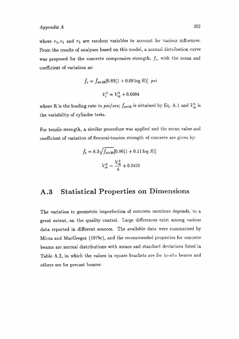
Appendtu A 202
where 11, 12 and l"3 ôr€ random variables to account for various influences.
From the results of analyses based on this model, a normal distribution curve
$¡as proposed for the concrete compressive stren8th, ,f", with the mean and
coefficient of variation as:
f " : f "t,ze[0.89(1 + o.oS log Æ)] psi
V.':Vâ+0.0084
where R is the loading rate in psif sec;.f",,r, it obtained by Eq. A'1 and Vlu is
the variability of cylinder tests.
For tensile strength, a similar procedure was applied and the mean value and
coefficient of variation of flexural-tension strength of concrete are given by:
f, :83\Ñ8[0.96(1 + o.11log rB)]
y2 -v& *o.o42l,n- +
| v.vzsr
4.3 Statistical Properties on Dimensions
The variation in geometric imperfection of concrete members depends, to a
great extent, on the quality control. Large differences exist among various
data reported in different sources. The available data \ryere summarised by
Mirza and MacGregor (1979c), and the recommended properties for concrete
beams are normal distributions with means and standard deviations listed in
Table 4.2, in which the values in square brackets are for in-situ beams and
others are for precast beams:
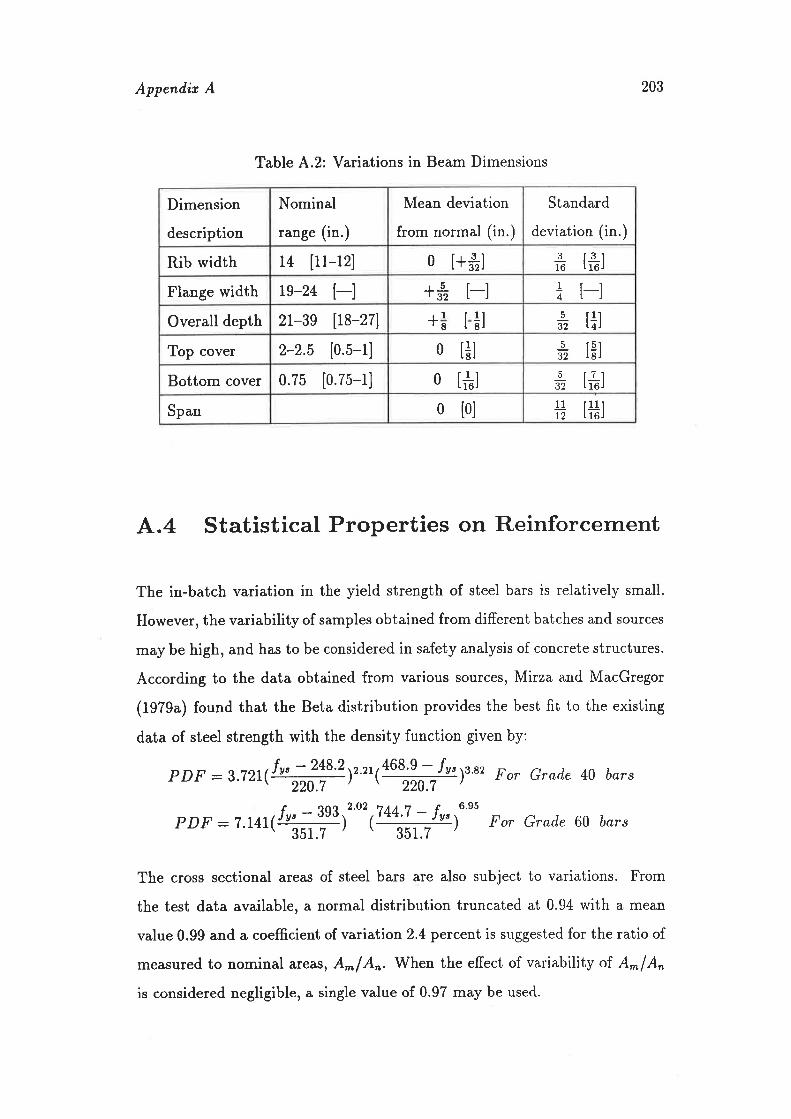
Append,ir A 203
Table 4.2: Variations in Beam Dimensions
Dimension
description
Nominal
range (in.)
Mean deviation
from normal (in.)
Standard
deviation (in.)
Rib width 14 [11-12] o t+#l 3 13 r
16 trol
Flange width rs-24 t-l +å t-l å r-lOverall depth 21-3e [18-27] + I
I ål5 flì32 LaJ
Top cover 2-2.5 [0.5-1] 0 tåj5 fsr32 lsJ
Bottom cover 0.75 [0.75-1] 0 [*!] 5 17132 Lrol
Span 0 [0]11 f11ttz L toj
^.4 Statistical Properties on Reinforcement
The in-batch variation in the yield strength of steel bars is relatively small.
However, the variability of samples obtained from different batches and sources
may be high, and has to be considered in safety analysis of concrete structures.
According to the data obtained from various sources, Mirza and MacGregor
(1979a) found that the Beta distribution provides the best fit to the existing
data of steel strength with the density function given by:
pDF :s.721é5#.¡r"'ça68;f,:-lu')r* Fo, Grad.e 40 bars
pDF _r.t+t(1u"..,,1!lr2'o2 rT44:!__-_Ív")u'nt Fo" Grad.e 60 bars-\ 351.7 / \ 351.7 ',
The cross sectional areas of steel bars are also subject to variations. From
the test data available, a normal distribution truncated at 0.94 with a mean
value 0.99 and a coefficient of variation2.4 percent is suggested for the ratio of
measured to nominal areas, A^lA^. When the efect of variability of. A*f A*
is considered negligible, a single value of 0.97 may be used.
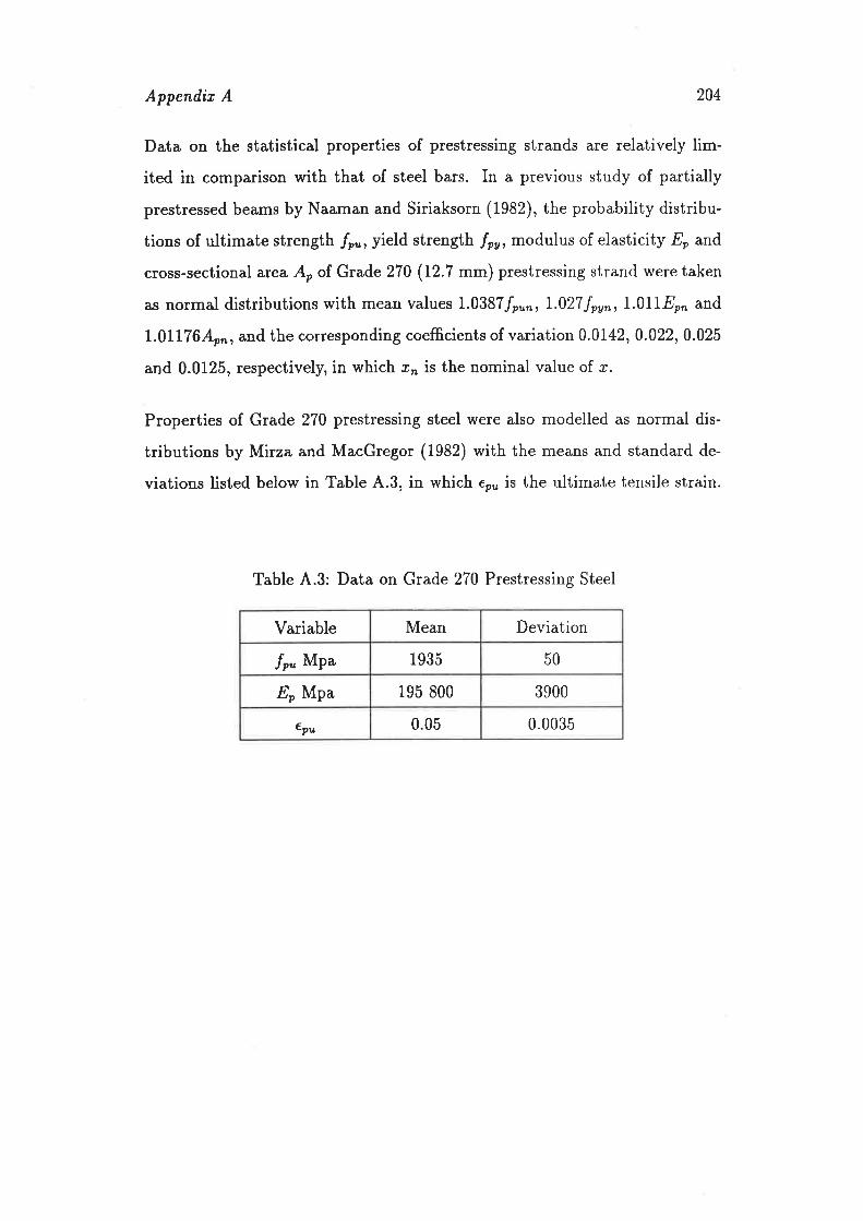
Appendtu A 204
Data on the statistical properties of prestressing strands are relatively lim-
ited in comparison with that of steel bars. In a previous study of partially
prestressed beams by Naaman and Siriaksorn (1982), the probability distribu-
tions of ultimate strength /p", yield strength /o' modulus of elasticity Eo and
cross-sectional area Ao of Grade 270 (I2.7 mm) prestressing strand were taken
as normal distributions with mean values I.0387fp.",I.027 fpy^, 1.0118o, and
I.0lI76Ap,,, and the corresponding coefficients of variation 0.0142, 0.022,0.025
and 0.0125, respectively, in which ø," is the nominal value of r.
Properties of Grade 270 prestressing steel were also modelled as normal dis-
tributions by Mirza and MacGregor (1982) with the means and standard de-
viations listed below in Table 4.3, in which er,, is the ultimate tensile strain.
Table 4.3: Data on Grade 270 Prestressing Steel
Variable Mean Deviation
,fp' MPa 1935 50
Eo Mpa 195 800 3900
epu 0.05 0.0035
Appendix B
Probabilistic Models forBuildittg Live Loads
B.L Introduction
Applied loads on structures usually consist of dead and live loads. Live load
contributes in a major way to the uncertainty involved in structural analysis,
while the dead load has relatively smaller variations and could be assessed with
satisfactory accuracy in many cases. In this section, only the office building
live load will be discussed.
Live loads in buildings consist of sustained and extraordinary (or tran-
sient) components. The former represents the load due to the weight of things
like desks, bookcases, which remain relatively constant for a long period. The
latter represents short-term effects caused by events like gatherings of people
and furniture storage.
205
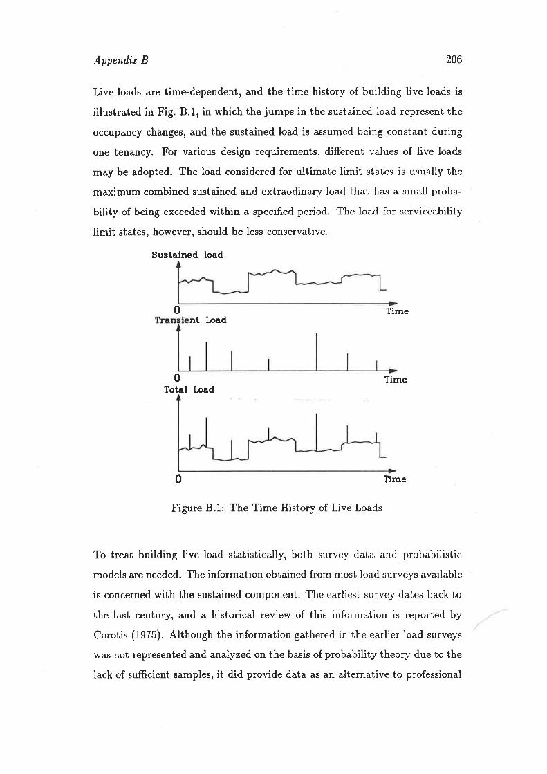
Appendir B 206
Live loads are time-dependent, and the time history of building live loads is
illustrated in Fig. B.1, in which the jumps in the sustained load represent the
occupancy changes, and the sustained load is assumed being constant during
one tenancy. For various design requirements, different values of live loads
may be adopted. The load considered for ultimate limit states is usually the
maximum combined sustained and extraodinary load that has a small proba-
bility of being exceeded within a specified period. The load for serviceability
limit states, however, should be less conservative.
Sustained load
Timent lpad
0
0Total load
Time
Time
Figure B.1: The Time History of Live Loads
To treat building live load statistically, both survey data and probabilistic
models are needed. The information obtained from most load surveys available
is concerned with the sustained component. The earliest survey dates back to
the last centur¡ and a historical review of this information is reported by
Corotis (1975). Although the information gathered in the earlier load surveys
was not represented and analyzed on the basis of probability theory due to the
lack of sufficient samples, it did provide data as an alternative to professional
0

Appendir B 207
judgement for load code committees to work with. On the other hand, itwas recognized from those surveys that the live load intensity in buildings
decreases with increasing tributary area. This important feature of live load
is now considered by many load committees in the world. In parallel with
developments in structural reliability theory, extensive load survey data have
been reported in the past decades (Dunharn, 1952; Mitchell et al. I97I; Culver,
1976), and statistical models have also been developed (Corotis, 1977).
Because the extraordinary component of live loads is due to unusual actions,
it is difficult to collect experimental data. A possible approach is to develop a
reasonable probabilistic model with the parameters estimated from judgement,
together with limited data available.
In the following, probabilistic models currently available (Peir and Cornell,
1973; McGuire and Cornell, 1974) for floor live loads in office buildings are
presented, which has been used in developing design load specifications in
different countries (Ellingwood et a1.,1980; Pham and Dayeh, 1986)'
8.2 Probabilistic Models for Sustained Live
Load
When concerning the sustained floor live loads, two aspects have to be consid-
ered. One is spatial correlation which reflects the dependence between loadings
at two different locations at the same point in time; Another is the temporal
correlation which reflects the dependence between loadings at the same loca-
tion at two difrerent points in time. Unfortunately, it is difficult to cletermine
these two correlations quantitatively from existing survey data, and statistical
models for live loads have generally been chosen from a prior considerations by
judgement. In the model proposed by Peir and Cornell (1973), the live load is

Append,ir B 208
represented in terms of load effect which is the structural response produced
by the load acting on it other than nominal load, which is the sum of all loads
on the floor. For analysis purposes, the terms unit load and equivalent uni-
formly distributed load (EUDL) are introduced. The former ¡efers to the
nominal load divided by floor area. The latter equals the load efect divided
by the integral over the influence surface, and this is the uniform load intensity
which would produce the same load effect if applied over the appropriate floor
area. The influence surface introduced here is the shape of a function whose
ordinate at any point (r,V) is the load effect of interest which would be caused
by a unit load applied at that point.
The load intensity at point (r,V) on the floor of a building at an arbitrary
point in time is expressed as:
W(r,U):m*tr+þ*e(x,y) (8.1)
in which rn :the mean value of all unit live loads; 1t :a zero-mean random
variable representing the deviation from m due to different buildings; .yz :azero-mean random variable accounting for the variation of different floors in
a building from rn * h; ,@,y) : ø stochastic process with nonzero spatial
correlation, i.e. Coule(rrryt),e(rz,Vz)l f 0, representing the variation of load
intensity oû a given floor at different points.
With u(x,y) determined, the unit load U and the EUDL load on area.4./ can
be obtained by:
U_ I Ï;',W(x,Y)drdY (B.2)
EUDL _
AtI I ¿,, I (r, v)W (x, y)dxdy
(8.3)D D¡, I(x,y)dxdy
in which I(r,V) is the coordinate of the influence surface
The properties of EUDL has to be determined from load survey data. Consid-
ering the live load acting on a influence area A¡ with load intensity W(r,,y),,

Appendh B
the total load effect is
209
(B.6)
(B 7)
L(A,) : I l^, I (a,y)W (n,y)d,zd,y
The mean and variance of. L(A¡) can be determined from stochastic theory:
EIL(Aù): ! I^,1(r,y)Elw(x,,y))dxdy (8.4)
v arlL(A¡)l : I I ̂, I I o,
I (r, v) I (xt, v)c oulw (*, v),w (' r, v )ld'r d'v dn fi'v 1
(8.5)
The mean and variance of EUDL are then:
EIEU DLl : EIL=(!t)l'V
varlEtJDn =@!ùr- v?
in which Vr is the volume under the influence surface
The above model was further simplified by McGuire and Cornell (1974) for
practical application. Firstly, the arbitrary point in timeload intensilyW(x,y)
is modified and represented bY
W(r,U):m*l * rþ,y) (8.8)
in which rn is the mean sustained load; 7 is a mean-zero random variable;
,(*,y) is a spatially varying random process. Secondly, it is assumed that the
correlation between the values of e (c, y) for two points is zero if the points are
separated by any finite distance. The mean and variance of EUDL can then
be simplified as:
EIEUDLI-w (B.e)
VørlEuDLl:o'+*x (B.10)¿'At
where ø2:variance from mi At- influence atea; o! and K are experimental
constants.
The preceding derivation of first and second-order moments does not depend
on any form of probability distributions. Based on the study of Corotis (1977),
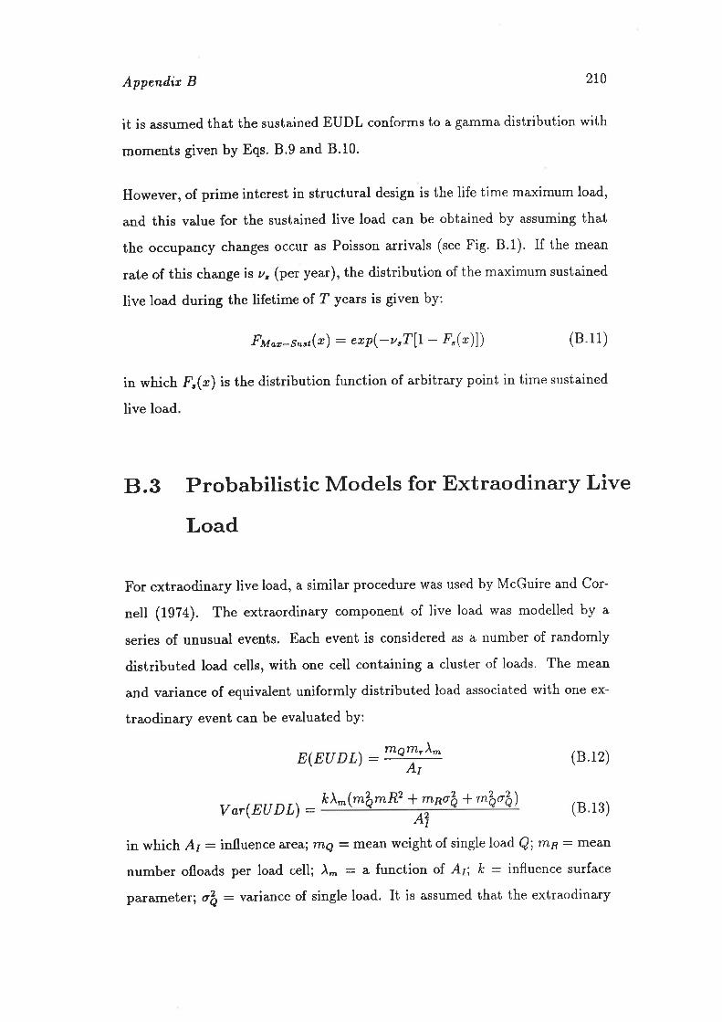
Append,iz B 210
it is assumed that the sustained EUDL conforms to a gamma distribution with
moments given by Eqs. B.9 and B.l0'
However, of prime interest in structural design is the life time maximum load,
and this value for the sustained live load can be obtained by assuming that
the occupancy changes occur as Poisson arrivals (see Fig. B'1)' If the mean
rate of this change is z" (per year), the distribution of the maximum sustained
live load during the lifetime of ? years is given by:
FM o,- su"t(r) : erP(- v "TlL - ¡"(")] ) (8.11)
in which F"(*) is the distribution function of arbitrary point in time sustained
live load
8.3 Probabilistic Models for Extraodinary Live
Load
For extraodinary live load, a similar procedure was used by McGuire and Cor-
nell (1974). The extraordinary component of live load was modelled by a
series of unusual events. Each event is considered as a number of randomly
distributed load cells, with one cell containing a cluster of loads. The mean
and variance of equivalent uniformly distributed load associated with one ex-
traodinary event can be evaluated by:
E(EUDL):OP (8.12)
Var(EUDL): k\^(mþ mR2 +mno2o+mþo'zo) (8.13)A,,
in which At : influence area; rng : mean weight of single load Q; TrL¡': mean
number ofloads per load cell; À- : a function of At; k : influence surface
parameter i oA : variance of single load. It is assumed that the extraodinary
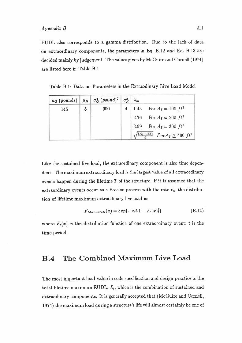
Appendir B 2IT
EUDL also corresponds to a gamma distribution. Due to the lack of data
on extraordinary components, the parameters in Eq. B.12 and Eq' 8.13 are
decided mainly by judgement. The values given by McGuire and Cornell (19i4)
are listed here in Table 8.1
Table B.1: Data on Paramete¡s in the Extraodinary Live Load Model
pq (pounds) ltn o2q (pound)2 o2p À-
145 5 900 4 1.43
2.76
3.99
For A¡ : L00 f*For A¡ :200 ft2For A¡ :300 f*
ForA¡ ) 400 r*
Like the sustained live load, the extra.ordinary component is also time depen-
dent. The maximum extraordinary load is the largest value of all extraordinary
events happen during the lifetime T of the structure. If it is assumed that the
extraordinary events occur as a Possion process with the rate ù., the distribu-
tion of lifetime maximum extraodinary live load is:
FMat-Eot¡(r) : exp{- u"tfr - a(")] } (8.14)
where F"(r) is the distribution function of one extraordinary event; ú is the
time period.
8.4 The Combined Maximum Live Load
The most important load value in code specification and design practice is the
total lifetime maximum EUDL, .[¡, which is the combination of sustained and
extraodinary components. It is generally accepted that (McGuire and Cornell,
1974) the maximum load during a structure's life will almost certainly be one of

Appenilíx B 2r2
the two canies or modes. The first mode is the maximum sustained load during
the structure's life plus the largest extraodinary event which occurs during the
random duration of this maximum sustained load. The second mode is the
largest extraodinary event during the structure's life plus the sustained load
acting at this (arbitrary) point of time.
Based on the first mode, the maximum total EUDL, Lr, was evaluated, and
the results were fitted to a Type I extreme value distribution with the following
properties (Ellingwood and Culver, 1977):
ElL,l: 18.7 - #n psf (B.15)
Vørll¿l : r4.2+ 18900 (ns f\2 (8.16)' A' \r"r )
where the influence area A¡ is different from the traditional tribut ary area 47,,
e.E. At - 2Ar for a beam, 4Ar for columns, and panel area for two-way slabs.

Bibliography
[1] Aboobucker, C. M. M., Majid, W. M. and Mohd Noh, M' S. (1989)
"Investigation of Cracking in Building At Shan Alam," Proceedings, In-
ternational Conference on Case Histories in Structural Failures - CHSF
89, 20-22 March 1989' Singapore.
[2] ACI Committee 503, (1978) "Standard specification for Repairing con-
crete'With Epoxy Mortars," ACI Journø( September 1978.
[3] Adams, E. W. and Fagot, R. F. (1959) "A Model of Riskless Choice,"
Behau. ,Sci., Vol. 4,1954, pp.1-10.
[4] Adtassnig, K.-P. (1982a) "A Survey on Medical Diagnosis and Fuzzy
Subsets," Approúmate Reasoning in Decision Analysis, Edited by M.
M. Gupta and E. Sanchez, North-Holland Publishing Company, 1982.
[5] Adlassnig, K.-P. and Kolarz, G. (1982b) "CADIAG-2: Computer-
Assisted Medical Diagnosis Using Ftzzy Subsets," Approrimate Rea-
soníng in Decision Analysis, Edited by M. M. Gupta and E' Sanchez,
North-Holland Publishing Company, 1982.
[6] Agbabian, M. S., Masri, S. F., Traina, M.-I. and Waqfi, O. (1990) "De-
tection of Structural Changes In A Bridge Model," Bridge Eaaluation,
Repair and Rehabilítati'on, Edited by A. S. Nowak, Kluwer Academic
Publishers, 1990.
2r3
Bibliography 214
[7] Ahlskog, J. J. (1990) "Bridge Management - The Answer To The Chal-
lenge," Briilge Eraluati,on, Repøir and Rehabilitation, Edited by A. S.
Nowak, Kluwer Academic Publishers, 1990.
[8] Allen, D. E. (1970) "Probabilistic Study of Reinforced Concrete in Bend-
ing," ACI Journal, Proceedings Vol. 67, No. 12, Dec. 1970.
[9] Andersen, E. Y. (1989) "Re-Evaluation of Structural Load Carrying
Capacity,n Durability of Structures, IABSE Symposium, Lisbon, 1989,
IABSE Report, YoI. 57 12.
[10] Andersen, N. H. (1990) .DANBRO - A Bridge Management System
For Many Levels," Brídge Eaaluation, Repair and Rehabilitation, Edited
by A. S. Nowak, Kluwer Academic Publishers, 1990.
[11] Andreassen, S., Woldbye, M., Falck, B. and Andersen, S. K. (1987)
'MUNIN - A Causal Probabilistic Network for Interpretation of Elec-
tromyographic Findin gs," Proceedi,ngs ol L}th International Joint Con-
ference on Artificial Intelligence, Milan, August 23-28, 1987.
[12] Ang, A. H-S and Cornell, C. A. (1974) "Reliability Bases of Structural
Safety and Design,n Journal of the Structural Diuision, ASCE, Vo1.100,
No. ST9, Sep., 1974.
[13] Arafah, A. M. and Nowak, A. S. (1986) "Sensitivity Analysis for Human
Errors,n Moileling Human Errors in Structural Design and Construction,
Edited by A. S. Nowak, Proceedings of a workshop sponsored by the
National Science Foundation, Ann Arbor, Michigan, June 4-6, 1986.
[14] ASCE,, (1972) "Structural Safety - A Literature Review," Task Commit-
tee on Structural Safety, Journal oJ Structural Diaision, ASCE, Vol. 98,
sT 4, 1972.
Bibliography 2r5
[15] ASCE, (1991) Guideline for Structural Condition Assessment of Erist-
ing Buílilings, ASCE 11-90, Published by the American society of civil
Engineers, New York, 1991.
[16] Baldwin, J. F. (1981) "Fuzzy Logic and Fuzzy Reasoning," Fuzzy Reo-
soning anil lts Applications, Edited by E. H. Mamdani and B' R' Gaines,
Acdemic Press 1981.
[17] Barlow, R. E. and Lambert, H. E. (1975) "Introduction to Fault Tree
Analysis," Reliability anil Fault Tree Analysis, Edited by Barlow, R. E.,
Fussell, J. B. and Singpurwalla, N. D., Published by Society for Industrial
and Applied Mathematics, 1975.
[1g] Beard, A. s. and Tung, H. s. s. (1988) "The Investigation and Proposed
Rehabilitation of the Tsing Yi South Bridge, Hong Kong," Canadian
Journal of Ciuil Engineering, Vol. 15' 1988.
[19] Ben-Bassat, M. (1980a) "Multimembership and Multiperspective Clas-
sification: Introduction, Application, and a Bayesian Model," IEEE
Transa,ctions on Systerns, Man, and Cybernetics, Vol. SMC-10, No. 6,
June 1980.
[20] Ben-Bassat, M. et øl (1980b) "Pattern-Based Interactive Diagnosis of
Multiple Disorders: The MEDAS System," IEEE Transactions on Pat-
tern Analysis and Machine Intelligence, Vol. PAMI-2, No. 2, March 1980.
[21] Benjamin, J. R. and Cornell, c. A. (1970) Probability, statistics and
Decision for Ciail Engineers, McGraw-Hill Book Company, 1970.
[22] Betaque, N. E. and Gorry, G. A. (1977) "Automating Judgemental
Decision-Making for a Serious Medical Problem," Modern Decision Anal-
ysis, Edited by Kaufman, G. M. and Thomas, H., Penguin Books, 1977.
Bibliography 2t6
[23] Blakey, F. A. (1989) "Managing the Maintenance of Australia's In-
frastructu re rn Proceeilings of N atio nal infrastra cture C o nf erence ) Perth,
Australia, 10-14 April, 1989.
[2a] Blockle¡ D. I. (1975) "Predicting the Likelihood of Structural Acci-
dents,,' Proceed,ings of The Institution of Ciail Engineers, Part 2, Decm-
ber 1975.
[25] Borges, J. F. and Castanheta, M. (1971) Structural Safety, Lisbon,
March 1971.
[26] Bosshard, w. (1979) "structural safety - A lwatter of Decision and
Control," IABSE Suraeys,, 5-9/79' May 1979.
[27] Bradley, J. V. (1976) Probability; Decision; Statistics, Prentice-Hall,Inc.,
1976.
[28] Brøndum-Nielsen, T. (1978) "Epoxy Resin Repair of Cracked Concrete
Beams,n Report No.89, 1978, Structural Research Laboratory, Technical
University of Denmark.
[29] Brown, C. B. (1979) "A Fuzzy Safety Measure," Journal of the Engi-
neering Mechanics Diuision, ASCE, Vol. 105, No. EM5, October 1979.
[30] Casas, J. R. and Aparicio, A. C. (1990) "Dynamic Testing of Bridges
Using Trafic-Induced Vibration," Briilge Eualuation, Repair and Reha-
bilitation, Edited by A. s. Nowak, Kluwer Academic Publishers, 1990.
[31] Chung, H. W. (1991) "Repair Strategy - A Prognosis of Repairing con-
crete Structure Damaged by Steel Corrosion," Ciuil Engineering Trans-
øctions, Vol. CE33, No. 4, December 1991, The Institute of Engineers,
Australia.
[32] CIRIA (1977) "Ratioanlisation of Safety and Serviceability Factors rn
Structural Codes," CIRIA Report 63, U. K. 1977.

Bibliogrøphy 2r7
[33] Cornell, C. A. (1969) "Structural Safety Specifications Based on Second
Moment Reliability Analysis," Final Publication, IABSE Symposiurn on
Concepts of Søfety and Methods of Design, Sept., 1969, London.
[34] Corotis, R. B. (1975) "Building Floor Load Surveys and Stochastic Anal-
ysis,n Proceeilings, Applications of Statistics and Probability in Soil and
Structurøl Engineering, 2d International Conference, l5¿å-18tå Sept.
1975, In Aachen, F. R. Germany.
[35] Corotis, R. B. (1977) " Probability Models for Live Load Survey Re-
sults,' Journal of the Structural Diaision, ASCE, Vol.103, No. 5T6, June
1977.
[36] Croce, S. (1986) "Proposal Regarding The Development of Fault-trees,"
CIB Report, 1986, W861217.
[37] Culver, C. (1976) "Survey Results of Fire Loads and Live Loads in Build-
ings,n Buililing Scíence Series 85, U. S. Department of Commerce, Na-
tional Bureau of Standards, May 1976.
[38] Dandy, G. C. and Warner, R. F. (1989) Planning and Design of Engi-
neering Systems, London, Unwin Hyman,1989.
[39] Davis, R. (1984) "Diagnostic Reasoning Based on Structure and Be-
haviour,n Artif,ci,al Intelli,gence, Vol. 24,, 1984, pp.347-410.
[a0] de Brito, J., Branco, F., Batista, A. R. and Cachadinha, M. G. (1989)
"Assessment of Existing Structures for Their Rehabilitation," Durabil-
ity of Structures, IABSE Symposium, Lisbon, 1989, IABSE Reports,
YoI. 5712.
[a1] de Kleer, J. (1986) "Problem Solving with the ATMS,' Artif,cial Intel-
Iigence,, 28 (1986), pp.I97-224.
[a2] de Kleer, J. and Williams, B. C. (1987) uDiagnosing Multiple Faults,"
Artifi,ci,al Intellig ence, 32 (L987), pp.97-l 30.

Bibliography 218
[a3] Diamantidis, D. (1987) uReliability Assessment of Existing Structures,'
Engineering Structures, Vol. 9, July 1987.
[44] Ditlevsen, O. (1980) "Formal and Real Structural Safety - Influence of
Gross Errors, ' IABSE Perioilica 4/1980.
[45] Domon, K. and Tezuka, M. (1989) "Repair and Countermeasures in Con-
crete Structures Due to Alkali Aggregate Reaction," Proccedings, Inter-
nati,onal Conference on Case Histories in Structural Failures - CHSF 89,
20-22 March 1989, Singapore.
[46] Dubois, D. and Prade, H. (1980) Fuzzy Sets and Systems: Theory anil
Applicøtions, Academic Press, New York, 1980.
[a7] Duda, R. O., Hart, P. E. and Nilsson, N. J. (1976) "Subjective Bayesian
Methods for Rule-based Inference Systemsr' National Cornputer Confer-
ence, AFIPS Conference Proceedings, Vol. 45, 1976.
[a8] Dunham, J. W. and Thompson, G. N. (1952) "Live Loads on Floors in
Buildings," Buililing Materials and Structures Report 133, United States
Department of Commerce, National Bureau of Standards, Decmber 1952.
[49] Eckenrode, R. T. (1965) "Weighting Multiple Criteria," Management
Science, Vol. 12, November, 1965, pp.180-192.
[50] Eckles, J. E. (1968) "Optimum Maintenance With Incomplete Informa-
tion,n Operations Research, Vol. 16, 1968, pp. 1058-1067.
[51] E[ingwood, B. (1977) "Statistical Analysis of Reinforced Concrete Beam
Column Interactions," Journal of Structural Diaision, ASCE, VoI.103,
No. ST7, 1977.
[52] Ellingwood, B. and Culver, C. (1977) " Analysis of Live Loads in OfÊce
Buildings," Journal of the Structural Diuision, ASCE, Vo1.103, No. ST8,
Aug. 1977.
Bibliography 2r9
[53] Ellingwood, 8., Theodore, V. G., MacGregor, J. G. and Cornell, C. A.
(1980) "Development of a Probability-based Load Criterion for American
National Standard 458,'NBS Specíal Publication 577,V. S. Department
of Commerce/National Bureau of Standards, June 1980.
[54] Esogbue, A. O. and Elder, R. C. (1980) "Frzzy Sets and the Modelling of
Physician Decision Processes, Part II: Frzzy Diagnosis Decision Models,"
Fuzzy Sets anil Systems 3 (1980).
[55] Farquhar, P. H. (1977) "A Survey of Multiattribute Utility Theory and
Applicatiotsr" TIMS Stuilies i'n the Management Sciences, Vol. 6, North-
Holland Publishing Company, 1977.
[56] Fishburn, P. C. (1964) Decision and Value Theory, J' Wiley, New York,
1964.
[57] Fishburn, P. C. (1965) "Independence in Utility Theory With Whole
Product Sets," Operations Research, Vol. 13, 1965, pp.28-45.
[58] Fishburn, P. C. (1966) "A Note on Recent Development in Additive
Utility Thoeries For Multiple Factor Situations," Operations Research,
Vol. 14, 1966, pp.1143-1148.
[59] Fishburn, P. C. (1967) "Methods of Estimating Additive Utilities," Me,n-
agement Science, Vol. 13, A, 1967, pp.435-453.
[60] Flesch, R. G. and Kernbichler, K. (1990) "A Dynamic Method for The
Safety Inspection of Large Prestressed Bridges," Bridge Eualuation, Re-
paír anil RehabilítationrEdited by A. S. Nowak, Kluwer Academic Pub-
lishers, 1990.
[61] Folayan, J. I., Hoeg, K. and Benjamin, J. R. (1970) "Decision Theory to
Settlement Predictious,," Jou,rnal of the Soil Mechanics and Foundations
Diaisíon, ASCE, Vol.96, No, SM4, July' 1970' pp.1127-1141'

Bibliography 220
[62] Freudenthal, A. M. (1956) "Safety and the Probability of Structural
Failure," Transøctions, ASCE, VoI.121, 1956, pp.1358'
[63] Freudenthal, A. M., Garrelts, J. M. and Shinozuka, M. (1966) "The
Analysis of Structural Safety," Journal of the Structural Diuision, ASCE,
Vol.92, No. ST1, Feb., 1966.
[6a] Fujino, Y. and Lind, N. c. (1977) "Proof-Load Factors and Reliability,n
Journal of Structural Engineering Diuisron, ASCE, Vol. 103, No. ST4,
April 1977.
[65] Ginsberg, A. S. and Offensend, F. L. (1968) "Att Application of Decision
Theory to a Medical Diagnosis - Treatment Problem," IEEE Transac'
tions on Systems Scí,ence and Cybernetícs,Yol. ssc-4, No. 3, Sept. 1968,
pp.355-363.
[66] Grant, L. H., Mirza, S. A. and MacGregor, J. G. (1978) "Monte Carlo
Study of Strength of Concrete Columns,' ACI Journal, Proceed'ings Vol.
75, No.8, Aug. 1978.
[67] Gulikers, J. (1989) "Infl.uence of Local Repairs on Corrosion of Steel
Reinforcement," Durabilíty of Structures, IABSE Symposium, Lisbon
1989.
[68] Gupta, M. M.,Saridis, G. N. and Gaines, B. R. (1977) Fuzzy Automats,
anil Decision Processes, Elsevier North-Holland New Yok, 1977.
[69] Gupta, M. M. and Sanchez,E. (Eds.) (1982) Approrimate Reasoníng in
Decisíon Analysis, North-Holland Publishing Company, 1982.
[70] Hadipriono, F. C. and Lin, C. S. (1986) "Errors in Construction," Model-
ing Hurnøn Errors in Structural Design anil Construction, Edited by A.
S. Nowak, Proceedings of a workshop sponsored by the National Science
Foundation, Ann Arbor, Michigan, June 4-6, 1986.
Bibliogrophy 221
[71] Hadipriono, F. C. and Toh, H.-S. (1989) "Modified Fault-tree Analysis
for Structural Safety," Ciuil Engineering Systems, Vol.6, No.4, 1989,
pp.190-199.
[72] Ha[,W. B. (1988) *Reliability of service-Proven structures," Journal of
StructurøI Engineering, ASCE, Vol. 114, No. 3, March 1988.
[73] Hampton, J. M., Moore, P.G., and Thomæ, H. (1973) "Subjective Prob-
ability and Its Measurement," Journal of the Royal Statistical Society,
Series A, Vol. 136, 1973, pp.2I-42.
[74] Hart, G. C. and Yao, J. T. P. (1977) "System Identification in Structural
Dynamics," Journal of Engingeering Mechanics Diuision, ASCE, L977,
v 103, EM6.
[75] Hart, G. C. (1981) "Damage Evaluation using Probability Indices,"
ProbabíIistic Methods in Structural Engineering,Eàited by M. Shinozuka
and J. T. P. Yao, Proceedings of the symposium on Probabilistic Meth-
ods in Structural Engineering, St. Louis, Missouri, October 1981, Pub-
lished by ASCE.
[76] Hartog, P. (1989) "Building Diagnostics - Making Choices Amongst Al-
ternatives In The Face of Uncertainty,," Buililing Failures and Forensics,
Proceedings of BSFA Seminar, 15 March, 1989. Published by Building
Science Forum of Australia, New South Wales Division.
[77] Hasofer, A. M. and Lind, N. c. (1974) "Exact and Invariant second-
Moment Code Format,' Journal of the Engineering Mechanics Diuision,
ASCE, Vol.l00, No. EMl, Feb., 1974.
[78] Hewlett, P. C. and Morgan, J.G.D. (1982) "Static,and Cyclic Response
of Reinforced Concrete Beams Repaired by Resin Injection," Magazine
of Concrete Research, Vol. 34, No. 118, March 1982.

Bibliogrøphy 222
[79] Hilsdorf, H. K. (1989) "Durability of Concrete A Measurable
Quantity ?" Duro.bility ol Strzctures, IABSE Symposium, Lisbon, 1989,
IABSE Report, Yol. 57 lI.
[80] Hillemeier, B. (1989) uNew Methods in the Rehabilitation of Prestressed
Concrete Structures," Durability of Structures, IABSE Symposium, Lis-
bon 1989.
[81] Howard, R. A. (1966) "Information Value Theory," IEEE Transactions
on Systerns Science and' Cybernetics, Vol. SSC-2, No. 1 August,1966,
pp.22-26.
[82] Howard, R. A. (1968) "The Foundations of Decision Analysis," IEEE
Transactions on Systems Science anil Cybernetics, Vol. ssc-4, No. 3, Sept.
1968, pp.22L-2I9.
[83] Hua, W.-G., Griffith, M. C. and Warner, R. F. (1989) "Diagnosis and
Assessment of Defective Concrete Structures r" Report No. R89, Depart-
rnent of ChiI Engineering, Uniuersity of Adelaide, Australia, August,
1989.
[84] Hua, W.-G., Griffith, M. C. and Warner, R. F. (1990) "Diagnostic Pro-
cedures for Defective Concrete Buildings" , Proceedings of the Second Na-
tional StructurøI Engineering Conference, Adelaide, 3 - 5 October, 1990.
[85] Hua, W.-G., McGee, R. and Warner, R. F. (1993) "Diagnostic and
Assessment Procedures for the Maintenance and Repair of In-service
Bridges," To be presented at AUSTROADS 1994 Bridge Conference,
Melbourne, Australia.
[86] Hull, J. C., Moore, P. G. and Thomas, H. (1977) "Utility and its Mea-
Moilern Decísion Analysis, Edited by Kaufman, G. M. and
, Penguin Books, 1977.Thomas, H.

Biblíography
[87] Itoh, s. and Itagaki, H. (1989) "Application of Fuzzy-Bayesian Analysrs
to Structural Reliability," Proceedings of 5'h International Conference
on Structurol Safety ønil Relíability, Edited by A. H-S' Ang and G. I.
Schueler, San Francisco, August 1989.
[gg] Jaynes, E. T. (1968) ,,Prior Probabilities," IEEE Transactions on Sys-
tems Science and Cybernetics, Vol. ssc-4, No. 3, Sept. 1968, pp'227-24I.
[89] Johnston, D. M. (1985) "Diagnosis of Wastewater Treatment Processes,"
Cornputer Applications In Water Resources, Proceedings of the Specialty
Conference, Edited by Harry C. Torno, June 1985, New York.
[90] Kalyanasundaram, P., Rajeev, S. and Udayakumar, H' (1990) UREP-
CON: Expert System For Building Repairs," Jou,rnal of Computing in
Ciail Engineering, ASCE, Vol. 4, No. 2, April 1990' pp.84-100.
[91] Keeney, R. L. (L972) "Utility Functions for Multiattributed Conse-
quences,' Management Science, Vol. 18, No. 5, Jan., Part I, 1972.
[g2] Keeney, R. L. (1974) ,,Multiplicative utility Functions," operations Re-
search, YoI. 22, January, 197 4, pp'22-34.
[g3] Keeney, R. L. and Raiffa, H. (1976) Decisions with Multiple objectiues:
Preferences and, Value Traileoffs, 'Wiley, New York, 1976.
[94] Keeney, R. L., (1977) "An Illust¡ated Procedure for Assessing Multi-
Attributed utility Functions," Modern Decision Analysis, Edited by
Kaufman, G. M. and Thomtr, H., Penguin Books, 1977.
[g5] Kim, J. H. and Pearl, J. (1987) .CONVINCE: A Conversational Infer-
ence Consolidation Engine," IEEE Transactions On Systems, Man, and
Cybernetics, Vol. SMC-17, No. 2, March/April, 1987, pp.120-132.
[96] Kiureghian, A. D. (1989) "Measules of Structural Safety Under Imper-
fect States of Knowledger" Journal of Structural Engineering, ASCET
Vol. 115, No. 5, May 1989.
223
Bibliogrøphy
[g7] Kmietowicz, z. w. and Pearman, A. D. (1981) Decision Theory and
Incomplete Knowledge, Gower Publishing company Limited, 1981.
[98] Lauritzen, S. L. and Spiegelhalter, D. J. (1988) "Local Computations
With Probabilities on Graphical Structures and Their Application to
Expert systems," Journal of Royal statistical society, B, vol. 50, No. 2,
1988, pp.l57-224.
[gg] Levine, R. I., Drang, D. E. and Edelson, B. (1987) A Comprehensiue
Guiile to AI and Etpert systems, McGraw-Hill Book company, 1987.
[100] Leicester, R. H., Pham, L., Holmes, J' D. and Bridge, R' Q. (1986)
"safety of Limit States," Seminar on Safety of Limit States - Structural
Design Codes,Institution of Engineers, Australia, March, 1986.
[101] Lesmo, L., Saitta, L. and Torasso, P. (1982) "Learning of.Ftzzy Produc-
tion Rules for Medical Diagnosisr" Approxirnate Reasoning in Decision
Analysis, Edited by M. M. Gupta and E. sanchez, North-Holland Pub-
lishing Company, 1982.
[102] Liu, s. c. and Yao, J. T. P. (1978) "structural Identification concept,"
Journøl of structural Engineering Diaision, ASCE, Vol. 104, No. ST12,
Dec. 1978.
[103] McGuire, R. K. and Cornell, c. A. (1974) " Live Load Effects in ofÊce
Buildings," Journal of the structural Diuision, ASCE, Vo1.100, No. ST7,
July 1974.
[10a] Mahmoud, N. S., Abel-Reheem, A. N. and Kamal, M. M. (1989)
,,strengthening of A Multi-story Building," Proceedings, International
Conlerence on Case Histoùes in Structural Failures - CHSF 89' 20'22
March 1989, Singapore.
[105] Majid, W. M. W. 4., Ismail, H. and Hai, L. C' (1989) "Assessment of
Structural Defects in Building Floors," Proceedings, International Con-
224
Bibliography 225
ference on Case Historíes in Structural Failures - CHSF 89, 20-22 March
1989, Singapore.
[106] Marquardt, R., Makens, J. and Larzelere, H. (1965) "Measuring the util-
ity Added by Branding and Grading," Journal of Marketing Research,
Vol. 2, 1965, pp.45-50.
[107] Markowitz, H. (1959) Portfolio Selection: Efficient Diuersification of In-
uestments, New York, WileY, 1959.
[108] Matheson, J. E. (1968) "The Economic Value of Analysis and Computa-
tion,n IEEE Transactions on Systems Science and Cybernetics, Vol. ssc-
4, No. 3, Sept. 1968, pp.325-332.
[l0g] Melchers, R. E. (198aa) "Human Error in Structural Reliability I - In-
vestigation of Typical Design Tasks," Report No.2/1984, Depertment of
Civil Engineering, Monash University, Australia.
[110] Melchers, R. E. (1984b) "Human Error in Structural Reliability II - Re-
view of Mathematical Models," Report No.3/198a, Depertment of civil
Engineering, Monash University, Australia.
[111] Melchers, R. E. (198ac) "Human Error in Structural Reliability III -Methods for Reduction of Gross Human Errors," Report No.4/1984, De-
pertment of Civil Engineering, Monash Universit¡ Australia.
[112] Metchers, R. E. (1987) Structural Reliability, Analysis and Prediction,
Ellis Horwood Limited, 1987.
[113] Melchers, R. E. (1988) "Smart Monte Carlo Methods for Probabil-
ity Integration," Proceeilings, ILth ACMSM, University of Auckland,,\Newzealand, 1988.
(
[114] Mirza, S. A. and MacGregor, J. G. (1979a) "Variability of Mechani-
cal Properties of Reinforced Bars," Journal of the Structural Diuision,
ASCE, VoI.105, No. ST5, MaY 1979.
Biblíogrophy 226
[115] Mirza, S. 4., Hatzinikolæ, M.and MacGregor, J. G. (1979b) "Statistical
Description of Strength of Concrete,n Journal of the Structural Diuision,,
ASCE, Vo1.105, No. 5T6, June 1979.
[116] Mirza, S. A. and MacGregor, J. G. (1979c) "Variations in Dimensions
of Reinforced Concrete Membersr'' Joltrnal of the Structural Diuision,
ASCE, VoI.105, No. ST4, April 1979'
[117] Mirza, S. A. and MacGregor, J. G. (1982) "Probabilistic Study of
Strength of Reinforced Concrete Members,," Canadian Journal of Ciail
Engi,neering, No. 9, pp.431-448, 1982.
[118] Mitchell, G. R. and Woodgate, R. W. (1971) "A Survey of Floor Load-
ings in Offce Buildings," Building Research Station, Report 25, London,
August 1971.
[119] Monnier, P. Y. and Schmalz, P. (1981) " Probability of Failure of a
Box Beam Using Simulation Techniques," Canadian Journal of Ciuil
Engineering, No. 8, pp.22-30, 1981.
[120J Naaman, A. E. and Siriaksorn, A. (1982) "Reliability of Partially Pre-
stressed Beams at Serviceability Limit States," Journal of the Structural
Diaision, ASCE, Vol.l08, No. ST12, November-December 1982.
[121] Nessim, M. A. and Jordaan, I. J. (1989) "The Choice of Optimal Check-
ing Strategies for Error Control in St¡uctural Engineering," Ciail Engi-
neering Systems, Vol. 6, No. 3, 1989, pp.83-91.
[122] North, D. W. (1968) "A Tutorial Introduction to Decision Theory," IEEE
Trønsactions on Systems Science and Cybernetics, Vol. ssc-4, No. 3, Sept.
1968.
[123] Nowak, A. S. (1990) "Diagnostic Procedures for Bridges," Bridge EuaI-
uøtion, Repøir ønd Rehabilitation, Edited by A.S. Nowak, Kluwer Aca-
demic Publishers, 1990.

Bibliography 227
[124] O'Donnell, K. (1989) "Repair Techniques," Proceedings, International
Conference on Case Histories in Structural Failures - CHSF 89, 20-22
March 1989, Singapore.
[125] Page, C. L., Treadaway, K. W. J. and Bamforth, P. B (Editors) (1990)
Corcosíon of Reínforcernent in Concrete, Papers presented at the Third
International Simposium on "Corrosion of Reinforcement in Concrete
Constructionn, Held at the Belfry Hotel, Wishaw, Warwickshire, UK, 21
- 24 May 1990.
[126] Pakvor, A. and Djurdjevic, M. (1989) "Causes of Damages and Rehabil-
itation of the Pancevo Bridge," Durability of Structures, IABSE Sympo-
sium, Lisbon, 1989, IABSE Report,YoL5712.
[127] Paloheimo, E. and Hannus, M. (1974) "Structural Design Based on
Weighted Fractiles," Journal of the Structural Diuision, ASCE, Vo1.100,
No. ST7, July, 1974.
[128] Pearl, J. (1986) "Fusion, Propagation, and Structuring in Belief Net-
works," Arti,ficial Intelligence, Vol. 29, 1986, pp.24I-288.
[129] Peir, J. C. and Cornell, C. A. (1973) " Spatial and Temporal Variability
of Live Load," Journal of the Structural Diuision, ASCE, Vol.99, No.
ST5, May 1973.
[130] Peng, Y. and Reggia, J. A. (1987a) "A Probabilistic Causal Model for
Diagnostic Problem Solving - Part I: Integrating Symbolic Causal Infer-
ence With Numeric Probabilistic Inferencer" IEEE Transactions On Sys-
terns, Man, and Cybernetics, Vol. 17, No. 2, March/April, 1987, pp.146-
162.
[131] Peng, Y. and Reggia, J. A. (1987b) ..A Probabilistic Causal Model for Di-
agnostic Problem Solving - Part II: Diagnostic Strategy," IEEE Trans-
øctions On Syaterns, Man, anil Cybernetics, Vol. 17, No. 3, May/June,
1987, pp.395-406.
Bibliography 228
[132] Pham, L. and Dayeh, R. (1986) "Floor Live Loads," I}th Australian
Conference on the Mechanics of structures and Materials, University of
Adelaide, Adelaide, Australia, 1986.
[133] Pichot, C. H. and Trouillet, P. (1990) "Diagnosis of Reinforced Struc-
tures: An Active Microwave Imaging System," Bridge Eualuation, Repair
and Rehabilítation, Edited by A. S. Nowak, Kluwer Academic Publishers,
1990.
[134] Poltak, R. A. (1967) "Additive Von Neumann-Morgenstern Utility Func-
tions," Econometri,ca, Yol 35, No. 3-4, July/October, 1967, pp.485-494.
[135] Pratt, J. W. (1964) "Risk Aversion in the Small and in the Large,"
Econometri,ca, Yol. 32, 1964, pp.I22-I36.
[136] Pratt, J. W., Raiffa, H. and Schlaifer, R. (1965) Introduction to Statistical
Decisi,on Theory, McGraw-Hill Book Company, 1965.
[137] Pugsley, A. (1973) "The Prediction of Proneness to Structural Acci-
dents," The Structural Engineer, No. 6, Vol. 51, June 1973.
[138] Raitra, H. A. (1970) Decision Analysis, Introductory Lectures on Choices
Uniler Uncertainty, Reading: Addison-Wesley, 1970.
[139] Ramsay, R. J., Mirza, S. A. a_nd MacGregor, J. G. (1979) " Monte-Carlo, --.
Study of Short Time Defelction)s of Reinforced Concrete Beams," ACI
Journal, Proceedings Vol. 76, No. 8, Aug. 1979.
[1a0] Ravindra, M. K., Heaney, A. C. and Lind, N. C. (1969) "Probabilistic
Evaluation of Safety Factors," IABSE Symposium on Concepts of Safety
of Structures and, Methoils of Design, London, 1969.
[141] Ravindra, M. K., Lind, N. C. and Siu, W. C. (1974) " Illustration of
Reliability-Based Design," Journal of the Structural Diaision, ASCE,
Vo1.100, No. ST9, Sep., 1974.
v'

Bibliogrøphy 229
[1a2] Reggia, J. 4., Perricone, 8.T., Nau, D' S. and Peng, Y. (1985a) "An-
swer Justification in Diagnostic Expert Systems - Part 1: Abductive
Inference and Its Justification," IEEE Transactions on Biomedical En-
gineering, Vol. BMD32, No. 4, April 1985.
[1a3] Reggia, J. 4., Perricone, B' T., Nau, D. S. and Peng, Y. (1985b) "Ao-
swer Justification in Diagnostic Expert Systems - Part 2: Abductive
Inference and Its Justification,' IEEE Transactions on Biomedical En-
gineering, Vol. BMÞ32, No. 4, April 1985.
[la4] Reiter, R. (1987) "A Theory of Diagnosis F¡om First Principles," Artif'-
cial Intelligence, 32 (1987), pp.57-95.
[145] Rewerts, T. L. (1985) "safety Requirements and the Evaluation of Ex-
isting Concrete Buildings," Concrete International, April 1985.
[la6] Robinson, E. A. (1981) Statistical Reasoning and Decision Malcing,
Goose Pond Press, 1981.
[1a7] Roper, H., Kirkby, G. A. and Baweja, D. (1985) "Durability - A Quan-
titative Approach," concrete 85 Conference) Brisbane, october 1985,
The Institution of Engineers, Australia.
[14g] Rostæy, F. S. and Ranisch, E. H. (1982) "strengthening of Bridges with
Epoxy Bonded Steel Plate,u IABSE Symposium, Washington, DC. 1982.
[1a9] Rostæy, F. S. and Bunte, D. (1989) "Evaluation of On-site Conditions
and Durability of Concrete Panels Exposed to 'Weathet," Durability of
Structures, IABSE Symposium, Lisbon 1989.
[150] Sabnis, G. M., Sorokko, R. and Doshi, K. (1990) "A Rating System for
Structural Evaluation of Concrete Buildings," Concrete International,
December 1990.
[151] sage, A. P. and Melsa, J. L. (1971) System Identif.cation, Academic
Press, New York, 1971.

Bi,bliography
[152] Sakai, H., Abe, H., Maruno, C., and Takahashi, K. (1990) "Deterioration,
Diagnosis and Repair Method of Concrete Structures in Chemical Plant,"
Proceeilíngs of the International Symposium on Property Maintenance
Management ond. Moilernisation, T - 9 March, 1990, Singapore.
[153] Sanchez, E. (1979a) "fnverses of.Ftzzy Relations - Application to Pos-
sibility Distributions and Medical Diagnosis," Fuzzy Set and' Systems,2
(1979), pp.75-86.
[154] Sanchez, E. (1979b) uMedical Diagnosis and Ftzzy Relations," Adaances
in Fuzzy Set Theory and Appli,cations, Edited by Gupta, M. M., Ra-
gade, R. K. and Yager, R. R., North-Holland Publishing Company,
Amsterdam-New York- Oxford, 1979.
[155] Satia, J. K. and Lave, R. E. (1973) "Markovian Decision Process with
Probabilistic Observation of States," Management Science, Vol. 20,
No. 1, Sept. 1973, pp.1-13.
[156] Schneider, J. (1992) "Some Thoughts on the Reliability Assessment of
Existing Structures," Structural Engineering International, Journal of
IABSE, SEI Vol. 2, No. 1, Feb. 1992.
[157] Shin, J.-C.,Cho, H.-N. and Chang, D.-I., (1988) "A Practical Reliability-
based Capacity Rating of Existing Road Bridges," Structural Engineer-
ing and Earthquake Engineering, Japan Society of Civil Engineers, Vol. 5,
No. 2, 245s-254s, October 1988.
[15S] Shinozuka, M. (1969) "Structural safety and Optimum Proof Load,"
Symposium on Concepts of Structural Safety and Methods of Design,
IABSE, London, England, Sept. 1969.
[159] Shiraishi, N. and Furuta, H. (1983) "Reliability Analysis Based onF,a,zzy
Probability,n Journal of the Engineering Mechanics, ASCE, Vol. 109,
No. 6, December 1983.
230
Bibliogrøphy 23L
[160] shroff, A.c.(1986) uold concrete Arches,n concrete International,May
1986.
[161] Sinha, K. C., Bowman, M.D., Jiang, Y., Saito, M. and Tee, A.-8.' (1990)
"Emerging Methodologies For Bridge Management Systems," Bridge
Eualuation, Repair anil Rehabili'tation, Edited by A. S' Nowak, Kluwer
Academic Publishers, 1990.
[162] Souta, G., Gouvernet, J. and Barre, A. (1980) " Application of Ftzzy
Relations to Medical Decision Making," MEDINFO 80, Edited by Lind-
berg, D. A. B. and Kaihara, S., North-Holland Publishing Company
Amsterdam-New York-Oxford, 1980.
[163] Stewart, C. (1992) "Australia Falling Apart at the Seams," The Weekend
Australio,n, February L-2, 1992.
[16a] Szolovits, P. and Pauker, S. G. (1978) "Categorical and Probabilistic
Reasoning in Medical Diagnosis," Artifi'cial Intelligence, Yol. 11, 1978,
pp.115-144.
[165] Tang, W. H. (1981) uupdating Reliability of offshore structures," Prob-
abilistic Methods in Structural Engineering,Ðdiled by M. Shinozuka and
J. T. P. Yao, Proceedings of the Symposium on Probabilistic Methods
in Structural Engineering, St. Louis, Missouri, October 1981, Published
by ASCE.
[166] Tassios, T. and Aligizaki, K. (1990) "Evaluation of an Old Prestressed
Concrete Bridge," Bri,ilge Eualuation, Repair and Rehabilitation, Edited
by A. S. Nowak, Kluwer Academic Publishers, 1990.
[167] Tee, A. 8., Bowman, M. D. and Sinha, K. C. (1988) "A' Ftzzy Mathe-
matical Approach for Bridge Condition Evaluation," Ciuil Engineering
Systems, Vol. 5, March 1988'

Bibliogruphy 232
[168] Thoft-Christensen, P. and Baker, M. J. (1982) Structural Reliability The-
ory ond its Applicoúíon, Springer-Verlag, Berlin 1982.
[169] Tichy, M. (1986) "Uncertainty and Information Problems in the Assess-
ment of Existing Concrete Structuresr" Studi E Ricerche, Vol. 8, 1986,
Corso Di Perfezionamento Per Le Costruzioni In Cemento Armato F. Lli
Pesenti Politecnico Di Milano.
[170] Tonini, D. E. and Dean, S. W. (Editors) (1976) Chloride Corrision
of Steel in Concreúe, Proceedings of the symposium presented at the
Seventy-ninth Annual Meeting, American Society for Testing and Mate-
rials, Chicago, III., 27 J.ur'e - 2 July 1976.
[171] Torgerson, W. S. (1958) The Theory and Methods of Scaling,, New York,
Wiley, 1958.
[f 72] Trinh, J. L. (1990) "Structural Strengthening by External Prestressing,"
Bridge Eualuation, Repair and Rehabilitation, Edited by A. S. Nowak,
Kluwer Academic Publishers, 1990.
[173] Tversky, A. (1974) "Assessing Uncertainty," Journal of Royal Statistical
Society, Series B, Vol. 36, 1974, pp.148-159'
[174] van den Beukel, A. (1986) "Examination of The Use of Fault-trees in
Failure Investigations,' Presented' at CIB working commission W 86 :
Build,ing Pathology, March 1986.
[175] van den Beukel, A. (1991) "Building Pathology - A State-of-the-Art
Report," W 86, CIB Repor| Second Draft, April 1991.
[176] Veneziano, D., Mell, R. and Rodriguez, M. (1978) "Proof Loading for
Target Reliability,' Journal ol Structural Engineering, ASCE, Vol. 104,
No. ST1, Jan. 1978.

Bibliography 233
[177] Vestroni, F. and Capecchi, D. (1987) "Aspect of the Application of Struc-
tural Identification in Damage Evaluation," Monitoring of Large Struc'
turesd ønd, Assessment of Their safety, IABSE Colloquium, Bergamo,
1987.
[178] von Neumann, J. and Morgenstern, o. (1947) Theory of Games anil
Economic Behaaiour, 2"d edition, Princeton, N.J.: Priceton University
Press, 1947.
[17g] warner, R. F. and Kabaila, A. P. (1968) "Monte Carlo Study of struc-
tural safet¡" Journal of the structural Diuision, ASCE, Vol.94, No.
ST12, Dec., 1968.
[180] Warner, R. F. (1931) "strengthening, Stiffening ancl Repair of Concrete
Structures," IABSE Periodica, 2 I I98I.
[1g1] warner, R. F., Rangan, B. V. and Hall, A. s. (1982) Reinforced concrete,
Second Edition, Pitman, 1982.
[1g2] warner, R. F. and Kay, J. N. (1983) "Decision Models for the Diagno-
sis and Treatment of Structural Defects," IABSE Syrnposium, Venezia,
1983.
[183] Warner, R. F. and Faulkes, K. A. (1988) Prestressed Concrete, Second
Edition, Longman Cheshire, 1988.
[18a] Weiss, S. M., Kulikowski, C. A. and Safir, A. (i978) "A Model-Based
Method for Computer-Aided Medical Decision-Making," Artificial Intel-
ligence, Vol. 11, 1978, pp.l45-I72.
[185] Whittington, H. W. and Sihwa, L. (1988) "Decision Support Software
Approach to the Assessment of Stone Masonry Bridges," Ciuil Engineer-
ing System, Vol. 5, Sept. 1988.
[186] Wiberg, U. (1989) "Ultrasonic Testing of Concrete,," Durability of Struc-
tures, IABSE Symposium, Lisbon, 1989.
Bibliogrophy 234
[187] Winkler, R. (1970) "The Consensus of Subjective Probability Distribu-
tions,' Managernent Science, Vol. 15, No. 2, 1968, pp.B-61-76.
[188] Wu, T. H. (1974) "Uncertainty, safety, and Decision in soil Engineer-
ing," Journal of the Geotechnical Engineering Diaision, ASCE, Vol. 100,
No. GT3, March, 1974, PP.329-348.
[18g] Yao, J. T. P. (1979) "Damage Assessment and Reliability Evaluation of
Existing structures ," Eng,ineering structures, England, vol. 1, oct. 1979.
[1g0] Yao, J. T. P. (1980) "Damage Assessment of Existing structures,," Jou,r-
nøl of Engineeri,ng Mechanícs Diuisi'on ASCE, Vol' 106, No. EM4, Au-
gust 1980.
[1g1] Yao, J.T.P. (1985) Safety and Reliability of Existing Structures, Pitman
Pulishing Pty Ltd., 1985'
llg2) zadeh, L. A. (1965) "Ftzzy Sets," Information and control, vol.8, 1965.
[193] Zadeh, L. A. (1973) "outline a New Approach to the Analysis of com-
plex Systems and Decision Process," IEEE Transactions on Systerns,
Man, anil Cybernetics, Vol. SMC-3, No. 1, January 1973,pp'28-44.
llga) zadeh, L. A. (1975a) "calculus of. Ftzzy Restrictions," Fuzzy sets and
Their Applications To Cognitiue and Decision Processes, Edited by L.
A. Zadeh et al, Academic Press' 1975.
[1g5] Zadeh, L. A. (1975b) "Ftzzy Logic and Approaximate Reasoning,"
Synthese 30 (1975), pp.407-428.
[196] Zadeh, L. A. (1983) "The Role of.Ftzzy Logic in the Management of un-
certainty in Expert Systems," Fuzzy Set and Systems,ll (1983), pp.199-
227.
ll97l Zirnrnermann, H. J. (1985) Fuzzy Set Theory - and lts Applications,
Kluwer-Nijhoff Publishing, U. S. A.' 1985.

Amendment
This amendment has been prepared to satisfy the comment numbercd 2'4
which was made by the second examiner of this thesis. The main part of
the amendment is actually an expansion of Example 1 described in Chapter 6
for the purpose of demonstrating how the proposed plocess can be applied in
practice.
Section 0.1.1 on page 184: The first sentence beginning with "The cracking
pattern" on line 1, and ending on line 2 with "Fig.6.1" is supelsedetl by the
following sentence:
The cracking pattern was recorded during the site inspection, ancl is given
schematically in Fig. 6.1, in which Part I (View From Below slab) shows the
typical cracking pattern on the bottom surface of the concrete slab at mid-
panel, and Part II (Plan View) shows the typical cracking pattern on the top
surface around the columns.
From page 190 to page 193 : Sections 6.1.7, 6.1.8 and 6.1'9 are superseded
by the following sections.
6.1..7 What to Do Next ?
At this stage, since the highest ranked hypothesis ,I/e has only the probability
of 0.161, which is far below a reasonable acceptable value (say 0.80), it is too
early to make a final diagnostic conclusion. Therefore, a decision has to be
made under risk. Using the proposed process described in Chapter 5, a set
of actions A: (at,,ú2,'",an) have to be created first, and the best action ¿*
chosen from A based on the expected utility criterion. For this purpose, the
assessment of utility functions is described in the next section.
6.1.8 Assessment of Utility Functions
1
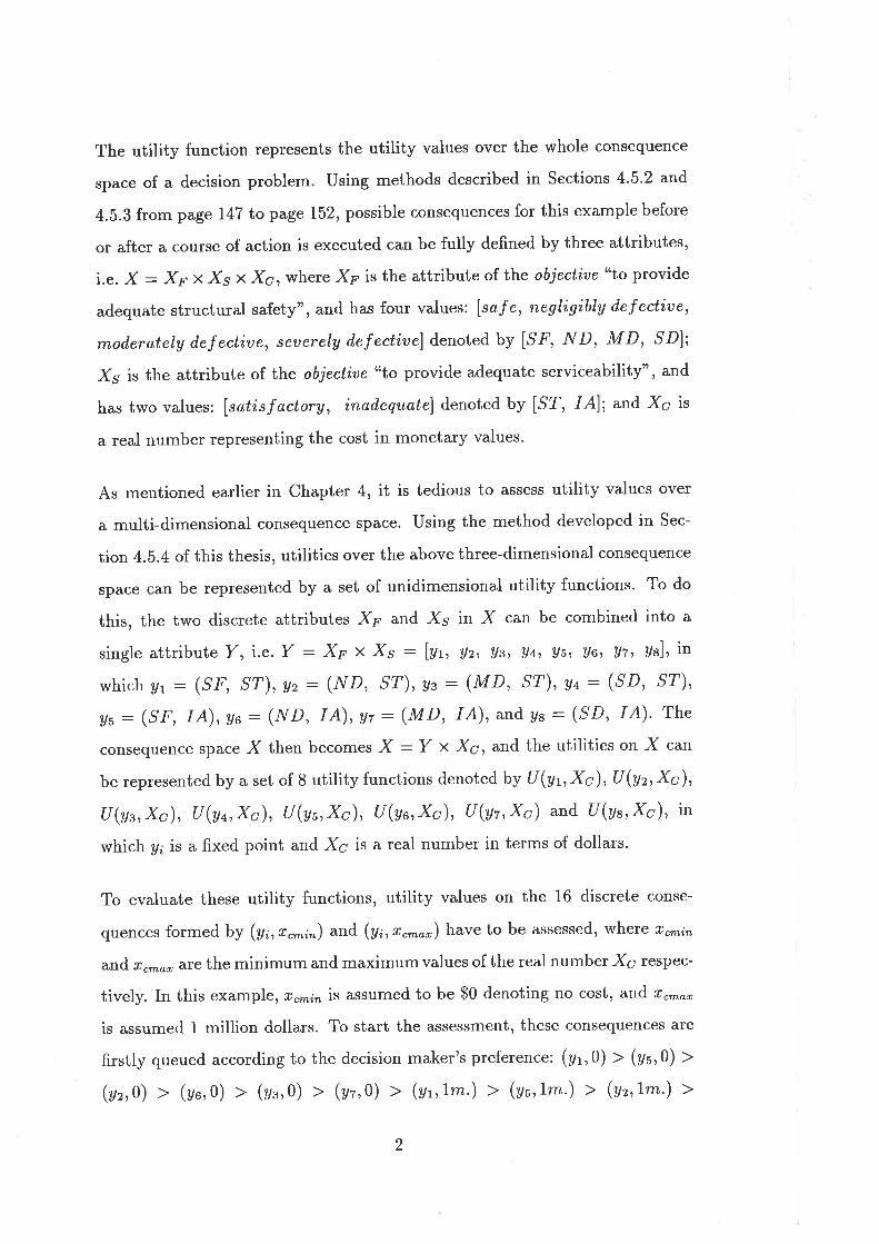
The utility function represents the utility values over the whole consequence
space of a d,ecision problem. Using methods described in Sections 4.5.2 and
4.b.8 from page I47 to page 152, possible consequences for this example before
or after a course of action is executed can be fully defined by three attributes,
i.e. X - Xp X Xs x X6, where X¡ is the attribute of the objectiue "to provide
adequate structural safety", and has four values: lsafe, negligibly defectiue,
mod,erately d,ef ectiue, seuerely def ectiue] denoted bV [Sl7, ND, MD, SDh
Xs is the attribute of the objectiue "to provide adequate serviceability", and
has two values: lsatisfactory, inadequate] denoted by [^9?, /A]; and Xc is
a real number representing the cost in monetary values.
As mentioned earlier in Chapter 4, it is tedious to assess utility values over
a multi-dimensional consequence space. Using the method developed in Sec-
tion 4.5.4 of this thesis, utilities over the above three-dimensional consequence
space can be represented by a set of unidimensional utility functions. To do
this, the two discrete attributes Xr and X5 in X can be combined into a
single attribute Y, i.e.Y : Xr x Xs : l1t,, Uz,t As, U¿,t Us¡ Us, Uz'¡ ye], in
which h: (5F,, ST), ar: (ND, ST), At: (MD, ST), yn: (SD, ST),
As: (5F,, IA),yu: (ND, IA),yz: (MD, 1A), and YB: (SD, IA)' The
consequence space X then becomes X : Y x Xc, and the utilities on X can
be represented by a set of 8 utility functions denoted by tl(ar,Xc), U(ar,Xc),
U(A",Xc), U(yn,Xc),, U(Au,Xc), U(Au,Xc), U(yr,X6) and U(v",Xç), in
which y¿ is a fixed point and xc is a real number in terms of dollars.
To evaluate these utility functions, utility values on the 16 discrete conse-
quences formed by (y;rr. in) and (y¿, r.^or) have to be assessed, where x.*¿n
aÍrd. t"*o, are the minimum and maximum values of the real number Xc respec-
tively. In this example, r.*¿nis assumed to be $0 denoting no cost, and I"*o,
is assumed I million dollars. To start the assessment, these consequences are
firstly queued according to the decision maker's preference: (yr,0) > (yu,0) >
@r,0) ) (vu,0) > (vr,O) > (vt,O) > (vt,L*') > (au,l*') ) (ar,r*') >
2
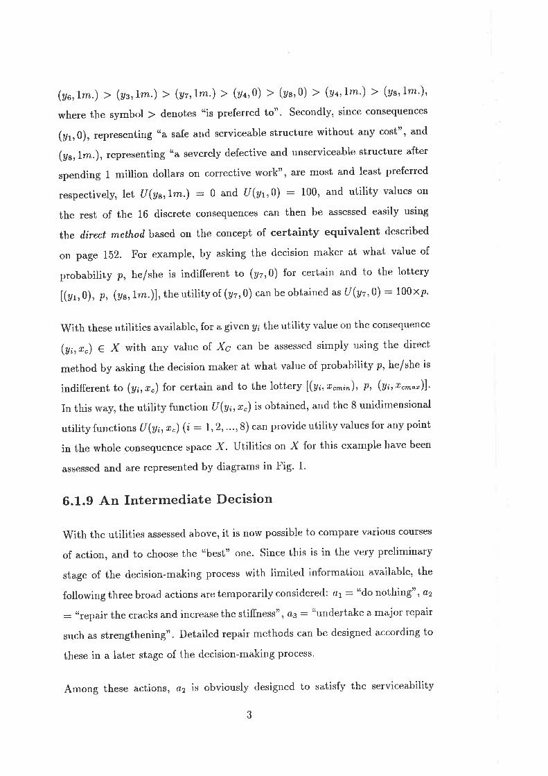
(yu,I^.) ) (yr, I*.) > (ar,,l*.) ) (an,O) > (vt,0) > (vn, l*') > (vt,1-'),
where the symbol > denotes "is preferred to". secondly, since consequences
(yr,0), representing "a safe and serviceable structure without any cost", and
(A"rl*.), representing "a severely defective and unserviceable structure after
spending 1 million dollars on corrective work", are most and least preferred
respectivelS let u(a",Im.) : 0 and u(ar,0) : 100, and utility values on
the rest of the 16 discrete consequences can then be assessed easily using
lhe d,irect rnethoil based on the concept of certainty equivalent described
on page 152. For example, by asking the decision maker at what value of
probability p, he/she is indifferent to (vr,O) for certain and to the lottery
[(yr,0), p, (Ua,l-.)], theutility of (a2,0) canbeobtainedasU(y7,0) : 100xp'
With these utilities available, for a given y; the utility value on the consequence
(y;,*.) € x with any value o1 xc can be assessed simply using the direct
method by asking the decision maker at what value of probability p, he/she is
indifferent to (yr,r.) for certain and to the lottery l(y¿,t. ¿^), P, (A;,r. o,)l'
In this way, the utility function tJ(yn,r.) is obtained, ancl the 8 unidimensional
utilityfunctions U(A¡,*")(i:1,2,...,8)canprovideutilityvaluesforanypoint
in the whole consequence space X. Utilities on X for this example have been
assessed and are represented by diagrams in Fig' 1'
6.1.9 An Intermediate Decision
With the utilities assessed above, it is now possible to compare various courses
of action, and to choose the "best" one. Since this is in the very preliminary
stage of the decision-making procesq with limited intbrmation available, the
following three broad actions are temporarily consiclered: (tr7 : "do nothing", a2
: ttrepair the cracks and increase the stiffness" , a3 : "undertake a major repair
such as strengthening". Detailed repair methods can be designed according to
these in a later stage of the decision-making process'
Among these actions, a2 is obviously designed to satisfy the serviceability
3
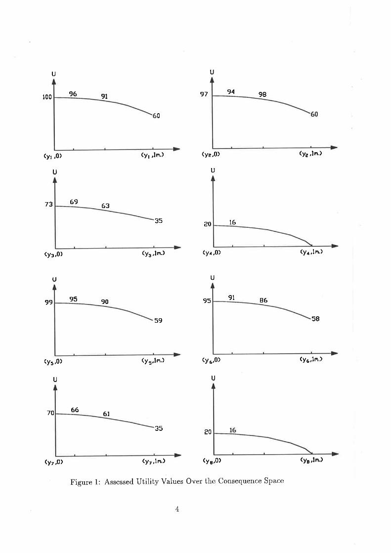
U U
97 94 98
(ya,0)
U
t00 96
(Yr ,o)
U
73 69
(Y3,0)
99
(y5,0)
70
9l
0
(y¡ ,ln') (y¿,ln')
(y4 ,ln.)
58
(y6,ln,)
63
20 t6
(yr.ln.) (yr,0)
95 90 95 9l 86
59
(y'ln,) (y.,0)
66
35
(y7,ln.) (ys,0)
Figure 1: Assessed Utility Values Over the Consequence Space
35
UU
UU
20
6t
4
(yt 'O)
(ys,ln.)
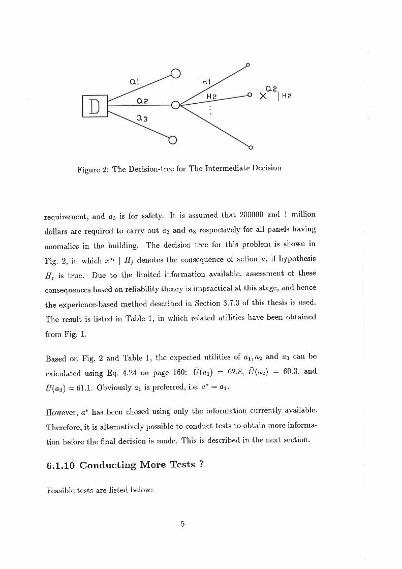
ol H1
HOaoe
X lH.
Os
Figure 2: The Decision-tree for The Intermediate Decision
requirement, and a3 is for safety. It is assumed that 200000 and 1 million
dollars are required to carry ort a2 and ø3 respectively for all panels having
anomalies in the building. The decision tree for this problem is shown in
Fig. 2, in which ,", I H¡ denotes the consequence of action ø¿ if hypothesis
f/¡ is true. Due to the limited information available, assessment of these
consequences based on reliability theory is impractical at this stage, and hence
the experience-based method described in Section 3.7.3 of this thesis is used.
The result is listed in Table 1, in which related utilities have been obtained
from Fig. 1.
Based on Fig. 2 and Table 1, the expected utilities o1 a1,o2 and 43 can be
calculated using Eq. 4.24 on page 160: U("t) - 62'8, U("r) : 60'3, and
Ú(""): 61.1. Obviously ø1 is preferred, i'e' o'* : o'r'
However, ¿* has been chosed using only the information currently available.
Therefore, it is alternatively possible to conduct tests to obtain more informa-
tion before the final decision is made. This is described in the next section.
6.1.10 Conducting More Tests ?
5
Feasible tests are listed below:

Table 1: Possible Consequences and Their Utilities
H 0,1 0,2 Ag
Consequence Utility Consequence Utility consequence Utility
H1 (yu, o) 99 (y1,200000) 96 (yt,l*') 62
H2 @.,0) 70 (y3,200000) 69 (at,,t*.) 62
Hs (yr, o) 99 (y1,200000) 96 (Yt,L*.) 62
Hq (yu, o) 99 (y1, 200000) 96 (ut,,l^.) 62
Hs (v',,0) 70 (y3,200000) 69 (yt,l*.) 62
Hø (v', o) 20 (ya,200000) 16 (ut,l*.) 62
Hz (ar,o) 70 (y3,200000) 69 (at,l*.) 62
H¿ (yr, o) 20 (9a,200000) 16 (Yt,L*.) 62
Hs (yr, o) 20 (ya,200000) 16 (at,l*.) 62
Hrc (yr, o) 20 (ya,200000) 16 (yt,r*.) 62
Hn (yr, o) 20 (ya,200000) 16 (Yt,r*.) 62
Hn (a', o) 70 (y3,200000) 69 (at,r^.) 62
Hß fur,,0) 70 (y3,200000) 69 (at,l^') 62
Hu (Yr',0) 70 (y3,200000) 69 (ut,L^') 62
Hrc @r,o) 70 (y3,200000) 69 (yt,r*.) 62
Ho (y',0) 72 (y',200000) 68 (Y',r*.) 39
6

o t1i seâ,rch for information on loading during construction ancl the in-
service period;
o t2i caff! out relevant structural analysis to calculate the deflection;
o ú3: detect locations and quantities of steel bars using appropriate devices;
o ú4: remove small regions of concrete to observe the steel reinforcement;
o f5: take core samples of concrete to test for compressive strength;
o t6: conduct non-d.estructive tests to estimate complessive strength of
concrete,
To decide on whether a test is preferred to the action ¿* chosen in the last
section, it is necessary to evaluate the expected utitity of the favoured test' For
this purpose, let us try test ú6 (cost 5000 dollars) first, and the relatecl decision-
tree is shown in Fig. 3, in which fi, il2 and d3 are three possible outcomes of
the test. Since this test is mainly to get more information on hypothesis
Hs - es : inad,equate concrete strength,, for simplicity, it is assumed that
dt : reject Hs, d,2: accePt fIs and ds: inf ormation is irreleuant, a'nd
probabitities of H¿ unchanged. It is also assumed that the probabilities of
these outcomes are p(d1) = 0.4, p(dr) = 0.4 and p(dt) :0'2'
o3?=Hs o2 Ha
ta .'
Figure 3: The Decision-tree for Test ú6
?
I
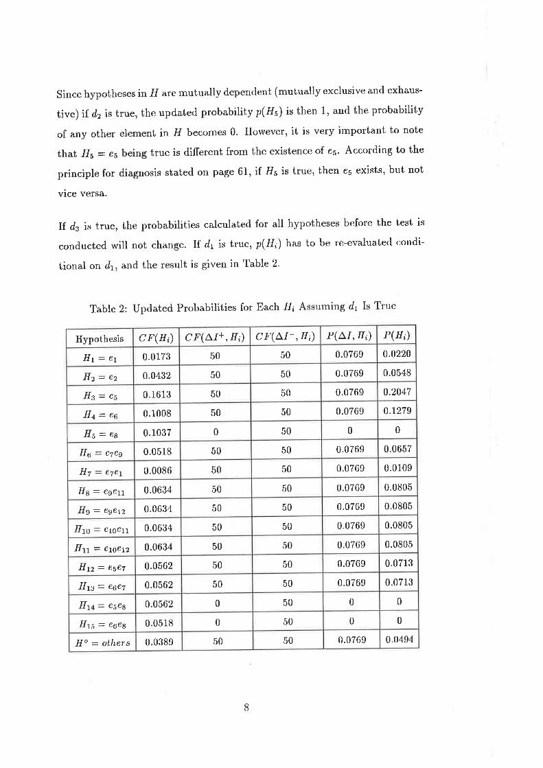
since hypotheses in f/ are mutually dependent (mutually exclusive and exhaus-
tive) if d2 is true, the updated probabilitv p(f/r) is then 1, and the probability
of any other element in f/ becomes 0. However, it is very important to note
that .it/s : e¡ being true is different from the existence of e5' According to the
principlefor diagnosis stated on page 61, if /15 is true, then e5 exists, but not
vlce versa.
If ds is true, the probabilities calculated for alt hypotheses before the test is
conducted will not change. If d1 is true, p(f4) has to be re-evaluated condi-
tional on d1, and the result is given in Table 2'
Table 2: updated Probabilities for Each H¡ Assuming d1 Is True
Hypothesis c F(Hi) C F(AI+ , H¿) c F(aI- , Hi) P(A,I, H¿) P(H;)
H e11 0.0173 50 50 0.0769 0.0220
Hz: ez 0.0432 50 50 0.0769 0.0548
Hz- es 0.1613 50 50 0.0769 0.2047
Ha=ea 0.1008 50 50 0.0769 0.1279
Hs=ee 0.1037 0 50 0 0
Ha: ezeg 0.0518 50 50 0.0769 0.0657
Hz = eTel 0.0086 50 50 0.0769 0.0109
H6 - ese¡1 0.0634 50 50 0.0769 0.0805
H9 = ege12 0.0634 50 50 0.0769 0.0805
Hto: etoell 0.0634 50 50 0.0769 0.0805
Ht = e7oet2 0.0634 50 50 0.0769 0.0805
Hr2 = ese| 0.0562 50 50 0.0769 0.0713
Hts = e6e7 0.0562 50 50 0.0769 0.0713
H1.+: esea 0.0562 0 50 0 0
Hts = eeee 0.0518 0 50 0 0
Ho = oth,ers 0.0389 50 50 0.0769 0.0494
8

Based on Fig. 3 and Table 2, the expected utility of fa is calculated as
tr(tu):0.4 x 6l *0.4 x 70+0.2 x 62.8:64.6 > u(".):62'8 (1)
Therefore, test ú6 is preferred to ø*. The intermediate decision is then to carry
out test f6 before a terminal decision is made.
6.1.11 The Second Stage of Decision-making
After f6 was executed., it was found that the concrete was in good condition,
and the compressive strength was acceptable. Using this information, the
diagnosis, i.e. the probability of 1/ has been updated, and the result is shown
in Table 2. Using the updated p(Ho), the utilities of the three courses of action
are calculated as: u("t) - 61'0, u("r):57'98 and u(ø3) :60'86' Therefore'
the most preferred action at this stage is again o,* : o't'
However, the diagnostic result is still not conclusive after the outcome of
ú6 is obtained. The same situation was faced in the first stage of decision-
making, and the alternative option of conducting further tests has again to
be assessed. For this purpose, Iet us try ú1 this time. The related decision-
tree is shown in Fig. 4, in which d4, d,2, d", d¿,, ds and d6 are possible out-
comes of the test. Since this test is mainly to get more information on
hypotheses f13 and Ha, for simplicity it is assumed that r/r : accePt He¡
d,z : øccept Ha, d,s: reject Hs, d¿: reject Hn, du : reject both Hz and, Ha,
d,e : inf ormation is irreleuant and Ttrobability ol p(H;) uncha'nged Proba-
bilities of these outcomes are assessed as p(d1) - 0.2, p(dr) :0'2, p(fu) :0'2,p(dn) - 0.2, p(du) :0.1 and p(du) : 0.1'
The expected utility of f1 is then evaluated, and the result is:
ú(tr) : 0.2x (99+99+60.43+60.58) *0.1 x 59.84*0.1 x 61.0 : 75.89 > 61.0
(2)
Therefore, test f1 is preferred to ¿* at this stage.
I
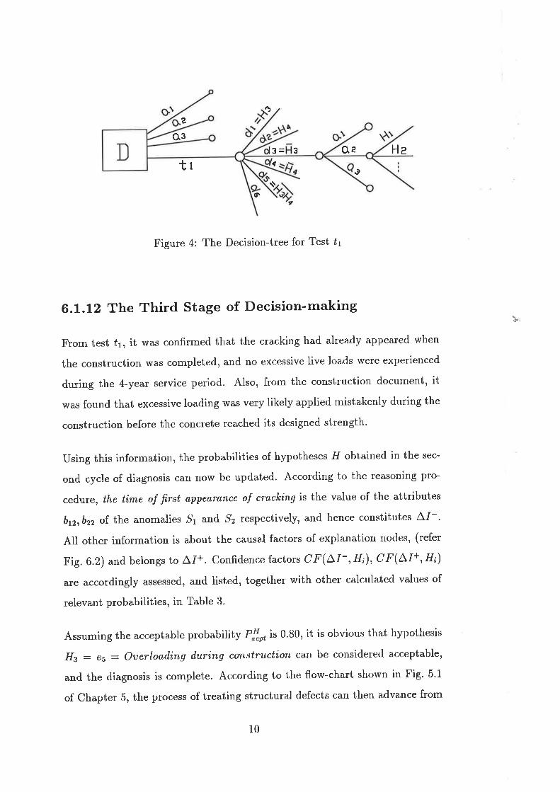
a,
?
o3À
J- 3
I
\\tt
Oe He
o
(F
Figure 4: The Decision-tree for Test ú1
6.L.I2 The Third Stage of Decision-making
From test ú1, it was confirmed that the cracking had already appeared when
the construction was completed, and no excessive live loads were experienced
during the 4-year service period. Also, from the construction document, it
was found that excessive loading was very likely applied mistakenly during the
construction before the concrete reached its designed strength.
Using this information, the probabilities of hypotheses fI obtained in the sec-
ond cycle of diagnosis can now be updated. According to the reasoning pro-
cedure, the time of fi,rst o,ppe&rúnce of cracking is the value of the attributes
btzrbrz of the anomalies,sl and ,92 respectively, and hence constitutes A1-'
All other information is about the causal factors of explanation nodes, (refer
Fig. 6.2) and belongs to a.I+. confrdence {actors cF(LI-,,Hi), CF(LI+,H¿)
are accordingly assessed, and listed, together with other calculated values of
relevant probabilities, in Table 3.
Assuming the acceptable probability Pf"oris 0.80, it is obvious that hypothesis
Hz - es : Ouerloading d,uring construction car: be considered acceptable,
and the diagnosis is complete. According to the flow-chart shown in Fig. 5'1
of Chapter 5, the process of treating structural defects can then advance from
ðt
10
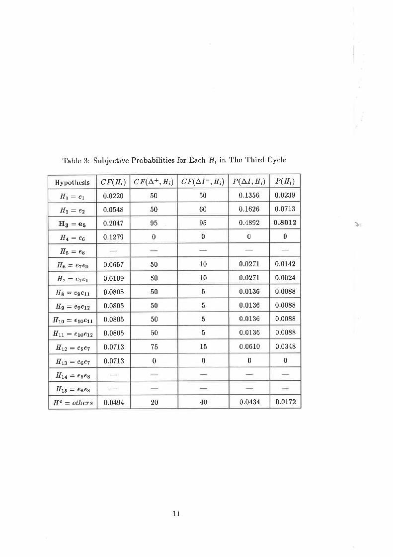
Hypothesis c F(H;) CF(L+,H¿) cF(LI-,Hi) P(LI,Hi) P(H¿)
Hl.: eL 0.0220 50 50 0.1356 0.0239
Hz=ez 0.0548 50 60 0.1626 0.0713
Hs -- er 0.2047 95 95 0.4892 0.8012
Ha: ea 0.t279 0 0 0 0
Hs=ee
He = eTeg 0.0657 50 10 0.027t 0.01.42
Hz = eTet 0.0109 50 10 0.027t 0.0024
He = egett 0.0805 50 5 0.0136 0.0088
Hs -- ese12 0.0805 50 5 0.0136 0.0088
Hto: eloêLt 0.0805 50 5 0.0136 0.0088
Htt: etoêt2 0.0805 50 5 0.0136 0.0088
Htz = esez 0.0713 75 15 0.0610 0.0348
Ht3: eae| 0.0713 0 0 0 0
Ht+ = esee
HLl: eae'
Ho : others 0.0494 20 40 0.0434 0.0172
Table 3: Subjective Probabilities for Each H¿ in The Third Cycle
d.-
11

step 6 directly to step L2, i.e. the design of a relevant course of action with
regard to explanations contained in fIs.
6.1.L2 The Final Decision
According to the accepted hypothesis Hs - e5 : ouerload' during construction,
there are no safety and durabitity problems, and hence the following four de-
tailed courses of action are considered:
o ø1:de nothing;
o û2 -repair the cracks using relevant epoxy resin;
o ø3:i¡1s¡ease the stiffness by epoxy-bonded steel plate;
o 0,4:q2 * ø2.
with costs of 0, 50000, 150000 and 200000 dollars respectively. Since the decr-
sion is to be made under certainty in this case, consequences related to each
action are assessed as sol : (Asr}), r", : (ysr50000), ro3 : (y5,150000) and
ro+ : (y1,200000), in whichyu: (SF,IA),^: (SF,^97), with S-F repre-
senting ttstructure is safe", ,9? and .IA denoting ttserviceability requirement is
satisfactory and inadequate respectively"'
Utilities of these consequences have been found from the assessed utility func-
tions shown in Fig. 1, and are: U("t) - 99, U("r) - 98, U("") : 96 and
U("n): 96. Obviously ¡ at : d,oing nothing is the best action according to the
decision maker's preference.
t2

Section 7.2 on page 199: Add the following sentence to the end of the first
paragraph of Section 7.2:
However, it should be mentioned that methods proposed in this thesis are
subject to further testing in practice and necessary refinement, before they
can be used by engineers as a useful tool in dealing with structural defects.
13